Long liquid slugs in stratified gas/liquid flow in horizontal and slightly inclined pipes

Welcome message from author
This document is posted to help you gain knowledge. Please leave a comment to let me know what you think about it! Share it to your friends and learn new things together.
Transcript
Long liquid slugs
in stratified gas/liquid flowin horizontal and slightly inclined pipes


Long liquid slugs
in stratified gas/liquid flowin horizontal and slightly inclined pipes
PROEFSCHRIFT
ter verkrijging van de graad van doctoraan de Technische Universiteit Delft,
op gezag van de Rector Magnificus prof. dr. ir. J. T. Fokkema,voorzitter van het College voor Promoties,
in het openbaar te verdedigen opVrijdag 28 September 2009 om 10:00
door
Usama Kadri
M.Sc. Aerospace Engineer, Technion – Israel Institute of Technologygeboren te Kfar Saba, Israel
Dit proefschrift is goedgekeurd door de promotor:Prof. dr. R.V.A. OliemansProf. dr. R.F. Mudde
Samenstelling promotiecommissie:
Rector Magnificus, voorzitterProf. dr. R.V.A. Oliemans, Technische Universiteit Delft, promotorProf. dr. R.F. Mudde, Technische Universiteit Delft, promotorProf. dr. ir. R.A.W.M Henkes, Technische Universiteit DelftProf. dr. ir. G. Ooms, Technische Universiteit DelftProf. dr. ir. H.W.M. Hoeijmakers, Universiteit TwenteProf. dr. P. Andreussi, University of PisaProf. dr. O.J. Nydal, Norwegian University of Science and Technology
This project was supported by the Dutch Foundation for Technological Research (STW)
Keywords: two–phase flow, gas–liquid, long slugs
Cover design by: Arch. Lidia Badarnah–Kadri
The cover of the thesis is based on M.C. Eschers “Sky and Water I” c©2009 The M.C.Escher Company – The Netherlands. All rights reserved. www.mcescher.com
Printed in The Netherlands. PrintPartners Ipskamp. www.ppi.nl
ISBN 978–90–9024536–2
c© 2009 Usama Kadri.
All rights reserved. No part of the material protected by this copyright notice may bereproduced or utilized in any form or by any means, electronic or mechanical, includingphotocopying, recording, or by any information storage and retrieval system without writtenpermission from the publisher.

For the ultimate victory of blood over sword


Contents
Nomenclature xi
Summary xiii
Samenvatting xv
1 Introduction 1
1.1 Motivation . . . . . . . . . . . . . . . . . . . . . . . . . . . . . . . . . . . . 11.2 Scope . . . . . . . . . . . . . . . . . . . . . . . . . . . . . . . . . . . . . . 21.3 Outline . . . . . . . . . . . . . . . . . . . . . . . . . . . . . . . . . . . . . 3
2 Dynamic slugs 5
2.1 Introduction . . . . . . . . . . . . . . . . . . . . . . . . . . . . . . . . . . . 62.2 Theoretical background . . . . . . . . . . . . . . . . . . . . . . . . . . . . . 8
2.2.1 Stratified flow pattern . . . . . . . . . . . . . . . . . . . . . . . . . . 82.2.2 Viscous long wavelength theory . . . . . . . . . . . . . . . . . . . . 82.2.3 Slug stability analysis . . . . . . . . . . . . . . . . . . . . . . . . . 10
2.3 Experiments on the occurrence of long slugs . . . . . . . . . . . . . . . . . . 112.3.1 Experiments . . . . . . . . . . . . . . . . . . . . . . . . . . . . . . 112.3.2 Sub–regimes in the slug flow map . . . . . . . . . . . . . . . . . . . 11
2.4 Dynamic slug model . . . . . . . . . . . . . . . . . . . . . . . . . . . . . . 142.4.1 Properties of forming slugs . . . . . . . . . . . . . . . . . . . . . . . 14
2.4.1.1 Wave velocity . . . . . . . . . . . . . . . . . . . . . . . . 142.4.1.2 Slug at initiation . . . . . . . . . . . . . . . . . . . . . . . 152.4.1.3 Slug tail extension . . . . . . . . . . . . . . . . . . . . . . 152.4.1.4 Initial slug length . . . . . . . . . . . . . . . . . . . . . . 16
2.4.2 Slug growth and final length . . . . . . . . . . . . . . . . . . . . . . 172.4.2.1 The liquid area downstream of the slug, ALmax . . . . . . . 172.4.2.2 The liquid area upstream of the slug, AL5(t) . . . . . . . . 172.4.2.3 Slug length, LS(t) . . . . . . . . . . . . . . . . . . . . . . 18

viii CONTENTS
2.4.3 End of slug growth . . . . . . . . . . . . . . . . . . . . . . . . . . . 192.5 Results . . . . . . . . . . . . . . . . . . . . . . . . . . . . . . . . . . . . . . 20
2.5.1 Predictions for horizontal air–water flow . . . . . . . . . . . . . . . . 222.5.2 Predictions for declined air–water flow . . . . . . . . . . . . . . . . 222.5.3 Predictions for SF6 gas–ExxsolD80 oil flow under varying pressure . 222.5.4 Predictions at large mixture velocities . . . . . . . . . . . . . . . . . 25
2.6 Conclusions . . . . . . . . . . . . . . . . . . . . . . . . . . . . . . . . . . . 27
3 Transition to slug flow and roll–waves 29
3.1 Introduction . . . . . . . . . . . . . . . . . . . . . . . . . . . . . . . . . . . 303.1.1 Waves . . . . . . . . . . . . . . . . . . . . . . . . . . . . . . . . . . 303.1.2 Transition to roll–waves . . . . . . . . . . . . . . . . . . . . . . . . 303.1.3 Transition to slug flow . . . . . . . . . . . . . . . . . . . . . . . . . 31
3.2 Theoretical background . . . . . . . . . . . . . . . . . . . . . . . . . . . . . 323.2.1 Stratified flow pattern . . . . . . . . . . . . . . . . . . . . . . . . . . 323.2.2 Slug stability theory . . . . . . . . . . . . . . . . . . . . . . . . . . 343.2.3 The liquid level downstream of the growing wave . . . . . . . . . . . 34
3.3 A roll–wave/slug formation time model . . . . . . . . . . . . . . . . . . . . 353.3.1 The vertical growth time . . . . . . . . . . . . . . . . . . . . . . . . 363.3.2 The axial growth time . . . . . . . . . . . . . . . . . . . . . . . . . 37
3.4 Experiments . . . . . . . . . . . . . . . . . . . . . . . . . . . . . . . . . . . 383.4.1 The KLFT flow loop . . . . . . . . . . . . . . . . . . . . . . . . . . 383.4.2 The NTNU flow loop . . . . . . . . . . . . . . . . . . . . . . . . . . 39
3.5 Numerical tests . . . . . . . . . . . . . . . . . . . . . . . . . . . . . . . . . 413.6 Results . . . . . . . . . . . . . . . . . . . . . . . . . . . . . . . . . . . . . . 43
3.6.1 Crest growth near the pipe top . . . . . . . . . . . . . . . . . . . . . 433.6.2 Prediction of roll–wave/slug formation time . . . . . . . . . . . . . . 443.6.3 Formation time predictions for different pipe diameters . . . . . . . . 453.6.4 Critical Froude number for the transition . . . . . . . . . . . . . . . 46
3.7 Conclusions . . . . . . . . . . . . . . . . . . . . . . . . . . . . . . . . . . . 48
4 Operation pressure and slug length 51
4.1 Introduction . . . . . . . . . . . . . . . . . . . . . . . . . . . . . . . . . . . 524.2 Background . . . . . . . . . . . . . . . . . . . . . . . . . . . . . . . . . . . 53
4.2.1 Stratified flow pattern . . . . . . . . . . . . . . . . . . . . . . . . . . 534.2.2 Average liquid area . . . . . . . . . . . . . . . . . . . . . . . . . . . 534.2.3 Slug stability model . . . . . . . . . . . . . . . . . . . . . . . . . . 54
4.3 Experiments . . . . . . . . . . . . . . . . . . . . . . . . . . . . . . . . . . . 554.4 Definition of slug types by liquid excess . . . . . . . . . . . . . . . . . . . . 57
4.4.1 Discrimination between slug types in measurements . . . . . . . . . 574.4.2 Measurements of the liquid excess, ΔhL . . . . . . . . . . . . . . . . 584.4.3 Theoretical predictions of the liquid excess, ΔhL . . . . . . . . . . . 59
4.4.3.1 Slugs type I . . . . . . . . . . . . . . . . . . . . . . . . . 594.4.3.2 Slugs type II . . . . . . . . . . . . . . . . . . . . . . . . . 59

CONTENTS ix
4.4.3.3 Slugs type III . . . . . . . . . . . . . . . . . . . . . . . . 594.5 Results . . . . . . . . . . . . . . . . . . . . . . . . . . . . . . . . . . . . . . 59
4.5.1 Slug types and the normalized liquid excess, ΔhL/D . . . . . . . . . 604.5.2 The length of the different slug types at atmospheric pressure . . . . . 614.5.3 The length of the different slug types at P = 1.5 barA (ρG = 9 kg/m3) 624.5.4 The length of the different slug types at P = 3 barA (ρG = 18.5 kg/m3) 634.5.5 Effect of pressure on the long slugs – summary . . . . . . . . . . . . 64
4.6 Conclusions . . . . . . . . . . . . . . . . . . . . . . . . . . . . . . . . . . . 65
5 A probabilistic slug frequency model 675.1 Introduction . . . . . . . . . . . . . . . . . . . . . . . . . . . . . . . . . . . 685.2 Background . . . . . . . . . . . . . . . . . . . . . . . . . . . . . . . . . . . 69
5.2.1 Stratified flow pattern . . . . . . . . . . . . . . . . . . . . . . . . . . 695.2.2 Average liquid area . . . . . . . . . . . . . . . . . . . . . . . . . . . 715.2.3 Slug stability model . . . . . . . . . . . . . . . . . . . . . . . . . . 71
5.3 Slug frequency model . . . . . . . . . . . . . . . . . . . . . . . . . . . . . . 725.3.1 Frequency of turbulent eddies in gas and liquid . . . . . . . . . . . . 725.3.2 Interfacial frequency of turbulent eddies, fr,i . . . . . . . . . . . . . 735.3.3 Triggering of slug precursors . . . . . . . . . . . . . . . . . . . . . . 745.3.4 Conditional probability of slug formation . . . . . . . . . . . . . . . 74
5.4 Results . . . . . . . . . . . . . . . . . . . . . . . . . . . . . . . . . . . . . . 765.5 Conclusions . . . . . . . . . . . . . . . . . . . . . . . . . . . . . . . . . . . 80
6 Conclusions and final remarks 816.1 Slug growth and the long slug region . . . . . . . . . . . . . . . . . . . . . . 826.2 Evolution of waves and transition to slug flow or roll–waves. . . . . . . . . . 826.3 The effect of operation pressure . . . . . . . . . . . . . . . . . . . . . . . . 836.4 Slug flow and turbulence . . . . . . . . . . . . . . . . . . . . . . . . . . . . 836.5 Final remarks . . . . . . . . . . . . . . . . . . . . . . . . . . . . . . . . . . 84
A Calculation of the wave growth coeffecient, C2 91
Publications 93
Acknowledgements 95
About the author 97

x CONTENTS
Nomenclature
Greek letters
δ boundary layer thickness mε gas void fraction -η wave amplitude mθ angle to horizontal degλ wavelength mν kinematic viscosity m2.s−1
ρ density kg.m−3
Δρ fluids density difference kg.m−3
τ wall shear stress kg.m.s−2
ω frequency of rotation s−1
Roman symbols
A cross–sectional area m2
C,CR wave velocity m.s−1
CF slug front velocity m.s−1
CB slug tail (bubble) velocity m.s−1
C1,C2 wave growth constants -cw a constant equal to 2 for air–water system -D pipe diameter mDH hydraulic diameter mFr Froude number -f frequency s−1
f friction factor -g gravity constant m.s−2
h height of the fluid layer mK nonlinear wave growth rate m.s−1
k1,k2 boundary layer constants -L length mlT turbulence length scale m

xii CONTENTS
m defined in Eq. (5.30) -n number of slug precursor locations -P conditional probability for slug formation -P,p pressure PaQ volume flux m3.s−1
Re Reynolds number -S cross–sectional length mSt Strouhal number -t superficial velocity of phase . m.s−1
U actual gas velocity m.s−1
UMix mixture velocity m.s−1
u actual liquid velocity m.s−1
u fluid velocity m.s−1
V volume m3
v velocity m.s−1
x axial coordinate -y distance from the wall m
Subscripts
a,b,c,O points along the slug tailavg averageB bubbleG gasL liquidF frontf finali interfacial, indexk indexo initial valuer rotationS slugSG superficial gasSL superficial liquids smooth surfaceW wallw wavex,y Cartesian coordinates∞ steady–state1,3,5 stations along the slug unit defined in Fig. 2.2

Summary
Long liquid slugsUsama Kadri, Delft University of Technology
Long liquid slugs reaching several hundreds pipe diameter may appear when transportinggas and liquid in horizontal and near horizontal pipes. The long slugs cause system vibrationand separation difficulties that may lead to operational failures. Identifying and predicting thetime and length scales of slugging is important for gas and oil production technologies (e.g.for the design of offshore gas and oil pipelines and process facilities). Although mainly shorthydrodynamic slugs (40 pipe diameters) have been observed in offshore production fields, theappearance of the long slugs becomes more likely as the field becomes older the operationpressure drops. Therefore, predicting the transition between the different slug types and theflow conditions at which the long slugs appear may be crucial preventing or reducing thenegative effects of slugging.
The approach adopted in this study is the construction of simplified theoretical modelsthat successively approximate the flow conditions and the corresponding time and lengthscales of slugging. Experiments and numerical modelling have been performed for validationand comparison matters.
The first part of the research deals with identifying the long slug region and sub–regions.Experiments carried out by Zoeteweij (2007) present a detailed flow map for the long slugregion and the transition to hydrodynamic slugs or stratified wavy flow. For the prediction ofthe long slug region a simplified predictive model was constructed. The model calculates theaverage slug length based on the volumetric liquid rates adjoining the slug, and derives thechange in the liquid level, at the tail of the slug, by linear kinematic relation between the tailand the following upstream wave. The model predicts the transition from hydrodynamic tolong slugs with a satisfactory agreement.
In the second part of the research the emphasis is put on predicting the transition fromstratified flow to slug flow or roll–waves. Slugs formed by coalescence between roll–wavesare hydrodynamic. Hence, only the flow conditions that lead to a direct transition from strat-
xiv CONTENTS
ified flow to slug flow (i.e. not via roll–waves) may lead to long slugs. For the predictionof the transition to slug flow or roll–waves a theoretical model was developed. The modeltracks the displacements of the crest of a long wavelength wave in axial and radial directions.If the wave crest reaches the top of the pipe a slug is formed, whereas if it approaches thedownstream end of the wave a roll–wave is produced. Besides to the predictive tool provided,the model sheds some light on the stage prior to forming a slug.
The third part of the research considers the effect of the operation pressure on the sluglength, and the effect of the liquid excess between the slug front and tail at the formation time.Measurements by Kristiansen (2004) for two–phase air–oil and SF6 gas–oil were investigated.The measurements were carried out at P = 1–8 barA with high density SF6 gas simulatinga pressure up to 65 bar. Three different types of slugs were categorized based on the liquidexcess. Slugs with larger liquid excess at formation can grow to become longer. Even a smalldifference in the liquid excess may lead to a large difference in the slug length. However, athigh operating pressures there is no liquid excess and only hydrodynamic slugs are observed.
In the final part of the research we investigated and derived the slug frequency by thefrequency of vortices due to turbulence in the gas and liquid. We found that the slug fre-quency and the frequency of oscillation at the interface behave similarly to the frequencyof oscillations in the gas phase. However, the intensity of the oscillation at the interface isdominated by the liquid phase. The proposed mechanism for the formation of slugs coversa large range of pipe diameters and flow conditions. Moreover, it reveals the significance ofthe small–scale initial turbulence on the final development of the large–scale slug flow.
Samenvatting
Lange vloeistof slugsUsama Kadri, Technische Universiteit Delft
Lange vloeistof slugs (vloeistof slokken) met lengtes van wel honderden buisdiameters,kunnen voorkomen bij transport van gas en vloeistof in horizontale en nagenoeg-horizontalepijpleidingen. Dergelijke lange slugs kunnen door drukfluctuaties en vloeistof/gas scheidingproblemen operationele verstoringen geven. Het identificeren en voorspellen van de tijd–en lengteschalen van de slugs is van belang voor de gas/olie productietechnologie (regelsvoor een betrouwbaar ontwerp van de pijpleiding en process apparatuur). Hoewel tot nutoe hoofdzakelijk korte, hydrodynamische, slugs van hooguit 40D in productieleidingen vanbuitengaatse olie/gas velden zijn waargenomen, zijn er aanwijzingen, dat bij oudere veldenmet lagere operatiedrukken de kans op lange slugs zal toenemen. Het is daarom zaak omdoor een verdieping van de kennis over lange slugs te pogen de negatieve effecten van hunaanwezigheid te reduceren.
De in deze studie gekozen aanpak is om eenvoudige, theoretische modellen te ontwikke-len, waarmee bij benadering de condities waaronder lange slugs ontstaan en hun tijd enlengteschalen berekend kunnen worden. Bestaande experimenten en computer simulatieszijn vervolgens gebruikt om de modellen te valideren.
Het eerste deel van het proefschrift betreft het identificeren van het lange slug gebieden sub–gebieden in het stromigspatroondiagram. Experimenten, uitgevoerd door Zoeteweij(2007), geven een uitstekend beeld van het gebied met lange slugs en de overgangen naarhydrodynamische slugs en gelaagde tweefasenstroming. Om het lange slug gebied te kunnenvaststellen is een eenvoudig theoretisch model ontwikkeld. Het model bepaalt de gemid-delde sluggrootte op basis van het vloeistofdebiet naar de slug en de verandering van hetvloeistofniveau achter de slug via een lineaire, kinematische, relatie tussen de slug–staart ende golf stroomopwaarts. Met het model kan de overgang van hydrodynamisch naar langeslugs redelijk goed voorspeld worden.
In het tweede deel van het onderzoek ligt het accent op het voorspellen van de overgang
xvi Samenvatting
van gelaagde gas/vloeistofstroming naar slug stroming of gelaagde stroming met rol–golven.Vloeistof slugs, die ontstaan door coalescentie van rol–golven hebben een hydrodynamischkarakter. Dit betekent, dat alleen slugs, die rechtstreeks ontstaan uit de gelaagde stroming,en niet via coalescerende rol–golven, lange slugs zijn. Ook voor deze genoemde overgangenis een theoretisch model ontwikkeld. Het model beschrijft de verplaatsing van de top vaneen lange golf in axiale en opwaartse richting. Als de top van de golf de top van de pijpraakt vormt zich een slug. Als de axiale snelheid zo hoog is dat de top het eind van degolf stroomafwaarts bereikt worden rol–golven gevormd. Het model geeft ook inzicht in destromingssituatie vlak voor de vorming van een slug.
Het derde deel van het onderzoek betreft het effect van de operatiedruk op het optredenvan lange slugs en de rol van het verschil in vloeistof hoogte aan voor en achterkant vande opbouwende slug. Metingen van Kristiansen (2004) met tweefasen lucht/olie en SF6–gas/olie zijn geanalyseerd. De metingen bij laboratoriumdrukken van 1–8 barA met hethoge dichtheid SF6–gas simuleren operatiedrukken tot 65 bar. Op basis van de overmaatvloeistof kunnen drie verschillende typen slugs worden onderscheiden. Slugs met zelfs maareen geringe vloeistof–overmaat kunnen in lange leidingen heel lang worden. Bij hoge drukis er echter geen vloeistofovermaat meer en ontstaan alleen hydrodynamische slugs.
In het laatste deel van het project hebben we onderzocht in hoeverre de slugfrequentiegerelateerd kan worden aan de frequenties van vortices in the turbulente gas en vloeistofgedeeltes van gelaagde gas/vloeistof stroming. De slug frequentie en de frequentie van os-cillaties aan het vloeistof/gas scheidingsvlak blijken te correleren met de oscillaties in degasfase. De intensiteit van de oscillaties aan het scheidingsvlak wordt echter bepaald doorde vloeistoffase. Het voorgestelde mechanisme voor de vorming van de slugs geeft goederesulaten voor bestaande waarnemingen voor een reeks van diameters en stromingscondities.Ook wordt duidelijk dat turbulente fluctuaties op kleine schaal grote gevolgen kunnen hebbenvoor de grote schaal aspecten van de slugs.

1Introduction
1.1 Motivation
Gas–liquid flows are present in various engineering applications including aerospace, atmo-spheric, biological, biomedical, chemical, civil, mechanical, and nuclear systems. Conduct-ing a multiphase flow system is clearly not a simple task. It involves serious multiphaseproduction technology challenges, that require various levels of understanding the processesinvolved. Unfortunately, our understanding of multiphase flows is quite immature comparedto single–phase flows. The need to improve the scientific understanding of the fundamentalsof multiphase flows is the main motivation in the current study.
Here, we focus on two–phase gas–liquid flows in a pipe. “The study of flow in a pipeis a starting point for a scientific treatment of gas–liquid flows, as was Poiseuille‘s law andmeasurements of fully–developed flows, a starting point for the analysis of single phase flows”(Hanratty (2004)). Moreover, application of the results by gas and oil production technologiesis rather direct, e.g. the design of offshore gas and oil pipelines.
The main challenges in gas–liquid flows are caused by the interfacial interactions leadingto different flow configurations evolving through a complex flow. The simultaneous trans-portation of gas and liquid in a pipeline may result in a number of flow patterns, characterisedby different time and length scales. In long pipelines, multiple flow regimes may exist simul-taneously in different parts of the pipe (Oliemans (1987)). Sketches of the different flowpatterns and flow regime maps in horizontal gas–liquid pipe flow are presented in Figures 1.1and 1.2. At relatively low gas and liquid flow rates, a stratified flow patterns occurs with a
2 Chapter 1. Introduction
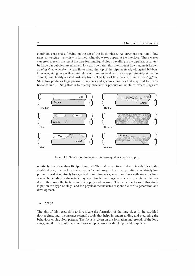
continuous gas phase flowing on the top of the liquid phase. At larger gas and liquid flowrates, a stratified–wavy flow is formed, whereby waves appear at the interface. These wavescan grow to reach the top of the pipe forming liquid plugs travelling in the pipeline, separatedby large gas bubbles. At relatively low gas flow rates, this intermittent flow regime is knownas plug flow, whereby the gas flows along the top of the pipe as steady elongated bubbles.However, at higher gas flow rates slugs of liquid move downstream approximately at the gasvelocity with highly aerated unsteady fronts. This type of flow pattern is known as slug flow.Slug flow produces large pressure transients and system vibrations that may lead to opera-tional failures. Slug flow is frequently observed in production pipelines, where slugs are
Figure 1.1: Sketches of flow regimes for gas–liquid in a horizontal pipe.
relatively short (less than 40 pipe diameter). These slugs are formed due to instabilities in thestratified flow, often referred to as hydrodynamic slugs. However, operating at relatively lowpressures and at relatively low gas and liquid flow rates, very long slugs with sizes reachingseveral hundreds pipe diameters may form. Such long slugs cause severe operational failuresdue to the strong fluctuations in flow supply and pressure. The particular focus of this studyis put on this type of slugs, and the physical mechanisms responsible for its generation anddevelopment.
1.2 Scope
The aim of this research is to investigate the formation of the long slugs in the stratifiedflow regime, and to construct scientific tools that helps in understanding and predicting thebehaviour of slug flow pattern. The focus is given on the formation and growth of the longslugs, and the effect of flow conditions and pipe sizes on slug length and frequency.
1.3. Outline 3
10−1
100
101
102
10−2
10−1
100
101
102
Superficial gas velocity [m/s]
Supe
rfic
ial l
iqui
d ve
loci
ty [
m/s
]
Dispersed bubbles
Annular flow
Wavy flow
Plug flowSlug flow
Very long slugs
Stratified flow
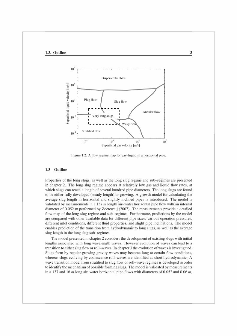
Figure 1.2: A flow regime map for gas–liquid in a horizontal pipe.
1.3 Outline
Properties of the long slugs, as well as the long slug regime and sub–regimes are presentedin chapter 2. The long slug regime appears at relatively low gas and liquid flow rates, atwhich slugs can reach a length of several hundred pipe diameters. The long slugs are foundto be either fully developed (steady length) or growing. A growth model for calculating theaverage slug length in horizontal and slightly inclined pipes is introduced. The model isvalidated by measurements in a 137 m length air–water horizontal pipe flow with an internaldiameter of 0.052 m performed by Zoeteweij (2007). The measurements provide a detailedflow map of the long slug regime and sub–regimes. Furthermore, predictions by the modelare compared with other available data for different pipe sizes, various operation pressures,different inlet conditions, different fluid properties, and slight pipe inclinations. The modelenables prediction of the transition from hydrodynamic to long slugs, as well as the averageslug length in the long slug sub–regimes.
The model presented in chapter 2 considers the development of existing slugs with initiallengths associated with long wavelength waves. However evolution of waves can lead to atransition to either slug flow or roll–waves. In chapter 3 the evolution of waves is investigated.Slugs form by regular growing gravity waves may become long at certain flow conditions,whereas slugs evolving by coalescence roll–waves are identified as short hydrodynamic. Awave transition model from stratified to slug flow or roll–wave regimes is developed in orderto identify the mechanism of possible forming slugs. The model is validated by measurementsin a 137 and 16 m long air–water horizontal pipe flows with diameters of 0.052 and 0.06 m,

4 Chapter 1. Introduction
respectively. Moreover, predictions by the model are compared with numerical calculationsusing a multiphase flow simulator, MAST, in order to investigate the pipe scaling effect whereno experimental data are found.
In chapter 4, gas–liquid pipe an analysis of flow measurements is presented in orderto investigate the dominant factors responsible for the formation of different slug lengths.Three types of slugs are defined based on the liquid excess between the slug front and tailimmediately after formation: (1) large liquid excess; (2) intermediate liquid excess; and (3)no liquid excess. The first two types are associated with the long growing and stable slugs,respectively. The third type is found to be always a short hydrodynamic slug. The conclusionis that small changes in the initial conditions of the liquid excess may lead to a large differencein the slug length and frequency. Moreover, the effect of practical field operation pressure onthe long slugs is investigated. The long slug region shrinks with increasing pressure, however,long stable slugs may still form at operation pressure below 65 bar.
Chapter 5 discusses the source of slug formation with stratified flow as a starting point.The frequency of oscillations generated by turbulent eddies in gas and liquid are found to beresponsible for the periodic formation of slugs. However, a moving slug destroys the memoryof the turbulent eddies downstream, preventing the formation of new slugs. The two–scalephysics of turbulent eddies and slug flow are coupled. Therefore, a probabilistic model,that defines sub–spaces at which each scale is dominant, is developed. The slug frequencyis derived from the frequency of oscillations and probabilistic effect, then compared withmeasurements for different pipe sizes and flow conditions.
Finally, the conclusions and final remarks are presented in chapter 6.

2Dynamic slugs 1
Long liquid slugs, with sizes reaching 500 pipe diameters or more, may form in gas–liquidhorizontal pipe flow at intermediate liquid loadings. Such slugs cause serious operationalupsets due to the strong fluctuations in flow supply and pressure. Therefore, predicting thetransition from short (hydrodynamic) to long slug flow regimes may play a significant role inpreventing or reducing the negative effects caused by the long slugs.
In this chapter we introduce a growth model for calculating the average slug length inhorizontal and near horizontal pipes. The model applies a volumetric balance between thefront and tail of the slug in order to calculate the slug growth rate. The dynamic behaviour ofthe liquid at the tail is described by a linear kinematic relation between the slug downstreamand the wave upstream.
For the validation of the model we performed measurements in a 137 m length air–waterhorizontal pipe flow of an internal diameter (i.d.) of 0.052 m. The measurements provide adetailed flow map of the long slug regime and sub–regimes. Furthermore, we compared pre-dictions by the model with data available from the open literature for a range of 0.019–0.095m i.d. pipes to investigate the effect of varying operation pressures, different inlet conditions,different fluid properties and slight inclinations. The model predicted the transitions from hy-drodynamic to long slugs with satisfactory agreements, however it underpredicts the averageslug length at relatively large mixture velocities.
1This chapter is based on Kadri et al. (2009a)
6 Chapter 2. Dynamic slugs
2.1 Introduction
Slug flow is commonly observed in horizontal and slightly inclined pipe flows. It is charac-terized by the appearance of plugs of liquids, moving downstream, separated by elongatedbubbles, moving along the top of the pipe. Although mostly short hydrodynamic slugs areobserved, at relatively low gas flow rates very long slugs with sizes reaching 500 pipe diam-eters or more may form. Such long slugs cause severe operational failures due to the strongfluctuations in flow supply and pressure. A frequent appearance of the long slugs is likely tooccur in older gas production offshore fields, where the operation pressure is low. Therefore,predicting the transition from regular hydrodynamic to long slug regimes plays a prominentrole in preventing or reducing future operational failures.
Two theoretical concepts are used to predict the flow conditions at which, both hydro-dynamic and long, slugs are observed: stability of stratified flow and stability of slugs. Thestability of stratified flow describes waves on thin films over which gas is blowing (Hanrattyand Hershman (1961)). Whereas slug stability analysis considers a volumetric liquid balancebetween the front and the tail of a slug. For a fully developed slug moving at the bubblevelocity, this balance results in the minimum liquid height, hLmin , at the front required for theslug to be stable (Ruder et al. (1989); Bendiksen (1984)). Measurements and photographsdone by Woods and Hanratty (1996) support the idea that the back of a slug can be mod-elled as a bubble (Benjamin (1968)). Hurlburt and Hanratty (2002) compared predictions byslug stability for the critical superficial liquid velocity, USLcrit , needed for transition to slugflow, with transition measurements by Andritsos et al. (1989). The comparisons show thatthe theoretical predictions of USLcrit overpredict the measurements with a factor of two. Theoverprediction reflects inaccuracies in estimating the interfacial shear stresses (Hurlburt andHanratty (2002)).
Wallis and Dobbins (1973), Lin and Hanratty (1986) and Wu et al. (1987) followed theanalysis by Hanratty and Hershman (1961) to examine the growth of a viscous long wave-length instability (VLW). The VLW theory correctly predicts that the critical gas velocityneeded for the transition from stratified to slug flow for air–water flows will increase withincreasing pipe diameter (Hurlburt and Hanratty (2002)). On the other hand, Kristiansen(2004) made an experimental investigation based on slug and stratified inlet conditions andfound different critical liquid height, hLcrit , and USLcrit for the two different flow inlet cases.He found that hLcrit and USLcrit are successfully predicted by the slug stability model for slugflow inlet conditions, whereas hLcrit , is well predicted by VLW for stratified flow inlet condi-tions only at low gas flow rates. On the basis of these findings, Kadri et al. (2008b) presenteda new model for predicting the average slug length as a function of time. The model ap-plies a volumetric balance between the front and tail of a slug in order to calculate the sluggrowth rate and length. At the front, VLW was used to calculate the liquid height, hLVLW ;and at the tail linear kinematic relations and geometric considerations were used to describethe dynamic behaviour of the liquid at the slug tail. Kadri et al. (2008b) postulated that theslug tail extends due to the fact that the back of the slug travels faster (at the bubble velocity)than the tail upstream, which they assumed to travel at the wave velocity. In their model, theslug reaches its final length when the ratio between the length of the extended slug tail to thecalculated slug length equals the ratio between the bubble to the slug average lengths. The
2.1. Introduction 7
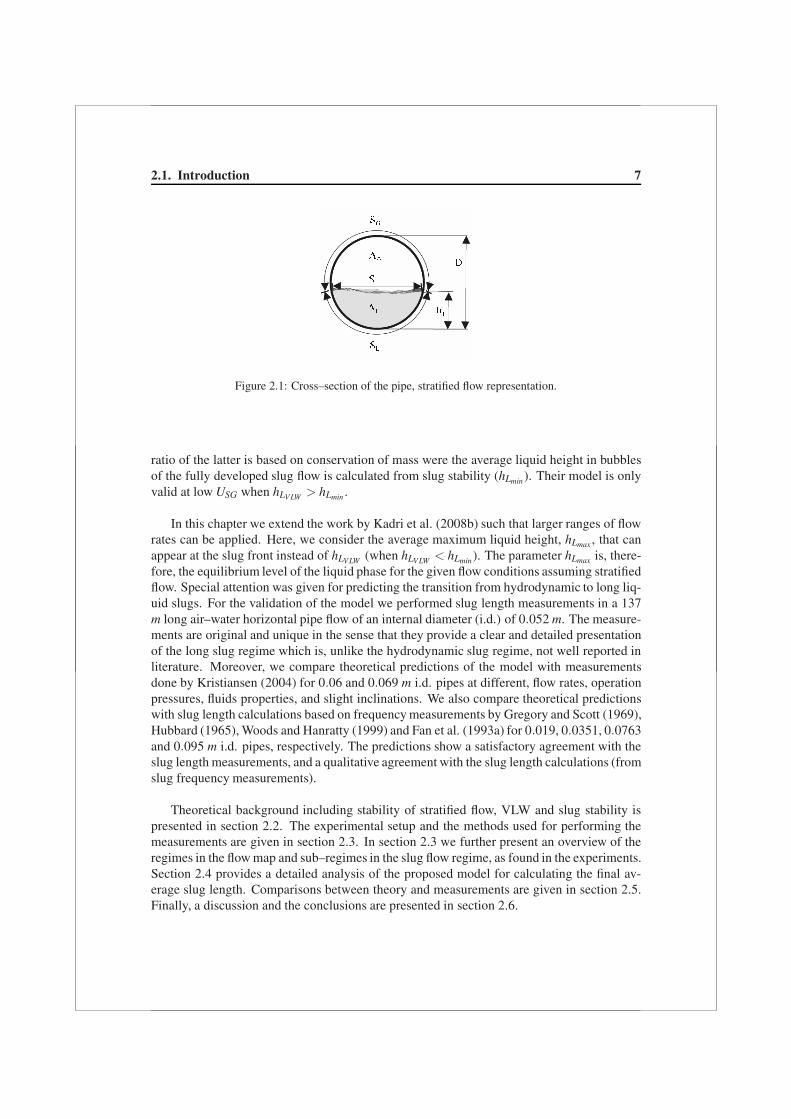
Figure 2.1: Cross–section of the pipe, stratified flow representation.
ratio of the latter is based on conservation of mass were the average liquid height in bubblesof the fully developed slug flow is calculated from slug stability (hLmin). Their model is onlyvalid at low USG when hLVLW > hLmin .
In this chapter we extend the work by Kadri et al. (2008b) such that larger ranges of flowrates can be applied. Here, we consider the average maximum liquid height, hLmax , that canappear at the slug front instead of hLVLW (when hLVLW < hLmin). The parameter hLmax is, there-fore, the equilibrium level of the liquid phase for the given flow conditions assuming stratifiedflow. Special attention was given for predicting the transition from hydrodynamic to long liq-uid slugs. For the validation of the model we performed slug length measurements in a 137m long air–water horizontal pipe flow of an internal diameter (i.d.) of 0.052 m. The measure-ments are original and unique in the sense that they provide a clear and detailed presentationof the long slug regime which is, unlike the hydrodynamic slug regime, not well reported inliterature. Moreover, we compare theoretical predictions of the model with measurementsdone by Kristiansen (2004) for 0.06 and 0.069 m i.d. pipes at different, flow rates, operationpressures, fluids properties, and slight inclinations. We also compare theoretical predictionswith slug length calculations based on frequency measurements by Gregory and Scott (1969),Hubbard (1965), Woods and Hanratty (1999) and Fan et al. (1993a) for 0.019, 0.0351, 0.0763and 0.095 m i.d. pipes, respectively. The predictions show a satisfactory agreement with theslug length measurements, and a qualitative agreement with the slug length calculations (fromslug frequency measurements).
Theoretical background including stability of stratified flow, VLW and slug stability ispresented in section 2.2. The experimental setup and the methods used for performing themeasurements are given in section 2.3. In section 2.3 we further present an overview of theregimes in the flow map and sub–regimes in the slug flow regime, as found in the experiments.Section 2.4 provides a detailed analysis of the proposed model for calculating the final av-erage slug length. Comparisons between theory and measurements are given in section 2.5.Finally, a discussion and the conclusions are presented in section 2.6.
8 Chapter 2. Dynamic slugs
2.2 Theoretical background
2.2.1 Stratified flow pattern
An idealized model of the stratified flow pattern is represented by a simplified geometry asgiven in Figure 2.1. The diameter of the pipe is D. The height of the liquid layer along thecenterline is hL. The length of the segments of the pipe circumference in contact with the gasand liquid are SG and SL, respectively. The length of the gas–water interface is representedby Si. The areas occupied by the gas and the liquid are AG and AL, respectively. Given thepipe diameter and the liquid height (or area), these parameters can be calculated using thegeometric formulae by Govier and Aziz (1972). Now we can write the momentum balancesfor the gas and the liquid flows as follows,
−AG
(dpdx
)− τWGSG − τiSi + ρGAGgsinθ = 0, (2.1)
−AL
[(dpdx
)−ρLgcosθ
(dhL
dx
)]− τW LSL + τiSi + ρLALgsinθ = 0 (2.2)
where ρG and ρL are the gas and the liquid densities, θ is the inclination angle of the pipefrom the horizontal, dp/dx is the pressure gradient, dhL/dx is the liquid hydraulic gradient,and g is the acceleration due to gravitational forces. The time-averaged resisting stress of thegas and the liquid at the wall are τW G and τW L, respectively. Term τi represents the resistingstress at the interface. The stresses τW G, τW L and τi are defined in terms of friction factors,which are calculated using the Blasius equation if Re < 105 and the wall roughness effectcan be ignored, otherwise the Churchill equation is used (see Churchill (1977)). For givenflow rates of the gas and the liquid, Eqs. (2.1) and (2.2) are used to find the pressure gradientand the height of the liquid layer. However, these equations do not determine the stabilityof the stratified flow. The flow is assumed to be varying slowly enough that pseudo–steady–state assumptions can be made (e.g. dhL/dx = 0 and τW G, τW L and τi can be related to flowvariables).
2.2.2 Viscous long wavelength theory
The transportation of gas and liquid in horizontal pipes results in a wide range of wavelengthwaves and wave frequencies along the pipe. At low gas and liquid flow rates, high frequencywaves are formed close to the inlet (Woods and Hanratty (1999)). Among those, waves withfrequencies 10–12 Hz grow and bifurcate further downstream due to energy accumulations(Fan et al. (1993a)). The bifurcation results, among other, in long wavelength waves that cangrow, roll or decay, depending on the height of the liquid layer (Fan et al. (1993a)). For the“right” flow conditions, they grow to become slugs. If the pipe is long enough and the longwavelength waves form far downstream the inlet such that the evolving slugs are independentfrom the flow disturbances at the inlet, the slugs can grow to become extremely large.
The viscous long wavelength (VLW) stability theory describes such long waves on thinfilms over which gas is blowing. The waves are assumed to be long enough so that a changein pressure can be described by a hydrostatic approximation and the stresses vary so slowly
2.2. Theoretical background 9
in time that a pseudo steady–state approximation describes the change in stresses. The equa-tions of conservation of mass and momentum for the liquid phase in the horizontal pipe are,respectively,
∂AL
∂t+
∂(uAL)∂x
= 0, (2.3)
and∂(uAL)
∂t+
∂(u2AL
)∂x
= −AL
ρL
[(∂p∂x
)+ ρLgcosθ
(∂hL
∂x
)]+
+1
ρL(τiSi − τWLSL)+ ALgsinθ, (2.4)
A disturbance is assumed to occur at the interface,
AL = AL + ALexp [ik(x−Ct)] , (2.5)
where AL is the average area occupied by the liquid, AL is the amplitude of the disturbance,C is the complex wave velocity and k is the wave number. Introducing complex amplitudesof the wave–induced variations of the pressure and of the resisting stresses and substitutingequations of the form of Eq. (2.5), Lin and Hanratty (1986) obtained a relation for the criticalvelocities for the initiation of a long wavelength disturbance,
0 = ρL(CR − u)2 +AL
AGρG(U −CR)2 −gALρLcosθ
h
AL. (2.6)
Terms U and u are the time average gas and liquid velocities. Term CR is the real part of C,for given superficial gas and liquid velocities at neutral stability, where CI , the imaginary partof C, is zero. Substituting the critical velocities in Eq. (2.4) results in the liquid area, ALVLW
(or hLVLW ), required for the initiation of instabilities at the surface (e.g. waves or slugs). Adetailed analysis of the VLW theory can be found in Lin and Hanratty (1986) and in Hurlburtand Hanratty (2002).
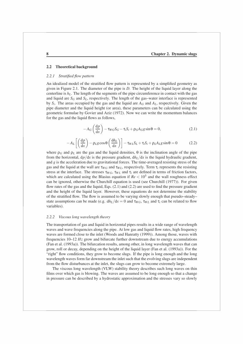
Figure 2.2: Sketch of a slug.

10 Chapter 2. Dynamic slugs
2.2.3 Slug stability analysis
The slug stability analysis considers the rates of liquid adjoining and detaching from a slugat its front and rear. Slugs are defined here as stable when the rates of liquid adjoining are notless than the rates at which liquid detaches, and they are addressed as “neutrally stable” whentheir length is neither growing nor decaying. Figure 2.2 gives an illustration of a slug movingwith a front velocity CF over a stratified liquid layer, at station 1, of area AL1 and velocity u1.The volumetric flow rate of liquid adjoining the slug is
Qin = (CF −u1)AL1. (2.7)
The rear of the slug is assumed to behave as a bubble moving with a velocity CB. FollowingBendiksen (1984), Woods and Hanratty (1996), Hurlburt and Hanratty (2002) and Soleimaniand Hanratty (2003) the velocity at the back of a slug can be modelled as a Benjamin bubble(Benjamin (1968)) where three main regimes are defined:
CB = UMix + 0.542√
gD UMix < 2√
gD, (2.8)
CB = 1.1UMix + 0.542√
gD 2√
gD < UMix < 3.5√
gD, (2.9)
CB = 1.2UMix UMix > 3.5√
gD. (2.10)
The velocity of the liquid in the slug is u3 (the liquid velocity at station 3). The volumefraction of the gas in the slug is ε. The volumetric flow rate of the liquid detaching from theslug is
Qout = (CB −u3)(1− ε)A, at station 3. (2.11)
Assuming neutral stability, Qin = Qout and CF = CB, and making use of Eqs. (2.7)–(2.11), thefollowing relation is obtained,
(AL1
A
)crit
=(CB −u3)(1− ε)
(CB −u1), (2.12)
for the area of the stratified flow. For incompressible flow, the term u3 is calculated from avolumetric balance between the inlet of the pipe and station 3 as follows,
UMix = εU3 +(1− ε)u3, (2.13)
where U3 is the gas velocity at station 3. At low mixture velocities aeration is negligible(ε = 0) so that Eq. (2.13) gives u3 = UMix. Eq. (2.12) is used later to calculate the averageliquid level below the elongated bubbles in the “fully developed” slug flow. The detailedanalysis of the slug stability model is well documented by Hurlburt and Hanratty (2002);Soleimani and Hanratty (2003).
2.3. Experiments on the occurrence of long slugs 11
2.3 Experiments on the occurrence of long slugs
2.3.1 Experiments
Experiments have been carried out in order to investigate the long slug regime (Zoeteweij(2007)). Not many researchers are aware of this regime and its properties due to a number ofconditions required for such slugs to appear, e.g. long pipe and low flow rates and operationpressure. The flow facility used for this aim consists of a 137 m long horizontal pipeline witha diameter of 0.052 m (see Figure 2.3). The pipe is made of Perspex (Plexiglass) to allowvisual observations of the flow conditions. At the inlet, the two phases are combined in aY–shaped section with the gas phase always entering from the top in a horizontal direction inorder to prevent the impact of the gas–jet coming from above. The pressure is atmosphericand the gas and liquid phases used are air and water, respectively.
Two different measurement techniques, based on liquid conductance, were installed. Thefirst technique consists of a set of sensors that measure the presence of passing slugs. Itconsists of point detector sections positioned at 8 locations along the pipe at: 29, 43, 62, 74,93, 107, 120, and 132 m from the inlet. A schematic drawing of these positions is given inFigure 2.4. Each measurement section contains 2 pairs of sensors separated by 0.7 m. Eachpair of sensors consists of two electrodes one at the bottom of the pipe and the second ontop. Due to the fact that the electrodes at the bottom are circular plates of 0.01 m diameter theelectrical conductance between the liquid phase and these electrodes are always good. On theother hand, the top electrodes consist of a metal pin with a diameter of 1 mm. The slug lengthand velocity are calculated from the time difference of the slug passing two different sensorsof the same section: (1) the velocity is calculated from the distance between the two sensorsdivided by the time difference; and (2) the slug length is calculated from the velocity and thetime difference between the front and tail passing the same sensor. The second measurementtechnique is based on wire–mesh sensors. Unlike the point probe sensors, this techniqueprovides a more detailed flow imaging in stratified and slug flows. The technique is based onthe difference in electrical conductivity of both phases. A set of 4 sensors is used at differentpositions: 38, 56, 105 and 125 m from the inlet (see Figure 2.4). Each sensor consists of twoplanes with 16 parallel 0.12 mm wires each. The wires in different planes are perpendicularto each other. Measuring the signal of all vertical receiver wires crossing a horizontal sendingone results in the local conductivity around the crossing points in the mesh. The conductivitysignals indicate the local phase composition in the grid cell. Further details on the wire–meshcan be found in Zoeteweij (2007).
The experiments were performed at atmospheric pressure and constant flow rates withsuperficial gas and liquid velocities being 0.5–2.5 and 0.05–0.30 m/s, respectively. Thedifferent combinations of flow rates used in the experiments resulted in a detailed overviewof the slug flow development in different regimes, and sub–regimes within the long slug flowregime.
2.3.2 Sub–regimes in the slug flow map
The different flow regimes and a number of different sub–regimes within the long slug flowregime observed in the experiments are shown in Figure 2.5. The dashed–dotted line is the

12 Chapter 2. Dynamic slugs
Figure 2.3: Sketch of the experimental setup (after Zoeteweij (2007)). The valves are indicated by ×.
observed transition from stratified (×) or stratified–wavy flow (∗) to slug flow; the solid–lineis the observed transition from hydrodynamic slug flow (◦) to the long slug flow regime.Within the long slug flow regime, two sub–regimes were observed: (1) above the dashed–linelong but neutrally stable slugs (�); and (2) below the dashed line, long and positively growingslugs were found (•).
The hydrodynamic slugs are characterized by a relatively short length, less than 40D.Whereas the long slugs have at least a length of 40D and can reach lengths up to severalhundred pipe diameters. Note that the long slug region shrinks for increasing gas velocity –the long slugs are found to exist only at low gas and liquid flow rates, as shown in Figure 2.5.Therefore, the transition from stratified flow to hydrodynamic slugs, at low superficial gasvelocities, passes through the long slug regime. For higher superficial gas velocities, USG >2.5 m/s, the transition from the stratified–wavy to hydrodynamic slug flow is direct. Theabsence of the long slugs at higher USG is related to the higher slug frequency and loweramount of liquid adjoining the passing slug due to a decrease of the liquid level (conservationof mass and momentum) which results in a neutral stability (Qin = Qout and CF = CB) earlier
Figure 2.4: Schematic drawing of the position of the point probe (|) and wire–mesh (•) sensors (afterZoeteweij (2007)).

2.3. Experiments on the occurrence of long slugs 13
0 0.5 1 1.5 2 2.5 30
0.05
0.1
0.15
0.2
0.25
0.3
0.35
USG
[m/s]
USL
[m
/s]
Long stable slugs, L
S > 40D
Hydrodynamic slugs, LS < 40D
Long growing slugs, LS > 40D
Stratified flowStratified−wavy flow
Long slugs Hydrodynamic slugs
Stratified flow Stratified−wavy flow
Long slugs(growing)
Figure 2.5: Air–water measurements of the slug flow regime and sub–regimes for different USG andUSL, D = 0.052 m, θ = 0o, P = 1 barA.
in the pipe. Consequently, in the long slug regime, the slug length and growth time decreaseat larger flow rates, as observed in the experiments.
Figure 2.6 is a flow regime map by Woods and Hanratty (1999) for air–water flow in ahorizontal 0.0763 m pipe. In the figure, curve A indicates the transition from stratified toslug flow; the region between curves A and B (areas I and II) covers slugs that form about40D downstream of the entrance; area III represents slugs that form within 40D from theentrance; and along curve C the Froude number, Fr = u/
√ghLmax, is unity at the inlet. Com-
paring Figures 2.5 and 2.6, and noting the difference in the diameters, we find the following:(1) The long growing slugs correspond to the slugs evolving from long wavelength wavesdownstream (at Fr < 1). (2) The long stable slugs evolve from the same type of waves butfurther upstream. Their frequency is higher and they travel over a thinner liquid layer, thatis why they reach neutral stability earlier in the pipe. (3) The hydrodynamic slugs corre-spond to slugs that form upstream (close to the inlet) at Fr > 1. These slugs are no longerformed by the long wavelengths but close to the entrance by disturbances that are createdthere (Woods and Hanratty (1999)). The high frequency of such slugs and the thin liquidlayer downstream result in their short length. These findings are in agreement with our abovementioned experimental observations.

14 Chapter 2. Dynamic slugs
Figure 2.6: Flow regime map for air–water flow in a horizontal 0.0763 m pipe. Curve A indicates thetransition to slug flow; between curves A and B, slugs from downstream ca. 40D; along curve C, Froudenumber Fr = 1 at the inlet (Woods and Hanratty (1999))1.
2.4 Dynamic slug model
In the model presented here, the average length of a fully developed slug is determined fromvolumetric liquid considerations between the front and the tail of a slug. The liquid level at thefront is assumed to be constant, whereas at the back, the liquid level drops during the initiationof the slug and then rebuilds during its growth. The liquid level at the back is obtained fromlinear kinematic relations between the slug and the wave behind it. The properties of slugs atformation time are presented in section 2.4.1. In section 2.4.2, the calculation method of thedynamic slug is introduced. A stopping criterion for the calculation of the slug growth, basedon conservation of mass of the gas and liquid phases, is addressed in section 2.4.3.
2.4.1 Properties of forming slugs
2.4.1.1 Wave velocity
We address the formation of slugs from growing waves. The growing waves are assumed tobe sinusoidal with an initial wavelength, λ, large compared to the average maximum liquidheight, hLmax . A characteristic property of such waves is the dependency of the wave velocity,C, on the liquid level alone,
C =√
ghLmax . (2.14)
1Reprinted from International Journal of Multiphase Flow, Vol 25, Bennett D. Woods, Thomas J. Hanratty,Influence of Froude number on physical processes determining frequency of slugging in horizontal gas–liquid flows,1195–1223, Copyright (1999), with permission from Elsevier.
2.4. Dynamic slug model 15
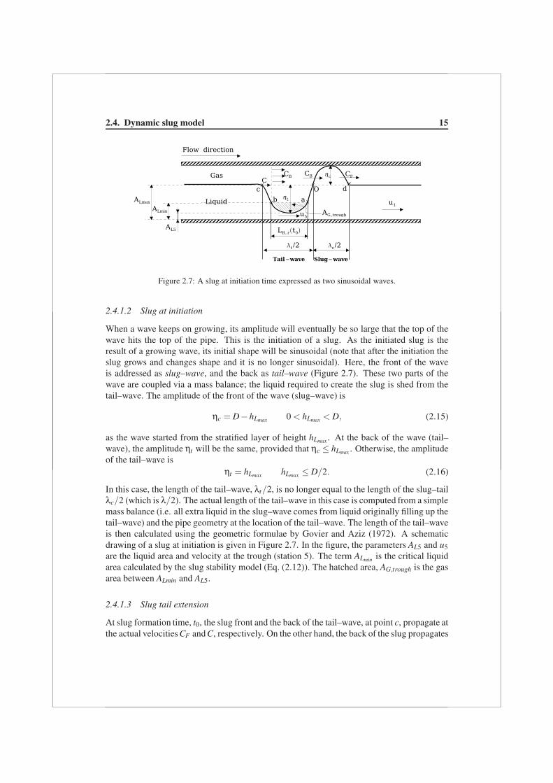
Figure 2.7: A slug at initiation time expressed as two sinusoidal waves.
2.4.1.2 Slug at initiation
When a wave keeps on growing, its amplitude will eventually be so large that the top of thewave hits the top of the pipe. This is the initiation of a slug. As the initiated slug is theresult of a growing wave, its initial shape will be sinusoidal (note that after the initiation theslug grows and changes shape and it is no longer sinusoidal). Here, the front of the waveis addressed as slug–wave, and the back as tail–wave (Figure 2.7). These two parts of thewave are coupled via a mass balance; the liquid required to create the slug is shed from thetail–wave. The amplitude of the front of the wave (slug–wave) is
ηc = D−hLmax 0 < hLmax < D, (2.15)
as the wave started from the stratified layer of height hLmax . At the back of the wave (tail–wave), the amplitude ηt will be the same, provided that ηc ≤ hLmax . Otherwise, the amplitudeof the tail–wave is
ηt = hLmax hLmax ≤ D/2. (2.16)
In this case, the length of the tail–wave, λt/2, is no longer equal to the length of the slug–tailλc/2 (which is λ/2). The actual length of the tail–wave in this case is computed from a simplemass balance (i.e. all extra liquid in the slug–wave comes from liquid originally filling up thetail–wave) and the pipe geometry at the location of the tail–wave. The length of the tail–waveis then calculated using the geometric formulae by Govier and Aziz (1972). A schematicdrawing of a slug at initiation is given in Figure 2.7. In the figure, the parameters AL5 and u5are the liquid area and velocity at the trough (station 5). The term ALmin is the critical liquidarea calculated by the slug stability model (Eq. (2.12)). The hatched area, AG,trough is the gasarea between ALmin and AL5.
2.4.1.3 Slug tail extension
At slug formation time, t0, the slug front and the back of the tail–wave, at point c, propagate atthe actual velocities CF and C, respectively. On the other hand, the back of the slug propagates

16 Chapter 2. Dynamic slugs
at the bubble velocity CB. The front of the tail–wave (point O) is obviously the back of theslug. Therefore, it propagates together with the back of the slug. The ALmin line in Figure 2.7is the slug stability line representing the average liquid level below the bubbles in the fullydeveloped slug flow. Points a and b refer to two points on the tail–wave (at time t0) being atthe height of the final liquid level, hLmin (calculated from ALmin).
Due to the relative velocity between the two sides of the tail–wave (points O and c) thewave volume in between is expanded in time. While point a propagates with the slug back atvelocity CB, from a linear expansion point b propagates at a velocity,
vb = C + r(CB −C), (2.17)
where r is the ratio between the horizontal displacements of points b, calculated from thewave equation, and a relative to c. The ratio r has a value 0 ≤ r ≤ 1. Due to the relativevelocity between points a and b the relative distance between them, LB,r, grows linearly as
LB,r (t) = LB,r (t0)+ (vb −C)t. (2.18)
Eq. (2.18) describes the extension of the tail in time. It plays a major role in a stoppingcriterion for the calculations of the average slug length, as will be seen in section 2.4.3.
2.4.1.4 Initial slug length
The initial slug length, L0, is calculated from the wavelength, λ,
L0 =λ2. (2.19)
Term λ is calculated from the wave velocity (λ =C/fw) and the relation fw = cwfS by Tronconi(1990) for the slug and the wave frequencies, fS and fw, as follows,
λ =C
cwfS, (2.20)
where cw is a constant equal to 2 for air–water systems (Tronconi (1990)). In this chapter thesame value of cw was used for the different fluids. Kadri et al. (2008b) suggested to use acorrelation by Nydal (1991) for the slug frequency,
fS = 0.088(USL + 1.5)2
gD. (2.21)
Quantities in Eq. (2.21) are in meters and seconds. The application condition of Eq. (2.21)is that the frequency of slugs is dominated by USL. Note that the slug frequency correlationis used here only in order to obtain a “realistic” initial length of the long waves (which arein agreement with experiments). Other methods can be implemented to obtain an initialwavelength. Alternatively, L0 can be calculated from the minimum stable slug length byDukler et al. (1985).
2.4. Dynamic slug model 17
2.4.2 Slug growth and final length
The calculations of the slug growth are not sensitive to small changes in the initial wave-lengths especially for long slugs where the final length of slugs LS, f � λ. Therefore, themain contribution to the final slug length is the additional slug growth due to the volumetricdifferences between liquid adjoining the slug at the front and detaching from the slug at thetrough. The volume of the liquid in front of the slug is the product of the cross-sectional area,ALmax , occupied by the liquid times the length of this liquid part. Similarly, for the liquid vol-ume at the back of the slug, we need to calculate the cross–sectional area of the liquid layerat the trough. Hence, we need to calculate the two liquid areas, at the trough and downstreamof the slug.
2.4.2.1 The liquid area downstream of the slug, ALmax
The liquid area downstream is calculated from the momentum balances for the stratified flowpattern, Eqs. (2.1)–(2.2). Substituting AL = ALmax and AG = A−ALmax , Eq. (2.1) is written inthe following form, (
dpdx
)=
τW GSG + τiSi
A−ALmax
−ρGgsinθ. (2.22)
Plain stratified flow is reached when the pressure gradients of the two phases on the interfacecancel each other. Therefore, substituting Eq. (2.22) in Eq. (2.2) and after basic algebra weobtain,
ALmax = AτW LSL − τiSi
τW LSL + τWGSG+ gALmax(A−ALmax)
[ρL cosθ
(dhL
dx
)− sinθ(ρL −ρG)
]. (2.23)
For a fully developed horizontal flow Eq. (2.23) reduces to the simple form,
ALmax = AτW LSL − τiSi
τWLSL + τW GSG. (2.24)
Eq. (2.24) successfully predicts that increasing the gas flow rates or decreasing the liquid flowrates results in a lower ALmax .
At low flow rates slugs evolve downstream from long wavelength waves as mentionedabove. In that case, the liquid level of the stratified flow at t0 is calculated by VLW theory. Ifthe liquid flow rates are larger than those predicted by VLW theory, we use Eq. (2.24) for thecalculation of the stratified liquid level. On the other hand, the minimum liquid area, ALmin ,at the front of a fully developed slug is calculated by the slug stability model, Eq. (2.12), asmentioned earlier.
2.4.2.2 The liquid area upstream of the slug, AL5(t)
Making use of the neutral stability assumptions (Qin = Qout and CF = CB), the liquid velocityat the trough u5 is obtained from a volumetric flow balance between the liquid entering atstation 1 (front) and detaching at station 5 (see Figure 2.2) for the fully developed case, thus
u5 = u1ALmin
AL5(t), (2.25)
18 Chapter 2. Dynamic slugs
where u1 is the liquid velocity downstream of the slug (station 1) and AL5(t) is the cross–sectional area of the liquid at the trough.
The average velocity of the gas above AG,trough is assumed to be the bubble velocity CB
and therefore the gas volume is conserved there. This also implies that the initial gas volumeabove the trough and below ALmin is constant (see the hatched area in Figure 2.7). Since h� λthe area AG,trough was considered instead of the volume. The parameter AG,trough is calculatedby integrating the wave function between points a and b at any time t as follows,
AG,trough = [hLmin −hL5(t)]∫ a
bsin
[2π
λc + 2(CB −C)tx
]dx. (2.26)
The left hand side of Eq. (2.26) is a constant. Therefore, substituting two cases in Eq. (2.26),the first t = 0 and the other t = t, and equating between them results in the liquid level at thetrough, hL5(t), as follows,
hL5(t) = hLmin
[1− λc
λc + 2(CB − c)t
]+ hL5(0)
λc
λc + 2(CB − c)t, (2.27)
where hL5(0) = D−ηc −ηt . For the pipe diameter and flow conditions used in this chapterhL5(0) � (D− h) and therefore was neglected. The liquid area AL5(t) is calculated fromhL5(t) in Eq. (2.27) and the geometric formulae presented by Govier and Aziz (1972).
Eq. (2.27) provides an explanation for the behaviour of the slug length at different flowrates, which decreases when increasing the flow rates (as shown in Figure 2.9). In the equa-tion, increasing the flow rates results in larger values of, hL5. This means that the rebuild rateof the liquid behind a slug increases with the flow rates, and thus the growth time of the slugdecreases which results in a shorter slug.
2.4.2.3 Slug length, LS(t)
The change in the additional liquid volume entering the slug describes the rate of change ofthe slug volume,
dVdt
= [CF (t)−u1]ALmax − (CB −u5)AL5(t), (2.28)
and the front velocity is
CF (t) =dV
d(At)+CB. (2.29)
To simplify the problem we assumed that CB is constant in time.The total slug volume is calculated from the sum of Eqs. (2.19) and (2.28),
Vslug (t) = L0A +∫ t∞
0((CF (t)−u1)ALmax − (CB −u5)AL5 (t))dt. (2.30)
Once Eq. (2.30) is solved, the slug length follows as
LS(t) =Vslug (t)
A. (2.31)

2.4. Dynamic slug model 19
2.4.3 End of slug growth
If only one slug would have been initiated in the pipe, it would keep growing until it finallyexits the pipe. However, in general more slugs are present at the same time. A slug willstop growing as soon as its front approaches the back of the tail of the next slug downstream.Thus, we need to estimate when this happens. We do so by inspecting what happens whenall slugs are formed at regular distances. This means that we will find the average slug lengthand ignore that actually a distribution of slug lengths develops as slugs are initiated in anirregular way. However, with this approach we can estimate the average slug length and bythat predict where the long slug regime is located in the flow map. As a consequence, allslugs and bubbles reach their final lengths simultaneously, say at time t∞. This conclusionleads to a stopping criterion for the calculation of the average slug length: the final averageslug length is reached when the extension of the tail (the distance between points a and b)becomes equal to the bubble final length,
LB,r (t) = LB, f , (2.32)
as shown in Figure 2.8. In the figure, the fully developed average slug problem is presentedfor a pipe cross–sectional area A. The cross–sectional liquid area of the stratified flow is ALmax
and for the fully developed slug flow is ALmin along the bubble. Choosing a control volumewith the unit length, LU = LB, f +LS, f , and making a volumetric balance between the stratifiedflow and the fully developed slug flow cases, a relation between the bubble and slug lengthsis obtained as follows,
LB, f = LS, fA−ALmax
ALmax −ALmin. (2.33)
At the limit of Eq. (2.33) when ALmax → ALmin , term LB, f → ∞, which means that there are noslugs in the pipe, as expected.
Since LS, f , LB, f , LU and t∞ are unknowns, t∞ is calculated recursively by substitutingEqs. (2.18) and (2.32), and LS(t) instead of LS, f , in Eq. (2.33) as follows,
t∞ =1vb
[LS(t∞)
A−ALmax
ALmax −ALmin−LB,r(t0)
]. (2.34)
Figure 2.8: A presentation of the average fully developed slug flow.
20 Chapter 2. Dynamic slugs
0 0.5 1 1.5 2 2.5 30
100
200
LS [
D]
0 0.5 1 1.5 2 2.5 30
100
200
LS [
D]
0 0.5 1 1.5 2 2.5 30
100
200
LS [
D]
USG
[m/s]
Slug length measurementsCurrent model
USL
= 0.25 [m/s]
USL
= 0.29 [m/s]
USL
= 0.1032 [m/s]
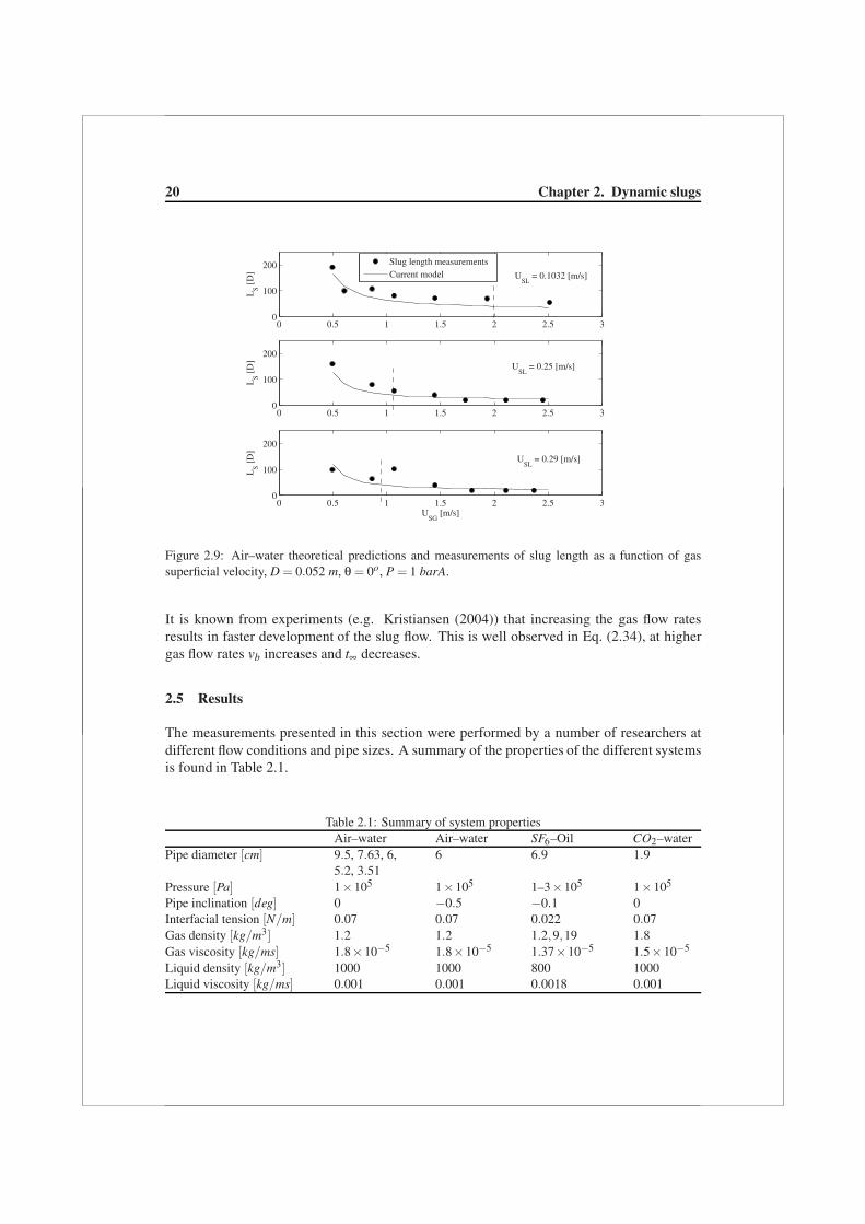
Figure 2.9: Air–water theoretical predictions and measurements of slug length as a function of gassuperficial velocity, D = 0.052 m, θ = 0o, P = 1 barA.
It is known from experiments (e.g. Kristiansen (2004)) that increasing the gas flow ratesresults in faster development of the slug flow. This is well observed in Eq. (2.34), at highergas flow rates vb increases and t∞ decreases.
2.5 Results
The measurements presented in this section were performed by a number of researchers atdifferent flow conditions and pipe sizes. A summary of the properties of the different systemsis found in Table 2.1.
Table 2.1: Summary of system propertiesAir–water Air–water SF6–Oil CO2–water
Pipe diameter [cm] 9.5, 7.63, 6, 6 6.9 1.95.2, 3.51
Pressure [Pa] 1×10⁵ 1×10⁵ 1–3×10⁵ 1×10⁵
Pipe inclination [deg] 0 −0.5 −0.1 0Interfacial tension [N/m] 0.07 0.07 0.022 0.07Gas density [kg/m3] 1.2 1.2 1.2,9,19 1.8Gas viscosity [kg/ms] 1.8×10⁻⁵ 1.8×10⁻⁵ 1.37×10⁻⁵ 1.5×10⁻⁵
Liquid density [kg/m3] 1000 1000 800 1000Liquid viscosity [kg/ms] 0.001 0.001 0.0018 0.001
2.5. Results 21
0 0.5 1 1.5 2 2.5 30
0.05
0.1
0.15
0.2
0.25
0.3
0.35
USG
[m/s]
USL
[m
/s]
Long stable slugs, LS > 40D
Hydrodynamic slugs, LS < 40D
Long growing slugs, LS > 40D
Stratified / stratified−wavy flowCurrent model, L
S = 40D
Slug stability model
Long slugs Hydrodynamic slugs
Stratified/ stratified−wavy flow
Figure 2.10: Air–water theoretical predictions and measurements of the flow regime transition for dif-ferent USG and USL , D = 0.052 m, θ = 0o, P = 1 barA.
0 0.2 0.4 0.6 0.8 1 1.20
20
40
60
80
100
120
LS [
D]
USL
[m/s]
Fluids: Air/WaterU
SG = 1 m/s
P = 1 barAρ
G = 1.2 kg/m3
θ = 0°x/D = 219
Current modelSlug inlet, slug flow measurements (Kristiansen, 2004)Stratified inlet, slug flow measurements (Kristiansen, 2004)
Figure 2.11: Air–water theoretical predictions and measurements of slug length as a function of liquidsuperficial velocity, D = 0.06 m, θ = 0o, P = 1 barA, USG = 1 m/s.
22 Chapter 2. Dynamic slugs
2.5.1 Predictions for horizontal air–water flow
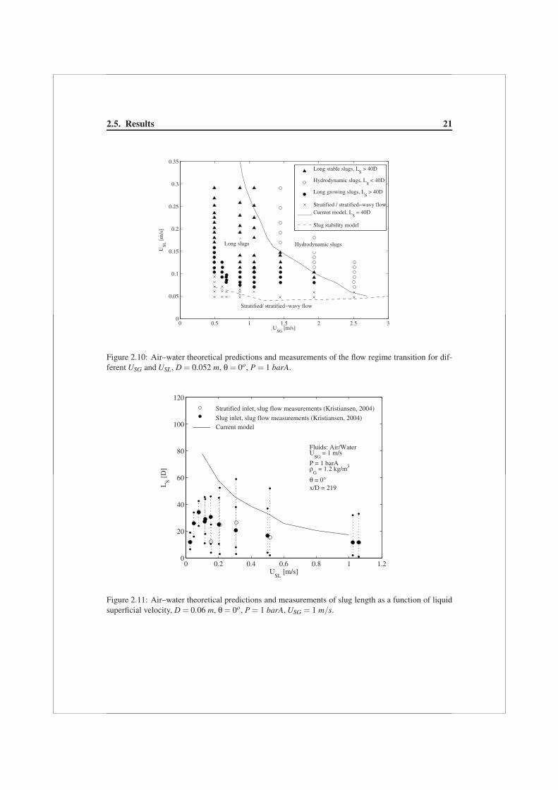
Theoretical calculations of slug final lengths, LS, f , are compared with measurements for air–water horizontal flow in Figures 2.9, 2.10 and 2.11. The measurements in Figures 2.9 and2.10 were carried out in a 137 m long pipe with 0.052 m i.d. at the TU Delft facility (Zoeteweij(2007)). The subplots in Figure 2.9 show LS, f as a function of USG for three different USL:0.1032, 0.25 and 0.29 m/s. The figure shows a satisfactory agreement between predictionsand measurements for the given flow rates. The vertical dashed lines indicate the criticalUSG for the transition from hydrodynamic to long slugs (i.e. slugs larger than 40D). Thetransition is further presented in Figure 2.10, a flow map for different slug flow regimes andsub–regimes. Here, the dashed line represents the transition from stratified to slug flow by theslug stability model, and the solid line is the prediction by the current model for LS, f = 40D,which represents the transition from hydrodynamic to long slug regimes. The current modelfor the transition from hydrodynamic to long slugs underpredicts the measurement at lowUSG, but quite accurately predicts the transition at higher USG.
The measurements in Figure 2.11 were done by Kristiansen (2004) in a 16 m pipe withi.d. of 0.06 m. Two different inlet conditions were considered here, stratified and slug flowrepresented by empty and filled circles, respectively. The dotted vertical lines are the devi-ation from the average slug length. The figure shows the behaviour of the slug length as afunction of USL, at USG = 1 m/s. It is noticeable that the theoretical model (the solid line)overpredicts the average values of the slug lengths with about a factor of 4 at low USL. Apossible reason for this deviation between predictions and measurements is the short pipelength being not sufficient for developed slug flow (the slug growth rate at x/D = 219 is stillpositive, Kristiansen (2004)). Note that the inlet conditions do not have a significant impacton the slug length in the short loop.
2.5.2 Predictions for declined air–water flow
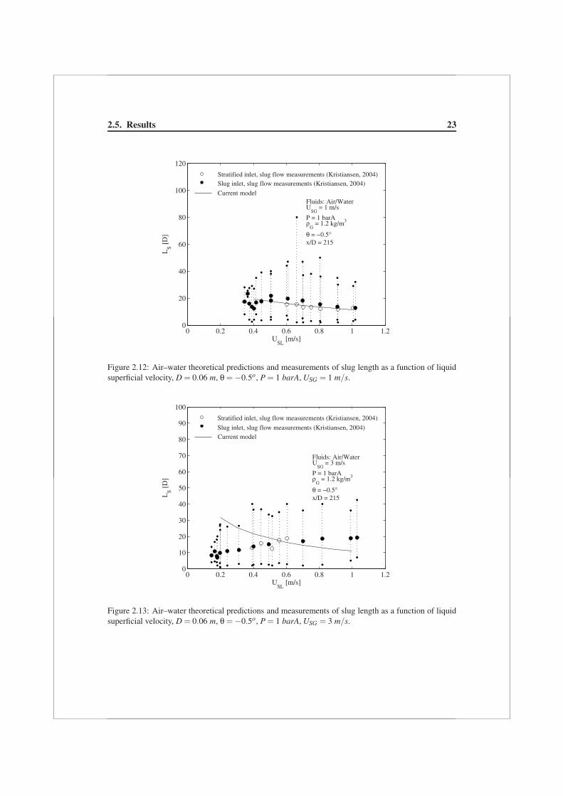
Figures 2.12 and 2.13 compare theoretical predictions of the slug length with measurements,as a function of USL for USG = 1 and 3 m/s, respectively. The measurements were alsodone by Kristiansen (2004) and carried out in the same short flow loop as in Figure 2.11.However, a negative inclination of −0.5o was considered here. Kristiansen (2004) found thatthe declination of the pipe results in lower growth rates so that slugs reach their final lengthearlier in the pipe, especially at lower USG. In the case of Figure 2.12, where USG = 1 m/s,the measured slugs have reached their final length and they are in good agreement with thetheoretical predictions. On the other hand, for the measurements in Figure 2.13, carried outat higher USG, the pipe is too short to obtain a fully developed slug flow. Here, the modeloverpredicts the slug length with a factor of three at low USL, and underpredicts it with afactor of two at high USL.
2.5.3 Predictions for SF6 gas–ExxsolD80 oil flow under varying pressure
The measurements shown in Figures 2.14–2.15 are those performed by Kristiansen (2004) fordifferent inlet conditions with different fluids in a longer and slightly larger facility (horizon-tal, 103 m long test loop with an i.d. of 0.069 m). Instead of air/water he used SF6 (sulphur
2.5. Results 23
0 0.2 0.4 0.6 0.8 1 1.20
20
40
60
80
100
120L
S [D
]
USL
[m/s]
Fluids: Air/WaterU
SG = 1 m/s
P = 1 barAρ
G = 1.2 kg/m3
θ = −0.5°x/D = 215
Stratified inlet, slug flow measurements (Kristiansen, 2004)Slug inlet, slug flow measurements (Kristiansen, 2004)
Current model
Figure 2.12: Air–water theoretical predictions and measurements of slug length as a function of liquidsuperficial velocity, D = 0.06 m, θ = −0.5o, P = 1 barA, USG = 1 m/s.
0 0.2 0.4 0.6 0.8 1 1.20
10
20
30
40
50
60
70
80
90
100
LS [
D]
USL
[m/s]
Stratified inlet, slug flow measurements (Kristiansen, 2004)Slug inlet, slug flow measurements (Kristiansen, 2004)Current model
Fluids: Air/WaterU
SG = 3 m/s
P = 1 barAρ
G = 1.2 kg/m3
θ = −0.5°x/D = 215
Figure 2.13: Air–water theoretical predictions and measurements of slug length as a function of liquidsuperficial velocity, D = 0.06 m, θ = −0.5o, P = 1 barA, USG = 3 m/s.

24 Chapter 2. Dynamic slugs
hexafluoride) gas and ExxsolD80 (hydrocarbon fluid) liquid at two different pressures. Sul-phur hexafluoride is a dense gas, approximately 5.5 times of the air density, that simulateshigh operation pressure conditions. The figures compare theoretical predictions of LS, f withmeasurements as a function of USL at constant USG and varying pressure. The predictions ofLS, f in Figure 2.14 (P = 1.5 barA and ρG = 9.1 kg/m3 simulating P = 12 bar) are in a goodagreement with the slug inlet measurements. However, a deviation between the predictionsand the stratified inlet measurements at USL < 0.15 m/s is noticed. The reason behind thedeviation is the proximity of the low USL to the pattern transition value that moves the sluginitiation point further downstream in the pipe. As a result, the slugs close to the outlet arenot fully developed.
At higher pressure, P = 3 barA (ρG = 18 kg/m3 simulating P = 23 bar), a deviationis noticed, as well, between predictions and slug inlet measurements at USL = 0.1 m/s (seeFigure 2.15). The deviation between the predictions and the stratified inlet measurementsbecomes even larger and for a wider range of USL (USL < 0.4 m/s). In the stratified inlet case,increasing the pressure results in increasing USLcrit needed for the transition from stratifiedto slug flow. Therefore, the delay of the slug initiation point further downstream in the pipecorresponds, as well, to higher values of USL. That is also why in the case of P = 3 barAno slugs appeared for USL < 0.17 m/s at the given USG (the flow rates are below the criticalvalues required for the pattern transition). In the case of the slug inlet, slugs at USL < 0.12m/s are unstable (slug stability) and their growth is sensitive to small perturbations at their
0 0.1 0.2 0.3 0.4 0.5 0.60
20
40
60
80
100
120
140
160
180
200
LS [
D]
USL
[m/s]
Fluids: SF6/ExxsolD80
USG
= 1.5 m/s
P = 1.5 barAρ
G = 9.1 kg/m3
θ = −0.1°x/D = 2903
Stratified inlet, slug flow measurements (Kristiansen, 2004)Slug inlet, slug flow measurements (Kristiansen, 2004)Current model
Figure 2.14: SF6–ExxsolD80 theoretical predictions and measurements of slug length as a function ofliquid superficial velocity, D = 0.069 m, θ = −0.1o, P = 1.5 barA, USG = 1.5 m/s.

2.5. Results 25
0 0.1 0.2 0.3 0.4 0.5 0.6 0.70
20
40
60
80
100
120
140
160
180
200L
S [D
]
USL
[m/s]
Slug inlet, slug flow measurements (Kristiansen, 2004) Stratified inlet, slug flow measurements (Kristiansen, 2004)
Current modelFluids: SF
6/ExxsolD80
USG
= 1.5 m/s
P = 3 barAρ
G = 18 kg/m3
θ = −0.1°x/D = 2642
Figure 2.15: SF6–ExxsolD80 theoretical predictions and measurements of slug length as a function ofliquid superficial velocity, D = 0.069 m, θ = −0.1o, P = 3 barA, USG = 1.5 m/s.
fronts. Therefore, they can grow or decay accordingly.
2.5.4 Predictions at large mixture velocities
In this subsection we examine the effect of large mixture velocities on the predictions bythe proposed model and compare the predictions to available measurements. Unfortunately,in these experiments there were no direct measurements for the slug length but for the slugfrequency. For that reason, we used the following approximation, suggested by Woods andHanratty (1996), for the relation between fS and LS, f under “fully developed” conditions,
fSDUSL
= 1.2(
LS, f
D
)−1
. (2.35)
Please note that we shall denote the slug lengths derived from the slug frequency measure-ments via Eq. (2.35) in the subsequent comparisons by slug “measurements”. Figures 2.16–2.17 compare predictions and measurements for a 20 m length and 0.0763 m i.d. pipe. Theslug frequency measurements were done by Woods and Hanratty (1999). In Figure 2.16 wesee that the current model overpredicts the measurements at low USL, underpredicts them athigh USL and successfully predicts them at “intermediate” USL. Predictions at intermediateliquid flow rates are important for the transition from hydrodynamic to long slug flows asshown in Figure 2.17, a flow map for the long (•) and hydrodynamic (◦) slug measurements
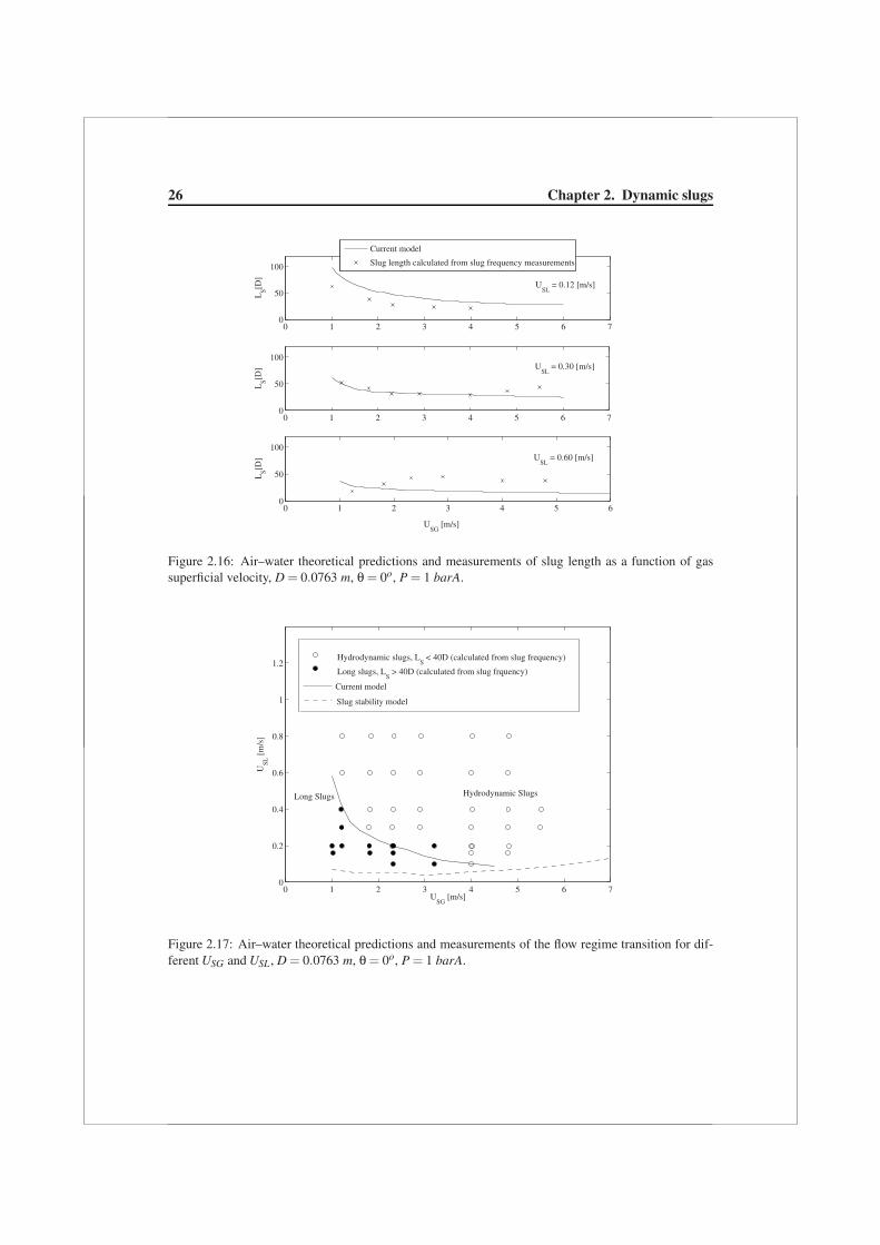
26 Chapter 2. Dynamic slugs
0 1 2 3 4 5 6 70
50
100L
S[D]
0 1 2 3 4 5 60
50
100
LS[D
]
0 1 2 3 4 5 6 70
50
100
USG
[m/s]
LS[D
]Current model
Slug length calculated from slug frequency measurements
USL
= 0.12 [m/s]
USL
= 0.30 [m/s]
USL
= 0.60 [m/s]
Figure 2.16: Air–water theoretical predictions and measurements of slug length as a function of gassuperficial velocity, D = 0.0763 m, θ = 0o, P = 1 barA.
0 1 2 3 4 5 6 70
0.2
0.4
0.6
0.8
1
1.2
USG
[m/s]
USL
[m
/s]
Hydrodynamic SlugsLong Slugs
Hydrodynamic slugs, LS < 40D (calculated from slug frequency)
Long slugs, LS > 40D (calculated from slug frquency)
Current model
Slug stability model
Figure 2.17: Air–water theoretical predictions and measurements of the flow regime transition for dif-ferent USG and USL , D = 0.0763 m, θ = 0o, P = 1 barA.
2.6. Conclusions 27
0 1 2 3 4 5 6 7 80
50
100
USG
[m/s]
LS[D
]
0 1 2 3 4 5 6 7 80
50
100
LS[D
]
0 1 2 3 4 5 6 7 80
50
100L
S[D]
Slug length calculated from slug frequency measurements
Current model
USL
= 0.50 [m/s]
USL
= 0.432 [m/s]
USL
= 0.442 [m/s]
D = 1.905 [cm]
D = 3.51 [cm]
D = 9.5 [cm]
Figure 2.18: Air–water theoretical predictions and measurements of slug length as a function of gassuperficial velocity, θ = 0o, P = 1 barA, top subplot: D = 0.019 m, middle subplot: D = 0.0351 m,bottom subplot: D = 0.095 m.
at different superficial flow rates. The dashed line is the slug stability line, and the solid line(L = 40D) represents the transition from long to hydrodynamic slugs.
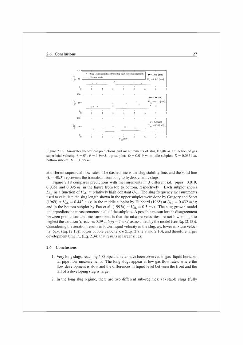
Figure 2.18 compares predictions with measurements in 3 different i.d. pipes: 0.019,0.0351 and 0.095 m (in the figure from top to bottom, respectively). Each subplot showsLS, f as a function of USG at relatively high constant USL. The slug frequency measurementsused to calculate the slug length shown in the upper subplot were done by Gregory and Scott(1969) at USL = 0.442 m/s; in the middle subplot by Hubbard (1965) at USL = 0.432 m/s;and in the bottom subplot by Fan et al. (1993a) at USL = 0.5 m/s. The slug growth modelunderpredicts the measurements in all of the subplots. A possible reason for the disagreementbetween predictions and measurements is that the mixture velocities are not low enough toneglect the aeration (ε reaches 0.39 at USG = 7 m/s) as assumed by the model (see Eq. (2.13)).Considering the aeration results in lower liquid velocity in the slug, u3, lower mixture veloc-ity, UMix (Eq. (2.13)), lower bubble velocity, CB (Eqs. 2.8, 2.9 and 2.10), and therefore largerdevelopment time, t∞ (Eq. 2.34) that results in larger slugs.
2.6 Conclusions
1. Very long slugs, reaching 500 pipe diameter have been observed in gas–liquid horizon-tal pipe flow measurements. The long slugs appear at low gas flow rates, where theflow development is slow and the differences in liquid level between the front and thetail of a developing slug is large.
2. In the long slug regime, there are two different sub–regimes: (a) stable slugs (fully

28 Chapter 2. Dynamic slugs
developed), that have reached their final length; and (b) growing slugs. The secondtype appears, at critical liquid flow rates close to the transition from stratified to slugflow.
3. At low gas flow rates the transition from stratified to hydrodynamic slug flow occurs viathe long slug regime. At high gas flow rates such a long slug region does not exist andfor favourable flow conditions stratified flow directly transforms into hydrodynamicslug flow.
4. A slug growth model was presented. The growth model applies a volumetric balancebetween the front and the tail of a slug. In the model, the behaviour of the liquid phaseat the slug tail is simplified by applying a linear kinematic relation between the back ofthe slug and the wave upstream. This relation is used to calculate the tail extension andthe change in the liquid level. The growth model captures the main factors contribut-ing to the slug growth behaviour. As a result, it accurately predicts the transition fromhydrodynamic to long slug regimes for different pipe diameters. However, it underpre-dicts the average slug length at high mixture velocities. To improve the predictions,gas entrainment should be taken into consideration.
5. The model provides an explanation for a number of important observations in the slugflow regime: (a) in the long slug regime, the slug length decreases with increasingliquid flow rates as a result of the faster development of the liquid level behind theslug (Eqs. (2.27) and (2.34)); (b) increasing the operation pressure results in largerinterfacial shear stresses, lower equilibrium liquid level (Eq. (2.24)) and volumetricgrowth rate (Eq. (2.28)), and thus shorter average slug length – that is why at highpressure only hydrodynamic slugs are observed; (c) further increase of the pressureresults in liquid levels approaching the minimum slug stability level, so that no stableslugs (long or hydrodynamic) can appear anymore (unless produced at the inlet).
6. Our study with the long slug growth model raises important questions on: (a) the criti-cal operation pressure and flow development time at which the long slugs appear; and(b) the contribution of the interfacial shear stresses and gas entrainment to the long slugdevelopment. Answers to these questions are key issues in reducing the negative effectsof long slugs when operating at low pressure and low gas rates. These are subjects ofresearch in progress.
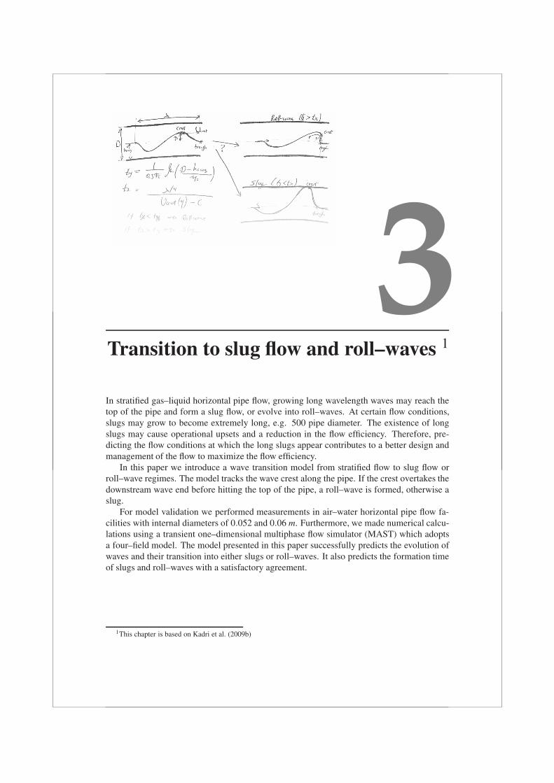
3Transition to slug flow and roll–waves 1
In stratified gas–liquid horizontal pipe flow, growing long wavelength waves may reach thetop of the pipe and form a slug flow, or evolve into roll–waves. At certain flow conditions,slugs may grow to become extremely long, e.g. 500 pipe diameter. The existence of longslugs may cause operational upsets and a reduction in the flow efficiency. Therefore, pre-dicting the flow conditions at which the long slugs appear contributes to a better design andmanagement of the flow to maximize the flow efficiency.
In this paper we introduce a wave transition model from stratified flow to slug flow orroll–wave regimes. The model tracks the wave crest along the pipe. If the crest overtakes thedownstream wave end before hitting the top of the pipe, a roll–wave is formed, otherwise aslug.
For model validation we performed measurements in air–water horizontal pipe flow fa-cilities with internal diameters of 0.052 and 0.06 m. Furthermore, we made numerical calcu-lations using a transient one–dimensional multiphase flow simulator (MAST) which adoptsa four–field model. The model presented in this paper successfully predicts the evolution ofwaves and their transition into either slugs or roll–waves. It also predicts the formation timeof slugs and roll–waves with a satisfactory agreement.
1This chapter is based on Kadri et al. (2009b)

30 Chapter 3. Transition to slug flow and roll–waves
3.1 Introduction
The transportation of gas and liquid in horizontal pipes can lead to a number of flow patterns.A stratified flow pattern has the configuration of a continuous gas phase flowing on the top ofthe liquid phase. This pattern occurs at relatively low gas and liquid superficial velocities. Athigher liquid superficial velocity waves may initiate at the interface. These waves can growto reach the top of the pipe forming liquid plugs travelling in the pipeline, separated by largegas bubbles. This intermittent regime is characterized as slug flow. However, if the growthrate of the waves is insufficient it can be shown, from momentum and mass balances, that thecrests of the growing waves move faster than the troughs (Lighthill and Whitman (1955)).This behaviour might cause the crests to roll over the downstream end of the wave formingroll–waves.
3.1.1 Waves
The wave growth can be described by the Kelvin–Helmholtz instability as follows. The localgas velocity is highest in the neighbourhood of the wave crest so that the local gas pressuredrops there. As a result, suction forces elevate the interface further toward the top of the pipewhile gravity forces work at the opposite direction tending to stabilize the wave. At sufficientgas velocity the suction forces overcome gravity and the liquid level increases.
Several researchers (such as Jeffreys (1924); Jeffreys (1925a); Benjamin (1959); Lighthill(1962)) developed theories on the basis of transfer of energy from the gas phase to the liquid.They obtained wave growth at lower gas velocities than predicted by the Kelvin–Helmholtzapproach. The sheltering hypothesis of Jeffreys (1925a) considers the variable pressure dis-tribution at the water surface and the energy further supplied to the wave due to its geometry.Phillips (1957) proposed a theory for the generation of waves by turbulent wind. Unlike theinstability concept of the Kelvin–Helmholtz model, he based his work on the generation andgrowth of waves by a mechanism of resonance between the components of the surface pres-sure distribution and the free surface waves. Miles (1957) introduced a mechanism for thegeneration of surface waves by a parallel inviscid shear flow and obtained a qualitative agree-ment with observations. Miles (1996) introduced a viscoelastic model for the generation ofsurface–waves. He concluded that the difference in energy transferred from the wind to thewave using quasi–laminar and viscoelastic models is small over a wide range of wave veloc-ity for a logarithmic mean–wind profile. Belcher (1999) used the sheltering mechanism toexplain wave growth considering the displacement over the undulating surface, the pressurevariations over the wave and the contribution of the turbulent stresses in the air flow. He andothers (Belcher and Hunt (1993); Cohen and Belcher (1999)) claimed that the non–separatedsheltering approach is the primary mechanism responsible for the growth and decay of thewaves.
3.1.2 Transition to roll–waves
Roll–waves were first described by Cornish (1910) who observed them in water runwaysin the mountains. Jeffreys (1925b) suggested theoretical relations to predict the initiation

3.1. Introduction 31
of roll waves by using integral forms of momentum and mass balances and by examiningthe conditions under which a disturbance will grow. Hanratty and Engen (1957) describedthe initiation of roll–waves by an air stream blowing over a horizontal flowing water filmin a 2.54× 30.48 cm2 channel. The frequency of the observed roll–waves increased forincreasing the gas superficial velocity. Hanratty and Hershman (1961) applied the theoryproposed by Jeffreys (1925b) to explain roll–wave transition and suggested initiation of roll–waves from predictions of conditions under which long wave disturbances occur in gas–liquidflows. They showed that their appearance is due to an instability in the flow. Soleimani andHanratty (2003) claimed that the viscous long wavelength (VLW) theory (which is essentiallythe same as was used by Hanratty and Hershman (1961)) can be used to predict the initiationof roll–waves in a pipe flow. They concluded that as the gas superficial velocity increasesthe frequency of the roll–waves increases, and a larger critical superficial liquid velocity isrequired for the transition to slug flow.
3.1.3 Transition to slug flow
Taitel and Dukler (1976) suggested a critical condition for the gas velocity when gravity canno longer restore the fluctuating pressure of the wave, taking into account non–linear effectsusing inviscid Kelvin–Helmholtz (IKH). The Taitel and Dukler approach is widely used topredict the transition to intermittent flow. This transition can be defined by one (or more) ofthree criteria: a viscous linear instability of a stratified flow to long wavelength disturbances;the stability of a slug; and a Kelvin–Helmholtz instability of a stratified flow.
The viscous linear stability analysis (viscous Kelvin–Helmholtz - VKH) done by Lin andHanratty (1986) and by Wu et al. (1987) describes waves on thin films over which air isblowing. They showed that the influence of the interfacial stress and the resisting stressesat the wall should be included. The theory of viscous long wavelength (VLW) predicts thetransitions in gas–liquid systems at low gas velocities. It predicts the gas velocity for theappearance of long wavelength waves and their growth into a slug as reported by Woods andHanratty (2000).
A number of researchers (Lin and Hanratty (1986); Wu et al. (1987); Hall (1992); Crow-ley et al. (1992); Barnea and Taitel (1994a); Barnea and Taitel (1994b)) claimed that VKH,in general, gives better predictions for the onset of slug flow. McCready (1998) argued thatthis analysis fails if the viscosity difference between the two fluids is very large. Hurlburtand Hanratty (2002) suggested that the transition to the slug region in a plot with superficialvelocities of gas and liquid is predicted by the VLW model for low gas velocities, and bythe slug stability model for high gas velocities. They argued that better predictions can beobtained if the interfacial friction factors are better estimated. The work of Andritsos andHanratty (1987) together with other results (Bontozoglu and Hanratty (1989); Simmons andHanratty (2001)) provided a correlation for the interfacial friction factor for the air–waterflows.
Woods and Hanratty (1999) suggested two main mechanisms for the transition to slugflow: (1) at low gas and liquid velocities, where the liquid flow rate is subcritical, large am-plitude gravity waves may reach the top of the pipe forming a slug; whereas (2) at supercrit-ical flow rates, slug formation is determined by coalescing roll–waves and can be described
32 Chapter 3. Transition to slug flow and roll–waves
by a probabilistic process. Kadri et al. (2009a) showed that the long slugs form only at lowgas and liquid superficial velocities, i.e. via gravity waves.
In this chapter we consider the transition from stratified flow to slug flow or roll–waveregimes – slugs that may form by coalescing roll–waves are not addressed. In order to deter-mine the evolution of waves we developed a simplified model that tracks the axial and verticalpositions of the wave crest of a growing long wavelength wave in gas–liquid horizontal pipeflow. A linear assumption, for the momentum transfer from the gas phase to the wave crest,has been made in order to calculate the axial velocity of the wave crest. Whereas, for thevertical growth an exponential wave growth with a nonlinear growth rate based on slug fre-quency correlations (Nydal (1991)) is used. If the wave crest approaches its downstream endbefore it reaches the top of the pipe, the crest rolls over the downstream wave front forming aroll–wave. Otherwise, at sufficiently high superficial velocities, if the wave crest hits the topof the pipe before approaching the downstream wave end, a slug is formed.
Constructing such a simplified theoretical model that successively approximates the tran-sition from waves into slug flow or roll–waves has two major advantages: (I) The computingtime of the current model is extremely low. (II) Physical parameters can be easily trackedwithin the different stages of the model.
For the validation of the model we performed wave growth time measurements using ahigh speed camera in a 137 m long air–water horizontal pipe flow of an internal diameter(i.d.) of 0.052 m. The measurements provide clearly the behaviour of the wave crest justbefore hitting the top of the pipe. Another set of experiments was carried out in a 16 mlong air–water horizontal pipe flow of 0.06 m i.d. pipe at different gas and liquid superficialvelocities. In this set of experiments we tracked the crest of growing waves and measuredthe slug/roll–wave formation time. The measurements were compared with the theoreticalpredictions of the current model at different gas and liquid superficial velocities. Moreover,theoretical predictions of different pipe sizes were tested against MAST, a transient one–dimensional multiphase flow simulator whose numerical framework is based on a multi–fieldapproach as described by Bonizzi et al. (2009). MAST is capable to predict transitions fromone flow pattern to another retaining the same set of closure laws and governing equations,provided that high spatial resolution of the computational grid is adopted.
A theoretical background including stability of stratified flow and slug stability modelis presented in section 3.2. The detailed analysis of the proposed model for the transitionfrom stratified flow to slug flow or roll–wave regimes is given in section 3.3. Section 3.4provides an overview of the experimental setup and the methods used for performing themeasurements. Details on the numerical tests by MAST are given in section 3.5. Compar-isons between theory and measurements, and theory and simulations are given in section 3.6.Finally, the conclusions are presented in section 3.7.
3.2 Theoretical background
3.2.1 Stratified flow pattern
A simplified geometric representation of the time–averaged stratified flow is considered priorto the transition to slug flow or roll–wave regimes. The pipe diameter is denoted by D. The
3.2. Theoretical background 33
length of the segments of the pipe circumference that are in contact with the gas and withthe liquid are, respectively, SG and SL. The length of the gas–water interface is presented bySi. The areas occupied by the gas and the liquid are denoted by AG and AL. The parameterhL is the height of the liquid layer along the centerline. Given the pipe diameter, D, and anyother parameter the remaining parameters are calculated using geometric considerations (e.g.Govier and Aziz (1972)).
Based on the simplified geometry, the momentum balances for the gas and liquid phasescan be expressed by:
−AG
(dpdx
)− τWGSG − τiSi + ρGAGgsinθ = 0; (3.1)
−AL
[(dpdx
)−ρLgcosθ
(dhL
dx
)]− τWLSL + τiSi + ρLALgsinθ = 0; (3.2)
where ρG and ρL are the gas and liquid densities, θ is the inclination angle of the pipe fromthe horizontal. dp/dx is the pressure gradient, dhL/dx is the liquid hydraulic gradient, g is theacceleration due to gravitational forces, τW G and τW L are the time-averaged resisting stressesof the gas and liquid phases at the wall, and τi is the resisting stress at the interface. Thestresses τW G, τW L and τi are defined in terms of friction factors, which are calculated usingthe Blasius equation if Re < 105 and the wall roughness effect can be ignored, otherwise theChurchill equation is used (see Churchill (1977)). However, because of the presence of wavesat the interface, the interfacial friction factor, fi, becomes larger than the friction factor for asmooth surface, fs. A number of previous works (Andritsos and Hanratty (1987); Bontozogluand Hanratty (1989); Simmons and Hanratty (2001); Hurlburt and Hanratty (2002)) suggestan estimation for interfacial friction factors (near the transition) for air–water flows from thefollowing relations:
fi
fs= 2, smooth liquid surface (U −u)≤ (U −u)crit ; (3.3)
fi
fs= 5, wavy liquid surface (U −u)≤ (U −u)crit ; (3.4)
fi
fs= 5 + 15
(hL
D
)0.5 [(U −u)
(U −u)crit−1
], (U −u) > (U −u)crit ; (3.5)
where U and u are the actual gas and liquid velocities, and (U − u)crit is the critical relativevelocity at which waves become unstable.
Note that the flow is assumed to be varying slowly enough so that pseudo–steady–stateassumptions can be made (e.g. dhL/dx = 0 and τW G, τW L and τi can be related to flowvariables). Based on the pseudo–steady–state assumptions, Eqs. (3.1) and (3.2) are usedto find the pressure gradient and the height of the liquid layer provided that the superficialvelocities of the gas and the liquid are given.
34 Chapter 3. Transition to slug flow and roll–waves
3.2.2 Slug stability theory
Slug stability theory considers the rates of liquid adjoining or detaching from the slug atits front or back. The back of the slug is assumed to propagate together with the bubble atthe bubble velocity CB. The bubble velocity is modelled as a Benjamin bubble (Benjamin(1968)). Following Bendiksen (1984), Woods and Hanratty (1996), Hurlburt and Hanratty(2002) and Soleimani and Hanratty (2003), three main regimes of CB are defined:
CB = UMix + 0.542√
gD UMix < 2√
gD; (3.6)
CB = 1.1UMix + 0.542√
gD 2√
gD < UMix < 3.5√
gD; (3.7)
CB = 1.2UMix UMix > 3.5√
gD; (3.8)
where the mixture velocity UMix = USG +USL, and USG and USL are the superficial gas andliquid velocities, respectively.
Slugs are defined neutrally stable (following Hurlburt and Hanratty (2002)) when the flowrate of liquid adjoining is equal to the rate at which liquid detaches (Qin = Qout). This alsorequires that the slug front and back velocities are equal, CF = CB. Applying the two condi-tions of neutral stability, and making a volumetric flow balance between the liquid enteringthe front and leaving the back result in a critical liquid area at the front of the slug belowwhich it will be unstable (Hurlburt and Hanratty (2002); Soleimani and Hanratty (2003);Kadri et al. (2009a)): (
AL1
A
)Crit
=(CB −u3)(1− ε)
(CB −u1), (3.9)
where ε is the void fraction in the slug, and u1 and AL1 are, respectively, the actual liquidvelocity and liquid cross–sectional area downstream the slug at station 1 (2.2). For incom-pressible flow, the term u3 is calculated from a volumetric balance between the inlet of thepipe and station 3 as follows,
UMix = εU3 +(1− ε)u3, (3.10)
where U3 is the actual gas velocity at station 3. At low mixture velocities aeration is negligible(ε = 0) so that Eq. (3.10) gives u3 = UMix. From Eq. (3.9) we calculate the minimum liquidheight, hLmin , in front of a stable slug. A more detailed analysis of the slug stability theorycan be found in Hurlburt and Hanratty (2002); Soleimani and Hanratty (2003).
3.2.3 The liquid level downstream of the growing wave
The average liquid cross–sectional area of the stratified layer, ALavg , is calculated from themomentum balances for the stratified flow pattern, Eqs. (3.1) and (3.2). Following Kadri etal. (2009a), substituting AL = ALavg and AG = A−ALavg , Eq. (3.1) is written in the followingform: (
dpdx
)=
τW GSG + τiSi
A−ALavg
−ρGgsinθ. (3.11)

3.3. A roll–wave/slug formation time model 35
Plain stratified flow is reached when the pressure gradients of the two phases on the interfacecancel each other. Therefore, substituting Eq. (3.11) in Eq. (3.2) and after basic algebra weobtain,
ALavg = AτW LSL − τiSi
τW LSL + τWGSG+ gALavg(A−ALavg)
[ρL cosθ
(dhL
dx
)− (ρL −ρG)sinθ
]. (3.12)
For a fully developed stratified flow Eq. (3.12) reduces to the simple form:
ALavg = AτW LSL − τiSi
τW LSL + τWGSG. (3.13)
In this chapter we do not consider the evolution of unstable slugs. Therefore, we only addressproblems that satisfy the following condition,(
ALavg
A
)≥
(AL1
A
)Crit
. (3.14)
From Eq. (3.13) and geometric consideration we calculate the liquid height of the averagedstratified flow, hLavg .
3.3 A roll–wave/slug formation time model
In the model presented here, we address the formation of either slugs or roll–waves fromgrowing waves. The waves are assumed to have a wavelength, λ, large compared to theaverage liquid height of the stratified flow, hLavg . Such waves have an average wave velocity,C, that depends on the liquid level alone,
C =√
ghLavg . (3.15)
The long wavelength waves grow in two different directions:(1) Growth in the vertical direction. The local velocity of the gas phase above the rising wavecrest increases. As a result, the pressure drops and local suction forces (associated with theBernoulli effect) tend to elevate the surface in the neighbourhood of the wave crest, whereasgravity acts in the opposite direction tending to stabilize the wave surface. At sufficientlyhigh gas velocities, the local suction forces overcome the gravitational forces and the liquidlevel surrounding the crest grows toward the top of the pipe.(2) Growth in the axial direction. It can be shown, from the law of conservation of mass,that the wave crest propagates at a higher axial velocity than the wave trough (Lighthill andWhitman (1955)). If the crest overtakes the downstream wave end, the crest will steepen androll upon itself creating a roll–wave (Hanratty and Hershman (1961)).
In our model, we calculate the time required for the crest to reach the top of the pipe, ty,and the time needed for the crest to approach the horizontal displacement of the downstreamtrough, tx. If the crest reaches the top of the pipe before it approaches the downstream trough,the wave grows into a slug. On the other hand, if the crest approaches the downstream troughfirst, a roll–wave is generated. This is the outline of the model presented here:
if ty < tx the wave evolves into a slug, (3.16)
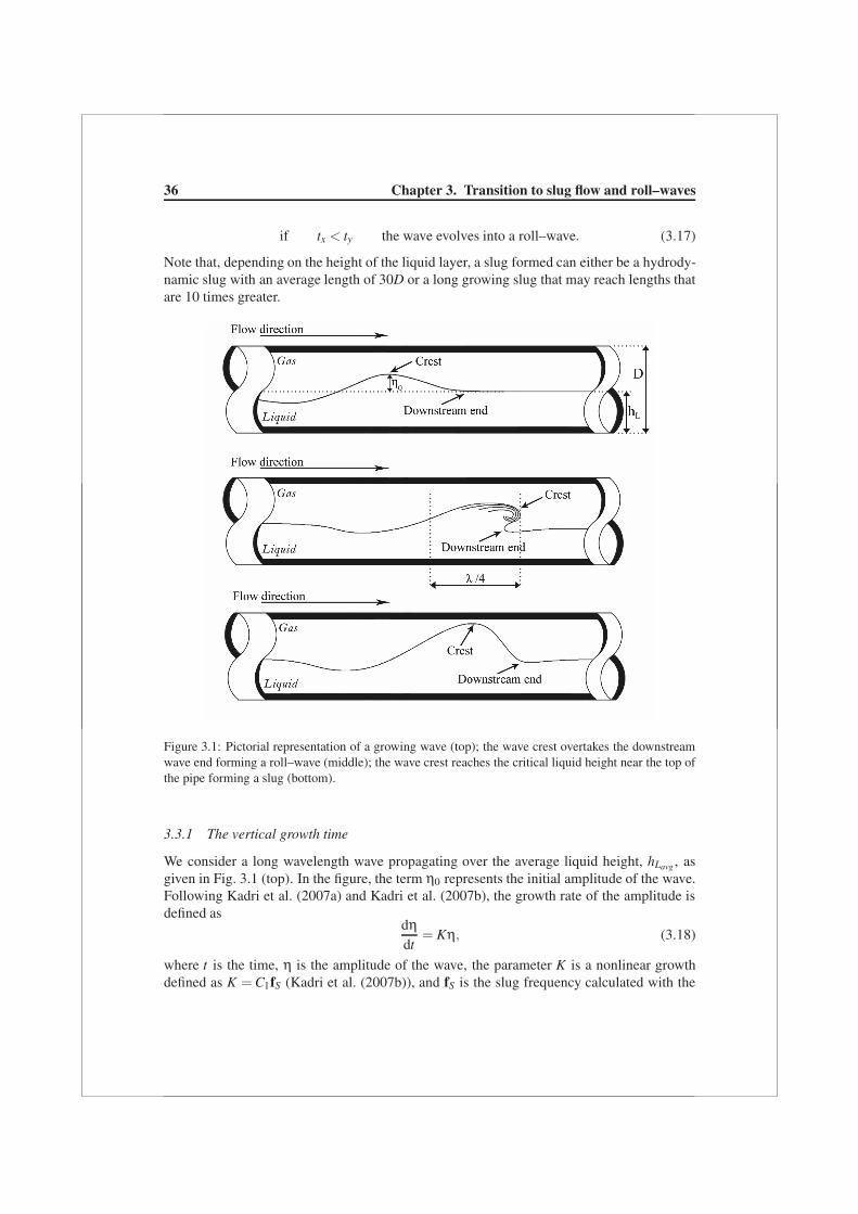
36 Chapter 3. Transition to slug flow and roll–waves
if tx < ty the wave evolves into a roll–wave. (3.17)
Note that, depending on the height of the liquid layer, a slug formed can either be a hydrody-namic slug with an average length of 30D or a long growing slug that may reach lengths thatare 10 times greater.
Figure 3.1: Pictorial representation of a growing wave (top); the wave crest overtakes the downstreamwave end forming a roll–wave (middle); the wave crest reaches the critical liquid height near the top ofthe pipe forming a slug (bottom).
3.3.1 The vertical growth time
We consider a long wavelength wave propagating over the average liquid height, hLavg , asgiven in Fig. 3.1 (top). In the figure, the term η0 represents the initial amplitude of the wave.Following Kadri et al. (2007a) and Kadri et al. (2007b), the growth rate of the amplitude isdefined as
dηdt
= Kη, (3.18)
where t is the time, η is the amplitude of the wave, the parameter K is a nonlinear growthdefined as K = C1fS (Kadri et al. (2007b)), and fS is the slug frequency calculated with the

3.3. A roll–wave/slug formation time model 37
correlation suggested by Nydal (1991):
fS = 0.088(USL + 1.5)2
gD. (3.19)
The definition of K based on the slug frequency is a logical choice, since the slug time (1/fS)is an actual limit for the average growth time of waves that evolve into slugs. The smaller theslug frequency is, the greater the growth time becomes. The parameter C1 is a constant thatwas chosen as C1 = 0.3 for the best agreement with air–water horizontal pipe flow measure-ments (Kadri et al. (2007b)). Solving Eq. (3.18) and substituting K = 0.3fS results in,
η(t) = η0e0.3fSt . (3.20)
The initial amplitude, η0, is estimated from the pressure fluctuations at the surface caused byturbulence (Phillips (1957); Longuet-Higgins (1952)). Therefore, and to a first approxima-tion, we consider the initial wave amplitude, η0, to be proportional to the turbulence lengthscale, lT . The proportionality between η0 and lT is expressed as function of D alone (seeappendix). Thus, we write η0 = C2D, where C2 is the proportionality constant. A range of0.01 < C2 < 0.03 is obtained, and for a maximum vertical growth time, the minimum valueof the proportionality constant, C2 = 0.01, is considered.
Using the amplitude growth rate (Eq. (3.20)), the time needed for the crest to hit the topof the pipe, ty, is calculated. By substituting t = ty and η(t = ty) = D−hLavg in Eq. (3.20), weobtain the following relation for ty:
ty =1
0.3fSln
D−hLavg
η0. (3.21)
3.3.2 The axial growth time
A roll–wave is formed when the crest overtakes the downstream wave end (see Fig. 3.1 (mid-dle)). The distance between the crest and the downstream wave end is λ/4, as shown in thefigure. The downstream end of the wave propagates with the wave at the propagation velocityC. Whereas due to the contribution of the momentum of the gas phase, the crest has an axialvelocity:
Ucrest(η) =ρGU + ρLC
ρG + ρL, (3.22)
where U is the actual mean velocity of the gas phase at the crest, U ≡USG(A/AG). Note thatthe cross–sectional area of the gas phase, AG, at the crest decreases when the wave amplitudeη grows, and therefore Ucrest = f (η).
The time needed for the crest to approach the downstream wave end can be determinedfrom the relative velocity, and the distance between the crest and the downstream wave end,
tx =λ/4
Ucrest(η)−C. (3.23)

38 Chapter 3. Transition to slug flow and roll–waves
Following Kadri et al. (2009a), the term λ is calculated from the wave velocity (λ = C/fw)and the relation fw = cwfS by Tronconi (1990) for the slug and the wave frequencies, fS andfw, as follows,
λ =C
cwfS, (3.24)
where cw is a constant equal to 2 for air–water systems (Tronconi (1990)). Note that Woodsand Hanratty (1999) reported slug frequency measurements to be inconsistent with the re-lation between slug frequency and wave frequency by Tronconi (1990) (e.g. Eq. (3.24)).However, here we use Eq. (3.24) only to estimate a realistic value of λ, which plays no rolefor predicting the vertical growth time (3.21).
3.4 Experiments
Experiments have been carried out in two multiphase flow laboratory facilities. The firstfacility, located at the Kramers Laboratorium of Fysische Technologie (KLFT) at TU Delft,The Netherlands, is denoted as the KLFT flow loop. In this facility, we investigated thebehaviour of wave crests of growing waves just before they evolve into slugs. The secondfacility is the NTNU (Norwegian University of Science and Technology) flow loop located inTrondheim, Norway. Here, we tracked growing waves using a moving camera, and measuredthe time needed for initial disturbances to evolve into either roll–waves or slugs. Descriptionsof the experimental setup of each facility are given in the following sub–sections.
3.4.1 The KLFT flow loop
The flow loop used in the experiments consists of a 137 m long horizontal pipeline with a0.052 m i.d. pipe. The pipe is made of Perspex (Plexiglass) to allow visual observations of theflow conditions. The experiments are performed at atmospheric pressure with gas and liquidbeing air and water, respectively. The two phases are combined at the inlet in a Y–shapedsection. The gas enters from the top in a horizontal direction, in order to prevent the impactof gas–jet coming from above. At the outlet, the last element of the pipe is connected to ashort near–horizontal hose. The hose enters a larger diameter pipe through which the liquidreturns down to the storage tank positioned 5 m below, and the gas is allowed to escape. Asketch of the experimental setup is given in Fig. 3.2. In the sketch Lpipe stands for the lengthof the pipeline test section.
The shape and movement of the growing waves are measured by means of a high speedcamera (Olympus, i–SPEED). The camera is positioned at 4 locations along the pipe at: 2–3.5, 4, 7.5, and 13 m from the inlet (see Fig. 3.2). The locations are denoted by 1, 2, 3 and 4,respectively. The camera is setup such that the field of view in one image covers a length of0.5 m, while still having high enough resolution to resolve the gas–liquid interface accurately.The frame rate of the camera is 955.5 frames per second ( f ps), with an uncertainty of 2 f ps.Images of the growing waves were evaluated by tracking their position in time. At location1, we tracked the crest of growing waves just before they hit the top of the pipe creatingslugs. For that matter, the camera at position 1 had to be located between 2–3.5 m from theinlet depending on the gas and liquid superficial velocities. At the other three locations we
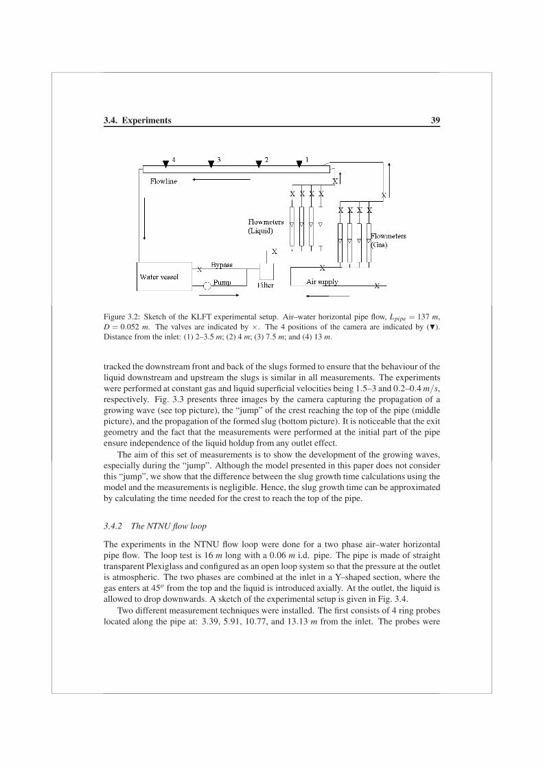
3.4. Experiments 39
Figure 3.2: Sketch of the KLFT experimental setup. Air–water horizontal pipe flow, Lpipe = 137 m,D = 0.052 m. The valves are indicated by ×. The 4 positions of the camera are indicated by (�).Distance from the inlet: (1) 2–3.5 m; (2) 4 m; (3) 7.5 m; and (4) 13 m.
tracked the downstream front and back of the slugs formed to ensure that the behaviour of theliquid downstream and upstream the slugs is similar in all measurements. The experimentswere performed at constant gas and liquid superficial velocities being 1.5–3 and 0.2–0.4 m/s,respectively. Fig. 3.3 presents three images by the camera capturing the propagation of agrowing wave (see top picture), the “jump” of the crest reaching the top of the pipe (middlepicture), and the propagation of the formed slug (bottom picture). It is noticeable that the exitgeometry and the fact that the measurements were performed at the initial part of the pipeensure independence of the liquid holdup from any outlet effect.
The aim of this set of measurements is to show the development of the growing waves,especially during the “jump”. Although the model presented in this paper does not considerthis “jump”, we show that the difference between the slug growth time calculations using themodel and the measurements is negligible. Hence, the slug growth time can be approximatedby calculating the time needed for the crest to reach the top of the pipe.
3.4.2 The NTNU flow loop
The experiments in the NTNU flow loop were done for a two phase air–water horizontalpipe flow. The loop test is 16 m long with a 0.06 m i.d. pipe. The pipe is made of straighttransparent Plexiglass and configured as an open loop system so that the pressure at the outletis atmospheric. The two phases are combined at the inlet in a Y–shaped section, where thegas enters at 45o from the top and the liquid is introduced axially. At the outlet, the liquid isallowed to drop downwards. A sketch of the experimental setup is given in Fig. 3.4.
Two different measurement techniques were installed. The first consists of 4 ring probeslocated along the pipe at: 3.39, 5.91, 10.77, and 13.13 m from the inlet. The probes were

40 Chapter 3. Transition to slug flow and roll–waves
Figure 3.3: Three images captured by the camera. Top: the propagation of a growing wave. Middle:the “jump” of the crest reaching the top of the pipe. Bottom: slightly after the slug is formed.
used to record the time dependent liquid height behaviour. The probes were primarily used asslug detectors. In the second measurement technique the growing waves were tracked using amoving camera (webcam) (see Fig. 3.4). The camera slides over a track along the pipeline ata speed that is manually controlled. The time that takes the waves to evolve into either slugsor roll–waves was measured.
Two sets of experiments were performed, each at different constant superficial liquid ve-locities, 0.17 and 0.22 m/s, and varying superficial gas velocities, 0.5–6 m/s. For consistency,the following procedure was applied to all measurements: (a) the superficial gas and liquidvelocities are set to the desired values – the liquid valve was 50% opened for USL = 0.17 m/sand 75% for USL = 0.22 m/s, and the liquid pump frequency was 30–35 Hz; (b) the pump fre-quency is reduced to 10 Hz for 10 seconds – this was necessary in order to reduce the liquidlevel close to hLavg , and to have a smoother interface; (c) the pump is set back to the originalvalue and the time measurement starts; and (d) each time measurement is stopped when thecrest of a growing wave rolls over the downstream wave end or hits the top of the pipe. Thestopping criterion is based on visual observations and verified using the time dependent liq-uid height measurements. Note that only the first slug or roll–wave were considered in eachmeasurement. Therefore, the exit effects of slugs or roll–waves are irrelevant. It is also worthnoting that perturbations that may appear at the interface due to procedures (b) and (c) result

3.5. Numerical tests 41
Figure 3.4: Sketch of the NTNU experimental setup, the position of the impedance ring probes, andthe moving camera track. Air–water horizontal pipe flow, Lpipe = 16 m, D = 0.06 m. The valves areindicated by ×.
in shorter growth times in the measurements. However, the appearance time of perturbationson a “perfectly” smooth interface is associated with a turbulence time scale in gas and liquid,that is much shorter than the wave growth time. Therefore, the effect of induced perturbationson the total measuring time is negligible.
3.5 Numerical tests
The numerical code used to conduct computational tests is MAST (Multiphase Analysis andSimulation of Transitions). The simulator, in the case of gas–liquid flows, solves the gov-erning equations of the flow (mass, momentum and pressure) for each field which locallymaybe generated inside each control volume (liquid continuous, liquid dispersed – droplets,gas continuous, gas dispersed – bubbles). In this approach, mass conservation is enforced.
The governing equations of the flow are discretised on a staggered grid arrangement usinga fully explicit discretisation in time and a first order upwind scheme for the spatial terms.The developed methodology allows the prediction of the flow pattern which prevails in eachcomputational node retaining the same set of closure laws and governing equations. Hence,different fields may exist from control volume to control volume, depending on the flowpattern which prevails. Qualitatively we identify the local flow pattern that prevails in eachcomputational cell as follows:
1. Stratified flow: stratified layers (of continuous gas and continuous liquid with possiblysome entrained gas–dispersed gas field) with low void fraction fluctuations (no distinc-tion is made between wavy and smooth regimes).

42 Chapter 3. Transition to slug flow and roll–waves
2. Annular flow: stratified layers (a layer of continuous gas with dispersed liquid and alayer of continuous liquid) where the liquid layer tends to wet the whole perimeter ofthe pipe wall and the gas flows in the core.
3. Slug flow: stratified layers with large void fraction fluctuations which do bridge thepipe, causing regions with very thin stratified gas layers (i.e. the liquid film is domi-nated by the presence of two stratified layers – continuous gas with possibly dispersedliquid, and continuous liquid with in general dispersed bubbles; the slug body is dom-inated by a continuous liquid film with dispersed gas with a very thin continuous gaslayer on top).
4. Bubbly flow: the pipe is fully bridged with no regions where there are stratified gaslayers that are not very thin (continuous liquid with dispersed gas bubbles)
Unstable waves may grow until the pipe is fully bridged and a slug is generated. Slug-ging is predicted because the governing equations are capable to capture the viscous Kelvin–Helmholtz instabilities that lead to flow pattern transition from stratified to slug flow (Issa andKempf (2003)). In order to ensure that these instabilities are not smeared out by numericaldiffusion, a fine numerical mesh is adopted with a spatial resolution of some pipe diameters.The growth of the instabilities is then an outcome of the transient numerical solution of theequations. When slugging occurs, regardless of its specific nature (hydrodynamic, terrain–induced or severe), trains of slugs are generated automatically. Provided that reasonableclosure laws (i.e. friction factors) are adopted, MAST has the capability to predict the correctflow pattern that results from the boundary and geometry conditions under investigation.
Fig. 3.5 shows typical profiles of the liquid holdup and gas velocity at different timeinstants for a wave which grows and eventually leads to hydrodynamic slugging for gas–liquid horizontal pipe flow. The pipe is 137 m long with 0.052 m i.d. (the KLFT facility),the gas and liquid phases are air and water travelling at USG = 8 m/s and USL = 0.3 m/s,respectively.
Slugs of different sizes may be generated, depending on the pipe geometry and flowconditions, leading to a slug length distribution. The simulator, MAST, gives estimates ofthe average slug length as shown in figure 5 of the paper by Bonizzi et al. (2009), wherepredictions by MAST are compared with the measurements of Nydal et al. (1992) for air–water flow in a horizontal 0.05 m i.d. pipe at USL = 0.6 and 2.4 m/s.
The robustness of the slug criterion can be appreciated by referring to figure 7 of thepaper by Bonizzi et al. (2009), where predictions of the critical height of the liquid layerat the transition to slug flow for air–water horizontal pipe flow at atmospheric pressure areplotted against USG and compared with measurements by Andritsos et al. (1989) and thetheoretical transition boundary according to Hurlburt and Hanratty (2002). The accuracy ofthe criteria used for identification, noting that the closure relationships are not adjusted, issatisfactory. For the tests presented in this paper, the closures proposed by Taitel and Dukler(1976) were selected.

3.6. Results 43
Figure 3.5: Hydrodynamic instabilities in the KLFT loop calculated by MAST, for air–water 0.052 mi.d. pipe, USG = 8 m/s and USL = 0.3 m/s.
3.6 Results
In this section we compare theoretical calculations, of the wave growth and the formation timeof slugs and roll–waves, with measurements and simulations. A summary of the propertiesof the different systems is found in Table 3.1. For all calculations presented in this paper thelowest initial wave amplitude was applied in order to obtain the largest growth time of thewave crest, hence C2 = 0.01 is chosen (see appendix).
3.6.1 Crest growth near the pipe top
Measurements of growing waves just before they hit the pipe top for air–water horizontalflow are presented in Fig. 3.6. The measurements were carried out in a 137 m long pipe with0.052 m i.d. at the KLFT flow loop. A description of the experimental setup is found insection 3.4.1. The sub–plots in Fig. 3.6 show the liquid holdup at the crest, (hL/D)crest , asfunction of time, t, at USG = 1.85 m/s and different superficial liquid velocities. The averageliquid holdup is denoted by (×), whereas the minimum and maximum values of the holdupare represented by the error–bars. The solid line represent theoretical predictions of the crestgrowth from η0. The wave grows exponentially until the top of the pipe is reached. A zoomover the measurement region is given on the right hand side of each sub–plot.
In the sub–plots (a), (b) and (c) we see that the time needed for a growing crest beforethe “jump” is two orders of magnitude greater than the time needed for the crest to hit the topof the pipe (during the “jump”). This observation is true for all superficial velocities of gas
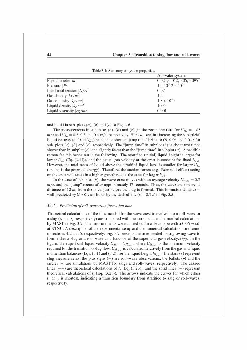
44 Chapter 3. Transition to slug flow and roll–waves
Table 3.1: Summary of system properties.Air-water system
Pipe diameter [m] 0.025,0.052,0.06,0.095Pressure [Pa] 1×105,2×105
Interfacial tension [N/m] 0.07Gas density [kg/m3] 1.2Gas viscosity [kg/ms] 1.8×10⁻⁵
Liquid density [kg/m3] 1000Liquid viscosity [kg/ms] 0.001
and liquid in sub–plots (a), (b) and (c) of Fig. 3.6.The measurements in sub–plots (a), (b) and (c) (in the zoom area) are for USG = 1.85
m/s and USL = 0.2, 0.3 and 0.4 m/s, respectively. Here we see that increasing the superficialliquid velocity (at fixed USG) results in a shorter “jump time” being: 0.09, 0.06 and 0.04 s forsub–plots (a), (b) and (c), respectively. The “jump time” in subplot (b) is about two timesslower than in subplot (c), and slightly faster than the “jump time” in subplot (a). A possiblereason for this behaviour is the following. The stratified (initial) liquid height is larger forlarger USL (Eq. (3.13)), and the actual gas velocity at the crest is constant for fixed USG.However, the total mass of liquid above the stratified liquid level is smaller for larger USL
(and so is the potential energy). Therefore, the suction forces (e.g. Bernoulli effect) actingon the crest will result in a higher growth rate of the crest for larger USL.
In the case of sub–plot (b), the wave crest moves with an average velocity Ucrest = 0.7m/s, and the “jump” occurs after approximately 17 seconds. Thus, the wave crest moves adistance of 12 m, from the inlet, just before the slug is formed. This formation distance iswell predicted by MAST, as shown by the dashed line (t0 + 0.7 s) in Fig. 3.5
3.6.2 Prediction of roll–wave/slug formation time
Theoretical calculations of the time needed for the wave crest to evolve into a roll–wave ora slug (tx and ty, respectively) are compared with measurements and numerical calculationsby MAST in Fig. 3.7. The measurements were carried out in a 16 m pipe with a 0.06 m i.d.at NTNU. A description of the experimental setup and the numerical calculations are foundin sections 4.2 and 5, respectively. Fig. 3.7 presents the time needed for a growing wave toform either a slug or a roll–wave as a function of the superficial gas velocity, USG. In thefigure, the superficial liquid velocity USL = USLmin , where USLmin is the minimum velocityrequired for the transition to slug flow. USLmin is calculated iteratively from the gas and liquidmomentum balances (Eqs. (3.1) and (3.2)) for the liquid height hLmin . The stars (∗) representslug measurements, the plus signs (+) are roll–wave observations, the bullets (•) and thecircles (◦) are simulations by MAST for slugs and roll–waves, respectively. The dashedlines (−−) are theoretical calculations of tx (Eq. (3.23)), and the solid lines (−) representtheoretical calculations of ty (Eq. (3.21)). The arrows indicate the curves for which eithertx or ty is shortest, indicating a transition boundary from stratified to slug or roll–waves,respectively.
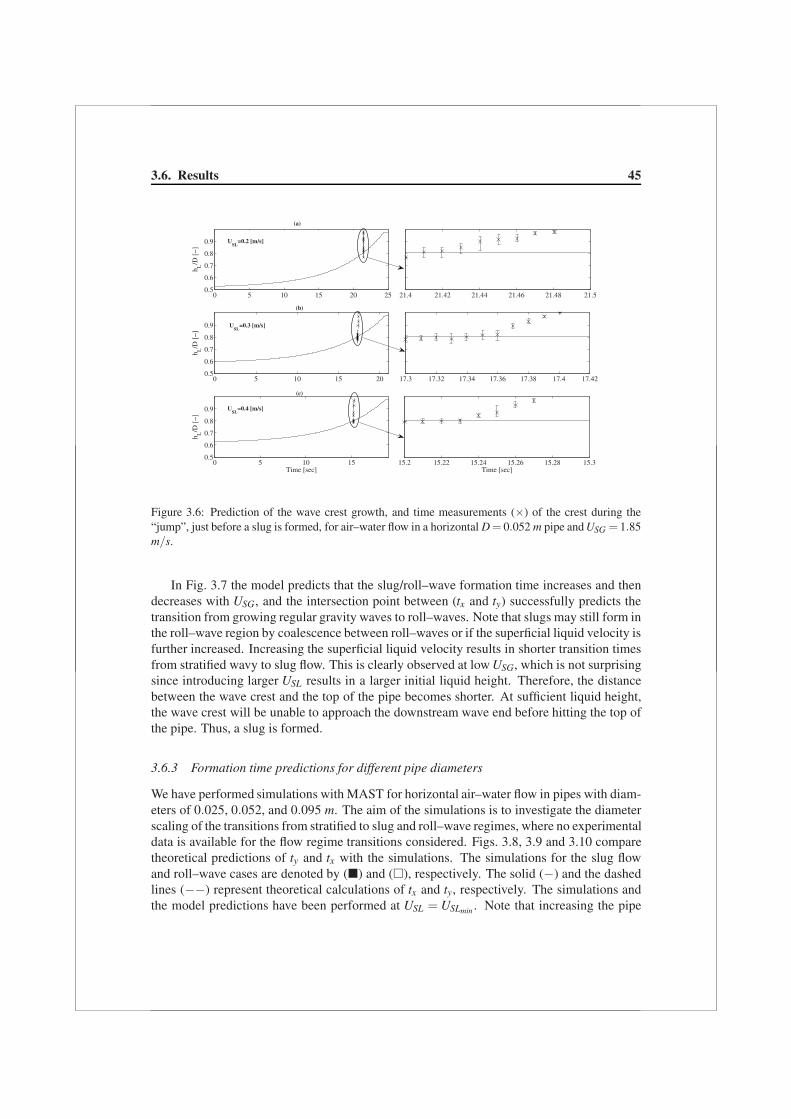
3.6. Results 45
21.4 21.42 21.44 21.46 21.48 21.50 5 10 15 20 250.5
0.6
0.7
0.8
0.9
(a)
h L/D
[−]
0 5 10 15 200.5
0.6
0.7
0.8
0.9
h L/D
[−]
(b)
17.3 17.32 17.34 17.36 17.38 17.4 17.42
15.2 15.22 15.24 15.26 15.28 15.3Time [sec]
0 5 10 150.5
0.6
0.7
0.8
0.9
Time [sec]
h L/D
[−]
(c)
USL
=0.2 [m/s]
USL
=0.4 [m/s]
USL
=0.3 [m/s]
Figure 3.6: Prediction of the wave crest growth, and time measurements (×) of the crest during the“jump”, just before a slug is formed, for air–water flow in a horizontal D = 0.052 m pipe and USG = 1.85m/s.
In Fig. 3.7 the model predicts that the slug/roll–wave formation time increases and thendecreases with USG, and the intersection point between (tx and ty) successfully predicts thetransition from growing regular gravity waves to roll–waves. Note that slugs may still form inthe roll–wave region by coalescence between roll–waves or if the superficial liquid velocity isfurther increased. Increasing the superficial liquid velocity results in shorter transition timesfrom stratified wavy to slug flow. This is clearly observed at low USG, which is not surprisingsince introducing larger USL results in a larger initial liquid height. Therefore, the distancebetween the wave crest and the top of the pipe becomes shorter. At sufficient liquid height,the wave crest will be unable to approach the downstream wave end before hitting the top ofthe pipe. Thus, a slug is formed.
3.6.3 Formation time predictions for different pipe diameters
We have performed simulations with MAST for horizontal air–water flow in pipes with diam-eters of 0.025, 0.052, and 0.095 m. The aim of the simulations is to investigate the diameterscaling of the transitions from stratified to slug and roll–wave regimes, where no experimentaldata is available for the flow regime transitions considered. Figs. 3.8, 3.9 and 3.10 comparetheoretical predictions of ty and tx with the simulations. The simulations for the slug flowand roll–wave cases are denoted by (�) and (�), respectively. The solid (−) and the dashedlines (−−) represent theoretical calculations of tx and ty, respectively. The simulations andthe model predictions have been performed at USL = USLmin . Note that increasing the pipe
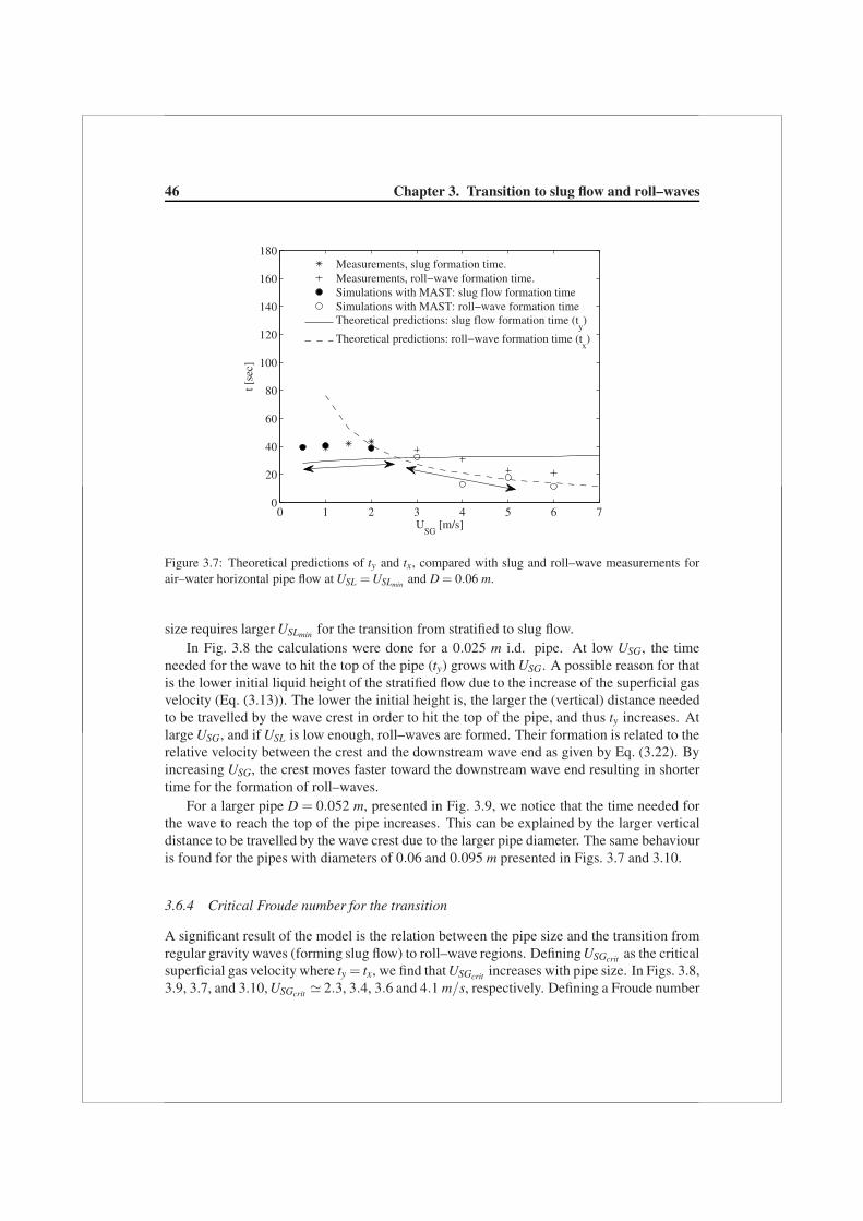
46 Chapter 3. Transition to slug flow and roll–waves
0 1 2 3 4 5 6 70
20
40
60
80
100
120
140
160
180
USG
[m/s]
t [se
c]
Measurements, slug formation time.Measurements, roll−wave formation time.Simulations with MAST: slug flow formation timeSimulations with MAST: roll−wave formation timeTheoretical predictions: slug flow formation time (t
y)
Theoretical predictions: roll−wave formation time (tx)
Figure 3.7: Theoretical predictions of ty and tx, compared with slug and roll–wave measurements forair–water horizontal pipe flow at USL = USLmin and D = 0.06 m.
size requires larger USLmin for the transition from stratified to slug flow.In Fig. 3.8 the calculations were done for a 0.025 m i.d. pipe. At low USG, the time
needed for the wave to hit the top of the pipe (ty) grows with USG. A possible reason for thatis the lower initial liquid height of the stratified flow due to the increase of the superficial gasvelocity (Eq. (3.13)). The lower the initial height is, the larger the (vertical) distance neededto be travelled by the wave crest in order to hit the top of the pipe, and thus ty increases. Atlarge USG, and if USL is low enough, roll–waves are formed. Their formation is related to therelative velocity between the crest and the downstream wave end as given by Eq. (3.22). Byincreasing USG, the crest moves faster toward the downstream wave end resulting in shortertime for the formation of roll–waves.
For a larger pipe D = 0.052 m, presented in Fig. 3.9, we notice that the time needed forthe wave to reach the top of the pipe increases. This can be explained by the larger verticaldistance to be travelled by the wave crest due to the larger pipe diameter. The same behaviouris found for the pipes with diameters of 0.06 and 0.095 m presented in Figs. 3.7 and 3.10.
3.6.4 Critical Froude number for the transition
A significant result of the model is the relation between the pipe size and the transition fromregular gravity waves (forming slug flow) to roll–wave regions. Defining USGcrit as the criticalsuperficial gas velocity where ty = tx, we find that USGcrit increases with pipe size. In Figs. 3.8,3.9, 3.7, and 3.10, USGcrit � 2.3, 3.4, 3.6 and 4.1 m/s, respectively. Defining a Froude number

3.6. Results 47
0 1 2 3 4 5 6 70
5
10
15
20
25
30
35
40
45
50
USG
[m/s]
t [se
c]
Theoretical predictions: slug flow formation time (ty)
Theoretical predictions: roll−wave formation time (tx)
Simulations with MAST: slug flow formation timeSimulations with MAST: roll−wave formation time
Figure 3.8: Simulations and theoretical predictions of ty and tx for air–water horizontal pipe flow atUSL = USLmin and D = 0.025 m.
0 1 2 3 4 5 6 70
10
20
30
40
50
60
70
80
90
100
USG
[m/s]
t [se
c]
Theoretical predictions: slug flow formation time (ty)
Theoretical predictions: roll−wave formation time (tx)
Simulations with MAST: slug flow formation timeSimulations with MAST: roll−wave formation time
Figure 3.9: Simulations and theoretical predictions of ty and tx for air–water horizontal pipe flow atUSL = USLmin and D = 0.052 m.

48 Chapter 3. Transition to slug flow and roll–waves
0 1 2 3 4 5 6 70
50
100
150
USG
[m/s]
t [se
c]
Theoretical predictions: slug flow formation time (ty)
Theoretical predictions: roll−wave formation time (tx)
Simulations with MAST: slug flow formation timeSimulations with MAST: roll−wave formation time
Figure 3.10: Simulations and theoretical predictions of ty and tx for air–water horizontal pipe flow atUSL = USLmin and D = 0.095 m.
Frcrit =√
ρGU2SGcrit
/(ΔρgD), where Δρ = ρL−ρG, we obtain that Frcrit � 0.15 is the critical
Froude number at which the transition from slug flow (formed by gravity waves) to roll–waves occurs, for the different pipe diameters and USLmin in Figs. 3.8, 3.9, 3.7, and 3.10.
This result agrees well with previous work by Woods and Hanratty (1999) who showedthat the flow becomes supercritical, at USG > 4 m/s (that is at Frcrit > 0.16), and slug for-mation is determined by coalescing roll–waves, whereas at lower USG slugging is reachedwhen large wavelength waves reach the top of the pipe. They also noted that the minimumUSG required for the transition from stratified to slug flow increases with the pipe size, whichagrees with the behaviour of USGcrit for the transition from slug flow to roll–wave region, asaforementioned.
3.7 Conclusions
1. The evolution of long wavelength waves in horizontal pipes may result in differentflow patterns in the pipe. If the wave crest reaches the top of the pipe a slug may form.However, if the crest overtakes the downstream wave end (before it reaches the top ofthe pipe) a roll wave is formed.
2. A “jump” in the liquid phase toward the top of the pipe is observed just before the wavecrest bridges the pipe. A possible reason for this “jump” is the suction forces actingin the neighbourhood of the crest. The suction forces may become large enough to
3.7. Conclusions 49
elevate the liquid surface as the actual gas velocity becomes relatively high due to theexponential decrease of the gas cross–sectional area at the crest.
3. Measurements carried out in a 137 m long horizontal pipeline with a 0.052 m i.d. showthat the time required for a wave to reach the height at which the crest “jumps” towardthe top of the pipe, is much longer than the “jump time”. Increasing the superficialliquid velocity results in shorter “jump” time.
4. A wave transition model was presented. The model is based on calculating the timerequired for a long wavelength wave with a small initial amplitude, on the order ofthe turbulent length scale, to grow and reach the top of the pipe (see Eq. (3.21)), andthe time it takes the axial propagation of the wave crest to overtake the downstreamwave end (see Eq. (3.23)). The model predicts the transition from stratified flow toslug flow or roll–wave regimes for different pipe diameters and different gas and liquidsuperficial velocities.
5. The model predicts a number of important observations regarding the behaviour ofslug/roll–wave formation time: (a) increasing the superficial liquid velocity results inshorter transition times from stratified wavy to slug flow; (b) at relatively low USG, theformation of slug/roll–wave time increases with increasing USG, which is a result of thelower initial stratified height; however, (c) at relatively high USG, due to the dominationof inertial forces, the formation time decreases with increasing USG and a roll–wave isformed; and (d) increasing the pipe size results in larger axial growth compared to thegrowth of the vertical direction, making the appearance of long slugs less likely.
6. Numerical simulations have been carried out using a transient one–dimensional multi-phase flow simulator in order to investigate the diameter scaling of the transitions fromstratified to slug and roll–wave regimes. Comparing predictions by the model with thesimulations we found that increasing the pipe diameter results in larger formation timesfor both ty and tx. However, since tx is function of both vertical and axial displacementsof the crest, its sensitivity to a change in the pipe diameter is greater. As a result, largerUSG is required for the transition from slug flow (formed by regular gravity waves) toroll–wave regimes.
7. Based on predictions by the model presented in this paper we obtained a critical densi-metric gas Froude number, Fr � 0.15, for the transition from regular growing gravitywaves, to roll–wave regimes. The critical Froude number was obtained for superficialvelocities close to the transition to slug flow.
8. The accuracy of the modelling could be improved if the interfacial friction factor attransition, the wave length, and the gas entrainment were better known over a widerrange of flow conditions. The theories applied in the modelling are sensitive to thevalue of the interfacial friction factor which is of a critical importance at all flow rates.Whereas, the accuracy in the wave length and the gas entrainment (which was neglectedin this paper) becomes important at relatively large flow rates.

50 Chapter 3. Transition to slug flow and roll–waves

4Operation pressure and slug length1
Slug flow is commonly observed in gas production offshore fields. At high operation pressureonly short hydrodynamic slugs are observed. However, as the offshore fields become older,the operation pressure becomes lower and long slugs may form. At near atmospheric pres-sures the long slugs may reach a size of 500 pipe diameters or more. Such slugs can causeserious operational failures due to the strong fluctuating pressure. Identifying the operationpressure conditions at which the long slugs appear, may reduce or prevent these negativeeffects.
In this chapter we process and analyse gas–liquid flow measurements in order to investi-gate the different slug types and their sensitivity to the operation pressure. The measurementswere performed by Kristiansen (2004) in a 103 m long pipe with an internal diameter of 0.069m and an inclination of −0.1o from the horizontal. Three types of slugs were categorized ac-cording to the difference in liquid levels (liquid excess) between the slug front and tail. Thelong slugs were found to have the largest liquid excess after formation, whereas the hydro-dynamic slugs had no liquid excess. The analysis of the measurements provides a detailedoverview on the effect of pressure on the long slug length, and a safe operation region werelong slugs will not appear.
1This chapter is based on Kadri et al. (2009c)

52 Chapter 4. Operation pressure and slug length
4.1 Introduction
The cocurrent flow of gas and liquid in horizontal and near horizontal pipes results in anumber of flow patterns. A stratified flow occurs at relatively low gas and liquid flow rateswhereby the gas moves on top of the liquid. At higher rates of gas and liquid a slug flowpattern might exist where plugs of liquid move downstream separated by elongated bubblesmoving along the top of the pipe. Although mostly short hydrodynamic slugs are observed,long slugs with sizes reaching 500 pipe diameters or more may form if the operation pressurebecomes sufficiently low, e.g. in older gas production offshore fields. Such long slugs inducestrong pressure fluctuations large enough to cause severe operational failures. Therefore,identifying the transition to the long slugs and the critical pressure at which they may appear,will be helpful in preventing or reducing such future operational failures.
Two main theoretical approaches are used to predict the transition from stratified to slugflow: stability of stratified flow and stability of slug flow. The stability of stratified flow wasinitially used by Hanratty and Hershman (1961) to describe waves on thin films over which airis blowing. A number of researchers (Wallis and Dobbins (1973); Lin and Hanratty (1986);Wu et al. (1987)) followed this analysis to investigate the viscous wavelength wave instability(VLW). The VLW theory successfully predicts that increasing the pipe size requires larger gasflow rates for the transition from stratified to slug flow in air–water horizontal pipe flow. Thestability of slug flow considers the amount of liquid entering and leaving the slug. The slugbecomes neutrally stable, not growing neither decaying, when a volumetric liquid balance isreached between the slug front and tail. This balance results in a minimum liquid area at thefront, below it the slug becomes unstable (Bendiksen (1984); Ruder et al. (1989); Woods andHanratty (1996)).
Slug lengths have been reported to be in a range of 12–30D for horizontal air–water flow(Dukler and Hubbard (1975); Nicholson et al. (1978); Nydal et al. (1992)). This type of slugsis known as hydrodynamic slugs. Kristiansen (2004) found a similar range of slug lengthsfor gas–liquid near horizontal pipe flow when introducing slugs at the inlet. However, whenintroducing stratified flow at the inlet he observed both short hydrodynamic and long slugs.Zoeteweij (2007) observed very long slugs reaching 500 pipe diameters. The long slugs format relatively low gas and liquid velocities, where two sub–regimes are observed: neutrallystable, and growing slugs (Kadri et al. (2009a)).
In this chapter we analyse measurements performed by Kristiansen (2004) in a 103 m longgas–liquid near horizontal pipe flow with an internal diameter of 0.069 m. The measurementswere performed with air or high density gas at atmospheric and higher operation pressures.The analysis of the measurements is unique in the sense that it provides a simple mechanismfor the appearance of different slug types in the long slug regime. Slugs were categorizedinto three types according to the difference in liquid levels (liquid excess) between the frontand tail: (1) slugs with large and initially constant excess; (2) slugs with decreasing excess;and (3) slugs with no excess. Slugs with large liquid excess can grow to become very long,whereas slugs that have no liquid excess are the shortest. We also found that small changesin the liquid excess, at the formation time, may result in large differences in slug length.Moreover, we identified the operation pressures at which the growing and stable slugs mayappear.

4.2. Background 53
A background on the theoretical approaches, stability of stratified flow and slug stability,is given in section 4.2. Section 4.3 provides a description of the experimental facility andmethods used for performing the measurements. A discrimination method between slug typesis given in section 4.4. In section 4.5 we present results of the effect of slug types on the sluglength at atmospheric and high operation pressures. Finally, the conclusions are presented insection 4.6.
4.2 Background
4.2.1 Stratified flow pattern
An idealized model of the stratified flow pattern is represented by a simplified geometry. Thediameter of the pipe is D. The height of the liquid layer along the centerline is hL. The lengthof the segments of the pipe circumference in contact with the gas and liquid are SG and SL,respectively. The length of the gas–water interface is presented by Si. The areas occupied bythe gas and the liquid are AG and AL, respectively. Given the pipe diameter, these parameterscan be calculated, from measurements of hL, by using geometric relations (e.g. Govier andAziz (1972)). The momentum balances for the gas and the liquid flows are as follows,
−AG
(dpdx
)− τWGSG − τiSi + ρGAGgsinθ = 0, (4.1)
−AL
[(dpdx
)−ρLgcosθ
(dhL
dx
)]− τWLSL + τiSi + ρLALgsinθ = 0, (4.2)
where ρG and ρL are the gas and the liquid densities, θ is the inclination angle of the pipe fromthe horizontal, dp/dx is the pressure gradient, dhL/dx is the liquid hydraulic gradient, and gis the acceleration due to gravity. The time–averaged stress of the gas and liquid phases at thewall and the stress at the interface, τW G, τW L and τi, are defined in terms of friction factors,and calculated using the Blasius equation if Re < 105 and the wall roughness effect can beignored, otherwise the Churchill equation is used (see Churchill (1977)). Due to the presenceof waves at the interface, the interfacial friction factor becomes larger than the friction factorfor a smooth surface. In this chapter we use an estimation for the interfacial friction factorsuggested by Hurlburt and Hanratty (2002). For given flow rates of liquid and gas Eqs. (4.1)and (4.2) are used to find the pressure gradient and the height of the liquid layer. However,these equations do not determine the stability of the stratified flow.
4.2.2 Average liquid area
The average liquid area, AL = ALavg , is calculated from the momentum balances for the strat-ified flow pattern, Eqs. (4.1) and (4.2). Substituting AL = ALavg and AG = A−ALavg , Kadri etal. (2009a) wrote Eq. (4.1) in the following form,
(dpdx
)=
τW GSG + τiSi
A−ALavg
−ρGgsinθ. (4.3)

54 Chapter 4. Operation pressure and slug length
Figure 4.1: Sketch of a slug.
The average liquid area is the initial plain stratified flow in the pipe. This occurs when thepressure gradients of the two phases on the interface cancel. Substituting Eq. (4.3) in Eq. (4.2)and assuming a fully developed horizontal pipe flow Kadri et al. (2009a) obtained a relationfor ALavg as follows,
ALavg = AτW LSL − τiSi
τW LSL + τWGSG. (4.4)
The average liquid height hLavg is calculated using Eq. (4.4) and geometric relations (e.g.Govier and Aziz (1972)). Eq. (4.4) successfully predicts the inverse proportionality betweenthe gas flow rates and hLavg .
4.2.3 Slug stability model
The slug stability model considers the rates of liquid adjoining or detaching from the slug atits front or rear. Slugs are stable (not decaying) when the rates of liquid adjoining are not lessthan the rates at which liquid detaches. Figure 4.1 gives an illustration of a slug moving withfront velocity CF over a stratified liquid layer at station 1 of area AL1 and actual velocity u1.The volumetric flow rate of liquid adjoining the slug is
Qin = (CF −u1)AL1. (4.5)
The rear of the slug is assumed to behave as a bubble moving with a velocity CB. The volumefraction of the gas in the slug is ε. The volumetric flow rate of the liquid detaching from theslug is
Qout = (CB −u3)(1− ε)A at station 3. (4.6)
The parameter u3 is the actual liquid velocity at stations 3. Assuming neutral stability, Qin =Qout and CF = CB, and making use of Eqs. (4.5) and (4.6), the following relation is obtainedfor the area of the stratified layer:(
AL1
A
)crit
=(CB −u3)(1− ε)
(CB −u1), (4.7)
for the area of the stratified flow at the front. Using Eq. (4.7) and geometric relations, thecritical height, hLcrit , at the slug front required for the slug to be neutrally stable is obtained.A detailed analysis of the slug stability model is well documented by Hurlburt and Hanratty(2002); Soleimani and Hanratty (2003).
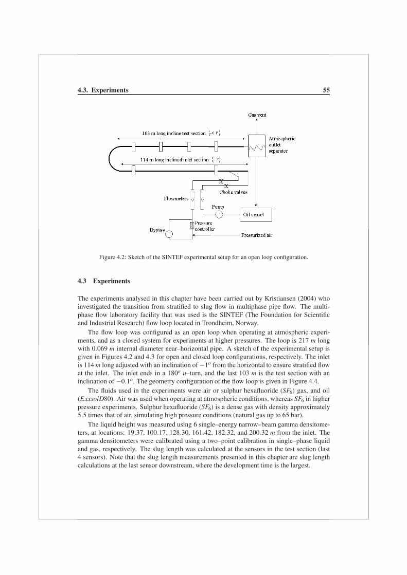
4.3. Experiments 55
Figure 4.2: Sketch of the SINTEF experimental setup for an open loop configuration.
4.3 Experiments
The experiments analysed in this chapter have been carried out by Kristiansen (2004) whoinvestigated the transition from stratified to slug flow in multiphase pipe flow. The multi-phase flow laboratory facility that was used is the SINTEF (The Foundation for Scientificand Industrial Research) flow loop located in Trondheim, Norway.
The flow loop was configured as an open loop when operating at atmospheric experi-ments, and as a closed system for experiments at higher pressures. The loop is 217 m longwith 0.069 m internal diameter near–horizontal pipe. A sketch of the experimental setup isgiven in Figures 4.2 and 4.3 for open and closed loop configurations, respectively. The inletis 114 m long adjusted with an inclination of −1o from the horizontal to ensure stratified flowat the inlet. The inlet ends in a 180o u–turn, and the last 103 m is the test section with aninclination of −0.1o. The geometry configuration of the flow loop is given in Figure 4.4.
The fluids used in the experiments were air or sulphur hexafluoride (SF6) gas, and oil(ExxsolD80). Air was used when operating at atmospheric conditions, whereas SF6 in higherpressure experiments. Sulphur hexafluoride (SF6) is a dense gas with density approximately5.5 times that of air, simulating high pressure conditions (natural gas up to 65 bar).
The liquid height was measured using 6 single–energy narrow–beam gamma densitome-ters, at locations: 19.37, 100.17, 128.30, 161.42, 182.32, and 200.32 m from the inlet. Thegamma densitometers were calibrated using a two–point calibration in single–phase liquidand gas, respectively. The slug length was calculated at the sensors in the test section (last4 sensors). Note that the slug length measurements presented in this chapter are slug lengthcalculations at the last sensor downstream, where the development time is the largest.
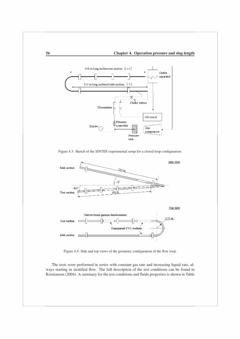
56 Chapter 4. Operation pressure and slug length
Figure 4.3: Sketch of the SINTEF experimental setup for a closed loop configuration.
Figure 4.4: Side and top views of the geometry configuration of the flow loop.
The tests were performed in series with constant gas rate and increasing liquid rate, al-ways starting in stratified flow. The full description of the test conditions can be found inKristiansen (2004). A summary for the test conditions and fluids properties is shown in Table

4.4. Definition of slug types by liquid excess 57
4.1.All measurements presented in this chapter have been processed according to the differ-
ent slug types presented in the next section. The processed measurements are addressed as“measurements”.
Table 4.1: Summary of test conditions and fluids properties.Pipe diameter [m] 0.069Pipe length [m] 217.24Test section length [m] 103Inlet section inclination [deg] −1Test section inclination [deg] −0.1Gas phase Air or SF6 gasLiquid phase ExxsolD80 oilGas density [kg/m3] 1.2,9,19,46,52Liquid density [kg/m3] 810Air viscosity [kg/ms] 1.8×10⁻⁵
Gas (SF6) viscosity [kg/ms] 1.5×10⁻⁵
Liquid viscosity [kg/ms] 0.0018Interfacial tension (σoil/air) [N/m] 0.025Interfacial tension (σoil/SF6
) [N/m] 0.021Pressure [barA] 1,1.5,3,7,8USG [m/s] 0.2–8USL [m/s] 0.05–0.5
4.4 Definition of slug types by liquid excess
The slug formation is associated with liquid depletion at the tail of the slug (Woods andHanratty (1999)). The slug becomes neutrally stable, neither growing nor decaying, whena volumetric balance between the liquid detaching, at the tail, and joining, at the front, isreached. For a constant gas density and a continuous liquid phase, it can be shown fromconservation of mass of the liquid phase that the liquid heights at the tail and front should beequal in order to reach neutral stability. That happens when the slug front approaches the tailof a second slug downstream, and the liquid excess becomes zero (i.e. that is why the firstslug in the pipe can grow indefinitely).
4.4.1 Discrimination between slug types in measurements
Figure 4.5 presents an example of time traces of three different slug types measured withthe first sensor downstream. In Figure 4.5(a), the liquid height at the slug front is constantalong a relatively large distance downstream, and remarkably higher than the liquid heightat the tail. This observation indicates that such a slug is not influenced by the presence of asecond slug (probably far) downstream. Such slugs are defined as type I. In Figure 4.5(b),

58 Chapter 4. Operation pressure and slug length
450 500 550 600 650 700 7500.4
0.6
0.8
1(a)
Time traces [s]
h L/D
[−]
370 380 390 400 410 420 430 440 450 460
0.4
0.6
0.8
1
Time traces [s]
h L/D
[−]
(b)
315 320 325 330 335 3400
0.5
1
Time traces [s]
h L/D
[−]
(c)
Front and tail at
equal levels
Constant front
Decreasing front
Tail
Tail
USG
= 0.5 [m/s]
USL
= 0.2 [m/s]
USG
= 1 [m/s]
USL
= 0.2 [m/s]
USG
= 4 [m/s]
USL
= 0.5 [m/s]
Figure 4.5: Time traces of different slug types in SF6 gas–oil pipe flow, D = 0.069 m, θ = −0.1o,P = 1.5 barA (ρG = 9 kg/m3): (a) type I, (b) type II, and (c) type III.
the liquid height at the front decreases as a slug moves downstream. In this case, the sluggrowth is dependant on the downstream liquid depletion due to the existence of a second slugdownstream. This type of slugs is defined as type II. In Figure 4.5(c), the liquid at the frontand at the tail are equal, indicating a fully developed slug where the slug front approaches thetail of a second slug downstream. This type of slugs is denoted as type III.
The overall slug type of each measurement is denoted as one of the three types only ifat least 90% of the individual slugs share the same type. Otherwise, the overall slug type isaddressed as “undefined”.
4.4.2 Measurements of the liquid excess, ΔhL
In order to calculate the average liquid excess of the different slug types the following stepsare made: (1) The time traces of the liquid height are examined at the first sensor where slugsare observed, at constant gas and liquid flow rates. (2) The average liquid height at the tail,hLtail , is calculated from the average height around the lowest point in the tail of each slugin the time traces. (3) The average liquid height at the front, hLf ront , is calculated from theaverage over a distance on the order of 10D from the front of all slugs in the time traces. (4)The average liquid excess of each measurement is calculated as follows,
ΔhL = hLf ront −hLtail . (4.8)

4.5. Results 59
4.4.3 Theoretical predictions of the liquid excess, ΔhL
4.4.3.1 Slugs type I
At low gas and liquid flow rates, where the slug frequency is relatively low, a forming slug isfar enough from a second slug downstream, as mentioned above. As a result, the liquid heightat the front is not affected by the presence of the second slug. In this case, the liquid height atthe front is the average height of the stratified flow, hLf ront = hLavg , whereas the liquid heightat the tail is the minimum height calculated by slug stability (hLtail = hLcrit ). Therefore, theliquid excess of slugs type I is calculated as follows,
(ΔhL)typeI = hLavg −hLcrit , (4.9)
where hLavg and hLcrit are calculated from Eqs. (4.4) and (4.7), respectively. A comparisonbetween the predicted and measured liquid heights is given in Figure 4.6(a).
4.4.3.2 Slugs type II
Increasing the gas or liquid flow rates results in higher slug frequency (e.g. Gregory and Scott(1969)). At a sufficiently high frequency the liquid height at the front of the slug is affectedby the presence of another slug downstream, so that the average liquid height at the front islower than the initial height as presented in Figure 4.6(b). In this case, ΔhL is approximatedby the average height between hLavg and hLcrit as follows,
(ΔhL)typeII =hLavg −hLcrit
2. (4.10)
Eq. 4.10 presents an upper limit of (ΔhL)typeII .
4.4.3.3 Slugs type III
Further increase of the flow rates results in the generation of a larger number of slugs. In thiscase, a forming slug reaches neutral stability immediately after formation. Thus, the liquidheight at the front and tail are approximately the same (see Figure 4.6(c)), thus:
(ΔhL)typeIII = 0. (4.11)
4.5 Results
In this section we compare theoretical predictions of the liquid excess, ΔhL, of the differentslug types with (the processed) measurements. Additionally, we present a flow map andslug length measurements, at atmospheric and higher operation pressures, and identify theconditions at which the long slugs form.
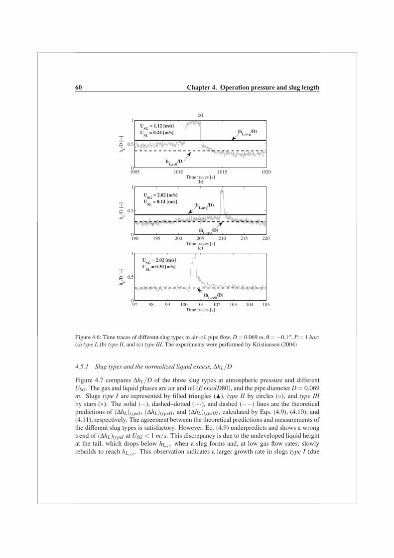
60 Chapter 4. Operation pressure and slug length
1005 1010 1015 10200
0.5
1(a)
Time traces [s]
h L/D
[−]
190 195 200 205 210 215 2200
0.5
1
Time traces [s]
h L/D
[−]
(b)
97 98 99 100 101 102 103 104 1050
0.5
1
Time traces [s]
h L/D
[−]
(c)
USG
= 2.02 [m/s]
USL
= 0.30 [m/s]
USG
= 1.12 [m/s]
USL
= 0.24 [m/s]
hL,crit
/D
USG
= 2.02 [m/s]
USL
= 0.14 [m/s]
(hL,crit
/D)
(hL,crit
/D)
(hL,avg
/D)
(hL,avg
/D)
Figure 4.6: Time traces of different slug types in air–oil pipe flow, D = 0.069 m, θ = −0.1o, P = 1 bar:(a) type I, (b) type II, and (c) type III. The experiments were performed by Kristiansen (2004)
4.5.1 Slug types and the normalized liquid excess, ΔhL/D
Figure 4.7 compares ΔhL/D of the three slug types at atmospheric pressure and differentUSG. The gas and liquid phases are air and oil (ExxsolD80), and the pipe diameter D = 0.069m. Slugs type I are represented by filled triangles (�), type II by circles (◦), and type IIIby stars (∗). The solid (−), dashed–dotted (−·), and dashed (−−) lines are the theoreticalpredictions of (ΔhL)typeI , (ΔhL)typeII , and (ΔhL)typeIII , calculated by Eqs. (4.9), (4.10), and(4.11), respectively. The agreement between the theoretical predictions and measurements ofthe different slug types is satisfactory. However, Eq. (4.9) underpredicts and shows a wrongtrend of (ΔhL)typeI at USG < 1 m/s. This discrepancy is due to the undeveloped liquid heightat the tail, which drops below hLcrit when a slug forms and, at low gas flow rates, slowlyrebuilds to reach hLcrit . This observation indicates a larger growth rate in slugs type I (due
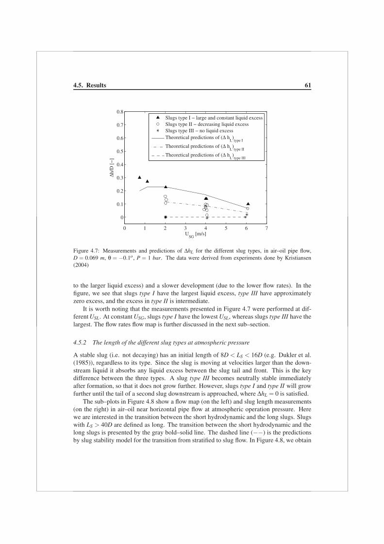
4.5. Results 61
0 1 2 3 4 5 6 7
0
0.1
0.2
0.3
0.4
0.5
0.6
0.7
0.8
USG
[m/s]
Δh/D
[−]
Slugs type I − large and constant liquid excessSlugs type II − decreasing liquid excessSlugs type III − no liquid excessTheoretical predictions of (Δ h
L)type I
Theoretical predictions of (Δ hL)type II
Theoretical predictions of (Δ hL)type III
Figure 4.7: Measurements and predictions of ΔhL for the different slug types, in air–oil pipe flow,D = 0.069 m, θ = −0.1o, P = 1 bar. The data were derived from experiments done by Kristiansen(2004)
to the larger liquid excess) and a slower development (due to the lower flow rates). In thefigure, we see that slugs type I have the largest liquid excess, type III have approximatelyzero excess, and the excess in type II is intermediate.
It is worth noting that the measurements presented in Figure 4.7 were performed at dif-ferent USL. At constant USG, slugs type I have the lowest USL, whereas slugs type III have thelargest. The flow rates flow map is further discussed in the next sub–section.
4.5.2 The length of the different slug types at atmospheric pressure
A stable slug (i.e. not decaying) has an initial length of 8D < LS < 16D (e.g. Dukler et al.(1985)), regardless to its type. Since the slug is moving at velocities larger than the down-stream liquid it absorbs any liquid excess between the slug tail and front. This is the keydifference between the three types. A slug type III becomes neutrally stable immediatelyafter formation, so that it does not grow further. However, slugs type I and type II will growfurther until the tail of a second slug downstream is approached, where ΔhL = 0 is satisfied.
The sub–plots in Figure 4.8 show a flow map (on the left) and slug length measurements(on the right) in air–oil near horizontal pipe flow at atmospheric operation pressure. Herewe are interested in the transition between the short hydrodynamic and the long slugs. Slugswith LS > 40D are defined as long. The transition between the short hydrodynamic and thelong slugs is presented by the gray bold–solid line. The dashed line (−−) is the predictionsby slug stability model for the transition from stratified to slug flow. In Figure 4.8, we obtain
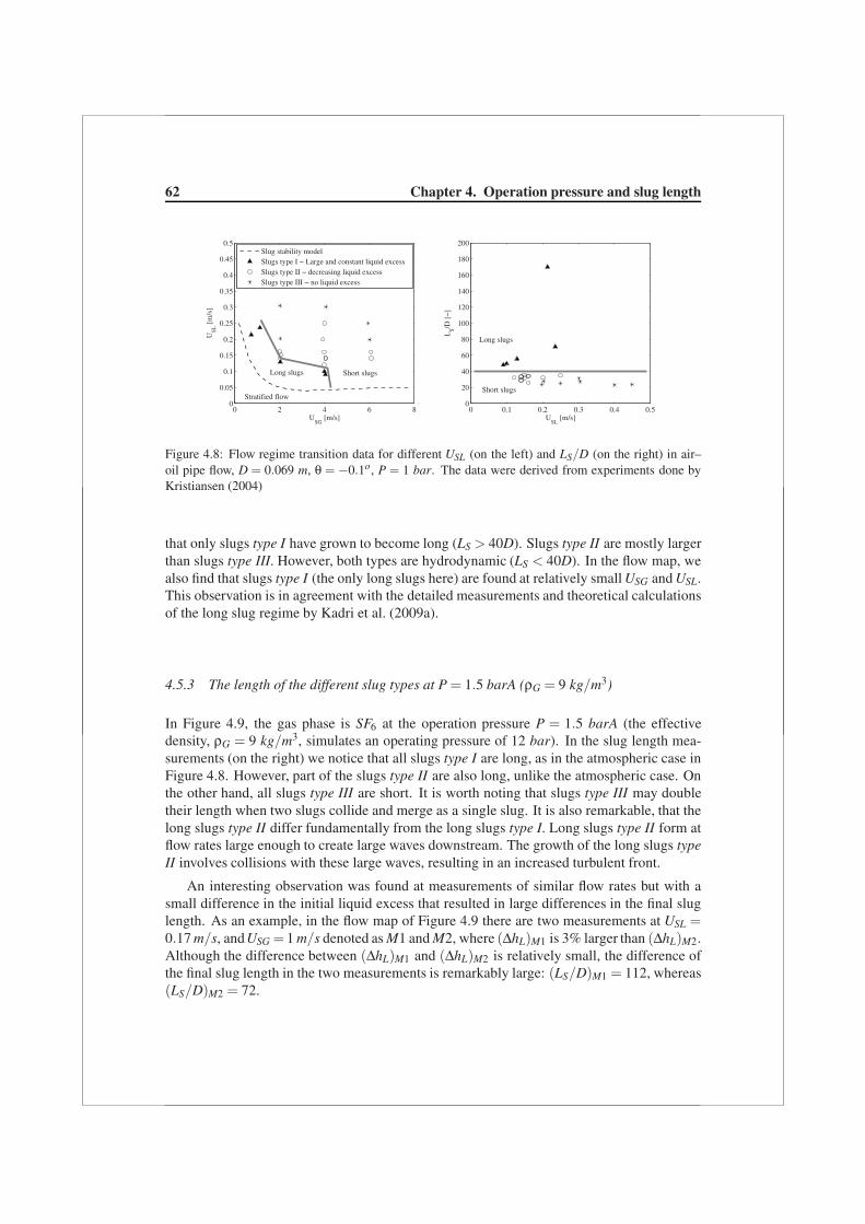
62 Chapter 4. Operation pressure and slug length
0 2 4 6 80
0.05
0.1
0.15
0.2
0.25
0.3
0.35
0.4
0.45
0.5
USG
[m/s]
USL
[m
/s]
0 0.1 0.2 0.3 0.4 0.50
20
40
60
80
100
120
140
160
180
200
USL
[m/s]
LS/D
[−]
Slug stability modelSlugs type I − Large and constant liquid excessSlugs type II − decreasing liquid excessSlugs type III − no liquid excess
Stratified flow
Long slugs Short slugs
Short slugs
Long slugs
Figure 4.8: Flow regime transition data for different USL (on the left) and LS/D (on the right) in air–oil pipe flow, D = 0.069 m, θ = −0.1o, P = 1 bar. The data were derived from experiments done byKristiansen (2004)
that only slugs type I have grown to become long (LS > 40D). Slugs type II are mostly largerthan slugs type III. However, both types are hydrodynamic (LS < 40D). In the flow map, wealso find that slugs type I (the only long slugs here) are found at relatively small USG and USL.This observation is in agreement with the detailed measurements and theoretical calculationsof the long slug regime by Kadri et al. (2009a).
4.5.3 The length of the different slug types at P = 1.5 barA (ρG = 9 kg/m3)
In Figure 4.9, the gas phase is SF6 at the operation pressure P = 1.5 barA (the effectivedensity, ρG = 9 kg/m3, simulates an operating pressure of 12 bar). In the slug length mea-surements (on the right) we notice that all slugs type I are long, as in the atmospheric case inFigure 4.8. However, part of the slugs type II are also long, unlike the atmospheric case. Onthe other hand, all slugs type III are short. It is worth noting that slugs type III may doubletheir length when two slugs collide and merge as a single slug. It is also remarkable, that thelong slugs type II differ fundamentally from the long slugs type I. Long slugs type II form atflow rates large enough to create large waves downstream. The growth of the long slugs typeII involves collisions with these large waves, resulting in an increased turbulent front.
An interesting observation was found at measurements of similar flow rates but with asmall difference in the initial liquid excess that resulted in large differences in the final sluglength. As an example, in the flow map of Figure 4.9 there are two measurements at USL =0.17 m/s, and USG = 1 m/s denoted as M1 and M2, where (ΔhL)M1 is 3% larger than (ΔhL)M2.Although the difference between (ΔhL)M1 and (ΔhL)M2 is relatively small, the difference ofthe final slug length in the two measurements is remarkably large: (LS/D)M1 = 112, whereas(LS/D)M2 = 72.
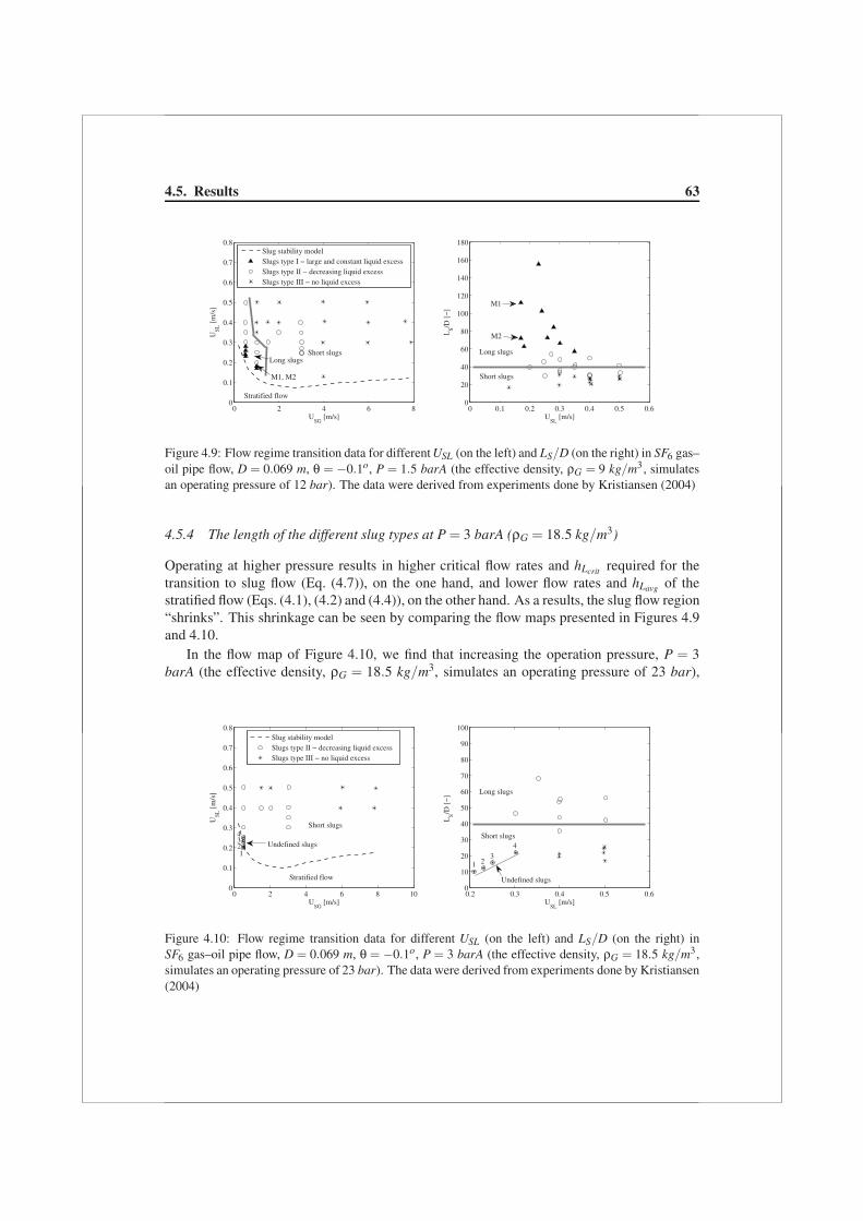
4.5. Results 63
0 2 4 6 80
0.1
0.2
0.3
0.4
0.5
0.6
0.7
0.8
USG
[m/s]
USL
[m
/s]
0 0.1 0.2 0.3 0.4 0.5 0.60
20
40
60
80
100
120
140
160
180
USL
[m/s]
LS/D
[−]
Slug stability modelSlugs type I − large and constant liquid excessSlugs type II − decreasing liquid excessSlugs type III − no liquid excess
Short slugs
Stratified flow
Long slugsLong slugs
M1, M2
Short slugs
M2
M1
Figure 4.9: Flow regime transition data for different USL (on the left) and LS/D (on the right) in SF6 gas–oil pipe flow, D = 0.069 m, θ = −0.1o, P = 1.5 barA (the effective density, ρG = 9 kg/m3, simulatesan operating pressure of 12 bar). The data were derived from experiments done by Kristiansen (2004)
4.5.4 The length of the different slug types at P = 3 barA (ρG = 18.5 kg/m3)
Operating at higher pressure results in higher critical flow rates and hLcrit required for thetransition to slug flow (Eq. (4.7)), on the one hand, and lower flow rates and hLavg of thestratified flow (Eqs. (4.1), (4.2) and (4.4)), on the other hand. As a results, the slug flow region“shrinks”. This shrinkage can be seen by comparing the flow maps presented in Figures 4.9and 4.10.
In the flow map of Figure 4.10, we find that increasing the operation pressure, P = 3barA (the effective density, ρG = 18.5 kg/m3, simulates an operating pressure of 23 bar),
0 2 4 6 8 100
0.1
0.2
0.3
0.4
0.5
0.6
0.7
0.8
USG
[m/s]
USL
[m
/s]
0.2 0.3 0.4 0.5 0.60
10
20
30
40
50
60
70
80
90
100
USL
[m/s]
LS/D
[−]
Slug stability modelSlugs type II − decreasing liquid excessSlugs type III − no liquid excess
Long slugs
Stratified flow
Short slugs Short slugs
Undefined slugs
Undefined slugs 23
1
4
1 23
4
Figure 4.10: Flow regime transition data for different USL (on the left) and LS/D (on the right) inSF6 gas–oil pipe flow, D = 0.069 m, θ = −0.1o, P = 3 barA (the effective density, ρG = 18.5 kg/m3,simulates an operating pressure of 23 bar). The data were derived from experiments done by Kristiansen(2004)

64 Chapter 4. Operation pressure and slug length
215 220 225 230 235 240 245 250 255 2600.4
0.5
0.6
0.7
0.8
0.9
1
Time traces [s]
hL/D
[−]
Type II
Type III
Type II
(hL,avg
/D)
(hL,crit
/D)
Large waves
Figure 4.11: Time traces of SF6 gas–oil pipe flow, D = 0.069 m, θ = −0.1o, P = 3 barA (the effectivedensity, ρG = 18.5 kg/m3, simulates an operating pressure of 23 bar). The experiments were performedby Kristiansen (2004)
results in the appearance of slugs only at higher USL, as shown in the flow map. In this set ofmeasurements no slugs type I were observed in the same measurements, and all long slugs aretype II with lengths that do not exceed 70D. At low flow rates, slugs type II and type III, andwaves were observed, simultaneously. Such slug measurements, at which multiple slug typesappeared, were indicated as “undefined slugs” in Figure 4.10. Time traces of these slugs showthe combination of slugs type II, type III, and large waves, as presented in Figure 4.11. Theseslugs form close to the inlet (of the test section) and propagate at relatively low velocities. Asa result, the slugs are being formed within, relatively, small distances, leading to a larger slugfrequency compared with that of the long slugs. In addition, increasing USL results, contraryto slugs type I, in increasing LS (see slug numbers in Figure 4.10).
4.5.5 Effect of pressure on the long slugs – summary
Figure 4.12 summarizes the effect of pressure on the presence of the long slugs in the pipe.In the figure, the bullets (•) represent measurements of the maximum slug length in the pipeat the given flow conditions. For a gas density of air at atmospheric and near atmosphericoperation pressures, the long slugs (a and b) are the longest in the long slug region (LS >150D). On the other hand, at gas density 18.5 < ρG < 52 kg/m3 simulating operation pressureof 23 < P < 65 bar, the long slugs are neutrally stable and their length did not exceed LS =70D. Above ρG = 52 kg/m3 (P > 65 bar), no long slugs have been observed.
From Figures 4.8, 4.9, 4.10, and 4.12 we conclude that the average slug length decreases

4.6. Conclusions 65
0 13 26 39 52 650
50
100
150
200
ρG
[kg/m3]
(LS/D
) max
[−]
Maximum slug length measurements
Short slugs (hydrodynamic)
b
c
e
d
a
Long slugs
P [bar]0 16 4933 65 81
Figure 4.12: Largest normalized slug length, (LS/D)max, as function of gas density and simulatedpressure in gas–liquid pipe flow, D = 0.069 m, θ = −0.1o. The data were derived from experimentsdone by Kristiansen (2004)
when increasing the operation pressure, at constant USG and USL. This conclusion is in agree-ment with findings by Ujang et al. (2006), who examined the pressure effect on the slugfrequency at flow conditions and a pipe diameter similar to these presented in this chapter.Ujang et al. (2006) reported that the slug frequency is not sensitive to a change in the opera-tion pressure. When increasing the operating pressure ΔhL decreases (Eqs. (4.4) and (4.7)),and since the slug frequency remains constant the slug length has to decrease in order toconserve the liquid mass.
4.6 Conclusions
1. Slug flow measurements have been analysed in order to investigate the sub–regimes inthe long slug regime, and the effect of pressure on the appearance of the long slugs.
2. Slugs have been categorized into three types according to the liquid excess betweenthe front and tail: (1) type I– slugs that are unaffected by the presence of other slugsdownstream. They have relatively large and constant initial liquid excess. Due to thelarge liquid excess, this type of slugs may become extremely long O(100D); (2) typeII– slugs moving over a depleted liquid layer due to the passage of other slugs. Thus,these slugs have a decreasing liquid excess. Depending on the flow conditions, thelength of this type of slugs varies from short hydrodynamic to long; and (3) type III–fully developed slugs with no liquid excess. These slugs are the shortest, being 8–16D

66 Chapter 4. Operation pressure and slug length
long at low flow rates, but double their lengths at larger flow rates due to collisions andmerging with other slugs.
3. Theoretical predictions by stratified and slug stability models correctly predict ΔhL ofthe different slug types. However, the models underpredict (ΔhL)typeI at USG < 1 m/s.
4. At atmospheric pressure, the long slugs were found to be type I. When increasing theliquid flow rates, the frequency of slugs type I increases, and neutral stability is reachedearlier in the pipe, due to the presence of a larger number of slugs. As a result, the sluglength decreases.
5. Increasing the operation pressure results, on one hand, in larger flow rates that arerequired for the transition from stratified to slug flow. On the other hand, the stratifiedliquid height decreases (due to the larger gas density), and slugs become neutrallystable earlier. As a result, slugs become shorter and the long slug sub–regime “shrinks”.
6. Slugs type II may also become long (LS > 40D). However, the mechanism behind theirgrowth is related to the collision and absorption of large waves travelling downstream.
7. Slugs type I have not been observed at ρG ≥ 18.5 kg/m3 (P ≥ 23 bar). At 18.5 <ρG < 46 kg/m3 (23 < P < 65 bar) the long slugs were only type II, neutrally stableat the outlet, with lengths less than 70D. At ρG = 52 kg/m3 (P = 65 bar) only shorthydrodynamic slugs (type III) were found.
8. Slight changes in the liquid excess can lead to large difference in the final slug length,and thus slug frequency.
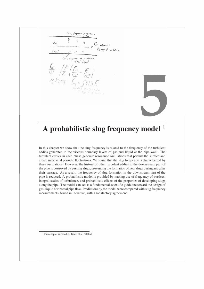
5A probabilistic slug frequency model 1
In this chapter we show that the slug frequency is related to the frequency of the turbulenteddies generated in the viscous boundary layers of gas and liquid at the pipe wall. Theturbulent eddies in each phase generate resonance oscillations that perturb the surface andcreate interfacial periodic fluctuations. We found that the slug frequency is characterized bythese oscillations. However, the history of other turbulent eddies in the downstream part ofthe pipe is destroyed by passing slugs, preventing the formation of new slugs during and aftertheir passage. As a result, the frequency of slug formation in the downstream part of thepipe is reduced. A probabilistic model is provided by making use of frequency of vortices,integral scales of turbulence, and probabilistic effects of the properties of developing slugsalong the pipe. The model can act as a fundamental scientific guideline toward the design ofgas–liquid horizontal pipe flow. Predictions by the model were compared with slug frequencymeasurements, found in literature, with a satisfactory agreement.
1This chapter is based on Kadri et al. (2009d)
68 Chapter 5. A probabilistic slug frequency model
5.1 Introduction
A slug flow pattern is commonly observed when transporting gas and liquid in horizontal andnear–horizontal pipe flows. Slug flow is characterized by plugs of liquid moving downstreamseparated by elongated bubbles moving along the top of the pipe.
The formation of slugs follows from surface waves evolving on the gas–liquid interface.One of the explanations of the occurrence of the surface waves is the presence of turbulencein the gas and liquid layers. The turbulent pressure and velocity fluctuations drive the waveformation, where the turbulence near the interface is usually maintained by a sheared meanflow (Teixeira and Belcher (2006)). At low Froude numbers there is no vertical motion inthe turbulence over a depth comparable with the integral scale of the turbulence, and energyredistributes into horizontal fluctuations (Teixeira and Belcher (2006); Hunt and Graham(1978); Magnaudet (2003); Pan and Banerjee (1995)). At larger Froude numbers of the gasand liquid phases, the pressure fluctuations associated with the turbulence cause a resonantforcing of the free surface modes, which then grow indefinitely (Phillips (1957)). If the flowrates are sufficiently high, the evolving waves can reach the top of the pipe and form slugflow. On the other hand, the interfacial waves may grow in the turbulent layer towards thebottom of the pipe. However, their growth is unlikely to be of a considerable order, since theliquid momentum dominates and the gas turbulence is relatively weak.
Predictions of the flow conditionsTwo main theories are involved for predicting the necessary flow conditions at which slugsmay form: theories on the stability of stratified flow and the stability of slugs.
Hanratty and Hershman (1961) used the stability of stratified flow to describe waves onthin films over which air is blowing. Their analysis was followed by Kordyban and Ranov(1970), Wallis and Dobbins (1973), Taitel and Dukler (1976) Lin and Hanratty (1986), andWu et al. (1987) who used the Kelvin–Helmholtz instabilities by analysing small sinusoidalperturbations on the interface of the stratified flow. This approach gives a criterion for thetransition from stratified–smooth to wavy flow. On the other hand, the stability of slug flowconcerns a volumetric balance between the liquid flow rate shedding from the back of a slugand the liquid rate accumulating on the front. This balance results in a minimum liquid areaat the front that is required for a slug to be stable (Ruder et al. (1989); Bendiksen and Espedal(1992), Hurlburt and Hanratty (2002)). In this approach, the back of the slug is modelled as abubble (Benjamin (1968)), which is supported by measurements and photographs by Woodsand Hanratty (1996).
The two stability theories provide predictions of the flow conditions that are necessary.However, they do not provide prediction of slug length or frequency. In this chapter, we usethe predictions by the two theories to obtain the properties of a stable slug flow.
Prediction of slug frequencySlug frequency has been investigated by several researchers in the last decades. Gregoryand Scott (1969) modelled the slug frequency as a function of the superficial gas and liquidvelocities and the liquid Froude number. The correlation by Gregory and Scott (1969) isbased on slug flow measurements performed in a wide range of pipe diameters, at relativelylarge liquid flow rates. Similar correlations based on additional data have been suggestedby a number of researchers (e.g. Greskovich and Shrier (1972); Heywood and Richardson
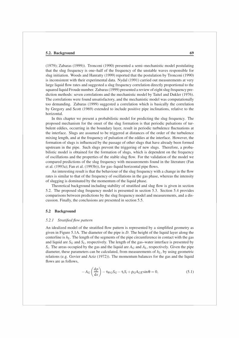
5.2. Background 69
(1979); Zabaras (1999)). Tronconi (1990) presented a semi–mechanistic model postulatingthat the slug frequency is one–half of the frequency of the unstable waves responsible forslug initiation. Woods and Hanratty (1999) reported that the postulation by Tronconi (1990)is inconsistent with their experimental data. Nydal (1991) carried out measurements at verylarge liquid flow rates and suggested a slug frequency correlation directly proportional to thesquared liquid Froude number. Zabaras (1999) presented a review of eight slug frequency pre-diction methods: seven correlations and the mechanistic model by Taitel and Dukler (1976).The correlations were found unsatisfactory, and the mechanistic model was computationallytoo demanding. Zabaras (1999) suggested a correlation which is basically the correlationby Gregory and Scott (1969) extended to include positive pipe inclinations, relative to thehorizontal.
In this chapter we present a probabilistic model for predicting the slug frequency. Theproposed mechanism for the onset of the slug formation is that periodic pulsations of tur-bulent eddies, occurring in the boundary layer, result in periodic turbulence fluctuations atthe interface. Slugs are assumed to be triggered at distances of the order of the turbulencemixing length, and at the frequency of pulsation of the eddies at the interface. However, theformation of slugs is influenced by the passage of other slugs that have already been formedupstream in the pipe. Such slugs prevent the triggering of new slugs. Therefore, a proba-bilistic model is obtained for the formation of slugs, which is dependent on the frequencyof oscillations and the properties of the stable slug flow. For the validation of the model wecompared predictions of the slug frequency with measurements found in the literature (Fanet al. (1993a); Fan et al. (1993b)), for gas–liquid horizontal pipe flows.
An interesting result is that the behaviour of the slug frequency with a change in the flowrates is similar to that of the frequency of oscillations in the gas phase, whereas the intensityof slugging is dominated by the momentum of the liquid phase.
Theoretical background including stability of stratified and slug flow is given in section5.2. The proposed slug frequency model is presented in section 5.3. Section 5.4 providescomparisons between predictions by the slug frequency model and measurements, and a dis-cussion. Finally, the conclusions are presented in section 5.5.
5.2 Background
5.2.1 Stratified flow pattern
An idealized model of the stratified flow pattern is represented by a simplified geometry asgiven in Figure 5.1A. The diameter of the pipe is D. The height of the liquid layer along thecenterline is hL. The length of the segments of the pipe circumference in contact with the gasand liquid are SG and SL, respectively. The length of the gas–water interface is presented bySi. The areas occupied by the gas and the liquid are AG and AL, respectively. Given the pipediameter, these parameters can be calculated, from measurements of hL, by using geometricrelations (e.g. Govier and Aziz (1972)). The momentum balances for the gas and the liquidflows are as follows,
−AG
(dpdx
)− τWGSG − τiSi + ρGAGgsinθ = 0, (5.1)
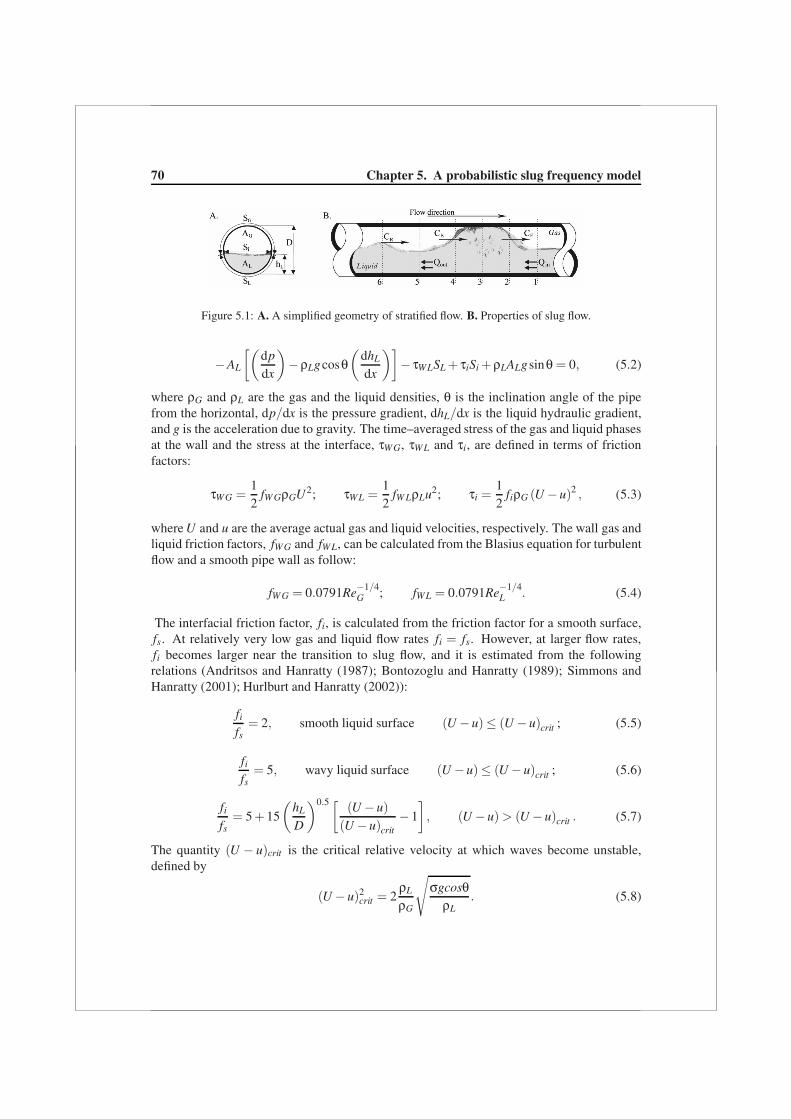
70 Chapter 5. A probabilistic slug frequency model
Figure 5.1: A. A simplified geometry of stratified flow. B. Properties of slug flow.
−AL
[(dpdx
)−ρLgcosθ
(dhL
dx
)]− τWLSL + τiSi + ρLALgsinθ = 0, (5.2)
where ρG and ρL are the gas and the liquid densities, θ is the inclination angle of the pipefrom the horizontal, dp/dx is the pressure gradient, dhL/dx is the liquid hydraulic gradient,and g is the acceleration due to gravity. The time–averaged stress of the gas and liquid phasesat the wall and the stress at the interface, τW G, τW L and τi, are defined in terms of frictionfactors:
τW G =12
fW GρGU2; τW L =12
fW LρLu2; τi =12
fiρG (U −u)2 , (5.3)
where U and u are the average actual gas and liquid velocities, respectively. The wall gas andliquid friction factors, fW G and fW L, can be calculated from the Blasius equation for turbulentflow and a smooth pipe wall as follow:
fW G = 0.0791Re−1/4G ; fW L = 0.0791Re−1/4
L . (5.4)
The interfacial friction factor, fi, is calculated from the friction factor for a smooth surface,fs. At relatively very low gas and liquid flow rates fi = fs. However, at larger flow rates,fi becomes larger near the transition to slug flow, and it is estimated from the followingrelations (Andritsos and Hanratty (1987); Bontozoglu and Hanratty (1989); Simmons andHanratty (2001); Hurlburt and Hanratty (2002)):
fi
fs= 2, smooth liquid surface (U −u)≤ (U −u)crit ; (5.5)
fi
fs= 5, wavy liquid surface (U −u)≤ (U −u)crit ; (5.6)
fi
fs= 5 + 15
(hL
D
)0.5 [(U −u)
(U −u)crit−1
], (U −u) > (U −u)crit . (5.7)
The quantity (U − u)crit is the critical relative velocity at which waves become unstable,defined by
(U −u)2crit = 2
ρL
ρG
√σgcosθ
ρL. (5.8)

5.2. Background 71
The gas and liquid Reynolds number given in Eq. (5.4) are given by
ReG =DHGU
νG; ReL =
DHLuνL
, (5.9)
where νG and νL are the kinematic viscosities of gas and liquid, and DHG and DHL are thehydraulic diameters defined as
DHG =4AG
SG + Si; DHL =
4AL
SL. (5.10)
5.2.2 Average liquid area
The average liquid area, AL = ALavg , is calculated from the momentum balances for the strat-ified flow pattern, Eqs. (5.1) and (5.2). Substituting AL = ALavg and AG = A−ALavg , Kadri etal. (2009a) wrote Eq. (5.1) in the following form,
(dpdx
)=
τW GSG + τiSi
A−ALavg
−ρGgsinθ. (5.11)
The average liquid area is the initial plain stratified flow in the pipe. This occurs whenthe pressure gradients of the two phases on the interface cancel. Substituting Eq. (5.11) inEq. (5.2) and assuming a fully developed horizontal pipe flow Kadri et al. (2009a) obtained arelation for ALavg as follows,
ALavg = AτW LSL − τiSi
τW LSL + τWGSG. (5.12)
The average liquid height hLavg is calculated using Eq. (5.12) and geometric relations (e.g.Govier and Aziz (1972)). Eq. (5.12) successfully predicts the inverse proportionality betweenthe gas flow rates and hLavg .
5.2.3 Slug stability model
The slug stability model considers the rates of liquid adjoining or detaching from the slug atits front or rear. Slugs are stable (not decaying) when the rates of liquid adjoining are not lessthan the rates at which liquid detaches. Figure 5.1B gives an illustration of a slug movingwith front velocity CF over a stratified liquid layer at station 1 of area AL1 and actual velocityu1. The volumetric flow rate of liquid adjoining the slug is:
Qin = (CF −u1)AL1. (5.13)
The rear of the slug is assumed to behave as a bubble moving with a velocity CB. Thevolumetric flow rate of the liquid detaching from the slug is:
Qout = (CB −u3)(1− ε)A at section 3. (5.14)

72 Chapter 5. A probabilistic slug frequency model
The parameter u3 is the actual liquid velocity at stations 3, and ε is the volume fraction of thegas in the slug (Woods and Hanratty (1998); Woods and Hanratty (1996)):
ε = 0.8
⎡⎣1− 1(
1 +(UMix/8.66)1.39)
⎤⎦ , (5.15)
where UMix is the mixture velocity (UMix = USG +USL, where USG and USL are the superficialgas and liquid velocities, respectively). Assuming neutral stability, Qin = Qout and CF = CB,and making use of Eqs. (5.13) and (5.14), the following relation is obtained,(
AL1
A
)crit
=(CB −u3)(1− ε)
(CB −u1), (5.16)
for the area of the stratified flow at the front. Using Eq. (5.16) and geometric relations, thecritical height, hLcrit , at the slug front required for the slug to be neutrally stable is obtained.The detailed analysis of slug stability model is well documented by Hurlburt and Hanratty(2002); Soleimani and Hanratty (2003).
5.3 Slug frequency model
Slug flow is an outcome of a complex two–phase flow field that contains periodic and nonper-iodic–chaotic events. These events can be either dependent or independent, and variant orinvariant with transformations in space–time. The complex flow field evolves in space–timethrough different stages: (1) stratified flow; (2) stratified–wavy; (3) transition to slug flow;(4) development of slugs; and (5) periodic “fully” developed slug flow. Solving the flow dy-namics of the different stages involves many computational challenges. Instead, we considerslugging as a steady periodic event that is invariant for constant flow conditions. We postu-late that slug flow (and so slug frequency) is an outcome of two main factors: (1) dominantindependent periodic events that occur at the initial stage in stratified flow; (2) and the effectof slugging on these events.
5.3.1 Frequency of turbulent eddies in gas and liquid
The dominant initial independent periodic events in stratified flow are the quasi–ordered mo-tions in the wall boundary layer of each fluid. Such motions create periodic ejections of slowmoving fluid from the viscous sublayer to the external region of the boundary layer (Surkov(1985)); Roshko (1976)); Ginevskii et al. (1978)); Alshamani et al. (1982)). The regionsof the quasi–ordered motion are characterised by high intensity pulsation and an increase ofthe scale of turbulence with a pairwise combination of eddies (Surkov (1985)). Each regionoccupies a viscous sublayer in the wall boundary layer. The distance from the wall to theexternal boundary of the eddy formation region is proportional to the thickness of the bound-ary layer, whereas the distance to the internal boundary is proportional to the thickness of theviscous sublayer (Grabovskii and Surkov. (1984)):
k1νuτ
≤ y ≤ k2δ, (5.17)

5.3. Slug frequency model 73
where y is the distance from the wall, ν is the kinematic viscosity of the fluid, δ is the viscousboundary layer, and uτ is the friction velocity:
uτ =√
τW
ρ, (5.18)
where ρ is the fluid density and τW is the time–averaged stress of the fluid defined in Eq. (5.3).The coefficient k1 was evaluated in accordance with data by Surkov (1985): k1 = 11 beingthe average maximum intensity of pulsations (for gas or liquid). For the case of gas–liquidpipe flow, a maximum distance from the wall is considered for the increase of turbulence ineach phase, k2δ = DH , where DH is the hydraulic diameter of the phase defined in Eq. (5.10).
The discrete eddy is represented in the form of a circular fluid disk, where the angularvelocity is one–half of the vorticity (Wu et al. (2006)). Therefore, the frequency of rotationis determined by the averaged tangential velocity of a point about the axis of rotation in thefollowing form:
ω =12
d〈u〉dy
. (5.19)
The frequency of oscillations generated by a discrete eddy into the surrounding medium isassumed to be of the order of magnitude of the frequency of rotation of the eddy. Thus,
fr =1
2πω. (5.20)
Assuming that the source of oscillations is located at an antinode of the stationary wave, thefamily of n resonance frequencies can be expressed by:
fnr =
2n−14π
uτk1
y. (5.21)
The first harmonic, in Eq. (5.21), dominates the resonance frequencies, since the wave damp-ing factor grows proportionally to the square root of the frequency (Lighthill (1978)). Thus,for the frequency of oscillations in gas and liquid we obtain the following relations:
fr,G =uτ,Gk1
4πy, fr,L =
uτ,Lk1
4πy. (5.22)
Eq. (5.22) provides uncorrelated quantities of two independent periodic events (frequencyof oscillations in gas and liquid). However, since slug flow is an interfacial periodic event(involving both gas and liquid), quantities fr,G and fr,L need to be coupled as a single periodicevent, which we define as an interfacial oscillation frequency, fr,i. The scale of y is consideredto be of the same order of magnitude for the two phases. This consideration is valid for theflow rates considered in this chapter where non of the phases is relatively thin.
5.3.2 Interfacial frequency of turbulent eddies, fr,i
From similarity consideration we define an interfacial frequency of turbulent eddies thatobeys the same laws in Eq. (5.22), thus,
fr,i � uτ,ik1
4πy. (5.23)

74 Chapter 5. A probabilistic slug frequency model
We also introduce an interfacial velocity:
uτ,i =√
τi
ρL. (5.24)
Substituting τi (from Eq. (5.3)) into Eq.(5.24), and expressing the result as function of fr,G
and fr,L, we obtain
uτ,i =2πk1
√fi
(fr,G√fW G
− fr,L√fW L
). (5.25)
Finally, substituting Eq. (5.25) into Eq. (5.23) gives a relation for an interfacial frequency:
fr,i√fi
=√
ρG
ρL
(fr,G√fW G
− fr,L√fW L
). (5.26)
5.3.3 Triggering of slug precursors
Slug flow evolves from turbulent fluctuations at the interface into growing waves that reachthe top of the pipe. Therefore, at the initial stage, a slug precursor can be triggered at thesame frequency of the turbulent eddies at locations i = 1, ...,n along the pipe, as shown inFigure 5.2. The length of the pipe is lpipe, and the distance between every two neighbouringslug precursors is the average turbulence scale length, lT . For a fully developed pipe flow lTis estimated as follows,
lT = 0.07D. (5.27)
Figure 5.2: Sketch of triggering slug precursors along the pipe.
5.3.4 Conditional probability of slug formation
We assume that a precursor slug will form if triggered at any location k unless another slug (orslug precursor) is passing at that location, at the triggering time, as illustrated in Figure 5.2.The passing slug unit (slug and bubble) is referred to as a “dead–zone”. The initial length ofthe “dead–zone” is defined as the length passed by a perturbation moving with the interfaceat the velocity CR for a time period Δt = 1/fr,i:
ldead = CRΔt, (5.28)

5.3. Slug frequency model 75
The wave velocity CR is calculated from the classical Kelvin–Helmholtz analysis of a strati-fied flow (e.g. Simmons and Hanratty (2001)):
CR =ρGUhL + ρLuH
ρLH + ρGh, (5.29)
where h and H are the height of the liquid and gas.Figure 5.3 shows examples of triggering slug precursors that form slugs (a and d), and
others that fail to form (b and c) due to its existence in the dead–zone at the triggering time.With tk being the time at which a slug precursor is triggered at location k, we define a factormi,k which is a measure for the effect of a slug at location i on the triggered slug precursor,
mi,k = max
[0,
min [tk,ti,w]− ti,FΔt
], (5.30)
where ti,w is the time that takes the upstream wave behind a slug at location i to reach thetriggered slug precursor at location k,
ti,w =(k− i)lT
CR, (5.31)
whereas ti,F is the time needed for the front of a slug at location i to reach the triggered slugprecursor at location k,
ti,F =(k− i)lT − ldead
CF. (5.32)
Eq. (5.30) provides the number of slugs that may form upstream and their passage will preventthe formation of a slug precursor that is triggered at location k, within the time interval (ti,w−ti,F). Therefore, the conditional probability of forming a slug (if triggered) at location k is:
Pk = 1−∑ mi,kPi
n, (5.33)
where P1 = 1 is the conditional probability of forming a slug, if triggered, at location 1. Av-eraging the probability of slug formation along the pipe 〈Pk〉, the slug frequency is obtainedas follows,
fS = 〈Pk〉fr,i. (5.34)
Figure 5.3: An example for triggering slug precursors at different locations a, b, c, and d. The triggeringat locations a and d may form slugs, whereas triggering at b and c, in the “dead zone”, fails to formslugs.

76 Chapter 5. A probabilistic slug frequency model
Note that an expression for the average fully developed slug length can be obtained by makinguse of the bubble velocity and Eqs. (5.26), (5.33) and (5.34):
LS =CB√
fi
√ρL
ρG
√fW Lfr,G −√
fW Gfr,L√fW L fW G〈1−∑k−1
i=1mi,kPi
n 〉. (5.35)
5.4 Results
Theoretical calculations of the frequency of oscillations in the gas and liquid phases, and atthe interface are given in Figure 5.4. The calculations were performed for air–water flow in a20 m long pipe with 0.095 m i.d. The subplots (a) and (b) indicate constant USL = 1.2 m/s andUSG = 3.5 m/s, respectively. The dashed and dotted curves are calculations of the frequencyof the oscillations generated in the gas and liquid (Eq. (5.22)), respectively; whereas thesolid curve is the calculation of the frequency at the interface (Eq. (5.26)). In Figure 5.4,the frequency of the oscillations generated in the gas phase, fr,G, is order of magnitude largerthan that in the liquid, fr,L, or at the interface, fr,i. However, the behaviour of fr,i with the flowrates is similar to that of fr,G. This indicates that the momentum of the liquid phase dictatesthe magnitude of the interfacial oscillations, whereas the intensity of eddy ejections in the gasphase dictates the behaviour of fr,i with the flow rates.
0 5 10 15 2010
−1
100
101
102
USG
[m/s]
Freq
uenc
y of
osc
illat
ion
[1/s
]
(a) USL
= 0.5 [m/s]
0 0.2 0.4 0.6 0.8 1 1.2 1.410
−1
100
101
102
(b) USG
= 3.5 [m/s]
USL
[m/s]
Freq
uenc
y of
osc
illat
ion
[1/s
]
fr,G
− frequency of oscillations in air
fr,L
− frequency of oscillations in water
fr,i
− frequency of oscillation at the interface
Figure 5.4: Theoretical calculations of the frequency of oscillations in air and water, and at the interface.D = 0.095 m, lpipe = 20 m. (a) Constant liquid flow rate, USL = 0.5 m/s. (b) Constant gas flow rate,USG = 3.5 m/s.
The relative scale of the dominating instabilities in each phase can be obtained by a fre-quency Strouhal number which is defined by the identity: St = frDH/u, where DH is thehydraulic diameter, defined in Eq.(5.10), and u is the average actual velocity of the fluid.Figure 5.5 shows the change of the frequency Strouhal number of the gas (solid curves) andliquid (dashed curves), as function of USG. Curves with the symbols (×) are predictions forrelatively low USL, whereas the other curves are for large USL. The larger frequency Strouhalnumber indicates smaller–scale instabilities from the separation of the shear layer (Kim and

5.4. Results 77
0 2 4 6 8 10 12 14 16
0.04
0.045
0.05
0.055
0.06
0.065
0.07
USG
[m/s]
Stro
uhal
num
ber
[−]
Strouhal frequency in the gas, USL
= 1.2 [m/s]
Strouhal frequency in the liquid, USL
= 1.2 [m/s]
Strouhal frequency in the gas, USL
= 0.09 [m/s]
Strouhal frequency in the liquid, USL
= 0.09 [m/s]
Figure 5.5: Strouhal number in air (solid curves) and water (dashed curves). D = 0.095 m, lpipe = 20m, curves without symbols: USL = 1.2 m/s, curves with ×: USL = 0.09 m/s.
Durbin (1988)). In the case of large USL the gas phase is dominated by smaller–scale insta-bilities compared with the liquid phase, for all gas flow rates. However, at USL = 0.09 m/sthe liquid phase is dominated by larger–scale instabilities at USG ≤ 4 m/s, and smaller–scaleat USG > 4 m/s (compared with the gas phase). As the liquid flow rate decreases, the actualgas velocity only indirectly changes (due to the decrease of the liquid level), therefore thegas Strouhal number increases slightly. However, the actual liquid velocity decreases signif-icantly and the liquid Strouhal number increases dramatically, especially at low USG wherethe change of the liquid level is enormous. At low flow rates, the small–scale instabilitiesare associated with low oscillation frequency (see Figure 5.4). As as result, ripples and largewavelength waves are generated at the surface. Slugs that evolve from such large wavelengthwaves and low frequencies may become very long (Kadri et al. (2009a)).
Figure 5.6 presents theoretical calculations with the above model of the conditional prob-ability of slug formation as function of the location on the pipe. The pipe is horizontal, 137m long with a diameter of 0.052 m, and the fluids are air and water with USG = 3.5 m/s. Theprobability of slug formation corresponds to Eq. (5.33). In Figure 5.6, the probability mono-tonically decreases downstream in the pipe, which is due to the more probable passage ofslugs formed upstream (see Eq. (5.33)). Increasing USL results in a smaller turbulence lengthscale, lT , and the number of the slug precursors (triggering locations) increases. Thus, theprobability of slug formation increases.
Theoretical predictions of slug frequency are compared with measurements in Figure 5.7.The measurements were carried out by Fan et al. (1993a) and Fan et al. (1993b) (publishedin Woods et al. (2006)) at USL = 0.5, 0.8 and 1.2 m/s, and a range of USG = 1...16 m/s. Thepipe is 20 m long with a diameter D = 0.095 m. The agreement between predictions and mea-surements is satisfactory. Eq. (5.34) successfully predicts that the slug frequency increaseswith increasing USG. However, a systematic overprediction is noticed as USL decreases. It is

78 Chapter 5. A probabilistic slug frequency model
0 20 40 60 80 100 120 1400
0.1
0.2
0.3
0.4
0.5
0.6
0.7
0.8
0.9
1
Position along the pipe [m]
Con
ditio
nal p
roba
bilit
y of
slu
g fo
rmat
ion
[−]
USL
= 1.2 [m/s]
USL
= 0.4 [m/s]
USL
= 0.09 [m/s]
Figure 5.6: Theoretical predictions of the conditional probability of slug formation in air–water hori-zontal pipe flow. USG = 3.5 m/s, D = 0.052 m, lpipe = 137 m.
0 2 4 6 8 10 12 14 160
0.2
0.4
0.6
0.8
1
1.2
1.4
1.6
1.8
2
USG
[m/s]
f s [1/
sec]
Measurements: USL
= 1.2 [m/s]
Measurements: USL
= 0.8 [m/s]
Measurements: USL
= 0.5 [m/s]
Predictions: USL
= 1.2 [m/s]
Predictions: USL
= 0.8 [m/s]
Predictions: USL
= 0.5 [m/s]
Figure 5.7: Theoretical predictions and measurements of slug frequency at fixed USL = 1.2 m/s andvarying USG. D = 0.095 m, lpipe = 20 m. The measurements were performed by Fan et al. (1993a) andFan et al. (1993b).
also noticeable that the region USG > 10 m/s is a transition region to annular flow. In orderto improve the accuracy of the predictions of slug frequency, the effect of annular flow needsto be considered.
Figure 5.8 compares theoretical predictions with measurements in pipes with diameters of

5.4. Results 79
0 0.1 0.2 0.3 0.4 0.5 0.60.03
0.04
0.05
0.06
0.07
0.08
0.09
0.1
0.11
USL
/Umix
f s D/U
SL [
−]
D=0.042 [m], Heywood and Richardson (1979)D=0.095 [m], Fan et al.(1993a,b)D=0.15 [m], Crowley et al.(1986)D=0.042 [m], current model (U
SL=1.2 [m/s])
D=0.095 [m], current model (USL
=1.2 [m/s])
D=0.15 [m], current model (USL
=1.2 [m/s])
Figure 5.8: Theoretical predictions and measurements of slug frequency for different pipe diameters.
0 0.5 1 1.5 2 2.5 30
0.05
0.1
0.15
f s [1/
sec]
USG
[m/s]
USL
= 0.15 [m/s], Zoeteweij (2007)
USL
= 0.06 [m/s], Zoeteweij (2007)
USL
= 0.15 [m/s], fi = f
s
USL
= 0.06 [m/s], fi = f
s
Figure 5.9: Theoretical predictions and measurements of slug frequency at low fixed USL and varyingUSG. D = 0.052 m, lpipe = 137 m. The measurements were performed by Zoeteweij (2007).
0.042 m (Heywood and Richardson (1979)), 0.095 m (Fan et al. (1993a); Fan et al. (1993b))and 0.15 m (Crowley et al. (1986)). The ordinate is fsD/USL and the abscissa is USL/UMix.The current model successfully predicts the slug frequency for the different pipe diameters.
In the case of (very) low flow rates, slugs evolving from long wavelength waves (as men-tioned previously) may grow to become several hundreds pipe diameter (Kadri et al. (2009a)).

80 Chapter 5. A probabilistic slug frequency model
Such slugs are not desirable due to the strong pressure fluctuations and separation difficultiesthey cause. The long slugs are characterised by a very low slug frequency that behaves in a“different” way compared to the case of large flow rates (Zoeteweij (2007)): in the long slugregion (at low flow rates) the slug frequency becomes a monotonically increasing function ofUSG (without a minimum). Predictions for the behaviour of fS with USG are compared withmeasurements in Figure 5.9. In the figure, the bullets (•) and circles (◦) are slug frequencymeasurements at USL = 0.06 and 0.15 m/s, respectively; whereas the solid and dashed curvesare the corresponding predictions. The model predicts that fS increases with USG, however,at USL = 0.15 m/s the trend becomes wrong. A possible reason for the wrong capture of thetrend is the lack of precise interfacial friction values at very low flow rates.
5.5 Conclusions
1. Slug frequency in gas–liquid horizontal pipe flow was investigated and derived by thefrequency of vortices in the two phases. Turbulent eddies, generated in the viscousboundary layer of the pipe wall, generate resonance oscillations that perturb the surfaceand create interfacial periodic fluctuations. Slug frequency is characterized by thesefluctuations.
2. At varying flow rates, slug frequency is found to behave similar to the frequency ofoscillations in the gas phase. However, the scale of frequency is dominated by theliquid momentum.
3. The history of turbulent eddies (slug precursors) in the downstream part of the pipeis destroyed by passing slugs, preventing the formation of new slugs. As a result, thefrequency of slug formation in the downstream part of the pipe is reduced.
4. A probabilistic model was provided by making use of frequency of vortices, integralscales of turbulence, and probabilistic effects of the properties of developing slugsalong the pipe. Predictions by the model were compared with slug frequency measure-ments, found in literature, with a satisfactory agreement.
5. The probability of forming a slug decreases in the downstream part of the pipe as aresult of the passage of other slugs formed upstream earlier.
6. The model was validated by comparing slug frequency calculations with measurementsfound in literature. The agreement between predictions and measurements is satisfac-tory at USG < 10 m/s. However, at large gas or low liquid flow rates the model over-predicts the slug frequency. A possible reason for this deviation between predictionsand measurements is the transition to annular flow, gas entrainment, and liquid breakupthat is not considered in the chapter.
7. The model predicts the change in the behaviour of the slug frequency in the long slugregion, i.e. at very low gas and liquid flow rates. However, the trend becomes wrongas the liquid flow rate increases. The accuracy of predictions by the model could beimproved if the interfacial friction factor was better estimated at very low flow rates.

6Conclusions and final remarks
The aim of this thesis was to investigate slug flow characteristics in stratified gas–liquid flowin horizontal and near horizontal pipes. The focus of the research was on the long liquid slugsthat may grow up to several hundreds of pipe diameter causing undesired system vibrationand serious operational failures. Simplified theoretical models, numerical simulations andexperiments have been carried out to investigate the following subjects: (1) the slug growthand the long slug region; (2) a detailed investigation of mechanisms in wave evolution (grav-ity and roll–waves) and their effect on the long slugs; (3) the effect of the operation pressure(on the long slugs); (4) the role of turbulence.
82 Chapter 6. Conclusions and final remarks
6.1 Slug growth and the long slug region
Very long slugs reaching 500 pipe diameter have been observed in gas–liquid horizontal pipeflow measurements. The long slugs appear at low gas and liquid flow rates, where the slugfrequency is relatively low and the difference in liquid level between the front and tail (liquidexcess) of a slug is large. As a result, decreasing the gas or liquid flow rate, in the longslug region, produces larger slugs. The long slug regime can be divided in two main sub–regimes: (a) long fully developed slugs; and (b) long growing slugs. The long growing slugs,were observed at flow rates close to the transition from stratified to slug flow, where the slugfrequency is lowest and the liquid excess is largest.
A dynamic slug growth model was presented. The model calculates the transient growthof a slug by applying a volumetric balance between the front and tail of the slug. The liquidat the front is calculated from the gas and liquid momentum equations. However, at the tail,the dynamics of the liquid level was simplified by a linear kinematic relation between the tailand the following upstream wave.
The model provides an explanation for a number of important observations in the slugflow regime: (a) in the long slug regime, the slug length decreases with increasing liquid flowrates as a result of the faster development of the liquid level behind the slug; (b) increasingthe operation pressure results in larger interfacial shear stresses, lower equilibrium liquidlevel and volumetric growth rate, and thus shorter average slug length – that is why at highpressure only hydrodynamic slugs are observed; (c) further increase of the pressure resultsin liquid levels approaching the minimum slug stability level, so that no stable slugs (long orhydrodynamic) can appear anymore (unless produced at the inlet).
6.2 Evolution of waves and transition to slug flow or roll–waves.
Slugs may form either directly by growing gravity waves that bridge the pipe, or by coalescingroll–waves. These are two different mechanisms for the formation of slug flow. Slugs thatform by roll–wave coalescence are short (Ls < 40D) and have relatively a large frequency,whereas slugs that form by growing large amplitude gravity waves are growing slugs that canbecome long. Therefore, it is important to identify and predict the conditions at which thecrest of a growing wave bridges the pipe, and the condition where the crest approaches thedownstream end of the wave producing a roll–wave.
In order to predict the evolution of waves into either slug flow or roll–waves, we devel-oped a time–difference wave transition model. The model calculates the time required fora long wavelength wave to grow and reach the top of the pipe, and the time needed for thewave crest to approach its downstream end. The model predicts the transition from stratifiedflow to slug flow or roll–wave regimes for different flow conditions and pipe diameters. Italso predicts a number of important observations regarding the behaviour of slug/roll–waveformation time: (a) increasing the liquid flow rates results in shorter transition times fromstratified wavy to slug flow; (b) at relatively low USG, the formation of slug/roll–wave timeincreases with increasing USG, which is a result of the lower initial stratified height; how-ever (c) at relatively high USG, due to the domination of inertial forces, the formation timedecreases with increasing USG and a roll–wave is formed; and (d) increasing the pipe size

6.3. The effect of operation pressure 83
results in larger axial growth compared to the growth in the vertical direction, making theappearance of long slugs less likely.
Based on predictions by the time–difference model we obtained a critical densimetricgas Froude number, Fr � 0.15, for the transition from slug flow to roll–wave regimes. Thecritical Froude number was obtained for flow rates close to the transition to slug flow.
6.3 The effect of operation pressure
In order to evaluate the effect of the operation pressure on the long slugs, air–oil and SF6gas–oil pipe flow measurements by Kristiansen (2004) were investigated. The measurementswere carried out at P = 1–8 barA with high density SF6 gas simulating a pressure up to 65bar.
Slugs have been categorized into three types according to the liquid excess between thefront and tail: (1) type I– slugs that are unaffected by the presence of other slugs downstream.They have relatively large and constant initial liquid excess. Due to the large liquid excess,this type of slugs may become extremely long O(100D); (2) type II– slugs moving over adepleted liquid layer due to the passage of other slugs. Thus, these slugs have a decreasingliquid excess. The length of this type of slugs vary from short hydrodynamic to long de-pending on the flow conditions; and (3) type III– fully developed slugs with no liquid excess.These type of slugs are the shortest, being 8–16D at low flow rates and doubling their lengthat larger flow rates due to collisions and merging with other slugs.
At atmospheric pressure, the long slugs were found to be type I. When increasing theliquid flow rates, the frequency of slugs type I increases, and neutral stability is reachedearlier in the pipe, due to the presence of a larger number of slugs. As a result, the slug lengthdecreases.
Slugs type I have not been observed at ρG ≥ 18.5 kg/m3 (P≥ 23 bar). At 18.5 < ρG < 46kg/m3 (23 < P < 65 bar)the long slugs were only type II, neutrally stable at the outlet. AtρG = 52 kg/m3 (P = 65 bar) only hydrodynamic slugs (type III) were found.
Slight changes in the liquid excess can lead to large difference in the final slug length,and thus slug frequency.
6.4 Slug flow and turbulence
Slug frequency in gas–liquid horizontal pipe flow was investigated and derived by the fre-quency of vortices in the two phases. Turbulent eddies, generated in the viscous boundarylayer of the pipe wall, generate resonance oscillations that perturb the surface and createinterfacial periodic fluctuations. Slug frequency is characterized by these fluctuations.
At varying flow rates, the slug frequency is found to behave similar to the frequency ofoscillations in the gas phase. However, the scale of frequency is dominated by the liquidmomentum.
The history of turbulent eddies downstream of the pipe is destroyed by passing slugs, pre-venting the formation of new slugs. As a result, the frequency of slug formation downstreamof the pipe is reduced.
84 Chapter 6. Conclusions and final remarks
A probabilistic model was provided by making use of frequency of vortices, integralscales of turbulence, and probabilistic effects of the properties of developing slugs along thepipe. Predictions by the model were compared with slug frequency measurements, foundin literature, with a satisfactory agreement. The probability of forming a slug decreasesdownstream the pipe as a result of the passage of other slugs formed upstream earlier.
The model was validated by comparing slug frequency calculations with measurementsfound in literature. The agreement between predictions and measurements is satisfactory atUSG < 10 m/s. However, at large gas flow rates the model overpredicts the slug frequency. Apossible reason for this deviation between predictions and measurements is the transition toannular flow.
The model predicts that the slug frequency increases with USG in the long slug region.However, the trend becomes wrong as the liquid flow rate increases. The interfacial frictionfactor plays an important role in the derivation of the slug frequency (fS f 1/2
i ). The accuracyof predictions by the model could be improved if the interfacial friction factor was betterestimated at very low flow rates.
6.5 Final remarks
Studying the characteristic length and time scales of slug flow in horizontal pipes, with aparticular focus on the long slugs, gave some insight into the dominating effects in stratifiedand slug flow regimes.
It is possible to derive slugging, considered as a periodic problem, from the dominatingperiodic events in stratified flow. However, mapping these events as a single “interfacial” pe-riodic event results in the involvement of the interfacial friction factor. A basic understandingof the interfacial friction factor could lead to more accurate predictions of the flow–field, ingeneral, and slug flow in particular.
It might be useful to repeat the periodicity approach presented in chapter 5 for otherperiodic flow patterns in pipe flow, e.g. annular flow, constructing a theoretical model foreach pattern. Then, combining the different models may give a general overview on thetransportation of gas and liquid in pipelines. Moreover, once all periodic events are treated,the chaotic part of the flow–field should be related to the remaining non–periodic events.

Bibliography
Alshamani, K.M.M, Laivsi, J.L., Edwards, F.J., 1982. Sound excitation of the boundary re-gion in a channel with a turbulent flow. Raket. Tekh. Kosmon. 20, 41–48.
Andritsos, N., Hanratty, T.J., 1987. Influence of interfacial waves in stratified gas–liquidflows. AIChE J. 33, 444–454.
Andritsos, N., Williams, L., Hanratty, T.J., 1989. Effect of liquid viscosity on the stratified–slug transition in horizontal pipe flow. Int. J. Multiphase Flow 15, 877–892.
Barnea, D., Taitel, Y., 1994a. Interfacial and structural stability of separated flow. Int. J.Multiphase Flow 20, 387–414.
Barnea, D., Taitel, Y., 1994b. Non–linear interfacial instability of separated flow. Chem. Eng.Sci. 49, 2341–2349.
Belcher, S., 1999. Wave growth by non–separated sheltering. Eur. J. Mech. B/Fluids 18, 447–462.
Belcher, S., Hunt, J., 1993. Turbulent shear flow over slowly moving waves. J. Fluid Mech.251, 119–148.
Bendiksen, K.H., 1984. An experimental investigation of the motion of long bubbles in in-clined tubes. Int. J. Multiphase Flow 10, 467–483.
Bendiksen, K.H., Espedal, M., 1992. Onset of slugging in horizontal gas–liquid pipe flow.Int. J. Multiphase Flow 18, 234–247.
Benjamin, T.B., 1959. Shear flow over a wavy boundary. J. Fluid Mech. 6, 161–205.
Benjamin, T.B., 1968. Gravity currents and related phenomena. J. Fluid Mech. 31, 209–248.
Bonizzi, M., Andreussi, P., Banerjee, S., 2009. Flow regime independent, high resolutionmulti–field modelling of near–horizontal gas–liquid flows in pipelines. Int. J. MultiphaseFlow 35, 34–46.

86 BIBLIOGRAPHY
Bontozoglu, V., Hanratty, T.J., 1989. Wave height estimation in stratified gas–liquid flows.AIChE J. 35, 1346–1350.
Bradshaw, P., 1976. Topics in applied physics. Turbulence 12(3) Chapter 3. Springer, Berlin.
Churchill, S.W., 1977. Friction–factor equation spans all fluid–flow regimes. Chem. Eng. 7,91.
Cohen, J., Belcher, S., 1999. Turbulent shear flow over fast–moving waves. J. Fluid Mech.386, 345–371.
Cornish, V., 1910. Waves of sea and other water waves. T. Fisher, Unwin, London, England.
Crowley, C.J., Sam, R.G., Rothe, P.H., 1986. Investigation of two–phase flow in horizontaland inclined pipes at large pipe size and high gas density. Report prepared for the AmericanGas Association by Creae Inc.
Crowley, C.J., Wallis, G.B., Barry, J.J., 1992. Validation of a one–dimensional wave modelfor the stratified–to–slug flow regime transition, with consequences for wave growth andslug frequency. Int. J. Multiphase Flow 18, 249–271.
Dukler, A.E., Hubbard, M.G., 1975. A model for gas–liquid slug flow in horizontal tubes.Ind. Eng. Chem. Fundam. 14, 337–347.
Dukler, A.E., Maron, D.M., Brauner, N., 1985. A physical model for predicting the minimumstable slug length. Chem. Eng. Sci. 40, 1379–1385.
Fan, G.W., Lusseyran, F., Hanratty, T.J., 1993. Initiation of slugs in horizontal gas–liquidflows. AIChE J. 39, 1741–1753.
Fan, Z., Ruder, Z., Hanratty, T.J., 1993b. Pressure profiles for slugs in horizontal pipelines.Int. J. Multiphase Flow 19, 421-437.
Ginevskii, A.S., Vlasov, E.F., Kolesnikov, A.V., 1978. Aeroacoustic Interaction [in Russian],Mashinostroenie, Moscow.
Govier, G.W., Aziz, K., 1972. The Flow of Complex Mixtures in Pipes. Van Nostrand Rein-hold Co, NY, p.563.
Grabovskii, A.M., Surkov, S.V., 1984. Frequency spectra of turbulent pulsations and stabilityof the laminar boundary layer, Inzh. Fiz. Zh. 46, 900–905.
Gregory, G.A., Scott, D.S., 1969. Correlation of liquid slug velocity and frequency in hori-zontal cocurrent gas–liquid slug flow. AIChE J. 15, 933–935.
Greskovich, E.J., Shrier, A.L., 1972. Slug frequency in horizontal gas–liquid slug flow. Ind.Eng. Chem. Proc. Design Dev. 11, No. 2, 317–318.
Hall, A., 1992. Multiphase Flow of Oil, Water and Gas in Horizontal Pipes. Ph.D. thesis,University of London.

BIBLIOGRAPHY 87
Hanratty, T.J., 2004. Final report on gas–liquid flow in pipelines. University of Illinois, Ur-
bana.
Hanratty, T.J., Engen, J., 1957. Interaction between a turbulent air stream and a moving water
surface. AIChE J. 3, 299–304.
Hanratty, T.J., Hershman, A., 1961. Initiation of roll waves. AIChE J. 7, 488–497.
Heywood, N.I., Richardson, J.F., 1979. Slug flow of air–water mixtures in a horizontal pipe:
Determination of liquid holdup by gamma–ray absorption. Chem. Eng. Sci. 34, 17–30.
Hubbard, M.G., 1965. An analysis of horizontal gas liquid slug flow. Ph.D. thesis, University
of Houston.
Hunt, J.C.R., Graham, J.M.R., 1978. Free–stream turbulence near plane boundaries. J. Fluid
Mech. 84, 209-235.
Hurlburt, E.T., Hanratty, T.J., 2002. Prediction of the transition from stratified to slug and
plug flow for long pipes. Int. J. Multiphase Flow 28, 707–729.
Jeffreys, H., 1924. On the formation of water waves by wind. Proc. Royal Soc. A107, 189–
205.
Jeffreys, H., 1925a. On the formation of water waves by wind. Proc. Royal Soc. A110, 241–
247.
Jeffreys, H., 1925b. The flow of water in an inclined channel of rectangular section. Phil.
Mag. (6) 49, 793–807.
Issa, R.I., Kempf, M.H.W., 2003. Simulation of slug flow in horizontal and nearly horizontal
pipes with the two–fluid model. Int. J. Multiphase Flow 29, 69–95.
Kadri, U., Mudde, R.F., Oliemans, R.V.A., 2009c. Influence of the operation pressure on slug
length in near horizontal gas–liquid pipe flow. Submitted to: Int. J. Multiphase Flow.
Kadri, U., Mudde, R.F., Oliemans, R.V.A., 2007a. On the prediction of the transition from
stratified flow to roll waves and slug flow in horizontal pipes. Proceedings 13th Inter-
national Conference on Multiphase Production Technology, Edinburgh, Scotland 13, pp.
65–78.
Kadri, U., Mudde, R.F., Oliemans, R.V.A., 2007b. On the development of waves into roll
waves and slugs in gas–liquid horizontal pipe flow. Proceedings 6th International Confer-
ence on Multiphase Flow, Leipzig, Germany 6, 332.
Kadri, U., Mudde, R.F., Oliemans, R.V.A., 2008b. A growth model for dynamic slugs in
gas/liquid horizontal pipes. In proc. BHR Conf., Banff, Canada, pp. 241–254.
Kadri, U., Mudde, R.F., Oliemans, R.V.A. 2009d. Prediction of slug frequency by a prob-
abilistic model from periodic interfacial turbulence fluctuations in gas/liquid pipe flow.
Submitted to: SPE J.

88 BIBLIOGRAPHY
Kadri, U., Bonizzi M., Mudde, R.F., Oliemans, R.V.A., Andreussi P., 2009b. Prediction ofthe transition from stratified to slug flow or roll–waves in gas–liquid horizontal pipes. Int.J. Multiphase Flow, doi:10.1016/j.ijmultiphaseflow.2009.07.002.
Kadri, U., Zoeteweij, M.L., Mudde, R.F., Oliemans, R.V.A., 2009a. A growth model fordynamic slugs in gas–liquid horizontal pipes. Int. J. Multiphase Flow 35, 439-449.
Kim, K.J., Durbin, P.A., 1988. Observations of the frequencies in a sphere wake and of dragincrease by acoustic excitation. Phys. Fluids 31, 3260–3265.
Kordyban, E., Ranov, T., 1970. Mechanism of slug formation in horizontal two–phase flow.J. Basic Eng. 92, 857–864.
Kristiansen, O., 2004. Experiments on the transition from stratified to slug flow in multi-phase pipe flow. Ph.D. thesis, Norwegian University of Science and Technology (NTNU),Trondheim.
Lighthill, M., 1962. Physical interpretation of the mathematical theory of wave generation bywind. J. Fluid Mech. 14, 385–398.
Lighthill, M.J., 1978. Waves in fluids, Cambridge/New York, Cambridge University Press,pp. 221–229
Lighthill, M., Whitman, G., 1955. On kinematics of waves: Part 1 and 2. Proc. Royal Soc.London. A229, 281–345.
Lin, P.Y., Hanratty, T.J., 1986. Prediction of the initiation of slugs with linear stability theory.Int. J. Multiphase Flow 12, 79–98.
Longuet–Higgins, M.S., 1952. On Statistical Distribution of the Heights of Sea Waves. J.Mar. Res., 11:245-266.
Magnaudet, J., 2003. High–Reynolds number turbulence in a shear–free boundary layer: re-visiting the Hunt–Graham theory. J. Fluid Mech. 484, 167–196.
McCready, M.J., 1998. Introduction to hydrodynamic stability. Lecture notes (version3/16/98), University of Notre Dame.
Miles, J., 1957. On the generation of surface waves by shear flows. J. Fluid Mech. 3, 185–204.
Miles, J., 1996. Surface–wave generation: a viscoelastic model. J. Fluid Mech. 322, 131–145.
Oliemans, R.V.A., 1987. Modelling of gas–condensate flow in horizontal and inclined pipes.In: ASME Pipeline Engineering Symposium–ETCE. pp. 72-81.
Nydal, O.J., 1991. An experimental investigation of slug flow. Ph.D. thesis, University ofOslo, Department of Mathematics, Oslo, Norway.
Nydal, O.J., Pintus, S., Andreussi, P., 1992. Statistical characterization of slug flow in hori-zontal pipes. Int. J. Multiphase Flow 18, 439–453.
BIBLIOGRAPHY 89
Nicholson, M.K., Aziz, K., Gregory, G.A., 1978. Intermittent two phase flow in horizontalpipes: predictive models. The Can. J. of Chemical Eng. 56, 653–663.
Pan, Y., Banerjee, S., 1995. A numerical study of free–surface turbulence in channel flow.Phys. Fluids 7, 1649-1664.
Phillips, O., 1957. On the generation of waves by turbulent wind. J. Fluid Mech. 2, 417–445.
Roshko, A., 1976. Structure of turbulent shear flows: a new point of view. Raket. Tekh.Kosmon. 14, 8–20.
Ruder, Z., Hanratty, P.J., Hanratty, T.J., 1989. Necessary conditions for the existence of stableslugs. Int. J. Multiphase Flow 15, 209–226.
Scott, S.L., Shoham, O., Brill, J.P., 1987. Modelling slug growth in large diameter pipes. In:3rd International Conference on Multiphase Flow, The Hague, Netherlands. BHRA Vol. 1,55–64.
Simmons, M.J.H., Hanratty, T.J., 2001. Transition from stratified to intermittent flow in smallangle upflows. Int. J. Multiphase Flow 27, 599–616.
Soleimani, A., Hanratty, T.J., 2003. Critical liquid flows for the transition from the pseudo–slug and stratified patterns to slug flow. Int. J. Multiphase Flow 29, 51–67.
Surkov, S.V., 1985. Cascade character of the growth of turbulent eddies. Inzh.–Fiz. Zh. 48,561–568.
Taitel, Y., Dukler, A., 1976. A model for predicting flow regime transitions in horizontal andnear horizontal gas–liquid flow. AIChE J. 22, 47–55.
Teixeira, M.A.C., Belcher, S.E., 2006. On the initiation of surface waves by turbulence shearflow. Dynamics of Atmospheres and Oceans 41, 1–27.
Tronconi, E., 1990. Prediction of slug frequency in horizontal two–phase slug flow. AIChEJ. 36, 701–709.
Ujang, P.M., Lawrence, C.J., Hale, C.P., Hewitt, G.F., 2006. Slug initiation and evolution intwo–phase horizontal flow. Int. J. Multiphase Flow 32, 527–552.
Wallis, G.B., Dobbins, J.E., 1973. The onset of slugging in horizontal stratified air–waterflow. Int. J. Multiphase Flow 1, 173–193.
Woods, B.D., 1998. Slug formation and frequency of slugging in gas–liquid flows. Ph.D.thesis, University of Illinois, Urbana.
Woods, B.D., Hanratty, T.J., 1996. Relation of slug stability to shedding rate. Int. J. Multi-phase Flow 22, 809–828.

90 BIBLIOGRAPHY
Woods, B.D., Hanratty, T.J., 1999. Influence of Froude number on physical processes deter-mining frequency of slugging in horizontal gas–liquid flows. Int. J. Multiphase Flow 25,1195–1223.
Woods, B.D., Hanratty, T.J., 2000. Mechanism of slug formation in downwardly inclinedpipes. Int. J. Multiphase Flow 26, 977–998.
Woods, B.D., Fan, Z., Hanratty, T.J., 2006. Frequency and development of slugs in a hori-zontal pipe at large liquid flows. Int. J. Multiphase Flow 32, 902–925.
Wu, H.L., Pots, B.F.M., Hollenberg, J.F., Meerhoff, R., 1987. Flow pattern transitions intwo–phase gas/condinsate flow at high pressure in an 8–inch horizontal pipe. Proc. BHRAConf., The Hague, The Netherlands, pp. 13–21.
Wu, J.Z., Ma, H.Y, Zhou, M.D., 2006. Vorticity and vortex dynamics, Springer Berlin Hei-delberg, pp. 67–68.
Zabaras, G.J., 1999. Prediction of slug frequency for gas–liquid flows. In: Annual TechnicalConference, SPE 56462. pp. 181–188.
Zoeteweij, M.L., 2007. Long liquid slugs in horizontal tubes. Development study and char-acterisation with electrical conductance techniques. Ph.D. thesis, Delft University of Tech-nology, Department of Multi–Scale Physics, Delft, The Netherlands.
ACalculation of the wave growth
coeffecient, C2
In this appendix, the calculation of the wave growth coeffecient, C2, is presented:
The initial wave amplitude, η0, is assumed to be half the turbulence length scale, lT , in afully developed pipe flow:
η0 =lT2
, (A.1)
wherelT = 0.07DHG. (A.2)
The parameter DHG is the hydraulic diameter of the gas phase give by
DHG =4AG
Si + SG. (A.3)
From Eq. 3.13, we calculate the range of the normalized average gas area for the flow ratesand pipe diameters considered in this paper as follows,
0.2 �AGavg
D2 � 0.7. (A.4)
Using geometric relations to calculate Si and SG (e.g. Govier and Aziz (1972)) we obtain:
2 � Si + SG
D� 3. (A.5)

92 Chapter A. Calculation of the wave growth coeffecient, C2
Substituting Eqs. A.4–A.5 into Eq. A.3 results in a lower and upper values of DHG as functionof the pipe diameter:
0.4D � DHG � 0.9. (A.6)
Substituting Eqs. A.6–A.2 into Eq. A.1 we obtain the following range for the initial ampli-tude:
0.01D � η0 � 0.03D. (A.7)
In order to obtain the maximum growth time of the crest we consider the smallest possibleinitial wave amplitude, η0 = 0.01D. Hence, the constant C2 = 0.01. It is noticeable that whenoperating at larger pressure the lower value of DHG increases, due to momentum considera-tions. As a result C2 should be modified (C2 > 0.01). However, C2 cannot be larger than 0.03since the upper value of DHG decreases with the pressure, due to the increase in the minimumliquid height downstream that is required for the formation of slugs (Eq. 3.9). As a result, theupper value of C2 decreases with the pressure (thus 0.01D < C2 < 0.03D).

Publications
U. Kadri, R.F. Mudde and R.V.A. Oliemans, 2009. Prediction of slug frequency by a
probabilistic model from periodic interfacial turbulence fluctuations in gas/liquid pipe flow.
Preprint submitted to SPE J.
U. Kadri, R.F. Mudde and R.V.A. Oliemans, 2009. Influence of the operation pressure on
slug length in near horizontal gas–liquid pipe flow. Preprint submitted to Int. J. Multiphase
Flow.
U. Kadri, R.F. Mudde and R.V.A. Oliemans, M. Bonizzi, P. Andreussi, 2009. On the
evolution of waves into roll–waves and slugs in gas–liquid horizontal pipe flow. Int. J. Mul-
tiphase Flow, doi:10.1016/j.ijmultiphaseflow.2009.07.002.
U. Kadri, M.L. Zoeteweij, R.F. Mudde and R.V.A. Oliemans, 2009. A growth model for
dynamic slugs in gas–liquid horizontal pipes. Int. J. Multiphase Flow 35, 439–449.
U. Kadri, R.F. Mudde and R.V.A. Oliemans, 2009. Slugs, turbulence and the butterfly
effect. Proceedings 14th International Conference on Multiphase Production Technology,
Cannes, France 14, pp. 319–330.
U. Kadri, R.F. Mudde and R.V.A. Oliemans, 2008. A theoretical growth model for hy-
drodynamic slugs in gas/liquid horizontal pipes. Proceedings 22nd International Congress of
Theoretical and Applied Mechanics (ICTAM2008), Adelaide, Australia 22, pp. 113.
L. Badarnah, U. Kadri, U. Knaack, 2008. A bio–inspired ventilating envelope optimized
by air–flow simulations. The World Sustainable Building (SB) Conference series, Melbourne,
Australia, pp. 29.
U. Kadri, R.F. Mudde and R.V.A. Oliemans, 2008. A growth model for dynamic slugs
in gas/liquid horizontal pipes. Proceedings 6th North American Conference on Multiphase
Technology, Banff, Canada 6, pp. 241–254.
94 Publications
U. Kadri, R.F. Mudde and R.V.A. Oliemans, 2008. The effect of the liquid level on thecharacteristics of forming slugs. Proceedings 7th International ERCOFTAC Symposium onEngineering Turbulence Modelling and Measurements, Limassol, Cyprus 7.
U. Kadri, R.F. Mudde and R.V.A. Oliemans, 2007. On the prediction of the transitionfrom stratified flow to roll waves and slug flow in horizontal pipes. Proceedings 13th Interna-tional Conference on Multiphase Production Technology, Edinburgh, Scotland 13, pp. 65–78.
U. Kadri, R.F. Mudde and R.V.A. Oliemans, 2007. On the development of waves into rollwaves and slugs in gas–liquid horizontal pipe flow. Proceedings 6th International Conferenceon Multiphase Flow, Leipzig, Germany 6, 332.

Acknowledgements
AdvisorsMy deep gratitude goes to my advisors, Rene Oliemans and Rob Mudde, for the delightfuldiscussions, and continuous guidance, encouragement, and supervision. After this formality,it is time for honesty. Before starting my PhD, I was offered PhD positions at other locations,all had research titles much more attractive and exciting than “Long slugs . . . ”. However, itwas not difficult for me to make the “right” choice. I chose the “right” supervisors.
StaffI would like to thank all the support staff including Thea, Amanda, Angela, Wouter, Jaap (vanRaamt), Jaap (Kamminga) and Jan for their support, whether directly or indirectly related tothe research and research facilities.
ColleaguesI thank Maria for the unforgettable atmosphere she made, Ruurd for his valuable advisesand tips, Jos for providing 3D–shooter games and Lan addiction support group, Marcos forarranging sports activities, Marco for the experiments and the “slug” discussions, Michael forproviding excellent working atmosphere, Andrea for justifying the atmosphere in the Italianway, Volkert for the valuable advices, discussions and willingness to help, Annekatrien forproviding an emergency–information support point on how to deal with the Dutch systems,Ozgur for the precious spontaneous scientific discussions we had almost about any object(except humans) that moved around, Federico for “taking care” of MY neighbourhood andfor surviving the “head–shot”, Anton for being on holidays for a sufficient period of time thatwas required to finalize my thesis, Mohammad for carrying my 200 kg washing machine,the successive roommates, Reza, Gallelio and Duong for the relaxed working environment,as well other PhD’s among which Amer, Adrian, Davide, Hamid, Laurens and Farzad whocontributed to this environment, Chris, Luis, and other professors for the open door policy(does not necessarily mean that someone is inside). For the third year PhD students, whenyou lastly start seeing the light in the tunnel, take a deep breath, turn around, run as fast asyou can, and climb the closest platform you find.
OthersI thank my PhD users’ committee for their critical remarks and their valuable suggestionsduring the meetings we had. I thank Prof. Ole Jørgen Nydal for the hospitality at his group,

96 Acknowledgements
and Dr. Olav Kristiansen for providing the detailed measurements of his PhD thesis, that hada valuable contribution to the research. I thank Dr. Marco Bonizzi and Prof. Paolo Andreussifor the fruitful cooperation we had.
FriendsMy friends withstanding back home, and those enduring foreignness, never skimped orscrimped a moment of being real friends. Thank you.
FamilyThe deepest gratitude goes to my family, and in particular to you, my parents. For yourability to discern what is true and right, inculcating in me the dedication and discipline of afree man with independent insights, the guidance with wisdom and continuous prays... halfof this work is definitely yours, and the other is due to you (but it is mine!). For my sistersand brothers I’ve been watching you the last 29 years closely. Thank you all for being olderthan me, providing me a large database of your own different mixed life experiences, givingme the possibility to learn and adapt your wise choices, and to avoid repeating mistakesanalogous to those committed by you. My stay in the Netherlands could not have been betterunforgettably delightful without the time spent with Basim & Hafsa family, the neverendingadventures, the unlimited quality food, and the 48,000 minutes of phone calls!. Hanan, thanksfor being the first to accompany me and Lidia to the Netherlands, the first to visit us at the 3different houses we moved to, and no doubt, the first to attend the defence. Anan, thanks forappreciating time (probably yours), having only well controlled time–optimised remarkablyshort up–to–the–point communications. For Ashraf, Amal and Nashid, thanks for taking careof many arrangements back home. For my parents–in–law, thanks for all your support andfaith. My wife, Lidia, your daily support and encouragements had a valuable contributionto my research. However, your enduring support accompanying me to my conferences, andme accompanying you to yours, have created a set of unforgettable adventures around theworld, with Grizzly Bears, Crocodiles, harmless 10 m long snakes but deadly tiny mosquitos(and of course many slugs); diving with great white sharks, whales, and dolphin troupes; thenever–ending land with thorny and Tasmanian devils, wild Kangaroos, and sleepy Koalas;the peaceful silence of snow covering the horizon of the arctic, the ghostly fjords, and thedominant trees on the steep canyons. . . Your crazy trip plans, to be able to see and do as muchas possible, but also to give space for appreciating the harmony, the peace, and the wonderfulbeauty of nature, all in all made the last 3 years .. extraordinary.
GodPraises are due to the Lord, source of all knowledge and all wisdom.

About the author
Usama Kadri was born in November 18, 1979, Kfar Saba, Israel. He started to play thePiano when he was 6 years old and made his Abitur at the Israel Arts and Science Academy(I.A.S.A) in Jerusalem. Between 1998 and 2002 he studied at the Technion - Israel Instituteof Technology, Haifa and obtained a B.Sc. degree in Aerospace Engineering. In 2005 heobtained the M.Sc. degree at the same faculty under the supervision of Prof. Daniel Weihs.Between 2005 and 2009 he became a research assistant at the Department of Multi–ScalePhysics, Faculty of Applied Sciences, Delft University of Technology, The Netherlands.

Related Documents