Logistic Regression Tree Analysis - Home | …loh/treeprogs/lotus/springer.pdfLogistic Regression Tree Analysis (In Handbook of Engineering Statistics, H. Pham, ed., 537–549, Springer,

Logistic Regression Tree Analysis

(In Handbook of Engineering Statistics, H. Pham, ed., 537–549, Springer, 2006)

Wei-Yin LohDepartment of Statistics

University of Wisconsin, Madison

SUMMARY

This chapter describes a tree-structured extension and generalization of the logisticregression method for fitting models to a binary-valued response variable. The tech-nique overcomes a significant disadvantage of logistic regression, which is interpretabil-ity of the model in the face of multicollinearity and Simpson’s paradox. Section 1summarizes the statistical theory underlying the logistic regression model and the esti-mation of its parameters. Section 2 reviews two standard approaches to model selectionfor logistic regression, namely, model deviance relative to its degrees of freedom andthe AIC criterion. A dataset on tree damage during a severe thunderstorm is usedto compare the approaches and to highlight their weaknesses. A recently publishedpartial one-dimensional model that addresses some of the weaknesses is also reviewed.

Section 3 introduces the idea of a logistic regression tree model. The latter con-sists of a binary tree in which a simple linear logistic regression (i.e., a linear logisticregression using a single predictor variable) is fitted to each leaf node. A split at anintermediate node is characterized by a subset of values taken by a (possibly different)predictor variable. The objective is to partition the dataset into rectangular piecesaccording to the values of the predictor variables such that a simple linear logisticregression model adequately fits the data in each piece. Because the tree structureand the piecewise models can be presented graphically, the whole model can be eas-ily understood. This is illustrated with the thunderstorm dataset using the LOTUSalgorithm.

Section 4 describes the basic elements of the LOTUS algorithm, which is basedon recursive partitioning and cost-complexity pruning. A key feature of the algorithmis a correction for bias in variable selection at the splits of the tree. Without biascorrection, the splits can yield incorrect inferences. Section 5 shows an application ofLOTUS to a dataset on automobile crash-tests involving dummies. This dataset ischallenging because of its large size, its mix of ordered and unordered variables, and itslarge number missing values. It also provides a demonstration of Simpson’s paradox.The chapter concludes with some remarks in Section 6.Key Words and Phrases: AIC criterion, deviance, LOTUS, maximum likelihood,multicollinearity, recursive partitioning, selection bias, Simpson’s paradox

1 Introduction

Logistic regression is a technique for modeling the probability of an event in terms of suitableexplanatory or predictor variables. For example, [4] use it to model the probability that atree in a forest is blown down during an unusually severe thunderstorm that occurred on July4, 1999, and caused great damage over 477,000-acres of the Boundary Waters Canoe Area

1

Wilderness in northeastern Minnesota. Data from a sample of 3666 trees were collected,including for each tree, whether it was blown down (Y = 1) or not (Y = 0), its trunkdiameter D in centimeters, its species S, and the local intensity L of the storm, as measuredby the fraction of damaged trees in its vicinity. The dataset may be obtained from www.

stat.umn.edu/~sandy/pod.Let p = Pr(Y = 1) denote the probability that a tree is blown down. In linear logistic

regression, we model log(p/(1−p)) as a function of the predictor variables, with the require-ment that it be linear in any unknown parameters. The function log(p/(1− p)) is also oftenwritten as logit(p). If we use a single predictor such as L, we have the simple linear logisticregression model

logit(p) = log(p/(1 − p)) = β0 + β1L (1)

which can be re-expressed in terms of p as p = exp(β0 + β1L)/{1 + exp(β0 + β1L)}.In general, given k predictor variables X1, . . . , Xk, a linear logistic regression model

in these variables is logit(p) = β0 +∑k

j=1 βjXj. The parameters β0, β1, . . . , βk are typi-cally estimated using maximum likelihood theory. Let n denote the sample size and let(xi1, . . . , xik, yi) denote the of values of (X1, . . . , Xk, Y ) for the ith observation (i = 1, . . . , n).Treating each yi as the outcome of an independent Bernoulli random variable with successprobability pi, we have the likelihood function

n∏

i=1

pyi

i (1 − pi)1−yi =

exp{∑

i yi(β0 +∑

j βjxij)}∏i{1 + exp(β0 +

∑j βjxij)}

.

The maximum likelihood estimates (MLEs) (β̂0, β̂1, . . . , β̂k) are the values of (β0, β1, . . . , βk)that maximize this function. Newton-Raphson iteration is usually needed to compute theMLEs.

2 Approaches to model fitting

The result of fitting model (1) is

logit(p) = −1.999 + 4.407L. (2)

Figure 1 shows a plot of the estimated p function. Clearly, the stronger the local stormintensity, the higher the chance for a tree to be blown down.

Figure 2 shows boxplots of D by species. Because of the skewness of the distributions,we follow [4] and use log(D), the natural logarithm of D, in our analysis. With log(D) inplace of L, the fitted model becomes

logit(p) = −4.792 + 1.749 log(D) (3)

suggesting that tall trees are less likely to survive a storm than short ones. If we use bothlog(D) and L, we obtain the model

logit(p) = −6.677 + 1.763 log(D) + 4.420L. (4)

2

0.0 0.2 0.4 0.6 0.8 1.0

0.0

0.2

0.4

0.6

0.8

1.0

Local storm intensity (L)

Pro

b(B

low

dow

n)

Figure 1: Estimated probability of blowdown computed from a simple linear logistic regres-sion model using L as predictor

A BA BF BS C JP PB RM RP

2040

6080

Species

Tru

nk d

iam

eter

(D

)

Figure 2: Boxplots of trunk diameter D. The median value of 14 for D, or 2.64 for log(D),is marked with a dotted line.

3

Table 1: Indicator variable coding for the species variable S

Species U1 U2 U3 U4 U5 U6 U7 U8

A (aspen) 0 0 0 0 0 0 0 0BA (black ash) 1 0 0 0 0 0 0 0BF (balsam fir) 0 1 0 0 0 0 0 0BS (black spruce) 0 0 1 0 0 0 0 0C (cedar) 0 0 0 1 0 0 0 0JP (jack pine) 0 0 0 0 1 0 0 0PB (paper birch) 0 0 0 0 0 1 0 0RM (red maple) 0 0 0 0 0 0 1 0RP (red pine) 0 0 0 0 0 0 0 1

Finally, if we include the product L log(D) to account for interactions between D and L, weobtain

logit(p) = −4.341 + 0.891 log(D) − 1.482L + 2.235L log(D). (5)

So far, we have ignored the species S of each tree in our sample. We might get a modelwith higher prediction accuracy if we include S. As with least squares regression, we caninclude a categorical variable that takes m distinct values by first defining m − 1 indicatorvariables, U1, . . . , Um−1, each taking value 0 or 1. The definitions of the indicator variablescorresponding to our nine-species variable S are shown in Table 1. Note that we use the“set-to-zero constraint,” which sets all the indicator variables to 0 for the first category(aspen). A model that assumes the same slope coefficients for all species but that gives eacha different intercept term is

logit(p) = −5.997 + 1.581 log(D) + 4.629L − 2.243U1 + 0.0002U2 + 0.167U3

− 2.077U4 + 1.040U5 − 1.724U6 − 1.796U7 − 0.003U8. (6)

How well do models (2)–(6) fit the data? One popular method of assessing fit is by meansof significance tests based on the model deviance and its degrees of freedom (df)—see, e.g.,[1, p. 96] for the definitions. The deviance is analogous to the residual sum of squares inleast squares regression. For model (6), the deviance is 3259 with 3655 df. We can evaluatethe fit of this model by comparing its deviance against that of a larger one, such as the27-parameter model

logit(p) = β0 + β1 log(D) + β2L +8∑

j=1

γjUj +8∑

j=1

β1jUj log(D) +8∑

j=1

β2jUjL (7)

which allows the slope coefficients for log(D) and L to vary across species. Model (7) has adeviance of 3163 with 3639 df. If model (6) provides a suitable fit for the data, statisticaltheory says that the difference in deviance should be approximately distributed as a chi-square random variable with df equal to the difference in the df of the two models. For ourexample, the difference in deviance of 3259 − 3163 = 96 is much too large to be explainedby a chi-square distribution with 3655 − 3639 = 16 df.

4

Rejection of model (6) does not necessarily imply, however, that model (7) is satisfactory.To find out, we need to compare it with a larger model, such as the 28-parameter model

logit(p) = β0 + β1 log(D) + β2L + β3L log(D) +8∑

j=1

γjUj +8∑

j=1

β1jUj log(D) +8∑

j=1

β2jUjL (8)

which includes an interaction between log(D) and L. This has a deviance of 3121 with 3638df. Model (7) is therefore rejected because its deviance differs from that of (8) by 42 buttheir dfs differ only by 1. It turns out that, using this procedure, each of models (2) through(7) is rejected when compared against the next larger model in the set.

A second approach chooses a model from a given set by minimizing some criterion thatbalances model fit with model complexity. One such is the AIC criterion, defined as thedeviance plus twice the number of estimated parameters (see, e.g., [5, p. 234]). It is well-known, however, that the AIC criterion tends to over-fit the data. That is, it often choosesa large model. For example, if we apply it to the set of all models up to third-order for thecurrent data, it chooses the largest, i.e., the 36-parameter model

logit(p) = β0 + β1 log(D) + β2L +8∑

j=1

γjUj + β3L log(D)

+8∑

j=1

β1jUj log(D) +8∑

j=1

β2jUjL +8∑

j=1

δjUjL log(D). (9)

Graphical interpretation of models (8) and (9) is impossible. The simple and intuitivesolution of viewing the estimated p-function by a graph such as Fig. 1 is unavailable when amodel involves more than one predictor variable. This problem is exacerbated by the fact thatmodel complexity typically increases with increase in sample size or number of predictors.Interpretation of the estimated coefficients is frequently futile, because the estimates typicallydo not remain the same from one model to another. For example, the coefficient for L is4.407, 4.424, 1.870, and 4.632 in models (2), (4), (5), and (6), respectively. This is due tomulticollinearity among the predictor variables.

Cook and Weisberg [4] try to solve the problem of interpretation by using a partial one-

dimensional (POD) model, which employs a single linear combination of the non-categoricalvariables, Z = δ1 log(D) + δ2L, as predictor. For the tree data, they find that if balsamfir (BF) and black spruce (BS) are excluded, the model logit(p) = β0 + Z +

∑j γjUj, with

Z = 0.78 log(D) + 4.1L, fits the other species quite well. One advantage of this model isthat the estimated p-functions may be displayed graphically as shown in Fig. 3. The graphis not as natural as Fig. 1, however, because Z is a linear combination of two variables. Inorder to include species BF and BS, [4] choose the larger model

logit(p) = β0 + Z +9∑

j=1

γjUj + {θ1IBF + θ2IBS} log(D) + {φ1IBF + φ2IBS}L (10)

which contains separate coefficients, θj and φj, for BF and BS. Here I(·) denotes the indicatorfunction, i.e., IA = 1 if the species is A, and IA = 0 otherwise. Of course, this model doesnot allow a graphical representation for BF and BS.

5

2 3 4 5 6 7

0.0

0.2

0.4

0.6

0.8

1.0

Z = 0.78 log(D) + 4.10 L

Pro

b(B

low

dow

n)

1

1

1

1

11 1 1

2

2

2

2

22

2 2

3

3

3

3

3

33

3

4 44

4

4

4

4

4

5 55

5

5

5

5

5

6 66

6

6

6

6

6

7 7 7 77

7

7

7

1234567

JPRPAPBRMCBA

Figure 3: Estimated probability of blowdown for seven species, excluding balsam fir (BF)and black spruce (BS), according to model (10)

3 Logistic regression trees

The type of models and the method of selection described in the previous section are clearlynot totally satisfactory. As the sample size or the number of predictor variables increases,so typically does model complexity. But a more complex model is always harder to interpretthan a simple one. On the other hand, an overly simple model may have little predictivepower.

A logistic regression tree model offers one way to simultaneously retain the graphicalinterpretability of simple models and the predictive accuracy of richer ones. Its underlyingmotivation is that of “divide and conquer.” That is, a complex set of data is divided intosufficiently many subsets such that a simple linear logistic regression model adequately fitsthe data in each subset. Data subsetting is performed recursively, with the sample split onone variable at a time. This results in the partitions being representable as a binary decisiontree. The method is implemented by [3] in a computer program called LOTUS.

Figure 4 shows a LOTUS model fitted to the tree data. The data are divided into tensubsets, labeled 0–9. Balsam fir (BF), one of the two species excluded from the [4] model,is isolated in subsets 0 and 9, where log(D) is the best linear predictor. The estimatedp-functions for these two subsets are shown in Fig. 5. The estimated p-functions for thenon-balsam firs can be displayed together in one graph, as shown in Fig. 6, because they allemploy L as the best simple linear predictor.

From the graphs, we can draw the following conclusions.

1. The probability of blowdown consistently increases with D and L, although the valueand rate of increase are species dependent.

6

S=BA,BF,C,PB,RM

S=BF

L ≤ 0.3

0

38/263log(D)

9

195/396log(D)

log(D)≤ 2.4

8

44/459L

7

118/591L

log(D) ≤ 2.64

log(D)≤ 2.2

6

60/237L

S=A,BS,RP

5

226/391L

1

49/60L

L ≤ 0.404

S=A,BS

3

145/309L

2

137/200L

4

672/760L

Figure 4: A piecewise simple linear LOTUS model for estimating the probability that a treeis blown down. A splitting rule is given beside each intermediate node. If a case satisfies therule, it goes to the left child node; otherwise the right child node. The second level split atlog(D) = 2.64 corresponds to the median value of D. Beneath each leaf node are the ratioof cases with Y = 1 to the node sample size and the name of the selected predictor variable.

0 00

00

0

0

0

2.0 2.5 3.0 3.5

0.0

0.2

0.4

0.6

0.8

1.0

log(D)

P(B

low

dow

n)

9

9

9

9

9

99 9

90

L > 0.3L ≤ 0.3

Figure 5: Estimated probability of blowdown for balsam fir (BF), according to the LOTUSmodel in Fig. 4

7

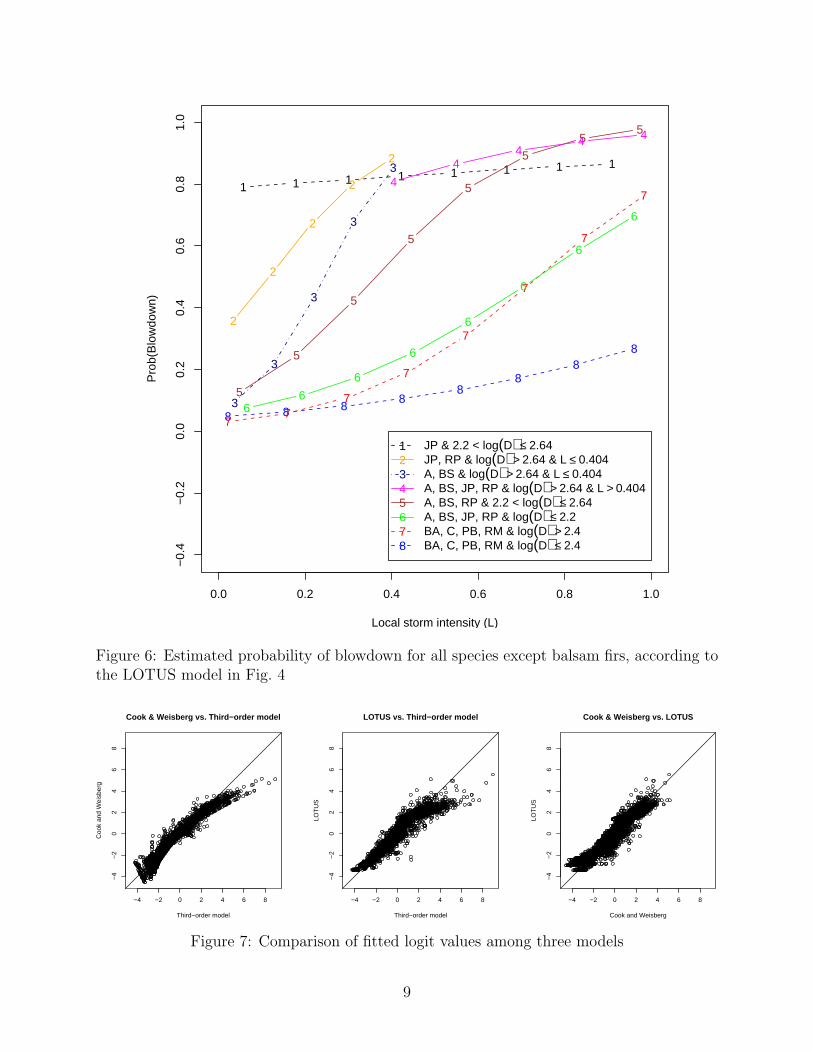
2. Balsam fir (BF) has the highest chance of blowdown, given any values of D and L.

3. The eight non-balsam fir species can be divided into two groups. Group I consists ofblack ash (BA), cedar (C), paper birch (PB), and red maple (RM). They belong tosubsets 7 and 8, and are most likely to survive. This is consistent with the POD modelof [4]. Group II contains aspen (A), black spruce (BS), jack pine (JP), and red pine(RP).

4. The closeness of the estimated p-functions for subsets 6 and 7 show that the smallerGroup II trees and the larger Group I trees have similar blowdown probabilities forany given value of L.

5. Although aspen (A) and black spruce (BS) are always grouped together, namely, insubsets 3–6, less than 15% of the aspen trees are in subsets 5 and 6. Similarly, only 2%of the red pines (RP) are in these two subsets. Hence the p-function of aspen (A) ismainly described by the curves for subsets 3 and 4, and that for red pine (RP) by thecurves for subsets 2 and 4. We conclude that, after balsam fir (BF), the three speciesmost at risk of blowdown are jack pine (JP), red pine (RP), and aspen (A), in thatorder. This ordering of JP, RP, and A is the same as the POD model of [4], as can beseen in Fig. 3.

6. Recall that black spruce (BS) was the other species that [4] could not include in theirPOD model. The reason for this is quite clear from Fig. 5, where we use solid lines todraw the estimated p-function for black spruce. Four curves are required, correspondingto subsets 2, 4, 5, and 6. The spread of these curves suggests that the p-function ofblack spruce is highly sensitive to changes in D. This explains why the species cannotbe included in the POD model.

How does the LOTUS model compare with the others? The former is clearly superiorin terms of interpretability. But does it predict future observations as well as the othermodels? Unfortunately, this question cannot be answered completely, because we do nothave an independent set of data to test the models. The best we can do is to comparethe fitted values from the different models. This is done in Fig. 7, which plots the fittedlogit values of the LOTUS model against those of the POD and the linear logistic regressionmodel with all interactions up to third order. The plots show that there is not much tochoose among them.

4 LOTUS algorithm

As already mentioned, the idea behind LOTUS is to partition the sample space into one ormore pieces such that a simple model can be fitted to each piece. This raises two questions:(i) how to carry out the partitioning, and (ii) how to decide when a partition is good enough?We discuss each question in turn.

8

8 8 88

88

88

0.0 0.2 0.4 0.6 0.8 1.0

−0.

4−

0.2

0.0

0.2

0.4

0.6

0.8

1.0

Local storm intensity (L)

Pro

b(B

low

dow

n)

77

7

7

7

7

7

7

66

6

6

6

6

6

6

1 1 1 1 1 1 1 1

5

5

5

5

5

5

55

4

44

4 4

2

2

2

2

2

3

3

3

3

3

12345678

JP & 2.2 < log(D) ≤ 2.64JP, RP & log(D) > 2.64 & L ≤ 0.404A, BS & log(D) > 2.64 & L ≤ 0.404A, BS, JP, RP & log(D) > 2.64 & L > 0.404A, BS, RP & 2.2 < log(D) ≤ 2.64A, BS, JP, RP & log(D) ≤ 2.2BA, C, PB, RM & log(D) > 2.4BA, C, PB, RM & log(D) ≤ 2.4

Figure 6: Estimated probability of blowdown for all species except balsam firs, according tothe LOTUS model in Fig. 4

−4 −2 0 2 4 6 8

−4

−2

02

46

8

Third−order model

Coo

k an

d W

eisb

erg

Cook & Weisberg vs. Third−order model

−4 −2 0 2 4 6 8

−4

−2

02

46

8

Third−order model

LOT

US

LOTUS vs. Third−order model

−4 −2 0 2 4 6 8

−4

−2

02

46

8

Cook and Weisberg

LOT

US

Cook & Weisberg vs. LOTUS

Figure 7: Comparison of fitted logit values among three models

9

4.1 Recursive partitioning

Like all other regression tree algorithms, LOTUS splits the dataset recursively, each timechoosing a single variable X for the split. If X is an ordered variable, the split has the forms = {X ≤ c}, where c is a constant. On the other hand, if X is a categorical variable, thesplit has the form s = {X ∈ ω}, where ω is a subset of the values taken by X. The ways is chosen is critically important if the tree structure is to be used for inference about thevariables.

For least squares regression trees, many algorithms, such as AID [8], CART [2] and M5[9], choose the split s that minimizes the total sum of squared residuals of the regressionmodels fitted to the two data subsets created by s. Although this approach can be directlyextended to logistic regression by replacing sum of squared residuals with the deviance, itis fundamentally flawed, because it is biased toward choosing X variables that allow moresplits. To see this, suppose that X is an ordered variable taking n unique values. Then thereare n−1 ways to split the data along the X axis, with each split s = {X ≤ c} being such thatc is the midpoint between two consecutively ordered values. This creates a selection biastoward X variables for which n is large. For example, in our tree dataset, variable L has 709unique values but variable log(D) has only 87. Hence if all other things are equal, L is eighttimes more likely to be selected than log(D).

The situation can be worse if there are one or more categorical X variables with manyvalues. If X takes n categorical values, there are 2n−1 − 1 splits of the form s = {X ∈ ω}.Thus the number of splits grows exponentially with the number of categorical values. In ourexample, the species variable S generates 29−1 − 1 = 255 splits, almost three times as manysplits as log(D).

Doyle [6] is the first to warn that this bias can yield incorrect inferences about the effectsof the variables. The GUIDE [7] least squares regression tree algorithm avoids the bias byemploying a two-step approach to split selection. First, it uses statistical significance teststo select X. Then it searches for c or ω. The default behavior of GUIDE is to use categoricalvariables for split selection only; they are not converted into indicator variables for regressionmodeling in the nodes. LOTUS extends this approach to logistic regression. The details aregiven in [3], but the essential steps in the recursive partitioning algorithm can described asfollows.

1. Fit a logistic regression model to the data using only the non-categorical variables.

2. For each ordered X variable, discretize its values into five groups at the sample quintiles.Form a 2 × 5 contingency table with the Y values as rows and the five X groups ascolumns. Compute the significance probability of a trend-adjusted chi-square test fornonlinearity in the data.

3. For each categorical X variable, since they are not used as predictors in the logis-tic regression models, compute the significance probability of the chi-square test ofassociation between Y and X.

4. Select the variable with the smallest significance probability to partition the data.

10

By using tests of statistical significance, the selection bias problem due to some X variablestaking more values than others disappears. Simulation results to support the claim are givenin [3].

After the X variable is selected, the split value c or split subset ω can be found in manyways. At the time of this writing, LOTUS examines only five candidates. If X is an orderedvariable, LOTUS evaluates the splits at c equal to the 0.3, 0.4, 0.5, 0.6, and 0.7 quantilesof X. If X is categorical, it evaluates the five splits around the subset ω that minimizesa weighted sum of the binomial variance in Y in the two partitions induced by the split.The full details are given in [3]. For each candidate split, LOTUS computes the sum of thedeviances in the logistic regression models fitted to the data subsets. The split with thesmallest sum of deviances is selected.

4.2 Tree selection

Instead of trying to decide when to stop the partitioning, GUIDE and LOTUS follow theCART method of first growing a very big tree and then progressively pruning it back to theroot node. This yields a nested sequence of trees from which one is chosen. If an independenttest dataset is available, the choice is easy: just apply each tree in the sequence to the testset and choose the tree with the lowest prediction deviance.

If a test set is not available, as is the case in our example, the choice is made by ten-foldcross-validation. The original dataset is divided randomly into ten subsets. Leaving out onesubset at a time, the entire tree growing process is applied to the data in the remaining ninesubsets to obtain another nested sequence of trees. The subset that is left out is then usedas test set to evaluate this sequence. After the process is repeated ten times, by leavingout one subset in turn each time, the combined results are used to choose a tree from theoriginal tree sequence grown from all the data. The reader is referred to [2, Chap. 3] fordetails on pruning and tree selection. The only difference between CART and LOTUS hereis that LOTUS uses deviance instead of sum of squared residuals.

5 Example with missing values

We now show how LOTUS works when the dataset has missing values. We use a large datasetfrom the National Highway Transportation Safety Administration (ftp://www.nhtsa.dot.gov/ges) on crash-tests of vehicles involving test dummies. The dataset gives the results of15,941 crash-tests conducted between 1972 and 2004. Each record consists of measurementsfrom the crash of a vehicle into a fixed barrier. The head injury criterion (hic), which is theamount of head injury sustained by a test dummy seated in the vehicle, is the main variableof interest. Also reported are eight continuous variables and sixteen categorical variables;their names and descriptions are given in Table 2. For our purposes, we define Y = 1 if hicexceeds 1000, and Y = 0 otherwise. Thus Y indicates when severe head injury occurs.

One thousand two hundred and eleven of the records are missing one or more data values.Therefore a linear logistic regression using all the variables can be fitted only to the subset of14,730 records that have complete values. After transforming each categorical variable intoa set of indicator variables, the model has 561 regression coefficients, including the constant

11

Table 2: Predictor variables in the crash-test dataset. Angular variables crbang, pdof, andimpang are measured in degrees clockwise (from -179 to 180) with 0 being straight ahead.

Name Description Variable typemake Vehicle manufacturer 63 categoriesmodel Vehicle model 466 categoriesyear Vehicle model year continuousbody Vehicle body type 18 categoriesengine Engine type 15 categoriesengdsp Engine displacement continuoustransm Transmission type 7 categoriesvehtwt Vehicle test weight continuousvehwid Vehicle width continuouscolmec Steering column collapse mechanism 10 categoriesmodind Vehicle modification indicator 4 categoriesvehspd Resultant speed of vehicle before impact continuouscrbang Crabbed angle continuouspdof Principal direction of force continuoustksurf Test track surface 5 categoriestkcond Test track condition 6 categoriesimpang Impact angle continuousoccloc Occupant location 6 categoriesocctyp Occupant type 12 categoriesdumsiz Dummy size percentile 8 categoriesseposn Seat position 6 categoriesrsttyp Restraint type 26 categoriesbarrig Rigid or deformable barrier 2 categoriesbarshp Barrier shape 15 categories

12

term. All but six variables (engine, vehwid, tkcond, impang, rsttyp, and barrig) arestatistically significant. As mentioned in Section 2, however, the regression coefficients inthe model cannot be relied upon to explain how each variable affects p = P (Y = 1). Forexample, although vehspd is highly significant in this model, it is not significant in a simplelinear logistic model that employs it as the only predictor. This phenomenon is known asSimpson’s paradox. It occurs when a variable has an effect in the same direction withinsubsets of the data, but when the subsets are combined, the effect vanishes or reverses indirection.

Being composed of piecewise simple linear logistic models, LOTUS is quite resistant toSimpson’s paradox. Further, by partitioning the dataset one variable at a time, LOTUS canuse all the information in the dataset, instead of only the complete data records. Specifically,when LOTUS fits a simple linear logistic model to a data subset, it uses all the records thathave complete information in Y and the X variable used in the model. Similarly, when Xis being evaluated for split selection, the chi-square test is applied to all the records in thesubset that have complete information in X and Y .

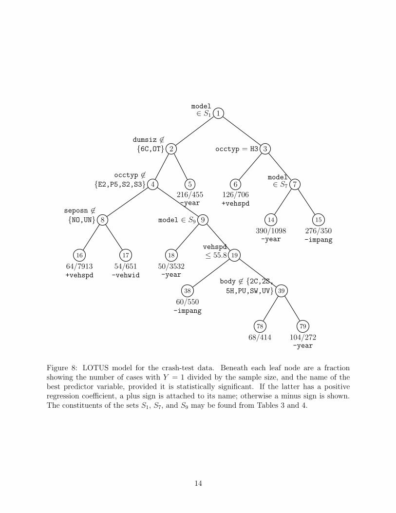
Figure 8 gives the LOTUS tree fitted to the crash-test data. The splits together with thep-functions fitted to the leaf nodes in Fig. 9 yield the following conclusions.

1. The tree splits first on model, showing that there are significant differences, with respectto p, among vehicle models. The variable is also selected for splitting in Nodes 7 and9. Tables 3 and 4 give the precise nature of the splits.

2. Immediately below the root node, the tree splits on dumsiz and occtyp, two character-istics of the test dummy. This shows that some types of dummies are more susceptibleto severe injury than others. In particular, the cases in Node 5 contain mainly dum-mies that correspond to a six-year-old child. The fitted p-function for this node canbe seen in the upper left panel of Fig. 9. Compared with the fitted p-functions of theother nodes, this node appears to have among the highest values of p. This suggeststhat six-year-old children are most at risk of injury. They may be too big for child carseats and too small for adult seat belts.

3. The split on seposn at Node 8 shows that passengers in vehicles with adjustable seatsare ten times (average p of 0.008 versus 0.08) less likely to suffer severe head injurythan those with non-adjustable seats. This could be due to the former type of vehiclebeing more expensive and hence able to withstand collisions better.

4. Similarly, the split on body at Node 39 shows that passengers in two-door cars, pick-ups, station wagons, and SUV’s are twice as likely (average p of 0.38 versus 0.16) tosuffer severe head injury than other vehicles.

5. The linear predictor variables selected in each leaf node tells us the behavior of thep-function within each partition of the dataset. Four nodes have year as their bestlinear predictor. Their fitted p-functions are shown in the upper left panel of Fig. 9.The decreasing trends show that crash safety is improving over time.

6. Three nodes have vehspd as their best linear predictor, although the variable is notstatistically significant in one (Node 78). The fitted p-functions are shown in the upper

13

model∈ S1 1

dumsiz 6∈{6C,OT} 2

occtyp 6∈{E2,P5,S2,S3} 4

seposn 6∈{NO,UN} 8

16

64/7913+vehspd

17

54/651-vehwid

model ∈ S9 9

18

50/3532-year

vehspd≤ 55.8 19

38

60/550-impang

body 6∈ {2C,2S,

5H,PU,SW,UV} 39

78

68/414

79

104/272-year

5

216/455-year

occtyp = H3 3

6

126/706+vehspd

model∈ S7 7

14

390/1098-year

15

276/350-impang

Figure 8: LOTUS model for the crash-test data. Beneath each leaf node are a fractionshowing the number of cases with Y = 1 divided by the sample size, and the name of thebest predictor variable, provided it is statistically significant. If the latter has a positiveregression coefficient, a plus sign is attached to its name; otherwise a minus sign is shown.The constituents of the sets S1, S7, and S9 may be found from Tables 3 and 4.

14

right panel of Fig. 9. As expected, p is non-decreasing in vehspd.

7. Two nodes employ impang as their best linear predictor. The fitted p-functions shownin the bottom left panel of Fig. 9 suggests that side impacts are more serious thanfrontal impacts.

8. One node has vehwid as its best linear predictor. The decreasing fitted p-functionshown in the lower right panel of Fig. 9 shows that vehicles that are smaller are lesssafe.

15

1975 1980 1985 1990 1995 2000 2005

0.0

0.2

0.4

0.6

0.8

1.0

year

Pro

b(S

ever

e he

ad in

jury

)

Nodes 5, 14, 18 and 79

55

55

5x

x

xx

x

| | | | |

o

o

o

o

o

5xo|

Node 5Node 14Node 79Node 18

40 60 80 100

0.0

0.2

0.4

0.6

0.8

1.0

vehspd

Pro

b(S

ever

e he

ad in

jury

)

Nodes 6, 16 and 78

66

6

6

6

| | ||

|o o o o

6o|

Node 6Node 78Node 16

−80 −60 −40 −20 0 20

0.0

0.2

0.4

0.6

0.8

1.0

impang

Pro

b(S

ever

e he

ad in

jury

)

Nodes 15 and 38

xx

x

x

x

o

o

o

oo

xo

Node 15Node 38

1400 1500 1600 1700 1800 1900 2000

0.0

0.2

0.4

0.6

0.8

1.0

vehwid

Pro

b(S

ever

e he

ad in

jury

)

Node 17

Figure 9: Fitted probabilities of severe head injury in the leaf nodes of Fig. 8

16

Table 3: Split at Node 7 of tree in Fig. 8

Make Node 14 Node 15American ConcordAudi 4000, 5000Buick ElectraChampion MotorhomeChevrolet K20 Pickup, Monza, Nova, S10 Blazer, Spectrum,

SportvanAstro, Malibu, Sprint

Chrysler Imperial, Lebaron IntrepidComuta-Car ElectricDodge Aries, Challenger, Colt, Lancer, Magnum Colt Pickup, St. RegisFord Clubwagon MPV, Courier, E100 Van, EXP, Fair-

mont, Fiesta, Granada, MerkurTorino

GMC SportvanHyundai Excel GLSIsuzu Impulse, Spacecab I-Mark, Trooper IIJeep ComancheKia SorentoLectric LeopardMazda GLC B2000Mercury BobcatMitsubishi Montero, Tredia PickupNissan 2000, 210, Kingcab Pickup, MuranoOldsmobile 98Peugeot 504, 505Plymouth Champ, Fury, Horizon Breeze, VolarePontiac T1000Renault 18, Alliance, LeCar, Medallion Fuego, SportswagonSaab 38235Saturn L200Subaru GF, GLF, WagonSuzuki SidekickToyota Celica, StarletVolkswagen Fox, Scirocco Beetle, EuroVanVolvo 244, XC90Yugo GV

17

Table 4: Split at Node 9 of tree in Fig. 8

Make Node 18 Node 19Acura Integra, Legend, Vigor 2.5TL, 3.2TL, 3.5RL, MDX, RSXAmerican Gremlin, Matador, SpiritAudi 100, 200, 80 A4, A6, A8Battronics VanBMW 325I, 525I 318, 328I, X5, Z4 RoadsterBuick Century, LeSabre, Regal, Riviera,

Skyhawk, Skylark, SomersetParkAvenue, Rendezvous, Road-master

Cadillac Deville, Seville Brougham, Catera, Concourse,CTS, Eldorado, Fleetwood

Chevrolet Beretta, Camaro, Cavalier,Celebrity, Chevette, Citation,Corsica, Corvette, Elcamino, Im-pala, Lumina, LUV, MonteCarlo,Pickup, S-10, Vega

Avalanche, Beauville, Blazer, C-1500, C10 Pickup, C1500 Pickup,Caprice, G-10, K1500 Pickup,K2500 Pickup, Silverado, Subur-ban, Tahoe, Tracker, Trailblazer,Venture

Chinook MotorhomeChrysler Cirrus, Conquest, FifthAvenue,

Newport, NewYorkerLHS, Pacifica, PT Cruiser, SebringConvertible

Daewoo Leganza, NubiraDaihatsu CharadeDelorean CoupeDodge 400, 600, Caravan, D-150, Dakota,

Daytona, Diplomat, Dynasty, Mi-rada, Neon, Rampage, Ramwag-onvan, Sportsman

Avenger, Durango, Grand Car-avan, Intrepid, Omni, Ram150,Ram1500, Ram, Ram250 Van,Shadow, Spirit, Stratus

Eagle Medallion, MPV, Premier Summit, VisionEva EvcortFiat 131, StradaFord Bronco, Bronco II, Crown Victoria,

Escort, F150 Pickup, F250 Pickup,F350 Pickup, Festiva, LTD, Mus-tang, Pickup, Probe, Ranger, Tau-rus, Thunderbird, Van, Windstar

Aerostar, Aspire, Contour, E150Van, Escape, Escort ZX2, EVRanger, Expedition, Explorer, Fo-cus, Freestar, Other, Tempo

Geo Metro, Prizm Storm, TrackerGMC Astro Truck, Vandura EV1Holden Commodore AcclaimHonda Accord Civic, CRV, Element, Insight,

Odyssey, Pilot, Prelude, S2000Hyundai Elantra, Scoupe, Sonata Accent, Pony Excel, Santa Fe,

TiburonIH Scout MPV

continued on next page

18

Make Node 18 Node 19Infinity G20, M30 J30Isuzu Amigo, Pup Axiom, Pickup, Rodeo, StylusJaguar X-TypeJeep CJ, Wrangler Cherokee, Cherokee Laredo, Grand

Cherokee, LibertyJet Courier, Electrica, Electrica 007Kia Sephia Rio, Sedona, Spectra, SportageLandrover Discovery, Discovery IILectra 400, CentauriLexus ES250 ES300, GS300, GS400, IS300,

RX300, RX330Lincoln Continental, Town Car LS, Mark, NavigatorMazda 323, 323-Protege, 929, Miata, Mil-

lenia, MPV, MX3, MX6, Pickup,RX

626, Mazda6, MX5

Mercedes 190, 240, 300 C220, C230, C240, E320, ML320Mercury Capri, Cougar, Lynx, Marquis,

Monarch, Sable, Topaz, Tracer, Vil-lager, Zephyr

Mystique

Mini CooperMitsubishi Diamante, Eclipse, Galant, Mighty-

max, Mirage, Precis, Starion, Van3000GT, Cordia, Endeavor, Lancer,Montero Sport, Outlander

Nissan 240SX, 810, Altima, Axxess,Pathfinder, Pulsar, Quest, Sentra,Van

200SX, 300ZX, 350Z, Frontier,Maxima, Pickup, Stanza, Xterra

Odyssey MotorhomeOldsmobile Calais, Cutlass, Delta 88, Omega,

ToronadoAchieva, Aurora, Intrigue, Royale

Other OtherPeugeot 604Plymouth Acclaim, Caravelle, Laser, Reliant,

Sundance, VoyagerColt Vista, Conquest, Neon

Pontiac Bonneville, Fiero, Firebird, GrandAM, Lemans, Parisienne, Sunbird

Aztek, Grand Prix, Sunfire, TransSport

Renaissance TropicaRenault EncoreSaab 900 38233, 9000Saturn SL1 Ion, LS, LS2, SC1, SL2, VueSebring ZEVSolectria E-10, ForceSubaru DL, Impreza, Justy, XT Forestee, GL, LegacySuzuki Samurai Swift, Vitara

continued on next page

19

Make Node 18 Node 19Toyota Camry, Corolla, Corona, Cosmo,

Landcruiser, MR2, Paseo, T100,Tercel, Van

4Runner, Avalon, Camry Solara,Cressida, Echo, Highlander, Ma-trix, Pickup, Previa, Prius, Rav4,Sequoia, Sienna, Tacoma, Tundra

UM ElectrekVolkswagen Cabrio, Corrado, Golf, Passat,

Quantum, RabbitJetta, Polo, Vanagon

Volvo 240, 740GL, 850, 940, DL, GLE 960, S60, S70, S80Winnebago Trekker

6 Conclusion

Logistic regression is a statistical technique for modeling the probability p of an event interms of the values of one or more predictor variables. The traditional approach expressesthe logit of p as a linear function of these variables. Although the model can be effectivefor predicting p, it is notoriously hard to interpret. In particular, multicollinearity can causethe regression coefficients to be misinterpreted.

A logistic regression tree model offers a practical alternative. The model has two com-ponents, namely, a binary tree structure showing the data partitions and a set of simplelinear logistic models, fitted one to each partition. It is this division of model complexitythat makes the model intuitive to interpret. By dividing the dataset into several pieces, thesample space is effectively split into different strata such that the p-function is adequatelyexplained by a single predictor variable in each stratum. This property is powerful because(i) the partitions can be understood through the binary tree and (ii) each p-function canbe visualized through its own graph. Further, stratification renders each of the individualp-functions resistant to the ravages of multicollinearity among the predictor variables andto Simpson’s paradox. Despite these advantages, it is crucial for the partitioning algorithmto be free of selection bias. Otherwise, it is very easy to draw misleading inferences fromthe tree structure. At the time of this writing, LOTUS is the only logistic regression treealgorithm designed to control such bias.

Finally, as a disclaimer, it is important to remember that in real applications, there is no“best” model for a given dataset. This situation is not unique to logistic regression problems;it is prevalent in least-squares and other forms of regression as well. Often there are two ormore models that give predictions of comparable average accuracy. Thus a LOTUS modelshould be regarded as merely one of possibly several different ways of explaining the data.Its main virtue is that, unlike many other methods, it provides an interpretable explanation.

Acknowledgements

Research partially supported by grants from the National Science Foundation and the U.S.Army Research Office. The author thanks Dr. Kin-Yee Chan for co-developing the LOTUSalgorithm and for maintaining the software. The software may be obtained through a link

20

on the author’s website www.stat.wisc.edu/~loh.

REFERENCES

[1] Agresti, A. (1996), An Introduction to Categorical Data Analysis, New York, Wiley.

[2] Breiman, L., Friedman, J. H., Olshen, R. A. and Stone, C. J. (1984), Classification and

Regression Trees, Belmont, California: Wadsworth.

[3] Chan, K.-Y. and Loh, W.-Y. (2004), “LOTUS: An algorithm for building accurateand comprehensible logistic regression trees,” Journal of Computational and Graphical

Statistics, in press.

[4] Cook, R. D. and Weisberg, S. (2004), “Partial one-dimensional regression models,”American Statistician, 58, 110–116.

[5] Chambers, J. M. and Hastie, T. J. (1992), Statistical Models in S, Pacific Grove:Wadsworth.

[6] Doyle, P. (1973), “The use of Automatic Interaction Detector and similar search pro-cedures,” Operational Research Quarterly, 24, 465–467.

[7] Loh, W.-Y. (2002), “Regression trees with unbiased variable selection and interactiondetection,” Statistica Sinica, 12, 361–386.

[8] Morgan, J. N. and Sonquist, J. A. (1963), “Problems in the analysis of survey data,and a proposal,” Journal of the American Statistical Association, 58, 415–434.

[9] Quinlan, J. R. (1992), “Learning with continuous classes,” in Proceedings of AI’92

Australian National Conference on Artificial Intelligence, 343–348, Singapore: WorldScientific.

21