Logical and Generalized Disjunctive Programming for Supplier and Contract Selection under Provision Uncertainty

Logical and Generalized Disjunctive Programming for Supplier and ContractSelection under Provision Uncertainty

Maria Analia Rodriguez and Aldo Vecchietti*

INGAR - Instituto de Desarrollo y Diseno (CONICET-UTN), AVellaneda 3657, Santa Fe 3000, Argentina

Supply-chain optimization is a key issue in gainnig competitiveness in today’s economies where buyers andsuppliers develop long-term relationships. Final agreements are formalized by signing contracts involvingthe purchasing of large amounts of materials, taking advantage of economies of scale. Although establishingagreements with suppliers is definitely an important step in reducing uncertainty, uncertainty never completelydisappears. For that reason, the problem addressed in this article is the delivery and purchase optimization ina supply chain under provision uncertainty. Several decisions are presented in this problem that can naturallybe posed in terms of of discrete decision models and generalized disjunctive programming. Uncertainty ismodeled through a new approach that avoids the drawbacks of traditional methods. The goal pursued in thisarticle is to contribute to better raw-material usage and tactical decisions to face an uncertain provision processin the supply chain.

1. Introduction

In recent years, supply-chain optimization has gained increas-ing interest in both research and business environments. Thissituation has been motivated by a tough competitive marketwhere the efficiency of the entire supply chain is essential forcompanies’ survival. In fact, there has been constant interest inthe integration process between partners. In this challenge,decisions related to suppliers are especially relevant; businessrelations with suppliers influence customer satisfaction andrepresent most of a company’s costs. For that reason, businesspartners are involved in a constant negotiation process, playinga dynamic role in the supply chain. As a consequence,permanent changes have occurred in the production anddistribution network.1 In this work, a dynamic representationof the supply chain is introduced in which, given a maximumnumber of suppliers, the provision channel is reconfigured ineach time period by selecting a subset of them.

As supported by Ojala and Hallikas,2 the provision processrepresents the core of supply-chain management. Indeed, manyworks have focused on this problem, pointing up different facetsof it. Some have stressed the importance of supplier selectionand designed graphical, heuristic, and optimization methods forthat purpose. Others have evaluated the most important suppliercharacteristics through qualitative methods. For instance, Chenet al.3 develop a supplier capability and price analysis chart forevaluating supplier performance. Mohebbi4 presented an ana-lytical model for computing the stationary distribution of theinventory system considering that a supplier can take twopossible states: available and unavailable. It was shown thatone of the main factors that greatly influence the efficiency ofevery production and inventory control operation is the reliabilityof its supply process. Random supply interruptions weremodeled to diminish their negative impacts on the customerservice level and the operating costs of the supply chain. Inaddition, Ruiz-Torres and Mahmoodi5 argued that supplier’sdecision making is a critical component given the recentincreased reliance of many organizations on their suppliers. Intheir article, they presented a decision model that optimizes thedemand allocation across a set of suppliers. Highlighting the

importance of supply network interruptions, they used adecision-tree approach to determine the optimal number ofsuppliers in the presence of risks. In the present work, adisjunctive optimization approach is developed to determine thenumber of suppliers, quantities to order, and material selectionto minimize the actualized expected costs in the time horizonconsidered.

Much work has been directed toward proving that contractualpoliciesareeffectivetoolsagainstrisksinsupply-chainmanagement.6,7

Berger et al.8 argued that the interdependency between partnersmotivates an integration process where buyers and suppliersdevelop long-term relationships characterized by stability, coopera-tion, and mutual benefit. Park et al.9 studied the purchasing processconsidering a disjunctive model formulation for the optimalselection of suppliers and purchase contracts. They showed thatsigning contracts is a business practice that contributes to reducinguncertainty and taking advantage of economies of scale. Contractselection has received increasing attention in the literature as waspointed out by Naraharisetti et al.10 Laınez et al.11 also supportedthe idea that the strategic use of option contracts with supplierscould be a hedge against supply-chain risks. Aligned with theseideas, the aim of this article is to encourage supply-chain integrationby signing purchase contract with suppliers, resulting in lower costsand decreasing negative effects of speculation and uncertainty.

The dynamic characteristics of supply chains underline theimportance of taking into account uncertainty as a major challenge.Although establishing agreements with suppliers is definitely animportant step in reducing uncertainty, uncertainty never completelydisappears. In fact, risks still exist in every link of supply chains,ultimately affecting costs and demand satisfaction. Subrahmanyamet al.12 identified various levels of uncertainty such as sales, materialpurchase, equipment purchase, equipment reliability, and manu-facturing. Hwarng and Xie13 presented a simulation approach ofthe supply-chain dynamics influenced by various factors, includingdemand pattern, ordering policy, demand-information sharing, andlead time. Although many risk sources have been recognized, ingeneral, much research deals with demand uncertainty. However,because supply interruptions could also strongly affect demandsatisfaction and enterprise revenue, uncertainty in the provisionprocess is modeled in this work.

* To whom correspondence should be addressed. E-mail: [email protected]. Tel.:54 342 4534155. Fax 54 342 4553439.

Ind. Eng. Chem. Res. 2009, 48, 5506–55215506

10.1021/ie801614x CCC: $40.75 2009 American Chemical SocietyPublished on Web 05/04/2009

Zimmermann14 provides a very detailed explanation andtaxonomy of the causes of uncertainty. According to this author,instead of deciding whether probabilistic, fuzzy set, or evidencetheory is the best method for modeling uncertainty, the choiceof the appropriate approach depends on the context in which itis applied. In general, there are two main strategies for treatinguncertainty: probabilistic and scenario-based methods.1,15-17

Probabilistic models formulate certain parameters as randomvariables with a known distribution. Alternatively, scenario-based formulations, also called stochastic models, includeuncertainty representing a set of probable scenarios. In this work,uncertainty is modeled using a discrete probabilistic distributionof the supply process, taking advantage of the linear scenario-based formulation and considering managers’ knowledge ofsupplier behavior.

Finally, in problems addressing supply-chain planning, theemphasis is generally placed on physical parameters such asstock level, demand satisfaction, and so on. However, it isrelevant to consider financial issues because of their impact onenterprise performance.11,18 Aside from the increase in inter-national prices, financial considerations are particularly impor-tant in Latin American countries where inflationary processesevolve, decreasing the value of the unit of currency even more.Cost functions are actualized with an appropriate discount ratein the objective function, and because of the economic contextmentioned before, cost data include the forecasted inflation rate.

This article presents a general formulation for purchasecontract selection in the supply chain under provision uncer-tainty. Uncertainty is handled through a new approach thatavoids the drawbacks of the traditional methods. Some discretedecisions presented in this problem are modeled by generalizeddisjunctive programming, thus strengthening the expressivenessof the formulation. The main purpose of this work is toencourage a better decision process whereby companies canselect their materials, purchase conditions, and suppliers on thebasis of lower costs and higher supplier reliability.

This work is outlined as follows: In the next section, theproblem is introduced and described; then, the model formula-tion is developed. In section 4, two case studies and their resultsare presented considering different representations of probabi-listic distributions of provision failure. A sensitivity analysis isshown in section 5 where uncertainty parameters are modifiedto capture some important features of the modeled context.Finally, conclusions and some discussion are presented in sec-tion 6.

2. Problem Description

The problem addressed in the present article is materialdelivery and purchase optimization in the supply chain. Amedium-term production plan divided into several time periodsis considered. A multilevel decision structure is presented inthe problem. Diverse materials are purchased from variousmanufacturers through the signing of different contract types.

The purchase problem was already presented by Rodrıguezand Vecchietti19 for the paper supply chain. With the aim of abroader application context, purchase, supplier, and contractselection is considered here for any supply chain handling aset of raw material families. The use of material families is acommon practice in many industries such as the production ofpaper, furniture, textile, and food, among others. Each suppliermight offer sets of material families with different types andqualities. Materials with similar properties are grouped intofamilies, giving flexibility to purchase decisions and allowinga set of possible material formulations for the same final product.In addition to this combinatory problem, raw material purchasedecisions have a great influence on company profits, emphasiz-ing the importance of purchase process optimization.

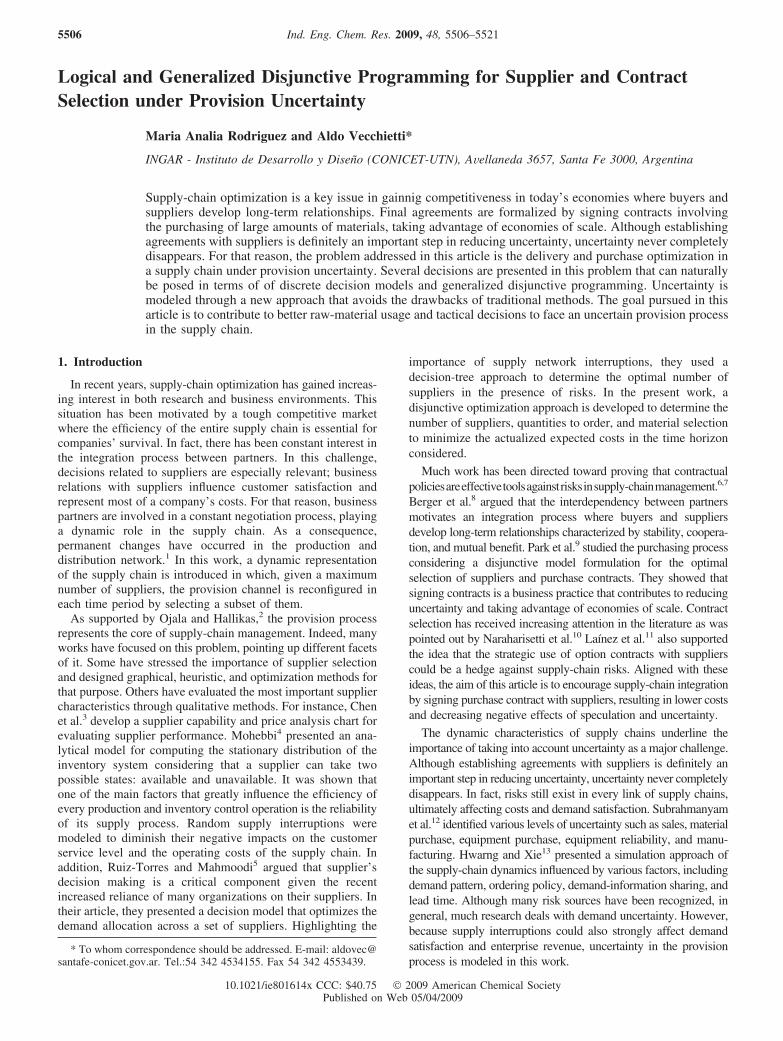
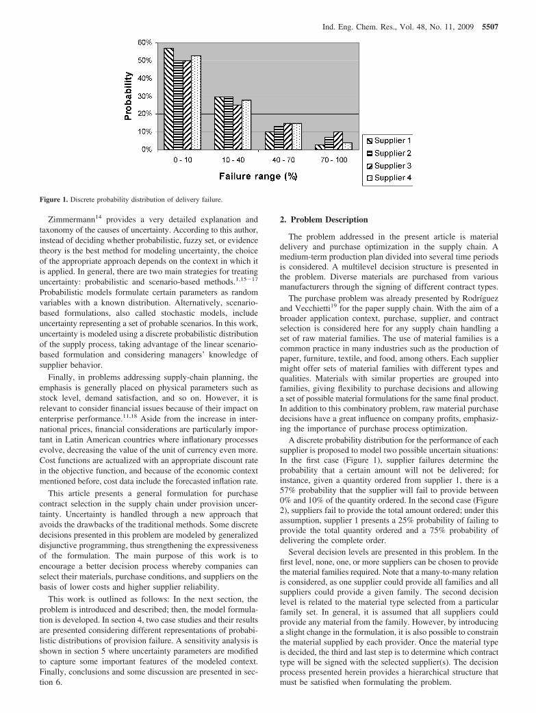
A discrete probability distribution for the performance of eachsupplier is proposed to model two possible uncertain situations:In the first case (Figure 1), supplier failures determine theprobability that a certain amount will not be delivered; forinstance, given a quantity ordered from supplier 1, there is a57% probability that the supplier will fail to provide between0% and 10% of the quantity ordered. In the second case (Figure2), suppliers fail to provide the total amount ordered; under thisassumption, supplier 1 presents a 25% probability of failing toprovide the total quantity ordered and a 75% probability ofdelivering the complete order.

Several decision levels are presented in this problem. In thefirst level, none, one, or more suppliers can be chosen to providethe material families required. Note that a many-to-many relationis considered, as one supplier could provide all families and allsuppliers could provide a given family. The second decisionlevel is related to the material type selected from a particularfamily set. In general, it is assumed that all suppliers couldprovide any material from the family. However, by introducinga slight change in the formulation, it is also possible to constrainthe material supplied by each provider. Once the material typeis decided, the third and last step is to determine which contracttype will be signed with the selected supplier(s). The decisionprocess presented herein provides a hierarchical structure thatmust be satisfied when formulating the problem.

Figure 1. Discrete probability distribution of delivery failure.

Ind. Eng. Chem. Res., Vol. 48, No. 11, 2009 5507

According to Laınez et al.,11 there are several contract typesthat can be signed with suppliers. The quantity-flexibilitycontract is defined in this work as a contract in which the buyercommits to purchase a certain amount of material at a fixedprice. The second contract type considered is the revenue-sharingcontract, in which the buyer pays an upfront fee to the supplierfor the right to sell the materials and commits to sharing revenueobtained from these sales. Finally, the buyback contract ispresented that basically is a put option whereby the buyer isable to sell excess material back to the supplier. Given thesedescriptions, the contracts considered in this work correspondto the quantity-flexibility contract type. Nevertheless, somespecial issues are included in the contract policies to capturethe true nature of the commitments tackled. In the first, aminimum quantity is established, and the price presents aminimum discount over the total quantity purchased. The secondcan be selected only in the case that the same material wasordered from the supplier in the previous period, encouraginglonger relationships between companies. Moreover, it considersa minimum quantity larger than in the first contract with aspecial discount. In the last contract type, the price includesthe corresponding interest rate due to longer payment terms andthe largest minimum quantity to order. This last contract couldbe an attractive alternative when a lack of financial liquidityand/or inflationary processes are presented.

The objective function to optimize is not a trivial decision. Indeveloping countries, it is particularly relevant to take into accountthe inflationary process and its consequences on purchase contractdecisions because of the time horizon involved. Therefore, it isimportant to evaluate the actualized costs, defining the objectivefunction as the minimization of the present value of purchase costs,financial costs due to payment terms, inventory costs, and expectedcosts due to unsatisfied demand.

3. Model Formulation

Because of the multilevel decision structure, Boolean vari-ables are used for selecting suppliers, material family, materialssupplied, and contract types in each time period, subject todemand, stock, and capacity constraints. To capture a repre-sentative formulation, discrete decisions and constraints areposed using nested disjunctions, by generalized disjunctiveprogramming (GDP),20 and logic propositions.

3.1. Algebraic Constraints. In the first place, certain alge-braic restrictions related to demand and stock must be satisfiedin the time horizon planned. These constraints are given by eqs1-6 below.

Equation 1 is the material family demand constraint. It deter-mines that the quantity ordered for all materials k of family f inperiod t from all suppliers j, qjkt, plus the quantity of family f instock in period t, sft, must be greater than or equal to the familydemand in period t, FDft. Without losing generality, it is consideredthat the time at which the order is made is the same as the deliverytime for every supplier. It is also assumed that stock, demand, andmaterial quantities are already transformed into comparative units.

Equation 2 establishes an excess of material upper bound, µ,that provides flexibility to the purchase plan. The quantityordered plus the quantity in stock, sft, for family f in period tmust be lower than the family demand plus the upper boundconstrained by the parameter µ > 0:

The initial stock expected of family f in period t, sft, is calculatedby eq 3 as the initial stock of family f in period t - 1 plus theexpected quantity of family f provided by all suppliers selected inperiod t - 1, eqf(t-1), minus the family sales in the previous period,df(t-1). Note that the variable eqf(t-1) is calculated using eqs 30-45(see section 3.3), depending on the suppliers selected, the amountof materials k from family f ordered from each of them, and theexpected failure distribution associated with the suppliers.

Equation 4 determines that sales of family f in period t mustbe lower than or equal to the demand forecast for family f inperiod t:

Equation 5 constrains the expected quantity in stock accordingto the stock capacity parameter, SC:

Equation 6 defines the initial stock of family f in period t1 asbeing equal to the parameter ISf, which is input data in themodel:

Figure 2. Discrete probability distribution of total failure.

∑k∈FKfk

∑j

qjkt + sft g FDft ∀t ∈ T, ∀f ∈ F (1)

∑k∈FKfk

∑j

qjkt + sft e FDft(1 + µ) ∀t ∈ T, ∀f ∈ F (2)

sft ) sf(t-1) + eqf(t-1) - df(t-1) ∀f ∈ F, ∀t g t2 ∈ T (3)

dft e FDft ∀f ∈ F, ∀t ∈ T (4)

∑f

sft e SC ∀t ∈ T (5)

5508 Ind. Eng. Chem. Res., Vol. 48, No. 11, 2009

3.2. Modeling Contract Discrete Decisions and LogicRestrictions. Disjunction 7 selects the contract type for eachmaterial k and supplier j in period t. Each term corresponds tothe contract types modeled. The first constraint in each caserestricts the minimum amount of material that must be orderedto the supplier. The second constraint calculates the purchasecosts, wjckt, according to the amount ordered, qjkt; the price, PCjkt;and the corresponding contract discount or interest rate, δjc. Inthe third constraint, the positive variable mjckt′ determines theamount paid for material k to supplier j in period t′ accordingto the payment policy of contract c. In this case, the set TPctt′establishes that the purchase ordered in period t must be paidin period t′ according to contract c. Note that the gap betweent and t′ gives the financial benefit offered. In the first twocontracts, period t is equal to t′; however, the third contract hasa longer payment term. Although variable mjckt′ could becalculated directly in the second constraint, thereby avoidingthe use of wjckt, this formulation is considered worthy todistinguish the cost concept given by the second equation andthe effective money outflows calculated in the last equation.

The first contract type establishes a minimum quantity toorder, given by Qminc1j. It also has a discount applied to thetotal amount ordered. The second contract type has a largerminimum quantity to order, Qminc2j, and a bigger discount.Encouraging longer business relations, proposition 8 determinesthat this contract type can be selected only in the case thatmaterial k was already ordered from supplier j in period t - 1.In the last contract type, the minimum quantity to order, Qminc3j,is the highest, and instead of a discount, the second equationconsiders an interest rate due to the payment term. In the restof the contract types, the payment must be made within thesame period in which the order was made.

In propposition 8, according to the corresponding contract rules,the second contarct type, c2, can be selected for material k ofsupplier j only if one of the contract types has been selected in theprevious period for material k of supplier j. If not, contract type c2

cannot be selected for this case. Because of this same rule, inproposition 9, contract type c2 cannot be chosen for the initial periodt1 because it is the first period in the planning horizon.

Considering the corresponding values of the parameters ineach contract type, disjunction 7 can be simplified to

where δjc1g 0, δjc2

g 0, and δjc3e 0.

As was mentioned in the Problem Description, two decisionlevels are needed before the contract types can be selected,which is posed in nested disjunction 11, including disjunction10 in the deepest term.

In the first level of eq 11, Boolean variable y1jft selects whichfamilies f are bought from each supplier j in each period t. Inthe negative case, no material is ordered related to family f fromsupplier j in period t. In the affirmative case, the total quantityordered must be lower than the maximum capacity of supplierj. In the next level, variable y2jfkt indicates that one material kmust be selected from family f, according to FKfk, in period t.The set FKfk defines which materials correspond to each familyf. In this term, the quantity ordered of material k in period tcannot be greater than the supplier capacity for that materialand period. In the third term, disjunction 10 is introduced, wherevariable y3jckt indicates that contract type c must be chosen toorder material k from supplier j in period t.

To present a broader formulation, the use of material familiesis considered in this approach. However, it is important to noticethat, if materials are considered instead of families, thisformulation is still valid, just with the first level in the decisionhierarchy ignored.

An additional logical constraint is also required in the problemformulation by

where proposition 12 determines that material k cannot beselected for family f if this material does not belong to familyf of set FKfk.

Although the expressiveness of the hierarchical decisions bymeans of nested disjunctions, they cannot be implementeddirectly. These disjunctions must be transformed into GDPform.21,22 For that purpose, the disjunctions in 11 must berewritten as single disjunctions, and some additional constraintsmust also be included in the model.

Disjunction 11 must be replaced by expressions 13-15 and10:

sft1) ISf ∀f ∈ F (6)

[ y3jc1kt

qjkt g Qminc1j

wjc1kt ) qjktPCjkt(1 - δjc1)

wjc1kt ) mjc1kt′] ∨ [ y3jc2kt

qjkt g Qminc2j

wjc2kt ) qjktPCjkt(1 - δjc2)

wjc2kt ) mjc2kt′] ∨

[ y3jc3kt

qjkt g Qminc3j

wjc3kt ) qjktPCjkt(1 + δjc3)

wjc3kt ) mjc3kt′] ∀j ∈ J, ∀k ∈ K, ∀(c, t, t′) ∈ TPctt′

(7)

[y3jc2kt ∧ (∨cy3jckt-1)] ∨ ¬ y3jc2kt ∀j ∈ J, ∀k ∈ K, ∀t ∈ T

(8)

¬y3jc2kt1∀j ∈ J, ∀k ∈ K (9)

∨c∈C[ y3jckt

qjkt g Qmincj

wjckt ) qjktPCjkt(1 - δjc)wjckt ) mjckt′

]∀j ∈ J, ∀k ∈ K, ∀(c, t, t′) ∈ TPctt′ (10)

[ y1jft

∑k∈FKjk

qjkt e ∑k∈FKjk

Qmaxjkt

∨k∈FKfk[ y2jfkt

qjkt e Qmaxjkt

∨c∈C

(c,t,t′)∈TPctt′ [ y3jckt

qjkt g Qmincj

wjckt ) qjktPCjkt(1 - δjc)wjckt ) mjckt′

] ] ]∨[ ¬y1jft

∑k∈FKfk

qjkt ) 0 ] ∀j ∈ J, ∀f ∈ F, ∀t ∈ T (11)

¬( ∨k∉FKfk

y2jfkt) ∀j ∈ J, ∀f ∈ F, ∀t ∈ T (12)

[ y1jft

∑k∈FKfk

qjkt e ∑k∈FKfk

Qmaxjkt ] ∨ [ ¬y1jft

∑k∈FKfk

qjkt ) 0 ]∀j ∈ J, ∀f ∈ F, ∀t ∈ T (13)


In proposition 15, if family f is selected for supplier j in periodt, then only one material k related to family f in FKfk must beselected for supplier j. If, instead, family f is not selected forsupplier j in period t, then material k related to family f in FKfk

must not be selected for supplier j.Proposition 16 determines that, if a material k of any family

is selected for supplier j in period t, then one contract type cmust also be selected for that material, supplier, and period.On the contrary, if material k is not selected from any familyfor supplier j in period t, then no contract c must be chosen forthat material, supplier, and period:

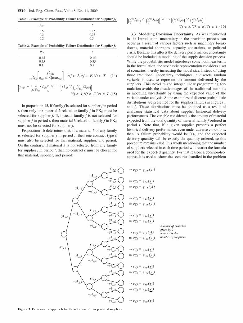
3.3. Modeling Provision Uncertainty. As was mentionedin the Introduction, uncertainty in the provision process canoccur as a result of various factors such as machinery break-downs, material shortages, capacity constraints, or politicalcrisis. Because this affects the delivery performance, uncertaintyshould be included in modeling of the supply decision process.While the probabilistic model introduces some nonlinear termsin the formulation, the stochastic representation considers a setof scenarios, thereby increasing the model size. Instead of usingthose traditional uncertainty techniques, a discrete randomvariable is used to represent the amount delivered by thesuppliers. This novel mixed integer linear programming for-mulation avoids the disadvantages of the traditional methodsin modeling uncertainty by using the expected value of thevariable under analysis. Some examples of discrete probabilisticdistributions are presented for the supplier failures in Figures 1and 2. These distributions must be obtained as a result ofanalyzing statistical data about supplier historical deliveryperformances. The variable considered is the amount of materialexpected from the total quantity of material family f ordered inperiod t. Note that, if a given supplier presents a perfecthistorical delivery performance, even under adverse conditions,then its failure probability would be 0%, and the expecteddelivery quantity will be exactly the quantity ordered, so thisprocedure remains valid. It is worth mentioning that the numberof suppliers selected in each time period will restrict the formulaused for the expected quantity. For that reason, a decision-treeapproach is used to show the scenarios handled in the problem

Table 1. Example of Probability Failure Distribution for Supplier j1

pj1r r

0.5 0.150.3 0.350.2 0.5

Table 2. Example of Probability Failure Distribution for Supplier j2

pj2r r

0.45 0.150.35 0.350.1 0.5

Figure 3. Decision-tree approach for the selection of four potential suppliers.

∨k∈FKkf

[ y2jfkt

qjkt e Qmaxjkt] ∀j ∈ J, ∀f ∈ F, ∀t ∈ T (14)

[y1jft ∧ ( ∨k∈FKfk

y2jfkt)] ∨ ¬ [y1jft ∨ ( ∨k∈FKfk

y2jfkt)]∀j ∈ J, ∀f ∈ F, ∀t ∈ T (15)

[(∨f y2jfkt) ∧ (∨c y3jckt)] ∨ ¬ [(∨f y2jfkt) ∨ (∨c y3jckt)]∀j ∈ J, ∀k ∈ K, ∀t ∈ T (16)


that are then jointly considered using the expected value formula.For illustrative purposes, the tree presented in Figure 3 representsthe possible formulations when a total of four suppliers couldbe selected in each time period.

The diagram of Figure 3 shows that, if all suppliers are selected,then the expected quantity of family f in period t, eqft, is given byg15ft(y1), where g15ft(y1) is a function of the four suppliers selected,their failure probability distributions, and the quantity of family fordered. Similarly, each branch is related to a different value ofeqft according to the variables and parameters mentioned. In thelast branch, for instance, no supplier is selected for family f in periodt; as a consequence, eqft is equal to zero.

Note that, if, for example, only supplier j1 is selected withthe failure probability distributions given by Table 1, then theexpected quantity is constrained by the probability pj1r of supplierj1 in each possible failure r. In this case, supplier j1 presents a50% probability of failure for 15% of the amount ordered, a30% probability to fail for 35% of the quantity ordered, and a20% probability to fail for 50% of the amount ordered.

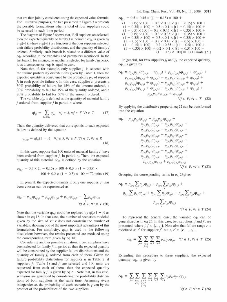
The variable qfjft is defined as the quantity of material familyf ordered from supplier j in period t, where

Then, the quantity delivered that corresponds to each expectedfailure is defined by the equation

In this case, suppose that 100 units of material family f1 havebeen ordered from supplier j1 in period t1. Then, the expectedquantity of this material, eqft, is defined by the equation

In general, the expected quantity if only one supplier, j1, hasbeen chosen can be represented as

Note that the variable qrjrft could be replaced by qfjft(1 - r) asshown in eq 18. In that case, the number of scenarios modeledgiven by the size of set r does not constrain the number ofvariables, showing one of the most important advantages of thisformulation. For simplicity, qrjrft is used in the followingdiscussion; however, the results presented are modeled usingthe corresponding term given by eq 18.

Considering another possible situation, if two suppliers havebeen selected for family f1 in period t1, then the expected quantitywill be constrained by the supplier failure distributions and thequantity of family f1 ordered from each of them. Given thefailure probability distribution for supplier j2 in Table 2, ifsuppliers j1 (Table 1) and j2 are selected and 100 units arerequested from each of them, then the expected quantityexpected for family f1 is given by eq 21. Note that, in this case,scenarios are generated by considering the probability distribu-tions of both suppliers at the same time. Assuming eventindependence, the probability of each scenario is given by theproduct of the probabilities of the two suppliers.

In general, for two suppliers j1 and j2, the expected quantity,eqft, is given by

By applying the distributive property, eq 22 can be transformedinto the equation

Grouping the corresponding terms in eq 23gives

To represent the general case, the variable eqft can begeneralized as in eq 25. In this case, two suppliers, j and j′, arepresented, where j, j′ ∈ {j1, j2}. Note also that failure range r isredefined as r′ for supplier j′, but r, r′ ∈ {r1,..., rn}.

Extending this procedure to three suppliers, the expectedquantity, eqft, is given by

qfjft ) ∑k∈FKft

qjkt ∀j ∈ J, ∀f ∈ F, ∀t ∈ T (17)

qrjrft ) qfjft(1 - r) ∀j ∈ J, ∀f ∈ F, ∀t ∈ T, ∀r ∈ R(18)

eqf1t1) 0.5 × (1 - 0.15) × 100 + 0.3 × (1 - 0.35) ×

100 + 0.2 × (1 - 0.5) × 100 ) 72 units (19)

eqft ) pj1r1qrj1r1ft + pj1r2

qrj1r2ft + pj1r3qrj1r3ft ) ∑

r

pj1rqrj1rft

∀f ∈ F, ∀t ∈ T (20)

eqf1t1) 0.5 × 0.45 × [(1 - 0.15) × 100 +

(1 - 0.15) × 100] + 0.5 × 0.35 × [(1 - 0.15) × 100 +(1 - 0.35) × 100] + 0.5 × 0.1 × [(1 - 0.15) × 100 +(1 - 0.5) × 100] + 0.3 × 0.45 × [(1 - 0.35) × 100 +

(1 - 0.15) × 100] + 0.3 × 0.35 × [(1 - 0.35) × 100 +(1 - 0.35) × 100] + 0.3 × 0.1 × [(1 - 0.35) × 100 +(1 - 0.5) × 100] + 0.2 × 0.45 × [(1 - 0.5) × 100 +

(1 - 0.15) × 100] + 0.2 × 0.35 × [(1 - 0.5) × 100 +(1 - 0.35) × 100] + 0.2 × 0.1 × [(1 - 0.5) × 100 +

(1 - 0.5) × 100] ) 130.8 units (21)

eqft ) pj1r1pj2r1

(qrj1r1ft + qrj2r1ft) + pj1r1pj2r2

(qrj1r1ft + qrj2r2ft) +pj1r1

pj2r3(qrj1r1ft + qrj2r3ft) + pj1r2

pj2r1(qrj1r2ft + qrj2r1ft) +

pj1r2pj2r2

(qrj1r2ft + qrj2r2ft) + pj1r2pj2r3

(qrj1r2ft + qrj2r3ft) +pj1r3

pj2r1(qrj1r3ft + qrj2r1ft) + pj1r3

pj2r2(qrj1r3ft + qrj2r2ft) +

pj1r3pj2r3

(qrj1r3ft + qrj2r3ft)

∀f ∈ F, ∀t ∈ T (22)

eqft ) pj1r1pj2r1

qrj1r1ft + pj1r1pj2r1

qrj2r1ft +pj1r1

pj2r2qrj1r1ft + pj1r1

pj2r2qrj2r2ft +

pj1r1pj2r3


qrj2r3ft +pj1r2


pj2r1qrj2r1ft +

pj1r2pj2r2


qrj2r2ft +pj1r2


pj2r3qrj2r3ft +

pj1r3pj2r1


qrj2r1ft +pj1r3


pj2r2qrj2r2ft +

pj1r3pj2r3


qrj2r3ft

∀f ∈ F, ∀t ∈ T (23)

eqft ) pj2r1 ∑r

pj1rqrj1rft + pj2r2 ∑r

pj1rqrj1rft +

pj2r3 ∑r



pj2rqrj2rft +

pj1r3 ∑r

pj2rqrj2rft

∀f ∈ F, ∀t ∈ T (24)

eqft ) ∑j∈J

∑j′∈Jj′*j

∑r∈R

∑r′∈R

pjrpj′r′qrjrft ∀f ∈ F, ∀t ∈ T (25)

eqft ) ∑j∈J

∑j′∈Jj′*j

∑j′′∈Jj′′<j′j′′*j

∑r∈R

∑r′∈R

∑r′′∈R

pjrpj′r′pj′′r′′qrjrft

∀f ∈ F, ∀t ∈ T (26)


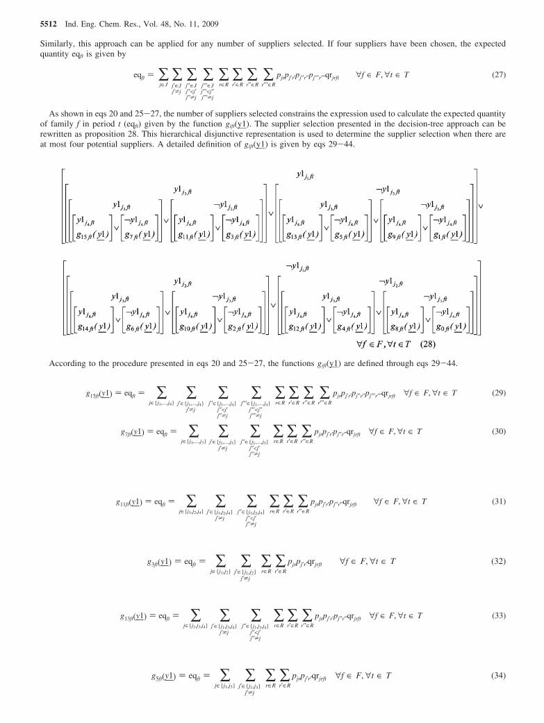
Similarly, this approach can be applied for any number of suppliers selected. If four suppliers have been chosen, the expectedquantity eqft is given by

As shown in eqs 20 and 25-27, the number of suppliers selected constrains the expression used to calculate the expected quantityof family f in period t (eqft) given by the function gift(y1). The supplier selection presented in the decision-tree approach can berewritten as proposition 28. This hierarchical disjunctive representation is used to determine the supplier selection when there areat most four potential suppliers. A detailed definition of gift(y1) is given by eqs 29-44.

According to the procedure presented in eqs 20 and 25-27, the functions gift(y1) are defined through eqs 29-44.

g15ft(y1) ) eqft ) ∑j∈{j1,...,j4}

∑j′∈{j1,...,j4}

j′*j

∑j′′∈{j1,...,j4}

j′′<j′j′′*j

∑j′′′∈{j1,...,j4}

j′′′<j′′j′′′*j

∑r∈R

∑r′∈R

∑r′′∈R

∑r′′′∈R

pjrpj′r′pj′′r′′pj′′′r′′′qrjrft ∀f ∈ F, ∀t ∈ T (29)

eqft ) ∑j∈J

∑j′∈Jj′*j

∑j′′∈Jj′′<j′j′′*j

∑j′′′∈Jj′′′<j′′j′′′*j

∑r∈R

∑r′∈R

∑r′′∈R

∑r′′′∈R

pjrpj′r′pj′′r′′pj′′′r′′′qrjrft ∀f ∈ F, ∀t ∈ T (27)

g7ft(y1) ) eqft ) ∑j∈{j1,...,j3}

∑j′∈{j1,...,j3}

j′*j

∑j′′∈{j1,...,j3}

j′′<j′j′′*j

∑r∈R

∑r′∈R

∑r′′∈R

pjrpj′r′pj′′r′′qrjrft ∀f ∈ F, ∀t ∈ T (30)

g11ft(y1) ) eqft ) ∑j∈{j1,j2,j4}

∑j′∈{j1,j2,j4}

j′*j

∑j′′∈{j1,j2,j4}

j′′<j′j′′*j

∑r∈R

∑r′∈R

∑r′′∈R


g3ft(y1) ) eqft ) ∑j∈{j1,j2}

∑j′∈{j1,j2}

j′*j

∑r∈R

∑r′∈R


g13ft(y1) ) eqft ) ∑j∈{j1,j3,j4}

∑j′∈{j1,j3,j4}

j′*j

∑j′′∈{j1,j3,j4}

j′′<j′j′′*j

∑r∈R

∑r′∈R

∑r′′∈R


g5ft(y1) ) eqft ) ∑j∈{j1,j3}

∑j′∈{j1,j3}

j′*j

∑r∈R

∑r′∈R



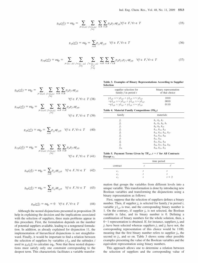
Although the nested disjunctions presented in proposition 28help in explaining the decision and the implications associatedwith the selection of suppliers, three main problems appear inthis procedure. First, the formulation depends on the numberof potential suppliers available, leading to a nongeneral formula-tion. In addition, as already explained for disjunction 11, theimplementation of hierarchical disjunctions is not straightfor-ward. Finally, it would be important to find a relation betweenthe selection of suppliers by variables y1jft and the subindex iused in gift(y1) to calculate eqft. Note that these nested disjunc-tions must satisfy only one constraint corresponding to thedeepest term. This characteristic facilitates a variable transfor-

mation that groups the variables from different levels into aunique variable. This transformation is done by introducing newBoolean variables and transforming the disjunctions using abinary representation as follows:

First, suppose that the selection of suppliers defines a binarynumber. Then, if supplier jn is selected for family f in period t,variable y1jnft is true, and the corresponding binary number is1. On the contrary, if supplier jn is not selected, the Booleanvariable is false, and its binary number is 0. Defining acombination of binary numbers for the whole solution, then, a0-1 representation is obtained. If, for instance, suppliers j4 andj3 have been selected whereas suppliers j1 and j2 have not, thecorresponding representation of this choice would be 1100,meaning that the first binary number refers to supplier j4, thesecond to j3, and so on. Table 3 shows some other possibleexamples presenting the value of the Boolean variables and theequivalent representation using binary numbers.

This approach allows one to determine a relation betweenthe selection of suppliers and the corresponding value of

g9ft(y1) ) eqft ) ∑j∈{j1,j4}

∑j′∈{j1,j4}

j′*j

∑r∈R

∑r′∈R

pjrpj′r′qrjrft∀f ∈ F, ∀t ∈ T (35)

g1ft(y1) ) eqft ) ∑r∈R

pj1rqrj1rft ∀f ∈ F, ∀t ∈ T (36)

g14ft(y1) ) eqft ) ∑j∈{j2,...,j4}

∑j′∈{j2,...,j4}

j′*j

∑j′′∈{j2,...,j4}

j′′<j′j′′*j

∑r∈R

∑r′∈R

∑r′′∈R


g6ft(y1) ) eqft ) ∑j∈{j2,j3}

∑j′∈{j2,j3}

j′*j

∑r∈R

∑r′∈R

pjrpj′r′qrjrft

∀f ∈ F, ∀t ∈ T (38)

g10ft(y1) ) eqft ) ∑j∈{j2,j4}

∑j′∈{j2,j4}

j′*j

∑r∈R

∑r′∈R

pjrpj′r′qrjrft

∀f ∈ F, ∀t ∈ T (39)



g12ft(y1) ) eqft ) ∑j∈{j3,j4}

∑j′∈{j3,j4}

j′*j

∑r∈R

∑r′∈R

pjrpj′r′qrjrft

∀f ∈ F, ∀t ∈ T (41)





g0ft(y1) ) eqft ) 0 ∀f ∈ F, ∀t ∈ T (44)

Table 3. Examples of Binary Representations According to SupplierSelection

supplier selection forfamily f in period t

binary representationof that choice

y1j4ft ∧¬ y1j3ft ∧ y1j2ft ∧¬ y1j1ft 1010¬y1j4ft ∧¬ y1j3ft ∧ y1j2ft ∧¬ y1j1ft 0010¬y1j4ft ∧ y1j3ft ∧ y1j2ft ∧¬ y1j1ft 0110

Table 4. Material Family Compositions (FKfk)

family materials

f1 k1, k2, k3

f2 k4, k5, k6, k7

f3 k8, k9, k10

f4 k11, k12, k13

f5 k14, k15, k16, k17

f6 k18, k19, k20

f7 k21, k22

f8 k23, k24, k25

f9 k26, k27, k28, k29

f10 k30, k31, k32

Table 5. Payment Terms Given by TPctt′, t ) t′ for All ContractsExcept c3

time period

contract t t′

c1 t tc2 t tc3 t t + 2


subindex i used in the definition of gift(y1), translating the binarynumber into its decimal representation. The conversion proce-dure to transform a number from binary to decimal base consistsof multiplying each binary number per 2ord, where ord representsthe order of the number in the binary representation. If thenumber 1010 given in base 2 is converted into a base-10 number,the procedure is

giving the equivalent number 10 in base 10.This algorithm establishes a relation between the set of

suppliers selected (represented as a binary number) and thecorresponding value of subindex i, as shown in eq 46:

where ift ∈ Ift ) {0,..., 2J - 1} and Y1jft ∈ {0, 1}.The value of subindex i will be the corresponding decimal

representation of the binary number that symbolizes the suppliersselected. Considering all possible solutions of supplier selection

leads to the complete representation of the set Ift for each familyf and period t.

In addition to the generality of the procedure presented andthe clear relation between the supply conformation and thecorresponding constraint gift(y1) to be satisfied, this approachalso makes it possible to simplify disjunction 28. To this end,a new Boolean variable, Vift, is introduced equivalent to theconformation of suppliers selected according to the value ofsubindex i. Then, function gift(y1_) must be satisfied if and onlyif Vift is true; that is

If, for instance, the solution for family f1 in period t1 is givenby ¬y1j4f1t1 ∧¬ y1j3f1t1 ∧ y1j2f1t1 ∧¬ y1j1f1t1, then the procedureapplies as follows

if1t1) 0 × 23 + 0 × 22 + 1 × 21 + 0 × 20

) 0 + 0 + 2 + 0) 2

Then, variable V2f1t1 is true, and function g2f1t1(y1_) must besatisfied.

By this general formulation, each combination of selectedsuppliers leads to a different value of the expected quantity (eqft)of family f in period t given by gift(y1_). It is worth mentioningthat the form of the expected quantity, eqft, is defined by theprocedure shown in eqs 20 and 25-27.The closer the eqft

variable is to the demand forecasted, the better, given that adeficit in the supplied quantity implies less real revenues andcould also affect customer satisfaction. As a consequence, thedecision regarding suppliers will also consider the expected costsdue to supplier delivery failures. It is extremely important toconsider this feature when formulating the objective function.

Finally, by applying the developed approach, disjunction 28can be replaced by the general disjunction

3.4. Modeling Additional Stock Constraints. The followingconstraints are modeled to calculate the average stock, savgft,of family f in period t, needed in the objective function. Thisvariable can be calculated as

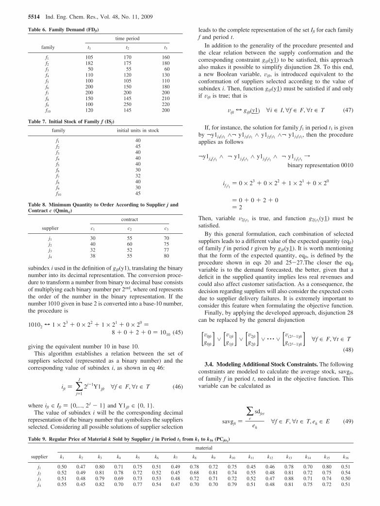
Table 6. Family Demand (FDft)

time period

family t1 t2 t3

f1 105 170 160f2 182 175 180f3 50 55 60f4 110 120 130f5 100 105 110f6 200 150 180f7 200 200 200f8 150 145 210f9 100 250 220f10 120 145 200

Table 7. Initial Stock of Family f (ISf)

family initial units in stock

f1 40f2 45f3 40f4 40f5 40f6 30f7 32f8 40f9 30f10 45

Table 8. Minimum Quantity to Order According to Supplier j andContract c (Qmincj)

contract

supplier c1 c2 c3

j1 30 55 70j2 40 60 75j3 32 52 77j4 38 55 80

Table 9. Regular Price of Material k Sold by Supplier j in Period t1 from k1 to k16 (PCjkt1)

material

supplier k1 k2 k3 k4 k5 k6 k7 k8 k9 k10 k11 k12 k13 k14 k15 k16

j1 0.50 0.47 0.80 0.71 0.75 0.51 0.49 0.78 0.72 0.75 0.45 0.46 0.78 0.70 0.80 0.51j2 0.52 0.49 0.81 0.78 0.72 0.52 0.45 0.68 0.81 0.74 0.55 0.48 0.81 0.72 0.75 0.54j3 0.51 0.48 0.79 0.69 0.73 0.53 0.48 0.72 0.71 0.72 0.52 0.47 0.88 0.71 0.74 0.50j4 0.55 0.45 0.82 0.70 0.77 0.54 0.47 0.70 0.70 0.79 0.51 0.48 0.81 0.75 0.72 0.51

10102 T 1 × 23 + 0 × 22 + 1 × 21 + 0 × 20 )8 + 0 + 2 + 0 ) 1010 (45)

ift ) ∑j)1

J

2j-1Y1jft ∀f ∈ F, ∀t ∈ T (46)

Vift S gift(y1) ∀i ∈ I, ∀f ∈ F, ∀t ∈ T (47)

¬y1j4f1t1∧ ¬ y1j3f1t1

∧ y1j2f1t1∧ ¬ y1j1f1t1

f

binary representation 0010

[V0ft

g0ft] ∨ [V1ft

g1ft] ∨ [V2ft

g2ft] ∨ · · · ∨ [V(2J-1)ft

g(2J-1)ft ] ∀f ∈ F, ∀t ∈ T

(48)

savgft )∑

e

sdfet

eh∀f ∈ F, ∀t ∈ T, eh ∈ E (49)


where

In eq 50, the variable sdfet indicates the family stock in eachsubperiod e of period t, sdf(e-1)t is the family stock in the previousperiod, and sft/eh represents a constant material output rate fromthe stock. In eq 51, the initial stock of family f in the firstsubperiod e1 of period t is constrained to be equal to the initialstock of family f in period t.

3.5. Objective Function. The objective function defines theminimization of the actualized expected costs over the timehorizon. The costs considered are the corresponding materialpurchase costs, the inventory costs, and the expected costs dueto the unsatisfied demand calculated as lost sales. The objectivefunction is presented as

The positive variable mjckt determines the money outflows dueto material k purchased from supplier j to be paid in period taccording to the payment policy of contract c.

In the second term, the positive variable savgft represents theaverage stock expected of family f in period t, calculated in eq49. The parameter COSTavgf corresponds to the average costof family f, and parameter MS indicates a percentage of theraw material average costs. This percentage is used to estimatethe average stock costs and includes the following majorcomponents: capital costs, storage costs, obsolescence costs, andquality costs. In general, all of these costs are rolled togetherinto a single inventory cost rate, expressed as a percentage ofthe product or material value per unit time.23

The last term corresponds to the expected loses due to theunsatisfied demand. It is considered that the difference betweenthe family demand and the expected sales of family f representsthe amount of product that could have been sold. These unitsare quantified by multiplying them by the average sale price offamily f in period t, Apft.

The return rate, RR, corresponds to the capital cost, which iscalculated with the capital asset pricing model.24 The formulafor the capital cost RR is

where RRfree corresponds to the expected return of a theoreticalrisk-free asset and is the minimum return an investor expectsfor any investment. Traditionally, for long-term investments,RRfree is equal to the country Treasury bill rate. In this case,the appropriate RRfree value considered is a certificate of depositrate (from a safe bank) because the time horizon is short andthe investment corresponds to working capital instead of fixedassets. The RRrisk element can be rewritten as

where RRmarket represents the expected return of the market and� indicates the sensitivity of returns from asset a to marketreturns. This parameter can be calculated as

where σa market in eq 55 represents the covariance between thereturns from asset a and the market returns and (σmarket)2 definesthe market variance. All of these coefficients are model data.

The final mathematical model for the case of four potentialsuppliers is given by expressions 1-6, 8-10, 12-16, 29-44,46, and 48-52.

4. Model Results

Two case studies considering four potential suppliers arepresented here to illustrate formulation performance. The modelswere posed in the GAMS system and executed over a PC havingan Intel Pentium D 2.8 GHz processor. Disjunctions weremodeled using GDP, and the disjunctive program was solvedwith LogMIP.25

4.1. Case Study 1. In this example, supplier uncertainty ismodeled by considering two possible extreme situations: rawmaterial order delivery completely fails or is completelysuccessful, meaning that, in the first case, no raw material isdelivered by the supplier, whereas in the second case, the whole

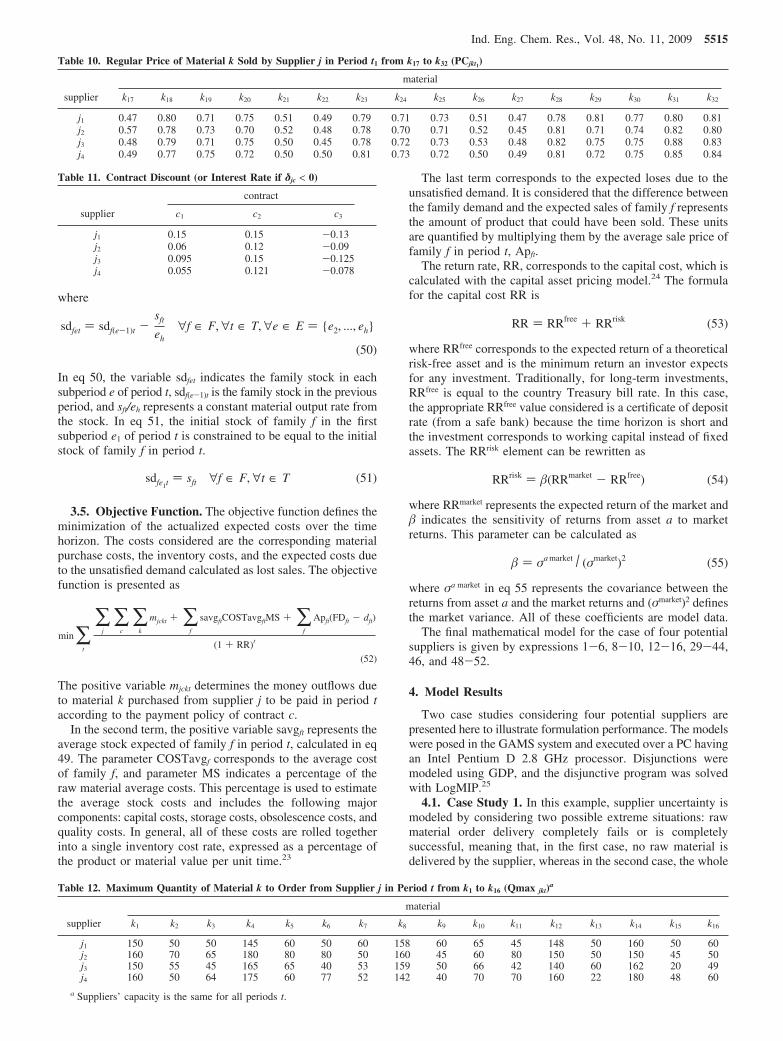
Table 10. Regular Price of Material k Sold by Supplier j in Period t1 from k17 to k32 (PCjkt1)

material


j1 0.47 0.80 0.71 0.75 0.51 0.49 0.79 0.71 0.73 0.51 0.47 0.78 0.81 0.77 0.80 0.81j2 0.57 0.78 0.73 0.70 0.52 0.48 0.78 0.70 0.71 0.52 0.45 0.81 0.71 0.74 0.82 0.80j3 0.48 0.79 0.71 0.75 0.50 0.45 0.78 0.72 0.73 0.53 0.48 0.82 0.75 0.75 0.88 0.83j4 0.49 0.77 0.75 0.72 0.50 0.50 0.81 0.73 0.72 0.50 0.49 0.81 0.72 0.75 0.85 0.84

Table 11. Contract Discount (or Interest Rate if δjc < 0)

contract

supplier c1 c2 c3

j1 0.15 0.15 -0.13j2 0.06 0.12 -0.09j3 0.095 0.15 -0.125j4 0.055 0.121 -0.078

Table 12. Maximum Quantity of Material k to Order from Supplier j in Period t from k1 to k16 (Qmax jkt)a

material


j1 150 50 50 145 60 50 60 158 60 65 45 148 50 160 50 60j2 160 70 65 180 80 80 50 160 45 60 80 150 50 150 45 50j3 150 55 45 165 65 40 53 159 50 66 42 140 60 162 20 49j4 160 50 64 175 60 77 52 142 40 70 70 160 22 180 48 60

a Suppliers’ capacity is the same for all periods t.

sdfet ) sdf(e-1)t -sft

eh∀f ∈ F, ∀t ∈ T, ∀e ∈ E ) {e2, ..., eh}

(50)

sdfe1t ) sft ∀f ∈ F, ∀t ∈ T (51)

min∑t

∑j

∑c

∑k

mjckt + ∑f

savgftCOSTavgftMS + ∑f

Apft(FDft - dft)

(1 + RR)t

(52)

RR ) RRfree + RRrisk (53)

RRrisk ) �(RRmarket - RRfree) (54)

� ) σa market / (σmarket)2 (55)


order is sent. The supplier failure probability distributions arepresented in Figure 2. Data for this example are provided inthe next two subsections.

4.1.1. Model Sets. The sizes of the model sets are as follows:number of families (F) ) 10, number of materials (K) ) 32,number of contract types (C) ) 3, and number of potentialsuppliers (J) ) 4.

Tables 4 and 5 provide data on the material family composi-tions and payment terms, respectively.

4.1.2. Model Parameters. Model parameters related to thefamily demands, initial stocks of family f, minimum quantitiesto order, regular prices, contract discounts, maximum quantitiesto order, supplier failure probabilities, and average prices areprovided in Tables 6-15.

The demand upper bound is given by µ ) 0.50, and the stockcapacity is SC ) 5000.

The regular price of material k sold by supplier j in period t(PCjkt) is calculated using the inflation rate ir (ir ) 0.10) as

The average cost of family f in period t (COSTavgft) isdetermined by calculating the average of PCjkt for all suppliersand for all materials belonging to f given by FKkf.

The average price of family f in period t is calculated usingthe interest rate ir as

The percentage of the raw material average costs used tocalculate stock costs is MS ) 0.25, and the discount rate is RR) 0.15.

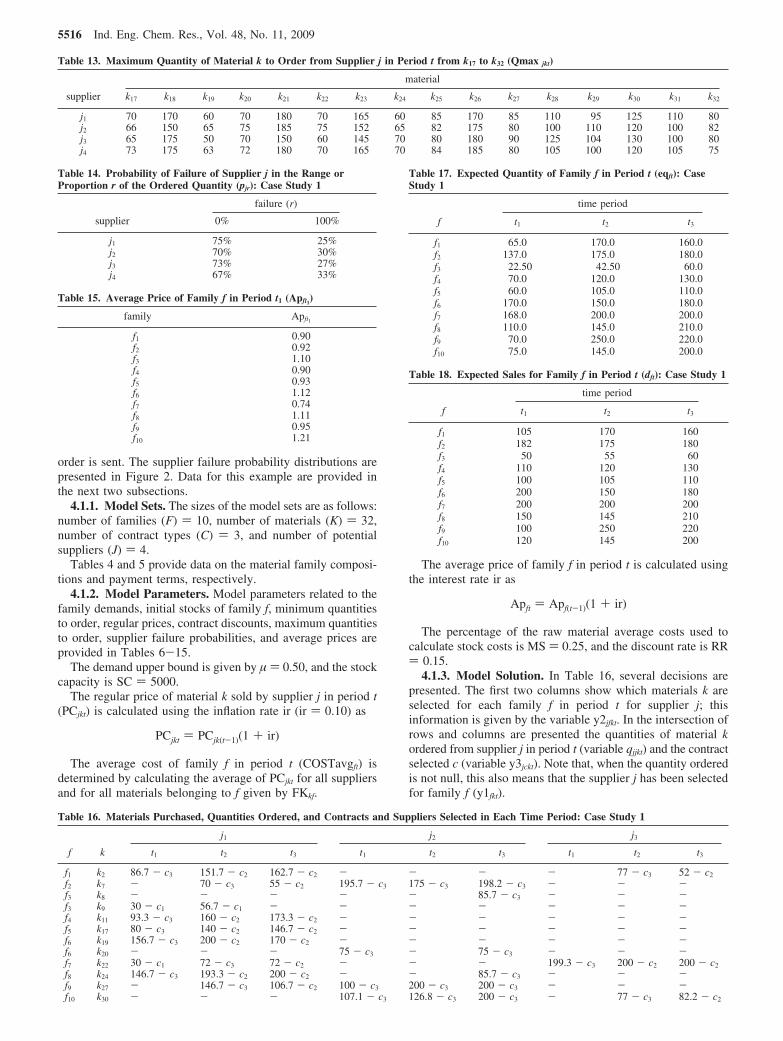
4.1.3. Model Solution. In Table 16, several decisions arepresented. The first two columns show which materials k areselected for each family f in period t for supplier j; thisinformation is given by the variable y2jfkt. In the intersection ofrows and columns are presented the quantities of material kordered from supplier j in period t (variable qjjkt) and the contractselected c (variable y3jckt). Note that, when the quantity orderedis not null, this also means that the supplier j has been selectedfor family f (y1fkt).

Table 13. Maximum Quantity of Material k to Order from Supplier j in Period t from k17 to k32 (Qmax jkt)

material


j1 70 170 60 70 180 70 165 60 85 170 85 110 95 125 110 80j2 66 150 65 75 185 75 152 65 82 175 80 100 110 120 100 82j3 65 175 50 70 150 60 145 70 80 180 90 125 104 130 100 80j4 73 175 63 72 180 70 165 70 84 185 80 105 100 120 105 75

Table 14. Probability of Failure of Supplier j in the Range orProportion r of the Ordered Quantity (pjr): Case Study 1

failure (r)

supplier 0% 100%

j1 75% 25%j2 70% 30%j3 73% 27%j4 67% 33%

Table 15. Average Price of Family f in Period t1 (Apft1)

family Apft1

f1 0.90f2 0.92f3 1.10f4 0.90f5 0.93f6 1.12f7 0.74f8 1.11f9 0.95f10 1.21

Table 16. Materials Purchased, Quantities Ordered, and Contracts and Suppliers Selected in Each Time Period: Case Study 1

j1 j2 j3

f k t1 t2 t3 t1 t2 t3 t1 t2 t3

f1 k2 86.7 - c3 151.7 - c2 162.7 - c2 - - - - 77 - c3 52 - c2

f2 k7 - 70 - c3 55 - c2 195.7 - c3 175 - c3 198.2 - c3 - - -f3 k8 - - - - - 85.7 - c3 - - -f3 k9 30 - c1 56.7 - c1 - - - - - - -f4 k11 93.3 - c3 160 - c2 173.3 - c2 - - - - - -f5 k17 80 - c3 140 - c2 146.7 - c2 - - - - - -f6 k19 156.7 - c3 200 - c2 170 - c2 - - - - - -f6 k20 - - - 75 - c3 - 75 - c3 - - -f7 k22 30 - c1 72 - c3 72 - c2 - - - 199.3 - c3 200 - c2 200 - c2

f8 k24 146.7 - c3 193.3 - c2 200 - c2 - - 85.7 - c3 - - -f9 k27 - 146.7 - c3 106.7 - c2 100 - c3 200 - c3 200 - c3 - - -f10 k30 - - - 107.1 - c3 126.8 - c3 200 - c3 - 77 - c3 82.2 - c2

PCjkt ) PCjk(t-1)(1 + ir)

Table 17. Expected Quantity of Family f in Period t (eqft): CaseStudy 1

time period

f t1 t2 t3

f1 65.0 170.0 160.0f2 137.0 175.0 180.0f3 22.50 42.50 60.0f4 70.0 120.0 130.0f5 60.0 105.0 110.0f6 170.0 150.0 180.0f7 168.0 200.0 200.0f8 110.0 145.0 210.0f9 70.0 250.0 220.0f10 75.0 145.0 200.0

Table 18. Expected Sales for Family f in Period t (dft): Case Study 1

time period

f t1 t2 t3

f1 105 170 160f2 182 175 180f3 50 55 60f4 110 120 130f5 100 105 110f6 200 150 180f7 200 200 200f8 150 145 210f9 100 250 220f10 120 145 200

Apft ) Apf(t-1)(1 + ir)


Additional results are reported in Tables 17-20.4.2. Case Study 2. According to the probabilistic distribution

of the undelivered expected quantities in Figure 1, in this secondcase study, suppliers can fail partially, not delivering certainportions of the quantity ordered.

4.2.1. Model Parameters. All data and model parametersare the same as in case study 1 except for the failure distribution,which is provided in Table 21.

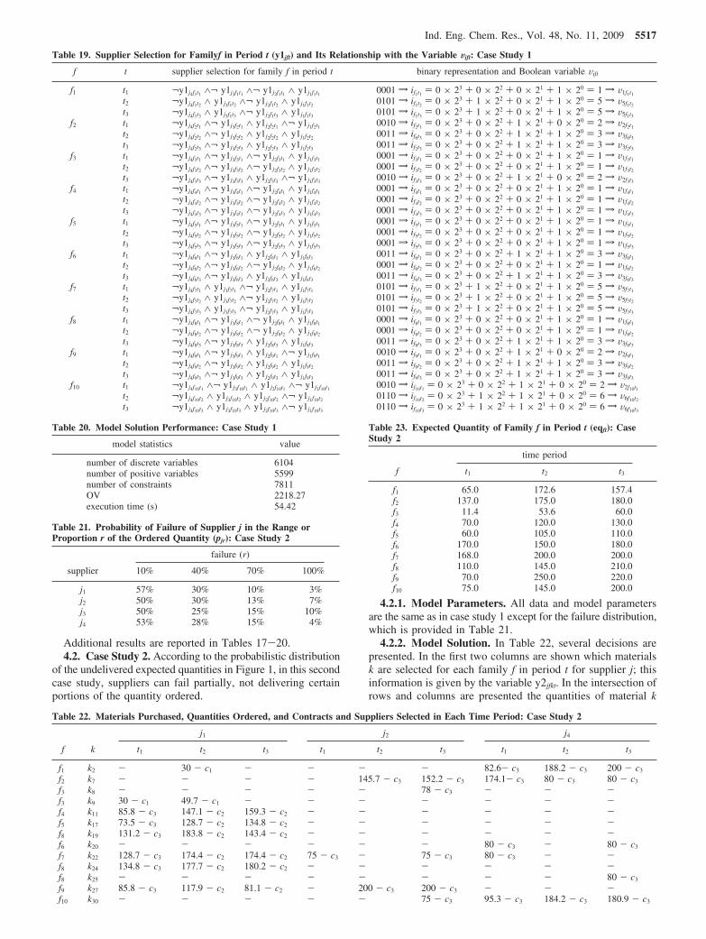
4.2.2. Model Solution. In Table 22, several decisions arepresented. In the first two columns are shown which materialsk are selected for each family f in period t for supplier j; thisinformation is given by the variable y2jfkt. In the intersection ofrows and columns are presented the quantities of material k

Table 19. Supplier Selection for Familyf in Period t (y1jft) and Its Relationship with the Variable Wift: Case Study 1

f t supplier selection for family f in period t binary representation and Boolean variable Vift

f1 t1 ¬y1j4f1t1 ∧¬ y1j3f1t1 ∧¬ y1j2f1t1 ∧ y1j1f1t1 0001 w if1t1 ) 0 × 23 + 0 × 22 + 0 × 21 + 1 × 20 ) 1 w V1f1t1t2 ¬y1j4f1t2 ∧ y1j3f1t2 ∧¬ y1j2f1t2 ∧ y1j1f1t2 0101 w if1t2 ) 0 × 23 + 1 × 22 + 0 × 21 + 1 × 20 ) 5 w V5f1t2t3 ¬y1j4f1t3 ∧ y1j3f1t3 ∧¬ y1j2f1t3 ∧ y1j1f1t3 0101 w if1t3 ) 0 × 23 + 1 × 22 + 0 × 21 + 1 × 20 ) 5 w V5f1t3

f2 t1 ¬y1j4f2t1 ∧¬ y1j3f2t1 ∧ y1j2f2t1 ∧¬ y1j1f2t1 0010 w if2t1 ) 0 × 23 + 0 × 22 + 1 × 21 + 0 × 20 ) 2 w V2f2t1t2 ¬y1j4f2t2 ∧¬ y1j3f2t2 ∧ y1j2f2t2 ∧ y1j1f2t2 0011 w if6t3 ) 0 × 23 + 0 × 22 + 1 × 21 + 1 × 20 ) 3 w V3f6t3t3 ¬y1j4f2t3 ∧¬ y1j3f2t3 ∧ y1j2f2t3 ∧ y1j1f2t3 0011 w if2t3 ) 0 × 23 + 0 × 22 + 1 × 21 + 1 × 20 ) 3 w V3f2t3

f3 t1 ¬y1j4f3t1 ∧¬ y1j3f3t1 ∧¬ y1j2f3t1 ∧ y1j1f3t1 0001 w if3t1 ) 0 × 23 + 0 × 22 + 0 × 21 + 1 × 20 ) 1 w V1f3t1t2 ¬y1j4f3t2 ∧¬ y1j3f3t2 ∧¬ y1j2f3t2 ∧ y1j1f3t2 0001 w if3t2 ) 0 × 23 + 0 × 22 + 0 × 21 + 1 × 20 ) 1 w V1f3t2t3 ¬y1j4f3t3 ∧¬ y1j3f3t3 ∧ y1j2f3t3 ∧¬ y1j1f3t3 0010 w if3t3 ) 0 × 23 + 0 × 22 + 1 × 21 + 0 × 20 ) 2 w V2f3t3

f4 t1 ¬y1j4f4t1 ∧¬ y1j3f4t1 ∧¬ y1j2f4t1 ∧ y1j1f4t1 0001 w if4t1 ) 0 × 23 + 0 × 22 + 0 × 21 + 1 × 20 ) 1 w V1f4t1t2 ¬y1j4f4t2 ∧¬ y1j3f4t2 ∧¬ y1j2f4t2 ∧ y1j1f4t2 0001 w if4t2 ) 0 × 23 + 0 × 22 + 0 × 21 + 1 × 20 ) 1 w V1f4t2t3 ¬y1j4f4t3 ∧¬ y1j3f4t3 ∧¬ y1j2f4t3 ∧ y1j1f4t3 0001 w if4t3 ) 0 × 23 + 0 × 22 + 0 × 21 + 1 × 20 ) 1 w V1f4t3


f6 t1 ¬y1j4f6t1 ∧¬ y1j3f6t1 ∧ y1j2f6t1 ∧ y1j1f6t1 0011 w if6t1 ) 0 × 23 + 0 × 22 + 1 × 21 + 1 × 20 ) 3 w V3f6t1t2 ¬y1j4f6t2 ∧¬ y1j3f6t2 ∧¬ y1j2f6t2 ∧ y1j1f6t2 0001 w if6t2 ) 0 × 23 + 0 × 22 + 0 × 21 + 1 × 20 ) 1 w V1f6t2t3 ¬y1j4f6t3 ∧¬ y1j3f6t3 ∧ y1j2f6t3 ∧ y1j1f6t3 0011 w if6t3 ) 0 × 23 + 0 × 22 + 1 × 21 + 1 × 20 ) 3 w V3f6t3

f7 t1 ¬y1j4f7t1 ∧ y1j3f7t1 ∧¬ y1j2f7t1 ∧ y1j1f7t1 0101 w if7t1 ) 0 × 23 + 1 × 22 + 0 × 21 + 1 × 20 ) 5 w V5f7t1t2 ¬y1j4f7t2 ∧ y1j3f7t2 ∧¬ y1j2f7t2 ∧ y1j1f7t2 0101 w if7t2 ) 0 × 23 + 1 × 22 + 0 × 21 + 1 × 20 ) 5 w V5f7t2t3 ¬y1j4f7t3 ∧ y1j3f7t3 ∧¬ y1j2f7t3 ∧ y1j1f7t3 0101 w if7t3 ) 0 × 23 + 1 × 22 + 0 × 21 + 1 × 20 ) 5 w V5f7t3

f8 t1 ¬y1j4f8t1 ∧¬ y1j3f8t1 ∧¬ y1j2f8t1 ∧ y1j1f8t1 0001 w if8t1 ) 0 × 23 + 0 × 22 + 0 × 21 + 1 × 20 ) 1 w V1f8t1t2 ¬y1j4f8t2 ∧¬ y1j3f8t2 ∧¬ y1j2f8t2 ∧ y1j1f8t2 0001 w if8t2 ) 0 × 23 + 0 × 22 + 0 × 21 + 1 × 20 ) 1 w V1f8t2t3 ¬y1j4f8t3 ∧¬ y1j3f8t3 ∧ y1j2f8t3 ∧ y1j1f8t3 0011 w if8t3 ) 0 × 23 + 0 × 22 + 1 × 21 + 1 × 20 ) 3 w V3f8t3

f9 t1 ¬y1j4f9t1 ∧¬ y1j3f9t1 ∧ y1j2f9t1 ∧¬ y1j1f9t1 0010 w if9t1 ) 0 × 23 + 0 × 22 + 1 × 21 + 0 × 20 ) 2 w V2f9t1t2 ¬y1j4f9t2 ∧¬ y1j3f9t2 ∧ y1j2f9t2 ∧ y1j1f9t2 0011 w if9t2 ) 0 × 23 + 0 × 22 + 1 × 21 + 1 × 20 ) 3 w V3f9t2t3 ¬y1j4f9t3 ∧¬ y1j3f9t3 ∧ y1j2f9t3 ∧ y1j1f9t3 0011 w if9t3 ) 0 × 23 + 0 × 22 + 1 × 21 + 1 × 20 ) 3 w V3f9t3

f10 t1 ¬y1j4f10t1 ∧¬ y1j3f10t1 ∧ y1j2f10t1 ∧¬ y1j1f10t1 0010 w if10t1 ) 0 × 23 + 0 × 22 + 1 × 21 + 0 × 20 ) 2 w V2f10t1t2 ¬y1j4f10t2 ∧ y1j3f10t2 ∧ y1j2f10t2 ∧¬ y1j1f10t2 0110 w if10t2 ) 0 × 23 + 1 × 22 + 1 × 21 + 0 × 20 ) 6 w V6f10t2t3 ¬y1j4f10t3 ∧ y1j3f10t3 ∧ y1j2f10t3 ∧¬ y1j1f10t3 0110 w if10t3 ) 0 × 23 + 1 × 22 + 1 × 21 + 0 × 20 ) 6 w V6f10t3

Table 20. Model Solution Performance: Case Study 1

model statistics value

number of discrete variables 6104number of positive variables 5599number of constraints 7811OV 2218.27execution time (s) 54.42


failure (r)

supplier 10% 40% 70% 100%

j1 57% 30% 10% 3%j2 50% 30% 13% 7%j3 50% 25% 15% 10%j4 53% 28% 15% 4%

Table 22. Materials Purchased, Quantities Ordered, and Contracts and Suppliers Selected in Each Time Period: Case Study 2

j1 j2 j4

f k t1 t2 t3 t1 t2 t3 t1 t2 t3

f1 k2 - 30 - c1 - - - - 82.6- c3 188.2 - c3 200 - c3

f2 k7 - - - - 145.7 - c3 152.2 - c3 174.1- c3 80 - c3 80 - c3

f3 k8 - - - - - 78 - c3 - - -f3 k9 30 - c1 49.7 - c1 - - - - - - -f4 k11 85.8 - c3 147.1 - c2 159.3 - c2 - - - - - -f5 k17 73.5 - c3 128.7 - c2 134.8 - c2 - - - - - -f8 k19 131.2 - c3 183.8 - c2 143.4 - c2 - - - - - -f6 k20 - - - - - - 80 - c3 - 80 - c3

f7 k22 128.7 - c3 174.4 - c2 174.4 - c2 75 - c3 - 75 - c3 80 - c3 - -f8 k24 134.8 - c3 177.7 - c2 180.2 - c2 - - - - - -f8 k25 - - - - - - - - 80 - c3

f9 k27 85.8 - c3 117.9 - c2 81.1 - c2 - 200 - c3 200 - c3 - - -f10 k30 - - - - - 75 - c3 95.3 - c3 184.2 - c3 180.9 - c3

Table 23. Expected Quantity of Family f in Period t (eqft): CaseStudy 2

time period

f t1 t2 t3

f1 65.0 172.6 157.4f2 137.0 175.0 180.0f3 11.4 53.6 60.0f4 70.0 120.0 130.0f5 60.0 105.0 110.0f6 170.0 150.0 180.0f7 168.0 200.0 200.0f8 110.0 145.0 210.0f9 70.0 250.0 220.0f10 75.0 145.0 200.0


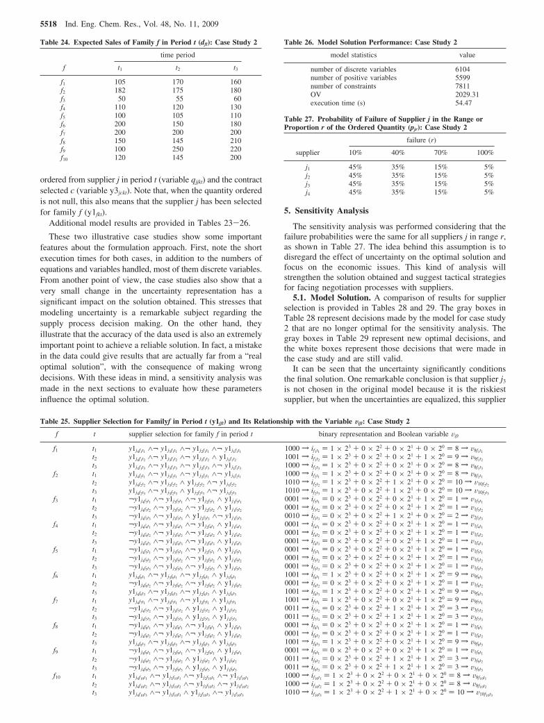
ordered from supplier j in period t (variable qjjkt) and the contractselected c (variable y3jckt). Note that, when the quantity orderedis not null, this also means that the supplier j has been selectedfor family f (y1fkt).

Additional model results are provided in Tables 23-26.

These two illustrative case studies show some importantfeatures about the formulation approach. First, note the shortexecution times for both cases, in addition to the numbers ofequations and variables handled, most of them discrete variables.From another point of view, the case studies also show that avery small change in the uncertainty representation has asignificant impact on the solution obtained. This stresses thatmodeling uncertainty is a remarkable subject regarding thesupply process decision making. On the other hand, theyillustrate that the accuracy of the data used is also an extremelyimportant point to achieve a reliable solution. In fact, a mistakein the data could give results that are actually far from a “realoptimal solution”, with the consequence of making wrongdecisions. With these ideas in mind, a sensitivity analysis wasmade in the next sections to evaluate how these parametersinfluence the optimal solution.

5. Sensitivity Analysis

The sensitivity analysis was performed considering that thefailure probabilities were the same for all suppliers j in range r,as shown in Table 27. The idea behind this assumption is todisregard the effect of uncertainty on the optimal solution andfocus on the economic issues. This kind of analysis willstrengthen the solution obtained and suggest tactical strategiesfor facing negotiation processes with suppliers.

5.1. Model Solution. A comparison of results for supplierselection is provided in Tables 28 and 29. The gray boxes inTable 28 represent decisions made by the model for case study2 that are no longer optimal for the sensitivity analysis. Thegray boxes in Table 29 represent new optimal decisions, andthe white boxes represent those decisions that were made inthe case study and are still valid.

It can be seen that the uncertainty significantly conditionsthe final solution. One remarkable conclusion is that supplier j3

is not chosen in the original model because it is the riskiestsupplier, but when the uncertainties are equalized, this supplier

Table 24. Expected Sales of Family f in Period t (dft): Case Study 2

time period

f t1 t2 t3

f1 105 170 160f2 182 175 180f3 50 55 60f4 110 120 130f5 100 105 110f6 200 150 180f7 200 200 200f8 150 145 210f9 100 250 220f10 120 145 200

Table 25. Supplier Selection for Familyf in Period t (y1jft) and Its Relationship with the Variable Wift: Case Study 2

f t supplier selection for family f in period t binary representation and Boolean variable Vift

f1 t1 y1j4f1t1 ∧¬ y1j3f1t1 ∧¬ y1j2f1t1 ∧¬ y1j1f1t1 1000 w if1t1 ) 1 × 23 + 0 × 22 + 0 × 21 + 0 × 20 ) 8 w V8f1t1t2 y1j4f1t2 ∧¬ y1j3f1t2 ∧¬ y1j2f1t2 ∧ y1j1f1t2 1001 w if1t2 ) 1 × 23 + 0 × 22 + 0 × 21 + 1 × 20 ) 9 w V9f1t2t3 y1j4f1t3 ∧¬ y1j3f1t3 ∧¬ y1j2f1t3 ∧¬ y1j1f1t3 1000 w if1t3 ) 1 × 23 + 0 × 22 + 0 × 21 + 0 × 20 ) 8 w V8f1t3

f2 t1 y1j4f2t1 ∧¬ y1j3f2t1 ∧¬ y1j2f2t1 ∧¬ y1j1f2t1 1000 w if2t1 ) 1 × 23 + 0 × 22 + 0 × 21 + 0 × 20 ) 8 w V8f2t1t2 y1j4f2t2 ∧¬ y1j3f2t2 ∧ y1j2f2t2 ∧¬ y1j1f2t2 1010 w if2t2 ) 1 × 23 + 0 × 22 + 1 × 21 + 0 × 20 ) 10 w V10f2t2t3 y1j4f2t3 ∧¬ y1j3f2t3 ∧ y1j2f2t3 ∧¬ y1j1f2t3 1010 w if2t3 ) 1 × 23 + 0 × 22 + 1 × 21 + 0 × 20 ) 10 w V10f2t3

f3 t1 ¬y1j4f3t1 ∧¬ y1j3f3t1 ∧¬ y1j2f3t1 ∧ y1j1f3t1 0001 w if3t1 ) 0 × 23 + 0 × 22 + 0 × 21 + 1 × 20 ) 1 w V1f3t1t2 ¬y1j4f3t2 ∧¬ y1j3f3t2 ∧¬ y1j2f3t2 ∧ y1j1f3t2 0001 w if3t2 ) 0 × 23 + 0 × 22 + 0 × 21 + 1 × 20 ) 1 w V1f3t2t3 ¬y1j4f3t3 ∧¬ y1j3f3t3 ∧ y1j2f3t3 ∧¬ y1j1f3t3 0010 w if3t3 ) 0 × 23 + 0 × 22 + 1 × 21 + 0 × 20 ) 2 w V2f3t3



f6 t1 y1j4f6t1 ∧¬ y1j3f6t1 ∧¬ y1j2f6t1 ∧ y1j1f6t1 1001 w if6t1 ) 1 × 23 + 0 × 22 + 0 × 21 + 1 × 20 ) 9 w V9f6t1t2 ¬y1j4f6t2 ∧¬ y1j3f6t2 ∧¬ y1j2f6t2 ∧ y1j1f6t2 0001 w if6t2 ) 0 × 23 + 0 × 22 + 0 × 21 + 1 × 20 ) 1 w V1f6t2t3 y1j4f6t3 ∧¬ y1j3f6t3 ∧¬ y1j2f6t3 ∧ y1j1f6t3 1001 w if6t3 ) 1 × 23 + 0 × 22 + 0 × 21 + 1 × 20 ) 9 w V9f6t3

f7 t1 y1j4f7t1 ∧¬ y1j3f7t1 ∧¬ y1j2f7t1 ∧ y1j1f7t1 1001 w if7t1 ) 1 × 23 + 0 × 22 + 0 × 21 + 1 × 20 ) 9 w V9f7t1t2 ¬y1j4f7t2 ∧¬ y1j3f7t2 ∧ y1j2f7t2 ∧ y1j1f7t2 0011 w if7t2 ) 0 × 23 + 0 × 22 + 1 × 21 + 1 × 20 ) 3 w V3f7t2t3 ¬y1j4f7t3 ∧¬ y1j3f7t3 ∧ y1j2f7t3 ∧ y1j1f7t3 0011 w if7t3 ) 0 × 23 + 0 × 22 + 1 × 21 + 1 × 20 ) 3 w V3f7t3

f8 t1 ¬y1j4f8t1 ∧¬ y1j3f8t1 ∧¬ y1j2f8t1 ∧ y1j1f8t1 0001 w if8t1 ) 0 × 23 + 0 × 22 + 0 × 21 + 1 × 20 ) 1 w V1f8t1t2 ¬y1j4f8t2 ∧¬ y1j3f8t2 ∧¬ y1j2f8t2 ∧ y1j1f8t2 0001 w if8t2 ) 0 × 23 + 0 × 22 + 0 × 21 + 1 × 20 ) 1 w V1f8t2t3 y1j4f8t3 ∧¬ y1j3f8t3 ∧¬ y1j2f8t3 ∧ y1j1f8t3 1001 w if8t3 ) 1 × 23 + 0 × 22 + 0 × 21 + 1 × 20 ) 9 w V9f8t3

f9 t1 ¬y1j4f9t1 ∧¬ y1j3f9t1 ∧¬ y1j2f9t1 ∧ y1j1f9t1 0001 w if9t1 ) 0 × 23 + 0 × 22 + 0 × 21 + 1 × 20 ) 1 w V1f9t1t2 ¬y1j4f9t2 ∧¬ y1j3f9t2 ∧ y1j2f9t2 ∧ y1j1f9t2 0011 w if9t2 ) 0 × 23 + 0 × 22 + 1 × 21 + 1 × 20 ) 3 w V3f9t2t3 ¬y1j4f9t3 ∧¬ y1j3f9t3 ∧ y1j2f9t3 ∧ y1j1f9t3 0011 w if9t3 ) 0 × 23 + 0 × 22 + 1 × 21 + 1 × 20 ) 3 w V3f9t3

f10 t1 y1j4f10t1 ∧¬ y1j3f10t1 ∧¬ y1j2f10t1 ∧¬ y1j1f10t1 1000 w if10t1 ) 1 × 23 + 0 × 22 + 0 × 21 + 0 × 20 ) 8 w V8f10t1t2 y1j4f10t2 ∧¬ y1j3f10t2 ∧¬ y1j2f10t2 ∧¬ y1j1f10t2 1000 w if10t2 ) 1 × 23 + 0 × 22 + 0 × 21 + 0 × 20 ) 8 w V8f10t2t3 y1j4f10t3 ∧¬ y1j3f10t3 ∧ y1j2f10t3 ∧¬ y1j1f10t3 1010 w if10t3 ) 1 × 23 + 0 × 22 + 1 × 21 + 0 × 20 ) 10 w V10f10t3

Table 26. Model Solution Performance: Case Study 2




failure (r)

supplier 10% 40% 70% 100%

j1 45% 35% 15% 5%j2 45% 35% 15% 5%j3 45% 35% 15% 5%j4 45% 35% 15% 5%


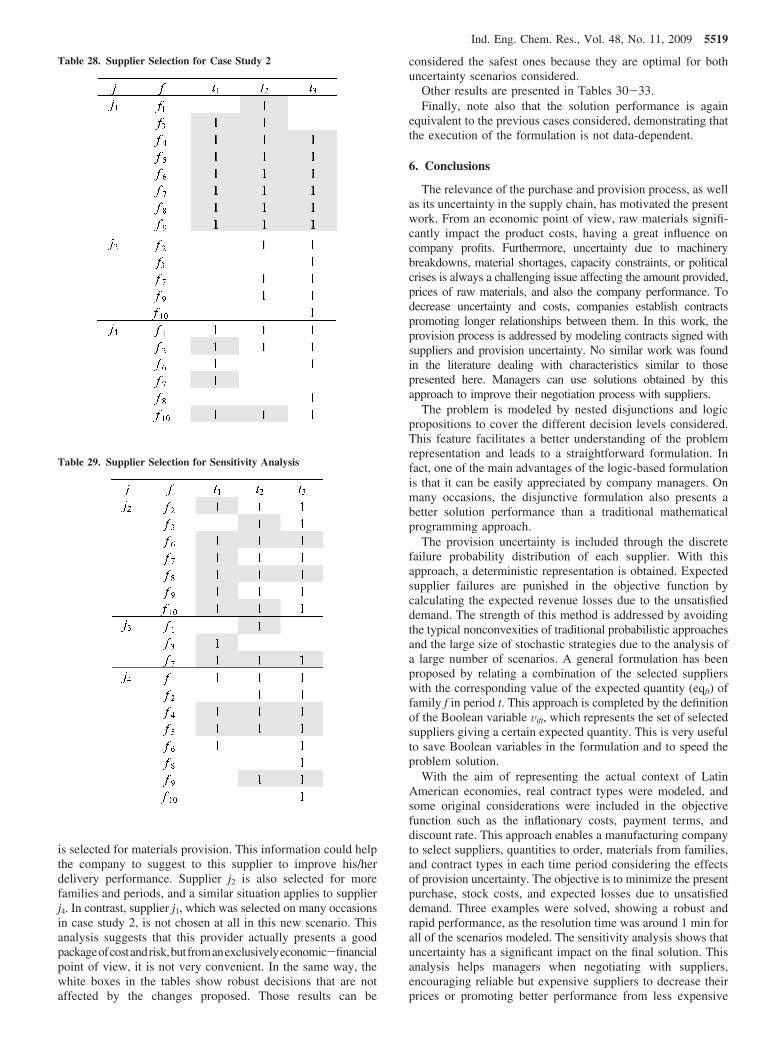
is selected for materials provision. This information could helpthe company to suggest to this supplier to improve his/herdelivery performance. Supplier j2 is also selected for morefamilies and periods, and a similar situation applies to supplierj4. In contrast, supplier j1, which was selected on many occasionsin case study 2, is not chosen at all in this new scenario. Thisanalysis suggests that this provider actually presents a goodpackageofcostandrisk,butfromanexclusivelyeconomic-financialpoint of view, it is not very convenient. In the same way, thewhite boxes in the tables show robust decisions that are notaffected by the changes proposed. Those results can be

considered the safest ones because they are optimal for bothuncertainty scenarios considered.

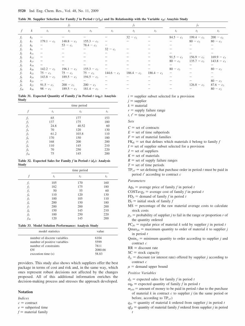
Other results are presented in Tables 30-33.Finally, note also that the solution performance is again

equivalent to the previous cases considered, demonstrating thatthe execution of the formulation is not data-dependent.

6. Conclusions

The relevance of the purchase and provision process, as wellas its uncertainty in the supply chain, has motivated the presentwork. From an economic point of view, raw materials signifi-cantly impact the product costs, having a great influence oncompany profits. Furthermore, uncertainty due to machinerybreakdowns, material shortages, capacity constraints, or politicalcrises is always a challenging issue affecting the amount provided,prices of raw materials, and also the company performance. Todecrease uncertainty and costs, companies establish contractspromoting longer relationships between them. In this work, theprovision process is addressed by modeling contracts signed withsuppliers and provision uncertainty. No similar work was foundin the literature dealing with characteristics similar to thosepresented here. Managers can use solutions obtained by thisapproach to improve their negotiation process with suppliers.

The problem is modeled by nested disjunctions and logicpropositions to cover the different decision levels considered.This feature facilitates a better understanding of the problemrepresentation and leads to a straightforward formulation. Infact, one of the main advantages of the logic-based formulationis that it can be easily appreciated by company managers. Onmany occasions, the disjunctive formulation also presents abetter solution performance than a traditional mathematicalprogramming approach.

The provision uncertainty is included through the discretefailure probability distribution of each supplier. With thisapproach, a deterministic representation is obtained. Expectedsupplier failures are punished in the objective function bycalculating the expected revenue losses due to the unsatisfieddemand. The strength of this method is addressed by avoidingthe typical nonconvexities of traditional probabilistic approachesand the large size of stochastic strategies due to the analysis ofa large number of scenarios. A general formulation has beenproposed by relating a combination of the selected supplierswith the corresponding value of the expected quantity (eqft) offamily f in period t. This approach is completed by the definitionof the Boolean variable Vift, which represents the set of selectedsuppliers giving a certain expected quantity. This is very usefulto save Boolean variables in the formulation and to speed theproblem solution.

With the aim of representing the actual context of LatinAmerican economies, real contract types were modeled, andsome original considerations were included in the objectivefunction such as the inflationary costs, payment terms, anddiscount rate. This approach enables a manufacturing companyto select suppliers, quantities to order, materials from families,and contract types in each time period considering the effectsof provision uncertainty. The objective is to minimize the presentpurchase, stock costs, and expected losses due to unsatisfieddemand. Three examples were solved, showing a robust andrapid performance, as the resolution time was around 1 min forall of the scenarios modeled. The sensitivity analysis shows thatuncertainty has a significant impact on the final solution. Thisanalysis helps managers when negotiating with suppliers,encouraging reliable but expensive suppliers to decrease theirprices or promoting better performance from less expensive

Table 28. Supplier Selection for Case Study 2

Table 29. Supplier Selection for Sensitivity Analysis


providers. This study also shows which suppliers offer the bestpackage in terms of cost and risk and, in the same way, whichones represent robust decisions not affected by the changesproposed. All of this additional information enriches thedecision-making process and stresses the approach developed.

Notation

Indicesc ) contracte ) subperiod timef ) material family

i ) supplier subset selected for a provisionj ) supplierk ) materialr ) supply failure ranget, t′ ) time period

Sets

C ) set of contractsE ) set of time subperiodsF ) set of material familiesFKfk ) set that defines which materials k belong to family fI ) set of supplier subset selected for a provisionJ ) set of suppliersK ) set of materialsR ) set of supply failure rangesT ) set of time periodsTPctt′ ) set defining that purchase order in period t must be paid in

period t′ according to contract c

Parameters

Apft ) average price of family f in period tCOSTavgft ) average cost of family f in period tFDft ) demand of family f in period tISf ) initial stock of family fMS ) percentage of the raw material average costs to calculate

stock costspjr ) probability of supplier j to fail in the range or proportion r of

the quantity orderedPCjkt ) regular price of material k sold by supplier j in period tQmaxjkt ) maximum quantity to order of material k to supplier j

in period tQmincj ) minimum quantity to order according to supplier j and

contract cRR ) discount rateSC ) stock capacityδjc ) discount (or interest rate) offered by supplier j according to

contract cµ ) demand upper bound

PositiVe Variables

dft ) expected sales for family f in period teqft ) expected quantity of family f in period tmjckt ) amount of money to be paid in period t due to the purchase

of material k in contract c to supplier j (in the same period orbefore, according to TPctt′)

qjkt ) quantity of material k ordered from supplier j in period tqfjft ) quantity of material family f ordered from supplier j in period

t

Table 30. Supplier Selection for Family f in Period t (y1jft) and Its Relationship with the Variable Wift: Anaylsis Study

j2 j3 j4

f k t1 t2 t3 t1 t2 t3 t1 t2 t3

f1 k2 - - - - 32 - c1 - 84.5 - c3 199.4 - c3 200 - c2

f2 k7 179.1 - c3 148.8 - c3 155.3 - c3 - - - - 80 - c3 80 - c3

f3 k8 - 53 - c1 78.4 - c3 - - - - -f3 k9 - - - 32 - c1 - - - - -f4 k11 - - - - - - - - -f4 k12 - - - - - - 91.5 - c3 156.9 - c3 169.9 - c3

f5 k17 - - - - - - 80 - c3 135.7 - c3 143.8 - c3

f6 k19 - - - - - - - - -f6 k20 142.2 - c3 196.1 - c3 155.3 - c3 - - - 80 - c3 - 80 - c3

f7 k22 75 - c3 75 - c3 75 - c3 144.6 - c3 186.4 - c2 186.4 - c2 - - -f8 k24 143.8 - c3 189.5 - c3 194.5 - c3 - - - - - -f8 k25 - - - - - - - - 80 - c3

f9 k27 91.5 - c3 200 - c3 200 - c3 - - - - 126.8 - c3 87.6 - c3

f10 k30 98 - c3 189.5 - c3 181.4 - c3 - - - - - 80 - c2

Table 31. Expected Quantity of Family f in Period t (eqft): AnaylsisStudy

time period

f t1 t2 t3

f1 65 177 153f2 137 175 180f3 24.8 40.52 60f4 70 120 130f5 61.2 103.8 110f6 170 150 180f7 168 200 200f8 110 145 210f9 70 250 220f10 75 145 200

Table 32. Expected Sales for Family f in Period t (dft): AnalysisStudy

time period

f t1 t2 t3

f1 105 170 160f2 182 175 180f3 50 55 60f4 110 120 130f5 100 105 110f6 200 150 180f7 200 200 200f8 150 145 210f9 100 250 220f10 120 145 200

Table 33. Model Solution Performance: Analysis Study




qrjrft ) expected quantity of family f from supplier j in period taccording to the failure range r

sft ) expected initial stock of family f in period tsavgft ) expected average stock of family f in period tsdfet ) expected initial stock of family f in subperiod e of period twjckt ) purchase cost of contract c due to the quantity of material

k ordered from supplier j in period t

Boolean Variables

y1jft ) true if supplier j is selected to buy family f in period ty2jfkt ) true if material k is selected from family f to be purchased

from supplier j in period ty3jckt ) true if contract c is selected to be signed with supplier j to

purchase material k in period tVift ) true is the supplier conformation given by subindex i is

selected for family f in period t

Binary Variable

Y1jft ) 1 if supplier j is selected to buy family f in period t and 0otherwise

Acknowledgment

The authors gratefully acknowledge financial support fromAgencia Nacional de Promocion Cientifica y Tecnologica andUniversidad Tecnologica Nacional.

Literature Cited

(1) Bansal, M.; Karimi, I. A.; Srinivasan, R. Optimal contract selectionfor the global supply under uncertainty. Presented at Foundations ofComputer-Aided Process Operations (FOCAPO 2008), Boston, MA, Jun29-Jul 2, 2008.

(2) Ojala, M.; Hallikas, J. Investment decision-making in suppliernetworks: Management of risk. Int. J. Prod. Econ. 2006, 104, 201.

(3) Chen, K. L.; Chen, K. S.; Li, R. K. Suppliers capability and priceanalysis chart. Int. J. Prod. Econ. 2005, 98, 315.

(4) Mohebbi, E. Supply interruptions in a lost-sales inventory systemwith random lead time. Comput. Oper. Res. 2003, 30, 411.

(5) Ruiz-Torres, A. J; Mahmoodi, F. A supplier allocation modelconsidering delivery failure, maintenance and supplier cycle costs. Int. J.Prod. Econ. 2006, 103, 755.

(6) Lindroth, R.; Norrman, A. Supply chain risks and risk sharinginstrumentssAn illustration from the telecommunications industry. Pre-sented at the Logistics Research Network 6th Annual Conference, Edinburgh,Scotland, Sep 12-14, 2001.

(7) Harland, C.; Brenchley, R.; Walker, H. Risk in supply networks. J.Purchasing Supply Manage. 2003, 9, 51.

(8) Berger, P. D.; Gerstendfeld, A.; Zeng, A. Z. How many suppliersare best? A decision-analysis approach. Omega 2004, 32, 9.

(9) Park, M.; Park, S.; Mele, F.; Grossmann, I. E. Modeling of purchaseand sales contracts in supply chain optimization. Ind. Eng. Chem. Res. 2006,45, 5013.

(10) Naraharisetti, P. K.; Adhitya, A., Karimi, I.; Srinivasan, R. Decisionsupport for resilient enterprisessFrom suppliers to shareholders. Presentedat Foundations of Computer-Aided Process Operations (FOCAPO 2008),Boston, MA, Jun 29-Jul 2, 2008.

(11) Laınez, J. M; Puigjaner, L.; Reklaitis, G. V. Financial and financialengineering considerations in supply chain and product development pipelinemanagement. Presented at Foundations of Computer-Aided Process Opera-tions (FOCAPO 2008), Boston, MA, Jun 29-Jul 2, 2008.

(12) Subrahmanyam, S.; Pekny, J. F.; Reklaitis, G. V. Design of batchchemical plants under market uncertainty. Ind. Eng. Chem. Res. 1994, 33,2688.

(13) Hwarng, H. B.; Xie, N. Understanding supply chain dynamics: Achaos perspective. Eur. J. Oper. Res. 2008, 184, 1163.

(14) Zimmermann, H. J. An application-oriented view of modelinguncertainty. Eur. J. Oper. Res. 2000, 122, 190.

(15) Tsiakis, P.; Shah, N.; Pantelides, C. C. Design of multi-echelonsupply chain networks under demand uncertainty. Ind. Eng. Chem. Res.2001, 40, 3583.

(16) You, F.; Grossmann, I. E. Design of responsive supply chains underdemand uncertainty. Comput. Chem. Eng. 2008, 32, 3090.

(17) Kallrath, J. Combined strategic design and operational planning inthe process industry. Presented at Foundations of Computer-Aided ProcessOperations (FOCAPO 2008), Boston, MA, Jun 29-Jul 2, 2008.

(18) Comelli, M.; Fenies, P.; Tchernev, N. A combined financial andphysical flows evaluation for logistic process and tactical productionplanning: Application in a company supply chain. Int. J. Prod. Econ 2007,. accepted.

(19) Rodrıguez, M. A; Vecchietti, A. R. Hierarchical purchase decisionswith generalized disjunctive programming in the paper supply chain: Afirst step towards supply chain integration. Presented at Foundations ofComputer-Aided Process Operations (FOCAPO 2008), Boston, MA, Jun29-Jul 2, 2008.

(20) Lee, S.; Grossmann, I. E. New algorithms for nonlinear generalizeddisjunctive programming. Comput. Chem. Eng. 2000, 24, 2125.

(21) Vecchietti, A.; Grossmann, I. E. Modeling issues and implementa-tion of language for disjunctive programming. Comput. Chem. Eng. 2000,24, 2143.

(22) Montagna, J. M.; Vecchietti, A. Hierarchical decisions for linear/non-linear disjunctive problems. Presented at the 4th Mercosur Congresson Process Systems Engineering, Costa Verde, Brazil, Aug 14-18,2005.

(23) van Ryzin, G. J. Analyzing InVentory Cost and SerVice in SupplyChains; Columbia Business School: New York, 2001; available at http://www.columbia.edu/∼gjv1/invnote4.PDF.

(24) Sharpe, W. F. Capital asset prices: A theory of market equilibriumunder conditions of risk. J. Finance 1964, 19, 425.

(25) Grossmann, I. E.; Meeraus, A.; Vecchietti, A. R. Computationalexperience with LogMIP solving linear and nonlinear disjunctive program-ming problems. Presented at the 9th INFORMS Computing Society (ICS)Conference, Annapolis, MD, Jan 5-7, 2005.

ReceiVed for reView October 23, 2008ReVised manuscript receiVed January 29, 2009

Accepted February 11, 2009

IE801614X


Logical and Generalized Disjunctive Programming for Supplier and Contract Selection under Provision Uncertainty

Documents