LOCATING OPTIMAL WATER QUALITY MONITORING LOCATIONS USING DEMAND COVERAGE INDEX METHOD A Thesis presented to the Faculty of California Polytechnic State University, San Luis Obispo In Partial Fulfillment of the Requirements for the Degree Master of Science in Civil and Environmental Engineering by Jeffrey Scott Brake June 2015

Welcome message from author
This document is posted to help you gain knowledge. Please leave a comment to let me know what you think about it! Share it to your friends and learn new things together.
Transcript
LOCATING OPTIMAL WATER QUALITY MONITORING LOCATIONS USING
DEMAND COVERAGE INDEX METHOD
A Thesis
presented to
the Faculty of California Polytechnic State University,
San Luis Obispo
In Partial Fulfillment
of the Requirements for the Degree
Master of Science in Civil and Environmental Engineering
by
Jeffrey Scott Brake
June 2015

ii
©2015
Jeffrey Scott Brake
ALL RIGHTS RESERVED

iii
COMMITTEE MEMBERSHIP
TITLE:
AUTHOR:
DATE SUBMITTED:
COMMITTEE CHAIR:
COMMITTEE MEMBER:
COMMITTEE MEMBER:
Locating Optimal Water Quality Monitoring Locations
Using Demand Coverage Index Method
Jeffrey Scott Brake
June 2015
Shikha Rahman, Ph.D.
Associate Professor of Civil and Environmental
Engineering
Misgana Muleta, Ph.D., P.E.
Associate Professor of Civil and Environmental
Engineering
Rebekah Oulton, Ph.D., P.E.
Assistant Professor of Civil and Environmental
Engineering

iv
ABSTRACT
Locating Optimal Water Quality Monitoring Locations Using
Demand Coverage Index Method
Jeffrey Scott Brake
Water quality regulations are always expanding especially in the field of water
quality monitoring; however, threats to our water distribution systems still remain.
Components of water distribution systems are susceptible to intentional and accidental
contamination; therefore, they represent highly vulnerable aspects of our infrastructure.
An analysis was performed on a city in California with a population of 30,000 to
40,000 residents. The analysis is performed to determine the optimal locations of
monitoring stations throughout the water distribution system. The method presented by
Liu and colleagues (Liu et al, 2012) selects the optimal monitoring locations for the
virtual California city using the Demand Coverage Index (DCI) method. In order to study
small scale systems which are typically more vulnerable to tampering, the method
attempts to use the virtual city to show the effectiveness of the DCI method and how it
can be implemented on smaller water distribution systems (WDS).
The analysis results lay out a number of monitoring stations that should be used to
prevent a large scale contamination event from occurring. The number of monitoring
stations will vary depending on funding for water infrastructure and coverage
requirements. The results represent an outline for improving the effectiveness of the
monitoring capabilities in the WDS. The monitoring stations increase the resilience of the
WDS from potential terrorist sabotage and mitigate potential outbreaks due to
microorganisms, pipeline leaks, or hazardous chemicals entering the WDS.

v
ACKNOWLEDGMENTS
I would like to thank all the teachers and staff at Cal Poly for their dedication and
willingness to help. The teachers are the heart of Cal Poly and I cannot thank them
enough for their support. I’d like to thank my committee members for taking time to
guide me through the thesis process and especially my thesis advisor, Shikha Rahman,
for always being able to help me. Dr. Rahman has been very influential in my college life
due to the many classes and projects that we have been involved with.
I also want to thank my fellow students in the civil and environmental engineering
department for always being willing to stay up late to work on projects or study for finals.
Finally, I’d like to thank my family for always being supportive in my life. Your
guys unrelenting encouragements have gone so far in helping me accomplish my goals.

vi
TABLE OF CONTENTS
Page
LIST OF TABLES ............................................................................................................. ix
LIST OF FIGURES .............................................................................................................x
ACRONYMS AND ABBREVIATIONS ........................................................................ xiii
CHAPTER
1. PROBLEM STATEMENT ..............................................................................................1
1.1 Other Methods ............................................................................................................3
2. WATER SYSTEM EXAMINATION .............................................................................4
2.1 Drinking Water Infrastructure.....................................................................................4
2.1.1 Solution to Aging Pipes .......................................................................................6
2.2 Hardening ....................................................................................................................8
2.3 Water Distribution System Components ..................................................................12
2.3.1 Water Sources ....................................................................................................12
2.3.1.1 Groundwater ...............................................................................................12
2.3.1.2 Surface Water..............................................................................................14
2.3.1.3 Groundwater Under the Direct Influence of Surface Water (GWUDI) ......15
2.3.1.4 Brackish Water............................................................................................15
2.3.2 Treatment Plants ................................................................................................15
2.3.3 Distribution Network .........................................................................................16
2.4 Redundancy...............................................................................................................16
2.5 System Residual ........................................................................................................17
2.6 Water Rules and Regulations ....................................................................................20
2.6.1 Clean Water Act ................................................................................................20
2.6.2 Safe Drinking Water Act ...................................................................................20
2.6.3 Surface Water Treatment Rules .........................................................................21
2.6.3.1 Surface Water Treatment Rule of 1989 ......................................................21
2.6.3.2 Interim Enhanced Surface Water Treatment Rule of 1998 .........................22
2.6.3.3 Filter Backwash Recycling Rule of 2001 ...................................................22
2.6.3.4 Long Term 1 Enhanced Surface Water Treatment Rule of 2002 ...............23

vii
2.6.3.5. Long Term 2 Enhanced Surface Water Treatment Rule of 2006 ..............23
2.6.4 Drinking Water Strategy ....................................................................................24
2.7 Contaminants and Monitoring ..................................................................................25
2.7.1 Contaminants of Concern ..................................................................................25
2.7.2 Monitoring .........................................................................................................27
3. VULNERABILITY ANALYSIS...................................................................................29
3.1 Vulnerability Categories ...........................................................................................29
3.1.1 Physical Threats .................................................................................................29
3.1.2 Chemical and Biological Threats ......................................................................29
3.1.3 Cyber Threats ....................................................................................................30
3.2 Points of Contamination ...........................................................................................32
3.2.1 Water Treatment Plant .......................................................................................32
3.2.2 Tanks and Reservoirs .........................................................................................32
3.2.3 Pump Stations ....................................................................................................33
3.2.4 Hydrants.............................................................................................................33
4. METHODOLOGY ........................................................................................................34
4.1 Terminology ..............................................................................................................34
4.1.1 Water Fraction ...................................................................................................34
4.1.2 Coverage ............................................................................................................34
4.1.3 Coverage Criterion ............................................................................................34
4.1.4 Coverage Ratio ..................................................................................................35
4.1.5 Demand Pattern .................................................................................................35
4.2 EPANET Theories ....................................................................................................36
4.2.1 Advection Transport Theory .............................................................................36
4.2.2 Junction Mixing Theory ....................................................................................37
4.2.3 Storage Mixing Theory ......................................................................................38
4.2.4 System of Equations ..........................................................................................39
4.2.5 Bulk Flow Reactions .........................................................................................39
4.2.6 Lagrangian Transport Algorithm .......................................................................39
4.3 Number of Optimal Monitoring Stations ..................................................................40
4.4 Chosen Model Type ..................................................................................................41
viii
4.5 The “CITY” Examined .............................................................................................44
4.6 Scenarios ...................................................................................................................46
4.6.1 Scenario 1: Steady State with Max Daily Demand and Cc=50%......................46
4.6.2 Scenario 2-7: Extended Period Simulation with Cc=50% and Pattern 2.0,
3.0, 4.0, 5.0, 6.0, and 7.0 ........................................................................................46
4.6.3 Scenario 8: Max Daily Demand and Pattern 2.0 with Cc=25%, 50%, and
75% ........................................................................................................................46
4.6.4 Scenario 9: A Coverage Ratio of 95% is Desired Using Pattern 2.0.................47
4.6.5 Scenario 10: Demand Coverage (DC) vs Demand Coverage Index (DCI)
Methods..................................................................................................................47
4.7 Summarization of Demand Coverage Index Methodology ......................................48
4.8 Optimization Procedure ............................................................................................56
4.9 Exporting WaterCAD Results to Excel ....................................................................59
4.10 Summary and Discussion of Results.......................................................................63
4.10.1 Scenario 1: Max Daily Demand ......................................................................63
4.10.2 Scenario 2-7 Demand Pattern 2.0, 3.0, 4.0, 5.0, 6.0, & 7.0 .............................63
4.10.3 Scenario 8: Pattern 2.0 with Cc=25%, 50%, and 75% ....................................73
4.10.4 Scenario 9: 95% Coverage Ratio .....................................................................75
4.10.5 Scenario 10: Demand Coverage vs Demand Coverage Index .........................79
4.11 Comparison of Results ............................................................................................81
4.12 Weaknesses of the DCI Method .............................................................................83
WORKS CITED ................................................................................................................86
APPENDICES
APPENDIX A ....................................................................................................................92
APPENDIX B ..................................................................................................................131
ix
LIST OF TABLES
Table Page
Table 1: Regulations for Secondary Disinfectant Residual (HDR) ...................................19
Table 2: Abbreviated Version of Microorganisms of Concern (Drinking Water) .............26
Table 3: Pollutants Associated with Certain Sources (Chapter 5) .....................................28
Table 4: Booster Schedule for Tanks .................................................................................44
Table 5: Water Fraction Matrix For Pattern 2.0 at Hr 13 ..................................................52
Table 6: Coverage of Pattern 2.0 at Hr 13 .........................................................................52
Table 7: Demand Coverage Matrix for Pattern 2.0 at Hr 13 .............................................53
Table 8: Demand Coverage Matrix for Pattern 2.0 ............................................................53
Table 9: Results Table for Pattern 2.0 ...............................................................................54
Table 10: Example of Demand Coverage and Demand Coverage Index Methods ...........55
Table 11: Comparison of Similarly Covered Source Nodes ..............................................57
Table 12: Final Output for Optimization Procedure for Pattern 2.0 ..................................58
Table 13: WaterCAD Output for Trace % and Demand at Hour 12 .................................60
Table 14: WaterCAD Output in Excel (Pre-Macro) ..........................................................61
Table 15: Water Fraction Matrix for Hr 13 (Post-Macro) .................................................62
Table 16: Summary of Results Using the DCI Method and Max Daily Demand
(Total DCI = 23351.5) .................................................................................................64
Table 17: Summary of Results Using the DCI Method and Demand Pattern 2.0
(Total DCI = 24867.8) .................................................................................................65
Table 18: Summary of Results Using the DCI Method and Demand Pattern 3.0
(Total DCI = 24109.6) .................................................................................................65
Table 19: Summary of Results Using the DCI Method and Demand Pattern 4.0
(Total DCI = 11582.7) .................................................................................................66
Table 20: Summary of Results Using the DCI Method and Demand Pattern 5.0
(Total DCI = 10591.4) .................................................................................................66
Table 21: Summary of Results Using the DCI Method and Demand Pattern 6.0
(Total DCI = 9114.5) ...................................................................................................67
Table 22: Summary of Results Using the DCI Method and Demand Pattern 7.0
(Total DCI = 9654.5) ...................................................................................................67
Table 23: Results of Changing Coverage Criterion ...........................................................73
Table 24: Results for Additional MS’s in Order to Achieve a 95% Coverage Ratio
(Total DCI =24867.8) ..................................................................................................75
Table 25: Results Using The Demand Coverage Method For Max Daily Demand
Pattern ..........................................................................................................................79
Table 26: Results Using The Demand Coverage Method For Demand Pattern 2.0 ..........80

x
LIST OF FIGURES
Figure Page
Figure 1: EPA Estimate of 20-yr Water Investment to Update WDS (Drinking Water,
2013) ....................................................................................................................................5
Figure 2: State Revolving Loan Fund for 2008-2012 (Drinking Water, 2013) ...................5
Figure 3: Cross Section of Aqua-Pipe (Home, 2015) ..........................................................6
Figure 4: Impact on Residents due to Installation (Bright, 2010)........................................7
Figure 5: Before and After Rehabilitation (Home, 2015) ....................................................7
Figure 6: Installation Process (Bright, 2010) .......................................................................8
Figure 7: Sketch of Unconfined Aquifer with Perched Water Tables (Todd et al, 2005) .13
Figure 8: Sketch of Confined and Unconfined Aquifers (Todd et al, 2005) .....................13
Figure 9: Sketch of Semiconfined, or Leaky Aquifer (Todd et al, 2005) ..........................13
Figure 10: Schematic of Branched Network ......................................................................17
Figure 11: Schematic of Looped Network .........................................................................17
Figure 12: Example WDS ..................................................................................................35
Figure 13: Max Daily Demand Pattern ..............................................................................41
Figure 14: Demand Pattern 2.0 and 3.0 .............................................................................42
Figure 15: Demand Pattern 4.0 and 5.0 .............................................................................43
Figure 16: Demand Pattern 6.0 and 7.0 .............................................................................43
Figure 17: Water Distribution System of “the CITY” .......................................................45
Figure 18: Top 15 Monitoring Stations .............................................................................68
Figure 19: Monitoring Station 1-5 with Corresponding Coverages ..................................69
Figure 20: Monitoring Station 6-10 with Corresponding Coverages ................................70
Figure 21: Monitoring Station 11-15 with Corresponding Coverages ..............................71
Figure 22: Top 15 Monitoring Stations with Corresponding Coverages ...........................72
Figure 23: MSs 1-5 with Cc=25% .....................................................................................74
Figure 24: MSs 1-5 with Cc=50% .....................................................................................74
Figure 25: MSs Stations 1-5 with Cc=75% .......................................................................74
Figure 26: MS 16-20 with Corresponding Coverages .......................................................76
Figure 27: MS 21-22 with Corresponding Coverages .......................................................77
Figure 28: Top 22 Monitoring Stations with Corresponding Coverages ...........................78
Figure 29: Areas of Significance Determined by Laurence (Johnson, 2012) ....................82
Figure 30: Locations of the Pressure Release Valves (PRVs) Connecting to the Main
Transmission Line ........................................................................................................84
Figure 31: Close Up of PRV-162.......................................................................................85
Figure 32: Monitoring Station 1-5 with Corresponding Coverages for Max Daily
Demand (Steady State) ................................................................................................93
Figure 33: Monitoring Station 6-10 with Corresponding Coverages for Max Daily
Demand (Steady State) ................................................................................................94

xi
Figure 34: Monitoring Station 11-15 with Corresponding Coverages for Max Daily
Demand (Steady State) ................................................................................................95
Figure 35: Top 15 Monitoring Stations with Corresponding Coverages for Max Daily
Demand (Steady State) ................................................................................................96
Figure 36: Top 15 Monitoring Stations for Max Daily Demand (Steady State) ...............97
Figure 37: Monitoring Station 1-5 with Corresponding Coverages for Demand
Pattern 2.0 (Unsteady State) ........................................................................................98
Figure 38: Monitoring Station 6-10 with Corresponding Coverages for Demand
Pattern 2.0 (Unsteady State) ........................................................................................99
Figure 39: Monitoring Station 11-15 with Corresponding Coverages for Demand
Pattern 2.0 (Unsteady State) ......................................................................................100
Figure 40: Top 15 Monitoring Stations with Corresponding Coverages for Demand
Pattern 2.0 (Unsteady State) ......................................................................................101
Figure 41: Top 15 Monitoring Stations for Demand Pattern 2.0 (Unsteady State) .........102
Figure 42: Monitoring Station 16-20 with Corresponding Coverages for Demand
Pattern 2.0 (Unsteady State) ......................................................................................103
Figure 43: Monitoring Station 21-22 with Corresponding Coverages for Demand
Pattern 2.0 (Unsteady State) ......................................................................................104
Figure 44: Top 22 Monitoring Stations with Corresponding Coverages for Demand
Pattern 2.0 (Unsteady State) ......................................................................................105
Figure 45: Monitoring Station 1-5 with Corresponding Coverages for Demand
Pattern 3.0 (Unsteady State) ......................................................................................106
Figure 46: Monitoring Station 6-10 with Corresponding Coverages for Demand
Pattern 3.0 (Unsteady State) ......................................................................................107
Figure 47: Monitoring Station 11-15 with Corresponding Coverages for Demand
Pattern 3.0 (Unsteady State) ......................................................................................108
Figure 48: Top 15 Monitoring Stations with Corresponding Coverages for Demand
Pattern 3.0 (Unsteady State) ......................................................................................109
Figure 49: Top 15 Monitoring Stations for Demand Pattern 3.0 (Unsteady State) .........110
Figure 50: Monitoring Station 1-5 with Corresponding Coverages for Demand
Pattern 4.0 (Unsteady State) ......................................................................................111
Figure 51: Monitoring Station 6-10 with Corresponding Coverages for Demand
Pattern 4.0 (Unsteady State) ......................................................................................112
Figure 52: Monitoring Station 11-15 with Corresponding Coverages for Demand
Pattern 4.0 (Unsteady State) ......................................................................................113
Figure 53: Top 15 Monitoring Stations with Corresponding Coverages for Demand
Pattern 4.0 (Unsteady State) ......................................................................................114
Figure 54: Top 15 Monitoring Stations for Demand Pattern 4.0 (Unsteady State) .........115

xii
Figure 55: Monitoring Station 1-5 with Corresponding Coverages for Demand
Pattern 5.0 (Unsteady State) ......................................................................................116
Figure 56: Monitoring Station 6-10 with Corresponding Coverages for Demand
Pattern 5.0 (Unsteady State) ......................................................................................117
Figure 57: Monitoring Station 11-15 with Corresponding Coverages for Demand
Pattern 5.0 (Unsteady State) ......................................................................................118
Figure 58: Top 15 Monitoring Stations with Corresponding Coverages for Demand
Pattern 5.0 (Unsteady State) ......................................................................................119
Figure 59: Top 15 Monitoring Stations for Demand Pattern 5.0 (Unsteady State) .........120
Figure 60: Monitoring Station 1-5 with Corresponding Coverages for Demand
Pattern 6.0 (Unsteady State) ......................................................................................121
Figure 61: Monitoring Station 6-10 with Corresponding Coverages for Demand
Pattern 6.0 (Unsteady State) ......................................................................................122
Figure 62: Monitoring Station 11-15 with Corresponding Coverages for Demand
Pattern 6.0 (Unsteady State) ......................................................................................123
Figure 63: Top 15 Monitoring Stations with Corresponding Coverages for Demand
Pattern 6.0 (Unsteady State) ......................................................................................124
Figure 64: Top 15 Monitoring Stations for Demand Pattern 6.0 (Unsteady State) .........125
Figure 65: Monitoring Station 1-5 with Corresponding Coverages for Demand
Pattern 7.0 (Unsteady State) ......................................................................................126
Figure 66: Monitoring Station 6-10 with Corresponding Coverages for Demand
Pattern 7.0 (Unsteady State) ......................................................................................127
Figure 67: Monitoring Station 11-15 with Corresponding Coverages for Demand
Pattern 7.0 (Unsteady State) ......................................................................................128
Figure 68: Top 15 Monitoring Stations with Corresponding Coverages for Demand
Pattern 7.0 (Unsteady State) ......................................................................................129
Figure 69: Top 15 Monitoring Stations for Demand Pattern 7.0 (Unsteady State) .........130
xiii
ACRONYMS AND ABBREVIATIONS
ADCR Accumulation of Demand Coverage Ranking
AOP Advanced Oxidation Process
ASCE American Society of Civil Engineers
AWWA American Water Works Association
Cc Coverage Criterion
cVOC Carcinogenic Volatile Organic Compound
CWA Clean Water Act
DBP Disinfection Byproducts
DBPR Disinfection Byproducts Rule
DC Demand Coverage
DCI Demand Coverage Index
DWS Drinking Water Strategy
EPA Environmental Protection Agency
FBI Federal Bureau of Investigations
FBRR Filter Backwash Recycling Rule
GPM Gallons per Minute
HAA Haloacetic Acid
IESWTR Interim Enhanced Surface Water Treatment Rule
ISAC Information Sharing and Analysis Center
GWUDI Groundwater Under the Direct Influence of surface water
LT1 Long Term 1 enhanced surface water treatment rule
LT2 Long Term 2 enhanced surface water treatment rule
MCL Maximum Contaminant Level
MCLG Maximum Contaminant Level Goal
MRDL Maximum Residual Disinfectant Level
MS Monitoring Station
NCDCR Normalized Cumulative Demand Coverage Ranking
NPDES National Pollutant Discharge Elimination System
PRV Pressure Reducing Valve
SDWA Safe Drinking Water Act
SRF State Revolving Loan Fund
SWTR Surface Water Treatment Rule
TCR Total Coliform Rule
TDC Total Demand Coverage
THM Trihalomethanes
TOC Total Organic Carbon
TTHM Total Trihalomethanes
WDS Water Distribution System
WIFIA Water Infrastructure Finance Innovations Authority
UV Ultraviolet
UIC Underground Injection Control
1
1. PROBLEM STATEMENT
Water quality monitoring is a constant concern in water distribution systems,
especially with increasing threats of terrorism and a crumbling water infrastructure. This
is made obvious with the Homeland Security Presidential Directive 7 and the
Bioterrorism Preparedness Act of 2002 which heightened alertness about protecting
critical water infrastructure and the need to harden the overall system. Quality of intake
water and application of treatment technologies are difficult aspects of distribution
systems, but when contamination and the threat of a terrorist attack are possible
scenarios, water quality monitoring throughout the system is essential. Security is also
vital but difficult to maintain because of the vast areas these systems cover and how vital
clean drinking water is. Monitoring is not possible everywhere due to limited resources;
hence optimal, or efficient, locations of sensors and monitoring stations are necessary to
screen the water for contaminations and discrepancies.
Data concerning water distribution networks, including the population a system
serves, physical characteristics, and security, are extremely difficult to obtain due to
obvious security concerns. However, Brumbelow (Brumbelow et al, 2007) proposed
using a virtual city to analyze and obtain realistic water distribution data. This virtual city
is an optimal solution because realistic world data can be used for various threat or
disaster scenarios to create security or relief plans.
For the current study, a water distribution system was obtained for a 30,000 to
40,000 resident community. This is a real system in California but for protection of the
operators and users, the community will only be referred to as “the CITY” in this study.
This system was modelled and analyzed in a previous Master of Science thesis (Johnson,
2
2012), where a heuristic method was used to solve for the optimal locations for
monitoring stations. The method counted the number of contamination detections a
particular node obtained when the storage tanks were contaminated. The nodes with the
highest number of detections are considered the optimal locations. Another, more
complex, method presented by Liu (Liu et al., 2012) will be used in this study to analyze
the WDS to compare results and discuss the validity and accuracy of both methods.
The method used in this study is called the Demand Coverage Index (DCI)
method and it differs from the heuristic method since it takes into consideration the
impact of the temporal distribution of the system as the demand is changing throughout a
given day. The method begins with a steady state analysis of the WDS. A trace analysis is
then then conducted to determine the fraction of water that contributes to the water
distribution system and a water fraction matrix is created. Using a coverage criterion, a
coverage matrix and then a demand coverage matrix are created to determine the demand
coverage index at each node. Finally, maximizing the demand coverage index gives the
most optimal locations for the monitoring stations. The same analysis is then performed
for several extended period simulations to represent a more realistic analysis of the WDS.

3
1.1 Other Methods
The heuristic method used in the previous study on the same WDS was
introduced by Chastain (Chastain, 2004). The method counts the times a node detects a
contamination event when a particular source node is injected with contaminant. The
previous thesis (Johnson, 2012) used the tanks as injection sites to determine the
locations of the monitoring stations.
Another method that Liu and colleagues discuss is the Demand Coverage (DC)
method presented by Lee and Deininger (Lee et al., 1992). This method is based on the
notion that sampling at an upstream location will give information about the water at a
downstream location. Then, it maximizes the coverage of water with the minimum
number of monitoring stations. Lee and Deininger (Lee et al., 1992) optimize this
problem using an integer programming method but a variety of methods can be used. For
example, Kumar et al (Kumar et al., 1997), used a heuristic based algorithm, Al-Zahrani
and Moied (Al-Zahrani et al., 2001) used a genetic algorithm, and Tryby and Uber
(Tryby et al., 2001) used a mixed integer linear programming model to use water age to
determine how representative a sample may be. All these alternatives are derived from
the Demand Coverage method.
The DC method differs from the DCI method because it ignores how the different
time periods will affect the representativeness of a node. This could lead to problems
calculating the demand coverage and therefore change the location of the monitoring
stations. An example of how these two methods differ can be seen in Table 10 in the
Methodology section.
4
2. WATER SYSTEM EXAMINATION
2.1 Drinking Water Infrastructure
The problem of monitoring the water distribution system is compounded by the
deteriorating water infrastructure. The water systems are declining at an alarming rate
where frequently the pipes are over 100 years old and significantly past their design lives.
According to the 2013 Report Card for Drinking Water (Drinking Water, 2013) by the
American Society of Civil Engineers (ASCE), the drinking water infrastructure receives a
D+ grade. This rating is unacceptable for a first world country that relies heavily on water
distribution systems to supply water to citizens. The U.S. has over 170,000 public
drinking water systems and 54,000 are community water systems serving over 264
million people. Approximately 240,000 water mains break per year in the U.S. causing
major damage and interruption to roadways, structures, fire control, and transportation.
The main reason for the large number of main pipe ruptures is the difficulty in
examining the pipes because they are buried underground and it would be financially
unrealistic to examine every pipe. Communities are using analysis tools to determine the
worst-condition pipes which should be replaced or repaired first. Another reason for the
poor infrastructure is the lack of funding and the additional costs due to requirements set
forth by regulations such as the Safe Drinking Water Act (SDWA). These regulations
force communities to improve their systems while providing insufficient funding to
accomplish this. According to the Environmental Protection Agency (EPA), an
investment of $335 billion would be needed to update and repair our failing infrastructure
(Figure 1). This investment is likely to be much higher taking into account population
growth especially if the U.S. waits years to take action.

5
Figure 1: EPA Estimate of 20-yr Water Investment to Update WDS (Drinking Water, 2013)
In order to improve the drinking water infrastructure, significant changes will
have to occur. The options presented in the report card by ASCE (Drinking Water, 2013)
are as follows:
1. Increase public knowledge of the actual cost of water. Raising knowledge of the
need for water infrastructure and the associated costs will show people that the current
water rates are unrealistic for providing clean, reliable water. Higher water rates are
required to help improve the drinking water infrastructure.
2. Bolster the State Revolving Loan Fund (SRF) program. This can be done by
reauthorizing more federal funding over the coming years. Figure 2 shows funding for
2008-2012.
Figure 2: State Revolving Loan Fund for 2008-2012 (Drinking Water, 2013)
6
3. Suspend state caps on private activity bonds for water infrastructure. This could
bring an estimated $6-7 billion annually to be used to rebuild and improve the current
infrastructure.
4. Assess the possibility of a Water Infrastructure Finance Innovations Authority
(WIFIA). The WIFIA would use funds loaned from the U.S. Treasury to support water
projects. Eventually, the loans would be paid back to WIFIA and then the Treasury.
5. Create a federal Water Infrastructure Trust Fund. The Trust Fund would help
finance infrastructure projects under the Clean Water Act (CWA) and SDWA.
2.1.1 Solution to Aging Pipes
An innovative solution to the aging pipes is the Aqua-Pipe. The Aqua-Pipe is a
trenchless technology used in drinking water systems to reline water main pipes. It is 20-
40% less expensive than traditional rehabilitation, causes less impacts to residents
because roads do not need to be excavated and repaved (Figure 4), requires no future
maintenance, and it can be used under bridges and highways without requiring large
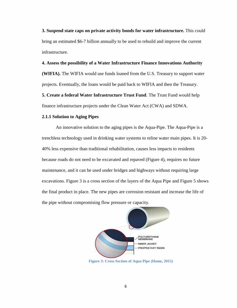
excavations. Figure 3 is a cross section of the layers of the Aqua Pipe and Figure 5 shows
the final product in place. The new pipes are corrosion resistant and increase the life of
the pipe without compromising flow pressure or capacity.
Figure 3: Cross Section of Aqua Pipe (Home, 2015)
7
Installing this system is significantly easier to accomplish because access pits are
only needed at the ends of the section as opposed to digging up the whole pipeline
(Figure 6). The new pipe material is then pulled through the pipe and is cured in place
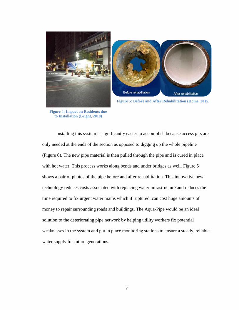
with hot water. This process works along bends and under bridges as well. Figure 5
shows a pair of photos of the pipe before and after rehabilitation. This innovative new
technology reduces costs associated with replacing water infrastructure and reduces the
time required to fix urgent water mains which if ruptured, can cost huge amounts of
money to repair surrounding roads and buildings. The Aqua-Pipe would be an ideal
solution to the deteriorating pipe network by helping utility workers fix potential
weaknesses in the system and put in place monitoring stations to ensure a steady, reliable
water supply for future generations.
Figure 4: Impact on Residents due
to Installation (Bright, 2010)
Figure 5: Before and After Rehabilitation (Home, 2015)

8
2.2 Hardening
Water system hardening is the process of protecting a system by reducing possible
weaknesses or vulnerabilities. It continues to be an important aspect of water resources as
threats of intentional sabotage or contamination rise, regulations expand to include more
contaminants and stricter guidelines, and technology advances. For water distribution
systems, hardening means protecting vulnerable locations from tampering (i.e. treatment
plants, storage tanks, etc.) and reducing the risk of microorganisms contaminating the
water supply.
Updated in 2007, the Key Features to achieve system hardening were developed
by the EPA to “enhance resiliency and promote continuity of service, regardless of the
exact type of hazard or adverse effect a utility might experience (Water: Key Features,
2014).” The Key features are as follows:
Figure 6: Installation Process (Bright, 2010)

9
1. Integrate protective concepts into organizational culture, leadership, and daily
operations.
Protection must be a daily routine supported by senior leadership who are
receptive to employees that may observe suspicious activities or may have concerns
about potential problems. Well informed leadership is a key aspect of this feature.
Leaders are encouraged to stay up to date with advances in security and threat
information while working collaboratively with employees to ensure a safe environment.
2. Identify and support protective program priorities, resources, and utility-specific
measures.
Continuous focus on protective programs requires resources and investments such
as time and effort from managers. Resources should be allocated to the utilities at the
most risk and these resources should be used to determine specific protective program
needs. Metrics should be used to evaluate performance of the protective programs so
adjustments can be made. Self-assessment and progress measurements are vital metrics
that should be evaluated regularly.
3. Employ protocols for detection of contamination.
An overall contamination warning system is made up of monitoring water quality,
sampling and analysis, enhanced security, and monitoring customer complaints. These
aspects help to reduce the public health risk associated with potential contamination
events.
10
4. Assess risks and review vulnerability assessments.
Due to the ever changing threats to water systems, utilities should continually
update and review their vulnerability assessments in order to stay up to date on potential
susceptibilities and possible consequences.
5. Establish facility and information access controls.
Restrictions should be made to utilities to limit access to authorized users only
and controls should be established to detect unauthorized intrusions by physical and
cyber threats. Examples of these controls include fences, motion detectors, security
patrol, changing access codes regularly, inventorying keys, maintaining firewalls, and
denying remote access to data networks.
6. Incorporate resiliency concepts into physical infrastructure.
Utilities should be designed with plans that contribute to overall protection of the
utility while also designing for effective daily operations that ensure the safety of
workers.
7. Prepare, test and update emergency response, recovery and business continuity
plans.
The plans should constantly be updated to manage the evolving threats that
utilities face. These plans should involve emergency services in the larger community
and utilities should test these plans frequently to ensure preparedness of the community
in the event of an emergency.

11
8. Form partnerships with peers and interdependent sectors.
Building relationships with emergency services and managers of critical
infrastructure, such as the power sector, will help people work together to manage an
emergency effectively with a minimal interruption of service.
9. Develop and implement internal and external communication strategies.
Utilities should increase awareness of employees, customers, and the general
public about response plans. This is accomplished through regular communications about
developing strategies. Websites, social media, and annual reports can be great ways to
keep all stakeholders informed.
10. Monitor incidents and threat level information.
Systems that analyze threat information should be developed by utilities so proper
procedures can be followed based on the threat level. Collaboration with local law
enforcement as well as the Federal Bureau of Investigations (FBI) is essential.
The vital characteristics of the Key Features are consistency and flexibility among
all utilities, regardless of size, type of source water, treatment capacity, budget, etc. The
Key Features will help ensure that all utilities are working toward protecting critical
drinking water supplies and that those supplies are monitored to mitigate risks to public
health.
12
2.3 Water Distribution System Components
2.3.1 Water Sources
Drinking water sources are provided by public utilities, commercial entities,
communities, or individuals and are supplied through a distribution system consisting of
pumps and pipes. These water sources can be categorized into groundwater, surface
water, ground water under the direct influence of surface water (GWUDI), and brackish
water.
2.3.1.1 Groundwater
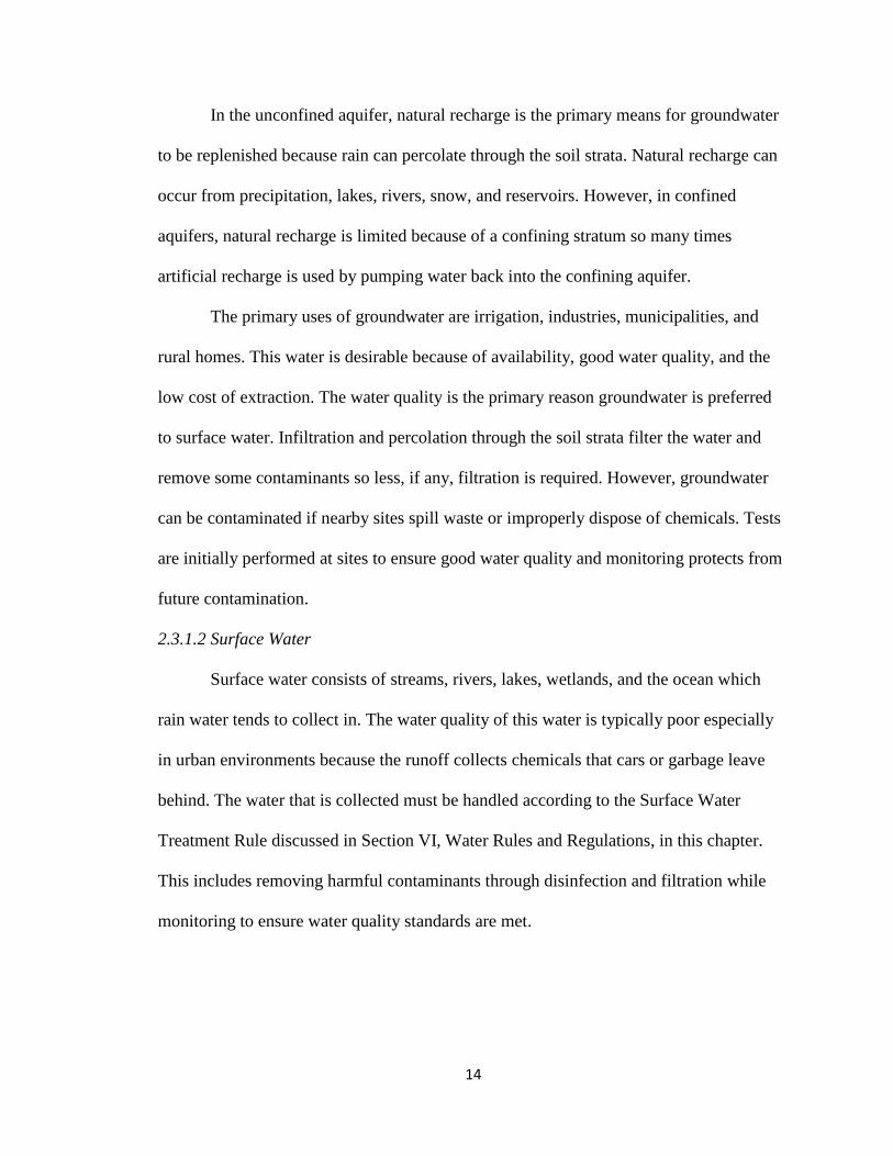
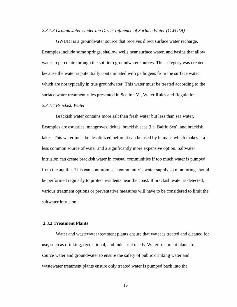
Groundwater is water in all the voids within a geologic layer of fractured rock or
soil. The sources of this groundwater are confined aquifers, unconfined aquifers
including perched water tables, and leaky, or semiconfined aquifers. A confined aquifer
is where impermeable strata covers groundwater so it is under more than atmospheric
pressure as demonstrated by Figure 7. An unconfined aquifer (Figure 8) is where the
water table fluctuates depending on recharge, human use, and permeability. A perched
water table is an unconfined aquifer where water has been trapped by impermeable strata
due to the rise and fall of the water table as seen in Figure 8. Figure 9 is a sketch of a
leaky aquifer, or semiconfined aquifer. This is the most common type and is where a
semiconfining, or semipervious layer, has a permeable strata on top or underneath it.
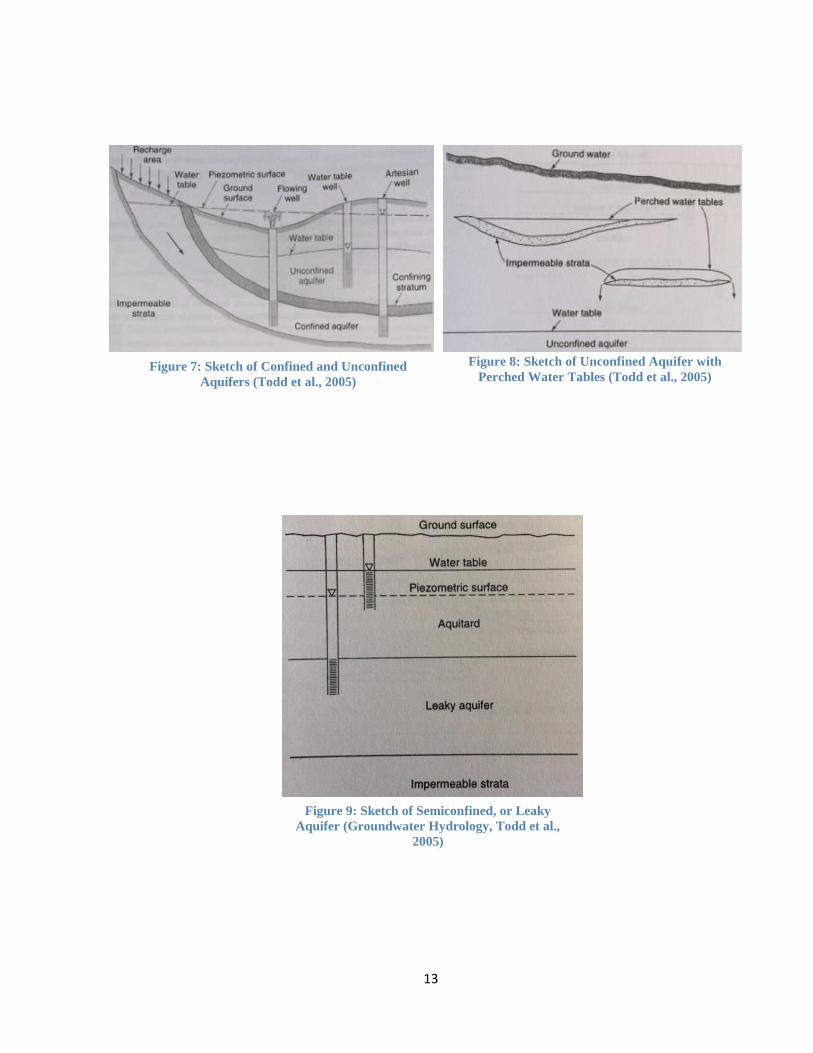
13
Figure 8: Sketch of Unconfined Aquifer with
Perched Water Tables (Todd et al., 2005) Figure 7: Sketch of Confined and Unconfined
Aquifers (Todd et al., 2005)
Figure 9: Sketch of Semiconfined, or Leaky
Aquifer (Groundwater Hydrology, Todd et al.,
2005)
14
In the unconfined aquifer, natural recharge is the primary means for groundwater
to be replenished because rain can percolate through the soil strata. Natural recharge can
occur from precipitation, lakes, rivers, snow, and reservoirs. However, in confined
aquifers, natural recharge is limited because of a confining stratum so many times
artificial recharge is used by pumping water back into the confining aquifer.
The primary uses of groundwater are irrigation, industries, municipalities, and
rural homes. This water is desirable because of availability, good water quality, and the
low cost of extraction. The water quality is the primary reason groundwater is preferred
to surface water. Infiltration and percolation through the soil strata filter the water and
remove some contaminants so less, if any, filtration is required. However, groundwater
can be contaminated if nearby sites spill waste or improperly dispose of chemicals. Tests
are initially performed at sites to ensure good water quality and monitoring protects from
future contamination.
2.3.1.2 Surface Water
Surface water consists of streams, rivers, lakes, wetlands, and the ocean which
rain water tends to collect in. The water quality of this water is typically poor especially
in urban environments because the runoff collects chemicals that cars or garbage leave
behind. The water that is collected must be handled according to the Surface Water
Treatment Rule discussed in Section VI, Water Rules and Regulations, in this chapter.
This includes removing harmful contaminants through disinfection and filtration while
monitoring to ensure water quality standards are met.
15
2.3.1.3 Groundwater Under the Direct Influence of Surface Water (GWUDI)
GWUDI is a groundwater source that receives direct surface water recharge.
Examples include some springs, shallow wells near surface water, and basins that allow
water to percolate through the soil into groundwater sources. This category was created
because the water is potentially contaminated with pathogens from the surface water
which are not typically in true groundwater. This water must be treated according to the
surface water treatment rules presented in Section VI, Water Rules and Regulations.
2.3.1.4 Brackish Water
Brackish water contains more salt than fresh water but less than sea water.
Examples are estuaries, mangroves, deltas, brackish seas (i.e. Baltic Sea), and brackish
lakes. This water must be desalinized before it can be used by humans which makes it a
less common source of water and a significantly more expensive option. Saltwater
intrusion can create brackish water in coastal communities if too much water is pumped
from the aquifer. This can compromise a community’s water supply so monitoring should
be performed regularly to protect residents near the coast. If brackish water is detected,
various treatment options or preventative measures will have to be considered to limit the
saltwater intrusion.
2.3.2 Treatment Plants
Water and wastewater treatment plants ensure that water is treated and cleaned for
use, such as drinking, recreational, and industrial needs. Water treatment plants treat
source water and groundwater to ensure the safety of public drinking water and
wastewater treatment plants ensure only treated water is pumped back into the
16
environment. There is a wide variety of treatment options depending on the quality of
water and thorough sampling is required to determine which method is most viable.
Treatment options include chlorine disinfection, ozone disinfection, ultraviolet (UV)
disinfection, advanced oxidation process (AOP), and many more.
2.3.3 Distribution Network
A water distribution network is composed of many parts that are interconnected in
order to ensure the delivery of clean drinking water. Typically a water treatment plant
receives water from a source such as a lake, river, reservoir, or groundwater. The water is
treated and pumped through main transmission lines to large scale industrial users,
storage reservoirs, or other water users. Water is conveyed from the storage reservoirs to
the public through distribution mains and domestic lines. The network uses a looped
system to distribute the water to ensure a certain level of redundancy in case of an event
that disrupts part of the water distribution network.
2.4 Redundancy
Water distribution systems are built with a certain level of redundancy in order to
operate normally during times of interruption. Such interruptions include maintenance,
power outages, pump failures, intentional attacks, pipe failures, etc. The redundancy can
be observed in a WDS with backup power generators, additional pumps, looped
networks, etc.
Redundancy can be achieved through the basic design of the distribution network,
branched vs looped networks. Branched networks (Figure 10) are less expensive but do
not provide service to customers if a pipe failure were to occur. Looped networks (Figure

17
11) are preferred because even if a pipe failure were to occur, the water can be redirected
to continually provide services. Figure 10 shows a scenario where a pipe failure has
occurred in a branched network and three customers are without service. In contrast,
Figure 11 shows a similar looped network with a pipe failure but no customers are
affected. The benefits of a looped network and the idea of redundancy are easily seen by
the continued service to all customers in Figure 11. The redundancy of the WDS is very
important as it ensures consumer service even if a failure were to occur somewhere in the
system.
2.5 System Residual
With the implementation of the Surface Water Treatment Rule of 1989, a
disinfectant residual must be maintained throughout the water distribution system after
primary disinfection. This residual is typically referred to as secondary disinfection. The
reasons for this residual are to inactive microorganisms, indicate imbalances in the
system, and control biofilm build up. Two problems with residuals are certain microbial
pathogens are resilient, Cryptosporidium, and residuals can react with naturally occurring
materials to form byproducts, trihalomethanes and haloacetic acids. The main secondary
disinfectants are free chlorine, chloramines, and chlorine dioxide. Other secondary
Figure 11: Schematic of Looped Network Figure 10: Schematic of Branched Network
18
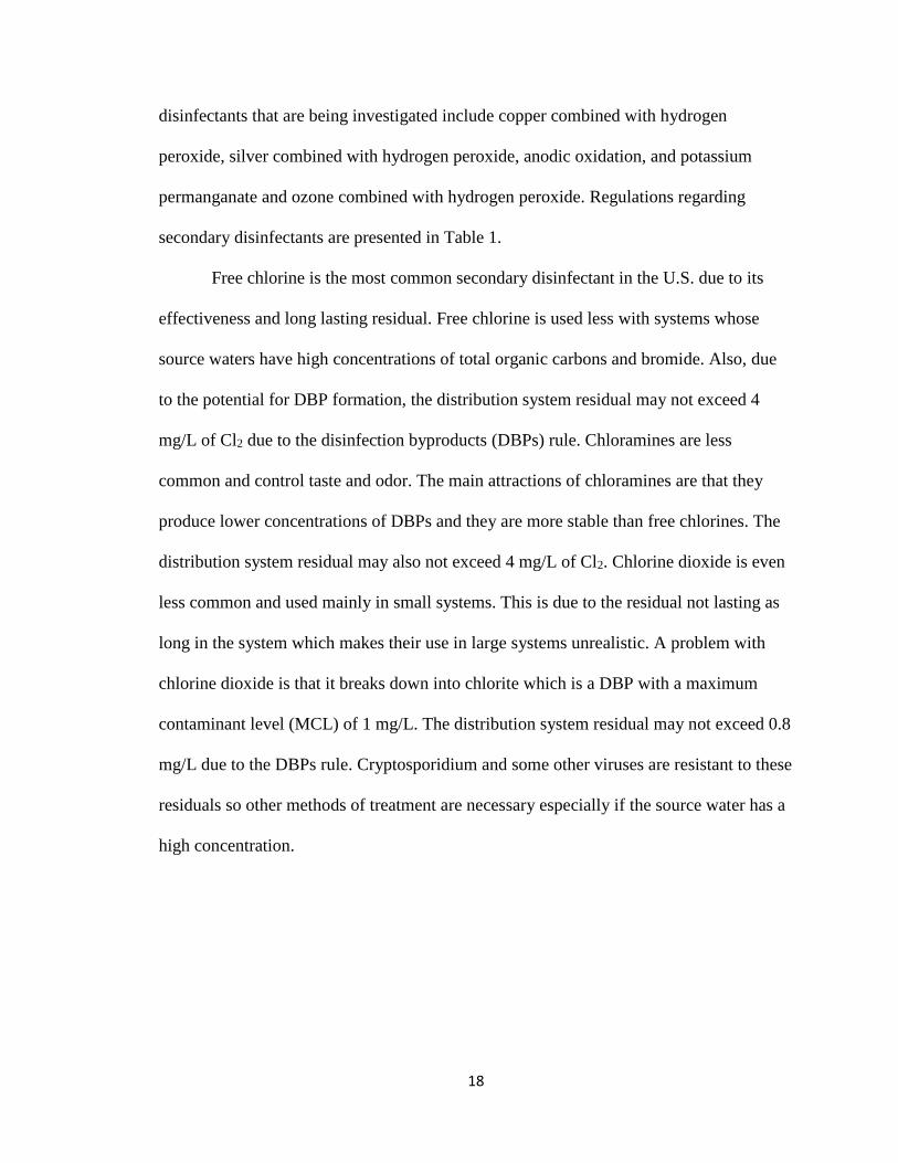
disinfectants that are being investigated include copper combined with hydrogen
peroxide, silver combined with hydrogen peroxide, anodic oxidation, and potassium
permanganate and ozone combined with hydrogen peroxide. Regulations regarding
secondary disinfectants are presented in Table 1.
Free chlorine is the most common secondary disinfectant in the U.S. due to its
effectiveness and long lasting residual. Free chlorine is used less with systems whose
source waters have high concentrations of total organic carbons and bromide. Also, due
to the potential for DBP formation, the distribution system residual may not exceed 4
mg/L of Cl2 due to the disinfection byproducts (DBPs) rule. Chloramines are less
common and control taste and odor. The main attractions of chloramines are that they
produce lower concentrations of DBPs and they are more stable than free chlorines. The
distribution system residual may also not exceed 4 mg/L of Cl2. Chlorine dioxide is even
less common and used mainly in small systems. This is due to the residual not lasting as
long in the system which makes their use in large systems unrealistic. A problem with
chlorine dioxide is that it breaks down into chlorite which is a DBP with a maximum
contaminant level (MCL) of 1 mg/L. The distribution system residual may not exceed 0.8
mg/L due to the DBPs rule. Cryptosporidium and some other viruses are resistant to these
residuals so other methods of treatment are necessary especially if the source water has a
high concentration.
19
Table 1: Regulations for Secondary Disinfectant Residual (HDR)

20
2.6 Water Rules and Regulations
This section presents rules and regulations that increase the safety of the public
drinking water systems throughout the US. These rules are created and implemented by
the EPA in order to provide cleaner drinking water by reducing the risk of microbial
contaminants in the WDS.
2.6.1 Clean Water Act
The Clean Water Act (CWA) was passed through Congress in 1972. This act is a
significant change of the Federal Water Pollution Control Act of 1948. The purpose was
to provide a regulating structure for discharge of pollutants and for quality standards of
waters in the United States. The act forbade the discharge pollutants from a point source,
such as a pipe or ditch, into navigable waters without a National Pollutant Discharge
Elimination System (NPDES) permit. In addition, the act helps to get funding the
construction of sewage treatment plants due to new wastewater standards that the EPA
implemented with the CWA.
2.6.2 Safe Drinking Water Act
The Safe Drinking Water Act (SDWA) of 1974 was created to protect drinking
water and its sources as well as to regulate the nation’s public drinking water supply. The
SDWA is the main federal law that safeguards water quality. Threats to the system
include animal and human waste, pesticides, improperly disposed of chemicals, and
naturally occurring substances. The EPA set national health-based standards for drinking
water quality that applies to all 160,000+ public water systems in the US. These
standards protect drinking water from contaminants and other threats. This does not apply
to private wells that serve less than 25 people. An amendment in 1996 changed the focus

21
of the SDWA from treatment of the water to increasing laws relating to funding for
system improvements, source water protections, and public information. These
components greatly increase the protection of drinking water by ensuring the quality from
source to tap. Another important aspect of the SDWA is the underground injection
control (UIC) program which regulates injection wells that put liquid into the ground for
storage or disposal purposes.
2.6.3 Surface Water Treatment Rules
In order to further increase the safety of drinking water supplies, the EPA created
the surface water treatment rules (SWTR) in conjunction with the disinfectants and
disinfectants byproducts rules. All these rules were developed to decrease the presence of
microbial contaminants in the water and reduce the risk posed by disinfectants and
disinfectant byproducts (DBPs). Figure 11 shows the progression of rules relating to
limiting DBPs. Presented below are the five SWTRs with a brief description of each.
a. Surface Water Treatment Rule of 1989
b. Interim Enhanced Surface Water Treatment Rule of 1998
c. Filter Backwash Recycling Rule of 2001
d. Long Term 1 Enhanced Surface Water Treatment Rule of 2002
e. Long Term 2 Enhanced Surface Water Treatment Rule of 2006
2.6.3.1 Surface Water Treatment Rule of 1989
The SWTR of 1989 requires microbial contaminants to be removed through
filtration and disinfection in surface water and groundwater under the direct influence of
surface water (GWUDI). The rule is intended to decrease public health risk to
contaminants such as viruses, Giardia lamblia, and Legionella by setting maximum
contaminant level goals (MCLGs) at zero mg/L. The goals are set at zero because the
22
presence of the contaminants at source waters and the health risks associated with
exposure. The rule specifies that treatment should be adequate to reduce source water
concentration of Giardia lamblia by 99.9% (3 log removal) and viruses by 99.99% (4 log
removal). The SWTR determines filtration systems performance by measuring turbidity
and requiring a disinfectant residual to be maintained throughout the water system at a
detectable level. The most common residual disinfectant is chlorine but chlorine may
interact with some naturally-occurring materials to create byproducts which could be a
hazard to the health of users. Another important part of the SWTR is the absence of any
control for Cryptosporidium, which has a high resilience to chorine disinfection.
2.6.3.2 Interim Enhanced Surface Water Treatment Rule of 1998
The Interim Enhanced Surface Water Treatment Rule (IESWTR) of 1998
improves public health protection by reducing the risk of microbial contaminants, in
particular, Cryptosporidium and disinfection byproducts. Cryptosporidium is an
important contaminant because of its resistance to chlorine disinfection combined with its
adverse health effects. The IESWTR requires a lower turbidity standard which improves
filtration performance. It also only applies to systems serving greater than 10,000 people
with surface water sources or groundwater under the direct influence of surface water.
2.6.3.3 Filter Backwash Recycling Rule of 2001
The Filter Backwash Recycling Rule (FBRR) requires the filter backwash water
from treatment plants to be recycled. This backwash must be filtered through all
processes of filtration and monitoring data must be sent to the state. The FBRR is
employed to reduce the presence of microbial contaminants in public drinking water
systems.

23
2.6.3.4 Long Term 1 Enhanced Surface Water Treatment Rule of 2002
Long Term 1 Enhanced Surface Water Treatment Rule (LT1) expands the
IESWTR to water systems serving less than 10,000 people. It increases control of
microbial pathogens, such as Cryptosporidium, and addresses additional concerns with
disinfection byproducts. These controls include improving filtration requirements and
requiring systems to determine microbial inactivation. The latter requirement is used for
microbial protection of systems that make changes to avoid disinfection byproducts.
2.6.3.5. Long Term 2 Enhanced Surface Water Treatment Rule of 2006
Long Term 2 Enhanced Surface Water Treatment Rule (LT2) specifies additional
treatment for Cryptosporidium and other microbial contaminants if significant levels are
found at the source waters. This applies to surface water or GWUDI systems. In addition,
the LT2SWTR reduces potential risk from disinfection byproducts by implementing rules
that address the cost/benefit of certain pathogens and DBPs.
24
2.6.4 Drinking Water Strategy
The Drinking Water Strategy (DWS) was developed in 2010 by the EPA to
further increase protection of drinking water from contaminants as well as to promote
speedy and cost-effective new technologies. The DWS has 4 goals as described below:
The first goal is to address contaminants in groups as opposed to individually.
This promotes a cost and time effective means to protect water supplies. Grouping
contaminants like this allows facilities to improve treatment methods more efficiently by
protecting against a greater number of contaminants more easily.
The second goal is to promote new drinking water technologies that will protect
against a wider variety of contaminants. The Water Technology Innovation Cluster was
created to develop, test, and market these new technologies.
The third goal is to use laws to ensure our drinking water is protected. A list of
over 130 chemicals was compiled due to their potential harmful effects to the endocrine
system. This list allows for screening of these chemicals to determine their concentrations
in water sources and determine if additional testing is necessary.
The last goal is to allow for shared access to public water systems monitoring data
between the EPA and states. This will increase the use of advanced information
technologies and will allow states, industry, and consumers to obtain information about
drinking water quality and performance. The sharing of data will also enhance review of
drinking water health issues without further information collecting problems.

25
2.7 Contaminants and Monitoring
2.7.1 Contaminants of Concern
The National Public Drinking Water Regulations have standards for limiting
contaminants in drinking water. Contaminants that may endanger public safety are being
continuously updated to ensure the safety of drinking water systems. There are several
types of contaminants that may put public health at risk and they include microorganisms,
disinfection byproducts, disinfectants, inorganic chemicals, and organic chemicals. Table
2 provides an abbreviated list of the microorganisms that are monitored and their
maximum contaminant level goals (MCLG). A complete list of the contaminants of
concern is located in Appendix B.
Cryptosporidium is particularly important to examine because of its resistance to
chlorine disinfection and history of outbreaks. The most notable outbreak was in
Milwaukee, Wisconsin in 1993 where more than 400,000 people became ill due to the
contaminated drinking water. This contaminated drinking water was linked back to the
city water supply system. The outbreak along with the several other incidents involving
Cryptosporidium around the world has prompted new regulations and monitoring
standards. For more information on the regulations, view section VI of Chapter 2, Water
Rules and Regulations.
26
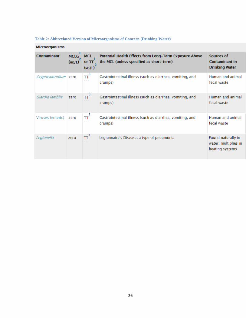
Table 2: Abbreviated Version of Microorganisms of Concern (Drinking Water)

27
2.7.2 Monitoring
The EPA must remain vigilant against all threats to water supplies and this is
accomplished through monitoring water quality. Water quality monitoring includes
sampling and analysis to determine water constituents and current conditions. These
constituents include pollutants that are introduced by humans (oils, pesticides, metals,
microorganisms, etc) and naturally occurring constituents (dissolved oxygen, bacteria,
nutrients, etc). According to the EPA, there are 4 reasons to monitor water quality.
1. Determine if the water is meeting designated usage guidelines. These uses include
fishing, swimming, and drinking. Pollutants must be monitored to ensure that they do not
exceed certain thresholds.
2. Identify specific pollutants and their sources. This allows the EPA to determine
responsible parties if pollutants are introduced into water sources.
3. Access trends in long term monitoring. This helps determine if water sources are
changing due to human involvement and aid in rehabilitating contaminated sources to
natural conditions.
4. Screen for impairment. Monitoring provides an early warning system to users of the
water so pollutants can be contained to mitigate risk to human health.
Due to the wide variety of contaminants, monitoring is performed by using
sensors and instruments that are able to detect changes in baseline water quality. Some of
the factors that the sensors measure are pH, total chlorine, total organic carbon (TOC),
temperature, and turbidity. An important contribution to water quality monitoring is the
development of network based detection systems in order to create a clearer overall
picture of the WDS. In addition to this system, continuous sampling is being

28
implemented to replace sampling every day or every month. The cheap, commercially
available sensors are typically between $5,000 to $10,000 (Hall, 2009), therefore it is
reasonable to assume sensors that continuously monitor water quality and are networked
together may be quite expensive. With new developments in technology and software,
monitoring will become easier to implement and will continue to protect water supplies
from a broad array of contaminants, both naturally occurring and man-made.
When designing a water quality monitoring program, an engineer must use the
monitoring location to determine what pollutants will most likely be associated with that
location. Table 4 shows several examples of sources along with associated pollutants.
Also, volunteer water quality monitoring programs should be involved to ensure
continuously uncontaminated water.
Table 3: Pollutants Associated with Certain Sources (Chapter 5)

29
3. VULNERABILITY ANALYSIS
3.1 Vulnerability Categories
Analyzing various vulnerability categories is an important aspect of determining
possible weaknesses and threats associated with the WDS. According to Haimes and
colleagues (Haimes et al., 1998), the vulnerability categories are as follows.
3.1.1 Physical Threats
Physical threats to water facilities are physical damage to the water system.
Facilities that are at risk include dams, levees, water and wastewater facilities, storage
tanks, pipes, etc. These types of threats can be acts of terrorism or natural disasters.
Possible solutions to these physical threats are designing for natural disasters,
fencing in vital areas, locking doors and gates, installing cameras, maintaining well lit
areas, employee patrols, and using alarm systems. Other procedural controls can be
implemented to deter threats such as changing access codes regularly, requiring
identification cards, inventorying keys, and monitoring contractors and other temporary
workers in the area. These are only a few of the solutions that could help to mitigate
physical threats to critical water infrastructure.
3.1.2 Chemical and Biological Threats
Chemical and biological threats include both intentional and accidental
contamination events that affect the water distribution system. These threats can be the
most dangerous because if the contamination is not detected, thousands of people can be
exposed to the harmful contaminants. Contamination events can include reservoir
contamination, terrorists introducing harmful microorganisms, accidental over- or under-

30
dosing chemicals in the treatment process, and groundwater or surface water
contamination.
3.1.3 Cyber Threats
Water facilities are at risk for cyber intrusion because of their use of industrial
control systems and electronic networks. These systems monitor and control intakes,
sewage collection, water and sewage treatment, effluent discharge, and other processes.
In the event of a cyber-attack, a hacker may use chemicals to overdose or under dose,
discharge untreated sewage, disrupt water distribution, or send tampered or false data to
the operators. This can have serious consequences on users who may receive
contaminated drinking water or swim in waters that have untreated sewage flowing in
them.
Due to several recent cyber intrusions, a more detailed description of cyber
security will be provided. These intrusions include threats that ended in physical damage,
the centrifuges in Iran (Sanger, 2012) where hackers were able to send false data to the
centrifuges in order to make them run faster and ultimately break. Another type of cyber
intrusion is information theft such as the hack on Sony (Pepitone, 2015) where hackers
were able to obtain extensive personal information about individuals in the company. In
recent years, there have been several important measures to reduce cybersecurity risks. In
2008, the “Roadmap to Secure Control Systems in the Water Section” was developed to
provide a 10-yr vision for water facility control systems to remain functional in the event
of a cyber-attack. The document expresses the need for finding ways to detect, respond
to, and mitigate consequences of attacks on the control systems. In response to this, the
American Water Works Association (AWWA) developed guidelines that reduce the risk
31
of cyber-attack by identifying prioritized actions for water and wastewater facilities.
Another measure is to promote information sharing through analysis centers, host
monthly cyber threat briefings to always be informed on evolving threats, and have a
Water Information Sharing and Analysis Center (ISAC) that receives reports on cyber
incidents in order to relay the possible threats to facility operators.
Many techniques have been developed in recent years to ensure minimal
consequences if a cyber-attack occur. The first is to employ manual overrides should
critical systems be compromised. Also, storing water in the distribution system and
having the capability to isolate certain systems from the Internet are important options
that ensure facilities can stay operational during an attack. Another technique is for
facilities to be custom designed which ensures that there are very few common processes
or systems that hackers could use to spread out to multiple facilities and disrupt large
water systems. Finally, chemicals cannot be remotely released and control systems do not
allow operators to perform actions that may endanger containment.
Cybersecurity will always be an important topic but due to recent developments
and safety procedures, it is unlikely that a cyber-attack will cause widespread
contamination with adverse effects on public health or safety. However, an attack may
cause a temporary disruption of normal operations in water and wastewater facilities.
For the research presented in this study, we examine the threat of intentional
chemical or biological contamination in the distribution system because it is the most
likely method that would be employed. This is due to the higher level of cyber security
and the inherent difficulty in physically harming the water infrastructure to a level that
would be significant and far reaching.

32
3.2 Points of Contamination
Water distribution systems are large systems covering many square miles so
intentional and accidental contaminations are inherent. There are numerous points where
contamination is likely and some of these are more susceptible than others. Chemical or
biological contamination is the most serious because of the likeliness of intentional
contamination and widespread distribution. The entry points of possible contamination
are highlighted and briefly discussed below.
3.2.1 Water Treatment Plant
Treatment plants rely on surface water for large scale water systems and
groundwater for smaller, community water systems. According to the EPA, about 68% of
the population is served with water from surface water sources while about 32% of the
population gets their water from groundwater sources. As discussed earlier, surface water
is more easily contaminated than groundwater due to its ease of access. Contaminated
surface or groundwater does not mean the population is at risk due to the strict treatment
and monitoring guidelines set up by the EPA. The regulations ensure that source water
will be properly treated and monitored in order to ensure the safety of the public. Even if
no treatment is available for a specific contaminant, a treatment plant may shutdown to
stop the spread of the contaminant.
3.2.2 Tanks and Reservoirs
For this research, tanks and reservoirs will be a primary target for an intentional
contamination event because these are the easiest to access. This ease of access is due to
their remote locations and limited security. Fencing may be the only line of defense for
the tanks and there is an extensive challenge in constantly surveying the entire reservoir.

33
These systems are desirable as contamination sources because they could quickly affect a
large population. Tanks receive water during low demand periods while delivering water
during high periods which make high demand periods enticing times to contaminate.
3.2.3 Pump Stations
Pump stations are usually protected from tampering or sabotage by reinforced
concrete, steel, and masonry wall construction with no standard windows. Occasionally
some pumping equipment may be located in outside enclosures which increases the
chances of tampering. However, these locations are not constantly monitored so outside
access is still possible. If accessed, the shutdown or tampering of valves may cause
significant problems throughout the system especially if contaminants are allowed to
enter the system at these key locations.
3.2.4 Hydrants
Hydrants are easily accessible to people and the only current means of protection
is hydrant locks which are aftermarket ad-ons. These locks are often only used in places
that have experienced vandalism and are not used “preemptively over broader areas of
the distributions system (Hydrant, 2011).” A possible solution is a check valve which
blocks the backflow so contaminants cannot enter the system while allowing emergency
services access to the hydrants for firefighting capabilities. Another difficult part of
contaminating hydrants is having the proper equipment (portable tank, pump, and motor
assembly) and not attracting unwanted attention which is difficult because the pumping
would be loud and obvious to nearby people. The proximity of hydrants to largely
populated areas is the main reason that this contamination issue is unlikely and will not
be examined in this research.
34
4. METHODOLOGY
4.1 Terminology
4.1.1 Water Fraction
W(i,j) is the fraction of water that contributes to monitoring station i from node j.
An example water distribution network is shown in Figure 12. It shows node
J3000 contributes 85% of its water to monitoring station J4000, therefore,
W(J4000,J3000) = 0.85. It can be assumed that the water quality at J4000 is
representative of the water quality at J3000 if W(i,j) is greater than the coverage criterion.
4.1.2 Coverage
Refers to whether the water quality at a particular node is representative of the source
node. If the water fraction is greater than the coverage criterion then it is covered.
In Figure 12, node J4000 is a coverage of J3000 or node J4000 is covered by
J3000.
4.1.3 Coverage Criterion
A pre-defined criterion to determine if the water quality at one node can represent the
water quality at another.
In this study a coverage criterion of 0.50 is used. The W(J4000,J3000) is 0.85,
meaning that node J4000 is representative of node J3000, or covered by J3000. If the
water fraction were to be less than 0.50 than node J4000 is not representative of J3000.
Since W(J5000, J3000) = 0.15, the water quality at J5000 cannot be representative of the
water quality at J3000 because it is less than the coverage criterion.

35
4.1.4 Coverage Ratio
The ratio of demand covered by the selected monitoring stations to the total demand.
For example, say the set of monitoring stations covers a demand of 905 out of a
total demand of 1000. The coverage ratio of the WDS is calculated to be 0.905 which
means that 90.5% of the total demand is covered by the selected monitoring stations.
4.1.5 Demand Pattern
The usage demands at a single node combined with a demand multiplier that changes
throughout a 24 hour cycle.
Figure 13-16 show the demand patterns used in this study. Demand pattern 2.0
will raise a nodes demand in the morning and at night to simulate peak hours of water
use. While demand pattern 3.0 will raise the demand during the middle of the day (Figure
14).
J4000
J5000
J3000
0.85
0.15
Figure 12: Example WDS
36
4.2 EPANET Theories
EPANET is the software utilized by WaterCAD for the analysis of the system
response to various demands.
4.2.1 Advection Transport Theory
The principal transport mechanism throughout the system is advection while
longitudinal dispersion is negligible under normal operating conditions. This means that a
dissolved substance will travel at the same average velocity in the pipe as the surrounding
fluid while reacting (growing or decaying) at a given rate. No mixing occurs between
adjacent segments of water. This transport mechanism is expressed in the following
equation:
𝜕𝐶𝑖
𝜕𝑡= −𝑢𝑖
𝜕𝐶𝑖
𝜕𝑥+ 𝑟(𝐶𝑖)
(1)
Where: Ci = Concentration (mass/volume) in pipe i
ui = Flow velocity (length/time) in pipe i
r = Rate of reaction (mass/volume/time)
t = Time
x = Longitudinal distance in pipe i
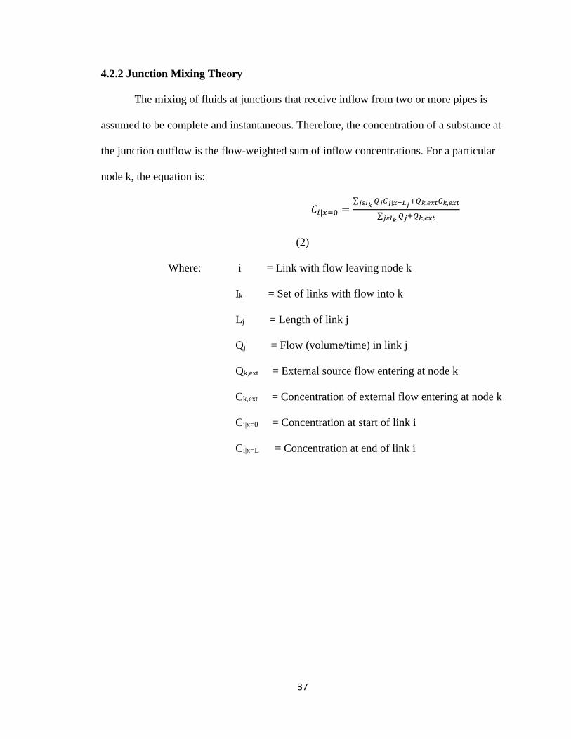
37
4.2.2 Junction Mixing Theory
The mixing of fluids at junctions that receive inflow from two or more pipes is
assumed to be complete and instantaneous. Therefore, the concentration of a substance at
the junction outflow is the flow-weighted sum of inflow concentrations. For a particular
node k, the equation is:
𝐶𝑖|𝑥=0 =∑ 𝑄𝑗𝐶𝑗|𝑥=𝐿𝑗
+𝑄𝑘,𝑒𝑥𝑡𝐶𝑘,𝑒𝑥𝑡𝑗𝜀𝐼𝑘
∑ 𝑄𝑗+𝑄𝑘,𝑒𝑥𝑡𝑗𝜀𝐼𝑘
(2)
Where: i = Link with flow leaving node k
Ik = Set of links with flow into k
Lj = Length of link j
Qj = Flow (volume/time) in link j
Qk,ext = External source flow entering at node k
Ck,ext = Concentration of external flow entering at node k
Ci|x=0 = Concentration at start of link i
Ci|x=L = Concentration at end of link i

38
4.2.3 Storage Mixing Theory
The contents of tanks, reservoirs, and other storage facilities are assumed to be
completely mixed. This is a valid assumption because the tanks operate under fill-and-
draw conditions with minimum momentum flux being conveyed to the inflow (Rossmand
and Grayman, 1999). With this assumption, the contents of the tanks are a mixture of
current contents and inflow water. Due to various reactions, however, the internal
concentration may be changing. The equation that represents the mixing is:
𝜕(𝑉𝑠𝐶𝑠)
𝜕𝑡= ∑ 𝑄𝑖𝐶𝑖|𝑥=𝐿𝑖
− ∑ 𝑄𝑗𝐶𝑠 + 𝑟(𝐶𝑠)𝑗𝜀𝑂𝑠𝐼𝜀𝐼𝑠
(3)
Where: Vs = volume in storage at time t
Cs = concentration within the storage facility
Is = set of links providing flow into facility
Os = set of links withdrawing flow from facility
39
4.2.4 System of Equations
The following conditions are applied to equation 1-3 in order to solve for the
concentration in each pipe as well as the concentration in each storage facility (tank or
reservoir):
initial conditions specifying Ci for all x in each pipe i and Cs in each storage
facility s at t = 0
boundary conditions specifying values for Ck,ext and Qk,ext for all time t at each
node k which has external mass inputs
hydraulic conditions specifying the volume Vs in each storage facility s and the
flow Qi in each link i at all times t
4.2.5 Bulk Flow Reactions
These reactions occur between substances in the pipe or storage facility and the
constituents in the water. For this study the bulk flow is assumed to be zero. This is a
conservative approach because the study is assuming the contaminant does not degrade
throughout the system but rather is primarily traveling by advection. Without
degradation, the contaminant would have a higher concentration when humans consumed
it so the analysis is for a worst case scenario.
4.2.6 Lagrangian Transport Algorithm
A Lagrangian time-based approach is used by EPANET to track discrete water
parcels as they travel and mix together throughout the system. Due to the quick travel
times within pipes, short water quality time steps (minutes) are used instead of the longer
hydraulic time steps (hours).

40
4.3 Number of Optimal Monitoring Stations
The optimal number of monitoring stations is difficult to determine due to limits
in funding and evolving threats to the WDS. The number of monitoring stations should
be at least the same as the number of tanks, if economically feasible, but more would be
recommended for complete coverage. The closest nodes to the tanks will detect
contamination immediately before it spreads throughout the system so these would be the
bare minimum of the monitoring locations. This results in at least seven monitoring
stations for the CITY in this study.
However, if contamination occurred in another point of the distribution system or
along the main transmission line then the optimal locations for monitoring stations would
be different and there should be an increase in the number of nodes being monitored. This
makes it difficult to determine the most vulnerable aspect of the system because it is an
ever-evolving threat. The ultimate number of nodes should be dependent on economic
feasibility as well as inherent risk to the distribution system. In this study, the best 15
monitoring locations in the WDS are determined because these will provide significant
protection at a reasonable cost for a WDS serving 30,000 to 40,000 residents. The
monitoring stations are listed in order of importance in case the CITY cannot afford all
15 but must purchase fewer due to insufficient funding.
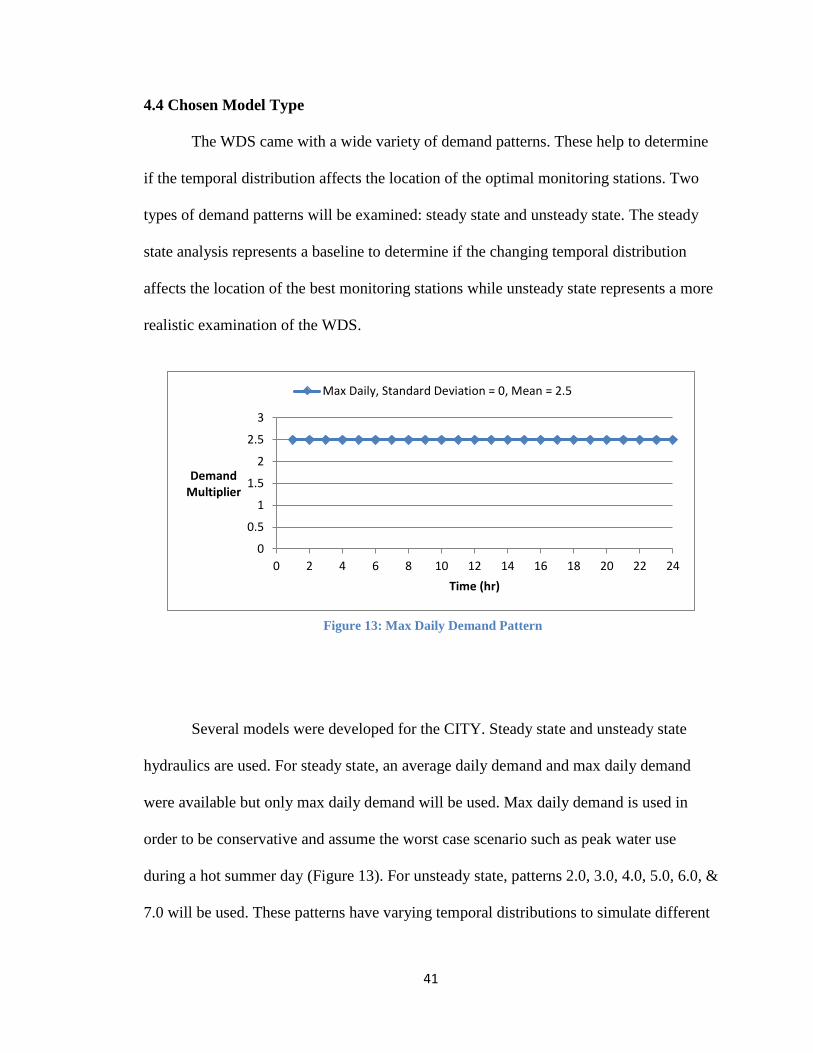
41
4.4 Chosen Model Type
The WDS came with a wide variety of demand patterns. These help to determine
if the temporal distribution affects the location of the optimal monitoring stations. Two
types of demand patterns will be examined: steady state and unsteady state. The steady
state analysis represents a baseline to determine if the changing temporal distribution
affects the location of the best monitoring stations while unsteady state represents a more
realistic examination of the WDS.
Several models were developed for the CITY. Steady state and unsteady state
hydraulics are used. For steady state, an average daily demand and max daily demand
were available but only max daily demand will be used. Max daily demand is used in
order to be conservative and assume the worst case scenario such as peak water use
during a hot summer day (Figure 13). For unsteady state, patterns 2.0, 3.0, 4.0, 5.0, 6.0, &
7.0 will be used. These patterns have varying temporal distributions to simulate different
0
0.5
1
1.5
2
2.5
3
0 2 4 6 8 10 12 14 16 18 20 22 24
Demand Multiplier
Time (hr)
Max Daily, Standard Deviation = 0, Mean = 2.5
Figure 13: Max Daily Demand Pattern
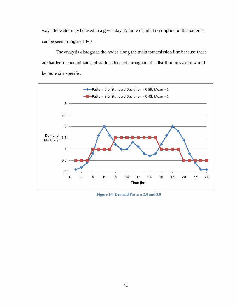
42
ways the water may be used in a given day. A more detailed description of the patterns
can be seen in Figure 14-16.
The analysis disregards the nodes along the main transmission line because these
are harder to contaminate and stations located throughout the distribution system would
be more site specific.
0
0.5
1
1.5
2
2.5
3
0 2 4 6 8 10 12 14 16 18 20 22 24
Demand Multiplier
Time (hr)
Pattern 2.0, Standard Deviation = 0.59, Mean = 1
Pattern 3.0, Standard Deviation = 0.42, Mean = 1
Figure 14: Demand Pattern 2.0 and 3.0
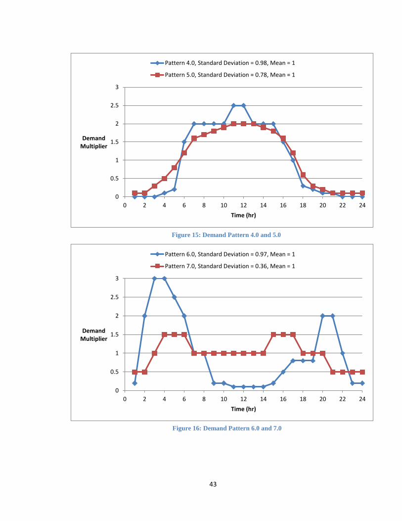
43
0
0.5
1
1.5
2
2.5
3
0 2 4 6 8 10 12 14 16 18 20 22 24
Demand Multiplier
Time (hr)
Pattern 4.0, Standard Deviation = 0.98, Mean = 1
Pattern 5.0, Standard Deviation = 0.78, Mean = 1
0
0.5
1
1.5
2
2.5
3
0 2 4 6 8 10 12 14 16 18 20 22 24
Demand Multiplier
Time (hr)
Pattern 6.0, Standard Deviation = 0.97, Mean = 1
Pattern 7.0, Standard Deviation = 0.36, Mean = 1
Figure 16: Demand Pattern 6.0 and 7.0
Figure 15: Demand Pattern 4.0 and 5.0
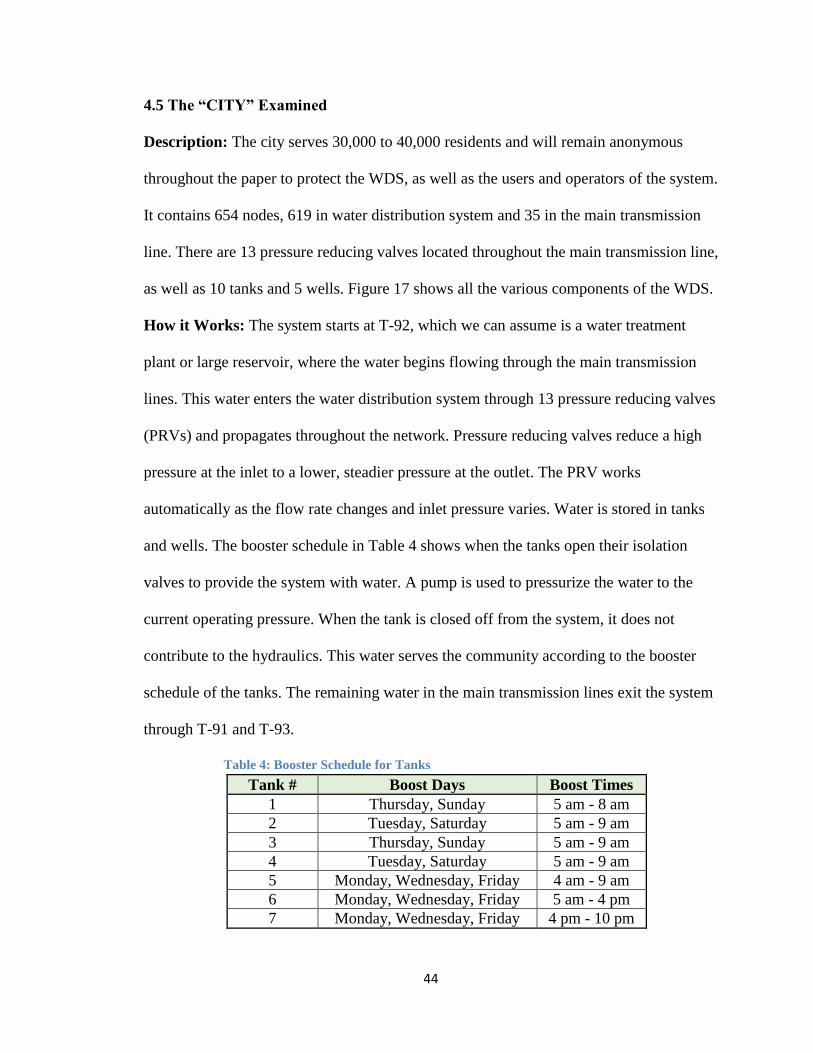
44
4.5 The “CITY” Examined
Description: The city serves 30,000 to 40,000 residents and will remain anonymous
throughout the paper to protect the WDS, as well as the users and operators of the system.
It contains 654 nodes, 619 in water distribution system and 35 in the main transmission
line. There are 13 pressure reducing valves located throughout the main transmission line,
as well as 10 tanks and 5 wells. Figure 17 shows all the various components of the WDS.
How it Works: The system starts at T-92, which we can assume is a water treatment
plant or large reservoir, where the water begins flowing through the main transmission
lines. This water enters the water distribution system through 13 pressure reducing valves
(PRVs) and propagates throughout the network. Pressure reducing valves reduce a high
pressure at the inlet to a lower, steadier pressure at the outlet. The PRV works
automatically as the flow rate changes and inlet pressure varies. Water is stored in tanks
and wells. The booster schedule in Table 4 shows when the tanks open their isolation
valves to provide the system with water. A pump is used to pressurize the water to the
current operating pressure. When the tank is closed off from the system, it does not
contribute to the hydraulics. This water serves the community according to the booster
schedule of the tanks. The remaining water in the main transmission lines exit the system
through T-91 and T-93.
Table 4: Booster Schedule for Tanks
Tank # Boost Days Boost Times
1 Thursday, Sunday 5 am - 8 am
2 Tuesday, Saturday 5 am - 9 am
3 Thursday, Sunday 5 am - 9 am
4 Tuesday, Saturday 5 am - 9 am
5 Monday, Wednesday, Friday 4 am - 9 am
6 Monday, Wednesday, Friday 5 am - 4 pm
7 Monday, Wednesday, Friday 4 pm - 10 pm
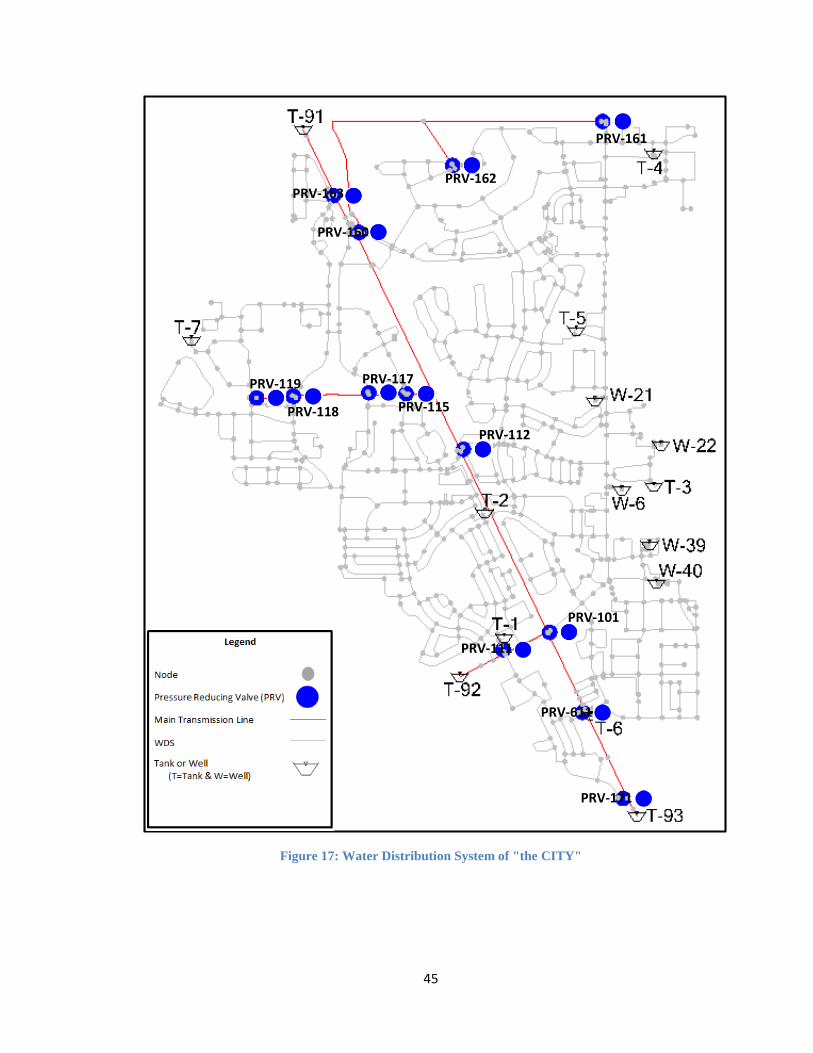
45
Figure 17: Water Distribution System of "the CITY"
PRV-162 PRV-163
PRV-160
PRV-119
PRV-118
PRV-117
PRV-115
PRV-112
PRV-111
PRV-101
PRV-171
PRV-611
PRV-161
46
4.6 Scenarios
4.6.1 Scenario 1: Steady State with Max Daily Demand and Cc=50%
Scenario 1 represents steady state conditions where demand and pump pattern are
fixed. Under these conditions, a node’s representativeness is constant because the system
hydraulics do not change. The scenario does not accurately represent a real life scenario
because the demand throughout a 24 hour duration typically fluctuates with people’s
changing water use. The coverage criterion is 50% for scenario 1-7.
4.6.2 Scenario 2-7: Extended Period Simulation with Cc=50% and Pattern 2.0, 3.0,
4.0, 5.0, 6.0, and 7.0
Scenarios 2-7 are more realistic analogs because water distribution systems run
under extended periods of unsteady hydraulic conditions. The different patterns simulate
varying seasons and alternate usage schedules. They are used to determine how temporal
distribution may affect the optimal locations of the monitoring stations. A node’s
representativeness is more difficult to evaluate in these scenarios because they change
with time, e.g. hourly. Important characteristics to examine with the demand patterns are
the mean and standard deviations. All the means are 1.0 but the standard deviations vary
considerably. This means that the temporal distribution fluctuates which may alter the
demand coverage ratio of the monitoring stations. The higher the standard deviation, the
more the node demand varies which can easily be seen in Figure 16 as one compares
demand pattern 6.0 to 7.0. The standard deviations for pattern 6.0 and 7.0 are 0.97 and
0.36 respectively and pattern 6.0 clearly varies more than pattern 7.0.
4.6.3 Scenario 8: Max Daily Demand and Pattern 2.0 with Cc=25%, 50%, and 75%
This scenario demonstrates how the changing coverage criterion will affect the
location and coverage ratio of monitoring stations for steady and unsteady state
conditions. The coverage criterion is important to examine because if a contaminant is

47
highly concentrated and dangerous in small doses, then a lower coverage criterion may be
used to locate potentially contaminated locations. Note that the coverage criterion does
not affect the demand pattern.
4.6.4 Scenario 9: A Coverage Ratio of 95% is Desired Using Pattern 2.0
This scenario demonstrates a city requesting to have 95% coverage of their WDS.
For this particular city, funds are not the limiting factor so coverage ratio is used. More
monitoring stations can be afforded by some cities due to economics or growth and a
95% coverage ratio adequately protects a city from large outbreaks due to contaminants.
The demand pattern 2.0 is used because it represents the most likely pattern of a city.
4.6.5 Scenario 10: Demand Coverage (DC) vs Demand Coverage Index (DCI)
Methods
The last scenario examines how the demand coverage method compares to the
demand coverage index method. The DC method has weaknesses we have already
discussed but it is still instructive to examine how the two methods compare.
Components to examine are order of the monitoring stations and the demand coverage
ratio.
48
4.7 Summarization of Demand Coverage Index Methodology
This section will include a detailed description of the steps performed in this
analysis as well as a simplified example of the steps required in the DCI method. The
simplified example is in Table 10 and follows the exact methodology as the DCI method
but with 5 nodes as opposed to 619 nodes. The exact process and equations necessary to
calculate the DCI and other results can be seen in the steps preceding the example.
1. A trace analysis is employed for all nodes using EPANET 2.0 in WaterCAD to
construct a water fraction matrix. The trace analysis uses a source, or trace, node to
determine the percent of water contributing to all downstream nodes in the system. The
trace analysis must be employed for every node and results will give an output for every
hour since the water from the source node needs time to propagate through the system.
Also, note a coverage criterion of 50% is used which means nodes with 50% or more
water contributed to them by the source node can be assumed to represent the same water
quality as that source node.
2. WaterCAD outputs are exported to excel. Refer to section VIII, Exporting
WaterCAD Results to Excel, for a more detailed description and example. Table 5 shows
the results of all trace analyses combined on a table for pattern 2.0 at hour 13. A similar
table is created for each hour in the 24 hr duration. The rows in Table 5 represent the
source nodes with the columns showing the percent of water contributing to that
downstream node.
3. WaterCAD outputs are converted to a more usable form in excel with a
coverage criterion of 50%. Since the results are in a percentage, the Cc = 50. If the Cc ≥
50, then the node is covered and it gets a value of 1 and nodes that are not covered are
49
given a 0. Doing this also allows for an easy calculation of results if one alters the
coverage criterion as in scenario 8. The results with a coverage criterion of 50% for
pattern 2.0 at hour 13 is seen in Table 6.
4. A steady state analysis or extended period simulation for hydraulic analyses is
completed using WaterCAD for 7 demand patterns (max, patt 2.0, 3.0, 4.0, 5.0, 6.0, &
7.0).
5. WaterCAD outputs are exported to excel to be used with the water fraction
matrix. The demand at each hour is multiplied by the water fraction matrix for that hour
in order to obtain the demand coverage matrix. The total demand is also calculated for
every node at every hour. Also, note that the demand coverage will be either the demand
from the pattern at that particular hour or 0 depending on if it is covered or not. Table 7 is
the demand coverage matrix after being exported to excel. The demand for demand
pattern 2.0 can be seen by the orange highlighted section and the total demand for every
node can be seen by the yellow highlighted section. A similar table will be created for
every hour, 0-24.
6. All hours of demand coverage are combined on a single table and a demand
coverage ranking of the demand coverage matrix is added. This allows for a better
understanding of which nodes are temporally important throughout the 24 hour duration.
Table 8 shows how this set of data is organized.
7. The total demand coverage index (DCI) is calculated by first determining the
total demand coverage (TDC), accumulation of demand coverage ranking (ADCR), and
normalized cumulative demand coverage ranking (NCDCR) for the full 24 hour duration.
The TDC is the summation of all demand coverages for a single node. The ADCR is the
50
summation of the demand coverage rankings for a single node and is represented by the
equation below. The NCDCR is calculated by dividing the ADCR by the minimum
ADCR of all the nodes. The minimum for the figure below is 37 so for node J8205, the
NCDCR is 1453/37=39.27. DCI is finally calculated for each node based on the below
equations.
𝑇𝐷𝐶 = ∑ 𝐷𝐶𝑘𝑘𝑘=0 𝐴𝐷𝐶𝑅 = ∑ 𝐷𝐶𝑅𝑘
𝑘𝑘=0
𝑁𝐶𝐷𝐶𝑅 =𝑇𝐷𝐶
𝐴𝐷𝐶𝑅𝑚𝑖𝑛 𝐷𝐶𝐼 =
𝑇𝐷𝐶
𝐴𝐷𝐶𝑅
Note, Table 8 and 9 show hr 0-8 for simplification but hr 9-24 are also included. Add a
ranking for the total DCI to determine the nodes with the highest DCI. Table 9 shows the
completed results for the final step in the demand coverage index method.
The Demand Coverage Index method will now be observed in a simplified
example which is seen in Table 10. The example has 4 demand patterns, each
representing 6 hours for a total duration of 24 hours. It gives results for both the Demand
Coverage method, where the total demand coverage (TDC) is maximized, as well as the
Demand Coverage Index method, where the demand coverage index (DCI) is maximized.
The example shows a formatted results table after the trace and hydraulic analysis
is exported to excel and reorganized. Therefore, the example shows a results table for
step 6 and 7 and skips 1-5 because those involved exporting WaterCAD results and
reformatting them into excel. The important information to examine in Table 10 is the
results and how they are calculated and interpreted.
Based on the Demand Coverage method, the best location to put a node is node 3
because the total demand coverage is the highest, 105 units. However, this does not take
into account the change in representativeness that occurs throughout the 24 hour time
51
period. Node 3 best reflects the water quality for the first 6 hrs as seen by the demand
coverage ranking (DCR) of 1 for pattern 1 and node 4 best reflects the water quality for
the remaining 18 hrs. Therefore, node 4 has a better representativeness than node 3 even
though node 3 has a slightly higher TDC. The optimal location of the monitoring station
should be node 4, not node 3, and this weakness in the DC method is due to the fact that
it ignores the temporal distribution and only takes into account the demand covered. The
Demand Coverage Index method is the best indicator to pinpoint the optimal locations
based on the temporal distribution and the total demand covered by a monitoring station.
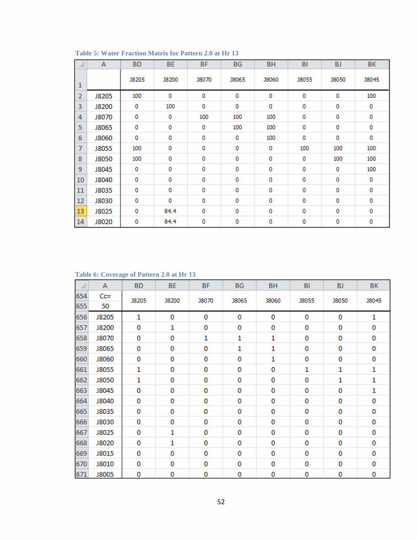
52
Table 5: Water Fraction Matrix for Pattern 2.0 at Hr 13
Table 6: Coverage of Pattern 2.0 at Hr 13
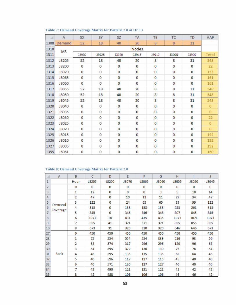
53
Table 7: Demand Coverage Matrix for Pattern 2.0 at Hr 13
Table 8: Demand Coverage Matrix for Pattern 2.0
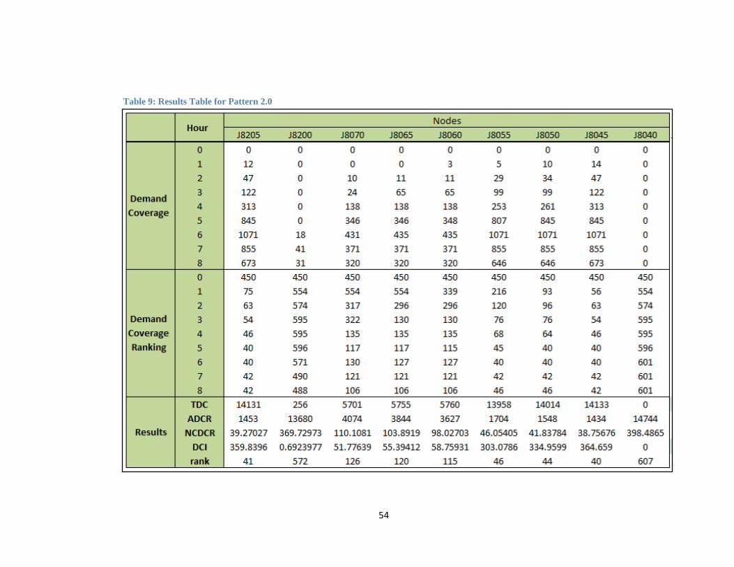
54
Table 9: Results Table for Pattern 2.0

55
Table 10: Example of Demand Coverage and Demand Coverage Index Methods
Keys to Table 5: Demand Coverage (GPM) Demand Coverage Ranking TDC: Total Demand Coverage ADCR: Accumulated Demand Coverage Ranking NCDCR: Normalized Cumulative Demand Coverage Ranking DCI: Demand Coverage Index
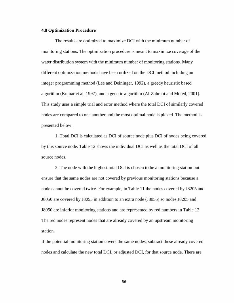
56
4.8 Optimization Procedure
The results are optimized to maximize DCI with the minimum number of
monitoring stations. The optimization procedure is meant to maximize coverage of the
water distribution system with the minimum number of monitoring stations. Many
different optimization methods have been utilized on the DCI method including an
integer programming method (Lee and Deininger, 1992), a greedy heuristic based
algorithm (Kumar et al, 1997), and a genetic algorithm (Al-Zahrani and Moied, 2001).
This study uses a simple trial and error method where the total DCI of similarly covered
nodes are compared to one another and the most optimal node is picked. The method is
presented below:
1. Total DCI is calculated as DCI of source node plus DCI of nodes being covered
by this source node. Table 12 shows the individual DCI as well as the total DCI of all
source nodes.
2. The node with the highest total DCI is chosen to be a monitoring station but
ensure that the same nodes are not covered by previous monitoring stations because a
node cannot be covered twice. For example, in Table 11 the nodes covered by J8205 and
J8050 are covered by J8055 in addition to an extra node (J8055) so nodes J8205 and
J8050 are inferior monitoring stations and are represented by red numbers in Table 12.
The red nodes represent nodes that are already covered by an upstream monitoring
station.
If the potential monitoring station covers the same nodes, subtract these already covered
nodes and calculate the new total DCI, or adjusted DCI, for that source node. There are
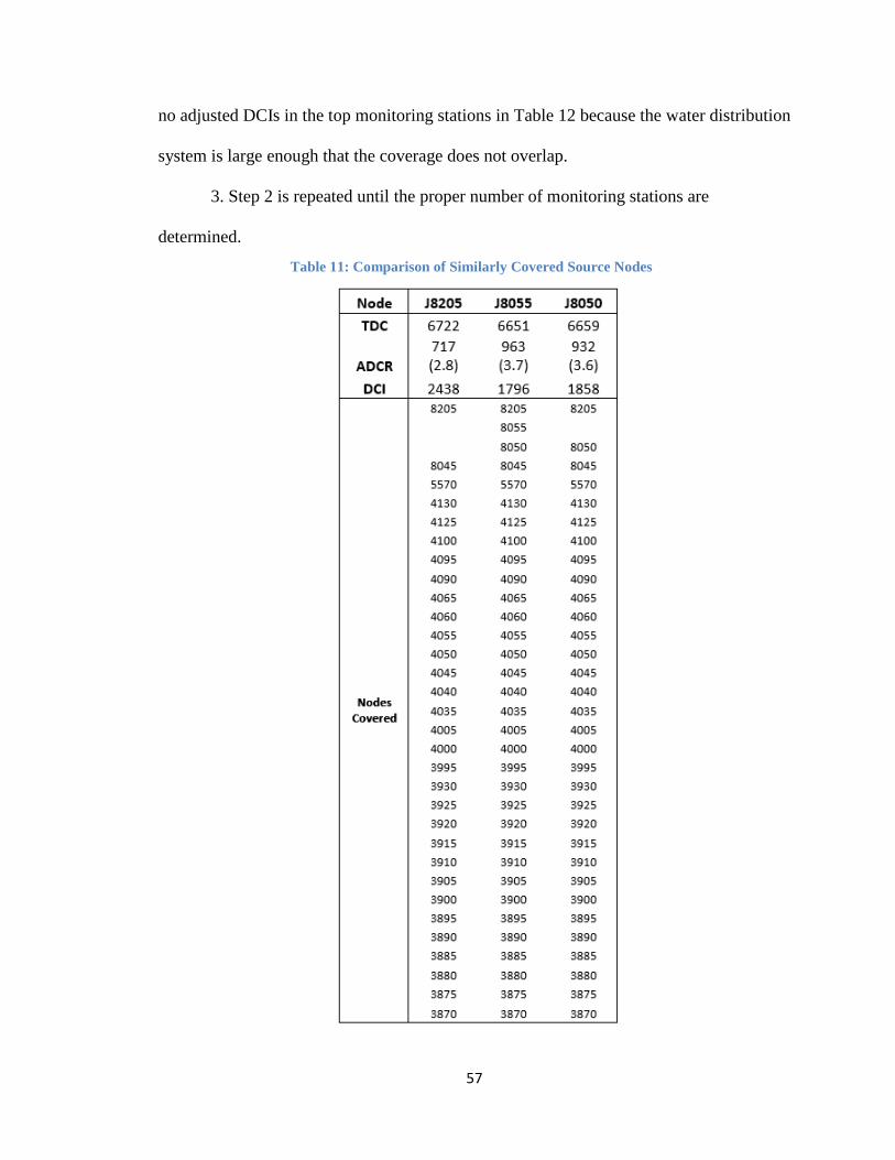
57
no adjusted DCIs in the top monitoring stations in Table 12 because the water distribution
system is large enough that the coverage does not overlap.
3. Step 2 is repeated until the proper number of monitoring stations are
determined.
Table 11: Comparison of Similarly Covered Source Nodes

58
Table 12: Final Output for Optimization Procedure for Pattern 2.0

59
4.9 Exporting WaterCAD Results to Excel
The trace percent and demand data from WaterCAD needs to be exported into an
excel file in order to perform an analysis. The first step is to modify the flex table for the
junctions to include trace percent and demand when performing the steady state or
extended period simulations. This is done by using the edit feature at the top of the flex
table. All categories should be removed in order to limit the amount of data being
analyzed and to speed up the exporting process. The categories of importance are trace
(%) when performing the trace analysis and demand (gpm) when performing the steady
state or extended period simulation analysis. For the trace percent, all time steps are
required to do a proper analysis. This is achieved at the top of the flextable by looking at
the results options and selecting report all time steps. A report is generated but the format
does not allow for proper analysis and must be exported to an excel file. Under file and
export document, a few options are available to export the document but an excel file is
the desired format. The WaterCAD output will look similar to Table 13.
In order to efficiently format the data, macros are necessary to rearrange the data
into a useful form. Excel makes creating macros simple by selecting record macro under
the developer tab and inputting a desired keystroke for that particular macro. The desired
transferring of data is completed and then the stop macro button is selected. That macro
will now occur every time the associated keystroke is pressed.

60
An example macro is the trace analysis to water fraction matrix transformation.
Table 14 is the WaterCAD output of a trace analysis for node J8205 after being exported
to excel. The output contains the trace analysis for hour 0-24 but only hr 13 is seen in the
table. This data needs to be arranged into a more accessible table; therefore, a macro will
be used due to the large amounts of data and repetitious nature of the transformation. The
macro takes the WaterCAD output arranged in columns and transforms them into rows
Table 13: WaterCAD Output for Trace % and Demand at Hour 12

61
Table 14: WaterCAD Output in Excel (Pre-Macro)
with each hour getting its own tab in excel. Each WaterCAD output is only for one node
however so the macro has to be used 619 times. Table 15 shows the results of the macro
after all nodes have been transferred. This is the water fraction matrix for hr 13 but one is
created for each hour. The highlighted region of the tables show how the macro functions
for hr 13.

62
Problems that may occur with the macro are too much data to format and the data
is automatically converted to text. The first problem is addressed by dividing the macro
into several macros to reduce how much data is changed under a specific keystroke. The
trace percent reformatting requires the use of 4 keystrokes to complete the macro. The
text problem can be solved by changing all values formatted as text to numerical values
by hand. The text values created problems because calculations cannot be done with the
text data so the analysis can be temporarily delayed by this problem.
Table 15: Water Fraction Matrix for Hr 13 (Post-Macro)
63
4.10 Summary and Discussion of Results
4.10.1 Scenario 1: Max Daily Demand
The results for scenario 1 and 2-7 will be presented together due to the many
similarities.
4.10.2 Scenario 2-7 Demand Pattern 2.0, 3.0, 4.0, 5.0, 6.0, & 7.0
The optimal locations of the monitoring stations for max daily demand, demand
pattern 2.0, 3.0, 4.0, 5.0, 6.0, & 7.0 are identical; however, the order of importance is
slightly different for several of the patterns. This is only relevant if funding is limited and
fewer than 15 monitoring stations will be built. Tables 16-22 give a detailed look at the
monitoring stations and corresponding coverage ratio for the desired number of
monitoring stations.
The result verifies that the temporal distribution of the different patterns does not
affect the representativeness of a significant node. A monitoring station location will be
the same regardless if the peak demand is in the middle of the day or if it peaks in the
morning and at night. This is an ideal result because throughout a year, the demand
pattern may change with seasons and varying usage schedule but this method shows that
the location of the monitoring stations will remain the same and provide significant
monitoring capabilities.
The coverage ratios vary from about 88% to 91% which means about 90% of the
total network demand can be monitored depending on the demand pattern being used.
This is an important result because if one demand pattern had a coverage ratio that is
significantly less, then the monitoring stations would be significantly less effective for
that day or season. This would be a huge weakness that could be exploited to disrupt or
infect the whole system without detection. Depending on the funding available for a
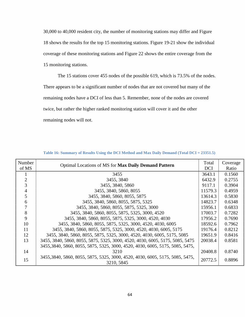
64
30,000 to 40,000 resident city, the number of monitoring stations may differ and Figure
18 shows the results for the top 15 monitoring stations. Figure 19-21 show the individual
coverage of these monitoring stations and Figure 22 shows the entire coverage from the
15 monitoring stations.
The 15 stations cover 455 nodes of the possible 619, which is 73.5% of the nodes.
There appears to be a significant number of nodes that are not covered but many of the
remaining nodes have a DCI of less than 5. Remember, none of the nodes are covered
twice, but rather the higher ranked monitoring station will cover it and the other
remaining nodes will not.
Table 16: Summary of Results Using the DCI Method and Max Daily Demand (Total DCI = 23351.5)
Number
of MS Optimal Locations of MS for Max Daily Demand Pattern
Total
DCI
Coverage
Ratio
1 3455 3643.1 0.1560
2 3455, 3840 6432.9 0.2755
3 3455, 3840, 5860 9117.1 0.3904
4 3455, 3840, 5860, 8055 11579.3 0.4959
5 3455, 3840, 5860, 8055, 5875 13614.3 0.5830
6 3455, 3840, 5860, 8055, 5875, 5325 14823.7 0.6348
7 3455, 3840, 5860, 8055, 5875, 5325, 3000 15956.1 0.6833
8 3455, 3840, 5860, 8055, 5875, 5325, 3000, 4520 17003.7 0.7282
9 3455, 3840, 5860, 8055, 5875, 5325, 3000, 4520, 4030 17956.2 0.7690
10 3455, 3840, 5860, 8055, 5875, 5325, 3000, 4520, 4030, 6005 18592.6 0.7962
11 3455, 3840, 5860, 8055, 5875, 5325, 3000, 4520, 4030, 6005, 5175 19176.4 0.8212
12 3455, 3840, 5860, 8055, 5875, 5325, 3000, 4520, 4030, 6005, 5175, 5085 19651.9 0.8416
13 3455, 3840, 5860, 8055, 5875, 5325, 3000, 4520, 4030, 6005, 5175, 5085, 5475 20038.4 0.8581
14
3455,3840, 5860, 8055, 5875, 5325, 3000, 4520, 4030, 6005, 5175, 5085, 5475,
3210 20408.8 0.8740
15 3455,3840, 5860, 8055, 5875, 5325, 3000, 4520, 4030, 6005, 5175, 5085, 5475,
3210, 5845 20772.5 0.8896
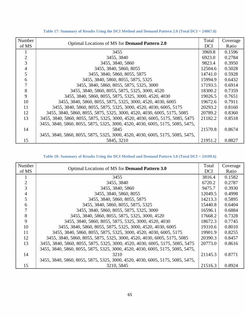
65
Table 17: Summary of Results Using the DCI Method and Demand Pattern 2.0 (Total DCI = 24867.8)
Number
of MS Optimal Locations of MS for Demand Pattern 2.0
Total
DCI
Coverage
Ratio
1 3455 3969.8 0.1596
2 3455, 3840 6923.0 0.2784
3 3455, 3840, 5860 9823.4 0.3950
4 3455, 3840, 5860, 8055 12504.6 0.5028
5 3455, 3840, 5860, 8055, 5875 14741.0 0.5928
6 3455, 3840, 5860, 8055, 5875, 5325 15994.9 0.6432
7 3455, 3840, 5860, 8055, 5875, 5325, 3000 17193.5 0.6914
8 3455, 3840, 5860, 8055, 5875, 5325, 3000, 4520 18300.2 0.7359
9 3455, 3840, 5860, 8055, 5875, 5325, 3000, 4520, 4030 19026.5 0.7651
10 3455, 3840, 5860, 8055, 5875, 5325, 3000, 4520, 4030, 6005 19672.6 0.7911
11 3455, 3840, 5860, 8055, 5875, 5325, 3000, 4520, 4030, 6005, 5175 20293.2 0.8160
12 3455, 3840, 5860, 8055, 5875, 5325, 3000, 4520, 4030, 6005, 5175, 5085 20789.2 0.8360
13 3455, 3840, 5860, 8055, 5875, 5325, 3000, 4520, 4030, 6005, 5175, 5085, 5475 21182.2 0.8518
14
3455, 3840, 5860, 8055, 5875, 5325, 3000, 4520, 4030, 6005, 5175, 5085, 5475,
5845 21570.8 0.8674
15
3455, 3840, 5860, 8055, 5875, 5325, 3000, 4520, 4030, 6005, 5175, 5085, 5475,
5845, 3210 21951.2 0.8827
Table 18: Summary of Results Using the DCI Method and Demand Pattern 3.0 (Total DCI = 24109.6)
Number
of MS Optimal Locations of MS for Demand Pattern 3.0
Total
DCI
Coverage
Ratio
1 3455 3816.4 0.1582
2 3455, 3840 6720.2 0.2787
3 3455, 3840, 5860 9475.7 0.3930
4 3455, 3840, 5860, 8055 12049.5 0.4998
5 3455, 3840, 5860, 8055, 5875 14213.3 0.5895
6 3455, 3840, 5860, 8055, 5875, 5325 15440.8 0.6404
7 3455, 3840, 5860, 8055, 5875, 5325, 3000 16596.1 0.6884
8 3455, 3840, 5860, 8055, 5875, 5325, 3000, 4520 17668.2 0.7328
9 3455, 3840, 5860, 8055, 5875, 5325, 3000, 4520, 4030 18672.3 0.7745
10 3455, 3840, 5860, 8055, 5875, 5325, 3000, 4520, 4030, 6005 19310.6 0.8010
11 3455, 3840, 5860, 8055, 5875, 5325, 3000, 4520, 4030, 6005, 5175 19901.9 0.8255
12 3455, 3840, 5860, 8055, 5875, 5325, 3000, 4520, 4030, 6005, 5175, 5085 20390.3 0.8457
13 3455, 3840, 5860, 8055, 5875, 5325, 3000, 4520, 4030, 6005, 5175, 5085, 5475 20773.0 0.8616
14
3455, 3840, 5860, 8055, 5875, 5325, 3000, 4520, 4030, 6005, 5175, 5085, 5475,
3210 21145.3 0.8771
15
3455, 3840, 5860, 8055, 5875, 5325, 3000, 4520, 4030, 6005, 5175, 5085, 5475,
3210, 5845 21516.3 0.8924
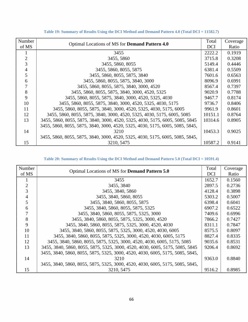
66
Table 19: Summary of Results Using the DCI Method and Demand Pattern 4.0 (Total DCI = 11582.7)
Number
of MS Optimal Locations of MS for Demand Pattern 4.0
Total
DCI
Coverage
Ratio
1 3455 2222.2 0.1919
2 3455, 5860 3715.8 0.3208
3 3455, 5860, 8055 5149.4 0.4446
4 3455, 5860, 8055, 5875 6381.4 0.5509
5 3455, 5860, 8055, 5875, 3840 7601.6 0.6563
6 3455, 5860, 8055, 5875, 3840, 3000 8096.9 0.6991
7 3455, 5860, 8055, 5875, 3840, 3000, 4520 8567.4 0.7397
8 3455, 5860, 8055, 5875, 3840, 3000, 4520, 5325 9020.9 0.7788
9 3455, 5860, 8055, 5875, 3840, 3000, 4520, 5325, 4030 9467.7 0.8174
10 3455, 5860, 8055, 5875, 3840, 3000, 4520, 5325, 4030, 5175 9736.7 0.8406
11 3455, 5860, 8055, 5875, 3840, 3000, 4520, 5325, 4030, 5175, 6005 9961.9 0.8601
12 3455, 5860, 8055, 5875, 3840, 3000, 4520, 5325, 4030, 5175, 6005, 5085 10151.1 0.8764
13 3455, 5860, 8055, 5875, 3840, 3000, 4520, 5325, 4030, 5175, 6005, 5085, 5845 10314.6 0.8905
14
3455, 5860, 8055, 5875, 3840, 3000, 4520, 5325, 4030, 5175, 6005, 5085, 5845,
3210 10453.3 0.9025
15
3455, 5860, 8055, 5875, 3840, 3000, 4520, 5325, 4030, 5175, 6005, 5085, 5845,
3210, 5475 10587.2 0.9141
Table 20: Summary of Results Using the DCI Method and Demand Pattern 5.0 (Total DCI = 10591.4)
Number
of MS Optimal Locations of MS for Demand Pattern 5.0
Total
DCI
Coverage
Ratio
1 3455 1652.7 0.1560
2 3455, 3840 2897.5 0.2736
3 3455, 3840, 5860 4128.4 0.3898
4 3455, 3840, 5860, 8055 5303.2 0.5007
5 3455, 3840, 5860, 8055, 5875 6398.4 0.6041
6 3455, 3840, 5860, 8055, 5875, 5325 6907.2 0.6522
7 3455, 3840, 5860, 8055, 5875, 5325, 3000 7409.6 0.6996
8 3455, 3840, 5860, 8055, 5875, 5325, 3000, 4520 7866.2 0.7427
9 3455, 3840, 5860, 8055, 5875, 5325, 3000, 4520, 4030 8311.1 0.7847
10 3455, 3840, 5860, 8055, 5875, 5325, 3000, 4520, 4030, 6005 8575.5 0.8097
11 3455, 3840, 5860, 8055, 5875, 5325, 3000, 4520, 4030, 6005, 5175 8827.4 0.8335
12 3455, 3840, 5860, 8055, 5875, 5325, 3000, 4520, 4030, 6005, 5175, 5085 9035.6 0.8531
13 3455, 3840, 5860, 8055, 5875, 5325, 3000, 4520, 4030, 6005, 5175, 5085, 5845 9206.4 0.8692
14
3455, 3840, 5860, 8055, 5875, 5325, 3000, 4520, 4030, 6005, 5175, 5085, 5845,
3210 9363.0 0.8840
15
3455, 3840, 5860, 8055, 5875, 5325, 3000, 4520, 4030, 6005, 5175, 5085, 5845,
3210, 5475 9516.2 0.8985
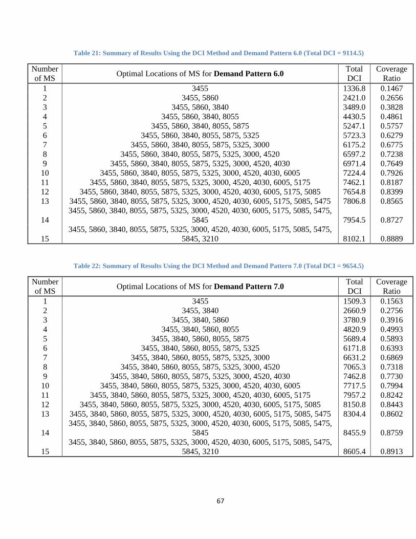
67
Table 21: Summary of Results Using the DCI Method and Demand Pattern 6.0 (Total DCI = 9114.5)
Number
of MS Optimal Locations of MS for Demand Pattern 6.0
Total
DCI
Coverage
Ratio
1 3455 1336.8 0.1467
2 3455, 5860 2421.0 0.2656
3 3455, 5860, 3840 3489.0 0.3828
4 3455, 5860, 3840, 8055 4430.5 0.4861
5 3455, 5860, 3840, 8055, 5875 5247.1 0.5757
6 3455, 5860, 3840, 8055, 5875, 5325 5723.3 0.6279
7 3455, 5860, 3840, 8055, 5875, 5325, 3000 6175.2 0.6775
8 3455, 5860, 3840, 8055, 5875, 5325, 3000, 4520 6597.2 0.7238
9 3455, 5860, 3840, 8055, 5875, 5325, 3000, 4520, 4030 6971.4 0.7649
10 3455, 5860, 3840, 8055, 5875, 5325, 3000, 4520, 4030, 6005 7224.4 0.7926
11 3455, 5860, 3840, 8055, 5875, 5325, 3000, 4520, 4030, 6005, 5175 7462.1 0.8187
12 3455, 5860, 3840, 8055, 5875, 5325, 3000, 4520, 4030, 6005, 5175, 5085 7654.8 0.8399
13 3455, 5860, 3840, 8055, 5875, 5325, 3000, 4520, 4030, 6005, 5175, 5085, 5475 7806.8 0.8565
14
3455, 5860, 3840, 8055, 5875, 5325, 3000, 4520, 4030, 6005, 5175, 5085, 5475,
5845 7954.5 0.8727
15
3455, 5860, 3840, 8055, 5875, 5325, 3000, 4520, 4030, 6005, 5175, 5085, 5475,
5845, 3210 8102.1 0.8889
Table 22: Summary of Results Using the DCI Method and Demand Pattern 7.0 (Total DCI = 9654.5)
Number
of MS Optimal Locations of MS for Demand Pattern 7.0
Total
DCI
Coverage
Ratio
1 3455 1509.3 0.1563
2 3455, 3840 2660.9 0.2756
3 3455, 3840, 5860 3780.9 0.3916
4 3455, 3840, 5860, 8055 4820.9 0.4993
5 3455, 3840, 5860, 8055, 5875 5689.4 0.5893
6 3455, 3840, 5860, 8055, 5875, 5325 6171.8 0.6393
7 3455, 3840, 5860, 8055, 5875, 5325, 3000 6631.2 0.6869
8 3455, 3840, 5860, 8055, 5875, 5325, 3000, 4520 7065.3 0.7318
9 3455, 3840, 5860, 8055, 5875, 5325, 3000, 4520, 4030 7462.8 0.7730
10 3455, 3840, 5860, 8055, 5875, 5325, 3000, 4520, 4030, 6005 7717.5 0.7994
11 3455, 3840, 5860, 8055, 5875, 5325, 3000, 4520, 4030, 6005, 5175 7957.2 0.8242
12 3455, 3840, 5860, 8055, 5875, 5325, 3000, 4520, 4030, 6005, 5175, 5085 8150.8 0.8443
13 3455, 3840, 5860, 8055, 5875, 5325, 3000, 4520, 4030, 6005, 5175, 5085, 5475 8304.4 0.8602
14
3455, 3840, 5860, 8055, 5875, 5325, 3000, 4520, 4030, 6005, 5175, 5085, 5475,
5845 8455.9 0.8759
15
3455, 3840, 5860, 8055, 5875, 5325, 3000, 4520, 4030, 6005, 5175, 5085, 5475,
5845, 3210 8605.4 0.8913

68
Figure 18: Top 15 Monitoring Stations
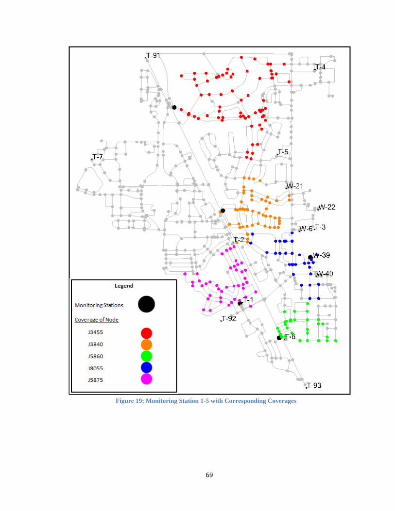
69
Figure 19: Monitoring Station 1-5 with Corresponding Coverages
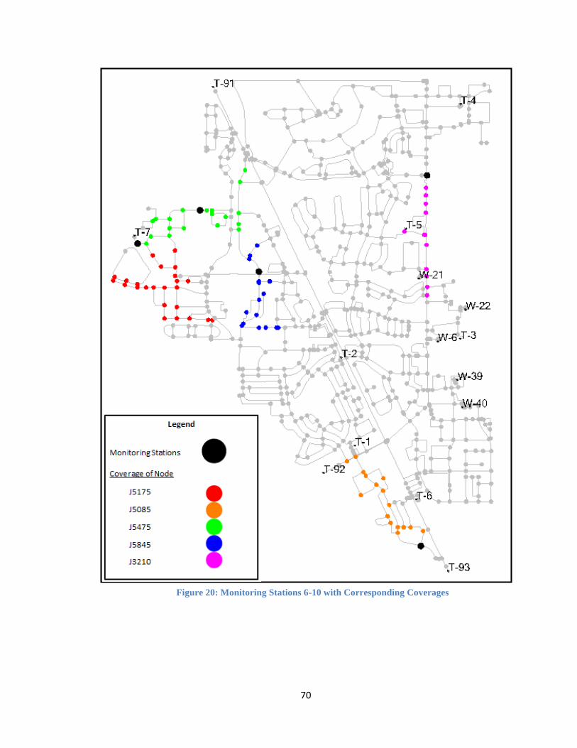
70
Figure 20: Monitoring Stations 6-10 with Corresponding Coverages
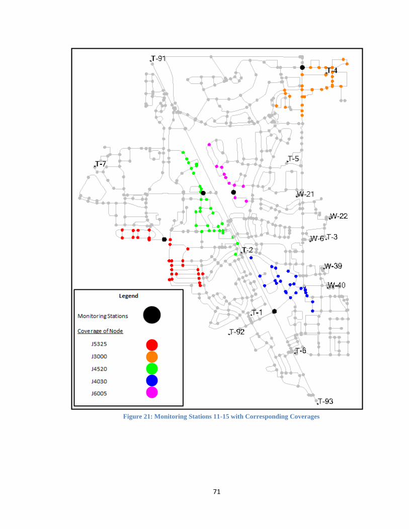
71
Figure 21: Monitoring Stations 11-15 with Corresponding Coverages
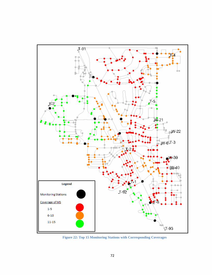
72
Figure 22: Top 15 Monitoring Stations with Corresponding Coverages
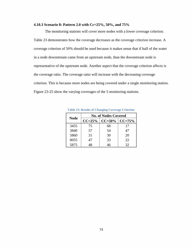
73
4.10.3 Scenario 8: Pattern 2.0 with Cc=25%, 50%, and 75%
The monitoring stations will cover more nodes with a lower coverage criterion.
Table 23 demonstrates how the coverage decreases as the coverage criterion increase. A
coverage criterion of 50% should be used because it makes sense that if half of the water
in a node downstream came from an upstream node, than the downstream node is
representative of the upstream node. Another aspect that the coverage criterion affects is
the coverage ratio. The coverage ratio will increase with the decreasing coverage
criterion. This is because more nodes are being covered under a single monitoring station.
Figure 23-25 show the varying coverages of the 5 monitoring stations.
Node No. of Nodes Covered
CC=25% CC=50% CC=75%
3455 75 68 17
3840 57 54 47
5860 31 30 20
8055 47 33 22
5875 48 46 32
Table 23: Results of Changing Coverage Criterion

74
Figure 23: MSs 1-5 with Cc=25% Figure 24: MSs 1-5 with Cc=50% Figure 25: MSs 1-5 with Cc=75%

75
4.10.4 Scenario 9: 95% Coverage Ratio
In reply to a city’s request for added protection due to increased funds, 22
monitoring stations would be needed to achieve a coverage ratio of 95.3% as seen in table
24. Demand pattern 2.0 was used in this analysis but the different temporal distributions
will not vary significantly as demonstrated by the results of scenario 1-7. These
additional monitoring stations represent enhanced protection a city can employ in the
WDS if funds are available. 549 of the 619 nodes are covered, or 88.7%, with all but 17
having a DCI of less than 5. Figure 26 and 27 show the additional coverage of monitoring
stations 16-22. Figure 28 shows all 22 monitoring stations for this city with
corresponding coverages.
Table 24: Results for Additional MS’s in Order to Achieve a 95% Coverage Ratio (Total
DCI =24867.8)
Number
of MS Additional Optimal Locations of MS for Demand Pattern 2.0
Total
DCI
Coverage
Ratio
16 8005 22276.7 0.8958
17 8005, 8070 22567.4 0.9075
18 8005, 8070, 3662 22834.7 0.9182
19 8005, 8070, 3662, 4580 23097.6 0.9288
20 8005, 8070, 3662, 4580, 5850 23326.2 0.9380
21 8005, 8070, 3662, 4580, 5850, 5840 23532.6 0.9463
22 8005, 8070, 3662, 4580, 5850, 5840, 6015 23697.1 0.9529

76
Figure 26: MS 16-20 with Corresponding Coverages

77
Figure 27: MS 21-22 with Corresponding Coverages
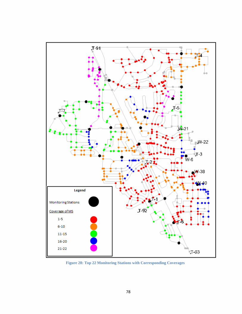
78
Figure 28: Top 22 Monitoring Stations with Corresponding Coverages
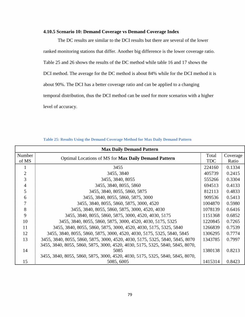
79
4.10.5 Scenario 10: Demand Coverage vs Demand Coverage Index
The DC results are similar to the DCI results but there are several of the lower
ranked monitoring stations that differ. Another big difference is the lower coverage ratio.
Table 25 and 26 shows the results of the DC method while table 16 and 17 shows the
DCI method. The average for the DC method is about 84% while for the DCI method it is
about 90%. The DCI has a better coverage ratio and can be applied to a changing
temporal distribution, thus the DCI method can be used for more scenarios with a higher
level of accuracy.
Table 25: Results Using the Demand Coverage Method for Max Daily Demand Pattern
Max Daily Demand Pattern
Number
of MS Optimal Locations of MS for Max Daily Demand Pattern
Total
TDC
Coverage
Ratio
1 3455 224160 0.1334
2 3455, 3840 405739 0.2415
3 3455, 3840, 8055 555266 0.3304
4 3455, 3840, 8055, 5860 694513 0.4133
5 3455, 3840, 8055, 5860, 5875 812113 0.4833
6 3455, 3840, 8055, 5860, 5875, 3000 909536 0.5413
7 3455, 3840, 8055, 5860, 5875, 3000, 4520 1004870 0.5980
8 3455, 3840, 8055, 5860, 5875, 3000, 4520, 4030 1078139 0.6416
9 3455, 3840, 8055, 5860, 5875, 3000, 4520, 4030, 5175 1151368 0.6852
10 3455, 3840, 8055, 5860, 5875, 3000, 4520, 4030, 5175, 5325 1220845 0.7265
11 3455, 3840, 8055, 5860, 5875, 3000, 4520, 4030, 5175, 5325, 5840 1266839 0.7539
12 3455, 3840, 8055, 5860, 5875, 3000, 4520, 4030, 5175, 5325, 5840, 5845 1306295 0.7774
13 3455, 3840, 8055, 5860, 5875, 3000, 4520, 4030, 5175, 5325, 5840, 5845, 8070 1343785 0.7997
14
3455, 3840, 8055, 5860, 5875, 3000, 4520, 4030, 5175, 5325, 5840, 5845, 8070,
5085 1380138 0.8213
15
3455, 3840, 8055, 5860, 5875, 3000, 4520, 4030, 5175, 5325, 5840, 5845, 8070,
5085, 6005 1415314 0.8423
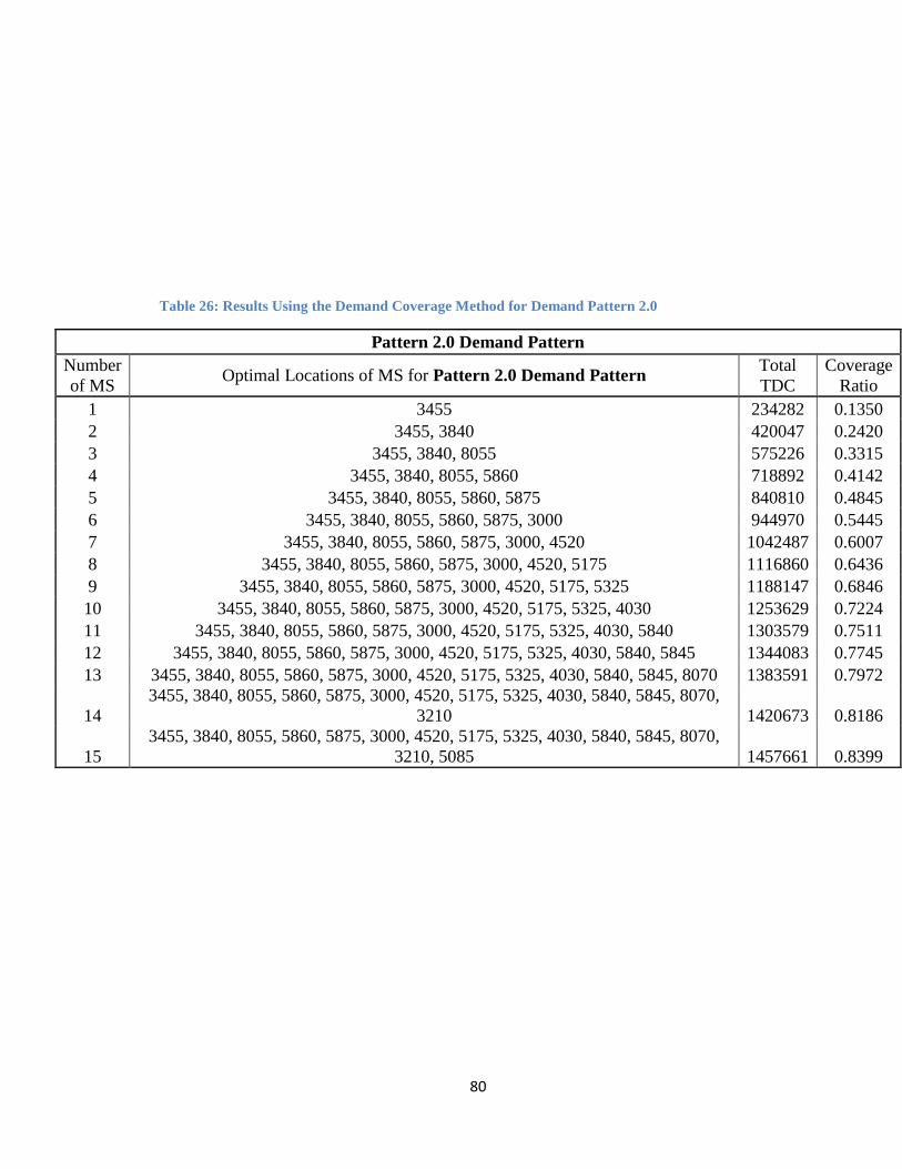
80
Table 26: Results Using the Demand Coverage Method for Demand Pattern 2.0
Pattern 2.0 Demand Pattern
Number
of MS Optimal Locations of MS for Pattern 2.0 Demand Pattern
Total
TDC
Coverage
Ratio
1 3455 234282 0.1350
2 3455, 3840 420047 0.2420
3 3455, 3840, 8055 575226 0.3315
4 3455, 3840, 8055, 5860 718892 0.4142
5 3455, 3840, 8055, 5860, 5875 840810 0.4845
6 3455, 3840, 8055, 5860, 5875, 3000 944970 0.5445
7 3455, 3840, 8055, 5860, 5875, 3000, 4520 1042487 0.6007
8 3455, 3840, 8055, 5860, 5875, 3000, 4520, 5175 1116860 0.6436
9 3455, 3840, 8055, 5860, 5875, 3000, 4520, 5175, 5325 1188147 0.6846
10 3455, 3840, 8055, 5860, 5875, 3000, 4520, 5175, 5325, 4030 1253629 0.7224
11 3455, 3840, 8055, 5860, 5875, 3000, 4520, 5175, 5325, 4030, 5840 1303579 0.7511
12 3455, 3840, 8055, 5860, 5875, 3000, 4520, 5175, 5325, 4030, 5840, 5845 1344083 0.7745
13 3455, 3840, 8055, 5860, 5875, 3000, 4520, 5175, 5325, 4030, 5840, 5845, 8070 1383591 0.7972
14
3455, 3840, 8055, 5860, 5875, 3000, 4520, 5175, 5325, 4030, 5840, 5845, 8070,
3210 1420673 0.8186
15
3455, 3840, 8055, 5860, 5875, 3000, 4520, 5175, 5325, 4030, 5840, 5845, 8070,
3210, 5085 1457661 0.8399
81
4.11 Comparison of Results
Laurence (Johnson, 2012) performed an analysis on this same model to determine
optimal locations for monitoring stations using a heuristic method. His method involved
counting how many times a node detected contamination when the tanks were
contaminated during their particular booster schedule (Table 5). This was a simple
method and his results are seen in figure 29. The results show 3 areas of significance
where monitoring stations should be placed. He simulated tanks being contaminated
because that is the most likely delivery point if intentional contamination were to occur.
It was also assumed that there would be fewer monitoring stations than the number of
tanks which is 7. This is a major difference between our results because this study
suggested at least 15 monitoring stations.
Results of this study vary significantly from Laurence because his method
accounted for contamination events of the tanks only which is the most likely event but
all nodes should be assumed likely candidates for contamination. This should be done
because people looking to contaminate a WDS will not always pick the most likely
location but instead will be intelligent and look for weak spots in the system. This study’s
method assumes that any node can be contaminated so monitoring stations are
strategically scattered around the WDS while his are clustered in three areas of
significance. These three areas are covered by three monitoring stations in this study but
this still leaves a huge number of nodes not being monitoring.
Laurence also did not analyze multiple demand patterns which can affect the
locations of monitoring stations. Using multiple demand patterns is important because

82
cities may have different demand patterns depending on location, usage, and seasons
which will affect where monitoring stations should be located.
Figure 29: Areas of Significance Determined by Laurence (Johnson, 2012)
83
4.12 Weaknesses of the DCI Method
The DCI method is a great way to determine the optimal location of monitoring
stations but it does have some significant weaknesses. A flaw in the method is that at
PRV-118, PRV-119, and PRV-162 there should be monitoring stations to monitor water
entering the WDS from the main transmission line. The entire WDS can be seen in figure
30 with the location of the PRV’s and top 15 monitoring stations being indicated. The
flaw will be examined more closely by looking at PRV-162 in figure 31. This figure
shows that water from the main line enters the WDS at PRV-160, PRV-161, and PRV-
162 but since there is a monitoring station near PRV-160 that covers the nodes
downstream of PRV-162, the DCI method does not indicate that there should be a
monitoring station there. This flaw is relatively easy to fix by including monitoring
stations near PRV-162. Other locations where this flaw is repeated is at PRV-118 and
PRV-119 which are also connected to the main transmission line.
Another flaw is that the DCI method does not take into consideration the water
from the tanks being used by the distribution systems. The method only accounts for
water being used from the main line. These tanks store water that will ultimately be used
by consumers but this water can be contaminated and spread throughout the system.
Therefore, there should be a monitoring station near every tank. Tank 2, 3, and 5 are the
only tanks without monitoring stations nearby where this flaw would occur.
These flaws are easy to overcome but it is hard to determine how important these
extra monitoring stations are compared to the top 15 monitoring station of the WDS. An
additional study should be performed to determine if these stations would be in the top 15
monitoring locations.

84
PRV-162
PRV-162
Figure 30: Locations of the Pressure Release Valves (PRVs) Connecting to the Main Transmission Line
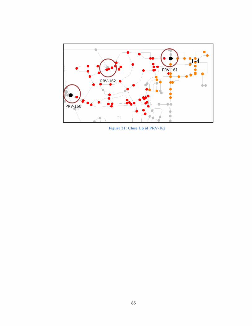
85
Figure 31: Close Up of PRV-162
PRV-160
PRV-160
PRV-162
PRV-161
PRV-161
PRV-161

86
WORKS CITED
Al-Zahrani M A, Moied K. Locating optimum water quality monitoring stations in water
distribution system, in Bridging the Gap: Meeting the World’s Water and
Environmental Resources Challenges. In Proceedings of the ASCE annual
conference on Water Resources Planning and Management. Virginia: Reston, 2001
“An Introduction to Water Quality Monitoring.” United States Environmental Protection
Agency. EPA, 2 Oct. 2012. Web. 08 Mar. 2014.
<http://water.epa.gov/type/watersheds/monitoring/monintr.cfm>.
“Basic Information about Disinfectants in Drinking Water: Chloramine, Chlorine and
Chlorine Dioxide.” United States Environmental Protection Agency. EPA, 13 Dec.
2013. Web. 06 Mar. 2014.
<http://water.epa.gov/drink/contaminants/basicinformation/disinfectants.cfm>.
“Bioterrorism Act of 2002.” US Food and Drug Administration. U.S. Department of
Health and Human Services, 12 June 2002. Web. 10 June 2014.
<http://www.fda.gov/RegulatoryInformation/Legislation/ucm148797.htm.>
“Bright Lights of Madison Avenue Shine on Trenchless Rehab Project.” Trenchless
Technology. Benjamin Media, Inc, June 2010. Web. May 2014.
<http://trenchlessonline.com/bright-lights-of-madison-avenue-shine-on-trenchless-
rehab-project/>.
Brumbelow, Kelly, Jacob Torres, Seth Guikema, Elizabeth Bristow, and Lufthansa
Kanta. Virtual Cities For Water Distribution and Infrastructure System Research.
World Environmental and Water Resources Congress 2007: Restoring Our Natural
Habitat (2007). Print.
Chastain, James R., A heuristic methodology for locating monitoring stations to detect
contamination events in potable water distribution systems. (2004). Theses and
Dissertations. Paper 988.
"Cryptosporidium." Minnesota Department of Health. Minnesota.gov, Mar. 2014. Web.
May 2014.
<http://www.health.state.mn.us/divs/eh/water/factsheet/com/cryptosporidium.html>
.
Cybersecurity Executive Order: EPA Response on Adoption of the Cybersecurity
Framework by the Water Sector (n.d.): n. pag.United States Environmental
Protection Agency. USEPA. Web. May 2014.
<http://water.epa.gov/infrastructure/watersecurity/upload/EO_13696_10-b-
_EPA_response.pdf>.

87
"Cyber Security 101 for Water Utilities." (n.d.): n. pag. United States Environmental
Protection Agency. USEPA, July 2012. Web. Aug. 2014.
<http://water.epa.gov/infrastructure/watersecurity/features/upload/epa817k12004.pd
f>.
"Drinking Water D." 2013 Report Card for America's Infrastructure. American Society
of Civil Engineers, 2013. Web. Dec. 2014.
<http://infrastructurereportcard.org/drinking-water/>.
“Filter Backwash Recycling Rule.” United States Environmental Protection Agency.
EPA, 11 Sept. 2013. Web. 7 Mar. 2014.
<http://water.epa.gov/lawsregs/rulesregs/sdwa/filterbackwash.cfm>.
"Groundwater Under the Direct Influence of Surface Water." Oregon.gov. Oregon Public
Health Division, n.d. Web. Apr. 2014.
<http://public.health.oregon.gov/HealthyEnvironments/DrinkingWater/SourceWate
r/Pages/gwudi.aspx>.
“Hack Attack Causes ‘Massive Damage’ at Steel Works.” BBC News. BBC, 22 Dec.
2014. Web. 28 Jan. 2015. <http://www.bbc.com/news/technology-30575104>.
Haimes, Y. Y., Matalas, N. C., Lambert, J. H., Jackson, B. A., & Fellows, J. F. (1998).
Reducing vulnerability of water supply systems to attack. Journal of Infrastructure
Systems, 4(4), 164-177.
Hall, John S., and Jeffrey G. Szabo. Distribution System Water Quality Monitoring:
Sensor Technology Evaluation Methodology and Results. USEPA, Oct. 2009. PDF.
"Home." Aqua-Pipe: Water Main Rehabilitation. Aqua-Pipe, n.d. Web. 30 Apr. 2015.
<http://www.aqua-pipe.com/>.
“Homeland Security Presidential Directive 5.” Department of Homeland Security. 28
Feb. 2003. Web. 10 June 2014. <http://www.dhs.gov/publication/homeland-
security-presidential-directive-5.>
Hydrant Security: Taking the First Step. Chattanooga: Mueller Co., Apr. 2011. PDF.
Johnson, Lawrence D. “Application of a Heuristic Method to a Water Distribution
System for Determining Optimal Water Quality Monitoring Locations.” Thesis. San
Luis Obispo, 2012. Print.
Kumar A, Kansal M L, Arora G. Identification of monitoring stations in water
distribution system. Journal of Environmental Engineering-ASCE, 1997, 123(8):
746-752

88
Lee B H, Deininger R A. Optimal locations of monitoring stations in water distribution
system. Journal of Environmental Engineering-ASCE, 1992, 118(1): 4-16
Liu, Shuming, Wenjun Liu, Jinduan Chen, and Qi Wang. “Optimal Locations of
Monitoring Stations in Water Distribution Systems Under Multiple Demand
Patterns: A Flaw of Demand Coverage Method and Modification.” Frontiers of
Environmental Science and Engineering 6.2 (2012): 204-12. Print.
“Long Term 1 Enhanced Surface Water Treatment Rule.” United States Environmental
Protection Agency. EPA, 8 Dec. 2014. Web. 07 Mar. 2014.
<http://water.epa.gov/lawsregs/rulesregs/sdwa/mdbp/lt1/lt1eswtr.cfm>.
Pepitone, Julianne. “Sony Hack: ‘Critical’ Systems Won’t Be Back Online Until
February.” NBC News. NBC, 23 Jan. 2015. Web. 28 Jan. 2015.
<http://www.nbcnews.com/storyline/sony-hack/sony-hack-critical-systems-wont-
be-back-online-until-february-n292126>.
Perlman, Howard. "Runoff (Surfacewater Runoff)." United States Geological Survey.
USDI and USGS, Mar. 2014. Web. Apr. 2014.
<http://water.usgs.gov/edu/runoff.html>.
“Nature Wildlife.” BBC News. BBC, Oct. 2014. Web. 15 June 2014.
<http://www.bbc.co.uk/nature/habitats/Brackish>.
Rossman, Lewis A. “EPANET 2 Users Manual.” United States Environmental Protection
Agency. N.p., Sept. 2000. Web. Feb. 2014.
<ftp2.bentley.com/dist/collateral/docs/EPANET/EPANET_Manual.pdf>.
Rossman, L.A. and Grayman, W.M., “Scale-model studies of mixing in drinking water
storage tanks,” Journal of Environmental Engineering, Vol. 125, No. 8, pp. 755-
761, 1999.
“Safe Drinking Water Act (SDWA).” United States Environmental Protection Agency.
EPA, 30 July 2014. Web. 21 Mar. 2014.
<http://water.epa.gov/lawsregs/rulesregs/sdwa/index.cfm>.
Sanger, David E. “Obama Order Sped Up Wave of Cyberattacks Against Iran.” The New
York Times. The New York Times Company, 1 June 2012. Web. 28 Mar. 2014.
<http://www.nytimes.com/2012/06/01/world/middleeast/obama-ordered-wave-of-
cyberattacks-against-iran.html?pagewanted=all>.
“Summary of the Clean Water Act.” United States Environmental Protection Agency.
EPA, 12 Nov. 2014. Web. 7 Mar. 2014. <http://www2.epa.gov/laws-
regulations/summary-clean-water-act>.
89
Surface Water Treatment Rules: What Do They Mean to You? (n.d.): n. pag. United
States Environmental Protection Agency. USEPA, Oct. 2011. Web. Mar. 2014.
<http://water.epa.gov/lawsregs/rulesregs/sdwa/swtr/upload/SWTRPlainEnglishGuid
eFinal.pdf>.
The Cadmus Group, Inc., and USEPA Office of Groundwater and Drinking Water. The
Effectiveness of Disinfectant Residuals in the Distribution System, March
2007 (n.d.): n. pag. United States Environmental Protection Agency. May 2014.
Web. Aug. 2014.
<http://www.epa.gov/ogwdw/disinfection/tcr/pdfs/issuepaper_effectiveness.pdf>.
Todd, David K., and Larry W. Mays. Groundwater Hydrology. 3rd ed. N.p.: Argosy,
2005. Print.
"Water: Basic Information about Regulated Drinking Water Contaminants." United
States Environmental Protection Agency. USEPA, Dec. 2013. Web. Apr. 2014.
<http://water.epa.gov/drink/contaminants/basicinformation/disinfectants.cfm>.
Tryby M E, Uber J G. Representative water quality sampling in water distribution
systems, in Bridging the Gap: Meeting the World’s Water and Environmental
Resources Challenges. In Proceedings of the ASCE annual conference on Water
Resources Planning and Management. Virginia: Reston, 2001
"Water: Drinking Water Contaminants." United States Environmental Protection Agency.
USEPA, Oct. 2014. Web. May 2014. <http://water.epa.gov/drink/contaminants/>.
"Water: Drinking Water Strategy." United States Environmental Protection Agency.
USEPA, Oct. 2012. Web. May 2014.
<http://water.epa.gov/lawsregs/rulesregs/sdwa/dwstrategy/>.
"Water: Interim Enhanced Surface Water Treatment Rule." United States Environmental
Protection Agency. USEPA, Mar. 2012. Web. May 2014.
<http://water.epa.gov/lawsregs/rulesregs/sdwa/ieswtr/>.
"Water: Key Features of an Active and Effective Security Program." United States
Environmental Protection Agency. USEPA, May 2014. Web. Jan. 2014.
<http://water.epa.gov/infrastructure/watersecurity/features/index.cfm#one>.
"Water: Long Term 2 Enhanced Surface Water Treatment Rule (LT2)." United States
Environmental Protection Agency. USEPA, Sept. 2013. Web. May 2014.
<http://water.epa.gov/lawsregs/rulesregs/sdwa/lt2/index.cfm>.
"Water: Monitoring and Assessment." United States Environmental Protection Agency.
USEPA, Mar. 2012. Web. June 2014.
<http://water.epa.gov/type/rsl/monitoring/vms50.cfm>.

90
"Water: Surface Water Treatment Rule." United States Environmental Protection Agency.
USEPA, Mar. 2012. Web. Apr. 2014.
<http://water.epa.gov/lawsregs/rulesregs/sdwa/swtr/>.
“2.2 Designing the Stream Study.” United States Environmental Protection Agency. EPA,
6 Mar. 2012. Web. 09 Mar. 2014.
<http://water.epa.gov/type/rsl/monitoring/vms22.cfm>.

91
APPENDICES

92
APPENDIX A
The contents of Appendix A include visual representations of the locations of monitoring
stations with their corresponding coverages. The coverage criterion is assumed to be 50%
unless otherwise stated.
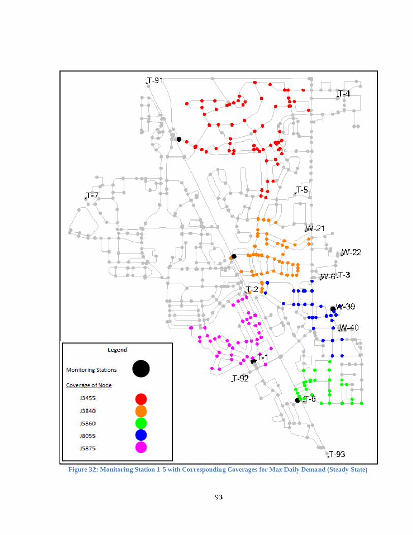
93
Figure 32: Monitoring Station 1-5 with Corresponding Coverages for Max Daily Demand (Steady State)
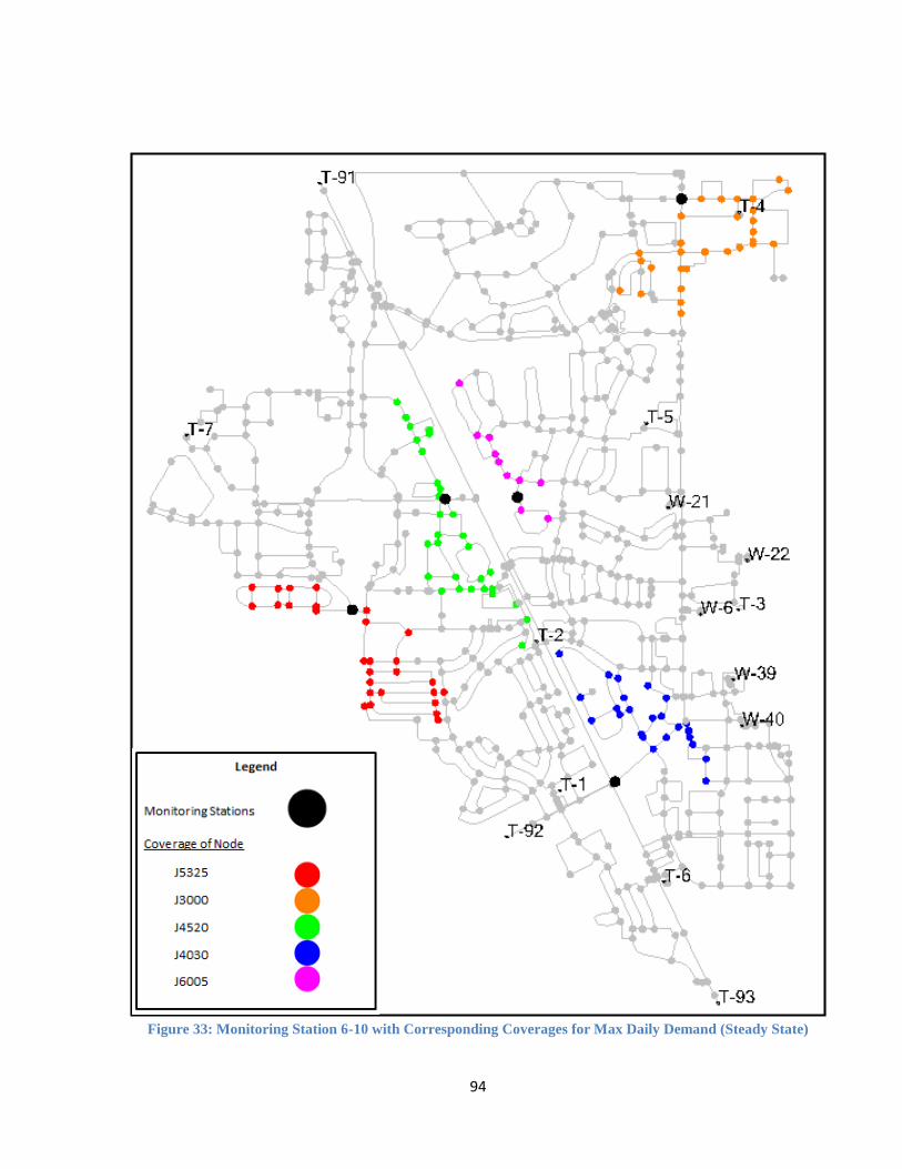
94
Figure 33: Monitoring Station 6-10 with Corresponding Coverages for Max Daily Demand (Steady State)

95
Figure 34: Monitoring Station 11-15 with Corresponding Coverages for Max Daily Demand (Steady State)

96
Figure 35: Top 15 Monitoring Stations with Corresponding Coverages for Max Daily Demand (Steady State)
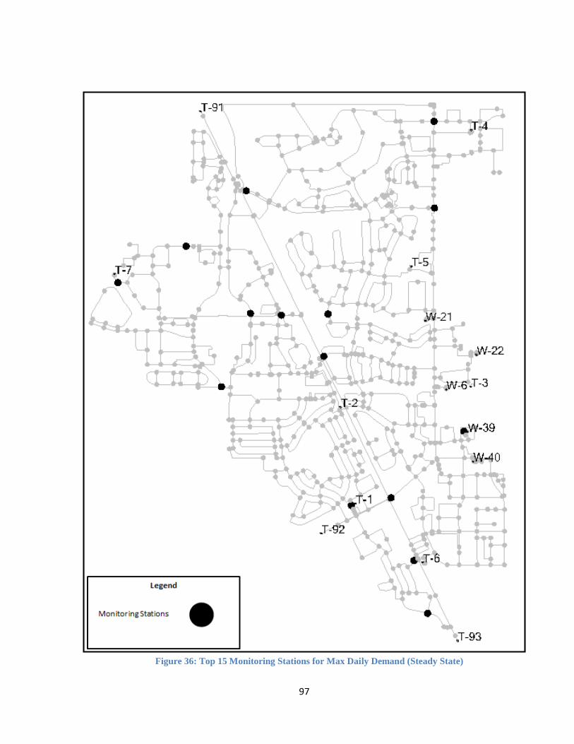
97
Figure 36: Top 15 Monitoring Stations for Max Daily Demand (Steady State)

98
Figure 37: Monitoring Station 1-5 with Corresponding Coverages for Demand Pattern 2.0 (Unsteady State)

99
Figure 38: Monitoring Station 6-10 with Corresponding Coverages for Demand Pattern 2.0 (Unsteady State)
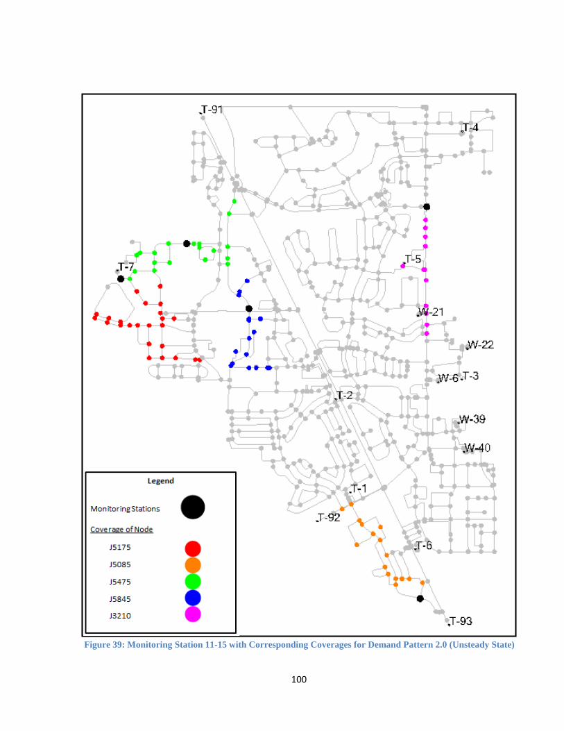
100
Figure 39: Monitoring Station 11-15 with Corresponding Coverages for Demand Pattern 2.0 (Unsteady State)

101
Figure 40: Top 15 Monitoring Stations with Corresponding Coverages for Demand Pattern 2.0 (Unsteady State)
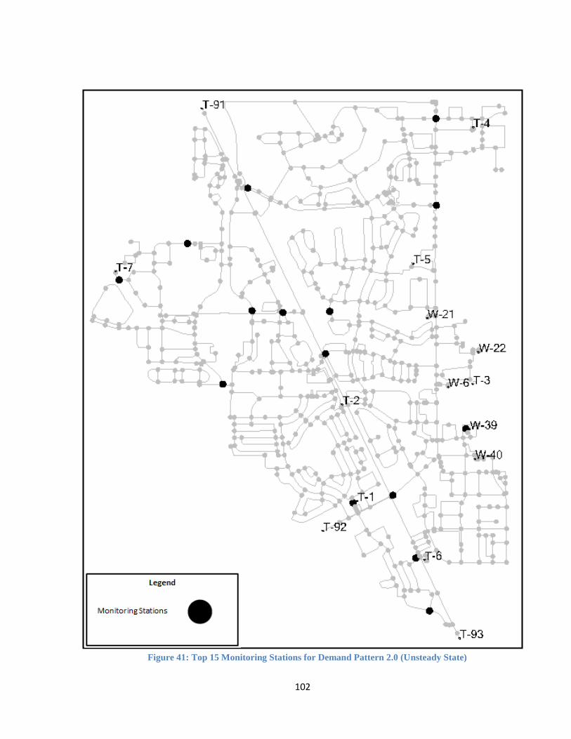
102
Figure 41: Top 15 Monitoring Stations for Demand Pattern 2.0 (Unsteady State)
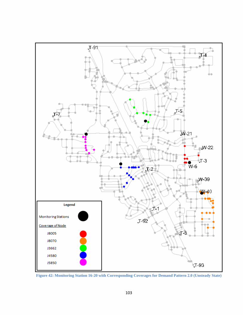
103
Figure 42: Monitoring Station 16-20 with Corresponding Coverages for Demand Pattern 2.0 (Unsteady State)
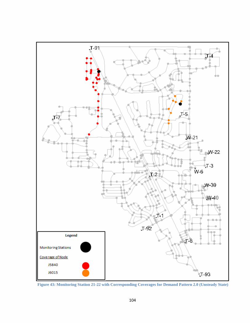
104
Figure 43: Monitoring Station 21-22 with Corresponding Coverages for Demand Pattern 2.0 (Unsteady State)
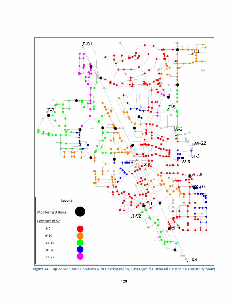
105
Figure 44: Top 22 Monitoring Stations with Corresponding Coverages for Demand Pattern 2.0 (Unsteady State)

106
Figure 45: Monitoring Station 1-5 with Corresponding Coverages for Demand Pattern 3.0 (Unsteady State)

107
Figure 46: Monitoring Station 6-10 with Corresponding Coverages for Demand Pattern 3.0 (Unsteady State)
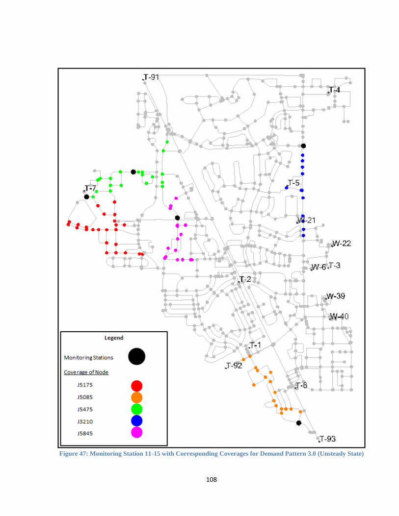
108
Figure 47: Monitoring Station 11-15 with Corresponding Coverages for Demand Pattern 3.0 (Unsteady State)
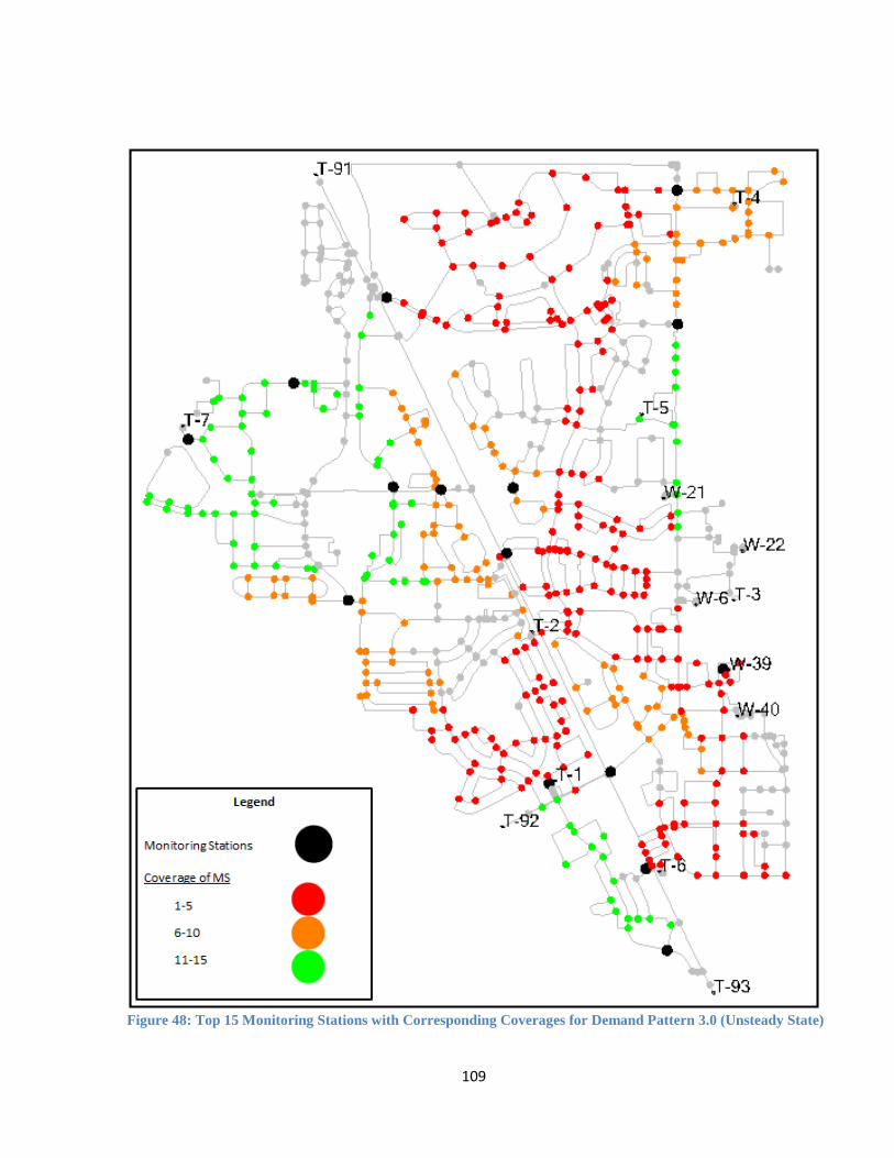
109
Figure 48: Top 15 Monitoring Stations with Corresponding Coverages for Demand Pattern 3.0 (Unsteady State)

110
Figure 49: Top 15 Monitoring Stations for Demand Pattern 3.0 (Unsteady State)
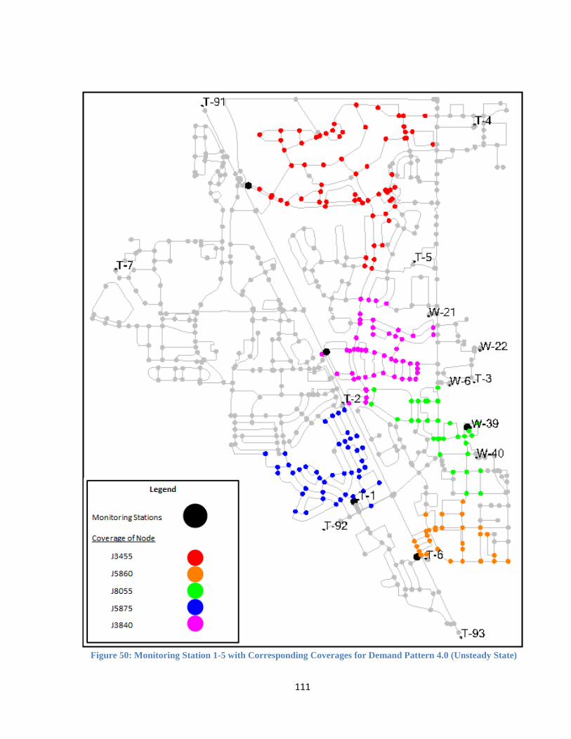
111
Figure 50: Monitoring Station 1-5 with Corresponding Coverages for Demand Pattern 4.0 (Unsteady State)
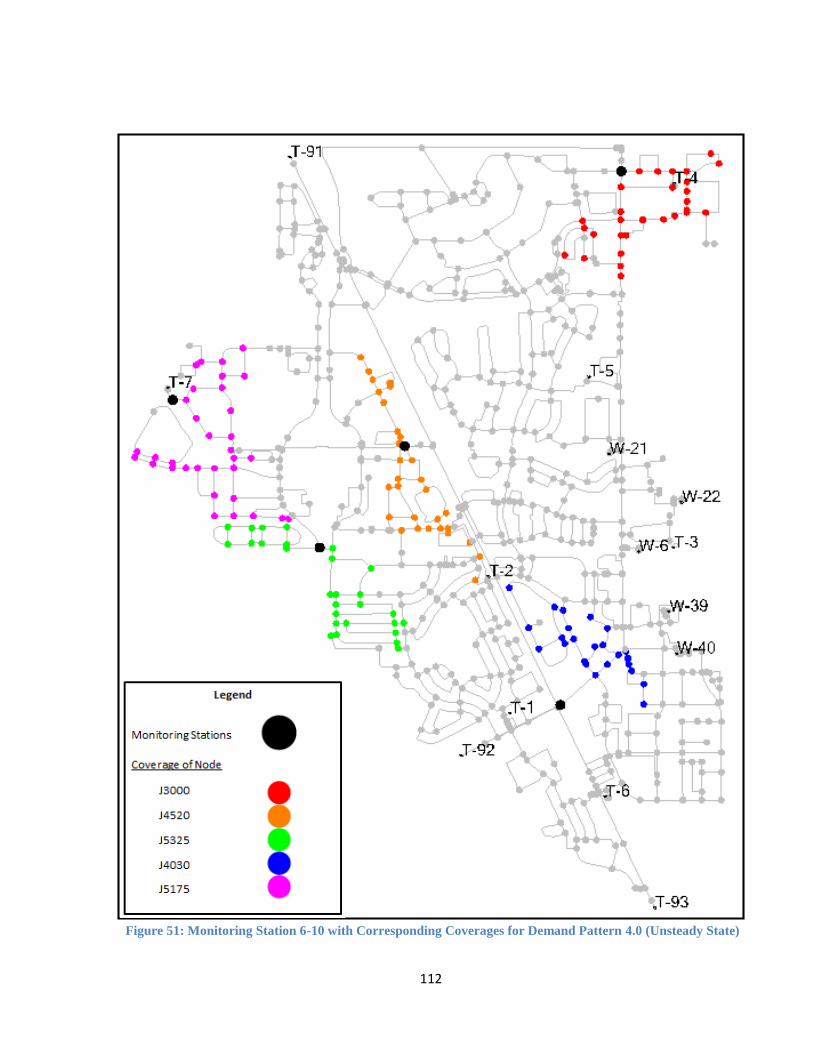
112
Figure 51: Monitoring Station 6-10 with Corresponding Coverages for Demand Pattern 4.0 (Unsteady State)
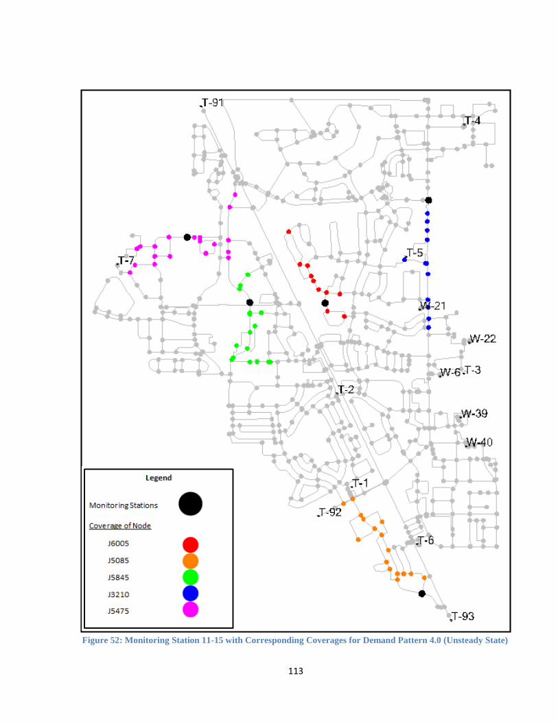
113
Figure 52: Monitoring Station 11-15 with Corresponding Coverages for Demand Pattern 4.0 (Unsteady State)
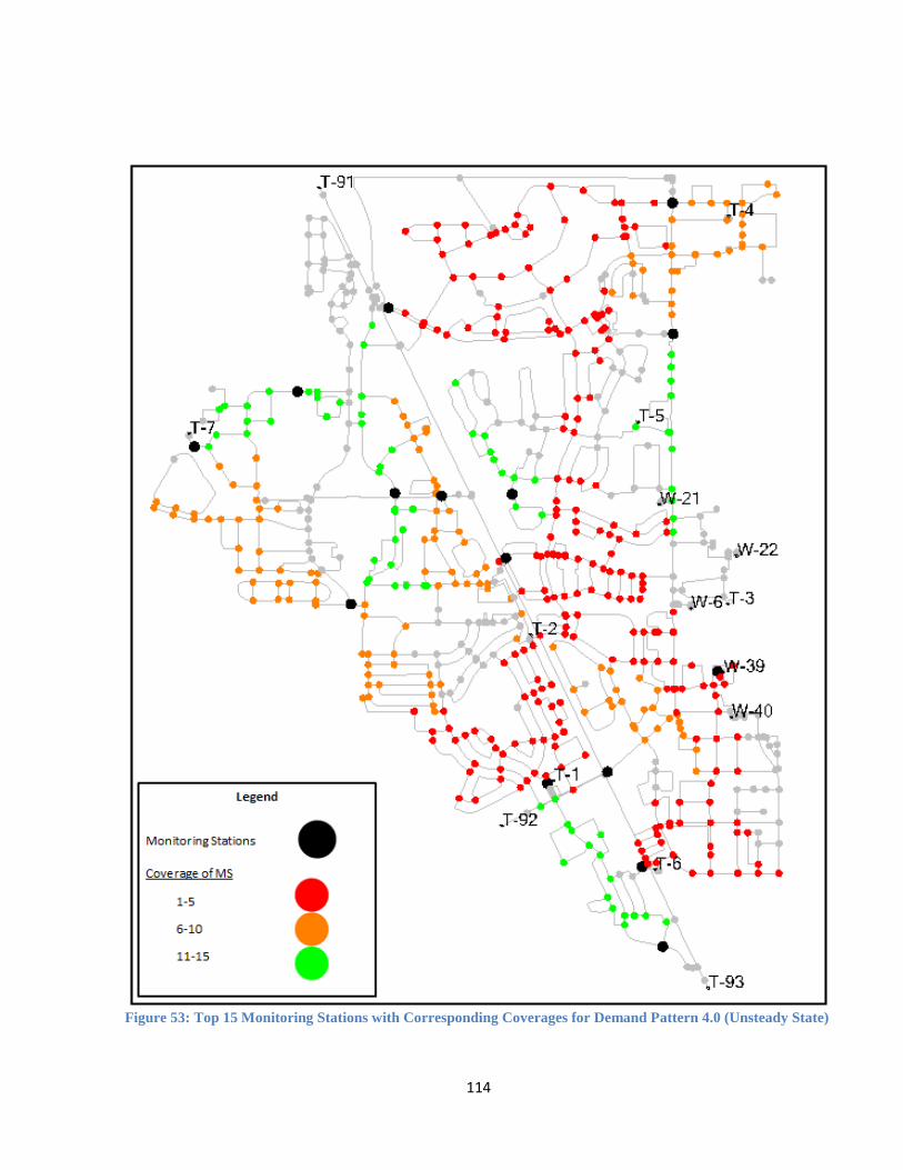
114
Figure 53: Top 15 Monitoring Stations with Corresponding Coverages for Demand Pattern 4.0 (Unsteady State)

115
Figure 54: Top 15 Monitoring Stations for Demand Pattern 4.0 (Unsteady State)

116
Figure 55: Monitoring Station 1-5 with Corresponding Coverages for Demand Pattern 5.0 (Unsteady State)

117
Figure 56: Monitoring Station 6-10 with Corresponding Coverages for Demand Pattern 5.0 (Unsteady State)

118
Figure 57: Monitoring Station 11-15 with Corresponding Coverages for Demand Pattern 5.0 (Unsteady State)

119
Figure 58: Top 15 Monitoring Stations with Corresponding Coverages for Demand Pattern 5.0 (Unsteady State)

120
Figure 59: Top 15 Monitoring Stations for Demand Pattern 5.0 (Unsteady State)
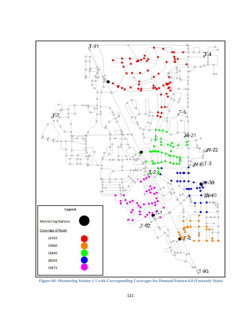
121
Figure 60: Monitoring Station 1-5 with Corresponding Coverages for Demand Pattern 6.0 (Unsteady State)
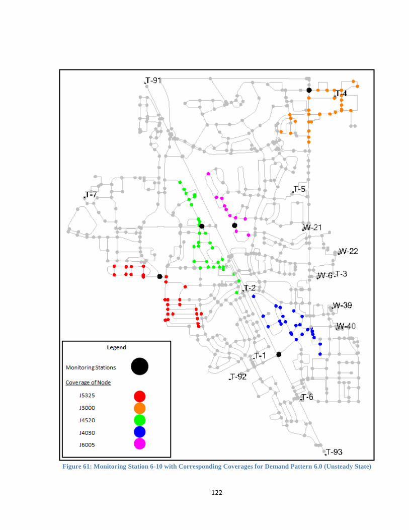
122
Figure 61: Monitoring Station 6-10 with Corresponding Coverages for Demand Pattern 6.0 (Unsteady State)

123
Figure 62: Monitoring Station 11-15 with Corresponding Coverages for Demand Pattern 6.0 (Unsteady State)
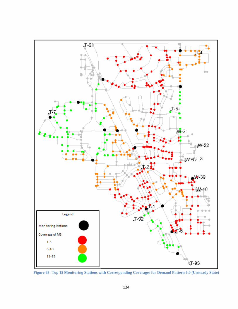
124
Figure 63: Top 15 Monitoring Stations with Corresponding Coverages for Demand Pattern 6.0 (Unsteady State)

125
Figure 64: Top 15 Monitoring Stations for Demand Pattern 6.0 (Unsteady State)

126
Figure 65: Monitoring Station 1-5 with Corresponding Coverages for Demand Pattern 7.0 (Unsteady State)

127
Figure 66: Monitoring Station 6-10 with Corresponding Coverages for Demand Pattern 7.0 (Unsteady State)

128
Figure 67: Monitoring Station 11-15 with Corresponding Coverages for Demand Pattern 7.0 (Unsteady State)

129
Figure 68: Top 15 Monitoring Stations with Corresponding Coverages for Demand Pattern 7.0 (Unsteady State)
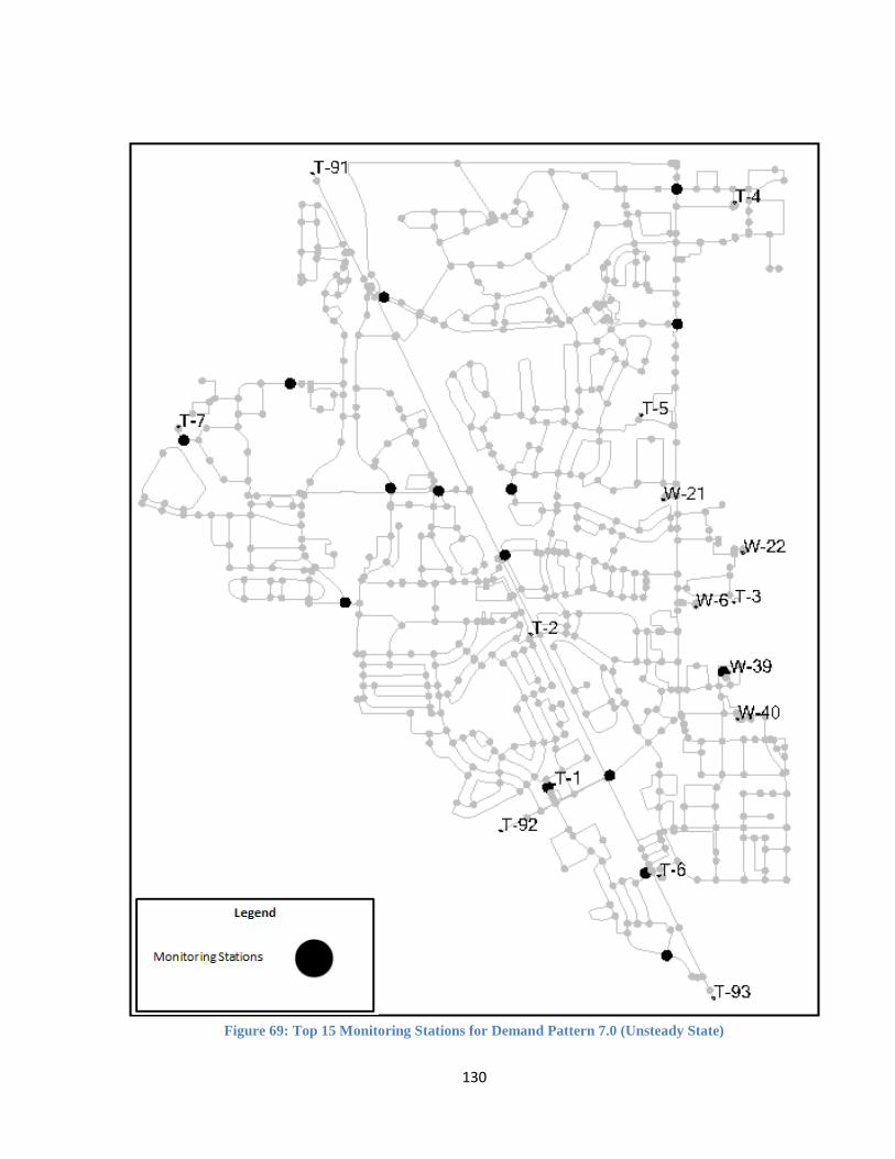
130
Figure 69: Top 15 Monitoring Stations for Demand Pattern 7.0 (Unsteady State)
131
APPENDIX B
The contents of Appendix B contain a list compiled by the Environmental Protection
Agency of contaminants, including microorganisms, disinfection byproducts,
disinfectants, inorganic chemicals, organic chemicals, and radionuclides.
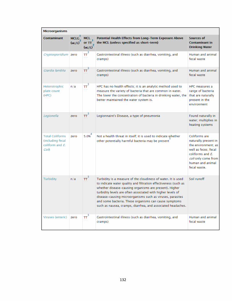
132
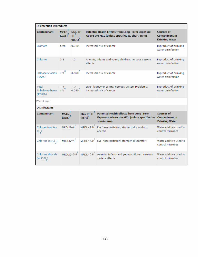
133
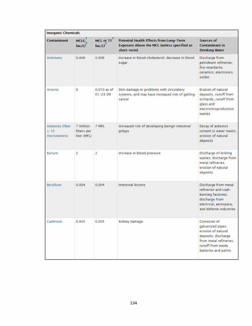
134

135
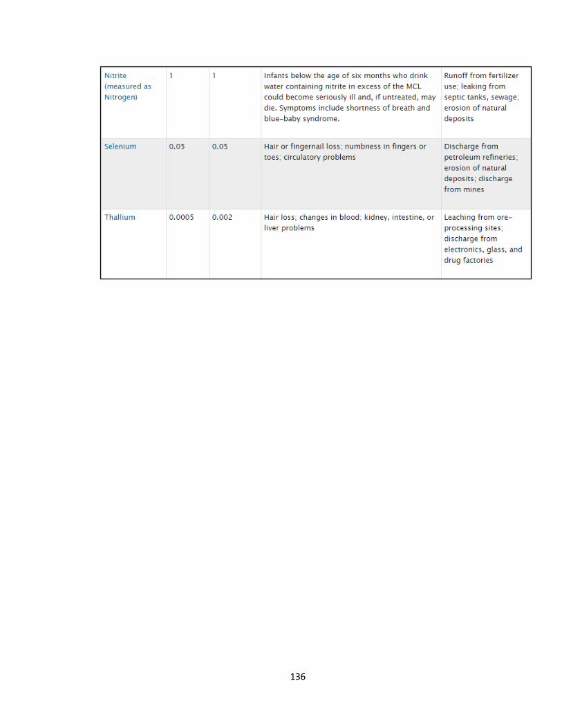
136
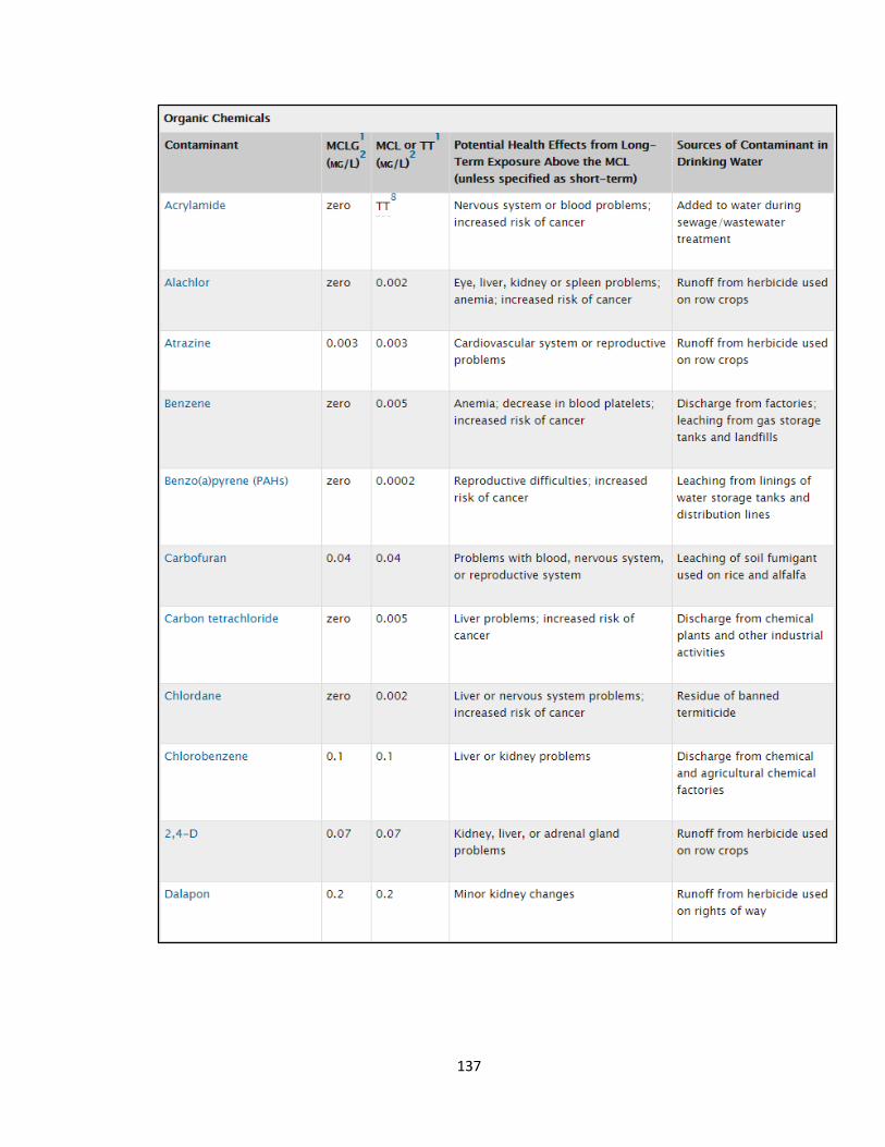
137

138
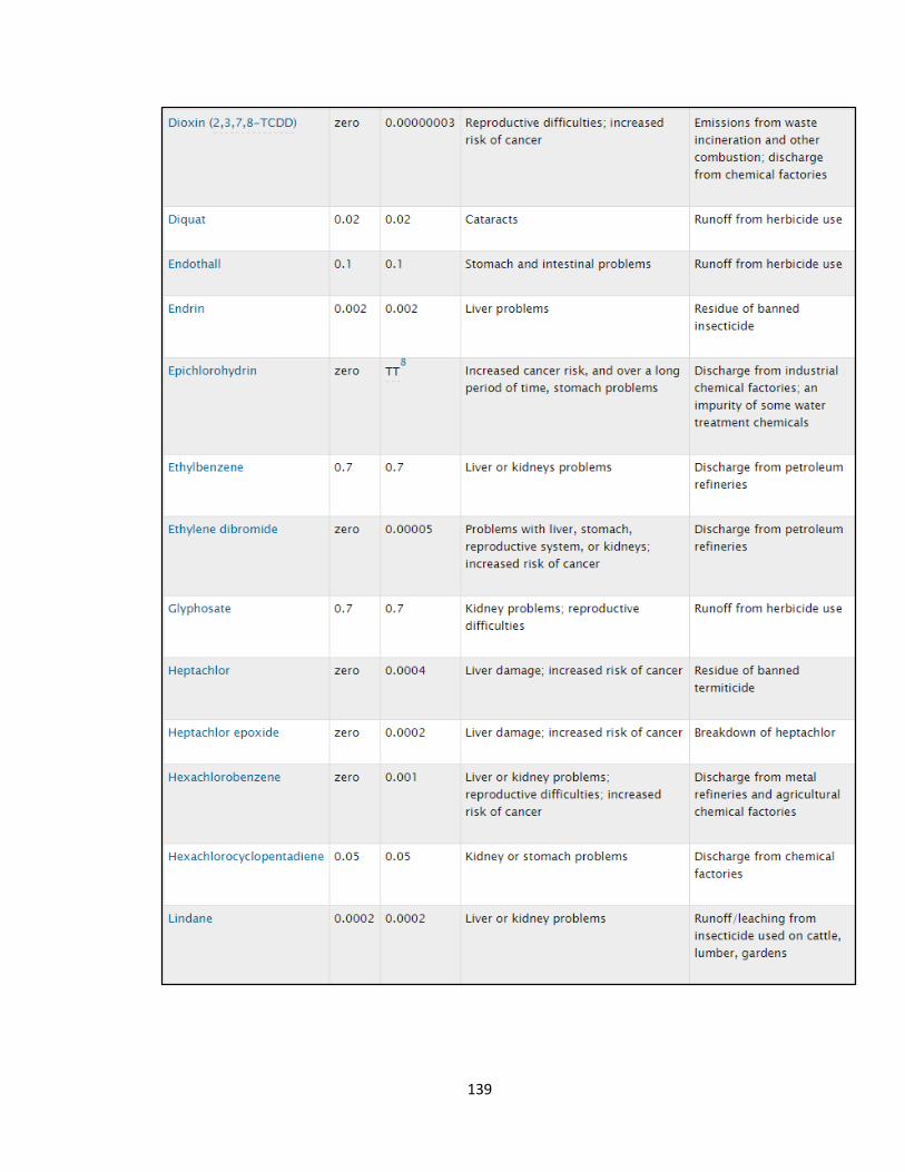
139
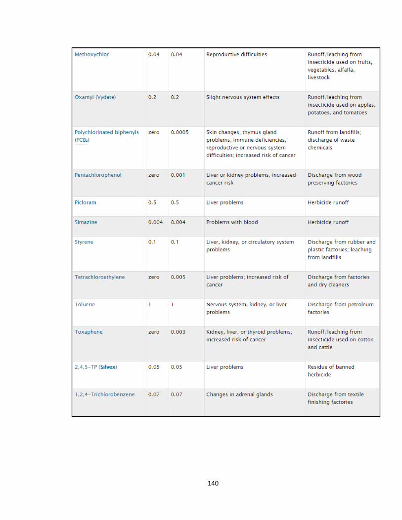
140

141
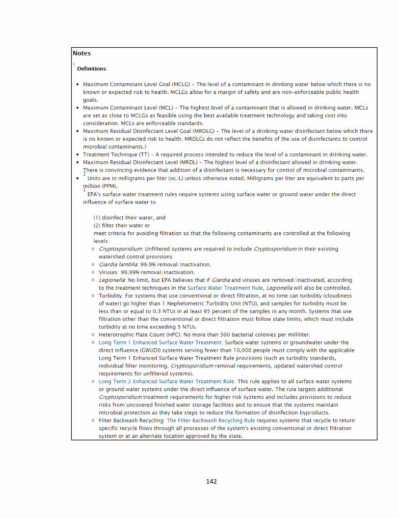
142
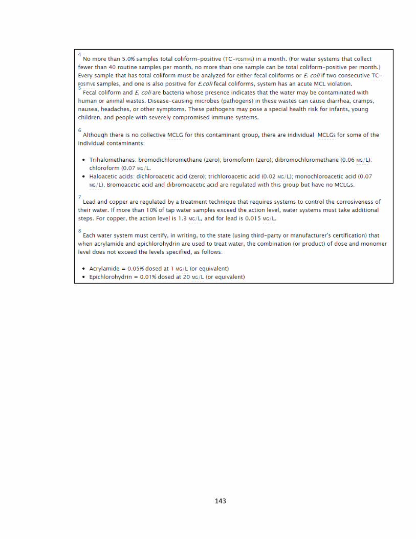
143
Related Documents