Locally conservative, stabilized finite element methods for variably saturated flow

Coa

stal

and

Hyd

raul

ics

Labo

rato

ryER

DC

/CH

LTR

-09-

12

Navigation Systems Research Program

Locally Conservative, Stabilized Finite ElementMethods for a Class of Variable CoefficientNavier-Stokes Equations

9002tsuguAgnoF.T.Mdna,gnihtraF.W.M,seeK.E.C

Approved for public release; distribution is unlimited.

Navigation Systems Research Program ERDC/CHL TR-09-12

August 2009

Locally Conservative, Stabilized Finite

Element Methods for a Class of Variable

Coefficient Navier-Stokes Equations

C. E. Kees, M. W. Farthing, and M. T. Fong

Coastal and Hydraulics Laboratory

U.S. Army Engineer Research and Development Center

3909 Halls Ferry Road.

Vicksburg, MS 39180-6199

Final Report

Approved for public release; distribution is unlimited.

Prepared for U.S. Army Corps of Engineers

Washington, DC 20314-1000

Under Work Unit KHBCGD

ERDC/CHL TR-09-12 ii

Abstract: Computer simulation of three-dimensional incompressible

flow is of interest in many navigation, coastal, and geophysical applica-

tions. This report is the the fifth in a series of publications that documents

research and development on a state-of-the-art computational model-

ing capability for fully three-dimensional two-phase fluid flows with ves-

sel/structure interaction in complex geometries (Farthing and Kees, 2008;

Kees et al., 2008; Farthing and Kees, 2009; Kees et al., 2009). It is pri-

marily concerned with model verification, often defined as “solving the

equations right” (Roache, 1998). Model verification is a critical step on

the way to producing reliable numerical models, but it is a step that is of-

ten neglected (Oberkampf and Trucano, 2002). Quantitative and qualita-

tive methods for verification also provide metrics for evaluating numerical

methods and identifying promising lines of future research.

Fully-three dimensional flows are often described by the incompressible

Navier-Stokes (NS) equations or related model equations such as the

Reynolds Averaged Navier Stokes (RANS) equations and Two-Phase Reynolds

Averaged Navier-Stokes equations (TPRANS). We will describe spatial and

temporal discretization methods for this class of equations and test prob-

lems for evaluating the methods and implementations. The discretization

methods are based on stabilized continuous Galerkin methods (variational

multiscale methods) and discontinous Galerkin methods. The test prob-

lems are taken from classical fluid mechanics and well-known benchmarks

for incompressible flow codes (Batchelor, 1967; Chorin, 1968; Schäfer

et al., 1996; Williams and Baker, 1997; John et al., 2006). We demonstrate

that the methods described herein meet three minimal requirements for

use in a wide variety of applications: 1) they apply to complex geometries

and a range of mesh types; 2) they robustly provide accurate results over a

wide range of flow conditions; and 3) they yield qualitatively correct solu-

tions, in particular mass and volume conserving velocity approximations.

Disclaimer: The contents of this report are not to be used for advertising, publication, or promotional purposes. Citationof trade names does not constitute an official endorsement or approval of the use of such commercial products. All productnames and trademarks cited are the property of their respective owners. The findings of this report are not to be construed asan official Department of the Army position unless so designated by other authorized documents.

DESTROY THIS REPORTWHEN NO LONGER NEEDED. DO NOT RETURN IT TO THE ORIGINATOR.

ERDC/CHL TR-09-12 iii

Table of Contents

Figures and Tables ................................................................................................. iv

Preface.................................................................................................................. v

1 Introduction .................................................................................................... 1

2 Formulation .................................................................................................... 3

2.1 Test equation ............................................................................................. 4

2.2 Weak formulation ....................................................................................... 4

3 Discrete Approximation .................................................................................... 6

3.1 Time discretization ...................................................................................... 6

3.2 Multiscale formulation ................................................................................. 7

3.3 Algebraic sub-grid scale approximation........................................................... 8

3.4 Velocity post-processing ............................................................................... 8

3.5 Additional details ........................................................................................ 9

4 Model Verification .......................................................................................... 10

4.1 Plane Poiseuille and Couette Flow ............................................................... 10

4.2 Vortex decay ............................................................................................ 11

4.3 Lid driven cavity........................................................................................ 13

4.4 Backward facing step ................................................................................ 13

4.5 Flow past a cylinder................................................................................... 15

5 Conclusions .................................................................................................. 23

References.......................................................................................................... 24

ERDC/CHL TR-09-12 iv

Figures and Tables

Figures

Figure 1. Periodic vortex shedding at Re ≈ 100. ............................................................. 2

Figure 2. Lid driven cavity in 2D at Re = 100. ............................................................... 14

Figure 3. Lid driven cavity in 2D at Re = 20000. ........................................................... 15

Figure 4. Lid driven cavity in 3D at Re = 100. ............................................................... 16

Figure 5. Primary reattachment length versus Re.......................................................... 16

Figure 6. Backward facing step in 2D at Re = 400 and 800............................................ 20

Figure 7. Backward facing step in 3D at Re = 1000. ...................................................... 21

Figure 8. Lift coefficient versus time for 0 ≤ Re(t) ≤ 100. ............................................... 21

Figure 9. Flow around a square cylinder in 3D at Re = 70 .............................................. 22

Tables

Table 1. Grid refinement study for 2D Poiseuille problem................................................ 11

Table 2. Grid refinement study for 3D Poiseuille problem. .............................................. 12

Table 3. Grid refinement study for vortex decy problem Re = 1. ....................................... 17

Table 4. Grid refinement study for vortex decy problem Re = 1×106................................. 18

Table 5. 2D lid driven cavity at Re = 100,400,1000....................................................... 19

ERDC/CHL TR-09-12 v

Preface

This report is a product of the High Fidelity Vessel Effects Work Unit

of the Navigation Systems Research Program being conducted at the

U.S. Army Engineer Research and Development Center, Coastal and Hy-

draulics Laboratory.

The report was prepared by Dr. Christopher E. Kees, Dr. Matthew W. Far-

thing, and Ms. Moira T. Fong under the supervision of Mr. Earl V. Edris,

Jr., Chief, Hydrologic Systems Branch. General supervision was provided

by Mr. Thomas W. Richardson, Director, CHL; Dr. William D. Martin,

Deputy Director, CHL; and Mr. Bruce A. Ebersole, Chief Flood and Storm

Protection Division.

Technical advice needed to complete this work was provided by Drs. Stacy

E. Howington and Robert S. Bernard, Coastal and Hydraulics Laboratory

and Professor Yuri Bazilevs, University of California.

Mr. James E. Clausner, Navigation Systems Program Manager, was the

project manager for this effort. Mr. W. Jeff Lillycrop was the Technical

Director.

COL Gary E. Johnston was Commander and Executive Director of the

Engineer Research and Development Center. Dr. James E. Houston was

Director.

This report was typeset by the authors with the LATEX document prepa-

ration system. The report uses the erdc document class and mathgifg

fonts package developed by Dr. Boris Veytsman under the supervision of

Mr. Ryan E. North, Geotechnical and Structures Laboratory. The pack-

ages are available from http://ctan.tug.org.

ERDC/CHL TR-09-12 1

1 Introduction

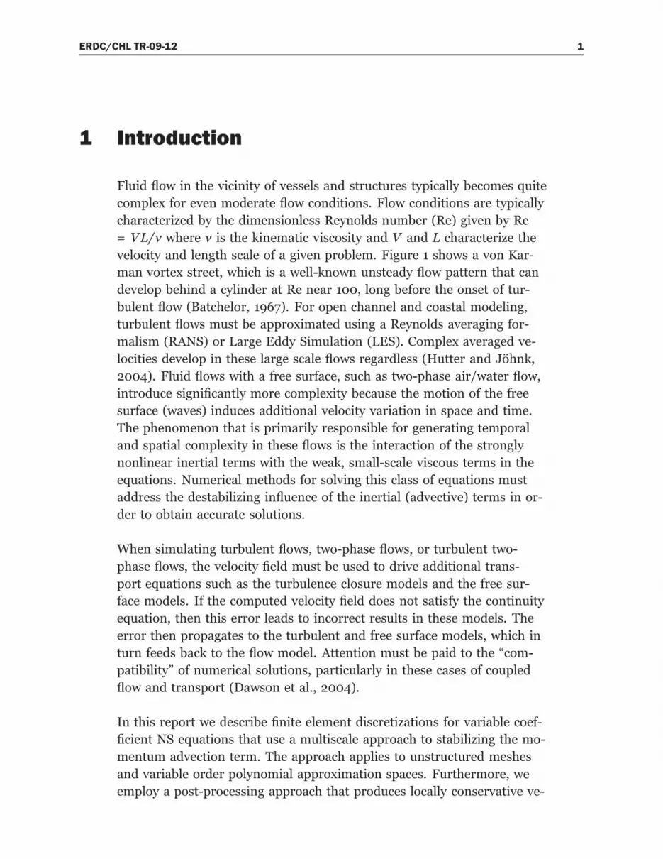
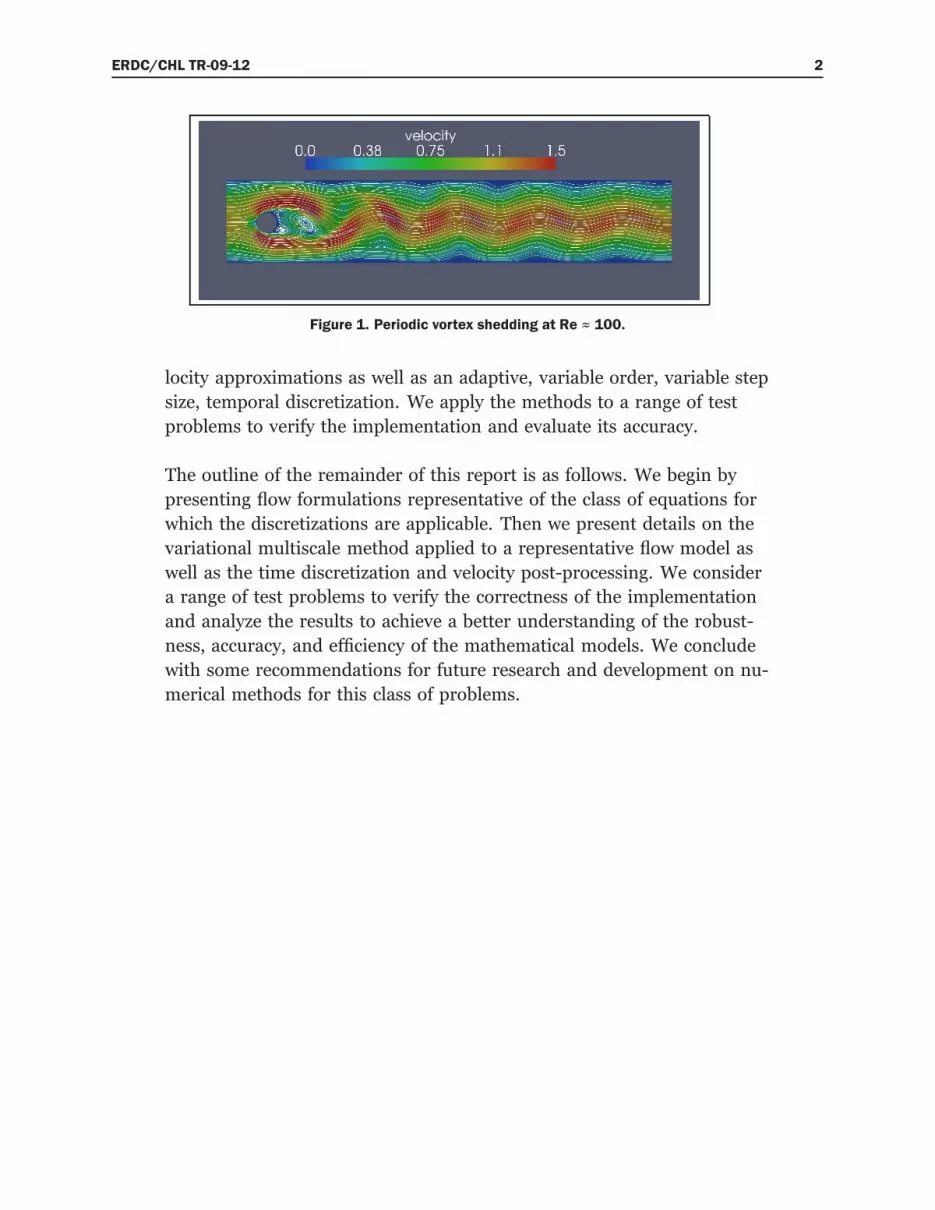
Fluid flow in the vicinity of vessels and structures typically becomes quite

complex for even moderate flow conditions. Flow conditions are typically

characterized by the dimensionless Reynolds number (Re) given by Re

= VL/ν where ν is the kinematic viscosity and V and L characterize the

velocity and length scale of a given problem. Figure 1 shows a von Kar-

man vortex street, which is a well-known unsteady flow pattern that can

develop behind a cylinder at Re near 100, long before the onset of tur-

bulent flow (Batchelor, 1967). For open channel and coastal modeling,

turbulent flows must be approximated using a Reynolds averaging for-

malism (RANS) or Large Eddy Simulation (LES). Complex averaged ve-

locities develop in these large scale flows regardless (Hutter and Jöhnk,

2004). Fluid flows with a free surface, such as two-phase air/water flow,

introduce significantly more complexity because the motion of the free

surface (waves) induces additional velocity variation in space and time.

The phenomenon that is primarily responsible for generating temporal

and spatial complexity in these flows is the interaction of the strongly

nonlinear inertial terms with the weak, small-scale viscous terms in the

equations. Numerical methods for solving this class of equations must

address the destabilizing influence of the inertial (advective) terms in or-

der to obtain accurate solutions.

When simulating turbulent flows, two-phase flows, or turbulent two-

phase flows, the velocity field must be used to drive additional trans-

port equations such as the turbulence closure models and the free sur-

face models. If the computed velocity field does not satisfy the continuity

equation, then this error leads to incorrect results in these models. The

error then propagates to the turbulent and free surface models, which in

turn feeds back to the flow model. Attention must be paid to the “com-

patibility” of numerical solutions, particularly in these cases of coupled

flow and transport (Dawson et al., 2004).

In this report we describe finite element discretizations for variable coef-

ficient NS equations that use a multiscale approach to stabilizing the mo-

mentum advection term. The approach applies to unstructured meshes

and variable order polynomial approximation spaces. Furthermore, we

employ a post-processing approach that produces locally conservative ve-

ERDC/CHL TR-09-12 2

Figure 1. Periodic vortex shedding at Re ≈ 100.

locity approximations as well as an adaptive, variable order, variable step

size, temporal discretization. We apply the methods to a range of test

problems to verify the implementation and evaluate its accuracy.

The outline of the remainder of this report is as follows. We begin by

presenting flow formulations representative of the class of equations for

which the discretizations are applicable. Then we present details on the

variational multiscale method applied to a representative flow model as

well as the time discretization and velocity post-processing. We consider

a range of test problems to verify the correctness of the implementation

and analyze the results to achieve a better understanding of the robust-

ness, accuracy, and efficiency of the mathematical models. We conclude

with some recommendations for future research and development on nu-

merical methods for this class of problems.

ERDC/CHL TR-09-12 3

2 Formulation

We begin with a physical domain Ω and a time interval [0, T]. We write

the NS equations for an incompressible, Newtonian fluid in Ω × [0, T] as

∇ · v = 0 (1)

∂v

∂t+∇ ·

[

v⊗ v − ν(∇v +∇vt)]

= g −1

ρ∇p (2)

where v is the velocity, v ⊗ v is the tensor

vivj

, i, j = 1,2,3, ν is the

kinematic viscosity, g is the gravitational acceleration, and ρ is the den-

sity. Fully describing either RANS or TPRANS models is beyond the

scope of this report and we merely give a representative formulation. A

RANS formulation with a first order turbulence closure model can be

written as

∇ · v = 0 (3)

∂v

∂t+∇ ·

[

v⊗ v − (ν + νt)(∇v +∇vt)]

= g −1

ρ∇(p +

2k

3) (4)

where v and p are the Reynold’s averaged velocity and pressure, νt is the

turbulent kinematic viscosity, and k is the turbulent kinetic energy (Hut-

ter and Jöhnk, 2004; Bernard et al., 2007). In this case v and p are the

unknowns and νt and k are also part of the solution arising through the

coupling to a turbulence closure model. For an air/water flow, neglecting

the effect of surface tension, we can write the TPRANS model equations

as

∇ · v = 0 (5)

∂v

∂t+∇ ·

[

v⊗ v − (ν(φ) + νt(φ))(∇v +∇vt)]

= g −1

ρ(φ)∇(p +

2k

3) (6)

where φ is a function describing the fluid distribution (e.g. a level set or

volume of fluid function). In this case φ is an additional solution vari-

able arising through the coupling of an equation for the fluid-fluid inter-

face.

ERDC/CHL TR-09-12 4

2.1 Test equation

Since our focus in this report is specifically on spatial discretizations for

the flow equation and not on turbulence or free surface modeling, we

will focus on the general variable coefficient NS equation

∇ · v = 0 (7)

∂v

∂t+∇ ·

[

v⊗ v − ν(x)(∇v +∇vt)]

= g −1

ρ(x)∇p (8)

Henceforth we will drop the explicit dependence on x.

2.2 Weak formulation

We proceed by defining a standard weak formulation of the NS equation.

Boundary conditions are an important and complex aspect of real world

modeling that we will not treat fully in this report. Instead we will as-

sume that the boundary of the domain has two partitionings:

∂ΓpD, ∂Γ

pN

and ΓvD,ΓvN on which the boundary conditions are given as

p = pD on ΓpD (9)

v · n = hpn on ΓpN (10)

v = vD on ΓvD (11)

[

v⊗ v − ν(x)(∇v +∇vt)]

· n = hvN on ΓvN (12)

Furthermore we assume that p(x,0) = p0 and v(x,0) = v0 are pre-

scribed initial conditions. Since our focus is on numerical methods and

test problems, we state an abstract weak formulation of NS problems

leaving out almost all rigorous details except those necessary to define

the numerical methods. First, we will seek a solutions p and v that are

members of spaces of functions VpT (0, T;V

p(Ω)), and VvT(0, T; Vv(Ω)). In

particular this means that p(t) ∈ V p(Ω), v(t) ∈ Vv(Ω) and that the Dirich-

let boundary conditions are incorporated into the definition of V p(Ω)

and Vv(Ω). We say a solution is a weak solution if

−

∫

Ω

v ·∇wpdV = −

∫

ΓpN

hpdS ∀wp ∈Wp(Ω) (13)

∫

Ω

∂v

∂tw − v⊗ v ·∇wvdV = −

∫

Ω

ν(x)(∇v +∇vt) ·∇wvdV

+

∫

Ω

(

g −1

ρ(x)∇p

)

wvdV

−

∫

ΓvN

hvNdS ∀wv ∈ Wv(Ω) (14)

ERDC/CHL TR-09-12 5

where we interpret vector-vector multiplication as component-wise mul-

tiplication (i.e. equation 14 is a vector equation). We call V p(Ω) the trial

space for p and Wp(Ω) the test space for p.

ERDC/CHL TR-09-12 6

3 Discrete Approximation

We now define finite dimensional approximation spaces corresponding

to the abstract function spaces above. This converts that abstract weak

formulation into a problem on the finite dimensional vector space RN ,

where N is the number of discrete degrees of freedom.

3.1 Time discretization

First we partition the time interval as [t0, t1, . . . , tn, tn+1, . . . , T]. Our choice

of space for VvT(0, T; Vv(Ω)) will be a subspace of the continuous func-

tions, C0(0, T; Vv(Ω)), including certain polynomials defined on the time

discretization. In particular, we will assume that for n + 1 ≥ k that v is a

Lagrange polynomial in t of the form

v(t) =

nk∑

k=0

lk(t)v(tn+1−k, x) (15)

where lk is the Lagrange basis function at tn+1−k. Assuming v(tn+1−k) is

known for k > 0, this implies that

∂v

∂t(tn+1) = αv(tn+1, x) + β (16)

where α and β depends on lk and v(tn+1−k, x) for k = 1, . . . , nk and l0.

To simplify the notation we define

Dtvn+1(x) := αv(tn+1, x) + β (17)

This approximation converts the initial-boundary value problem into a

sequence of boundary value problems at t1, t2, . . . , T . Dropping the time

subscript n + 1 we write the weak formulation of the boundary value

problem as

−

∫

Ω

v ·∇wpdV = −

∫

ΓpN

hpdS ∀wp ∈Wp(Ω) (18)

∫

Ω

Dtvw − v⊗ v ·∇wvdV = −

∫

Ω

ν(x)(∇v +∇vt) ·∇wvdV

+

∫

Ω

(

g −1

ρ(x)∇p

)

wvdV

−

∫

ΓvN

hvNdS ∀wv ∈W v(Ω) (19)

ERDC/CHL TR-09-12 7

3.2 Multiscale formulation

We now build an approximate weak formulation in time using the mul-

tiscale formalism of (Hughes, 1995). Let Mh be a simplicial mesh on Ω

in Rnd , nd = 2,3, containing Ne elements, Ωe, e = 1, . . . , Ne, Nf faces,

γf , f = 1, . . . , Nf , and Nn nodes, xn, n = 1, . . . , Nn. The collection of

faces in the domain interior is denoted ΓI . We also assume that the in-

tersection of elements Ωe,Ωe′ ∈ Mh is either empty, a unique γf ∈ ΓI ,

an edge (for R3), or a point. The diameter of Ωe is he and its unit outer

normal is written ne.

Consider test and trial spaces V and W . The basic idea of a multiscale

method is to split V and W into resolved and unresolved scales using

direct sum decompositions

V = Vh ⊕ δV (20)

W = Wh ⊕ δW (21)

For this work Vh and Wh are the continuous, piecewise polynomial spaces

of the classical Galerkin finite element method:

Vh = vh ∈ V ∩ C0(Ω) : vh|Ωe ∈ Pk(Ωe) (22)

Wh = wh ∈W ∩ C0(Ω) : wh|Ωe ∈ Pk(Ωe) (23)

while δV and δW remain infinite dimensional. We will consider k = 1

or k = 2 and the standard extensions of these spaces to spaces of vector

valued functions written as Vh and Wh.

With this decomposition for V p and Vv, the solution is written uniquely

as p = ph + p′ and v = vh + v

′. After some manipulation and approximation

(Hughes, 1995), we obtain the weak formulation

−

∫

Ω

vh ·∇wp

hdV +

∫

Ω

v′L∗v,pwp

hdV = −

∫

ΓpN

hpdS ∀wp

h ∈Wp

h (Ω) (24)

∫

Ω

Dtvhwh −[

vh ⊗ vh − ν(∇vh + ∇vth)]

·∇wvhdV +

∫

Ω

v′L∗v,vwvhdV

=

∫

Ω

(

g −1

ρ∇ph

)

wvhdV

+

∫

Ω

p′L∗p,vwvhdV (25)

−

∫

ΓvN

hvNdS ∀wvh ∈Wvh (Ω)

ERDC/CHL TR-09-12 8

where

L∗v,pwp

h = −∇wp

h (26)

L∗v,vwvh = −∇w

vhvn − ν∆w

vh (27)

L∗p,vwvh = (

∂wh,x∂x,∂wh,y

∂y,∂wh,z∂z)t (28)

The operators L∗v,p and L∗p,v are the adjoint operators corresponding to

the divergence and pressure gradient operators. The operator L∗v,v is the

adjoint of the operator obtained by linearizing the first term in 25 and

assuming that Dtwh and ∇ · v are zero.

3.3 Algebraic sub-grid scale approximation

To obtain a closed set of equations for ph, vh we need approximations for

p′ and v′. We use the standard Algebraic-Sub-Grid Scale (ASGS) approxi-

mations given by

p′ = −τpRp (29)

v′ = −τvRv (30)

where

τp = 4ν + 2ρ‖vh,n−1‖h + |D′

t|h2

(31)

τv =1

4ν

h2+2ρ‖vh,n−1‖

h+ |D

′

t|(32)

and

Rp = ∇ · vh (33)

Rv = Dtvh + vh,n−1 ·∇vh − ν∆vh − g +1

ρ∇p (34)

h =

he k = 1

he/2 k = 2(35)

3.4 Velocity post-processing

Quite often a velocity approximation along the boundaries of the mesh

elements is required as input to other models such as chemical species

ERDC/CHL TR-09-12 9

transport and particle tracking. One shortcoming of the finite element

approximations above is that the condition ∇ · v = 0 may not be locally

conservative, i.e.∫

∂Ωe

vh · ndS 6= 0 (36)

For this reason we post-process v to obtain a new velocity v in the space

V defined by

V(Ω) =

v ∈ C0(Ω) : v|Ωe ∈ (P0(Ωe))

2 ⊕ (xP0(Ωe))

(37)

The space V(Ω) is the velocity space for the well-known Raviart-Thomas

space of order zero (RT0). The post-processed velocity satisfies equation

36 up to the accuracy of the nonlinear solver and the error is

‖v − v∗‖(L2(Ω))nd ≤ Ch (38)

for some constant C depending on the exact solution v∗ but independent

of the maximum element diameter h. This approach was originally pre-

sented in (Larson and Niklasson, 2004) and the implementation in this

work was evaluated on a variety of variable coefficient test problems and

unstructured meshes in (Kees et al., 2008).

3.5 Additional details

The discretization above yields a system of nonlinear algebraic equations

at each time step. To solve these systems in the time-dependent case we

used Newton’s method. In steady state cases we used either Newton’s

method or Pseudo-transience continuation (Knoll and McHugh, 1998;

Farthing et al., 2003). The 2D simulations were run on a MacPro 2x3

GHz Quad-Core Intel Xeon processor with 16 GB of memory. On this

system linear systems were solved using the SuperLU (serial) sparse di-

rect solver (Demmel et al., 1999). The 3D simulations were run on 32

or 64 cores of a Dell Linux Cluster with 1955 2x2.66 GHz Quad-Core

Intel Xeon nodes with 8GB of memory. On this platform we used the

SPOOLES parallel sparse direct solver (Ashcraft and Grimes, 1999) via

the PETSc framework (Balay et al., 2001, 2004, 1997).

ERDC/CHL TR-09-12 10

4 Model Verification

4.1 Plane Poiseuille and Couette Flow

First we consider steady-state flow between two parallel plates of infinite

extent, where the flow is driven by the movement of the top plate and/or

an externally applied pressure gradient. Assuming the Z-axis is normal

to the plates and that the flow and pressure gradient are alligned with

the X-axis, the solution to the incompressible NS equations in this case

is

u∗(Z) =ZU

LZ+1

2µ

∂p∗

∂XZ(Z − LZ) V =W = 0 (39)

p∗(X) =∂p∗

∂XX + p0 (40)

where H is the distance between the plates, (U,0,0) is the velocity of the

top plate relative to the bottom plate and p0 is an arbitrary constant. To

use this solution for model verification on a finite domain we consider

a translated and rotated coordinate system (x, y, z) and a rectangular re-

gion between the plates given by Ω = [0, Lx]×[0, Ly]×[0, Lz]. In particular

we use

X = x · nv (41)

Z = x · np − Zs (42)

np = (cos(θp) sin(φp), sin(θp) sin(φp), cos(φp))t

(43)

nv = (cos(θv) sin(φv), sin(θv) sin(φv), cos(φv))t

(44)

To verify the spatial discretizations we solved this problem with four lev-

els of mesh refinement choosing θp, φp, θv, φv so that flow is skew to the

grid. The results for 2D with

θp φp θv φv Zs

2π/3 π/2 π/6 π/2 -1/2

and 3D with


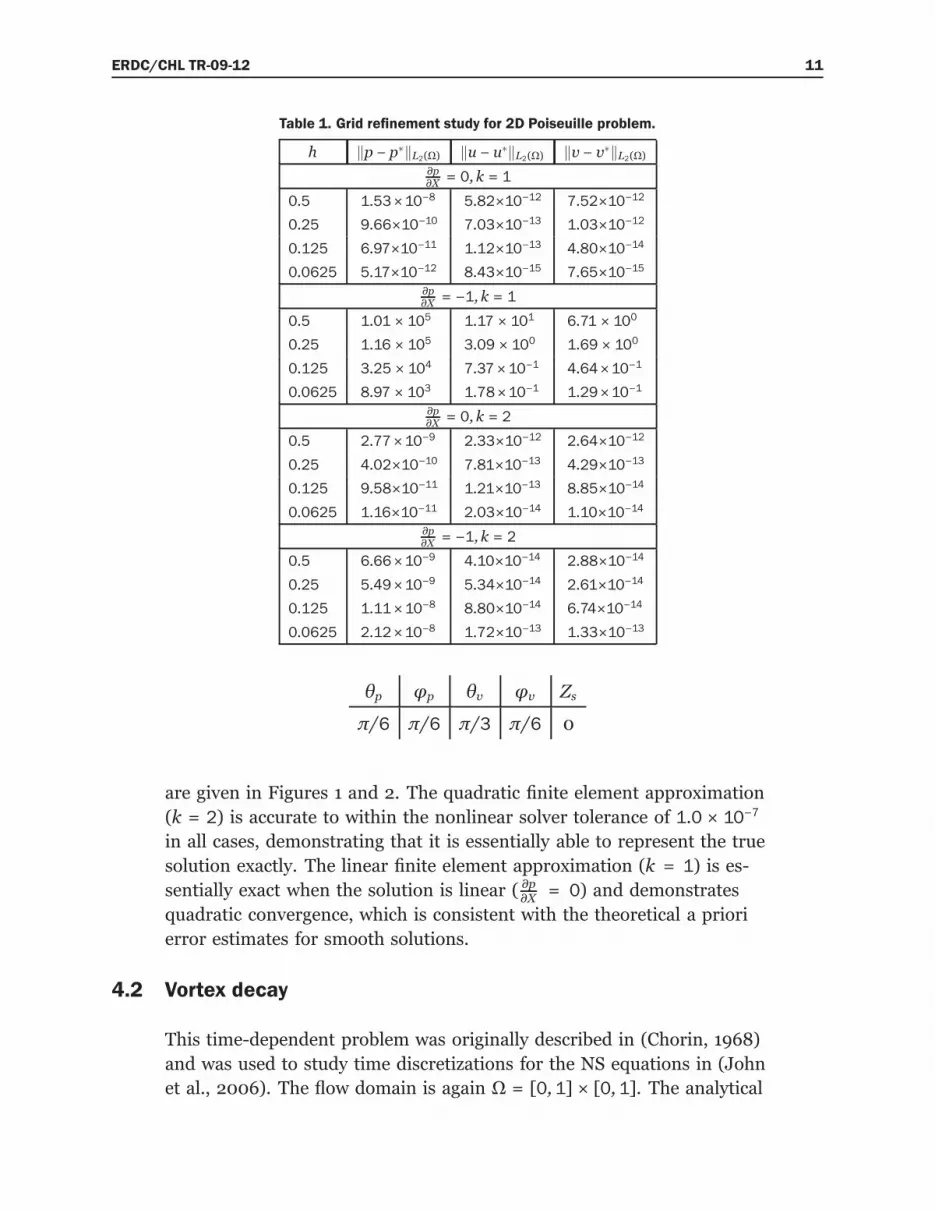
Table 1. Grid refinement study for 2D Poiseuille problem.

h ‖p − p∗‖L2(Ω) ‖u − u∗‖L2(Ω) ‖v − v∗‖L2(Ω)∂p∂X= 0, k = 1

0.5 1.53×10−8 5.82×10−12 7.52×10−12

0.25 9.66×10−10 7.03×10−13 1.03×10−12

0.125 6.97×10−11 1.12×10−13 4.80×10−14

0.0625 5.17×10−12 8.43×10−15 7.65×10−15

∂p∂X= −1, k = 1

0.5 1.01 × 105 1.17 × 101 6.71 × 100

0.25 1.16 × 105 3.09 × 100 1.69 × 100

0.125 3.25 × 104 7.37×10−1 4.64×10−1

0.0625 8.97 × 103 1.78×10−1 1.29×10−1

∂p∂X= 0, k = 2

0.5 2.77×10−9 2.33×10−12 2.64×10−12

0.25 4.02×10−10 7.81×10−13 4.29×10−13

0.125 9.58×10−11 1.21×10−13 8.85×10−14

0.0625 1.16×10−11 2.03×10−14 1.10×10−14

∂p∂X = −1, k = 2

0.5 6.66×10−9 4.10×10−14 2.88×10−14

0.25 5.49×10−9 5.34×10−14 2.61×10−14

0.125 1.11×10−8 8.80×10−14 6.74×10−14

0.0625 2.12×10−8 1.72×10−13 1.33×10−13

θp φp θv φv Zs

π/6 π/6 π/3 π/6 0

are given in Figures 1 and 2. The quadratic finite element approximation

(k = 2) is accurate to within the nonlinear solver tolerance of 1.0 × 10−7

in all cases, demonstrating that it is essentially able to represent the true

solution exactly. The linear finite element approximation (k = 1) is es-

sentially exact when the solution is linear ( ∂p∂X= 0) and demonstrates

quadratic convergence, which is consistent with the theoretical a priori

error estimates for smooth solutions.

4.2 Vortex decay

This time-dependent problem was originally described in (Chorin, 1968)

and was used to study time discretizations for the NS equations in (John

et al., 2006). The flow domain is again Ω = [0,1] × [0,1]. The analytical


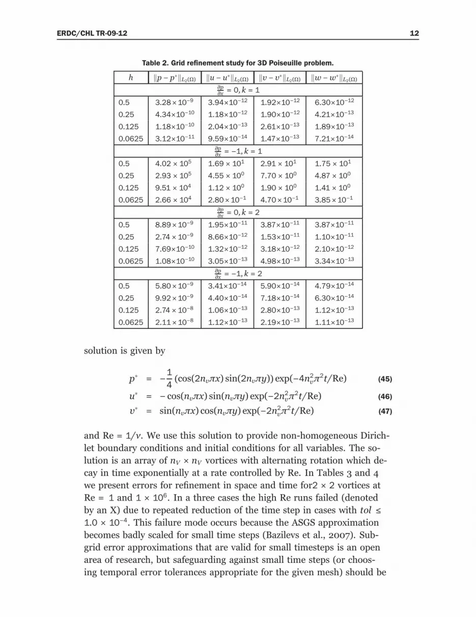
Table 2. Grid refinement study for 3D Poiseuille problem.

h ‖p − p∗‖L2(Ω) ‖u − u∗‖L2(Ω) ‖v − v∗‖L2(Ω) ‖w −w∗‖L2(Ω)∂p∂x= 0, k = 1

0.5 3.28×10−9 3.94×10−12 1.92×10−12 6.30×10−12

0.25 4.34×10−10 1.18×10−12 1.90×10−12 4.21×10−13

0.125 1.18×10−10 2.04×10−13 2.61×10−13 1.89×10−13

0.0625 3.12×10−11 9.59×10−14 1.47×10−13 7.21×10−14

∂p∂x= −1, k = 1

0.5 4.02 × 105 1.69 × 101 2.91 × 101 1.75 × 101

0.25 2.93 × 105 4.55 × 100 7.70 × 100 4.87 × 100

0.125 9.51 × 104 1.12 × 100 1.90 × 100 1.41 × 100

0.0625 2.66 × 104 2.80×10−1 4.70×10−1 3.85×10−1

∂p∂x= 0, k = 2

0.5 8.89×10−9 1.95×10−11 3.87×10−11 3.87×10−11

0.25 2.74×10−9 8.66×10−12 1.53×10−11 1.10×10−11

0.125 7.69×10−10 1.32×10−12 3.18×10−12 2.10×10−12

0.0625 1.08×10−10 3.05×10−13 4.98×10−13 3.34×10−13

∂p∂x = −1, k = 2

0.5 5.80×10−9 3.41×10−14 5.90×10−14 4.79×10−14

0.25 9.92×10−9 4.40×10−14 7.18×10−14 6.30×10−14

0.125 2.74×10−8 1.06×10−13 2.80×10−13 1.12×10−13

0.0625 2.11×10−8 1.12×10−13 2.19×10−13 1.11×10−13

solution is given by

p∗ = −1

4(cos(2nvπx) sin(2nvπy)) exp(−4n

2vπ2t/Re) (45)

u∗ = − cos(nvπx) sin(nvπy) exp(−2n2vπ2t/Re) (46)

v∗ = sin(nvπx) cos(nvπy) exp(−2n2vπ2t/Re) (47)

and Re = 1/ν. We use this solution to provide non-homogeneous Dirich-

let boundary conditions and initial conditions for all variables. The so-

lution is an array of nV × nV vortices with alternating rotation which de-

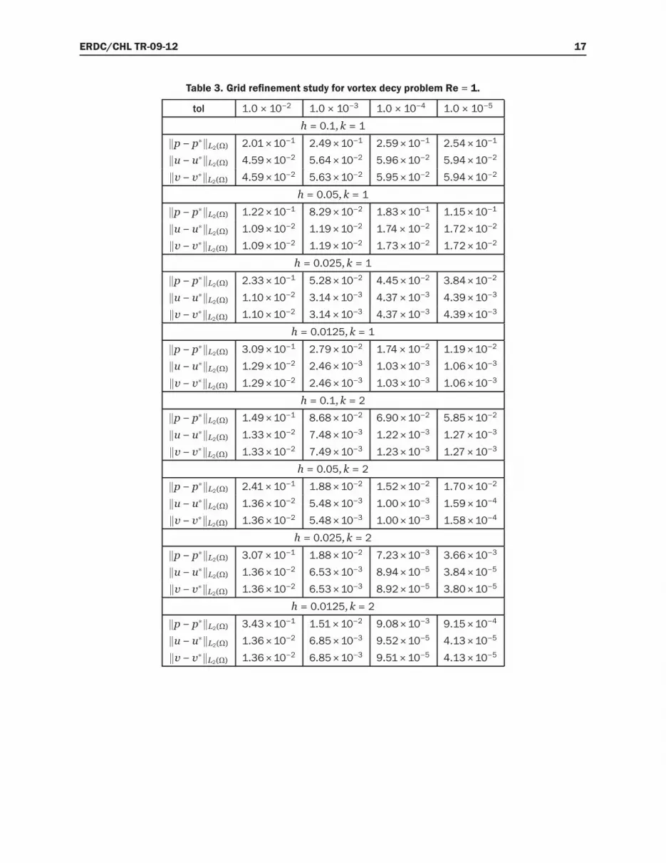
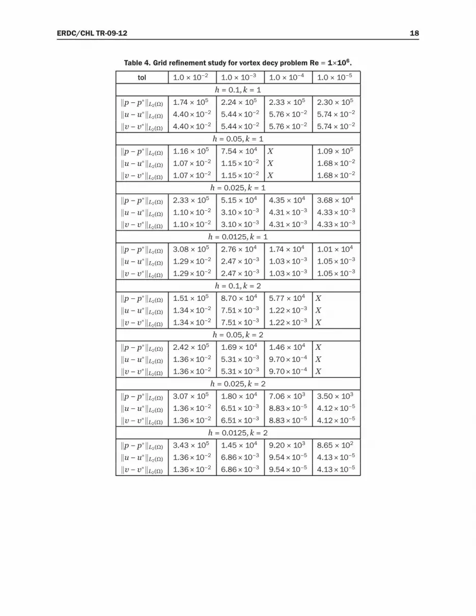
cay in time exponentially at a rate controlled by Re. In Tables 3 and 4

we present errors for refinement in space and time for2 × 2 vortices at

Re = 1 and 1 × 106. In a three cases the high Re runs failed (denoted

by an X) due to repeated reduction of the time step in cases with tol ≤

1.0 × 10−4. This failure mode occurs because the ASGS approximation

becomes badly scaled for small time steps (Bazilevs et al., 2007). Sub-

grid error approximations that are valid for small timesteps is an open

area of research, but safeguarding against small time steps (or choos-

ing temporal error tolerances appropriate for the given mesh) should be


sufficient for most applications where a time step on the order of the ad-

vective Courant-Friedrich-Levy condition is appropriate.

4.3 Lid driven cavity

The flow domain is Ω = [0, a] × [0, b] × [0, c]. The boundary conditions

are given by

v = (U,V,0) on z = c,0 < x < a,0 < y < b

v = 0 on x = 0, a, y = 0, b, z = 0

p(a/2, b/2, c) = 0

(48)

This problem has no analytical solution and exhibits a wide range of be-

havior depending on the Re. There is a discontinuity in the velocity at

the boundary along the upper edges of the cavity (corners in 2D). The

discontinuity reduces the regularity of the solution and consequently

produces a reduction in the asymptotic order of convergence. Never-

theless, it is a standard verification problem, and a great deal is known

about the structure of solutions (Bassi et al., 2006; Erturk et al., 2005).

In Figure 5 we present the results of a grid refinement study with four

levels of mesh refinement using the fourth level as the “exact” solution.

This measure of error is not accurate enough to compare two methods

of different orders. The L2 error estimates are shown to be decreasing

monotonically but clearly the order of convergence is less than the

quadratic and cubic rates predicted by the theory for smooth solutions.

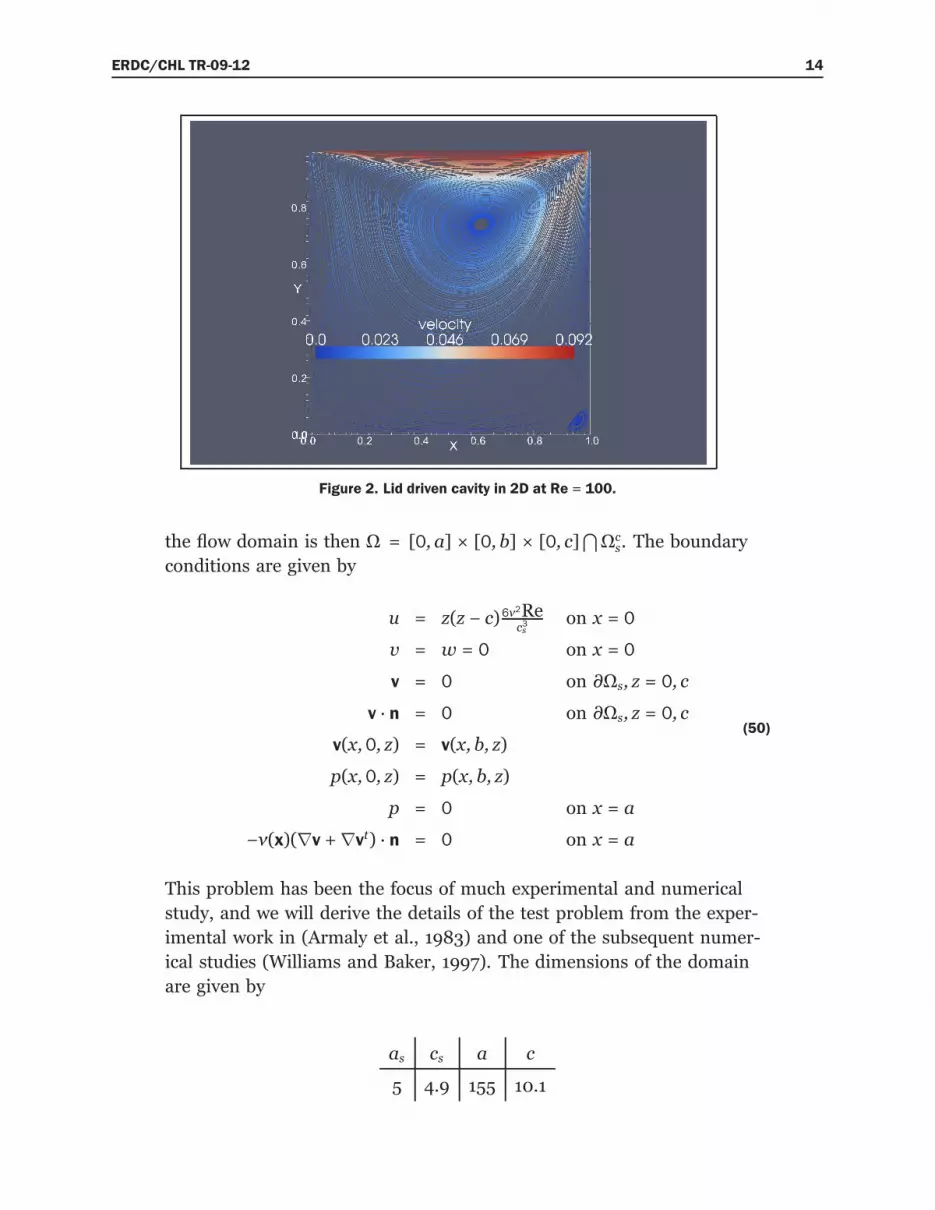
The streamlines for the driven cavity in 2D and 3D are given in Fig-

ures 2 - 4. The structure of the flows is in close agreement with previous

numerical studies, in particular the detailed high Re studies in (Erturk

et al., 2005).

4.4 Backward facing step

In this problem we consider flow over a square step at the lower left

hand edge of the domain. We can describe the step as

Ωs = x : 0 < x < as,0 < y < b,0 < z < cs (49)


Figure 2. Lid driven cavity in 2D at Re = 100.

the flow domain is then Ω = [0, a] × [0, b] × [0, c]⋂

Ωcs. The boundary

conditions are given by

u = z(z − c)6ν2Rec3s

on x = 0

v = w = 0 on x = 0

v = 0 on ∂Ωs, z = 0, c

v · n = 0 on ∂Ωs, z = 0, c

v(x,0, z) = v(x, b, z)

p(x,0, z) = p(x, b, z)

p = 0 on x = a

−ν(x)(∇v +∇vt) · n = 0 on x = a

(50)

This problem has been the focus of much experimental and numerical

study, and we will derive the details of the test problem from the exper-

imental work in (Armaly et al., 1983) and one of the subsequent numer-

ical studies (Williams and Baker, 1997). The dimensions of the domain

are given by

as cs a c

5 4.9 155 10.1



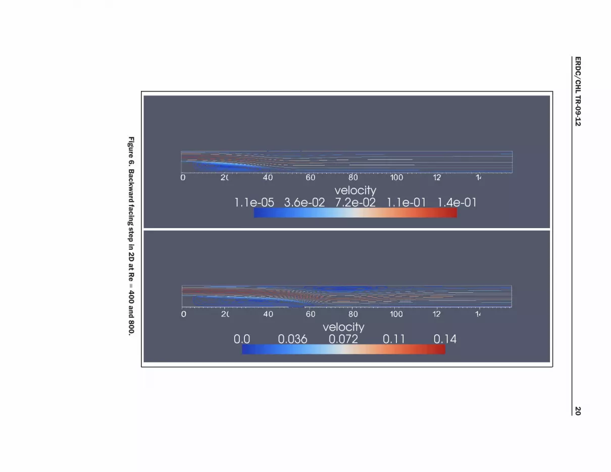
The recirculation length of the primary vortex for Re= 100 − 800 is

given in Figure 5, which is in close agreement with (Williams and Baker,

1997). Examples of the vortex structure in 2D and 3D are given in Fig-

ures 6 and 7.

4.5 Flow past a cylinder

We consider flow around a cylinder of radius R, oriented along the y-

axis. The cylinder can be described implicitly by

Ωs =

x :√

(x − xc)2 + (z − zc)2 < r

(51)

the flow domain is the Ω = [0, a] × [0, b] × [0, c]⋂

Ωcs where Ωcs is the

complement of Ωs. The boundary conditions are given by

u = sin(πt8)6z(c−z)c2

on x = 0

u = v = 0 on x = 0

v = 0 on ∂Ωs, z = 0, c

v · 0 = 0 on y = 0, b

−ν(x)(∇v +∇vt) · n = 0 on x = a, y = 0, b

p = 0 on x = a

(52)

This problem has no analytical solution and exhibits a wide range of be-

havior depending on Re. The variation in the lift coefficient is shown in



0 100 200 300 400 500 600 700 800 900 10002

4

6

8

10

12

14

Reynolds Number, Re

Rea

ttach

men

t Len

gth,

x1/c

s

Figure 5. Primary reattachment length versus Re.

Figure 8, which closely matches prior results studying higher-order time

discretizations (John et al., 2006).


Table 3. Grid refinement study for vortex decy problem Re = 1.

tol 1.0 × 10−2 1.0 × 10−3 1.0 × 10−4 1.0 × 10−5

h = 0.1, k = 1

‖p − p∗‖L2(Ω) 2.01×10−1 2.49×10−1 2.59×10−1 2.54×10−1

‖u − u∗‖L2(Ω) 4.59×10−2 5.64×10−2 5.96×10−2 5.94×10−2

‖v − v∗‖L2(Ω) 4.59×10−2 5.63×10−2 5.95×10−2 5.94×10−2

h = 0.05, k = 1

‖p − p∗‖L2(Ω) 1.22×10−1 8.29×10−2 1.83×10−1 1.15×10−1

‖u − u∗‖L2(Ω) 1.09×10−2 1.19×10−2 1.74× 10−2 1.72×10−2

‖v − v∗‖L2(Ω) 1.09×10−2 1.19×10−2 1.73×10−2 1.72×10−2

h = 0.025, k = 1

‖p − p∗‖L2(Ω) 2.33×10−1 5.28×10−2 4.45×10−2 3.84×10−2

‖u − u∗‖L2(Ω) 1.10×10−2 3.14×10−3 4.37×10−3 4.39×10−3

‖v − v∗‖L2(Ω) 1.10×10−2 3.14×10−3 4.37×10−3 4.39×10−3

h = 0.0125, k = 1

‖p − p∗‖L2(Ω) 3.09×10−1 2.79×10−2 1.74× 10−2 1.19×10−2

‖u − u∗‖L2(Ω) 1.29×10−2 2.46×10−3 1.03×10−3 1.06×10−3

‖v − v∗‖L2(Ω) 1.29×10−2 2.46×10−3 1.03×10−3 1.06×10−3

h = 0.1, k = 2

‖p − p∗‖L2(Ω) 1.49×10−1 8.68×10−2 6.90×10−2 5.85×10−2

‖u − u∗‖L2(Ω) 1.33×10−2 7.48×10−3 1.22×10−3 1.27×10−3

‖v − v∗‖L2(Ω) 1.33×10−2 7.49×10−3 1.23×10−3 1.27×10−3

h = 0.05, k = 2

‖p − p∗‖L2(Ω) 2.41×10−1 1.88×10−2 1.52×10−2 1.70×10−2

‖u − u∗‖L2(Ω) 1.36×10−2 5.48×10−3 1.00×10−3 1.59×10−4

‖v − v∗‖L2(Ω) 1.36×10−2 5.48×10−3 1.00×10−3 1.58×10−4

h = 0.025, k = 2

‖p − p∗‖L2(Ω) 3.07×10−1 1.88×10−2 7.23×10−3 3.66×10−3

‖u − u∗‖L2(Ω) 1.36×10−2 6.53×10−3 8.94×10−5 3.84×10−5

‖v − v∗‖L2(Ω) 1.36×10−2 6.53×10−3 8.92×10−5 3.80×10−5

h = 0.0125, k = 2

‖p − p∗‖L2(Ω) 3.43×10−1 1.51×10−2 9.08×10−3 9.15×10−4

‖u − u∗‖L2(Ω) 1.36×10−2 6.85×10−3 9.52×10−5 4.13×10−5

‖v − v∗‖L2(Ω) 1.36×10−2 6.85×10−3 9.51×10−5 4.13×10−5


Table 4. Grid refinement study for vortex decy problem Re = 1×106.

tol 1.0 × 10−2 1.0 × 10−3 1.0 × 10−4 1.0 × 10−5

h = 0.1, k = 1

‖p − p∗‖L2(Ω) 1.74 × 105 2.24 × 105 2.33 × 105 2.30 × 105

‖u − u∗‖L2(Ω) 4.40×10−2 5.44×10−2 5.76×10−2 5.74×10−2

‖v − v∗‖L2(Ω) 4.40×10−2 5.44×10−2 5.76×10−2 5.74×10−2

h = 0.05, k = 1

‖p − p∗‖L2(Ω) 1.16 × 105 7.54 × 104 X 1.09 × 105

‖u − u∗‖L2(Ω) 1.07×10−2 1.15×10−2 X 1.68×10−2

‖v − v∗‖L2(Ω) 1.07×10−2 1.15×10−2 X 1.68×10−2

h = 0.025, k = 1

‖p − p∗‖L2(Ω) 2.33 × 105 5.15 × 104 4.35 × 104 3.68 × 104

‖u − u∗‖L2(Ω) 1.10×10−2 3.10×10−3 4.31×10−3 4.33×10−3

‖v − v∗‖L2(Ω) 1.10×10−2 3.10×10−3 4.31×10−3 4.33×10−3

h = 0.0125, k = 1

‖p − p∗‖L2(Ω) 3.08 × 105 2.76 × 104 1.74 × 104 1.01 × 104

‖u − u∗‖L2(Ω) 1.29×10−2 2.47×10−3 1.03×10−3 1.05×10−3

‖v − v∗‖L2(Ω) 1.29×10−2 2.47×10−3 1.03×10−3 1.05×10−3

h = 0.1, k = 2

‖p − p∗‖L2(Ω) 1.51 × 105 8.70 × 104 5.77 × 104 X

‖u − u∗‖L2(Ω) 1.34×10−2 7.51×10−3 1.22×10−3 X

‖v − v∗‖L2(Ω) 1.34×10−2 7.51×10−3 1.22×10−3 X

h = 0.05, k = 2

‖p − p∗‖L2(Ω) 2.42 × 105 1.69 × 104 1.46 × 104 X

‖u − u∗‖L2(Ω) 1.36×10−2 5.31×10−3 9.70×10−4 X

‖v − v∗‖L2(Ω) 1.36×10−2 5.31×10−3 9.70×10−4 X

h = 0.025, k = 2

‖p − p∗‖L2(Ω) 3.07 × 105 1.80 × 104 7.06 × 103 3.50 × 103

‖u − u∗‖L2(Ω) 1.36×10−2 6.51×10−3 8.83×10−5 4.12×10−5

‖v − v∗‖L2(Ω) 1.36×10−2 6.51×10−3 8.83×10−5 4.12×10−5

h = 0.0125, k = 2

‖p − p∗‖L2(Ω) 3.43 × 105 1.45 × 104 9.20 × 103 8.65 × 102

‖u − u∗‖L2(Ω) 1.36×10−2 6.86×10−3 9.54×10−5 4.13×10−5

‖v − v∗‖L2(Ω) 1.36×10−2 6.86×10−3 9.54×10−5 4.13×10−5


Table 5. 2D lid driven cavity at Re = 100,400,1000.

h ‖p − p4‖L2(Ω) ‖u − u4‖L2(Ω) ‖v − v4‖L2(Ω)

Re= 100,k = 1

0.1 3.41×10−3 5.85×10−3 5.53×10−3

0.05 2.52×10−3 3.32×10−3 3.88×10−3

0.025 1.52×10−3 1.39×10−3 1.66×10−3

Re= 100,k = 2

0.1 1.16×10−3 2.97×10−3 3.26×10−3

0.05 7.96×10−4 1.39×10−3 1.56×10−3

0.025 4.98×10−4 6.16 × 104 7.74× 10−4

Re= 400,k = 1

0.1 1.44×10−2 2.88×10−2 2.80×10−2

0.05 1.01×10−2 1.52×10−2 1.64×10−2

0.025 6.07×10−3 5.27×10−3 6.46×10−3

Re= 400,k = 2

0.1 6.71×10−3 2.07×10−2 1.82×10−2

0.05 3.88×10−3 9.40×10−3 8.73×10−3

0.025 2.12×10−3 3.04×10−3 3.40×10−3

Re= 1000,k = 1

0.1 4.59×10−2 9.04×10−2 8.44×10−2

0.05 3.61×10−2 6.29×10−2 5.97×10−2

0.025 1.94×10−2 2.53×10−2 2.55×10−2

Re= 1000,k = 2

0.1 4.34×10−2 8.99×10−2 8.22×10−2

0.05 2.87×10−2 5.89×10−2 5.32×10−2

0.025 1.18×10−2 2.15×10−2 1.99×10−2

ERDC/CHLTR-09-12

20

Figure6.Backwardfacingstepin2DatRe=400and800.


Figure 7. Backward facing step in 3D at Re = 1000.

0 1 2 3 4 5 6 7 8−0.5

−0.4

−0.3

−0.2

−0.1

0

0.1

0.2

0.3

0.4

0.5

t

lift c

oeffi

cien

t

Figure 8. Lift coefficient versus time for 0 ≤ Re(t) ≤ 100.


Figure 9. Flow around a square cylinder in 3D at Re = 70 .


5 Conclusions

We described a set of numerical methods for approximating widely used

models of incompressible flow. The methods apply to complex geome-

tries and unstructured meshes, provide locally conservative velocity fields,

and achieve higher-order accuracy in space and time. Furthermore the

multiscale variational method employed provides reasonable accuracy

for high Re flows and has shown promise as a hybrid LES/DNS method

(Hoffman and Johnson, 2006; Bazilevs et al., 2007). The methods and

implementation were verified on a set of two- and three-dimensional

benchmark problems. Several issues for future work were identified:

• An alternative to the quasi-static subgrid scales assumption in the

subgrid error approximation should be implemented for small times

steps.

• Futher work on error estimation and startup heuristics are needed

since spatial and temporal error are tightly coupled and error

• Work vs. error studies should be conducted to verify that the second-

order methods are superior to first-order methods.


References

Armaly, B. F., F. Durst, J. C. F. Pereira, and B. Schönung (1983). Experimental and the-oretical investigation of backward-facing step flow. Journal of Fluid Mechan-ics 127, 473–496.

Ashcraft, C. and R. Grimes (1999). Spooles: An object-oriented sparse matrix library.In Proceedings of the 9th SIAM Conference on Parallel Processing for ScientificComputing.

Balay, S., K. Buschelman, V. Eijkhout, W. D. Gropp, D. Kaushik, M. G. Knepley, L. C.McInnes, B. F. Smith, and H. Zhang (2004). PETSc users manual. TechnicalReport ANL-95/11 - Revision 2.1.5, Argonne National Laboratory.

Balay, S., K. Buschelman, W. D. Gropp, D. Kaushik, M. G. Knepley, L. C. McInnes, B. F.Smith, and H. Zhang (2001). PETSc Web page. http://www.mcs.anl.gov/petsc.

Balay, S., W. D. Gropp, L. C. McInnes, and B. F. Smith (1997). Efficient managementof parallelism in object oriented numerical software libraries. In E. Arge, A. M.Bruaset, and H. P. Langtangen (Eds.),Modern Software Tools in Scientific Com-puting, pp. 163–202. Birkhäuser Press.

Bassi, F., A. Crivellini, D. A. D. Pietro, and S. Rebay (2006). An artificial compressibilityflux for the discontinuous Galerkin solution of the incompressible Navier–Stokesequations. Journal of Computational Physics 218, 794–815.

Batchelor, G. K. (1967). An Introduction to Fluid Dynamics. Cambridge.

Bazilevs, Y., V. M. Calo, J. A. Cottrel, T. J. R. Hughes, A. Reali, and G. Scovazzi (2007).Variational multiscale residual-based turbulence modeling for large eddy simu-lation of incompressible flows. Computer Methods in Applied Mechanics andEngineering 197, 173–201.

Bernard, R. S., P. V. Luong, and M. J. Sanchez (2007). Par3d: Numerical model for in-compressible flow with applications to aerosal dispersion in complex enclosures.Technical Report TR-07-9, U.S. Army Engineer Research and Development Cen-ter.

Chorin, A. J. (1968). Numerical solution of the Navier–Stokes equations. Mathematics ofComputation 22(104), 745–762.

Dawson, C., S. Sun, and M. F. Wheeler (2004). Compatible algorithms for coupled flowand transport. Computer Methods in Applied Mechanics and Engineering 193,2565–2580.

Demmel, J. W., S. C. Eisenstat, J. R. Gilbert, X. S. Li, and J. W. H. Liu (1999). A supern-odal approach to sparse partial pivoting. SIAM J. Matrix Analysis and Applica-tions 20(3), 720–755.

Erturk, E., T. C. Corke, and C. Gökçöl (2005). Numerical solution of 2-d steady incom-pressible driven cavity flow at high Reynolds numbers. International Journal for


Numerical Methods in Fluids 48, 747–774.

Farthing, M. W. and C. E. Kees (2008). Implementation of discontinuous galerking meth-ods for level set equations on unstructured meshes. Technical Note CHETN-XII-2, U. S. Army Engineer Research and Development Center, Coastal and Hy-draulics Laboratory.

Farthing, M. W. and C. E. Kees (2009). Evaluating finite element methods for the levelset equation. Technical Report TR-09-11, U. S. Army Engineer Research andDevelopment Center, Coastal and Hydraulics Laboratory.

Farthing, M. W., C. E. Kees, T. S. Coffey, C. T. Kelley, and C. T. Miller (2003). Efficientsteady-state solution techniques for variably saturated groundwater flow. Ad-vances in Water Resources 26, 833–849.

Hoffman, J. and C. Johnson (2006). A new approach to turbulence modeling. ComputerMethods in Applied Mechanics and Engineering 23-24, 2865–2880.

Hughes, T. (1995). Multiscale phenomena: Greens’s functions, the Dirichlet-to-Neumannformulation, subgrid scale models, bubbles and the origins of stabilized methods.Computer Methods in Applied Mechanics and Engineering 127, 387–401.

Hutter, K. and K. D. Jöhnk (2004). ContinuumMethods of PhysicalModeling: Contin-uumMechanics, Dimensional Analysis, Turbulence. Springer.

John, V., G. Matthies, and J. Rang (2006). A comparison of time-discretization/linearization approaches for the incompressible Navier–Stokesequations. Computer Methods in Applied Mechanics and Engineering 195,5995–6010.

Kees, C. E., M. W. Farthing, and C. N. Dawson (2008). Locally conservative, stabilizedfinite element methods for variably saturated flow. Computer Methods in AppliedMechanics and Engineering 197(51-52), 4610–4625.

Kees, C. E., M. W. Farthing, and M. T. Fong (2009). Evaluating finite element methods forthe level set equation. Technical Report TR-09-11, U. S. Army Engineer Researchand Development Center, Coastal and Hydraulics Laboratory.

Knoll, D. A. and P. R. McHugh (1998). Enhanced nonlinear iterative techniques appliedto nonequilibrium plasma flow. SIAM Journal on Scientific Computing 19(1),291–301.

Larson, M. and A. Niklasson (2004). A conservative flux for the continuous Galerkinmethod based on discontinuous enrichment. CALCOLO 41, 65–76.

Oberkampf, W. L. and T. G. Trucano (2002). Verification and validation in computationalfluid dynamics. Progress in Aerospace Sciences 33, 209–272.

Roache, P. J. (1998). Verification of codes and calculations. AIAA Journal 36(5), 696–702.

Schäfer, M., S. Turek, F. Durst, E. Krause, and R. Rannacher (1996). Benchmark com-putations of laminar flow around a cylinder. Notes on Numerical Fluid Mechan-ics 52, 547–566.


Williams, P. T. and A. J. Baker (1997). Numerical simulations of laminar flow over abackward-facing step. International Journal for Numerical Methods in Flu-ids 24, 1159–1183.

REPORT DOCUMENTATION PAGE Form Approved

OMB No. 0704-0188 Public reporting burden for this collection of information is estimated to average 1 hour per response, including the time for reviewing instructions, searching existing data sources, gathering and maintaining the data needed, and completing and reviewing this collection of information. Send comments regarding this burden estimate or any other aspect of this collection of information, including suggestions for reducing this burden to Department of Defense, Washington Headquarters Services, Directorate for Information Operations and Reports (0704-0188), 1215 Jefferson Davis Highway, Suite 1204, Arlington, VA 22202-4302. Respondents should be aware that notwithstanding any other provision of law, no person shall be subject to any penalty for failing to comply with a collection of information if it does not display a currently valid OMB control number. PLEASE DO NOT RETURN YOUR FORM TO THE ABOVE ADDRESS.

1. REPORT DATE (DD-MM-YYYY) August 2009

2. REPORT TYPE Final Report

3. DATES COVERED (From - To)

5a. CONTRACT NUMBER

5b. GRANT NUMBER

4. TITLE AND SUBTITLE

Locally Conservative, Stabilized Finite Element Methods for a Class of Variable Coefficient Navier-Stokes Equations

5c. PROGRAM ELEMENT NUMBER

5d. PROJECT NUMBER

5e. TASK NUMBER

6. AUTHOR(S)

C.E. Kees, M.W. Farthing, and M.T. Fong

5f. WORK UNIT NUMBER KHBCGD

7. PERFORMING ORGANIZATION NAME(S) AND ADDRESS(ES) 8. PERFORMING ORGANIZATION REPORT NUMBER

U.S. Army Engineer Research and Development Center Coastal and Hydraulics Laboratory 3909 Halls Ferry Road Vicksburg, MS 39180-6199

ERDC/CHL TR-09-12

9. SPONSORING / MONITORING AGENCY NAME(S) AND ADDRESS(ES) 10. SPONSOR/MONITOR’S ACRONYM(S)

11. SPONSOR/MONITOR’S REPORT NUMBER(S)

12. DISTRIBUTION / AVAILABILITY STATEMENT Approved for distribution; distribution is unlimited.

13. SUPPLEMENTARY NOTES

14. ABSTRACT

Computer simulation of three-dimensional incompressible flow is of interest in many navigation, coastal, and geophysical applications. This report is the the fifth in a series of publications that documents research and development on a state-of-the-art computational modeling capability for fully three-dimensional two-phase fluid flows with vessel/ structure interaction in complex geometries (Farthing and Kees, 2008; Kees et al., 2008; Farthing and Kees, 2009; Kees et al., 2009). It is primarily concerned with model verification, often defined as “solving the equations right” (Roache, 1998). Model verification is a critical step on the way to producing reliable numerical models, but it is a step that is often neglected (Oberkampf and Trucano, 2002). Quantitative and qualitative methods for verification also provide metrics for evaluating numerical methods and identifying promising lines of future research. (continued next page)

15. SUBJECT TERMS

Backward difference formulas Backward facing step

Computational fluid dynamics Driven cavity Finite elements

Model verificatoin Reynolds averaging Variational multiscale methods

16. SECURITY CLASSIFICATION OF: 17. LIMITATION OF ABSTRACT

18. NUMBER OF PAGES

19a. NAME OF RESPONSIBLE PERSON

a. REPORT

UNCLASSIFIED

b. ABSTRACT

UNCLASSIFIED

c. THIS PAGE

UNCLASSIFIED 35 19b. TELEPHONE NUMBER (include area code)

Standard Form 298 (Rev. 8-98) Prescribed by ANSI Std. 239.18

Abstract (continued)

Fully-three dimensional flows are often described by the incompressible Navier-Stokes (NS) equations or related model equations such as the Reynolds Averaged Navier Stokes (RANS) equations and Two-Phase Reynolds Averaged Navier-Stokes equations (TPRANS).We will describe spatial and temporal discretization methods for this class of equations and test problems for evaluating the methods and implementations. The discretization methods are based on stabilized continuous Galerkin methods (variational multiscale methods) and discontinous Galerkin methods. The test problems are taken from classical fluid mechanics and well-known benchmarks for incompressible flow codes (Batchelor, 1967; Chorin, 1968; Schäfer et al., 1996; Williams and Baker, 1997; John et al., 2006). We demonstrate that the methods described herein meet three minimal requirements for use in a wide variety of applications: 1) they apply to complex geometries and a range of mesh types; 2) they robustly provide accurate results over a wide range of flow conditions; and 3) they yield qualitatively correct solutions, in particular mass and volume conserving velocity approximations.

Locally conservative, stabilized finite element methods for variably saturated flow

Documents