Local–global mode interaction in stringer-stiffened plates

Local–global mode interaction in stringer-stiffened plates

M. Ahmer Wadee∗, Maryam Farsi

Department of Civil & Environmental Engineering, Imperial College London,

South Kensington Campus, London SW7 2AZ, UK

Abstract

A recently developed nonlinear analytical model for axially loaded thin-walled stringer-stiffened plates based on variational principles is extended to include local buckling of themain plate. Interaction between the weakly stable global buckling mode and the stronglystable local buckling mode is highlighted. Highly unstable post-buckling behaviour and aprogressively changing wavelength in the local buckling mode profile is observed under in-creasing compressive deformation. The analytical model is compared against both physicalexperiments from the literature and finite element analysis conducted in the commercialcode Abaqus; excellent agreement is found both in terms of the mechanical response andthe predicted deflections.

Keywords: Mode interaction; Stiffened plates; Cellular buckling; Snaking; Nonlinearmechanics.

1. Introduction

Thin-walled stringer-stiffened plates under axial compression are well known to be vul-nerable to buckling where local and global modes interact nonlinearly [1, 2, 3, 4]. However,since stiffened plates are highly mass-efficient structural components, their application isubiquitous in long-span bridge decks [5], ships and offshore structures [6], and aerospacestructures [7, 8]. Hence, understanding the behaviour of these components represents astructural problem of enormous practical significance [9, 10, 11]. Other significant struc-tural components such as sandwich struts [12], built-up columns [13], corrugated plates[14] and other thin-walled components [15, 16, 17, 18] are also well-known to suffer fromthe instabilities arising from the interaction of global and local buckling modes.

In the authors’ recent work [19], the aforementioned problem was studied using ananalytical approach by considering that interactive buckling was wholly confined to thestringer (or stiffener) only. So-called “cellular buckling” [20, 21, 18, 22] or “snaking” [23,24, 25] was captured, where snap-backs in the response, showing sequential destabilization

∗Corresponding authorEmail addresses: [email protected] (M. Ahmer Wadee), [email protected]

(Maryam Farsi)Article accepted on 19 September 2014

Preprint submitted to Thin-Walled Structures 18 September 2014

and restabilization and a progressive spreading of the initial localized buckling mode, wererevealed. The results showed reasonably good comparisons with a finite element (FE)model formulated in the commercial code Abaqus [26]. The current work extends theprevious model such that the interaction between global Euler buckling and the localbuckling of the main plate, as well as the stiffener, are accounted. A system of nonlinearordinary differential equations subject to integral constraints is derived using variationalprinciples and is subsequently solved using the numerical continuation package Auto-

07p [27]. The relative rigidity of the main plate–stiffener joint is adjusted by means of arotational spring, increasing the stiffness of which results in the erosion of the snap-backsthat signify cellular buckling. However, the changing local buckling wavelength is stillobserved, although the effect is not quite so marked as compared with the case where thejoint is assumed to be pinned [19]. A finite element model is also developed using thecommercial code Abaqus for validation purposes. Moreover, given that local bucklingof the main plate is included alongside the buckling of the stiffener in the current model,which is often observed in experiments, the present results are also compared with a coupleof physical test results from the literature [2]. The comparisons turn out to be excellentboth in terms of the mechanical response and the physical post-buckling profiles.

2. Analytical Model

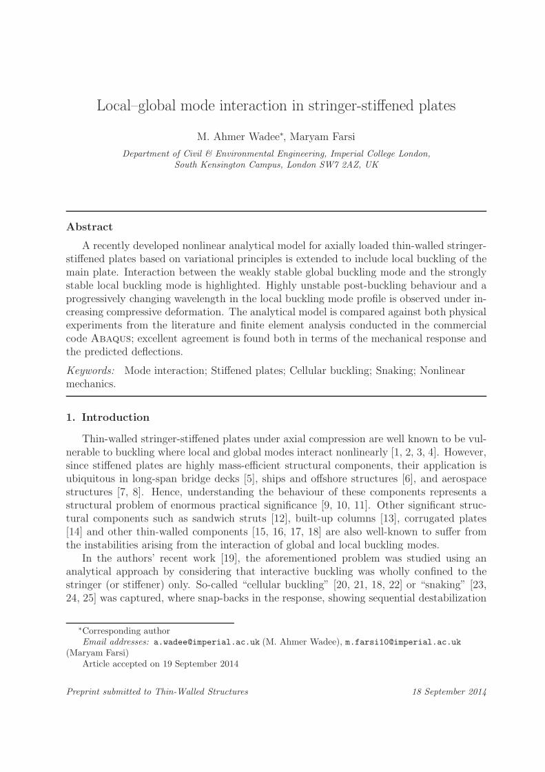
Consider a thin-walled simply-supported plated panel that has uniformly spaced stiff-eners above and below the main plate, as shown in Figure 1, with panel length L and

Simply-supported stiffened panel:

b

L

b

Focus on this portion

Figure 1: An axially compressed simply-supported stiffened panel of length L and evenly spaced stiffenersseparated by a distance b.

the spacing between the stiffeners being b. It is made from a linear elastic, homogeneousand isotropic material with Young’s modulus E, Poisson’s ratio ν and shear modulusG = E/[2(1 + ν)]. If the panel is much wider than long, i.e. L ≪ nsb, where ns is thenumber of stiffeners in the panel, the critical buckling behaviour of the panel would be

2

strut-like with a half-sine wave eigenmode along the length. Moreover, this would allowa portion of the panel that is representative of its entirety to be isolated as a strut asdepicted in Figure 1, since the transverse bending curvature of the panel during initialpost-buckling would be relatively small.

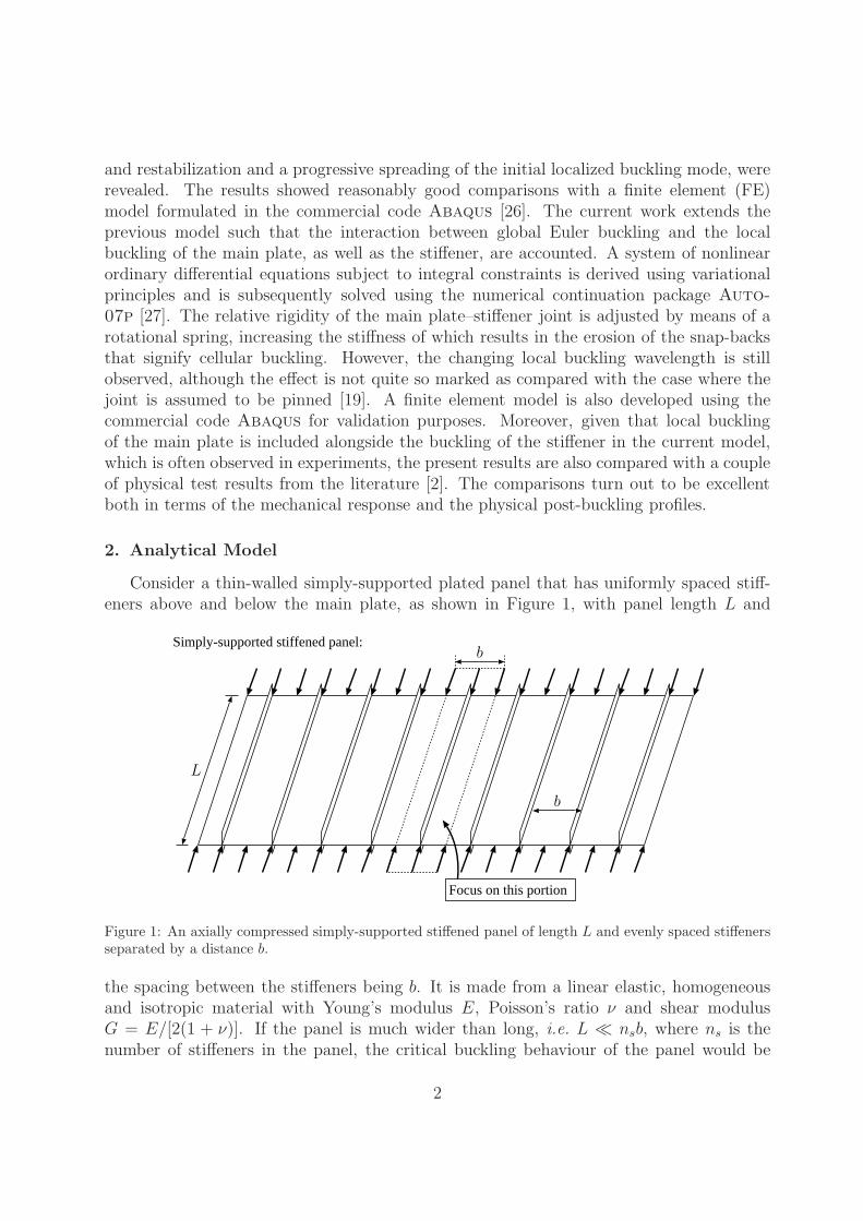
Therefore, the current article presents an analytical model of a representative portionof an axially-compressed stiffened panel, which simplifies to a simply supported strut withgeometric properties defined in Figure 2. The strut has length L and comprises a main

z L

yP Neutral axis of bending

(a)

ts

tstp

h1

h2

y

y

bx

(b)

cp

x

(c)

zy W(z)

Sway mode:

zy θ(z)

Tilt mode:

(d)

Figure 2: (a) Elevation of the representative portion of the stiffened plate modelled as strut of length Lthat is compressed axially by a force P . (b) Strut cross-section geometry. (c) Modelling the joint rigidityof the main plate–stiffener connection with a rotational spring of stiffness cp. (d) Sway and tilt componentsof the global buckling mode.

plate (or skin) of width b and thickness tp with two attached longitudinal stiffeners ofheights h1 and h2 with thickness ts, as shown in Figure 2(b). The axial load P is appliedat the centroid of the whole cross-section denoted as the distance y from the centre line ofthe plate. The rigidity of the connection between the main plate and stiffeners is modelledwith a rotational spring of stiffness cp, as shown in Figure 2(c). If cp = 0, a pinned jointis modelled, but if cp is large, the joint is considered to be completely fixed or rigid. Notethat the rotational spring with stiffness cp only stores strain energy by local bending of thestiffener or the main plate at the joint coordinates (x = 0, y = −y) and not by rigid bodyrotation of the entire joint in a twisting action.

2.1. Modal descriptions

To model interactive buckling analytically, it has been demonstrated that shear strainsneed to be included [28, 29] and for thin-walled metallic elements Timoshenko beam theory

3

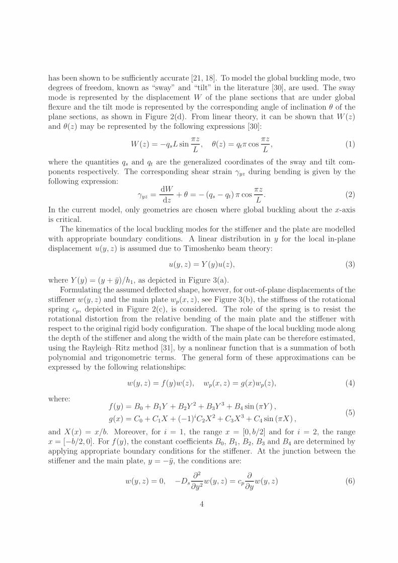
has been shown to be sufficiently accurate [21, 18]. To model the global buckling mode, twodegrees of freedom, known as “sway” and “tilt” in the literature [30], are used. The swaymode is represented by the displacement W of the plane sections that are under globalflexure and the tilt mode is represented by the corresponding angle of inclination θ of theplane sections, as shown in Figure 2(d). From linear theory, it can be shown that W (z)and θ(z) may be represented by the following expressions [30]:

W (z) = −qsL sinπz

L, θ(z) = qtπ cos

πz

L, (1)

where the quantities qs and qt are the generalized coordinates of the sway and tilt com-ponents respectively. The corresponding shear strain γyz during bending is given by thefollowing expression:

γyz =dW

dz+ θ = − (qs − qt)π cos

πz

L. (2)

In the current model, only geometries are chosen where global buckling about the x-axisis critical.

The kinematics of the local buckling modes for the stiffener and the plate are modelledwith appropriate boundary conditions. A linear distribution in y for the local in-planedisplacement u(y, z) is assumed due to Timoshenko beam theory:

u(y, z) = Y (y)u(z), (3)

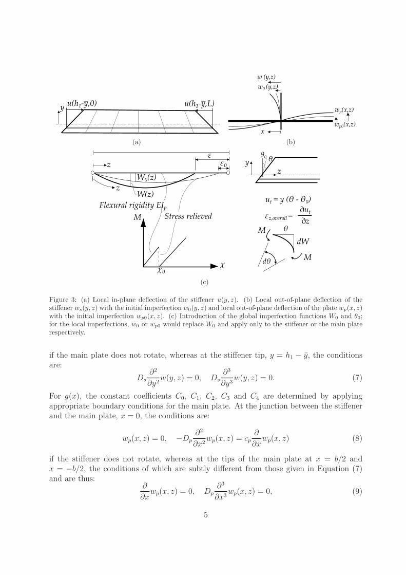
where Y (y) = (y + y)/h1, as depicted in Figure 3(a).Formulating the assumed deflected shape, however, for out-of-plane displacements of the

stiffener w(y, z) and the main plate wp(x, z), see Figure 3(b), the stiffness of the rotationalspring cp, depicted in Figure 2(c), is considered. The role of the spring is to resist therotational distortion from the relative bending of the main plate and the stiffener withrespect to the original rigid body configuration. The shape of the local buckling mode alongthe depth of the stiffener and along the width of the main plate can be therefore estimated,using the Rayleigh–Ritz method [31], by a nonlinear function that is a summation of bothpolynomial and trigonometric terms. The general form of these approximations can beexpressed by the following relationships:

w(y, z) = f(y)w(z), wp(x, z) = g(x)wp(z), (4)

where:f(y) = B0 +B1Y +B2Y

2 +B3Y3 +B4 sin (πY ) ,

g(x) = C0 + C1X + (−1)iC2X2 + C3X

3 + C4 sin (πX) ,(5)

and X(x) = x/b. Moreover, for i = 1, the range x = [0, b/2] and for i = 2, the rangex = [−b/2, 0]. For f(y), the constant coefficients B0, B1, B2, B3 and B4 are determined byapplying appropriate boundary conditions for the stiffener. At the junction between thestiffener and the main plate, y = −y, the conditions are:

w(y, z) = 0, −Ds∂2

∂y2w(y, z) = cp

∂

∂yw(y, z) (6)

4

u(h1-y,0) u(h1-y,L)y

(a)

w (y,z)

wp(x,z)

x

w0 (y,z)

wp0(x,z)

(b)

ε0

ε

z

W0(z)

W(z)z

y θθ0

z

Stress relieved

Flexural rigidity EIp

χχ0

M

ut = y (θ - θ0)

εz,overall = ∂ut

∂zθ

dθ

M

M

dW

(c)

Figure 3: (a) Local in-plane deflection of the stiffener u(y, z). (b) Local out-of-plane deflection of thestiffener ws(y, z) with the initial imperfection w0(y, z) and local out-of-plane deflection of the plate wp(x, z)with the initial imperfection wp0(x, z). (c) Introduction of the global imperfection functions W0 and θ0;for the local imperfections, w0 or wp0 would replace W0 and apply only to the stiffener or the main platerespectively.

if the main plate does not rotate, whereas at the stiffener tip, y = h1 − y, the conditionsare:

Ds∂2

∂y2w(y, z) = 0, Ds

∂3

∂y3w(y, z) = 0. (7)

For g(x), the constant coefficients C0, C1, C2, C3 and C4 are determined by applyingappropriate boundary conditions for the main plate. At the junction between the stiffenerand the main plate, x = 0, the conditions are:

wp(x, z) = 0, −Dp∂2

∂x2wp(x, z) = cp

∂

∂xwp(x, z) (8)

if the stiffener does not rotate, whereas at the tips of the main plate at x = b/2 andx = −b/2, the conditions of which are subtly different from those given in Equation (7)and are thus:

∂

∂xwp(x, z) = 0, Dp

∂3

∂x3wp(x, z) = 0, (9)

5

where Ds and Dp are the stiffener and the plate flexural rigidities given by the expressionsEt3s/[12(1−ν

2)] and Et3p/[12(1−ν2)] respectively. It is worth emphasizing that the second

(mechanical) boundary conditions for determining Bn and Cn, given in Equations (6) and(8), are simplifying approximations that are admissible since the formulation is basedessentially on the Rayleigh–Ritz method [31].

The length y gives the location of the neutral-axis of bending measured from the centreline of the main plate and is expressed thus:

y =ts [h

21 − h22]

2 [(b− ts) tp + (h1 + h2) ts]. (10)

The final constants are fixed by imposing the normalizing conditions with f(h1 − y) = 1and g(b/2) = 1. The functions for the deflected shapes w(y, z) and wp(x, z) can be writtenthus:

w(y, z) =

{

Y − Jsπ3

6

[

2Y − 3Y 2 + Y 3 −6

π3sin (πY )

]}

w(z),

wp(x, z) = −

{

sin (πX) + Jp

[

X + (−1)iX2 −1

4sin (πX)

]}

wp(z),

(11)

where:

Js =

{

π

[

Dsπ2

cph1+π2

3− 1

]}−1

, Jp =

{[

1

4−

2Dp

cpbπ−

1

π

]}−1

. (12)

In physical experiments, it is often observed that the main plate deflects in sympathywith the stiffener to some extent and so in the current work, the following relationship isassumed, wp(z) = λpw(z). Since the rotations would therefore be all in the same sensethey can be expressed as first derivatives of w or wp; these are multiplied by the jointrotational stiffness cp such that the total bending moment is established. By allowing boththe main plate and the stiffener to rotate locally and summing the bending moments forthe stiffener and both sides of the main plate at the intersection (x = 0, y = −y), anexplicit relationship can be derived:

Ds∂2w

∂y2+ Dp

∂2wp

∂x2

∣

∣

∣

∣

i=1

−Dp∂2wp

∂x2

∣

∣

∣

∣

i=2

= cp

(

∂w

∂y+∂wp

∂x

∣

∣

∣

∣

i=1

+∂wp

∂x

∣

∣

∣

∣

i=2

)

. (13)

The negative sign in front of the final term of the left hand side of Equation (13) reflectsthe fact the main plate bending moment changes sign at x = 0. The expression forthe deflection relating parameter λp can be determined by substituting the aforementionedexpression wp(z) = λpw(z) into Equation (13) and, after a bit of manipulation, the followingrelationship is derived:

λp =

(

2b2

3h21

)[

cph1 [3 + Jsπ(3− π2)]− 3DsJsπ3

8DpJp + cpb [4π + Jp(4− π)]

]

. (14)

This simplifies the formulation considerably by allowing the system to be modelled witheffectively only one out-of-plane displacement function w.

6

2.2. Imperfection modelling

Since real structures contain imperfections, the current model incorporates the possi-bility of both global and local initial imperfections within the geometry. This is performedby introducing initial deflections that are stress-relieved, as shown in Figure 3(c), such thatthe strain energies are zero in the initially imperfect state. An initial out-of-straightnessW0 is introduced as a global imperfection as well as the corresponding initial rotation ofthe plane section θ0 of the stiffener. The expressions for these functions are:

W0(z) = −qs0L sinπz

L, θ0 = qt0π cos

πz

L, (15)

with qs0 and qt0 defining the amplitudes of the global imperfection. The local out-of-plane imperfection for the stiffener and the main plate is formulated from a first orderapproximation of a multiple scale perturbation analysis of a strut on a softening elasticfoundation [32], the mathematical shape of which is expressed as:

w0(z) = A0 sech

[

α (z − η)

L

]

cos

[

βπ (z − η)

L

]

, (16)

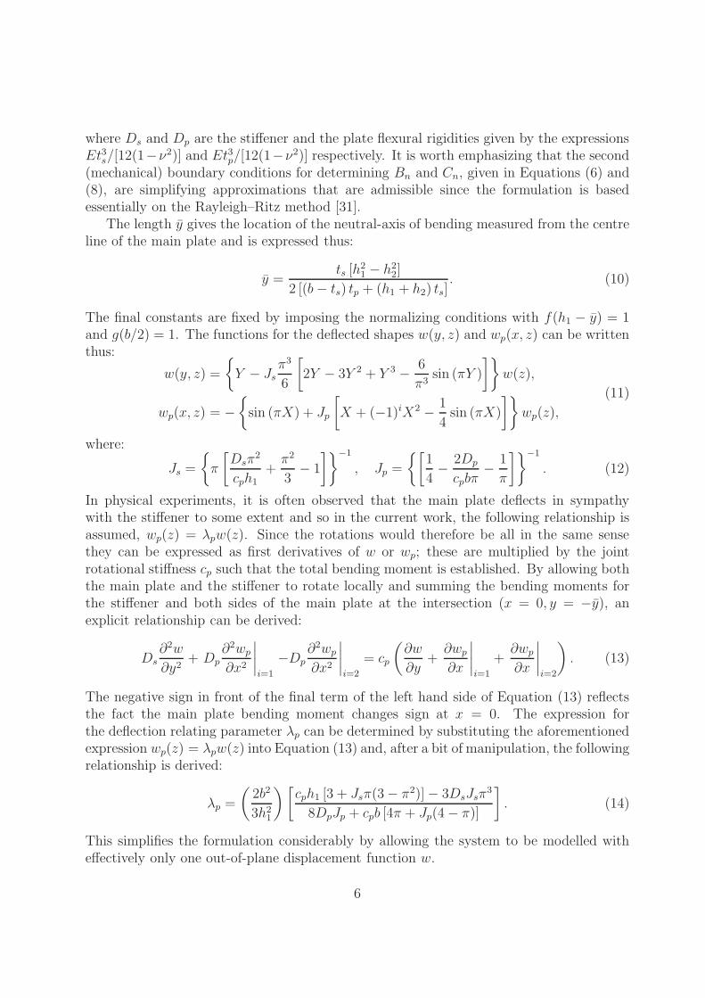
where z = [0, L] and w0 is symmetric about z = η. This function has been shown inthe literature to provide a representative imperfection for local–global mode interactionproblems [33]. Moreover, this form for w0 enables the study of periodic and localizedimperfections; a local imperfection is periodic when α = 0 with a number of half sine wavesequal to β along the length of the panel. It is also noted that the relationship betweenwp0 and w0 corresponds to that for the perfect case; hence, wp0 = λpw0 is assumed. Theshape of the initial imperfection is illustrated in Figure 4. By increasing the α value, the

0 1 2−1

0

1

w0/A

0

2z/L

increasing α

(a)

0 1 2−1

0

1

w0/A

0

2z/L

increasing β

(b)

Figure 4: Local imperfection profile w0. (a) Localized imperfections introduced by increasing α. (b)Periodic imperfections (α = 0) with different numbers of half sine waves by changing β. In both casesη = L/2.

initial imperfection forms into a localized shape, as shown in Figure 4(a), otherwise theimperfection shape is periodic, as shown in Figure 4(b).

2.3. Total potential energy

A well established procedure for deriving the total potential energy V , has been pre-sented in previous work [19]; the current work follows the same approach but now includes

7

the local buckling deflection of the main plate. The global strain energy Ubo due to Eulerbuckling is given by the equation below:

Ubo =1

2EIp

∫ L

0

(

W − W0

)2

dz =1

2EIp

∫ L

0

(qs − qs0)2 π

4

L2sin2 πz

Ldz, (17)

where dots represent differentiation with respect to z and Ip = (b− ts)t3p/12 + (b− ts)tpy

2

is the second moment of area of the plate about the global x-axis. The strain energy fromlocal bending of the stiffener and the main plate Ubl is given by the following expression:

Ubl =Ds

2

∫ L

0

∫ h1−y

−y

{

[

∂2(w − w0)

∂z2+∂2(w − w0)

∂y2

]2

−2 (1− ν)

[

∂2(w − w0)

∂z2∂2(w − w0)

∂y2−

(

∂2(w − w0)

∂z∂y

)2]}

dy dz

+Dp

2

∫ L

0

∫ b/2

−b/2

{

[

∂2(wp − wp0)

∂z2+∂2(wp − wp0)

∂x2

]2

−2 (1− ν)

[

∂2(wp − wp0)

∂z2∂2(wp − wp0)

∂x2−

(

∂2(wp − wp0)

∂z∂x

)2]}

dx dz,

=Ds

2

∫ L

0

[

{f 2}y (w − w0)2 +

{

f ′′2}

y(w − w0)

2 + 2ν{

ff ′′}

y(w − w0)(w − w0)

+2(1− ν){

f ′2}

y(w − w0)

2]

dz +Dp

2

∫ L

0

[

{g2}x (wp − wp0)2 +

{

g′′2}

x(wp − wp0)

2

+2ν{

gg′′}

x(wp − wp0)(wp − wp0) + 2(1− ν)

{

g′2}

x(wp − wp0)

2]

dz.

(18)

The terms within the braces are definite integrals, thus:

{F (y)}y =

∫ h1−y

−y

F (y) dy, {H(x)}x =

∫ b/2

−b/2

H(x) dx, (19)

where F and H are example functions representing the actual expressions within the bracesand primes denote differentiation with respect to the subscript outside the closing brace.

The membrane energy Um is derived from the direct strains (ε) and shear strains (γ)in the plate and the stiffener. It is thus:

Um = Ud + Us

=1

2

∫ L

0

{

∫ ts/2

−ts/2

[∫ h1−y

−y

(

Eε2zt +Gγ2yzt)

dy +

∫ −y

−(h2+y)

(

Eε2zb +Gγ2yzb)

dy

]

dx

+

∫ tp/2

−tp/2

∫ (b−ts)/2

−(b−ts)/2

Eε2zp dx dy

}

dz.

(20)

8

Note that the transverse component of the strain εy is neglected since it has been shown thatit has no effect on the post-buckling behaviour of a long plate with three simply-supportededges and one free edge [1]. The global buckling contribution for the longitudinal strain εzcan be obtained from the tilt component of the global mode, which is given by:

εz,global = y∂θ

∂z= −y (qt − qt0)

π2

Lsin

πz

L. (21)

The local mode contribution is based on von Karman plate theory [34]. A pure in-planecompressive strain ∆ is also included. The combined expressions for the direct strains forthe top and bottom stiffeners εzt and εzb respectively, and for the main plate εzp are giventhus:

εzt = −y (qt − qt0)π2

Lsin

πz

L−∆+

∂u

∂z+

1

2

(

∂w

∂z

)2

−1

2

(

∂w0

∂z

)2

,

= −y (qt − qt0)π2

Lsin

πz

L−∆+ Y u+

1

2{f 2}y

(

w2 − w20

)

,

εzb = −y (qt − qt0)π2

Lsin

πz

L−∆

εzp = −∆+1

2

(

∂wp

∂z

)2

−1

2

(

∂wp0

∂z

)2

.

(22)

The membrane energy contribution from the direct strains Ud is therefore:

Ud =1

2Ets

∫ L

0

{

1

3

[

(h1 − y)3 + (h2 + y)3]

(qt − qt0)2 π

4

L2sin2 πz

L+∆2 (h1 + h2)

+[

(h1 − y)2 − (h2 + y)2]

∆(qt − qt0)π2

Lsin

πz

L

+ h1

[

1

3u2 +

1

4h1{f 4}y

(

w2 − w20

)2+

{

Y f 2

h1

}

y

u(

w2 − w20

)

]

− (qt − qt0)h1π

2

Lsin

πz

L

[(

2

3h1 − y

)

u+1

h1{yf 2}y

(

w2 − w20

)

]

− h1∆

[

u+1

h1{f 2}y

(

w2 − w20

)

]

+

(

tpts

)[

(b− ts)∆2 +

1

4{g4}x

(

w2p − w2

p0

)2−∆{g2}x

(

w2p − w2

p0

)

]}

dz.

(23)

The membrane energy contribution from shear strains arises from those in the main plateγxz as well those in the stiffeners γyz; the respective general expressions being:

γxz =∂wp

∂z

∂wp

∂x−∂wp0

∂z

∂wp0

∂x,

γyz =∂

∂z(W −W0) + (θ − θ0) +

∂u

∂y+∂w

∂z

∂w

∂y−∂w0

∂z

∂w0

∂y,

(24)

9

hence, the expressions for the top and bottom stiffeners and the plate are given respectively:

γyzt = − [(qs − qs0)− (qt − qt0)] π cosπz

L+

u

h1+ {ff ′}y(ww − w0w0),

γyzb = − [(qs − qs0)− (qt − qt0)] π cosπz

L,

(25)

with the explicit expression for the main plate shear strain:

γxz = {gg′}x(wpwp − wp0wp0). (26)

The membrane energy contribution from the shear strains Us is therefore:

Us =1

2Gts

∫ L

0

{

[(qs − qs0)− (qt − qt0)]2 π2 cos2

πz

L(h1 + h2)

+1

h1

[

u2 + h1{(ff′)2}y (ww − w0w0)

2 + 2{ff ′}yu (ww − w0w0)]

− [(qs − qs0)− (qt − qt0)]

[

2u+ 2{ff ′}y(ww − w0w0)

]

π cosπz

L

+

(

tpts

)

{

(gg′)2}

x(wpwp − wp0wp0)

2

}

dz.

(27)

The final component of strain energy is that stored in the rotational spring of stiffnesscp representing the rigidity of the main plate–stiffener joint. It is given thus:

Usp =1

2cp

∫ L

0

{[

∂

∂y[w(−y, z)− w0(−y, z)]−

∂

∂x[wp(0, z)− wp0(0, z)]

]2}

dz,

=1

2cp

∫ L

0

{[

f ′(−y) (w − w0)− g′(0)(wp − wp0)

]2}

dz,

(28)

where f ′(−y) and g′(0) indicate the values of f ′ and g′ at y = −y (or Y = 0) and x = 0respectively. The final component of V is the work done by the axial load P , which isgiven by:

PE =P

2

∫ L

0

[

2∆ + q2sπ2 cos2

πz

L− 2

(

h2 + y

h1 + h2

)

u

]

dz, (29)

where the end-displacement E comprises components from pure squash, sway from globalbuckling and the component from local buckling of the stiffener. Therefore, the totalpotential energy V is given by the summation of all the strain energy terms minus thework done, thus:

V = Ubo + Ubl + Um + Usp − PE . (30)

2.4. Variational Formulation

The governing equations of equilibrium are obtained by performing the calculus ofvariations on the total potential energy V following the well established procedure presented

10

in previous work [12, 19]. The integrand of the total potential energy V can be expressedas the Lagrangian (L) of the form:

V =

∫ L

0

L (w, w, w, u, u, z) dz, (31)

of course, this is after substituting the relationship, wp = λpw. Hence, the first variationof V is:

δV =

∫ L

0

[

∂L

∂wδw +

∂L

∂wδw +

∂L

∂wδw +

∂L

∂uδu+

∂L

∂uδu

]

dz. (32)

To determine the equilibrium states, V must be stationary, hence the first variation δVmust vanish for any small change in w and u. Since δw = d(δw)/ dz, δw = d(δw)/dzand similarly δu = d(δu)/dz, integration by parts allows the development of the Euler–Lagrange equations for w and u; these comprise a fourth-order and a second-order non-linear differential equation for w and u respectively. To facilitate the solution within thepackage Auto-07p, the variables are rescaled with respect to the non-dimensional spatialcoordinate z, defined as z = 2z/L. Similarly, non-dimensional out-of-plane and in-planedisplacements w and u are defined with the scalings 2w/L and 2u/L respectively. Notethat the scalings exploit symmetry about midspan and the equations are hence solved forhalf the strut length; this assumption has been shown to be perfectly acceptable for caseswhere global buckling is critical [33]. The non-dimensional differential equations for w andu are thus:

[

1 + λ2p

(

tpts

)3{

g2}

x{

f 2}

y

]

(

˜....w − ˜....w0

)

+L2

2{f 2}y

{

[

ν{ff ′′}y − (1− ν){f ′2}y]

+ λ2p

(

tpts

)3[

ν{gg′′}x − (1− ν){g′2}x]

}

(

˜w − ˜w0

)

+ k (w − w0)

− D

[

{f 4}y{f 2}y

(

3 ˜w2 ˜w − ˜w ˜w20 − 2 ˜w0

˜w0˜w)

+{2Y f 2}y{f 2}y

(

˜u ˜w + ˜w ˜u)

− 2∆ ˜w − 2 (qt − qt0)π2

L

{yf 2}y{f 2}y

(

sinπz

2˜w +

π

2cos

πz

2˜w

)]

−GL2w

2{f 2}y

[

{(ff ′)2}y

(

˜w2 + w ˜w − ˜w20 − w0

˜w0

)

+1

h1{ff ′}y ˜u

+ [(qs − qs0)− (qt − qt0)]π2

L{ff ′}y sin

πz

2

]

−

(

tpts

)

Dλ2p{f 2}y

[

λ2p{g4}x

(

3 ˜w2 ˜w − ˜ww20 − 2 ˜w0

˜w0˜w)

− 2∆{g2}x ˜w

]

−

(

tpts

)

L2Gλ4pw

2{f 2}y

[

{(gg′)2}x

(

˜w2 + w ˜w − ˜w20 − w0

˜w0

)

]

= 0,

(33)

11

˜u−3

4

G

Dψ

[

ψ(

u+ {ff ′}y(

w ˜w − w0˜w0

))

− 2π [(qs − qs0)− (qt − qt0)] cosπz

2

]

−

{

3Y f 2

h1

}

y

(

˜w ˜w + ˜w0˜w0

)

+1

2(qt − qt0) π

3

(

ψ −3y

2L

)

cosπz

2= 0,

(34)

where the non-dimensional parameters are defined thus:

D =EtsL

2

8Ds

, G =GtsL

2

8Ds

,

k =L4

16 {f 2}y

[

{

f ′′2}

y+ λ2p (tp/ts)

3 {g′′2}x + cp [f′(−y)− λpg

′(0)]2/Ds

]

,(35)

and w0 = 2w0/L, ψ = L/h1. There are further equilibrium conditions that relate to Vbeing minimized with respect to the generalized coordinates qs, qt and ∆. This leads tothe derivation of three integral conditions in non-dimensional form as follows:

∂V

∂qs= π2 (qs − qs0) + s [(qs − qs0)− (qt − qt0)]−

PL2

EIpqs

−sφ

2π

∫ 2

0

cosπz

2

[

u+ {ff ′}y(

w ˜w − w0˜w0

)

]

dz = 0,

(36)

∂V

∂qt= π2 (qt − qt0) + Γ3∆− t [(qs − qs0)− (qt − qt0)]−

1

2

∫ 2

0

{

sinπz

2

[

Γ1˜u

+Γ2

(

˜w2 − ˜w20

)

]

+tφ

πcos

πz

L

[

u+ {ff ′}y(

w ˜w − w0˜w0

)

]

}

dz = 0,

(37)

∂V

∂∆= ∆

[

1 +h2h1

+tp(b− ts)

tsh1

]

−P

Etsh1+ (qt − qt0)

π

Lh1

[

(h1 − y)2 − (h2 + y)2]

−1

4

∫ 2

0

[

˜u+1

h1

{

f 2}

y

(

˜w2 − w20

)

]

dz −

(

tpts

)

λ2p4h1

∫ 2

0

[

{g2}x(

˜w2 − w20

)

]

dz = 0.

(38)

where the rescaled quantities are defined thus:

Γ1 =Lh1 (2h1 − 3y)

(h1 − y)3 + (h2 + y)3, Γ2 =

3L {yf 2}y

(h1 − y)3 + (h2 + y)3,

Γ3 =6L

[

(h1 − y)2 − (h2 + y)2]

π[

(h1 − y)3 + (h2 + y)3] , φ =

L

h1 + h2,

s =Gts(h1 + h2)L

2

EIp, t =

3GL2(h1 + h2)

E[

(h1 − y)3 + (h2 + y)3] .

(39)

Since the stiffened panel is an integral member, Equation (38) provides a relationshiplinking qs and qt before any interactive buckling occurs, i.e. when w = u = 0. This

12

relationship is also assumed to hold between qs0 and qt0, which has the beneficial effectof reducing the number of imperfection amplitude parameters to one; this relationship isgiven by:

qs0 =(

1 + π2/t)

qt0. (40)

The boundary conditions for w and u and their derivatives are for pinned conditions forz = 0 and for reflective symmetry at z = 1:

w(0) = ˜w(0) = ˜w(1) =...w(1) = u(1) = 0, (41)

with a further condition from matching the in-plane strain:

1

3˜u(0) +

1

2

{

Y

h1f 2

}

y

[

˜w2(0)− w20(0)

]

−1

2∆ +

P

Etsh1

(

h2 + y

h1 + h2

)

= 0. (42)

Linear eigenvalue analysis for the perfect column (qs0 = qt0 = 0) is conducted to determinethe critical load for global buckling PC

o . This is achieved by considering the Hessian matrixVij, thus:

Vij =

[

∂2V∂q2s

∂2V∂qs∂qt

∂2V∂qt∂qs

∂2V∂q2t

]

, (43)

where the matrix Vij is singular at the global critical load PCo . Hence, the critical load for

global buckling is:

PCo =

π2EIpL2

[

1 +s

π2 + t

]

. (44)

If the limit G → ∞ is taken, which represents a principal assumption in Euler–Bernoullibending theory, it can be shown that the critical load expression converges to the Eulerbuckling load for the modelled strut, as would be expected.

3. Numerical results

Numerical results with a varying rotational spring stiffness cp are now presented forthe perfect system. The continuation and bifurcation software Auto-07p [27] is used tosolve the complete system of equilibrium equations presented in the previous section. Anexample set of section and material properties are chosen thus: L = 5000 mm, b = 120 mm,tp = 2.4 mm, ts = 1.2 mm, h1 = 38 mm, h2 = 1.2 mm, E = 210 kN/mm2, ν = 0.3. Theglobal critical load PC

o can be calculated using Equation (44), whereas the local bucklingcritical stress σC

l can be evaluated using the well-known formula σCl = kpDπ

2/(b2t), wherethe coefficient kp depends on the plate boundary conditions. By increasing the cp value,the relative rigidity between the main plate and the stiffener varies from being completelypinned (cp = 0) to fully-fixed (cp → ∞). Therefore the limiting values for kp are 0.426or 1.247 for a long stiffener connected to the main plate with one edge free and the edgedefining the junction between the stiffener and the main plate being taken to be pinned orfixed respectively [34]. However, the value of the global critical buckling load PC

o remainsthe same since it is independent of cp.

13

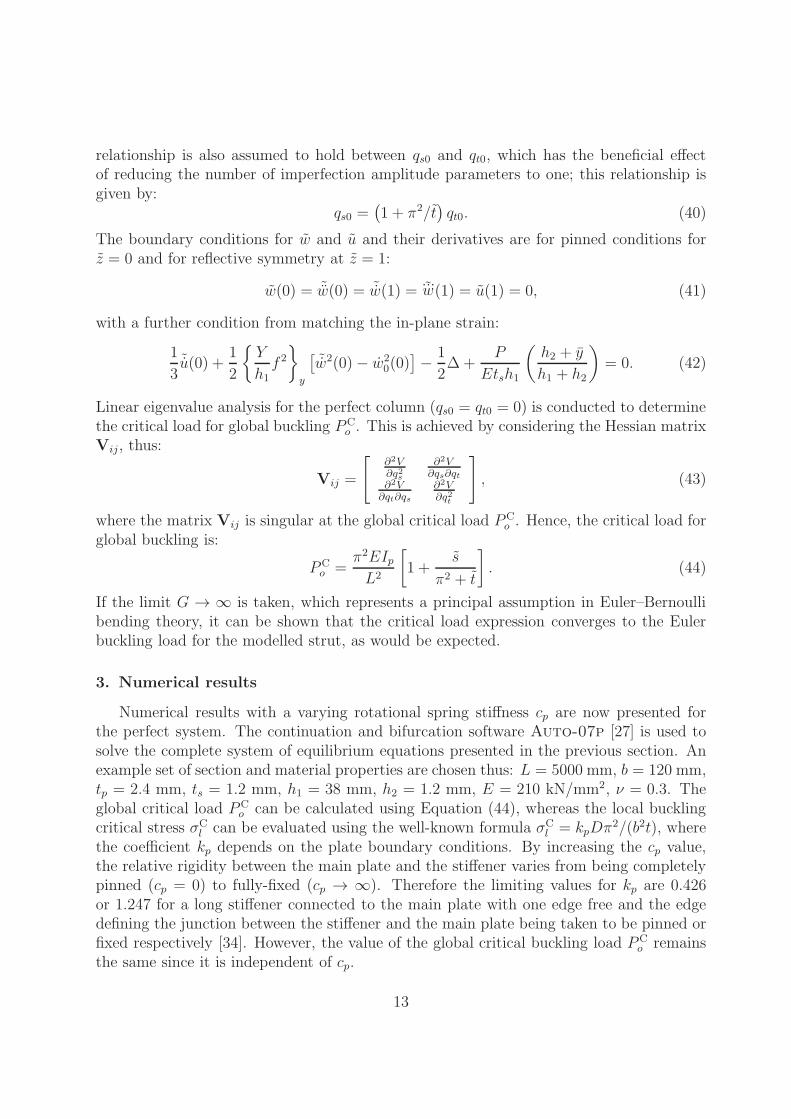
To find the equilibrium path in the fundamental and post-buckling states, a similarsolution strategy is performed as in [18, 19], which is illustrated diagrammatically in Figure5. For a perfect strut, the initial post-buckling path is computed first from the critical

P

qs

PC SRun-1

Run-2

qSS

C

(a)

P

qs

SRun-1

Run-2

qS0

Run-1

PC C

(b)

P

qs

S1

Run-1

S2 S3 S4

cp increasing

PCC

Run-2

(c)

Figure 5: Diagrammatic representation of the sequence of computing the equilibrium paths for the (a)perfect and (b) imperfect cases; (c) shows the perfect cases for different values of cp with the correspondingsecondary bifurcation points changing as cp is increased.

buckling load PC(≡ PCo ) with qs being varied. Many bifurcation points are detected on the

weakly stable post-buckling path; the focus being on the one with the lowest value of qs,termed the secondary bifurcation point S, see Figure 5(a). Note that the corresponding qsvalue is labelled as qSs . For an imperfect strut, however, the equilibrium path is computedinitially from zero axial load and then P is increased up to the maximum value where alimit point is detected. The load subsequently drops and the path is asymptotic to theperfect path, as shown in Figure 5(b). If the joint stiffness cp is varied, the value of qSswould be expected to increase, see Figure 5. This is owing to the local buckling criticalstress increasing, which in turn causes the required global mode amplitude to trigger localbuckling to increase also.

It is worth noting that for the perfect case, the model is in fact only valid where globalbuckling or stiffener local buckling is critical since the assumption is made such that themain plate can only buckle in sympathy with the stiffener. For the stiffener local bucklingbeing critical, the bifurcation would occur when P = PC

l and a stable post-buckling pathwould initially emerge from the fundamental path. To include the main plate bucklinglocally first, the explicit link between wp and w would have to be broken.

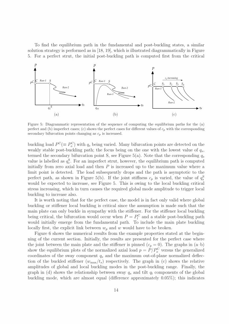
Figure 6 shows the numerical results from the example properties stated at the begin-ning of the current section. Initially, the results are presented for the perfect case wherethe joint between the main plate and the stiffener is pinned (cp = 0). The graphs in (a–b)show the equilibrium plots of the normalized axial load p = P/PC

o versus the generalizedcoordinates of the sway component qs and the maximum out-of-plane normalized deflec-tion of the buckled stiffener (wmax/ts) respectively. The graph in (c) shows the relativeamplitudes of global and local buckling modes in the post-buckling range. Finally, thegraph in (d) shows the relationship between sway qs and tilt qt components of the globalbuckling mode, which are almost equal (difference approximately 0.05%); this indicates

14

0 0.5 1 1.5 20.8

0.85

0.9

0.95

1

qs

p

x10−2

C S

C2

C4

C6

C8

(a)

0 0.5 1 1.5 20.8

0.85

0.9

0.95

1

wmax/ts

p

C, S

C2

C4

C6

C8

(b)

0 0.5 1 1.5 20

0.5

1

1.5

2

qs

wmax/t s

x10−2

C S

C2

C4

C6

C8

(c)

0 0.5 1 1.5 20

0.5

1

1.5

2

qs

q t

x10−2

x10−2

C

S

C2

C4

C6

C8

(d)

Figure 6: Results for the panel with example properties and assuming the main plate–stiffener joint ispinned (cp = 0). The normalized force ratio p = P/PC

o is plotted versus (a) the global mode amplitudeqs and (b) the normalized maximum out-of-plane deflection of the stiffener wmax/ts; (c) shows the localmode amplitude wmax/ts versus the global mode amplitude qs in the post-buckling range; (d) shows therelationship between the generalized coordinates qt and qs that define the global mode.

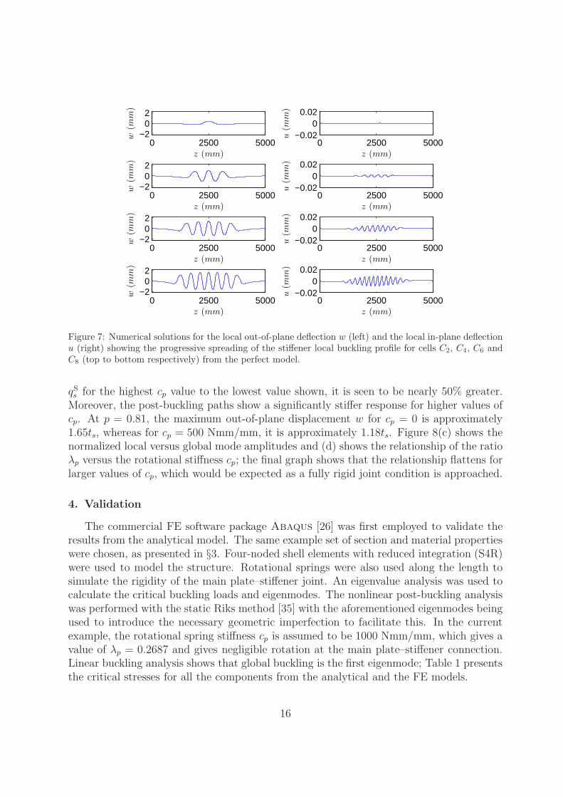
that the shear strain is small but, importantly, not zero. As found in [19], for the casewhere only the stiffener buckles locally, there is a sequence of snap-backs observed. Thisis the signature of cellular buckling [20] and the cells are labelled Ci. Figure 7 shows thecorresponding progression of the numerical solutions for the local buckling functions w andu for cells C2, C4, C6 and C8 defined in Figure 6. It can be seen that the initially localizedbuckling mode progressively becomes more periodic as the system post-buckling advances.

By comparing the equilibrium paths against those for cp = 0, it is observed that thesnap-backs begin to vanish as cp is increased. Figure 8 shows the equilibrium paths forthe strut with an increasingly rigid connection between the plate and the stiffener. In thegraphs of the analytical results, the values of cp, in Nmm/mm, are taken as 1, 100 and 500respectively. The graphs in Figure 8(a–b) show the equilibrium path of the normalized axialload p = P/PC

o versus the normalized total end-shortening E/L, see Equation (29), andthe global mode amplitude qs respectively. It is found that qSs increases with cp; comparing

15

0 2500 5000−2

02

w(m

m)

z (mm)0 2500 5000

−0.020

0.02

u(m

m)

z (mm)

0 2500 5000−2

02

w(m

m)

z (mm)0 2500 5000

−0.020

0.02

u(m

m)

z (mm)

0 2500 5000−2

02

w(m

m)

z (mm)0 2500 5000

−0.020

0.02

u(m

m)

z (mm)

0 2500 5000−2

02

w(m

m)

z (mm)0 2500 5000

−0.020

0.02

u(m

m)

z (mm)

Figure 7: Numerical solutions for the local out-of-plane deflection w (left) and the local in-plane deflectionu (right) showing the progressive spreading of the stiffener local buckling profile for cells C2, C4, C6 andC8 (top to bottom respectively) from the perfect model.

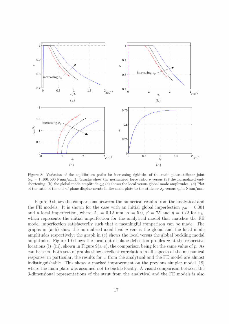
qSs for the highest cp value to the lowest value shown, it is seen to be nearly 50% greater.Moreover, the post-buckling paths show a significantly stiffer response for higher values ofcp. At p = 0.81, the maximum out-of-plane displacement w for cp = 0 is approximately1.65ts, whereas for cp = 500 Nmm/mm, it is approximately 1.18ts. Figure 8(c) shows thenormalized local versus global mode amplitudes and (d) shows the relationship of the ratioλp versus the rotational stiffness cp; the final graph shows that the relationship flattens forlarger values of cp, which would be expected as a fully rigid joint condition is approached.

4. Validation

The commercial FE software package Abaqus [26] was first employed to validate theresults from the analytical model. The same example set of section and material propertieswere chosen, as presented in §3. Four-noded shell elements with reduced integration (S4R)were used to model the structure. Rotational springs were also used along the length tosimulate the rigidity of the main plate–stiffener joint. An eigenvalue analysis was used tocalculate the critical buckling loads and eigenmodes. The nonlinear post-buckling analysiswas performed with the static Riks method [35] with the aforementioned eigenmodes beingused to introduce the necessary geometric imperfection to facilitate this. In the currentexample, the rotational spring stiffness cp is assumed to be 1000 Nmm/mm, which gives avalue of λp = 0.2687 and gives negligible rotation at the main plate–stiffener connection.Linear buckling analysis shows that global buckling is the first eigenmode; Table 1 presentsthe critical stresses for all the components from the analytical and the FE models.

16

0 0.5 1 1.5 20.7

0.8

0.9

1

E/L

p

x10−3

increasing cp

(a)

0 1 2 30.7

0.8

0.9

1

qs

p

x10−2

increasing cp

(b)

0 1 2 30

0.5

1

1.5

2

qs

wmax/t s

x10−2

increasing cp

(c)

0 0.5 1 1.5 20

0.25

0.5

0.75

cp

λp

x104

(d)

Figure 8: Variation of the equilibrium paths for increasing rigidities of the main plate–stiffener joint(cp = 1, 100, 500 Nmm/mm). Graphs show the normalized force ratio p versus (a) the normalized end-shortening, (b) the global mode amplitude qs; (c) shows the local versus global mode amplitudes. (d) Plotof the ratio of the out-of-plane displacements in the main plate to the stiffener λp versus cp in Nmm/mm.

Figure 9 shows the comparisons between the numerical results from the analytical andthe FE models. It is shown for the case with an initial global imperfection qs0 = 0.001and a local imperfection, where A0 = 0.12 mm, α = 5.0, β = 75 and η = L/2 for w0,which represents the initial imperfection for the analytical model that matches the FEmodel imperfection satisfactorily such that a meaningful comparison can be made. Thegraphs in (a–b) show the normalized axial load p versus the global and the local modeamplitudes respectively; the graph in (c) shows the local versus the global buckling modalamplitudes. Figure 10 shows the local out-of-plane deflection profiles w at the respectivelocations (i)–(iii), shown in Figure 9(a–c), the comparison being for the same value of p. Ascan be seen, both sets of graphs show excellent correlation in all aspects of the mechanicalresponse; in particular, the results for w from the analytical and the FE model are almostindistinguishable. This shows a marked improvement on the previous simpler model [19]where the main plate was assumed not to buckle locally. A visual comparison between the3-dimensional representations of the strut from the analytical and the FE models is also

17

0 0.01 0.02 0.030

0.2

0.4

0.6

0.8

1

qs

p

(i)

(ii)

(iii)

AutoAbaqus

(a)

0 0.5 1 1.5 20

0.2

0.4

0.6

0.8

1

wmax/ts

p

(i)

(ii)(iii)

AutoAbaqus

(b)

0 0.01 0.02 0.030

0.5

1

1.5

2

qs

wmax/t s

(i)

(ii)

(iii)

AutoAbaqus

(c)

Figure 9: Comparisons of the analytical model (solid lines) versus the FE model (dashed lines) solutions,both with cp = 1000 Nmm/mm. The plots show the normalized force ratio p versus (a) the global modeamplitude qs and (b) the maximum out-of-plane normalized stiffener deflection wmax/ts; (c) local versusglobal mode amplitudes.

18

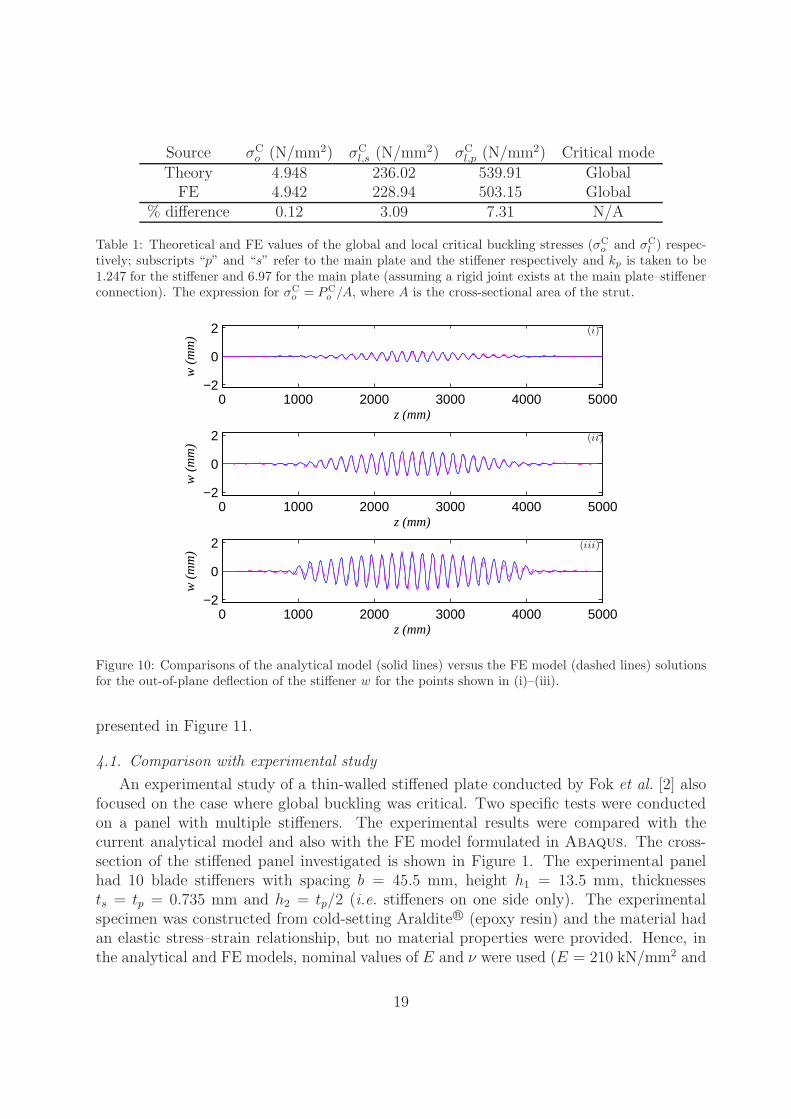
Source σCo (N/mm2) σC

l,s (N/mm2) σCl,p (N/mm2) Critical mode

Theory 4.948 236.02 539.91 GlobalFE 4.942 228.94 503.15 Global

% difference 0.12 3.09 7.31 N/A

Table 1: Theoretical and FE values of the global and local critical buckling stresses (σCo and σC

l ) respec-tively; subscripts “p” and “s” refer to the main plate and the stiffener respectively and kp is taken to be1.247 for the stiffener and 6.97 for the main plate (assuming a rigid joint exists at the main plate–stiffenerconnection). The expression for σC

o = PCo /A, where A is the cross-sectional area of the strut.

0 1000 2000 3000 4000 5000−2

0

2

w (

mm

)

z (mm)

(i)

0 1000 2000 3000 4000 5000−2

0

2

w (

mm

)

z (mm)

(ii)

0 1000 2000 3000 4000 5000−2

0

2

w (

mm

)

z (mm)

(iii)

Figure 10: Comparisons of the analytical model (solid lines) versus the FE model (dashed lines) solutionsfor the out-of-plane deflection of the stiffener w for the points shown in (i)–(iii).

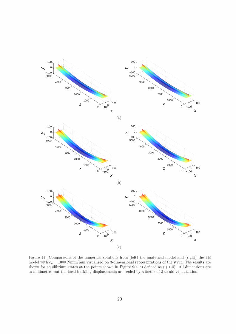
presented in Figure 11.

4.1. Comparison with experimental study

An experimental study of a thin-walled stiffened plate conducted by Fok et al. [2] alsofocused on the case where global buckling was critical. Two specific tests were conductedon a panel with multiple stiffeners. The experimental results were compared with thecurrent analytical model and also with the FE model formulated in Abaqus. The cross-section of the stiffened panel investigated is shown in Figure 1. The experimental panelhad 10 blade stiffeners with spacing b = 45.5 mm, height h1 = 13.5 mm, thicknessests = tp = 0.735 mm and h2 = tp/2 (i.e. stiffeners on one side only). The experimentalspecimen was constructed from cold-setting AralditeR© (epoxy resin) and the material hadan elastic stress–strain relationship, but no material properties were provided. Hence, inthe analytical and FE models, nominal values of E and ν were used (E = 210 kN/mm2 and

19

−1000

1000

1000

2000

3000

4000

5000−100

0

100

xz

y

−1000

1000

1000

2000

3000

4000

5000−100

0

100

xz

y

(a)

−1000

1000

1000

2000

3000

4000

5000−100

0

100

xz

y

−1000

1000

1000

2000

3000

4000

5000−100

0

100

xz

y

(b)

−1000

1000

1000

2000

3000

4000

5000−100

0

100

xz

y

−1000

1000

1000

2000

3000

4000

5000−100

0

100

xz

y

(c)

Figure 11: Comparisons of the numerical solutions from (left) the analytical model and (right) the FEmodel with cp = 1000 Nmm/mm visualized on 3-dimensional representations of the strut. The results areshown for equilibrium states at the points shown in Figure 9(a–c) defined as (i)–(iii). All dimensions arein millimetres but the local buckling displacements are scaled by a factor of 2 to aid visualization.

20

ν = 0.3 as before); this did not pose a problem so long as the same values were used in bothmodels. Moreover, it is worth noting that the behaviour of the experimental specimenswas reported to be elastic and only ratios of loads and displacements were reported as theresults [2].

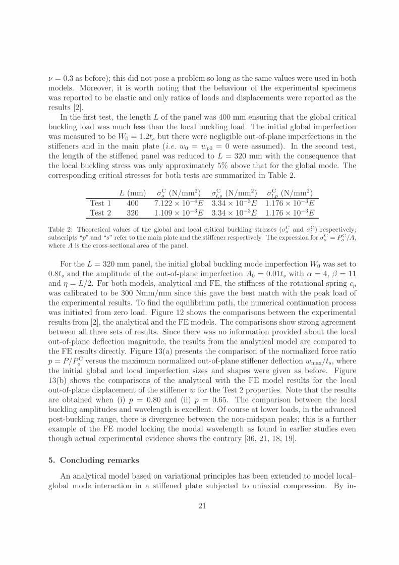
In the first test, the length L of the panel was 400 mm ensuring that the global criticalbuckling load was much less than the local buckling load. The initial global imperfectionwas measured to be W0 = 1.2ts but there were negligible out-of-plane imperfections in thestiffeners and in the main plate (i.e. w0 = wp0 = 0 were assumed). In the second test,the length of the stiffened panel was reduced to L = 320 mm with the consequence thatthe local buckling stress was only approximately 5% above that for the global mode. Thecorresponding critical stresses for both tests are summarized in Table 2.

L (mm) σCo (N/mm2) σC

l,s (N/mm2) σCl,p (N/mm2)

Test 1 400 7.122× 10−4E 3.34× 10−3E 1.176× 10−3ETest 2 320 1.109× 10−3E 3.34× 10−3E 1.176× 10−3E

Table 2: Theoretical values of the global and local critical buckling stresses (σCo and σC

l ) respectively;subscripts “p” and “s” refer to the main plate and the stiffener respectively. The expression for σC

o = PCo /A,

where A is the cross-sectional area of the panel.

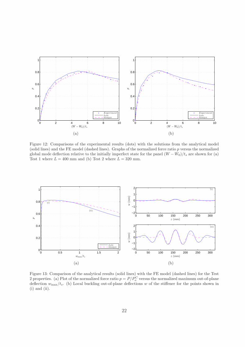
For the L = 320 mm panel, the initial global buckling mode imperfection W0 was set to0.8ts and the amplitude of the out-of-plane imperfection A0 = 0.01ts with α = 4, β = 11and η = L/2. For both models, analytical and FE, the stiffness of the rotational spring cpwas calibrated to be 300 Nmm/mm since this gave the best match with the peak load ofthe experimental results. To find the equilibrium path, the numerical continuation processwas initiated from zero load. Figure 12 shows the comparisons between the experimentalresults from [2], the analytical and the FE models. The comparisons show strong agreementbetween all three sets of results. Since there was no information provided about the localout-of-plane deflection magnitude, the results from the analytical model are compared tothe FE results directly. Figure 13(a) presents the comparison of the normalized force ratiop = P/PC

o versus the maximum normalized out-of-plane stiffener deflection wmax/ts, wherethe initial global and local imperfection sizes and shapes were given as before. Figure13(b) shows the comparisons of the analytical with the FE model results for the localout-of-plane displacement of the stiffener w for the Test 2 properties. Note that the resultsare obtained when (i) p = 0.80 and (ii) p = 0.65. The comparison between the localbuckling amplitudes and wavelength is excellent. Of course at lower loads, in the advancedpost-buckling range, there is divergence between the non-midspan peaks; this is a furtherexample of the FE model locking the modal wavelength as found in earlier studies eventhough actual experimental evidence shows the contrary [36, 21, 18, 19].

5. Concluding remarks

An analytical model based on variational principles has been extended to model local–global mode interaction in a stiffened plate subjected to uniaxial compression. By in-

21

0 2 4 6 8 100

0.2

0.4

0.6

0.8

1

(W −W0)/ts

p

ExperimentAutoAbaqus

(a)

0 2 4 6 8 100

0.2

0.4

0.6

0.8

1

(W −W0)/tsp

ExperimentAutoAbaqus

(b)

Figure 12: Comparisons of the experimental results (dots) with the solutions from the analytical model(solid lines) and the FE model (dashed lines). Graphs of the normalized force ratio p versus the normalizedglobal mode deflection relative to the initially imperfect state for the panel (W −W0)/ts are shown for (a)Test 1 where L = 400 mm and (b) Test 2 where L = 320 mm.

0 0.5 1 1.5 20

0.2

0.4

0.6

0.8

1

wmax/ts

p

(i)

(ii)

AutoAbaqus

(a)

0 50 100 150 200 250 300−2

−1

0

1

2

w(m

m)

z (mm)

(i)

0 50 100 150 200 250 300−2

−1

0

1

2

w(m

m)

z (mm)

(ii)

(b)

Figure 13: Comparison of the analytical results (solid lines) with the FE model (dashed lines) for the Test2 properties. (a) Plot of the normalized force ratio p = P/PC

o versus the normalized maximum out-of-planedeflection wmax/ts. (b) Local buckling out-of-plane deflections w of the stiffener for the points shown in(i) and (ii).

22

troducing the sympathetic deflection of the main plate along with the locally bucklingstiffener, the current model could now be compared to published experiments [2] and afinite element model formulated in Abaqus; results from both are found to be excellent.Currently, the authors are conducting an imperfection sensitivity study to quantify theparametric space for designers to avoid such dangerous structural behaviour, the resultsof which would provide greater understanding of the interactive buckling phenomena andhighlight the practical implications.

References

[1] W. T. Koiter, M. Pignataro, A general theory for the interaction between local andoverall buckling of stiffened panels, Tech. Rep. WTHD 83, Delft University of Tech-nology, Delft, The Netherlands (1976).

[2] W. C. Fok, J. Rhodes, A. C. Walker, Local buckling of outstands in stiffened plates,Aeronautical Quarterly 27 (1976) 277–291.

[3] B. Budiansky (Ed.), Buckling of structures, Springer, Berlin, 1976, iUTAM sympo-sium.

[4] J. M. T. Thompson, G. W. Hunt, Elastic instability phenomena, Wiley, London, 1984.

[5] B. F. Ronalds, Torsional buckling and tripping strength of slender flat-bar stiffenersin steel plating, Proc. Instn. Civ. Engrs. 87 (1989) 583–604.

[6] N. W. Murray, Buckling of stiffened panels loaded axially and in bending, The Struc-tural Engineer 51 (8) (1973) 285–300.

[7] R. Butler, M. Lillico, G. W. Hunt, N. J. McDonald, Experiment on interactive bucklingin optimized stiffened panels, Structural and Multidisciplinary Optimization 23 (1)(2000) 40–48.

[8] J. Loughlan (Ed.), Thin-Walled Structures: Advances in Research, Design and Man-ufacturing Technology, Taylor & Francis, 2004.

[9] G. Y. Grondin, A. E. Elwi, J. Cheng, Buckling of stiffened steel plates – a parametricstudy, J. Constr. Steel Res. 50 (2) (1999) 151–175.

[10] I. A. Sheikh, G. Grondin, A. E. Elwi, Stiffened steel plates under uniaxial compression,J. Constr. Steel Res. 58 (5–8) (2002) 1061–1080.

[11] K. G. Ghavami, M. R. Khedmati, Numerical and experimental investigation on thecompression behaviour of stiffened plates, J. Constr. Steel Res. 62 (11) (2006) 1087–1100.

[12] G. W. Hunt, M. A. Wadee, Localization and mode interaction in sandwich structures,Proc. R. Soc. A 454 (1972) (1998) 1197–1216.

23

[13] J. M. T. Thompson, G. W. Hunt, A general theory of elastic stability, Wiley, London,1973.

[14] M. Pignataro, M. Pasca, P. Franchin, Post-buckling analysis of corrugated panels inthe presence of multiple interacting modes., Thin-Walled Struct. 36 (1) (2000) 47–66.

[15] G. J. Hancock, Interaction buckling in I-section columns, ASCE J. Struct. Eng 107 (1)(1981) 165–179.

[16] B. W. Schafer, Local, distortional, and Euler buckling of thin-walled columns, ASCEJournal of Structural Engineering 128 (3) (2002) 289–299.

[17] J. Becque, K. J. R. Rasmussen, Experimental investigation of the interaction of localand overall buckling of stainless steel I-columns, ASCE Journal of Structural Engi-neering 135 (11) (2009) 1340–1348.

[18] M. A. Wadee, L. Bai, Cellular buckling in I-section struts, Thin-Walled Struct. 81(2014) 89–100.

[19] M. A. Wadee, M. Farsi, Cellular buckling in stiffened plates, Proc. R. Soc. A 470 (2168)(2014) 20140094.

[20] G. W. Hunt, M. A. Peletier, A. R. Champneys, P. D. Woods, M. A. Wadee, C. J.Budd, G. J. Lord, Cellular buckling in long structures, Nonlinear Dyn. 21 (1) (2000)3–29.

[21] M. A. Wadee, L. Gardner, Cellular buckling from mode interaction in I-beams underuniform bending, Proc. R. Soc. A 468 (2137) (2012) 245–268.

[22] L. Bai, M. A. Wadee, Mode interaction in thin-walled I-section struts with semi-rigidflange-web joints, Int. J. Non-Linear Mech.Submitted.

[23] P. D. Woods, A. R. Champneys, Heteroclinic tangles and homoclinic snaking in theunfolding of a degenerate reversible Hamiltonian–Hopf bifurcation, Physica D 129 (3–4) (1999) 147–170.

[24] J. Burke, E. Knobloch, Homoclinic snaking: Structure and stability, Chaos 17 (3)(2007) 037102.

[25] S. J. Chapman, G. Kozyreff, Exponential asymptotics of localised patterns and snakingbifurcation diagrams, Physica D 238 (3) (2009) 319–354.

[26] Abaqus, Version 6.10, Dassault Systemes, Providence, USA, 2011.

[27] E. J. Doedel, B. E. Oldeman, AUTO-07P: Continuation and Bifurcation Software forOrdinary Differential Equations, Concordia University, Montreal, Canada, 2011.

24

[28] M. A. Wadee, G. W. Hunt, Interactively induced localized buckling in sandwich struc-tures with core orthotropy, Trans. ASME J. Appl. Mech. 65 (2) (1998) 523–528.

[29] M. A. Wadee, S. Yiatros, M. Theofanous, Comparative studies of localized bucklingin sandwich struts with different core bending models, Int. J. Non-Linear Mech. 45 (2)(2010) 111–120.

[30] G. W. Hunt, L. S. Da Silva, G. M. E. Manzocchi, Interactive buckling in sandwichstructures, Proc. R. Soc. A 417 (1852) (1988) 155–177.

[31] F. Guarracino, A. Walker, Energy methods in structural mechanics, Thomas Telford,1999.

[32] M. K. Wadee, G. W. Hunt, A. I. M. Whiting, Asymptotic and Rayleigh–Ritz routesto localized buckling solutions in an elastic instability problem, Proc. R. Soc. A453 (1965) (1997) 2085–2107.

[33] M. A. Wadee, Effects of periodic and localized imperfections on struts on nonlinearfoundations and compression sandwich panels, Int. J. Solids Struct. 37 (8) (2000)1191–1209.

[34] P. S. Bulson, The stability of flat plates, Chatto & Windus, London, UK, 1970.

[35] E. Riks, Application of Newton’s method to problem of elastic stability, Trans. ASMEJ. Appl. Mech 39 (4) (1972) 1060–1065.

[36] J. Becque, The interaction of local and overall buckling of cold-formed stainless steelcolumns, Ph.D. thesis, School of Civil Engineering, University of Sydney, Sydney,Australia (2008).

25