Local POD plus Galerkin projection in the unsteady lid-driven cavity problem

SIAM J. SCI. COMPUT. c© 2011 Society for Industrial and Applied MathematicsVol. 33, No. 6, pp. 3538–3561

LOCAL POD PLUS GALERKIN PROJECTIONIN THE UNSTEADY LID-DRIVEN CAVITY PROBLEM∗

FILIPPO TERRAGNI† , EUSEBIO VALERO† , AND JOSE M. VEGA†

Abstract. A local proper orthogonal decomposition (POD) plus Galerkin projection methodis applied to the unsteady lid-driven cavity problem, namely the incompressible fluid flow in a two-dimensional box whose upper wall is moved back and forth at moderately large values of the Reynoldsnumber. Such a method was recently developed for one-dimensional parabolic problems. Its extensionto fluid dynamics problems is nontrivial (especially if rough CFD codes are used) and consists ofusing a computational fluid dynamics (CFD) code and a Galerkin system (GS) in a sequence ofinterspersed intervals ICFD and IGS , respectively. The POD manifold is calculated retaining themost energetic POD modes resulting from the snapshots computed in the ICFD intervals; in fact,the POD manifold is completely calculated in the first ICFD interval but only updated in subsequentICFD intervals. Intended to mimic industrial solvers, the CFD code contains unphysical terms thatare introduced for purely numerical reasons to accelerate runs. The use of such a CFD code posesthe question of which equations should be Galerkin projected onto the POD manifold, the exactgoverning equations or the CFD numerical scheme. Also, Galerkin projection can be made usingeither the standard L2 inner product or a nonstandard one, based on a limited number of meshpoints. After addressing these issues, a method is constructed that is able to accelerate the CFDcode by a factor of the order of 5–15, depending on the Reynolds number and the nature (steady,periodic, or quasi-periodic) of the forcing velocity.

Key words. unsteady driven cavity, proper orthogonal decomposition, reduced order models,Galerkin projection, computational fluid dynamics

AMS subject classifications. 65M60, 65M70, 35Q30, 76D05, 35Q68, 68U01

DOI. 10.1137/100816006

1. Introduction. Design of devices involving fluid dynamics is largely done inindustry currently using low fidelity simulation, ad hoc modeling, and experiments.The former two essentially provide rough approximations, which are tested by thelatter. Since both design improvement and cost and time to market reduction arebecoming crucial issues, a trend is observed in mature sectors such as automotive andaeronautics to substitute wind tunnel tests by CFD simulations. The main difficultyis that the Reynolds number is quite large in realistic industrial problems, whichdoes not (and will not, in the predictable future) allow for using direct numericalsimulation. Thus, turbulence models are generally used, but these still require hugecomputational resources and CPU time (for instance, calculating each aerodynamicflow around a commercial aircraft requires about two CPU days), which makes theresulting solvers still impractical, especially in multiparameter problems. As a con-sequence, reducing the computational time required by CFD solvers is becoming thekey step in facilitating their industrial use.

Basic problems of scientific interest bear simplifications that make these problemsmore accessible to CFD, or even to direct numerical simulation, but computationalcost is also becoming an issue when many parameters are present.

∗Submitted to the journal’s Computational Methods in Science and Engineering section Novem-ber 24, 2010; accepted for publication (in revised form) October 10, 2011; published electronicallyDecember 22, 2011. This work was supported by the Spanish Ministry of Education and the SpanishMinistry of Science and Technology under grants TRA2007–65699 and TRA2010–18054.

http://www.siam.org/journals/sisc/33-6/81600.html†E.T.S.I. Aeronauticos, Universidad Politecnica de Madrid, 28040 Madrid, Spain (filippo.

[email protected], [email protected], [email protected]).

3538

LOCAL POD PLUS GALERKIN IN THE UNSTEADY CAVITY 3539

Reduced order models (ROMs) are good candidates to provide reasonable approx-imations with a small computational cost; see [22, 11, 37] and the references therein.Among these, those based on POD have been developed during the last twenty yearssince they drastically decrease computational time and allow for treating complexgeometries. These models consist of (i) CFD computing some flow snapshots, (ii)extracting the most energetic POD modes from the snapshots, and (iii) projectingthe governing equations onto the resulting POD manifold. These ROMs have beendeveloped for both steady [21, 2] and time dependent [16, 28, 23] problems of directindustrial interest. Concerning the former, steady states are of interest in industrialproblems either (a) because they are the industrially interesting states or (b) becauseturbulence modeling (via Reynolds averaged Navier–Stokes equations) somehow aver-ages in time the genuinely unsteady flow and produces steady states of the averagedequations. Also, POD-based ROMs for steady problems can be so computationally ef-ficient that the key step to improve the whole process is to reduce the computationaleffort associated with the CFD calculation of the snapshots. These are frequentlycomputed as the final states of a time dependent solver, which itself could be replacedby a time dependent ROM.

POD-based time dependent ROMs were introduced for the fast time dependentsimulation of complex dynamics of incompressible fluid flow problems [10]. The snap-shots are flow portraits at specific values of time, which should be representative ofthe dynamics that are being simulated [35]. In other words, the snapshots must spana portion of the phase space of the associated dynamical system that contains allrelevant orbits. Thus, these ROMs are suitable to reproduce attractors, not transientbehaviors. The ROM is obtained via Galerkin projection of the governing equationsonto the POD manifold. The resulting reduced equations will be referred to as theGalerkin system (GS). A major difficulty is that these truncated GSs may exhibitspurious dynamics in a somewhat unpredictable way. The reason for that is still con-troversial. In some cases, instability seems to be due to the noninvariance of the PODmanifold under the true dynamics [27]. Thus, intended solutions to this difficultysomehow correct either the GS or the POD manifold, to make the latter invariant.This is done by either introducing some additional terms in the GS [15, 32, 34] or com-bining the GS with the CFD solver [34, 9]; see also [33] for the effect of time dependentboundary conditions. In these cases, the GS is intended to approach the dynamics ofthe system in a particular attractor, which can be periodic, quasi-periodic, or chaotic.POD modes are calculated from the outset, as explained above. Thus, this methodwill be referred to as the preprocessed POD plus Galerkin projection method. Insta-bilities play a major role in the simulation of transient, transitional, and turbulentflows since the pioneering work by Sirovich [35] and Aubry et al. [6]. In particular,the open flow around a cylinder has been taken as a benchmark problem to identifymeans of stabilizing POD-based ROMs, using the so-called shift modes, which wereintroduced by Noack et al. [24] and Siegel, Cohen, and McLaughlin [30] and furtherpursued and extended by others, especially in the context of optimal control of thecylinder wake (see [31, 8, 36] and the references therein); it is also worth mentioningthe use of residual modes [9].

A somewhat different approach was presented in [25] for one-dimensional parabolicequations, which allowed for treating transient dynamics and did not show any numer-ical instability. As further explained and illustrated in [25], the method is intendedto apply to general parabolic systems and relies on two observations:

1. If a set of representative snapshots is CFD calculated in a time interval [t0, t1]and POD is applied, then the resulting POD manifold approximates well the

3540 FILIPPO TERRAGNI, EUSEBIO VALERO, AND JOSE M. VEGA

Fig. 1. The local POD plus Galerkin projection method. Snapshots (the planes) are computedvia CFD in each ICFD interval and are used to either calculate (in the first ICFD interval) orupdate (in subsequent ICFD intervals) some POD modes. The governing equations are Galerkinprojected onto these modes to obtain a Galerkin system that is integrated in the next IGS interval.

solution in a larger time interval, [t0, t2], with t2 > t1, provided that somemore POD modes than necessary are retained in the smaller time interval.This can be seen as a natural consequence of the well posedness of the evolu-tion problems that are being considered. Namely, the dynamics in the nearfuture depend continuously on the present.

2. The instability resulting from high-order modes truncation can be detectedcomparing the solutions of two Galerkin systems, which result from retainingn1 and n2 > n1 modes.

The method (see the cartoon in Figure 1) is called the local POD plus Galerkin pro-jection (LPOD+GP) method and is based on the combined use of CFD and Galerkinprojection in interspersed time intervals, ICFD and IGS , respectively. POD modes arecalculated in the ICFD intervals. In fact, the POD manifold is completely calculatedin the first ICFD interval, and just updated in subsequent ICFD intervals, which canthus be quite small. Of course, the key point is to decide when each IGS interval mustbe terminated (because the GS approximation is no longer acceptable) and switchingto a new ICFD interval is necessary. This is decided in [25] using an a priori errorestimate based on the amplitude of some additional high-order modes. Such error es-timate is similar to those used in the numerical analysis of spectral methods [19] andworks quite well. In addition, a second GS is also integrated that retains a few moremodes than necessary and (in conjunction with the above mentioned a priori errorestimate) provides a safe criterion for switching between IGS and ICFD intervals, evenin cases in which the transient dynamics that are being calculated are really complex.The method was applied in [25] to the complex Ginzburg–Landau (CGL) equation,

(1.1) ∂tu = (1 + iα)∂xxu+ μu− (1 + iβ)|u|2u, with u = 0 at x = 0, 1,

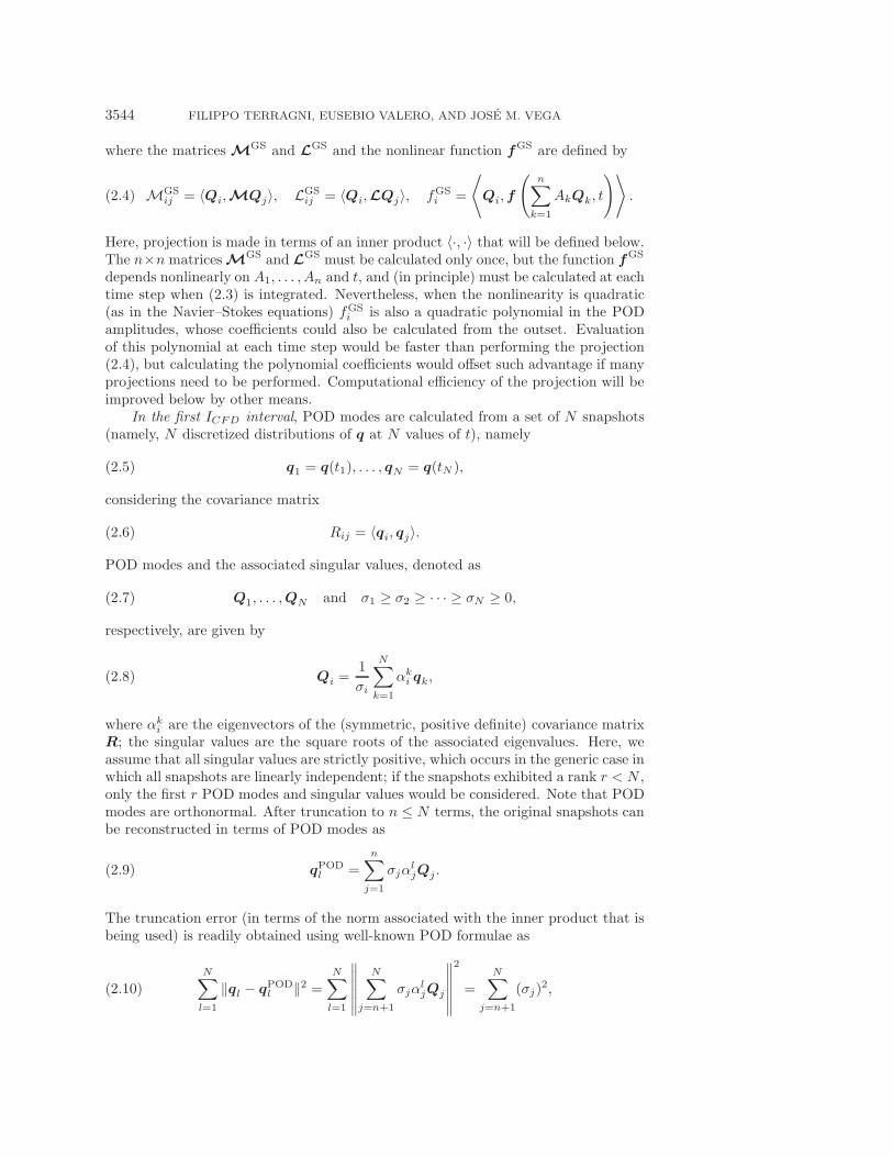
which is a well-known paradigm of a simple equation that exhibits intrinsically com-plex dynamics [3]. Here, the state variable u is complex and the parameters μ,α, and β are real. If μ = 90, α = −2, and β = 14, and the initial condition isu = i sin(2πx) + (1 + i) sin(3πx) at t = 0, then the solution exhibits transient chaos[20], which is a quite demanding test for the method. A plot of the evolution of |u| atthree values of x is given in Figure 2, left, while the evolution of the root mean square(RMS) error estimated by the method retaining 24 modes is given in the right plot,where a comparison with the exact value of the error is made. Note that the plots ofthe estimated and the exact error are indistinguishable. For reference, the estimatederror retaining 38 modes is also provided. The ICFD intervals can be identified be-cause the errors have been set to zero in these intervals. The first of such intervals isclearly appreciated, but subsequent ICFD intervals consist of only one snapshot each.

LOCAL POD PLUS GALERKIN IN THE UNSTEADY CAVITY 3541

0 0.5 1 1.5 20

3

6

9

12

t

|u|

0 0.5 1 1.5 210

−7

10−6

10−5

10−4

10−3

t

E

Fig. 2. Application of the LPOD+GP method to the complex Ginzburg–Landau equation (1.1),with (μ, α, β) = (90,−2, 14). Left: Time evolution of |u| at x = 1/4 (thin solid), 3/4 (thick dashed),and 1/2 (thick solid). Right: Estimated (thin solid) and exact (thick dashed) errors of the GSsolution retaining 24 POD modes and estimated error retaining 38 POD modes (thick dot-dashed).Courtesy of Dr. Marıa-Luisa Rapun.

Thus, they can only be identified in Figure 2 as enclosed by two nearby vertical lines.As described above, the LPOD+GP method has something in common with ref-

erences [34] and [9] (where short runs with a CFD code were also combined withGalerkin projection to stabilize the latter) with four main differences. Namely, theLPOD+GP method (i) is able to simulate transients, not only a given attractor, (ii)uses the short runs with the numerical code to recalculate the POD modes, not tocompute the GS (which is calculated in a standard way), (iii) does not require precal-culating the POD modes, and (iv) is designed to accelerate the numerical code, notto stabilize the GS (stabilization of the GS is a byproduct of the control of the trun-cation errors). Bergmann, Bruneau, and Iollo [9] also presented a method to updatethe POD manifold, but it is different in both strategy and aim from the one in thepresent paper. The method is also connected with other methods mentioned above.In particular, other adaptive methods are available in the literature (see [26, 8, 36]and the references therein), as are various methods cited above that are able to dealwith transient behaviors. The main difference with all these is that adaptation ismade here based on the two above mentioned observations.

The results in [25] dealt with one-dimensional equations and were based on a well-controlled numerical code. They were a first step towards the intention to develop amethod to accelerate industrial solvers in realistic industrial problems, which posestwo main difficulties. (i) These solvers frequently use coarse computational meshesand include unphysical terms to accelerate calculations and/or gain robustness bysuppressing numerical instability; the required numerical precision is not too large.(ii) Realistic configurations (e.g., a whole aircraft) require a quite large computationaltime, which makes the associated ROM too slow to perform the necessary test runs.Thus, using a simpler configuration and a simpler solver is advisable, as it will bedone in this paper to complete a further step towards the above mentioned final goal.

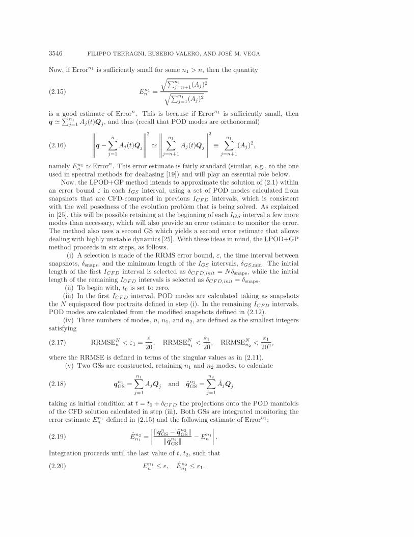
As a test problem, we chose the unsteady lid-driven cavity problem [17, 1] (Fig-ure 3). The governing equations are

∇ · v = 0,(1.2)

∂v

∂t+ (v ·∇)v = −∇p+Re−1�v(1.3)

3542 FILIPPO TERRAGNI, EUSEBIO VALERO, AND JOSE M. VEGA

x

y

10

1

Fig. 3. The lid-driven cavity: streamlines under steady forcing.

in the spatial domain 0 < x < 1, 0 < y < 1, with boundary conditions

(1.4) v = 0 at x = 0, 1 and y = 0, v = (h(t)g(x), 0) at y = 1.

Here, v = (vx, vy) and p are the dimensionless velocity and pressure, and the timedependent boundary condition (1.4) at y = 1 accounts for the lid forcing of theflow. The Reynolds number is Re = u∗L/ν, where u∗ is the maximum lid forcing(horizontal) velocity, L is the width of the cavity, and ν is the kinematic viscosity.

This formulation is somewhat more general than the standard lid-driven cavityproblem [18, 29, 13], in which the upper boundary moves steadily in a rigid-solidfashion, namely g ≡ 1 and h ≡ 1. Here, we assume instead that

(1.5) g(x) = 16x2(1− x)2

and account for temporal oscillations in the function h, either periodic (e.g., h = sin t)or quasi-periodic (e.g., h = sin(πt/4) cos(t/16)). Thus we regularize the singularitynear the upper corners of the cavity, which will allow for using a spectral method tocheck the CFD results (see below). In addition, the time dependence of the drivingvelocity will permit nontrivial dynamics at large time for moderate Reynolds number.If instead forcing were constant, the solution would converge to a steady state for largetime unless Re > Rec, where the threshold Reynolds number is of the order of 104.At the smaller Reynolds numbers considered in this paper, the solution convergesto an attractor, which is steady, periodic, or quasi-periodic, depending on forcing.Convergence occurs in the viscous time scale (t ∼ T ∼ Re). For, e.g., Re = 100 andRe = 800, this transient period is T ∼ 40 and T ∼ 250, respectively.

In order to mimic industrial solvers, CFD will be based on a fast solver providedby the second author. As it happens with industrial solvers, (i) some particular detailsof the CFD code remain unknown and (ii) the CFD code produces results that aresomewhat rough. The latter is illustrated in Figure 4, where the solution for Re = 100and periodic forcing h(t) = sin t provided by the CFD solver in a 64×64 spatial meshis compared with that obtained using a more accurate Chebyshev-spectral method.Note that the CFD solution does not satisfy well the nonhomogeneous boundarycondition. In addition, the relative RMS error is slightly smaller than 10−2, whichwill be the relative RMS error bound of the solution provided by the ROM that willbe constructed in this paper.

Using this CFD solver to construct the LPOD+GP method poses the questionof whether the GS should be constructed projecting (onto the POD manifold) theexact governing equations or the CFD numerical scheme. See [7] (and the references

LOCAL POD PLUS GALERKIN IN THE UNSTEADY CAVITY 3543

Fig. 4. Errors of the CFD solution in a 64 × 64 mesh, at Re=100, with periodic forcingh(t) = sin t. Left: Error in the upper boundary condition, E = vx(x, 1, t)− h(t)g(x), at four equallyspaced values of t along a forcing period. Right: Time evolution of the relative RMS error.

therein) for a discussion on this issue, which will be analyzed in this paper comparingresults obtained with both strategies.

The remainder of the paper is organized as follows. The LPOD+GP method isdescribed in section 2, where POD is briefly recalled, discussed, and modified to besuitable for the method, and notation is established. A first application of the methodto the lid-driven cavity, projecting the exact Navier–Stokes equations, is presented insection 3. Sections 4 and 5 are devoted to the LPOD+GP method based on theprojection of the CFD code and a Crank–Nicolson scheme, respectively. The CFDcode is briefly described in the appendix. The results of the paper are discussed insection 6, where some concluding remarks are also given.

2. The local POD plus Galerkin projection method. Let us now describethe LPOD+GP method; see [25] for a more complete description and a justification ofthe various ingredients of the method. For the sake of clarity, a unique vector equationis considered, in terms of a state vector q. This could also be split into various statevectors, and the corresponding vector equations could be projected independently(after expanding each state vector in its own POD modes) to obtain a system ofGalerkin equations (see section 4). The description in this section will be made interms of a system of semilinear parabolic equations of the type

(2.1) M∂tq = Lq + f(q, t),

where M and L are linear operators, with the highest-order derivatives accounted forin L, and f is a nonlinear operator. Equation (2.1) is generally an infinite-dimensionalpartial differential equation or system, but will be treated as finite dimensional uponspatial discretization. In the IGS intervals, q will be approximated as a linear combi-nation of POD modes as

(2.2) q � qnGS =

n∑i=1

Ai(t)Qi(x, y)

for certain amplitudes Ai. When the boundary conditions are nonhomogeneous (seesection 3), it is a usual practice to replace q by q − q0 in the expansion (2.2), whereq0 satisfies the nonhomogeneous boundary conditions. Replacing (2.2) into (2.1) andprojecting the resulting equations onto the POD modes yields the following GS:

(2.3)

n∑j=1

MGSij

dAj

dt=

n∑j=1

LGSij Aj + fGS

i (A1, . . . , An, t),

3544 FILIPPO TERRAGNI, EUSEBIO VALERO, AND JOSE M. VEGA

where the matrices MGS and LGS and the nonlinear function fGS are defined by

MGSij = 〈Qi,MQj〉, LGS

ij = 〈Qi,LQj〉, fGSi =

⟨Qi,f

(n∑

k=1

AkQk, t

)⟩.(2.4)

Here, projection is made in terms of an inner product 〈·, ·〉 that will be defined below.The n×n matricesMGS and LGS must be calculated only once, but the function fGS

depends nonlinearly on A1, . . . , An and t, and (in principle) must be calculated at eachtime step when (2.3) is integrated. Nevertheless, when the nonlinearity is quadratic(as in the Navier–Stokes equations) fGS

i is also a quadratic polynomial in the PODamplitudes, whose coefficients could also be calculated from the outset. Evaluationof this polynomial at each time step would be faster than performing the projection(2.4), but calculating the polynomial coefficients would offset such advantage if manyprojections need to be performed. Computational efficiency of the projection will beimproved below by other means.

In the first ICFD interval, POD modes are calculated from a set of N snapshots(namely, N discretized distributions of q at N values of t), namely

(2.5) q1 = q(t1), . . . , qN = q(tN ),

considering the covariance matrix

(2.6) Rij = 〈qi, qj〉.

POD modes and the associated singular values, denoted as

(2.7) Q1, . . . ,QN and σ1 ≥ σ2 ≥ · · · ≥ σN ≥ 0,

respectively, are given by

(2.8) Qi =1

σi

N∑k=1

αki qk,

where αki are the eigenvectors of the (symmetric, positive definite) covariance matrix

R; the singular values are the square roots of the associated eigenvalues. Here, weassume that all singular values are strictly positive, which occurs in the generic case inwhich all snapshots are linearly independent; if the snapshots exhibited a rank r < N ,only the first r POD modes and singular values would be considered. Note that PODmodes are orthonormal. After truncation to n ≤ N terms, the original snapshots canbe reconstructed in terms of POD modes as

(2.9) qPODl =

n∑j=1

σjαljQj .

The truncation error (in terms of the norm associated with the inner product that isbeing used) is readily obtained using well-known POD formulae as

(2.10)

N∑l=1

‖ql − qPODl ‖2 =

N∑l=1

∥∥∥∥∥∥N∑

j=n+1

σjαljQj

∥∥∥∥∥∥2

=

N∑j=n+1

(σj)2,

LOCAL POD PLUS GALERKIN IN THE UNSTEADY CAVITY 3545

which means that the relative root mean square (RRMS) error when reconstructingthe N snapshots after truncation to n modes is

(2.11) RRMSENn =

√√√√∑Nj=n+1(σj)2∑Nj=1(σj)2

.

This formula is used to select the number of retained modes.In subsequent ICFD intervals, the POD manifold is only updated, which is done

applying POD to the following set of vectors:

(2.12) ν1Q1, . . . , νnQn, ν1Q1, . . . , νNQN .

Here, Q1, . . . , Qn are the POD modes used in the last IGS interval, and the weightsν1, . . . , νn, ν1, . . . , νN are defined as

(2.13) νj = min

{σj√∑n

k=1(σk)2,

〈|Aj |〉√∑nk=1〈|Ak|〉2

}, νj =

σj√∑Nk=1(σk)2

,

where, for each j, σj is the singular value associated with Qj calculated in the lastICFD interval and 〈|Aj |〉 is the temporal mean value of |Aj | in the last IGS interval;Q1, . . . ,QN are the POD modes calculated from the new snapshots in the new ICFD

interval, and σ1, . . . , σN are the associated singular values. Defining the weights of theformer POD modes as in (2.13) (i) eliminates those older modes that have decreasedtoo much in the last IGS interval (because they will exhibit a small value of 〈|Aj |〉);and (ii) does not enhance those modes that have increased (because the weight ofthose modes with a too large value of 〈|Aj |〉 will be limited by σj , according to thefirst equation in (2.13)), which could be due to the above mentioned instability of theGS.

This way of updating the POD manifold makes this manifold dependent on thelocal dynamics, and thus the resulting POD will be called local POD. Roughly speak-ing, the POD manifold is updated by appropriately mixing old and new POD modes.In the first (unpublished) version of the method, old and new snapshots (insteadof POD modes) were mixed to update the POD manifold (as it is done in [9] in asomewhat different context), but such strategy was seen to produce a progressivecontamination of the POD manifold as updating was applied again and again. Thisis because adding new snapshots to the already calculated ones and applying PODbears implicitly the same weight for all snapshots (old and new), which means thatresults depend on the numbers of old and new snapshots that are being considered.Equation (2.13), instead, somewhat assigns comparable weights to the old and newPOD modes and, even more, the weights of the old modes are selected according tothe size of the associated amplitudes in the last Galerkin interval. In other words, itis the POD modes (not the snapshots) what defines the POD manifold. Note thatthe POD manifold depends only on the dynamics, while the snapshots depend on theparticular choice that is made; the only requirement for the POD modes to define agood POD manifold is that the snapshots be representative of the dynamics, whichis a fairly mild requirement.

Concerning errors, the (instantaneous) spatial, relative error associated with theGalerkin approximation (2.2) in each IGS interval is measured as

(2.14) Errorn =‖q − qn

GS‖‖q‖ .

3546 FILIPPO TERRAGNI, EUSEBIO VALERO, AND JOSE M. VEGA

Now, if Errorn1 is sufficiently small for some n1 > n, then the quantity

(2.15) En1n =

√∑n1

j=n+1(Aj)2√∑n1

j=1(Aj)2

is a good estimate of Errorn. This is because if Errorn1 is sufficiently small, thenq �∑n1

j=1 Aj(t)Qj , and thus (recall that POD modes are orthonormal)

(2.16)

∥∥∥∥∥∥q −n∑

j=1

Aj(t)Qj

∥∥∥∥∥∥2

�∥∥∥∥∥∥

n1∑j=n+1

Aj(t)Qj

∥∥∥∥∥∥2

≡n1∑

j=n+1

(Aj)2,

namely En1n � Errorn. This error estimate is fairly standard (similar, e.g., to the one

used in spectral methods for dealiasing [19]) and will play an essential role below.Now, the LPOD+GP method intends to approximate the solution of (2.1) within

an error bound ε in each IGS interval, using a set of POD modes calculated fromsnapshots that are CFD-computed in previous ICFD intervals, which is consistentwith the well posedness of the evolution problem that is being solved. As explainedin [25], this will be possible retaining at the beginning of each IGS interval a few moremodes than necessary, which will also provide an error estimate to monitor the error.The method also uses a second GS which yields a second error estimate that allowsdealing with highly unstable dynamics [25]. With these ideas in mind, the LPOD+GPmethod proceeds in six steps, as follows.

(i) A selection is made of the RRMS error bound, ε, the time interval betweensnapshots, δsnaps, and the minimum length of the IGS intervals, δGS,min. The initiallength of the first ICFD interval is selected as δCFD,init = Nδsnaps, while the initiallength of the remaining ICFD intervals is selected as δCFD,init = δsnaps.

(ii) To begin with, t0 is set to zero.(iii) In the first ICFD interval, POD modes are calculated taking as snapshots

the N equispaced flow portraits defined in step (i). In the remaining ICFD intervals,POD modes are calculated from the modified snapshots defined in (2.12).

(iv) Three numbers of modes, n, n1, and n2, are defined as the smallest integerssatisfying

(2.17) RRMSENn < ε1 =

ε

20, RRMSEN

n1<

ε120

, RRMSENn2

<ε1202

,

where the RRMSE is defined in terms of the singular values as in (2.11).(v) Two GSs are constructed, retaining n1 and n2 modes, to calculate

(2.18) qn1

GS =

n1∑j=1

AjQj and qn2

GS =

n2∑j=1

AjQj

taking as initial condition at t = t0 + δCFD the projections onto the POD manifoldsof the CFD solution calculated in step (iii). Both GSs are integrated monitoring theerror estimate En1

n defined in (2.15) and the following estimate of Errorn1 :

(2.19) En2n1

=

∣∣∣∣‖qnGS − qn2

GS‖‖qn2

GS‖− En1

n

∣∣∣∣ .Integration proceeds until the last value of t, t2, such that

(2.20) En1n ≤ ε, En2

n1≤ ε1.

LOCAL POD PLUS GALERKIN IN THE UNSTEADY CAVITY 3547

Note that

(2.21) ‖qnGS − qn2

GS‖ =

√√√√ n∑j=1

(Aj − Aj)2 +

n2∑j=n+1

(Aj)2, ‖qn2

GS‖ =

√√√√ n2∑j=1

(Aj)2.

Requiring that En2n1

be small can be seen as imposing consistency between the twoGSs in connection with high-order modes. Now, there are two alternatives.

1. If the resulting value of δGS < δGS,min, then the new value of δCFD is esti-mated as that multiple of δsnaps which is closest to

(2.22) δCFD,estimated = δCFD,old +max

{δsnaps,

δGS,min − δGS

δGS,minδCFD,old

}

and it is finally defined as

(2.23) δCFD,new = min{δCFD,estimated, 2δCFD,old}.The CFD solution is completed in the new part of the ICFD interval that has beenadded and step (iv) is repeated.

2. Otherwise, the method proceeds to the next step.(vi) If t2 < T (final value of t), then t0 is set equal to t2, the value of q at t2

reconstructed from the last Galerkin state with n2 modes is taken as initial condition,and step (iii) is repeated. Otherwise, the procedure ends.

In the applications of the method below to the lid-driven cavity, the transientbehavior will be considered from the quiescent state v = 0 to the final attractor. Theimposed length of the Galerkin intervals can be greater in the attractor than in thetransient phase. Thus this value will be maintained constant in an initial period andlinearly increased until the final time T , namely

(2.24) δGS,min = δGS0 if t ≤ T0, δGS,min = δGS0 + δGS1(t− T0)/(T − T0) if t > T0.

In addition, we set a maximum length of the Galerkin intervals, δGS,max, which helpsto clean the POD manifold.

The effectiveness of the method is defined in terms of the theoretical compressionfactor, which is the ratio of the total time span to the total length of the ICFD

intervals, namely

(2.25) theoretical compression =T∑δCFD

.

The CPU compression factor is defined as the ratio of the CPU time needed by theCFD solver to the CPU time required by the ROM (which includes POD plus Galerkinprojection calculations and CFD calculations in IGS and ICFD intervals, respectively),namely

(2.26) CPU compression =CFD–CPU time

ROM–CPU time.

These CPU times are measured in actual calculations. Of course, the latter dependson the CPU unit. It could be improved using appropriate software to constructthe ROM (as is usually done with the industrial CFD solvers), instead of the crudesoftware that will be used below. Note that the theoretical compression factor is the

3548 FILIPPO TERRAGNI, EUSEBIO VALERO, AND JOSE M. VEGA

asymptotic value of the CPU compression factor as the computational cost of PODplus Galerkin projection vanishes.

As a general comment, the LPOD+GP method is quite robust in connectionwith all tunable parameters, which can be selected according to some simple, flexiblecriteria. In other words, multiplying or dividing by two any of the tunable parameters(e.g., the factors 1/20, 1/20, and 1/202 in (2.17)) has only a slight, quantitative effecton the performance of the method. Some remarks about the method and the tunableparameters are now in order:

A. The selection (2.17) means that some more modes than necessary are retainedin both GSs, to obtain approximations within relative RMS error bounds ε and ε1.

B. The additional n1−n modes in the first GS are used to obtain the En1n error

estimate, which is required in the first error control in (2.20) involving the first GS toterminate the (next) IGS interval.

C. The second error control in (2.20) involves both GSs and allows for dealingwith possible instabilities due to truncation error in the first GS.

D. The interval between snapshots, δsnaps, should range between one CFD-timestep and a few CFD-time steps, to obtain a set of representative snapshots. Sucha selection is not critical, and in fact δsnaps can be taken as one CFD-time step ifno better judgement is available. The initial guess for the length of the first ICFD

interval is only introduced to decrease the number of iterations implicit in (2.23). Agood choice is δCFD,init = n2 δsnaps, where n2 is the expected dimension of the PODmanifold, as defined above.

E. The minimum acceptable length of the IGS intervals, δGS,min, can be taken asa portion of the timescale associated with possible instabilities (namely, the convectivetimescale, t ∼ 1, in the lid-driven cavity, which will be considered below). Smallervalues of δGS,min could not produce a sufficiently good approximation, and largervalues could not be attained due to intrinsic instabilities.

F. The maximum length of the IGS intervals, δGS,max, is introduced to eliminatethose older POD modes that are either no longer necessary to describe the actualdynamics or have been contaminated by the accumulation of numerical errors throughrepeated iterations of the method. As a result, both the quality of the POD manifoldand the performance of the method itself are improved. It must be noted, however,that if a maximum length of the IGS intervals is not imposed, then the method stillworks well, except for the fact that the number of retained POD modes is somewhatlarger as time proceeds. In fact, if no maximum length is imposed, then the retainednumber of POD modes generally increases (which decreases the CPU compressionfactor), but some ICFD intervals can be avoided (which increases the theoreticalcompression factor). For instance, in the test case considered in the upper plot inFigure 10, the CPU compression factor decreases from 5.4 to 4.3, while the theoreticalcompression factor increases from 11.6 to 18.6 when no maximum length of the IGS

intervals is imposed.

3. Projecting the governing equations. The state vector for the Navier–Stokes equations (1.2)–(1.3) is q = (v, p). The governing equations are projectedconsidering the staggered meshes of the CFD code (see the appendix) with the L2

inner product (also used to perform POD)

(3.1) 〈q1, q2〉L2 =

∫Ω

v1 · v2 dxdy,

where Ω = (0, 1) × (0, 1) is the spatial domain. There are various ways of combin-ing POD with nonhomogeneous boundary conditions (such as that at y = 1). For

LOCAL POD PLUS GALERKIN IN THE UNSTEADY CAVITY 3549

Fig. 5. Application of the LPOD+GP method to the lid-driven cavity, projecting the governingequations at Re = 100, with steady (left) and periodic (right) forcing. Top: Time evolution of thehorizontal velocity at two points near left (dot-dashed) and right (dashed) upper corners, the centerof the domain (thick solid), and a point near the right lower corner (thin solid). Bottom: Estimated(solid) and exact (dashed) RRMS errors of the GS solution, namely En1

n and ‖q − qnGS‖L2/‖q‖L2 ,

respectively, and the quantity En2n1

appearing in (2.19) (dot-dashed).

instance, a weak formulation can be used or the CFD code (which already accountsfor the boundary conditions) can be projected, as will be done in the next two sec-tions. Here, a vector q0 = h(t)(v0, 0) will be considered, where v0 satisfies both thecontinuity equation and all boundary conditions. Among various possible definitionsof v0, we select it as v0 = vN/h(tN ), where vN is the velocity field associated withthe last snapshot in the first ICFD interval. Using q0, the POD modes are calculatedmodifying the snapshots (2.5) as qj − q0, and the solution q is approximated as (see(2.2))

(3.2) q � h(t)(v0, 0) +

n∑j=1

AjQj ,

with Qj = (V j , Pj). Then both the continuity equation and all boundary condi-tions are automatically satisfied by q and only the momentum equation needs to beprojected. The pressure term does not provide any contribution, which is seen uponapplication of the divergence theorem, which yields

〈Qj ,∇p〉L2 ≡∫Ω

V j · ∇p dxdy =

∫Ω

∇ · (V j p) dxdy =

∫∂Ω

pV j · n ds = 0,(3.3)

where n denotes the outward unit normal. The LPOD+GP method is then con-structed proceeding as explained in section 2. The resulting GS is integrated using astandard implicit ODE solver, taken from the FORTRAN90/IMSL library.

Results for Re = 100 are given in Figure 5, for both steady (h(t) = 1) and periodic(h(t) = sin t) boundary conditions. The total time span, 0 < t ≤ T = 40, is enoughto reach the final attractor at Re = 100. The CFD code uses three staggered 64× 64

3550 FILIPPO TERRAGNI, EUSEBIO VALERO, AND JOSE M. VEGA

computational grids and a time step δt = 0.005 such that the CFD numerical schemeis stable. The required RRMS error bound is ε = 10−2, and the numbers of retainedmodes defined by (2.17) depend on the IGS interval, but oscillate around (n, n1, n2) =(10, 14, 16) and (n, n1, n2) = (11, 21, 25) for steady and periodic boundary conditions,respectively. Note the following:

A. Under both steady and unsteady forcing, the horizontal velocity near theright upper corner and the center of the domain is about ten times smaller than themaximum forcing velocity (which is 1), and it is even smaller near both the left uppercorner and the lower corners (only the right lower corner is plotted). This is because(i) the upper boundary condition was smoothed out, (ii) the Reynolds number issomewhat large, and (iii) forcing involves a shear mechanism. All these facts makethe approximation of the unsteady case quite demanding.

B. The method works just well enough in connection with the error estimateand quite well in connection with the sizes of the ICFD intervals. The latter are quitesmall, except, of course, for the first ICFD interval (δCFD = 60 δsnaps), where the PODmanifold must be completely calculated. The remaining ICFD intervals (where thePOD manifold needs only to be updated) are much shorter (δsnaps ≤ δCFD ≤ 4 δsnaps).Here, δsnaps is six times the CFD integration time step. In fact, these values for thenumber of snapshots are typical values for all the cases illustrated in this paper.

C. The theoretical compression factors (see (2.25)) are 19.9 and 13.5 in thesteady and unsteady cases, respectively, but the CPU compression factors (see (2.26))are quite small, namely 0.027 and 0.036, respectively. This is partly due to the factthat the software of the CFD code was optimized, while that used to construct theROMwas not. But the large CPU time needed by the ROM is also due to the standardL2 inner product that was used in the Galerkin projection, which requires computingconvective terms at all mesh points, in order to avoid errors in the calculation of theintegral appearing in (3.1). This will be improved below using a new inner productwhich requires calculating convective terms only in a limited number of mesh points.This idea is not new (see [5] and the references therein). It has already been success-fully used in connection with the LPOD+GP method by one of us [25] and will befurther checked in the following sections.

D. The performance of the method can be further improved projecting the CFDcode, instead of the exact governing equations, which is also done in the next section.

4. Projecting the CFD code. The CFD code is summarized in the appendix.Transition from the kth to the (k + 1)th time step is made in the CFD code solvingthe linear problem (A.10)–(A.11), which is rewritten here for convenience as

(I− δtL1

2Reδ2s

)(vk+1

∗ − vk) = δt2L1v

k + (hk + hk+1)G2Reδ2s

− δtL3pk

δs

− δt3F (vk) + 3hkL2v

k − F (vk−1)− hk−1L2vk−1

2δs,(4.1)

L4pk+1∗

δs=

L5vk+1∗

δt, pk+1 = pk + pk+1

∗ ,vk+1 − vk+1∗

δt= −L3p

k+1∗δs

,(4.2)

where δs and δt are the spatial and temporal mesh sizes, respectively. The matricesL1, . . . ,L5, the vector G, and the nonlinear function F are constructed as explainedin the appendix.

At each time step, (4.1)–(4.2) are four vector equations with four vector unknowns,vk+1∗ , vk+1, pk+1

∗ , and pk+1. Since v∗ and p∗ are linearly linked by the first equation

LOCAL POD PLUS GALERKIN IN THE UNSTEADY CAVITY 3551

x

y1

10 x

y1

0 1

Fig. 6. Selected points to perform POD and Galerkin projection in the 64 × 64 (left) and the256 × 256 (right) vx-meshes.

in (4.2), this equation can be ignored by using joint modes in vk+1∗ and pk+1∗ . Sincethe CFD code (4.1)–(4.2) (which already accounts for the nonhomogeneous boundaryconditions) will be projected, no change of variable of the type (3.2) is needed. Instead,we introduce the following truncated expansions in terms of POD modes:

vk =

nv∑j=1

AkjV

j , (vk+1∗ ,pk+1

∗ ) =

n∗v∑

j=1

Ak+1∗j (V j

∗,Pj∗), pk =

np∑j=1

BkjP

j ,(4.3)

where the numbers of retained modes nv, n∗v, and np may not coincide. The numbers

of modes (n, n1, n2) defined by (2.17) are denoted in connection with the expansions(4.3) as (nv, nv1, nv2), (n

∗v, n

∗v1, n

∗v2), and (np, np1, np2). POD modes are calculated

(from snapshots provided by the CFD code, as explained in section 2) using thefollowing inner products (the first one is used to calculate V j and (V j

∗,Pj∗), and the

second one to calculate P j):

〈v1,v2〉Iv =1

card(Iv)

∑i∈Iv

vi1vi2, 〈p1,p2〉Ip =

1

card(Ip)

∑i∈Ip

pi1pi2.(4.4)

Here, only a limited number of points is used, which correspond to the index setsIv and Ip. These can be selected under mild assumptions, namely (i) the number ofselected points can be a few times the number of retained modes in the second GS, saycard(Iv) = 3max{nv2, n

∗v2} and card(Ip) = 3np2; and (ii) the selected points should

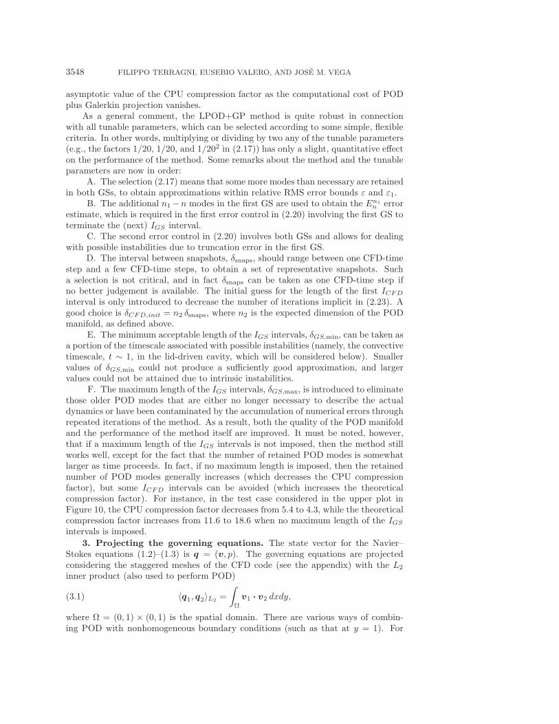
be concentrated near the upper and lateral boundaries, where the solution exhibitsa richer spatial structure. In order to illustrate how this is done, the points that areselected in the 64 × 64 and the 256 × 256 vx-meshes (which are used in the casesRe = 100 and Re = 800, respectively; see Figures 7 and 9) are plotted in Figure 6.

The first GS is obtained substituting the expansions (4.3) in (4.1)–(4.2) (retainingnv1, n

∗v1, and np1 modes, respectively), multiplying (with the first inner product in

(4.4)) (4.1) by the POD modes V i∗ and the last equation in (4.2) by the POD modes

V i, and multiplying (with the second inner product in (4.4)) the second equation in(4.2) by the POD modes P i. Taking into account that POD modes are orthonormal,

3552 FILIPPO TERRAGNI, EUSEBIO VALERO, AND JOSE M. VEGA

Fig. 7. As in Figure 5, bottom, but projecting the CFD code at Re = 100, with steady (top)and periodic (bottom) forcing.

the projected equations are(I− δtLGS

11

2Reδ2s

)Ak+1

∗ = LGS01 A

k + δtLGS

12 Ak + (hk + hk+1)GGS

2Reδ2s− δtLGS

31 Bk

δs

− δt3FGS(Ak) + 3hkLGS

2 Ak − FGS(Ak−1)− hk−1LGS2 Ak−1

2δs,(4.5)

Bk+1 = Bk +LGS02 Ak+1

∗ , Ak+1 = (LGS01 )

�Ak+1∗ − δt

LGS32 A

k+1∗δs

,(4.6)

where Ak = (Ak1 , . . . , A

knv1

), Ak+1∗ = (Ak+1∗1 , . . . , Ak+1

∗n∗v1), and Bk = (Bk

1 , . . . , Bknp1

) are

the amplitude vectors and the superscript � stands for the transpose; the matricesLGS

11 , LGS01 , LGS

12 , LGS2 , LGS

31 , LGS32 , and LGS

02 , the vector GGS, and the function FGS

are defined as

LGS11,ij = 〈V i

∗,L1Vj∗〉Iv , LGS

01,ij = 〈V i∗,V

j〉Iv , LGS12,ij = 〈V i

∗,L1Vj〉Iv ,(4.7)

LGS2,ij = 〈V i

∗,L2Vj〉Iv , LGS

31,ij = 〈V i∗,L3P

j〉Iv ,(4.8)

LGS32,ij = 〈V i,L3P

j∗〉Iv , LGS

02,ij = 〈P i,P j∗〉Ip ,(4.9)

GGSi = 〈V i

∗,G〉Iv , FGSi (Ak) =

⟨V i

∗,F

(nv1∑j=1

AkjV

j

)⟩Iv

.(4.10)

Thus, the kth step of the first GS is performed by solving the linear system (4.5) andreplacing Ak+1∗ into (4.6), which yields Bk+1 and Ak+1. The second GS is obtainedsimilarly and the LPOD+GP method is constructed proceeding as explained in section2. Note that projecting the CFD code means that the same time step is used in boththe CFD and Galerkin calculations.

The counterpart of Figure 5, bottom, is Figure 7, with the same computationalgrids and the same method parameters, except for the minimum length of the Galerkin

LOCAL POD PLUS GALERKIN IN THE UNSTEADY CAVITY 3553

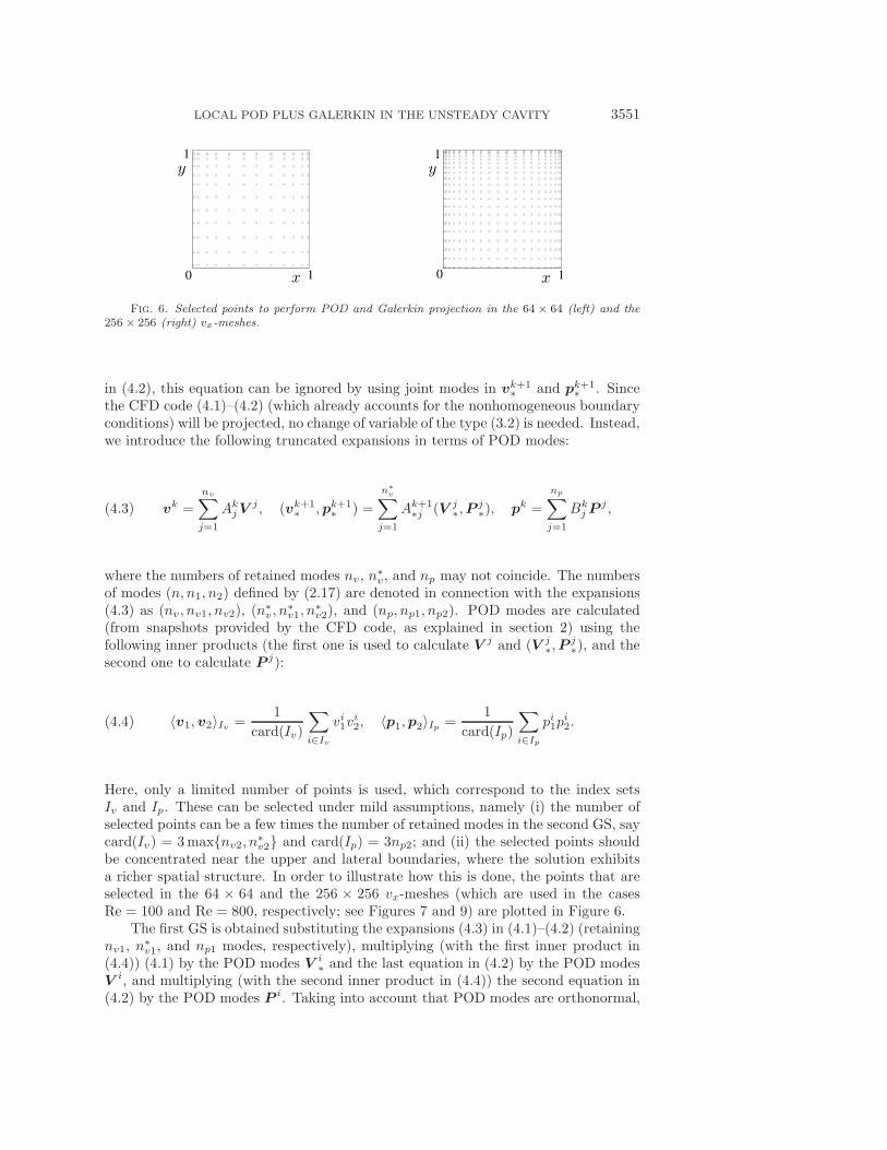
Fig. 8. As in Figure 5, top, but projecting the CFD code at Re = 800, with periodic (left) andquasi-periodic (right) forcing.

intervals, δGS,min, which is now varied according to (2.24), with δGS0 = 0.2, δGS1 =0.5, T0 = 10, and 16 in the cases of steady and periodic forcing, respectively, andδGS,max = 3 in both cases. Here δsnaps = 6 δt, the first ICFD interval requires N = 104and 60 snapshots for steady and periodic forcing, respectively, while the remainingICFD intervals are fairly short, and typically require 1 or 2 snapshots. The numbersof retained modes oscillate around nv ∼ n∗

v ∼ np ∼ 3 and 7, nv1 ∼ n∗v1 ∼ np1 ∼ 8 and

12, and nv2 ∼ n∗v2 ∼ np2 ∼ 10 and 14 for steady and periodic forcing, respectively,

while the theoretical/CPU compression factors are 10.8/5.6 and 9.3/7.2, respectively.Note the following:

A. The numbers of retained modes are much smaller than when the exact equa-tions were projected (Figure 5), even though three sets of modes are now required.

B. Both the theoretical and CPU compression factors are quite good: the CPUtime required by the CFD solver is roughly divided by 6.

C. The error estimate works much better than when the exact equations wereprojected, as comparison with Figure 5, bottom, shows. Note that now the errorestimate is essentially indistinguishable from its exact counterpart, especially whenboth of them are close to their upper bound, ε = 10−2.

D. Some of the Galerkin intervals are terminated because the second error con-trol in (2.20) reaches its cutting value, ε1 = ε/20 = 5 · 10−4.

E. Periodic forcing with other periods produces similar results, as quasi-periodicforcing does at this value of the Reynolds number.

In order to further check the performance of the method, we consider the caseRe = 800, with steady (h(t) = 1), periodic (h(t) = sin t), and quasi-periodic (h(t) =sin(πt/4) cos(t/16)) boundary conditions. The CFD code now (and in the remainingruns at Re = 800) uses staggered 256 × 256 grids and a time step δt = 0.0025. Thedistance between snapshots is δsnaps = 0.03, the number of snapshots in the first ICFD

interval is N = 150, 140, and 101 for steady, periodic, and quasi-periodic forcing,respectively, while in the remaining ICFD intervals only 2–8 snapshots are typicallyrequired. The maximum length of the Galerkin intervals is set to δGS,max = 15. Theminimum length, δGS,min, is varied according to (2.24), with δGS0 = 0.2, δGS1 = 2and 0.3 in the cases of steady and periodic forcing, respectively, and T0 = 50; withquasi-periodic forcing, the constant value δGS,min = 0.2 seems to be a better optionbecause, as two timescales are present, the POD manifold needs to be updated quiteoften (see remarks below).

a. The counterpart of Figure 5, top, for periodic and quasi-periodic forcing isFigure 8, where only the interval 130 < t ≤ T = 250 is plotted; reaching the attractornow requires a larger time (namely, T = 250). The evolution in the steady case is

3554 FILIPPO TERRAGNI, EUSEBIO VALERO, AND JOSE M. VEGA

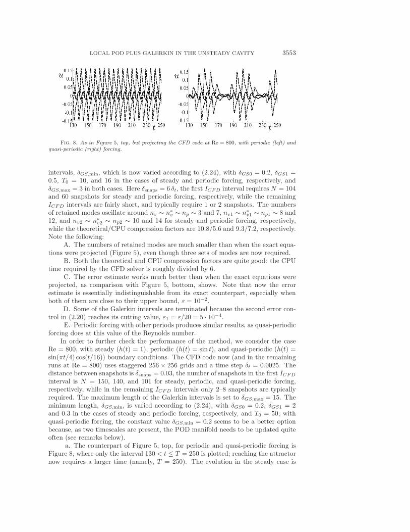
Fig. 9. As in Figure 5, bottom, but projecting the CFD code at Re = 800, with steady (top),periodic (middle) and quasi-periodic (bottom) forcing.

qualitatively similar to its counterpart at Re = 100 and is omitted.b. The amplitude of the oscillations near the right upper corner is larger than

at Re = 100 but the amplitude at the center of the cavity is smaller, which is due tothe effect of the larger value of Re in the shear forcing mechanism.

c. Two timescales are appreciated in Figure 8, right, which were induced onpurpose and make quasi-periodic forcing a fairly demanding test case.

d. The associated error estimates are given in Figure 9, where only a shorttime span is plotted to allow for well appreciating the error estimates. Note thatthese are again quite good. The theoretical/CPU compression factors are 9.5/4.9,7.2/5.8, and 3.7/2.6 in the steady, periodic, and quasi-periodic cases, respectively.The required numbers of POD modes for the second GS at the beginning/end of thetime span 0 < t ≤ T are nv2 ∼ n∗

v2 ∼ np2 ∼ 25/5, 23/19, and 19/31 in the steady,periodic, and quasi-periodic cases, respectively. The smaller compression factors forquasi-periodic forcing are due to the fact that the dimension of the attractor is largerin this case, which is seen in the larger number of required POD modes. The smallerCPU compression factor for steady forcing is due to the fact that the CFD solver isquite fast in this case.

5. Projecting the governing equations revisited. Let us now project thegoverning equations using the Crank–Nicolson scheme (A.6)–(A.8). In other words, itis the scheme (A.12) that will be Galerkin projected. The continuity equation (A.6)

LOCAL POD PLUS GALERKIN IN THE UNSTEADY CAVITY 3555

does not need to be considered, since it is well satisfied by the snapshots. Thus, wedefine joint modes for the velocity and the pressure as

(vk,pk) =n∑

j=1

Akj (V

j ,P j).(5.1)

Proceeding with (A.12) as we did with (A.10)–(A.11) in section 4, the following equa-tion follows for the kth step of the GSs:(

I− δtLGS12

2Reδ2s+

δtLGS31

δs

)Ak+1 = Ak + δt

LGS12 A

k + (hk + hk+1)GGS

2Reδ2s

− δt3FGS(Ak) + 3hkLGS

2 Ak − FGS(Ak−1)− hk−1LGS2 Ak−1

2δs,(5.2)

where LGS12 , LGS

2 , LGS31 , GGS, and FGS are defined as in (4.7), (4.8), and (4.10) with

V i∗ replaced by V i in the first argument of the inner products.Note that the GS in (5.2) is simpler and computationally cheaper than its coun-

terpart in sections 3 and 4. This is because the nonhomogeneous boundary conditionsare imposed in a more natural way than in section 3, since no change of variable isneeded. Also, both construction of POD modes and Galerkin projection are per-formed by using a limited number of mesh points, which makes these two processesless CPU time consuming. Finally only one set of POD modes is needed, instead ofthe three sets of POD modes that were defined in section 4.

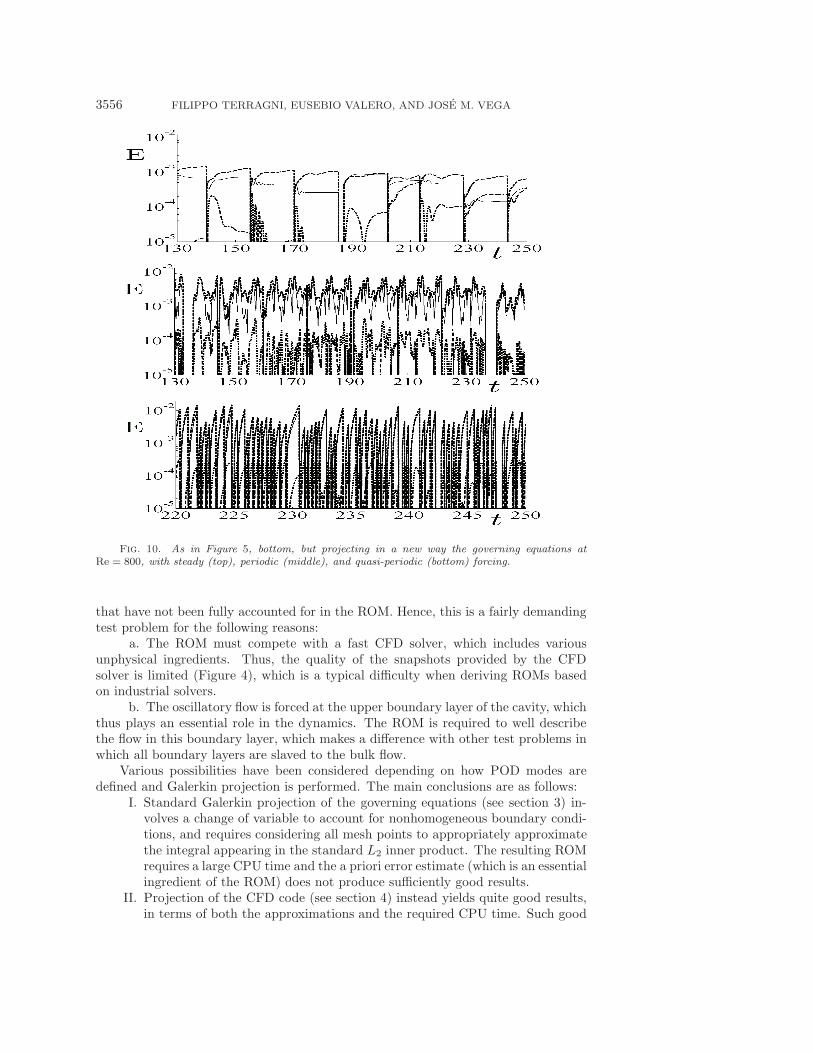
Results for Re = 100 show similar error estimates but better compression factorsthan in section 4. In fact, the theoretical/CPU compression factors in the interval 0 <t ≤ 40 are 15.5/7.2 and 10.0/8.0 for steady and periodic forcing, respectively. Resultsfor Re = 800 are given in Figure 10, which is the counterpart of Figure 9. Note thatthe Galerkin intervals are somewhat larger than when the CFD code was projected.The theoretical/CPU compression factors in the interval 0 < t ≤ 250 are 11.6/5.4,9.3/8.4, and 4.4/3.3 in the steady, periodic, and quasi-periodic cases, respectively.The required numbers of POD modes for the second GS at the beginning/end of thetime span 0 < t ≤ 250 are n2 ∼ 25/6, 24/22, and 19/37 in the steady, periodic,and quasi-periodic cases, respectively. Again, the steady ROM gives a smaller CPUcompression factor, while the quasi-periodic forcing requires a larger number of modesand yields smaller compression factors. It is worth mentioning that once the attractorhas been reached, the compression factors increase; for instance, the CPU compressionfactor in the interval 250 < t ≤ 300 is 31.5 in the periodic case.

Summarizing, this latter ROM based on a more careful projection of the governingequations produces better results than both standard projection of the governingequations and projection of the CFD code. In particular, it produces results whoseaccuracy is comparable to that of the CFD code in a much smaller CPU time.

6. Concluding remarks. A ROM has been constructed based on the combineduse of local POD plus Galerkin projection and CFD calculations in interspersed timeintervals. The method is an extension of its counterpart developed in [25], whichworked quite well for one-dimensional parabolic problems, including transient chaosdynamics in the complex Ginzburg–Landau equation (Figure 2). Such extension hasbeen performed considering the unsteady lid-driven cavity problem, at moderate val-ues of the Reynolds number. The CFD solver is a rough (and computationally quick)finite differences scheme in staggered grids, which involves various approximations

3556 FILIPPO TERRAGNI, EUSEBIO VALERO, AND JOSE M. VEGA

Fig. 10. As in Figure 5, bottom, but projecting in a new way the governing equations atRe = 800, with steady (top), periodic (middle), and quasi-periodic (bottom) forcing.

that have not been fully accounted for in the ROM. Hence, this is a fairly demandingtest problem for the following reasons:

a. The ROM must compete with a fast CFD solver, which includes variousunphysical ingredients. Thus, the quality of the snapshots provided by the CFDsolver is limited (Figure 4), which is a typical difficulty when deriving ROMs basedon industrial solvers.

b. The oscillatory flow is forced at the upper boundary layer of the cavity, whichthus plays an essential role in the dynamics. The ROM is required to well describethe flow in this boundary layer, which makes a difference with other test problems inwhich all boundary layers are slaved to the bulk flow.

Various possibilities have been considered depending on how POD modes aredefined and Galerkin projection is performed. The main conclusions are as follows:

I. Standard Galerkin projection of the governing equations (see section 3) in-volves a change of variable to account for nonhomogeneous boundary condi-tions, and requires considering all mesh points to appropriately approximatethe integral appearing in the standard L2 inner product. The resulting ROMrequires a large CPU time and the a priori error estimate (which is an essentialingredient of the ROM) does not produce sufficiently good results.

II. Projection of the CFD code (see section 4) instead yields quite good results,in terms of both the approximations and the required CPU time. Such good

LOCAL POD PLUS GALERKIN IN THE UNSTEADY CAVITY 3557

results have suggested a second direct projection of the governing equations(see section 5), which ignores the intermediate (fractional stepping) variablesand provides results that are even better than those obtained projecting theCFD code. In both cases, projection is based on a limited number of meshpoints (namely, a few times the number of retained POD modes) concentratednear the boundary, which greatly reduces the required computational effort.

As a consequence, the following overall conclusions are in order:1. The computational cost of industrial solvers can be significantly reduced us-

ing ROMs based on local POD description and Galerkin projection, which is promisingenvisaging industrial applications.

2. Industrial solvers are usually run many times for different values of someparameters and deal with systems of equations whose properties (e.g., existence ofboundary layers, timescales to be expected) are known a priori, which facilitates thecalibration of the various tunable parameters exhibited by the method.

3. The way in which Galerkin projection is performed is crucial. Standardprojection may not produce good results. Projection that mimics the CFD code inconnection with the spatial discretization seems to be a better option. Fractionalstepping instead does not need to be performed in the GS.

4. Compression factors are preserved as the Reynolds number increases. Forinstance, the CPU compression factor under periodic forcing is 8.0 and 8.4 for Re =100 and Re = 800. This shows that the ROM works well at moderate values of Re.These are of industrial interest in, e.g., the design of microcooling devices [2]. Atreally large values of Re, industrial CFD solvers are based on turbulence modelingand can also be combined with the LPOD+GP method. A similar comment applies tospectral solvers, which are frequently used in purely scientific applications at large Re.

5. Comparison with preprocessed ROMs is enlightening. These ROMs are de-signed to simulate attractors and require, as a first step, calculating a set of repre-sentative snapshots in the attractor itself, which usually requires running the CFDsolver in the viscous timescale. As shown, the ROM derived in this paper greatlyaccelerates such approach to the attractor. Simulation of the attractor itself is alsoefficiently performed by the ROM (e.g., at Re = 800, the CPU compression factorunder periodic forcing is 31.5).

6. Various improvements can be envisaged, but they are well ahead of the scopeof this paper. Some of these are currently under research. They include the following:

i. The inner products (4.4) are based on a set of mesh points that have beenselected with the only requirement that they concentrate near the boundary. Anoptimal selection of these points is related to the so-called sampling problem (see[5, 12] and the references therein) and would lead to a further improvement of thecomputational efficiency of the method.

ii. The use of snapshots libraries to decrease the computational cost of com-pletely calculating the POD manifold in the first ICFD interval.

iii. Alternative ways of imposing in the ROM the forcing, nonhomogeneousboundary condition, which is poorly satisfied by the CFD solver (Figure 4).

iv. The combination of the ROM with a better CFD code (e.g., a spectralsolver), which would be more natural in purely scientific applications (but not intypical industrial applications) at larger values of the Reynolds number.

v. The method seems to be robust and to preserve the dynamics of the exactequations, at least in the particular problems considered in [25] and in this paper.A rigorous proof of this would help to ascertain both the scope and the possibleextensions of the main ideas the method is based upon. In particular, it would be

3558 FILIPPO TERRAGNI, EUSEBIO VALERO, AND JOSE M. VEGA

necessary to elucidate the ability of the method to cope with open flows and withturbulent flows, in which the large number of required POD modes can be a limit tothe efficiency of the present method.

In any event, we expect the results in this paper to be a solid step towardsimproving CFD calculations in typical industrial tasks associated with efficient designand certification of industrial products, which is a trend that can be easily traced inthe specialized literature.

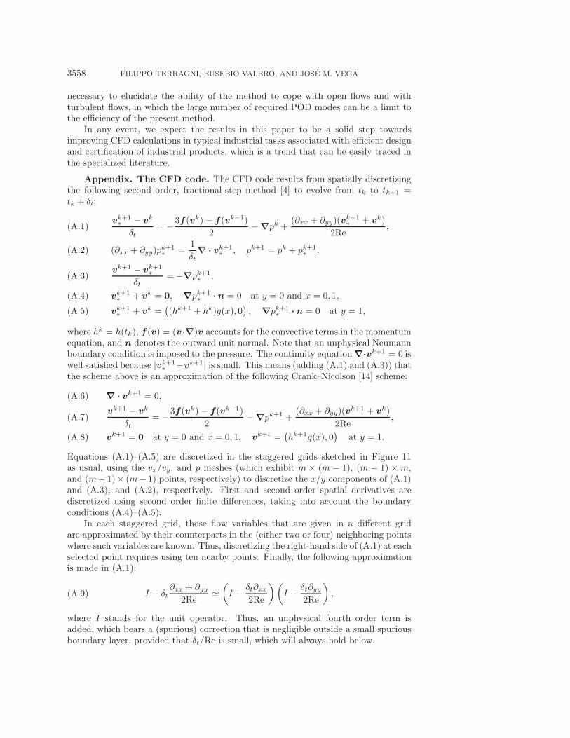
Appendix. The CFD code. The CFD code results from spatially discretizingthe following second order, fractional-step method [4] to evolve from tk to tk+1 =tk + δt:

vk+1∗ − vk

δt= −3f(vk)− f(vk−1)

2−∇pk +

(∂xx + ∂yy)(vk+1∗ + vk)

2Re,(A.1)

(∂xx + ∂yy)pk+1∗ =

1

δt∇ · vk+1

∗ , pk+1 = pk + pk+1∗ ,(A.2)

vk+1 − vk+1∗

δt= −∇pk+1

∗ ,(A.3)

vk+1∗ + vk = 0, ∇pk+1

∗ · n = 0 at y = 0 and x = 0, 1,(A.4)

vk+1∗ + vk =

((hk+1 + hk)g(x), 0

), ∇pk+1

∗ ·n = 0 at y = 1,(A.5)

where hk = h(tk), f (v) = (v ·∇)v accounts for the convective terms in the momentumequation, and n denotes the outward unit normal. Note that an unphysical Neumannboundary condition is imposed to the pressure. The continuity equation∇·vk+1 = 0 iswell satisfied because |vk+1

∗ −vk+1| is small. This means (adding (A.1) and (A.3)) thatthe scheme above is an approximation of the following Crank–Nicolson [14] scheme:

∇ · vk+1 = 0,(A.6)

vk+1 − vk

δt= −3f(vk)− f(vk−1)

2−∇pk+1 +

(∂xx + ∂yy)(vk+1 + vk)

2Re,(A.7)

vk+1 = 0 at y = 0 and x = 0, 1, vk+1 =(hk+1g(x), 0

)at y = 1.(A.8)

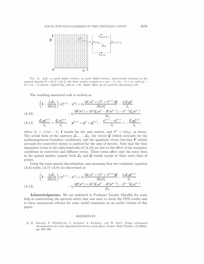
Equations (A.1)–(A.5) are discretized in the staggered grids sketched in Figure 11as usual, using the vx/vy, and p meshes (which exhibit m × (m − 1), (m − 1) × m,and (m− 1)× (m− 1) points, respectively) to discretize the x/y components of (A.1)and (A.3), and (A.2), respectively. First and second order spatial derivatives arediscretized using second order finite differences, taking into account the boundaryconditions (A.4)–(A.5).

In each staggered grid, those flow variables that are given in a different gridare approximated by their counterparts in the (either two or four) neighboring pointswhere such variables are known. Thus, discretizing the right-hand side of (A.1) at eachselected point requires using ten nearby points. Finally, the following approximationis made in (A.1):

(A.9) I − δt∂xx + ∂yy

2Re�(I − δt∂xx

2Re

)(I − δt∂yy

2Re

),

where I stands for the unit operator. Thus, an unphysical fourth order term isadded, which bears a (spurious) correction that is negligible outside a small spuriousboundary layer, provided that δt/Re is small, which will always hold below.

LOCAL POD PLUS GALERKIN IN THE UNSTEADY CAVITY 3559

Fig. 11. Left: vx-mesh (plain circles), vy-mesh (filled circles), and p-mesh (crosses) in thesquared domain Ω = [0, 1] × [0, 1]; the three meshes contain m × (m − 1), (m − 1) × m, and (m −1)× (m − 1) points, respectively, with m = 16. Right: Blow up of a generic elementary cell.

The resulting numerical code is written as(I− δtL1

2Reδ2s

)(vk+1

∗ − vk) = δt2L1v

k + (hk + hk+1)G2Reδ2s

− δtL3pk

δs

− δt3F (vk) + 3hkL2v

k − F (vk−1)− hk−1L2vk−1

2δs,(A.10)

L4pk+1∗

δs=

L5vk+1∗

δt, pk+1 = pk + pk+1

∗ ,vk+1 − vk+1

∗δt

= −L3pk+1∗

δs,(A.11)

where δs = 1/(m − 1), I stands for the unit matrix, and hk = h(tk), as above.The actual form of the matrices L1, . . . ,L5, the vector G (which accounts for thenonhomogeneous boundary conditions), and the quadratic vector function F (whichaccounts for convective terms) is omitted for the sake of brevity. Note that the timedependent terms in the right-hand side of (A.10) are due to the effect of the boundaryconditions in convective and diffusive terms. These terms affect only the outer linesin the spatial meshes, namely both L2 and G vanish except at these outer lines ofpoints.

Using the same spatial discretization, and assuming that the continuity equation(A.6) holds, (A.7)–(A.8) are discretized as(

I− δtL1

2Reδ2s

)(vk+1 − vk) = δt

2L1vk + (hk + hk+1)G

2Reδ2s− δtL3p

k+1

δs

− δt3F (vk) + 3hkL2v

k − F (vk−1)− hk−1L2vk−1

2δs.(A.12)

Acknowledgments. We are indebted to Professor Vassilis Theofilis for somehelp in constructing the spectral solver that was used to check the CFD results andto three anonymous referees for some useful comments on an earlier version of thispaper.

REFERENCES

[1] D. Ahlman, F. Soderlund, J. Jackson, A. Kurdila, and W. Shyy, Proper orthogonaldecomposition for time-dependent lid-driven cavity flows, Numer. Heat Transfer, 42 (2002),pp. 285–306.

3560 FILIPPO TERRAGNI, EUSEBIO VALERO, AND JOSE M. VEGA

[2] D. Alonso, A. Velazquez, and J. M. Vega, A method to generate computationally efficientreduced order models, Comput. Methods Appl. Mech. Engrg., 198 (2009), pp. 2683–2691.

[3] I. S. Aranson and L. Kramer, The world of the complex Ginzburg-Landau equation, Rev.Mod. Phys., 74 (2002), pp. 100–142.

[4] S. Armfield and R. Street, An analysis and comparison of the time accuracy of fractional-step methods for the Navier-Stokes equations on staggered grids, Int. J. Numer. MethodsFluids, 38 (2002), pp. 255–282.

[5] P. Astrid, S. Weiland, K. Willcox, and T. Backx, Missing point estimation in modelsdescribed by proper orthogonal decomposition, IEEE Trans. Automat. Control, 53 (2008),pp. 2237–2251.

[6] N. Aubry, P. Holmes, J. L. Lumley, and E. Stone, The dynamics of coherent structures inthe wall region of a turbulent boundary layer, J. Fluid Mech., 192 (1988), pp. 115–173.

[7] M. F. Barone, I. Kalashnikova, D. J. Segalman, and H. K. Thornquist, Stable Galerkinreduced order models for linearized compressible flow, J. Comput. Phys., 288 (2009),pp. 1932–1946.

[8] M. Bergmann and L. Cordier, Optimal control of the cylinder wake in the laminar regimeby trust-region methods and POD reduced-order models, J. Comput. Phys., 227 (2008),pp. 7813–7840.

[9] M. Bergmann, C. H. Bruneau, and A. Iollo, Enablers for robust POD models, J. Comput.Phys., 228 (2009), pp. 516–538.

[10] G. Berkooz, P. Holmes, and J. L. Lumley, The proper orthogonal decomposition in theanalysis of turbulent flows, Annu. Rev. Fluid Mech., 25 (1993), pp. 539–575.

[11] K. Bizon, G. Continillo, L. Russo, and J. Smula, On POD reduced models of tubular reactorwith periodic regimes, Comput. Chem. Eng., 32 (2008), pp. 1305–1315.

[12] T. Braconnier, M. Ferrier, J.-C. Jouhaud, M. Montagnac, and P. Sagaut, Towards anadaptive POD/SVD surrogate model for aeronautic design, Comput. & Fluids, 40 (2011),pp. 195–209.

[13] W. Cazemier, R. W. C. P. Verstappen, and A. E. P. Veldman, Proper orthogonal de-composition and low-dimensional models for driven cavity flows, Phys. Fluids, 10 (1998),pp. 1685–1699.

[14] T. Cebeci, Convective Heat Transfer, Springer-Verlag, Berlin, 2002.[15] M. Couplet, C. Basdevant, and P. Sagaut, Calibrated reduced-order POD-Galerkin system

for fluid flow modelling, J. Comput. Phys., 207 (2005), pp. 192–220.[16] E. H. Dowell and K. C. Hall, Modeling of fluid-structure interaction, Annu. Rev. Fluid

Mech., 33 (2001), pp. 445–490.[17] P. W. Duck, Oscillatory flow inside a square cavity, J. Fluid Mech., 122 (1982), pp. 215–234.[18] U. Ghia, K. N. Ghia, and C. T. Shin, High-Re solutions for incompressible flow using the

Navier-Stokes equations and a multigrid method, J. Comput. Phys., 48 (1982), pp. 387–411.[19] D. Gottlieb and S. A. Orszag, Numerical Analysis of Spectral Methods: Theory and Appli-

cations, SIAM, Philadelphia, 1977.[20] C. Grebogi, E. Ott, and J. A. Yorke, Chaotic attractors in crisis, Phys. Rev. Lett., 48

(1982), pp. 1507–1510.[21] P. A. LeGresley and J. J. Alonso, Investigation of Non-linear Projection for POD Based

Reduced Order Models for Aerodynamics, AIAA Paper 2001-0926, 39th AIAA AerospaceSciences Meeting & Exhibit, Reno, NV, 2001.

[22] T. Lieu, C. Farhat, and M. Lesoinne, Reduced-order fluid/structure modeling of a completeaircraft configuration, Comput. Methods Appl. Mech. Engrg., 195 (2006), pp. 5730–5742.

[23] D. J. Lucia, P. S. Beran, and W. A. Silva, Reduced-order modelling: New approaches forcomputations physics, Prog. Aeosp. Sci., 40 (2004), pp. 51–117.

[24] B. R. Noack, K. Afanasiev, M. Morzynski, G. Tadmor, and F. Thiele, A hierarchy oflow-dimensional models for the transient and post-transient cylinder wake, J. Fluid Mech.,497 (2003), pp. 335–363.

[25] M. L. Rapun and J. M. Vega, Reduced order models based on local POD plus Galerkinprojection, J. Comput. Phys., 229 (2010), pp. 3046–3063.

[26] S. S. Ravindran, Reduced-order adaptive controllers for fluid flows using POD, J. Sci. Com-put., 15 (2000), pp. 457–478.

[27] D. Rempfer, On low-dimensional Galerkin models for fluid flow, Theoret. Comput. FluidDyn., 14 (2000), pp. 75–88.

[28] D. Rempfer, Low-dimensional modeling and numerical simulation of transition in simple shearflows, in Annual Review of Fluid Mechanics, Annu. Rev. Fluid Mech. 35, Annual Reviews,Palo Alto, CA, 2003, pp. 229–265.

LOCAL POD PLUS GALERKIN IN THE UNSTEADY CAVITY 3561

[29] R. Schreiber and H. B. Keller, Driven cavity flows by efficient numerical techniques, J.Comput. Phys., 49 (1983), pp. 310–333.

[30] S. G. Siegel, K. Cohen, and T. McLaughlin, Feedback Control of a Circular Cylinder Wakein Experiment and Simulation, AIAA Paper 2003-3569, AIAA, Reno, NV, 2003.

[31] S. G. Siegel, J. Seidel, C. Fagley, D. M. Luchtenburg, K. Cohen, and T. McLaughlin,Low-dimensional modelling of a transient cylinder wake using double proper orthogonaldecomposition, J. Fluid Mech., 610 (2008), pp. 1–42.

[32] S. Sirisup and G. E. Karniadakis, A spectral viscosity method for correcting the long-termbehavior of POD models, J. Comput. Phys., 194 (2004), pp. 92–116.

[33] S. Sirisup and G. E. Karniadakis, Stability and accuracy of periodic flow solutions obtainedby a POD-penalty method, Phys. D, 202 (2005), pp. 218–237.

[34] S. Sirisup, G. E. Karniadakis, D. Xiu, and I. G. Kevrekidis, Equations-free/Galerkin-freePOD assisted computation of incompressible flows, J. Comput. Phys., 207 (2005), pp. 568–587.

[35] L. Sirovich, Turbulence and the dynamics of coherent structures, Quart. Appl. Math., 45(1987), pp. 561–590.

[36] G. Tadmor, O. Lehmann, B. R. Noack, and M. Morzynski, Mean field representation ofthe natural and actuated cylinder wake, Phys. Fluids, 22 (2010), 034102.

[37] J. P. Thomas, E. H. Dowell, and K. C. Hall, Using automatic differentiation to create anonlinear reduced-order-model aerodynamic solver, AIAA J., 48 (2010), pp. 19–24.