Local Mirror Symmetry at Higher Genus

arX

iv:h

ep-t

h/99

0604

6v3

11

Jun

1999

hep-th/9906046

IASSNS-HEP–99/55

Local Mirror Symmetry at Higher Genus

Albrecht Klemm∗ and Eric Zaslow∗∗

∗School of Natural Sciences, IAS, Olden Lane, Princeton, NJ 08540, USA

∗∗Department of Mathematics, Northwestern University, Evanston, IL 60208, USA

Abstract

We discuss local mirror symmetry for higher-genus curves. Specifically, we consider

the topological string partition function of higher-genus curves contained in a Fano surface

within a Calabi-Yau. Our main example is the local P2 case. The Kodaira-Spencer

theory of gravity, tailored to this local geometry, can be solved to compute this partition

function. Then, using the results of Gopakumar and Vafa [1] and the local mirror map [2],

the partition function can be rewritten in terms of expansion coefficients, which are found

to be integers. We verify, through localization calculations in the A-model, many of these

Gromov-Witten predictions. The integrality is a mystery, mathematically speaking. The

asymptotic growth (with degree) of the invariants is analyzed. Some suggestions are made

towards an enumerative interpretation, following the BPS-state description of Gopakumar

and Vafa.

∗ e-mail: [email protected]∗∗ e-mail: [email protected]

1. Introduction and Summary

In [2], the techniques of mirror symmetry were applied to the local geometry of a

Fano surface inside a Calabi-Yau manifold. Namely, from the data of the canonical bun-

dle of the surface, differential equations were proposed whose solutions yield genus-zero,

Gromov-Witten-type invariants.1 From these, one arrives at integers after accounting for

contributions from multiple coverings. The mirror symmetry predictions were corrobo-

rated by independent A-model calculations using localization. The mirror principle was

the main tool used for verification; some more explicit fixed point calculations were made,

as well. Excess intersection considerations showed that the integers represent the effective

number of rational curves “coming from” the Fano surface.

In this paper, we extend these techniques to higher-genus curves. For the A-model

calculations, we use localization techniques on higher-genus moduli spaces to compute the

Gromov-Witten invariants. The mirror principle does not apply at higher genus. The

analogue of the prepotential at higher genus is the topological partition function at genus

g, whose coefficients are the Gromov-Witten invariants.

For the B-model, equations governing the dependence of these partition functions,

F (g), on the complex structure moduli of the Calabi-Yau were found in [3][4]. In the effec-

tive 4-d N=2 supergravity theory, emerging from type IIB string theory compactification

on the Calabi-Yau, the F (g≥1) appear as coefficients of the R2F2g−2 terms (here R and F

are the self-dual parts of the Riemann tensor and the graviphoton field strength, respec-

tively).2 The recursive nature of the equations comes from the fact that Riemann surfaces

with marked points degenerate at the boundaries of moduli space – either into pairs of

lower-genus surfaces or surfaces with fewer marked points. As the anti-holomorphic de-

pendence of the topological partition functions is determined by an exact form, it only

receives contributions from the boundaries.

One can tailor the methods of [4] to the local situation we seek. Our motivation

for doing so depends on two simplifications in the local case. First, the solution of the

holomorphic anomaly equation using Kodaira-Spencer gravity simplifies considerably in

1 These invariants are like the relative invariants of Ionel and Parker, except that the degen-

erations are sort of “one-sided.”2 The genus zero prepotential F (0) determines the gauge kinetic terms and the masses of the

charged BPS states. The information contained in the local geometry suffices to obtain the rigid

theory (Seiberg-Witten theory) – see [5] for reviews.

1

the local case due to the fact that the propagators involving the descendents of the puncture

operator (2-d dilaton) can be gauged to zero. Second, the higher-genus Gromov-Witten

invariants are computable using localization. This is in constrast to complete-intersection

Calabi-Yau manifolds in toric varities, where the moduli space of higher-genus maps into

the Calabi-Yau is not simply expressible as the zero locus of a section of a bundle over

the moduli space of maps into an ambient toric manifold.3 For Fano surfaces which are

themselves toric, we need not cut with a section to obtain the moduli space of interest.

This implies in particular that calculations can be made to fix the ambiguity in solving the

Kodaira-Spencer recursions in the local case. In the global case of the quintic, by contrast,

classical geometry cannot fix certain unknown constants.

After solving the Kodaira-Spencer theory and using the mirror map, we verify mirror

symmetry and apply the work of Gopakumar and Vafa [1] to organize the topological

partition functions in terms of coefficients which should be integers, as they count BPS

states of specified spin and charge (in the four-dimensional theory, spin refers to a Lefschetz-

type SU(2) action on the BPS states). This integrality check is a strong test of the power

of M-theory and the approach of Gopakumar and Vafa. The asymptotic growth of the

invariants is also analyzed directly.

The mathematical interpretation of these integers is still unclear. A proper explana-

tion seems to involve moduli spaces of objects in derived categories. Heuristic evidence

exists in support of this observation.

Another explanation is lacking. The form of the partition functions predicted by

Gopakumar and Vafa is a generalization of the multiple cover formula (1/k3). The multiple

cover formula is well-understood mathematically, but the higher-genus generalizations are

a mystery.

We would like to note that Hosono, Saito, and Takahashi [6] obtain BPS counts and

compute topological partition functions via B-model calculations for the rational elliptic

surface, though their techniques are somewhat different. They achieve good corroboration

of Vafa and Gopakumar’s formulas. A-model calculations for this surface would presum-

ably be prohibitive. Moore and Marino also have achieved higher-genus results via heterotic

duality [7].

3 We thank R. Pandharipande for explaining this to us.

2

2. Localization at Higher Genus

The tools for the localization calculations have been available since the work of Kont-

sevich [8], Li-Tian [9], Behrend-Fantechi [10], Graber-Pandharipande [11], and Faber [12].

The moduli space, Mg,0(β;P), of stable maps from genus g curves into some toric

variety P with image in β ∈ H2(P;Z) can have components of various dimensions. To do

intersection theory on it, we need a fundamental cycle of some “appropriate” dimension –

the virtual fundamental class.

This procedure was developed in [10], and the equivariant localization for spaces with

perfect deformation theories was developed in [11]. In that paper, the authors treat the

case of interest to us: the restrictions to the fixed point loci (under the torus action) of the

equivariant fundamental cycle on the space of holomorphic maps of genus g. The authors

give explicit formulas for the weights.

In our examples, we are interested in calculating Chern classes of Uβ, the bundle over

moduli space whose fiber at a point (C, f) ∈ Mg,0(β;P) is equal to H1(C, f∗KP). It is

not difficult to compute the equivariant Chern classes at the fixed loci.

Using these ingredients, we can perform localization calculations at higher genus. The

Atiyah-Bott fixed point formula – true for virtual classes by [11] – reduces the calculation to

integrals over these fixed loci. The different components of the fixed loci are represented

by different graphs. We sum over the graphs using a computer algorithm. As all the

higher-genus behavior must be centered at the fixed points (there are no fixed higher-

genus curves), the fixed loci are all products of moduli spaces of curves, and the graphs

are decorated by genus data at each vertex as well as degree data at each edge, as in [8].

The integrals over the moduli spaces are performed using the algorithm of Faber [12].

In the following subsections, we summarize this procedure.

2.1. Localization Formulas

As discussed in [2], a Fano surface within a complete-intersection Calabi-Yau con-

tributes to the Gromov-Witten invariants, producing an effective “number” of rational

curves. In fact, the curves are not isolated and there is a whole moduli space of maps

into the Fano surface, arising as a non-discrete zero locus of a section of a bundle over the

moduli space of maps in the Calabi-Yau. Just as spaces of multiple coverings of isolated

3

curves contribute to the Gromov-Witten invariants by the excess intersection formula,4

the contribution from the surface B can be calculated as well. It is

Kgβ =

∫

Mg,0(β;B)

c(Uβ), (2.1)

where β ∈ H2(B;Z) and Uβ is the bundle whose fiber over (C, f) ∈ Mg,0(β;B) is the

vector space H1(C, f∗KB).5

We assume that B has a toric description so that we may use the torus action to define

an action on M0,0(β;B) (moving the image curves) and on Uβ, which inherits the natural

action on the canonical bundle. We evaluate the Gromov-Witten invariants by localizing

to the fixed points using the Atiyah-Bott formula

∫

M

φ =∑

P

∫

P

(

i∗Pφe(νP )

)

,

where the sum is over fixed point sets P, iP is the embedding into M, and e(NP/M ) is the

Euler class of the normal bundle of P in M.

Graber and Pandharipande proved that this formula holds mutatis mutandis, with the

replacement of the integral of a class by evaluation over virtual fundamental cycles (in the

equivariant Chow ring) of equivariant classes of deformation complexes. The equivariant

Chern classes and bundles involved are then computed in the standard way, e.g. by looking

at the weights of sections and taking alternating products over terms in a complex. In our

case, following Kontsevich, the fixed moduli can be labeled by graphs. The fixed locus MΓ

corresponding a graph Γ is a product of moduli spaces:

MΓ =∏

v

Mg(v),val(v).

Here v are the vertices of the graph and g(v) and val(v) are the genus and valence of the

vertex. (At a vertex, which is mapped to a torus fixed point, the choice of a val(v)-marked

genus g(v) curve represents the only moduli.)

4 The contribution, from a component of the zero locus Y of some section, to the Chern class

c(E) of some vector bundle E over M is∫

Y

c(E)c(NY/M )

, where NY/M represents the normal bundle

of Y in M. The equation here follows from the reasoning between eqs. (5.4) and (5.5) in [2].5 Let ev be the evaluation map from Mg,1(β;B) to B and let π be the map Mg,1(β;B) →

Mg,0(β;B) which forgets the marked point. Then Uβ = R1π∗ev∗KB.

4

Graber and Pandharipande [11] found the weights of the inverse of the Euler class of

the normal bundle to be:

1

e(Nvir)=∏

e

(−1)ded2dee

(de!)2(λi(e) − λj(e))2de

∏

a+b=dea,b≥0

k 6=i(e),j(e)

1adeλi(e) + b

deλj(e) − λk

×∏

v

∏

j 6=i(v)

(λi(v) − λj)val(v)−1

×

∏

v

(

∑

F

w−1F

)val(v)−3∏

F∋v

w−1F

if g(v) = 0

∏

v

∏

j 6=i(v)

Pg(v)(λi(v) − λj , E∗)∏

F∋v

1

wF − eFif g(v) ≥ 1

(2.2)

where the case with g(v) = 0 is from [13]. Here i(v) is the fixed-point image of the vertex

v; edges e represent invariant P1’s connecting the fixed point labeled i(e) to j(e); and

flags F are pairs (v, e) of vertices and edges attached to them. ωF = (λi(F ) − λj(F ))/de,

where i(F ) = i(e) and j(F ) = j(e) for the associated edge e ∈ F. eF is the Chern

class of the line bundle over MΓ whose fiber is the point e(F ) ∩ Cv, a “gravitational

descendant” in physical terms – also known as a κ class. We have defined the polynomial

Pg(λ,E∗) =

∑gr=0 λ

rcg−r(E∗), where E is the Hodge bundle with fibersH0(KC) on moduli

space.

The bundle Uβ , whose top Chern class φ we are calculating, has fibers H1(C, f∗KB)

over a point (C, f). Let us now fix B = P2 and put β = d since H2(P2) is one-dimensional.

Since the invariant maps are known and the maps from the genus g(v) > 0 pieces are

constants, we explicitly calculate the weights of the numerator in the Atiyah-Bott formula

to be:

i∗(φ) =∏

v

Λval(v)−1i(v) Pg(v)(Λi(v), E

∗)∏

e

[

3de−1∏

m=1

Λi(e) +m

de(λi(e) − λj(e))

]

, (2.3)

where Λi = λ1 + λ2 + λ3 − 3λi.

2.2. Faber’s algorithm

We therefore have explicit formulas for the class to integrate along MΓ. The integrals

involve the κ classes and the Mumford classes (from the Hodge bundle). The integrals can

be performed by the recursive algorithm developed by Faber.

5

A rough sketch of the idea of Faber’s algorithm is as follows [12]. Witten’s origi-

nal recursion relations from topological gravity [14], proved by Kontsevich [15], suffice to

determine integrals of powers of the ψi’s, which are the first Chern classes of the line

bundles whose fiber is the cotangent space of the corresponding marked point, i = 1, ..., n

(the gravitational descendents). However, the integrals over MΓ involve the λ classes as

well – the Chern classes of the Hodge bundle. These classes can be represented by cycles

involving the boundary components of moduli space as well as the ψi’s.

So a proper intersection theory including boundary classes is needed. The boundary

components are images under maps from Mg−1,n+2 (the map identifying the last two

points; this map is of degree two since swapping the points gives the same boundary

curve) and Mh,s+1 × Mg−h,(n−s)+1 (the map identifying the two last points, which is

degree one except when both n = 0 and h = g/2). Understanding the pull-back of the

boundary classes under these maps completes the reduction of intersection calculations

to lower genera. For example, the ψi’s pull back to ψi’s of corresponding points in the

new moduli spaces. One must also note that since the boundary divisors can intersect

(transversely, in fact), boundary classes must also be pulled back to moduli spaces to

which they do not correspond. We refer the reader to [12] for details.

What remains, then, is to express the Chern classes of the Hodge bundle E in terms of

the boundary divisors. This is precisely the content of Mumford’s Grothendieck-Riemann-

Roch (G-R-R) calculation. Briefly (too briefly!), there is the forgetful map ρ : Mg,1 →

Mg,0 (we now set C ≡ Mg,1), with respect to which we wish to push forward the relative

canonical sheaf ωC,M. Since ρ∗ωC,M = E, the G-R-R formula tells us the Chern character

classes of E (we need that R1ρ∗ωC,M = O). The formula calls for integration of ch(ωC,M)

with the Todd class of the relative tangent sheaf. The former involves the descendents,

while the relative tangent sheaf is dual to the relative cotangent sheaf, which differs from

ωC,M only at the singular locus (on smooth parts, sections of the canonical bundle are just

one-forms). The Todd expansion is responsible for the appearance of Bernoulli numbers,

while the difference from the canonical sheaf introduces the divisor classes.

Therefore, integrals of descendent classes and λ classes can be performed by using

Mumford’s formula (see section 1 of [16]) to convert λ classes to descendents and divisor

classes, then on the boundaries of M pulling these clases back to the moduli spaces which

cover the boundaries. As these spaces have lower genera, the integrals can be performed

recursively. Faber has written a computer algorithm in Maple for this procedure, which

he generously lent us for this calculation.

6

2.3. Summing over graphs

The contribution to the free energy F (g) from genus g curves in the class β is given

from the fixed point formula as

Kgβ =

∑

Γ

1

|AΓ|

∫

MΓ

i∗(φ)

e(Nvir), (2.4)

with e(Nvir)−1 and i∗(φ) as described in (2.2)(2.3). The formal expansion of the integrand

yields cohomology elements of Mg,n, the moduli space of pointed curves at the vertices.

The integral over MΓ splits into integrals over these moduli spaces, against which the co-

homology elements of the right degree have to be integrated. In addition, the contribution

of a given graph must be divided by the order of the automorphism group AΓ, as we are

performing intersection theory in the orbifold sense. AΓ contains the automorphism group

of Γ as a marked graph and a Zdefactor for each edge which maps with degree de.

Hence it remains to construct the graphs Γ which label the fixed point loci of

Mg,k(d,P2) under the induced torus action, then to carry out the summation and in-

tegration. A graph is labeled by a set of vertices and edges, and can be viewed as a

degenerate domain curve with additional data specifying the map to P2. The vertices v

represent the irreducible components Cv. They are mapped to fixed points in P2 under

the torus action. The index of this fixed point i(v) and the arithmetic genus g(v) of the

component Cv are additional data of the graph. The edges e represent projective lines

which are mapped invariantly, with degree de, to projective lines in the toric space con-

necting the pair of fixed points. A graph without the additional data g(v), de, i(v) will be

referred to as undecorated.

The following combinatorial conditions specify a Γg,d,k graph representing a fixed-

point locus of genus g, degree d maps with k marked points:6

(1) if e ∈ Edge(Γ) connects the vertices (u, v) then i(u) 6= i(v)

(2) 1 − #(Vertices) + #(Edges) +∑

v∈Vert(Γ) g(v) = g

(3)∑

e∈Edge(Γ) de = d

(4) 1, . . . , k = ∪v∈Vert(Γ)S(v).

To construct all Γg,d,0 graphs we start by generating a list of all possible undecorated

graphs that can be decorated to yield Γg,d,0 graphs. Hence the number of edges is restricted

6 Condition four is relevant only for maps with k marked points, which we do not consider

(k = 0). S(v) is then the subset of marked points on the component Cv.

7

by (3) while the number of vertices is restricted by (2). The undecorated graphs with nv

vertices can be represented by an nv×nv symmetric incidence matrix, m. Entries mi,j = 1

or 0 represent a link or no link between vi and vj , so with a fixed number of edges ne there

will be(

(nv+1)nv2

ne

)

possibilities. A main problem is to identify among the graphs those

which have different topology. To obtain invariant data, independent of the ordering of the

vertices and depending only on the topology of the graph, we use a so called depth-first-

search algorithm. This starts with a vertex vk and descends level-by-level along all occuring

branches collecting the data of the encountered vertices, namely the valence (and in later

applications the additional information g(v) and i(v) as well as edge data dα for the map),

into a list Tk graded by the level, until all vertices have been encountered. A lexicographic

ordering can be imposed on the combined lists of all vertices TΓ = T1, . . . , Tnv and

TΓi= TΓk

only if Γi is isomorphic to Γk. These invariants will be used for a.) generating

distinct undecorated graphs, b.) decorating them without redundancy, and c.) finding the

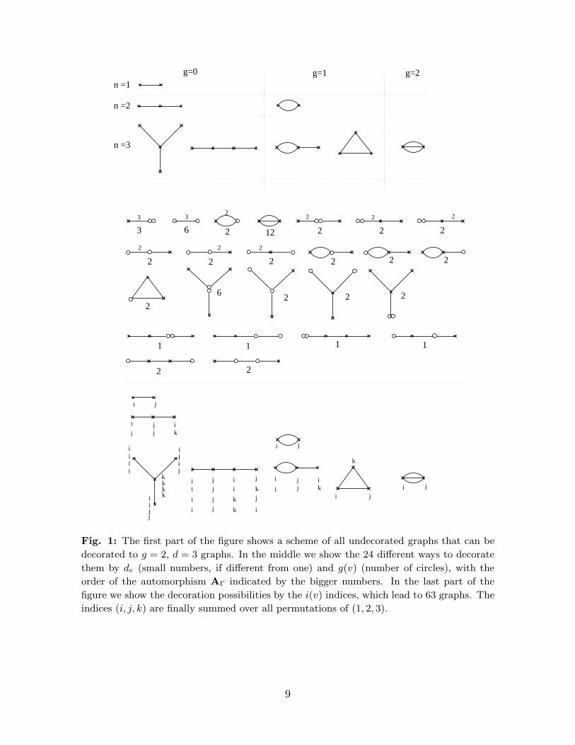
automorphism group.7 Fig. 1 shows as an example the generation of genus 2, degree 3

graphs.

We have implemented the above generation of graphs8 of (2.4) in a completely au-

tomated computer algorithm that uses Faber’s algorithm to perform the integrals over

Mg,n. We exhibit the results of these localization calculations in the instanton pieces

F(g)inst =

∑

d>0Kgdq

d of the partition functions F (g) listed below:

7 A useful computer program [17] was used to check the number of undecorated graphs.8 The number of graphs grows very quickly with the genus. E.g., to calculate the d = 5 term

(for g = 0, . . . , 5) in (2.5), one sums over six times 17321, 733101, 2295313, 5353719,

111011442, 203452570 fully-decorated graphs, where the number in braces indicates the num-

ber of graphs with just g(v) and de decorations. For example, in the calculation of (g, d) = (4, 5)

the maximal dimension of a vertex moduli space dim(Mg,n) = 14 occurs in the “star graphs” –

irreducible genus 4 curves with five legs. At this dimension, 22462 different 2-d gravity integrands

must be evaluated.

8

i j

k

i j

i j i

i kj

i j i

i kj

iijj

iiii

kkkk

ijij

1263 2 2 2 2

2 2 2 2 2 2

226 2 2

2

1 1 1 1

3 32

2 2

2 2

n =1

n =2

n =3

g=1g=0 g=2

2

j i jii j i k

i j k j

i j k i

i j

i j

2

2

Fig. 1: The first part of the figure shows a scheme of all undecorated graphs that can be

decorated to g = 2, d = 3 graphs. In the middle we show the 24 different ways to decorate

them by de (small numbers, if different from one) and g(v) (number of circles), with the

order of the automorphism AΓ indicated by the bigger numbers. In the last part of the

figure we show the decoration possibilities by the i(v) indices, which lead to 63 graphs. The

indices (i, j, k) are finally summed over all permutations of (1, 2, 3).

9

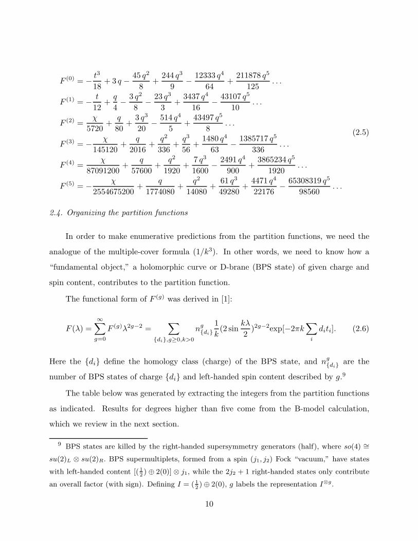
F (0) = −t3

18+ 3 q −

45 q2

8+

244 q3

9−

12333 q4

64+

211878 q5

125. . .

F (1) = −t

12+q

4−

3 q2

8−

23 q3

3+

3437 q4

16−

43107 q5

10. . .

F (2) =χ

5720+

q

80+

3 q3

20−

514 q4

5+

43497 q5

8. . .

F (3) = −χ

145120+

q

2016+

q2

336+q3

56+

1480 q4

63−

1385717 q5

336. . .

F (4) =χ

87091200+

q

57600+

q2

1920+

7 q3

1600−

2491 q4

900+

3865234 q5

1920. . .

F (5) = −χ

2554675200+

q

1774080+

q2

14080+

61 q3

49280+

4471 q4

22176−

65308319 q5

98560. . .

(2.5)

2.4. Organizing the partition functions

In order to make enumerative predictions from the partition functions, we need the

analogue of the multiple-cover formula (1/k3). In other words, we need to know how a

“fundamental object,” a holomorphic curve or D-brane (BPS state) of given charge and

spin content, contributes to the partition function.

The functional form of F (g) was derived in [1]:

F (λ) =∞∑

g=0

F (g)λ2g−2 =∑

di,g≥0,k>0

ngdi

1

k(2 sin

kλ

2)2g−2exp[−2πk

∑

i

diti]. (2.6)

Here the di define the homology class (charge) of the BPS state, and ngdi are the

number of BPS states of charge di and left-handed spin content described by g.9

The table below was generated by extracting the integers from the partition functions

as indicated. Results for degrees higher than five come from the B-model calculation,

which we review in the next section.

9 BPS states are killed by the right-handed supersymmetry generators (half), where so(4) ∼=su(2)L ⊗ su(2)R. BPS supermultiplets, formed from a spin (j1, j2) Fock “vacuum,” have states

with left-handed content [( 12) ⊕ 2(0)] ⊗ j1, while the 2j2 + 1 right-handed states only contribute

an overall factor (with sign). Defining I = ( 12) ⊕ 2(0), g labels the representation I⊗g.

10

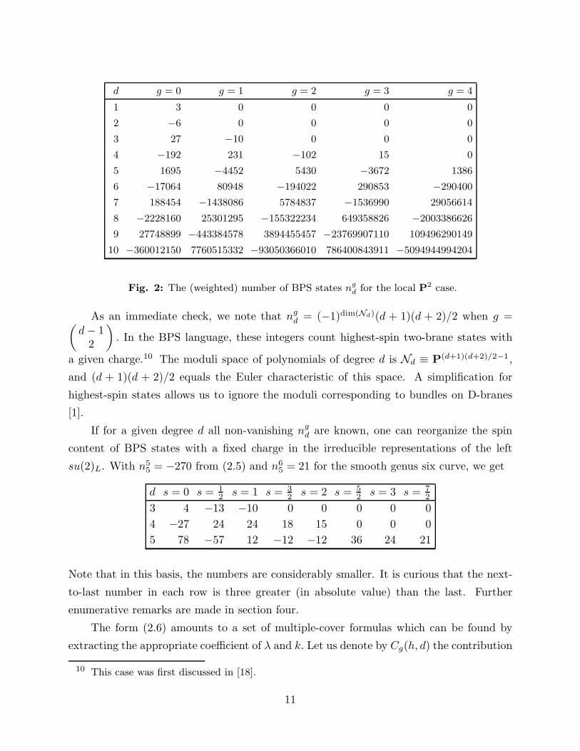
d g = 0 g = 1 g = 2 g = 3 g = 4

1 3 0 0 0 0

2 −6 0 0 0 0

3 27 −10 0 0 0

4 −192 231 −102 15 0

5 1695 −4452 5430 −3672 1386

6 −17064 80948 −194022 290853 −290400

7 188454 −1438086 5784837 −1536990 29056614

8 −2228160 25301295 −155322234 649358826 −2003386626

9 27748899 −443384578 3894455457 −23769907110 109496290149

10 −360012150 7760515332 −93050366010 786400843911 −5094944994204

Fig. 2: The (weighted) number of BPS states ngd for the local P2 case.

As an immediate check, we note that ngd = (−1)dim(Nd)(d + 1)(d + 2)/2 when g =

(

d− 12

)

. In the BPS language, these integers count highest-spin two-brane states with

a given charge.10 The moduli space of polynomials of degree d is Nd ≡ P(d+1)(d+2)/2−1,

and (d + 1)(d + 2)/2 equals the Euler characteristic of this space. A simplification for

highest-spin states allows us to ignore the moduli corresponding to bundles on D-branes

[1].

If for a given degree d all non-vanishing ngd are known, one can reorganize the spin

content of BPS states with a fixed charge in the irreducible representations of the left

su(2)L. With n55 = −270 from (2.5) and n6

5 = 21 for the smooth genus six curve, we get

d s = 0 s = 12 s = 1 s = 3

2 s = 2 s = 52 s = 3 s = 7

2

3 4 −13 −10 0 0 0 0 0

4 −27 24 24 18 15 0 0 0

5 78 −57 12 −12 −12 36 24 21

Note that in this basis, the numbers are considerably smaller. It is curious that the next-

to-last number in each row is three greater (in absolute value) than the last. Further

enumerative remarks are made in section four.

The form (2.6) amounts to a set of multiple-cover formulas which can be found by

extracting the appropriate coefficient of λ and k. Let us denote by Cg(h, d) the contribution

10 This case was first discussed in [18].

11

of a genus g object in a class β to the partition function at genus g+ h in class dβ. ¿From

(2.6) we see that Cg(h, d) is the coefficient of λ2(g+h)−2 in d−1(2 sin(dλ/2))2g−2. Some

of these numbers have been corroborated by mathematical calculations. For example,

C0(0, d) = 1/d3 [19][20]. C0(h, d) was calculated in [16], and Cg(h, 1), g ≥ 1 in [21]. R.

Pandharipande has communicated to us another subtraction scheme when h = 0 which

also yields integers.

A puzzle remains, however. The multiple-cover formulas predict, for example, that

genus two objects of degree four contribute to the partition function at genus two, degree

eight. However, no double covers of genus two curves by genus two curves are expected.

In general, since no covering maps from genus g to g + h curves exist, how does one even

define the covering contribution? Perhaps a formulation via spaces of sheaves (which we

discuss in section four) is in order.

2.5. Example

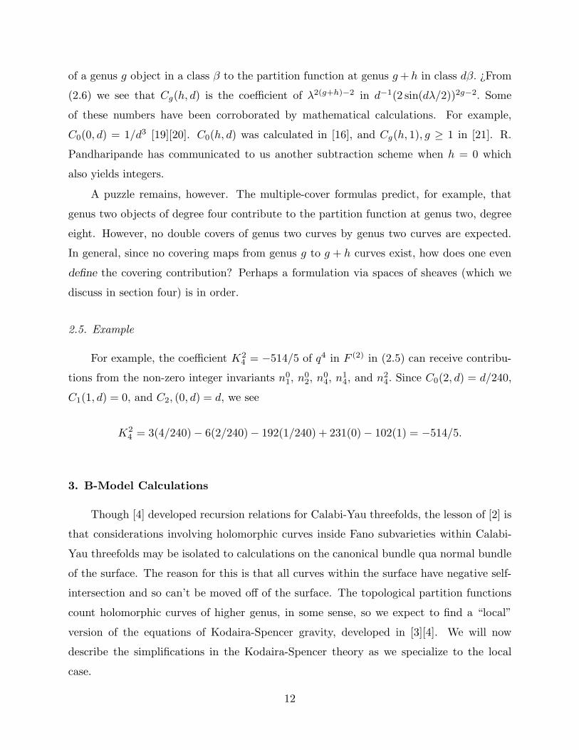
For example, the coefficient K24 = −514/5 of q4 in F (2) in (2.5) can receive contribu-

tions from the non-zero integer invariants n01, n

02, n

04, n

14, and n2

4. Since C0(2, d) = d/240,

C1(1, d) = 0, and C2, (0, d) = d, we see

K24 = 3(4/240) − 6(2/240)− 192(1/240) + 231(0) − 102(1) = −514/5.

3. B-Model Calculations

Though [4] developed recursion relations for Calabi-Yau threefolds, the lesson of [2] is

that considerations involving holomorphic curves inside Fano subvarieties within Calabi-

Yau threefolds may be isolated to calculations on the canonical bundle qua normal bundle

of the surface. The reason for this is that all curves within the surface have negative self-

intersection and so can’t be moved off of the surface. The topological partition functions

count holomorphic curves of higher genus, in some sense, so we expect to find a “local”

version of the equations of Kodaira-Spencer gravity, developed in [3][4]. We will now

describe the simplifications in the Kodaira-Spencer theory as we specialize to the local

case.

12

3.1. The vacuum line bundle and correlation functions

In N = 2 topological theories the vacuum state |0〉 transforms as a section of a

holomorphic line bundle L over the moduli space M of the theory. In the case of the

B-type topological σ-models, the former will be identified with the holomorphic (3,0)-form

Ω while M will be identified with the complex structure moduli space of the Calabi-Yau

geometry X , which is mirror dual to the geometry X on which we count the holomorphic

maps. M has a special Kahler structure, with Kahler potential K(z, z).

By the sewing axioms of topological field theory the vacuum amplitudes at genus g

F (g) are sections of L2−2g over M. The general topological correlations function F(g)i1...in

∈

L2−2g⊗SymnT∗M are defined as covariant derivatives of the “potentials” F (g) as F

(g)i1...in

=

Di1 . . .DinF (g). The Di are covariant with respect to metric connection Γi

lk = Gim∂lGkm

of the Weil-Peterson-Zamolodchikov metric Gkl(z, z) = ∂k∂lK on M as well as the Kahler

connection Ai = ∂iK of the line bundle L.

3.2. The key holomorphic object at genus zero: F(0)i1,i2,i3

The genus zero three-point functions F(0)i1,i2,i3

, physically well-known as the Yukawa

couplings of the heterotic string with standard embedding or the magnetic moments in

the type-II compactifications, are of special importance because, as their moduli space has

no boundaries, they are truly holomorphic and appear as building blocks in the recursive

definition of the higher loop amplitudes.

They can be explicitly calculated as integrals over the Calabi-Yau manifold X

F(0)i1,i2,i3

(z) = −

∫

X

Ω ∂zi1∂zi2

∂zi3Ω (3.1)

which can be expressed as the derivatives of suitable combinations of period integrals over

the the cycles of X. These period integrals can be most easily reconstructed from solutions

of the Picard-Fuchs system of X. For the local case, the F(0)i1,i2,i3

can be defined either as

a limit of a global Calabi-Yau geometry or intrinsicially from the Picard-Fuchs system for

the local geometry. We sometimes write Ci,j,k for F(0)i,j,k.

13

3.3. The canonical coordinates ti and the holomorphic limit

Other correlation functions F(g)i1,...,ir

for g > 0 are not holomorphic.11 However, due

to a uniquely distinguished class of coordinate systems on M, the canonical coordinates,

there is a well-defined limit one can take to define holomorphic correlators.

Of the 2h2,1 + 2 = 2dim(M) + 2 period integrals ωi =∫

γiΩ, near the maximal

unipotent point PM = (zi = 0, Im(ti) → ∞) ∈ M, exactly h2,1 will have logarithmic

behavior ωi ∼ log(zi) +O(z), i = 1, . . . , h2,1. A unique one ω0 = 1 +O(z) is analytic. The

homogeneous coordinates, defined as 2πi ti = ωi

ω0∼ log(zi), have the following properties,

which define canonical coordinates near any point P0.

All holomorphic derivatives vanish at P0

∂t1 . . . ∂trΓk

ij |P0= 0, ∂t1 . . . ∂tr

K|P0= 0 . (3.2)

Let as above P0 be at z = 0, t = t0. Then (3.2) implies that in the t coordinates the

leading term in λi = (ti − t0) of K = C +O(λ) and Gij = Ci,j +O(λ) is constant. When

re-expressed in the coordinates zi, the holomorphic parts of K and G in the λi → 0 limit

are

K = C − log(ω0), Gim =∂tk∂zi

Ckm . (3.3)

In all quantities to be discussed below we will take the holomorphic λ→ 0 limit.

The ti at PM have the additional property that they are identified by mirror symmetry

with the complexified Kahler parameters of the mirror X, and the F(g)i1,...,ir

are curve-

counting functions for holomorphic maps of genus g into X . Note also that ti at PM are

the special coordinates in which the holomorphic parts of the Kahler connection and the

Weil-Peterson connection vanish, i.e. Di becomes the ordinary derivative ∂ti.

At this point there is important simplification in the local case. As is clear from the

differential equations associated to the local case [22][2], ω0 = 1 is always a holomorphic

solution, and hence for the local case the holomorphic part of the Kahler potential becomes

trivial in the limit (3.3).

11 Note that F(0)i1,...,in

for n = 0, 1, 2, may have an anti-holomorphic dependence.

14

3.4. The holomorphic anomaly at genus one and the derivation of F (1)

The genus one topological partition function is defined as

F (1) =1

2

∫

F

d2τ

Im(τ)TrRa,Ra (−1)FFLFRq

HL qHR . (3.4)

Note that without the insertions of the left and right fermion number operators, the in-

tegrand would be the Witten index and just receive contributions from the ground states

Tr(−1)F = χ. The holomorphic anomaly due to contributions from the boundary of the

moduli space was derived in [3] for general N = 2 theories and specializes for the c = 3

case to12

∂i∂jF(1) =

1

2F

(0)ijk F

(0)

jkle2KGjkGkl −

( χ

24− 1)

Gij . (3.5)

Using Rij = −12

∂2 log det(G)∂i∂j

and the special geometry relation

Rkijl = Gijδ

kl +Gljδ

ki − F

(0)ilmF

(0)

jpqe2KGkpGmq , (3.6)

one can integrate (3.5) up to an unknown holomorphic function f to yield

F (1) = log(

det(G−1)12 e

K2 (3+h2,1− 1

12χ)|f2|)

. (3.7)

The holomorphic ambiguity f can be parameterized by the vanishing or pole behavior

at the discriminant loci f =∏k

i=1(∆k)ri∏h2,1

i=1 zxii . In particular, the xi can all be deter-

mined by the limiting behavior limzi→0 F(1) = − 1

24

∑h2,1

i=1 ti∫

Xc2Ji. The behavior of F (1)

at certain types of singularities is universal – e.g., for the conifold singularity rcon = − 112

.

By virtue of the remark at the end of the previous section, χ and h1,2 only affect an

irrelevant additive constant to F (1) in the local case. Note that on the other hand, the

topological number∫

Xc2Ji is crucial for fixing the large ti behaviour of F (1) in the local

case. Formulas for∫

Xc2Ji in the local case can be found in [2].

12 The normalization of F (1) in [3] is by a factor 2 greater than the one in [4]. We will adopt

the latter.

15

3.5. The higher genus anomaly and the derivation of the F (g)

The higher genus correlators are defined by a recursive procedure using the holomor-

phic anomaly equation

∂iF(g)i1,...,in

=1

2Cjk

iF

(g−1)jki1,...,in

+

1

2Cjk

i

∑

r=0

∑

s=0

1

s!(n− s)!

∑

σ∈Sn

F(r)jiσ(1)...iσ(s)

F(g−r)kiσ(s+1)...iσ(n)

− (2g − 2 + n− 1)

n∑

s=1

Gi,isF

(g)i1...is−1is+1...in ,

(3.8)

where Ciji

≡ F(0)

ijke2KGjjGkk. The right-hand side corresponds to the boundary contribu-

tions of the moduli space of marked Riemann surfaces, Mg,n. The first term comes from

pinching a handle, the next from splitting the surface into two components by growing a

long tube, the last from when the insertion approaches marked points.

The solution of the equation is provided by the calculation of potentials for the non-

holomorphic quantities Ciji

. In the first, step one calculates Sij ∈ L−2 ⊗ Sym2TM such

that Ciji

= ∂iSij . This follows from (3.6) by noting that in Kahler geometry Rk

ijl= −∂jΓ

kil,

and hence

∂k[SijCjkl] = ∂k[δil∂kK + δi

k∂lK + Γikl] . (3.9)

The derivatives ∂k on both sides can be removed at the price of introducing a meromorphicobject f i

kl, which also has to compensate the non-covariant transformation properties ofquantities on the right-hand side.

Therefore it is natural to split f ikl into quantities with simple transformation proper-

ties: f ikl = δi

k∂l log f + δil∂k log f − vl,a∂kv

i,a + f ikl, where f i

kl now transforms covariantly,

f ∈ L, and vi,a transform as tangent vectors. The choices of the f , vi,a, f ikl are by no

means independent, however. If we specialize to the one-modulus case, as in our main

example the local P2, we can in addition set fzzz = 0 and in the holomorphic limit get the

simplified expression

Szz =1

F(0)zzz

[

2∂z log(eK |f |2) − (Gzzv)−1∂z(vGzz)

]

= −1

F(0)zzz

∂z log

(

v∂t

∂z

)

as λ→ 0,

(3.10)

where v ∈ TM to render Szz covariant. The simplification in the second line is due to the

fact that K is constant in the holomorphic limit for the local case and f can chosen to be

16

--41

8+

-

-

- -

- -

1-2

- 1-2

+ + 16-

1-2

- 1-4

-1-4

-

1-4

+ 1-2

+1-2

+

- 1-4

1-4

-

1-4

- 1-8

- 1-4

-

1-4

+ 1-4

+ + 16-

1-8

+

1-8

-

16--

1-1-4

+1-4

+

1-2

-

1-12

1-16

-

1-8

+1-8

+ 1-8

+

1-16

+

1-12

+

1-16

-

- __148

__148

+

1-16

1-8

1-16

124-

__148

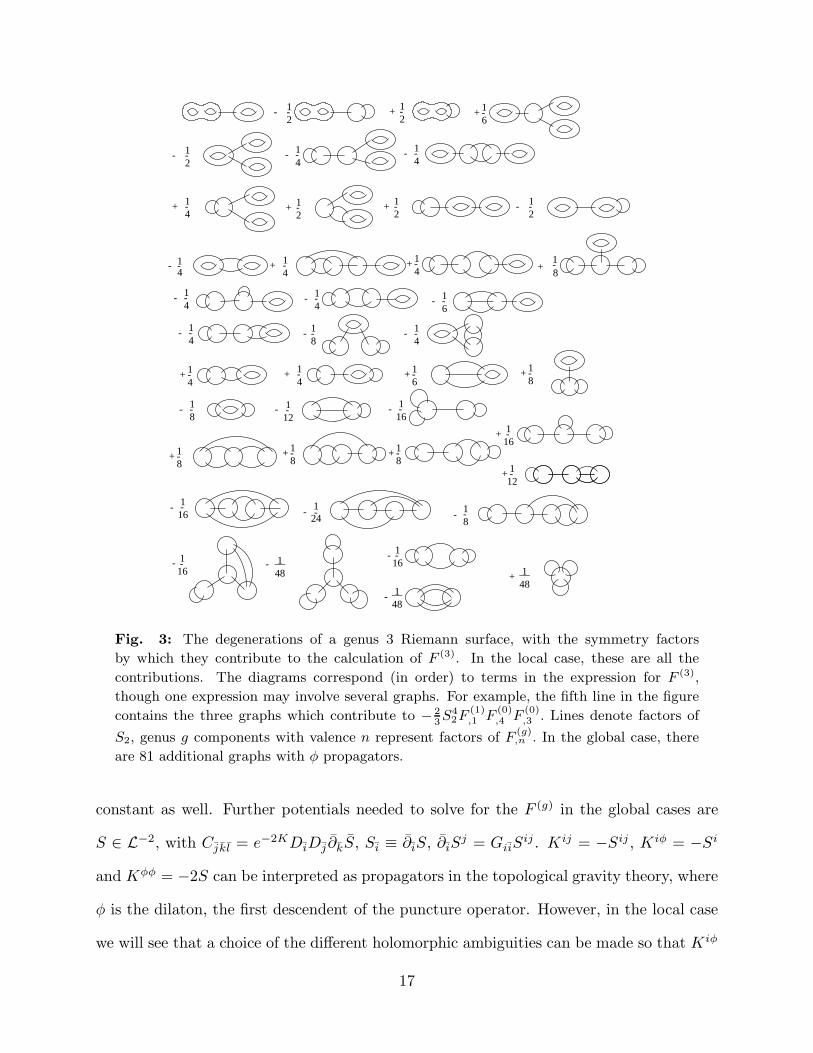
Fig. 3: The degenerations of a genus 3 Riemann surface, with the symmetry factors

by which they contribute to the calculation of F (3). In the local case, these are all the

contributions. The diagrams correspond (in order) to terms in the expression for F (3),

though one expression may involve several graphs. For example, the fifth line in the figure

contains the three graphs which contribute to − 23S4

2F(1),1 F

(0),4 F

(0),3 . Lines denote factors of

S2, genus g components with valence n represent factors of F(g),n . In the global case, there

are 81 additional graphs with φ propagators.

constant as well. Further potentials needed to solve for the F (g) in the global cases are

S ∈ L−2, with Cjkl = e−2KDiDj ∂kS, Si ≡ ∂iS, ∂iSj = GiiS

ij . Kij = −Sij , Kiφ = −Si

and Kφφ = −2S can be interpreted as propagators in the topological gravity theory, where

φ is the dilaton, the first descendent of the puncture operator. However, in the local case

we will see that a choice of the different holomorphic ambiguities can be made so that Kiφ

17

and Kφφ vanish. Si is derived from

∂zSz =

1

F(0)zzz

∂z

[

2∂z log(eK |f |2)2 − v−1∂z(v∂zK)]

,

and if we set the holomorphic ambiguity in the special solution to this equation to zero, it

vanishes in the holomorphic limit for the local case. Similarly one can see that S vanishes.

The derivation of F (g) proceeds recursively. One first considers the holomorphic anom-

aly equation of F (g), and using Ciji

= ∂iSij , one can write the right-hand side e.g. for g = 2

as 12 ∂i[S

jk(F(1)jk +F

(1)j F

(1)k )]− 1

2Sjk∂i[F

(1)jk +F

(1)j F

(1)k ]. Using the definition of the Riemann

tensor as commutator and special geometry, i.e. [∂i, Dj ]lk = −Gijδ

lk − Gikδ

lj + CjkmC

mli,

one lets the ∂i derivative act on F (g−1) and repeats the procedure until an expression

∂iF(g) = ∂i[. . .] is derived, where [. . .] contains the propagators and lower-genus correla-

tion functions.

This yields, again up to holomorphic ambiguity at every final integration step,

F (2) = −1

8S2

2F(0),4 +

1

2S2F

(1),2 +

5

24S3

2(F(0),3 )2 −

1

2S2

2F(1),1 F

(0),3 +

1

2S2(F

(1),1 )2 + f (2)

F (3) =S2F(2),1 F

(1),1 −

1

2S2

2F(2),1 F

(0),3 +

1

2S2F

(2),2 +

1

6S3

2(F(1),1 )3F

(0),3 −

1

2S2

2F(1),2 (F

(1),1 )2

−1

2S4

2(F(1),1 )2(F

(0),3 )2 +

1

4S3

2(F(1),1 )2F

(0),4 + S3

2F(1),2 F

(1),1 F

(0),3 −

1

2S2

2F(1),3 F

(1),1

−1

4S2

2(F(1),2 )2 +

5

8S5

2F(1),1 (F

(0),3 )3 −

2

3S4

2F(1),1 F

(0),4 F

(0),3 −

5

8S4

2F(1),2 (F

(0),3 )2

+1

4S3

2F(1),2 F

(0),4 +

5

12S3

2F(1),3 F

(0),3 +

1

8S3

2F(0),5 F

(1),1 −

1

8S2

2F(1),4 −

7

48S4

2F(0),5 F

(0),3

+25

48S5

2F(0),4 (F

(0),3 )2 −

5

16S6

2(F(0),3 )4 −

1

12S4

2(F(0),4 )2 +

1

48S3

2F(0),6 + f (3) ,

where S2 ≡ Szz and F(g),n ≡ (Dz)

nF (g).

Notice that in the local case the χ drops out, as expected. These terms represent the

various degenerations of the genus g Riemann surface, and it is useful to keep track of the

calculation by interpreting them as Feynman rules for the auxiliary finite quantum system.

Clearly the symmetry factors are of the utmost importance to the calculation. We exhibit

these and all 41 diagrams which contribute in the local limit to F (3) in Fig. 3.

18

3.6. The local P2 case

P2 is torically defined by the integral lattice polyhedron Σ = conv(−1,−1), (1, 0), (0, 1).

The non-compact A-model geometry13 O(−3) → P2 is torically described by a fan spanned

by (1,−1,−1), (1, 1, 0), (1, 0, 1). By the mirror construction of [24] applied to the local

case [22], the mirror B-model geometry follows then from the periods of a meromorphic

differential λ on the Riemann surface described by the vanishing of the (1, 1)-shifted New-

ton polynomial associated to the dual polyhedron Σ∗ = conv(−1,−1), (2,−1), (−1, 2).

In this case, we simply have a cubic P = x31 + x3

2 + x33 − 3ψx1x2x3 = 0 in P2 = PΣ∗ .

Differential equations for the periods of λ in the mirror geometry follow from the C∗

scaling actions on the local A-model geometry. As described in [22] these translate directly

into Picard-Fuchs differential operators, which in the P2 case gives14

L = θ3 − x3∏

i+1

(θ − ai + 1) = Lθ, a1 =1

3, a2 =

2

3, a3 = 1, (3.11)

where θ = x ddx . This is the defining equation for the Meijer G-function G2,2

3,3

(

−x∣

∣

∣

∣

a1a2a3

0 0 0

)

,

which we denote G(a1, a2, a3; x) for short [25].15

To find the solutions to (3.11) which correspond to actual integrals of λ over cycles, we

relate them to the periods over the vanishing cycles. Both periods (apart from the trivial

residue) are fixed up to an overall normalization by the Lefschetz theorem on vanishing

cycles:

• td = ∂F∂t from the logarithmic solution td log(1 − 27z) + hol. at z = 1

27 .

• t = σ0 log(z) + σ2 from the double-logarithmic solution at the large complex structure

limit z = 0: log(z)(σ0 log(z) + 2σ1), where σ0 has no constant term.

13 A simple global Calabi-Yau, in which this geometry is embedded, is e.g. defined by the

vanishing locus of a degree 18 polynomial in P4(1, 1, 1, 6, 9). Using mirror symmetry some Gromov-

Witten invariants for this space have been calculated [23].14 Here we have set x = 27z = 1/ψ3 = 27(−1/a3

0) (in comparison with [2]) to bring the

singularities to 0, 1,∞.15 This function is the logarithmic integral Γ(a1)Γ(a2)

Γ(a3)

∫

dxx 2F1 of the hypergeometric function

2F1(a1, a2; a3, x) solving L. Solutions ωi of L are related to the periods of P = 0, ωi =∫

γiΩ with

Ω = dxy, by ωi = ωi

ψ. To check this one may use the Weierstrass form of the Γ(3) curve P = 0

y2 = 4x3−xg2−g3 with g2 = 3ψ(8+ψ3), g3 = 8+20ψ3 −ψ6. The general theory of Picard-Fuchs

equations for elliptic curves then gives for ωi the differential equation (ψ3−1)ω′′+3ψ2ω′+ψω = 0,

the same as that which follows from L(ψω) = 0.

19

It turns out that t(x) = i Γ(a3)2πΓ(a1)Γ(a2)

G(a1, a2, a3; x) is precisely the mirror map16 and

td follows by analytic continuation of the vanishing period at x = 1 to produce at z = 0

the basis of periods

∂F∂ti

1ti

=

−dijk

2 titk + aiktk + 124c2Ji +O(q)

1ti

(3.12)

with d = −13, a = −1

6and c2J = −2 as expected from the local limit. Here we have chosen

a normalization17 of td such that the derivative ∂3t F of the period which stays finite in the

local limit, ∂F∂t = −1

3(∂tE− 3∂tB

), reproduces Cttt. This choice is also natural in the sense

that the value of c2J = −2 reproduces the leading behavior of F(1)top = c2J

12 t+ . . ..

With this normalization and u = 1 − x, one has near u = 0:

2πi td = Au+ higher order,

2πi t = 2πi t(1) +B u+ C u log u+ higher order,(3.13)

with A = 3−3/2 i, B = i (log(27)+1)√

3(2π)

, C =√

3(2π)

.

At this point, we can use the three-point functions to solve the P2 topological partition

functions at higher-genus as we have outlined in this section. We will use this analysis to

investigate the asymptotic growth of the n0d in the next section. The numerical invariants

extracted from these higher-genus calculations were listed in Fig. 2. These B-model

calculations yield results for very high degree, though adding genera requires fixing the

holomorphic ambiguity.

Solving the B-model recursion relations gives the topological partition functions. As

with knowing the prepotential in (genus zero) mirror symmetry, this is not enough to make

enumerative predictions. First one needs to find the Kahler parameters ti (the “mirror

map”). In the present case, the mirror map states that the Kahler parameter t is equal

to the logarithmic solution of the Picard-Fuchs equation (3.11) of the local geometry (no

ratio is needed since the holomorphic solution is constant). Then one must organize the

16 The implicit choice of the constant term log(27) fits the definition of the mirror map, a fact

which turns out to be right for all local mirror symmetry systems whose Picard-Fuchs equation

is Meijer’s equation.17 If we simply take the limit of the 3-fold periods, the normalization of td differs from this

choice by −3.

20

prepotential according to (2.6), as outlined in section 2.4, to account for multiple-cover

contributions. The result is an expansion in terms of integer coefficients ngdi.

Of course, this process demands that the ambiguity (the holomorphic section f (g)) at

each step in the recursion be fixed. There are 2g − 1 unknowns in this function, which we

fix by matching Gromov-Witten invariants for the first 2g − 1 degrees at genus g.

There is another way to fix one of these coefficients. Ghoshal and Vafa argue in [26]

that the leading coefficient of the ambiguity f (g) at the conifold singularity is determined

by the free energy of the c = 1 string evaluated at the self-dual radius. Recall that f (g) has

the form∑2g−2

k=0 A(g)k u−k, where the conifold is at u = 0.18 It turns out that the leading

behavior of F (g) is determined by A(g)2g−2 alone, as the other terms both in the anomaly

and from the recursion have subleading contributions. Ghoshal and Vafa’s identification

then gives

A(g)2g−2 =

B2g

2g(2g − 2),

where the B2g are Bernoulli numbers. We should comment that as f (g) is a section of the

vacuum line bundle L, this equation only makes sense in a certain gauge. One can use the

g = 0 contribution to fix the gauge, then determine the higher A(g)2g−2. Note that the inde-

pendent determination of the ambiguity via localization calculations gives a corroboration

of this formula at g = 2, 3. In Fig. 2, the entries n4d≥6 rely on this procedure.

This is how Fig. 2 was derived from the B-model.

4. Some Enumerative Issues

The holomorphic curves that these numbers count are not simply worldsheet instan-

tons. As shown by Vafa and Gopakumar [1], they represent D-branes in type-II or M-

theory compactifications. In this section, we will analyze the growth of these invariants

at genus zero, then make some remarks regarding a proper mathematical interpretation of

the integers.

18 Ghoshal and Vafa employ a double-scaling limit λ → 0 and u → 0 with λ/u fixed, where

λ is the string coupling. This isolates the leading behavior of F (g) from the subleading terms in

F (g+h).

21

4.1. Asymptotic growth of states

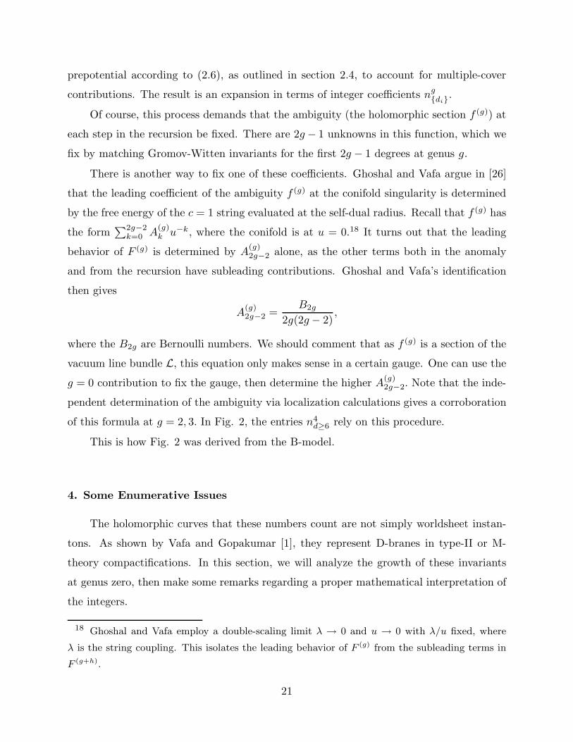
Let us return now to the solutions (3.13) of the P2 period equations.

The singularity at x = 1 limits the radius of convergence of the instanton expansion

and in particular the exponential growth of |nd| must be e2πt2(1), where t2 = Im(t). For

an interpretation of the nd ≡ n0d as BPS counts for some physical system, the logarithm

of the multiplicity of the BPS states is the entropy in the large d limit and an important

critical exponent of the theory. The value

t(1) =i

2πΓ( 13 )Γ( 2

3 )G

(

1

3,2

3, 1; 1

)

∼ −1

2+ i 0.462757788 . . . , (4.1)

is therefore of particular interest. The real part 12

means that the nd come with alternating

sign. Fig. 4 shows how the logarithmic slope of |nd| approaches t2(1) = Im(t(1)).

50 100 150 200

0.445

0.45

0.455

0.46

50 100 150 200

0.2

0.4

0.6

0.8

1

1.2

1.4

Fig. 4: Left: the slope of log(|nd|)2π

for d = 1, . . . 240 approaches t2(1) for high d. Right:

Sensitivity of the third Richardson transform of nd/nasymd on t2(1). The curve approaching

1 is for correct t2(1) value (4.1) the lower/upper curve is for t2(1) ± ε with ε = 2 × 10−6.

More precisely, one can also determine as in [27] the first subleading logarithms by

comparing the ansatz for nasymd ∼ Ndρ log(d)σe2πdt2(1) in the asymptotic expansion with

Cuuu. The Yukawa coupling in the x variable

F (0)xxx = −

1

3(2πi)31

x3(1 − x)(4.2)

is normalized so that that F(0)ttt =

(

dzdt

)3F

(0)zzz = −1

3 +∑

d=1d3ndqd

1−qd reproduces the genus

0 instantons as in Fig. 2. This and the knowledge of the u log u coefficient in the t(u)

expansion yields

nasymd ∼

−∫

J3

C2

e−2πidt(1)

d3 log(d)2. (4.3)

22

Instead of just comparing nd/nasymd one can suppress further subleading logarithms by

considering higher order Richardson transforms [27], which also approach one. This gives

a far more sensitive check on the t2(1) slope from the instanton numbers – see Fig. 4.

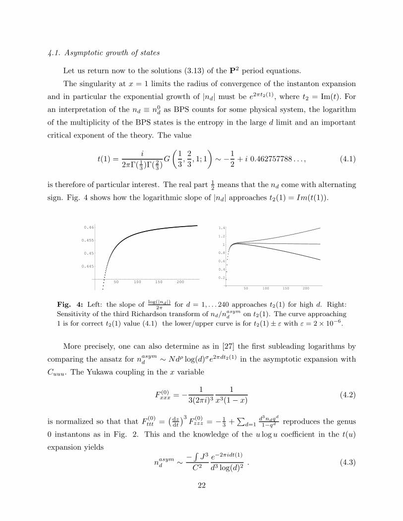
The formula (4.1) describes the asymptotic of other one-modulus local mirror sym-

metry systems with Picard-Fuchs equations given by Meijer’s equation with solution

G(a1, a2, a3; x). These cases were discussed in [28][29][2]. If we define b ≡ b(~a) ≡

2Ψ(a3) − Ψ(a1) − Ψ(a2) (here Ψ(x) = d(log Γ(x))/dx is the digamma function), then

we have:

• ( 12 ,

12 , 1): describes the diagonal direction in P1 × P1 with x = ebz [2] as well as a

direction in the E5 del Pezzo, with x = −ebz.

• ( 13, 2

3, 1): describes P2 as discussed, with x = ebz, as well as a direction in the E6 del

Pezzo, with x = −ebz.

• ( 14, 3

4, 1): describes a direction in the E7 del Pezzo, with x = −ebz .

• ( 16 ,

56 , 1): describes a direction in the E8 del Pezzo, with x = −ebz.

With B(~a) ≡ i b(~a)+12π we summarize some of their relevant properties, which follow to

a large extent from Meijer’s fundamental system of solutions.∫

J3∫

c2J a A B C t(1) Γ

P 1 × P 1 −1 2 0 − i2

2B(~a) 1π

.371226 i Γ0(4)

E5 −4 −∗4 − 42

−√

4i√

4B(~a) 1π

− 12

+ .371226 i Γ0(4)

P 2 − 13

−2 − 16

i

33/2

√3B(~a)

√3

2π− 1

2+ .462757 i Γ0(3)

E6 −3 −∗6 − 32

i√

3√

3B(~a)√

32π

− 12

+ .462757 i Γ0(3)

E7 −2 −8 − 22

−i√

2√

2B(~a)√

22π

− 12

+ .610262 i Γ0(2)

E8 −1 −10 − 12

−i B(~a) 12π

− 12

+ .928067 i Γ(1)

The exact value of the critical exponent is G(a1, a2, a3; 1) and the asymptotic ex-

pansion follows from (4.3). Note that for all del Pezzo surfaces, −

∫

J3

C2 = (2π)2 in good

agreement with the instanton numbers.19 If there is a star on∫

Jc2, we find an additional

constant shift by one in the double-logarithmic solution (3.12). The monodromies are

generated by the two shift operators at x = 0 and x = 1, which follow from the constants

listed in the table.

There is an important difference between the ( 12, 1

2, 1) system and the other cases. It

follows from the Riemann symbol that the former has a logarithmic solution at 1z = 0, while

19 This can be seen from the third Richardson transform. The asymptotic formula for the E8

del Pezzo given in [30] is not quite correct. The monotonically increasing function nd/nasymd would

cross 1 at about d = 100.

23

the others have, as in the one-modulus compact three-folds [31], power series solutions at

this point signaling a conformal field theory. In the compact case these can be identified

as Gepner-type conformal field theories: tensor products of minimal N = 2 models.

The analytic continuation to 1z

= 0 is particularly simple due to a Barnes integral

representation – see [27][31][32] for similar applications. As in [32] it is easy to see that,

given the above definition of t at z = 0, which corresponds to a choice of the B-field, one

gets t = 12

at 1/z = 0, if z = ebx and t = 0 and at 1/z = 0 if z = −ebx. In particular, the

P2 example has a conformal point at 1/z = 0, which is the C3/Z3 non-compact orbifold.

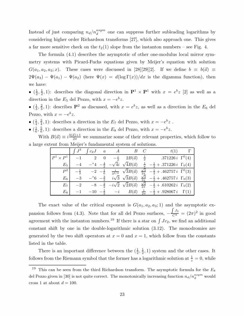
5 10 15 20 25 30cox

0.2

0.4

0.6

0.8

1Im t

Fig. 5: Near linear dependence of the growth rate of instantons with the Euler (Coxeter)

number.

Clearly it would be extremely interesting to find the physical system whose entropy of

BPS states approaches in some limit the critical exponents which we have provided here.

It is noteworthy that the coefficients t2(1) for the del Pezzo cases grow linearly (to a close

approximation) with the Euler number assigned to the corresponding local Calabi-Yau,

i.e. twice the Coxeter number of the associated group. If, as for K3, there is a bosonic

string-like oscillator algebra on the moduli spaces, this would be the expected behavior.

For example, in the local P1 × P1 case, an oscillator-type partition function for some of

the local invariants was found by Nekrasov and Kol [33], though the sense in which the

coefficients were Euler characteristics of a moduli space remains unclear. This brings us

to our next question.

4.2. What is the moduli space?

From the work of Gopakumar and Vafa II [1], we learn that the integers arising from a

proper organization of the topological string partition functions simply encode the number

24

and properties of BPS states in the specified charge (homology class). Note that the BPS

charges are specified by a homology class, not a genus. In fact, different genera are part

of a connected moduli space of BPS states of specified charge.

The integers describe the representation content of the BPS states under an additional

conjectural Lefschetz-type SU(2) action on the cohomology of this moduli space. As is

familiar from BPS counting on K3 [34][35], this moduli space is naively comprised of pairs

of holomorphic curves together with flat U(1) connections. This thinking may be too naive.

What is the proper definition of the moduli space? Experience is teaching us that D-

branes can be thought of as objects in the bounded derived category of coherent sheaves.

Indeed, this category is important for Kontsevich’s homological mirror conjecture [13].

The conjecture is that the derived category of coherent sheaves (D-branes/instantons

in IIA/B) is equivalent to a category of Fukaya whose objects are Lagrangian (perhaps

special-Lagrangian) objects (D-branes/instantons in IIB/A). This conjecture satisfies the

correspondence principle. For example, it captures the idea of constructing the mirror

Calabi-Yau through special-Lagrangian tori [36] as the equivalence of the moduli spaces of

two distinguished objects (the structure sheaf of a point versus the distinguished toroidal

Lagrangian submanifold). It also includes work of Vafa [37] by interpreting the three-

point functions of massless excitations above a D-brane state as structure constants in

the composition of morphisms – though Vafa has taken this further by identifying special

coordinates through which to make identifications across mirror theories. Finally, ordinary

mirror symmetry would be recovered by looking at similar considerations by treating the

Calabi-Yau three-fold M as a (diagonal) D-brane in M ×M.

There is further evidence for the derived category. Hilbert schemes of points are a

kind of intermediate step between moduli spaces of vector bundles and full-out derived

moduli spaces, and they appear prominently in D-brane counts. Evidence also comes from

requiring the Fourier-Mukai transform to act as a symmetry of objects for K3 compacti-

fications [38]. As well, D-brane charges naturally live in K-theory [39][40]. For P2 these

moduli spaces of objects are not well known, though some Poincare polynomials of moduli

spaces of points (sheaves supported on points or schemes of finite length) have been com-

puted, as have some moduli spaces of higher-rank bundles. Heisenberg algebras have been

found to act on cohomology, as for K3, which we take as loose evidence that these are the

right spaces to study [41]. In addition, the exponential growth of the local invariants (with

exponent depending on the “non-compact Euler number”) is in line with (super-)oscillator

partition functions.

25

Let us now think of sheaves as one-term complexes, so as objects in a derived cat-

egory. Then the moduli spaces of objects in this category should be the proper general

framework for these questions. Moduli spaces of derived objects in general do not exist

due to obstructions. For this reason, derived moduli spaces 20 [42] may be the technology

necessary to study the higher-genus integer invariants in the general case. Euler characters

for such “spaces” can be defined. One can hope that this formulation of the question will

lead to insight regarding the higher-genus problem for the quintic, which is not amenable

to localization calculations.

Thinking of derived moduli spaces rather than moduli of sheaves is more in line with

the spirit of Kontsevich’s mirror symmetry conjecture [13]. His motivation for introducing

an A∞ structure came in part from trying to define an extended moduli space of Calabi-

Yau manifold as the moduli space of the structure sheaf of the diagonal M in M ×M by

deforming the associative algebra of functions as a homotopy associative differential graded

(A∞) algebra. The relation to the algebra to BRST cohomology classes on the conformal

field theory of the D-brane, and of the grading to ghost number would be interesting to

explore.

In fact, it is likely that we must treat our sheaves as sheaves in the total space of the

canonical bundle of P2. This would introduce further complexity.

4.3. Counting singular curves

For many applications, the differences between D-brane as cycle with bundle, as sheaf,

or as derived object are unimportant. However, we may not be so lucky here. The argument

in the second paper of [1] gives a heuristic derivation of n03(P

2) = 27. This should be equal

to χ(M3), the Euler characteristic of the D-brane moduli space M3 of curves in the class

3H, where H is the hyperplane class generating H2(P2). The ng

d for g 6= 0 represent the

different characters of the additional fiber-Lefschetz SU(2) action on cohomology. n03(P

2)

is obtained by noting that the Jacobian of a smooth degree three curve can be identified

with the curve itself (which has genus one). Therefore the choice of curve plus point on

Jacobian is the same as the choice of curve plus point on curve. If we choose the point

first (a P2 worth of such choices) and ask how many degree three curves pass through the

point (a P8), we see M3 to be a P8 fibration over P2, with Euler characteristic 9×3 = 27.

20 “Derived quot schemes,” in fact, which retain all obstruction data in the form of a complex.

In short, dg-schemes do not have tangent spaces, they have tangent complexes.

26

Following [35], one might attempt to count the Euler characteristic by noting that

M3 must be a fibration over the moduli space of degree three curves in P2, with fiber

equal to the Jacobian of a given curve. As Jacobians of smooth curves have trivial Euler

characteristic, we can localize our counting to the singular (more specifically, the rational

curves). There is a moduli space of such curves (for K3 this space was zero dimensional),

each of which should contribute some fixed amount determined by the singularity type.

However, among the degree three curves we necessarily have reducible (e.g., (X+Y )(X2 +

Y 2 +Z2) = 0 ⊂ P2) and even unreduced (e.g., (X + Y )3 = 0 ⊂ P2) curves. Here is where

the sheaf interpretation is necessary. Over the unreduced curves, which can be thought

of as multiply-wrapped branes, we should have rank k bundles (if k is the number of

wrappings). These sheaves then have the same characteristic numbers as the non-singular

curves. We are still unsure of how to perform the counting (e.g., there is a discrete infinity

of higher-rank bundles over P1 with fixed degree). This interpretation is consistent with

the moduli spaces of objects in the elliptic curve.

We can now hope to state Gopakumar and Vafa’s approach as a conjecture that

the Euler characteristics of the appropriate moduli dg-stack of derived objects on P2 of

characteristic numbers (r = 0, c1 = d, c2 = d2) have Euler characteristic equal to n0d. This

conjecture might have to be tailored to account for the fact that the objects properly live

on KP2 with support in P2. Whether we need the full weight of dg-stacks (which have

tangent spaces which include all obstructions to deformations) to check this, remains to

be seen. For the general situation, it is likely that we would.

These spaces may give some insight into the multiple cover formulas of Vafa and

Gopakumar, as well. One also must find an additional fiber-Lefschetz SU(2) action on

the derived moduli spaces to agree with Vafa and Gopakumar’s interpretation for ng≥1d .

Exciting work lies ahead.

Acknowledgements

We are grateful to S. Katz, R. Pandharipande, T. Graber and C. Vafa for illuminating

conversations. Also we would like to thank C. Faber for sending us his Maple program for

the intersection calculation on Mg,n. The work of A. Klemm is supported in part by a

DFG Heisenberg fellowship and NSF Math/Phys DMS-9627351.

27

References

[1] C. Vafa and R. Gopakumar, “M-theory and Topological Strings-I & II,” hep-

th/9809187, hep-th/9812127.

[2] T.-M. Chiang, A. Klemm, S.-T. Yau, and E. Zaslow, “Nonlocal Mirror Symmetry:

Calculations and Interpretations,” hep-th/9903053.

[3] M. Bershadsky, S. Cecotti, H. Ooguri, and C. Vafa, “Holomorphic Anomalies in Topo-

logical Field Theories,” Nucl. Phys. 405B (1993) 279-304.

[4] M. Bershadsky, S. Cecotti, H. Ooguri, and C. Vafa, “Kodaira-Spencer Theory of Grav-

ity and Exact Results for Quantum String Amplitudes,” Commun. Math. Phys. 165

(1994) 311-428.

[5] W. Lerche, “Introduction to Seiberg-Witten Theory and its Stringy Origin,” Nucl.

Phys. Proc. Suppl. 55B (1997) 83-117, hep-th/9611190; A. Klemm, “On the Geometry

behind N=2 Supersymmetric Effective Actions in Four-Dimensions”, Proceedings of

the Trieste Summer School on High Energy Physics and Cosmology 96, World Scientic,

Singapore (1997) 120-242, hep-th/9705131; P. Mayr, “Geometric Construction of N=2

Gauge Theories,” Fortsch. Phys. 47 (1999) 39-63, hep-th/9807096.

[6] S. Hosono, M.-H. Saito, and A. Takahashi, “Holomorphic Anomaly Equation and BPS

State Counting of Rational Elliptic Surface,” hep-th/9901151.

[7] M Marino and G. Moore, “Counting Higher Genus Curves in a Calabi-Yau Manifold,”

Nucl. Phys. B543 (1999) 592-614; hep-th/9808131.

[8] M. Kontsevich, “Enumeration of Rational Curves via Torus Actions,” in The Mod-

uli Space of Curves, Dijkgraaf et al eds., Progress in Mathematics 129, Birkhauser

(Boston) 1995.

[9] J. Li and G. Tian, “Virtual Moduli Cycles and Gromov-Witten Invariants of Algebraic

Varieties,” J. Amer. Math. Soc. 11, no. 1 (1998) 119-174.

[10] K. Behrend and B. Fantechi, “The Intrinsic Normal Cone,” math.AG/9601010.

[11] T. Graber and R. Pandharipande, “Localization of Virtual Classes,” math.AG/9708001.

[12] C. Faber, “Algorithm for Computing Intersection Numbers on Moduli Spaces

of Curves, with an Application to the Class of the Locus of the Jacobians,”

math.AG/9706006.

[13] M. Kontsevich, “Homological Algebra of Mirror Symmetry,” Proceedings of the

1994 International Congress of Mathematicians I, Birkauser, Zurich, 1995, p. 120;

math.AG/9411018.

[14] E. Witten, “Two-Dimensional Gravity and Intersection Theory on Moduli Space,”

Surveys in Diff. Geom. 1 (1991) 243-310.

[15] M. Kontsevich, “Intersection Theory on the Moduli Space of Curves and the Matrix

Airy Function,” Commun. Math. Phys. 147 (1992) 1-23.

28

[16] C. Faber and R. Pandharipande, “Hodge Integrals and Gromov-Witten Theory,”

math.AG/9810173.

[17] Brendan D. McKay, “nauty User’s Guide” available at http://cs.anu.edu.au∼bdm/ .

[18] E. Witten, “Phase Transitions in M-Theory and F-Theory,” Nucl. Phys. 471 (1996)

195-216; hep-th/96031150 .

[19] P. Aspinwall and D. Morrison, “Topological Field Theory and Rational Curves,” Com-

mun. Math. Phys. 51 (1993) 245-262.

[20] Yu. I. Manin, “Generating Functions in Algebraic Geometry and Sums over Trees”

in “The moduli space of curves” (Texel Island, 1994), Progr. Math. 129, Birkhauser,

Boston (1995) 401–417; alg-geom/9407005.

[21] R. Pandharipande, “Hodge Integrals and Degenerate Contributions,” math.AG/9811140.

[22] S. Katz, A. Klemm, and C. Vafa, “Geometric Engineering of Quantum Field Theories,”

Nucl. Phys. B497 (1997) 173-195.

[23] S. Hosono, A. Klemm, S. Theisen and S.T. Yau, “Mirror Symmetry, Mirror Map and

Applications to Calabi-Yau Hypersurfaces,” Commun. Math. Phys. 167 (1995) 301-

350, hep-th/9308122; P. Candelas, A. Font, S. Katz and D. Morrison, “Mirror Symme-

try for Two Parameter Models,” Nucl.Phys. B429 (1994) 626-674, hep-th/9403187.

[24] V. Batyrev, “Dual Polyhedra and Mirror Symmetry for Calabi-Yau Hypersurfaces in

Toric Varieties,” J. Algebraic Geom. 3 (1994) 493-535.

[25] The Bateman Project, Higher Transcendental Functions, Vol. 1, Sec. 5.3.-5.6, A. Erde-

lyi ed., McGraw-Hill Book Company, New York (1953).

[26] D. Ghoshal and C. Vafa, “c=1 String as the Topological Theory of the Conifold,”

Nucl. Phys. B453 (1995) 121.

[27] P. Candelas, X. C. De La Ossa, P. Green, and L. Parkes, “A Pair of Calabi-Yau

Manifolds as an Exactly Soluble Superconformal Theory,” Nucl. Phys. B359 (1991)

21.

[28] A. Klemm, P. Mayr, and C. Vafa, “BPS States of Exceptional Non-Critical Strings,”

Nucl. Phys. B (Proc. Suppl.) 58 (1997) 177-194; hep-th/9607139.

[29] W. Lerche, P. Mayr, and N. P. Warner, “Non-Critical Strings, Del Pezzo Singularities

and Seiberg-Witten Curves,” hep-th/9612085.

[30] J. A. Minahan, D. Nemechansky and N. P. Warner, “Partition function for the BPS

States of the Non-Critical E8 String,” Adv. Theor. Math.Phys. 1 (1998) 167-183;

hep-th/9707149.

[31] A. Klemm and S. Theisen, “Considerations of One-Modulus Calabi-Yau Compacti-

fications: Picard-Fuchs Equations, Kahler Potentials and Mirror Maps,” Nucl. Phys.

B389 (1993) 153-180.

[32] P. Aspinwall, B. Greene, and D. R. Morrison, “Measuring Small Distances in N=2

Sigma Models,” Nucl. Phys. 420 (1994) 184-242.

[33] N. Nekrasov, “In the Woods of M-Theory,” hep-th/9810168.

29

[34] M. Bershadsky, V. Sadov, and C. Vafa, “D-Branes and Topological Field Theories,”

Nucl. Phys. B463 (1996) 420-434; hep-th/9511222.

[35] S.-T. Yau and E. Zaslow, “BPS States, String Duality, and Nodal Curves on K3,”

Nucl. Phys. B471 (1996) 503-512; hep-th/9512121.

[36] A. Strominger, S.-T. Yau, and E. Zaslow, “Mirror Symmetry is T-Duality,” Nuclear

Physics B479 (1996) 243-259; hep-th/9606040.

[37] C. Vafa, “Extending Mirror Conjecture to Calabi-Yau with Bundles,” hep-th/9804131.

[38] P. S. Aspinwall and R. Y. Donagi, “The Heterotic String, the Tangent Bundle, and

Derived Categories,” Adv. Theor. Math. Phys. 2 (1998) 1041-1074; hep-th/9806094.

[39] R. Minasian and G. Moore, “K-Theory and Ramond-Ramond Charge,” hep-th/9710230.

[40] E. Witten, “D-Branes and K-Theory,” hep-th/9810188.

[41] See, e.g., H. Nakajima, “Lectures on Hilbert Schemes of Points on Surfaces,”

preprint http://kusm.kyoto-u.ac.jp∼nakajima/TeX.html; I. Grojnowski, “Instantons

and Affine Algebras I: The Hilbert Scheme and Vertex Operators,” Math. Res. Lett. 3,

no. 2 (1996) 275-291; and V. Baranovsky, “Moduli of Sheaves on Surfaces and Action

of the Oscillator Algebra,” math.AG/9811092.

[42] I. Ciocan-Fontanine and M. M. Kapranov, “Derived Quot Schemes,” math.AG/9905174.

30