Lobatto Implicit Sixth Order Runge-Kutta Method For Solving Ordinary Differential Equations with Stepsize Control

LOBATTO IMPLICIT SIXTH ORDER RUNGE-KUTTA METHOD

FOR SOLVING ORDINARY DIFFERENTIAL EQUATIONS

WITH STEPSIZE CONTROL

Andres L. Granados M.Universidad Simon Bolıvar, Dpto. Mecanica.

Apdo. 89000, Caracas 1080A. Venezuela

RESUMENEn este trabajo se ha desarrollado un metodo para resolver ecuaciones diferenciales ordinarias usando metodos Runge-

Kutta implıcitos. Los metodos Runge-Kutta aquı empleados estan basados en dos cuadraturas del tipo Lobatto. La primera

cuadratura conforma el metodo Runge-Kutta principal que es de sexto orden; la segunda cuadratura conforma un metodo de

Runge-Kutta de tercer orden y esta acoplado con el primero. Ambos metodos de Runge-Kutta implıcitos constituyen la forma

acoplada de Lobatto de tercer y sexto orden con cuatro etapas. La ventaja mas importante de este metodo es que es implıcito

solo en la segunda y tercera etapa, lo que reduce considerablemente los costos de calculo en la computadora, dentro de sus pocas

etapas. La notacion de Butcher es usada para el analisis de los metodos tratados aquı. Con la finalidad de resolver en cada paso

el sistema de ecuaciones no lineales originado en las variables k2 y k3, un metodo de Runge-Kutta explıcito de cuatro etapas

y cuarto orden es definido para los mismo puntos intermedios, como en el metodo de Runge-Kutta implıcito de sexto orden.

Este metodo explıcito estima los valores iniciales de las mencionadas variables auxiliares, y, luego, un metodo iterativo del tipo

“punto fijo” es usado para resolver el sistema de ecuaciones no lineales en cada paso. Con el metodo de Runge-Kutta de tercer

orden puede ser calculado una estimacion del error local de truncamiento, comparandolo con el metodo de sexto orden. Esto

es usado para controlar el tamano del paso cuando las tolerancias para los errores relativo y global absoluto son especificados.

Se presenta un algoritmo para realizar este control de paso automaticamente. El metodo implıcito, tal como se expone aquı,

es realmente util y ha demostrado ser eficiente para resolver sistemas de ecuaciones diferenciales ordinarias rıgidas y de gran

tamano. Finalmente, son elaborados los criterios de convergencia y los analisis de estabilidad para los metodos Runge-Kutta

implıcitos aquı presentados.

ABSTRACT

A method for solving ordinary differential equations has been developed using implicit Runge-Kutta methods. The

implicit Runge-Kutta methods used are based in two quadratures of Lobatto type. The first quadrature produces the principal

Runge-kutta method which is of sixth order, while the second quadrature produces a Runge-Kutta method of third order which

is embedded in the former. Both implicit Runge-Kutta methods constitute the Lobatto embedding form of third and sixth

orders with four stages. The most important advantage of this method is that it is implicit only in the second and third stages,

which reduces considerably the costs of computer calculations. The Butcher notation is used here for the analysis of the studied

methods. In order to solve, for each step, the system of non-linear equations in the implicit auxiliary variables k2 and k3, an

explicit Runge-Kutta method of four stages and fourth order is defined for the same intermediate points, such as the implicit

sixth order Runge-Kutta method. This explicit method estimates the inicial values for the aforementioned auxiliary variables,

and then, an iterative method of the type “fixed point” is used to solve the system of non-linear equations for each step. With

the third order Runge-Kutta method, an estimation of the local truncation error may be calculated using a comparison with

the sixth order method. This aspect is used to control the step size when tolerances for the relative and absolute global errors

are specified. An algorithm is presented to do this step control automatically. The implicit method, as is exposed here, is really

useful and has demonstrated to be efficient to solve huge and stiff systems of ordinary differential equations. Finally, convergence

criteria and stability analysis are studied for the Runge-Kutta methods presented here.

1

INTRODUCTION

The principal aim of this work is the development of an algorithm for solving ordinary differentialequations based on known implicit Runge-Kutta methods but where the selection of the methods and theapplication of iterative procedures have been accurately studied in order to produce the least number ofnumerical calculations and the highest order of exactitude with a reasonable stability.

As it is well known, the implicit Runge-Kutta methods are more stable than explicit ones. However,the solution of the system of non-linear equations with the auxiliary variables “k”, produced by the implicitdependence, generates an iterative process that can be extremely slow and can produce a restriction in thestepsize. This restriction can be overcome by the selection of a special implicit Runge-Kutta method based onthe Lobatto quadrature. This method is implicit only in the second and the third stages. This characteristicmakes the iterative process less restrictive respective to the size of the step, but, at the same time, reducesconsiderably the number of numerical calculations. This method conforms the principal implicit Runge-Kuttamethod.

In order to improve the speed of the iterative process, a good initial value for each auxiliary variable kis estimated by an algorithm using a fourth order, four stages explicit Runge-Kutta method. This method isnew and its best characteristic is that the auxiliary variables are evaluated in the same intermediate pointsas in the principal implicit Runge-Kutta method of sixth order and four stages.

Additionally to the aforementioned two aspects, a third order, three stages implicit Runge-Kutta hasbeen selected to control the step size in each jump of the method. This method is also based on the Lobattoquadrature and its best characteristic is that it is embedded in the principal implicit Runge-Kutta method.This makes the algorithm more efficient for the stepsize control purpose, and, as a consecuence, calculationsnecessary for solving the ordinary differential equations are the same to those necessary to control the sizeof the step.

Finally, convergence criteria for the iterative process and stability analysis are made for all the Runge-Kutta methods presented here.

IMPLICIT RUNGE-KUTTA METHODS

DIFFERENTIAL EQUATIONS

As it is well known, every system of ordinary differential equations of any order may be transformed,with a convenient change of variables, into a system of first order ordinary differential equations [1,2]. Thisis the reason why only this last type of differential equations will be studied.

Let the following system of M first order ordinary differential equations be expressed as dyi/dx =f i(x,y) with i = 1, 2, 3, . . . , M , being y a M -dimensional function with each component depending on x.This may be symbolically expressed as

dydx

= f(x,y) where y = y(x) = (y1(x), y2(x), y3(x), . . . , yM (x)) (1)

When each function f i(x,y) depends only on each yi the system is said to be uncoupled, otherwiseit is said to be coupled. If the system of ordinary differential equations is uncoupled then every differentialequation can be solved separately. When the system does not explicitly depends on x the system is said tobe autonomous. When the conditions of the solution y(x) are known at a unique specific point, for example,yi(xo) = yi

o at x = xo, or symbolically

x = xo y(xo) = yo (2)

Both expressions (1) and (2) are said to state an Initial Value Problem, otherwise they state a BoundaryValue Problem.

2

In deed, the system of differential equations (1) is a particular case of a general autonomous systemstated in the next form [2,3]

dydx

= f(y) ≡{

dyi/dx = 1 if i = 1dyi/dx = f i(y) if i = 2, 3, . . . , M + 1

(3)

but with an additional condition y1o = xo in (2).

RUNGE-KUTTA METHODS

Trying to make a general formulation, a Runge-Kutta method of order P and equiped with N stagesis defined [3] with the expression

yin+1 = yi

n + h(crkir) (4.a)

where the auxiliary M -dimensional variables kr are calculated by

kir = f i[ xn + brh , yn + h (arsks) ] (4.b)

for i = 1, 2, 3, . . . , M and r, s = 1, 2, 3, . . . , N . Notice that index convention of sum has been used. Thusevery time an index appears twice or more in a term, this should be summed up to complete its range (Inthis context, it is not important the number of factors with the same index within each term).

A Runge-Kutta method (4) has order P if, for a sufficiently smooth problem, the expressions (1) and(2) satisfy

‖y(xn + h) − yn+1‖ ≤ Φ(ζ) hP+1 = O(hP+1) ζ ∈ [xn, xn + h], (5)

i.e., the Taylor series for the exact solution y(xn + h) and for the numerical solution yn+1 coincide up to(and include) the term with hP [7].

The Runge-Kutta method thus defined can be applied for solving initial value problems, and it is usedrecurrently. Given a point (xn,yn), it can be obtained the next point (xn+1,yn+1) using the expressions(4), being xn+1 = xn + h, where h is named the stepsize of the method. Every time that this is made,the method goes forward (or backward if h is negative) an integration step h in x, offering the solution inconsecutive points, one for each jump. In this way, if the method begins with the initial conditions (x0,y0)stated by (2), it can calculate (x1,y1), (x2,y2), (x3,y3), . . . , (xn,yn), and continue this way, up to the desiredboundary in x. In each integration or jump the method reinitiates with the information from the adjacentpoint inmediately preceding. This characteristic clasifies the Runge-Kutta methods within the group of onestep methods. It should be notice, however, that the auxiliary variables ki

r are calculated for each r up to N

stages in each step. These calculations are no more than evaluations of the functions f i(x,y) for intermediatepoints x + brh in the interval [xn, xn+1] (0 ≤ br ≤ 1)

Let it now be introduced a condensed representation of the generalized Runge-Kutta method, formerlydeveloped by Butcher [4,5] and that is presented systematically in the book of Lapidus and Seinfeld [6] andin the books of Hairer, Norsett and Wanner [7,8]. This last books has a numerous collection of Runge-Kutta methods using the Butcher’s notation and an extensive bibliography. After the paper of Butcher [4]it became customary to symbolize the general Runge-Kutta method (4) by a tableau. In order to illustratethis representation, consider the expresions (4) applied to a method of four stages (N = 4). Accomodatingthe coefficients ars, br and cr in a adequate form, they may be schematically represented as

b1 a11 a12 a13 a14

b2 a21 a22 a23 a24

b3 a31 a32 a33 a34

b4 a41 a42 a43 a44

c1 c2 c3 c4

(6)

3

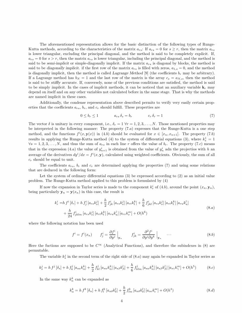
The aforementioned representation allows for the basic distinction of the following types of Runge-Kutta methods, according to the characteristics of the matrix ars: If ars = 0 for s ≥ r, then the matrix ars

is lower triangular, excluding the principal diagonal, and the method is said to be completely explicit. If,ars = 0 for s > r, then the matrix ars is lower triangular, including the principal diagonal, and the method issaid to be semi-implicit or simple-diagonally implicit. If the matrix ars is diagonal by blocks, the method issaid to be diagonally implicit. if the first row of the matrix ars is filled with zeros, a1,s = 0, and the methodis diagonally implicit, then the method is called Lagrange Method [9] (the coefficients br may be arbitrary).If a Lagrange method has bN = 1 and the last row of the matrix is the array cs = aN,s, then the methodis said to be stiffly accurate. If, conversely, none of the previous conditions are satisfied, the method is saidto be simply implicit. In the cases of implicit methods, it can be noticed that an auxiliary variable kr maydepend on itself and on any other variables not calculated before in the same stage. That is why the methodsare named implicit in these cases.

Additionally, the condense representation above described permits to verify very easily certain prop-erties that the coefficients ars, br, and cr should fulfill. These properties are

0 ≤ br ≤ 1 ars δs = br cr δr = 1 (7)

The vector δ is unitary in every component, i.e., δr = 1 ∀r = 1, 2, 3, . . . , N . Those mentioned properties maybe interpreted in the following manner: The property (7.a) expresses that the Runge-Kutta is a one stepmethod, and the functions f i(x,y(x)) in (4.b) should be evaluated for x ∈ [xn, xn+1]. The property (7.b)results in applying the Runge-Kutta method (4) to the system of differential equations (3), where k1

s = 1∀s = 1, 2, 3, . . . , N , and thus the sum of ars in each line r offers the value of br. The property (7.c) meansthat in the expression (4.a) the value of yi

n+1 is obtained from the value of yin adn the projectios with h an

average of the derivatives dyi/dx = f i(x,y), calculated using weighted coefficients. Obviously, the sum of allcr should be equal to unit.

The coefficients ars, br and cr are determined applying the properties (7) and using some relationsthat are deduced in the following form:

Let the system of ordinary differential equations (3) be expressed according to (2) as an initial valueproblem. The Runge-Kutta method applied to this problem is formulated by (4)

If now the expansion in Taylor series is made to the component kir of (4.b), around the point (xn,yn),

being particularly yn = y(xn) in this case, the result is

kir =h f i [δr] + h f i

j [arskjs] +

h

2f i

jk [arskjs] [artk

kt ] +

h

6f i

jkl [arskjs] [artk

kt ] [arukl

u]

+h

24f i

jklm [arskjs] [artk

kt ] [arukl

u] [arvkmv ] + O(h6)

(8.a)

where the following notation has been used

f i = f i(xn) f ij =

∂f i

∂yj

∣∣∣yn

f ijk =

∂2f i

∂yj∂yk

∣∣∣yn

· · · (8.b)

Here the fuctions are supposed to be C∞ (Analytical Functions), and therefore the subindexes in (8) arepermutable.

The variable kjs in the second term of the right side of (8.a) may again be expanded in Taylor series as

kjs = h f j [δs] + h f j

k [asαkkα] +

h

2f j

kl [asαkkα] [asβkl

β ] +h

6f j

klm [asαkkα] [asβkl

β ] [asγkmγ ] + O(h5) (8.c)

In the same way kkα can be expanded as

kkα = h fk [δα] + h fk

l [aαδklδ] +

h

2fk

lm [aαδklδ] [aαεk

mε ] + O(h4) (8.d)

4

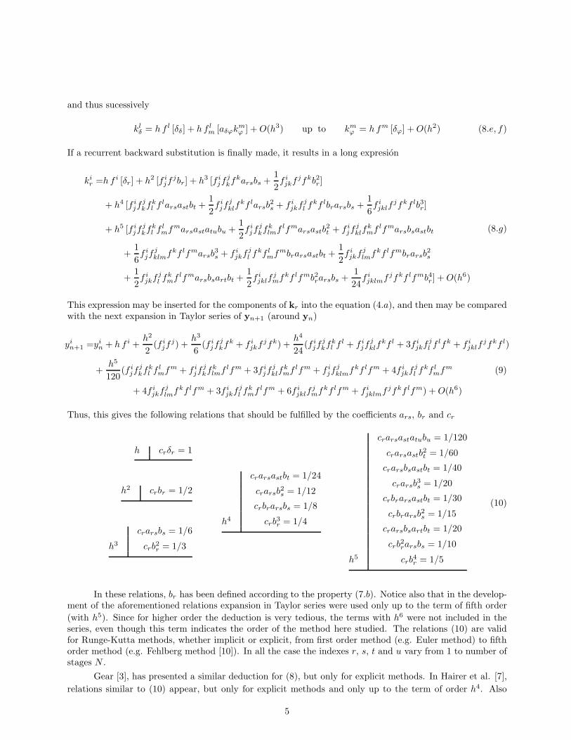
and thus sucessively

klδ = h f l [δδ] + h f l

m [aδϕkmϕ ] + O(h3) up to km

ϕ = h fm [δϕ] + O(h2) (8.e, f)

If a recurrent backward substitution is finally made, it results in a long expresion

kir =h f i [δr] + h2 [f i

jfjbr] + h3 [f i

jfjkfkarsbs +

12f i

jkf jfkb2r]

+ h4 [f ijf

jkfk

l f larsastbt +12f i

jfjklf

kf larsb2s + f i

jkf jl fkf lbrarsbs +

16f i

jklfjfkf lb3

r]

+ h5 [f ijf

jkfk

l f lmfmarsastatubu +

12f i

jfjkfk

lmf lfmarsastb2t + f i

jfjklf

kmf lfmarsbsastbt

+16f i

jfjklmfkf lfmarsb

3s + f i

jkf jl fkf l

mfmbrarsastbt +12f i

jkf jlmfkf lfmbrarsb

2s

+12f i

jkf jl fk

mf lfmarsbsartbt +12f i

jklfjmfkf lfmb2

rarsbs +124

f ijklmf jfkf lfmb4

r] + O(h6)

(8.g)

This expression may be inserted for the components of kr into the equation (4.a), and then may be comparedwith the next expansion in Taylor series of yn+1 (around yn)

yin+1 =yi

n + h f i +h2

2(f i

jfj) +

h3

6(f i

jfjkfk + f i

jkf jfk) +h4

24(f i

jfjkfk

l f l + f ijf

jklf

kf l + 3f ijkf j

l f lfk + f ijklf

jfkf l)

+h5

120(f i

jfjkfk

l f lmfm + f i

jfjkfk

lmf lfm + 3f ijf

jklf

kmf lfm + f i

jfjklmfkf lfm + 4f i

jkf jl fkf l

mfm (9)

+ 4f ijkf j

lmfkf lfm + 3f ijkf j

l fkmf lfm + 6f i

jklfjmfkf lfm + f i

jklmf jfkf lfm) + O(h6)

Thus, this gives the following relations that should be fulfilled by the coefficients ars, br and cr

h crδr = 1

h2 crbr = 1/2

crarsbs = 1/6

h3 crb2r = 1/3

crarsastbt = 1/24

crarsb2s = 1/12

crbrarsbs = 1/8

h4 crb3r = 1/4

crarsastatubu = 1/120

crarsastb2t = 1/60

crarsbsastbt = 1/40

crarsb3s = 1/20

crbrarsastbt = 1/30

crbrarsb2s = 1/15

crarsbsartbt = 1/20

crb2rarsbs = 1/10

h5 crb4r = 1/5

(10)

In these relations, br has been defined according to the property (7.b). Notice also that in the develop-ment of the aforementioned relations expansion in Taylor series were used only up to the term of fifth order(with h5). Since for higher order the deduction is very tedious, the terms with h6 were not included in theseries, even though this term indicates the order of the method here studied. The relations (10) are validfor Runge-Kutta methods, whether implicit or explicit, from first order method (e.g. Euler method) to fifthorder method (e.g. Fehlberg method [10]). In all the case the indexes r, s, t and u vary from 1 to number ofstages N .

Gear [3], has presented a similar deduction for (8), but only for explicit methods. In Hairer et al. [7],relations similar to (10) appear, but only for explicit methods and only up to the term of order h4. Also

5

Hairer et al. deduce a theorem that expresses the equivalence of the implicit Runge-Kutta methods and theorthogonal collocation methods.[7,8]

Ralston in 1965 (see for example [11]) made a similar analysis to (8), to obtain the relations of thecoefficients, but for an explicit Runge-Kutta method of fourth order and four stages, and found the followingfamily of solutions of relations (10)

b1 = 0 b4 = 1 ars = 0 (s ≥ r) (11.a − c)

a21 = b2 a31 = b3 − a32 a32 =b3(b3 − b2)

2 b2(1 − 2 b2)a41 = 1 − a42 − a43 (11.d − g)

a42 =(1 − b2)[b2 + b3 − 1 − (2 b3 − 1)2]

2 b2(b3 − b2)[6 b2b3 − 4 (b2 + b3) + 3]a43 =

(1 − 2 b2)(1 − b2)(1 − b3)b3(b3 − b2)[6 b2b3 − 4 (b2 + b3) + 3]

(11.h, i)

c1 =12

+1 − 2(b2 + b3)

12 b2b3c2 =

2 b3 − 112 b2(b3 − b2)(1 − b2)

(11.j, k)

c3 =1 − 2 b2

12 b3(b3 − b2)(1 − b3)c4 =

12

+2 (b2 + b3) − 3

12 (1 − b2)(1 − b3)(11.l, m)

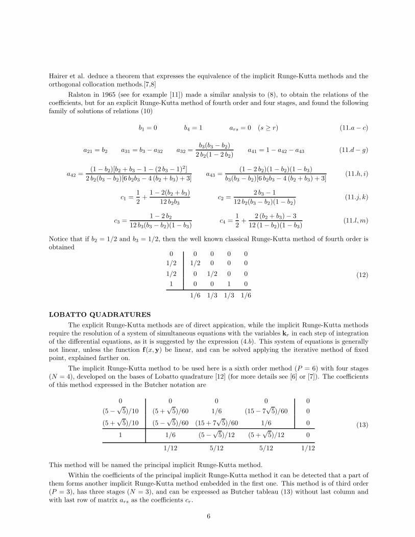
Notice that if b2 = 1/2 and b3 = 1/2, then the well known classical Runge-Kutta method of fourth order isobtained

0 0 0 0 01/2 1/2 0 0 0

1/2 0 1/2 0 01 0 0 1 0

1/6 1/3 1/3 1/6

(12)

LOBATTO QUADRATURES

The explicit Runge-Kutta methods are of direct appication, while the implicit Runge-Kutta methodsrequire the resolution of a system of simultaneous equations with the variables kr in each step of integrationof the differential equations, as it is suggested by the expression (4.b). This system of equations is generallynot linear, unless the function f(x,y) be linear, and can be solved applying the iterative method of fixedpoint, explained farther on.

The implicit Runge-Kutta method to be used here is a sixth order method (P = 6) with four stages(N = 4), developed on the bases of Lobatto quadrature [12] (for more details see [6] or [7]). The coefficientsof this method expressed in the Butcher notation are

0 0 0 0 0(5 −√

5)/10 (5 +√

5)/60 1/6 (15 − 7√

5)/60 0

(5 +√

5)/10 (5 −√5)/60 (15 + 7

√5)/60 1/6 0

1 1/6 (5 −√5)/12 (5 +

√5)/12 0

1/12 5/12 5/12 1/12

(13)

This method will be named the principal implicit Runge-Kutta method.

Within the coefficients of the principal implicit Runge-Kutta method it can be detected that a part ofthem forms another implicit Runge-Kutta method embedded in the first one. This method is of third order(P = 3), has three stages (N = 3), and can be expressed as Butcher tableau (13) without last column andwith last row of matrix ars as the coefficients cr.

6

Both methods, the principal and the embedded, form what is named the Lobatto embedding form ofthird and sixth orders with four stages. Notice that these methods are implicit only in the auxiliary variablesk2 and k3, and therefore the system of non-linear equations should be solved only in the mentioned variables.The other variables are of direct solution.

In order to apply an iterative process to solve the system of non-linear equations, initial estimationsof the values of the auxiliary variables are required. The best way to carry out the latter is to obtain thesevalues from an explicit Runge-Kutta method, where the auxiliary variables kr are evaluated in the sameintermediate point in each step, i.e. an explicit method having the same coefficient br of the implicit method.Observing the method (13), it is clear that the aforementioned explicit method is rapidly obtained from therelations (11) assuming b1 = 0, b2 = (5−√

5)/10, b3 = (5+√

5)/10 and b4 = 1. Notice that these coefficientsare consistent with the characteristics of an explicit method. This last aspect makes the implicit method (13)ideal for the desired purpose.

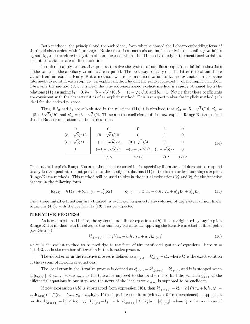
Thus, if b2 and b3 are substituted in the relations (11), it is obtained that a′21 = (5 − √

5)/10, a′31 =

−(5 + 3√

5)/20, and a′32 = (3 +

√5)/4. These are the coefficients of the new explicit Runge-Kutta method

that in Butcher’s notation can be expressed as

0 0 0 0 0(5 −√

5)/10 (5 −√5)/10 0 0 0

(5 +√

5)/10 −(5 + 3√

5)/20 (3 +√

5)/4 0 0

1 (−1 + 5√

5)/4 −(5 + 3√

5)/4 (5 −√5)/2 0

1/12 5/12 5/12 1/12

(14)

The obtained explicit Runge-Kutta method is not reported in the speciality literature and does not correspondto any known quadrature, but pertains to the family of solutions (11) of the fourth order, four stages explicitRunge-Kutta methods. This method will be used to obtain the initial estimations k′

2 and k′3 for the iterative

process in the following form

k2,(0) = h f(xn + b2h , yn + a′21k1) k3,(0) = h f(xn + b3h , yn + a′

31k1 + a′32k2) (15)

Once these initial estimations are obtained, a rapid convergence to the solution of the system of non-linearequations (4.b), with the coefficients (13), can be expected.

ITERATIVE PROCESSAs it was mentioned before, the system of non-linear equations (4.b), that is originated by any implicit

Runge-Kutta method, can be solved in the auxiliary variables kr applying the iterative method of fixed point(see Gear[3])

kir,(m+1) = h f i(xn + brh , yn + arsks,(m)) (16)

which is the easiest method to be used due to the form of the mentioned system of equations. Here m =0, 1, 2, 3, . . . is the number of iteration in the iterative process.

The global error in the iterative process is defined as εir,(m) = ki

r,(m)−kir, where ki

r is the exact solutionof the system of non-linear equations.

The local error in the iterative process is defined as εir,(m) = ki

r,(m+1) − kir,(m), and it is stopped when

cr‖εr,(m)‖ < εmax, where εmax is the tolerance imposed to the local error to find the solution yin+1 of the

differential equations in one step, and the norm of the local error εr,(m) is supposed to be euclidean.

If now expression (4.b) is substracted from expression (16), then kir,(m+1) − ki

r = h [f i(xn + brh , yn +

arsks,(m)) −f i(xn + brh , yn + arsks)]. If the Lipschitz condition (with h > 0 for convenience) is applied, it

results |kir,(m+1) − ki

r| ≤ h lij |ars| |kjs,(m) − kj

s| with |εir,(m+1)| ≤ h lij |ars| |εj

s,(m)|, where lij is the maximum of

7

the absolute value of each element in the jacobean matrix of f . This is |f ij | ≤ lij. Thus, if it is satisfied that

ε(m) = max1≤j≤M

(max1≤s≤N |εj

s,(m)|), then |εi

r,(m+1)| ≤ h lij |ars| |εjs,(m)| ≤ h lijδj |ars| δsε(m), where

max1≤i≤M

max1≤r≤N

(|εir,(m+1)|

) ≤ max1≤i≤M

[max

1≤r≤N

(h lijδj |ars| δsε(m)

)](17)

Thusε(m+1) ≤ h L A ε(m) where L = max

1≤i≤M

(lijδj

)A = max

1≤r≤N

(|ars| δs

)(18)

The expression (18) means that for a high number of iterations, m → ∞, the global error ε(m) → 0 whenh ≤ 1/(L A) and the iterative process is convergent locally (also globally) in the form

cr‖εr,(m+1)‖ < cr‖εr,(m)‖ (19)

The expression (18) is the limit of the stepsize, for the iterative method of fixed point to be convergent,when the system of non-linear equation is being solved in the implicit Runge-Kutta method. This is theonly restriction of the implicit Runge-Kutta methods, compared to the explicit methods which are much lessstable.

STEPSIZE CONTROL

ERROR ANALYSISThe implicit Runge-Kutta method of sixth order with four stages that is defined by the coefficients

(13), in fact represents two different embedded methods, one of third order within the other of sixth order,i.e. the coefficients (13) include both sixth and third order methods. This aspect is relevant to control thestepsize, because solving the system of non-linear equations (4.b) for the same coefficients, it can be obtainedtwo solutions of different order in the local truncation error, reducing to a minimum the number of numericalcalculations to be made. Fehlberg [10] reported this aspect to control the stepsize in his explicit Runge-Kuttamethods of fourth and fifth orders in a embedded form.

Let yn and yn+1 be the solutions of the system of differential equations (1), offered by the Runge-Kuttamethods type Lobatto of sixth and third orders, respectively, embedded in only one formulation as it wasdescribed before. This is

yin+1 = yi

n +112

(ki1 + 5ki

2 + 5ki3 + ki

4) yin+1 = yi

n +112

[2ki1 + (5 −

√5)ki

2 + (5 +√

5)ki3] (20)

The auxiliary variables k1, k2, k3 and k4 are the same for both expressions and are obtained using theequation (4.b) with the coefficients (13).

It will be denoted as Ein+1 the difference of the equation (20.a) minus the equation (20.b). This is

Ein+1 = yi

n+1 − yin+1 =

112

[−ki1 +

√5(ki

2 − ki3) + ki

4] (21)

If y(xn) is the exact solution of the differential equation (1) in the value x = xn, the local truncation errors ofthe numerical solutions (20) are defined respectively as ei

n = yin−yi(xn) = O(h7

n−1), where ein = yi

n−yi(xn) =O(h4

n−1), and thenEi

n+1 = yin+1 − yi

n+1 = ein+1 − ei

n+1 = O(h4n) (22)

Remember that the local truncation error is of order P + 1 if the Runge-Kutta method is of order P .If the expression (22) is organized in the following form

Ein+1 =

[yin+1 − yi(xn+1)

yi(xn+1)

]yi(xn+1) − [yi

n+1 − yi(xn+1)] (23)

8

it is obtained

Ein+1 = ei

(r),n+1yi(xn+1) − ei

n+1 where ei(r),n+1 =

[yin+1 − yi(xn+1)

yi(xn+1)

](24)

is the relative local truncation error.

If now it is assumed that yi(xn+1) is approximated by yin+1 in the denominator of (24), it can be

applied the Cauchy-Schwartz and the triangular desequalities to the expression (23), and this results

|Ein+1| ≤ |ei

(r),n+1| |yi(xn+1)| + |ein+1| ≤ e(r),max |yi

n+1| + emax (25)

where e(r),max and emax are respectively the tolerances for the relative and absolute local truncation errorsfor the implicit Runge-Kutta methods of sixth and third orders. The expression (25) also means that, forthe solution of the differential equations in one step be accepted, it should be verified that

Qin =

|Ein+1|

e(r),max |yin+1| + emax

≤ 1 (26)

being the tolerances for the relative and absolute local truncation errors proposed by the user of the algorithm.

CONTROL ALGORITHM

Let hn+1 be the stepsize in the next step that tends to make Qin∼= 1. Taken into account the order of

the difference Ein+1 defined by (22), the parameter Qn may be redefined as

Qn =( hn

hn+1

)4

where Qn = max1≤i≤M

(Qi

n

)(27)

and thus, solving for hn+1, it results

hn+1 = hn

( 1Qn

)1/4

= hnSn with Sn =( 1

Qn

)1/4

(28, 29)

Here, it is convenient to mention that Shampine et al. [13] use expressions similar to (28) and (29)to control the size of the step of integration in the Runge-Kutta method of fourth and fifth orders with fivestages developed by Fehlberg [10], but with some modifications, in order to guarantee that Sn always bebound in the interval [Smin, Smax], and that hn+1 always be greater than a limit value hmin. Additionally,the mentioned authors multiply Sn of (29) by a coefficient Cq less than unit, to make hn+1 tends to hn, andthus to make Qn

∼= 1, but a little lower. All the aforementioned modifications are resumed in continuationas

Sn = Cq

( 1Qn

)1/4

Cq = 0.9 ∼ 0.99 (30)

S′n = max(min(Sn, Smax), Smin) hn+1 = hnS′

n h′n+1 = max(hn+1, hmin) (31)

While in [13] the exponent is 1/5 in the expression (30), here the exponent is 1/4, and they alsorecommend for the coefficients and limits the values Cq = 0.9, Smin = 0.1 and Smax = 5. The value of theminimum stepsize, hmin, is determined by the precision of the computer to be used. In this work they arerecommended the same values for the coefficients in the expressions (30) to (31).

The procedure to calculate the optimal value of the size of the integration step, that permits to satisfythe tolerances e(r),max and emax, is described in continuation:

9

• Estimated an initial stepsize hn, the implicit Runge-Kutta method type Lobatto is used to calculate theauxiliary variables ki

1, ki2, ki

3 and ki4 with the expression (4.b), using the coefficients (13) and with the

iterative process (16), using the initial values (15).

• The expressions (20) permit to find the solutions yin+1 and yi

n+1 of the methods of sixth and third orders,respectively.

• The definition (21) permits to calculate the difference Ein+1 between both methods.

• With the equation (26) it can be calculated the parameters Qin, and with the equation (27) it can be

obtained the maximum of them.

• The relations (30) to (31) determine the value of the size of the next step hn+1.

• If Qn ≤ 1, the integration with the step hn (or the application of the Runge-Kutta method from xn toxn+1) is accepted and the step hn+1 is considered the step for the next integration (or the next applicationof the Runge-Kutta method from xn+1 to xn+2).

• If Qn > 1, the integration with the stepsize hn is rejected and it is repeated all the algorithm but withhn = h′

n+1 obtained from (31).

This procedure, sometimes increases the stepsize, and other times decreases the stepsize, in a optimal form,in order to guarantee that the relative error ei

(r),n+1 of the sixth order Runge-Kutta method be less than

the tolerance e(r),max, and the error ein+1 of the third order Runge-Kutta method be less than the tolerance

emax. In any case, the solution of the Runge-Kutta method will be yin+1, i.e. the solution with the implicit

Runge-Kutta method of sixth order.

ANALYSIS OF THE METHODS

PRECISION

The order of precision of any Runge-Kutta method comes from the comparison between this and theexpansion in Taylor series of y(xn+1) around y(xn). From this comparison was obtained the relations (10)that should be fulfilled by the coefficients of the Runge-Kutta methods. For a Runge-Kutta method of orderP , it should be satisfied the relations (10) up to the term of the Taylor series that contains hP . The remainderterms in the Taylor series are they which determine the order of the local truncation error. Thus, a methodof order P has a local truncation error of order P +1, i.e. that depends on hP+1. The global truncation erroralways is one order less than the local truncation error [3], i.e. that depends on hP . All these criterions canbe applied to the implicit Runge-Kutta type Lobatto of third and sixth order. In this form it is obtained that,the method of third order satisfy the relations (10) up to term with h3 and the local and global truncationerrors depend, respectively, on h4 and h3. The method of sixth order satisfy the relations (10) up to termwith h6 (the relations for this last term does not appear for the reasons explained there) and the local andglobal truncation depend, respectively, on h7 and h6. The dependence of an error respect to hP is indicatedas O(hP ) and is said that the order of precision is P , according to the definition xn+1 = xn + h. Also it issatisfied that O(hP ) + O(hQ) = O(hP ) when Q ≥ P .

CONVERGENCY

In the section of Iterative Process it was indicated that the implicit Runge-Kutta methods generated asystem of equations of the type (4.b), in general of non-linear characteristics, where the unknowns were theauxiliary variables kr. As it was said before, this system of non-linear equations may be solved using aniterative method of fixed point, which converges for the treated problem in particular, if it is satisfied (18)and the local convergence is established according to (19).

For the specific case when it is being solved the problem with only one differential equation of the form

dy

dx= f(y) f(y) = λy (32)

10

it is obtained that L = |λ|. For the implicit Runge-Kutta methods type Lobatto of third and sixth orders, itis obtained that A = (5 +

√5)/10 and A = 1, respectively. Thus, to assure the convergence of the iterative

process stated in these cases, particularly to the linear problem (32), it should be satisfied the following twoconditions (assuming h positive)

h ≤ 5 −√5

2 |λ|∼= 1.38

|λ| (Implicit 3rd order method) h ≤ 1|λ| (Implicit 6th order method) (33)

respectively. Notice that the condition (33.b) is the most restrictive of the two.

STABILITY

The stability of the Runge-Kutta methods is generally studied on the bases of their performance for solvingthe specific problem (32) with only one linear ordinary differential equation. In Appendix C it can be foundthe analysis of the stability for the more general case of a system of linear ordinary differential equations.

Thus, if the expression (4.b) is applied, taken into account that the problem being solved is (32), it isobtained that kr = h f(yn + arsks) = h λ (yn + arsks) = h λ yn + h λars ks. Moreover, if kr is substituted asδrsks and the therms are regrouped, it results δrsks = h λ yn + h λars ks, where δrsks − h λars ks = h λ yn,and thus, if ks is factorized, then [δrs − h λars] ks = h λ yn δr with r, s = 1, 2, 3, . . . , N .

Thes latter expression represents a system of N linear equations with N unknowns ks. If this systemof linear equations is solved and if the solutions kr are substituted in the equation (4.a), then, it is founda relation for yn+1 depending only on yn and on the coefficients of the used Runge-Kutta method. Thementioned relation is of the form yn+1 = µ1(hλ) yn, where µ1(hλ) is found applying, for example, to theimplicit sixth order Runge-Kutta method of Lobatto type, the procedure above explained. In this case theresult is

µ1(z) =

[1 + 2

3z + 15z2 + 1

30z3 + 1360z4

1 − 13z + 1

30z2

](34)

where the function µ1(z) was deduced from the coefficients (13). For the case of the implicit third orderRunge-Kutta method type Lobatto resumed in the inner coefficients (13), the result is yn+1 = µ1(hλ) yn,where

µ1(z) =

[1 + 2

3z + 15z2 + 1

30z3

1 − 13z + 1

30z2

](35)

The functions µ1(z) and µ1(z) are denominated characteristic roots of the Runge-Kutta methods of thirdand sixth orders, respectively. The characteristic roots are also known as stability functions. The Runge-Kutta methods, to which these roots pertain, are considered stables if their absolute values are less thanunit, for a determined real value of z = hλ. Notice that, if |µ1(hλ)| or |µ1(hλ)| is less than the unit, then itis satisfied that |yn+1| or |yn+1| is less than |yn| and the stability is guaranteed.

The functions (34) and (35) may be represented graphically as µ1(hλ) and µ1(hλ) vs. hλ, and the regionof stability for each one may be observed. The methods are stable if it is satisfied the following two conditions(assuming that h is positive and λ is negative).

h ≤ 6.8232|λ| (Implicit 3rd order method) h ≤ 9.6485

|λ| (Implicit 6th order method) (36)

Therefore, the mentioned methods are not A-stable. When comparing the conditions (33) with the conditions(36), the condition (33.b) continues being the most restrictive of all.

The function µ1(z) constitutes an aproximation of Pade [2] for the function y = ex (see Lapidus andSeinfeld [6]), and, additionally, is always positive and less than unit in the interval [−9.648495252 , 0.0].Notice that the function µ1(z) approximates well to the function y = ez for the range z > −4.

11

The function µ1(z), however, is not an approximation of Pade, has only one root in the point z =−2.706010973 . . ., and is, in absolute value, less or equal to the unit within the interval [−6.823183583 , 0.0].This can be observed graphically.

The conditions (36) reveal that the implicit Runge-Kutta methods type Lobatto of third and sixth ordersare more stable than the explicit Runge-Kutta methods type Fehlberg of fourth and fifth orders, having theselast methods the following stability conditions

h ≤ 2.785|λ| (Explicit 4th order method) h ≤ 3.15

|λ| (Explicit 5th order method) (37)

The only limitation of the implicit Runge-Kutta methods comes from the convergency conditions (33),which are based on the way used to solve the system of equations (4.b), and on the assumption that thedifferential equation has a linear form (32). These convergency conditions permit an increase of the stepsizeh much less than the stability conditions (36). This aspect brakes the advance of the implicit Runge-Kuttamethods in a notable manner, but the difficulty may be compensated partially in two forms. First, estimatingconveniently the initial values of the auxiliary variables kr for the iterative process. As it was treated before,this can be made using an explicit Runge-Kutta method with the expressions (15). Secondly, it may be usedthe fixed point method in a efficient manner, similar to the Gauss-Seidel method, i.e. when an unknownis approximately calculated, it is substituted inmediately in the next equation, and thus on. These twomodifications of the implicit Runge-Kutta methods here used may improve the performance of the method,in the sense of that the stepsize h is liberated from the convergency conditions (33) and thus it may bepermitted to increase much more.

A more sofisticated solution to the problem mentioned before can be developed, if it is used the Newton-Rapson method to solve the system of non-linear equations (4.b). This may increase the number of numericalcalculations to be performed by the algorithm, but the convergence will be more rapid.

RESULTS

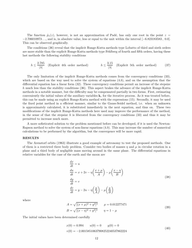
The Arenstorf orbits (1963) illustrate a good example of astronomy to test the proposed methods. Oneof them is a restricted three body problem. Consider two bodies of masses η and µ in circular rotation in aplane and a third body of negligible mass moving around in the same plane. The differential equations inrelative variables for the case of the earth and the moon are

dx

dt= u

du

dt= x + 2v − η

(x + µ

A

)− µ

(x − η

B

)dy

dt= v

dv

dt= y − 2u − η

(y

A

)− µ

(y

B

)(38)

whereA =

√[(x + µ)2 + y2]3 µ = 0.012277471

B =√

[(x − η)2 + y2]3 η = 1 − µ(39)

The initial values have been determined carefully

x(0) = 0.994 u(0) = 0 y(0) = 0

v(0) = −2.00158510637908252240537862224(40)

12

so that the solution becomes periodic with period

T = 17.0652165601579625588917206249 (41)

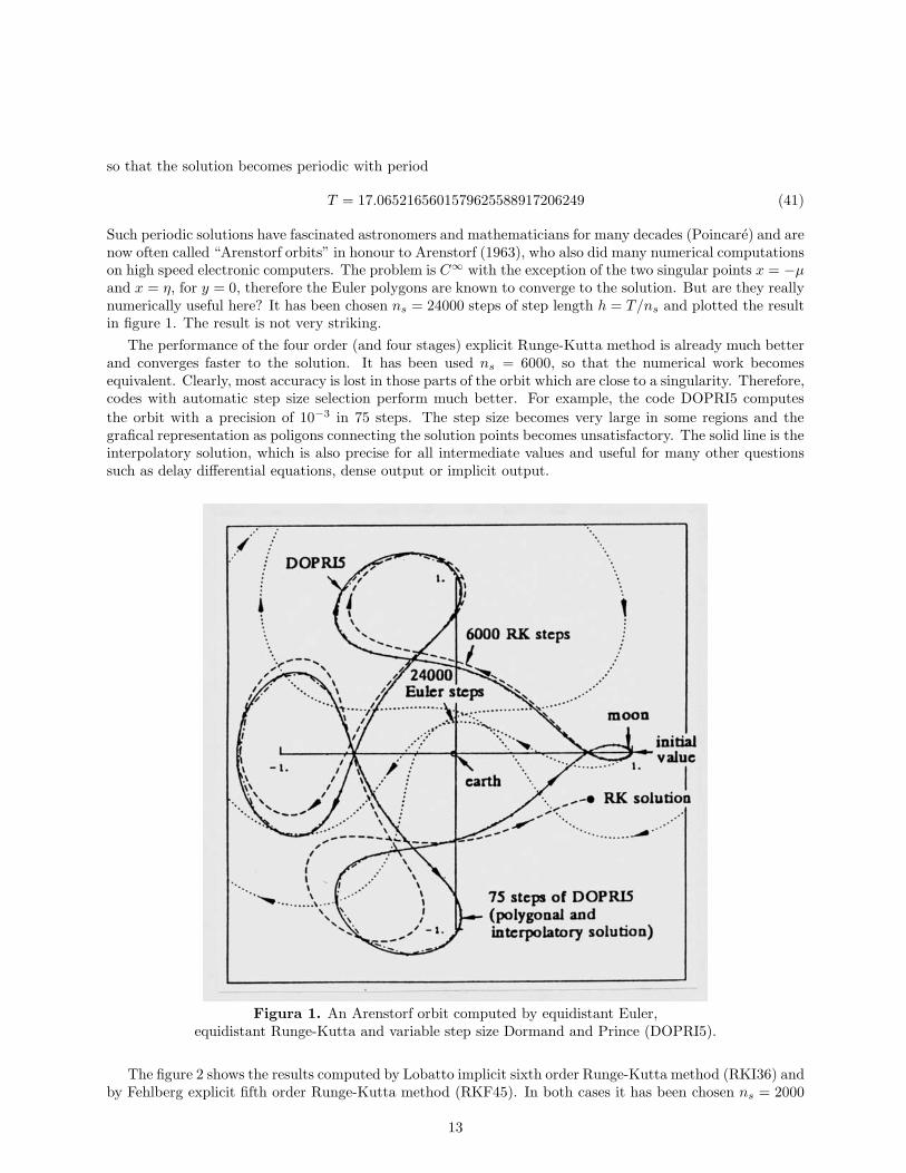
Such periodic solutions have fascinated astronomers and mathematicians for many decades (Poincare) and arenow often called “Arenstorf orbits” in honour to Arenstorf (1963), who also did many numerical computationson high speed electronic computers. The problem is C∞ with the exception of the two singular points x = −µand x = η, for y = 0, therefore the Euler polygons are known to converge to the solution. But are they reallynumerically useful here? It has been chosen ns = 24000 steps of step length h = T/ns and plotted the resultin figure 1. The result is not very striking.

The performance of the four order (and four stages) explicit Runge-Kutta method is already much betterand converges faster to the solution. It has been used ns = 6000, so that the numerical work becomesequivalent. Clearly, most accuracy is lost in those parts of the orbit which are close to a singularity. Therefore,codes with automatic step size selection perform much better. For example, the code DOPRI5 computesthe orbit with a precision of 10−3 in 75 steps. The step size becomes very large in some regions and thegrafical representation as poligons connecting the solution points becomes unsatisfactory. The solid line is theinterpolatory solution, which is also precise for all intermediate values and useful for many other questionssuch as delay differential equations, dense output or implicit output.

Figura 1. An Arenstorf orbit computed by equidistant Euler,equidistant Runge-Kutta and variable step size Dormand and Prince (DOPRI5).

The figure 2 shows the results computed by Lobatto implicit sixth order Runge-Kutta method (RKI36) andby Fehlberg explicit fifth order Runge-Kutta method (RKF45). In both cases it has been chosen ns = 2000

13

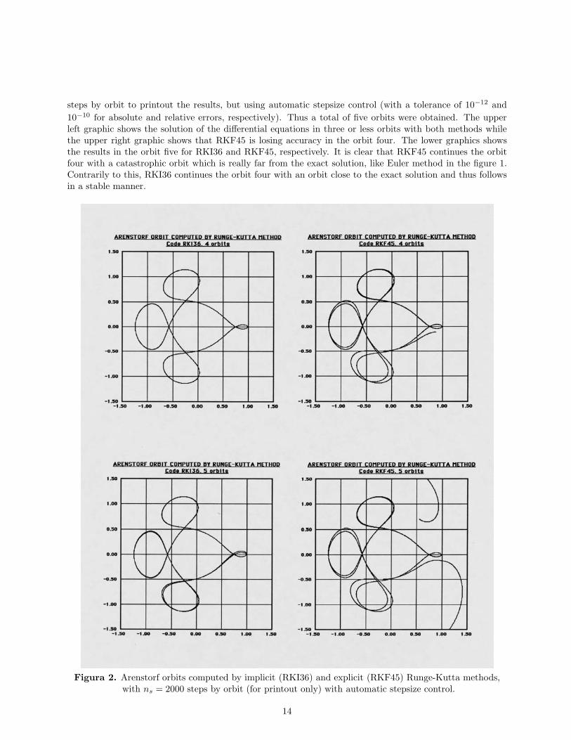
steps by orbit to printout the results, but using automatic stepsize control (with a tolerance of 10−12 and10−10 for absolute and relative errors, respectively). Thus a total of five orbits were obtained. The upperleft graphic shows the solution of the differential equations in three or less orbits with both methods whilethe upper right graphic shows that RKF45 is losing accuracy in the orbit four. The lower graphics showsthe results in the orbit five for RKI36 and RKF45, respectively. It is clear that RKF45 continues the orbitfour with a catastrophic orbit which is really far from the exact solution, like Euler method in the figure 1.Contrarily to this, RKI36 continues the orbit four with an orbit close to the exact solution and thus followsin a stable manner.

Figura 2. Arenstorf orbits computed by implicit (RKI36) and explicit (RKF45) Runge-Kutta methods,with ns = 2000 steps by orbit (for printout only) with automatic stepsize control.

14

Speaking in absolute terms, the method RKI36 with automatic stepsize control perform as good as thecode DOPRI5, computing 75 steps in an orbit with a tolerance in the absolute local error of 10−3. Finallyfor a time t = T it was obtained almost the initial location with errors of ∆x = 8∗10−5 and ∆y = 3∗10−3.However, the method RKF45 with automatic stepsize control computed the results in 44 steps with errors of∆x = −3∗10−1 and ∆y = −3∗10−1 for the final location, using the same tolerance. This mean that RKF45is more rapid than RKI36, aproximately twice, but much less stable.

It is interesting to mention that for the method RKI36 with equidistant step size, i.e. without theautomatic stepsize control, to reach the final location at t = T with errors of ∆x = −2∗10−2 and ∆y = 8∗10−4,it was necessary approximately 6000 steps. This indicates how efficient is the method when automatic stepzisecontrol is used.

The conclusions for the analysis of the aforementioned results are: The implicitness of the method makesthe performance more stable. The algorithm of automatic stepsize control makes the method more efficient.

REFERENCES

[1] Gerald, C. F. Applied Numerical Analysis. 2nd Edition. Addison-Wesley, New York, 1970.

[2] Burden R. L.; Faires, J. D. Numerical Analysis. 3rd Edition. PWS. Boston, 1985.[3] Gear, C. W. Numerical Initial Value Problems in Ordinary Differential Equations. Prentice-

Hall, Englewood Cliffs, New Jersey, 1971.[4] Butcher, J. C. “On the Runge-Kutta Processes of High Order”. J. Austral. Math. Soc., Vol. IV,

Part 2, 1964, pp. 179-194.[5] Butcher, J. C. The Numerical Analysis of Ordinary Differential Equations, Runge-Kutta and

General Linear Methods. John Wiley, New York, 1987.[6] Lapidus, L.; Seinfeld, J. H. Numerical Solution of Ordinary Differential Equations. Academic

Press, New York, 1971.[7] Hairer, E.; Norsett, S. P.; Wanner, G. Solving Ordinary Differential Equations I. Nonstiff Prob-

lems. Springer-Verlag, Berlin, 1987.[8] Hairer, E.; Wanner, G. Solving Ordinary Differential Equations II: Stiff and Differential- Al-

gebraic Problems. Springer-Verlag, Berlin, 1991.[9] van der Houwen, P. J.; Sommeijer, B. P. “Iterated Runge-Kutta Methods on Parallel Computers”. SIAM

J. Sci. Stat. Comput., Vol.12, No.5, pp.1000-1028, (1991).[10] Fehlberg, E. “Low-Order Classical Runge-Kutta Formulas with Stepsize Control”. NASA Report No.

TR R-315, 1971.[11] Ralston, A.; Rabinowitz, P. A First Course in Numerical Analysis. 2nd Edition. McGraw-Hill,

New York, 1978.[12] Lobatto, R. Lessen over Differentiaal- en Integraal-Rekening. 2 Vol. La Haye, 1851-52.[13] Shampine, L. F.; Watts, H. A.; Davenport, S. M. “Solving Non-Stiff Ordinary Differential Equations -

The State of the Art”. SANDIA Laboratories, Report No. SAND75-0182, 1975. SIAM Review, Vol.18, No. 3, 1976, pp. 376-411.

15