LOAN COPY: d4iWL TECHNICAL I5 &=LAND AFB, A for Calculating · In calculating equation (3) we used data for the solar flux from Detwiler et al ... It is seen in figure 1 that the

-

NASA TP

! c.1 1398

NASA Technical Paper 1398

A Simplified Method for

LOAN COPY: RETL 0 E d4iWL TECHNICAL I5

&=LAND AFB, 1.5

Calculating .! I

the Atmospheric Heating Rate by Absorption of Solar Radiation in the Stratosphere and Mesosphere

Tatsuo Shimazaki and Leland C. Helmle

JANUARY 1979

N K A

!

https://ntrs.nasa.gov/search.jsp?R=19790008322 2018-06-26T13:52:08+00:00Z

TECH LIBRARY KAFB. NM

01134744

NASA Technical Paper 1398

A Simplified Method for Calculating the Atmospheric Heating Rate by Absorption of Solar Radiation in the Stratosphere and Mesosphere

Tatsuo Shimazaki Ames Research Celzter M o ffett Field, Califortziu

and Leland C. Helmle Irgormatics, Inc. Palo Alto, California

National Aeronautics and Space Administration

Scientific and Technical information Office

1979

A SIMPLIFIED METHOD FOR CALCULATING THE ATMOSPHERIC HEATING RATE BY

ABSORPTION OF SOLAR RADIATION IN THE

STRATOSPHERE AND MESOSPHERE

Tatsuo Shimazaki and Leland C. Helmle*

Ames Research Center

A simple analytical formula is worked out for calculations of the atmospheric heating rate by absorption of solar radiation by 03, H20, and C02. The method needs only seven parameters for each molecule and can save computational time and memory locations. It is particularly useful for heating calculations in three-dimensional global circulation models below 80 km. Applying the formula to the observed distributions of 0 3 , H20, and CO2 produces reasonable latitudinal and seasonal variations in the heating rate. The calculated heating rate, however, is sensitive to the global dis- tributions of the absorbing gases, and uncertainties in rhe 0 3 distribution above -50 km and the H20 distribution below -20 km may seriously affect the global distributions of the heating rate in these regions.

INTRODUCTION

Heating the atmosphere by solar radiation of wavelengths shorter than -4 1-1 is the ultimate source of energy to drive the atmospheric motion. About 99% of the solar radiation energy is in this spectrum range with the maximum radiation at -4828 a corresponding to the 6000 K black body radiation. The main radiative processes in the earth's atmosphere for this spectrum range are absorption, reflection, and scattering; emission is entirely negligible because the atmospheric temperature is too low.

Calculations of the atmospheric heating rate due to gaseous absorption of solar radiation are essential in studies of radiative balance and global circuiation models of the atmosphere. The main absorbing molecules are water vapor (H20) in the troposphere and ozone ( 0 3 ) in the stratosphere and meso- sphere, whereas carbon dioxide (C02) is of secondary importance as an absorber throughout the region from troposphere to mesosphere. Molecular oxygen ( 0 2 ) becomes the dominant absorber in the thermosphere. The absorption of each constituent is highly selective and strongly dependent on wavelength, and cal- culations of the heating rate taking into account the detailed wavelength dependence are very time consuming if not impossible. To avoid such incon- veniences and to facilitate the heating rate calculations, empirical formulae

*Informatics, Inc., Palo Alto, California 94303

have been developed by var ious invest igators . Formulae differ widely, however, and i n most cases d i f f e ren t fo rmulae have been u sed fo r d i f f e ren t cons t i t uen t s and fo r d i f f e ren t wave leng th r anges even by t h e same a u t h o r ( s ) . Thus, w e need d i f fe ren t computer p rograms for ca lcu la t ing the hea t ing rate i n each case.

The purposes o f th i s t echnica l paper are ( 1 ) t o c a l c u l a t e t h e h e a t i n g rate d u e t o 03 a b s o r p t i o n w i t h h i g h p r e c i s i o n a n d t o f o r m u l a t e t h i s r e s u l t and exper imenta l resu l t s of h e a t i n g d u e t o H20 and C02 abso rp t ion by Howard et a l . ( r e f s . 1 and 2) i n t o a s i m p l e a n a l y t i c a l e x p r e s s i o n ; (2) t o s u r v e y t h e e x i s t i n g f o r m u l a e f o r h e a t i n g rate ca l cu la t ions and compare our r e s u l t w i t h t h e r e s u l t s c a l c u l a t e d by these formulae; and (3) t o i l l u s t r a t e t h e g l o b a l d i s t r i b u t i o n of t h e h e a t i n g rate c a l c u l a t e d by our formula using t h e g l o b a l d a t a o n 03, H 2 0 , and C02 d e n s i t y d i s t r i b u t i o n s . Development of such an ana ly t ica l formula is u s e f u l f o r s i m p l i f y i n g t h e r a d i a t i o n c a l c u l a - t i o n s i n g l o b a l c i r c u l a t i o n m o d e l s , s i n c e t h e c o m p u t a t i o n time and s torage l o c a t i o n s are v e r y l i m i t e d by t h e f a c t t h a t a l a r g e amount must be r e se rved fo r ca l cu la t ions o f dynamics .

We i n t e n d t o u s e t h e same formula used i n c a l c u l a t i o n s of the photodisso- c i a t i o n rates of molecules a t t h e Schumann-Runge band (Shimazaki e t a l . , r e f . 3 ) , s o t h a t t h e h e a t i n g rate and t he pho tod i s soc ia t ion rate can be cal- c u l a t e d by t h e i d e n t i c a l f o r m u l a . We need only several parameters in each c a l c u l a t i o n , a n d t h e same s h o r t s u b r o u t i n e c a n b e u s e d f o r c a l c u l a t i o n s o f bo th t he hea t ing rate and the photodissoc ia t ion rate, thereby sav ing bo th computation time and s to rage l oca t ions .

METHOD OF ANALYSES

Heating by Ozone

Ozone abso rbs so l a r r ad ia t ion ene rgy ma in ly a t the Har t ley band ( 2 4 0 0 t o 3000 A ) , Huggins band (3000 t o 3600 A) and Chappuis band ( 4 0 0 0 t o 8500 A ) . The d i v i s i o n a t 3000 A between the Hartley and Huggins bands i s somewhat a r b i t r a r y , and t h e H a r t l e y band inc ludes the wavelengths sho r t e r t han 2400 A. The abso rp t ion by 0 2 becomes increas ingly impor tan t below 2400 8, b u t h e a t i n g by those absorp t ions should be small i n t h e atmo- spheric region under our present concern. Since the absorpt ion cross sec- t ions of ozone are w e l l de t e rmined fo r t he en t i r e spec t rum r ange , t he exac t h e a t i n g ra te can be ca l cu la t ed s t r a igh t fo rward ly by

where A is the wavelength, u t h e t o t a l amount of ozone i n cm a t m NTP, I t h e i n c i d e n t s o l a r e n e r g y f l u x , and 0 t h e a b s o r p t i o n c r o s s s e c t i o n . I is r e l a t e d t o t h e p h o t o n f l u x 4 by t h e r e l a t i o n

I(A) = - $ hc x

2

where h is the Planck 's constant and c the speed of l igh t . In the reg ion of i n t e r e s t (below 80 ha) , t h e 0 ( 3P) formed by the ozone photo lys i s qu ick ly recombines ; the por t ion o f energy spent for d i ssoc ia t ion w i l l be r ega ined fo r atmospheric heating through chemical recombination processes. Thus, the energy loss by d i s s o c i a t i o n c a n b e n e g l e c t e d .

The absorbed energy f lux a long the pa th i s t h e n c a l c u l a t e d by

Q(A,u)du = I ( X ) [ l - e -u(A)u 1

In c a l c u l a t i n g e q u a t i o n ( 3 ) w e u s e d d a t a f o r t h e s o l a r f l u x f r o m Detwiler e t a l . ( r e f . 4 ) and Ackerman ( r e f . 5 ) f o r t h e 2400 t o 3000 range and from Thekaekara and Drummond ( r e f . 6 ) f o r t h e 3000 t o 8500 a range, and the data fo r t he abso rp t ion c ros s s ec t ion f rom Inn and Tanaka ( r e f . 7): The e n t i r e spectrum range 2400 t o 8500 ii is d iv ided i n to 122 subd iv i s ions w i th t he equa l i n t e r v a l (50 a) , and t h e i n t e g r a t e d s o l a r f l u x and the averaged c ross sec t ion have been ca lcu la ted for each subdiv is ion .

Taking the summation of equa t ion ( 3 ) for the per t inent spec t rum range would give the absorbed energy a t t h e r e s p e c t i v e band

The calculated absorbed energy i s shown i n f i g u r e 1 fo r t he Har t l ey band , Huggins band, and Chappuis band, as w e l l as f o r t h e t o t a l o f the th ree bands . The a b s c i s s a i n d i c a t e s t h e o z o n e column dens i ty measured in cm a t m NTP, and the co r re spond ing s ca l e fo r t he he igh t (km) is shown a t t h e t o p f o r t h e t h r e e r ep resen ta t ive s easons and l a t i t udes . In ca l cu la t ing t hese he igh t s ca l e s , t he d iu rna l ly ave raged mass f a c t o r is m u l t i p l i e d by t h e v e r t i c a l column den- s i t y t o o b t a i n t h e t o t a l o z o n e d e n s i t y i n t h e column a long the ob l ique pa th i n e a c h case. Effects of the dependence of abso rp t ion on p res su re are a l s o inco rpora t ed fo r eva lua t ing t hese he igh t s ca l e s ( s ee t he la ter d i s c u s s i o n on t h e e f f e c t i v e m a s s fo r the p ressure dependence of absorp t ion) .

It is s e e n i n f i g u r e 1 t h a t t h e s o l a r e n e r g y is absorbed mainly a t t h e Har t l ey band f o r u less than -0.1 cm, whereas the absorpt ion occurs mainly a t the Chappuis band for u g r e a t e r t h a n -1 cm. I n t h e t r a n s i t i o n r e g i o n t h e r e is a d e p r e s s i o n f o r t h e t o t a l o f t h e t h r e e b a n d s . The r e s u l t o f t h e c a l c u l a t i o n s shown i n f i g u r e 1 is f i t t e d t o t h e a n a l y t i c a l e x p r e s s i o n

l o g s = c g + c1 l o g u + C2(log u p + . . . + ck(log u) k (5)

fo r t he r ange o f u between and l o 2 cm. The c o e f f i c i e n t s C i are determined by the least squa re method so t h a t t h e v a r i a t i o n s of t he cu rves are b e s t f i t t e d w i t h t h e e q u a t i o n ( 5 ) . The r e s u l t a n t c o e f f i c i e n t s are t a b u l a t e d i n t a b l e l ( a ) f o r t h e case of k = 7; f o r t h e t o t a l of three bands t h e r e s u l t c a l c u l a t e d f r o m e q u a t i o n (5) is shown i n f i g u r e 1 by a dash-dotted curve, which agrees w e l l w i th t he o r ig ina l so l id cu rve . Fo r t he conven ience

3

of some mode le r s , coe f f i c i en t s de t e rmined fo r t he MKS sys tem of un i t s are g i v e n i n t a b l e l ( b ) . The mean e r r o r of l o g S , o r t h e mean relative e r r o r of S, i s de f ined by

where S4 and S5 are the va lues o f S c a l c u l a t e d by equa t ions ( 4 ) and (5), r e s p e c t i v e l y , n is t h e t o t a l number of obse rva t iona l po in t s and k i s t h e degree of the polynomial .

I f t h e s o l a r f l u x c h a n g e s o r is measured more accura te ly in the fu ture , our method requires simply to modify CO t o

cot = c g + l o g I ' - l o g I (7)

where I and I' are the o ld and new so la r f l ux , r e spec t ive ly , whereas a l l o t h e r c o e f f i c i e n t s C i ( i+ 0) remain unchanged. The correction can also be made, i f n e c e s s a r y , f o r t h e e f f e c t s of changes i n t h e s u n - e a r t h d i s t a n c e ; t h e e a r t h is a b o u t 3 . 2 8 p e r c e n t c l o s e r t o t h e s u n i n e a r l y J a n u a r y t h a n i n e a r l y J u l y . The same method c a n a l s o b e u s e d t o c a l c u l a t e a t m o s p h e r i c h e a t - i ng by d i f fuse r ad ia t ion r e f l ec t ed o r s ca t t e r ed f rom c louds o r g round . Us ing a known (or assumed) albedo, I ' is then ca l cu la t ed f rom the downward r a d i - a t i o n f l u x a r r i v i n g a t t h e r e f l e c t i o n h e i g h t s . The a n g u l a r i n t e g r a t i o n f o r t h e d i f f u s e r a d i a t i o n is taken in to account by us ing an a i r mass f a c t o r of 1 .66 . Using the more r e c e n t v a l u e 1 . 9 by Lacis and Hansen ( r e f . 8) would i n c r e a s e t h e c a l c u l a t e d h e a t i n g ra te by d i f f u s e r a d i a t i o n by -5 pe rcen t .

Our r e s u l t is compared w i t h t h e r e s u l t s c a l c u l a t e d by d i f f e ren t fo rmulae developed by o t h e r i n v e s t i g a t o r s i n f i g u r e 2 . S ince t he r e su l t s are s o c l o s e , t h e i l l u s t r a t i o n o f comparison of each model with our result is shown by s h i f t i n g v e r t i c a l l y w i t h e a c h o t h e r .

Manabe a n d S t r i c k l e r ( r e f . 9) have u sed an ana ly t i ca l equa t ion fo r a b s o r p t i v i t y ; m u l t i p l y i n g t h e t o t a l i n c i d e n t s o l a r e n e r g y (-2 cal cm-2 min-l o r - 1 . 3 9 ~ 1 0 ~ e r g cm-2 s e c - 1 ) t o t h e a b s o r p t i v i t y would g i v e t h e t o t a l absorbed energy. A s i s s e e n i n f i g u r e 2 t h e i r r e s u l t is i n good agreement w i t h t h e p r e s e n t s t u d y f o r t h e r a n g e of u between 10" and 1 cm, which cove r s t he ma in pa r t o f t he s t r a tosphe re bu t g ives much smaller abso rp t ion a t l a r g e r v a l u e s o f u (22 cm) and a t smaller va lues o f u cm). Thus t h e i r e q u a t i o n would cause se r ious e r rors and should no t be used for the region above -50 t o 70 km ( the ac tua l he igh t depends upon seasons and la t i - tudes) , where the path of t h e s o l a r beam is smaller than c m , and f o r t h e region below -25 km i n w i n t e r a t h igh l a t i t udes , where t he beam p a t h i s g rea t e r t han -2 cm.

Lacis and Hansen ( r e f . 8) u s e d a n a l y t i c a l f o r m u l a e f o r a b s o r p t i v i t i e s represent ing the spec t rum of u l t r a v i o l e t a n d v i s i b l e r a d i a t i o n . A s s e e n i n f igu re 2 , t he t o t a l abso rbed ene rgy ca l cu la t ed fo r t he two spectrum ranges

4

by the i r fo rmulae is s l i g h t l y smaller than the cor responding va lue ca lcu la ted by our formula in mos t o f the range of u except for the range between about 1 and 10 cm.

Lindzen and Will ( r e f . 1 0 ) h a v e f o r m u l a t e d t h e d i f f e r e n t i a l h e a t i n g rate f o r t h e t h r e e b a n d s i n t o t h r e e d i f f e r e n t f o r m u l a e . The absorbed energy can be ca l cu la t ed by in t eg ra t ing t hese equa t ions f rom 0 to u . Us ing equat ions similar to those of Lindzen and Will, Strobe1 ( re f . 11) has de te rmined the new c o e f f i c i e n t s t o c a l c u l a t e t h e h e a t i n g rate f o r t h e . t h r e e b a n d s . The to t a l abso rbed ene rgy ca l cu la t ed by these equa t ions is compared with our r e s u l t ( f i g . 2 ) . Both Strobe1 and Lindzen formulae give absorbed energies i n good agreement wi th the resu l t o f the p resent s tudy for the range of u between and 10 c m , wh ich cove r s mos t r eg ions o f t he s t r a tosphe re . Our formula gives , however , general ly larger absorpt ion than most other formulae, and p a r t o f t h e r e a s o n f o r t h i s d i f f e r e n c e may be caused by t h e f a c t t h a t o u r ana lyses i nc lude w ide r spec t r a , a l t hough t he r anges are no t a lways c l ea r ly s t a t e d i n some models.

Heating by Water Vapor

Water vapor i s the main absorber of s o l a r r a d i a t i o n i n t h e t r o p o s p h e r e . Howard e t a l . ( r e f . 2) have fo rmula t ed t he i r expe r imen ta l r e su l t s fo r i n t eg ra t ed abso rp t ion func t ion fo r s even bands ( 6 . 3 p, 3 . 2 1-1, 2 . 7 u, 1.87 1-1, 1.38 1-1, 1.1 u , and 0.94 u ) in to the fo l lowing formulae

d v A v d v = cu d (p + e ) k

f o r weaker absorption, and

f o r s t r o n g e r a b s o r p t i o n , w h e r e u is t h e water vapor column density i n g cm-2, p and e r e p r e s e n t t h e t o t a l p r e s s u r e a n d t h e par t ia l p r e s s u r e of water vapor i n mm Hg, r e s p e c t i v e l y . The c o n s t a n t s c y d , k , C , D and K are given for each band (see Burch e t a l . , r e f . 1 2 , f o r t h e r e v i s e d v a l u e s f o r t h e s e c o n s t a n t s ) . The abso rbed so l a r ene rg ie s ca l cu la t ed u s ing t hese equa - t i o n s are shown fo r each band and fo r t he t o t a l o f s even bands i n f i gu re 3 . Sudden jumps on some cu rves are caused by the t ransi t ion between the range where the weaker absorption form (8) i s a p p l i c a b l e and the range where the s t ronger absorp t ion form (9) is appl icable . There i s no apparent d i scont i - n u i t y on t h e c u r v e f o r t h e t o t a l of seven bands. We h a v e f i t t e d t h e t o t a l curve wi th equat ion (5) f o r t h e r a n g e o f u between and l o 2 g cm-2; t h e de te rmined coef f ic ien ts for the seventh-order po lynomia l are t a b u l a t e d i n t a b l e 2. The v a r i a t i o n c a l c u l a t e d by t h i s e q u a t i o n a g r e e s w e l l w i th t he o r i g i n a l v a r i a t i o n w h i c h i s shown by a dot -dashed curve in f igure 3 .

Many at tempts have been made i n t h e l i t e r a t u r e t o e x p r e s s t h e s o l a r energy absorbed by water v a p o r i n s i m p l e a n a l y t i c a l f o r m s , a n d t h e r e s u l t s

5

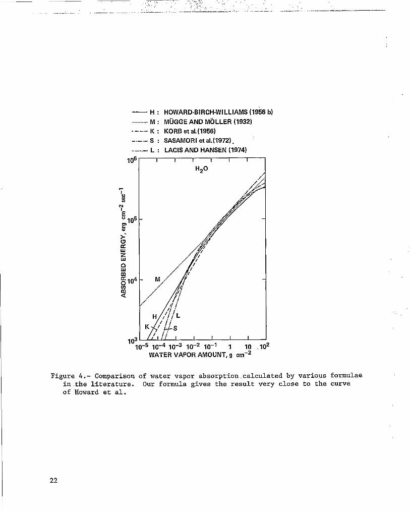
of c a l c u l a t i o n s by these formulae are compared i n f i g u r e 4. The formula of Mugge and M6ller ( r e f . 1 3 ) is e s s e n t i a l l y t h e f i r s t - o r d e r p o l y n o m i a l of t h e type of equation (5) , and changing the uni ts f rom cal cm-2 min-l t o e r g cm’2 sec-l, t h e i r e q u a t i o n c a n b e w r i t t e n as

l o g S = 5.079 + 0.303 log mu ( 1 0 4

where m is t h e a i r mass f a c t o r . Our corresponding equat ion is expressed as

l o g S = 5.007 + 0.429 log mu

Korb e t a l . (ref. 14) have improved equation (loa) and ob ta ined t he t h i rd - order polynomial

l og S = 5.1036 + 0.347 log mu - 0.056 (log mu)2 - 0.006 ( l o g ( l l a )

which can be compared with our third-order polynomial

l o g S = 5.0791 + 0.3150 log mu - 0.0416 ( log mu)2 - 0.0029 (log mu)3 (1 lb )

The r e s u l t f rom the Rorb formula g ives the c loses t var ia t ion to the p r e s e n t r e s u l t , w h i c h i s very c lose to the one ca lcu la ted f rom the formula of Howard e t a l . A s seen f rom tab le 3 , the mean e r r o r o f o u r t h i r d - o r d e r polynomial i s about 2.4 times l a r g e r t h a n t h e mean e r r o r of the seventh- order po lynomia l ; therefore , i t i s preferab le to use the seventh-order po ly- nomial.

The analyt ical forms of Sasamori e t a l . ( r e f . 15 ) and Lacis and Hansen ( r e f . 8 ) are bo th based on abso rp t iv i t i e s eva lua ted w i th t he r ad ia t ion cha r t of Yamamoto ( r e f . 1 6 ) ; t h u s , t h e g e n e r a l t e n d e n c y o f t h e v a r i a t i o n i n t h e s e two r e s u l t s is similar over the range of mu = - 10 c m for which the formulae may have been approximated. Extension of the formulae beyond t h i s range causes l a rge d i screpancies be tween the two r e s u l t s . I t i s s e e n i n f i g u r e 4 tha t the formula o f Howard e t a l . ( r e f . 2 ) g i v e s smaller abso rp t ion than most other formulae for the range of u g r e a t e r t h a n -10-2 g cm-2, whereas i t g i v e s l a r g e r a b s o r p t i o n f o r t h e smaller u t h a n t h i s v a l u e .

Heating by Carbon Dioxide

Howard e t a l . ( r e f . 1 ) have u sed t he same formulae as equat ions (8) and (9) to express their experimental data on the absorpt ion by CO2 i n eight bands (14.7 1 ~ - , 5.2 1-1, 4.8 p, 4.3 1-1, 2 . 7 p , 2 .0 1-1, 1.6 1-1, and 1 . 4 p). The c a l c u l a t e d a b s o r p t i o n i n e a c h band and t h e t o t a l of eight bands are shown i n f i g u r e 5 . The l a r g e jump appear ing in the curve o f the 4 .3 1-1 band causes a d i scon t inu i ty fo r t he cu rve o f t o t a l o f e igh t bands , s ince t he 4 .3 p band g i v e s t h e l a r g e s t c o n t r i b u t i o n . We have smoothed i n t h e r e g i o n of t h e d iscont inui ty and have then appl ied the curve f i t t ing p rocess us ing equa- t ion (5) for the range of u between and IO3 cm. The c o e f f i c i e n t s d e t e r - mined for the seventh-order polynomial are t a b u l a t e d i n t a b l e 2 a long wi th the mean e r r o r s i n e a c h c a s e of th i rd to seventh-order po lynomia ls .

6

I

DISTRIBUTION OF GASES

To ca l cu la t e t he a tmosphe r i c hea t ing ra te us ing t he ana ly t i ca l fo rmula developed i n p r e v i o u s s e c t i o n s , w e need t he da t a o f g loba l d i s t r ibu t ions o f absorbing gases .

Ozone

The g e n e r a l l a t i t u d i n a l a n d s e a s o n a l v a r i a t i o n s o f t h e v e r t i c a l o z o n e d i s t r i b u t i o n s up t o -35 km are reasonably w e l l known. We have used data analyzed and compiled by Wilcox e t a l . ( r e f . 1 7 ) based on ozonesonde data obtained a t v a r i o u s s t a t i o n s i n t h e w o r l d f r o m 1957 to 1972. Wilcox e t a l . g ive t he ozone dens i t i e s fo r eve ry 2.5 km up t o t h e h e i g h t of 32.5 km, and we have i n t e rpo la t ed t hese va lues t o ob ta in t he ozone dens i t i e s a t every km i n t e r v a l . For the region above 30 km up t o -55 km, t h e sa te l l i t e measurements of b a c k s c a t t e r u l t r a v i o l e t (BUV) s o l a r r a d i a t i o n from the a tmosphere can give the in format ion of ozone prof i les on a g loba l bas i s . Taking the da ta a t 50 km obtained by t h e Nimbus-4 sa te l l i t e expe r imen t s ( I . Ebe r s t e in , p r iva t e communi- cation, 1977) and combining i t with the ozonesonde data a t 32.5 km, w e have c a l c u l a t e d by i n t e r p o l a t i o n a n d e x t r a p o l a t i o n t h e o z o n e d e n s i t i e s a t every km up t o t h e h e i g h t of 80 km, assuming the exponent ia l decrease with height . The r e s u l t is shown i n f i g u r e 6 ( a ) f o r March (no r the rn sp r ing and southern f a l l ) and i n f i g u r e 6 ( b ) f o r J u n e ( n o r t h e r n summer and southern win ter ) .

Water Vapor

The d i s t r i b u t i o n of w a t e r vapor mix ing r a t io i n t he t roposphe re is expressed in the ana ly t ica l form of

where x is t h e l a t i t u d e , z is t h e h e i g h t and s is the parameter changing s inusoida l ly wi th season f rom 0.016 i n summer t o 0.032 i n w i n t e r . T h e s e va lues o f s and the func t iona l form of f (z ) are determined based on data published by Oort and Rasmusson ( r e f . 18 ) . The adopted va lues o f f (z ) are given i n t a b l e 3. I n t h e s t r a t o s p h e r e t h e m i x i n g r a t i o is assumed t o b e con- s t a n t a t 3.5x10-6. Since the t ropopause i s low (-8 km) a t h i g h l a t i t u d e s , the above procedure would cause sudden la rge changes in the water vapor mix- i n g r a t i o a t -8 km a t l a t i t u d e s a b o v e -60", as i s s e e n i n f i g u r e s 7 ( a ) a n d ( b ) .

Carbon Dioxide

We assume the cons t an t mix ing r a t io o f 3 . 2 ~ 1 0 - ~ f o r C02. Recent model ca l cu la t ions (Sh imazak i , unpub l i shed r e su l t ) i nd ica t e t ha t t he mix ing r a t io d e c r e a s e s s l i g h t l y w i t h h e i g h t ( f r o m 3.2~10-~ a t t h e g r o u n d t o - 1 . 8 6 ~ 1 0 - ~ a t 60 km), b u t t h i s s l i g h t c h a n g e s h o u l d n o t g r e a t l y a f f e c t t h e c a l c u l a t i o n o f

the a tmospher ic hea t ing ra te , s i n c e t h e C02 a b s o r p t i o n i s n o t t h e p r imary source of the a tmospher ic hea t ing .

RESULT AND DISCUSSION

Calculat ing the absorbed energy in the a tmosphere by equat ion ( 5 ) , w e have taken into account the dependence of a b s o r p t i o n on p r e s s u r e by introduc- i n g t h e e f f e c t i v e mass o f t he r ad ia t ive abso rben t

U ef f = u ( g ” n

where Po is the normal pressure of one atmosphere (1013.25 mb). For H 2 0 and C02 t h e power n can be evaluated f rom k/d in equat ion (8) and from K / D i n equa t ion (9 ) , and t he ave rage va lues fo r a l l bands under considerat ion g i v e -0.6 f o r H 2 0 and -0.8 f o r CO2. The power n f o r 03 i s taken as 0.2 r e f e r r i n g t o K o n d r a t y e v ( r e f . 1 9 ) .

The g loba l average o f he ight p rof i les o f the hea t ing rate c a l c u l a t e d f o r e a c h c o n s t i t u e n t f o r March i s i l l u s t r a t e d i n f i g u r e 8. The f i g u r e demon- strates t h e s t r o n g e f f e c t of n on t he hea t ing rate by O 3 a b s o r p t i o n i n regions above -40 km. The v a l u e of 0.4 has been ob ta ined for n by McClatchy e t a l . ( r e f . 20), b u t it i s i n a p p r o p r i a t e t o u s e t h i s v a l u e f o r t h e u l t r a v i o l e t r a n g e , s i n c e i t would g ive t oo small h e a t i n g ra te above -35 km as is s e e n i n f i g u r e 8. McClatchy’s value is based on the experimental data on o z o n e t r a n s m i t t a n c e f o r t h e i n f r a r e d r a d i a t i d n . The r e s u l t f o r n = 0 gives too much heat ing above -50 km p a r t i c u l a r l y a t h i g h l a t i t u d e s .

Heating by t h e r e f l e c t e d s o l a r r a d i a t i o n is calculated assuming the g loba l average o f the e f fec t ive a lbedo to be 0 .25 . The e f f e c t i v e a l b e d o t akes i n to accoun t t he combined e f f e c t of r e f l ec t ion f rom c louds and t h e ground surface and i s u s e f u l i n c a l c u l a t i n g t h e h e a t i n g by t h e r e f l e c t e d waves above the clouds. The p resen t s tudy is concerned mainly with the s t ra tosphere and mesosphere, and the concept of t he e f f ec t ive a lbedo shou ld g ive t he r easonab le hea t ing ra te i n t h e s e r e g i o n s . It is e s s e n t i a l , however, fo r t he t roposphe re t o t ake i n to accoun t t he c loud a lbedo and t he su r f ace a lbedo s epa ra t e ly and t o ca l cu la t e t he r ad ia t ive hea t f l uxes be tween t he c loud and the ground surface and a lso within the c louds.

The c a l c u l a t e d h e a t i n g rates by r e f l e c t e d waves due t o H 2 0 and C 0 2 abso rp t ion are ve ry small i n t h e s t r a t o s p h e r e ( f i g . 8 ) . Furthermore, s ince the a lbedo of c louds is r e l a t i v e l y small i n t h e i n f r a r e d and a l s o s i n c e water vapor d rop le t s i n c louds abso rb r ad ia t ion a lmos t a t t h e same spectrum as water vapor , t he hea t ing by r e f l e c t e d waves due t o H 2 0 and CO2 abso rp t ion should be smaller than t hose shown i n f i g u r e 8 and can be en t i re ly neglec ted . On the other hand, the a lbedo of c louds is h i g h i n t h e v i s i b l e and u l t r a - v i o l e t , t h e r e f o r e h e a t i n g by t h e r e f l e c t e d waves due t o t he 0 3 abso rp t ion canno t be neg lec t ed . In f ac t , as is s e e n i n f i g u r e 8, t h i s h e a t i n g is com- p a r a b l e t o t h e h e a t i n g by C 0 2 ( d i r e c t r a d i a t i o n ) i n t h e l o w e r s t r a t o s p h e r e , and is about 22 pe rcen t of t h e 03 h e a t i n g by d i r e c t r a d i a t i o n a t 25 km.

Applicability of our formula is limited to the range of u greater than g cm-2 for H20 and cm atm NTP for 03 and C02; these critical values

are met somewhere above -40 km for H20 and above -80 km for CO2 and 0 3 (see the top abscissa of figs. 1, 3 , and 5), although these heights depend upon the season and latitude and should be much higher near the sunrise and sunset times. The heating rate in the regions outside of these critical heights are not shown in figure 8 and are neglected in our calculation of atmospheric heating. Fortunately, however, contributions from these heatings are gener- ally small and their neglect should not affect the global distribution of the total heating rate in the region below 80 km. The upper limits of the for- mula's applicability are l o 2 g for H20, lo2 cm atm NTP for 03 and l o 3 cm atm NTP for C02. The column densities of the absorbents are usually within these limits.

The heating rate due to C02 and H20 absorption represented in terms of O K per day is almost constant above certain heights (fig. 8). This phenom- enon is caused by the assumption of the constant mixing ratio, that is, these constituents' concentrations change with height in proportion to the mass density of atmosphere. Since the heat capacity also decreases with height in proportion to the mass density of the atmosphere, the rate of change in tem- perature should remain almost constant with height, although the actual absorbed energy decreases with height.

Latitudinal distributions of the diurnal heating rate are illustrated in figures 9(a) and 9(b) for March and June, respectively, in terms of tempera- ture change per day. The top 1 to 2 km region is affected by the assumption on the total amount of 03 above the upper boundary: we assume that the 03 density decreases above 80 km with the scale height of its own mass. The actual distribution is complicated and has some bulge around 80 km (see, for instance, Schimazaki and Laird, ref. 21). For March, the global maximum occurs around 40 to 45 km in the equatorial region. Whereas the distribution is almost symmetrical around the equator in regions below this height, a marked asymmetry appears in higher regions; the larger heating rate is cal- culated at high latitudes in the southern hemisphere. This is certainly related to the larger ozone density calculated in that same area (see fig. 6(a)).

It is well known that there is a worldwide maximum of the total ozone density at the northern high latitudes in March and April. This tendency is clearly seen in the ozone density at -30 km in figure 6(a); that is, the ozone density observed at the northern high latitudes is appreciably larger than the corresponding values at the southern high latitudes. It is not cer- tain, however, whether or not this tendency should remain the same in the higher regions since contribution of that region to the total ozone density is very small.

The ozone density above 50 km shown in figure 6(a) 5 s calculated by extrapolation from the ozonesonde value at 32.5 km and the B W value at 50 km. The larger ozone density above 50 km at the southern high latitudes results from the fact that the ozone density is relatively low at 32.5 km, whereas the value at 5 0 km is about the same between the southern and

9

n o r t h e r n h i g h l a t i t u d e s . T h e r e may be l i t t l e hemisphe r i c d i f f e rence fo r ozone dens i ty i n t he en t i r e r eg ion above 50 km, b u t t h e l a r g e r o z o n e d e n s i t y above 50 km c a l c u l a t e d i n t h e s o u t h e r n h i g h l a t i t u d e s i s c o n s i s t e n t w i t h t h e smaller dens i ty i n t he l ower r eg ion , s ince t he l a rge r ozone dens i ty a t h ighe r region should absorb more r a d i a t i o n , making t h e r a d i a t i o n a v a i l a b l e f o r o z o n e product ion smaller i n t h e l o w e r r e g i o n . However, i t is t r u e t h a t t h e r e i s a g r e a t u n c e r t a i n t y o n t h e l a t i t u d i n a l d i s t r i b u t i o n o f t h e o z o n e d e n s i t y (and t h e r e f o r e t h e h e a t i n g r a t e ) a b o v e 50 km.

C a l c u l a t i n g t h e h e a t i n g rate assuming the uniform dis t r ibut ion of ozone d e n s i t y w i t h l a t i t u d e s r e p r e s e n t e d , f o r i n s t a n c e , by t h e d i s t r i b u t i o n a t 35" N, we ob ta in t he un i fo rm d i s t r ibu t ion o f t he hea t ing ra te w i t h l a t i t u d e above -50 km. The d i s t r i b u t i o n below t h i s h e i g h t is a f f e c t e d v e r y l i t t l e ; t h e g e n e r a l f e a t u r e s are similar t o t h o s e shown i n f i g u r e 9 ( a ) . It i s evi- d e n t t h a t t h e g l o b a l d i s t r i b u t i o n of h e a t i n g rate is s e n s i t i v e t o t h e o z o n e dens i ty d i s t r ibu t ion . Unfo r tuna te ly , t he re i s no direct measurement of g l o b a l d i s t r ibu t ion above 50 km. Rocket observa t ions p rovide scant da ta for l imi ted l o c a t i o n s and time per iod . S ince the a tmospher ic sca t te r ing is ve ry weak above -55 km, t h e r e is a p r a c t i c a l u p p e r l i m i t o f t he a l t i t ude f rom,which ozone information may be obtained by t h e BUV method. A good t h e o r e t i c a l model would be u s e f u l i n f i l l i n g t h i s i n f o r m a t i o n g a p .

Heating below -20 km i s mainly due to H 2 0 abso rp t ion , and t he h igh dens i ty o f H20 n e a r t h e s u r f a c e i n t h e l o w e r l a t i t u d e s shown i n f i g u r e 7 ( a ) causes an increase o f the hea t ing rate i n t h a t r e g i o n .

For June there is a g l o b a l maximum o f t h e h e a t i n g rate a t -50 km near t h e n o r t h (summer) p o l e (see f i g . 9 ( b ) ) . Above t h i s h e i g h t , w e a g a i n see t h e e f f e c t of the nonuni form d is t r ibu t ion of the ozone dens i ty shown i n f i g u r e 7 ( b ) . Below -20 km where the heat ing by H 2 0 is dominant, we see a l a r g e h e a t i n g i n t h e summer a t h i g h l a t i t u d e s , p a r t i c u l a r l y n e a r t h e tropopause (-8 km). This i s caused by the sudden change of the humidity f rom the t roposphe re t o t he s t r a tosphe re . S ince t he t ropopause i s r e l a t i v e l y low a t h igh l a t i t udes , and s ince w e have assumed t h e same small m i x i n g r a t i o f o r H20 f o r t h e e n t i r e s t r a t o s p h e r e , t h e model has produced a v e r y l a r g e sudden change of the H 2 0 concen t r a t ion a t the t ropopause a t h i g h l a t i t u d e s ( see f ig . 7 (a) and ( b ) ) .

The h o r i z o n t a l d i s t r i b u t i o n o f t h e h e a t i n g rate is shown i n f i g u r e 1 0 ( a ) through (h) a t every 10 km f o r t h e month of June. A t t h e s u r f a c e , t h e maxi- mum hea t ing occu r s a t -10" no r th o f t he equa to r (summer) around noon (180" of l o n g i t u d e ) a n d d e c r e a s e s r a t h e r s t e a d i l y i n a l l d i r e c t i o n s . A t 10 km, a s low var ia t ion occurs f rom the equator to -55" N d u r i n g t h e midday pe r iod , and a sudden decrease appears a t the nor thern end . This i s caused by the sudden change of Hz0 concen t r a t ion ; t he 10 km l e v e l is i n t h e t r o p o s p h e r e (wet atmosphere) a t the lower l a t i tudes , whereas i t is i n t h e s t r a t o s p h e r e (dry atmosphere) a t t h e h i g h e r l a t i t u d e s .

Above 20 km, the ozone hea t ing is the dominant heat source, and the s i n g l e maximum a p p e a r s i n t h e d i s t r i b u t i o n a t 30 and 40 km. There are two maxima, however, one l a r g e r maximum a t t h e n o r t h e r n summer h i g h l a t i t u d e s

1 0

(-50 t o 70") and a smaller maximum a t t h e s o u t h e r n w i n t e r l a t i t u d e s ("35 t o 50°) a t 20 and 50 t o 70 km. The l a t i t u d e w h e r e t h e maximum appears s h i f t s t o w a r d s h i g h e r l a t i t u d e s as t h e a l t i t u d e g o e s up. These f e a t u r e s o f t h e maximum h e a t i n g rates d i r e c t l y r e f l e c t t h e similar f e a t u r e s of t h e s i n g l e and double maxima i n t h e d i s t r i b u t i o n of the ozone densi ty (see f i g . 6 ( b ) ) .

CONCLUDING REMARKS

Th i s s tudy p re sen t s a c o n v e n i e n t a n a l y t i c a l f o r m u l a f o r c a l c u l a t i o n s o f the a tmospher ic hea t ing rate. Its form is i d e n t i c a l t o t h a t u s e d f o r cal- c u l a t i o n s o f t h e p h o t o d i s s o c i a t i o n rate a t t h e 0 2 Schumann-Runge band system (Shimazaki e t a l . , r e f . 3 ) ; i t should be usefu l for reducing the com- p u t a t i o n a l t i m e and memory a l l o c a t i o n f o r computer programs i n heat ing and d i s s o c i a t i o n c a l c u l a t i o n s i n t h r e e - d i m e n s i o n a l g l o b a l c i r c u l a t i o n m o d e l s . We p l a n t o work o u t similar f o r m u l a t i o n f o r d i s s o c i a t i o n c a l c u l a t i o n s f o r many other molecules a t different wavelength ranges.

The mean r e l a t ive e r ro r o f ou r fo rmula fo r ca l cu la t ions o f ozone hea t ing i s -2.4 percent o f the exac t ca lcu la t ions , and our formulae for H20 and C02 are wi th in 1% of t h e c a l c u l a t i o n s by formulae of Howard e t a l . ( r e f s . 1 and 2 ) . The formulae of Howard e t a l . c a n p r e d i c t t h e i r o b s e r v a t i o n s t o t3%. The l a r g e r e r r o r f o r o z o n e h e a t i n g c a l c u l a t i o n s t h a n f o r H20 and C 0 2 h e a t i n g c a l c u l a t i o n s i s caused mainly by t h e f a c t t h a t we c a l c u l a t e t h e h e a t i n g ra te due t o t h e t h r e e b a n d s by a s ingle equat ion. These three bands are a t very d i f f e ren t wave leng th r anges . Tab le s l ( a ) and l ( b ) i n c l u d e t h e c o e f f i c i e n t s tha t should be used for each band separa te ly . Us ing such coef f ic ien ts can reduce the mean e r r o r f o r o z o n e h e a t i n g c a l c u l a t i o n s ; i t would a l so be u se fu l f o r some spec i f ic purpose , such as d e t a i l e d c a l c u l a t i o n s o f t h e c h a n g e i n t h e h e a t i n g r a t e a t the ozone cut-off range near 3000 A, when the ozone dens i ty changes l a rge ly f rom the cur ren t ly observed va lue .

Our formula can be used only for the range of column d e n s i t y g r e a t e r t han cm a t m NTP f o r O 3 and C 0 2 , and g f o r H 2 0 . These values cover most regions below 80 km e x c e p t f o r t h e H 2 0 heat ing above -40 km. However, t h e h e a t i n g by H 2 0 i n t h i s r e g i o n s h o u l d n o t a f f e c t t h e t o t a l h e a t i n g rate. The ozone hea t ing by t h e r e f l e c t e d s o l a r s h o r t waves con t r ib - u t e s a b o u t 20 t o 30% o f t h e h e a t i n g by t h e d i r e c t s o l a r r a d i a t i o n i n r e g i o n s of 20 t o 30 km.

The ca lcu la ted a tmospher ic hea t ing rate and i ts g l o b a l d i s t r i b u t i o n are reasonable , bu t they are s e n s i t i v e t o t h e o z o n e d e n s i t y d i s t r i b u t i o n i n t h e s t ra tosphere and the mesosphere and to the water vapor d i s t r ibu t ion be low 20 km. The g loba l ozone d i s t r ibu t ion above 50 km is n o t known w e l l , and o b s e r v a t i o n a l as well as t h e o r e t i c a l s t u d i e s f o r t h i s r e g i o n s h o u l d b e

11

important. The distribution of water vapor in the troposphere and its change through the tropopause are also important for calculating the realistic distribution of the heating rate below -20 km.

Ames Research Center National Aeronautics and Space Administration

Moffett Field, Calif. 94035, July 19, 1978

REFERENCES

1. Howard, J. N.; Burch, D. E.; and Williams, Dudley: Infrared Trans- mission of Synthetic Atmosphere. 11. Absorption of Carbon Dixoide. J. Opt. SOC. of America, vol. 46, no. 4 , April 1956, pp. 237-241.

2. Howard, J. N.; Burch, D. E.; and Williams, Dudley: Infrared Trans- mission of Synthetic Atmospheres. 111. Absorption of Water Vapor. J. Opt. SOC. of America, vol. 46, no. 4, April 1956, pp. 242-245.

3. Shimazaki, Tatsuo; Ogawa, Toshihiro; and Farrell, B. C.: Simplified Methods for Calculating Photodissociation Rates of Various Molecules in Schumann-Runge Band Systems in the Upper Atmosphere. NASA TN D-8399, 1977, p. 39.

4. Detwiler, C. R.; Garrett, D. L.; Purcell, J. D.; and Tousey, R.: The Intensity Distribution in the Ultraviolet Solar Spectrum. Ann. Geophys., vol. 17, 1961, pp. 263-272.

5. Ackerman, M: Ultraviolet Solar Radiation Related to Mesospheric Processes. Mesospheric Models and Related Experiments. G. Fiocco, ed., D. Reidel, Dordrecht, Holland, 1971, pp. 149-159.

6. Thekaekara, M. P.; and Drummond, A. J.: Standard Values for the Solar Constant and Its Spectral Components. Nature, Phys. Sci., vol. 229, 1971, pp. 6-9.

7. Inn, Edward C.Y.; and Tanaka, Yoshio: Absorption Coefficient of Ozone in the Ultraviolet and Visible Regions. J. Opt. SOC. Amer., vol. 43, no. 10, Oct. 1953, pp. 870-873.

8. Lacis, Andrew A.; and Hansen, James E.: A Parameterization for the Absorption of Solar Radiation in the Earth's Atmosphere. J. Atmos. Sci., vol. 31, no. 1 Jan. 1974, pp. 118-133.

9. Manabe, Syukuro; and Strickler, Robert F.: Thermal Equilibrium of the Atmosphere with a Convective Adjustment. J. Atmos. Sci., vol. 21, no. 4 , July 1964, pp. 361-385.

12

10. Lindzen, R. S.; and Will, D. I.: An Analytical Formula for Heating due to Ozone Absorption. NASA CR-132778, Aug. 1972, p. 8.

11. Strobel, Darrell F.: Parameterization of the Atmospheric Heating Rate from 15 to 120 km due to 0 2 and O3 Absorption of Solar Radiation. NRL Memorandum Report 3398, 1976, p. 26.

12. Burch, D. E.; Gryvnak, D.; Singleton, E. G.; France, W. L.; and Williams, D.: Infrared Absorption by Carbon Dioxide, Water Vapor, and Minor Atmospheric Constituents. Research report, AFCRL-62-698, 1962, p. 316.

13. Migge, R. ; and MGller, F.: Zur Berechnung von StrahlungsstrGmen und Temperaturanderungen in Atmospharen von beliebigem Aufbau. Z. fur Geophysik, vol. 8, 1932, pp. 53-64.

14. Korb , Ginther ; Michalowsky , Johannes ; and Miiller , Fritz : Investigations on the Heat Balance of the Troposphere. Air Force Cambridge Research Center, TN-58-238, 1957.

15. Sasamori, Takashi; London, Julius; and Hoyt, Douglas V.: Radiation Budget of the Southern Hemisphere. Meteorological Monographs, vol. 13, no. 55, Nov. 1972, pp. 9-23.

16. Yamamoto, Gi-ici: On a Radiation chart. Science Rept. Tohoku Univ. Japan, Series 5, Geophysics, vol. 4, no. a, June 1952, pp. 9-23.

17. Wilcox, R. W.; Nastrom, G. D.; and Belmont, A. D.: Periodic Analysis of Total Ozone and Its Vertical Distribution. Control Data Corpo- ration, NASA CR-137737, Aug. 1975, p.27.

18. Oort, A. H.; and Rasmusson, E. M.: Atmospheric Circulation Statistics, NOAA Professional Paper 5, U. S. Dept. Commerce, Sept. 1971, p. 323.

19. Kondratyev, K. Ya: Radiation in the Atmosphere. Academic Press, New York and London (translated from Russian), 1969, p. 912.

20. McClatchey, R. A . ; Fenn, R. W.; Selby, J.E.A.; Volz, F. E.; and Garing, J. S.: Optical Properties of the Atmosphere. 3rd edition Air Force Cambridge Research Laboratory Environmental Research Paper NO. 411, Aug. 1972, p. 108.

21. Shimazaki, Tatsuo; and Laird, A. R.: A Model Calculation of the Diurnal Variation in Minor Neutral Constituents in the Mesosphere and Lower Thermosphere Including Transport Effects. J. Geophy. Res., vol. 75, no. 16, June 1970, pp. 3221-3235.

13

TABLE l(a).- COEFFICIENTS OF THE SEVENTH-ORDER POLYNOMIAL FOR €EATING CALCULA- TIONS DUE TO O 3 ABSORPTION AND MEAN RELATIVE ERROR FOR THIRD- TO SEVENTH-ORDER POLYNOMIALS (CGS UNITS)

. . -~ . ~

d , Huggins band, Chappuis band, T o t a l , . ~ - " -~ " . -

3000-3600 A ~~~ ~~ 4000-8500 A ~~~ 1 2400-8500 "~ A

Coef f i c i en t s -~ -_

4.14292071 (0) 4.23361218 (0) -5.33910483 (-2)

1.26356978 (-2) 5.36079604 (-2) -1.60939373(-1) 1.38771166 (-2)

4.12314108 (-1)

-8.90746861 (-33 9.98975983(-3) -6.07296255 (-3) 6.52086922 (-4) -8.42668609 (-4) -1.25888537 (-4) -3.75005646 ("5) -1.27022887-(-5)

. - - ~. .~

4.43346790 (0) 9.50434910 (-1)

-6.23836459 (-2) -3.20014961 (-2) -7.37424271(-3) -6.81798995 (-4) -1.89154394(-6)

2.17012054 (-6)

Mean relat ive e r r o r s

E ( 3 )

5.576 (-3) 1.361 (-2) 2.365 (-2) E(6) 9.653(-3) 2.348 (-2) 4.339 (-2) E(5) 2.708 (-2) 4.429 (-2) 5.294(-2) E(4) 5.796 (-2) 4.413 (-2) 1.264(-1)

. .E(7) 1.678(-2) 1.255 (-2) 5.583(-3) ~

. . . . . . ~~~= . .

4.75812947 (0) 4.93805176 (-1) 1.26465765 (-1) 2.10425653 (-2)

-2.45982304(-2) -7.96267282 (-3) -8.71717239(-4) -3.24914714(-5)

~~

1.043 (-1) 6.865 (-2) 6.588 (-2) 2.795 (-2) 2.419 (-2)

"A(b) should read as A x 1 0 . b

1 4

.. ...

TABLE l ( b ) . - COEFFICIENT OF THE SEVENTK-ORDER POLYNOMIAL FOR HEATING CALCULATIONS DUE TO 0, ABSORPTION (MKS UNITS)

Huggins band, Chappuis band, T o t a l , . ~~~ .. -

range 1 3000-3600 . . a [ 4000-8500 . . A ." _I 2400-8500 A I

I n c i d e n t solar' energy (J III-~ sec-l) . " ~ .~ "

1.406 (1)" 1. 5.915(1) - I 6.918(2) I 8.097(2) . . . . .~ - - - ~~

I - - . . - . .~ . . ~ . .

~ ~~

. . . .

1.12492560 (0) -3.04055682 (-1) -5 91532217 (-1) -4.16397584 (-1) -1.30697369 (-1)

Coefficients - - . . . . . .

1.68658866 (0) 2.62163034 (-1) 1.68046817 (-1) 9.13818058 (-2) 5.40067599(-3)

-1.92556778 (-3) -3.03720579 (-4)

~ ~. -1.27022887(-5)- . . " . .

"~ ~ . . - ""

2.68914243(0) 2.69717248 (-2)

-4.84914017(-1) -1.17354777 (-1) -1.36980916 (-2) -5.22207398 (-4)

2.84901436 (-5) 2.17012054 . . . _ _ (-6)

. ~ . . .

2.71161737 (0) -3.53904066 (-1) -1.20569660(0) -6.51920173 (-1) -1.65625605 (-1) -2.11525633(-2) -1.32659784 (-3) -3.24914714 (-5) - ~~ "

a A(b) should read as A x IO . b

15

'TABLE 2.- COEFFICIENTS OF THE SEVENTH-ORDER POLYNOMIAL FOR XEATING CALCULA- TIONS DUE TO H20 AND C 0 2 ABSORPTION AND MEAN RELATIVE ERROR FOR THE THIRD- TO SEmNTH-ORDER POLYNOMIALS

S p e c t r u m range

Incident solar incident

- ~~ ". ""

CO C1

5.05447794 (0)

1 .37174940 ( -2 ) c3

2.91792812 (-1) C 2 -8 .46611844 ( -3)

C4 -3 .04986573(-3) C g -4 .03685379 ( -3 )

c6 -5.10273302 ( -4) c7 -2.72098338 (-5)"

1 . 5 6 0 ( - 2 )

I

3.53768885 ( 0 ) 3.70827458(-1)

-5 .91767097( -2) 9 .35607274 ( -4) 3 .04430731 ( -3) 2 .00068263 ( -4 )

-5 .18423869 ( -5) - - .~~ 5 245 4 G3L . <.-$)

1.73903147 ( 0 ) 3.53646788 (-1)

-5 .04237590 ( -2 ) 8 .61937376 ( -3 ) 4 .51071951 ( -3 )

-5 .59632427( -4) -3 .19804466 ( -4 ) -2 .72098338( -5) . ~- ~

q e a n re la t ive errors ~- . .. . . - ~~

2 .780 ( -2 ) 2 .613 ( -2 ) 1 .238 ( -2 ) 9 .552 ( -3 ) 8 .329 ( -3 )

~~

1 . 8 2 7 ( - 2 ) 1 . 7 7 1 ( - 2 ) 1 . 5 6 0 ( - 2 ) 1 . 4 4 3 ( - 2 ) 7 . 6 8 1 ( - 3 )

-~ ~ . . . -

1 . 1 0 1 2 4 3 5 6 ( 0 ) 2 .46467496 (-1) 1.95386476( -2) 2 .20605560 ( -2 ) 4.65717546 ( - 4 )

-8 .62659134( -4) -1 .25278846( -4) ~- -5 .24546137 ( -6) - . " .

-~ " . .

2.780 ( -2 ) 2 .613 ( -2 ) 1 . 2 3 8 ( - 2 ) 9 .552 ( -3 )

1 8.329(-?) -

"A(b) should read as A x 10 . b

1 6

. .

TABLE 3 . - ASSUMED H z 0 MIXING RATIO AT EQUATOR (FUNCTION f(z) IN EQ. (12))

17

HEIGHT, km

1 06

lo5

I# N I

6 P lo4 z 0)

W

3 103 9 m K v) 0 m a 102

10

80 70 60 50 40 30 20 0 I I I WINTER,65'

80 70. 60 50 40 30 20 0 I I I I I I I ( EQUINOXES, 0'

80 70 60 50 40 30 I I I I I I I 1 SUMMER.65'

CHAPPUIS BAND (4000 - 8500w)

1 P R F S ~ N T HUGGINS BAND / STUDY (3000 - 3600w)

// /' HARTLEY BbND / / (2400 - 3000A)

10: 2

Figure 1.- Absorption by ozone at Hartley band, Huggins band, and Chappuis band. The total of the three bands is compared with the result calculated by our formula. The abscissa indicates the ozone column density, and the corresponding height scales are shown at the top for three representative seasons and latitudes.

19

-1 1

- PRESENT STUDY

10-6 10-5 10-4 10-3 10-2 10-1 I IO 102 OZONE COLUMN DENSITY, cm-atm NTP

Figure 2.- Comparison of ozone absorption calculated by our formula with those calculated by various other formulae in the literature. Arrows indicate the ordinate at l o 2 erg*cm-2 sec-' 'for each pair of curves.

20

HEIGHT, km

40 30 20 15 10 8 5 0 WINTER, 65"

40 30 20 12,'15 10 5 0 EQUINOXES, 0" I I I I I I I

I I I I I I 1

z a (3

W

E lo3

W

a m

a %

102

4nl

40 30 20 15 10 8 5 0 SUMMER, 65" I I I~~ 1 I I 1

0 TROPOPAUSE I 1 1 1 I I I I

/

IU ~ 1 107 10-6 10-5 10-4 10-3 10-2 10-1 1 101 102

WATER VAPOR AMOUNT, g cm-2

, 1 . 8 7 ~

Figure 3.- Absorption by water vapor at seven bands in the range of 0.94 to 6.3 LI calculated by the formulae of Howard et al. (ref. 2). The total of seven bands is compared with the result calculated by our formula.

21

L

- H : HOWARD-BIRCH-WILLIAMS (1956 b) .. . . . . . . . .. M : MUGGE AND MOLLER (1932) "" K : KORB et aL(1956) -.-.- S : SASAMORI et aL(1972). .--..- L : LACIS AND HANSEN (1974)

I I I 1 I I

H2O

I I I 1 I I

H2O

.+

10-5 10-4 10-3 IO-' IO-' I IO . lo2 WATER VAPOR AMOUNT, g cm-'

Figure 4.- Comparison of water vapor absorpt ion.calcu1ated by var ious formulae i n - t h e l i t e r a t u r e . Our f o r m u l a g i v e s t h e r e s u l t v e r y c l o s e t o t h e c u r v e of Howard e t a l .

22

HEIGHT, krn WINTER, 65"

80 70 60 50 40 30 20 10 0 I I I I I I I I 1

80 70 60 50 40 30 20 I I I I I I I 'p NOXES,

EQUI-

0" 80 70 60 50 40 30 20 10 0 SUMMER,

1 I I I I I I I I 65"

I I I I ! I I I I

I

1

C02 COLUMN DENSITY, crn-am NTP

Figure 5.- Absorption by carbon dioxide a t e igh t bands i n t he r ange of 1 . 4 t o 1 4 . 7 p c a l c u l a t e d by the formulae of Howard e t a l . ( r e f . 1). The t o t a l o f e ight bands i s compared wi th the resu l t ca lcu la ted by our formula. The area of d i s c o n t i n u i t y a t u - 10-1 cm i s smoothed out before the curve- f i t t i n g p r o c e s s is app l i ed .

23

L

0, NUMBER DENSITY

80

70

60

E 50 Y

I- I 40 2 30

20

10

c FALL SPRING

"--- 6 x 10- /

\ \\. I 1 1 ~~ I

-90 -60 -30 0 30 60 90 LATITUDE, deg

(a) March.

O3 NUMBER DENSITY

WINTER 80 I- L------k x

70 -4x

. 4 x I x

Y 10'1

-90 -60 -30 0 30 60 90 LATITUDE, deg

(b) June.

Figure 6 . - L a t i t u d i n a l d i s t r i b u t i o n of the ozone dens i ty .

24

H,O NUMBER DENSITY

45 r FALL SPRING

3 x IO"

35

30 - 1 x 1012

3 x 1012

"

E

X 12 20

_ _ 1 x

Y E

I" 2 I

Lu I

" I 1

-90 -60 -30 0 30 60 ! ~"

"-----,_

30 LATITUDE, deg

(a) March.

H20 NUMBER DENSITY

45 r WINTER SUMMER

40 t/ 3 x 1011" 35 t

LATITUDE, deg

25

I1111 I 11Il111111m111111 I

GLOBAL AVERAGE, MARCH

70 t *O r \ \ ' ' \ \ og("=o)

03(n = 0.2)

I = 0.4)

6o t

30 t 2ot n

DIRECT SW REFLECTEDSW ""

ALBEDO = 0.25

1 o - ~ 10-2 10-1 1 10 1 02 HEATING RATE, K day-'

Figure 8.- H e i g h t v a r i a t i o n o f t h e h e a t i n g ra te d u e t o 03, H 2 0 and C 0 2 a b s o r p t i o n , r e p r e s e n t i n g t h e g l o b a l a v e r a g e f o r March. The hea t ing ra te due t o r e f l e c t e d waves is ca lcu la ted assuming an e f fec t ive a lbedo of 0.25. A very l a rge p re s su re e f f ec t appea r s on t he ozone hea t ing above -40 km. The v a l u e of n = 0.2 w a s a d o p t e d i n t h e p r e s e n t s t u d y .

26

I

HEATING RATE, K/day

FALL SPRING

Vd 0.5 "1

-30 0 30 fin I

LATITUDE, deg "V 90

(a) March.

HEATING RATE, K/day

WINTER SUMMER

80; 1

70 -

60 1

Y E 501

w- 5 40; -

c : 2 301 20 -

10 -

O-90 '

Figure 9 . -

(b) June.

Latitudinal distributions of the diurnal heating rate.

27

HEATING RATE, erg/cm3 S ~ C NORTHERN SUMMER 90 . . . . . . . . . . . . . . . . . . . . . . . . . . . . . . . . . . .

1.5 x IO-’

60 - 2 x IO” -

a 3 t I- ’c1 u- Q cn 3 0 - 01- 1 2.5 x IO”

4 -30 - 5 x 10-2

1 x 10-1 -

-90 -60L . l L r I ~ l L ~ L . I I I I L I I 1 l . l I L I I , O k m 1 0 30 60 90 120 150 180 21 0 240 270 300 330 360

LONGITUDE, deg

-90 0 30 60 90 120 150 180 210 240 270 300 330 360

LONGITUDE, deg

(b) 10 km

Figure 10.- Horizontal distributions of the heating rate for June.

28

90

60

30 ul aa TI

-60

HEATING RATE, erg/cm3 - sec NORTHERN SUMMER

-90 t , , 1 1 , 1 , , 1 , , 1 , 1 1 , 1 1 1 1 1 1 1 1

0 30 60 90 120 150 180 210 240 270 300 330 360 LONGITUDE, deg

( c ) 20 km

HEATING RATE, erg/cm3 sec NORTHERN SUMMER g o - 1 1 , 1 I I I I , "7-7 T T , T . , 1 8 1 T ' T . ' T T - 1 I I , I I

-60 -

-90 8 , " 1 ~ , , I , , I I , I I L ! 1 1 1 1 1 1 1 1 1 1 1 1

0 30 60 90 120 150 180 210 240 270 300 330 360 LONGITUDE, deg

(d) 30 km

Figure 10.- Continued.

29

(e) 40 km

HEATING RATE, erg/cm3 S ~ C NORTHERN SUMMER

5 x 1 0 ' ~ 50 km

- 9 ~ ~ " " ~ ~ " " ' ~ " " ' " ' ~ " " ~ " ~ " ~ ~ 0 30 60 90 120 150 180 210 240 270 300 330 360

, I

LONGITUDE, deg

( f ) 50 lun

Figure 10.- Continued.

30

I -

HEATING RATE, erg/cm3 - sec NORTHERN SUMMER

-go!-, , I 1 , I 1 , I 1 - L I L . I I I i _ L l L 1 ” I I 8 I I L-

O 30 60 90 120 150 180 210 240 270 300 330 360 LONGITUDE, deg

90

60

30 m U 0)

d 0 0 3 c I-

: -30

-60

I

1 -2 u5

-90 0 30 60 90 120 150 180 210 240 270 300 330 360

2x 70 km - 1 x 1u5

LONGITUDE, deg

(h) 70 km

Figure 10.- Concluded.

31

- 1. Report No. 2. Government Accession No.

NASA TP-1398 3. Recipient's Catalog No.

4. Title and Subtitle

STRATOSPHERE N D MESOSPHERE 7. Author(s)

Tatsuo Shimazaki and Leland C. Helmle" . .

9. Performing Organization Name and Address "

Ames Research Center, NASA 11. Contract or Grant No, Moffett Field, Calif. 94035

- ." 12. Sponsoring Agency Name and Address

National Aeronautics and Space Administration Washington, 0 . C., 20546

L= - ..

15. Supplementary Notes ~

*Informatics, Inc., Palo Alto, California 94303 - ." . " -. . . - ". ." - - . ". " . . - . " I

16. Abstract I A simple analytical formula is worked out for calculations of the

atmospheric heating rate by absorption of solar radiation by 0 3 , H20, and C02. The method needs only seven parameters for each molecule and can save computational time and memory locations. It is particularly useful for heating calculations in three-dimensional global circulation models below 80 km. Applying the formula to the observed distributions of 0 3 , H20, and C 0 2 produces reasonable latitudinal and seasonal variations in the heating rate. The calculated heating rate, however, is sensitive to the global distributions of the absorbing gases, and uncertainties in the O3 distri- bution above -50 km and the H z 0 distribution below -20 km may seriously affect the global distributions of the heating rate in these regions.

. - . . . - .

Atmospheric heating Absorption of solar radiation

" ." .

18. Distribution Statement . .". .

Unlimited

I STAR Category - 47

_" - ~ i 19. Security Classif. (of this report) 20. Security Classif. (of this page) Pages

Unclassified Unclassified .~

For sale by the National Technical Information Service, Smingfield, Virginia 22161

I

NASA-Langley, 1979

National Aeronautics and Space Administration

Washington, D.C. 20546 Official Business

Penalty for Private Use, $300

THIRD-CLASS BULK RATE Postage and Fees Paid National Aeronautics and Space Administration NASA451

I

(SI USMAIL

POSTMASTER: If Undeliverable (Section 158 Postal Manual) Do Not Return