fJBS RESEARCH INFORMATION CENTER LNG Measurement A User’s Manual for Custody Transfer Douglas Mann, General Editor Chemical Engineering Science Division Center for Chemical Engineering National Bureau of Standards Boulder, Colorado 80303 Sponsored by Groupe International des Importateurs Center for Chemical Engineering de Gaz Naturel Liquefie (G.I.I.G.N.L.) and National Bureau of Standards NBSIR 85-3028 FIRST EDITION 1985 U.S. DEPARTMENT OF COMMERCE, Malcolm Baldrige, Secretary National Bureau of Standards, Ernest Ambler, Director

Welcome message from author
This document is posted to help you gain knowledge. Please leave a comment to let me know what you think about it! Share it to your friends and learn new things together.
Transcript
fJBS
RESEARCH
INFORMATION
CENTER
LNG MeasurementA User’s Manual for Custody Transfer
Douglas Mann, General Editor
Chemical Engineering Science Division
Center for Chemical EngineeringNational Bureau of Standards
Boulder, Colorado 80303
Sponsored by
Groupe International des Importateurs Center for Chemical Engineering
de Gaz Naturel Liquefie (G.I.I.G.N.L.)and National Bureau of Standards
NBSIR 85-3028
FIRST EDITION1985
U.S. DEPARTMENT OF COMMERCE, Malcolm Baldrige, SecretaryNational Bureau of Standards, Ernest Ambler, Director

LNG MEASUREMENT Preface Page i i
i
PREFACE
This LNG Measurement Manual in combination with the previously published LNG Materials and FluidsUser's Manual [1 9,50,55 of section 1.] will provide measurement engineers and others with a source of
critically evaluated basic physical property data, a description of recent relevant measurementresearch, and detailed examples of several methods of establishing the quantity and quality of
liquefied natural gas(LNG) as a commercial commodity at the custody transfer point of sale. Thecontents of the manual are edited condensations of published research on properties and measurementprocesses. Explanations of the several methods of cargo valuation are considered as examples only and
are not intended as recommended practice. Other methods of determining LNG cargo value may certainlybe used. The procedures examined here utilize a consistent set of basic physical and thermophysicalproperties data and conversion factors which must be considered when comparing other measurementmethods with those considered in this study. The concept of measurement as a process operating on a
system is used both to describe the individual measurement elements and to show the integration of
these elements into a total measurement process for LNG.
A fundamental requirement in the selection of reference material for this manual was an inclusion in
the references of detailed descriptions of all aspects of the particular measurement process includingsources and magnitude of error, and the calculation and propagation of measurement error through the
entire measurement process. This procedure allows independent assessment of the magnitude of error of
an individual measurement process and the intercomparison of several different measurement processes.
For the purposes of this measurement manual, liquefied natural gas(LNG) is considered a mixture ofmethane, ethane, propane, butane, pentane, hexane and nitrogen. Heavier hydrocarbons, such as thepentanes and hexanes, are generally present in LNG at less than 0.5 mol percent. Properties of
mixtures containing these heavier constituents are less well known than mixtures of the lighterfractions, but the greater heating value (mol basis) of the heavier constituents can have a
significant effect on the total mixture value. For example; the molar heating value of3-methylpentane (a hexane isomer) is nearly five times the molar heating value of methane.
The major component of LNG is methane, which is generally present at a concentration of greater than80 mol percent. Typical mixture compositions for imported LNG as a function of source are given intable 2.1.1 of the manual section on Elements. Typical mixture compositions of LNG in peak-shaving orsatellite facilities are a strong function of the pipeline source and will vary as to location of thenatural gas liquefaction plant. Concentrations of ethane and propane in most LNG are generally lessthan 10 mol percent, and the concentrations of butanes, pentanes, hexanes and nitrogen are generallyless than 5 mol percent.
The value of LNG is assessed primarily in respect to its end point use as a heat energy source or as a
chemical feedstock. Accurate and precise knowledge of the mol fraction of each component and thetotal quantity of the component and the mixture are necessary and sufficient measurements for feedstock use. Additional knowledge of heating value per unit of quantity is necessary to establish valueas a heat energy fuel. Heating values and methods of gas analysis are presented in this manual as
applied to the LNG as a liquid commodity at temperatures of 90 to 150 K. The data and procedurescould, of course, be used for other fluid mixtures.
LNG is a commodity in national and international commerce. It is bought and sold worldwide on thebasis of values established at the point of sale. It is the intent of NBS to provide a common base
for a broad range of calculations which may be necessary to establish commodity value under a wi
variety of field conditions. The selection of the SI system for dimensional units with • ..
conversion tables should allow use of the included measurement methods by most workers in the f i• • 1
Section 1 provides base physical properties data and is intended as a definition of th-from which most if not all the measurement calculations are made. It is not the purpose t >
•
this section as a basic reference source for these values, but it is the intent to define tc-values of the most currently acceptable physical property data, provide the uncertainty ;
' r-•
values, and to reference the source documents. The benefits of this approach shoul i•• • - :
calculations will be made on a common base so that different methods may be compare- i, n
estimated uncertainty in the measurement of the value of the commodity should allow •• ;•••
economic decisions.
Page iv LNG MEASUREMENT Preface
Once the base physical properties data are defined, it is then possible to describe in detail theindividual measurement elements, the summary process for combining these elements, and finally theexamination of field applications. At the time the manual was planned, it was anticipated that one or
more of the major LNG import terminals would be available to experimentally verify and compare theindividual measurement processes. This would include both calculated and measured values off-loadedfrom the LNG ship, at a measurement station located in the off-loading pipeline and at the shore-basedstorage tank. As the supply situation within the natural gas industry changed in the early 1980'sfrom shortage to surplus, only cursory field measurements were possible as the larger LNG importterminals were shut down and new construction was postponed.
The content of the applications section of the manual was most affected by this turn of events.Simple combinations of the individual measurement elements were substituted for actual fieldmeasurements under real operating conditions. The result of this modification to the original planwas to give, what will be, an optimistic view of the accuracy and precision of the LNG measurementprocess. The errors found in practice may be greater than estimated from controlled laboratory-typeconditions. The editor regrets this possible limitation, but it is believed to be unavoidable eventhough care was taken during most of the laboratory experiments to anticipate field-type experimentalerrors
.
ACKNOWLEDGMENT
The technical program which produced this LNG Measurement Manual has been guided by a SteeringCommittee appointed by Groupe International des Importateurs de Gaz Naturel Liquefi^ ( G. I . I . G . N . L . ) .
The members of this committee have contributed freely of their time and talent to make this manual a
success. Committee meetings were held at NBS in Boulder, Colorado, on a semiannual basis. Theindividual Steering Committee members in their capacities as technical reviewers spent many hours withthe manuscript and their comments and suggestions are greatly appreciated. The members of theSteering Committee were:
Mr. Lee Bell (Chairman)Manager of EngineeringWestern LNG Terminal Associates
Mr. Kimio Kurahashi , ManagerProduction and Engineering DepartmentTokyo Gas Company
Mr. Bland Osborn (past Chairman)Chief EngineerColumbia LNG Corporation
Mr. Ivan W. Schmitt (past Chairman)Vice PresidentEl Paso LNG Company
Dr. Klaus SchwierManaging DirectorRuhrgas LNG
Mr. Hiroaki Tanaka, ManagerControl & Systems Eng. Lab.
Tokyo Gas Company
The Steering Committee, in outlining the content of the manual, requested that particular attention be
directed by NBS to the numeric values of the base physical properties. These values would includemolecular and atomic masses of the LNG components and the combustion enthalpies of the pure componentsand their mixtures. The selected values should reflect the most recent national and internationalagreement and contain the full support of NBS and other standards groups.
To accomplish this objective, a sub-task was set up by NBS to issue a separate publication containingthe required base physical property data but with additional supporting data and references. Thisprogram was placed under the direction of Dr. George T. Armstrong a recognized national andinternational expert in the subject. Dr. Armstrong, with the assistance of Mr. Thomas L. Jobe, Jr.,had carried the program to near completion at the time of his death in March of 1982. Dr. DavidGarvin of the NBS Chemical Thermodynamics Data Center assumed the responsibility for completion andpublication of the document (see [12a] of section 1.). The contributions of Dr. Armstrong, Dr. Garvinand the staff of the Data Center, to the original publication and the resulting portions of that studyincluded in this manual are gratefully acknowledged.

LNG MEASUREMENT
CANVEY TERMINAL
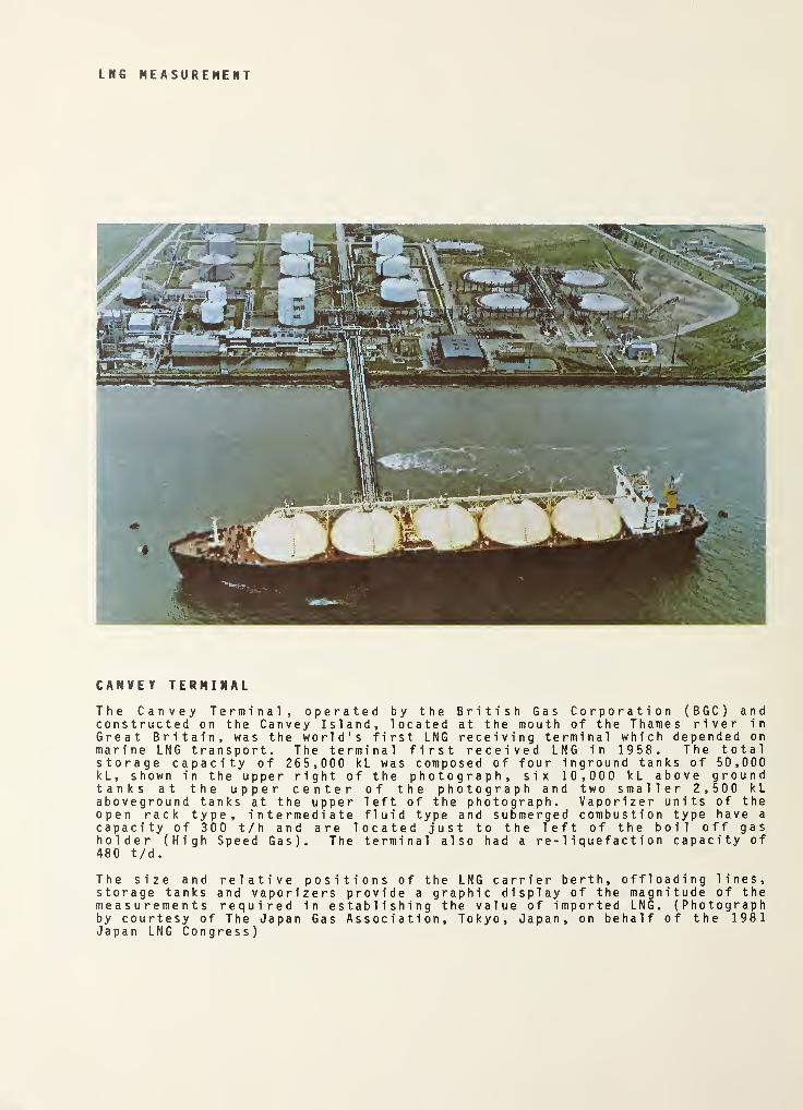
The Canvey Terminal, operated by the British Gas Corporation (BGC) andconstructed on the Canvey Island, located at the mouth of the Thames river inGreat Britain, was the world's first LNG receiving terminal which depended onmarine LNG transport. The terminal first received LNG in 1958. The totalstorage capacity of 265,000 kL was composed of four inground tanks of 50,000kL, shown in the upper right of the photograph, six 10,000 kL above groundtanks at the upper center of the photograph and two smaller 2,500 kLaboveground tanks at the upper left of the photograph. Vaporizer units of theopen rack type, intermediate fluid type and submerged combustion type have a
capacity of 300 t/h and are located just to the left of the boil off gasholder (High Speed Gas). The terminal also had a re-liquefaction capacity of480 t/d.
The size and relative positions of the LNG carrier berth, offloading lines,storage tanks and vaporizers provide a graphic display of the magnitude of themeasurements required in establishing the value of imported LNG. (Photographby courtesy of The Japan Gas Association, Tokyo, Japan, on behalf of the 1981Japan LNG Congress)
LNG MEASUREMENT - Contents Page v
CONTENTS
1.0 BASE PHYSICAL PROPERTIES PAGE
SISystem 1.1-1
Pure Fluid Properties 1 . 2-1
Combustion Enthalpies 1.3-1
References 1.4-1
2.0 MEASUREMENT ELEMENTS
The Measurement Process Applied to LNG 2.1-1
LNG Sampling and Analysis 2.2-1
LNG Calorific Values 2.3-1
LNG Density 2.4-1
LNG Volume 2.5-1
3.0 MEASUREMENT APPLICATIONS
Measurement Uncertainties 3.1-1
Ship Un 1 o ad i ng / Lo ad i ng 3.2-1
Pipeline Flowmetering 3.3-1
Land Based Storage 3.4-1


LNG MEASUREMENT
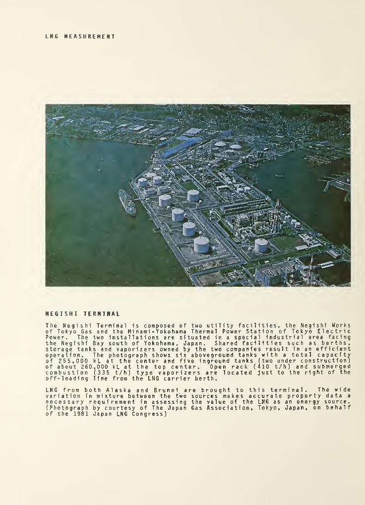
NEGISHI TERMINAL
The Negishi Terminal is composed of two utility facilities, the Negishi Worksof Tokyo Gas and the Minami -Yokohama Thermal Power Station of Tokyo ElectricPower. The two installations are situated in a special industrial area facingthe Negishi Bay south of Yokohama, Japan. Shared facilities such as berths,storage tanks and vaporizers owned by the two companies result in an efficientoperation. The photograph shows six aboveground tanks with a total capacityof 255,000 kL at the center and five inground tanks (two under construction)of about 260,000 kL at the top center. Open rack (410 t/h) and submergedcombustion (335 t/h) type vaporizers are located just to the right of theoff-loading line from the LNG carrier berth.
LNG from both Alaska and Brunei are brought to this terminal. The widevariation in mixture between the two sources makes accurate property data a
necessary requirement in assessing the value of the LNG as an energy source.(Photograph by courtesy of The Japan Gas Association, Tokyo, Japan, on behalfof the 1981 Japan LNG Congress)
l.NG MEASUREMENT - Base Physical Properties Page 1.1-0
CONTENTS
1.0 BASE PHYSICAL PROPERTIES
SI System Page
1.1 The International System of Units (SI) 1.1-1
1.1.1 Units Acceptable for Use with SI 1.1-1
1.1.2 Descriptive and Essential Data 1.1-4
Pure Fluid Properties1.2 Selected Pure Component Physical Properties ... 1.2-1
1.2.1 Relative Atomic and Molecular Masses 1.2-1
1.2.2 Data Reference States 1.2-2
1.2.3 Pure Component Properties 1.2-3
1.2. 3.1 Methane 1.2-4
1 . 2 . 3 . 2 Ethane 1.2-5
1.2. 3. 3 Propane 1.2-6
1.2. 3.4 n-Butane 1.2-7
1.2. 3. 5 iso-Butane 1.2-71.2. 3. 6 n-Pentane 1.2-81.2. 3. 7 iso-Pentane 1.2-8
1.2. 3. 8 neo-Pentane 1.2-91.2. 3. 9 n-Hexane and Hexane Isomers 1.2-9
1.2.3.10 Nitrogen ’ 1.2-11
Combustion Enthalpies1.3 Heating Value of Natural Gas Components 1.3-11.3.1 Enthalpy of Combustion 1.3-11.3.2 Standard Enthalpy of Combustion 1.3-21.3.3 Standard Enthalpy of Combustion at Reference Conditions .... 1.3-31.3.4 Real Gas Enthalpy of Combustion 1.3-51.3.5 Total Uncertainty Estimates for Combustion Enthalpy 1.3-10
1.4 References 1.4-1

.


LNG MEASUREMENT SI System Page 1.1-1
LNG MEASUREMENTA User's Manual for Custody Transfer
1.0
BASE PHYSICAL PROPERTIES1.1
The International System of Units(SI).
In 1948 the 9th General Conference on Weights and Measures (CGPM), by means of Resolution 6,
instructed the International Committee for Weights and Measures (CIPM) "to make recommendations for a
single practical system of units of measurement, suitable for adoption by all countries adhering to
the Meter Convention". This same CGPM gave general principles for unit symbols and a list of units
with special names. Subsequent CGPM of 1954 and I960 established base, derived and supplementary units
for this "practical system" and adopted the name International System of units with the international
abbreviation SI.
The United States holds a place on these international bodies by virtue of its adherence to the Treaty
of the Meter, signed in 1875. The National Bureau of Standards (NBS) acts as the official U.S.
representative to the various International bodies formed by the treaty. NBS, in light of the Metric
Conversion Act of 1975, recommends the use of metric units except in contexts where the exclusive useof metric units would needlessly confuse the intended audience. In these cases, the dual use of metric
and customary units will serve the two purposes of communicating the contents and also familiarizingthe reader with the SI system.
In the following sections on the SI system, reference is made to the original work published by the
International Bureau of Weights and Measures [44], and NBS Special Publication 330 [22], which is theEnglish translation published independently by NBS and Her Majesty's Stationery Office, UK. In
addition, a number of sections and tables have been taken verbatim from Guidelines for Use of theModernized Metric System [72], which are the NBS recommendations on the use of the SI system of units.
These tables include entries which may be beyond the immediate scope of this LNG manual but areincluded for completeness and general interest.
The Metric System: SI The SI is constructed from seven base units for independent quantities plus two
supplementary units for plane angle and solid angle. (See table 1.1.1). Units for all other quantitiesare derived from these nine units. In table 1.1.2 are listed 19 SI derived units with special names.These units are derived from the base and supplementary units in a coherent manner, which means theyare expressed as products and quotients of the nine base and supplementary units without numericalfactors. All other SI derived units, such as those in tables 1.1.3 and 1.1.4, are similarly derived in
a coherent manner from the 28 base, supplementary, and special-name SI units. For use with the SI
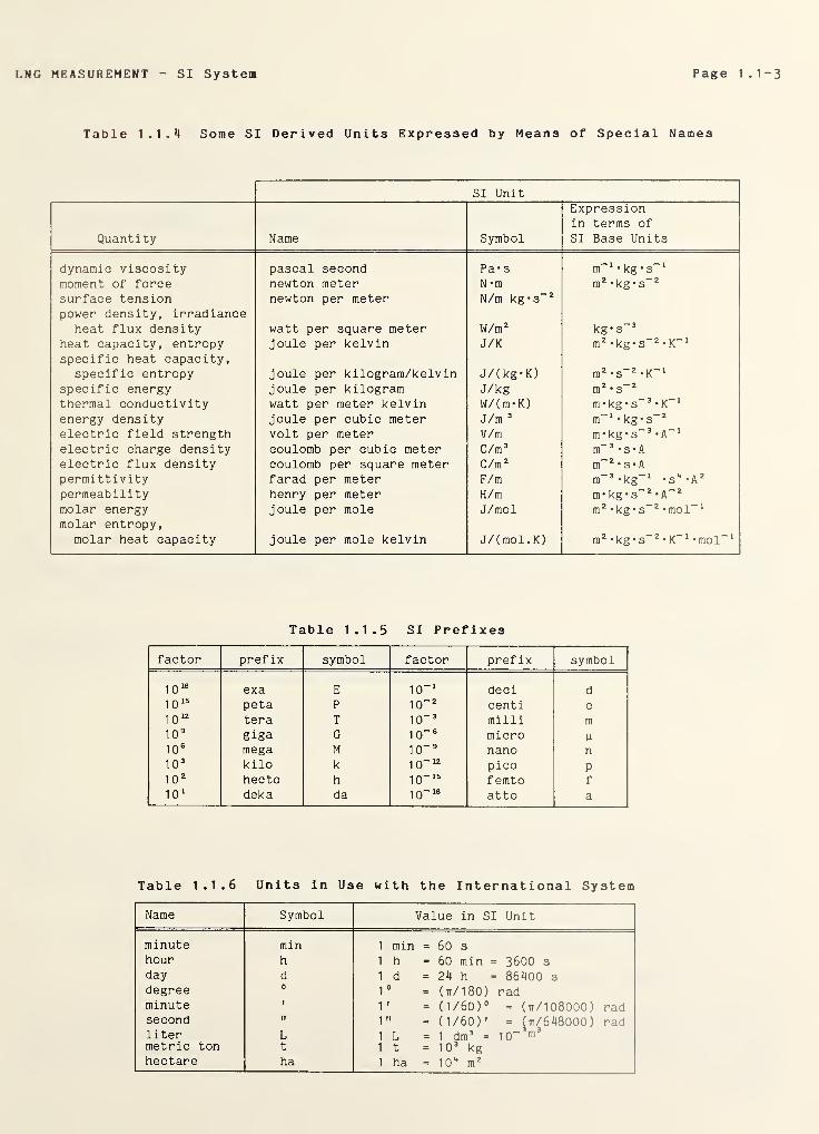
units, there is a set of 16 prefixes (see table 1.1.5) to form multiples and submultiples of theseunits. For mass, the prefixes are to be applied to the gram instead of to the SI base unit, thekilogram.
1.1.1
Units Acceptable for Use with SI
Certain units which are not part of the SI are used so widely that it is impractical to abandon then.
The units that are accepted by NBS for continued used with the Internat ional System are listed in
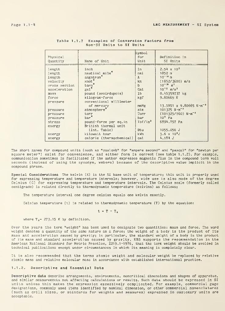
table 1.1.6. In those cases where their usage is already well established, the International Committeefor Weights and Measures (CIPM) also has authorized, for a limited time, the use of the common unitsshown with an asterisk in table 1.1.7.
Table 1.1.1 SI Base and Supplementary Units
Quantity UnitName
UnitSymbol
SI Base Units length meter mmass kilogram kgtime second s
electric current ampere A
thermodynamic temperature kelvin K
amount of substance mole molluminous intensity candela cd
SI supplementary units plane angle radian radsolid angle steradian sr
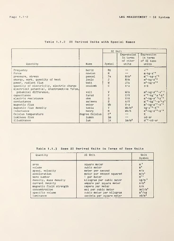
Page 1.1-2 LNG MEASUREMENT SI System
Table 1.1.2 SI Derived Units with Special Names
SI Unit
Quantity Name Symbol
Expressionin termsof otherunits
Expressionin terms
of SI baseunits
frequency hertz Hz — s-1
force newton N — m*kg*s~ 2
pressure, stress pascal Pa N/m 2 m_l • kg* s-2
energy, work, quantity of heat joule J N/m m 2• kg* s
-2
power, radiant flux watt W J/s m z• kg'
s~ 3
quantity of electricity, electric chargeelectrical potential, electromotive force,
coulomb C A • s s*A
potential difference, volt V W/A m 2• kg'
s
-3•
s“ 1
capacitance farad F C/V m-2
• kg-1
s ‘‘•A2
electric resistance ohm fi V/A m 2• kg* s" 3
'A-2
conductance seimens S A/V m-2
• kg-1
• s3*A 2
magnetic flux weber Wb V-s m 2• kg'
s~ 2'A
-1
magnetic flux density tesla T Wb/m 2 kg.
s
-2.a
-1
inductance henry H Wb/A m 2• kg'
s~ 2'A
-2
Celsius temperature degree Celsius C° — K
luminous flux lumen lm — cd' sr
illuminance lux lx lm/m 2 m~ 2• cd* sr
Table 1.1.3 Some SI Derived Units in Terms of Base Units
Quantity SI Unit UnitSymbol
area square meter m 2
volume cubic meter m 3
speed, velocity meter per second m/sacceleration meter per second squared m/s 2
wave number 1 per meter m-1
density, mass density kilogram per cubic meter kg/m 3
current density ampere per square meter A/m 2
magnetic field strength ampere per meter A/mconcentration mol per cubic meter mol/m 3
specific volume cubic meter per kilogram m 3 /kg
luminance candela per square meter cd/m 2
LNG MEASUREMENT SI System Page 1.1-3
Table 1.1.4 Some SI Derived Units Expressed by Means of Special Names
SI Unit
Quantity Name Symbol
Expressionin terms ofSI Base Units
dynamic viscosity pascal second Pa- s m-1
*kg*s-1
moment of force newton meter N*m m 2 *kg*s-2
surface tensionpower density, irradiance
heat flux density
newton per meter
watt per square meter
N/m kg*s~ 2
W/m 2 kg*s-3
heat capacity, entropy joule per kelvin J/K m 2 *kg*s-2
*K~‘
specific heat capacity,specific entropy joule per kilogram/kelvin J/(kg*K) m 2 *s“ 2 *K
_1
specific energy joule per kilogram J/kg m 2•
s
-2
thermal conductivity watt per meter kelvin W/(m*K) m*kg*s-3 •
K~1
energy density joule per cubic meter J/m 3 m-1
• kg* s-2
electric field strength volt per meter V/m m* kg •
s
-3•
A
-1
electric charge density coulomb per cubic meter C/m 3 m~ 3•s
•
A
electric flux density coulomb per square meter C/m 2 m-2
• s*Apermittivity farad per meter F/m m
-3*kg
_1"S^'A 2
permeability henry per meter H/m m* kg* s~ 2•
A
-2
molar energy joule per mole J/mol m 2 *kg* s-2
*mol-1
molar entropy,molar heat capacity joule per mole kelvin J/(mol.K) m 2 *kg* s
-2•K~ 1 -mol
-1
Table 1.1.5 SI Prefixes
factor prefix symbol factor prefix symbol
10 18 exa E 10_1
deci d
10 15 peta P 10" 2 centi c
10 12 tera T 10“ 3 milli m1 O
9 giga G 10~ 6 micro M10 s mega M 10~ 9 nano n10 3 kilo k 1
0~ 12 pico P10 2 hecto h 10“ 15
femto f
10 1 deka da 10" 18 atto a
Table 1.1.6 Units in U3e with the International System
Name Symbol Value in SI Unit
minute min 1 min = 60 s
hour h 1 h =60 min = 3600 s
day d Id = 24 h = 86400 s
degree 01
0 = ( it/ 1 80) radminute I 1’ = (1/60)° = (tt/ 108000) radsecond If 1" = (1/60)’ = U/648000) radliter L tr ii CL3 II O
1 3metric ton t It = 10 3 kghectare ha 1 ha = 10“ m 2
Page 1 1-4 LNG MEASUREMENT SI System
Table 1.1.7 Examples of Conversion Factors fromNon-SI Unit3 to SI Units
PhysicalQuantity Name of Unit
SymbolforUnit
Definition in
SI Units
length inch in 2.54 x 10 2
length nautical mile* nmi 1852 m
length angstrom* A 10“ 10 m
velocity knot* kn (1852/3600) m/scross section barn* b 1 0
-2S m 2
acceleration gal* Gal 10“ 2 m/s 2
mass pound (avoirdupois) lb 0.45359237 kgforce kilogram-force kgf 9.80665 N
pressure conventional millimeterof mercury mmHg 13.5951 x 9.80665 N-nT 2
pressure atmosphere* atm 101325 N-m“ 2
pressure torr Torr (101325/760) N-m“ 2
pressure bar* bar 10 5 Pa
stress pound-force per sq.in lbf/in 2 6894.757 Paenergy British thermal unit
(Int. Table) Btu 1055.056 J
energy kilowatt hour kWh 3.6 x 10 6J
energy calorie (thermochemical) cal 4.184 J
The short names for compound units (such as "coulomb" for "ampere second" and "pascal" for "newton persquare meter") exist for convenience, and either form is correct (see table 1.1.2). For example,communication sometimes is facilitated if the author expresses magnetic flux in the compound term voltseconds (instead of using the synonym, webers) because of the descriptive value implicit in thecompound phrase.
Special Considerations The kelvin (K) is the SI base unit of temperature; this unit is properly usedfor expressing temperature and temperature intervals; however, wide use is also made of the degreeCelsius (C) for expressing temperature and temperature intervals. The Celsius scale (formerly calledcentigrade) is related directly to thermodynamic temperature (kelvins) as follows;
The temperature interval one degree Celsius equals one kelvin exactly.
Celsius temperature (t) is related to thermodynamic temperature (T) by the equation:
t = T - T 0
where T 0= 273.15 K by definition.
Over the years the term "weight" has been used to designate two quantities: mass and force. The wordweight denotes a quantity of the same nature as a force; the weight of a body is the product of itsmass and acceleration caused by gravity; in particular, the standard weight of a body is the productof its mass and standard acceleration caused by gravity. NBS supports the recommendation in theAmerican National Standard for Metric Practice, Z21 9. 1-1976, that the term weight should be avoided in
technical publications except under circumstances in which its meaning is completely clear.
It is also recommended that the terms atomic weight and molecular weight be replaced by relativeatomic mass and relative molecular mass in accordance with established international practice.
1.1.2. Descriptive and Essential Data
Descriptive data describe arrangements, environments, noncritical dimensions and shapes of apparatus,and similar measurements not affecting calculations or results. Such data should be expressed in SI
units unless this makes the expression excessively complicated. For example, commercial gagedesignations, commonly used items identified by nominal dimension, or other commercial nomenclatures(such as drill sizes, or standards for weights and measures) expressed in customary units areacceptable.

LNG MEASUREMENT SI System Page 1.1-5
Essential data express or interpret the quantitative results being reported. All such data shall beexpressed solely in SI units except in those fields where (a) the sole use of SI units would create a
serious impediment to communications, or (b) SI units have not been specified. Exceptions may alsooccur when dealing with commercial devices, standards, or units having some legal definition, such ascommercial weights and measures. Even in such instances, SI units should be used when practical andmeaningful; for example, this may be done by adding non-SI units in parentheses after SI units. Intables, SI and customary units may be shown in parallel columns. If coordinate markings in non-SIunits are included in graphs, they should be displayed on the top and right-hand sides of the figure.

'


LNG MEASUREMENT Fluid Properties Page 1.2-1
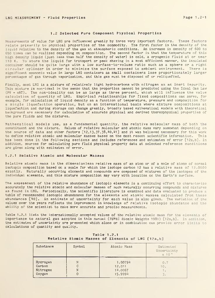
1.2 Selected Pure Component Physical Properties
Measurements of value for LNG are influenced greatly by three very important factors. These factorsrelate primarily to physical properties of the commodity. The first factor is the density of the
liquid relative to the density of the gas at atmospheric conditions. An increase in density of 600 to
650 times can be realized depending on composition. The second factor is that the temperature of this
high density liquid (just less than half the density of water) is cold, a cryogenic fluid at or near110 K. To store the liquid for transport or peak shaving in a most efficient manner, the insulated
container should be quite large with a low surface-to-volume ratio such as a sphere or a rightcircular cylinder in order to minimize the surface exposed to ambient environment. There is
significant economic value in large LNG containers as small containers lose proportionately largerpercentages of gas through vaporization, and this gas must be disposed of or reliquefied.
Finally, most LNG is a mixture of relatively light hydrocarbons with nitrogen as an inert impurity.This mixture is non-ideal in the sense that the properties cannot be predicted using the Ideal Gas Law(PV = nRT). The non-ideality can be as large as three percent, which will influence the valuecalculation of quantity of LNG. Empirical relationships for fixed compositions can serve, for
example, for calculation of liquid density as a function of temperature, pressure and composition fora single liquefaction operation, but on an international basis where mixture compositions atliquefaction and during storage can change greatly, broadly based mathematical models with theoreticalbackground are necessary for calculation of accurate physical and derived thermophysical properties ofthe pure fluids and the mixtures.
Mathematical models use, as a fundamental quantity, the relative molecular mass of both theconstituent and the mixture. Values of relative molecular and atomic mass vary somewhat depending onthe source of data and other factors [12,13,37,38,40,41] and it was believed necessary for this workto define relative atomic and molecular masses based on the most recent scientific information. Thishas been done in the following sections and includes references and estimates of error [12a, b] . Inaddition, sources for calculating pure fluid physical property data at selected reference conditionsare given along with estimates of error.
1.2.1 Relative Atomic and Molecular Masses
Relative atomic mass is the dimensionless relative mass of an atom or of a mole of atoms of normalisotopic composition based on a scale for which the isotope carbon 12 has a relative mass of 12.0000exactly. Naturally occurring elements and compounds are composed of mixtures of the isotopes of theindividual elements, and this mixture composition may vary with location on the Earth's surface.
The assessment of the relative abundance of isotopic elements is a continuing effort to characterizeaccurately the relative atomic and molecular masses of such naturally occurring compounds and mixturesas found in LNG. Periodically, the scientific literature is examined and data evaluated to produce a
table of recommended isotopic abundances for the elements and atomic masses calculated from theseabundances [40]. An estimate of uncertainty for each value is also given. The variation of thevalues over the years reflects the improvement in knowledge of relative isotopic abundance and theability of the scientist to make more accurate and precise measurements.
Table 1.2.1 lists the internationally accepted values of the relative atomic mass for the elements f
importance to natural gas adopted in this manual (IUPAC Atomic Weights 1981) [12a, b]. In add:t. n,
the estimates of uncertainty are presented which alone or in combination can provide error limit; •
calculations of quantity and quality.
Table 1.2.1Relative Atomic Masses of Elements of LNG [12a, b]
Substance Symbol Atomic Mass EstimatedUncertainty
x 10 -
Hydrogen H 1.00794 0.7Carbon C 12.011 10.Nitrogen N 14.0067 1
.
Oxygen 0 15.9994 3.
Page 1 . 2-2 LNG MEASUREMENT Fluid Properties
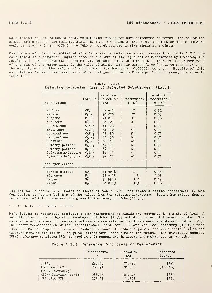
Calculation of the values of relative molecular masses for pure components of natural gas follow thesimple combination of the relative atomic masses. For example; the relative molecular mass of methanewould be 12.011 + (4 x 1 . 0079 ^4 ) = 16.0428 or 1 6.043 rounded to five significant digits.
Combination of individual estimated uncertainties in relative atomic masses from table 1.2.1 arecalculated by quadrature (square root of the sum of the squares) as recommended by Armstrong andJobe[12a,b]. The uncertainty of the relative molecular mass of methane will then be the square rootof the sum of the uncertainty in the value of atomic mass for carbon (0.001) squared plus four timesthe uncertainty in the values of atomic mass for hydrogen (0.00007) squared. Results of thiscalculation for important components of natural gas rounded to five significant figures) are given in
table 1.2.2.
Table 1.2.2Relative Molecular Mass of Selected Substances [12a, b]
HydrocarbonFormula
RelativeMolecularMass
Uncertaintyx 10 4
RelativeUncertainty
x 10 4
methane CH4 16.043 10 0.62ethane c2h 6 30.070 20 0.67propane c
3h 8 44.097 31 0.70
n-butane c 4h 1 0 58.123 41 0.71
iso-butane C 4H 1
0
58.123 41 0.71
n-pentane c5h 1 2 72.150 51 0.71iso-pentane c5h 12 72.150 51 0.71
neo-pentane C5Hi2 72.150 51 0.71
n-hexane C6H12 86.177 61 0.71
2-methylpentane c6h 1 4 86.177 61 0.713-methylpentane c 6h 1 4 86.177 61 0.71
2 , 2-dimethylbutane C6H 1 4 86.177 61 0.71
2 , 3-dimethylbutane C6H 1 4 86.177 61 0.71
Non-hydrocarbon
carbon dioxide C0 2 44.0098 12. 0.15nitrogen n 2 28.0134 1 .4 0.05oxygen 0 2 31 .9988 4.2 0.13water h 2o 18.0153 3.3 0.18
The values in table 1.2.2 based on those of table 1.2.1 represent a recent assessment by theCommission on Atomic Weights of the values from the relevant literature. Recent historical changesand sources of this assessment are given in Armstrong and Jobe [12a,b].
1.2.2 Data Reference States
Definitions of reference conditions for measurement of fluids are currently in a state of flux. A
selection has been made based on Armstrong and Jobe [12a,b] and other industrial requirements. Thereference conditions of pressure and temperature selected for this manual are shown in table 1.2.3.The recent recommendation of the International Union for Pure and Applied Chemistry (IUPAC) that100.000 kPa be adopted as a new standard pressure for thermodynamic standard state [39] is notfollowed here as its use will be quite limited until some time in the future. The previously adoptedIUPAC reference condition [42] is used in this manual and is listed and referenced in the table.
Table 1.2.3 Reference Conditions of Measurement
TemperatureK
PressurekPa
ReferenceSource
IUPAC 298.15 101 .325 [42]ASTM-ANSI-API 288.71 101 .560 [3,7,45](U.S. Customary)ASTM-ANSI- ISO/me trie 288.15 101 .325 [45]JlS/also STP 273.15 101 .325 [47]
LNG MEASUREMENT Fluid Properties Page 1.2-3
The reference state of the Japanese Industrial Standard (JIS) [47] is identical to the reference state
referred to traditionally as Standard Temperature and Pressure (STP).
In the following sections, pure fluid data are given for the components of LNG with relative molecular
masses through the hexanes. Nitrogen is included as it is the most important impurity found in LNG.
Sources of data and state equations are included. In general, reference data at standard conditionsare found from the virial equation form to be consistent with later developed combustion enthalpy data
while broad ranges of pressure and temperature are provided when available by references to the morecomplex mathematical forms.
The reference data values for each fluid can be generated at temperatures and pressures other than
those shown is table 1.2.3. This can be done by reference to section 1.3.4 on Real Gas Enthalpy of
Combustion. Equations (6), (7), (9), (10) of section 1.3 and the equation constants of table 1.3.4
along with the descriptive text should allow calculation of the second virial coefficient and the real
gas molar volume within the stated temperature range and at moderate pressures near one atmosphere.
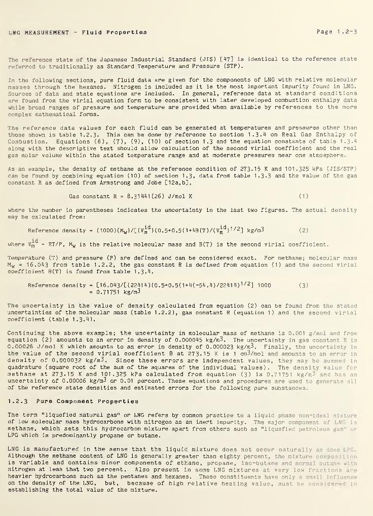
As an example, the density of methane at the reference condition of 273.15 K and 101.325 kPa (JIS/STP)can be found by combining equation (10) of section 1.3, data from table 1.3.3 and the value of the gasconstant R as defined from Armstrong and Jobe [12a,b],
Gas constant R = 8.31441(26) J/mol K (1)
where the number in parentheses indicates the uncertainty in the last two figures. The actual densitymay be calculated from:
Reference density = ( 1 000) (Mw )/[ (V^) (0. 5+0.5 ( 1 + 4B(T)/(Vmd
)1 /2
] kg/m3 (2)
where V^d
= RT/P, Mw is the relative molecular mass and B(T) is the second virial coefficient.
Temperature (T) and pressure (P) are defined and can be considered exact. For methane; molecular massM w = 16.043 from table 1.2.2, the gas constant R is defined from equation (1) and the second virialcoefficient B(T) is found from table 1.3.4.
Reference density = [1 6 .043/[ (2241 4 ) (0. 5+0. 5( 1 +4(-54 .4)/224l 4) 1 /2] 1000 (3)
= 0.71751 kg/m3
The uncertainty in the value of density calculated from equation (2) can be found from the stateduncertainties of the molecular mass (table 1.2.2), gas constant R (equation 1) and the second virialcoefficient (table 1.3.4).
Continuing the above example; the uncertainty in molecular mass of methane is 0.001 g/mol and fromequation (2) amounts to an error in density of 0.000045 kg/m3. The uncertainty in gas constant R is
0.00026 J/mol K which amounts to an error in density of 0.000023 kg/m3. Finally, the uncertainty in
the value of the second virial coefficient B at 273.1 5 K is 1 cm3/mol and amounts to an error in
density of 0.000032 kg/m3. Since these errors are independent values, they may be summed in
quadrature (square root of the sum of the squares of the individual values). The density value f r
methane at 273-15 K and 101.325 kPa calculated from equation (3) is 0.71751 kg/m3 and has muncertainty of 0. 00006 kg/m3 or 0.01 percent. These equations and procedures are used to generateof the reference state densities and estimated errors for the following pure substances.
1.2.3 Pure Component Properties
The term "liquefied natural gas" or LNG refers by common practice to a liquid phase non-idea 1
.-
: >:
•
of low molecular mass hydrocarbons with nitrogen as an inert impurity. The major componentmethane, which sets this hydrocarbon mixture apart from others such as "liquefied petrol--";-
LPG which is predominantly propane or butane.
LNG is manufactured in the sense that the liquid mixture does not occur natural lvAlthough the methane content of LNG is generally greater than eighty percent, the mixturis variable and contains minor components of ethane, propane, iso-butane and normal -
•
nitrogen at less that two percent. Also present in some LNG mixtures at very 1 )w fra • inheavier hydrocarbons such as the pentanes and hexanes. These constituents have only a small •: • ;e
on the density of the LNG, but, because of high relative heating value, mustestablishing the total value of the mixture.
Page 1 .2-4 LNG MEASUREMENT Fluid Properties
The single most attractive characteristic of LNG is the increased density over that of the natural gasat atmospheric pressure and temperature. To achieve and maintain this high density of about 600 timesnormal density, the liquid is maintained at low pressures and temperatures in insulated containersboth for storage and shipment. Boiling points for the LNG mixtures do not normally exceed 150 K andprimary containment vessels are especially designed to limit heat input (see section 2.5).
Commerce in LNG is conducted by establishing the value of the LNG at the point of sale. The value, ofcourse, depends on the end point use of the fluid, either as a primary heat source or as a feed stockin a chemical process. If the LNG is purchased as a heat source, the total heating value must bedetermined. If the LNG is purchased as a feed stock, then the total mass and constituent fractionsmust be established. No single direct measurement device is currently available to accomplish theseobjectives. In either case, the value of the LNG is established through a series of measurementswhich are then combined to give the desired result. Each individual measurement ultimately requires a
precise knowledge of fluid properties.
The prediction of density or other derived properties of the non-ideal mixtures of the lighthydrocarbons with nitrogen has been a long term research effort conducted by research groups in theU.S. and abroad: One approach has been to determine the thermophysical properties of the purecomponents of th.e mixture and then to establish the value of the interaction quantities whichinfluence the mixture properties. A mathematical model of the mixture can then be generated, testedand used to provide the necessary derived thermophysical properties. Several mathematical models orequations of state have been used to derive properties of the pure fluid state and of the mixtures.Simple models such as the virial form [21] with one or two coefficients are used to develop a
theoretical basis for the gas phase properties of pure fluids and mixtures. This form gives bestresults at moderate pressures and temperatures and can be used to predict properties where only a
minimum amount of experimental data are available. With larger quantities of experimental data, morepowerful multi-constant mathematical models may be used if large main frame computers are available.
It is not the purpose of this manual to included a detailed discussion of the above fluid propertiesmodeling process. A description and examples of the use of several mixture models will be found undersection 2.4 of this manual. The cited references should be consulted for more detailed information onthe development of the thermophysical properties of the LNG pure fluids and mixtures.
In order to assure greatest accuracy and precision in assessing the value of LNG, it is necessary to
consider the real gas properties as opposed to ideal gas properties which are an approximation and mayintroduce significant errors. Mathematical models which represent existing experimental fluidproperty data become increasingly complex as the range of pressure and temperature is extended toinclude liquefaction, mixture and storage processes. The major pure fluid components of LNG such asmethane, ethane and propane have been examined by experimentalists in great detail in respect tothermophysical properties (pressure, temperature, density), thermodynamic properties (enthalpy,entropy, specific heats, etc.) and transport properties (thermal conductivity, viscosity, etc.)properties. State equations and tabular data are available as will be shown in the followingsections. The more minor LNG components such as the butanes, pentanes and hexanes have received lessattention by the experimentalists, and broadly based experimental property data are less available.This is also shown in the following sections. However, every effort has been made to include the mostrecent reliable values and references for all the components of LNG.
1 .2.3*1 Methane
The primary reference for the thermophysical properties of methane is the work of Goodwin [24]. Thiswork was the first in a series designed to provide broad range, internally consistent thermophysicalproperties data for pure hydrocarbon fluids and LNG mixtures. The derived properties tables have beendesignated an ASTM Standard [8], Thermophysical properties of methane are tabulated at uniformtemperatures from 90.68 K to 500 K along isobars to 70 MPa(700 bar). A novel equation of state is
employed for the first time, having origin on the vapor-liquid coexistence boundary. Tabulated datafor each isobar include temperature, specific volume, density, internal energy, enthalpy, entropy,specific heats, velocity of sound and the pressure derivatives in respect to temperature and density.Computer program listings for the tabulations are provided. Other treatments of these data are in theliterature [51,52]. Other properties data for methane appear in the literature[2,10,30,35,52,56,58,64,65,67,77].
LNG MEASUREMENT Fluid Properties Page 1 . 2-5
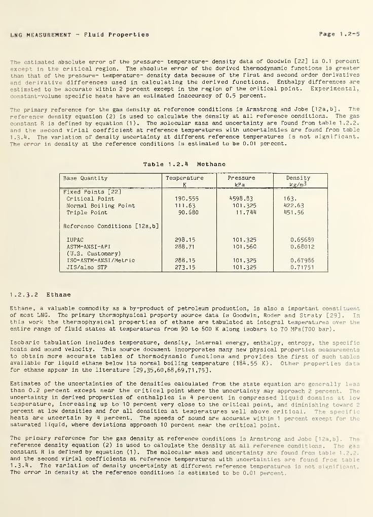
The estimated absolute error of the pressure- temperature- density data of Goodwin [22] is 0.1 percent
except in the critical region. The absolute error of the derived thermodynamic functions is greater
than that of the pressure- temperature- density data because of the first and second order derivatives
and derivative differences used in calculating the derived functions. Enthalpy differences are
estimated to be accurate within 2 percent except in the region of the critical point. Experimental,constant-volume specific heats have an estimated inaccuracy of 0.5 percent.
The primary reference for the gas density at reference conditions is Armstrong and Jobe [12a, b] . Thereference density equation (2) is used to calculate the density at all reference conditions. The gas
constant R is defined by equation (1). The molecular mass and uncertainty are found from table 1.2.2.
and the second virial coefficient at reference temperatures with uncertainties are found from table
1 . 3 . A. The variation of density uncertainty at different reference temperatures is not significant.The error in density at the reference conditions is estimated to be 0.01 percent.
Table 1.2.4 Methane
Base Quantity TemperatureK
PressurekPa
Densitykg/m3
Fixed Points [22]Critical Point 190.555 4598.83 163.
Normal Boiling Point 111.63 101 .325 422.63Triple Point 90.680 1 1 .744 451 .56
Reference Conditions [12a,b]
IUPAC 298.15 101 .325 0.65689ASTM-ANSI-API 288.71 101 .560 0.68012(U.S. Customary)IS0-ASTM-ANSI /Metric 288.15 101 .325 0.67986JlS/also STP 273.15 101 .325 0.71751
1 .2.3-2 Ethane
Ethane, a valuable commodity as a by-product of petroleum production, is also a important constituentof most LNG. The primary thermophysical property source data is Goodwin, Roder and Straty [29]. Inthis work the thermophysical properties of ethane are tabulated at integral temperatures over theentire range of fluid states at temperatures from 90 to 600 K along isobars to 70 MPa(700 bar).
Isobaric tabulation includes temperature, density, internal energy, enthalpy, entropy, the specificheats and sound velocity. This source document incorporates many new physical properties measurementsto obtain more accurate tables of thermodynamic functions and provides the first of such tablesavailable for liquid ethane below its normal boiling temperature (184.55 K). Other properties datafor ethane appear in the literature [29,35,60,68,69,71,75].
Estimates of the uncertainties of the densities calculated from the state equation are generallythan 0.2 percent except near the critical point where the uncertainty may approach 2 percent. Theuncertainty in derived properties of enthalpies is 4 percent in compressed liquid domains at lowtemperature, increasing up to 10 percent very close to the critical point, and diminishing towardpercent at low densities and for all densities at temperatures well above critical. The speoi* .
heats are uncertain by 4 percent. The speeds of sound are accurate within 1 percent except f r t.vsaturated liquid, where deviations approach 10 percent near the critical point.
The primary reference for the gas density at reference conditions is Armstrong and Jobe [1?t,' .
reference density equation (2) is used to calculate the density at all reference condition . Tic .
constant R is defined by equation (1). The molecular mass and uncertainty are found from ' n>> .
and the second virial coefficients at reference temperatures with uncertainties are found fr - ••
1.3.4. The variation of density uncertainty at different reference temperatures is not slgnlflThe error in density at the reference conditions is estimated to be 0.01 percent.
Page 1 . 2-6 LNG MEASUREMENT Fluid Properties
Table 1.2.5 Ethane
Base Quantity TemperatureK
PressurekPa
Densitykg/m3
Fixed Points [29]
Critical Point 305.33 4871 .4 204.5Normal Boiling Point 184.55 101 .325 544.09Triple Point 90.348 0.001 651 .92
Reference Conditions [12a, b]
IUPAC 298.15 101 .325 1 .2387ASTM-ANSI-API 288.71 101 .560 1.2833(U.S. Customary)IS0-ASTM-ANSI /Metric 288.15 101 .325 1 .2829JlS/also STP 273.15 101 .325 1 .3557
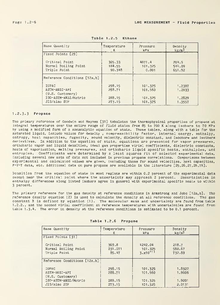
1 .2.3*3 Propane
The primary reference of Goodwin and Haynes [31] tabulates the thermophysical properties of propane atintegral temperatures over the entire range of fluid states from 85 to 700 K along isobars to 70 MPaby using a modified form of a nonanalytic equation of state. These tables, along with a table for thesaturated liquid, include values for density , compressibility factor, internal energy, enthalpy,entropy, heat capacities, fugacity, sound velocity, dielectric constant, and isochore and isothermderivatives. In addition to the equation of state, equations are presented for vapor pressures,orthobaric vapor and liquid densities, ideal gas properties virial coefficients, dielectric constants,heats of vaporization, melting pressures, and orthobaric liquid specific heats, enthalpies, andentropies. Coefficients were determined by a least squares fit of selected experimental data,including several new sets of data not included in previous propane correlations. Comparisons betweenexperimental and calculated values are given, including those for sound velocities, heat capacities,P-V-T data, etc. Additional data on pure propane are available in the literature [25,26,27,28,78].
Densities from the equation of state in most regions are within 0.2 percent of the experimental dataexcept near the critical point where the uncertainty may approach 2 percent. Uncertainties inenthalpy differences along listed isobars agree in general with experimental specific heats to within
3 percent.
The primary reference for the gas density at reference conditions is Armstrong and Jobe [12a,b]. Thereference density equation (2) is used to calculate the density at all reference conditions. The gasconstant R is defined by equation (1). The molecular mass and uncertainty are found from table1.2.2., and the second virial coefficient at reference temperatures with uncertainties are found fromtable 1.3.4. The error in density at the reference conditions is estimated to be 0.1 percent.
Table 1.2.6 Propane
Base Quantity Temperature Pressure DensityK kPa kg/m3
Fixed Points [ 31 ]
Critical Point 369.8 4242.04 218.7Normal Boiling Point 231 .071 101 .325 580.67Triple Point 85.47 3 . xl
0
_1
1
732.89
Reference Conditions [12a, b]
IUPAC 298.15 101 .325 1 .8322ASTM-ANSI-API 288.71 101 .560 1 .9006(U.S. Customary)ISO-ASTM-ANSI /Metric 288.15 101 .325 1 .9001
JlS/also STP 273.15 101 .325 2.0131
LNG MEASUREMENT Fluid Properties Page 1.2-7
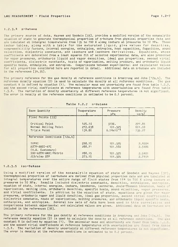
1.2. 3. 4 n-Butane
The primary source of data, Haynes and Goodwin [33], provides a modified version of the nonanalyticequation of state to generate thermophysical properties of n-butane from physical properties data andare tabulated at intergral temperatures from 135 to 700 K along isobars at pressures to 70 MPa. TheseIsobar tables, along with a table for the saturated liquid, give values for densities,compressiblility factors, internal energies, enthalpies, entropies, heat capacities, fugacities, soundvelocities, dielectric constants, and isochore and isotherm derivatives. Equations, whosecoefficients are determined from a least squares fit of selected experimental data, are also presentedfor vapor pressures, orthobaric liquid and vapor densities, ideal gas properties, second virialcoefficients, dielectric constants, heats of vaporization, melting pressure, and orthobaric liquidspecific heats, enthalpies, and entropies. Comparisions between experimental and calculated valuesfor all properties considered here are reported in detail. Additional data on n-butane are includedin the references [34,35].
The primary reference for the gas density at reference conditions is Armstrong and Jobe [12a, b] . Thereference density equation (2) is used to calculate the density at all reference conditions. The gasconstant R is defined by equation (1). The molecular mass and uncertainty are found from table 1.2.2,and the second virial coefficients at reference temperatures with uncertainties are found from table1.3.4. The variation of density uncertainty at different reference temperatures is not significant.The error in density at the reference conditions is estimated to be 0.1 percent.
Table 1.2.7 n-Butane
Base Quantity TemperatureK
PressurekPa
Densitykg/m3
Fixed Points [33]
Critical Point 425.16 3796. 227.85Normal Boiling Point 272.638 101 .325 601 .09Triple Point 134.86 6 .74x1
0“^735.27
Reference Conditions [12a,b]
IUPAC 298.15 101 .325 2.4504ASTM-ANSI-API 288.71 101 .560 2.5486(U.S. Customary)ISO-ASTM-ANSI/Metric 288.15 101 .325 2.5481JlS/also STP 273.15 101.325 2.7154
1.2. 3. 5 iso-Butane
Using a modified version of the nonanalytic equation of state of Goodwin and Haynes [32;,thermophysical properties of iso-butane are derived from physical properties data and are tabulated vintegral temperatures over the entire range of fluid states from 114 to 700 K along isobars it
pressures to 70 MPa. Results included dielectric constants, densities, enthalpies, entropi' ,
equation of state, internal energies, isobars, isochores, isotherms, Joule-Thomson inversion,vaporization, melting line, orthobaric densities, specific heats, sound velocities, vapor or' .
,
and virial coefficients. In addition to the equation of state, equations are given for .
•
pressures, orthobaric vapor and liquid densities, ideal gas properties, second virial coef f i c : ,
dielectric constants, heats of vaporization, melting pressures, and orthobaric liquid specific ,
enthalpies, and entropies. Several new sets of data have been used in this correi it .
comparisons between experimental and calculated values are given. Additional data on ! s.e •
included in the references [35].
The primary reference for the gas density at reference conditions is Armstrong and Jobs- [1; .,! ].
reference density equation (2) is used to calculate the density at all reference conditi m3,constant R is defined by equation (1). The molecular mass and uncertainty are found !>-- •
. . .
and the second virial coefficients at reference temperatures with uncertainties are ':
:
1.3.4. The variation of density uncertainty at different reference temperatures ;
• • •
The error in density at the reference conditions is estimated to be 0.2 percent.
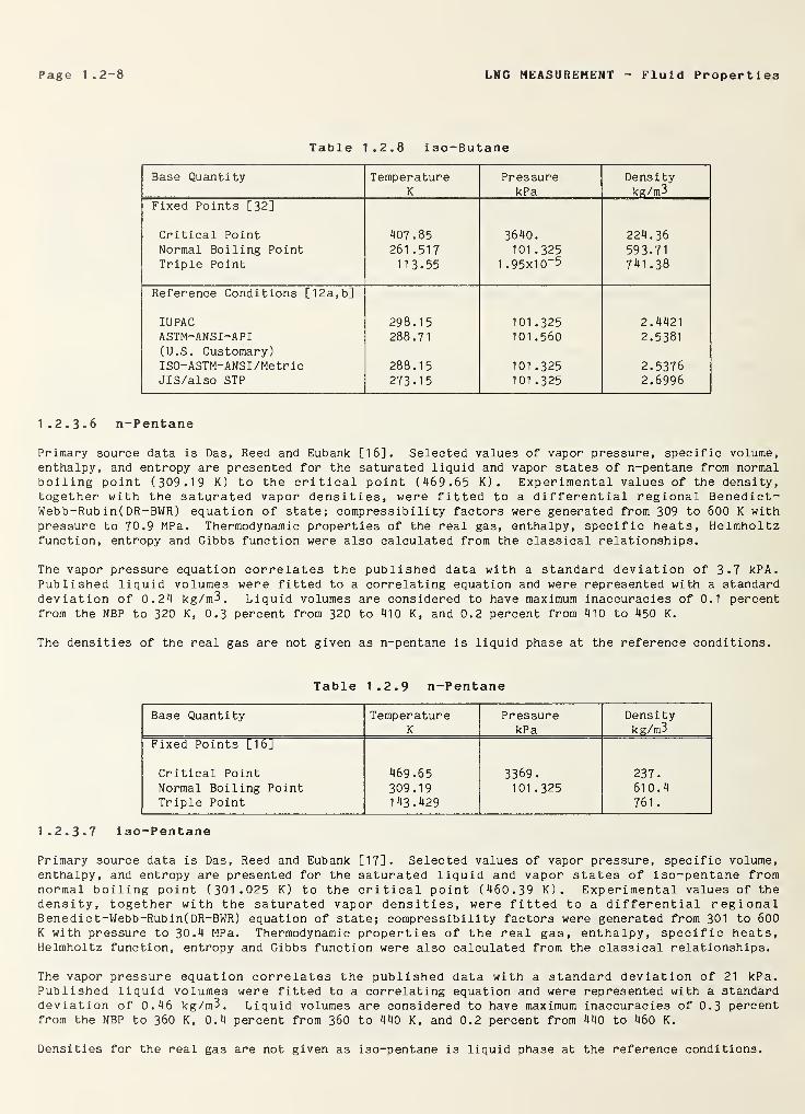
Page 1 .2-8 LNG MEASUREMENT Fluid Properties
Table 1.2.8 iso-Butane
Base Quantity TemperatureK
PressurekPa
Densitykg/m3
Fixed Points [32]
Critical Point 407.85 3640. 224.36Normal Boiling Point 261 .517 101 .325 593.71Triple Point 113.55 1 . 95x1
0“5 741 .38
Reference Conditions [12a, b]
IUPAC 298.15 101 .325 2.4421ASTM-ANSI-API 288.71 101 .560 2.5381(U.S. Customary)ISO-ASTM-ANSI/Metric 288.15 101 .325 2.5376JlS/also STP 273.15 101 .325 2.6996
1.2. 3. 6 n-Pentane
Primary source data is Das, Reed and Eubank [16]. Selected values of vapor pressure, specific volume,enthalpy, and entropy are presented for the saturated liquid and vapor states of n-pentane from normalboiling point ( 309.19 K) to the critical point (469.65 K) . Experimental values of the density,together with the saturated vapor densities, were fitted to a differential regional Benedict-Webb-Rub in ( DR-BWR ) equation of state; compressibility factors were generated from 309 to 600 K withpressure to 70.9 MPa. Thermodynamic properties of the real gas, enthalpy, specific heats, Helmholtzfunction, entropy and Gibbs function were also calculated from the classical relationships.
The vapor pressure equation correlates the published data with a standard deviation of 3.7 kPA.Published liquid volumes were fitted to a correlating equation and were represented with a standarddeviation of 0.24 kg/m3. Liquid volumes are considered to have maximum inaccuracies of 0.1 percentfrom the NBP to 320 K, 0.3 percent from 320 to 410 K, and 0.2 percent from 410 to 450 K.
The densities of the real gas are not given as n-pentane is liquid phase at the reference conditions.
Table 1.2.9 n-Pentane
Base Quantity TemperatureK
PressurekPa
Densitykg/m3
Fixed Points [l6]
Critical Point 469.65 3369. 237.Normal Boiling Point 309.19 101.325 610.4Triple Point 143.429 761 .
1.2. 3. 7 iso-Pentane
Primary source data is Das, Reed and Eubank [17]. Selected values of vapor pressure, specific volume,
enthalpy, and entropy are presented for the saturated liquid and vapor states of iso-pentane fromnormal boiling point ( 301 .025 K) to the critical point ( 460.39 K) . Experimental values of thedensity, together with the saturated vapor densities, were fitted to a differential regionalBenedict-Webb-Rubin(DR-BWR) equation of state; compressibility factors were generated from 301 to 600K with pressure to 30.4 MPa. Thermodynamic properties of the real gas, enthalpy, specific heats,Helmholtz function, entropy and Gibbs function were also calculated from the classical relationships.
The vapor pressure equation correlates the published data with a standard deviation of 21 kPa.Published liquid volumes were fitted to a correlating equation and were represented with a standarddeviation of 0.46 kg/m3. Liquid volumes are considered to have maximum inaccuracies of 0.3 percentfrom the NBP to 360 K, 0.4 percent from 360 to 440 K, and 0.2 percent from 440 to 460 K.
Densities for the real gas are not given as iso-pentane is liquid phase at the reference conditions.

LNG MEASUREMENT Fluid Properties Page 1.2-9
Table 1.2.10 iso-Pentane
Base Quantity TemperatureK
PressurekPa
Densitykg/m3
Fixed Points [17]
Critical Point 460.39 3381
.
236.
Normal Boiling Point 301 .025 101.325 61 2.5
Triple Point 113.25 787.
1.2. 3-8 neo-Pentane
Primary source data is Das, Reed and Eubank [18]. Selected values of vapor pressure, specific volume,
enthalpy, and entropy are presented for the saturated liquid and vapor states of neo-pentane fromnormal boiling point (282.628 K) to the critical point (433.75 K) . Experimental values of the
density, together with the saturated vapor densities, were fitted to a differential regional Benedict-Webb-Rub in( DR-BWR) equation of state; compressibility factors were generated from 282.628 to 600 K
with pressure to 40.5 MPa. Thermodynamic properties of the real gas, enthalpy, specific heats,Helmholtz function, entropy and Gibbs function were also calculated from the classical relationships.
The vapor pressure equation is believed to be accurate to 0.49 percent from 300 K to the criticalpoint, with a maximum uncertainty of 8.1 kPa near the critical point. Published liquid volumes werefitted to a correlating equation and were represented with a standard deviation of 0.27 kg/m3 from 256to 433 K. Liquid Volumes are considered to have maximum inaccuracies of 0.2 percent from the NBP to370 K, 0.1 percent from 370 to 420 K, and 0.2 percent from 420 to 433 K.
The primary reference for the gas density at reference conditions is Armstrong and Jobe [12a, b] . Thereference density equation (2) is used to calculate the density at all reference conditions. The gasconstant R is defined by equation (1). The molecular mass and uncertainty are found from table 1.2.2.and the second virial coefficients at reference temperatures with uncertainties are found from table1.3.4. The variation of density uncertainty at different reference temperatures is not significant.The error in density at the reference conditions is estimated to be 0.2 percent. Neo-pentane is
liquid phase at the reference condition of 273.15 K and 101.325 kPa.
Table 1.2.11 neo-Pentane
Base Quantity TemperatureK
PressurekPa
Densitykg/m3
Fixed Points [18]
Critical Point 433.75 3196. 232.Normal Boiling PointTriple Point
282.628256.6
101 .325 603.3
Reference Conditions [12a, b]
IUPAC 298.15 101.325 3.0693ASTM-ANSI-API 288.71 101 .560 3.1974(U.S. Customary)ISQ-ASTM-ANSI /Metric 288.15 101 .325 3-1971
1.2. 3- 9 n-Hexane and Hexane Isomers
The primary source of data for n-hexane is Weber [74]. Thermodynamic properties of n-hex ane h.ivcalculated over a a temperature range of 273.15 K to 556 K and up to a pressure of 4.1 m: .
properties were determined from vapor pressure, volumetric heat capacity, indvaporization data through the application of rigorous thermodynamic relationships acc rli: -• •
and the calculated data have been found to be internally consistent. A Benedlct-Webb-Rui !• w :
>
state equation was used and resulted in an estimated average error of 0.74 percent.
Densities of the real gas are not given as the hexanes are liquid phase at the refer-v-
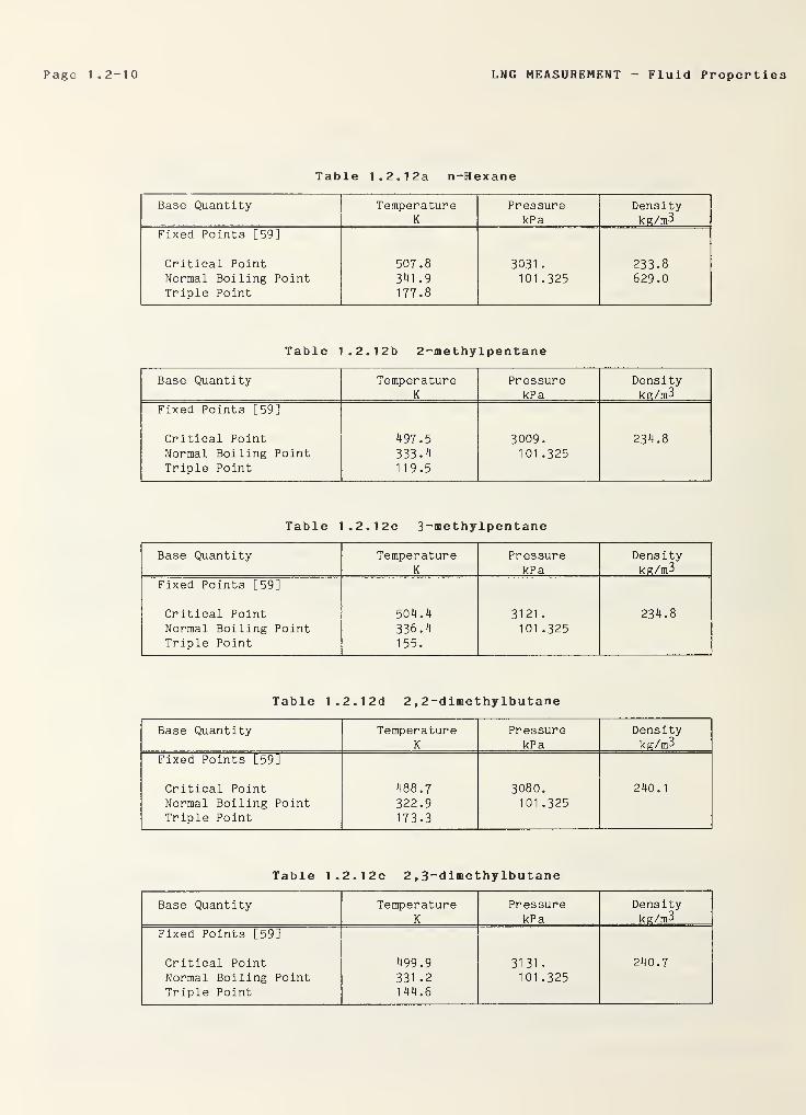
Page 1.2-10 LNG MEASUREMENT - Fluid Properties
Table 1.2.12a n-Hexane
Base Quantity TemperatureK
PressurekPa
Densitykg/m3
Fixed Points [59]
Critical Point 507.8 3031 . 233.8Normal Boiling Point 3^1 .9 101 .325 629 .0
Triple Point 177.8
Table 1.2.12b 2-methylpentane
Base Quantity TemperatureK
PressurekPa
Densitykg/m3
Fixed Points [59]
Critical Point 497.5 3009. 234.8Normal Boiling Point 333.4 101 .325Triple Point 119.5
Table 1.2.12c 3_methy lpentane
Base Quantity TemperatureK
PressurekPa
DensitykR/m3
Fixed Points [59]
Critical Point 504.4 3121 . 234.8Normal Boiling Point 336.4 101 .325Triple Point 155.
Table 1.2.12d 2 , 2-d imethy lbutane
Base Quantity TemperatureK
PressurekPa
Densitykg/m3
Fixed Points [59]
Critical Point 488.7 3080. 240.1
Normal Boiling Point 322.9 101 .325Triple Point 173.3
Table 1
.
2.12e 2 , 3~d imethy lbutane
Base Quantity TemperatureK
PressurekPa
Densitykg/m3
Fixed Points [59]
Critical Point 499.9 3131 . 240.7Normal Boiling Point 331 .2 101.325Triple Point 144.6
LNG MEASUREMENT Fluid Properties Page 1.2-11
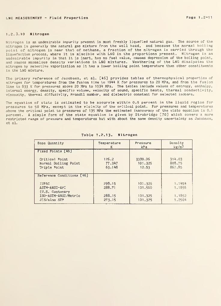
1.2.3.10 N i trogen
Nitrogen is an undesirable impurity present in most freshly liquefied natural gas. The source of the
nitrogen is generally the natural gas mixture from the well head, and because the normal boilingpoint of nitrogen is near that of methane, a fraction of the nitrogen is carried through the
liquefaction process, where it is miscible with LNG in the proportions present. Nitrogen is an
undesirable impurity in that it is inert, has no fuel value, causes depression of the boiling point,
and causes anomalous density variations in LNG mixtures. Weathering of the LNG dissipates the
nitrogen by selective vaporization as it has a lower boiling point temperature than other constituents
in the LNG mixture.
The primary reference of Jacobsen, et al. [46] provides tables of thermophysical properties of
nitrogen for temperatures from the fusion line to 1944 K for pressures to 20 MPa, and from the fusionline to 833 K for pressures above 20 MPa to 1034 MPa. The tables include values of entropy, enthalpy,
internal energy, density, specific volume, velocity of sound, specific heats, thermal conductivity,viscosity, thermal diffusivity, Prandtl number, and dielectric constant for selected isobars.
The equation of state is estimated to be accurate within 0.5 percent in the liquid region for
pressures to 50 MPa, except in the vicinity of the critical point. For pressures and temperatures
above the critical point to pressures of 135 MPa the estimated inaccuracy of the state equation is 0.1
percent. A simple form of the state equation is given by Strobridge [70] which covers a more
restricted range of pressure and temperatures but with about the same density uncertainty as Jacobsen,
et al.
Table 1.2.13. Nitrogen
Base Quantity Temperature Pressure DensityK kPa kg/m3
Fixed Points [46]
Critical Point 126.2 3399.96 314.03Normal Boiling Point 77.347 101 .325 808.75Triple Point 63-148 12.53 867.85
Reference Conditions [46]
IUPAC 298.15 101 .325 1.1454ASTM-ANSI-API 288.71 101 .560 1 .1856(U.S. CustomaryISO-ASTM-ANSI /Metric 288.15 101 .325 1 .1852JlS/also STP 273.15 101 .325 1 .2504


LNG MEASUREMENT Combustion Enthalpies Page 1 .3-1
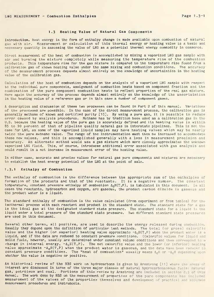
1.3 Heating Value of Natural Gas Components
Introduction. Heat energy in the form of enthalpy change is made available upon combustion of naturalgas with air. Measurement or calculation of this thermal energy or heating value is a basic and
necessary quantity in assessing the value of LNG as a potential thermal energy commodity in commerce.
Direct measurement of the heat of combustion is accomplished by mixing a vaporized LNG gas sample with
air and burning the mixture completely while measuring the temperature rise of the combustionproducts. This temperature rise for the gas mixture is compared to the temperature rise found from a
calibration gas of known heating value under the same mixing and combustion conditions. The accuracyof the measurement process depends almost entirely on the knowledge of uncertainties in the heatingvalue of the calibration gas.
Calculation of the heat of combustion depends on the analysis of a vaporized LNG sample with respect
to the individual pure components, assignment of combustion heats based on component fraction and thecombination of the pure component combustion heats to reflect properties of the real gas mixture.Here again the accuracy of the process depends almost entirely on the knowledge of the uncertaintiesin the heating value of a reference gas or in this case a number of component gases.
A description and discussion of these two processes can be found in Part 2 of this manual. Variationsof the processes are possible. In the case of the direct measurement process, the calibration gas is
generally methane of known and certified purity [10]. By using a pure gas, it is possible to reduceerror caused by analysis procedures. Methane has by tradition been used as a calibration gas in theU.S. because the heating value of the pure gas is accurately defined and its heating value is within85 to 90 percent of that of pipeline quality natural gas in interstate pipelines. This is not the
case for LNG, as some of the vaporized liquid samples may have heating values which may be nearlytwice the pure methane value. The range of the instrumentation must then be increased to accommodatethese new values, and this is accomplished generally with a loss in measurement precision andaccuracy. An alternate method would use a gas mixture which more closely approximates the unknownvaporized LNG fluid. This, of course, introduces additional error associated with gas analysis andcould result in a net increase in measurement error of the heating value.
In either case, accurate and precise values for natural gas pure components and mixtures are necessaryto establish the heat energy potential of the LNG at the point of sale.
1.3.1 Enthalpy of Combustion
The enthalpy of combustion is the difference between the appropriate sum of the enthalpies offormation of the products and that of the reactants. It is a negative number. The constanttemperature, constant pressure enthalpy of combustion ACH(T,P), is tabulated in this document. In allcases the reactants, hydrocarbon and oxygen, are gaseous, the product carbon dioxide is gaseous andthe product water is a liquid.
The standard enthalpy of combustion is the value calculated (from experiment or from tables) for theisothermal process with each reactant and product in the standard state. The standard state for a -• is
is the ideal gas at the designated standard state pressure. The standard state for a liquid is theliquid under a total pressure of the standard state pressure. Two different standard state pressureare used in this document.
Several other terms, all positive, are used to describe the energy released during comb .•
.
Usually they depend upon the definition of particular test methods. The total (or gross) cal ) r i f i
value and the higher (or superior) heating value approximate -ACH(T,P) when the product water . 1
liquid, and if the data are reduced to constant pressure conditions. (Calorific values for liquidsolid fuels, however, usually are determined under constant volume conditions and then com-. :
•. :
•1
change in internal energy, -A CU(T,P). The net calorific value and the lower (or infer; >r
value approximate -A CH(T,P) when the product water is gaseous, and the data have bee;constant pressure conditions. The "heat of combustion" usually means A CH or -A CH depend -• ..
whether the value is negative or positive.
An historical review of the NBS work on hydrocarbons is given by Armstrong [11] w:i<••
interest are discussed in terms of the three major classes of natural hydrocarbonaceou.- f u- •• il
gas, petroleum and coal. Portions of this review by Armstrong are included in sent f
manual. The work done by NBS on the measurement of properties of the pure component:; mimeasurement of the values of the properties themselves and development of prv .
• rmeasurement procedures and instruments.
Page 1 .3~2 LNG MEASUREMENT Combustion Enthalpies
Additional values of combustion energies, densities, viscosities, vapor pressures, refractive indices,elemental compositions and other parameters have been determined for complex fuel mixtures andcorrelated to find methods of estimating properties. Extensive standard reference data tables havebeen compiled, and a number of standard reference materials have been developed. For the lighthydrocarbons of interest to the natural gas industry, the detailed work on methane properties seemedto be adequate in establishing the values for this important fuel.
Early in the development of the LNG industry, ethane, propane, butane, pentane and hexane in additionto methane became important when defining the value of this fuel in the liquid state. Some time wasto pass before it was found that additional critically evaluated data were needed to accomplish thismeasurement process. The quantity and quality of LNG were found to depend strongly on more accuratevalues of enthalpy of combustion for hydrocarbons in addition to methane, and since the measurementprocess for LNG was composed of several submeasurement processes, a measure of accuracy and precisionfor each substance was found necessary in calculating total uncertainty or error of measurement. Aspart of the task to develop this LNG Measurement manual, Groupe International des Importateurs de GazNaturel Liquefie (G .I.I.G.N.L) contracted with NBS to develop the required information.
Dr. G. T. Armstrong of NBS, an internationally recognized authority on the subject, directed the workwhich was first published in 1 982 [12a]. This document provides the basic data, the recommendedprocedures and illustrative calculations for computing heating values of natural gas pure componentsand mixtures. The composition of the mixtures and the properties of the components are given atcommonly used reference conditions for gas measurement within the range 273.15 K to 298.15 K.
Symbols, terms and units of measurement are defined, and conversion factors and physical constants aregiven.
Selected values for standard enthalpies of combustion and heat capacities of the pure hydrocarbongases C-| through C 5 are tabulated at the reference temperatures 273.15 K (0° C), 288.15 K (15° C),
288.71 K (60°F) and 298.15 K (25 °C) on a molar and a volumetric basis. Both the dry gases and theideal water-saturated gas are treated. The calculation of enthalpies of combustion of gas mixtures ona molar, mass, or volumetric basis is described.
Second virial coefficients are presented as functions of temperature for the pure substances and for
binary interactions with methane. Tables are given for molar volumes, enthalpic effects and theheating values of the dry real-gas hydrocarbons on a molar, mass and volumetric basis at two referenceconditions, 288.15 K (15°C), 101.325 kPa; and 288.71 K (60°F), 101.560 kPa (14.73 psia). An analysisis presented of the effects of errors in the data on calculated heating values.
The recommended values in this publication by Armstrong and Jobe [12a] were revised, in 1984, in orderto give more emphasis to recent measurements and to develop a common set of basic data to be used by
G. I.I.G.N.L. and the Gas Producers Association (GPA)(U.S.) [12b, 37]. This re-evaluation slightlychanges the values for the C-| to C 5 alkanes, except for n-pentane, previously recommended to bothgroups. These revised values are quoted here and are implied whenever Armstrong and Jobe are cited.The revision was carried out by a joint working party from the NBS Chemical Thermodynamics Data Centerand the Texas A&M University Thermodynamics Research Center. The revision will be documentedseparately. For now it should be kept in mind that this revision affects all tables of enthalpies andvirial coefficients in reference [ 12 a].
The content of this publication by Armstrong and Jobe is much more extensive than required for thismeasurement manual. It will serve as a basic reference document for this section on heating values.Selected calculation procedures and tabular data have been taken directly from Armstrong and Jobe[12a] and are reproduced here. The following discussion will emphasize only the origin anduncertainty of the standard enthalpy of combustion for the hydrocarbons Cl through C 6 and the
calculation methods required to present the values in terms of the required reference states. Onlypure component data will be considered in this section. Gas mixture properties and enthalpies of
combustion will be considered in Section 3.
1.3.2 Standard Enthalpy of Combustion
The standard enthalpy of combustion is the enthalpy of combustion calculated for the isothermalprocess with all reactants and products in their thermodynamic standard state. The standardthermodynamic properties for a gaseous substance, whether pure or in a gaseous mixture, apply to thepure substance at the standard state pressure and in a hypothetical state in which the gas exhibitsideal gas behavior. A gas which conforms to the ideal gas behavior follows the Ideal Gas Law of
PV=nRT.
LNG MEASUREMENT Combustion Enthalpies Page 1 .3~3
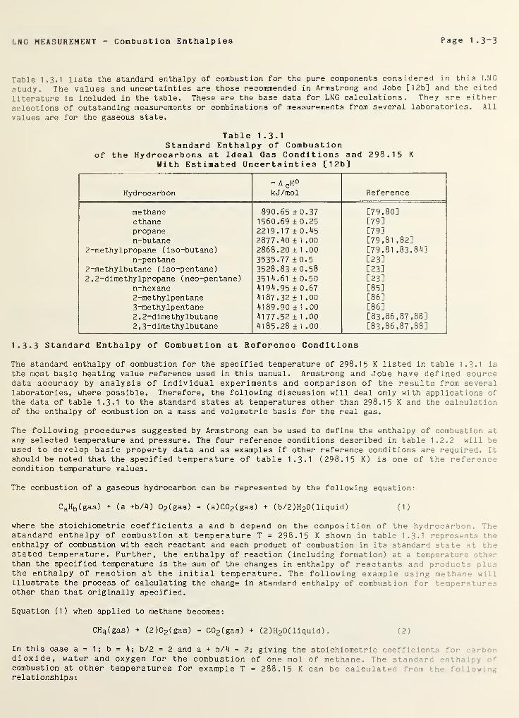
Table 1.3.1 lists the standard enthalpy of combustion for the pure components considered in this LNG
study. The values and uncertainties are those recommended in Armstrong and Jobe [12b] and the cited
literature is included in the table. These are the base data for LNG calculations. They are either
selections of outstanding measurements or combinations of measurements from several laboratories . All
values are for the gaseous state.
Table 1
.
3 .
1
Standard Enthalpy of Combustionof the Hydrocarbons at Ideal Gas Conditions and 298.15 K
With Estimated Uncertainties [12b]
Hydrocarbon
- A CH°kJ/mol Reference
methane 890.65 ± 0.37 [79,80]ethane 1560.69 ± 0.25 [79]
propane 2219.17 ± 0.45 [79]n-butane 2877.40 ± 1 .00 [79,81 ,82]
2-methylpropane (iso-butane) 2868.20 ± 1 .00 [79,81 ,83,84]n-pentane 3535.77 + 0.5 [23]
2-methylbutane (iso-pentane) 3528.83 ±0.58 [23]
2 ,2-dimethylpropane (neo-pentane) 351 4.61 ± 0.50 [23]n-hexane 4194 .95 ±0.67 [85]2-methylpentane 4187.32 ± 1 .00 [86]
3-methylpentane 4189.90 ±1.00 [86]
2 ,2-dime thylbutane 4177.52 ± 1 .00 [83,86,87,88]2 ,
3
-dimethylbutane 4185.28 ± 1 .00 [83,86,87,88]
1.3.3 Standard Enthalpy of Combustion at Reference Conditions
The standard enthalpy of combustion for the specified temperature of 298.15 K listed in table 1.3-1 is
the most basic heating value reference used in this manual. Armstrong and Jobe have defined sourcedata accuracy by analysis of individual experiments and comparison of the results from severallaboratories, where possible. Therefore, the following discussion will deal only with applications ofthe data of table 1.3.1 to the standard states at temperatures other than 298.15 K and the calculationof the enthalpy of combustion on a mass and volumetric basis for the real gas.
The following procedures suggested by Armstrong can be used to define the enthalpy of combustion atany selected temperature and pressure. The four reference conditions described in table 1.2.2 will beused to develop basic property data and as examples if other reference conditions are required. It
should be noted that the specified temperature of table 1 .3-1 (298.15 K) is one of the referencecondition temperature values.
The combustion of a gaseous hydrocarbon can be represented by the following equation:
CaHb (gas) + (a +b/4) 02 (gas) = (a)C02(gas) + (b/2)H20(liquid) (1)
where the stoichiometric coefficients a and b depend on the composition of the hydrocarbon. Thestandard enthalpy of combustion at temperature T = 298.15 K shown in table 1.3-1 represent', theenthalpy of combustion with each reactant and each product of combustion in its standard state at thestated temperature. Further, the enthalpy of reaction (including formation) at a temperaturethan the specified temperature is the sum of the changes in enthalpy of reactants and product." plusthe enthalpy of reaction at the initial temperature. The following example using methan*' willillustrate the process of calculating the change in standard enthalpy of combustion for temperatother than that originally specified.
Equation (1) when applied to methane becomes:
CH||(gas) + (2)02(gas) = C0 2 (gas) + (2)H20(liquid) . (2)
In this case a = 1; b = 4; b/2 = 2 and a + b/4 = 2; giving the stoichiometric coefficient t
dioxide, water and oxygen for the combustion of one mol of methane. The standard 1;
.
combustion at other temperatures for example T = 288.15 K can be calculated from *: -•
:
relationships:
Page 1 . 3~
4
LNG MEASUREMENT - Combustion Enthalpies
A CH°( 298 . 1 5 K) - A CH°(288.15 K) =
a[H°(C0 2 , gas, 298.15 K) - H°(C0 2 , gas, 288.15 K)]
+ b/2[H°(H 20, liquid, 298.15 K) - H°(H 20, liquid, 288.15 K)]
- (a + b/4)[H°(02 , gas, 298.15 K) - H°(02 , gas, 288.15 K)]
- [H°(CaHb , gas, 298.15 K) - H°(CaHb , gas, 288.15)] (3)
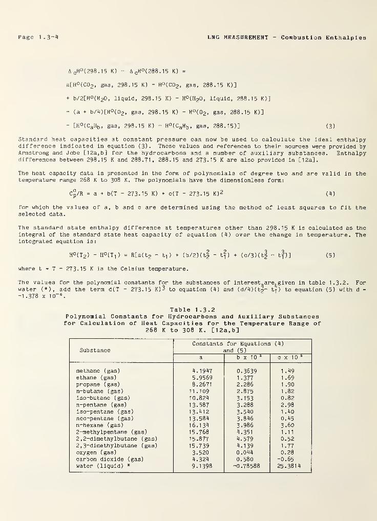
Standard heat capacities at constant pressure can now be used to calculate the ideal enthalpydifference indicated in equation (3). These values and references to their sources were provided byArmstrong and Jobe [12a, b] for the hydrocarbons and a number of auxiliary substances. Enthalpydifferences between 298.15 K and 288.71, 288.15 and 273.15 K are also provided in [12a].
The heat capacity data is presented in the form of polynomials of degree two and are valid in thetemperature range 268 K to 308 K. The polynomials have the dimensionless form:
C°/R = a + b(T - 273-15 K) + c(T - 273-15 K) 2 (4)
for which the values of a, b and c are determined using the method of least squares to fit theselected data.
The standard state enthalpy difference at temperatures other than 298.15 K is calculated as theintegral of the standard state heat capacity of equation (4) over the change in temperature. Theintegrated equation is:
H°(T 2 )- H0^) = R[a( t2 - t-, ) + (b/2) (
t
2 - tf) + (c/3) (
t
2 - t?)] (5)
where t = T - 273.15 K is the Celsius temperature.
The values for the polynomial constants for the substances of interest^are^given in table 1.3.2. Forwater (*), add the term d(T - 273.15 K)3 to equation (4) and (d/4)(t2- t-| ) to equation (5) with d =
-1 .378 x 10~ 6.
Table 1.3.2Polynomial Constants for Hydrocarbons and Auxiliary Substancesfor Calculation of Heat Capacities for the Temperature Range of
268 K to 308 K. [12a, b]
SubstanceConstants for Equations (4)
and (5)
a b x 10 2o X o
methane (gas) 4.1947 0.3639 1 .49
ethane (gas) 5.9569 1 .377 1 .69
propane (gas) 8.2671 2.286 1 .90
n-butane (gas) 11 .109 2.875 1 .82
iso-butane (gas) 10.824 3.153 0.82n-pentane (gas) 13.587 3.288 2.98iso-pentane (gas) 13.412 3.540 1 .40
neo-pentane (gas) 13.584 3.846 0.45n-hexane (gas) 16.134 3.986 3.602-methylpentane (gas) 15.768 4.351 1.11
2,2-dimethylbutane (gas) 15.877 4.579 0.52
2 , 3~dimethylbutane (gas) 15.739 4.139 1 .77
oxygen (gas) 3.520 0.044 0.28carbon dioxide (gas) 4.324 0.580 -0.65water (liquid) * 9.1398 -0.78588 25.381
4
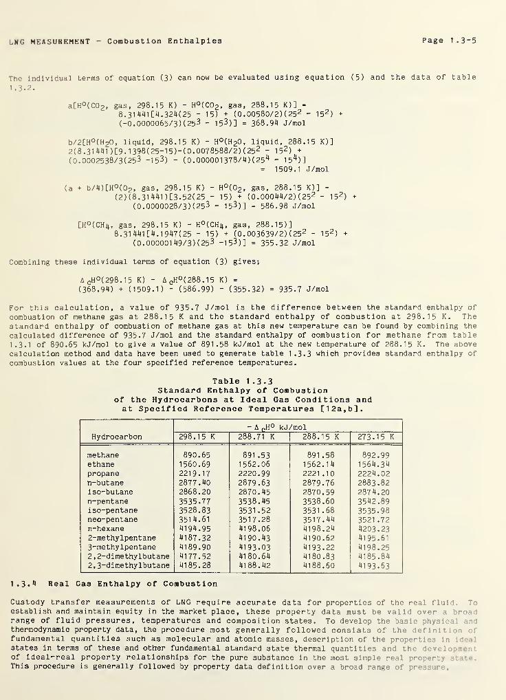
LNG MEASUREMENT Combustion Enthalpies Page 1 .3“5
The individual terms of equation (3) can now be evaluated using equation (5) and the data of table
1 . 3 . 2 .
a[H°(C0 2 , gas, 298.15 K) - H°(C0 2 , gas, 288.15 K)] =
8. 31 H^l [4 .324(25 - 15) + (0.00580/2) (25 2 -1
5
2)
+
(-0.0000065/3) (25^ - 153)] = 368.94 J/mol
b/2[H°(H 20, liquid, 298.15 K) - H°(H 20, liquid, 288.15 K)]
2(8.31441 ) [ 9 • 1 398(25-1 5 )-(0 . 0078588/2) ( 25 2 - 15 2 )+
(0.0002538/3(253 -153) - (0.000001378/4)(25 4 - 15 4 )]
= 1509.1 J/mol
(a + b/4) [H°(0 2 , gas, 298.15 K) - H°(0 2 , gas, 288.15 K)] =
(2) ( 8 . 31441 )[3. 52(25 - 15) + (0.00044/2) (25 2 - 15 2 )+
(0. 0000028/3) (25 3 - 153)] = 586.98 J/mol
[H°(CH 4 , gas, 298.15 K) - H0 (CHij, gas, 288.15)]8. 31 441 [4 . 1947(25 - 15) + (0. 003639/2) (25 2 - 15 2 )
+
(0.000001 49/3) (25 3 -153)] = 355.32 J/mol
Combining these individual terms of equation (3) gives;
A CH°( 298 . 1 5 K) - A CH°(288.15 K) =
(368.94) + (1509.1) - (586.99) - (355.32) = 935.7 J/mol
For this calculation, a value of 935.7 J/mol is the difference between the standard enthalpy of
combustion of methane gas at 288.15 K and the standard enthalpy of combustion at 298.15 K. Thestandard enthalpy of combustion of methane gas at this new temperature can be found by combining the
calculated difference of 935.7 J/mol and the standard enthalpy of combustion for methane from table1.3.1 of 890.65 kJ/mol to give a value of 891.58 kJ/mol at the new temperature of 288.15 K. The abovecalculation method and data have been used to generate table 1.3.3 which provides standard enthalpy of
combustion values at the four specified reference temperatures.
Table 1.3-3Standard Enthalpy of Combustion
of the Hydrocarbons at Ideal Gas Conditions andat Specified Reference Temperatures [12a, b].
Hydrocarbon
- A nH° kJ/mol298.15 K 288.71 K 288.15 K 273.15 K
methane 890.65 891 .53 891 .58 892.99ethane 1560.69 1562.06 1562.14 1564.34propane 2219.17 2220.99 2221 .10 2224.02n-butane 2877.40 2879.63 2879.76 2883.82iso-butane 2868.20 2870.45 2870.59 2874.20n-pentane 3535.77 3538.45 3538.60 3542.89iso-pentane 3528.83 3531 .52 3531 .68 3535.98neo-pentane 3514.61 3517.28 3517.44 3521 .72n-hexane 4194.95 4198.06 4198.24 4203.232-methylpentane 4187.32 4190.43 4190.62 4195.613-methylpentane 4189.90 4193-03 4193-22 4198.252 , 2-dimethylbutane 4177.52 4180.64 4180.83 4185.842 ,
3
_dimethylbutane 4185.28 4188.42 4188.60 4193-63
1.3.4 Real Gas Enthalpy of Combustion
Custody transfer measurements of LNG require accurate data for properties of the real flul :.
establish and maintain equity in the market place, these property data must be valid over 1 r r
range of fluid pressures, temperatures and composition states. To develop the basic phyni . r. :
thermodynamic property data, the procedure most generally followed consists of the deflni* .•.
fundamental quantities such as molecular and atomic masses, description of the properties in .
states in terms of these and other fundamental standard state thermal quantities and the devcl pmon*of ideal-real property relationships for the pure substance in the most simple real property '
This procedure is generally followed by property data definition over a broad range of pressure.
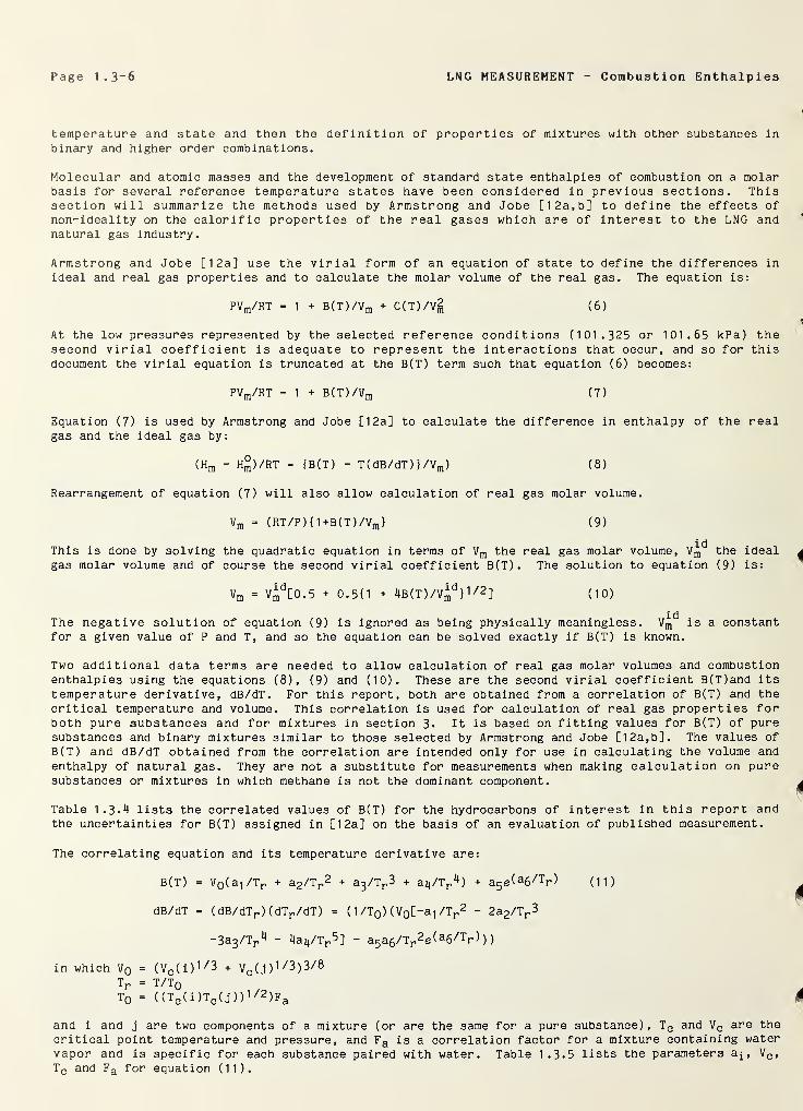
Page 1 .3-6 LNG MEASUREMENT Combustion Enthalpies
temperature and state and then the definition of properties of mixtures with other substances in
binary and higher order combinations.
Molecular and atomic masses and the development of standard state enthalpies of combustion on a molarbasis for several reference temperature states have been considered in previous sections. Thissection will summarize the methods used by Armstrong and Jobe [12a,b] to define the effects of
non-ideality on the calorific properties of the real gases which are of interest to the LNG andnatural gas industry.
Armstrong and Jobe [12a] use the virial form of an equation of state to define the differences in
ideal and real gas properties and to calculate the molar volume of the real gas. The equation is:
PVm/RT = 1 + B(T)/Vm + C(T)/Vg ( 6 )
At the low pressures represented by the selected reference conditions (101.325 or 101.65 kPa) thesecond virial coefficient is adequate to represent the interactions that occur, and so for thisdocument the virial equation is truncated at the B(T) term such that equation ( 6 ) becomes:
PVm/RT = 1 + B(T)/Vm (7)
Equation (7) is used by Armstrong and Jobe [12a] to calculate the difference in enthalpy of the realgas and the ideal gas by:
(Hm - H°)/RT = {B(T) - T(dB/dT)}/Vm ) (8)
Rearrangement of equation (7) will also allow calculation of real gas molar volume.
Vm = (RT/P) { 1 +B(T ) /
V
m } (9)
This is done by solving the quadratic equation in terms of Vm the real gas molar volume, the ideal
gas molar volume and of course the second virial coefficient B(T). The solution to equation (9) is:
vm = Vmd[0.5 + 0.5(1 + 4B(T)/Vm
d}1/2
] (10)
The negative solution of equation (9) is ignored as being physically meaningless. V^d
is a constantfor a given value of P and T, and so the equation can be solved exactly if B(T) is known.
Two additional data terms are needed to allow calculation of real gas molar volumes and combustionenthalpies using the equations ( 8 ), (9) and (10). These are the second virial coefficient B(T)and its
temperature derivative, dB/dT. For this report, both are obtained from a correlation of B(T) and thecritical temperature and volume. This correlation is used for calculation of real gas properties forboth pure substances and for mixtures in section 3. It is based on fitting values for B(T) of puresubstances and binary mixtures similar to those selected by Armstrong and Jobe [12a, b]. The values of
B ( T ) and dB/dT obtained from the correlation are intended only for use in calculating the volume and
enthalpy of natural gas. They are not a substitute for measurements when making calculation on puresubstances or mixtures in which methane is not the dominant component.
Table 1.3.4 lists the correlated values of B(T) for the hydrocarbons of interest in this report andthe uncertainties for B(T) assigned in [12a] on the basis of an evaluation of published measurement.
The correlating equation and its temperature derivative are:
B(T) = V0 (a-|/Tr + a2/Tr2 + a
3/Tp 3 + 34/^) + a5 e(
a6/Tr) (11)
dB/dT = (dB/dTr )(dTr/dT) = ( 1 /T0 ) (V0 [-a 1/Tr
2 - 2a2/Tp3
~3a3/Tr1< - 4a4/Tr5] - a5ag/Tr
2e( a 6 /Tr ) )
)
in which Vq = (Vc (i)1 /3 + Vc (j)
1 /3)3/8
T r = T/TqT0 = ((Tc (i)Tc (j))1/
2 )Fa
and i and j are two components of a mixture (or are the same for a pure substance), Tc and Vc are the
critical point temperature and pressure, and Fa is a correlation factor for a mixture containing water
vapor and is specific for each substance paired with water. Table 1.3*5 lists the parameters a^, Vc ,
Tc and Fa for equation (11).
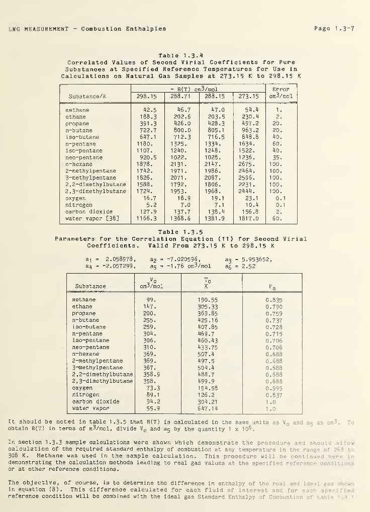
LNG MEASUREMENT Combustion Enthalpies Page 1 .3“7
Table 1 . 3 .
4
Correlated Values of Second Virial Coefficients for PureSubstances at Specified Reference Temperatures for Use in
Calculations on Natural Gas Samples at 273.15 K to 298.15 K
Substance/K
- B(T) cm3/mol Errorcm3/mol298.15 288.71 288.15 273.15
methane 42.5 46.7 47.0 54.4 1 .
ethane 188.3 202.6 203.5 230.4 2.
propane 391 .3 426.0 428.3 497.2 20.
n-butane 722.7 800.0 805.1 963.2 20.
iso-butane 647.1 712.3 716.5 848.8 40.
n-pentane 1180. 1325. 1334. 1 634. 60.
iso-pentane 1107. 1240. 1248. 1522. 40.
neo-pentane 920.5 1022. 1028. 1236. 35.
n-hexane 1878. 2131 • 21 47. 2675. 100.2-methylpentane 1742. 1971 . 1986. 2464. 100.
3-methylpentane 1826. 2071 . 2087. 2596. 100.
2 ,2-dimethylbutane 1588. 1792. 1806. 2231 . 100.
2
,
3-dimethylbutane 1724. 1953. 1968. 2444. 100.
oxygen 16.7 18.9 19.1 23.1 0.1
nitrogen 5.2 7.0 7.1 10.4 0.1
carbon dioxide 127.9 137.7 138.4 156.8 2.
water vapor [ 38 ] 1166.3 1368.6 1381 .9 1817.0 60.
Table 1.3.5Parameters for the Correlation Equation (11) for Second Virial
Coefficients. Valid From 273-15 K to 298.15 K
a1
= 2.058978, a2 = -7.020596, a3 = 5.953652,
ai| = -2.057299, 35 = - 1.76 cm3/mol a5 = 2.52
Substance cm3/molT cK Fa
methane 99. 190.55 0.835ethane 147. 305.33 0.790propane 200. 369.85 0.759n-butane 255. 425.16 0.737iso-butane 259. 407.85 0.728n-pentane 304. 469.7 0.715iso-pentane 306. 460.43 0.706neo-pentane 310. 433.75 0.706n-hexane 369. 507.4 0.6882-methylpentane 369. 497.5 0.6883-methylpentane 367. 504.4 0.6882 , 2-dimethylbutane 358.9 488.7 0.6882 , 3-dimethylbutane 358. 499.9 0.688oxygen 73.3 154.58 0.995nitrogen 89.1 126.2 0.837carbon dioxide 94.2 304.21 1 .0water vapor 55.9 647.14 1 .0
It should be noted in table 1.3.5 that B(T) is calculated in the same units as V c and a 5 asobtain B(T) in terms of m3/mol, divide Vc and by the quantity 1 x 10^.
In section 1.3-3 sample calculations were shown which demonstrate the procedure and sbcalculation of the required standard enthalpy of combustion at any temperature in the r
308 K. Methane was used in the sample calculation. This procedure will be continueddemonstrating the calculation methods leading to real gas values at the specif:* : v <
or at other reference conditions.
The objective, of course, is to determine the difference in enthalpy of the ref m : 1
in equation (8). This difference calculated for each fluid of interest and for •
reference condition will be combined with the ideal gas Standard Enthalpy of Combust; 1 r • • '
.
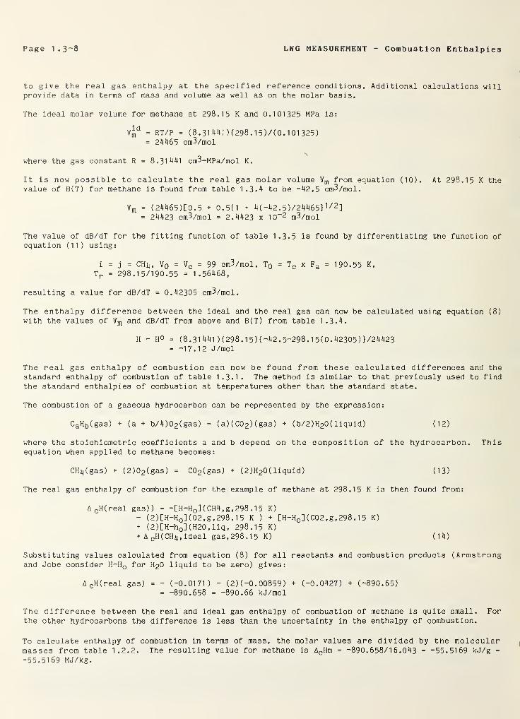
Page 1 .3-8 LNG MEASUREMENT - Combustion Enthalpies
to give the real gas enthalpy at the specified reference conditions. Additional calculations willprovide data in terms of mass and volume as well as on the molar basis.
The ideal molar volume for methane at 298.15 K and 0.101325 MPa is:
= RT/P = ( 8 . 3144; > ( 298 . 1 5 ) /( 0 . 101325)= 24465 cm3/mol
where the gas constant R = 8.31441 cnP-MPa/mol K.
It is now possible to calculate the real gas molar volume Vm from equation (10). At 298.15 K thevalue of B(T) for methane is found from table 1.3.4 to be -42.5 cm3/mol.
Vm = ( 24465 ) [0 . 5 + 0.5{1 + 4( -42 . 5 ) /24465
}
1 /2]
= 24423 cm3/mol = 2.4423 x 10~2 m3/mol
The value of dB/dT for the fitting function of table 1.3.5 is found by differentiating the function ofequation ( 11 ) using:
i = j = CH 4 , V0 = V c = 99 cm3/mol, T0 = T c x Fa = 190.55 K,
Tr = 298.15/190.55 = 1.56468,
resulting a value for dB/dT = 0.42305 cm3/mol.
The enthalpy difference between the ideal and the real gas can now be calculated using equation ( 8 )
with the values of Vm and dB/dT from above and B(T) from table 1.3.4.
H - H° = (8.31441 )(298.15){-42. 5-298. 15(0. 42305)1/24423= -17.12 J/mol
The real gas enthalpy of combustion can now be found from these calculated differences and thestandard enthalpy of combustion of table 1.3.1. The method is similar to that previously used to findthe standard enthalpies of combustion at temperatures other than the standard state.
The combustion of a gaseous hydrocarbon can be represented by the expression:
CaHb(gas) + (a + b/ 4 ) 02 (gas) = (a) (CO2 ) (gas) + (b/ 2 )H20 ( liquid) (12)
where the stoichiometric coefficients a and b depend on the composition of the hydrocarbon. Thisequation when applied to methane becomes:
CHij(gas) + ( 2 )C>2 (gas) = C02 (gas) + (2)H 20( liquid) (13)
The real gas enthalpy of combustion for the example of methane at 298.15 K is then found from:
A CH( real gas)) = -[H-H0 ] (CH4 , g, 298 . 1 5 K)
- (2) [H-H0 ] (02 , g, 298 . 1 5 K ) + [H-H 0 ] (C02 ,g, 298 . 1 5 K)
+ (2)[H-ho ](H20,liq, 298.15 K)
+ A cH(CH 4 , ideal gas.298.15 K) (14)
Substituting values calculated from equation ( 8 ) for all reactants and combustion products (Armstrongand Jobe consider H-H 0 for H2O liquid to be zero) gives:
A cH(real gas) = - (-0.0171 )- (2) (-0. 00859) + (-0.0427) + (-890.65)
= -890.658 = -890.66 kJ/mol
The difference between the real and ideal gas enthalpy of combustion of methane is quite small. Forthe other hydrocarbons the difference is less than the uncertainty in the enthalpy of combustion.
To calculate enthalpy of combustion in terms of mass, the molar values are divided by the molecularmasses from table 1.2.2. The resulting value for methane is AcHm = -890.658/16.043 = -55.5169 kJ/g =
-55.5169 MJ/kg.
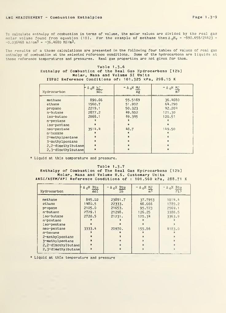
LNG MEASUREMENT Combustion Enthalpies Page 1 .3~9
To calculate enthalpy of combustion in terms of volume, the molar values are divided by the real gas
molar volume found from equation (10). For the example of methane then A CH V = -890.658/241123 =
-0.036468 kJ/cm3 = -36.4680 MJ/m3.
The results of a these calculations are presented in the following four tables of values of real gas
enthalpy of combustion at the selected reference conditions. Some of the hydrocarbons are liquids at
these reference temperatures and pressures. Real gas properties are not given for them.
Table 1.3.6Enthalpy of Combustion of the Real Gas Hydrocarbons [12b]
Molar, Mass and Volume SI UnitsIUPAC Reference Conditions of: 101.325 kPa, 298.15 K
Hydrocarbon
- A CH kJ
mol
- A CH MJ
kg
- A PH MJ
m?
methane 890.66 55.5169 36.4680ethane 1560.7 51 .902 64.290propane 2219.1 50.323 92.204n-butane 2877.2 49.502 121 .30
iso-butane 2868.1 49.345 120.51n-pentane * * *
iso-pentane * * *
neo-pentane 3514.4 48.7 149.50n-hexane * * *
2-methylpentane * * #
3-methylpentane * * *
2 , 2-dime thylbutane * * *
2 ,
3
-dimethylbutane * * *
* Liquid at this temperature and pressure.
Table 1-3-7Enthalpy of Combustion of The Real Gas Hydrocarbons [12b]
Molar, Mass and Volume U.S. Customary UnitsANSI /ASTM/API Reference Conditions of : 101.560 kPa, 288.71 K
Hydrocarbon
- A CH Btumol
- A CH Btulb
- A pH MJ
m3”
- A CH BtuTU
methane 845.02 23891 .7 37.7953 1014.4ethane 1480.5 22333. 66.666 1789.2propane 2105.0 21653. 95.723 2569.1n-butane 2729.1 21298. 126.25 3388.5iso-butane 2720.5 21231
.
125.34 3363.9n-pentane # * * #
iso-pentane * * # #
neo-pentane 3333.4 20970. 155.86 4183.0n-hexane * * # #
2-methylpentane * * * #
3-methylpentane * # # #
2, 2-dimethylbutane * * # *
2 ,
3
-dimethylbutane * * # #
* Liquid at this temperature and pressure
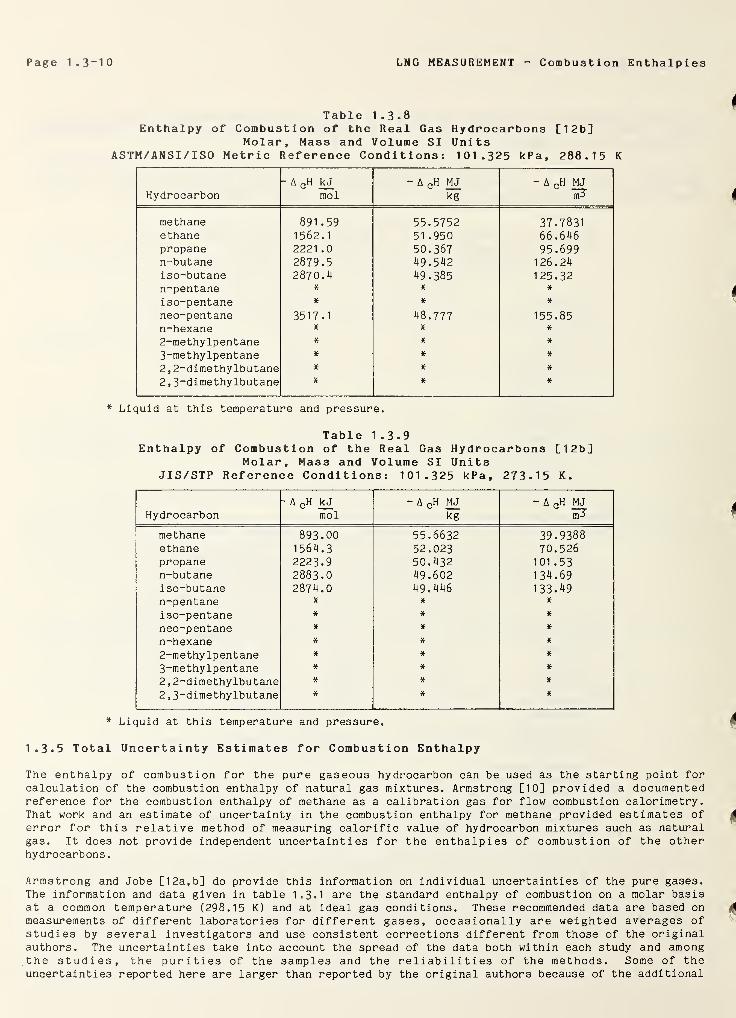
Page 1 .3-10 LNG MEASUREMENT Combustion Enthalpies
Table 1.3.8Enthalpy of Combustion of the Real Gas Hydrocarbons [12b]
Molar, Mass and Volume SI UnitsASTM/ANSI/ISO Metric Reference Conditions: 101.325 kPa, 288.15 K
Hydrocarbon
- A CH _kJ
mol
- A CH MJ
kg
- A CH MJ
methane 891.59 55.5752 37.7831ethane 1562.1 51 .950 66.646propane 2221 .0 50.367 95.699n-butane 2879.5 49.542 126.24iso-butane 2870.4 49.385 125.32n-pentane * * *
iso-pentane * * *
neo-pentane 3517.1 48.777 155.85n-hexane # * *
2-methylpentane * * *
3-methylpentane * * #
2 , 2-dimethylbutane * * #
2 , 3-dimethylbutane * * #
* Liquid at this temperature and pressure.
Table 1.3.9Enthalpy of Combustion of the Real Gas Hydrocarbons [12b]
Molar, Mass and Volume SI UnitsJIS/STP Reference Conditions: 101.325 kPa, 273-15 K.
Hydrocarbon
- A CH kJ
mol
- A CH MJkg
- A 0H MJ
methane 893.00 55.6632 39.9388ethane 1564.3 52.023 70.526propane 2223.9 50.432 101 .53n-butane 2883.0 49.602 134.69iso-butane 2874.0 49.446 133.49n-pentane # * #
iso-pentane * # *
neo-pentane * * *
n-hexane * * *
2-methylpentane * * *
3-methylpentane * * *
2 , 2-dimethylbutane * * #
2 , 3-dimethylbutane * # #
* Liquid at this temperature and pressure.
1.3.5 Total Uncertainty Estimates for Combustion Enthalpy
The enthalpy of combustion for the pure gaseous hydrocarbon can be used as the starting point forcalculation of the combustion enthalpy of natural gas mixtures. Armstrong [10] provided a documentedreference for the combustion enthalpy of methane as a calibration gas for flow combustion calorimetry.That work and an estimate of uncertainty in the combustion enthalpy for methane provided estimates oferror for this relative method of measuring calorific value of hydrocarbon mixtures such as naturalgas. It does not provide independent uncertainties for the enthalpies of combustion of the otherhydrocarbons
.
Armstrong and Jobe [12a, b] do provide this information on individual uncertainties of the pure gases.The information and data given in table 1.3.1 are the standard enthalpy of combustion on a molar basisat a common temperature (298.15 K) and at ideal gas conditions. These recommended data are based on
measurements of different laboratories for different gases, occasionally are weighted averages ofstudies by several investigators and use consistent corrections different from those of the originalauthors. The uncertainties take into account the spread of the data both within each study and amongthe studies, the purities of the samples and the reliabilities of the methods. Some of theuncertainties reported here are larger than reported by the original authors because of the additional
LNG MEASUREMENT Combustion Enthalpies Page 1 . 3-11
factors considered. For data at temperatures other than 298.15 K (see table 1.3.1) and for the realgases there are additional uncertainties in the heat capacities and the virial coefficients. Theseare, however, smaller than those in the enthalpies of combustion. For details, the reader is referredto Armstrong and Jobe [12a, b].
The basic thermal data of table 1.3.6 through table 1.3.9, when combined with the data on molecularmass of table 1.2.1 and the pure component real gas densities at various reference states of tables1.2.14 through 1.2.12e, are the required base physical and thermal properties data and uncertaintiesnecessary to support the measurements considered in the following parts of this manual.

LNG MEASUREMENTS References Page 1 . 4-1
1 . 4 References
[1] Ackerson, B. J. and G. C. Straty, Rayleigh scattering from methane, J. Chem. Phys. _6£, No. 3,
1207-12 (1978).
[2] Ackerson, B. J. and H. J. M. Hanley, The thermal diffusivity of methane in the critical region,
Chem. Phys. Letters ^3, 596 (1978).
[3] American National Standards Institute, Base conditions of pressure and temperature for the
volumetric measurement of natural gas, ANSI Standard Z 132.1 1969, API Standard 2562, Am. Pet.
Inst., New York, NY(1969).
[4] American Petroleum Institute, Measuring, sampling, testing and base conditions for natural gas
fluids, Am. Pet. Inst., Publ. 2529, 3rd Ed., p 1 (1979).
[5] American Petroleum Institute, Research Project 44, Selected values of properties of hydrocarbonsand related compounds, data sheets, Texas A&M University, College Station, TX(1973).
[6] American Petroleum Institute, Technical Data Book- Petroleum Refining, American PetroleumInstitute, Washington, D. C. (1970).
[7] American Society for Testing and Materials Committee D~3 on Gaseous Fuels, Standard methods for
volumetric measurement of gaseous fuel samples, ANSI/ASTM D 1071~78a, Part 26, Am. Soc. Testingand Materials, Philadelphia, Pa (1980).
[8] American Society for Testing and Materials Committee D~3 on Gaseous fuels, Standard methanethermophysical property tables, ASTM D 3956-82, Am. Soc. Testing and Materials, Philadelphia, PA
( 1982 ).
[9] American Society for Testing and Materials, Standard methods for volumetric measurement of
gaseous fuel samples, ANSI/ASTM D 1071~78a, Am. Soc. Testing and Materials, Philadelphia, PA
( 1980 ).
[10] Armstrong, G. T., Calculation of the heating value of a sample of high purity methane for use asa reference material, Nat. Bur. Stand. (U.S.), Tech. Note 299, 19 pp (December, 1966).
[11] Armstrong, G. T., Hydrocarbons for fuel- 75 years of research at NBS, Nat. Bur. Stand. (U.S),Special Publ. 434, 20 pp (May, 1976).
[12] a) Armstrong, G. T. and T. L. Jobe, Jr., Heating values of natural gas and its components, Nat.Bur. Stand. (U.S.), NBSIR 82-2401, 168 pp (August, 1982).b) Garvin, D., E. S. Domalski, G. R. Somayajulu, R. C. Wilhoit and K. N. Marsh, PhysicalProperties of Pure Components of Natural Gas, (to be presented at the International Congress onGas Quality, Groningen, Netherlands, April 22-25, 1986).
[13] Armstrong, G. T.,E. S. Domalski and J. I. Minor, Jr., Standard combustion data for the fuel gasindustry, Am. Gas Assoc. Operating Section Proc., pp D-74 to D-88 (1972).
[14] Cameron, A. E. and Wichers, E. J., Report of the international commission on atomic weights1961, J. Am. Chem. Soc., 84_, pp 4175 (1962).
[15] Canjar, L. N. and F. S. Manning, Thermodynamic properties and reduced correlations for gases
,
Gulf Publishing Co., Houston, TX(1967).
[16] Das, T. R., C. 0. Reed and P. T. Eubank, PVT surface and thermodynamic properties of n-perr e
J. Chem. Eng. Data, 22, No. 1, 3~9 ( 1 977 )
.
[17] Das, T. R., C. 0. Reed and P. T. Eubank, PVT surface and thermodynamic properties of isopentane,J. Chem. Eng. Data, _22, No. 1, 9-15 (1977).
[18] Das, T. R., C. 0. Reed and P. T. Eubank, PVT surface and thermodynamic properties of re*
Chem. Eng. Data, 22, No. 1, 16-21 (1977).
Page 1 . 4-2 LNG MEASUREMENTS References
[19] Diller, D. E., Editor, LNG Materials and fluids users manual, Supplement 1 (see [50,55]), Nat.Bur. Stand. (U.S. ) , Boulder, Co 80303 (1979).
[20] Domalski, E. S., J. Phys. Chem. Reference Data, _1_, pp 221-77 (1972).
[21] Dymond, J. H. and E. B. Smith, The virial coefficients of pure gases and mixtures, ClarendonPress, Oxford UK, 536 pp (1980).
[22] Goldman, D. T. and R. J. Bell, Editors, The international system of units (SI), Nat. Bur. Stand.(U.S. ) , Special Pub. 330, 48 pp (December, 1981).
[23] Good, W. D., J. Chem. Thermodynamics, _2, pp 237~244 (1970).
[24] Goodwin, R. D., The thermophysical properties of methane from 90 to 500 K at pressures to 700bar, Nat. Bur. Stand. (U.S. ) , Tech. Note 653, 280 pp(April 1974).
[25] Goodwin, R. D., Provisional thermodynamic properties of propane, from 85 to 700 K at pressuresto 700 bar, Nat. Bur. Stand. (U.S .) , NBSIR 77~860, 239 pp, (July 1977).
[26] Goodwin, R. D., On the non-analytic equation of state for propane, Adv. Cryo. Eng. 23, 611,Plenum Press, NY (1978).
[27] Goodwin, R. D., Specific heats of saturated and compressed liquid propane, J. Res. Nat. Bur.
Stand. (U.S.) 83 , No. 5, 449~58(Sept. 1 978)
.
[28] Goodwin, R. D., The nonanalytic equation of state for pure fluids applied to propane, Adv. in
Chem., Ser. No. 182, Am. Chem. Soc., Washington, D. C., 345-64 (1979).
[29] Goodwin, R. D., H. M. Roder and G. C. Straty, Thermophysical properties of ethane from 90 to 600K at pressures to 700 bar, Nat. Bur. Stand. (U.S.), Tech. Note 684, 320 pp(August 1976).
[30] Goodwin, R. D. and R. Prydz, Densities of compressed liquid methane and the equation of state,J. Res. Nat. Bur. Stand. (U.S.), 76A, 81 (1972).
[31] Goodwin, R. D. and W. M. Haynes, Thermophysical properties of propane from 85 to 700 K atpressures to 70 MPa, Nat. Bur. Stand. (U.S.), Monograph 170, 249 pp (April, 1982).
[32] Goodwin, R. D. and W. M. Haynes, Thermophysical properties of isobutane from 114 to 700 K atpressures to 70 MPa, Nat. Bur. Stand. (U.S. ) , Tech. Note 1051, 196 pp, (January, 1982)
.
[33] Haynes, W. M. and R. D. Goodwin, Thermophysical properties of normal butane from 135 to 700 K at
pressures to 70 MPa, Nat. Bur. Stand. (U.S.), Monograph 169, 197 pp (April, 1982).
[34] Haynes, W. M. , Orthobaric liquid densities of normal butane from 135 to 300 K, paper M-6, Adv.
Cryo. Eng. _21_, 516-21, Plenum Press, NY( 1 976 )
.
[35] Haynes, W. M. and M. J. Hiza, Measurements of the orthobaric liquid densities of methane,ethane, propane, isobutane & normal butane, J. Chem. Thermodynamics 9_, 179 (1977).
[ 36 ] Hiza, M. J., An empirical excess volume model for estimating LNG densities, Fluid PhaseEquilibria, 2_, pp 27 _38, Elsevier Scientific Publishing Company, Amsterdam( 1 978)
.
[37] Gas Producers Association Publication 2172, Calculation of gross heating value, relative densityand compressibility factor for natural gas mixtures from composition analysis, Appendix (1984).
[ 38 ] Haar,L., J. S. Gallagher and F. S. Kell, NBS/NCA steam tables, Hemisphere Pub. Corp. Washington,D.C. (1984).
[39] IUPAC Commision on Thermodynamics, Manual of symbols and terminology for physicochemicalquantities and units. Pure and Applied Chem., 51 , pp 393“400 (1979).
[40] IUPAC Commission on Atomic Weights and Isotopic Abundances, Atomic weights of the elements 1981,
Pure and Applied Chem., _55, 1119 (1983).
[41] IUPAC Commission on Atomic Weights, Atomic weights of the elements, Pure and Applied Chem., 30 .
pp 637-49 (1972).
LNG MEASUREMENTS References Page 1 . 4-3
C42]
[43]
[^]
[45]
[46]
[ 47 ]
[48]
[49]
[50]
[51]
[52]
[53]
[54]
[55]
[56]
[57]
[58]
[59]
[60]
[61]
[ 62 ]
[ 63 ]
IUPAC Commission on Thermodynamics and Thermochemistry, A guide to procedures for the
publication of thermodynamic data, J. Pure and Applied Chem., _29_, 399-408(1972).
IUPAC Commission on Thermodynamics, Manual of symbols and terminology for physiochemicalquanties and units, Appendix IV, _54, 1239-1250 (1982).
International Bureau of Weights and Measures (BIPM), Le systeme international d'unites, 1970,
OFFILIB, 84 Rue Gay-Lussac, F. 75005 Paris (1977).
International Organization for Standardization, Petroleum liquids and gases - measurement -
standard reference conditions, ISO 5024-1976 (E), Int. Org. Std. (1976).
Jacobsen, R. T., R. B. Steward, R. D. McCarty and H. J. M. Hanley, Thermophysical properties of
nitrogen from the fusion line to 3500 R for pressures to 150,000 psia, Nat. Bur. S tand . ( U . S . ) ,
Tech. Note 648, 162 pp(December 1973).
Japanese Industrial Standards Committee, Methods for chemical analysis and testing of fuel gasesand natural gas, Japanese, Ind. Stand., JIS K 2301-1980, Japanese Stand. Assoc., Tokyo, Japan( 1980 ).
Kelso, E. A. and W. A. Felsing, The pressure-volume-temperature relations of n-hexane and of
2-methylpentane, J. Am. Chem. Soc., _62 ( 1 1 ) , 3132 (1940).
Kudchadker, A. P., G. H. Alani and B. J. Zwolinski, The critical constants of organicsubstances, Chem Rev. _68^, No. 6, 659-673 (1968).
Mann, D. B., Editor, LNG Materials and fluids user's manual, first edition, Nat. Bur. Stand.(U.S.), Boulder, Co 80303(1977).
McCarty, R. D., Interactive FORTRAN IV computer programs for the thermodynamic and transportproperties of cryogens, Nat. Bur. Stand. (U.S.), Tech. Note 1025, 112 pp(0ctober, 1980).
McCarty, R. D., A modified Benedict-Webb-Rubin equation of state for methane using recentexperimental data, Cryogenics J_4, No. 5, 276-80 (May, 1974).
McClune, C. R., Measurement of the densities of liquefied hydrocarbons from -100 to — 1 8 0 C (173- 93 K), Cryogenics 16, 289-95(1976).
Mopsik, F. I., Dielectric constant of n-hexane as a function of temperature, pressure anddensity, J. Research Nat. Bur. Stand., 71A(4) (1967)
-
Olien, N. A., Editor, LNG Materials and fluids user's manual, Supplement 2, Nat. Bur. Stand.(U.S.), Boulder, CO 80303(1980).
Olson, J. D., The refractive index and Lorenz-Lorentz function of fluid methane, J. Chem. Phvs.
63, 474 (1975).
Orrit, J. and J. M. Laupretre, Density of liquefied natural gas constituents, Adv. Cryo. : 'ng.,
23, 573-9, Plenum Press, NY(1978).
Prydz, R., and R. D. Goodwin, Experimental melting and vapor pressures of methane, J. .
Thermodynamics _4, 127 (1972).
Reid, R. C., J. H. Prausnitz and T. K. Sherwood, The properties of gases and liquid.’, -t :
McGraw-Hill Book Co., New York, NY, 688 pp (1977).
Roder, H. M. , Heats of transition of solid ethane, J. Chem. Phys. _65^, 1371 (1976).
Roder, H. M., Measurements of the specific heats, C and Cv of dense gaseous and ii . .. ,
J. Res. Nat. Bur. Stand (U.S.), 80A , p 739 (1976).
Shim, J. and J. P. Kohn, J. Chem. Eng. Data, 7(1), pp 3—8 ( 1 962 )
.
Stewart, D. E., Volumetric behavior of n-hexane in the liquid phase, Ind.2529 (1954).
Page 1.4-4 LNG MEASUREMENTS References
[64] Straty, G. C., Hypersonic velocities in saturated and compressed fluid methane, Cryogenics 15,
729 (1975).
[65] Straty, G, C., Velocity of sound in dense fluid methane, Cryogenics, J_4, 367 (1974).
[66] Straty, G, C. and D. E. Diller, PVT properties of saturated and compressed fluid nitrogen, J.
Chem. Thermodynamics, 12 , 927(1980).
[67] Straty, G. C. and R. D. Goodwin, Dielectric constant and polarizability of saturated andcompressed fluid methane, Cryogenics J_3» 712 (1973).
[68] Straty, G. C. and R. Tsumura, Phase transition and melting pressures of solid ethane, J. Chem.Phys. 64_, 859 (1976).
[69] Straty, G. C. and R. Tsumura, PVT and vapor pressure measurements on ethane, J. Res. Nat. Bur.
Stand. (U.S. ) , 80a, 35 (1976).
[70] Strobridge, T. R., The thermodynamic properties of nitrogen from 64 to 300 K between 0.1 and 200atmospheres, Nat. Bur. Stand. (U.S. ) , Tech. Note 129, 85 pp(January, 1962).
[71] Tsumura, R. and G. C. Straty, Speed of sound in saturated and compressed fluid ethane,Cryogenics j_7_, 193 (1977).
[72] U.S. Department of Commerce, National Bureau of Standards, Guidlines for use of the modernizedmetric system, Nat. Bur. Stand. (U.S.), Dimensions, LC 1120, pp 12-19 (December, 1979).
[73] Vargaftik, N. B., Tables on the thermophysical properties of liquids and gases, John Wiley &
Sons, NY, Second Ed. 262-65(1975).
[74] Weber, J. H., Thermodynamic properties of n-hexane, AICHE J. _2(4), 514 (1954).
[75] Weber, L. A., Dielectric constant data and derived Clausius-Mossotti function for compressedgaseous & liquid ethane, J. Chem. Phys. 65_, 446 (1976).
[76] Weber, L. A., Some vapor pressure and PVT data on nitrogen in the range 65 to 140 K, J. Chem.Thermodynamics _2, 839 (1970).
[77] Younglove, B. A., The specific heats, C and Cv of compressed and liquefied methane, J. Res. Nat.
Bur. Stand. (U.S.) , 78A, 401 (1974).
[78] Younglove, B, A. .Velocity of sound in liquid propane, J. Res. Nat. Bur. Stand. (U.S.) 86_, No. 2,
l65-70(March, 1981).
[ 79 ] Pittam, D. A . and G. Pilcher, J. Chem. Soc., Faraday Trans . I, 68, 2225-2229 (1972).
[80] Rossini
,
,F. D., J. Res. Nat. Bur. Stand. (U.S.), 6, 37-49 , 329-330 (1931 ).
[81] Prosen
,
(1951 ).
E. J . , F . W. Maron and F. D. Rossini , J . Res . Nat. Bur. Stand. (U.S.)
[82] Rossini
,
,F. D . , J . Res . Nat
.
Bur. Stand. (U.S.),]_2 ,
735-'750 (1934).
[83] Scott, D. W., J. Chem. Phys., 60, 3144-3165 (1974).
[84] Pines, H., B. Kvetinskas, L. S. Kassel, and V. N. Ipatieff, J. Am. Chem. Soc., 67_, 631*637(1945).
[85] Good, W. D. and N. K. Smith, J. Chem. Eng. Data, _1_4, 102-106 (1969).
[86] Prosen, E. J. and F. D. Rossini, J. Res. Nat. Bur. Stand. (U.S.), 27, 289~310 (1941).
[ 87 ] Somayajulu, G. R. and B. J. Zwolinski, J. Chem. Soc. Faraday Trans. (2), J2_, 2213 ( 1976).
[88] Evering, B. L. and E. L. d’Ouville, J. Am. Chem. Soc., 71, 440-445 (1949).

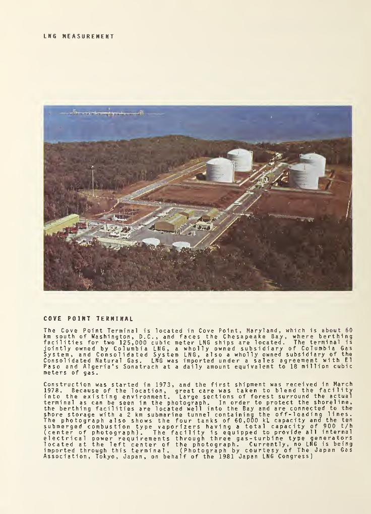
LNG MEASUREMENT
COVE POINT TERMINAL
The Cove Point Terminal is located in Cove Point, Maryland, which is about 60km south of Washington, D.C., and faces the Chesapeake Bay, where berthingfacilities for two 125,000 cubic meter LNG ships are located. The terminal isjointly owned by Columbia LNG, a wholly owned subsidiary of Columbia GasSystem, and Consolidated System LNG, also a wholly owned subsidiary of theConsolidated Natural Gas. LNG was imported under a sales agreement with ElPaso and Algeria's Sonatrach at a daily amount equivalent to 18 million cubicmeters of gas.
Construction was started in 1973, and the first shipment was received in March1978. Because of the location, great care was taken to blend the facilityinto the existing environment. Large sections of forest surround the actualterminal as can be seen in the photograph. In order to protect the shoreline,the berthing facilities are located well into the Bay and are connected to theshore storage with a 2 km submarine tunnel containing the off-loading lines.The photograph also shows the four tanks of 60,000 kL capacity and the tensubmerged combustion type vaporizers having a total capacity of 900 t/h(center of photograph). The facility is equipped to provide all internalelectrical power requirements through three gas-turbine type generatorslocated at the left center of the photograph. Currently, no LNG is beingimported through this terminal. (Photograph by courtesy of The Japan GasAssociation, Tokyo, Japan, on behalf of the 1981 Japan LNG Congress)
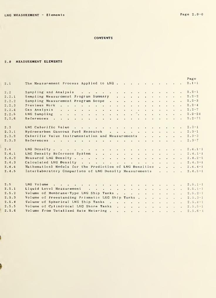
LNG MEASUREMENT E 1 emen t s Page 2.0-0
CONTENTS
2.0
MEASUREMENT ELEMENTS
Page
2.1 The Measurement Process Applied to LNG 2.1-1
2.2 Sampling and Analysis 2.2-1
2.2.1 Sampling Measurement Program Summary 2.2-2
2.2.2 Sampling Measurement Program Scope 2.2-3
2.2.3 Previous Work 2.2-4
2.2.4 Gas Analysis 2.2-7
2.2.5 LNG Sampling " 2.2-24
2.2.6 References 2.2-71
2.3 LNG Calorific Value 2.3-1
2.3.1 Hydrocarbon Gaseous Fuel Research 2.3-1
2.3.2 Calorific Value Instrumentation and Measurements 2.3-32.3.3 References 2.3-7
2.4 LNG Density 2. 4. 1-1
2.4.1 LNG Density Reference System 2.4. 1-1
2.4.2 Measured LNG Density 2. 4. 2-1
2.4.3 Calculated LNG Density 2.4. 3-1
2.4.4 Mathematical Models for the Prediction of LNG Densities .... 2. 4. 4-1
2.4.5 Interlaboratory Comparison of LNG Density Measurements .... 2. 4. 5-1
2.5 LNG Volume 2. 5. 1-1
2.5.1 Liquid Level Measurement 2.5. 1-1
2.5.2 Volume of Membrane-Type LNG Ship Tanks 2. 5. 2-1
2.5.3 Volume of Freestanding Prismatic LNG Ship Tanks 2. 5. 3-1
2.5.4 Volume of Spherical LNG Ship Tanks 2. 5. 4-1
2.5.5 Volume of Cylindrical LNG Shore Tanks 2. 5. 5-1
2.5.6 Volume From Totalized Rate Metering 2. 5. 6-1

.
LNG MEASUREMENT Measurement Process Page 2.1-0
CONTENTS
2.0 MEASUREMENT ELEMENTS
Measurement Process Page
2.1 The Measurement Process Applied to LNG 2.1-1
2.1.1 Introduction 2.1-1
2.1.2 Components of the LNG Measurements Process 2.1-4
2.1.3 Statistical Terms 2.1-4
2.1.4 References 2.1-6


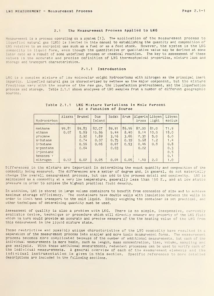
LNG MEASUREMENT Measurement Process Page 2.1-1
2.1 The Measurement Process Applied to LNG
Measurement is a process operating on a system [1]. The application of the measurement process to
liquefied natural gas (LNG) is limited in this manual to establishing the quantity and composition of
LNG relative to an end-point use such as a fuel or as a feed stock. However, the system is the LNGcommodity in liquid form, even though the quantitative or qualitative value may be derived at some
later date as a result of some undefined process or chemical reaction. The key to assessment of these
values is the accurate and precise definition of LNG thermophysical properties, mixture laws and
storage and transport characteristics.
2.1.1 Introduction
LNG is a complex mixture of low molecular weight hydrocarbons with nitrogen as the principal inert
impurity. Liquefied natural gas is characterized by methane as the major component, but the mixturefractions vary with the source of the raw gas, the liquefaction pretreatment, and the liquefactionprocess and storage. Table 2.1.1 shows analyses of LNG samples from a number of different geographicsources.
Table 2.1.1 LNG Mixture Variations in Mole PercentAs a Function of Source
HydrocarbonAlaska Brunei Das
IslandBadak Arum Algeria
ArzewLibyanlight
Libyanmedium
methane 99.81 89.83 82.07 89.91 86.96 87.00 81 .0 71.9ethane 0.07 5.89 15.86 5.44 8.40 8.14 10.0 18.0propane 2.92 1 .89 3.16 3.66 2.30 5.0 6.0n-butane 0.74 0.07 0.75 0.39 0.68 1 .2 1.4
i-butane 0.56 0.06 0.67 0.53 0.46 0.8 0.8n-pentane 0.04 0.03 0.02 0.3i-pentane 0.5hexanes + 0.1
nitrogen 0.12 0.02 0.05 0.04 0.06 1 .40 2.0 1.0
Differences in the mixture are important in determining the exact quantity and composition of thecommodity being measured. The differences are a matter of degree and, in general, do not materiallychange the overall measurement process, but can add to the process detail and complexity. LNG ismaintained as a commodity at a very low temperature, generally less than 150 K., and at low staticpressure in order to achieve the highest practical fluid density.
In addition, LNG is stored in large volume containers to benefit from economies of size and to achievemaximum storage efficiency. The containers have double walls with insulation between the walls in
order to limit heat transport to the cold liquid. Simply weighing the container is not practical, andother techniques of determining quantity must be used.
Assessment of quality is also a problem with LNG. There is no simple, inexpensive, currentlyavailable device, technique or procedure which will directly measure any property of the LNG fluidwhich in turn could provide an accurate and precise measure of the the heating value of the LNG fro-,
this measurement in the liquid mixture state.
These restrictive and possibly unique characteristics of the LNG commodity have resultedseparation of the measurement process into simpler and more basic measurement forms. The measur-process becomes more complicated because of the number of additional measurements, but each of theindividual measurements is more basic, such as length, mass concentration, time, volume, sampling in :
gas analysis. With these additional measurements, redundant processes can be used to verifythe individual measurements. A general overview of each of the measurement elements m ;
••.
individual instrumentation is given in this section. Specific references to more !"t i
;
descriptions are included in the following sections.
Page 2.1-2 LNG MEASUREMENT Measurement Process
2.1.2 Components of the LNG Measurement Process
The quantity of LNG can be measured in terms of mass or of volume. If the fluid density is known,then total mass may be calculated from volume measurements. This method is generally the mostcommonly used with LNG for two reasons; (1) LNG is quite difficult to measure directly because of thevery low fluid temperature, the combustible nature of the the vapor and the fact that the fluid is at
or near its normal boiling point, (2) the LNG storage containers are generally so large in volume thatit is either impractical or impossible to accurately weigh the fluid. As a result, container volumeand LNG density are basic, necessary elements of the LNG measurement process. If the LNG is to beused as a fuel, then the calorific value either on a mass basis or a volume basis will also be a
required measurement element. Thus:
Total calorific value = (calorific value) (density) (volume)
Sampling and Analysis Sampling for analysis of the LNG pipeline flow or the contents of the largecontainers may be used to meet the requirements of the measurement process both in quantity andquality. The sample must, of course, be representative of the entire fluid volume. As the size ofthe container is increased, it becomes more difficult to demonstrate that the sample is trulyrepresentative. A detailed discussion of this very important phase of the LNG measurement problemwill be found in section 2.2.
Calorific Values Qualitative assessment of LNG requires some type of measurement of each individualcomponent fraction or the calorific or heating value of the actual fluid mixture. The measurement ofvolume and fluid density allows calculation of a mass of fluid but does not address either the amountof the individual components which may have value as feed stock or the fuel heating value of the fluidmixture. LNG sampling and analysis will provide quantitative measurements which, when combined withthe total mass measurement, will give the amount of an individual component available from the totalmass
.
A second measure of quality, the calorific or heating value, may be found from the assessment of the
combustion enthalpy of the mixture or by a sum of the individual component combustion enthalpies. Aswill be shown in the following sections on the elements of volume and density, there are also twomethods of finding specific combustion enthalpies of the LNG mixture. The two methods, if used on thesame mixture, should give the same result within the experimental error.
The first method is direct and simple in concept. A representati ve LNG sample is taken and vaporizedat near ambient temperature and pressure. A volume of the mixture is measured and mixed with a knownvolume of air and burned in a specially designed combustion cell. The temperature rise caused by thecombustion process is measured and compared with the temperature rise found with a calibration gas of
known calorific or heating value. The device which accomplishes this process is called a combustioncalorimeter and may also contain a "specific gravity" meter which relates the density of the LNGmixture to that of the calibration gas or to the density of the ambient air. This additionalmeasurement of LNG mixture density will allow calculation of the heating value of the mixture in termsof mass.
The calibration gas used in the combustion calorimeter may be a pure fluid such as methane or a
precisely characterized mixture which closely resembles the actual LNG mixture. The lattercalibration gas should be used with LNG containing relatively large amounts of the heavierhydrocarbons , because the accuracy of the combustion calorimeter measurement can be improved if theknown heating value of the calibration gas is near that of the actual LNG mixture. Values of theenthalpy of combustion and other related property data are given in sections 1.2 and 1.3 of thismanual. A description of current devices and methods of operation are given in section 2.3.
The second method of determining the calorific or heating value of the LNG fluid mixtures requires LNGsampling and mixture component analysis. Combustion enthalpies for each of the components can be
found from section 1.3 and combined to give a predicted heating value of the real gas mixture. A
discussion of the methods are given in sections 2.2, 2.3 and 3.
Density Measurement Direct measurement of LNG density can be accomplished by placing the densitymeasuring device (densimeter) directly in the LNG. At the present time, all available commercialfield-type LNG densimeters are of the relative type and must be calibrated at the conditions of
intended use.
Several different types of densimeters have been successfully tested and used in LNG service. The
least complicated device from the standpoint of a simple primary measurement element is thecapacitance type. Electrically isolated plates are installed in the liquid container, and
LNG MEASUREMENT Measurement Process Page 2 . 1-3
measurements of the dielectric constant of the liquid are made and compared to known correlations of
LNG density and dielectric properties. Precision of the device can be quite good, but the accuracy
has been found to depend on the mixture and is sensitive to the quantity of nitrogen. A continuousmixture analysis is required to achieve highest accuracy.
A second type of LNG densimeter is based on a primary element which is caused to vibrate at a measured
frequency. The actual frequency can be shown to be a function of the density of the fluid in which
the primary element is immersed. Two different physical configurations of vibrating elementdensimeters have been used with LNG. These are a flat plate and a cylinder. Both configurations have
performed well under test.
A third type of LNG densimeter is based on the Archimedes principle which relates the buoyancy of a
fluid to its density. The actual instrument consists of a float which is weighed by an electricbalance. The density of the LNG is found by comparing the apparent weight of the float in LNG to that
of the calibration fluid. This device has the potential to perform as an absolute densimeter by
careful calibrations in vacuum and has been configured in this way in the laboratory environment. A
more detailed description of this and the other densimeters is given in section 2.4.
LNG density may be found by calculation using mathematical models which relate various properties of
the fluid mixture. Pressure and temperature of the liquid LNG are certainly two of the most oftenused independent variables. Identification of the components of the mixture and an accurate and
precise quantitative analysis has been found to be necessary to predict LNG mass concentration or
density. However, even with these measured independent variables of pressure (P), temperature (T) andmixture fraction (X), mixing rules must be considered. LNG is a non-ideal mixture, and, therefore,the ideal mixing rules do not apply. Liquid density errors of up to 3 percent have been found in
comparing experimental mixture density with that predicted from ideal solution calculations.
Major research efforts have been made to establish the real mixing relationships between density andpressure, temperature and mixture fraction. Techniques have varied from simple empirical curvefitting of experimental data to theoretical model optimization to pure fluid property data in additionto binary, ternary and higher-order component property data. A summary of this work is presented in
section 2.4.
Volume Measurement Two methods of determining the volume of LNG are possible with existingtechnology. The first method is the traditional "strapping" or in-place physical length measurement,starting generally at the lowest point in the container and resulting in a series of plane areaswhich, when combined with an incremental height, provide volume sums as a function of container heightor depth. Tabular summaries of these measurements and calculations may be referred to as tank tables,although modifications must be made to the tables before actual use.
These in-place measurements are generally made during the construction of the container and may beinternal, external or a combination of the two. The containers may be designed for shipment as wellas storage or may be simply for storage alone. If the container is for shipment, such as part of aLNG tanker, then additional measurements and calculations must be made to take into account therelative orientation of the container and the liquid. It should be noted that in all likelihood norepeat measurements will ever be made to verify either the original dimensions or to ascertain changescaused by damage.
Liquid level devices are used to provide an external indication of the internal liquid lev-:.Generally, two different level devices are required with the second as a redundant backup for theprimary device. The liquid level must be referenced to a bench-mark or reference system within •tank so that the indicated level accurately corresponds to the tank tables derived by "strapping".
Finally, the tank tables and liquid level indications must be adjusted to account for t( n.* 1
contraction of the container materials and tank distortions caused by hydrostatic 1 0 n ! .
adjustments directly modify the volume-height relationships of the tank tables. Tempera tunon the liquid level measurement device may involve both changes in device performance and •
physical dimensions. The calculations are complicated if the container and level devic- anuniform temperature.
Each of these physical and electrical measurements and adjustments have associated men •
and these errors must be summed to define the total uncertainty of the volume me a r ur •••••
• ‘.
2.5 provides some examples of actual field measurements and estimated values of err r.
The second method of determining volume of LNG is to totalize the flow into or ,•
1
This method utilizes a dynamic rather than a static technique. In add' ion,
Page 2.1-4 LNG MEASUREMENT Measurement Process
an indirect primary measurement which relies on calculations and inferred physical relationships suchas flowmeter calibrations.
The measurement process involves a flowmeter installed in the LNG container supply piping which willindicate total flow per unit time. The actual flowmeter type is not important other than it must havea known precision and a stable performance. The meter may be an orifice meter, turbine, vortexdevice, positive displacement meter or any other process device which develops an output indicationwhich has a known relationship to a quantity of LNG passing through the piping during some period oftime. Mass flow meters have been adapted for cryogenic service [2] but are not available in thelarger line sizes of interest in LNG service.
At this time, all of the flowmetering devices are relative in that all must be calibrated using sometype of flow reference system. Water calibration is the most commonly used method but does notprovide performance adjustments caused by low temperature operation. It is possible to defineflowmeter performance at low temperatures for small line sizes and to relate this performance to waterflow calibrations. Scaling of the meters to larger pipe diameters has been done by careful step bystep performance evaluations. A description of the research in this subject area is given in section2.5.
The following sections of this portion of the LNG Measurement Manual are designed to provideengineering detail of instrumentation and technology developed to address the measurement process forLNG. Estimates of error have been given, and extensive detailed explanations have been provided in
order to give the reader a general knowledge of the process and also to provide a gauge of theimportant and critical elements of the measurement.
With this background it will then be possible to discuss actual field-type measurements and to providedetailed explanations of the actual methods of combining the individual measurement elements. Thiswill be done in section 3-
2.1.3 Statistical Terms
In all of the measurement elements presented above, it is assumed that adequate experimental evidenceand verification are available in order to completely define the accuracy and precision of each of themeasurement processes. Extensive use of statistical techniques is required to evaluate theexperimental data. This is particularly true in the following sections on LNG sampling and analysisas well as the sections dealing with density and volume measurements. Because of this extensivegeneral use of statistical techniques in this section and throughout the balance of the manual, thefollowing is a summary list of the definitions of statistical terms which may be useful inunderstanding the techniques and procedures used.
Accuracy denotes the closeness of computations or estimates to the exact or true value.
Average value x is the arithmetic average of replicate measurements. The average value represents the
most likely value of the mean.
Bias (B) is a systematic offset between the mean and true value.
Confidence interval is the interval, based on replicate measurements, f or a parameter which willinclude the true value of the parameter at a specified percentage of the time.
Mean (X) is a value, usually unknown, about which the measured values of replicate measurementsrandomly scatter.
Measurement process is a series of steps used to assign a numerical value to a physical property.
Precision is the closeness with which the results of independent replicate measurements agree --
usually quantified by the estimated standard deviation.
Quadrature is an average which involves the squares of the values being averaged. The square root of
the average reduces it to the same dimensions as the values being averaged. The quadratic mean whichis also used in propagation of error calculations.
LNG MEASUREMENT Measurement Process Page 2.1-5
Random error is an error related only to the random behavior within a measurement process; i.e., not a
systematic offset.
Replicate measurements are two or more measurements made under conditions where all controllable
variables are identical for all measurements.
Standard deviation a is the most widely used measure of dispersion or scatter of a frequencydistribution. If x ^ is a series of n measurements, x is the average value of these measurements then;
n1 /2
o = s = [£ (xj-x)/(n-1 )] (1)
i=1
The symbol o generally refers to the total population while the symbol s refers
estimate.
Systematic error is an estimate of the upper limit of the unknown but fixed
process
.
Total uncertainty, for the purposes of this manual, is the estimated maximumprocess and is computed by summing the known sources of systematic errorincluding the confidence interval.
The following general comments apply directly to the the following section on sampling and analysisbut also apply to other sections which included discussions of data and error estimates. Foradditional information on this subject, the reader is referred to Natrella [3], and the work of Mandel
[1] and other standard statistical texts on treatment of experimental data.
Replicate measurements yield estimates of both bias and precision. The difference between the averagevalue, x, of the measured values, x^, and the true value is an estimate of the bias in the measurementprocess. Scatter in the data values about the average value is an estimate of the precision; normallythe scatter is given in terms of the estimated standard deviation, a It is assumed that the randomerrors follow the statistics of a normal distribution.
The values of x and a will vary among different sets of the same measurement. However, they will varyabout the true mean, X, and standard deviation a . The values of X and o are considered known onlyafter making a very large number of measurements. Where only a limited number of measurements areavailable, special statistical estimating techniques must be used. The values of X and o may beestimated by using x and confidence intervals; for example, a 99 percent confidence interval for the
mean value signifies that 99 percent of the time the interval will include the true value. In thiscase the interval is given by
x - t*s/ /n < X < x + t*s//n (2)
where t is the Student's statistic for a 99 percent confidence of n repeated measurements.
The concept of total uncertainty was used in assuming a limit on the error in a measuremen' pr—
Total uncertainty reflects two errors — systematic and random. The systematic error represent.-,estimate of the upper limit of the unknown, nonrandom errors of the measurement process. It: •
•
* '
is based on understanding the nonrandom errors of the components within the measurement pro •• .
random error may be defined to be three times the estimated standard deviation - thi r
corresponds to a 99.7 percent confidence interval.
One of the major goals of the sampling and analysis study was to determine which opera* :ng .
•
affected the precision of composition measurement. To determine if a given variableprecision, measurements would be made at two (or more) values of the variable,detecting the change in precision depended upon the number of samples taken under • e*
conditions and upon the observed change in the estimated standard d • • v .
*
to a particular sample
error of a measurement
error in a measurementand the random error
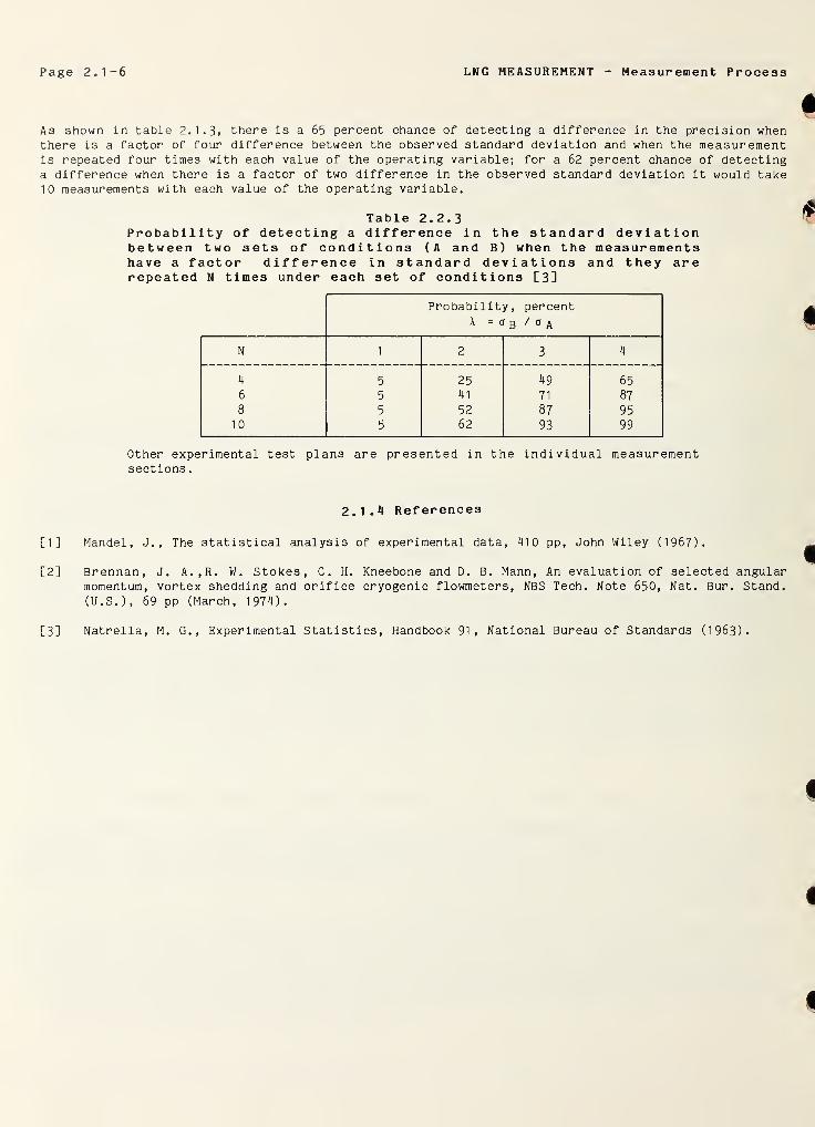
Page 2.1-6 LNG MEASUREMENT Measurement Process
As shown in table 2.1.3, there is a 65 percent chance of detecting a difference in the precision whenthere is a factor of four difference between the observed standard deviation and when the measurementis repeated four times with each value of the operating variable; for a 62 percent chance of detectinga difference when there is a factor of two difference in the observed standard deviation it would take10 measurements with each value of the operating variable.
Table 2.2.3Probability of detecting a difference in the standard deviationbetween two sets of conditions (A and B) when the measurementshave a factor difference in standard deviations and they arerepeated N times under each set of conditions [3]
Probability, percent
X = o b / o a
N 1 2 3 4
4 5 25 49 65
6 5 41 71 87
8 5 52 87 951 0 5 62 93 99
Other experimental test plans are presented in the individual measurementsections
.
2.1.4 References
[1] Mandel, J., The statistical analysis of experimental data, 410 pp, John Wiley (1967).
[2] Brennan, J. A.,R. W. Stokes, C. H. Kneebone and D. B. Mann, An evaluation of selected angularmomentum, vortex shedding and orifice cryogenic flowmeters, NBS Tech. Note 650, Nat. Bur. Stand.(U.S.), 69 pp (March, 1974).
[3] Natrella, M. G., Experimental Statistics, Handbook 91, National Bureau of Standards (1963).

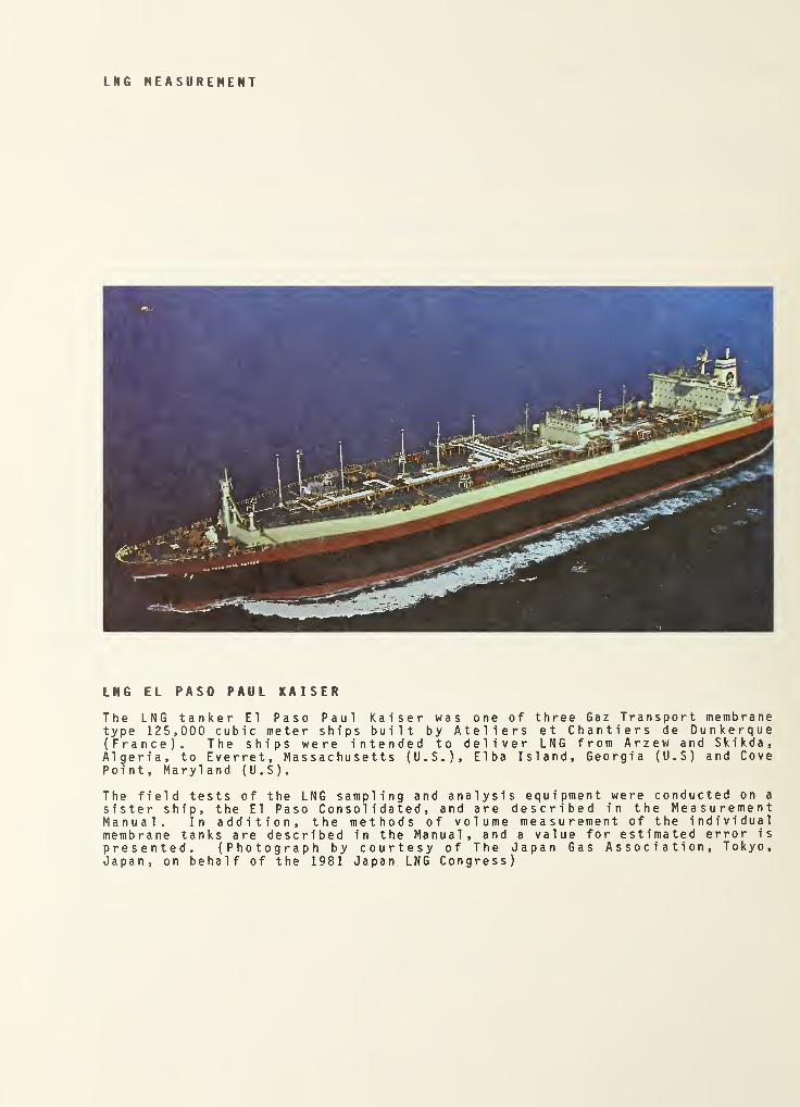
LNG MEASUREMENT
LNG EL PASO PAUL KAISER
The LNG tanker El Paso Paul Kaiser was one of three Gaz Transport membranetype 125,000 cubic meter ships built by Ateliers et Chantiers de Dunkerque(France). The ships were intended to deliver LNG from Arzew and Skikda,Algeria, to Everret, Massachusetts (U.S.), Elba Island, Georgia (U.S) and CovePoint, Maryland (U.S).
The field tests of the LNG sampling and analysis equipment were conducted on a
sister ship, the El Paso Consolidated, and are described in the MeasurementManual. In addition, the methods of volume measurement of the individualmembrane tanks are described in the Manual, and a value for estimated error is
presented. (Photograph by courtesy of The Japan Gas Association, Tokyo,Japan, on behalf of the 1981 Japan LNG Congress)
LNG MEASUREMENT Sampling and Analysis Page 2.2-0
CONTENTS
2.0 MEASUREMENT ELEMENTS
Sampling and Analysis Page
2.2 LNG Sampling and Analysis 2.1-1
2.2.1 Sampling Measurement Program Summary 2.2-2
2.2.2 Sampling Measurement Program Scope 2.2-3
2.2.3 Previous Work 2.2-4
2.2.42.2.42.2.42.2.42.2.42.2.42.2.42.2.42.2.42.2.42.2.42.2.4
Gas Analysis1 Comparison Between Gas Analysis Methods2 Gas Chromatograph ( GC ) System3 Mass Spectrometer (MS) System4 Results of Comparison Tests5 Detailed Evaluation of GC Analysis System .
6 GC Column Configurations and Digital Integrators7 GC Column Con f i qu r a t i on s and Column Packings .
8 Digital Integrator Evaluation9 GC Analysis Accuracy and Precision ....10 Sample Handling Procedures11 Conclusions and Recommendations
2.2-72.2-7
2.2-
7
2 . 2
-
11
2 . 2-11
2.2-
13
2.2-
15
2.2-
16
2 . 2-21
2 . 2-21
2 . 2-222.2-23
2.2.5 LNG Sampling 2.2-242. 2. 5.1 Laboratory Tests 2.2-252. 2. 5. 2 Instrumentation 2.2-262. 2. 5. 3 Safety Features 2.2-272. 2. 5. 4 Experimental Procedure 2.2-272. 2. 5. 5 Experimental Results 2.2-292. 2. 5. 6 Probe Evaluation 2.2-292. 2. 5. 7 Vaporizer Evaluation 2.2-352. 2. 5. 8 Field Tests at NBS Flow Facility 2.2-472. 2. 5. 9 Shipboard Tests 2.2-512.2.5.10 Conclusions and Recommendations 2.2-68
2 . 2.6 References 2 2-71

- « ». •
.
LNG MEASUREMENT - Sampling and Analysis Page 2.2-1
2.2 LNG Sampling and Analysis
The importance of accurate sampling and analysis of LNG cannot be overemphasized. The results of these
measurements are used in several of the other elements which provide a measure of LNG quantity and
quality. Sampling means the acquiring of a relatively small quantity of LNG which is identical in all
respects to the bulk liquid mixture. Direct analysis of the liquid phase is, at the present time, not
within the contemporary state of the art, and, therefore, this representative LNG sample must be
vaporized in such a way that the mixture composition is not changed in any manner. The gas phase must
be identical to the liquid phase in respect to composition. State of the art gas analysis is thenable to identify the molecular species and to establish the fraction of each component in the mixture
sample.
Mixture composition is used directly to calculate the calorific or heating value of the LNG mixture.
The calculation method is described in section 2.3 of this manual. In like manner the mixturefraction may be used with measured LNG pressures and temperatures to predict the liquid density over a
broad range of conditions both in the liquid and gas phases. A number of calculation methods aredescribed in section 2.4.3 of this manual, and specific examples are given in section 3-
This section of the manual contains a detailed description of the development and evaluation of an LNG
sampling measurement system. The text is an edited version of the work of Parrish, Arvidson andLaBrecque [1]. The choice of this particular work was based on the completeness of the treatment ofthe sampling and analysis measurement process as applied to LNG. The project, conducted by the
Boulder Laboratories of NBS, was sponsored by the LNG Sampling Measurement Committee, a natural gasindustry consortium. It should be noted that some of the tables and figures contain dimensions whichare not in SI terms. Duplicate units were used in the original publication to accommodate theintended audience and are included here to provide continuity with the original work.
The concept of LNG sampling, vaporization and analysis is basically quite simple and straightforward.The complete process, including all three sub-components, had not been treated extensively, if at all,
in the technical literature. Since the objective of the study was the development of a recommendedfield- type measurement system, extreme care was exercised by Parrish, et al. in examining the separatecomponents of sampling, vaporizing and gas analysis and just how the individual components wouldoperate when assembled into a single self-contained measurement system. Because of the importance ofthe sampling and analysis process, it was deemed necessary to include most of the original study whichcontained the selection decisions and supporting data.
The main body of the study begins with the selection of the gas analysis method in sections 2.2.4.
1
through 2. 2. 4. 4. Of the various methods available, gas chromatography and mass spectrometry werechosen as having the necessary accuracy, precision and industry acceptance as reliable measurementdevices.
Gas chromatography is based on the separation of mixtures into their constituents by preferentialadsorption on a solid or liquid, and mass spectrometry is based on the separation of mixtures based onrelative mass of the ionized constituent or molecular fragment of the constituent. Each method hasattractive features, and available equipment was assessed by Parrish, et al. in order to select the onemethod best suited for use as a field-operated LNG analysis system. Comparison testing was describedand criteria for selection of the gas chromatagraph was given.
The analysis method was selected, and it was then necessary to establish the accuracy and precision f
the instrument over a broad range of anticipated operating conditions and with different kind'auxiliary equipment. This included operation with various adsorption column configuration:-,packings and digital integrators used to integrate the response curve of the detector. The extentesting and selection process is described in sections 2. 2. 4. 5 through 2. 2. 4. 9.
It was then possible to begin the assessment of various types of sampling and vaporizingequipment. These devices are generally custom fabricated for field installation. The studythe sampling to that of flowing LNG in a pipeline, but it was believed that the equipmenttechniques which were developed could be used in other applications. The proven gnequipment was used to experimentally verify the sampling process.
Page 2.2-2 LNG MEASUREMENT - Sampling and Analysis
The actual description of the sampling investigation is covered in section 2.2.5. Different samplingtap configurations and several types of vaporizer designs were tested and evaluated. Testing wasconducted under controlled laboratory conditions, then in a controlled field-type facility and finallywith an actual LNG shipboard installation which consisted of the most favorable configurations ofsampling tap, vaporizer and gas analysis equipment.
The conclusions and recommendations are extensive and detailed as are most of the evaluation testing.However, the document is the most comprehensive work on the subject, and to accept only the shipboarddesign as a recommended system could lead to problems in application where design constraints aresignificantly different, such as with a land-based LNG peakshaving storage tank. A broad base of dataand technique result in an understanding of the entire process and should allow useful applications.
2.2.1 Sampling Measurement Program Summary [1]
Laboratory and field test results showed that the total uncertainty in the computed heating value ofsamples taken with the recommended sampling system could be made routinely to within ±0.3 percent:this included the ±0.1 percent uncertainty in analysis by gas chromatography. Three sample probes andtwo vaporizer designs were considered. Of the ten operating variables considered, six were found tobe important in sampling. Test results were used to establish recommended design and operatingcriteria.
Accurate LNG composition determination requires:
a) a sample probe for drawing a sample representative of the fluid passing the samplingpoint,
b) a sample conditioner for completely vaporizing the sample,c) a gas analyzer for accurately and precisely analyzing the sample composition, andd) a correct set of operating parameters and procedures.
A systematic study evaluating all of the above components was confined to the problem of sampling froma flowing LNG stream. Instead of directly measuring the heating value by combustion calorimetry, the
gas composition was analyzed so that both heating value and liquid density could be computed.
Gas chromatography was selected for analyzing vaporized LNG samples over mass spectrometry, because it
was found to be more precise and accurate. By using a gas chromatograph-programmable integratorsystem, the total uncertainty in the heating value (on a unit volume basis), as computed from the
analyzed composition, routinely can be less than ±0.1 percent. This figure includes a ±0.03 percentuncertainty in the calibration gas composition; this uncertainty, which neglects the uncertainty of
the individual components heating value (see section 1.3 of this manual), is based only on theuncertainty in the weighing process used to prepare the mixtures. The ±0.1 percent uncertainty alsoincludes a random error of ±0.06 percent. The random error is three times the estimated standarddeviation of ±0.02 percent. This value represents the maximum value obtained from over 100measurements of three or more repetitive analyses employing a properly operating gaschromatograph-programmable integrator system. Procedures and equipment are recommended for analyzingvaporized LNG samples.
The results of sampling tests at a NBS field site (see 2. 2. 5. 8) show that the total uncertainty of a
single measurement in sampling and analyzing LNG mixtures can be less than ±0.3 percent in thecomputed heating value. This uncertainty includes the ±0.03 percent uncertainty in the calibrationgas composition plus an uncertainty of ±0.27 percent for random error. The ±0.27 percent figurerepresents three times the upper limit of the standard deviation determined for the combined samplingplus analysis measurement process. The recommended sampling system consists of a side tap probe, a
steam or electrically heated tube vaporizer, a gas mixing chamber and a sampling manifold. Samplingsystem design criteria are recommended, including ranges of the operating variables found to affectsampling precision.
Data obtained during a shipboard test has limits of precision of ±0.30 percent. These limits comparevery favorably to the ±0.27 percent obtained on the flow facility.
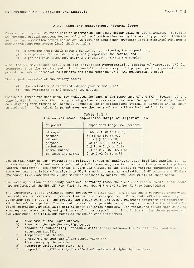
LNG MEASUREMENT Sampling and Analysis Page 2.2-3
2.2.2 Sampling Measurement Program Scope
Composition plays an important role in determining the total dollar value of LNG shipments. Sampling
LNG presents special problems because of possible fractionation during the sampling process. Accurate
and precise composition determination of LNG mixtures (and other cryogenic liquid mixtures) requires a
Sampling-Measurement System (SMS) which contains:
a) a sampling probe which draws a sample without altering the composition,
b) a sample conditioner which completely vaporizes the sample, and
c) a gas analyzer which accurately and precisely analyzes the sample.
Also, the SMS may include facilities for collecting representative samples of vaporized LNG for
transport from the sampling point to the analytical laboratory. The proper operating parameters and
procedures must be specified to minimize the total uncertainty in the measurement process.
The project consisted of two primary tasks:
a) the evaluation of vaporized LNG analysis methods, and
b) the evaluation of LNG sampling techniques.
Possible alternatives were carefully evaluated for each of the components of the SMS. Because of the
time limitations, only the most promising alternatives were considered in depth. The study covered
only sampling from flowing LNG streams. Emphasis was on compositions typical of Algerian LNG as shown
in table 2.2.1. The values in parentheses are the range of compositions included in this study.
Table 2.2.1The Anticipated Composition Range of Algerian LNG
Component Composition Range, mol percent
nitrogenmethaneethanepropaneisobutanenormal butanepentanes and heavier
0.60 to 1.40 (0 to 11)
84 to 92 (65 to 90)
6 to 9.5 (5 to 18)
2.2 to 3.5 (1 to 5.4)
0.3 to 0.5 (0 to 0.8)
0.3 to 0.7 (0.2 to 4.8)
0 to 0.02 (0 to 0.3)
The initial phase of work evaluated the relative merits of analyzing vaporized LNG samples by gaschromatography (GC) and mass spectrometry (MS); accuracy, precision and simplicity were the primaryfactors considered. The second phase of work was a study of the effect of various parameters on theaccuracy and precision of analysis by GC; the work included an evaluation of GC columns and GC dataprocessors ( i. e. , integrators) . Gas mixtures prepared by weight were used in all of these tests.
The sampling portion of the study contained laboratory tests and field confirmation tests; these testswere performed at the NBS LNG Flow Facility and aboard the LNG tanker El Paso Consolidated.
The laboratory tests evaluated three probes —- a pitot tube, a side tap and a reference probe — andtwo continuous vaporizers — vaporizer A and a reference vaporizer. To separate effects caused by thevaporizer from those of the probes, the probes were used with a reference vaporizer and vaporizer A
with the reference probe. The laboratory evaluation provided a rapid way to determine the effect of a
given operating variable while holding other variables constant. The variable's effect upon samplingaccuracy was determined by using mixtures of known composition. In addition to the three probes an !
two vaporizers, the following operating variables were considered:
a) flow rate of the liquid stream,b) flow rate through the sampling device,c) amount of subcooling (pressure differential between the sample point and the
saturated liquid),d) temperature of the LNG,
e) pressure drop upstream of the sample vaporizer,f) time-averaging the sample,
g) vaporizer outlet temperature, andh) composition, particularly the effect of pentane and higher hydrocarbons.
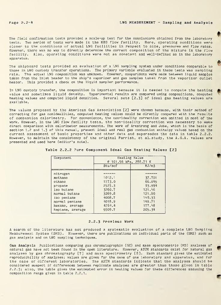
Page 2.2-4 LNG MEASUREMENT Sampling and Analysis
The field confirmation tests provided a scale-up test for the conclusions obtained from the laboratorytests. Two series of tests were made in the NBS flow facility. Here, operating conditions werecloser to the conditions of actual LNG facilities in respect to size, pressures and flow rates.However, there was no way to directly determine the correct composition of the mixture in the flowfacility. Also, operating conditions were not as constant and well-defined as in the laboratoryapparatus.
The shipboard tests provided an evaluation of a LNG sampling system under conditions comparable tothose in LNG custody transfer operations. The primary variable evaluated in these tests was samplingrate. The actual LNG composition was unknown. However, comparisons were made between liquid samplestaken from the inlet header to the ship's vaporizer and gas samples taken from the vaporizer outletheader. This provided a check on the liquid sampler performance.
In LNG custody transfer, the composition is important because it is needed to compute the heatingvalue and sometimes liquid density. Experimental results are compared using compositions, computedheating values and computed liquid densities. Several sets [2,3] of ideal gas heating values areavailable.
The values proposed by the American Gas Association [2] were chosen because, with their method of
correcting for gas nonidealities, computed heating values could be directly compared with the resultsof combustion calorimetry. For convenience, the non-ideality correction was omitted in most of thework. However, in the LNG flow facility tests, the non-ideality correction was necessary to makedirect comparison with calorimeter measurements. The work of Armstrong and Jobe, which is the basis ofsection 1.2 and 1.3 of this manual, present ideal and real gas combustion enthalpy values based on the
current assessment of basic properties and other data and supersedes the data in table 2.2.2.However, to maintain the consistency of the original Parrish, et al. study, the A.G.A. values arepresented and used here (editor's note).
Table 2.2.2 Pure Component Ideal Gas Heating Values [2]
Component Heating Value§ 101 .56 kPa, 288.71 K
Btu/scf MJ/m3
nitrogenmethane 1012.1 37.701ethane 1773.0 66.045propane 2523.3 93-994iso butane 3260.7 121.46normal butane 3269.8 121 .80
iso pentane 4008.7 149.33normal pentane 4018.9 149.71
hexane, average 4764.4 177.48heptane, average 5509.7 205.34
2.2.3 Previous Work
A search of the literature has not produced a systematic evaluation of a complete LNG SamplingMeasurement System (SMS). However, there are publications on individual parts of the (SMS) such as
gas analysis and on LNG sampling techniques.
Gas Analysis Publications comparing gas chromatographic (GC) and mass spectrometric (MS) analyses of
natural gas have not been found in the open literature. However, ASTM standards exist for natural gasanalyses by gas chromatography [7] and mass spectrometry [8]. Each standard gives the estimatedreproducibility of analyses; values are given for the case of one laboratory and apparatus, and forthe case of different laboratories. The ASTM standards indicate that the analyses should beconsidered suspect if differences between replicate analyses are greater than those given in table2.2.3; also, the table gives the estimated error in heating values for these differences assuming the
composition range given in table 2.2.1.
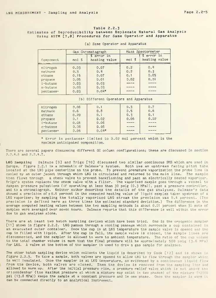
LNG MEASUREMENT Sampling and Analysis Page 2.2-5
Table 2.2.3Estimates of Reproducibility between Replecate Natural Gas Analysis
Using ASTM [7,8] Procedures for Same Operator and Apparatus
(a) Same Operator and Apparatus
Component
Gas Chromatagraph Mass Spectormeter
mol %
% error in
heating value mol %
% error in
heating value
nitrogen 0.03 0.07 0.2 0.4
methane 0.3 0.4 0.2 0.3
ethane 0.15 0.07 0.1 0.05
propane 0.05 0.01 0.02 0.01
i-butane 0.03 0.03 ~ —n-butane 0.03 0.03 — —pentanes+ 0.03 0.04* — —
(b) Different Operators and Apparatus
nitrogen 0.06 0.1 0.3 0.7
methane 0.6 0.8 0.5 0.6
ethane 0.20 0.1 0.3 0.1
propane 0.1 0.02 0.06 0.02
i-butane 0.06 0.06 — —n-butane 0.06 0.06 — —pentanes+ 0.06 0.04* — —* Error in pentanes+ limited to 0.02 mol percent which is the
maximim anticipated composition.
There are several papers discussing different GC column configurations; these are discussed in section2.2.4 .6 and 2. 2. 4. 7.
LNG Sampling Dalmaze [9] and Trigo [10] discussed two similar continuous SMS which are used in
Europe. Figure 2.2.1 is a schematic of Dalmaze ' s system. Both use an upstream facing pitot tubelocated at the LNG pipe centerline as the probe. To prevent premature vaporization the probe line is
cooled by an outer jacket through which LNG is circulated and returned to the main line. The samplethen flows through a check valve to prevent backflashing and past an electrically heated vaporizer.Trigo's system replaces the check valve with a filter. The vaporized sample goes through a vessel todampen pressure pulsations (if operating at less than 30 psig (0.3 MPa)), past a pressure controller,and to a chromatograph. Neither author describes the details of the gas analyses. Dalmaze' s datashowed a precision of ±0.6 percent in the computed heating value of liquid samples taken upstream of a
LNG vaporizer; by sampling the totally vaporized LNG stream the precision was 0.4 percent. (Theprecision is defined here as three times the estimated standard deviation.) The difference in theaverage computed heating values between the two sampling methods is about 0.01 percent when 30 sets ofsamples were averaged over seven hours. Dalmaze reports that this difference is well within the errordue to gas analyses alone.
There are at least two batch sampling devices which have been tried. One is the cryogenic sampler[11] shown in figure 2.2.2. LNG passes through a cooling passage which surrounds a cup contained in
an evacuated outer container. Once the cup is at LNG temperature the sample valve is opened and thecup is filled with liquid. After the cup is full, the sample valve is closed, the sample lines aredisconnected, and the sampler is allowed to warm to ambient temperature. The ratio of the cup v ine
to the total chamber volume is such that the final pressure will be approximately 500 psig (3.6 VP Vfor LNG. A valve at the bottom of the sampler is used to draw a gas sample for analyses.
The other batch sampling device which collects the liquid is described by Cook [12] and is sh w.figure 2.2.3. To take a sample, both valves are opened to allow LNG to flow through the sampler w:
is well insulated. Once the sampler is at LNG temperature, as evidenced by a continuous liqui i . w
from the device, both valves are closed. Then the device is removed from the sampling llr mdallowed to warm up. After the initial pressure rise, a pressure relief valve which is set if
*• >
cricondenbar (the maximum pressure at which a mixture may exist in two phases) of the mixture :
psi (13.8 MPa)) keeps the sample at a constant pressure and in one phase. Once the sampler is wtr-. :*
can be connected directly to an analytical instrument.
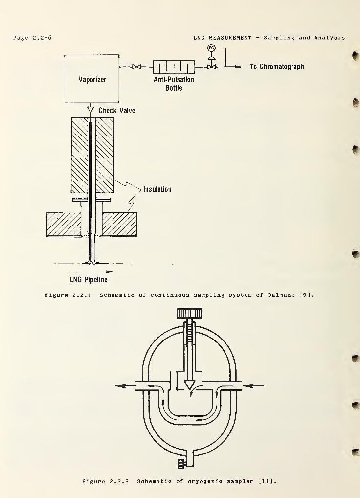
Page 2.2-6 LNG MEASUREMENT - Sampling and Analysis
- To Chromatograph
LNG Pipeline
Figure 2.2.1 Schematic of continuous sampling system of Dalmaze [9]
Figure 2.2.2 Schematic of cryogenic sampler [11].
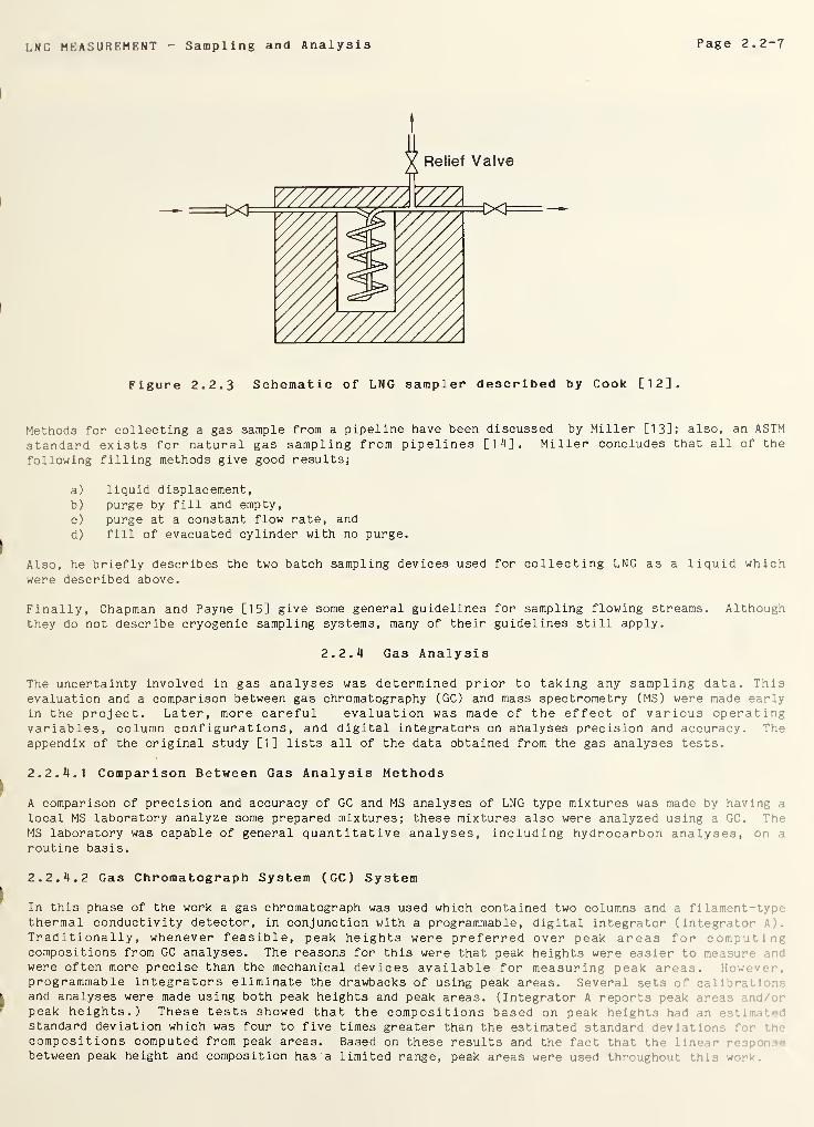
LNG MEASUREMENT - Sampling and Analysis Page 2.2-7
Figure 2.2.3 Schematic of LNG sampler described by Cook [12].
Methods for collecting a gas sample from a pipeline have been discussed by Miller [13]; also, an ASTM
standard exists for natural gas sampling from pipelines [14], Miller concludes that all of the
following filling methods give good results;
a) liquid displacement,b) purge by fill and empty,
c) purge at a constant flow rate, and
d) fill of evacuated cylinder with no purge.
Also, he briefly describes the two batch sampling devices used for collecting LNG as a liquid whichwere described above.
Finally, Chapman and Payne [15] give some general guidelines for sampling flowing streams. Althoughthey do not describe cryogenic sampling systems, many of their guidelines still apply.
2.2.4 Gas Analysis
The uncertainty involved in gas analyses was determined prior to taking any sampling data. Thisevaluation and a comparison between gas chromatography (GC) and mass spectrometry (MS) were made earlyin the project. Later, more careful evaluation was made of the effect of various operatingvariables, column configurations, and digital integrators on analyses precision and accuracy. Theappendix of the original study [1] lists all of the data obtained from the gas analyses tests.
2. 2. 4.1 Comparison Between Gas Analysis Methods
A comparison of precision and accuracy of GC and MS analyses of LNG type mixtures was made by having a
local MS laboratory analyze some prepared mixtures; these mixtures also were analyzed using a GC. TheMS laboratory was capable of general quantitative analyses, including hydrocarbon analyses, on *.
routine basis.
2. 2. 4. 2 Gas Chromatograph System ( GC ) System
In this phase of the work a gas chromatograph was used which contained two columns and a filament-typethermal conductivity detector, in conjunction with a programmable, digital integrator (integrator A .
Traditionally, whenever feasible, peak heights were preferred over peak areas for computingcompositions from GC analyses. The reasons for this were that peak heights were easier to measure andwere often more precise than the mechanical devices available for measuring peak areas. However,programmable integrators eliminate the drawbacks of using peak areas. Several sets of cal i t;rfand analyses were made using both peak heights and peak areas. (Integrator A reports peak are
t
peak heights.) These tests showed that the compositions based on peak heights hid an estlmav* '
standard deviation which was four to five times greater than the estimated standard dev: v ion :
compositions computed from peak areas. Based on these results and the fact that the linear;
•
between peak height and composition has a limited range, peak areas were used throughout *•: w .
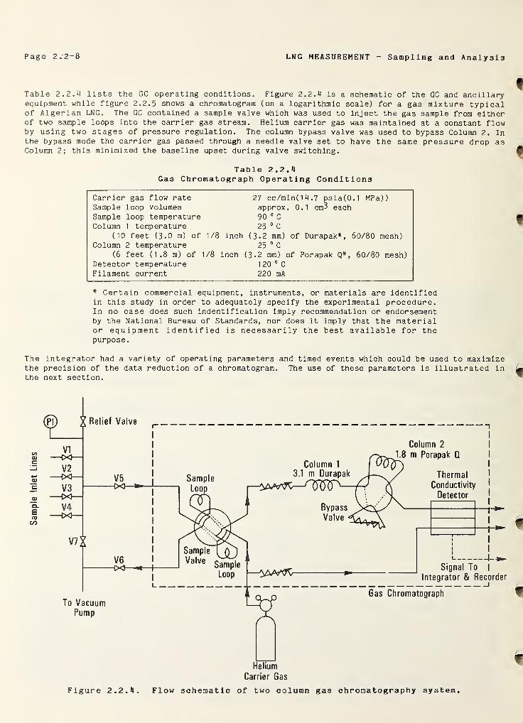
Page 2.2-8 LNG MEASUREMENT Sampling and Analysis
Table 2.2.4 lists the GC operating conditions. Figure 2.2.4 is a schematic of the GC and ancillaryequipment while figure 2.2.5 shows a chromatogram (on a logarithmic scale) for a gas mixture typicalof Algerian LNG. The GC contained a sample valve which was used to inject the gas sample from eitherof two sample loops into the carrier gas stream. Helium carrier gas was maintained at a constant flowby using two stages of pressure regulation. The column bypass valve was used to bypass Column 2. Inthe bypass mode the carrier gas passed through a needle valve set to have the same pressure drop asColumn 2; this minimized the baseline upset during valve switching.
Table 2.2.4Gas Chromatograph Operating Conditions
Carrier gas flow rate 27 cc/min(l4.7 psia(0.1 MPa))Sample loop volumes approx. 0.1 cm3 eachSample loop temperature 90 0 C
Column 1 temperature 25 0 C
(10 feet (3.0 m) of 1/8 inch (3-2 mm) of Durapak*, 60/80 mesh)Column 2 temperature no 'sJl
Oo
(6 feet (1.8 m) of 1/8 inch (3.2 mm) of Porapak Q* , 60/80 mesh)Detector temperature 120 0
C
Filament current 220 mA
* Certain commercial equipment, instruments, or materials are identifiedin this study in order to adequately specify the experimental procedure.In no case does such indentif ication imply recommendation or endorsementby the National Bureau of Standards, nor does it imply that the materialor equipment identified is necessarily the best available for thepurpose.
The integrator had a variety of operating parameters and timed events which could be used to maximizethe precision of the data reduction of a chromatogram. The use of these parameters is illustrated inthe next section.
Carrier Gas
Figure 2.2.4. Flow schematic of two column gas chromatography system.
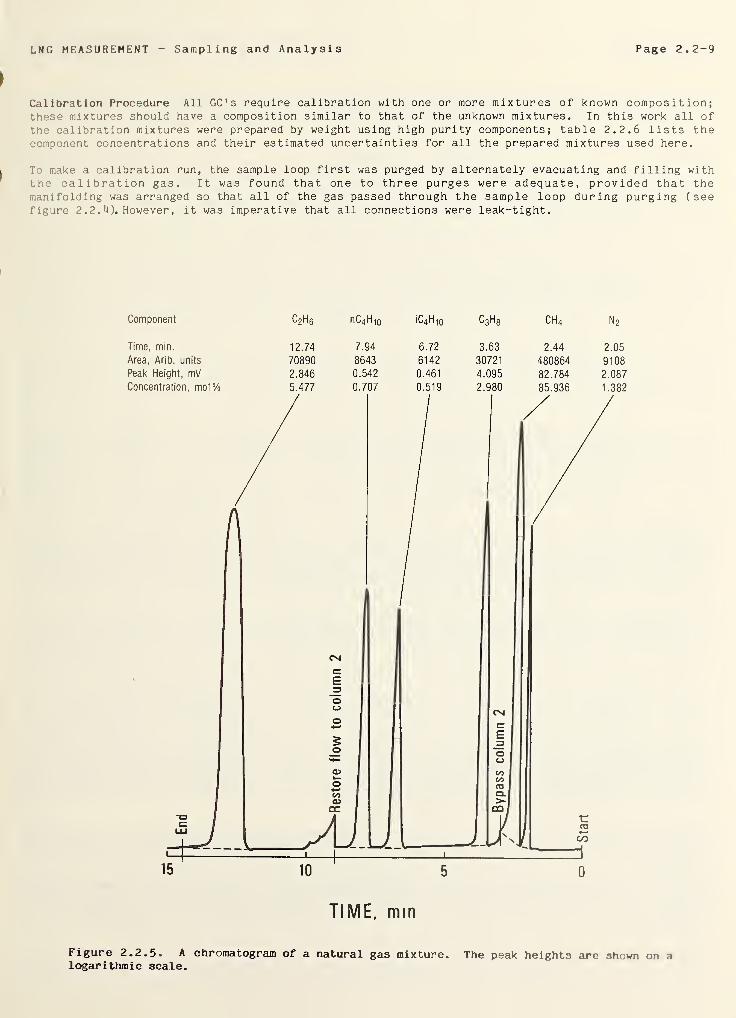
LNG MEASUREMENT Sampling and Analysis Page 2.2-9
Calibration Procedure All GC's require calibration with one or more mixtures of known composition;these mixtures should have a composition similar to that of the unknown mixtures. In this work all of
the calibration mixtures were prepared by weight using high purity components; table 2.2.6 lists thecomponent concentrations and their estimated uncertainties for all the prepared mixtures used here.
To make a calibration run, the sample loop first was purged by alternately evacuating and filling withthe calibration gas. It was found that one to three purges were adequate, provided that themanifolding was arranged so that all of the gas passed through the sample loop during purging (seefigure 2.2.4). However, it was imperative that all connections were leak-tight.
Component c 2 h 6 nC-iHio 1 C 4 H 10 c 3 h 8 ch 4 n 2
Time, min. 12.74 7.94 6.72 3.63 2.44 2.05
Area, Arib. units 70890 8643 6142 30721 480864 9108
Peak Height, mV 2.846 0.542 0.461 4.095 82.784 2.087
Concentration, mo1% 5.477 0.707 0.519 2.980 85.936 1.382
TIME, min
Figure 2.2.5. A chromatogram of a natural gas mixture. The peak heights are shown on alogarithmic scale.
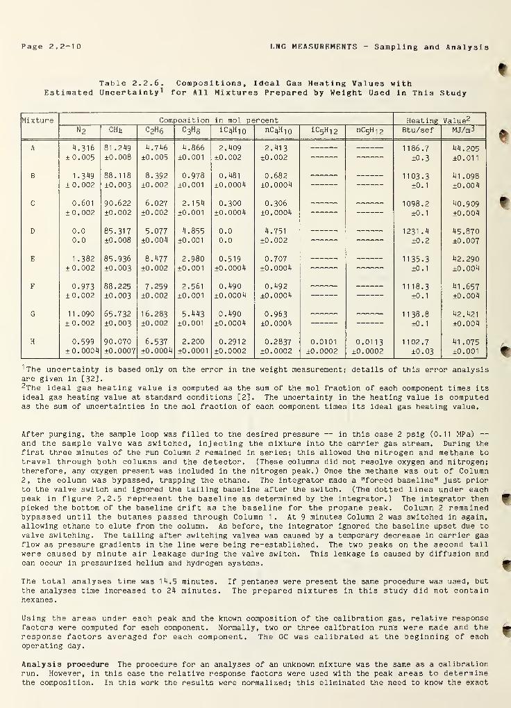
Page 2.2-10 LNG MEASUREMENTS - Sampling and Analysis
Table 2.2.6. Compositions, Ideal Gas Heating Values withEstimated Uncertainty 1 for All Mixtures Prepared by Weight Used in Thi3 Study
^The uncertainty is based only on the error in the weight measurement; details of this error analysisare given in [32].2The ideal gas heating value is computed as the sum of the mol fraction of each component times itsideal gas heating value at standard conditions [2]. The uncertainty in the heating value is computedas the sum of uncertainties in the mol fraction of each component times its ideal gas heating value.
After purging, the sample loop was filled to the desired pressure — in this case 2 psig (0.11 MPa) —and the sample valve was switched, injecting the mixture into the carrier gas stream. During thefirst three minutes of the run Column 2 remained in series; this allowed the nitrogen and methane totravel through both columns and the detector. (These columns did not resolve oxygen and nitrogen;therefore, any oxygen present was included in the nitrogen peak.) Once the methane was out of Column2, the column was bypassed, trapping the ethane. The integrator made a "forced baseline" just priorto the valve switch and ignored the tailing baseline after the switch. (The dotted lines under eachpeak in figure 2.2.5 represent the baseline as determined by the integrator.) The integrator thenpicked the bottom of the baseline drift as the baseline for the propane peak. Column 2 remainedbypassed until the butanes passed through Column 1 . At 9 minutes Column 2 was switched in again,allowing ethane to elute from the column. As before, the integrator ignored the baseline upset due to
valve switching. The tailing after switching valves was caused by a temporary decrease in carrier gasflow as pressure gradients in the line were being re-established. The two peaks on the second tailwere caused by minute air leakage during the valve switch. This leakage is caused by diffusion andcan occur in pressurized helium and hydrogen systems.
The total analyses time was 14.5 minutes. If pentanes were present the same procedure was used, but
the analyses time increased to 24 minutes. The prepared mixtures in this study did not containhexanes
.
Using the areas under each peak and the known composition of the calibration gas, relative responsefactors were computed for each component. Normally, two or three calibration runs were made and theresponse factors averaged for each component. The GC was calibrated at the beginning of eachoperating day.
Analysis procedure The procedure for an analyses of an unknown mixture was the same as a calibrationrun. However, in this case the relative response factors were used with the peak areas to determinethe composition. In this work the results were normalized; this eliminated the need to know the exact
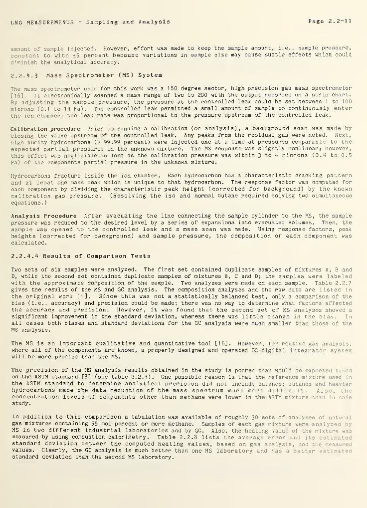
LNG MEASUREMENTS - Sampling and Analysis Page 2.2-11
amount of sample injected. However, effort was made to keep the sample amount, i.e., sample pressure,
constant to with ±5 percent because variations in sample size may cause subtle effects which could
d'minish the analytical accuracy.
2.2.11.3 Mass Spectrometer (MS) System
The mass spectrometer used for this work was a 180 degree sector, high precision gas mass spectrometer
[16]. It electronically scanned a mass range of two to 200 with the output recorded on a strip chart.
By adjusting the sample pressure, the pressure at the controlled leak could be set between 1 to 100
microns (0.1 to 13 Pa). The controlled leak permitted a small amount of sample to continuously enter
the ion chamber; the leak rate was proportional to the pressure upstream of the controlled leak.
Calibration procedure Prior to running a calibration (or analysis), a background scan was made by
closing the valve upstream of the controlled leak. Any peaks from the residual gas were noted. Next,
high purity hydrocarbons (> 99.99 percent) were injected one at a time at pressures comparable to the
expected partial pressures in the unknown mixture. The MS response was slightly nonlinear; however,
this effect was negligible as long as the calibration pressure was within 3 to 4 microns (0.4 to 0.5Pa) of the components partial pressure in the unknown mixture.
Hydrocarbons fracture inside the ion chamber. Each hydrocarbon has a characteristic cracking patternand at least one mass peak which is unique to that hydrocarbon. The response factor was computed for
each component by dividing the characteristic peak height (corrected for background) by the knowncalibration gas pressure. (Resolving the iso and normal butane required solving two simultaneousequations .
)
Analysis Procedure After evacuating the line connecting the sample cylinder to the MS, the samplepressure was reduced to the desired level by a series of expansions into evacuated volumes. Then, the
sample was opened to the controlled leak and a mass scan was made. Using response factors, peakheights (corrected for background) and sample pressure, the composition of each component wascalculated.
2. 2. 4. 4 Results of Comparison Tests
Two sets of six samples were analyzed. The first set contained duplicate samples of mixtures A, B andD, while the second set contained duplicate samples of mixtures B, C and D; the samples were labeledwith the approximate composition of the sample. Two analyses were made on each sample. Table 2.2.7gives the results of the MS and GC analysis. The composition analyses and the raw data are listed in
the original work [1]. Since this was not a statistically balanced test, only a comparison of thebias (i.e., accuracy) and precision could be made; there was no way to determine what factors affectedthe accuracy and precision. However, it was found that the second set of MS analyses showed a
significant improvement in the standard deviation, whereas there was little change in the bias. Inall cases both biases and standard deviations for the GC analysis were much smaller than those of theMS analysis.
The MS is an important qualitative and quantitative tool [16]. However, for routine gas analysis,where all of the components are known, a properly designed and operated GC-digital integrator systemwill be more precise than the MS.
The precision of the MS analysis results obtained in the study is poorer than would be expected basedon the ASTM standard [8] (see table 2.2.3). One possible reason is that the reference mixture used in
the ASTM standard to determine analytical precision did not include butanes; butanes and heavierhydrocarbons made the data reduction of the mass spectrum much more difficult. Also, •
concentration levels of components other than methane were lower in the ASTM mixture than in tni:
study.
In addition to this comparison a tabulation was available of roughly 30 sets of analyses of nvgas mixtures containing 95 mol percent or more methane. Samples of each gas mixture were am. • ,
MS in two different industrial laboratories and by GC. Also, the heating value of the mlxt jr-
measured by using combustion calorimetry. Table 2.2.8 lists the average error and its :
standard deviation between the computed heating values, based on gas analysis, andvalues. Clearly, the GC analysis is much better than one MS laboratory and has a better •• *
i~
standard deviation than the second MS laboratory.
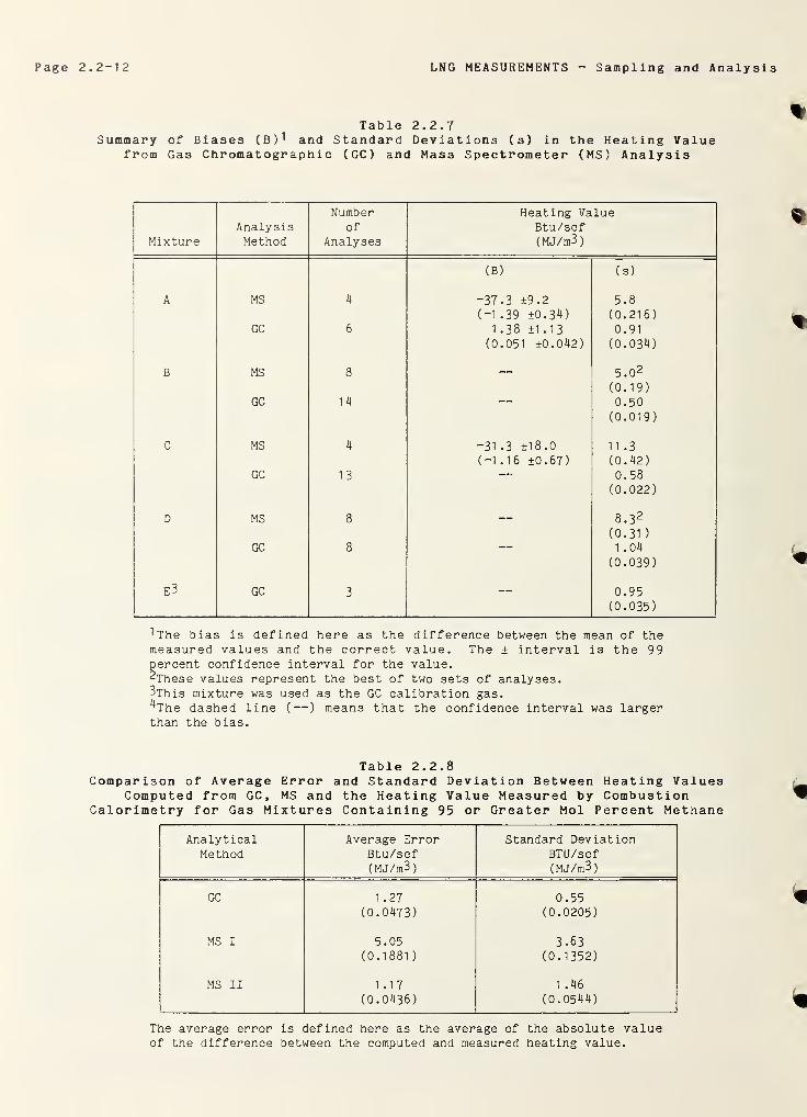
Page 2.2-12 LNG MEASUREMENTS - Sampling and Analysis
Table 2.2.7Summary of Biases (B)1 and Standard Deviations (s) in the Heating Value
from Gas Chromatographic (GC) and Mass Spectrometer (MS) Analysis
%
*
%
*
1 The bias is defined here as the difference between the mean of themeasured values and the correct value. The ± interval is the 99percent confidence interval for the value.2These values represent the best of two sets of analyses.3This mixture was used as the GC calibration gas.
^The dashed line (— ) means that the confidence interval was largerthan the bias.
MixtureAnalysisMethod
Numberof
Analyses
Heating ValueBtu/scf(MJ/m3)
(B) (s)
A MS 4 -37.3 ±9.2(-1 .39 ±0.34)
5.8
(0.216)GC 6 1.38 ±1.13
(0.051 ±0.042)0.91
(0.034)
B MS 8 — 5.0 2
(0.19)GC 14 0.50
(0.019)
C MS 4 -31 .3 ±18.0(-1.16 ±0.67)
11.3(0.42)
GC 13 0.58(0.022)
D MS 8 — 8.3 2
(0.31 )
GC 8 1 .04
(0.039)
E3 GC 3— 0.95
(0.035)
Table 2.2.8Comparison of Average Error and Standard Deviation Between Heating Values
Computed from GC, MS and the Heating Value Measured by CombustionCalorimetry for Gas Mixtures Containing 95 or Greater Mol Percent Methane
AnalyticalMethod
Average ErrorBtu/scf(MJ/m3)
Standard DeviationBTU/scf(MJ/m3)
GC 1 .27 0.55(0.0473) (0.0205)
MS I 5.05 3.63(0.1881
)
(0.1352)
MS II 1.17 1 .46
(0.0436) (0.0544)
The average error is defined here as the average of the absolute valueof the difference between the computed and measured heating value.
«
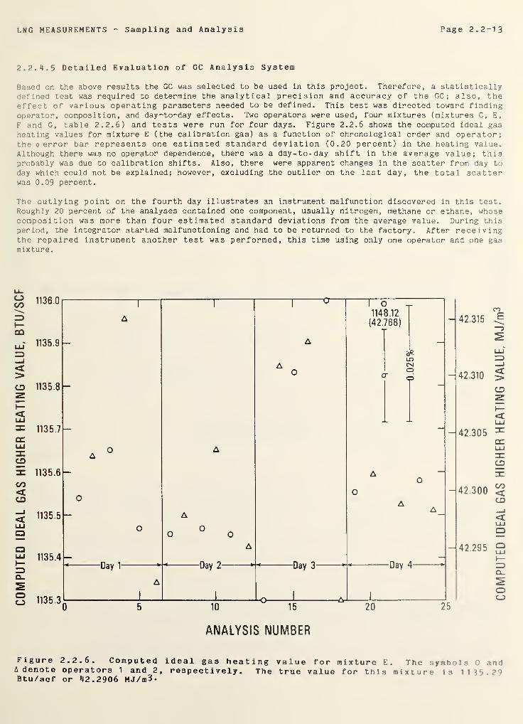
COMPUTED
IDEAL
GAS
HIGHER
HEATING
VALUE.
BTU/SCF
LNG MEASUREMENTS Sampling and Analysis Page 2.2-13
2. 2.
5
Detailed Evaluation of GC Analysis System
Based on the above results the GC was selected to be used in this project. Therefore, a statisticallydefined test was required to determine the analytical precision and accuracy of the GC ; also, theeffect of various operating parameters needed to be defined. This test was directed toward findingoperator, composition, and day-to-day effects. Two operators were used, four mixtures (mixtures C, E,
F and G, table 2.2.6) and tests were run for four days. Figure 2.2.6 shows the computed ideal gas
heating values for mixture E (the calibration gas) as a function of chronological order and operator;the o error bar represents one estimated standard deviation (0.20 percent) in the heating value.Although there was no operator dependence, there was a day-to-day shift in the average value; thisprobably was due to calibration shifts. Also, there were apparent changes in the scatter from day to
day which could not be explained; however, excluding the outlier on the last day, the total scatterwas 0.09 percent.
The outlying point on the fourth day illustrates an instrument malfunction discovered in this test.Roughly 20 percent of the analyses contained one component, usually nitrogen, methane or ethane, whosecomposition was more than four estimated standard deviations from the average value. During thisperiod, the integrator started malfunctioning and had to be returned to the factory. After receivingthe repaired instrument another test was performed, this time using only one operator and one gasmixture.
42.315
42.310
42.305
42.300
42.295
Figure 2.2.6. Computed ideal gas heating value for mixture E. The symbols > indA denote operators 1 and 2, respectively. The true value for this mixture IsBtu/scf or 42.2906 MJ/m3-
COMPUTED
IDEAL
GAS
HIGHER
HEATING
VALUE,
MJ/m
3
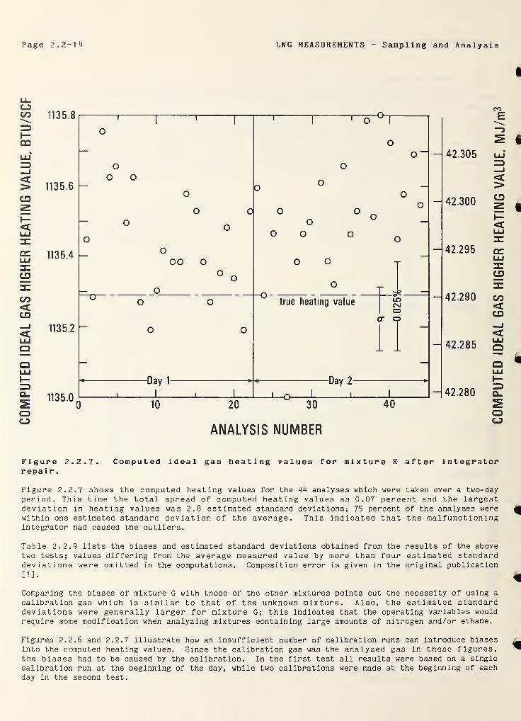
COMPUTED
IDEAL
GAS
HIGHER
HEATING
VALUE,
BTU/SCF
Page 2.2-14 LNG MEASUREMENTS Sampling and Analysis
42.305
42.300
42.295
42.290
42.285
42.280
Figure 2.2.7. Computed ideal gas heating values for mixture E after integratorrepair
.
Figure 2.2.7 shows the computed heating values for the 44 analyses which were taken over a two-dayperiod. This time the total spread of computed heating values as 0.07 percent and the largestdeviation in heating values was 2.8 estimated standard deviations; 75 percent of the analyses werewithin one estimated standard deviation of the average. This indicated that the malfunctioningintegrator had caused the outliers.
Table 2.2.9 lists the biases and estimated standard deviations obtained from the
two tests; values differing from the average measured value by more than fourdeviations were omitted in the computations. Composition error is given in the
[ 1 ].
results of the aboveestimated standardoriginal publication
Comparing the biases of mixture G with those of the other mixtures points out the necessity of using a
calibration gas which is similar to that of the unknown mixture. Also, the estimated standarddeviations were generally larger for mixture G; this indicates that the operating variables wouldrequire some modification when analyzing mixtures containing large amounts of nitrogen and/or ethane.
Figures 2.2.6 and 2.2.7 illustrate how an insufficient number of calibration runs can introduce biasesinto the computed heating values. Since the calibration gas was the analyzed gas in these figures,the biases had to be caused by the calibration. In the first test all results were based on a singlecalibration run at the beginning of the day, while two calibrations were made at the beginning of eachday in the second test.
COMPUTED
IDEAL
GAS
HIGHER
HEATING
VALUE,
MJ/m
3
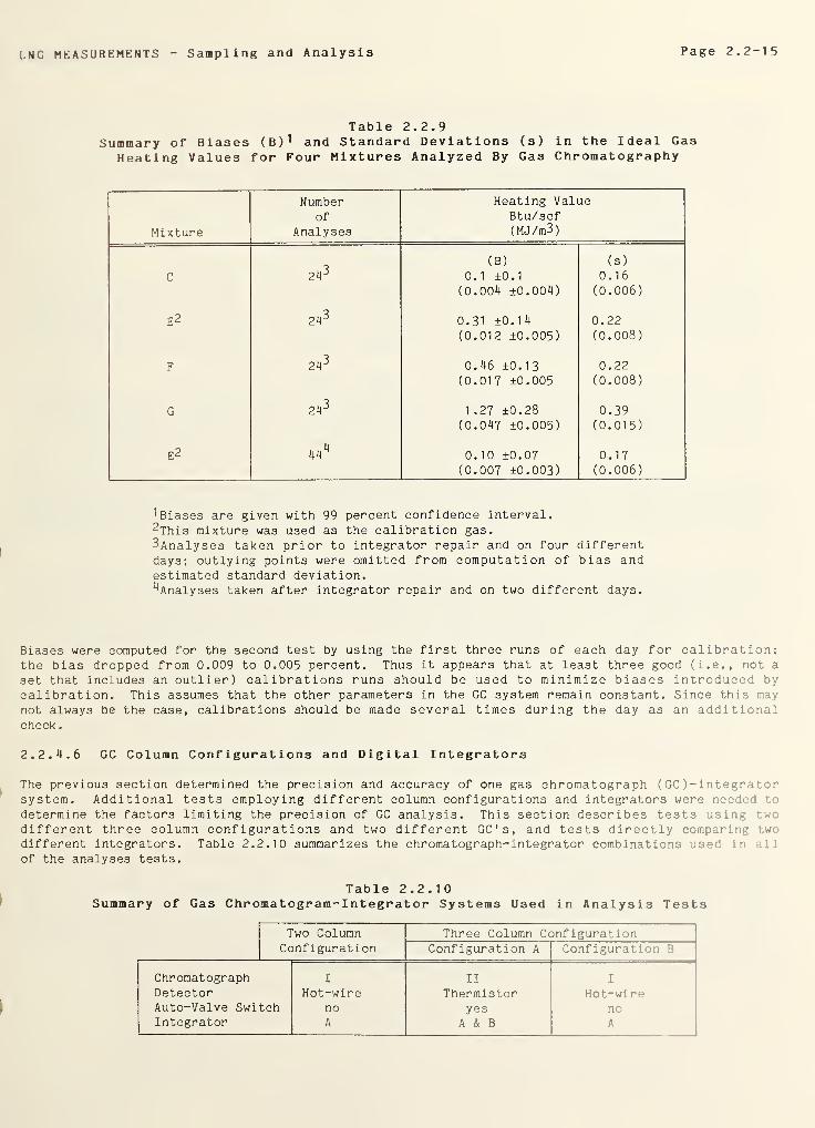
LNG MEASUREMENTS Sampling and Analysis Page 2.2-15
Table 2.2.9Summary of Biases (B) 1 and Standard Deviations (s) in the Ideal Gas
Heating Values for Four Mixtures Analyzed By Gas Chromatography
Mixture
Numberof
Analyses
Heating ValueBtu/scf(MJ/m3)
243
(B) (s)
C 0.1 ±0.1
(0.004 ±0.004)0.16(0.006)
E 2 24 3 0.31 ±0.14(0.012 ±0.005)
0.22(0.008)
F 243 0.46 ±0.13
(0.017 ±0.0050.22(0.008)
G 243
1 .27 ±0.28(0.047 ±0.005)
0.39(0.015)
E 2 0.10 ±0.07(0.007 ±0.003)
0.17(0.006)
biases are given with 99 percent confidence interval.2This mixture was used as the calibration gas.
3Analyses taken prior to integrator repair and on four differentdays; outlying points were omitted from computation of bias andestimated standard deviation.^Analyses taken after integrator repair and on two different days.
Biases were computed for the second test by using the first three runs of each day for calibration;the bias dropped from 0.009 to 0.005 percent. Thus it appears that at least three good (i.e., not a
set that includes an outlier) calibrations runs should be used to minimize biases introduced bycalibration. This assumes that the other parameters in the GC system remain constant. Since this may
not always be the case, calibrations should be made several times during the day as an additionalcheck
.
2 . 2 . 4 . 6 GC Column Configurations and Digital Integrators
The previous section determined the precision and accuracy of one gas chromatograph ( GC )- integratorsystem. Additional tests employing different column configurations and integrators were needed to
determine the factors limiting the precision of GC analysis. This section describes tests using twodifferent three column configurations and two different GC ' s ,
and tests directly comparing twodifferent integrators. Table 2.2.10 summarizes the chromatograph-integrator combinations used in allof the analyses tests.
Table 2.2.10Summary of Gas Chromatogram-Integrator Systems Used in Analysis Tests
Two ColumnConfiguration
Three Column ConfigurationConfiguration A Configuration B
ChromatographDetectorAuto-Valve SwitchIntegrator
I
Hot-wirenoA
II
Thermistoryes
A & B
I
Hot-wireno
*1
Page 2.2-16 LNG MEASUREMENTS - Sampling and Analysis
2. 2. 4. 7 GC Column Configurations and Column Packings
Obtaining the most accurate and precise analysis of vaporized LNG samples requires:
a) resolving oxygen, nitrogen and methane through pentane and column back flushing(i.e., carrier gas flow reversal) to obtain a composite hexane+ peak,
b) analyzing for all components in a single sample injection,
c) completing the analysis within approximately 30 minutes,d) operating the column ovens in an isothermal mode,
e) minimizing the effect of baseline upset by valve switches, andf) computing the composition by using peak areas.
The primary purpose in resolving the nitrogen and oxygen peaks is to detect contaminated samples,since the most likely contaminant is air. Also, it is a good way to detect leaks in the GC plumbing.The need for good resolution between the hydrocarbons is obvious. The anticipated concentrations ofhexane and heavier components is small (> 0.01 mol percent); therefore, combining the hexane+ peakfraction into one peak by backf lushing causes an insignificant error in the computed heating value.
The GPA [18] and ASTM [7] analysis procedures suggest using two sample injections — one injectioninto a column to resolve air and methane through pentane followed by a backf lush for the hexane+ peak:
a second injection into a different column to resolve nitrogen, oxygen and methane (the column then is
backflushed to remove the remaining hydrocarbons) . However, the two analyses must be combined. Thisis done through sample size or methane peak area. Both methods diminish analytical precision.
The primary reason for minimizing the analysis time is that the peak height to peak width ratiodecreases with increasing residence time. Maximum accuracy and precision in peak area measurementdecreases as the ratio decreases. It was found that, for the column configurations and operatingparameters considered here, the analysis times fell in two ranges — one was 40 minutes or greater andthe other was 24 to 30 minutes. Configurations having long analysis times elute the hexane+ peaklast; the other configurations elute methane last.
Temperature programming is an attractive way of reducing analysis time and sharpening peaks of the
heavier components. However, whenever feasible, isothermal column oven operation is normallypreferred over temperature programming when using thermal conductivity detectors. This is becauseflow variations caused by changing column temperature produce baseline drift when using thesedetectors. Temperature programming becomes attractive if the baseline drift can be compensated forreliably by the integrator or if flame ionization detectors are used. These detectors are insensitiveto flow variations but also do not detect nitrogen, oxygen and carbon dioxide.
Multicolumn configurations require valve switching with its associated carrier gas flow upsets; these,
in turn, produce baseline upsets. The time duration of baseline upsets are minimized by;
a) adjusting flow restrictors in column bypass lines so that the steady-state carriergas flow rate remains constant after switching the column in or out, and
b) using the carrier gas inlet pressure instead of mass flow to control the flow rate[18].
To minimize peak integration problems, each valve switch should occur far enough away from the nearestpeaks to allow baseline establishment between the peaks and the valve switch.
Traditionally, peak height measurement was preferred over peak area measurement for computingcomposition from chromatograms. Peak height was used because it was easy, quick and usually moreprecise than peak area. However, the peak height response is linear over a narrow concentrationrange, using a 0.5 cm3 sample loop volume, peak height response is linear at concentrations belowroughly 10 mol percent (peak area response is close to linear over the entire composition range).Also, peak heights cannot be used with composite backflush peaks. The currently availableprogrammable integrators eliminate the drawbacks to using peak areas. Also, since both methane andC 5 + peaks must be measured, peak area measurement was selected.
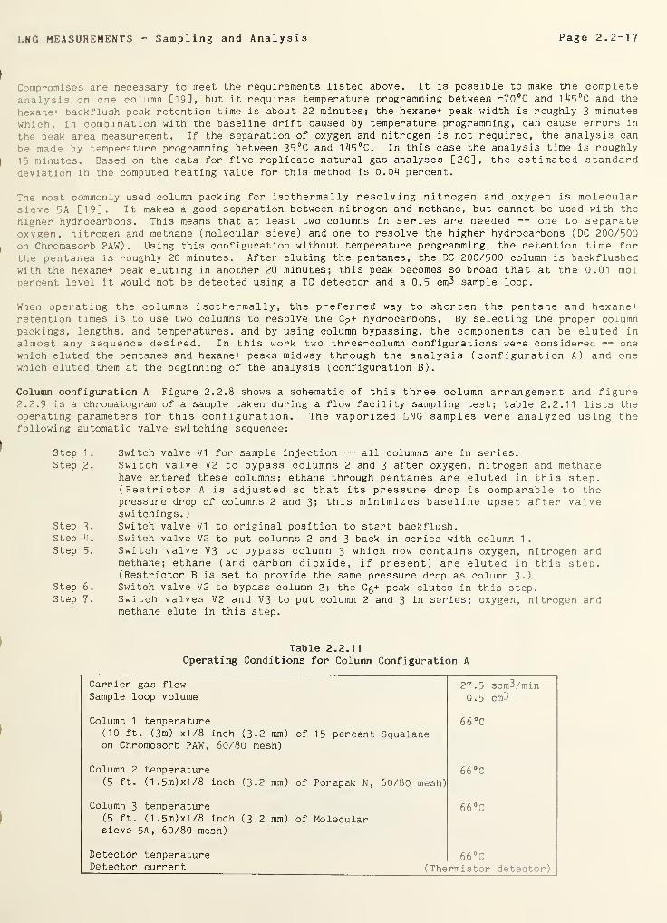
LNG MEASUREMENTS - Sampling and Analysis Page 2.2-17
I
I’ompromises are necessary to meet the requirements listed above. It is possible to make the completeanalysis on one column [19], but it requires temperature programming between ~70°C and 145°C and the
hexane+ backflush peak retention time is about 22 minutes; the hexane+ peak width is roughly 3 minutes
which, in combination with the baseline drift caused by temperature programming, can cause errors in
the peak area measurement. If the separation of oxygen and nitrogen is not required, the analysis can
be made by temperature programming between 35°C and 145°C. In this case the analysis time is roughly
|
15 minutes. Based on the data for five replicate natural gas analyses [20], the estimated standarddeviation in the computed heating value for this method is 0.04 percent.
The most commonly used column packing for isothermally resolving nitrogen and oxygen is molecularsieve 5A [19]. It makes a good separation between nitrogen and methane, but cannot be used with the
higher hydrocarbons. This means that at least two columns in series are needed — one to separateoxygen, nitrogen and methane (molecular sieve) and one to resolve the higher hydrocarbons (DC 200/500
I
on Chromasorb PAW). Using this configuration without temperature programming, the retention time forthe pentanes is roughly 20 minutes. After eluting the pentanes, the DC 200/500 column is backflushedwith the hexane+ peak eluting in another 20 minutes; this peak becomes so broad that at the 0.01 molpercent level it would not be detected using a TC detector and a 0.5 cm3 sample loop.
When operating the columns isothermally, the preferred way to shorten the pentane and hexane+retention times is to use two columns to resolve the C2 + hydrocarbons. By selecting the proper columnpackings, lengths, and temperatures, and by using column bypassing, the components can be eluted in
almost any sequence desired. In this work two three-column configurations were considered — onewhich eluted the pentanes and hexane+ peaks midway through the analysis (configuration A) and onewhich eluted them at the beginning of the analysis (configuration B).
Column configuration A Figure 2.2.8 shows a schematic of this three-column arrangement and figure2.2.9 is a chromatogram of a sample taken during a flow facility sampling test; table 2.2.11 lists theoperating parameters for this configuration. The vaporized LNG samples were analyzed using thefollowing automatic valve switching sequence:
Step 1 . Switch valve VI for sample injection — all columns are in series.Step 2. Switch valve V2 to bypass columns 2 and 3 after oxygen, nitrogen and methane
have entered these columns; ethane through pentanes are eluted in this step.(Restrictor A is adjusted so that its pressure drop is comparable to thepressure drop of columns 2 and 3; this minimizes baseline upset after valveswitchings.
)
Step 3. Switch valve VI to original position to start backflush.Step 4. Switch valve V2 to put columns 2 and 3 back in series with column 1
.
Step 5. Switch valve V3 to bypass column 3 which now contains oxygen, nitrogen andmethane; ethane (and carbon dioxide, if present) are eluted in this step.(Restrictor B is set to provide the same pressure drop as column 3.)
Step 6. Switch valve V2 to bypass column 2; the Cg+ peak elutes in this step.Step 7. Switch valves V2 and V3 to put column 2 and 3 in series; oxygen, nitrogen and
methane elute in this step.
Table 2.2.11Operating Conditions for Column Configuration A
Carrier gas flow 27.5 scm3/minSample loop volume 0.5 cm3
Column 1 temperature 66°C(10 ft. (3m) xl/8 inch (3.2 mm) of 15 percent Squalaneon Chromosorb PAW, 60/80 mesh)
Column 2 temperature 66°C(5 ft. (1.5m)x1/8 inch (3.2 mm) of Porapak N, 60/80 mesh)
Column 3 temperature 66°C(5 ft. (1.5m)x1/8 inch (3.2 mm) of Molecularsieve 5A, 60/80 mesh)
Detector temperature 66°CDetector current (Thermistor detector
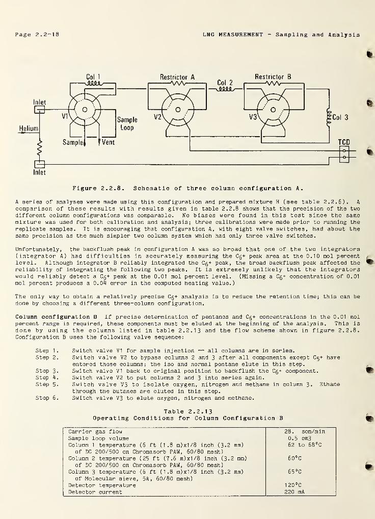
Page 2.2-18 LNG MEASUREMENT - Sampling and Analysis
Inlet
Figure 2.2.8. Schematic of three column configuration A.
A series of analyses were made using this configuration and prepared mixture H (see table 2.2.6). A
comparison of these results with results given in table 2 . 2.8 shows that the precision of the twodifferent column configurations was comparable. No biases were found in this test since the samemixture was used for both calibration and analysis; three calibrations were made prior to running thereplicate samples. It is encouraging that configuration A, with eight valve switches, had about thesame precision as the much simpler two column system which had only three valve switches.
Unfortunately, the backflush peak in configuration A was so broad that one of the two integrators(integrator A) had difficulties in accurately measuring the Cg+ peak area at the 0.10 mol percentlevel. Although integrator B reliably integrated the C 5 + peak, the broad backflush peak affected thereliability of integrating the following two peaks. It is extremely unlikely that the integratorswould reliably detect a Cg+ peak at the 0.01 mol percent level. (Missing a Cg+ concentration of 0.01
mol percent produces a 0.04 error in the computed heating value.)
The only way to obtain a relatively precise Cg+ analysis is to reduce the retention time; this can bedone by choosing a different three-column configuration.
Column configuration B If precise determination of pentanes and C5 + concentrations in the 0.01 molpercent range is required, these components must be eluted at the beginning of the analysis. This is
done by using the columns listed in table 2 . 2.13 and the flow scheme shown in figure 2.2.8.Configuration B uses the following valve sequence:
Step 1. Switch valve VI for sample injection — all columns are in series.
Step 2. Switch valve V2 to bypass columns 2 and 3 after all components except C 5+ have
entered these columns; the iso and normal pentane elute in this step.Step 3- Switch valve VI back to original position to backflush the C5 + component.Step 4. Switch valve V2 to put columns 2 and 3 into series again.Step 5. Switch valve V3 to isolate oxygen, nitrogen and methane in column 3. Ethane
through the butanes are eluted in this step.Step 6 . Switch valve V3 to elute oxygen, nitrogen and methane.
Table 2.2.13Operating Conditions for Column Configuration B
Carrier gas flow 28. scm/minSample loop volume 0.5 cm3
Column 1 temperature (6 ft (1.8 m)x1/8 inch (3.2 mm) 62 to 68 °C
of DC 200/500 on Chromasorb PAW, 60/80 mesh)Column 2 temperature (25 ft (7.6 m)x1/8 inch (3.2 mm) 60°C
of DC 200/500 on Chromasorb PAW, 60/80 mesh)Column 3 temperature (6 ft (1.8 m)x1/8 inch (3.2 mm) 65 °C
of Molecular sieve, 5A , 60/80 mesh)Detector temperature 1 20 °C
Detector current 220 mA
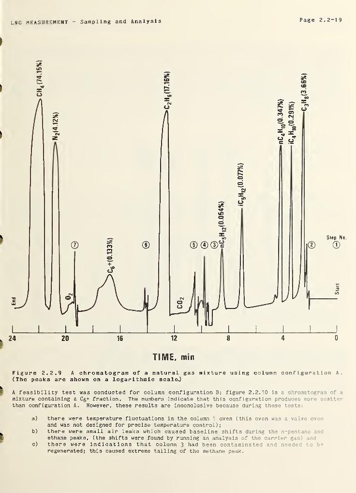
LNG MEASUREMENT - Sampling and Analysis Page 2.2 19
ID
TIME, min
Figure 2.2.9 A chromatogram of a natural gas mixture using column configuration A.
(The peaks are shown on a logarithmic scale.)
A feasibility test was conducted for column configuration B; figure 2.2.10 is a chromatogram >f i
mixture containing a Cg+ fraction. The numbers indicate that this configuration produces monthan configuration A. However, these results are inconclusive because during these tests:
a) there were temperature fluctuations in the column 1 oven (this oven was a valve > v
and was not designed for precise temperature control);b) there were small air leaks which caused baseline shifts during the n-pentane m 1
ethane peaks, (the shifts were found by running an analysis of the carrier -• t
there were indications that column 3 had been contaminated and need-; • '
regenerated; this caused extreme tailing of the methane peak.
c)
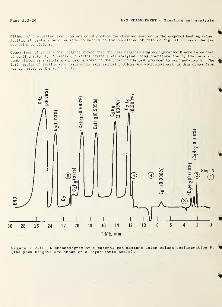
Page 2.2-20 LNG MEASUREMENT - Sampling and Analysis
Either of the latter two problems could produce the observed scatter in the computed heating value.
Additional tests should be made to determine the precision of this configuration under betteroperating conditions.
Comparison of pentane peak heights showed that the peak heights using configuration B were twice that
of configuration A. A sample containing hexane + was analyzed using configuration B; the hexane +
peak eluted as a single sharp peak instead of the broad double peak produced by configuration A. Thefull results of testing were hampered by experimental problems and additional work in this comparisonwas suggested by the authors [1].
aP
TIME, min
Figure 2.2.10 A chromatogram of a natural gas mixture using column configuration B.
(The peak heights are shown on a logarithmic scale).
LNG MEASUREMENT - Sampling and Analysis Page 2.2-21
2. 2. 4. 8 Digital Integrator Evaluation
The purpose of this work was to directly compare the accuracy and precision of two differentprogrammable digital integrators. All digital GC integrators use voltage to frequency converters and
counters to convert the detector output voltage into peak areas. The primary difference in
integrators is the way they treat the converted signal. Both integrators used in this evaluationemployed sophisticated software programs; these programs identified peaks, baseline segments and small
peaks riding on the tail of larger peaks. Also, they compensated for transient baselines whencomputing peak areas. Both integrators were programmable so that automatic adjustments, which were
unique to the particular analysis, could be made during the analysis. The primary differences between
the two integrators were that the software programs used different peak detection algorithms and that
integrator B had considerable more programming capabilities; however, this versatility was unnecessary
for analyzing vaporized LNG samples.
During the last 2 days of a 4 day test period both integrators produced one or more extraneous
results. The outliers appeared to occur randomly among the integrators which excluded the GC as the
cause. It is suspected that the outliers were caused by power fluctuations since the integrators were
on different circuits; the GC detector power supply was connected to a constant voltage transformer.Shortly after these tests there were several power fluctuations severe enough to shut down the
integrators.
2.2. 4.9 GC Analysis Accuracy and Precision
Variation in any of the operating parameters listed in table 2.2.11 could affect analysis precisionand accuracy. However, variables such as column temperature are electronically controlled.Therefore, they will be constant unless the set point is changed. The variables most subject to
change are sample amount (i.e., sample pressure since a fixed volume sample loop is used) and carriergas flow rate because it must be set manually.
A test was conducted using column configuration A and both integrators. In one test injected sampleswere used at pressures of 13-7, 21.1 and 8.6 psia (94,145 and 59 kPa); the calibration sample pressurewas 13.7 psia (95kPa). The results of the test showed that the precision was insensitive to samplepressure. However, there was an apparent linear relationship between bias and sample pressure. Thistest indicates that maintaining the sample pressure within ± 10 percent of that used for calibrationwill keep the bias to less than 0.025 percent in the computed heating value.
The observed bias was caused by the method the integrators used to determine the peak area. Unlessthe peak was very large and sharp, part of the peak area was lost during the baseline determination.The absolute amount of area lost remained nearly constant as the peak area changed, provided that thepeak width at the half-height did not change. Therefore, the relative amount of area lost decreasedwith increasing peak size. Since the methane peak was so large there was a negligible amount of arealost during baseline determination. However, this was not the case for all other components exceptthe pentanes. (The pentane peak areas were so small that the effect was within the data scatter.)This explains why the apparent methane content decreased and the ethane through butane contentsincreased with increasing sample injection pressure.
In the second test the carrier gas flow was varied by ±
7
percent. Integrator A results wereinsensitive to the flow variation, whereas, integrator B showed a bias in the computed heating value.This bias was caused by the method used to establish a baseline between the nitrogen and methanepeaks. During these tests integrator B was programmed to force a baseline at a specified time.time was set at the bottom of the valley between the two peaks (see figure 2.2.9) when the carri':- gn:
flow rate was 26.5 scm3/min. Increasing the carrier gas flow rate made the valley bottom occur hepthe forced baseline. Therefore, the forced baseline caused the integrator to ignore part f •••
methane peak; this lowered the apparent methane content and raised the apparent compositiother components. This problem can be eliminated by having the integrator automatically ••
•
valley bottom as the baseline when two peaks are not completely resolved.
Based on these tests it appears that the precision and accuracy of the computed heating v .
unaffected by changes of ± 7 percent in the carrier gas flow rate. This conclusion strict lyonly to configuration A. However, it should apply to other column configuration- whl !
comparable time spacings between valve switches and peak elutions.
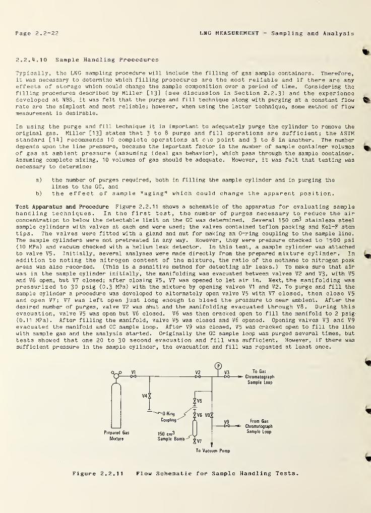
Page 2.2-22 LNG MEASUREMENT - Sampling and Analysis
2.2. JI.10 Sample Handling Procedures
Typically, the LNG sampling procedure will include the filling of gas sample containers. Therefore,it was necessary to determine which filling procedures are the most reliable and if there are anyeffects of storage which could change the sample composition over a period of time. Considering thefilling procedures described by Miller [13] (see discussion in Section 2.2.3) and the experiencedeveloped at NBS, it was felt that the purge and fill technique along with purging at a constant flowrate are the simplest and most reliable; however, when using the latter technique, some method of flowmeasurement is desirable.
In using the purge and fill technique it is important to adequately purge the cylinder to remove theoriginal gas. Miller [13] states that 3 to 8 purge and fill operations are sufficient; the ASTMstandard [14] recommends 10 complete operations at one point and 3 to 8 in another. The numberdepends upon the line pressure, because the important factor is the number of sample container volumesof gas at ambient pressure (assuming ideal gas behavior), which pass through the sample container.Assuming complete mixing, 10 volumes of gas should be adequate. However, it was felt that testing wasnecessary to determine:
a) the number of purges required, both in filling the sample cylinder and in purging the
lines to the GC, and
b) the effect of sample "aging" which could change the apparent position.
Test Apparatus and Procedure Figure 2.2.11 shows a schematic of the apparatus for evaluating samplehandling techniques. In the first test, the number of purges necessary to reduce the airconcentration to below the detectable limit on the GC was determined. Several 150 cm3 stainless steelsample cylinders with valves at each end were used; the valves contained teflon packing and Kel-F stemtips. The valves were fitted with a gland and nut for making an 0-ring coupling to the sample line.
The sample cylinders were not pretreated in any way. However, they were pressure checked to 1500 psi(10 MPa) and vacuum checked with a helium leak detector. In this test, a sample cylinder was attachedto valve V5 . Initially, several analyses were made directly from the prepared mixture cylinder. Inaddition to noting the nitrogen content of the mixture, the ratio of the methane to nitrogen peakareas was also recorded. (This is a sensitive method for detecting air leaks.) To make sure that airwas in the sample cylinder initially, the manifolding was evacuated between Valves V2 and V3, with V5and V6 open, but V7 closed; after closing V5
,V7 was opened to let air in. Next, the manifolding was
pressurized to 30 psig (0.3 MPa) with the mixture by opening valves VI and V2. To purge and fill thesample cylinder a procedure was developed to alternately open valve V5 with V7 closed, then close V5and open V7 ; V7 was left open just long enough to bleed the pressure to near ambient. After the
desired number of purges, valve V2 was shut and the manifolding evacuated through V8. During thisevacuation, valve V5 was open but V6 closed. V6 was then cracked open to fill the manifold to 2 psig-
(0.11 MPa). After filling the manifold, valve V5 was closed and V6 opened. Opening valves V3 and V9evacuated the manifold and GC sample loop. After V9 was closed, V5 was cracked open to fill the linewith sample gas and the analysis started. Originally the GC sample loop was purged several times, but
tests showed that one 20 to 30 second evacuation and fill was sufficient. However, if there was
sufficient pressure in the sample cylinder, the evacuation and fill was repeated at least once.
To Gas
Chromatograph
Sample Loop
From Gas
Chromatograph
Sample [oop
Figure 2.2.11 Flow Schematic for Sample Handling Tests.
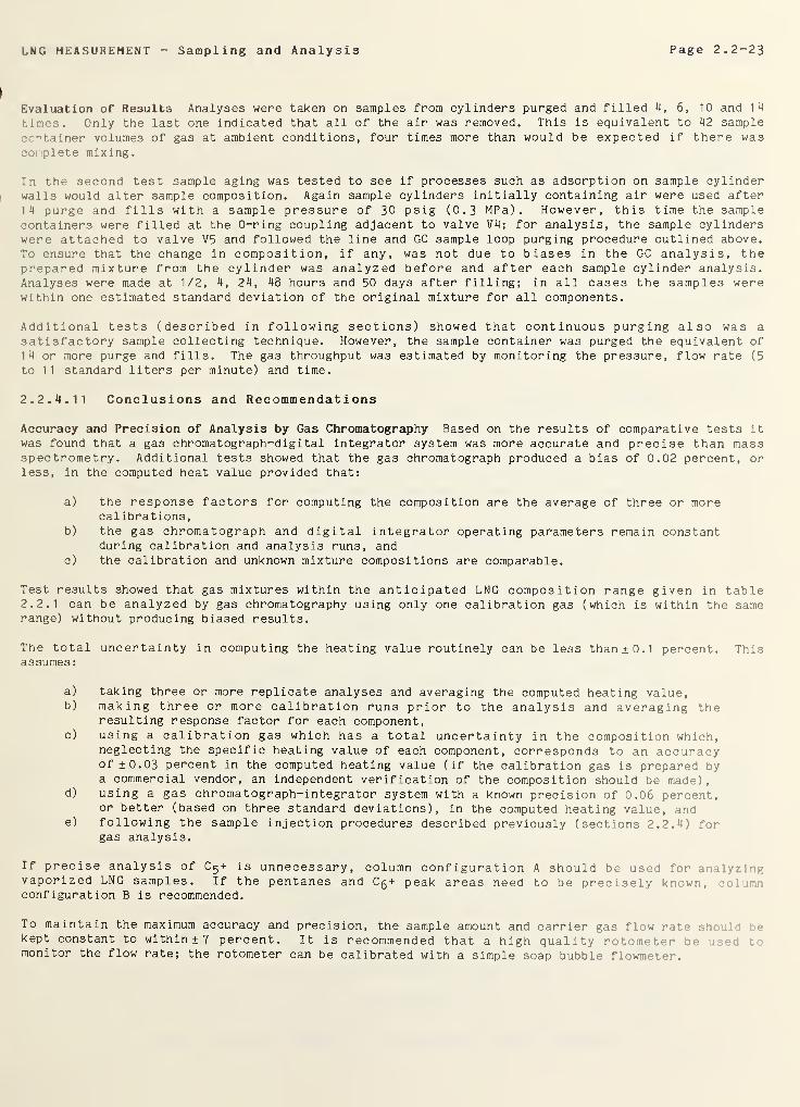
LNG MEASUREMENT Sampling and Analysis Page 2.2-23
Evaluation of Results Analyses were taken on samples from cylinders purged and filled 4, 6 , 10 and 14
times. Only the last one indicated that all of the air was removed. This is equivalent to 42 sample
c -'tainer volumes of gas at ambient conditions, four times more than would be expected if there wascomplete mixing.
In the second test sample aging was tested to see if processes such as adsorption on sample cylinderwalls would alter sample composition. Again sample cylinders initially containing air were used after
14 purge and fills with a sample pressure of 30 psig (0.3 MPa). However, this time the samplecontainers were filled at the 0-ring coupling adjacent to valve V4; for analysis, the sample cylinderswere attached to valve V5 and followed the line and GC sample loop purging procedure outlined above.
To ensure that the change in composition, if any, was not due to biases in the GC analysis, theprepared mixture from the cylinder was analyzed before and after each sample cylinder analysis.Analyses were made at 1/2, 4, 24, 48 hours and 50 days after filling; in all cases the samples werewithin one estimated standard deviation of the original mixture for all components.
Additional tests (described in following sections) showed that continuous purging also was a
satisfactory sample collecting technique. However, the sample container was purged the equivalent of14 or more purge and fills. The gas throughput was estimated by monitoring the pressure, flow rate (5
to 11 standard liters per minute) and time.
2.2.4.11 Conclusions and Recommendations
Accuracy and Precision of Analysis by Gas Chromatography Based on the results of comparative tests itwas found that a gas chromatograph-digital integrator system was more accurate and precise than massspectrometry . Additional tests showed that the gas chromatograph produced a bias of 0.02 percent, orless, in the computed heat value provided that:
a) the response factors for computing the composition are the average of three or morecalibrations,
b) the gas chromatograph and digital integrator operating parameters remain constantduring calibration and analysis runs, and
c) the calibration and unknown mixture compositions are comparable.
Test results showed that gas mixtures within the anticipated LNG composition range given in table2 . 2.1 can be analyzed by gas chromatography using only one calibration gas (which is within the samerange) without producing biased results.
The total uncertainty in computing the heating value routinely can be less than ±0.1 percent. Thisassumes
:
a) taking three or more replicate analyses and averaging the computed heating value,b) making three or more calibration runs prior to the analysis and averaging the
resulting response factor for each component,c) using a calibration gas which has a total uncertainty in the composition which,
neglecting the specific heating value of each component, corresponds to an accuracyof ± 0.03 percent in the computed heating value (if the calibration gas is prepared bya commercial vendor, an independent verification of the composition should be made),
d) using a gas chromatograph-integrator system with a known precision of 0.06 percent,or better (based on three standard deviations), in the computed heating value, and
e) following the sample injection procedures described previously (sections 2.2.4) forgas analysis.
If precise analysis of C 5+ is unnecessary, column configuration A should be used for analyzing
vaporized LNG samples. If the pentanes and C 5 + peak areas need to be precisely known,configuration B is recommended.
To maintain the maximum accuracy and precision, the sample amount and carrier gas flow rate •.
kept constant to within ±7 percent. It is recommended that a high quality rotometer be . :
•
monitor the flow rate; the rotometer can be calibrated with a simple soap bubble flowmeter.
Page 2. 2~24 LNG MEASUREMENT Sampling and Analysis
Direct comparison of two different integrators showed that the two instruments had comparableprecision. Based on all of the tests (see section 2.2.4), it was concluded that, at present, thedigital integrator is less precise than the gas chromatograph employing a thermal conductivitydetector. Therefore, the most precise analysis will be one in which the integrator "sees" thesharpest peaks and the least baseline fluctuations before and after peaks. To maximize the precision,a programmable integrator should be used.
Sample Handling Tests showed that both the purge and fill technique and the continuous purgetechnique were accurate methods for collecting vaporized LNG samples. However, both techniquesrequire some care to insure that the cylinder has been purged properly. Commercially availablestainless steel sample cylinders are recommended for collecting gas samples. No special preparationof the cylinders is required prior to their use. Tests showed that stainless steel cylinders do not
alter the hydrocarbon content over a six week period (However, stainless steel is not inert to sulphurcompounds.
)
Selection of a Gas Chromatograph-Integrator System It is recommended that the following features be
included in any gas chromatograph-integrator system dedicated to routine analysis of vaporized LNGsamples:
a) Automatic valve switching - this is required to insure that the right valve is
switched at the right time.
b) Thermal conductivity detector - this is the only detector that is sensitive to all
the components in natural gas and is linear in response over the anticipatedconcentration ranges (i.e., the output signal is directly proportional to theconcentration). Hot wire filaments are preferred over thermistors because theyprovide superior stability, longer operating life and fewer anomalies of operation[20]. The instrument should contain a thermal protecting device to minimize the riskof oxidizing the filaments. To maximize sensitivity the detector cell volume shouldbe as small as possible.
c) Isolated power supply - this is necessary to prevent electrical noise generated by
oven temperature controllers from entering the detector circuitry. The detectorpower input should be connected to a constant voltage transformer to minimize effect
of line power fluctuations.d) Carrier gas flow control by inlet pressure - this is preferable to mass flow control
when the analysis involves valve switching [18]. A two-stage pressure regulatorshould be used to keep the inlet pressure constant.
e) Readily accessible valve and column connections - this is needed to make routine
maintenance and leak checking easy.
f) Programmable digital integrator - this is necessary to maximize the analyticalprecision. A memory protect feature should be used to prevent losing programs duringmomentary power failures. A constant voltage transformer should be connected to the
integrator to minimize noise due to line power fluctuations.
2.2.5 LNG Sampling
The sampling tests included both laboratory and field tests. The laboratory tests provided closecontrol of all operating variables whereas the field tests permitted evaluation of a full scale
sampling system.
The chronological order of the tests and the variables considered for their effect on sampling
accuracy and precision were:
a) laboratory tests (Probe Evaluation) - sampling rate, LNG flow rate, temperature,
pressure, degree of subcooling and three probes;
b) laboratory tests (Vaporizer Evaluation) - sampling rate, temperature, degree of
subcooling, LNG flow rate and two vaporizer designs,
c) field tests (LNG Flow Facility Test 1 )- three probes and three vaporizers,
d) laboratory tests (General Tests) - accumulator residence time, vaporizer outlet
temperature, pressure drop upstream of vaporizer, heat leak to sample probe andpresence of heavy components (C
5 +) in the LNG,
e) field tests (Shipboard Tests) - sampling rate and comparison between liquid and vapor
sampling,f) field tests (LNG Flow Facility Test 2) - sampling rate, heat leak, start-up
transients and three variations of a vaporizer design.
The following section discusses all the laboratory tests before describing the field tests.
LNG MEASUREMENT Sampling and Analysis Page 2.2-25
2.2.5. 1 Laboratory Tests
Laboratory Scale Apparatus Figure 2.2.12 shows a schematic of the laboratory scale apparatus used in
this work. The cryogenic portion of the apparatus was contained in an evacuated double walled dewarwhich was 33 inches (838 millimeters) deep and had a 1 0— 3/*4 inch (273 millimeters) inside diameter.
The LNG vessel, which was 8-1/2 inch (215 millimeters) long with an outer diameter of 8 inches (203millimeters), had an inner volume of roughly 6 liters; the wall was copper and the two end plates were
brass. A centrifugal pump circulated LNG through a turbine flowmeter, with a range of 0.25 to 2.5gallons per minute (0.016 to 0.16 liters/second), and through the test section between valves T1 and
T2 . All of the lines in this loop were 1/2 inch (12.7 millimeters) O.D. copper tubing except for a 3
inch (76 millimeters) long section containing 1 inch (25 millimeters) O.D. copper tubing justdownstream of valve T1 . This short section acted as a mixing chamber to reduce flow turbulence causedby the valve. The test section was a 6 — 3 / ^ inch (171 millimeters) long straight section. It
contained two probes — an upstream facing pitot tube and a side tap. Both probes were mountedvertically and were made of 1/16 inch (1.59 millimeters) O.D. by 0.023 inch (0.58 millimeter) I.D.
stainless steel tubing. There was roughly 6 inches (150 millimeters) of line between the probes andvalves T4 and T5.
Besides the pitot tube and side tap, a "reference" probe was located in the straight-run leg of a teepositioned just upstream of valve T1. Since the flow into the tee was downward, the reference probewas in essence located on the bottom of the line. There were 8 inches (200 millimeters) of 0.023 inch(0.58 millimeter) I.D. stainless steel tubing between this probe and valve T3.
Valves T 1 through T6 were bellows valves which were located inside the insulating vacuum space at LNGtemperature. They were actuated by stem extensions protruding through the top plate of the apparatus.Valves T3 through T6 were mounted on a brass plate which was soldered to the top of the mixingchamber.
T17 To Gas
Figure 2.2. 1 2« Schematic of laboratory scale apparatus.
Page 2.2-26 LNG MEASUREMENT Sampling and Analysis
After a probe was selected by opening either valve T3, T4, or T5, the sample passed through 1/16 inch(1.59 millimeters) O.D. by 0.023 inch (0.58 millimeter) I.D. stainless steel tubing to one of threevaporizers. If the sample went to the reference vaporizer, it first passed through valve T6 and 8
inches (203 millimeters) of tubing; valve T6 was a needle valve used to provide additional pressuredrop to prevent sample backflash, i.e., flow reversal due to vaporization. The reference vaporizerconsisted of a 5 inch (127 millimeters) long section of 1/16 inch (1.58 millimeters) O.D. by 0.051inch (1.28 millimeters) I.D. stainless steel tubing and a 12 inch (304 millimeters) long section of1/8 inch (3.18 millimeters) O.D. by 0.101 inch (2.56 millimeters) I.D. stainless steel tubing. Thesample was vaporized by passing a low voltage, high amperage dc current through the two sections oftubing. To prevent shorts, the two ends of the vaporizer were epoxied into micarta couplings. Thereference vaporizer was located less than 1/2 inch (13 millimeters) from where the sample line leftthe vacuum insulated space.
After the sample left the vaporizer it went to a manifold containing a 2 liter accumulator, through a
0 to 11.4 liter per minute rotometer and back to the LNG vessel. The lines between the vaporizer androtometer were 1/4 inch (6.35 millimeters) O.D. by 0.190 inch (4.83 millimeters) I.D. copper tubing;the copper tubing downstream of the rotometer was 3/8 inch (9.53 millimeters) O.D. by 0.343 inch (8.71
millimeters) I.D. The accumulator could be isolated by closing valves T7 and T8; to maintain the
sample flow, valves T9 and T10 (a regulating valve) were opened when the accumulator was isolated.Samples could be taken from the accumulator through valve T 1 4 and from the bypass line through valveT 1 7 •
The second vaporizer, vaporizer A, contained an electrically heated vaporizing element, an adjustableback pressure regulator and a 0 to 30 psig (0.1 to 0.3 MPa) pressure gauge in a single unit. Theheating element was a 1-1/4 inch (31.8 millimeters) wide by 28 inch (71.1 centimeters) long section of
100 mesh, 316 stainless steel screen wrapped around a 1/2 inch (12.7 millimeters) O.D. stainless steeltube. The diameter of the tube plus screen was 0.71 inches (18 millimeters). The vaporizer wasdesigned to have the sample flow through the screen perpendicular to the axis of the tube. Also, thevaporizer contained a bypass valve and a pressure relief valve to protect the pressure gauge; both of
these valves were capped in this study. Approximately 15 inches (381 millimeters) of stainless steeltubing connected the probes to vaporizer A. To prevent premature vaporization the line was vacuumjacketed to within 1 inch (25 millimeters) of the vaporizer inlet. When using this vaporizer, valveTil and T12 replaced the function of valves T7 and T9. The third vaporizer was a Cook sampler, whilethe reference vaporizer and vaporizer A were for continuous sampling, the Cook sampler was designedfor the batch sampling. Since the LNG sample was used to cool the sampler, the lines were piped to
return the vapor to the LNG vessel; otherwise, the mixture would be depleted too quickly. The linefrom the probes to the sampler was roughly 15 inches (381 millimeters) long and vacuum jacketed.
Liquid nitrogen (LN 2 ) was used as the refrigerant in this study. The LN 2 vessel was 9“7/8 inches (251
millimeters) in diameter and 10-3/4 inches (273 millimeters) long and could contain about 10 liters of
liquid. The LNG vessel was cooled by liquid flowing from the LN 2 vessel and through a coil wrappedand soldered on the LNG vessel. Cold nitrogen vapor leaving the coil went to another coil soldered on
a 1/8 inch (3.2 millimeters) thick copper plate located roughly 2 inches (50 millimeters) below the
top plate. All lines into the vacuum space were in thermal contact with this plate to reduce heatleakage. After leaving the copper plate the nitrogen went to valve N1 and to a 0-44 liter per minutefull scale rotometer and/or to bypass valve N2 . When the apparatus was temporarily shut down, e.g.,
overnight, nitrogen gas was vented through another line which contained a relief valve set at 8 psig(0.16 MPa). During these periods the LN 2 vessel needed to be filled every 24 to 28 hours. The LNGvessel cooled at a rate of 1 to 2 K per day during idle periods.
To minimize radiation heat leak in the vacuum space, the apparatus was surrounded by a copperradiation shield. This shield was fastened to the LN 2 vessel and extended up to the copper plate.
2. 2. 5. 2 Instrumentation
The temperature was measured using a platinum resistance thermometer (PRT) calibrated on the IPTS-68
temperature scale. The PRT was encased in a copper sheath pressurized with helium gas and positionednear the bottom of the LNG vessel. To measure the resistance, a one milliampere constant current
source was used with a potentiometer and a nanovolt null detector. The thermometer current wasmonitored by measuring the voltage drop across a 100 ohm standard resistor. Initially, the outputfrom the null detector was directed to a power regulator; this regulator powered either a 120 or a 230
ohm heater wrapped on the LNG vessel. Although the temperature control was good ( ±0.01 K) , crosstalkdeveloped between the power regulator and the null detector. This control method was dropped andthereafter the temperature was controlled by manually adjusting the LN2 flow rate; using this method,
it was possible to control the temperature to ±0.03 K or better.
LNG MEASUREMENT Sampling and Analysis Page 2.2-27
The saturation pressure of the LNG was measured with a 0 to 100 psia (0 to 6.9 MPa) quartz bourdontube pressure gauge; this gauge was calibrated against an air dead weight gauge. The difference
between the LNG pressure in the test section and in the LNG vessel was measured with a 0-300 inches of
water (0 to 0.075 MPa) differential pressure gauge; this gauge was not calibrated during this study.
2.2.5. 3 Safety Features
Since the study involved flammable fluids, all vents on the LNG system were tied to the room vent
system. In addition, all vacuum pump outlets were connected to the same vent system. A relief valve,
set at 120 psig (0.93 MPa), was located on the sample return line; this relief valve led to the vent
system. Finally, the insulating vacuum system had a relief valve connected to the vent and a pressure
switch-solenoid valve combination. If the vacuum pressure increased to 100 microns (13 Pa), or, if
there was a power failure, the solenoid closed, isolating the vacuum space from the vacuum pump.
Recirculation Pump Motor In the early stages of the study some problems developed with the motors
selected to drive the recirculation pump. The same pump had been operated in liquid helium using a
small three phase induction motor [21]. However, this motor had too much slippage when used with LNG
(the density of LNG is four times greater than that of liquid helium). Two small motors in tandemstill did not provide sufficient torque. A 1/7 HP (106 watt) dc brush motor was then tried, and the
motor had sufficient torque but operated only 100 hours before the brushes failed. The brushes werereplaced and the same motor operated for another 90 hours. Finally, a larger capacity three phaseinduction motor (1/2 HP ( 373 watt) at 1 0,000 rpm) was purchased and installed; it workedsatisfactorily for the remainder of the study.
2.2.5. 4 Experimental Procedure
After checking for leaks the insulating vacuum space was evacuated for 15 or more hours. By this timethe pressure was down to 10
-1^ millimeters Hg (0.1 Pa) or less. The complete LNG system was evacuated
and back filled several times with high purity nitrogen which passed through a molecular sievepurifier. The cooldown was started by filling the LN 2 vessel with liquid nitrogen. With bypass valveN2 (see figure 2.2.12) wide open it took about 2 hours to bring the apparatus to 110 K.
Once at LNG temperature, all instruments and the pump were tested, and the system was checked for coldleaks. If all was well, the prepared mixture was condensed into the LNG vessel. Using a pressure of40 to 50 psi (0.27 to 0.34 MPa) above the mixture's saturation pressure it took about, one hour to fillthe LNG vessel; when the LNG vessel was full there was a sudden rise in the pressure of the LNGsystem. At this point the startup was complete.
Preparation of Known Mixture Because the accuracy of Sampling Measurement Systems (SMS) needed to beknown, prepared mixtures of known composition were required in the laboratory scale apparatus. Of theseveral preparation methods considered, it was decided that the fastest and most accurate method wasto fill a large (1.75 ft3 (49.6 liters)) gas cylinder with pure fluids and analyze the resultingmixture. (Size and weight limitations of the mass balance made preparation by weight unfeasible.)Partial pressures were used as a guide for estimating how much of each component should be added.Prior to filling, the cylinder was evacuated while being warmed with a heat lamp for at least ^3
hours.
The cylinder was filled to 1100 psi (7.59 MPa), which was well below the dew point pressure ofmixtures used here, and warmed with heat lamps for at least 6 hours. To enhance mixing, the cy 1
was alternately heated in vertical and horizontal positions; when in the horizontal position t helamp was placed at each end of the cylinder. Next, a sample of the mixture was analyzed on th<
the cylinder then was heated for several more hours before making another analysis. If the analy esdid not agree, the procedure was repeated until they did. (It never took more than 48 hour:: to •
•
complete mixing.) Next, a series of at least 6 analyses were made on the mixture and • •• •
averaged to determine the composition as accurately as possible.
After filling the LNG vessel the cylinder pressure was 100 to 150 psig (0.79 to 1 . 1 u m; , .
mixture remaining in the cylinders was analyzed again to see if the composition had change- :.
this gas mixture was analyzed several times during each operating day so that day-t< -d ry
analysis could be detected. Table 2.2.15 gives the a summary of the average valu-heating value and liquid density from the final sets of analyses for the prep r- '
.
analyses are included in the original publication [1].
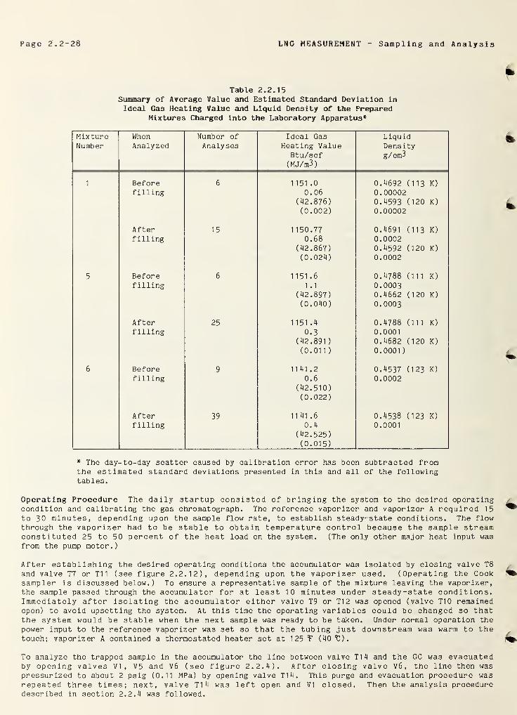
Page 2.2-28 LNG MEASUREMENT - Sampling and Analysis
Table 2.2.15Summary of Average Value and Estimated Standard Deviation in
Ideal Gas Heating Value and Liquid Density of the PreparedMixtures Charged into the Laboratory Apparatus*
MixtureNumber
WhenAnalyzed
Number of
AnalysesIdeal Gas
Heating ValueBtu/scf(MJ/m3)
LiquidDensityg/cm3
1 Beforefilling
6 1151 .0
0.06(42.876)(0.002)
0.4692 (113 K)
0.000020.4593 (120 K)
0.00002
Afterfilling
15 1150.770.68
(42.867)(0.024)
0.4691 (113 K)
0.00020.4592 (120 K)
0.0002
5 Beforefilling
6 1151.61 .1
(42.897)(0.040)
0.4788 (111 K)
0.00030.4662 (120 K)
0.0003
Afterfilling
25 1151.4
0.3(42.891
)
(0.01 1
)
0.4788 (111 K)
0.0001
0.4682 (120 K)
0.0001
)
6 Beforefilling
9 1141.20.6
(42.510)(0.022)
0.4537 (123 K)
0.0002
Afterfilling
39 1 1 41 .6
0.4
(42.525)
(0.015)
0.4538 (123 K)
0.0001
* The day-to-day scatter caused by calibration error has been subtracted fromthe estimated standard deviations presented in this and all of the followingtables.
Operating Procedure The daily startup consisted of bringing the system to the desired operatingcondition and calibrating the gas chromatograph. The reference vaporizer and vaporizer A required 15
to 30 minutes, depending upon the sample flow rate, to establish steady-state conditions. The flowthrough the vaporizer had to be stable to obtain temperature control because the sample streamconstituted 25 to 50 percent of the heat load on the system. (The only other major heat input wasfrom the pump motor.)
After establishing the desired operating conditions the accumulator was isolated by closing valve T8
and valve T7 or Til (see figure 2.2.12), depending upon the vaporizer used. (Operating the Cooksampler is discussed below.) To ensure a representative sample of the mixture leaving the vaporizer,the sample passed through the accumulator for at least 10 minutes under steady-state conditions.Immediately after isolating the accumulator either valve T9 or T12 was opened (valve T10 remainedopen) to avoid upsetting the system. At this time the operating variables could be changed so thatthe system would be stable when the next sample was ready to be taken. Under normal operation the
power input to the reference vaporizer was set so that the tubing just downstream was warm to thetouch; vaporizer A contained a thermostated heater set at 1 25 $’ (40 t).
To analyze the trapped sample in the accumulator the line between valve T14 and the GC was evacuatedby opening valves VI, V5 and V6 (see figure 2.2.4). After closing valve V6, the line then was
pressurized to about 2 psig (0.11 MPa) by opening valve T 1 4 . This purge and evacuation procedure wasrepeated three times; next, valve T 1 4 was left open and VI closed. Then the analysis proceduredescribed in section 2.2.4 was followed.
LNG MEASUREMENT - Sampling and Analysis Page 2.2-29
To draw a sample from the accumulator bypass line, valves V2 and V7 were opened to evacuate the lineconnecting V2 and T 1 6 . After closing V7, valve T 1 7 was opened to pressurize the line to about 2 psig
(0.11 MPa). After repeating the purge procedure three times, valve V2 was closed and T17 left open.Next, the analysis procedure was followed. The sample flow in the bypass line was uninterruptedduring the purging procedure.
Initially, at least two analyses were made on each sample. Since each analysis took 14.5 minutes,
this limited the analysis to a maximum of two samples per hour. Once the integrator was repaired,only one analysis was made on each sample unless the results were more than three estimated standarddeviations, for gas analysis alone, from the expected values. In this case, another analysis wasmade; in all cases, duplicate analyses were within one estimated standard deviation of the first
analysis for all components. The prepared mixture from the cylinder was analyzed several times a day.
Most often these were made during a temperature change and/or a LN 2 vessel filling — each of whichtook about 30 minutes. The prepared mixture also was analyzed at the end of the day after shuttingdown the apparatus.
Sample flow to the Cook sampler was obtained by closing valves T6, Til, and T12 and by opening valvesT7 and T8 and the valves on the Cook sampler (see figure 2.2.12). Once the sampler contained onlyliquid the valves on the sampler were closed, and it was allowed to warm up. Next the accumulator wasevacuated by closing valve T8 and opening valve T13 for several minutes. After closing valve T13, thedownstream valve on the Cook sampler was opened. Then the accumulator was isolated by closing valveT7 and the mixture analyzed following the procedures described above.
Control of Operating Variables The operating variables initially considered in this study weretemperature, Reynold's number in the test section (Re), difference between the pressure at thesampling point and saturation pressure (pp) and sampling rate (Q). The temperature was maintained bybalancing the refrigerant flow against the heat input. Usually temperature control was maintained byhaving only valve N1 open (see figure 2.2.12); however, when operating at high sample flow rates,bypass valve N2 had to be opened as much as 1/4 turn. Both Re, i.e., flow rate in the test section,and pp were set by adjusting pump speed and valve T2. (In all tests reported here valve T1 remainedwide open.) Valve T15 controlled the sampling rate.
2. 2. 5. 5 Experimental Results
The laboratory tests were divided into three phases:a) Probe Evaluationb) Vaporizer Evaluationc) General Tests.
The first two phases were conducted prior to the first flow facility tests. The last series of testswere made to explain the unexpectedly poor results obtained at the flow facility. The second flowfacility tests and the shipboard tests followed the general laboratory tests.
2. 2. 5. 6 Probe Evaluation
The purpose of this phase of work was to:a) determine which, if any, operating variables affected the reliability of the three
probes,b) determine which of the test probes was the most reliable,c) show that the reference probe produced samples of the same composition as the test
probes, andd) establish the precision and accuracy of the reference probe.
The reason for using a reference probe was to determine the mixture composition. This prob" igs :
unfeasible for most industrial applications. However, proving the probe's reliability n : :
• •
using mixtures of known composition. In the probe evaluation three different composit; •; wand two of these were mixtures of known composition.
In addition to the composition, the following operating variables were considered:a) three sample flow rates (Q),b) four Reynold's numbers (Re) in the test section,c) two operating pressures, i.e., temperatures, andd) five differential pressures (pp) i.e., the difference between the pr> • •
sampling point and the saturation pressure of the mixture.
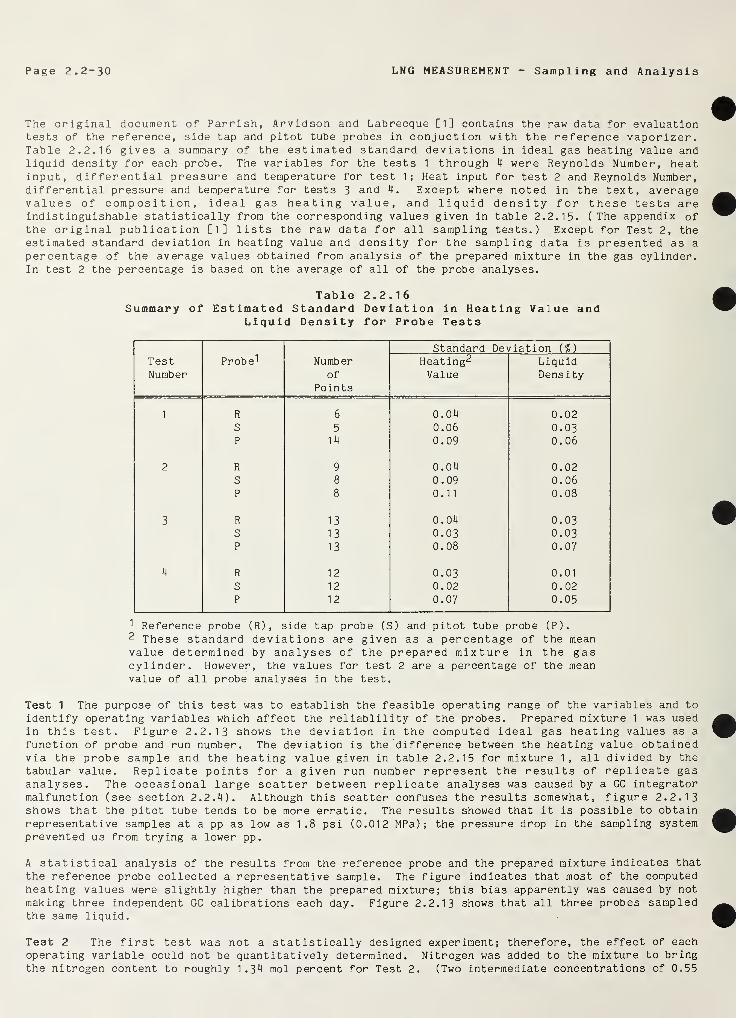
Page 2.2-30 LNG MEASUREMENT - Sampling and Analysis
The original document of Parrish, Arvidson and Labrecque [1] contains the raw data for evaluationtests of the reference, side tap and pitot tube probes in conjuction with the reference vaporizer.Table 2.2.16 gives a summary of the estimated standard deviations in ideal gas heating value andliquid density for each probe. The variables for the tests 1 through 4 were Reynolds Number, heatinput, differential pressure and temperature for test 1; Heat input for test 2 and Reynolds Number,differential pressure and temperature for tests 3 and 4. Except where noted in the text, averagevalues of composition, ideal gas heating value, and liquid density for these tests areindistinguishable statistically from the corresponding values given in table 2.2.15. (The appendix ofthe original publication [1] lists the raw data for all sampling tests.) Except for Test 2, theestimated standard deviation in heating value and density for the sampling data is presented as a
percentage of the average values obtained from analysis of the prepared mixture in the gas cylinder.In test 2 the percentage is based on the average of all of the probe analyses.
Table 2.2.16Summary of Estimated Standard Deviation in Heating Value and
Liquid Density for Probe Tests
TestNumber
Probe 1 Numberof
Points
Standard Deviation {%)
Heating2
ValueLiquidDensity
1 R 6 0.04 0.02S 5 0.06 0.03P 14 0.09 0.06
2 R 9 0.04 0.02S 8 0.09 0.06P 8 0.11 0.08
3 R 13 0.04 0.03S 13 0.03 0.03P 13 0.08 0.07
4 R 12 0.03 0.01
S 12 0.02 0.02P 12 0.07 0.05
1 Reference probe (R), side tap probe (S) and pitot tube probe (P).2 These standard deviations are given as a percentage of the meanvalue determined by analyses of the prepared mixture in the gascylinder. However, the values for test 2 are a percentage of the meanvalue of all probe analyses in the test.
Test 1 The purpose of this test was to establish the feasible operating range of the variables and to
identify operating variables which affect the reliablility of the probes. Prepared mixture 1 was usedin this test. Figure 2.2.13 shows the deviation in the computed ideal gas heating values as a
function of probe and run number. The deviation is the difference between the heating value obtainedvia the probe sample and the heating value given in table 2.2.15 for mixture 1, all divided by thetabular value. Replicate points for a given run number represent the results of replicate gasanalyses. The occasional large scatter between replicate analyses was caused by a GC integratormalfunction (see section 2.2.4). Although this scatter confuses the results somewhat, figure 2.2.13shows that the pitot tube tends to be more erratic. The results showed that it is possible to obtainrepresentative samples at a pp as low as 1.8 psi (0.012 MPa); the pressure drop in the sampling systemprevented us from trying a lower pp.
A statistical analysis of the results from the reference probe and the prepared mixture indicates that
the reference probe collected a representative sample. The figure indicates that most of the computedheating values were slightly higher than the prepared mixture; this bias apparently was caused by notmaking three independent GC calibrations each day. Figure 2.2.13 shows that all three probes sampledthe same liquid.
Test 2 The first test was not a statistically designed experiment; therefore, the effect of eachoperating variable could not be quantitatively determined. Nitrogen was added to the mixture to bringthe nitrogen content to roughly 1.34 mol percent for Test 2. (Two intermediate concentrations of 0.55
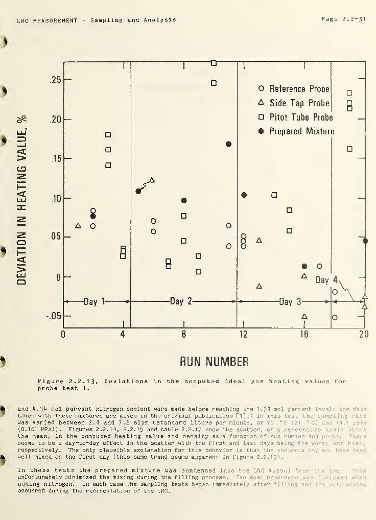
LNG MEASUREMENT Sampling and Analysis Fage 2.2-31
<CD
OI—<
.25
.20
.15
.10 -
.05
r 1—
—
•
A
— •
8 nA O
o°
R O0 D
—H
* uay i Udy L
L 1
0 ~
o Reference Probe
a Side Tap Probe
Pitot Tube Probe
• Prepared Mixture
B
o
Day 4>
-Day 3
O
0 8 12
RUN NUMBER
16
t
20
Figure 2.2.13. Deviations in the computed ideal gas heating values forprobe test 1 .
and 4.34 mol percent nitrogen content were made before reaching the 1.34 mol percent level; ‘v- : r *.
taken with these mixtures are given in the original publication [1].) In this test the . *mp . . ra**-*
was varied between 2.4 and 7.2 slpm (standard liters per minute, at 70 °F (21 °C .n 1 1-. ':
(0.101 MPa)). Figures 2.2.14, 2.2.15 and table 2.2.17 show the scatter, on a percent;:--' •
the mean, in the computed heating value and density as a function of run nunb‘ -r i:
seems to be a day-to-day effect in the scatter with the first and last days being the wr .•
respectively. The only plausible explanation for this behavior is that the cont-n* - iv - •
well mixed on the first day (this same trend seems apparent in figure 2 . 2 . 13 ).
In these tests the prepared mixture was condensed into the LNG ve fr •
unfortunately minimized the mixing during the filling process. The same prc .'
1 - •
adding nitrogen. In each case the sampling tests began immediately after f :
-
occurred during the recirculation of the LNG.
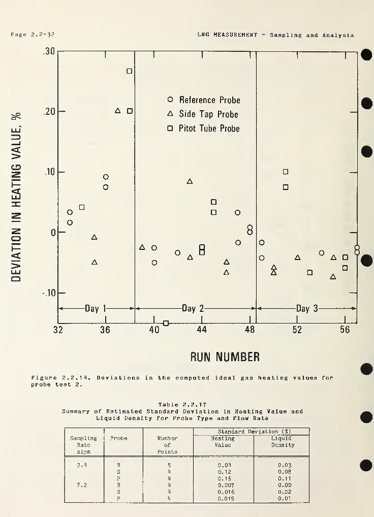
Page 2.2-32 LNG MEASUREMENT - Sampling and Analysis
<CD
OH-<
.30
.20 A
.10 -oo
oo
0
-.10 -
-Day 1-
32 36
TT
o Reference Probe
a Side Tap Probe
Pitot Tube Probe
o
8
A O
O° A B
AA
-Day 2-
o
o A ° A
k
-Day 3-
40 44 48 52 56
RUN NUMBER
Figure 2.2.14, Deviations in the computed ideal gas heating values forprobe test 2.
Table 2.2.17Summary of Estimated Standard Deviation in Heating Value and
Liquid Density for Probe Type and Flow Rate
SamplingRateslpm
Probe Numberof
Points
Standard Deviation (%)
HeatingValue
LiquidDensity
2.4 R 5 0.04 0.03S 4 0.12 0.08P 4 0.16 0.1
1
7.2 R 4 0.007 0.00S 4 0.016 0.02P 4 0.015 0.01
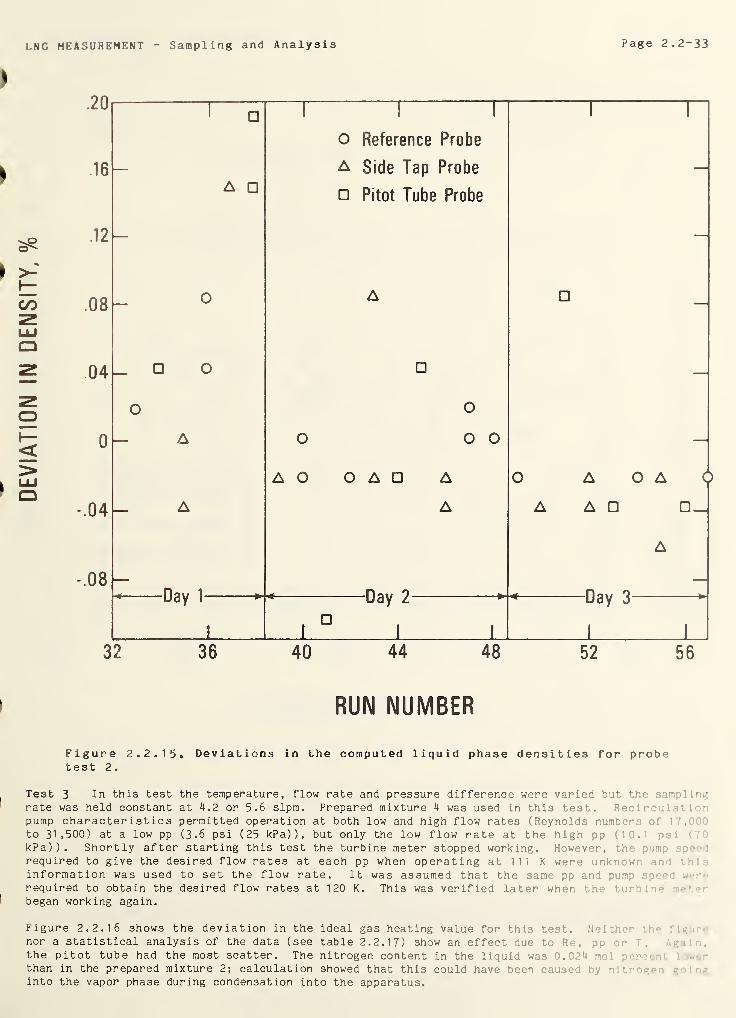
LNG MEASUREMENT Sampling and Analysis Page 2.2-33
sOO'"
o
.20
.16
.12
.08
.04
0
-.04
-.08
1 —i
1 n i ro Reference Probe
— A Side Tap Probe —A
Pitot Tube Probe
_ o A _
_ O
O o
— A o o 0 —
<1<oo< <o<1O
_ A A > > _1_
A
Udy I* Udy L * uay j
1 1 L 1 L_32 36 40 44 48 52 56
RUN NUMBER
Figure 2.2.15* Deviations in the computed liquid phase densities for probetest 2.
Test 3 In this test the temperature, flow rate and pressure difference were varied but the samp; i r.-:
rate was held constant at 4.2 or 5.6 slpm. Prepared mixture 4 was used in this test. Recirculat . n
pump characteristics permitted operation at both low and high flow rates (Reynolds number: o', i”,
to 31,500) at a low pp (3.6 psi (25 kPa)), but only the low flow rate at the high pp (10.i
kPa)). Shortly after starting this test the turbine meter stopped working. However, th-required to give the desired flow rates at each pp when operating at 1 1 1 K were unknown :
•
information was used to set the flow rate. It was assumed that the same pp and pumrrequired to obtain the desired flow rates at 120 K. This was verified later when the • .r
began working again.
Figure 2.2.16 shows the deviation in the ideal gas heating value for this test. N-inor a statistical analysis of the data (see table 2.2.17) show an effect due to Re,the pitot tube had the most scatter. The nitrogen content in the liquid was 0.024 m 1 ;
erthan in the prepared mixture 2; calculation showed that this could have been caused V/ n i
• .•
into the vapor phase during condensation into the apparatus.
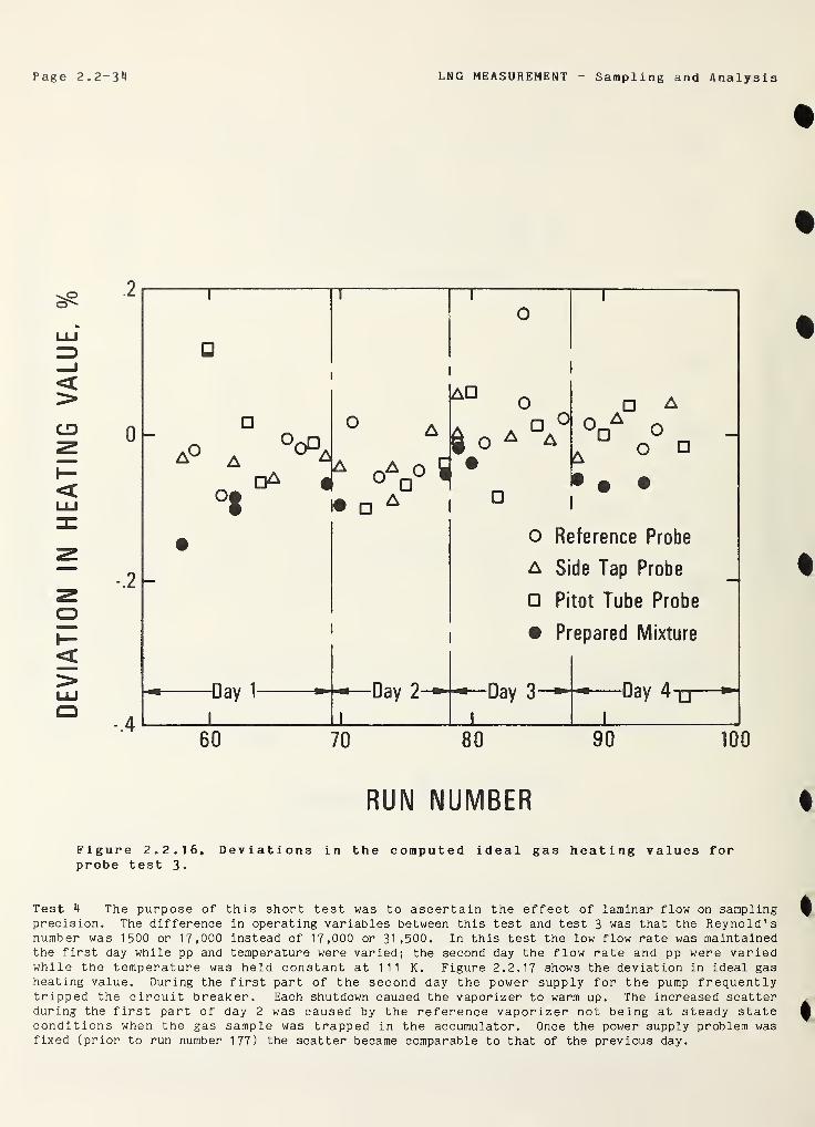
Page 2.2-34 LNG MEASUREMENT Sampling and Analysis
<
CD
O<
0 -
i1
1
O—5 —
> O A
£0<3°<1 O A
A A 0 ! •0 > >
n 0O
O
<10<
0 • • •
°t • A
-.2 -
-Day 1-
o Reference Probe
a Side Tap Probe
Pitot Tube Probe
• Prepared Mixture
Day 2- Day 3 -Day 4-g—
-
60 70 80 90
RUN NUMBER
100
Figure 2.2.16. Deviations in the computed ideal gas heating values forprobe test 3.
Test 4 The purpose of this short test was to ascertain the effect of laminar flow on samplingprecision. The difference in operating variables between this test and test 3 was that the Reynold'snumber was 1500 or 17,000 instead of 17,000 or 31,500. In this test the low flow rate was maintainedthe first day while pp and temperature were varied; the second day the flow rate and pp were variedwhile the temperature was held constant at 1 1 1 K. Figure 2.2.17 shows the deviation in ideal gasheating value. During the first part of the second day the power supply for the pump frequentlytripped the circuit breaker. Each shutdown caused the vaporizer to warm up. The increased scatterduring the first part of day 2 was caused by the reference vaporizer not being at steady stateconditions when the gas sample was trapped in the accumulator. Once the power supply problem wasfixed (prior to run number 177) the scatter became comparable to that of the previous day.
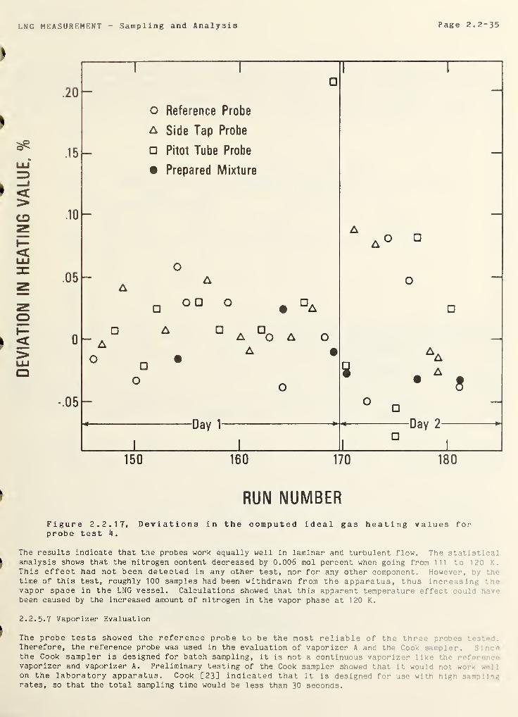
LNG MEASUREMENT Sampling and Analysis Page 2.2-35
<CD
O<
.15 -
o Reference Probe
a Side Tap Probe
Pitot Tube Probe
• Prepared Mixture
RUN NUMBER
Figure 2.2.17* Deviations in the computed ideal gas heating values forprobe test 4.
The results indicate that the probes work equally well in laminar and turbulent flow. The statisticalanalysis shows that the nitrogen content decreased by 0.006 mol percent when going from 111 to IP' Y.
.
This effect had not been detected in any other test, nor for any other component. However, /•
time of this test, roughly 100 samples had been withdrawn from the apparatus, thus increasingvapor space in the LNG vessel. Calculations showed that this apparent temperature effect c .1 1 •. iv>-
been caused by the increased amount of nitrogen in the vapor phase at 120 K.
2. 2. 5. 7 Vaporizer Evaluation
The probe tests showed the reference probe to be the most reliable of the three pr t. »t- .
Therefore, the reference probe was used in the evaluation of vaporizer A and the Cook sampler,the Cook sampler is designed for batch sampling, it is not a continuous vaporizer like r< •
• •
vaporizer and vaporizer A. Preliminary testing of the Cook sampler showed that it would r. t w
on the laboratory apparatus. Cook [23] indicated that it is designed for u 3 c with hi.-- •
rates, so that the total sampling time would be less than 30 seconds.
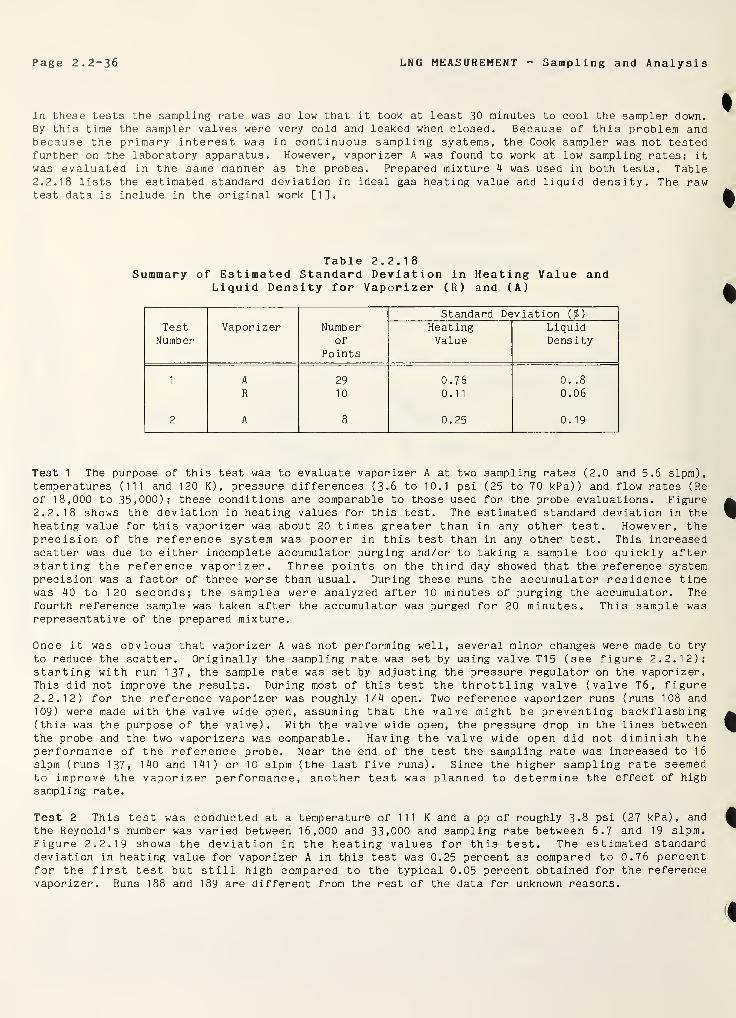
Page 2.2-36 LNG MEASUREMENT - Sampling and Analysis
In these tests the sampling rate was so low that it took at least 30 minutes to cool the sampler down.By this time the sampler valves were very cold and leaked when closed. Because of this problem andbecause the primary interest was in continuous sampling systems, the Cook sampler was not testedfurther on the laboratory apparatus. However, vaporizer A was found to work at low sampling rates; it
was evaluated in the same manner as the probes. Prepared mixture 4 was used in both tests. Table2.2.18 lists the estimated standard deviation in ideal gas heating value and liquid density. The rawtest data is include in the original work [1].
Table 2.2.18Summary of Estimated Standard Deviation in Heating Value and
Liquid Density for Vaporizer (R) and (A)
TestNumber
Vaporizer Numberof
Points
Standard Deviation (%)
HeatingValue
LiquidDensity
1 A 29 0.76 0. .8
R 10 0.11 0.06
2 A 8 0.25 0.19
Test 1 The purpose of this test was to evaluate vaporizer A at two sampling rates (2.0 and 5.6 slpm),temperatures (111 and 120 K), pressure differences (3.6 to 10.1 psi (25 to 70 kPa)) and flow rates (Re
of 18,000 to 35,000); these conditions are comparable to those used for the probe evaluations. Figure2.2.18 shows the deviation in heating values for this test. The estimated standard deviation in theheating value for this vaporizer was about 20 times greater than in any other test. However, theprecision of the reference system was poorer in this test than in any other test. This increasedscatter was due to either incomplete accumulator purging and/or to taking a sample too quickly afterstarting the reference vaporizer. Three points on the third day showed that the reference systemprecision was a factor of three worse than usual. During these runs the accumulator residence timewas 40 to 120 seconds; the samples were analyzed after 10 minutes of purging the accumulator. Thefourth reference sample was taken after the accumulator was purged for 20 minutes. This sample wasrepresentative of the prepared mixture.
Once it was obvious that vaporizer A was not performing well, several minor changes were made to try
to reduce the scatter. Originally the sampling rate was set by using valve T15 (see figure 2.2.12);starting with run 137, the sample rate was set by adjusting the pressure regulator on the vaporizer.This did not improve the results. During most of this test the throttling valve (valve T6, figure2.2.12) for the reference vaporizer was roughly 1/4 open. Two reference vaporizer runs (runs 108 and
109) were made with the valve wide open, assuming that the valve might be preventing backflashing(this was the purpose of the valve). With the valve wide open, the pressure drop in the lines betweenthe probe and the two vaporizers was comparable. Having the valve wide open did not diminish theperformance of the reference probe. Near the end of the test the sampling rate was increased to 16
slpm (runs 1 37, 1 40 and 141) or 10 slpm (the last five runs). Since the higher sampling rate seemedto improve the vaporizer performance, another test was planned to determine the effect of highsampling rate.
Test 2 This test was conducted at a temperature of 1 1 1 K and a pp of roughly 3-8 psi (27 kPa), and
the Reynold's number was varied between 16,000 and 33 ( 000 and sampling rate between 6.7 and 19 slpm.Figure 2.2.19 shows the deviation in the heating values for this test. The estimated standarddeviation in heating value for vaporizer A in this test was 0.25 percent as compared to 0.76 percentfor the first test but still high compared to the typical 0.05 percent obtained for the referencevaporizer. Runs 188 and 189 are different from the rest of the data for unknown reasons.
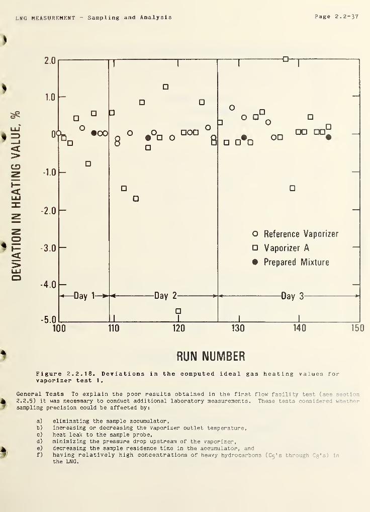
DEVIATION
IN
HEATING
VALUE.
%
LNG MEASUREMENT Sampling and Analysis Page 2.2-37
01 LL_ I I I
100 110 120 130 140 150
RUN NUMBERFigure 2.2.18. Deviations in the computed ideal gas heating values forvaporizer test 1 .
General Tests To explain the poor results obtained in the first flow facility test (see •
2.2.5) it was necessary to conduct additional laboratory measurements. These tests considered wo •
-
sampling precision could be affected by:
a) eliminating the sample accumulator,b) increasing or decreasing the vaporizer outlet temperature,c) heat leak to the sample probe,d) minimizing the pressure drop upstream of the vaporizer,e) decreasing the sample residence time in the accumulator, andf) having relatively high concentrations of heavy hydrocarbons (C 5 's throuvs
the LNG.
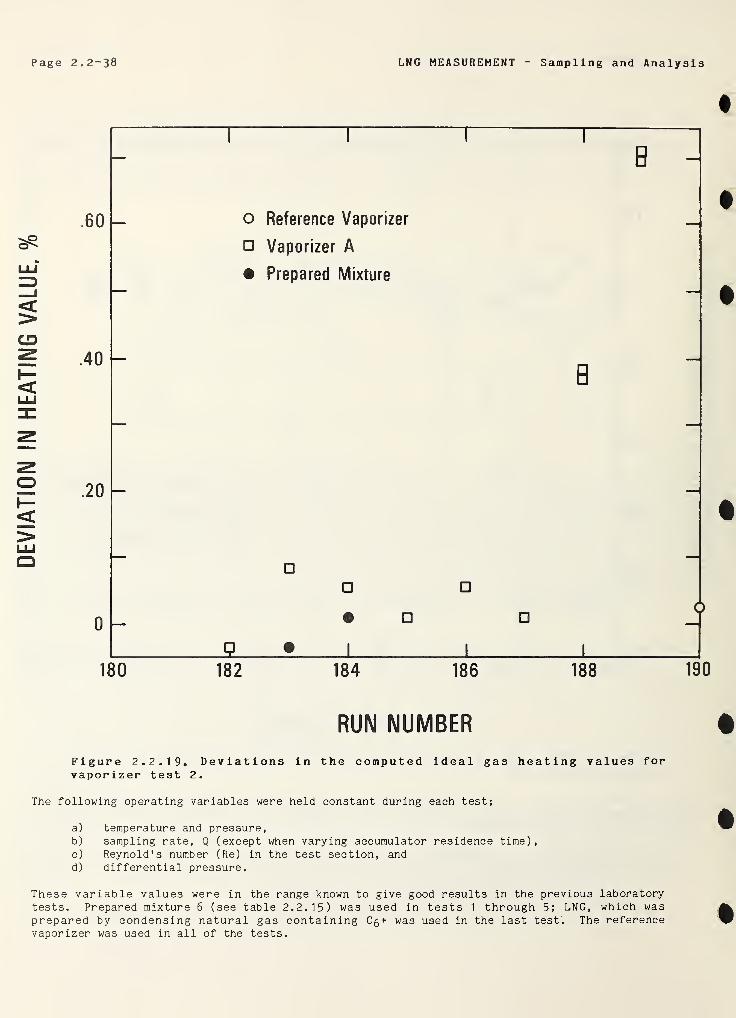
Page 2.2-38 LNG MEASUREMENT Sampling and Analysis
<CD
.60 - o Reference Vaporizer
Vaporizer A
• Prepared Mixture
B
B
— .20 -OI—<
0 -
180 182 184 186 188
RUN NUMBER
Figure 2.2.19, Deviations in the computed ideal gas heating values forvaporizer test 2.
The following operating variables were held constant during each test;
a) temperature and pressure,b) sampling rate, Q (except when varying accumulator residence time),c) Reynold's number (Re) in the test section, andd) differential pressure.
These variable values were in the range known to give good results in the previous laboratorytests. Prepared mixture 6 (see table 2.2.15) was used in tests 1 through 5; LNG, which wasprepared by condensing natural gas containing C 5 + was used in the last test. The referencevaporizer was used in all of the tests.
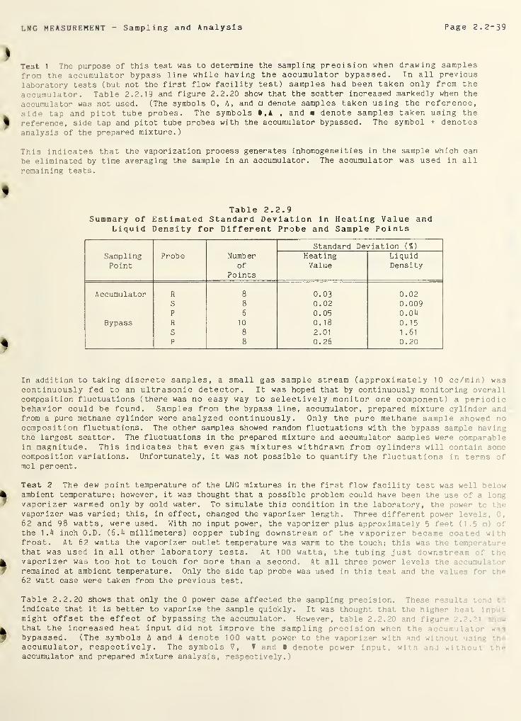
LNG MEASUREMENT Sampling and Analysis Page 2.2-39
Test 1 The purpose of this test was to determine the sampling precision when drawing samplesfrom the accumulator bypass line while having the accumulator bypassed. In all previous
laboratory tests (but not the first flow facility test) samples had been taken only from the
accumulator. Table 2.2.19 and figure 2.2.20 show that the scatter increased markedly when the
accumulator was not used. (The symbols 0, A, and denote samples taken using the reference,
side tap and pitot tube probes. The symbols t,4 , and denote samples taken using the
reference, side tap and pitot tube probes with the accumulator bypassed. The symbol + denotesanalysis of the prepared mixture.)
This indicates that the vaporization process generates inhomogeneities in the sample which can
be eliminated by time averaging the sample in an accumulator. The accumulator was used in allremaining tests.
Table 2.2.9Summary of Estimated Standard Deviation in Heating Value and
Liquid Density for Different Probe and Sample Points
SamplingPoint
Probe Numberof
Points
Standard Deviation {%)
HeatingValue
LiquidDensity
Accumulator R 8 0.03 0.02S 8 0.02 0.009P 6 0.05 0.04
Bypass R 10 0.18 0.15S 8 2.01 1 .61
P 8 0.26 0.20
In addition to taking discrete samples, a small gas sample stream (approximately 10 cc/min) wascontinuously fed to an ultrasonic detector. It was hoped that by continuously monitoring overallcomposition fluctuations (there was no easy way to selectively monitor one component) a periodicbehavior could be found. Samples from the bypass line, accumulator, prepared mixture cylinder andfrom a pure methane cylinder were analyzed continuously. Only the pure methane sample showed nocomposition fluctuations. The other samples showed random fluctuations with the bypass sample havingthe largest scatter. The fluctuations in the prepared mixture and accumulator samples were comparablein magnitude. This indicates that even gas mixtures withdrawn from cylinders will contain somecomposition variations. Unfortunately, it was not possible to quantify the fluctuations in terms ofmol percent.
Test 2 The dew point temperature of the LNG mixtures in the first flow facility test was well belowambient temperature; however, it was thought that a possible problem could have been the use of a longvaporizer warmed only by cold water. To simulate this condition in the laboratory, the power to V’vvaporizer was varied; this, in effect, changed the vaporizer length. Three different power level',62 and 98 watts, were used. With no input power, the vaporizer plus approximately 5 feet (1.5 m) ofthe 1.4 inch O.D. (6.4 millimeters) copper tubing downstream of the vaporizer became coated withfrost. At 62 watts the vaporizer outlet temperature was warm to the touch; this was the tempera’ ir-
that was used in all other laboratory tests. At 100 watts, the tubing just downstream of thevaporizer was too hot to touch for more than a second. At all three power levels the accumul 1
* '
remained at ambient temperature. Only the side tap probe was used in this test and the values f - t
62 watt case were taken from the previous test.
Table 2.2.20 shows that only the 0 power case affected the sampling precision. These ro V. •
indicate that it is better to vaporize the sample quickly. It was thought that the higher h- 1
*
might offset the effect of bypassing the accumulator. However, table 2.2.20 and figur- . .
' ~
that the increased heat input did not improve the sampling precision when th • a' , :
,• • „
bypassed. (The symbols A and A denote 100 watt power to the vaporizer with and without using theaccumulator, respectively. The symbols V, f and • denote power input, w :’n : v. i
• r. .
• •••
accumulator and prepared mixture analysis, respectively.)
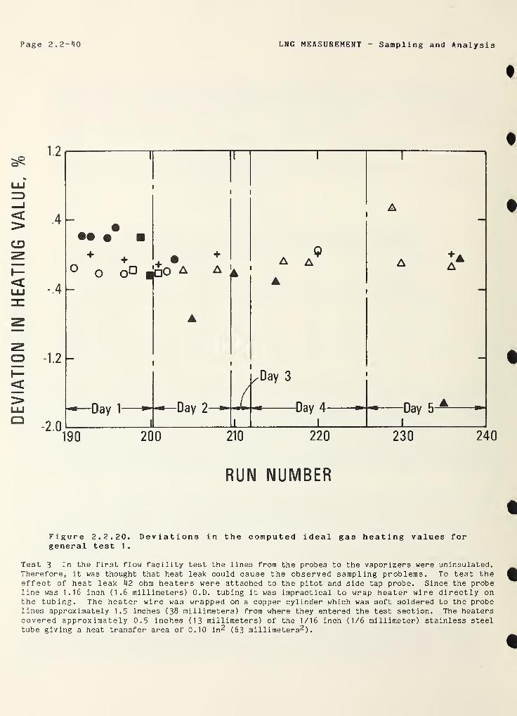
DEVIATION
IN
HEATING
VALUE,
Page 2.2-40 LNG MEASUREMENT Sampling and Analysis
RUN NUMBER
Figure 2.2.20. Deviations in the computed ideal gas heating values forgeneral test 1
.
Test 3 In the first flow facility test the lines from the probes to the vaporizers were uninsulated.Therefore, it was thought that heat leak could cause the observed sampling problems. To test theeffect of heat leak 42 ohm heaters were attached to the pitot and side tap probe. Since the probeline was 1.16 inch (1.6 millimeters) O.D. tubing it was impractical to wrap heater wire directly onthe tubing. The heater wire was wrapped on a copper cylinder which was soft soldered to the probelines approximately 1.5 inches (38 millimeters) from where they entered the test section. The heaterscovered approximately 0.5 inches (13 millimeters) of the 1/16 inch (1/6 millimeter) stainless steeltube giving a heat transfer area of 0.10 in 2 (63 millimeters2 ).
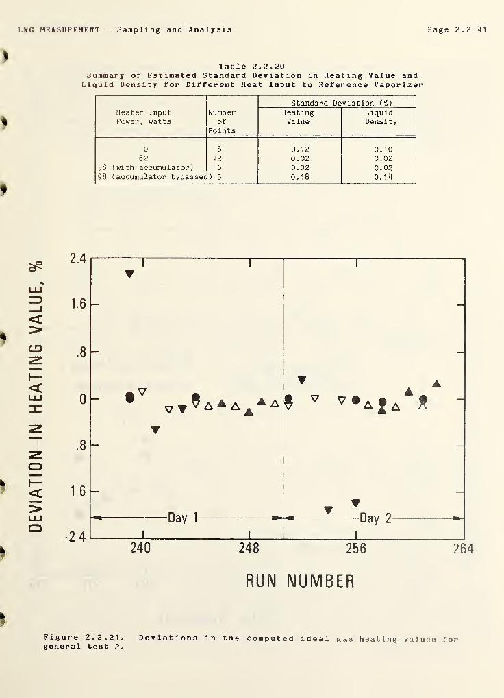
DEVIATION
IN
HEATING
VALUE,
LNG MEASUREMENT Sampling and Analysis Page 2.2-41
Table 2.2.20Summary of Estimated Standard Deviation in Heating Value andLiquid Density for Different Heat Input to Reference Vaporizer
Heater InputPower, watts
Numberof
Points
Standard Deviation (%)
HeatingValue
LiquidDensity
0 6 0.12 0.1062 12 0.02 0.02
98 (with accumulator) 6 0.02 0.0298 (accumulator bypassed) 5 0.18 0.14
RUN NUMBER
Figure 2.2.21.general test 2.
Deviations in the computed ideal gas heating values for
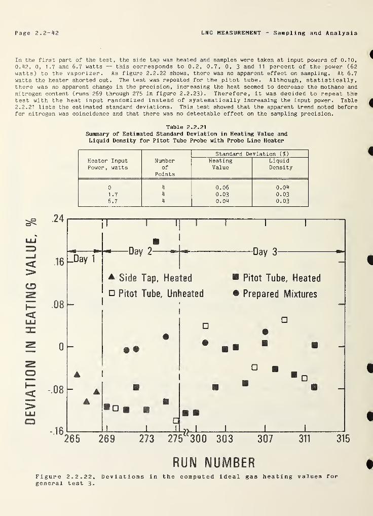
Page 2.2-42 LNG MEASUREMENT - Sampling and Analysis
In the first part of the test, the side tap was heated and samples were taken at input powers of 0.10,
0.42, 0, 1.7 and 6.7 watts — this corresponds to 0.2, 0.7, 0, 3 and 11 percent of the power (62watts) to the vaporizer. As figure 2.2.22 shows, there was no apparent effect on sampling. At 6.7
watts the heater shorted out. The test was repeated for the pitot tube. Although, statistically,there was no apparent change in the precision, increasing the heat seemed to decrease the methane andnitrogen content (runs 269 through 275 in figure 2.2.23). Therefore, it was decided to repeat thetest with the heat input randomized instead of systematically increasing the input power. Table2.2.21 lists the estimated standard deviations. This test showed that the apparent trend noted beforefor nitrogen was coincidence and that there was no detectable effect on the sampling precision.
Table 2.2.21Summary of Estimated Standard Deviation in Heating Value andLiquid Density for Pitot Tube Probe with Probe Line Heater
Heater InputPower, watts
Numberof
Points
Standard Deviation (%)
HeatingValue
LiquidDensity
0 4 0.06 0.04
1 .7 4 0.03 0.036.7 4 0.04 0.03
LLJ
<CD
<LLJ
<LUCD
Figure 2.2.22, Deviations in the computed ideal gas heating values forgeneral test 3.
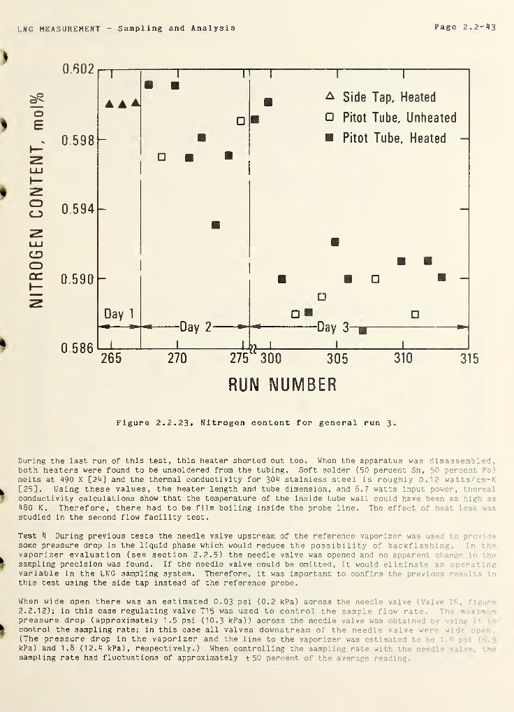
LNG MEASUREMENT - Sampling and Analysis Page 2.2-43
"oE
oCJ
CDOGC
0.602
0.598 -
0.594 -
0.590 -
0.586
“T
—
1 n 1
1
1
A A A m & side Tap, Heated
m 0 Pitot Tube, Unheated
Pitot Tube, Heated -
-
Day 1
1
uay z
1 1
*• bay 0 gg
^ r265 270 310 315
RUN NUMBER
Figure 2.2.23* Nitrogen content for general run 3.
During the last run of this test, this heater shorted out too. When the apparatus was disassembled,both heaters were found to be unsoldered from the tubing. Soft solder (50 percent Sn, 50 percent Pbl
melts at 490 K [24] and the thermal conductivity for 304 stainless steel is roughly 0.12 watts/cm-K[25]. Using these values, the heater length and tube dimension, and 6.7 watts input power, thermalconductivity calculations show that the temperature of the inside tube wall could have been as high as
480 K. Therefore, there had to be film boiling inside the probe line. The effect of heat leak was
studied in the second flow facility test.
Test 4 During previous tests the needle valve upstream of the reference vaporizer was used to prov:some pressure drop in the liquid phase which would reduce the possibility of backf lash ing . in ‘
-
vaporizer evaluation (see section 2.2.5) the needle valve was opened and no apparent chanv in •
sampling precision was found. If the needle valve could be omitted, it would eliminate an -. in-
variable in the LNG sampling system. Therefore, it was important to confirm the previous r .
•
this test using the side tap instead of the reference probe.
When wide open there was an estimated 0.03 psi (0.2 kPa) across the needle valve (V-l
2.2.12); in this case regulating valve T15 was used to control the sample flow rate. T -•
pressure drop (approximately 1.5 psi (10.3 kPa)) across the needle valve was obtain'-: by u •:
control the sampling rate; in this case all valves downstream of the needle valve w< ~ •
(The pressure drop in the vaporizer and the line to the vaporizer was estimated to 1 . .
kPa) and 1.8 (12.4 kPa),respectively.) When controlling the sampling rate with t-v :
.•. ;
sampling rate had fluctuations of approximately ±50 percent of the average reading.
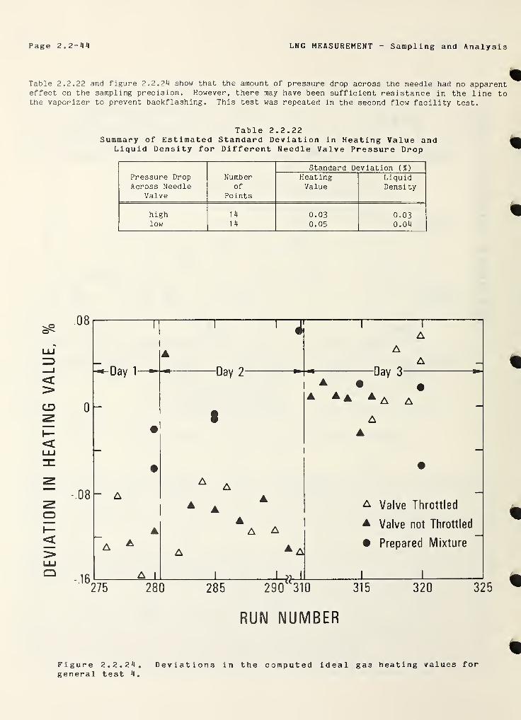
Page 2.2-44 LNG MEASUREMENT Sampling and Analysis
Table 2.2.22 and figure 2.2.24 show that the amount of pressure drop across the needle had no apparenteffect on the sampling precision. However, there may have been sufficient resistance in the line tothe vaporizer to prevent backflashing . This test was repeated in the second flow facility test.
Table 2.2.22Summary of Estimated Standard Deviation in Heating Value and
Liquid Density for Different Needle Valve Pressure Drop
Standard Deviation {%)
Pressure Drop Number Heating LiquidAcross Needle
Valveof
PointsValue Density
high 14 0.03 0.03low 14 0.05 0.04
<>CD
OI—<
A Valve Throttled
* Valve not Throttled
• Prepared Mixture
290 310 325
RUN NUMBER
Figure 2.2.24. Deviations in the computed ideal gas heating values forgeneral test 4.
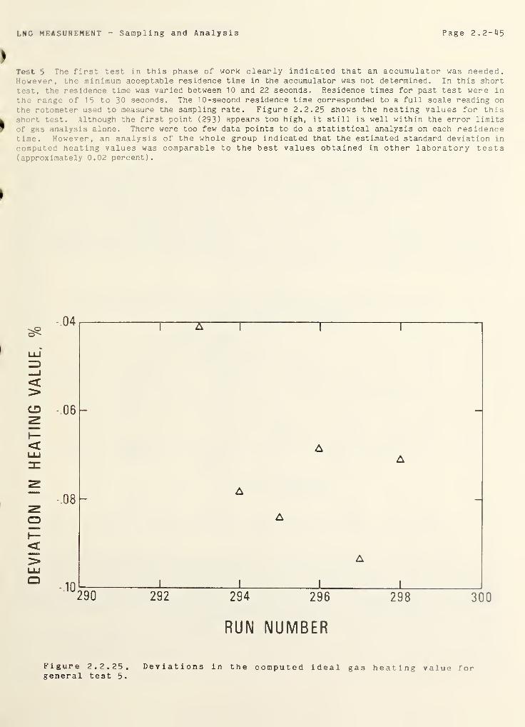
LNG MEASUREMENT Sampling and Analysis Page 2.2-45
Test 5 The first test in this phase of work clearly indicated that an accumulator was needed.However, the minimum acceptable residence time in the accumulator was not determined. In this shorttest, the residence time was varied between 10 and 22 seconds. Residence times for past test were in
the range of 15 to 30 seconds. The 10-second residence time corresponded to a full scale reading onthe rotometer used to measure the sampling rate. Figure 2.2.25 shows the heating values for thisshort test. Although the first point (293) appears too high, it still is well within the error limitsof gas analysis alone. There were too few data points to do a statistical analysis on each residencetime. However, an analysis of the whole group indicated that the estimated standard deviation in
computed heating values was comparable to the best values obtained in other laboratory tests(approximately 0.02 percent).
O'''
LU
<CD
<LU
O<LUCD
RUN NUMBER
Figure 2.2.25. Deviations in the computed ideal gas heating value forgeneral test 5.
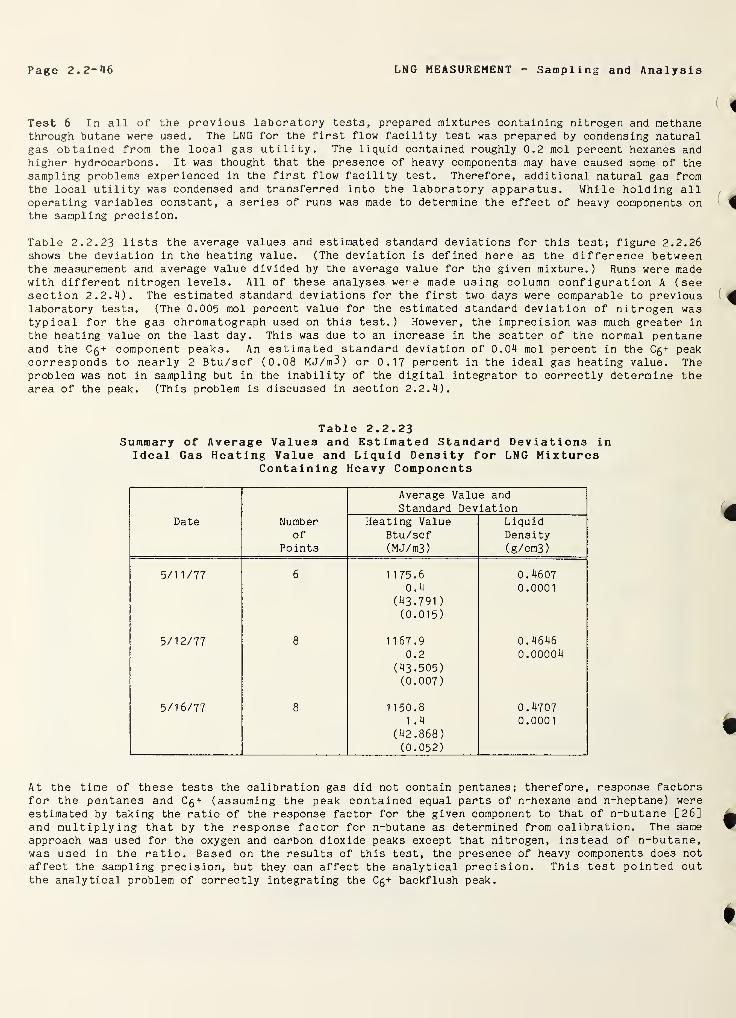
Page 2. 2-46 LNG MEASUREMENT - Sampling and Analysis
Test 6 In all of the previous laboratory tests, prepared mixtures containing nitrogen and methanethrough butane were used. The LNG for the first flow facility test was prepared by condensing naturalgas obtained from the local gas utility. The liquid contained roughly 0.2 mol percent hexanes andhigher hydrocarbons. It was thought that the presence of heavy components may have caused some of thesampling problems experienced in the first flow facility test. Therefore, additional natural gas fromthe local utility was condensed and transferred into the laboratory apparatus. While holding alloperating variables constant, a series of runs was made to determine the effect of heavy components onthe sampling precision.
Table 2.2.23 lists the average values and estimated standard deviations for this test; figure 2.2.26shows the deviation in the heating value. (The deviation is defined here as the difference betweenthe measurement and average value divided by the average value for the given mixture.) Runs were madewith different nitrogen levels. All of these analyses were made using column configuration A (seesection 2.2.4). The estimated standard deviations for the first two days were comparable to previouslaboratory tests. (The 0.005 mol percent value for the estimated standard deviation of nitrogen wastypical for the gas chromatograph used on this test.) However, the imprecision was much greater in
the heating value on the last day. This was due to an increase in the scatter of the normal pentaneand the C 5
+ component peaks. An estimated standard deviation of 0.04 mol percent in the C5 + peakcorresponds to nearly 2 Btu/scf (0.08 MJ/m3) or 0.17 percent in the ideal gas heating value. Theproblem was not in sampling but in the inability of the digital integrator to correctly determine thearea of the peak. (This problem is discussed in section 2.2.4).
Table 2.2.23Summary of Average Values and Estimated Standard Deviations InIdeal Gas Heating Value and Liquid Density for LNG Mixtures
Containing Heavy Components
Average Value andStandard Deviation
Date Numberof
Points
Heating ValueBtu/scf(MJ/m3)
LiquidDensity(g/cm3)
5/11/77 6 1175.60.4
(43.791
)
(0.015)
0.46070.0001
5/12/77 8 1167.90.2
(43.505)(0.007)
0.46460.00004
5/16/77 8 1150.81 .4
(42.868)(0.052)
0.47070.0001
At the time of these tests the calibration gas did not contain pentanes; therefore, response factorsfor the pentanes and C 5 + (assuming the peak contained equal parts of n-hexane and n-heptane) wereestimated by taking the ratio of the response factor for the given component to that of n-butane [ 26 ]
and multiplying that by the response factor for n-butane as determined from calibration. The same
approach was used for the oxygen and carbon dioxide peaks except that nitrogen, instead of n-butane,was used in the ratio. Based on the results of this test, the presence of heavy components does notaffect the sampling precision, but they can affect the analytical precision. This test pointed outthe analytical problem of correctly integrating the C5 + backflush peak.
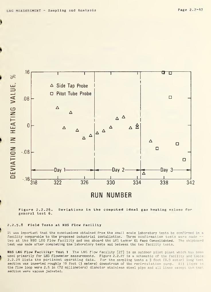
LNG MEASUREMENT - Sampling and Analysis Page 2.2-47
RUN NUMBER
Figure 2.2.26. Deviations in the computed ideal gas heating values forgeneral test 6.
2. 2. 5. 8 Field Tests at NBS Flow Facility
It was important that the conclusions obtained from the small scale laboratory tests be confirmed In a
facility comparable to the proposed industrial installation. Three confirmation tests were made --
two at the NBS LNG Flow Facility and one aboard the LNG tanker El Paso Consolidated. The shipboardtest was made after completing the laboratory tests and between the two facility tests.
NBS LNG Flow Facility- Test 1 The LNG flow facility [27] is an outdoor pilot plant which ha.'
used primarily for LNG flowmeter measurements. Figure 2.2.27 is a schematic of the facility and • r
2.2.24 lists the pertinent operating data. For the sampling tests a 3 foot (0.9 meter) ng ••
•
section was inserted roughly 10 foot (3 meters) downstream of the recirculation pump. A.
the flow loop were 2.5 in (72 millimeters) diameter stainless steel pipe and all linen exc"; • •••
•
section were vacuum jacketed.
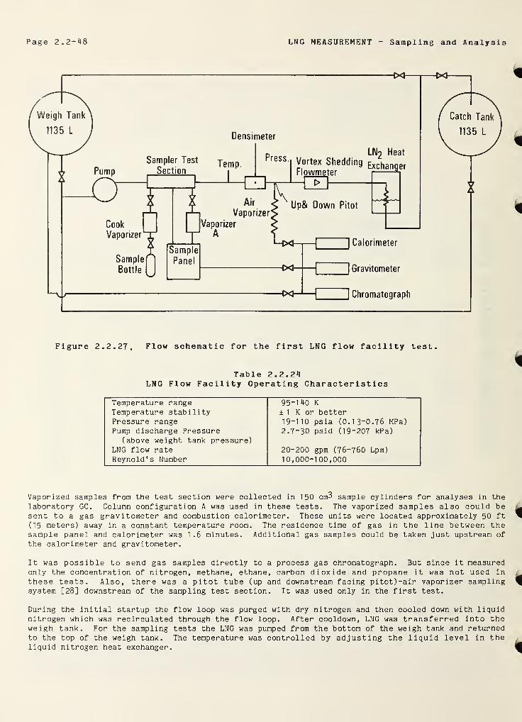
Page 2.2-48 LNG MEASUREMENT - Sampling and Analysis
Figure 2.2.27,
Flow schematic for the first LNG flow facility test.
Table 2.2.24LNG Flow Facility Operating Characteristics
Temperature range 95-140 K
Temperature stability ±1 K or betterPressure range 19-110 psia (0.13-0.76 MPa)Pump discharge Pressure 2.7-30 psid (19-207 kPa)
(above weight tank pressure)LNG flow rate 20-200 gpm (76-760 Lpm)
Reynold's Number 10,000-100,000
Vaporized samples from the test section were collected in 150 cm3 sample cylinders for analyses in thelaboratory GC. Column configuration A was used in these tests. The vaporized samples also could besent to a gas gravitometer and combustion calorimeter. These units were located approximately 50 ft
(15 meters) away in a constant temperature room. The residence time of gas in the line between thesample panel and calorimeter was 1 .6 minutes. Additional gas samples could be taken just upstream of
the calorimeter and gravitometer.
It was possible to send gas samples directly to a process gas chromatograph. But since it measuredonly the concentration of nitrogen, methane, ethane, carbon dioxide and propane it was not used in
these tests. Also, there was a pitot tube (up and downstream facing pitot)-air vaporizer samplingsystem [28] downstream of the sampling test section. It was used only in the first test.
During the initial startup the flow loop was purged with dry nitrogen and then cooled down with liquidnitrogen which was recirculated through the flow loop. After cooldown, LNG was transferred into theweigh tank. For the sampling tests the LNG was pumped from the bottom of the weigh tank and returnedto the top of the weigh tank. The temperature was controlled by adjusting the liquid level in theliquid nitrogen heat exchanger.
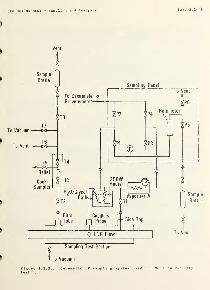
LNG MEASUREMENT - Sampling and Analysis Page 2.2-49
IVent
Figure 2.2.28.test 1 .
Schematic of sampling system used in LNG flow facility
Page 2.2-50 LNG MEASUREMENT Sampling and Analysis
The "true" composition of the LNG in the flow facility could not be measured. This limited the teststo comparing only the precision of the various sampling systems. However, the composition could beheld constant throughout an operating day. System venting during shutdown caused day to day shifts in
the composition. LNG for this test was made by condensing the natural gas supplied by the local gasutility. The gas was dried with a desiccant and the carbon dioxide was removed by filtering theliquid [28].
In Test 1, three probes were compared. These probes were a side tap, a side tap with a capillaryopening and an upstream facing pitot tube; two vaporizers which were a water heated coil and vaporizerA; and the Cook sampler. Figure 2.2.28 shows a schematic of the sampling system (a sample accumulatorwas not used). All three probes were mounted horizontally in the test section and were 6 inch (152millimeters) apart. The test section was enclosed in a 5 inch (127 millimeters) section of coppertubing. The annular space was evacuated to provide insulation. (However, during the tests it becameobvious that the vacuum was very poor because a heavy layer of frost formed on the outer tube.) Allthree probes were made of 1.8 inch (3-2 millimeters) O.D. by 0.101 inch (2.56 millimeters) I.D.stainless steel tubing. The probe lines were vacuum jacketed 6-1/2 inch (165 millimeters) beyond the
5 inch (127 millimeters) tube. The pitot tube had a 90 degree bend with the intake on the flowsection center line.
It was thought that if part of the pressure drop between the probe and vaporizer could be taken in theliquid phase there would be no danger of backflash; hence, it would not matter how the sample wasvaporized downstream. Therefore, a capillary probe was built which contained a 1/4 inch (6.4millimeters) long section of 0.007 inch (0.18 millimeter) I.D. tubing. This was soldered into the 1/8
inch (3.2 millimeters) O.D. tubing. The capillary section produced roughly 5 ~ 1 / 2 psi (38 kPa)
pressure drop for a liquid flow corresponding to 8 standard liters per minute of gas flow.
The water heated vaporizer consisted of 10 feet (3 m) of 1/4 inch (6.35 millimeters) O.D. x 0.190 inch
(4.83) I.D. copper tubing immersed in a water-glycol bath which was at approximately 30 ^(-1 33).
During operation the coil would have an ice layer which extended about 3 feet (0.9 m) along the tubingin the bath.
Test Results The results of this test were extremely poor; the best agreement between two samples was
0.04 percent in the heating value. However, this was fortuitous because the typical scatter was onthe order of one percent. The scatter was unaffected by the probe and vaporizer used. It was foundthat the heating values of the samples taken five minutes apart from the same sampling system variedby 0.7 percent; samples taken simultaneously from the same stream at the panel and at the gravitometerinlet differed by 1.5 percent. However, during all of these tests the calorimeter and gravitometerremained steady. (The gas specific gravity is much less sensitive to composition than the heatingvalue, e.g., in the composition range studied a 1.5 percent change in the heating value corresponds to
only 0.4 percent change in the specific gravity.)
Initially, it was thought that the scatter could be caused by the different methods of filling the
sample cylinder. Samples taken at the panel were purged and filled 14 times; the sample cylinders at
the gravitometer/calor imeter inlet were filled by continuous purge. To test the effect of samplecylinder filling procedure on precision, one of the calibration gases was connected to the samplepanel. Using comparable sample flows and pressures to those used in the other tests, samples were
taken at both the panel and the gravitometer/calorimeter inlet, The resulting sample compositionswere within the error of the gas analysis alone; therefore, the sample cylinder filling procedure was
not a problem.
The possibility that the scatter was caused by either liquid composition fluctuations or by the
presence of vapor in the test section was considered. The stability of the densimeter in the LNG flow
facility indicated that there were no composition fluctuations. The possibility of two phase flow was
eliminated because the vortex shedding flowmeter would have behaved erratically in two phase flow. At
this point it was decided to make additional laboratory tests (see section 2.2.5) to determine the
cause of the poor sampling precision.
LNG MEASUREMENT - Sampling and Analysis Page 2.2-51
Even with the erratic sampling precision, the following qualitative results were obtained:
1) It was not possible to obtain reliable samples from the Cook sampler as tested; this
sampler should have been insensitive to the problems experienced with the continuoussamplers. However, it is possible that valve T2 (figure 2.2.28) was leaking during
the warm up period or that the reduction in sample pressure when filling the samplecylinder caused partial condensation. (The ambient air during these tests was 30 to
40 V (-1 .1 to 4.4 t)).
2) Based on the band width of the gravitometer trace, the up and down pitot-airvaporizer and the capillary probe-water vaporizer systems produced more precisesamples than did the side tap-vaporizer A system. The gravitometer band width for
the capillary probe-water vaporizer samples and gravitometer calibration gas (air)
were comparable. Also, it was found that the heating values for the sidetap-vaporizer A samples were 0.5 to 1 percent higher than those from the other two
systems; the heating value difference between these two systems was less than 0.2
percent.
3) The capillary probe is not a feasible probe in industrial applications whereentrained solids could cause plugging. In the flow facility there were small amountsof solid carbon dioxide which plugged the capillary line.
2. 2. 5. 9 Shipboard Tests
Using the information obtained in the laboratory and first flow facility tests, a full scale samplingsystem was designed for tests aboard the LNG tanker El Paso Consolidated. Sampling tests were made at
Canvey Island, England during the ship's cargo system trials. Two sampling systems were installed —a liquid sampling system was installed on the 3 inch (76 millimeters) diameter header to the ship'sLNG vaporizer; a gas sampling system was placed on the 16 inch (406 millimeters) diameter vaporizeroutlet header. Sampling the gas phase provided a check on the liquid sampling system.
Figure 2.2.29 shows a schematic of the liquid sampling system and table 2.2.25 lists the componentdimensions. The system had a 1.4 inch, schedule 80 pipe (13.7 millimeters O.D. x 7.67 millimetersI.D.) side tap probe mounted horizontally on the header. All valves, fittings and tubing upstream of
the sample panel were stainless steel; tubing in the panel was copper and the other components werebrass. Except for the filter connections and union just upstream of the vaporizer, all connectionsupstream of the vaporizer were socket welds. The line between the header and vaporizer was wrappedwith a one inch (25 millimeters) layer of fiberglass pipe insulation and sealed with duct tape.
Valves T1 and T2 were bellows valves with the valve components welded together. Valve T2 was a
metering valve; it and the back pressure regulator were used to control the sampling rate.
The nitrogen purge connection (which was insulated up to valve T3) was used for displacing air fromthe sampling system; it was located downstream of the 60 micron filter so that nitrogen could be usedto back purge the filter, if necessary. However, the filter never clogged during these tests.
Because of film boiling, a precise ( ± 20 percent) design of the sample vaporizer would have beenextremely tedious. Therefore, the design was based on the warming of methane gas from 115 to 310 K.
A flow rate of 65 standard liters per minute was used. It was assumed that the steam side temperaturewas constant at 340 *F (171 t) ; this corresponds to the temperature of 205 psia (1.41 MPa) steamisenthalpically expanded to 60 psia (0.4 MPa). The heat transfer resistances on the steam side and in
the tube wall were negligible compared to the gas phase resistance; properties of methane [29,30] at150 K were used in the calculations. The final vaporizer tube length was twice the length computedusing the above assumptions.
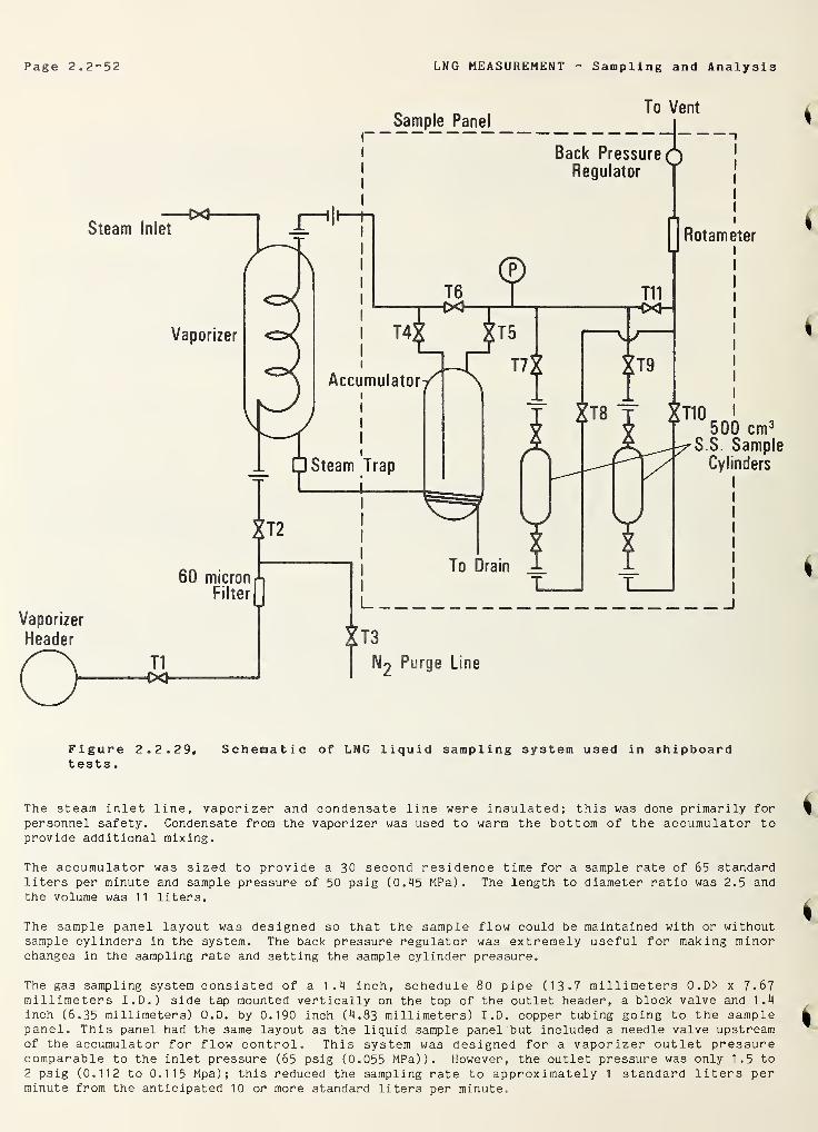
Page 2.2-52 LNG MEASUREMENT - Sampling and Analysis
Figure 2.2.29. Schematic of LNG liquid sampling system used in shipboardtests
.
The steam inlet line, vaporizer and condensate line were insulated; this was done primarily for
personnel safety. Condensate from the vaporizer was used to warm the bottom of the accumulator toprovide additional mixing.
The accumulator was sized to provide a 30 second residence time for a sample rate of 65 standardliters per minute and sample pressure of 50 psig (0.45 MPa). The length to diameter ratio was 2.5 andthe volume was 11 liters.
The sample panel layout was designed so that the sample flow could be maintained with or withoutsample cylinders in the system. The back pressure regulator was extremely useful for making minorchanges in the sampling rate and setting the sample cylinder pressure.
The gas sampling system consisted of a 1.4 inch, schedule 80 pipe (13.7 millimeters O.D> x 7.67millimeters I.D.) side tap mounted vertically on the top of the outlet header, a block valve and 1.4
inch (6.35 millimeters) O.D. by 0.190 inch (4.83 millimeters) I.D. copper tubing going to the samplepanel. This panel had the same layout as the liquid sample panel but included a needle valve upstreamof the accumulator for flow control. This system was designed for a vaporizer outlet pressurecomparable to the inlet pressure (65 psig (0.055 MPa)). However, the outlet pressure was only 1.5 to
2 psig (0.112 to 0.115 Mpa) ; this reduced the sampling rate to approximately 1 standard liters perminute from the anticipated 10 or more standard liters per minute.

LNC MEASUREMENT Sampling and Analysis Page 2.2-53
Dimensions of LNG Sampling System Used on Shipboard Tests
DiameterComponent
Length
inches (mm)
Outer Diameter
inches (mm) inches
Inner
(mm)
Vaporizer Header 3.5 (88.9)(3 inch pipe)
Side tap and line(7.67)between header andValve T1
4.5 (114) 0.540 (13.7)
(1/4 inch Sch.80 pipe)
0.302
Line between Valve(4.57)T1 and filter (con-tained a long radius90 degree bend)
1 1 (279) 0.25 (6.4) 0.180
Line between filter(4.57)and Valve T2
3 (76) 0.25 (6.4) 0.180
Line between valve(2.56)T2 and union atvaporizer
18 (460) 0.125 (3-18) 0.101
Vaporizer tubing4.15)(formed into a 4inch (102 mm) dia-meter helix)
45 (1140) 0.188 (4.76) 0.164
Vaporizer casing(with welded capends)
20 (508) 6.00 (150) 5.94 (151)
Line from vaporizer(4.57)to union (containeda 90 degree longradius bend)
1 1 (279) 0.25 (6.4) 0.180
Line to valve T3(4.57)
1 4 ( 356 ) 0.25 (6.4) 0.180
Accumulator(with welded endcap)
24 (610) 6.00 (152) 5.94 (151)
Gas analyses were made using a gas chromatograph containing a 30 foot (9.1 m) long column of DC200/500 on Chromasorb P and a 5 foot (1.5 m) molecular sieve 5A (MS) column. The column valveconfiguration permitted backflushing the DC 200/500 column and bypassing the MS column. Nitrogen andmethane were resolved on the MS column. Ethane through the butanes were separated on the DC 200/500
|volume; the column was backflushed to obtain a C 5 + peak. Digital integrator A was used to measurepeak areas. The precision of the analytical system was found to be 0.06 percent in the computedheating value.
Test Results The primary purpose of this test was to examine the precision of the LNG samplingsystem. The LNG was totally vaporized downstream of the sampling probe and the analysis of this gaswas to serve as the basis on which to evaluate the liquid sample analysis. However, the analysis of
> the vaporized gas produced erratic results that are felt to be more a function of the low pressure ofthe gas than composition change in the pipeline. Of the six sets of sampling data taken, only '
second set contained sufficient samples taken under constant vaporizer conditions to directly c;
ir-the gas and liquid sample compositions (see figure 2.2.30). Since composition variation •
probably less of a factor than the gas analysis, separate means and standard deviations were c j * -
for the liquid samples and for the gas samples for each of the six data sets (see table 2.2.2' .
heating values are computed using the A.G.A. method [2] and assumes equal parts of iso and n< r~
i pentane; the liquid phase densities were computed from the extended corresponding states"
( the original publication [1] lists the compositions and operating parameters for all of the test.- .
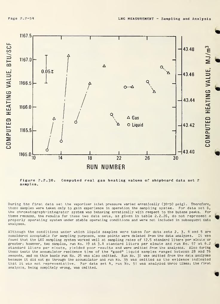
COMPUTED
HEATING
VALUE,
BTU/SCF
Page 2.2-54 LNG MEASUREMENT Sampling and Analysis
RUN NUMBER
Figure 2.2.30. Computed real gas heating values of shipboard data set 2
samples
.
During the first data set the vaporizer inlet pressure varied erratically (30-50 psig) . Therefore,these samples were taken only to gain experience in operation the sampling system. For data set 6,
the chromatograph-integrator system was behaving erratically with respect to the butane peaks. Forthese reasons, the results for these two data sets, as given in table 2.2.26, do not represent a
properly operating system under stable operating conditions and were not included in subsequent dataanalyses.
Although the conditions under which liquid samples were taken for data sets 2, 3, 4 and 5 are
considered acceptable for sampling purposes, some points were deleted from the data analyses. It wasfound that the LNG sampling system worked well at sampling rates of 12.5 standard liters per minute or
greater; however, two samples, run No. 19 at 3.4 standard liters per minute and run No. 57 at 6.2standard liters per minute, yielded poor results and were omitted from the analyses. Also duringthese tests the accumulator residence time of the "good" liquid samples ranged between 28 and 76
seconds, and on this basis run No. 25 was also omitted. Run No. 31 was omitted from the data analysesbecause it did not go through the accumulator and run No. 35 was omitted as the evidence indicatedthat it was not representative. For data set 4, run No. 51 was analyzed three times; the first
analysis, being compltely wrong, was omitted.
COMPUTED
HEATING
VALUE.
MJ/m
3
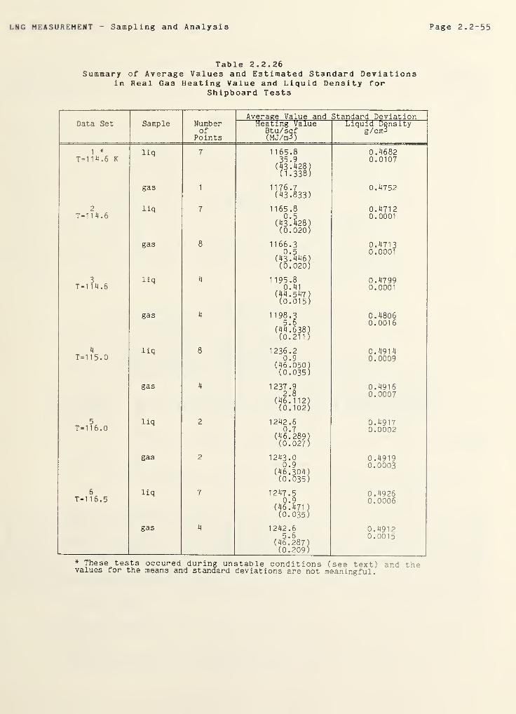
LNG MEASUREMENT Sampling and Analysis Page 2.2-55
Table 2.2.26Summary of Average Values and Estimated Standard Deviations
in Real Gas Heating Value and Liquid Density forShipboard Tests
Average Value and Standard DeviationData Set Sample Number
ofPoints
Heating ValueBtu/sqf(MJ/m3)
Liquid Densityg/cm3
1*
T=1 14.6 Kliq 7 1165.8
35.9(43.428)(1.338)
0.46820.0107
gas 1 1176.7(43.833)
0.4752
2T=1 14.6
liq 7 1165.80.5
(43.428)(0.020)
0.47120.0001
gas 8 1166.30.5
(43.446)(0.020)
0.47130.0001
T=n4.6liq 4 1 195.8
0.41(44.547)(0.015)
0.47990.0001
gas 4 1198.3
(44.638)(0.21 1
)
0.48060.0016
4T = 1 15.0
liq 8 1236.20.9
(46.050)(0.035)
0.49140.0009
gas 4 1237.92.8
(46.112)(0.102)
0.49160.0007
5T=1 1 6 .0
liq 2 1242.60.7
(46.289)(0.027)
0.49170.0002
gas 2 1243.00.9
(46.304)(0.035)
0.49190.0003
6T=1 1 6 .5
liq 7 1247.50.9
(46.471)
(0.035)
0.49260.0006
gas 4 1242.65 .
6
(46.287)(0.209)
0.49120.0015
* These tests oecured during unstable conditions (see text) and thevalues for the means and standard deviations are not meaningful.
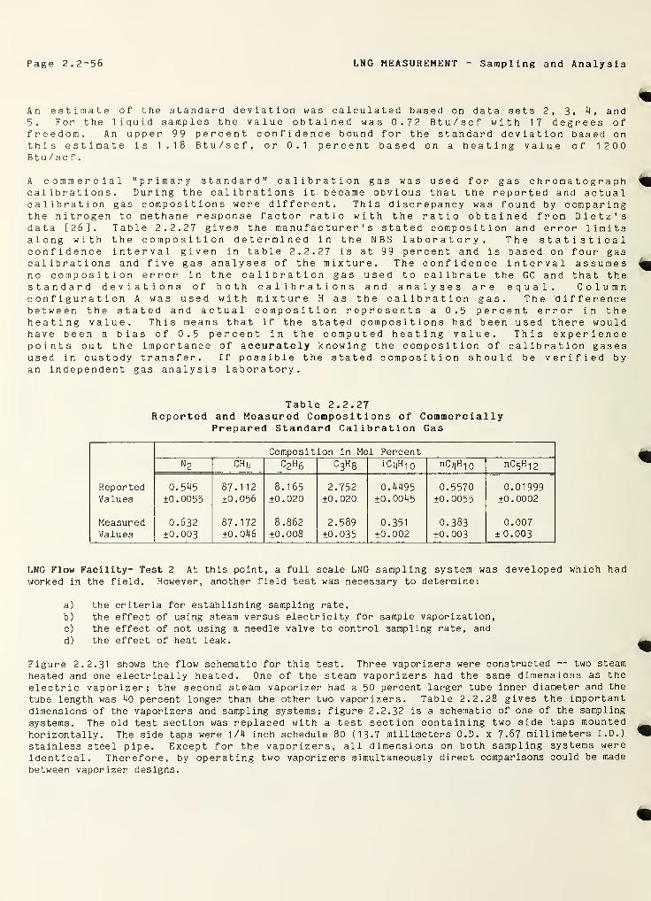
Page 2.2-56 LNG MEASUREMENT - Sampling and Analysis
An estimate of the standard deviation was calculated based on data sets 2, 3, 4, and5. For the liquid samples the value obtained was 0.72 Btu/scf with 17 degrees offreedom. An upper 99 percent confidence bound for the standard deviation based onthis estimate is 1.18 Btu/scf, or 0.1 percent based on a heating value of 1200Btu/scf
.
A commercial "primary standard" calibration gas was used for gas chromatographcalibrations. During the calibrations it became obvious that the reported and actualcalibration gas compositions were different. This discrepancy was found by comparingthe nitrogen to methane response factor ratio with the ratio obtained from Dietz'sdata [26]. Table 2.2.27 gives the ma nu f a c t ur er ' s stated composition and error limitsalong with the composition determined in the NBS laboratory. The statisticalconfidence interval given in table 2.2.27 is at 99 percent and is based on four gascalibrations and five gas analyses of the mixture. The confidence interval assumesno composition error in the calibration gas used to calibrate the GC and that thestandard deviations of both calibrations and analyses are equal. Columnconfiguration A was used with mixture H as the calibration gas. The differencebetween the stated and actual composition represents a 0.5 percent error in theheating value. This means that if the stated compositions had been used there wouldhave been a bias of 0.5 percent in the computed heating value. This experiencepoints out the importance of accurately knowing the composition of calibration gasesused in custody transfer. If possible the stated composition should be verified byan independent gas analysis laboratory.
Table 2.2.27Reported and Measured Compositions of Commercially
Prepared Standard Calibration Gas
Composition in Mol Percentn 2 CH 4 c2h 6 c
3h 8 1C 4H 10 nC 4H 1
0
nC5H 12
ReportedValues
0.545±0.0055
87.112±0.056
8.165±0.020
2.752±0.020
0.4495±0.0045
0.5570±0.0055
0.01999±0.0002
MeasuredValues
0.632±0.003
87.172±0.046
8.862±0.008
2.589±0.035
0.351
±0.0020.383
±0.0030.007
± 0.003
LNG Flow Facility- Test 2 At this point, a full scale LNG sampling system was developed which hadworked in the field. However, another field test was necessary to determine:
a) the criteria for establishing sampling rate,
b) the effect of using steam versus electricity for sample vaporization,c) the effect of not using a needle valve to control sampling rate, and
d) the effect of heat leak.
Figure 2.2.31 shows the flow schematic for this test. Three vaporizers were constructed — two steam
heated and one electrically heated. One of the steam vaporizers had the same dimensions as the
electric vaporizer; the second steam vaporizer had a 50 percent larger tube inner diameter and the
tube length was 40 percent longer than the other two vaporizers. Table 2.2.28 gives the importantdimensions of the vaporizers and sampling systems; figure 2 . 2.32 is a schematic of one of the sampling
systems. The old test section was replaced with a test section containing two side taps mountedhorizontally. The side taps were 1/4 inch schedule 80 (13.7 millimeters O.D. x 7.67 millimeters I.D.)
stainless steel pipe. Except for the vaporizers, all dimensions on both sampling systems wereidentical. Therefore, by operating two vaporizers simultaneously direct comparisons could be made
between vaporizer designs.
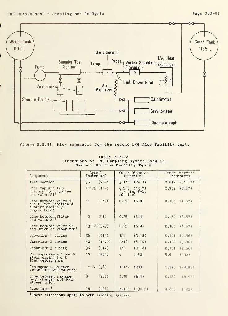
LNG MEASUREMENT Sampling and Analysis Page 2.2-57
Figure 2.2.31, Flow schematic for the second LNG flow facility test.
Table 2.2.28Dimensions of LNG Sampling System Used in
Second LNG Flow Facility Tests
ComponentLength
Inches(mm)Outer Diameter
Inches (mm)Inner Diameter
Inches(mm)
Test section 36 (914) 3-1/8 (79.4) 2.812 (71 .42)
Side tap and linebetween test sectionand valve SI 1
4-1/2 (114) 0.540 (13.7)(1/4 in. Sch.80 pipe)
0.302 (7.67)
Line between valve SIand filter (containeda short radius 90degree bend)
1
1
(279) 0.25 (6.4) 0.180 (4.57)
Line between filterand valve S2'
2 (51 ) 0.25 (6.4) 0.180 (4.57)
Line between valve S2and union at vaporizer 1
13-1/2(343) 0.25 (6.4) 0.180 (4.57)
Vaporizer 1 tubing 36 (914) 1/8 (3.18) 0.101 (2.56)
Vaporizer 2 tubing 50 (1270) 3/16 (4.76) 0.156 (3.96)
Vaporizer 3 tubing 36 (914) 1/8 (3.18) 0.101 (2.56)
For vaporizers 1 and 2steam casing (withflat welded ends)
10 (254) 6 (152) 5.5 (140)
Inpingement chamber(with flat welded ends)
1-1/2 (38) 1-1/2 (38) 1.376 (34.95)
Line between impinge-ment chamber and down-stream union
8 (200) 0.25 (6.4) 0.180 (4.57)
Accumlator 1 16 (406) 5.125 (130.2) 4.805 (122)
1 These dimensions apply to both sampling systems
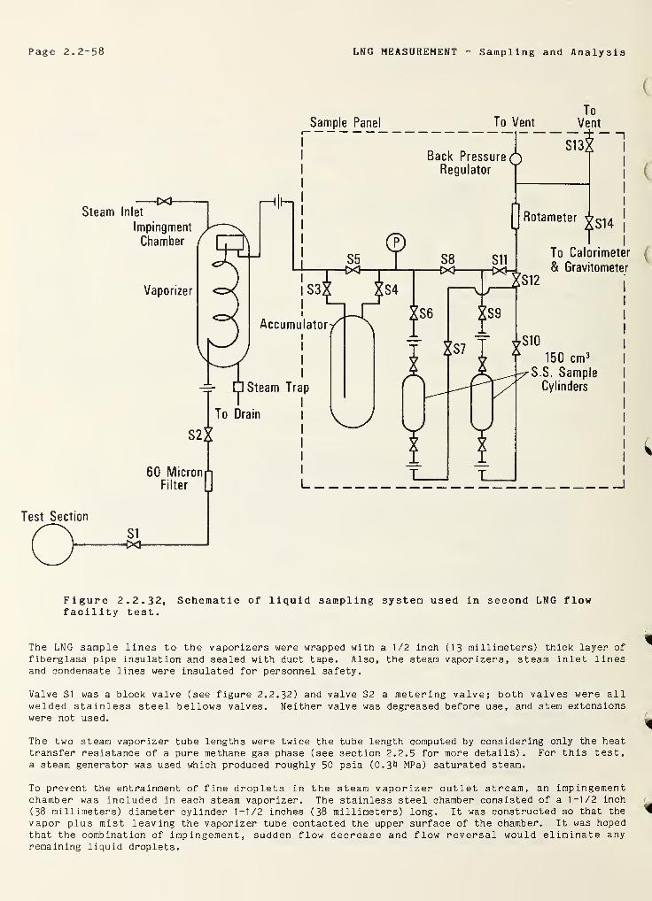
Page 2.2-58 LNG MEASUREMENT Sampling and Analysis
To
Figure 2.2.32, Schematic of liquid sampling system used in second LNG flowfacility test.
The LNG sample lines to the vaporizers were wrapped with a 1/2 inch (13 millimeters) thick layer of
fiberglass pipe insulation and sealed with duct tape. Also, the steam vaporizers, steam inlet linesand condensate lines were insulated for personnel safety.
Valve SI was a block valve (see figure 2.2.32) and valve S2 a metering valve; both valves were allwelded stainless steel bellows valves. Neither valve was degreased before use, and stem extensionswere not used.
The two steam vaporizer tube lengths were twice the tube length computed by considering only the heattransfer resistance of a pure methane gas phase (see section 2.2.5 for more details). For this test,a steam generator was used which produced roughly 50 psia (0.34 MPa) saturated steam.
To prevent the entrainment of fine droplets in the steam vaporizer outlet stream, an impingementchamber was included in each steam vaporizer. The stainless steel chamber consisted of a 1-1/2 inch
(38 millimeters) diameter cylinder 1-1/2 inches (38 millimeters) long. It was constructed so that the
vapor plus mist leaving the vaporizer tube contacted the upper surface of the chamber. It was hopedthat the combination of impingement, sudden flow decrease and flow reversal would eliminate anyremaining liquid droplets.
LNG MEASUREMENT Sampling and Analysis Page 2.2-59
The electric vaporizer dimensions were chosen to correspond to one of the steam vaporizers so that a
direct comparison between vaporizers could be made. However, the impingement chamber was not used
w! *"h the electric vaporizer. This vaporizer consisted of thin wall (0.012 inch (0.30 millimeter))st tinless steel tubing with electrical leads attached at each end. Since the tubing was used as the
resistive heater, a high amperage (18 amps) low voltage (-4.3 volts) direct current was used. Toprevent possible shorts, the vaporizer tube was epoxied into micarta couplings at each end.
Initially, the accumulator volume was two liters, but the first day's test results showed that theaccumulator was too small. Thereafter, a four liter accumulator was used.
Analyses of the LNG used in the first flow facility test showed relatively high concentration of C 5+.
To obtain a more representative LNG mixture, the LNG for this test was purchased from San Diego Gasand Electric Company. However, even this LNG contained approximately 0.08 mol percent Cg+.
For sample analysis, column configuration A was used. Prepared mixture H (table 2.2.6) was used as thecalibration gas. Both integrators A and B were connected to gas chromatograph II so that theirresults could be compared.
Test Results A total of seven tests were made in the flow facility over a four day period. Table2.2.29 lists the pertinent operating parameters and lists a comparison of measured and computedheating values and specific gravities. The computed quantities are real gas values computed from thecompositions using the A.G.A methods [2]. Table 2.2.29 gives the average values and estimatedstandard deviation of the compositions and the liquid densities computed using the extendedcorresponding states method [4],
Test A Because the sampling rates would be comparable to those used in laboratory tests, two literaccumulators were used in test A. However, the test results suggested that the accumulator was toosmall. Figure 2.2.33 shows the deviation from the average heating value for this test. At the samplerates used in this test the accumulator residence time ranged between 10 and 18 seconds; this samerange gave good results in laboratory tests. All remaining tests were made using four literaccumulators.
Test B As shown in figure 2.2.34, results of test B clearly confirmed the need for the largeraccumulator. Possible reasons for this include:
a) the use of a constant wall temperature vaporizer (as opposed to the constant heatflux vaporizer used in the laboratory apparatus, or
b) the presence of a finite heat leak into the sample line.
Unfortunately, there was not sufficient time to identify the reason for needing the longer residence
time.
Two points were eliminated from figure 2.2.34 and from the statistical analysis of test B results.For no obvious reason, one sample had a methane content five standard deviations higher than theaverage value for the test (both integrators gave the same result). However, the second outlier wasthe first sample taken after changing the sampling rate; it was taken less than 20 minutes after thechange. This suggested the possibility of flow transients affecting the sampling precision.
Test C Test C was a short test to determine if sampling system startup transients affected samplingprecision. Figure 2.2.35 shows the deviation in heating value for this test. The deviations arerelative to the average values obtained under steady conditions in test D, which was run on the sameday. In this test, samples were taken every 15 minutes after putting the sampling system :noperation. Although the scatter was greater, especially in the nitrogen, methane and ethane content ,
there was no obvious trend with time.
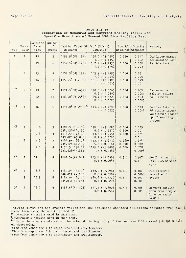
Page 2.2-60 LNG MEASUREMENT Sampling and Analysis
Table 2.2.29Comparison of Measured and Computed Heating Values andSpecific Gravities of Second LNG Flow Facility Test
Sampling NumberVapor- Rate of Heating Value Btu/scf (MJ/rrP) Specific Gravity Remarks
Test izer slpm points Measured Computed' Measured Computed
A 1 14 3 1 159.
5
6( 43 - 192) 1158.6 (43.159) 0.650 0.647 Two liter sample
1 1 59 -
5
5( 43 . 1 92)
3.9 ( 0.145) 0.002 accumulator used19 6 1162.2 (43.293) 0.650 0.650 in this test
4.7 ( 0.175) 0.003
2 13 4 1159.
5
6( 43 . 192) 1163.7 (43.349) 0.650 0.651
1 1 59 .
5
5( 43 . 1 92
)
7.9 ( 0.294) 0.00516 3 1161 .0 (43.248) 0.650 0.649
1 .4 ( 0.052) 0.001
B2 2 13 7 1171 .
5
6( 43 . 639
)
1170.6 (43.606) 0.658 0.655 Increased acc-0.8 ( 0.030) 0.0007 mulator volume
22 13 1 1 69 .
0
6( 43 . 546
)
1169.7 (43.572) 0.658 0.654 to 4 liters0.6 ( 0.022) 0.0005
C3 1 16 5 1 174.0^(43- 733
)
6 1173.9 (43.729) 0.680 0.674 Samples taken at1.4 ( 0.052) 0.0007 15 minute inter-
vals after start-up of samplingsystem
d3 1 6.0 3 1 184.5-1 186.
0
6 1178.6 (43.804) 0.680- 0.675(44.124-44.180) 6.9 ( 0.257) 0.690 0.001
9.8 4 1176. 5-1178.
0
6 1174.6 (43.755) 0.680 0.674(43.826-43.882) 0.7 ( 0.026) 0.0
2 4.9 2 1 184.5-1 186.
0
6 1172.4 (43.673) 0.680- 0.674(44.124-44.180) 5.8 ( 0.216) 0.690 0.004
9.5 4 1176. 5-1178.
0
6 1175.8 (43.788) 0.680 0.674(43.826-43.882) 1 .3 ( 0.048) 0.0008
E 2 1 19 4 1 1 82 .
5
5( 44 . 049
)
1183.8 (44.098) 0.717 0.707 Needle Value S2,
0.1 ( 0.004) 0.1 fig. 2.2.32 wideopen
F 2 1 16.8 3 1182.0-1183.0? 1184.2 coO=r-=r 0.717 0.707 Put electric(44.031-44.068) 0.8 ( 0.030) 0.0006 vaporizer in
3 15.3 8 1182.0-1183.0? 1184.6 (44.127) 0.717 0.707 system(44.031-44.068) 0.6 ( 0.022) 0.0005
G2 1 16.9 4 1 1 86 . 5? ( 44 . 1 98
)
1197.3 (44.600) 0.715 0.706 Removed insula-4.2 ( 0.156) 0.005 tion from sample
line to vapor-izer 1
'Values given are the average values and the estimated standard deviations computed from thecomposition using the A.G.A. method [2].integrator A results used in this test.3lntegrator B results used in this test.ihis is the steady state value; the value at the beginning of the test was 1188 Btu/scf (44.254 MJ/m3)and decreasing.ilow from vaporizer 1 to calorimeter and gravitometer
.
^Flow from vaporizer 2 to calorimeter and gravitometer.?Flow from vaporizer 3 to calorimeter and gravitometer.
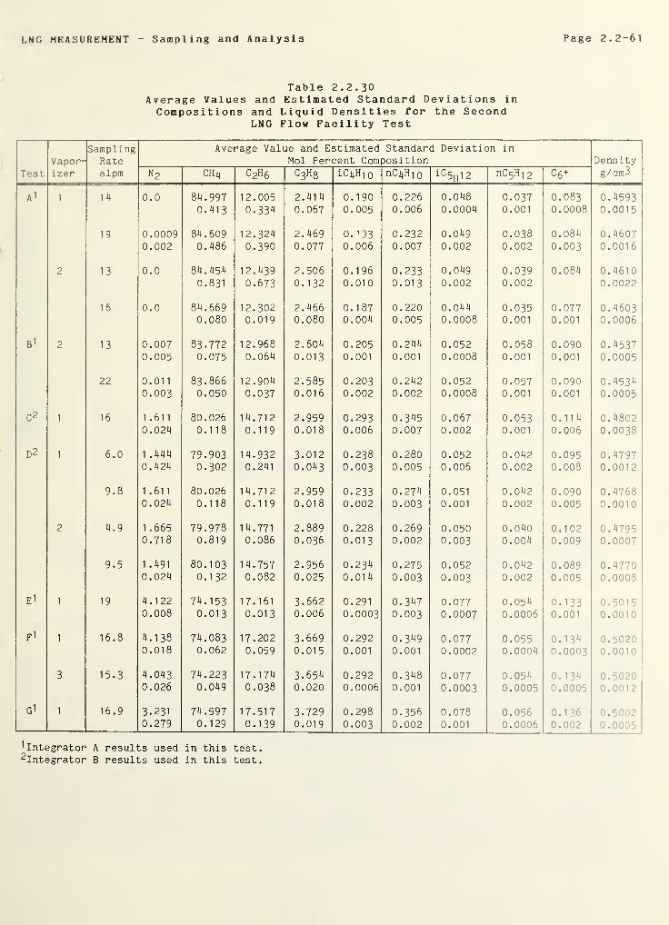
LNG MEASUREMENT Sampling and Analysis Page 2.2-61
Table 2.2.30Average Values and Estimated Standard Deviations inCompositions and Liquid Densities for the Second
LNG Flow Facility Test
Vapor-Sampling
Rate
Average Value and Estimated Standard Deviation in
Mol Percent Composition Density
Test izer slpm n 2 CH4 c2h 6 c3h8 i C 4h i o nCi^Hi 0 iC 5H 12
nC 5H 12 C6 + g/cm3
Al 1 1
4
0.0 84.9970.413
12.005
0.334
2.414
0.0670.1900.005
0.2260.006
0.0480.0004
0.0370.001
0.0830.0008
0.45930.0015
19 0.00090.002
84.6090.486
12.3240.390
2.4690.077
0.1930.006
0.2320.007
0.0490.002
0.0380.002
0.0840.003
0.46070.0016
2 13 0.0 84.4540.831
12.4390.673
2.5060.132
0.1960.010
0.2330.013
0.0490.002
0.0390.002
0.084 0.46100.0022
16 0.0 84.6690.080
12.3020.019
2.4660.080
0.1870.004
0.2200.005
0.0440.0008
0.0350.001
0.0770.001
0.46030.0006
B 1 2 13 0.0070.005
83.7720.075
12.9680.064
2.604
0.0130.2050.001
0.2440.001
0.0520.0008
0.0580.001
0.0900.001
0.45370.0005
22 0.01
1
0.00383.8660.050
12.9040.037
2.5850.016
0.2030.002
0.2420.002
0.0520.0008
0.0570.001
0.0900.001
0.45340.0005
C2 1 16 1 .61
1
0.02480.0260.118
14.7120.119
2.9590.018
0.2930.006
0.3450.007
0.0670.002
0.0530.001
0.1140.006
0.48020.0038
D2 1 6.0 1.4440.424
79.9030.302
14.9320.241
3.0120.043
0.2380.003
0.2800.005
0.0520.006
0.0420.002
0.0950.008
0.47970.0012
9.8 1 .61
1
0.02480.0260.118
14.71
2
0.1192.9590.018
0.2330.002
0.2740.003
0.051
0.001
0.0420.002
0.0900.005
0.47680.0010
2 4.9 1 .665
0.71879.9780.819
14.771
0.0862.8890.036
0.2280.013
0.2690.002
0.0500.003
0.0400.004
0.1020.009
0.47950.0007
9.5 1 .491
0.02480.1030.132
14.7570.082
2.9560.025
0.2340.014
0.2750.003
0.0520.003
0.0420.002
0.0890.005
0.47700.0008
E 11 19 4.122
0.00874.1530.013
17.161
0.0133.6620.006
0.291
0.00030.3470.003
0.0770.0007
0.0540.0006
0.1330.001
0.50150.0010
F 11 16.8 4.138
0.01874.0830.062
17.2020.059
3.6690.015
0.2920.001
0.3490.001
0.0770.0002
0.0550.0004
0.1340.0003
0.50200.0010
3 15.3 4.0430.026
74.2230.049
17.1740.038
3.6540.020
0.2920.0006
0.3480.001
0.0770.0003
0.0540.0005
0.1340.0005
0.50200.0012
G 11 16.9 3.231
0.27974.5970.129
17.5170.139
3.7290.019
0.2980.003
0.3560.002
0.0780.001
0.0560.0006
0.1360.002
0.50020.0005
|
1 Integrator A results used in this test.^Integrator B results used in this test.
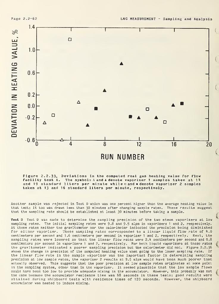
Page 2 .
2
- 62 LNG MEASUREMENT Sampling and Analysis
UU
<CD
<uu
O<LLJo
RUN NUMBER
Figure 2.2.33. Deviations in the computed real gas heating value for flowfacility test A. The symbols A and k denote vaporizer 1 samples taken at 1 4
and 19 standard liters per minute wh i 1 e and denote vaporizer 2 samplestaken at 13 and 16 standard liters per minute, respectively.
Another sample was rejected in Test D which was one percent higher than the average heating value in
that test; it too was drawn less than 30 minutes after changing sample rates. These results suggestthat the sampling rate should be established at least 30 minutes before taking a sample.
Test D Test D was made to determine the sampling precision of the two steam vaporizers at lowsampling rates. The initial sampling rates were 9.8 and 9.5 slpm in vaporizers 1 and 2, respectively
.
At these rates neither the gravitometer nor the calorimeter indicated the precision being diminishedfor either vaporizer. These sampling rates corresponded to a linear liquid flow rate of 4.0centimeters per second and 1.6 centimeters per second in vaporizer 1 and 2, respectively. Next, thesampling rates were lowered so that the linear flow rates were 2.4 centimeters per second and 0.8centimeters per second in vaporizers 1 and 2, respectively. For both liquid vaporizers at these ratesthe gravitometer indicated a poorer sampling precision but the calorimeter did not. Figure 2.2.36shows the change in precision of the computed heating value when going to the lower sampling rate. If
the linear flow rate in the sample vaporizer was the important factor in determining samplingprecision at low sample rates, the vaporizer 2 results at 9.5 slpm would have been much poorer thanactually observed. This suggests that the poor precision at low sample rates originates at some pointin the sampling system, other than in the vaporizer. It seemed plausible that the low sample flowscould have been too low to provide adequate mixing in the accumulator. However, this probably was not
the case because the accumulator residence time was 68 seconds in these tests; good results wereobtained during shipboard tests with residence times of 120 seconds. However, the shipboardaccumulator was heated to induce mixing.
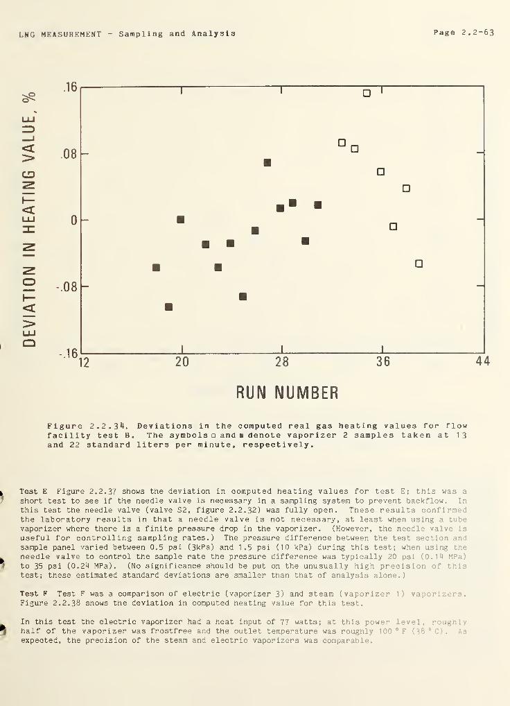
LNG MEASUREMENT Sampling and Analysis Page 2.2-63
RUN NUMBER
Figure 2.2.34, Deviations in the computed real gas heating values for flowfacility test B. The symbols and a denote vaporizer 2 samples taken at 1 3
and 22 standard liters per minute, respectively.
Test E Figure 2.2.37 shows the deviation in computed heating values for test E; this was a
short test to see if the needle valve is necessary in a sampling system to prevent backflow. In
this test the needle valve (valve S2, figure 2.2.32) was fully open. These results confirmedthe laboratory results in that a needle valve is not necessary, at least when using a tubevaporizer where there is a finite pressure drop in the vaporizer. (However, the needle valve in
useful for controlling sampling rates.) The pressure difference between the test section andsample panel varied between 0.5 psi (3kPa) and 1.5 psi (10 kPa) during this test; when using the
needle valve to control the sample rate the pressure difference was typically 20 psi (0.14 MPa)
to 35 psi (0.24 MPa). (No significance should be put on the unusually high precision of thintest; these estimated standard deviations are smaller than that of analysis alone.)
Test F Test F was a comparison of electric (vaporizer 3) and steam (vaporizer 1) vaporizern.Figure 2.2.38 shows the deviation in computed heating value for this test.
In this test the electric vaporizer had a heat input of 77 watts; at this power level, r
half of the vaporizer was frostfree and the outlet temperature was roughly 100 0F
expected, the precision of the steam and electric vaporizers was comparable.
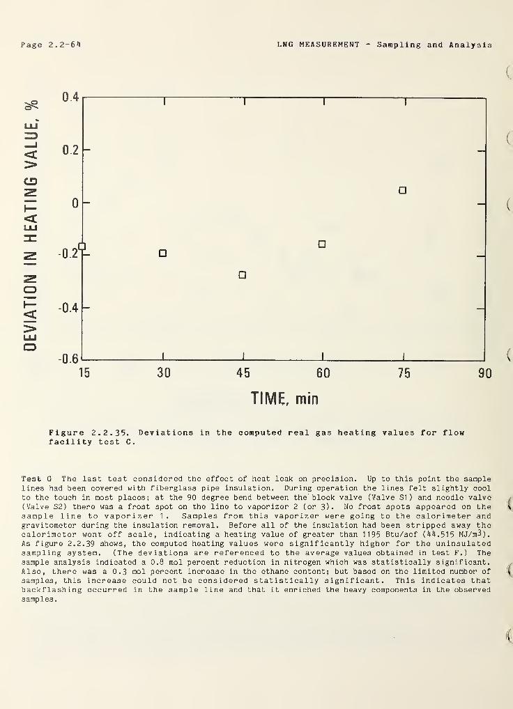
Page 2.2-64 LNG MEASUREMENT - Sampling and Analysis
<CD
Oh-<
45 60
TIME, min
Figure 2.2.35. Deviations in the computed real gas heating values for flowfacility test C.
Test G The last test considered the effect of heat leak on precision. Up to this point the samplelines had been covered with fiberglass pipe insulation. During operation the lines felt slightly cool
to the touch in most places; at the 90 degree bend between the block valve (Valve SI) and needle valve(Valve S2 ) there was a frost spot on the line to vaporizer 2 (or 3). No frost spots appeared on thesample line to vaporizer 1. Samples from this vaporizer were going to the calorimeter andgravitometer during the insulation removal. Before all of the insulation had been stripped away thecalorimeter went off scale, indicating a heating value of greater than 1195 Btu/scf (44.515 MJ/m3).As figure 2.2.39 shows, the computed heating values were significantly higher for the uninsulatedsampling system. (The deviations are referenced to the average values obtained in test F.) Thesample analysis indicated a 0.8 mol percent reduction in nitrogen which was statistically significant.Also, there was a 0.3 mol percent increase in the ethane content; but based on the limited number of
samples, this increase could not be considered statistically significant. This indicates thatbackflashing occurred in the sample line and that it enriched the heavy components in the observedsamples.
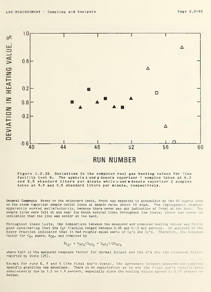
LNG MEASUREMENT Sampling and Analysis Page 2.2-65
<
Figure 2.2.36. Deviations in the computed real gas heating values for flowfacility test D. The symbols A and A denote vaporizer 1 samples taken at 6.0and 9.8 standard liters per minute while and denote vaporizer 2 samplestaken at 4 _ 9 and 9.5 standard liters per minute, respectively.
General Comments Based on the shipboard tests, frost was expected to accumulate at the 90 degree bendon the steam vaporizer sample outlet lines at sample rates above 10 slpm. The impingement chamberapparently worked satisfactorily, because there never was any indication of frost at the bend. Thesample lines were felt at and near the bends several times throughout the tests; there was never anindication that the line was cooler at the bend.
Throughout these tests, the comparison between the measured and computed heating values was fairlygood considering that the Cg+ fraction ranged between 0.08 and 0.13 mol percent. An analyst' f •••
heavy fraction indicated that it had roughly equal parts of Cg’s and Cy's. Therefore, the r<-s; r.
factor for Cg+ peaks, Kq5 + was computed by
kC 6 += KnCi/DnCg + DnC7
) /2DnC^
where KnC4 is the measured response factor for normal butane and the D's are the rasper fa 1
reported by Dietz [25].
Except for runs E, F and G (the final day's tests), the agreement between measured as i
specific gravities was excellent. There is no explaination as to why the final day'
•
.
•
consistently low by 1.3 to 1.4 percent, especially since the heating values agreed tobetter.
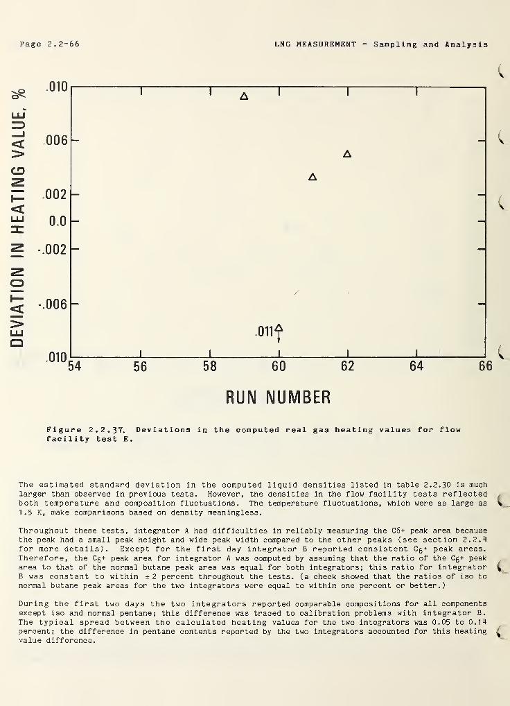
DEVIATION
IN
HEATING
VALUE,
Page 2.2-66 LNG MEASUREMENT Sampling and Analysis
RUN NUMBER
Figure 2.2.37. Deviations in the computed real gas heating values for flowfacility test E.
The estimated standard deviation in the computed liquid densities listed in table 2.2.30 is muchlarger than observed in previous tests. However, the densities in the flow facility tests reflectedboth temperature and composition fluctuations. The temperature fluctuations, which were as large as
1.5 K, make comparisons based on density meaningless.
Throughout these tests, integrator A had difficulties in reliably measuring the C6 + peak area becausethe peak had a small peak height and wide peak width compared to the other peaks (see section 2.2.4for more details). Except for the first day integrator B reported consistent Cg + peak areas.Therefore, the C5 + peak area for integrator A was computed by assuming that the ratio of the C5 + peakarea to that of the normal butane peak area was equal for both integrators; this ratio for integratorB was constant to within ±2 percent throughout the tests, (a check showed that the ratios of iso to
normal butane peak areas for the two integrators were equal to within one percent or better.)
During the first two days the two integrators reported comparable compositions for all componentsexcept iso and normal pentane; this difference was traced to calibration problems with integrator B.
The typical spread between the calculated heating values for the two integrators was 0.05 to 0.14percent; the difference in pentane contents reported by the two integrators accounted for this heatingvalue difference.
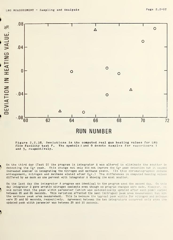
LNG MEASUREMENT - Sampling and Analysis Page 2.2-67
o'''
CD
Figure 2.2.38. Deviations in the computed real gas heating values for LNGflow facility test F. The symbols A and 0 denote samples for vaporizers 1
and 3, respectively.
On the third day (Test D) the program in integrator A was altered to eliminate the scatter in
detecting the C5+ peak. This change not only did not improve the Cg+ peak detection but it causedincreased scatter in integrating the nitrogen and methane peaks. (In this chromatographic columnarrangement, nitrogen and methane eluted after C5+.) The differences in computed heating val jes
differed by as much as one percent with integrator A showing the most scatter.
On the last day the integrator A program was identical to the program used the second day.day integrator B gave erratic nitrogen contents even though no program changes were made. .w .•• •
,
was noted that the peak width parameter (which was automatically updated after each c :
between 20 and 66 seconds. This variation affected the next (nitrogen) peak area measurement but •
the methane peak area measurement. This is because the typical peak widths for nitrogenwere 20 and 60 seconds, respectively. Agreement between the two integrators occurred r.ly -
• •
updated peak width parameter was between 20 and 30 seconds.
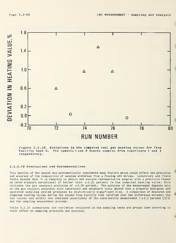
DEVIATION
IN
HEATING
VALUE.%
Page 2.2-68 LNG MEASUREMENT - Sampling and Analysis
RUN NUMBER
Figure 2.2.39. Deviations in the computed real gas heating values for flowfacility test G. The symbols A and 0 denote samples from vaporizers 1 and 3
respectively
.
2.2.5.10 Conclusions and Recommendations
This section of the manual has systematically considered many factors which could affect the precisionand accuracy of the composition of samples withdrawn from a flowing LNG stream. Laboratory and fieldtests showed that it is feasible to obtain and analyze representative samples with a precision (basedon three standard deviations) of better than ±0.30 percent in the computed heating value; thisincludes the gas analysis precision of ±0.06 percent. The accuracy of the measurement depends onlyon the gas analysis accuracy; both laboratory and shipboard tests showed that a properly designed andoperated sampling system produces no statistically significant bias. A comparison of measured andcomputed heating values during the second flow facility test verified that the difference between thetwo values was within the combined uncertainty of the calorimetric measurement ( ±0.3 percent [31])and the sampling measurement process.
Table 2.2.31 summarizes the variables evaluated in the sampling tests and groups them according to
their effect on sampling precision and accuracy.
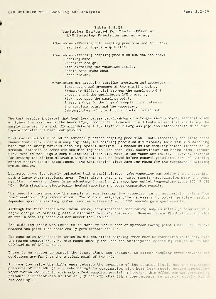
LNG MEASUREMENT Sampling and Analysis Page 2.2-69
Table 2.2.31Variables Evaluated for Their Effect on
LNG Sampling Precision and Accuracy
Variables affecting both sampling precision and accuracy:
Heat leak to liquid sample line.
Variables affecting sampling precision but not accuracy:
Sampling rate,
Vaporizer design,Time-averaging the vaporized sample,
Sample rate transients,Probe design.
Variables not affecting sampling precision and accuracy:
Temperature and pressure at the sampling point,
Pressure differential between the sampling pointpressure and the equilibrium LNG pressure,Flow rate past the sampling point,Pressure drop in the liquid sample line betweenthe sampling point and the vaporizer,Composition of the liquid being sampled.
The test results indicated that heat leak causes backflashing of nitrogen (and probably methane) which
enriches the samples in the heavy (C2 +) components. However, field tests showed that insulating the
sample line with one inch (25 millimeters) thick layer of fiberglass pipe insulation sealed with ducttape eliminates the heat leak problem.
Five variables were found to adversely affect sampling precision. Both laboratory and field testsshowed that below a certain sampling rate, the sampling precision diminishes; this minimum samplingrate varied among various sampling system designs. A mechanism for sampling rate's importance is
unknown. Attempts to correlate the sampling rate with heat leak, accumulator residence time, linearflow rate in the liquid sample line and linear flow rate in the vaporizer failed, However, criteriafor setting the minimum allowable sample rate must be found before general guidelines for LNG samplingsystem design can be established. The next section gives sampling rates for the recommended samplingsystem design.
Laboratory results clearly indicated that a small diameter tube vaporizer was better than a vaporizerwith a large cross sectional area. Tests also showed that rapid sample vaporization gave the bestresults. However, there is no advantage in having the vaporizer outlet temperature above 100 °F (38
°C). Both steam and electrically heated vaporizers produce comparable results.
The need to time-average the sample stream leaving the vaporizer in an accumulator arises fromfractionation during vaporization. The minimum residence time necessary to obtain precise resultsdepended upon the sampling system; residence times of 20 to 120 seconds gave good results.
Although the field tests were inconclusive, they indicated that taking samples within 30 minutes of t
major change in sampling rate diminishes sampling precision. However, minor fluctuations and slowdrifts in sampling rates did not affect the results.
The side tap probe was found to be more reliable than an upstream facing pitot tube. For unkn wn
reasons the pitot tube occasionally gave erratic results.
The conclusion that certain variables did not affect sampling error must be considered valid onlythe ranges tested; however, this range usually included the anticipated operating ranges f •
:
off-loading of LNG tankers.
There is no reason to expect the temperature and pressure to affect sampling err r ; r
conditions are far from the critical point of the LNG.
At some low value the difference between the pressure of the sampled liquidpressure of the LNG (i.e., subcooling) in combination with heat leak shoul :
vaporization which could adversely affect sampling precision; however, this effect wi e
pressure differentials as low as 3.9 psi (25 kPa) (this corresponds to a p p r .
sub-cooling)
.
Page 2.2-70 LNG MEASUREMENT Sampling and Analysis
LNG flow rates corresponding to Reynold's numbers ranging between 1500 and 50,000 did not affectsampling precision; it is unlikely that there would be any adverse effect on precision at the higherReynold's numbers anticipated in on and off loading operations.
The fact that a pressure drop in the liquid sample line which is comparable to the pressure drop inthe vaporizer is unnecessary eliminates the need for liquid flow control valve. However, thisconclusion is known to be valid only when using a tube vaporizer.
Finally, there is no problem in sampling LNG mixtures which contain up to 0.15 percent C5 +. Theheavies would be a problem if they raised the sample dew point temperature to near ambienttemp erature.
Recommended LNG Sampling System Design and Operating Criteria Based on the laboratory and field testresults, the following sampling system design criteria are recommended:
Probe - side tap mounted horizontally with the probe flush with the wall of the LNG pipe; probe innerdiameter should be as small as feasible (<0.25 inch (6.4 millimeters)).
Liquid phase needle valve - optional, but useful for flow control.
Liquid sample line - use as small a bore tubing as feasible ( S0.20 inch (5.1 millimeters)) and makethe line as short as possible. (A filter is recommended to prevent line plugging.)
Sample vaporizer - use a coiled tube vaporizer with the tube inner diameter comparable to that of thesample line tubing. If steam is the vaporizing medium, use the design procedure outlined in section2.2.5 with an impingement chamber. Electrically heated vaporizers can be designed using the sameprocedure as steam vaporizers; however, thin walled tubing is necessary to minimize the necessaryamperage. Also, a thermostatic control is necessary to prevent the vaporizer from overheating if thesample flow rate decreases.
Accumulator - size for a residence time of at least 45 seconds; the length to diameter ratio of theaccumulator should be greater than 1.5. The sample inlet line should extend to near the bottom of thevessel but the outlet line should not penetrate the vessel volume. Heating the bottom of theaccumulator may improve mixing.
Insulation - the probe and liquid sample line should be insulated sufficiently to prevent moisturefrom condensing on the lines.
The following sample system operating conditions are within the range of values found to give goodresults in the field tests and therefore are recommended;
Sampling rate - greater than 20 slpm; this criteria applies only to the recommended sampling system.
Sample pressure - preferrably greater than 20 psig (0.24 MPa) to provide sufficient gas sample forpurging and replicate analyses from a 500 cm3 sample cylinder.
Vaporizer outlet temperature - 80 to 100 °F (27 to 380C)
.
The shipboard tests and flow facility test 2 sampling systems both worked satisfactorily and may beconsidered proven sampling systems.
LNG MEASUREMENT Sampling and Analysis Page 2.2-71
2.2.6 References
[ 11 Parrish, W. R., J. M. Arvidson and J. F. LaBrecque, Development and evaluation of an LNG
Sampling Measurement System, Nat. Bur. Stand. (U.S.), NBSIR 78-887, 199 pp(July, 1978).
[2]
|)
Caldwell, B. J., Fuel gas energy metering, Transmission Measurement Committee Report Number 5
(revised), page 55 (1976), American Gas Association, Inc., Arlington, VA.
[3] Armstrong, G. T., E. S. Domalski and J. I. Minor, Standard combustion data for the fuel gas
industry, American Gas Association 1972 Operating Section Proceedings, page D-72 (1972).
[4] McCarty, R. D., A comparison of mathematical models for the prediction of LNG densities, Nat.
Bur. Stand. (U.S.) Internal Report, NBSIR 77~867 (Oct. 1977).
[5] Hiza, M. J., An empirical excess volume model for estimating liquefied natural gas densities,Fluid Phase Equilibria, 2(2), pp 27~38 (August 1978).
[6] Natrella, M. G. ,Experimental Statistics, Handbook 91, National Bureau of Standards (1963).
[7] "Standard Method for Analysis of Natural Gas by Gas Chromatography," ASTM Designation: D1945“64(Reapproved 1973).
[8] "Standard Method for Analysis of Natural Gases and Related Types of Gaseous Mixtures by the MassSpectrometer," ASTM Designation: D1 1
37“53 -
[9] Dalmaze, M. R., LNG sampling technique. Gas Aujourdhui 96, 448 (Nov. 1972).
[10] Trigo, J., System samples LNG accurately, Hydrocarbon Proc. p. 83 (April 1976).
[11] The Cosmodyne Corporation, Cryogenic Sampler Bulletin TDS-8064, Torrance, Calif.
[12] Cook, H. L., Method and apparatus for sampling refrigerated volatile liquids, U.S. Patent No.
3,487,692 (Jan. 1970).
[13] Miller, A. J., Techniques for sampling natural gas, SNG, and LNG, Pipe Line Industry 39 (3), 70(Sept. 1973).
[14] "Standard Method of Sampling Natural Gas," ASTM Designation: Dll 45—53 -
[15] Chapman, J. A. and G. D. Payne, Sampling system guidelines, paper presented at the 19th AnnualISA Analysis Instrumentation Symp. , April 24-26, 1973, St. Louis, MO.
[16] Turbett, J. R., Rockwell International, Atomics International Division, Golden, CO (privatecommunication, 1977).
i
t,7]
[18]
Conn, A. P., Transco, Houston, TX (private communication, 1976).
GPA Publication 2261-72, Method of analysis for natural gas and similar gaseous mixtures by gaschromatography,, Gas Processors Association, Tulsa, OK.
[19] Thompson, B., Fundamentals of Gas Analysis by Gas Chromatography, Varian Associates, Inc., Pa'.o
Alto, CA (1977).
1
—
1
rv> 0
1
iPurcell, J. E. and C. P. Gilson, Improved analysis of natural gas. Chromatography Newsletter 1
(2), 45 (Nov. 1972), published by Perkin-Elmer Corp., Norwalk, CT.
[21] Lawson, A. E., A versatile, low cost gas chromatograph, American Laboratory (May 1969).
[22] Ludtke, P. R., Performance characteristics of a liquid helium pump, Nat. Bur. Stanl. . .
Internal Report, NBSIR 7 5~ 8 1 6 (July 1975).
[23] Cook, H. L., Transco, Houston, TX (private communication, 1977).
[24] Handbook of Chemistry and Physics, 45th Ed., p. D86, The Chemical Rubber Co., 'lev '.
•
Page 2.2-72 LNG MEASUREMENT Sampling and Analysis
[25] Childs, G. E., L. J. Ericks, and R. L. Powell, Thermal conductivity of solids at roomtemperature and below, Nat. Bur. Stand. (U.S.) Monograph 131. p. 257 (Sept. 1973).
[26] Dietz, W. A., Response factors for gas chromatographic analyses, J. of Gas Chromatography, p. 68
(Feb. 1967).
[27] Mann, D. B., Cryogenic flowmetering research at NBS , CryogenicsJ_1_, 179 (1971 ).
[28] Brennan, J. A., Cryogenics Division, National Bureau of Standards, Boulder, CO (privatecommunication, 1976).
[29]
Goodwin, R. D., The thermophysical properties of methane from 90 to 500 K at pressure to 700bar, Nat. Bur. Stand. (U.S.) Technical Note 653 (April 1974).
[30] Hanley, H. J. M. , W. M. Haynes, and R. D. McCarty, The viscosity and thermal conductivitycoefficients for dense gaseous and liquid methane, J. of Phys. and Chem. Ref. Data 6_ (2), 597
(1977).
[31] "Standard Method of Test for Calorific Value of Gases in Natural Gas Range by ContinuousRecording Calorimeter," ASTM Designation: Dll 45 —53
•
[32]
Hiza, M. J., W. M. Haynes and W. R. Parrish, Orthobaric liquid densities and excess volumes for
binary mixtures of low molar-mass alkanes and nitrogen between 105 and 1 40 K, J. Chem.Thermodynamics 9, 873 (1977).


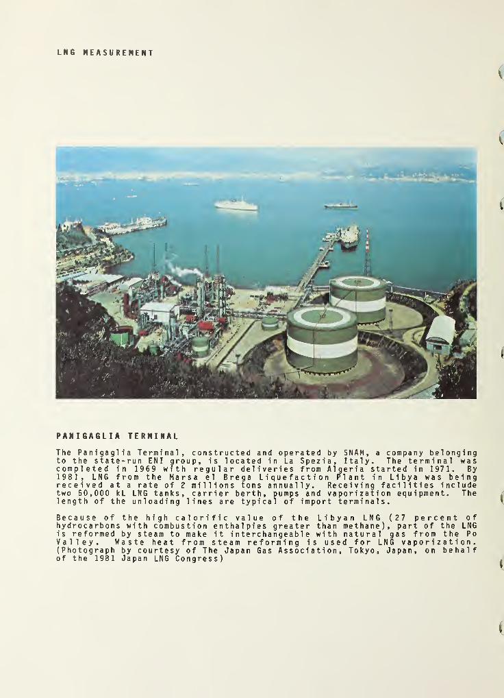
LN6 MEASUREMENT
PANIGAGLIA TERMINAL
The Panigaglia Terminal, constructed and operated by SNAM, a company belongingto the state-run ENI group, is located in La Spezia, Italy. The terminal wascompleted in 1969 with regular deliveries from Algeria started in 1971. By1981, LNG from the Marsa el Brega Liquefaction Plant in Libya was beingreceived at a rate of 2 millions tons annually. Receiving facilities includetwo 50,000 kL LNG tanks, carrier berth, pumps and vaporization equipment. Thelength of the unloading lines are typical of import terminals.
Because of the high calorific value of the Libyan LNG (27 percent ofhydrocarbons with combustion enthalpies greater than methane), part of the LNGis reformed by steam to make it interchangeable with natural gas from the PoValley. Waste heat from steam reforming is used for LNG vaporization.(Photograph by courtesy of The Japan Gas Association, Tokyo, Japan, on behalfof the 1981 Japan LNG Congress)
LNG MEASUREMENT Calorific Value Page 2.3-0
CONTENTS
2.0 MEASUREMENT ELEMENTS
Calorific Value Page
2.3 LNG Calorific Value 2.3-1
2.3.1 Hydrocarbon Gaseous Fuel Research 2.3-1
2. 3. 1.1 Industrial Gas Measurement, Analysis and Calorimetry 2.3-1
2. 3. 1.2 Properties of Pure Components and Mixtures 2.3-2
2.3.2 Calorific Value Instrumentation and Measurements 2.3-3
2.3.2. 1 Measured Methods- Automatic Recording Calorimeter 2.3-4
3. 3. 2. 2 Other Comb u s t i o n - Type Calorimeters 2.3-5
2. 3. 2. 3 Calculated Methods- Gas Analysis 2.3-5
2. 3. 2.4 Measured and Calculated Methods Compared 2.3-5
2.3.3 References 2.3-7

LNG MEASUREMENT Calorific Value Page 2.3-1
2.3 LNG Calorific Values
It is the purpose of this section of the manual to provide information on the methods of measurementof the calorific or heating value of natural gas and the accuracy and precision of these methods.
Instrumentation and properties data necessary for determination of the actual values are alsodiscussed in section 2.2 and 1.3. However, these sections deal with specific methods developed for
LNG or LNG mixtures and describe relatively recent technological advances.
The general problem of assessing heating values of gaseous fuels dates back to the beginning of the
current century, and the methods and techniques developed over the years since then are still verymuch in use. Advances certainly have been made in accuracy and precision, but in general very little
has changed in the techniques used. The historical perspective and a discussion of the accuracy andprecision of the methods, both direct and calculated, are presented.
2.3.1 Hydrocarbon Gaseous Fuel Research
A principal value of natural gas is the quantity of thermal energy derived when the natural gas is
burned in air. The following is an edited portion of an historical review by Armstrong [32] publishedon the occasion of the 75th anniversary of the National Bureau of Standards. Only that portion of the
publication dealing with natural gas is included here. The complete publication deals withhydrocarbon fuels in general, and the reader is referred to the original document for details.
In the early days of NBS , which was founded in 1901, natural gas was just coming into service as a
domestic heating and cooking fuel, its prior use having been mainly for illumination. Early NBS workwas directed to the goals of safety and quality of this new fuel and to measurement of its properties.Studies included methods of measurement of gas quantities ( volumetr ically) and of density, measurementof heating value and candlepower, and determination of impurities. Circulars were prepared describinghow these could be determined accurately. For the United States the NBS also tested calorimeters formeasuring the heating value of gaseous fuels. In later years NBS evaluated automatic calorimeters forcontinuous recording of gas heating values. One important result of NBS work has been the adoption ofheating value as the measure of a gaseous fuel in trade; this is the current practice. In order toprovide measurement validity, a reference material (a good quality methane) is certified for real-gasheating value provided at intervals by NBS for the Institute of Gas Technology, which is the presentsource of reference fuels for the fuel gas industry.
2. 3. 1.1 Industrial Gas Measurement, Analysis, and Calorimetry
Study of natural gas began at NBS as part of an extensive program guided by E. B. Rosa (1901-1921) inthe early years of NBS to establish standards of safety, quality, measurement, and performance in thepublic utilities industries. Natural gas was in transition from its principal use for illumination toits later use for heating [1], At the turn of the century gas was measured to individual customers byvolume and charged for on that basis. Important properties were "candlepower" and "heating value".E. B. Rosa almost immediately began advocating the use of heating value as a measure of quality andvalue of natural gas [2]. Heating value was ultimately adopted as the measure of the commodity as a
result of this NBS activity [1], The procedure is still in practice.
Early NBS work included studies of the measurement of quantity of gas [3,4], measurement of heatingvalue [5], determination of candlepower [6], determination of impurities, in particular ammonia [7]and hydrogen sulfide [8]
}and determination of gas density [9]. Other aspects of commercial gas
technology were also involved, including safety and fittings for gas service.
Calorimetry of gaseous methane on a routine basis required the conduct of the combustion procesr. in a
reproducible way, the use of commercial gas calorimeters (such as the Junkers or the B y
calorimeters) 1 together with commercial gas metering devices (usually the wet test meter , andassociated temperature and mass measurements. The process was fairly complex for a rout ine-
quality-test procedure. It consisted of measuring volumetrically the amount of gas flowingsystem, burning the gas with a controlled amount of combustion air in the calorimeter, in wr. :
heat was absorbed in flowing water, and observing the heat effect of the combustion when •
state was achieved.
Certain trade names and company products are identified in order to ad«--q jv • :>•
specify the experimental procedures. In no case does such indent i f i ca
t
i n -
recommendation or endorsement by the National Bureau of Standards, nor does it .
the products are necessarily the best available for the purpose.
Page 2.3-2 LNG MEASUREMENT Calorific Value
The NBS studies established the conditions for carrying out the measurements accurately, withinaccuracies lying between 0.2 and 0.5 percent. Factors requiring measurement or control includetemperature, pressure, and humidity of the gas, amount of gas burned, amount of combustion air used,degree of completeness of combustion, rate of water flow in the calorimeter, temperature rise of theflowing water in the calorimeter, heat losses due to extraneous processes, and mass of water condensedfrom the combustion gases.
With heating value proposed as a criterion of value for trade in natural gas, methods for determiningit and adequate auxiliary data for interpreting the measurements were needed. These were prepared asNBS Circulars: Standard Methods of Gas Testing (Circular No. 48 [4]) and Gas Calorimeter Tables(Circular No. 65, revised and reissued at intervals as Circulars C417 and C464) [10].
The NBS also undertook to test calorimeters for the states that adopted heating value as a measure for
pricing fuel. This was to provide regulatory commissions with the necessary equipment and measurementverification to enable them to test fuels and approve of charges by public utilities corporations.Although the gas-flow calorimeter is an absolute instrument for which calibration is not appropriate,demonstration of the accuracy of the complete process in a particular calorimeter required analysis ofcombustion gas and products and a careful mathematical treatment of the results. This was a
relatively time consuming process. The testing of manually operated calorimeters for the statescontinued until about 1955, when the number tested annually had become very small. The gas industryby that time had almost universally adopted the automatic recording calorimeter, and this accountedfor the absence of manually operated instruments.
The automatic recording gas calorimeter of the type principally in use in the United Stated was the
subject of two extensive investigations at NBS. R. S. Jessup [11] compared the Thomas RecordingCalorimeter (later called Cutler-Hammer Automatic Recording Calorimeter) with the Junkers calorimeter,and established the reliability of the former as being well within 1 .0 percent.
The calorimeter suffered to a certain extent from a lag in responding to sudden changes of heatingvalue of the gas. However, the convenience of use and the continuous record obtained providedsufficient incentive to cause this calorimeter and its later versions to replace the manually operatedcalorimeters.
J. H. Eiseman and E. A. Potter [12] later established that with gas of high heating value(methane-like) the calorimeter could provide measurements with uncertainties of 0.25 percent or less.Their study was necessitated by the higher heating value of gases that had come into the market sincethe earlier study.
In the period of World War I (see [18]) the NBS became involved intensively in measures forconservation and rationing of natural gas. Toward the end of the war period the necessity of obtaininghelium from natural gas created a need for measurement of physical and thermodynamic properties of
methane as a cryogenic fluid in order to establish conditions for separation of methane from thehelium. This led to an initiation of studies on the physical properties of methane [16] such as the
vapor pressure measurements by Cragoe [19,20b],
2. 3. 1.2 Properties of Pure Components and Mixtures
With the discovery of deuterium in 1932 by Urey, Brickwedde, and Murphy [17], the theoretical interest
in isotope effects led Brickwedde and Scott to undertake a study of the thermodynamic properties of
deuterated methanes. This work, including the original vapor pressure work on CH 4 by Cragoe,unpublished for many years, was finally summarized by Armstrong and published [20]. The vapor-pressure study of the deuteromethanes is unique in the number of closely related deuterium-substitutedmolecules for which precise data were reported, and showed a strong and very regular isotopesubstituent effect.
Three of the most important thermochemical studies made by F. D. Rossini, and among his earliest
studies at NBS, were the definitive determinations of the enthalpies of combustion of hydrogen [13],methane [14], and carbon monoxide [14]. Not only are these substances important ingredients of
commercial fuels, but the products of combustion, water and carbon dioxide, are universal products of
combustion of hydrocarbon fuels. The enthalpies of formation of the products are essential in fuel
energy calculations.
LNG MEASUREMENT Calorific Value Page 2.3-3
Rossini's studies reduced the uncertainties in the combustion energies by a factor of three or more.
These studies were followed by other studies covering the principal hydrocarbon constituents of
gaseous fuels, the low molecular weight aliphatic hydrocarbons ethane, propane, and the butanes. Themeasured values are generally accepted as standard reference data for the ideal gas hydrocarbons.
In further support of the combustion calorimetry of natural gas as a pricing measurement, a standardreference material consisting of a natural gas of good quality was certified as to its heating value
and issued by NBS for some years. This reference material was used in the industry to verify theaccuracy of calorimeters in the natural gas range of heating values. The responsibility for
distribution of this reference material was transferred to the Institute of Gas Technology in 1961,with the provision that NBS would supply a certification of a reference fuel as needed to providetraceability of the energy measurement to the national standards.
The last certification of such a reference material was prepared in 1965 [15]. The material certifiedwas analyzed by mass spectrometr ic and gas chromatographic techniques by E. E. Hughes and J. K.
Taylor. It was about 99.95 percent methane, with 0.04 percent ethane and much smaller amounts of
non-combustible constituents. The heating value was calculated for unit volume of the real gas bothdry and water-saturated under the standard pressure and temperature conditions in use by the gasindustry. The calculation, which was done by G. T. Armstrong, was based upon Rossini's determinationof the standard enthalpies of combustion of methane and ethane (adopted as standard reference data),the compressibility data of Douslin (Bureau of Mines) and the vapor pressure of water measured by H.
F . Stimson (NBS)
.
Calculation of the heating value of gas mixtures from composition has long been considered attractiveas an alternative to calorimetry for many purposes requiring less than the highest accuracy. To meetthe needs of the gas industry in particular, and to prepare users for coming metric practice, a
recommended set of values of combustion energies of the ideal gases was prepared in 1972 [16]. Thiscompilation gave heating values on a dry and on a water-saturated basis for ideal gases: H 2 , H2S, CO,CH 4 , and 49 other selected gaseous hydrocarbons (C-| to Cg) in kilojoules per mole, megajoules percubic meter, and British thermal units per cubic foot. Values were tabulated under two standardconditions: 288.71 K, 101591.3 N-m“3 (60°F, 30 inches Hg.) used for many years by ASTM; and 288.71 K,
101559.8 N*m“3 (60°F, 14.73 psia) recently adopted by ANSI. An outline was given of a procedure toderive data for the real gases, and to adjust temperature and pressure bases.
In deriving these values, advantage was taken of a recent critical review and compilation by E. S.
Domalski [21] of the enthalpies of combustion of organic substances including many hydrocarbons. Thisreview was a partial updating of the well known compilation made at NBS by Kharasch [22], which formany years stood as the only extensive authoritative collection of enthalpies of combustion of organiccompounds
.
Finally, as a direct result of the project to generate this measurement manual, a review andreassessment of the basic physical properties of natural gas was generated by Armstrong and Jobe [23].The pure components and mixtures were primarily of interest to the LNG industry but have w; ie
applicability to the natural gas industry as a whole. This publication, although similar to theArmstrong [16] work includes discussions of atomic and molecular constants in addition to combustionenthalpies of pure components for hydrocarbons C-) through Cg. A summary of the Armstrong and ' rework [23] is included in this manual in section 1.2 and 1.3.
2.3.2 Calorific Value Instrumentation and Measurements
The automatic recording calorimeter has, until recently, dominated the process of measurement ‘ •
natural gas calorific value. With the develpment of more accurate properties data and tnemicroprocessor, a number of new instrumentation techniques have been developed to compete wi*:. '
more traditional combustion calorimeter.
These devices can be separated into two general catagories. The first is the type referencedpreceding section, the combustion calorimeter. Natural gas is mixed with air and burned ,
resulting temperature rise is measured and compared to that found using a calibration gas. Tv .
•
of this process can be considered a measured calorific value in the sense that the magnitvalue is related directly to the combustion process.
Page 2. 3-4 LNG MEASUREMENT Calorific Value
The second category is based on more indirect methods such as gas analysis and calculation of thecalorific value from pure component combustion enthalpies. Combustion of the fuel and air are notnecessary. Other methods in this category would include the measurement of one or more stateproperties of the natural gas mixture (dielectric, acoustic, etc.) and correlating these propertieswith combustion enthalpies of the gas. These methods may have difficulty in assessing thecontribution of the inert nitrogen impurity and may require an additional measurement of the amount ofnitrogen present in the LNG mixture.
2. 3-2.1 Measured Methods—Automatic Recording Calorimeter
A description of the operation of this device is taken from Armstrong [32]. "The Cutler-Hammercalorimeter operates on the following principle: Gas is burned at a constant rate, and the heatdeveloped is absorbed by a stream of air. The rates of flow of the gas, the air for combustion, andthe air for absorption of heat are regulated by metering devices similar to the ordinary wet-gasmeter. These metering devices are geared together and driven by an electric motor so that the ratiosof the three rates of flow are constant. The products of combustion are kept separate from theheat-absorbing air and are cooled very nearly to the initial temperature of the air. The water formedin the combustion is condensed to the liquid state. The rise in temperature of the heat-absorbing airis proportional to the total or gross heating value of the gas. The rise in temperature is measuredby means of resistance thermometers and is recorded graphically. Gas calorimeters of the above type,with public reliance justified by NBS studies, give the basis for calculating heating values of fuelsdelivered to the homeowner and exchanged in trade between producers, transmission companies, andindustrial or public utilities consumers."
The calorimeter requires a stable environment and, in many cases, a dedicated room or building is
necessary. Stable temperatures are critical and are specified to be controlled in the range 22-24 0 C
± 0.56 0 C.
Several detailed studies of the accuracy and precision have been made, particularly the work ofEiseman and Potter [12] in which the calorific value of a sample of propane was very carefullycalculated and compared to the value found by the calorimeter. This publication provides detaileddescriptions of the preparation of a standard gas of high calorific value, a comparison of hydrogenand methane as calibrating gases, and the effect upon the instrument of changes in room and tank watertemperature. In addition, the accuracy of the measurement instrument when burning propane is given asto within 0.25 percent (which is approximately 0.24 MJ/m3), and the effects of bleeder burner heightdifferences and instrument performance differences caused by changes in inlet gas pressures arepresented. However, this information was developed nearly 30 years ago, and changes in the equipmentand process may not reflect current findings.
Accuracy and precision of this device operating with LNG-type mixtures are difficult to assess. Themanufacturer states an accuracy of ±0.5 percent of full scale (44.71 MJ/m3) or ±0.22 MJ/m3. Warner[30] provides support for this value at the 99.7 percent confidence level. Gilbert, Ludwig and Warner
[31] provide additional installation and maintenance information.
The recording combustion calorimeter is a volumetric device and gives calorific values in terms ofcubic meters. A sample gas density is required to give this information on a mass basis for use in
the total LNG measurement process. In many recording calorimeter installations, a density value isfound by comparing the gas sample density to that of air at standard conditions. Blanchard [28]describes a simple beam balance method, and Lewis [29] describes a dynamic system which themanufacturer claims to have an error of ±0.5 percent. It is assumed that this is a maximum error andincludes the uncertainty in applying the density of standard air.
An estimate of total error of the calorific value of the recording combustion calorimeter and the gassample density measurements can be found by combining the individual estimates of ±0.5 percent(calorimeter) and ±0.5 percent (density) in quadrature. The total estimate is then ±0.71 percent.
The unexpectedly large uncertainty in measured calorific value is probably a result of limitedpublished research quality data. In Europe, where combustion calorimetry is, in many cases, the
official accounting method, supporting data is believed to be adequate to show a lower error value.Actual performance data beyond that cited in the open literature is not available at this time.
LNG MEASUREMENT Calorific Value Page 2.3-5
2. 3. 2. 2 Other Combustion-Type Calorimeters
Although the recording combustion calorimeter is unquestionably the most widely recognized calorific
value instrumentation, the device has at least two serious limitations.
1) The device requires a closely controlled environment in which to operate. The
controlled ambient temperature requirement of ±0.55 0C in the range of 22-24 °C means
as a practical matter that a separate building with 28 m3 or more of space complete
with heating and air conditioning must be considered part of the installation [26].
Further, separate additional instrumentation is required to determine the gas sample
density, a necessity for determining calorific value for LNG.
2) The response time of the calorimeter is quite slow. This time varies but has been
reported as 20 to 45 minutes to show a 7.5 MJ/m3 change in gas sample calorific value
[25].
For these and other reasons, such as high maintenance cost [26], alternate methods are under study.
In addition to the obvious miniaturization possibilities, stoichiometric combustion calorimetry has
been suggested as a possible alternative [25,28].
The operation of the stoichiometric combustion calorimeter, sometimes referred to as a thermal
titrator, takes advantage of the fact that the ratio of air to fuel that results in the maximum flametemperature is directly related to the calorific value of the fuel. Combustion air flow through the
instrument is generally fixed while the fuel flow is controlled to give the maximum measured flametemperature.
Shimps [27] reports results of some applications and Light [25] presents results of a performance
comparison of the titrator with that of the recording combustion colorimeter. The reported responsetime has been shortened to 1 minute to show a 7.5 MJ/m3 change in gas sample calorific value. The
device required no special ambient temperature control, small floor space (0.6 by 1.2 meters) and wasportable. A separate gas density measurement was required.
The manufacturer claims an accuracy after calibration in which the standard deviation between measuredand stated values of a standard calibration gas is ±0.5 percent. If the calibration gas is methanewith a calorific value of 37.7804 MJ/m3 (101.560 kPa and 288.71 K) , the error estimate is ±0.57 MJ/m3,
assuming three standard deviations.
2. 3. 2. 3 Calculated Methods— Gas Analysis
Gas chromatography has developed as a field type measurement process for the determination ofcalorific value on both a volume and mass basis. Mass spectrometry is a traditional analyticalinstrument which provides a similar result but requires a more rigidly controlled environment andhigher skill of the operator. Both methods are discussed in detail in section 2.2.4 of thi3 manual,with the gas chromatograph showing greater accuracy and precision for the particular application to
LNG.
Although it was shown in section 2.2 that it was possible to routinely compute the calorific valuefrom chromatographically analyzed composition to less than ±0.1 percent, this was performed in a
controlled laboratory environment. It is further shown as a result of field site sampling tests that
the total uncertainty of a single measurement in sampling and analyzing LNG mixtures can be less than±0.3 percent in the computed calorific value. Section 2.2 should be consulted for details. Thisestimate of error does not include the uncertainty in the values of combustion enthalpy o!' t heindividual components which are contained in 1.2 and 1.3. The combination of these and other err< r
summaries are presented in the examples of 3.0.
2. 3. 2. 4 Measured and Calculated Methods Compared
A study of the potential uncertainty of the calculated and measured calorific values is provl :• y
Melrose [24]. Although this publication is somewhat dated, it does provide a fairly •
assessment of the uncertainty of the measurement process.
Page 2.3~6 LNG MEASUREMENT Calorific Value
In the Melrose publication, analytical data for 879 samples of natural gas were studied to correlatethe difference in calorific value found with a recording combustion calorimeter and that calculatedfrom a composition analysis using a gas chromatograph. In addition to the data for calorific value,Melrose presented data on specific gravity, range of calorific value, concentrations of various inertgases and classification of gaseous mixtures.
The differences in measured and calculated specific gravities were found to be similar in magnitudeand algebraic sign to the corresponding differences in calorific values. The similarities may be a ^
result of the resolution character i st ics of both the higher hydrocarbons and the water that arepresent in the chromatographic back-flush which was part of the gas analysis instrumentation.
The differences of measured and calculated calorific values were found in the Melrose study to beindependent of nitrogen concentrations from 0 percent to 7 percent but may be dependent uponconcentrations of carbon dioxide that are greater than the 1 .5 percent limit of most of the samples in
the study. +
The greatest differences in calorimeter and calculated calorific values were for samples of productiongases and for samples with either a calorific value greater than 39 MJ/m3 or specific gravitiesgreater than 0.63. or both.
In the Melrose study, the average absolute difference in calorimeter calorific value and calculatedcalorific value was 74.5 kJ/m3, and the average algebraic difference was 111.7 kJ/m3. The standarddeviation of all calorific data over the range investigated was ±0.28 percent. A conservativestatistical confidence level of three standard deviations would give a maximum estimated error of
±0.32 MJ/m3 (99.7 percent confidence level), which is somewhat greater than that found in the Eisemanand Potter [12] study or that claimed by the calorimeter manufacturer. However, this value applies to
the difference in the two measurement techniques, and a portion of the error must be allocated to the
gas analysis instrumentation.
Broadwater [26] provides recent data comparing the performance of the recording combustion calorimeterand the gas chromatograph in measurement of natural gas heating values. The data was the result of i-
studies made by a major natural gas transmission company to select instrumentation and techniques for
the measurement of natural gas on an energy basis. The instrumentation considered under the studyconsisted of the recording combustion calorimeter, two gas chromatography analyzers and a
"gravitometer" (gas density relative to standard air density). The two chromatographs differed as to
the number of natural gas constituents which could be analyzed. The simpler device analyzed for
methane, ethane, propane, iso and normal butane, iso, normal and neo pentane, hexanes +, nitrogen andcarbon dioxide. The second chromatograh also resolved a number of higher molecular mass constituents.The data from the simpler chromatograph is adequate for the purposes of this manual.
A much smaller number of samples were reported in the Broadwater work as compared to the Melrosestudy. However, enough data were presented to provide a fairly good statistical basis for analysis.
On the basis of 22 samples with calorific values ranging from 36 MJ/m3 to 48 MJ/m3, the averagedifference in calorific value between the recording combustion calorimeter and the simpler of the twogas chromatographs was found to be -0.002 percent with a standard deviation of ±0.18 percent. On a
basis of three standard deviations, this amounts to ±0.21 MJ/m3. I
On the basis of 22 samples with specific gravities ranging from 0.5750 to 0.6930, the averagedifference in specific gravity between a gravitometer and the simpler of the tvfo gas chromatographswas 0.12 percent with a standard deviation of 0.14 percent [26]. Although the two measurementdifferences are not independent observations, it is possible to estimate the combined error in
calorific value on a mass basis by quadrature. This procedure gives a value of ±0.68 percent on the
basis of three standard deviations. The value is somewhat less than the value found in section ^2. 3 . 2.1 above but is comparable in the absence of additional critical evaluations.
LNG MEASUREMENT Calorific Values Page 2.3-7
2.3-3 References
[1] Weaver, E.R., History of the gas chemistry section of the National Bureau of Standards,
1910-1957, manuscript, NBS Archives, Oct. 1964.
[2] Rosa, E.B., Use of gas for heat, and power testing of gas, J. Franklin Institute_6 , 157-86
(1912).
[ 3 ] Stillman, M.H., A portable cubic foot standard for gas, Nat. Bur. Stand. (U.S.), Tech. Paper 114
(1919).
[4] Anon. (McBride, R.S., Edwards, J.D., Weaver, E.R., et al., see [11]), Standard methods of gas
testing, Nat. Bur. Stand. (U.S.), Circ. 48 (1916).
[5] Waidner, C.W. and Mueller, E.F., Industrial gas calorimetry, Nat. Bur. Stand. (U.S.), Tech.
Paper 36 (Mar. 1914).
[6] Crittenden, E.C., An experimental study of flame standards, Trans. Illumin. Eng. Soc. _6, 4
1
3— 37
(1911).
[7] Edwards, J.D., Determination of ammonia in illuminating gas, Nat. Bur. Stand (U.S.), Tech. Paper
34 (1919).
[8] McBride, R.S. and Weaver, E.R., Determination of sulphur in illuminating gas, Nat. Bur. Stand.
(U.S.), Tech. Paper 20 (1913).
[9] Edwards, J.D., The determination of gas density, J. Ind. Eng. Chem. _9, 790-2 (1914).
[10] Anon. Gas calorimeter tables, Nat. Bur. Stand. (U.S.)., Circ. 65 (July 1917); Anon., Nat. Bur.
Stand. (U.S.), Circ. Cl 47 (Mar. 1938); Jessup, R.S. and Weaver, E.R., Nat. Bur. Stand. (U.S.),Circ. 464 (March 1948).
[11] Jessup, R.S., The Thomas recording calorimeter, J. Res. Nat. Bur. Stand. (U.S.) J_0,99-122
(1933) RP 519.
[12] Eiseman, J.H. and Potter, E.A., Accuracy of the Cutler-Hammer recording gas calorimeter whenused with gases of high heating value, J. Res. Nat. Bur. Stand. (U.S.) 58, 213-226 (1957) RP
1 605.
[13] Rossini, F.D., The heat of formation of water, J. Res. Nat. Bur. Stand. (U.S.) _6, 1 —36 (1931) RP
259.
[14] Rossini, F.D., The heats of combustion of methane and carbon monoxide, J. Res. Nat. Bur. Stand(U.S.) _6, 37-50 (1931 ) RP 260.
[15] Armstrong, G.T., Calculation of the heating value of a sample of high purity methane for use as
a reference material, Nat. Bur. Stand. (U.S.), Tech. Note 299, 19 pp. (Dec. 1966).
[16] Armstrong, G.T., Domalski, E.S., and Minor, J.I., Jr., Standard combustion data for the fuel gasindustry, American Gas Association, Operating Section Proceedings, Atlanta, GA , 1972, pp.D-74-87. (American Gas Association, Arlington, VA (1972)).
[17] Urey, H. C. , F. G. Brickwedde and G. M. Murphy, A hydrogen isotope of mass 2, Phys. Rev.164-65 (1932); 40 1-15 (1932).
[18] Anon., War Work of the Bureau of Standards, Nat. Bur. Stand (U.S.), Misc. Publ. 46, (192H.pp. 23-24, aviation gasoline; (b) pp. 179-183, natural gas; (c) pp. 291-293, toluene recovry.
[19] Cragoe, C.S., unpublished work, See, for instances: International Critical Tab ’ .v.
Washburn, ed.), Vol. _V (1929). Vapor pressure tables.
[20] Armstrong, G.T., Brickwedde, F.G., and Scott, R.B.: (a) The vapor pres su r < ‘ •
deuteromethanes, J. Chem. Phys. _21_, 1297-8 (1953); (b) Vapor pressures of the methanes, J. Res.Nat. Bur. Stand. (U.S.), 55, 39~52 (1955) RP 2603-
Page 2.3~8 LNG MEASUREMENT Calorific Values
[21] Domalski, E.S., Selected values of heats of combustion and heats of formation of organic ^compounds containing the elements C, H, N, 0, P, and S. f J. Phys. Chem. Ref. Data
J_,221-277
(1972).
[22] Kharasch, M.S., Heats of combustion of organic compounds, J. Res. Nat. Bur. Stand. (U.S.), _2,
359 (1929) RP 41
.
[23] Armstrong, G. T. and T. L. Jobe, Jr., Heating values of natural gas and its components, Nat. ^Bur. Stand. (U.S.), NBSIR 82-2401, 1 68 pp (May, 1982).
[24] Melrose, D. C., Comparison of calculated and measured heating value of natural gas, Paper72-D-2, Am. Gas Assoc. 1972 Operating Section Proceedings, American Gas Association, 1515 WilsonBlvd., Arlington, VA 22209 (1972).
[25] Light J., How does the therm-titrator compare?, Paper 80-t-47, Am. Gas Assoc. 1980 Operating ^Section Proceedings, American Gas Association, 1515 Wilson Blvd., Arlington, VA 22209, pT 191 ~ 93
( 1982 ).
[26] Broadwater, S. R., One company's approach to energy measurement, Paper 80-T-78, Am. Gas Assoc.
1980 Operating Section Proceedings, American Gas Association, 1515 Wilson Blvd., Arlington, VA
22209 pT369-88 (1982).
[27] Shimps, A. J., Applications of the stoichiometric combustion calorimeter, Paper 84-DT-26, Am.
Gas Assoc. 1984 Operating Section Proceedings, American Gas Association, 1515 Wilson Blvd.,Arlington, VA 22209, pDl6~25 (1984).
[28] Blanchard, E. F., Specific gravity instruments- installation & operation, Proc. 55thInternational School of Hydrocarbon Meas., Univ. Oklahoma Center for Cont. Ed., Norman, OK,198-204 (April, 1980).
[29] Lewis, H. E., Kinetic type indicating & recording instruments for determing specific gravity, t
Proc. 55th International School of Hydrocarbon Meas., Univ. Oklahoma Center for Cont. Ed.,Norman, OK, 205-210 (April, 1980).
[30] Warner, C. W. , Cutler-Hammer calorimeter accuracy and maintenance requirements, American GasAssociation Distribution Conference, Atlanta, GA, May 8 - 10, 1972.
[31] Gilbert, T. M. , J. B. Ludwig and C. W. Warner, Installation and maintenance of Cutler-Hammer,Inc. recording calorimetrer for accuracy and reliability. Proceed. Thirteenth An. AppalachianGas Measurement Short Course, West Virginia University, Morgantown, WV.
[32] Armstrong, G. T., Hydrocarbons for fuel- 75 year’s of research at NBS, Nat. Bur. Stand. (U.S.),
Special Publ. 434, 20 pp ("May 1976)
I
*

f
0
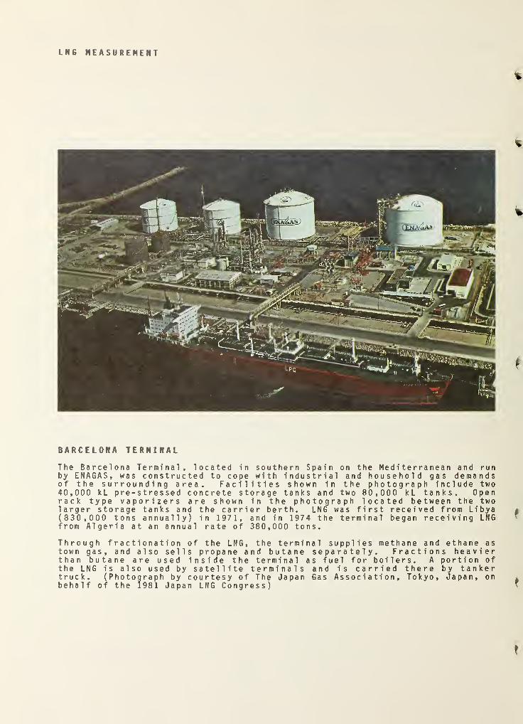
LNG MEASUREMENT
BARCELONA TERMINAL
The Barcelona Terminal, located in southern Spain on the Mediterranean and runby ENAGAS, was constructed to cope with industrial and household gas demandsof the surrounding area. Facilities shown in the photograph include two40,000 kL pre-stressed concrete storage tanks and two 80,000 kL tanks. Openrack type vaporizers are shown in the photograph located between the twolarger storage tanks and the carrier berth. LNG was first received from Libya(830,000 tons annually) in 1971, and in 1974 the terminal began receiving LNGfrom Algeria at an annual rate of 380,000 tons.
Through fractionation of the LNG, the terminal supplies methane and ethane astown gas, and also sells propane and butane separately. Fractions heavierthan butane are used inside the terminal as fuel for boilers. A portion ofthe LNG is also used by satellite terminals and is carried there by tankertruck. (Photograph by courtesy of The Japan Gas Association, Tokyo, Japan, onbehalf of the 1981 Japan LNG Congress)
LNG MEASUREMENT - Density Page 2.4-0
CONTENTS
2.0 MEASUREMENT ELEMENTS
Dens 1 ty Page2.4 LNG Density 2.4. 1-1
2.4.1 LNG Density Reference System 2.4. 1-1
2.4. 1.1 Introduction 2. 4. 1-1
2. 4. 1.2 Cryogenic Fluids Density Reference System 2.4. 1-1
2.4. 1.3 Description of Improved Density Reference System 2. 4. 1-2
2.4. 1.4 Densimeter and Instrumentation 2. 4. 1-6
2. 4. 1.5 Measurement Process Parameters 2. 4. 1-82.4. 1.6 Measurement Process Control 2.4.1-142.4. 1.7 Summary 2.4.1-142.4. 1.8 References 2.4.1-15
2.4.2 Measured LNG Density 2.4. 2-12.4.2. 1 Introduction 2. 4. 2-12.4. 2. 2 LNG Densimetry 2.4. 2-12.4. 2. 3 Vibrating Element Densimeter 2. 4. 2-12.4. 2.4 Dielectric Cell Densimeter 2. 4. 2-22.4. 2. 5 Displacement or Archimedes Densimeter 2.4. 2-32. 4. 2. 6 Testing Commercial Densimeters 2. 4. 2-42.4. 2. 7 Test Results 2. 4. 2-42. 4. 2. 8 Calibration 2.4. 2-82. 4. 2. 9 Conclusions 2.4.2-112.4.2.10 References 2.4.2-12
2.4.3 Calculated LNG Density 2.4. 3-12. 4. 3.1 General Comments 2.4. 3-12.4. 3. 2 Introduction .... 2.4. 3-12.4. 3. 3 Major Accomplishments- Experimental Apparatus 2. 4. 3-22.4. 3.4 Experimental Measurements—Pure Fluid Data 2. 4. 3-32. 4. 3. 5 Binary Mixture Data 2. 4. 3-32.4. 3. 6 Multicomponent Mixture Data 2.4. 3-42.4. 3. 7 Mathematical Models 2.4. 3-42.4. 3. 8 LNG Density Research at Other Laboratories 2.4. 3-52.4. 3. 9 Acknowledgments 2.4. 3-62.4.3.10 References 2.4. 3-7
2.4.4 Mathematical Models for the Prediction of LNG Densities .... 2. 4. 4-12.4.4. 1 Introduction . 2. 4. 4-12. 4. 4. 2 Extended Corresponding States Method 2. 4. 4-12.4.4. 3 Hard Sphere Method 2. 4. 4-42. 4. 4. 4 A Revised Klosek and McKinley Method 2. 4. 4-52. 4. 4. 5 The Cell Model 2 . 4
.*
4 - 7
2.4.4. 6 Use of the Methods 2. 4. 4-82.4.4. 7 Conclusions 2. 4. 4-82. 4. 4. 8 References 2.4.4-10
2.4.5 Interlaboratory Comparison of LNG Density Measurements .... 2 . 4 . > - 1
2.4. 5.1 Introduction 2. 4. -1
2.4. 5. 2 The Density Calibration Systems 2.4.2. 4. 5. 3 Intercomparison of Calibration Systems 2.4.5-2. 4. 5. 4 Experimental Results 2.4...2.4. 5. 5 Conclusions 2 . 1 .
2.4. 5. 6 References. l .
i

LNG MEASUREMENT Density Page 2 . 4 . 1 —
1
2.4 LNG Density2.4.1
LNG Density Reference System
2. 4. 1.1 Introduction
Full shiploads or entire shore storage tanks cannot be weighed directly to the accuracy and precision
consistent with the requirements of the measurement process. The tare weight portion or the tank
weight itself may be many times greater than the active weight of the LNG. The uncertainty in the
tare weight will dominate the uncertainty in the weighing process. In addition, routine weighing of
these containers would certainly be difficult to justify on an economic basis and in some
circumstances might be impossible and therefore could jeopardize the entire measurement process.
Alternatives to gross weighing involve representative measurements on a much smaller scale and
extrapolation of these representative measurements to the total contents of the LNG container.
A measure of LNG density or the mass concentration per unit volume, if established as representativeof the entire contents, can be combined with a volume measurement to give a total weight or mass of
the contents of the LNG container. This measure of LNG density is commonly performed either directlywith a LNG densimeter, or by calculation, by sampling, analysis and the use of mathematicalcorrelations . The latter methods are discussed in sections 2.2, 2.4.3 and 2.4.4. The methodsinvolving direct density measurement using densimeters will be presented in the following sections of
this part of the measurement manual.
LNG density may vary throughout the contents of a large LNG container, and it may be necessary to
place more than one density measurement element within the container volume to assure that themeasurement is representative of the total contents. Several commercial densimeters are available for
use with LNG and are discussed in section 2.4.2. No matter which device is selected, it is necessaryat the present time to calibrate these commercial devices in a reference system specifically designedfor use at cryogenic temperatures.
As a part of the overall LNG program at NBS, a LNG Density Reference System (DRS) was constructed andevaluated [1], Improvements were made in the DRS as it was used to calibrate individual commercialdensimeters. A description of the improved DRS, the major design characteristics and the estimatedaccuracy and precision are given by Siegwarth and LaBrecque [7]. The general subject is so importantto the understanding of the total LNG measurement process that an edited version of the reference [7]is presented here in the following sections.
2. 4. 1.2 Cryogenic Fluids Density Reference System [7]
In an earlier report [1], a density reference system (DRS) was described which had been used to testsome commercially available densimeters in liquefied natural gas (LNG). These tests involvedcomparing the density measurement by the densimeter under test to the density measured by the DRSdensimeter in a well-characterized liquid sample. This earlier report gives an estimate of theuncertainty associated with a density measurement by the DRS densimeter used as standard forcomparison. The uncertainty of a single determination of the density at the instrument under test wastaken to be ±0.076 percent. This includes a systematic error of 0.028 percent and a random error of±0.048 percent, which is three times the estimated standard deviation of ±0.016 percent. Fourdifferent commercial densimeters were tested and the results reported [2], The major problem with thecommercial densimeters found from these tests and some later measurements was in the calibrationthe commercial instrument by the manufacturer. None of the factory calibrations were entire!suitable at LNG temperatures at the time of these tests.
Because of this calibration problem, NBS offered a calibration service through "transfer standard.'."NBS would calibrate a manufacturer's densimeter, which was then installed in a calibration ays' ,*
the manufacturer's plant and used to calibrate production densimeters. The densimeter manufa •'
would then periodically return the transfer standards to NBS for recalibration . The pr-
eventually yield data on the stability as a function of time of the instruments u3ed as tr m ‘ -
standards. The manufacturer's calibration system and methods could be evaluated by testing in th< !
some of the instruments calibrated by the manufacturer.
The DRS sample container used in the tests of these first four commercial densimeters was :•
around the densimeters tested. The densimeters in some cases were specially built. fir •1
of the DRS was too inflexible to deal with any design modifications of the commercial den imeter .

Page 2. *1.1-2 LNG MEASUREMENT Density
A more flexible sample container dewar system was constructed for use in densimeter evaluation andcalibration work. This DRS design with a companion liquid sample storage dewar should be suitable fora commercial calibration facility. This new sample container was found to be more temperature stablethan that of the original DRS. The DRS densimeter has been modified several times before, during andsince the rebuild. Details of these modifications and a shift in the measured density after therebuild are discussed in 2. 4. 1.4, along with the other measuring devices.
In 2. 4. 1.5, the measurement process is discussed. The associated systematic errors are identified,their magnitudes estimated and the overall error estimate of a density measurement is given. Thisestimated deviation of the density for one measurement from the true value is ±0.055 percent for puremethane at the normal boiling point. The maintenance of this accuracy is discussed in 2. 4. 1.6.
Since the improved version of the DRS was completed, a number of additional commercial densimetershave been tested. Each test consisted of a series of measurements in pure liquid methane thenapproxamately about 5 percent propane and 1 percent to 2 percent nitrogen are added to simulate an LNGmixture and another series of measurements was made. This mixture was used, because both propane andnitrogen can be added without any danger of solids forming in the fill line, since both have freezingpoints below 110 K. Measurements in an LNG-like fluid permit LNG densimeters to be tested in a fluidaround the temperature and density at which they will be used. The tests in liquid methane provide a
fluid with a known temperature density relationship, provided 99.97 percent pure methane is used, towhich the DRS density value can be compared. Also, the methane density data along with the LNG-likeliquid density data provide a much wider range of densities for determining the calibration equationfor the instruments under test.
2. 4. 1.3 Description of the Improved Density Reference System
The improved DRS operates on the same principle as the original. Densimeters under test are comparedto the density reference system densimeter in a very nearly isothermal liquid sample. The DRSdensimeter is an Archimedes-type densimeter consisting of a single crystal silicon float weighed whileimmersed in the sample liquid by an electronic balance. Density measurements are made over anapproximately 15 t temperature range along the saturation curve of the sample liquid. Themeasurements are made with the sample at equilibrium after a change of sample temperature has beenaffected either by a liquid nitrogen cooling coil or an electrical resistance heater. The sampleequilibrium is obtained by stirring the liquid with a turbine pump. Equilibrium conditions remain for
the period of time required for measurement without stirring, because the heat leak to the sample hasbeen reduced to a small value by means of radiation shields and other heat flux interrupting devices.
Sample Container A schematic of this improved DRS is shown in Figure 2. 4. 1.1. The sample containerconsists of a 25.4 centimeters 0D, 1.6 millimeters wall stainless steel tube extending 760 millimetersdown from an ambient temperature stainless steel flange to a 3 millimeters thick dished bottom head.A similar stainless steel vessel or vacuum jacket 35.6 centimeters 0D forms an outer wall enclosingthe sample container.
The space between these two vessels contains radiation shields and is maintained at a pressure below10
-i* Pa by an oil diffusion type vacuum pump. All the stainless steel to stainless steel joints are
heliarc welded. All flanges and other gasketed joints in both the insulating vacuum jacket and samplecontainer employ "0" ring seals. Unlike the sample container of the original system, which required a
low temperature indium wire vacuum seal to close it, all demountable seals on the new DRS are locatedat ambient temperature. A 73 millimeters high aluminum ring, clamped between the sample vessel andvacuum jacket flanges, provides six 38 millimeters ID flange-covered access ports into the vacuumspace. Through these flanges passes the liquid nitrogen line to the various cooling coils, the gas
vent lines from these coils and the electrical leads for heaters and thermocouples. The connection to
the vacuum pump is also through one of these ports. All lines and leads can be readily disconnectedto permit the counterbalanced dewar assembly to be lowered enough so that the top flange is below thebottom of the sample space. The time required to disconnect the few lines, remove the nuts from the
twelve 13 millimeters studs clamping the sample container to the top flange and lower the dewar is
only a few minutes. A valve between the vacuum jacket and the vacuum line disconnect permits the
dewar to be lowered without breaking the insulating vacuum.
Another 73 millimeters high aluminum ring is located between the top of the sample container flangeand the top cover of the sample container. Again, six flange-covered 3.8 millimeters diameter accessports provide locations to introduce electrical leads, the vapor pressure bulb tubes shown in figure
2. 4. 1.1 and for pressure gauge connections. The sample vessel seals are "0" rings. The samplepressure is maintained above atmospheric pressure in case small leaks are present.
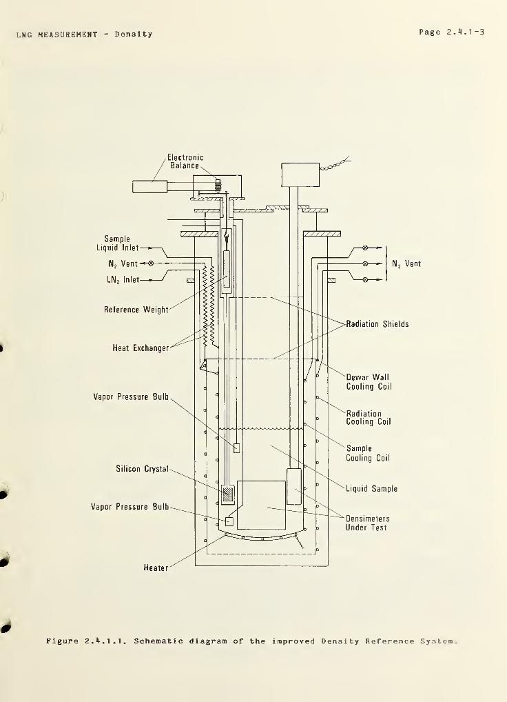
LNG MEASUREMENT Density Page 2 . 4 .1 ~3
0Figure 2. 4. 1.1. Schematic diagram of the improved Density Reference System.
Page 2. 4. 1-4 LNG MEASUREMENT Density
The top plate of the sample container has a port for the DRS densimeter, a 153 millimeters access portshown in figure 2. 4. 1.1 and a port for the stirrer drive shaft (not shown). The access port flangecover can be modified as required to provide mountings for various insertion-type densimeters. Figure2. 4. 1.1 illustrates the mount for a vibrating cylinder densimeter. An "0" ring sealed gland on theaccess flange provides a gas tight stem seal. To avoid a seal on a rotating shaft, the stirrer driveshaft is coupled magnqtically from the exterior to the interior of the sample chamber.
I
The evacuated annular space between the sample container and the vacuum jacket contains all the ^
refrigeration systems used to condense and maintain the sample at cryogenic temperature. All therefrigeration is supplied from an adjacent liquid nitrogen storage dewar through a vacuum-insulatedtransfer line into the liquid nitrogen inlet shown in figure 2. 4. 1.1. This inlet is connected to allthe various cooling coils, and the amount of cooling by each coil is regulated by throttling theindependent nitrogen gas vent lines from the various coils.
The coil on the radiation shield, figure 2. 4. 1.1, is vented continuously, and the temperature of this t
polished copper shield is maintained below the sample temperature. The dewar wall cooling coilattached to the shield mounting ring a few centimeters above the sample level is maintained at atemperature a few degrees above the sample temperature to minimize the heat conducted down the samplevessel wall. Within the sample vessel, a copper radiation shield, with an aluminum foil shield ontop, interrupts the heat radiated down from the top of the sample holder. A second radiation shieldis placed a few centimeters above the lower shield. The operating temperature of the lower shield is
normally a few degrees above the liquid temperature. The cooling coil and heater on the samplevessel, figure 2. 4. 1.1, are used only to change the sample temperature.
The sample is condensed into the DRS from gas bottles using liquid nitrogen via the counterflow heatexchanger. This parallel tube heat exchanger, composed of two 8 millimeters I.D. copper tubes about 7
meters long soft soldered together along their length, will condense the 16 liters required in thesample holder in about an hour. The actual time depends on the liquid nitrogen supply rate. Mostjoints in these coils and lines are soft soldered, and all coils and heaters are soft soldered to thesurfaces to which they transfer heat.
Each time the density of an LNG or methane sample is measured, the temperatures of the sample near thetop and bottom are also determined by measuring the methane vapor pressure in the vapor pressure bulbsshown in figure 2. 4. 1.1. The vapor lines are connected through a selector valve to a quartz spiralBourdon tube pressure gauge. The temperature difference is nearly always less than 20 mK and usuallyless than 10 mK. This low temperature gradient is obtained without the low speed stirring used in theoriginal system [1]. The temperature drift during the measuring period is comparable in magnitude tothe temperature difference cited above. Temperatures of the radiation shields and the annular shieldsupport ring are monitored by thermocouples to provide information for minimizing the heat leak to thesample. The temperature and pressure of the gas surrounding the reference weight are recorded andused to provide the gas buoyancy correction to this weight reading.
A larger system of similar design should be suitable for a manufacturer's calibration facility. To
speed up the operation, a manufacturer could employ additional cryogenic vessels into which he couldtransfer the calibration liquids. Heated nitrogen gas or additional electrical heaters could be usedto rapidly warm the sample holder and to change densimeters; and a liquid nitrogen spray nozzle couldbe used to rapidly cool the calibration dewar. Or the instruments calibrated could be introduced andremoved from the top, without warming the whole dewar. Either way, some modest care is required toascertain that the dewar is properly purged and inerted before introducing a cryogenic sample.
Safety Considerations in the DRS Design Manufacturers of densimeters suitable for cryogenic use havedemonstrated some reluctance to employ calibration methods using cryogenic liquid combustible gases.In this section, safety considerations incorporated by NBS in the DRS are presented.
An experimental system using combustible gases can be made safe by eliminating any opportunity for a
combustible mixture of air and the gas to form, or by eliminating all ignition sources in any area
where combustible mixtures might form. The elimination of combustible mixtures is the preferred way
to make a system safe. Thus, the DRS sample handling system is gas tight and evacuated before
introducing the combustible gas. However, should a leak develop in the system or an accident occur, a
combustible mixture could result; so ignition sources have been minimized in the laboratory. Since it
is not possible to be assured that all existing or potential ignition sources are completely
(5
<S
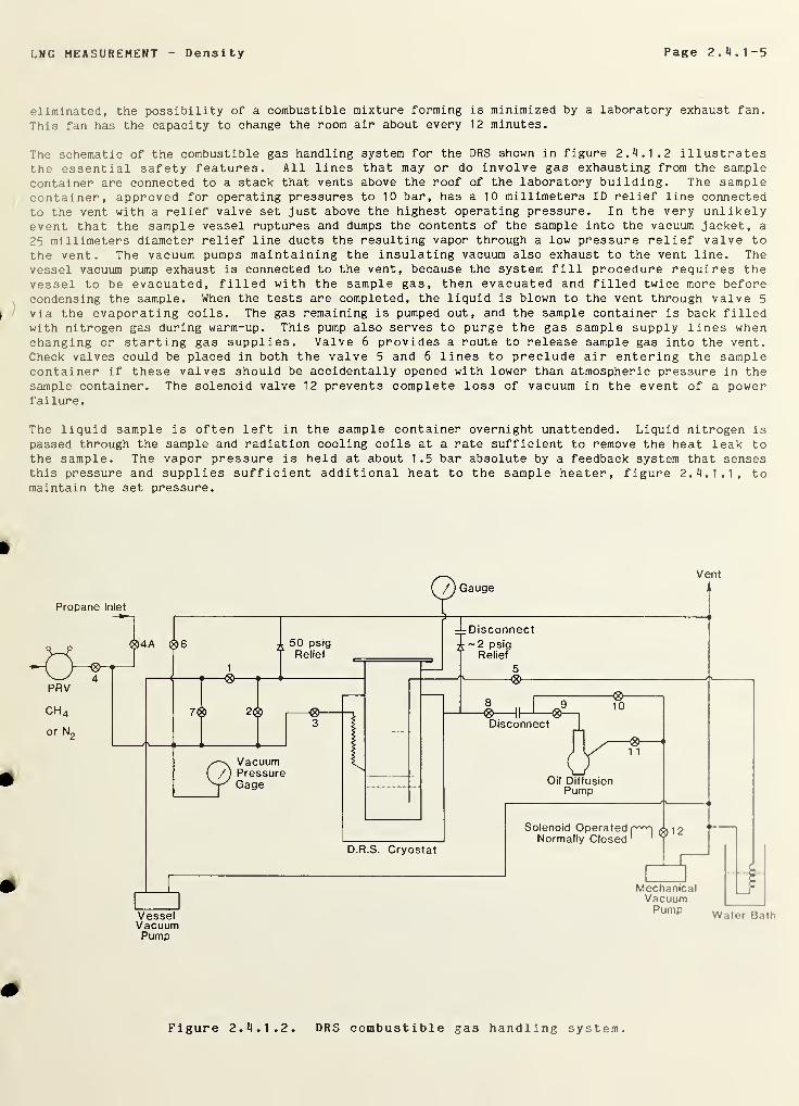
LNG MEASUREMENT Density Page 2.11.1-5
eliminated, the possibility of a combustible mixture forming is minimized by a laboratory exhaust fan.
This fan has the capacity to change the room air about every 12 minutes.
The schematic of the combustible gas handling system for the DRS shown in figure 2 . M . 1 .2 illustratesthe essential safety features. All lines that may or do involve gas exhausting from the samplecontainer are connected to a stack that vents above the roof of the laboratory building. The samplecontainer, approved for operating pressures to 10 bar, has a 10 millimeters ID relief line connected
to the vent with a relief valve set just above the highest operating pressure. In the very unlikelyevent that the sample vessel ruptures and dumps the contents of the sample into the vacuum jacket, a
25 millimeters diameter relief line ducts the resulting vapor through a low pressure relief valve to
the vent. The vacuum pumps maintaining the insulating vacuum also exhaust to the vent line. Thevessel vacuum pump exhaust is connected to the vent, because the system fill procedure requires thevessel to be evacuated, filled with the sample gas, then evacuated and filled twice more beforecondensing the sample. When the tests are completed, the liquid is blown to the vent through valve 5
via the evaporating coils. The gas remaining is pumped out, and the sample container is back filledwith nitrogen gas during warm-up. This pump also serves to purge the gas sample supply lines whenchanging or starting gas supplies. Valve 6 provides a route to release sample gas into the vent.
Check valves could be placed in both the valve 5 and 6 lines to preclude air entering the samplecontainer if these valves should be accidentally opened with lower than atmospheric pressure in thesample container. The solenoid valve 12 prevents complete loss of vacuum in the event of a powerfailure.
The liquid sample is often left in the sample container overnight unattended. Liquid nitrogen is
passed through the sample and radiation cooling coils at a rate sufficient to remove the heat leak tothe sample. The vapor pressure is held at about 1.5 bar absolute by a feedback system that sensesthis pressure and supplies sufficient additional heat to the sample heater, figure 2. 4. 1.1, tomaintain the set pressure.
Pump
Figure 2.4.1 . 2
.
DRS combustible gas handling system.
Page 2.11.1-6 LNG MEASUREMENT Density
Small quantities of gas escaping from the DRS would be swept out of the room by the laboratory ceilingvent fan. To reduce the chances of igniting any larger spill, mainly "explosion proof" electricalequipment operates in the room during tests. The stirrer motor case is purged with compressed air.All the electrical cabinets are enclosed and purged with compressed air. Access to the laboratory islimited, and since the floor is conducting, conducting shoes or ground straps are used by anyoneregularly in the laboratory. A combustion gas detector connected to a warning horn is located nearthe DRS.
The vapor pressure bulbs contain less than a liter of methane at ambient temperature and pressure, butthis can result in a very high vapor bulb pressure if not properly vented to the storage cylinderduring warmup. Two bypass relief valves between the vapor bulbs and the storage cylinder eliminatethis potential hazard.
2. 4. 1.4 Densimeter and Instrumentation
The DRS densimeter described in the previous publication [1] has undergone several modifications sincethat report was prepared. A major modification occurred when the electronic balance used to weigh thesingle crystal was replaced.
Since manually disconnecting and connecting the silicon single crystal and reference weight causedoccasional discontinuities in the electrical balance reading, pneumatic drive cylinders were connectedto both actuators. These cylinders were mounted on the scale case and were sufficiently slow-movingto gently place the weights on the balance while not shaking the balance mounting.
This modification decreased the scatter of the methane density values determined by the DRS relativeto the Haynes-Hiza [ 3 ] density values calculated from the average sample temperature.
When the sample containment portion of the DRS was reconstructed, as described in 2. 4.1. 3, the siliconcrystal disconnect mechanism was rebuilt. The suspension wire in the vapor region was replaced by a
1.6 millimeters diameter thin wall stainless tube, and the assembly connecting the suspension to thebottom of the balance was modified. The balance was readjusted for corner load effects. Theseadjustments, when properly made, make the balance weight reading independent of the position on thepan a weight is placed. The density of methane in the new sample holder as determined by the DRSdensimeter was offset by approximately 0.07 percent relative to the Haynes-Hiza [ 3 ] and Goodwin [4]
values for the density calculated from average temperature for six subsequent methane fillings.
The vapor bulb positions were altered and the methane in the bulbs changed without affecting thisoffset. To ascertain that the pressure gauge had not shifted calibration, it was compared to thebarometric pressure and found to be in agreement. The temperature difference represented by thedifference between the barometric pressure and the vapor pressure gauge reading amounted to less than0.01 K. The methane density difference corresponding to 0.01 K is too small for the DRS densimeter to
measure. This offset will be discussed in more detail below.
Addition of a New Balance Recently an electronic balance with sufficient range to directly weigh the
128 gram crystal to 1 milligram has become commercially available. This balance has other advantages;it is more compact and much less sensitive to vibration than the original balance. It is lightweightand can be transported in any orientation without securing the moving parts. The DRS densimeter hasbeen rebuilt to incorporate one of these electronic balances. Conceptually, and in actual design,
this densimeter differs little from the original densimeter. However, because it has sufficientcapacity to weigh the silicon directly, a reference weight [1] with the attendant buoyancy correctionis no longer required. The reference weight has been retained as a means of calibrating the balanceand monitoring the calibration during tests.
A suspension system consisting of two cages, one for a reference weight and one for the siliconcrystal, is attached to the underside of the balance. The reference weight cage is about 20centimeters below the balance and in the sample gas space, while the silicon crystal cage is 76
centimeters below the balance and completely immersed in the sample liquid. The section of thesuspension system passing through the liquid surface is a wire. The suspension is always attached to
the balance. Lifting mechanisms permit the weights to be attached and detached from the suspensionindependently. Surface tension effects on the suspension should cancel, since weight off (zero)
readings are included in the measurements and subsequent density calculations.
LNG MEASUREMENT Density Page 2. 4. 1-7
The liquid density pis now given by the relation (equation 4, Reference 1) with Ma replaced by
( Ma-Mao) :
P =P s£ 1
-( Ma - Mao)/Ms ] ( 1
)
where p s is the silicon density, M s is the silicon crystal mass in vacuum, Ma is the apparent mass
when weighed in the liquid and M ao is the balance reading with the crystal and reference weight
disconnected. This latter value nearly always is zero to ± 1 milligram as the balance is tared(zeroed) with the silicon crystal removed before the density readings are taken.
The systematic offset in the observed density of liquid methane compared to Haynes-Hiza discussed in
2. 4. 1.4 remained and even increased slightly with the introduction of the new balance. The previously
reported data [1] are probably in error because of an undetected corner loading error in the balance.This error cannot be directly confirmed as it is not possible to recover the old balance adjustment.
Because of the way the silicon crystal and the reference weight were placed on the balance in the
original system, any corner loading error must have had some effect on density measurement. The
reference weight was placed on the pan, and the crystal was suspended from a part of the balanceassembly well below the pan. This vertical offset in attachment points probably did not contribute a
systematic error to the density determination, but the relative displacement in the horizontal planeof the attachment points that existed could affect the results. 100 gram weights were placed on the
pan which were weighed relative to a counterweight so that the balance reading was on scale on the 20
gram range of the balance. However, the pan was only corner load adjusted so 20 grams could be read
to within a milligram, thus a mass value error approaching 5 milligrams at the edge of the pan waspossible for a 100 gram weight even for a properly adjusted balance. The results of a series of tests
of the balance Indicated some corner loading error was still present even after the balance wasreadjusted.
Comparison tests between the DRS densimeter and a silicon crystal densimeter built for a commercialcalibration facility showed agreement to about 0.01 percent. These results are shown in the appendixof the original publication [7] and lend added support to the contention that the systematic shift in
the measured methane densities relative to the measurements reported in reference [1] resulted from anerror in the adjustment of the original electronic balance.
In some later tests, a third silicon densimeter, the Portable Reference Densimeter (PRD) was comparedto the DRS densimeter in the DRS [5]. The PRD and DRS densimeters are similar in design, but thesilicon single crystal was obtained from a different source. The density readings wereindistinguishable.
Calibration of the Balance Even though the present DRS densimeter no longer requires a referenceweight to determine LNG density, the weight has been retained for calibrating the balance andmonitoring the calibration. The balance is calibrated by weighing the reference weight in air andadjusting the balance to read the apparent true mass in air. The reference weight still weighsapproximately the same as the silicon crystal when the latter is submerged in liquid methane.
In the course of taking data at each sample temperature setting, this reference weight is measured andrecorded. The apparent mass is corrected for gas buoyancy and compared to the true mass value. Thiscorrection is readily made for methane or methane-nitrogen samples but not formethane-propane-nitrogen samples, because propane suppresses the methane vapor pressure by an
uncertain amount, and because the gas mixture is slow to reach equilibrium. The method of calculatingthe buoyancy correction is detailed in the appendix of the original publication [7]. The refer* r,
weight is located in a region in which the gas temperature is -10 to -20 *£, which contributes to thebuoyancy correction uncertainty in the ternary mixture, even though the gas temperature is measur
1
and applied to the buoyancy calculation.
The reference weight is weighed periodically in air to monitor the balance calibrat . .:•
calibration can be adjusted if needed, or a calibration factor can be introduced. In the sixof operation, the calibration has not been adjusted. A calibration correction amounting •
milligrams was included in the calculations for two fillings. For later fillings, a corr- *:
• w t
not needed.
The results of monitoring the reference weight during tests are presented in 2. 4.1. 5. Go rn*--r
errors are unlikely in the new silicon crystal weighing system since both the referen w* .
•
silicon weight are suspended below and placed on the suspension axial to the suspension w .
eliminating essentially all possibility of corner loading errors.
Page 2.4.1 —
8
LNG MEASUREMENT Density
Sample Temperature Temperature is measured using vapor pressure thermometers. One thermometer bulbwas located at the bottom of the sample volume and the other near the top. Each thermometer containsa few cubic centimeters of liquid methane. Pressure communicates from each thermometer bulb via a 1.6millimeters O.D. stainless capillary tubing through a selector valve to a quartz spiral Bourdon tubepressure gauge. The temperature range used is 110 K to 126 K.
The accuracy of the quartz spiral gauge is 0.01 percent of full-scale pressure as determined by a
master piston gauge calibrated by NBS. This pressure uncertainty is equivalent to 0.01 K at 110 K and0.003 K at 125 K.
Sample Vapor Pressure The liquid sample vapor pressure was measured using a Bourdon tube pressuregauge with a 0 to 4 bar range and an 0.2 percent of full scale accuracy according to the manufacturer.The vapor pressure is used only for a small buoyancy correction to the reference weight and need notbe accurately known.
2.4.1 .5 Measurement Process Parameters
Bounds for Systematic Errors The primary sources of uncertainty in the density measurements can be
obtained from examination of the measurement equation. The knowledge of the basic uncertainties of
the separately measured quantities, such as the masses and densities, can be combined to give anestimate of the systematic errors in the density as measured by the density reference system.
Equation (1), the measurement equation, gives the density as a function of several independentlymeasured variables.
The temperature is included here, because the density at the test densimeter is the quantity requiredand a temperature gradient may exist.
The uncertainty in liquid density arising from uncertainty in some variable x, for example, can be
evaluated from
The total uncertainty in density is taken to be the square root of the sum of the squares of thevarious contributions,
This is the propagation of error relationship for systematic error when the variables are independent,and the magnitudes of the relative errors are small, so that second-order terms are negligible [6],
Table 2. 4. 1.1 is a summary of the most significant contributions to the total systematic uncertaintyin density as estimated from the various contributing sources. The first column, labelled x,
identifies the variable for which the uncertainty is calculated. The second column is the partialderivative of the liquid density with respect to the variable of the first column, and the thirdcolumn gives its maximum magnitude. The column labelled 6 x is the estimated largest error of thatvariable.
The systematic error, 6x, of M s , is estimated from the standard deviation of the weighings and the
uncertainties of the 5 weights used (Appendix [7]). The estimate of the systematic error for Ma and
M ao is the resolution of the electronic balance or 1 milligram. The calibration of the electronic
balance is monitored by weighing the reference weight, as discussed earlier, which permits holding
this uncertainty within the balance resolution. The error estimate of the silicon crystal density
covers uncertainties because of the temperature and pressure effects as well as uncertainties in
published densities (Appendix [7]).
P p ( Mg ,
M
jj, Mqq
,
pg , T
)
(2)
(3)
(4)
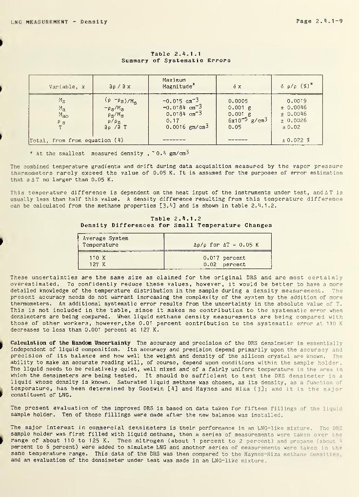
LNG MEASUREMENT Density Page 2 . 4 .1 -9
Table 2 . 4 . 1 .
1
Summary of Systematic Errors
Variable, x 9p / 9 x
MaximumMagnitude* 6 x 6 p/p (%)*
Ms (p -p s )/ms -0.015 cm"3 0.0005 0.0019
Ma “Ps^Ms -0.0184 cm”3 0.001 g ± 0.G046
Mao Ps^Mg 0.0184 cm-3 0.001 g ± 0.0046
P s p/ps 0.17 6x1 0~5 g/cm3 ± 0.0026
T 9p /9 T 0.0016 gm/em3 0.05 ±0.02
Total , from from eqilation (4) ± 0.022 %
* At the smallest measured density ,~0.4 gm/cm3
The combined temperature gradients and drift during data acquisition measured by the vapor pressurethermometers rarely exceed the value of 0.05 K. It is assumed for the purposes of error estimationthat a A T no larger than 0.05 K.
This temperature difference is dependent on the heat input of the instruments under test, and A T is
usually less than half this value. A density difference resulting from this temperature differencecan be calculated from the methane properties [3,4] and is shown in table 2. 4. 1.2.
Table 2.4.1 .2Density Differences for Small Temperature Changes
Average SystemTemperature Ap/p for AT = 0.05 K
110 K 0.017 percent127 K 0.02 percent
These uncertainties are the same size as claimed for the original DRS and are most certainlyoverestimated. To confidently reduce these values, however, it would be better to have a moredetailed knowledge of the temperature distribution in the sample during a density measurement. Thepresent accuracy needs do not warrant increasing the complexity of the system by the addition of morethermometers. An additional systematic error results from the uncertainty in the absolute value of T.
This is not included in the table, since it makes no contribution to the systematic error whendensimeters are being compared. When liquid methane density measurements are being compared withthose of other workers, however, the 0.01 percent contribution to the systematic error at 110 K
decreases to less than 0.001 percent at 127 K.
Calculation of the Random Uncertainty The accuracy and precision of the DRS densimeter is essentiallyindependent of liquid composition. Its accuracy and precision depend primarily upon the accuracy andprecision of its balance and how well the weight and density of the silicon crystal are known. Theability to make an accurate reading will, of course, depend upon conditions within the sample holder.The liquid needs to be relatively quiet, well mixed and of a fairly uniform temperature in the area in
which the densimeters are being tested. It should be sufficient to test the DRS densimeter in •.
liquid whose density is known. Saturated liquid methane was chosen, as its density, as a functiontemperature, has been determined by Goodwin [4] and Haynes and Hiza (3]; and it is the m
a
constituent of LNG.
The present evaluation of the improved DRS is based on data taken for fifteen fillings of the : ...
sample holder. Ten of these fillings were made after the new balance was installed.
The major interest in commercial densimeters is their performance in an LNG-like mixture. Th<-'
sample holder was first filled with liquid methane, then a series of measurements were taken ••
range of about 110 to 125 K. Then nitrogen (about 1 percent to 2 percent) and propari"percent to 6 percent) were added to simulate LNG and another series of measurements werf *
same temperature range. This data of the DRS was then compared to the Haynes-Hiza methane ion t.
and an evaluation of the densimeter under test was made in an LNG-like mixture.
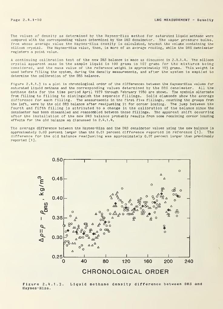
Page 2.4.1-10 LNG MEASUREMENT Dens i ty
The values of density as determined by the Haynes-Hiza method for saturated liquid methane werecompared with the corresponding values determined by the DRS densimeter. The vapor pressure bulbs,from whose average value the Haynes-Hiza density is calculated, bracket the volume containing thesilicon crystal. The Haynes-Hiza value, then, is more of an average reading, while the DRS densimeterregisters a point value.
A continuing calibration test of the new DRS balance is made as discussed in 2. 4. 1.4. The siliconcrystal apparent mass in the sample liquid is 100 grams to 107 grams for the mixtures beingconsidered, and the mass value of the reference weight is approximately 103 grams. This weight is
used before filling the system, during the density measurements, and after the system is emptied todetermine the calibration of the DRS balance.
Figure 2. 4. 1.3 is a plot in chronological order of the differences between the Haynes-Hiza values forsaturated liquid methane and the corresponding values determined by the DRS densimeter. All themethane data for the time period April 1979 through February 1980 are shown. The symbols alternatefrom filling to filling to distinguish the separate fillings. Solid diamonds show the averagedifference for each filling. The measurements in the first five fillings, counting the groups fromthe left, were by the old DRS balance after readjusting it for corner loading. The jump between thefourth and fifth filling is attributed to a change in the calibration of the balance since thedensimeter had been dismantled and reassembled between these fillings. The apparent shift occurringafter the installation of the new DRS balance probably results from some remaining corner loadingeffects for the old balance as discussed in 2. 4. 1.4.
The average difference between the Haynes-Hiza and the DRS densimeter values using the new balance is
approximately 0.09 percent larger than the 0.01 percent difference reported in reference [1], Thedifference for the old balance readjusting was approximately 0.07 percent larger than previouslyreported [1],
CHRONOLOGICAL ORDER
Figure 2. 4.1.3-Haynes-H i za
.
Liquid methane density difference between DRS and
LNG MEASUREMENT Density Page 2.4.1 — 11
The average difference between the methane densities determined by the Haynes-Hiza method and thosedetermined by the DRS densimeter shows the latter to be approximately 0.1 percent lower. That the DRS
densimeter is now measuring density correctly is supported by the data for fillings 11 through 14.
The meter under test for these fillings was also an Archimedes densimeter using a silicon crystal.
See Appendix 9.1 [7] for details of this comparison.
The average difference between the corresponding density values given by this meter and the DRS
densimeter is 0.004 percent ± 0. 01 7 percent (95 percent confidence interval), i.e., the density valueswere not statistically distinguishable. The comparison between the DRS and Portable ReferenceDensimeter, to be reported later, also shows the present DRS densimeter to be correctly measuring thedensity.
Each time a commercial densimeter was tested in pure methane, data were taken to permit comparing the
DRS measured density to the Haynes-Hiza density calculated from the average temperature. A series of
density measurements with each liquid sample were taken over a range of temperatures by either heatingor cooling the sample to a target temperature, waiting for equilibrium while stirring the sample, andtaking the desired schedule of readings with the stirrer off. The target temperature was only
nominally achieved at equilibrium. The sample was stirred again and the readings duplicated. Theduplicate readings provided assurance that the DRS and test densimeters had reached equilibrium. A
lack of equilibrium was never noted. The second reading also reduced the chance of losing a datapoint through a reading error or a malfunction of a test densimeter, which are often sensitive to
bubbles. The temperature drift between the duplicate sets of readings for the new DRS had a standarddeviation of approximately 0.1 K with the second reading averaging 0.05 K higher.
The random errors of the duplicate density values obtained from a densimeter as described above wouldbe expected to correlate more closely with each other than with values at different temperatures. Infact, the correlation between duplicates for the difference between the Haynes-Hiza and DRS densitiesis about 0.5. A correlation of 1.0 would mean the duplicates provide the same information, while acorrelation of 0 would mean the duplicates provide independent information on the process. Sincethere is much more data than needed for the error estimate, and the correlation between the duplicatedata at each temperature complicates the analysis, only the first of each duplicate reading has beenused to analyze the DRS.
The model used to analyze the methane data is:
H(T)-Y(T)ij
= y (T)+ a i+ eij (5)
where Y(T)jj is the jth density determination by the DRS on the ith methane filling for temperature T;H(T) is the corresponding density value derived from the Haynes-Hiza relationship, y (T) represents anysystematic difference between the two methods at temperature T, aj represents a shift in the mean formeasurements on the ith filling, and e^j , the random contribution to the jth measurement made on theith filling.
The solid diamonds in figure 2. 4. 1.3 show the average difference for each filling and show the shiftsa i in the mean of the Yjj from one filling to the next. Considering the data before the new balance,the only significant shift is between the 4th and 5th fillings, and this probably resulted fromdismantling the densimeter between the two fillings. The data taken after the installation of the newbalance show the shifts from filling to filling to be rather small for the first five fillings, butsomewhat larger for the last five.
The a i appear to be random in nature and have an estimated standard deviation of 0 .X) 1 3 kg/m3(0.0031percent). A 99 percent upper confidence bound for this value is 0.036 kg/m3 (0.0082 percent). Whataccounts for the shifts in the a ^ is at present unknown. The deviations of the measured values of toecalibration weight from the true mass value of 1 02.9022 grams, A W, are shown versus chronologicalorder in figure 2. 4. 1.4. A buoyancy correction must be made to the balance reading to obtain the truemass value (see Appendix 9.3 [7]). The changes in the mean of the observed true mass values of thecalibration weight from filling to filling are statistically significant, but they are not wl 1
correlated with the a i , and if they were, their estimated standard deviation could account for only i
0.0020 percent component in the variation of the a j , leaving additional effects to account for ).
percent. A difference between the temperature of the liquid at the crystal and the averagetemperature given by the two vapor pressure bulbs might also contribute to this uncertaintydifference were to persist over the time of the run (filling). Based on the differences show-figure 2. 4. 1.3, the within filling standard deviation for fillings through the 15th is estimated to be0.0216 kg/m3( . 0051 percent) with a 99 percent upper bound of 0.0277 kg/m3(.0065 percent). This is aconservative estimate.
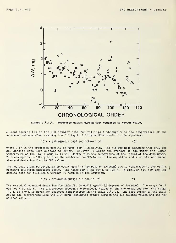
Page 2.4.1-12 LNG MEASUREMENT Density
CHRONOLOGICAL ORDERFigure 2. 4. 1.4. Reference weight during test compared to vacuum value.
A least squares fit of the DRS density data for fillings 1 through 5 to the temperature of thesaturated methane after removing the filling-to-filling shifts results in the equation,
D(T) = 526.935-0.410996 T-0. 0047017 T2 ( 6 )
where D(T) is the predicted density in kg/m3 for T in kelvin. The fit was made assuming that only theDRS density data were subject to error. However, T being the average of the upper and lowertemperature of the liquid sample, it will differ from the temperature of the liquid at the densimeter.This assumption is likely to bias the estimated coefficients in the equation and also the estimatedstandard deviation for the DRS values.
The residual standard deviation is 0.027 kg/m3 (37 degrees of freedom) and is comparable to the withinstandard deviation discussed above. The range for T was 109 K to 128 K. A similar fit for the DRSdensity data for fillings 6 through 15 results in the equation:
D(T) = 525.092-0.382535 T-0. 0048151 T2 (7)
The residual standard deviation for this fit is 0.019 kg/m3 (53 degrees of freedom). The range for T
was 109 K to 130 K. The differences between the predicted values of the two equations over the range110 K to 130 K is given for selected temperatures in the table 2. 4. 1.3. The last column of the tablegives the differences less the 0.07 kg/m3 estimated offset between the old balance values and the newbalance values.
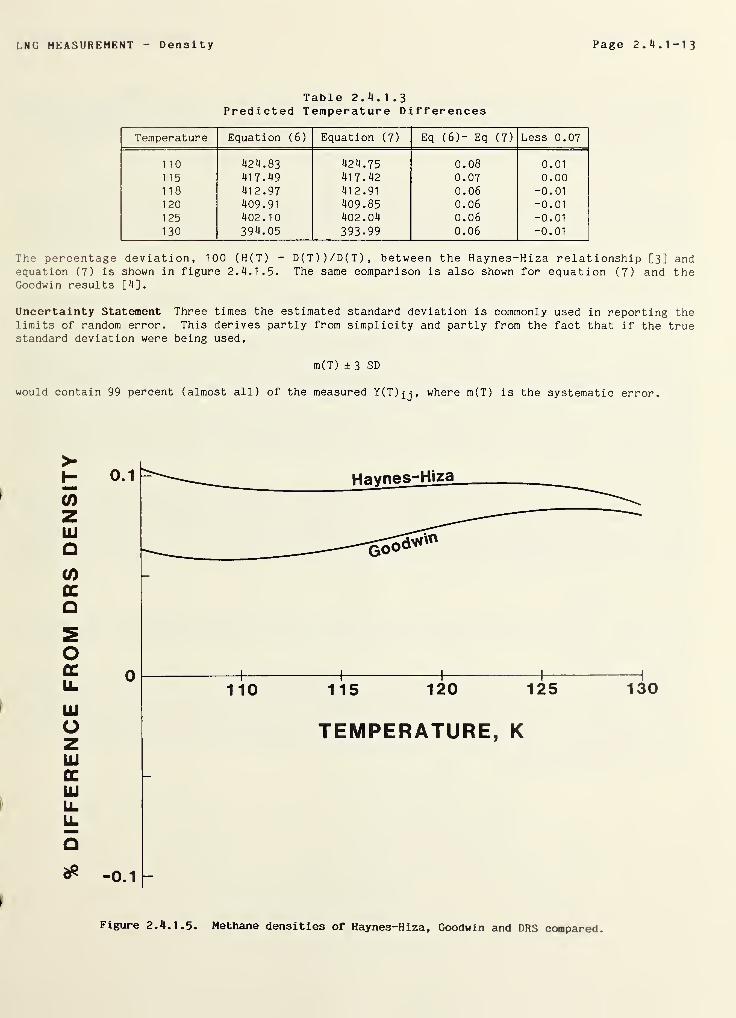
LNG MEASUREMENT Density Page 2.4.1-13
Table 2.4.1 .3Predicted Temperature Differences
Temperature Equation (6) Equation (7) Eq (6)- Eq (7) Less 0.07
110 424.83 424.75 0.08 0.01
115 41 7.49 417.42 0.07 0.00118 412.97 412.91 0.06 -0.01
120 409.91 409.85 0.06 -0.01
125 402.10 402.04 0.06 -0.01
130 394.05 393.99 0.06 -0.01
The percentage deviation, 100 (H(T) - D(T))/D(T), between the Haynes-Hiza relationship [3] andequation (7) is shown in figure 2. 4. 1.5. The same comparison is also shown for equation (7) and theGoodwin results [4],
Uncertainty Statement Three times the estimated standard deviation is commonly used in reporting thelimits of random error. This derives partly from simplicity and partly from the fact that if the truestandard deviation were being used,
m(T) ±3 SD
would contain 99 percent (almost all) of the measured Y(T)jj, where m(T) is the systematic error.
Figure 2. 4. 1.5. Methane densities of Haynes-Hiza, Goodwin and DRS compared.
Page 2. *1.1-14 LNG MEASUREMENT Density
Table 2. 4. 1.3 gives bounds to this value of ± 0.022 percent. From figure 2. 4. 1.4, thefilling-to-filling standard deviations 99 percent upper bound is 0.036 kg/m3 and that for within a
filling has a 99 percent upper bound of 0.028 kg/m3. Combining these two to obtain an upper bound onthe standard deviation of a single determination of Haynes-Hiza minus DRS , gives ((.036) 2 +
(.028) 2)
1 / 2 =0.046 kg/m3. Although this value contains the uncertainty for both densitydeterminations (Haynes-Hiza and DRS), all of the uncertainty is assigned to the DRS. The 3 o valuefor this uncertainty is 0.138 kg/m3.
Transforming the estimated standard deviaton of ±0.046 kg/m3 to percent at 422.63 kg/m3, the normalboiling point density of methane, gives a value of ±0.011 percent. The sum of 3 x 0.011 percent plus0.022 percent gives the present estimated limit of total uncertainty for a single density measurementmade on pure methane with the DRS as ± 0.055 percent. This uncertainty decreases for LNG mixturesbecause of the increased density.
2. 4. 1.6 Measurement Process Control
As future measurements are made, the random errors will be continually monitored, and the systematicerror estimates will be confirmed experimentally as described below.
Each time a set of density reference measurements is made using the system, measurements on at leasttwo separate fillings of pure liquid methane will be included in the tests. Density measurements willbe made at temperatures around 110 K, 115 K, 120 K and 125 K with some randomness in the order. Theremeasured methane densities will be compared to the Haynes-Hiza results and to the earlier referencesystem measurements to determine whether the system has shifted. This reliability of the system willbe checked only in conjunction with density comparison work rather than periodically because of theexpense of making density measurements. The reference weight, of course, now permits a continuingmonitoring of the balance performance and can provide information to correct any drift within a run.The methane tests will primarily monitor the silicon crystal itself and the vapor pressure bulbthermometer performances.
For future occasions, the within standard deviations will be compared statistically to those of
previous occasions to test for any change in this measure of precision. Tests will be made to detectthe presence of occasion-to- occasion shifts or signs of non-random behavior (e.g., drifting). If
there are no apparent changes, the data from previous occasions will be combined with the new data toobtain updated estimates. Any statistically verifiable changes in the DRS process will call forcorrective action with respect to the process. Revised uncertainty statements will be presented asneeded.
2 . 4 . 1 .
7
Summary
The density reference system of the National Bureau of Standards is described. The procedure for
determining the density from weighing, zeroing and calibrating the balance and the calculationalmethod is discussed.
The uncertainty of the improved density reference system for pure methane at the normal boiling point
is ± 0.055 percent. The contribution from the estimated systematic error in density was ±0.022percent. The estimated uncertainty caused by random error is three times the standard deviation of
0.011 percent and is based on sixty-three measurements of the densities of saturated liquid methane.This total density uncertainty is taken to be the sum of the systematic and random errors and should
vary approximately as p m /p where p m is the density of normal boiling point liquid methane and p is the
density of the sample liquid.
LNG MEASUREMENT Density Page 2.11.1-15
2.11.1.8 References
[1] Siegwarth, J. D., B. A. Younglove and J. F. LaBrecque, Cryogenic fluids density referencesystem: Provisional Accuracy Statement, Nat. Bur. Stand. (U.S.), Tech. Note 698 , (November1977).
[2] Siegwarth, J. D., B. A. Younglove, and J. F. LaBrecque, An evaluation of commercial densimetersfor use in LNG, Nat. Bur. Stand. (U.S.), Tech. Note 697, (October, 1977).
[3] Haynes, W. M. , Hiza, M. J., Measurements of orthobaric liquid densities of methane, ethane,
propane, isobutane and normal butane, J. Chem. Thermodynamics 9, 179 (1977).
[il] Goodwin, R. D., The thermophysical properties of methane, from 90 to 500 K at pressures to 700bar, Nat. Bur. Stand. (U.S.), Tech. Note 653, (April, 1 97 ^ )
.
[5] Siegwarth, J. D. and J. F. LaBrecque, A portable calibration densimeter for use in cryogenicliquids, Nat. Bur. Stand. (U.S.), Tech. Note 1035, (1981).
[6] Cook, N. H. and E. Rabinowitz, Physical Measurement and Analysis, Addison Wesley Publishing Co.,
Inc., 1963.
[7] Siegwarth, J. D. and J. F. LaBrecque, Cryogenic fluids density reference system: provisionalaccuracy statement (1980), Nat. Bur. Stand. (U.S.), Tech. Note 101J1, 60pp (April, 1091).

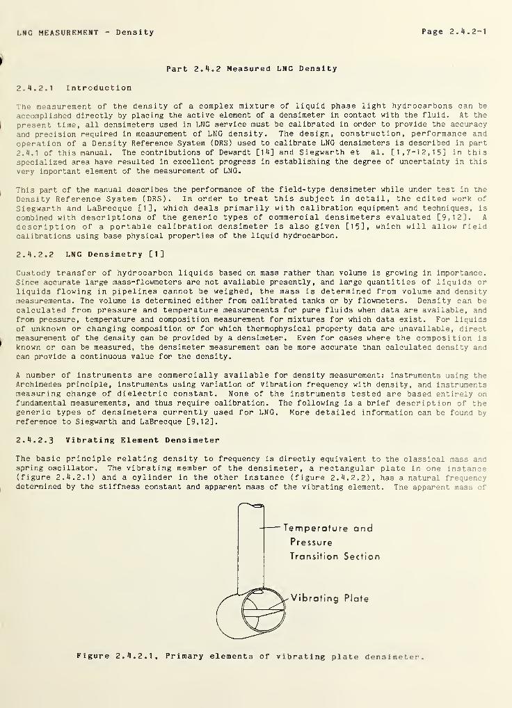
LNG MEASUREMENT Density Page 2. 4.2-1
Part 2.4.2 Measured LNG Density
2. 4.2.1 Introduction
The measurement of the density of a complex mixture of liquid phase light hydrocarbons can be
accomplished directly by placing the active element of a densimeter in contact with the fluid. At the
present time, all densimeters used in LNG service must be calibrated in order to provide the accuracy
and precision required in measurement of LNG density. The design, construction, performance andoperation of a Density Reference System (DRS) used to calibrate LNG densimeters is described in part
2.4.1 of this manual. The contributions of Dewardt [14] and Siegwarth et al. [1,7-12,15] in thisspecialized area have resulted in excellent progress in establishing the degree of uncertainty in this
very important element of the measurement of LNG.
This part of the manual describes the performance of the field-type densimeter while under test in the
Density Reference System (DRS). In order to treat this subject in detail, the edited work of
Siegwarth and LaBrecque [1], which deals primarily with calibration equipment and techniques, is
combined with descriptions of the generic types of commercial densimeters evaluated [9,12]. A
description of a portable calibration densimeter is also given [15], which will allow fieldcalibrations using base physical properties of the liquid hydrocarbon.
2. 4.2.2 LNG Densimetry [1]
Custody transfer of hydrocarbon liquids based on mass rather than volume is growing in importance.Since accurate large mass-flowmeters are not available presently, and large quantities of liquids orliquids flowing in pipelines cannot be weighed, the mass is determined from volume and densitymeasurements. The volume is determined either from calibrated tanks or by flowmeters. Density can becalculated from pressure and temperature measurements for pure fluids when data are available, andfrom pressure, temperature and composition measurement for mixtures for which data exist. For liquidsof unknown or changing composition or for which thermophysical property data are unavailable, directmeasurement of the density can be provided by a densimeter. Even for cases where the composition isknown or can be measured, the densimeter measurement can be more accurate than calculated density andcan provide a continuous value for the density.
A number of instruments are commercially available for density measurement: instruments using theArchimedes principle, instruments using variation of vibration frequency with density, and instrumentsmeasuring change of dielectric constant. None of the instruments tested are based entirely onfundamental measurements, and thus require calibration. The following is a brief description of thegeneric types of densimeters currently used for LNG. More detailed information can be found byreference to Siegwarth and LaBrecque [9,12].
2. 4. 2. 3 Vibrating Element Densimeter
The basic principle relating density to frequency is directly equivalent to the classical mass andspring oscillator. The vibrating member of the densimeter, a rectangular plate in one instance(figure 2. 4. 2.1) and a cylinder in the other instance (figure 2. 4. 2. 2), has a natural frequencydetermined by the stiffness constant and apparent mass of the vibrating element. The apparent mass of
Figure 2. 4 . 2 .
1
Primary elements of vibrating plate densimeter.
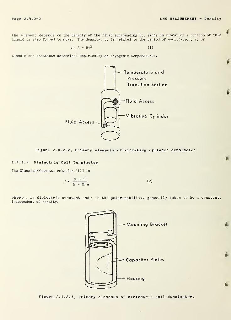
Page 2.1». 2-2 LNG MEASUREMENT Density
the element depends on the density of the fluid surrounding it, since in vibration a portion of this
liquid is also forced to move. The density, p, is related to the period of oscillation, t, by
p = A + Bx 2 (1
)
A and B are constants determined empirically at cryogenic temperatures.
Figure 2.^.2. 2. Primary elements of vibrating cylinder densimeter.
2 . U . 2 . U Dielectric Cell Densimeter
The Clausius-Mossitti relation [17] is
P- (2)(e + 2) a
where e is dielectric constant and a is the polarizability, generally taken to be a constant,independent of density.
Mounting Bracket
Capacitor Plates
Housing
Figure 2.M.2.3. Primary elements of dielectric cell densimeter.
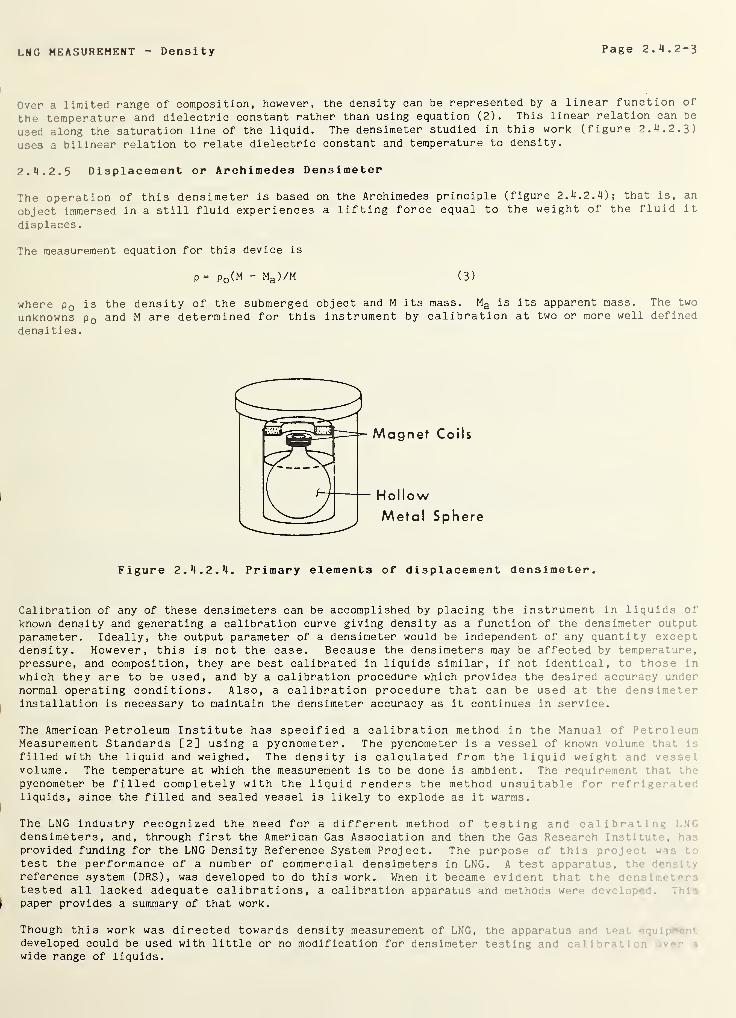
LNG MEASUREMENT Density Page 2. 4. 2-3
Over a limited range of composition, however, the density can be represented by a linear function of
the temperature and dielectric constant rather than using equation (2). This linear relation can be
used along the saturation line of the liquid. The densimeter studied in this work (figure 2. 4. 2. 3)
uses a bilinear relation to relate dielectric constant and temperature to density.
2. 4. 2. 5 Displacement or Archimedes Densimeter
The operation of this densimeter is based on the Archimedes principle (figure 2. 4. 2. 4); that is, an
object immersed in a still fluid experiences a lifting force equal to the weight of the fluid it
displaces.
The measurement equation for this device is
p = Po (M - Ma )/M (3)
where p 0 is the density of the submerged object and M its mass. Ma is its apparent mass. The two
unknowns p 0 and M are determined for this instrument by calibration at two or more well defined
densities.
Magnet Coils
Hollow
Metal Sphere
Figure 2. 4. 2. 4. Primary elements of displacement densimeter.
Calibration of any of these densimeters can be accomplished by placing the instrument in liquids of
known density and generating a calibration curve giving density as a function of the densimeter outputparameter. Ideally, the output parameter of a densimeter would be independent of any quantity exceptdensity. However, this is not the case. Because the densimeters may be affected by temperature,
pressure, and composition, they are best calibrated in liquids similar, if not identical, to those in
which they are to be used, and by a calibration procedure which provides the desired accuracy undernormal operating conditions. Also, a calibration procedure that can be used at the densimet-
r
|
installation is necessary to maintain the densimeter accuracy as it continues in service.
The American Petroleum Institute has specified a calibration method in the Manual of Petr'
Measurement Standards [2] using a pycnometer. The pycnometer is a vessel of known volume the' i
filled with the liquid and weighed. The density is calculated from the liquid weight and ves: el
volume. The temperature at which the measurement is to be done is ambient. The requirement that the
pycnometer be filled completely with the liquid renders the method unsuitable for ref r i ger i
• •
liquids, since the filled and sealed vessel is likely to explode as it warms.
The LNG industry recognized the need for a different method of testing and call bra 1
.
.
densimeters, and, through first the American Gas Association and then the Gas Research In.-. M* ,
provided funding for the LNG Density Reference System Project. The purpose of this pr • ~
test the performance of a number of commercial densimeters in LNG. A test apparatu: ,
••
reference system (DRS), was developed to do this work. When it became evident that th<-- .•
tested all lacked adequate calibrations, a calibration apparatus and methods wer- :• . .1
|paper provides a summary of that work.
Though this work was directed towards density measurement of LNG, the apparatus, ir. :
• •• • ei; .
developed could be used with little or no modification for densimeter testing and • a 1 c • >•. >,
wide range of liquids.
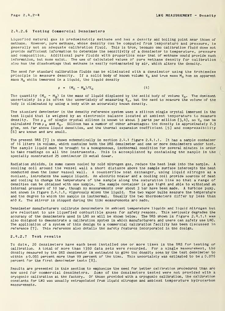
Page 2. 4. 2-4 LNG MEASUREMENT Density
2. 4. 2. 6 Testing Commercial Densimeters
Liquefied natural gas is predominately methane and has a density and boiling point near those ofmethane. However, pure methane, whose density can be computed from temperature and pressure, isgenerally not an adequate calibration fluid. This is true, because one calibration fluid does notprovide sufficient information to determine the sensitivity of a densimeter to temperature, pressureand composition. Additional pure fluids with properties near that of methane could provide suchinformation, but none exist. The use of calculated values of pure methane density for calibrationalso has the disadvantage that methane is easily contaminated by air, which alters the density.
The need for standard calibration fluids can be eliminated with a densimeter using the Archimedesprinciple to measure density. If a solid body of known volume VQ and true mass M0 has an apparentmass Ma while immersed in a liquid, the liquid density
P = (M0 - Ma )/V 0 (4)
The quantity (M 0 - Ma ) is the mass of liquid displaced by the solid body of volume VQ . The dominantuncertainty in p is often the uncertainty of measuring VQ , but the need to measure the volume of thebody is eliminated by using a body with an accurately known density.
The standard densimeter in the density reference system uses a silicon single crystal immersed in thetest liquid that is weighed by an electronic balance located at ambient temperature to measuredensity. The p s of single crystal silicon is known to about 3 parts per million [3.4], so V0 can becalculated from p s and M0 . Silicon has a number of other advantages: the density is approximately 2.3g/cm, not far above liquid densities, and the thermal expansion coefficient [5] and compressibility[6] are known and are small.
The present DRS [7] is shown schematically in section 2.4.1 figure 2. 4. 1.1. It has a sample containerof 16 liters in volume, which contains both the DRS densimeter and one or more densimeters under test.The sample liquid must be brought to a homogeneous, isothermal condition for several minutes in orderto take readings on all the instruments. This is accomplished by containing the sample in thespecially constructed 25 centimeter ID metal dewar.
Radiation shields, in some cases cooled by cold nitrogen gas, reduce the heat leak into the sample. A
cooling coil around the vessel wall a short distance above the sample surface intercepts the heatconducted down the inner vessel wall. A counterflow heat exchanger, using liquid nitrogen as a
coolant, introduces the sample liquid. An electric heater and a cooling coil provide sources of heatand cooling to change the temperature of the sample along the saturation line so that a range ofdensities can be obtained with one sample. The sample container is gas tight and able to withstand an
internal pressure of 10 bar, though no measurements over about 3 bar have been made. A turbine pump,not shown in figure 2. 4. 1.1, vigorously mixes the liquid. The two vapor bulbs measure the temperatureand the degree to which the sample is isothermal. Usually the two thermometers differ by less thanmIO K. The stirrer is stopped during the time measurements are made.
Densimeter manufacturers calibrate densimeters in ambient temperature liquids and liquid nitrogen butare reluctant to use liquefied combustible gases for safety reasons. This seriously degrades the
accuracy of the densimeters used in LNG as will be shown below. The DRS shown in figure 2. 4. 1.1 wasalso designed to demonstrate a calibration system in which manufacturers and users can safely use LNG.
The application of a system of this design to a commercial calibration facility has been discussed in
reference [7]. This reference also details the safety features incorporated in the design.
2. 4. 2. 7 Test results
To date, 20 densimeters have each been installed one or more times in the DRS for testing or
calibration. A total of more than 1350 data sets were recorded. For a single measurement, thedensity measured by the DRS densimeter is estimated to give the density seen by the test densimeter to
within ±0.055 percent more than 99 percent of the time. This uncertainty was estimated to be ±0.076percent for the first densimeter tests [8].
Results are presented in this section to emphasize the need for better calibration procedures than are
now used for commercial densimeters. Some of the densimeters tested were not provided with a
cryogenic calibration at the factory. Of those provided with a cryogenic calibration, the calibrationconstants for LNG was usually extrapolated from liquid nitrogen and ambient temperature hydrocarbonmeasurements.
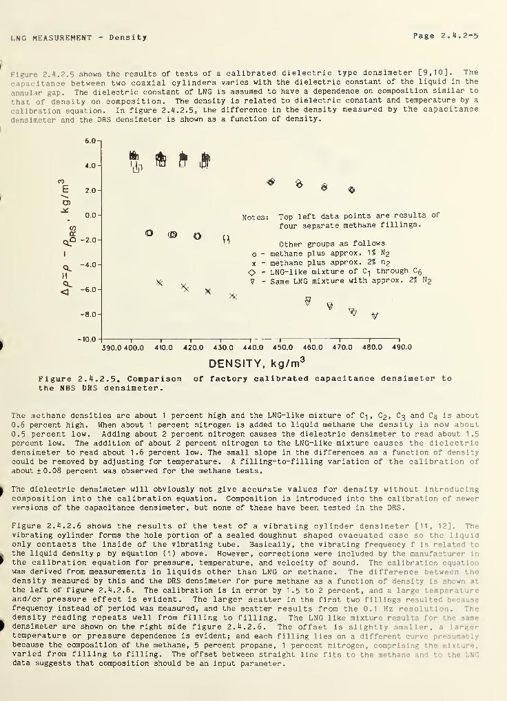
LNG MEASUREMENT Density Page 2. 4.2-5
Figure 2. 4. 2. 5 shows the results of tests of a calibrated dielectric type densimeter [9,10]. The
capacitance between two coaxial cylinders varies with the dielectric constant of the liquid in the
annular gap. The dielectric constant of LNG is assumed to have a dependence on composition similar to
that of density on composition. The density is related to dielectric constant and temperature by a
calibration equation. In figure 2. 4. 2. 5, the difference in the density measured by the capacitance
densimeter and the DRS densimeter is shown as a function of density.
6.O-1
5
4.0-
E 2.0-
cn
0.0-
wCE
Q?I
-2.0-
1
CL-4.0-
II
CL<1
-6.0-
-8.0-
- 10.0
ft
'dp
O Qft
>$< X
& $
Notes:
o
x
OV
Top left data points are results of
four separate methane fillings.
Other groups as follows
methane plus approx. 1 ? N2
methane plus approx. 2% n 2
LNG-like mixture of C-j through Cg
Same LNG mixture with approx. 2% N2
*¥
T ~r r ~\
390.0 400.0 410.0 420.0 430.0 440.0 450.0
DENSITY, kg/m
460.0
3
470.0 480.0 490.0
Figure 2. 4.2.5. Comparison of factory calibrated capacitance densimeter tothe NBS DRS densimeter.
The methane densities are about 1 percent high and the LNG-like mixture of C-| , C 2 , C3
and C 4 is about0.6 percent high. When about 1 percent nitrogen is added to liquid methane the density is now about0.5 percent low. Adding about 2 percent nitrogen causes the dielectric densimeter to read about 1.5
percent low. The addition of about 2 percent nitrogen to the LNG-like mixture causes the dielectricdensimeter to read about 1.6 percent low. The small slope in the differences as a function of densitycould be removed by adjusting for temperature. A filling-to-filling variation of the calibration ofabout ± 0.08 percent was observed for the methane tests.
The dielectric densimeter will obviously not give accurate values for density without introducingcomposition into the calibration equation. Composition is introduced into the calibration of newerversions of the capacitance densimeter, but none of these have been tested in the DRS.
Figure 2. 4.
2
.
6
shows the results of the test of a vibrating cylinder densimeter [11, 12]. Thevibrating cylinder forms the hole portion of a sealed doughnut shaped evacuated case so the liquidonly contacts the inside of the vibrating tube. Basically, the vibrating frequency f is related to
the liquid density p by equation (1) above. However, corrections were included by the manufacturer in
the calibration equation for pressure, temperature, and velocity of sound. The calibration equv !•.
was derived from measurements in liquids other than LNG or methane. The difference between •
density measured by this and the DRS densimeter for pure methane as a function of density is .shown rthe left of figure 2. 4. 2. 6 . The calibration is in error by 1.5 to 2 percent, and a large temperatureand/or pressure effect is evident. The larger scatter in the first two fillings resultedfrequency instead of period was measured, and the scatter results from the 0.1 Hz resolution. :
•
density reading repeats well from filling to filling. The LNG like mixture results fordensimeter are shown on the right side figure 2. 4. 2. 6 . The offset is slightly smaller, a :
temperature or pressure dependence is evident; and each filling lies on a different curve;
.
because the composition of the methane, 5 percent propane, 1 percent nitrogen, comprising - ••,
varied from filling to filling. The offset between straight line fits to the methane ir. :
•• •
data suggests that composition should be an input parameter.
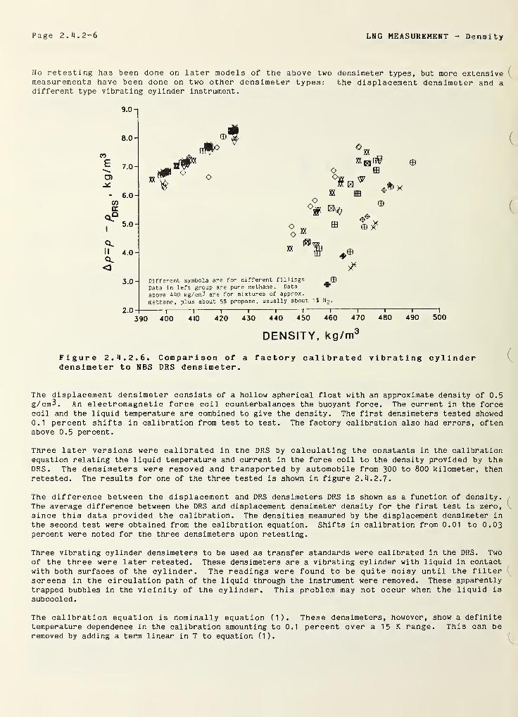
Page 2. 4.2-6 LNG MEASUREMENT Density
No retesting has been done on later models of the above two densimeter types, but more extensivemeasurements have been done on two other densimeter types: the displacement densimeter and adifferent type vibrating cylinder instrument.
9.0-1
8 .0 -
co
^ 7.0-
O)
- 6.0
COa.
clq
I
5.0-
II 4.0CL<
3.0-1
2.0
©1
.f# v OO ffl
Ow ^
OO,
oo
ffl
X
©
© #
Different symbols are for different fillings f
Data in left group are pure methane. Data“
above MO kg/om3 are for mixtures of approx,
methane, plus about 5 % propane, usually about 1? N 2 .
1
—
390 400—1
—
410—I
—
420~r T430 440 450
—r~460
T T470 480 490
DENSITY, kg/nr
i
500
Figure 2. 4. 2. 6. Comparison of a factory calibrated vibrating cylinderdensimeter to NBS DRS densimeter.
The displacement densimeter consists of a hollow spherical float with an approximate density of 0.5g/cm3. An electromagnetic force coil counterbalances the buoyant force. The current in the forcecoil and the liquid temperature are combined to give the density. The first densimeters tested showed0.1 percent shifts in calibration from test to test. The factory calibration also had errors, oftenabove 0.5 percent.
Three later versions were calibrated in the DRS by calculating the constants in the calibrationequation relating the liquid temperature and current in the force coil to the density provided by theDRS. The densimeters were removed and transported by automobile from 300 to 800 kilometer, thenretested. The results for one of the three tested is shown in figure 2. 4. 2.7.
The difference between the displacement and DRS densimeters DRS is shown as a function of density.The average difference between the DRS and displacement densimeter density for the first test is zero,
since this data provided the calibration. The densities measured by the displacement densimeter in
the second test were obtained from the calibration equation. Shifts in calibration from 0.01 to 0.03percent were noted for the three densimeters upon retesting.
Three vibrating cylinder densimeters to be used as transfer standards were calibrated in the DRS. Twoof the three were later retested. These densimeters are a vibrating cylinder with liquid in contactwith both surfaces of the cylinder. The readings were found to be quite noisy until the filterscreens in the circulation path of the liquid through the instrument were removed. These apparentlytrapped bubbles in the vicinity of the cylinder. This problem may not occur when the liquid is
subcooled.
The calibration equation is nominally equation (1). These densimeters, however, show a definitetemperature dependence in the calibration amounting to 0.1 percent over a 15 K range. This can beremoved by adding a term linear in T to equation (1).
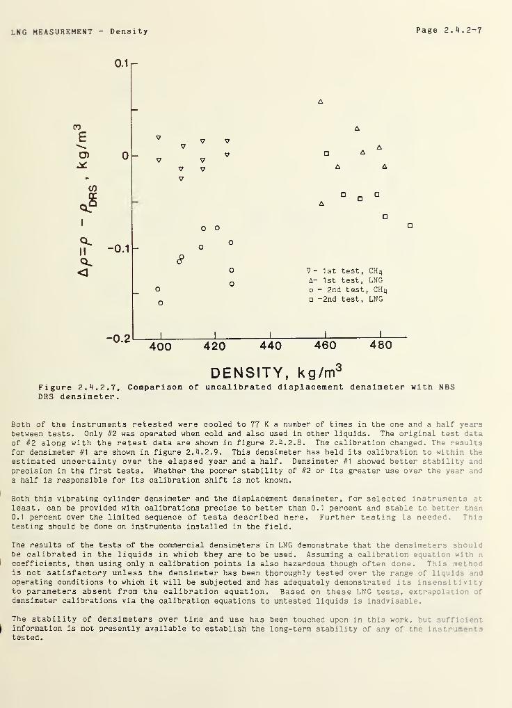
LNG MEASUREMENT Density Page 2. 4. 2-7
Figure 2. 4. 2. 7. Comparison of uncalibrated displacement densimeter with NBSDRS densimeter.
Both of the instruments retested were cooled to 77 K a number of times in the one and a half yearsbetween tests. Only #2 was operated when cold and also used in other liquids. The original test dataof #2 along with the retest data are shown in figure 2. 4. 2. 8. The calibration changed. The resultsfor densimeter #1 are shown in figure 2. 4. 2. 9. This densimeter has held its calibration to within theestimated uncertainty over the elapsed year and a half. Densimeter #1 showed better stability andprecision in the first tests. Whether the poorer stability of #2 or its greater use over the year anda half is responsible for its calibration shift is not known.
Both this vibrating cylinder densimeter and the displacement densimeter, for selected instruments at
least, can be provided with calibrations precise to better than 0.1 percent and stable to better than0.1 percent over the limited sequence of tests described here. Further testing is needed. Thintesting should be done on instruments installed in the field.
The results of the tests of the commercial densimeters in LNG demonstrate that the densimeters s'noui :
be calibrated in the liquids in which they are to be used. Assuming a calibration equation •
coefficients, then using only n calibration points is also hazardous though often done. Thi3 meth :
is not satisfactory unless the densimeter has been thoroughly tested over the range of liqui :
operating conditions to which it will be subjected and has adequately demonstrated its lnsen3 i t i v
1
*
y
to parameters absent from the calibration equation. Based on these LNG tests, extrapoi .* i •. :
densimeter calibrations via the calibration equations to untested liquids is inadvisable.
The stability of densimeters over time and use has been touched upon in this work, • .*
information is not presently available to establish the long-term stability of any of the lnstr 1
tested.
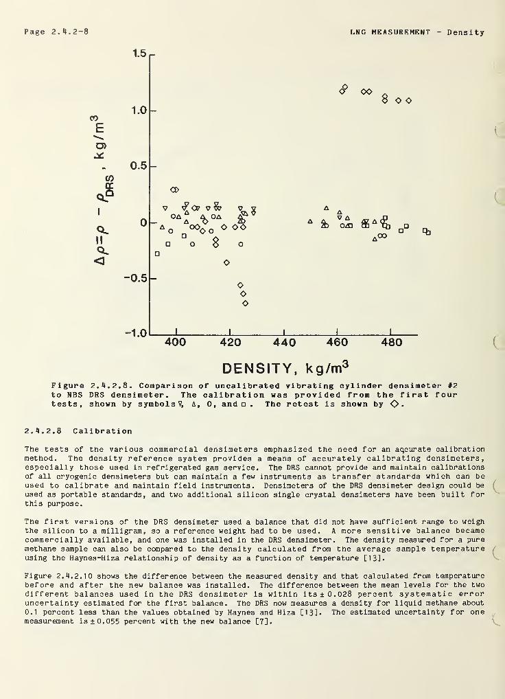
Page 2. *1.2-8 LNG MEASUREMENT Densi ty
Figure 2. **.2. 8. Comparison of uncalibrated vibrating cylinder densimeter #2to NBS DRS densimeter. The calibration was provided from the first fourtests, shown by symbols V, A, 0, and . The retest is shown by <C>
.
2.*l.2.8 Calibration
The tests of the various commercial densimeters emphasized the need for an accurate calibrationmethod. The density reference system provides a means of accurately calibrating densimeters,especially those used in refrigerated gas service. The DRS cannot provide and maintain calibrationsof all cryogenic densimeters but can maintain a few instruments as transfer standards which can beused to calibrate and maintain field instruments. Densimeters of the DRS densimeter design could be
used as portable standards, and two additional silicon single crystal densimeters have been built forthis purpose.
(
The first versions of the DRS densimeter used a balance that did not have sufficient range to weighthe silicon to a milligram, so a reference weight had to be used. A more sensitive balance becamecommercially available, and one was installed in the DRS densimeter. The density measured for a puremethane sample can also be compared to the density calculated from the average sample temperatureusing the Haynes-Hiza relationship of density as a function of temperature [13].
Figure 2.4.2.10 shows the difference between the measured density and that calculated from temperaturebefore and after the new balance was installed. The difference between the mean levels for the twodifferent balances used in the DRS densimeter is within its ±0.028 percent systematic erroruncertainty estimated for the first balance. The DRS now measures a density for liquid methane about
0.1 percent less than the values obtained by Haynes and Hiza [13]. The estimated uncertainty for onemeasurement is ±0.055 percent with the new balance [7]. c
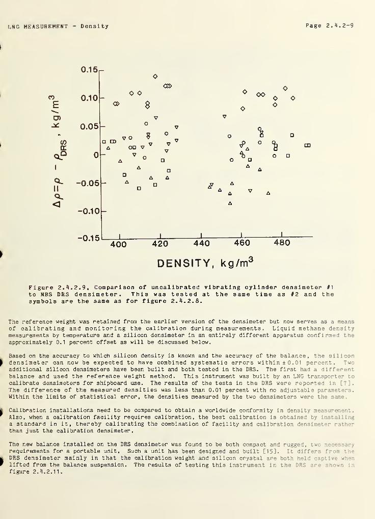
LNG MEASUREMENT Density Page 2.11.2-9
Figure 2. 4. 2. 9. Comparison of uncalibrated vibrating cylinder densimeter #1
to NBS DRS densimeter. This was tested at the same time as #2 and thesymbols are the same as for figure 2. 4. 2. 8.
The reference weight was retained from the earlier version of the densimeter but now serves as a meansof calibrating and monitoring the calibration during measurements. Liquid methane densitymeasurements by temperature and a silicon densimeter in an entirely different apparatus confirmed theapproximately 0.1 percent offset as will be discussed below.
Based on the accuracy to which silicon density is known and the accuracy of the balance, the silicondensimeter can now be expected to have combined systematic errors within +0.01 percent. Twoadditional silicon densimeters have been built and both tested in the DRS. The first had a differentbalance and used the reference weight method. This instrument was built by an LNG transporter to
calibrate densimeters for shipboard use. The results of the tests in the DRS were reported in [7].The difference of the measured densities was less than 0.01 percent with no adjustable parameter.-:
.
Within the limits of statistical error, the densities measured by the two densimeters were the same.
Calibration installations need to be compared to obtain a worldwide conformity in density measure-"-.' .
Also, when a calibration facility requires calibration, the best calibration is obtained by install is*:
a standard in it, thereby calibrating the combination of facility and calibration densimeter r i'-;- -
than just the calibration densimeter.
The new balance installed on the DRS densimeter was found to be both compact and rugged, twr r.•
requirements for a portable unit. Such a unit has been designed and built [15]. It differ.-- fr rDRS densimeter mainly in that the calibration weight and silicon crystal are both held cap’Iv wlifted from the balance suspension. The results of testing this instrument in the DRS are : wr .
•
f i gur e 2.4.2.11.
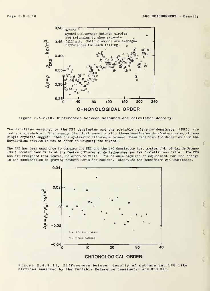
Page 2.11.2-10 LNG MEASUREMENT - Density
CHRONOLOGICAL ORDER
Figure 2.4.2.10, Differences between measured and calculated density.
The densities measured by the DRS densimeter and the portable reference densimeter (PRD) areindistinguishable. The nearly identical results with three Archimedes densimeters using siliconsingle crystals suggest that the systematic difference between these densities and densities from theHaynes-Hiza results is not an error in weighing the crystal.
The PRD has been used once to compare the DRS and the LNG densimeter test system [14] of Gaz de France( GDF ) located near Paris at the Centre d'Etudes et de Recherches sur les Installations Gazie. The PRDwas air freighted from Denver, Colorado to Paris. The balance required an adjustment for the changein the acceleration of gravity between Paris and Boulder. Otherwise the densimeter was unaffected.
0.04
0.02 -mCO
O)
QQ.I
a.
ii
< -002
-0.04
||_ M M
M
L = LNG-like mixture
M = Liquid methane
I
10
L M
M
20 30 40
CHRONOLOGICAL ORDER
Figure 2.4.2.11, Differences between density of methane and LNG-likemixtures measured by the Portable Reference Densimeter and NBS DRS.
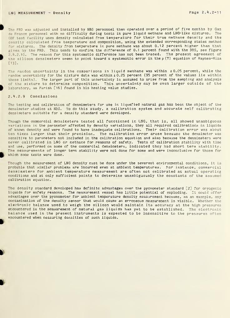
LNG MEASUREMENT Density Page 2.4.2-11
The PRD was adjusted and installed by NBS personnel then operated over a period of five months by Gaz
de France personnel with no difficulty during tests in pure liquid methane and LNG-like mixtures. The
GDF test facility uses density calculated from temperature for their true methane density and the
density calculated from temperature and composition, using the extended corresponding states method
for mixtures. The density from temperature in pure methane was about 0.12 percent higher than thatgiven by the PRD. This tends to confirm the difference of 0.1 percent found with the DRS , see figure
2.4.2.10. The reason for this systematic difference has not been traced. The present agreement of
the silicon densimeters seems to point toward a systematic error in the p (T) equation of Haynes-Hiza
[13].
The random uncertainty in the comparisons in liquid methane was within ±0.05 percent, while the
random uncertainty for the mixture data was within ±0.25 percent (95 percent of the values lie withinthese limits). The larger part of this uncertainty is assumed to arise from the sampling and analysis
of the mixture to determine composition. This uncertainty may be even larger outside of thelaboratory, as Parish [16] found in his heating value studies.
2. 4.2.9 Conclusions
The testing and calibration of densimeters for use in liquefied natural gas has been the object of the
densimeter studies at NBS. To do this study, a calibration system and accurate self calibratingdensimeters suitable for a density standard were developed.
Though the commercial densimeters tested all functioned in LNG, that is, all showed unambiguousvariations in the parameter affected by density variations, they all required calibrations in liquidsof known density and were found to have inadequate calibrations. Their calibration error was aboutten times larger than their precision. The calibration error arose because the densimeter wassensitive to parameters not included in the calibration equation and also because the densimeters werenever calibrated in LNG or methane for reasons of safety. Tests of calibration stability with timeand use, performed on some of the commercial densimeters, indicated they had short term stability.The measurements of longer term stability were not done for some and were inconclusive for those forwhich some tests were done.
Though the measurement of LNG density must be done under the severest environmental conditions, it isprobable that similar problems are incurred even at ambient temperatures. For instance, commercialdensimeters for ambient temperature measurement are often not calibrated at actual operatingconditions and at only sufficient points to determine unambiguously the constants of the assumedcalibration equation.
The density standard developed has definite advantages over the pycnometer standard [2] for cryogenicliquids for safety reasons. The measurement vessel has little potential of exploding. It could offeradvantages over the pycnometer for ambient temperature density measurement because, as an example, anycontamination of the density sensor that would cause an erroneous measurement is visible. Whether theelectronic balance used to weigh the silicon would maintain its accuracy at the high pressuresencountered in the measurement of natural gas liquids has yet to be established. The electronicbalance used in the present instruments is expected to be insensitive to the pressures oftenencountered when measuring densities of such liquids.
Page 2.4.2-12 LNG MEASUREMENT Density
2.4.2.10 References
[ 1 ]
[ 2 ]
[3]
[4]
[5]
C6]
[7]
[ 8 ]
[9]
CIO]
[ 11 ]
[ 12 ]
[13]
[14]
[15]
[ 16 ]
[17]
Siegwarth, J. D. and J. F. LaBrecque , Calibration of densimeters for liquefied lighthydrocarbons, Oil & Gas Journal, pp 64-9 (December 20, 1982).
API Manual of Petroleum Measurement Standards, Chapter 14, Section 6, Installing and provingdensity meters used to measure hydrocarbon liquid with densities between 0.3 to 0.7 gm/cc at15.56°C (60°F) and saturation vapor pressure, (1979).
Bowman, H. A., R. M. Schoonover and M. V. Jones, Procedure for high precision densitydeterminations by hydrostatic weighting, J. Research, NBS, 71C, 178 (1967).
Henins, I. and J. A. Bearden, Silicon crystal determination of the absolute scale of x-raywavelengths, Phys. Rev. 135, A890 (1964).
Corruccini, R. J. and J. J. Gniewek, Thermal expansion of technical solids at low temperatures,Nat. Bur. Stand. (U.S.), Monograph 29, (May, 1961).
McSkimin, H. J., Measurement of elastic constants at low temperatures by means of ultrasonicwaves— data for silicon and germanium single crystals and fused silica, J. Appl. Phys. 24, 988(1953).
Siegwarth, J. D., B. A. Younglove and J. F. LaBrecque, Cryogenic fluids density referencesystem: provisional accuracy statement (1980) , Nat. Bur. Stand. (U.S.), Technical Note 1041
(1981 )
.
Siegwarth, J. D., B. A. Younglove and J. F. LaBrecque, Cryogenic fluids density referencesystem: provisional accuracy statement , Nat. Bur. Stand. (U.S.), Technical Note 698 (November,1977)
.
Siegwarth, J. D. and J. F. LaBrecque, An evaluation of commercial densimeters for use in LNG,
Nat. Bur. Stand. (U.S.), Technical Note 697 (October, 1977).
Siegwarth, J. D., J. F. LaBrecque and B. A. Younglove, Test of densimeters for use in custodytransfer of LNG, Proceedings, 53rd International School of Hydrocarbon Measurement, Norman,Oklahoma, p 385(1978)
.
Siegwarth, J. D. and J. A. Brennan, LNG instrumentation for custody transfer, AGA OperatingSection Proceedings, Proceedings of the Transmission Conference, Atlanta, Georgia, T-119 (1981).
Siegwarth, J. D. and J. F. LaBrecque, Tests of commercial densimeters, Nat. Bur. Stand. (U.S.),Technical Note 1055 (June, 1982).
Haynes, W. M. and M. J. Hiza, Measurements of orthobaric liquid densities of methane, ethane,
propane, isobutane and normal butane, J. Chem. Thermodynamics 9_, 179, (1977).
Dewardt, F. and P. Mousset, Contribution a l'Amelioration de Comptage du GNL - Evaluation de
densimetres et echantillonneur pour GNL, Sixth International Conference on Liquefied NaturalGas, Appendex Paper 8, Kyoto, Japan (1980).
Siegwarth, J. D. and J. F. LaBrecque, A portable calibration densimeter for use in cryogenicliquids, Nat. Bur. Stand. (U.S.), Technical Note 1035 (1981).
Parrish, W. R., J. M. Arvidson and J. F. LaBrecque, Development and evaluation of an LNGsampling measurement system, Nat. Bur. Stand., NBSIR 78-887, (July, 1978).
Handbook of Physics, Condon, E.
(1967).
U. and N. V. Frederick, Editors, 4-112, Mcgraw-Hill Book, Inc.
LNG MEASUREMENT Densi ty Page 2. 4. 3-1
2.4.3 Calculated LNG Density
2. 4. 3.1 General Comments
The measurement process by which the density of the LNG mixture is calculated from measurements of
other properties, such as pressure, temperature and constituent fraction is considered in this section
of the manual. The process requires some type of mathematical structure which relates the measured
properties to that of density. In the case of LNG, the structure can vary from a purely empiricalrelationship to very complex models having extensive theoretical basis.
A recently completed program, which focused exclusively on LNG mixture density, has providedextensive, accurate and precise experimental data upon which both empirical and theoretical models
were optimized and tested. Haynes, McCarty and Hiza [51] have summarized the work of this program,and this edited summary is reproduced in the following sections. The program was truly an
international effort by natural gas companies and agencies who supported and guided the research.
The report summarizes the results of a project concerning the densities of liquefied natural gas (LNG)
and its components. This project was initiated in the Properties of Fluids Section of the CryogenicsDivision of the National Bureau of Standards in July, 1972 and was carried out under the sponsorshipof a consortium of eighteen energy companies, through a grant administered by the American GasAssociation, Inc.
The experimental part of this project has included the following accomplishments: (a) development of
a magnetic suspension densimeter for absolute density measurements on liquids, including liquidmixtures in equilibrium with their vapor, at temperatures from 90 to 300 K; (b) orthobaric liquiddensity measurements on the major components of LNG, which include nitrogen (95-120 K) , methane(105-160 K), ethane (100-270 K), propane (100-288.7 K), isobutane (115-300 K), and normal butane(135-300 K); (c) orthobaric liquid density measurements on approximately thirty-five binary mixturesof the above components for all combinations except nitrogen + butane systems, primarily in thetemperature range of 105 to 1 30 K; and (d) orthobaric liquid density measurements on twenty-sevenmulticomponent mixtures (105-120 K), including several LNG-like mixtures with up to eight components.The total uncertainty of a single density measurement is approximately 0.1 percent at low temperaturesand decreases to approximately 0.06 percent at room temperature. The estimated standard deviation of
a single density measurement is less than 0.02 percent.
The density data have been used to optimize, test, and compare several mathematical models as to theirsuitability for the calculation of LNG densities for custody transfer. Models selected foroptimization and testing included an extended corresponding states method, a hard sphere model, a cellmodel, and an empirical model by Klosek and McKinley. The ultimate goal of this project was toproduce one or more mathematical models that could be used to predict the density of any LNG mixtureto within an uncertainty of 0.1 percent from an input of pressure, temperature, and composition. Eachof the models investigated here satisfies this goal within their inherent limitations. Thelimitations and ranges of validity of the various models are discussed. Also presented are techniquesfor predicting LNG densities from dielectric constant measurements and from excess volumecalculations
.
The last section of the original publication [51] provides a complete and detailed account of theresults of the project. This section is not included as a part of this measurement manual, 3 and thereader is referred to the program summary papers which are references 1-4.
2. 4. 3.2 Introduction
During the past decade liquefied natural gas has become an increasingly important commodity on h:-world energy market. This trend is expected to continue into the foreseeable future. In the buy In-:
and selling of LNG, the basis of custody transfer is its heating value. The determination of r re-
heating value of LNG requires a knowledge of its density, which in turn is dependent uponcomposition, temperature, and pressure. Since, for example, an error of one percent in densityresult in an inequity of between $1 00,000 and $200,000 (at 1983 prices) per 125,000 m3 snip: id f
LNG, the accuracy to which the density of the liquid can be determined is extremely import it •
transactions involving LNG. A one percent error in density was not uncommon at the time thi ; r
was initiated.
There are, at least, two means for determining the density of a large volume of LNG. On-
direct field measurements using commercially available densimeters. A second method r. :•
•
-i
use of a mathematical model or correlation to calculate a density based on direct measur* - • •
liquid composition and temperature.
Page 2.4.3-2 LNG MEASUREMENT Dens i ty
This report [51] has been concerned with the determination of the density by the second method. Inactual transfer situations it is likely that both methods will be used to compliment each other. Byeither method, the accuracy to which the density can be determined is limited by both practical andstate-of-the-art considerations. This has resulted in setting a goal of 0.1 percent for the totaluncertainty in the determination of the density of LNG.
In July 1972, a project was initiated with an ultimate goal of providing one or more mathematicalmodels that could be used to calculate the density of any LNG mixture with a total uncertainty of lessthan 0.1 percent based on a knowledge of the pressure, temperature, and composition of the liquidmixture. The mathematical models would be developed and/or optimized using density data for the majorcomponents of LNG and for binary mixtures of these components. Density data for multicomponentmixtures of LNG components would be used to evaluate and compare the performance of the mathematicalmodels. Some of the test mixtures would be selected to simulate commercial LNG compositions. LNGconsists primarily of methane (concentration level typically greater than 75 percent) with lesseramounts of ethane (up to 15 percent), propane (up to 5 percent), butanes (up to 2 percent), nitrogen(up to 2 percent), and pentanes plus heavier hydrocarbons (up to 0.5 percent).
The accuracy of a calculational technique based on experimental data can be no better than the inputdata from which the technique is developed. At the time this project was initiated, comparisons of
saturated (orthobaric) liquid density data for the pure components of LNG exhibited differences aslarge as 0.5 percent, while each investigator was generally claiming inaccuracies of 0.1 percent or
less. Furthermore, there were only a few sets of published data for liquid mixtures containing LNGcomponents, especially at low temperatures. These data were generally limited in scope or had claimedinaccuracies larger than the desired 0.1 percent. (The pure fluid and mixture data for LNG componentsfrom other investigations are summarized in section 2. 4. 3-8 of this report.) Thus, a major task of
the LNG density project was to provide an accurate and internally consistent set of density data forthe major components of LNG and for mixtures of these components. (These data could also serve as a
basis for calibration or development of gauging and metering methods of LNG.)
This project was sponsored by a consortium of eighteen international energy companies, five of whichwere from countries outside the United States. The sponsors represented both buyers and sellers ofLNG. The American Gas Association, Incorporated has provided administration of project funds. In
carrying out this research project, the National Bureau of Standards was serving in its traditionalrole as an independent third party. All results of this project would be published in the openliterature and hopefully gain wide acceptance throughout the LNG industry, since qualified sponsorrepresentatives from all parts of the i nternat i onal LNG market would have closely followed theprogress of this project throughout its entirety.
2. 4. 3-3 Major Accomplishments— Experimental Apparatus
The experimental technique selected for performing the density measurements for this project had tosatisfy relatively stringent criteria. It must be capable of absolute density measurements of highaccuracy and precision on a liquid, including mixtures, in equilibrium with vapor at cryogenictemperatures and at pressures to approximately 4 MPa using an optical cell. A magnetic suspensiondensimeter based on an application of Archimedes' principle was developed for this purpose.
Two apparatuses [5,6], each incorporating a magnetic suspension technique in the densitydetermination, were constructed for the measurements on liquids, including liquid mixtures. For bothapparatuses, the total uncertainty of a single density measurement, which is taken as three times the
standard deviation plus the systematic error, is approximately 0.1 percent at low temperatures anddecreases to approximately 0.06 percent at room temperature. The estimated standard deviation of a
single density measurement is less than 0.02 percent.
A brief description of the method for determining densities with either apparatus is as follows. A
small magnetic buoy is freely suspended in the fluid whose density is to be determined. The densityof the buoy is significantly greater (by approximately an order of magnitude) than the density of the
fluids investigated here. The force necessary to lift the buoy is supplied by one or more air-coresolenoids. The buoy is maintained at a stable (vertical) position through the automatic regulation of
an electronic servocircuit containing the lift coil and either a differential transformer [5] or a
differential capacitor [7] that detects the motion of the buoy. The horizontal position of the buoyis maintained by the axially symmetrical, diverging field of the lift coil.
When the buoy is supported at the same position in vacuum and in the fluid of interest, the upwardmagnetic force on the buoy supplied by the air-core solenoids gives a means for measuring the densityof the fluid, since this is the force that must be added to the buoyant force to balance the downward
LNG MEASUREMENT Density Page 2. 4.3-3
gravitational force. Thus, the density is deduced from measurements of the currents in the support
coils necessary to support the buoy in vacuum and in the fluid of interest at the same temperature and
at the same vertical position (determined with a 125X microscope).
The mass and volume of the buoy must be determined from independent measurements. The mass was
determined using an analytical microbalance. The volume of the buoy at room temperature was
determined by using distilled water as a reference fluid of known density. Thermal expansion data [8]
for barium ferrite, the material from which the buoy was fabricated, were obtained so that the volume
of the buoy at low temperatures could be calculated.
The first apparatus [5] could be used at temperatures between 90 and 300 K and at pressures to 5 MPa.
After initial tests with a three-coil arrangement to support the buoy, the densimeter was simplified
considerably by reducing to a system employing only one coil [9]. The second apparatus [6], whichemployed exactly the same technique for determining density, was significantly different from, and
more versatile than, the first apparatus. The second apparatus contained a concentric cylindercapacitor that was used to make dielectric constant measurements on the same liquid samples for which
density data were obtained. The major reason for the construction of the second apparatus was a need
in other research projects (e.g., PVT and dielectric constant measurements on liquid propane [10],
isobutane [11], and normal butane [12]) for a higher pressure capability (35 MPa) for the magneticsuspension densimeter. The extension to higher pressures was not needed in the LNG density project.
It should be noted that the second apparatus gave no improvement over the first in the accuracy towhich the density could be determined. The consistency of the density data from both apparatusesshould be equivalent to that for either apparatus alone. To insure that this was the case,measurements on liquid methane were used as a control throughout the project with both apparatuses.
2. 4. 3. 4 Experimental Measurements- Pure Fluid Data
The first experimental measurements for the LNG density project consisted of the acquisition oforthobaric liquid density data for the major components of LNG. Comprehensive results were obtainedfor nitrogen (95-120 K) [5], methane (105-160 K) [5,13], ethane (100-270 K) [13], propane (100-288.7K) [13], isobutane (115-300 K) [13], and normal butane (135-300 K) [13,14]. Detailed comparisonsbetween the data from this project and independent results demonstrated the need for an accurate andinternally consistent set of data for the major components of LNG. Differences as large as 0.5percent between the density data of independent investigators were common. At the time this projectwas initiated, there were no published data for normal butane at low temperatures. (In the course ofevaluating the performance of the magnetic suspension densimeter, density data were also obtained forsaturated liquid argon (100-120 K) and ethylene (105-200 K) [15].)
2. 4. 3 . 5 Binary Mixture Data
Orthobaric liquid density measurements were then carried out on thirty-five binary mixtures [ 1 6—1 8
]
containing the major components of LNG. Most of the binary mixture data were taken in the temperaturerange of 105 to 1 40 K. All binary combinations of the six major components of LNG were investigatedin this project, with the exception of the nitrogen + isobutane and nitrogen + normal butane systems.
Prior to the LNG density project, no low temperature, liquid density data could be found in theliterature for the following systems: nitrogen + ethane, nitrogen + propane, ethane + isobutane,propane + isobutane, propane + normal butane, and isobutane + normal butane, all of which have beeninvestigated under this program. All of the binary mixture measurements were carried out on liquidsamples condensed into the cell from gravimetrically prepared gas mixtures. This was considered to bethe most accurate method to fix the compositions of the liquid mixtures. For all mixtures containingnitrogen and/or methane, total vapor pressures have also been measured. For the methane-rich binarymixtures containing either isobutane or normal butane, dielectric constant data [17] were obtainedsimultaneously with the density results.
Extensive comparisons of the binary mixture data from this study have been made with ava:’. v>literature data. In general, differences were less than 0.1 percent, except that the density dat i f r
the ethane + propane system exhibited approximately an 0.8 percent discrepancy when compare: w: •
data of Shana'a and Canfield [19]. This was inconsistent with comparisons with the same author: r••
the methane + ethane and methane + propane systems as well as for pure fluid result ...
agreement was typically better than 0.1 percent.
Page 2. 4. 3-4 LNG MEASUREMENT Density
2. 4. 3. 6 Multicomponent Mixture Data
In order to evaluate and test the mathematical models that have been developed and optimized using thebinary mixture and pure component data, orthobaric liquid density measurements were performed ontwenty-seven multicomponent mixtures [20,21] of LNG components, primarily in the temperature range of110 to 120 K. The multicomponent mixtures investigated in this project ranged from ternary mixturescontaining methane and binary combinations of nitrogen, ethane, propane, and normal butane to four toeight component methane-rich (75-90 mole percent) mixtures containing up to 5 mole percent nitrogen,15 mole percent ethane, 7 mole percent propane, 5 mole percent butanes, and 0.44 mole percentpentanes.
The compositions of some of the six to eight component mixtures were selected to simulate commercialLNG mixtures. The compositions of other multicomponent mixtures were chosen to provide severe testsof the mathematical models and to complement the use of binary mixture data in the optimization of themodels. Except for three of the multicomponent mixtures, the compositions were determined from thepreparation of the gas mixtures by gravimetric means. For the other three mixtures, the compositionswere determined by gas chromatographic analysis using a thermal conductivity detector. Thechromatograph was calibrated with a gravimetrically prepared mixture. Vapor pressure data have alsobeen obtained for the multicomponent mixtures. For those multicomponent mixtures investigated withthe second apparatus, dielectric constant measurements [22] were performed simultaneously with thedensity measurements.
Although the pure fluid and binary mixture measurements from this project have not included data for
pentanes, five multicomponent mixtures containing pentanes [21] have been investigated. It wasthought that densities of these systems could be predicted with the mathematical models using existingpure fluid data for the pentanes from other sources [23,24] and predicting the interaction parametersfor binary mixtures containing pentanes from the behavior of the binary mixtures studied in the LNGdensity project. (Expressions for representing the pentane data of Orrit and Laupretre [24] arereported by Hiza [25].) High accuracy in these predictions is not required, since LNG mixturescontain relatively small fractions of pentanes.
2. 4. 3. 7 Mathematical Models
As mentioned earlier, one method of determining the density of LNG is to predict that density with a
mathematical model of the equation of state, given the pressure, temperature, and composition of theLNG. The ultimate goal of this study was to produce such a model (or models) that would be accurateto within 0.1 percent of the true density. The scope of this study was limited to saturated liquidsover a temperature range of 105 to 140 K with pressures to 2 MPa. The components of LNG were assumedto be nitrogen, methane, ethane, propane, isobutane, normal butane, isopentane and normal pentane.
Four different models were chosen to fit to the experimental data. Each of the selected modelsrepresent a different approach to modeling the equation of state of a fluid. These are an extendedcorresponding states model [26-27], a hard sphere model [28], a cell model [ 29— 3 1 ] , and a graphicalmodel by Klosek and McKinley [32]. During the course of optimizing the four models using theexperimental data, it became necessary to revise the functional form of the model proposed by Klosekand McKinley. No revisions of the functional form of the other three models were necessary, and onlythe adjustable parameters were changed to achieve the desired fit of the experimental data. The final
result was that all four of the models originally chosen can be used to predict the density of LNG to
within 0.1 percent of the true density, given the temperature, pressure, and composition of the LNG.
Details of the fitting procedures, comparisons to experimental data, and computer program listings are
given in references [ 33 — 35 ]
.
Also during the course of this study, an excess volume model was developed by Hiza [25]. This model
also achieves the 0.1 percent criteria outlined above under the same restrictions as the other models.
Lastly, a model has been developed by Haynes and McCarty [22] that does not require either the
temperature or pressure as input information (all of the other models require a minimum of temperature
as input and most require both temperature and pressure). This model requires an input of dielectric
constant and composition of the LNG and predicts the .density to within 0.15 percent of theexperimental value.
All of the models have restrictions on pressure, temperature, and composition ranges, which must be
defined for each model. The models are of widely ranging computational complexity. The selection of
a particular model is dependent on the needs and objectives of the individual user. However, on the
basis of the accuracy of the calculated density of a commercial LNG mixture, each of the modelsappears to be equally acceptable.
LNG MEASUREMENT Density Page 2.M.3-5
One final comment about accuracy should be emphasized. No mathematical model of the equation of state
can be more accurate than the experimental data to which it has been fit. Therefore, all of the
accuracy claims are dependent upon the accuracy of the experimental data from this study, which wereused almost exclusively to optimize and test the models.
2. *1.3.8 LNG Density Research at Other Laboratories
Because of the widespread interest in reliable data and the prediction of properties of multicomponent
liquefied natural gas mixtures, in particular saturated liquid (bubble point) densities, a number of
independent research programs were conducted from which a significant amount of density results have
been published in the open literature. These include the studies at Gaz de France (Morlett [36]), Air
Products and Chemicals, Inc. (Klosek and McKinley [32]), Institute of Gas Technology (Gonzalez, et al
.
[37,38], Huebler, et al. [39]), University of Kansas (Huang, et al . [40], Jensen and Kurata [41]),University of Oklahoma (Shana'a and Canfield [19]), Shell Research, Ltd. (Boyle and Reece [42],
McClune [23]), University of Wyoming (Miller, et al. [28,43-46]), and Societe Nationale Elf Aquitane(Roche, et al . [47,48], Orrit and Laupretre [24,49], and Orrit [50]). 1 There is considerable variation
in the precision and accuracy of measurement and in the completeness of the data published from thesestudies. Therefore, the contributions of these programs to the precise knowledge of the density
behavior of LNG mixtures are also quite variable.
From comparisons with these independent results, it appears that the data from the University of
Wyoming are the most precise and are uniformly consistent with the results of the NBS program. Directcomparisons of measurement precision were also made between the NBS densimeter and the Wyomingapparatus. Measurements were made at the University of Wyoming on one binary mixture and fourmulticomponent mixtures, prepared at NBS, with the apparatus calibrated with pure methane densitiesdetermined with the NBS densimeter [46]. Densities for the binary mixture and three of themulticomponent mixtures were also measured with the NBS densimeter. Comparisons were made through the
extended corresponding states model when measured temperatures were not exactly the same. The maximumdifference found was 0.10 percent for one multicomponent mixture point; the remaining differences wereless than 0.03 percent and random. Though the Wyoming program was carefully planned, measurements for
some of the important binary mixtures (e.g., nitrogen + ethane, nitrogen + propane, ethane + propane,etc.) were not included, and the accuracy of the molar volume results (though not that of derivedexcess volumes) depends directly on the accuracy of the density data of the low temperature liquidused to calibrate the apparatus.
The most extensive experimental measurements are those from the Elf Aquitane program. The precisionof measurement does not appear to be quite as good as the measurements of the University of Wyoming,and there is a systematic bias of about -0.1 percent in a sample of multicomponent mixtures data [49]compared to the extended corresponding states model optimized to the NBS results. Though not all ofthe important binary mixtures were included in their study, it is notable that measurements were madeon a nearly equimolar mixture of ethane + propane [50]. Excess volumes derived from these data andtheir pure fluid data between 105 and 140 K are in excellent agreement with those of the NBS program.Most of their V E values are between -0.01 and -0.04 cm3/mol compared to -0.03 to -0.05 cm3/mol for a
comparable mixture from the present study and about -0.49 cm3/mol from the University of Oklahoma dataat 108.15 K for a mixture containing 58.52 mole percent ethane.
With the exception of this large discrepancy in the University of Oklahoma data for the ethanepropane mixture, the remainder of the data from the University of Oklahoma, as well as those fromShell Research, Ltd., are of comparable precision as those from the University of Wyoming and from ElfAquitane. From the Shell Research, Ltd. program, only the pure component density data has beenpublished. None of the remaining programs have provided data approaching the precision and accuracygoals desired for custody transfer.
The programs of Elf Aquitane and Shell Research, Ltd. provide the only low temperature expor i •:
densities for pure isopentane and normal pentane, and these data sets are in good agreement.within about 0.1 percent. With the small concentrations of pentanes normally encountered i r.
mixtures, and the fact that the densities from these investigations are generally within about
''Certain companies are identified in this paper for the purpose of clarity on'.y.
identification does not imply any type of endorsement by the National Bureau of •
Page 2 . 4 .3~6 LNG MEASUREMENT Density
percent of the NBS value for the lower molar mass alkanes, it was felt that additional measurements onthe pure pentanes were unnecessary. In the NBS program, the pentanes were included only inmulticomponent mixtures, with compositions much like LNG mixtures that would be encountered in
practice. These measurements were made to provide proof that the mathematical models developed couldproperly account for the presence of pentanes.
Compared to the LNG research programs noted above, the NBS program is unique in that a single set of
data are provided of uniformly high precision and accuracy for all of the pure components (i.e.,nitrogen and the lower mass alkanes through the butanes), all the possible binary combinations whereliquid phase separation does not occur, the important ternary combinations, and multicomponentmixtures that contain the highest probable amounts of nitrogen, butanes, and pentanes. .The
measurement method employed is a sophisticated state- of-the-art method for which a detailed analysisof the measurement uncertainties has been made and published, and statistical control of theexperiments was assured throughout the program by repeating measurements of the density of liquidmethane with each experimental run. The mathematical models optimized to the data are representativeof existing theoretical and empirical models in wide use from the most simple to the most complex.The concurrent experimental and mathematical modeling efforts also served to guarantee that sufficientdata were obtained to optimize and to identify the inherent limitations of each.
2. 4. 3. 9 Acknowledgments [51]
The contributions of the members of the LNG Density Project Steering Committee are gratefullyacknowledged. The Steering Committee, comprised of representatives from each of the sponsoringcompanies, met quarterly from May 11, 1972 to February 15, 1979. The critique of research progressand numerous suggestions offered by the members were extremely valuable. Special thanks are dueMartin R. Cines of the Phillips Petroleum Company who served as Chairman of the LNG Density ProjectSteering Committee during that time, and who, in fact, was chiefly responsible for obtaining financialsupport for this work. Thanks are also due Louis A. Sarkes of the American Gas Association for hiscontributions to this project and for his general support of LNG properties research. L. James Kempof Southern California Gas Company assumed Chairmanship of the Steering Committee following theretirement of Martin R. Cines from Phillips Petroleum Company.
LNG MEASUREMENT Densi ty Page 2. 4. 3-7
2.4.3.10 References
[1] Haynes, W. M., M. J. Hiza, and R. D. McCarty, Densities of LNG for custody transfer. Proceedings
of Fifth International Conference on LNG, 1 977 August 29-September 1, Dusseldorf, Germany.Institute of Gas Technology, Chicago, 111. Paper 11, Section III. 36 p.
[2] Haynes, W. M. and R. D. McCarty, The density of liquefied natural gas. Proceeding of the
Fifty-Eighth Annual ( GP A ) Convention of the Gas Processors Association, 1979 March 19-21,
Denver, Colo. Gas Processors Association, Tulsa, Okla.
[3] Diller, D. E., LNG density determination, Hydrocarbon Processing 56(4), 142-144, 1977 April.
[4] McCarty, R. D. LNG densities for custody transfer. Proceedings of the Fifty-Sixth International
School of Hydrocarbon Measurements, Norman, OK, pp 515-17 (April 14-16, 1981).
[5] Haynes, W. M.,M. J. Hiza and N. V. Frederick, Magnetic suspension densimeter for measurements on
fluids of cryogenic interest, Rev. Sci. Instrum. 47(10), pp 1 237“50 (October, 1976).
[6] Haynes, W. M., Apparatus for density and dielectric constant measurements to 35 MPa on fluids of
cryogenic interest, J. Res. Nat. Bur. Stand. (U.S.), 84(4): 241-252; (July-August, 1983).
[7] Frederick, N. V. and W. M. Haynes, Differential capacitance sensor as position detector for a
magnetic suspension densimeter, Rev. Sci. Instrum. 50(9), pp 1154-55 (September, 1979).
[8] Clark, A. F., W. M. Haynes, V. A. Deason and R. J. Trapani, Low temperature thermal expansion of
barium ferrite, Cryogenics 16(3), PP 267-70, (May, 1976).
[9] Haynes, W. M., Simplified magnetic suspension densimeter for absolute density measurements, Rev.
Sci. Instrum. 48(1), pp 39-41, (January , 1 977)
.
[10] Haynes, W. M., Measurements of densities and dielectric constants of liquid propane from 90 to
300 K at pressures to 35 MPa, J. Chem. Thermodynamics, 15(5): 419-424 (May, 1983).
[11] Haynes, W. M., Measurements of densities and dielectric constants of liquid isobutane from 120
to 300 K at pressures to 35 MPa, J. Chem. Eng. Data. 28(4), pp 367-69 (October, 1983).
[12] Haynes, W. M., Measurements of densities and dielectric constants of liquid normal butane from1 40 to 300 K at pressures to 35 MPa, J. Chem. Thermodynamics, 15(9): 801-805 (September, 1983).
[13] Haynes, W. M. and M. J. Hiza, Measurements of the orthobaric liquid densities of methane,ethane, propane, isobutane, and normal butane, J. Chem. Thermodynamics 9(2), pp 179-87(February, 1977)
[14] Haynes, W. M. and M. J. Hiza, Orthobaric liquid densities of normal butane from 135 to 300 K as
determined with a magnetic suspension densimeter, Advances in Cryogenic Engineering, Vol 21, K.D. Timmerhaus and D. H. Weitzel, ed., pp 516-21, Plemum Press, New York, NY (1976).
[15] Haynes, W. M., Measurements of the orthobaric liquid densities of argon (100-120 K) and ethylene(105-200 K), Cryogenics 18(10), pp 621-23 (October, 1978).
[16] Hiza, M. J., W. M. Haynes and W. R. Parrish, Orthobaric liquid densities and excess volumes r
binary mixtures of low molar-mass alkanes and nitrogen between 105 and 140 K, L •
.
Thermodynamics 9(9), pp 873-96, (September, 1977).
[17] Haynes, W. M., Orthobaric liquid densities and dielectric constants of (methane + isobutan*(methane + normal butane) at low temperatures, J. Chem. Thermodynamics, 15(10): <
(October , 1 983)
.
[18] Hiza, M. J. and W. M. Haynes, Liquid mixture excess volumes and total vapor pr< ..•
magnetic suspension densimeter with compositions determined by chromatograph! e .
- ••1r
plus ethane, Advances in Cryogenic Engineering, Vol 23, K. D. Timmerhaus, ed. pp • * '
,
'
Press, New York, NY (1976).
[19] Shana’a, M. Y. and F. B. Canfield, Liquid density and excess volume of livh* ,mixtures at -165C, Trans. Faraday Soc. 64(549), pp 2281-2286 (September, 1
r"
Page 2. 4. 3-8 LNG MEASUREMENT - Density
[20] Hiza, M. J. and W. M. Haynes, Orthobaric liquid densities and excess volumes for multicomponentmixtures of low molar-mass alkanes and nitrogen between 105 and 125 K, J. Chem. Thermodynamics12(1), pp 1-10 (January, 1980).
[21] Haynes, W. M. Measurements of or thobari c-li qui d densities of multicomponent mixtures of LNGcomponents (N2, CH4 , C2H6, C3H8, CH3CH(CH3)CH3, C4H10, CH3CH(CH3 )C2H5 , and C5H12) between 110and 130 K, J. Chem. Thermodynamics 14(7), pp 603-12 (July, 1982).
[22] Haynes, W. M. and R. D. McCarty, Prediction of 1 i quef i ed-natur al-gas (LNG) densities fromdielectric constant measurements. Cryogenics, 23(8): 421-426 (August, 1983).
[23] McClune, C. R., Measurement of the densities of liquefied hydrocarbons from -100 to -180C (173to 93 K), Cryogenics 16(5), pp 289-95 (May, 1976).
[24] Orrit, J. and J. M. Laupretre, Density of liquefied natural gas constituents, Advances in
Cryogenic Engineering, Vol. 23, K. D. Timmerhaus, ed . , pp 573”79, Plenum Press, New York, NY(1978).
[25] Hiza, M. J., An empirical excess volume model for estimating liquefied natural gas densities,Fluid Phase Equilibria 2(2), pp 27~38 (August, 1978).
[26] Rowlinson, J. S. and I. D. Watson, The prediction of the thermodynamic properties of fluids andfluid mixtures - I. The principle of corresponding states and its extensions, Chem. Eng. Sci.24(10), pp 1565-74 (October, 1969).
[27] Mollerup, J. and J. S. Rowlinson, The prediction of the densities of liquefied natural gas andof lower molecular weight hydrocarbons, Chem. Eng. Sci. 29(6), pp 1 373 —82 (June, 1974).
[28] Rodosevich, J. B. and R. C. Miller, Calculation of LNG excess volumes by a modified hard-spheremodel. Advances in Cryogenic Engineering, Vol. 19, K. D. Timmerhaus, ed., pp 339-45, PlenumPress, New York, NY (1974).
[29] Renon, H., C. A. Eckert and J. M. Prausnitz, Molecular thermodynamics of simple liquids, Ind.
Eng. Chem. Fundam., 6(1), pp 52-8 (February, 1967).
[30] Eckert, C. A., H. Renon and J. M. Prausnitz, Molecular thermodynamics of simple liquids, Ind.
Eng. Chem. Fundam, 6(1), pp 58-67 (February, 1967).
[31] Albright, M. A., A model for the precise calculation of liquefied natural gas densities. NGPATech. Pub. TP-3, (1973).
[32] Klosek, J. and C. McKinley, Densities of liquefied natural gas and of low molecular weighthydrocarbons. White, J. W., Neumann, A. E. S., ed. Proceeding of the First InternationalConference on LNG, Session 5 Paper 21, 15 pp, Chicago, IL (April, 1968).
[33] McCarty, R. D., A comparison of mathematical models for the prediction of LNG densities, Nat.
Bur. Stand. (U.S.), NBSIR 77-867, 60 pp (October , 1 977)
.
[34] McCarty, R. D., Four mathematical models for the prediction of LNG densities, Nat. Bur. Stand.
(U.S.) Tech. Note 1030, 76 pp (December, 1980).
[35] McCarty, R. D., Mathematical models for the prediction of liquefied- natural-gas densities, J.
Chem. Thermodynamics, 14(9), 837“54 (September, 1982).
[ 36 ] Morlet, J., The density and miscibility of liquefied hydrocarbon gases at low temperatures, Rev.
Inst. Francais Petrole, 18, pp 127-43 (January , 1 963)
•
[37] Gonzalez, M. H., T. K. Subramanian, R. L. Kao and A. L. Lee, Physical properties of natural
gases at cryogenic conditions, White, J.W., Neumann, A. E. S., ed., Proceedings of the FirstInternational Conference on LNG, Session 5 Paper 21, 38 pp, Chicago, IL (April , 1968)
.
[ 38 ] Gonzalez, M. H., A. L. Lee, Dew and bubble points of simulated natural gases, J. Chem. Eng.
Data ,13(2), pp 172-6 (April, 1968 ).
LNG MEASUREMENT Densi ty Page 2. 4.3-9
[39] Huebler, J. ,B. E. Eakin, A. L. L ee, Physical properties of natural gas at cryogenic
conditions. White, J. W., ed., Proceedings of the Second International Conference on LNG, Vol.
I, Session 2 Paper 9, 10 pp, Paris, France (October, 1970).
[40] Huang, E. T. S., G. W. Swift, and F. Kurata, Viscosities and densities of methane-propanemixtures at low temperatures and high pressures, AIChE J. 13(5), pp 846-50 (September, 1967).
[41] Jensen, R. H. and F. Kurata, Density of liquefied natural gas, J. Petrol. Tech. 21, pp 683~91
(June, 1969).
[42] Boyle, G. J. and D. Reece, Bulk measurement of LNG. White, J. W., ed. Proceedings of the SecondInternational Conference on LNG, Vol. I, Session 2 Paper 5, 14 pp, Paris, France (October,1970).
[43] Rodosevich, J. B. and R. C. Miller, Experimental liquid mixture densities for testing andimproving correlations for liquefied natural gas, AIChE J. 19(4), pp 729~35 (1973, July).
[44] Miller, R. C., Estimating the densities of natural gas mixtures, Chem. Eng. 81(23), PP 134-35
(October, 1974).
[45] Pan, W. P., M. H. Mady, R. C. Miller, Dielectric constants and Clausius-Mossotti functions for
simple liquid mixtures: systems containing nitrogen, argon and light hydrocarbons, AIChE J.
21(2), pp 283-89 (March, 1975).
[46] Miller, R. C. and M. J. Hiza, Experimental molar volumes for some LNG-related saturated liquidmixtures, Fluid Phase Equilibria 2(1), pp 49~57 (August, 1978).
[47] Roche, Y., J. Perret, and L. Bochirol, Density of LNG and of its constituents, White, J. W.,
ed., Proceedings of the Second International Conference on LNG, Vol I, Session 2 Paper 8, 8 pp
,
Paris, France, (October, 1970).
[48] Roche, Y., J. Perret, L. Bochirol and P. Brauns, Density of LNG and of its constituents, White,J. W., ed., Proceedings of the Third International Conference on LNG, Session II Paper 13. 11
pp, Washington, D.C. (September, 1972).
[49] Orrit, J. , and J. M. Laupretre, A calculational method for obtaining the density of a liquefiednatural gas, Advances in Cryogenic Engineering, Vol. 23. K. D. Timmerhaus, ed . , pp 566-79,Plenum Press, New York, NY (1978).
[50] Orrit, J. E., Orthobaric liwuid densities of natural gas component mixtures, Fluid PhaseEquilibria, 12(3), pp253“8l (September, 1983).
[51] Haynes, W. M., R. D. McCarty and M. J. Hiza, Liquefied natural gas densities: summary ofresearch program at the National Bureau of Standards, Nat. Bur. Stand. (U.S), Monograph 172, 241
pp (October, 1 983 )
.

f
LNG MEASUREMENTS Densi ty Page 2. 4. 4-1
2.4.4 Mathematical Models for the Prediction of LNG Densities
general description of the extensive study program on the development of data for thermophysical.ropertles of LNG is summarized in 2.4.3. Accurate and precise experimental data on this complex
riuid mixture was necessary in order to provide a basis for data correlation programs which would give
useful accurate density data from measurements of other properties. Of the numerous possiblemathematical relationships considered, just four were chosen for the NBS program. These four modelsrepresented a spectrum of methods from the purely empirical to the more theoretical. The brief
ummary of 2. 4. 3. 7 does not provide the scope or depth to be useful for measurements and calculationsof LNG density. The work of McCarty [39] provides a detailed description of the development, and
resulting accuracy and precision of each of these models. Because of the importance of these methodsand techniques, re-publication of McCarty has been included in this section of the manual. It is
reproduced in detail (except for the original experimental data) with only minor editing.
2.4.4. 1 Introduction
The purpose of the study was to present in final form the four mathematical models which wereoptimized to the experimentally determined orthobaric liquid PVTx data of Miller and Hiza [25], Haynes
and Hiza [12], Haynes, et al. [11], Hiza, et al . [14], Hiza and Haynes [15] and Haynes [9]. Interimresults of the project have been reported by Haynes, et al . [13] and by McCarty [23]. The modelsreported in these two interim publications differ only slightly from those presented here. A
companion archival document, McCarty [24], with the same results but in much less detail, has beensubmitted to the Journal of Chemical Thermodynamics. The intent of the documentation here is more in
the vein of a user's handbook. The above experimental data are for the liquid phase of nitrogen,methane, ethane, propane, normal and isobutane and various mixtures thereof.
The goal of the project (the project included the above referenced experimental work) was to produceone or more computer models which would predict the density of LNG to within 0.1 percent of the truevalue from a knowledge of the temperature, pressure and composition of the LNG. At the beginning ofthis study LNG was defined as mixtures of the above components (nitrogen, methane, ethane, propane,normal and isobutane), and only the saturated liquid between 95-150 K was to be considered. Near theend of the project, normal and isopentane were added to the list of allowable components, but no
experimental PVTx of pure normal and isopentane or binary systems containing normal and isopentanewere measured as part of the project. The inclusion of these two components is based on data fromOrrit, et al. [29] and Orrit, et al. [30].
Four models were considered: the extended corresponding states model, a hard sphere model, a cellmodel and a Revised Klosek and McKinley model. With the exception of the Revised Klosek and McKinleymodel, only pure fluid and binary system data were used to optimize the models. In the case of theRevised Klosek and McKinley model, multicomponent PVTx data were used in the optimization process.
Over a normal range of LNG composition and temperature, all four of the models predict densities whichagree to within 0.1 percent of experiment. This is true of all of the experimental PVTx measurementson LNG like mixtures made as part of this project.
No equation or mathematical model based on experimental data can be more accurate than the originaldata, and, therefore, the extent to which the original goal of 0.1 percent accuracy has been metdepends entirely upon the accuracy of the experimental data referenced above.
There is no reason to doubt the experimental data, and, therefore, there is every reason to believethat the goal of the project has been achieved.
2. 4. 4. 2 Extended Corresponding States Method
The thermodynamic equations for the extended corresponding states method are developed in a paperRowlinson and Watson [35], and only a very brief description will be given here. Leach [20] dev.; .•
transformation functions for hydrocarbons which are called shape factor functions. Mollerup r .?7’ ar. t
Mollerup and Rowlinson [26] combined the earlier work with the equation of state for methan*. •.
Goodwin [8] to produce a computer program to calculate the density of LNG mixtures, which wvmodified by Mollerup [28].
The computer programs for the calculation of LNG densities based on the extended correnp nding *
method are an extensive revision of the Mollerup program. The program listings ar in :
McCarty [39]. Earlier versions were reported by McCarty [23] and Haynes, Hiza and McGar 1
/'
1 .
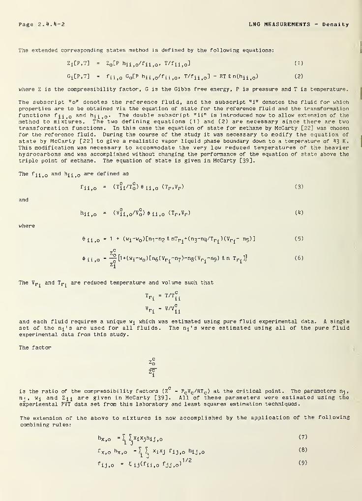
Page 2.11.4-2 LNG MEASUREMENTS Density
The extended corresponding states method is defined by the following equations:
ZiEP.T] = ZD [P hii>0/f ii>0 , T/f ii>0 ] (1)
GiEP.T] = fii,o ^o^P ^ii .o^f'ii ,o» ^^^ii.o-l- RT£n(h^ >0 ) (2)
where Z is the compressibility factor, G is the Gibbs free energy, P is pressure and T is temperature.
The subscript "o" denotes the reference fluid, and the subscript "i" denotes the fluid for whichproperties are to be obtained via the equation of state for the reference fluid and the transformationfunctions f^ 0 and h^i 0 . The double subscript "ii" is introduced now to allow extension of themethod to mixtures. The two defining equations (1) and (2) are necessary since there are twotransf ormat i on functions. In this case the equation of state for methane by McCarty [22] was chosenfor the reference fluid. During the course of the study it was necessary to modify the equation of
state by McCarty [22] to give a realistic vapor liquid phase boundary down to a temperature of 43 K.
This modification was necessary to accommodate the very low reduced temperatures of the heavierhydrocarbons and was accomplished without changing the performance of the equation of state above thetriple point of methane. The equation of state is given in McCarty [39].
The fii )Q and h^ 0 are defined as
f ii,o = (Tii/T 0 ) 0 ii , 0 (Tr ,Vr )
and
hii,o =( v ii , 0^0 ) <P ii ,0 (Tr ,Vr )
where
9 ii ,0 = 1 +( wi~w0 ) [n-| -n2 & nT r ^
+ (n^-ni^/T r ^) (Vr ^~ n5 )] (5)
2°
4> ii ,0 = -|[l + (wi-Wo)[ n6(Vri-n7)-n8( vr i
-n9) l n TP .]] (6)
zi
(3)
(4)
The Vr^
and T r ^are reduced temperature and volume such that
T-i
Vri
T/T?
.
11
v/vc
.
1
1
and each fluid requires a unique w^ which was estimated using pure fluid experimental data. A singleset of the n^'s are used for all fluids. The n^'s were estimated using all of the pure fluidexperimental data from this study.
The factor
Z?1
is the rationj , w
j_and
experimental
of the compressibility factors (ZL = PC VC/RT C ) at the critical point. The parameters nj
,
Zn are given in McCarty [39]. All of these parameters were estimated using thePVT data set from this laboratory and least squares estimation techniques.
The extension of the above to mixtures is now accomplished by the application of the followingcombining rules:
hx,o =I
^x i xj
h i j ,0
^x.o hx,o =I I x i xj ^ij,o hij,o
fi
j
,0= £ ij ii ,0 f
j j
,
0 )
(7)
( 8 )
( 9 )
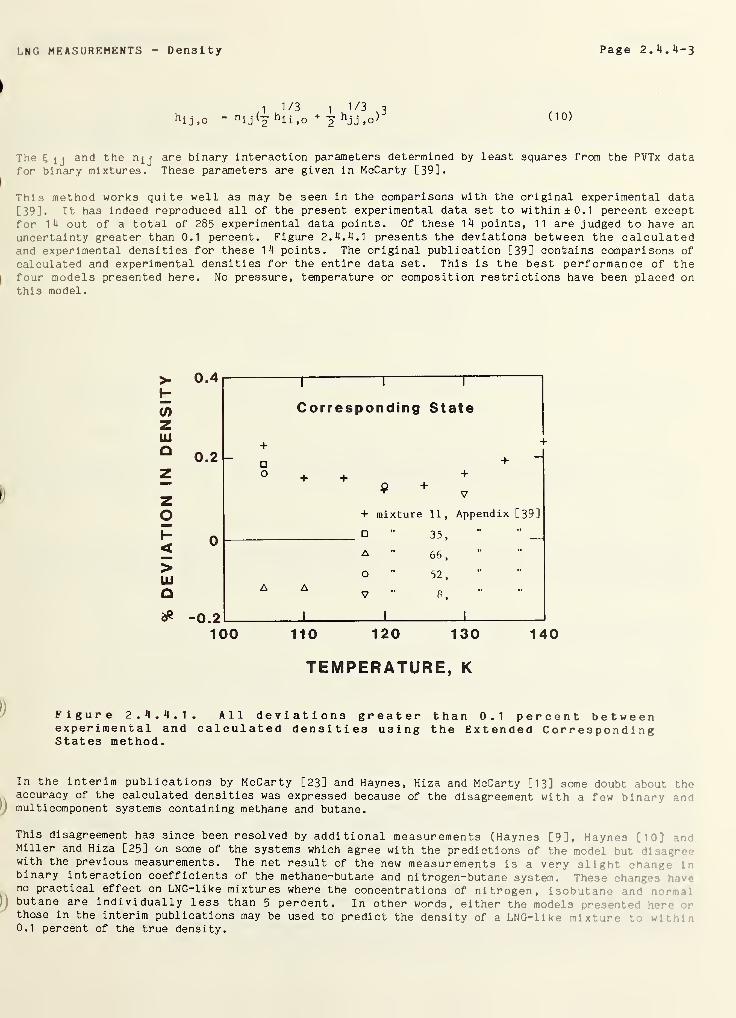
LNG MEASUREMENTS Density Page 2. 4. 4-3
)
11 /3
i 1/3 3hij,o " n ij h ii ,o
+~2 h
j j ,o) ( 10 )
The £ ij and the njj are binary interaction parameters determined by least squares from the PVTx datafor binary mixtures. These parameters are given in McCarty [39].
I
This method works quite well as may be seen in the comparisons with the original experimental data
[39]. It has indeed reproduced all of the present experimental data set to within +0.1 percent exceptfor 14 out of a total of 285 experimental data points. Of these 14 points, 11 are judged to have anuncertainty greater than 0.1 percent. Figure 2. 4. 4.1 presents the deviations between the calculatedand experimental densities for these 14 points. The original publication [39] contains comparisons of
calculated and experimental densities for the entire data set. This is the best performance of the
I
four models presented here. No pressure, temperature or composition restrictions have been placed onthis model.
>•
</>
LU
O
0.4
0.2
< 0
>HI
o-0.2
o
T
Corresponding State
A
!
+ +Q +T v
+ mixture 11, Appendix [39]
" 35,"
".
A " 66
,
O " 52
,
V 8 .
100 110 120 130 140
TEMPERATURE, K
Figure 2. 4. 4.1. All deviations greater than 0.1 percent betweenexperimental and calculated densities using the Extended CorrespondingStates method.
In the interim publications by McCarty [23] and Haynes, Hiza and McCarty [13] some doubt about theaccuracy of the calculated densities was expressed because of the disagreement with a few binary m :
multicomponent systems containing methane and butane.
This disagreement has since been resolved by additional measurements (Haynes [9], Haynes [10' tnlMiller and Hiza [25] on some of the systems which agree with the predictions of the model but di •
with the previous measurements. The net result of the new measurements is a very slight change : nbinary interaction coefficients of the methane-butane and nitrogen-butane system. These on mg •. .ono practical effect on LNG-like mixtures where the concentrations of nitrogen, isobutan^ md n r~
)butane are individually less than 5 percent. In other words, either the models pre 3 enti-d ••••
those in the interim publications may be used to predict the density of a LNG-like mixture • w .
• • •
0.1 percent of the true density.
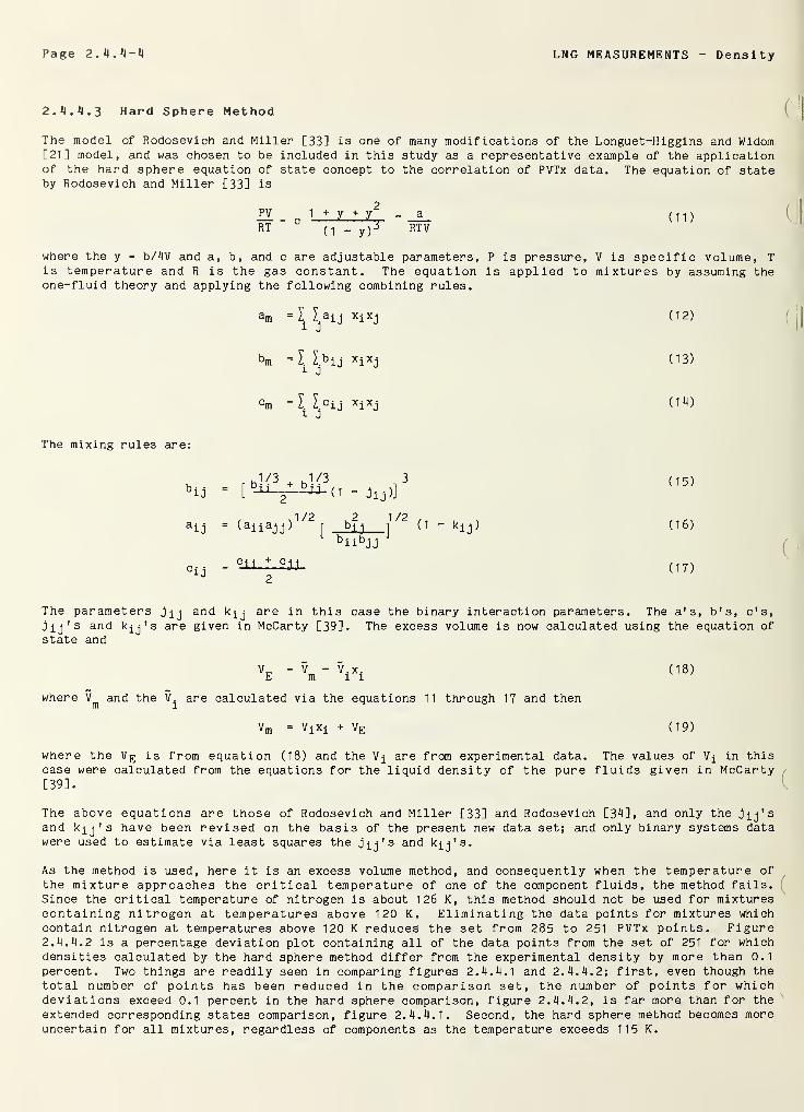
Page 2. 4. 4-4 LNG MEASUREMENTS Dens i ty
2.4.11.3 Hard Sphere Method
The model of Rodosevich and Miller [33] is one of many modifications of the Longuet-Higgins and Widom[21] model, and was chosen to be included in this study as a representative example of the applicationof the hard sphere equation of state concept to the correlation of PVTx data. The equation of stateby Rodosevich and Miller [33] is
= c1 + y + - _L_ (11)
RT (] - y)i RTV
where the y = b/4V and a, b, and c are adjustable parameters, P is pressure, V is specific volume, T
is temperature and R is the gas constant. The equation is applied to mixtures by assuming theone-fluid theory and applying the following combining rules.
am ~ I. I. aiji J
bm =I I. b iji J
cm =I I.°iji J
The mixing rules are:
Xl Xj (12)
XiXj (13)
XiXj (14)
The parametersjij's and kjj'
state and
'ij
„i/3 . J/3‘ - Jij
3
)]
(15)
l ij, .1/2 ,2
- (a^ia-j-j) r bjj1 /21
(1 kjj) (16)
b ii bjjJ
c ii + c ij
2(17)
and kji are in this case the binary interaction parameters. The a'ss are given in McCarty [39]. The excess volume is now calculated using the equation of
where and the V are calculated via the equations 11 through 17 and then
Vm = ViXi + VE (19)
where the V E is from equation (18) and the V ^ are from experimental data. The values of in thiscase were calculated from the equations for the liquid density of the pure fluids given in McCarty[39].
The above equations are those of Rodosevich and Miller [33] and Rodosevich [34], and only the jij'sand kjj's have been revised on the basis of the present new data set; and only binary systems datawere used to estimate via least squares the jij's and k-jj's.
As the method is used, here it is an excess volume method, and consequently when the temperature ofthe mixture approaches the critical temperature of one of the component fluids, the method fails.Since the critical temperature of nitrogen is about 126 K, this method should not be used for mixturescontaining nitrogen at temperatures above 120 K. Eliminating the data points for mixtures whichcontain nitrogen at temperatures above 120 K reduces the set from 285 to 251 PVTx points. Figure2.4. 4.2 is a percentage deviation plot containing all of the data points from the set of 251 for whichdensities calculated by the hard sphere method differ from the experimental density by more than 0.1
percent. Two things are readily seen in comparing figures 2. 4. 4.1 and 2. 4. 4. 2; first, even though thetotal number of points has been reduced in the comparison set, the number of points for whichdeviations exceed 0.1 percent in the hard sphere comparison, figure 2. 4. 4. 2, is far more than for the
extended corresponding states comparison, figure 2. 4. 4.1. Second, the hard sphere method becomes moreuncertain for all mixtures, regardless of components as the temperature exceeds 115 K
.
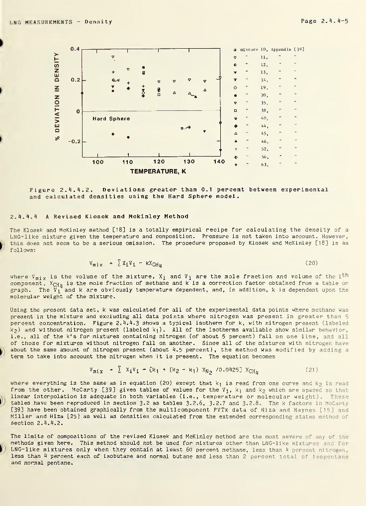
LNG MEASUREMENTS Densi ty Page 2. 4. 4-5
9 mixture 10, Appendix [39]
v " 11,
O '• 12,
V " 13,
V •• 14
,
O ” 19,
• 20,
v " 35,
- 38
,
e " 40,
44
,
A " 45,
A " 46,
+ " 52,
<> ” 56
,
100 110 120 130 140 ^ 63
TEMPERATURE, K
Figure 2. 4. 4.2. Deviations greater than 0.1 percent between experimentaland calculated densities using the Hard Sphere model.
2. 4. 4.
4
A Revised Klosek and Mckinley Method
The Klosek and McKinley method [18] is a totally empirical recipe for calculating the density of a
LNG-like mixture given the temperature and composition. Pressure is not taken into account. However,
this does not seem to be a serious omission. The procedure proposed by Klosek and McKinley [18] is as
follows:
</)
ZHi
o
>UJ
o
u.a
0.2 -
-0.2 -
Vmix = I*iVi - kXCHl4 (20)
where V m i x is the volume of the mixture, and are the mole fraction and volume of the i th
component, Xq^ is the mole fraction of methane and k is a correction factor obtained from a table or
graph. The and k are obviously temperature dependent, and, in addition, k is dependent upon the
molecular weight of the mixture.
Using the present data set, k was calculated for all of the experimental data points where methane waspresent in the mixture and excluding all data points where nitrogen was present in greater than 5
percent concentration. Figure 2. 4. 4. 3 shows a typical isotherm for k, with nitrogen present (labeledk 2 ) and without nitrogen present (labeled k-| ) . All of the isotherms available show similar behavior,i.e., all of the k's for mixtures containing nitrogen (of about 5 percent) fall on one line, and allof those for mixtures without nitrogen fall on another. Since all of the mixtures with nitrogen haveabout the same amount of nitrogen present (about 4.5 percent), the method was modified by adding a
term to take into account the nitrogen when it is present. The equation becomes
Vmix = I *iVi " <! + (k 2 - k-| ) XN2 /0.0425] XCHlj (21)
where everything is the same as in equation (20) except that k-j is read from one curve and k 2 is readfrom the other. McCarty [39] gives tables of values for the V^, k-] and k 2 which are spaced so thatlinear interpolation is adequate in both variables (i.e., temperature or molecular weight). Thesetables have been reproduced in section 3.2 as tables 3.2.6, 3.2.7 and 3.2.8. The k factors in McCarty[39] have been obtained graphically from the multicomponent PVTx data of Hiza and Haynes [15] mlMiller and Hiza [25] as well as densities calculated from the extended corresponding states method ofsection 2. 4. 4. 2.
The limits of compositions of the revised Klosek and McKinley method are the most severe of anymethods given here. This method should not be used for mixtures other than LNG-like mixture' m : :
••
LNG-like mixtures only when they contain at least 60 percent methane, less than 4 perron' nit- gen,less than 4 percent each of isobutane and normal butane and less than 2 percent total of is ' r •
and normal pentane.
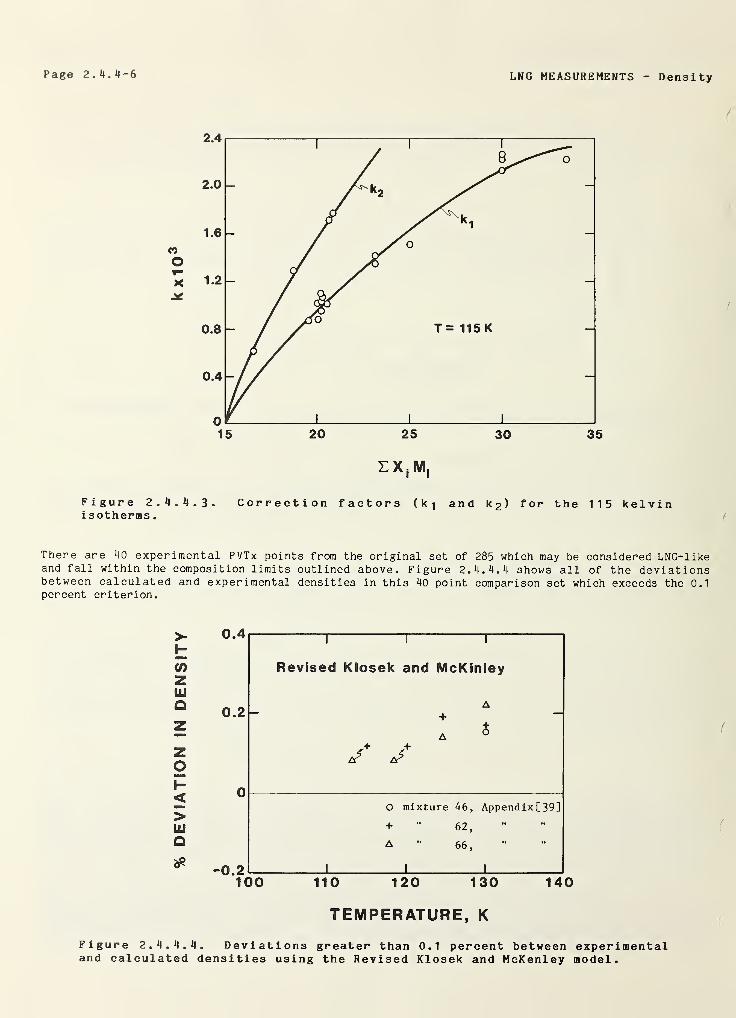
Page 2. 4. 4-6 LNG MEASUREMENTS Density
Figure 2. 4. 4. 3. Correction factors (k-j and k 2 > for the 115 kelvinisotherms
.
There are 40 experimental PVTx points from the original set of 285 which may be considered LNG-likeand fall within the composition limits outlined above. Figure 2. 4. 4.
4
shows all of the deviationsbetween calculated and experimental densities in this 40 point comparison set which exceeds the 0.1percent criterion.
>Hif)
ZHi
o
<>yj
o
0.4i 1 r
Revised Klosek and McKinley
0.2 -
-0.2
+
A
A
s
O mixture 46, Appendix [39]
+ " 62,
A " 66
,
I
100 110 120 130 140
TEMPERATURE, K
Figure 2. 4. 4. 4. Deviations greater than 0.1 percent between experimentaland calculated densities using the Revised Klosek and McKenley model.
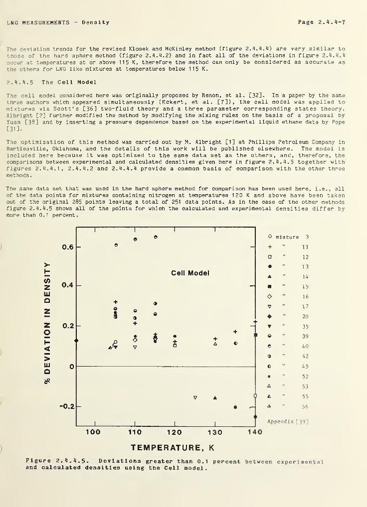
LNG MEASUREMENTS Densi ty Page 2.11.4-7
The deviation trends for the revised Klosek and McKinley method (figure 2. 4. 4. 4) are very similar to
those of the hard sphere method (figure 2. 4. 4.2) and in fact all of the deviations in figure 2.4. 4.
4
occur at temperatures at or above 115 K, therefore the method can only be considered as accurate as
the others for LNG like mixtures at temperatures below 115 K.
2. 4. 4.5 The Cell Model
The cell model considered here was originally proposed by Renon, et al. [32]. In a paper by the samethree authors which appeared simultaneously (Eckert, et al. [7]), the cell model was applied tomixtures via Scott's [36] two-fluid theory and a three parameter corresponding states theory.Albright [2] further modified the method by modifying the mixing rules on the basis of a proposal byYuan [38] and by inserting a pressure dependence based on the experimental liquid ethane data by Pope
[31].
The optimization of this method was carried out by M. Albright [1] at Phillips Petroleum Company in
Bartlesville, Oklahoma, and the details of this work will be published elsewhere. The model is
included here because it was optimized to the same data set as the others, and, therefore, thecomparisons between experimental and calculated densities given here in figure 2. 4. 4. 5 together withfigures 2. 4. 4.1, 2. 4. 4. 2 and 2. 4. 4. 4 provide a common basis of comparison with the other threemethods
.
The same data set that was used in the hard sphere method for comparison has been used here, i.e., allof the data points for mixtures containing nitrogen at temperatures 120 K and above have been takenout of the original 285 points leaving a total of 251 data points. As in the case of the other methodsfigure 2. 4. 4. 5 shows all of the points for which the calculated and experimental densities differ bymore than 0.1 percent.
>
</)
ZUJ
a
O
<>in
Q
0.6
0.4
0.2
0
-0.2
1 1
© ©l i
o mixture 3
_ © + 11
o 12
• 13
Cell Model14
-15
O 16+ O
179 eV
$ ©9
20
+ Hl-
35+
* t * +1 i © 39
a oV
¥£ * c © 40
© 42
45
* 52
A 53
V A I ) 55
— •
( »
A 56
i 1 1 1
Appendix [ 39]
100 110 120 130 140
TEMPERATURE, K
Figure 2. 4. 4. 5. Deviations greater than 0.1 percent between experiment il
and calculated densities using the Cell model.
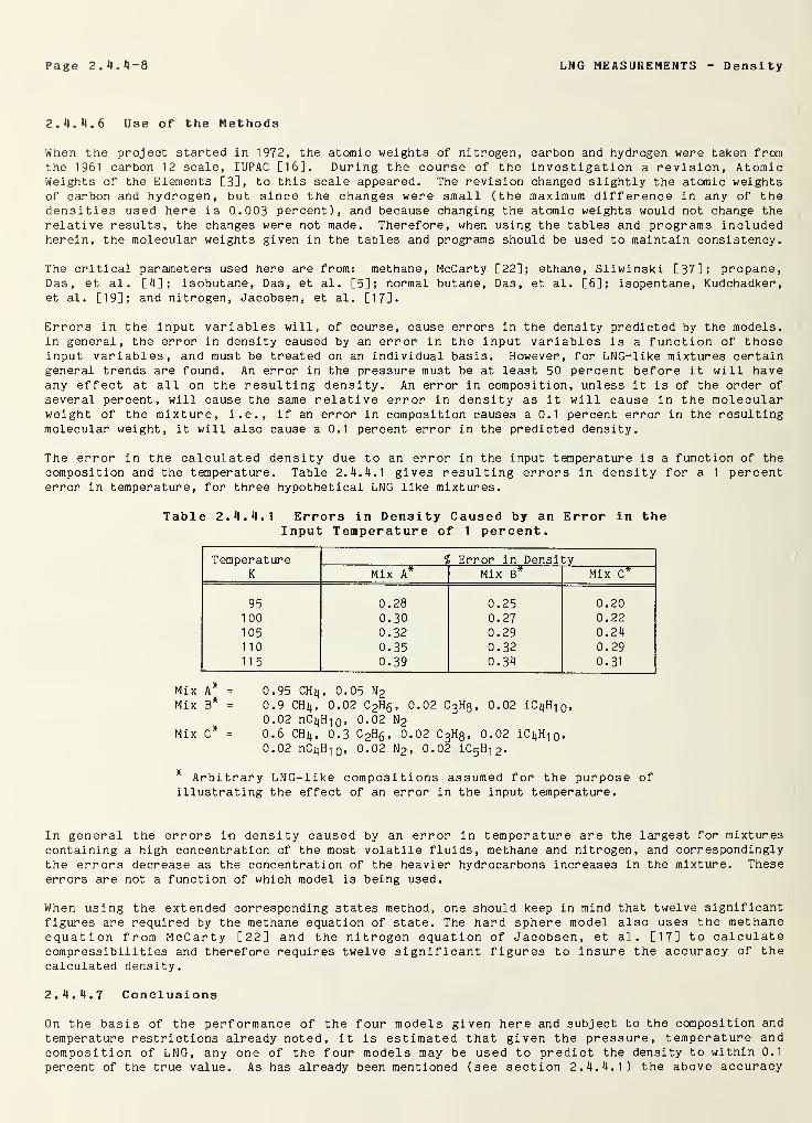
Page 2. 4. 4-8 LNG MEASUREMENTS Density
2. 4. 4. 6 Use of the Methods
When the project started in 1972, the atomic weights of nitrogen, carbon and hydrogen were taken fromthe 1961 carbon 12 scale, IUPAC [16]. During the course of the investigation a revision, AtomicWeights of the Elements [ 3 ], to this scale appeared. The revision changed slightly the atomic weightsof carbon and hydrogen, but since the changes were small (the maximum difference in any of thedensities used here is 0.003 percent), and because changing the atomic weights would not change the
relative results, the changes were not made. Therefore, when using the tables and programs includedherein, the molecular weights given in the tables and programs should be used to maintain consistency.
The critical parameters used here are from: methane, McCarty [22]; ethane, Sliwinski [37]; propane,Das, et al . [4]; isobutane, Das, et al . [5]; normal butane, Das, et al. [6]; isopentane, Kudchadker,et al. [19]; and nitrogen, Jacobsen, et al. [17].
Errors in the input variables will, of course, cause errors in the density predicted by the models.In general, the error in density caused by an error in the input variables is a function of thoseinput variables, and must be treated on an individual basis. However, for LNG-like mixtures certaingeneral trends are found. An error in the pressure must be at least 50 percent before it will haveany effect at all on the resulting density. An error in composition, unless it is of the order of
several percent, will cause the same relative error in density as it will cause in the molecularweight of the mixture, i.e., if an error in composition causes a 0.1 percent error in the resultingmolecular weight, it will also cause a 0.1 percent error in the predicted density.
The error in the calculated density due to an error in the input temperature is a function of the
composition and the temperature. Table 2.4.4. 1 gives resulting errors in density for a 1 percenterror in temperature, for three hypothetical LNG like mixtures.
Table 2. 4. 4.1 Errors in Density Caused by an Error in theInput Temperature of 1 percent.
MixMix
Mix
* Arbitrary LNG-like compositions assumed for the purpose ofillustrating the effect of an error in the input temperature.
TemperatureK
l Error in DensityMix A Mix B* Mix C*
95 0.28 0.25 0.20100 0.30 0.27 0.22105 0.32 0.29 0.24110 0.35 0.32 0.29115 0.39 0.34 0.31
A* = 0.95 CH 4 , 0.05 N2B* = 0.9 CHij , 0.02 C 2H6 , 0.02 C
3H8 , 0.02 iCijHio,
0.02 nCi)H 10 , 0.02 N2C* = 0.6 CH 4 , 0.3 C 2Hg, 0.02 C
3H8 , 0.02 iCijH 10 ,
0.02 nCnH 10 , 0.02 N2 , 0.02 iC5 H-| 2 .
In general the errors in density caused by an error in temperature are the largest for mixturescontaining a high concentration of the most volatile fluids, methane and nitrogen, and correspondinglythe errors decrease as the concentration of the heavier hydrocarbons increases in the mixture. Theseerrors are not a function of which model is being used.
When using the extended corresponding states method, one should keep in mind that twelve significantfigures are required by the methane equation of state. The hard sphere model also uses the methaneequation from McCarty [22] and the nitrogen equation of Jacobsen, et al . [17] to calculatecompressibilities and therefore requires twelve significant figures to insure the accuracy of thecalculated density.
2. 4. 4.7 Conclusions
On the basis of the performance of the four models given here and subject to the composition and
temperature restrictions already noted, it is estimated that given the pressure, temperature andcomposition of LNG, any one of the four models may be used to predict the density to within 0.1
percent of the true value. As has already been mentioned (see section 2. 4. 4.1) the above accuracy
LNG MEASUREMENTS Density Page 2.4. 4-9
statement is dependent entirely upon the accuracy of the experimental data in Haynes, et al . [11],Haynes, et al . [13], Hiza, et al . [14], Haynes [9], Hiza and Haynes [15], Miller and Hiza [25] andHaynes [10]. These data have been estimated by the authors to be accurate to within 0.1 percent of
the true value with a precision of a few hundredths of a percent. The work on the models given herehave provided no basis for questioning the claims of the experimenters, in fact the ability of themodels to predict the densities of the multicomponent mixtures to within 0.1 percent of the measuredvalues tends to support the accuracy claims of the experimenters.
Interim results of this study were reported by Haynes, et al. [13] and McCarty [23], both of whichcontain earlier versions of the mathematical models given here. These earlier versions are onlyslightly different from the final ones, and, for the purposes of calculating LNG densities, either of
the versions may be used. The reader is, however, cautioned to read the limitations of each model asdefined in the earlier sections.
Computer programs for the four models are available at the Thermophysical Properties Division of theNational Bureau of Standards in Boulder, Colorado.
Page 2.4.4-10 LNG MEASUREMENT Density
2 . 4 . 4 . 8 References[1]
Albright, M. A., Private communication (1976).
[2]
Albright, M. A., A Model for the precise calculation of liquefied natural gas densities, NGPATechnical Publication TP-3 (1973).
[ 5 ] Das, T. R. and P.
(1973), p. 253.
T. Eubank
[6] Das,
T . R . and P
.
(1973), p. 244.
T. Eubank
[7] Eckert , C . A . , H
.
Renon andFund 6, 58 (1967).
Chemistry, Vol 37,
Engineering Vol 18,
Engineering Vol 18,
Engineering Vol 18,
J. M. Prausnitz, Molecular Thermodynamics
[3] Atomic weights of the elements 1973, Pure and Applied
[4] Das, T. R. and P. T. Eubank, Advances in Cryogenic
(1973), p. 208.
Advances in Cryogenic
Advances in Cryogenic
589-603 (1974) •
Plenum Press
,
New York
Plenum Press, New York
Plenum Press
,
New York
of Simple Liquids, IEC
[8]
Goodwin, R. D., The thermophysical properties of methane, from 90 to 500 K at pressures up to700 bars, Nat. Bur. Stand. (U.S.), Tech. Note 653 (1974).
[9] Haynes, W. M., Orthobaric liquid densities and dielectric constants of (methane +
2-methylpropane) and (methane + n-butane) at low temperatures, J. Chem. Thermodynamics 15(10),pp 903-11 (Oct 1983).
[10] Haynes, W. M., Measurements of orthobaric liquid densities of multicomponent mixtures of LNGcomponents (N2 , CH 4 , C 2H5 , C
3H8 , iC^Hi q
,
nCijHio. iC^H^, r^H-^) between 110 and 130 K, J. Chem.Thermodynamics 14(7), pp 603“12 (July 1982).
[11] Haynes, W. M., M. J. Hiza and N. V. Frederick, A magnetic suspension densimeter for measurementson fluids of cryogenic interest, Review of Scientific Instruments _47, No. 10, 1237~50 (Oct
1976).
[12] Haynes, W. M. and M. J. Hiza, Measurements of the orthobaric liquid densities of methane,ethane, propane, isobutane, and normal butane, J. Chem. Thermodyn., _9, 179 (1977).
[13] Haynes, W. M., M. J. Hiza and R. D. McCarty, Densities of LNG for custody transfer, (Proc. FifthInternational Conference of LNG, Dusseldorf, Germany), J. W. White, W. McGrew, S. Farmer, D.
Hansen, H. Jacobshagen, editors; Institute of Gas Technology, Chicago, 111., Vol. 2, Paper II,
Section III (1977).
[14] Hiza, M. J., W. M. Haynes and W. R. Parrish, Orthobaric liquid densities and excess volumes for
binary mixtures of low molecular weight alkanes and nitrogen between 105 and 140 K, J. Chem.Thermodyn. 9_, 873 (1977).
[15] Hiza, M. J. and W. M. Haynes, Orthobaric liquid densities and excess volumes for multicomponentmixtures of low molar mass alkanes and nitrogen between 105 and 125 K, J. Chem. Thermodyn. J_2, 1
(1980).
[16] International Union of Pure and Applied Chemistry, 1961 Carbon 12 Scale.
[17] Jacobsen, R. T., R. B. Stewart, R. D. McCarty and H. J. M. Hanley, Thermophysical properties of
nitrogen from the fusion line to 3500 R ( 1 944 K) for pressures to 150,000 psia (10342 x 10^
N/m2 ), Nat. Bur. Stand. (U.S.), Technical Note No. 648 (Dec 1973).
[18] Klosek, J. and C. McKinley, Densities of liquefied natural gas and of low molecular weighthydrocarbons, Proc. First Int. Conf. on LNG, IGT, Chicago (1968).
[19] Kudchadker, A. P., G. H. Alani and B. J. Zwolinski, The Critical Constants of OrganicSubstances, Chem. Rev. _68_, 659-735 (1968).
[20] Leach, J. W. , Molecular structure correction for applying the theory of corresponding states to
non-spherieal pure fluids and mixtures, Ph.D. Thesis, Rice University (1967).
LNG MEASUREMENT Density Page 2.4.4-11
[21] Longuet-Higgins ,H. C. and B. Widom, A rigid sphere model for melting of Argon, Mol. Phys . 8_,
549 (19610.
[22] McCarty, R. D., A modified Benedi ct-Webb-Rubin equation of state for methane using recent
experimental data, Cryogenics J_4, No. 5, 276-80 (May, 1974).
[23] McCarty, R. D., A comparison of mathematical models for the prediction of LNG densities, Nat.
Bur. Stand. (U.S.), Interagency Report NBSIR 77-867 (Oct 1977).
[24] McCarty, R. D., Mathematical models for the prediction of liquefied natural gas densities, J.
Chem. Thermodynnamics 14(9), pp 837~54 (Sept 1982).
[25] Miller, R. C. and M. J. Hiza, Experimental molar volumes for some LNG related saturated liquid
mixtures. Fluid Phase Equilibria _2, 49-57 (1978).
[26] Mollerup, J. and J. S. Rowlinscn, The prediction of densities of liquefied natural gas and of
lower molecular weight hydrocarbons, Chem. Engng. Sci . 29_ (1973).
[27] Mollerup, J., Correlated and predicted thermodynamic properties of LNG and related mixtures in
the normal and critical region, Adv. Cryog. Eng. 20_, 172 (K. D. Timmerhaus, editor, PlenumPress, New York, 1975).
[28] Mollerup, J,, Thermodynamic properties of natural gas, petroleum gas, and related mixturesenthalpy predictions, Adv. Cryog. Eng. _23_ 550 (K. D. Timmerhaus, editor, Plenum Press, New York,
1978).
[29] Orrit, J. and J. F. Olives, Density of liquefied natural gas and its components, Distributed at
the 4th International Conference on Liquefied Natural Gas, Algeria (1974).
[30] Orrit, J. E. and T. M. Laupretre, Density of liquefied natural gas components, Adv. Cryog. Eng.
23 573 (K. D. Timmerhaus, editor, Plenum Press, New York, 1978).
[31] Pope, G. A., Calculation of argon, methane and ethane virial coefficients at low reducedtemperature, Ph.D. Thesis, Rice University (1971).
[32] Renon, H. , C. A. Eckert and J. M. Prausnitz, Molecular Thermodynamics of Simple Liquids, IECFund. 6_, 52 (1967).
[33] Rodosevich, J. B. and R. C. Miller, Calculation of LNG excess volumes by a modified hard-spheremodel, Adv. Cryog. Eng.
_1J9, 339 (1974).
[34] Rodosevich, J. B. , Measurements and prediction of liquefied natural gas densities, M.Sc. Thesis,Univ. Wyoming (1973).
[35] Rowlinson, J. S. and I. D. Watson, The prediction of the thermodynamic properties of fluids andfluid Mixtures - I. The Principle of Corresponding States and Its Extensions, Chem. Eng. Sci.24, 1565 (1969).
[36] Scott, R. L., J. Chem. Phys. 25, 193 (1956).
[37] Sliwinski, P. Z., Die Lorentz-Lorenz funktion von dampfformigem und fluessiyem athan, proparbutan, Phys. Chem. (Frankfurt) _63_ 263 (1969).
[38] Yuan, I. C., Correlation and prediction of excess properties for selected binaries in the •
hydrocarbon boiling range of conformal solution theory, D.Sc. Dissertation, Washing* •
University ( 1 971 )
.
[39] McCarty, R. D., Four mathematical models for the prediction of LNG densities, Nat., 8.-., • •
.
(U.S.), Technical Note 1030, 84 pp (December, 1980).

LNG MEASUREMENT Density Page 2.4. 5-1
2.4.5 Interlaboratory Comparison of LNG Density Measurements
It has been shown in the previous sections of this part of the manual that LNG density may be
determined both by direct measurement and by calculation. However, most commercial direct density
measurement devices are relative in the sense that a calibration is required to establish and maintain
the densimeter's accuracy and precision. In many cases the calibrations rely on calculationtechniques and mathematical models, and, as a result, the two density measurement techniques are
highly interdependent. In order to establish and maintain a dependable measurement system, it is
necessary to develop tests to insure against error.
One such test is the interlaboratory comparison, in which one or more portable density measurement
devices are calibrated at different density reference systems, and the results compared. Both in situ
meter performance and density calculation can be performed. The following sections describe an
international interlaboratory LNG densimetry comparison which was conducted at NBS in Boulder,Colorado, and Gaz de France, Saint-Denis, France. The text is an edited version of a the work of
Roncier, Philippe, Saint-Just and Dewerdt of Gaz de France and Siegwarth and LaBrecque of NBS [17].
The comparison between the two test faci 1 ities, using a portable version of an absolute densimeter,
provides an experimental estimate of the uncertainty of the indirect method of density measurement for
the first time, on a large (32 liter) sample. The two test facilities agree for pure methane to
within about 0.02 percent. For the LNG-like mixtures consisting of methane , ethane, propane, andnitrogen with the methane concentrations always in excess of 86 percent, the calculated density is
within 0.25 percent of the directly measured density for a confidence level of 95 percent.
2. 4.5.1 Introduction
The density of liquefied natural gas (LNG) is one of the factors needed to establish the value of a
quantity of LNG for custody transfer. Two methods are available to determine density: by calculationfrom correlations of density as a function of composition, pressure and temperature, and by directmeasurement
.
The calculational method is one of several commonly used. The density is inferred from measurementsof pressure, temperature and composition using correlations such as one of those developed during theLNG density project at the National Bureau of Standards (NBS) [1]. These calculational methods arebased on a series of density measurements of LNG pure components [2] and mixtures [1] done at NBS.The composition is determined by gas chromatographic analysis of vaporized LNG samples [3,4,5].
Direct density measurement can be accomplished by determining the effect of a change in the liquiddensity on some physical property which is sensed by the density measuring instrument or densimeterimmersed in the liquid. This property might be a buoyancy, frequency, or capacitance. Ideally, noother property of the liquid, such as temperature or composition, will affect the density measurement.
Though direct density measurement is not now used for custody transfer measurement, the measurementsimplicity and the concurrent promise of a greater accuracy have generated an interest in applyingdensimeters to LNG density measurement.
A number of commercially built densimeters are presently available. Some of these instruments arecapable of making cryogenic density measurements. In fact, some were designed specifically for LNGservice. However, those built for LNG service are not necessarily tested or calibrated in LNG. LNGcalibrations, when provided for the densimeters, are generally extrapolated from measurements inliquid nitrogen and ambient temperature hydrocarbons.
Gaz de France (GDF ) has built a facility to test and calibrate commercial densimeters for LNG service[6]. The National Bureau of Standards, at the request of and with the support of the American gasindustry [7], also built a test facility, the density reference system ( DRS) [5,8-12].
Both test facilities are similar in that the densimeters are tested in nominally isothermal sample.'pure methane and LNG-like mixtures. They differ in that the GDF apparatus uses a calculation.! 1 moth l
to determine the density of the test liquid, while NBS uses an absolute densimeter to determinedensity. The densimeter is absolute in that the density of the liquid is determined by the Arch:method, using a single crystal of silicon as the plummet. No calibration liquid is needed or us-
\
If densimeters are used in custody transfer measurement of density, calibration facilities will horequired to maintain measurement accuracy. A means of intercomparing such calibration system.-. w‘. : :
required. A portable version of the DRS densimeter has been built for this purpose [13]. This .• •
,
the portable reference densimeter (PRD), has been used to intercompare the DRS and the Gaz de Frfacility
.
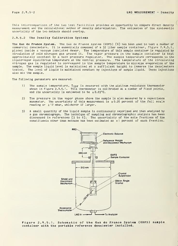
Page 2. 4.5-2 LNG MEASUREMENT Density
This intercomparison of the two test facilities provides an opportunity to compare direct densitymeasurement and the calculational method of density determination. The estimates of the systematicuncertainty of the two methods should overlap.
2. 4.5.2 The Density Calibration Systems
The Gaz de France System. The Gaz de France system (GDFS) [6] has been used to test a number of
commercial densimeters. It is essentially composed of a 32 liter sample container, figure 2. 4. 5.1,placed inside a vacuum insulated dewar. The temperature of this sample container is regulated bycirculation of cold nitrogen gas around it. The vapor pressure in the sample container is keptapproximately constant by a back pressure regulator. The sample temperature corresponds to theliquid-vapor equilibrium temperature at the control pressure. The temperature of the circulatingnitrogen gas is regulated to correspond to the sample temperature to minimize evaporation of thesample. The sample liquid level is maintained at a sufficient height to immerse the densimeterstested. The level of liquid is maintained constant by injections of sample liquid. These injectionsalso mix the sample.
The following parameters are measured:
1) The sample temperature, Tqdf i s measured with the platinum resistance thermometershown in figure 2. 4. 5.1. This thermometer is calibrated at a number of fixed points,and its uncertainty is estimated to be ±0.03°C.
2) The pressure in the vapor phase above the sample is also measured by a capacitancemanometer. The uncertainty of this measurement is ±0.25 percent of the full scalereading or ±12 mbar, whichever if larger.
3) A small quantity of the liquid sample is continuously vaporized and then analyzed by
a gas chromatograph. The technique of sampling and chromatographic analysis has beendiscussed in references [3 to 6]. The uncertainty of the mole fractions of the
constituents other than methane has been estimated as ±1 percent of each fraction.
Figure 2. 4. 5.1. Schematic of the Gaz de France System (GDFS) samplecontainer with the portable reference densimeter installed.
LNG MEASUREMENT - Density Page 2.JJ.5-3
When a satisfactory liquid-vapor equilibrium is reached in the apparatus, the sample temperature, the
vapor pressure, and the composition in the case of mixtures, are recorded at approximately 10-minute
intervals. Then, after changing the control pressure, possibly modifying the composition of the
mixture, and injecting liquid until a new equilibrium is reached, a new set of data are recorded.
The sample density is calculated from the measurements of temperature, pressure, and composition of
the sample. To determine the pure liquid methane density, only the temperature, TqDp of the liquid
near the bottom of the sample container is needed.
The density pqdf for pure saturated liquid methane as a function of temperature is given by a
correlation developed by Haynes and Hiza [2]:
To obtain the mass density values given here, p must be multiplied by the molecular weight, 16.04303g/mol
.
The experimental apparatus was designed to obtain a good liquid-vapor equilibrium, and, ideally, T^pand the temperature Tp calculated from the vapor pressure, using a parabolic interpolation of the
pressure-temperature values in table 13 of reference [14], should agree. Since the sample chamber is
not likely to be perfectly at equilibrium,
can be used as a measure of the quality of the equilibrium within it.
From equation (1) and the two temperatures T^pp and Tp, two values for the sample density can be
calculated: p Q^p = p (Tqdf) and P p = P (Tp) . The difference 6p = p qdf ” P p provides an estimate of themeasurement uncertainty when measuring the density of pure methane. This estimated uncertainty, 6p /
p was found to be ±0.15 percent assumes A T is entirely caused by a liquid temperature gradient.
The density of a mixture is calculated from measurements of Tqdf» P and from measurements of thecomposition by the liquid sampling and calculation methods discussed earlier. The correspondingstates method [1,15], with an estimated uncertainty of ±0.1 percent, was used for this calculation.The vapor pressure and composition are used to calculate a sample temperature [16] as in the case ofmethane. This temperature is used along with the composition to calculate a second density value bythe corresponding states method. This second density value again serves as an evaluation of theequilibrium. This apparatus has been used to test a number of commercially built densimeters.
The determination of LNG density from correlations of density with composition and temperature is
subject to a number of sources of error. The estimated uncertainty of the mathematical models forpredicting LNG density is 0.1 percent [1], The composition determination is subject to uncertainty f
the composition of the chromatograph calibration gas, the uncertainty of the chromatograph measure-men 1
and the uncertainty introduced by the sampling procedure. The uncertainty of the tempera; j remeasurement must also be included. The uncertainties associated with“the various parameters -
• t
follows:
1) The uncertainty assigned to the sampling has been estimated to be 0.1 to 0.15 percentfrom tests of the sampling system [6],
2) The gas chromatograph used for the composition analysis is a state-of-the-artinstrument. The uncertainty it introduces into a density determination will hedependent on the composition of the sample and the accuracy of the calibration g .
P‘Pc (1)
where: p = density in mol/liter
p c = 10.16 mol/liter (critical density)
T = methane temperature in K
T c = 190.555 K (critical temperature)a = 18.65812, b-| = 6.71203, b 2 = - 0.947202 in moles/liter.
A T = Tp - T gdf (2)
Page 2.11.5-4 LNG MEASUREMENT Den3i ty
The uncertainty that the chr omatogr aphi c measurement contributes to the densitydetermination has been estimated in one study to be 0.11 percent for LNG [5].Parrish et al . [ 3 ] estimated an uncertainty contribution of 0.1 percent by thechromatograph to the heating value calculation. The uncertainty introduced into thedensity calculation is generally equal to or slightly less than the heating valueuncertainty
.
3) Errors introduced by the calibration gas uncertainty are based on estimates of theweighing uncertainties when the standard is prepared and is probably no more than±0.03 percent [ 3 ]. An estimate for uncertainty introduced by deviations of theconstituent gases was not available.
4) The density uncertainty introduced by the temperature measurement is about ±0.01percent for a ± 30 mK temperature uncertainty.
Parrish et al . [5] estimated that in the laboratory, the saturated density based on compositiondeterminations from sampling and analysis combined with temperature and pressure measurement could becalculated to an uncertainty of 0.1 percent. This value seems optimistic since combining the
uncertainties above in quadrature gives the uncertainty of a laboratory determination of densitycalculated from temperature and composition measurements of at least 0.2 percent. This includes no
estimate of the uncertainty of the calibration mixture for the chromatograph other than thatintroduced by weighing the mixture.
The Density Reference System (NBS) . The NBS densimeter test facility, the density reference system(DRS) , has been described in the literature [5,8,9,11,12] and in 2.4.1. It is a vacuum insulatedsample container into which 16 liters of methane or LNG-like mixtures can be condensed. The system is
completely closed. No gas vents at any time. Radiation shields cooled by liquid nitrogen reduce theheat leaks into the sample container, and cooling coils remove the remainder. The liquid can bestirred by a turbine pump. The thermal isolation of the sample maintains its isothermal state forminutes after the stirring has ceased. The density of the sample liquid is measured by an absolutedensimeter. This densimeter uses the Archimedes principle, a silicon single crystal immersed in theliquid is weighed by an electronic balance. The density of single crystal silicon is known to a fewppm, and if the vacuum weight of the crystal is measured, no calibrating fluid is necessary. Thedensity of the liquid, p ]_ , is
Pi = P S (1-M/Ms ) (3)
where p s is the crystal density, Ms is its vacuum weight and M is its apparent weight when completelyimmersed in the liquid.
When commercial densimeters were found to lack adequate calibrations, a transfer standards program wasinitiated by NBS to provide a better method of calibration to manufacturers and users (see 2.4.2).Densimeters of a manufacturer's or user's choice were calibrated in the DRS then returned to them.
They would then use these calibrated instruments in their own sample container to calibratedensimeters sold. The calibration should be done in an LNG-like mixture for best results.
The transfer standard method of providing calibrations has disadvantages, however. The calibration of
a standard could change with time or through shipping and handling. Repeated calibrations arenecessary at least until a long term stability is established for the instrument. If the long termstability is adequate, there still remains the question of how well the calibration system in whichthe transfer standard is employed transfers the calibration from the standard to the densimeter undercalibration. Testing calibrated densimeters in the DRS or GDFS could establish whether thecalibration has been adequately transferred. Continual monitoring of the calibration operation is
desirable to ensure the best calibration of the commercially available densimeters.
During the course of testing the commercial densimeters, both the DRS and the DRS densimeter wereimproved. The densimeter was improved by replacing the original electronic balance with a morecompact and rugged one of greater range. The greater range permits the silicon crystal to be weigheddirectly instead of relative to a reference weight. The reference weight is retained in the new
densimeter but now provides a means of adjusting and monitoring the balance calibration. Thisredesign suggested the possibility of making a portable standard densimeter of a design similar to thenew DRS densimeter. This portable standard could be transported to other calibration facilities to
measure their calibration uncertainty and to intercompare calibration facilities. A portablestandard, the portable reference densimeter (PRD), has been built for this purpose. The PRD is shownschematically in figure 2. 4. 5.1 in place in the GDFS. This densimeter and comparison densitymeasurements between it and the DRS are described in [12] and [13].
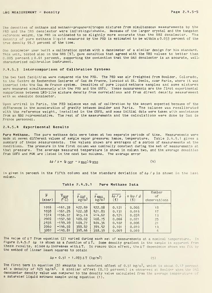
LN G MEASUREMENT Density Page 2. 4. 5-5
The densities of methane and methane-propane-nitrogen mixtures from simultaneous measurements by the
PRD and the DRS densimeter were indistinguishable. Because of the larger crystal and the tungsten
reference weight, the PRD is estimated to be slightly more accurate than the DRS densimeter. Thedensity of pure methane liquid measured by the PRD is estimated to be within ± 0.033 percent of the
true density 99.7 percent of the time.
One densimeter user built a calibration system with a densimeter of a similar design for his standard.
This unit, tested also in the DRS [9], gave densities that agreed with the DRS values to better than
0.005 percent ±0.01 percent, supporting the contention that the DRS densimeter is an accurate, well-
characterized calibration instrument.
2. 4. 5. 3 Intercomparison of Calibration Systems
The two test facilities were compared via the PRD. The PRD was air freighted from Boulder, Colorado,to the Centre de Recherches Gazieres of Gaz de France, located at St. Denis, near Paris, where it was
inserted into the Gaz de France system. Densities of pure liquid methane samples and some mixtureswere measured simultaneously with the PRD and the GDFS. These measurements are the first experimentalcomparisons between LNG-like mixture density from correlations and from direct density measurementwith an absolute densimeter.
Upon arrival in Paris, the PRD balance was out of calibration by the amount expected because of the
difference in the acceleration of gravity between Boulder and Paris. The balance was recalibratedwith the reference weight, installed in the GDFS, and some initial data were taken with assistancefrom an NBS representative. The rest of the measurements and the calculations were done by Gaz deFrance personnel.
2. 4. 5. 4 Experimental Results
Pure Methane. The pure methane data were taken at two separate periods of time. Measurements weremade at seven different values of sample vapor pressure; hence, temperature. Table 2. 4.5.1 gives a
summary of these measurements. The values shown are averages of a series of measurements at theconditions. The pressure in the first column was nominally constant during the set of measurements at
that pressure. The average measured temperature is shown in column two, and the average densitiesfrom GDFS and PDR are listed in the next two columns. The average error
Ap / p = (p GDF P NBS^/P NBS ( *0
is given in percent in the fifth column and the standard deviation of Ap / p is shown in the lastcolumn.
Table 2. 4.5.1 Pure Methane Data
p
(mbar
)
TGDF(° C)
P GDFkg/mu
P NBSkg/irp
Ap / p
(%)
o (Ap / p)
(%)
Numberof
observations
1018 -161.39 422.59 422.08 0.121 0.005 18
1038 -161 .25 422.38 421 .83 0.131 0.015 171514 -156.37 415.14 41 4.62 0.124 0.034 13
2009 -152.50 409.02 408.75 0.066 0.021 252435 -149.49 404.77 404.36 0.102 0.006 21
2960 -146.59 399.92 399.52 0.101 0.010 1 4
3092 -145.81 398.66 398.39 0.069 0.069 6
The value of A T from equation (2) varied during each set of measurements at a nominal temper v . jr-.figure 2. 4.5.2 Ap is shown as a function of AT. Some density gradient in the sample is apparent fr -
these results, since Ap increases with AT. To remove this effect, the A T dependence shown w.t' •
the method of linear least squares to obtain
Ap = 0.51 + 1 .093 AT (kg/m3) (5)
The first term in equation (5) amounts to a constant offset of 0.51 kg/m3, which is about ).i; perat a density of 425 kg/m3. A similar offset (0.10 percent) is observed at Bou! i<-r w *
densimeter density value was compared to the density value calculated from the aver iv'- ••••.; .•••
a saturated liquid methane sample using equation (1).
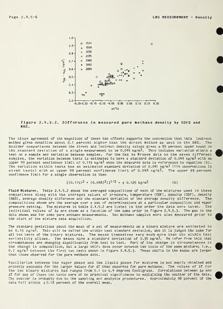
Page 2. 4.5-6 LNG MEASUREMENT Den3i ty
4T(°C)
Figure 2. 4. 5. 2, Difference in measured pure methane density by GDFS andNBS
.
The close agreement of the magnitude of these two offsets supports the contention that this indirectmethod gives densities about 0.1 percent higher than the direct method as used in the DRS. TheBoulder comparisons between the direct and indirect density values gives a 99 percent upper bound onthe standard deviation of a single measurement to be 0.046 kg/m3. This includes variation within a
test on a sample and variation between samples. For the Gaz de France data on the seven differentsamples, the variation between tests is estimated to have a standard deviation of 0.044 kg/m3 with anupper 99 percent confidence limit of 0.115 kg/m3 when the measured data is referenced to equation (5).The variation within tests has an estimated standard deviation of 0.041 kg/m3 (114 observations inseven tests) with an upper 99 percent confidence limit of 0.048 kg/m3. The upper 99 percentconfidence limit for a single observation is then
[(0.115)2 + (0.048)2)
J
1 /2 = + 0.125 kg/m3 (6)
Fluid Mixtures. Table 2. 4. 5. 2 shows the averaged compositions of each of the mixtures used in thesecomparisons along with the averaged values of pressure, temperature (GDF), density (GDF), density(NBS), average density difference and the standard deviation of the average density difference. Thecompositions shown are the average over a set of determinations at a particular composition and vapor
pressure setting. The mixtures in table 2. 4.5.2 are listed in the order the data were taken. Theindividual values of Ap are shown as a function of the same order in figure 2. 4. 5. 3. The gap in the
data shown was for some pure methane measurements. Two methane samples were also measured prior tothe start of the mixture data acquisition.
The standard deviations about the mean of a set of measurements on a binary mixture are estimated to
be 0.15 kg/m3. This will be called the within test standard deviation, and it is judged the same for
all ten tests of the binary mixtures. The means themselves vary much more than the within testvariability allows. The means have a standard deviation of 0.35 kg/m3. We infer from this that
circumstances are changing significantly from test to test. Part of the change in circumstances is
the change in composition, but a large shift does occur between two tests of the same mixture; i.e.,
0.7 kg/m3 between the first two tests shown in figure 2. 4.5. 3. These shifts in the means are largerthan those observed for the pure methane data.
Equilibrium between the vapor phase and the liquid phase for mixtures is not easily obtained andprobably accounts for the larger values for AT than observed for pure methane. The values of AT forthe ten binary mixtures had ranges from 0.1 to 0.4 degrees Centigrade. Correlations between Ap andAT for any of these ten tests were of no practical significance in explaining the scatter of the data.
The scatter is probably due to the sampling and analysis procedures. Approximately 98 percent of the
data fall within ±0.18 percent of the overall mean.
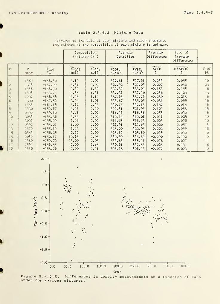
LNG MEASUREMENT Density Page 2. 4.5-7
Table 2. 4.5.2 Mixture Data
Averages of the data at each mixture and vapor pressure.
The balance of the composition of each mixture is methane.
Composition(balance CH 4 )
AverageDensities
AverageDifference
S.D. of
AverageDifference
P tGDF XC 2H 6 xc3h8 PGDF PNBS Ap/p 0 ( Ap/p) # of
mbar °C mol? mol? kg/m3 kg/nP ? ? Pt
1 1 460 -156.40 4.13 0.00 427.81 427.61 0.044 0.044 10
2 1378 -157.22 3.87 0.00 427.92 427.04 0.207 0.030 23
3 1 446 -156.30 3.43 1.32 432.32 433.01 -0.153 0.1 44 16
4 1494 -155.75 5.45 1.31 437.31 437.10 0.048 0.123 13
5 1237 -158.54 4.45 1.12 437.63 437.76 -0.030 0.213 6
6 1330 -157.52 3.94 1 .01 433.87 434.04 -0.038 0.099 16
7 1356 -161 .14 3.62 0.94 440.73 440.14 0.132 0.015 16
8 1930 -152.67 4.25 0.00 422.41 421 .99 0.101 0.053 14
9 2390 -149.10 4.71 0.00 418.46 418.58 0.055 0.032 16
10 3034 -1 45.36 4.55 0.00 412.15 412.06 0.018 0.024 12
11 3026 -1 44.99 6.98 0.00 418.85 418.83 0.003 0.028 1 2
12 2992 -145.01 8.00 0.00 421 .91 421 .83 0.020 0.047 4
13 2970 -1 45.12 8.29 0.00 423.00 422.94 0.002 0.099 18
1 4 2454 -1 48.24 7.60 0.00 425.66 425.60 0.01 4 0.032 10
15 2040 -150.17 12.63 0.03 442.99 443.39 -0.090 0.120 12
16 1980 -150.72 13.00 0.03 444.83 445.18 -0.078 0.027 1 1
17 1 491 -156.55 0.00 2.85 430.61 430.54 0.025 0.131 16
18 1958 -153.06 0.00 2.91 425.83 426.14 -0.071 0.023 1 2
Order
Figure 2. 4. 5. 3. Differences in density measurements as a function of dataorder for various mixtures.
Page 2 . 4 .5-8 LNG MEASUREMENT Densi ty
The estimated standard deviations about the mean of a set of measurements of a ternary mixture aremostly around 0.5 kg/m3. One is as low as 0.1 kg/m3and one as high as 0.9 kg/m3. The eight meansthemselves are varying with an estimated standard deviation of 0.3 kg/m3. Approximately 95 percent of
this data fall within ±0.25 percent of the overall mean.
2. 4.5.5 Conclusions
Though the density determined from temperature and composition measurements using a correlation hasbeen compared to the density measured by commercial densimeters [6], this work represents the firstknown comparison to an absolute densimeter. This comparison provides a direct experimental estimateof the uncertainty associated with the method of determining density from correlations using measuredtemperature and composition.
The density measured by the PRD in pure liquid methane was 0.12 percent smaller than the densitydetermined by the GDFS by calculation from a sample temperature measurement, provided a correction is
introduced for AT. Similar results were obtained in the DRS. When the directly measured liquidmethane density is compared to the density calculated from the averaged readings of two thermometers,the directly measured density is 0.10 percent low. This means that the GDFS and the DRS agree towithin 0.02 percent on density measurements in pure methane when a correction is made for the 0.1
percent offset between direct density measurement by the DRS or PRD and the Haynes-Hiza density fromtemperature correlation [2]. Thus, the two test systems show good agreement on liquid methanedensity. The upper 99 percent limit of a measurement of density in this comparison is 0.125 kg/m3compared to a similar limit of 0.046 kg/m3 for the DRS [9].
The densities of the mixtures examined in this work measured by the GDFS and the PRD differed by nomore than 0.25 percent in 95 percent of the measurements. This value does not conflict with theestimated errors for the two measurement methods but is larger than the 0.1 percent estimated from the
heating value studies [5]. The uncertainty in heating value was estimated to be ±0.15 percent in thelaboratory [5] and ±0.3 percent for measurements on shipboard [ 3 ]. Based on this, the uncertainty infield measurement of LNG density by sampling and analysis of the liquid could be larger than the ±0.25percent obtained in the comparison of the DRS and GDFS described here.
LNG MEASUREMENT Dens i ty Page 2. 5-9
2. *1.5.6 References
McCarty, R. D., Four mathematical models for prediction of LNG densities, Nat. Bur. of Stand.
(U.S.), Technical Note 1030 (December 1980). Also, McCarty, R. D., Mathematical models for the
prediction of liquefied natural gas densities, J. Chem. Thermodynamics _1_4, 837, 1982.
[2] Haynes, W. M. and M. J. Hiza, Measurements of orthobaric liquid densities of methane, ethane,
propane isobutane and normal butane, J. Chem. Thermodynamics _9, 179 (1977).
[ 3 ] Parrish, W. R., J. M. Arvidson and J. F. La3recque, Development and evaluation of an LNGsampling measurement system, Nat. Bur. of Stand. (U.S.), NBSIR 78-887 (July 1978).
[4] Parrish, W. R., J. M. Arvidson and J. F. LaBrecque, Evaluation of LNG sampling measurementsystems for custody transfer, AGA Operating Section Proceedings, Proceedings of the TransmissionConference; Montreal, Quebec, T-236 (1978).
[5] Parrish, W. R., J. A. Brennan and J. D. Siegwarth, LNG custody transfer research at the NationalBureau of Standards, AGA Operating Section Proceedings; Proceedings of the TransmissionConference, Montreal, Quebec, Canada, T-243 (1978).
[ 6 ] Dewerdt, F. and P. Mousset, Contribution a 1' amelioration du comptage du GNL - evaluation de
densimetres et echantillonneur pour GNL, Sixth International Conference on Liquefied NaturalGas, Kyoto, Japan (1980), Appendix, Paper 8 .
[7] The work was supported first by the American Gas Association, 1515 Wilson Blvd., Arlington, VA
22209 and later by the Gas Research Institute, 8600 West Bryn Mawr Avenue, Chicago, IL 6O 631 .
[ 8 ] Siegwarth, J. D., B. A. Younglove and J. F. LaBrecque, Cryogenic fluids density referencesystem: provisional accuracy statement, Nat. Bur. of Stand. (U.S.), Technical Note 698(November 1977).
[9] Siegwarth, J. D. and J. F. LaBrecque, Cryogenic fluids density reference system: provisionalaccuracy statement (1980), Nat. Bur. of Stand. (U.S.), Technical Note 1041 (1981).
[10] Siegwarth, J. D., B. A. Younglove and J. F. LaBrecque, An evaluation of commercial densimetersfor use in LNG, Nat. Bur. of Stand. (U.S.), Technical Note 697 (October 1977).
[11] Siegwarth, J. D., J. F. LaBrecque and B. A. Younglove, Test of densimeters for use in custodytransfer of LNG, Proceedings 53rd International School of Hydrocarbon Measurement, Norman,Oklahoma (1978) p 385.
[12] Siegwarth, J. D. and J. A. Brennan, LNG instrumentation for custody transfer, AGA OperatingSection Proceedings; Proceedings of the Transmission Conference, Atlanta, Georgia, T— 119 (1981).
[13] Siegwarth, J. D. and J. F. LaBrecque, A portable calibration densimeter for use in cryogenicliquids, Nat. Bur. of Stand. (U.S.), Technical Note 1035 (1981).
[14] Goodwin, R. D., The thermophysical properties of methane from 90 to 500K at pressures to 703bar, Nat. Bur. of Stand. (U.S.), Technical Note 653, (April 1974).
[15] McCarty, R. D., A comparison of mathematical models for the prediction of LNG densities, Nat.Bur. of Stand. (U.S.), Interagency Report 77-867 (October 1977).
[16] The method is described in an unpublished note by Gaz de France. The method is based on thework by B. Lee, J. H. Erbar, and W. C. Edminster, Prediction of thermodynamic properties for -
temperature hydrocarbon process calculations, AIChE Journal _1_9, 349 (1973).
[17] Roncier, R. P., J. Saint-Just, J. F. Dewerdt, J. D. Siegwarth and J. F. LaBrecque, Esti-v- :
uncertainty of calculated liquefied natural gas density from a comparison of NBS ar.t Giz ;•
France densimeter test facilities, Nat. Bur. Stand. (U.S.), J. Research, 88 No. 3, In--’(May-June, 1983).


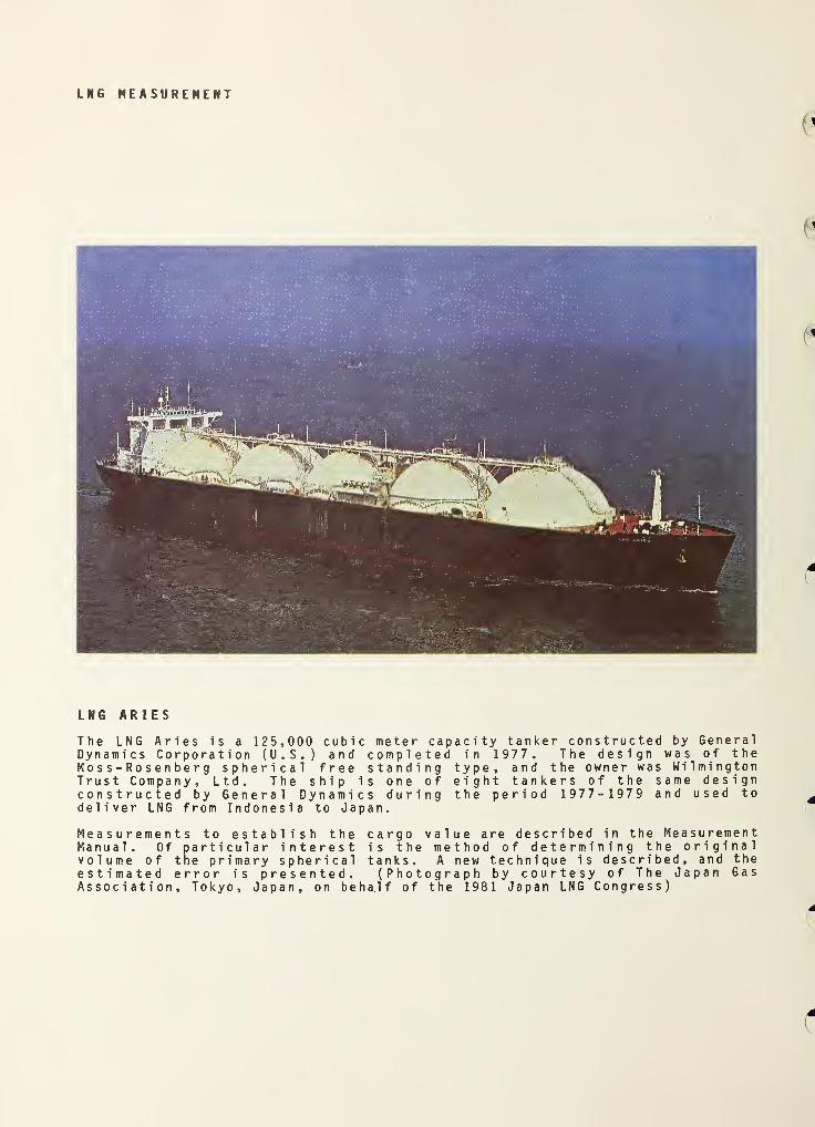
LNG MEASUREMENT
0
LNG ARIES
The LNG Aries is a 125,000 cubic meterDynamics Corporation (U.S.) and compleMoss-Rosenberg spherical free standiTrust Company, Ltd. The ship is oneconstructed by General Dynamics durideliver LNG from Indonesia to Japan.
capacity tanker constructed by Generalted in 1977. The design was of theng type, and the owner was Wilmingtonof eight tankers of the same designng the period 1977-1979 and used to
value are described in the Measurementmethod of determining the originalA new technique is described, and the
ograph by courtesy of The Japan Gasthe 1981 Japan LNG Congress)
Measurements to establish the cargoManual. Of particular interest is thevolume of the primary spherical tanks,estimated error is presented. (PhotAssociation, Tokyo, Japan, on behalf of
4
A
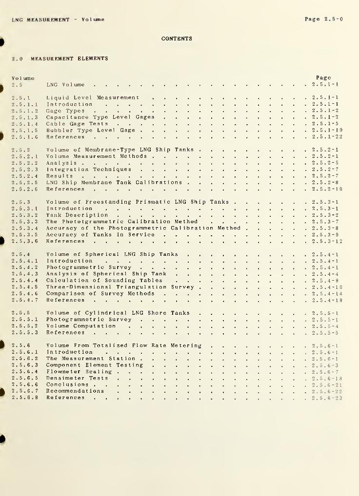
LNG MEASUREMENT Vo 1 ume Page 2.5-0
CONTENTS
2.0 MEASUREMENT ELEMENTS
Vo 1 ume Page2 . 5 LNG Volume 2. 5. 1-1
2.5.1 Liquid Level Measurement 2. 5. 1-1
2.5. 1.1 Introduction 2. 5. 1-1
2.5. 1.2 Gage Types 2.5. 1-2
2.5. 1.3 Capacitance Type Level Gages 2. 5. 1-2
2.5. 1.4 Cable Gage Tests 2.5. 1-5
2.5. 1.5 Bubbler Type Level Gage 2.5.1-192.5. 1.6 References 2.5.1-22
2.5.2 Volume of Membrane-Type LNG Ship Tanks 2. 5. 2-1
2.5.2. 1 Volume Measurement Methods 2. 5. 2-1
2. 5. 2. 2 Analysis 2. 5. 2-5
2. 5. 2. 3 Integration Techniques 2. 5. 2-7
2. 5. 2. 4 Results 2. 5. 2-7
2. 5. 2. 5 LNG Ship Membrane Tank Calibrations 2. 5. 2-8
2. 5. 2. 6 References 2.5.2-10
2.5.3 Volume of Freestanding Prismatic LNG Ship Tanks 2.5. 3-1
2. 5. 3.1 Introduction 2. 5. 3-1
2. 5. 3. 2 Tank Description 2. 5. 3-2
2. 5. 3. 3 The Phototgrammetric Calibration Method 2. 5. 3-72. 5. 3. 4 Accuracy of the Photogrammetric Calibration Method 2. 5. 3-8
2. 5. 3. 5 Accuracy of Tanks in Service 2. 5. 3-92. 5. 3. 6 References 2.5.3-12
2.5.4 Volume of Spherical LNG Ship Tanks 2. 5. 4-12. 5. 4.1 Introduction 2. 5. 4-12. 5. 4. 2 Photogrammetric Survey 2. 5. 4-12. 5. 4. 3 Analysis of Spherical Ship Tank 2. 5. 4-42. 5. 4. 4 Calculation of Sounding Tables 2. 5. 4-82. 5. 4. 5 Three-Dimensional Tr i angu 1 a t i on Survey 2.5.4-102. 5. 4. 6 Comparison of Survey Methods 2.5.4-142. 5. 4. 7 References 2.5.4-18
2.5.5 Volume of Cylindrical LNG Shore Tanks 2. 5. 5-12. 5. 5.1 Photogrammetric Survey 2. 5. 5-12. 5. 5. 2 Volume Computation 2. 5. 5-42. 5. 5. 3 References 2. 5. 5-5
2.5.6 Volume From Totalized Flow Rate Metering 2. 5. 6-12. 5. 6.1 Introduction 2. 5. 6-12. 5. 6. 2 The Measurement Station 2. 5.6-12. 5. 6. 3 Component Element Testing 2. 5. 6-32. 5. 6. 4 Flowmeter Scaling 2. 5. 6-72. 5. 6. 5 Densimeter Tests 2.5.6-182. 5. 6. 6 Conclusions 2.5.6-212. 5. 6. 7 Recommendations 2.5.6-222. 5. 6. 8 References 2.5.6-23

LNG MEASUREMENT Volume Page 2.5. 1-1
2.5 LNG Volume
2.5.1 Liquid Level Measurement
The level of liquid in a fixed volume container is a measure of quantity but is in itself of limitedpractical use. Combination of this measurement with that of volume-height calibrations (see 2.5.2 and
following sections) allow calculation of volume quantities as a function of liquid level above a fixed
datum plane. A direct or calculated density (see 2.4), which must be representative of the entire
volume, can then be combined with the volume calculation to give the mass of LNG associated with the
liquid level. Liquid level is then only a portion of a rather complex process which is designed to
provide a measure of quantity and quality of LNG. A critical assessment of the measurementuncertainties associated with the performance of several types of these devices has been made by
Siegwarth [23]. This work, conducted at NBS-Boulder and sponsored by the Maritime Administration of
the U.S. Department of Commerce, is presented in edited form in the following sections.
The measurement uncertainties of three types of gages commonly used in large liquefied natural gas
storage and ship transport tanks were studied. The types are bubbler, capacitance, and cable gages.
Measurement uncertainties for various types can be determined, but the test conditions must be
carefully specified, because many of the largest errors result from parameters external to the gaging
device. The gage installation, the tank design, and the liquid properties all influence gagingaccuracy. A modification of cable gage installations that should significantly improve gagingaccuracy is presented. Intrinsic accuracies of some representative cable gages are reported fromtests done at ambient temperature under nearly isothermal conditions. The gages tested, if
calibrated, can all measure level to about one millimeter under the test conditions. Capacitancegages should be tested in liquefied natural gas to establish their measurement uncertainty. Bubblergages require knowledge of liquid density, the temperature distributions in and contents of theconnecting tubes, pressure drops, and head corrections; otherwise, the errors can be severalcentimeters
.
2. 5. 1.1 Introduction
Custody transfer of shipload quantities of liquefied natural gas (LNG) is currently accomplished by
measurement of the volume, density and heating value per unit mass of the liquid. The volume incustody transfer is determined by measuring liquid level in calibrated ship transport tanks withliquid level gages. The National Bureau of Standards has had an active program in custody transfermeasurement in which measurement methods have been examined and improved, and uncertainties for manyof the measurements have been established (see References 1 through 11).
Extensive work has been completed and reported on all custody transfer measurements but liquid levelmeasurement. The only cryogenic liquid level work at NBS to date has been a survey of level gagingmethods [12].
Level gage manufacturers usually supply gage accuracy estimates for their instruments. Theseestimates are based on design analysis, and perhaps ambient temperature tests of the gages, butgenerally not cryogenic tests except on a very limited scale. This is not surprising, since the greatheights of tanks, up to 40 meters in some cases, preclude full scale cryogenic testing of gages by anyone manufacturer because of the high cost of both the facility and the tests. A few papers in thepublished literature discuss some of the gaging methods and usually give some estimates of gageaccuracy [13 through 19]. Few sub-ambient temperature tests have been done on any gages, and noindependent tests of gages or tests of a number of gages in a single facility have been reported inthe literature. The following should be considered an initial step in independently evaluating levelgage accuracy.
The three types of level gages considered are the main choice for custody transfer measuremen” ofin shipload quantities. They are the capacitance type, the cable type and the bubbler type. T; •
types are described in more detail in later sections. The capacitance type is generally used is th<
primary gage for custody transfer, while the cable gage or the bubbler usually serves as a bigage. Gaging methods used for small tanks, such as truck tanks, are not included in this study.
The measurement uncertainties of some representative gages of the three types have been •. • :
estimated from available information. Level gaging for custody transfer is assumed to take wo-the tank level is static, so the liquid surface is relatively quiet. Gage accuracy when th-is moving is not estimated. Some of the gaging devices are too slow to even follow theif the tank is rapidly filled. The uncertainty and hysteresis of four different types of cable .-.."shave been measured at ambient conditions.
Page 2. 5. 1-2 LNG MEASUREMENT Volume
Because the measurement of level by capacitance gages and bubbler gages depends on bulk parametersrather than the difference between liquid and vapor, as do the cable gages, adequate testing requiresthe use of a liquid, preferably LNG. No test facility presently exists that is capable of suchmeasurements. Limited resources precluded such tests in this work. The measurement uncertainties forcapacitance gages and bubbler gages have been estimated from existing information. The temperaturewithin a tank and the external environment affect cable gage accuracies. The uncertainties introducedinto cable gage measurements by the environment and ways of reducing these uncertainties are coveredin Siegwarth [23]
.
2. 5. 1.2 Gage Types
Capacitance Gage Capacitance level gages are conceptually simple devices. One type has beendescribed in the literature [18]. They are cylindrical capacitors consisting of two uniform coaxialtubes whose total capacitance is proportional to length if end effects are neglected. A verticalcoaxial capacitor in vacuum has a capacitance of . If this capacitor is filled with a dielectricliquid to a height h, then
C = 2irh(e^-1)ln b/a + C-| = hCjiq + C-j (1)
where is the dielectric constant of the liquid, b and a are the outer tube ID and inner tube ODrespectively, and C]_jn is the capacitance over and above the vacuum value added by the liquiddielectric. Actually, the empty portion of the gage contains a gas, so the term e£ -1 is replaced bythe term - e
gwhere e
gis the gas dielectric constant and C-| is now the gas filled value of C.
For Cjiq to remain proportional to h, and eg must remain independent of time and fill level.
Capacitance gages have limited application because the liquids in which they are used must leave noresidue on the surfaces of the capacitor. Also, the liquids must have very low electricalconductivity. Liquefied natural gas appears to meet both these requirements.
Cable Gage Cable type level gages consist of a surface sensor suspended on a vertical wire, tape or
cable [14-17, 19]. As the liquid surface and the surface sensor move, the wire, tape or cable iswound on, or unwound from, a storage drum in the gage head to maintain the sensor at the liquidsurface. The change in length of wire, etc., is measured either by the drum rotation or by a
calibrated sprocket located in the gage head. The drum or sprocket drives a counter which gives the
level of the liquid. This type of gage is widely used and can be used for almost any liquid.
A number of manufacturers build cable operated gages in a range of designs. Some gages, calledautomatic gages, are mechanical, while others are servo driven. In the latter the surface sensortransmits signals enabling the drive motor to maintain the sensor at the liquid surface.
Bubbler Gage Bubbler gages measure hydrostatic head. The pressure of a noncondensing gas required to
displace all the liquid out the open bottom end of a drop tube that extends to the tank bottom is
approximately the hydrostatic pressure. Usually, gas is bubbled slowly out the bottom of the tube toinsure the liquid level has been forced to the bottom. From the hydrostatic head and the liquiddensity, the liquid level can be calculated.
2. 5. 1.3 Capacitance Type Level Gages
General Description A schematic diagram of a capacitance level gage is shown in figure 2. 5. 1.1. Thegage consists of flanged sections of tube 1 with sections of smaller tube 2 mounted concentricallyinside and supported by insulating posts 3. The inner tube sections are electrically isolated from
each other by either a gap or a dielectric plug 4. The outer tube flanges 6 are bolted together sothe outer tubes form a single conductor. This outer tube is electrically isolated by the insulator 5
from the tank 8. One lead from the outer tube and leads from each of the center tube sections arebrought out of the tank through a seal 7. The center sections of a capacitance gage are oftenconnected together electrically within the tank so that leads from only a top, bottom and centersection need be brought out along with a lead from the outer tube.
A properly installed gage is supported vertically by the floor of the tank and is supported in thetransverse directions but not constrained in the vertical direction at all other points. The
segmented design insures that the gage can be handled and installed. It also permits selecting tubesof uniform dimension to minimize variation in the capacitance per unit length. The main purpose of
segmenting the gages is to electrically isolate the center segments. Isolating sections allows thegage segments to be electrically switched so only the segment containing the liquid surface and a
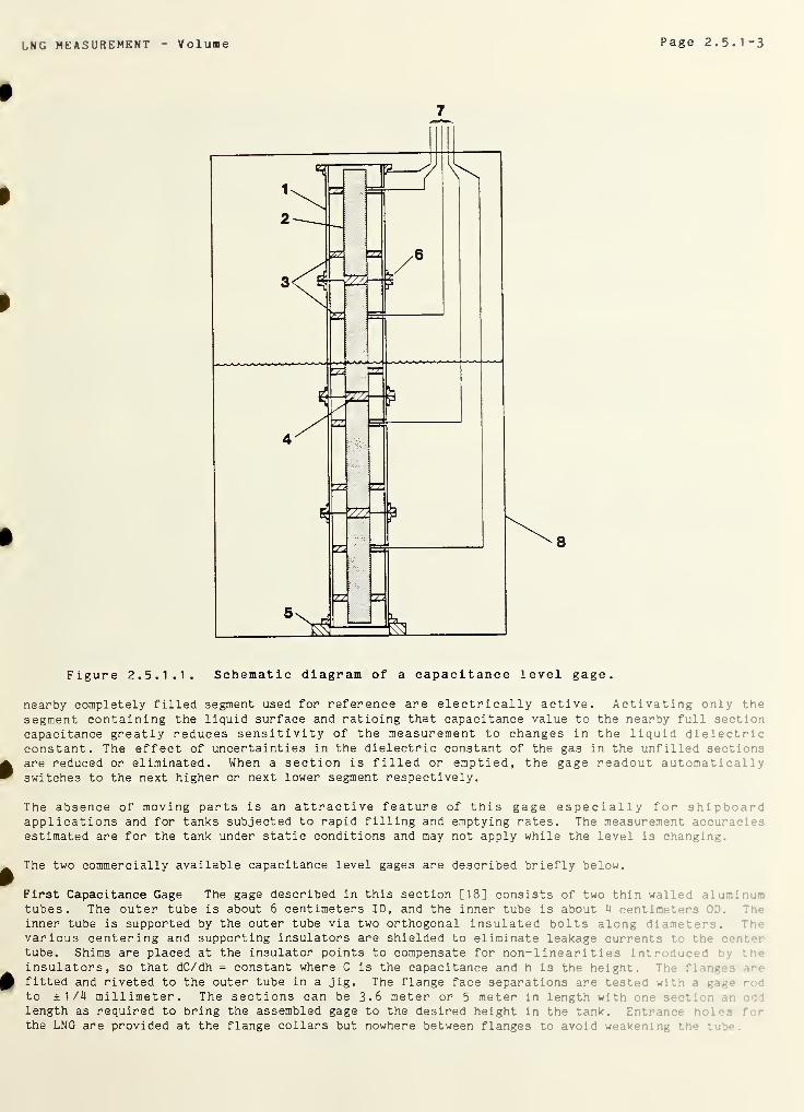
LNG MEASUREMENT Volume Page 2. 5. 1-3
7
Figure 2. 5.1.1. Schematic diagram of a capacitance level gage.
nearby completely filled segment used for reference are electrically active. Activating only thesegment containing the liquid surface and ratioing that capacitance value to the nearby full sectioncapacitance greatly reduces sensitivity of the measurement to changes in the liquid dielectricconstant. The effect of uncertainties in the dielectric constant of the gas in the unfilled sectionsare reduced or eliminated. When a section is filled or emptied, the gage readout automaticallyswitches to the next higher or next lower segment respectively.
The absence of moving parts is an attractive feature of this gage especially for shipboardapplications and for tanks subjected to rapid filling and emptying rates. The measurement accuraciesestimated are for the tank under static conditions and may not apply while the level is changing.
The two commercially available capacitance level gages are described briefly below.
First Capacitance Gage The gage described in this section [18] consists of two thin walled alum in .in
tubes. The outer tube is about 6 centimeters ID, and the inner tube is about 4 centimeters :>.
inner tube is supported by the outer tube via two orthogonal insulated bolts along diameters.various centering and supporting insulators are shielded to eliminate leakage currents t th^tube. Shims are placed at the insulator points to compensate for non-linearities int o lu red • i
'
insulators, so that dC/dh = constant where C is the capacitance and h is the height.fitted and riveted to the outer tube in a jig. The flange face separations are tested :
to ±1/4 millimeter. The sections can be 3.6 meter or 5 meter in length with on<
length as required to bring the assembled gage to the desired height in the tank. •
the LNG are provided at the flange collars but nowhere between flanges to avoid weaken in.” • .
Page 2 . 5 . 1- 1
* LNG MEASUREMENT Volume
The gage and associated electronic circuitry is designed so that the full and empty conditions can besimulated at ambient conditions. This provides a method of calibrating the gage when the tank and gageare at ambient temperature. This calibration procedure cannot be used in an empty cold tank, becausevariations in the gas temperature result in sufficiently large variations in the capacitance of thegage sections. When the tanks are empty and cold, the zero values of each segment can be tested bymanually switching in each segment and observing the level reading. If the level reading is not theknown height to the bottom of the segment, the segment zero level value is adjusted to read thecorrect value. When the tank is filled with LNG, and the same segment is switched in, the gain orspan of the electronics can be adjusted to give the correct full reading. This is done for eachsegment.
Measurement Uncertainties The lengths of the segments at the LNG boiling temperature of about - 1 60
degrees Centigrade, are known to
± 1 /4 ± 0. 03 A£ millimeters
The second term in this uncertainty arises from the uncertainty of the thermal expansion coefficientof aluminum and Al is the change in length from ambient to the LNG boiling point. The gage sectionsabove the liquid surface can be expected to be at some temperature other than the liquid temperature,but these sections do not enter the level measurement. The temperature uncertainty there contributesno error. The uncertainty of a level measurement when the level reaches a joint between twoelectrically separated segments n and n + 1 is
n
a= [0.25 / n+ 0.35 £ n ] millimeters (2)
1
Only the uncertainty of the section length and the uncertainty of the expansion coefficient [21]contribute to the measurement error when the liquid level is located at a joint. This equationassumes that no error is introduced by the readout circuitry.
As the level of the liquid moves above a joint between electrically separated segments, the linearityand resolution of the electrical components must be included in the gage accuracy. Some unpublishedtests of gage sections using freon indicate a level measurement uncertainty no larger than ± 3
millimeters [20]. This error should be maximum when the level is around the mid point of a segment.The non-linearity introduced by the gap between the ends of the center tube segments is small andincluded in the ±3 millimeters according to the manufacturer.
The manufacturer estimates the total uncertainty caused by calibration, capacitor dimensions andlinearity, and the electronics as ±3.5 millimeters for a single section of the gage. The totaluncertainty is placed at ±7.5 millimeters. The system measures level with a resolution of 0.1
millimeters and displays the measurement to 1 millimeter.
Second Capacitance Gage This gage consists of a 6.65 centimeter diameter ID 5 millimeter wallaluminum tube with a 1.3 centimeter diameter aluminum tube down the center. The 1.3 centimeter tube
is centered by three plastic insulating rods inserted through holes placed 120 degrees apart aroundthe tube in a plane perpendicular to the tube axis, and clamped against the inner tube by a band
around the outside of the outer tube. These support assemblies are placed periodically along thetubes. No shielding of the insulators or compensation for them was found necessary.
The tubes are segmented usually in 5 meter lengths by flanges welded to the outer tube. The innertube axial spacing is maintained by insulating spacers between adjacent ends. Holes are provided at
intervals in the outer tube walls to permit entrance of the tank contents. The flanged outer tube is
built to a length and measured. The variation in length is estimated to be ±1 millimeter.
The gage calibration is done when the tank is completely empty and completely full. With the tankempty, the segments are switched in one at a time and the zero reading of each segment is adjusted to
the proper level reading. When the tank is filled, each segment is switched in and the span is
adjusted to give the proper full reading. A point sensor on the top segment provides an intermediatepoint to calibrate the top segment.
Measurement Uncertainties The uncertainty o of the level at a joint for this gage is estimated to be
n
o= [ /"n + 0.3 Ia l n ] millimeters1
( 3 )
LNG MEASUREMENT V ol ume Page 2.5. 1-5
where n is the number of segments submerged and A£ n is the thermal contraction of the cooled
segments. The level measurement uncertainty increases as the liquid level moves up into a segment.
Non-linearity of the gage results from variation in the tube dimensions (- 0.013 millimeters on the
inner tube 0D and 0.0025 millimeters on the outer tube ID). The height uncertainty from these
variations is +4.25 millimeters, but only a maximum of ±3 millimeters has been observed according to
the manufacturer. The manufacturer estimates that temperature variations in the tank and variation of
the electronics contribute errors of ±1.2 millimeters and ±5 millimeters respectively. The sum of
these errors is 9.2 millimeters and the RMS value would be 6 millimeters. The systematic error from
equation (3) for 5 meter sections with a 1 millimeter length uncertainty is ±5 millimeters at the top
of a 25 meter high tank which raises the RMS uncertainty to about ±8 millimeters at the top of the
tank
.
Discussion The capacitance level gages of the two manufacturers differ in detail. Fundamentally,
they are similar, and the experiences and needs of field use have resulted in modifications that haveenhanced their similarities.
The uncertainty estimates cited in the manuf actur er s' literature are ±7.5 millimeters and ±10
millimeters for the first and second type gages respectively. If the error estimates by themanufacturers for linearity, gas temperature in the unfilled portion, electronics and thermalexpansion coefficients of the aluminum tube are correct, then the error estimates by bothmanufacturers are conservative. Test data taken by one manufacturer, using freon at ambienttemperature to simulate LNG, tends to confirm the conservative nature of the estimate, since the gageagreed with a ruled standard to ±3 millimeters [20].
Freon, however, will not behave the same as LNG. The latter can foam, the heavier hydrocarbons mightpreferentially adhere to the gage surfaces and cause larger level error readings than noted for freon.Variation in both gas and liquid density in the tank can introduce measurement error. Segmenting thegage eliminates any error that otherwise would have been introduced by the completely filled or
completely empty segments. The gage accuracy cannot be tested or monitored readily. The full andempty calibration measurements are probably separated by 24 hours at least for transport tanks andperhaps by weeks or months in storage tanks. The top section-full calibration can only be tested byraising the liquid level above the gage either while filling or after filling by pumping liquid fromtank to tank, unless an intermediate level sensor is provided.
Circulation of the liquid and gases during the filling and emptying of the tanks and ship motion whileat sea can be expected to minimize liquid variations. However, special precautions are necessary toprevent density stratification at the very bottom of spherical tanks during filling. Stratificationhas been observed in spherical tanks especially when top filled. As the tank is cooled to the LNGcargo temperature, methane is flashed off while heavier components collect. Since a very small volumeis incorporated in the bottom of a spherical tank, these heavy components can form a layer ofsufficient depth to interfere with the automatic switching of the gage to higher segments as theliquid level rises. If the gage can be calibrated at ambient temperature, then in ship tanks it couldpresumably be calibrated once a year during the usual yearly inspection. Shore-based storage tankgages, since the tanks may never be warmed to ambient, do not present sufficient opportunities forambient recalibration.
A possibility of overestimating capacitance gage accuracy exists. To establish accuracy ofcapacitance gages, the gages should be tested over a period of time in LNG service. This could bedone in a special calibration facility or in a storage tank by comparing them to another gage ofproven accuracy. Such a gage does not now exist, but a cable compensated gage, if tested f r
accuracy, could be used.
2. 5. 1.4 Cable Gage Tests
Introduction Cable gages as presently installed can be subject to large level measurem-’ •
However, the compensation methods outlined in Siegwarth [23] could significantly impr vaccuracy. With compensation, cable gages could meet and probably exceed the estimated aecura >'
capacitance level gages. The low cost of a cable gage and the relative ease with whichremoved and serviced make the cable gage an attractive alternative for the capacitance gag<'.
The error estimates for cable gage measurements in Siegwarth [23] assume that th<
contributes a negligible amount to the level measurement error when compared to t.h'.v- .
•
temperature and tank movements. To ascertain that the intrinsic errors of the gage ar--
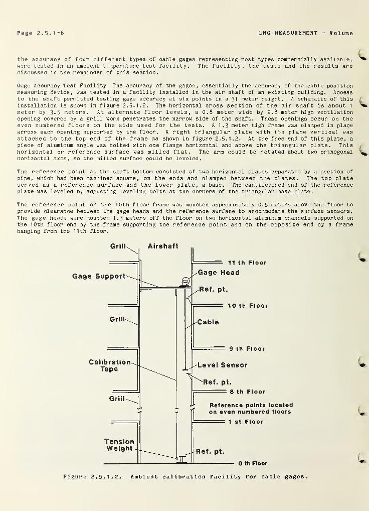
Page 2 . 5 .1 -6 LNG MEASUREMENT V olume
the accuracy of four different types of cable gages representing most types commercially available,were tested in an ambient temperature test facility. The facility, the tests and the results arediscussed in the remainder of this section.
Gage Accuracy Test Facility The accuracy of the gages, essentially the accuracy of the cable positionmeasuring device, was tested in a facility installed in the air shaft of an existing building. Accessto the shaft permitted testing gage accuracy at six points in a 31 meter height. A schematic of thisinstallation is shown in figure 2. 5. 1.2. The horizontal cross section of the air shaft is about 1
meter by 3.5 meters. At alternate floor levels, a 0.8 meter wide by 2.8 meter high ventilationopening covered by a grill work penetrates the narrow side of the shaft. These openings occur on theeven numbered floors on the side used for the tests. A 1.3 meter high frame was clamped in placeacross each opening supported by the floor. A right triangular plate with its plane vertical wasattached to the top end of the frame as shown in figure 2. 5. 1.2. At the free end of this plate, a
piece of aluminum angle was bolted with one flange horizontal and above the triangular plate. Thishorizontal or reference surface was milled flat. The arm could be rotated about two orthogonalhorizontal axes, so the milled surface could be leveled.
The reference point at the shaft bottom consisted of two horizontal plates separated by a section of
pipe, which had been machined square, on the ends and clamped between the plates. The top plateserved as a reference surface and the lower plate, a base. The cantilevered end of the referenceplate was leveled by adjusting leveling bolts at the corners of the triangular base plate.
The reference point on the 10th floor frame was mounted approximately 0.5 meters above the floor toprovide clearance between the gage heads and the reference surface to accommodate the surface sensors.The gage heads were mounted 1.3 meters off the floor on two horizontal aluminum channels supported onthe 10th floor end by the frame supporting the reference point and on the opposite end by a framehanging from the 11th floor.
Figure 2. 5. 1.2. Ambient calibration facility for cable gages.
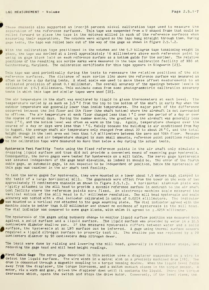
LNG MEASUREMENT Volume Page 2.5. 1-7
These channels also supported an iron -36 percent nickel calibration tape used to measure the
separation of the reference surfaces. This tape was suspended from a U shaped frame that could be
rolled forward to place the tape in the notches milled in each of the reference surfaces when
measuring their separations. The notches were aligned so the tape hung straight through them. During
gage tests, the tape was rolled back out of the way of the gage as shown in figure 2. 5. 1.2.
With the calibration tape positioned in the notches and the 5.2 kilogram tape tensioning weight in
place, the tape was scribed at a level approximately 16 millimeters above each reference point by
using an gage block laid on each reference surface as a bottom guide for the scriber. The relativepositions of the resulting six scribe marks were measured in the tape calibration facility of NBS at
Gaithersburg, Maryland. The calibration certificate for this tape appears in Siegwarth [23].
This tape was used periodically during the tests to remeasure the relative positions of the sixreference surfaces. The distance of each scribe line above the reference surface was measured as
often as twice a day during tests. A steel scale was used to make these offset measurements to anestimated precision of about 0.1 millimeter. The overall accuracy of the spacings between levels is
estimated at ±0.3 millimeters. This estimate comes from some photogr ammetr i c calibration accuracytests in which this tape and similar tapes were used [22].
The air temperature in the shaft was monitored by liquid in glass thermometers at each level. Thetemperature varied by as much as 3.5 0 C from the top to the bottom of the shaft in early May when theoutdoor temperature was generally lower than inside temperatures. The major part of the differenceoccurred between the 2nd floor and 0th floor (the shaft bottom) where the airshaft is not surroundedby offices. The air temperature at each floor changed less than 1
0 C over the period of a day or overthe course of several days. During the summer months, the gradient up the airshaft was generally lessthan 2 °C, and the bottom level was often as warm as the top. Again, temperature changes over thecourse of a day or days were less than 1
0 C. Mainly because the building is air conditioned from Mayto August, the average shaft air temperature only changed from about 22 to about 26 °C, and the totalheight change in the test area was less than 1.5 millimeters between the zero and 10th floor. Becausethe shaft height and air temperature changed by such small amounts, reference point positions relativeto the calibration tape were measured no more than twice a day during the actual tests.
Hysteresis Test Facility Tests using the fixed reference points in the air shaft only simulate a
dropping liquid surface and thus did not provide a convenient means of examining gage hysteresis.Consequently, the servo gages were tested for hysteresis on a mill table. The servo gage hysteresiswas assumed independent of the gage head elevation, as indeed it should be. The error of the fourthcable gage, an automatic gage, is not expected to be independent of position, hence the hysteresis ofthis gage was examined in the air shaft test facility.
To test the servo gages for hysteresis, they were mounted on a tower about 1.5 meters high clamped tothe table of a large horizontal mill. The gageheads were offset from the tower on the ends of twoapproximately 15 centimeters channels as shown in figure 2. 5. 1.3. A horizontal aluminum plate wasrigidly attached to the mill head to provide a movable reference surface in contrast to the air shafttest facility where the reference points were fixed. An electronic machine scale measured thevertical motion of the mill head to 0.1 millimeter resolution. The mill head hysteresis and scaleaccuracy was tested with a dial indicator calibrated in units of 0.0254 millimeters. The indicatorwas mounted on a vertical rod attached to the gage mounting plate. The dial indicator agreed with themachine scale to better than 0.02 millimeter and showed no evidence of hysteresis in the mill head.The dial indicator was compared to some gage blocks, with which it agreed to ± .0254 millimeter.
The hysteresis of the gages using buoyancy change to monitor liquid surface position was measure! : tnagainst a solid surface and a liquid surface. The liquid surface was provided by water in 1
centimeters diameter shallow pan. If the measured hysteresis differs between water and 1 -:
surface, the hysteresis at an LNG surface can be inferred. A gage using thermal surf ac- -
required a liquid nitrogen surface to properly test it. The shallow pan was replaced by 1
centimeters diameter by 90 centimeters deep nitrogen dewar.
The tests were done by raising and lowering the mill head, generally in millimeter st >’
recording the gage head and mill head height readings.
First Cable Gage The servo gage described in this section uses a displacer suspended n
detect the liquid surface. The wire winds in a spiral slot on a precisely machined drum [id],drum is connected through a magnetic coupling to a torque sensing device. When the liqui : :• .. -
away from the displacer, the torque increases, and a switch contact closes in the t >rque sen .
motor, via a worm and gear, drives the displacer down until it contacts the liquid. ••• •
decreases which, opens the switch and stops the drive motor. Conversely, if the
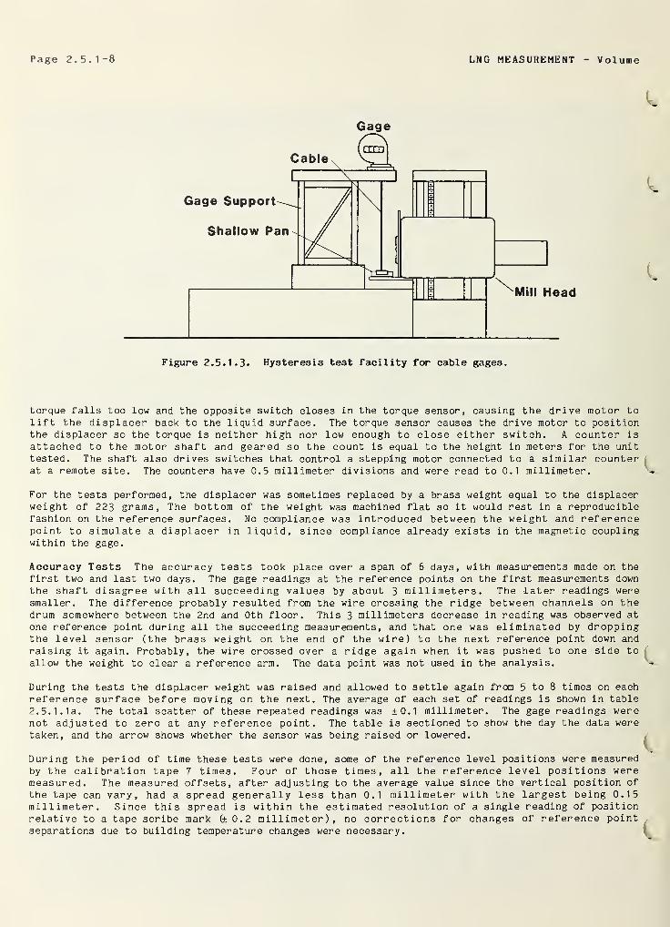
Page 2.5. 1-8 LNG MEASUREMENT V olume
Gage
torque falls too low and the opposite switch closes in the torque sensor, causing the drive motor tolift the displacer back to the liquid surface. The torque sensor causes the drive motor to positionthe displacer so the torque is neither high nor low enough to close either switch. A counter is
attached to the motor shaft and geared so the count is equal to the height in meters for the unit
tested. The shaft also drives switches that control a stepping motor connected to a similar counterat a remote site. The counters have 0.5 millimeter divisions and were read to 0.1 millimeter.
For the tests performed, the displacer was sometimes replaced by a brass weight equal to the displacerweight of 223 grams. The bottom of the weight was machined flat so it would rest in a reproduciblefashion on the reference surfaces. No compliance was introduced between the weight and referencepoint to simulate a displacer in liquid, since compliance already exists in the magnetic couplingwithin the gage.
Accuracy Tests The accuracy tests took place over a span of 6 days, with measurements made on the
first two and last two days. The gage readings at the reference points on the first measurements downthe shaft disagree with all succeeding values by about 3 millimeters. The later readings weresmaller. The difference probably resulted from the wire crossing the ridge between channels on thedrum somewhere between the 2nd and 0th floor. This 3 millimeters decrease in reading was observed at
one reference point during all the succeeding measurements, and that one was eliminated by droppingthe level sensor (the brass weight on the end of the wire) to the next reference point down andraising it again. Probably, the wire crossed over a ridge again when it was pushed to one side to
allow the weight to clear a reference arm. The data point was not used in the analysis.
During the tests the displacer weight was raised and allowed to settle again from 5 to 8 times on eachreference surface before moving on the next. The average of each set of readings is shown in table
2.5.1.1a. The total scatter of these repeated readings was ±0.1 millimeter. The gage readings werenot adjusted to zero at any reference point. The table is sectioned to show the day the data were
taken, and the arrow shows whether the sensor was being raised or lowered.
During the period of time these tests were done, some of the reference level positions were measuredby the calibration tape 7 times. Four of those times, all the reference level positions weremeasured. The measured offsets, after adjusting to the average value since the vertical position of
the tape can vary, had a spread generally less than 0.1 millimeter with the largest being 0.15millimeter. Since this spread is within the estimated resolution of a single reading of positionrelative to a tape scribe mark (±0.2 millimeter), no corrections for changes of reference pointseparations due to building temperature changes were necessary.
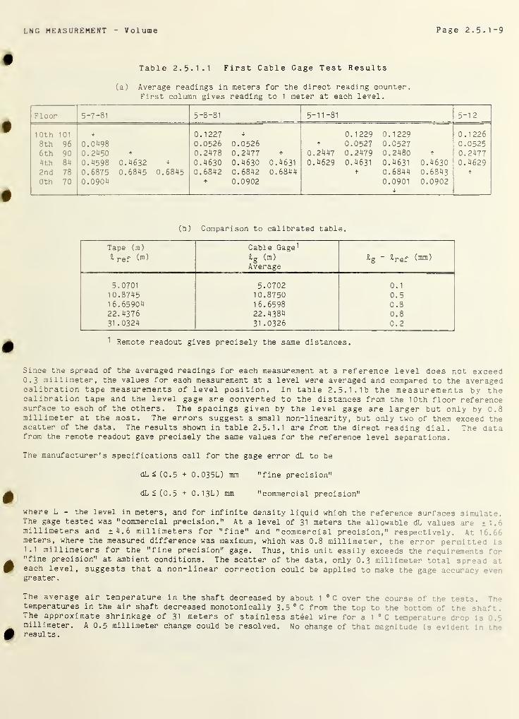
LNG MEASUREMENT Volume Page 2. 5 .1 -9
Table 2. 5. 1.1 First Cable Gage Test Results
(a) Average readings in meters for the direct reading counter.First column gives reading to 1 meter at each level.
Floor 5-7-81 5-8-81 5-11-81 5-12
10th 101
8th 96
6th 90
4th 84
2nd 78
0th 70
+
0.04980.2450 +
0.4598 0.4632 +
0.6875 0.6845 0.68450.0904
0.1227 +
0.0526 0.05260.2478 0.2477 +
0.4630 0.4630 0.46310.6842 0.6842 0.6844
+ 0.0902
0.1229 0.1229+ 0.0527 0.0527
0.2447 0.2479 0.2480 +
0.4629 0.4631 0.4631 0.4630t 0.6844 0.6843
0.0901 0.0902+
0.12260.05250.24770.4629
+
(b) Comparison to calibrated table.
Tape (m)
£ ref )
Cable Gage 1
£g
(m)
Average& g & 0 (mm
)
5.0701 5.0702 0.1
10.8745 10.8750 0.516.65904 16.6598 0.822.4376 22.4384 0.831 .0324 31 .0326 0.2
1 Remote readout gives precisely the same distances.
Since the spread of the averaged readings for each measurement at a reference level does not exceed0.3 millimeter, the values for each measurement at a level were averaged and compared to the averagedcalibration tape measurements of level position. In table 2.5.1.1b the measurements by thecalibration tape and the level gage are converted to the distances from the 10th floor referencesurface to each of the others. The spacings given by the level gage are larger but only by 0.8millimeter at the most. The errors suggest a small non-linearity, but only two of them exceed thescatter of the data. The results shown in table 2. 5. 1.1 are from the direct reading dial. The datafrom the remote readout gave precisely the same values for the reference level separations.
The manufacturer's specifications call for the gage error dL to be
dL S (0.5 + 0.035L) mm "fine precision"
dL i (0.5 + 0.13L) mm "commercial precision"
where L = the level in meters, and for infinite density liquid which the reference surfaces simulate.The gage tested was "commercial precision." At a level of 31 meters the allowable dL values are ± 1.-
millimeters and ±4.6 millimeters for "fine" and "commercial precision," respectively. At 16."meters, where the measured difference was maximum, which was 0.8 millimeter, the error permitted is1.1 millimeters for the "fine precision" gage. Thus, this unit easily exceeds the requirements for"fine precision" at ambient conditions. The scatter of the data, only 0.3 millimeter total spread r.
each level, suggests that a non-linear correction could be applied to make the gage accur a ,
greater
.
The average air temperature in the shaft decreased by about 1 °C over the course of the tests. 7-
temperatures in the air shaft decreased monotonically 3.5 °C from the top to the bottom of the sr. it* .
The approximate shrinkage of 31 meters of stainless steel wire for a 1 °C temperature dr : ; .
millimeter. A 0.5 millimeter change could be resolved. No change of that magnitude is ev; l-r.t
results.
Page 2.5.1-10 LNG MEASUREMENT V olume
Hy3teresi3 Tests The gage was tested for hysteresis on the horizontal mill first by using the brassweight against the flat table. The table was moved up and down between +1, 0, and -1 millimeter forfive complete cycles. The five readings at each level generally showed a spread of 0.2 to 0.3millimeter total. The averaged value of level reading for decreasing levels were 0.1 millimeterhigher than the average values for increasing levels at the same mill head position and for both thelocal and remote readout. This indicated hysteresis is well within the scatter of the individualmeasurements
.
When the reference surface was water, the direct readout suggested 0.1 to 0.2 millimeter hysteresis,while the remote readout suggested 0.2 to 0.3 millimeter. The displacer sensed a water surface thathad a cross- sectional area about 8 times larger than the float, so the water height correctionbetween the extremes of the displacer position relative to the surface is 0.04 millimeter. Hysteresisto a liquefied gas surface could be expected to double the hysteresis added by water, which could be
the difference between the water and solid surface hysteresis, 0.2 millimeter - 0.1 millimeter = 0.1
millimeter, doubled plus 0.1 millimeter or 0.3 millimeter for the direct readout. The above estimatesof hysteresis are tenuous, because the magnitudes estimated are smaller than the scatter of theindividual measurements at each level. Therefore, to within the measurement precision, hysteresis is
not detectable. Some additional level measurement error results because the wire weight adds to thedisplacer weight as the level drops. The wire weighs 0.15 gram per meter which is 4.5 gram whenextended 31 meters. The displacer is 14 centimeters diameter, so that in LNG at 500 kg/m3, the
displacer can be expected to ride about 0.6 millimeter lower at 30 meters depth than at 0 metersdepth. This error is proportional to level, and if more precise measurements are desired, heightcorrections for the wire weight can easily be made.
Second Cable Gage The servo gage described in this section suspends the surface sensor on a stainlesssteel tape. The tape is actually two side by side strips of stainless steel electrically insulatedfrom the environment and each other by a plastic coating. The level sensor is a 10 centimetersdiameter foam float free to move over a range of about 1 centimeter with respect to the sensing head.A coil in the sensing head, driven by an AC voltage supplied from the gage head through the stainlesssteel tapes, senses the position of the same magnetic material attached to the float. A servo motoris controlled by the signal from the sensing head and adjusts the position of the head until a null
position is achieved. The servo motor drives the tape storage drum. The tape passes over a sprocketwheel whose teeth engage in perforations in the wider of the two stainless steel strips then down tothe sensing head. The sprocket wheel drives a mechanical counter and can also drive a transmitter toa remote readout. The least count on the counter drum corresponds to 1 millimeter. The 1 millimeterlines are about 1.5 millimeters apart, permitting the counter position to be estimated to 0.1
millimeter. Because the storage drum diameter increases as the tape is wound, the driving speed was
greater than 0.6 meters/minute near full and about 0.4 meters/minute near empty. The control circuitdrives at a rate proportional to offset near the null point, making overshoot almost undetectable as
the sensing head approaches the rest position.
Accuracy Tests The gage accuracy was tested relative to the reference levels during three round trips
up and down the air shaft. The gage head approaches the reference levels always from above so thefloat could rest on the reference surface. The bottom reference point was raised by a gage block
approximately 10 centimeters because the tape was not long enough by a few centimeters to reach thebottom reference surface.
The averaged value for the level gage reading at each reference level for all the measurements at each
level is shown in table 2.5.1.2a. The total spread of the data at each level is 0.5 millimeter or
less. This precision approaches the resolution of the gage scale. The location of the dial referencecauses some reduction of reading precision because of parallax.
Table 2.5.1.2b and figure 2. 5. 1.4 show the difference between the reference surface spacingsdetermined by calibration tape and from the gage readings.
The bars on the averaged data points in figure 2. 5. 1.4 show the total spread of the data averaged at
that point. The gage reads a value for the reference point readings 6 millimeters too smallcorresponding to a liquid level 6 millimeters high at the 31 meter level. The average differences for
the intermediate levels fit a linear correction to ±0.2 millimeter, which is well within the limitsof the combined precision of the gage readability and the calibration tape measurement. A correctionfactor can readily be applied to the gage readings for high accuracy measurement. For this gage1.00020 x (gage reading) corrects the readings to the calibration tape scale.
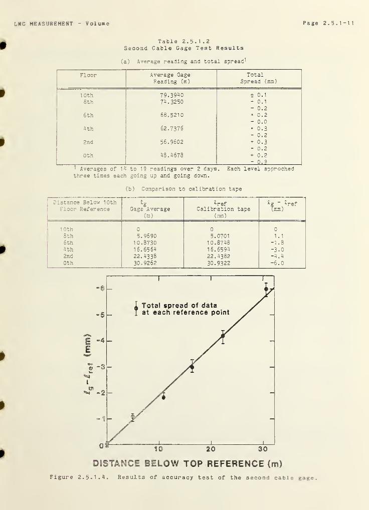
LN G MEASUREMENT Volume Page 2.5.1-11
Table 2.5.1 .2
Second Cable Gage Test Results
(a) Average reading and total spread 1
Floor Average GageReading (m)
TotalSpread (mm)
10th 79.3940 ± 0.1
8th 74.3250 + 0.1- 0.2
6th 68.5210 + 0.2- 0.0
nth 62.7376 + 0.3- 0.2
2nd 56.9602 + 0.3- 0.2
0th 48.4678 + 0.2- 0.3
1 Averages of 14 to 19 readings over 2 days. Each level approchedthree times each going up and going down.
(b) Comparison to calibration tape
Distance Below 10thFloor Reference
lS
Gage Average(m)
^refCalibration tape
(mm)
(mm)
:
r—
10th o 01
o
8th 5.9690 5.0701 1.1
6th 10.8730 10.8748 -1 .8
4th 16.6564 16.6594 -3.02nd 22.4338 22.4382 -4.4
0th 30.9262 30.9322 -6.0
DISTANCE BELOW TOP REFERENCE (m)
Figure 2.5.1 . 4
.
Results of accuracy test of the second cable gage.
Page 2.5.1-12 LNG MEASUREMENT Volume
The effect of cryogenic temperatures on the plastic coated tape was given cursory examination by
cooling a section of the tape in liquid nitrogen. No reduction in the tape flexibility was evident in
the section at liquid nitrogen temperature, nor was there any evident effects from differentialcontraction.
Hysteresis Tests The hysteresis tests on this gage were done first with the float in the sensor headresting on the shelf attached to the mill head. Three complete cycles (moving the table zero to + 1
millimeter to zero to - 1 millimeter to zero is one cycle) and a cycle to ± 0.2 millimeter resulted in
no measurable difference between the gage and the mill head reading.
Next, the float was tested with a water surface in a 30.4 centimeters diameter pan. Over the courseof three cycles through 1, 0 and - 1 millimeter, the maximum hysteresis was again less than 0.1
millimeter, i.e., no hysteresis was detected to the readability of the gage. During these watertests, the float settled 2 to 3 millimeters into the liquid. If the liquid were 500 kg/m3 naturalgas, the float would be expected to settle 4 to 6 millimeters into the liquid. If the LNG densitychanged by 10 percent, the gage would change by 0.6 millimeter at the same liquid level. If higherprecision is desired, a correction can be introduced by measuring the liquid density and calculatingthe relative shift resulting from density change.
Third Cable Gage The cable gage described in this section uses a hollow cable to connect the surfacesensor to the gage head [17]. A number of electrical leads pass through this hollow cable.
The leads connect a densimeter, a thermometer and the surface detectors in the surface sensor to theirrespective electronics in the gage head. The two surface detectors are thermal devices and cause thesurface sensor to be driven to a position such that the lower detector is immersed, and the upperdetector is above the liquid surface. The surface detectors are separated vertically by about 3
mill imeters
.
The cable consists of a flat wire wound in a tight coil around which one layer of 30 to 40 fine wiresis twisted in a spiral of about one turn in 5.5 centimeters. Around the outside, a single muchheavier wire is sprialled at a pitch of about one turn per 4 millimeters. A notched drive wheelmeshes with this spiral wire and drives the sensor up and down. A stepping motor powers the drivewheel, and the sensor position is monitored by counting the pulses to the stepping motor. Theinstrument is provided with a calibration by setting an appropriate number into some switches. Thisnumber determines the advance of the counter per pulse to the stepping motor. The excess cable is
stored on a spring-motor-driven drum in the drive head. The readout resolution of 1 millimeter cannotbe interpolated, since this is the least count of an electronic counter.
This gage has a unique feature. Rather than using a point on the tank roof for a reference point forsetting the gage zero, this gage can be rezeroed by allowing the surface sensor to come to rest on thetank bottom. The ensuing reduction of weight trips a switch in the gage head that resets the levelreadout to a zero value. Then the surface sensor is returned to the liquid surface. This method of
determining the gage zero removes errors introduced by temperature distributions in the tank walls andullage provided, the tank and environment are at steady state conditions (see Siegwarth [23] for
details)
.
Accuracy Tests This device senses level by means of temperature probes and always hangs with full
weight on the cable other than for a small buoyancy effect change. Thus, the level sensor could notbe lowered against a reference surface to measure its position because the cable would slack. Insteadthe sensor was brought to a point where the counter read a fixed level, around 13 to 15 centimeters,above each reference surface, and the separation from the reference was measured with a dialindicator. The dial gage reading remained 15.57 millimeters throughout the test of this gage whenplaced between the two plates separated by 127.0 millimeters by a gage block. The dial gage read so
that the spacing between the sensor bottom and the reference point was
S = (5.000-r + 0.61 3) (0.0254) meters
where r is the dial gage reading in inches. The spacing S was subtracted from the gage reading x togive the reference point position in the gage coordinates. The reference position p is then
p=x-(5 - r+ 0.61 3) (0.0254) meters
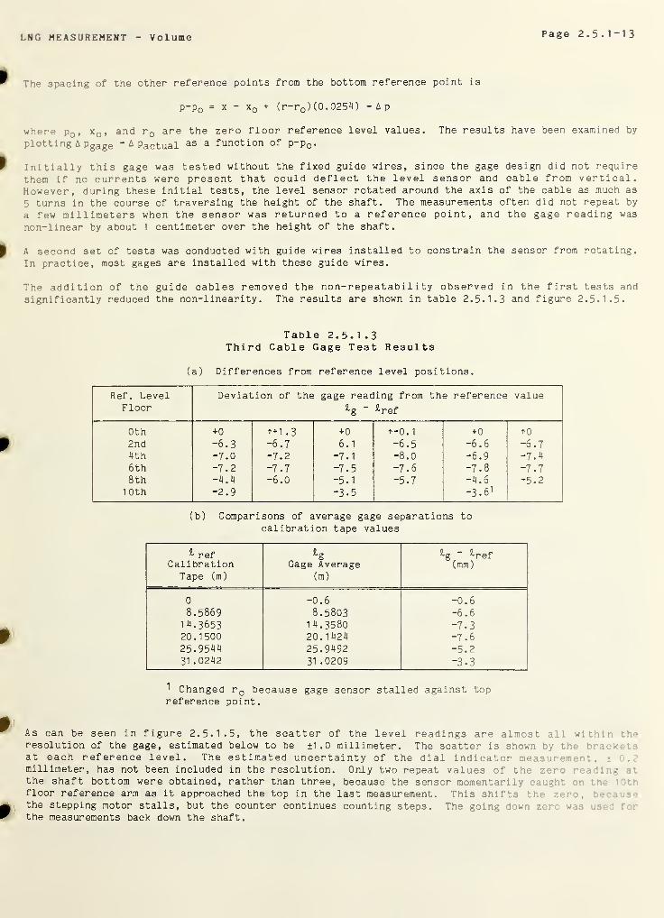
LNG MEASUREMENT Volume Page 2.5.1-13
The spacing of the other reference points from the bottom reference point is
p-p0 = x - x0 + (r-r0 ) (0.0254) =Ap
where p 0 , x 0 , and r 0 are the zero floor reference level values. The results have been examined by
plotting A Pgage A Pactual ^ function of p—
P
q.
Initially this gage was tested without the fixed guide wires, since the gage design did not require
them if no currents were present that could deflect the level sensor and cable from vertical.However, during these initial tests, the level sensor rotated around the axis of the cable as much as
5 turns in the course of traversing the height of the shaft. The measurements often did not repeat by
a few millimeters when the sensor was returned to a reference point, and the gage reading was
non-linear by about 1 centimeter over the height of the shaft.
A second set of tests was conducted with guide wires installed to constrain the sensor from rotating.
In practice, most gages are installed with these guide wires.
The addition of the guide cables removed the non-repeatability observed in the first tests and
significantly reduced the non-linearity. The results are shown in table 2. 5. 1.3 and figure 2. 5. 1.5.
Table 2.5. 1 .3Third Cable Gage Test Results
(a) Differences from reference level positions.
Ref. LevelFloor
Deviation of the gage reading from the reference
^g “ ^ref
value
0th *0 ++1 .3 +
0
+-0.
1
+ 0 +0
2nd -6.3 -6.7 6.1 -6.5 -6.6 -6.7
4th -7.0 -7.2 -7.1 -8.0 -6.9 -7.4
6th -7.2 -7.7 -7.5 -7.6 -7.8 -7.78th
10th
-4.4
-2.9-6.0 -5.1
-3.5-5.7 -4.6
-3.6 1
-5.2
(b) Comparisons of average gage separations tocalibration tape values
^ refCalibration
Tape (m)
Gage Average(m)
^g~ ^ref(mm)
0 -0.6 -0.6
8.5869 8.5803 -6.6
14.3653 1 4.3580 -7.320.1500 20.1424 -7.625.9544 25.9492 -5.2
31 .0242 31 .0209 -3.3
1 Changed r 0 because gage sensor stalled against topreference point.
As can be seen in figure 2. 5. 1.5, the scatter of the level readings are almost all withlrresolution of the gage, estimated below to be ±1.0 millimeter. The scatter is shown by the braat each reference level. The estimated uncertainty of the dial indicator measurer!"-'. - ,
• ).
millimeter, has not been included in the resolution. Only two repeat values of the zero : : :• .•
the shaft bottom were obtained, rather than three, because the sensor momentarily caj.-r* or.• •
floor reference arm as it approached the top in the last measurement. This shifts thethe stepping motor stalls, but the counter continues counting steps. The going down zer wa .
•
1
r •
the measurements back down the shaft.
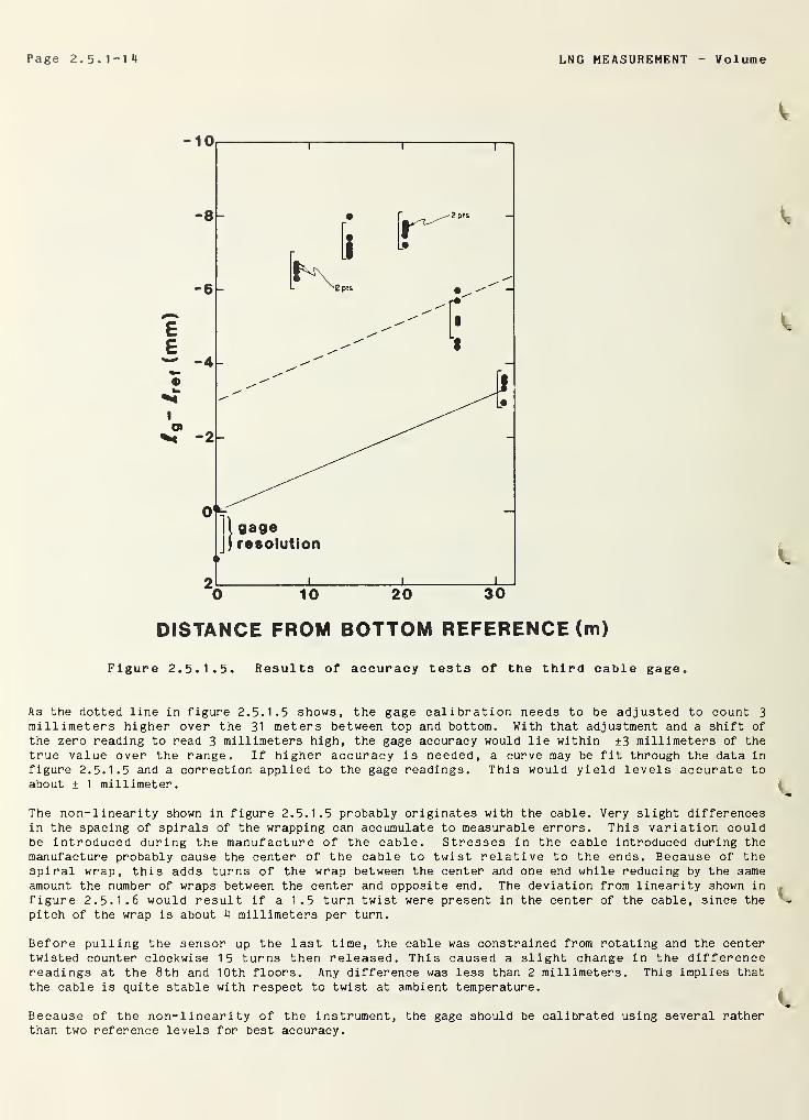
Page 2. 5. 1-1*1 LNG MEASUREMENT Volume
DISTANCE FROM BOTTOM REFERENCE (m)
Figure 2.5. 1.5. Results of accuracy tests of the third cable gage.
As the dotted line in figure 2. 5. 1.5 shows, the gage calibration needs to be adjusted to count 3
millimeters higher over the 31 meters between top and bottom. With that adjustment and a shift of
the zero reading to read 3 millimeters high, the gage accuracy would lie within ±3 millimeters of thetrue value over the range. If higher accuracy is needed, a curve may be fit through the data in
figure 2. 5. 1.5 and a correction applied to the gage readings. This would yield levels accurate toabout ± 1 millimeter.
The non-linearity shown in figure 2. 5. 1.5 probably originates with the cable. Very slight differencesin the spacing of spirals of the wrapping can accumulate to measurable errors. This variation couldbe introduced during the manufacture of the cable. Stresses in the cable introduced during themanufacture probably cause the center of the cable to twist relative to the ends. Because of thespiral wrap, this adds turns of the wrap between the center and one end while reducing by the sameamount the number of wraps between the center and opposite end. The deviation from linearity shown in
figure 2. 5. 1.6 would result if a 1.5 turn twist were present in the center of the cable, since thepitch of the wrap is about *1 millimeters per turn.
Before pulling the sensor up the last time, the cable was constrained from rotating and the centertwisted counter clockwise 15 turns then released. This caused a slight change in the differencereadings at the 8th and 10th floors. Any difference was less than 2 millimeters. This implies thatthe cable is quite stable with respect to twist at ambient temperature.
Because of the non-linearity of the instrument, the gage should be calibrated using several ratherthan two reference levels for best accuracy.
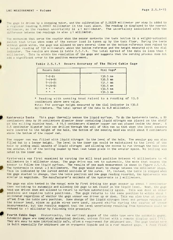
LNG MEASUREMENT Volume Page 2.5.1-15
The gage is driven by a stepping motor, and the calibration of 0.26229 millimeter per step is added to
a register reading 0.00001 millimeter in the last place. The reading is displayed to the nearest
millimeter, so the readout uncertainty is ± 1 millimeter. The uncertainty associated with the
difference between two readings is also ±1 millimeter.
The mechanism that zeros the counter when the sensor contacts the tank bottom is a weight-actuatedswitch that trips when some of the sensor load is taken up by the tank floor. During the tests
without guide wires, the gage was allowed to zero several times on the bottom reference then raised to
a height reading of 130 millimeters above the bottom reference and the height measured with the dial
indicator. The results are shown in table 2.5.1 - ^ . The total spread of the data is less than 1
millimeter. This is within the resolution of the gage and suggests that the zeroing process does not
add a significant error to the position measurement.
Table 2. 5. I. 1! Rezero Accuracy of The Third Cable Gage
Rezero Date Dial Gage*
7-8-81 130.5 mm7-14-81 130.5 mm7-15-81 131.1 mm7-24-81 130.5 mm?! If If 130.5 mm1! f? ?? 130.3 mm
* Reading with sensing head raised to a reading of 13-0centimeters above zero value.
Note: The average height measured by the dial indicator is 130.6millimeters. The total spread of the data is 0.8 millimeter.
Hysteresis Tests This gage thermally senses the liquid surface. To do the hysteresis tests, a 90
centimeters deep by 20 centimeters diameter dewar containing liquid nitrogen was placed on the shelfon the milling machine head. A 16.5 centimeters diameter copper can was placed inside the dewar. A
0.5 centimeter diameter hole was drilled through the wall of this can so that when the level sensorswere lowered to the height of the hole, the bottom of the sensing head was still about 8 centimetersabove the bottom of the copper can.
The copper can was filled with liquid nitrogen to the level of the hole. The annular gap was alsofilled but to a lesser height. The level in the inner can could be maintained to the level of thehole by adding small amounts of liquid nitrogen and allowing the excess to run through the hole intothe annulus. All of the boiling caused by heat leak takes place in the annular space. No boiling wasnoted in the inner can.
Hysteresis was first examined by varying the mill head position between +5 millimeters to -5
millimeters in 1 millimeter steps. The gage drive was set to automatic, the mode that causes thesensor to follow the liquid surface. The results of one such measurement is shown in figure 2. 5. 1.6.The hysteresis is about ± 3 millimeters. The gage would start to change between the millimeter steps.This is indicated by the curved dotted sections of the curve. If, instead, the table is stopped whenthe gage started to change, then the table position and new gage reading recorded, the hysteresis wassimilar in magnitude. The manufacturer's estimate of the hysteresis is 3 millimeters.
The gage was also tested in the manual mode by first driving the gage sensor up about 1 centimeterthen switching to automatic and allowing the gage to set itself at the liquid level. Next, the gag-head was driven down and allowed to return to surface automatically again. This was done at ot h-rpositive and negative table positions. The gage returns to the same position to within abou*
'
millimeter regardless of whether the gage sensor was driven up or down. This was also true at;
offset from the table zero position. Some change of the liquid nitrogen level and perhaps rot r : t
the sensor head, since no guide wires were used, caused shifts during the course or •
measurements, but the results suggest that the level uncertainty resulting from hysteresis . . :
reduced to ± 1 millimeter by following this procedure.
Fourth Cable Gage Historically, the earliest gages of the cable type were the automatic gag< .
Automatic gages are completely mechanical devices, unless fitted with a remote display uni’They are easy to make intrinsically safe, often a requirement for shipboard use. The gag- •- ••
is built especially Tor shipboard use on cryogenic liquids and is a roof mounted gage. A ! r:
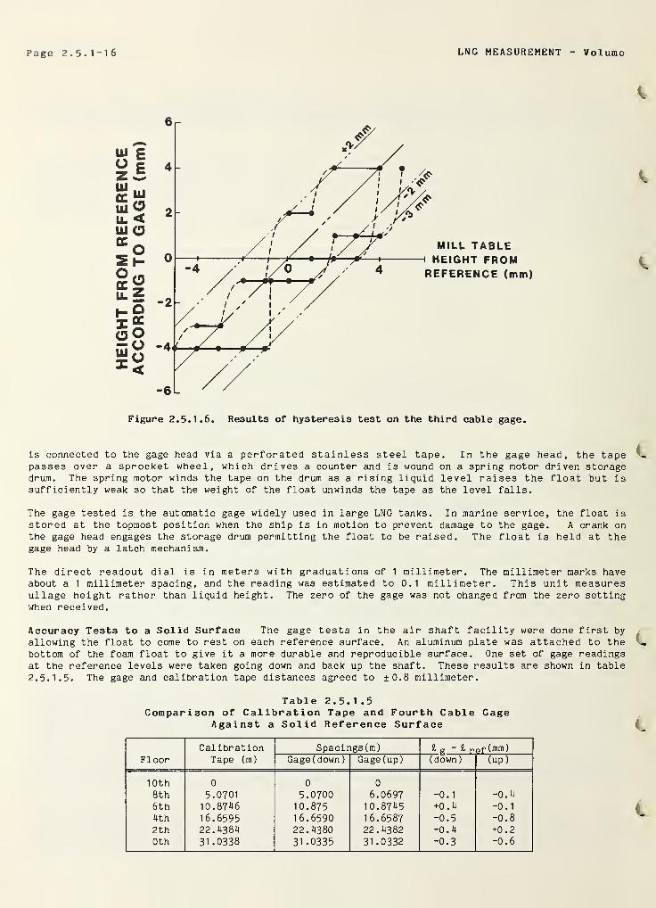
VolumePage 2.5.1-16 LNG MEASUREMENT -
Figure 2. 5. 1.6. Results of hysteresis test on the third cable gage.
is connected to the gage head via a perforated stainless steel tape. In the gage head, the tapepasses over a sprocket wheel, which drives a counter and is wound on a spring motor driven storagedrum. The spring motor winds the tape on the drum as a rising liquid level raises the float but issufficiently weak so that the weight of the float unwinds the tape as the level falls.
The gage tested is the automatic gage widely used in large LNG tanks. In marine service, the float isstored at the topmost position when the ship is in motion to prevent damage to the gage. A crank onthe gage head engages the storage drum permitting the float to be raised. The float is held at thegage head by a latch mechanism.
The direct readout dial is in meters with graduations of 1 millimeter. The millimeter marks haveabout a 1 millimeter spacing, and the reading was estimated to 0.1 millimeter. This unit measuresullage height rather than liquid height. The zero of the gage was not changed from the zero settingwhen received.
Accuracy Tests to a Solid Surface The gage tests in the air shaft facility were done first by
allowing the float to come to rest on each reference surface. An aluminum plate was attached to thebottom of the foam float to give it a more durable and reproducible surface. One set of gage readingsat the reference levels were taken going down and back up the shaft. These results are shown in table
2. 5. 1.5. The gage and calibration tape distances agreed to +0.8 millimeter.
Table 2.5. 1 .5Comparison of Calibration Tape and Fourth Cable Gage
Against a Solid Reference Surface
FloorCal ibration
Tape (m)
Spacings(m) 9j g & ref (mm)Gage (down) Gage (up) (down) (up)
10th 0 0 0
8th 5.0701 5.0700 6.0697 -0.1 -0.4
6th 10.8746 10.875 10.8745 +0.4 -0.1
4th 16.6595 16.6590 16.6587 -0.5 -0.8
2th 22.4384 22.4380 22.4382 -0.4 +0.2
0th 31.0338 31 .0335 31 .0332 -0.3 -0.6
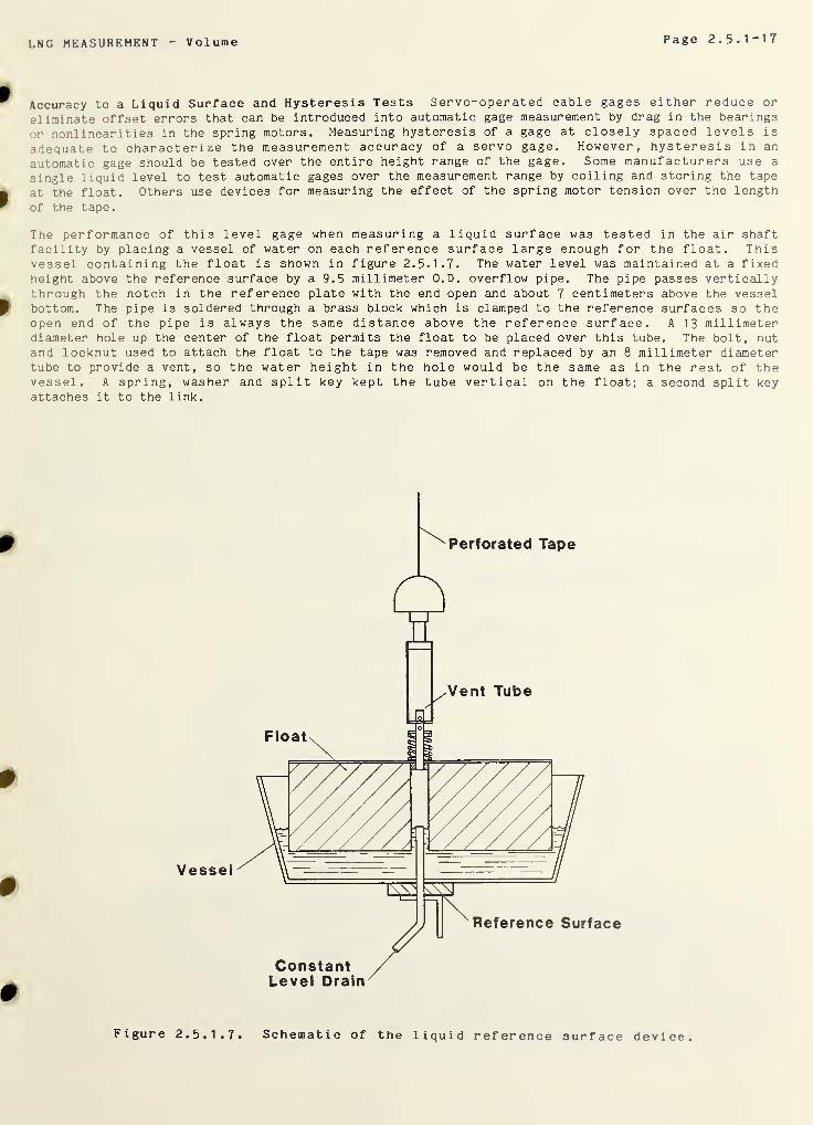
LNG MEASUREMENT Volume Page 2 . 5 •1 “1
7
Accuracy to a Liquid Surface and Hysteresis Tests Servo-operated cable gages either reduce or
eliminate offset errors that can be introduced into automatic gage measurement by drag in the bearings
or nonlinearities in the spring motors. Measuring hysteresis of a gage at closely spaced levels is
adequate to characterize the measurement accuracy of a servo gage. However, hysteresis in an
automatic gage should be tested over the entire height range of the gage. Some manufacturers use a
single liquid level to test automatic gages over the measurement range by coiling and storing the tape
at the float. Others use devices for measuring the effect of the spring motor tension over the length
of the tape.
The performance of this level gage when measuring a liquid surface was tested in the air shaftfacility by placing a vessel of water on each reference surface large enough for the float. Thisvessel containing the float is shown in figure 2. 5. 1.7. The water level was maintained at a fixedheight above the reference surface by a 9.5 millimeter O.D. overflow pipe. The pipe passes verticallythrough the notch in the reference plate with the end open and about 7 centimeters above the vesselbottom. The pipe is soldered through a brass block which is clamped to the reference surfaces so theopen end of the pipe is always the same distance above the reference surface. A 13 millimeterdiameter hole up the center of the float permits the float to be placed over this tube. The bolt, nutand locknut used to attach the float to the tape was removed and replaced by an 8 millimeter diametertube to provide a vent, so the water height in the hole would be the same as in the rest of thevessel. A spring, washer and split key kept the tube vertical on the float; a second split keyattaches it to the link.
Vessel
Figure 2.5. 1 .7. Schematic of the liquid reference surface device.
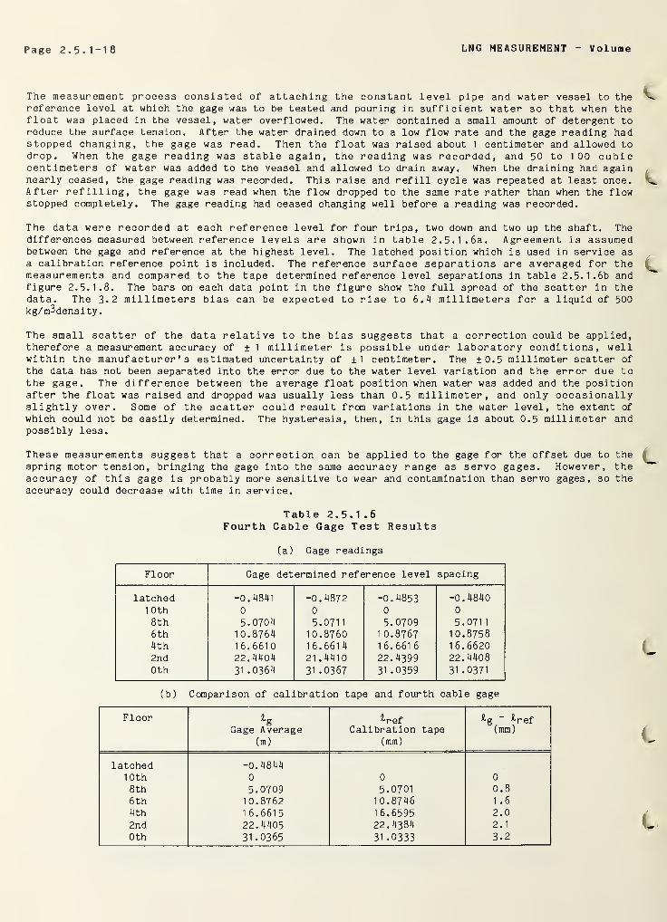
Page 2.5.1-18 LNG MEASUREMENT - Volume
The measurement process consisted of attaching the constant level pipe and water vessel to thereference level at which the gage was to be tested and pouring in sufficient water so that when thefloat was placed in the vessel, water overflowed. The water contained a small amount of detergent toreduce the surface tension. After the water drained down to a low flow rate and the gage reading hadstopped changing, the gage was read. Then the float was raised about 1 centimeter and allowed todrop. When the gage reading was stable again, the reading was recorded, and 50 to 100 cubiccentimeters of water was added to the vessel and allowed to drain away. When the draining had againnearly ceased, the gage reading was recorded. This raise and refill cycle was repeated at least once.After refilling, the gage was read when the flow dropped to the same rate rather than when the flowstopped completely. The gage reading had ceased changing well before a reading was recorded.
The data were recorded at each reference level for four trips, two down and two up the shaft. Thedifferences measured between reference levels are shown in table 2.5.1.6a. Agreement is assumedbetween the gage and reference at the highest level. The latched position which is used in service asa calibration reference point is included. The reference surface separations are averaged for themeasurements and compared to the tape determined reference level separations in table 2.5.1.6b andfigure 2. 5. 1.8. The bars on each data point in the figure show the full spread of the scatter in thedata. The 3-2 millimeters bias can be expected to rise to 6.4 millimeters for a liquid of 500kg/m3density.
The small scatter of the data relative to the bias suggests that a correction could be applied,therefore a measurement accuracy of ± 1 millimeter is possible under laboratory conditions, wellwithin the manufacturer's estimated uncertainty of ±1 centimeter. The ±0.5 millimeter scatter of
the data has not been separated into the error due to the water level variation and the error due tothe gage. The difference between the average float position when water was added and the positionafter the float was raised and dropped was usually less than 0.5 millimeter, and only occasionallyslightly over. Some of the scatter could result from variations in the water level, the extent of
which could not be easily determined. The hysteresis, then, in this gage is about 0.5 millimeter andpossibly less.
These measurements suggest that a correction can be applied to the gage for the offset due to thespring motor tension, bringing the gage into the same accuracy range as servo gages. However, theaccuracy of this gage is probably more sensitive to wear and contamination than servo gages, so the
accuracy could decrease with time in service.
Table 2.5. 1 .6Fourth Cable Gage Test Results
(a) Gage readings
Floor Gage determined reference level spacing
latched10th8th6th4th2nd
0th
-0.4841
0
5.070410.876416.661022.440431 .0364
-0.48720
5.0711
10.876016.661421 .4410
31 .0367
-0.48530
5.07091 0.87671 6.661
6
22.439931 .0359
-0.4840
0
5.071
1
10.875816.662022.4408
31 .0371
(b) Comparison of calibration tape and fourth cable gage
FloorGage Average
(m)
^refCalibration tape
(mm)
^g " ^ref(mm)
latched -0.484410th 0 0 0
8th 5.0709 5.0701 0.8
6 th 10.8762 10.8746 1.6
4th 16.6615 1 6.6595 2.0
2nd 22.4405 22.4384 2.1
0th 31.0365 31.0333 3.2
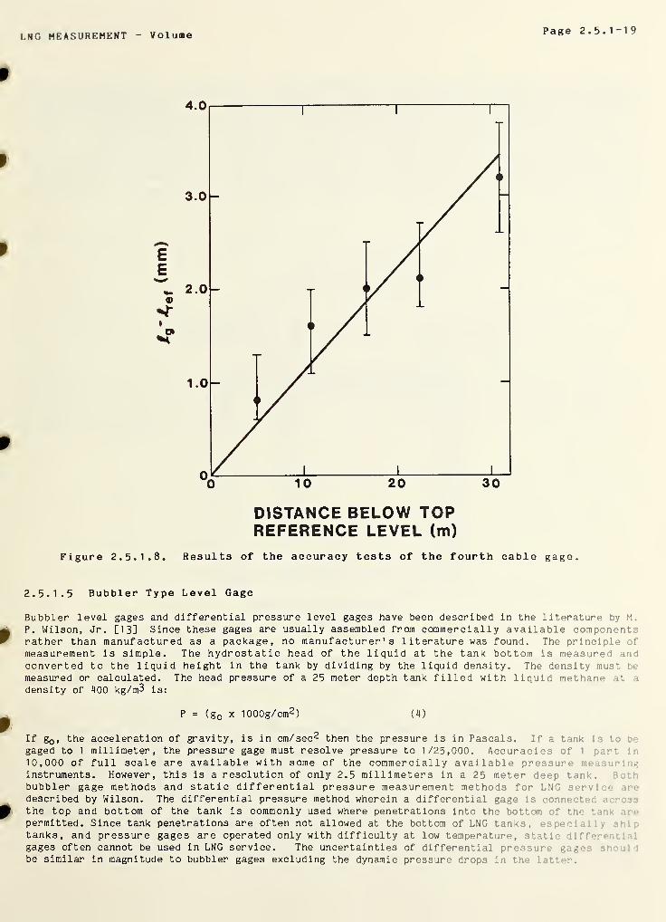
LNG MEASUREMENT Volume Page 2.5.1-19
DISTANCE BELOW TOPREFERENCE LEVEL (m)
Figure 2. 5. 1.8. Results of the accuracy tests of the fourth cable gage.
2. 5. 1.5 Bubbler Type Level Gage
Bubbler level gages and differential pressure level gages have been described in the literature by M.
P. Wilson, Jr. [13] Since these gages are usually assembled from commercially available componentsrather than manufactured as a package, no manufacturer's literature was found. The principle of
measurement is simple. The hydrostatic head of the liquid at the tank bottom is measured andconverted to the liquid height in the tank by dividing by the liquid density. The density must be
measured or calculated. The head pressure of a 25 meter depth tank filled with liquid methane it i
density of 400 kg/m3 is:
P = (go x 1000g/cm2 ) (4)
If g0 , the acceleration of gravity, is in cm/sec 2 then the pressure is in Pascals. If a tank is t
gaged to 1 millimeter, the pressure gage must resolve pressure to 1/25,000. Accuracies of 1 par* in
10,000 of full scale are available with some of the commercially available pressure m- r . -
instruments. However, this is a resolution of only 2.5 millimeters in a 25 meter deep tank,bubbler gage methods and static differential pressure measurement methods for LNG s«tv: • .v •
described by Wilson. The differential pressure method wherein a differential gage is connect" i•
the top and bottom of the tank is commonly used where penetrations into the bottom of * *;•• •
permitted. Since tank penetrations are often not allowed at the bottom of LNG tanks,tanks, and pressure gages are operated only with difficulty at low temperature, ctabi .
gages often cannot be used in LNG service. The uncertainties of differential prennur"be similar in magnitude to bubbler gages excluding the dynamic pressure drops in tri" :
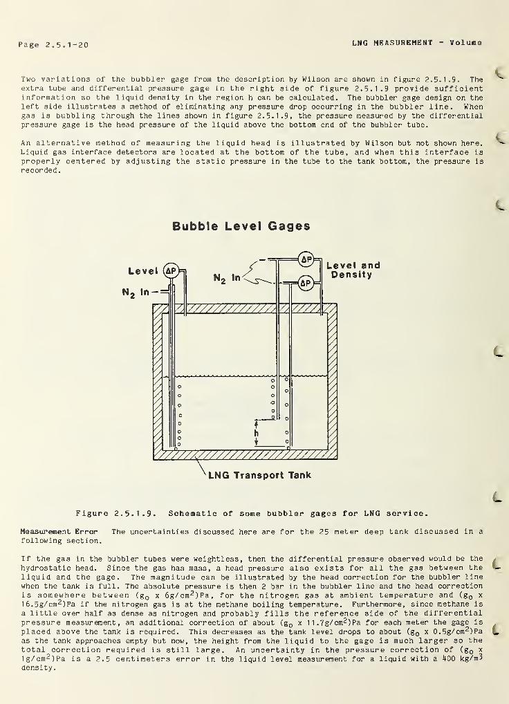
Page 2.5.1-20 LNG MEASUREMENT Volume
Two variations of the bubbler gage from the description by Wilson are shown in figure 2. 5. 1.9. Theextra tube and differential pressure gage in the right side of figure 2. 5. 1.9 provide sufficientinformation so the liquid density in the region h can be calculated. The bubbler gage design on theleft side illustrates a method of eliminating any pressure drop occurring in the bubbler line. Whengas is bubbling through the lines shown in figure 2. 5. 1.9, the pressure measured by the differentialpressure gage is the head pressure of the liquid above the bottom end of the bubbler tube.
An alternative method of measuring the liquid head is illustrated by Wilson but not shown here.Liquid gas interface detectors are located at the bottom of the tube, and when this interface is
properly centered by adjusting the static pressure in the tube to the tank bottom, the pressure is
recorded
.
Bubble Level Gages
Level (^P)=j
N 2 In — =|
N 2 In
<5h Level andDensity
7A
LNG Transport Tank
Figure 2. 5. 1.9. Schematic of some bubbler gages for LNG service.
Measurement Error The uncertainties discussed here are for the 25 meter deep tank discussed in a
following section.
If the gas in the bubbler tubes were weightless, then the differential pressure observed would be the
hydrostatic head. Since the gas has mass, a head pressure also exists for all the gas between theliquid and the gage. The magnitude can be illustrated by the head correction for the bubbler linewhen the tank is full. The absolute pressure is then 2 bar in the bubbler line and the head correctionis somewhere between (g Q x 6g/cm 2 )Pa, for the nitrogen gas at ambient temperature and (g Q x
l6.5g/cm2 )Pa if the nitrogen gas is at the methane boiling temperature. Furthermore, since methane is
a little over half as dense as nitrogen and probably fills the reference side of the differentialpressure measurement, an additional correction of about (gQ x 11.7g/cm2)Pa for each meter the gage is
placed above the tank is required. This decreases as the tank level drops to about (g0 x 0.5g/cm2)Paas the tank approaches empty but now, the height from the liquid to the gage is much larger so thetotal correction required is still large. An uncertainty in the pressure correction of (g Q x
1g/cm2)Pa is a 2.5 centimeters error in the liquid level measurement for a liquid with a 400 kg/m3density.
LNG MEASUREMENT Volume Page 2.5.1-21
The density measurement should be made near the bottom of a tank to provide a density value at lowfilling levels. If h in figure 2. 5. 1.9 represents 10 percent of the tank height, then the differenceof the two gage readings from equation (4) will be (g0 x 100g/cm2 )Pa for liquid methane of 400kg/m3density. The pressure gages can introduce a 1 percent error in the density measurement if they are
0.1 percent gages. Also, the uncertainty in the bubbler line nitrogen gas density contributes to the
density uncertainty. The density measurement in a full tank may not represent the density at otherlevels in the tank especially in a shore storage tank where stratification can take place. The
bubbling nitrogen also could alter the local density around the bubblers. A density measurementuncertainty of 1 percent does not seem unlikely. An error of 1 percent in density introduces an
uncertainty of 1 percent in the level even before the gas column uncertainties are included.
If the gas is bubbling into the tank, probably the bubbler line contains nitrogen, but a pressure dropis present in the line. If the static method shown in figure 2. 5. 1.9, left side, is used or theinterface detector method, the composition of the gas in the lines can be expected to be some mixtureof methane and nitrogen. The uncertainty of the gas column density could easily be as large as anypressure drop that might be experienced in a line through which gas is flowing.
Bubbler gages have been relegated to backup use for capacitance gages on ship tanks. Gage accuracyhas probably been a factor in this, but reliability has been a large consideration too. Very dryclean gas, usually nitrogen gas, must be used, or the bubbler nozzles rapidly plug with ice or othersolids. Plugging has been a problem. Any leak in the lines from the pressure gage to the tank resultin a false level reading, and errors introduced by small leaks can easily go undetected.
A bubbler gage can easily be in error by tenths of a meter in a 25 meter tank mainly because ofuncertainty in the liquid density measurement and several centimeters additional because ofuncertainty in gas head corrections. The poorer accuracy, along with failure due to leaks andplugging, limits the application of these gages to back up use for custody transfer measurement. Ifthe gaging application does not require high accuracy, differential pressure and bubbler gages haveadvantages. They are least affected by surface turbulence, thus are useful for level monitoringduring rapid filling of a tank.
Page 2.5.1-22 LNG MEASUREMENT Volume
2. 5. 1.6 References
[1] Armstrong, G. T., Hydrocarbons for fuel — 75 years of materials research at NBS, Nat. Bur.
Stand. (U.S.), Spec. Publ. 434 (May 1976).
[2] Haynes, W. M., M. J. Hiza and R. D. McCarty, Densities of LNG for custody transfer, LNG 5,
International Conf. on Liquefied Natural Gas, Proc. 5th (Dusseldorf, Germany, Aug 29~Sep 1,
1977), Vol 2, Session III, Paper 11 (Institute of Gas Technology, Chicago, 111., 1977).
[3] McCarty, R. D., Four mathematical models for the prediction of LNG densities, Nat. Bur. Stand.(U.S.), Tech. Note 1030 (Dec 1980).
[4] Brennan, J. A., Better LNG flow measurement sought, Oil Gas J. 76(5), 168+173-4+177 (Jan 1978).
[5] Parrish, W. R., J. M. Arvidson and J. F. LaBrecque, Development and evaluation of an LNGsampling system, Nat. Bur. Stand. (U.S.), NBSIR 78-887 (July 1978).
[6] Jackson, R. H. F., R. S. Collier, S. Haber and P. V. Tryon, Custody transfer systems for LNGships: tank survey techniques and sounding tables, Nat. Bur. Stand. (U.S.), NBSIR 79-1751(1979)
.
[7] Haight, W. C., R. J. Hocken, B. R. Borchardt, C. L. Carroll, R. G. Hartsock, C. P. Reeve, F. E.
Scire and R. C. Veale, Estimated accuracy of calibration of some membrane-type LNG transporttanks, Nat. Bur. Stand. (U.S.), NBSIR 80-2141 (1981).
[8] Hocken, R. J. and W. C. Haight, Multiple redundancy in the measurement of large structures, CIRPAnn. 27, 357-60 (1978).
[9] Siegwarth, J. D., B. A. Younglove and J. F. LaBrecque, An evaluation of commercial densimetersfor use in LNG, Nat. Bur. Stand. (U.S.), Tech. Note 697 (October 1977).
[10] Siegwarth, J. D. and J. F. LaBrecque, A portable calibration densimeter for use in cryogenicliquids, Nat. Bur. Stand. (U.S.), Tech. Note 1035 (March 1981).
[11] Siegwarth, J. D. and J. F. Labrecque, Cryogenic fluid density reference system: provisionalaccuracy statement (1980), Nat. Bur. Stand. (U.S.), Tech. Note 1 0 4 1 (June 1981).
[12] Roder, H. M., ASRDI oxygen technology survey volume V: density and liquid level measurementinstrumentation for cryogenic fluids oxygen, hydrogen, and nitrogen, NASA SP 3083 (1974).
[13] Wilson, Jr., M. P., LNG tank level measurement, AGA Operating Section Proceedings, Proceedingsof the Transmission Conference, Las Vegas, Nevada, T-223 (1976).
[14] Jelffs, P. A. M., Calibration of containers and gauges, Journal of the Institute of Petroleum,
58, No. 561, pp117-25 (May 1972).
[15] Paterson, I.W.F., Standardization for installation of automatic gages, Journal of the Instituteof Petroluem, 58, 209, (1972).
[16] Watson, P. B. , Instrumentation for the Measurement of Refrigerated Hydrocarbon Liquids, Journalof the Institute of Petroleum, _58, No. 561, pp 1 26—3 1 (May 1972).
[17] Halverson, G., Automatic continuous LNG level-gauging and temperature measuring systems,
Instrumentation in Cryogenic Industry, 1, paper 602 Houston, Texas, (1976).
[18] Williams, R. A., High accuracy level gaging, Proceedings 55th International School of
Hydrocarbon Measurement, Norman, Oklahoma (1980) pp 332. Similar papers appear in 1977 to 1982schools. Also, see Moore, C. F. and Blanchard, R. L., Custody transfer instrumentation systemsfor LNG marine transport projects, Fourth International Conference on Liquefied Natural Gas,Algiers, Algeria (1974).
[19] Eilers, C., Modern automatic tankgauging systems, Proceedings 55th International School of
Hydrocarbon Measurement, Norman, Oklahoma (1980) pg 345.
[20] Unpublished report of gage tests in a freon by manufacturer.
LNG MEASUREMENT Volume Page 2.5.1-23
[21] LNG Materials and Fluids - A user's manual of property data in graphic format, by D. B. Mann,Editor. Manual sponsored by American Gas Association, Maritime Administration, Office ofStandard Reference Data and American Bureau of Shipping. Published by National Bureau of Stand-ards, Thermophysical Properties Division 773, Boulder, Colo., 325 pages (1977).
[22] Siegwarth, J. D. and J. F. LaBrecque, Estimated uncertainty of calibrations of free standingprismatic Liquefied Natural Gas cargo tanks, Nat. Bur. Stand. (U.S.), NBSIR 81-1655, 294pp(January, 1982).
[23] Siegwarth, J. D., Measurement uncertainties of level gages for liquefied natural gas, NBSIR82-1668, Nat. Bur. Stand. (U.S.), 52 pp (June, 1982).
.
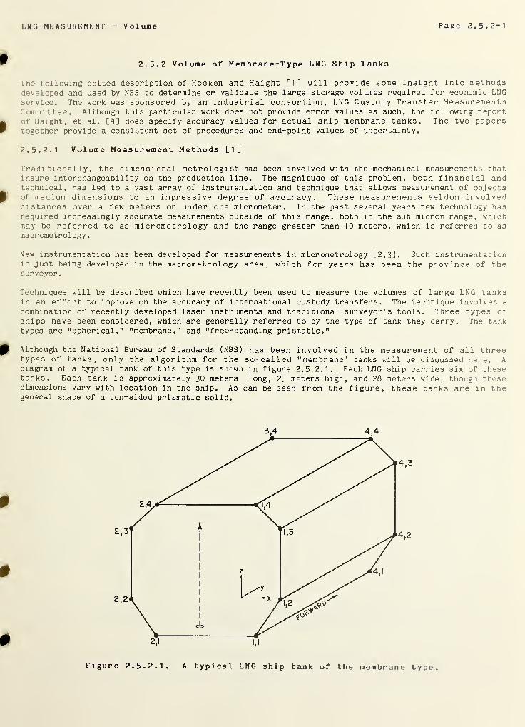
LNG MEASUREMENT Volume Page 2. 5. 2-1
2.5.2 Volume of Membrane-Type LNG Ship Tanks
The following edited description of Hocken and Haight [1] will provide some insight into methodsdeveloped and used by NBS to determine or validate the large storage volumes required for economic LNGservice. The work was sponsored by an industrial consortium, LNG Custody Transfer MeasurementsCommittee. Although this particular work does not provide error values as such, the following reportof Haight, et al. [4] does specify accuracy values for actual ship membrane tanks. The two paperstogether provide a consistent set of procedures and end-point values of uncertainty.
2. 5. 2.1 Volume Measurement Methods [1]
Traditionally, the dimensional metrologist has been involved with the mechanical measurements thatinsure interchangeability on the production line. The magnitude of this problem, both financial andtechnical, has led to a vast array of instrumentation and technique that allows measurement of objects
B of medium dimensions to an impressive degree of accuracy. These measurements seldom involveddistances over a few meters or under one micrometer. In the past several years new technology hasrequired increasingly accurate measurements outside of this range, both in the sub-micron range, whichmay be referred to as micrometrology and the range greater than 10 meters, which is referred to asmacrometrology
.
New instrumentation has been developed for measurements in micrometrology [2,3]. Such instrumentationis just being developed in the macrometrology area, which for years has been the province of thesurveyor
.
Techniques will be described which have recently been used to measure the volumes of large LNG tanksin an effort to improve on the accuracy of international custody transfers. The technique involves a
combination of recently developed laser instruments and traditional surveyor's tools. Three types ofships have been considered, which are generally referred to by the type of tank they carry. The tanktypes are "spherical," "membrane," and "free-standing prismatic."
0 Although the National Bureau of Standards (NBS) has been involved in the measurement of all threetypes of tanks, only the algorithm for the so-called "membrane" tanks will be discussed here. Adiagram of a typical tank of this type is shown in figure 2. 5. 2.1. Each LNG ship carries six of thesetanks. Each tank is approximately 30 meters long, 25 meters high, and 28 meters wide, though thesedimensions vary with location in the ship. As can be seen from the figure, these tanks are in thegeneral shape of a ten-sided prismatic solid.
0
9
9Figure 2.5.2. 1
.
A typical LNG ship tank of the membrane type.
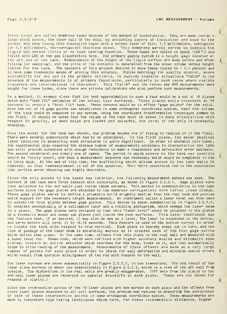
Page 2. 5-2-2 LNG MEASUREMENT V olume
These tanks are called membrane tanks because of the method of construction. They are made inside a
large steel socket, the inner hull of the ship, by attaching layers of insulation and wood to thesocket and then lining this insulation layer with a welded layer of thin, 1.2 millimeters, corrugated(or 0.7 millimeters, non-corrugated) stainless steel. This membrane merely serves to contain theliquid and serves little or no load bearing function. These tanks are cooled to about -160 0 C andfilled with LNG at the gas liquefaction site. The primary gaging system is a height gage located atthe aft end of the tank. Measurements of the height of the liquid surface are made before and afterfilling (or emptying), and the price of the contents is determined from the known volume versus heighttables for the tank. The sponsors of this project desired to know these tables to + 0.1 percent andto have some reasonable means of proving this accuracy. Unlike metrology for quality control, wheresuitability for end use is the primary criteria, in custody transfer situations "faith" in theaccuracy of the measurements is of primary importance, particularly in such cases where custodytransfers are international in character. This "faith" was the reason why NBS measurements weresought for these tanks, since there are private calibrators who also perform such measurements.
As a method, it seemed clear that the best approximation to such a tank would be a set of 10 planeswhich were "best fit" estimates of the actual tank surfaces. These planes would intersect at 16corners to create a "best fit" tank. These corners would be in effect "gage points" for the solid.Once the set of 16 gage points was established in some orthogonal coordinate system, then the volumeof the tank could be computed in any system, using the coordinate transformation techniques common inthe field. It should be noted that the volume of the tank must be known in many orientations withrespect to gravity, as when ships are loaded and unloaded, the level of the ship is constantlychanging.
Once the model for the tank was chosen, the problem became one of trying to realize it in the field.There were several constraints which had to be considered. In the first place, the sheer physicallabor involved in measuring such structures is quite significant. In order to minimize this labor,the experimental plan required the minimum number of measurements necessary to characterize the tankand still provide ourselves with enough redundancy to make a reasonable and defensible error estimate.The second constraint was simply one of speed. The period in which access to the tank was possiblewould be fairly short, and thus a measurement sequence was necessary which could be completed in twoto three days. At the end of this time, the scaffolding which allows access to the tank walls isremoved, so that remeasurement is out of the question. This third constraint led to the conclusionthat on-line error checking was highly desirable.
Since the only access to the tanks was interior, the following measurement method was used. Thecorners of the tank were first labeled with subscripts, as shown in figure 2. 5. 2.1. Gage plates werethen attached to the end walls just inside these corners. This method is nondestructive to the tanksurfaces since the gage plates are attached to the membrane corrugations with teflon lined clamps.These gage plates serve to define a prismatic solid slightly smaller than the real tank and providesolid support for the necessary length measurements. An instrument called a laser level was then usedto establish true planes between gage points. This device is shown schematically in figure 2.5. 2.2.
It consists conceptually of a collimated laser and a rotating pentaprism, which sweeps the laser beamin a plane. The gage plates were designed so that this "laser level" could be attached to the plateson a kinematic mount and sweep out planes just inside the tank surfaces. This laser instrument hasthe feature that, if so desired, it may also be use as a level. The laser is suspended in the device,
and servo motors will level it to +0.10 seconds. This feature is used on the bottom survey in orderto locate the tank with respect to true vertical. Each plane is thereby swept out in turn, and the
line of passage of the laser beam is accurately marked as it crosses each of the four gage pointswhich define that plane. At the same time, offsets from this plane to the real wall are measured witha laser level rod. These rods, which were refitted with higher accuracy scales and kinematic baseplates, contain an active detector which searches for the beam, locks on it, and then automaticallystops to allow reading of the measurement. Measurements of these offsets are made at a very largenumber of points for each plane in order to check for wall deformation and minimize cosine errors
which result from operator misalignment of the rod with respect to the wall.
The laser surveys are shown schematically in figure 2. 5. 2. 2, in two dimensions. The end result of the
laser plane surveys is shown two dimensionally in figure 2. 5. 2. 3, which is a view of the aft wall fromoutside. The distortions in the real walls are greatly exaggerated. (Off sets from the plates to the
end wall laser planes are recorded on special standoffs at each plate. These are not shown forreasons of clarity.)
Since the intersection points of the 10 laser planes are now marked on each plate and the offsets fromthese laser planes measured to all wall surfaces, the problem now reduces to measuring the coordinatesof each of these intersection points in some orthogonal coordinate system. These measurements are
made by laboratory type taping techniques which have, for these intermediate distances, higher
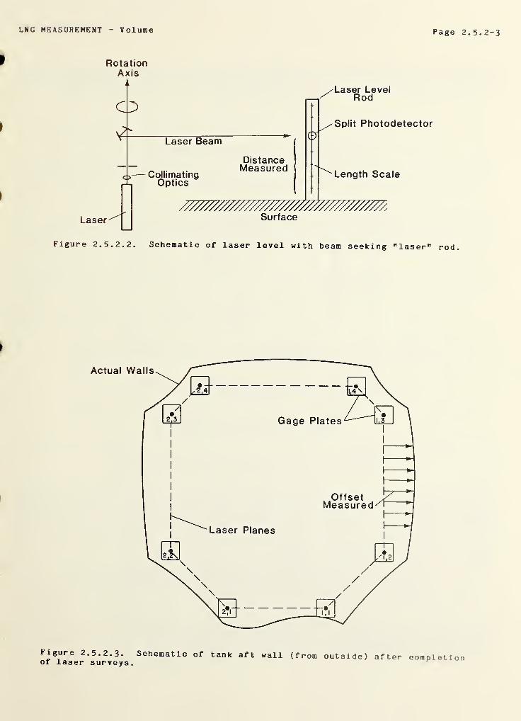
LNG MEASUREMENT Volume Page 2. 5. 2-3
RotationAxis
Laser
Figure 2.5. 2. 2. Schematic of laser level with beam seeking "laser" rod.
>
Figure 2. 5. 2. 3. Schematic of tank aft wall (from outside)of laser surveys.
after completion
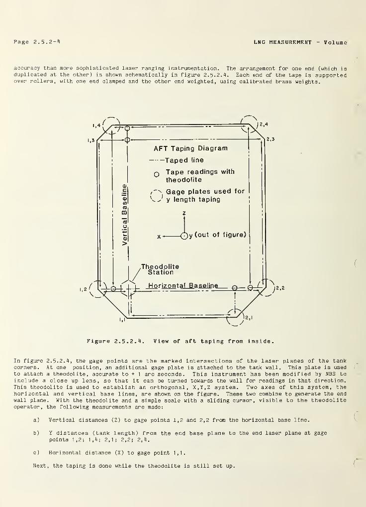
Page 2. 5.2-4 LNG MEASUREMENT V ol ume
accuracy than more sophisticated laser ranging instrumentation. The arrangement for one end (which isduplicated at the other) is shown schematically in figure 2.5.2. 4. Each end of the tape is supportedover rollers, with one end clamped and the other end weighted, using calibrated brass weights.
2,2
Figure 2.5.2. 4. View of aft taping from inside.
In figure 2. 5. 2. 4, the gage points are the marked intersections of the laser planes of the tankcorners. At one position, an additional gage plate is attached to the tank wall. This plate is usedto attach a theodolite, accurate to + 1 arc seconds. This instrument has been modified by NBS toinclude a close up lens, so that it can be turned towards the wall for readings in that direction.This theodolite is used to establish an orthogonal, X,Y,Z system. Two axes of this system, thehorizontal and vertical base lines, are shown on the figure. These two combine to generate the endwall plane. With the theodolite and a simple scale with a sliding cursor, visible to the theodoliteoperator, the following measurements are made:
a) Vertical distances (Z) to gage points 1,2 and 2,2 from the horizontal base line.
b) Y distances (tank length) from the end base plane to the end laser plane at gagepoints 1,2; 1,4; 2,1 ; 2,2; 2,4.
c) Horizontal distance (X) to gage point 1,1.
Next, the taping is done while the theodolite is still set up.
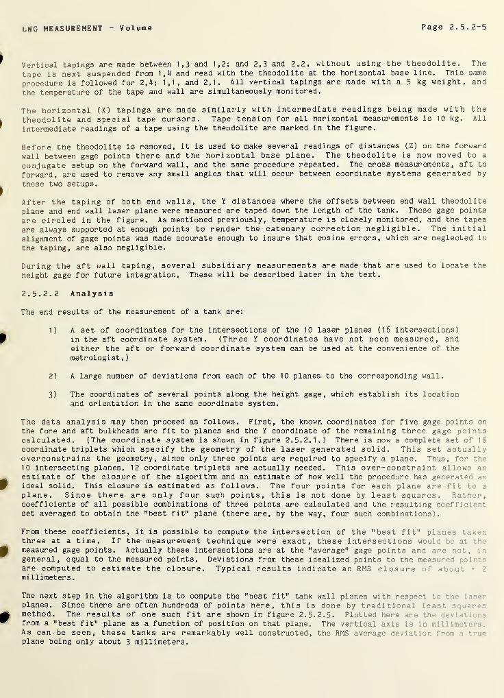
LNG MEASUREMENT V olume Page 2. 5. 2-5
Vertical tapings are made between 1,3 and 1,2; and 2,3 and 2,2, without using the theodolite. The
tape is next suspended from 1,4 and read with the theodolite at the horizontal base line. This same
procedure is followed for 2,4; 1,1, and 2,1. All vertical tapings are made with a 5 kg weight, and
the temperature of the tape and wall are simultaneously monitored.
The horizontal (X) tapings are made similarly with intermediate readings being made with the
theodolite and special tape cursors. Tape tension for all horizontal measurements is 10 kg. All
intermediate readings of a tape using the theodolite are marked in the figure.
Before the theodolite is removed, it is used to make several readings of distances (Z) on the forward
wall between gage points there and the horizontal base plane. The theodolite is now moved to a
conjugate setup on the forward wall, and the same procedure repeated. The cross measurements, aft to
forward, are used to remove any small angles that will occur between coordinate systems generated by
these two setups.
After the taping of both end walls, the Y distances where the offsets between end wall theodolite
plane and end wall laser plane were measured are taped down the length of the tank. These gage points
are circled in the figure. As mentioned previously, temperature is closely monitored, and the tapes
are always supported at enough points to render the catenary correction negligible. The initialalignment of gage points was made accurate enough to insure that cosine errors, which are neglected in
the taping, are also negligible.
During the aft wall taping, several subsidiary measurements are made that are used to locate the
height gage for future integration. These will be described later in the text.
2. 5. 2. 2 Analysis
The end results of the measurement of a tank are:
1) A set of coordinates for the intersections of the 10 laser planes (16 intersections)in the aft coordinate system. (Three Y coordinates have not been measured, andeither the aft or forward coordinate system can be used at the convenience of the
metrologist .
)
2) A large number of deviations from each of the 10 planes to the corresponding wall.
3) The coordinates of several points along the height gage, which establish its locationand orientation in the same coordinate system.
The data analysis may then proceed as follows. First, the known coordinates for five gage points on
the fore and aft bulkheads are fit to planes and the Y coordinate of the remaining three gage pointscalculated. (The coordinate system is shown in figure 2. 5. 2.1.) There is now a complete set of 16
coordinate triplets which specify the geometry of the laser generated solid. This set actuallyover constrai ns the geometry, since only three points are required to specify a plane. Thus, for the
10 intersecting planes, 12 coordinate triplets are actually needed. This over-constraint allows anestimate of the closure of the algorithm and an estimate of how well the procedure has generated an
ideal solid. This closure is estimated as follows. The four points for each plane are fit to a
plane. Since there are only four such points, this is not done by least squares. Rather,coefficients of all possible combinations of three points are calculated and the resulting coeffic:- :.*
set averaged to obtain the "best fit" plane (there are, by the way, four such combinations).
From these coefficients, it is possible to compute the intersection of the "best fit" planes taker,
three at a time. If the measurement technique were exact, these intersections would be at •••
measured gage points. Actually these intersections are at the "average" gage points and are •. •,
general, equal to the measured points. Deviations from these idealized points to the measured;
in*
are computed to estimate the closure. Typical results indicate an RMS closure of abc .* •
millimeters.
The next step in the algorithm is to compute the "best fit" tank wall planes with respect to t bi-
planes. Since there are often hundreds of points here, this is done by traditional :< ,*
method. The results of one such fit are shown in figure 2. 5. 2. 5. Plotted here are the .
from a "best fit" plane as a function of position on that plane. The vertical axis is In -•••-
As can be seen, these tanks are remarkably well constructed, the RMS average deviation :
r
plane being only about 3 millimeters.
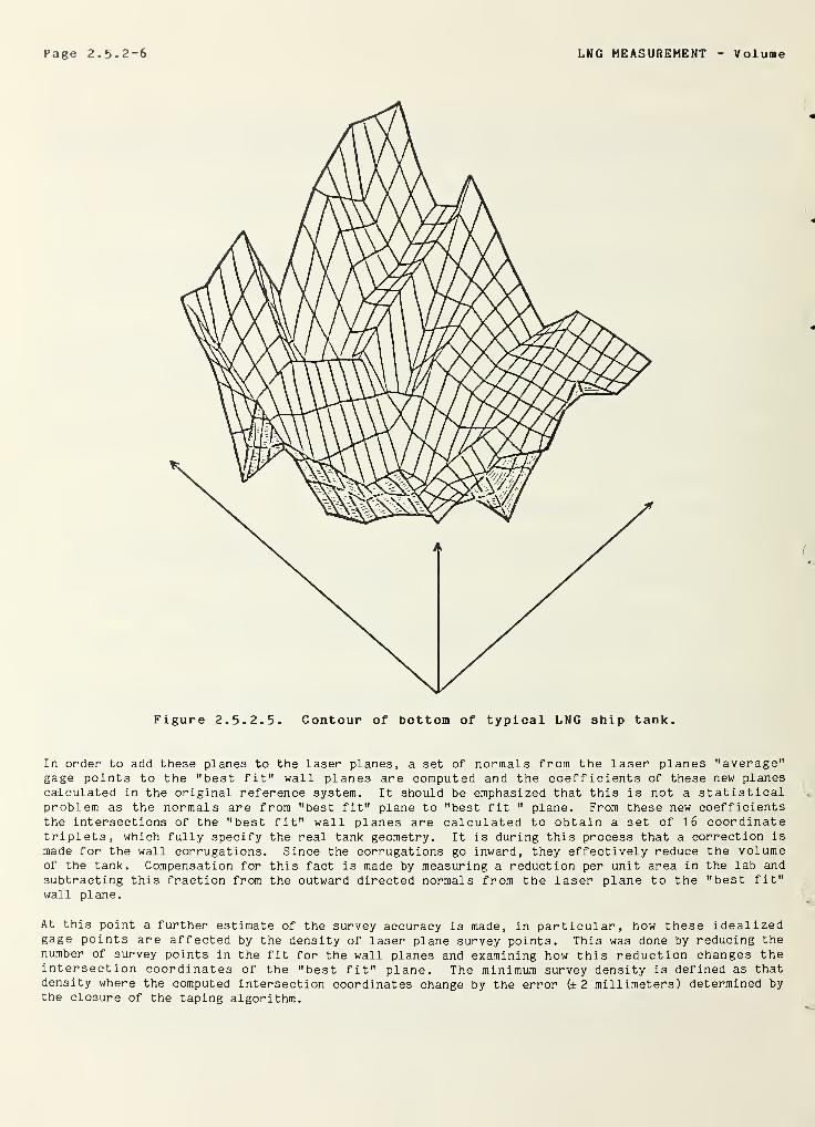
Page 2. 5. 2-6 LNG MEASUREMENT V olume
In order to add these planes to the laser planes, a set of normals from the laser planes "average"gage points to the "best fit" wall planes are computed and the coefficients of these new planescalculated in the original reference system. It should be emphasized that this is not a statisticalproblem as the normals are from "best fit" plane to "best fit " plane. From these new coefficientsthe intersections of the "best fit" wall planes are calculated to obtain a set of 16 coordinatetriplets, which fully specify the real tank geometry. It is during this process that a correction is
made for the wall corrugations. Since the corrugations go inward, they effectively reduce the volumeof the tank. Compensation for this fact is made by measuring a reduction per unit area in the lab and
subtracting this fraction from the outward directed normals from the laser plane to the "best fit"wall plane.
At this point a further estimate of the survey accuracy is made, in particular, how these idealizedgage points are affected by the density of laser plane survey points. This was done by reducing thenumber of survey points in the fit for the wall planes and examining how this reduction changes theintersection coordinates of the "best fit" plane. The minimum survey density is defined as thatdensity where the computed intersection coordinates change by the error (± 2 millimeters) determined bythe closure of the taping algorithm.
LNG MEASUREMENT V ol ume Page 2. 5. 2-7
2. 5. 2. 3 Integration Technique
In the section on tank measurement, it was described how a set of 16 (or 12) tank coordinates are
obtained. These coordinates are in a system with its origin at the theodolite on the aft bulkhead.At the time of the actual tank measurement, several subsidiary measurements necessary for the
integration were made. They were:
1) The location of base of the height gage in the theodolite coordinate system was
established.
2) The orientation of the tank bottom plane with respect to the ship's list and trimmarks was established. This was done using the laser's self leveling feature andnearly simultaneously reading the list and trim marks on the hull of the ship. (List
and trim translated to roll and pitch, respectively.)
The integration algorithm now proceeds as follows. A translation is performed to put the tank
coordinates into a system whose origin is at the origin of the height gage. These coordinates are in
an orthogonal system, but in general this system is rotated with respect to the ship system (list and
trim marks). From the level survey and the list and trim readings, two angles are calculated. Theseangles are used to rotate the tank system into the ship system. Thus, the coordinates of the tank in
the ship system are now known except for some offset vector between the two origins (which is
irrelevant anyway). It is assumed here that the tank has no yaw (rotation around the Z axis in figure2.5.2. 1) with respect to the ship. This is probably a non-trivial assumption, since the yaw of thetank is strongly coupled to the volume when the list and trim (roll and pitch) are non-zero. (Thisis easiest to see by imagining a yaw of 90 degrees). Nevertheless , since a method to accuratelymeasure this angle was not available , it was assumed to be small.
The integration algorithm works entirely with this ship coordinate set, for each tank, and the pitchand roll angles. The following is a description of this algorithm for one orientation of pitch androll
.
1) The finite rotation matrix with pitch and roll is constructed and the coordinates arerotated to define the tank in this orientation. Z is still the vertical axis, withrespect to gravity.
2) The coordinate array is searched for the maximum and minimum Z and the difference isdivided into N steps; where N is approximately 10000. The integration then proceedsby taking steps A Z and at each Z height computing the intersections of the tankplanes with the horizontal plane. These intersections define a k sided figure, inthe general case, with k i 8. The area of each of these figures is calculated, andthe integration proceeds by Simpson's rule. The number of steps N, was determined byintegrating dummy tank data (with calculatable volumes, i.e., right angles, etc.) atarbitrary orientations and determining the number of steps necessary to reduce thenumerical error to less than parts in one million. The height of the liquid at thegage is determined by calculating the Z intersection of the horizontal plane with a
vector parallel to the height gage. (The origin is already at the gage zero.)
2 . 5 .
2
.
H
Results
Measurements have been completed on three tanks of this type. The algorithm described here was
implemented in full on the last of these tanks. A crew of four metrologists took two days to completethe task, and data were entered to a remote computer using a telephone link at the end of the nee nd
day. This computer cross check showed an error which was removed by remeasurement the followingmorning, thus demonstrating the advantages of on-line checking. The closure of the algorithm,the error was corrected, was about ± 2 millmeters RMS in three dimensions, which can be converts ;
’.
volume accuracy of parts in 10000 or better. The method has thus met the original criteriafast, self checking, and highly accurate. The key elements of this system are; the genera’ ; n ! anideal solid using laser techniques, measuring deviations from this solid in a proper:
coordinate system and including enough redundancy for on-line error checking. The use of
instead of lengths allows using the existing techniques of 3-D metrology, which gr*-a’ !y
software needed for the task.
Page 2. 5. 2-8 LNG MEASUREMENT V ol ume
The original contract called for these measurements to be made on empty tanks at ambient temperature,and no attempt has been made to compute volume changes caused by liquid load or temperature effects,both of which may be considerable.
2. 5. 2. 5 LNG Ship Membrane Tank Calibrations [4]
The National Bureau of Standards, supported by the Department of Commerce Maritime Administration, didsome preliminary studies to establish an upper limit for the tank volume uncertainty of a sphericaltransport tank calibrated by photogrammetry [5]. Additional support from the Maritime Administrationand the LNG Ship Custody Transfer Committee (an industrial consortium) has made possible a
considerably expanded study of the calibration uncertainties of LNG transport tanks. The tankcalibrations examined in this work are those of the three LNG Transports built by Newport NewsShipbuilding and Drydock Company for El Paso Marine Company.
The cargo tanks on these nominal 125,000 cubic meter capacity ships are membrane types of theTechnigaz design described in reference [6]. The tanks are ten-sided prismatic solids and rectangularin horizontal cross section. The walls are all plane surfaces. The end walls are vertical as are theside walls. The side walls are connected to the horizontal floor and ceiling by sloping chine planes.All eight of the longitudinal planes are parallel to the longitudinal axis of the ship. Thesupporting walls of the tanks are the inner hull of the ship. Layers of insulation are attached tothese walls, and the internal surfaces of the insulation are covered with a liquid tight, 1.2millmeters stainless steel membrane. This membrane has corrugations stamped into it forming a wafflepattern.
The measurements used to calculate the tank volume were generally made after the membrane installationwas complete but before the removal of the construction scaffolding, since it is needed to provideaccess to the tank surface. Briefly, the calibration method used by the calibration contractorconsisted of measuring horizontal cross section areas of the tank at intervals from the bottom to thetop of the tank. The products of areas and the separation from the area immediately below summed tothe level gives the volume to that level. This method is discussed in reference [7], The crosssectional areas of these tanks were determined by measuring short distances to the wall from the sidesof a horizontal rectangle of known dimension defined by laser beams.
A calibration method developed at NBS and described above and in reference [1] was used by NBS to
assess the accuracy of the method used by the calibration contractor. The method used by NBSconsists, in brief, of inscribing with laser planes a slightly smaller closed volume with the sameshape as the tank. The dimensions of this laser-plane-defined volume are accurately measured.Perpendicular distances from the laser planes to the tank walls are measured at several hundredspecified points distributed around the tank. The integration method used to determine volume as a
function of height is also outlined in reference [1],
The calibration reports for each of the six tanks of the three ships, the El Paso Southern, The ElPaso Arzew and the El Paso Howard Boyd, appear in the appendix of the original work [4], Eachindividual tank report supplies the following information:
a. A calibration report or a report of test describing the measurement technique,measurement conditions, and error estimate.
b. A summary main gaging table showing tank volume as a function of gage height.
c. Summary list and trim correction tables to supplement the main table under expectedconditions of ship list and trim.
d. A plot comparing the NBS main gaging tables at selected intervals to the gage books
for each tank provided by the calibration contractor.
The staging was removed in four of the tanks before the NBS measurements were made; hence the
calibration check was done only to the height accessible from the bottom of the tank.
The calibration accuracy required by the ship owner is ±0.2 percent of total tank volume. The NBS
results range in accuracy from ±0.05 percent to ±0.1 percent as indicated in the Reports of
Calibration [4]. In every case, the calibration contractor's results are well within ±0.2 percent of
the NBS results. It therefore appears that the accuracy requirement has been achieved for the tanksat ambient temperature. The tank tables at ambient temperature are used by the transporter to
determine LNG volume at operating temperature, because the tank dimensions have been assumedindependent of cargo temperature. This assumption is based on the fact that the shape of the tank is
LNG MEASUREMENT Volume Page 2. 5. 2-9
determined by the external tank wall via the insulation. The corrugated design of the membrane allows
the membrane to shrink on cooling without altering the internal volume.
In actual operation, the external tank wall might be as cold as 00 C depending on weather conditions.
The temperature of the interior of the tanks was as high as 30 0 C during calibration of the tanks.Provided the external tank wall reached temperatures that high, The difference between the calibrationand operating temperature could be as large as 30
0 C.
The thermal expansion coefficient of iron as well as iron containing small quantities of nickel [8] is
approximately 0.0000116 m/m 0C. This contraction only affects the length and width of the tank with
regard to calibration, since the liquid height is determined by the level gage rather than the tankheight. The tank volume change between the calibration and operating temperature could be as much as-0.07 percent.
The shrinkage of the balsa wood insulation upon cooling (since the balsa is not a rigid body) as wellas any bulging of the tank sides counteract the reduction in volume due to cooling the walls. Thebalsa shrinkage contributes a negligible change in tank volume. If this is also true with respect totank wall bulging due to hydrostatic head, then the maximum systematic error introduced into the tankcalibration due to cooling is estimated to be no more than -0.07 percent.
Page 2.5.2-10 LNG MEASUREMENT V olume
2. 5. 2. 6 References
[1] Hocken, R. J. and W. C. Haight, Multiple redundancy in the measurement of large structures,Annals of the CIRP, 27 (1978).
[2] Young, R. D., Length calibrations in the micrometer and sub-micrometer range, Annals of theCIRP, 25 (1977).
[3] R. Hocken, J. A. Simpson, B. Borchardt, J. Lazar, C. Reeve and P. Stein, Three-DimensionalMetrology, Annals of the CIRP, 26_ (1977).
[4] Haight, W. C., R. J. Hocken, B. R. Borchardt, C. L. Carroll, R. G. Hartsock, C. P Reeve, F. E.
Scire and R. C. Veale, Estimated accuracy of calibration of some membrane-type LNG transporttanks, Nat. Bur. Stand. (U.S.), NBSIR 80-2141, 79 pp (February, 1980).
[5] Jackson, R. H. F., R. S. Collier, S. Haber and P. V. Tryon, Custody transfer systems for LNGships: tank survey techniques and sounding tables, Nat. Bur. Stand. (U.S.), NBSIR 79-1751, 84 pp(May, 1979).
[6] Jackson, R. G. and M. Kotcharian, Testing and technology of models of integrated tanks for LNGcarriers, Paper 35, Session 6, First International Conference on LNG, Chicago, IL (April, 1968)
[7] Jelffs, P. A., Calibration of containers and gages, J. Inst. Pet., _58_, No. 561, pp 117-25, (May,
1972)
.
[8] LNG Materials and Fluids User's Manual, D. B. Mann, Editor, Nat. Bur. Stand. (U.S.), Boulder, CO
(1977).
LNG MEASUREMENT Volume Page 2.5. 3-1
2.5.3 Volume of Freestanding Prismatic LNG Ship Tanks
The actual physical structure of the tank is composed of a set of plane surfaces attached at the edges
and designed to conform to the internal structure of the ship. These tanks differ from the membrane
tanks of 2.5.2 in that the tank walls are self-supporting, or freestanding. This is accomplished by
complex internal bracing and structure and allow tank construction to be performed separately from the
ship yard.
A new technique, photogrammetry , was adapted to allow measurements of the volume enclosed by the
outside walls of the tank, and then the wall material and internal structure volumes could be
subtracted to give the required internal free volume and volume-height relationships for the tank
tables. The following edited work of Siegwarth and LaBrecque [8] provides a description of the new
measurement process and a detailed look at individual measurement techniques, estimated accuracies and
precision.
The accuracy of the tank calibrated by the photogrammetri c technique was examined during the
calibration of fifteen freestanding prismatic LNG transport tanks. This examination indicated that
the calibration accuracy of the tanks calibrated in the storage position was better than ±0.1
percent. Additional factors influencing the accuracy of the calibration of the tanks, such as the
effects of installing the tanks into the ship and loading the ships with LNG, were examined in the
course of this work and, the results are reported here. The various measurements used by NBSpersonnel to analyze the calibration accuracy are detailed in the eight appendices included in the
original publication.
2. 5. 3-1 Introduction
The National Bureau of Standards has done preliminary studies [1] to establish an upper limit for the
tank volume uncertainty of a spherical transport tank calibrated by photogrammetry [2,3]. TheMaritime Administration of the Department of Commerce and the LNG Custody Transfer MeasurementsSupervisory Committee [4] have sponsored studies to test the accuracy of the present state of the artof tank calibration and to develop new methods of calibrating tanks that are suitable for industrialuse. This additional support has made possible an expanded study of the calibration uncertainties of
freestanding prismatic LNG transport tanks.
The objectives of this work were twofold. The first objective was to make more extensive measurementsto provide an independent verification of the uncertainty of the photogrammetric method of determiningspatial coordinates of points on the surface of the tanks. The second objective was to provide anupper limit for the uncertainty of the calibration of these particular tanks. This latter objectivecontains the first, but additional factors must be considered. As in the case of the spherical tanks,the photogrammetric survey may be completed before the tanks are transported to and installed in theship. In addition, the photogrammetry is done with the tank empty. Effects of lifting, installing,cooling, and loading the tanks should be included in the calibration uncertainty.
The photogrammetric calibration method and effects on the tank volume of tank history following thetank calibration have been examined by independent measurements and calculations. The photogrammetriccalibration has been analyzed for each of the tanks, using length standards. The NBS has tested thecalibration of one tank by a completely independent volume determination method. The laser planemethod developed by NBS for the conformation of the volume tables of membrane tanks [5] was modifiedand used on the exterior of the tank.
The method of volume calculations has also been tested for accuracy by independent calculations, usingthe photogrammetrically determined coordinate data for points on the tank surface. The dimensions ofthe aluminum in the tank walls and internal structure were measured for one tank to obtain an estimateof the error induced when using the blueprint dimensions in the correcting for volume taken by th"tank walls and structure. The same tank dimensioned by laser planes was also dimensioned while filledwith the maximum amount of water during the hydrostatic tests. A distortion study was perform" l 1
•
which the tank bottom was re-surveyed after the tanks were installed to determine whether th" •
support blocks were properly shimmed so that the original bottom contour of the tank was ret .
Finally, two of the early tanks were surveyed both before and after they were lifted into pi . it r- :
the ship, to investigate the effects the lifting might have on the tank volume calibration. Tvmethods used and the results obtained from the various measurements by NBS are detailed in the r--;
•*
contained in the original document [8]. An estimate of the uncertainty of the photogrammetri :,•
technique as applied to this particular calibration problem is also provided.
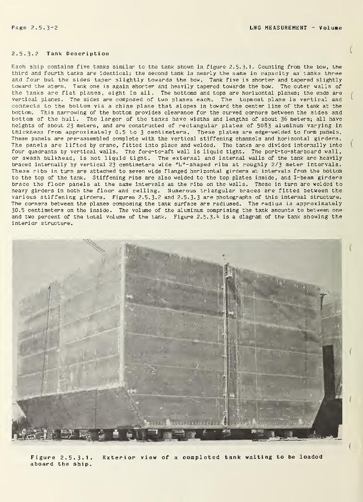
Page 2. 5. 3-2 LNG MEASUREMENT V olume
2.5. 3.2 Tank Description
Each ship contains five tanks similar to the tank shown in figure 2. 5. 3.1. Counting from the bow, thethird and fourth tanks are identical; the second tank is nearly the same in capacity as tanks threeand four but the sides taper slightly towards the bow. Tank five is shorter and tapered slightlytoward the stern. Tank one is again shorter and heavily tapered towards the bow. The outer walls ofthe tanks are flat planes, eight in all. The bottoms and tops are horizontal planes; the ends arevertical planes. The sides are composed of two planes each. The topmost plane is vertical andconnects to the bottom via a chine plane that slopes in toward the center line of the tank at the
bottom. This narrowing of the bottom provides clearance for the curved corners between the sides andbottom of the hull. The larger of the tanks have widths and lengths of about 36 meters; all haveheights of about 23 meters, and are constructed of rectangular plates of 5083 aluminum varying in
thickness from approximately 0.5 to 3 centimeters. These plates are edge-welded to form panels.These panels are pre-assembled complete with the vertical stiffening channels and horizontal girders.The panels are lifted by crane, fitted into place and welded. The tanks are divided internally intofour quadrants by vertical walls. The fore-to-aft wall is liquid tight. The port-to-starboar d wall,or swash bulkhead, is not liquid tight. The external and internal walls of the tank are heavilybraced internally by vertical 23 centimeters wide "L"-shaped ribs at roughly 2/3 meter intervals.These ribs in turn are attached to seven wide flanged horizontal girders at intervals from the bottomto the top of the tank. Stiffening ribs are also welded to the top plates inside, and I-beam girdersbrace the floor panels at the same intervals as the ribs on the walls. These in turn are welded toheavy girders in both the floor and ceiling. Numerous triangular braces are fitted between thevarious stiffening girders. Figures 2.5. 3-2 and 2.5. 3-3 are photographs of this internal structure.The corners between the planes composing the tank surface are radiused. The radius is approximately30.5 centimeters on the inside. The volume of the aluminum comprising the tank amounts to between oneand two percent of the total volume of the tank. Figure 2. 5. 3.4 is a diagram of the tank showing theinterior structure.
Figure 2. 5. 3.1. Exterior view of a completed tank waiting to be loadedaboard the ship.
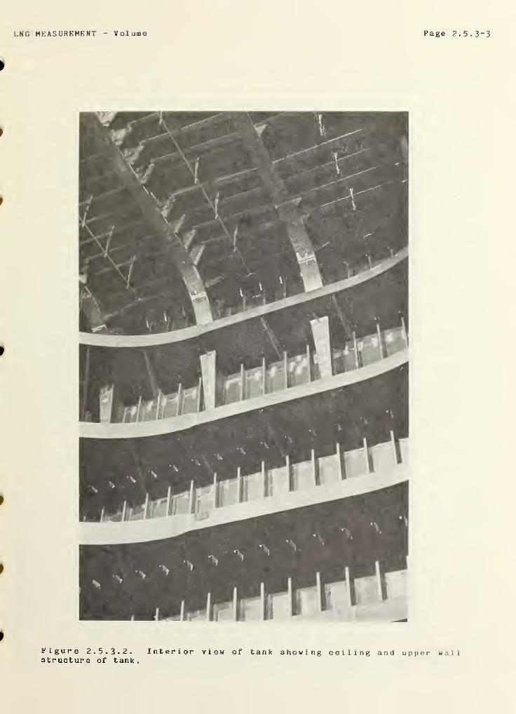
LNG MEASUREMENT Volume Page 2. 5. 3-3
Figure 2. 5. 3. 2. Interior view of tank showing ceiling and upper wallstructure of tank.
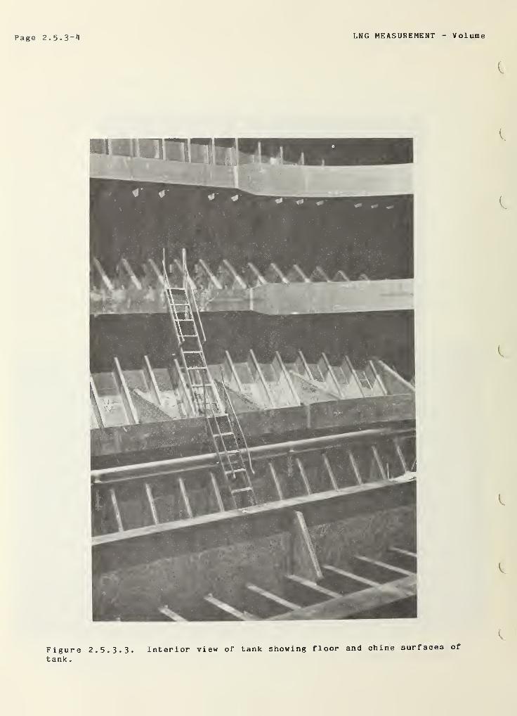
Page 2.5.3 -1*
LNG MEASUREMENT V olume
Figure 2 . 5 . 3 • 3 •
tank
.
Interior view of tank showing floor and chine surfaces of
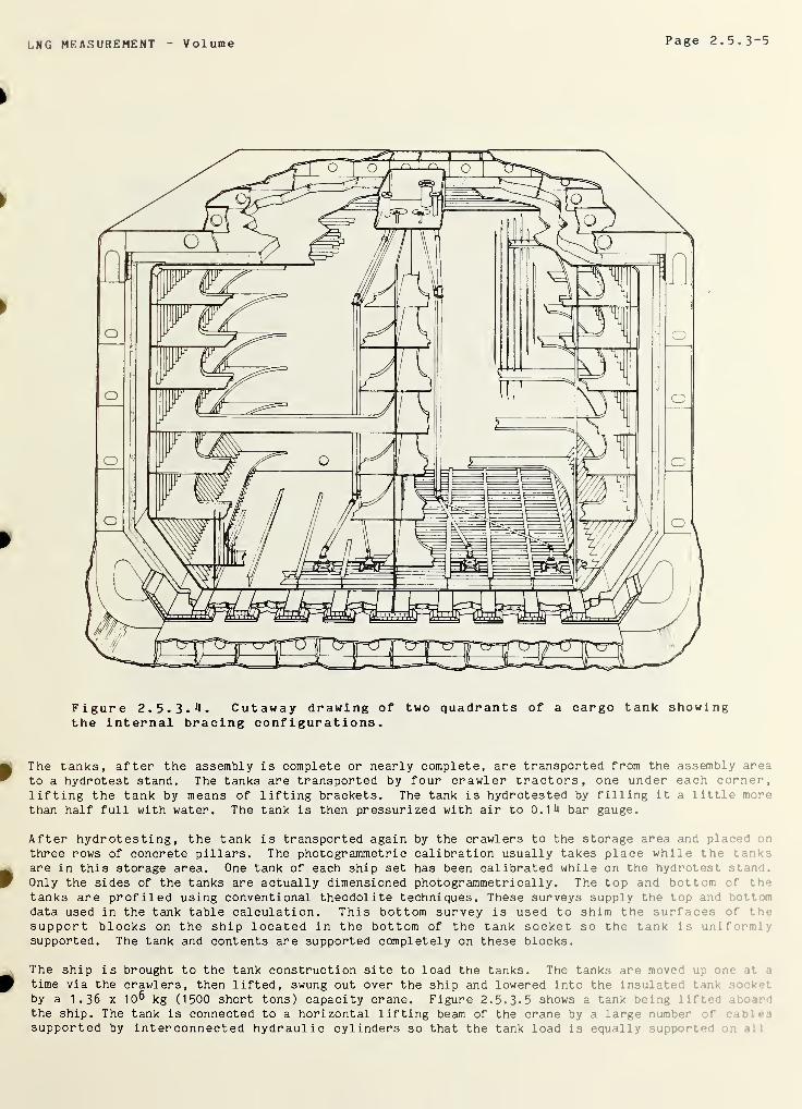
LNG MEASUREMENT Volume Page 2.5. 3-5
Figure 2 . 5 . 3 .
4
. Cutaway drawing of two quadrants of a cargo tank showingthe internal bracing configurations.
The tanks, after the assembly is complete or nearly complete, are transported from the assembly area
to a hydrotest stand. The tanks are transported by four crawler tractors, one under each corner,lifting the tank by means of lifting brackets. The tank is hydrotested by filling it a little morethan half full with water. The tank is then pressurized with air to 0.1*4 bar gauge.
After hydrotesting, the tank is transported again by the crawlers to the storage area and placed n
three rows of concrete pillars. The photogrammetric calibration usually takes place while the t i-<-
are in this storage area. One tank of each ship set has been calibrated while on the hydrotest st m :.
Only the sides of the tanks are actually dimensioned photogrammetrically . The top and bottom of ‘•
tanks are profiled using conventional theodolite techniques. These surveys supply the top an :
• ‘
* n
data used in the tank table calculation. This bottom survey is used to shim the surfaces of ' he
support blocks on the ship located in the bottom of the tank socket so the tank is unif rrr. : .
supported. The tank and contents are supported completely on these blocks.
The ship is brought to the tank construction site to load the tanks. The tanks are moved r
time via the crawlers, then lifted, swung out over the ship and lowered into the insul .•••: * m-by a 1.36 x 10® kg (1500 short tons) capacity crane. Figure 2.5. 3. 5 shows a tank being lift": i* •
:
the ship. The tank is connected to a horizontal lifting beam of the crane by a large number : 1
supported by interconnected hydraulic cylinders so that the tank load is equally su; :• .1
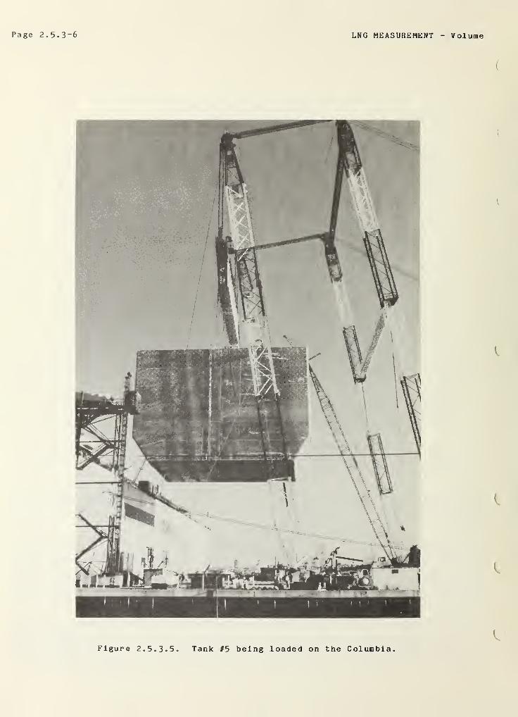
Page 2. 5. 3~6 LNG MEASUREMENT V olume
Figure 2.5. 3-5 Tank #5 being loaded on the Columbia
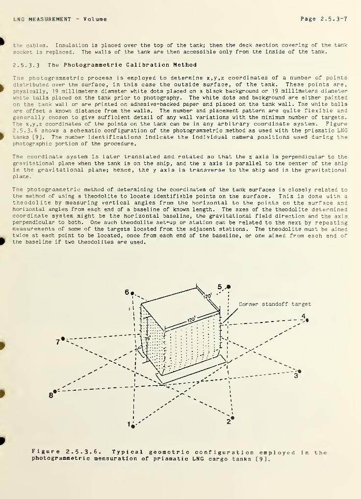
LNG MEASUREMENT Volume Page 2. 5. 3-7
the cables. Insulation is placed over the top of the tank; then the deck section covering of the tank
socket is replaced. The walls of the tank are then accessible only from the inside of the tank.
2. 5. 3. 3 The Photogr ammetr i c Calibration Method
The photogrammetric process is employed to determine x,y,z coordinates of a number of pointsdistributed over the surface, in this case the outside surface, of the tank. These points are,physically, 19 millimeters diameter white dots placed on a black background or 19 millimeters diameterwhite balls placed on the tank prior to photography. The white dots and background are either paintedon the tank wall or are printed on adhesive-backed paper and placed on the tank wall. The white ballsare offset a known distance from the walls. The number and placement pattern are quite flexible andgenerally chosen to give sufficient detail of any wall variations with the minimum number of targets.The x,y,z coordinates of the points on the tank can be in any arbitrary coordinate system. Figure2. 5. 3. 6 shows a schematic configuration of the photogrammetric method as used with the prismatic LNGtanks [9]. The number identifications indicate the individual camera positions used during thephotographic portion of the procedure.
The coordinate system is later translated and rotated so that the z axis is perpendicular to thegravitational plane when the tank is on the ship, and the x axis is parallel to the center of the shipin the gravitational plane; hence, the y axis is transverse to the ship and in the gravitationalplane.
The photogrammetric method of determining the coordinates of the tank surfaces is closely related tothe method of using a theodolite to locate identifiable points on the surface. This is done with a
theodolite by measuring vertical angles from the horizontal to the points on the surface andhorizontal angles from each end of a baseline of known length. The axes of the theodolite determinedcoordinate system might be the horizontal baseline, the gravitational field direction and the axisperpendicular to both. One such theodolite set-up or station can be related to the next by repeatingmeasurements of some of the targets located from the adjacent stations. The theodolite must be aimedtwice at each point to be located, once from each end of the baseline, or one aimed from each end ofthe baseline if two theodolites are used.
Figure 2. 5. 3. 6. Typical geometric configuration employedphotogrammetric mensuration of prismatic LNG cargo tanks [9].
In the
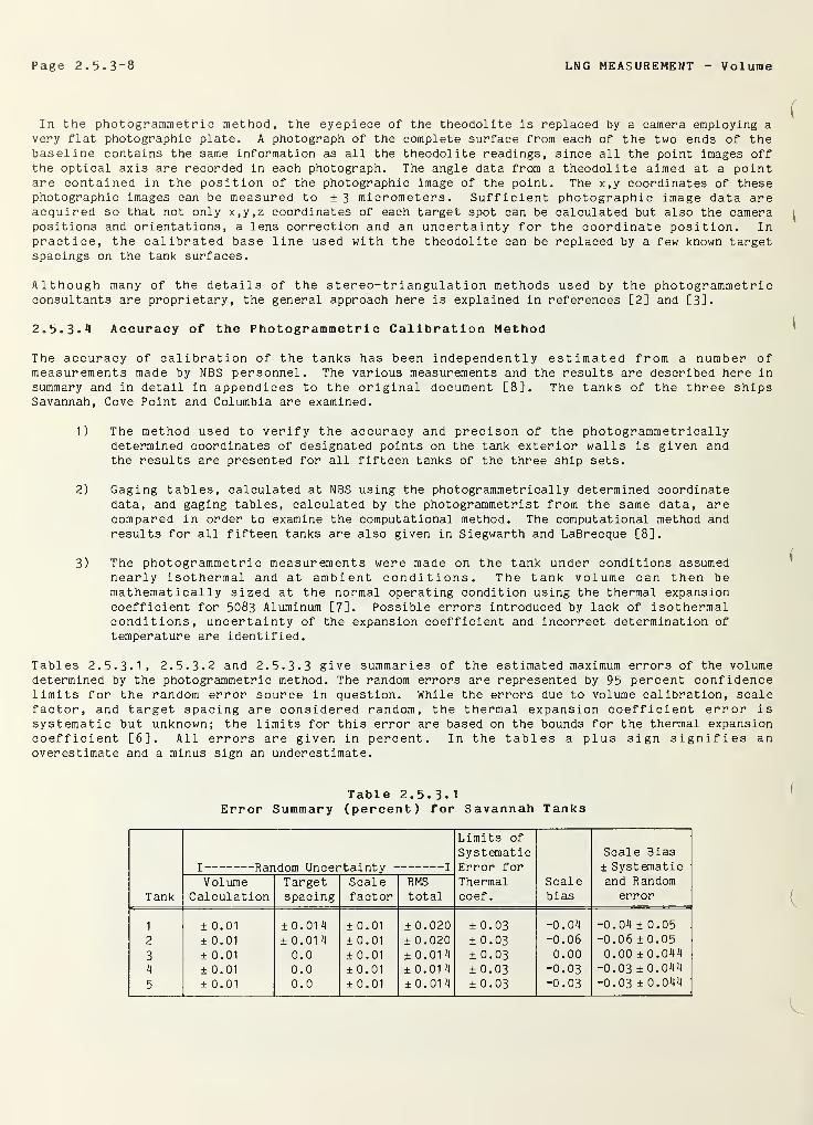
Page 2 . 5 •3~8 LNG MEASUREMENT V olume
In the photogrammetri c method, the eyepiece of the theodolite is replaced by a camera employing a
very flat photographic plate. A photograph of the complete surface from each of the two ends of thebaseline contains the same information as all the theodolite readings, since all the point images offthe optical axis are recorded in each photograph. The angle data from a theodolite aimed at a pointare contained in the position of the photographic image of the point. The x,y coordinates of thesephotographic images can be measured to ± 3 micrometers. Sufficient photographic image data areacquired so that not only x,y,z coordinates of each target spot can be calculated but also the camerapositions and orientations, a lens correction and an uncertainty for the coordinate position. Inpractice, the calibrated base line used with the theodolite can be replaced by a few known targetspacings on the tank surfaces.
Although many of the details of the stereo-triangulation methods used by the photogrammetri
c
consultants are proprietary, the general approach here is explained in references [2] and [3].
2 . 5 . 3 • 4 Accuracy of the Photogrammetri c Calibration Method
The accuracy of calibration of the tanks has been independently estimated from a number ofmeasurements made by NBS personnel. The various measurements and the results are described here insummary and in detail in appendices to the original document [8]. The tanks of the three shipsSavannah, Cove Point and Columbia are examined.
1) The method used to verify the accuracy and precison of the photogr ammetr icallydetermined coordinates of designated points on the tank exterior walls is given andthe results are presented for all fifteen tanks of the three ship sets.
2) Gaging tables, calculated at NBS using the photogrammetrically determined coordinatedata, and gaging tables, calculated by the photogrammetrist from the same data, arecompared in order to examine the computational method. The computational method andresults for all fifteen tanks are also given in Siegwarth and LaBrecque [8].
3) The photogrammetri c measurements were made on the tank under conditions assumednearly isothermal and at ambient conditions. The tank volume can then bemathematically sized at the normal operating condition using the thermal expansioncoefficient for 5083 Aluminum [7]. Possible errors introduced by lack of isothermalconditions, uncertainty of the expansion coefficient and incorrect determination of
temperature are identified.
Tables 2. 5. 3.1, 2. 5. 3. 2 and 2. 5. 3. 3 give summaries of the estimated maximum errors of the volumedetermined by the photogrammetric method. The random errors are represented by 95 percent confidencelimits for the random error source in question. While the errors due to volume calibration, scalefactor, and target spacing are considered random, the thermal expansion coefficient error issystematic but unknown; the limits for this error are based on the bounds for the thermal expansioncoefficient [6]. All errors are given in percent. In the tables a plus sign signifies anoverestimate and a minus sign an underestimate.
Table 2. 5. 3-
1
Error Summary (percent) for Savannah Tanks
Tank
I -Random Uncertainty - j
Limits of
SystematicError forThermalcoef
.
Scalebias
Scale Bias± Systematicand Random
errorVolume
CalculationTargetspacing
Scalefactor
RMStotal
1 ± 0.01 ± 0.01
4
± 0.01 ±0.020 ± 0.03 -0.04 -0.04 ± 0.05
2 ± 0.01 ± 0.01
4
± 0.01 ± 0.020 ± 0.03 -0.06 -0.06 ±0.05
3 ± 0.01 0.0 ± 0.01 ± 0.01
4
± 0.03 0.00 0.00 ± 0.044
4 ± 0.01 0.0 ± 0.01 ± 0.01
4
± 0.03 -0.03 -0.03 ± 0.044
5 ± 0.01 0.0 ± 0.01 ± 0.01
4
± 0.03 -0.03 -0.03 ± 0.044
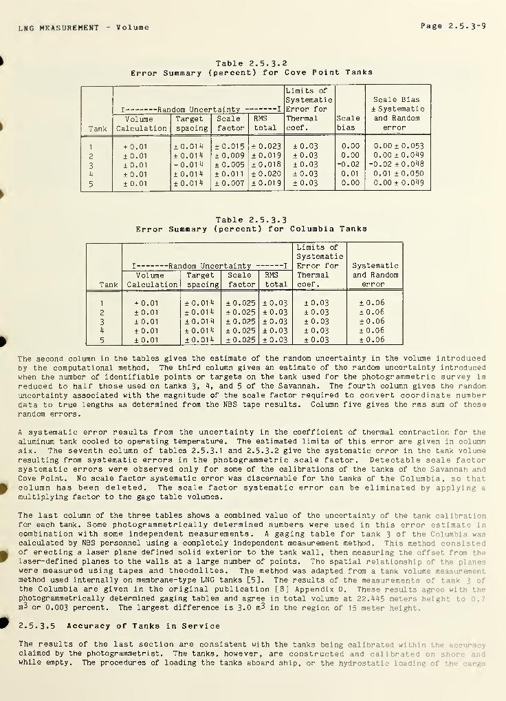
LNG MEASUREMENT V ol ume Page 2. 5. 3“9
Table 2. 5. 3.
2
Error Summary (percent) for Cove Point Tanks
Tank
I -Random Uncertainty - x
Limits of
SystematicError for
Thermalcoef
.
Scalebias
Scale Bias
± Systematicand Random
errorVolume
CalculationTargetspacing
Scalefactor
RMStotal
1 + 0.01 ± 0.01
4
± 0.015 ± 0.023 ± 0.03 0.00 0.00 ± 0.053
2 ± 0.01 ± 0.01
4
± 0.009 ± 0.019 ± 0.03 0.00 0.00 ± 0.049
3 ± 0.01 + 0.01
4
± 0.005 ±0.018 ± 0.03 -0.02 -0.02 ± 0.048
4 ± 0.01 ± 0.01
4
±0.011 ± 0.020 ±0.03 0.01 0.01 ± 0.050
5 ± 0.01 ± 0.01
4
± 0.007 ± 0.01
9
± 0.03 0.00 0.00 ± 0.049
Table 2. 5. 3-3Error Summary (percent) for Columbia Tanks
Tank
I -Random Uncertainty - x
Limits of
SystematicError forThermalcoef
.
Systematicand Random
errorVolume
CalculationTargetspacing
Scalefactor
RMS
total
1 + 0.01 ± 0.01
4
± 0.025 ± 0.03 ± 0.03 ± 0.06
2 ± 0.01 ± 0.01
4
± 0.025 ± 0.03 ±0.03 ± 0.06
3 ± 0.01 ± 0.01
4
± 0.025 ± 0.03 ± 0.03 ± 0.064 ± 0.01 ± 0.01
4
±0.025 ± 0.03 ± 0.03 ±0.065 ± 0.01 ± 0.01
4
± 0.025 ± 0.03 ± 0.03 ± 0.06
The second column in the tables gives the estimate of the random uncertainty in the volume introducedby the computational method. The third column gives an estimate of the random uncertainty introducedwhen the number of identifiable points or targets on the tank used for the photogrammetric survey is
reduced to half those used on tanks 3, 4, and 5 of the Savannah. The fourth column gives the randomuncertainty associated with the magnitude of the scale factor required to convert coordinate numberdata to true lengths as determined from the NBS tape results. Column five gives the rms sum of theserandom errors.
A systematic error results from the uncertainty in the coefficient of thermal contraction for thealuminum tank cooled to operating temperature. The estimated limits of this error are given in columnsix. The seventh column of tables 2. 5. 3.1 and 2.5. 3.2 give the systematic error in the tank volumeresulting from systematic errors in the photogrammetric scale factor. Detectable scale factorsystematic errors were observed only for some of the calibrations of the tanks of the Savannah andCove Point. No scale factor systematic error was discernable for the tanks of the Columbia, so thatcolumn has been deleted. The scale factor systematic error can be eliminated by applying a
multiplying factor to the gage table volumes.
The last column of the three tables shows a combined value of the uncertainty of the tank calibrationfor each tank. Some photogr ammetri cally determined numbers were used in this error estimate incombination with some independent measurements. A gaging table for tank 3 of the Columbia wascalculated by NBS personnel using a completely independent measurement method. This method consistedof erecting a laser plane defined solid exterior to the tank wall, then measuring the offset from *
•
laser-defined planes to the walls at a large number of points. The spatial relationship of the pi aneswere measured using tapes and theodolites. The method was adapted from a tank volume measurementmethod used internally on membrane-type LNG tanks [5]. The results of the measurements of tankthe Columbia are given in the original publication [8] Appendix D. These results agre-* wltt •••
photogrammetrically determined gaging tables and agree in total volume at 22.445 meters hoi •.
'
m3 or 0.003 percent. The largest difference is 3.0 m3 in the region of 15 meter height.
2. 5. 3. 5 Accuracy of Tanks in Service
The results of the last section are consistent with the tanks being calibrated within •
claimed by the photogrammetrist. The tanks, however, are constructed and calibrated onwhile empty. The procedures of loading the tanks aboard ship, or the hydrostatic loading of
Page 2.5.3-10 LNG MEASUREMENT V ol ume
could change the volume of the tank. Furthermore, the volumes discussed in the previous section wereexternal, so that the volume of aluminum in the walls and internal framing must be subtracted from theexternal volume to obtain the actual liquid volume. This deadwood correction is 1.3 percent for thesmallest tank (tank 1) and ranges down to 0.9 percent for the largest tank. The distortion of thetank caused by lifting it into the ship, the hydrostatic distortion and the deadwood have been studiedby NBS personnel to determine what errors may be introduced into the gaging tables.
To test for lifting distortion and surface flatness, surveys as described in the original publication ^
[8] Appendix E were performed on the top and bottom surfaces of tanks and 5 of the Savannah. Thetanks were surveyed in the storage yard and then immediately after being placed in the ship. The rootmean square differences of the surveyed points from a fitted plane were calculated for each survey.The comparison showed that there was no significant change in the rms values of any of the before andafter surveys; and, therefore, there could not be a significant change in tank volume as a result of
tank moving process. Also, it was assumed that since the top and bottom of the tank, which would be
most affected by the move, did not distort, then the walls did not distort either.
The hydrostatic pressure on the bottom of the tank when filled with LNG is about 1 bar. Since the
tanks were hydrostatically tested by filling them half-full of water, it was possible for NBSpersonnel to measure hydrostatic deformation of the tank. Flatness measurements were made on thewalls of tank 3 of the Columbia both with and without water in the tank. The results of thesemeasurements are given in the original publication [8] Appendix F. The rms differences of the
surveyed points from a fitted plane were calculated and compared for the survey done before thehydrostatic test and for the survey made during the test. As no significant differences were detectedfor the rms values, it was inferred that no significant volume change had occurred.
The tank volume comparisons are for the outside dimensions of the tank. To obtain the liquid volume,
the volume of aluminum in the walls and internal structure must be calculated as a function of height.The deadwood volume at height h must be subtracted from the external tank volume at height h to get
the liquid volume at this height. The photogrammetric contractor determined deadwood volume as a
function of height from drawings of the tanks and the nominal dimensions of the various plates. In
measurements made by NBS on tank 3 of the Columbia, it was found that the deadwood dimensions are 1
generally slightly larger than nominal. For this tank, the larger dimensions decrease the totalliquid volume by about 8 m3 or 0.03 percent. The actual measurements are reported in the originalpublication [8] Appendix G.
The survey effort and the results obtained for the tank bottom surveys of the 10 tanks of the firsttwo ships are presented as Appendix H in the original publication [8]. The desired measurementaccuracy was not achieved with these measurements, because the ship yard continued work during the
measurements, which caused both constant movement and permanent changes of the list and trim. Theflatness surveys of the four tank quadrants could not be satisfactorily correlated by the water tube
measurements. The flatness surveys by quadrant did suggest, however, that little bottom distortionhad resulted from placing the tanks. The motions of the ship during the surveys also precludedaccurate measurement of the orientation of the tank with respect to the draft marks. The surveys of
the third ship were not completed, because the gas trials of the Savannah showed the insulation systemused was unsatisfactory for LNG service.
Because of the central location of the liquid level gages in these tanks, the volume error is not a
strong function of list or trim. For example, a 5 centimeter list adds an error of ±3 m3 to the
volume of the largest tanks, the sign depending on whether the list is to starboard (positive) or to
port. The attempt to measure the tank and gage orientations with respect to the draft marks was done
when the ships were essentially complete. This measurement could be repeated anytime in the futurewhen the ship tanks are brought up to air during the periodic inspections. This could best be done in
a non-floating drydock. The measurements might also be done with the ship afloat in a quiet body of
water when no other work is being done either on the ship or nearby. I
Of the three sources of error considered in this section—lifting distortion, hydrostatic distortion,and errors in deadwood specification— only errors in the deadwood corrections are seen to be
significant. For the lifting and hydrostatic distortions, no bounds have been calculated for how muchchange in volume could have occurred without having been detected by the methods of measurement used.
The study by NBS of tank 3 of the Columbia showed the deadwood volume to be 2.9 percent larger thanthe deadwood volume calculated from the tank's nominal dimensions. ,
LNG MEASUREMENT Volume Page 2.5.3-11
The uncertainty of this 2.9 percent value has been calculated to be approximately ±0.2 percent.While it is not possible to predict what the error in the deadwood volume caused by oversizeddimensions would be for the remaining fourteen tanks, the material from which the other tanks wereconstructed is likely to be similar in sizing to the material for this tank, and it is not expectedthat this deadwood volume error would exceed 5 percent.
In conclusion, the NBS verification of the photogrammetric method of determining the external tankvolumes found the uncertainty of this method to be within ±0.1 percent of total volume. Thisincludes the errors in the use of the temperature coefficient to calculate the volume at operatingtemperature and in the deadwood calculation, but not the errors in the bottom survey or the effects of
lifting, installing, and loading the tanks. The deadwood calculation error is expected to be within+ 0.0^ percent for the largest tank and within ±0.06 percent for the smallest. There exists no goodestimate of the bottom survey error. There is no indication of any distortion due to hydrostaticloading or to moving the tanks, and no estimate of how much volume change could have occurred withoutbeing detected by the techniques used in this study.
Page 2.5.3-12 LNG MEASUREMENT Volume
2. 5. 3. 6 References
[1] Jackson, R.H.F., R.S. Collier, S. Haber and R.V. Tryon, Custody transfer systems for LNG ships:
tank survey techniques and sounding tables, Nat. Bur. Stand. (U.S.), NBSIR 79-1 751 (July 1,
1978)
.
[2] Brown, D.C., A solution to the general problem of multiple station analytical stereoangulation,Air Force Missile Test Center Report No. 58-8, Patrick AFB, Florida( 1 958)
.
[3] Kenefick, J.F., 1971. Ultra-precise analytics, Photogrammetric Engineering, Vol. 37, p. 1
1
67 .
[ 4 3 The members of the LNG Custody Transfer Measurements Supervisory Committee are Ivan W. Schmitt,Chairman, El Paso Marine Company; Bland Osborn, Columbia LNG Corporation; Howard S. Joiner,Consolidated Systems LNG Company; and Ed Crenshaw, Southern Energy Company.
[5] Hocken, R. J. and W. C. Haight, Multiple redundancy in the measurement of large structures,Annals of the International Institution of Production Engineering Research (CIRP), Volume 27, p.
1,(1978).
[6] Brown, D.C., Application of close-range photogrammetry to structures in orbit, Vol. 1 and 2, GSI
Technical Report #20-012. Available from Geodetic Services incorporated, 1511 South River ViewDrive, Melbourne, Florida 32901
.
[7] Mann, D. B., Editor, LNG materials and fluids. Thermophysical Properties Division, NationalBureau of Standards, Boulder, Colorado( 1 977)
.
[8] Siegwarth, J. D. and J. F. LaBrecque, Estimated uncertainty of calibrations of free standingprismatic liquefied natural gas cargo tanks, Nat. Bur. Stand. (U. S.), 294 pp (January 1982).
[9] Brown, D. C., LNG tank inventory measurement by photogrammetry, 1981 Operating SectionProceedings, 81-T-55, ppT-127~37, Am. Gas Assoc., 1515 Wilson Blvd., Arlington, VA 22209(1981 ).
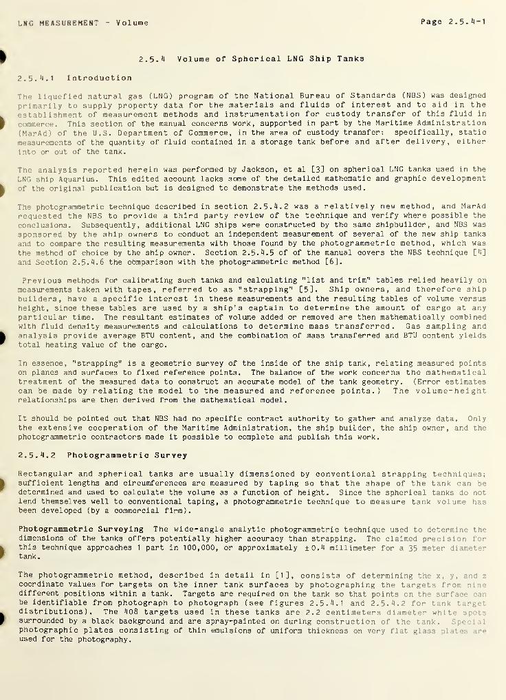
LNG MEASUREMENT Volume Page 2. 5.4-1
2.5.4 Volume of Spherical LNG Ship Tanks
2.5. *4.1 Introduction
The liquefied natural gas (LNG) program of the National Bureau of Standards ( NBS ) was designed
primarily to supply property data for the materials and fluids of interest and to aid in theestablishment of measurement methods and instrumentation for custody transfer of this fluid in
commerce. This section of the manual concerns work, supported in part by the Maritime Administration(MarAd) of the U.S. Department of Commerce, in the area of custody transfer: specifically, static
measurements of the quantity of fluid contained in a storage tank before and after delivery, either
into or out of the tank.
The analysis reported herein was performed by Jackson, et al [3] on spherical LNG tanks used in the
LNG ship Aquarius. This edited account lacks some of the detailed mathematic and graphic developmentof the original publication but is designed to demonstrate the methods used.
The photogrammetric technique described in section 2. 5. 4. 2 was a relatively new method, and MarAdrequested the NBS to provide a third party review of the technique and verify where possible the
conclusions. Subsequently, additional LNG ships were constructed by the same shipbuilder, and NBS was
sponsored by the ship owners to conduct an independent measurement of several of the new ship tanks
and to compare the resulting measurements with those found by the photogrammetric method, which wasthe method of choice by the ship owner. Section 2. 5. 4. 5 of of the manual covers the NBS technique [4]
and Section 2. 5. 4. 6 the comparison with the photogrammetric method [6].
Previous methods for calibrating such tanks and calculating "list and trim" tables relied heavily on
measurements taken with tapes, referred to as "strapping" [5]. Ship owners, and therefore shipbuilders, have a specific interest in these measurements and the resulting tables of volume versusheight, since these tables are used by a ship's captain to determine the amount of cargo at anyparticular time. The resultant estimates of volume added or removed are then mathematically combinedwith fluid density measurements and calculations to determine mass transferred. Gas sampling andanalysis provide average BTU content, and the combination of mass transferred and BTU content yieldstotal heating value of the cargo.
In essence, "strapping" is a geometric survey of the inside of the ship tank, relating measured pointson planes and surfaces to fixed reference points. The balance of the work concerns the mathematicaltreatment of the measured data to construct an accurate model of the tank geometry. (Error estimatescan be made by relating the model to the measured and reference points.) The volume-heightrelationships are then derived from the mathematical model.
It should be pointed out that NBS had no specific contract authority to gather and analyze data. Onlythe extensive cooperation of the Maritime Administration, the ship builder, the ship owner, and thephotogrammetric contractors made it possible to complete and publish this work.
2. 5. 4. 2 Photogrammetric Survey
Rectangular and spherical tanks are usually dimensioned by conventional strapping techniques;sufficient lengths and circumferences are measured by taping so that the shape of the tank can bedetermined and used to calculate the volume as a function of height. Since the spherical tanks do notlend themselves well to conventional taping, a photogrammetric technique to measure tank volume hasbeen developed (by a commercial firm).
Photogrammetric Surveying The wide-angle analytic photogrammetric technique used to determine thedimensions of the tanks offers potentially higher accuracy than strapping. The claimed precision forthis technique approaches 1 part in 100,000, or approximately ±0.4 millimeter for a 35 meter di ime": • r
tank.
The photogrammetric method, described in detail in [1], consists of determining the x, y,• •
coordinate values for targets on the inner tank surfaces by photographing the targets from r. in-different positions within a tank. Targets are required on the tank so that points on the sur: ice
be identifiable from photograph to photograph (see figures 2.5. 4.1 and 2.5. 4.2 for tank r
distributions). The 408 targets used in these tanks are 2.2 centimeters diameter whir- ;
'
surrounded by a black background and are spray-painted on during construction of the tank. !
photographic plates consisting of thin emulsions of uniform thickness on very flat gl
used for the photography.
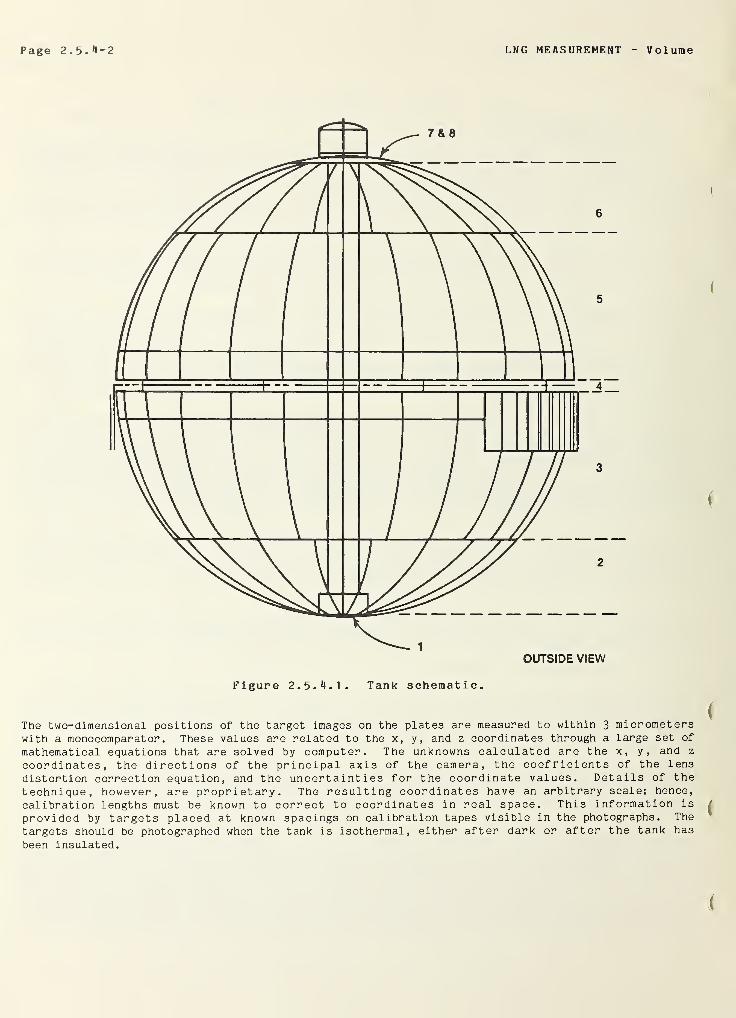
Page 2. 5. 4-2 LNG MEASUREMENT V ol ume
The two-dimensional positions of the target images on the plates are measured to within 3 micrometerswith a monocomparator. These values are related to the x, y, and z coordinates through a large set of
mathematical equations that are solved by computer. The unknowns calculated are the x, y, and z
coordinates, the directions of the principal axis of the camera, the coefficients of the lens
distortion correction equation, and the uncertainties for the coordinate values. Details of the
technique, however, are proprietary. The resulting coordinates have an arbitrary scale; hence,
calibration lengths must be known to correct to coordinates in real space. This information is
provided by targets placed at known spacings on calibration tapes visible in the photographs. The
targets should be photographed when the tank is isothermal, either after dark or after the tank has
been insulated.
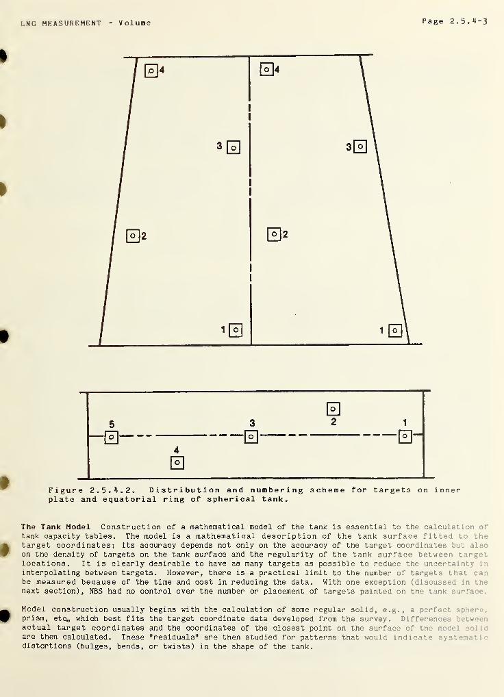
LNG MKASUREMENT Volume Page 2. 5. 4-3
I
I
>
Figure 2 . 5 • 4 . 2
.
Distribution and numbering scheme for targets on innerplate and equatorial ring of spherical tank.
§
The Tank Model Construction of a mathematical model of the tank is essential to the calculation of
tank capacity tables. The model is a mathematical description of the tank surface fitted to thetarget coordinates; its accuracy depends not only on the accuracy of the target coordinates but alsoon the density of targets on the tank surface and the regularity of the tank surface between targe’-,
locations. It is clearly desirable to have as many targets as possible to reduce the uncertainty ir.
interpolating between targets. However, there is a practical limit to the number of targets that canbe measured because of the time and cost in reducing the data. With one exception (discussed in thenext section), NBS had no control over the number or placement of targets painted on the tank surface.
Model construction usually begins with the calculation of some regular solid, e.g., a perfect ;•••••,
' prism, etc,, which best fits the target coordinate data developed from the survey. Differences b<-tw-«T
actual target coordinates and the coordinates of the closest point on the surface of the mode;are then calculated. These "residuals" are then studied for patterns that would indicat"distortions (bulges, bends, or twists) in the shape of the tank.
Page 2.5.*t- 1J LNG MEASUREMENT V olume
On the basis of patterns discovered during this exploratory residual analysis, a special-purposetechnique is developed to integrate numerically the composite tank model, which specifies a regularsolid along with a table of deviations or residuals.
The final step in this analysis is the calculation of sounding tables giving tank volumes at regularintervals of liquid height in the tank. Error bounds on these tank values can then be developed.
Tank Table Modifications There are a number of modifications to the sounding tables that must be madebefore their construction is completed. List, trim, thermal contraction, and stress effects must be
accounted for. List and trim corrections, however, are not addressed here, as NBS did not have accessto the data or the procedures used in making these corrections.
It is standard practice to correct tank tables for thermal contraction by applying contractioncoefficients as if the tank were mechanically unconstrained. The dimensions of the tank are decreaseduniformly according to the thermal contraction of the material. Actually, tank mounting constraintsand variations in the thermal expansions of the structural material can introduce strains in the tankthat might affect cargo capacity. These thermal stress effects cannot presently be analyzed, becausedata on constraint effects and anisotropic thermal coefficients are lacking.
Another effect is the cargo load, which stresses both the tank and the ship hull. An analysis of theeffects of these strains on the tank tables is beyond the scope of this work. Furthermore, thephotogrammetric contractors do not include such corrections in their report.
2 . 5 . 4 .
3
Analysis of Spherical Ship Tank
As part of the Maritime Administration Custody Transfer Program mentioned earlier, NBS was asked toevaluate the methodology used to calibrate the spherical tanks. In addition, NBS was asked to commenton the accuracy of the sounding tables subsequently constructed. In this section, the NBS analysis is
presented and described as to how it differs from the analysis performed by the photogrammetricconsultants. Included also is a discussion of the accuracy of the sounding tables constructed and an
assessment of the limitations, additional to those implicit in the last paragraph, to theapplicability of those tables.
Each tank calibrated is spherical, with a diameter of approximately 36.5 meters and a capacity(volume) of 25,000 cubic meters. Constructed of four bands ("strakes") of aluminum plates in theshape of spherical trapezoids (see figure 2.5.4.1), with special cap plates at the top and bottom.The only internal structure is a cylindrical tower extending from cap, to cap containing piping,wiring, depth gauges, etc.
The first step in constructing the tanks discussed in this section is to weld together the equatorialring by which the tank is supported. The ring is set up on jigs, and the tank plates making up thecentral strakes (previously welded into pairs) are welded in place above and below the equatorialring. The top and bottom strakes are then welded in place. The bottom and top circular plates arewelded in after the rest of the welding is completed, and the internal staging is removed.
After a tank is completed, it is loaded on a crawler, supported from beneath, and moved to thehydrostatic test stand. After the test, the tank is moved to the insulation building and insulated.
Then it is moved to a barge for transporting to the shipyard, where it is lifted into place on theship.
The procedure for constructing sounding tables consists of:
a) photogrammetrically surveying target coordinates on the inside surface of the tank;
b) constructing a mathematical model of the tank geometry;
c) developing a mathematical technique for computing volumes below specified heights in
the tank; and
d) determining effects on tank shape (and therefore tank volume) of tank loading,cooling, liquid loading, sagging, sloshing, etc.
Each stage of calculation has associated with it an error bound on the accuracy of the result. These
error bounds can be calculated using the appropriate statistical analysis; this can always be done and
is straightforward. Difficulties arise only in regard to the "tightness" of those bounds, i.e., their
balance between realism and conservatism. These error bounds will be discussed later in this section.
LNC MEASUREMENT Volume Page 2. 5. 4-5
The following is a result of an exploratory statistical analysis of the target coordinate data for
Aquarius tank number obtained from the photogr ammetri c consultants. A best-fitting sphere is
obtained by using linear least squares to minimize the sum of the squares of the radial residuals.
Analysis of these residuals then provides information on how the tank wall deviates from a true
sphere, information of value to the numerical integration procedure described later.
In fitting a sphere, if the usual concept of a distance measured d = (x 2 + y2 + z 2 )
1/2 is used, the
distance between a point and the surface of a sphere is a nonlinear function of the unknown parameters
of the sphere. This complexity results in a nonlinear least squares problem for finding the
best-fitting sphere. Witzgall [2] has developed a technique that avoids this complexity and reduces
the problem to a linear one, allowing the use of linear least squares. This approach, is described as
well as methods to remove its bias. The formulation is for an arbitrary n-dimensional space and thus
applies equally well to circles in 2-space, spheres in 3-space, and hyperspheres in n-space (Rn ).
The detailed method used in calculating the best-fitting sphere is given in the original publication
[3] and will not be repeated here. However, using the technique described, the radius of the
best-fitting sphere for Aquarius tank number 4 was determined to be:
r = 18.2682 meters,
with a standard error of
SE = 0.0071 meters.
With respect to the coordinate system defined by the consultants, the coordinates of the center are:
.0005 meters SE = .0013 meters;-.0009 meters SE = .0013 meters;-.0137 meters SE = .001
1
meters
.
The standard errors given above are computed, using the usual least squares theory that assumes theradial residuals from a perfect sphere are random. As shown below, this assumption is incorrect. The
purpose of the best-fitting sphere, however, is only to serve as a reference surface for furtheranalysis.
Analysis of Residuals With the calculation of the best-fitting sphere, it is now possible to performthe exploratory analysis of residuals that provides specific information on tank shape. These"residuals'1 are the differences between actual target coordinates and the coordinates of the closestpoint on the surface of the model or best fitting sphere. A thorough residual analysis, such as wasperformed for the original publication [ 3 ], typically includes many types of graphical displays. In
the interest of brevity, only a descriptive summary of the analyis will be presented here. If
additional detail is required, the original publication should be consulted.
The targets are arranged in 21 rows around the sphere: 1 row on each of the top and bottom polarplates; 3 rows on the equatorial ring; and 4 rows on each of the four strakes. On each plate thereare 4 targets arranged and numbered as indicated in figure 2. 5. 4. 2.
The analysis of the residuals shows the nature of the tank distortion. The bottom polar plate and thebottom edge of the #1 strake are flattened (as if the tank were free-standing on a flat surface' andlie internal to the model sphere by as much as 6 centimeters. The #1 strake must have a "sharp" bendnear the second row of targets, because the residuals for the upper three rows of targets on the •
1
strake and all points on the #2 strake average 0.8 centimeter outside the sphere.
Table 2. 5. 4.1 summarizes the residuals by row. The term "Degrees of Freedom" used in the table :
equal to one less than the number of targets in a row. The most interesting fact from a study f
table is that in some regions the residuals are following some major distortion of the tar. - an :
thus not random. In other areas (at joints between strakes), the residuals appear random • .*
standard deviations similar to those in the nonrandom regions. In particular,randomness are adjacent to the seams where 42 plates are joined. However, in only or.* (• •• ~
polar plate) do the "non-random" residuals appear to be such that the values could be appra simple surface or polynomial. In fact the first strake, row 1 residuals can be !
.“ ' .
sine curve, though not nearly as well as those for the bottom polar plate.
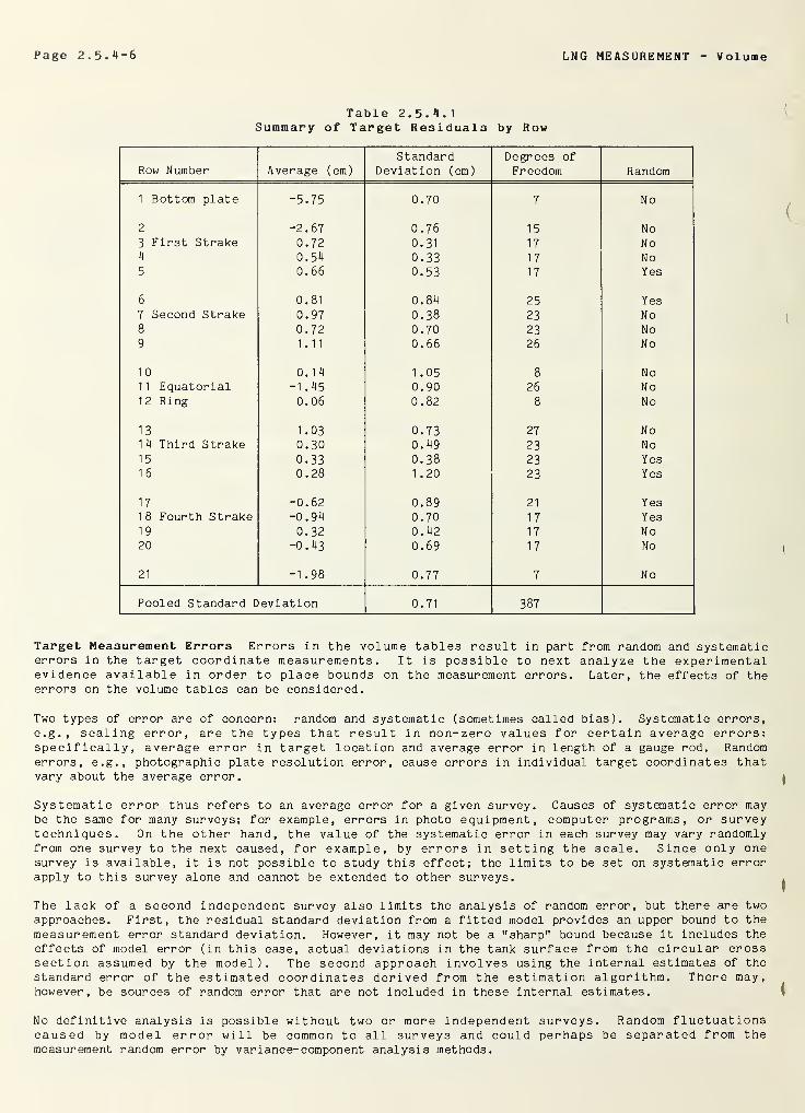
Page 2. 5. 4-6 LNG MEASUREMENT V ol ume
Table 2.5.4.
1
Summary of Target Residuals by Row
Row Number Average (cm)
StandardDeviation (cm)
Degrees of
Freedom Random
1 Bottom plate -5.75 0.70 7 No
2 -2.67 0.76 15 No
3 First Strake 0.72 0.31 17 No4 0.54 0.33 17 No5 0.66 0.53 17 Yes
6 0.81 0.84 25 Yes
7 Second Strake 0.97 0.38 23 No8 0.72 0.70 23 No9 1.11 0.66 26 No
10 0.1 4 1 .05 8 No11 Equatorial -1.45 0.90 26 No12 Ring 0.06 0.82 8 No
13 1.03 0.73 27 No1 4 Third Strake 0.30 0.49 23 No15 0.33 0.38 23 Yes16 0.28 1 .20 23 Yes
17 -0.62 0.89 21 Yes1 8 Fourth Strake -0.94 0.70 17 Yes19 0.32 0.42 17 No20 -0.43 0.69 17 No
21 -1.98 0.77 7 No
Pooled Standard Deviation 0.71 387
Target Measurement Errors Errors in the volume tables result in part from random and systematicerrors in the target coordinate measurements. It is possible to next analyze the experimentalevidence available in order to place bounds on the measurement errors. Later, the effects of theerrors on the volume tables can be considered.
Two types of error are of concern: random and systematic (sometimes called bias). Systematic errors,e.g., scaling error, are the types that result in non-zero values for certain average errors:specifically, average error in target location and average error in length of a gauge rod. Randomerrors, e.g., photographic plate resolution error, cause errors in individual target coordinates thatvary about the average error.
Systematic error thus refers to an average error for a given survey. Causes of systematic error maybe the same for many surveys; for example, errors in photo equipment, computer programs, or surveytechniques. On the other hand, the value of the systematic error in each survey may vary randomlyfrom one survey to the next caused, for example, by errors in setting the scale. Since only onesurvey is available, it is not possible to study this effect; the limits to be set on systematic errorapply to this survey alone and cannot be extended to other surveys.
The lack of a second independent survey also limits the analysis of random error, but there are twoapproaches. First, the residual standard deviation from a fitted model provides an upper bound to the
measurement error standard deviation. However, it may not be a "sharp" bound because it includes the
effects of model error (in this case, actual deviations in the tank surface from the circular crosssection assumed by the model). The second approach involves using the internal estimates of the
standard error of the estimated coordinates derived from the estimation algorithm. There may,however, be sources of random error that are not included in these internal estimates.
No definitive analysis is possible without two or more independent surveys. Random fluctuationscaused by model error will be common to all surveys and could perhaps be separated from themeasurement random error by variance-component analysis methods.

LNG MEASUREMENT Volume Page 2.5. 4-7
Random Error An upper bound to the standard deviation of the random errors of the photogrammetricsurvey in the radial direction can be obtained from table 2.5. 4.1. The standard deviation given for
each horizontal row of targets is computed from the deviations of individual residuals from the
average for that row. It is thus the standard deviation from the best-fitting circle at each height
on the sphere. Each standard deviation includes both the target measurement error and the localdeviations of the sphere from a circle at each level. These two error components cannot be separated
without analyzing repeated independent surveys.
The standard deviations for each row appear to be reasonably consistent from top to bottom of the
tank. The pooled value (rms weighted by the number of degrees of freedom) is 7.1 millimeters. Thevalue of 7 millimeters will be used as the upper bound to the standard deviation of the target
coordinates in the radial direction.
Systematic Error As a check for systematic error in the survey, seven gauge rods with targets at each
end were placed in the tank during the survey. The rods were constructed from two-inch square 5093aluminum tubing in two pieces, joined by a flange in the center.
Rods 1-5 were placed around the bottom of the tank, while rods 6 and 7 were placed near the top. Thex, y, and z coordinates locating the ends of each rod are given in table 2. 5. 4. 2. All rods wereplaced with the targets against the tank surface, so that length is in the tangential direction. Theexact rod orientations can be determined from the above coordinates.
Table 2. 5. 4.
2
Rod End-Point Coordinates (meters)
Rod X Y Z
1 2.1885 -8.9500 -15.71021 .3089 -5.1 156 -1 7.4291
2 4.6285 -6.3103 -16.44567.1239 -2.8493 -16.5168
3 7.5256 0.71 20 -16.5691
5.8784 4.6593 -16.59974 3.0506 7.0377 -16.5191
-1 .1255 7.3089 -16.65045 -4.0084 5.7746 -16.8055
-6.6706 2.4913 -1 6.761
9
6 0.9479 -2.4609 1 7.8288-2.6246 -0.1752 17.8466
7 2.6472 0.0806 17.8384-0.8601 2.4881 17.8441
The first six rods were measured by NBS-Washington (D.C.). Each rod was broken down, reassembled, andmeasured three times. The average length for each rod, corrected to 68 °F, is given in table 2. 5. 4. 3.
The pooled standard deviation from the reassemblies of the rods was 0.024 millimeters (12 degrees of
freedom), and a 95 percent tolerance interval for 95 percent of future reassembled lengths is 0.074millimeter. It follows that the random error in the rod lengths (caused by reassembly, primarily) isa negligible component of the standard deviation of the differences between NBS measurements and thephoto survey (s = 0.85 millimeter). The limit to systematic error in the NBS measurements is ±0.001millimeter, which is a negligible fraction of the systematic difference observed.
Rod 7 is a special case, since it was measured only at NBS-Boulder (CO). The NBS-Boulder grou: r.
measured all 6 other rods. A bias between NBS-Boulder and NBS-Washington (caused in part :y t
measurement of the halves separately?) of 0.452 millimeter (SE = 0.086 millimeter) was observed. Tv-length given for rod 7 is the NBS-Boulder length minus the estimated bias.
The lengths obtained by the photo survey and their differences from the NBS values are als giv-table 2.5. 4.3. The photo survey lengths have been adjusted from those supplied by the contr •
.
The contractors originally corrected the lengths to 68 0F, assuming a common starting tem; I
.•
NBS temperature measurements showed that the rods were actually at different temperature.-, ',-r -table 2. 5. 4. 3) when measured. The differences between the NBS and photo survey re.-.u)
showed a systematic error, which was removed by correcting the lengths for the actual t- t e
measurement
.
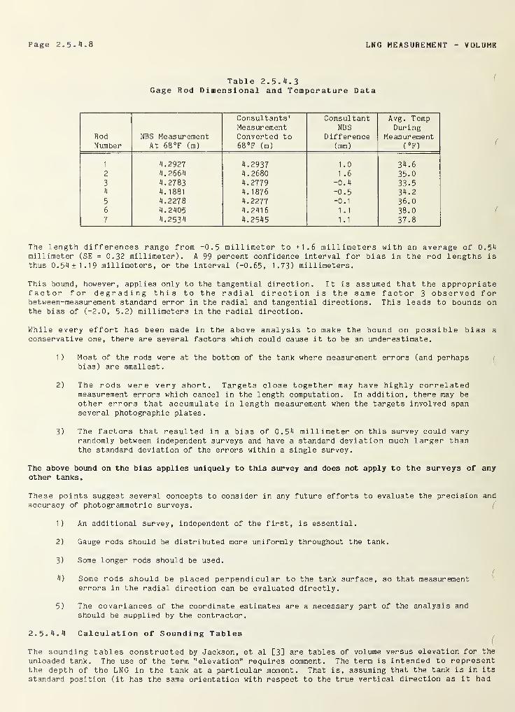
Page 2. 5. 4.8 LNG MEASUREMENT VOLUME
Table 2. 5. 4.3Gage Rod Dimensional and Temperature Data
RodNumber
NBS MeasurementAt 68°F (m)
Consultants'MeasurementConverted to68°F (m)
ConsultantNBS
Difference(mm
)
Avg. TempDuring
Measurement(°F)
1 4.2927 4.2937 1.0 34.62 4.2664 4.2680 1.6 35.03 4.2783 4.2779 -0.4 33.54 4. 1881 4.1876 -0.5 34.25 4.2278 4.2277 -0.1 36.06 4.2405 4. 241
6
1 .
1
38.0
7 4.2534 4.2545 1 .1 37.8
The length differences range from -0.5 millimeter to +1.6 millimeters with an average of 0.54millimeter (SE = 0.32 millimeter). A 99 percent confidence interval for bias in the rod lengths isthus 0.54 ±1.19 millimeters, or the interval (-0.65, 1.73) millimeters.
This bound, however, applies only to the tangential direction. It is assumed that the appropriatefactor for degrading this to the radial direction is the same factor 3 observed forbetween-measurement standard error in the radial and tangential directions. This leads to bounds onthe bias of (-2.0, 5.2) millimeters in the radial direction.
While every effort has been made in the above analysis to make the bound on possible bias a
conservative one, there are several factors which could cause it to be an underestimate.
1 ) Most of the rods were at the bottom of the tank where measurement errors (and perhapsbias) are smallest.
2) The rods were very short. Targets close together may have highly correlatedmeasurement errors which cancel in the length computation. In addition, there may beother errors that accumulate in length measurement when the targets involved spanseveral photographic plates.
3) The factors that resulted in a bias of 0.54 millimeter on this survey could varyrandomly between independent surveys and have a standard deviation much larger thanthe standard deviation of the errors within a single survey.
The above bound on the bias applies uniquely to this survey and does not apply to the surveys of anyother tanks.
These points suggest several concepts to consider in any future efforts to evaluate the precision andaccuracy of photogrammetric surveys.
1) An additional survey, independent of the first, is essential.
2) Gauge rods should be distributed more uniformly throughout the tank.
3) Some longer rods should be used.
4) Some rods should be placed perpendicular to the tank surface, so that measurementerrors in the radial direction can be evaluated directly.
5) The covariances of the coordinate estimates are a necessary part of the analysis andshould be supplied by the contractor.
2.5. 4.
4
Calculation of Sounding Tables
The sounding tables constructed by Jackson, et al [ 3 ] are tables of volume versus elevation for the
unloaded tank. The use of the term "elevation" requires comment. The term is intended to representthe depth of the LNG in the tank at a particular moment. That is, assuming that the tank is in its
standard position (it has the same orientation with respect to the true vertical direction as it had
c
LNG MEASUREMENT Volume Page 2.5.11-9
while being measured), and assuming that the liquid surface is a horizontal plane, the elevationshould be the distance from that horizontal plane to the (inside) bottom of the tank. However, that
last point is apparently not accessible to measurement. It has been assumed that what is, in fact,measured is the distance from the liquid surface plane to an internal reference point called the
pedestal probe point, and the elevation is then determined by adding to that measured distance theknown vertical distance of the reference point above the bottom of the tank.
The elevation of the pedestal probe point, however, is not obtained through direct measurement. Thephotogrammetri c consultants estimated the location of the tank bottom by using a mathematical model.After determining a "sphere of best fit", they determined a second, concentric sphere that best fitthe bottom-most ring of targets on the bottom cap of the tank. They then took the bottom of thissecond sphere as the bottom of the tank.
In the Jackson, et al. analysis [ 3 ], the elevation of the pedestal probe point was also determined froma mathematical model of the bottom region of the tank. However, the model used here is morecomplicated and considered to be more reasonable. It is described below in the description of model
3.
Three different sounding tables were constructed and analysed in the original publication [ 3 ]. Thetables were based on two different mathematical models and one system of volume corrections applied to
the second model. The three tables are based on increasingly sophisticated analyses, but the finalresults differ only slightly. Only a general description of each model will be given here as anexample of the extensive analysis, and reference is made to the original publication for details.
Tank Model 1 The first model developed was a simple mathematical sphere. The sphere that best fitthe target location measurements (at ambient temperature) was found earlier in this section to havecenter (.005, -.0009, -.0137) and radius 18.2682. It is assumed that an isotropic contraction occursas the tank is loaded with LNG. The sphere measurements were converted to the average temperature ofLNG, -160 °C, by use of the following linear thermal expansion coefficient obtained from the 1967edition of the Alcoa Aluminum Handbook:
L t ( 0 to -320 0 F) = L o (1+C(11.74t-0.00125t2-0.0000248t3)10-6 ),
L t (0 to 1000 0 F) = L o (1+C(12.19t+0.0031 1 5t 2) 1
0
-6,
where
L 0 = length at 0 0 F,
L^ = length at t0 F within range indicated,
C = alloy constant (1.020 for 5083 aluminum).
This resulted in a sphere with the same center but a radius of 18.201)85 meters. However, it was feltthat for the purposes of building tank models a modification to this "contracted" best-fitting spherewas necessary. The modification considered was one that resulted in a sphere which would best fit thedata if the points on the top and bottom caps of the tank and those on the equatorial ring wereexcluded. This resulted in a sphere with the same center but with a radius of 18.2113 meters. Tablesfor this model could then be calculated.
Tank Model 2 In this case, Model 1 is modified by replacing the top and bottom regions of the nominalsphere with segments (caps) of other, flatter spheres. The nominal sphere is now the sphere of Mod'1. Each such flatter (higher radius) sphere was taken to have its center on the polar axis ofnominal sphere, but not to be concentric with the latter. If the spherical surfaces were conocniriand touched somewhere—which they must for the model not to be discontinuous— the spherical surfa-'-nwould coincide.
Comparing the volume figures for Model 1 and 2 shows that the caps of Model 2 subtract ?. 1
meters from the volume of the tank and does not significantly affect the sounding table.
The calculation of the sounding tables involved accounting for the volume displaced • .••
structure inside the tank. This was called "tank internals" by the consultants, and th" - al .1 .
was based on blueprint specifications rather than on direct measurement. This seems valid, ,
total volume of the tower structure is about 7.6 cubic meters, so that high accuracy is not
Tank Model 3 In this case the sounding table is constructed by a numerical int"gr,r. - r •••
discrepancy between the actual measurements and Model 2. The procedure is as follows:
Page 2.5.4.10 LNG MEASUREMENT VOLUME
1) For each horizontal ring of targets, a mean z coordinate value is established, andthe mean radial residual is determined. This is the same as integrating the radialresiduals around each ring of targets by the trapezoid rule.
2) By linear interpolation between adjacent targets on a horizontal ring, a piecewiselinear function of z is constructed, approximating the mean radial residual at allvalues of z; at the top and bottom of the model tank, the radial residuals are takento be zero for this purpose.
3) The piecewise linear function is then integrated to give the volume corrections to
Model 2 and results in the final sounding table of Model 3. The integration requiresthree parts; the bottom cap, the nominal sphere and the top cap.
A comparison of the tables generated from Tank Model 3 to those generated independently by thephotogr ammetr i c consultant show values of 0.05 percent to 0.07 percent higher than the consultant'sfigures. This is probably caused by the different methods used for the last numerical integration.The consultant used a polynomial of high degree.
The sources of other contributing sounding table errors were examined by Jackson, et al [3]. Theseincluded target coordinate error, model error and plate curvature error. After consideration of theseerror sources, Jackson, et al concludes that tables generated using Tank Model 3 are accurate to
±0.06 percent or ±2 cubic meters.
2. 5. 4. 5 Three-Dimensional Triangulation Survey
In response to a request by a U.S. shipbuilder, NBS [4] developed a computer-based three-dimensionalcoordinate measurement system for determination of the spatial location of points on the interiorsurface of spherical LNG ship tank. This system utilizes three microprocessor-based digitaltheodolites in a precisely measured triangulation network for data acquisition, coupled to a dedicatedcentral computer for real-time data processing. Also implemented is a mathematical model of the tankgeometry under consideration, from which coordinate data on the tank surface is used to produce tablesrelating liquid cargo volume to liquid surface location.
The development goal of the NBS effort was to provide a precision determination of tank size andshape, unrelated to existing field measurement systems presently in use for such structures. This has
been achieved through an application of state-of-the-art optical instrumentation and computertechnology. The results reported here are intended to provide the basis for an independentverification of the accuracy of a photogrammetric measurement technique presently in use.
The following is an edited version of the final report of NBS to the sponsoring shipbuilder [4] anddescribes the NBS measurement system, the mathematical models used, and presents the results of a
calibration conducted on Cargo Tank No. 3 of the LNG Tanker Lake Charles.
Measurement Method The three-dimensional coordinate measurement system used for this survey is basedon the principle of simultaneous angular triangulation to a single target from three physicallyseparate measurement stations. Three measurement stations are installed on the interior surface of the
LNG tank at the vertices of a roughly equilateral triangle as shown in figure 2. 5. 4. 3. Each stationconsists of an operator-suppor t platform and a tripod-mounted digital theodolite. The operatorplatforms and tripods are physically separated from each other to ensure maximum instrument stabilityover the course of the survey. All support fixtures are bonded to the tank surface with a highstrength epoxy to avoid damaging the tank shell and to assist in equipment removal at the end of thesurvey. Each theodolite incorporates a 30-power telescope with optically encoded metal film glass
disks for measurement of horizontal and vertical telescope orientation. The angular encoderresolution is 1/4,096,000, and readout is provided to 1 arc second. Additionally, a two axisgravitational level sensor is built in to correct horizontal and vertical angle data for instrumentmislevel relative to the earth's gravitational field. Local data processing and scaling is performedin an internal microprocessor in the theodolite, and each unit is lined to a central desktop computerfor on-line real-time data acquisition and analysis.
The target definition system is a laser projector consisting of a He-Ne laser illuminator, a crosshair target and a 600 millimeter zoom telephoto camera lens. The laser illuminated cross hair is
projected through the camera lens and can be focused at any point on the tank surface. The lens zoomfeature can be used to vary the cross hair size to meet measurement requirements. A 22-X spottingtelescope is attached to the system to aid in target centering over the white disks of thephotogrammetric targets and for assistance in focusing. The centering overlap of this cross hair on
the photogrammetric target is estimated to be ±5 millimeters, which is sufficient for providing a
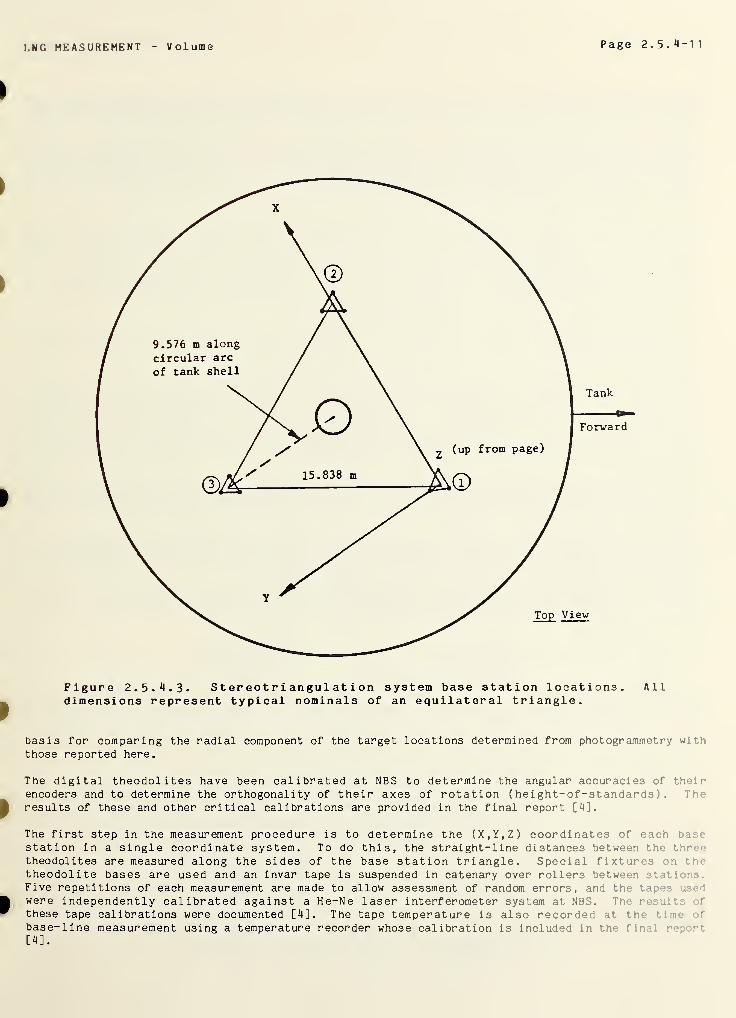
LNG MEASUREMENT Volume Page 2.5.4-11
Figure 2. 5. 4. 3. S t er eo t r i an gul at i on system base station locations. Alldimensions represent typical nominals of an equilateral triangle.
basis for comparing the radial component of the target locations determined from photogrammetry withthose reported here.
The digital theodolites have been calibrated at NBS to determine the angular accuracies of theirencoders and to determine the orthogonality of their axes of rotation ( hei gh t- of-st andards ) . Tv-results of these and other critical calibrations are provided in the final report [4].
The first step in the measurement procedure is to determine the (X,Y,Z) coordinates of each bas-station in a single coordinate system. To do this, the straight-line distances between the
theodolites are measured along the sides of the base station triangle. Special fixtures n1
•
theodolite bases are used and an invar tape is suspended in catenary over rollers betw<-< -n • r . .
Five repetitions of each measurement are made to allow assessment of random errors, and the * t;
were independently calibrated against a He-Ne laser interf erometer system at NBS. The r •• . .
•
these tape calibrations were documented [4]. The tape temperature is also recorded at the •
base-line measurement using a temperature recorder whose calibration is included in the final r
m.
Page 2.5.4.12 LNG MEASUREMENT VOLUME
The second procedural step is to measure the horizontal and vertical angular orientation of the threebase stations relative to each other. The technique used is to align two opposing units sighting oneach others' cross hairs.
Throughout the course of base station triangulation, each theodolite operator monitors a fixedbacksight on the central column. This backsight is an illuminated optical alignment target, andrepeated observations are stored by the computer system for detection of any shift in theodoliteangular orientation during the course of the target survey.
Upon completion of the base station triangulation, the target survey is started. Targets areidentified one at a time by the laser projector, and each theodolite operator sights on the projectedcross hair and transmits horizontal and vertical angle observations to the central computer. In thegeneral case of all three theodolites being able to see the target, a total of 6 angular observationsare acquired for determination of the (X,Y,Z) coordinates of the point. This angle redundancy is usedin a least squares solution of the measurement equations to compute point coordinates and angularresiduals for each instrument. A statistical chi-squared test is used as a pass/fail criteria, andany target failing to close properly is immediately resurveyed.
For a small percentage of targets, only two of the three observers have clear lines of sight caused by
obstruction by the central column and minumum focal distances of the theodolites. For these targets,4 angular observations are acquired.
Supplemental measurements are made with the stereotriangulation system to determine the coordinate of
the center of the pedestal upon which the capacitance gauge is mounted. In addition, a laser level is
used to measure the vertical orientation of the gauge along the ships longitudinal and tranverse axeswith respect to gravity. The laser level is also used to measure the list and trim of the ship frombeneath the hull relative to the ship keel and draft marks. The results of these measurements areused to compute the list and trim correction tables reported [4].
All measurement data recorded during the course of the tank survey is stored on cassette tapes forlater geometric modeling and table preparation. The on-line self-checking algorithms employed duringthe survey ensures the integrity of all measurement data before leaving the job site.
Mathematical Model of the Tank The output of the target survey discussed in the previous section is a
set of (X,Y,Z) coordinates for each point measured in the coordinate system shown in figure 2. 5. 4.1.
These data are reported at the tank ambient temperature at the time of determination of themeasurement system length scale, which was 11.6 °C for this tank.
The initial computation uses the method of least squares to fit the observed coordinate data for allsurface points to a perfect sphere. The results of this computation are:
A detailed residual analysis of this data indicates that the major deviations from sphericity occur at
the polar caps and at the equatorial ring. To quantify this, two additional data fits are performed.
First, the following targets are omitted:
Tank RadiusTank VolumeRadial Standard DeviationResidual Standard Deviation
18.27295 meters25557.3 cubic meters
0.00085 meters0.0166 meters
-the 8 targets on the south polar cap,
-the 12 targets on the north polar cap,-all targets on the rings adjacent to the polar cap weld seams-all equatorial ring targets.
The remaining targets were fitted to a sphere, yielding the following parameters:
Tank RadiusRadial Standard DeviationResidual Standard Deviation
18.27536 meters0.00057 meters0.00991 meters
Next, the north polar cap points were fitted to a sphere, yielding the following parameters:
Tank RadiusResidual Standard Deviation
21 .94682 meters0.01089 meters
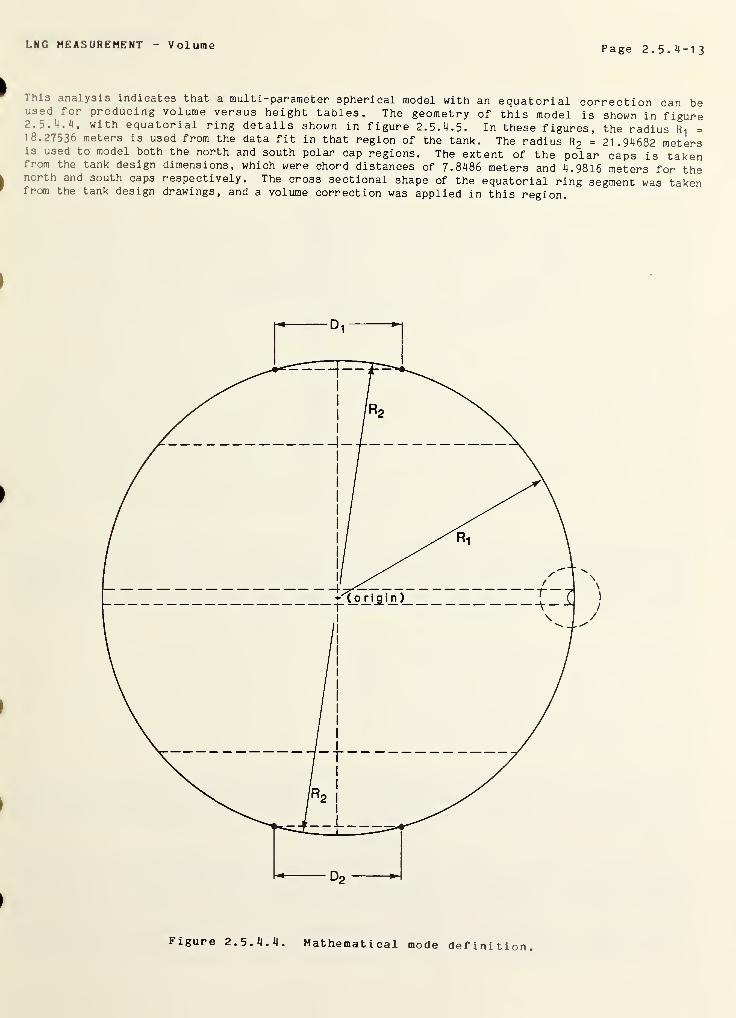
LNG MEASUREMENT Volume Page 2.5.4-13
This analysis indicates that a multi-parameter spherical model with an equatorial correction can beused for producing volume versus height tables. The geometry of this model is shown in figure2 . 5 . 4. 4, with equatorial ring details shown in figure 2.5. 4.5. In these figures, the radius Ri =18.27536 meters is used from the data fit in that region of the tank. The radius R 2 = 21.94682 metersis used to model both the north and south polar cap regions. The extent of the polar caps is takenfrom the tank design dimensions, which were chord distances of 7.8486 meters and 4.9816 meters for thenorth and south caps respectively. The cross sectional shape of the equatorial ring segment was takenfrom the tank design drawings, and a volume correction was applied in this region.
Figure 2. 5. 4. 4. Mathematical mode definition.
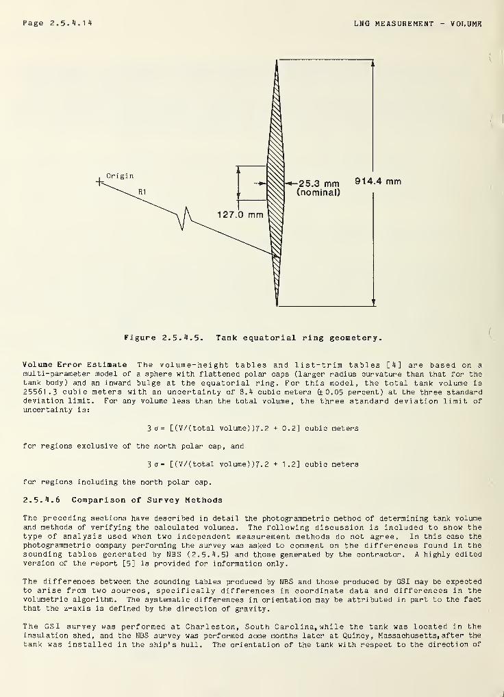
Page 2.5.4.14 LNG MEASUREMENT VOLUME
Figure 2.5. 4.5. Tank equatorial ring geometery.
Volume Error Estimate The vol um e- hei ght tables and list-trim tables [4] are based on a
multi-parameter model of a sphere with flattened polar caps (larger radius curvature than that for thetank body) and an inward bulge at the equatorial ring. For this model, the total tank volume is25561. 3 cubic meters with an uncertainty of 8.4 cubic meters (+0.05 percent) at the three standarddeviation limit. For any volume less than the total volume, the three standard deviation limit ofuncertainty is:
3 0 = [(V/(total volume))7.2 + 0.2] cubic meters
for regions exclusive of the north polar cap, and
3o= [(V/(total volume))7.2 + 1.2] cubic meters
for regions including the north polar cap.
2.5. 4.6 Comparison of Survey Methods
The preceding sections have described in detail the photogrammetri c method of determining tank volumeand methods of verifying the calculated volumes. The following discussion is included to show thetype of analysis used when two independent measurement methods do not agree. In this case thephotogrammetri c company performing the survey was asked to comment on the differences found in thesounding tables generated by NBS (2. 5. 4. 5) and those generated by the contractor. A highly editedversion of the report [5] is provided for information only.
The differences between the sounding tables produced by NBS and those produced by GSI may be expectedto arise from two sources, specifically differences in coordinate data and differences in thevolumetric algorithm. The systematic differences in orientation may be attributed in part to the factthat the z-axis is defined by the direction of gravity.
The GSI survey was performed at Charleston, South Carol ina, while the tank was located in theinsulation shed, and the NBS survey was performed some months later at Quincy, Massachusetts, after the
tank was installed in the ship's hull. The orientation of the tank with respect to the direction of
LNG MEASUREMENT Volume Page 2.5. 4-1
5
gravity cannot be expected to coincide precisely for the two surveys. Some additional contribution to
systematic differences for both orientation and origin arises from the fact that the GSI coordinates
refer to the center of the painted targets, while NBS , for operational reasons, was obliged to survey
coordinates of locations slightly displaced from the target centers. The systematic shift in origin
is primarily attributable to the difference in definition of the origin. The GSI coordinates are
referred to the center of a sphere which best-fits all targets on the spherical surface, whereas the
NBS coordinates are referred to the center of a sphere which best-fits all targets except certaintargets near the poles.
Direct comparison of the two sets of target coordinates does not reveal any significant differences
which might account for the differences in the sounding tables. Therefore, it must be suspected that
the differences are predominantly a result of the differences between the volumetric algorithms used
by NBS and GSI. Accordingly, several additional volume computations were made. Each of thesecomputations was made using the GSI volumetric algorithm with one modification. The originalalgorithm utilizes an adaptive weighting scheme to determine the influence of each level row of
targets to the polynomial used to represent departing volumes. Each level weight was a function of
the computed sigmas of the individual targets in that level. Since these data are not supplied withthe NBS data, it was decided to use unit weighting, i.e., weight equals one, for each level in place
of the original adaptive weighting scheme.
Before describing the additional computations, it is necessary to review the manner in which NBSelevation origin is defined. Specificaly, the terms "flattened" and "unflattened" bottom must beintroduced, as they are basic to the discussion which follows. The NBS volumes are computed usingreference spheres with one of two radii. The main portion, excluding the polar caps, is based on a
reference sphere whose radius has been designated R-| . The polar caps are computed from referencespheres having a radius which NBS has designated R 2 . Contrary to the presentation shown in figure2. 5. 4. 4, these reference spheres do not share a common origin. Rather, they have origins which liealong a common z-axis. The vertical separation of the origins is very nearly equal to the differencein the two radii, R-j and R 2 . It can be shown that the vertical separation of the origins is exactlyequal to the difference in the two radii plus the flattening of the pole. The actual value for the"flattening of the south pole" is given by the relation:
F = R1-R 2-[R 1
" (D 2 /2)2]1/2 + [R2- (D 2/2
)
2]
1 72
It now seems natural to adopt the term "NBS flattened bottom" for the horizontal plane which lies at a
distance of (R-j-F) below the origin of the sphere whose radius is Ri . Similarly, the term "NBSunflattened bottom" will be used when referring to the horizontal plane which lies at a distance of R 1
below the origin of the sphere whose radius is R-| . Thus the flattened bottom is situated above theunflattened bottom, at a distance equal to the flattening of the south pole.
The first computation was to process the NBS coordinates through the modified GSI algorithm. Theelevation origin was adopted at the NBS flattened bottom, such that the elevation of the pedestsJ i
the value given in the NBS report. The differences in volume from this computation with respect tothe volume data in the NBS report are plotted in figure 2.5. 4.6 as curve A. GSI asserted that a shiftof the elevation origin of 2~3 centimeters could substantially account for differences of ; ii
-
Noting that the NBS report contained a value for the flattening of the south pole, and that thi s va 1
was nearly 3 centimeters, another run was made using the NBS coordinates but with the elevationplaced at the NBS unflattened bottom. The difference in volume with respect to the volume data in theNBS report is plotted on figure 2. 5. 4. 6 as curve B.
With the objective of further evaluating the significance of coordinate differences on inacomputations, the GSI coordinates were run through the modified GSI algorithm first with thorigin at the NBS flattened bottom, and then with the elevation origin at the NBS unflattener :
•••
The volume difference with respect to the respective NBS data computations using the nodi'' . :
algorithm plotted in figure 2.5. 4. 6 as curves C and D.
An examination of the plots suggests several conclusions. First, the NBS versusdifferences caused by differences in target coordinate sets is almost neglig b -
shifts in elevation origin can account for significant volume differences which arc ... 0 •
poles and maximal near the equator. Third, it appears likely that the elevation :: f t
data in the NBS report is their unflattened bottom, rather than the flatten : '>o - r t, a
Finally, assuming for the sake of argument that this last conclusion is true, curve r can d<- .
as a plot of volume differences caused by volumetric algorithm differences.
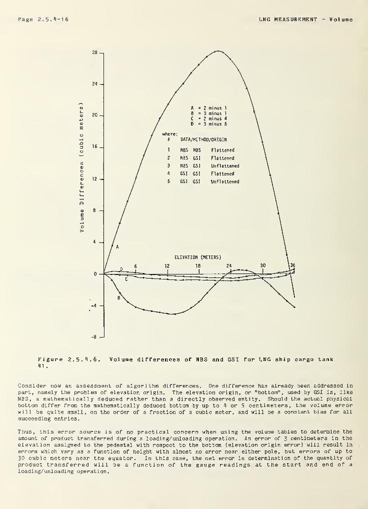
Page 2 • 5 . *•- 1 6 LNG MEASUREMENT V ol ume
Figure 2 . 5
.
*• . 6 . Volume differences of NBS and GSI for LNG ship cargo tank*11 .
Consider now an assessment of algorithm differences. One difference has already been addressed in
part, namely the problem of elevation origin. The elevation origin, or "bottom", used by GSI is, likeNBS, a mathematically deduced rather than a directly observed entity. Should the actual physicalbottom differ from the mathematically deduced bottom by up to 4 or 5 centimeters, the volume errorwill be quite small, on the order of a fraction of a cubic meter, and will be a constant bias for all
succeeding entries.
Thus, this error source is of no practical concern when using the volume tables to determine theamount of product transferred during a loading/unloading operation. An error of 3 centimeters in theelevation assigned to the pedestal with respect to the bottom (elevation origin error) will result in
errors which vary as a function of height with almost no error near either pole, but errors of up to
30 cubic meters near the equator. In this case, the net error in determination of the quantity of
product transferred will be a function of the gauge readings at the start and end of a
loading/ unloading operation.
LNG MEASUREMENT Volume Page 2.5. 4-17
Another source of volume differences inherent in the two volume algorithms is the manner in whichvolume displaced by tank internal structures is handled. GSI accounts for the effects of all tank
internal structures, as described in the individual tank reports. NBS accounts only for the volume
di splaced, caused by the intrusion of the equatorial ring structure, which represents approximately
one-fourth of the total volume displaced by all internal structures. The remaining effects are moreor less uniformly distributed with respect to elevation, with a total effect of approximately 6.8
cubic meters.
There are several differences in the modeling approach for volume computations. The first difference
is that NBS utilized trapezoidal modeling to integrate volume; differences from a reference sphere,while GSI used a polynomial for this purpose. The volume differences caused by this modelingdifference are estimated to be on the order of 3 cubic meters.
Another difference between the two algorithms is the manner in which horizontal departures are
computed. The effects of this modeling error are dependent upon the actual departures of each levelin any given tank, particularly the near-polar target levels. The actual value of this affect is
estimated to be on the order of ±0.5 cubic meters, assuming that the actual departures from thereference sphere are near zero at the extreme near-polar target levels. If, however, the actualdepartures were significant, as would be the case if the reference sphere used for the integration wasdisplaced vertically, then the resulting computed volumes would be adversely affected. A computationwas made using NBS data, through the modified GSI algorithm in which the reference sphere used to
represent the middle (main) portion of the elevation range was displaced vertically downward by 2
centimeters. The resulting volumes were approximately 1.2 cubic meters smaller for all elevationentries greater than one meter. Thus, this error source seems to produce bias errors in thevolumetric computations, which are of no practical concern when using the volume tables to measureproduct transfer.
Yet another difference between the volumetric algorithms is the difference in weighting schemes. Themodified GSI algorithm (using unit weighting) is estimated to produce volumes that differ from thosefrom the unmodified (adaptive weighting) by no more than 5 cubic meters. The actual differences willbe largely a function of the size of the departing volumes for a given tank. The smaller thedeparting volumes the smaller the volume differences from these two weighting options. Experiencesuggests that volume differences caused by weighting choices will tend to average less than 3 cubicmeters for these tanks.
A final note on volume differences is the effect of scaling. A scale change of one part in tenthousand is sufficient to produce volume changes of 7.5 cubic meters.
In summary, the coordinate sets determined by NBS and GSI agree very well, and the difference betweenNBS and GSI volume tables can be accounted for by the various algorithmic differences cited above.
Page 2.5.4-18 LNG MEASUREMENT Volume
2. 5. 4. 7 References
[1] Brown, D. C., Close-range camera calibration, Photogrammetri c Engineering, _37_, 855-66(1971 ).
[2] Witzgall, C., Best approximating sphere in R n , unpublished working paper, Center for AppliedMathematics, Nat. Bur. Stand. (U.S. ) ,
Washington, D.C.
[3] Jackson, R. H. F., R. S. Collier, S. Haber and P. Tryon, Custody transfer systems for LNG ships:
Tank survey techniques and sounding tables, Nat. Bur. Stand . (U. S .) ,NBSIR 79-1 751, 84 pp (May
1979)
.
[4] Final report on three-dimensional triangulation survey of cargo tank no. 3 on the LNG tanker LakeCharles, General Dynamics tank no. 41, prepared for General Dynamics Shipbuilding Division,Quincy, MA , by Nat. Bur. Stand .( U . S .) , Automated Production Technology Division, Washington,D.C. 20234 (1980).
[5] Jelffs, P. A., Calibration of containers and gages, J. Inst. Pet., _58_, No. 561, pp 1 1
7
—25 , (May,
1972) .
[6] Final report for General Dynamics cargo tank no. 41, tank no. 3 on hull no. 53, prepared forGeneral Dynamics Shipbuilding Division, Quincy, MA, by Geodetic Services, Inc., P.O.Box 3669,Indial antic, FL 32903 (1981).
LNG MEASUREMENT Volume Page 2. 5. 5-1
2.5.5 Volume of Cylindrical LNG Shore Tanks
The shape and size of LNG land based storage tanks are more traditional since for more than thirty
years, cryogenic tanks of this type have been constructed and installed for liquid oxygen, nitrogen,
hydrogen and other atmospheric gases as well as LNG. The primary containment tank is generally
cylindrical in shape and is surrounded by one or more meters in thickness of bulk insulation. A
weather protective outside wall is constructed to protect and support the insulation. Tanks may be
inground or above ground and have incorporated both metallic and non-metallic materials of
construction.
Natural gas has been stored in liquid form for peak shaving purposes and in satellite storage to
service customers remote from the main natural gas pipelines. The construction of large baseloadimportation terminals involved more than one large storage container to accommodate periodic LNG ship
arrivals and to allow continuous high volume send out of natural gas. The measurement of quantity and
quality became very important economically, and new instrumentation methods and procedures were
adopted to ensure efficient operation of the import terminal. Many of these techniques are describedin this part of the manual, in those sections dealing with volume measurements of LNG ship tanks.
The following edited section presents the results of a photogrammetric survey to determine the size,
shape and volume of a 600,000 barrel (58 meters diameter by 37 meters in height) Liquid Natural Gas
(LNG) Storage Tank, for Trunkline LNG Terminal at Lake Charles, LA. It is based on the final reportof the photogrammetric contractor [7] and , as in the previous sections, it is designed to describe
the process in detail and to provide an estimate of error for the measurement, which may then be
integrated into the total custody transfer.
2.5.5. 1 Photogrammetric Survey [10]
Preparatory to acquisition of the photographic data, which was obtained at Lake Charles, Louisiana,
approximately 500 "bulls-eye" type targets were placed throughout the interior of the tank at
pre-selected plate positions as shown by the following figures. Each target is a 1.27 centimeterdiameter circle of a retro-reflecti ve material mounted in the center of a black 2.22 centimeterdiameter, 0.32 centimeter inch thick circular magnetic disc.
During the survey, the internal surface of the tank was photographed on special 0.64 centimeter thickmicro-flat glass plates having a format of 24.13 by 24.13 centimeter by means of a custom-built metriccamera, strategically positioned at six selected sites. Figure 2.5.5. 1 shows the nominal positions of
the exposure sites, which are located approximately 1.5 meters inside the inner surface of tank in a
circular ring, at points approximately 7.6 meters above the tank floor, and distributed symmetricallyabout the vertical center line of the tank. At each of the six sites, three exposures were made for a
total of eighteen exposures for the survey. The aim points of one of these exposures is diametricallyopposite the exposure site, and ten degrees above the horizontal plane containing the exposure site.The aim points of the other two exposures at a site are approximately 35 degrees to the left and rightof the center exposure, and also ten degrees above the horizontal plane. The combination of cameraparameters, including location, angular field of view and direction of the optical axis, guaranteesthat each surface target will be imaged on no less than three photographic plates with an average of
4.5 images per target, and that no less than 25 percent of the internal surface of the tank will beimaged on each photographic plate.
In addition to the basic photographic equipment, auxiliary survey gear, including three calibratedsurvey tapes and two precision temperature sensors, were installed in the tank during the survey. Thescale tapes provide an accurate scale reference for the final target coordinates, and the temperaturesensors provide a means for determining the internal tank temperature at the time of the survey.
To ensure that the desired photographic results were obtained, the photographic plates were processedand carefully inspected on-site. Upon successful data acquisition, the plates were ready forsubsequent data processing and reduction.
Every target on the photographic plates was identified and annotated with a unique identifies* .
number and measured on a two-axis monocomparator, calibrated to one micrometer along each ixi: .
plate coordinate data were then processed through a series of proprietary programs, which pr< vl t
simultaneous least squares adjustment of all measured data, ultimately yielding X,Y,Z object u; .
coordinates of the triangulated points. Detailed treatments on the mathematics of theadjustment, error propagation and lens calibration are available in references [1] through 1
.
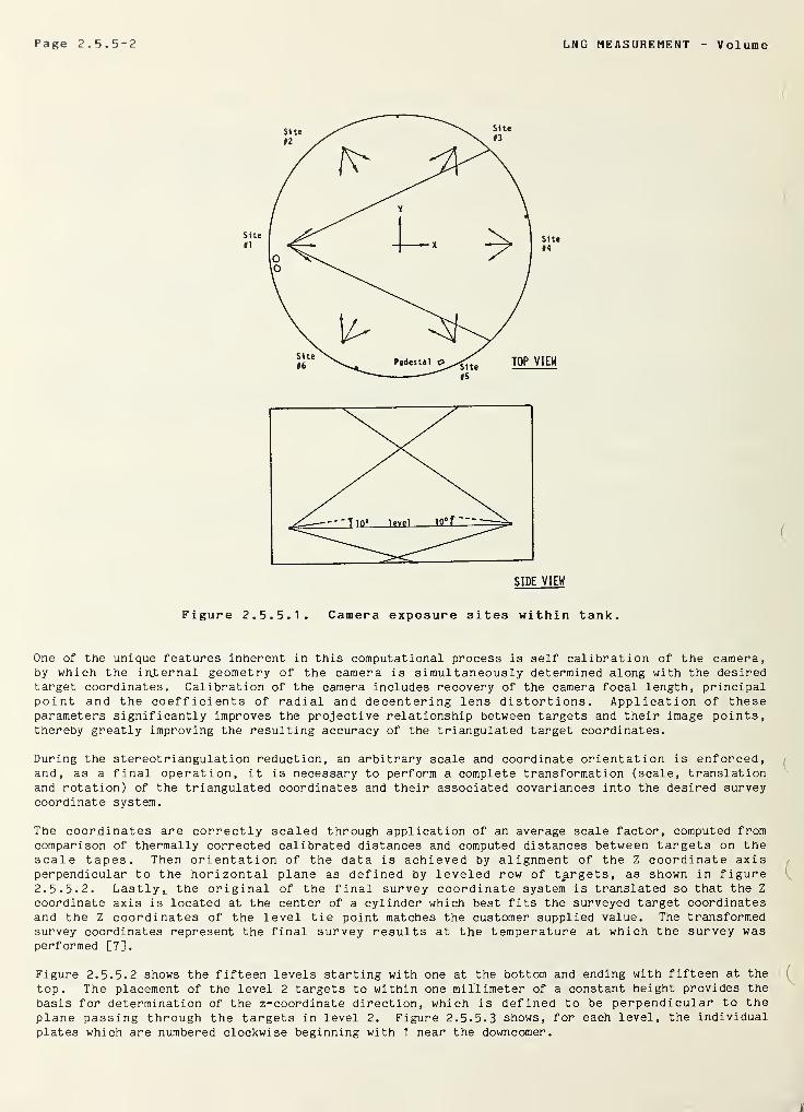
Page 2. 5. 5-2 LNG MEASUREMENT V olume
Figure 2. 5. 5.1. Camera exposure sites within tank.
One of the unique features inherent in this computational process is self calibration of the camera,by which the internal geometry of the camera is simultaneously determined along with the desiredtarget coordinates. Calibration of the camera includes recovery of the camera focal length, principalpoint and the coefficients of radial and decentering lens distortions. Application of theseparameters significantly improves the projective relationship between targets and their image points,thereby greatly improving the resulting accuracy of the triangulated target coordinates.
During the stereotriangulation reduction, an arbitrary scale and coordinate orientation is enforced,and, as a final operation, it is necessary to perform a complete transformation (scale, translationand rotation) of the triangulated coordinates and their associated covariances into the desired surveycoordinate system.
The coordinates are correctly scaled through application of an average scale factor, computed fromcomparison of thermally corrected calibrated distances and computed distances between targets on thescale tapes. Then orientation of the data is achieved by alignment of the Z coordinate axisperpendicular to the horizontal plane as defined by leveled row of targets, as shown in figure2. 5. 5. 2. Lastly,, the original of the final survey coordinate system is translated so that the Z
coordinate axis is located at the center of a cylinder which best fits the surveyed target coordinatesand the Z coordinates of the level tie point matches the customer supplied value. The transformedsurvey coordinates represent the final survey results at the temperature at which the survey wasperformed [7].
Figure 2. 5. 5. 2 shows the fifteen levels starting with one at the bottom and ending with fifteen at the
top. The placement of the level 2 targets to within one millimeter of a constant height provides the
basis for determination of the z-coordinate direction, which is defined to be perpendicular to theplane passing through the targets in level 2. Figure 2. 5. 5. 3 shows, for each level, the individual
plates which are numbered clockwise beginning with 1 near the downcomer.
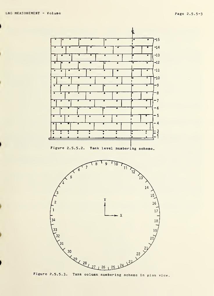
LNG MEASUREMENT V ol ume Page 2. 5. 5-3
Figure 2. 5. 5. 3. Tank column numbering scheme in plan view.
Page 2. 5.5-4 LNG MEASUREMENT V olume
The final photogrammetrically determined X,Y,Z target coordinates for all targets within the tank aretabulated [7] at the survey temperature. These target coordinates have been adjusted to remove thethickness of the magnetic disc.
2. 5. 5. 2 Volume Computation
Since the storage tank very nearly approximates a cylindrical body, the total and partial volumes of
the tank were derived from "cylindrical" computations. Basically, the final volume was determined bytaking the computed volume of a reference cylinder and algebraically summing the computed differencesin volume between the reference surface and the real surface plus the volume deviations caused by thetank internals and to the structural deformations ("barreling") which occur under loading.
A brief summary of the actual procedure follows. The X,Y,Z target coordinates were separated intofifteen layers or rings, so that all targets labeled "level number 1" formed a ring, all targetslabeled "level number 2" formed another ring and likewise for the targets in the remaining levels.For each ring, the horizontal departures were modeled by Fourier polynomials as a function of
longitude or angular distribution around the ring. Integration of the Fourier polynomial resulted inthe departing cross-sectional area of the true targeted surface from the reference cylinder.
Through use of the principles of array algebra [6], the departing volume of the actual surface fromthe reference cylinder was determined by integration of the departing areas as a function ofelevation.
The bottom of the tank is slightly coned, complicating rigorous volume computations for elevationsbetween zero and the peak of the cone. However, the minimum product level will always be well abovethis elevation for the pumps to be able to function properly.
Before computing the final volume, it was necessary to remove the volumetric contribution of thepermanent internal fixtures of the tank. The volumes of the tank internals were provided by the tank
contractor at 10 centimeter increments of elevation. The tank was divided into 58 elevation rangesdepending upon where significant changes in the concentration of the tank internals occured. The
volumetric contribution with each volume range is obtained by linear interpolation with respect to
elevation.
The final volume computation also required consideration of volume increases caused by barreling under
loading conditions. The necessary data were supplied by the tank contractor, and the effects at 112.5
K are included in the final sounding tables.
The desired sounding table of partitional volumes as a function of vertical elevation, beginning withzero volume at the bottom of the tank and ending with the final total volume at the top of the tank,is included in the photogrammetric contractor final report [7,8,9]. The partial volumes of the tank
(minus internals plus barreling) were then evaluated for every 1.52 centimeter of elevation range.The data in the table for each intermediate elevation included the total accumulated partial volume in
both cubic meters and barrels.
The total single tank volume was calculated to be 96,493*91 cubic meters at a tank temperature of
112.5 K. The computed estimate of accuracy of the total volume at 112.5 K was 4.8 cubic meters or
± 0.005 percent
.
LN G MEASUREMENT Volume Page 2. 5. 5-5
2. 5. 5. 3 References
[1] Brown, D., Advanced methods for calibration of metric cameras, DBA Systems, Inc., Final Report
Part 1 , U. S. Army Engineering Topographic Laboratories, Fort Bel voir, VA, (December 1968).
[2] Brown, D., Decentering distortion of lenses, Photogrammetric Eng., XXXII , No. 3 (May 1966).
[3] Brown, D., Precise calibration of surfaces of large radio reflectors by means of analyticalphotogrammetric triangulation, Research and Analysis Tech. Report No. 10, Instrument Corporationof Florida (November 1962).
[i| ] Brown, D., A solution to the general problem of multiple station analytical stereotriangulation,
RCA Data Reduction Tech. Report No. 43, ASTIA Doc. No. 134278 (February, 1958).
[5] Brown, D., A treatment of analytical photogr ammetry with emphasis on ballistic cameraapplications, RCA Data Reduction Tech. Report No. 39, (November 1956).
[6] Rauhala, U., A review of array algebra, Fotogrammetri ska Meddelanden, 2:38, Division ofPhotogr ammetry ,
Royal Inst, of Tech., S-100 44 Stockholm, Sweden (April 1976).
[7] Geodetic Services,tank No. A at LakeHouston, TX (April
Inc., Photogrammetric survey of Trunkline LNG Company 600,000 bbl LNG storageCharles, LA, Final Report for Trunkline LNG Corp., 3000 Bissonnet Avenue,1980 )
.
[ 8 ] Geodetic Services,tank No. B at LakeHouston, TX (April
Inc., Photogrammetric survey of Trunkline LNG Company 600,000 bbl LNG storageCharles, LA, Final Report for Trunkline LNG Corp., 3000 Bissonnet Avenue,1980)
.
[9] Geodetic Services,tank No. C at LakeHouston, TX (April
Inc., Photogrammetric survey of Trunkline LNG Company 600,000 bbl LNG storageCharles, LA, Final Report for Trunkline LNG Corp., 3000 Bissonnet Avenue,1980)
.
[10] Brown, D. C., LNG tank inventory measurement by photogr ammetry , 1981 Operating SectionProceedings, 81-T-55, ppT-127~37, Am. Gas Assoc., 1515 Wilson Blvd., Arlington, VA 22209( 1981 ).

q
a
c
c
(
(
o
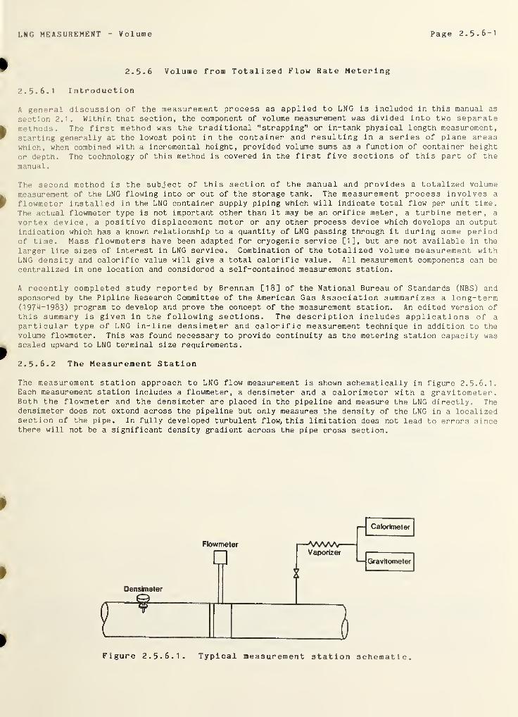
LNG MEASUREMENT Volume Page 2. 5.6-1
2.5.6 Volume from Totalized Flow Rate Metering
2.5.6. 1 Introduction
A general discussion of the measurement process as applied to LNG is included in this manual as
section 2.1. Within that section, the component of volume measurement was divided into two separatemethods. The first method was the traditional "strapping" or in-tank physical length measurement,
starting generally at the lowest point in the container and resulting in a series of plane areaswhich, when combined with a incremental height, provided volume sums as a function of container height
or depth. The technology of this method is covered in the first five sections of this part of themanual
.
The second method is the subject of this section of the manual and provides a totalized volume
measurement of the LNG flowing into or out of the storage tank. The measurement process involves a
flowmeter installed in the LNG container supply piping which will indicate total flow per unit time.
The actual flowmeter type is not important other than it may be an orifice meter, a turbine meter, a
vortex device, a positive displacement meter or any other process device which develops an outputindication which has a known relationship to a quantity of LNG passing through it during some periodof time. Mass flowmeters have been adapted for cryogenic service [1], but are not available in the
larger line sizes of interest in LNG service. Combination of the totalized volume measurement withLNG density and calorific value will give a total calorific value. All measurement components can be
centralized in one location and considered a self-contained measurement station.
A recently completed study reported by Brennan [18] of the National Bureau of Standards (NBS) andsponsored by the Pipline Research Committee of the American Gas Association summarizes a long-term(197^-1983) program to develop and prove the concept of the measurement station. An edited version ofthis summary is given in the following sections. The description includes applications of a
particular type of LNG in-line densimeter and calorific measurement technique in addition to thevolume flowmeter. This was found necessary to provide continuity as the metering station capacity wasscaled upward to LNG terminal size requirements.
2. 5. 6. 2 The Measurement Station
The measurement station approach to LNG flow measurement is shown schematically in figure 2.5. 6.1.Each measurement station includes a flowmeter, a densimeter and a calorimeter with a gravitometer
.
Both the flowmeter and the densimeter are placed in the pipeline and measure the LNG directly. Thedensimeter does not extend across the pipeline but only measures the density of the LNG in a localizedsection of the pipe. In fully developed turbulent flow, this limitation does not lead to errors sincethere will not be a significant density gradient across the pipe cross section.
Figure 2. 5. 6.1. Typical measurement station schematic.
Page 2. 5. 6-2 LNG MEASUREMENT V olume
The calorimeter and gravitometer must be supplied with a vaporized sample representative of the LNGflowing in the pipeline. This requires a well- designed and operated LNG sampling system. Thesampling requirements are the same for any measurement technique, however, not just the measurementstation method (see section 2 . 2 ).
LNG flow measurement with a measurement station where all measurement components are either in or
attached to a pipeline has some very desirable characteristics. The measurement station can provide a
continuous output of not only flow rates but also heating value on either an instantaneous or
totalized basis. Individual elements are capable of independent calibration and, with the possibleexception of the flowmeter, can be removed from the line for calibration or repair without taking theline out of service. Because of certain design features, it is usually not possible to remove theflowmeter from the line without removing a section of the pipeline.
To prove the feasibility of the measurement station approach, an extensive test program was started at
the National Bureau of Standards in 1 97 -4 . The purpose of the test program was to demonstrate that a
measurement station could be used to accurately and reliably measure LNG flowing in a pipeline,including large diameter off-loading lines. Since only the flowmeter is line size dependent, theprogram logically divided into two parts. The first part was to show that individual measurements offlow rate, density, heating value and specific gravity could be integrated into a single measurementresult. This work was completed on the NBS LNG flow facility. The second part of the program was todetermine the factors for scaling the flowmeter to large diameter pipes.
Selection of components for a feasibility study of the measurement station approach was based on thefollowing requirements:
A. Flowmeter1 . proven cryogenic performance2 . full line cross section measurement elements
3 . no moving parts4. ability to scale to large line sizes5. at least 10:1 rangeability
B. Densimeter1 . proven cryogenic performance2. ability to operate dynamically in LNG pipelines as opposed to a side stream or
statically in a storage tank
C. Calorimeter1 . the standard industry calorimeter was specified because it already had thedocumented precision and accuracy
D. Gravitometer1 . continuous measurement2 . electrical output
3 . proven precision and accuracy.
The type of components initially selected for the first tests were used in all subsequent teststhroughout the program. All components were not included in all tests but, whenever tests were made,the same type elements were always used.
The flowmeter selected was a vortex shedding type with a thermal sensor for detecting the vortices.The selection was based on test results obtained in a previous flowmeter evaluation program at NBS in
which all the different types of flowmeters used in custody transfer of cryogenic liquids were tested
[1]. Of all the flowmeters tested in that extensive test program, the vortex shedding flowmeter wasthe only one that met all the selection criteria.
Selection of the densimeter was not based on a large body of test data, since none existed. Only one
densimeter was found that had demonstrated cryogenic performance [2]. Therefore, that densimeter,which was a vibrating plate type, was selected for further study. During the later stages of the
program, data on other densimeters operating in static cryogenic liquids became available [3]. Basedon the data in [ 3 ], other choices are now available and include not only the vibrating plate type but
also a vibrating cylinder type. A full description of the performance of these and other types of LNGdensimeters are given in sections 2.4.1 and 2.4.2 of this manual.
LNG MEASUREMENT Volume Page 2 . 5 . 6-3
Installation requirements are somewhat different for the two vibrating element types of densimeterswith the vibrating cylinder requiring larger pipeline cross sections. From that standpoint, the
selected vibrating plate densimeter allow easier installation in the NBS flow reference facilities.
C ilorimeter selection was based entirely on previous industrial experience. The calorimeter had been
evaluated by NBS and the American Gas Association (AGA) [4] and is very widely accepted as the
industry standard. Manufacturers data were collected on other types for comparative purposes, but
none could be shown to have the potential for superior performance. Data made available since the
selection of the calorimeter for this project may change this conclusion. Other methods and
techniques are presented and compared in section 2.3 of this manual.
Input information from several of the gas companies was used in selecting the gravitometer . Operating
experience expressed by the company representatives combined with manufacturers data lead to the
choice of a continuously sampling gravitometer which operates on an impulse ratio principle.
2. 5. 6. 3 Component Element Testing
All components used in the measurement station were tested individually before integration into a
system. Individual element tests were conducted so that a base line performance characteristic couldbe established. The base line was then used as the reference point for all later tests. Those tests
also provided the first step in the flowmeter scaling work.
Flowmeter and densimeter liquid nitrogen tests The NBS liquid nitrogen flow facility was used for
determining the flow characteristics of the flowmeter and densimeter. This flow facility has a flowrange of 76-760 liters per minute over a range of temperatures and pressures. Facility accuracy on a
mass basis is +0.1 8 percent, which is composed of ±0.12 percent systematic error and ±0.06 percentrandom error (3 sigma) [5].
A two-inch flowmeter was chosen for those tests because it best matched the flow range of both theliquid nitrogen and the LNG flow facilities. When this work was started it was unknown how closelythe manufacturer could predict the meter factor for the flowmeter. Therefore, the flowmeter was alsocalibrated in water at the NBS flow facility in Gaithersburg, Maryland. This was done because scalingfactors could either be based on size alone or on both size and a meter factor in a surrogate fluid.It was anticipated that reliable data on larger diameter flowmeters to be tested later in the programmight not exist. So all flowmeters tested in the project were calibrated in water to help establish a
data base in a common liquid. Water was used as the calibration medium because no large capacitycryogenic flow facilities were in operation.
Figure 2. 5. 6. 2 shows the results of the test on the two-inch flowmeter in liquid nitrogen and water.The change in meter factor between the two fluids was predicted by the manufacturer to be 0.9 percent.As can be seen in the figure, the change was nearly 1.6 percent. This fact illustrates the danger ofrelying on seemingly logical theoretical considerations that have not been verified.
Liquid nitrogen tests on the densimeter are shown in figure 2. 5. 6. 3. These data covered almost a 13percent density range with flow velocities of 0.3 to 3 meters per second. Densimeter output was a
frequency that was related to density according to equation (1). The densimeter frequency wasmonitored and fit, by the method of least squares, to equation (1) to determine the equationcoefficients
.
where
p = A/f 2 + B
p = densityA and B = constants
f = densimeter output frequency.
(1)
The deviation shown in figure 2. 5. 6. 3 is the percentage difference between the densities cals- :•
from equation (1) and from a PVT correlation by Strobridge [6]. The residual standard dev; s.
-
the data from the calculated value was ±0.15 percent.
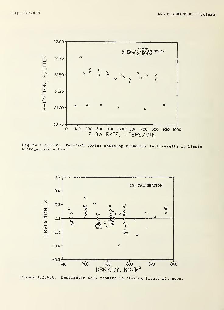
Page 2. 5. 6-4 LNG MEASUREMENT - Volume
JZ.UU -
LECEND0= LIQ NITROGEN CALIBRATIONA = WATER CALIBRATION
F, 31.75- OLd1—
Zj O n
^ 31.50-OO O
o
(
o°
ooo o
o
oo
o
o
•» ocro1- 31.25-U<l_L_
1A A A A
^ 31.00- A A
30.75- 1
1
1 1
1
1
1 1 1i i i i i i i i I
0 100 200 300 400 500 600 700 800 900 1000
FLOW RATE, LI TERS/M I
N
Figure 2. 5. 6. 2. Two-inch vortex shedding flowmeter test results in liquidnitrogen and water.
fc?
zo
<>wQ
0.6-
LN, CALIBRATION
0.4-
O
0.2-o 99
6>
on O
O Q^
o oo 6b—
—
o°o OO ° °
0.0- Q0 O — o n 2
840
DENSITY, KG/M'Figure 2. 5. 6. 3. Densimeter test results in flowing liquid nitrogen.
LNG MEASUREMENT Volume Page 2. 5. 6-5
LNG flow facility. LNG tests on the measurement station components were performed on the LNG flow
facility at NBS Boulder, Colorado. That facility contained all the measurement station components and
a process chromatograph.
The process chromatograph was used for gas analysis of vaporized LNG samples. The chromatograph was
insensitive to hydrocarbons above C 4 , so it proved to be inadequate for most of the projectrequirements.
LNG samples could be taken from two locations within the test section or from the weigh tank. One
sample tap was an adjustable probe using a dual pitot tube arrangement positioned so the tube axis was
parallel to the flow stream with one inlet directed upstream and the other downstream. The vertical
positioning of the pitot probe was adjustable and could traverse the flow stream so that a samplecould be taken at any point across the inside pipe diameter. See section 2.2, figures 2.2.27 and
2.2.31 for general schematic of LNG flow facility at NBS Boulder, Colorado.
LNG from these sample taps was vaporized in an air or water heat exchanger and the pressure reduced to
approximately 0.2 MPa before entering the gas line supplying the chromatograph, calorimeter andgravitometer
.
Flow rate was variable from 150 to 760 liters per minute by means of a variable speed pump.Temperature control was provided with a liquid nitrogen heat exchanger. Pressure was dependent ontemperature, flow rate and valve position up to maximum of 0.69 MPa. Helium gas was also used topressurize the LNG. By maintaining constant pressure and temperature within the flow facility, it waspossible to run with no venting. This condition ensured the constant LNG composition which wasrequired to test the various elements.
The weigh tank was mounted on three load cells. Output from the three cells were summed to give a
total reading of the change in weight in the tank. To reduce the flow disturbance on the load cellsto a minimum, weight measurements were always made emptying rather than filling the tank.
LNG tests. Tests of each of the measurement station components were run on the LNG flow facilityduring 1975. These tests were designed to show that each of the separate components was functionaland responsive to changes in flow rate, temperature, pressure, density and composition.
The vortex shedding flowmeter was unaffected by the wide variations in the LNG composition andcontinued to function properly throughout the test program. The vortex shedding flowmeter properlyresponded to all changes in flow rate.
Individual tests on the densimeter, calorimeter and gravitometer proved much more difficult than onthe flowmeter. Densimeter output was being compared to calculated densities using the compositionsobtained from vaporized LNG gas analysis. Those density calculations were performed using theextended corresponding states model as modified by McCarty [7]. See also sections 2.11.3 and 2 . 14 . 4 ofthis manual.
Calorimeter and gravitometer indications were also being compared to values calculated using the LNGcomposition. The calculations were performed following the procedures specified by Caldwell [8].
One of the main reasons that tests on the densimeter, calorimeter and gravitometer were difficult wasrelated to getting and analyzing the gas sample. While sampling is a critically import intconsideration in the application of the measurement station approach, it is not unique to thatconcept. In fact it is equally important to all measurement methods now in use. Since the sam; lingproblem was not unique to this project, an extensive investigation was not included within th-of work. At the same time, however, it was not possible to fulfill the requirements of the proje -t
without spending considerable effort in the sampling area.
Fortunately another project was started within NBS specifically designed to develop trv r-
sampling and gas analysis techniques. Facilities and personnel from the sampling or • „
utilized in some of the work on this project, and, when the sampling project was ready '
testing the two projects were combined.
The results from the combined projects proved to be of great benefit to both pr • •.
significant findings were:
Page 2. 5-6-6 LNG MEASUREMENT V olume
1- all LNG mixture fraction components must be shown, rather than assumed, to be absentwhen analyzing gas samples;
2. flow rate in the sampling tap must be above a minimum value;
3. laboratory sampling criteria are not directly transferable to field typemeasurements;
4. any one of several different vaporizer techniques can be used;
5. some method of time averaging the vaporized sample must be provided.
A complete description of the sampling project has been reported by Parrish [9], and an edited versionis included as section 2.2 of this manual. The reader is referred to these sections for specificdetails. Ironically, the net result of the investigations demonstrated that the pitot tube samplingscheme originally installed in the LNG flow loop when used to supply gas to the calorimeter plus thegravitometer was an adequate sampling system. This may have been fortuitous, since the flow raterequired to run both instruments was only about one half Parrish's [9] recommended 20 standard litersper minute minimum value. Therefore, it is recommended that Parrish's procedure be followed in anyfuture design. The flow rate required by the calorimeter alone was not sufficient to provide goodresults, however. The measured heating value decreased from 41 MJ/m3 to that of methane 37.8 MJ/m3when the flow rate was reduced to only that required by the calorimeter. Increasing the flow tohigher values did not affect the measured heating value. The time response of the instruments alsoprovided the time averaging required.
Parrish [9] found that a simple side tap flush with the inside wall of the flow line was somewhatbetter than a pitot tube tap. He found that there were fewer erroneous gas analyses with the sidetap. In this project, no difference could be found between the two tap designs. The side tap is muchsimpler, so it would seem to be the logical choice for future work.
Integration of the individual elements of the measurement station was completed during 1976-1977. Themethod used for the integration was to bring all signals to a minicomputer, where the required datareduction was completed. Output from these tests was simply printed on an on-line printer.Alternative data handling schemes are numerous and include telemetering the data to a central locationor storing the data on some mass storage device, such as punched paper tape, magnetic tape, discs,etc. for later computation. No attempt was made to include these devices. Each is dependent on userpreferences and requirements, but each could be used with no adverse effect on the end result of the
measurement
.
Densimeter and flowmeter frequencies were calculated by bringing total counts into the computer anddividing by the elapsed time. Density and flow rate were calculated from equations derived from testsin liquid nitrogen. Nitrogen data were used for these calculations because they were obtained on theliquid nitrogen flow facility, which is much more accurate than the LNG flow facility. The two flowfacilities operate on similar principles, but the nitrogen facility is of a different design, whichminimizes the adverse affects of environmental conditions, tare weight and restraints. Consequently,it has higher accuracy capability. Also, it was necessary to know the LNG density in order to
determine new values on the LNG facility. Since there was originally considerable uncertainty in thegas analysis and consequently the density calculation, it was decided to use the nitrogen values.
This was changed in later tests completed after some sampling and analysis problems were resolved.
The gravitometer and calorimeter both had analog outputs which were entered into the computer, fromwhich specific gravity and heating value were calculated. For these tests the following informationwas printed:
1
.
LNG density2. LNG volume flow rate3. LNG mass flow rate4. Vaporized LNG specific gravity5. Vaporized LNG heating value6. LNG heating value flow rate7. Total LNG heating value in time interval
During the tests in which sampling and analysis problems were being investigated, the uncertainty in
the integrated values was large, perhaps 3 to 4 percent. After these problems were resolved, the
uncertainty was reduced to approximately ± 1 percent. LNG flow facility uncertainty presently
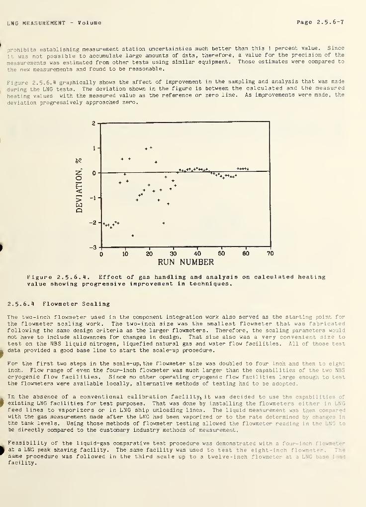
LNG MEASUREMENT Volume Page 2. 5. 6-7
prohibits establishing measurement station uncertainties much better than this 1 percent value. Since
it was not possible to accumulate large amounts of data, therefore, a value for the precision of the
measurements was estimated from other tests using similar equipment. Those estimates were compared to
the new measurements and found to be reasonable.
Figure 2. 5. 6. <4 graphically shows the affect of improvement in the sampling and analysis that was made
during the LNG tests. The deviation shown in the figure is between the calculated and the measured
heating values with the measured value as the reference or zero line. As improvements were made, the
deviation progressively approached zero.
Figure 2. 5. 6. 4. Effect of gas handling and analysis on calculated heatingvalue showing progressive improvement in techniques.
2. 5. 6. 4 Flowmeter Scaling
The two-inch flowmeter used in the component integration work also served as the starting point for
the flowmeter scaling work. The two-inch size was the smallest flowmeter that was fabricatedfollowing the same design criteria as the larger flowmeters. Therefore, the scaling parameters wouldnot have to include allowances for changes in design. That size also was a very convenient size to
test on the NBS liquid nitrogen, liquefied natural gas and water flow facilities. All of those testdata provided a good base line to start the scale-up procedure.
For the first two steps in the scale-up, the flowmeter size was doubled to four inch and then to eightinch. Flow range of even the four-inch flowmeter was much larger than the capabilities of the two NBS
cryogenic flow facilities. Since no other operating cryogenic flow facilities large enough to testthe flowmeters were available locally, alternative methods of testing had to be adopted.
In the absence of a conventional calibration facility, it was decided to use the capabi 1 1 1
i
existing LNG facilities for test purposes. That was done by installing the flowmeters either in LN .
feed lines to vaporizers or in LNG ship unloading lines. The liquid measurement was thenwith the gas measurement made after the LNG had been vaporized or to the rate determined by chang in
the tank levels. Using those methods of flowmeter testing allowed the flowmeter reading in trio '
be directly compared to the customary industry methods of measurement.
Feasibility of the liquid-gas comparative test procedure was demonstrated with a four-inn fi w--' . r
at a LNG peak shaving facility. The same facility was used to test the eight- inch fl >wm-
same procedure was followed in the third scale up to a twelve-inch flowmeter r i :.N
facility.
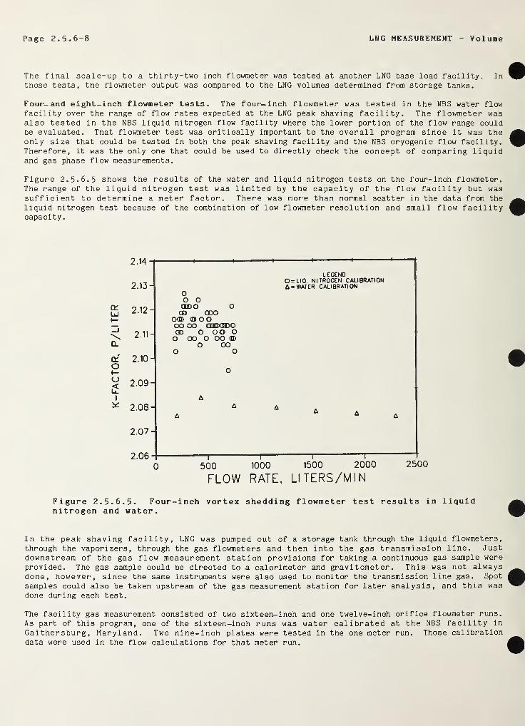
Page 2. 5. 6-8 LNG MEASUREMENT V ol ume
The final scale-up to a thirty-two inch flowmeter was tested at another LNG base load facility. Inthose tests, the flowmeter output was compared to the LNG volumes determined from storage tanks.
Four-and eight-inch flowmeter tests. The four-inch flowmeter was tested in the NBS water flowfacility over the range of flow rates expected at the LNG peak shaving facility. The flowmeter wasalso tested in the NBS liquid nitrogen flow facility where the lower portion of the flow range couldbe evaluated. That flowmeter test was critically important to the overall program since it was theonly size that could be tested in both the peak shaving facility and the NBS cryogenic flow facility.Therefore, it was the only one that could be used to directly check the concept of comparing liquidand gas phase flow measurements.
Figure 2. 5. 6. 5 shows the results of the water and liquid nitrogen tests on the four-inch flowmeter.The range of the liquid nitrogen test was limited by the capacity of the flow facility but wa3sufficient to determine a meter factor. There was more than normal scatter in the data from theliquid nitrogen test because of the combination of low flowmeter resolution and small flow facilitycapacity.
2.14-
LECEND
2.13-O=U0 NITROGEN CALIBRATION
oo o
A “WATER CALIBRATION
QLUJ
2.12- CSBO OCD <JDO
*— OdD OOO— oo OO CUDCBDO—
J
\ 2.11- CD O OO OO OO O OO (ID
0l O OOo o
QC 2.10-Ot— oO< 2.09-Li.
I A
2.08- A ^ A AA A A
2.07-
2.06 I | i i i
'
0 500 1000 1500 2000 2500
FLOW RATE, LI TERS/M I
N
Figure 2. 5. 6. 5. Four-inch vortex shedding flowmeter test results in liquidnitrogen and water.
In the peak shaving facility, LNG was pumped out of a storage tank through the liquid flowmeters,
through the vaporizers, through the gas flowmeters and then into the gas transmission line. Justdownstream of the gas flow measurement station provisions for taking a continuous gas sample wereprovided. The gas sample could be directed to a calorimeter and gravitometer . This was not alwaysdone, however, since the same instruments were also used to monitor the transmission line gas. Spot
samples could also be taken upstream of the gas measurement station for later analysis, and this wasdone during each test.
The facility gas measurement consisted of two sixteen-inch and one twelve-inch orifice flowmeter runs.
As part of this program, one of the sixteen-inch runs was water calibrated at the NBS facility in
Gaithersburg, Maryland. Two nine-inch plates were tested in the one meter run. Those calibrationdata were used in the flow calculations for that meter run.
LNG MEASUREMENT Volume Page 2. 5. 6-9
An ultrasonic flowmeter had previously been installed in the peak shaving facility by its owner. That
flowmeter was not part of this program, but data were collected during some of the tests for
comparison with the vortex shedding flowmeter for informational purposes.
Flowmeter tests were made by recording the output of the vortex shedding flowmeter along with the LNG
pressure and temperature on magnetic tape. The gas flow data consisting of line pressure, orifice
pressure drop and temperature were all recorded on the peak shaving facilities circular chart
recorders. Gas flow rates were calculated from those chart recordings following the procedures
specified in AGA Report No. 3 [10]. If more than one orifice flowmeter was in use, a combined flow
rate was calculated.
Gas equivalents of the LNG flow rates were calculated from the vortex shedding flowmeter using
equation (3) and the meter factor previously determined. For the four inch flowmeter the meter factor
determined in the liquid nitrogen test was used. For the eight-inch flowmeter a meter factor
calculated from the water calibration was used.
Ql = (f/K) ( p L/
p G) (3)
where
Ql = gas equivalent of LNG flow ratef = flowmeter output frequencyK = meter factor
p ^= LNG density at flowing conditions
p „ = gas density at base conditionsU
Recordings of the LNG temperature, pressure and flowmeter output were made every 10 seconds. Fiveindividual temperature and pressure recordings were averaged and used in the density calculations.The LNG density was calculated from the gas analysis of the spot gas samples taken during each test.That analysis combined with the pressure and temperature data were used in the density calculationdescribed by McCarty [7] as an extended corresponding states method. As one check on the correctnessof the gas analysis, the heating value and specific gravity were also calculated following the
procedures specified by Caldwell [8], Whenever possible, the calculated values were compared tovalues measured on the peak shaving facilities calorimeter and gravitometer . As mentioned above, themeasured values were not always available, but, whenever they were, they agreed with the calculatedvalues to within the uncertainty limits specified by the instrument manufacturers.
Flowmeter frequency was determined by dividing the difference in the recorded flowmeter output by theelapsed time between selected recordings.
Comparisons between the liquid and gas flow measurements were made during periods of constant flowrate. Those periods were selected from the gas flow recordings. The comparisons were made bycalculating the percentage deviation between them using equation (4).
Deviation (percent) = 100 (Ql - Qq)/Qq (4)
where
Ql = gas equivalent of LNG flow rate
Qq = gas flow rate from orifice flow measurement
As previously stated the four-inch flowmeter was the first to be tested in the peak shaving facil i' v .
The facility piping was all eight inch, and the flowmeter test section had to be made to f i*I
• • w •-
existing eight-inch flanges. After installation, the test section was wrapped with insulation m :
plastic vapor barrier.
A very brief test of the f oui— inch flowmeter was finally run during a vaporizer test in D<
1975. The four-inch test section significantly reduced the facility output, so the vaporizer •• • ~
the only test permitted before the test section had to be removed and the eight-inch t
installed.
Since that test was the only opportunity available to test the four-inch flowmeter, t-
made to maximize the data obtained. Therefore, a test plan was adopted to give a ran,’' : . «
with some indication of reproducibility rather than collect all data at a single flow rv*-.of test plan did not permit waiting long periods of time to ensure equilibrium w m i .-hi* v
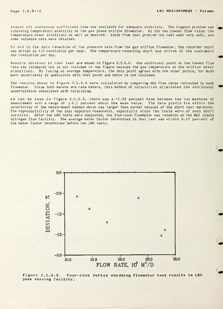
Page 2.5.6-10 LNG MEASUREMENT V ol ume
almost all instances sufficient time was available for adequate stability. The biggest problem was
achieving temperature stability at the gas phase orifice flowmeter. At the two lowest flow rates thetemperature never stabilized as well as desired. Aside from that problem the test went very well, andsome valuable data were obtained.
To aid in the data reduction of the pressure data from the gas orifice flowmeter, the recorder chartwas driven at 1/2 revolution per hour. The temperature recording chart was driven at the customaryone revolution per day.
Results obtained in that test are shown in figure 2. 5. 6. 6. One additional point at the lowest flowrate was attempted but is not included in the figure because the gas temperature at the orifice neverstabilized. By taking an average temperature, the data point agreed with the other points, but muchmore uncertainty is associated with that point and hence is not included.
The results shown in figure 2. 5. 6. 6 were calculated by comparing the flow rates indicated by eachflowmeter. Since both meters are rate meters, this method of calculation eliminated the additionaluncertainties associated with totalizing.
As can be seen in figure 2. 5. 6. 6, there was a -1.03 percent bias between the two methods ofmeasurement with a range of ± 0.5 percent about the mean value. The data points lie within theuncertainty of the measurement method which was larger than normal because of the short test duration.The reproducibility of the data appeared reasonable, especially since the tests were of such shortduration. After the LNG tests were completed, the four-inch flowmeter was retested on the NBS liquidnitrogen flow facility. The average meter factor determined in that test was within 0.12 percent ofthe meter factor determined before the LNG tests.
fc?
o
<>C£J
Q
0.0
-0 .5 -
-1 .0 -
-1 .5 -
-2.0 H i
—i l
10.0 15.0 20.0 25.0 30.0
FLOW RATE, 101 M 3/D
Figure 2. 5. 6. 6. Four—inch vortex 3hedding flowmeter test results in LNGpeak shaving facility.
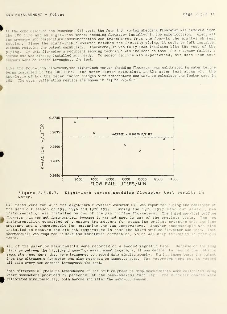
LNG MEASUREMENT Volume Page 2.5.6-11
At the conclusion of the December 1975 test, the four-inch vortex shedding flowmeter was removed from
the LNG line and an eight-inch vortex shedding flowmeter installed in the same location. Also, all
the pressure and temperature instrumentation was transferred from the four-to the eight-inch test
section. Since the eight-inch flowmeter matched the facility piping, it could be left installed
without reducing the output capability. Therefore, it was fully foam insulated like the rest of the
piping. In this flowmeter a redundant sensing technique was included so that if one sensor failed, a
second one was already installed and ready. No sensor failure was experienced, but data from both
sensors were collected throughout the test.
Like the four-inch flowmeter, the eight-inch vortex shedding flowmeter was calibrated in water before
being installed in the LNG line. The meter factor determined in the water test along with the
knowledge of how the meter factor changes with temperature was used to calculate the factor used in
LNG. The water calibration results are shown in figure 2. 5. 6. 7.
0.2700
crLJ
!Z 0.2695_J
CL
q2 0.2690
OI—ou; 0.2685
I
0.2680
0 2000 4000 6000 8000 10000 12000 14000
FLOW RATE, LITERS/M IN
Figure 2. 5. 6. 7. Eight-inch vortex shedding flowmeter test results inwater
.
LNG tests were run with the eight-inch flowmeter whenever LNG was vaporized during the remainder of
the send-out season of 1975-1976 and 1976-1977. During the 1976-1977 send-out season, newinstrumentation was installed on two of the gas orifice flowmeters. The third parallel or:f:;eflowmeter run was not instrumented, because it was not used in any of the previous tests. The newinstrumentation consisted of pressure transducers for measuring orifice pressure drop and linepressure and a thermocouple for measuring the gas temperature. Another thermocouple was alsinstalled to measure the ambient temperature in case the third orifice flowmeter was used. Thatthermocouple was required to make the manometer correction, which was only estimated in prev ; .
tests.
All of the gas-flow measurements were recorded on a second magnetic tape. Because of the 1 r.g,
distance between the liquid-and gas-flow measurement locations, it was decided to record the :
'
separate recorders that were triggered to record data simultaneously. During those tests the : r
from the ultrasonic flowmeter was also recorded on magnetic tape. The recorders were set t
all data every ten seconds throughout the test.
Both differential pressure transducers on the orifice pressure drop measurements wer<
water manometers provided by personnel at the peak-shaving facility. The circul ir ••
calibrated simultaneously, both before and after the send-out season.
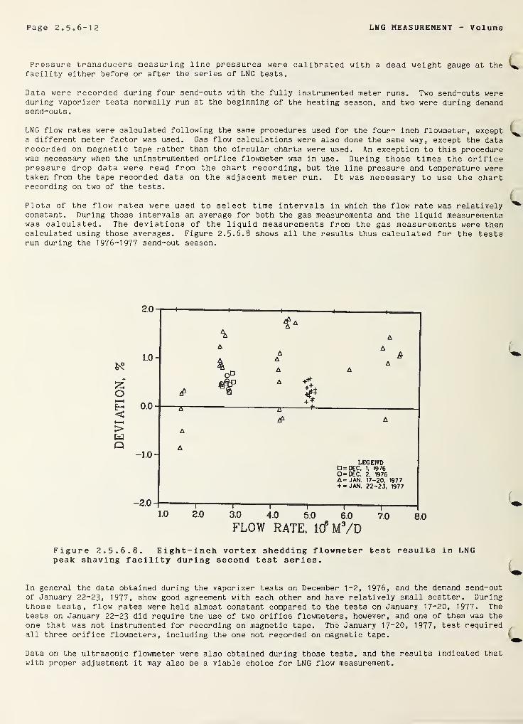
Page 2.5.6-12 LNG MEASUREMENT Volume
Pressure transducers measuring line pressures were calibrated with a dead weight gauge at thefacility either before or after the series of LNG tests.
Data were recorded during four send-outs with the fully instrumented meter runs. Two send-outs wereduring vaporizer tests normally run at the beginning of the heating season, and two were during demandsend-outs
.
LNG flow rates were calculated following the same procedures used for the four- inch flowmeter, excepta different meter factor was used. Gas flow calculations were also done the same way, except the datarecorded on magnetic tape rather than the circular charts were used. An exception to this procedurewas necessary when the uninstrumented orifice flowmeter was in use. During those times the orificepressure drop data were read from the chart recording, but the line pressure and temperature weretaken from the tape recorded data on the adjacent meter run. It was necessary to use the chartrecording on two of the tests.
Plots of the flow rates were used to select time intervals in which the flow rate was relativelyconstant. During those intervals an average for both the gas measurements and the liquid measurementswas calculated. The deviations of the liquid measurements from the gas measurements were thencalculated using those averages. Figure 2. 5.6.8 shows all the results thus calculated for the testsrun during the 1976-1977 send-out season.
Figure 2. 5. 6. 8. Eight-inch vortex shedding flowmeter test results in LNGpeak shaving facility during second test series.
In general the data obtained during the vaporizer tests on December 1-2, 1976, and the demand send-outof January 22-23, 1977, show good agreement with each other and have relatively small scatter. Duringthose tests, flow rates were held almost constant compared to the tests on January 17-20, 1977. Thetests on January 22-23 did require the use of two orifice flowmeters, however, and one of them was theone that was not instrumented for recording on magnetic tape. The January 17~20, 1977, test requiredall three orifice flowmeters, including the one not recorded on magnetic tape.
Data on the ultrasonic flowmeter were also obtained during those tests, and the results indicated thatwith proper adjustment it may also be a viable choice for LNG flow measurement.
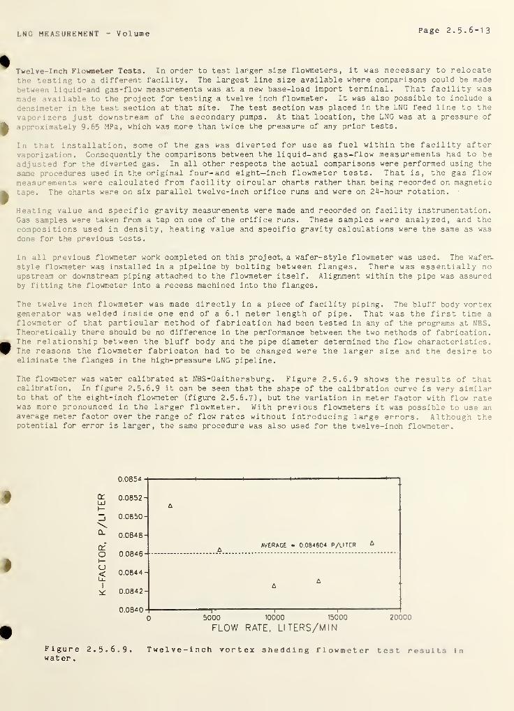
LN C MEASUREMENT Volume Page 2.5.6-13
Twelve-Inch Flowmeter Tests. In order to test larger size flowmeters, it was necessary to relocatethe testing to a different facility. The largest line size available where comparisons could be made
between liquid-and gas-flow measurements was at a new base-load import terminal. That facility was
made available to the project for testing a twelve inch flowmeter. It was also possible to include a
densimeter in the test section at that site. The test section was placed in the LNG feed line to the
vaporizers just downstream of the secondary pumps. At that location, the LNG was at a pressure of
approximately 9.65 MPa, which was more than twice the pressure of any prior tests.
In that installation, some of the gas was diverted for use as fuel within the facility aftervaporization. Consequently the comparisons between the liquid-and gas-flow measurements had to be
adjusted for the diverted gas. In all other respects the actual comparisons were performed using the
same procedures used in the original four- and eight—inch flowmeter tests. That is, the gas flowmeasurements were calculated from facility circular charts rather than being recorded on magnetictape. The charts were on six parallel twelve-inch orifice runs and were on 24-hour rotation.
Heating value and specific gravity measurements were made and recorded on facility instrumentation.Gas samples were taken from a tap on one of the orifice runs. These samples were analyzed, and thecompositions used in density, heating value and specific gravity calculations were the same as was
done for the previous tests.
In all previous flowmeter work completed on this project, a wafer-style flowmeter was used. The wafer-
style flowmeter was installed in a pipeline by bolting between flanges. There was essentially noupstream or downstream piping attached to the flowmeter itself. Alignment within the pipe was assuredby fitting the flowmeter into a recess machined into the flanges.
The twelve inch flowmeter was made directly in a piece of facility piping. The bluff body vortexgenerator was welded inside one end of a 6.1 meter length of pipe. That was the first time a
flowmeter of that particular method of fabrication had been tested in any of the programs at NBS.Theoretically there should be no difference in the performance between the two methods of fabrication.The relationship between the bluff body and the pipe diameter determined the flow characteristics.The reasons the flowmeter fabrieaton had to be changed were the larger size and the desire toeliminate the flanges in the high-pressure LNG pipeline.
The flowmeter was water calibrated at NBS-Gaithersburg . Figure 2. 5. 6. 9 shows the results of thatcalibration. In figure 2. 5. 6. 9 it can be seen that the shape of the calibration curve is very similarto that of the eight-inch flowmeter (figure 2. 5. 6. 7), but the variation in meter factor with flow ratewas more pronounced in the larger flowmeter. With previous flowmeters it was possible to use anaverage meter factor over the range of flow rates without introducing large errors. Although thepotential for error is larger, the same procedure was also used for the twelve-inch flowmeter.
0.0854
Qi 0.0852uJy—
0.0850
\0.0848
ofO 0.0846I—O< 0.0844Li_
0.0842
0.08400 5000 10000 15000 20000
FLOW RATE, LI TERS/MIN
Figure 2. 5. 6. 9. Twelve-inch vortex shedding flowmeter test results Inwater
.
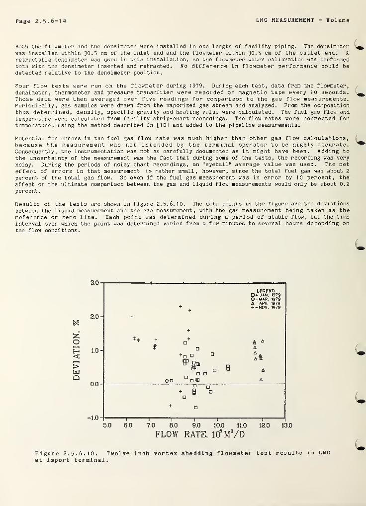
Page 2. 5.6-1 *1 LNG MEASUREMENT V olume
Both the flowmeter and the densimeter were installed in one length of facility piping. The densimeterwas installed within 30.5 cm of the inlet end and the flowmeter within 30.5 cm of the outlet end. A
retractable densimeter was used in this installation, so the flowmeter water calibration was performedboth with the densimeter inserted and retracted. No difference in flowmeter performance could be
detected relative to the densimeter position.
Four flow tests were run on the flowmeter during 1979. During each test, data from the flowmeter,
densimeter, thermometer and pressure transmitter were recorded on magnetic tape every 10 seconds.Those data were then averaged over five readings for comparison to the gas flow measurements.Periodically, gas samples were drawn from the vaporized gas stream and analyzed. From the composition
thus determined, density, specific gravity and heating value were calculated. The fuel gas flow and
temperature were calculated from facility strip-chart recordings. The flow rates were corrected fortemperature, using the method described in [10] and added to the pipeline measurements.
Potential for errors in the fuel gas flow rate was much higher than other gas flow calculations,because the measurement was not intended by the terminal operator to be highly accurate.Consequently, the instrumentation was not as carefully documented as it might have been. Adding to
the uncertainty of the measurement was the fact that during some of the tests, the recording was very
noisy. During the periods of noisy chart recordings, an "eyeball" average value was used. The neteffect of errors in that measurement is rather small, however, since the total fuel gas was about 2
percent of the total gas flow. So even if the fuel gas measurement was in error by 10 percent, theaffect on the ultimate comparison between the gas and liquid flow measurements would only be about 0.2
percent.
Results of the tests are shown in figure 2.5.6.10. The data points in the figure are the deviationsbetween the liquid measurement and the gas measurement, with the gas measurement being taken as thereference or zero line. Each point was determined during a period of stable flow, but the time
interval over which the point was determined varied from a few minutes to several hours depending on
the flow conditions.
Figure 2.5.6.10. Twelve inch vortex shedding flowmeter test results in LNGat import terminal.
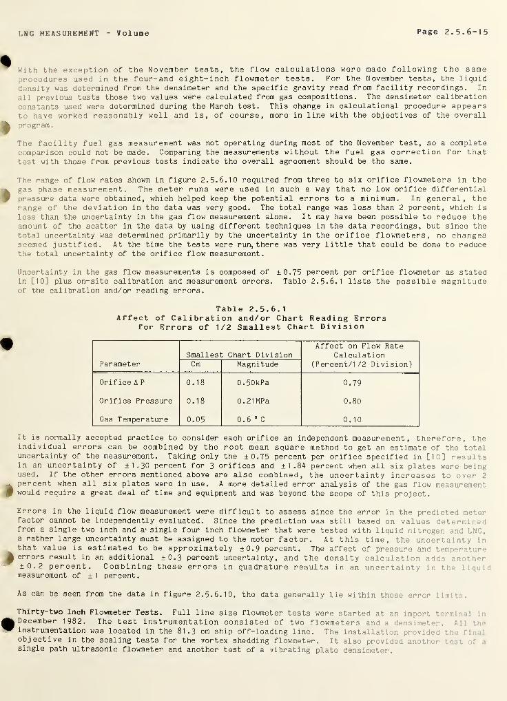
LNG MEASUREMENT Volume Page 2.5.6-15
With the exception of the November tests, the flow calculations were made following the sameprocedures used in the four- and eight-inch flowmeter tests. For the November tests, the liquid
density was determined from the densimeter and the specific gravity read from facility recordings. In
ill previous tests those two values were calculated from gas compositions. The densimeter calibration
constants used were determined during the March test. This change in calculational procedure appearsto have worked reasonably well and is, of course, more in line with the objectives of the overall
program.
The facility fuel gas measurement was not operating during most of the November test, so a completecomparison could not be made. Comparing the measurements without the fuel gas correction for thattest with those from previous tests indicate the overall agreement should be the same.
The range of flow rates shown in figure 2.5.6.10 required from three to six orifice flowmeters in thegas phase measurement. The meter runs were used in such a way that no low orifice differentialpressure data were obtained, which helped keep the potential errors to a minimum. In general, therange of the deviation in the data was very good. The total range was less than 2 percent, which is
less than the uncertainty in the gas flow measurement alone. It may have been possible to reduce theamount of the scatter in the data by using different techniques in the data recordings, but since thetotal uncertainty was determined primarily by the uncertainty in the orifice flowmeters, no changesseemed justified. At the time the tests were run, there was very little that could be done to reducethe total uncertainty of the orifice flow measurement.
Uncertainty in the gas flow measurements is composed of ±0.75 percent per orifice flowmeter as statedin [10] plus on-site calibration and measurement errors. Table 2.5.6. 1 lists the possible magnitudeof the calibration and/or reading errors.
Table 2.5.6.
1
Affect of Calibration and/or Chart Reading Errorsfor Errors of 1/2 Smallest Chart Division
ParameterSmallest Chart Division
Affect on Flow RateCalculation
(Percent/1 /2 Division)Cm Magnitude
Orifice A P 0.18 0 . 50kPa 0.79
Orifice Pressure 0.18 0. 21 MPa 0.80
Gas Temperature 0.05 0.6 0 C 0.10
It is normally accepted practice to consider each orifice an independent measurement, therefore, theindividual errors can be combined by the root mean square method to get an estimate of the totaluncertainty of the measurement. Taking only the ±0.75 percent per orifice specified in [10] resultsin an uncertainty of ±1.30 percent for 3 orifices and ±1.84 percent when all six plates were beingused. If the other errors mentioned above are also combined, the uncertainty increases to over 2
percent when all six plates were in use. A more detailed error analysis of the gas flow measurementwould require a great deal of time and equipment and was beyond the scope of this project.
Errors in the liquid flow measurement were difficult to assess since the error in the predicted meterfactor cannot be independently evaluated. Since the prediction was still based on values determinedfrom a single two inch and a i single four inch flowmeter that were tested with liquid nitrogen and LNG
,
a rather large uncertainty must be assigned to the meter factor. At this time, the uncertainty inthat value is estimated to be approximately ±0.9 percent. The affect of pressure and temperatureerrors result in an additional ±0.3 percent uncertainty, and the density calculation adds another±0.2 percent. Combining these errors in quadrature results in an uncertainty in themeasurement of ±1 percent.
As can be seen from the data in figure 2.5.6.10, the data generally lie within those error I i rr> :*
.
Thirty-two Inch Flowmeter Tests. Full line size flowmeter tests were started at an importDecember 1982. The test instrumentation consisted of two flowmeters and a densimeter, a::instrumentation was located in the 81.3 cm ship off-loading line. The installation provided ' :•
objective in the scaling tests for the vortex shedding flowmeter. It also provided m • * •
single path ultrasonic flowmeter and another test of a vibrating plate densimeter.
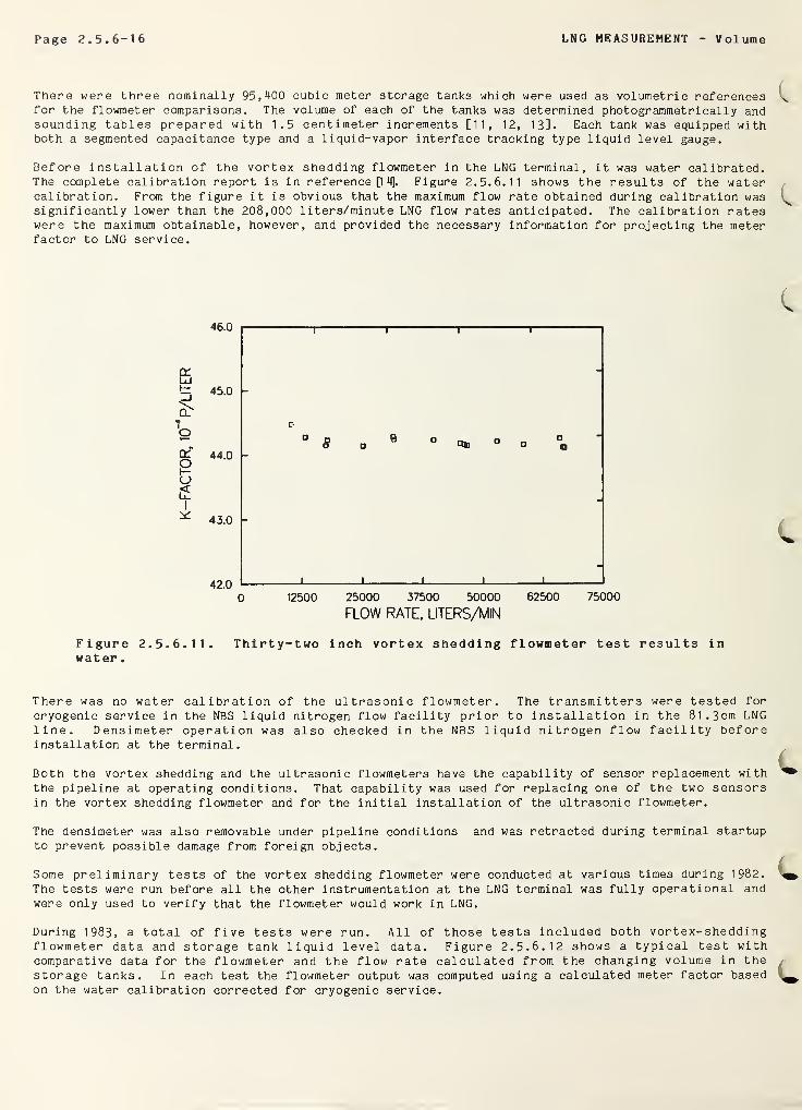
Page 2.5.6-16 LNG MEASUREMENT V ol ume
There were three nominally 95,^00 cubic meter storage tanks which were used as volumetric referencesfor the flowmeter comparisons. The volume of each of the tanks was determined photogrammetrically andsounding tables prepared with 1.5 centimeter increments [11, 12, 13]. Each tank was equipped withboth a segmented capacitance type and a liquid-vapor interface tracking type liquid level gauge.
Before installation of the vortex shedding flowmeter in the LNG terminal, it was water calibrated.The complete calibration report is in reference [1 4]. Figure 2.5.6.11 shows the results of the watercalibration. From the figure it is obvious that the maximum flow rate obtained during calibration wassignificantly lower than the 208,000 liters/minute LNG flow rates anticipated. The calibration rateswere the maximum obtainable, however, and provided the necessary information for projecting the meterfactor to LNG service.
Figure 2.5.6.11. Thirty-two inch vortex shedding flowmeter test results inwater
.
There was no water calibration of the ultrasonic flowmeter. The transmitters were tested for
cryogenic service in the NBS liquid nitrogen flow facility prior to installation in the 81. 3cm LNGline. Densimeter operation was also checked in the NBS liquid nitrogen flow facility beforeinstallation at the terminal.
Both the vortex shedding and the ultrasonic flowmeters have the capability of sensor replacement withthe pipeline at operating conditions. That capability was used for replacing one of the two sensorsin the vortex shedding flowmeter and for the initial installation of the ultrasonic flowmeter.
The densimeter was also removable under pipeline conditions and was retracted during terminal startupto prevent possible damage from foreign objects.
Some preliminary tests of the vortex shedding flowmeter were conducted at various times during 1982.
The tests were run before all the other instrumentation at the LNG terminal was fully operational andwere only used to verify that the flowmeter would work in LNG.
During 1983, a total of five tests were run. All of those tests included both vortex-sheddingflowmeter data and storage tank liquid level data. Figure 2.5.6.12 shows a typical test withcomparative data for the flowmeter and the flow rate calculated from the changing volume in thestorage tanks. In each test the flowmeter output was computed using a calculated meter factor basedon the water calibration corrected for cryogenic service.
_MG MEASUREMENT Volume Page 2.5.6-17
Iifc
UJ
<CZ
ELAPSED m€, HR
Figure 2.5.6.12, September 1983 test results showing average flow ratesindicated by the vortex-shedding flowmeter and the tank level change.
Tte tar.-: levels were deterrired frer the capaciear.ee level gauges. The gauges consisted of five
segrer.ts that were each ".2 raters long, plus ore segment at the top that was '.2 meters lerg. A
sepa-ate segment was included at the hotter art served as a refereree for the first segrert. Tte
active segrert was idertified as the highest segrert with ar output greater than the threshold value.Tar- level was calculated by addirg the fixed heights of each segrert to the level indicated :y theactive segrert.
The data showr ir figure 2.5.6 . '2 were recorded at '5 minute averages,
rates durirg other tests. Tank level data taker at ~3 arc 60 seeord ir
scatter art rate irs tart ar ecus ccrparisors with the flcwreter raprobably origi rated frtr two sources. Ire was the disturbed lieu:process. The other was ar ocoasioral discontinuity ir the level irdic
the segrer.ts of the gauge. Scatter frer both those sources was largelyover longer tire periods.
Tata were recorded at variousitervals exhibited corsiderablether rear.i r.gl ess . The scatte-. d surface durirg the fillitg:ated as the liruid level tasseteliminated by taking averages
The segrert charges occasionally caused adjacent averages to give large discrepancies. Tree : ; : :e
ignored without adversely affecting the overall comparison of flowmeter to tank volume ctar.ge.was true since the phenomena was clearly a liruid level gauge problem caused by = risacj ..stmer: .'
electronics. The oorparisor between the flcwreter and the tar.-: levels at all tee ot'.er levelsrot corpr crises by those ocoasioral erroneous indications.
During ar. reloading it was customary to flow into two tanks. IMG for send cut -as ta-:er -
tank. For the test test of the flowmeters it was obviously desirable to have the set: 1Mfrtr a tank rot receiving IMG. Urfortur.ateiy , this operating condition was rot always ;:ss.:. .
Turing the test shown ir. figure 2. 5. 5.
' 2, IMG for sere out was taker, free ore of tse : a- .
throughout the entire unloading period. According to the facility’s personnel, tr.e se-.
:
tela nearly constant throughout the ship unloading. Therefore, a constant correct .:
-
flew rate calculated free the tank volume charge. The actual correction was deter-. t-
ohe withdrawal rate as irdi cater by the tank level gauge at the conclusion of teerate was assured to have existed throughout the unloading, arc hence all the tar- le . . . -
rates were increased by that amount.
Figure 2.5.5. '3 shows the iata free figure 2.5. 5. '2 or a percentage deviate :' :
calculated from tank levels was used as the reference or zero lire ir tte f.v .
indicated by the vortex shedding flcwreter was also compared to tte stip totai .
-
The difference was no worse than ± 2 .-” percent between the total volure ur.l cede: f
-
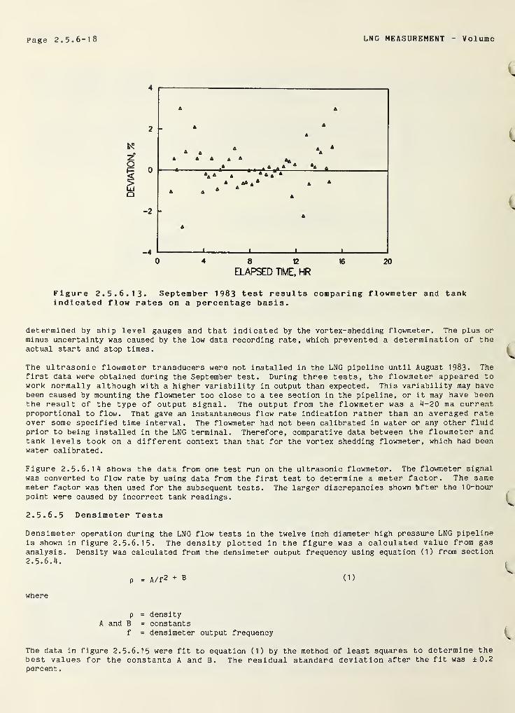
Page 2.5.6-18 LNG MEASUREMENT V olume
01>UJo
0 4 8 12 16 20
ELAPSED TIME, HR
Figure 2.5.6.13. September 1983 test results comparing flowmeter and tankindicated flow rates on a percentage basis.
determined by ship level gauges and that indicated by the vortex-shedding flowmeter. The plus or
minus uncertainty was caused by the low data recording rate, which prevented a determination of theactual start and stop times.
The ultrasonic flowmeter transducers were not installed in the LNG pipeline until August 1983. Thefirst data were obtained during the September test. During three tests, the flowmeter appeared towork normally although with a higher variability in output than expected. This variability may havebeen caused by mounting the flowmeter too close to a tee section in the pipeline, or it may have beenthe result of the type of output signal. The output from the flowmeter was a 4-20 ma currentproportional to flow. That gave an instantaneous flow rate indication rather than an averaged rateover some specified time interval. The flowmeter had not been calibrated in water or any other fluidprior to being installed in the LNG terminal. Therefore, comparative data between the flowmeter andtank levels took on a different context than that for the vortex shedding flowmeter, which had beenwater calibrated.
Figure 2.5.6.14 shows the data from one test run on the ultrasonic flowmeter. The flowmeter signalwas converted to flow rate by using data from the first test to determine a meter factor. The samemeter factor was then used for the subsequent tests. The larger discrepancies shown bfter the 10-hour
point were caused by incorrect tank readings.
2. 5. 6. 5 Densimeter Tests
Densimeter operation during the LNG flow tests in the twelve inch diameter high pressure LNG pipelineis shown in figure 2.5.6.15. The density plotted in the figure was a calculated value from gasanalysis. Density was calculated from the densimeter output frequency using equation (1) from section2 . 5 . 6 . 4 .
where
p = A/f2 + B
P
A and B
f
= density= constants= densimeter output frequency
(1)
The data in figure 2.5.6.15 were fit to equation (1) by the method of least squares to determine thebest values for the constants A and B. The residual standard deviation after the fit was ±0.2percent
.
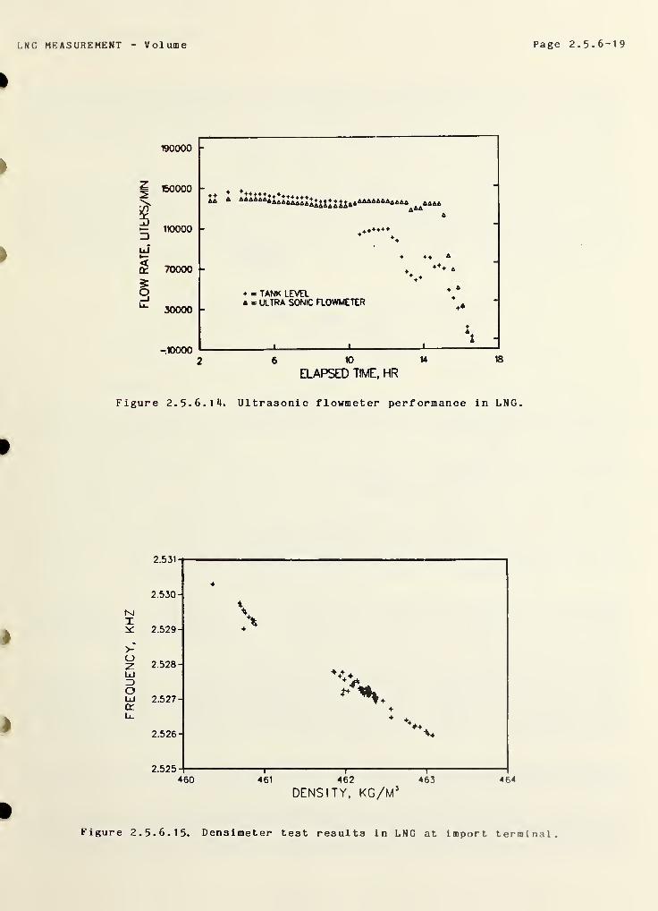
FREQUENCY,
KHZ
LNG MEASUREMENT Volume Page 2.5.6-19
190000 -
150000 - + .. . .
^ 110000 -
uJ
^ 70000
£
30000 -
-10000
A
« TANK LEVELa - ULTRA SONIC FLOWMETER
6 10 14
ELAPSED TIME, HR18
Figure 2.5.6.14. Ultrasonic flowmeter performance in LNG.
Figure 2.5.6.15. Densimeter test results in LNG at import terminal.
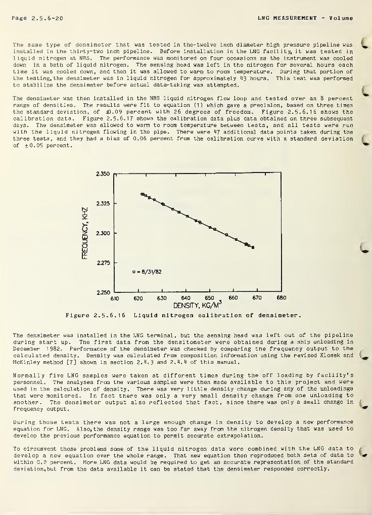
Page 2.5.6-20 LNG MEASUREMENT V olume
The same type of densimeter that was tested in the-twelve inch diameter high pressure pipeline wasinstalled in the thirty-two inch pipeline. Before installation in the LNG facility, it was tested inliquid nitrogen at NBS. The performance was monitored on four occasions as the instrument was cooleddown in a bath of liquid nitrogen. The sensing head was left in the nitrogen for several hours eachtime it was cooled down, and then it was allowed to warm to room temperature. During that portion ofthe testing, the densimeter was in liquid nitrogen for approximately 43 hours. This test was performedto stabilize the densimeter before actual data-taking was attempted.
The densimeter was then installed in the NBS liquid nitrogen flow loop and tested over an 8 percentrange of densities. The results were fit to equation (1) which gave a precision, based on three timesthe standard deviation, of dO.09 percent with 26 degrees of freedom. Figure 2.5.6.16 shows thecalibration data. Figure 2.5.6.17 shows the calibration data plus data obtained on three subsequentdays. The densimeter was allowed to warm to room temperature between tests, and all tests were runwith the liquid nitrogen flowing in the pipe. There were 47 additional data points taken during thethree tests, and they had a bias of 0.06 percent from the calibration curve with a standard deviationof +0.05 percent.
Figure 2.5.6.16 Liquid nitrogen calibration of densimeter.
The densimeter was installed in the LNG terminal, but the sensing head was left out of the pipelineduring start up. The first data from the densitometer were obtained during a ship unloading in
December 1982. Performance of the densimeter was checked by comparing the frequency output to thecalculated density. Density was calculated from composition information using the revised Klosek andMcKinley method [7] shown in section 2.4.3 and 2.4.4 of this manual.
Normally five LNG samples were taken at different times during the off loading by facility'spersonnel. The analyses from the various samples were then made available to this project and wereused in the calculation of density. There was very little density change during any of the unloadingsthat were monitored. In fact there was only a very small density change from one unloading toanother. The densimeter output also reflected that fact, since there was only a small change in
frequency output.
During those tests there was not a large enough change in density to develop a new performance
equation for LNG. Also, the density range was too far away from the nitrogen density that was used to
develop the previous performance equation to permit accurate extrapolation.
To circumvent those problems some of the liquid nitrogen data were combined with the LNG data to
develop a new equation over the whole range. That new equation then reproduced both sets of data to
within 0.2 percent. More LNG data would be required to get an accurate representation of the standard
deviation, but from the data available it can be stated that the densimeter responded correctly.
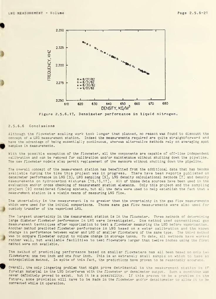
LNG MEASUREMENT Volume Page 2.5.6-21
Figure 2.5.6.17. Densimeter performance in liquid nitrogen.
2. 5. 6. 6 Conclusions
Although the flowmeter scaling work took longer than planned, no reason was found to discount the
concept of a LNG measurement station. Indeed the measurements required are quite straightforward andhave the advantage of being essentially continuous, whereas alternative methods rely on averaging spot
samples in measurements.
With the possible exception of the flowmeter, all the components are capable of off-line independentcalibration and can be removed for calibration and/or maintenance without shutting down the pipeline.The new flowmeter models also permit replacement of the sensors without shutting down the pipeline.
The overall concept of the measurement station has benefitted from the additional data that has becomeavailable during the time this project was in progress. There have been reports published ondensimeter performance in LNG [3], LNG sampling [9], LNG density calculational methods [7] and densitymeasurements on hydrocarbon mixtures [15,16,17]. All of those data sources have been used in theevaluation and/or cross checking of measurement station elements. Only this project and the samplingproject [9] considered flowing systems, but all the data were used to help establish the fact that a
measurement station is a viable means of measuring LNG flow.
The uncertainty in the measurement is no greater than the uncertainty in the gas flow measurementswhich were used for the initial comparisons. Those same gas flow measurements were also used forcustody transfer of the vaporized LNG.
The largest uncertainty in the measurement station is in the flowmeter. Three methods of determininglarge diameter flowmeter performance in LNG were investigated. One method used conventional gasmeasurement techniques after vaporization to test a flowmeter measuring the LNG before vaporization.Another method predicted flowmeter performance in LNG based on a water calibration and the knownchange in performance between water and LNG of smaller flowmeters of the same type. The third meth" :
was to compare flowmeter output to volume change in storage tanks. To date, all methods have wcr-:-irather well, but available facilities to test flowmeters larger than twelve inches using the firstmethod were not available.
The method of predicting performance based on smaller flowmeters has all been based on •-
flowmeters; one two inch and one four inch. This is an extremely small sample on which to -
extrapolation method. In spite of this fact, the predictions have proven to be reasonably i
Overall, the only lingering problem that might prove detrimental to the measuremer.* sto*: n
foreign material in the LNG interferes with the flowmeter or densimeter output. Such a cordiii r - :
never definitely proved to exist, but it is a possibility. If this proves to be a pro- .•
-
future, some provision will have to be made in the flowmeter and/or densitometer - w .
• •
corrected while in operation.
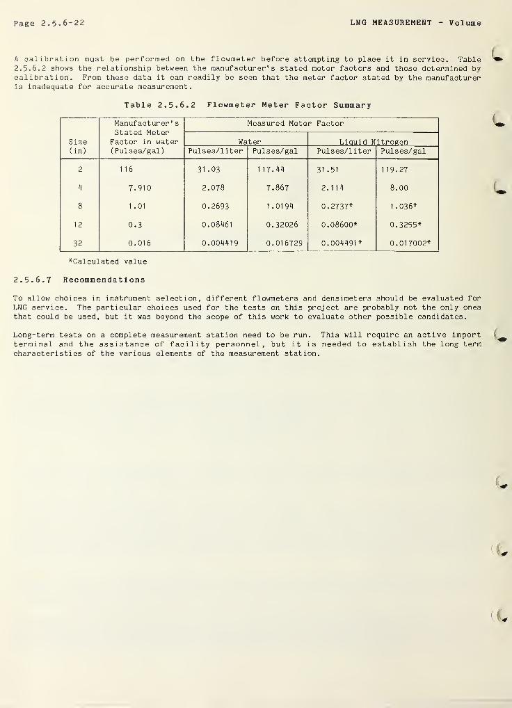
Page 2.5.6-22 LNG MEASUREMENT Volume
A calibration must be performed on the flowmeter before attempting to place it in service. Table2. 5. 6. 2 shows the relationship between the manufacturer's stated meter factors and those determined bycalibration. From these data it can readily be seen that the meter factor stated by the manufactureris inadequate for accurate measurement.
Table 2. 5. 6. 2 Flowmeter Meter Factor Summary
Size(in)
Manufacturer '
s
Stated MeterFactor in water( Pulses/gal
)
Measured Meter Factor
Water Liquid NitrogenPulses/liter Pulses/gal Pulses/liter Pulses/gal
2 116 31 .03 117.44 31 .51 119.27
4 7.910 2.078 7.867 2.114 8.00
8 1 .01 0.2693 1 .0194 0.2737* 1 .036*
12 0.3 0.08461 0.32026 0.08600* 0.3255*
32 0.016 0.004419 0.016729 0.004491 * 0.017002*
^Calculated value
2. 5. 6. 7 Recommendations
To allow choices in instrument selection, different flowmeters and densimeters should be evaluated for
LNG service. The particular choices used for the tests on this project are probably not the only onesthat could be used, but it was beyond the scope of this work to evaluate other possible candidates.
Long-term tests on a complete measurement station need to be run. This will require an active importterminal and the assistance of facility personnel, but it is needed to establish the long termcharacteristics of the various elements of the measurement station.
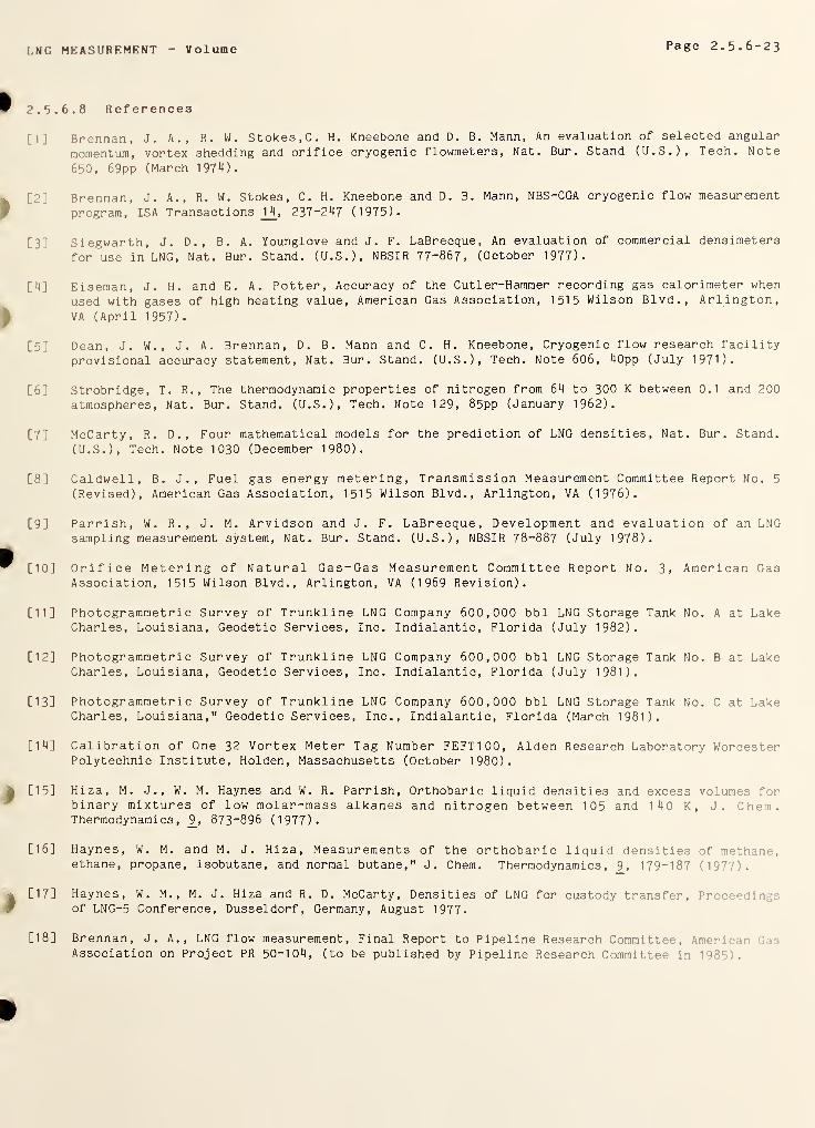
LNG MEASUREMENT Volume Page 2.5.6-23
2. 5. 6. 8 References
[ 1 ] Brennan, J. A., R. W. Stokes, C. H. Kneebone and D. B. Mann, An evaluation of selected angular
momentum, vortex shedding and orifice cryogenic flowmeters, Nat. Bur. Stand (U.S.), Tech. Note
650, 69pp (March 1974).
[2] Brennan, J. A., R. W. Stokes, C. H. Kneebone and D. B. Mann, NBS-CGA cryogenic flow measurement
program, ISA Transactions J_4,237-247 (1975).
[3] Siegwarth, J. D., B. A. Younglove and J. F. LaBrecque, An evaluation of commercial densimeters
for use in LNG, Nat. Bur. Stand. (U.S.), NBSIR 77-867, (October 1977).
[4] Eiseman, J. H. and E. A. Potter, Accuracy of the Cutler-Hammer recording gas calorimeter when
used with gases of high heating value, American Gas Association, 1515 Wilson Blvd., Arlington,
VA (April 1957).
[5] Dean, J. W., J. A. Brennan, D. B. Mann and C. H. Kneebone, Cryogenic flow research facility
provisional accuracy statement, Nat. Bur. Stand. (U.S.), Tech. Note 606, 40pp (July 1971).
[6] Strobridge, T. R., The thermodynamic properties of nitrogen from 64 to 300 K between 0.1 and 200
atmospheres, Nat. Bur. Stand. (U.S.), Tech. Note 129, 85pp (January 1962).
[7] McCarty, R. D., Four mathematical models for the prediction of LNG densities, Nat. Bur. Stand.
(U.S.), Tech. Note 1030 (December 1980).
[8] Caldwell, B. J., Fuel gas energy metering, Transmission Measurement Committee Report No. 5
(Revised), American Gas Association, 1515 Wilson Blvd., Arlington, VA (1976).
[9] Parrish, W. R., J. M. Arvidson and J. F. LaBrecque, Development and evaluation of an LNGsampling measurement system, Nat. Bur. Stand. (U.S.), NBSIR 78-887 (July 1978).
[10] Orifice Metering of Natural Gas-Gas Measurement Committee Report No. 3, American GasAssociation, 1515 Wilson Blvd., Arlington, VA (1969 Revision).
[11] Photogrammetr i c Survey of Trunkline LNG Company 600,000 bbl LNG Storage Tank No. A at LakeCharles, Louisiana, Geodetic Services, Inc. Indialantic, Florida (July 1982).
[12] Photogrammetri c Survey of Trunkline LNG Company 600,000 bbl LNG Storage Tank No. B at LakeCharles, Louisiana, Geodetic Services, Inc. Indialantic, Florida (July 1981).
[13] Photogrammetr i c Survey of Trunkline LNG Company 600,000 bbl LNG Storage Tank No. C at LakeCharles, Louisiana," Geodetic Services, Inc., Indialantic, Florida (March 1981).
[14] Calibration of One 32 Vortex Meter Tag Number FEFT100, Alden Research Laboratory WorcesterPolytechnic Institute, Holden, Massachusetts (October 1980).
[15] Hiza, M. J., W. M. Haynes and W. R. Parrish, Orthobaric liquid densities and excess volumes forbinary mixtures of low molar-mass alkanes and nitrogen between 105 and 1 4 0 K, J. Chem.Thermodynamics, 9_, 873—896 (1977).
[16] Haynes, W. M. and M. J. Hiza, Measurements of the orthobaric liquid densities of methane,ethane, propane, isobutane, and normal butane," J. Chem. Thermodynamics, 9, 179-187 (1977).
[17] Haynes, W. M., M. J. Hiza and R. D. McCarty, Densities of LNG for custody transfer, Proceed::.-of LNG-5 Conference, Dusseldorf, Germany, August 1977.
[18] Brennan, J. A., LNG flow measurement, Final Report to Pipeline Research Committee, AmeriAssociation on Project PR 50-104, (to be published by Pipeline Research Committee in 1985 ).
i

I
)
jj

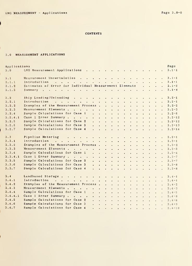
l.NG MEASUREMENT Appl icat ions Page 3.0-0
CONTENTS
3.0
MEASUREMENT APPLICATIONS
Applications Page
3.0 LNG Measurement Applications 3.1-
3.1 Measurement Uncertainties 3.1-
3.1.1 Introduction 3.1-
3.1.2 Estimates of Error for Individual Measurement Elements .... 3.1-
3.1.3 Summary 3.1-
3.2 Ship Lo ad i ng /Un 1 o ad i ng 3.2-
3.2.1 Introduction 3.2-
3.2.2 Examples of the Measurement Process 3.2-
3.2.3 Measurement Elements 3.2-
3.2.4 Sample Calculations for Case 1 3.2-
3. 2. 4.1 Case 1 Error Summary 3.2-
3.2.5 Sample Calculations for Case 2 3.2-
3.2.6 Sample Calculations for Case 3 3.2-3.2.7 Sample Calculations for Case 4 3.2-
3.3 Pipeline Metering 3.2-3.3.1 Introduction 3.3-3.3.2 Examples of the Measurement Process 3.3-3.3.3 Measurement Elements 3.3-3.3.4 Sample Calculations for Case 1 3.3-3. 3.4.1 Case 1 Error Summary 3.3-3.3.5 Sample Calculations for Case 2 3.3-3.3.6 Sample Calculations for Case 3 3.3-3.3.7 Sample Calculations for Case 4 3.3-
3.4 Landbased Storage 3.4-3.4.1 Introduction 3.4-3.4.2 Examples of the Measurement Process 3.4-3.4.3 Measurement Elements 3.4-3.4.4 Sample Calculations for Case 1 . 3.4-3. 4. 4.1 Case 1 Error Summary 3.4-3.4.5 Sample Calculations for Case 2 3.4-3.4.6 Sample Calculations for Case 3 3.4-3.4.7 Sample Calculations for Case 4 3.4-
1
1
1
2
4
1
1
2
3
6
12
12
13
14
1
1
2
3
4
7
7
8
8
1
1
2
3
5
8
8
9
10

LNG MEASUREMENT Measurement Uncertainties Page 3.1-1
3.0 LNG Measurement Applications
3.1 Measurement Uncertainties
The original concept of this LNG Measurements Manual provided for extensive treatment of the
measurement process as applied specifically to LNG baseload terminals and secondarily to LNG peak
shaving and satellite operations. It was anticipated that extensive performance data would be
available from measurement instrumentation for one or more of the U.S. LNG terminals. The results of
the properties and instrumentation research at NBS and elsewhere were to be extensively documented in
section 2 of this manual with estimates of error for each measurement element. The performance data
of the field instruments could then be combined with basic physical property data of section 1 of this
manual to give extensive examples of actual custody transfer measurements. Also included would be
examples of cases where procedures could not be carried out because of equipment failure of one or
more measurement elements and what could be done to complete the total measurement even though one or
more elements were not available.
It has not been possible to complete the manual as planned. The importation of LNG to the U.S. at the
date of this writing has been halted except for a relatively small quantity received at the Boston,Massachusetts, terminal. A limited amount of performance data has been taken at the Trunkline LNGCorporation terminal at Lake Charles, Louisiana, and this information has been included in section2.5.6, but the data is not as extensive as anticipated.
This section of the manual has been revised to take into account the lack of field performanceinformation and data. The approach is to be a set of example calculations based on assumed conditionsat a typical LNG import terminal. The calculations will be based on the information provided andreferenced to sections 1 and 2 of this manual, but the cases will, by necessity, be hypothetical and
will not provide the practical sense of field applications.
However, the format of the manual is of loose-leaf design, and users may wish to add their owninformation to that included at this printing. If, in the near future, the LNG imports to the U.S.resume, then it may be possible to complete the manual as planned by replacing this section 3 with a
revised section 3 based on actual LNG terminal measurement and instrumentation performance.
3-1.1 Introduction
The following sections describe three applications of the measurement process to establish the valueof a quantity of LNG prior to sale. The first application is that of a LNG ship unloading (orloading) at a terminal. The second is where a flow measurement station is located in a LNG pipelinebetween the LNG ship and on-shore LNG tank storage; and the third application is where LNG is loadedinto (or unloaded from) a shore LNG tank.
The first and third applications are considered static measurements, and the second is dynamicmeasurement. All three applications of the measurement process have a number of similarities.
1) All three allow calculation of the volume of LNG to be measured. Thd ship tanks are,in general, discrete volumes having individual measurement instrumentation such asliquid level gauges and densimeters. The same comments can be made for the shoretanks, which may be several times greater in volume but have similar instrumentationto that of the individual ship tank. Strapping and the calculation of tank tablesare also similar operations for both ship tank and shore tank applications. Trim andlist tables which may be used for correcting the measurement as a function of tankorientation are only required for the ship tanks.
Volume flowmeter measurements during loading and unloading operations are quitedifferent. Strapping, tank tables and liquid level instrumentation are not required ,
but the volume passing through the meter must be totalized over the flow period.
2) Density measurements and instrumentation can be quite similar. However, not all ofthe commercially available densimeters can measure the density of a LNG flowing In i
pipeline, but the calibration requirements are nearly the same. An "in-pipel In--"
densimeter will actually be exposed to all the contents of a tank during the loadingor unloading operation where the "in-tank" densimeter may be exposed to only thelimited volume of LNG in proximity to the primary measurement element.
Page 3.1-2 LNG MEASUREMENT Measurement Uncertainties
3) Sampling of LNG for calculation of density and/or calorific value is possible eitherby separate tank taps or by tapping main cargo piping at or near the flowmeter. Gasanalysis is then made possible either on a continuous basis or by periodicallyfilling sample bottles.
Based on the above, it is possible to assess the measurement process for all three applications. Theassessment will take the form of estimating errors for the measurement processes involved in each ofthe applications and then performing sample calculations for each of the applications. The estimatesof error are discussed in the following portions of this section, while sample calculations will beincluded with each of the applications sections.
3.1.2 Estimates of Error for Individual Measurement Elements
The following discussion is designed to provide estimates of error for each of the LNG measurementelements other than volume. The sources for the estimates of error are all within the text of LNGManual and are referenced to the individual section, figure or table.
Volume This measurement is specific to each application and will be discussed with the samplecalculations for each application (see sections 3-2, 3.3. and 3.4). There may be several values for
the estimate of error depending on tank construction, tank size and liquid level devices used.
Gas Analysis This extremely important measurement process contributes to calculated density andcalculated calorific value estimates. In addition, it is used to estimate the uncertainty in thecalorific value found from the combustion calorimeter.
The estimate of total uncertainty is composed of an allocation for known sources of systematic errorplus random error. Each component must include the value and a description of the source of error.
The estimate of random error for the gas analysis process comes from section 2.2.1. The random errorof ±0.06 percent is three times the standard deviation of ±0.02 percent. This value represents the
maximum value obtained from over 100 measurements of three or more repetitive analyses employing a
properly operating gas chromatograph with programmable integrator system.
The known sources of systematic error are the uncertainty in the calibration gas composition of ±0.03percent based on the uncertainty in the weighing process used to prepare the calibration mixtures.Great care must be taken to assure the purity of the components of the calibration gas in order tomaintain this uncertainty value.
The total uncertainty in gas analysis is estimated to be ±0.09 percent, which is composed of an
allocation of ±0.03 percent for known sources of systematic error plus a random error of ±0.06percent. The random error is three times the standard deviation of ±0.02 percent found from over 100
measurements of three or more repetitive analyses employing a properly operating gas chr omatographwith programmable integrator.
Calculated LNG Density The total uncertainty in calculated density is composed of two parts. The
first is the estimate of error in calculation of density by means of the mathematical models which in
turn are based on an extensive experimental data program described in section 2. 4. 3.1. "The total
uncertainty of a single density measurement is approximately 0.1 percent at low temperatures ..." Themost likely use of this data by the measurement engineer would be through the application of one or
more of the mathematical models optimized to fit these experimental data. As described in section2. 4. 3- 7 "The result was that all four of the models originally chosen can be used to predict the
density of LNG to within 0.1 percent of the true density, given the temperature, pressure (for thesemodels) and composition." The resultant systematic error contribution would be these two errors
combined in quadrature to give ±0.14 percent.
The second part of the total uncertainty in calculated density are known sources of random error which
consist of errors in measurement of pressure, temperature and composition and are the required inputvariables for the above mathematical models. The error in composition is that found above from gas
analysis and is assumed to be ±0.09 percent.
LNG MEASUREMENT Measurement Uncertainties Page 3.1-3
Errors in pressure measurement are assumed not to exceed ±0.25 percent of reading at a pressure of
0.7 MPa. This error of about ±1.8 kPa in pressure must be converted to percent error in density.
The isothermal compressibility of the fluid may be used which is:
Isothermal Compressibility = —— 1 /MPa (1)
p 3 P
where p is the density of the fluid and 3p / 3 P can be found from thermodynamic properties of the
fluid. It is assumed for simplicity that pure methane is the fluid, and the work of Goodwin [24 of
section 1 . 3 ] is used as a source for the thermodynamic data. The above value is calculated to be
less than 0.001 percent change in density for a error of ±1.8 kPa and therefore can be neglected.
Temperature measurement errors have a greater influence on the calculated density error. Assume here
that the error in temperature measurement does not exceed ± 0.1 K.
The thermodynamic property of expansivity is:
Expansivity = - —— 1 /K (2)
p 3 T
where p is the density of the fluid and 3p/3T can be found for methane from Goodwin as above.
The error in density calculated from the expansivity value is ±0.016 percent for the ±0.1 K errorassumed for the temperature measurement.
Combining these sources of random error (pressure, temperature and composition) in quadrature gives a
value of ±0.091 percent for these known sources of error.
The total uncertainty in calculated density is estimated to be ±0.23 percent, which is composed of
±0.14 percent for known sources of systematic error plus a random error of ±0.091 percent. Therandom error, estimated as a limit, is assumed to be at a 99.7 percent confidence level or threestandard deviations.
Measured Density The uncertainty in direct density measurements is composed of the densimetercalibration error and the random error of the densimeter used. The value of the random error is foundin section 2. 4. 2. 7. Four commercial densimeters were evaluated, and it was found that performancedepended on application, that for selected instruments at least, a calibration can be provided whichis precise to better than 0.1 percent and stable to better than 0.1 percent. This is interpreted tobe the limit of the random error of the densimeter and is consistent with the performance dataincluded in the figures of section 2.4.2.
The allocation of known sources of systematic error is the estimated calibration error. This is foundin section 2. 4. 1.7. The uncertainty of the density reference system for pure methane at the normalboiling point is ±0.055 percent. This value will vary somewhat with the density of the test fluid,but this value of ± 0.055 percent is the maximum value and will be less for LNG mixtures of higherdensity.
The total calibration uncertainty in direct density measurement is estimated to be ±0.16 percentwhich is composed of ± 0.06 percent for known sources of systematic error plus a random error of ± 0.1
percent. The random error is the limit of calibration error for selected commercial densimeters and
is considered to be at a confidence level of 99.7 percent or three standard deviations.
In practice, an additional error must be added to this calibration error to reflect actual fieldmeasurements of the LNG density. It is estimated that this additional random error will not be l.--.
than the ±0.1 percent random error component found during calibration. This additional errorapplied by considering the above calculated total calibration error as the systematic component :
•
field density measurements and the additional random error as the random component. Total unc^r’in direct density measurement is then ± 0.26 percent, which is composed of ±0.16 percent :•
calibration error plus a random error of ±0.1 percent. The random error, estimated an
assumed to be at a confidence level of 99.7 percent or three standard deviations.
Calculated Calorific Value The uncertainty in calculated calorific value is con: :
• •
systematic components. The random component is taken from section 2.2.5.10. "Labor i* ,
•1
tests showed that it is feasible to obtain and analyze representative samples wivon three standard deviations) of better than ±0.3 percent in the computed heat ::.g v r. . .
includes the gas analysis precision of ±0.06 percent" (see above).
Page 3. I- 1! LNG MEASUREMENT Measurement Uncertainties
The allocation of error for known sources of systematic error is composed of +0.03 percentuncertainty in the calibration gas composition, which neglects the uncertainty of the individualcomponents heating value and is based only on the uncertainty in the weighing process used to preparethe mixtures (see section 2.2.1). The estimate of error in the individual components' heating valueis taken from table 1.3.1 of section 1.3. There is a small variation in the estimated uncertainty in
heating value depending on the composition. Referring to table 2.1.1 which shows the mixturevariations of LNG as a function of source, LNG may vary from 99.81 percent methane with smallfractions of ethane and nitrogen to 71.9 percent methane and over 18 percent of the heavierhydr ocarbons . Table 1.3.1 shows that the greatest uncertainty in component heating value is that of
methane which is 890.65 ±0.37 kJ/mol. This value of ±0.04 percent is assumed as the maximum valuefor the present calculations. The two values of systematic error, ±0.03 percent and ±0.04 percentare combined in quadrature to give ±0.05 percent.
The total uncertainty in measured calorific value is ±0.77 percent, which is composed of anallocation of ±0.06 percent for known sources of systematic error plus ±0.71 percent random error.
The random error is assumed to be at a 99.7 percent confidence level.
Measured Calorific Value This uncertainty may have the largest value of all the measurement elements,
because a greater number of assumptions have been made to establish the value. Additional research is
required if this value is to be reduced. As discussed in section 2. 3. 2.1, a value of ±0.71 percentwas calculated as the estimated error in calorific value on a mass basis as found by the recordingcombustion calorimeter. An additional estimate of error must be added to this value to account for
the uncertainty in the calorific value of the calibration gas. This value, based on a 99.7 percentconfidence level, has been found for methane to be ±0.06 percent (see reference [15], section 2.3).
The total uncertainty in measured calorific value is ±0.77 percent, which is composed an allocationof ±0.06 percent for known sources of systematic error plus ±0.71 percent random error. The randomerror is assumed to be at a 99.7 percent confidence level.
The unexpectedly large uncertainty in measured calorific value is probably a result of limitedpublished research quality data. In Europe, where combustion calorimetry is, in many cases, theofficial accounting method, supporting data is believed to be adequate to show a lower error value.Actual performance data beyond that cited in the open literature are not available at this time.
3-1-3 Summary
The above calculations assume in all cases that the sampling process does in fact provide a
representative sample of the LNG container under consideration. This may not be true in practice.This can also be said of the temperature and pressure measurements. Any variations in the abovevalues caused by non-homogeneous fluid mixtures are unpredictable, and great care should be given to
assuring uniform temperatures, pressures, densities and compositions. Cross checks using several
combinations of the measurement elements are an excellent procedure to assure accurate and precisemeasurements. Table 3 . 1.1 contains a summary of the above developed estimates of error.
Table 3-1.1Estimates of Measurement Error
LNG Measurement Process
LNG Measurement TotalElement Uncertainty
( percent
)
Measured Calculated
Density ± 0.26 ±0.23
Calorific Value ±0.77 ± 0.35

D
!)
')
f
I
0
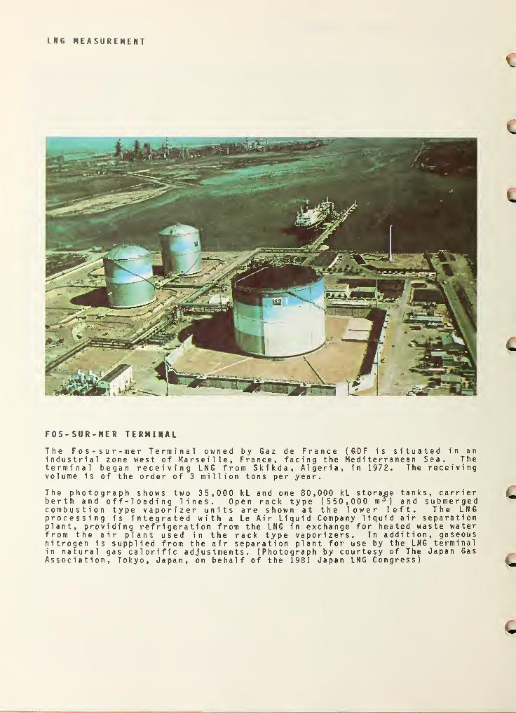
LNG MEASUREMENT
FOS-SUR-MER TERMINAL
The Fos-sur-mer Terminal owned by Gaz de France (GDF is situated in anindustrial zone west of Marseille, France, facing the Mediterranean Sea. Theterminal began receiving LNG from Skikda, Algeria, in 1972. The receivingvolume is of the order of 3 million tons per year.
The photograph shows two 35,000 kL and one 80,000 kL storage tanks, carrierberth and off-loading lines. Open rack type (550,000 m *
) and submergedcombustion type vaporizer units are shown at the lower left. The LNGprocessing is integrated with a Le Air Liquid Company liquid air separationplant, providing refrigeration from the LNG in exchange for heated waste waterfrom the air plant used in the rack type vaporizers. In addition, gaseousnitrogen is supplied from the air separation plant for use by the LNG terminalin natural gas calorific adjustments. (Photograph by courtesy of The Japan GasAssociation, Tokyo, Japan, on behalf of the 1981 Japan LNG Congress)
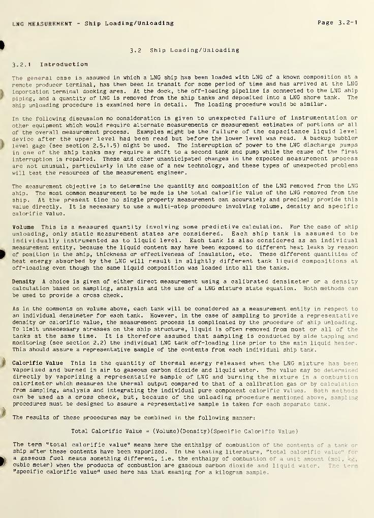
LNG MEASUREMENT - Ship Loading/Unloading Page 3-2-1
3.2 Ship Loading/Unloading
3.2.1 Introduction
The general case is assumed in which a LNG ship has been loaded with LNG of a known composition at a
remote producer terminal, has then been in transit for some period of time and has arrived at the LNG
importation terminal docking area. At the dock, the off-loading pipeline is connected to the LNG ship
piping, and a quantity of LNG is removed from the ship tanks and deposited into a LNG shore tank. The
ship unloading procedure is examined here in detail. The loading procedure would be similar.
In the following discussion no consideration is given to unexpected failure of instrumentation or
other equipment which would require alternate measurements or measurement estimates of portions or all
of the overall measurement process. Examples might be the failure of the capacitance liquid level
device after the upper level had been read but before the lower level was read. A backup bubbler
level gage (see section 2. 5. 1.5) might be used. The interruption of power to the LNG discharge pumps
in one of the ship tanks may require a shift to a second tank and pump while the cause of the first
interruption is repaired. These and other unanticipated changes in the expected measurement processare not unusual, particularly in the case of a new technology, and these types of unexpected problems
will test the resources of the measurement engineer.
The measurement objective is to determine the quantity and composition of the LNG removed from the LNG
ship. The most common measurement to be made is the total calorific value of the LNG removed from the
ship. At the present time no single property measurement can accurately and precisely provide this
value directly. It is necessary to use a multi-step procedure involving volume, density and specificcalorific value.
Volume This is a measured quantity involving some predictive calculation. For the case of ship
unloading, only static measurement states are considered. Each ship tank is assumed to beindividually instrumented as to liquid level. Each tank is also considered as an individualmeasurement entity, because the liquid content may have been exposed to different heat leaks by reasonof position in the ship, thickness or effectiveness of insulation, etc. These different quantities of
heat energy absorbed by the LNG will result in slightly different tank liquid compositions atoff-loading even though the same liquid composition was loaded into all the tanks.
Density A choice is given of either direct measurement using a calibrated densimeter or a densitycalculation based on sampling, analysis and the use of a LNG mixture state equation. Both methods can
be used to provide a cross check.
As in the comments on volume above, each tank will be considered as a measurement entity in respect toan individual densimeter for each tank. However, in the case of sampling to provide a representativedensity or calorific value, the measurement process is complicated by the procedure of ship unloading.To limit unnecessary stresses on the ship structure, liquid is often removed from most or all of thetanks at the same time. It is therefore assumed that sampling is conducted by side tapping andmonitoring (see section 2.2) the individual LNG tank off-loading line prior to the main liquid header.This should assure a representative sample of the contents from each individual ship tank.
Calorific Value This is the quantity of thermal energy released when the LNG mixture has beenvaporized and burned in air to gaseous carbon dioxide and liquid water. The value may be determineddirectly by vaporizing a repr esentati ve sample of LNG and burning the mixture in a combusticalorimeter which measures the thermal output compared to that of a calibration gas or by calculati n
from sampling, analysis and integrating the individual pure component calorific values. Both meth !
can be used as a cross check, but, because of the unloading procedure mentioned above, s t:n ;.
-•
procedures must be designed to assure a representative sample is taken for each separate tank.
The results of these procedures may be combined in the following manner:
Total Calorific Value = (Volume) (Density) (Specif ic Calorific Value)
The term "total calorific value" means here the enthalpy of combustion of the contents nf . • -
ship after these contents have been vaporized. In the testing literature, "total calorifi vs'.•
a gaseous fuel means something different, i.e. the enthalpy of combustion of a unit am' in* -,
cubic meter) when the products of combustion are gaseous carbon dioxide and liquid water. •
"specific calorific value" used here has that meaning for a kilogram sample.
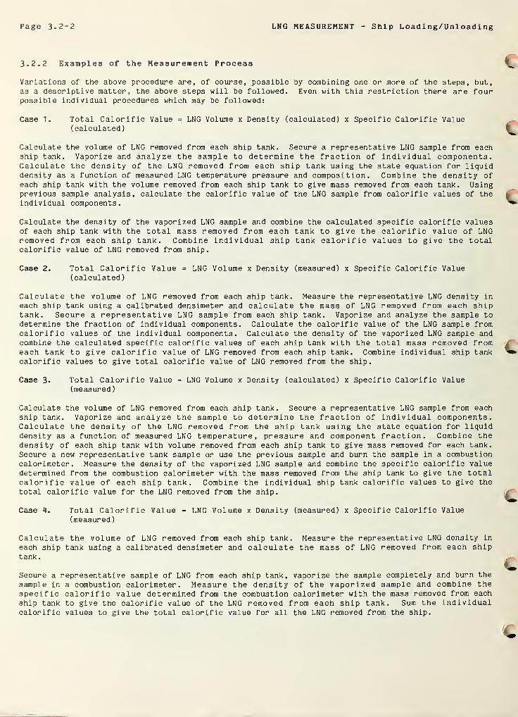
Page 3*2-2 LNG MEASUREMENT Ship Loading/Unloading
3*2.2 Examples of the Measurement Process
Variations of the above procedure are, of course, possible by combining one or more of the steps, but,as a descriptive matter, the above steps will be followed. Even with this restriction there are fourpossible individual procedures which may be followed:
Case 1. Total Calorific Value = LNG Volume x Density (calculated) x Specific Calorific Value(calculated)
Calculate the volume of LNG removed from each ship tank. Secure a representative LNG sample from eachship tank. Vaporize and analyze the sample to determine the fraction of individual components.Calculate the density of the LNG removed from each ship tank using the state equation for liquiddensity as a function of measured LNG temperature pressure and composition. Combine the density ofeach ship tank with the volume removed from each ship tank to give mass removed from each tank. Usingprevious sample analysis, calculate the calorific value of the LNG sample from calorific values of theindividual components.
Calculate the density of the vaporized LNG sample and combine the calculated specific calorific valuesof each ship tank with the total mass removed from each tank to give the calorific value of LNGremoved from each ship tank. Combine individual ship tank calorific values to give the totalcalorific value of LNG removed from ship.
Case 2. Total Calorific Value = LNG Volume x Density (measured) x Specific Calorific Value(calculated)
Calculate the volume of LNG removed from each ship tank. Measure the representative LNG density in
each ship tank using a calibrated densimeter and calculate the mass of LNG removed from each shiptank. Secure a representative LNG sample from each ship tank. Vaporize and analyze the sample todetermine the fraction of individual components. Calculate the calorific value of the LNG sample fromcalorific values of the individual components. Calculate the density of the vaporized LNG sample andcombine the calculated specific calorific values of each ship tank with the total mass removed fromeach tank to give calorific value of LNG removed from each ship tank. Combine individual ship tankcalorific values to give total calorific value of LNG removed from the ship.
Case 3* Total Calorific Value = LNG Volume x Density (calculated) x Specific Calorific Value(measured)
Calculate the volume of LNG removed from each ship tank. Secure a representative LNG sample from eachship tank. Vaporize and analyze the sample to determine the fraction of individual components.Calculate the density of the LNG removed from the ship tank using the state equation for liquiddensity as a function of measured LNG temperature, pressure and component fraction. Combine thedensity of each ship tank with volume removed from each ship tank to give mass removed for each tank.
Secure a new representative tank sample or use the previous sample and burn the sample in a combustioncalorimeter. Measure the density of the vaporized LNG sample and combine the specific calorific valuedetermined from the combustion calorimeter with the mass removed from the ship tank to give the totalcalorific value of each ship tank. Combine the individual ship tank calorific values to give the
total calorific value for the LNG removed from the ship.
Case Total Calorific Value = LNG Volume x Density (measured) x Specific Calorific Value(measured
)
Calculate the volume of LNG removed from each ship tank. Measure the representative LNG density in
each ship tank using a calibrated densimeter and calculate the mass of LNG removed from each shiptank
.
Secure a representative sample of LNG from each ship tank, vaporize the sample completely and burn the
sample in a combustion calorimeter. Measure the density of the vaporized sample and combine thespecific calorific value determined from the combustion calorimeter with the mass removed from each
ship tank to give the calorific value of the LNG removed from each ship tank. Sum the individualcalorific values to give the total calorific value for all the LNG removed from the ship.
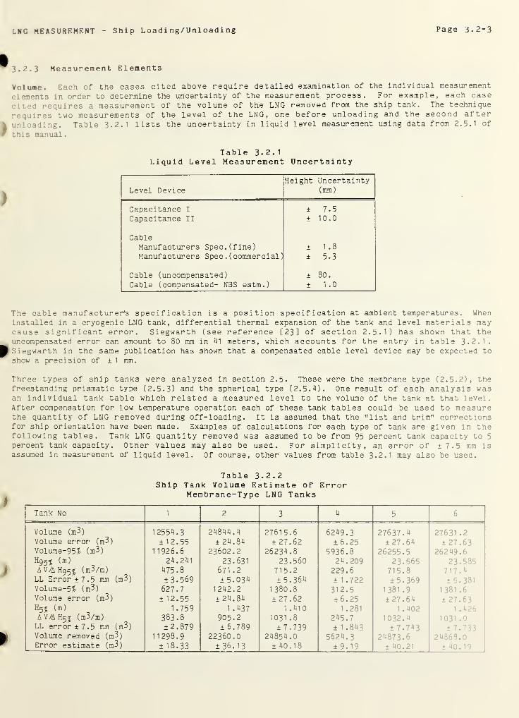
LNG MEASUREMENT Ship Loading/Unloading Page 3.2-3
3.2.3 Measurement Elements
Volume. Each of the cases cited above require detailed examination of the individual measurement
elements in order to determine the uncertainty of the measurement process. For example, each case
cited requires a measurement of the volume of the LNG removed from the ship tank. The technique
requires two measurements of the level of the LNG, one before unloading and the second afterunloading. Table 3.2.1 lists the uncertainty in liquid level measurement using data from 2.5.1 of
this manual.
Table 3.2.1Liquid Level Measurement Uncertainty
Level DeviceHeight Uncertainty
(mm)
Capacitance I ± 7.5Capacitance II ± 10.0
CableManufacturers Spec. (fine) ± 1 .8
Manufacturers Spec . (commercial) ± 5.3
Cable (uncompensated) ± 80.
Cable (compensated- NBS estm.) ± 1.0
The cable manufacturer's specification is a position specification at ambient temperatures. Wheninstalled in a cryogenic LNG tank, differential thermal expansion of the tank and level materials maycause significant error. Siegwarth (see reference [23] of section 2.5.1) has shown that theuncompensated error can amount to 80 mm in 41 meters, which accounts for the entry in table 3*2.1.Siegwarth in the same publication has shown that a compensated cable level device may be expected toshow a precision of ± 1 mm.
Three types of ship tanks were analyzed in section 2.5. These were the membrane type (2.5.2), thefreestanding prismatic type (2.5.3) and the spherical type (2.5. i+) . One result of each analysis wasan individual tank table which related a measured level to the volume of the tank at that level.After compensation for low temperature operation each of these tank tables could be used to measurethe quantity of LNG removed during off-loading. It is assumed that the "list and trim" correctionsfor ship orientation have been made. Examples of calculations for each type of tank are given in thefollowing tables. Tank LNG quantity removed was assumed to be from 95 percent tank capacity to 5
percent tank capacity. Other values may also be used. For simplicity, an error of ± 7.5 mm isassumed in measurement of liquid level. Of course, other values from table 3-2.1 may also be used.
Table 3.2.2Ship Tank Volume Estimate of Error
Membrane-Type LNG Tanks
Tank No 1 2 3 4 5 6.
Volume (m3) 12554.3 24844.4 27615.6 6249.3 27637.41
27631 .2
Volume error (m3) ±12.55 ± 24.84 ± 27.62 ± 6.25 ± 27.64 ± 27.63Volume-95? (m3) 11926.6 23602.2 26234.8 5936.8 26255.5 26249.6H95? (m) 24.241 23.631 23.560 24.209 23.565 23.585AV/AH95 J
(m3/m) 475.8 671 .2 715.2 229.6 715.8 717.4LL Error ±7.5 mm (m3) ± 3.569 ±5.034 ±5.364 ±1.722 ± 5.369 ± 5.381Volume-5? (m3) 627.7 1242.2 1380.8 312.5 1381 .9 1 381 .6
Volume error (m3) ±12.55 ±24.84 ± 27.62 ± 6.25 ±27.64 ± 27.63H51 (m) 1 .759 1.437 1 .410 1 .281 1 .402 1.426AV/AH5? (m3/m) 383.8 905.2 1031 .8 245.7 1032.4 1031.0LL error +7.5 mm (m3) ±2.879 ± 6.789 ± 7.739 ± 1 .843 ± 7.743 ± 7.733Volume removed (m3) 11298.9 22360.0 24854.0 5624.3 24873-6 24868.0Error estimate (m3) ±18.33 ±36.13 ± 40.18 ± 9.19 ± 40.21 £ HO. 19
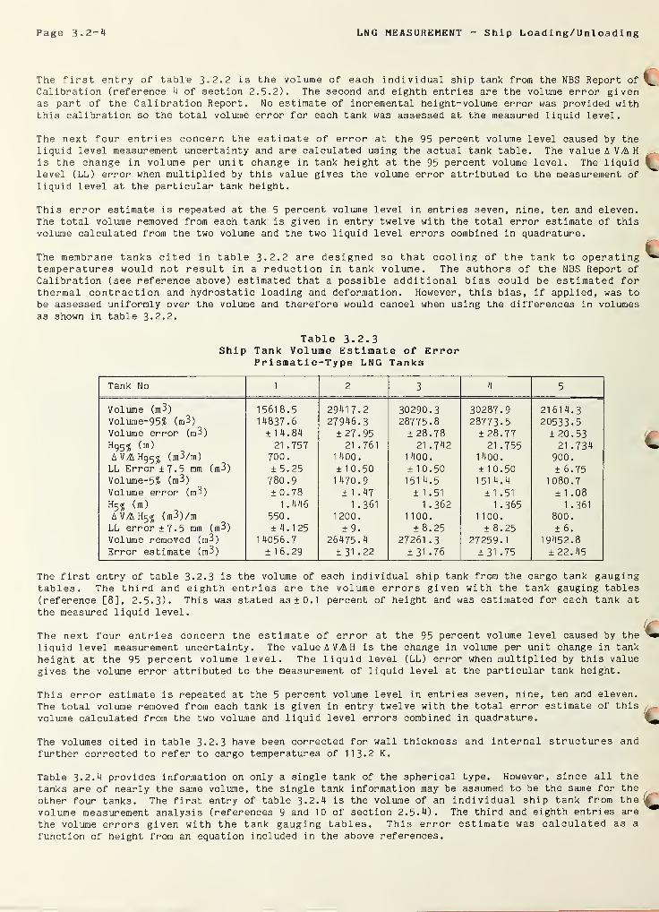
Page 3-2-4 LN G MEASUREMENT - Ship Load i ng/ Unload i ng
The first entry of table 3-2.2 is the volume of each individual ship tank from the NBS Report of
Calibration (reference 4 of section 2.5.2). The second and eighth entries are the volume error givenas part of the Calibration Report. No estimate of incremental height-volume error was provided withthis calibration so the total volume error for each tank was assessed at the measured liquid level.
The next four entries concern the estimate of error at the 95 percent volume level caused by theliquid level measurement uncertainty and are calculated using the actual tank table. The value A V/A H
is the change in volume per unit change in tank height at the 95 percent volume level. The liquidlevel (LL) error when multiplied by this value gives the volume error attributed to the measurement of
liquid level at the particular tank height.
This error estimate is repeated at the 5 percent volume level in entries seven, nine, ten and eleven.The total volume removed from each tank is given in entry twelve with the total error estimate of thisvolume calculated from the two volume and the two liquid level errors combined in quadrature.
The membrane tanks cited in table 3-2.2 are designed so that cooling of the tank to operatingtemperatures would not result in a reduction in tank volume. The authors of the NBS Report ofCalibration (see reference above) estimated that a possible additional bias could be estimated forthermal contraction and hydrostatic loading and deformation. However, this bias, if applied, was to
be assessed uniformly over the volume and therefore would cancel when using the differences in volumesas shown in table 3 - 2 . 2 .
Table 3-2.3Ship Tank Volume Estimate of Error
Prismatic-Type LNG Tanks
Tank No 1 2 3 4 5
Volume (m3) 15618.5 29417.2 30290.3 30287.9 2161 4.3Volume-95? (m3) 14837.6 27946.3 28775.8 28773-5 20533-5Volume error (m3) ±14.84 ±27.95 ± 28.78 ± 28.77 ± 20.53h95? (m) 21 .757 21 .761 21 .742 21 .755 21 .734AV/AH955&
(m3/m) 700 . 1 400. 1 400. 1 400. 900.LL Error±7.5 mm (m3) ± 5.25 ±10.50 ± 1 0.50 ±10.50 ± 6.75Volume-5? (m3) 780.9 1 470.9 1 51 4.5 1514.4 1080.7Volume error (m3) ± 0.78 ±1.47 ±1.51 ±1.51 ±1.08h5? 1.446 1 .361 1 .362 1.365 1 .361
A V/A H^ (m3)/m 550. 1 200 . 1100 . 1100 . 800 .
LL error ±7.5 mm (m3) ±4.125 ± 9. ±8.25 ± 8.25 ± 6 .
Volume removed (m3) 14056.7 26475.4 27261 .3 27259.1 19452.8Error estimate (m3) ±16.29 ± 31-22 ± 31 .76 ± 31 -75 ± 22.45
The first entry of table 3-2.3 is the volume of each individual ship tank from the cargo tank gaugingtables. The third and eighth entries are the volume errors given with the tank gauging tables
(reference [ 8 ], 2.5.3). This was stated as ±0.1 percent of height and was estimated for each tank at
the measured liquid level.
The next four entries concern the estimate of error at the 95 percent volume level caused by the
liquid level measurement uncertainty. The value A V/A H is the change in volume per unit change in tank
height at the 95 percent volume level. The liquid level (LL) error when multiplied by this value
gives the volume error attributed to the measurement of liquid level at the particular tank height.
This error estimate is repeated at the 5 percent volume level in entries seven, nine, ten and eleven.
The total volume removed from each tank is given in entry twelve with the total error estimate of this
volume calculated from the two volume and liquid level errors combined in quadrature.
The volumes cited in table 3.2.3 have been corrected for wall thickness and internal structures andfurther corrected to refer to cargo temperatures of 113-2 K.
Table 3.2.4 provides information on only a single tank of the spherical type. However, since all the
tanks are of nearly the same volume, the single tank information may be assumed to be the same for the
other four tanks. The first entry of table 3.2.4 is the volume of an individual ship tank from the
volume measurement analysis (references 9 and 10 of section 2.5.4). The third and eighth entries are
the volume errors given with the tank gauging tables. This error estimate was calculated as a
function of height from an equation included in the above references.
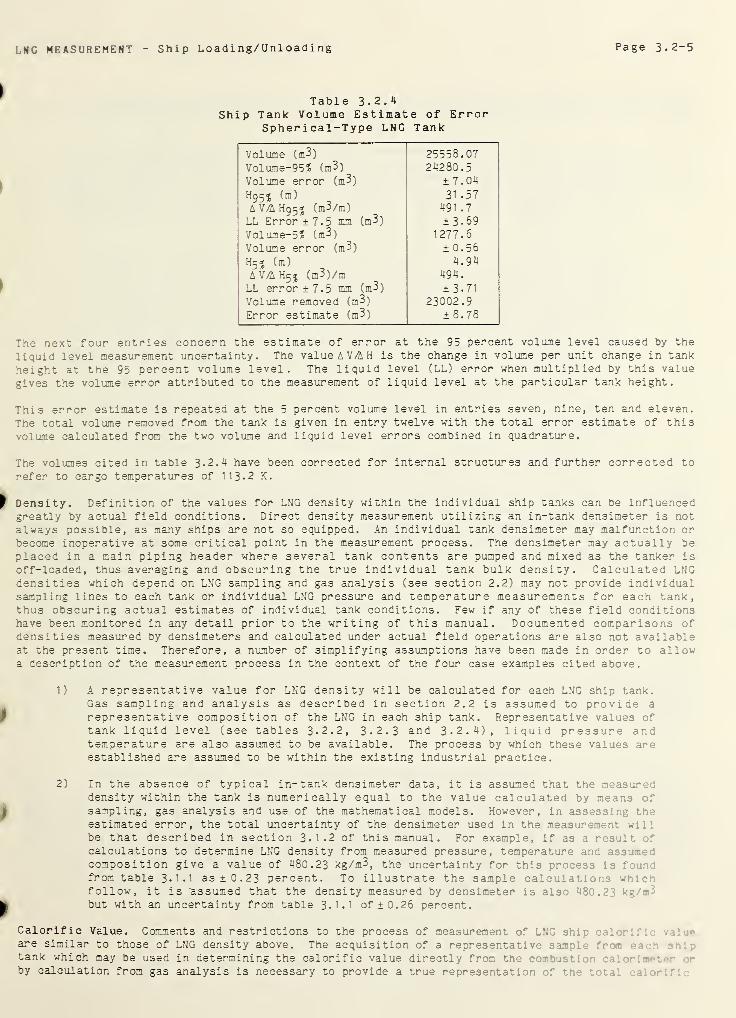
LNC MEASUREMENT Ship Loading/Unloading Page 3.2-5
Table 3.2.4Ship Tank Volume Estimate of Error
Spherical-Type LNG Tank
Volume (m3) 25558.07Volume-95? (m3) 24280.5Volume error (m3) ±7.04h95? (m) 31 -57
AVAHg^* (m3/m) 491 .7
LL Error ±7.5 mm (m3) ±3-69Volume-5? (m3) 1277.6Volume error (m3) ± 0.56
H5 J(m) 4.94
AVAH52 (m3)/m 494.
LL error ±7. 5 mm (m3) ±3-71Volume removed (m3) 23002.9Error estimate (m3) ±8.78
The next four entries concern the estimate of error at the 95 percent volume level caused by the
liquid level measurement uncertainty. The valueAV/AH is the change in volume per unit change in tank
height at the 95 percent volume level. The liquid level (LL) error when multiplied by this value
gives the volume error attributed to the measurement of liquid level at the particular tank height.
This error estimate is repeated at the 5 percent volume level in entries seven, nine, ten and eleven.
The total volume removed from the tank is given in entry twelve with the total error estimate of thisvolume calculated from the two volume and liquid level errors combined in quadrature.
The volumes cited in table 3-2.4 have been corrected for internal structures and further corrected to
refer to cargo temperatures of 113-2 K.
Density. Definition of the values for LNG density within the individual ship tanks can be influencedgreatly by actual field conditions. Direct density measurement utilizing an in-tank densimeter is notalways possible, as many ships are not so equipped. An individual tank densimeter may malfunction orbecome inoperative at some critical point in the measurement process. The densimeter may actually beplaced in a main piping header where several tank contents are pumped and mixed as the tanker is
off-loaded, thus averaging and obscuring the true individual tank bulk density. Calculated LNGdensities which depend on LNG sampling and gas analysis (see section 2.2) may not provide individualsampling lines to each tank or individual LNG pressure and temperature measurements for each tank,thus obscuring actual estimates of individual tank conditions. Few if any of these field conditionshave been monitored in any detail prior to the writing of this manual. Documented comparisons ofdensities measured by densimeters and calculated under actual field operations are also not availableat the present time. Therefore, a number of simplifying assumptions have been made in order to allowa description of the measurement process in the context of the four case examples cited above.
1) A representative value for LNG density will be calculated for each LNG ship tank.Gas sampling and analysis as described in section 2.2 is assumed to provide a
representative composition of the LNG in each ship tank. Representative values of
tank liquid level (see tables 3-2.2, 3.2.3 and 3.2.4), liquid pressure andtemperature are also assumed to be available. The process by which these values areestablished are assumed to be within the existing industrial practice.
2) In the absence of typical in-tank densimeter data, it is assumed that the measureddensity within the tank is numerically equal to the value calculated by means ofsampling, gas analysis and use of the mathematical models. However, in assessing t.-.e
estimated error, the total uncertainty of the densimeter used in the measurement wii .
be that described in section 3.1.2 of this manual. For example, if as a result f
calculations to determine LNG density from measured pressure, temperature art assume i
composition give a value of 480.23 kg/m3, the uncertainty for this process is f:/from table 3-1 • 1 as ±0.23 percent. To illustrate the sample calculations wri~nfollow, it is assumed that the density measured by densimeter is also U8C .
- -
but with an uncertainty from table 3.1.1 of ±0.26 percent.
Calorific Value. Comments and restrictions to the process of measurement of LNC snip rtf:are similar to those of LNG density above. The acquisition of a representative sample Tr -
tank which may be used in determining the calorific value directly from the combustionby calculation from gas analysis is necessary to provide a true representati :r. f
••
.
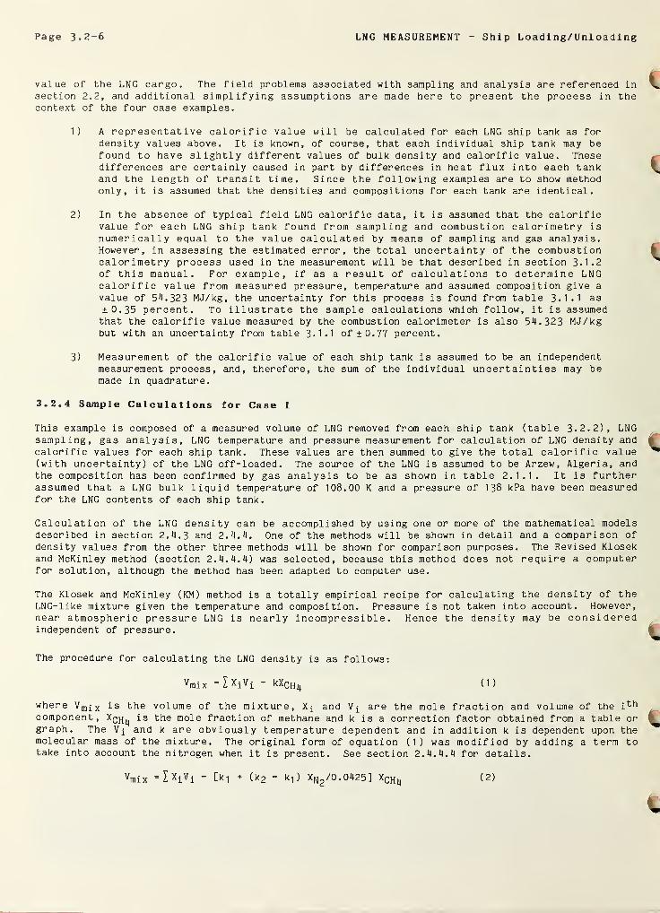
Page 3.2-6 LNG MEASUREMENT Ship Loading/Unloading
value of the LNG cargo. The field problems associated with sampling and analysis are referenced insection 2.2, and additional simplifying assumptions are made here to present the process in thecontext of the four case examples.
1) A representative calorific value will be calculated for each LNG ship tank as fordensity values above. It is known, of course, that each individual ship tank may befound to have slightly different values of bulk density and calorific value. Thesedifferences are certainly caused in part by differences in heat flux into each tankand the length of transit time. Since the following examples are to show methodonly, it is assumed that the densities and compositions for each tank are identical.
2) In the absence of typical field LNG calorific data, it is assumed that the calorificvalue for each LNG ship tank found from sampling and combustion calorimetry is
numerically equal to the value calculated by means of sampling and gas analysis.However, in assessing the estimated error, the total uncertainty of the combustioncalorimetry process used in the measurement will be that described in section 3.1.2of this manual. For example, if as a result of calculations to determine LNGcalorific value from measured pressure, temperature and assumed composition give a
value of 54.323 MJ/kg, the uncertainty for this process is found from table 3-1*1 as
±0.35 percent. To illustrate the sample calculations which follow, it is assumedthat the calorific value measured by the combustion calorimeter is also 54.323 MJ/kgbut with an uncertainty from table 3-1-1 of ±0-77 percent.
3) Measurement of the calorific value of each ship tank is assumed to be an independentmeasurement process, and, therefore, the sum of the individual uncertainties may bemade in quadrature.
3.2.4 Sample Calculations for Case 1
This example is composed of a measured volume of LNG removed from each ship tank (table 3-2.2), LNGsampling, gas analysis, LNG temperature and pressure measurement for calculation of LNG density andcalorific values for each ship tank. These values are then summed to give the total calorific value(with uncertainty) of the LNG off-loaded. The source of the LNG is assumed to be Arzew, Algeria, andthe composition has been confirmed by gas analysis to be as shown in table 2.1.1. It is furtherassumed that a LNG bulk liquid temperature of 108.00 K and a pressure of 138 kPa have been measuredfor the LNG contents of each ship tank.
Calculation of the LNG density can be accomplished by using one or more of the mathematical modelsdescribed in section 2.4.3 and 2.4.4. One of the methods will be shown in detail and a comparison of
density values from the other three methods will be shown for comparison purposes. The Revised Klosekand McKinley method (section 2. 4. 4. 4) was selected, because this method does not require a computerfor solution, although the method has been adapted to computer use.
The Klosek and McKinley (KM) method is a totally empirical recipe for calculating the density of theLNG-like mixture given the temperature and composition. Pressure is not taken into account. However,near atmospheric pressure LNG is nearly incompressible. Hence the density may be consideredindependent of pressure.
The procedure for calculating the LNG density is as follows:
vmix =I x i v i
~ k^CHij (1)
where V m ^ x is the volume of the mixture, and are the mole fraction and volume of the itl-1
component, is the mole fraction of methane and k is a correction factor obtained from a table orgraph. The and k are obviously temperature dependent and in addition k is dependent upon themolecular mass of the mixture. The original form of equation (1) was modified by adding a term totake into account the nitrogen when it is present. See section 2. 4. 4. 4 for details.
vmix =1*iVi ~ Ck-, + (k 2 - k-,) XN2 /0.0425] XCHl< (2)
LNG MEASUREMENT - Ship Loading/Unloading Page 3.2-7
where k-| refers to mixtures without nitrogen and 1<2 refers to mixtures with nitrogen. All other terms
are the same as in equation (1). Tabular values for solving the equation are given in section 1, in
the references of section 2. A. 4 and are reproduced here for convenience.
Table 3.2.5 provides initial data for the solution. Values for molecular mass are from tables 1.2.1
and 1.2.2. Volumes of saturated liquid of the pure components are found from table 3-2.6. The slight
differences in the molecular masses between tables 3*2.5 and 3*2.6 are caused by a revision of the
values used in table 3.2.6 in accord with section 1.2 of this manual. This revision is too small to
affect the mass and volume fractions in table 3*2.5.
Table 3-2.5Molecular Mass and Volume of Algerian LNG Mixture
Temperature = 108 K, Pressure = 138 kPa
Constituent *i Mwg/mol
XiMwg/mol
ViL/mol
XViL/mol
methane 0.8700 16.043 13*9574 0.037481 0.032608ethane 0.081
4
30.070 2.4477 0.047512 0.003867propane 0.0230 44.097 1 .01 42 0.062033 0.001 427
n-butane 0.0068 58.123 0.3952 0.076384 0.00051
9
i-butane 0.0046 58.123 0.2674 0.077836 0.000358n- pentane 0.0002 72.1 50 0.0144 0.091042 0.00001
8
nitrogen 0.01 40 28.01 34 0.392218.4885
0.043963 0.0006150.0394124
Values for the correction factors of equation (2) are found by linear interpolation of temperature andvolume in table 3*2.7 for correction factor k-| and table 3*2.8 for correction factor k 2 - For thetemperature and composition selection for the example (table 3*2.5), the values for the correctionfactors were found to be k-j = 0.434 and k 2 = 0.61.
Substituting in equation (2) gives:
Vm = 0.03941 24-{0.434(10“3)+[o.6l (
1
0—3 ) — 0 . 43 4 (
1
0—3 ) ][ 0. 01 4] /0. 425} 0.8700 (3)
Vm = 0.038985 liters/mol (4)
p (density) = 1 /Vm = 25.6509 mol/liter. (5)
In terms of the actual mixture, the molar density is multiplied by the molecular mass of the mixturefrom table 3*2.5 to give:
p (mixture density) = ( 25 . 6509)/ ( 1 8. 4885 ) = 474.246 kg/m3 (6)
Computer programs which provide a calculated value for the required density of the LNG mixture ir-
discussed in detail in section 2.4.4 and include a simple computer program for solving equationabove and more extensive programs for the other models. A comparison of the mixture lenpredicted by the four mathematical models are shown in table 3.2.9. The four models are the '<
and McKinley (KM), the Corresponding States (CS),the Cell (C) and the Hard Sphere (HS).
The maximum error of the five calculation methods from the mean mixture density example astable 3*2.9 is ±0.122 kilograms/cubic meter or ±0.026 percent. This is within the est :
for calculation of LNG density from the four mathematical models (0.1 percent) given in :• ••
. i
and 3.1.2. The value from equation (6) will be used in all the following example calcuiati •.
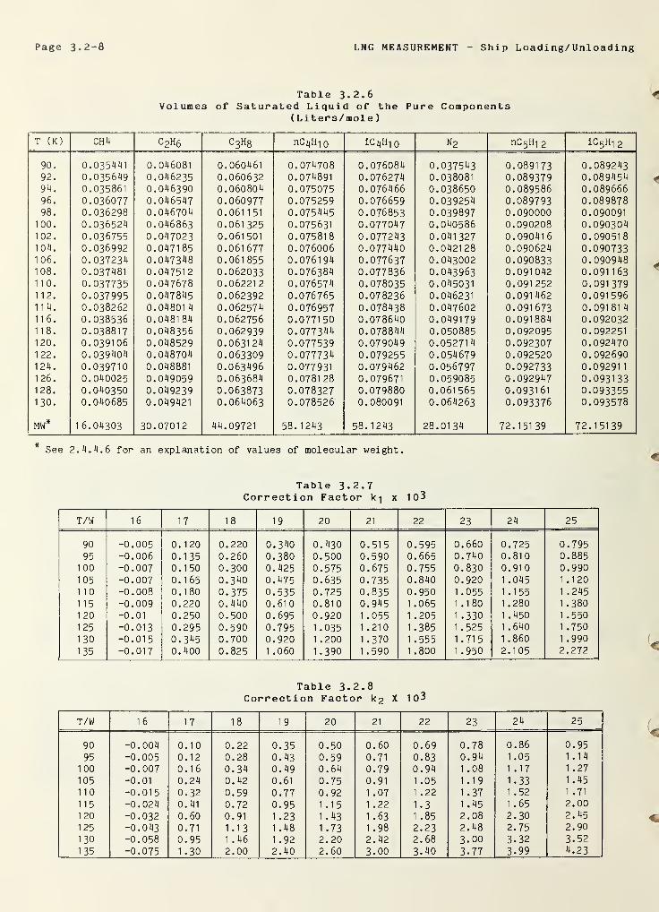
Page 3.2-8 LNG MEASUREMENT Ship Loading/Unloading
Table 3.2.6Volumes of Saturated Liquid of the Pure Components
(Liters/mole
)
T (K) CH4 c 2h6 c3h8 nC4Hi
0
1C4H1
0
n2 nC^Hi
2
iC 5 H i
2
90. 0.035441 0.046081 0.060461 0.074708 0.076084 0.037543 0.089173 0.08924392. 0.035649 0.046235 0.060632 0.074891 0.076274 0.038081 0.089379 0.08945494. 0.035861 0.046390 0.060804 0.075075 0.076466 0.038650 0.089586 0 . 08966696. 0.036077 0.046547 0.060977 0.075259 0.076659 0.039254 0.089793 0.08987898. 0.036298 0.046704 0.0611 51 0.075445 0.076853 0.039897 0.090000 0.090091
100. 0.036524 0.046863 0.061 325 0.075631 0.077047 0.040586 0.090208 0.090304102. 0.036755 0.047023 0.061501 0.075818 0.077243 0.041 327 0.09041
6
0.0905181 04. 0.036992 0.0471 85 0.061677 0.076006 0.077440 0.042128 0.090624 0.090733106. 0.037234 0.047348 0.061855 0.076194 0.077637 0.043002 0.090833 0.090948108. 0.037481 0.047512 0.062033 0.076384 0.077836 0.043963 0.091042 0.091 1 63110. 0.037735 0.047678 0.06221
2
0.076574 0.078035 0.045031 0.091 252 0.091 3791 1 2. 0.037995 0.047845 0.062392 0.076765 0.078236 0.046231 0.091 462 0.0915961 14. 0.038262 0.04801
4
0.062574 0.076957 0.078438 0.047602 0.091 673 0.09181
4
116. 0.038536 0.048184 0.062756 0.077150 0.078640 0.049179 0.091884 0.092032118. 0.03881
7
0.048356 0.062939 0.077344 0.078844 0.050885 0.092095 0.092251120. 0.039106 0.048529 0.063124 0.077539 0.079049 0.05271
4
0.092307 0.0924701 22. 0.039404 0.048704 0.063309 0.077734 0.079255 0.054679 0.092520 0.092690124. 0.039710 0.048881 0.063496 0.077931 0.079462 0.056797 0.092733 0.09291
1
1 26. 0.040025 0.049059 0.063684 0.0781 28 0.079671 0.059085 0.092947 0.093133128. 0.040350 0.049239 0.063873 0.078327 0.079880 0.061565 0.093161 0.0933551 30. 0.040685 0.049421 0.064063 0.078526 0.080091 0.064263 0.093376 0.093578
MW* 16.04303 30.07012 44.09721 58.1243 58.1243 28.01 34 72.15139 72.15139
* See 2. 4. 4. 6 for an explanation of values of molecular weight.
Table 3.2.7Correction Factor x 1 03
T/W 16 17 18 19 20 21 22 23 24 25
90 -0.005 0.120 0.220 0.340 0.430 0.515 0.595 0 . 660 0.725 0.79595 -0.006 0.135 0.260 0.380 0.500 0.590 0.665 0.740 0.810 0.885
100 -0.007 0.150 0.300 0. 425 0.575 0.675 0.755 0.830 0.91 0 0.990
105 -0.007 0.165 0.340 0.475 0.635 0.735 0.840 0.920 1 .045 1.120
1 1 0 -0.008 0.180 0.375 0.535 0.725 0.835 0.950 1.055 1.155 1 .245
115 -0.009 0.220 0.440 0.610 0.810 0.945 1.065 1.180 1.280 1.3801 20 -0.01 0.250 0.500 0.695 0.920 1.055 1 .205 1.330 1 .450 1 .550
125 -0.013 0.295 0.590 0.795 1.035 1 .210 1.385 1.525 1 .640 1.750
1 30 -0.015 0.345 0.700 0.920 1 .200 1.370 1.555 1 .715 1 .860 1.990
135 -0.017 0.400 0.825 1 .060 1.390 1 .590 1 .800 1 .950 2.105 2.272
Table 3.2.8Correction Factor k 2 X 1 03
T/W 16 17 18 19 20 21 22 23 24 25
90 -0.004 0.10 0.22 0.35 0.50 0.60 0.69 0.78 0.86 0.95
95 -0.005 0.12 0.28 0.43 0.59 0.71 0.83 0.94 1 .05 1.14
100 -0.007 0.16 0.34 0.49 0.64 0.79 0.94 1 .08 1 .17 1 .27
105 -0.01 0.24 0.42 0.61 0.75 0.91 1 .05 1.19 1.33 1.45
110 -0.01
5
0.32 0.59 0.77 0.92 1.07 1 .22 1.37 1.52 1 .71
115 -0.024 0.41 0.72 0.95 1.15 1 .22 1.3 1.45 1.65 2.00
120 -0.032 0.60 0.91 1 .23 1 .43 1.63 1 .85 2.08 2.30 2.45
125 -0.043 0.71 1.13 1.48 1 .73 1 .98 2.23 2.48 2.75 2.90
1 30 -0.058 0.95 1.46 1 .92 2.20 2.42 2.68 3.00 3.32 3.52
135 -0.075 1.30 2.00 2.40 2.60 3.00 3.40 3.77 3.99 4.23
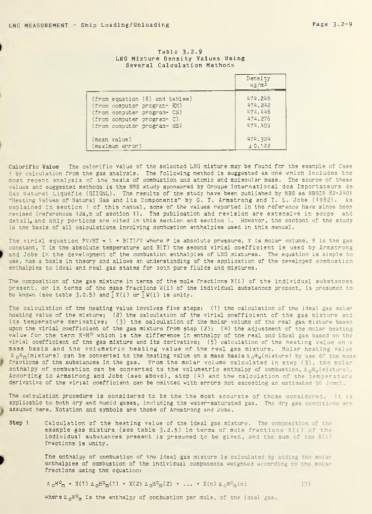
LNG MEASUREMENT - Ship Loading/Unloading Page 3.2-9
Table 3.2.9LNG Mixture Density Values Using
Several Calculation Methods
Densitykg/m3
(from equation (6) and tables) 474.246(from computer program- KM) 474.242
(from computer program- CS) 474.446
(from computer program- C) 474.276(from computer program- HS) 474.409
(mean value) 474.324(maximum error) ±0.122
Calorific Value The calorific value of the selected LNG mixture may be found for the example of Case
1 by calculation from the gas analysis. The following method is suggested as one which includes themost recent analysis of the heats of combustion and atomic and molecular mass. The source of these
values and suggested methods is the NBS study sponsored by Groupe International des Importateurs de
Gaz Naturel Liquefie (GIIGNL). The results of the study have been published by NBS as NBSIR 82-2401
"Heating Values of Natural Gas and Its Components" by G. T. Armstrong and T. L. Jobe ( 1 982). As
explained in section 1 of this manual, some of the values reported in the reference have since been
revised (references 12a,b of section 1). The publication and revision are extensive in scope anddetail, and only portions are cited in this section and section 1. However, the content of the studyis the basis of all calculations involving combustion enthalpies used in this manual.
The virial equation PV/RT = 1 + B(T)/V where P is absolute pressure, V is molar volume, R is the gas
constant, T is the absolute temperature and B(T) the second virial coefficient is used by Armstrong
^ and Jobe in the development of the combustion enthalpies of LNG mixtures. The equation is simple touse, has a basis in theory and allows an understanding of the application of the developed combustionenthalpies to ideal and real gas states for both pure fluids and mixtures.
The composition of the gas mixture in terms of the mole fractions X(i) of the individual substancespresent, or in terms of the mass fractions W(i) of the individual substances present, is presumed tobe known (see table 3.2.5) and£x(i) or£w(i) is unity.
The calculation of the heating value involves five steps: (1) the calculation of the ideal gas molarheating value of the mixture; (2) the calculation of the virial coefficient of the gas mixture andits temperature derivative; (3) the calculation of the molar volume of the real gas mixture basedupon the virial coefficient of the gas mixture from step (2); (4) the adjustment of the molar heatingvalue for the term H-H° which is the difference in enthalpy of the real and ideal gas based on thevirial coefficient of the gas mixture and its derivative; (5) calculation of the heating value on a
mass basis and the volumetric heating value of the real gas mixture. Molar heating valueA c Hm (mi xtur e ) can be converted to the heating value on a mass basis A cHw (mixture) by use of the mass
I fractions of the substances in the gas. From the molar volume calculated in step (3), the me la-enthalpy of combustion can be converted to the volumetric enthalpy of combustion, A cH v (mixture .
According to Armstrong and Jobe (see above), step (4) and the calculation of the temperat .r-
derivative of the virial coefficient can be omitted with errors not exceeding an estimated 50 j-
The calculation procedure is considered to be the the most accurate of those considered. :*
applicable to both dry and humid gases, including the water-saturated gas. The dry gas cord.'.« assumed here. Notation and symbols are those of Armstrong and Jobe.
Step 1 Calculation of the heating value of the ideal gas mixture. The composition f
example gas mixture (see table 3.2.5) in terms of mole fractions X(1 f• •
individual substances present is presumed to be given, and the sum of tn- :
fractions is unity.
k The enthalpy of combustion of the ideal gas mixture is calculated by adding the -.
W enthalpies of combustion of the individual components weighted according to t.n-j-
fractions using the equation:
A GH°m = X(1) A cH°m (1) + X(2) A cH°m (2) + ... + X(n) A cH°m (n)
where A cH°m is the enthalpy of combustion per mole, of the ideal gas.
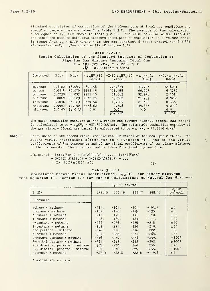
Page 3.2-10 LNG MEASUREMENT Ship Loading/Unloading
Standard enthalpies of combustion of the hydrocarbons at ideal gas conditions andspecified temperatures are taken from table 1.3.2. The results of the calculationfrom equation (7) are shown in table 3.2.10. The value of molar volume listed in
the table and used to calculate standard enthalpies of combustion on a volume basisis found from V m = RT/P where R is the gas constant 8.31 441 J/mol-K (or 8.31441m3-pascal/mole-K) . (See equation (1) of section 1.2).
Table 3.2.10Sample Calculation of the Standard Enthalpy of Combustion of
Algerian Gas Mixture Assuming Ideal GasP = 101.325 kPa , T = 288.15 K
V 1^ = 0.023641*7 m3/mol
Component X(i
)
M(i) A cH°m( i
)
kJ/mol-X(i) A cH°m ( i
)
kJ/mol
- A cH°v ( i
)
MJ/m3-X(i) A cH°v (i)
MJ/m3
methaneethanepropanen-butanei-butanen-pentanenitrogen
0.87000.081
4
0.02300.00680.00460.00020.01 40
16.04330.07044.09758.12358.12372.15028.01 34
891 .581562.1
4
2221 .10
2879.762870.583538.60
0.0
775.674127.15851 .083
19.58213.2050.7080.0
987.410
37.70766.06793.976
1 21 .7931 21 .405
1 49.6570.0
32.8051
5.37792. 161
4
0.82820.55850.02990.0
41 .7610
The molar combustion enthalpy of the Algerian gas mixture example (ideal gas basis)is calculated to be - A cH°m = 987.410 kJ/mol. The volumetric combustion enthalpy ofthe gas mixture (ideal gas basis) is calculated to be - A CH°V = 41.7610 MJ/m3.
Step 2 Calculation of the second virial coefficient B(mixture) of the real gas mixture. Thesecond virial coefficient B(mixture) is a function of T and of the virialcoefficients of the components and of the virial coefficients of the binary mixturesof the components. The equation used is taken from Armstrong and Jobe.
B(mixture) = [ X ( 1 )
]
2 B( 1 ) + [X(2)] 2 B(2) + ... + [X(n)] 2 B(n)+ 2X(1 )X(2)B(1 ,2) + 2X(1 )X(3)B( 1 ,3) + ...
+ 2X ( 1 ) X (n ) B( 1 ,n) ) (8)
Table 3.2.11Correlated Second Virial Coefficients, B^2( T )» f or Binary Mixtures
From Equation 11, Section 1.3 for Use in Calculations on Natural Gas Mixtures
B-|2(T) cm 3/mol
T (K) 273.15 288.15 288.71 298.15
error(cm3/mol
)
Substance
ethane + methane -114. -101 . -101 . - 93.4 ± 6
propane + methane -164. -146. -1 45. -135. ± 6
n-butane + methane -21 7. -192. -191 . -178. ± 20
i-butane + methane -208. -185. -184. -171 . ±30n-pentane + methane -266. -236. -235. -218 + 50
i-pentane + methane -261 . -231 . -230. -21 4. ± 50
neo-pentane + methane -246. -218. -216. -202. ± 50
n-hexane + methane -324. -286. -284. -264. ± 55
2-methyl pentane + methane -316. -279. -278. -259. ± 1 00*
3-methyl pentane + methane -321 . -283. -282. -262. ± 100*
2,2-dimethyl pentane + methane -305. -270. -268. -250. ± 40
2,3-dimethyl pentane + methane -313. -276. -275. -255. ±100*nitrogen + methane -27.9 -22.8 -22.6 -119.8 ± 5
* estimated- no data.
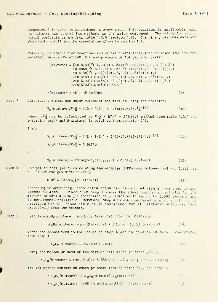
LNG MEASUREMENT Ship Loading/Unloading Page 3.2-11
Component 1 is taken to be methane in every case. This equation is applicable onlyto natural gas containing methane as the major component. The values for secondvirial coefficients are from table 1.3.4 (section 1.3). The binary mixtures data arefrom table 3-2.11 and the correlation given in section 1.3-
Step 3
Step 4
Entering the composition fractions and virial coefficients into equation (8) for theselected temperature of 288.15 K and pressure of 101.325 kPa. gives:
B (mixture) = [ ( 0. 8700) 2 ( -47. 0) +( 0 . 081 4) 2 ( -203. ) +(0.0230) 2 ( -428.
)
+( 0. 0068) 2 ( -805. )+( 0.0046) 2 ( -71 6. )+(0. 0002) 2 (-1 334.
)
+(0.01 40) 2 ( -7 . 1 )]+[ 2(0. 8700) (0.081 4) (-101 .
)
+2(0.8700) (0.0230) (-1 46. ) +2(0. 8700) (0.0068) (-192.)
+2(0.8700) (0.0046) (- 1 85 .) +2( 0 . 8700 ) (0 . 0002) (-236.
)
+2(0.8700)(0.01 40) (-22.8)]
B(mixture) = -61.738 cm3/mol (9)
Calculate the real gas molar volume of the mixture using the equation:
Vm (mixture)/V1^ = 1/2 + 1/2[1 + 4B(mixture)/V i
$]1 /2
( 10 )
where may be calculated as vi$ = RT/P = 23644.7 cm3/mol (see table 3.2.9 andpreceding text) and B(mixture) is obtained from equation (9).
Then:
and
:
Vm (mixture)/Vi^
Vm (mixture)/Vi^
1/2 + 1/2[1 + (4) (-61 .738)/23644.7] 1 72
0.99738
( 11 )
Vm (mixture) = ( 0 . 0236447) (0 . 99738) = 0.023583 m3/mol (12)
Correct to real gas by calculating the enthalpy difference between real and ideal gas(H-H°) for the gas mixture using:
H-H° = (RT/Vm )[B- T(dB/dT) ] (13)
According to Armstrong, this calculation can be omitted with errors that do notexceed 50 J/mol. Since from step 1 above the ideal combustion enthalpy for themixture is 987410 J/mol, a correction of 50 J/mol would amount to 0.005 percent andis considered negligible. Therefore, step 4 is not considered here but should not beneglected for all cases and must be considered for all mixtures which may varyextensively from the example.
Step 5 Calculate A cHm (mixture) , and A CH V (mixture) from the following:
A cHm (mixture) = A cH$(mixture) + ( A cHm -A CH$) (mixture) (14)
where the second term is the result of step 4 and is considered zero. Therefor" ,
from step 1
,
- A cHm (mixture) = 987.409 kJ/mole
Using the molecular mass of the mixture calculated in table 3.2.5,
- A cHm (mixture) = ( 987 . 41 0)/ ( 1 8 . 4885 ) = 53-407 kJ/g = 53-407 MJ/kg (16
The volumetric combustion enthalpy comes from equation (15) and step 3.
- A cH v (mixture) =- A cHm(mixture)/Vm (mixture)
- A cH v (mixture) = ( 987 . 41 0) / (0. 023583) = 41.870 MJ/m3
Page 3.2-12 LNG MEASUREMENT - Ship Loading/Unloading
3. 2. 4.1 Case 1 Error Summary
From the above calculations of volume, density and calorific value, it is possible to assemble thetotal calorific value and estimate of error of the LNG removed from the LNG ship.
From table 3.2.2 the volume removed from tank 1 is 11,298.9 m3. Equation (6) gives a density of474.246 kg/m3 for the LNG within the tank, and, therefore, the mass removed is the volume removedmultiplied by the density or 5,358.46 Mg. The calorific value of the LNG removed is the mass removedmultiplied by the specific calorific value on a mass basis from equation (16). This value of 53.407MJ/kg multiplied by the mass removed gives the total calorific value of 286.179 TJ (286.179 x 10^ 2J)
removed from tank 1. (T is the SI prefix symbol for Tera or lO^ 2, see section 1.1)
From table 3*2.2 the volume error is ±18.33 m3 or ±0.16 percent of the tank 1 volume removed. Fromtable 3-1.1 the estimated error in calculated density is ±0.23 percent, and the estimated error incalculated calorific value is ±0.35 percent. These individual estimates of error are independentvariables and may be combined in quadrature. The combination of volume, density and specificcalorific value is a simple multiplication, and, therefore, the error in total calorific value of theLNG removed is:
Estimated Tank Error Case 1 = [ev2 + e^2 + e c
2]
1 ^ 2
= ±0.45 percent (19)
where e v is the estimated volume error, e^ is the estimated density error, and ec is the estimatederror in calorific value. The total error in LNG removed from tank 1 is (286.179 TJ)( ± 0.45)/100) =
1 .288 TJ.
In like manner, total calorific values and estimated error may be calculated for ship tanks 2, 3. 4, 5
and 6. The results are summarized in table 3.2.11.
3-2.5 Sample Calculations for Case 2
The example is composed of a measured volume of LNG removed from each ship tank of the LNGmembrane-type ship (table 3.2.2). A representative LNG density is measured for each tank using a
calibrated LNG densimeter. A representative sample of LNG is removed from each ship tank, vaporizedand analyzed to determine the fraction of each of the LNG components. Calculations are then made todetermine the calorific value of the representative LNG sample on a mass basis.
As has been stressed in earlier sections of this manual, actual field data taken and assessed undercontrolled conditions are not available at the present time. The case in point would normally requireindividual measurements of the in-tank densimeters of the LNG ship prior to, during and afteroff-loading. Since these data are not available, the representative LNG density calculated for Case 1
above (Algerian LNG of table 3.2.5) will be used for this example. In addition, the required sampling,
analysis and calculation of calorific value described under Case 1 will also be assumed to be validfor this Case 2. This procedure will allow simple calculations and comparisons of the estimates of
error for each of the combinations of measurement elements. For the membrane-ship of the example, the
individual tank quantities and calorific values will remain the same as in Case 1. The totalcalorific values will also be the same for all the cases. Only the estimated errors will change, andthese will be a function of the measurement elements selected for each case. The values of estimatederror for each element are given in table 3.1.1.
In a manner similar to that described under Case 1, it is possible to assemble the total calorificvalue and estimate of error of the LNG removed from the LNG ship for the measurement assumptions of
Case 2.
From table 3.2.2 the volume removed from tank 1 is 11,298.9 m3. Equation (6) gives a density of
474.246 kg/m3 for the LNG within the tank, and, therefore, the mass removed is the volume removedmultiplied by the density or 5,358.46 Mg. The calorific value of the LNG removed is the mass removedmultiplied by the specific calorific value on a mass basis from equation (16). This value of 53.407MJ/kg multiplied by the mass removed gives the total calorific value of 286.179 TJ (286.179 x 10 12J)
removed from tank 1
.
From table 3.2.2 the volume error is ± 18.33 m3 or ±0.16 percent of the tank 1 volume. From table
3.1.1 the estimated error in measured density is ±0.26 percent, and the estimated error in calculatedcalorific value is ±0.35 percent. These individual estimates of error are independent variables and
may be combined in quadrature. The combination of volume, density and specific calorific value is a
LNG MEASUREMENT - Ship Loading/Unloading Page 3 . 2-13
simple multiplication, and, therefore, the error in total calorific value of the LNG removed is:
Estimated Tank Error Case 2 = [ev2 + e<j 2 + e c
2]1/2
= + 0.46 percent (20)
where ev is the estimated volume error, e^ is the estimated density error and e c is the estimate error
in calorific value. The total error in LNG removed from tank 1 is (286.179 TJ) ( ± 0. 46 )/1 00) = 1.31 6
TJ.
In like manner, total calorific values and estimated error may be calculated for ship tanks 2, 3, 4, 5
and 6. The results are summarized in table 3.2.11.
3 . 2.6 Sample Calculations for Case 3i
This third example is composed of a measured volume of LNG removed from each ship tank of the LNGmembrane-type ship (table 3.2.2). A representative sample of LNG is removed from each ship tank,vaporized and analyzed to determine the fraction of each of the LNG components. The density of the
sample is calculated using the mathematical models as shown in the example of Case 1 . From the
previous sample or a newly drawn one, the sample is burned in the combustion calorimeter to determine
the calorific value. A measured sample gas density will allow calculation of the calorific value on a
mass basis.
The assumptions for Case 2 are made also for Case 3- For the membrane- type ship of the example, the
individual tank quantities and calorific values will remain the same as in Case 1. The totalcalorific values will also be the same for all the cases. Only the estimated errors will change, andthese will be a function of the measurement elements selected for each case. The values of estimatederror for each element is given in table 3-1.1.
In a manner similar to that described under Case 1, it is possible to assemble the total calorific
}value and estimate of error of the LNG removed from the LNG ship for the measurement assumptions ofCase 2.
From table 3.2.2 the volume removed from tank 1 is 11,298.9 m3. Equation (6) gives a density of474.246 kg/m3 for the LNG within the tank, and, therefore, the mass removed is the volume removedmultiplied by the density or 5,358.46 Mg. The calorific value of the LNG removed is the mass removedmultiplied by the specific calorific value on a mass basis from equation (16). This value of 53.407MJ/kg multiplied by the mass removed gives the total calorific value of 286.179 TJ (286.179 x 10¹²J)removed from tank 1 .
From table 3.2.2 the volume error is ±18.33 m3 or ±0.16 percent of the tank 1 volume. From table3.1.1 the estimated error in calculated density is ±0.23 percent, and the estimated error in measuredcalorific value is ±0.77 percent. These individual estimates of error are independent variables andmay be combined in quadrature.
The combination of volume, density and specific calorific value is a simple multiplication, and,
ftherefore, the error in total calorific value of the LNG removed is:
Estimated Tank Error Case 3 = [e v2 + e^ 2 + e c
2]1//2
= ± 0.81 percent (21
)
i where e v is the estimated volume error, e^ is the estimated density error and ec is the es+' error in calorific value. The total error in LNG removed from tank 1 is (286.179 TJ)( * 0.81 )/1 r
2.318 TJ.
In like manner, total calorific values and estimated error may be calculated for ship tanks 2, , •.
and 6. The results are summarized in table 3.2.11.
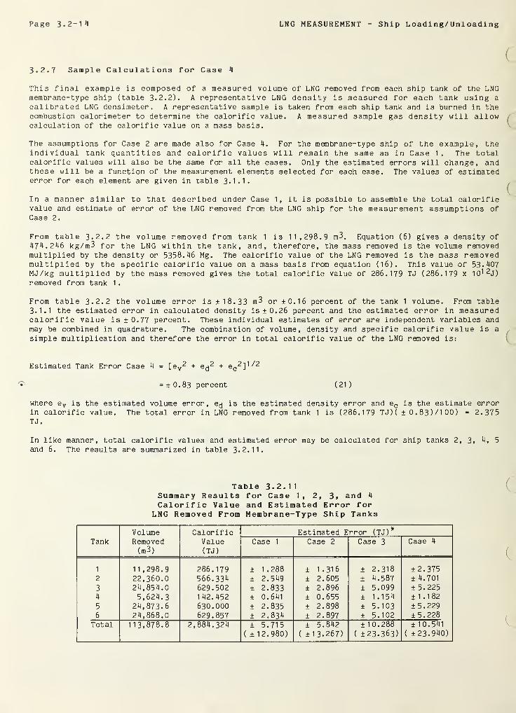
Page 3.2-1
4
LNG MEASUREMENT Ship Loading/Unloading
3.2.7 Sample Calculations for Case 4
This final example is composed of a measured volume of LNG removed from each ship tank of the LNGmembrane-type ship (table 3.2.2). A representative LNG density is measured for each tank using a
calibrated LNG densimeter. A representative sample is taken from each ship tank and is burned in thecombustion calorimeter to determine the calorific value. A measured sample gas density will allowcalculation of the calorific value on a mass basis.
The assumptions for Case 2 are made also for Case 4. For the membrane-type ship of the example, theindividual tank quantities and calorific values will remain the same as in Case 1. The totalcalorific values will also be the same for all the cases. Only the estimated errors will change, andthese will be a function of the measurement elements selected for each case. The values of estimatederror for each element are given in table 3.1.1.
In a manner similar to that described under Case 1, it is possible to assemble the total calorificvalue and estimate of error of the LNG removed from the LNG ship for the measurement assumptions ofCase 2.
From table 3.2.2 the volume removed from tank 1 is 11,298.9 m3. Equation (6) gives a density of
474.246 kg/m3 for the LNG within the tank, and, therefore, the mass removed is the volume removedmultiplied by the density or 5358.46 Mg. The calorific value of the LNG removed is the mass removedmultiplied by the specific calorific value on a mass basis from equation (16). This value of 53.407MJ/kg multiplied by the mass removed gives the total calorific value of 286.179 TJ (286.179 x 1
ol 2J
)
removed from tank 1
.
From table 3.2.2 the volume error is + 18.33 m3 or ±0.16 percent of the tank 1 volume. From table3.1.1 the estimated error in calculated density is ±0.26 percent and the estimated error in measuredcalorific value is ±0.77 percent. These individual estimates of error are independent variables andmay be combined in quadrature. The combination of volume, density and specific calorific value is a
simple multiplication and therefore the error in total calorific value of the LNG removed is:
Estimated Tank Error Case 4 = [ey2 + e^ + Sc2]1/2
• =±0.83 percent (21)
where ev is the estimated volume error, e^ is the estimated density error and e c is the estimate errorin calorific value. The total error in LNG removed from tank 1 is (286.179 TJ)( ± 0.83)/100) = 2.375TJ.
In like manner, total calorific values and estimated error may be calculated for ship tanks 2, 3, 4, 5
and 6. The results are summarized in table 3.2.11.
Table 3.2.11Summary Results for Case 1, 2, 3. and 4
Calorific Value and Estimated Error forLNG Removed From Membrane-Type Ship Tanks
Volume Calorific Estimated Error (TJ)*
Tank Removed(m3)
Value(TJ)
Case 1 Case 2 Case 3 Case 4
1 11,298.9 286.179 ± 1.288 ± 1.316 ± 2.318 ±2.3752 22,360.0 566.334 ± 2.549 ± 2.605 ± 4.587 ± 4.701
3 24,854.0 629.502 ± 2.833 ± 2.896 ± 5.099 ± 5.2254 5,624.3 1 42.452 ± 0.641 ± 0.655 ± 1.154 ±1.1825 24,873.6 630.000 ± 2.835 ± 2.898 ± 5.103 ±5.2296 24,868.0 629.857 ± 2.834 ± 2.897 ± 5.102 ±5.228
Total 113,878.8 2,884.324 ± 5.715( + 1 2.980)
± 5.842
( ± 13.267)
± 10.288
( ± 23.363)
± 10. 5^1
( ± 23.940)
LNG MEASUREMENT Ship Loading/Unloading Page 3.2-15
It should be noted that the error for each case shown in Table 12 has been found by combining theerrors from each tank in quadrature. It was assumed that measurements for each tank are independentof each other. This may not be true in practice and a simple sum is included in parenthesis. It is
one objective of this manual to provide enough of the basic data and a description of the method sothat if other procedures are preferred then these procedures may be followed using the original data.
The estimates of error for the total ship off-loading vary as to the measurement elements used andthe level of detail and control of the measurement process. For example; the total error (independenttank measurements) varies from ±0.20 percent to ±0.37 percent, a rather small number and rangeconsidering the magnitude of the individual error estimates of the measurement elements. To hold thetotal uncertainty to a minimum, it pays to plan carefully for the entire measurement process.


»)
>)
I
»
J
9
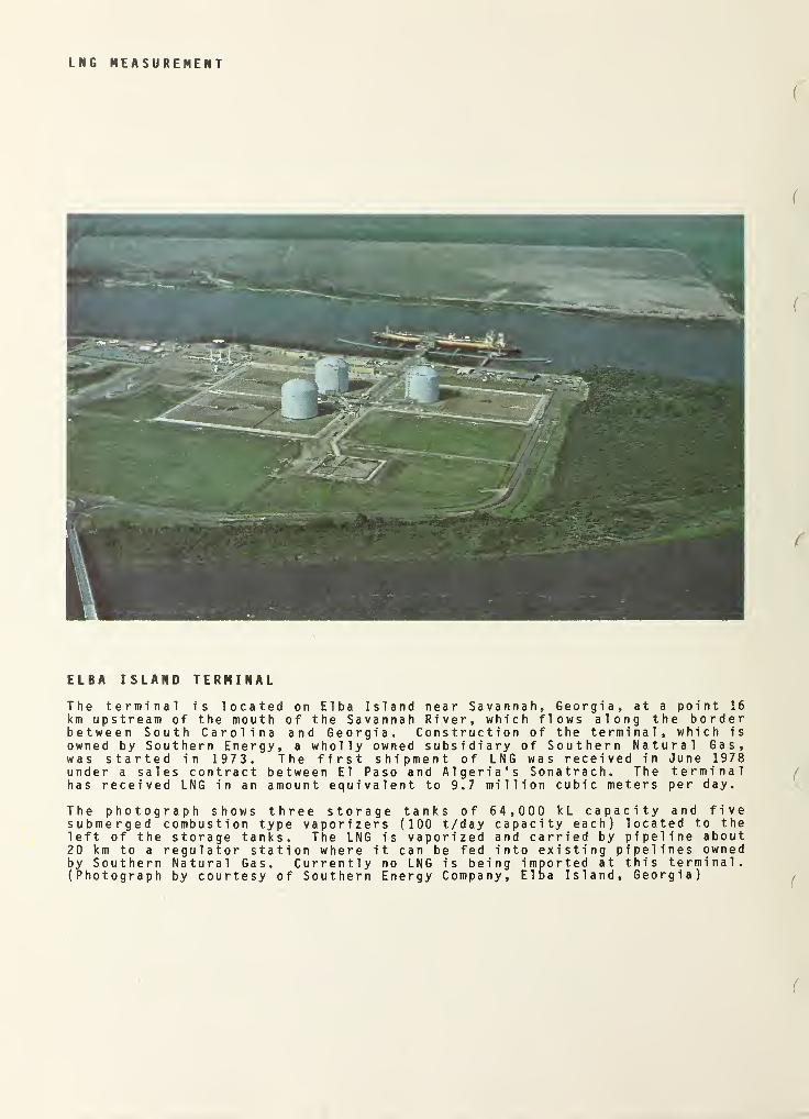
LNG MEASUREMENT
ELBA ISLAND TERMINAL
The terminal is located on Elba Island near Savannah, Georgia, at a point 16km upstream of the mouth of the Savannah River, which flows along the borderbetween South Carolina and Georgia. Construction of the terminal, which isowned by Southern Energy, a wholly owned subsidiary of Southern Natural Gas,was started in 1973. The first shipment of LNG was received in June 1978under a sales contract between El Paso and Algeria's Sonatrach. The terminalhas received LNG in an amount equivalent to 9.7 million cubic meters per day.
The photograph shows three storage tanks of 64,000 kL capacity and fivesubmerged combustion type vaporizers (100 t/day capacity each) located to theleft of the storage tanks. The LNG is vaporized and carried by pipeline about20 km to a regulator station where it can be fed into existing pipelines ownedby Southern Natural Gas. Currently no LNG is being imported at this terminal.(Photograph by courtesy of Southern Energy Company, Elba Island, Georgia)
LNG MEASUREMENT Pipeline Metering Page 3.3-1
3.3 Pipeline Metering
3 . 3 .I Introduction
The general case is assumed in which an LNG ship has been loaded with LNG of a known composition at a
remote producer terminal, has then been in transit for some period of time and has arrived at the LNG
importation terminal docking area. At the dock, the off-loading pipeline is connected to the LNG ship
piping and a quantity of LNG is removed from the ship tanks and deposited into a LNG shore storage
tank. The off-loading pipeline contains a measurement station composed of instrumentation for the
dynamic measurements of LNG volume flow, liquid density and calorific value (see section 2. 5. 6 . 2).
For this example, it is not necessary to define either the ship or shore tank instrumentation or
capacities, as the only consideration is the quantity and composition of the LNG passing through the
measurement station. However, in order to allow comparisons between the methods, accuracy and
precision of the measurement station with that of the ship loading/unloading ( 3 . 2 ) and landbasedstorage ( 3 . 4) measurements, it will be assumed that a quantity of 114,000 m3 of LNG (approximately net
from one 130,000 m3 ship load) is metered through the station, and the composition of the LNG was that
of the Algerian LNG mixture shown in table 2.1.1.
It should be noted that in practice the quantity and composition of the LNG measured in the pipeline
will not be precisely the same as that measured in the LNG ship. Pipeline heat leak and cooldownlosses will result in changes in the quantity and composition of the liquid. The same caution is made
here as to the expected changes of quantity and composition of the LNG delivered to the individualshore tank. Shore tank liquid content and composition prior to loading will additionally complicate
the measurement process. In general, the following process will be concerned with the quantity andcomposition of the liquid passing through the metering station. Other considerations must be made in
comparing the actual individual measurements of LNG removed from the ship, LNG metered in theoff-loading line and LNG loaded into the shore tanks.
As in the preceding examples, no consideration is given to unexpected failure of instrumentation or
other equipment which would require alternate measurements or measurement estimates of portions or all
of the overall measurement process. Examples might be the interruption of power to the LNG dischargepumps in one of the ship tanks which may delay LNG flow through the off-loading line. Since the
measurement station is an online dynamic system designed to integrate in time a series of short termobservations, any departure from steady state flow conditions will certainly have some effect on thetotal measurement precision and accuracy. If the measurement station is chosen as the primarymeasurement, every effort should be made to minimize variations in flow rate, pressure andtemperature
.
The measurement objective is to determine the quantity and composition of the LNG passing through theoff-loading line. The most common measurement to be made is the total calorific value. At thepresent time, no single property measurement can accurately and precisely provide this value directly.It is necessary to use a multi-step procedure involving volume, density and specific calorific value.
Volume. Dynamic quantitative totalized flow measurement of cryogenic fluids applied specifically toLNG is discussed in detail in section 2.5.6. Both mass and volume metering could have been usedsuccessfully with LNG. As the quantities of LNG and pipeline size requirements increased, volume'.'';?
metering became the meter of choice because of ease of adaptation and scaling cost when compared t
the direct reading mass flowmeter. The generic vortex type flowmeter was selected as an example ofvolume metering only because extensive experimental data was available (see section 2.5.6). linermetering may certainly be used if demonstrated accuracy, precision and scaling laws have Peer,
established. Continuous observation of the meter output and an accurate measurement of elapse 1 timeto give totalized flow is necessary to achieve maximum measurement accuracy and precision.
Density. A choice is available of either direct measurement using a calibrated inline flow den-
or a density calculation based on sampling, analysis and a mathematical model LNG mixtureequation. Both methods can be used to provide a cross check. Continuous monitoring of the f. w :
necessary to achieve greatest accuracy and precision of measurement.
Calorific Value. This is the quantity of thermal energy released when the LNG mix', ure -1
vaporized and burned in air to gaseous carbon dioxide and liquid water. The value may •
directly by vaporizing a representative sample of LNG drawn from the flowing fluid ir. tr>-
burning the mixture in a combustion calorimeter which measures the thermal outpu'. -1
- •
a calibration gas or by calculation from sampling, analysis and integrating thecomponent calorific values. Both methods can be used as a cross check, but con'; - . .
-•
.
• • .-i
necessary to achieve greatest accuracy and precision of measurement.
Page 3-3-2 LNG MEASUREMENT Pipeline Metering
The results of these procedures may be combined in the following manner:
Total Calorific Value = (Totalized Volume) (Density) (Specif ic Calorific Value)
The term "total calorific value" means here the enthalpy of combustion of the contents of a tank orship after these contents have been vaporized. In the testing literature, "total calorific value" fora gaseous fuel means something different, i.e. the enthalpy of combustion of a unit amount (mol, kg,cubic meter) when the products of combustion are gaseous carbon dioxide and liquid water. The term"specific calorific value" used here has that meaning for a kilogram sample.
3-3-2 Examples of the Measurement Process
Variations of the above procedure are, of course, possible by combining one or more of the steps, butas a descriptive matter, the above steps will be followed. Even with this restriction there are fourpossible individual procedures which may be followed:
Case 1 Total Calorific Value = LNG Volume x Density (calculated) x Specific Calorific Value(calculated)
Calculate the total volume of LNG passing through the measurement station byintegrating the flow rate over the total time of metering. Secure a continuousrepresentative LNG sample from the off-loading pipeline. Vaporize and analyze thesample to determine the fraction of individual components. Calculate the density of
the flowing LNG using the state equation for liquid density as a function of measuredLNG temperature, pressure and composition. Combine the density found from theequation with the volume passing through the measurement station to give the totalmass metered by the station. This may be done by using an average volume flow rateduring the sampling period and then integrating over the full off-loading time periodor by averaging the calculated density from the individual samplings and multiplyingthis value by the totalized flow.
Using the previous sample analysis and averaging technique calculate the averagespecific calorific value of the LNG sample from calorific values of the individualcomponents. Calculate the average density of the vaporized LNG sample and combinethe calculated specific calorific values with the total mass measured at themeasurement station.
Case 2 Total Calorific Value = LNG Volume x Density (measured) x Specific Calorific Value(calculated)
Calculate the total volume of LNG passing through the measurement station byintegrating the flow rate over the total time of metering. Continuously measure thedensity of the LNG passing through the measurement station using a calibrated"in-line" densimeter and calculate the total mass of LNG passing through themeasurement station. Secure a continuous representative LNG sample from theoff-loading pipeline. Vaporize and analyze the sample to determine the fraction ofindividual components. Calculate the specific calorific value of the LNG sample fromcalorific values of the individual components. Calculate the density of thevaporized LNG sample and combine the calculated specific calorific values with the
total mass passing through the measurement station to give the total calorific valueof LNG.
Case 3 Total Calorific Value = LNG Volume x Density (calculated) x Specific Calorific Value(measured)
Calculate the total volume of LNG passing through the measurement station by
integrating the flow rate over the total time of metering. Secure a continuousrepresentative LNG sample from the off-loading pipeline. Vaporize and analyze the
sample to determine the fraction of individual components. Calculate the density of
the LNG using a state equation for liquid density as a function of measured LNGtemperature, pressure and component fraction. Combine the density found from theequation with the volurne passing through the measurement station to give the total
mass metered by the station. This may be done by using an average volume flow rateduring the sampling period and then integrating over the full off-loading time periodor by averaging the calculated density from the individual samplings and multiplyingthis value by the totalized flow.
LNG MEASUREMENT - Pipeline Metering Page 3.3-3
Secure a representative pipeline LNG sample and burn the sample in a combustion
calorimeter to give a specific calorific value. Measure the density of the vaporized
LNG sample and combine the specific calorific value determined from the combustion
calorimeter with the measured mass passing through the off-loading pipeline at the
measurement station.
Case 4 Total Calorific Value = LNG Volume x Density (measured) x Specific Calorific Value
(measured)
Calculate the total volume of LNG passing through the measurement station by
integrating the flow rate over the total time of metering. Continuously measure the
density of the LNG passing through the measurement station using a calibrated"in-line" densimeter and calculate the total mass of LNG passing through themeasurement station. Secure a continuous representative sample of LNG the pipeline,
completely vaporize the sample and burn the sample in a combustion calorimeter to
give the specific calorific value. Measure the density of the vaporized sample and
combine the specific calorific value determined from the combustion calorimeter withthe total mass passed through the measurement station to give the total calorific
value of the LNG passing through the measurement station.
3.3.3 Measurement Elements
Volume. The basis for analysis of volume error measurement is taken from section 2.5.6 of this
manual. Admittedly, the direct experimental evidence which may be used to establish the totaluncertainty in the total LNG volume measured at the measurement station is minimal. However, the
estimates of error given in 2.5.6 are those available and are believed to be representative of whatwill be found in the future as additional studies are completed. The selection of error values will
be defined so that if new information becomes available or the reader wishes to use other data, thismay be done.
At this time it is estimated that the uncertainty in measurement of the total volume of LNG passedthrough a typical measurement station is ±0.5 percent. This value is the sum in quadrature of twoerror estimates. The first estimate is that from section 2. 5. 6. 4 which describes field testing of a
thirty-two inch vortex shedding flowmeter. The total volume flow measured by the vortex sheddingflowmeter was compared to the total volume removed from the LNG ship referenced to the ship levelgauges. The difference was found not to exceed ±0.4? percent between the two measurements.
The second value used to provide flowmeter total volume uncertainty is found from section 3.2.3 of
this manual which provides an estimate of error for LNG ship tank volume measurement which includesliquid level and tank volume error estimates. From table 3.2.2, the error estimate from tank 1 is
listed as ±0.16 percent of the tank volume. This value when added in quadrature to the aboveflowmetering error is found to be ±0.5 percent as stated.
Density. Definition of the values for LNG density as the fluid passes through the off-loadingpipeline measurement station can be influenced greatly by actual field conditions. Direct densitymeasurement utilizing an in-line densimeter is not always possible, as many pipelines are not soequipped. An individual densimeter may malfunction or become inoperative at some critical point in
the measurement process. To realize maximum accuracy and precision, the densimeter primary elementmust be located in the main pipeline flow and must not be sensitive to fluid velocities. CalculatedLNG densities which depend on LNG sampling and gas analysis (see section 2.2) must be located at ornear the measurement station and should continuously monitor the fluid density.
Few if any of these field conditions have been monitored in any detail prior to the writing of
j
manual. Documented comparisons of densities measured by densimeters and calculated under actual f lei 1
operations are also not available at the present time. The summary of LNG flowmeter to.-, t ir.g
section 2.5.6 contains some data on in-line densimeters, but the small variation in density •
during the tests was not adequate to assess process measurement error. Therefore a num* • r
simplifying assumptions have been made in order to allow a description of the measurement prothe context of the four case examples cited above.
1) A representative value for LNG density will be calculated for the LNG of' -: idlnvpipeline flowmetering process. Gas sampling and analysis as described In '
i
is assumed to provide a representative composition of the LNG in theAccurate measurement of pipeline liquid pressure and temperature are al.no n :
•
be available. The process by which these values are established aro ,
•
within the existing industrial practice.
Page 3 - 3 — ^ LNG MEASUREMENT Pipeline Metering
2) In the absence of typical in-line densimeter data, it is assumed that the measuredLNG density within the pipeline is numerically equal to the value calculated by meansof sampling, gas analysis and use of the mathematical models. However, in assessingthe estimated error, the total uncertainty of the densimeter used in the measurementwill be that described in section 3.1.2 of this manual. For example, if as a resultof calculations to determine LNG density from measured pressure, temperature andassumed composition give a value of 1180.23 kg/m3, the uncertainty for this process isfound from table 3.1.1 as ±0.23 percent. To illustrate the sample calculationswhich follow, it is assumed that the density measured by the in-line densimeter is
also found to be 480.23 kg/m3 but with an uncertainty from table 3-1.1 of ±0.26percent.
Calorific Value. Comments and restrictions to the process of measurement of LNG calorific value aresimilar to those of LNG density above. The continuous acquisition of a representative sample from thepipeline which may be used in determining the calorific value directly from the combustion calorimeteror by calculation from gas analysis is necessary to provide a true representation of the totalcalorific value of the LNG cargo. The field problems associated with sampling and analysis arereferenced in section 2.2, and additional simplifying assumptions are made here to present the processin the context of the four case examples.
1) A representative calorific value will be calculated as for density values above. It
is known, of course, that the continuous observation will show variations incomposition and density. These differences may be caused in part by differences in
compositions of liquid in the individual ship tanks and in practice must beconsidered and averaged. Since the following examples are to show method only, it is
assumed that the densities and compositions for each tank are constant values.
2) In the absence of typical field LNG calorific data, it is assumed that the calorificvalue of the pipeline fluid found from sampling and combustion calorimetry isnumerically equal to the value calculated by means of sampling and gas analysis.However, in assessing the estimated error, the total uncertainty of the combustioncalorimetry process used in the measurement will be that described in section 3-1.2of this manual.
For example, if as a result of calculations to determine LNG calorific value frommeasured pressure, temperature and assumed composition give a value of 54.323 MJ/kg,the uncertainty for this process is found from table 3-1.1 as 0.35 percent. Toillustrate the sample calculations which follow, it is assumed that the calorificvalue measured by the combustion calorimeter is also found to be 54.323 MJ/kg butwith an uncertainty from table 3.1.1 of ±0.77 percent.
3-3-4 Sample Calculations for Case 1
This example is composed of a volume of LNG passed through the off-loading pipeline measurementstation. It is assumed that the measurement station provides instrumentation for LNG sampling, gasanalysis, LNG temperature and pressure measurement used in the calculation of LNG density andcalorific values. These values are then combined to give the total calorific value (with uncertainty)of the LNG passed through the pipeline. The source of the LNG is assumed to be Arzew, Algeria, andthe composition has been confirmed by gas analysis to be as shown in table 2.1.1. It is furtherassumed that an LNG bulk liquid temperature of 108.00 K and a pressure of 138 kPa are the results of
measured averages of the pipeline liquid over the off-loading time period. These liquid conditionsare the same as those cited in sections 3.2 and 3.4.
(
Calculation of the LNG density can be accomplished by using one or more of the mathematical modelsdescribed in section 2.4.3 and 2.4.4. One of the methods will be shown in detail, and a comparison of
density values from the other three methods will be shown for comparison purposes. The Revised Klosek
and McKinley method (section 2. 4. 4. 4) was selected, because this method does not require a computerfor solution; although the method has been adapted to computer use.
The Klosek and McKinley (KM) method is a totally empirical recipe for calculating the density of the
LNG-like mixture given the temperature and composition. Pressure is not taken into account. However,
at near atmospheric pressure LNG is nearly incompressible, hence the density may be consideredindependent of pressure.
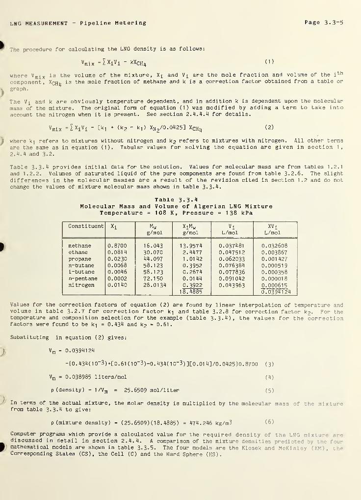
LNG MEASUREMENT Pipeline Metering Page 3-3-5
The procedure for calculating the LNG density is as follows:
Vmix -I ^i^i
~( 1 )
where V mix is the volume of the mixture, and V* are the mole fraction and volume of the i th
component, Xq^ is the mole fraction of methane and k is a correction factor obtained from a table or
graph.
The Vi
and k are obviously temperature dependent, and in addition k is dependent upon the molecular
mass of the mixture. The original form of equation (1) was modified by adding a term to take intoaccount the nitrogen when it is present. See section 2. 4. 4. 4 for details.
Vmix =I*iVi - [ K i+ (k 2 - k, ) XN2/0.0425] XCHl( (2)
i where k-| refers to mixtures without nitrogen and k 2 refers to mixtures with nitrogen. All other terms
are the same as in equation (1). Tabular values for solving the equation are given in section 1,
2.4.4 and 3.2.
Table 3.3.4 provides initial data for the solution. Values for molecular mass are from tables 1.2.1
and 1.2.2. Volumes of saturated liquid of the pure components are found from table 3.2.6. The slightdifferences in the molecular masses are a result of the revision cited in section 1.2 and do not
change the values of mixture molecular mass shown in table 3.3.4.
Table 3-3.4Molecular Mass and Volume of Algerian LNG Mixture
Temperature = 108 K, Pressure = 138 kPa
Consti tuent *i Mwg/mol
*iMwg/mol
ViL/mol
XViL/mol
methane 0.8700 16.043 13.9574 0.037481 0.032608ethane 0.081
4
30.070 2.4477 0.047512 0.003867propane 0.0230 44.097 1 .01 42 0.062033 0.001 427n-butane 0.0068 58.123 0.3952 0.076384 0.000519i-butane 0.0046 58.123 0.2674 0.077836 0.000358n-pentane 0.0002 72.150 0.0144 0.091 042 0.000018ni trogen 0.01 40 28.01 34 0.3922
18.48850.043963 0.000615
0.0394124
Values for the correction factors of equation (2) are found by linear interpolation of temperature andvolume in table 3.2.7 for correction factor k-| and table 3.2.8 for correction factor k 2 . For thetemperature and composition selection for the example (table 3.3.4), the values for the correctionfactors were found to be k-| = 0.434 and k2 = 0.61.
Substituting in equation (2) gives:
)Vm = 0.0394124
-{ 0. 434 (10“3)+[ 0.61 ( 1 0“3)-0 .434(1
0
-3) ][0. 01 4]/0. 0425}0. 8700 (3)
Vm = 0.038985 liters/mol (4)
p (density) = 1 /Vm = 25.6509 mol/liter (5)
In terms of the actual mixture, the molar density is multiplied by the molecular mass of the mix’ ir<-
from table 3-3.4 to give:
p (mixture density) = ( 25 . 6509) ( 1 8 . 4885 ) = 474.246 kg/m3 (6)
Computer programs which provide a calculated value for the required density of the LNG nix*discussed in detail in section 2.4.4. A comparison of the mixture densities pr • •
J i
•
|mathematical models are shown in table 3-3.5. The four models are the Klosek and McKirT. •
, -,
•
Corresponding States (CS), the Cell (C) and the Hard Sphere (HS).
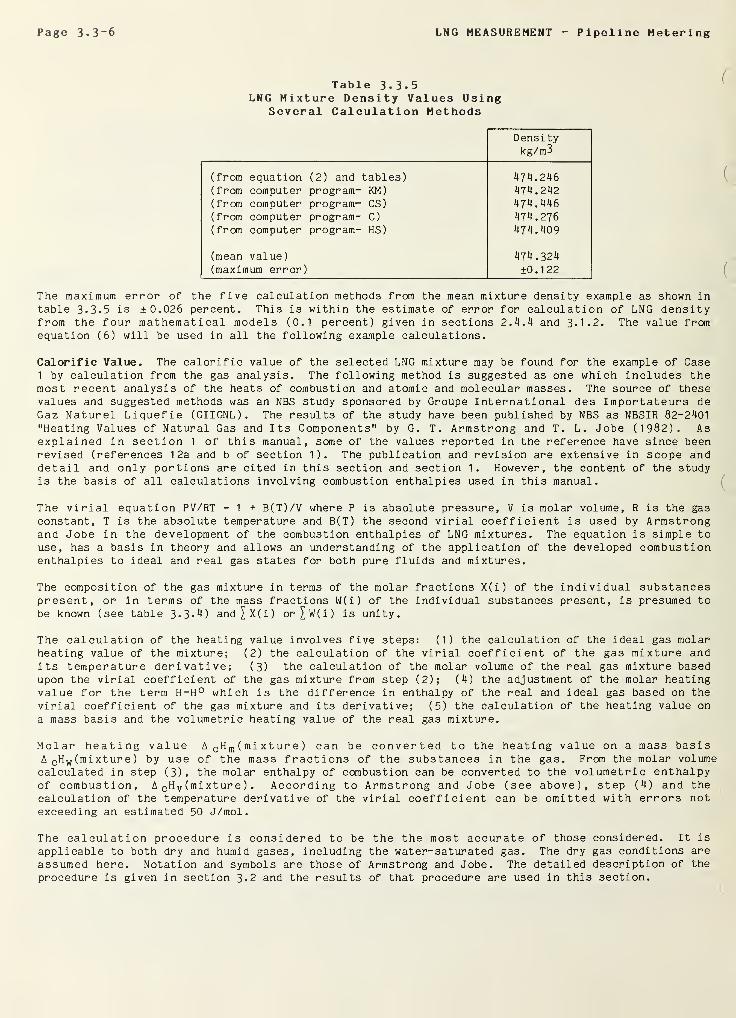
Page 3*3-6 LNG MEASUREMENT - Pipeline Metering
Table 3-3-5LNG Mixture Density Values Using
Several Calculation Methods
Densitykg/m3
(from equation (2) and tables) 474.246474.242474.446474.276474.409
(from computer program- KM)
(from computer program- CS)
(from computer program- C)
(from computer program- HS)
(mean value)(maximum error)
474.324±0.122
The maximum error of the five calculation methods from the mean mixture density example as shown intable 3-3-5 is ±0.026 percent. This is within the estimate of error for calculation of LNG densityfrom the four mathematical models (0.1 percent) given in sections 2.4.4 and 3-1.2. The value fromequation (6) will be used in all the following example calculations.
Calorific Value. The calorific value of the selected LNG mixture may be found for the example of Case1 by calculation from the gas analysis. The following method is suggested as one which includes themost recent analysis of the heats of combustion and atomic and molecular masses. The source of thesevalues and suggested methods was an NBS study sponsored by Groupe International des Importateurs deGaz Naturel Liquefie (GIIGNL). The results of the study have been published by NBS as NBSIR 82-2401
"Heating Values of Natural Gas and Its Components" by G. T. Armstrong and T. L. Jobe ( 1 982). Asexplained in section 1 of this manual, some of the values reported in the reference have since beenrevised (references 12a and b of section 1). The publication and revision are extensive in scope anddetail and only portions are cited in this section and section 1. However, the content of the studyis the basis of all calculations involving combustion enthalpies used in this manual.
The virial equation PV/RT = 1 + B(T)/V where P is absolute pressure, V is molar volume, R is the gas
constant, T is the absolute temperature and B(T) the second virial coefficient is used by Armstrongand Jobe in the development of the combustion enthalpies of LNG mixtures. The equation is simple to
use, has a basis in theory and allows an understanding of the application of the developed combustionenthalpies to ideal and real gas states for both pure fluids and mixtures.
The composition of the gas mixture in terms of the molar fractions X(i) of the individual substancespresent, or in terms of the mass fractions W(i) of the individual substances present, is presumed to
be known (see table 3-3.4) and^X(i) or£w(i) is unity.
The calculation of the heating value involves five steps: (1) the calculation of the ideal gas molarheating value of the mixture; (2) the calculation of the virial coefficient of the gas mixture andits temperature derivative; (3) the calculation of the molar volume of the real gas mixture basedupon the virial coefficient of the gas mixture from step (2); (4) the adjustment of the molar heatingvalue for the term H-H° which is the difference in enthalpy of the real and ideal gas based on the
virial coefficient of the gas mixture and its derivative; (5) the calculation of the heating value on
a mass basis and the volumetric heating value of the real gas mixture.
Molar heating value A c H m ( mi xt ur e ) can be converted to the heating value on a mass basisA c H w (mixture) by use of the mass fractions of the substances in the gas. From the molar volumecalculated in step (3), the molar enthalpy of combustion can be converted to the volumetric enthalpyof combustion, A CH v (mi xtur e ) . According to Armstrong and Jobe (see above), step (4) and the
calculation of the temperature derivative of the virial coefficient can be omitted with errors notexceeding an estimated 50 J/mol.
The calculation procedure is considered to be the the most accurate of those considered. It is
applicable to both dry and humid gases, including the water-saturated gas. The dry gas conditions are
assumed here. Notation and symbols are those of Armstrong and Jobe. The detailed description of the
procedure is given in section 3.2 and the results of that procedure are used in this section.
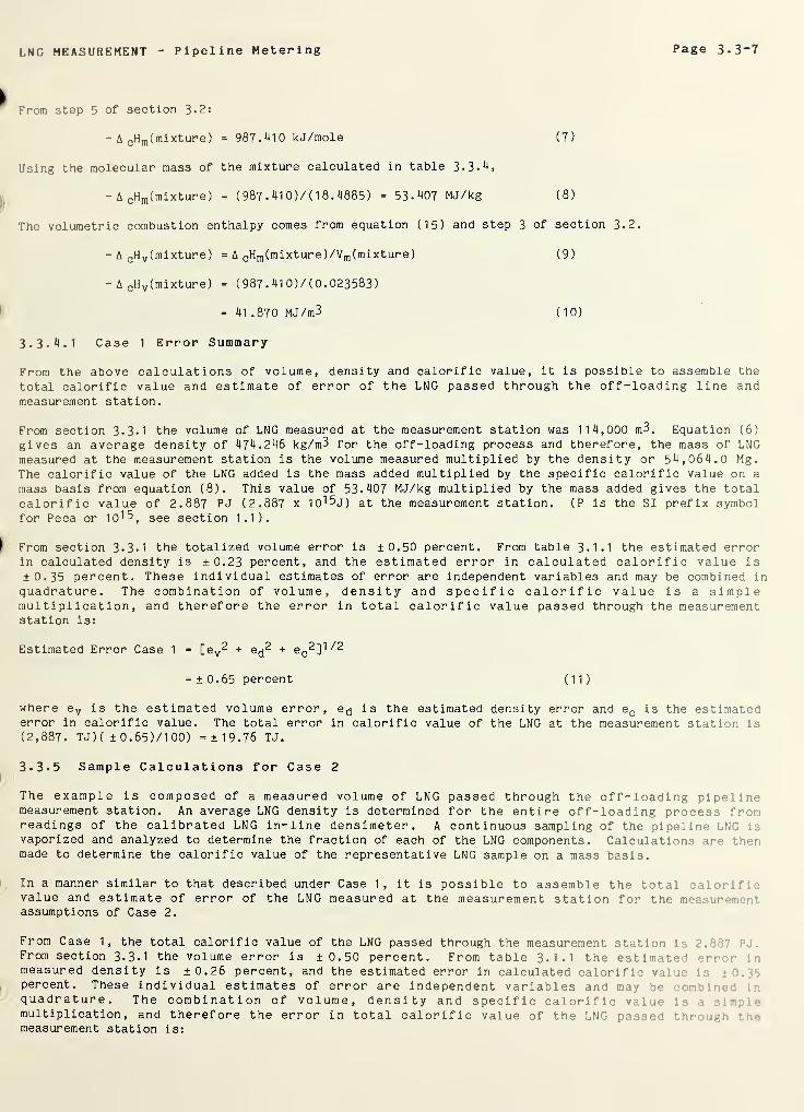
LNG MEASUREMENT Pipeline Metering Page 3.3-7
From step 5 of section 3-2:
- A cHm (mixture) = 987.410 kJ/mole (7)
Using the molecular mass of the mixture calculated in table 3.3.4.
- A cHm (mixture) = ( 987 . 41 0)/ ( 18.4885) = 53-407 MJ/kg (8)
The volumetric combustion enthalpy comes from equation (15) and step 3 of section 3.2.
- A cH v (mixture) = A cHm (mixture)/Vm (mixture) (9)
- A cH v (mixture) = ( 987 . 41 0) / (0. 023583)
= 41 .870 MJ/m3 (10)
3. 3. 4.1 Case 1 Error Summary
From the above calculations of volume, density and calorific value, it is possible to assemble the
total calorific value and estimate of error of the LNG passed through the off-loading line andmeasurement station.
From section 3.3.1 the volume of LNG measured at the measurement station was 114,000 m3. Equation (6)
gives an average density of 474.246 kg/m3 for the off-loading process and therefore, the mass of LNGmeasured at the measurement station is the volume measured multiplied by the density or 54,064.0 Mg.The calorific value of the LNG added is the mass added multiplied by the specific calorific value on a
mass basis from equation (8). This value of 53.407 MJ/kg multiplied by the mass added gives the totalcalorific value of 2.887 PJ (2.887 x IO^j) at the measurement station. (P is the SI prefix symbolfor Peca or 10^5, see section 1.1).
From section 3-3.1 the totalized volume error is ±0.50 percent. From table 3.1.1 the estimated errorin calculated density is +0.23 percent, and the estimated error in calculated calorific value is
±0.35 percent. These individual estimates of error are independent variables and may be combined in
quadrature. The combination of volume, density and specific calorific value is a simplemultiplication, and therefore the error in total calorific value passed through the measurementstation is:
Estimated Error Case 1 = [ev2 + e^2 + e c
2]1//2
= ± 0.65 percent (11)
where e v is the estimated volume error, e^ is the estimated density error and ec is the estimatederror in calorific value. The total error in calorific value of the LNG at the measurement station is(2,887. TJ ) ( ± 0 . 65 ) /I 00 ) =±19.76 TJ.
3.3.5 Sample Calculations for Case 2
The example is composed of a measured volume of LNG passed through the off-loading pipelinemeasurement station. An average LNG density is determined for the entire off-loading process fromreadings of the calibrated LNG in-line densimeter. A continuous sampling of the pipeline LNG isvaporized and analyzed to determine the fraction of each of the LNG components. Calculations are then,
made to determine the calorific value of the representative LNG sample on a mass basis.
In a manner similar to that described under Case 1, it is possible to assemble the total calorif:value and estimate of error of the LNG measured at the measurement station for the meanurassumptions of Case 2.
From Case 1, the total calorific value of the LNG passed through the measurement station is . .
•••' p.r.
From section 3-3.1 the volume error is ±0.50 percent. From table 3 . 1.1 the estimated -rr- •.
measured density is ±0.26 percent, and the estimated error in calculated calorific va]u<- *
percent. These individual estimates of error are independent variables and may be :
quadrature. The combination of volume, density and specific calorific valuemultiplication, and therefore the error in total calorific value of the LNG passed thr >ugh themeasurement station is:
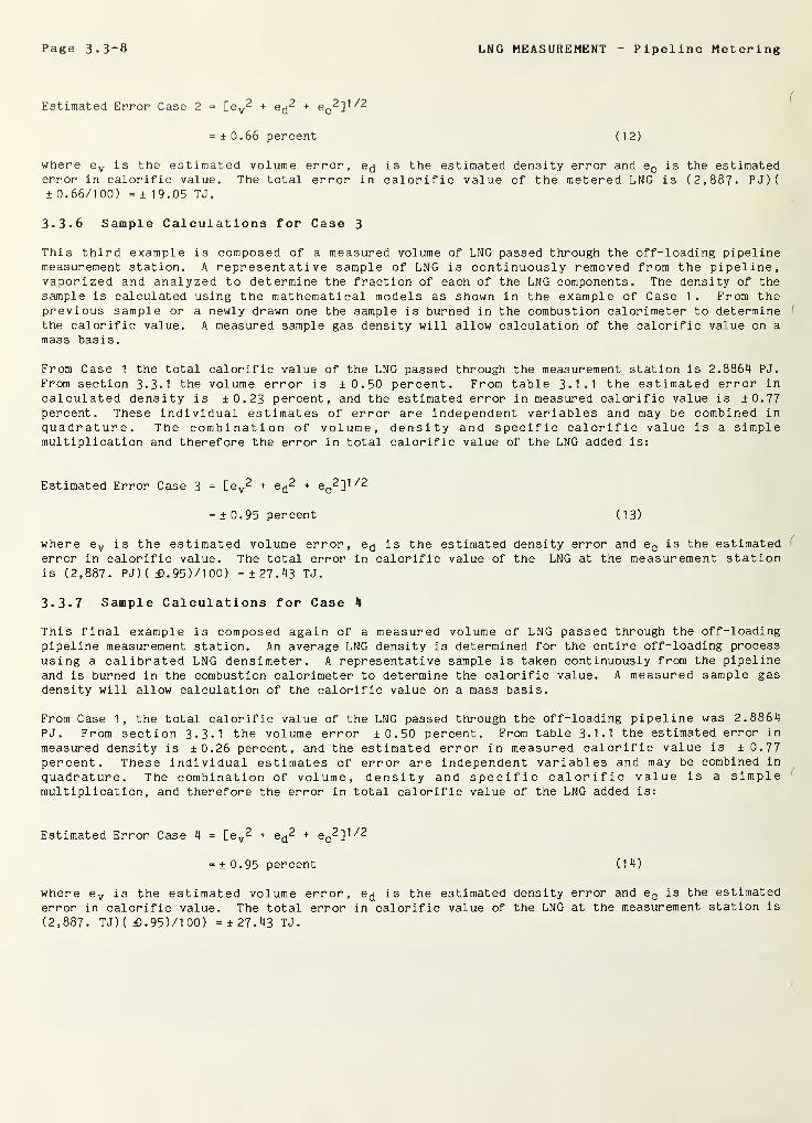
Page 3.3-8 LNG MEASUREMENT - Pipeline Metering
Estimated Error Case 2 = [ev2 + e^2 + ec
2]^2
= ± 0.66 percent ( 12 )
where e v is the estimated volume error, e^ is the estimated density error and e c is the estimatederror in calorific value. The total error in calorific value of the metered LNG is ( 2,887. PJ)(± 0.66/1 00) =±19.05 TJ.
3-3-6 Sample Calculations for Case 3
This third example is composed of a measured volume of LNG passed through the off-loading pipelinemeasurement station. A representative sample of LNG is continuously removed from the pipeline,vaporized and analyzed to determine the fraction of each of the LNG components. The density of the
sample is calculated using the mathematical models as shown in the example of Case 1. From theprevious sample or a newly drawn one the sample is burned in the combustion calorimeter to determinethe calorific value. A measured sample gas density will allow calculation of the calorific value on a
mass basis.
From Case 1 the total calorific value of the LNG passed through the measurement station is 2.8864 PJ.
From section 3.3.1 the volume error is ±0.50 percent. From table 3.1.1 the estimated error incalculated density is ±0.23 percent, and the estimated error in measured calorific value is ±0.77percent. These individual estimates of error are independent variables and may be combined inquadrature. The combination of volume, density and specific calorific value is a simplemultiplication and therefore the error in total calorific value of the LNG added is:
Estimated Error Case 3 = [e v2 + e^2 + ec
2]^2
where e v is the estimated volume error, e<j is the estimated density error and e c is the estimatederror in calorific value. The total error in calorific value of the LNG at the measurement stationis (2,887. PJ) ( d0 . 95 ) / 1 00) =± 27.43 TJ.
3.3.7 Sample Calculations for Case 4
This final example is composed again of a measured volume of LNG passed through the off-loadingpipeline measurement station. An average LNG density is determined for the entire off-loading process
using a calibrated LNG densimeter. A representative sample is taken continuously from the pipelineand is burned in the combustion calorimeter to determine the calorific value. A measured sample gasdensity will allow calculation of the calorific value on a mass basis.
From Case 1, the total calorific value of the LNG passed through the off-loading pipeline was 2.8864PJ. From section 3.3.1 the volume error ±0.50 percent. From table 3.1.1 the estimated error in
measured density is ±0.26 percent, and the estimated error in measured calorific value is ± 0.77percent. These individual estimates of error are independent variables and may be combined in
quadrature. The combination of volume, density and specific calorific value is a simplemultiplication, and therefore the error in total calorific value of the LNG added is:
Estimated Error Case 4 = [ev2 + e^2 + eG
2]^ 2
where e v is the estimated volume error, e^ is the estimated density error and e c is the estimated
error in calorific value. The total error in calorific value of the LNG at the measurement station is
(2,887. TJ) ( . 95 ) / 1 00) =± 27.43 TJ.
= ± 0.95 percent (13)
= ± 0.95 percent (14)
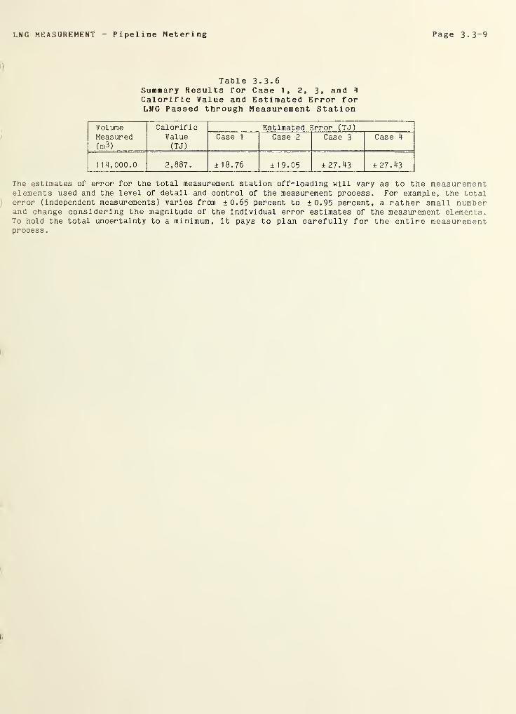
LNG MEASUREMENT Pipeline Metering Page 3.3-9
TableSummary Results forCalorific Value andLNG Passed through
3.3.6Case 1 , 2 , 3 , and 4
Estimated Error forMeasurement Station
VolumeMeasured(m3)
CalorificValue(TJ)
Estimated Error (TJ)
Case 1 Case 2 Case 3 Case 4
114,000.0 2,887. ±18.76 ± 19.05 ± 27.43 ± 27.43
The estimates of error for the total measurement station off-loading will vary as to the measurementelements used and the level of detail and control of the measurement process. For example, the totalerror (independent measurements) varies from ±0.65 percent to ±0.95 percent, a rather small numberand change considering the magnitude of the individual error estimates of the measurement elements.To hold the total uncertainty to a minimum, it pays to plan carefully for the entire measurementprocess
.

-
-
-
f

D
D
>)
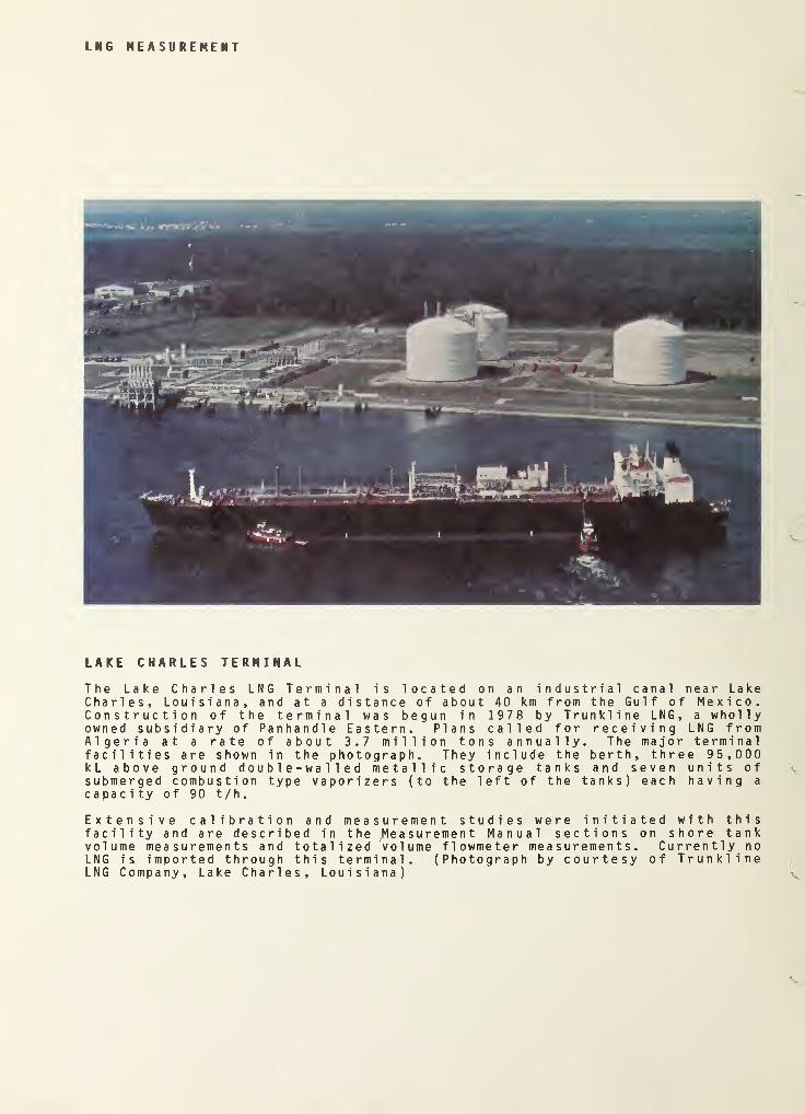
LNG MEASUREMENT
LAKE CHARLES TERMINAL
The Lake Charles LNG Terminal is located on an industrial canal near LakeCharles, Louisiana, and at a distance of about 40 km from the Gulf of Mexico.Construction of the terminal was begun in 1978 by Trunkline LNG, a whollyowned subsidiary of Panhandle Eastern. Plans called for receiving LNG fromAlgeria at a rate of about 3.7 million tons annually. The major terminalfacilities are shown in the photograph. They include the berth, three 95,000kL above ground double-walled metallic storage tanks and seven units ofsubmerged combustion type vaporizers (to the left of the tanks) each having a
capacity of 90 t/h.
Extensive calibration and measurement studies were initiated with thisfacility and are described in the Measurement Manual sections on shore tankvolume measurements and totalized volume flowmeter measurements. Currently noLNG is imported through this terminal. (Photograph by courtesy of TrunklineLNG Company, Lake Charles, Louisiana)
[,NG MEASUREMENT - Landbased Storage Page 3.4-1
i3.4 Landbased Storage
3.4.1 Introduction
The general case is assumed in which an LNG ship has been loaded with LNG of a known composition at a
remote producer terminal, has then been in transit for some period of time and has arrived at the LNG
Importation terminal docking area. At the dock, the off-loading pipeline is connected to the LNG ship
piping, and a quantity of LNG is removed from the ship tanks and deposited into a LNG shore tank.
There are, of course, large differences in LNG ship capacities and shore storage facilities. For this
example, it is assumed that the volume of LNG off-loaded to the shore facility is nearly that of the
membrane-type LNG ship having tank capacities and characteristics as shown in table 3.2.2. It is also
assumed that more than one shore tank will be required to contain and store the contents of the LNG
ship. This section of the manual considers the off-loading of LNG to the shore tanks.
It was noted in the previous section on pipline flowmetering that the quantity and composition of the
LNG measured in the pipeline will not be precisely the same as that measured in the LNG ship tanks.
Pipeline heat leak and cooldown losses will result in changes in composition of the liquid. The same
caution is made here as to the expected changes of quantity and composition quality of the LNG
delivered to the individual shore tank. Shore tank liquid content and composition prior to loadingwill additionally complicate the measurement process. In general, the following process will be
concerned with the quantity and composition of the liquid content of the shore tank. Otherconsiderations must be made in comparing the individual measurements of LNG removed from the ship, LNG
metered in the off-loading line and LNG loaded into the shore tanks.
As in the preceding examples, no consideration is given to unexpected failure of instrumentation or
other equipment which would require alternate measurements or measurement estimates of portions or all
of the overall measurement process. Examples might be the failure of the capacitance liquid level
device after the upper level had been read but before the lower level was read. A backup bubblerlevel gage or other liquid level measurement device (see section 2.5.1) might be used. The
k interruption of power to the LNG discharge pumps in one of the ship tanks may delay LNG flow into thef shore tank, and the off-loading may be halted for a period of time. These and other unanticipated
changes in the expected measurement process are not unusual, particularly in the case of a newtechnology; and these types of unexpected problems will test the resources of the measurementengineer
.
The measurement objective is to determine the quantity and composition of the LNG delivered and storedin the shore tanks. The most common measurement to be made is the total calorific value of the LNGstored. At the present time, no single property measurement can accurately and precisely provide thisvalue directly. It is necessary to use a multistep procedure involving volume, density and specificcalorific value.
Volume. This is a measured quantity involving some predictive calculation. For the case of shoretank storage (see section 2.5.5), only static measurement states are considered. Each shore tank is
assumed to be individually instrumented as to liquid level. Each tank is also considered as anindividual measurement entity, because the temperature, pressure and composition of the liquid mayvary during the loading ^operation.
Density. A choice may be made of either direct density measurement using a calibrated densimeter or a
density calculation based on sampling, analysis and a LNG mixture state equation. Both methods can be
used to provide a cross check. As in the comments on volume above, each tank will be considered as a
measurement entity in respect to an individual densimeter for each tank. Sampling and analysis of theliquid from each individual tank is also assumed.
Calorific Value. This is the quantity of thermal energy released when the LNG mixture has b>-'-n
vaporized and burned in air to gaseous carbon dioxide and liquid water. The value may be del •tt. : :
directly by vaporizing a representative sample of LNG and burning the mixture in a combust 1•.
calorimeter which measures the thermal output compared to that of a calibration gas or by calc j l a ». 1
from sampling, analysis and integration of the individual pure component calorific val ; .
methods can be used as a cross check, but because of the loading procedure mentioned abov- ,
procedures must be designed to assure that a representati ve sample is taken for each separa* <• •
The results of these procedures may be combined in the following manner:
Total Calorific Value = (Volume) (Density) (Specif ic Calorific Value)
Page 3.4-2 LNG MEASUREMENT - Landbased Storage
The term "total calorific value" means here the enthalpy of combustion of the contents of a tank or
ship after these contents have been vaporized. In the testing literature, "total calorific value" fora gaseous fuel means something different, i.e. the enthalpy of combustion of a unit amount (mol, kg,
cubic meter) when the products of combustion are gaseous carbon dioxide and liquid water. The term"specific calorific value" used here has that meaning for a kilogram sample.
3.4.2 Examples of the Measurement Process
Variations of the above procedure are, of course, possible by combining one or more of the steps, but,as a descriptive matter, the above steps will be followed. Even with this restriction there are fourpossible individual procedures which may be followed:
Case 1 Total Calorific Value = LNG Volume x Density (calculated) x Specific Calorific Value(calculated)
Calculate the volume of LNG added to each shore tank. Secure a representative LNGsample from each shore tank. Vaporize and analyze the sample to determine thefraction of individual components. Calculate the density of the LNG added to eachshore tank using the state equation for liquid density as a function of measured LNGtemperature, pressure and composition. Combine the density of each shore tank withthe volume added to give mass added to each tank. Using the previous sample analysiscalculate the specific calorific value of the LNG sample from calorific values of the
individual components. Calculate the density of the vaporized LNG sample and combinethe calculated specific calorific values of each shore tank to give the totalcalorific value of LNG delivered.
Case 2 Total Calorific Value = LNG Volume x Density (measured) x Specific Calorific Value(calculated)
Calculate the volume of LNG added to each shore tank. Measure the representative LNGdensity in each shore tank using a calibrated densimeter and calculate the mass ofLNG added to each tank. Secure a representative LNG sample from each shore tank.
Vaporize and analyze the sample to determine the fraction of individual components.Calculate the specific calorific value of the LNG sample from calorific values of the
individual components. Calculate the density of the vaporized LNG sample and combinethe calculated specific calorific values of each shore tank with the total mass addedto each tank to give calorific value of LNG removed. Combine individual tankcalorific values to give the total calorific value of LNG delivered.
Case 3 Total Calorific Value = LNG Volume x Density (calculated) x Specific Calorific Value(measured)
Calculate the volume of LNG added to each shore tank. Secure a representative LNGsample from each tank. Vaporize and analyze the sample to determine the fraction of
individual components. Calculate the density of the LNG added to the shore tank
using the state equation for liquid density as a function of measured LNGtemperature, pressure and component fraction. Combine the density of each shore tank
with volume added to each tank to give mass added to each tank. Secure a newrepresentative tank sample or use the previous sample and burn the sample in a
combustion calorimeter. Measure the density of the vaporized LNG sample and combinethe specific calorific value determined from the combustion calorimeter with the mass
added to each shore tank to give the total calorific value of each tank. Combine theindividual shore tank calorific values to give the total calorific value for the LNGdelivered.
Case 4 Total Calorific Value = LNG Volume x Density (measured) x Specific Calorific Value
(measured)
Calculate the volume of LNG added to each shore tank. Measure the representative LNGdensity in each tank using a calibrated densimeter and calculate the mass of LNGadded to each shore tank. Secure a representative sample of LNG from each shore
tank, vaporize the sample completely and burn the sample in a combustion calorimeter.Measure the density of the vaporized sample and combine the specific calorific value
determined from the combustion calorimeter with the mass added to each shore tank to
give the calorific value of the LNG added to tank. Sum the individual calorificvalues to give the total calorific value for all the LNG delivered.
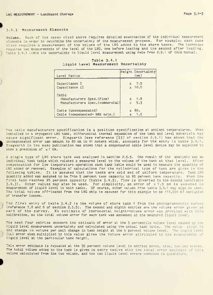
LNG MEASUREMENT - Landbased Storage Page 3.^-3
3.4.3 Measurement Elements
Volume. Each of the cases cited above requires detailed examination of the individual measurement
elements in order to determine the uncertainty of the measurement process. For example; each case
cited requires a measurement of the volume of the LNG added to the shore tanks. The technique
requires two measurements of the level of the LNG, one before loading and the second after loading.
\ Table 3.4.1 lists the uncertainty in liquid level measurement using data from 2.5.1 of this manual.
Table 3-4.1Liquid Level Measurement Uncertainty
Level DeviceHeight Uncertainty
(mm)
Capacitance I ± 7.5
Capacitance II ± 10.0
CableManufacturers Spec. (fine) ± 1 .8
Manufacturers Spec . (commercial) ± 5.3
Cable (uncompensated) ± 80 .
Cable (compensated- NBS estm.) ± 1.0
The cable manufacturers specification is a position specification at ambient temperatures. Wheninstalled in a cryogenic LNG tank, differential thermal expansion of the tank and level materials maycause significant error. Siegwarth (see reference [23] of section 2.5.1) has shown that the
k uncompensated error can amount to 80 mm in 41 meters which, accounts for the entry in table 3-4.1.' Siegwarth in the same publication has shown that a compensated cable level device may be expected to
show a precision of ±
1
mm.
A single type of LNG shore tank was analyzed in section 2.5.5. One result of the analysis was an
individual tank table which related a measured level to the volume of the tank at that level. Aftercompensation for low temperature operation each tank table could be used to measure the quantity ofLNG added or removed. Examples of calculations for the cylindrical type of tank are given in thefollowing tables. It is assumed that the tanks are cold and of uniform temperature. Tank LNGquantity added was assumed to be from 5 percent tank capacity to 95 percent tank capacity. When thefirst tank reaches 95 percent capacity (table 3-4.2), flow is diverted to the second tank(table3.4.3). Other values may also be used. For simplicity, an error of ± 7.5 mm is assumed inmeasurement of liquid level in both tanks. Of course, other values from table 3-4.1 may also be used.The total volume off-loaded from the LNG ship is assumed for this example to be 114,000 m3 exclusiveof transfer losses.
The first entry of table 3-4.2 is the volume of shore tank 1 from the photogr ammetr i c survey) (reference 7,8 and 9 of section 2.5.5). The second and eighth entries are the volume error giver. 13
part of the survey. No estimate of incremental height-volume error was provided with t r.
:
calibration, so the total volume error for each tank was assessed at the measured liquid level.
The next four entries concern the estimate of error at the 5 percentile volume level caused byliquid level measurement uncertainty and calculated using the actual tank table. The value AV/t.H ;
the change in volume per unit change in tank height at the 5 percent volume level. The li i lev'.
) (LL) error when multiplied by this value gives the volume error attributed to the meas ure-.^r.’ r
liquid level at the particular tank height.
This error estimate is repeated at the 95 percent volume level in entries seven, nin-, •• •
The total volume added to the tank is given in entry twelve with the total error cr" r.• •
volume calculated from the two volume, and the two liquid level errors combined i r. quad” 1*
.
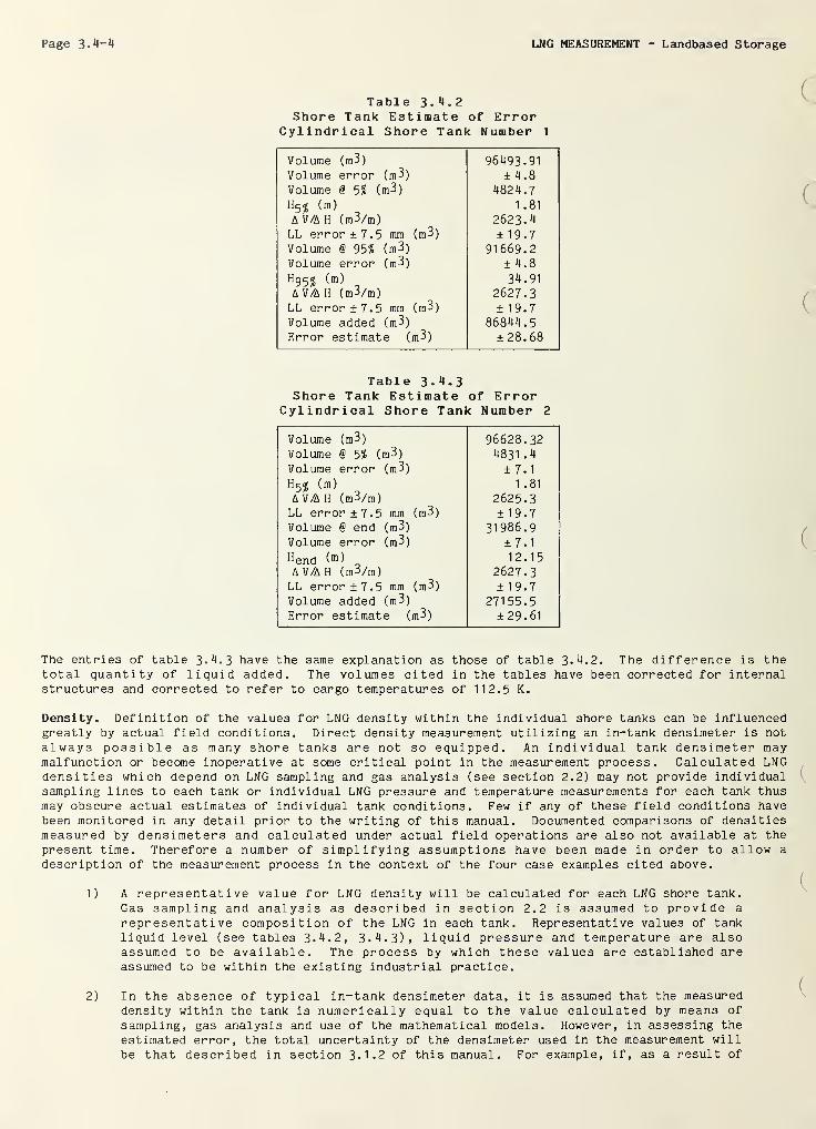
Page 3.4-4 LNG MEASUREMENT - Landbased Storage
Table 3-^-2Shore Tank Estimate of Error
Cylindrical Shore Tank Number 1
Volume (m3) 96493.91Volume error (m3) ± 4.8
Volume § 5% (m3) 4824.7H5? (m) _ 1 .81
AV/AH (m3/m) 2623.4LL error ±7.5 mm (m3) ±19.7Volume @ 95? (m3) 91669.2Volume error (m3) ± 4.8
h95? < m) _ 34.91
A V/A H (m3/m) 2627.3LL error ±7.5 mm (m3) ± 19.7Volume added (m3) 86844.5Error estimate (m3) ± 28.68
Table 3-4.3Shore Tank Estimate of Error
Cylindrical Shore Tank Number 2
Volume (m3) 96628.32Volume § 5% (m3) 4831 .4
Volume error (m3) ±7.1h5? 0
1 .81
AV/AH (m3/m) 2625.3LL error ±7.5 mm (m3) ±19.7Volume § end (m3) 31986.9Volume error (m3) ± 7.1
^end 12.15AV/AH (m3/m) 2627.3LL error ±7.5 mm (m3) ±19.7Volume added (m3) 27155.5Error estimate (m3) ± 29.61
The entries of table 3-4.3 have the same explanation as those of table 3.4.2. The difference is thetotal quantity of liquid added. The volumes cited in the tables have been corrected for internalstructures and corrected to refer to cargo temperatures of 112.5 K.
Density. Definition of the values for LNG density within the individual shore tanks can be influencedgreatly by actual field conditions. Direct density measurement utilizing an in-tank densimeter is not
always possible as many shore tanks are not so equipped. An individual tank densimeter maymalfunction or become inoperative at some critical point in the measurement process. Calculated LNGdensities which depend on LNG sampling and gas analysis (see section 2.2) may not provide individualsampling lines to each tank or individual LNG pressure and temperature measurements for each tank thusmay obscure actual estimates of individual tank conditions. Few if any of these field conditions havebeen monitored in any detail prior to the writing of this manual. Documented comparisons of densitiesmeasured by densimeters and calculated under actual field operations are also not available at the
present time. Therefore a number of simplifying assumptions have been made in order to allow a
description of the measurement process in the context of the four case examples cited above.
1) A repr esentati ve value for LNG density will be calculated for each LNG shore tank.
Gas sampling and analysis as described in section 2.2 is assumed to provide a
representative composition of the LNG in each tank. Representative values of tank
liquid level (see tables 3.4.2, 3.4.3). liquid pressure and temperature are alsoassumed to be available. The process by which these values are established areassumed to be within the existing industrial practice.
2) In the absence of typical in-tank densimeter data, it is assumed that the measureddensity within the tank is numerically equal to the value calculated by means of
sampling, gas analysis and use of the mathematical models. However, in assessing the
estimated error, the total uncertainty of the densimeter used in the measurement willbe that described in section 3.1.2 of this manual. For example, if, as a result of
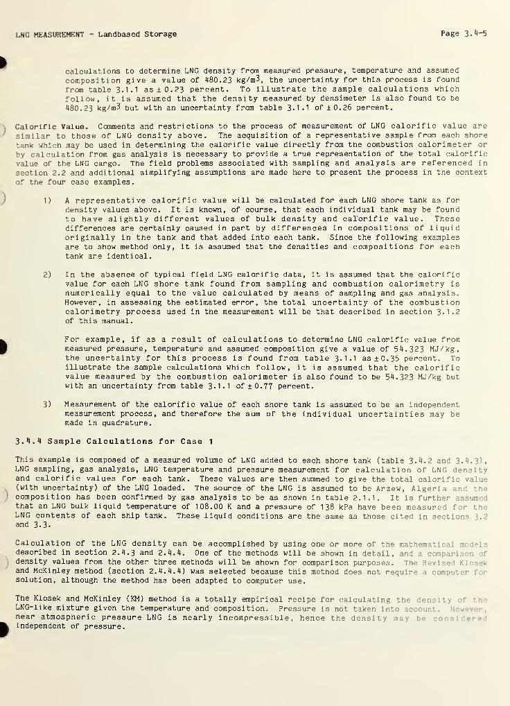
LNG MEASUREMENT - Landbased Storage Page 3.4-5
calculations to determine LNG density from measured pressure, temperature and assumed
composition give a value of 480.23 kg/m3, the uncertainty for this process is found
from table 3.1.1 as +0.23 percent. To illustrate the sample calculations whichfollow, it is assumed that the density measured by densimeter is also found to be
480.23 kg/m3 but with an uncertainty from table 3.1.1 of ±0.26 percent.
Calorific Value. Comments and restrictions to the process of measurement of LNG calorific value are
similar to those of LNG density above. The acquisition of a representative sample from each shore
tank which may be used in determining the calorific value directly from the combustion calorimeter or
by calculation from gas analysis is necessary to provide a true representation of the total calorific
value of the LNG cargo. The field problems associated with sampling and analysis are referenced in
section 2.2 and additional simplifying assumptions are made here to present the process in the context
of the four case examples.
1) A representative calorific value will be calculated for each LNG shore tank as for
density values above. It is known, of course, that each individual tank may be foundto have slightly different values of bulk density and calorific value. Thesedifferences are certainly caused in part by differences in compositions of liquidoriginally in the tank and that added into each tank. Since the following examplesare to show method only, it is assumed that the densities and compositions for eachtank are identical.
2) In the absence of typical field LNG calorific data, it is assumed that the calorificvalue for each LNG shore tank found from sampling and combustion calorimetry isnumerically equal to the value calculated by means of sampling and gas analysis.However, in assessing the estimated error, the total uncertainty of the combustioncalorimetry process used in the measurement will be that described in section 3*1.2of this manual.
For example, if as a result of calculations to determine LNG calorific value frommeasured pressure, temperature and assumed composition give a value of 54.323 MJ/kg,the uncertainty for this process is found from table 3.1.1 as ±0.35 percent. Toillustrate the sample calculations which follow, it is assumed that the calorificvalue measured by the combustion calorimeter is also found to be 54.323 MJ/kg butwith an uncertainty from table 3-1.1 of ±0.77 percent.
3) Measurement of the calorific value of each shore tank is assumed to be an independentmeasurement process, and therefore the sum of the individual uncertainties may bemade in quadrature.
3.4.4 Sample Calculations for Case 1
This example is composed of a measured volume of LNG added to each shore tank (table 3.4.2 and 3.4.3),LNG sampling, gas analysis, LNG temperature and pressure measurement for calculation of LNG densityand calorific values for each tank. These values are then summed to give the total calorific value(with uncertainty) of the LNG loaded. The source of the LNG is assumed to be Arzew, Algeria and thecomposition has been confirmed by gas analysis to be as shown in table 2.1.1. It is further assumedthat an LNG bulk liquid temperature of 108.00 K and a pressure of 138 kPa have been measured for theLNG contents of each ship tank. These liquid conditions are the same as those cited in section. ’
and 3.3.
Calculation of the LNG density can be accomplished by using one or more of the mathematical model.-i
described in section 2.4.3 and 2.4.4. One of the methods will be shown in detail, and a comparisondensity values from the other three methods will be shown for comparison purposes. The Revised K1and McKinley method (section 2. 4. 4. 4) was selected because this method does not require a :om; ;• *t '
solution, although the method has been adapted to computer use.
The Klosek and McKinley (KM) method is a totally empirical recipe for calculating the don: 1
y r• * ..
LNG-like mixture given the temperature and composition. Pressure is not taken into account. -•
near atmospheric pressure LNG is nearly incompressible, hence the density may bindependent of pressure.
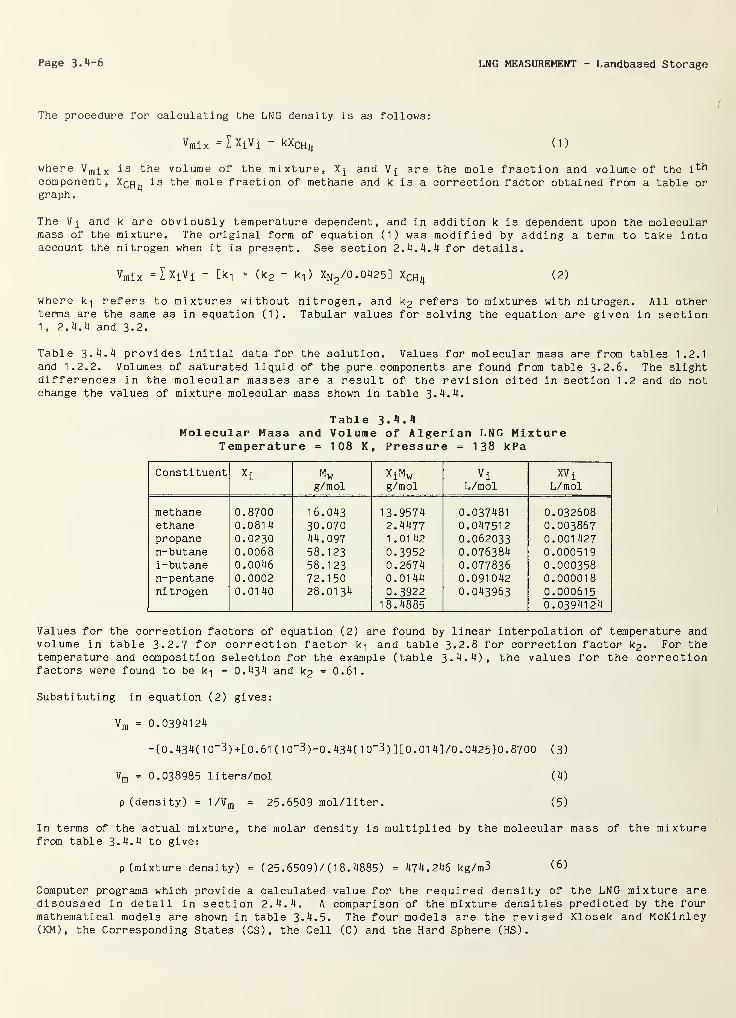
Page 3.4-6 LNG MEASUREMENT - Landbased Storage
The procedure for calculating the LNG density is as follows:
vmix =1 ^i^i “ kXCHn (D
where V m ^ x is the volume of the mixture, Xj and V^ are the mole fraction and volume of the i^h
component, X^h^ is the mole fraction of methane and k is a correction factor obtained from a table orgraph.
The and k are obviously temperature dependent, and in addition k is dependent upon the molecularmass of the mixture. The original form of equation (1) was modified by adding a term to take intoaccount the nitrogen when it is present. See section 2. 4. 4. 4 for details.
Vmix =Ix i V i - [k-, + (k 2 - k,) XN2 /0.0425] XCHl| (2)
where k-| refers to mixtures without nitrogen, and k 2 refers to mixtures with nitrogen. All otherterms are the same as in equation (1). Tabular values for solving the equation are given in section1 , 2.4.4 and 3.2.
Table 3*4.4 provides initial data for the solution. Values for molecular mass are from tables 1.2.1and 1.2.2. Volumes of saturated liquid of the pure components are found from table 3*2.6. The slightdifferences in the molecular masses are a result of the revision cited in section 1.2 and do notchange the values of mixture molecular mass shown in table 3.4.4.
Table 3.4.4Molecular Mass and Volume of Algerian LNG Mixture
Temperature = 108 K, Pressure = 138 kPa
Constituent Xi Mwg/mol
XiMwg/mol
ViL/mol
XV i
L/mol
methane 0.8700 16.043 13*9574 0.037481 0.032608ethane 0.081
4
30.070 2.4477 0.047512 0.003867propane 0.0230 44.097 1 .01 42 0.062033 0.001 427n-butane 0.0068 58.123 0.3952 0.076384 0.000519i-butane 0.0046 58.123 0.2674 0.077836 0.000358n-pentane 0.0002 72.150 0.01 44 0.091042 0.000018nitrogen 0.01 40 28.01 34 0.3922
18.48850.043963 0.000615
0.03941 24
Values for the correction factors of equation (2) are found by linear interpolation of temperature andvolume in table 3*2.7 for correction factor k-| and table 3*2.8 for correction factor k 2 . For thetemperature and composition selection for the example (table 3*4.4), the values for the correctionfactors were found to be k-j = 0.434 and k 2 = 0.61.
Substituting in equation (2) gives:
Vm = 0.0394124
-{0.434(1 0“3 ) +[ 0. 61 (10"3)-o.434(10_3)][o.01 4] /0. 0425)0.8700 (3)
Vm = 0.038985 liters/mol (4)
p (density) = 1 /Vm = 25.6509 mol/liter. (5)
In terms of the actual mixture, the molar density is multiplied by the molecular mass of the mixturefrom table 3*4.4 to give:
p (mixture density) = ( 25. 6509)/ ( 1 8. 4885) = 474.246 kg/m3 (8)
Computer programs which provide a calculated value for the required density of the LNG mixture arediscussed in detail in section 2.4.4. A comparison of the mixture densities predicted by the fourmathematical models are shown in table 3.4.5. The four models are the revised Klosek and McKinley(KM), the Corresponding States (CS) , the Cell (C) and the Hard Sphere (HS).
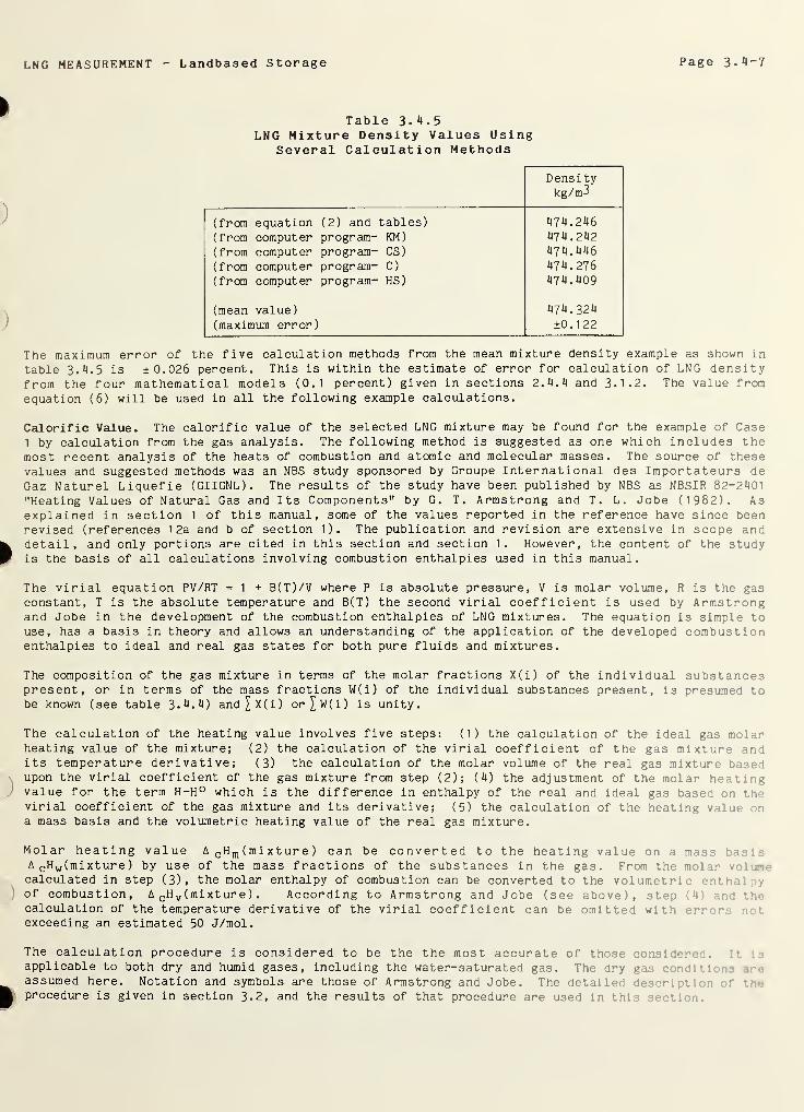
LNG MEASUREMENT - Landbased Storage Page 3-4-7
Table 3.4.5LNG Mixture Density Values Using
Several Calculation Methods
Densitykg/m3
(from equation (2) and tables) 474.246474.242474.446474.276474.409
(from computer program- KM)
(from computer program- CS)
(from computer program- C)
(from computer program- HS)
(mean value)
(maximum error)
474.324±0.122
The maximum error of the five calculation methods from the mean mixture density example as shown in
table 3.4.5 is ±0.026 percent. This is within the estimate of error for calculation of LNG densityfrom the four mathematical models (0.1 percent) given in sections 2.4.4 and 3.1.2. The value from
equation (6) will be used in all the following example calculations.
Calorific Value. The calorific value of the selected LNG mixture may be found for the example of Case1 by calculation from the gas analysis. The following method is suggested as one which includes themost recent analysis of the heats of combustion and atomic and molecular masses. The source of thesevalues and suggested methods was an NBS study sponsored by Groupe International des Importateurs deGaz Naturel Liquefie (GIIGNL). The results of the study have been published by NBS as NBSIR 82-2401
"Heating Values of Natural Gas and Its Components" by G. T. Armstrong and T. L. Jobe ( 1 982). Asexplained in section 1 of this manual, some of the values reported in the reference have since beenrevised (references 12a and b of section 1). The publication and revision are extensive in scope anddetail, and only portions are cited in this section and section 1. However, the content of the studyis the basis of all calculations involving combustion enthalpies used in this manual.
The virial equation PV/RT = 1 + B(T)/V where P is absolute pressure, V is molar volume, R is the gasconstant, T is the absolute temperature and B(T) the second virial coefficient is used by Armstrongand Jobe in the development of the combustion enthalpies of LNG mixtures. The equation is simple touse, has a basis in theory and allows an understanding of the application of the developed combustionenthalpies to ideal and real gas states for both pure fluids and mixtures.
The composition of the gas mixture in terms of the molar fractions X(i) of the individual substancespresent, or in terms of the mass fractions W(i) of the individual substances present, is presumed tobe known (see table 3.4.4) and^X(i) or£w(i) is unity.
The calculation of the heating value involves five steps: (1) the calculation of the ideal gas molarheating value of the mixture; (2) the calculation of the virial coefficient of the gas mixture andits temperature derivative; (3) the calculation of the molar volume of the real gas mixture basedupon the virial coefficient of the gas mixture from step (2); (4) the adjustment of the molar heatingvalue for the term H-H° which is the difference in enthalpy of the real and ideal gas based on th*->
virial coefficient of the gas mixture and its derivative; (5) the calculation of the heating value u
a mass basis and the volumetric heating value of the real gas mixture.
Molar heating value A c H m (mi xt ur e ) can be converted to the heating value on a mass basinA cH w (mixture) by use of the mass fractions of the substances in the gas. From the mol ir v :
calculated in step (3), the molar enthalpy of combustion can be converted to the volumetri • •,
of combustion, A cH v (mixture) . According to Armstrong and Jobe (see above), stepcalculation of the temperature derivative of the virial coefficient can be omitted withexceeding an estimated 50 J/mol.
The calculation procedure is considered to be the the most accurate of those considered. It inapplicable to both dry and humid gases, including the water-saturated gas. The dry gas a- •
assumed here. Notation and symbols are those of Armstrong and Jobe. The detailed den • r
procedure is given in section 3.2, and the results of that procedure are used in thin necti
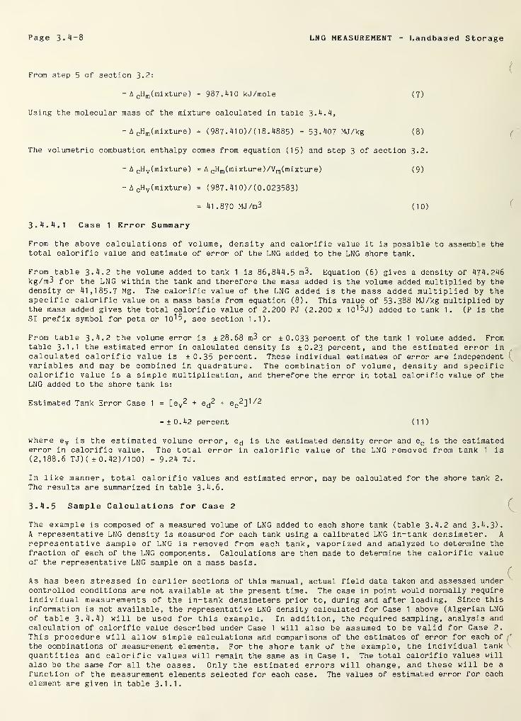
Page 3.4-8 LNG MEASUREMENT - Landbased Storage
From step 5 of section 3.2:
- A cH m (mixture) = 987.410 kJ/mole (7)
Using the molecular mass of the mixture calculated in table 3.4.4,
- A cHm (mixture) = (987.410)7(18.4885) = 53.407 MJ/kg ( 8 )
The volumetric combustion enthalpy comes from equation (15) and step 3 of section 3.2.
- A cH v (mixture) = A cHm (mixture)/Vm (mixture)
- A cH v (mixture) = (987.410)7(0.023583)
(9)
= 41 .870 MJ/m3 ( 10 )
3. 4. 4.1 Case 1 Error Summary
From the above calculations of volume, density and calorific value it is possible to assemble thetotal calorific value and estimate of error of the LNG added to the LNG shore tank.
From table 3.4.2 the volume added to tank 1 is 86,844.5 m3. Equation (6) gives a density of 474.246kg/m3 for the LNG within the tank and therefore the mass added is the volume added multiplied by thedensity or 41,185.7 Mg. The calorific value of the LNG added is the mass added multiplied by thespecific calorific value on a mass basis from equation (8). This value of 53.388 MJ/kg multiplied bythe mass added gives the total calorific value of 2.200 PJ (2.200 x IO^j) added to tank 1. (P is theSI prefix symbol for peta or 10^5
j see section 1.1).
From table 3.4.2 the volume error is ±28.68 m3 or ±0.033 percent of the tank 1 volume added. Fromtable 3.1.1 the estimated error in calculated density is ± 0.23 percent, and the estimated error incalculated calorific value is ±0.35 percent. These individual estimates of error are independentvariables and may be combined in quadrature. The combination of volume, density and specificcalorific value is a simple multiplication, and therefore the error in total calorific value of theLNG added to the shore tank is:
Estimated Tank Error Case 1 = [ev2 + e^2 + e c
2]1/2
where e v is the estimated volume error, e,j is the estimated density error and ec is the estimatederror in calorific value. The total error in calorific value of the LNG removed from tank 1 is
(2,188.6 TJ ) ( ± 0. 42 ) / 1 00) = 9.24 TJ.
In like manner, total calorific values and estimated error, may be calculated for the shore tank 2.
The results are summarized in table 3.4.6.
3.4.5 Sample Calculations for Case 2
The example is composed of a measured volume of LNG added to each shore tank (table 3-4.2 and 3.4.3).A representative LNG density is measured for each tank using a calibrated LNG in-tank densimeter. A
representative sample of LNG is removed from each tank, vaporized and analyzed to determine thefraction of each of the LNG components. Calculations are then made to determine the calorific valueof the representative LNG sample on a mass basis.
As has been stressed in earlier sections of this manual, actual field data taken and assessed undercontrolled conditions are not available at the present time. The case in point would normally requireindividual measurements of the in-tank densimeters prior to, during and after loading. Since thisinformation is not available, the representative LNG density calculated for Case 1 above (Algerian LNGof table 3.4.4) will be used for this example. In addition, the required sampling, analysis andcalculation of calorific value described under Case 1 will also be assumed to be valid for Case 2.
This procedure will allow simple calculations and comparisons of the estimates of error for each of
the combinations of measurement elements. For the shore tank of the example, the individual tankquantities and calorific values will remain the same as in Case 1. The total calorific values will
also be the same for all the cases. Only the estimated errors will change, and these will be a
function of the measurement elements selected for each case. The values of estimated error for eachelement are given in table 3.1.1.
= ±0.42 percent ( 11 )
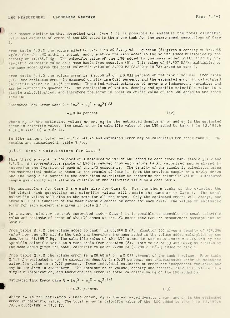
LNG MEASUREMENT Landbased Storage Page 3-4-9
In a manner similar to that described under Case 1 it is possible to assemble the total calorific
value and estimate of error of the LNG added to the shore tank for the measurement assumptions of Case
2 .
From table 3.2.2 the volume added to tank 1 is 86,844.5 m3. Equation (6) gives a density of 474.246
kg/m3 for the LNG within the tank, and therefore the mass added is the volume added multiplied by the
density or 41,185.7 Mg. The calorific value of the LNG added is the mass added multiplied by the
specific calorific value on a mass basis from equation (8). This value of 53-407 MJ/kg multiplied by
the mass added gives the total calorific value of 2.200 PJ (2.200 x lO^j) added to tank 1.
From table 3.4.2 the volume error is ± 28.68 m3 or ± 0.033 percent of the tank 1 volume. From table
3.1.1 the estimated error in measured density is ±0.26 percent, and the estimated error in calculatedcalorific value is ±0.35 percent. These individual estimates of error are independent variables and
may be combined in quadrature. The combination of volume, density and specific calorific value is a
simple multiplication, and therefore the error in total calorific value of the LNG added to the shore
tank is:
Estimated Tank Error Case 2 = [e v2 + e^2 + ec
2]1/2
= ±0.44 percent ( 1 2)
where e v is the estimated volume error, e^ is the estimated density error and e c is the estimatederror in calorific value. The total error in calorific value of the LNG added to tank 1 is (2,199.6TJ) ( ± 0. 44 ) / 1 00) = 9.67 TJ.
In like manner, total calorific values and estimated error may be calculated for shore tank 2. The
results are summarized in table 3.4.6.
3.4.6 Sample Calculations for Case 3
This third example is composed of a measured volume of LNG added to each shore tank (table 3.4.2 and
3.4.3). A representative sample of LNG is removed from each shore tank, vaporized and analyzed to
determine the fraction of each of the LNG components. The density of the sample is calculated usingthe mathematical models as shown in the example of Case 1 . From the previous sample or a newly drawnone the sample is burned in the combustion calorimeter to determine the calorific value. A measuredsample gas density will allow calculation of the calorific value on a mass basis.
The assumptions for Case 2 are made also for Case 3- For the shore tanks of the example, theindividual tank quantities and calorific values will remain the same as in Case 1 . The totalcalorific values will also be the same for all the cases. Only the estimated errors will change, andthese will be a function of the measurement elements selected for each case. The values of estimatederror for each element are given in table 3-1 * 1 -
In a manner similar to that described under Case 1 it is possible to assemble the total calorificvalue and estimate of error of the LNG added to the LNG shore tank for the measurement assumptions ofCase 2.
From table 3.4.2 the volume added to tank 1 is 86,844.5 m3. Equation (6) gives a density of 474.21’kg/m3 for the LNG within the tank and therefore the mass added is the volume added multiplied by thedensity or 41,185.7 Mg. The calorific value of the LNG added is the mass added multiplied by thespecific calorific value on a mass basis from equation (8). This value of 53.407 MJ/kg multiplied bythe mass added gives the total calorific value of 2.200 PJ (2.200 x IO^j) added to tank 1.
From table 3-4.2 the volume error is ± 28.68 m3 or ± 0.033 percent of the tank 1 volume. Fr xn tat 1
3.1.1 the estimated error in calculated density is ± 0.23 percent, and the- estimated error in :
calorific value is ±0.77 percent. These individual estimates of error are independent variable .•:
may be combined in quadrature. The combination of volume, density and specific calorific valsimple multiplication, and therefore the error in total calorific value of the LNG added in:
Estimated Tank Error Case 3 = [ev2 + e^2 + ec
2]1,/2
= ±0.80 percent ( 1 3)
where ev is the estimated volume error, e,j is the estimated density error, and in vn :
error in calorific value. The total error in calorific value of the LNG added to tan* 1 :
TJ) ( ± 0.80)/1 00) = 17.6 TJ.
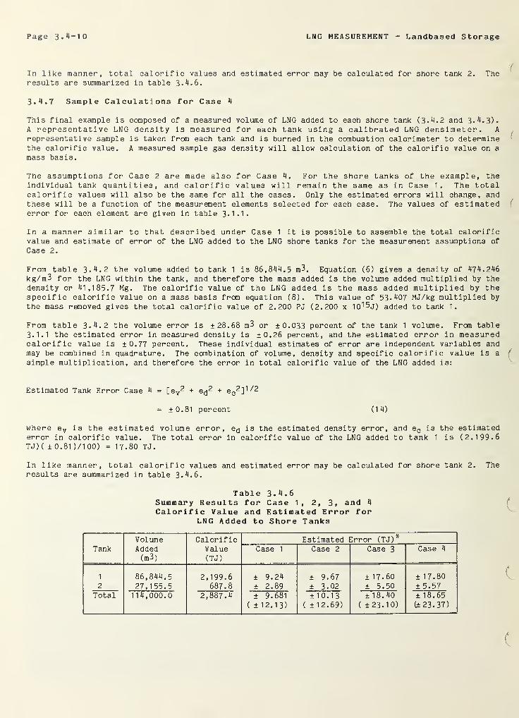
Page 3.4-10 LNG MEASUREMENT Landbased Storage
In like manner, total calorific values and estimated error may be calculated for shore tank 2. Theresults are summarized in table 3.4.6.
3.4.7 Sample Calculations for Case 4
This final example is composed of a measured volume of LNG added to each shore tank (3.4.2 and 3*4.3).A representative LNG density is measured for each tank using a calibrated LNG densimeter. A
representative sample is taken from each tank and is burned in the combustion calorimeter to determinethe calorific value. A measured sample gas density will allow calculation of the calorific value on a
mass basis.
The assumptions for Case 2 are made also for Case 4. For the shore tanks of the example, theindividual tank quantities, and calorific values will remain the same as in Case 1. The totalcalorific values will also be the same for all the cases. Only the estimated errors will change, andthese will be a function of the measurement elements selected for each case. The values of estimatederror for each element are given in table 3.1.1.
In a manner similar to that described under Case 1 it is possible to assemble the total calorificvalue and estimate of error of the LNG added to the LNG shore tanks for the measurement assumptions of
Case 2.
From table 3.4.2 the volume added to tank 1 is 86,844.5 m3. Equation (6) gives a density of 474.246kg/m3 for the LNG within the tank, and therefore the mass added is the volume added multiplied by thedensity or 41, 185. 7 Mg. The calorific value of the LNG added is the mass added multiplied by thespecific calorific value on a mass basis from equation (8). This value of 53.407 MJ/kg multiplied by
the mass removed gives the total calorific value of 2.200 PJ (2.200 x lO^j) added to tank 1.
From table 3.4.2 the volume error is ± 28.68 m3 or ± 0.033 percent of the tank 1 volume. From table3.1.1 the estimated error in measured density is ±0.26 percent, and the estimated error in measuredcalorific value is ±0.77 percent. These individual estimates of error are independent variables andmay be combined in quadrature. The combination of volume, density and specific calorific value is a
simple multiplication, and therefore the error in total calorific value of the LNG added is:
Estimated Tank Error Case 4 = [ey2 + + ec
^]1/2
= ±0.81 percent ( 1 4)
where e v is the estimated volume error, e<j is the estimated density error, and e c is the estimatederror in calorific value. The total error in calorific value of the LNG added to tank 1 is (2.199.6T J) ( ± 0.81 )/1 00) = 17.80 TJ.
In like manner, total calorific values and estimated error may be calculated for shore tank 2. Theresults are summarized in table 3.4.6.
Table 3-4.6Summary Results for Case 1, 2, 3, and 4
Calorific Value and Estimated Error forLNG Added to Shore Tanks
TankVolumeAdded(m3)
CalorificValue(TJ)
Estimated Error (TJ)*
Case 1 Case 2 Case 3 Case 4
1
2
86.844.527.155.5
2,199.6687.8
± 9.24± 2.89
± 9.67± 3.02
± 17.60
± 5.50
±17.80± 5.57
Total 114,000.0 2,887.4 ± 9.681
( ± 12.13)
±10.13( ±12.69)
±18.40( ±23.10)
± 18.65
(± 23.37)
LNG MEASUREMENT Landbased Storage Page 3.4-11
It should be noted that the total error for each case has been found by combining the errors from each
tank in quadrature. It was assumed that measurements for each tank are independent of each other.
This may not be true in practice, and a simple sum is included in parenthesis. It is one objective of
this manual to provide enough of the basic data and a description of the method so that if other-
procedures are preferred, then these procedures may be followed using the original data.
The estimates of error for the total shore loading will vary as to the measurement elements used, andthe level of detail and control of the measurement process. For example, the total error (independenttank measurements) varies from ±0.34 percent to +0.65 percent, a rather small number and changeconsidering the magnitude of the individual error estimates of the measurement elements. To hold thetotal uncertainty to a minimum, it pays to plan carefully for the entire measurement process.
(
'.It
<v
'•
-i S
'•,
'
(V
i ;
'
> .
/ « i-
1
L!
i-.
(.I.? yl-T-'~-\.L' -V.--
c
c
c
c
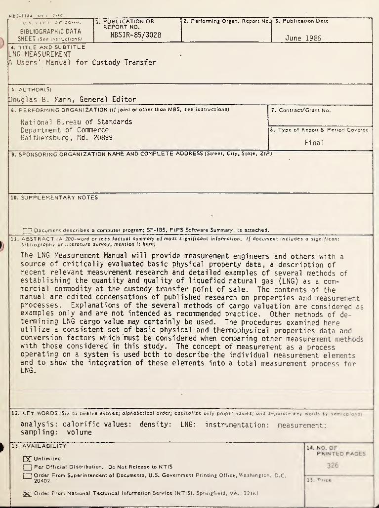
NBS-M4A rev - r-«c i
U.S. - CRT 5F COMM.
BIBLIOGRAPHIC DATASHEET i See msirjC lions)
1. PUBLICATION ORREPORT NO.
NBSIR-85/3028
2. Performing Organ. Report No. 3. Publication Date
June 1986
4 . TITLE and subtitleNG MEASUREMENT
A Users' Manual for Custody Transfer
5. AUTHOR(S)
Douglas B. Mann, General Editor
6. PERFORMING ORGANIZATION (If joint or other thanNBS. see instructions)
National Bureau of Standards
Department of CommerceGaithersburg, Md. 20899
7. Contract/Grant No.
8. Type of Report & Period Covered
Fi nal
9. SPONSORING ORGANIZATION NAME AND COMPLETE ADDRESS (Street, City, Stote, ZIP)
10. SUPPLEMENTARY NOTES
Document describes a computer program; SF-185, FIPS Software Summary, is attached.
I)
11. ABSTRACT {A 200-word or less factual summary of most significant information. If document includes a significant
bi bhography or literature Survey, mention it here)
The LNG Measurement Manual will provide measurement engineers and others with a
source of critically evaluated basic physical property data, a description ofrecent relevant measurement research and detailed examples of several methods ofestablishing the quantity and quality of liquefied natural gas (LNG) as a com-mercial commodity at the custody transfer point of sale. The contents of themanual are edited condensations of published research on properties and measurementprocesses. Explanations of the several methods of cargo valuation are considered asexamples only and are not intended as recommended practice. Other methods of de-termining LNG cargo value may certainly be used. The procedures examined hereutilize a consistent set of basic physical and thermophysical properties data andconversion factors which must be considered when comparing other measurement methodswith those considered in this study. The concept of measurement as a processoperating on a system is used both to describe the individual measurement elementsand to show the integration of these elements into a total measurement process forLNG.
i
12. KEY V.ORDS (Six to twelve entries; alphabetical order; capitalize only proper names; ond separate key word'. by \r~
analysis: calorific values: density: LNG: instrumentation: measurement:sampling: volume
13. AVAILABILITY
{
y
Unl imited
I|
Far Official Distribution, Do Not Release to NTIS
jOrder From Superintendent of Documents, U.S. Government Printing Office, VS ashington, D.C.20402.
'
Order P'om National Technical Information Service (NTIS), Springfield, VA. 22161
14. NO. OFPRINTED PAGES
326
15. Price


(
(
(
(
(
Related Documents


