Welcome message from author
This document is posted to help you gain knowledge. Please leave a comment to let me know what you think about it! Share it to your friends and learn new things together.
Transcript


1
1.0 Introduction
This document presents a summary of the hydrologic and hydraulic study performed by Stantec Consulting, Inc. for specific Lee Moore watershed areas situated within southeastern Pima County, and represents only a portion of the study area for the Lee Moore Wash Basin Management Study (LMWBMS). The Lee Moore watershed has been the subject of study in previous efforts performed by the County in 1988 (PCDTFCD, 1988), and more recently by URS in a study prepared for the Arizona State Land Department Engineering Section (ASLD, 2006). The current study addresses watershed areas that were characterized through the use of the U. S. Army Corps of Engineers Hydrologic Modeling System watershed model (herein referenced as HEC-HMS), and floodplain areas delineated through the use of the U. S. Army Corps of Engineers River Analysis System hydraulic model (herein referenced as HEC-RAS and/or GEO HEC-RAS). The watershed areas associated with the current study represent about 35% of the total Lee Moore Wash drainage basin. The study excludes floodplain delineation within the Santa Rita Experimental Range and Coronado National Forest, both located in the southernmost portion of the watershed. However, these areas are included by necessity within the hydrologic modeling efforts, as they represent the headwaters for the majority of the Lee Moore tributary watercourses. The remaining watershed areas not addressed in the current report were modeled using two-dimensional FLO-2D hydrologic and hydraulic modeling. Results and procedures associated with this aspect of the LMWBMS are presented in the hydrology/hydraulic report prepared by JE Fuller Hydrology & Geomorphology, Inc. (2008), appended as a separate volume.
The following sections provide a brief description of the study areas, project scope, and objectives of the tasks associated with the current study, relative to the overall Lee Moore Wash Basin Management Study. Hydrologic and hydraulic methods, techniques, and parameter estimation routines employed for the study were all developed in collaboration with staff from the Pima County Regional Flood Control District (PCRFCD). A detailed description of the study procedures and results will comprise the subsequent sections of this report.

2
1.1 DESCRIPTION OF STUDY AREAS
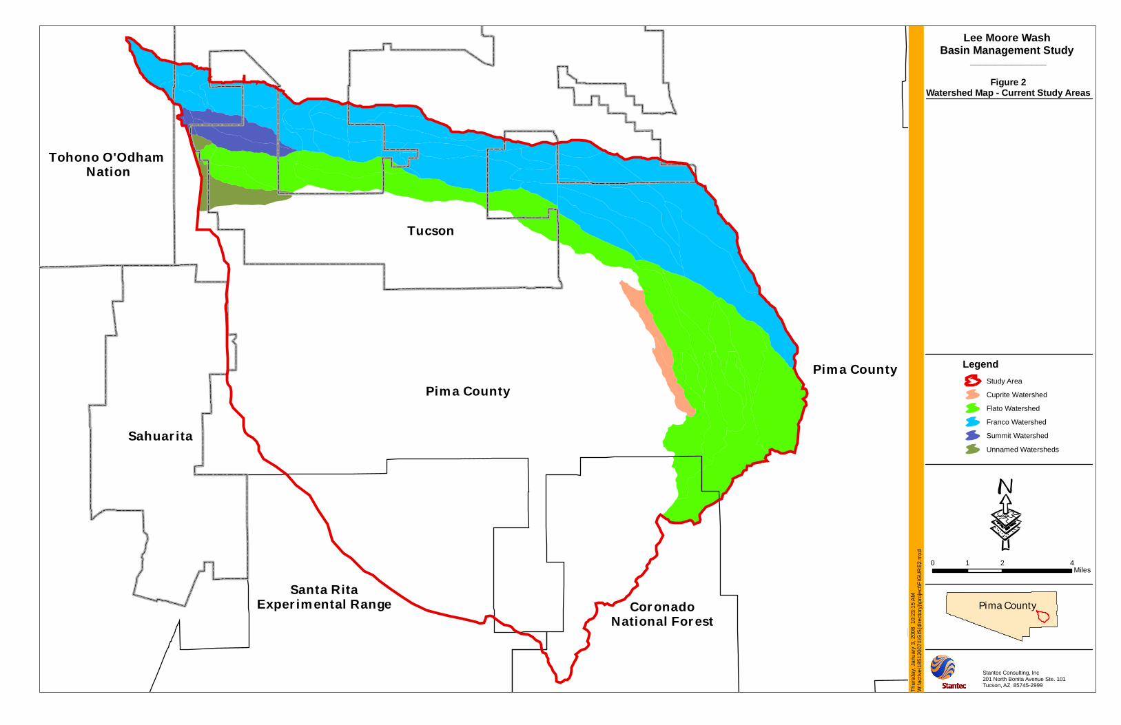
The Lee Moore watershed (Figure 1) extends from the Santa Rita Mountains in the east/ southeast portion of the project area to the Lee Moore Wash and/or Santa Cruz River along the western margin of the watershed. The areas associated with this study represent the northernmost portion of the watershed. Specifically, this study represents the hydrologic and hydraulic modeling efforts for the Franco Wash watershed, the Flato Wash watershed, a portion of the Cuprite Wash watershed, watersheds within the Summit area, and the extreme lower extent of the Lee Moore Wash. These watersheds typically drain west/northwest from the mountain and/or foothill areas to the Lee Moore Wash channel, and ultimately to the Santa Cruz River. The Franco watershed represents the northernmost watershed within the Lee Moore study area, and is tributary to the Santa Cruz River about 2 miles north of the Lee Moore channel confluence with the Santa Cruz. However, it is generally considered part of the Lee Moore watershed, and thus is a focus of the current study. The headwaters of the Franco watershed are generally situated within the northernmost foothill areas of the Santa Rita Mountains, and the watershed consists of a total drainage area of about 33 square miles. The Flato drainage basin is situated immediately south of Franco, and forms the southern Franco watershed boundary except within the westernmost extent of the watershed. The total watershed area of Flato Wash at the Lee Moore channel is about 29 square miles, with the headwaters situated within the higher elevations of the Santa Rita Mountains. The Cuprite watershed is situated south and west of the Flato watershed. Only a small portion of this watershed modeled in the current study, and will be discussed in a later section. The other watersheds included in the current study are the Summit Wash watershed and three unnamed watershed areas, all situated within the valley area in the northwest portion of the Lee Moore watershed. The drainage areas of these watersheds are about 2.5 square miles, 1.4 square miles (UN1), 0.2 square miles (UN2), and 0.14 square miles (UN3), respectively. The composite peak flow anticipated along the downstream extent of the Lee Moore Wash watershed is also documented within this report. A watershed map exhibiting the watershed boundaries of these areas is presented as Figure 2.
The study area is generally characterized by a variety of landscapes common to the arid/semi-arid areas of the southwest, with the Santa Rita Mountains rising as much as 3600 ft. (Mount Fagan – elevation 6189 feet) above the valley floor within the headwater areas of the Flato watershed, and alluvial fans in varied erosional stages situated near

Tucson
Santa RitaExperimental Range
CoronadoNational Forest
Tohono O'OdhamNation
Sahuarita
Pima County Pima CountyS
WIL
MO
T R
D
S H
OU
GH
TON
RD
S S
AN
TA R
ITA
RD
E SAHUARITA RD
S S
WAN
RD
S SO
NOIT
A H
Y
W DUVAL MINE RD
E MARSH STATION RD
W PIMA MINE RD
S OLD
SON
OITA H
Y
S R
ITA
RD
S AB
REG
O D
R
E WHITEHOUSE CANYON RD
S K
OLB
RD
S LA
CA
NA
DA
DR
S O
LD N
OG
ALE
S H
Y
W HELMET PEAK RD
W TWIN BUTTES RD
E COLOSSAL CAVE RD
E OLD VAIL CONNECTION RD
E RITA RD
W SAHUARITA RD
S AL
VER
NO
N W
Y
S H
AR
RIS
ON
RD
W BENSON HY
E ROCKET RD
E VA
IL R
D
S W
EN
TWO
RT
H R
D
E HUGHES ACCESS RD
N C
ALL
E R
INC
ON
AD
O
S PIS
TOL HILL
RD
S C
AM
INO
DE
LA
CA
NO
A
S C
OU
NTR
Y C
LUB
RD
N W
EN
TWO
RTH
RD
E DAWN RD
S LA
VIL
LITA
RD
E BREKKE RD
E OLD SPANISH TR
E QUAIL CROSSING BL
E ANDRADA RD
E HERMANS RD
S M
ELP
OM
EN
E W
Y
N D
AVID
SO
N R
D
E CAMINO AURELIA W CAMINO AURELIA
S C
AM
INO
LO
MA
ALTA
W CAMINO DEL TORO
E WETSTONES RD
N D
AVID
SO
N R
D
S WE
NTW
OR
TH
RD
S SO
NO
ITA HY
E OLD VAIL RD
S C
OU
NTR
Y C
LUB
RD
S H
AR
RIS
ON
RD
E ANDRADA RD
Lee Moore WashBasin Management Study
LegendStudy Area
0 2 41Miles
·Pima County
_______________
Figure 1Lee Moore Watershed
Stantec Consulting, Inc201 North Bonita Avenue Ste. 101Tucson, AZ 85745-2999W
edne
sday
, Dec
embe
r 19,
200
7 1
0:56
:48
AMW
:\act
ive\
1851
2007
1\G
IS(d
irect
ory)
\pro
ject
\FIG
UR
E1.m
xd
Tucson
Santa RitaExperimental Range Coronado
National Forest
Tohono O'Odham Nation
Sahuarita
Pima CountyPima County
Lee Moore WashBasin Management Study
LegendStudy Area
Cuprite Watershed
Flato Watershed
Franco Watershed
Summit Watershed
Unnamed Watersheds
0 2 41Miles
·Pima County
_______________
Figure 2Watershed Map - Current Study Areas
Stantec Consulting, Inc201 North Bonita Avenue Ste. 101Tucson, AZ 85745-2999
Thur
sday
, Jan
uary
3, 2
008
10:
23:1
5 A
MW
:\act
ive\
1851
2007
1\G
IS(d
irect
ory)
\pro
ject
\FIG
UR
E2.m
xd

5
the base of the mountains and comprising the foothills of the study area. The vegetation in the study area also displays a wide array of the typical southwest desert plant types, with limited woodlands in the higher elevations, an herbaceous and/or mountain brush mix within the foothills, and desert shrub/scrub mix prevalent along the valley floor areas. The channel system exhibits the full range of ephemeral stream types, from steep gradient mountain streams displaying a coarse sediment load to sand-bed washes comprised of a much less coarse sediment distribution. The dominant stream channel morphology within the study area, however, is a distributary channel system comprised of numerous, ill-defined channels capable of flowing in multiple directions during a given storm event. As discussed in more detail later in this report (and to a great extent in appended reports by others), the unpredictable nature of these systems plays a major role in the study efforts for this study, as well as the overall Lee Moore study area.
1.2 PROJECT SCOPE AND OBJECTIVES
The scope for the LMWBMS was developed in conjunction with the staff at the PCRFCD, and the study presented in this report represents only a portion of the overall project scope. The intent of the subject report presented herein is to document existing hydrologic and hydraulic conditions within the subject watershed areas for the 100-year storm event, with the results ultimately employed in conjunction with planning efforts to guide future development within the Lee Moore watershed areas. More specifically, this report presents the procedures and results performed by Stantec Consulting, Inc. for those watershed areas that lent themselves to one-dimensional hydrologic and hydraulic modeling through the use of the U.S. Army Corps of Engineers (USACE) HEC-HMS and HEC-RAS computer programs. Additional analyses performed by subconsultant JE Fuller Hydrology & Geomorphology, Inc. are also incorporated in the study results presented in this report. This report summarizes the overall tasks and procedures generally employed with the current study, with results and discussions presented individually for each watershed.
6
2.0 Procedures
2.1 DATA COLLECTION
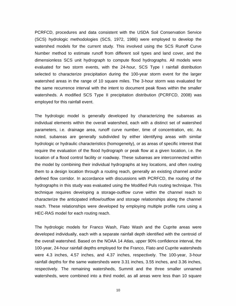
Several sources of data were collected and reviewed for the study, and are referenced in detail as appropriate at the end of this report. The following discussion presents the data collection approach. The initial task involved collecting all available GIS data relevant to hydrology and/or hydraulics from local municipalities and government agencies, such as topographic mapping, soils mapping, land cover mapping, etc. All major watersheds within the LMWBMS study area were then delineated from their headwaters, typically in the Santa Rita Mountains or foothills, and extended to their discharge points at either the Lee Moore Wash and/or Santa Cruz River. This effort was performed employing available 2-foot contour interval topography from various years (1998, 2000 and 2005), and U.S Geological Survey topographic quadrangles for areas where these data were not available. The areas lacking 2-foot topographic coverage generally occurred within the southernmost portion of the watershed, typically within mountain areas with well-defined topography. Thus, the topographic resolution was sufficiently accurate for watershed delineation. Whenever possible, the 2005 data provided by the Pima Association of Governments (PAG) in LIDAR format were employed to differentiate watershed areas, while the 2-foot topography available on the Pima County (PC) MapGuide website (based on PAG orthophotos) was employed with 2005 color aerial photography where 2005 LIDAR data were not available. Specific watershed maps resulting from these efforts are presented in this report, or as attachments within appendices.
In summary, the following GIS sources were employed with the current study to develop relevant data sets for each individual drainage area:
• 2-foot topographic topography (PAG) 1998, 2000, 2002 (from PC website)
• PAG 2005 LIDAR data
• Digital raster graphics
• Pima County shapefiles for Base Data Layers (examples: roads, washes, etc.)

7
• 2002 orthophotos
• 2005 orthophotos
• Soil Survey Geographic (SSURGO) database for Pima County, Arizona , Eastern Part
• 1999-2004 Landcover Grid (Southwest Regional Gap Analysis Project)
2.2 HYDROLOGIC INVESTIGATION
2.2.1 Hydrologic Modeling
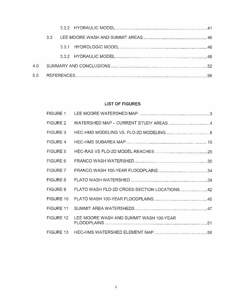
Generally speaking, the Lee Moore watershed is comprised of nine major identified watercourses: Franco Wash, Flato Wash, Summit Wash, Petty Ranch Wash, Cuprite Wash, Fagan Wash, Sycamore Canyon Wash, Gunnery Wash and the Lee Moore Wash. Based on conversations with the staff at PCRFCD, the Franco and Flato Wash watersheds were chosen as the focus of initial study efforts, as current flooding problems are prevalent in their downstream areas. It was during these efforts that areas of potential split flow, breakout and/or channel avulsion mechanics were identified in specific areas of these watersheds, and the two-dimensional FLO-2D model was chosen as the appropriate tool to characterize these flow distributions. The results of this task were subsequently combined with the HEC-HMS modeling efforts. A brief description of these efforts is presented later in this section, as well as in the discussion of the results for each watershed. Furthermore, it became evident that these fluvial processes were even more widespread within the watershed areas south of Flato Wash, i.e. Cuprite, Fagan, Sycamore Canyon and Gunnery Range, thus leading to the decision that FLO-2D modeling would be more appropriate as the sole modeling tool for these watershed areas, where little channel development or watershed definition is prevalent. The efforts associated with this aspect of the study are provided in detail within a separate report prepared by JE Fuller Hydrology & Geomorphology, Inc., thus no detailed discussion of these watershed areas is provided in the current report. Neither of the previously noted studies (PCDTFCD, 1988; ASLD, 2006) addressed increases and/or reduction of peak flows within watersheds associated with these types of fluvial processes. Figure 3 displays the areas evaluated with the current study, versus those areas employing FLO-2D for both hydrologic and hydraulic modeling efforts. For general reference, a summary of the drainage area and hydrologic modeling approach associated with the referenced major watersheds comprising the Lee Moore watershed is presented in Table 1.

Tucson
Santa RitaExperimental Range Coronado
National Forest
Toho
no O
'Odh
am N
ation
Sahuarita
Pima County
!"a$
S NO
GA
LES H
Y
!"d$
S SANTA RITA RD
!"d$
!"a$
S W
ILM
OT
RD
S H
OU
GH
TON
RD
S S
AN
TA R
ITA
RD
E SAHUARITA RD
S S
WA
N R
D
S SO
NO
ITA
HY
S M
ISS
ION
RD
W DUVAL MINE RD
E MARSH STATION RD
W PIMA MINE RD
S OLD SO
NO
ITA HY
S R
ITA
RD
S AB
REG
O D
R
E WHITEHOUSE CANYON RD
S K
OLB
RD
S LA
CA
NA
DA
DR
S O
LD N
OG
ALE
S H
Y
W HELMET PEAK RD
W TWIN BUTTES RD
E COLOSSAL CAVE RD
E OLD VAIL CONNECTION RD
E RITA RD
W SAHUARITA RD
S A
LVE
RN
ON
WY
S H
AR
RIS
ON
RD
W BENSON HY
E ROCKET RD
E VA
IL R
D
S W
EN
TWO
RTH
RD
E HUGHES ACCESS RD
N C
ALLE
RIN
CO
NA
DO
S PIS
TOL H
ILL R
D
S C
AM
INO
DE
LA
CAN
OA
S C
OU
NTR
Y C
LUB
RD
N W
EN
TWO
RTH
RD
E DAWN RD
S LA
VIL
LITA
RD
E BREKKE RD
E OLD SPANISH TR
E QUAIL CROSSING BL
E ANDRADA RD
E HERMANS RD
S M
ELP
OM
EN
E W
Y
N D
AVID
SON
RD
E CAMINO AURELIA W CAMINO AURELIA
S 6TH AV EXTENSION RD
S C
AM
INO
LO
MA
ALT
A
W CAMINO DEL TORO
E WETSTONES RD
N D
AVID
SON
RD
S WE
NTW
OR
TH R
D
S SO
NO
ITA HY
E OLD VAIL RD
S C
OU
NTR
Y C
LUB
RD
S H
AR
RIS
ON
RD
E ANDRADA RD
Lee Moore WashBasin Management Study
LegendStudy Area
HEC-HMS Modeling Area
FLO 2D Modeling Area
0 2 41Miles
·Pima County
_______________
Figure 3HEC-HMS Modeling
vs.FLO-2D Modeling
Stantec Consulting, Inc201 North Bonita Avenue Ste. 101Tucson, AZ 85745-2999
Thur
sday
, Jan
uary
3, 2
008
10:
24:4
6 A
MW
:\act
ive\
1851
2007
1\G
IS(d
irect
ory)
\pro
ject
\FIG
UR
E3.m
xd
9
Table 1 Lee Moore Wash Major Watersheds and Hydrologic Modeling Technique
Watershed Drainage Area (square miles) Hydrologic Model(s)
Gunnery Range Wash 42.0* FLO2D
Sycamore Canyon Wash 36.3* FLO2D
Fagan Wash 32.1* FLO2D
Cuprite Wash 26.9* HEC-HMS/FLO2D
Petty Ranch Wash 5.4 FLO2D
Flato Wash 29.1 HEC-HMS/FLO2D
Summit Wash 2.5 HEC-HMS
Lee Moore Wash (at Santa Cruz River) 178* HEC-HMS/FLO2D
Franco Wash (at Santa Cruz River) 32.9 HEC-HMS/FLO2D
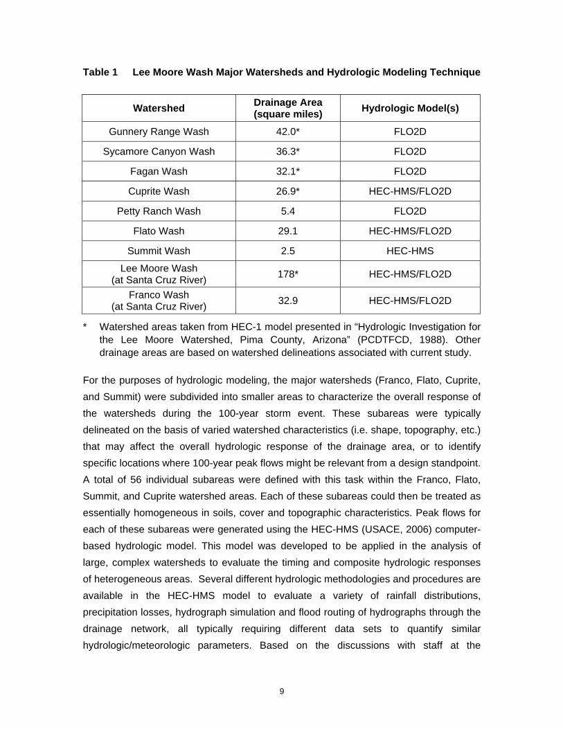
* Watershed areas taken from HEC-1 model presented in “Hydrologic Investigation for the Lee Moore Watershed, Pima County, Arizona” (PCDTFCD, 1988). Other drainage areas are based on watershed delineations associated with current study.
For the purposes of hydrologic modeling, the major watersheds (Franco, Flato, Cuprite, and Summit) were subdivided into smaller areas to characterize the overall response of the watersheds during the 100-year storm event. These subareas were typically delineated on the basis of varied watershed characteristics (i.e. shape, topography, etc.) that may affect the overall hydrologic response of the drainage area, or to identify specific locations where 100-year peak flows might be relevant from a design standpoint. A total of 56 individual subareas were defined with this task within the Franco, Flato, Summit, and Cuprite watershed areas. Each of these subareas could then be treated as essentially homogeneous in soils, cover and topographic characteristics. Peak flows for each of these subareas were generated using the HEC-HMS (USACE, 2006) computer-based hydrologic model. This model was developed to be applied in the analysis of large, complex watersheds to evaluate the timing and composite hydrologic responses of heterogeneous areas. Several different hydrologic methodologies and procedures are available in the HEC-HMS model to evaluate a variety of rainfall distributions, precipitation losses, hydrograph simulation and flood routing of hydrographs through the drainage network, all typically requiring different data sets to quantify similar hydrologic/meteorologic parameters. Based on the discussions with staff at the
10
PCRFCD, procedures and data consistent with the USDA Soil Conservation Service (SCS) hydrologic methodologies (SCS, 1972, 1986) were employed to develop the watershed models for the current study. This involved using the SCS Runoff Curve Number method to estimate runoff from different soil types and land cover, and the dimensionless SCS unit hydrograph to compute flood hydrographs. All models were evaluated for two storm events, with the 24-hour, SCS Type I rainfall distribution selected to characterize precipitation during the 100-year storm event for the larger watershed areas in the range of 10 square miles. The 3-hour storm was evaluated for the same recurrence interval with the intent to document peak flows within the smaller watersheds. A modified SCS Type II precipitation distribution (PCRFCD, 2008) was employed for this rainfall event.
The hydrologic model is generally developed by characterizing the subareas as individual elements within the overall watershed, each with a distinct set of watershed parameters, i.e. drainage area, runoff curve number, time of concentration, etc. As noted, subareas are generally subdivided by either identifying areas with similar hydrologic or hydraulic characteristics (homogeneity), or as areas of specific interest that require the evaluation of the flood hydrograph or peak flow at a given location, i.e. the location of a flood control facility or roadway. These subareas are interconnected within the model by combining their individual hydrographs at key locations, and often routing them to a design location through a routing reach, generally an existing channel and/or defined flow corridor. In accordance with discussions with PCRFCD, the routing of the hydrographs in this study was evaluated using the Modified Puls routing technique. This technique requires developing a storage-outflow curve within the channel reach to characterize the anticipated inflow/outflow and storage relationships along the channel reach. These relationships were developed by employing multiple profile runs using a HEC-RAS model for each routing reach.
The hydrologic models for Franco Wash, Flato Wash and the Cuprite areas were developed individually, each with a separate rainfall depth identified with the centroid of the overall watershed. Based on the NOAA 14 Atlas, upper 90% confidence interval, the 100-year, 24-hour rainfall depths employed for the Franco, Flato and Cuprite watersheds were 4.3 inches, 4.57 inches, and 4.37 inches, respectively. The 100-year, 3-hour rainfall depths for the same watersheds were 3.31 inches, 3.55 inches, and 3.36 inches, respectively. The remaining watersheds, Summit and the three smaller unnamed watersheds, were combined into a third model, as all areas were less than 10 square
11
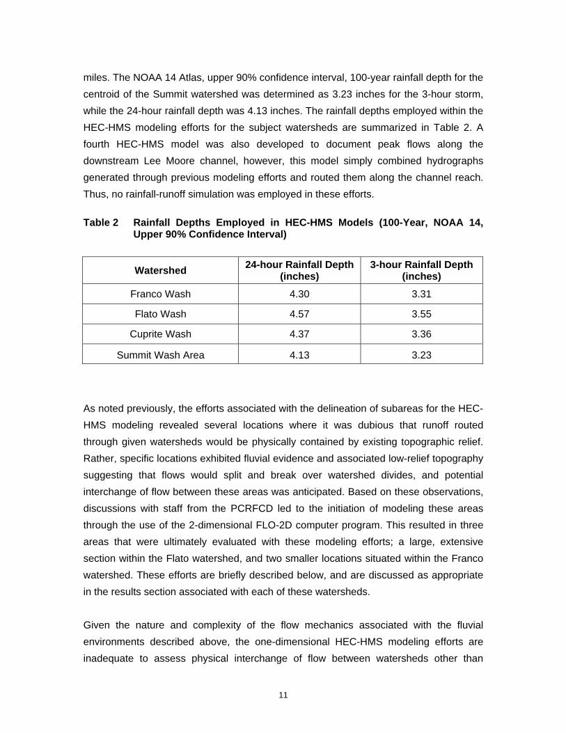
miles. The NOAA 14 Atlas, upper 90% confidence interval, 100-year rainfall depth for the centroid of the Summit watershed was determined as 3.23 inches for the 3-hour storm, while the 24-hour rainfall depth was 4.13 inches. The rainfall depths employed within the HEC-HMS modeling efforts for the subject watersheds are summarized in Table 2. A fourth HEC-HMS model was also developed to document peak flows along the downstream Lee Moore channel, however, this model simply combined hydrographs generated through previous modeling efforts and routed them along the channel reach. Thus, no rainfall-runoff simulation was employed in these efforts.
Table 2 Rainfall Depths Employed in HEC-HMS Models (100-Year, NOAA 14, Upper 90% Confidence Interval)
Watershed 24-hour Rainfall Depth (inches)
3-hour Rainfall Depth (inches)
Franco Wash 4.30 3.31
Flato Wash 4.57 3.55
Cuprite Wash 4.37 3.36
Summit Wash Area 4.13 3.23
As noted previously, the efforts associated with the delineation of subareas for the HEC-HMS modeling revealed several locations where it was dubious that runoff routed through given watersheds would be physically contained by existing topographic relief. Rather, specific locations exhibited fluvial evidence and associated low-relief topography suggesting that flows would split and break over watershed divides, and potential interchange of flow between these areas was anticipated. Based on these observations, discussions with staff from the PCRFCD led to the initiation of modeling these areas through the use of the 2-dimensional FLO-2D computer program. This resulted in three areas that were ultimately evaluated with these modeling efforts; a large, extensive section within the Flato watershed, and two smaller locations situated within the Franco watershed. These efforts are briefly described below, and are discussed as appropriate in the results section associated with each of these watersheds.
Given the nature and complexity of the flow mechanics associated with the fluvial environments described above, the one-dimensional HEC-HMS modeling efforts are inadequate to assess physical interchange of flow between watersheds other than

12
through a very simplified approach using the flow diversion routine within the model. This routine is based on providing a rating curve within a watershed element, through which “loss” of runoff from a subarea can be modeled. However, the model does not provide sufficient capabilities for modeling potential flow interchange between watersheds at multiple locations, thus leading to the decision to employ the 2-dimensional FLO-2D computer modeling routine. This model allows the three-dimensional surface of the subject watersheds to be evaluated, and can analyze flow occurring within flow corridors in eight different directions. The HEC-HMS model generally can only evaluate flow in two directions, i.e. flow upstream to downstream within an area, and a potential diversion of flow out and/or into the subject watershed. Thus, the FLO-2D model can evaluate any number of flow exchanges and splits, based on flow depths and topography, as the runoff hydrograph travels across the three-dimensional surface. In this manner, flow hydrographs at specified outfalls, and/or concentration points delineated in the watershed mapping efforts, are based on the actual physical flow mechanics associated with split flows, watershed divide “breakovers” and multiple flow exchanges between low-relief, adjacent watersheds.
The FLO-2D program can also serve as a hydrologic model, and has the capabilities to evaluate rainfall on the natural surface and generate runoff hydrographs. However, the original 2-dimensional analyses employed the hydrographs generated for individual subareas through the HEC-HMS modeling efforts, and routed these flows across the flow surface. This was generally due to existing limitations within the FLO-2D modeling routines at the time of the early study efforts, as FLO-2D modeling capabilities included only the Green-Ampt runoff transformation procedures. This procedure is generally considered inconsistent with the SCS methodology employed with the current HEC-HMS efforts. Thus, in order to maintain consistency in hydrologic methodologies, the HEC-HMS hydrographs at the upstream end of the model areas were manually input into the FLO-2D model to physically analyze the flow mechanics of the hydrograph as it traveled through the downstream flow corridors. This modeling technique was sufficient for the Franco watershed analyses, and was maintained through the final modeling efforts.
However, the area identified for FLO-2D analysis within the Flato watershed was expansive, and the original analysis required multiple HEC-HMS flow hydrographs to be manually input at subarea concentration points within the FLO-2D flow corridor. These hydrographs would then combine with the routed upstream runoff hydrograph at their point of input, and were physically routed across the downstream surface by the FLO-2D
13
model. Certain anomalies were apparent with these efforts, although the magnitude and distribution of runoff was deemed consistent. As the Lee Moore study progressed, algorithms were developed for the FLO-2D model that simulates runoff from watershed areas consistent with SCS methodologies. Consequently, it was determined that this procedure would be more appropriate for the Flato hydrologic analysis. Thus, the Flato FLO-2D model was developed by allowing the program to compute excess runoff from the watershed surface within the FLO-2D area, and combining these flows accordingly with the HEC-HMS hydrograph input at the upstream extent and routed through the subject FLO2D corridor. This is in contrast to the Franco FLO-2D effort noted above, where all runoff hydrographs were generated by HEC-HMS modeling methods, with the FLO-2D model utilized only for the purposes of routing the resulting hydrograph through the flow corridors. A more detailed discussion of each individual scenario will be provided in the results section for each subject watershed as appropriate.
2.2.2 Watershed Parameters
A total of fifty-six (56) subareas were delineated to develop the HEC-HMS models generated for the Franco, Flato, Cuprite and Summit watersheds evaluated with the current study, including the three small unnamed watersheds individually analyzed with the Summit model. In order to develop peak flows at each specific watershed concentration point, four general parameters were required for each subarea; drainage area, runoff curve number (CN), time of concentration, and estimated impervious percentage. In addition to these watershed parameters, storage-outflow curves were generated to model flow attenuation through each downstream routing reach employing the Modified Puls channel routing routine. The following discussion provides details associated with the development of each parameter, and the methodologies employed.
Drainage areas were developed from watershed delineations employing 2-foot contour interval topography from various years (1998, 2000 and 2005) when available, and U.S Geological Survey topographic quadrangles for areas where these data were not available. The areas lacking 2-foot coverage for the current study area occurred only within the southernmost mountain headwater areas of the Flato watershed, with well-defined topography. Thus, the topographic resolution was sufficiently accurate for watershed delineation. Whenever possible, the 2005 data provided by the Pima Association of Governments (PAG) in LIDAR format were employed to differentiate watershed areas. The 2-foot topography available on the Pima County MapGuide
14
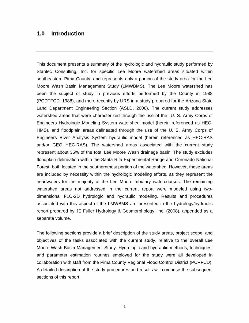
website (based on PAG orthophotos) was utilized with 2005 or 2002 color aerial photography when 2005 LIDAR data were not available. Each of these subareas were identified with a number and specific watershed identity, i.e. Flato watersheds were designated FL1, FL2, Franco watersheds were identified as FR1, FR2, etc. A watershed map identifying the major watershed boundaries and subareas is displayed as Figure 4.
The SCS runoff curve number generally represents the relationship of runoff characteristics for given soil groups mapped by the USDA Soil Conservation Service (now the NRCS, National Resources Conservation Service) as a function of soil cover and land use types. The use of a subarea’s curve number in the SCS runoff equation, in conjunction with the anticipated 24-hour rainfall depth, provides the basis for the precipitation excess estimate, i.e. runoff for a unit area associated with the given curve number. Based on the GIS data assembled for the current study efforts, soil cover and existing conditions land cover maps of the project area were generated, and the individual watersheds were superimposed on these maps. Land cover and soils mapping were available for the entire project area, and the specific sources employed for these analyses are provided within the reference section of this report. Given the relative percentage of soil types in each subarea, these areas were related to the existing land cover associated with each soil type in order to develop a composite (weighted) curve number for the watershed. As per the land cover mapping, innumerable different land cover types were identified in the various subareas. However, review of the mapping noted that many of the areas that covered the significant portions of the watershed had similar runoff characteristics and curve numbers, and/or could be considered as the same vegetation group. Thus, the numerous land cover types were grouped together as appropriate, and categorized into one of five land cover types; herbaceous, mountain brush, juniper-grass, desert shrub, and urban. Once these categories were identified for each area, they were then associated with their appropriate soil type and assigned a runoff curve number.
The curve numbers used in this study were taken directly from Figure D-1 “Hydrologic Soil-Cover Complexes and their Associated SCS Curve Numbers” of the Pima County Hydrology Procedures PC-Hydro User’s Guide (PCRFCD, 2007). Curve numbers vary for different hydrologic conditions, which generally represents the density of plant and residue cover for the given land cover. For the current study, vegetative cover density was assumed to be 20% within the valley and foothill areas below 4000 feet in elevation,

Lee Moore WashBasin Management Study
LegendStudy Area
Cuprite Watershed
Flato Watershed
Franco Watershed
Summit Watershed
Unnamed watersheds
0 2 41Miles
·Pima County
_______________
Figure 4HEC-HMS Subarea Map
Stantec Consulting, Inc201 North Bonita Avenue Ste. 101Tucson, AZ 85745-2999
Thur
sday
, Jan
uary
3, 2
008
10:
25:5
1 A
MW
:\act
ive\
1851
2007
1\G
IS(d
irect
ory)
\pro
ject
\FIG
UR
E4.m
xd
16
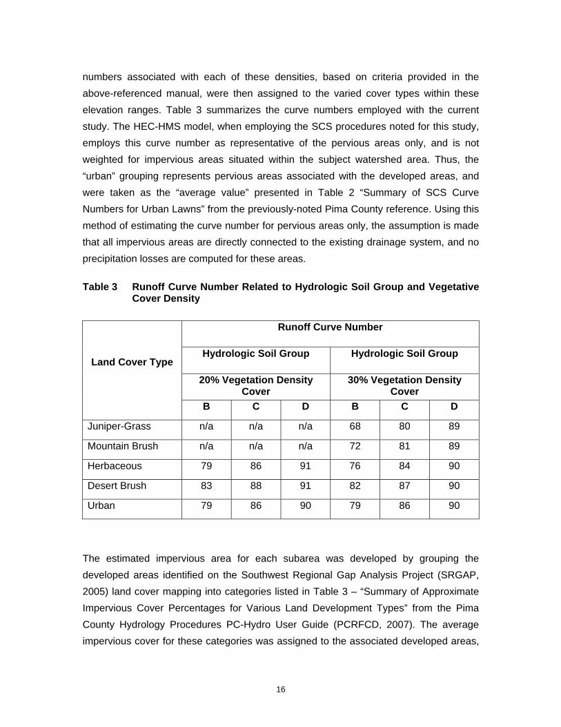
numbers associated with each of these densities, based on criteria provided in the above-referenced manual, were then assigned to the varied cover types within these elevation ranges. Table 3 summarizes the curve numbers employed with the current study. The HEC-HMS model, when employing the SCS procedures noted for this study, employs this curve number as representative of the pervious areas only, and is not weighted for impervious areas situated within the subject watershed area. Thus, the “urban” grouping represents pervious areas associated with the developed areas, and were taken as the “average value” presented in Table 2 “Summary of SCS Curve Numbers for Urban Lawns” from the previously-noted Pima County reference. Using this method of estimating the curve number for pervious areas only, the assumption is made that all impervious areas are directly connected to the existing drainage system, and no precipitation losses are computed for these areas.
Table 3 Runoff Curve Number Related to Hydrologic Soil Group and Vegetative Cover Density
Runoff Curve Number
Hydrologic Soil Group Hydrologic Soil Group
20% Vegetation Density Cover
30% Vegetation Density Cover
Land Cover Type
B C D B C D
Juniper-Grass n/a n/a n/a 68 80 89
Mountain Brush n/a n/a n/a 72 81 89
Herbaceous 79 86 91 76 84 90
Desert Brush 83 88 91 82 87 90
Urban 79 86 90 79 86 90
The estimated impervious area for each subarea was developed by grouping the developed areas identified on the Southwest Regional Gap Analysis Project (SRGAP, 2005) land cover mapping into categories listed in Table 3 – “Summary of Approximate Impervious Cover Percentages for Various Land Development Types” from the Pima County Hydrology Procedures PC-Hydro User Guide (PCRFCD, 2007). The average impervious cover for these categories was assigned to the associated developed areas,
17
and a weighted impervious percentage was generated based on the areal extent of the subject developments within the watershed. All undeveloped areas were assumed to have an impervious cover of 1% for weighting purposes in order to account for miscellaneous pavement, roadways and/or exposed bedrock and/or hardpan areas.
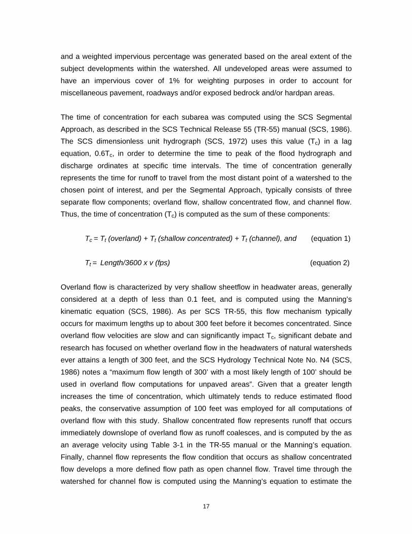
The time of concentration for each subarea was computed using the SCS Segmental Approach, as described in the SCS Technical Release 55 (TR-55) manual (SCS, 1986). The SCS dimensionless unit hydrograph (SCS, 1972) uses this value (Tc) in a lag equation, 0.6Tc, in order to determine the time to peak of the flood hydrograph and discharge ordinates at specific time intervals. The time of concentration generally represents the time for runoff to travel from the most distant point of a watershed to the chosen point of interest, and per the Segmental Approach, typically consists of three separate flow components; overland flow, shallow concentrated flow, and channel flow. Thus, the time of concentration (Tc) is computed as the sum of these components:
Tc = Tt (overland) + Tt (shallow concentrated) + Tt (channel), and (equation 1)
Tt = Length/3600 x v (fps) (equation 2)
Overland flow is characterized by very shallow sheetflow in headwater areas, generally considered at a depth of less than 0.1 feet, and is computed using the Manning’s kinematic equation (SCS, 1986). As per SCS TR-55, this flow mechanism typically occurs for maximum lengths up to about 300 feet before it becomes concentrated. Since overland flow velocities are slow and can significantly impact Tc, significant debate and research has focused on whether overland flow in the headwaters of natural watersheds ever attains a length of 300 feet, and the SCS Hydrology Technical Note No. N4 (SCS, 1986) notes a “maximum flow length of 300’ with a most likely length of 100’ should be used in overland flow computations for unpaved areas”. Given that a greater length increases the time of concentration, which ultimately tends to reduce estimated flood peaks, the conservative assumption of 100 feet was employed for all computations of overland flow with this study. Shallow concentrated flow represents runoff that occurs immediately downslope of overland flow as runoff coalesces, and is computed by the as an average velocity using Table 3-1 in the TR-55 manual or the Manning’s equation. Finally, channel flow represents the flow condition that occurs as shallow concentrated flow develops a more defined flow path as open channel flow. Travel time through the watershed for channel flow is computed using the Manning’s equation to estimate the

18
channel velocity for the bankfull discharge, and the length between typical channel segments (equation 2).
In order to generate the time of concentration, certain assumptions were necessary due to the lack of physical data and/or extensive field work. The assumptions employed to determine overland flow and shallow concentrated flow are rather straight forward, and parameters and guidelines are provided in the TR-55 manual. For the overland flow calculations, a length, slope and 2-year, 24-hour rainfall depth are all known, measurable or easily computed, while the Manning’s “n” is estimated from hydrologic literature. Table 4 presents the values used for the current study and their associated literature references for overland flow. Shallow concentrated flow simply requires the length and slope, and a determination of whether the watercourse is paved or unpaved (the predominant condition for this study). The velocity is then obtained from a nomograph, Figure 3-1 in the SCS TR-55 manual, and travel time is computed based on the flow length (equation 2). For the purposes of this study, shallow concentrated flow was generally assumed to end where it was evident from aerial photography that two or more significant rills or ill-defined swales coalesce into an apparent channel, and thus channel flow would be the dominant fluvial process.
Table 4 Manning’s “n” Values - Overland Flow for Travel Time Calculation (eq.1)
Watercourse Description Manning’s "n" Value Reference/Description
Mountain 0.4 TR-55, HEC-1 - Dense Shrubbery/Forest Litter
Foothill 0.3 HEC-1 - Poor grass cover on moderately rough surface
Valley 0.15 TR55/HEC-1 - Short Grass Prairie
Since minimal slopes are exhibited in valley areas, and associated velocities for concentrated flow at these slopes are very low, the travel time associated with long lengths of the shallow concentrated flow component of the Tc computation can become excessive. Thus, overestimating this length can affect peak flows in a similar manner as assuming a 300-foot overland flow length. Given this circumstance, a maximum length of

19
3000 feet was typically assumed for shallow concentrated flow along reaches lacking a well-defined flow pattern along the chosen time of concentration path.
In order to estimate the travel time for channel flow through the watershed, additional assumptions were required, and were based on research and hydrologic experience. Generally, the Manning’s equation requires a channel slope, Manning’s “n”, and channel hydraulic radius (bankfull flow area/wetted perimeter) to compute the flow velocity for a given channel reach from the following equation:
V (average) = 1.486/n x R 0.67 x S 0.5 (Equation 3)
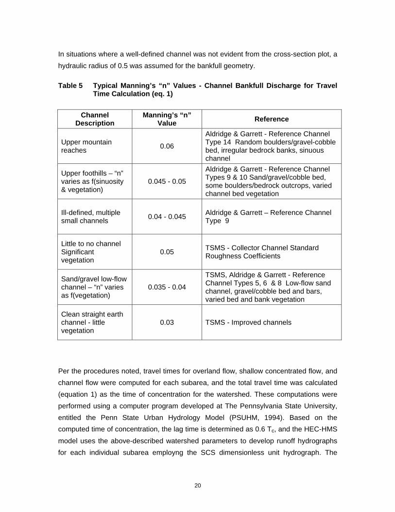
The slope is a straightforward calculation taken from the available topography, while the Manning’s “n” represents the roughness or friction component of the channel, dependent on vegetation, bed material, etc. This value is best estimated by field investigation. However, given the nature of this study, extensive field investigation of all the channels was outside the scope of work. Thus, for the purposes of this study, these values were estimated based upon several field visits, spot checks, experience, topography, and hydrologic literature. From these data, characteristic Manning’s “n” values were determined and employed in a consistent manner to estimate roughness conditions, and ultimately an average flow velocity for the bankfull discharge. It should be noted here that the bankfull discharge represents flow conditions within the low-flow channel for a given watercourse, considered to be representative of flows associated with a flow event on the order of a 2-year storm. Thus, the channel roughness and flow parameters can be different than what might represent full flow conditions during a 100-year storm or greater. Table 5 summarizes the roughness coefficients used for the current study along with cited references, corroborating that the coefficients are representative of typical values for channel analyses in other areas of Arizona. In order to determine the flow area and wetted perimeter of the channels without extensive field data, channel cross-sections were identified along reaches that exhibited similar characteristics, and typical cross-sections were developed from available topographic data. As noted previously, these data varied from USGS data for some mountainous reaches to cross-sections developed from available 2005 LIDAR data. These cross-sections were then evaluated to assess the bankfull channel geometry, and an estimated flow area and wetted perimeter was determined. Given these data, a bankfull velocity for each channel reach was determined, and the travel time for various channel reaches computed (equation 2).
20
In situations where a well-defined channel was not evident from the cross-section plot, a hydraulic radius of 0.5 was assumed for the bankfull geometry.
Table 5 Typical Manning’s “n” Values - Channel Bankfull Discharge for Travel Time Calculation (eq. 1)
Channel Description
Manning’s “n” Value Reference
Upper mountain reaches 0.06
Aldridge & Garrett - Reference Channel Type 14 Random boulders/gravel-cobble bed, irregular bedrock banks, sinuous channel
Upper foothills – “n” varies as f(sinuosity & vegetation)
0.045 - 0.05
Aldridge & Garrett - Reference Channel Types 9 & 10 Sand/gravel/cobble bed, some boulders/bedrock outcrops, varied channel bed vegetation
Ill-defined, multiple small channels 0.04 - 0.045 Aldridge & Garrett – Reference Channel
Type 9
Little to no channel Significant vegetation
0.05 TSMS - Collector Channel Standard Roughness Coefficients
Sand/gravel low-flow channel – “n” varies as f(vegetation)
0.035 - 0.04
TSMS, Aldridge & Garrett - Reference Channel Types 5, 6 & 8 Low-flow sand channel, gravel/cobble bed and bars, varied bed and bank vegetation
Clean straight earth channel - little vegetation
0.03 TSMS - Improved channels
Per the procedures noted, travel times for overland flow, shallow concentrated flow, and channel flow were computed for each subarea, and the total travel time was calculated (equation 1) as the time of concentration for the watershed. These computations were performed using a computer program developed at The Pennsylvania State University, entitled the Penn State Urban Hydrology Model (PSUHM, 1994). Based on the computed time of concentration, the lag time is determined as 0.6 Tc, and the HEC-HMS model uses the above-described watershed parameters to develop runoff hydrographs for each individual subarea employng the SCS dimensionless unit hydrograph. The

21
hydrographs are then routed through the watershed by channel routing reaches, and combined with other reaches and/or subareas at specific locations (junctions) downstream within the watershed network.
The channel routing reaches were evaluated using the Modified Puls channel routing methodology, and requires a storage-outflow relationship to be developed for each given reach. In general, the storage is computed as the flow area at given discharges over a specific channel length, thus representing volume. Channel reaches with significant storage volumes, relative to the total runoff volume passing through the reach, will tend to attenuate peak flows as flow spreads out and is temporarily stored within the channel and overbank areas, thus effectively reducing the peak at the outfall of the channel reach. Channel reaches with minimal storage volumes, relative to the runoff volume passing through the reach, will experience little attenuation of peak flows, with outflow essentially equivalent to inflow because there is virtually no channel reach storage.
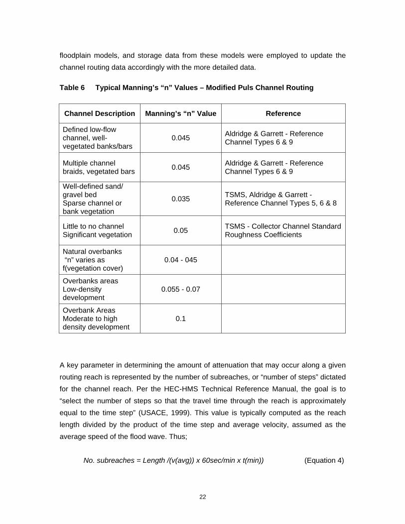
In order to develop storage-outflow curves for the HEC-HMS modeling efforts, typically a single eight point cross-section is chosen to characterize the routing reach, flow areas for given peak flows are computed, and storage volumes computed based on the chosen channel length. With the current study, however, channel reaches were identified and, initially, a few to several “typical” cross-sections were identified along the given reach. Channel cross-sections were then generated from available topographic data, and simplified HEC-RAS models developed for each reach. The hydraulic models were then run for multiple peak flows, and a table generated from the HEC-RAS data that provided the total storage volume along the channel reach as a summation of storage between each cross-section. Manning’s “n” values employed with these models generally represent anticipated roughness for full-flow flow conditions, versus those presented in the previous discussion for bankfull conditions. These values typically varied from 0.035 for a well-defined sand/gravel bed channel with sparse channel or bank vegetation, up to 0.05 for reaches with little channel definition and significant vegetative growth. Overbank areas were typically characterized with roughness coefficients of 0.04 to 0.1 depending on apparent vegetal cover and/or existing development. Table 6 summarizes the various roughness coefficients used for these analyses, along with references as appropriate. The storage-outflow data were then used in the HEC-HMS modeling for the Modified Puls channel routing routine. It should be noted here that many of the referenced “simplified” channel routing reaches developed for the HEC-HMS models were later analyzed with detailed HEC-RAS
22
floodplain models, and storage data from these models were employed to update the channel routing data accordingly with the more detailed data.
Table 6 Typical Manning’s “n” Values – Modified Puls Channel Routing
Channel Description Manning’s “n” Value Reference
Defined low-flow channel, well-vegetated banks/bars
0.045 Aldridge & Garrett - Reference Channel Types 6 & 9
Multiple channel braids, vegetated bars 0.045 Aldridge & Garrett - Reference
Channel Types 6 & 9
Well-defined sand/ gravel bed Sparse channel or bank vegetation
0.035 TSMS, Aldridge & Garrett - Reference Channel Types 5, 6 & 8
Little to no channel Significant vegetation 0.05 TSMS - Collector Channel Standard
Roughness Coefficients
Natural overbanks “n” varies as f(vegetation cover)
0.04 - 045
Overbanks areas Low-density development
0.055 - 0.07
Overbank Areas Moderate to high density development
0.1
A key parameter in determining the amount of attenuation that may occur along a given routing reach is represented by the number of subreaches, or “number of steps” dictated for the channel reach. Per the HEC-HMS Technical Reference Manual, the goal is to “select the number of steps so that the travel time through the reach is approximately equal to the time step” (USACE, 1999). This value is typically computed as the reach length divided by the product of the time step and average velocity, assumed as the average speed of the flood wave. Thus;
No. subreaches = Length /(v(avg)) x 60sec/min x t(min)) (Equation 4)
23
The HEC-HMS manual goes on further to describe that as the number of routing stepincrease, the amount of attenuation decreases, and “maximum attenuation corresponds to one step; this is used commonly for routing through ponds, lakes, wide, flat floodplains…” The initial HEC-HMS modeling efforts employed the “standard” criteria noted above, however, it was evident that specific reaches displaying significant storage volume within the study areas displayed very little attenuation of peak flows. Given the apparent broad floodplains and gentle slopes of downstream flow corridors along these washes, a review of the hydraulic modeling efforts for the channel routing routines was performed. The results of this assessment revealed that several of the specific reaches evaluated displayed low percentages of defined channel flow within their associated cross-sections, rather, flow hydraulics were characterized predominantly by very shallow overbank flow depths within expansive floodplains. These flow characteristics would be anticipated to display relatively significant flood peak attenuation effects, as suggested for reaches assigned a single subreach. Thus, based on conversations with PCRFCD staff, specific channel reaches were further evaluated, and assigned single subreaches where deemed appropriate. A table is provided in the technical appendices presenting a summary of the data employed to determine the number of subreaches for each channel routing reach for the current study, and denotes those reaches specifically chosen to fit the above-referenced category.
2.3 HYDRAULIC ANALYSES
Hydraulic analyses employing the U.S Army Corps of Engineers HEC-RAS/GEO HEC-RAS computer programs were performed along all the major washes identified in the hydrologic investigation where it was deemed appropriate to employ one-dimensional hydraulic modeling, versus the more sophisticated FLO-2D hydraulic model. These modeling efforts were employed to determine the approximate 100-year floodplains based on the peak flows generated with the HEC-HMS modeling. A 100-year peak flow of 1000 cfs was employed as the threshold flow to delineate floodplains. Peak flows generated by the 24-hour storm were modeled along the main channel reaches (drainage areas ranging from eight (8) square miles and greater), while the 3-hour peak flows were modeled along tributary reaches with contributing watershed areas typically less than five (5) square miles. In specific instances, peak flows were modeled along certain channel reaches with peak flows below this threshold, such as within the Summit watershed. Due to the prevalence of flooding within this area, the floodplains along Summit Wash were also evaluated from the confluence with Lee Moore Wash to the

24
Country Club Road alignment. Additional floodplains were mapped for peak flows less than 1000 cfs with the FLO-2D modeling efforts, as these areas generally tie into floodplain limits that meet the above-noted criteria. All other floodplains associated with the LMWBMS other than the Flato Wash, Franco Wash and Summit Wash are determined through hydraulic efforts associated with FLO-2D modeling, and are presented in the separate volume prepared by subconsultant J.E. Fuller Hydrology & Geomorphology, Inc.
2.3.1 HEC-RAS Modeling
As noted, HEC-RAS hydraulic models were developed for all channel reaches within the study area that met the referenced 100-year discharge threshold, and where it was readily evident that flood flows would remain within defined flow corridors, i.e. one-dimensional flow modeling was deemed appropriate. In general, Franco Wash and Summit Wash exhibit flow corridors that lend themselves to these hydraulic efforts, with the exception of a 4-mile stretch within the northernmost portion of Franco Wash, between the Pima County Fairgrounds and Wilmot Road. These areas were modeled through the use of the FLO-2D model, and indicated that flow concentrating at the northwest corner of the fairgrounds was dispersed over three separate watersheds. A small area at the southwest corner of the fairgrounds was also modeled with FLO-2D, resulting in breakover flow to the south into Flato watershed. Flato Wash does not remain contained within any well-defined flow corridor upstream of Wilmot Road until a point about 2.5 miles east of Houghton Road. Thus, the flow corridors upstream of Wilmot Road were modeled with the FLO-2D two-dimensional flow routine, where innumerable flow splits and watershed exchange occurs with the Cuprite watershed to the south. The Flato Wash corridor downstream of Wilmot Road to the confluence with Lee Moore Wash was modeled employing HEC-RAS, with peak flows based on hydrographs generated by the upstream FLO-2D modeling. Figure 5 illustrates the areas modeled through the use of the two separate modeling efforts. A more detailed description of the areas evaluated with FLO-2D modeling and the results as they pertain to the subject wash corridors are presented in the discussion sections for the individual watersheds.
Three-dimensional surfaces were developed from the PAG 2005 LIDAR data employing the GEO HEC-RAS computer software along designated flow corridors, and channel cross-sections were oriented across the channel and anticipated floodplain areas. In

!"a$
S NO
GA
LES H
Y
!"d$
!"d$
S W
ILM
OT
RD
S H
OU
GH
TON
RD
S S
AN
TA R
ITA
RD
E SAHUARITA RD
S S
WA
N R
D
S SO
NO
ITA
HY
W DUVAL MINE RD
E MARSH STATION RD
W PIMA MINE RD
S OLD SO
NO
ITA HY
S R
ITA
RD
S AB
REG
O D
R
E WHITEHOUSE CANYON RD
S K
OLB
RD
S LA
CA
NA
DA
DR
S O
LD N
OG
ALE
S H
Y
W HELMET PEAK RD
E COLOSSAL CAVE RD
E OLD VAIL CONNECTION RD
W SAHUARITA RD
S A
LVE
RN
ON
WY
S H
AR
RIS
ON
RD
W BENSON HY
E ROCKET RD
E VA
IL R
D
S W
EN
TWO
RTH
RD
E HUGHES ACCESS RD
N C
ALLE
RIN
CO
NA
DO
S PIS
TOL H
ILL R
D
S C
AM
INO
DE
LA
CAN
OA
S C
OU
NTR
Y C
LUB
RD
N W
EN
TWO
RTH
RD
E DAWN RD
S LA
VIL
LITA
RD
E BREKKE RD
E OLD SPANISH TR
E QUAIL CROSSING BL
E ANDRADA RD
E HERMANS RD
S M
ELP
OM
EN
E W
Y
N D
AVID
SON
RD
E CAMINO AURELIA W CAMINO AURELIA
S C
AM
INO
LO
MA
ALT
A
W CAMINO DEL TORO
E WETSTONES RD
N D
AVID
SON
RD
S WE
NTW
OR
TH R
D
S SO
NO
ITA HY
E OLD VAIL RD
S C
OU
NTR
Y C
LUB
RD
S H
AR
RIS
ON
RD
E ANDRADA RD
Lee Moore WashBasin Management Study
LegendStudy Area
Subbasin
FLO 2D Modeling Area
HEC RAS Modeling Area
0 2 41Miles
W:\A
ctiv
e\18
5120
071\
GIS
\Pro
ject
\FIG
UR
E5.m
xd 1
0012
007
·Pima County
_______________
Figure 5HEC-RAS Modeling
Vs.FLO-2D Modeling
Stantec Consulting, Inc201 North Bonita Avenue Ste. 101Tucson, AZ 85745-2999
26
areas where LIDAR data was not complete, surfaces were generated from previously referenced 2-foot topography based on PAG orthophotography. Typically, cross-sections were spaced at 500-foot intervals. However, cross-sections were spaced at 200-foot intervals along the Franco and Summit Wash corridors downstream of the Country Club Road alignment, as this area represents one of the more developed areas within the watershed. This area is identified as the Summit area, and has experienced significant flooding in recent years. A more detailed study of this area was performed as part of the overall Lee Moore (LMWBMS) project, and is summarized in a separate report. It was the focus of this study that initiated the County’s desire to provide additional cross-sections in order to evaluate the flooding impact in these areas in more detail. The identified cross-sections were drawn along the channel corridors defined with the GEO HEC-RAS software, and HEC-RAS hydraulic models were developed from these data.
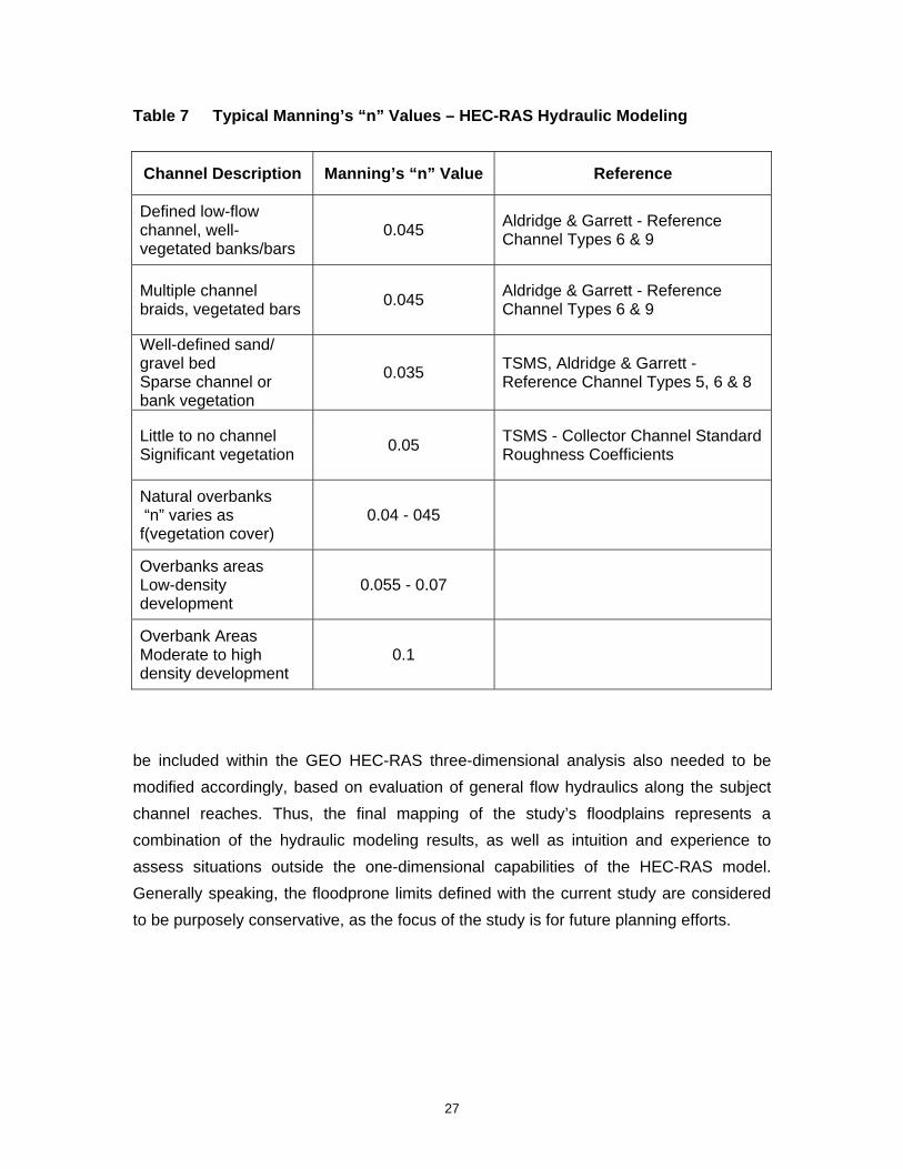
Approximately 28 miles of Franco Wash and tributaries, 31 miles of Flato Wash and tributaries, and about 4.4 miles of the Summit Wash and tributary were analyzed with the HEC-RAS modeling efforts. An additional 4 miles of the Lee Moore Wash channel west of Nogales Highway was also evaluated. In general, since only the 100-year floodplains were delineated, channel banks and roughness coefficients were characterized by assuming full-flow corridors, rather than the smaller low-flow channels and/or thalwegs that might exist within the 100-year flow corridors. Thus, roughness coefficients were typically higher than those that might be considered for low-flow channels, as generally more vegetation, irregular channel banks and/or multiple braids within the flow corridors are prevalent. With a few exceptions, the roughness coefficients employed for the hydraulic analyses were predominantly the same as those used for the HEC-HMS channel routing, and are presented in Table 7.
There are several stock ponds and/or diversion berms along the existing main channel washes and tributaries of Franco and Flato Washes that obstruct, impound, or divert flows within these corridors. Since there is no documentation on the stability of these structures, they were ignored for the current hydraulic modeling efforts, as failure of the structures is possible. However, they are automatically evaluated within the GEO HEC-RAS software, as the GIS-based model analyzes flow along the three-dimensional surface generated for the HEC-RAS. Thus, floodplain limits developed by the GEO HEC-RAS program were modified accordingly to exclude anomalies that might be associated with these structures. Similarly, flow areas outside the 100-year flow influence that might
27
Table 7 Typical Manning’s “n” Values – HEC-RAS Hydraulic Modeling
Channel Description Manning’s “n” Value Reference
Defined low-flow channel, well-vegetated banks/bars
0.045 Aldridge & Garrett - Reference Channel Types 6 & 9
Multiple channel braids, vegetated bars 0.045 Aldridge & Garrett - Reference
Channel Types 6 & 9
Well-defined sand/ gravel bed Sparse channel or bank vegetation
0.035 TSMS, Aldridge & Garrett - Reference Channel Types 5, 6 & 8
Little to no channel Significant vegetation 0.05 TSMS - Collector Channel Standard
Roughness Coefficients
Natural overbanks “n” varies as f(vegetation cover)
0.04 - 045
Overbanks areas Low-density development
0.055 - 0.07
Overbank Areas Moderate to high density development
0.1
be included within the GEO HEC-RAS three-dimensional analysis also needed to be modified accordingly, based on evaluation of general flow hydraulics along the subject channel reaches. Thus, the final mapping of the study’s floodplains represents a combination of the hydraulic modeling results, as well as intuition and experience to assess situations outside the one-dimensional capabilities of the HEC-RAS model. Generally speaking, the floodprone limits defined with the current study are considered to be purposely conservative, as the focus of the study is for future planning efforts.

28
3.0 Results
3.1 FRANCO WASH
Franco Wash is the northernmost watershed within the Lee Moore Wash Basin Management Study area, and is not tributary to the Lee Moore Wash. Rather, Franco Wash discharges directly to the Santa Cruz River north of the Lee Moore Wash confluence with the Santa Cruz River. The Franco watershed comprises 32.9 square miles from the uplands located at the eastern margin of the Lee Moore watershed to the confluence at the Santa Cruz River. The watershed headwaters are situated in the northernmost foothills of the Santa Rita Mountains, just east of Mountain View Sonoita Highway. The upland watershed drains northwest from an elevation of about 3800 feet toward Interstate 10, and then trends more westerly as it approaches Houghton Road and drains toward the Santa Cruz River. Franco Wash discharges to the Santa Cruz River at the northwest extent of the Lee Moore study area at an elevation of about 2510 feet. The lower extent of the watershed from the Country Club Road alignment to Nogales Highway flows through the developed area generally known as the Summit neighborhood, which has experienced several flood events along the Franco Wash corridor in recent years.
3.1.1 Hydrologic Model
3.1.1.1 HEC- HMS Model
The Franco watershed was delineated into twenty-six (26) separate subareas, labeled FR1 through FR26 within the HEC-HMS model. Watersheds were subdivided on the basis of similarity of watershed characteristics, tributary confluences, or points chosen at key locations, such as road crossings. Thus, concentration points are located at Wentworth Road, Houghton Road, Wilmot Road, and Old Vail Connection, as well as Nogales Highway. Runoff generated by each of these subareas was routed per the existing channel and/or flow path (in the case of ill-defined channels) through the watershed network, which were designated as routing reaches by an identifier along with the upstream subarea or element (i.e. R0FR1 representing the routing reach for subarea

29
FR1). Several routing reaches along the Franco Wash flow corridor exhibit broad, flat floodplain areas without a well-defined channel, and a single subreach was employed for these reaches to model flow attenuation associated with their significant overbank storage volumes. These reaches are identified in a summary table in the technical appendices. Hydrographs from routing reaches and/or subareas were combined at junctions, each designated as J1, J2, etc. as the watershed network was developed. Auxiliary junctions were identified upstream of major confluences in order to provide data on individual peak flows along tributary branches, as well as combined flows at the major junction. Figure 6 illustrates the watershed subarea network that was developed for the Franco Wash HEC-HMS modeling efforts. Figure 13 displays the detailed model elements for all watersheds analyzed with the HEC-HMS study efforts.
As previously noted in the discussion in Section 2.2.2, each subarea was assigned a watershed area, runoff curve number, impervious percentage and lag time (based on time of concentration) in order for the model to generate runoff hydrographs. Routing reaches were assigned storage-outflow curves to evaluate the potential attenuation of runoff hydrographs through the existing channel network of the Franco watershed. Routing reaches representing flow corridors that were analyzed to define 100-year floodplains (Q(100) > 1000 cfs, typically) provided significantly more detailed information relative to channel and overbank storage, and these data were employed in the model as appropriate. Drainage areas for the Franco watershed model varied from about 0.35 square miles (FR15) up to 4.2 square miles (FR1), with weighted runoff curve numbers in the range of 82 to 89. Summary tables for all watershed parameters for the Franco HEC-HMS model are provided in the technical appendices, including data employed for channel routing reaches. A rainfall depth of 4.3 inches was used to model peak flows for the SCS 24-hour, Type 1 storm event, while a rainfall depth of 3.31 inches was used to develop peak flows for the 3-hour storm with an SCS Type II rainfall distribution. These values represent the upper 90% confidence interval value for the 100-year storm based on point precipitation frequency estimates from NOAA Atlas 14 (2006).
3.1.1.2 Modified Model
Two locations within the Franco watershed were identified where the two-dimensional FLO-2D program was deemed the more appropriate modeling tool than the HEC-HMS one-dimensional analysis procedures. These locations were both situated just west of
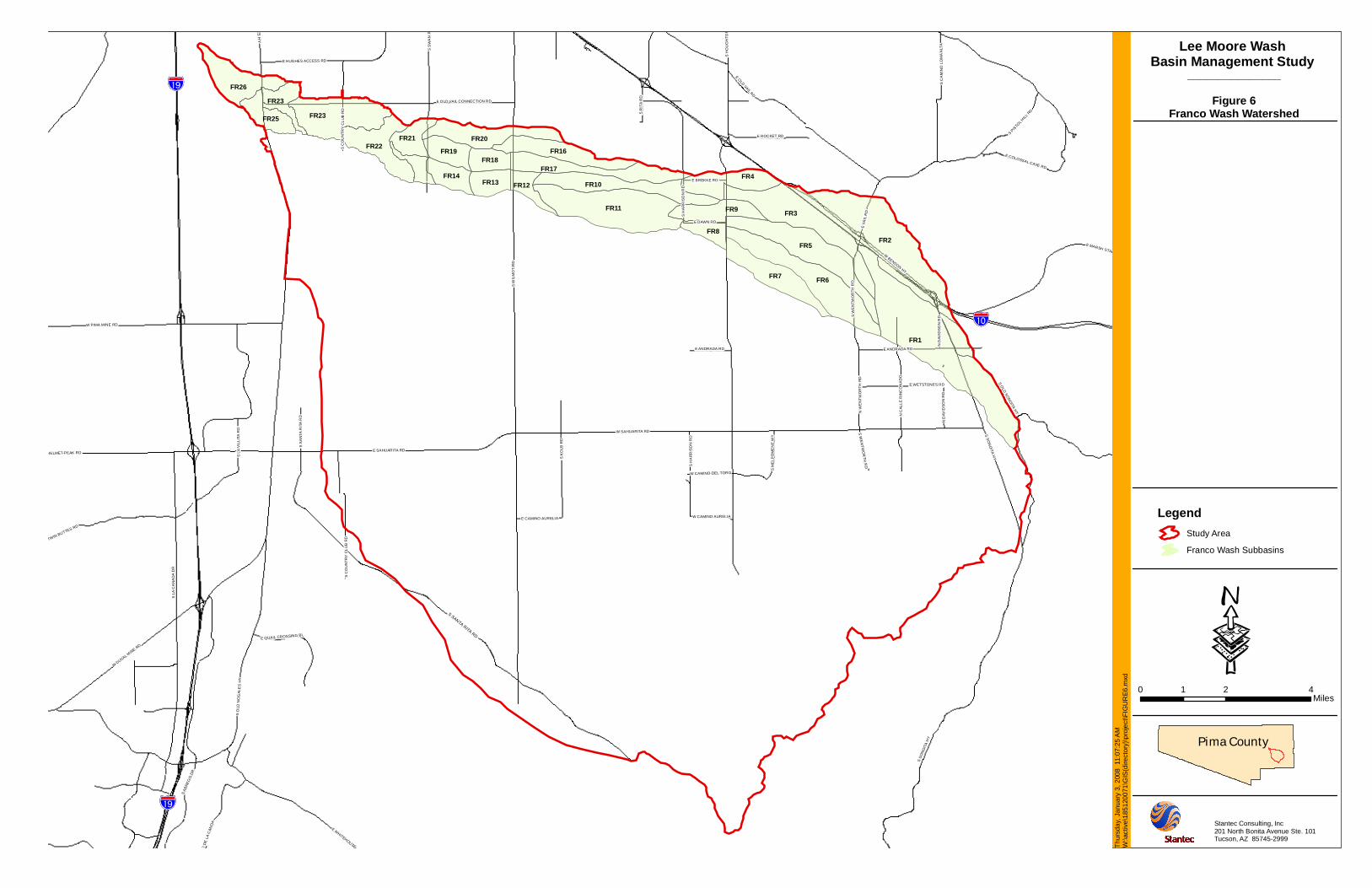
Lee Moore WashBasin Management Study
LegendStudy Area
Franco Wash Subbasins
0 2 41Miles
·Pima County
_______________
Figure 6Franco Wash Watershed
Stantec Consulting, Inc201 North Bonita Avenue Ste. 101Tucson, AZ 85745-2999
Thur
sday
, Jan
uary
3, 2
008
11:
07:2
5 A
MW
:\act
ive\
1851
2007
1\G
IS(d
irect
ory)
\pro
ject
\FIG
UR
E6.m
xd
!"a$
S N
OG
ALE
S H
Y
!"d$
S SANTA RITA RD
!"d$
S W
ILM
OT
RD
S H
OU
GH
TON
RD
S S
AN
TA R
ITA
RD
E SAHUARITA RD
S S
WA
N R
D
S SO
NO
ITA
HY
W DUVAL MINE RD
E MARSH STATION RD
W PIMA MINE RD
S OLD SO
NO
ITA HY
S R
ITA
RD
S AB
REG
O D
R
E WHITEHOUSE CANYON RD
S K
OLB
RD
S LA
CA
NA
DA
DR
S O
LD N
OG
ALE
S H
Y
W HELMET PEAK RD
W TWIN BUTTES RD
E COLOSSAL CAVE RD
E OLD VAIL CONNECTION RD
W DUVAL M
INE WATERLINE RD
W SAHUARITA RD
S A
LVE
RN
ON
WY
S H
AR
RIS
ON
RD
W BENSON HY
E ROCKET RD
E VA
IL R
D
S W
EN
TWO
RTH
RD
E HUGHES ACCESS RD
N C
ALLE
RIN
CO
NA
DO
S PIS
TOL H
ILL R
D
S C
AM
INO
DE
LA
CAN
OA
S C
OU
NTR
Y C
LUB
RD
N W
EN
TWO
RTH
RD
E DAWN RD
S LA
VIL
LITA
RD
E BREKKE RD
E QUAIL CROSSING BL
E ANDRADA RD
S M
ELP
OM
EN
E W
Y
N D
AVID
SON
RD
E CAMINO AURELIA W CAMINO AURELIA
S C
AM
INO
LO
MA
ALT
A
W CAMINO DEL TORO
E WETSTONES RD
N D
AVID
SON
RD
S WE
NTW
OR
TH R
D
S SO
NO
ITA HY
E OLD VAIL RD
S C
OU
NTR
Y C
LUB
RD
S H
AR
RIS
ON
RD
E ANDRADA RD
FR1
FR2
FR6
FR3FR11
FR5
FR23
FR7
FR10FR4
FR17
FR20
FR26
FR22FR16
FR9
FR25
FR19
FR21
FR14
FR8
FR23
FR13
FR18
FR12

31
Houghton Road, with one area located at the northwest corner of the Pima County fairgrounds and the other located near the southwest corner of the fairgrounds. These locations will be referenced as J2 and J4, respectively, in the following discussion, representing the HEC-HMS identifier for the hydrograph used in the FLO-2D analysis. Based on the initial watershed delineation and base modeling efforts, it was evident that runoff concentrating near the northwest corner of the fairgrounds at J2 had no well-defined flow corridor through the downstream watersheds FR10, FR16 and FR17 (Figure 6). Rather, aerial photography, topography and flow patterns suggested that flow could potentially split and/or breakover into any one of the three watersheds, depending on flow depths and channel patterns. Furthermore, these patterns continue as far west as Wilmot Road, thus, the entire corridor including FR10, FR16 and FR17 was analyzed using the FLO-2D computer program in order to assess the distribution of flow for the J2 hydrograph through these areas. Based on the HEC-HMS model, a peak flow of 2712 cfs is estimated at junction J2 during the 100-year, SCS Type 1 storm event, with an upstream watershed area of about 11 square miles (Table 8).
Due to the size of the area studied (in excess of four square miles), the FLO-2D model for J2 was evaluated using a three-dimensional surface based on a 150-foot grid element. Manning’s “n “ values ranged from 0.03 to 0.04 in channel areas, and an estimated roughness value of 0.05 within overbank areas where shallow flow depths were anticipated. The methodology and procedures employed with these modeling efforts are discussed in more detail in the report prepared by JE Fuller Geomorphology and Hydrology, Inc (2008). Based on the modeling results, runoff concentrating at J2 (2712 cfs) spreads out and is dispersed among the three downstream watersheds FR10, FR16, and FR17, with peak flows of 1112 cfs, 811 cfs, and 606 cfs, respectively for the 24-hour storm event. These flows represent the FLO-2D runoff peaks at the mouth of each subject watershed, with FR10 concentrating at a tributary confluence, FR16 at the southern boundary of the State prison, and FR17 at Wilmot Road. The HEC-HMS model was modified by manually inputting each of the FLO2D hydrographs (noted as 2DJ2FR10, etc.) as a source element with a discharge gage, and combining them with their associated HEC-HMS hydrograph (i.e. FR10, FR16 and FR17) for each given subarea. Thus, junctions J3, J14A, and J13A on Figure 13 represent the combined hydrographs for the upstream watershed area and their associated FLO-2D hydrograph from J2 (i.e. FR10 and 2DFR10, respectively at J3, etc.).
32
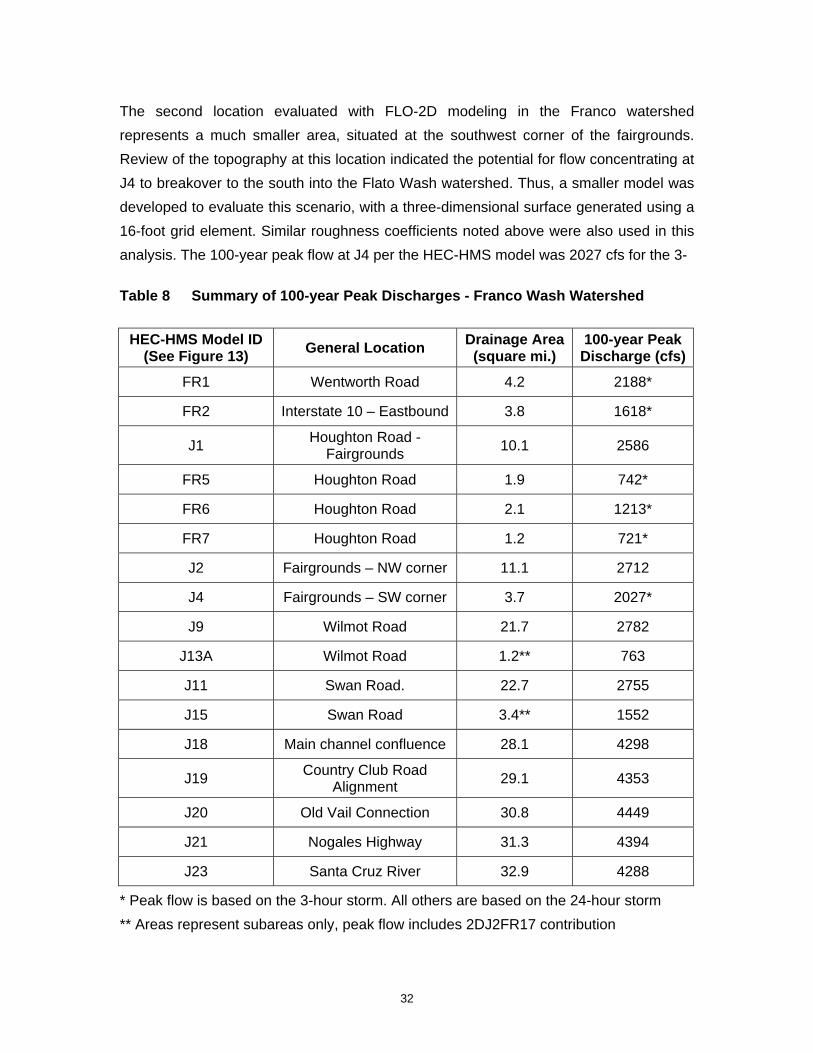
The second location evaluated with FLO-2D modeling in the Franco watershed represents a much smaller area, situated at the southwest corner of the fairgrounds. Review of the topography at this location indicated the potential for flow concentrating at J4 to breakover to the south into the Flato Wash watershed. Thus, a smaller model was developed to evaluate this scenario, with a three-dimensional surface generated using a 16-foot grid element. Similar roughness coefficients noted above were also used in this analysis. The 100-year peak flow at J4 per the HEC-HMS model was 2027 cfs for the 3-
Table 8 Summary of 100-year Peak Discharges - Franco Wash Watershed
HEC-HMS Model ID (See Figure 13) General Location Drainage Area
(square mi.) 100-year Peak Discharge (cfs)
FR1 Wentworth Road 4.2 2188*
FR2 Interstate 10 – Eastbound 3.8 1618*
J1 Houghton Road - Fairgrounds 10.1 2586
FR5 Houghton Road 1.9 742*
FR6 Houghton Road 2.1 1213*
FR7 Houghton Road 1.2 721*
J2 Fairgrounds – NW corner 11.1 2712
J4 Fairgrounds – SW corner 3.7 2027*
J9 Wilmot Road 21.7 2782
J13A Wilmot Road 1.2** 763
J11 Swan Road. 22.7 2755
J15 Swan Road 3.4** 1552
J18 Main channel confluence 28.1 4298
J19 Country Club Road Alignment 29.1 4353
J20 Old Vail Connection 30.8 4449
J21 Nogales Highway 31.3 4394
J23 Santa Cruz River 32.9 4288
* Peak flow is based on the 3-hour storm. All others are based on the 24-hour storm ** Areas represent subareas only, peak flow includes 2DJ2FR17 contribution
33
hour storm event, and based on the FLO-2D modeling efforts, an estimated 530 cfs will discharge south into the Flato watershed rather than remain within the Franco flow corridor. This flow split is represented as a source hydrograph within the HEC-HMS model (2DJ4FLATO), and the resultant FLO-2D hydrograph remaining within the Franco flow corridor was manually input into the HEC-HMS model as 2DJ4FR11. The 2DJ4FR11 hydrograph was combined (J6) with the composite hydrograph of FR5 and FR9 (J5), and routed downstream in the HEC-HMS model through FR11 to the confluence with the previously referenced junction J3 (see Figure 13). Table 8 provides peak flow data for key locations based on the results of the Franco Wash modified HEC-HMS model, with the 100-year, 3-hour peak flows noted as the controlling discharge for the smaller watershed areas.
3.1.2 Hydraulic Model
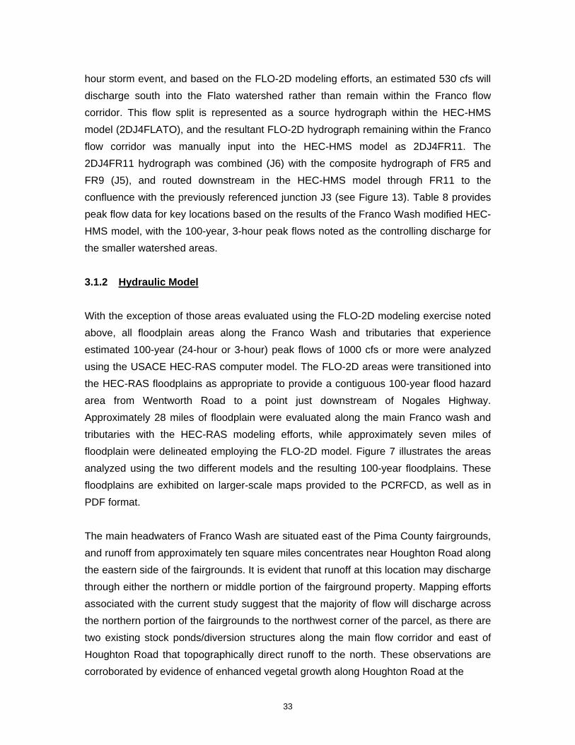
With the exception of those areas evaluated using the FLO-2D modeling exercise noted above, all floodplain areas along the Franco Wash and tributaries that experience estimated 100-year (24-hour or 3-hour) peak flows of 1000 cfs or more were analyzed using the USACE HEC-RAS computer model. The FLO-2D areas were transitioned into the HEC-RAS floodplains as appropriate to provide a contiguous 100-year flood hazard area from Wentworth Road to a point just downstream of Nogales Highway. Approximately 28 miles of floodplain were evaluated along the main Franco wash and tributaries with the HEC-RAS modeling efforts, while approximately seven miles of floodplain were delineated employing the FLO-2D model. Figure 7 illustrates the areas analyzed using the two different models and the resulting 100-year floodplains. These floodplains are exhibited on larger-scale maps provided to the PCRFCD, as well as in PDF format.
The main headwaters of Franco Wash are situated east of the Pima County fairgrounds, and runoff from approximately ten square miles concentrates near Houghton Road along the eastern side of the fairgrounds. It is evident that runoff at this location may discharge through either the northern or middle portion of the fairground property. Mapping efforts associated with the current study suggest that the majority of flow will discharge across the northern portion of the fairgrounds to the northwest corner of the parcel, as there are two existing stock ponds/diversion structures along the main flow corridor and east of Houghton Road that topographically direct runoff to the north. These observations are corroborated by evidence of enhanced vegetal growth along Houghton Road at the
!"a$
S NO
GA
LES
HY
!"a$
S W
ILM
OT
RD
S H
OU
GH
TON
RD
S SA
NTA
RIT
A R
D
E SAHUARITA RD
S SW
AN
RD
E VALENCIA RD
S R
ITA
RD
S K
OLB
RD
E LOS REALES RD
E OLD VAIL CONNECTION RD
E RITA RD
W SAHUARITA RD
S A
LVER
NO
N W
Y
S H
AR
RIS
ON
RD
W BENSON HY
E ROCKET RD
E VA
IL R
D
S W
ENTW
OR
TH R
D
E HUGHES ACCESS RD
N C
ALL
E R
INC
ON
AD
O
S C
OU
NTR
Y C
LUB
RD
N W
ENTW
OR
TH R
D
E DAWN RD
S LA
VIL
LITA
RD
E BREKKE RD
E OLD SPANISH TR
E ANDRADA RD
E HERMANS RD
S M
ELPO
MEN
E W
Y
N D
AVID
SON
RD
W CAMINO AURELIA
S 6TH AV EXTENSION RD
S C
AM
INO
LO
MA
ALT
A
W CAMINO DEL TORO
S C
RAY
CR
OFT
RD
E WETSTONES RD
N D
AVID
SON
RD
S WEN
TWO
RTH
RD
S K
OLB
RD
S C
OU
NTR
Y C
LUB
RD
E OLD VAIL RD
E LOS REALES RD
S H
AR
RIS
ON
RD
E ANDRADA RD
Lee Moore WashBasin Management Study
LegendStudy Area
HEC-RAS Floodplain
FLO-2D Floodplain
0 1 20.5Miles
·
_______________
Figure 7Franco Wash 100-Year Floodplains
Stantec Consulting, Inc201 North Bonita Avenue Ste. 101Tucson, AZ 85745-2999Th
ursd
ay, J
anua
ry 3
, 200
8 1
0:29
:06
AM
W:\a
ctiv
e\18
5120
071\
GIS
(dire
ctor
y)\p
roje
ct\F
IGU
RE7
.mxd
35
broad dip crossing along the northern half of the fairground parcel, as well as the presence of an improved channel constructed on the fairground property to convey flow in this direction. Thus, the floodplain along this reach of the Franco watershed and west of Houghton Road was delineated through the northern portion of the fairground to the northwest corner, where the FLO-2D model was used to rout flow westward from the previously referenced J2. The HEC-RAS modeling from Interstate 10 through the fairgrounds, as well as the downstream FLO-2D model, indicates that these areas are characterized by a wide floodplain zone exhibiting shallow overbank flow depths. However, whereas the upstream floodplains are on the order of a few to several hundred feet, areas delineated within the downstream FLO-2D model area are commonly in excess of 1000 feet wide. The hydraulic model for the reach parallel to Interstate 10 and trending southeast indicates that flows are fairly well-contained up to the Wentworth Road interchange. Floodplain areas situated upstream of Interstate 10 are also relatively contained, although this reach exhibits broader floodplain zones. The culverts underneath the Interstate and frontage road at these locations could not be accessed, and their dimensions were estimated from field observations for the purposes of hydraulic modeling. Based on approximated structure characteristics, the existing culverts have ample capacity to convey estimated 100-year, 3-hour peak discharge. The floodplains along the above-referenced channel reaches upstream and parallel to Interstate 10 were each mapped on the basis of the 100-year, 3-hour peak flow, while all channel reaches downstream of I-10 and through the FLO2D areas (all areas downstream of J2, Figure 13) were modeled using 24-hour peak flows.
The southern branch of Franco Wash that concentrates runoff near the southwest corner of the fairgrounds has several stock ponds and diversion berms situated along the watercourse downstream of the fairground. These areas are also characterized by broad floodplain areas. Since the integrity of these structures is unknown, failure of the structures during large storm events such as the 100-year storm could result in local flooding downstream, and/or around the structures, and mapping modifications were made accordingly to reflect these circumstances. The 3-hour peak flow was employed to map this channel reach and upstream through subbasin FR6. This branch of Franco Wash combines with a portion of the FLO2D flow split from J2 (hydrograph referenced as 2DJ2FR10) just upstream of Wilmot Road (J8 on Figure 13), and the 24-hour discharge was utilized to map all remaining floodplains downstream of J8.
36
Although the flow corridor is relatively well-defined downstream of the above-noted confluence (J8), most areas within the corridor to Swan Road exhibit broad 100-year floodplains with significant overbank flow. These areas typically coincide with the reaches in the HEC-HMS model that have been defined with a single subreach for storage routing purposes. The channel system downstream of Swan Road is well-defined, and flows are predominantly contained for approximately one mile west of Swan Road until the confluence of flow at J18 about two miles upstream of the Country Club Road alignment. The tributary branch that combines with the main channel at this location exhibits similar upstream floodplain morphologies as described along the main channel reach. The 24-hour, 100-year composite peak discharge is about 4300 cfs at this location, and floodwaters gradually spill out into overbank areas downstream as the channel capacity diminishes. Floodplain areas downstream of the Country Club Road alignment that impact the previously referenced Summit neighborhoods are several hundred feet wide, with significant flow in the overbanks areas during the 100-year storm event. Several existing drainage structures along the Franco Wash were modeled within the HEC-RAS modeling efforts, including a USPS (Union Pacific/Southern Pacific) railroad bridge upstream of Nogales Highway, a six-cell 10-ft x 7-ft box culvert at Nogales Highway, a five-cell box culvert at Swan Road, and the Interstate 10 structures previously referenced. Survey data for the structures at the railroad and Nogales Highway were obtained by Stantec Consulting Inc. field survey personnel, while the culvert at Swan Road was modeled on the basis of field measurements and available one-foot topography developed for the proposed Verano subdivision. Information for the structures upstream of the fairgrounds at Interstate 10 was previously discussed. Based on the hydraulic modeling efforts, all structures appear to have capacity to convey their associated 100-year peak discharge. However, it was evident that flow upstream of the USPS railroad bridge would spill over Old Nogales Highway, and overtop Nogales Highway at a point south of the existing box culvert at the Franco main channel. At the direction of County staff, a split flow analysis was performed at this location, as well as a storage routing to determine the effect of the roadway overtopping. On the basis of this analysis, it was determined that both the railroad bridge and culvert under Nogales Highway have capacity to convey the 100-year flow underneath the roadway, however, the roadway will be flooded to the south to a depth of about one foot. Approximately 1800 cfs of the estimated 4400 cfs concentrating at the railroad bridge will spill south over Old Nogales Highway at this location, and ultimately overtop Nogales Highway south of the Franco Wash stream crossing.
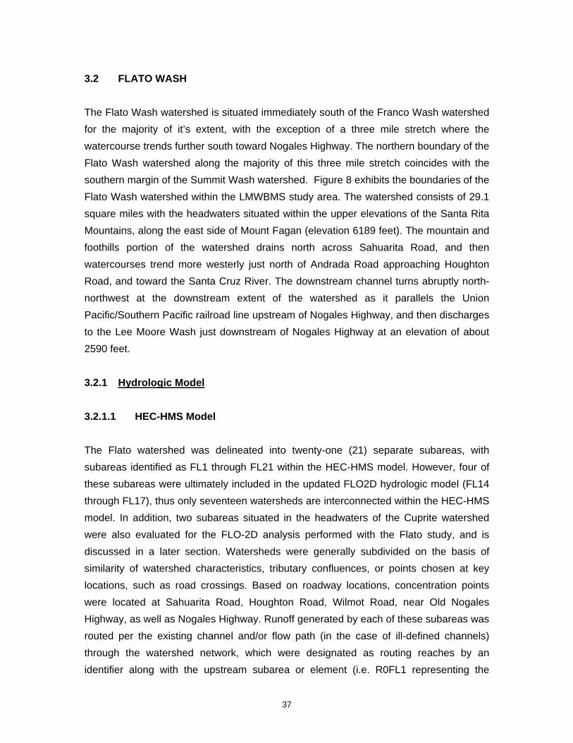
37
3.2 FLATO WASH
The Flato Wash watershed is situated immediately south of the Franco Wash watershed for the majority of it’s extent, with the exception of a three mile stretch where the watercourse trends further south toward Nogales Highway. The northern boundary of the Flato Wash watershed along the majority of this three mile stretch coincides with the southern margin of the Summit Wash watershed. Figure 8 exhibits the boundaries of the Flato Wash watershed within the LMWBMS study area. The watershed consists of 29.1 square miles with the headwaters situated within the upper elevations of the Santa Rita Mountains, along the east side of Mount Fagan (elevation 6189 feet). The mountain and foothills portion of the watershed drains north across Sahuarita Road, and then watercourses trend more westerly just north of Andrada Road approaching Houghton Road, and toward the Santa Cruz River. The downstream channel turns abruptly north-northwest at the downstream extent of the watershed as it parallels the Union Pacific/Southern Pacific railroad line upstream of Nogales Highway, and then discharges to the Lee Moore Wash just downstream of Nogales Highway at an elevation of about 2590 feet.
3.2.1 Hydrologic Model
3.2.1.1 HEC-HMS Model
The Flato watershed was delineated into twenty-one (21) separate subareas, with subareas identified as FL1 through FL21 within the HEC-HMS model. However, four of these subareas were ultimately included in the updated FLO2D hydrologic model (FL14 through FL17), thus only seventeen watersheds are interconnected within the HEC-HMS model. In addition, two subareas situated in the headwaters of the Cuprite watershed were also evaluated for the FLO-2D analysis performed with the Flato study, and is discussed in a later section. Watersheds were generally subdivided on the basis of similarity of watershed characteristics, tributary confluences, or points chosen at key locations, such as road crossings. Based on roadway locations, concentration points were located at Sahuarita Road, Houghton Road, Wilmot Road, near Old Nogales Highway, as well as Nogales Highway. Runoff generated by each of these subareas was routed per the existing channel and/or flow path (in the case of ill-defined channels) through the watershed network, which were designated as routing reaches by an identifier along with the upstream subarea or element (i.e. R0FL1 representing the
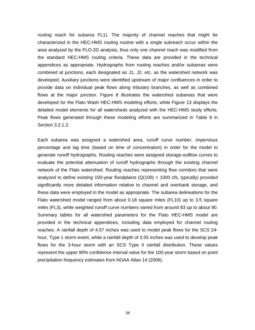
38
routing reach for subarea FL1). The majority of channel reaches that might be characterized in the HEC-HMS routing routine with a single subreach occur within the area analyzed by the FLO-2D analysis, thus only one channel reach was modified from the standard HEC-HMS routing criteria. These data are provided in the technical appendices as appropriate. Hydrographs from routing reaches and/or subareas were combined at junctions, each designated as J1, J2, etc. as the watershed network was developed. Auxiliary junctions were identified upstream of major confluences in order to provide data on individual peak flows along tributary branches, as well as combined flows at the major junction. Figure 8 illustrates the watershed subareas that were developed for the Flato Wash HEC-HMS modeling efforts, while Figure 13 displays the detailed model elements for all watersheds analyzed with the HEC-HMS study efforts. Peak flows generated through these modeling efforts are summarized in Table 9 in Section 3.2.1.2.
Each subarea was assigned a watershed area, runoff curve number, impervious percentage and lag time (based on time of concentration) in order for the model to generate runoff hydrographs. Routing reaches were assigned storage-outflow curves to evaluate the potential attenuation of runoff hydrographs through the existing channel network of the Flato watershed. Routing reaches representing flow corridors that were analyzed to define existing 100-year floodplains (Q(100) > 1000 cfs, typically) provided significantly more detailed information relative to channel and overbank storage, and these data were employed in the model as appropriate. The subarea delineations for the Flato watershed model ranged from about 0.18 square miles (FL10) up to 3.5 square miles (FL3), while weighted runoff curve numbers varied from around 83 up to about 90. Summary tables for all watershed parameters for the Flato HEC-HMS model are provided in the technical appendices, including data employed for channel routing reaches. A rainfall depth of 4.57 inches was used to model peak flows for the SCS 24-hour, Type 1 storm event, while a rainfall depth of 3.55 inches was used to develop peak flows for the 3-hour storm with an SCS Type II rainfall distribution. These values represent the upper 90% confidence interval value for the 100-year storm based on point precipitation frequency estimates from NOAA Atlas 14 (2006).

Lee Moore WashBasin Management Plan
LegendStudy Area
Cuprite Wash Subbasin
Flato Wash Subbasin
0 2 41Miles
·Pima County
_______________
Figure 8Flato Wash Watershed
Stantec Consulting, Inc201 North Bonita Avenue Ste. 101Tucson, AZ 85745-2999
Thur
sday
, Jan
uary
3, 2
008
10:
33:0
4 A
MW
:\act
ive\
1851
2007
1\G
IS(d
irect
ory)
\pro
ject
\FIG
UR
E8.m
xd
!"a$
S N
OG
ALE
S H
Y
!"d$
S SANTA RITA RD
!"d$
CU1
CU2
S W
ILM
OT
RD
S H
OU
GH
TON
RD
S S
AN
TA R
ITA
RD
E SAHUARITA RD
S S
WA
N R
D
S SO
NO
ITA
HY
W DUVAL MINE RD
E MARSH STATION RD
W PIMA MINE RD
S OLD SO
NO
ITA HY
S R
ITA
RD
S AB
REG
O D
R
E WHITEHOUSE CANYON RD
S K
OLB
RD
S LA
CA
NA
DA
DR
S O
LD N
OG
ALE
S H
Y
W HELMET PEAK RD
W TWIN BUTTES RD
E COLOSSAL CAVE RD
E OLD VAIL CONNECTION RD
W DUVAL M
INE WATERLINE RD
W SAHUARITA RD
S A
LVE
RN
ON
WY
S H
AR
RIS
ON
RD
W BENSON HY
E ROCKET RD
E VA
IL R
D
S W
EN
TWO
RTH
RD
E HUGHES ACCESS RD
N C
ALLE
RIN
CO
NA
DO
S PIS
TOL H
ILL R
D
S C
AM
INO
DE
LA
CAN
OA
S C
OU
NTR
Y C
LUB
RD
N W
EN
TWO
RTH
RD
E DAWN RD
S LA
VIL
LITA
RD
E BREKKE RD
E OLD SPANISH TR
E QUAIL CROSSING BL
E ANDRADA RD
E HERMANS RD
S M
ELP
OM
EN
E W
Y
N D
AVID
SON
RD
E CAMINO AURELIA W CAMINO AURELIA
S C
AM
INO
LO
MA
ALT
A
W CAMINO DEL TORO
E WETSTONES RD
N D
AVID
SON
RD
S WE
NTW
OR
TH R
D
S SO
NO
ITA HY
E OLD VAIL RD
S C
OU
NTR
Y C
LUB
RD
S H
AR
RIS
ON
RD
E ANDRADA RD
FL3
FL1
FLO2D
FL11
FL2
FL20
FL6FL13
FL8
FL7
FL19
FL9
FL18
FL5
FL21
FL4FL12
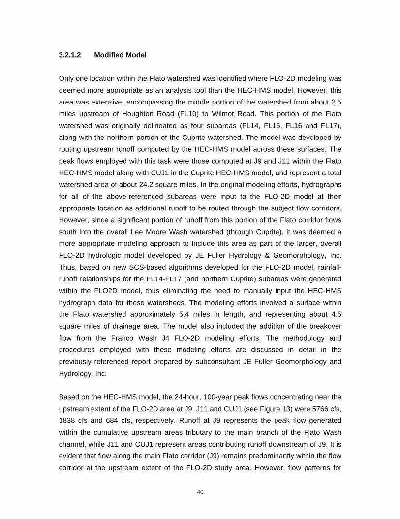
40
3.2.1.2 Modified Model
Only one location within the Flato watershed was identified where FLO-2D modeling was deemed more appropriate as an analysis tool than the HEC-HMS model. However, this area was extensive, encompassing the middle portion of the watershed from about 2.5 miles upstream of Houghton Road (FL10) to Wilmot Road. This portion of the Flato watershed was originally delineated as four subareas (FL14, FL15, FL16 and FL17), along with the northern portion of the Cuprite watershed. The model was developed by routing upstream runoff computed by the HEC-HMS model across these surfaces. The peak flows employed with this task were those computed at J9 and J11 within the Flato HEC-HMS model along with CUJ1 in the Cuprite HEC-HMS model, and represent a total watershed area of about 24.2 square miles. In the original modeling efforts, hydrographs for all of the above-referenced subareas were input to the FLO-2D model at their appropriate location as additional runoff to be routed through the subject flow corridors. However, since a significant portion of runoff from this portion of the Flato corridor flows south into the overall Lee Moore Wash watershed (through Cuprite), it was deemed a more appropriate modeling approach to include this area as part of the larger, overall FLO-2D hydrologic model developed by JE Fuller Hydrology & Geomorphology, Inc. Thus, based on new SCS-based algorithms developed for the FLO-2D model, rainfall-runoff relationships for the FL14-FL17 (and northern Cuprite) subareas were generated within the FLO2D model, thus eliminating the need to manually input the HEC-HMS hydrograph data for these watersheds. The modeling efforts involved a surface within the Flato watershed approximately 5.4 miles in length, and representing about 4.5 square miles of drainage area. The model also included the addition of the breakover flow from the Franco Wash J4 FLO-2D modeling efforts. The methodology and procedures employed with these modeling efforts are discussed in detail in the previously referenced report prepared by subconsultant JE Fuller Geomorphology and Hydrology, Inc.
Based on the HEC-HMS model, the 24-hour, 100-year peak flows concentrating near the upstream extent of the FLO-2D area at J9, J11 and CUJ1 (see Figure 13) were 5766 cfs, 1838 cfs and 684 cfs, respectively. Runoff at J9 represents the peak flow generated within the cumulative upstream areas tributary to the main branch of the Flato Wash channel, while J11 and CUJ1 represent areas contributing runoff downstream of J9. It is evident that flow along the main Flato corridor (J9) remains predominantly within the flow corridor at the upstream extent of the FLO-2D study area. However, flow patterns for
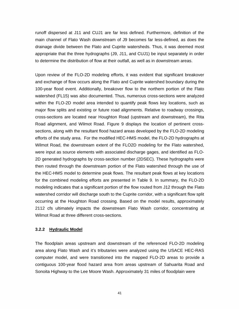
41
runoff dispersed at J11 and CUJ1 are far less defined. Furthermore, definition of the main channel of Flato Wash downstream of J9 becomes far less-defined, as does the drainage divide between the Flato and Cuprite watersheds. Thus, it was deemed most appropriate that the three hydrographs (J9, J11, and CUJ1) be input separately in order to determine the distribution of flow at their outfall, as well as in downstream areas.
Upon review of the FLO-2D modeling efforts, it was evident that significant breakover and exchange of flow occurs along the Flato and Cuprite watershed boundary during the 100-year flood event. Additionally, breakover flow to the northern portion of the Flato watershed (FL15) was also documented. Thus, numerous cross-sections were analyzed within the FLO-2D model area intended to quantify peak flows key locations, such as major flow splits and existing or future road alignments. Relative to roadway crossings, cross-sections are located near Houghton Road (upstream and downstream), the Rita Road alignment, and Wilmot Road. Figure 9 displays the location of pertinent cross-sections, along with the resultant flood hazard areas developed by the FLO-2D modeling efforts of the study area. For the modified HEC-HMS model, the FLO-2D hydrographs at Wilmot Road, the downstream extent of the FLO2D modeling for the Flato watershed, were input as source elements with associated discharge gages, and identified as FLO-2D generated hydrographs by cross-section number (2DSEC). These hydrographs were then routed through the downstream portion of the Flato watershed through the use of the HEC-HMS model to determine peak flows. The resultant peak flows at key locations for the combined modeling efforts are presented in Table 9. In summary, the FLO-2D modeling indicates that a significant portion of the flow routed from J12 through the Flato watershed corridor will discharge south to the Cuprite corridor, with a significant flow split occurring at the Houghton Road crossing. Based on the model results, approximately 2112 cfs ultimately impacts the downstream Flato Wash corridor, concentrating at Wilmot Road at three different cross-sections.
3.2.2 Hydraulic Model
The floodplain areas upstream and downstream of the referenced FLO-2D modeling area along Flato Wash and it’s tributaries were analyzed using the USACE HEC-RAS computer model, and were transitioned into the mapped FLO-2D areas to provide a contiguous 100-year flood hazard area from areas upstream of Sahuarita Road and Sonoita Highway to the Lee Moore Wash. Approximately 31 miles of floodplain were
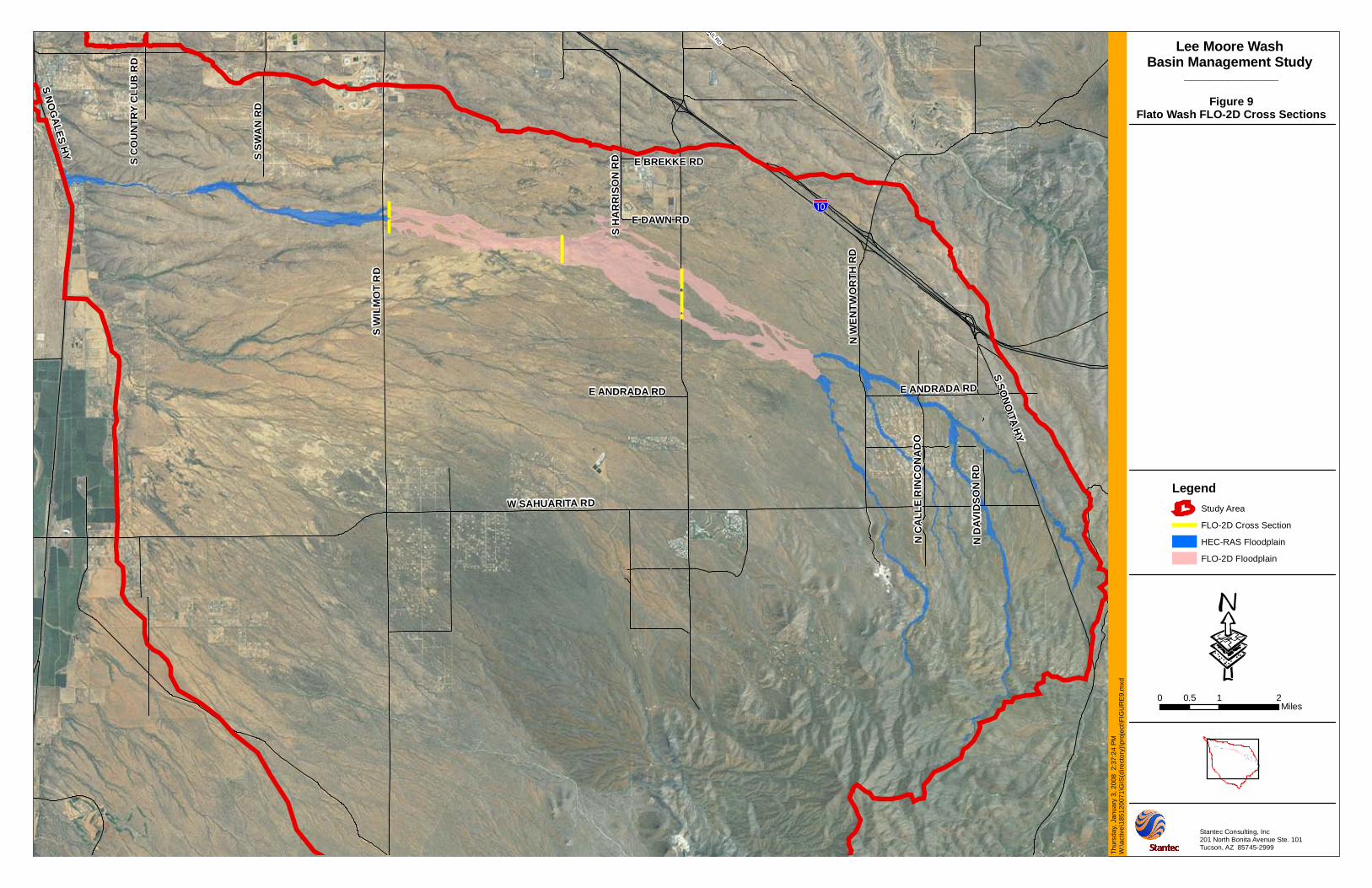
!"a$
S NO
GA
LES HY
S W
ILM
OT
RD
S C
OU
NTR
Y C
LUB
RD
S SW
AN
RD
N W
ENTW
OR
TH R
D
E ANDRADA RD
N D
AVID
SON
RD
N C
ALL
E R
INC
ON
AD
O
S SONO
ITA HY
E ANDRADA RD
W SAHUARITA RD
E DAWN RD
S H
AR
RIS
ON
RD E BREKKE RD
S C
AM
INO
LO
MA
ALTA
E OLD VAIL RD Lee Moore WashBasin Management Study
LegendStudy Area
FLO-2D Cross Section
HEC-RAS Floodplain
FLO-2D Floodplain
0 1 20.5Miles
·
_______________
Figure 9Flato Wash FLO-2D Cross Sections
Stantec Consulting, Inc201 North Bonita Avenue Ste. 101Tucson, AZ 85745-2999
Thur
sday
, Jan
uary
3, 2
008
2:3
7:24
PM
W:\a
ctiv
e\18
5120
071\
GIS
(dire
ctor
y)\p
roje
ct\F
IGU
RE
9.m
xd
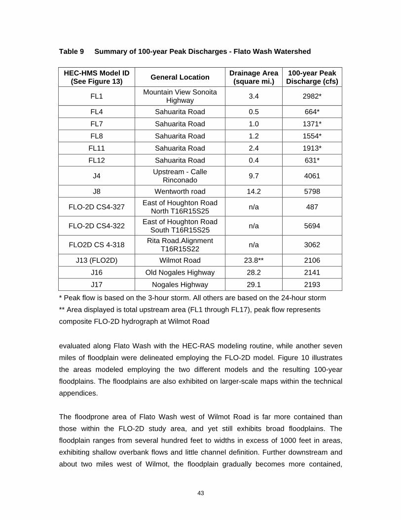
43
Table 9 Summary of 100-year Peak Discharges - Flato Wash Watershed
HEC-HMS Model ID (See Figure 13) General Location Drainage Area
(square mi.) 100-year Peak Discharge (cfs)
FL1 Mountain View Sonoita Highway 3.4 2982*
FL4 Sahuarita Road 0.5 664*
FL7 Sahuarita Road 1.0 1371*
FL8 Sahuarita Road 1.2 1554*
FL11 Sahuarita Road 2.4 1913*
FL12 Sahuarita Road 0.4 631*
J4 Upstream - Calle Rinconado 9.7 4061
J8 Wentworth road 14.2 5798
FLO-2D CS4-327 East of Houghton Road North T16R15S25 n/a 487
FLO-2D CS4-322 East of Houghton Road South T16R15S25 n/a 5694
FLO2D CS 4-318 Rita Road.Alignment T16R15S22 n/a 3062
J13 (FLO2D) Wilmot Road 23.8** 2106
J16 Old Nogales Highway 28.2 2141
J17 Nogales Highway 29.1 2193
* Peak flow is based on the 3-hour storm. All others are based on the 24-hour storm ** Area displayed is total upstream area (FL1 through FL17), peak flow represents composite FLO-2D hydrograph at Wilmot Road
evaluated along Flato Wash with the HEC-RAS modeling routine, while another seven miles of floodplain were delineated employing the FLO-2D model. Figure 10 illustrates the areas modeled employing the two different models and the resulting 100-year floodplains. The floodplains are also exhibited on larger-scale maps within the technical appendices.
The floodprone area of Flato Wash west of Wilmot Road is far more contained than those within the FLO-2D study area, and yet still exhibits broad floodplains. The floodplain ranges from several hundred feet to widths in excess of 1000 feet in areas, exhibiting shallow overbank flows and little channel definition. Further downstream and about two miles west of Wilmot, the floodplain gradually becomes more contained,

44
narrowing to a few to several hundred feet. At a point about 3.25 miles west of Wilmot, the channel becomes well-defined and incised, and predominantly contains the 100-year flow within a flow corridor less than 300 feet wide. However, similar to the previously referenced Franco channel, the channel loses definition at a point about 3600 feet upstream of Nogales Highway, and flows again break out into overbank areas. The floodplain within this area attains widths of several hundred feet to in excess of 1000 feet upstream of the Union Pacific/Southern Pacific railroad bridge. Similar to the downstream areas described above, the floodplains along the main Flato Wash corridor and associated tributaries upstream of the FLO-2D area are also predominantly contained within well-defined flow corridors, with a few exceptions. These areas occur near the tributary confluence with the main Flato flow corridor, as well as specific areas along the tributaries where defined channel flow disperses into a more braided, multiple channel nature. All floodplain mapping along the main Flato Wash corridor downstream of junction J4 (Figure 13) to Nogales Hwy was modeled using the 24-hour peak flows, while all tributaries to the south and the channel reach east of J4 were mapped using the 3-hout discharges generated with the Flato HEC-HMS model.
Three structures along the Flato Wash were modeled within the HEC-RAS modeling efforts; a USPS railroad bridge upstream of Nogales Highway, a two-cell box structure at Nogales Highway, approximately 16.5 feet wide and 8.5 feet high, and a 4-cell structure underneath Sonoita Highway in the upstream reach of the Flato Wash main flow corridor. Survey data for the structures at the railroad and Nogales Highway were obtained by Stantec Consulting Inc. field survey personnel, while the upstream structure was estimated employing field observations and aerial photography. The Nogales Highway structure was assumed to be a 16.5-ft x 8-ft RCB for modeling purposes, and accounting for existing sediment deposits along the structure floor. Based on the modeling efforts, it was determined that all of the structures evaluated have capacity to convey their associated estimated 100-year flow. An incised, erosional channel downstream of Nogales Highway conveys flow to the Lee Moore Wash, fully contained within the channel.
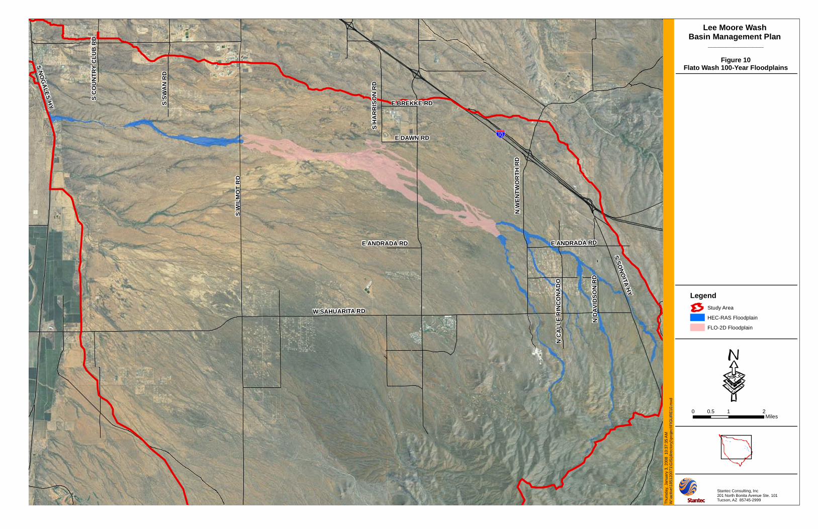
!"a$
S NO
GA
LES HY
S W
ILM
OT
RD
S C
OU
NTR
Y C
LUB
RD
S SW
AN
RD
N W
ENTW
OR
TH R
D
E ANDRADA RD
N D
AVID
SON
RD
N C
ALL
E R
INC
ON
AD
O
S SONO
ITA HY
E ANDRADA RD
W SAHUARITA RD
E DAWN RD
S H
AR
RIS
ON
RD
E BREKKE RD
Lee Moore WashBasin Management Plan
LegendStudy Area
HEC-RAS Floodplain
FLO-2D Floodplain
0 1 20.5Miles
·
_______________
Figure 10Flato Wash 100-Year Floodplains
Stantec Consulting, Inc201 North Bonita Avenue Ste. 101Tucson, AZ 85745-2999
Thur
sday
, Jan
uary
3, 2
008
10:
37:3
5 A
MW
:\act
ive\
1851
2007
1\G
IS(d
irect
ory)
\pro
ject
\FIG
UR
E10.
mxd

46
3.3 LEE MOORE WASH AND SUMMIT AREAS
The Lee Moore Wash evaluated with the current study is situated west of Nogales Highway, where the channel trends north-northwest to the Santa Cruz River. The Summit Wash and associated watersheds are situated east of Nogales Highway. Given the nominal drainage areas and limited number of sub-basins employed in the analyses, all of the Summit area watersheds were grouped together as a single HEC-HMS model. Summit Wash is bounded by the Franco Wash watershed to the north, and the Flato Wash watershed to the south. The three, unnamed watersheds are smaller areas that concentrate runoff at the USPS railroad, and their discharges are conveyed individually underneath the railroad and Nogales Highway to the Lee Moore Wash. Thus, they are not tributary to any of the larger watersheds modeled in the current study. The Lee Moore Wash watershed, as defined with the FLO-2D modeling efforts, consists of all watershed areas south of Flato, with the exception of the watershed area comprising UN1 (Figure 11). The Lee Moore channel conveys flow underneath the railroad and Nogales Highway about 1.5 miles north of Pima Mine Road. The Summit Wash watershed is about 2.5 square miles, while the drainage areas for the unnamed watersheds UN1, UN2, and UN3 are 1.4 square miles, 0.2 square miles, and 0.14 square miles, respectively. The headwaters of all these watersheds lie within the lower valley areas to Santa Cruz River, and their locations are displayed in Figure 11.
3.3.1 Hydrologic Model
The HEC-HMS model for the Summit watershed is comprised of four subareas, designated as S1 through S4 in the model. Each of the unnamed watersheds is modeled as a single watershed designated as UN1, UN2 and UN3. Watersheds within the Summit model were subdivided on the basis of tributary confluences, with the composite peak flow generated from all watersheds computed at the confluence with the Lee Moore channel, west of Nogales Highway. Runoff from subareas were routed through the watershed network for Summit Wash with a limited number of routing reaches, and hydrographs from routing reaches and/or subareas were combined at junctions as described in the previous HEC-HMS analyses. Figure 11 illustrates the watershed subareas that were used in the HEC-HMS model, while Figure 13 displays the detailed model elements. The Lee Moore Wash model was also developed as a separate model, and generally consists of the resulting HEC-HMS hydrographs at the mouths of Summit Wash, unnamed watersheds and Flato Wash, combined with the FLO-2D hydrograph

S N
OG
ALE
S H
Y
S W
ILM
OT
RD
E OLD VAIL CONNECTION RD
S C
OU
NTR
Y C
LUB
RD
S1
S2
UN1
S3
UN2
UN3
S4
Lee Moore WashBasin Management Study
LegendStudy Area
Summit Area Watershed
0 0.5 10.25Miles
·
_______________
Figure 11Summit Area Watersheds
Stantec Consulting, Inc201 North Bonita Avenue Ste. 101Tucson, AZ 85745-2999
Thur
sday
, Jan
uary
3, 2
008
3:4
2:43
PM
W:\a
ctiv
e\18
5120
071\
GIS
(dire
ctor
y)\p
roje
ct\F
IGU
RE
11.m
xd
48
generated at the Lee Moore USPP railroad bridge. The 24-hour, Type 1 runoff hydrographs for the referenced Lee Moore tributaries (Summit, Flato, etc.) were employed within these modeling efforts, consistent with the FLO-2D hydrologic model hydrograph for the Lee Moore Wash.
Each subarea was assigned a watershed area, runoff curve number, impervious percentage and lag time (based on time of concentration) in order for the model to generate runoff hydrographs. Routing reaches were assigned storage-outflow curves to evaluate the potential attenuation of runoff hydrographs through the existing channel network for each watershed. Summary tables for all HEC-HMS watershed parameters for the Summit watershed model are provided in the technical appendices, including data employed for channel routing reaches. The rainfall depths for all watersheds are similar, thus the 3-hour rainfall depth of 3.23 inches for the Summit watershed was employed to model runoff for the 3-hour storm event. A rainfall depth of 4.13 inches was used to model peak flows for the 24-hour storm event. All rainfall depths employed with these analyses are representative of the upper 90% confidence interval value for the 100-year storm, based on point precipitation frequency estimates from NOAA Atlas 14 (2006). Table 10 presents a summary of the peak flows generated by the HEC-HMS modeling for the associated watershed areas.
3.3.2 Hydraulic Model
Although the 100-year peak flows fell below the general threshold peak developed for the LMWBMS study, the floodplain areas downstream of Country Club Road along the Summit Wash were analyzed using the USACE HEC-RAS computer model. These efforts were performed at the request of the PCRFCD due to the existence of innumerable homes within the area, and the occurrence of recent flooding events over the past few years. Cross-sections were developed at approximately 200-foot intervals in order to generate a more detailed assessment of anticipated flood hazards within these areas. Peak flows developed from the 3-hour storm HEC-HMS analysis were employed for the associated floodplain mapping efforts. About 4.4 miles were evaluated along Summit Wash and its tributary to the south with the HEC-RAS modeling routine. There is very little channel definition along either of these watercourses, thus floodplains are typically broad areas displaying shallow depths, often several hundred feet wide. Figure 12 displays the 100-year floodplains defined with the HEC-RAS modeling within the Summit watershed.
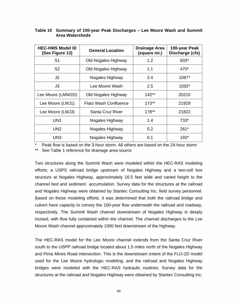
49
Table 10 Summary of 100-year Peak Discharges – Lee Moore Wash and Summit Area Watersheds
HEC-HMS Model ID (See Figure 13) General Location Drainage Area
(square mi.) 100-year Peak Discharge (cfs)
S1 Old Nogales Highway 1.2 603*
S2 Old Nogales Highway 1.1 470*
J2 Nogales Highway 2.4 1087*
J3 Lee Moore Wash 2.5 1092*
Lee Moore (LMW2D) Old Nogales Highway 142** 20210
Lee Moore (LMJ1) Flato Wash Confluence 173** 21929
Lee Moore (LMJ3) Santa Cruz River 178** 21822
UN1 Nogales Highway 1.4 733*
UN2 Nogales Highway 0.2 261*
UN3 Nogales Highway 0.1 192*
* Peak flow is based on the 3-hour storm. All others are based on the 24-hour storm ** See Table 1 reference for drainage area source Two structures along the Summit Wash were modeled within the HEC-RAS modeling efforts; a USPS railroad bridge upstream of Nogales Highway and a two-cell box structure at Nogales Highway, approximately 16.5 feet wide and varied height to the channel bed and sediment accumulation. Survey data for the structures at the railroad and Nogales Highway were obtained by Stantec Consulting Inc. field survey personnel. Based on these modeling efforts, it was determined that both the railroad bridge and culvert have capacity to convey the 100-year flow underneath the railroad and roadway, respectively. The Summit Wash channel downstream of Nogales Highway is deeply incised, with flow fully contained within the channel. The channel discharges to the Lee Moore Wash channel approximately 1000 feet downstream of the highway.
The HEC-RAS model for the Lee Moore channel extends from the Santa Cruz River south to the USPP railroad bridge located about 1.5 miles north of the Nogales Highway and Pima Mines Road intersection. This is the downstream extent of the FLO-2D model used for the Lee Moore hydrologic modeling, and the railroad and Nogales Highway bridges were modeled with the HEC-RAS hydraulic routines. Survey data for the structures at the railroad and Nogales Highway were obtained by Stantec Consulting Inc.

50
field survey personnel. The results of the floodplain modeling efforts indicate that the 100-year peak flow estimated for the Lee Moore channel, approximately 22,000 cfs, is predominantly contained within the downstream channel to the Santa Cruz River, with some localized overbank flooding. The resulting 100-year floodplain along the Lee Moore Wash developed with this effort is also illustrated on Figure 12.
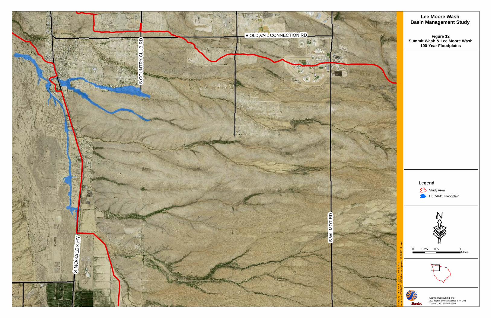
S N
OG
ALE
S H
Y S W
ILM
OT
RD
E OLD VAIL CONNECTION RD
S C
OU
NTR
Y C
LUB
RD
Lee Moore WashBasin Management Study
LegendStudy Area
HEC-RAS Floodplain
0 0.5 10.25Miles
·
_______________
Figure 12Summit Wash & Lee Moore Wash
100-Year Floodplains
Stantec Consulting, Inc201 North Bonita Avenue Ste. 101Tucson, AZ 85745-2999
Thur
sday
, Jan
uary
3, 2
008
11:
05:2
1 A
MW
:\act
ive\
1851
2007
1\G
IS(d
irect
ory)
\pro
ject
\FIG
UR
E12
.mxd
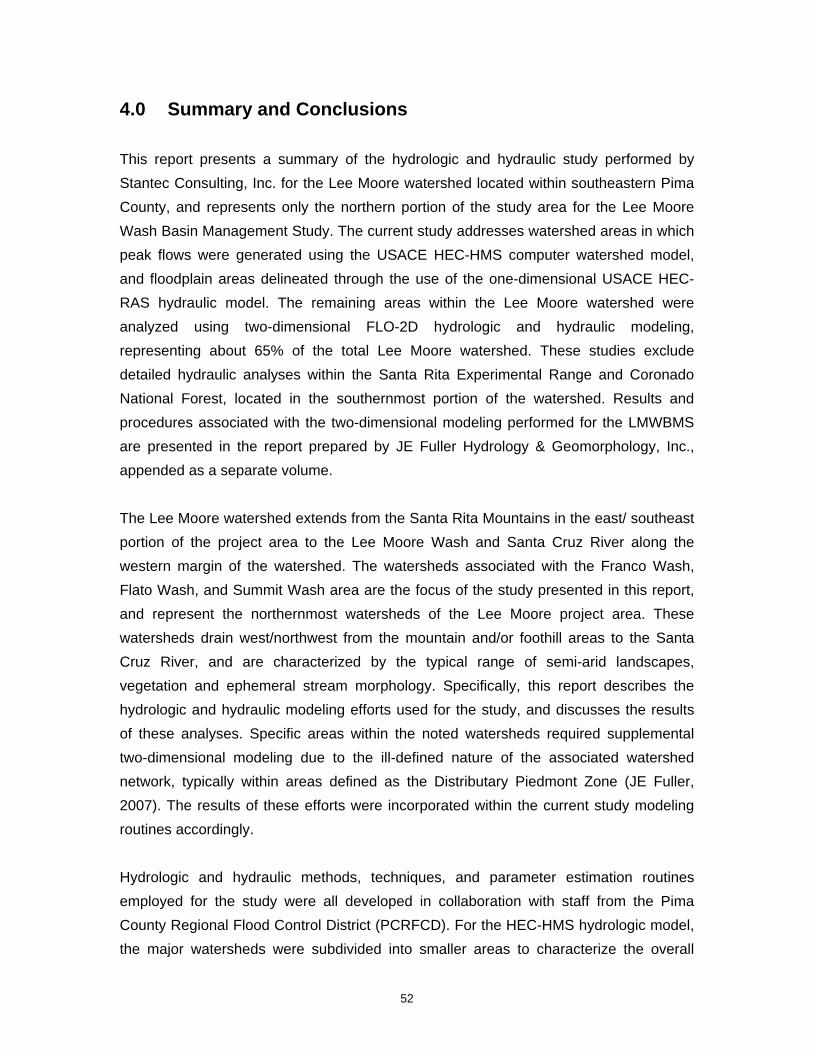
52
4.0 Summary and Conclusions
This report presents a summary of the hydrologic and hydraulic study performed by Stantec Consulting, Inc. for the Lee Moore watershed located within southeastern Pima County, and represents only the northern portion of the study area for the Lee Moore Wash Basin Management Study. The current study addresses watershed areas in which peak flows were generated using the USACE HEC-HMS computer watershed model, and floodplain areas delineated through the use of the one-dimensional USACE HEC-RAS hydraulic model. The remaining areas within the Lee Moore watershed were analyzed using two-dimensional FLO-2D hydrologic and hydraulic modeling, representing about 65% of the total Lee Moore watershed. These studies exclude detailed hydraulic analyses within the Santa Rita Experimental Range and Coronado National Forest, located in the southernmost portion of the watershed. Results and procedures associated with the two-dimensional modeling performed for the LMWBMS are presented in the report prepared by JE Fuller Hydrology & Geomorphology, Inc., appended as a separate volume.
The Lee Moore watershed extends from the Santa Rita Mountains in the east/ southeast portion of the project area to the Lee Moore Wash and Santa Cruz River along the western margin of the watershed. The watersheds associated with the Franco Wash, Flato Wash, and Summit Wash area are the focus of the study presented in this report, and represent the northernmost watersheds of the Lee Moore project area. These watersheds drain west/northwest from the mountain and/or foothill areas to the Santa Cruz River, and are characterized by the typical range of semi-arid landscapes, vegetation and ephemeral stream morphology. Specifically, this report describes the hydrologic and hydraulic modeling efforts used for the study, and discusses the results of these analyses. Specific areas within the noted watersheds required supplemental two-dimensional modeling due to the ill-defined nature of the associated watershed network, typically within areas defined as the Distributary Piedmont Zone (JE Fuller, 2007). The results of these efforts were incorporated within the current study modeling routines accordingly.
Hydrologic and hydraulic methods, techniques, and parameter estimation routines employed for the study were all developed in collaboration with staff from the Pima County Regional Flood Control District (PCRFCD). For the HEC-HMS hydrologic model, the major watersheds were subdivided into smaller areas to characterize the overall
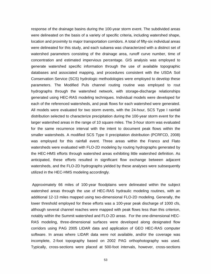
53
response of the drainage basins during the 100-year storm event. The subdivided areas were delineated on the basis of a variety of specific criteria, including watershed shape, location and proximity to major transportation corridors. A total of fifty-six individual areas were delineated for this study, and each subarea was characterized with a distinct set of watershed parameters consisting of the drainage area, runoff curve number, time of concentration and estimated impervious percentage. GIS analysis was employed to generate watershed specific information through the use of available topographic databases and associated mapping, and procedures consistent with the USDA Soil Conservation Service (SCS) hydrologic methodologies were employed to develop these parameters. The Modified Puls channel routing routine was employed to rout hydrographs through the watershed network, with storage-discharge relationships generated using HEC-RAS modeling techniques. Individual models were developed for each of the referenced watersheds, and peak flows for each watershed were generated. All models were evaluated for two storm events, with the 24-hour, SCS Type I rainfall distribution selected to characterize precipitation during the 100-year storm event for the larger watershed areas in the range of 10 square miles. The 3-hour storm was evaluated for the same recurrence interval with the intent to document peak flows within the smaller watersheds. A modified SCS Type II precipitation distribution (PCRFCD, 2008) was employed for this rainfall event. Three areas within the Franco and Flato watersheds were evaluated with FLO-2D modeling by routing hydrographs generated by the HEC-HMS efforts through watershed areas exhibiting little watershed definition. As anticipated, these efforts resulted in significant flow exchange between adjacent watersheds, and the FLO-2D hydrographs yielded by these analyses were subsequently utilized in the HEC-HMS modeling accordingly.
Approximately 66 miles of 100-year floodplains were delineated within the subject watershed areas through the use of HEC-RAS hydraulic modeling routines, with an additional 12-13 miles mapped using two-dimensional FLO-2D modeling. Generally, the lower threshold employed for these efforts was a 100-year peak discharge of 1000 cfs, although several channel reaches were mapped with peak flows less than this criterion, notably within the Summit watershed and FLO-2D areas. For the one-dimensional HEC-RAS modeling, three-dimensional surfaces were developed along designated flow corridors using PAG 2005 LIDAR data and application of GEO HEC-RAS computer software. In areas where LIDAR data were not available, and/or the coverage was incomplete, 2-foot topography based on 2002 PAG orthophotography was used. Typically, cross-sections were placed at 500-foot intervals, however, cross-sections
54
were spaced at 200-foot intervals within the Summit area in order to evaluate potential flood hazards in more detail. This area represents one of the more intensely developed areas within the Lee Moore watershed, situated downstream of the Country Club Road alignment, and has experienced significant flooding in recent years. Cross-sections were drawn along the channel corridors developed with the GEO HEC-RAS software, and HEC-RAS hydraulic models were developed from these data.
Since only the 100-year floodplains were evaluated with the current study, channel banks and roughness coefficients were characterized assuming full-flow corridors, in contrast to existing low-flow channels that generally play a larger role in characterizing floodplain areas of lesser storm events. Roughness coefficients employed with these analyses are representative of typical values used in channel investigations in other areas of Arizona, and were corroborated by literature references. Several stock ponds and/or diversion berms were identified along the existing main channel washes and tributaries within the study area that obstruct, impound, or divert flows within the flow corridors. Since there is no documentation on the stability of these structures, they were ignored with the current hydraulic modeling efforts, as potential failure of the structures was deemed a practical consideration. Given these circumstances, floodplain limits developed within the three-dimensional surfaces developed by GEO HEC-RAS software required editing to eliminate potential model-interpreted effects associated with these structures, as well as extraneous low-lying areas outside the potential flooding influence. Thus, the final mapping efforts for the study represent a combination of the hydraulic modeling results, as well as intuition and experience to assess situations outside the one-dimensional capabilities of the HEC-RAS model. Generally speaking, the floodplain limits defined with the current study are considered conservative, and intended to be employed for future planning efforts.
The 100-year peak flows generated for the major watersheds associated with this study ranged from about 1100 cfs at the mouth of the Summit watershed (3-hour storm) to an estimated 7500 cfs (24-hour storm) along the main channel (J12) in the Flato watershed where the FLO-2D modeling was initiated. The peak flow at the mouth of Flato Wash at Lee Moore Wash is estimated as approximately 2200 cfs, while the 100-year peak flow for Franco Wash at the Santa Cruz River is about 4300 cfs. These peak flows, along with others at major confluences, were used for the floodplain modeling, and contiguous flood hazard areas were delineated from areas east of Sonoita Highway within the Flato watershed to the Lee Moore Wash and Santa Cruz River. Peak flows developed for the
55
24-hour storm event were employed for the floodplain mapping along the main channel reaches where contributing watershed areas were in the excess of 8-10 square miles, while peak flows associated with the 3-hour storm were used to map floodplains associated with smaller watershed areas. Floodplains ranged from fully-contained channel flows to areas inundating several thousand feet in width within the shallow sheetflow, FLO-2D areas, and have been displayed on maps for planning purposes. Based on the study, it appears that most major existing culvert and bridge structures along the primary flow corridors have capacity to convey the 100-year storm peak flows with nominal flooding impacts. A 100-year peak flow of 20,210 cfs is estimated from the FLO-2D hydrologic modeling efforts for the Lee Moore watershed area. This discharge represents cumulative runoff generated within areas south of the current study area. The specific concentration point of this peak flow is situated at the USPS railroad bridge located north of Pima Mines Road in the western extent of the study area. The HEC-RAS modeling along the downstream channel of the Lee Moore channel indicates the existing channel has marginal capacity to convey the 100-year peak flow within existing channel banks. The estimated 100-year discharge of the Lee Moore Wash at the Santa Cruz River for the 24-hour storm event is about 22,000 cfs, when combined with additional tributary flows from the Flato watershed and Summit areas.

56
5.0 References
Aldridge, B.N., and Garrett, J.M., 1973, Roughness coefficients for stream channels in Arizona, USGS Open File Report
Arizona State Land Department – Engineering Section, June 2006, Southlands Drainage master Plan (preliminary maps)
JE Fuller Hydrology & Geomorphology, Inc., 2007, Lee Moore Wash Basin Management Study – Geomorphic Analysis Report
JE Fuller Hydrology & Geomorphology, Inc., 2008, Lee Moore Wash Basin Management Study – Two Dimensional Flow Analysis Report
Kibler, D. F., and Seybert, T.A., 1994, PSUHM - Penn State Urban Hydrology Model
Linsley, Jr., R.K., Kohler, M.A., and Paulhus, J.L.H., 1982, Hydrology for Engineers
National Oceanic and Atmospheric Administration (NOAA) Atlas 14, 2006, Precipitation Frequency Atlas for the United States: Volume 1 - The Semiarid Southwest.
Pima County Department of Transportation – Flood Control District, September, 1979, Hydrology Manual for Engineering Design and Flood Plain Management within Pima County, Arizona
Pima County Department of Transportation and Flood Control District, Planning Division, 1988, Hydrologic Investigation for the Lee Moore Wash Watershed, Pima County, Arizona
Pima County Regional Flood Control District, 2007, PC-Hydro V.5, Pima County Hydrology Procedures – PC-Hydro User Guide
Simons, Li & Associates, Inc., October 1993, Data Collection Summary Report for the TSMS, Phase II, Stormwater Management Plan
Simons, Li & Associates, Inc., November 1995, Existing-Conditions Hydrologic Modeling for the Tucson Stormwater Management Study, Phase II, Stormwater Master Plan
Soil Conservation Service (SCS), 1972, National Engineering Handbook, Section 4
Soil Conservation Service (SCS), 1986, Hydrology Technical Note No. N4, Time Of Concentration
57
Soil Conservation Service (SCS), 1986, Urban Hydrology for Small Watersheds, Technical Release No. 55
Southwest Regional Gap Analysis Project, October 2005, Final Report on Land Cover Mapping Methods
The Pennsylvania State University, Department of Civil & Environmental Engineering, Version 1994, PSUHM: Penn State Urban Hydrology Model
U. S. Army Corps of Engineers, Hydrologic Engineering Center, 1990, HEC-1 Flood Hydrograph Package User’s Manual
U. S. Army Corps of Engineers, Hydrologic Engineering Center, July 1999, HEC-HMS Hydrologic Modeling System, Technical Reference Manual
U. S. Army Corps of Engineers, Hydrologic Engineering Center, Version 3.1, 2002, HEC-RAS User’s Manual
U. S. Army Corps of Engineers, Hydrologic Engineering Center, September 2005, HEC-GeoRAS User’s Manual
U. S. Army Corps of Engineers, Hydrologic Engineering Center, Version 3.0.1, April 2006, HEC-HMS User’s Manual
U. S. Department of Agriculture, National Resources Conservation Service, 2006, Soil Survey Geographic database for Pima County, Arizona, Eastern Part
U. S. Department of Transportation, September 1985, Hydraulic Design of Highway Culverts, Hydraulic Design Circular No. 5
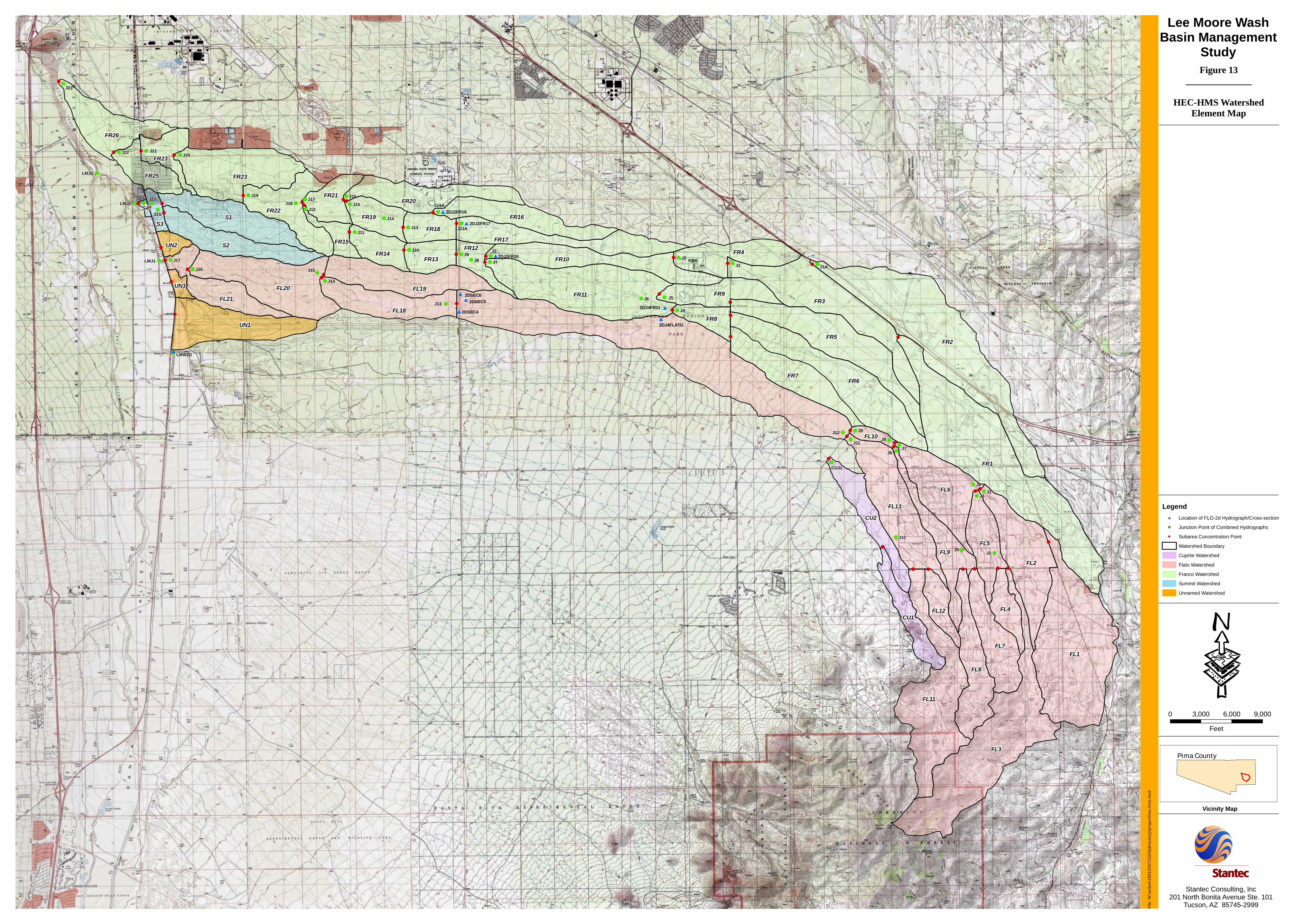
Legend#* Location of FLO-2d Hydrograph/Cross-section
%, Junction Point of Combined Hydrographs
!. Subarea Concentration Point
Watershed Boundary
Cuprite Watershed
Flato Watershed
Franco Watershed
Summit Watershed
Unnamed Watershed
·Pima County
Vicinity Map
Figure 13______________
HEC-HMS WatershedElement Map
Stantec Consulting, Inc201 North Bonita Avenue Ste. 101
Tucson, AZ 85745-2999
Lee Moore WashBasin Management
Study
!.
!.
!.
!.
!.!.
!.
!.!.!.!.
!.
!. !.
!.
!.!. !.
!.
!.
!.
!.!.
!.
!.
!.
!.
!.
!.
!.
!.
!.
!.
!.
!.
!.!.
!.
!. !. !. !. !. !.
!.
!.
!.
!.
!.
!.
!.
!.
!.
%
%
%
%
%
%
%%
%
%
% %%
%% %
%
%
%
%% %
%
%
%
%%
%
%%%
%
%%
%
%
%
%
%
%
%%
%
%
%
%
%%
%
%
%
#
#
#
#
#
#
#
#
#
EE
E
2DSEC6
LMW2D
LMJ1
LMJ2
LMJ3
2DJ4FLATO
2DJ4FR112DSEC5
2DSEC4
2DJ2FR10
2DJ2FR17
2DJ2FR16
J8
J8
J4
J3
J6
J9
J1
J2J5
J6J7
J1
J2
J5
J4
J7
J12
J14
J18
J23
J1A
J10
J11
J10
J13
J21J22 J20
J1S
J2SJ3S J19
J12
J17J16
J15
J11
J15
J14
J16
J17
J13
CUJ1
J3J9
J13A
J14A
FR1
FR2
FL3
FL1
FR6
FL11
FR3FR11
FR5
S1
FL2
FL20
S2
FL13
FL6
UN1
FR23
FL8
FR7
FL19
FL7
FR10FR4
FR17
FL9
FL18
FR20
FR26
FR22FR16
FL5
FR9
CU2
FL21
CU1FL4
FR25
FR19
FR21
FR14
FR23
FR8
FR13
FR18
FL12
FR12
S3
FR15UN2
UN3
FL10
S4
0 3,000 6,000 9,000
Feet
File
: W:\a
ctiv
e\18
5120
071\
GIS
(dire
ctor
y)\p
roje
ct\h
ec-h
ms.
mxd
Related Documents