HAL Id: tel-01653082 https://tel.archives-ouvertes.fr/tel-01653082 Submitted on 1 Dec 2017 HAL is a multi-disciplinary open access archive for the deposit and dissemination of sci- entific research documents, whether they are pub- lished or not. The documents may come from teaching and research institutions in France or abroad, or from public or private research centers. L’archive ouverte pluridisciplinaire HAL, est destinée au dépôt et à la diffusion de documents scientifiques de niveau recherche, publiés ou non, émanant des établissements d’enseignement et de recherche français ou étrangers, des laboratoires publics ou privés. Living the street life : long-term carbon and nitrogen dynamics in parisian soil-tree systems Aleksandar Rankovic To cite this version: Aleksandar Rankovic. Living the street life : long-term carbon and nitrogen dynamics in parisian soil-tree systems. Ecology, environment. Université Pierre et Marie Curie - Paris VI, 2016. English. NNT : 2016PA066728. tel-01653082

Welcome message from author
This document is posted to help you gain knowledge. Please leave a comment to let me know what you think about it! Share it to your friends and learn new things together.
Transcript
HAL Id: tel-01653082https://tel.archives-ouvertes.fr/tel-01653082
Submitted on 1 Dec 2017
HAL is a multi-disciplinary open accessarchive for the deposit and dissemination of sci-entific research documents, whether they are pub-lished or not. The documents may come fromteaching and research institutions in France orabroad, or from public or private research centers.
L’archive ouverte pluridisciplinaire HAL, estdestinée au dépôt et à la diffusion de documentsscientifiques de niveau recherche, publiés ou non,émanant des établissements d’enseignement et derecherche français ou étrangers, des laboratoirespublics ou privés.
Living the street life : long-term carbon and nitrogendynamics in parisian soil-tree systems
Aleksandar Rankovic
To cite this version:Aleksandar Rankovic. Living the street life : long-term carbon and nitrogen dynamics in parisiansoil-tree systems. Ecology, environment. Université Pierre et Marie Curie - Paris VI, 2016. English.�NNT : 2016PA066728�. �tel-01653082�
THÈSE DE DOCTORAT DE
L’UNIVERSITÉ PIERRE ET MARIE CURIE – PARIS VI
ÉCOLE DOCTORALE SCIENCES DE LA NATURE ET DE l’HOMME : ÉCOLOGIE ET ÉVOLUTION (ED 227)
SPÉCIALITÉ
ÉCOLOGIE
PRESENTÉE PAR
ALEKSANDAR RANKOVIC
POUR OBTENIR LE GRADE DE
DOCTEUR DE L’UNIVERSITÉ PIERRE ET MARIE CURIE – PARIS VI
LIVING THE STREET LIFE:
LONG-TERM CARBON AND NITROGEN DYNAMICS IN PARISIAN SOIL-TREE SYSTEMS
DYNAMIQUES DE LONG TERME DU CARBONE ET DE l’AZOTE DANS DES SYSTÈMES SOL-ARBRE PARISIENS
SOUTENUE PUBLIQUEMENT LE 29 NOVEMBRE 2016
DEVANT LE JURY COMPOSÉ DE :
LUC ABBADIE, PROFESSEUR À L’UPMC SÉBASTIEN BAROT, DIRECTEUR DE RECHERCHE À L’IRD SÉBASTIEN FONTAINE, CHARGÉ DE RECHERCHE À L’INRA NATHALIE FRASCARIA-LACOSTE, PROFESSEUR À AGROPARISTECH JEAN-CHRISTOPHE LATA, MAÎTRE DE CONFÉRENCES À L’UPMC JEAN LOUIS MOREL, PROFESSEUR À L’UNIVERSITÉ DE LORRAINE FRANÇOIS RAVETTA, PROFESSEUR À L’UPMC
DIRECTEUR DE THÈSE CO-ENCADRANT
EXAMINATEUR RAPPORTEUR
CO-ENCADRANT RAPPORTEUR
EXAMINATEUR

! 2
! 3
À Ranisav, Zorka et Lazar, pour m’avoir élevé.
À Milorad et Prodana, Vlado et Draginja, que j’aurais aimé connaître plus.
À Michiko, pour m’avoir amené jusque là !

! 4

! 5
“O chestnut-tree, great-rooted blossomer, Are you the leaf, the blossom or the bole?
O body swayed to music, O brightening glance, How can we know the dancer from the dance?”
William B. Yeats, “Among school children”, The Tower, 1928
“A lifetime can be spent in a Magellanic voyage around the trunk of a single tree.”
Edward O. Wilson, Naturalist, 1994
“I play the street life Because there’s no place I can go
Street life It’s the only life I know”
The Crusaders, “Street life”, 1979.
“The weeds in a city lot convey the same lessons as the redwoods.” Aldo Leopold, A Sand County Almanac, 1949.

! 6
! 7
Summary
Urban areas impose multiple and intense environmental changes on the ecosystems they contain or that surround them, and the ecosystem responses to urban environments are still poorly known, even on fundamental ecosystem processes such as carbon (C) and nitrogen (N) cycling. The dynamics of urban ecosystems, especially on the long-term, have received little attention. The present work uses a 75-year chronosequence of street soil-tree systems (plantations of Tilia tomentosa Moench) in Paris, France, as its main case study to detect long-term patterns in urban C and N cycling and infer potential underlying mechanisms.
This thesis describes age-related patterns of C and N accumulation in soils, and we hypothesize that tree root-derived C and deposited N from the atmosphere and animal waste accumulate in soils. Then, an analysis of soil particle-size fractions further points towards a recent accumulation of soil organic matter (SOM), and 13C and 15N analysis suggests that tree roots are a major contributor to the increase of SOM content and N retention. Potential nitrification and denitrification rates increase with street system age, which seems driven by an increase in ammonia-oxidising bacteria. The long-term dynamics of C seem characterized by increasing belowground inputs coupled with root-C stabilization mechanisms. For N, the losses are likely compensated by exogenous inputs, part of which is retained in plant biomass (roots) and SOM.
These results are then discussed in light of results obtained on Parisian black locust systems (Robinia pseudoacacia Linnæus), as well as other data, and management recommendations are proposed.
Résumé Les régions urbaines imposent d’intenses et multiples changements environnementaux
sur les écosystèmes qu’elles contiennent et qui les entourent, et les réponses des écosystèmes à ces environnements urbains est encore relativement peu connue, même pour des processus fondamentaux comme les cycles du carbone (C) et de l’azote (N). Ce travail utilise une chronoséquence de systèmes sol-arbre d’alignement (plantations de Tilia tomentosa Moench) de 75 ans, situés à Paris, comme étude de cas principale, afin de détecter des tendances de long terme dans les cycles urbain du C et du N et d’en inférer les potentiels mécanismes sous-jacents.
Un patron d’accumulation du C et du N dans les sols de rue est décrit, et nous faisons l’hypothèse que le C dérivé des racines, et le N issu des dépôts atmosphérique et apports animaux, s’accumulent dans ces sols. Ensuite, une analyse des fractions organo-minérales des sols suggère qu’il y a bien une accumulation de matière organique du sol (MOS) relativement récente. Les analyses 13C et 15N suggèrent que les racines sont un contributeur majeur à cette augmentation de la teneur en MOS et de la rétention du N exogène. Les taux de nitrification et de dénitrification potentielles augmentent avec l’âge des systèmes de rue, ce qui semble être déterminé par une augmentation des bactéries oxydant l’ammoniaque.
Les dynamiques de long terme pour le C semblent caractérisées by une augmentation des apport hypogés couplée à des mécanismes de stabilisation du C racinaire. Pour le N, les sorties de N semblent contrebalancées par d’importants apports exogènes et les racines, apports dont une partie est retenue dans la biomasse végétale (racines) et la MOS.
Ces résultats sont ensuite mis en perspective d’autres données, portant notamment sur des plantations parisiennes de robinier (Robinia pseudoacacia Linnæus), et des recommandations de gestion sont proposées.

! 8

! 9
Extended summary
Human influence on the biosphere is deep and pervasive, to the point that our geological epoch may soon be officially recognized as the Anthropocene. To better depict the ecology of contemporary Earth, ecologists must increase their research efforts on anthropized ecosystems, which now represent the majority of ice-free land on the planet. In particular, a major planetary shift occurred during the 20th century, when humans became a predominantly urban species, and it is a trend that will persist in the decades to come.
Urban areas impose multiple and intense environmental changes on the ecosystems they contain or that surround them, and the ecosystem responses to urban environments are still poorly known, even on fundamental ecosystem processes such as carbon (C) and nitrogen (N) cycling. A particularly neglected aspect of urban ecosystems is their dynamics, especially on the long-term. The knowledge base on which one could anticipate the trajectory of urban ecosystems, and thus the sustainability of urban ecological engineering projects, is thus rather weak.
This is particularly problematic in a context where calls to rely on “green infrastructure” to enhance urban sustainability are increasing, and where fast-pace greening initiatives are multiplying in many cities worldwide. The principal goal of this work is to increase our understanding of the long-term dynamics of urban ecosystems, as grasped through the C and N cycles, and thus also to increase knowledge on these central biogeochemical cycles in cities and infer recommendations for management. It thus wishes to describe parts of the ecology of some of the most anthropized ecosystems there is, in order to better understand and care after some of our closest non-human companions on Earth.
Urban environments have been shown to have profound, yet still poorly understood effects on C and N cycling in ecosystems. Patterns of increased cycling rates, coupled with long-term accumulations of both C and N, have been reported in numerous cities worldwide, but the involved mechanisms are still poorly known and require further investigation. The present work uses a 75-year chronosequence of street soil-tree systems (plantations of Tilia tomentosa Moench) in Paris, France, as its main case study. It combines approaches from stable isotope ecology (analyses of 13C and 15N natural abundances) and microbial ecology (qPCR and laboratory incubations to assess potential activities).
In Chapter 1, we detect age-related patterns of C and N accumulation in soils and we hypothesize that tree root-derived C and deposited N from the atmosphere and animal waste accumulate in soils. These hypotheses are supported, notably, by an enrichment of soil δ13C along the chronosequence, possibly due to chronic water stress of trees in streets, leading to an enrichment of foliar δ13C that could be subsequently transmitted to soil organic matter (SOM) through roots (via rhizodeposition and turn-over). For N, the exceptionally high soil and foliar δ15N in streets, as well as increased contents in mineral N forms, suggest chronic inputs of 15N-enriched N sources and subsequent microbial cycling, through nitrification and denitrification in particular.
In Chapter 2, an analysis of soil particle-size fractions further points towards a recent accumulation of C and N in older street soils, and fine root δ13C suggests that the enrichment in street foliar δ13C is transmitted to SOM and to microbial respiration. Analysis of root N suggests that exogenous N inputs are assimilated by surface roots and then incorporated into SOM, but a very strong difference between foliar and root δ15N, suggests that, as trees age, they diversify their N sources, and that whole-tree N nutrition relatively less depends, with time, on the N assimilated from topsoil.
In Chapter 3, we show that both potential nitrification and denitrification rates increase with street system age, and are much higher than at arboretum sites. While both ammonia-oxidising archaea (AOA) and bacteria (AOB) are more abundant in street soils than at the arboretum, the abundance of AOB in surface soils shows consistent age-related trends and is positively correlated to potential nitrification, soil mineral N contents and both soil and foliar δ15N. We suggest that the increase in nitrification rates could be driven by the observed increase in AOB populations, which itself could be due to increasingly favorable conditions for AOB in street soils, namely increased ammonium content and circumneutral soil pH. Denitrification, in turn, could be favored by increased soil nitrite and nitrate content, as well as soil organic C.
In the general discussion, these results are discussed and interpreted in terms of the long-term trajectory they seem to depict for street systems. Results are also discussed in light of results obtained on Parisian black locust systems (plantation of Robinia pseudoacacia Linnæus), as well as other data (urban pollinators, soil trace metal content), to assess the possibility to generalize our interpretations and to refine our recommendations for management. The discussion ends on a reflection on the role of urban ecological research in helping to solve environmental issues.

! 10

! 11
Remerciements !
Ce travail a bénéficié du généreux soutien de la région Île-de-France (R2DS), du GIS « Climat, Environnement, Société » (Projet CCTV2), du PIR IngEcoTech (projet IESUM), de Sorbonne Universités (projet Dens’Cité, programme Convergences), de Sorbonne Paris Cité (programme interdisciplinaire « Politiques de la Terre à l’épreuve de l’Anthropocène ») et de l’Institut du Développement Durable et des Relations Internationales (Iddri – Sciences Po). Une partie de ce travail a aussi bénéficié d’un séjour au Program on Science, Technology and Society (STS Program) de la Harvard Kennedy School. Un immense merci à toutes ces institutions, qui ont rendu cette recherche possible.
Je remercie vivement les membres de mon jury, Sébastien Fontaine, Nathalie Frascaria-Lacoste, Jean Louis Morel et François Ravetta, de m’avoir accordé le privilège de bien vouloir évaluer ce travail et me permettre de l’améliorer.
Merci à mes encadrants, Luc Abbadie, Sébastien Barot, Jean-Christophe Lata et Julie Leloup, pour avoir cru en ce projet et être parvenus à en obtenir les premiers financements. Merci à Luc de m’avoir encouragé à regarder dans cette direction, ainsi que pour ses cours (historiques !) du vendredi matin à 8h, rue Saint Guillaume, où la découverte de Lamto et de la brousse tigrée ont fini de me convaincre que je voulais étudier l’écologie encore un peu plus. Merci à Sébastien pour nos nombreuses discussions et pour tous ses conseils en stats, et pour son aide sur le terrain qui lui a coûté un short, quelque part avenue Secrétan. Merci à Jean-Christophe pour toutes ses attentions souvent précieuses et nos discussions éclairantes sur l’azote, ainsi que pour son aide sur le terrain qui a failli lui coûter un pouce, quelque part avenue de Choisy. Merci à Julie pour son aide dans la préparation des terrains et pour avoir supervisé toute une partie de la mise au point de protocoles utilisés dans ce travail ; le tout lui ayant coûté quelques cheveux blancs, quelque part rue d’Ulm ! Merci à tous pour votre confiance et pour avoir accompagné ce travail.
Un très grand merci à Paola Paradisi, Catherine Muneghina, Véronique Marciat et Jean-Robert Gowe, pour m’avoir tant de fois permis de m’y retrouver dans l’administration complexe d’une grande UMR comme Bioemco/IEES. À Catherine, en particulier, un énorme merci pour sa gentillesse et sa présence constantes, son attention au bien-être de tous.
J’ai eu la chance, au cours de ces recherches, de pouvoir bénéficier des apports précieux de nombreux collègues. Merci à Pierre Barré pour notre travail sur les fractions organo-minérales des sols, pour ses encouragements et conseils et nos discussions qui ont toujours enrichi mes réflexions. Grâce à son savoir encyclopédique sur la FFF, j’ai aussi beaucoup appris sur le ballon rond et les coulisses de 98 (Président !). Un très grand merci à Naoise Nunan, pour avoir si souvent été mon point de repère à Grignon, pour m’avoir guidé dans la MIRS, pour avoir à chaque fois partagé son bureau de bon cœur (et parfois sa blouse, et parfois ses stylos...). Merci, dans les moments de détente, d’avoir toujours essayé de me faire boire comme un homme, et désolé de t’avoir déçu tant de fois. Merci à Sabrina(aaaaaa) Juarez pour les précieux moments de camaraderie et nos discussions dans le train. Merci à Daniel Billou pour ses conseils et son aide pour les analyses carbone. Un grand merci, de manière générale, à tous les autres collègues de Grignon pour leur accueil toujours chaleureux.
« Pokémon Go » n’était même pas encore sorti que ma route croisait celle de Thomas « Draco » Lerch. Mille mercis, Thomas, pour toutes les manipes effectuées ensemble, les longues discussions, les super moments de détente. J’y inclus, entre autres, un mémorable

! 12
bowling-billard nocturne en claquettes à Bari (avec les acolytes Mathieu Thévenot et JC Lata) et ce fameux « poc » d’anthologie à cause de mes gros pouces. Mention spéciale, aussi, à l’escalade nocturne à Vincennes, et cet autre « poc » mémorable (au niveau des baskets cette fois ; et pas des miennes !). Merci, et cela vaut aussi pour Frédérique Changey, pour tout ce temps passé ensemble sur Carapuce, Respiflore et Carbotope, au son de Carapicho ou autres réjouissances sonores du même acabit. Merci pour ces discussions passionnées, incessantes, sur comment mieux comprendre les sols et aller toujours... deepaah !!! Merci à tous les autres collègues de Créteil pour leur accueil.
À Jussieu, j’ai une énorme dette auprès de Véronique Vaury, sans l’aide de qui ce manuscrit aurait été bien plus mince... Merci pour ta disponibilité, ton écoute, tes conseils, la qualité de ton boulot. Merci à Katell Quenea et Maryse Castrec-Rouelle pour notre collaboration sur les métaux, nos super discussions et leur accueil – toujours extra ! – dans leur bureau. Je suis très reconnaissant envers Marie Alexis également, pour toute son aide et ses conseils sur mes protocoles, pour m’avoir fait découvrir l’étuve Popov et les « beaux tubes ». Merci à Mathieu Sebilo pour ses cours qui m’ont fait découvrir le 15N et pour toutes nos discussions isotopiques. Merci à tous les collègues de Jussieu pour leur accueil, toujours si chaleureux.
À l’ENS, merci en premier lieu à mes camarades doctorants, pour tout ce que l’on a partagé. Une pensée particulière pour Henri de Parseval et Alix Sauve, et le lancement de l’aventure HPSE. Un grand merci à Benoît « Rihanna » Geslin pour nos discussions, son amitié, et tant de grands moments musicaux ; et puis nos recherches passionnantes sur les isotopes et les pollinisateurs. Le 2BAD, c’était quand même quelque chose ! À Ambre David, pour tout notre travail commun, son aide précieuse et son amitié, et pour avoir développé une si belle recherche sur les arbres parisiens ; vraiment merci. Merci à Imen Louati pour tous les moments d’échanges sur les manipes – et puis aussi les moments d’encouragements quand il y avait besoin ! Merci à tous les autres, anciens et nouveaux, pour tant de moments précieux. Merci également à David Carmignac, Jacques Mériguet et Stéphane Loisel, pour les coups de main ponctuels sur le terrain ou au labo, mais surtout leur camaraderie constante. Un grand merci à Battle Karimi, notamment pour avoir participé aux premiers jours de terrain de cette recherche et immortalisé le « cric »... À Benjamin Izac, un immense merci pour ce premier mois de terrain formidable ensemble, plein de fabuleux souvenirs. À Julien Robardet, toute ma gratitude pour le travail analytique abattu ensemble – enfin, par toi surtout ! Un grand merci à Gérard Lacroix pour ses précieux conseils, à Xavier Raynaud pour des coups de mains stats toujours patients et avisés, à Isabelle Dajoz pour notre travail avec Benoit et notre collaboration dans Politiques de la Terre, à Patricia Genet pour nos discussions autour de Mycopolis. À Élisa Thébault, merci de m’avoir fait découvrir la Suze ! Merci à Jacques Gignoux de m’avoir emmené vers les savanes. Merci à Florence Maunoury-Danger et Michael Danger pour leur accueil dans la belle ville de Metz.
Merci, bien sûr, à Augusto Zanella, pour tous ses conseils et tout le terrain effectué ensemble ; merci également, donc, à sa fourgonnette ! Merci également pour tout le travail de mise en réseau avec les collègues italiens, que je salue au passage.
Merci à tous les agents de la Division des Espaces Verts et de l’Environnement de Paris que j’ai pu rencontrer, et en particulier Caroline Lohou, Emmanuel Herbain, Barbara Lefort, François Nold, Henri Peyrétout et Christophe Simonetti. Merci de m’avoir aidé à obtenir l’autorisation pour faire cette recherche, et plus encore pour le temps que vous avez pu m’accorder et pour les discussions passionnantes sur votre métier.
! 13
Je remercie également les stagiaires dont j’ai pu participer à l’encadrement, et les étudiants que j’ai pu avoir en cours ; j’espère qu’ils ont au moins autant appris à mon contact que moi au leur.
Les échanges et travaux ayant eu lieu au sein du projet CCTV2 ont été extrêmement enrichissants, et je remercie vivement ses participants et notamment Nathalie Blanc, Anne Sourdril, Thomas Lamarche, Sandrine Glatron et Philippe Boudes. Un grand merci, aussi, à Chantal Pacteau, pour son précieux travail d’animation et pour ses encouragements constants.
À tous mes collègues de l’Iddri, et en particulier à Lisa Dacosta, Sébastien Treyer et Yann Laurans, un énorme merci pour votre soutien et encouragements répétés. Merci à Sébastien, en outre, d’avoir organisé une « séance de coaching » – en fait un dîner autour d’un succulent pho du 13ème ! – avec Laurent Mermet. Merci à Laurent pour plein de précieuses discussions ces dernières années. Merci aussi, évidemment, à Raphaël Billé pour tous les précieux conseils qu’il a pu me prodiguer. Merci à Bruno Latour d’avoir contribué, par petites touches, à ce que je ne perde pas foi en l’intérêt intellectuel d’étudier les arbres parisiens !
Je me suis rarement autant senti accepté dans ma diversité que pendant mon séjour au STS Program. Je remercie affectueusement Sheila Jasanoff de m’y avoir accueilli. Merci également à tous mes camarades sur place, pour tout ce qu’ils m’ont apporté, et en particulier Gabriel Dorthe, Mascha Gugganig et Samantha Vanderslott pour tout ce que l’on a partagé et partageons encore.
Merci à tous mes amis pour leur affection constante. Clément Feger, Youssef Iskrane et Wolly Taing, en particulier, ont été des soutiens inestimables malgré les trop nombreux kilomètres qui nous séparent. Miss you, guys.
J’ai la chance d’avoir toujours pu compter sur les encouragements de ma famille. Merci à mes parents, Ranisav et Zorka, de m’avoir encouragé à faire des études et d’être comme ils sont. Merci à mon frère Lazar pour tout ce qu’il m’a apporté, et à Tina, Nola et Ezio pour tous les super moments passés ensemble. Je n’ai pas vraiment de mots pour dire tout ce que ce travail doit à Michiko. Il n’aurait probablement même pas débuté si je ne l’avais pas rencontrée ! Merci de me supporter autant... dans tous les sens du terme !!! Un immense merci à la famille Ikezawa également, à qui ce travail doit énormément.
Je tiens enfin à remercier les arbres et les sols des rues de Paris. Dans les pages qui suivent, ils sont représentés par des points, des tableaux, des graphes. Mais ils sont bien plus beaux en vrai et j’espère que ce travail pourra contribuer à ce qu’on leur prête plus d’attention.

! 14

! 15
Table of contents !SUMMARY ............................................................................................................................................. 7 EXTENDED SUMMARY ...................................................................................................................... 9 REMERCIPDFEMENTS .................................................................................................................... 11 TABLE OF CONTENTS ..................................................................................................................... 15
GENERAL INTRODUCTION ........................................................................................................... 21 1. ECOLOGY AND THE FIRST URBAN CENTURY .................................................................................. 21 2. CARBON AND NITROGEN DYNAMICS IN URBAN ECOSYSTEMS ....................................................... 26
2.1. Carbon and nitrogen cycles as ecological crossroads ........................................................... 26 2.2. Overview of urban studies on carbon and nutrient cycling .................................................... 29
3. THE LONG-TERM CARBON AND NITROGEN DYNAMICS IN “HAUSSMANNIAN ECOSYSTEMS” AS A CASE STUDY ........................................................................................................................................ 33
CHAPTER 1 LONG-TERM TRENDS IN CARBON AND NITROGEN CYCLING IN PARISIAN STREET SOIL-TREE SYSTEMS ....................................................................................................................... 45
1. INTRODUCTION ............................................................................................................................... 45 2. MATERIALS AND METHODS ............................................................................................................ 50
2.1. Site description and chronosequence design .......................................................................... 50 2.2. Sample collection and processing ........................................................................................... 54 2.3. Soil characteristics ................................................................................................................. 55 2.4. C and N contents and isotope ratios ....................................................................................... 56 2.5. Statistical analyses .................................................................................................................. 57
3. RESULTS ......................................................................................................................................... 58 3.1. Soil characteristics ................................................................................................................. 58 3.2. Soil C and N contents and isotope ratios ................................................................................ 59 3.3. Foliar δ13C and δ15N and N content ....................................................................................... 67 3.4. Soil and plant coupling ........................................................................................................... 67
4. DISCUSSION .................................................................................................................................... 70 4.1. Age-related trends in soil organic C: Accumulation of root C? ............................................. 70 4.2. Age-related trends in N cycling: Rapid N saturation of street systems? ................................ 72 4.3. Uncertainties linked to potential legacy effects ...................................................................... 77
5. CONCLUSION .................................................................................................................................. 79
CHAPTER 2 LEGACY OR ACCUMULATION? A STUDY OF LONG-TERM SOIL ORGANIC MATTER DYNAMICS IN HAUSSMANNIAN TREE PLANTATIONS IN PARIS ...................................... 83
1. INTRODUCTION ............................................................................................................................... 83 2. MATERIALS AND METHODS ............................................................................................................ 87
2.1. Site description and chronosequence design .......................................................................... 87 2.2. Sample collection and processing ........................................................................................... 89 2.3. Soil characteristics ................................................................................................................. 89 2.4. Physical fractionation procedure ........................................................................................... 91

! 16
2.5. Mineralogical analysis of clay fractions by X-ray diffraction ................................................ 94 2.6. C and N contents and isotope ratios ....................................................................................... 94 2.7. Soil incubation, CO2 and 13C-CO2 analysis ............................................................................ 95 2.8. Statistical analyses .................................................................................................................. 96
3. RESULTS ......................................................................................................................................... 97 3.1. Soil texture, quality of fractionation and clay minerals ......................................................... 97 3.2. Soil C and N contents and isotope ratios ................................................................................ 99 3.3. Root C and N contents and isotope ratios ............................................................................ 111 3.4. C mineralization and δ13C-CO2 ............................................................................................ 113 3.5. Soil and plant coupling ......................................................................................................... 116
4. DISCUSSION .................................................................................................................................. 118 4.1. Evidence of recent C and N accumulation in street soils ..................................................... 118 4.2. Possible mechanisms for root-C accumulation in street soils .............................................. 121 4.3. Street trees diversify their N sources .................................................................................... 124
5. CONCLUSION ................................................................................................................................ 126
CHAPTER 3 STRUCTURE AND ACTIVITY OF MICROBIAL N-CYCLING COMMUNITIES ALONG A 75-YEAR URBAN SOIL-TREE CHRONOSEQUENCE .............................................................. 130
1. INTRODUCTION ............................................................................................................................. 130 2. MATERIALS AND METHODS .......................................................................................................... 131
2.1. Site description and chronosequence design ........................................................................ 131 2.2. Sample collection and processing ......................................................................................... 133 2.3. Real-time quantitative PCR .................................................................................................. 134 2.4. Potential nitrifying and denitrifying activities ...................................................................... 136 2.5. Statistical analyses ................................................................................................................ 137
3. RESULTS ....................................................................................................................................... 138 3.1. Abundances of soil AOB and AOA ....................................................................................... 138 3.2. Abundances of soil bacterial denitrifiers .............................................................................. 141 3.3. Potential nitrification and denitrification ............................................................................. 142 3.4. Correlations among microbial parameters and between microbial, soil and plant parameters in street systems ........................................................................................................................... 144
4. DISCUSSION .................................................................................................................................. 147 5. CONCLUSION ................................................................................................................................ 151
GENERAL DISCUSSION ................................................................................................................. 156 1. THE LONG-TERM DYNAMICS OF HAUSSMANNIAN ECOSYSTEMS: A SCENARIO ............................ 156
1.1. Summary of chapters ............................................................................................................ 156 1.2. Possible interpretations for long-term C and N dynamics in street systems ........................ 159 1.3. Beyond silver lindens? Insights from black locust plantations and pollinators ................... 164
2. PERSPECTIVES FOR FUTURE WORKS AND STREET PLANTATION MANAGEMENT .......................... 169 3. “GLOBAL CHANGE IN YOUR STREET!”: ECOLOGY IN THE FIRST URBAN CENTURY ...................... 174
REFERENCES ................................................................................................................................... 180
APPENDIX 1: RANKOVIC ET AL. (2012) .................................................................................... 202 APPENDIX 2: AUTHORIZATION TO DO FIELDWORK IN PARIS ....................................... 204

! 17
APPENDIX 3: LAURANS ET AL. (2013) ....................................................................................... 208 APPENDIX 4: RANKOVIC & BILLE (2013) ................................................................................. 210 APPENDIX 5: RANKOVIC ET AL. (2016) .................................................................................... 212 APPENDIX 6: CURRICULUM VITÆ ............................................................................................ 214

! 18
! 19
!"
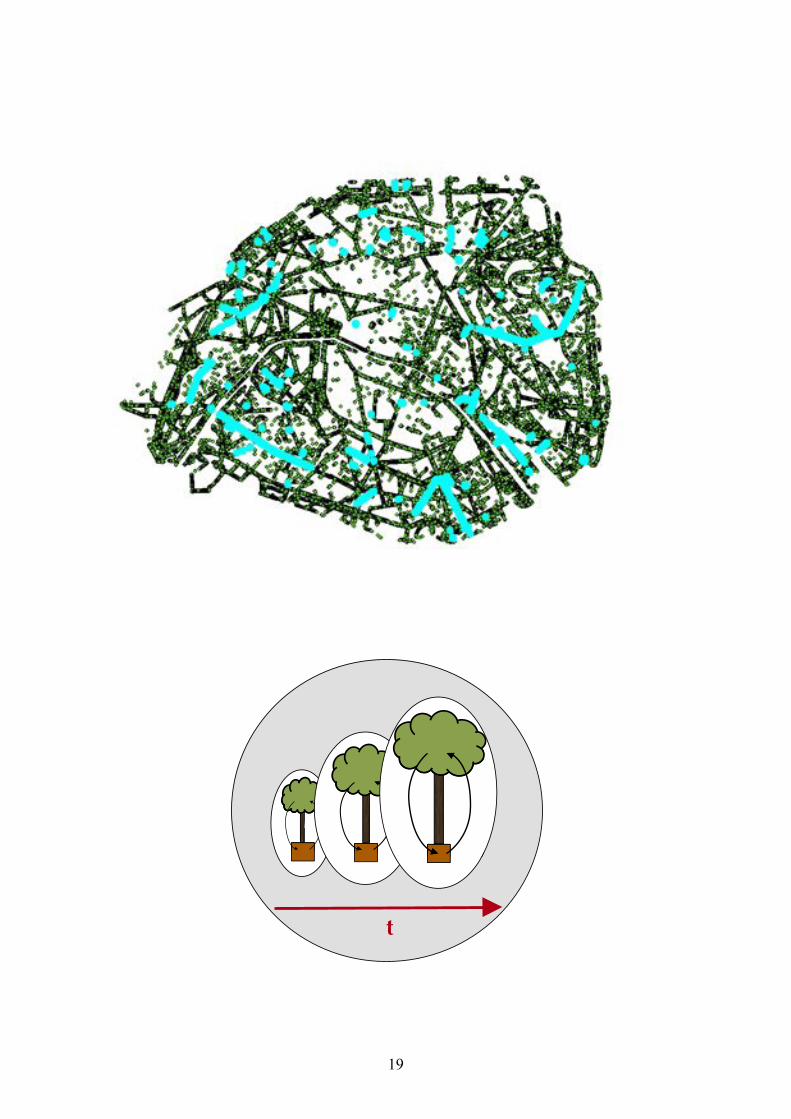
LES ÉCOSYSTÈMES HAUSSMANNIENS"
t !
Étude de leurs dynamiques de long terme vue au travers des cycles du C et du N
Combinaison analyses des abondances naturelles des
isotopes stables C & N et écologie microbienne

! 20
! 21
General introduction
1. Ecology and the first urban century
Human influence on the biosphere is deep and pervasive (Vitousek et al.,
1997a; Crutzen, 2002; Waters et al., 2016), to the point that our geological
epoch may soon be officially recognized as the Anthropocene (Waters et al.,
2016). When he proposed the ecosystem concept, Arthur Tansley already put
forth the necessity for ecologists to fully and explicitly include the multifold
influence of humans in their studies (Tansley, 1935). Yet, while this challenge
has undoubtedly been acknowledged in ecological sciences, the associated
research effort does not seem to be at scale. Martin et al. (2012), for instance,
reviewed over 8000 studies published in ten leading ecological journals between
2004 and 2009, and showed that 63-84 % of studies had been conducted in
protected areas (most often located in temperate, wealthy regions) even though
they represent less than 13 % of Earth’s ice-free land. On the other hand,
agricultural areas, rangelands and densely settled areas were found to be
strongly underrepresented (16.5 % of studies) relatively to their global extent
(47 %). This suggests that anthropized ecosystems, even though they now
represent the majority of the terrestrial biosphere (55 % in the year 2000: Ellis et
al., 2010), are understudied in ecology’s most influential research. As pointed by
Martin et al. (2012), this fundamentally questions the ability of ecological
research to properly depict the planetary ecology of contemporary Earth.
A major planetary shift occurred during the 20th century, when humans
became a predominantly urban species. Urban areas now concentrate more than
half of world population, and urban population will likely increase by between
2.5-3 billion people by 2050, representing about two thirds of the expected 9.7
billion world population (Seto et al., 2014; United Nations, 2015). Estimating
! 22
the extent of urban land cover area is not straightforward, and different global
satellite mappings have yielded a range of between 0.28 and 3.5 million km2,
representing between 0.2 % and 2.7 % of ice-free land (Potere 2009; Schneider
et al., 2009). When compared to 2000 estimates, urban land cover area
worldwide will possibly triple in size by 2030 (Seto et al., 2012, 2014).
Even though they represent a relatively small fraction of Earth’s surface,
urban areas have a considerable influence on the rest of the planet, either
indirectly through their “metabolism” and large “footprint” (Wolman, 1965;
Folke et al., 1997; Rees, 1998; Seto et al., 2014), or more directly through the
multiple and intense environmental changes they impose on the ecosystems they
contain or that surround them (Gregg et al., 2003; Kaye et al., 2006; Grimm et
al., 2008; Lorenz & Lal, 2009; Kaushal et al., 2014; Bai et al., 2015; Chambers
et al., 2016). Urban areas are often characterized by high spatial heterogeneity,
reduced connectivity, anthropized soils, surface sealing, high near-ground
atmospheric CO2 concentration, high levels of atmospheric nitrogen (N)
deposition, increased surface temperatures and heat island effects, high levels of
pollutant contamination, hydrologic changes, increased presence of non-native
organisms, intense management practices, and so on (McDonnell & Pickett,
1990; McDonnell et al., 1997; Morel et al., 1999; Schwartz et al., 2001; Carreiro
& Tripler, 2005; Kaye et al., 2006; Cheptou et al., 2008; Grimm et al., 2008;
Lorenz & Lal, 2009; Hahs & Evans, 2015; Alberti, 2015; Chambers et al., 2016).
These urban features, because of their individual magnitude and/or
because they can all occur simultaneously, constitute evolutionary novelties that
make cities interesting “ecological theaters” (Hutchinson, 1965) that can present
several interests for ecologists (McDonnell & Pickett, 1990; McDonnell & Hahs,
2014; Alberti, 2015). Over the last decades, it has thus been proposed that urban
ecological research could enhance general ecological knowledge by describing
the response of different ecological processes to the quite unique sets of
! 23
constraints and perturbation regimes that are found in cities (McDonnell &
Pickett, 1990; Cheptou et al., 2008; McDonnell & Hahs, 2014; Hahs & Evans,
2015; Alberti, 2015; Groffman et al., 2016). Given the similarities between
some urban features (e.g., near-ground CO2 concentrations that can be several
hundreds of parts per million (ppm) higher than background levels, high
amounts of N deposition, higher average temperature when compared to
surrounding areas), urban ecosystems have also been considered as “sentinels of
change”, foreshadowing what ecosystem responses to global changes, such as
global warming and human inputs of N into the biosphere, could look like in the
decades to come (Carreiro & Tripler, 2005; Grimm et al., 2008; Alberti, 2015).
Early on, urban ecology was also considered as an opportunity to provide
some answers to the intellectual challenge of better including the influence of
humans on ecosystems (e.g., McDonnell & Pickett, 1993), as well as for
ecologists to engage with the rest of society (e.g., McDonnell & Pickett, 1990;
Tanner et al., 2014; Pataki, 2015). In particular, urban ecologists have displayed
a growing interest in participating to urban planning, for different purposes. For
biodiversity conservation, ecological works have for instance contributed to the
design of greenways to try and mitigate the fragmentation of ecosystems due to
urbanization (Clergeau, 2007; Forman, 2008). Ecologists have also produced
works on the design and management of urban ecosystems, such as urban forests
or green roofs (Carreiro et al., 2008; Oberndorfer et al., 2007), both to increase
understanding of, and increase the services provided by, the “green
infrastructure” of cities (Pataki et al., 2011; Rankovic et al., 2012 – Appendix 1).
Calls to rely on green infrastructure to enhance urban sustainability are
increasing (European Commission, 2013; FAO, 2016). “Fast-pace” greening
initiatives are multiplying in many cities worldwide (Day & Amateis, 2011;
Pincetl et al., 2012; Churkina et al., 2015), as is probably best illustrated by New
York City’s “MillionTreesNYC” programme and its goal to plant one million

! 24
new trees across the city in a decade1. In Paris, an increase of 20 000 trees by
2020 is planned under the current mandate, in addition to the 183 000 trees
already planted in streets, parks, graveyards and other public areas, thus
representing an increase of 11 % in less than 6 years2. Justifications for such
initiatives are usually based on embellishment purposes but also, increasingly,
on a range of ecosystem services expected from tree plantings and other green
spaces. These typically include pollution removal from air and water, local
cooling, stormwater regulation, carbon (C) sequestration in soils and plants, or
even food provision (e.g., Bolund & Hunnamar, 1999; Nowak, 2003; Pataki et
al., 2011; Rankovic et al., 2012; FAO, 2016). Despite a long-standing interest in
these questions (Smith & Staskawicz, 1977; Meyer, 1991; Stewart et al., 2011),
uncertainties and even controversies among authors are still lively, especially on
the magnitude of said ecosystem services and their actual effects on the health of
urbanites (Pataki et al., 2011; Rankovic et al., 2012; see for instance the recent
sharp debates in Environmental Pollution on the magnitude of PM2.5 removal
by trees in US cities: Whithlow et al., 2014a,b; Nowak et al., 2014).
These difficulties are not surprising, given the complexity of urban
environments and the relatively recent structuring of the field of urban ecology.
Thus, notwithstanding a steady development of urban ecology over the last three
decades, many aspects of urban ecological processes remain unknown. A
particularly neglected aspect of urban ecosystems is their dynamics, especially
on the long-term. Besides remnant patches of “native” ecosystems, most
ecosystems in cities are the product of landscaping activities, where human
decisions and actions result in different types of “constructed ecosystems”, and
where soils, plants, water and sometimes animals are assembled as part of urban
design projects. Given the complexity of urban environments, once an
ecosystem is constructed in a city, predicting its own dynamics and long-term !!!!!!!!!!!!!!!!!!!!!!!!!!!!!!!!!!!!!!!!!!!!!!!!!!!!!!!!1 http://milliontreesnyc.org/; last consulted 15 September 2016. 2 http://www.paris.fr/arbres; last consulted 15 September 2016.

! 25
trajectory (changes in structure, in processes) is challenging. This question,
furthermore, has seldom been explicitly investigated in urban ecological
research, which has so far mostly relied on spatially-explicit studies (e.g., urban-
rural gradients or watershed-level analysis) and relatively less on temporally-
explicit approaches (e.g., chronosequences or long-term series of data). The
knowledge base on which one could anticipate the trajectory of urban
ecosystems, and thus the sustainability of urban ecological engineering projects,
is thus rather weak.
Other key aspects of urban ecosystems remain understudied.
Biogeochemical cycles, which underpin many of expected urban ecosystem
services (Pataki et al., 2011), count among the least studied aspects of urban
ecosystems. For instance, in a review covering 319 studies using urban-to-rural
gradients, published over 17 years, McDonnell & Hahs (2008) found that 63 %
of studies focused on the distribution of macroorganisms while only 17 %
concerned biogeochemical aspects (“pollution/disturbance/nutrient fluxes”
category in their review).
These considerations form the starting point of the present work. Its
principal goals are to increase our understanding of the long-term dynamics of
urban ecosystems, as grasped through the C and N cycles, and thus also to
increase knowledge on these central biogeochemical cycles in cities and infer
recommendations for management. It thus wishes to describe parts of the
ecology of some of the most anthropized ecosystems there is, in order to better
understand and care after some of our closest non-human companions on Earth.
In the following section, the importance of C and N cycling in ecosystems
is addressed. Then, a synthesis of studies on urban C and N cycling is provided,
with a particular attention to studies focusing on temporal dynamics. In the last
section of this general introduction, the rationale for choosing Parisian street
soil-tree systems as a case study will be outlined and the thesis structure will be
! 26
presented.
2. Carbon and nitrogen dynamics in urban ecosystems
2.1. Carbon and nitrogen cycles as ecological crossroads
The C and N cycles occupy a central role in ecosystem studies. In most
ecosystems, the solar energy fixed in carbohydrates (assembled from CO2 and
water) by plants during photosynthesis forms the basis of most available energy
that is used by organisms that feed on living or dead plant material and which
then circulates through foodwebs. The C compounds produced by plants also
make up important “structures” in terrestrial ecosystems, such as the living
plants themselves, dead wood, soil litter and soil organic matter (Bormann &
Likens, 1979). The amount of plant primary production partly determines the
amount of microbes and animals that can be sustained in an ecosystem. The
recycling of organic matter by soil microbes and animals is a key process
controlling the availability of major nutrients for plants. N is considered to be
the major limiting nutrient for primary production (Vitousek, 1982; Vitousek &
Howarth, 1991; Gruber & Galloway, 2008), and the C and N cycles are tightly
coupled. The availability of N strongly constrains primary production and thus
C inputs into ecosystems, notably because important amounts of available N are
required to synthetize the proteins that constitute the enzymatic apparatus of
photosynthesis (e.g., van Groenigen et al., 2006). N foraging strategies by plants,
in turn, can have strong influences on C cycling, for instance by increasing
belowground C allocation and providing fresh organic matter to soils, which can
increase decomposition rates by soil biota and in turn lead to increased N
availability (e.g., Bardgett et al., 2014; Shahzad et al., 2015). C and N
acquisition strategies both can differ among plant species and are the object of
numerous cooperative and competitive interactions between plants, plants and
soil microbes and between soil microbes. Herbivory, pollination and even
feedbacks from predation can also interact with C and N cycling. Through the

! 27
production of greenhouse gases such as CO2, CH4 and N2O, C and N dynamics
are also of significant importance for global biogeochemistry and climate (e.g.,
Schimel, 1995; Gruber & Galloway, 2008; Philippot et al., 2008; Ostle et al.,
2009).
The C and N cycles are thus at the crossroads of numerous ecological
interactions that link aboveground and belowground components of ecosystems
(e.g., Tateno & Chapin, 1997; Wardle et al., 2004) and they strongly constrain,
and are shaped by, biotic processes. As such, they are also a precious focal point
for the investigator, as changes in these dynamics can help detect ecosystem
changes and infer some of their causes, e.g., during ecosystem formation and
development. Accordingly, they are at the heart of the core research areas of the
US Long Term Ecological Research (LTER) network3 and have early on been
proposed as key indicators of ecosystem development and stability (Odum, 1969)
and as key attributes to monitor the success of ecological restoration projects
(Aronson et al., 1993).
Furthermore, human influences on C and N cycles are major components
of anthropogenic global environmental changes (Vitousek et al., 1997a; Ciais et
al., 2013; Waters et al., 2016) and “markers” of the Anthropocene (Waters et al.,
2016). Atmospheric CO2 concentrations have increased by 40 % between 1750
and 2011 (from 278 ppm to 390.5), with the most part due to the burning of
fossil fuels (Ciais et al., 2013). This increase in CO2 can have several
consequences at the individual plant level, as well as at the community and the
ecosystem levels (Bazzaz, 1990), and many uncertainties remain as to how
ecosystems will respond to rising CO2 concentrations on the long-term, and how
these responses will feed back to global C biogeochemistry. For instance,
terrestrial biogeochemical models attribute a “fertilization effect” to increased
CO2 levels, in order to explain the magnitude of the terrestrial C sink (Ciais et
!!!!!!!!!!!!!!!!!!!!!!!!!!!!!!!!!!!!!!!!!!!!!!!!!!!!!!!!3 https://lternet.edu/research/core-areas; last consulted 15 September 2016.
! 28
al., 2013). However, potential nutrient and/or water limitation of primary
production in the future make the long-term magnitude of this effect rather
uncertain (Ciais et al., 2013).
The strong human influence on the N cycle also adds uncertainties about
the future of Earth. Prior to the intensification of human activities, N could enter
ecosystems through atmospheric deposition of “reactive” N species produced in
the atmosphere by lightning, or through the microbial fixation of N2 by free or
symbiotic bacteria (Vitousek et al., 1997b). It is estimated that human activities,
through industrial N fixation (Haber-Bosch process), combustion processes and
legume crops, now inject an amount of reactive N into the biosphere that is
equivalent to all natural atmospheric, terrestrial and marine sources combined
(Gruber & Galloway, 2008; Ciais et al., 2013).
This added N, especially for ecosystems that were N-limited, can have
profound effects on N cycling rates in ecosystems. The additional N can
stimulate plant growth and be retained in plant biomass and soil organic matter,
but an important body of research has shown, through observational,
experimental and modeling works, that added N can lead to increased losses
through leaching or through gaseous emissions after microbial transformation in
soils (Aber et al., 1989, 1998; Pardo et al., 2006; Lovett & Goodale, 2011; Niu
et al., 2016). This phenomenon, where additional N inputs lead to increased N
losses, has been coined “N saturation” (Aber et al., 1989; Niu et al., 2016). It is
assumed that it is due to N inputs exceeding the capacity of plants and soils to
retain added N, leading to more N being available to enter N loss pathways such
as nitrification and denitrification (Lovett & Goodale, 2011; Niu et al., 2016).
Many unknowns remain concerning the response of ecosystem N cycling to
added N, such as the proportion of N that is retained or lost, the dominating
retention and loss processes, or the precise chain of mechanisms linking the
deposition of N to a saturation syndrome (Niu et al., 2016).

! 29
2.2. Overview of urban studies on carbon and nutrient cycling
Urban environments have been shown to have profound, yet still poorly
understood effects on C and N cycling in ecosystems (De Kimpe & Morel,
2000; Scharenbroch et al., 2005; Kaye et al., 2006; Lorenz & Lal, 2009; Pouyat
et al., 2010). There are only few syntheses and meta-analyses covering the topic,
and besides papers synthetizing specific research programmes (e.g., McDonnell
et al., 1997; Pickett et al., 2011) there is, to my knowledge, no international
synthesis covering urban C and N biogeochemistry.
Authors have suggested that the importance of urban drivers on ecosystem
processes, and their similarities across cities, could surpass natural drivers and
lead to similar ecosystem responses on key ecological variables in different
cities, an asumption coined the “urban ecosystem convergence hypothesis”
(Pouyat et al., 2003, 2010; see also Groffman et al., 2014). If studies have
indeed reported patterns of urban soil C and N accumulation worldwide (e.g.,
McDonnell et al., 1997; Ochimaru & Fukuda, 2007; Chen et al., 2010; Raciti et
al., 2011; Gough & Elliott, 2012; Vasenev et al., 2013; Huyler et al., 2016),
important unknowns remain, however, on the mechanisms leading to such
accumulation.
The body of research conducted in the Urban-Rural Gradient Ecology
(URGE) programme provides a good illustration of the interactive effects of
urban biotic and abiotic factors on C and N biogeochemistry. The studies
conducted between 1989 and 1997 in the New York metropolitan area in the
URGE programme probably constitute the first intensive research conducted on
urbanization effects on C and N cycling. The programme used a transect of 9
unmanaged forest sites (dominated by Quercus rubra and Quercus velutina)
spanning 140 km from the Bronx borough in New York City (NYC) to rural
Litchfield County, Connecticut (McDonnell et al., 1997; Carreiro et al., 2009).
The studies conducted in the URGE programme mainly focused on the
! 30
decomposition rates of leaf litter and N cycling. Initially, the underlying
rationale was that these processes would integrate a possible urban influence,
through changes in leaf litter chemistry (e.g., response to ozone) and changes in
microbial processes associated to temperature and pollutants (McDonnell et al.,
1997; Carreiro et al., 2009).
Decomposition rates in urban stands were found higher than in the rural
stands, despite a lower chemical quality (attributed to ozone exposure) for
decomposers (Pouyat et al., 1997; Carreiro et al., 1999). Higher N
mineralization and much higher nitrification rates were also found in the urban
stands, and despite a faster turn-over rate of litter, urban stands contained a
larger stable C pool (Zhu & Carreiro, 1999, 2004a, 2004b; Pouyat et al., 2002;
Carreiro et al., 2009). Urban litter was also shown to contain less microbial
biomass (both fungal and bacterial) than rural stands (Carreiro et al., 1999).
These rather puzzling patterns were found to be best explained by an up to ten-
fold higher abundance of earthworms in urban stands (Steinberg et al., 1997),
with urban earthworm populations being mostly composed of two exotic epigeic
species. Their activity was experimentally associated to faster litter decay,
higher N mineralization and nitrification, and C sequestration in
microaggregates inside casts was seen as a possible explanation for a larger
stable C pool in urban stands (McDonnell et al., 1997; Pouyat et al., 2002;
Carreiro et al., 2009). Other factors, such as higher temperatures in urban stands,
higher heavy metal content in urban soils and long-term exposure to higher
atmospheric N deposition rates (Lovett et al., 2000) are considered to possibly
interact with the influence of earthworms (Pouyat & Turechek, 2001; Pouyat &
Carreiro, 2003; Carreiro et al., 2009). For instance, the strong stimulation of
nitrifiers by earthworms could make nitrifiers more prompt to nitrify the
ammonium deposited from the atmosphere, thus leading to even higher
nitrification rates (Carreiro et al., 2009). Other studies conducted on this

! 31
gradient have, for instance, shown a decrease in methane uptake by urban soils
(Goldman et al., 2005) and reduced mycorrhization in urban sites when
compared to rural sites (Baxter et al., 1999). Detailed summaries of the URGE
programme results can be found in McDonnell et al. (1997), Cadenasso et al.
(2007), Carreiro et al. (2009) and Pouyat et al. (2009).
Studies conducted in other cities have reported similar results. Koerner &
Klopatek (2010) conducted a study in and around Phoenix (Arizona) on
communities dominated by the bush Larrea tridentata and found higher levels
of soil organic C, total N and nitrate levels in urban sites but found higher soil
respiration rates in rural sites, possibly because of reduced soil moisture and
litter quality in urban sites. Urban sites did not show the island of fertility effect
observed in more natural communities dominated by L. Tridentata: urban
interplant soils contained similar levels of total N and nitrate than soils under
plant canopy. Higher N levels in urban sites were attributed to higher
atmospheric N depositions in urban sites, which were also considered to cause
the disappearance of the “fertility island” pattern in urban sites. Rao et al. (2013)
studied N deposition levels and the fate of deposited N on an urban-rural
gradient spanning 100 km westward from Boston (Massachusetts). They showed
that urban sites received almost twice as much N, mostly in the form of
ammonium, than rural sites. Dual isotope analysis of leached nitrate showed that,
for 5 of their 9 studied sites, the leached nitrate came almost entirely from
nitrification in soils, suggesting that deposited N is first microbially transformed
before leaching. In France, Pellissier et al. (2008) report significantly higher
nitrate concentration in urban soils than in soils from peri-urban and rural sites
in and around Rennes, which was attributed to higher N deposition.
In a recent meta-analysis on N cycling rates in urban ecosystems (soils
and water), covering 85 studies conducted in 9 different countries, Reisinger et
al. (2016) report that urban forests and riparian areas show higher rates of N
! 32
mineralization and nitrification when compared to reference ecosystems.
When it comes to temporal dynamics, a limited number of studies have
adopted an “age”-explicit approach. Scharenbroch et al. (2005) showed that for
different types of systems (residential yards, mulch beds, street trees), soil
organic C content, N content and microbial biomass all increased as a function
of system age. Golubiewski (2006) showed that conversion of native grassland
to residential yards increased belowground and aboveground (ornamental trees)
stocks of C with time, and soil N stocks with time. Smetak et al. (2007) studied
turfs from residential yards and public parks, and showed that older sites
contained more C, more N and more earthworms than younger sites. Park et al.
(2010) sampled roadside soils and lawn soils of different ages and showed that
older soils of both types had higher C and N contents, with road-side soils of all
ages containing more C and N than lawns. Raciti et al. (2011) and Lewis et al.
(2014) found that residential lawn soils accumulated C and N over time. Similar
results were reported for C by Gough & Elliott (2012) and by Huyler et al.
(2014, 2016). Kargar et al. (2013, 2015) showed an increase in street tree pit C
and N content with tree age. Setälä et al. (2016) report similar results for parks
and show that the temporal trend in C and N accumulation differs according to
different vegetation types, with the strongest effect observed for soils under
evergreen trees.
From this overview, it appears that both spatially- and temporally-explicit
studies suggest that urban environments can influence C and N cycling and that
these changes at least partly persist on the long-term. The mechanisms that
could lead to C and N accumulation are not well understood. For instance, urban
aboveground litter is often exported and data on belowground litter inputs are
scarce (Templer et al., 2015; Huyler et al., 2016), and urban soils are subjected
to varying and sometimes substantial inputs of exogenous organic C depositions
such as “black C” particles produced by incomplete combustion of fossil fuels
! 33
and biomass (Rawlins et al., 2008; Edmonson et al., 2015). The origin of
accumulated organic C can thus be multifold and more data is required to assess,
in systems where aboveground litter is exported, whether belowground C inputs
are actually accumulated. Similarly, for N, the literature points towards either
fertilizers or deposited N as the source of accumulated N. In addition, the
mechanisms underlying the accumulation of N despite higher cycling rates
require more investigation. Similarly, the changes in the structure and/or activity
of microbial communities leading to changes in N cycling rates has received
little attention, while they could help better explain the biotic responses leading
to observed biogeochemical changes (Zhu & Carreiro, 1999; Zhu et al., 2004;
Hall et al., 2009). On this point, a stronger attention to plant strategies for
resource acquisition or use optimization (e.g., changes in metabolism, changes
in biomass allocation, changes in phenology etc.) is also necessary, as plants are
far from passive organisms and their responses to urban environments, while
still poorly known (Calfapietra et al., 2015), are very likely to influence C and N
cycling. Finally, street tree plantations, surprisingly, have received relatively
little attention, despite being the ecosystems that are the most directly exposed
to the environment of cities.
3. The long-term carbon and nitrogen dynamics in “Haussmannian ecosystems” as a case study
In the first months of this research, I started to discuss with city managers in
Paris, both to better understand green space management in Paris and,
importantly, to obtain the authorization (see Appendix 2) to do fieldwork in
Paris. These discussions proved very useful to identify the case study that I
would work on, namely the tree plantations that populate Parisian sidewalks.
The establishment of street plantations in Paris rests on similar principles
since the 19th century and the Haussmannian works that introduced street tree

! 34
plantations as part of the Parisian landscape (Pellegrini, 2012). When planting a
new sapling (of age 7-9), a pit about 1 m 30 deep and 3 m wide is opened in the
sidewalk and filled with a newly imported peri-urban agricultural soil (Paris
Green Space and Environmental Division, pers. comm.). If soil is already in
place for a previous tree, it is entirely excavated, disposed of and replaced by a
newly imported agricultural soil from the surrounding region. Tree age thus
provides a good proxy of soil-tree system age, e.g., the time that a tree and soil
have interacted in street conditions (Kargar et al., 2013, 2015). Aboveground
litter is completely exported and no fertilizers are applied by city managers.
Thus, they were pretty appealing for someone interested in the dynamics
of systems very much directly exposed (e.g., Bettez et al., 2013) to a range of
typical urban factors (traffic and domestic gaseous emissions, high amounts of
impervious surface and thus a strong heat island effect, strong human density
etc.). As systems dominated by trees, very long-lived organisms, they also
seemed suited for studying the long-term response of soil-plant systems to the
city (Calfapietra et al., 2015). They also seemed to constitute an interesting case
study from a C and N cycling perspective. They were systems where the
combination of aboveground litter exportation, exogenous N inputs (atmosphere,
animals), uncertainties about root ecology, and more generally about soil
ecology and long-term tree response to the street environment, made it
particularly challenging – and interesting! – to try and predict the temporal
trends that could be found in C and N cycling.
Furthermore, in the Parisian context, the potential existence of long-term
trends in street plantation biogeochemistry is also of interest for city managers.
It is currently assumed that soils get exhausted in nutrients with time and that
when replacing a tree, existing soils must be replaced by a newly imported peri-
urban soil. This “soil exhaustion” hypothesis has never been tested empirically,
which implied that a study on long-term C and N cycling in Parisian street soil-
! 35
tree systems could also help assess whether the assumption of a time-related soil
exhaustion, on which current practices are based, could be confirmed or not. For
ecologists, contrary to the soil exhaustion hypothesis, the fact that plants
(especially perennials), through the accumulation of dead and live plant material
and microbial biomass in soils, can lead to an increase in soil organic matter and
nutrients and have a “fertility island” effect in the landscape (e.g., Jackson &
Caldwell, 1993; Mordelet et al., 1993) is well established. However, as stressed
above, whether this applies to street systems is a rather opened question.
Studying temporal dynamics of urban soil-plant systems might also help
anticipate their future trajectories in a changing environment, which has
received relatively little attention. For instance, current estimates of the cooling
potential of urban soil-plant systems might not reflect their future potentials, if
plant productivity and evapotranspiration come to be affected by water shortages
imposed by climate change. The focus, currently, is so to speak more on how to
use ecosystems for urban climate change adaptation, but how urban ecosystems
will themselves adapt to climate change is highly uncertain and a relatively
opened question (Rankovic et al., 2012). This has important consequences for
projects of urban ecological engineering, because it can impede the long-term
efficiency of projects. It is also important for adjusting the care provided to
urban streets and soils, to improve their own living conditions.
On this point, some very basic features of street soil-tree systems are very
poorly known. There is a rather widespread acknowledgement that urban trees
have a shorter lifespan than their rural or forest conspecifics (Quigley, 2004;
Roman et al., 2015). However, the causes of this decline seems nor well
identified nor much hierarchized in the literature. In terms of design choices,
some fundamental aspects can be in cause. For instance, tree pit size (surface,
volume) seems to be a critical point for tree growth and lifespan, probably
because of the constraints it imposes on water infiltration and overall available

! 36
water and nutrient quantities for trees (Kopinga, 1991; Day & Amateis, 2011).
In Paris, because of space constraints on sidewalks, the current policy leads to
numerous trees being planted in even smaller soil volumes, which could prove
harmful to trees. A study of long-term C and N cycling could also bring
information, for instance via the detection of signs of nutrient limitation or water
stress, to the discussion of how trees fare under current practices and what could
be done to improve their situation.
Finally, something that I somewhat had in mind early on, but that revealed
itself even more clearly through fieldwork, is that a lot of people really interact
on a day to day basis with street plantations and that they are very familiar
ecosystems to many urbanites, especially children. They are systems on which it
is relatively easy to start discussions even on rather “technical” aspects such as
C and N cycling. I found them a particularly interesting occasion to illustrate
that even the most apparently mundane urban “green infrastructure” can have
unexplored long-term dynamics, and lot of stories to tell about its own “street
life”. I found these systems to be a rather powerful example of how urban
ecosystems can illustrate some important questions on C and N biogeochemistry
and thus provide an interesting tool for discussion and education on (planetary)
ecology.
In the research that follows, all of these aspects are to some respect
“meshed” together. The core of the present work is based on a 75-year
chronosequence of street plantations of the silver linden (Tilia tomentosa
Moench), comprising 78 sites spread across Paris. For the sake of comparison,
samples were also taken at the National Arboretum of Chèvreloup, near Paris,
where trees live “in freedom”, without litter export, without spatial constraint for
root exploration, without pruning etc. The silver linden is a species from Central
Europe, considered well suited for street plantations because of its aesthetics and
resistance to street conditions (Radoglou, 2009). It has been used in Paris since
! 37
at least the 19th century (Nanot, 1885; Lefevbre, 1897). A chronosequence of 15
street plantations of black locust (Robinia pseudoacacia Linnæus) was also
analyzed and its results are presented in the general discussion.
The chronosequence approach, widely used in ecology and soil sciences
(Strayer et al., 1986; Walker et al., 2010), is based on the asumption that similar
systems of different ages, when put into a series of data, can actually depict a
theoretical trajectory for the studied systems. Many factors, such as differences
in initial conditions or historical events, can actually blur or even falsify the
information that is reconstructed by the investigator. When using such
approaches, special care must thus be paid during interpretation. Ideally,
temporal patterns should be inferred on multiple variables, as independent from
each other as possible, in the systems, and confounding factors addressed when
possible (Walker et al., 2010). I tried to follow these principles as far as was
possible in this work.
Street plantations will often be referred to as “street soil-tree systems”,
“street ecosystems” or even by the nickname “Haussmannian ecosystems”,
which I tend to affectionate because it explicitly refers to all the hybridity of
these systems, stemming from a very centralized vision and planning of Paris,
yet now completely embedded in the daily experience of Parisians, while at the
same time still retaining their own agency (still mysterious, for the most part!),
despite their very human origin. However, it must be noted that the boundaries
of ecosystems are always partly a mental and practical construct (Tansley, 1935;
Gignoux et al., 2011), and the boundaries chosen by the analyst always contain a
part of arbitrary. Here, I tend to restrain my systems to the trees and the soils in
the pit, in part because I expected these components to be the most tightly
interacting ones (for instance, I expected to find more interactions between trees
and the pit soils than between trees and the mineral matrix of the sidewalks), and
also because of the practical constraints of this fieldwork which imposed to

! 38
restrict myself to the pit (top)soil (I could not dig further, nor break the concrete
around trees etc.). Other interactions, with atmospheric processes or animals, or
even with elements located outside the pit in the sidewalk, are considered to be
interactions with external elements from the soil-tree systems. Hopefully, these
distinctions and how they are used to describe and discuss the systems should be
relatively obvious to the reader in the next chapters.
In terms of tools, I made use of C and N stable isotopes, molecular
analyses on soil DNA and laboratory incubation to measure soil potential
activities. While investigating C and N cycling, the study of natural abundances
of C and N stable isotopes, 13C and 15N, can help infer mechanistic hypotheses
on the involved processes. Stable isotopes can act as “ecological recorders”
(West et al., 2006) and integrate information on the sources of elements, as well
as the transformations and circulations they undergo while they cycle in
ecosystems (Peterson & Fry, 1987; Mariotti, 1991; Högberg, 1997; Robinson,
2001; Craine et al., 2015). As such, they have been proven useful, albeit
arguably still underused, tools in urban ecology (Pataki et al., 2005). The heavy
isotopes of C and N, 13C and 15N, have one more neutron in their nucleus than
the light isotopes (12C and 14N). They behave almost exactly as the light isotopes
during chemical reactions, but because they are slightly heavier, they tend to be
more discriminated against by enzymatic reactions, leading to isotope
fractionation between the substrate and the product of a reaction (Fry, 2006). As
a consequence, for instance, C3 photosynthesis leads to a production of organic
matter that is more depleted in 13C than ambient CO2, and nitrification produces
nitrate that is more depleted in 15N than the nitrified ammonium pool. Similar
fractionation events occur in atmospheric chemical reactions that produce the
deposited N, which tends to be 15N enriched in urban environments (Pearson et
al., 2000; Widory, 2007; Wang & Pataki, 2009; Hall et al., 2016). While
investigating microbial N cycling, nitrification and denitrification are the most
! 39
widely studied loss pathways (Reisinger et al., 2016). In recent years, a
previously unknown group of microorganisms, ammonia-oxidising archaea, was
discovered to play a major role in nitrification besides ammonia-oxidising
bacteria, and an important contemporary question concerns their niche
partitioning and respective control on nitrification rates in ecosystems.
Molecular tools (quantitative PCR) enable to quantify the number of respective
gene copies for the two groups of ammonia-oxidisers and use it as a proxy for
their abundances. Put in regard of other soil data, potential activities, as well as
information on N cycling obtained through elemental and isotope analysis, this
can help infer underlying biotic causes of observed trends in ecosystem N
cycling.
In the following chapters, this research is presented in three chapters,
corresponding to three papers in preparation. In Chapter 1, C and N age-related
accumulation patterns in soils are detected and it is hypothesized that tree root-
derived C and deposited N from the atmosphere and animal waste accumulate in
soils. These hypotheses are supported, notably, by an enrichment of soil δ13C
along the chronosequence, possibly due to chronic water stress of trees in streets,
leading to an enrichment of foliar δ13C that could be subsequently transmitted to
soil organic matter (SOM) through roots (via rhizodeposition and turn-over). For
N, the exceptionally high soil and foliar δ15N in streets, as well as increased
contents in mineral N forms, suggest chronic inputs of 15N-enriched N sources
and subsequent microbial cycling, through nitrification and denitrification in
particular. Uncertainties remain however, on potential legacy effects due to
historical changes in the types of soils being imported in Paris. Indeed, expert
knowledge suggests that soils imported around 1950, especially those used
previously for market gardening agriculture, likely had higher SOM content than
soils entering Paris today, and further evidence was thus needed to confirm the
hypotheses of C and N accumulation, and investigate the mechanisms which
! 40
could underly such an accumulation.
In Chapter 2, the analysis of soil particle-size fractions shows that in older
street soils, most C and almost half of N is contained in coarse fractions (sands).
The proportion of C and N contained in coarse fractions increases along the soil
chronosequence, as do the proportion of 13C and 15N. This suggests a long-term
accumulation dynamics of organic C and N in street soils, with sources of both
elements being enriched in their respective heavy isotope. The δ13C of fine roots
showed an increase with soil-tree system age, confirming the possibility that a 13C signal is transferred from leaves to roots, and that root-C is accumulating in
soils. The δ13C-CO2 of soil respiration, assessed through laboratory incubations,
shows a consistent increase with street system age, suggesting that root inputs
imprint C cycling in street soils, and that the progressive 13C-enrichment of roots
is likely gradually transferred to SOM, via assimilation of root-C into microbial
biomass and accumulation of humified root material. SOM mineralization rates
show an age-related decrease in street soils, and are lower in all street soils when
compared to the arboretum. On the other hand, root-C inputs are likely to
increase with street system age (as fine root density increases with time). Taken
together, these two trends – increased root-C inputs and decreased SOM
mineralization with time – could lead to C accumulation in street soils. The
decrease in SOM mineralization rates in street systems could have several
causes, among which we suggested that the interplay between root chemical
composition and higher N availability in street soils could lead to accumulated
recalcitrant compounds (lignin-rich) becoming less interesting for soil microbes
to degrade. In addition, specific physico-chemical and physical protection
mechanisms could, compared to leaf litter, better protect root-C from microbial
degradation.
Concerning N dynamics, Chapter 2 also shows that root N concentrations are
higher in street systems than at the arboretum, and are higher closer to the

! 41
surface. This suggests a higher mineral N availability in street soils, and higher
at the surface. Root δ15N is exceptionally high and becomes progressively closer,
with time, to soil δ15N. These results are interpreted as a sign of close
dependence of root N uptake to N mineralization, which could be increased in
the vicinity of live roots through rhizosphere priming effect. However, a very
high difference is found between foliar and root δ15N, which could mean that, as
trees age, they diversify their N sources, and that whole-tree N nutrition
relatively less depends, with time, on the N assimilated from topsoil. This could
be due to older tree N demand surpassing the available N stocks at soil surface,
which would be consistent with the age-related decrease in foliar N content
shown in Chapter 1. We propose that the possible other sources include the
uptake of leached nitrate by deeper roots, N-foraging by tree roots outside the
tree pit, and foliar N uptake of reactive gaseous N forms.
In Chapter 3, we show that both potential nitrification and denitrification
rates increase with street system age, and are much higher than at the arboretum.
While both ammonia-oxidising archaea (AOA) and bacteria (AOB) are more
abundant in street soils than at the arboretum, the abundance of AOB in surface
soils shows consistent age-related trends and is positively correlated to potential
nitrification, soil mineral N contents and both soil and foliar δ15N. We suggest
that the increase in nitrification rates could be driven by the observed increase in
AOB populations, which itself could be due to increasingly favorable conditions
for AOB in street soils, namely increased ammonium content and circumneutral
soil pH. Denitrification, in turn, could be favored by increased soil nitrite and
nitrate content, as well as soil organic C. Taken together, these results on N i)
support the hypothesis that deposited N is assimilated by soil-tree systems,
which leads to an accumulation of N in soils, ii) that deposited N increases the
rates of N cycling and that N-loss pathways are stimulated by street conditions,
which contributes to the observed high soil, root, and foliar δ15N values. Even
! 42
though loss pathways are increased, the accumulation of N with time means that
N inputs are higher than losses and/or that N stabilization mechanisms, possibly
in microbial biomass and SOM, are involved.
In the general discussion, these results are recalled and discussed as to
what long-term trajectory they seem to depict for street systems. Result on silver
linden systems are also discussed in light of results obtained on black locust
systems, as well as other data (urban pollinators, soil trace metal content), to
assess the possibility to generalize our interpretations and to refine our
recommendations for management. The discussion ends on a reflection on the
role of urban ecological research in helping to solve environmental issues.

! 43

! 44
! 45
Chapter 1
Long-term trends in carbon and nitrogen cycling in Parisian street soil-tree systems4
1. Introduction
An increasing attention is being paid to the “green infrastructure” of cities,
for its role in supporting urban biodiversity and providing ecosystem services
such as urban heat island mitigation, stormwater runoff regulation, air pollution
reduction or carbon storage (Nowak, 2006; Pataki et al., 2011; Oldfield et al.,
2013; Livesley et al., 2016). However, the ecology of urban ecosystems, and
their long-term dynamics especially, are still poorly known. Once an ecosystem
is “constructed” in a city, its trajectory and future behavior are still difficult to
predict (Pouyat et al., 2009; Alberti, 2015). This complicates the assessment of
urban ecological engineering projects’ sustainability, especially under global
environmental change (Grimm et al., 2008). More generally, despite significant
progress in urban ecological research over the last decades, a mechanistic
understanding of urban ecosystem processes is often lacking, and many
unknowns remain as to how urban land-use influences key ecosystem processes
such as carbon (C) and nitrogen (N) cycling (Carreiro & Tripler, 2005; Pickett et
al., 2008; Pataki et al., 2011; McDonnell & MacGregor-Fors, 2016). In urban
areas, C and N cycling can be influenced by numerous interacting factors
including management practices, high atmospheric CO2 concentration, high
levels of atmospheric N deposition, increased surface temperatures, pollutants,
surface sealing, hydrologic changes or increased presence of non-native
!!!!!!!!!!!!!!!!!!!!!!!!!!!!!!!!!!!!!!!!!!!!!!!!!!!!!!!!4 A research article based on this chapter’s results will be prepared for an international journal by authors (in alphabetic order after first author) Rankovic, A., Abbadie, L., Barot, S., David, A., Lata, J.-C., Leloup, J., Quenea, K., Sebilo, M., Vaury, V. & Zanella, A. !

! 46
organisms (McDonnell & Pickett, 1990; McDonnell et al., 1997; Carreiro &
Tripler, 2005; Kaye et al., 2006; Grimm et al., 2008; Lorenz & Lal, 2009; Hahs
& Evans, 2015; Alberti, 2015).
Urban street tree plantations are one of the most widespread ecosystems
that can be found in densely urbanized areas, and given the long lifespan of trees,
street soil-tree systems can be a useful model to study long-term in situ
responses of ecosystems to urban conditions (Calfapietra et al., 2015). For these
systems, as for other types of urban ecosystems (Pickett et al., 2008; Pouyat et
al., 2009), predicting the net effect of street conditions on C and N cycling over
time is not straightforward. The exports of aerial litter and dead wood, for
instance, remove an important part of organic matter and mineral nutrients (in
their organic form) inputs to soil (Templer et al., 2015), which has usually been
considered to disrupt C and N cycling and could decrease soil C and N content
with time (Pufford, 1991; Craul, 1993). However, root inputs represent an
important part of plant C input to soils and studies have shown that root derived-
soil organic matter could constitute the major part of stabilized organic matter in
soils (e.g., Rasse et al., 2005; Xia et al., 2015). Similarly, important atmospheric
N deposition could balance or even exceed N losses through aerial litter exports,
especially in systems exposed to heavy traffic (Ammann et al., 1999; Lovett et
al., 2000; Pearson et al., 2000; Rao et al., 2013).
The resulting effects of these antagonistic processes have potentially
important consequences for our understanding of street soil-tree systems and
their management. Urban C and N biogeochemistry is closely tied to practical
issues such as the maintenance of urban soil fertility and tree survival (De
Kimpe & Morel, 2000; Scharenbroch & Lloyd, 2006; Pouyat et al., 2010; Morel
et al., 2015) or urban heat island mitigation through evapotranspiration, which is
linked to root development and plant productivity (Rahman et al., 2011; Pataki
et al., 2011). In Paris, France, for instance, it is currently assumed, though never
! 47
tested empirically, that tree-pit soils get exhausted in nutrients with time and that
when a tree is replaced, existing soils must be replaced by a newly imported
peri-urban soil (Paris Green Space and Environmental Division, pers. comm.).
This hypothesis of soil exhaustion, which underlies current street soil
management practices, could be questioned if opposing temporal trends were
shown to be at play. Beyond the Parisian context, such knowledge would likely
be of interest for the managers of other cities worldwide (James et al., 2009;
Kargar et al., 2013; Oldfield et al., 2013).
Ornamental trees in parks and yards have been associated to increased soil
C and N content with time (Scharenbroch & Lloyd, 2006; Park et al., 2010;
Huyler et al., 2016), and Kargar et al. (2013, 2015) report an increase of soil
organic matter and nutrient availability with tree age in Montreal street
plantations. Previous studies on urban forest remnants have also shown that
urban soils could contain larger C and N pools compared to their rural
counterparts (McDonnell et al., 1997; Pouyat et al., 2002; Carreiro et al., 2009;
Chen et al., 2010). Higher mineral N content, N mineralization, nitrification and
denitrification rates, have also been reported for urban sites (Zhu & Carreiro,
1999, 2004a, 2004b; Hope et al., 2005; Groffman et al., 2006; Pellissier et al.,
2008; Chen et al., 2010), suggesting symptoms of N saturation in urban
ecosystems (Fang et al., 2011). Given the complexity of urban environments and
the many anthropogenic influences that can simultaneously occur on C and N
cycling (either direct through management practices for instance, or indirect
through increased atmospheric CO2 levels or N depositions), the mechanisms
leading to such patterns, such as the sources and subsequent cycling of C and N,
are still poorly known (Huyler et al., 2016).
While investigating C and N cycling, the study of natural abundances of C
and N stable isotopes, 13C and 15N, can help infer mechanistic hypotheses on
involved processes. Stable isotopes can act as "ecological recorders" (West et al.,

! 48
2006) and integrate information on the sources of elements, as well as the
transformations and circulations they undergo while they cycle in ecosystems
(Peterson & Fry, 1987; Mariotti, 1991; Högberg, 1997; Robinson, 2001; Craine
et al., 2015). As such, they have been proven useful, albeit arguably still
underused, tools in urban ecology (Pataki et al., 2005).
Stable isotope analyses have been used to trace the assimilation of fossil
fuel CO2, strongly depleted in 13C compared to background levels, to urban
grasses in Paris and Los Angeles (Lichtfouse et al., 2003; Wang & Pataki, 2010).
Using δ15N measurements, Ammann et al. (1999) estimated that about 25% of N
in the needles of pines growing along a highway in Switzerland likely originated
from direct stomatal uptake of gaseous NOx from car exhausts. Similarly, Wang
& Pataki (2010) showed strong spatial patterns in the δ15N of annual grasses
sampled in the Los Angeles basin, with grasses in the mostly urbanized areas
being strongly enriched in 15N when compared to the rest of the basin, a result
consistent with several report indicating enriched δ15N values for deposited N
species (e.g., Ammann et al., 1999; Pearson et al., 2000; Widory, 2007).
Besides “tracing” urban pollutants, stable isotope analyses can also help
infer plant and soil responses to urban influences. For four tree species growing
in parks of New York City, Falxa-Raymond et al. (2014) report higher foliar
δ13C (e.g., less depleted) values than in rural areas, likely reflecting reduced
stomatal conductance in response to water stress (water-use efficiency – WUE –
strategy). In Los Angeles, Wang & Pataki (2012) found a strong relation
between soil moisture and grass δ13C, grasses were more depleted in 13C as soil
moisture increased. A similar result was found for roadside trees in Kyoto by
Kagotani et al. (2013), who suggest that isotopic effects linked to WUE could
compensate the isotopic imprint of fossil fuel-derived CO2 on the organic matter
produced by trees. Wang & Pataki (2012) also found that soil processes such as
nitrification interacted with N deposition in determining plant δ15N. As yet,
! 49
however, no study has jointly reported soil and foliar δ13C and δ15N values for
urban soil-tree systems.
We here present a study investigating the existence and trajectories of
long-term trends in C and N cycling in street soil-tree systems. We studied a 76-
year chronosequence of street plantations of silver lindens (Tilia tomentosa
Moench) in Paris, France. On 78 street sites spread across Paris, we analyzed
soil and foliar C and N content and 13C and 15N natural abundances. We also
analyzed soil concentration of mineral N forms as a “snapshot” to provide
additional indications of urban effects on N cycling (Hope et al., 2005). Fine
root density was used as a proxy to compare potential belowground litter inputs.
The same parameters were also measured on 7 silver linden stands at the
National Arboretum of Chèvreloup, where trees grow in open ground and
without aerial litter removal. Our specific objectives were:
(i) To compare the values measured on soils and leaves of street soil-tree
systems of increasing age;
(ii) To compare different depths in the soil profile to seek for trends in
stratification of C and N parameters;
(iii) To compare values obtained in street systems with values obtained at the
National Arboretum of Chèvreloup, taken as a point of contrast, to further
help infer interpretations from the observed patterns in street systems.
We hypothesized that the soil exhaustion hypothesis could be contradicted
if tree root inputs counterbalanced the lack of aerial litter return, which would
result either in an absence of soil C content decrease along the chronosequence
or even an increase if root C accumulated with time. Similarly, if urban N inputs
(atmosphere, animal sources) compensated N losses through aerial litter export,
no age-related decrease would be visible, and an increase could be possible if
exogenous N inputs surpassed N losses. Concerning 13C, as street plantations are
! 50
not irrigated, we hypothesized that street trees, more exposed to urban heat
island effects, could have more enriched foliar δ13C values compared to the
arboretum, and possibly gradually transmit this signal to soils through
belowground litter. On the other hand, urban CO2 influences could lead the δ13C
signal in the other direction, leading to more depleted foliar δ13C values and
consequently soil δ13C values over time. Finally, for δ15N values, we expected to
find trends similar as those reported in the literature, and see a progressive
enrichment of street systems, in both soils and leaves, in 15N with time.
Concerning soils, we overall expected to find some vertical stratification in
measured parameters, which would further indicate the existence of long-term
dynamics in these systems and help in general interpretations.
2. Materials and methods 2.1. Site description and chronosequence design
The study was conducted in Paris, France (48°51'12.2"N; 2°20'55.7"E)
and at the National Arboretum of Chèvreloup in Rocquencourt (48°49'49.9"N;
2°06'42.4"E), located about 20 km east of central Paris. The Parisian climate is
temperate, sub-Atlantic (Crippa et al., 2013), and mean annual temperatures are
on average 3°C warmer at night in the center of the agglomeration due to the
urban heat island effect (Cantat, 2004). The studied sites comprised silver linden
(Tilia tomentosa Moench) street plantations in Paris and silver linden stands at
the National Arboretum of Chèvreloup. The establishment of street plantations
rests on similar principles since the 19th century and the Haussmannian works
that introduced street tree plantations as part of the Parisian landscape
(Pellegrini, 2012). When planting a new sapling (of age 7-9), a pit about 1 m 30
deep and 3 m wide is opened in the sidewalk and filled with a newly imported
peri-urban agricultural soil (Paris Green Space and Environmental Division,
pers. comm.). If soil is already in place for a previous tree, it is entirely
excavated, disposed of and replaced. During the three first post-implementation
! 51
years, plantations are irrigated with 250 l of water every two weeks (Paris Green
Space and Environmental Division, pers. comm.). Subsequently, there is no
management practice other than pruning, litter removal and the occasional
cleansing of soil surfaces (e.g., waste withdrawal). There is no fertilizer input
during tree life (Pellegrini, 2012; Paris Green Space and Environmental Division,
pers. comm.). Tree age thus provides a good proxy of soil-tree ecosystem age,
e.g., the time that a tree and soil have interacted in street conditions (Kargar et
al., 2013, 2015).
The sampling design was based on 3 tree diameter at breast height (DBH)
classes, used as a proxy for tree age. The three classes were designed to cover
the DBH range of street silver lindens in Paris, which spans from approximately
6 to 76 cm, as retrieved in the databases provided by the Paris Green Space and
Environmental Division. This was done so that the chronosequence ranged from
about the youngest to the oldest silver lindens street plantations in Paris. Sites
were also selected so as to be spread across the city (Figure 1). Only sites with
either bare or drain-covered soils were selected to keep similar conditions of air
and water circulation in soils, and thus avoid important differences in terms of
rooting conditions (e.g., Rahman et al., 2011). In total, 78 street plantations were
sampled according to 3 DBH classes: Class 1 = [6.8; 14.6 cm] (n = 28), Class 2
= [32.5; 42.7 cm] (n = 29), Class 3 = [56.7; 73.2 cm] (n = 21). The sites were
located in 18 different streets across Paris.
Tree-ring counts on wood cores subsequently helped determine tree age
(David et al., submitted) and provide an estimation of “soil-tree system age”, by
subtracting 7 years to every tree age to account for sapling age at their plantation
in streets. A linear regression between street tree DBH and age yielded an R2 of
0.88 (p < 0.001). This was considered satisfying and the initial repartition of
sites in three DBH-based classes was kept. Overall, the street chronosequence
spans from ecosystems of age 1 to age 76. Class 1 includes systems of an

! 52
average age of 4.3 ± 4.7 years, Class 2 includes systems of age 39.1 ± 13.0 years,
and Class 3 includes systems of age 71.4 ± 9.6 years. Thereafter, these three
classes will respectively be referred to as ”younger systems”, “intermediate
systems” and “older systems” (Table 1). A Kruskal-Wallis test (H = 59.1, df = 2,
p < 0.001) followed by a Wilcoxon-Mann-Whitney test confirmed that age was
significantly different between each class (Younger-Intermediate: p < 0.001;
Younger-Older: p < 0.001; Intermediate-Older: p < 0.001).
Paris
Chèvreloup Arboretum
Paris
Class 3 (57-73 cm)
Class 2 (33-43 cm)
Class 1 (7-15 cm)
Street tree DBH classes
N
S
EW3 km
5 km
!
Figure 1. Location of sampled street plantations in Paris and the arboretum.
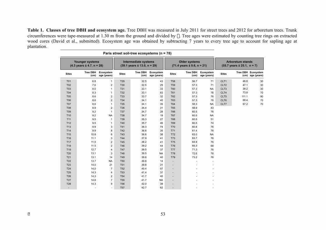
! 53
Table 1. Classes of tree DBH and ecosystem age. Tree DBH was measured in July 2011 for street trees and 2012 for arboretum trees. Trunk circumferences were tape-measured at 1.30 m from the ground and divided by π. Tree ages were estimated by counting tree rings on extracted wood cores (David et al., submitted). Ecosystem age was obtained by subtracting 7 years to every tree age to account for sapling age at plantation.
Sites Tree DBH (cm)
Ecosystem age (years) Sites Tree DBH
(cm)Ecosystem age (years) Sites Tree DBH
(cm)Ecosystem age (years) Sites Tree DBH
(cm)Ecosystem age (years)
T01 6.8 1 T29 32.5 43 T58 56.7 71 CLT1 46.8 30T02 7.6 2 T30 32.5 29 T59 57.3 71 CLT2 47.1 30T03 8.0 1 T31 33.1 33 T60 57.3 NA CLT3 38.2 30T04 8.3 1 T32 33.1 63 T61 57.3 76 CLT4 73.8 70T05 8.6 2 T33 33.7 32 T62 57.3 76 CLT5 111.1 90T06 8.6 2 T34 34.1 40 T63 57.3 76 CLT6 68.4 70T07 8.6 1 T35 34.1 35 T64 58.3 NA CLT7 67.2 70T08 8.9 2 T36 34.4 31 T65 58.9 43T09 9.2 1 T37 34.7 28 T66 60.5 76T10 9.2 NA T38 34.7 19 T67 60.5 NAT11 9.5 1 T39 35.3 27 T68 60.5 51T12 9.5 1 T40 35.7 46 T69 60.5 74T13 9.9 3 T41 36.3 74 T70 60.8 76T14 9.9 8 T42 36.6 35 T71 61.4 76T15 10.8 6 T43 36.6 38 T72 63.0 NAT16 11.1 3 T44 37.9 41 T73 63.7 76T17 11.5 2 T45 38.2 41 T75 64.9 76T18 11.5 2 T46 39.2 44 T76 65.3 68T19 12.7 4 T47 39.5 37 T77 71.3 76T20 13.1 3 T48 39.5 NA T78 72.6 76T21 13.1 14 T49 39.8 40 T79 73.2 76T22 13.7 NA T50 39.8 14 - - -T23 14.0 21 T51 39.8 31 - - -T24 14.0 7 T52 40.4 57 - - -T25 14.3 4 T53 41.4 37 - - -T26 14.3 2 T54 41.7 40 - - -T27 14.6 7 T55 41.7 NA - - -T28 14.3 9 T56 42.0 39 - - -- - - T57 42.7 62 - - -
Intermediate systems (39.1 years ± 13.0, n = 29)
Older systems (71.4 years ± 9.6, n = 21)
Paris street soil-tree ecosystems (n = 78)
Arboretum stands (55.7 years ± 25.1, n = 7)
Younger systems (4.3 years ± 4.7, n = 28)
! 54
The National Arboretum of Chèvreloup (http://chevreloup.mnhn.fr) is a
205-hectare arboretum adjacent to the Palace of Versailles complex and located
in the municipality of Rocquencourt in the Yvelines department, region of Île-
de-France (Figure 1). The current arboretum was created in 1927 and is the
property of the French National Museum of Natural History. At the arboretum,
trees are usually grown on site at the nursery and planted as saplings when about
10 years old. Trees are not submitted to pruning, not fertilized and aboveground
litter is not removed. There is little to no competition for crown development
space. Compared to street trees, there seem to be no space constraint for root
system development5. At the arboretum, 7 silver linden stands were sampled.
Their plantation date is known and was used to estimate soil-tree ecosystem age,
giving an average age of 55.7 ± 25.1 years (Table 1). Arboretum soil-tree
systems thus had an age comprised between intermediate and older street
systems.
2.2. Sample collection and processing
Samples from street plantations were collected over July 2011. At each
site, soil was sampled at 2 points around each tree trunk with a 3 cm diameter
gouge auger. The sampling points were situated at 25-40 cm from the trunk,
depending on accessibility (size of drain holes, obstruction by thick roots etc.).
The 10-30 cm and 30-40 cm depths of both soil cores were respectively pooled.
Samples from the arboretum were collected in July 2012. Four soil cores were
extracted around the trunk at the same distance from the trunk as for the street
sites. The four extracted soil cores were pooled at 0-10, 10-20, 20-30, 30-40 cm
depths respectively. For the arboretum, the 10-30 cm data presented here are an
average of values obtained for 10-20 and 20-30 cm depths. For street and
arboretum soils, subsamples were frozen in liquid N2 in the field for subsequent
NH4+, NO2
- and NO3- analysis.
!!!!!!!!!!!!!!!!!!!!!!!!!!!!!!!!!!!!!!!!!!!!!!!!!!!!!!!!5 A good overview of the arboretum can be seen here: http://www.dailymotion.com/video/x18igt6_arboretum-de-chevreloup (video copyright of the French National Museum of Natural History).
! 55
Twigs were sampled on four opposite points of the external lower canopy.
Leaves were either the antepenultimate or penultimate leaf of the cut twigs. Four
leaves were sampled per tree.
Soil samples were air-dried and manually sieved at 2 mm. Representative
subsamples were homogenized in an agate ball-mill for elemental and isotopic
analyses. Leaves were washed with MilliQ water, gently brushed and again
rinsed with MilliQ water to remove adsorbed particles (Freer-Smith et al., 1997).
They were air-dried and pulverized at < 80 µm with an ultracentrifugal grinding
mill (ZM100, Retsch, Haan, Germany).
Fine roots (diameter < 2 mm) were separated from soil samples with an
electrostatic method, following the principle described by Kuzyakov et al.
(2001). Additional purifying steps were added to separate the extracted roots
from the co-extracted soil particles and plant debris. The extracts were
immersed in a sonicating bath with MilliQ water and floating organic particles
were retrieved while the mineral particles sank to the vessel bottom. The process
was repeated until only the mineral fraction remained at the vessel bottom. If a
few roots remained mixed with the mineral fraction at the bottom, they were
recovered with tweezers. After oven-drying at 40°C, roots were weighed on a
microbalance which provided the fine root biomass of each sample. Fine root
biomass was then divided by the mass of dry < 2 mm soil samples from which
they were extracted, to obtain the fine root gravimetric density (fine root density,
thereafter; mg Root.g Soil-1).
2.3. Soil characteristics
Soil texture after decarbonatation, cationic exchange capacity (CEC), and
total CaCO3 were performed by a routine soil-testing laboratory (INRA-LAS,
France) according to French and international (AFNOR and ISO) standard
! 56
procedures6.
Soil pH was measured in water (5:1 v/v water:soil) with a pH meter
(SevenEasy™, Mettler Toledo, Viroflay, France) according to the norm NF ISO
10390 (AFNOR, 2005).
Bulk density (g.cm-3) was calculated by dividing the mass (g) of the fine
soil (< 2 mm) by its volume. Total soil core volume was estimated by immersing
a wax molding of the auger in a measuring cylinder filled with water and
reading the volume change. The volume for a 10 cm sample was estimated to be
45 cm3. The mass and volume of roots and rocks retained by the 2 mm sieve
were subtracted from the mass and volume of the total soil core. The volume
of > 2 mm rocks and roots was obtained by immersing them in a measuring
cylinder filled with water.
2.4. C and N contents and isotope ratios
Soils were analyzed for organic C content and δ13C after carbonate
removal with the HCl fumigation method (Harris, 2001). Briefly, 30 mg of
homogenized sample were weighted in silver capsules, moisturized with 50 µl
of milliQ water, and placed for 6 h in a vacuumed desiccator with a beaker
containing 200 ml of 16 M HCl. Then, samples were double-folded in tin
capsules for better combustion (Harris, 2001; Brodie et al., 2011) and analyzed
at INRA-Nancy by EA-IRMS (NA 1500, Carlo Erba, Milano, Italy, coupled
with a Delta S, Finnigan, Palo Alto, USA). For total N content and δ15N, soil
samples were analyzed by EA-IRMS (vario Pyro cube, Elementar, Hanau,
Germany, coupled with an IsoPrime, Gvi, Stockport, UK) without any pre-
treatment to avoid unnecessary bias on N parameters (Komada et al., 2008;
Brodie et al., 2011). Pulverized leaf samples were analyzed for C content, N
content, δ13C and δ15N by EA-IRMS (vario Pyro cube, Elementar, Hanau, !!!!!!!!!!!!!!!!!!!!!!!!!!!!!!!!!!!!!!!!!!!!!!!!!!!!!!!!6 List of norms: Texture: NF X 31-107 (AFNOR, 2003); CEC: NF ISO 23470 (AFNOR, 2011); Total CaCO3: NF ISO 10693 (AFNOR, 2014).
! 57
Germany coupled with an IsoPrime, Gvi, Stockport, UK).
For isotopic values, results are expressed using the usual delta notation
that allows expressing the content in 13C or 15N as the relative difference
between the isotopic ratio of the sample and a standard, calculated as:
δ(‰) = [(Rsample – Rstandard)/Rstandard]*1000
where Rsample is the isotope ratio (13C/12C and 15N/14N for C and N,
respectively) of the sample and Rstandard the isotope ratio of the standard. The
international standard for C is the Pee Dee Belemnite standard, with a 13C/12C
ratio of 0.0112372 (Craig, 1957). For N, the international standard is
atmospheric dinitrogen for which the 15N/14N ratio is 0.003676 (Mariotti et al.,
1983, 1984).
For measures of soil concentration in and NH4+, NO2
- and NO3- about 1 g
of frozen subsample was mixed with a 0.5 M KCl solution with a 1:2
soil:solution ratio. Samples were then placed on a rotary shaker for 30 minutes
and then centrifuged at 4000 rpm for 5 min. The surnatant was then analyzed by
colorimetric methods using an autoanalyser (Gallery, Thermo Fisher Scientific,
Cergy-Pontoise, France).
2.5. Statistical analyses
Statistical analyses were performed with the R-software (R Development
Core Team, 2013). Four sample classes (three DBH classes and the arboretum)
and two depths (10-30 and 30-40 cm) and their interaction were used as
explanatory factors for soil variables. For foliar parameters, as well as for
∆15Nleaf-soil, linear models were used with class as an expanatory factor. For soil
parameters, linear mixed-effects models with a “site” random effect were used
for soil variables to account for non-independence of soil depths at each
sampling site. R2 values for linear mixed-effects models were calculated with
the function r.squared.lme (version 0.2-4 (2014-07-10)) that follows the method
! 58
described in Nakagawa & Schielzeth (2013). Values for conditional R2, which
describes the proportion of variance explained by both the fixed and random
factors, are shown. Tukey post-hoc tests were performed for ANOVA models
yielding significant results. For variables that did not satisfy ANOVA
assumptions even after log transformation, non-parametric tests were used: a
Kruskal-Wallis test was used for each depth to test for differences between
classes, and a Wilcoxon-Mann-Whitney test was used for pairwise comparisons
of means for different depths. For all tests, the null hypothesis was rejected for p
< 0.05 and significativity was represented as follows: *** when p ≤ 0.001; **
for 0.001 < p ≤ 0.01 and * when 0.01 < p ≤ 0.05. Effects with 0.05 ≤ p < 0.10
are referred to as marginally significant.
3. Results
3.1. Soil characteristics
Clay, silt and sand contents significantly differed among classes for both
depths (Table 2, Table 3). Soils from younger street systems and the arboretum
had similar clay content that was significantly higher than soils from
intermediate and older systems. Soils from intermediate systems contained more
clay than soils from older systems. Overall, soils from younger systems and the
arboretum were finer textured than soils from street intermediate and older
systems and appeared as silt-loam soils. Soils from street intermediate systems
were loam soils and soils from older street systems were sandy loam soils (Table
2, Table 3).
Bulk density at 10-30 cm showed no significant difference between street
age classes. At 30-40 cm, soils from younger systems had a significantly lower
bulk density than soils from intermediate and older systems. Soils from
intermediate and older systems had higher bulk densities at 30-40 cm than in 10-
30 cm. Soils from all street age classes had a significantly higher bulk density at
both depths compared to arboretum soils (Table 2, Table 3). Soil pH did not
! 59
differ significantly between street age classes but was significantly different
between street systems and soils in the arboretum (Table 2, Table 3). CEC
showed no significant difference between street age classes and between street
sites and the arboretum (Table 2, Table 3).
Total CaCO3 was significantly higher in street soils compared to
arboretum soils, at both depths. At 10-30 cm, it showed a significant increase
with age classes. At 30-40 cm, soils from intermediate and older systems had
significantly more CaCO3 than soils from younger systems. A significant
difference between both depths was observed for each street class, with more
CaCO3 contained in the 10-30 cm than in 30-40 cm. This difference among
depths was not observed in the arboretum (Table 2, Table 3).
3.2. Soil C and N contents and isotope ratios
Soil organic C content was significantly different between street age
classes at 10-30 cm (Table 4, Figure 2A). Soils from intermediate and older
systems had higher organic C contents compared to soils from younger systems,
with respective means of 2.3 and 2.6 % for intermediate and older systems and
1.4 % for younger systems. The difference in organic C content between
younger and older systems was thus almost two-fold at 10-30 cm. At 30-40 cm,
the mean organic C content for soils of younger, intermediate and older systems
was respectively 1.5, 1.8 and 2.5 %. The difference between younger and
intermediate systems was not significant, and soils of older systems were
significantly above the other street systems. At 10-30 cm, mean organic C
content in arboretum soils was of 1.8 %, not significantly different from soils of
street young and intermediate systems but significantly lower than soils of older
street systems.
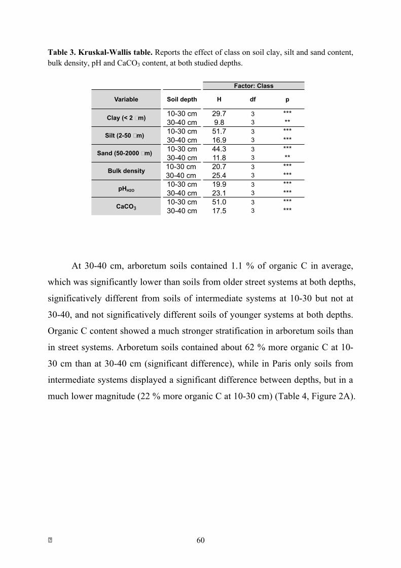
! 60
Table 3. Kruskal-Wallis table. Reports the effect of class on soil clay, silt and sand content, bulk density, pH and CaCO3 content, at both studied depths.
Variable Soil depth H df p
10-30 cm 29.7 3 ***30-40 cm 9.8 3 **10-30 cm 51.7 3 ***30-40 cm 16.9 3 ***10-30 cm 44.3 3 ***30-40 cm 11.8 3 **10-30 cm 20.7 3 ***30-40 cm 25.4 3 ***10-30 cm 19.9 3 ***30-40 cm 23.1 3 ***10-30 cm 51.0 3 ***30-40 cm 17.5 3 ***CaCO3
Factor: Class
Clay (< 2 µm)
Silt (2-50 µm)
Sand (50-2000 µm)
Bulk density
pHH2O
At 30-40 cm, arboretum soils contained 1.1 % of organic C in average,
which was significantly lower than soils from older street systems at both depths,
significatively different from soils of intermediate systems at 10-30 but not at
30-40, and not significatively different soils of younger systems at both depths.
Organic C content showed a much stronger stratification in arboretum soils than
in street systems. Arboretum soils contained about 62 % more organic C at 10-
30 cm than at 30-40 cm (significant difference), while in Paris only soils from
intermediate systems displayed a significant difference between depths, but in a
much lower magnitude (22 % more organic C at 10-30 cm) (Table 4, Figure 2A).
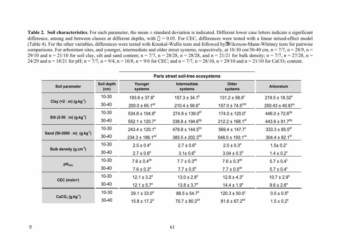
! 61
Table 2. Soil characteristics. For each parameter, the mean ± standard deviation is indicated. Different lower case letters indicate a significant difference, among and between classes at different depths, with α = 0.05. For CEC, differences were tested with a linear mixed-effect model (Table 4). For the other variables, differences were tested with Kruskal-Wallis tests and followed by!Wilcoxon-Mann-Whitney tests for pairwise comparisons. For arboretum sites, and younger, intermediate and older street systems, respectively, at 10-30 cm/30-40 cm, n = 7/7, n = 28/9, n = 29/10 and n = 21/10 for soil clay, silt and sand content; n = 7/7, n = 28/28, n = 28/28, and n = 21/21 for bulk density; n = 7/7, n = 27/28, n = 24/29 and n = 18/21 for pH; n = 7/7, n = 9/4, n = 10/8, n = 9/6 for CEC; and n = 7/7, n = 28/10, n = 29/10 and n = 21/10 for CaCO3 content.
Soil parameter Soil depth (cm)
Youngersystems
Intermediatesystems
Older systems Arboretum
10-30 193.6 ± 37.8a 157.3 ± 34.1b 131.2 ± 58.9c 219.5 ± 18.32a
30-40 200.0 ± 65.1ad 210.4 ± 56.6a 157.0 ± 74.5cbd 250.43 ± 40.87a
10-30 534.8 ± 104.9a 274.9 ± 139.0bf 174.0 ± 120.0c 446.0 ± 72.6dg
30-40 552.1 ± 120.7a 338.8 ± 194.6bg 212.2 ± 168.1ef 443.6 ± 91.7dg
10-30 243.4 ± 120.1a 478.8 ± 144.5be 569.4 ± 147.7c 333.3 ± 85.5af
30-40 234.3 ± 186.1ad 385.5 ± 202.3bd 548.0 ± 193.1ce 304.4 ± 82.1bf
10-30 2.5 ± 0.4a 2.7 ± 0.6a 2.5 ± 0.3a 1.5± 0.2c
30-40 2.7 ± 0.6a 3.1± 0.6b 3.04 ± 0.3b 1.4 ± 0.2c
10-30 7.6 ± 0.4ab 7.7 ± 0.3ab 7.6 ± 0.3ab 5.7 ± 0.4c
30-40 7.6 ± 0.3a 7.7 ± 0.5b 7.7 ± 0.5ab 5.7 ± 0.4c
10-30 12.1 ± 3.2a 13.0 ± 2.8a 12.8 ± 4.3a 10.7 ± 2.9a
30-40 12.1 ± 5.7a 13.8 ± 3.7a 14.4 ± 1.9a 9.6 ± 2.6a
10-30 0.15 ± 0.05a 0.17 ± 0.1ab 0.22 ± 0.08cde 0.06 ± 0.06ef
30-40 0.10 ± 0.04bf 0.17 ± 0.1abd 0.18 ± 0.12abe 0.02 ± 0.01e
10-30 29.1 ± 33.0a 88.5 ± 54.7b 120.3 ± 50.0c 0.5 ± 0.5e
30-40 15.8 ± 17.2a 70.7 ± 80.2ad 81.6 ± 67.2bd 1.5 ± 0.2e
CEC (molc+)
POlsen (g.kg-1)
CaCO3 (g.kg-1)
Paris street soil-tree ecosystems
Clay (<2 µm) (g.kg-1)
Silt (2-50 µm) (g.kg-1)
Sand (50-2000 µm) (g.kg-1)
Bulk density (g.cm-3)
pHH2O
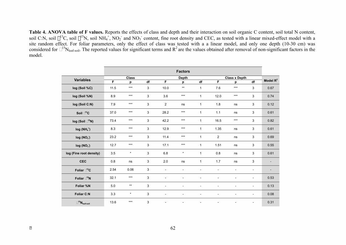
! 62
Table 4. ANOVA table of F values. Reports the effects of class and depth and their interaction on soil organic C content, soil total N content, soil C:N, soil δ13C, soil δ15N, soil NH4
+, NO2- and NO3
- content, fine root density and CEC, as tested with a linear mixed-effect model with a site random effect. For foliar parameters, only the effect of class was tested with a a linear model, and only one depth (10-30 cm) was considered for ∆15Nleaf-soil. The reported values for significant terms and R2 are the values obtained after removal of non-significant factors in the model.
F p df F p df F p df
- 0.08
∆15Nleaf-soil 13.6 *** 3 - - - - - - 0.31
Foliar C:N 3.3 * 3 - - - - -
- - - -
1.7 ns 3 -
Foliar %N 5.0 ** 3 - - - - - - 0.13
3 0.55
log (Fine root density) 3.5 * 3 6.8 * 1 0.8 ns 3 0.61
log (NO3-) 12.7 *** 3 17.1 *** 1 1.51 ns
3 0.61
log (NO2-) 23.2 *** 3 11.4 *** 1 2 ns 3 0.69
log (NH4+) 8.3 *** 3 12.9 *** 1 1.35 ns
3 0.61
log (Soil δ15N) 73.4 *** 3 42.2 *** 1 16.5 *** 3 0.82
Soil δ13C 37.0 *** 3 28.2 *** 1 1.1 ns
3 0.74
log (Soil C:N) 7.9 *** 3 2 ns 1 1.8 ns 3 0.12
log (Soil %N) 8.9 *** 3 3.6 *** 1 12.0 ***
Factors
Variables Class Depth Class x DepthModel R2
log (Soil %C) 11.5 *** 3 10.0 ** 1 7.6 *** 3 0.67
0.53------3***32.1Foliar δ15N
CEC 0.8 ns 3 2.0 ns 1
Foliar δ13C 2.54 0.06 3 - - -

! 63
At 30-40 cm, average soil δ13C was -26.1 ‰ for young systems, -25.3 ‰
for intermediate systems and -25.0 for older systems with a significant
difference between each class. At the arboretum, soil δ13C was -26.6 ‰ at 10-30
cm and -26.2 ‰ at 30-40 cm. At both depths, soil δ13C at the arboretum was not
significantly different from street younger systems but was significantly lower
than soil δ13C of intermediate and older street systems. Depth had a significant
effect on soil δ13C values, with notably intermediate and older street systems
showing a soil δ13C about 0.5 ‰ unit higher at 30-40 cm. Soils from older street
systems had about 1 ‰ unit more enriched δ13C values compared to arboretum
and young street system soils.
Soil total N content was significantly different between street age classes
at 10-30 cm (Table 4, Figure 3A). Average soil N content was 0.12 % for
younger street systems, 0.18 % for intermediate street systems and 0.21 % for
older street systems, with significant difference between each class. The
difference in soil N content between younger and older street systems was about
two-fold. At 30-40 cm, soil N content in younger systems (0.13 %) was not
significantly different from intermediate systems (0.13 %), but soils from older
systems contained significantly more N (0.17 %) than soils from younger and
intermediate systems. Soils from the arboretum contained more N (0.2 %) at 10-
30 cm than soils from younger street systems but had similar N content with
soils from intermediate and older street systems. Soil N content was different
between depths for all classes except for younger street systems. As for organic
C, the difference between depths was stronger for arboretum sites, with N
content at 10-30 cm being 83 % higher than N content at 30-40 cm (0.11 %)
(significant difference). In street systems, soil N content at 10-30 cm was 38 %
higher than at 30-40 cm in intermediate systems (significant difference) and a
similar trend was observed on older systems.
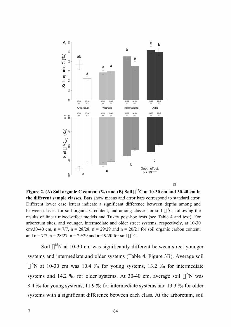
! 64
Soil δ15N at 10-30 cm was significantly different between street younger
systems and intermediate and older systems (Table 4, Figure 3B). Average soil
δ15N at 10-30 cm was 10.4 ‰ for young systems, 13.2 ‰ for intermediate
systems and 14.2 ‰ for older systems. At 30-40 cm, average soil δ15N was
8.4 ‰ for young systems, 11.9 ‰ for intermediate systems and 13.3 ‰ for older
systems with a significant difference between each class. At the arboretum, soil
Arboretum Younger Intermediate Older
0.0
0.5
1.0
1.5
2.0
2.5
3.0
10-30 cm
30-40 cm
10-30 cm
30-40 cm
10-30 cm
30-40 cm
10-30 cm
30-40 cm
Arboretum Younger Intermediate Older
−27
−26
−25
−24
−23
10-30 cm
30-40 cm
10-30 cm
30-40 cm
10-30 cm
30-40 cm
10-30 cm
30-40 cm
Arboretum Younger Intermediate Older
Soil
orga
nic
C (%
) So
il δ1
3 Cor
g (‰
)
A
B
ab
a
a a
b
a
b b
a a
b c
Depth effect: p < 10-4 ***
!Figure 2. (A) Soil organic C content (%) and (B) Soil δ13C at 10-30 cm and 30-40 cm in the different sample classes. Bars show means and error bars correspond to standard error. Different lower case letters indicate a significant difference between depths among and between classes for soil organic C content, and among classes for soil δ13C, following the results of linear mixed-effect models and Tukey post-hoc tests (see Table 4 and text). For arboretum sites, and younger, intermediate and older street systems, respectively, at 10-30 cm/30-40 cm, n = 7/7, n = 28/28, n = 29/29 and n = 20/21 for soil organic carbon content, and n = 7/7, n = 28/27, n = 29/29 and n=19/20 for soil δ13C.
! 65
δ15N was 6.9 ‰ at 10-30 cm and 9.5 ‰ at 30-40 cm, with soils being
significantly more enriched in 15N at 30-40 cm than at 10-30 cm. For street
systems in Paris, it was the opposite, with soils being significantly more
enriched in 15N at 10-30 cm than at 30-40 cm for younger and intermediate
street systems. At 10-30 cm, soils of younger street systems were significantly
more enriched in 15N compared to arboretum soils at the same depth but not
significantly different from arboretum soils at 30-40 cm. Soil δ15N at both
depths at the arboretum was significantly different from both depths in street
intermediate and older systems. Overall, average soil δ15N from older street
systems was 3.8 ‰ units higher at 10-30 cm and 4.9 ‰ units higher at 30-40 cm
when compared to soils from younger systems, and 7.4 ‰ units higher at 10-30
cm and 3.8 ‰ units higher at 30-40 cm when compared to soils from the
arboretum.
Soil NH4+ content did not differ between arboretum soils and intermediate
and older street soils (Table 4, Figure 4B). Soils from intermediate and older
systems had higher NH4+ content than soils from younger systems. There was an
observed trend in stratification between depths in all classes, with an overall
significant depth effect on NH4+ content. At 10-30 cm, soils from intermediate
and older street systems contained about twice the amount of NH4+ found in
younger street systems.
Soil NO2- content was higher in all street sites at both depths compared to
arboretum soils (Table 4, Figure 4C). Older street systems had higher soil NO2-
at 10-30 cm than younger systems at both depths. At 10-30 cm, soils from older
street systems contained almost ten times more NO2- when compared to
arboretum soils, four times more when compared to younger street systems and
1.6 times more when compared to intermediate systems. There was an observed
trend in stratification in intermediate and older street systems, with a significant
depth effect (Table 4, Figure 4C).

! 66
Arboretum Younger Intermediate Older0.00
0.05
0.10
0.15
0.20
0.25
Arboretum Younger Intermediate Older
05
1015
10-30 cm
30-40 cm
10-30 cm
30-40 cm
10-30 cm
30-40 cm
10-30 cm
30-40 cm
Arboretum Younger Intermediate Older
10-30 cm
30-40 cm
10-30 cm
30-40 cm
10-30 cm
30-40 cm
10-30 cm
30-40 cm
Arboretum Younger Intermediate Older
Soi
l tot
al N
(%)
Soi
l δ15
N (
‰)
A
B
abc
d d d
ab
cd
ab
ad
a
bc b
ac
d e
d d
!Figure 3. Figure 2. (A) Soil total N content (%) and (B) Soil δ15N at 10-30 cm and 30-40 cm in the different sample classes. Bars show means and error bars correspond to standard error. Different lower case letters indicate a significant difference between depths among and between classes, following the results of linear mixed-effect models and Tukey post-hoc tests (see Table 4 and text). For arboretum sites, and younger, intermediate and older street systems, respectively, at both depths n = 7, n = 28, n = 29 and n = 21 for both variables.
Soil NO3- content was higher in street systems at 10-30 cm when
compared to arboretum soils at both depths (Table 4, Figure 4D). Street soils
had, on average, 22 times more soil NO3- than arboretum sites at 10-30 cm, and
about 165 times more NO3- at 30-40 cm. There was an observed trend in
stratification in intermediate and older street systems (Table 4, Figure 4D), with
a significant effect of depth. Soil in intermediate systems contained 3 times
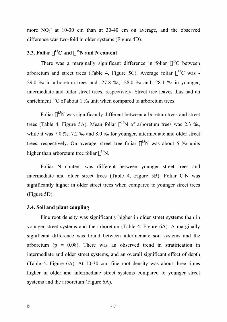
! 67
more NO3- at 10-30 cm than at 30-40 cm on average, and the observed
difference was two-fold in older systems (Figure 4D).
3.3. Foliar δ13C and δ15N and N content
There was a marginally significant difference in foliar δ13C between
arboretum and street trees (Table 4, Figure 5C). Average foliar δ13C was -
29.0 ‰ in arboretum trees and -27.8 ‰, -28.0 ‰ and -28.1 ‰ in younger,
intermediate and older street trees, respectively. Street tree leaves thus had an
enrichment 13C of about 1 ‰ unit when compared to arboretum trees.
Foliar δ15N was significantly different between arboretum trees and street
trees (Table 4, Figure 5A). Mean foliar δ15N of arboretum trees was 2.3 ‰,
while it was 7.0 ‰, 7.2 ‰ and 8.0 ‰ for younger, intermediate and older street
trees, respectively. On average, street tree foliar δ15N was about 5 ‰ units
higher than arboretum tree foliar δ15N.
Foliar N content was different between younger street trees and
intermediate and older street trees (Table 4, Figure 5B). Foliar C:N was
significantly higher in older street trees when compared to younger street trees
(Figure 5D).
3.4. Soil and plant coupling
Fine root density was significantly higher in older street systems than in
younger street systems and the arboretum (Table 4, Figure 6A). A marginally
significant difference was found between intermediate soil systems and the
arboretum (p = 0.08). There was an observed trend in stratification in
intermediate and older street systems, and an overall significant effect of depth
(Table 4, Figure 6A). At 10-30 cm, fine root density was about three times
higher in older and intermediate street systems compared to younger street
systems and the arboretum (Figure 6A).
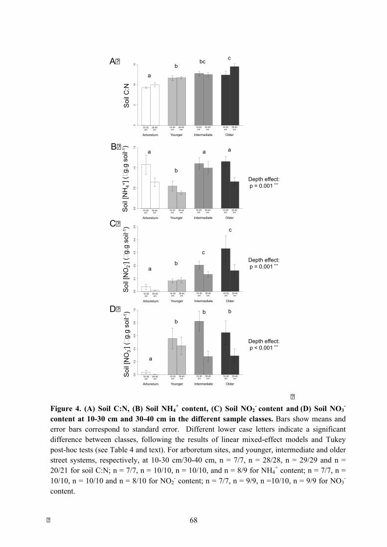
! 68
Arboretum Younger Intermediate Older
0.0
0.5
1.0
1.5
Arboretum Younger Intermediate Older
0.0
0.1
0.2
0.3
0.4
0.5
Arboretum Younger Intermediate Older
0.0
0.2
0.4
0.6
0.8
1.0
Arboretum Younger Intermediate Older
05
1015
10-30 cm
Arboretum Younger Intermediate Older
30-40 cm
10-30 cm
30-40 cm
10-30 cm
30-40 cm
10-30 cm
30-40 cm
10-30 cm
Arboretum Younger Intermediate Older
30-40 cm
10-30 cm
30-40 cm
10-30 cm
30-40 cm
10-30 cm
30-40 cm
10-30 cm
Arboretum Younger Intermediate Older
30-40 cm
10-30 cm
30-40 cm
10-30 cm
30-40 cm
10-30 cm
30-40 cm
10-30 cm
Arboretum Younger Intermediate Older
30-40 cm
10-30 cm
30-40 cm
10-30 cm
30-40 cm
10-30 cm
30-40 cm
Soi
l C:N
S
oil [
NH
4+ ] (µ
g.g
soil-
1 )
Soi
l [N
O2- ]
(µg.
g so
il-1 )
S
oil [
NO
3- ] (µ
g.g
soil-
1 )
A!
B!
C!
D!
a
b bc c
a
b
a a
a b
c
c
a
b
b b
Depth effect: p = 0.001 ***
Depth effect: p = 0.001 ***
Depth effect: p < 0.001 ***
!Figure 4. (A) Soil C:N, (B) Soil NH4
+ content, (C) Soil NO2- content and (D) Soil NO3
-
content at 10-30 cm and 30-40 cm in the different sample classes. Bars show means and error bars correspond to standard error. Different lower case letters indicate a significant difference between classes, following the results of linear mixed-effect models and Tukey post-hoc tests (see Table 4 and text). For arboretum sites, and younger, intermediate and older street systems, respectively, at 10-30 cm/30-40 cm, n = 7/7, n = 28/28, n = 29/29 and n = 20/21 for soil C:N; n = 7/7, n = 10/10, n = 10/10, and n = 8/9 for NH4
+ content; n = 7/7, n = 10/10, n = 10/10 and n = 8/10 for NO2
- content; n = 7/7, n = 9/9, n =10/10, n = 9/9 for NO3-
content.

! 69
Arboretum Younger Intermediate Older
02
46
810
Arboretum Younger Intermediate Older
−30
−29
−28
−27
−26
−25
Arboretum Younger Intermediate Older
Folia
r δ15
N (
‰)
Folia
r δ13
C (
‰)
A!
C!
a
b b
Arboretum Younger Intermediate Older
2.0
2.2
2.4
2.6
2.8
3.0
3.2
3.4
Folia
r %N
Arboretum Younger Intermediate Older
Arboretum Younger Intermediate Older
1012
1416
18
Arboretum Younger Intermediate Older
Folia
r C:N
B!
D!
b
Class effect: p = 0.06
ab a
b b
ab a
ab b
!
Figure 5. (A) Foliar δ15N, (B) Foliar %N, (C) Foliar δ13C and (D) Foliar C:N, in the different sample classes. Bars show means and error bars correspond to standard error. Different lower case letters indicate a significant difference between classes, following the results of linear models and Tukey post-hoc tests (see Table 4 and text). For arboretum sites, and younger, intermediate and older street systems, respectively, n = 7, n = 28, n = 29 and n = 20 for all variables.
The difference between foliar δ15N and soil δ15N, ∆15Nleaf-soil, was
calculated by using the soil δ15N at 10-30 cm. It was significantly lower in older
and intermediate street systems when compared to younger street systems, and
significantly lower than in the arboretum in older street systems (Table 4, Figure
6B). ∆15Nleaf-soil in older street systems was about 3 ‰ units lower than in
younger street systems (Figure 6B).

! 70
Arboretum Younger Intermediate Older
010
020
030
040
050
060
070
0
10-30 cm
Arboretum Younger Intermediate Older
30-40 cm
10-30 cm
30-40 cm
10-30 cm
30-40 cm
10-30 cm
30-40 cm
Fine
root
den
sity
(mg.
g so
il-1 )
Arboretum Younger Intermediate Older
−8−6
−4−2
0
Arboretum Younger Intermediate Older
∆15 N
leaf
-soi
l (‰
)
B!
A!
a
ab
a
ab
b
a
b b
Depth effect: p = 0.01 *
!Figure 6. (A) Fine root density and (B) ∆15Nleaf-soil. Bars show means and error bars correspond to standard error. Different lower case letters indicate a significant difference between classes, following the results of a linear mixed-effect model for fine roots and of a linear model for ∆15Nleaf-soil, and Tukey post-hoc tests (see Table 4 and text). For arboretum sites, and younger, intermediate and older street systems, respectively, at 10-30 cm/30-40 cm, n = 7/6, n = 10/10, n = 9/9 and n = 10/10 for fine root density ; and n = 7, n = 28, n = 29 and n = 20 for ∆15Nleaf-soil.
!
4. Discussion 4.1. Age-related trends in soil organic C: Accumulation of root C?
Our results show that in Parisian street tree plantations, soil organic C
content is higher in older plantations than in younger ones, which could suggest
a dynamics of C accumulation over time. Compared to arboretum sites, foliar
! 71
δ13C values in Parisian trees were higher, possibly indicating a tree response to
water scarcity, leading to a foliar enrichment in 13C through higher WUE
(Farquhar et al., 1989). The important amount of impervious surface around
street trees, impeding water infiltration, as well as the Parisian urban heat island
effect imposing higher evaporation demand, could indeed expectedly lead to
increased water scarcity in street conditions compared to the arboretum. This is
confirmed by dendroclimatic works on the same chronosequence, which have
shown that street silver linden growth in Paris is particularly sensitive to spring
and autumn precipitation (David et al., submitted). Even slight changes in the
δ13C of organic matter produced through photosynthesis by trees can quickly be
reflected in the C allocated belowground (Mariotti, 1991; Ekblad & Högberg,
2001), and thus imprint this isotopic signal on soil organic matter (SOM). Soil
δ13C consistently showed a significant increase with soil-tree system age, which
had the same order of magnitude between younger and older street soils (about
1 ‰ unit) than the difference observed in foliar δ13C between street and
arboretum trees. Even in a context where most aboveground litter is exported,
this gradual 13C signal transfer between trees and soils could thus occur through
belowground C inputs (Ekblad & Högberg, 2001).
The trends we observed in fine root densities would tend to support such a
scenario. At a depth of 10-30 cm, fine root densities in older street systems were
more than four times higher than in younger street systems and the arboretum,
suggesting a higher allocation of C belowground as street trees age, further
imprinting a 13C-enriched signal to SOM. Furthermore, a higher allocation of C
belowground, in the form of fine roots, could also represent a drought response
strategy by trees (Craine, 2009), and is theoretically expected as a possible water
acquisition strategy for forest tree species (Gaul et al., 2008; Meier & Leuschner,
2008; Craine, 2009), which could be consistent with the trends discussed above.
Another result that points towards an accumulation of organic C through

! 72
continuous belowground input is the trend in soil C:N, which gradually
increases across street system age classes and is higher in older street systems
than at the arboretum. This trend is, too, consistent with a scenario where street
systems, as they age, experience an increased and sustained input of fresh
organic matter through roots.
Another possible factor explaining age-related trends in soil δ13C could be
the influence of microbial biomass. Indeed, the microbial assimilation of C is
known to cause a 13C enrichment of microbial biomass compared to the original
substrate (Lerch et al., 2011). The trend in stratification of soil δ13C values that
seem to occur in street soils with time, with more 13C-enriched organic carbon at
30-40 cm than at 10-30 cm, would be consistent with a scenario where the δ13C
values at 10-30 cm would more reflect the fresh root inputs while the more
enriched δ13C values at 30-40 cm, where SOM would be relatively more
humified, would bear a stronger microbial imprint.
Taken together, these converging trends and putative underlying
mechanisms tend to support the hypothesis of a root-derived C accumulation in
street soils.
4.2. Age-related trends in N cycling: Rapid N saturation of street systems?
Similarly to soil C, total soil N seemed to increase with street system age,
reaching a similar level as found in the arboretum despite aboveground litter
export. Furthermore, one of the most striking trends observed in this study was
the exceptionally high average soil δ15N value of intermediate and older street
systems, with respective averages of 13.2 ‰ and 14.2 ‰. These values fall in
the range of the 10 % of highest values measured worldwide, and three sites had
a δ15N above 17 ‰, close to some of the highest soil δ15N measured worldwide
(Martinelli et al., 1999; Amundson et al., 2003; Craine et al., 2015). The δ15N
values measured at 10-30 cm at the arboretum, with an average of 6.9 ‰, were
! 73
close to typical values found for surface plain soils in the Île-de-France region
(Billy et al., 2010). The stratification of soil δ15N values in street systems, with
δ15N values higher in near-surface horizons than at higher depths, was opposite
to the one found at the arboretum where soils showed higher δ15N with depth, as
is generally observed in soil profiles (Mariotti et al., 1980; Högberg, 1997;
Hobbie & Ouimette, 2009). Street foliar δ15N values also fall among the highest
values measured in temperate forests (Martinelli, 1999; Pardo et al., 2006, 2013).
This firstly suggests that N inputs with enriched δ15N values enter street
soils from the surface. In Paris, Widory (2007) measured that atmospheric
particulate N (ammonium and nitrate) had a δ15N as high as 10 ‰ on a yearly
average. Direct measures from vehicle exhaust yielded a δ15N for particulate N
of 3.9 to 5.6 ‰ (Widory, 2007). Depositions from such sources are likely to
occur for street soils, as they are very closely exposed to traffic. Animal sources
(humans, pets), in the form of urine or feces, are another likely source of N. The
δ15N of such sources would be highly dependent on animal diet. Kuhnle et al.
(2013) report, for humans feeding on a diversified diet (red meat, fish,
vegetables), δ15N values of about 5.4 ‰ for feces and 6.7 ‰ for urine. Heaton
(1986) considers a typical animal waste δ15N of 5 ‰, which is consistent with
the order of magnitude reported by Kuhnle et al. (2013). In contemporary
human and pet hair samples, Bol & Pflieger (2002) report that δ15N values were
of the same order of magnitude for human and dog samples in England,
suggesting a diet based on similar (mostly processed) food sources. Dog waste
δ15N could thus likely reflect the values found in human waste.
Both likely sources of exogenous N, atmospheric deposition and animal,
are suspected to have high δ15N values, which is consistent with the possibility
of a gradual imprint by these sources of surface soil δ15N with time. However,
the δ15N of potential sources cannot alone explain the massive shift that seems to
take place with time towards extreme soil δ15N values. Such a shift requires
! 74
further processing of deposited N, especially by microbial activity. As a matter
of fact, the trends observed on N parameters in street systems match certain
symptoms of N saturation, which refers to a process where N-limited forests
chronically receive elevated N inputs, ultimately resulting in higher ecosystem
N outflows by increased volatilization, nitrification and denitrification (Aber et
al., 1998; Pardo et al., 2006; Lovett & Goodale, 2011).
The observed trends in street soil and foliar δ15N closely match, for
instance, the theoretical expectations of Högberg (1997) for a forest receiving
high rates of N deposition. An important deposition of NH4+ can lead to
increased nitrification, further enriching the substrate NH4+ pool in 15N, thus
leading to an increase in plant tissue δ15N. The recycling of plant biomass in the
upper horizons would then lead to a relative 15N enrichment of soil surface
compared to deeper layers, where, furthermore, stabilized fractions of the
relatively 15N-depleted nitrate would have leached, further increasing the
abnormal stratification in soil δ15N values. Increased nitrification at the soil
surface could also make more nitrate available for uptake by plants, leading to
an increased difference between soil δ15N (more enriched) and foliar δ15N
(relatively less enriched). But increased nitrate availability could also lead to
increased denitrification, which would lead to a 15N enrichment of residual
nitrate. This nitrate, if absorbed by the plant and its 15N-enriched N recycled in
SOM, could too lead to an increase of surface soil δ15N. The difference between
soil and foliar δ15N would then depend on the equilibrium between nitrification
and denitrification, and the relative proportions of ammonium and nitrate
consumed by the tree.
The high values and inverse stratification of soil δ15N in street soils, as
well as the high foliar δ15N for street trees, tend to support such a scenario. The
mineral N content of street soils, especially in nitrite and nitrate, were much
superior than the values found at the arboretum and could suggest increased
! 75
nitrification and denitrification. Nitrite, especially, is an intermediary in both
nitrification and denitrification, and its accumulation in street soils could be seen
as a proxy of increased nitrification and denitrification (Burns et al., 1996;
Homyak et al., 2015). The decrease of ∆15Nleaf-soil between younger street
systems and older street systems suggests that trees in these systems have access,
in part, to a source of N that is 15N-depleted compared to SOM. This could, as
discussed above, be explained by an increased reliance on nitrate produced
through nitrification, which would be 15N-depleted when compared to
ammonium derived from the recycling of SOM, whose δ15N would be close to
the δ15N of bulk soil, since little fractionation occurs during N mineralization
(Högberg, 1997).
Taken together, these trends seem to point towards important N inputs to
street systems, which rather quickly lead these systems to a state of N saturation.
Younger street systems, for instance, with an average age of about 5 years,
already present important symptoms of N saturation: high foliar δ15N values,
higher δ15N values in soil surface, and high concentrations of mineral N forms
suggesting an increased activity in N-loss pathways (e.g., nitrification,
denitrification).
An intriguing result in foliar N values concerns foliar N content and foliar
C:N. In street systems, despite a likely increased soil N content with time, foliar
N content was lower in intermediate and older trees compared to younger trees
and, accordingly, younger trees had lower foliar C:N ratios. A first hypothesis
could be that physiological changes related to tree aging are involved (Gilson et
al., 2014). However, even though the differences between the arboretum trees
and the street systems were not significant, the mean value of both foliar N
content and foliar C:N were both closer to the values found in younger systems
and systematically higher and lower, respectively, than the foliar N content and
foliar C:N of intermediate and older street systems. This could thus also be
! 76
interpreted as a progressive N limitation for trees, portraying a paradoxical
situation of simultaneous N saturation and limitation. However, even if soil N
content increases in the upper part of the pit, and in the part that is unsealed, this
does not mean that, as trees develop and their N needs increase, that the total
soil pit N stock would be enough to meet their N needs, and trees might have to
develop strategies to acquire N. An increased fine root density could, in this case
too, be one of them, as it increases the fine root surface in contact with soil and
susceptible to uptake N. It also enables living roots to be closer to decaying dead
roots, thus increasing the chance of new roots to uptake N as it is being recycled
from old roots (Abbadie, 1992; de Parseval et al., 2015). The fact that fine root
density increases with street tree age, not only at the surface, but also in deeper
layers (30-40 cm, here), would also fit such a scenario. It could, furthermore,
also enable trees to uptake a higher proportion of the nitrate that leaches from
the surfaces with rainfall.
Trees could also increase their direct foliar uptake of gaseous NOx
compounds (Ammann et al., 1999; Sparks, 2009), which has been
experimentally shown to be a controlled process by plants, that can rely more on
foliar nutrition when root nutrition is limited (Vallano & Sparks, 2008). The
δ15N value of gaseous NOx compounds is usually lower than that of particulate
N that derives from them (Widory, 2007), and Ammann et al. (1999) report
values for traffic-derived NO2 of 5.78 ‰. Compared to the potential δ15N of
deposited N on soil, as discussed above, this atmospheric source of N would be
less enriched in 15N, and an increased reliance on foliar N uptake by trees would
be, too, consistent with the trends observed in ∆15Nleaf-soil in street systems.
The apparent tension between of saturation and limitation could thus be
released by distinguishing between soil N content (a percentage) and the actual
available N stock (a mass) in the pit soil. Comparing the latter to tree N demand
could further answer the question of whether nutrient supply in Parisian street

! 77
plantation is sufficient to sustain healthy trees on the long run. This would have
important practical interest, since it would shift the question from a “substrate”
perspective (“Is my soil chemically fertile enough?”) to a perspective where the
whole pit design and management (its volume, its irrigation, its greening etc.) as
a whole would be questioned regarding its performance to sustain healthy trees.
4.3. Uncertainties linked to potential legacy effects
As urban areas develop over natural or agricultural land, the potential
influence of past land-uses on current soil properties often constitutes an
important source of uncertainty when trying to interpret contemporary patterns
(Raciti et al., 2011; Lewis et al., 2014). Less often mentioned, however, are the
uncertainties due to varying characteristics of soils that are imported for
landscaping purposes. In the context of this study, such legacy effects of initial
soil conditions must be considered.
Soil texture differed among street age classes and probably reflects
historical differences in imported soil types. Indeed, the geographical origins of
imported soils are historically tightly linked to the development of urbanization
in the Parisian region during the 20th century. Prior to 1950, soils were coming
from areas closer to Paris, most likely from market gardening cultures that had
more sandy soils (Nold, 2011; Paris Green Space and Environmental Division,
pers. comm.). As the agglomeration spread across Île-de-France, imported soils
gradually came from further areas in the region, and now tend to come from
more peripheral plains and plateaux and are probably soils that were formerly
under cereal crops (Nold, 2011; Paris Green Space and Environmental Division,
pers. comm.). Such difference among imported soil types could also be reflected
in initial SOM content. Expert knowledge tends to confirm that soils imported
around 1950, especially those used previously for market gardening agriculture,
likely had higher organic matter content than soils entering Paris today (Nold,
2011; Paris Green Space and Environmental Division, pers. comm.). Different

! 78
agricultural practices between historical periods could also affect the δ15N of
imported soils, since the majority of recently imported soils likely have received
synthetic fertilizers while older soils likely received organic fertilizers (different
types of manure and compost). Synthetic fertilizers generally have low δ15N
values, while organic fertilizers usually have high δ15N values: for the former,
Bateman & Kelly (2007) report an average δ15N of 0.2 ‰, and an average of
8.2 ‰ for the latter. Soils that have received chronic applications of one or the
other type of fertilizers would likely have contrasted δ15N when arriving to Paris.
While these uncertainties are important and would require further
investigation to discriminate between legacy effects and actual dynamics in C
and N cycling, it seems difficult to attribute an overriding effect to potential
legacies in light of all the converging patterns described in previous sections.
The different stratification patterns, in particular, that were observed in street
systems, (e.g., fine root densities, soil δ15N and δ13C, and mineral N) rather
suggest an imprint from biological activity of trees and soil microbes and point
towards the existence of long-term dynamics in C and N cycling after street soil-
tree systems are “constructed” in streets.
Concerning the hypothesis of soil exhaustion that drives current
management practices of street soils in Paris, by taking SOM content, soil C:N,
soil total N and soil mineral N as proxies for fertility, the present work does not
confirm the hypothesis that older soils are less fertile than newly imported soils,
and even suggests the opposite trend. This means that reflections could be
engaged on the potential recycling of old street soils. Further investigations are
needed, however, on the question of whether current tree-pit design (volume
etc.) is appropriate to ensure a proper nutrient supply to trees. Signs of water
stress, confirming other studies on the same systems (David et al., submitted),
also suggest that irrigation might be considered to enhance tree health.
! 79
5. Conclusion
The combination of a long-term approach and stable isotope analysis
enabled the observation of age-related patterns in C and N cycling in Paris street
plantations. Even though the studied systems were spread across the city, the
variance of several key variables was strongly explained by system age and soil
depth alone. As most studies in urban ecosystem ecology have so far adopted a
spatial approach to study ecosystem response to urban environments, this study
suggests that the age of ecosystems, e.g., the time they have spent in a city, can
be a key explanatory variable for several ecosystem features, and help us better
understand ecosystem trajectory on a mechanistic basis. Here, we make the
hypothesis of a root-derived C accumulation, and the hypothesis of a fast
occurring, and amplifying with time, state of N saturation for street soil-tree
systems. Further works on this chronosequence should, in particular, focus on
SOM dynamics to confirm the root source of accumulating SOM, as well as
investigate the causes of SOM accumulation, and look at microbial N processing
to confirm whether a higher activity in N-loss pathways is detected. The
existence of these temporal trends if of interest for city managers, and open the
questions of whether old street soils should be recycled and tree pit design and
management adjusted to enhance the health of trees.

! 80

! 81

! 82

! 83
Chapter 2
Legacy or accumulation? A study of long-term soil organic matter dynamics in
Haussmannian tree plantations in Paris7
1. Introduction Urban environments have been shown to have profound, yet still poorly
understood effects on carbon (C) and nitrogen (N) cycling in ecosystems (De
Kimpe & Morel, 2000; Scharenbroch et al., 2005; Kaye et al., 2006; Lorenz &
Lal, 2009; Pouyat et al., 2010). Authors have suggested that the importance of
urban drivers on ecosystem processes, and their similarities across cities, could
surpass natural drivers and lead to similar ecosystem responses on key
ecological variables in different cities, an asumption coined the “urban
convergence hypothesis” (Pouyat et al., 2003, 2010; see also Groffman et al.,
2014). If studies have indeed reported patterns of urban soil C and N
accumulation worldwide (e.g., McDonnell et al., 1997; Ochimaru & Fukuda,
2007; Chen et al., 2010; Raciti et al., 2011; Gough & Elliott, 2012; Vasenev et
al., 2013; Huyler et al., 2016), important uncertainties remain, however, on the
mechanisms leading to such accumulation.
The effects of past land-uses on current soil C and N content (e.g., Raciti
et al., 2011; Vasenev et al., 2013; Lewis et al., 2014), or uncertainties on the
origin of soils, can add difficulties in interpreting patterns in urban C and N
cycling. Identifying the sources of the accumulated organic C is not
straightforward either, as urban aboveground litter is often exported and data on !!!!!!!!!!!!!!!!!!!!!!!!!!!!!!!!!!!!!!!!!!!!!!!!!!!!!!!!7 A research article presenting this chapter’s results will be prepared for an international journal by authors (in alphabetic order after first author) Rankovic, A., Abbadie, L., Barot, S., Barré, P., Camin, F., Cardénas, V., David, A., Lata, J.-C., Lerch, T. Z., Scattolin, L., Sebilo, M., Vaury, V. & Zanella, A.

! 84
belowground litter inputs are scarce (Templer et al., 2015; Huyler et al., 2016).
Furthermore, urban soils are subjected to varying and sometimes substantial
inputs of exogenous organic C depositions such as “black C” particles produced
by incomplete combustion of fossil fuels and biomass (Rawlins et al., 2008;
Edmonson et al., 2015). For N, similar uncertainties are found concerning
fertilization due to landscaping practices, or on the amount, origin and fate of
atmospheric N deposition to urban soils (e.g., Raciti et al., 2011; Bettez et al.,
2013; Rao et al., 2013). Various types of littering, especially animal dejections,
could also contribute to C and N inputs to urban soils.
Furthermore, after C and N inputs, the mechanisms leading to their
subsequent accumulation are not clearly elucidated either. Soil organic matter
(SOM) is the main source of energy and nutrients for soil organisms, and
without mechanisms of relative stabilization, organic C has a spontaneous
tendency to be mineralized as CO2 by soil microorganisms. Research on soil
organic C dynamics has identified several factors explaining how soil organic C
could escape from microbial degradation. These factors include the chemical
properties of SOM, making it more or less recalcitrant to microbial
biodegradation, the interaction with soil minerals that can for instance shield
SOM from microbial catabolic activity through its occlusion in soil aggregates
or its sorption to clay surfaces, and the abiotic environmental constraints to
microbial activity (temperature, nutrient availability, pH, soil water potential
etc.) (e.g., Six et al., 2002; Fontaine et al., 2003, 2007; von Lützow et al., 2006;
Schmidt et al., 2011; Feller & Chenu, 2012; Janzen, 2015; Paradelo et al., 2016).
How these factors, and their interactions, influence the fate of SOM in urban
soils is still poorly understood.
Here, we report on a study investigating the long-term dynamics of SOM
on a 75-year chronosequence of street soil-tree systems in Paris, France. The
establishment of street plantations in Paris rests on similar principles since the

! 85
19th century and the Haussmannian works that introduced street tree plantations
as part of the Parisian landscape (Pellegrini, 2012). When planting a new sapling
(of age 7-9), a pit about 1 m 30 deep and 3 m wide is opened in the sidewalk and
filled with a newly imported peri-urban agricultural soil (Paris Green Space and
Environmental Division, pers. comm.). If soil is already in place for a previous
tree, it is entirely excavated, disposed of and replaced by a newly imported
agricultural soil from the surrounding region. Tree age thus provides a good
proxy of soil-tree system age, e.g., the time that a tree and soil have interacted in
street conditions (Kargar et al., 2013, 2015). Aboveground litter is completely
exported and no fertilizers are applied by city managers. We also took soil
samples under 7 silver linden individuals at the National Arboretum of
Chèvreloup, where trees grow in open ground and without aerial litter removal.
Previous works on these systems have shown strong C and N age-related
accumulation patterns in soils and it was hypothesized that tree root-derived C
and deposited N from the atmosphere and animal waste accumulated in soils
(Rankovic et al., Chapter 1). These hypotheses were supported, notably, by an
enrichment of soil δ13C along the chronosequence, possibly due to chronic water
stress of trees in streets, leading to an enrichment of foliar δ13C subsequently
transmitted to SOM through roots (via rhizodeposition and turn-over). For N,
the exceptionally high soil and foliar δ15N in streets, as well as increased
contents in mineral N forms, suggested chronic inputs of 15N-enriched N sources
and subsequent microbial cycling, through nitrification and denitrification in
particular. Uncertainties remained however, on potential legacy effects due to
historical changes in the types of soils being imported in Paris. Indeed, expert
knowledge suggests that soils imported around 1950, especially those used
previously for market gardening agriculture, likely had higher SOM content than
soils entering Paris today, and further evidence is thus needed to confirm the
! 86
hypotheses of C and N accumulation, and investigate the mechanisms which
could underly such an accumulation.
While investigating C and N cycling, the study of natural abundances of C
and N stable isotopes, 13C and 15N, can help infer mechanistic hypotheses on
involved processes. Stable isotopes can act as "ecological recorders" (West et al.,
2006) and integrate information on the sources of elements, as well as the
transformations and circulations they undergo while they cycle in ecosystems
(Peterson & Fry, 1987; Mariotti, 1991; Högberg, 1997; Robinson, 2001; Craine
et al., 2015). Furthermore, the fractionation of soils into size classes of organo-
mineral particles is useful to study SOM dynamics, as SOM is distributed across
organo-mineral particles which range in size from coarse sands to clay, and
which have different chemical properties: SOM contained in coarser particle-
size fractions is, on average, younger and composed of relatively large
fragments of plant material, while SOM contained in finer fractions is on
average older and composed of more humified material (e.g., Christensen, 1987,
2001; Balesdent et al., 1991, 1998; Nacro et al., 1996; von Lützow et al., 2007;
Feller & Chenu, 2012; Yonekura et al., 2013; Feng et al., 2016).
In the present work, we combined a soil physical fractionation procedure, 13C and 15N abundance analysis and soil incubations. We assessed how C and N
and their isotopes were distributed among soil fractions, and we hypothesized
that if C and N accumulated from chronic inputs, respectively from roots and
urban N depositions, with both sources being enriched in the respective stable
isotope, then coarser soil fractions should contain an increasing proportion of C,
N, 13C and 15N along the chronosequence. We also measured the δ13C of tree
fine roots, to further assess the plausibility of a 13C signal transfer to soil from
roots. Soil incubations were performed to estimate the δ13C of respired CO2 and
see whether the hypothesized root 13C imprint on SOM would be further
detectable in soil C cycling (e.g., Ekblad & Högberg, 2001). During incubations,
! 87
soil respiration rates were also measured and used to calculate C mineralization
rates (Dommergues, 1960), to inform on potential changes in microbial activity
on the chronosequence and to help infer mechanisms of C and N accumulation.
Fine root N content and δ15N were measured to gain knowledge on soil N
cycling and accumulation (Pardo et al., 2006) and improve our understanding of
N nutrition in street trees.
2. Materials and methods
2.1. Site description and chronosequence design The study was conducted in Paris, France (48°51'12.2"N; 2°20'55.7"E)
and at the National Arboretum of Chèvreloup in Rocquencourt (48°49'49.9"N;
2°06'42.4"E), located about 20 km east of central Paris. The Parisian climate is
temperate, sub-Atlantic (Crippa et al., 2013), and mean annual temperatures are
on average 3°C warmer at night in the center of the agglomeration due to the
urban heat island effect (Cantat, 2004). The studied sites comprised silver linden
(Tilia tomentosa Moench) street plantations in Paris and soils under individual
silver lindens at the National Arboretum of Chèvreloup.
The sampling design was based on 3 tree diameter at breast height (DBH)
classes, used as a proxy for tree age. The three classes were designed to cover
the DBH range of street silver lindens in Paris, which spans from approximately
6 to 76 cm, as retrieved in the databases provided by the Paris Green Space and
Environmental Division. This was done so that the chronosequence ranged from
about the youngest to the oldest silver lindens street plantations in Paris. Sites
were also selected so as to be spread across the city (Figure 1). Only sites with
either bare or drain-covered soils were selected to keep similar conditions of air
and water circulation in soils, and thus avoid important differences in terms of
rooting conditions (e.g., Rahman et al., 2011). In total, for this study, 15 street
plantations were sampled according to 3 DBH classes: Class 1 = [7; 15 cm] (n =
! 88
5), Class 2 = [33; 40 cm] (n = 5), Class 3 = [57; 71 cm] (n = 5). The sites were
located in 9 different streets across Paris (Figure 1).
Tree-ring counts on wood cores subsequently helped determine tree age
(David et al., submitted) and provide an estimation of “soil-tree system age”, by
subtracting 7 years to every tree age to account for sapling age at their plantation
in streets. Overall, the sampling comprised ecosystems of age 1 to age 77. Class
1 sites included ecosystems of an average age of 3.4 ± 2.6 years, Class 2 sites
included ecosystems of age 47 ± 13.5 years, and Class 3 sites included
ecosystems of age 77 ± 0 years. A Kruskal-Wallis test (H = 10.8, df = 2, p <
0.01) followed by a Wilcoxon-Mann-Whitney test confirmed that age was
significantly different between each class (Younger-Intermediate: p < 0.05;
Younger-Older: p < 0.05; Intermediate-Older: p < 0.05). Thereafter, these three
classes will respectively be referred to as ”younger systems”, “intermediate
systems” and “older systems” (Table 1).
The National Arboretum of Chèvreloup (http://chevreloup.mnhn.fr) is a
205-hectare arboretum adjacent to the Palace of Versailles complex and located
in the municipality of Rocquencourt in the Yvelines department, region of Île-
de-France (Figure 1). The current arboretum was created in 1927 and is the
property of the French National Museum of Natural History. At the arboretum,
trees are usually grown on site at the nursery and planted as saplings when about
10 years old. Trees are not submitted to pruning, not fertilized and aboveground
litter is not removed. There is little to no competition for crown development
space. Compared to street trees, there seem to be no space constraint for root
system development. At the arboretum, 5 silver linden stands were sampled.
Their plantation date is known and was used to estimate tree age, giving an
average age of 54.0 ± 22 years (Table 1). Arboretum soil-tree systems thus had
an age comprised between intermediate and older street systems.
! 89
2.2. Sample collection and processing
Samples were collected in July 2012 over one week. At each site, soil was
sampled at four points around the tree trunk with a 2 cm diameter gouge auger.
The sampling points were situated at 25-40 cm from the trunk, depending on
accessibility (size of drain holes, obstruction by thick roots etc.). The four
extracted soil cores were pooled at 0-10, 10-20, 20-30, 30-40 cm depths
respectively. The 0-10 cm depth being more submitted to potential short-term
perturbations (littering, animal dejections, surface scraping for cleaning etc.) and
the 20-30 cm depths being intermediary, the 10-20 cm and 30-40 cm samples
were preferred for this study.
Soils were air-dried and manually sieved at 2 mm. Representative
subsamples were homogenized in an agate ball-mill for elemental and isotopic
analyses. Fresh soil subsamples were processed at the University of Padova to
retrieve fine roots (diameter < 2 mm) which were carefully cleaned in tap water.
Roots were then air-dried and manually grinded.
2.3. Soil characteristics
Soil texture after decarbonatation was analyzed at a routine soil-testing
laboratory (INRA-LAS, France) according to the norm NF X 31-107 (AFNOR,
2003), involving destruction of organic matter with H2O2.
Water holding capacity (WHC) was determined by saturating 5 g of soil
samples with water during 24 h. Samples were then suspended for 24 h at 15 °C
to allow the excess water to be drained away by gravity. Samples were then
weighed a first time. After drying for 48 °C at 105 °C, samples were weighed
again and WHC was then calculated as WHC=[(wet weight-dry weight)/dry
weight]*100. Each soil was analyzed in triplicate.

! 90
Paris
Chèvreloup Arboretum
Paris
Class 3 (58-72 cm)
Class 2 (34-41 cm)
Class 1 (7-15 cm)
Street tree DBH classes
N
S
EW3 km
5 km
Figure 7. Location of sampled street plantations in Paris and the arboretum.
20 g air-dried soil < 2 mm
50-2000 µm fraction
2-50 µm fraction
Dispersion in 100 ml water + glass beads Sieving at 50 µm
< 2 µm fraction
Centrifugation pellet recovery and drying at 60°C
Supernatant recovery with syringe and drying at 60°C
< 50 µm suspension
Recovery and drying at 60°C
Sonication at 400 J.ml-1 Centrifugation at 750 rpm for 10 min
“Sand fraction”!
“Silt fraction”! “Clay fraction”!
Figure 2. Summary of the physical fractionation procedure used to separate soil organo-mineral fractions. The procedure was applied to 40 samples.
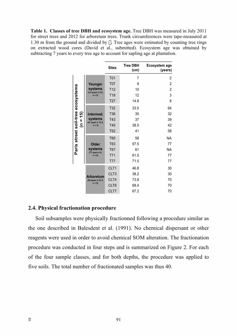
! 91
2.4. Physical fractionation procedure
Soil subsamples were physically fractionned following a procedure similar as
the one described in Balesdent et al. (1991). No chemical dispersant or other
reagents were used in order to avoid chemical SOM alteration. The fractionation
procedure was conducted in four steps and is summarized on Figure 2. For each
of the four sample classes, and for both depths, the procedure was applied to
five soils. The total number of fractionated samples was thus 40.
Sites Tree DBH (cm)
Ecosystem age (years)
T01 7 2T07 9 2T12 10 2T18 12 3T27 14.8 8
T32 33.5 64T36 35 32T43 37 39T45 38.5 42T52 41 58
T60 58 NAT63 57.5 77T67 61 NAT71 61.5 77T77 71.5 77
CLT1 46.8 30CLT3 38.2 30CLT4 73.8 70CLT6 68.4 70CLT7 67.2 70
791012
14.8
33.53537
38.541
5857.561
61.571.5
46,838,273,8
Younger systems
(3.4 years ± 2.6, n = 5)
Intermed. systems
(47 years ± 13.5, n = 5)
Older systems (77 years ± 0,
n = 5)
Arboretum (54 years ± 21.9,
n = 5)
Par
is s
tree
t soi
l-tre
e ec
osys
tem
s (n
= 1
5)
Table 1. Classes of tree DBH and ecosystem age. Tree DBH was measured in July 2011 for street trees and 2012 for arboretum trees. Trunk circumferences were tape-measured at 1.30 m from the ground and divided by π. Tree ages were estimated by counting tree rings on extracted wood cores (David et al., submitted). Ecosystem age was obtained by subtracting 7 years to every tree age to account for sapling age at plantation.
! 92
• Step 1: Dispersion in water with glass beads.
20 g of dry soil were placed in a plastic bottle and volume was completed to
100 ml with distilled water. 15 glass beads (5 mm diameter) were added and
bottles were horizontally shaken during 16 h. This process allowed physical
dispersion of macroaggregates without significant alteration of particulate
organic matter (Balesdent et al. 1991).
• Step 2: Sieving at 50 µm to separate the sand fraction.
The suspension obtained in Step 1 was then sieved at 50 µm. Particles of
diameter 50-2000 µm were recovered and oven-dried at 60 °C. They correspond
to what will be subsequently referred to as the “sand fraction”. The rest of the
initial suspension was carefully recovered and placed back in the plastic bottle.
• Step 3: Ultrasound dispersion of the < 50 µm suspension
Ultrasound dispersion was then used to disperse microaggregates and
separate elementary particules. An ultrasonic probe was immersed in the < 50
µm suspension and the protocol was set so that samples received between 400-
425 J.ml-1. The bottle containing the suspension was immersed in ice during
sonication, to avoid excessive temperature rise that could alter SOM and its
distribution.
• Step 4: Separation of silt and clay fractions by centrifugation
The suspension was then horizontally centrifuged at 750 rpm during 10
minutes (parameters set by using Stokes’ law). After centrifugation, the pellet
was considered to correspond to particles of size 2-50 µm, referred to as the “silt
fraction” here. The surnatant was considered to correspond to particles of size <
2 µm, referred to as the “clay fraction” here. The surnatant was carefully
recovered with a 100 ml syringe and oven-dried at 60 °C. The pellet was
recovered and oven-dried at 60 °C.
! 93
In summary, the following three fractions were obtained:
1. The sand fraction, corresponding to particles of size 50-2000 µm;
2. The silt fraction, corresponding to particles of size 2-50 µm;
3. The clay fraction, corresponding to particles of size < 2 µm.
Once dried, the fractions were weighed to obtain their mass and the
percentage of initial soil mass that they represented.
The distribution of C and N across soil fractions was evaluated by
calculating the contribution of each fraction to total C and N pools (Nacro et al.,
1996; Nacro, 1998), i.e. the percentage of total retrieved C and N pools
contained in each fraction, calculated by mass balance. For each fraction i and
element X, the percentage PXi was calculated as:
PXi = mi.%xi / (mi.%xi + mj.%xj + mk.%k)
with mi being the mass of the fraction i retrieved through physical
fractionation, %xi the element X content (%) of the fraction i and mj, %xj,
mk, %xk being respectively the retrieved masses and element X contents (%) of
the two other fractions j and k.
For the distribution of 13C and 15N pools across fractions, the δ value was
considered as an approximation of heavy isotope content in a given sample (Fry,
2006) and the contribution of each fraction to total 13C and 15N pool was
calculated as:
PisoXi = mi.%xi.δXi / (mi.%xi.δXi + mj.%xj.δXj + mk.%k.δXk )
with δXi, δXi and δXk being the δ value for the heavy isotope of element X
measured in the fraction i, j, and k respectively.
! 94
2.5. Mineralogical analysis of clay fractions by X-ray diffraction
X-ray diffraction analysis on "oriented" deposits was used to identify the
types of clay minerals present in the samples. Around 100 mg of clay fraction
were suspended in 3 ml of distilled water, and deposited on a glass slide. Once
dried, the preparation was analyzed with an X-ray diffractometer (PANalytical
Xpert Pro Diffractometer, Rigaku, Tokyo, Japan) equipped with a copper anode.
The diffraction measurement enables to obtain the distance between the sheets
of a cristalline structure following Bragg’s law: 2dsinθ = n.λ, where d is the
distance between two crystallographic planes, θ the scattering angle (half the
angle between the incident beam and the detector direction), n the order of the
reflection and λ the X-ray wavelenght. On the obtained diffractograms, each
peak corresponded to a different type of clay mineral. In the soils studied here,
the clay minerals were principally composed of illite-smectite, illite and
kaolinite. A qualitative analysis of each diffractogram was performed and the
height of each peak was compared to the other peaks. A scale from 0 to 3 was
then applied to score each mineral: 0 for an absent peak; 1 for a weak peak; 2 for
a moderate peak; 3 for a strong peak. This enabled a qualitative analysis of clay
mineral composition for each soil.
2.6. C and N contents and isotope ratios
Complete soils and soil fractions were analyzed for organic C content and
δ13C after carbonate removal with the HCl fumigation method (Harris, 2001).
Briefly, 30 mg of homogenized sample were weighted in silver capsules,
moisturized with 50 µl of milliQ water, and placed for 6 h in a vacuumed
desiccator with a beaker containing 200 ml of 16 M HCl. Then, samples were
double-folded in tin capsules for better combustion (Harris, 2001; Brodie et al.,
2011) and analyzed at INRA-Nancy by EA-IRMS (NA 1500, Carlo Erba,
Milano, Italy, coupled with a Delta S, Finnigan, Palo Alto, USA). For total N
content and δ15N, samples were analyzed by EA-IRMS (vario Pyro cube,
! 95
Elementar, Hanau, Germany, coupled with an IsoPrime, Gvi, Stockport, UK)
without any pre-treatment to avoid unnecessary bias on N parameters (Komada
et al., 2008; Brodie et al., 2011).
Root samples were analyzed for C content, N content, δ13C and δ15N at
the Piattaforma Analisi Isotopiche, Fondazione E. Mach (Italy) by EA-IRMS
(Flash EA 1112, ThermoFinnigan coupled with a Delta Plus V,
ThermoFinnigan).
For isotopic values, results are expressed using the usual delta notation
that allows expressing the content in 13C or 15N as the relative difference
between the isotopic ratio of the sample and a standard, calculated as:
δ(‰) = [(Rsample – Rstandard)/Rstandard]*1000
where Rsample is the isotope ratio (13C/12C and 15N/14N for C and N,
respectively) of the sample and Rstandard the isotope ratio of the standard. The
international standard for C is the Pee Dee Belemnite standard, with a 13C/12C
ratio of 0.0112372 (Craig, 1957). For N, the international standard is
atmospheric dinitrogen for which the 15N/14N ratio is 0.003676 (Mariotti et al.,
1983, 1984).
2.7. Soil incubation, CO2 and 13C-CO2 analysis
Soil sub-samples (6 g dry weight) were pre-incubated for a month at 40 %
WHC. They were brought to 80 % WHC at the beginning of the incubation.
Immediately after adding the water, the sample bottles were flushed with CO2
free air (19 % O2, 81 % N2). The bottles (100 ml) were closed with Teflon®
rubber stoppers crimped on with aluminium seals and the samples were
incubated at 25 °C in the dark for 2 months. Headspace CO2 concentration was
measured after 7, 15, 22, 29, 42 and 62 days of incubation. Measurements were
carried out with a micro-gas chromatograph (490 Micro GC, Agilent, Paris,
France). For each date, mineralization rates were expressed both in cumulated
! 96
mineralized carbon per gram of soil (soil respiration, mg C-CO2.g soil-1) and as
the ratio of mineralized soil organic carbon (% Soil Corg). The daily rate of
mineralization was calculated by dividing the final date by lenght of incubation
(62 days) (data expressed as mg C-CO2.g soil-1.day-1 and % Csoil.day-1). At each
sampling date, 1 ml of headspace gas was manually extracted with a gas syringe
and introduced in an evacuated 12 ml Exetainer® vial. The isotopic composition
(expressed in δ13C-CO2, ‰, calculated as above) of the CO2–C was measured at
INRA Nancy using the gas-bench inlet of an IRMS (Delta S, Finnigan, Palo
Alto, USA).
2.8. Statistical analyses
Statistical analyses were performed with the R-software (R Development
Core Team, 2013). Four sample classes (three DBH classes and the arboretum)
and two depths (10-20 cm and 30-40 cm) and their interaction were used as
explanatory factors for bulk soil, root and soil incubation data. For particle-size
data, four classes, two depths and three fractions and their interactions were used
as explanatory factors. Linear mixed-effects models with a "site" random effect
were used for soil variables to account for non-independence of soil depths at
each sampling site. R2 values for linear mixed-effects models were calculated
with the function r.squared.lme (version 0.2-4 (2014-07-10)) that follows the
method described in Nakagawa & Schielzeth (2013). Values for conditional R2,
which describes the proportion of variance explained by both the fixed and
random factors, are shown. For ∆15Nroot-soil and ∆15Nleaf-root, only the four classes
were used as explanatory factors in a linear model. Tukey post-hoc tests were
performed for ANOVA models yielding significant results. For variables that
did not satisfy ANOVA assumptions even after log transformation, non-
parametric tests were used: a Kruskal-Wallis test was used for each depth to test
for differences between classes, and a Wilcoxon-Mann-Whitney test was used
for pairwise comparisons of means. Simple linear regressions were performed

! 97
between soil, root and incubation data. For all tests, the null hypothesis was
rejected for p < 0.05 and significativity was represented as follows: *** when p
≤ 0.001; ** for 0.001 < p ≤ 0.01 and * when 0.01 < p ≤ 0.05. Effects with 0.05 ≤
p < 0.10 are referred to as marginally significant. Data on foliar δ15N, root
density and soil ammonium content are used from previous works (Rankovic et
al., Chapter 1)
3. Results 3.1. Soil texture, quality of fractionation and clay minerals
As already discussed in Chapter 1, soils from younger street systems and
the arboretum had a finer texture than soils from street intermediate and older
systems and appeared as silt-loam soils. Soils from street intermediate systems
were loamy soils and soils from older street systems were sandy loam soils.
The particle-size distribution obtained by the physical fractionation
procedure was compared to the particle-size distribution obtained by textural
analysis after H2O2 destruction of organic matter and decarbonatation (Table 2).
A Kruskal-Wallis test showed that there was no significant difference between
the two particle-size distributions for the silt and sand fractions, but a significant
difference for the clay fraction (H = 23.6, df = 1, p < 0.001). A pairwise
comparison through a Wilcoxon-Mann-Whitney test showed that the difference
was significant for the soils from younger systems and from the arboretum.
Overall, the clay fraction appeared to be underestimated by the physical
fractionation procedure (about 60 % of the clay content obtained through
textural analysis) and the silt fraction appeared to be overstimated (130 % when
compared to textural data). The sand fraction yielded similar results with both
methods (ratio of about 100 %). This is similar to the results obtained by Nacro
et al. (1996) on a savanna soil when comparing particle-size distributions
obtained by textural analysis after H2O2 destruction of SOM and a physical
fractionation procedure similar to the one employed here. In their study, the clay
! 98
fraction retrieved by physical fractionation represented about 77 % of the clay
fraction retrieved by textural analysis, and the silt fraction about 130 %, a result
similar to ours.
This means that silt and clay fractions were not optimally separated
during steps 3 and 4 of the fractionation procedure, and that part of the clay
fraction was retrieved with the silt fraction. This difference between the physical
fractionation and textural analysis could be explained by the fact that organic
matter was not destroyed by H2O2 during physical fractionation, and that part of
the clay-size particles may have remained binded together, forming silt-size
microaggregates that were retrieved with the silt fraction, thus leading to its
overestimation. When added together, silt and clay fractions retrieved by
physical fractionation represented about 100 % of the sum of silt and clay
contents measured by textural data, which tends to confirm this hypothesis. This
also indicates that the fractionation procedure adequately separated the finer
fractions (silt and clay, < 50 µm) from the coarse fraction (sand, > 50 µm) when
compared to textural data. A linear regression of physical fractionation results
against textural data confirmed that physical fractionation yielded similar results
across the 40 fractionned soils for the sand fraction (R2 = 0.98, ***) and the sum
of silt and clay (R2 = 0.97, ***), which indicates that the coarse and finer
fractions were well separated for all samples. As the present study is especially
interested in comparing SOM distribution between coarse fractions and finer
fractions, this result is satisfying and validates the physical fractionation
procedure that was used for the present study.
The qualitative analysis of X-ray diffractograms (Figure 3) obtained for
clay minerals suggested that soils from younger systems had a higher proportion
of smectite than soils from intermediate and older street systems. Soils from
older street systems, in particular, seemed to have a lower proportion of smectite.
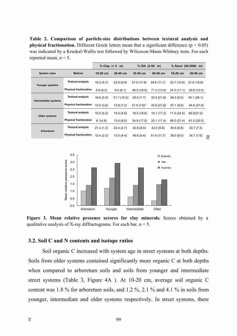
! 99
3.2. Soil C and N contents and isotope ratios
Soil organic C increased with system age in street systems at both depths.
Soils from older systems contained significantly more organic C at both depths
when compared to arboretum soils and soils from younger and intermediate
street systems (Table 3, Figure 4A ). At 10-20 cm, average soil organic C
content was 1.8 % for arboretum soils, and 1.2 %, 2.1 % and 4.1 % in soils from
younger, intermediate and older systems respectively. In street systems, there
Table 2. Comparison of particle-size distributions between textural analysis and physical fractionation. Different Greek letters mean that a significant difference (p < 0.05) was indicated by a Kruskal-Wallis test followed by Wilcoxon-Mann-Whitney tests. For each reported mean, n = 5.
Particle-size Soil depth (cm)
Younger systems
Intermediate systems
Older systems
10-20 19.3 (5.7)a,α 16.6 (5.0)b,α 10.5 (5.0)c,α
30-40 23.8 (6.9)ad,α 21.7 (10.2)a,α 15.0 (4.9)cbd,α
10-20 57.0 (11.9)a,α 25.0 (7.7)bf,α 18.5 (19.6)c,α
30-40 54.6 (11.7)a,α 33.3 (21.8)bg,α 19.1 (17.3)ef,α
10-20 23.7 (16.9)a,α 58.3 (9.5)be,α 71.0 (24.5)c,α
30-40 21.6
(16.8)ad,α
45.1
(26.1)bd,α 66.0(21.2)ce,α
10-20 6.8 (6.2)a,β 12.0 (3.6)a,α 6.1(4.8)a,α
30-40 8.0 (6.1)a,β 12.8 (7.2)a,α 13.4 (9.5)a,α
10-20 69.0 (18.9)acd,α 31.0 (7.6)b,α 24.9 (17.0)b,α
30-40 71.3 (13.0)a,α 42.6 (21.8)bc,α 25.1 (17.4)b,α
10-20 24.3 (17.1)α 57.1 (9.9)α 69.0 (21.4)α
30-40 20.8 (10.5)α 44.6 (27.9)α 61.5 (20.5)α
System class Method 10-20 cm 30-40 cm 10-20 cm 30-40 cm 10-20 cm 30-40 cm
Textural analysis 19.3 (5.7)α 23.8 (6.9)α 57.0 (11.9)α 54.6 (11.7)α 23.7 (16.9)α 21.6 (16.8)α
Physical fractionation 6.8 (6.2)β 8.0 (6.1)β 69.0 (18.9)α 71.3 (13.0)α 24.3 (17.1)α 20.8 (10.5)α
Textural analysis 16.6 (5.0)α 21.7 (10.2)α 25.0 (7.7)α 33.3 (21.8)α 58.3 (9.5)α 45.1 (26.1)α
Physical fractionation 12.0 (3.6)α 12.8 (7.2)α 31.0 (7.6)b,α 42.6 (21.8)α 57.1 (9.9)α 44.6 (27.9)α
Textural analysis 10.5 (5.0)α 15.0 (4.9)α 18.5 (19.6)α 19.1 (17.3)α 71.0 (24.5)α 66.0(21.2)α
Physical fractionation 6.1(4.8)α 13.4 (9.5)α 24.9 (17.0)α 25.1 (17.4)α 69.0 (21.4)α 61.5 (20.5)α
Textural analysis 21.4 (1.2)α 24.4 (4.7)α 42.6 (8.0)α 42.0 (9.9)α 35.9 (8.8)α 33.7 (7.3)α
Physical fractionation 12.4 (2.3)β 13.5 (4.4)β 49.6 (9.4)α 51.9 (11.7)α 38.0 (8.0)α 34.7 (7.6)α
% Silt (2-50 µm) % Sand (50-2000 µm)
Younger systems
Intermediate systems
Older systems
Arboretum
% Clay (< 2 µm)
Paris
str
eet s
oil-t
ree
ecos
yste
ms
Paris street soil-tree ecosystems
Textural analysis
% Clay (< 2 µm)
% Silt (2-50 µm)
% Sand (50-2000 µm)
Fractionation procedure
% Clay (< 2 µm)
% Silt (2-50 µm)
% Sand (50-2000 µm)
!
! 11
and 105 %. These results suggest very little matter loss during the fractionation
procedure and further validate the method.
The qualitative analysis of X-ray diffractograms obtained for clay minerals suggested
that soils from younger systems had a higher proportion of smectite than soils from
intermediate and younger plantation. Soils from older street systems in particular
seemed to have a lower proportion of smectite.
!
3.2. Soil C and N contents and isotope ratios
Particle-size Soil depth (cm)
Younger systems
Intermediate systems
Older systems
10-20 19.3 (5.7)a,α 16.6 (5.0)b,α 10.5 (5.0)c,α
30-40 23.8 (6.9)ad,α 21.7 (10.2)a,α 15.0 (4.9)cbd,α
10-20 57.0 (11.9)a,α 25.0 (7.7)bf,α 18.5 (19.6)c,α
30-40 54.6 (11.7)a,α 33.3 (21.8)bg,α 19.1 (17.3)ef,α
10-20 23.7 (16.9)a,α 58.3 (9.5)be,α 71.0 (24.5)c,α
30-40 21.6
(16.8)ad,α
45.1
(26.1)bd,α 66.0(21.2)ce,α
10-20 6.8 (6.2)a,β 12.0 (3.6)a,α 6.1(4.8)a,α
30-40 8.0 (6.1)a,β 12.8 (7.2)a,α 13.4 (9.5)a,α
10-20 69.0 (18.9)acd,α 31.0 (7.6)b,α 24.9 (17.0)b,α
30-40 71.3 (13.0)a,α 42.6 (21.8)bc,α 25.1 (17.4)b,α
10-20 24.3 (17.1)α 57.1 (9.9)α 69.0 (21.4)α
30-40 20.8 (10.5)α 44.6 (27.9)α 61.5 (20.5)α
System class Method 10-20 cm 30-40 cm 10-20 cm 30-40 cm 10-20 cm 30-40 cm
Textural analysis 19.3 (5.7)α 23.8 (6.9)α 57.0 (11.9)α 54.6 (11.7)α 23.7 (16.9)α 21.6 (16.8)α
Physical fractionation 6.8 (6.2)β 8.0 (6.1)β 69.0 (18.9)α 71.3 (13.0)α 24.3 (17.1)α 20.8 (10.5)α
Textural analysis 16.6 (5.0)α 21.7 (10.2)α 25.0 (7.7)α 33.3 (21.8)α 58.3 (9.5)α 45.1 (26.1)α
Physical fractionation 12.0 (3.6)α 12.8 (7.2)α 31.0 (7.6)b,α 42.6 (21.8)α 57.1 (9.9)α 44.6 (27.9)α
Textural analysis 10.5 (5.0)α 15.0 (4.9)α 18.5 (19.6)α 19.1 (17.3)α 71.0 (24.5)α 66.0(21.2)α
Physical fractionation 6.1(4.8)α 13.4 (9.5)α 24.9 (17.0)α 25.1 (17.4)α 69.0 (21.4)α 61.5 (20.5)α
Textural analysis 21.4 (1.2)α 24.4 (4.7)α 42.6 (8.0)α 42.0 (9.9)α 35.9 (8.8)α 33.7 (7.3)α
Physical fractionation 12.4 (2.3)β 13.5 (4.4)β 49.6 (9.4)α 51.9 (11.7)α 38.0 (8.0)α 34.7 (7.6)α
% Silt (2-50 µm) % Sand (50-2000 µm)
Younger systems
Intermediate systems
Older systems
Arboretum
% Clay (< 2 µm)
Paris
str
eet s
oil-t
ree
ecos
yste
ms
Paris street soil-tree ecosystems
Textural analysis
% Clay (< 2 µm)
% Silt (2-50 µm)
% Sand (50-2000 µm)
Fractionation procedure
% Clay (< 2 µm)
% Silt (2-50 µm)
% Sand (50-2000 µm)
Table 2. Comparison of particle-size distributions between textural analysis and physical fractionation. Different Greek letters mean that a significant difference (p < 0.05) was indicated by a Wilcoxon-Mann-Whitney.
0.0
0.1
0.1
0.2
0.2
0.3
0.3
0.4
Chevreloup* Classe*1* Classe*2* Classe*3*Arboretum Younger Intermediate Older
0.0
0.1
0.1
0.2
0.2
0.3
0.3
0.4
Chevreloup* Classe*1* Classe*2* Classe*3*
Sméc4te*
Illite*
Caolinite*
Arboretum Younger Intermediate Older
Smectite
Illite
Kaolinite
0.0
0.5
1.0
1.5
2.0
2.5
3.0
3.5
Mea
n re
lativ
e pr
esen
ce s
core
Figure 3. Mean relative presence scores for clay minerals .
Figure 3. Mean relative presence scrores for clay minerals. Scores obtained by a qualitative analysis of X-ray diffractograms. For each bar, n = 5.

! 100
was thus about a two-fold increase in soil organic C among age classes. At 30-
40 cm, soils contained 1.1 % at the arboretum and 1.5 %, 1.4 % and 2.7 % in
younger, intermediate and older systems, respectively. Soils from older systems
contained significantly more organic C than soils from the arboretum and
younger and intermediate street systems (Table 3, Figure 4A).
Soil δ13C at 10-20 cm was significantly higher in soils from intermediate
and older street systems when compared to soils from younger street systems
and arboretum soils (Table 3, Figure 4B). At the arboretum, soil δ13C was -
26.6 ‰ at 10-20 cm. In street systems at the same depth, average soil δ13C was -
26.3 ‰, -25.4 ‰ and -24.9 ‰ for younger, intermediate and older systems,
respectively. The same trend was observed at 30-40 cm, with soils from older
systems being significantly more enriched than arboretum soils and soils from
younger street systems (Table 3, Figure 4B). Average soil δ13C at 30-40 cm was
-26.2 ‰ at the arboretum and -26.1 ‰, -25.7 ‰ and -25 ‰ in younger,
intermediate and older systems, respectively. At 10-20 cm, average soil δ13C
was 1.4 ‰ units higher in older street systems than in younger street systems,
and 1.7 ‰ higher in older street systems when compared to the arboretum. At
30-40 cm, soil δ13C was 1.1 ‰ units higher in older street systems when
compared to younger systems, and 1.2 ‰ units higher in older street systems
when compared to the arboretum (Figure 4B).
Soil total N content at 10-20 cm was significantly higher in older street
systems than in younger street systems (Table 3, Figure 4C). At 30-40 cm, soils
from older street systems contained significantly more N than soils from
younger and intermediate systems and soils from the arboretum (Table 3, Figure
4C).
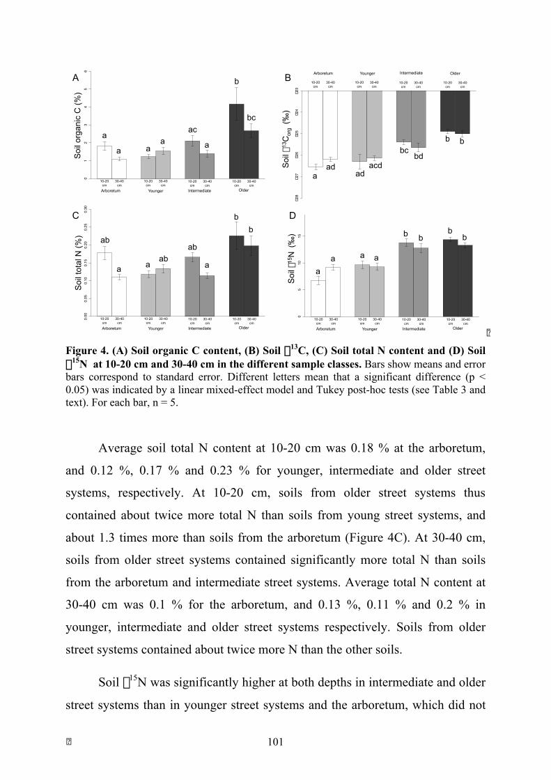
! 101
Arboretum Younger Intermediate Older0.00
0.05
0.10
0.15
0.20
0.25
0.30
10-20 cm
Arboretum Younger Intermediate Older
30-40 cm
10-20 cm
30-40 cm
10-20 cm
30-40 cm
10-20 cm
30-40 cm
Soi
l tot
al N
(%)
10-30 cm
Arboretum Younger Intermediate Older
30-40 cm
10-30 cm
30-40 cm
10-30 cm
30-40 cm
10-30 cm
30-40 cm
Arboretum Younger Intermediate Older
05
1015
20
10-20 cm
Arboretum Younger Intermediate Older
30-40 cm
10-20 cm
30-40 cm
10-20 cm
30-40 cm
10-20 cm
30-40 cm
Arboretum Younger Intermediate Older
−28
−27
−26
−25
−24
−23
Arboretum Younger Intermediate Older
10-20 cm
30-40 cm
10-20 cm
30-40 cm
10-20 cm
30-40 cm
10-20 cm
30-40 cm
Soi
l δ13
Cor
g (‰
)
Arboretum Younger Intermediate Older
01
23
45
6
10-20 cm
Arboretum Younger Intermediate Older
30-40 cm
10-20 cm
30-40 cm
10-20 cm
30-40 cm
10-20 cm
30-40 cm
Soi
l org
anic
C (%
)
Soi
l δ15
N (
‰)
A
C
B
D
ac a
a a a a
b
bc
ab
a a ab
ab
a
b b
a ad
ad acd
bc bd
b b
a a a a
b b b
b
!Figure 4. (A) Soil organic C content, (B) Soil δ13C, (C) Soil total N content and (D) Soil δ15N at 10-20 cm and 30-40 cm in the different sample classes. Bars show means and error bars correspond to standard error. Different letters mean that a significant difference (p < 0.05) was indicated by a linear mixed-effect model and Tukey post-hoc tests (see Table 3 and text). For each bar, n = 5.
Average soil total N content at 10-20 cm was 0.18 % at the arboretum,
and 0.12 %, 0.17 % and 0.23 % for younger, intermediate and older street
systems, respectively. At 10-20 cm, soils from older street systems thus
contained about twice more total N than soils from young street systems, and
about 1.3 times more than soils from the arboretum (Figure 4C). At 30-40 cm,
soils from older street systems contained significantly more total N than soils
from the arboretum and intermediate street systems. Average total N content at
30-40 cm was 0.1 % for the arboretum, and 0.13 %, 0.11 % and 0.2 % in
younger, intermediate and older street systems respectively. Soils from older
street systems contained about twice more N than the other soils.
Soil δ15N was significantly higher at both depths in intermediate and older
street systems than in younger street systems and the arboretum, which did not
! 102
differ significantly (Table 3, Figure 4D). At 10-20 cm, average soil δ15N was
6.7 ‰ at the arboretum, and 9.6 ‰, 13.8 ‰ and 14.3 ‰ in younger,
intermediate and older systems, respectively (Figure 4D). At 30-40 cm, average
soil δ15N was 9.2 ‰ at the arboretum, and 9.3 ‰, 12.8 ‰ and 13.3 ‰ in
younger, intermediate and older systems, respectively (Figure 4D). At 10-20 cm,
soil δ15N in older street systems was thus 7.6 ‰ units higher than at the
arboretum, and 4.7 ‰ units higher when compared to younger street systems. At
30-40 cm, soil δ15N in older street systems was 4.1 ‰ units higher than at the
arboretum, and 4 ‰ units higher when compared to younger street systems.
Soil C:N was significantly higher in older street systems than in other
street systems and the arboretum (Table 3). Older soils had a C:N of 17.7 at 10-
20 cm and of 13.5 at 30-40 cm. This was significantly higher (p = 0.01) than
values for intermediate street systems, which had an average soil C:N of 12.5 at
10-20 cm and 12.1 at 30-40 cm. Soil C:N in intermediate and older street
systems both differed significantly from arboretum soils (p < 0.05 and p <
0.0001, respectively).

! 103
Table 3. ANOVA table of F values. Reports the effects of class and depth and their interaction on soil organic C, soil total N content, soil C:N, soil δ13C, soil δ15N, root N content, root C:N, root δ15N, root δ13C, soil respiration, soil organic C mineralization coefficient, δ13C-CO2, as tested with a linear mixed-effect model. For ∆15Nleaf-root and ∆15Nroot-soil, a linear model was used and only included the class factor since the values were measured at only one depth. The reported values for significant terms and R2 are the values obtained after removal of non-significant factors in the model. For all soil, root and incubation variable, n = 5 for each class and each depth. For ∆15Nleaf-root and ∆15Nroot-soil,, n = 5 for each class.
F p df F p df F p df
**
Class Depth Class x Depth
Factors
1 33
0.77
Model R2
0.78
Variables
313
4.24 *
6.3 **log (Soil %N) 4.8 * 15.6 **
log (Soil %C) 8.0 ** 11.8
3 0.51
Soil δ13C 27.1 *** 3 0.1 ns 1 1.4
log (Soil C:N) 13.1 *** 3 1.5 ns 1 2.5 ns
ns 3 0.72
0.7 ns 3 0.80
11.6 ** 3 0.93Soil δ15N 22.3 *** 3 0.008 ns 1
Root %N 7.7 ** 3 10.40 ** 1
ns 3 0.93
1 2.44 0.1 3 0.53
Root δ15N 21.12 *** 3 0.06
Root C:N 10.0 *** 3 3.3 ns
Root δ13C 5.01 * 3 0.9 ns
ns 1 1.3
1 1.1 ns 3 0.79
-
∆15Nleaf-root 19.8 *** 3 - - - - - - 0.77
0.36
- - - -
Soil respiration day-1 4.2 * 3 7.8
∆15Nroot-soil 3.6 0.06 3 - -
1 1.24 ns 3 0.69log (% Soil C mineralised day-1) 8.7 ** 3 0.0 ns
* 1 2.5 0.1 3
ns 3 0.70 δ13C-CO2 6.5 ** 3 0.1 ns 1 0.7
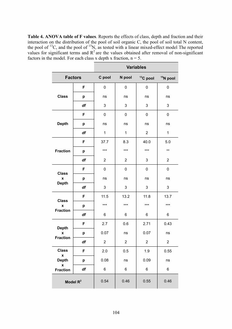
104
Table 4. ANOVA table of F values. Reports the effects of class, depth and fraction and their interaction on the distribution of the pool of soil organic C, the pool of soil total N content, the pool of 13C, and the pool of 15N, as tested with a linear mixed-effect model The reported values for significant terms and R2 are the values obtained after removal of non-significant factors in the model. For each class x depth x fraction, n = 5.
C pool N pool 13C pool 15N pool
F 0 0 0 0
p ns ns ns ns
df 3 3 3 3
F 0 0 0 0
p ns ns ns ns
df 1 1 2 1
F 37.7 8.3 40.0 5.0
p *** *** *** **
df 2 2 3 2
F 0 0 0 0
p ns ns ns ns
df 3 3 3 3
F 11.5 13.2 11.8 13.7
p *** *** *** ***
df 6 6 6 6
F 2.7 0.6 2.71 0.43
p 0.07 ns 0.07 ns
df 2 2 2 2
F 2.0 0.5 1.9 0.55
p 0.08 ns 0.09 ns
df 6 6 6 6
Class
Depth
Factors
Variables
Fraction
Class x
Depth
Class x
Fraction
Depth x
Fraction
Class x
Depthx
Fraction
Model R2 0.54 0.46 0.55 0.46
! 105
3.3. Distribution of SOM across particle-size fractions
For soil organic C, the distribution was significantly different across fractions
and the distribution among fractions significantly varied between soil-tree
system classes (significant interaction between fraction and system class, Table
4, Figure 5A). In younger street systems at 10-20 cm, the mean percentage of
soil C pool contained in the sand fraction was 27.4 %, significantly lower than
in the silt fraction (61.1 %) and higher than the clay fraction (11.5 %). The finer
fractions together accounted for about 72.6 %. Though the difference between
fractions were not significant, in soils from intermediate street systems the
distribution of C across fractions had a mean of 46.7 % for the sand fraction,
31.6 % for the silt fraction and 21.8 % for the clay fraction. The finer fraction
accounted for about 53.4 % of the C pool in intermediate street systems. In older
street systems, the sand fraction contained a significantly higher proportion
(57.9 %) of the soil C pool than both the silt (32.3 %) and clay (9.8 %) fractions,
and contained a higher proportion of the soil C pool than the finer fractions
combined (42.1 %) (Figure 5A). The proportion of soil C contained in the sand
fraction in intermediate street systems did not differ significantly from the
proportion contained in the sand fraction in younger and older street systems,
but this proportion was higher in older systems when compared to younger
systems (Tukey post-hoc test, p < 0.05). The mean proportion of soil C
contained in the sand fraction did not differ between street younger and
intermediate systems and the arboretum (32.1 %), but was significantly higher in
older street systems when compared to the arboretum (Tukey post-hoc test, p >
0.0001).
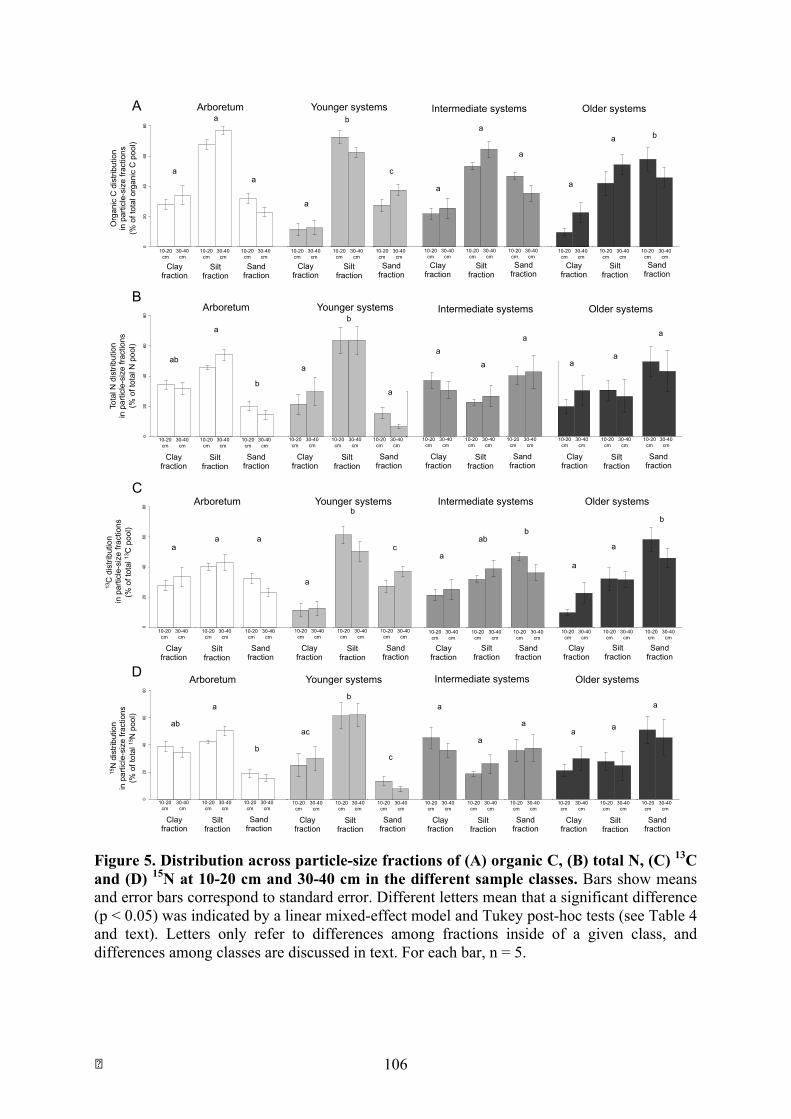
! 106
Arboretum Younger Intermediate Older
020
4060
80
Arboretum Younger Intermediate Older
020
4060
80
Arboretum Younger Intermediate Older
020
4060
80
Arboretum Younger Intermediate Older
020
4060
80
Arboretum Younger Intermediate Older
020
4060
80
Arboretum Younger Intermediate Older
020
4060
80
Arboretum Younger Intermediate Older
020
4060
80
Arboretum Younger Intermediate Older
020
4060
80
Arboretum Younger Intermediate Older
020
4060
80
Arboretum Younger Intermediate Older
020
4060
80
Arboretum Younger Intermediate Older
020
4060
80
Arboretum Younger Intermediate Older
020
4060
80
10-20 cm
30-40 cm
10-20 cm
30-40 cm
10-20 cm
30-40 cm
10-20 cm
30-40 cm
10-20 cm
30-40 cm
10-20 cm
30-40 cm
10-20 cm
30-40 cm
10-20 cm
30-40 cm
10-20 cm
30-40 cm
10-20 cm
30-40 cm
10-20 cm
30-40 cm
10-20 cm
30-40 cm
Clay fraction
Silt fraction
Sand fraction
Clay fraction
Silt fraction
Sand fraction
Clay fraction
Silt fraction
Sand fraction
Clay fraction
Silt fraction
Sand fraction
Arboretum Younger systems Intermediate systems Older systems
C"Pool"
a
a
a
a
b
c
a
a
a
a
a b
Org
anic
C d
istri
butio
n
in p
artic
le-s
ize
fract
ions
(%
of t
otal
org
anic
C p
ool)
Arboretum Younger Intermediate Older
020
4060
80
Arboretum Younger Intermediate Older
020
4060
80
Arboretum Younger Intermediate Older
020
4060
80
Arboretum Younger Intermediate Older
020
4060
80
Arboretum Younger Intermediate Older
020
4060
80
Arboretum Younger Intermediate Older
020
4060
80
Arboretum Younger Intermediate Older
020
4060
80
Arboretum Younger Intermediate Older
020
4060
80
Arboretum Younger Intermediate Older
020
4060
80
Arboretum Younger Intermediate Older
020
4060
80
Arboretum Younger Intermediate Older0
2040
6080
Arboretum Younger Intermediate Older
020
4060
80
10-20 cm
30-40 cm
10-20 cm
10-20 cm
30-40 cm
Clay fraction
Silt fraction
Sand fraction
30-40 cm
10-20 cm
30-40 cm
10-20 cm
10-20 cm
30-40 cm
Clay fraction
Silt fraction
Sand fraction
30-40 cm
10-20 cm
30-40 cm
10-20 cm
10-20 cm
30-40 cm
Clay fraction
Silt fraction
Sand fraction
30-40 cm
10-20 cm
30-40 cm
10-20 cm
10-20 cm
30-40 cm
Clay fraction
Silt fraction
Sand fraction
30-40 cm
Arboretum Younger systems Intermediate systems Older systems
N"Pool"
ab
a
b
b
a
a
a
a
a
a a
a
Tota
l N d
istri
butio
n
in p
artic
le-s
ize
fract
ions
(%
of t
otal
N p
ool)
13C"Pool"
Arboretum Younger Intermediate Older
020
4060
80
Arboretum Younger Intermediate Older
020
4060
80
Arboretum Younger Intermediate Older
020
4060
80
Arboretum Younger Intermediate Older
020
4060
80
Arboretum Younger Intermediate Older
020
4060
80
Arboretum Younger Intermediate Older
020
4060
80
Arboretum Younger Intermediate Older
020
4060
80
Arboretum Younger Intermediate Older
020
4060
80
Arboretum Younger Intermediate Older
020
4060
80
Arboretum Younger Intermediate Older
020
4060
80
Arboretum Younger Intermediate Older
020
4060
80
Arboretum Younger Intermediate Older
020
4060
80
10-20 cm
30-40 cm
10-20 cm
10-20 cm
30-40 cm
Clay fraction
Silt fraction
Sand fraction
30-40 cm
10-20 cm
30-40 cm
10-20 cm
10-20 cm
30-40 cm
Clay fraction
Silt fraction
Sand fraction
30-40 cm
10-20 cm
30-40 cm
10-20 cm
10-20 cm
30-40 cm
Clay fraction
Silt fraction
Sand fraction
30-40 cm
10-20 cm
30-40 cm
10-20 cm
10-20 cm
30-40 cm
Clay fraction
Silt fraction
Sand fraction
30-40 cm
Arboretum Younger systems Intermediate systems Older systems
a a a
a
b
c a
ab b
a
a
b
13C
dis
tribu
tion
in p
artic
le-s
ize
fract
ions
(%
of t
otal
13C
poo
l)
15N"Pool"
Arboretum Younger Intermediate Older
020
4060
80
Arboretum Younger Intermediate Older
020
4060
80
Arboretum Younger Intermediate Older
020
4060
80
Arboretum Younger Intermediate Older
020
4060
80
Arboretum Younger Intermediate Older
020
4060
80
Arboretum Younger Intermediate Older
020
4060
80
Arboretum Younger Intermediate Older
020
4060
80
Arboretum Younger Intermediate Older
020
4060
80
Arboretum Younger Intermediate Older
020
4060
80
Arboretum Younger Intermediate Older
020
4060
80
Arboretum Younger Intermediate Older
020
4060
80
Arboretum Younger Intermediate Older
020
4060
80
10-20 cm
30-40 cm
10-20 cm
10-20 cm
30-40 cm
Clay fraction
Silt fraction
Sand fraction
30-40 cm
10-20 cm
30-40 cm
10-20 cm
10-20 cm
30-40 cm
Clay fraction
Silt fraction
Sand fraction
30-40 cm
10-20 cm
30-40 cm
10-20 cm
10-20 cm
30-40 cm
Clay fraction
Silt fraction
Sand fraction
30-40 cm
10-20 cm
30-40 cm
10-20 cm
10-20 cm
30-40 cm
Clay fraction
Silt fraction
Sand fraction
30-40 cm
Arboretum Younger systems Intermediate systems Older systems
ab
a
b
ac
b
c
a
a
a a a
a
15N
dis
tribu
tion
in
par
ticle
-siz
e fra
ctio
ns
(% o
f tot
al 15
N p
ool)
A
B
C
D
Figure 5. Distribution across particle-size fractions of (A) organic C, (B) total N, (C) 13C and (D) 15N at 10-20 cm and 30-40 cm in the different sample classes. Bars show means and error bars correspond to standard error. Different letters mean that a significant difference (p < 0.05) was indicated by a linear mixed-effect model and Tukey post-hoc tests (see Table 4 and text). Letters only refer to differences among fractions inside of a given class, and differences among classes are discussed in text. For each bar, n = 5.
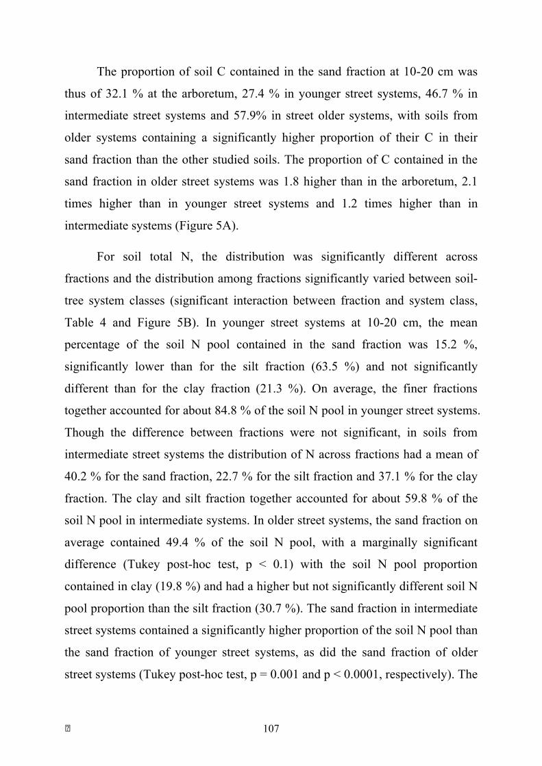
! 107
The proportion of soil C contained in the sand fraction at 10-20 cm was
thus of 32.1 % at the arboretum, 27.4 % in younger street systems, 46.7 % in
intermediate street systems and 57.9% in street older systems, with soils from
older systems containing a significantly higher proportion of their C in their
sand fraction than the other studied soils. The proportion of C contained in the
sand fraction in older street systems was 1.8 higher than in the arboretum, 2.1
times higher than in younger street systems and 1.2 times higher than in
intermediate systems (Figure 5A).
For soil total N, the distribution was significantly different across
fractions and the distribution among fractions significantly varied between soil-
tree system classes (significant interaction between fraction and system class,
Table 4 and Figure 5B). In younger street systems at 10-20 cm, the mean
percentage of the soil N pool contained in the sand fraction was 15.2 %,
significantly lower than for the silt fraction (63.5 %) and not significantly
different than for the clay fraction (21.3 %). On average, the finer fractions
together accounted for about 84.8 % of the soil N pool in younger street systems.
Though the difference between fractions were not significant, in soils from
intermediate street systems the distribution of N across fractions had a mean of
40.2 % for the sand fraction, 22.7 % for the silt fraction and 37.1 % for the clay
fraction. The clay and silt fraction together accounted for about 59.8 % of the
soil N pool in intermediate systems. In older street systems, the sand fraction on
average contained 49.4 % of the soil N pool, with a marginally significant
difference (Tukey post-hoc test, p < 0.1) with the soil N pool proportion
contained in clay (19.8 %) and had a higher but not significantly different soil N
pool proportion than the silt fraction (30.7 %). The sand fraction in intermediate
street systems contained a significantly higher proportion of the soil N pool than
the sand fraction of younger street systems, as did the sand fraction of older
street systems (Tukey post-hoc test, p = 0.001 and p < 0.0001, respectively). The
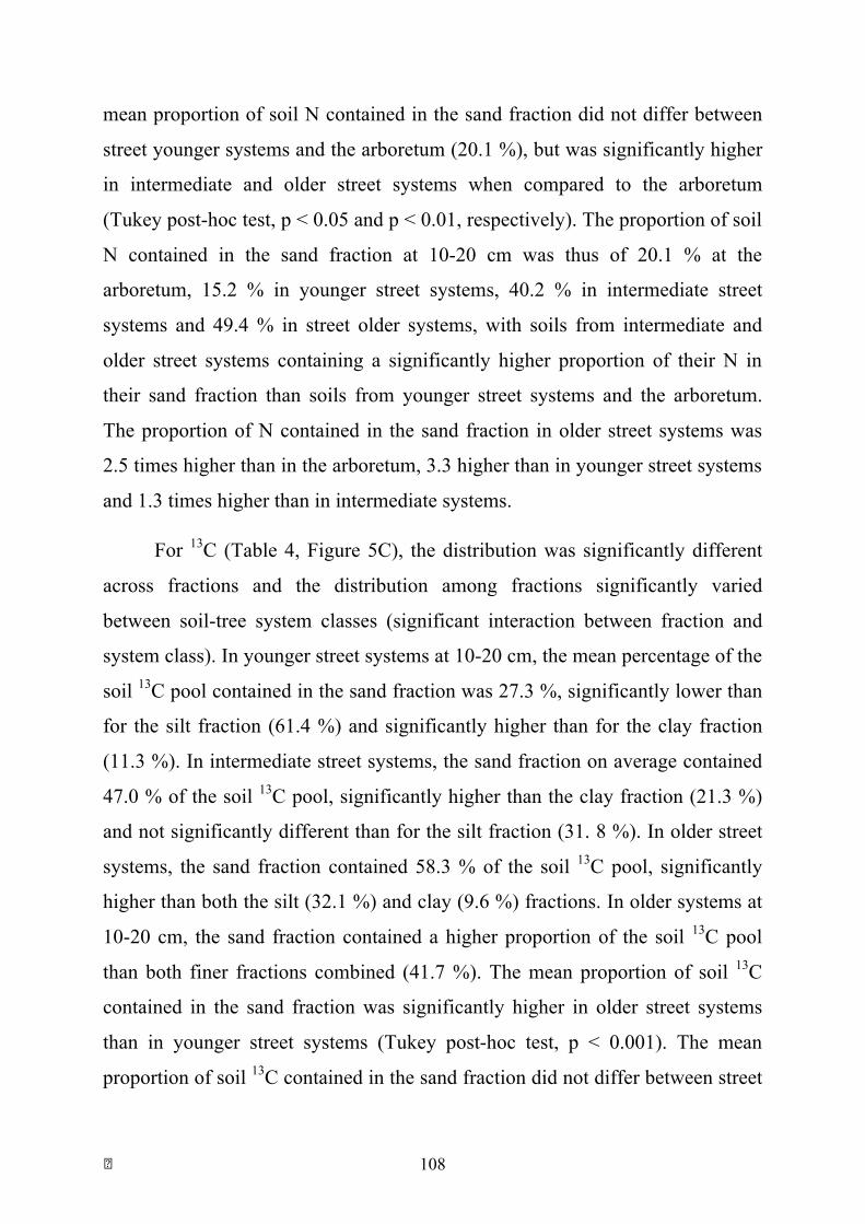
! 108
mean proportion of soil N contained in the sand fraction did not differ between
street younger systems and the arboretum (20.1 %), but was significantly higher
in intermediate and older street systems when compared to the arboretum
(Tukey post-hoc test, p < 0.05 and p < 0.01, respectively). The proportion of soil
N contained in the sand fraction at 10-20 cm was thus of 20.1 % at the
arboretum, 15.2 % in younger street systems, 40.2 % in intermediate street
systems and 49.4 % in street older systems, with soils from intermediate and
older street systems containing a significantly higher proportion of their N in
their sand fraction than soils from younger street systems and the arboretum.
The proportion of N contained in the sand fraction in older street systems was
2.5 times higher than in the arboretum, 3.3 higher than in younger street systems
and 1.3 times higher than in intermediate systems.
For 13C (Table 4, Figure 5C), the distribution was significantly different
across fractions and the distribution among fractions significantly varied
between soil-tree system classes (significant interaction between fraction and
system class). In younger street systems at 10-20 cm, the mean percentage of the
soil 13C pool contained in the sand fraction was 27.3 %, significantly lower than
for the silt fraction (61.4 %) and significantly higher than for the clay fraction
(11.3 %). In intermediate street systems, the sand fraction on average contained
47.0 % of the soil 13C pool, significantly higher than the clay fraction (21.3 %)
and not significantly different than for the silt fraction (31. 8 %). In older street
systems, the sand fraction contained 58.3 % of the soil 13C pool, significantly
higher than both the silt (32.1 %) and clay (9.6 %) fractions. In older systems at
10-20 cm, the sand fraction contained a higher proportion of the soil 13C pool
than both finer fractions combined (41.7 %). The mean proportion of soil 13C
contained in the sand fraction was significantly higher in older street systems
than in younger street systems (Tukey post-hoc test, p < 0.001). The mean
proportion of soil 13C contained in the sand fraction did not differ between street
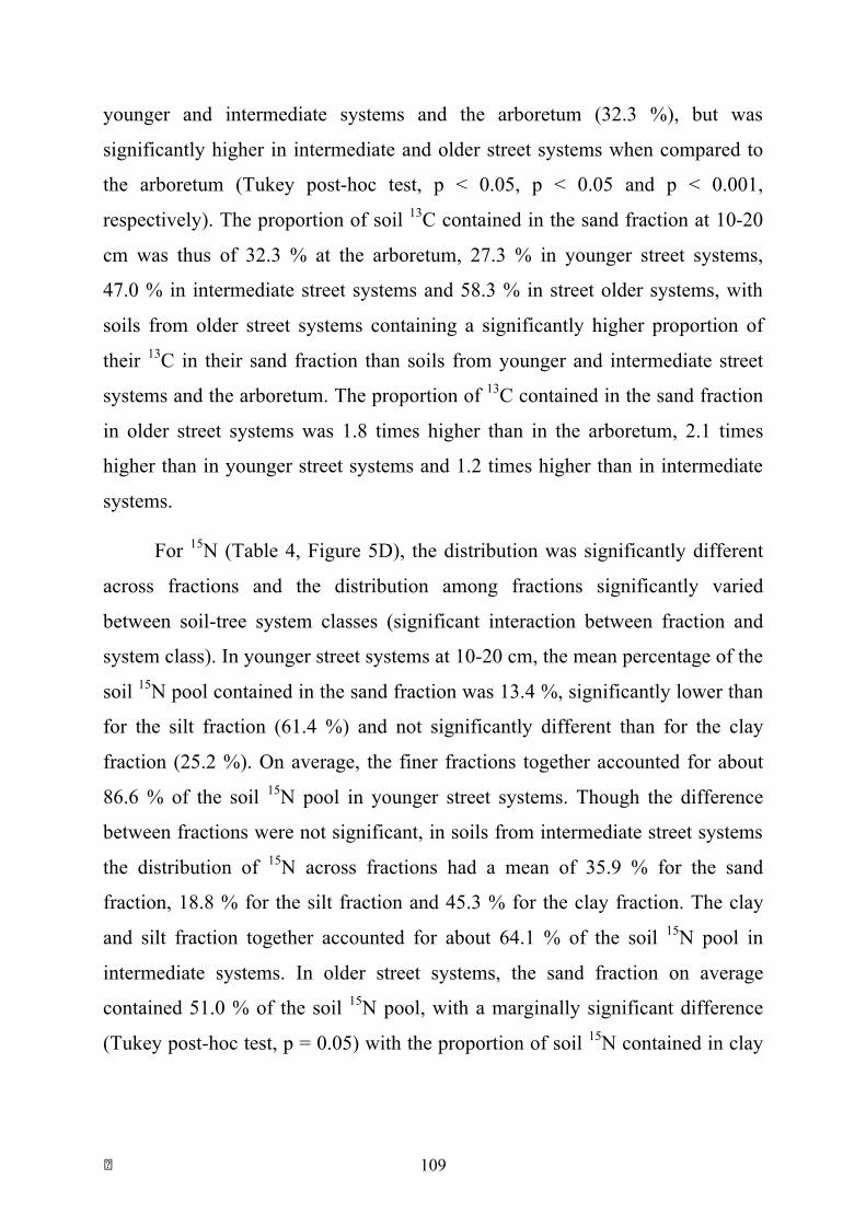
! 109
younger and intermediate systems and the arboretum (32.3 %), but was
significantly higher in intermediate and older street systems when compared to
the arboretum (Tukey post-hoc test, p < 0.05, p < 0.05 and p < 0.001,
respectively). The proportion of soil 13C contained in the sand fraction at 10-20
cm was thus of 32.3 % at the arboretum, 27.3 % in younger street systems,
47.0 % in intermediate street systems and 58.3 % in street older systems, with
soils from older street systems containing a significantly higher proportion of
their 13C in their sand fraction than soils from younger and intermediate street
systems and the arboretum. The proportion of 13C contained in the sand fraction
in older street systems was 1.8 times higher than in the arboretum, 2.1 times
higher than in younger street systems and 1.2 times higher than in intermediate
systems.
For 15N (Table 4, Figure 5D), the distribution was significantly different
across fractions and the distribution among fractions significantly varied
between soil-tree system classes (significant interaction between fraction and
system class). In younger street systems at 10-20 cm, the mean percentage of the
soil 15N pool contained in the sand fraction was 13.4 %, significantly lower than
for the silt fraction (61.4 %) and not significantly different than for the clay
fraction (25.2 %). On average, the finer fractions together accounted for about
86.6 % of the soil 15N pool in younger street systems. Though the difference
between fractions were not significant, in soils from intermediate street systems
the distribution of 15N across fractions had a mean of 35.9 % for the sand
fraction, 18.8 % for the silt fraction and 45.3 % for the clay fraction. The clay
and silt fraction together accounted for about 64.1 % of the soil 15N pool in
intermediate systems. In older street systems, the sand fraction on average
contained 51.0 % of the soil 15N pool, with a marginally significant difference
(Tukey post-hoc test, p = 0.05) with the proportion of soil 15N contained in clay
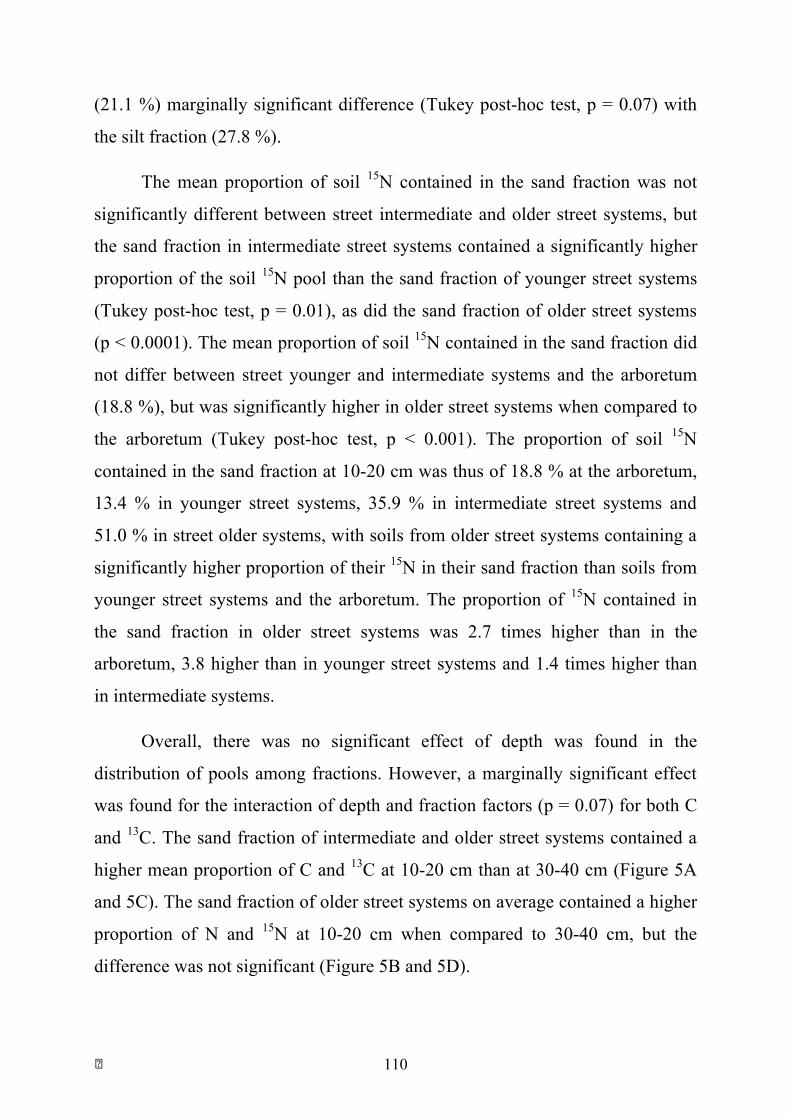
! 110
(21.1 %) marginally significant difference (Tukey post-hoc test, p = 0.07) with
the silt fraction (27.8 %).
The mean proportion of soil 15N contained in the sand fraction was not
significantly different between street intermediate and older street systems, but
the sand fraction in intermediate street systems contained a significantly higher
proportion of the soil 15N pool than the sand fraction of younger street systems
(Tukey post-hoc test, p = 0.01), as did the sand fraction of older street systems
(p < 0.0001). The mean proportion of soil 15N contained in the sand fraction did
not differ between street younger and intermediate systems and the arboretum
(18.8 %), but was significantly higher in older street systems when compared to
the arboretum (Tukey post-hoc test, p < 0.001). The proportion of soil 15N
contained in the sand fraction at 10-20 cm was thus of 18.8 % at the arboretum,
13.4 % in younger street systems, 35.9 % in intermediate street systems and
51.0 % in street older systems, with soils from older street systems containing a
significantly higher proportion of their 15N in their sand fraction than soils from
younger street systems and the arboretum. The proportion of 15N contained in
the sand fraction in older street systems was 2.7 times higher than in the
arboretum, 3.8 higher than in younger street systems and 1.4 times higher than
in intermediate systems.
Overall, there was no significant effect of depth was found in the
distribution of pools among fractions. However, a marginally significant effect
was found for the interaction of depth and fraction factors (p = 0.07) for both C
and 13C. The sand fraction of intermediate and older street systems contained a
higher mean proportion of C and 13C at 10-20 cm than at 30-40 cm (Figure 5A
and 5C). The sand fraction of older street systems on average contained a higher
proportion of N and 15N at 10-20 cm when compared to 30-40 cm, but the
difference was not significant (Figure 5B and 5D).
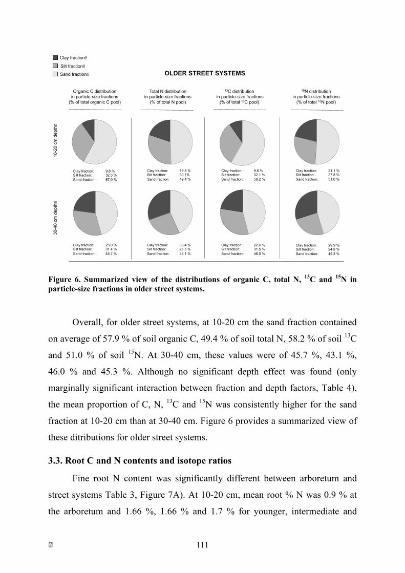
! 111
Silt fraction!
Clay fraction!
Sand fraction!
Clay fraction: 9.8 % Silt fraction: 32.3 % Sand fraction: 57.9 %
Clay fraction: 23.0 % Silt fraction: 31.4 % Sand fraction: 45.7 %
Clay fraction: 19.8 % Silt fraction: 30.7% Sand fraction: 49.4 %
Clay fraction: 30.4 % Silt fraction: 26.5 % Sand fraction: 43.1 %
Clay fraction: 9.6 % Silt fraction: 32.1 % Sand fraction: 58.2 %
Clay fraction: 22.6 % Silt fraction: 31.5 % Sand fraction: 46.0 %
Clay fraction: 29.9 % Silt fraction: 24.8 % Sand fraction: 45.3 %
Clay fraction: 21.1 % Silt fraction: 27.8 % Sand fraction: 51.0 %
Organic C distribution in particle-size fractions
(% of total organic C pool)
15N distribution in particle-size fractions
(% of total 15N pool)
13C distribution in particle-size fractions
(% of total 13C pool)
Total N distribution in particle-size fractions
(% of total N pool)
30-4
0 cm
dep
th!
10-2
0 cm
dep
th!
OLDER STREET SYSTEMS
Figure 6. Summarized view of the distributions of organic C, total N, 13C and 15N in particle-size fractions in older street systems.
Overall, for older street systems, at 10-20 cm the sand fraction contained
on average of 57.9 % of soil organic C, 49.4 % of soil total N, 58.2 % of soil 13C
and 51.0 % of soil 15N. At 30-40 cm, these values were of 45.7 %, 43.1 %,
46.0 % and 45.3 %. Although no significant depth effect was found (only
marginally significant interaction between fraction and depth factors, Table 4),
the mean proportion of C, N, 13C and 15N was consistently higher for the sand
fraction at 10-20 cm than at 30-40 cm. Figure 6 provides a summarized view of
these ditributions for older street systems.
3.3. Root C and N contents and isotope ratios
Fine root N content was significantly different between arboretum and
street systems Table 3, Figure 7A). At 10-20 cm, mean root % N was 0.9 % at
the arboretum and 1.66 %, 1.66 % and 1.7 % for younger, intermediate and
! 112
older street systems, respectively. At 30-40 cm, mean root % N was 0.8 % at the
arboretum and 1.5 %, 1.3 % and 1.6 % for younger, intermediate and older street
systems, respectively.
Fine root C:N was significantly higher at the arboretum at both depths
when compared to street systems (Table 3, Figure 7B). At 10-20 cm, root C:N
was 44.7 at the arboretum and 26.0, 21.7 and 23.7 for younger, intermediate and
older street systems. At 30-40 cm, average root C:N was 40.3 for the arboretum
and 28.5, 33.5 and 25.3 in younger, intermediate and older street systems.
Fine root δ13C was significantly different between older street systems
and the arboretum and younger street systems (Table 3, Figure 7C). Roots from
intermediate street systems did not differ significantly from younger and older
street systems. At 10-20 cm, mean fine root δ13C at the arboretum was -27.7 ‰
and was -27.1 ‰, -26.4 ‰ and -25.7 ‰ for younger, intermediate and older
street systems, respectively. At 30-40 cm, mean fine root δ13C at the arboretum
was -27.4 ‰ and -27.1 ‰, -26.9 ‰ and -26 ‰ for younger, intermediate and
older street systems. At 10-20 cm, mean fine root δ13C in older street systems
was 2 ‰ units higher when compared to the arboretum, and 1.4 ‰ units higher
when compared to younger street systems. At 30-40 cm, mean fine root δ13C in
older street systems was 1.4 ‰ units higher when compared to the arboretum,
and 1.1 ‰ units higher when compared to younger street systems.
Fine root δ15N was significantly different between intermediate and older
street systems and the arboretum and younger street systems, respectively (Table
3, Figure 7D). At 10-20 cm, mean fine root δ15N was 3.1 ‰ at the arboretum
and 6.8 ‰, 14.7 ‰ and 13.9 ‰ in younger, intermediate and older street
systems, respectively. At 30-40 cm, mean fine root δ15N was 4.9 ‰ at the
arboretum and 6.1 ‰, 14.5 ‰ and 13.3 ‰ in younger, intermediate and older
street systems, respectively. The difference between intermediate and older
! 113
street systems and the arboretum was thus of about 10 ‰ units at both depths,
and of about 7 ‰ units at both depth when compared to younger street systems.
3.4. C mineralization and δ13C-CO2
The mean daily respiration rate measured at the end of incubation was
significantly different between the arboretum and younger street systems (Table
3, Figure 9A), but not significantly different between street system classes, and
intermediate and older street systems did not differ significantly from the
arboretum. Mean respiration rates at 10-20 cm were 8.2 µg C-CO2.g soil-1.day-1
at the arboretum, and 3.1, 4.9 and 6.0 µg C-CO2.g soil-1.day-1 for the younger,
intermediate and older systems, respectively. At 30-40 cm, mean respiration
rates were 4.4 µg C-CO2.g soil-1.day-1 at the arboretum and 3.4, 4.0 and 4.4 µg
C-CO2.g soil-1.day-1 in younger, intermediate and older street systems,
Figure 7. Fine root (A) N content, (B) C:N, (C) δ13C and (D) δ15N at 10-20 cm and 30-40 cm in the different sample classes. Bars show means and error bars correspond to standard error. Different letters mean that a significant difference (p < 0.05) was indicated by a linear mixed-effect model and Tukey post-hoc tests (see Table 3 and text). For each bar, n = 5.
Arboretum Younger Intermediate Older
010
2030
4050
60
10-20 cm
Arboretum Younger Intermediate Older
30-40 cm
10-20 cm
30-40 cm
10-20 cm
30-40 cm
10-20 cm
30-40 cm
Roo
t C
:N
a
b b
b
Arboretum Younger Intermediate Older
05
1015
20
10-20 cm
Arboretum Younger Intermediate Older
30-40 cm
10-20 cm
30-40 cm
10-20 cm
30-40 cm
10-20 cm
30-40 cm
Roo
t δ15
N (
‰)
a a
b b
Arboretum Younger Intermediate Older
−29
−28
−27
−26
−25
−24
−23
Arboretum Younger Intermediate Older
10-20 cm
30-40 cm
10-20 cm
30-40 cm
10-20 cm
30-40 cm
10-20 cm
30-40 cm
Roo
t δ13
C (
‰)
a a
ac bc
Arboretum Younger Intermediate Older
0.0
0.5
1.0
1.5
2.0
10-20 cm
Arboretum Younger Intermediate Older
30-40 cm
10-20 cm
30-40 cm
10-20 cm
30-40 cm
10-20 cm
30-40 cm
Roo
t %
N a
b b b A
B
C
D

! 114
respectively. Older street systems thus had a two times higher soil respiration
rate compared to younger street systems at 10-20 cm, and 1.3 times higher at 30-
40 cm. Stratification increased with street system age, with respiration rates
being 1.4 times higher at 10-20 cm than at 30-40 cm in older street systems. At
the arboretum, respiration rates at 10-20 cm were 1.9 times higher than at 30-40
cm (Figure 9A).
The coefficient of soil organic C mineralization was obtained by
calculating the percentage of soil organic C represented by soil respiration
(Dommergues, 1960), e.g., by dividing soil respiration rates by the mass of
organic C initiqlly contained in the sample and multiplying it by 100. It thus
corresponds to the mineralization rate of C per mass unit of soil organic C. Soil
organic C mineralization rate (cumulated, Figure 8; daily rate, Figure 9B) was
significantly different between the arboretum and all street system classes, and
was significantly lower in older street systems when compared to younger and
intermediate street systems (Table 3). The mean daily soil organic C
mineralization rate at 10-20 cm was of 0.045 % at the arboretum and 0.026 %,
0.024 % and 0.017 % in younger, intermediate and older street systems,
respectively.
At 30-40 cm, the mean daily soil organic C mineralization rate was
0.039 % at the arboretum and 0.024 %, 0.032 % and 0.016 % in younger,
intermediate and older street systems, respectively. Overall, the observed trend
in street systems was a decreased soil organic C mineralization rate with
increasing average system age, the rate being 1.5 times higher in younger
systems when compared to older systems and 2.6 times higher at the arboretum
when compared to older street systems at 10-20 cm. The trend was similar for
both depths, apart from a higher rate for intermediate systems at 30-40 cm.

! 115
0-10 cm
Time (days)
0 10 20 30 40 50 60 70
CO
2 min
eral
ised
(% C
org)
0,0
0,5
1,0
1,5
2,0
2,5
3,0
3,5
ChevreloupClass 1Class 2Class 3
20-40 cm
Time (days)
0 10 20 30 40 50 60 70
CO
2 min
eral
ised
(% C
org)
0,0
0,5
1,0
1,5
2,0
2,5
3,0
3,5
ChevreloupClass 1Class 2Class 3Older systems
Intermediate systems Younger systems Arboretum
Intermediate systems Younger systems Arboretum
Cum
ulat
ed s
oil o
rgan
ic c
arbo
n m
iner
aliz
atio
n (%
Soi
l C)
Cum
ulat
ed s
oil o
rgan
ic c
arbo
n m
iner
aliz
atio
n (%
Soi
l C)
10-20 cm 30-40 cm
3.5
3.0
2.5
2.0
1.5
1.0
0.5
0.0
3.5
3.0
2.5
2.0
1.5
1.0
0.5
0.0
Older systems
A! B!
!Figure 8. Cumulated soil organic C mineralization over the incubation period at (A) 10-20 cm and (B) 30-40 cm.
Arboretum Younger Intermediate Older
−28
−27
−26
−25
−24
−23
Arboretum Younger Intermediate Older
10-20 cm
30-40 cm
10-20 cm
30-40 cm
10-20 cm
30-40 cm
10-20 cm
30-40 cm
δ13 C
-CO
2 (‰
)
ab a
bc
c
Arboretum Younger Intermediate Older0.00
0.01
0.02
0.03
0.04
0.05
0.06
Dai
ly s
oil o
rgan
ic c
arbo
n
min
eral
izat
ion
(% S
oil C
.day
-1)
b b
c
a
10-20 cm
Arboretum Younger Intermediate Older
30-40 cm
10-20 cm
30-40 cm
10-20 cm
30-40 cm
10-20 cm
30-40 cm
Dai
ly s
oil r
espi
ratio
n (µ
g C
-CO
2.g s
oil-1
day-
1 )
Arboretum Younger Intermediate Older
02
46
810
10-20 cm
Arboretum Younger Intermediate Older
30-40 cm
10-20 cm
30-40 cm
10-20 cm
30-40 cm
10-20 cm
30-40 cm
b
ab
a
ab
A B
C
Figure 9. Mean (A) Daily soil respiration, (B) Daily soil organic carbon mineralization and (C) δ13C-CO2 at 62 days, at 10-20 cm and 30-40 cm in the different sample classes. Bars show means and error bars correspond to standard error. Different letters mean that a significant difference (p < 0.05) was indicated by a linear mixed-effect model and Tukey post-hoc tests (see Table 3 and text). For each bar, n = 5.
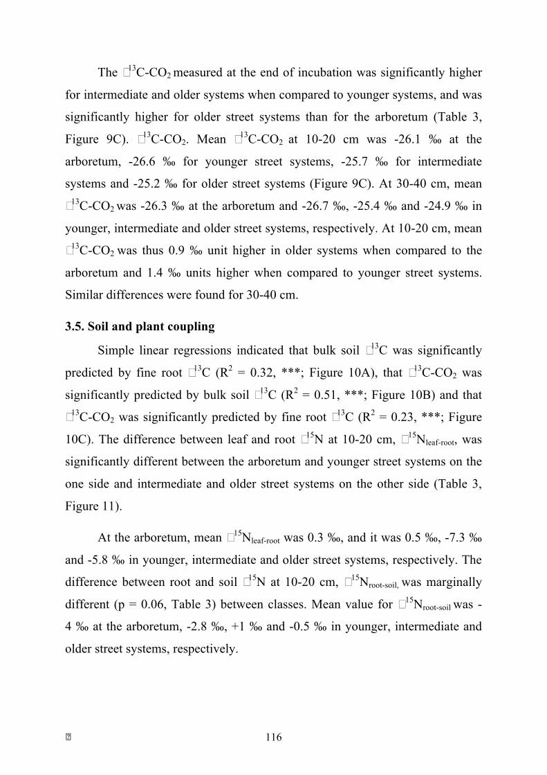
! 116
The δ13C-CO2 measured at the end of incubation was significantly higher
for intermediate and older systems when compared to younger systems, and was
significantly higher for older street systems than for the arboretum (Table 3,
Figure 9C). δ13C-CO2. Mean δ13C-CO2 at 10-20 cm was -26.1 ‰ at the
arboretum, -26.6 ‰ for younger street systems, -25.7 ‰ for intermediate
systems and -25.2 ‰ for older street systems (Figure 9C). At 30-40 cm, mean
δ13C-CO2 was -26.3 ‰ at the arboretum and -26.7 ‰, -25.4 ‰ and -24.9 ‰ in
younger, intermediate and older street systems, respectively. At 10-20 cm, mean
δ13C-CO2 was thus 0.9 ‰ unit higher in older systems when compared to the
arboretum and 1.4 ‰ units higher when compared to younger street systems.
Similar differences were found for 30-40 cm.
3.5. Soil and plant coupling
Simple linear regressions indicated that bulk soil δ13C was significantly
predicted by fine root δ13C (R2 = 0.32, ***; Figure 10A), that δ13C-CO2 was
significantly predicted by bulk soil δ13C (R2 = 0.51, ***; Figure 10B) and that
δ13C-CO2 was significantly predicted by fine root δ13C (R2 = 0.23, ***; Figure
10C). The difference between leaf and root δ15N at 10-20 cm, ∆15Nleaf-root, was
significantly different between the arboretum and younger street systems on the
one side and intermediate and older street systems on the other side (Table 3,
Figure 11).
At the arboretum, mean ∆15Nleaf-root was 0.3 ‰, and it was 0.5 ‰, -7.3 ‰
and -5.8 ‰ in younger, intermediate and older street systems, respectively. The
difference between root and soil δ15N at 10-20 cm, ∆15Nroot-soil, was marginally
different (p = 0.06, Table 3) between classes. Mean value for ∆15Nroot-soil was -
4 ‰ at the arboretum, -2.8 ‰, +1 ‰ and -0.5 ‰ in younger, intermediate and
older street systems, respectively.
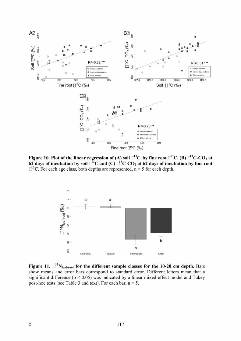
! 117
−28 −27 −26 −25 −24−27.0
−26.0
−25.0
−24.0A!
Soi
l !δ1
3 C (‰
)
Fine root δ13C (‰)
R2=0.32 ***
Older systems
Intermediate systems
Younger systems
−27.0 −26.5 −26.0 −25.5 −25.0 −24.5
−28
−27
−26
−25
−24
Soil δ13C (‰)
δ13 C
-CO
2 (‰
)
R2=0.51 ***
B!
Older systems
Intermediate systems
Younger systems
−28 −27 −26 −25 −24
−28
−27
−26
−25
−24
δ13 C
-CO
2 (‰
)
R2=0.23 **
C!
Older systems
Intermediate systems
Younger systems
Fine root δ13C (‰) Figure 10. Plot of the linear regression of (A) soil δ13C by fine root δ13C, (B) δ13C-CO2 at 62 days of incubation by soil δ13C and (C) δ13C-CO2 at 62 days of incubation by fine root δ13C. For each age class, both depths are represented, n = 5 for each depth.
Arboretum Younger Intermediate Older
−10
−8−6
−4−2
02
4
∆15 N
leaf
-roo
t (‰
)
a a
b
b
6 8 10 12 14 16
05
1015
2025
Roo
t δ15
N (
‰)
Soil δ15N (‰)
4 6 8 10 12 14 16 18
05
1015
2025
Sand fraction δ15N (‰)
Roo
t δ15
N (
‰)
R2=0.58 *** R2=0.54 ***
Arboretum Younger Intermediate Older
−10
−8−6
−4−2
02
4
∆15 N
leaf
-roo
t (‰
)
a a
b
b
6 8 10 12 14 16
05
1015
2025
Roo
t δ15
N (
‰)
Soil δ15N (‰) 4 6 8 10 12 14 16 18
05
1015
2025
Sand fraction δ15N (‰)
Roo
t δ15
N (
‰)
R2=0.58 *** R2=0.54 *** Older systems
Intermediate systems
Younger systems
Arboretum Younger Intermediate Older
−10
−8−6
−4−2
02
4
∆15 N
leaf
-roo
t (‰
)
a a
b
b
6 8 10 12 14 16
05
1015
2025
Roo
t δ15
N (
‰)
Soil δ15N (‰) 4 6 8 10 12 14 16 18
05
1015
2025
Sand fraction δ15N (‰)
Roo
t δ15
N (
‰)
R2=0.58 *** R2=0.54 *** Older systems
Intermediate systems
Younger systems
A! B!
Figure 11. ∆15Nleaf-root for the different sample classes for the 10-20 cm depth. Bars show means and error bars correspond to standard error. Different letters mean that a significant difference (p < 0.05) was indicated by a linear mixed-effect model and Tukey post-hoc tests (see Table 3 and text). For each bar, n = 5.
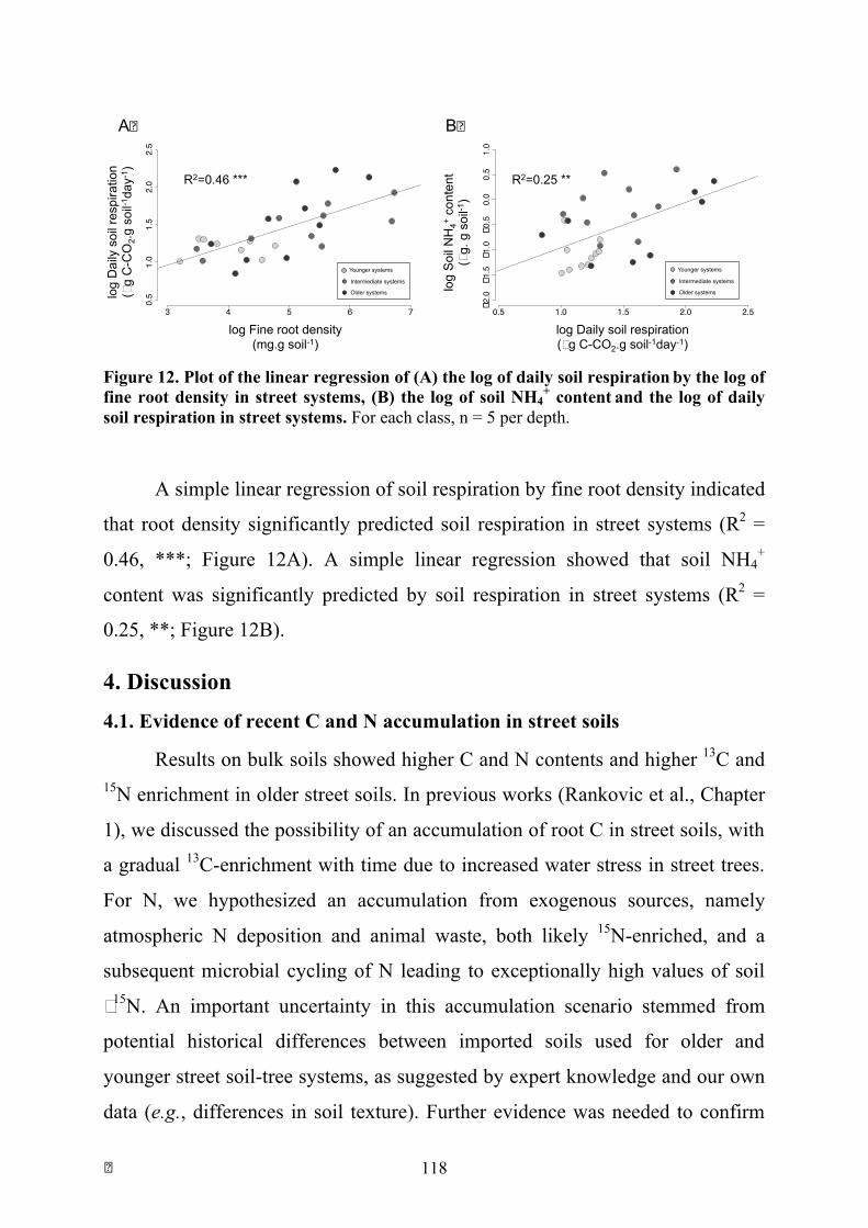
! 118
3 4 5 6 7
0.5
1.0
1.5
2.0
2.5
log
Dai
ly s
oil r
espi
ratio
n (µ
g C
-CO
2.g s
oil-1
day-
1 )
log Fine root density (mg.g soil-1)
Arboretum Younger Intermediate Older
−10
−8−6
−4−2
02
4
∆15 N
leaf
-roo
t (‰
)
a a
b
b
6 8 10 12 14 16
05
1015
2025
Roo
t δ15
N (
‰)
Soil δ15N (‰) 4 6 8 10 12 14 16 18
05
1015
2025
Sand fraction δ15N (‰)
Roo
t δ15
N (
‰)
R2=0.58 *** R2=0.54 *** Older systems
Intermediate systems
Younger systems
R2=0.46 ***
A!
0.5 1.0 1.5 2.0 2.5
−2.0
−1.5
−1.0
−0.5
0.0
0.5
1.0
log Daily soil respiration (µg C-CO2.g soil-1day-1)
log
Soi
l NH
4+ co
nten
t (µ
g. g
soi
l-1)
Arboretum Younger Intermediate Older
−10
−8−6
−4−2
02
4
∆15 N
leaf
-roo
t (‰
)
a a
b
b
6 8 10 12 14 16
05
1015
2025
Roo
t δ15
N (
‰)
Soil δ15N (‰) 4 6 8 10 12 14 16 18
05
1015
2025
Sand fraction δ15N (‰) R
oot δ
15N
(‰
)
R2=0.58 *** R2=0.54 *** Older systems
Intermediate systems
Younger systems
R2=0.25 **
B!
Figure 12. Plot of the linear regression of (A) the log of daily soil respiration by the log of fine root density in street systems, (B) the log of soil NH4
+ content and the log of daily soil respiration in street systems. For each class, n = 5 per depth.
A simple linear regression of soil respiration by fine root density indicated
that root density significantly predicted soil respiration in street systems (R2 =
0.46, ***; Figure 12A). A simple linear regression showed that soil NH4+
content was significantly predicted by soil respiration in street systems (R2 =
0.25, **; Figure 12B).
4. Discussion
4.1. Evidence of recent C and N accumulation in street soils
Results on bulk soils showed higher C and N contents and higher 13C and 15N enrichment in older street soils. In previous works (Rankovic et al., Chapter
1), we discussed the possibility of an accumulation of root C in street soils, with
a gradual 13C-enrichment with time due to increased water stress in street trees.
For N, we hypothesized an accumulation from exogenous sources, namely
atmospheric N deposition and animal waste, both likely 15N-enriched, and a
subsequent microbial cycling of N leading to exceptionally high values of soil
δ15N. An important uncertainty in this accumulation scenario stemmed from
potential historical differences between imported soils used for older and
younger street soil-tree systems, as suggested by expert knowledge and our own
data (e.g., differences in soil texture). Further evidence was needed to confirm
! 119
the hypothesized C and N accumulation processes and that the observed age-
related patterns were not solely due to legacy effects.
In the present study, the analysis of particle-size fractions first shows that
in older street soils, more than half of C and almost half of N are contained in
the coarser SOM fractions. Even though the estimates of C mean residence time
differ among fractionation methods and C turnover assessment methods (e.g.,
laboratory incubation, C3/C4 chronosequences, 14C analyses), the mean
residence time of soil C associated with the sand fraction is reported to be of a
few years to a couple of decades at most, while it is in the range of centuries to
millennia for the C associated to the silt and clay fractions (Wattel-Koekkoek et
al., 2003; Fontaine et al., 2007; von Lützow et al., 2007; Feng et al., 2016). For
our older street systems, of which the oldest are 77 years old, this suggests that
an important proportion of their C and N stocks are composed of C and N that
accumulated after trees and soils were assembled in streets.
This asumption is supported by our results. C and N distribution differed
among street age classes, with the coarse fraction containing an increasing
proportion of C and N as systems age, which too could mean that recently added
C and N represent an increasing proportion of soil C and N stocks with time in
street soils. The observed trends in stratification, where surface horizons (10-20
cm) tended to contain a higher proportion of C and N, in their coarse fraction
when compared to deeper layers (30-40 cm), also suggest chronic inputs of 13C-
enriched C and 15N-enriched N from the soil surface. Such trends were also
observed for both 13C and 15N, suggesting that recent C and N inputs are
characterized by enriched δ13C and δ15N values.
For the potential sources of N, we have previously discussed that atmospheric N
depositions and animal waste could contribute to exogenous 15N-enriched inputs
in street systems, that could be assimilated by roots and soil microbial biomass
(Rankovic et al., Chapter 1). Concerning the sources of C, root δ13C increased
! 120
with tree age and was significantly higher in older street soils than in younger
and arboretum soils. This could be due to increasing water stress as street trees
grow and thus higher water-use efficiency in older trees, leading to lower
stomatal conductance and less discrimination towards 13C during C3
photosynthesis, resulting in more 13C-enriched organic matter produced by trees
(e.g., Farquhar et al., 1989; Kagotani et al., 2013; Falxa-Raymond et al., 2014).
The urban CO2, because of 13C-depleted fossil fuels, tends to be depleted in 13C
compared to background CO2 (Lichtfouse, 2003; Widory & Javoy, 2003), and
rather than confounding this effect, it is probably weakening the observed
pattern.
As fine roots can have a lifespan of several years (Gill & Jackson, 2000;
Gaudinski et al., 2001; McCormack et al. 2012), root δ13C might thus integrate
over several growing seasons the 13C signal of the chronic water stress that is
suggested for street silver lindens in Paris (David et al., submitted). Root δ13C,
alone, predicted more than 30 % of bulk soil δ13C. As shown in a previous study
(Rankovic et al., Chapter 1), fine root density in older and intermediate street
systems was respectively five and three times higher when compared to younger
street systems and the arboretum. Taken together, these results suggest that as
street systems age, there is an increasing input of root C, itself increasingly 13C-
enriched. This is consistent with the age-related trends observed in coarse
fractions (discussed above) and tends to further confirm the likelihood of a
scenario of important root C input and accumulation. The progressive increase
of soil C:N (average of about 17 for oldest street soils), getting closer to root
C:N (≈ 20), is also consistent with such a scenario.
Furthermore, data on δ13C-CO2 showed an age-related 13C-enrichment of
respired CO2 by soils, with the same order of magnitude than age-related
enrichment of root δ13C (an increase of 1.4 ‰ units in older systems compared
to younger systems). Root δ13C significantly predicted δ13C-CO2 by (23 % of
! 121
explained variance by root δ13C alone). These results indicate that besides
imprinting C stocks with time, root-C seems to imprint the whole C cycling in
soils. This can be seen as further evidence that a dynamics in C cycling takes
place in street systems and is strongly shaped by tree influence on soils, which is
consistent with contemporary views of a close and dynamic interdependence of
the plant–microbe–soil system and the imprint of plant physiology on C cycling
(Ekblad & Högberg, 2001; Ekblad et al., 2005; Högberg & Read, 2006; Shahzad
et al., 2015).
Even though inherited C and N can contribute to current street soil C and
N stocks, the results discussed above form, together, a body of converging
evidence which strongly suggests that a long-term soil C and N accumulation
dynamics indeed takes place in street systems, and that accumulated C and N
constitute an increasing proportion, and perhaps the majority in the oldest
systems, of C and N stocks in street soils.
4.2. Possible mechanisms for root-C accumulation in street soils
As root C inputs increase, several mechanisms could lead to C
accumulation in street soils. Firstly, additional C can be incorporated into a
growing microbial biomass, which could be responsible for increased soil
respiration.
We also found that soil C mineralization decreased with street system age,
which means that as root inputs increase, an increasing portion of inputs is more
slowly mineralized in street soils. This could be due to several factors. A first
hypothesis could be that older street soils offer higher levels of physical
protection to SOM. However, textural data showed that older street soils were
sandy loam soils and contained less clay than the other street soils. Furthermore,
the qualitative analysis of X-ray diffractograms obtained for clay minerals
suggested that, overall, clay mineralogy was dominated by kaolinite, and
! 122
especially in older street soils. Textural and mineralogical properties thus did
not confer an increased SOM physical protection potential to older soils.
A second hypothesis would involve the higher bulk density found in street
soils (Rankovic et al., Chapter 1), which had an almost two-fold bulk density
(about 2.5 g.cm-3) when compared to arboretum soils. Such high bulk density
could impede air and water circulation and negatively influence microbial
aerobic activities. However, bulk density was similar between street soils, and
thus could not explain why older street soils present lower C mineralization
rates compared to younger street systems. In addition, as soils were disturbed
prior incubation (sieving at < 2 mm) and incubated at similar water potential
(80 % of WHC), it appears unlikely that differences in soil physical properties
could alone explain the important differences in C mineralization rates that were
observed (2.6 times higher rates in arboretum and 1.5 higher rates in younger
street soils, when compared to older street soils).
A third hypothesis would involve the chemical composition of root inputs.
Compared to the arboretum, a major difference in street soils is the export of
aboveground litter and the three-fold higher fine root density in intermediate and
older street soils (fine root density was similar between arboretum and younger
street soils) (Rankovic et al., Chapter 1). As they age, street soils thus probably
receive a much higher amount of root litter than younger street soils and
arboretum soils. Root litter has been shown to have slower decomposition rates
than leaf litter: in a global synthesis, Freschet at al. (2013) report that root litter
decomposes about 2.8 times slower than leaf litter derived from the same plant
species. This is attributed to a higher content of recalcitrant compounds, such as
lignin and tannins, in roots compared to leaves (Rasse et al., 2005; Xia et al.,
2015). For street soils, which are deprived of relatively more labile leaf litter
inputs, this means that they receive higher inputs of relatively more recalcitrant
C, of which, when compared to arboretum soils, a higher part could accumulate
! 123
in soils as chemically recalcitrant, leading to the lower C mineralization rates
observed in street soils.
However, “intrinsic” chemical recalcitrance alone cannot control SOM
stabilization, notably because soil microorganisms can degrade most organic
molecules produced by plants (Schmidt et al., 2011). Another mechanism,
involving the mediation of soil microbes is thus needed to explain the reduced C
mineralization rates in street soils despite increased root-C inputs. Compared to
arboretum soils, another major difference for street soils is their exposure to
potentially high and chronic exogenous N inputs, which are likely to occur in
street soils. High N depositions have been shown to decrease SOM
mineralization in a wide range of soils (Bowden et al., 2004; Craine et al., 2007;
Zak et al., 2008; Ramirez et al., 2012; Xia et al., 2015) and this has been
predicted by theoretical works (e.g., Ägren et al., 2001; Fontaine & Barot, 2005;
Perveen et al., 2014). The literature suggests that the underlying mechanisms
involve shifts in heterotrophic microbial physiologies and/or community
composition associated to increased soil N availability. As N depositions
increase soil N availability, soil microbial communities could reduce their N-
mining on more recalcitrant SOM and shift towards a decomposition of more
labile C when available, overall leading to a decreased soil C mineralization
(Fontaine et al., 2003; Craine et al., 2007; Fontaine et al., 2011; Fierer et al.,
2011; Ramirez et al., 2012). The lower C mineralization rates observed in street
soils, and their decrease with system age, could then be due to a reduction in the
mining of more recalcitrant root-C (e.g., lignin). Accordingly, several studies
report a decrease in activity of lignin-degrading enzymes in N enriched soils
(Carreiro et al., 2000; DeForest et al., 2004; Edwards et al., 2011).
Finally, Rasse et al. (2005) proposed that root-C could benefit from
specific physico-chemical and physical protection compared to leaf litter. Given
its closer proximity to soil minerals which could facilitate its sorption, root-C
! 124
could be less accessible to microbial degradation. In addition, as very fine roots,
root hair and mycorrhizal hyphae feeding on root exudates, can grow inside soil
pores of just a few micrometers across, a higher proportion of root-derived C
than leaf-derived C could be physically shielded from microbial degradation.
4.3. Street trees diversify their N sources
We previously hypothesized that N inputs, potentially 15N-enriched, could
be assimilated by roots and microbial biomass and contribute to the increase of
soil N content. Here, we found that fine root N content presented sharply higher
values, and root C:N lower values, in street systems when compared to the
arboretum. This suggests that in street soils, a higher amount of N is available
for root uptake than in the arboretum, especially at the surface. This is consistent
with previously reported results showing an increase in soil mineral N content
with soil age, especially at the surface of street soils (Rankovic et al., Chapter 1).
Root δ15N was on average 7 to 10 ‰ units higher in street systems than in the
arboretum, and reached exceptionally high δ15N values (≈ 14 ‰) in intermediate
and older street systems, which range among the highest values measured
worldwide in roots (Pardo et al., 2006, 2013).
We were not able to measure N mineralization rates in this study,
however it could be expected that N mineralization rates increase with fine root
density, as roots, especially through exudates, can stimulate the mineralization
of SOM and release of ammonium into the soil solution through rhizosphere
priming effect (e.g., Kuzyakov, 2002; Raynaud et al., 2006; Cheng et al., 2014;
Shahzad et al., 2012, 2015). In street soils, we found that fine root density
significantly predicted soil microbial respiration rates, which significantly
predicted soil ammonium content. This could mean that as soil-tree systems age,
N mineralization rates increase. This is not contradictory with the above
discussion on SOM stabilization and accumulation: we saw a relative decrease
in SOM mineralization in street systems, not its suppression.
! 125
To explain the observed patterns in soil and root δ15N, we thus propose
the following scenario. As 15N-enriched exogenous N enters street soils, part of
it is directly assimilated by roots and microbial biomass. Besides likely having
high initial δ15N values (Rankovic et al., Chapter 1), both deposited ammonium
and nitrate pools can become further 15N-enriched if volatilization, nitrification
and denitrification take place in street soils before they are assimilated by roots
and microbes. After being assimilated by roots and microbial biomass, the
ammonium released as roots and microbial biomass are recycled could be partly
nitrified as well, further 15N-enriching the ammonium pool that is available for
uptake, and further 15N-enriching the next generation of roots and microbes.
Retention and recycling of the added N can last over decades (Sebilo et al.,
2013). Such a δ15N “amplifying loop”, repeated over time, could explain the
very high δ15N values found in street soils. The various losses (leaching, gaseous
losses, belowground litter exports) could be compensated and even surpassed by
continuous inputs.
N mineralization induces little 15N fractionation (Högberg, 1997; Dawson
et al., 2002), so that the δ15N of the produced ammonium is very close to soil
δ15N (N in SOM), and an ammonium uptake (which, too, induces little
fractionation) by roots leads to root δ15N closely matching soil δ15N. ∆15Nroot-soil
values tended to get closer to 0 ‰ with increasing system age, which would be
consistent with a root uptake of ammonium originating from SOM recycling.
This is consistent with the soil δ15N amplifying loop hypothesized above, and
suggests that in street soils a tighter coupling takes place, over time, between
dead root- and microbial biomass-N recycling, on one side, and live root N
uptake on the other side (Abbadie et al., 1992; de Parseval et al., 2015).
How significant this tight coupling is for whole tree N nutrition, however,
is uncertain. Contrary to root data, foliar data suggested the possibility that street
trees become N limited as they age, possibly because tree pits, of relatively
! 126
limited volume, do not contain sufficient N stocks to match older tree N demand
(Rankovic et al., Chapter 1). Contrary to ∆15Nroot-soil, ∆15Nleaf-soil was found highly
negative in intermediate and older street systems (Rankovic et al., Chapter 1).
∆15Nleaf-root was close to 0 ‰ in arboretum and younger street systems,
suggesting a very tight coupling between root and foliar N nutrition. However,
∆15Nleaf-root had much more negative values in intermediate and older street
systems (-7.3 ‰ and -5.8 ‰, respectively). These are the highest differences
reported in the literature between topsoil roots and leaves (Pardo et al., 2006,
2013), and suggest that street trees, as they age, access less 15N-enriched N
sources. This would mean that trees, as they age, probably diversify their N
sources and that their N nutrition becomes less coupled to N available at the soil
surface (here, the first 40 cm of soil; we found similar values at 10-20 cm and
30-40 cm, both for soil and roots). Possible sources include leached nitrate, that
roots could uptake deeper in the soil pit. Foliar uptake of gaseous NOx forms,
that are likely to be less 15N-enriched than dry deposited forms (Widory, 2007),
could also substantially contribute to foliar N nutrition. It was shown to
contribute to up to 25 % of needle N in Norway spruce along a highway in
Switzerland (Ammann et al., 1999). Finally, there is considerable uncertainty as
to the extent of street tree root systems, and even though their pits are
surrounded by a mostly mineral matrix, there is a possibility that tree roots
explore important underground volumes and possibly acquire N outside of their
pits.
5. Conclusion
Current street soil management in Paris is based on the hypothesis that
soils get exhausted with time. We previously reported that long-term age-related
patterns in C and N cycling suggested an accumulation of root-C and exogenous
N in Parisian street soil-tree systems. Further work was needed, however, to lift
uncertainties about potentially overriding legacy effects. In the present study,

! 127
the strongly converging results in soil particle-size analysis, root δ13C, δ13C of
CO2 respired during soil incubations, and SOM mineralization rates, further
suggest an important accumulation of root-derived C in street soils. For N,
particle-size analysis, root N content and δ15N also further suggested an
accumulation of exogenous N in street systems.
We propose several mechanisms that can lead to the joint accumulation of
C and N in street systems. In particular, we suggest that important inputs of
relatively more recalcitrant root litter and N-induced changes in soil microbial
communities, where increased N availability in street systems would reduce
microbial N-mining on recalcitrant SOM, can lead to reduced SOM
mineralization rates in street soils and thus gradual accumulation of root-C. On
the other hand, it it likely that high levels of fresh organic matter inputs through
roots stimulate the mineralization of part of the SOM, at least in the vicinity of
live roots. A growing body of research suggests that SOM dynamics are
mediated by the complex interactions of C, N and energy foraging strategies of
soil decomposers, and involve mechanisms named priming effects (PE)
(Kuzyakov et al., 2000; Fontaine et al., 2003, 2007, 2011; Guenet et al., 2010a).
PE involve an increase (positive PE) or a decrease (negative PE) of SOM
mineralization rates following the addition of labile forms of C, N or both
(Kuzyakov et al., 2000; Guenet et al., 2010a,b). Different PE can co-occur in
soils (e.g., Guenet et al., 2010b) and involve different substrates and microbial
guilds. A possibility, in street soils, is that both a positive (rhizosphere PE) and a
negative PE (interaction of recalcitrant root compounds and increased available
N) co-occur in street soils, and that the balance between both mechanisms is
favorable to the accumulation of root-C.
Removal of aerial litter is arguably a widespread practice across cities
(Templer et al., 2015), and increase in root density following water stress,
nutrient stress or as a response to increased urban CO2 concentration is likely to
! 128
occur in other cities. Similarly, important levels of N deposition in urban
environments are documented worldwide. Therefore, the mechanisms that we
propose, if confirmed by future works, could likely occur in other cities and
could in part explain the urban convergence in ecosystem processes that is
mentioned in urban ecological literature.
In future works, 14C dating could provide the absolute age of C in street
soils, and definitely confirm the accumulation hypothesis. Furthermore, data on
the chemical composition of SOM could further confirm the root-origin of
accumulated C in street soils and its degree of transformation into microbial
biomass. The microbial ecology – community structure and catabolic activity –
of these soils could provide further information on the mechanisms underlying
SOM accumulation, especially in relation to N dynamics. Finally, our results
suggest that street trees present a surprising N-nutrition behavior. Future works
should develop an integrated perspective on street tree N nutrition, documenting
all potential N sources, including the different atmospheric and underground
sources.
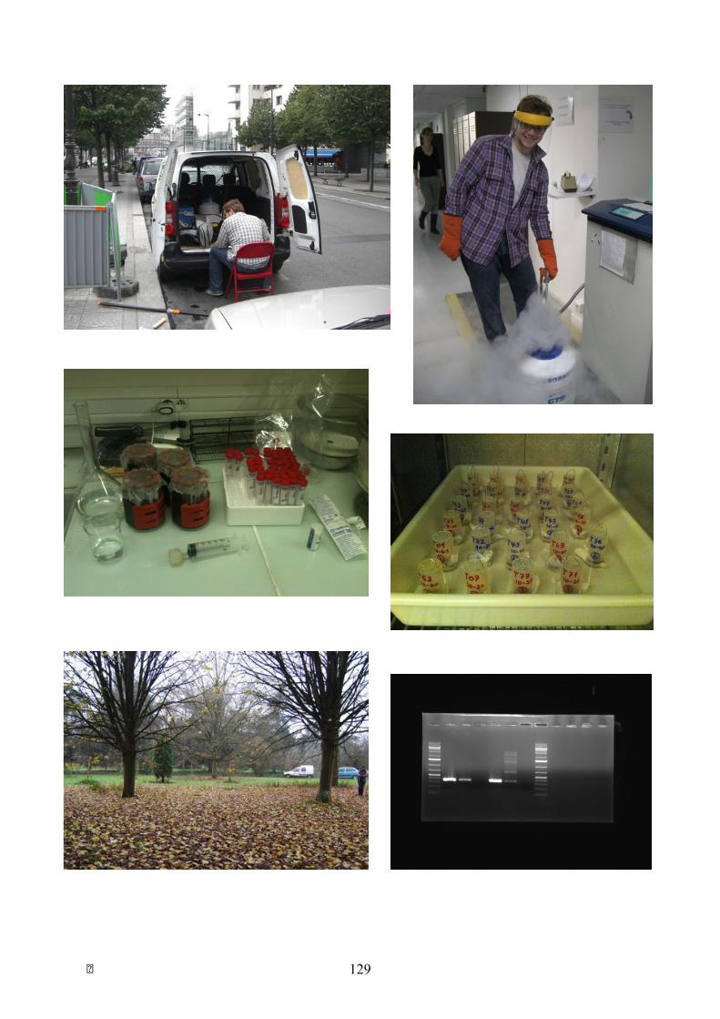
! 129

! 130
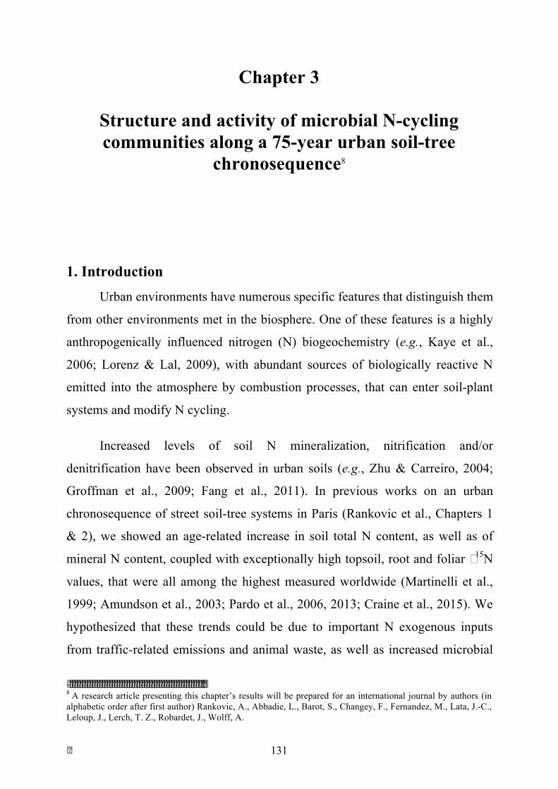
! 131
Chapter 3
Structure and activity of microbial N-cycling communities along a 75-year urban soil-tree
chronosequence8
1. Introduction Urban environments have numerous specific features that distinguish them
from other environments met in the biosphere. One of these features is a highly
anthropogenically influenced nitrogen (N) biogeochemistry (e.g., Kaye et al.,
2006; Lorenz & Lal, 2009), with abundant sources of biologically reactive N
emitted into the atmosphere by combustion processes, that can enter soil-plant
systems and modify N cycling.
Increased levels of soil N mineralization, nitrification and/or
denitrification have been observed in urban soils (e.g., Zhu & Carreiro, 2004;
Groffman et al., 2009; Fang et al., 2011). In previous works on an urban
chronosequence of street soil-tree systems in Paris (Rankovic et al., Chapters 1
& 2), we showed an age-related increase in soil total N content, as well as of
mineral N content, coupled with exceptionally high topsoil, root and foliar δ15N
values, that were all among the highest measured worldwide (Martinelli et al.,
1999; Amundson et al., 2003; Pardo et al., 2006, 2013; Craine et al., 2015). We
hypothesized that these trends could be due to important N exogenous inputs
from traffic-related emissions and animal waste, as well as increased microbial
!!!!!!!!!!!!!!!!!!!!!!!!!!!!!!!!!!!!!!!!!!!!!!!!!!!!!!!!8 A research article presenting this chapter’s results will be prepared for an international journal by authors (in alphabetic order after first author) Rankovic, A., Abbadie, L., Barot, S., Changey, F., Fernandez, M., Lata, J.-C., Leloup, J., Lerch, T. Z., Robardet, J., Wolff, A.
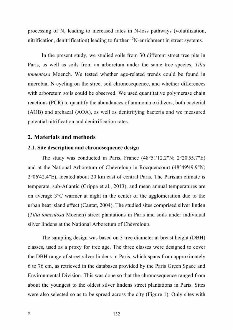
! 132
processing of N, leading to increased rates in N-loss pathways (volatilization,
nitrification, denitrification) leading to further 15N-enrichment in street systems.
In the present study, we studied soils from 30 different street tree pits in
Paris, as well as soils from an arboretum under the same tree species, Tilia
tomentosa Moench. We tested whether age-related trends could be found in
microbial N-cycling on the street soil chronosequence, and whether differences
with arboretum soils could be observed. We used quantitative polymerase chain
reactions (PCR) to quantify the abundances of ammonia oxidizers, both bacterial
(AOB) and archaeal (AOA), as well as denitrifying bacteria and we measured
potential nitrification and denitrification rates.
2. Materials and methods 2.1. Site description and chronosequence design
The study was conducted in Paris, France (48°51'12.2"N; 2°20'55.7"E)
and at the National Arboretum of Chèvreloup in Rocquencourt (48°49'49.9"N;
2°06'42.4"E), located about 20 km east of central Paris. The Parisian climate is
temperate, sub-Atlantic (Crippa et al., 2013), and mean annual temperatures are
on average 3°C warmer at night in the center of the agglomeration due to the
urban heat island effect (Cantat, 2004). The studied sites comprised silver linden
(Tilia tomentosa Moench) street plantations in Paris and soils under individual
silver lindens at the National Arboretum of Chèvreloup.
The sampling design was based on 3 tree diameter at breast height (DBH)
classes, used as a proxy for tree age. The three classes were designed to cover
the DBH range of street silver lindens in Paris, which spans from approximately
6 to 76 cm, as retrieved in the databases provided by the Paris Green Space and
Environmental Division. This was done so that the chronosequence ranged from
about the youngest to the oldest silver lindens street plantations in Paris. Sites
were also selected so as to be spread across the city (Figure 1). Only sites with
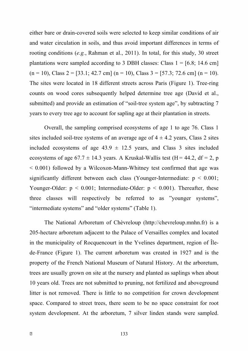
! 133
either bare or drain-covered soils were selected to keep similar conditions of air
and water circulation in soils, and thus avoid important differences in terms of
rooting conditions (e.g., Rahman et al., 2011). In total, for this study, 30 street
plantations were sampled according to 3 DBH classes: Class 1 = [6.8; 14.6 cm]
(n = 10), Class 2 = [33.1; 42.7 cm] (n = 10), Class 3 = [57.3; 72.6 cm] (n = 10).
The sites were located in 18 different streets across Paris (Figure 1). Tree-ring
counts on wood cores subsequently helped determine tree age (David et al.,
submitted) and provide an estimation of “soil-tree system age”, by subtracting 7
years to every tree age to account for sapling age at their plantation in streets.
Overall, the sampling comprised ecosystems of age 1 to age 76. Class 1
sites included soil-tree systems of an average age of 4 ± 4.2 years, Class 2 sites
included ecosystems of age 43.9 ± 12.5 years, and Class 3 sites included
ecosystems of age 67.7 ± 14.3 years. A Kruskal-Wallis test (H = 44.2, df = 2, p
< 0.001) followed by a Wilcoxon-Mann-Whitney test confirmed that age was
significantly different between each class (Younger-Intermediate: p < 0.001;
Younger-Older: p < 0.001; Intermediate-Older: p < 0.001). Thereafter, these
three classes will respectively be referred to as ”younger systems”,
“intermediate systems” and “older systems” (Table 1).
The National Arboretum of Chèvreloup (http://chevreloup.mnhn.fr) is a
205-hectare arboretum adjacent to the Palace of Versailles complex and located
in the municipality of Rocquencourt in the Yvelines department, region of Île-
de-France (Figure 1). The current arboretum was created in 1927 and is the
property of the French National Museum of Natural History. At the arboretum,
trees are usually grown on site at the nursery and planted as saplings when about
10 years old. Trees are not submitted to pruning, not fertilized and aboveground
litter is not removed. There is little to no competition for crown development
space. Compared to street trees, there seem to be no space constraint for root
system development. At the arboretum, 7 silver linden stands were sampled.
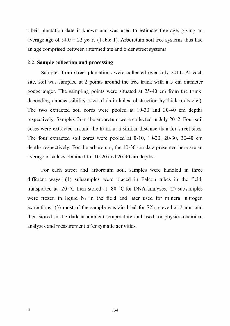
! 134
Their plantation date is known and was used to estimate tree age, giving an
average age of 54.0 ± 22 years (Table 1). Arboretum soil-tree systems thus had
an age comprised between intermediate and older street systems.
2.2. Sample collection and processing
Samples from street plantations were collected over July 2011. At each
site, soil was sampled at 2 points around the tree trunk with a 3 cm diameter
gouge auger. The sampling points were situated at 25-40 cm from the trunk,
depending on accessibility (size of drain holes, obstruction by thick roots etc.).
The two extracted soil cores were pooled at 10-30 and 30-40 cm depths
respectively. Samples from the arboretum were collected in July 2012. Four soil
cores were extracted around the trunk at a similar distance than for street sites.
The four extracted soil cores were pooled at 0-10, 10-20, 20-30, 30-40 cm
depths respectively. For the arboretum, the 10-30 cm data presented here are an
average of values obtained for 10-20 and 20-30 cm depths.
For each street and arboretum soil, samples were handled in three
different ways: (1) subsamples were placed in Falcon tubes in the field,
transported at -20 °C then stored at -80 °C for DNA analyses; (2) subsamples
were frozen in liquid N2 in the field and later used for mineral nitrogen
extractions; (3) most of the sample was air-dried for 72h, sieved at 2 mm and
then stored in the dark at ambient temperature and used for physico-chemical
analyses and measurement of enzymatic activities.
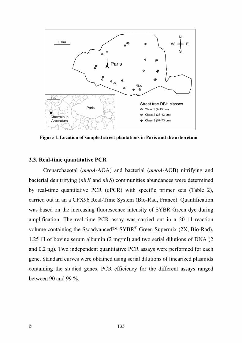
! 135
2.3. Real-time quantitative PCR
Crenarchaeotal (amoA-AOA) and bacterial (amoA-AOB) nitrifying and
bacterial denitrifying (nirK and nirS) communities abundances were determined
by real-time quantitative PCR (qPCR) with specific primer sets (Table 2),
carried out in an a CFX96 Real-Time System (Bio-Rad, France). Quantification
was based on the increasing fluorescence intensity of SYBR Green dye during
amplification. The real-time PCR assay was carried out in a 20 µl reaction
volume containing the Ssoadvanced™ SYBR® Green Supermix (2X, Bio-Rad),
1.25 µl of bovine serum albumin (2 mg/ml) and two serial dilutions of DNA (2
and 0.2 ng). Two independent quantitative PCR assays were performed for each
gene. Standard curves were obtained using serial dilutions of linearized plasmids
containing the studied genes. PCR efficiency for the different assays ranged
between 90 and 99 %.
Paris
Chèvreloup Arboretum
N
S
EW3 km
5 km
Paris
Class 3 (57-73 cm)
Class 2 (33-43 cm)
Class 1 (7-15 cm)
Street tree DBH classes
Figure 1. Location of sampled street plantations in Paris and the arboretum
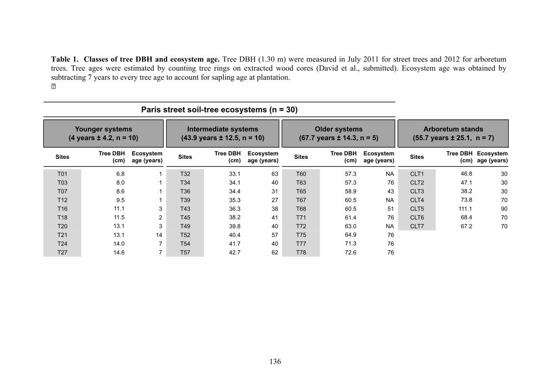
136
Sites Tree DBH (cm)
Ecosystem age (years) Sites Tree DBH
(cm)Ecosystem age (years) Sites Tree DBH
(cm)Ecosystem age (years) Sites Tree DBH
(cm)Ecosystem age (years)
T01 6.8 1 T32 33.1 63 T60 57.3 NA CLT1 46.8 30T03 8.0 1 T34 34.1 40 T63 57.3 76 CLT2 47.1 30T07 8.6 1 T36 34.4 31 T65 58.9 43 CLT3 38.2 30T12 9.5 1 T39 35.3 27 T67 60.5 NA CLT4 73.8 70T16 11.1 3 T43 36.3 38 T68 60.5 51 CLT5 111.1 90T18 11.5 2 T45 38.2 41 T71 61.4 76 CLT6 68.4 70T20 13.1 3 T49 39.8 40 T72 63.0 NA CLT7 67.2 70T21 13.1 14 T52 40.4 57 T75 64.9 76T24 14.0 7 T54 41.7 40 T77 71.3 76T27 14.6 7 T57 42.7 62 T78 72.6 76
Paris street soil-tree ecosystems (n = 30)
Younger systems (4 years ± 4.2, n = 10)
Intermediate systems (43.9 years ± 12.5, n = 10)
Older systems (67.7 years ± 14.3, n = 5)
Arboretum stands (55.7 years ± 25.1, n = 7)
Table 1. Classes of tree DBH and ecosystem age. Tree DBH (1.30 m) were measured in July 2011 for street trees and 2012 for arboretum trees. Tree ages were estimated by counting tree rings on extracted wood cores (David et al., submitted). Ecosystem age was obtained by subtracting 7 years to every tree age to account for sapling age at plantation. !!
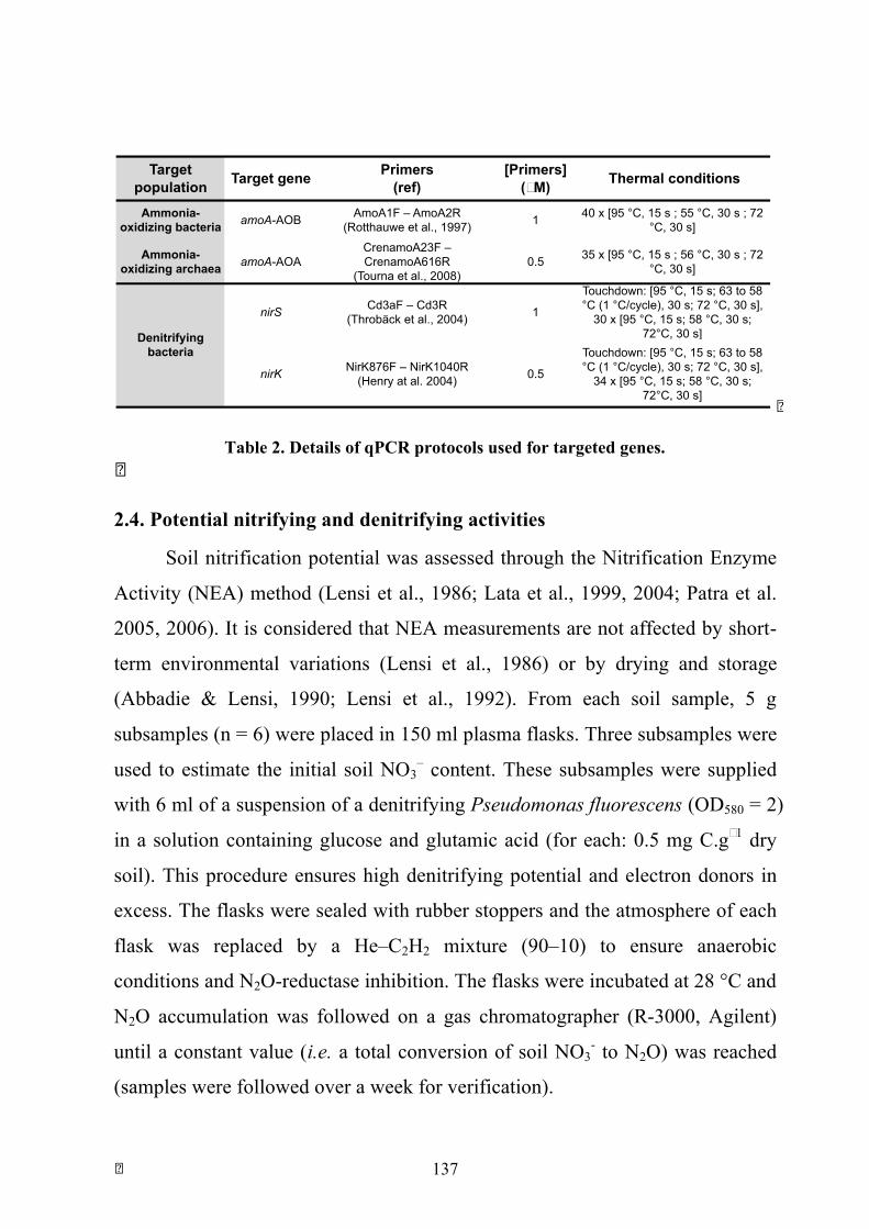
! 137
Targetpopulation
Target gene Primers(ref)
[Primers] (µM)
Thermal conditions
Ammonia-oxidizing bacteria amoA-AOB AmoA1F – AmoA2R
(Rotthauwe et al., 1997) 1 40 x [95 °C, 15 s ; 55 °C, 30 s ; 72 °C, 30 s]
Ammonia-oxidizing archaea amoA-AOA
CrenamoA23F – CrenamoA616R
(Tourna et al., 2008)0.5 35 x [95 °C, 15 s ; 56 °C, 30 s ; 72
°C, 30 s]
nirS Cd3aF – Cd3R(Throbäck et al., 2004) 1
Touchdown: [95 °C, 15 s; 63 to 58 °C (1 °C/cycle), 30 s; 72 °C, 30 s],
30 x [95 °C, 15 s; 58 °C, 30 s; 72°C, 30 s]
nirK NirK876F – NirK1040R(Henry at al. 2004) 0.5
Touchdown: [95 °C, 15 s; 63 to 58 °C (1 °C/cycle), 30 s; 72 °C, 30 s],
34 x [95 °C, 15 s; 58 °C, 30 s; 72°C, 30 s]
Denitrifying bacteria
!
Table 2. Details of qPCR protocols used for targeted genes. !
2.4. Potential nitrifying and denitrifying activities
Soil nitrification potential was assessed through the Nitrification Enzyme
Activity (NEA) method (Lensi et al., 1986; Lata et al., 1999, 2004; Patra et al.
2005, 2006). It is considered that NEA measurements are not affected by short-
term environmental variations (Lensi et al., 1986) or by drying and storage
(Abbadie & Lensi, 1990; Lensi et al., 1992). From each soil sample, 5 g
subsamples (n = 6) were placed in 150 ml plasma flasks. Three subsamples were
used to estimate the initial soil NO3– content. These subsamples were supplied
with 6 ml of a suspension of a denitrifying Pseudomonas fluorescens (OD580 = 2)
in a solution containing glucose and glutamic acid (for each: 0.5 mg C.g−1 dry
soil). This procedure ensures high denitrifying potential and electron donors in
excess. The flasks were sealed with rubber stoppers and the atmosphere of each
flask was replaced by a He–C2H2 mixture (90–10) to ensure anaerobic
conditions and N2O-reductase inhibition. The flasks were incubated at 28 °C and
N2O accumulation was followed on a gas chromatographer (R-3000, Agilent)
until a constant value (i.e. a total conversion of soil NO3- to N2O) was reached
(samples were followed over a week for verification).
! 138
The other three subsamples were used to determine potential NO3–
accumulation. For these subsamples, 4 ml of a (NH4)2SO4 solution was added
(200 µg N.g−1 dry soil) in order to ensure a moisture content equivalent to 80%
WHC, and no limitation by ammonium. Flasks were then sealed with parafilm,
which prevents soil from drying but allows gas exchange, and incubated at
28 °C for 7 h in a horizontal position to ensure optimal, homogeneous aeration
of the soil. After this aerobic incubation, which allows nitrate to accumulate, the
soil samples were enriched with Pseudomonas fluorescens and incubated as
described above for the other three subsamples. Nitrification potential was
computed by subtracting the nitrate initially present in the soil from that present
after aerobic incubation (g N.h-1.g-1 dry soil).
Soil denitrification potential was assessed through the Denitrification
Enzyme Activity (DEA) as described in Patra et al. (2005, 2006). For each soil,
10 g of dry soil were placed in a 150 ml plasma flask. 6 ml of distilled water
containing KNO3 (200 µg NO3—N.g-1 dry soil), glucose (0.5 mg C.g-1 dry soil)
and glutamic acid (0.5 mg C.g-1 dry soil) were added. Additional water was
added to achieve 100% WHC. Flasks were then sealed with rubber stoppers and
the atmosphere of each flask was evacuated and replaced by a 90:10 He:C2H2
mixture to provide anaerobic conditions and inhibit N2O-reductase activity. The
flasks were incubated at 28 °C and N2O accumulation was followed on a gas
chromatographer (R-3000, Agilent) at 2, 4, 6 and 8 h of incubation.
Denitrification potential was computed as g N.h-1.g-1 dry soil.
2.5. Statistical analyses
Statistical analyses were performed with the R-software (R Development
Core Team, 2013). Four sample classes (three DBH classes and the arboretum)
and two depths (10-30 cm and 30-40 cm) and their interaction were used as
explanatory factors. Linear mixed-effects models with a "site" random effect
were used for soil variables to account for non-independence of soil depths at
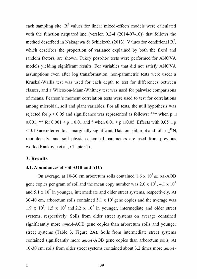
! 139
each sampling site. R2 values for linear mixed-effects models were calculated
with the function r.squared.lme (version 0.2-4 (2014-07-10)) that follows the
method described in Nakagawa & Schielzeth (2013). Values for conditional R2,
which describes the proportion of variance explained by both the fixed and
random factors, are shown. Tukey post-hoc tests were performed for ANOVA
models yielding significant results. For variables that did not satisfy ANOVA
assumptions even after log transformation, non-parametric tests were used: a
Kruskal-Wallis test was used for each depth to test for differences between
classes, and a Wilcoxon-Mann-Whitney test was used for pairwise comparisons
of means. Pearson’s moment correlation tests were used to test for correlations
among microbial, soil and plant variables. For all tests, the null hypothesis was
rejected for p < 0.05 and significance was represented as follows: *** when p ≤
0.001; ** for 0.001 < p ≤ 0.01 and * when 0.01 < p ≤ 0.05. Effects with 0.05 ≤ p
< 0.10 are referred to as marginally significant. Data on soil, root and foliar δ15N,
root density, and soil physico-chemical parameters are used from previous
works (Rankovic et al., Chapter 1).
3. Results
3.1. Abundances of soil AOB and AOA
On average, at 10-30 cm arboretum soils contained 1.6 x 10⁷ amoA-AOB
gene copies per gram of soil and the mean copy number was 2.0 x 10⁷ , 4.1 x 10⁷
and 5.1 x 10⁷ in younger, intermediate and older street systems, respectively. At
30-40 cm, arboretum soils contained 5.1 x 10⁶ gene copies and the average was
1.9 x 10⁷, 1.5 x 10⁷ and 2.2 x 10⁷ in younger, intermediate and older street
systems, respectively. Soils from older street systems on average contained
significantly more amoA-AOB gene copies than arboretum soils and younger
street systems (Table 3, Figure 2A). Soils from intermediate street systems
contained significantly more amoA-AOB gene copies than arboretum soils. At
10-30 cm, soils from older street systems contained about 3.2 times more amoA-
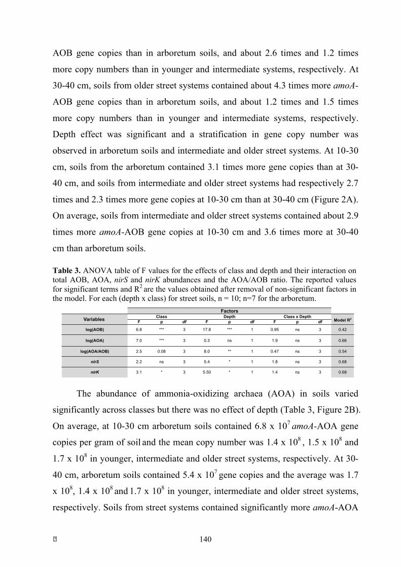
! 140
AOB gene copies than in arboretum soils, and about 2.6 times and 1.2 times
more copy numbers than in younger and intermediate systems, respectively. At
30-40 cm, soils from older street systems contained about 4.3 times more amoA-
AOB gene copies than in arboretum soils, and about 1.2 times and 1.5 times
more copy numbers than in younger and intermediate systems, respectively.
Depth effect was significant and a stratification in gene copy number was
observed in arboretum soils and intermediate and older street systems. At 10-30
cm, soils from the arboretum contained 3.1 times more gene copies than at 30-
40 cm, and soils from intermediate and older street systems had respectively 2.7
times and 2.3 times more gene copies at 10-30 cm than at 30-40 cm (Figure 2A).
On average, soils from intermediate and older street systems contained about 2.9
times more amoA-AOB gene copies at 10-30 cm and 3.6 times more at 30-40
cm than arboretum soils.
Table 3. ANOVA table of F values for the effects of class and depth and their interaction on total AOB, AOA, nirS and nirK abundances and the AOA/AOB ratio. The reported values for significant terms and R2 are the values obtained after removal of non-significant factors in the model. For each (depth x class) for street soils, n = 10; n=7 for the arboretum.
F p df F p df F p df
0.66ns 1 1.9 ns 3
log(AOB) 6.8 *** 3 17.8 *** 1 0.95 ns 3 0.42
Factors
Variables Class Depth Class x DepthModel R2
ns 3 0.68
1 0.47 ns 3 0.54
nirS 2.2 ns 3 5.4
log(AOA/AOB) 2.5 0.08 3 8.0 **
1 1.4 ns 3 0.68nirK 3.1 * 3 5.50 *
* 1 1.8
log(AOA) 7.0 *** 3 0.3
The abundance of ammonia-oxidizing archaea (AOA) in soils varied
significantly across classes but there was no effect of depth (Table 3, Figure 2B).
On average, at 10-30 cm arboretum soils contained 6.8 x 10⁷ amoA-AOA gene
copies per gram of soil and the mean copy number was 1.4 x 10⁸ , 1.5 x 10⁸ and
1.7 x 10⁸ in younger, intermediate and older street systems, respectively. At 30-
40 cm, arboretum soils contained 5.4 x 10⁷ gene copies and the average was 1.7
x 108, 1.4 x 10⁸ and 1.7 x 10⁸ in younger, intermediate and older street systems,
respectively. Soils from street systems contained significantly more amoA-AOA
! 141
gene copies than arboretum soils, with average abundance for street systems
being 2.6 times higher than the average abundance in arboretum soils (Figure
2B).
Arboretum Younger Intermediate Older0e+0
02e
+07
4e+0
76e
+07
8e+0
7
10-30 cm
Arboretum Younger Intermediate Older
30-40 cm
10-30 cm
30-40 cm
10-30 cm
30-40 cm
10-30 cm
30-40 cm
Num
ber o
f am
oA-A
OB
ge
ne c
opie
s.g-
1 dry
soi
l
Arboretum Younger Intermediate Older0.0e
+00
5.0e
+07
1.0e
+08
1.5e
+08
2.0e
+08
2.5e
+08
Num
ber o
f am
oA-A
OA
ge
ne c
opie
s.g-
1 dry
soi
l
10-30 cm
Arboretum Younger Intermediate Older
30-40 cm
10-30 cm
30-40 cm
10-30 cm
30-40 cm
10-30 cm
30-40 cm
Arboretum Younger Intermediate Older
05
1015
2025
AO
A/A
OB
ratio
10-30 cm
Arboretum Younger Intermediate Older
30-40 cm
10-30 cm
30-40 cm
10-30 cm
30-40 cm
10-30 cm
30-40 cm
A B
C
a ab
bd cd
a
b b b
Depth effect: p < 0.01
Depth effect: p < 10-3
There was a marginally significant effect (p = 0.08) of system class on the
AOA/AOB ratio and a significant effect of depth (Table 3, Figure 2C). At 10-30
cm, AOA/AOB averaged 5.2 at the arboretum and 12.7, 6.9 and 8.2 in younger,
intermediate and street systems, respectively (Figure 3C). At 30-40 cm,
AOA/AOB averaged 6.7 at the arboretum and 16.7, 13.9 and 10.2 in younger,
intermediate and older systems, respectively (Figure 2C). AOA/AOB was 1.3
times higher at 10-30 cm than at 30-40 cm in arboretum soils and 1.3, 2.0, 1.2
times higher at 10-30 cm than at 30-40 cm in younger, intermediate and older
Figure 2. (A) Abundance of amoA-AOB, (B) Abundance of amoA-AOA and (C) AOA/AOB ratio at 10-30 cm and 30-40 cm in the different sample classes. Bars show means and error bars correspond to standard error. Different letters mean that a significant difference (p < 0.05) was indicated by a Tukey post-hoc test performed after an ANOVA. For each bar, n = 10 for street soils, n = 7 for the arboretum.

! 142
street systems, respectively (Figure 2C). At 10-30 cm, AOA/AOB was 1.8 times
higher and 1.5 times higher in younger street systems when compared to
intermediate and older street systems, respectively. At 30-40 cm, AOA/AOB
was 1.2 times higher and 1.6 times higher in younger street systems when
compared to intermediate and older street systems.
3.2. Abundances of soil bacterial denitrifiers
The abundance of nirK differed across classes and depths but there was no
significant interaction between class and depth factors (Table 3, Figure 3A). On
average, at 10-30 cm arboretum soils contained 1.4 x 10⁸ nirK gene copies per
gram of soil and the mean copy number was 2.3 x 10⁸, 1.7 x 10⁸ and 3.1 x 10⁸ in
younger, intermediate and older street systems, respectively. At 30-40 cm,
arboretum soils contained 1.2 x 10⁸ gene copies and the average was 2.7 x 10⁸,
1.4 x 10⁸ and 1.8 x 10⁸ in younger, intermediate and older street systems,
respectively. Soils from younger and older street systems contained significantly
more nirK gene copies than arboretum soils. At 10-30 cm, street systems on
average contained 1.7 times more nirK gene copies than arboretum soils. At 30-
40 cm, they contained 1.6 times more nirK gene copies than arboretum soils
(Figure 3A). Soils from older street systems contained 1.7 times more nirK gene
copies at 10-30 cm than at 30-40 cm.
There was a significant effect of depth on the abundance of nirS (Table 3,
Figure 3B). On average, at 10-30 cm arboretum soils contained 2.9 x 10⁸ nirS
gene copies per gram of soil and the mean copy number was 2.4 x 10⁸ , 1.8 x 10⁸
and 2.8 x 10⁸ in younger, intermediate and older street systems, respectively. At
30-40 cm, arboretum soils contained 2.3 x 10⁸ gene copies and the average was
3.6 x 10⁸, 1.3 x 10⁸ and 2.1 x 10⁸ in younger, intermediate and older street
systems, respectively (Figure 3B). Arboretum soils contained 1.3 times more
nirS copies at 10-30 cm than at 30-40 cm, and intermediate and older street
systems respectively contained 1.4 times and 2.2 more copies at 10-30 cm than
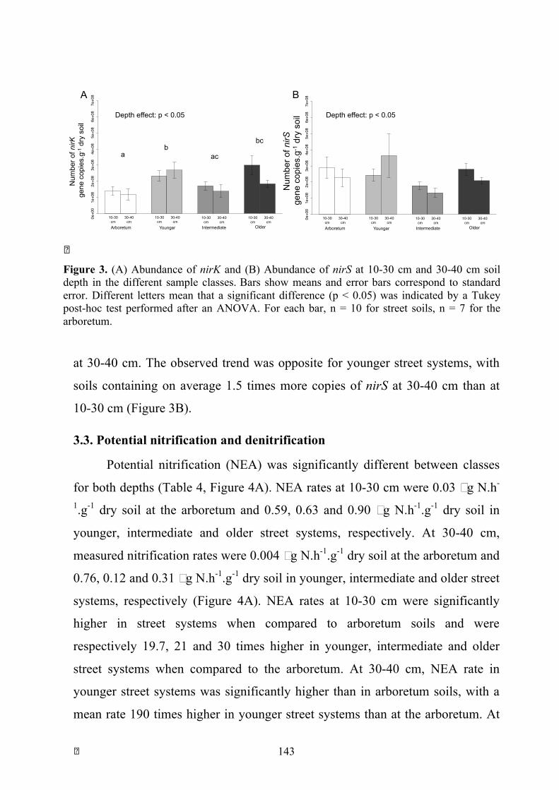
! 143
at 30-40 cm. The observed trend was opposite for younger street systems, with
soils containing on average 1.5 times more copies of nirS at 30-40 cm than at
10-30 cm (Figure 3B).
3.3. Potential nitrification and denitrification
Potential nitrification (NEA) was significantly different between classes
for both depths (Table 4, Figure 4A). NEA rates at 10-30 cm were 0.03 µg N.h-
1.g-1 dry soil at the arboretum and 0.59, 0.63 and 0.90 µg N.h-1.g-1 dry soil in
younger, intermediate and older street systems, respectively. At 30-40 cm,
measured nitrification rates were 0.004 µg N.h-1.g-1 dry soil at the arboretum and
0.76, 0.12 and 0.31 µg N.h-1.g-1 dry soil in younger, intermediate and older street
systems, respectively (Figure 4A). NEA rates at 10-30 cm were significantly
higher in street systems when compared to arboretum soils and were
respectively 19.7, 21 and 30 times higher in younger, intermediate and older
street systems when compared to the arboretum. At 30-40 cm, NEA rate in
younger street systems was significantly higher than in arboretum soils, with a
mean rate 190 times higher in younger street systems than at the arboretum. At
!Figure 3. (A) Abundance of nirK and (B) Abundance of nirS at 10-30 cm and 30-40 cm soil depth in the different sample classes. Bars show means and error bars correspond to standard error. Different letters mean that a significant difference (p < 0.05) was indicated by a Tukey post-hoc test performed after an ANOVA. For each bar, n = 10 for street soils, n = 7 for the arboretum.
Arboretum Younger Intermediate Older0e+0
01e
+08
2e+0
83e
+08
4e+0
85e
+08
6e+0
87e
+08
10-30 cm
Arboretum Younger Intermediate Older
30-40 cm
10-30 cm
30-40 cm
10-30 cm
30-40 cm
10-30 cm
30-40 cm
Arboretum Younger Intermediate Older0e+0
01e
+08
2e+0
83e
+08
4e+0
85e
+08
6e+0
87e
+08
10-30 cm
Arboretum Younger Intermediate Older
30-40 cm
10-30 cm
30-40 cm
10-30 cm
30-40 cm
10-30 cm
30-40 cm
Num
ber o
f nirK
ge
ne c
opie
s.g-
1 dry
soi
l
Num
ber o
f nirS
ge
ne c
opie
s.g-
1 dry
soi
l
A B
a b
ac
bc
Depth effect: p < 0.05 Depth effect: p < 0.05

! 144
30-40 cm, NEA rates were not significantly different between intermediate and
older street systems and the arboretum, however the observed trend was that
NEA rates were respectively 30 times and 77.5 times higher in intermediate and
older street systems than at the arboretum. There was no significant difference
among depths for younger street systems. However a significant stratification
was observed in arboretum soils, with rates at 10-30 cm being 7.5 times higher
than at 30-40 cm. A significant difference between depths was also observed for
intermediate and older street systems, with rates at 10-30 cm being respectively
5.25 and 2.9 higher than at 30-40 cm.
Arboretum Younger Intermediate Older
0.0
0.2
0.4
0.6
0.8
1.0
1.2
1.4
10-30 cm
Arboretum Younger Intermediate Older
30-40 cm
10-30 cm
30-40 cm
10-30 cm
30-40 cm
10-30 cm
30-40 cm
Pote
ntia
l den
itrifi
catio
n (µ
g N
.h-1
.g-1
dry
soi
l)
Arboretum Younger Intermediate Older
0.0
0.2
0.4
0.6
0.8
1.0
1.2
1.4
10-30 cm
Arboretum Younger Intermediate Older
30-40 cm
10-30 cm
30-40 cm
10-30 cm
30-40 cm
10-30 cm
30-40 cm
Pote
ntia
l nitr
ifica
tion
(µ
g N
.h-1
.g-1
dry
soi
l)
A B
a b
c
cd c
abd
c
abd a
b
c c
cd
ac
ed c
Potential denitrification (DEA) was significantly different between classes
for both depths (Table 4, Figure 4B). DEA rates at 10-30 cm were 0.2 µg N.h-
1.g-1 dry soil at the arboretum and 0.9, 1.2 and 1.3 µg N.h-1.g-1 dry soil in
younger, intermediate and older street systems, respectively. At 30-40 cm,
measured denitrification rates were 0.01 µg N.h-1.g-1 dry soil at the arboretum
and 0.80, 0.60 and 0.88 µg N.h-1.g-1 dry soil in younger, intermediate and older
street systems, respectively (Figure 4B). DEA rates were significantly higher in
street systems than in the arboretum at both depths (Figure 4B). When compared
to arboretum soils, younger, intermediate and older street systems showed
Figure 4. (A) Potential nitrification and (B) Potential denitrification at 10-30 cm and 30-40 cm soil depth in the different sample classes. Bars show means and error bars correspond to standard error. Different letters mean that a significant difference (p < 0.05) was indicated by a Wilcoxon-Mann-Whitney test. For each bar, n = 10 for street soils, n = 7 for the arboretum.

! 145
respectively 4.5, 6, and 6.5 higher DEA rates at 10-30 cm, and 80, 60 and 88
times higher rates at 30-40 cm. Soils from older street systems showed
significantly 1.4 higher DEA rates than younger street systems at 10-30 cm
(Figure 4B). An observed stratification trend was observed in arboretum soils
and in intermediate and older street systems, with a significant difference
between depths at the arboretum and in intermediate and older street systems
(Figure 4B). Arboretum soils showed 20 times higher DEA rates at 10-30 cm
when compared to 30-40 cm and soils from older street systems had about 1.5
higher rates at 10-30 cm when compared to 30-40 cm (Figure 4B). Although not
found significant, a similar trend was observed in intermediate soils, with rates
at 10-30 cm being 2 times higher than at 30-40 cm.
Table 4. Summary of Kruskal-Wallis tests for potential nitrification (NEA) and denitrification (DEA).
3.4. Correlations among microbial parameters and between microbial, soil and plant parameters in street systems
The results presented below concern Parisian street soil-tree systems only,
i.e. they do not include the arboretum sites.
NEA was positively correlated to AOA abundance, and a marginally significant
positive correlation was found between NEA and AOB abundance (Table 5). No
significant correlation was found between NEA and AOA/AOB ratio.
F p df F p df F p df
F p df F p df F p df
Depth H df p10-30 cm 12.9 3 **30-40 cm 8.7 3 *10-30 cm 12.7 3 **30-40 cm 14.6 3 **
Factor: Class
DEA
1 1.4 ns 3 0.68
NEA
nirK 3.1 * 3 5.50 *
* 1 1.8 ns 3 0.68
1 0.47 ns 3 0.54
nirS 2.2 ns 3 5.4
log(AOA/AOB) 2.5 0.08 3 8.0 **
ns 1 1.9 ns 3 0.66
1 0.95 ns 3 0.42
log(AOA) 7.0 *** 3 0.3
log(AOB) 6.8 *** 3 17.8 ***
Factors
Variables Class Depth Class x Depth
Model R2
log(Total bacteria) 4.1 * 3 9.6 ** 1 3.6 *
1 0.7 ns 3 0.70
3 0.54
δ13C-CO2 6.5 ** 3 0.1 ns
ns 1 1.45 ns 3 0.57
1 2.5 0.1 ns 0.36
% Soil C mineralised day-1 12.1 *** 3 0.0
Soil respiration day-1 4.2 * 3 7.8 *
Total crenarchaea 4.24 * 3 12.88
- - - - 0.77
** 1 1.95 ns 3
∆15Nleaf-root 19.8 *** 3 - -
1 1.1 ns 3 0.79
0.63
Root δ13C 5.01 * 3 0.9 ns
ns 1 1.3 ns 3 0.93
1 2.44 0.1 3 0.53
Root δ15N 21.12 *** 3 0.06
Root C:N 10.0 *** f 3.3 ns
** 1 0.7 ns 3 0.80
1 2.0 ns 3 -
Root %N 7.7 ** 3 10.40
11.6 ** 3 0.93
log (Live apices) 0.44 ns 3 4.09 0.06
ns 3 0.72
Soil δ15N 22.3 *** 3 0.008 ns 1
3 0.51
Soil δ13C 27.1 *** 3 0.1 ns 1 1.4
Class Depth Class x Depth
Factors
1 33
Variables
313
log (Soil C:N) 13.1 *** 3 1.5 ns
4.24 *
6.3 **
1 2.5 ns
log (Soil %N) 4.8 * 15.6 ** 0.77
Model R2
log (Soil %C) 8.0 ** 11.8 ** 0.78

! 146
The abundances of nirS and nirK genes were found to be positively
correlated and DEA was found to be positively correlated with the abundances
of both genes (Table 5).
The abundances of nirS were positively correlated to AOA and AOB
abundances. The abundances of nirK and nirS were found to be positively
correlated with NEA, as was DEA. DEA was positively correlated with AOA
and AOB abundances. NEA and DEA were positively correlated (Table 5).
AOB abundances were positively correlated to soil total N content.
AOA/AOB was negatively correlated to soil total N content (Table 6).
Marginally significant positive correlations were found between total soil N and
nirS abundance, nirK abundance and DEA.
Table 5. Correlations between soil microbial parameters. When the correlation is significant (bold) or marginally significant Pearson’s correlation coefficient (r) is given. r p r p r p r p r p r p r p r p
Total bacteria - - - - - - - - - - - - - - - -
Total crenarchaea 0.74 10-11 - - - - - - - - - - - - - -
AOA 0.3log 0.01 0.29log 0.03 - - - - - - - - - - - -
AOB 0.37 0.004 0.29 0.03 0.26 - - - - - - - - - -
AOA/AOB - 0.26 0.049 0.44 0.60log 10-7 - 0.52 10-5 - - - - - - - -
NEA 0.75 0.30log 0.03 0.36log 0.012 0.27 0.06 0.374 - - - - - -
nirS 0.41 0.001 0.25 0.05 0.41log 0.002 0.31log 0.015 0.7 0.32log 0.02 - - - -
nirK 0.72 10-10 0.80 10-15 0.35 0.17 0.42 0.50 0.003 0.56log 10-6 - -
DEA 0.39 0.002 0.33log 0.009 0.30 0.03 0.31 0.015 0.9 0.50log 0.003 0.34log 0.009 0.28 0.027
nirS nirKTotal bacteria Total crenarchaea AOA AOB AOA/AOB NEA
r p r p r p r p r p r p r p r p
Total bacteria - - - - - - - - - - - - - - - -
Total crenarchaea 0.74 10-11 - - - - - - - - - - - - - -
AOA 0.3log 0.01 0.29log 0.03 - - - - - - - - - - - -
AOB 0.37 0.004 0.29 0.03 0.26 - - - - - - - - - -
AOA/AOB - 0.26 0.049 0.44 0.60log 10-7 - 0.52 10-5 - - - - - - - -
NEA 0.75 0.30log 0.03 0.36log 0.012 0.27 0.06 0.374 - - - - - -
nirS 0.41 0.001 0.25 0.05 0.41log 0.002 0.31log 0.015 0.7 0.32log 0.02 - - - -
nirK 0.72 10-10 0.80 10-15 0.35 0.17 0.42 0.50 0.003 0.56log 10-6 - -
DEA 0.39 0.002 0.33log 0.009 0.30 0.03 0.31 0.015 0.9 0.50log 0.003 0.34log 0.009 0.28 0.027
nirS nirKTotal bacteria Total crenarchaea AOA AOB AOA/AOB NEA
Soil NH4+ content was positively correlated to AOB abundance and
negatively correlated with the AOA/AOB ratio. Soil NO2- content was positively
correlated to AOB abundance and positively correlated to NEA. It was also
positively correlated to DEA. A marginally significant (p = 0.07) negative
correlation was found between soil NO2- content and the AOA/AOB ratio. Soil
NO3- content was positively correlated with AOB abundance, NEA, nirK
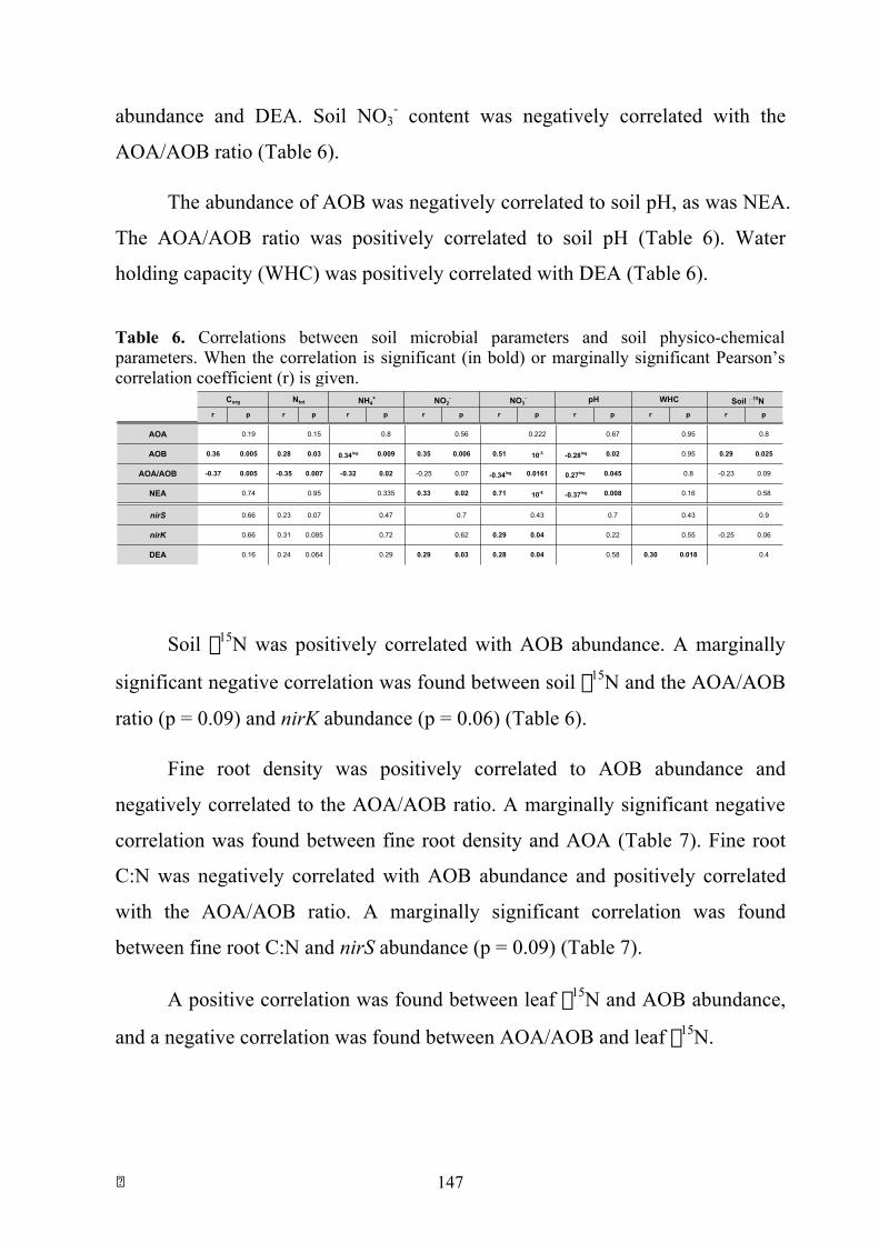
! 147
abundance and DEA. Soil NO3- content was negatively correlated with the
AOA/AOB ratio (Table 6).
The abundance of AOB was negatively correlated to soil pH, as was NEA.
The AOA/AOB ratio was positively correlated to soil pH (Table 6). Water
holding capacity (WHC) was positively correlated with DEA (Table 6).
Table 6. Correlations between soil microbial parameters and soil physico-chemical parameters. When the correlation is significant (in bold) or marginally significant Pearson’s correlation coefficient (r) is given. r p r p r p r p r p r p r p r p
Total bacteria 0.31 0.02 0.47 0.0001 0.27 0.0445 0.22 0.08 0.36 0.008 0.99 0.97 0.7
Total crenarchaea 0.50 0.38 0.003 0.44 0.9 0.40 0.003 0.42 0.93 0.5
AOA 0.19 0.15 0.8 0.56 0.222 0.67 0.95 0.8
AOB 0.36 0.005 0.28 0.03 0.34log 0.009 0.35 0.006 0.51 10-5 -0.28log 0.02 0.95 0.29 0.025
AOA/AOB -0.37 0.005 -0.35 0.007 -0.32 0.02 -0.25 0.07 -0.34log 0.0161 0.27log 0.045 0.8 -0.23 0.09
NEA 0.74 0.95 0.335 0.33 0.02 0.71 10-8 -0.37log 0.008 0.16 0.58
nirS 0.66 0.23 0.07 0.47 0.7 0.43 0.7 0.43 0.9
nirK 0.66 0.31 0.085 0.72 0.62 0.29 0.04 0.22 0.55 -0.25 0.06
DEA 0.16 0.24 0.064 0.29 0.29 0.03 0.28 0.04 0.58 0.30 0.018 0.4
r p r p r p r p r p r p r p r p r p r p
Total bacteria 0.3 0.177 0.17 0.16 0.22 0.08 0.7 0.95 0.3 0.4 0,4
Total crenarchaea 0.3 0.38 0.04 0.288 - 0.23 0.08 0.26 0.04 0.84 0.93 0.9 0.4 0,70.5
AOA -0.23 0.09 0.47 0.48 0.42 0.61 0.96 0.95 0.3 0.5 1
AOB 0.26 0.049 0.31 0.10 -0.43log 0.02 0.68 0.83 0.14 0.26 0.048 0.8 0.44 0.1 -0.50 0,06
AOA/AOB -0.31log 0.02 -0.30 0.10 0.49 0.006 0.9 0.9 0.37 -0.27 0.04 0.6 0.2 0.40
NEA 0.38 0.63 0.63 0.71 0.74 0.7 0.98 0.9 0.4 0.80.9 0.4
nirS 0.65 0.94 0.075 0.09 0.6 0.8 -0.38 0.03 0.22 0.9 0.4 0.4
nirK 0.779 0.41log 0.02 0.5 -0.21 0.10 0.27 0.03 0.4 0.9 0.4 0.3 0.6
DEA 0.93 0.79 0.9 0.9 0.92 0.64 0.13 0.4 0.6 0.8
∆15Nroot-soil ∆15Nleaf-root
pH WHC Soil δ15N
Fine root density Root %N Root C:N Leaf %N Leaf C:N Root δ15N Leaf δ15N
Corg Ntot NH4+ NO2
- NO3-
∆15Nleaf-soil
Nitr
ifica
tion
Den
itrifi
catio
nN
itrifi
catio
nD
enitr
ifica
tion
r p r p r p r p r p r p r p r p
Total bacteria 0.31 0.02 0.47 0.0001 0.27 0.0445 0.22 0.08 0.36 0.008 0.99 0.97 0.7
Total crenarchaea 0.50 0.38 0.003 0.44 0.9 0.40 0.003 0.42 0.93 0.5
AOA 0.19 0.15 0.8 0.56 0.222 0.67 0.95 0.8
AOB 0.36 0.005 0.28 0.03 0.34log 0.009 0.35 0.006 0.51 10-5 -0.28log 0.02 0.95 0.29 0.025
AOA/AOB -0.37 0.005 -0.35 0.007 -0.32 0.02 -0.25 0.07 -0.34log 0.0161 0.27log 0.045 0.8 -0.23 0.09
NEA 0.74 0.95 0.335 0.33 0.02 0.71 10-8 -0.37log 0.008 0.16 0.58
nirS 0.66 0.23 0.07 0.47 0.7 0.43 0.7 0.43 0.9
nirK 0.66 0.31 0.085 0.72 0.62 0.29 0.04 0.22 0.55 -0.25 0.06
DEA 0.16 0.24 0.064 0.29 0.29 0.03 0.28 0.04 0.58 0.30 0.018 0.4
r p r p r p r p r p r p r p r p r p r p
Total bacteria 0.3 0.177 0.17 0.16 0.22 0.08 0.7 0.95 0.3 0.4 0,4
Total crenarchaea 0.3 0.38 0.04 0.288 - 0.23 0.08 0.26 0.04 0.84 0.93 0.9 0.4 0,70.5
AOA -0.23 0.09 0.47 0.48 0.42 0.61 0.96 0.95 0.3 0.5 1
AOB 0.26 0.049 0.31 0.10 -0.43log 0.02 0.68 0.83 0.14 0.26 0.048 0.8 0.44 0.1 -0.50 0,06
AOA/AOB -0.31log 0.02 -0.30 0.10 0.49 0.006 0.9 0.9 0.37 -0.27 0.04 0.6 0.2 0.40
NEA 0.38 0.63 0.63 0.71 0.74 0.7 0.98 0.9 0.4 0.80.9 0.4
nirS 0.65 0.94 0.075 0.09 0.6 0.8 -0.38 0.03 0.22 0.9 0.4 0.4
nirK 0.779 0.41log 0.02 0.5 -0.21 0.10 0.27 0.03 0.4 0.9 0.4 0.3 0.6
DEA 0.93 0.79 0.9 0.9 0.92 0.64 0.13 0.4 0.6 0.8
∆15Nroot-soil ∆15Nleaf-root
pH WHC Soil δ15N
Fine root density Root %N Root C:N Leaf %N Leaf C:N Root δ15N Leaf δ15N
Corg Ntot NH4+ NO2
- NO3-
∆15Nleaf-soil
Nitr
ifica
tion
Den
itrifi
catio
nN
itrifi
catio
nD
enitr
ifica
tion
Soil δ15N was positively correlated with AOB abundance. A marginally
significant negative correlation was found between soil δ15N and the AOA/AOB
ratio (p = 0.09) and nirK abundance (p = 0.06) (Table 6).
Fine root density was positively correlated to AOB abundance and
negatively correlated to the AOA/AOB ratio. A marginally significant negative
correlation was found between fine root density and AOA (Table 7). Fine root
C:N was negatively correlated with AOB abundance and positively correlated
with the AOA/AOB ratio. A marginally significant correlation was found
between fine root C:N and nirS abundance (p = 0.09) (Table 7).
A positive correlation was found between leaf δ15N and AOB abundance,
and a negative correlation was found between AOA/AOB and leaf δ15N.
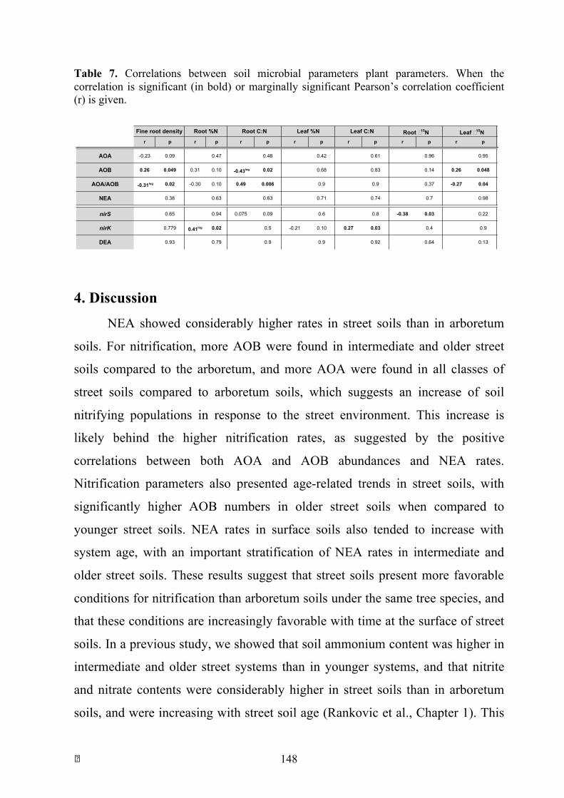
! 148
Table 7. Correlations between soil microbial parameters plant parameters. When the correlation is significant (in bold) or marginally significant Pearson’s correlation coefficient (r) is given.
4. Discussion NEA showed considerably higher rates in street soils than in arboretum
soils. For nitrification, more AOB were found in intermediate and older street
soils compared to the arboretum, and more AOA were found in all classes of
street soils compared to arboretum soils, which suggests an increase of soil
nitrifying populations in response to the street environment. This increase is
likely behind the higher nitrification rates, as suggested by the positive
correlations between both AOA and AOB abundances and NEA rates.
Nitrification parameters also presented age-related trends in street soils, with
significantly higher AOB numbers in older street soils when compared to
younger street soils. NEA rates in surface soils also tended to increase with
system age, with an important stratification of NEA rates in intermediate and
older street soils. These results suggest that street soils present more favorable
conditions for nitrification than arboretum soils under the same tree species, and
that these conditions are increasingly favorable with time at the surface of street
soils. In a previous study, we showed that soil ammonium content was higher in
intermediate and older street systems than in younger systems, and that nitrite
and nitrate contents were considerably higher in street soils than in arboretum
soils, and were increasing with street soil age (Rankovic et al., Chapter 1). This
r p r p r p r p r p r p r p r p
Total bacteria 0.31 0.02 0.47 0.0001 0.27 0.0445 0.22 0.08 0.36 0.008 0.99 0.97 0.7
Total crenarchaea 0.50 0.38 0.003 0.44 0.9 0.40 0.003 0.42 0.93 0.5
AOA 0.19 0.15 0.8 0.56 0.222 0.67 0.95 0.8
AOB 0.36 0.005 0.28 0.03 0.34log 0.009 0.35 0.006 0.51 10-5 -0.28log 0.02 0.95 0.29 0.025
AOA/AOB -0.37 0.005 -0.35 0.007 -0.32 0.02 -0.25 0.07 -0.34log 0.0161 0.27log 0.045 0.8 -0.23 0.09
NEA 0.74 0.95 0.335 0.33 0.02 0.71 10-8 -0.37log 0.008 0.16 0.58
nirS 0.66 0.23 0.07 0.47 0.7 0.43 0.7 0.43 0.9
nirK 0.66 0.31 0.085 0.72 0.62 0.29 0.04 0.22 0.55 -0.25 0.06
DEA 0.16 0.24 0.064 0.29 0.29 0.03 0.28 0.04 0.58 0.30 0.018 0.4
r p r p r p r p r p r p r p r p r p r p
Total bacteria 0.3 0.177 0.17 0.16 0.22 0.08 0.7 0.95 0.3 0.4 0,4
Total crenarchaea 0.3 0.38 0.04 0.288 - 0.23 0.08 0.26 0.04 0.84 0.93 0.9 0.4 0,70.5
AOA -0.23 0.09 0.47 0.48 0.42 0.61 0.96 0.95 0.3 0.5 1
AOB 0.26 0.049 0.31 0.10 -0.43log 0.02 0.68 0.83 0.14 0.26 0.048 0.8 0.44 0.1 -0.50 0,06
AOA/AOB -0.31log 0.02 -0.30 0.10 0.49 0.006 0.9 0.9 0.37 -0.27 0.04 0.6 0.2 0.40
NEA 0.38 0.63 0.63 0.71 0.74 0.7 0.98 0.9 0.4 0.80.9 0.4
nirS 0.65 0.94 0.075 0.09 0.6 0.8 -0.38 0.03 0.22 0.9 0.4 0.4
nirK 0.779 0.41log 0.02 0.5 -0.21 0.10 0.27 0.03 0.4 0.9 0.4 0.3 0.6
DEA 0.93 0.79 0.9 0.9 0.92 0.64 0.13 0.4 0.6 0.8
∆15Nroot-soil ∆15Nleaf-root
pH WHC Soil δ15N
Fine root density Root %N Root C:N Leaf %N Leaf C:N Root δ15N Leaf δ15N
Corg Ntot NH4+ NO2
- NO3-
∆15Nleaf-soil
Nitr
ifica
tion
Den
itrifi
catio
nN
itrifi
catio
nD
enitr
ifica
tion

! 149
could mean that as street systems age, an increasing amount of ammonium is
available for ammonia oxidizers, and is oxidized to nitrite and then to nitrate.
Here, several results suggest that AOB are responsible for the age-related
increase in nitrification in street soils. The age-related patterns found in AOB, of
which the abundance increases with soil age at the surface, closely match the
trends observed in NEA rates and previously observed in soil nitrite and nitrate
content (Rankovic et al., Chapter 1). A positive correlation between AOB, soil
ammonium content, nitrite content and nitrate content was found, while no
correlation was found between AOA and these parameters. Furthermore,
AOA/AOB showed a marginally significant decrease with street soil age, and
was negatively correlated with soil ammonium content. AOB was positively
correlated to NEA (marginally significant), while the correlation found between
AOA and NEA was due to two outliers, and disappeared when they were
removed.
These results are consistent with recent research on niche differentiation
among AOA and AOB, which suggests that AOA are more competitive in low-
nutrient conditions while AOB are more adapted to nutrient-rich environments
(Martens-Habbena et al., 2009; Di et al., 2009; Simonin et al., 2015; Carey et al.,
2016). In a recent meta-analysis of 33 studies on the effects of N-enrichment on
soil AOA, AOB and nitrification rates, Carey et al. (2016) found that N
additions increased both AOA and AOB abundances, but with an average
increase of 27 % for AOA and 326 % for AOB. Furthermore, they found a
positive correlation between the increase response of AOB and NEA rates
across studies, while no correlation was found between AOA response and
nitrification rates.
The increase of ammonia oxidizers, and especially of AOB, in street soils,
is likely due, at least in part, to increased ammonium content. This higher
mineral N content could be due to higher N deposition, likely to occur in such

! 150
roadside systems (Bettez et al., 2013), and to animal waste (especially urine).
The added N could directly stimulate nitrification by increasing substrate
availability. An increase in N mineralization with soil age could also lead to
more ammonium being available to nitrifiers. We previously reported an almost
five-fold increase in fine root density in older street systems when compared to
arboretum and younger street systems (Rankovic et al., Chapter 1), and that fine
root density was found to predict almost 50 % of the variance of soil respiration
rates measured through soil incubations (Rankovic et al., Chapter 2). Soil
respiration rates, in turn, significantly predicted 25 % of soil ammonium content.
This suggests that in street soils, at least part of the age-related increase in
ammonium content could come from higher N mineralization, stimulated by fine
roots. The positive correlation between fine root density and AOB, negative
correlation between fine root density and AOA, and negative correlation
between fine root density and AOA/AOB, indeed suggest that the increase in
fine root density might be, at least indirectly through an increase in N
mineralization, involved in favoring AOB versus AOA.
Compared to arboretum soils, another feature of street soils that is likely
to favor AOB nitrification is pH, which averages around 7.5 in street soils and
5.7 at the arboretum (Rankovic et al., Chapter 1). AOA are thought to dominate
nitrification in acidic soils, while AOB are favored at circumneutral pH (Nicol et
al., 2008; Prosser & Nicol, 2012; Carey et al., 2016). Nicol et al. (2008) found
that AOB transcriptional activity was highest around a pH of 6.9 but then
decreased at pH values of 7.3 and 7.5. In the present study, we found a negative
correlation between pH and AOB abundance in street soils. AOB abundance
seemed to slightly decrease in soils with pH higher than 7.5, as did NEA (data
not shown). This result, firstly, further suggests that the increase in NEA in
street soils is indeed driven by an increase in the abundance of AOB. Then, it
! 151
also suggests that the response of AOB to street conditions can, quite expectedly,
be partly modulated by other soil properties besides ammonium content.
In the case of pH, street conditions could, too, have an influence and lead
to the observed differences with arboretum soils. A first factor influencing street
soil pH is the criteria employed by the city of Paris for its imported soils, for
which the city requires a pH comprised between 6.5 and 7.5 (Paris Green Space
and Environmental Division, pers. comm.), thus falling in the range of pH
values likely to favor AOB. Then, the tendency of urban environments to
alkalinize soil pH is a commonly observed feature and is usually explained,
among other causes, by the weathering of calcium from building materials
(concrete, cement, plaster etc.), the application of deicing salts on streets or the
use of calcium enriched water for irrigation (Craul, 1982, 1999; De Kimpe &
Morel, 2000), which could all occur in the Parisian context (irrigation during the
first three years following soil-tree system establishment in streets). With initial
pH values already higher than those measured at the arboretum, and subsequent
potential alkalinization due to street conditions, street soils could thus reach pH
values suitable for AOB activity. With the increase of ammonium availability in
street soils, this could lead to much increased nitrification rates when compared
to the arboretum, and an increase with time as ammonium becomes increasingly
available. This increase of nitrification with time seems to be slightly offset by
some pH values higher than 7.5, which could also be due to alkalinizing street
conditions.
For denitrification, the abundance of denitrifiers, as assessed by the copy
numbers of nirS and nirK, showed no significant trend between the arboretum
and street soils, while being positively correlated with denitrification rates that
showed an increase with mean street system age in surface soils. This suggests a
partial decoupling between the responses of the number of nirS- and nirK-
bearing populations and DEA rates. As most microorganisms are dormant in
! 152
soils (e.g., Fierer & Lennon, 2011) and awaiting favorable conditions to become
active, this could be due to denitrifiers increasing their activity, and not
necessarily multiplying, as conditions become more favorable to denitrification
in street soils. In street soils, as nitrification increases, and as organic C
increases with system age, more denitrification might become possible with time.
5. Conclusion In previous works, we reported that street soils presented an age-related
increase in δ15N, to the point of reaching exceptionally enriched values, and that
root and foliar δ15N also reached high values (Rankovic et al., Chapter 1 and 2).
We hypothesized that, on top of 15N-enriched exogenous N inputs, microbial N-
cycling, especially in N-loss pathways, might further lead to an enrichment of
soil δ15N. Here, we found that potential nitrification and denitrification rates in
street soils were much higher than in the arboretum, and showed an increase
with street system age. The increase of nitrification in street systems may be
caused by street conditions, namely high ammonium content and circumneutral
pH, favoring the growth of AOB abundance and activity. Denitrification, in turn,
might be increased by increasingly favorable conditions for denitrifier activity
with time, namely higher soil nitrate and organic C content. AOB abundance
was positively correlated to both soil and foliar δ15N. Taken together, the present
study suggests that increased levels of nitrification and denitrification in street
soils could indeed be involved in the age-related trends found in δ15N in street
soil-tree systems.
In the context of a broader research on long-term C and N dynamics in
street soil-tree systems in Paris, these results have several other implications.
Firstly, the age-related trends observed in nitrification and denitrification
parameters further reinforces the likeliness that a long-term dynamics is taking
place in these systems. For N, these results suggest that high amounts of
exogenous inputs enter soil-tree systems and are assimilated by trees and
! 153
microbes, and lead to increased N cycling, with likely increased rates of N
losses (leaching losses, gaseous losses). Despite these losses, to which the loss
of N through aboveground litter export must be added, the fact that soil N
content increases with age further points towards important N inputs (higher
than losses) and suggests an important N retention capacity in street soils.
Finally, as increasing attention is being paid to the environmental quality of
urban soils, this study confirms results reported for urban soils across the world
of increased risks of nitrate leaching and emissions of N2O, a potent greenhouse
gas. To our knowledge, it is the first study, however, to provide evidence that
these trends might be driven by an increase in AOB abundance and activity in
non-acidic urban soils, opening the way to mitigation strategies targeting AOB
in urban soils, such as pH manipulation.

! 154

! 155
Matériel et Méthodes
- Régime alimentaire phytophage strict à tous les étapes du cycle de vie excepté pour les syrphes se nourrissant depucerons à l’état larvaire
- Quatre espèces (photos à même échelle) :
Episyrphus balteatus(11mm)
Lasioglossum laticeps(7,5mm)
Lasioglossum morio (6,5mm)
Lasioglossum nitidulum(7mm)
Paysage Episyrphusbalteatus
Lasioglossumlaticeps
Lasioglossummorio
Lasioglossumnitidulum
Seminaturel 14 6 11 10
Agricole 15 8 10 1
Suburbain 15 6 12 10
Urbain 11 9 12 13

! 156
! 157
General discussion
1. The long-term dynamics of Haussmannian ecosystems: a scenario
The long-term trajectory of urban ecosystems has received relatively little
attention from urban ecological research. I have argued, in the general
introduction, that focusing on long-term trends in C and N cycling in urban
ecosystems could help improve our understanding of the effects of urban
environments on ecosystems and provide useful information for their
management, and that a chronosequence of street soil-tree systems could
constitute an appropriate model for such investigations. Here, I will first recall
the main results presented in the three chapters of this manuscript, and then use
them to infer a scenario depicting the potential long-term trajectory of soil-tree
systems as they experience the Parisian street life. Then, I will present data
gathered on black locust plantations and pollinators, to discuss whether the
observed trends in silver linden plantations are representative of more general
trends in Paris ecosystems.
1.1. Summary of chapters
In Chapter 1, we saw that street soil-tree systems presented an age-related
increase in soil C and N contents, as well as an increase of soil δ13C and δ15N
values. Foliar δ13C were higher in street trees when compared to trees growing
in an arboretum, and fine root densities were found to strongly increase with
soil-tree system age. It was thus hypothesized that root-C could be the source of
accumulated C in street soils, if the foliar 13C-enrichment was transmitted to
roots. For N, the exceptionnaly high soil and foliar δ15N values in street systems
suggested the deposition and assimilation of 15N-enriched compounds in soil-
tree systems, as well as increased rates of N cycling that would further 15N-
! 158
enrich the soil-tree system N pool. This increase in N-cycling was considered to
be likely because of an increase in soil mineral N content (ammonium, nitrite,
nitrate) with system age. Uncertainties remained however, on potential legacy
effects due to historical changes in the types of soils being imported in Paris,
and further evidence was needed to confirm the hypothesis of C and N
accumulation.
In Chapter 2, the analysis of soil particle-size fractions showed that in
older street soils, most C and almost half of N was contained in coarse fractions
(sands). The proportion of C and N contained in coarse fractions increased along
the soil chronosequence, and so did the proportion of 13C and 15N. This
suggested a long-term accumulation dynamics of organic C and N in street soils,
with sources of both elements being enriched in their respective heavy isotope.
The δ13C of fine roots showed an increase with soil-tree system age, confirming
the possibility that a 13C signal is transfered from leaves to roots, and that root-C
is accumulating in soils. The δ13C-CO2 of soil respiration, assessed through
laboratory incubations, showed a consistent increase with street system age,
suggesting that root inputs imprint C cycling in street soils, and that the
progressive 13C-enrichment of roots is likely gradually transfered to soil organic
matter (SOM), via assimilation of root-C into microbial biomass and
accumulation of humified root material.
SOM mineralization rates showed an age-related decrease in street soils,
and was lower in all street soils when compared to the arboretum. On the other
hand, root-C inputs are likely to increase with street system age (as fine root
density increases with time). Taken together, these two trends – increased root-C
inputs and decreased SOM mineralization with time – could lead to C
accumulation in street soils. The decrease in SOM mineralization rates in street
systems could have several causes, among which we suggested that the interplay
between root chemical composition and higher N availability in street soils

! 159
could lead to accumulated recalcitrant compounds (lignin-rich) becoming less
interesting for soil microbes to degrade. In addition, specific physico-chemical
and physical protection mechanisms could, compared to leaf litter, better protect
root-C from microbial degradation.
Concerning N dynamics, in Chapter 2 we saw that root N concentrations
were higher in street systems than at the arboretum, and were higher closer to
the surface. This suggested a higher mineral N availability in street soils, and
higher at the surface. Root δ15N was exceptionally high and became
progressively closer, with time, to soil δ15N. We interpreted these results as a
sign of close dependance of root N uptake to N mineralization, which could be
increased in the vicinity of live roots through rhizosphere priming effect.
However, we found a very high difference between foliar and root δ15N, which
could mean that, as trees age, they diversify their N sources, and that whole-tree
N nutrition relatively less depends, with time, on the N assimilated from topsoil.
This could be due to older tree N demand surpassing the available N stocks at
soil surface, which would be consistent with the age-related decrease in foliar N
content shown in Chapter 1. We proposed that the possible other sources
included the uptake of leached nitrate by deeper roots, N-foraging by tree roots
outside the tree pit, and foliar N uptake of reactive gaseous N forms.
In Chapter 3, we found out that both potential nitrification and
denitrification rates increased with street system age, and were much higher than
at the arboretum. While both ammonia-oxidising archaea (AOA) and bacteria
(AOB) were more abundant in street soils than at the arboretum, the abundance
of AOB in surface soils showed consistent age-related trends and was positively
correlated to potential nitrification, soil mineral N contents and both soil and
foliar δ15N. We suggested that the increase in nitrification rates could be driven
by the observed increase in AOB populations, which itself could be due to
increasingly favorable conditions for AOB in street soils, namely increased
! 160
ammonium content and circumneutral soil pH. Denitrification, in turn, could be
favored by increased soil nitrite and nitrate content, as well as soil organic C.
Taken together, these results on N i) support the hypothesis that deposited N is
assimilated by soil-tree systems, which leads to an accumulation of N in soils, ii)
that deposited N increases the rates of N cycling and that N-loss pathways are
stimulated by street conditions, which contributes to the observed high soil, root,
and foliar δ15N values. Even though loss pathways are increased, the
accumulation of N with time means that N inputs are higher than losses and/or
that N stabilization mechanisms, possibly in microbial biomass and SOM, are
involved.
1.2. Possible interpretations for long-term C and N dynamics in street systems
Concerning the possibility of long-term dynamics in C and N cycling
taking place in Parisian street soil-tree systems, these results suggest several
things. Firstly, age-related patterns were repeatedly found in multiple soil and
tree parameters. These parameters were, moreover, measured with different and
independant analytical techniques, that ranged from mass spectrometry to gas
chromatography and molecular analysis. Rather simple and straightforward
statistical models showed, overall, a high explanatory power of system age on
these variables. This suggests that, in Paris, system age strongly influences C
and N cycling parameters. In other words, based on these results on T.
tomentosa plantations, it can be said that it is very likely that when sampling
soil-tree systems in Paris, one can expect to find important differences in C and
N parameters between younger and older systems. A corollary to this conclusion
is that, if not controlled for, system age can induce an important variability in
data. A spatial, random and non-age explicit sampling of T. tomentosa street
plantations across Paris may have produced useful information too, but given the
observed explanatory power of system age, it is probable that such an approach
would have yielded rather idiosyncratic results, especially on soil data.
! 161
Most urban ecological studies, to date, have adopted a spatially explicit
approach (especially the use of urban-rural-gradients, or sampling designs based
on spatial grids), but relatively few have adopted a temporally explicit approach.
The results presented here, as well as the studies reviewed in the general
introduction, suggest that systematically controlling for system age may help
detecting clearer patterns and improve our understanding of urban ecosystem
processes. Of course, the spatial context of a given system is obviously
important to consider too, and it is thus the development of spatio-temporally
explicit approaches to urban ecosystem functioning that could prove most useful.
In the context of this study, this would mean addressing how the local spatial
context of street soil-tree systems may change across Paris (e.g., street- or
neighborhood-specific levels of N deposition, atmospheric CO2, microclimate
etc.) and modulate the effect of age on C and N cycling parameters.
Secondly, even though the age-related patterns were quite clear, in this
work we have tried to be cautious in inferring their underlying causes. Early and
repeated discussions with city managers made us better aware of the past and
present complexity of greenspace management in Paris, and especially with
respect to historical changes in the origin of greenspace soils. We have already
discussed some of the uncertainties posed by potential legacy effects. Another
type of uncertainty, that we have not mentionned yet, is linked to the fact that
the urban context probably changes as well with time. How the atmospheric
chemistry of Paris, its climate, its sidewalk structure etc., have changed over the
20th century might have an influence on the age-related patterns that we observe
today, as systems of different ages might not have been exposed to the same past
environmental conditions. Besides differences in imported soils, other changes
in management practices could also occur over time and influence contemporary
patterns. Thus, inferring a long-term dynamics based on contemporary patterns
bears the risk of taking an observation artefact for an actual temporal trend – an
! 162
issue quite common in chronosequence studies in ecology (e.g., Walker et al.,
2010). With all this in mind, the recurring age-related trends that were found in
this work, their magnitude, their convergence, and the several “stairway-like”
patterns that we observed among classes, lead us to propose that the age-related
trends in C and N cycling are indeed linked to long-term dynamics in street
systems. How all the other factors (historical, etc.) might influence this
dynamics should be addressed in future works, through multivariate analyses for
example.
From the data presented here, the long-term dynamics that seems to take
place is one where street trees, possibly in response to limited access to water
and small soil volume to explore, increase their belowground C allocation for
resource-foraging purposes (water, N and possibly other nutrients). In parallel,
soil-tree systems are subjected to high amounts of deposited N, due to
combustion processes occuring in the city or to animal waste. In topsoils, this N
is rapidly taken up by roots and soil microbial biomass. The increased
belowground C inputs through roots, as well as the increased N availability in
soil-tree systems, induce important changes in soil microbial communities. They
can favor the growth of microbial biomass, increasing soil activity. In the direct
vicinity of living roots, the availability of labile organic compounds can increase
microbial activity and potentially lead to an increase in N mineralization rates as
previous generations of roots are degraded. The availability of N could make it
less interesting for microorganisms to N-mine the more recalcitrant root
compounds, reducing their degradation. The assimilation and retention of N in
roots and microbes, and the assimilation of root-C into microbial biomass and
plant and microbial necromass, can lead to a long-term accumulation of C and N.
Why would more N be available in soils? A possibility is that, in topsoils,
because of deposition and increased mineralization, N is becoming available
faster than maximum uptake rates by roots and microorganisms. A consequence
! 163
is that the “excess” ammonium can then stimulate the growth and activity of
ammonia-oxidizing organisms, and especially bacteria, who gain advantage over
archaea at high ammonium availability and who can be favored by the
circumneutral pH found in urban soils. This leads to an increase in nitrification
in street soils. Higher nitrate content and organic C in soils also increase
denitrification, further enhancing N-loss pathways in soil-tree systems. However,
if the annual amounts of chronic N inputs are higher that the amounts of losses,
a net long-term N accumulation over time takes place.
All these processes, together, can lead to visible patterns in stable isotope
abundances. For C, 13C-enriched root inputs lead to an enrichment of SOM δ13C,
which can be further enriched by microbial processing of SOM. For N, a δ15N
amplifying loop (schematized on Figure 1) could take place and lead to a very
strong 15N-enrichment of SOM over time. As 15N-enriched compounds are
deposited on soils, they are assimilated by roots and microbes. Part of deposited
ammonium can be nitrified, and part of the resulting nitrate, as well as part of
the directly deposited nitrate, can be denitrified. These processes lead to a 15N-
enrichment of the ammonium and nitrate that are available for plant and
microbial assimilation. The ammonium released by SOM mineralization (root
and microbial necromass) enters the same process, making the recycled
available N even further 15N-enriched when compared to initial inputs. As
multiple iterations of this loop occur on the long term, SOM δ15N values reach
exceptionnaly high values over time.

! 164
N inputs to soil-tree systems δ15N > 0 ‰
NH4+ NO2
-
NO3-
N2
+ 15N
+ 15N
+ 15N
Multiple iterations on the long-term
Tree fine roots
Mineralization
Uptake
Uptake
Nitritation
Nitratation
Denitrification
SOM Microbial biomass
(K strategists), humified plant and
microbial necromass
Uptake
Mineralization
More recalcitrant root OM
Uptake
Microbes (r strategists)
More labile root OM Uptake
Figure 8. (Very) Schematic view of the hypothesized δ15N amplifying loop in street soils. Full lines represent N movements inside soils. Dotted gray lines represent exogenous N inputs. Broken lines highlight major 15N-enriching processes during soil N cycling. The view is not exhaustive nor on N cycling processes nor on isotope fractionation events.
Overall, these long-term dynamics depict systems where trees seem to be
under water and nutrient stress, and where they develop strategies to alleviate
these stresses. These strategies (e.g., the increase in belowground C allocation),
in addition to street features such as increased N deposition or soil pH, induce
changes in soil microbial communities, leading to both more rentention of C and
N and a higher rate of N cycling, possibly involving different SOM pools and
microbial communities. Where does this take the systems? Actually, the older
soil-tree systems that we studied here are among the oldest in Paris, where the
maximum life expectancy of trees is about 80 years. Several of the oldest trees

! 165
that I sampled have already been cut as I write these lines... The reasons for
cutting trees are, in most cases, related to safety issues, because trees start to
show signs of (more or less) advanced cavitation, often due to lignivorous fungi.
How the water, nutrient, and the several other potential stresses that we have not
addressed here, interact to make trees more vulnerable to parasites, should be
addressed in future works.
1.3. Beyond silver lindens? Insights from black locust plantations and pollinators
Besides silver linden plantations, can we expect to find these patterns in
other Parisian ecosystems? During this research, fifteen street plantations of
black locust (Robinia pseudoacacia Linnæus) were sampled in Paris, based on
three DBH classes, and at the Chèvreloup Arboretum. The black locust was
chosen because, as an N-fixating tree (Fabaceae family), it provided a functional
contrast to silver lindens with respect to N cycling. Given the C cost of
symbiotic fixation for trees, we hypothesized that if reactive N depositions were
abundant in street conditions, black locusts would less rely on symbiotic N-
fixation in streets than at the arboretum. Since symbiotic fixation provides trees
with an N whose δ15N is close to 0 ‰, we expected that such changes in the
rates of N fixation would be visible on δ15N values found in these soil-tree
systems.
On Figure 2, soil organic C content, soil total N content, and soil, foliar
and root δ13C and δ15N for black locust systems are displayed. The age-related
patterns very closely matched those found for silver lindens, with an age-related
increase in soil organic C and total N content. For C, street leaves, roots and
soils were enriched in 13C when compared to the arboretum, suggesting the same
mechanisms as desribed for lindens. For N, soil, root and foliar δ15N were higher
in street systems, possibly due to the same δ15N amplifying loop hypothesized
above. Root δ15N was expectedly close to 0 ‰ at the arboretum, but strongly
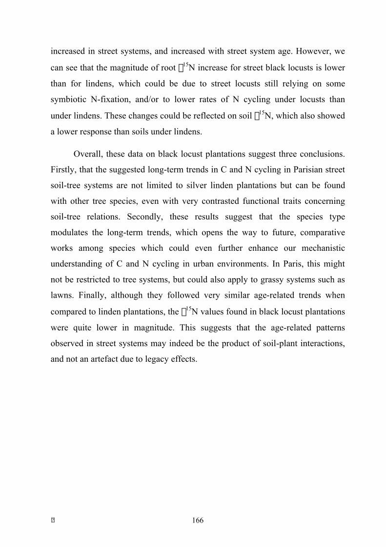
! 166
increased in street systems, and increased with street system age. However, we
can see that the magnitude of root δ15N increase for street black locusts is lower
than for lindens, which could be due to street locusts still relying on some
symbiotic N-fixation, and/or to lower rates of N cycling under locusts than
under lindens. These changes could be reflected on soil δ15N, which also showed
a lower response than soils under lindens.
Overall, these data on black locust plantations suggest three conclusions.
Firstly, that the suggested long-term trends in C and N cycling in Parisian street
soil-tree systems are not limited to silver linden plantations but can be found
with other tree species, even with very contrasted functional traits concerning
soil-tree relations. Secondly, these results suggest that the species type
modulates the long-term trends, which opens the way to future, comparative
works among species which could even further enhance our mechanistic
understanding of C and N cycling in urban environments. In Paris, this might
not be restricted to tree systems, but could also apply to grassy systems such as
lawns. Finally, although they followed very similar age-related trends when
compared to linden plantations, the δ15N values found in black locust plantations
were quite lower in magnitude. This suggests that the age-related patterns
observed in street systems may indeed be the product of soil-plant interactions,
and not an artefact due to legacy effects.
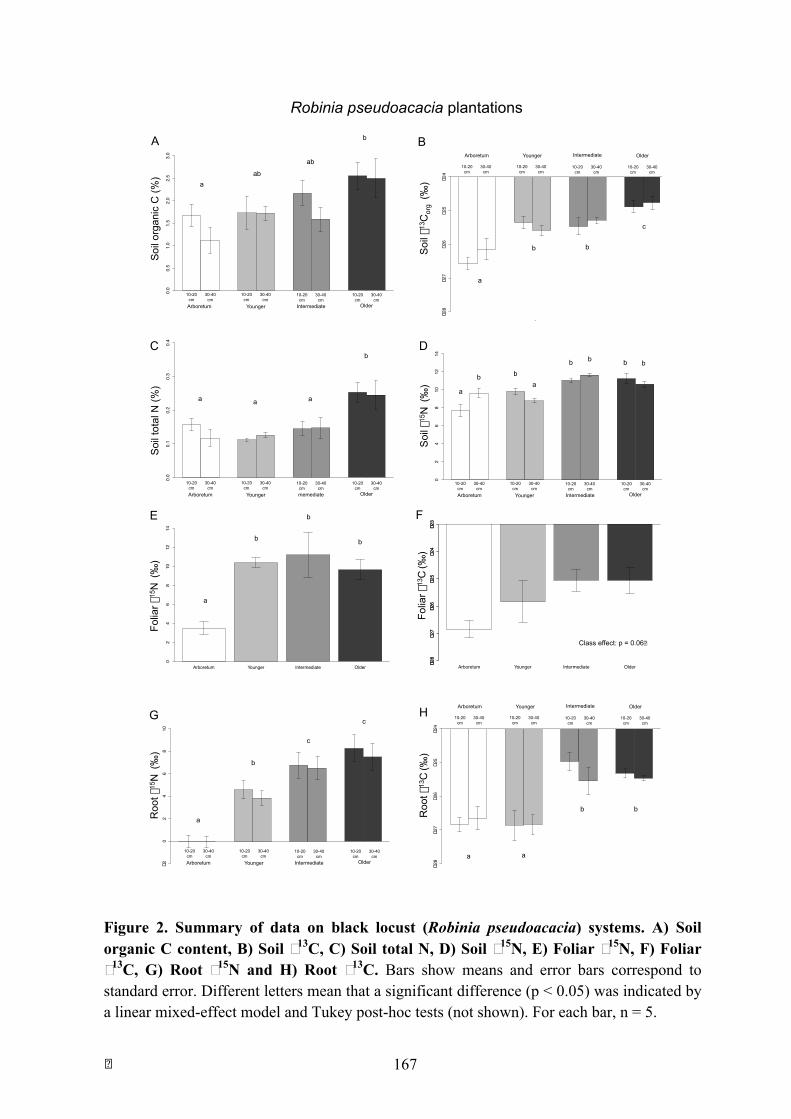
! 167
Arboretum Younger Intermediate Older
02
46
810
1214
Arboretum Younger Intermediate Older
0.0
0.1
0.2
0.3
0.4
Arboretum Younger Intermediate Older
0.0
0.5
1.0
1.5
2.0
2.5
3.0
10-20 cm Arboretum Younger memediate Older
30-40 cm
10-20 cm
30-40 cm
10-20 cm
30-40 cm
10-20 cm
30-40 cm
Soi
l tot
al N
(%)
10-20 cm Arboretum Younger Intermediate Older
30-40 cm
10-20 cm
30-40 cm
10-20 cm
30-40 cm
10-20 cm
30-40 cm
Soi
l δ13
Cor
g (‰
)
Soi
l org
anic
C (%
)
Soi
l δ15
N (
‰)
A
C
B
D
10-20 cm Arboretum Younger Intermediate Older
30-40 cm
10-20 cm
30-40 cm
10-20 cm
30-40 cm
10-20 cm
30-40 cm
Arboretum Younger Intermediate Older
−28
−27
−26
−25
−24
Arboretum Younger Intermediate Older
10-20 cm
30-40 cm
10-20 cm
30-40 cm
10-20 cm
30-40 cm
10-20 cm
30-40 cm
a ab
ab
b
a a a
b
a
b b
c
a
b b a
b b b b
Robinia pseudoacacia plantations
Arboretum Younger Intermediate Older
−28
−27
−26
−25
−24
−23
−28
−27
−26
−25
−24
−23
Arboretum Younger Intermediate Older
02
46
810
1214
Arboretum Younger Intermediate Older
−20
24
68
10
10-20 cm Arboretum Younger Intermediate Older
30-40 cm
10-20 cm
30-40 cm
10-20 cm
30-40 cm
10-20 cm
30-40 cm
a
b
c
c
a
b
b
b
E
G
F
Folia
r δ13
C (‰
)
Folia
r δ15
N (
‰)
Arboretum Younger Intermediate Older
−28
−27
−26
−25
−24
Arboretum Younger Intermediate Older
10-20 cm
30-40 cm
10-20 cm
30-40 cm
10-20 cm
30-40 cm
10-20 cm
30-40 cm
a a
b b Roo
t δ13
C (‰
)
H
Roo
t δ15
N (
‰)
Class effect: p = 0.06!
Figure 2. Summary of data on black locust (Robinia pseudoacacia) systems. A) Soil organic C content, B) Soil δ13C, C) Soil total N, D) Soil δ15N, E) Foliar δ15N, F) Foliar δ13C, G) Root δ15N and H) Root δ13C. Bars show means and error bars correspond to standard error. Different letters mean that a significant difference (p < 0.05) was indicated by a linear mixed-effect model and Tukey post-hoc tests (not shown). For each bar, n = 5.
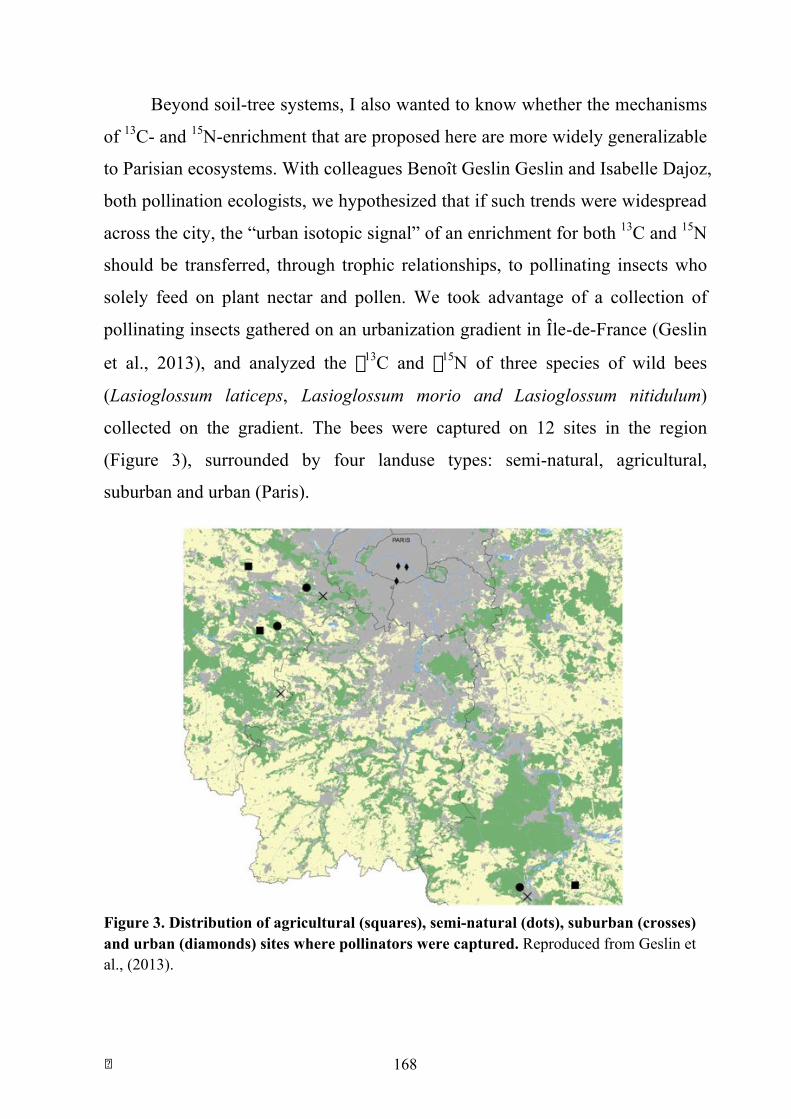
! 168
Beyond soil-tree systems, I also wanted to know whether the mechanisms
of 13C- and 15N-enrichment that are proposed here are more widely generalizable
to Parisian ecosystems. With colleagues Benoît Geslin Geslin and Isabelle Dajoz,
both pollination ecologists, we hypothesized that if such trends were widespread
across the city, the “urban isotopic signal” of an enrichment for both 13C and 15N
should be transferred, through trophic relationships, to pollinating insects who
solely feed on plant nectar and pollen. We took advantage of a collection of
pollinating insects gathered on an urbanization gradient in Île-de-France (Geslin
et al., 2013), and analyzed the δ13C and δ15N of three species of wild bees
(Lasioglossum laticeps, Lasioglossum morio and Lasioglossum nitidulum)
collected on the gradient. The bees were captured on 12 sites in the region
(Figure 3), surrounded by four landuse types: semi-natural, agricultural,
suburban and urban (Paris).
Figure 3. Distribution of agricultural (squares), semi-natural (dots), suburban (crosses) and urban (diamonds) sites where pollinators were captured. Reproduced from Geslin et al., (2013).
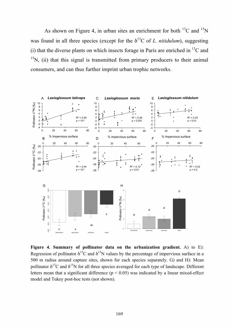
169
As shown on Figure 4, in urban sites an enrichment for both 13C and 15N
was found in all three species (except for the �13C of L. nitidulum), suggesting
(i) that the diverse plants on which insects forage in Paris are enriched in 13C and 15N, (ii) that this signal is transmitted from primary producers to their animal
consumers, and can thus further imprint urban trophic networks.
Figure 4. Summary of pollinator data on the urbanization gradient. A) to E): Regression of pollinator �13C and �15N values by the percentage of impervious surface in a 500 m radius around capture sites, shown for each species separately. G) and H): Mean pollinator �13C and �15N for all three species averaged for each type of landscape. Different letters mean that a significant difference (p < 0.05) was indicated by a linear mixed-effect model and Tukey post-hoc tests (not shown).
-28
-26
-24
-22
-20 0 20 40 60 80
-4 -2 0 2 4 6 8
10
0 20 40 60 80
-28
-26
-24
-22
-20 0 20 40 60
-4 -2 0 2 4 6 8
10
0 20 40 60 80
-28
-26
-24
-22
-20 0 20 40 60 80
-4 -2 0 2 4 6 8
10
0 20 40 60 80
% Impervious surface % Impervious surface % Impervious surface
Pol
linat
or �
13C
(‰)
Pol
linat
or �
15N
(‰)
Lasioglossum laticeps Lasioglossum morio Lasioglossum nitidulum
R2 = 0.55 p < 10-5
R2 = 0.26 p < 0.001
R2 = 0.22 p < 0.01
R2 = 0.44 p < 10-4
R2 = 0.12 p = 0.01
R2 = 0.02 p = 0.2
A
B
C
D
E
F
Seminatural Agricultural Suburban Urban�26.0
�25.5
�25.0
�24.5
�24.0
�23.5
�23.0
Pol
linat
or �
13C
(‰)
G
a a ab
b
Seminatural Agricultural Suburban Urban
02
46
8
Pol
linat
or �
15N
(‰)
H
a
a a
b
! 170
Taken together, the results on silver linden systems, black locust systems
and pollinators suggest that the 13C- and 15N-enrichment of plants might be a
widespread phenomenon in the Parisian context, found in several types of
systems. These results also highlight the fact that isotopic effects stemming from
rather localized biological strategies and processes (13C enrichment for water use
efficiency, 15N enrichment because of deposited N assimilation and microbial
cycling) can feed back to, and imprint, biogeochemical cycles in whole
ecosystems, from soils to animals.
2. Perspectives for future works and street plantation management These results contribute to urban ecological research in several ways.
(i) This study, to my knowledge, is the first to try and describe C and N
cycling in street soil-tree systems, an ubiquitous type of ecosystem that
can be found in most cities worldwide.
(ii) It contributes to research on urban C and N cycling by showing strong
age-related patterns and suggesting a long-term C and N accumulation
in street soils, and proposes mechanisms that could potentially explain
these patterns and that could occur in many other urban areas.
(iii) It contributes to the rather small corpus of urban stable isotope studies,
and reports the first values ever measured of urban root δ13C and δ15N.
It is also the first urban study to report such record-breaking soil and
plant δ15N values and to propose a long-term “loop” that could lead to
the observed δ15N values.
(iv) The study provides the first molecular evidence that in urban soils of
circumneutral pH, AOB might be a key group of organisms
responsible for triggering an increase in the rates of N-loss pathways in
urban ecosystems.
! 171
(v) The results on silver linden and black locust plantations, as well as on
wild pollinators, suggest a widespread enrichment of soil-pant systems
in 13C and 15N in Paris. These resutlts are the first, to my knowledge, to
show such isotopic transfers in the urban soil-plant-animal continuum,
and this suggests that urban environmental features (e.g., urban heat
islands, depositions of reactive N) can influence all compartment of
ecosystems at the elemental level and leave an “urban isotopic imprit.”
Future works on these systems will help enhance our mechanistic
understanding of C and N cycling. Concerning C dynamics, more work is
needed to elucidate the underlyning mechanisms of C accumulation, and we can
identify some avenues for future resarch. Firtsly, 14C measurements could
provide definitive evidence of accumulation and estimates of the proportion of
inherited C from accumulated C. Chemical analyses of SOM (on the different
soil fractions for instance) could also shed light on the form of accumulated C,
and whether it is stored as non-degraded plant (root) material or in microbially
processed forms. Opening the microbial ecology black-box of SOM degradation
in street soils could also help better understand the potential long-term microbial
dynamics that lead to C accumulation. On this last point, more data have been
acquired on soil microbial communities on the chronosequence: total bacterial,
fungal and archaeal populations have been quantified by quantitative PCR, their
respective structure has been assessed through molecular fingerprinting (T-
RFLP), and a community-level physiological profiling technique
(MicroRespTM)9 has been applied to seek for differences in their potential
catabolic activities. This dataset, when analyzed, will help investigate for long-
term changes in microbial communities and further infer potential microbial
mechanisms involved in the accumulation of C in street systems.
!!!!!!!!!!!!!!!!!!!!!!!!!!!!!!!!!!!!!!!!!!!!!!!!!!!!!!!!9 For T-RFLP and MicroRespTM, in particular, I am very much indebted to Thomas "Z" Lerch for his friendly guidance and close collaboration.

! 172
Concerning N dynamics, we have mentionned that quantitative
assessments of N stocks and fluxes would be needed. A clearer understanding of
how much N is available in tree pits, how much N is lost (leaf litter export, N-
loss pathways), how much N is needed by trees, will help better understand the
street N cycle and whether trees are N limited or not. The reality and magnitude
of foliar N uptake in Parisian streets should be assessed, as well as the fate of
this assimilated N and where it is allocated. Other tree physiological processes
pertianing to N (e.g., translocation) could be studied, too. In soils, we have only
analyzed parts of the N cycle, and the other steps (e.g., nitritation) could be
further analyzed. Data on N mineralization rates, in particular, would be
important here, and help better link C and N cycling in street systems.
On this point, a study of mycorrhization in street systems may also
provide important insights. Mycorrhizal symbiosis has been proposed as key
mediator explaining soil-plant responses to increased N depositions (e.g., Aber
et al., 1998) and a key component of soil C accumulation. As mycorrhizal fungi
rely on root carbohydrates, and are highly competitive for mineral N uptake in
soils, an increase in fine root density and N availability could lead to an increase
in the biomass of mycorrhizal fungi, leading to less mineralization of SOM and
retention of N in soils. A collaboration was established with the University of
Padova (Italy) to asses the mycorrhizal status of the studied silver lindens, and
its preliminary results showed a strong age-related increase in the number of
mycorrhized root apices in street soils (Figure 5)10. Further work on street
mycorrhization in Paris is undergoing in the MycoPolis (funded by Paris 2030
Programme) project led by Patricia Genet and its results could provide important
insights to better interpret the long-term trends in C and N cycling in street
systems, and better link them to tree N-foraging strategies. Finally, we solely !!!!!!!!!!!!!!!!!!!!!!!!!!!!!!!!!!!!!!!!!!!!!!!!!!!!!!!!10 The study on mycorrhizal symbiosis was principally conducted by Linda Scattolin, Assistant Professor at the University of Padova. An accomplished triathlete, Linda deceased in a tragic accident while training in South Africa. We honour her memory.

! 173
focused on N in this, but other nutrients should be studied in the future, as
carbon-nutrient and nutrient-nutrient interactions are key aspects of the coupling
among biogeochemical cycles11.
Concerning the management of street plantations, we propose several
perpectives based on this manuscript. At the moment, these are more speculative
reflections than precise recommendations, and they require further discussion
with city managers, and possibly experimentation.
(i) Questioning the hypothesis of soil exhaustion. From the age-related
trends in C and N content and microbial activity, we suggest that the
current hypothesis of a temporal decrease of soil fertility is not
verified. On this basis, the current practices of soil replacement and
disposal could be questioned. On this point, it is important to note,
however, that soil fertility is not only concern for city managers. With !!!!!!!!!!!!!!!!!!!!!!!!!!!!!!!!!!!!!!!!!!!!!!!!!!!!!!!!11 With the kind guidance and collaboration of Florence Maunoury-Danger and Michael Danger from the Université de Lorraine, silver linden foliar P concentrations were analyzed and will be put in regard of soil P concentrations in future works.
Arboretum Younger Intermediate Older
050
010
0015
0020
00
Num
ber o
f obs
erve
d
ecto
myc
orrh
ized
api
ces
(kg-
1 so
il)
0-10 cm
10-20 cm
20-30 cm
30-40 cm
Figure 5. Estimated means of ectomycorrhized apices per kg of soil at four depths in silver linden systems. Data acquired by L. Scattolin and collaboarators.
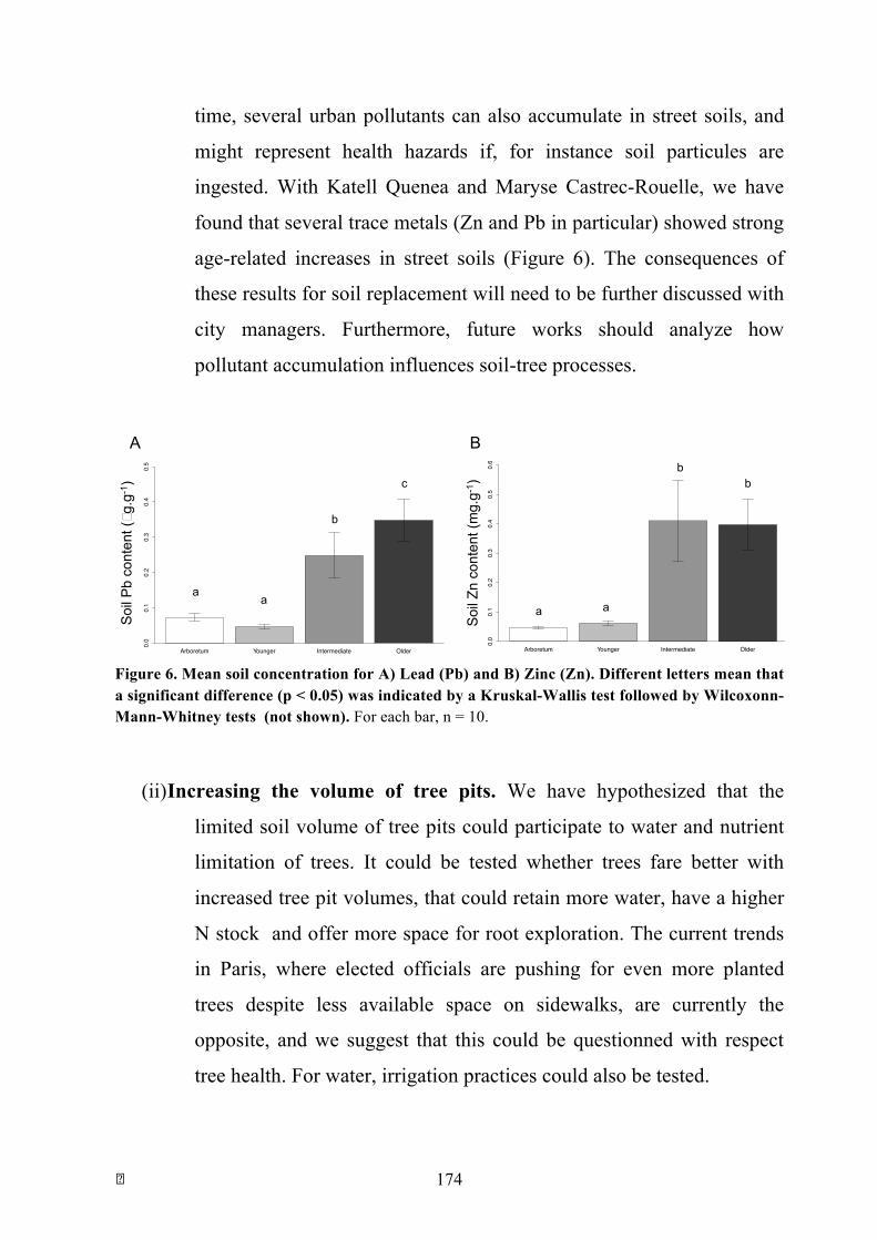
! 174
time, several urban pollutants can also accumulate in street soils, and
might represent health hazards if, for instance soil particules are
ingested. With Katell Quenea and Maryse Castrec-Rouelle, we have
found that several trace metals (Zn and Pb in particular) showed strong
age-related increases in street soils (Figure 6). The consequences of
these results for soil replacement will need to be further discussed with
city managers. Furthermore, future works should analyze how
pollutant accumulation influences soil-tree processes.
Figure 6. Mean soil concentration for A) Lead (Pb) and B) Zinc (Zn). Different letters mean that a significant difference (p < 0.05) was indicated by a Kruskal-Wallis test followed by Wilcoxonn-Mann-Whitney tests (not shown). For each bar, n = 10.
(ii) Increasing the volume of tree pits. We have hypothesized that the
limited soil volume of tree pits could participate to water and nutrient
limitation of trees. It could be tested whether trees fare better with
increased tree pit volumes, that could retain more water, have a higher
N stock and offer more space for root exploration. The current trends
in Paris, where elected officials are pushing for even more planted
trees despite less available space on sidewalks, are currently the
opposite, and we suggest that this could be questionned with respect
tree health. For water, irrigation practices could also be tested.
Arboretum Younger Intermediate Older
0.0
0.1
0.2
0.3
0.4
0.5
Arboretum Younger Intermediate Older
0.0
0.1
0.2
0.3
0.4
0.5
0.6
Soi
l Pb
cont
ent (µg
.g-1
)
Soi
l Zn
cont
ent (
mg.
g-1)
a
b
c
a a a
b b
A B
! 175
(iii) Increasing N retention by planting understory plants. In several
cities worldwide, there is a trend of “greening” the soil surface
surrounding tree trunks by planting ornamental plant species. We
suggest that this practice might not only have aesthetic benefits, but
could provide soil-tree systems with understory species that could
uptake the “excess” N and increase its retention in plant biomass, thus
potentially decreasing the rates of nitrification and denitrification.
Species that could slightly acidify soil pH might also make soils less
favorable to AOB.
3. “Global change in your street!”: Ecology in the first urban century
Despite lots of accumulated knowledge on the causes and consequences
of environmental degradation worldwide, the environmental crisis is enduring
and deepening on many levels. There is a tendancy, especially in scientific
audiences, to believe (or hope?) that the environment keeps degrading because
evidence is lacking, or is not understood enough, or is not well communicated
enough, or that we have yet to find the technical fix that would enable to solve
the issue. The reality is probably much more complex, and there is a myriad of
factors, rooted in human collective action, that can make a given environmental
issue persist despite vast amounts of available knowledge on it (see for instance:
Laurans et al., 2013; Rankovic & Billé, 2013 – Appendices 3 and 4).
Fundamental inconsistencies in sectoral public policies, how international trade
is organized and governed, or good old power asymmetries among actors are all
components of what, in the biodiversity arena for instance, the international
jargon calls “underlying causes” (Convention on Biological Diversity) or
“indirect drivers” (IPBES) of biodiversity loss. These factors should receive
acute attention if we wish to solve environmental issues (for more
argumentation on this point, with the example of IPBES works, see Rankovic et
! 176
al., 2016 – Appendix 5).
However, I think that the importance of worldviews and imaginaries
(Jasanoff, 2015) in shaping human collective action should not be
underestimated. If the exclusion of non-human entities from human politics is
indeed one of the anthropological roots of the environmental crisis (e.g., Latour,
1999), then spreading the worldview of ecology might be a non-trivial
contribution to environmental conservation (Descola, 2014). Here, I think that
beyond the engineering aspects mentioned above, urban ecological research can
be important precisely for this objective. As recently put by Janzen (2015),
“[o]ur legacy as carbon scientists may be measured not only in tonnes of carbon
stashed away, but in the restorative, hopeful images planted in human minds.”
Cities constitute the local environment of an increasing share of the world
population, and urban ecosystems may be the most familiar ecosystems for a
majority of people (Pickett, 2003). As Miller and Hobbs (2002) put it, many of
the ecological processes seen in popular documentaries on television also occur
in one’s own backyard, and this also applies to streets or urban parks. Quoting
Aldo Leopold, they remind us that “the weeds in a city lot convey the same
lessons as the redwoods”, and that an increased perception of ecological
processes in urban areas could lead to a broader perception of ecological
processes that occur in the rest of the planet (see also McKinney, 2002; Miller,
2005). Telling ecological stories about the environment where people “live and
work” (Miller & Hobbs, 2002), and calling attention to entites with which
people interact on a day-to-day basis thus appears to be of strategic importance.
This has important consequences for the engagement of the urban
ecologist as a researcher and a teacher. As Pickett (2003) notes, conducting
urban ecological research first requires to gain access to the sites to be studied,
and this constitutes a first opportunity to exchange with other stakeholders, share
the perspectives of ecologists and learn from other actors. Urban ecological
! 177
research is also “visible” to people, and discussions with curious pedestrians are
priviledged, serendipitous moments of sharing ecological research with people
(Pickett, 2003). Moreover, an important part of city dwellers are children, and
using urban ecosystems as learning tools can develop an early sensitivity to the
subtle processes at play in the biosphere and an early sense of care (Chawla &
Salvadori, 2003). This very much applies to biogeochemical cycles, probably
amongst the least known features of the biosphere by the “general public,” but at
the heart of some of the most important challenges of our time such as climate
change, biodiversity loss, and food production – to name just a few...
Taken together, these considerations give urban ecology an important
potential to contribute to the contemporary challenge of paying a greater
attention to non-humans’ own agency and how it is meshed with human actions
(Latour, 2014). Case-studies in urban ecology can constitute powerful
illustrations of complex ecological dynamics by showing that even the most
“man-made” entities, those whose essence is the most taken for granted, actually
have their own dynamics and are full of surprises, and that there is a lot to be
told on their history and its links with our own (Cronon, 1993). Here, even
though more work is needed to obtain a clearer understanding of the processes
occuring in street systems, I hope that I was able to show that even such
apparently mundane systems like street soils and trees can illustrate some of the
questions that haunt the ecologists trying to understand the biosphere and its
future.

! 178

! 179

! 180
! 181
References
Abbadie, L. & Lensi, R. (1990) Carbon and nitrogen mineralization and denitrification in a humid savanna of West Africa (Lamto, Côte d’Ivoire). Acta Œcologica, 11, 717–728.
Abbadie, L., Mariotti, A., & Menaut, J. (1992). Independence of Savanna Grasses from Soil Organic Matter for Their Nitrogen Supply. Ecology, 73(2), 608-613.
Aber, J. D., Nadelhoffer, K. J., Steudler, P., & Melillo, J. M. (1989). Nitrogen Saturation in Northern Forest Ecosystems. BioScience, 39(6), 378–386.
Aber, J., McDowell, W., & Nadelhoffer, K. (1998). Nitrogen saturation in temperate forest ecosystems. BioScience, 48(11), 921–934.
AFNOR (2003). Norme NF X 31-107. Qualité du sol - Détermination de la distribution granulométrique des particules du sol - Méthode à la pipette. AFNOR, Paris.
AFNOR (2005). Qualité du sol - Détermination du pH. AFNOR, Paris.
AFNOR (2011). Norme NF ISO 23470. Qualité du sol - Détermination de la capacité d'échange cationique (CEC) effective et des cations échangeables à l'aide d'une solution de trichlorure de cobaltihexammine. AFNOR, Paris.
AFNOR (2014). Norme NF ISO 10693. Qualité du sol - Détermination de la teneur en carbonate - Méthode volumétrique. AFNOR, Paris.
Ågren, G., Bosatta, E., & Magill, A. (2001). Combining theory and experiment to understand effects of inorganic nitrogen on litter decomposition. Oecologia, 128(1), 94–98.
Alberti, M. (2015). Eco-evolutionary dynamics in an urbanizing planet. Trends in Ecology & Evolution, 30(2), 114–26.
Ammann, M., Siegwolf, R., & Pichlmayer, F. (1999). Estimating the uptake of traffic-derived NO2 from 15N abundance in Norway spruce needles. Oecologia, (1999), 124–131.
Amundson, R., Austin, a. T., Schuur, E. A. G., Yoo, K., Matzek, V., Kendall, C., Uebersax, A., Brenner, D., & Baisden, W. T. (2003). Global patterns of the isotopic composition of soil and plant nitrogen. Global Biogeochemical Cycles, 17(1), 1031.
Aronson, J., Floret, C., Floc’h, E., Ovalle, C., & Pontanier, R. (1993). Restoration and Rehabilitation of Degraded Ecosystems in Arid and Semi-Arid Lands. I. A View from the South. Restoration Ecology, 1(1), 8–17.
Bai, S. H., Xu, Z., Blumfield, T. J., & Reverchon, F. (2015). Human footprints in urban forests: implication of nitrogen deposition for nitrogen and carbon storage. Journal of Soils and Sediments, 15(9), 1927–1936.
! 182
Balesdent, J., Besnard, E., Arrouays, D., & Chenu, C. (1998). The dynamics of carbon in particle-size fractions of soil in a forest-cultivation sequence. Plant and Soil, 201, 49–57.
Balesdent, J., Pétraud, J., & Feller, C. (1991). Effets des ultrasons sur la distribution granulométrique des matières organiques des sols. Science Du Sol, (1), 95–106.
Bardgett, R. D., Mommer, L., & De Vries, F. T. (2014). Going underground: root traits as drivers of ecosystem processes. Trends in Ecology & Evolution, 29(12), 692–699.
Bateman, A., & Kelly, S. (2007). Fertilizer nitrogen isotope signatures. Isotopes in Environmental and Health Studies, 43(3), 237–247.
Baxter, J. W., Pickett, S. T., Carreiro, M. M., & Dighton, J. (1999). Ectomycorrhizal diversity and community structure in oak forest stands exposed to contrasting anthropogenic impacts. Canadian Journal of Botany, 77(6), 771–782.
Bazzaz, F. A. (1990). The Response of Natural Ecosystems to the Rising Global CO2 Levels. Annual Review of Ecology and Systematics, 21(1), 167–196.
Bettez, N. D., Marino, R., Howarth, R. W., & Davidson, E. a. (2013). Roads as nitrogen deposition hot spots. Biogeochemistry, 114(1-3), 149–163.
Billy, C., Billen, G., Sebilo, M., Birgand, F., & Tournebize, J. (2010). Nitrogen isotopic composition of leached nitrate and soil organic matter as an indicator of denitrification in a sloping drained agricultural plot and adjacent uncultivated riparian buffer strips. Soil Biology and Biochemistry, 42(1), 108–117.
Bol, R., & Pflieger, C. (2002). Stable isotope (13C, 15N and 34S) analysis of the hair of modern humans and their domestic animals. Rapid Communications in Mass Spectrometry, 16(23), 2195–200.
Bolund, P., & Hunhammar, S. (1999). Ecosystem services in urban areas. Ecological Economics, 29(2), 293–301.
Bormann, F. H., & Likens, G. E. (1979). Pattern and process in a forested ecosystem. Springer-Verlag, New York, USA, 262 p.
Bowden, R. D., Davidson, E., Savage, K., Arabia, C., & Steudler, P. (2004). Chronic nitrogen additions reduce total soil respiration and microbial respiration in temperate forest soils at the Harvard Forest. Forest Ecology and Management, 196(1), 43–56.
Brodie, C., Heaton, T., Leng, M., Kendrick, C., Casford, J., & Lloyd, J. (2011). Evidence for bias in measured δ15N values of terrestrial and aquatic organic materials due to pre-analysis acid treatment methods. Rapid Communications in Mass Spectrometry, (January), 1089–1099.
Burns, L., Stevens, R., & Laughlin, R. (1996). Production of nitrite in soil by simultaneous nitrification and denitrification. Soil Biology and Biochemistry, 28(4/5), 609-616.
! 183
Cadenasso, M.L., Pickett, S. T. A., McDonnell, M. J., & Pouyat, P. V. (2007). Forest vegetation along an urban-rural gradient in the New York City metropolitan area: patterns and relationships to ecosystem processes. Transactions of the Linnean Society of New York, 10, 79-99.
Calfapietra, C., Peñuelas, J., & Niinemets, Ü. (2015). Urban plant physiology: adaptation-mitigation strategies under permanent stress. Trends in Plant Science, 20(2), 72–75.
Cantat, O. (2004). L’îlot de chaleur urbain parisien selon les types de temps. Norois. Environnement, Aménagement, Société. https://norois.revues.org/1373
Carey, C. J., Dove, N. C., Beman, J. M., Hart, S. C., & Aronson, E. L. (2016). Meta-analysis reveals ammonia-oxidizing bacteria respond more strongly to nitrogen addition than ammonia-oxidizing archaea. Soil Biology and Biochemistry, 99(2016), 158–166.
Carreiro, M. M., Howe, K., Parkhurst, D. F., & Pouyat, R. V. (1999). Variation in quality and decomposability of red oak leaf litter along an urban-rural gradient. Biology and Fertility of Soils, 30(3), 258–268.
Carreiro, M. M., Sinsabaugh, R. L., Repert, D. A., & Parkhurst, D. F. (2000). Microbial enzyme shifts explain litter decay responses to simulated nitrogen deposition. Ecology, 81(9), 2359–2365.
Carreiro, M. M., & Tripler, C. E. (2005). Forest Remnants Along Urban-Rural Gradients: Examining Their Potential for Global Change Research. Ecosystems, 8(5), 568–582.
Carreiro, M. M., Song, Y.-C., Wu, J. (2008). Ecology, Planning, and Management of Urban Forests: International Perspective. Springer, New York, USA, 468 p.
Carreiro, M. M., Pouyat, R. V., Tripler, C. E., Zhu, W.-X. (2009). Carbon and nitrogen cycling in soils of remnant forests along urban–rural gradients: case studies in the New York metropolitan area and Louisville, Kentucky. In McDonnell, M. J., Hahs, A. K., & Breuste, J. H. (2009). Ecology of Cities and Towns. A Comparative Approach. Cambridge University Press, New York, USA, 746 p.
Chalwa, L., & Salvadori, I. (2003). Children for Cities and Cities for Children: Learning to Know and Care About Urban Ecosystems. In Berkowitz, A. R., Nilon, C. H., & Hollweg, K. S. (Eds). Understanding Urban Ecosystems: A New Frontier for Science and Education. Springer, New York, USA, 526 p.
Chambers, L. G., Chin, Y.-P., Filippelli, G. M., Gardner, C. B., Herndon, E. M., Long, D. T., Lyons, W. B., Macpherson, G. L., McElmurry, S. P., McLean, C. E., Moore, J., Moyer, R. P., Neumann, K., Nezat, C. A., Soderberg, K., Teutsch, N., Widom, E. (2016). Developing the scientific framework for urban geochemistry. Applied Geochemistry, 67, 1–20.
Chen, F., Fahey, T. J., Yu, M., & Gan, L. (2010). Key nitrogen cycling processes in pine plantations along a short urban–rural gradient in Nanchang, China. Forest Ecology and Management, 259(3), 477–486.
! 184
Cheng, W., Parton, W. J., Gonzalez-Meler, M. A., Phillips, R., Asao, S., McNickle, G. G., Brzostek, E., & Jastrow, J. D. (2014). Synthesis and modeling perspectives of rhizosphere priming. The New Phytologist, 201(1), 31–44.
Cheptou, P., Carrue, O., Rouifed, S., & Cantarel, A. (2008). Rapid evolution of seed dispersal in an urban environment in the weed Crepis sancta. Proceedings of the National Academy of Sciences of the United States of America, 105(10), 3796–9.
Christensen, B. (2001). Physical fractionation of soil and structural and functional complexity in organic matter turnover. European Journal of Soil Science, 53, 345-353
Christensen, B. T. (1987). Decomposability of organic matter in particle size fractions from field soils with straw incorporation. Soil Biology and Biochemistry, 19(4), 429–435.
Churkina, G., Grote, R., Butler, T. M., & Lawrence, M. (2015). Natural selection? Picking the right trees for urban greening. Environmental Science & Policy, 47, 12–17.
Ciais, P., Sabine, C., Bala, G., Bopp, L., Brovkin, V., Canadell, J., Chhabra, A., DeFries, R., Galloway, J., Heimann, M., Jones, C., Le Quéré, C., Myneni, R.B., Piao, S., & Thornton, P. (2013). Carbon and Other Biogeochemical Cycles. In: Climate Change 2013: The Physical Science Basis. Contribution of Working Group I to the Fifth Assessment Report of the Intergovernmental Panel on Climate Change [Stocker, T.F., D. Qin, G.-K. Plattner, M. Tignor, S.K. Allen, J. Boschung, A. Nauels, Y. Xia, V. Bex and P.M. Midgley (eds.)]. Cambridge University Press, Cambridge, United Kingdom and New York, NY, USA.
Clergeau, P. (2007). Une écologie du paysage urbain, Éditions Apogée, 136 p.
Craig, H. (1957). Isotopic standards for carbon and oxygen and correction factors for mass-spectrometric analysis of carbon dioxide. Geochimica et Cosmochimica Acta, 12(1-2), 133–149.
Craine, J.M. (2009). Resource strategies of wild plants. Princeton University Press, USA, 344 p.
Craine, J. M., Brookshire, E. N. J., Cramer, M. D., Hasselquist, N. J., Koba, K., Marin-Spiotta, E., & Wang, L. (2015). Ecological interpretations of nitrogen isotope ratios of terrestrial plants and soils. Plant and Soil, 396(1-2), 1–26.
Craine, J. M., Morrow, C., & Fierer, N. (2007). Microbial nitrogen limitation increases decomposition. Ecology, 88(8), 2105–2113.
Craul, P.J. (1993). Urban soils: an overview and their future. In Watson, G.W., Neely, D. (Eds.), The Landscape Below Ground. Proceedings of an International Workshop on Tree Root Development in Urban Soils. International Society of Arboriculture, Savoy, IL.
Craul, P.J. (1999). Urban Soils: Applications and Practices. Wiley, New York.
! 185
Crippa, M., El Haddad, I., Slowik, J. G., DeCarlo, P. F., Mohr, C., Heringa, M. F., … Prévôt, A. S. H. (2013). Identification of marine and continental aerosol sources in Paris using high resolution aerosol mass spectrometry. Journal of Geophysical Research: Atmospheres, 118(4), 1950–1963.
Cronon, W. J. (1993). Foreword: The Turn Toward History. In McDonnell, M., & Pickett, S. (1993) (Eds). Humans as Components of Ecosystems. The Ecology of Subtle Human Effects and Populated Areas. Springer, USA, 364 p.
Crutzen, P. J. (2002). Geology of mankind. Nature, 415(6867), 23.
David, A. A. J., Boura, A., Lata, J.-C., Rankovic, A., Kraepiel, Y., Charlot, C., Barot, S., Abbadie, L., Ngao, J. (submitted). Street trees in Paris are sensitive to spring and autumn precipitation and recent climate changes.
Dawson, T. E., Mambelli, S., Plamboeck, A. H., Templer, P. H., & Tu, K. P. (2002). Stable Isotopes in Plant Ecology. Annual Review of Ecology and Systematics, 33(1), 507–559.
Day, S. D., & Amateis, R. L. (2011). Predicting canopy and trunk cross-sectional area of silver linden (Tilia tomentosa) in confined planting cutouts. Urban Forestry & Urban Greening, 10(4), 317–322.
De Kimpe, C. R., & Morel, J.-L. (2000). Urban Soil Management: a Growing Concern. Soil Science, 165(1), 31–40.
De Parseval, H., Abbadie, L., Barot, S., Gignoux, J., Lata, J.-C., & Raynaud, X. (2016). Explore less to control more: why and when should plants limit the horizontal exploration of soil by their roots? Oikos, 125(8), 1110–1120.
DeForest, J. L., Zak, D. R., Pregitzer, K. S., & Burton, A. J. (2004). Atmospheric nitrate deposition and the microbial degradation of cellobiose and vanillin in a northern hardwood forest. Soil Biology and Biochemistry, 36(6), 965–971.
Descola, P. (2014). La composition des mondes. Entretiens avec Pierre Charbonnier. Flammarion, Paris, 288 p.
Di, H. J., Cameron, K. C., Shen, J. P., Winefield, C. S., O’Callaghan, M., Bowatte, S., & He, J. Z. (2009). Nitrification driven by bacteria and not archaea in nitrogen-rich grassland soils. Nature Geoscience, 2(9), 621–624.
Dommergues, Y. (1960). La notion de coefficient de minéralisation du carbone dans les sols. Agronomie Tropicale, 15(1), 54–60.
Edmondson, J. L., Stott, I., Potter, J., Lopez-Capel, E., Manning, D. a C., Gaston, K. J., & Leake, J. R. (2015). Black Carbon Contribution to Organic Carbon Stocks in Urban Soil. Environmental Science & Technology, 49(14), 8339–46.
Edwards, I. P., Zak, D. R., Kellner, H., Eisenlord, S. D., & Pregitzer, K. S. (2011). Simulated atmospheric N deposition alters fungal community composition and suppresses ligninolytic gene expression in a northern hardwood forest. PloS One, 6(6), e20421.
! 186
Ekblad, a., & Högberg, P. (2001). Natural abundance of 13 C in CO 2 respired from forest soils reveals speed of link between tree photosynthesis and root respiration. Oecologia, 127(3), 305–308.
Ekblad, A., Boström, B., Holm, A., & Comstedt, D. (2005). Forest soil respiration rate and delta13C is regulated by recent above ground weather conditions. Oecologia, 143(1), 136–42.
Ellis, E. C., Klein Goldewijk, K., Siebert, S., Lightman, D., & Ramankutty, N. (2010). Anthropogenic transformation of the biomes, 1700 to 2000. Global Ecology and Biogeography, 19, 589–606.
European Commission (2013). Building a green infrastructure for Europe. Publications Office of the European Union, Luxembourg, 24 p.
Falxa-Raymond, N., Palmer, M. I., McPhearson, T., & Griffin, K. L. (2014). Foliar nitrogen characteristics of four tree species planted in New York City forest restoration sites. Urban Ecosystems, 17(3), 807–824.
Fang, Y., Yoh, M., Koba, K., Zhu, W., Takebayashi, Y., Xiao, Y., Lei, C., Mo, J., Zhang, W., & Lu, X. (2011). Nitrogen deposition and forest nitrogen cycling along an urban-rural transect in southern China. Global Change Biology, 17(2), 872–885.
FAO (2016). Benefits of urban trees. Forest Assessment, Management and Conservation Division, FAO, 1 p.
Farquhar, G. D., Ehleringer, J. R., & Hubick, K. T. (1989). Carbon Isotope Discrimination and Photosynthesis. Annual Review of Plant Physiology and Plant Molecular Biology, 40(1), 503–537.
Feller, C., & Chenu, C. (2012). Les inter-actions bio-organo-argileuses et la stabilisation du carbone dans les sols Aperçu historique. Etude et Gestion Des Sols, 19(3-4), 235–248.
Feng, W., Shi, Z., Jiang, J., Xia, J., Liang, J., Zhou, J., & Luo, Y. (2016). Methodological uncertainty in estimating carbon turnover times of soil fractions. Soil Biology and Biochemistry, 100, 118–124.
Fierer, N., Lauber, C. L., Ramirez, K. S., Zaneveld, J., Bradford, M. a, & Knight, R. (2012). Comparative metagenomic, phylogenetic and physiological analyses of soil microbial communities across nitrogen gradients. The ISME Journal, 6(5), 1007–17.
Fierer, N., & Lennon, J. T. (2011). The generation and maintenance of diversity in microbial communities. American Journal of Botany, 98(3), 439–48.
Folke, C., Jansson, A., & Larsson, J. (1997). Ecosystem appropriation by cities. Ambio, 27(6), 569–77.
Fontaine, S., & Barot, S. (2005). Size and functional diversity of microbe populations control plant persistence and long-term soil carbon accumulation. Ecology Letters, 8(10), 1075–1087.
! 187
Fontaine, S., Barot, S., Barré, P., Bdioui, N., Mary, B., & Rumpel, C. (2007). Stability of organic carbon in deep soil layers controlled by fresh carbon supply. Nature, 450(7167), 277–80.
Fontaine, S., Henault, C., Aamor, a., Bdioui, N., Bloor, J. M. G., Maire, V., … Maron, P. a. (2011). Fungi mediate long term sequestration of carbon and nitrogen in soil through their priming effect. Soil Biology and Biochemistry, 43(1), 86–96.
Fontaine, S., Mariotti, A., & Abbadie, L. (2003). The priming effect of organic matter: a question of microbial competition? Soil Biology and Biochemistry, 35(6), 837–843.
Forman, R.T.T. (2008). Urban Regions. Ecology and Planning Beyond the City, Cambridge University Press, 432 p.
Freer-Smith, P. H., Holloway, S., & Goodman, A. (1997). The uptake of particulates by an urban woodland: Site description and particulate composition. Environmental Pollution, 95(1), 27–35.
Freschet, G. T., Cornwell, W. K., Wardle, D. a., Elumeeva, T. G., Liu, W., Jackson, B. G., … Cornelissen, J. H. C. (2013). Linking litter decomposition of above- and below-ground organs to plant-soil feedbacks worldwide. Journal of Ecology, 101(4), 943–952.
Fry, B. (2006). Stable Isotope Ecology. Springer, USA, 308 p.
Gaudinski, J., Trumbore, S., Davidson, E., Cook, a., Markewitz, D., & Richter, D. (2001). The age of fine-root carbon in three forests of the eastern United States measured by radiocarbon. Oecologia, 129(3), 420–429.
Gaul, D., Hertel, D., Borken, W., Matzner, E., & Leuschner, C. (2008). Effects of experimental drought on the fine root system of mature Norway spruce. Forest Ecology and Management, 256(5), 1151–1159.
Geslin, B., Gauzens, B., Thébault, E., & Dajoz, I. (2013). Plant pollinator networks along a gradient of urbanisation. PloS One, (May), 1–13.
Gignoux, J., Davies, I. D., Flint, S. R., & Zucker, J.-D. (2011). The Ecosystem in Practice: Interest and Problems of an Old Definition for Constructing Ecological Models. Ecosystems, 14(7), 1039–1054.
Gill, R., & Jackson, R. (2000). Global patterns of root turnover for terrestrial ecosystems. New Phytologist, 147, 13–31.
Gilson, A., Barthes, L., Delpierre, N., Dufrêne, É., Fresneau, C., & Bazot, S. (2014). Seasonal changes in carbon and nitrogen compound concentrations in a Quercus petraea chronosequence. Tree Physiology, 34(7), 716–29.
Goldman, M. B., Groffman, P. M., Pouyat, R. V., McDonnell, M. J., & Pickett, S. T. A. (1995). CH4 uptake and N availability in forest soils along an urban to rural gradient. Soil Biology and Biochemistry, 27(3), 281–286.
! 188
Golubiewski, N. E. (2006). Urbanization Increases Grassland Carbon Pools: Effects Of Landscaping In Colorado’s Front Range. Ecological Applications, 16(2), 555–571.
Gough, C. M., & Elliott, H. L. (2012). Lawn soil carbon storage in abandoned residential properties: an examination of ecosystem structure and function following partial human-natural decoupling. Journal of Environmental Management, 98(September 2015), 155–62.
Gregg, J. W., Jones, C. G., & Dawson, T. E. (2003). Urbanization effects on tree growth in the vicinity of New York City. Nature, 424(6945), 183–187.
Grimm, N. B., Faeth, S. H., Golubiewski, N. E., Redman, C. L., Wu, J., Bai, X., & Briggs, J. M. (2008). Global change and the ecology of cities. Science, 319(5864), 756–60.
Groffman, P. M., Cadenasso, M. L., Cavender-Bares, J., Childers, D. L., Grimm, N. B., Grove, J. M., Hobbie, S. E., Hutyra, L. R., Jenerette, G. D., McPhearson, T., Pataki, D. E., Pickett, S. T. A., Pouyat, R. V., Rosi-Marshall, E., & Ruddell, B. L. (2016). Moving Towards a New Urban Systems Science. Ecosystems. DOI: 10.1007/s10021-016-0053-4
Groffman, P. M., Cavender-Bares, J., Bettez, N. D., Grove, J. M., Hall, S. J., Heffernan, J. B., Hobbie, S. E., Larson, K. L., Morse, J. L., Neill, C., Nelson, K. C., O’Neil-Dunne, J., Pataki, D. E., Polsky, C., Chowdhury, R. R., & Steele, M. K. (2014). Ecological homogenization of urban USA. Frontiers in Ecology and the Environment, 12(1), 74–81.
Groffman, P. M., Pouyat, R. V., Cadenasso, M. L., Zipperer, W. C., Szlavecz, K., Yesilonis, I. D., Band, L. E., & Brush, G. S. (2006). Land use context and natural soil controls on plant community composition and soil nitrogen and carbon dynamics in urban and rural forests. Forest Ecology and Management, 236(2-3), 177–192.
Gruber, N., & Galloway, J. N. (2008). An Earth-system perspective of the global nitrogen cycle. Nature, 451(7176), 293–6.
Guenet, B., Danger, M., Abbadie, L., & Lacroix, G. (2010a). Priming effect: bridging the gap between terrestrial and aquatic ecology. Ecology, 91(10), 2850–2861.
Guenet, B., Leloup, J., Raynaud, X., Bardoux, G., & Abbadie, L. (2010b). Negative priming effect on mineralization in a soil free of vegetation for 80 years. European Journal of Soil Science, 61(3), 384–391.
Hahs, A. K., & Evans, K. L. (2015). Expanding fundamental ecological knowledge by studying urban ecosystems. Functional Ecology, 29(7), 863–867.
Hall, S. J., Ahmed, B., Ortiz, P., Davies, R., Sponseller, R. a., & Grimm, N. B. (2009). Urbanization Alters Soil Microbial Functioning in the Sonoran Desert. Ecosystems, 12(4), 654–671.
Hall, S. J., Ogata, E. M., Weintraub, S. R., Baker, M. A., Ehleringer, J. R., Czimczik, C. I., & Bowling, D. R. (2016). Convergence in nitrogen deposition and cryptic isotopic variation across urban and agricultural valleys in northern Utah. Journal of Geophysical Research: Biogeosciences, 2340–2355.

! 189
Harris, D., Horwa, W. R., & Kessel, C. Van. (2001). Acid fumigation of soils to remove carbonates prior to total organic carbon. Soil Science Society of America Journal, 1856(July 2000), 1853–1856.
Heaton, T. H. . (1986). Isotopic studies of nitrogen pollution in the hydrosphere and atmosphere: A review. Chemical Geology: Isotope Geoscience Section, 59(1986), 87–102.
Henry, S., Baudoin, E., López-Gutiérrez, J. C., Martin-Laurent, F., Brauman, A., & Philippot, L. (2004). Quantification of denitrifying bacteria in soils by nirK gene targeted real-time PCR. Journal of microbiological methods, 59(3), 327-335.
Hobbie, E. a., & Ouimette, A. P. (2009). Controls of nitrogen isotope patterns in soil profiles. Biogeochemistry, 95(2-3), 355–371.
Högberg, P. (1997). 15N natural abundance in soil‐plant systems. New Phytologist, (1997), 179–203.
Högberg, P., & Read, D. J. (2006). Towards a more plant physiological perspective on soil ecology. Trends in Ecology & Evolution, 21(10), 548–54.
Homyak, P. M., Vasquez, K. T., Sickman, J. O., Parker, D. R., & Schimel, J. P. (2015). Improving Nitrite Analysis in Soils: Drawbacks of the Conventional 2 M KCl Extraction. Soil Science Society of America Journal, 79(4), 1237.
Hope, D., Zhu, W., Gries, C., Oleson, J., & Kaye, J. (2005). Spatial variation in soil inorganic nitrogen across an arid urban ecosystem. Urban Ecosystems, 8, 251–273.
Hutchinson, G. E. (1965). The ecological theater and the evolutionary play. Yale University Press, New Haven, USA, 164 p.
Huyler, A., Chappelka, A. H., Fan, Z., & Prior, S. a. (2016). A comparison of soil carbon dynamics in residential yards with and without trees. Urban Ecosystems.
Huyler, A., Chappelka, A. H., Prior, S. A., & Somers, G. L. (2013). Drivers of soil carbon in residential “pure lawns” in Auburn, Alabama. Urban Ecosystems, 17(1), 205–219.
Jackson, R., & Caldwell, M. (1993). Geostatistical patterns of soil heterogeneity around individual perennial plants. Journal of Ecology, 81, 683–692.
James, P., Tzoulas, K., Adams, M. D., Barber, a., Box, J., Breuste, J., … Ward Thompson, C. (2009). Towards an integrated understanding of green space in the European built environment. Urban Forestry & Urban Greening, 8(2), 65–75.
Janzen, H. H. (2015). Beyond carbon sequestration: soil as conduit of solar energy. European Journal of Soil Science, 66(1), 19–32.
Jasanoff, S. (2015). Future Imperfect: Science, Technology, and the Imaginations of Modernity. In Jasanoff, S. & Kim, S.-H. (Eds) Dreamscapes of modernity:
! 190
Sociotechnical imaginaries and the fabrication of power. University of Chicago Press, Chiacago, 362 p.
Kagotani, Y., Fujino, K., Kazama, T., & Hanba, Y. T. (2013). Leaf carbon isotope ratio and water use efficiency of urban roadside trees in summer in Kyoto city. Ecological Research, 28(5), 725–734.
Kargar, M., Jutras, P., Clark, O. G., Hendershot, W. H., & Prasher, S. O. (2013). Trace metal contamination influenced by land use, soil age, and organic matter in montreal tree pit soil. Journal of Environmental Quality, 42(5), 1527–33.
Kargar, M., Jutras, P., Clark, O. G., Hendershot, W. H., & Prasher, S. O. (2015). Macro-nutrient availability in surface soil of urban tree pits influenced by land use, soil age, and soil organic matter content. Urban Ecosystems.
Kaushal, S. S., McDowell, W. H., & Wollheim, W. M. (2014). Tracking evolution of urban biogeochemical cycles: past, present, and future. Biogeochemistry, 121(1), 1–21.
Kaye, J. P., Groffman, P. M., Grimm, N. B., Baker, L. a, & Pouyat, R. V. (2006a). A distinct urban biogeochemistry? Trends in Ecology & Evolution, 21(4), 192–9.
Kaye, J. P., Groffman, P. M., Grimm, N. B., Baker, L. a, & Pouyat, R. V. (2006b). A distinct urban biogeochemistry? Trends in Ecology & Evolution, 21(4), 192–9.
Koerner, B. a., & Klopatek, J. M. (2009). Carbon fluxes and nitrogen availability along an urban–rural gradient in a desert landscape. Urban Ecosystems, 13(1), 1–21.
Komada, T., Anderson, M., & Dorfmeier, C. (2008). Carbonate removal from coastal sediments for the determination of organic carbon and its isotopic signatures, δ13C and Δ14C: comparison of fumigation and direct acidification by hydrochloric acid. Limnol. Oceanogr. Methods, 6, 254–262.
Kopinga, J. (1991). The effects of restricted volumes of soil on the growth and development of street trees. Journal of Arboriculture, 17(3), 57–63.
Kuhnle, G. G. C., Joosen, A. M. C. P., Kneale, C. J., & O’Connell, T. C. (2013). Carbon and nitrogen isotopic ratios of urine and faeces as novel nutritional biomarkers of meat and fish intake. European Journal of Nutrition, 52(1), 389–95.
Kuzyakov, Y. (2002). Review: factors affecting rhizosphere priming effects. Journal of Plant Nutrition and Soil Science (2002), 165, 382–396.
Kuzyakov, Y., Biriukova, O., Turyabahika, F., & Stahr, K. (2001). Electrostatic method to separate roots from soil. Journal of Plant Nutrition and Soil Science, 164(5), 541.
Kuzyakov, Y., Friedel, J., & Stahr, K. (2000). Review of mechanisms and quantification of priming effects. Soil Biology and Biochemistry, 32(11-12), 1485–1498.
! 191
Lata, J. C., Durand, J., Lensi, R., & Abbadie, L. (1999). Stable coexistence of contrasted nitrification statuses in a wet tropical savanna ecosystem. Functional Ecology, 13(6), 762–768.
Lata, J.-C., Degrange, V., Raynaud, X., Maron, P. -a., Lensi, R., & Abbadie, L. (2004). Grass populations control nitrification in savanna soils. Functional Ecology, 18(4), 605–611.
Latour, B. (1999). Politiques de la nature. Comment faire entrer les sciences en démocratie. La Découverte, Paris, 392 pages
Latour, B. (2014). Agency at the Time of the Anthropocene. New Literary History, 45(1), 1–18.
Laurans, Y., Rankovic, A., Billé, R., Pirard, R, Mermet, L. (2013). Use of ecosystem services economic valuation for decision making: Questioning a litterature blindspot, Journal of Environmental Management, 119, 208-219
Lefebvre, G. (1897). Plantations d’alignements. Promenades, parcs et jardins publics. P. Vicq-Dunod Éditions, Paris, 365 p.
Leininger, S., Urich, T., Schloter, M., Schwark, L., Qi, J., Nicol, G. W., Prosser, J. I., Schuster, S. C., & Schleper, C. (2006). Archaea predominate among ammonia-oxidizing prokaryotes in soils. Nature, 442(7104), 806–9.
Lensi, R., Mazurier, S., Gourbière, F. & Josserand, A. (1986) Rapid determination of the nitrification potential of an acid forest soil and assessment of its variability. Soil Biology and Biochemistry, 18, 239–240.
Lensi, R., Domenach, A.M. & Abbadie, L. (1992) Field study of nitrification and denitrification in a wet savanna of West Africa (Lamto, Côte d’Ivoire). Plant and Soil, 147, 107– 113.
Lerch, T. Z., Nunan, N., Dignac, M.-F., Chenu, C., & Mariotti, A. (2011). Variations in microbial isotopic fractionation during soil organic matter decomposition. Biogeochemistry, 106(1), 5–21.
Lewis, D., Kaye, J., & Kinzig, A. (2014). Legacies of agriculture and urbanization in labile and stable organic carbon and nitrogen in Sonoran Desert soils. Ecosphere, 5(May).
Lichtfouse, E., Lichtfouse, M., & Jaffrézic, A. (2003). δ13C Values of Grasses as a Novel Indicator of Pollution by Fossil-Fuel-Derived Greenhouse Gas CO 2 in Urban Areas. Environmental Science & Technology, 37(1), 87–89.
Livesley, S. J., McPherson, G. M., & Calfapietra, C. (2016). The Urban Forest and Ecosystem Services: Impacts on Urban Water, Heat, and Pollution Cycles at the Tree, Street, and City Scale. Journal of Environmental Quality, 45(1), 119–24.
Lorenz, K., & Lal, R. (2009). Biogeochemical C and N cycles in urban soils. Environment International, 35(1), 1–8.

! 192
Lovett, G. M., & Goodale, C. L. (2011). A New Conceptual Model of Nitrogen Saturation Based on Experimental Nitrogen Addition to an Oak Forest. Ecosystems, 14(4), 615–631.
Lovett, G. M., Traynor, M. M., Pouyat, R. V., Carreiro, M. M., Zhu, W.-X., & Baxter, J. W. (2000). Atmospheric Deposition to Oak Forests along an Urban−Rural Gradient. Environmental Science & Technology, 34(20), 4294–4300.
Mariotti, A. (1983). Atmospheric nitrogen is a reliable standard for natural 15N abundance measurements. Nature, 303(5919), 685–687.
Mariotti, A. (1984). Natural 15N abundance measurements and atmospheric nitrogen standard calibration. Nature, 311(5983), 251–252.
Mariotti, A. (1991). Le carbone 13 en abondance naturelle, traceur de la dynamique de la matière organique des sols et de l’évolution des paléoenvironnements continentaux. Cahiers Orstom, Série Pédologie, 299–313.
Mariotti, A., Pierre, D., Vedy, J., Bruckert, S., & Guillemot, J. (1980). The abundance of natural nitrogen 15 in the organic matter of soils along an altitudinal gradient (Chablais, Haute Savoie, France). Catena, 7(4), 293–300.
Martens-Habbena, W., Berube, P. M., Urakawa, H., de la Torre, J. R., & Stahl, D. A. (2009). Ammonia oxidation kinetics determine niche separation of nitrifying Archaea and Bacteria. Nature, 461(7266), 976–9.
Martin, L. J., Blossey, B., & Ellis, E. (2012). Mapping where ecologists work: biases in the global distribution of terrestrial ecological observations. Frontiers in Ecology and the Environment, 10(4), 195–201.
Martinelli, L., Piccolo, M., Townsend, A. R., Vitousek, P. M., Cuevas, E., McDowell., W., Robertson, G. P., Santos, O. C., Treseder, K. (1999). Nitrogen stable isotopic composition of leaves and soil: Tropical versus temperate forests. Biogeochemistry, 46(1), 45–65.
McCormack, M., Adams, T. S., Smithwick, E. A. H., & Eissenstat, D. M. (2012). Predicting fine root lifespan from plant functional traits in temperate trees. The New Phytologist, 195(4), 823–31.
McDonnell, M. J., & Hahs, A. K. (2008). The use of gradient analysis studies in advancing our understanding of the ecology of urbanizing landscapes: current status and future directions. Landscape Ecology, 23(10), 1143–1155.
McDonnell, M. J., & Hahs, A. K. (2015). Adaptation and Adaptedness of Organisms to Urban Environments. Annual Review of Ecology, Evolution, and Systematics, 46(1), 261–280.
McDonnell, M. J., & MacGregor-Fors, I. (2016). The ecological future of cities. Science, 352(6288), 936–8.
! 193
McDonnell, M. J., Pickett, S. T. A., Groffman, P., Bohlen, P., Pouyat, R. V., Zipperer, W. C., Parmelee, R. W., Carreiro, M. M., & Medley, K. (1997). Ecosystem processes along an urban-to-rural gradient. Urban Ecosystems, 1(1), 21–36.
McDonnell, M., & Pickett, S. (1990). Ecosystem Structure and Function along Urban-Rural Gradients: An Unexploited Opportunity for Ecology. Ecology, 71(4), 1232–1237.
McDonnell, M., & Pickett, S. (1993) (Eds). Humans as Components of Ecosystems. The Ecology of Subtle Human Effects and Populated Areas. Springer, USA, 364 p.
McKinney, M. L. (2002). Urbanization, Biodiversity, and Conservation. BioScience, 52(10), 883–890.
Meier, I. C., & Leuschner, C. (2008). Belowground drought response of European beech: fine root biomass and carbon partitioning in 14 mature stands across a precipitation gradient. Global Change Biology, 14(9), 2081–2095.
Meyer, W. (1991). Urban Heat Island and Urban Health: Early American Perspectives. The Professional Geographer, 43(1), 38-48.
Miller, J. R. (2005). Biodiversity conservation and the extinction of experience. Trends in Ecology & Evolution, 20(8), 430–4.
Miller, J. R., & Hobbs, R. J. (2002). Conservation where people live and work. Conservation Biology, 16(2), 330–337.
Mordelet, P., Abbadie, L., & Menaut, J.-C. (1993). Effects of tree clumps on soil characteristics in a humid savanna of West Africa (Lamto, Côte d’Ivoire). Plant and Soil, 153(1), 103–111.
Morel, J.-L., Florentin, L., Scwartz, C. (1999). Définition, diversité et fonctions des sols urbains. Comptes rendus des séances de l'Académie d'agriculture de France, Séance du 10 mars 1999 – Écopédologie urbaine, 141-152
Morel, J. L., Chenu, C., & Lorenz, K. (2014). Ecosystem services provided by soils of urban, industrial, traffic, mining, and military areas (SUITMAs). Journal of Soils and Sediments, 15, 1659–1666
Nacro, H. B. (1998). Hétérogénéité de la matière organique dans un sol de savane humide (Lamto, Côte d’Ivoire)!: caractérisation chimique et étude, in vitro, des activités microbiennes de minéralisation du carbone et de l'azote. Thèse de doctorat, Université Paris 6.
Nacro, H. B., Benest, D., & Abbadie, L. (1996). Distribution of microbial activities and organic matter according to particle size in a humid savanna soil (Lamto, Côte d’Ivoire). Soil Biology and Biochemistry, 28(12), 1687–1697.
Nakagawa, S., & Schielzeth, H. (2013). A general and simple method for obtaining R2 from generalized linear mixed-effects models. Methods in Ecology and Evolution, 4(2), 133–142.

! 194
Nanot, J. (1885). Guide de l’ingénieur pour l’établissement et l’entretien des plantations d’alignement sur les voies publiques. Auguste Goin, Paris, 357 p.
Nicol, G. W., Leininger, S., Schleper, C., & Prosser, J. I. (2008). The influence of soil pH on the diversity, abundance and transcriptional activity of ammonia oxidizing archaea and bacteria. Environmental Microbiology, 10(11), 2966–78.
Niu, S., Classen, A. T., Dukes, J. S., Kardol, P., Liu, L., Luo, Y., Rustad, L., Sun, J., Tang, J., Templer, P. H., Thomas, R. Q., Tian, D., Vicca, S., Wang, Y.-.P, Xia, J., & Zaehle, S. (2016). Global patterns and substrate-based mechanisms of the terrestrial nitrogen cycle. Ecology Letters, 19(6), 697–709.
Nold, F. (2011). L’approvisionnement en terre végétale pour les aménagements en milieu urbain. Colloque ITIAPE 2011, « Terre et jardins », 20 mai, Lille (Lesquin), France
Nowak, D. J. (2006). Institutionalizing urban forestry as a “biotechnology” to improve environmental quality. Urban Forestry & Urban Greening, 5(2), 93–100.
Nowak, D. J., Hirabayashi, S., Bodine, A., & Hoehn, R. (2014). Author’s response to letter by Whitlow et al. Environmental Pollution, 191, 257; discussion 258–9.
Oberndorfer, E., Lundholm, J., Bass, B., Coffman, R. R., Doshi, H., Dunnett, N., Gaffin, S., Kölher, M., Liu, K .K. Y., & Rowe, B. (2007). Green Roofs as Urban Ecosystems: Ecological Structures, Functions, and Services. BioScience, 57(10), 823-833
Ochimaru, T., & Fukuda, K. (2007). Changes in fungal communities in evergreen broad-leaved forests across a gradient of urban to rural areas in Japan. Canadian Journal of Forest Research, 37(2), 247–258.
Odum, E. P. (1969). The Strategy of Ecosystem Development. Science, 164(3877), 262–270.
Oldfield, E. E., Warren, R. J., Felson, A. J., & Bradford, M. a. (2013). Challenges and future directions in urban afforestation. Journal of Applied Ecology, 50, 1169–1177.
Ostle, N. J., Smith, P., Fisher, R., Ian Woodward, F., Fisher, J. B., Smith, J. U., Galbraith, D., Levey, P., Meir, P., McNamara, N. P., & Bardgett, R. D. (2009). Integrating plant-soil interactions into global carbon cycle models. Journal of Ecology, 97(5), 851–863.
Paradelo, R., van Oort, F., Barré, P., Billiou, D., & Chenu, C. (2016). Soil organic matter stabilization at the pluri-decadal scale: Insight from bare fallow soils with contrasting physicochemical properties and macrostructures. Geoderma, 275(July 2016), 48–54.
Pardo, L. H., Semaoune, P., Schaberg, P. G., Eagar, C., & Sebilo, M. (2013). Patterns in δ15N in roots, stems, and leaves of sugar maple and American beech seedlings, saplings, and mature trees. Biogeochemistry, 112(1-3), 275–291.
Pardo, L. H., Templer, P. H., Goodale, C. L., Duke, S., Groffman, P. M., Adams, M. B., … Wessel, W. (2006). Regional Assessment of N Saturation using Foliar and Root δ 15N. Biogeochemistry, 80(2), 143–171.
! 195
Park, S.-J., Cheng, Z., Yang, H., Morris, E. E., Sutherland, M., McSpadden Gardener, B. B., & Grewal, P. S. (2010). Differences in soil chemical properties with distance to roads and age of development in urban areas. Urban Ecosystems, 13(4), 483–497.
Pataki, D. E. (2015). Grand challenges in urban ecology. Frontiers in Ecology and Evolution, 3(June), 1–6.
Pataki, D. E., Bush, S. E., Ehleringer, J. R. (2005). Stable isotopes as a tool in urban ecology. In Flanagan, L. B., Ehleringer, J. R. & Pataki, D. E. (Eds). Stable Isotopes and Biosphere - Atmosphere Interactions: Processes and Biological Controls. Elsevier Academic, USA, 318 p.
Pataki, D. E., Carreiro, M. M., Cherrier, J., Grulke, N. E., Jennings, V., Pincetl, S., … Zipperer, W. C. (2011). Coupling biogeochemical cycles in urban environments: ecosystem services, green solutions, and misconceptions. Frontiers in Ecology and the Environment, 9(1), 27–36.
Patra, A. K., Abbadie, L., Clays-Josserand, A., Degrange, V., Grayston, S. J., Guillaumaud, N., … Le Roux, X. (2006). Effects of management regime and plant species on the enzyme activity and genetic structure of N-fixing, denitrifying and nitrifying bacterial communities in grassland soils. Environmental Microbiology, 8(6), 1005–16.
Patra, A. K., Abbadie, L., Clays-Josserand, A., Degrange, V., Grayston, S. J., Loiseau, P., … Le Roux, X. (2005). Effects of grazing on microbial functional groups involved in soil n dynamics. Ecological Monographs, 75(1), 65–80.
Pearson, J., Wells, D. M., Seller, K. J., Bennett, A., Soares, A., Woodall, J., & Ingrouille, M. J. (2000). Traffic exposure increases natural 15N and heavy metal concentrations in mosses. New Phytologist, 147(2), 317–326.
Pellegrini, P. (2012) Pieds d’arbre, trottoirs et piétons : vers une combinaison durable ? Développement durable et territoires, 3, 1–16. https://developpementdurable.revues.org/9329
Pellissier, V., Rozé, F., Aguejdad, R., Quénol, H., & Clergeau, P. (2008). Relationships between soil seed bank, vegetation and soil fertility along an urbanisation gradient. Applied Vegetation Science, 11(3), 325–334.
Perveen, N., Barot, S., Alvarez, G., Klumpp, K., Martin, R., Rapaport, A., … Fontaine, S. (2014). Priming effect and microbial diversity in ecosystem functioning and response to global change: a modeling approach using the SYMPHONY model. Global Change Biology, 20(4), 1174–90.
Peterson, B. J., & Fry, B. (1987). Stable Isotopes in Ecosystem Studies. Annual Review of Ecology and Systematics, 18(1), 293–320.
Philippot, L., Hallin, S., Börjesson, G., & Baggs, E. M. (2008). Biochemical cycling in the rhizosphere having an impact on global change. Plant and Soil, 321(1-2), 61–81.
Pickett, S. T. A. (2003). Why Is Developing a Broad Understanding of Urban Ecosystems Important to Science and Scientists. In Berkowitz, A. R., Nilon, C. H., & Hollweg, K. S.

! 196
(Eds). Understanding Urban Ecosystems: A New Frontier for Science and Education. Springer, New York, USA, 526 p.
Pickett, S. T. A., Buckley, G., Kaushal, S., & Williams, Y. (2011). Social-ecological science in the humane metropolis. Urban Ecosystems, 14, 319–339.
Pickett, S. T. A., Cadenasso, M. L., Grove, J. M., Groffman, P. M., Band, L. E., Boone, C. G., … Wilson, M. A. (2008). Beyond Urban Legends: An Emerging Framework of Urban Ecology, as Illustrated by the Baltimore Ecosystem Study. BioScience, 58(2), 139.
Pincetl, S., Gillespie, T., Pataki, D. E., Saatchi, S., & Saphores, J.-D. (2012). Urban tree planting programs, function or fashion? Los Angeles and urban tree planting campaigns. GeoJournal, 78(3), 475–493.
Potere (2009). Mapping the world’s cities: an examination of global urban maps and their implications for conservation planning. PhD thesis, Princeton University, USA.
Pouyat, R., Groffman, P., Yesilonis, I., & Hernandez, L. (2002). Soil carbon pools and fluxes in urban ecosystems. Environmental Pollution, 116 Suppl (2002), S107–18.
Pouyat, R., & Turechek, W. (2001). Short-and long-term effects of site factors on net N-mineralization and nitrification rates along an urban-rural gradient. Urban Ecosystems, 159–178.
Pouyat, R. V., McDonnell, M. J., & Pickett, S. T. A. (1997). Litter decomposition and nitrogen mineralization in oak stands along an urban-rural land use gradient. Urban Ecosystems, 1(2), 117–131.
Pouyat, R. V, & Carreiro, M. M. (2003). Controls on mass loss and nitrogen dynamics of oak leaf litter along an urban-rural land-use gradient. Oecologia, 135(2), 288–98.
Pouyat, R. V., Carreiro, M. M., Groffman, P. M., Pavao-Zuckerman, M. A. (2009). Investigative approaches to urban biogeochemical cycles: New York metropolitan area and Baltimore as case studies. In McDonnell, M. J., Hahs, A. K., & Breuste, J. H. (2009). Ecology of Cities and Towns. A Comparative Approach. Cambridge University Press, New York, USA, 746 p.
Pouyat, R.V., Szlavecz, K., Yesilonis, I., Groffman, P.M., Schwarz, K. (2010) Chemical, physical and biological characteristics of urban soils. In Aitkenhead-Peterson, J., & Volder , A. (Eds), Urban Ecosystem Ecology, Agronomy Monographs 55, 119-152. American Society of Agronomy, Crop Science Society of America, Soil Science Society of America, USA, 480 p.
Prosser, J. I., & Nicol, G. W. (2012). Archaeal and bacterial ammonia-oxidisers in soil: the quest for niche specialisation and differentiation. Trends in Microbiology, 20(11), 523–31.
Pufford, I. D. (1991). Nutrient Provision and Cycling in Soils in Urban Areas. In Bullock, P., & Gregory, P. J. (Eds). Soils in the Urban Environment. Wiley-Blackwell, USA, 184 p.
! 197
Quigley, M. F. (2004). Street trees and rural conspecifics: Will long-lived trees reach full size in urban conditions? Urban Ecosystems, 7(1), 29–39.
R Development Core Team (2013). R: a language and environment for statistical computing. R Foundation for Statistical Computing, Vienna, Austria.
Raciti, S. M., Groffman, P. M., Jenkins, J. C., Pouyat, R. V., Fahey, T. J., Pickett, S. T. A., & Cadenasso, M. L. (2011). Accumulation of Carbon and Nitrogen in Residential Soils with Different Land-Use Histories. Ecosystems, 14(2), 287–297.
Radoglou, K., & Dobrowolska, D. (2009). A review on the ecology and silviculture of limes (Tilia cordata Mill., Tilia platyphyllos Scop. and Tilia tomentosa Moench.) in Europe. Die Bodenkultur, 60(3), 9-19
Rahman, M. a., Smith, J. G., Stringer, P., & Ennos, a. R. (2011). Effect of rooting conditions on the growth and cooling ability of Pyrus calleryana. Urban Forestry & Urban Greening, 10(3), 185–192.
Ramirez, K. S., Craine, J. M., & Fierer, N. (2012). Consistent effects of nitrogen amendments on soil microbial communities and processes across biomes. Global Change Biology, 18(6), 1918–1927.
Rankovic, A., Aubert, P.-M., Lapeyre, R., Laurans, Y., Treyer, S. (2016). IPBES after Kuala Lumpur: Assessing knowledge on underlying causes of biodiversity loss is needed. Policy Brief n°05/16, Institute for Sustainable Development and International Relations (IDDRI-Sciences Po), Paris, 4 p.
Rankovic, A., Billé, R. (2013). Les utilisations de l’évaluation économique des services écosystémiques : un état des lieux. Études et documents, n°98. Commissariat général au développement durable, Ministère de l’Écologie, du Développement Durable et de l’Énergie.
Rankovic, A., Pacteau, C., Abbadie, L. (2012). Ecosystem services and cross-scale urban adaptation to climate change: An articulation essay, VertigO, Special Issue 12, http://vertigo.revues.org/11851 (in French)
Rao, P., Hutyra, L. R., Raciti, S. M., & Templer, P. H. (2013). Atmospheric nitrogen inputs and losses along an urbanization gradient from Boston to Harvard Forest, MA. Biogeochemistry, 121(1), 229–245.
Rasse, D. P., Rumpel, C., & Dignac, M.-F. (2005). Is soil carbon mostly root carbon? Mechanisms for a specific stabilisation. Plant and Soil, 269(1-2), 341–356.
Rawlins, B. G., Vane, C. H., Kim, A. W., Tye, A. M., Kemp, S. J., & Bellamy, P. H. (2008). Methods for estimating types of soil organic carbon and their application to surveys of UK urban areas. Soil Use and Management, 24(1), 47–59.
Raynaud, X., Lata, J. C., & Leadley, P. W. (2006). Soil microbial loop and nutrient uptake by plants&: a test using a coupled C&: N model of plant – microbial interactions. Plant and Soil, 287(1), 95–116.
! 198
Rees, W. E. (2007). Is “sustainable city” an Oxymoron? Local Environment, 2(3), 303–310.
Reisinger, A. J., Groffman, P. M., & Rosi-Marshall, E. J. (2016). Nitrogen cycling process rates across urban ecosystems. FEMS Microbiology Ecology.
Robinson, D. (2001). δ15N as an integrator of the nitrogen cycle. Trends in Ecology & Evolution, 5347(March), 153–162.
Roman, L. A., Walker, L. A., Martineau, C. M., Muffly, D. J., MacQueen, S. A., & Harris, W. (2015). Stewardship matters: Case studies in establishment success of urban trees. Urban Forestry & Urban Greening, 14(4), 1174–1182.
Rotthauwe, J.-H., & Witzel, K-P. (1997). The ammonia monooxygenase structural gene amoA as a functional marker : molecular fine-scale analysis of natural ammonia-oxidizing populations. Appl. Environ. Microbiol., 63(12), 4704-12
Scharenbroch, B. C., Lloyd, J. E., & Johnson-Maynard, J. L. (2005). Distinguishing urban soils with physical, chemical, and biological properties. Pedobiologia, 49(4), 283–296.
Scharenbroch, B., & Lloyd, J. (2006). Particulate Organic Matter and Soil Nitrogen Availability in Urban Landscapes. Arboriculture and Urban Forestry, 180–191.
Schimel, D. (1995). Terrestrial ecosystems and the carbon cycle. Global Change Biology, 1, 77–91.
Schmidt, M. W. I., Torn, M. S., Abiven, S., Dittmar, T., Guggenberger, G., Janssens, I. a, … Trumbore, S. E. (2011). Persistence of soil organic matter as an ecosystem property. Nature, 478(7367), 49–56.
Schneider, A., Friedl, M. a, & Potere, D. (2009). A new map of global urban extent from MODIS satellite data. Environmental Research Letters, 4(4), 044003.
Schwartz, C., Florentin, L., Charpentier, D., & Muzika, S. (2001). Le pédologue en milieux industriels et urbains. Etude et Gestion Des Sols, 8(1), 135–148.
Sebilo, M., Mayer, B., Nicolardot, B., Pinay, G., & Mariotti, A. (2013). Long-term fate of nitrate fertilizer in agricultural soils. Proceedings of the National Academy of Sciences of the United States of America, 110(45), 18185–9.
Setälä, H. M., Francini, G., Allen, J. a., Hui, N., Jumpponen, A., & Kotze, D. J. (2016). Vegetation Type and Age Drive Changes in Soil Properties, Nitrogen, and Carbon Sequestration in Urban Parks under Cold Climate. Frontiers in Ecology and Evolution, 4(August), 1–14.
Seto, K. C., Güneralp, B., & Hutyra, L. R. (2012). Global forecasts of urban expansion to 2030 and direct impacts on biodiversity and carbon pools. Proceedings of the National Academy of Sciences of the United States of America, 109(40), 16083–8.
Seto, K. C., S. Dhakal, A. Bigio, H. Blanco, G. C. Delgado, D. Dewar, L. Huang, A. Inaba, A. Kansal, S. Lwasa, J. E. McMahon, D. B. Müller, J. Murakami, H. Nagendra, and A.
! 199
Ramaswami, 2014: Human Settlements, Infrastructure and Spatial Planning. In: Climate Change 2014: Mitigation of Climate Change. Contribution of Working Group III to the Fifth Assessment Report of the Intergovernmental Panel on Climate Change [Edenhofer, O., R. Pichs-Madruga, Y. Sokona, E. Farahani, S. Kadner, K. Seyboth, A. Adler, I. Baum, S. Brunner, P. Eickemeier, B. Kriemann, J. Savolainen, S. Schlömer, C. von Stechow, T. Zwickel and J.C. Minx (eds.)]. Cambridge University Press, Cambridge, United Kingdom and New York, NY, USA.
Shahzad, T., Chenu, C., & Genet, P. (2015). Contribution of exudates, arbuscular mycorrhizal fungi and litter depositions to the rhizosphere priming effect induced by grassland species. Soil Biology and …, (September 2015).
Shahzad, T., Chenu, C., Genet, P., Barot, S., Perveen, N., Mougin, C., & Fontaine, S. (2015). Contribution of exudates, arbuscular mycorrhizal fungi and litter depositions to the rhizosphere priming effect induced by grassland species. Soil Biology and Biochemistry, 80(September 2015), 146–155.
Shahzad, T., Chenu, C., Repinçay, C., Mougin, C., Ollier, J.-L., & Fontaine, S. (2012). Plant clipping decelerates the mineralization of recalcitrant soil organic matter under multiple grassland species. Soil Biology and Biochemistry, 51(2012), 73–80.
Simonin, M., Le Roux, X., Poly, F., Lerondelle, C., Hungate, B. A., Nunan, N., & Niboyet, A. (2015). Coupling Between and Among Ammonia Oxidizers and Nitrite Oxidizers in Grassland Mesocosms Submitted to Elevated CO2 and Nitrogen Supply. Microbial Ecology, 70(3), 809–18.
Six, J., Conant, R., Paul, E., & Paustian, K. (2002). Stabilization mechanisms of soil organic matter: implications for C-saturation of soils. Plant and Soil, 241, 155–176.
Smetak, K. M., Johnson-Maynard, J. L., & Lloyd, J. E. (2007). Earthworm population density and diversity in different-aged urban systems. Applied Soil Ecology, 37(1-2), 161–168.
Smith, W. H., & Staskawicz, B. J. (1977). Removal of atmospheric particles by leaves and twigs of urban trees: Some preliminary observations and assessment of research needs. Environmental Management, 1(4), 317–330.
Sparks, J. P. (2009). Ecological ramifications of the direct foliar uptake of nitrogen. Oecologia, 159(1), 1–13.
Steinberg, D. A., Pouyat, R. V, Parmelee, R. W., & Groffman, P. M. (1997). Earthworm abundance and nitrogen mineralization rates along an urban-rural land use gradient. Soil Biology and Biochemistry, 29(3-4), 427–430.
Stewart, I. D. (2011). A systematic review and scientific critique of methodology in modern urban heat island literature. International Journal of Climatology, 31(2), 200–217.
Strayer, D. L., Glitzenstein, J. S., Jones, C. G., Kolasa, J., Likens, G. E., McDonnell, M. J., … Pickett, S. T. A. (1986). Long-term ecological studies: an illustrated account of their design, operation, and importance to ecology. Occasional publication of the Institute for Ecosystem Studies, Volume 2. Millbrook, NY.

! 200
Tanner, C. J., Adler, F. R., Grimm, N. B., Groffman, P. M., Levin, S. a, Munshi-South, J., … Wilson, W. G. (2014). Urban ecology: advancing science and society. Frontiers in Ecology and the Environment, 12(10), 574–581.
Tansley, A. G. (1935). The Use and Abuse of Vegetational Concepts and Terms. Ecology, 16(3), 284–307.
Tateno, M., & Chapin, F. S. (1997). The Logic of Carbon and Nitrogen Interactions in Terrestrial Ecosystems. The American Naturalist, 149(4), 723–744.
Templer, P. H., Toll, J. W., Hutyra, L. R., & Raciti, S. M. (2015). Nitrogen and carbon export from urban areas through removal and export of litterfall. Environmental Pollution, 197(2015), 256–61.
Throbäck, I.N., Enwall, K., Jarvis, A., Hallin, S. (2004). Reassessing PCR primers targeting nirS, nirK and nosZ genes for community surveys of denitrifying bacteria with DGGE. FEMS Microbiology Ecology, 49(3), 401-17.
Tourna, M., Freitag, T. E., Nicol, G. W., & Prosser, J. I. (2008). Growth, activity and temperature responses of ammonia-oxidizing archaea and bacteria in soil microcosms. Environmental microbiology, 10(5), 1357-64.
United Nations (2015). World Urbanization Prospects: the 2014 Revision, (ST/ESA/SER.A/366). Department of Economic and Social Affairs, Population Division, 2015.
Vallano, D. M., & Sparks, J. P. (2008). Quantifying foliar uptake of gaseous nitrogen dioxide using enriched foliar δ15N values. New Phytologist, 177(4), 946–55.
Van Groenigen, K.-J., Six, J., Hungate, B. A., de Graaff, M.-A., van Breemen, N., & van Kessel, C. (2006). Element interactions limit soil carbon storage. Proceedings of the National Academy of Sciences of the United States of America, 103(17), 6571–4.
Vasenev, V. I., Stoorvogel, J. J., & Vasenev, I. I. (2013). Urban soil organic carbon and its spatial heterogeneity in comparison with natural and agricultural areas in the Moscow region. Catena, 107(2013), 96–102.
Vitousek, P. (1982). Nutrient Cycling and Nutrient Use Efficiency. The American Naturalist, 119(4), 553–572.
Vitousek, P., & Howarth, R. (1991). Nitrogen limitation on land and in the sea: how can it occur? Biogeochemistry, 13(2), 87-115.
Vitousek, P. M., Aber, J. D., Howarth, R. W., Likens, G. E., Matson, P. A., Schindler, D. W., … Tilman, D. G. (1997). Human alteration of the global nitrogen cycle: sources and consequences. Ecological Applications, 7(3), 737–750.
Vitousek, P., & Mooney, H. (1997). Human domination of Earth’s ecosystems. Science, 277(5325), 494–499.
! 201
Von Lützow, M., Kögel-Knabner, I., Ekschmitt, K., Matzner, E., Guggenberger, G., Marschner, B., & Flessa, H. (2006). Stabilization of organic matter in temperate soils: mechanisms and their relevance under different soil conditions - a review. European Journal of Soil Science, 57(4), 426–445.
Von Lützow, M., Kögel-Knabner, I., Ekschmitt, K., Flessa, H., Guggenberger, G., Matzner, E., & Marschner, B. (2007). SOM fractionation methods: Relevance to functional pools and to stabilization mechanisms. Soil Biology and Biochemistry, 39(9), 2183–2207.
Walker, L. R., Wardle, D. a., Bardgett, R. D., & Clarkson, B. D. (2010). The use of chronosequences in studies of ecological succession and soil development. Journal of Ecology, 98(4), 725–736.
Wang, W., & Pataki, D. E. (2009). Spatial patterns of plant isotope tracers in the Los Angeles urban region. Landscape Ecology, 25(1), 35–52.
Wang, W., & Pataki, D. E. (2011). Drivers of spatial variability in urban plant and soil isotopic composition in the Los Angeles basin. Plant and Soil, 350(1-2), 323–338.
Wardle, D. A., Bardgett, R. D., Klironomos, J. N., Setälä, H., van der Putten, W. H., & Wall, D. H. (2004). Ecological linkages between aboveground and belowground biota. Science, 304(5677), 1629–33.
Waters, C. N., Zalasiewicz, J., Summerhayes, C., Barnosky, A. D., Poirier, C., Gałuszka, A., … Wolfe, A. P. (2016). The Anthropocene is functionally and stratigraphically distinct from the Holocene. Science, 351(6269), aad2622.
Wattel- Koekkoek, E. J. W., Buurman, P., van der Plicht, J., Wattel, E., & van Breemen, N. (2003). Mean residence time of soil organic matter associated with kaolinite and smectite. European Journal of Soil Science, 54(2), 269–278.
West, J. B., Bowen, G. J., Cerling, T. E., & Ehleringer, J. R. (2006). Stable isotopes as one of nature’s ecological recorders. Trends in Ecology & Evolution, 21(7), 408–14.
Whitlow, T. H., Pataki, D. a, Alberti, M., Pincetl, S., Setala, H., Cadenasso, M., … McComas, K. (2014a). Comments on “Modeled PM2.5 removal by trees in ten U.S. cities and associated health effects” by Nowak et al. (2013). Environmental Pollution, 191, 256.
Whitlow, T. H., Pataki, D. a., Alberti, M., Pincetl, S., Setala, H., Cadenasso, M., … McComas, K. (2014b). Response to authors’ reply regarding “Modeled PM2.5 removal by trees in ten U.S. cities and associated health effects” by Nowak et al. (2013). Environmental Pollution, 191, 258–259.
Widory, D. (2007). Nitrogen isotopes: Tracers of origin and processes affecting PM10 in the atmosphere of Paris. Atmospheric Environment, 41(11), 2382–2390.
Widory, D., & Javoy, M. (2003). The carbon isotope composition of atmospheric CO2 in Paris. Earth and Planetary Science Letters, 215(1-2), 289–298.
Wolman, A. (1965). The Metabolism of Cities, Scientific American, 213(3), 179-190.
! 202
Xia, M., Talhelm, A., & Pregitzer, K. (2015). Fine roots are the dominant source of recalcitrant plant litter in sugar maple‐dominated northern hardwood forests. New Phytologist.
Yonekura, Y., Ohta, S., Kiyono, Y., Aksa, D., Morisada, K., Tanaka, N., & Tayasu, I. (2013). Soil organic matter dynamics in density and particle-size fractions following destruction of tropical rainforest and the subsequent establishment of Imperata grassland in Indonesian Borneo using stable carbon isotopes. Plant and Soil, 372(1-2), 683–699.
Zak, D. R., Holmes, W. E., Burton, A. J., Pregitzer, K. S., & Talhelm, A. F. (2008). Simulated atmospheric NO3
− deposition increases soil organic matter by slowing decomposition. Ecological Applications, 18(8), 2016–2027.
Zhu, W., & Carreiro, M. (1999). Chemoautotrophic nitrification in acidic forest soils along an urban-to-rural transect. Soil Biology and Biochemistry, 31, 1091-1100.
Zhu, W.-X., & Carreiro, M. M. (2004a). Temporal and spatial variations in nitrogen transformations in deciduous forest ecosystems along an urban–rural gradient. Soil Biology and Biochemistry, 36(2), 267–278.
Zhu, W., & Carreiro, M. M. (2004b). Variations of soluble organic nitrogen and microbial nitrogen in deciduous forest soils along an urban–rural gradient. Soil Biology and Biochemistry, 36(2004), 279–288.

! 203
Appendix 1 Rankovic et al. (2012)
Rankovic, A., Pacteau, C., Abbadie, L. (2012). Ecosystem services and cross-scale urban adaptation to climate change: An articulation essay, VertigO, Special Issue 12, http://vertigo.revues.org/11851 (in French)

! 204
CHAPITRE 1� &26* $ &3� : $ / 3834: - * 15&3�&4� " %" 04" 4* / . � 52# " * . &�* . 4&23$ " , " * 2&� " 5� $ ) " . ( &- &. 4�$ , * - " 4* 15&� � � 5. � &33" * �%A" 24* $ 5, " 4* / .
� ,&+ 3" . %" 2�K " . + / 6* $� )". 4",�� "$ 4&"5
�5$ � � # # "% *&�


� �
# � �� ��� � ����
�"�T / 52. : &�%A: 45%&� � � � � �"�3 / 5)"*4: �2&6*3 *4&2�,&�42*0 4815&�$ ,*-"4� . "452 &�6*,,& � 0/ 52� 2" 002/ $ )&2� ,&3� 15&34*/ . 3� ,*: &3� h� ,A"% "0 4"4*/ . � 52# " * . &� " 5� $ ) " . ( &�-& . 4� $ ,* - " 4*15&� &4� "5U � 42"-& 3� 6&24&3� 52# " * . &3� � &. � 02&. " . 4� "$ 4&� 15A5. &�W� 4&,,&� " 33/ $ * " 4* / . � : 4" * 4� &. $ / 2&� 2" 2&� \ � � � / 54&' / * 3� � , " � 6: ( : 4" 4* / . � 52# " * . &�" 6" * 4� %: Th� : 4: � %: 3* ( . : &� 0" 2� %&3� $ , * - " 4/ ,/ ( 5&3� $ / - - &� / 54* , � %&� - * 4* ( " 4* / . �%&� ,Al,/ 4�%&� $ )",& 52� 52# "*. � %&05*3 � ,&� � & � 3*; $ ,&� �� �/ ")� M&# 34&2� 0" 2� &U&- �0,&� : $ 2*6 "*4� &. � ����� 15&� %&� W�,"2 (&3� 25&3� � # / 2%: &3� 0"2 � %&3� 2". (3 � %A" 2# 2&3� �3&2"*& . 4� *. X. *-& . 4� 02: ' : 2"# ,&3� h� 4/54� ,A/ - # 2" ( &� "2 4*X$ *&,� 15* � 0/ 522" * 4�j 42&� * . 6&. 4: � � � &3� " 2# 2&3� 3/ . 4� ,&3� 2&' 2/ * %* 33&523� � 15*� . / 53� 3/ . 4�%/ . . : 3� 0"2 �, " � . " 452&� \ � BM&# 34&2� � � � � � � � $ * 4: � 0" 2� � &8&2� � � � � � C� � � 4&0) &. � � - * 4) � � $ ) * �252(*& . � "- : 2*$ "*. � &4� 0*/ . . *&2� %&3� 15&34*/ . 3� %&� 3". 4:� 05# , * 15&� � ' 54� &. �� ��� h� ,A/ 2*(*. &� %A5. � 2"0 0/ 24�*- 054". 4�h� ,A&U$ ; 3� %&� $ ) " ,&52� ,"� 352- / 24" , * 4:�&34*6 ",& � � 15*� 4/5$ )"*4� ,"� 6*,,& � %&� �& 7� ! / 2+ �� � / 24�%&� 3&3� $ / . $ ,53*/ . 3� � *,� 42" �6"*,,"� &. 35*4&� "5� %: 0< 4�%A5. � 02/ T&4�%&� ,/ *� =� . / . � " # / 54* � =� %/ . . ". 4� " 54/2* 4:�"5� � : 0"2 4&-& . 4�%&3� � "2 $ 3� 0/ 52� ,"� 0,". 4"4*/ . � &4� ,A&. 42&4*&. � W� %A" 2# 2&3� � %&�# 5* 33/ . 3� � %&� 0," . 4&3� &4� %&� 6* ( . &3� %" . 3� 4/ 54&3� ,&3� 25&3� � " 6&. 5&3� � &4� 0," $ &3�05# ,*1 5&3� %&� ,"� 6*,,& � \ � � 02/ T&4�15A*,� %: ' &. %� &. � � ��� %" . 3� 5. � "2 4*$ ,&� " 5� 4*42&�: 6/ $ "4&52 � B�-*4)� � � ��C �� �& 3� 05# ,*$ "4*/ . 3� 352� ,A* ,/ 4� %&� $ )",& 52� 52# " * . �
� � W� � %" 04" 4* / . � " 5U� � ) " . ( &- &. 43� � , * - " 4* 15&3� &4� � 2" - &3� &24&3� � � � 5&,3� &. T&5U� 0/ 52� ," �6* ,,&� G� \ � � � &2� � 62* , � � � � � � � � � � � W� � , * - " 4� � H. 6* 2/ . . &- &. 4� � � / $ * : 4: � \ � =� � � K� � 2" - &� &24&� L 2# " * . &� =��� � � ! � � � � � K� � =� � � � � � =� H� � � =� KHH� � DL � � � � e $ / ,&� %A� . ( : . * &523� %&� ," � * ,,&� %&� � " 2* 3� �� " 2* 3� � )440�DD777 �(*3 $ ,*-"4�' 2D3*4&3D%&' "5,4DX,&3DI/ 52. &&S����0 %' � B%&2. *; 2&� $ / . 35,4"4*/ . � ,&���T ". 6*&2�����C��� V� 2&&3�"2 &�4) &� ������� �( * 6&. �5 3�# 8�. " 452&� \ � �3 / 5,* ( . : �0 " 2�. / 53�� � � � 6&$ � , " � $ 5,452&� - : %* $ " ,&� %&� ,A: 0/ 15&� � � , " � - / 4* 6" 4* / . � : 4" * 4� " . 4* $ / . 4" ( * / . * 34&� � ,A&U$ ; 3� %&� $ ) " ,&52�%&6" . 4� j 42&� $ / - # " 445� � $ " 2� $ &. 3: � " 5( - &. 4&2� ," � 15" . 4* 4: � %&� - * " 3- &3� &4� %&� ( " 9� %&� 0542: ' " $ 4* / . �%" . 3� ,A" * 2� � " 5U15&,3� ," � 352- / 24" ,* 4: � &34* 6" ,&� : 4" * 4� " 442* # 5: &� B� - * 4) � � � � � � � &8&2� � � � � C� � � V &( &4" 4* / . � " 3� " � 2&- &%8� ' / 2� 4) &� 35- - &2� ) &" 4� / ' � $ * 4* &3� [� � 3/ 53� 4* 42: � V� � 0,&" � ' / 2� 4) &� $ 5,4* 6" �4* / . � / ' � 42&&3� � 3) 25# 3� � 0, " . 43� � 6* . &3� � " . %� ( 2" 33&3� * . � 4) &� 342&&43� / ' � � &7 � ! / 2+ � ' / 2� 4) &� * - 02/ 6&�- &. 4�/ ' �4) &�0 5# , * $ �) &" ,4) � �' / 2�4) &�$ / - ' / 24�/ ' �3 5- - &2�2&3* %&. 43� �" . %�' / 2�/ 2. &- &. 4" 4* / . [�
� �
� HK � � H� � e � � � ! � � e � � � L H� � H� � � � � � � � � � � � � L K� � � � H� � � � HK� � � � � � KH
3&� $ / -0 4&. 4� "5T / 52%A)5*� 0"2 � $ &. 4"*. &3� B�4&7 " 24�� ����C � � &4� ,&3� : 45%&3� %&�,A&' ' &4� 2&' 2/ *%*3 3". 4�%&3� &30"$ &3� 6&243� 52# "*. 3� $ / . 34*45&. 4� "53 3* � 5. � , " 2( &�$ / 2053�B6/ * 2�0 " 2�&U&- 0,&�� / 7 ,&2�&4�" , � � �� � � � C� �
� *. 3*� � 3*� . / 56&"54: � *,� 8� "� %". 3� ,&� 42*0 4815&� $ , * - " 4�. " 452&� 6* ,,&� � * , � . / 53�3&-# ,&� 15A&,,&� . &� 3&� 3*45&� 0"3 � %". 3� ,"� 15&34* / . � &. � 3/ * � %&3� ,*&. 3� &. 42&�6: (: 4"4*/ . � &4� $ ,*-"4� 52# "*. 3� � - "*3 � # *&. � %". 3� , " � . / 56&,,&� 15&34* / . � %5�2< ,&� %&3� : $ / 3834;-& 3� %". 3� ,A"% "0 4"4*/ . � 52# "*. &� "5� $ )". (&-& . 4� $ , * - " �4*15&�� � # / 2%&2� ,"� (&34*/ . � %&3� : $ / 3834;-& 3� $ / - - &� / 54*,� 342"4: ( * 15&� %" . 3�$ &� $ " %2&� * - 0/ 3&� " 5� 02: " , " # ,&� 5. � 6" 34&� 42" 6" * , � %A" 24* $ 5, " 4* / . � $ 2* 4* 15&� � H. �&' ' &4�� 3*� %&� . / -# 2&5U� &U&-0 ,&3� %&� 02/ T&43� W�%A" %" 04" 4* / . � # " 3: &� 352� ,&3�: $ / 3834;-& 3� \ � B����" ���� � � � ���� � � � � ��� �� � C� 3/ . 4� 2: 0&24/2*: 3� %". 3�,"� ,*44: 2"452 &� (2*3 &� B6/ *2 � 0"2 � &U&-0 ,&� L��� � � � � ����C � � 5. � 2" 0* %&� 3526/ ,��' "*4� "0 0"2 "l42 &� %&5U� ,*-*4& 3� *-0 / 24". 4&3� 0/ 52� $ &� 15* � . / 53� $ / . $ &2. &�� � " �02&-*; 2&� &34�15&� ,"� 6"3 4&� -"T / 2*4: � %&3� &U&-0 ,&3� . &� $ / . $ &2. &� 0" 3� ,&3� : $ / �3834; - &3� 52# " * . 3� � &4� 3&� $ / . $ &. 42&� 352� ,&3� : $ / 3834; - &3� " ( 2* $ / ,&3� � ' / 2&34* &23�/ 5� &. $ / 2&� -"2 * . 3� &4� $ < 4*&23� B� � � �( C� � � " � 3&$ / . %&� � 0,53� %/ - - " ( &" # ,&� 3&,/ . �. / 53� � &34�5. &� $ &24"*. &� 02/ 0&. 3*/ . � h� $ 2/ *2 &� "5� W� ( " ( . " . 4�( " ( . " . 4� \ � 3834:�-"4*1 5&� &. 42&� ,"� (2 ". %&� %*6 &23*4: � %A&. T&5U� 15&� $ / . 34*45&. 4� ,A"% "0 4"4*/ . �"5� $ )". (&-& . 4� $ ,*-"4*1 5&� � ,"� 02/ 4&$ 4*/ . � %&� ,"� # */ %*6 &23*4: � &4� ,"� (&34*/ . �%&3�3 &26*$ &3�: $ / 3834:-*1 5&3�
� &4� "2 4*$ ,&� 02/ 0/ 3&� %/ . $ � 5. &� 3: 2*&� %A"2 4*$ 5,"4*/ . 3� &. 42&� %*' ' : 2&. 43�&. T&5U� $ &. 42"5U � 15&� 2&$ / 562&� ,A&U0,/ 2"4 */ . � %5� 2< ,&� %&3� : $ / 3834;-& 3� %". 3�,A" %" 04" 4* / . � 52# " * . &� " 5� $ ) " . ( &- &. 4� $ , * - " 4* 15&� � � / 54� %A" # / 2%� � " 02; 3� " 6/ * 2�%*3 4*. (5: � ,&3� / # T&$ 4*' 3� %&� (&34*/ . � %&3� 3&26*$ &3� : $ / 3834:-*1 5&3� &4�%&� 02/ �4&$ 4*/ . � %&� ,"� # */ %*6 &23*4: � � *,� 3A"(*2 "� %&� $ / -0 2&. %2&� %&� 15&,,&� -". *; 2&� ,"�(&34*/ . � %&3� 3&26*$ &3� : $ / 3834:-*1 5&3� 0&54� 3A*. 3: 2&2� %". 3� ,&3� 342"4: (*& 3�52# "*. &3� %A"% "0 4"4*/ . � "5� $ )". (&-& . 4� $ ,*-"4*1 5&�� � &� 3&2"� ,A/ $ $ "3 */ . �%&� 02/ 0/ 3&2� 5. � 02&-*& 2� $ "%2&� %A: 6",5"4*/ . � %&� ,"� 0&24*. &. $ &� %5� 2&$ / 523�"5U � 3&26*$ &3� : $ / 3834:-*1 5&3� %". 3� %&3� 02/ T&43� %A"% "0 4"4*/ . � 52# "*. &� "5�$ )". (&-& . 4� $ ,*-"4 *1 5&�� H. 35*4&� � . / 53� 54*,*3 &2/ . 3� $ &� $ "%2&� 0/ 52� 3425$ �452&2� 5. &� 2&65&� %&3� 3&26*$ &3� : $ / 3834:-*1 5&3� %A"% "0 4"4*/ . � "5� $ )". (&-& . 4�$ ,*-"4*1 5&� � &4� . / 53� 2&6*&. %2/ . 3� 352� ,A*-0 / 24". $ &� %A5. &� 02*3 &� &. � $ / -0 4&�*. 4:(2: &� %&3� 3&26*$ &3� &4� W�%&33&26*$ &3� \ � : $ / 3834:-*1 5&3� � &. � 0" 24* $ 5, * &2�0/ 52� : 6*4&2� ,&3� 2*3 15&3� %&� -","% "0 4"4*/ . �� H. X. � � . / 53� "# / 2%&2/ . 3� ,&3� T&5U�%A: $ )&,,&3� *. ): 2&. 43� h� ,"� $ / . $ &04*/ . � %&� ,"� %52"# *,*4: � 52# "*. &� � &4� *. 4&22/ �(&2/ . 3� ,&� $ / . $ &04� %&� 42"-& � 6&24&� 15". 4� h� 3"� 0&24*. &. $ &� %". 3� ,&� $ "%2&�%A5. &�"% "0 4"4*/ . �52 # "*. &�*. 4&23$ ","*2 &�"5�$ )". (&-& . 4�$ ,*-"4*1 5&��
� �
� HK � � H� � e � � � ! � � e � � � L H� � H� � � � � � � � � � � � � L K� � � � H� � � � HK� � � � � � KH
� � � � � � � � � � � � � � � � � � � � � � � � � � � � � � � �� � � � � � � � � � � � � � � � � � � � � � � � � � � � � � � � � � � � � � � � � � � � � � �
������! � ����# ���" ��# � � � ������ � ����� ��� ��� ��� � �� ? �� � ���$� ��� ��d � ,A)&52&� / p� ,&� $ / . $ &04� %&� 3&26*$ &� : $ / 3834:-*1 5&� 3A&34� )*3 3: � &. � )"54� %&�,A" ( &. %" � 3$ * &. 4* X15&� B0" 2� &U&- 0,&� * %&2) " " 6"� &4� " , � � � � � � C� &4� 0/ , * 4* 15&�B�? (� , " � $ 2: " 4* / . � 2: $ &. 4&� %&� ,A� . 4&2( / 6&2. - &. 4" , � 3$ * &. $ &� 0/ , * $ 8� � , " 4' / 2- � / . ��*/ %*6 &23* 48� ". %� H$ / 3834&-� �& 26*$ &3C� � *,� &34� *-0 / 24". 4�%&� 3A*. 4&22/ (&2� 352�$ &� 15&� 2&02: 3&. 4&� ,A"%/ 04*/ . � %&3� 3&26*$ &3� : $ / 3834:-*1 5&3� $ / --& � $ / . $ &04�. / 2-"4*' � 0/ 52� ,A"$ 4*/ . � 352� ,&3� : $ / 3834;-& 3� � &. � 0"2 4*$ 5,*&2� $ " 2� ,"� %*3 4*. $ �4*/ . � &. 42&� / # T&$ 4*' 3� %&� 02/ 4&$ 4*/ . � %&� ,"� # */ %*6 &23*4: � &4� (&34*/ . � %&3� 3&2�6*$ &3� : $ / 3834:- *1 5&3� . A&34�0"3 � 4/5T/ 523� 42; 3� $ ,"*2 &�� �5*6 ". 4� � ",,*$ / 44�&4� ",��B����C � � 5. � $ / . $ &04� . / 2-"4*' � &34� 5. � $ / . $ &04� 15*� XU&� ,A"(& . %"� � ,&3� / # T&$ �4*' 3� � 15*� 3&2/ . 4�0/ 5235*6 *3 � %". 3� ,"� (&34*/ . � %&3� 3834;-& 3� : $ / ,/ (*1 5&3�� �*& . �15&� ,"� W�(&34*/ . � &' ' &$ 4*6&� \ � B� &2-& 4� &4� ",�� � ���C � %*' ' ; 2&� %". 3� # * &. � %&3�$ "3 � %&3� / # T&$ 4*' 3� %&� (&34*/ . � "' X$ ): 3� "5� 02: ","# ,&� � ,"� $ ,"2 *X$ "4*/ . � %&3� $ / . �$ &043� $ &. 3: 3� %* 2* ( &2� ,A" $ 4* / . � . / 53� 3&- # ,&� 4/ 54&' / * 3� - : 2* 4&2� 5. &� " 44&. 4* / . ��0 "2 4*$ 5,*; 2&� 0/ 52�-*. *-*3 &2�"5�0 / 33*# ,&�,&3�$ / . ' 53*/ . 3�
����$� � � ���� � ����$ � ���� ��� � ��� �� �� � � �" �� � ������� ���� �� ������� � ��� ! ���� �# �� ��������! � ����# ���" ��# � � � ��� A53"(& � 02&-*& 2� %5� $ / . $ &04�%&� 3&26*$ &� : $ / 3834:-*1 5&� � &. $ / 2&� ,"2 (&-& . 4�02"4*1 5: � "5T / 52%A)5*� � 6*3 "*4� h� 2"0 0&,&2� =� 3*� # &3/ *. � &. � : 4"*4� =� 15&� ,&3� : $ / �3834;-& 3� : 4"*& . 4� 5. &� 3/ 52$ &� *-0 / 24". 4&� %5� # *&. � j 42&� )5-"*. � � &4� 15&� ,"�%: ( 2" %" 4* / . � %&3� # * / $ : . / 3&3� " ' ' &$ 4" * 4� ,&52� ' / . $ 4* / . . &- &. 4� &4� %/ . $ � ,&3�W�3&26*$ &3� \ � 15&� ,&3� )5-"*. 3� &. � 2&4*2"*& . 4� B� / / . &8� &4� H)2,*$ )� � �� �C ���/ 53� $ &4�"3 0&$ 4�� ,"� 0/ 24:&� %5� $ / . $ &04�&34�%/ . $ � &33&. 4*&,,&-& . 4�2): 4/2*1 5&� �&4� ' "*4� : $ )/ � � $ / --& � ,&� -/ . 42&� � ,". %*. � B����C � � h� 5. &� 4&. %". $ &� 2: $ 522&. 4&�4/54� "5� ,/ . (� %5� ��& � 3*; $ ,&� %". 3� ,&3� -*,*& 5U� . "452 ",*3 4&3� � $ / . 3*3 4". 4� h�2&T&4&2� 0: 2*/ %*1 5&-& . 4�,&3� %*3 $ / 523� 352� ,"� 6",& 52� *. 42*. 3; 15&� %&� ,"� . " 452&� �T5(: 3� *. &' X$ "$ &3� � &4�%A8� 35# 34*45&2� 5. � "2 (5-& . 4"*2 &� 54*,*4"2 *3 4&� ". 4)2/ 0/ �$ &. 42: �1 5*�3 &2"*4�0 ,53�h�-j -& �%&�$ / . 6"*. $ 2&�,A/ 0*. */ . �&4�,&3�%: $ *%&523� �
�� � A"2 4*$ ,&� �� %&� ,"� � / . 6&. 4*/ . � 352� ,"� � *6 &23*4: � �*/ ,/ (*1 5&� %: X. *4� ,"� %*6 &23*4: � # */ ,/ (*1 5&�$ / --& � 35*4� �� W� "2 *"# *,*4: � %&3� / 2( ". *3 -& 3� 6*6 ". 43� %&� 4/54&� / 2*(*. &� 8� $ / -0 2*3 � � &. 42&� "542 &3� �,&3� : $ / 3834;-& 3� 4&22&342&3� � -"2 *. 3� &4� "542 &3� : $ / 3834;-& 3� "1 5"4*1 5&3� &4�,&3� $ / -0 ,&U&3� : $ / ,/ �( * 15&3� %/ . 4� * ,3� ' / . 4� 0" 24* &� E� $ &," � $ / - 02&. %� , " � %* 6&23* 4: � " 5� 3&* . � %&3� &30; $ &3� &4� &. 42&� &30; $ &3�"*. 3*�1 5&�$ &,,&�%&3�: $ / 3834;-& 3�\ ���� �"� $ *4"4*/ . � 35*6 ". 4&� &. � &34� 5. � &U&-0 ,&� 0"2 4*$ 5,*; 2&-& . 4� 0"2 ,". 4� �� W��& � 4&-0 3� &34� 0"3 3: �/ p� ,&3� 02/ 4&$ 4&523� %&� ,"� . "452 &� 0"2 ,"*& . 4�3&5,&-& . 4� "5� . / -� %&� ,"� -/ 2",& � &4�%&� ,A&34): 4*15&���,� . A&34� (5; 2&� h� ,A)/ . . &52� %&� ,A)/ --& � %&� %&6/ *2 � "*. 3*� "% -& 442&� 15&� $ &3� %&5U� 6",& 523� )5�-"*. &3� � 0"2 -*� ,&3� 0,53� 052&3� &4� ,&3� 0,53� : ,&6: &3� � . A/ . 4� $ &0&. %". 4� 352� 3/ . � $ / -0 / 24&-& . 4�
�
� HK � � H� � e � � � ! � � e � � � L H� � H� � � � � � � � � � � � � L K� � � � H� � � � HK� � � � � � KH
� 2� � �,� . / 53� 3&-# ,&� 02*-/ 2%*",� %A*. 3*3 4&2� 352� , " � $ / -0 ,&U*4: � %5� , * &. �&. 42&� # * / %* 6&23* 4: � � ' / . $ 4* / . . &- &. 4� %&3� : $ / 3834; - &3� &4� 3&26* $ &3� : $ / 383�4:-*1 5&3� B. / 53� "0 0&,,&2/ . 3� $ &� ,*&. � �� �H� �HC� � . / 4"--& . 4� h� $ " 53&� %&� , " �3*-0 ,*X$ "4*/ . � 2: $ 522&. 4&� %5� ,*&. � �� �H� �H� ,/ 2315&� ,&� $ / . $ &04� %&� 3&26* $ &�: $ / 3834:-*1 5&� &34�54*,*3 : � %&� ' "i / . � 2): 4/2*1 5&� &. � ' " 6&52� %&� , " � # * / %* 6&23* 4:�BW� ," � # * / %* 6&23* 4: � &34� * - 0/ 24" . 4&� � $ " 2� ���� � ' / 52. *4� %&3� 3&26*$ &3� : $ / 3834:�-*1 5&3� \ C�� �52 � ,"� # "3 &� %&3� 2: 35,4"43� 05# ,*: 3� %" . 3� ,"� 4): - " 4*15&� W� # * / %* �6&23*4: � &4� ' / . $ 4*/ . . &-& . 4�%&3� : $ / 3834;-& 3� \ � B0"2 � &U&-0 ,&� �/ / 0&2� &4� ",�� ���� ' � � *,� . A&34�0"3 � 0/ 33*# ,&� %&� $ / . $ ,52&� h� 5. &� 2&,"4*/ . � 0/ 3*4*6 &� 5. *6 &23&,,&�&. 42&� , " � # * / %* 6&23* 4: � &4� ,&� ' / . $ 4* / . . &- &. 4� %&3� : $ / 3834; - &3� B� ) / - 03/ . �&4� �4"2 9/ -3 + 8� � ���� (C�� L. &� -". *; 2&� 0,53� -& 352: &� %&� 02: 3&. 4&2� ,&3�$ )/ 3&3� 0/ 522"*4 � j 42&� %&� %*2 &� 15&� W�,"� # */ %*6 &23*4: � &34�5. &� $ "2 "$ 4:2*3 4*15&�&33&. 4*&,,&� %&3� 3834;-& 3� 6*6 ". 43� � h� 4/54&3� ,&523� : $ )&,,&3� � &4�&,,&� "� 5. � 2< ,&�*-0 / 24". 4�� -"*3 � 3/ 56&. 4�%*' X$ * ,&� h� $ "2 " $ 4:2*3 &2� $ / -0 ,; 4&-& . 4�%". 3� ,&52�' / . $ 4* / . . &- &. 4� &4� ,&52� 34" # * , * 4: � &4� %/ . $ � X. " ,&- &. 4� %" . 3� , " � ' / 52. * 452&�%52"# ,&� %&� 3&26*$ &3� : $ / 3834:- *1 5&3� "5 U� )5-"*. 3� \ �� �*� � %". 3� # *&. � %&3�$ "3 � � -"U *-*3 &2� ,"� # */ %*6 &23*4: � 0&2-& 4�%A"5(-& . 4&2� ,&3� 3&26*$ &3� : $ / 3834:�- * 15&3� , * : 3� " 5� ' / . $ 4* / . . &- &. 4� %A5. � : $ / 3834; - &� � ,&3� $ " 3� %&� X( 52&� / p� 5. �. *6 &"5� *. ' : 2*&52� %&� # */ %*6 &23*4: � 0&2-& 442"� -",(2 : � 4/54� %&� -"*. 4&. *2 � ,&3�3&26*$ &3� : $ / 3834:-*1 5&3� 3/ . 4� 0/ 4&. 4*&,,&-& . 4� . / -# 2&5U� : ( ",& -& . 4� �� *,�%/ * 4� 8� " 6/ * 2� � &. � 4&2- &3� %A/ # T&$ 4* ' 3� %A* . 4&26&. 4* / . � 352� ,&3� : $ / 3834; - &3� � 5. &�%* 34* . $ 4* / . � " . " ,84* 15&� ' / . %" - &. 4" ,&� B * 2" � &4� � %" - 3� � � � � � C� h� ' " * 2&� &. 42&�%&3� / # T&$ 4*' 3� %&� # */ %*6 &23*4: � &4�%&3� / # T&$ 4*' 3� %&� 3&26*$ &3� : $ / 3834:- * 15&3��e6 *%&--& . 4�� %&� . / -# 2&53&3� 38. &2(*& 3� 0&56&. 4� j 42&� 42/ 56: &3� &. 42&� ,&3�%&5U� "0 02/ $ )&3� � -"*3 � %A5. � 0/ *. 4�%&� 65&� ,/ (*1 5&� � ,"� 2: %5$ 4*/ . � %&� ,A5. &� h�,A" 542&�&34�* - 0/ 33* # ,&� �6 / * 2&�%" . ( &2&53&�
�,� ' "54� 3/ 5,*(. &2� 15&� ,A/ . � 4/5$ )&� *$ *� "5U � ,*-*4& 3� %&� ,A"2 (5-& . 4"*2 &� 54* , * �4"2 *3 4&� &. � ' "6 &52� %&� ,"� $ / . 3&26"4*/ . � �� / . � 3"*4� 15&� 4/54&3� ,&3� &30; $ &3� . &�. / 53� 3/ . 4�0"3 � W� 54*,&3� \ � � "5� -/ *. 3� h� $ / 524�4&2-& � B2"0 0&,/ . 3� 15&� $ &24" * . &3�&30; $ &3� 3/ . 4� -j -& � $ / . 3*%: 2: &3� $ / --& � . 5*3 *# ,&3� > C� � &4�,&� 2&4/52� %&� # f 4/. �0&54� j 42&� 3: 6; 2&� 4". 4� ,"� ,/ (*1 5&� 54*,*4"2 *3 4&� 0&54� 3*� ' "$ *,&-& . 4� "# / 54*2� "5�W�4". 4� 0*3 � 0/ 52� ,&3� &30; $ &3� # / . . &3� h� 2*&. � � 4". 4� 0*3 � 0/ 52� ,&3� : $ / 3834;-& 3�&. $ / -# 2". 43� \ � B�,". %*. � ����� � 0�� ���C �� �"� 02/ 4&$ 4*/ . � %&� ,"� # * / %* 6&23*4: �&34� 5. � $ )/ *U� 3/ $ *",� 15*� 0&54� 3&� 3"4*3 ' " *2 &� h� ,5*� -j -& � � &4� %/ *4� 02/ # "# ,&�-& . 4� 2&0/ 3&2� 352� %A"542 &3� %*3 $ / 523� %&� ,: (*4*-"4*/ . �� � / --& � ,&� 3/ 5,*(. &�
15A5. � 0/ 56/ *2 � %: 4&2-*. ". 4� *. $ / . 4&34"# ,&-& . 4�' "*# ,&�� � 5T/ 52%A)5*� � ,A)&52&� &34�6&. 5&� %A*. 6/ �15&2� &. � ' "6 &52� %A5. &� 6"3 4&� "$ 4*/ . � $ / . 3&26"42 *$ &� %&3� 3/ ,3� � %&3� $ / 56&243� 6: (: 4"5U � &4�%&3� ' "5. &3�3"56 "(& 3� � 5. � &. 3&-# ,&� %A"2 (5-& . 43� ". 4)2/ 0/ $ &. 42*1 5&-& . 4�54*,*4"*2 &3� � %/ . $ � $ / . 6"*. $ ". 43�0/ 52� ,&3� -"3 3&3�� \ � I&". � � "5,� �"2 2/ 8� � �& $ 2: 4"*2 &� �: . : 2",� %&� ,AL��� � � ���� � $ *4: � 0"2 � �,". %*. �B����C �

�
� HK � � H� � e � � � ! � � e � � � L H� � H� � � � � � � � � � � � � L K� � � � H� � � � HK� � � � � � KH
�"2 2; 2&� B���C � � W�,"� W2&-"2 15"# *,*4: \ � &34� 5. &� $ / . 3425$ 4*/ . � 3/ $ *",& � � 3". 3�2" 00/ 24� : 6* %&. 4� " 6&$ � ,A* . 4: 2j 4� . " 452&,� %&� , " � 02: 3&. $ &� %A5. &� &30; $ &� B/ 5�%A5. � ) " # * 4" 4C� 352� 5. � 3* 4&� B/ 5� %" . 3� 5. � &. 3&- # ,&� 0" 83" ( &2� 0,53� 6" 34&C� \ � � � * �,A/ . � 6&54� : 4&. %2&� $ &44&� 2&-"2 15"# *,*4: � h� ,A&. 3&-# ,&� %5� 6*6 " . 4�� -j -& � ,&�0,53� W�/ 2%*. "*2 &� \ � � ,&3� 3&26*$ &3� : $ / 3834:-*1 5&3� . &� 0&56&. 4� "5� -*& 5U� 15&�$ / . 34*45&2� 5. &� : 4"0 &� � &4� *,� ' "5% 2"*4� 3&,/ . � . / 53� 42; 3� 2"0 *%&-& . 4� 2: 533*2 � h�*. 4:(2&2� %". 3� ,A". ",83 &� &4�%". 3� ,A"$ 4*/ . � ,&3� "542 &3� 2&(*3 42&3� %A"44"$ )&-& . 4�%&3�)5-"*. 3�"5U �. / . � )5-"*. 3� �
� / 53� 8� 2&6* &. %2/ . 3� &. � %&2. * ; 2&� 0" 24* &� � - " * 3� $ &44&� %* 34* . $ 4* / . � &. 42&�/ # T&$ 4* ' 3� %&� # * / %* 6&23* 4: � &4� %&� 3&26* $ &3� : $ / 3834: - * 15&3� 3&� 0/ 3&� %&�. / 42&� 0/ * . 4� %&� 65&� " 6&$ � 5. &� " $ 5 * 4: � 0 " 24* $ 5, * ; 2&� ,/ 2315&� ,A/ . � " # / 2%&�,&3� 42" - &3� 6&24&3� 52# " * . &3� &4� ,&52� 2< ,&� %" . 3� ,A" %" 04" 4* / . � 52# " * . &� " 5�$ ) " . ( &- &. 4� $ , * - " 4* 15&�
� � � � � � � �� � � �� � � � � � � � �� � � � � � � � �� � �� � �? � � � � � � � � � � � � � �� � � �# � � � " � � J � � �L . &� ' / * 3� $ &$ * � 0/ 3: � � / . � 0&54� 3A* . 4&22/ ( &2� 352� $ &� 15&� ,&� $ / . $ &04� %&� 3&26* $ &�: $ / 3834:-*1 5&� "0 0/ 24&� &' ' &$ 4*6&-& . 4� &. � 4&2-& 3� / 0: 2"4*/ . . &,3�� �,� &. �&U*3 4&� %&� . / -# 2&53&3� %: X. *4*/ . 3� � &4�%&� -". *; 2&� ( : . : 2" ,&� *,� 2&. 6/ *&� "5U �# : . : X$ &3� 15&� ,&3� ) 5- " * . 3� 4* 2&. 4� %5� ' / . $ 4* / . . &- &. 4� %&3� : $ / 3834; - &3� B� (� ��,&�� *,,& . *5-�H$ / 3834&-� � 33&33-& . 4��6 / *2 �� ,&2(&"5� �����C ��
� A" 6" . 4" ( &� %5� $ / . $ &04� &34� 15A* , � / 562&� , " � # / l4&� . / * 2&� %&3� W� 2&33/ 52$ &3�. "452 &,,&3� \ � � 2" 00&,". 4� 15&� 4/54&� "$ 4*6 *4: � &U42" $ 4*6&� 2&0/ 3&� : ( ",& -& . 4�352� 5. � &. 3&-# ,&� %&� 02/ $ &3353� : $ / ,/ (*1 5&3� 15A*,� 3A" ( * 4� %A&. 42&4&. *2 � " * . 3* �15&� 352� 5. � &. 3&-# ,&� %&� 02/ $ &3353� � %A/ 2%2&� # */ (: / $ )*-*1 5&� � 15*� 0"2 4*$ *�0&. 4� " 5� ' / . $ 4* / . . &- &. 4� 2&," 4* 6&- &. 4� 34" # ,&� %&� , " � # * / 30) ; 2&� B� # # " %* &�&4� �"4& ,4*. � � ��� C�� H. � 0,"i ". 4� / . 4/,/ (*1 5&-& . 4� " 5� -j -& � 0,". � 4/53� $ &3�02/ $ &3353� B* , � . &� 3A" ( * 4� 0" 3� %&� %* 34* . ( 5&2� $ &� 15* � 2&,; 6&� � 0" 2� &U&- 0,&� � %&� , " �2&33/ 52$ &� / 5� %&� ,A" - : . * 4: C� ,&� $ / . $ &04� &. � " 00&,,&� %A" 54" . 4� 0,53� ' / 24&- &. 4�h� 5. &� ( &34* / . � * . 4: ( 2: &� � � , � 0, " $ &� 0" 2� " * ,,&523� , " � 2: Y&U* / . � %" . 3� 5. � $ / . 4&U4&�: $ / 3834: - * 15&� &U0,* $ * 4&� � 2&$ / . . " * 33" . 4� " * . 3* � ,A* - # 2* $ " 4* / . � %&3� 02/ $ &3353�: $ / ,/ (*1 5&3� h� 42"6 &23� ,&3� : $ )&,,&3�� � A&. T&5� &34� " ,/ 23� %&� $ / -0 2&. %2&� 4/54&�,"� $ )"l. &� $ "53 ",& � =� "0 0&,: &� ���! � ��� �� ��� �� � %". 3� , " � ,*44: 2"452 &� B�"*. &3�! / 5. (� &4� � / 43)*. � � ����� E��"-"2 15&� &4� ",�� � � ���C � 15* � , * &� ,&3� $ / -0 / 3" . 4&3�%&3� : $ / 3834;-& 3� � ,&523� *. 4&2"$ 4*/ . 3� &4�,"� 02/ %5$ 4* / . � %&� 0) : . / -; . &3� B15&�
��� � &$ *� &34�%A"*, ,&523� 42; 3� # *&. � 02: 3&. 4:� %". 3� ,&� 2"0 0/ 24�%5� � *,,& . *5-� H$ / 3834&-� � 33&33-& . 4�%: %*: � 30: $ *X1 5&-& . 4� h� ,"� # */ %*6 &23*4: � � h� 0"2 4*2� %&� ,"� 0"(& � ��� . / 4"--& . 4�� &4� ,"� X(52&� �����0�� �� B� *,,& . *5 -� H$ / 3834&-� � 33&33-& . 4� ���C �� �& 3� "54&523� 8� 3/ 54*&. . &. 4� 15&� ,&� . *6 &"5�%&� # * / %*6 &23*4: � 15&� ,A/ . � 0&54� &30: 2&2� &. � ����� . &� 3&2"� h� 3/ . � . *6 &"5� ,&� 0,53� : ,&6: � 15&� 3*� ,&3�$ / . 3*%: 2"4*/ . 3� . / . � 54*,*4"2 *3 4&3� 3/ . 4�02*3 &3� &. � $ / -0 4&� � &4�h� 5. � . *6 &"5� # *&. � 350: 2*&52� h� $ &,5*�/ # 4&. 5�3 *�$ A&34�5. *1 5&-& . 4�,&�2 < ,&�%&�,"�# */ %*6 &23*4: �%". 3�,&�,*& . ��� �H� �H�1 5*�& 34�$ / . 3*%: 2: �
� �
� HK � � H� � e � � � ! � � e � � � L H� � H� � � � � � � � � � � � � L K� � � � H� � � � HK� � � � � � KH
$ &� 3/ *4� ,"� 02/ %5$ 4*/ . � %&� # */ -"3 3&� 6: (: 4",&� / 5� , " � - / %5," 4* / . � %5� $ , * - " 4C�15*� / . 4� 5. &� 6",& 52� =� 54*,*4"2 *3 4&� =� 0/ 52� ,&3� 3/ $ * : 4:3� ) 5- " * . &3� � &4� &. X. ��,"� -". *; 2&� %/ . 4� $ &3� 0): . / -; . &3� $ / . 42*# 5&. 4� " 5� # * &. � j 42&� ) 5- " * . ��B15A* , � 3A" ( * 4� " 533* � %&� %: X. * 2� > C� � � 5* 3� � &. � ' / . $ 4* / . � %&� ,A" 002/ $ ) &� 2&4&. 5&� �$ / . 3425*2 &�%&3�480/ ,/ (*& 3�%&�3 &26*$ &3�"% "0 4:&3� �
�"� 15&34*/ . � %&3� $ / -0 / 3". 4&3� %&3� : $ / 3834;- &3� h� ,A/ 2* ( * . &� %&3� 3&26* $ &3�: $ / 3834: - * 15&3� &34� %: ,* $ " 4&� : 4" . 4� %/ . . : � , " � ' / 24&� * - # 2* $ " 4* / . � %&3� 02/ $ &3�353� : $ / ,/ (*1 5&3�� � &24"*. 3� "54&523� BM",,"$ &� � ��� �� E��/ 8%� &4� � " . 9) " ' � � ����C �02/ 0/ 3&. 4� " * . 3* � %&� %* 34* . ( 5&2� %&3� 3&26* $ &3� X. " 5U� � 2: 0/ . %" . 4� &' ' &$ 4* 6&�- &. 4� h� %&3� " 44&. 4&3� ) 5- " * . &3� � %&� $ / - 0/ 3" . 4&3� : $ / ,/ ( * 15&3� * . 4&2- : %* " * 2&3�352� ,&315&,,&3� , " � ' / 52. * 452&� %&� $ &3� 3&26* $ &3� 2&0/ 3&� � � &� 2" * 3/ . . &- &. 4� . A&34�0"3 � %: . 5: � %A*. 4:2j 4�� &4� 3/ 5,*(. &� ,A*-0 / 24". $ &� � %". 3� 5. � $ "%2&� / 0: 2"4*/ . �. &,� � %&� # *&. � %: X. *2 � $ &� 15&� ,A/ . � %: 3*(. &� $ / --& � 3&26*$ &� : $ / 3834:-*1 5&���: ". -/ *. 3� � / . � 0&54� %&� -". *; 2&� (: . : 2",& � 2&02/ $ )&2� h� $ &3� 3$ ): -"3 � 5. &�$ &24"*. &� 3*-0 ,*X $ "4*/ . � %&� ,"� 2: ",*4: � : $ / ,/ (*1 5&� 15*� $ / . %5*4� h� %*3 $ 2: %*4&2�%&3�0 2/ $ &3353�$ / . 4*. 53�&4�h�,*. : "2 *3 &2�%&3�0 2/ $ &3353�$ *2 $ 5,"*2 &3 ��
H. � 3A*. 30*2 ". 4� %&� � *3 )&2� &4� ",�� B����C � � / . � 0&54� %*3 4*. (5&2� ,&3� 3&26*$ &3�3&,/ . � 15A*,3 � 3/ * &. 4� $ / . 3/ --: 3� %&� -". *; 2&� %*2 &$ 4&� / 5� *. %*2 &$ 4&�� �& 3� 3&2�6* $ &3� $ / . 3/ - - : 3� %&� - " . * ; 2&� %* 2&$ 4&� . &� . : $ &33* 4&. 4� 0" 3� %&� 42" . 3' / 2�-"4*/ . � . * � %&� 42". 30/ 24�� *,3 � 02/ $ 52&. 4� %&3� # : . : X$ &3� 3". 3� *. 4&2- : %* " * 2&�)5-"*. � " � 0/ 34&2*/ 2*� B&U&-0 ,&� �� 3: 15&342"4*/ . � %5� $ "2 # / . &� 15*� 0"2 4*$ *0 &�h� ,"� 2: (5,"4*/ . � %5� $ ,*-"4� � XU"4*/ . � %&� 0/ ,,5". 43� 0"2 � ,&3� "2 # 2&3� 52# "*. 3�15*� 0"2 4*$ *0 &. 4� "*. 3*� h� ,A: 052"4*/ . � %&� ,A"*2 � � &4$ �C�� �& 3� 3&26*$ &3� $ / . 3/ --: 3�%&� - " . * ; 2&� * . %* 2&$ 4&� * - 0,* 15&. 4� � 0/ 52� 2&. %2&� 5. � # : . : X$ &� � 5. &� 42" . 3' / 2�-"4*/ . � &4D/5� 5. � 42". 30/ 24�B&U&-0 ,&� �� 02/ %5$ 4*/ . � ",*-& . 4"*2 &� . : $ &33*4". 4�5. &� 2: $ / ,4&� � 5. � $ / . %*4*/ . . &-& . 4� &4� %&3� 42". 30/ 243C�� � / 54&3� $ &3� : 4"0 &3�' / . 4� * . 4&26&. * 2� ,&� 42" 6" * , � ) 5- " * . � &4� , " � 4&$ ) . * 15&� � &4� 3/ . 4� %/ . $ � ' / 24&- &. 4�,*: &3� h� %&3� $ "2 "$ 4:2*3 4*15&3� 3/ $ *",& 3� B. *6 &"5� 4&$ ). / ,/ (*1 5&� � %*3 0/ . *# *,*4: �&. �- " * . � %Ab 562&�&4$ � C�
� / - - &� ,&� 3/ 5,* ( . &� � " # &2� B� � � � � � 0�� � � C� � ,&3� 3&26* $ &3� : $ / 3834: - * 15&3� . &�3/ . 4� 0" 3� # " 3: 3� 352� %&3� W� / # T&43� &. 6* 2/ . . &- &. 4" 5U� $ , " * 2&- &. 4� %: ,* - * 4: 3� �- " * 3� 352� %&3� 5. * 4: 3� ' / . $ 4* / . . &,,&3� %&� 4" * ,,&� &4� %&� $ / - 0/ 3* 4* / . � 6" 2* " # ,&� \ � �
� � � / 34" . 9" � B� � � C� � %" . 3� 5. &� - * . * � $ / . 42/ 6&23&� ,A/ 00/ 3" . 4� h� M" ,, " $ &� B5. &� 2: 0/ . 3&� h� 3/ . �" 24* $ ,&� %&� � � � � C� 0/ 3&� 42; 3� # * &. � ,&� 02/ # ,; - &� %&3� " 002/ $ ) &3� $ ) &2$ ) " . 4� h� %: X. * 2� %&3� 480/ �,/ ( * &3� 34" . %" 2%3� 42/ 0� 2* ( * %&3� 0/ 52� ,&3� 3&26* $ &3� : $ / 3834: - * 15&3� � � W� � " � 3/ ,54* / . � %&� M" ,, " $ &�" 5� 02/ # ,; - &� %&� $ , " 33* X$ " 4* / . � 0/ 522" * 4� - " 2$ ) &2� 3* � ,&� - / . %&� " 6" * 4� %&3� ' 2/ . 4* ; 2&3� 4/ 5T/ 523�# * &. � %: ,* - * 4: &3� � %&3� 02/ $ &3353� , * . : " * 2&3� 3" . 3� 2: 42/ " $ 4* / . 3� � 5. &� %* 34* . $ 4* / . � $ , " * 2&� &. 42&� ,&3�- / 8&. 3� &4� ,&3� X. 3� � 5. &� ' " * # ,&� * . $ &24* 45%&� � 5. � 3&5,� 53" ( &� 0/ 52� ,&3� 3834; - &3� %&� $ , " 33* X$ " �4* / . � � &4� %&3� * . %* 6* %53� 15* � $ / . . " * 33&. 4� 4/ 5T/ 523� 4/ 54� 352� ,&� - / . %&� &4� , " � ' " i / . � %/ . 4� $ &,5* � $ * �" ' ' &$ 4&� ,&52� # * &. � j 42&� =� &. � %A" 542&3� - / 43� 5. &� 0," . ; 4&� # * &. � %* ' ' : 2&. 4&� %&� $ &,,&� 15&� . / 53�) " # * 4/ . 3� � \ � B0� � � � C�
� �
� HK � � H� � e � � � ! � � e � � � L H� � H� � � � � � � � � � � � � L K� � � � H� � � � HK� � � � � � KH
* 3� h� 6* 3� %&� ,A/ 0: 2" 4* / . . &,� � . / 53� 3/ - - &3� ' " $ &� h� 5. � W� ( 2/ 3� 02/ # ,; - &� %&�- * 3&� &. � b 562&� \ � � W� . : $ &33* 4" . 4� 5. � &' ' / 24� - &. 4" , � * - - &. 3&� # " 3: � 352� ,&�$ / . $ &04� %A: $ / 3834; - &� \ � � H. � / 542&� � ,&3� " 44&. 4&3� 0," $ : &3� %" . 3� ,&� $ / . $ &04�%&� 3&26* $ &� : $ / 3834: - * 15&� * - 0/ 3&. 4� 5. &� W� : . / 2- &� 2&30/ . 3" # * , * 4: � h� , " ��3$ * &. $ &� : $ / ,/ ( * 15&� 15" . 4� " 5� %: 6&,/ 00&- &. 4� %A5. &� # " 3&� 4) : / 2* 15&� &4� 02" �4* 15&� X" # ,&� 0/ 52� ,&� $ / . $ &04� \ � B� � � � (C�� L . &� 02&- * ; 2&� : 4" 0&� . / 53� 3&- # ,&�j 42&� %&� 2&$ / . . " l42&� ,&3� %* ' X$ 5,4: 3� * . ) : 2&. 4&3� h� ,A/ 0: 2" 4* / . . " , * 3" 4* / . � %5�$ / . $ &04� � &4� / . � . &� 0&54� %" . 3� $ &� 3&. 3� 15&� 2&T/ * . %2&� ,A" 00&,� %&� � " 2. " 5%� &4�" , �� B� � � � C� h� 5. &� - * 3&� &. � %: # " 4� %&3� * . $ &24* 45%&3� , * : &3� h� , " � . / 4* / . � - j - &� %&�3&26* $ &� : $ / 3834: - * 15&�
� * � ,A/ . � $ / . 3* %; 2&� 15&� , " � %: X. * 4* / . � � 352� ,&� 4&22" * . � � %&� $ &� 15&� 3/ . 4� ,&3� 3&2�6*$ &3� : $ / 3834:-*1 5&3� � 3&2"� $ / . 4*. (&. 4&� "5� $ / . 4&U4&� 3/ $ *",� &4� : $ / ,/ ( * 15&�B&. � ' "*4� � "5U � $ "2 "$ 4: 2*3 4*15&3� %5� 3834;-& � 3/ $ * / � : $ / ,/ ( * 15&� %A*. 4:2j 4C� � *,�. / 53� 3&-# ,&� 15&� ,A&. T&5� $ &. 42",� 0/ 24&� ",/ 23� 352� , " � ' " i / . � %&� $ 2/ *3 &2� ,&3�* . ' / 2- " 4* / . 3� 352� ,&3� %&- " . %&3� ) 5- " * . &3� &4� $ &,,&3� 352� ,&3� $ " 2" $ 4: 2* 34* 15&3�%&3� : $ / 3834;-& 3� 352� ,&315&,,&3� $ &3� "44&. 4&3� 3/ . 4� 02/ T&4:&3�� � ". %*3 � 15&�,A" 002/ $ ) &� $ , " 33* 15&� %&� , " � � � � ! � � � � � � � � � � � � " %/ 04&� 5. � 2" * 3/ . . &- &. 4� 2&," �4* 6&- &. 4� , * . : " * 2&� � 5. &� %: - " 2$ ) &� 0,53� * 4: 2" 4* 6&� � 0,53� 3/ $ * / � : $ / ,/ ( * 15&- &. 4�&. 42&$ 2/ *3 : &� � 0/ 522"*4� 0&54� j 42&� 0&2-& 442&� 5. � -& *,,&52� ". $ 2"( &� %&3� 02/ �T&43� %" . 3� ,&52� $ / . 4&U4&� � � , � . &� 3A" ( * 2" * 4� 0,53� " ,/ 23� %&� 3&� %&- " . %&2� 15&,3�# : . : X$ &3� ,&3� : $ / 3834; - &3� ' / 52. * 33&. 4� " 5U� ) 5- " * . 3� � - " * 3� 0,54< 4� 15&,3�# : . : X$ &3� ,&3� )5-"*. 3� "44&. %&. 4� %&3� : $ / 3834;-& 3�� � / 54� ,&� 42"6 "*,� %&3��3$ *&. 4*X15&3� $ / . 3*3 4&2"*4� ",/ 23� h� 02/ T&4&2� $ &44&� %&-". %&� 352� ,&3� : $ / 383�4;-& 3� &4�h�W�%: $ 2804&2� \ � 4/53� ,&3� 02/ $ &3353� : $ / ,/ (*1 5&3� 15*� 3/ . 4�-/ # *,*3 : 3� �4/54&� ,"� $ / -0 ,&U*4: � : $ / ,/ (*1 5&� 15*� 3&� $ "$ )&� %&22*; 2&� 5. &� %&-". %&� 3/ $ * " ,&�' / 2- 5,: &� � 3/ 56&. 4� � %&� - " . * ; 2&� 0,53� ' 2534&� � � / - 02&. %2&� , " � ' " * 3" # * , * 4: � %&�$ &3� %&-". %&3� � ,&523� &' ' &43� 352� ,&3� : $ / 3834;-& 3� &4� ,"� 42"T &$ 4/*2 &� %&� $ &3�%&2. * &23� � &4� 2&- / # * , * 3&2� $ &3� * . ' / 2- " 4* / . 3� 0/ 52� 0&54� j 42&� � ,&� $ " 3� : $ ) : " . 4� �02/ 0/ 3&2� %&� 2: / 2*&. 4&2� ,&3� %&-". %&3� 6&23� %&3� / # T&$ 4*' 3� 0,53� W�%52"# ,&3� \ ��
� " . 3� , " � 35* 4&� %&� $ &� 4&U4&� � $ A&34� %/ . $ � � %" . 3� , " � - &352&� %5� 0/ 33* # ,&� � %" . 3�$ &44&� 0&230&$ 4*6&� 15&� . / 53� . / 53� 0,"$ &2/ . 3� �� . / 53� . / 53� *. 4&22/ (&2/ . 3�352� $ &� 15&� ,A/ . � 3/ 5)"*4& � %&-". %&2� "5U � : $ / 3834;-& 3� %". 3� ,&� $ "%2&� %&�,A"% "0 4"4*/ . � 52# "*. &� "5� $ )". (&-& . 4� $ ,*-"4*1 5&� � &4� 352� ,"� -". * ; 2&� %/ . 4�* ,3�0 / 522" * &. 4�8 �2 : 0/ . %2&� �
�
� HK � � H� � e � � � ! � � e � � � L H� � H� � � � � � � � � � � � � L K� � � � H� � � � HK� � � � � � KH
% � � � � � � & � � � � � � � � � � � � � � � � � � � � � � � � �� � � � � � � � � � � � � � � � � � � � � � � � � �� � � � � � � � � � � � � � � � � � � � � � � � � � � � � � � � � � �
� &3� 2* 315&3� 52# " * . 3� , * : 3� " 5� $ ) " . ( &- &. 4� $ , * - " 4* 15&� 3/ . 4� . / - # 2&5U� &4� - 5,4* �' / 2- &3� � � � A" %" 04" 4* / . � � $ / . $ &04� %: Th� ' / 24&- &. 4� 0/ ,83: - * 15&� 0" 2� " * ,,&523�B� * - / . &4� � � � � � C� � 6/ * 2&� " - # * ( 5� %" . 3� ,&� %/ - " * . &� %5� $ ) " . ( &- &. 4� $ , * - " 4* 15&�B�/ %" 2%� � � � � � C� � 0&54� ,Aj 42&� %A" 54" . 4� 0,53� ,/ 2315&� ,A/ . � 3&� - &4� h� 0&. 3&2� ,&3�3834; - &3� : $ / ,/ ( * 15&3� $ / - - &� / 54* ,3� 0/ 4&. 4* &,3� %A" %" 04" 4* / . � " 5� $ ) " . ( &- &. 4�$ , * - " 4* 15&� � � h� 15&,3� 2* 315&3� $ , * - " 4* 15&3� ,&3� : $ / 3834; - &3� 0&56&. 4� * ,3� " * %&2� h�3A" %" 04&2� G� d � 15&,,&� ) " 54&52� G� � " * 3� %A" * ,,&523� � 3A" %" 04&2/ . 4� * ,3� &5U� - j - &3� G�� &� - " . * ; 2&� ( : . : 2" ,&� � 15&� 0&54� / . � W� " 44&. %2&� \ � � &4� 3/ 53� 15&,,&3� - / %" , * 4: 3� �%&3� : $ / 3834; - &3� %" . 3� ,&� $ " %2&� %&� ,A" %" 04" 4* / . � G
�"� - *3 &� &. � b56 2&� %&� ,A"% "0 4"4*/ . � "5� $ ) ". (&-& . 4� $ , * - " 4*15&� 3&� ) &524&�h� %&� . / -# 2&53&3� # "2 2*; 2&3� � 15*� 0&56&. 4� j 42&� &. 42&� " 542&3� %A/ 2%2&� 038�$ )/ ,/ (*1 5&� � 3/ $ *",� � $ / (. *4*' � � *. 34*454*/ . . &,� B�-* 4) � &4� ",�� � ����C � � 6/ * 2&� , * : &3�h�%&3� 02/ # ,; -& 3� %A*%&. 4*X$ "4*/ . � %&3� 0: 2*-; 42&3� 2&30&$ 4*' 3� %&� ,A" %" 04" 4* / . �&4�%&� ,"� -*4*( "4* / . � B�*-/ . &4�� ����C �� � "*3 � 15". %� # * &. � -j -& � $ &3� # " 22* ; 2&3�3&2"*& . 4� ,&6: &3� � ,"� %: $ *3 */ . � &. � -"4*; 2&� %A"% "0 4"4*/ . � 2&34&2" * 4� - " , " * 3: &� � &. �02&-*& 2� ,*&5� 0"2 $ &� 15A&,,&� 3A*. 3$ 2*4� %". 3� ,&� $ )"-0 � %5� $ ) " . ( &- &. 4� $ , * - " �4* 15&� � $ " 3� 480* 15&� / p� , " � %: $ * 3* / . � %/ * 4� 3&� 02&. %2&� &. � 5. * 6&23� $ / . 42/ 6&23: 3* ) �B�/ %"2 %�&4�",�� �� ���C �
��� � ". 3� 5. � 2"0 0/ 24� 352� ,A"% "0 4"4*/ . � %&3� 6*,,&3� "5� $ )". (&-& . 4� $ ,*-"4*1 5&� � ,A� # 3&26"4/ *2 &��. "4*/ . ",� 352� ,&3� &' ' &43� %5� 2: $ )"5' ' &-& . 4� $ ,*-"4*1 5&� 2&6* &. 4� 352� ,&3� *-0 "$ 43� "44&. %53� %5�$ )". (&-& . 4� $ ,*-"4*1 5&� 352� ,&3� 6*,,&3� � *-0 "$ 43� 15*� 3A"T / 54&. 4� &4� -& . "$ &. 4� %A" ((2 "6 &2� %&3�2* 315&3� %: Th� &U* 34" . 43� B� . &2$ � � � � � � C� � � . � 0&54� " * . 3* � $ * 4&2� � &. � 4&2- &3� %A" ,: " 3� � � ,A" 5( - &. 4" 4* / . �%&� ,"� ' 2: 15&. $ &� %&3� 6"(5& 3� %&� $ )",& 52� &34*6 ",& 3� � 3A"T / 54". 4� "5� 342&33� 4)&2-*1 5&� %: Th� 02: 3&. 4�&4� ,*: � h� ,A&' ' &4� %Al,/ 4� %&� $ )",& 52� E�,"� %*-*. 54*/ . � %&3� 2&33/ 52$ &3� &. � &"5� � 02/ # ,: -"4*1 5&� &. �4&2-& � %&� 15". 4*4: � � -"*3 � : ( ",& -& . 4� %&� 15",*4: � %&� ,A&"5� � ,&3� 0/ ,,5". 43� 0/ 56". 4� 3&� 42/ 56&2�0,53� $ / . $ &. 42: 3� h� $ "53 &� %&� %: # *43� %A: 4* "(& 3� 0,53� ' "*# ,&3� E�5. � *-0 "$ 4� 352� ,"� 15",*4: � %&� ,A"*2 � �,"� $ )",& 52� "5(-& . 4". 4� . / 4"--& . 4� ,A*. 4&. 3*4: � %&� 2: "$ 4*/ . 3� 0)/ 4/$ )*-*1 5&3� h� ,A/ 2*(*. &� %&�0/ ,,54*/ . 3� h� ,A/ 9/ . &� 42/ 0/ 30): 2*1 5&� E�,&3� *. / . %"4*/ . 3� ,*: &3� "5U � $ 25&3� &4� "5� 25*3 3&,,&-& . 4��,&3� : 0* 3/ %&3� %&� ' / 24&3� 0,5* &3� 0/ 56" . 4� %: 0" 33&2� ,&3� $ " 0" $ * 4: 3� %&3� 2: 3&" 5U� %&� %2" * . " ( &� %&3�&" 5U� %&� 0,5* &� � 02/ # ,; - &� " ( ( 2" 6: � 0" 2� ,A* - 0&2- : " # * , * 3" 4* / . � %&3� 3/ ,3� &. � 6* ,,&� E� , " � 35# - &23* / . �%&3� 9/ . &3� $ < 4* ; 2&3� � h� $ " 53&� %&� , " � - / . 4: &� 0&2- " . &. 4&� %&3� &" 5U� &4D/ 5� %&3� : 0* 3/ %&3� %&� ' / 24&3�4&-0 j 4&3� / p� ,A&"5� &34� $ )"3 3: &� 6&23� ,A*. 4:2*&52� %&3� 4&22&3� E�&. X. � � / . � 0&54� "44&. %2&� %&3� $ )". �(&-& . 43� %". 3� ,&3� "*2 &3� %&� 2: 0"2 4*4*/ . � %&3� -","% *&3� � ,"� -/ %*X$ "4*/ . � %&3� Y5U� -*(2 "4/ *2 &3� / 5�&. $ / 2&� ,A"5(-& . 4" 4*/ . � %5� 0): . / -; . &� %&� 2&42"*4� (/ . Y&- &. 4� %&3� "2 (*,& 3�� � A"5(-& . 4"4*/ . �%&3� 2*3 15&3� "3 3/ $ *: 3� � 15&,� 15&� 3/ *4� ,&� 3&$ 4&52� &. 6*3 "(: � � 3&2"� ,*: &� "5U � &. T&5U� &. � 02: 3&. $ &� &4�h� ,&52� 65,. : 2" # * , * 4: � � $ &� 15* � 3&2" � : 6* %&- - &. 4� ' / . $ 4* / . � %&3� 30: $ * X$ * 4: 3� %5� $ / . 4&U4&� ( : . : 2" , �%&�$ ) " 15&�6 * ,,&�� � � � � &3� 5. * 6&23� $ / . 42/ 6&23: 3� 3A/ 00/ 3&. 4� " 5U� 5. * 6&23� 34" # * , * 3: 3� &4� 3/ . 4� $ " 2" $ 4: 2* 3: 3� 0" 2� ,&3�02/ 02* : 4: 3� 15* � 35* 6&. 4� � B� C� � " � 0&2$ &04* / . � %&3� 02/ # ,; - &3� 0" 2� ,&3� 0&23/ . . &3� " 8" . 4� h� %: $ * %&2�
� �
� HK � � H� � e � � � ! � � e � � � L H� � H� � � � � � � � � � � � � L K� � � � H� � � � HK� � � � � � KH
� . � 0&54� $ / . 3*%: 2&2� 15A5. &� 42; 3� (2". %&� 0"2 4�%&� , " � %* ' X$ 5,4:� %&3� 02* 3&3�%&� %: $ *3 */ . 3� &. � -" 4*; 2&� %&� $ )". (&-& . 4� $ ,*-"4*1 5&� %: $ / 5,&� %&� $ &� 02&�-*& 2� : 4" 4�%&� ' "*4�� � "*3 � ,A"% "0 4"4*/ . � "5� $ )". ( &- &. 4�$ ,*-"4*1 5&� 2"T / 54&� 5. &�%*' X$ 5,4: � 3500,: -& . 4"*2 &� h� $ "5 3&� %&� ,"� %5" , * 4:� $ / . $ &045&,,&� B�& 242" . %� &4�� * - / . &4� � � � � � � E� � , " . $ � &4� � * - / . &4� � � � � � C� � 15* � ' " * 4� %&� ,A" %" 04" 4* / . � h� , " � ' / * 3�5. � : 4"4� &4�5. � 02/ $ &3353� $ / . 4*. 5�� �& � 02/ # ,; -& � %&6* &. 4�%&� 3"6 / *2 � � h� $ ) " 15&�* . 34" . 4� � $ / - - &. 4� 4/ 54� h� , " � ' / * 3� I���� "% "0 4:3� 0/ 52� � � � � ��� � � � � � &4�0/ 56/ *2 ���� �� � �� �%&�3 A"% "0 4&2�0 / 52� � � �J � (�
� / . $ &2. " . 4� ,&3� 3834;-& 3� 52# "*. 3� � 4/54� $ &$ *� &34� 0"2 4*$ 5,*; 2&-& . 4� 02: � ��(. ". 4� : 4". 4� %/ . . : � 15A5. &� # / . . &� 0"2 4� %&3� %: $ *3 */ . 3� %A"-: . "( &-& . 4� 3&�02&. %� h� %&3� )/ 2*9 / . 3� 4&-0 / 2&,3� 2&,"4*6 &-& . 4� ,/ . (3 � �� ,A"% "0 4"4 */ . � %&62"�%" . 3� # * &. � %&3� $ " 3� � * $ * � � j 42&� 02/ " $ 4* 6&� � � " . %* 3� 15&� � W� " 6" . 4� \ � � , " � $ / . 3425$ 4* / . �%A/ 562"(& 3� 0/ 56"*4 � � � 3&� 2&0/ 3&2� 352� %&� ,/ . (5&3� 3: 2* &3� 4&- 0/ 2&,,&3� %&� %/ . �. : &3� -: 4:/ 2/ ,/ (*1 5&3� =� 0/ 52� 8� %: $ &,&2� -/ 8&. . &3� � 6"2 *"4*/ . 3� � &U42j -& 3� �&4$ �� =� ,"� 3425$ 452&� %5� 02/ # ,; -& � $ )". (&� 4/54�h� ' "*4� %; 3� ,/ 23� 15A*,� . A&34�0,53�0/ 33*# ,&� %&� 3&� # "3 &2� 352� $ &3� $ / . . "*3 3". $ &3� 34"# *,*3 : &3� 0/ 52� $ / . 3425*2 &�,&3� 02/ T&$ 4* / . 3� " 5U15&,,&3� � 0" 2� &U&- 0,&� � , " � $ / . $ &04* / . � %&3� %* ' ' : 2&. 43�/ 562"(& 3� 3&2"� "% / 33: &� B�",,& ( "4 4&� � ����C �� � / 52� ' "$ *,*4& 2� ,"� -*3 &� &. � b56 2&�%&� ,A"% "0 4"4*/ . � � *,� 3A"(*4� ",/ 23� %A53&2� %&� 342"4: (*& 3� %: $ *3 */ . . &,,&3� %*' ' : �2&. 4&3� 0&2- &44". 4�%&� 2: 0/ . %2&� "5U � # &3/ *. 3� 02: 3&. 43� 4/54�&. � *. 4:(2". 4� ,"�15&34*/ . � %&� ,A"% "0 4" 4*/ . � h� %&3� $ / . %*4*/ . 3� ' 5452&3� *. $ &24"*. &3�� �",,& ( "44&�B����C � 2&,; 6&� "*. 3*� $ *. 1� 480&3� %&� 342"4: (*& 3� 02"4*1 5&3� ' "$ *,*4". 4�,A*. $ ,53*/ . �%&�,A"% "0 4"4 */ . �%". 3�,&3�"-: . "(& -& . 43�B� "# ,&"5��C ��
. &� 0&54� 3&� ' " * 2&� %* 2&$ 4&- &. 4� � &,,&� 2&0/ 3&� 352� W� 5. &� $ / . 3425$ 4* / . � 3$ * &. 4* X15&� � " %- * . * 342" 4* 6&� �- : %* " 4* 15&� &4� 0/ , * 4* 15&� 02: " , " # ,&� \ � B� / %" 2%� &4� " , � � � � � � � � � 0� � C� � %/ . $ � * $ * � . / 4" - - &. 4� 352� ,&3�3$ * &. $ &3� $ , * - " 4* 15&3� &4� ,&52� " 002: ) &. 3* / . � 0" 2� ,&3� " $ 4&523� %&� , " � 6* &� 05# , * 15&� � B� C� H. � / 542&� �5. &� 0" 24* &� %&3� " $ 4&523� $ / . $ &2. : 3� 3/ . 4� W� " # 3&. 43� / 5� 02* 6: 3� %&� 4/ 54� - / 8&. � %&� ' " * 2&� $ / . . " l42&�,&523� 02: ' : 2&. $ &3� &4� %&� 0&3&2� 352� ,&3� $ ) / * U� $ / ,,&$ 4* ' 3� \ � &4� ,A* . 4: ( 2" 4* / . � %" . 3� ,&� %: # " 4� %&� ,&523�02: ' : 2&. $ &3� � * . 4: 2j 43� &4� %2/ * 43� &34� %: 0&. %" . 4&� %&� ,&52� 02* 3&� &. � $ / - 04&� 0" 2� ,&3� " $ 4&523� 02: 3&. 43�B� � � � (C� � � * , � &. � 6" � " * . 3* � %&3� ( : . : 2" 4* / . 3� ' 5452&3� 15* � 6&22/ . 4� ,&523� 3/ $ * : 4: 3� 0," $ : &3� %" . 3� %&3�$ / . %* 4* / . 3� &. 6* 2/ . . &- &. 4" ,&3� 3&- # ,&� 4� * , � # * &. � %* ' ' : 2&. 4&3� %&� $ &,,&3� / p� . / 53� . / 53� 42/ 56/ . 3�" 5T/ 52%A) 5* � � B� C� � &� 0,53� � ,&3� 0) : . / - ; . &3� &. � T&5� 3/ . 4� ' 2" 00: 3� W� %A5. &� 02: 3/ - 04* / . � %A* 22: 6&2�3* # * , * 4: � 15* � &. � %: - 5,4* 0,* &� , " � ( 2" 6* 4: � 0/ 4&. 4* &,,&� &4� , " � $ / - 0,&U* 4: � \ � B� � � � (� � 0� � � � � C� � $ &� 15* � &34�,&� $ " 3� %&3� - / %* X$ " 4* / . 3� &. � $ / 523� %5� $ , * - " 4� � B C� H. X. � � ,&� %&( 2: � %&� 34" # * , * 3" 4* / . � %&3� $ / . . " * 3�3" . $ &3� 3$ * &. 4* X15&3� &34� ' " * # ,&� � W� ,&3� 3" 6/ * 23� 3$ * &. 4* X15&3� %* 30/ . * # ,&3� 3/ . 4� 0" 24* &,3� � ) 80/ 4) : �4* 15&3� &4� - " 215: 3� %&� ' " i / . � %52" # ,&� 0" 2� %* 6&23&3� $ / . 42/ 6&23&3� 3$ * &. 4* X15&3� &4� 3/ $ * " ,&3� 15" . 4�h� , " � 2: " , * 4: � � " 5U� $ " 53&3� / 5� " 5U� $ / . 3: 15&. $ &3� %&3� %" . ( &23� \ � B� � � � � � � 0� � � C� � $ &� 15* � &34� ,&� $ " 3� %&�. / 3� $ / . . " * 33" . $ &3� 352� ,A" - 0,* 45%&� &4� ,&3� $ / . 3: 15&. $ &3� %5� $ ) " . ( &- &. 4� $ , * - " 4* 15&�� � � � � " . 3� ,&� ' " * 2&� 4/ 5T/ 523� 4/ 54&' / * 3� � � ? (� 0 " 2� &U&- 0,&� , " � $ / . 3425$ 4* / . � &. � 9/ . &3� h� ) " 54�2* 315&� %A* . / . %" 4* / . �
�
� HK � � H� � e � � � ! � � e � � � L H� � H� � � � � � � � � � � � � L K� � � � H� � � � HK� � � � � � KH
� � � � � � � � � � � � � ! � fi� � � � � �
���� �# �� ����� � �� ��������
� 42" 4: ( * &3�' / 52. * 33" . 4�%&3�# : . : X$ &3�- j - &�&. �, A" # 3&. $ &�%&�$ ) " . ( &- &. 4�$ , * - " 4* 15&� �&4�&,,&3�6 * 3&. 4�&. �0 2&- * &2�, * &5� %&3�02/ # ,; - &3� " $ 45&,3� 0/ 56" . 4� j 42&� " ( ( 2" 6: 3� 0" 2� $ &,5* � $ * � � � , ��3A" ( * 2" * 4�0 " 2�&U&- 0,&�%&�%* - * . 5&2�%; 3�h �0 2: 3&. 4�, &3�2 * 315&3�, * : 3�h �, Al,/ 4�%&�$ ) " ,&52� �h �, " �0 / ,,54* / . �" 4- / 30) : 2* 15&�/ 5�&. $ / 2&�" 5�3 42&33�) 8%2* 15&�B- " * 3�. / 53�0 / 522* / . 3�$ * 4&2�15" 3* - &. 4�4/53�, &3�2 * 315&3�, * 34: 3�&. �. / 4&�C � �1 5* �3 / . 4�%: Th�02/ # ,: - " 4* 15&3�" 5T/ 52%A) 5* �&4�1 5* �0 / 522" * &. 4�j 42&�" ( ( 2" 6: 3�0" 2�, &�$ ) " . ( &- &. 4�$ , * - " 4* 15&�
� � �� B�� �# ? # ��� �� �� ��$�� �� �� ���# ! �� �� � � � � � �� � �E � B� � � � � �
� &3�$ ) / * U�3 A/ 2* &. 4&. 4�6 &23�%&3�/ 04* / . 3�Y &U* # ,&3� �1 5* �0 &56&. 4�3A" %" 04&2�&. �' / . $ 4* / . �%&�, A" $ 15* 3* 4* / . �%A* . ' / 2- " 4* / . �B0" 2�&U&- 0,&� � ,&�$ ) / * U�%&3�9 / . &3�$ / . 3425$ 4* # ,&3�" 54/ 52�%A5. �) 8%2/ 3834;- &�%/ * 4�" 00,* 15&2�, &�0 2* . $ * 0&�%&�0 2: $ " 54* / . � �&4�3&�- / %5,&2�&. �' / . $ 4* / . �%&3�. / 56&,,&3�$ / . . " * 33" . $ &3�3 52�, &3�9/ . &3�1 5* �3 &2/ . 4�&U0/ 3: &3�" 5U�* . / . %" 4* / . 3�%" . 3�, &�' 5452C� �
4@ � ������ � ���������# � �� �# ��� � ������� � ! ���� � � �� �� � � �
� A" T/ 54�%&�- " 2( &3�%" . 3�, " �$ / . $ &04* / . �%A* . ' 2" 3425$ 452&3�B0" 2�&U&- 0,&� � , " �6 * ,,&�%&�� / 0&. ) " ( 5&�$ / . 3425* 4�3 / . �3 834; - &�%&�%2" * . " ( &�%&3�&" 5U�%&�0 ,5* &�&. �3 &�# " 3" . 4�3 52�%&3�$ ) * ' ' 2&3�%&����?�3 50: 2* &523�" 5�25* 33&,,&- &. 4�" $ 45&,C�0 &2- &4�5 . &�" %" 0�4" 4* / . � h� - / * . %2&� $ / o4� B/ 5� &. � 4/ 54� $ " 3� h� 5. � $ / o4� - / * . %2&� 15&�3* � ,A" %" 04" 4* / . � %/ * 4� 3&� ' " * 2&� 5,4: 2* &52&- &. 4� =� V� � � � � D� � � � � \ �F �&4�* - 0, * 15&�%&�$ ) " . ( &2�4/ 54�,&�3 834; - &�%&�%2" * . " ( &C�
��� ��� �� �������� �# �� ����� ��� ��$� �� � �� �� �� �
� &3�3 / ,54* / . 3�4&$ ) . * 15&3�. &�3 / . 4�0 " 3�, &3�3 &5,3�- / 8&. 3�h ��%* 30/ 3* 4* / . �0 / 52�, A" %" 04" 4* / . � �� &3�/ 54* ,3�* . 34* 454* / . . &,3�/ 5�%&3�* . 3425- &. 43�X . " . $ * &23�0 &56&. 4�&. 42&2�&. �T&5�� �0 " 2�&U&- 0,&� � ,A* . 34* 454* / . . " , * 3" 4* / . � %A) / 2* 9/ . 3� %&� 0," . * X$ " 4* / . � h�,/ . ( �4&2- &�B&. �� " , * ' / 2. * &�0 " 2�&U&- 0,&� �4/ 53�, &3�' / 52. * 33&523�%A&" 5�" 8" . 4�0 ,53�%&�� � � � �$ , * &. 43�%/ * 6&. 4� �4/ 53�, &3�� �" . 3� �0 2/ $ : %&2�h �5 . �&U&2$ * $ &�0 2/ 30&$ 4* ' �3 52�, " �%* 30/ . * # * , * 4: �&. �&" 5�h �� �" . 3C� �� &�- j - &� �%&3�$ ) " . ( &- &. 43�/ 2( " . * 3" 4* / . �. &,3�%" . 3�, A" - : . " ( &- &. 4�%5�4&22* 4/ * 2&�0 &56&. 4�: ( " ,&- &. 4�j 42&�$ / - 02* 3�$ / - - &�%&3�3 42" 4: ( * &3�%/ 5$ &3�B- j - &�3 A* ,3�" 52/ . 4� �&. 35* 4&� �%&3�$ / . 3: 15&. $ &3�&. �4&2- &3�%&�3 42" 4: ( * &3�W�%52&3�\ � �3 52�, &3�0 ," . 3�%&�$ / . 3425$ 4* / . �0 " 2�&U&- 0,&C�
�# � ��� �� ������ ��� C�� ����� � ����� �����# �� �� �� �
� 5 * 315&�, A* . $ &24* 45%&�$ , * - " 4* 15&�" 5( - &. 4&�2 " 0* %&- &. 4�" 6&$ �,A: ,/ * ( . &- &. 4�%&�, A) / 2* 9/ . �4&- 0/ 2&,� �5 . &�3 / ,54* / . �&34�%&�2: %5* 2&�, " �%52: &�%&�6 * &�%&3�* . 6&34* 33&- &. 43�&. �0 2* 6* ,: ( * " . 4�,&3�* . 6&34* 33&- &. 43�h �2 / 4" 4* / . �4&- 0/ 2&,,&�0 ,53�2 " 0* %&�B%" . 3�, " �' / 2&34&2* &�0 " 2�&U&- 0,&� �* , �&34�%: Th�2&$ / - - " . %: �%A54* , * 3&2�%&3�&33&. $ &3�h �0 ,53�$ / 524&�2 / 4" 4* / . C�
� � � � � �� ! ) � � � � � � � � � � � � + # � � � � � � � � � � � � � � � � � � � � � � # � & � � � � � % � & � � � ' � � � � � � � � � , � � � � % % � # � � � � � � � � � � �
�
� HK � � H� � e � � � ! � � e � � � L H� � H� � � � � � � � � � � � � L K� � � � H� � � � HK� � � � � � KH
� ". 3� 15&,� 480&� %&� 342"4: (*& � %A"% "0 4"4*/ . � 52# " * . &� 0/ 522" * 4�/ . � * . 4:( 2&2�,&3� : $ / 3834; - &3� G� H. � : $ ) / � h� $ &� 15* � 02: $ ; %&� � &4� %" . 3� 5. � &U&2$ * $ &� 30: $ 5, " 4* ' � �/ . � 0&54� *-"(*. &2� 15&� ,&� 2&$ / 523� "5U � 3&26*$ &3� : $ / 3834:- * 15&3� 0/ 522"*4�$ / . 34* 45&2� 5. &� 342" 4: ( * &� 3" . 3� 2&( 2&43� B0" 2� &U&- 0,&� � 2: %5* 2&� %; 3� " 5T/ 52%A) 5* �,Al,/ 4� %&� $ )",& 52� 52# "*. � ! � � � ,"� 6: (: 4"4*/ . C� E�15A*,� 0/ 522"*4� 3A" 00" 2&. 4&2� h�%&3� / 04*/ . 3� 2: 6&23*# ,&3� &4�Y&U*# ,&3� B"T 534&2� ,"� 42"T &$ 4/*2 &� %A5. � : $ / 3834;-& �0/ 52� / 04*-*3 &2� 3/ . � &' ' &4�4)&2-*1 5&� 0/ 522"*4� j 42&� 0,53� "*3 : � 15&� %&� %&6/ *2 �-/ %*X&2� 4/54&� 5. &� *. 34",,"4*/ . � %&� $ ,*-"4*3 "4*/ . C� E�15&� ,&3� 3&26* $ &3� : $ / �3834:-*1 5&3� 0/ 522"*& . 4� j 42&� 54*,*3 : 3� $ / --& � W�-"2 (&3� %&� 3: $ 52*4: � \ � �� 0 "2 �&U&- 0,&� � %" . 3� ,&� $ " 3� %5� %2" * . " ( &� 52# " * . � � - 5,4* 0,* &2� ,&3� 9/ . &3� 0&2- : " �# ,&3� B3/ ,3� %&3� : $ / 3834;-& 3C� 0&54� 3&26*2 � %&� $ / -0 ,: -& . 4� "5U � 3834;-& 3� %&�%2" * . " ( &� $ , " 33* 15&3� &. � $ " 3� %&� ' / 24&3� 0,5* &3� E� ,&3� 342" 4: ( * &3� %/ 5$ &3� � $ / - - &�,"� 02: 3&26"4 */ . � %&3� 9/ . &3� "(2 *$ / ,&3� 0: 2*52 # "*. &3� &4� ,&� %: 6&,/ 00&-& . 4�%&�$ 8$ ,&3� %A" 002/ 6* 3* / . . &- &. 4� $ / 5243� B# " 3: 3� 352� , " � 02/ %5$ 4* / . � ,/ $ " ,&C� 0&5�6&. 4� ' "6 / 2*3 &2� ,"� 2: 3*,*& . $ &� %A5. &� 2: (*/ . � 0"2 � 2"0 0/ 24� "5U � Y5$ 45"4*/ . 3� %&3�02*U� %&3� -" 4*; 2&3� 02&-*; 2&3� 0"2 � &U&-0 ,&� E�,A"-: . "(& -& . 4� %&� $ &24"*. 3�: $ / 3834;-& 3� B4/*43� 6: (: 4",*3 : 3� 0"2 � &U&-0 ,&C� 0&54�j 42&� 2&,"4*6 &-& . 4�-/ %5�,"# ,&� %". 3� ,&� 4&-0 3� B&4� . : $ &33*4&� %&� 4/54&� ' "i / . � 5. � &. 42&4*&. � 2: (5,*& 2� �-j -& � -/ %: 2: C� � $ &� 15*� 0&54� 0&2-& 442&� %&� 2: %5*2 &� ,&3� )/ 2*9 / . 3� 4&-0 / 2&,3�%&�%: $ *3 */ . � �
L . &� ' / * 3� ,&3� %* ' ' : 2&. 4&3� / 04* / . 3� %A" %" 04" 4* / . � 0/ 3: &3� � ,&� $ ) / * U� %&� $ &,,&3�15* � 3&2/ . 4� &' ' &$ 4* 6&- &. 4� 2&4&. 5&3� 0&54� j 42&� " 33* 34: � 0" 2� 5. &� 02/ $ : %52&�%A: 6" ,5" 4* / . �� � &,,&� $ * � 0/ 522" * 4� 3&� # " 3&2� 352� 42/ * 3� $ 2* 4; 2&3� B3&,/ . � � � � H��� � � � C� � � � $ � ? D� � � � � # � � 15* � : 6" ,5&� � 0/ 52� 5. &� 342" 4: ( * &� %/ . . : &� � ,&� %&( 2: � %&�2: %5$ 4* / . � %&� 65,. : 2" # * , * 4: � $ , * - " 4* 15&� &4� ,&3� $ / � # : . : X$ &3� 15&� , " � 342" 4: ( * &�02/ %5* 4� E� ,&� � � K � � � 15* � * . $ ,54� 480* 15&- &. 4� ,&3� $ / o43� * . * 4* " 5U� %&� - * 3&� &. �0, " $ &� � - " * 3� : ( " ,&- &. 4� ,&3� $ / o43� 5,4: 2* &523� � 4&,3� 15&� ,&3� $ / o43� %A/ 0: 2" # * , * 4: �&4� %&� - " * . 4&. " . $ &� � %A" %- * . * 342" 4* / . � � %&� 0&23/ . . &,3� � %A&. 42&4* &. � &4� %&�2&$ / . 3425$ 4* / . 3� � &4$ � � E� , " � ? � � � � � � � � � # � � 15* � $ / . $ &2. &� , " � %* 30/ . * # * , * 4: � %&3� 2&3�3/ 52$ &3� ,: ( " ,&3� � " %- * . * 342" 4* 6&3� � X. " . $ * ; 2&3� � 4&$ ) . * 15&3� � &4$ � � � &4� , " � $ / . �$ / 2%" . $ &� 4&- 0/ 2&,,&� &. 42&� 5. � 02/ T&4� %A" %" 04" 4* / . � &4� 5. &� / 00/ 245. * 4: � %&�,&� - &442&� &. � b 562&� � ,/ 23� %&� , " � 2: 6* 3* / . � %A5. � %/ $ 5- &. 4� %A" - : . " ( &- &. 4�0" 2� &U&- 0,&� B/ . � 0" 2,&� %&� W� ' &. j 42&� %A/ 00/ 245. * 4: � \ C� � K&. ' / 2$ &2� ,&3� 3&2�6* $ &3� : $ / 3834: - * 15&3� 0&2- &4� * , � %&� 2: %5* 2&� 3* ( . * X$ " 4* 6&- &. 4� ,&� %&( 2: � %&�65,. : 2" # * , * 4: � $ , * - " 4* 15&� %&3� 6* ,,&3� G� � 5&,3� $ / � # : . : X$ &3� 0&54� / . � &. � " 44&. �%2&� G� � 5&,3� 3&2" * &. 4� ,&3� $ / o43� %&� 4&,,&3� 342" 4: ( * &3� G� � 5&,,&� &34� ,&52� ' " * 3" �# * , * 4: � %" . 3� 5. � $ " %2&� 52# " * . � %&6" . 4� ( : 2&2� 4" . 4� %&� $ / . 42" * . 4&3� h� , " � ' / * 3� G�� 5&,,&3� 3&2" * &. 4� ,&3� $ / . 3: 15&. $ &3� %&3� 2: 0/ . 3&3� h� $ &3� 15&34* / . 3� 352� , " �$ / - 0: 4* 4* 6* 4: � %A5. &� 4&,,&� " 002/ $ ) &� ' " $ &� " 5U� " 542&3� 342" 4: ( * &3� %A" %" 04" 4* / . �0,53� $ , " 33* 15&3� G� � . � . &� 0&54� 15A&. 4" - &2� ,A" . " ,83&� * $ * � � - " * 3� : 45%* &2� $ &3�
�
� HK � � H� � e � � � ! � � e � � � L H� � H� � � � � � � � � � � � � L K� � � � H� � � � HK� � � � � � KH
) 80/ 4) ; 3&3� &4� 2: 0/ . %2&� h� $ &3� 15&34* / . 3� 2&02: 3&. 4&� 5. � 42" 6" * , � $ / ,/ 33" , � �- " * 3� . : " . - / * . 3� . : $ &33" * 2&� � � $ / . 3425* 2&� %&3� 342" 4: ( * &3� %A" %" 04" 4* / . �52# " * . &� 3&� # " 3" . 4� &. � 0" 24* &� 352� ,&3� : $ / 3834; - &3� 3&- # ,&� 0/ 33* # ,&� � - " * 3�* , � 2&34&� &. $ / 2&� h� &. � : 6" ,5&2� , " � 0&24* . &. $ &� &. � 4&2- &3� %&� $ / o4� &' X$ " $ * 4: � &4�%&� ' " * 3" # * , * 4: �
� &$ *� &34� %A"54". 4� 0,53� *-0 / 24". 4� 15&� ,A/ . � 0" 2,&� %&� 3834;-& 3� 6* 6" . 43� �"% "0 4"4*' 3� &4� : 6/ ,54*' 3� � 15*� 3&2/ . 4�%&� 02&-*& 2� $ ) &' � "' ' &$ 4:3� 0"2 � ,&� $ ) " . ( &�- &. 4� $ , * - " 4* 15&� � � / 52� 0" 2" 0) 2" 3&2� � " 23) " ,, � &4� " , � � � � � C� � ,&� $ , * - " 4� * . Y5&. $ &�,&3� 0): . / -; . &3� : $ / ,/ (*1 5&3� &. � -/ %5,". 4� ,"� %*3 42*# 54*/ . � &4� ,A"$ 4*6 *4: � %&3�/ 2( ". *3 -& 3� � &. � *. Y5&. i ". 4�,&� %: 6&,/ 00&-& . 4�%&3� 3/ ,3� � &. � "' ' &$ 4". 4�,"� %* 3�0/ . *# *,*4: � %&3� &"5U � 352' "$ *1 5&3� &4�35# � 352' "$ *1 5&3� � &4�,"� 6"2 *"# *,*4: � 4&-0 / �2&,,&� &4� 30"4*",& � %&� 62"*3 &-# ,"# ,&-& . 4� 4/53� ,&3� 02/ $ &3353� : $ / ,/ (*1 5&3�� �,�*. Y5&. $ &� ,&3� $ / . . &$ 4*/ . 3� &. 42&� : $ / 3834;-& 3� � &. � "(*3 3". 4� 352� ,&3� 4"5U � &4�0"42 / . 3� %&� 42". 30/ 24� %&� -"4: 2*"5U � ! � � � ,&� -/ 56&-& . 4� %&3� -"3 3&3� %A" * 2� �%&3� &"5U � %&� 352' "$ &� � %&3� ". *-"5U � -*(2 "4&523� &4�%&3� 02/ 0"(5,& 3� 6: (: 4",&3�&4� -*$ 2/ # *&. . &3� � &4� -/ %*X&� ,&� $ / -0 / 24&-& . 4� %A: ,: -& . 43� 0&2452# "4&523�4&,� ,&� ' &5� B� � � � �C�� � 5&,,&3� 3&2/ . 4� ,&3� $ / . 3: 15&. $ &3� %&3� - / %* X$ " 4* / . 3� %5�$ ,*-"4� � &. � 4". 4� 15&� ' "$ 4&52� "# */ 4*15&� 02*-/ 2%*",� %&3� : $ / 3834;-& 3� � 352� ,&�' / . $ 4* / . . &- &. 4� %&� $ &3� %&2. * &23� G� � 5&,,&3� - / %* X$ " 4* / . 3� " 44&. %2&� &. �4&2-& 3� %&� # */ %* 6&23*4: � G� � ". 3� 15&,,&� -& 352&� 4/54� $ &$ *� "' ' &$ 4&2"� 4� *,� ,&3�3&26*$ &3� : $ / 3834:-*1 5&3� � &4�&. � 0"2 4*$ 5,*&2� $ &5U� 15&� ,A/ . � $ )&2$ )&� h� -/ # *�,*3 &2�%". 3�,A"% "0 4"4*/ . �52 # "*. &�"5�$ )". (&-& . 4�$ ,*-"4*1 5&�G�
� . � 2&42/ 56&� *$ *� "3 3&9� $ ,"*2 &-& . 4� ,"� %/ 5# ,&� 3/ 52$ &� %A*. $ &24*45%&3� "44"�$ ): &3� "5� $ / . $ &04� %&� 3&26*$ &3� : $ / 3834:-*1 5&3� � 15&� 3/ 5,*(. &. 4� �"2 . "5% �&4� " , � � B� � � � C� � � . $ &24* 45%&3� 0/ 24" . 4� � h� , " � ' / * 3� � 352� , " � . " 452&� %&� , " � %&- " . %&�3/ $ *",& � &. 6&23� ,&3� : $ / 3834;-& 3� &4� 352� ,"� $ "0 "$ *4: � %&3� : $ / 3834;-& 3� h� ,5* �2: 0/ . %2&�� � 5A"44&. %� / . � %&3� : $ / 3834;-& 3� %". 3� ,&� $ "%2&� %&� ,A"% "0 4"4*/ . �52# "*. &� � %". 3� 15&,,&� 342"4: (*& � ,&3� *. 4:(2&2� G� � &5U� $ *� 0/ 522/ . 4� *,3 � 2: 0/ . %2&�h� . / 3� " 44&. 4&3� G� H4� $ &� - j - &� 3A* ,3� 3/ . 4� &5U� - j - &3� ' / 24&- &. 4� * - 0" $ 4: 3�0"2 � ,&� $ )". (&-& . 4� $ ,*-"4*1 5&� G� � ". 3� ,&� $ "%2&� %&� ,A"% "0 4"4*/ . � 52# " * . &�" 5� $ ) " . ( &- &. 4� $ , * - " 4* 15&� � 52# " * . &� � / . � " 52" * 4� 02/ # " # ,&- &. 4� 4/ 24� %&� $ / . �3*%: 2&2� ,"� -/ # *,*3 "4*/ . � %&3� 3&26*$ &3� : $ / 3834:-*1 5&3� $ / --& � 5. &� 3/ ,5�4*/ . � W� 4/ 54&� ' " * 4&� \ � � � ,/ * . � %&� 34" # * , * 3&2� ,A5. * 6&23� / p� 3&� 0/ 3&� ,&� 02/ # ,; - &� �&,,&� ,&� $ / . 42/ 6&23&� 02/ # " # ,&- &. 4� %" 6" . 4" ( &� � � &$ * � . A&34� 02/ # " # ,&- &. 4�0" 3� 02/ 02&� h� . / 42&� 35T&4� � &4� ,A/ . � 0&54� $ / . 3* %: 2&2� 15&� ,A" 002/ $ ) &� 0" 2� 3&2�6* $ &3� : $ / 3834: - * 15&3� &. 42" l. &� 3* - 0,&- &. 4� " 6&$ � &,,&� � %" . 3� ,&� $ ) " - 0� %&�,A" %" 04" 4* / . � 52# " * . &� � 3/ . � $ / 24; ( &� %&� %* ' X$ 5,4: 3� $ / . $ &045&,,&3� &4� / 0: 2" �4* / . . &,,&3� � � A* , � . &� ' " 54� 0" 3� 3A8� " 22j 4&2� � * , � $ / . 6* &. 4� 4/ 54&' / * 3� %&� 42" * 4&2� $ &3�" 30&$ 43� %&� ' 2/ . 4� &. � 2&$ / . . " * 33" . 4� &4� &U0,* $ * 4" . 4� ,&3� %* ' X$ 5,4: 3� 0/ 52� � 0&54�j 42&� � 2: 533* 2� h� ,&3� %: 0" 33&2�
�
� HK � � H� � e � � � ! � � e � � � L H� � H� � � � � � � � � � � � � L K� � � � H� � � � HK� � � � � � KH
� � ��� � � �� � � � � ��� � � � � �� � � � � � ��� � � �� � � � � � �� � �� � � � � � � � � � � � � � � � � � � � � � � � � � � � � � � � � � � � �� � � � � � � � � � � � � � � � � � � � � � � � � � � � � � � � � � � �
� � � � � � � � � � � � � � � � � � � � � � � � � � � � � � � � � � � �� � � � � � � � � � � � � � � � � � � � � � � � � � � � � � � � � � � � � � � � � A: 45%&� %&3� 3&26*$ &3� : $ / 3834:-* 15&3� 52# "*. 3� &34�&. $ / 2&� 0&5� %: 6&,/ 00: &��� / - - &� 3/ 5,* ( . : � &. � * . 42/ %5$ 4* / . � � %&� . / - # 2&5U� 42" 6" 5U� &U* 34&. 4� 352� ,&3�2< ,&3� %&3� &30"$ &3� 6&243� &4�%&� ,"� 6: (: 4"4* / . � 52# "*. &� &. � (: . : 2",& � � -"*3 � 0&5�%&� 42" 6" 5U� " # / 2%&. 4� , " � 15&34* / . � %&� - " . * ; 2&� * . 4: ( 2" 4* 6&� � � &3� 42" 6" 5U� 3/ . 4�%&� 0,53� %* 30&23: 3� %" . 3� %&3� 2&65&3� %A: $ / ,/ ( * &� � %&� 0) 83* / ,/ ( * &� 6: ( : 4" ,&� � %&�- : 4: / 2/ ,/ ( * &� � %A) 8%2/ ,/ ( * &� � %A" 2# / 2* $ 5,452&� � %A" - : . " ( &- &. 4� � %&� ( &34* / . �&. 6*2 / . . &-& . 4",&� � / 5� &. $ / 2&� %A: $ / . / -*& � %&� ,A&. 6*2 / . . &-& . 4�� � &$ *� . A&34�0"3 � 35202&. ". 4� : 4". 4� %/ . . : � ,"� %*6 &23*4: � &4� , " � $ / -0 ,&U*4: � %&3� 15&34*/ . 3�0/ 3: &3� � - " * 3� $ A&34� . : " . - / * . 3� 5. � ) " . %* $ " 0� 15* � &. 42" 6&� ' / 24&- &. 4� ,&3�42" 6" 5U� %&� 2&65&� � $ &� 15* � &U0,* 15&� 0&54� j 42&� ,&� - " . 15&� %&� 0&230&$ 4* 6&3�*. 4:(2: &3�3 52�,"�1 5&34*/ . �
� "2 � "*,,& 523� � ,&3� 4&22*4/ *2 &3� 52# " *. 3� 3/ . 4� 42; 3� 0&5� 2&02: 3&. 4:3� %" . 3� ,&3�2&$ )&2$ )&3� 0/ 24". 4�352� ,&3� 3&26*$ &3� : $ / 3834:- * 15&3� �� $ &,,&3� $ * � $ / . $ &2. &. 4�&33&. 4* &,,&- &. 4� %&3� - * , * &5U� . " 452&,3� B' / 2j 43� � 9/ . &3� ) 5- * %&3� � &4$ � C� &4� 3&- * �. " 452&,3� B0" 83" ( &3� " ( 2* $ / ,&3C� B * ) &26" " 2" � &4� " , � � � � � � � C� � H. 35* 4&� � 3* � ,&3�42"6 "5U � %A: $ / ,/ (*& � %&3� -*,*& 5U� 52# "*. 3� 3&� 3/ . 4� - 5,4*0,* : 3� $ &3� 6*. (4� %&2�. *; 2&3� ". . : &3� � *,3 � 2&34&. 4�0/ 52� ,"� 0,50 " 24�%&3$ 2* 04* ' 3� &4�0&5� / 2*&. 4:3� 6&23�%&3� / # T&$ 4*' 3� / 0: 2"4*/ . . &,3�� � / 524". 4�� ,&� $ / . $ &04�3&-# ,&� j 42&� " 5� $ &. 42&� %&3�02: / $ $ 50 "4*/ . 3� %&� . / -# 2&5U� $ )&2$ )&523� &4�02"4*$ *&. 3� &. � H52/ 0&� BI"-& 3�&4�" , � � �� � � � C�&4�%&�( &34* / . . " * 2&3� : 4" 435. * &. 3�B! / 5. ( � �� � � � C�
d � . / 42&� $ / . . "*3 3". $ &� � ,"� 3&5,&� 05# ,*$ "4*/ . � 02/ 0/ 3". 4� 5. &� 2&65&� %&3�3&26*$ &3� 2&. %53� 0"2 � ,&3� %*' ' : 2&. 43� 480&3� %A: $ / 3834;-& 3� 52# "*. 3� &34�$ &,,&� %&��/ ,5. %� &4�� 5. )"--"2 � B����C �� � &� -". *; 2&� *. 4:2&33". 4&� � ,&3� " 54&523� %: 6&�,/ 00&. 4�5. &� "0 02/ $ )&� 30: $ *X1 5&-& . 4�52# "*. &� 0/ 52� $ ,"3 3&2� ,&3� 3&26*$ &3� ��,&52� 2"*3 / . . &-& . 4� $ / . 3*3 4&� %A"# / 2%� h� 3&� %&-". %&2� 15&,3� 02/ # ,; -& 3� ,&3�3&26*$ &3� : $ / 3834:-*1 5&3� 0&56&. 4� $ / . 42*# 5&2� h� 2: 3/ 5%2&� "5� . *6 &"5� %&� ,"�6*,,& � � 05*3 � h� *%&. 4*X&2� ,&3� 480&3� %A: $ / 3834;-& 3� 2&. %". 4� $ &3� 3&26*$ &3�� � ,3�2&,; 6&. 4� " * . 3* � 3* U� 3&26* $ &3� 2&. %53� 0" 2� 3&04� 480&3� %A: $ / 3834; - &3� B� " # ,&" 5� � C� �
Z� ,"� X,42"4 * / . � %&� ,A" * 2� �� ,&3� 6: ( : 4" 5U� � &4� ,&3� " 2# 2&3� &. � 0" 24* $ 5, * &2� � $ " 0452&. 4� ,&3�0/ ,,5". 43�&4�0 "2 4*$ 5,&3�0 2: 3&. 43�%". 3�,A"*2 �E
Z� ,"� 2: (5,"4*/ . � %5� - * $ 2/ $ , * - " 4� �� ,&3� : 4&. %53� %A&" 5� &4� , " � 6: ( : 4" 4* / . � 0&2- &44&. 4�. / 4"--& . 4�%A"44: . 5&2�,A&' ' &4�%Al,/ 4�%&�$ )",& 52�5 2# " * . �E

� HK � � H� � e � � � ! � � e � � � L H� � H� � � � � � � � � � � � � L K� � � � H� � � � HK� � � � � � KH
Z� ,"� 2: %5$ 4*/ . � %5� # 25* 4� �� ,&3� 352' " $ &3� - / ,,&3� B3/ ,3� . / . � * - 0&2- : " # * , * 3: 3C� &4� , " �6: (: 4"4*/ . �0 &2- &44&. 4�%&�2 : %5* 2&�, &�. *6 &"5�% &�# 25* 4�, * : �h �, " �$ * 2$ 5, " 4* / . �E�
Z� ,&� %2"*. "(& � %&3� &" 5U� %&� 0,5* &� �� ,&3� : $ / 3834;- &3� 52# " * . 3� 0&2- &44&. 4�%&� 2&4&. * 2�,&3� 02: $ *0 *4"4*/ . 3� &4�%A: 6" $ 5&2� ,A&" 5� 0"2 � : 6"0 / 42" . 30* 2" 4* / . � � : 6* 4" . 4� " * . 3* � ,&3�02/ # ,; -& 3� %&� 0/ ,,54*/ . � %&3� $ / 523� %A&"5U � ! � � � ,&3� &" 5U� %&� 25* 33&,,&- &. 4�&4�%&�352$ ) " 2( &� %&3� 3834; - &3� %A: 6" $ 5" 4* / . � %&3� &" 5U� 53: &3� ,/ 23� %&3� ' / 24&3� 02: $ * 0* 4" �4*/ . 3� B,/ 2315&� ,&3� 3834;- &3� %A: 6"$ 5"4*/ . � %&3� &" 5U� 53: &3� %/ - &34*15&3� &4� %&3�&"5U �%&�25*3 3; ,&-& . 4�. &�3 / . 4�0 "3 �%: $ / 50,: 3C�E
Z� ,&� 42"*4& -& . 4�%&3� &"5U � 53: &3� �� ,&3� 9/ . &3� )5-*% &3� � . " 452&,,&3� / 5� " 24* X$ * &,,&3� �0&2-& 44&. 4�%A: 052&2� ,&3� &"5U � 53: &3� B$ / . 3/ --"4* / . � %&� , " � - " 4* ; 2&� / 2( " . * 15&�&4�"3 3*-*,"4*/ . �%&3�. 542*-& . 43�0 "2 �,&3�/ 2( ". *3 -& 3� �%: 0< 43�%&3�0 " 24* $ 5,&3C�E
Z� ,&3� 6",& 523� $ 5,452&,,&3� &4� 2: $ 2: "4*6 &3� �� ,&3� &30"$ &3� 6&243� 52# " * . 3� 3/ . 4� 5. � : ,: �- &. 4� - " T&52� %&� , " � 15" , * 4: � %5� $ " %2&� %&� 6* &� � * ,3� ' / 52. * 33&. 4� %&3� / 00/ 245. * 4: 3�%&�, / * 3* 23�&4� %&�%: 4&. 4&�
�& 3� 3&04�480&3� %A: $ / 3834;-& 3� *%&. 4*X: 3� 0"2 � ,&3� "54&523� 3/ . 4� �� ,&3� " 2# 2&3�%A" , * ( . &- &. 4� � ,&3� 0&,/ 53&3� %&3� 0" 2$ 3� � ,&3� 0" 2$ &,,&3� ' / 2&34* ; 2&3� 52# " * . &3� � ,&3�4&22&3�$ 5,4*6 : &3�52 # "*. &3� �,&3�9 / . &3�)5-*% &3�52 # "*. &3� �, &3�$ / 523�%A&" 5� �, &3�,"$ 3�&4�,A/ $ : ". �B,&52�-/ %; ,&�%A: 45%&�: 4"*4��4/ $ + ) / ,- C�
� ",(2 : � ,A*. 4:2j 4�%&� ,"� 65&� %A&. 3&-# ,&� 02/ 0/ 3: &� 0" 2� ,&3� "54&523� B- j - &�3* � &,,&� . A&34� 0" 3� &U) " 534* 6&C� � / . � 0&54� 2&( 2&44&2� ,&� - " . 15&� %A* . ' / 2- " 4* / . 3�352� ,&3� "0 4*45%&3� 2&30&$ 4*6&3� %&3� %*' ' : 2&. 43� 480&3� %A: $ / 3834;- &3� h� 2&. %2&�4&,� / 5� 4&,� 3&26*$ &� � $ &� 15*� . &� ' "$ *,*4& � 0"3 � ,&52� )*: 2"2 $ )*3 "4*/ . � 0"2 � 2" 00/ 24�h� ,"� 02/ # ,: -"4* 15&� %&� ,A"% "0 4"4*/ . �� � ". 3� ,&� $ "%2&� %&� $ &,,&� $ * � � 0 " 2- * � ,&3�3&26*$ &3� 15&� 2&,; 6&. 4� ,&3� "54&523� � *,� 3&-# ,&� 15&� $ &� 3/ *&. 4� ,&3� 3&26* $ &3� %&�2"' 2"l$ )*3 3&-& . 4�� %A: 052"4*/ . � %&� ,A"*2 � &4� %&� %2" * . " ( &� %&3� &"5U � %&� 0,5* &�15*� 02: 3&. 4&. 4�,A*. 4:2j 4�,&� 0,53� %*2 &$ 4� � � � � / - - &� . / 53� ,A" 6/ . 3� 3/ 5,* ( . : � " 5�%&3353� � ,&3� 2&65&3� &U) " 534* 6&3� 352� ,&� 35T&4� 3&- # ,&. 4� * . &U* 34" . 4&3� � � * � " 02; 3� �. / 53�0 2/ 0/ 3/ . 3�4/ 54&' / * 3�1 5&,15&3�: ,: - &. 43�* 3353�%&�, " �, * 44: 2" 452&� �
���� �/ 53� . &� 42"*4 &2/ . 3� 0"3 � %&� ,"� 15&34*/ . � *$ *� � -"*3 � / . � 0&54� : ( ",& -& . 4� 0&. 3&2� "5U ��: $ / 3834;-& 3� $ < 4*&23� 15*� 0&56&. 4� %". 3� 5. &� $ &24"*. &� -& 352&� %*-*. 5&2� ,"� 65,. : 2"# *,*4: � "5U �* . / . %" 4* / . 3�B6/ * 2�0 " 2�&U&- 0,&�� / 34" . 9" �&4�" , � �� � � C�

� HK � � H� � e � � � ! � � e � � � L H� � H� � � � � � � � � � � � � L K� � � � H� � � � HK� � � � � � KH
� � � � � � � � � ! � � % � � � � � ��� / . $ &2. " . 4� ,&� 2" ' 2" l $ ) * 33&- &. 4� � $ &� 3&26* $ &� &34� , * : � " 5 � 0) : . / - ; . &�
%A: 6" 0 / 42" . 30 * 2" 4* / . � &4� h� , A/ - # 2" ( &� " 0 0 / 24: � 0 " 2� , &3� " 2# 2&3� �� A: 6" 0/ 42" . 30* 2" 4* / . � &34� ,&� 0) : . / - ; . &� %&� 42" . 3' &24� %A&" 5� 6&23� ,A" 4- / 30) ; 2&�%&05* 3� ,&3� 3834; - &3� 3/ ,� 0," . 4&3� � ! � � � ,A: 6" 0/ 2" 4* / . � %&� ,A&" 5� %&3� 3/ ,3� &4� ," � 42" . 3�0 * 2" 4* / . � %&3� 0, " . 4&3� � H,,&� &34� 5. � - / %5," 4&52� * - 0/ 24" . 4� %5� - * $ 2/ $ , * - " 4� � �� " ) " � B� � � � C� 2" 00/ 24&� %&3� $ " 3� / p� ,A: 6" 0/ 42" . 30* 2" 4* / . � 52# " * . &� 0&54� $ 2: &2�%&3� W� / " 3* 3� %&� ' 2" l$ ) &52� \ � h� , " � 4&- 0: 2" 452&� * . ' : 2* &52&� %&� � c� � h� c� � 0" 2� 2" 0�0/ 24� " 5U� &. 6* 2/ . 3�� � &� ' " * # ,&� 4" 5U� %A: 6" 0/ 42" . 30* 2" 4* / . � &34� ,A5. � %&3� ' " $ 4&523�- " T&523� %&� ,A" 5( - &. 4" 4* / . � %&3� 4&- 0: 2" 452&3� %* 52. &3� &. � 6* ,,&� � &4� ,&3� &30" $ &3�6&243� 52# " * . 3� 3/ . 4� ( : . : 2" ,&- &. 4� 0,53� ' 2" * 3� � � h� � / + 8/ � � * , � " � : 4: � - &352: � 15&�,&3� 9/ . &3� h� $ / 56&24� 6: ( : 4" , � : 4" * &. 4� &. � - / 8&. . &� � � � c� � 0,53� ' 2" l$ ) &3� 15&� ,&3�9/ . &3� 3" . 3� $ / 56&24� 6: ( : 4" , � B$ * 4: � 0" 2� � " ) " � � � � � � C� � &4� 5. &� %* ' ' : 2&. $ &� %&� � � c� �" � : 4: � - * 3&� &. � : 6* %&. $ &� &. 42&� %&3� 0" 2$ 3� 52# " * . 3� &4� ,&� - * , * &5� # f 4* � " ,&. 4/ 52� h�� / . 42: " , � B� � � � (C� " * . 3* � 15Ah� " ,&. $ &� BH30" ( . &C� B� / - &9� &4� " , � � � � � � C� � � . &2$ �B� � � � C� $ * 4&. 4� 5. &� 3* - 5, " 4* / . � . 5- : 2* 15&� 0/ 24" . 4� 352� , " � 6* ,,&� %&� � &7 � ! / 2+ �&4� $ / . $ ,5" . 4� 15&� , " � $ / - # * . " * 3/ . � %&� 0," . 4" 4* / . � %A" 2# 2&3� &4� %&� 4/ * 452&3� 6: ( : �4" , * 3: &3� 0&2- &442" * 4� %&� 2: %5* 2&� , " � 4&- 0: 2" 452&� %&� ,A" * 2� 52# " * . � %&� � � c� � &. � �- / 8&. . &� � &4� T5315&� � � � c� � %" . 3� $ &24" * . 3� 15" 24* &23� / p� ,&� 0/ 4&. 4* &,� %&� 6: ( : �4" , * 3" 4* / . � &34� ,&� 0,53� : ,&6: � � � &3� 3* - 5," 4* / . 3� . 5- : 2* 15&3� 0/ 52� , " � 2: ( * / . � %&�� " . $ ) &34&2� 35( ( ; 2&. 4� 15&� , " � 6: ( : 4" , * 3" 4* / . � %&� 4/ 53� ,&3� 4/ * 43� %&3� $ &. 42&3�6* ,,&3� " # / 54* 2" * 4� � &. � $ " 3� %&� ' / 24� 2: $ ) " 5' ' &- &. 4� $ , * - " 4* 15&� � h� 5. &� %* - * . 54* / . �%&� � � � c� � 0 " 2� 2" 00/ 24� h� 5. � 3$ : . " 2* / � 3" . 3� 6: ( : 4" , * 3" 4* / . � B� * ,, � &4� " , �� � � � � � C� �
� / 52� $ &� 15*� &34� %&� ,A/ -# 2"(& � � ,&3� 42"6 "5U � %5� � ) * $ " ( / � L 2# " . � � / 2&34�� ,*-"4& � �2 / T&$ 4� B����� ����C � / . 4� &34*-: � 15&� ,A"5(-& . 4"4*/ . � %&� ��� ?� %&�,"� $ / 56&2452&� %&3� "2 # 2&3� B3/ *4� &. 6*2 / . � 42/ *3 � "2 # 2&3� 0" 2� # f4*-& . 4C� 0/ 52�2"*4� 2: %5*2 &� ,"� %: 0&. 3&� 4/4",&� : . &2(*& � %&� $ ) " 5' ' " ( &� &4� %&� $ , * -" 4*3" 4* / . �%&� � h� ��� ?� B� $ �)& 23/ . � &4� ",�� � ����C � � � / 52� 5. &� 0,53� (2". %&� &' X$ "$ *4: � �, " � %* 30/ 3* 4* / . � %&3� " 2# 2&3� %/ * 4� j 42&� / 2* &. 4: &� &. � ' / . $ 4* / . � %&3� 6&. 43� &4� %5�3/ ,&*,�� � / 5T/ 523� 0/ 52� � )*$ "(/ � � *,� "� : 4:� &34*-: � 15A5. � ,"2 (&� " 2# 2&� %&� 42/ 4�4/*2 � � 3*45: � h� ,A/ 5&34�%A5. &� 2: 3*%&. $ &� &. � # 2*1 5&� 480*1 5&� %&� ,"� 6*,,& � � 0/ 56"*4�2: %5*2 &� ,"� %&-". %&� ". . 5&,,&� &. � : . &2(*& � %&� $ , * - " 4*3" 4* / . � %&� �� h� �� ?� &4�,&3�%&-". %&3� %&� 0*$ 3� %&� �� h� �� ?�� � "2 � $ / . 42&� � ,&3� " 2# 2&3� 3* 45: 3� h� ,A&34�%&3� # f4*�-& . 43� � 3A*,3 � / . 4� ,&� -j -& � &' ' &4�352� ,"� %&-". %&� -/ 8&. . &� &. � $ ,*-"4*3 "4*/ . � �3&- # ,&. 4� " 6/ * 2� 5. � &' ' &4� . : ( , * ( &" # ,&� 352� , " � %&- " . %&� %&� 0* $ � &4� 3&- # ,&. 4�,: ( ; 2&- &. 4� " 5( - &. 4&2� ,&3� %: 0&. 3&3� &. � $ ) " 5' ' " ( &� � $ " 2� # ,/ 15" . 4� ,&3� 2" 8/ . 3�3/ ,"*2 &3� 0&. %". 4� ,A)*6 &2� B� � � �( C�� d � . / 4&� 15&� ,"� 02: 3&. $ &� %A"2 # 2&3� " 54/52�%A5. � # f4*-& . 4� "5(-& . 4&� ,"� 25(/ 3*4: � (: . : 2",& � %&� ,"� 352' "$ &� � 2: %5* 3" . 4�" * . 3* � , " � 6* 4&33&� %5� 6&. 4� &4� %/ . $ � 3" � ' / 2$ &� %&� 0: . : 42" 4* / . � � � $ &$ * � 0&2- &4� %&�

�
� HK � � H� � e � � � ! � � e � � � L H� � H� � � � � � � � � � � � � L K� � � � H� � � � HK� � � � � � KH
2: %5*2 &� ,&3� &. 42: &3� %A"*2 � $ )"5% � %". 3� ,&3� # f4*- &. 43� &. � : 4:� � &4� %A" * 2� ' 2/ * %��&. �)*6 &2�B� )&. �&4�I*-� ���� C �
� � � � � � � � �� � � � � �� � � � � ��& 3� 6: (: 4"5U � $ " 04&. 4� ,&3� 0/ ,,5". 43� "4-/ 30): 2* 15&3� ! � � � %*' ' : 2&. 43� -: $ "�. *3 -& 3�� � . � 0&54� $ *4&2� ,"� %: 0/ 3*4*/ . � 3; $ )&� � 15* � $ / . 3* 34&� &. � , " � XU" 4* / . �%&3� 0/ ,,5". 43� 352� ,&3� %*' ' : 2&. 4&3� 352' "$ &3� %&3� 6: (: 4"5U � B' &5* ,,&3� � 4* ( &3� �# 2". $ )&3� � &4$ �C�� L. � "542 &� -: $ ". *3 -& � $ / . $ &2. &� ,&� $ "0 4"(& � %*2 &$ 4� %&� 0/ ,�,5". 43� 0"2 � ,&3� 34/-" 4&3� � . / 4"--& . 4�� ,&� %*/ U8%&� %&� 3/ 5' ' 2&� &4� ,&� %* / U8%&�%A"9 / 4&� 0&56&. 4�j 42&� "# 3/ 2# : 3� &. � -j -& � 4&-0 3� 15&� ,&� %* / U8%&� %&� $ " 2# / . &�&4� ,&� %* / U8( ; . &� &4� j 42&� 42" . 3' / 2- : 3� &. � " $ * %&� 35,' 52* 15&� &4� &. � " $ * %&3� . * 42* 15&3�&4� . *42&5U� � 15*� 3&2/ . 4� "3 3*-*,: 3� %". 3� ,&3� 4*3353� %&3� 0,". 4&3� B� )&. � &4� I*-� �� � � C� � � " . 3� 5. � " 24* $ ,&� / p� * , � 02/ 0/ 3&� %A* . 34* 454* / . . " , * 3&2� , " � ' / 2&34&2* &�52# "*. &� $ / --& � 5. &� 6: 2*4"# ,&� W�# */ 4&$ ). / ,/ (*& � \ � 0/ 52� "-: ,*/ 2&2� ,"� 15"�,*4: � &. 6*2 / . . &-& . 4",&� � �/ 7 "+ � B����C � 2"0 0/ 24&� ,&3� 2: 35,4" 43� %A5. &� : 45%&�/ p� ,&� -/ %; ,&� L�� KH� BL2# ". � �� K&34� H' ' &$ 4C� " � : 4:� " 00,* 15: � 352� 42&* 9&�6*,,&3� : 4"3 5. *&. . &3�� H. � 4&2-& 3� %&� 0/ 52$ &. 4"(& � - / 8&. � %A" - : , * / 2" 4* / . � %&�,"� 15",*4: � %&� ,A"*2 � 0/ 52� %*' ' : 2&. 43� 0/ ,,5". 43� � ,A: 45%&� %/ . . &� �� �� ? � 0/ 52� ,&3�� � � � � � � � � � � ? � 0/ 52� ,A/ 9/ . &� � � � � � � ? � 0/ 52� ,&� %* / U8%&� %&� 3/ 5' ' 2&� � � � � � ? �0/ 52� ,&� %*/ U8%&� %A"9 / 4&� &4� �� ���� ?� 0/ 52� ,&� -/ . / U8%&� %&� $ " 2# / . &�� � &�%&6&. *2 � %&� $ &3� 0/ ,,5". 43� &34� &. 35*4&� -5,4*0 ,&� &4� * . $ &24" * . � � $ "2 � ,&3� 0/ , �,5". 43� 0&56&. 4� &. 35*4&� 2&4/52. &2� &. � 3530&. 3*/ . � � j 42&� ,&33*6 : 3� 6&23� ,&3�3/ ,3� / 5� # * &. � 4/ - # &2� " 5� 3/ , � " 6&$ � ,&3� %: # 2* 3� 6: ( : 4" 5U� B� / 7 " + � &4� " , � � � � � � � C� �� j - &� 3* � $ &3� %/ . . : &3� . &� 2&Y; 4&. 4� 0" 3� ' / 2$ : - &. 4� ,A&. 3&- # ,&� %&� , " � , * 44: 2" �452&� � / . � 0&54� 4/54� %&� -j -& � 3A*. 4&22/ (&2� 352� , " � %* - * . 54* / . � &' ' &$ 4*6&� %5�2*3 15&� 3". *4"*2 &� ,*: � h� 5. &� %*-*. 54*/ . � h� ,"� -"2 (&� %&� ,"� 0/ ,,54*/ . � " 4- / 30) : �2*1 5&�� � / --& � ,&� . / 4"*& . 4�%: Th� �-*4)� &4� �4"3 + " 7* $ 9� B����C � � 5. &� %&3� 15&3�4*/ . 3� $ &. 42",& 3� 2&34&� %&� 3"6 / *2 � ,A: 052"4*/ . � %&� ,A" * 2� 0" 2� ,&3� " 2# 2&3� 0&2- &4�%&��0"3 3&2�5. �3 &5*,�# */ ,/ (*1 5&�3 *(. *X$ "4*' ��
� � � � � � � � � � � � � � � � � " � � � � � �& � 3&26*$ &� %&� %2"*. "(& � %&3� &"5U � %&� 0,5* &� 2&0/ 3&� 352� ,A*. X,42"4*/ . � %&� ,A&" 5�&4�3/ . � 34/$ + "(& � %". 3� ,&3� 3/ ,3� � 05*3 � 352� 3/ . � : 6"$ 5"4*/ . � : 6&. 45&,,&� 0" 2� : 6" �0/ 42". 30*2 "4*/ . � / 5� 3/ . � 34/$ + "(& � h� 0,53� ,/ . (� 4&2- &� " 5� . * 6&"5� %&� 9/ . &3�) 5- * %&3� 0" 2� &U&- 0,&� � � &3� 4/ * 43� 6&243� 0&56&. 4� $ / . 34* 45&2� 5. &� / 04* / . � * . 4: �2&33" . 4&� � . / 4" - - &. 4� &. � $ / . 4&U4&� / p� ,A&30" $ &� &34� 2" 2&� � � * ,, � &4� " , � � B� � � � C�&34* - &. 4� 15&� 0/ 52� , " � 2: ( * / . � %&� � " . $ ) &34&2� � %" . 3� ,&� $ " 3� %A5. &� " 5( - &. 4" �4* / . � * - 0/ 24" . 4&� %&3� : 0* 3/ %&3� %&� ' / 24&3� 0,5* &3� � ,&� 6&2%* 33&- &. 4� %&3� 4/ * 43� %&3�
�
� HK � � H� � e � � � ! � � e � � � L H� � H� � � � � � � � � � � � � L K� � � � H� � � � HK� � � � � � KH
$ &. 42&3� 6* ,,&3� � %&3� 9/ . &3� $ / - - &2i " . 4&3� &4� %&3� 9/ . &3� 2: 3* %&. 4* &,,&3� 0&2- &4� %&�2: %5*2 &� ,&� 25*3 3&,,&- &. 4�%&� $ &3� 9/ . &3� %&� 2&30&$ 4*6&-& . 4���� � ?� � ��� � ?� &4���� �?�0 "2 �2 "0 0/ 24�h�5. �3 $ : . "2 */ �3 ". 3�6 &2%*3 3&-& . 4�%&3�4/ *43��
# � � � � � � � � � � � � � � � � &� $ &� # 2&' � 3526/ ,� � *, � 3&-# ,&� 15&� 6*3 � h� 6*3 � %&� ,A"% "0 4"4*/ . � "5� $ )". (&-& . 4�$ , * - " 4* 15&� � ,&3� : $ / 3834; - &3� 0" 2" * 33&. 4� 3524/ 54� �? D�� ��� � 0/ 52� ,&� 2"' 2"l�$ )*3 3&-& . 4� &4� ,&� %2"*. "(& �� � / . $ &2. ". 4� ,A: 052"4*/ . � %&� ,A"*2 � � 5. � 42"6 "*,� %&�-*3 &� &. � 2&( "2 %� %&3� / 2%2&3� %&� (2". %&52� � &. 42&� %A5. &� 0"2 4� ,"� $ "0 "$ *4: � %&3�: $ / 3834;-& 3� h� 34/$ + &2� ,&3� 0/ ,,5". 43� � &4� %A"542 &� 0"2 4� ,&3� 15". 4*4: 3� : - * 3&3�&4� 02: 3&. 4&3� %" . 3� ,A" 4- / 30) ; 2&� � . / 53� 3&- # ,&� . : $ &33" * 2&� � � " 2� " * ,,&523� �3A"0 058&2� 352� $ &3� 3&26*$ &3� : $ / 3834:-*1 5&3� %". 3� ,&� $ "%2&� %&� ,A"% " 04" 4* / . �0&54� 62"*3 &-# ,"# ,&-& . 4� 02/ %5*2 &� %&3� � �� � # � # D��� � � 0 "2 � &U&-0 ,&� , " �02/ %5$ 4* / . � %&� # * / - " 33&� � , " � ' / 52. * 452&� %A&30" $ &3� 2: $ 2: " 4* ' 3� / 5� &. $ / 2&�,A"-: ,*/ 2"4*/ . � &34): 4*15&� %&� 15"2 4*&23�� � � � � %&3� # : . : X$ &3� &. � 4&2-& 3� %&�-*4*( "4*/ . � %5� $ )". (&-& . 4� $ ,*-"4*1 5&� B0"2 � &U&-0 ,&� ,&� 34/$ + "(& � # * / ( : �. *1 5&� %&� $ "2 # / . &� / 5� ,&3� 2: %5$ 4*/ . 3� %&� $ / . 3/ --"4*/ . � %A: . &2( *&� ,*: &3� h�5. &� $ ,*-"4*3 "4*/ . � . "452 &,,&C� � ,&� 2&$ / 524�"5U � 3&26*$ &3� : $ / 3834:-*1 5&3� 0/ 52�2"*4� $ / . 34*45&2� %&3� W�"% "0 4"4*/ . 3� -*4*( "4*6 &3� \ � � 0/ 52� 2&02&. %2&� ,&� 4&2-& �%&� �*-/ . &4� B����C �� �& 3� ��K �� � "3 3/ $ *: 3� h� %&� 4&,,&3� 342"4: (*& 3� 3&2"*& . 4� ,&3�$ / o43� *. *4*"5U � %&� $ / . $ &04*/ . � &4� %A"-: . "(& -& . 4� 05*3 � ,&3� $ / o43� ,*: 3� h�,A&. 42&4*&. � %&3� : $ / 3834;-& 3�� �52 � $ &� %&2. *&2� 0/ *. 4�� *,� 3&2"*4� *-0 / 24". 4� %&�3&� 2&0/ 3&2� "54". 4� 15&� 0/ 33*# ,&� 352� ,&3� 02/ 02*: 4:3� "54/ � / 2( ". *3 " 42* $ &3� %&3�: $ / 3834;-& 3� =� ,A5. � %&3� / # T&$ 4*' 3� %&� ,A*. (: . *&2*&� : $ / ,/ (*1 5&� =� # *&. � 15&�$ &$ * � 05* 33&� j 42&� &. � $ / . 42" %* $ 4* / . � " 6&$ � $ &24" * . &3� %&- " . %&3� 3/ $ * " ,&3� B0" 2�&U&- 0,&� � ,A&U* ( &. $ &� &. $ / 2&� ' / 24&- &. 4� " . $ 2: &� %A" 6/ * 2� %&3� 0&,/ 53&3� # * &. �4/. %5&3� &4�W�02/ 02&3� \ C�� � / . $ &2. ". 4� ,"� ? � � �� � � �� �# � � ,"� $ / . 42" * . 4&� - " T&52&�&34� 62" * 3&- # , " # ,&- &. 4� $ &,,&� %&� ,A&30" $ &� � L . &� / 00/ 245. * 4: � * . 4: 2&33" . 4&� � &. �0,53� %A*. 4&26&. 4*/ . 3� 352� %&3� 3*4&3� 0,53� W�$ ,"3 3*1 5&3� \ � B&30"$ &3� 6&243� %: Th�&. � 0,"$ &C� � 0/ 522"*4� $ / . 3*3 4&2� h� W�) 8# 2*%&2� \ � $ &24" * . 3� &30"$ &3� " 50" 2" 6" . 4�*-0 &2-: "# *,*3 : 3� � / 5� h� "5(-& . 4&2� ,"� 352' "$ &� %&� 3/ ,3� B" 5� 3&. 3� 0: %/ ,/ ( * 15&C�,h� / p� *,� &. � &U*3 4&� %: Th�� �& 3� 4&$ ). *1 5&3� ",4&2. "4*6 &3� %&� (&34*/ . � %&3� &" 5U� %&�25* 33&,,&- &. 4� � 0" 2� &U&- 0,&� � 0&56&. 4� j 42&� &- 0,/ 8: &3� " 5� . * 6&" 5� %&3� 34" �4* / . . &- &. 43� � ,&� ,/ . ( � %&3� 42/ 44/ * 23� / 5� &. $ / 2&� %&3� 2/ . %0/ * . 43� B� / 6&,,� @ �I/ ). 34/. � � �� ��C �� � . � 0&54� "53 3*� : 6*%&--& . 4�0&. 3&2� "5U � 4/*452&3� 6: ( : 4" , * �3: &3�� � 5� . *6 &"5� %&3� "2 # 2&3� %A",*(. &-& . 4�� &. � 0,53� %&� , " � 0,". 4"4* / . � %A5. �-*,,*/ . � %A"2 # 2&3� � ,"� 6*,,& � %&� �& 7� ! / 2+ � 02: 6/ * 4� %A"(2 ". %*2 � ,&� 6/ ,5- &� %&�3/ ,� / p� ,&3� " 2# 2&3� 3/ . 4� 0," . 4: 3� B02/ ' / . %&52� &4� 352' " $ &C� � &4� %A* . 34" ,,&2� %&3�

� HK � � H� � e � � � ! � � e � � � L H� � H� � � � � � � � � � � � � L K� � � � H� � � � HK� � � � � � KH
$ )&. "5U � 6: (: 4",*3 : 3� 0/ 52� $ / ,,&$ 4&2� &4�$ / . 4&. *2 � ,&3� &" 5U� %&� 25*3 3&,,&- &. 4� � ��� " * 3� � ,h� &. $ / 2&� � %&3� $ / - 02/ - * 3� %&62/ . 4� j 42&� ' " * 43� 6* 3� h� 6* 3� � %" . 3� ,&� $ " 3� %&�, " � ( &34* / . � %&� ,A&30" $ &� %&3� 42/ 44/ * 23� 0" 2� &U&- 0,&� � %&3� %* 6&23� 2: 3&" 5U� &. ' / 5* 3�15* � . : $ &33* 4&. 4� %&� 2&34&2� " $ $ &33* # ,&� � %Aj 42&� 02/ 4: ( : 3� %&3� 2" $ * . &3� %A" 2# 2&3� �&4$ � � � , � 8� " � ,h� %&3� / 00/ 245. * 4: 3� %A* . . / 6" 4* / . � * - 0/ 24" . 4&3� 0/ 52� - 5,4* 0,* &2�,&3� ' &. j 42&3� %A/ 00/ 245. * 4: 3� � &4� - * &5U� " 24* $ 5,&2� ,&3� 3&26* $ &3� : $ / 3834: - * 15&3�%" . 3� ,&� $ " %2&� %&� 342" 4: ( * &3� %A" %" 04" 4* / . � 0/ 522" * 4� " * %&2� h� - * &5U� ' / 2- " , * 3&2�$ &� 15&� ,A/ . � &. � " 44&. %� &4� 2&. %2&� %&� 4&,,&3� " 002/ $ ) &3� 0,53� $ 2: %* # ,&3�
� � � � � � � � � � � � � � � � � � � � � � � � � � � � � � � � � � � � � � � � � � � � �� &� -". *; 2&� (: . : 2",& � � ,"� ,*44: 2"452 &� 352� ,&3� 3&26* $ &3� : $ / 384:- * 15&3� 4&. %� h�*(. / 2&2� ,&3� W�%&33&26*$ &3� \ � : $ / 3834:-*1 5&3� B�� �� " � � �� � �� ����! � ��� C� � $ A&34�h� %*2 &� ,A&. 3&-# ,&� %&3� 2*3 15&3� &4� . 5*3 ". $ &3� ,*: 3� "5U � : $ / 3834;- &3� 0/ 52� 5. �3&$ 4&52� %/ . . : � BO)". (� &4� ",�� � ����C �� � / - -& � ,&� . / 4&. 4� � 884*-g+ * � &4� � * 0 * ,g�B����C � � *,� 3A"(*4 � 0/ 524". 4� %A5. � &. T&5� - "T &52� ,/ 2315&� ,A/ . � "# / 2%&� , " � ( &3�4*/ . � %&3� : $ / 3834;-& 3� 52# "*. 3�� �& 3� "54&523� $ *4&. 4� ,&3� %/ - - " ( &3� $ " 53: 3�"5U � *. ' 2"3 425$ 452&3� B&U$ 2: -& . 43� %A/ *3 &"5U � 352� ,&3� - / . 5- &. 43� � 2" $ * . &3�%: ' / 2- " . 4� , " � $ ) " 533: &� � " . * - " 5U� $ 2&53" . 4� %&3� 4&22* &23� / 5� %&3� , * &5U� %&�. *%"4*/ . C� E� ,A/ -# 2"(& � %&� ,"� 6: (: 4"4*/ . � 15*� 0&54� j 42&� $ / . 3* %: 2: � $ / - - &�( j . " . 4� � &4� ' / 52. * 2� 5. � $ " - / 5Y" ( &� 0/ 52� %&3� " ( 2&33&523� : 6&. 45&,3� E� ,&3�&. T&5U� 3" . * 4" * 2&3� � , * : 3� " 5U� " ,,&2( * &3� " 5� 0/ ,,&. � 0" 2� &U&- 0,&� � / 5� ,&3� " . * �-"5U � B2"43 � � 0*(& / . 3� � $ )"43 � &4$ �C� 6&$ 4&523� %&� -", " %* &3�� �,3 � $ *4&. 4�: ( " ,&- &. 4�%A"542 &3� . 5*3 ". $ &3� � $ / --& � ,&3� ' &5*,,& 3� -/ 24&3� " 5( - &. 4" . 4� ,&3� %* 34" . $ &3�%&� ' 2&* . " ( &� %&3� 6: ) * $ 5,&3� 0" 2� &U&- 0,&� � H3$ / # &%/ � &4� " , � � B� � � � C� 02/ 0/ 3&. 4�5. &� ,*3 4&� 0,53� &U)"53 4*6&� %&� $ &3� %&33&26*$ &3� � 15&� . / 53� 2&02/ %5* 3/ . 3� %" . 3�,&� � "# ,&"5���
� &3� %&33&26*$ &3� 3/ . 4� 62"*3 &- # ,"# ,&-& . 4� : ( " ,&- &. 4� h� 02&. %2&� &. �$ / -0 4&� %". 3� ,"� 15&34*/ . � %&� ,A"% "0 4"4*/ . � 52# " * . &� " 5� $ )". (&- &. 4� $ , * - " �4*15&�� � / --& � ,&� . / 4&. 4� h� T534&� 4*42&� �*,,� &4� ",�� B����C � � ,&3� : $ / 3834;- &3�52# " * . 3� " 52/ . 4� # &3/ * . � %A&" 5� 0/ 52� ' / . $ 4* / . . &2� � &4� 3* � ,&52� * 22* ( " 4* / . � &34�. : $ &33" * 2&� � ,&� 2* 315&� &U* 34&� %A&. 42&2� &. � $ / - 0: 4* 4* / . � " 6&$ � %A" 542&3� 53" ( &3�%&� ,A&" 5� %" . 3� 5. � $ / . 4&U4&� / p� $ &44&� 2&33/ 52$ &� 3&2" * 4� 2" 2&� � � &� - j - &� � $ &24" * . 3�$ / -0 / 3: 3� : -*3 � 0"2 � ,&3� 6: (: 4"5U � B. / 4" --& . 4� ,&3� $ / -0 / 3: 3� / 2( " . * 15&3�6/ ,"4*,3 C� 0&56&. 4� "((2 "6 &2� ,"� 0/ ,,54*/ . � "4-/ 30) : 2* 15&� � &4� 4/53� ,&3� 6: ( : �4"5U �. A/ . 4�0 "3 �,&�-j -& �. *6 &"5�% &�42". 30*2 "4*/ . ��� " �3 : ,&$ 4* / . �%&3�&30; $ &3�0/ 52� ,&3� 02/ T&43� %&62"� 02&. %2&� &. � $ / -0 4&� 4/53� $ &3� ' "$ 4&523� B2: 3* 34" . $ &�
� � � �) 440� DD7 7 7 � . 8$ � ( / 6D) 4- ,D0," . 8$ � � � � D) 4- ,D) / - &D) / - &� 3) 4- , � �) 440� DD7 7 7 � - * ,, * / . 42&&3. 8$ � / 2( D) 4- ,D" # / 54D" # / 54� 3) 4- ,
�
� HK � � H� � e � � � ! � � e � � � L H� � H� � � � � � � � � � � � � L K� � � � H� � � � HK� � � � � � KH
" 5� 342&33� ) 8%2* 15&� � " 5� 342&33� 4) &2- * 15&� � # * , " . � . &4� 352� , " � 15" , * 4: � %&� ,A" * 2� �* - 0" $ 4� - * $ 2/ $ , * - " 4* 15&� � &4$ � C� &4� $ ) / * 3* 2� ,&3� &30; $ &3� 3&,/ . � , " � $ / - # * . " * �3/ . � %&� 42" * 43� ' / . $ 4* / . . &,3� , " � 0,53� 0&24* . &. 4&� 0" 2� 2" 00/ 24� h� ,A" %" 04" 4* / . �" 5� $ ) " . ( &- &. 4� $ , * - " 4* 15&� � � &� - " . * ; 2&� ( : . : 2" ,&� � * , � 3&- # ,&� 02* - / 2%* " , �%A*. 4:(2&2� ,&3� %&33&26*$ &3� : $ / 3834:-*1 5&3� h� ,"� 2: Y&U*/ . � � &4� $ &� . / 4"--& . 4�"X. � %A: 6*4&2� ,"� W�-","% "0 4"4*/ . � \ � � $ A&34�h� %*2 &� %&3� -& 352&3� %A"% "0 4"4*/ . �",,". 4� h� ,A&. $ / . 42&� %&� ,A"44: . 5"4*/ . � %5� $ )". (&-& . 4� $ ,*-"4*1 5&� B� "(. ". � �� � � � C� � � &� $ " 3� 480* 15&� %&� - " , " %" 04" 4* / . � &34� ,&� 2&. ' / 2$ &- &. 4� %&3� 3834; - &3�%&� $ , *-"4*3 "4*/ . � � 15*� "# / 54*4� h� 5. &� : -*3 3*/ . � 3500,: -& . 4"*2 &� %&� ( " 9� h�&' ' &4�%&� 3&22&� ,*: &� h� 5. &� 352$ / . 3/ --"4*/ . � %A: . &2(*& � E�-"*3 � $ &$ *� &34�: ( ",& �-& . 4� 6","# ,&� 0/ 52� %&3� : $ / 3834;-& 3� 52# "*. 3� . : $ &33*4". 4� 42/ 0� %A&. 42&4*&. �B� "# ,&"5��C �
H. � / 542&� � %" . 3� ,&� $ " %2&� %A/ # T&$ 4* ' 3� %&� 02/ 4&$ 4* / . � %&� , " � # * / %* 6&23* 4: � � $ &2�4"*. 3� $ )/ *U� %A"% "0 4"4*/ . � 0/ 522"*& . 4�&. (&. %2&2� %&3� %&33&26*$ &3�� � "2 � &U&-�0,&� � %". 3� ,&� $ "3 � %5� 2"' 2"l$ )*3 3&-& . 4� %&3� 25&3� � 3*� ,A/ . � 42/ 56"*4� ,"� 6"2 *: 4:�%A"2 # 2&3� / 04*-",& � &. � 4&2-& 3� %&� 3&26*$ &3� &4� %&33&26*$ &3� : $ / 3834:-*1 5&3�B' / 24&� : 6" 0/ 42" . 30* 2" 4* / . � � ' / 24� / - # 2" ( &� � ' / 24&� 25( / 3* 4: � � ' / 24&� 2: 3* 34" . $ &�"5U � $ / . %*4*/ . 3� 52# "*. &3� � ' "*# ,&� : -*3 3*/ . � %A",,& 2(; . &3� &4� %&� 0/ ,,5". 43� �&4$ �C� � ,"� ,/ ( *1 5&� 54*,*4"2 *3 4&� 6/ 5%2"*4� 15&� $ &44&� &30; $ &� 3/ *4� 02: 0/ . %: 2". 4&�&. � 6*,,& � � $ &� 15*� . &� 3&2"*4� %&� 4/54&� : 6*%&. $ &� 0"3 � / 04*-",� &. � 4&2-& 3� %&� # */ �%* 6&23* 4: � � � &4� &U&- 0,&� 0&54� 3&- # ,&2� &U42j - &� � - " * 3� %&3� $ " 3� %&� $ &� 480&�&U* 34&. 4� %: Th� � � &� 4* ,,&5,� " 2( &. 4: � B � �� � � ��� �� ���� C� 0" 2� &U&- 0,&� � &30; $ &�/ 2*(*. "*2 &� %5� # "3 3*. � -: %*4&22". : &. � � &34� 42; 3� 2: 3*3 4". 4� "5U � $ / . %*4*/ . 3�52# " * . &3� B3: $ ) &2&33&� � 0/ ,,54* / . � " 4- / 30) : 2* 15&� � &4$ � C� &4� &34) : 4* 15&- &. 4�"3 3&9� 0,"*3 ". 4��� *,� &34�%&� $ &� ' "*4� 42; 3� 54*,*3 : � $ / --& � "2 # 2&� %A",*(. &-& . 4�%". 3�%&� . / -# 2&53&3� 6*,,&3� %AH52/ 0&� / $ $ *%&. 4",&�� � 2� � 0/ 52� %&3� 2"*3 / . 3� &. $ / 2&�-",� $ / . . 5&3� � $ &44&� &30; $ &� &. 42"l. &� 5. &� (2". %&� -/ 24",*4: � %&� 0,53* &523�&30; $ &3� %A"# &*,,&3� &4�%&� # / 52%/ . 3� � 2&02: 3&. 4". 4�5. &� -& . "$ &� %A&U4* . $ 4* / . �0/ 52� %&3� 0/ 05,"4*/ . 3� 52# "*. &3� � %: Th� ' 2" (*,*3 : &3� � %&� $ &3� *. 3&$ 4&3� 0/ ,,*. *3 "�4&523�B6/ *2 �K "3 - / . 4������C ��

�
� HK � � H� � e � � � ! � � e � � � L H� � H� � � � � � � � � � � � � L K� � � � H� � � � HK� � � � � � KH
� � � � � �� �! ) � % # � � � � � � � � � � � � � � � � � � � + � � ) � � + & � ' � � � � � � " � � � � � � � � � ) � � � � � � � � - � � � � � � � � + � � ��� % �� � �� " � � � � �� �% � � �� � � � ��
�' �� ! � � � �� � � � � � � � � � � � � � �� �
6� � � � �� ����& �� � ��� �� �� � � � � �� � � ! � � � � �� � � � � � � '
Z�e ," ( " ( &� �0 , " . 4" 4* / . � �2&- 0," $ &- &. 4� �2&42" * 4� ��42" . 30," . 4" 4* / . 3� �$ / . 42< ,&�%&3�- " , " %* &3� �* 22* ( " 4* / .
Z�� / - - " ( &�%&�, " �6 : ( : 4" 4* / . �" 5U�* . ' 2" 3425$ 452&3�52# " * . &3�� �, * 4* ( &3� �) " # * 4" 4* / . 3�&4�0 2/ 02* : 4: � �$ f # ,&3� �42/ 44/ * 23� �2 / 54&3
Z�� 00/ 245. * 4:3�%A53" ( &3�%&3�3 / ,3�" ,4&2. " 4* 6&3
Z�� 5- * ; 2&�3 / , " * 2&�# ,/ 15: &� =�" 5( - &. 4" 4* / . ��%&3�%: 0&. 3&3�: . &2( : 4* 15&3
Z�� : $ ) &43�6 &243�=�% : # 2* 3� �" 2# 2&3�4/ - # : 3� ��# 2" . $ ) &3� �, * 4* ; 2&
Z�� / - - " ( &3�) 5- " * . 3�, * : 3�" 5U�- " , " %* &3� �" 5U�- / 2352&3�%A* . 3&$ 4&3�/ 5�" 542&3�" . * - " 5U�3 " 56" ( &3� �" ,,&2( * &3
: � �� � �������� � � ��
Z�� / ,,&. �" ,,&2( : . * 15&�&4�5253) * / ,
Z�K : 3&26/ * 2�0 / 52�%&3�- " , " %* &3�6 &$ 4/ 2* &,,&3���- " , " %* &��%&�, 8- &� � * 253�%5�� * , �/ $ $ * %&. 4" , � �%&. ( 5&� �2 " ( &
Z� � 442" $ 4* / . �%A" . * - " 5U�3 " 56" ( &3�=�% / - - " ( &3�" 5U�3425$ 452&3�&4�0 ," . 4&3�/ 2. &- &. 4" ,&3� �%: T&$ 4* / . 3� �" 44" 15&3�3 52�" . * - " 5U�%/ - &34* 15&3� �. 5* 3" . $ &3��" 5U�) 5- " * . 3� �- / 2352&3�%A" . * - " 5U�3 " 56" ( &3
Z� 5&�/ # 3425: &� �# " * 33&�%A&34) : 4* 15&
Z�� &52�%5�$ 2* - &
Z��2 / # ,; - &3�%&�3 : $ 52* 4: �, * : 3�" 5U�$ ) 54&3�%A" 2# 2&3
�� ! � ��� � �� �� �� B
Z�� 5" . 4* 4:�&4�15" , * 4: �%&�, A&" 5�=�" ' Y5U�%&�' &24* , * 3" . 43��&4�%&�0 &34* $ * %&3
Z� � 00/ 243�%&�' &24* , * 3" . 43�=�0 &2452# " 4* / . �%&3�$ 8$ ,&3��%&3�. 542* - &. 43
Z� � $ $ 2/ * 33&- &. 4�%&3�%: 0&. 3&3�: . &2( : 4* 15&3�h �$ " 53&��%&�, A&. 42&4*&.
Z�� / ,,54* / . �%&�, A" * 2�, * : &�h �, A&. 42&4* &. ���: - * 33* / . �%&�%* / U8%&�%&�$ " 2# / . &�&4�%&�- : 4) " . &�h �$ " 53&�%&�, " �%: $ / - 0/ 3* 4* / . � �0 / ,,5" . 43�" 4- / 30) : 2* 15&3
Z�e- * 33* / . �%&�$ / - 0/ 3: 3�/ 2( " . * 15&3�6 / , " 4* ,3��&4�%A" : 2/ 3/ ,3�3 &$ / . %" * 2&3
Z�K &42" * 4�%A&30; $ &3�. " 4*6&3
Z��. 42/ %5$ 4* / . �%A&30; $ &3�* . 6" 3* 6&3
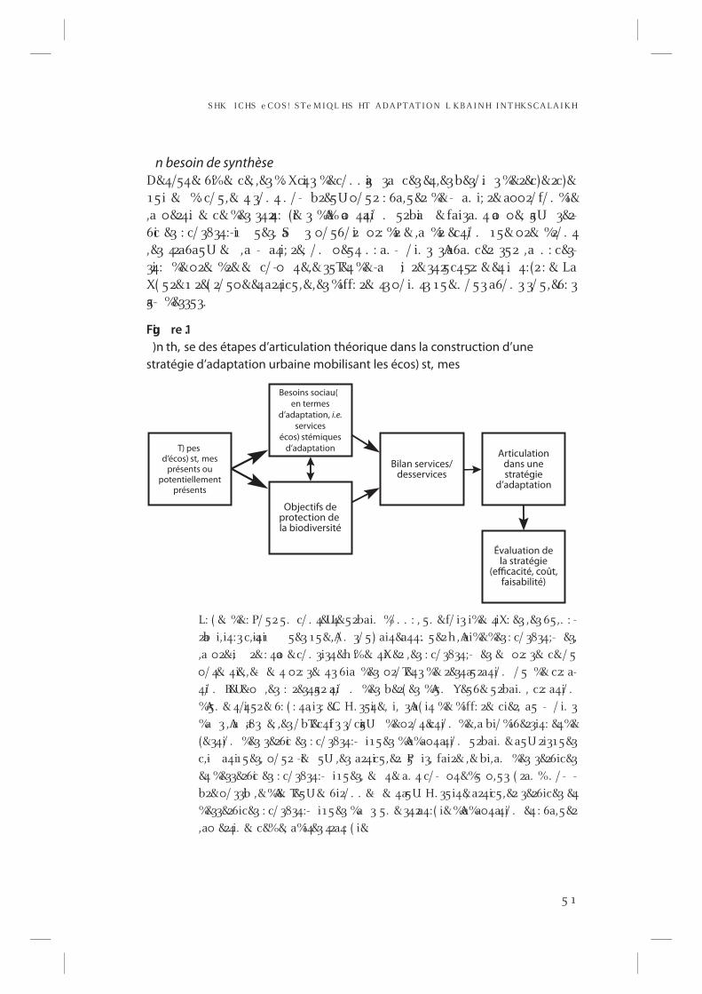
�
� HK � � H� � e � � � ! � � e � � � L H� � H� � � � � � � � � � � � � L K� � � � H� � � � HK� � � � � � KH
� � � � � � � � � � � � � $ � � &� 4/54&� : 6*%&. $ &� � ,&3� %: X$ *43� %&� $ / . . "*3 3". $ &3� &4�,&3� # &3/ *. 3� %&� 2&$ )&2$ )&�15* � &. � %: $ / 5,&. 4� 3/ . 4� . / - # 2&5U� 0/ 52� : 6" ,5&2� %&� - " . * ; 2&� " 002/ ' / . %* &�,"� 0&24*. &. $ &� %&3� 342"4: (*& 3� %A"% "0 4"4*/ . � 52# "*. &� ' " * 3" . 4� "0 0&,� "5U � 3&2�6*$ &3� : $ / 3834:-*1 5&3�� �". 3� 0/ 56/ *2 � 02: %*2 &� ,"� %*2 &$ 4*/ . � 15&� 02&. %2/ . 4�,&3� 42" 6" 5U� &. � , " � - " 4* ; 2&� � / . � 0&54� . : " . - / * . 3� 3A" 6" . $ &2� 352� , " � . : $ &3�3*4: � %&� 02&. %2&� &. � $ / -0 4&� ,&� 35T&4�%&� -". *; 2&� 3425$ 452: &� &4� *. 4:(2: &�� � " ��X( 52&� � � 2&( 2/ 50&� &4� " 24* $ 5,&� ,&3� %* ' ' : 2&. 43� 0/ * . 43� 15&� . / 53� " 6/ . 3� 3/ 5,&6: 3�"5� %&3353��
" ��� � � ��� � )� � , � � � � � � � + � � � � � � � � � � � � � � % � � � � � � + � � ' � � � � � � � � % � � � � � � � � � � � � � � � � � � � �� � � � � + # � � � � � � � � � � � � � � � � � " � � � � � & " � % � � � � � � % � � � + � � ) � � , & � �
! ) � � � �� � + � � ) � � , & � �
� � + � � � � � � �� � � � � � � % % � & � � �
� � + � � � � �
� � � � � � � � � � � � ( �� � � � � � & � �
� � � � � � � � � � � � � � �� � � � � � � �
+ � � ) � � + & � ' � � �� � � � � � � � � � �
� " $ � � � � � � � �� � � � � � � � � � � �% � � " � � � � � � � � � +
� � % � � � � � � � � � � � �� � � � � � � � � � �
� � � � � � % � � � �� � � � � � � �� � � � � + # � �
� � � � � � � � � � �
* � � % � � � � � � � �% � � � � � � � + # � �
� � ffi� � � � � + � � � - � � � � � � " � % � � + �
� : ( &. %&� � � � / 52� 5. � $ / . 4&U4&� 52# " * . � %/ . . : � � 5. &� ' / * 3� * %&. 4* X: &3� ,&3� 65,. : �2"# * , * 4:3� $ ,*-"4*1 5&3� 15&� ,A/ . � 3/ 5) " * 4&� " 44:. 5&2� h� ,A" * %&� %&3� : $ / 3834;- &3� �,"� 02&-*; 2&� : 4"0 &� $ / . 3* 34&� h� *%&. 4*X&2� ,&3� : $ / 3834;- &3� &. � 02: 3&. $ &� / 5�0/ 4&. 4*&,,&- &. 4� 02: 3&. 43� 6* " � %&3� 02/ T&43� %&� 2&34" 52" 4* / . � / 5� %&� $ 2: " �4*/ . � B&U&-0 ,&3� �� 2&34"52 "4*/ . � %&3� # &2( &3� %A5. � Y&56&� 52# " * . � � $ 2: " 4* / . �%A5. &� 4/*452&� 6: ( : 4" , * 3: &C�� H. 35*4&� � * , � 3A" ( * 4� %&� %* ' ' : 2&. $ * &2� � " 5� - / * . 3�%". 3� ,A". ",83 &� � ,&3� / # T&$ 4*' 3� 3/ $ *"5U � %&� 02/ 4&$ 4* / . � %&� , " � # * / %* 6&23* 4:� &4�%&�(&34* / . � %&3� 3&26*$ &3� : $ / 3834:- * 15&3� %A" %" 04" 4* / . � 52# " * . &� " 5U� 2* 315&3�$ ,*- " 4*15&3� � 0/ 52� -*& 5U� ,&3� " 24* $ 5,&2�� �5 * 3� � ' " * 2&� ,&� # * , " . � %&3� 3&26* $ &3�&4� %&33&26*$ &3� : $ / 3834:- * 15&3� � &. � 4&. " . 4� $ / - 04&� %5� 0,53� ( 2" . %� . / - �# 2&� 0/ 33*# ,&� %A&. T&5U� &. 6* 2/ . . &- &. 4" 5U�� H. 35* 4&� � " 24* $ 5,&2� 3&26* $ &3� &4�%&33&26* $ &3� : $ / 3834:- * 15&3� %". 3� 5. &� 342" 4:( * &� %A" %" 04" 4* / . � &4� : 6" ,5&2�, " �0 &24* . &. $ &�%&�, " %* 4&�3 42" 4: ( * &� �
�
� HK � � H� � e � � � ! � � e � � � L H� � H� � � � � � � � � � � � � L K� � � � H� � � � HK� � � � � � KH
�,� . / 53� 2&34&� h� 02: 3&. 4� h� "# / 2%&2� ,&� %&2. *&2� 0/ * . 4� 15* � . / 53� *. 4&20&,,&�%". 3� ,&� 35T&4�42"*4: � 0"2 � ,"� T/ 52. : &� � � � � � &4�15*� $ / . $ &2. &� ,A: $ ) &,,&� h� , " 15&,,&�3&�$ / . i / *4�,A"% "0 4"4*/ . �%&3�3 834;-& 3�52 # "*. 3�"5 �$ ) " . ( &- &. 4�$ , * - " 4*15&�
� � � � � � � � � � � � � � � � � � � � � � � � � � � & � � � � � � � � � � � � � � � � � � � �� � � � � � � � � � � � � � � � � � � � � � � � � � � � � � � � � � � � � � � � � � � � � � � � � � �
� � � � � � � � � � � � � � � � � � � � � � � � � � � � � � � � � � � � � � � � � �d � 15&,,&� : $ )&,,&� ,A"% "0 4"4*/ . � %&3� 3834;-& 3� 52# " * . 3� %/ * 4�&,,&� 3&� 0&. 3&2� G��$ / 4� &4� ",�� B��� C� 2: 35-& . 4� ,&� 02/ # ,; -& � "*. 3*� �� W� � &� $ ) " . ( &- &. 4� $ , * - " �4*15&� 0/ 522"*4� "' ' &$ 4&2� ,"� %52"# *,*4: � %&3� : 4"# ,*3 3&-& . 43� )5-"*. 3� � 3/ * 4�%*2 &$ 4&-& . 4�&. � "' ' &$ 4". 4� ,"� 15",*4: � %&� 6*&� %". 3� ,&3� : 4"# ,*3 3&-& . 43� B0�� &U��&. � $ )". (&". 4� , "� 02/ # "# *,*4: � %&3� *. / . %"4*/ . 3� / 5� %&3� : 0*3 / %&3� %&� 0/ ,,5�4*/ . 3� %&� ,A"*2 C� � &. � - / %*X". 4� ,&3� &' ' &43� %&3� : 4"# ,*3 3&-& . 43� 352� ,&3� -*,*& 5U�",& . 4/523� B0�� &U�� &. � $ )". (&". 4� ,"� %&- ". %&� &. � &"5� / 5� &. � $ )". ( &" . 4� ,"�$ " 0 " $ * 4: � " 33* - * , " 4* 6&� %&3� 9/ . &3� ) 5- * %&3C� � / 5� &. � $ ) " . ( &" . 4� ,&3� ' / . %&�-& . 43� : $ / . / -*1 5&3� %&� ,A: 4"# ,*3 3&-& . 4� B0�� &U�� &. � $ )". (&". 4� ,"� 02/ %5$ �4* 6* 4: � %&3� $ 5,452&3� � %&3� ' / 2j 43� � / 5� %&3� 0j $ ) &2* &3� %&315&,,&3� ,A: 4" # , * 33&- &. 4�%: 0&. %C� \ � B0�� ��C �� � *. 3*� � &. � 0,53� %A5. &� "44&. 4*/ . � 352� ,"� 6*,,& � &,,&� -j -& � �352� ,&� - *,* &5� # f4*� � ,A"0 02/ $ )&� %/ *4� %/ . $ � "53 3*� j 42&� *. 4&23$ ","*2 &� &4�0&. 3: &�&. �4&2-& 3�2&,"4 */ . . &,3�&. 42&�,"�6 *,,& �&4�,&3�&30"$ &3�1 5*�,A &. 4/52&. 4�
� . � 2&42/ 56&� *$ *� ,&� T&5� %A: $ )&,,&3� *. ): 2&. 4� "5U � 15&34*/ . 3� %&� %: 6&,/ 00&�- &. 4� %52" # ,&� � � / 52� 5. � 2" * 3/ . . &- &. 4� : $ / ,/ ( * 15&� � , " � 6* ,,&� %52" # ,&� � ,/ 2315&�W�6*,,& � \ � &34�%: X. *&� 5. *1 5&-& . 4� *. 42"� -52 / 3� %". 3� 3"� $ / -0 2: )&. 3*/ . � 42"�%* 4* / . . &,,&� � 2&,; 6&� 2" 0* %&- &. 4� %&� ,A/ U8- / 2&� BK&&3� � � � � C� � L . &� 6* ,,&� � 0&. �3: &� $ / --& � &. 4*4: � 30"4*",& � *3 / ,: &� � %: 0&. %� *. 42*. 3; 15&-& . 4�%&� 2&33/ 52$ &3�02/ %5*4&3� � &. � 42; 3� (2". %&� 0"2 4�� "5� %&,h� %&� 3&3� -52 3�� �& 3� 6*,,&3� %: 0&. %&. 4�%&3� - * , * &5U� " ,&. 4/ 52� � ,&52� W� ) * . 4&2," . %� \ � � 0/ 52� , " � ' / 52. * 452&� %A&" 5� � %&�. / 522* 452&� �/ 5�&. $ / 2&�%&�, / * 3* 23�' / 52. * 3�0 " 2�, &3�&30" $ &3�" ,&. 4/ 52�
� A&. T&5� &34� ",/ 23� %&� 2: 533*2 � h� 42"$ &2� %&� . / 56&"5U � 3$ ): -"3 � - &. 4"5U �0/ 52� B2&C%: X. *2 � ,&3� : $ )&,,&3� %A"$ 4*/ . �� H. � $ &� 3&. 3� � $ / --& � ,&� . / 4&. 4� � ) &83�&4� H- &,* " . / ' ' � B� � � � C� � W� P* ,Q� 3A" ( * 4� � h� 42" 6&23� ,&� 02/ T&4� %&� 6* ,,&� %52" # ,&� �%A"-: . "(& 2� %&3� 3/ ,54*/ . 3� %&� $ / . 4*. 5*4: � &. 42&� ,&3� : $ )&,,&3� � %&� $ 2: &2� %&3�$ / 5452&3� &. 42&� ,&3� 4&22*4/ *2 &3� \ � B0�� ��C �� H. � 0"2 4". 4� %&3� -/ 43� %&� �$ / 4� &4�",�� B���C � � ,A"% "0 4"4*/ . � %&3� 3834;-& 3� 52# "*. 3� "5� $ )". (&-& . 4� $ ,*-"4*1 5&�* - 0/ 3&� " * . 3* � %&� $ / - 02&. %2&� � %" . 3� 5. &� 0&230&$ 4* 6&� * . 4&23$ " , " * 2&� * . 4: ( 2: &� �$ / --& . 4�0&2-& 442&� %A"44: . 5&2� ,&3� 2*3 15&3� $ ,*-"4*1 5&3� "' ' &$ 4". 4�,"� 15",*4: �%5� $ "%2&� %&� 6*&� � ". 4*$ *0 &2� ,&3� . / 56&,,&3� 02&33*/ . 3� : 6&. 45&,,&3� 15&� , " � 6*,,& �
�
� HK � � H� � e � � � ! � � e � � � L H� � H� � � � � � � � � � � � � L K� � � � H� � � � HK� � � � � � KH
0/ 522"*4� ' " *2 &� 0&3&2� 352� 3/ . � )*. 4&2,". %� � &4�4&. 4&2� %&� 02: 6/ * 2� ,&3� -/ %*X$ "�4* / . 3� %5� ' / . $ 4* / . . &- &. 4� %&� ,A) * . 4&2," . %� , * : &3� " 5� $ ) " . ( &- &. 4� $ , * - " 4* 15&� �� &$ *� *-0 / 3&� 62"*3 &-# ,"# ,&-& . 4� 5. � %*"(. / 34*$ � 02: ","# ,&� 352� ,"� 15",*4: �%5� $ "%2&� # f4*� &4� ,A: 4"4� %&3� ,*&. 3� 6*,,& � )*. 4&2,". %� � &4� 0,53� (: . : 2",& -& . 4�%&3� : ,: -& . 43� $ / -0 / 3". 4� ,"� %52"# *,*4: � 52# "*. &� � %A&. � ' "*2 &� 5. &� : 6",5"4*/ . ��$ 2*4*1 5&� � %&� ,&3� $ / . ' 2/ . 4&2� h� %&3� 02/ T&$ 4*/ . 3� � &4�%A*%&. 4*X&2� ,&3� 42"T &$ 4/*2 &3�,&3� 0,53� %52"# ,&3� 0/ 52� %&3� 3834;-& 3� 52# "*. 3� 2: (*/ . "5U �� �& � $ )". (&-& . 4�$ , * - " 4* 15&� � 0" 2� ,&� 2* 315&� 15A* , � 2&02: 3&. 4&� � ' / 2$ &� 5. � 42" 6" * , � 2: Y&U* ' � 15* �2: 6; ,&� &4� 2&-& 4� &. � 15&34*/ . � ,"� . / . � %52"# * , * 4:� %&� $ &24"*. 3� $ ) / * U� / 2( ". *�3"4*/ . . &,3� &4� 4&$ ). *1 5&3�� H. � $ &� 3&. 3� � ,A"% "0 4"4*/ . � " 5� $ )". (&-& . 4� $ ,*-"�4*15&� 0&54� ",/ 23� j 42&� 65&� $ / -- &� 5. � W�$ ". " , � %A"0 0,*$ "4*/ . � %&3� 02*. $ *0 &3�%&� ,"� %52"# *,*4: � \ � B� "(. ". � � ����C �� � ". 3� ,&� 3*,,/ . � %&� ,A"% "0 4"4*/ . � 342*$ 4/�3&. 35� B$ �� h� %�� ,"� %*-*. 54*/ . � %5� 2*3 15&� $ ,*- " 4*15&C� � $ A&34� ",/ 23� 4/54� ,&� ,*&. �6*,,& � &. 6*2 / . . &-& . 4�15*�3 5*4�
�*� ,A/ . � 0&. 3&� &. � 4&2-& 3� %&� 3&26*$ &3� : $ / 3834:- * 15&3� � $ &$ * � %&-". %&� %/ . $ �5. &� 6* 3* / . � * . 4: ( 2: &� � h� 5. � . * 6&" 5� 2: ( * / . " , � � %5� ' / . $ 4* / . . &- &. 4� %&3� : $ / 383�4;-& 3� h� 42" 6&23� ,&3� : $ )&,,&3�� �,� 3A"(*2 "*4� ",/ 23� %&� $ / -0 2&. %2&� $ / --& . 4�*,3 � 0&56&. 4� $ / . 42*# 5&2� h� ,"� 2: %5$ 4*/ . � %5� 2*3 15&� $ ,*-"4*1 5&� � $ / --& . 4� ,&3�02&33*/ . 3� 52# "*. &3� B: 4",&-& . 4�52# "*. � � ' 2"(-& . 4"4*/ . � � 0/ ,,54* / . 3� %*6 &23&3� �* . 6" 3* / . 3� # * / ,/ ( * 15&3� � " $ 4* 6* 4: 3� &U42" $ 4* 6&3� � &4$ � C� " $ 45&,,&3� &4� ' 5452&3� 0/ 52�2" * &. 4� - / %* X&2� ,&52� ' / . $ 4* / . . &- &. 4� � &4� $ / - - &. 4� 4/ 54� $ &$ * � 3A* . 4; ( 2&� %" . 3�, " � 0&230&$ 4* 6&� %&� $ ) " . ( &- &. 4� $ , * - " 4* 15&� B# " * 33&� %&� , " � ' / 52. * 452&� %&� 3&2�6*$ &3� : $ / 3834:-*1 5&3� h� $ "53 &� %&3� *-0 "$ 43� %5� $ )". (&-& . 4� $ ,*-"4*1 5&� 352�,&3� : $ / 3834;-& 3� � "5 (-& . 4"4*/ . � %&3� 02&33* / . 3� 52# "*. &3� 352� ,&3� : $ / 383�4;-& 3� �� H4�$ &� &. � : 6*4". 4�,&3� %&33&26*$ &3� 0/ 4&. 4*&,3� &4�,"� - " , " %" 04"4*/ . �� � 52�$ &� %&2. *&2� 0/ *. 4�� ,A*%: &� %&� # : . : X$ &� *. %*2 &$ 4� B� *3 )&2� &4� " , �� � ����� � : 6/ 15: �&. � 02&-*; 2&� 0"2 4*&C� &34� *. 4:2&33". 4&� � $ "2 � &,,&� 0&2-& 4� %&� ,*&2� ,&3� 3&26*$ &3�B0" 2� &U&- 0,&� , " � 02/ %5$ 4* / . � %&� # * / - " 33&� 0/ 52� , " � ( : . : 2" 4* / . � %A: . &2( * &� �0"2 � $ / -# 534*/ . � / 5� -: 4)". *3 "4*/ . � 0"2 � &U&-0 ,&C� h� $ &24" * . &3� / 04*/ . 3� %&�42". 3*4*/ . � 4&$ ). / ,/ (*1 5&3� � &4�0/ 522"*4� ' "6 / 2*3 &2� , " � $ / . 3425$ 4*/ . � %&� # *,". 3�&. 6*2 / . . &-& . 4"5U � *. 4:(2: 3� 0/ 52� ,&� 2&$ / 523� "5U � 3&26*$ &3� : $ / 3834:-*1 5&3��� &$ *� 0&2-& 442"*4� . / 4"--& . 4� %&� # *&. � -"4: 2*",*3 &2� ,&� ' "*4� � %: Th� 3/ 5,*(. : �* $ * � � 15&� 4/ 54� 2&$ / 523� " 5U� 3&26* $ &3� : $ / 3834: - * 15&3� . &� ' " * 4� 3&. 3� 15A5. &� ' / * 3�2&0,"$ : � %". 3� ,&� ' "*3 $ &"5� 0,53� ,"2 (&� %&3� 02&33* / . 3� $ , * - " 4*15&3� B"% "0 4"4*/ . �"5U � 2*3 15&3� � 42". 3*4*/ . � : . &2(: 4*15&C� 15&� 35# * 33&. 4� ,&3� 3834;-& 3� 52# " * . 3�B� "$ 4&"5� � �� ��C �� � . � 2&42/ 56&� *$ *� � %A5. &� $ &24" * . &� - " . * ; 2&� � ,"� 6*3 */ . � 02/ 0/ �3: &�0 "2 ��& 242". %�&4��*-/ . &4�B����C ��
� HK � � H� � e � � � ! � � e � � � L H� � H� � � � � � � � � � � � � L K� � � � H� � � � HK� � � � � � KH
� � � � � � � � � � � � � � � � � � � � � � � � � � � � � � � � � � � � � � � � � � � � �� � � � � � � � � � � � � � � � � � � � � � � � � � � � �� ". 3� $ &� $ "%2&� � ,&� $ / . $ &04�%&� 42"-& � 6&24&� 52# "*. &� " � $ / - - &� * . 4:2j 4�- " T&52�%A*-0 / 3&2� 5. &� 0&230&$ 4*6&� $ / . 4*. 5&� &. 42&� ,&3� - * , * &5U� # f 4*3� &4� . / . � # f 4*3���: ". -/ *. 3� � / . � 0&54�3&� %&-". %&2� 3*� ,&� $ / . $ &04� 0&2- &4�&' ' &$ 4*6&- &. 4�%A8�2"44"$ )&2� 4/54&3� ,&3� "44&. 4&3� 15&� ,A/ . � 0," $ &� %". 3� ,&3� : $ / 3834;-& 3� 6* 3� h� 6* 3�%&�, A" %" 04" 4* / . � " 5�$ ) " . ( &- &. 4�$ , * - " 4* 15&�
H. � &' ' &4�� 4". 4�%". 3� 3"� %: X. *4*/ . � T52*%*1 5&� � 15&� 3$ *&. 4*X15&� � � ,A/ # T&$ 4* ' �%&3� 42" - &3� 6&24&3� &34� " 6" . 4� 4/ 54� %&� 2: 4" # , * 2� , " � $ / . 4* . 5* 4: � %&3� - * , * &5U� %" . 3�5. � / # T&$ 4*' � %&� 02/ 4&$ 4*/ . � %&� ,"� # */ %*6 &23*4: � �� $ &� 3/ . 4�,&3� Y5U� %A/ 2( " . * 3- &3�15A*,� 3A"(*4� %&� 2: 4"# ,*2 � &4�%&� 3/ 54&. *2 � � &. � 0"2 4*$ 5, * &2� %". 3� 5. � $ / . 4&U4&� %&�$ )". (&-& . 4� $ , *-"4 *1 5&�� � &� 3/ . 4� %&3� 9/ . &3� %&� $ / . . &U*/ . � # * / ,/ ( * 15&� � �15A*,�' "54�2 : 4"# , *2 �&4D/5�-"*. 4&. *2 ��
� &5U� 02&-*& 23� 02/ # ,; -& 3� 3&� 0/ 3&. 4� *$ *�� � / 54� %A"# / 2%� � %5� 0/ *. 4�%&� 65&�%&3� &30"$ &3� 15&� ,"� 42"-& � 6&24&� $ / . $ &2. &� � . / 53� 3/ --& 3� ,/ *. � %A*. 4:(2&2�4/54&� ,"� -/ 3"m15&� 4&22*4/ 2*",& � 15&� . : $ &33*4&� 5. &� 6*3 */ . � &. � 3834;-& � 6* ,,&�) * . 4&2," . %� � H. 35* 4&� � " 6&$ � 5. � " $ $ &. 4� - * 3� � &. � 4&2- &3� %A/ # T&$ 4* ' 3� 02&- * &23� �352� ,"� 02/ 4&$ 4*/ . � %&� ,"� # */ %*6 &23*4: � � / . � 3&� 2&42/ 56&� ' "$ &� "5U � 02/ # ,; -& 3�%A"2 4*$ 5,"4*/ . �3 / 5,&6: 3�. / 4"--& . 4�&. �0 2&-*; 2&�0 "2 4*&�%&�$ &4�"2 4*$ ,&��
H. � / 542&� � , " � . / 4* / . � %&� $ / . . &U* / . � # * / ,/ ( * 15&� . &� 2&$ / 562&� 15A&. � 0" 2�4*&� ,"� . / 4*/ . � %&� $ / . . &$ 4*6 *4: � : $ / ,/ (*1 5&�� � &,,&� $ *� %: 3*(. &� 0,53� ," 2( &- &. 4�W�,A&. 3&-# ,&� %&3� 42". 30/ 243� � "5� 3&*. � &4� &. 42&� ,&3� 3834;-& 3� 4&22&342&3� &4�"1 5"4*1 5&3� h� 42"6 &23� 5. &� ( "--& � %A: $ )&,,&3� 30"4*",& 3� &4� 4&- 0/ 2&,,&3� �%&� -"4: 2*"5U � &4� 2&33/ 52$ &3� B0/ 533*; 2&3� � 3/ ,� � &"5� � : . &2(*& � � . 542*-& . 43� ��02/ 0"(5,& 3� � -","% *&3� � $ / -0 / 3" . 43� $ )*-*1 5&3� � &4$ �C� 6*"� %&3� 6&$ 4&523� B,&�6&. 4�� ,A&"5� � ,&3� ". *-"5U � � ,&3� )5-"*. 3C� \ � B� &4&23� &4� ",�� � ��� C �� � / -0 2&. %2&�$ &44&� $ / . . &$ 4*6 *4: � *. 4&23$ ","*2 &� &34� B0"2 � %: X. *4*/ . � GC� 5. � &. T&5� *-0 / 2�4". 4� 0/ 52� ,&3� 3$ *&. $ &3� : $ / ,/ (*1 5&3� &4�� 0,53� ,"2 (&-& . 4�� ,&3� 3$ *&. $ &3� %&�
��� � &,/ . � ,A"2 4*$ ,&� ����� �� %&� ,"� �/ *� %5� ��� T5*,,& 4� ����� 0/ 24". 4� &. ( "(& -& . 4� . "4*/ . ",� 0/ 52�&. 6* 2/ . . &- &. 4� � � W� � " � 42" - &� 6&24&� &4� , " � 42" - &� # ,&5&� / . 4� 0/ 52� / # T&$ 4* ' � %A&. 2" 8&2� , " � 0&24&�%&� # */ %*6 &23*4: � &. � 0"2 4*$ *0 ". 4�h� ,"� 02: 3&26"4*/ . � � h� ,"� (&34*/ . � &4�h� ,"� 2&-*3 &� &. � # / . � : 4"4� %&3�-*,*& 5U� . : $ &33"*2 &3� "5U � $ / . 4*. 5*4: 3� : $ / ,/ (*1 5&3� � 4/54� &. � 02&. ". 4� &. � $ / -0 4&� ,&3� "$ 4*6 *4: 3�)5-"*. &3� �&4�. / 4"--& . 4�"(2 *$ / ,&3� �&. �-*,*& 5�2 52",��\��� �& ,/ . � ,&� 02/ T&4�� �K � � 2"-& � &24&� L2# "*. &� �� W��"� 42"-& � 6&24&� &34�5. � / 54*,� %A"-: . "(& -& . 4�%5� 4&22*4/ *2 &� � $ / . 34*45: � %&� (2". %3� &. 3&-# ,&3� . "452 &,3� &4�%&� $ / 22*%/ 23� ,&3� 2&,*". 4� / 5� 3&26". 4�%A&30"$ &3� 4"-0 / . 3�� �"� 42"-& � 6&24&� &34�5. � 02/ T&4�%&� -"*,,"(& � 6&24�15*� -& 4�&. � $ / . . &U*/ . � %&3�$ )&-*. 3� � %&3� )"*& 3� / 5� %&3� $ ". "5U � 3/ 53� ' / 2-& � %&� $ / 22*%/ 23� 15*� 0&2-& 44&. 4�,&3� Y5U� %A&30; $ &3�". *-",& 3�&4�6: (: 4",&3��\ �)440 �DD777 �42"-& 6&24&52# "*. &�$ / -D30*0 �0 )0 �G25# 2*1 5&������ L. &� 9/ . &� %&� $ / . . &U*/ . � # */ ,/ (*1 5&� &34� W�P5. Q� &. 3&-# ,&� %&� $ / 22*%/ 23� 15*� 0/ 522"*4� j 42&�$ / . 34*45: � "53 3*� # *&. � %&� )"*& 3� � 25*3 3&"5U � � # / 2%3� %&� 2/ 54&� � # / *3 � � $ 5,452&3� � 15*� 3&26*2 / . 4� $ )"$ 5. �"5�% : 0,"$ &-& . 4�%A5. �480&�%A&30; $ &�\ �B� ,&2(&"5� ������ �0 � �� C�
� HK � � H� � e � � � ! � � e � � � L H� � H� � � � � � � � � � � � � L K� � � � H� � � � HK� � � � � � KH
,A&. 6* 2/ . . &- &. 4� � � &3� Y5U� " . 4) 2/ 0* 15&3� %&� - " 4* ; 2&� &4� %A: . &2( * &� &. � ' / . 4�%&�4/ 54&�: 6* %&. $ &�0 " 24* &�
�,� &34� "3 3&9� $ ,"*2 � 15&� ,&� $ / . $ &04�%&� 42"-& � 6&24&� " 5� 3&. 3� 342*$ 4�B&4� - j - &�"%T/ *. 4�%A5. &� 42"-& � # ,&5&� 0/ 52� ,A&"5� / 5� %A5. &� 42"-& � # 25. &� 0/ 52� ,&3� 3/ ,3C�. &� 0&2-& 4� 0"3 � %A*. $ ,52&� 4/54&� ,"� $ / . . &$ 4*6 *4: � : $ / ,/ ( * 15&� "5� 2"*3 / . . &�-& . 4�� �"� $ / . . &U*/ . � # */ ,/ (*1 5&� : 4". 4�5. &� $ / - 0/ 3" . 4&� %&� ,"� $ / . . &$ 4*6 *4: �: $ / ,/ (*1 5&� � *,� 3&-# ,&� 0,54< 4� 15&� ,A*. $ ,53*/ . � 3&� ' " 33&� %". 3� ,A"542 &� 3&. 3� ��$ A&34� ",/ 23� ," � 42"-& � 6&24&� 15*� &34� *. $ ,53&� %". 3� 5. � $ / . $ &04�0,53� ,"2 (&� � 5. &�6*3 */ . � *. 4:(2"4*6 &� %&3� 4&22*4/ *2 &3� � 15*� 2&34&� &. $ / 2&� h� # f 4*2�� � " � 42"-& � 6&24&�&34� 5. � $ / . $ &04� %A&. 42: &� � h� ,"� 0/ 24:&� ) &52*3 4*15&� *. %: . *"# ,&� $ / - - &� ,&�2&,; 6&� �/ 5%&3� B���� C� � -"*3 � &,,&� 3&-# ,&� "5 33* � j 42&� 5. � $ / . $ &04� %A"44&. 4&�B� " , * . * : � � � � � C� � 15* � . &� 2&$ / 562&� 15A5. &� 0" 24* &� %&3� , * &. 3� $ / - 0,&U&3� &. 42&�6*,,& � &4� )*. 4&2,". %�� � &54� j 42&� 15&� ,"� $ / . . &$ 4*6 *4: � : $ / ,/ ( * 15&� � 15*� *. 4;(2&�5. &� 6*3 */ . � 0,53� &U)"53 4*6&� %&3� Y5U� &4�%&3� T&5U� %A: $ )&,,&3� � &4� 15*� *. 4;(2&�&U0,*$ *4&-& . 4� ,"� 0,"$ &� %&3� )5-"*. 3� %". 3� $ &3� Y5U� � 0/ 522" * 4� j 42&� 5. � $ / . �$ &04� W�0"2 "0 ,5*& � \ � 0,53� h� -j -& � %A&. (,/ # &2� 4/54&3� ,&3� " 44&. 4&3� 15&� ,A/ . �' "*4� 0/ 24&2� "5U � : $ / 3834;-& 3� 52# "*. 3� &4� 0: 2* � 52# " * . 3� %" . 3� ,&� $ "%2&� %&�,A"% "0 4"4*/ . � "5� $ )". (&-& . 4� $ ,*-"4*1 5&�� H,,&� 0&2-& 442"*4� &. � 4/54� $ "3 � %&�4*33&2� 0,53� %&� W�$ / 5452&3� \ � � . &� 3&2"*4� $ &� 15A"5� . * 6&" 5� %5� 2"*3 / . . &-& . 4�� � "2 �"*,,& 523� �0 &. 3&2�,&�,*& . �&. 42&
K* $ ) " 2%� � / 2- " . � � $ : ,; # 2&� : $ / ,/ ( 5&� %5� 0" 83" ( &� � 02/ 0/ 3&� 5. � / 54* , � $ / . $ &0�45&,� *. 4:2&33". 4�� ,"� W�2: (*/ . � 52# "*. &� \ � B� / 2- " . � � ��� C �� � &� 15A* , � 02/ 0/ 3&� &34�%&� 2&0&. 3&2� ,A: $ )&,,&� %&� 0,". *X$ "4*/ . � %&3� (2". %&3� 6*,,&3� � &. � $ / . 3425*3 ". 4�%&3� 0,". 3� 2: (*/ . "5U � � $ &. 42: 3� "54/ 52� %A" *2 &3� -: 42/ 0/ ,*4"*. &3� &4� *. 4:(2". 4�,&3� -*,*& 5U� &4� 0&4*4&3� 6*,,&3� ",& . 4/52�� �"� 2: ( * / . � 52# " * . &� 3&� %: X. *4� ",/ 23�$ / --& � ,"� 9/ . &� %&� ��� h� ���� + -� %&� %*"-; 42&� 15*� &. 4/52&� 5. &� ( 2". %&� 6*,,& �&4� / p� ,"� 6*,,& � &4� 3&3� &. 6*2 / . 3� *. 4&2"(*3 3&. 4� *. 4&. 3: -& . 4�� �,� 3A"(*4� � $ / --& �,&� 35((; 2&� ,&� 4*42&� %&� 3/ . � ,*6 2&� � %&� W�0,". *X &2� " 5� %&,h� %&� ,"� $ * 4:� \ �� � A/ 54*,�. A&34� 0"3 � 3" . 3� ' "*2 &� 0&. 3&2� "5U � �� � � � / 5� �K � H� ' 2". i "*3 � � -"*3 � *,� 6" � 0,53�,/ * . �%" . 3�, " �' / 2- " , * 3" 4* / . �
� 5� 0/ *. 4�%&� 65&� 3425$ 452&,� � ,"� 2: (*/ . � 52# "*. &� %&� � / 2-". � &34� $ / -0 / 3: &�%A5. � . / 8"5� � 15*� &34�,"� 0,53� (2". %&� 6*,,& � %&� ,"� 2: (*/ . � $ / -# *. : &� h� 3/ . � "((,/ �-: 2"4*/ . � � &. 4/52: � %A5. &� -/ 3" m15&� %A&30"$ &3� . "452 &,3� &4� 3&-*� . "452 &,3�B,&3� W�&30"$ &3� 6&243� \ C� � / p� 3A*. 4;(2&. 4� %&3� 6*,,&3� 3"4&,,*4&3�� �"� 2: (*/ . �3A: 4&. %� T5315Ah� 5. &� ' 2/ . 4*; 2&� Y/ 5&� � T5315Ah� ,"1 5&,,&� *,� 8� "� %: %&. 3*X$ "�4*/ . � 02/ (2&33*6 &� %5� # f4*� &4�%&3� *. 4&2"$ 4*/ . 3� 3/ $ *",& 3� � &4�5. &� "5(- &. 4"4*/ . �$ / 22: ,: &� %&3� &30"$ &3� . / . � # f4*3 �� �/ 2315&� $ &3� %&5U� 4&. %". $ &3� � 2&30&$ 4*6&�-& . 4�� 3A*. 6&23&. 4�� $ &,"� 3*(. *X&� 15&� . / 53� &. 42/ . 3� %". 3� 5. &� "5 42&� 2: (*/ . �52# " * . &� � &4� 15&� . / 53� " 6" . i / . 3� 6&23� 3/ . � . / 8" 5� $ &. 42" , � � � / 2- " . � � " 33* 34: �%A5. &� : 15* 0&� 0,52* %* 3$ * 0, * . " * 2&� � " � " 00,* 15: � � 352� $ / - - " . %&� � ,&� $ / . $ &04� h�
�
� HK � � H� � e � � � ! � � e � � � L H� � H� � � � � � � � � � � � � L K� � � � H� � � � HK� � � � � � KH
," � 2: ( * / . � # " 2$ &,/ . " * 3&� � H. � " %/ 04" . 4� 5. &� 6* 3* / . � 02/ 30&$ 4* 6* 34&� � ,A: 15* 0&� " �4&. 4:� %A*%&. 4*X&2� ,&3� 4&. %". $ &3� h� -/ 8&. � 4&2- &� %&� , " � 2: ( * / . � � &. � 4&2- &3�%A53" ( &� %&3� 3/ ,3� � %&� %* 30/ . * # * , * 4: � &. � 2&33/ 52$ &3� � %&� %: - / ( 2" 0) * &� � &4$ � � � &4� " �02/ 0/ 3: � %* ' ' : 2&. 43� 0," . 3� %A" - : . " ( &- &. 4� 0/ 52� , " � 2: ( * / . � � " 6&$ � 5. � " $ $ &. 4�0"2 4*$ 5,*&2� 352� ,"� -*3 &� &. � 0,"$ &� %&� $ / 22*%/ 23� &4� , " � ( &34* / . � %&3� 2&33/ 52$ &3�"(2 *$ / ,&3�&4�%&�,A&"5�
�*� ,&� $ / . $ &04�%&� W�2: (*/ . � 52# "*. &� \ � &34�0"2 4*$ 5, * ; 2&- &. 4� * . 4:2&33" . 4�0" 2�2"0 0/ 24�h� ,A: $ )&,,&� 15A*,� "% / 04&� � / . � 0&54�2&(2&44&2� , " � ' " * # ,&� 0," $ &� , " * 33: &� " 5U�15&34*/ . 3� %&� Y5U� 2: (*/ . "5U � B$ A&34�&. $ / 2&� ,"� $ / . . &U* / . � # * / ,/ ( * 15&� 15* � &34�02: 0/ . %: 2". 4&C�� �,� . / 53� 3&-# ,&� 15A*,� 8� " � 0/ 524" . 4� * $ * � ,A/ $ $ " 3* / . � %A" 33/ $ * &2�5. &� 6*3 */ . � 30"4*",*3 : &� %A5. � -: 4"# / ,*3 -& � 52# "* . � 2: ( * / . " , � � ' "*3 " . 4� : $ ) / � h�,A"0 0&,� %&� �*,,& . � B�� ��C � h� ,"� $ / . 34*454*/ . � %A5. &� 6: 2* 4" # ,&� W�: $ / ,/ ( * &� %&3�". 4)2/ 0/ 3834;-& 3� 2: (*/ . "5U � \ � -j ,". 4�&. 42&� " 542&3� : $ / ,/ ( * &� 3$ * &. 4*X15&�W�$ ,"3 3*1 5&� \ � � : $ / ,/ (*& � *. %5342*&,,&� B". " ,83&� %&3� Y5U� 2: ( * / . " 5U� &4� * %&. 4* �X$ "4*/ . � %&� ,&6*&23� 0/ 52� $ *2 $ 5,"2 *3 &2� ,&� -: 4"# / ,*3 -& � 2: (*/ . ",C � &4�3$ *&. $ &3�) 5- " * . &3� &4� 3/ $ * " ,&3� B� * ,,&. � � � � � � C� � � . � 2&' &2" * 4� " * . 3* � ,&� , * &. � " 6&$ � , " � 6&23* / . �-: 4"# / ,*1 5&� %&� ,A: $ / ,/ (*& � 52# "*. &� *. *4*: &� 0"2 � M/ ,-". � &. � ���� BM/ ,- " . � ����C � � -"*3 � %". 3� 5. &� 6&23*/ . � 30"4*",*3 : &� "5� . *6 &"5� %&3� 3834;-& 3� 6*,,& �)*. 4&2,". %� &4�0,53� : 15*,*# 2: &� &. � 4&2-& 3� %&� $ / ,,"# / 2"4*/ . � &. 42&� %*3 $ *0 ,*. &3�B6/ *2 � �"2 ,&3� � ����� 0/ 52� 5. &� 0&230&$ 4*6&� )*3 4/2*1 5&� 352� $ &3� 15&34*/ . 3C�� �& �$ / . $ &04�%A: $ / $ / -0 ,&U&� 02/ 0/ 3: � 0"2 � �,". %*. � &4��"-/ 44&� &. � �� � B� , " . %* . �&4� � " - / 44&� � � � C� 0/ 522" * 4� : ( " ,&- &. 4� &. 2* $ ) * 2� , " � 2: Y&U* / . � � $ " 2� * , � 2&$ / . �. "l4� ,&3� W�-5,4*0 ,&3� *. 4&2%: 0&. %". $ &3� 0) 83*1 5&3� � $ )*-*1 5&3� � # */ ,/ ( * 15&3�&4� )5-"*. &3� P15*Q� " 33/ $ *&. 4� ,&3� %*6 &23� : $ / 3834;-& 3� %A5. � 4&22* 4/* 2&� � $ )"�$ 5. � %&6&. ". 4� 5. � : ,: -& . 4� %A5. � W3834;-& � 30"4*",\ � h� ,A: $ )&,,&� %515&,� *,�%&6* &. 4� 0/ 33* # ,&� %&� %: 6&,/ 00&2� 5. &� " . " ,83&� 3425$ 452" ,&� &4� ' / . $ 4* / . . &,,&� \ �B�,". %*. � ����� � 0�� � �C �� � A". ",8 3&� 3&-# ,&� &. � 4/54� $ "3 � 3&� 0,"$ &2� %" . 3� ,&�$ "%2&� %A5. &� ". ",83 &� 2: (*/ . ",& � %&3� 3834;-& 3� 3/ $ */ � : $ / ,/ (*1 5&3� B�/ 52(&2/ . �&4� ",�� � ����C � 15&� ,&� $ / . $ &04�%&� 42"-& � 6&24&� � -j -& � 3A*,� 2: 0/ . %� h� %&3� / # T&$ �4* ' 3� . : $ &33" * 2&3� %&� $ / . . &U* / . � # * / ,/ ( * 15&� � . &� 2&$ / 562&� 15&� %A5. &� - " . * ; 2&�. : " . - / * . 3�42; 3�0 " 24* &,,&�
�� � � � � ���
� &. 3&2� ,A" %"0 4" 4*/ . � . : $ &33*4&� %&� 30: $ *X &2� 15* � / 5� 15/ * � 3A"% "0 4&� � h� 15/ * � �" * . 3* � 15&� ,&� $ ) &- * . &- &. 4� &4� , " � ' / 2- &� 15&� $ &44&� " %" 04" 4* / . � 0&54� 02&. %2&�B�-*4� &4� ",�� ��� �C �� � / 52� . / 53� *$ *� � 15*� / 5� 15/ *� 3A"% "0 4&� �� $ A&34�,&� - * , * &5� # f 4* � �-"*3 � : ( ",& -& . 4� 4/54� ,&� 3834;-& � 6*,,& � )*. 4&2,". %�� � &� 34* - 5,53� �� ,&3� 2* 315&3�$ ,*-"4*1 5&3� 15* � 0; 3&. 4�352� ,&� -*,*& 5� # f4*� � -"*3 � : ( " ,&- &. 4�,&3� $ ) " . ( &- &. 43�
�
� HK � � H� � e � � � ! � � e � � � L H� � H� � � � � � � � � � � � � L K� � � � H� � � � HK� � � � � � KH
%A* . 4&2" $ 4* / . � B. / 56&,,&3� 02&33* / . 3� � 2&. ' / 2$ &- &. 4� %A" . $ * &. . &3� 02&33* / . 3� �2" 2: ' " $ 4* / . � %&3� 2&33/ 52$ &3� ,/ $ " ,&3� � &4$ � C� " 6&$ � ,&3� - * , * &5U� " ,&. 4/ 523� � � " �' / 2- &� %&� ,A" %" 04" 4* / . � � � 0/ 52� $ &� 15* � . / 53� $ / . $ &2. &� * $ * � � 5. &� ( &34* / . � * . 4: ( 2: &�%&3� 3&26* $ &3� : $ / 3834: - * 15&3� " 5� . * 6&" 5� %&� , " � 2: ( * / . � 52# " * . &� � " 6&$ � 62" * 3&- �# , " # ,&- &. 4� 5. &� " 44&. 4* / . � 0" 24* $ 5, * ; 2&� � " 5� . * 6&" 5� %&� ,A52# " * . � %&. 3&� � " 5U�3&26*$ &3� %&� 2"' 2"l$ )*3 3&-& . 4�� %&� %2"*. "( &� %&3� &"5U � &4�%A: 052" 4* / . � %&� ,A"*2 � �&4�" 5�. * 6&" 5�2 : ( * / . " , �" 5U�3 &26* $ &3�%A" 002/ 6* 3* / . . &- &. 4� �
� A/ # T&4�42"-& � 6&24&� ' / 52. *4� 5. � 0/ *. 4� ' / $ ",� *. 4:2&33". 4�%". 3� $ &� $ / . 4&U4&� �-"*3 � 0&54� j 42&� ,&3� 15&34*/ . 3� %&� ,A"% "0 4"4*/ . � &4� %&� ,"� %52"# *,*4: � 52# "*. &3�&. � "0 0&,,&. 4�&,,&3� h� 5. � $ "%2&� $ / . $ &045&,� 0,53� ,"2 (&�� �/ 4"--& . 4�� &4� $ A&34�&. � , * &. � " 6&$ � $ &� 15&� . / 53� : 6/ 15* / . 3� &. � %&5U* ; - &� 0" 24* &� � ,A/ # T&$ 4* ' � %&�$ / . . &U* / . � # * / ,/ ( * 15&� � %" . 3� 5. � / # T&$ 4* ' � %&� 02/ 4&$ 4* / . � %&� , " � # * / %* 6&23* 4: � �. / 53� 3&-# ,&� %". 3� ,A". ",83 &� 0/ 56/ *2 � 3&� T534*X&2� h� ,5*� -j -& �� � ) &2$ ) &2� %&3�# : . : X$ &3� ". . &U&3� � &. � 4&2-& 3� %A"% "0 4"4*/ . � "5� $ )". (&-& . 4�$ , * -"4*1 5&� 0"2 �&U&- 0,&� � &34� : ( " ,&- &. 4� $ / - 02: ) &. 3* # ,&� &4� T534* X: � %" . 3� 5. &� 0&230&$ 4* 6&�%&� - 5,4* ' / . $ 4* / . . " , * 4: � %&3� 4&22* 4/ * 2&3� � � / 54&' / * 3� � / . � 0&54� 3&� %&- " . %&2�3*� ,&� # 54� 02&-*& 2� %&3� 42"-& 3� 6&24&3� . &� 2*3 15&� 0"3 � %Aj 42&� W� %* ,5: � \ � %". 3�%&3� "44&. 4&3� 15*� ,&� %: 0"3 3&. 4�X. ",& -& . 4� ,"2 (&-& . 4�� K: "2 4*$ 5,&2� ,"� 42"-& �6&24&� %". 3� 5. � &. 3&-# ,&� 0,53� 6"3 4&� %&� 342"4: (*& 3� %A"% "0 4"4*/ . � 52# "*. &� "5�$ )". (&-& . 4� $ ,* -"4*1 5&� 0/ 522"*4� 0&2-& 442&� %&� ,5*� %/ . . &2� 5. &� *%&. 4*4: �$ , " * 2&� � &4� %/ . $ � 0/ 56/ * 2� " ' X2- &2� " 6&$ � 0&54� j 42&� 0,53� %&� ' / 2$ &� 3&3� / # T&$ 4* ' 3�02&- * &23� � � &," � 0/ 522" * 4� 2&6&. * 2� � 0" 2� &U&- 0,&� � h� 4/ 5T/ 523� # * &. � " 0058&2� ,&3�/ # T&$ 4*' 3� %&� $ / . . &U*/ . � # */ ,/ (*1 5&� %". 3� %&3� / # T&$ 4*' 3� 0,53� (: . : 2"5U � %&�$ / . . &$ 4* 6* 4: �: $ / ,/ ( * 15&�
� A&U0,/ 2"4 */ . � %&3� ,*&. 3� &. 42&� : $ / 3834;-& 3� &4� 342"4: (*& 3� %A"% "0 4"4*/ . �"5� $ )". (&- &. 4� $ ,*- "4*1 5&� $ 2: &� %&� . / -# 2&5U� # &3/ *. 3� %&� 2&$ )&2$ )&� &. �: $ / ,/ (*& � � &4�/ . � 0&54�&. � $ *4&2� 15&,15&3� 5. 3�� � / 54�%A"# / 2%� � 3*� %&� . / -# 2&53&3�: 45%&3� 352� ,A*-0 "$ 4�%5� $ )". (&- &. 4� $ ,*-"4*1 5&� 352� ,&3� : $ / 3834;-& 3� &U*3 �4&. 4�%: Th� &4�3/ . 4�&. � $ / 523� � *,� . / 53� 3&-# ,&� 15&� ,A: 45%&� %5� 2< ,&� %&3� : $ / 383�4;-& 3� $ / -- &� / 54*,� %A"% "0 4"4*/ . � 2&34&� &. $ / 2&� ,"2 (&-& . 4�h� %: 6&,/ 00&2� E� *,�8� "� ,h� 5. � # &3/ *. � *-0 / 24". 4�%&� $ 2: "4*/ . � %A*. 4&2' "$ &3� &. 42&� ,A: $ / ,/ (*& � &4� ,&3�2&$ ) &2$ ) &3� 352� ,A" %" 04" 4* / . � " 5� $ ) " . ( &- &. 4� $ , * - " 4* 15&� � 15&� . / 53� " 6/ . 3� h�0&*. &� &315* 33: &3� *$ * �� � &� -j -& � � $ / . 3/ ,*%&2� ,"� 4): / 2*&� &4� ,"� 02"4*1 5&� %&� ,"�(&34*/ . � %&3� 3&26*$ &3� : $ / 3834:-*1 5&3� . : $ &33*4&� / # ,*( "4/ *2 &-& . 4� 5. &� $ / ,�, " # / 2" 4* / . � 0/ 533: &� " 6&$ � ,A&. 3&- # ,&� %&3� 3$ * &. $ &3� ) 5- " * . &3� &4� 3/ $ * " ,&3� � &4�62"*3 &-# ,"# ,&-& . 4�,&3� "542 &3� 3$ *&. $ &3� %&� ,A&. 6*2 / . . &-& . 4�� � A: $ / ,/ (*& � %&3�- * , * &5U� 52# " * . 3� %/ * 4� $ / . 4* . 5&2� %&� 3&� 2&. ' / 2$ &2� � %&� . / - # 2&53&3� $ / . . " * 3�3" . $ &3� ' / . %" - &. 4" ,&3� - " . 15&. 4� &. $ / 2&� � H. X. � � 0&. 3&2� , " � $ / . . &$ 4* 6* 4: �: $ / ,/ (*1 5&� 2: (*/ . ", &� %&-". %&� %&� ' "*2 &� "0 0&,� "5U � %/ -"*. &3� %&� ,A: $ / ,/ (*& �*. %532*&,,&� &4�%5� -: 4"# / ,*3 -& � 52# "*. � 15*� : 45%*&. 4� ,&3� Y5U� ". 4)2/ 0*1 5&3�
� HK � � H� � e � � � ! � � e � � � L H� � H� � � � � � � � � � � � � L K� � � � H� � � � HK� � � � � � KH
%&� -"4*; 2&� &4� %A: . &2(*& �� H. X. � � ,&� $ "2 "$ 4;2&� )&52* 34*15&� %&� $ &3� 15&34* / . 3�. / 53� 3&-# ,&� j 42&� 5. &� / $ $ "3 */ . � 0"2 4*$ 5,*; 2&- &. 4� ' : $ / . %&� %A5. � 42" 6" * , �2: Y&U*' � 0"2 4*$ 5,*&2� 0/ 52� ,&3� 3$ * &. $ &3� : $ / ,/ (*1 5&3�� � " � . : $ &33*4: � 0/ 3: &� h�,A: $ / ,/ ( * &� %A* . 4: ( 2&2� ,&3� 02/ # ,; - &3� %&� 3425$ 452&� &4� %&� ' / . $ 4* / . . &- &. 4�%" . 3� 5. &� 0&230&$ 4* 6&� 30" 4* " , * 3: &� &4� 4&- 0/ 2&,,&� , " � 2&. 6/ * &� " 5� B3&- 0* 4&2. &,C�02/ # ,; - &� %5� 2" 002/ $ ) &- &. 4� &. 42&� 3&3� $ / - 0/ 3" . 4&3� ' / . $ 4* / . . &,,&� � 0/ 05�, " 4* / . . &,,&� � : 6/ ,54* 6&� &4� 0" 83" ( ; 2&� � 2" 002/ $ ) &- &. 4� 15A* , � 3&2" � 3" . 3� %/ 54&�. : $ &33"*2 &� %A"%2&33&2� 0/ 52� 15&� ,A: $ / ,/ (*& � $ / . 42*# 5&� %&� 3/ . � 0,&*. � 0/ 4&. 4*&,�h�$ &44&�4) : - " 4* 15&�
�,� 8� "� *$ *� %&3� 0&230&$ 4*6&3� %A: $ )". (&3� %*3 $ *0 ,*. "*2 &3� *. $ 2/ 8"# ,&-& . 4�' : $ / . %3� � 15*� 0&2-& 442/ . 4� 3/ 5)"*4/ . 3� ,&� %&� -*& 5U� $ / -0 2&. %2&� $ / --& . 4�,&3� : $ / 3834; - &3� � h� , " � ' / * 3� &. T&5� B/ . � $ ) &2$ ) &� h� ,&3� 02/ 4: ( &2C� &4� - / 8&. � B/ . �,&52� %&-". %&� %&� . / 53� 02/ 4:(&2� > C� %&� ,A"% "0 4"4*/ . � � 3A*. 4;(2&. 4� %". 3� 5. &�0&230&$ 4*6&� 2: ( */ . ",& � %A"% "0 4"4*/ . � 52# "*. &� h� 5. � $ )". (&-& . 4� $ ,*-"4*1 5&�h�, A" - 0,&52�* . $ &24" * . &�
$ � � � � � � � �
� &3� " 54&523� 2&- &2$ * &. 4� ," � 2: ( * / . � � ,&� %&� � 2" . $ &� � ,&� � � � � K� � � � � ,&� � � � � W� � , * - " 4� �H. 6* 2/ . . &- &. 4� � � / $ * : 4: � \ � &4� ,&� � � K� � . ( H� � 4&$ ) � B� � K� � � � &- " ( 2&' � � K� � H� C�0/ 52� ,&52� 3500/ 24� X. " . $ * &2� � � ,3� 2&- &2$ * &. 4� $ ) " ,&52&53&- &. 4� � ) * , * 00&��/ 5%&3� � K"0 )"k ,� �*,,: � &4� �& . / l4� �& 3,*. � 0/ 52� ,&523� $ / --& . 4"*2 &3� 352� 5. &�6&23*/ . �0 2: $ : %&. 4&�%5�-". 53$ 2*4�
Bibliographie
� # # " %* &� � � � � &4� H� � � " 4&,4* . � � � � � � � � * / %* 6&23* 4: � � ' / . $ 4* / . . &- &. 4� %&3� : $ / 3834; - &3�&4� $ )". (&-& . 43� (,/ # "5U �� �. � �"2 # "5,4� � K�� &4� � ) &6" 3353� " 5� � / 5* 3� � � � � B� * 2� C� ���*/ %*6 &23* 4:� &4� � )". (&-& . 43� �,/ # "5 U�� � � �� � =� - * . * 34; 2&� %&3� � ' ' " * 2&3�: 42". (; 2&3� ����0 0��
�"2 ,&3� � � � � � ����� � e $ / ,/ (*& 3� 52# "*. &3� � * . %5342* &,,&� &4� 4&22* 4/2* " ,&�� � . � � / 54" 2%� � � � &4��: 68� � I�� � �� BH%3C� B��� �C � e$ / ,/ ( * &3� 52# "*. &3� � H$ / . / - * $ " � � � � . 4) 2/ 0/ 3� � � / ,,&$ 4* / . � *,,&3� �� "2 *3 � �����0 �
�"2 . "5% � � � �� � � �� � . 4/. "� &4� I�� � " 29*. � � � ���� � &23� 5. &� - * 3&� &. � %: # " 4� %&3� * . $ &24* �45%&3� "3 3/ $ *: &3� h� ,"� . / 4*/ . � %&� 3&26*$ &� : $ / 3834:- * 15&�� / ,5- &� ��� �5 - : 2/ � �� � &24*(� � � � ,"� 2&65&� : ,&$ 42/ . * 15&� &. � 3$ *&. $ &3� %&� ,A&. 6* 2/ . . &- &. 4�PH. � , * ( . &Q� � L K� �)440�DD6&24*(/ �2&65&3�/ 2(D����� � � � �� �� �� ����D6 &24* ( / ������ � � / . 35,4:� ,&� � ��T5*,,& 4������
�& 242". %� � � �� &4� � �� � * - / . &4�� ����� � � &3� 42" - &3� 6&24&3� 52# " * . &3� &4� ,A" %" 04" 4* / . � " 5�$ ) ". (&-& . 4� $ ,*-" 4*15&� �� 0&230&$ 4*6&3� 0/ 52� ,A" - : . " ( &- &. 4�%5� 4&22* 4/* 2&� � � / 23�3: 2*&� ��� � &24*( � � � � , " � 2&65&� : ,&$ 42/ . * 15&� &. � 3$ * &. $ &3� %&� ,A&. 6* 2/ . . &- &. 4� PH. �,*(. &Q� �LK ����
�
� HK � � H� � e � � � ! � � e � � � L H� � H� � � � � � � � � � � � � L K� � � � H� � � � HK� � � � � � KH
�*,,& . � � � �� � ����� � � 2/ - � &$ / ,/ (8� / ' � . "452 " ,� 3834&- 3� 4/� * . %5342* " , � &$ / ,/ ( 8�� � ) &� . &&%�' / 2� " . � &U4&. 3* / . � / ' � 4) &� 3$ / 0&� / ' � &$ / ,/ ( 8� � � . � � / 52( � � � � � &4� H2+ - " . � � � �� BH%3C� B� � � � C�� &230&$ 4* 6&3�/ . �* . %5342* " , �&$ / ,/ ( 8� �� 2&&. ,&" ' � � 5 # , * 3) * . ( � �� � �0 �
� , " . %* . � � � � � &4� � � � � " - / 44&� � � � � � e $ / ,/ ( * &� %&3� 3834; - &3� &4� " - : . " ( &- &. 4� � � ' / . %&�- &. 43� 4) : / 2* 15&3� &4� 02* . $ * 0&3� - : 4) / %/ ,/ ( * 15&3� � � . � �" - / 44&� � � � � B� / / 2%� C� � � / . %&�- &. 43� 2" 4* / . . &,3� %&� ,A" - : . " ( &- &. 4� %A5. � 4&22* 4/ * 2&� � � " 33/ . � � � " 2* 3� � � � � � � � � �
� , " . %* . � � � �� � � � � � � � � &� ,A: $ / 3834; - &� h� ,A: $ / $ / - 0,&U&� � � . � I/ ,, * 6&4� � � � � B� * 2� C� � � $ * &. $ &3�%&� , " � � " 452&� � � $ * &. $ &3� %&� , " � � / $ * : 4: � � � &3� 0" 33&523� %&� ' 2/ . 4* ; 2&3� � � � K� � H%* 4* / . 3� �� "2 *3 � ����� � � ��0
�,". %*. � � � �� � ����� � � &� , " � 02/ 4&$ 4* / . � %&� , " � � "452 &� " 5� 0* ,/ 4" ( &� %&� , " � # * / %* 6&23* 4:�� �H%* 4* / . 3�� 5` � �� � � �0 �
� , " . %* . � �� �� �� � � � � �� * / %* 6&23* 4: � �� A" 6&. * 2�%5�6 * 6" . 4� � � , # * . �� * $ ) &,� �� � � �0 �� / ,5. %� � � �� &4� � �� � 5. ) " - - " 2� � � � � � � � H$ / 3834&- � 3&26* $ &3� * . � 52# " . � " 2&" 3� � H$ / ,/ ( * $ " , �
H$ / . / -*$ 3� ���B �C � ����� ������/ 5%&3� � � � � � ����� � � ) " . ( &- &. 43� � ,*-"4*1 5&3� @� � 2" - &3� &24&3� L 2# " * . &3� =� K" 00/ 24�
� *. ",� %&� ,"� �) " 3&� %A*. $ 5# "4*/ . � B/ $ 4�� ����� / $ 4�� � ���C � � � �� � � , * - " 4� H. 6* 2/ . . &- &. 4�� / $ * : 4: � � � � K� � 2" - &3� &24&3�L 2# " * . &3�@ �� � � ! � � � � � K� � �� �0 �
�/ 52(&2/ . � � � �� � �� � ��� �� � 5- 0) 2* &3� &4� ��� K*# / ,*� � " 3$ / � � ����� � K&( * / . " , � " . " ,83* 3� / ' �3/ $ *",� &$ / ,/ (*$ ",�3 834&-3 ��� " 452&3��$ * &. $ &3�� / $ * : 4: 3� ���B �C � �� � ����
� / 8%� � I� � &4� � � � � " . 9) " ' � � � � � � � � M ) " 4� " 2&� &$ / 3834&- � 3&26* $ &3� G� � ) &� . &&%� ' / 2� 34" . %" 2%* 9&%�&. 6*2 / . -& . 4",�"$ $ / 5. 4*. (�5. *43��H$ / ,/ (* $ " , �H $ / . / - * $ 3� ���B �� �C � ����� ���� �
�/ 7,&2� � � �� H�� � ��� � 585. (� � ,*� � � �� �� J . *()4� &4� � � � � � �5 ,, * . � � ������ L 2# " . � ( 2&&. * . ( ��4/� $ / / ,� 4/7. 3� ". %� $ *4*& 3�� � � 3834&-"4*$ � 2&6* &7� / ' � 4) &� &- 0* 2* $ " , � &6* %&. $ &� ��� " . %3$ " 0&�" . %�L 2# " . �� , " . . * . ( � �� � B� C� �� � � � �
� " ,, * $ / 44� � I�� �� � � � � � � � 2/ 7 %&2� &4� J � � � 5- ' / 2%� � � � � � � � � 522&. 4� � / 2- " 4* 6&� � / . $ &043� * . �� / . 3&26"4* / . ��� / . 3&26" 4* / . �� * / ,/ (8 � ��� B�C � ���� �� �
� )&. � � M�� ! �� &4�� �! �� I* -� � ��� � � � 33&33-& . 4�" . %� 6" ,5" 4* / . � / ' � 4) &� &$ / 3834&- � 3&26* $ &3�02/ 6* %&%� # 8� 52# " . � ' / 2&343� � � . � � " 22&* 2/ � � � � � � � � � � / . ( � � ! � � � � � � M5� � I�� BH%3C� B� � � C� �H$ / ,/ ( 8� �� , " . . * . ( � �" . %�� " . " ( &- &. 4�/ ' �L 2# " . �� / 2&343� �� 02* . ( &2� � � � �0 �
� / 34". 9"� � K� � � ��� � � H$ / 3834&- � 3&26*$ &3�� � 5,4* 0,&� $ , " 33* X$ " 4* / . � 3834&- 3� " 2&��. &&%&%���*/ ,/ (*$ ",�� / . 3&26"4*/ . � �� �B �C � ���= ��
� / 34". 9"� � K�� � � �� � : 2&9� � "1 5&/ � � � ���� � "2 4*. &9� � � � � � 544/. � � � � I� � � . %&23/ . � &4� J � ��� 5,%&2� � � � � � � � ) &� 6" ,5&� / ' � $ / " 34" , � 7 &4," . %3� ' / 2� ) 522* $ " . &� 02/ 4&$ 4* / . � � � - # * / � ���B C � ��� � ��
� ,&2( &" 5� � � ��B � � � � C� � L . &�: $ / ,/ ( * &�%5�0 " 83" ( &�5 2# " * . � �e %* 4* / . 3� � 0/ ( : &� �� � � �0 �� ,&2(&"5� � � �� � ����� � �& 26*$ &3� : $ / ,/ (*1 5&3� &4� � 2"- &� &24&� L 2# " * . &� � � / 23� 3: 2* &� ��� �
&24*(� � � � ,"� 2&65&� : ,&$ 42/ . *1 5&� &. � 3$ *&. $ &3� %&� ,A&. 6* 2/ . . &- &. 4� PH. � , * ( . &Q� � L K� � �H)2,*$ )� � � �K �� &4���� �� � / / . &8� � �� ��� HU4*. $ 4* / . � � � � 5 # 34*454* / . � � � H$ / 3834&- � � &26* $ &3� �
� * / � $ * &. $ &� �� � B C� �� =� �H3$ / # &%/ � � � �I �� � � �� J 2/ &( &2� &4� I� H� � M" ( . &2� � � � � � � � L 2# " . � ' / 2&343� " . %� 0/ ,,54* / . � - * 4* ( " �
4*/ . �� � . ",89 *. (� &$ / 3834&-� 3&26*$ &3� ". %� %*3 3&26* $ &3�� H. 6* 2/ . - &. 4" , � 0/ ,,54* / . ��� L���K H��H
� *3 )&2� � � �� � K� � � 52. &2� &4� � �� � / 2, * . (� � ����� � � &X. * . ( � " . %� $ , " 33* ' 8* . ( � &$ / 3834&- ��3&26*$ &3�' / 2�%&$ *3 */ . �-"+ *. (��H$ / ,/ (*$ ",�H$ / . / - * $ 3� �� B �C � ���� ���
� / , + &� � � � � � � � � I" . 33/ . � &4� I�� � " 233/ . � � � � � � � � H$ / 3834&- � " 002/ 02* " 4* / . � # 8� $ * 4* &3� � � - # * / � ���B �C � ��� � ����
� �
� HK � � H� � e � � � ! � � e � � � L H� � H� � � � � � � � � � � � � L K� � � � H� � � � HK� � � � � � KH
� / 2-". � � K�� �� �� � � �� � � L2# ". � K&(*/ . 3�� H$ / ,/ (8� ". %� � , " . . * . ( � � &8/ . %� 4) &� � * 48� �� "-# 2*%(&�L. *6 &23* 48��2 &33� ����0 �
� " , * . * : � � � � � � � � � � � � A&U02&33* / . � 4&22&3� . / * 2&3� � 5. � $ / . $ &04� %A" 44&. 4&� � � &3� 0&4* 43� $ " ) * &23�%A� . " 4/ ,&� �. c�� � �� � D� � D� � �
� * ,, � � � �� H� � � � " . %,&8� � I�� � �� � H. . / 3� � � � � K� � � &4� � " 5,&* 4� � � � � B� � � � C� � � %" 04* . ( � � * 4* &3� ' / 2�� ,*-"4& � � )". (&�� � )&� K/ ,&� / ' � 4)&� �2 &&. � �. ' 2" 3425$ 452&�� � 5* ,4� H. 6* 2/ . - &. 4����B �C ��� ����
�/ %"2 %� � � �� � �& . 28� � � �� � �"( " %&$ � � � �� &4� � *$ )&,� J &2T". � � H� � � ����� � � 2" * 4:� %&3� . / 56&" 5U�2*3 15&3��e% *4*/ . 3��",,*-"2 %� �� / ,,&$ 4* / . �� / ,*/ D� $ 45&,� �����0 �
�/ %"2 %� � � �� � ����� � � &44&� "-# *(5k � " %"0 4"4*/ . � "5� $ ) " . ( &- &. 4� $ , * - " 4* 15&�� � " 452&3��$ *&. $ &3��/ $ *: 4:3� �� B �C � �� �� ����
�/ -& 9� � � �� � H�� �"T "� &4� � �� K&* ( � � ��� � � &(&4"4*/ . � ". %� $ , * - " 4* $ � $ ) " . ( &3� * . � " � $ * 48�� �H$ / ,/ ( * $ " , �H. ( * . &&2* . ( � �� � B C� �� � � � � � �
�"# &2� � M�� � ����� � � . � &$ / 3834&-� 6*&7� *. 4/ � 4)&� 47&. 48�X234� $ &. 4528�� �. � � $ ) 7 " 29� � � ��&4�I"U � �J � �BH%3�C�B����C ��H$ / ,/ ( 8�K &6*3 *4&%���0 2*. (&2� ��0 �
�"*. &3� ! / 5. (� � K�� &4� � / 43)*. � � � �� � ����� � � ) &� ,*. + 3� # &47 &&. � # * / %* 6&23* 48� � &$ / 3834&- �3&26*$ &3� ". %� )5-". � 7 &,,� # &*. (�� �. � K"' ' "& ,,*� � � �� I�� &4� � 2* %� � � �� � �� I� � BH%3C� B����C � �H$ / 3834&-�H$ / ,/ (8�� � ��& 7�� 8. 4)&3*3 �� � � " - # 2* %( &�L . * 6&23* 48�� 2&33� �����0 �
� " ,,&( " 44&� � � �� � � � � � � � � 42" 4&( * &3� 4/ � " %" 04� 4/ � " . � 5. $ &24" * . � $ , * - " 4&� $ ) " . ( &� � � ,/ # " , �H. 6* 2/ . - &. 4" , �� ) " . ( &� �� � B� C� �� � � � � � �
� / / 0&2� � � �L �� � � �� �� � � � � � ) " 0* . � � I�I �� H7 &,� � � � � � &$ 4/ 2� � � �� � . $ ) " 534* � � � �� � " 6/ 2&,� � I� � � ���"74/ . � � � �� �� �/ %(&� � � �� � / 2&" 5� � � �� � "& &-� � � �� �$ )- * %� � � �� � &4g,g� � � � I� � � 8- 34" %� �I� � &. %&2- &&2� � &4� � � � � � M" 2%,&� � � � � � � H' ' &$ 43� / ' � # * / %* 6&23* 48� / . � &$ / 3834&- � ' 5. $ �4* / . * . ( � � " � $ / . 3&. 353� / ' � $ 522&. 4� + . / 7, &%( &� � H$ / ,/ ( * $ " , � - / . / ( 2" 0) 3� � � B� C� � � =� �
I" - &3� � � �� � � 9/ 5," 3� � J � � � � %" - 3� � � � � � �� � � " 2# &2� � " � � � / U� � I� � � � 2&534&� � I� � � &4� " , � � B� � � � C� �� / 7 "2 %3� " . � *. 4&(2"4&%� 5. %&234". %*. (� / ' � (2&&. � 30" $ &� * . � 4)&� H52/ 0&" . � # 5* ,4�&. 6*2 / . -& . 4�� <�� � � �6 ������" �%�<�� � � ������ � � � � � 1B�C � ��� �
� " - " 215&� � � �� � � �� � 5: 4* &2� &4� � �� � " 6/ 2&,� � � � � � � � � ) &� %* 6&23* 48� / ' � 4) &� &$ / 3834&- ��3&26* $ &3� $ / . $ &04� " . %� * 43� * - 0, * $ " 4* / . 3� ' / 2� 4) &* 2� " 33&33- &. 4� " . %� - " . " ( &- &. 4� �� �� � ������� � ��5 � ����� �� � � ,,- B� �C � ��� ��
� " 22; 2&� � K� � � � � � � � � 5 " . %� ,A: $ / ,/ ( * &� � 3$ * &. $ &� %A/ # 3&26" 4* / . � � %&6* &. 4� 3$ * &. $ &� %&�,A" $ 4* / . � � K&- " 215&3� 352� ,&� ( : . * &� : $ / ,/ ( * 15&� � �� � � "2 48� � � �� � * 6* &. � � � �� � � � � � &0" 24� � I�� �� " 22; 2&� � K� � BH%3C� � ��� 5 � ��� ! ���� �# �� 3� ; � @ ��� � � � # ��� �� � � �� � � � �� � � � �K � � e%* 4* / . 3� ����0 �
� / 6&,,� � � �� �� &4� � � � � � I/ ) . 34/ . � � � � � � � � � &3* ( . * . ( � � " . %3$ " 0&3� ' / 2� � &2' / 2- " . $ &� � " 3&%�/ . �H-& 2(*. (��2 *. $ *0 ,&3�*. ��". %3$ "0 &�H$ / ,/ (8 �� ������" � 4� ��� ��� �� " � � *- B�C �
� 884*-g+ *� � I�� &4� � �� � * 0 * ,g� � ������ � / 00*. (� / . � / . &� ,&(� =� � ) &� $ ) " ,,&. ( &� / ' � &$ / 3834&- �%* 33&26* $ &3� ' / 2� 52# " . � ( 2&&. � - " . " ( &- &. 4� � <�� � � � 6���� � �" � % � < �� � � � � ���� � � � � �1BC � �� ��� �� �
� "(. ". � � � �� � ����� � � 5&34*/ . 3� %&� 2&$ )&2$ )&� "54/ 52� %&� ,A" %" 04" 4* / . � " 5� $ ) " . ( &- &. 4�$ , * - " 4* 15&� � : � � ������� �� �������� # �# � � � *1 B�C � ����� � ����
� "2 3)",,� � I�� � �� � I�� � �,"*2 � � � �� �� � &4&23� � � �� � + *. � � � �� K" . ( / � &4� � � � M * ,, * " - 3� � ��� � ���2 &%*$ 4*. (� ". %� 5. %&234" . %* . ( � &$ / 3834&- � 2&30/ . 3&3� 4/ � $ , * - " 4&� $ ) " . ( &� " 4� $ / . 4* �. &. 4",�3 $ ",& 3�� 6��� �� ����� � �������" �� � ���� ���� ! � ��� � �� � � � / BC � ����� � ���
� $ � ) &23/ . � � H� � � �� � � L � H� � � 2* - - / . %� &4� � � � � / 5$ ) � � � � � � � � � 5 " . 4* ' 8* . ( � 52# " . � ' / 2�&34� 3425$ 452&� � ' 5. $ 4* / . � � ". %� 6" ,5&�� 4)&� � )*$ "(/ � L2# " . � � / 2&34� � , * - " 4&� � 2/ T&$ 4� ��<�� � � �����" ���� � � �* � ��� ���
� �
� HK � � H� � e � � � ! � � e � � � L H� � H� � � � � � � � � � � � � L K� � � � H� � � � HK� � � � � � KH
� *,,& . . *5-� H$ / 3834&- � � 33&33- &. 4�� ���� � ���� " � � �� � � � � �� 7 � � � � = ���� � �� � � � 3�5� ��� ! ���� �" �� " � � � �� � � � � M/ 2,%�K &3/ 52$ &3�� . 34* 454&� � M" 3) * . ( 4/ . � �� � � �� � � �0 �
� &2-& 4�� ��� � K�� � * ,,: � � � �� �& 2/ 8� � I�� �� � "2 $ 8� &4� N�� � / 5U� � ���� � � A" . " ,83&� 342" 4:( * 15&�%&� ," � (&34*/ . � &. 6*2 / . . &-& . 4",&� �� 5. � $ "%2&� 4): / 2* 15&� 0/ 52� 0&. 3&2� ,A&' X$ " $ * 4: � &. �-"4*; 2&�%A&. 6*2 / . . &-& . 4�� : � � ������ � �� ��� �� ��� # � # � � � *, B�C � ����=����
� &8&2� � M�� � ����� � L2# " . � �& "4� �3 ,". %� ". %� L2# ". � � &" ,4) �� H" 2,8� � - &2* $ " . � � &230&$ �4*6&3�� � �� ��? ���� �� � �������� � � �� � � -, B�C � �� � �
� / / . &8� � ��� �� &4� � �K �� H)2,*$ )� � �� � � � H$ / 3834&-� 3&26* $ &3� �� " � ' 2" ( - &. 4" 28� ) * 34/28���� � � "*,8 � � � �� � �� BH%C� B����C �� : � � ��$ � � ���! � ���� 3� � ��� �� � �� � �� �� � �� �� � � � � � � � �� � �����" ���� � � ��3 ,". %��2 &33� ����0 �
� / 7 " + � � � �I �� � � � H� � � 2" . &� &4� I� � � � � 4&6&. 3� � � � � � � � � * 2� 0/ ,,54* / . � 2&- / 6" , � # 8� 52# " . ��42&&3� ". %� 3)25# 3� * . � 4)&� L . * 4&%� �4"4& 3�� <�� � � � 6���� � �" � % � < �� � � � � ���� � � � � � - B�� C � ���� ����
� / 7 " + � � � �� � � � � � � � � . 34* 454* / . " , * 9* . ( � 52# " . � ' / 2&3428� " 3� " � V# * / 4&$ ) . / ,/ ( 8[� 4/ ��* - 02/ 6&� &. 6* 2/ . - &. 4" , � 15" , * 48� � <�� � � � 6������" � % � < �� � � � � ���� � � � � � . B�C � � ��� �����
� � � H�� ����� � �� ����� �� � �� � �� � � � �� � � � � ��� 4�� � � � � � � � � � � � � � � �! ���� � �� � ��� �� �� ��� �� �� 3� ��� �" �� � �� � �� � �� H� � �� 5 # , * 3) * . ( � �� " 2* 3� �� � �0 �
� . &2$ � � � � � � � � � � ����� ��� � �� � �� �� �� � � � � � � � ��� �� � � �� � � � � � � �( � K" 00/ 24� %&� ,A� . &2$ �"5� �2 &-*& 2� -*. *3 4&2� &4� "5� � " 2,&- &. 4�� �" � � / $ 5- &. 4" 4* / . � ' 2" . i " * 3&� � � " 2* 3� � � � 0�
� "$ 4&"5� � � �� � ����� � � �� # �� � � �� �# �� �� � � � �� � 3� ��� � � � � ��� �� � � �� � � � � � � � �� � &230&$ 4* 6&3�%52"# ,&3� �� A"2 $ )*4& $ 452&�%A"5T / 52%A)5*� ���� ���
� &4&23� � � �� �� � � �� �� �2 / ' ' -". � � J �I �� � "%&,)/ ' ' &2� � � �� � � 2* - - � � � �� �� � / ,, * . 3� � M�J ��� *$ )&. &2� &4� " , �� � ��� � � � * 6* . ( � *. � ". � *. $ 2&"3 *. ( ,8� $ / . . &$ 4&%� 7 / 2,%� �� " � ' 2" - &�7 / 2+ � ' / 2� $ / . 4*. &. 4",� 3$ ",& � &. 6*2 / . -& . 4",� 3$ *&. $ &� � 6��� � � ��� � � � � ������" � � � �� � � �� ��� ! � ��� � �� � � � / BC � ����� �� ��
K"3 -/ . 4�� � �� � ����� � �/ 4&� %&� 38. 4); 3&� 352� ,"� - / 24" , * 4: � %&3� # 54* . &523� %&� � �� � ����� �� ���� � � $ / 522* &2� " %2&33: � W�d � 15* � %&� %2/ *4� \ � � ,&� � � T" . 6* &2� ����� � � / . 3� � � &,�(*1 5&�� PH. � ,*(. &Q� L K� � �� )440�DD777 �,/ . ($ )"- 0� - &33* %/ 2�# &D%/ $ 5- &. 43�0 ) 0��G35# "$ 4*/ . � F3) / 7' 5,, @* %� F���� �@"2 $ ) * 6&� F@3 4" 24S'2/ - � F@5 $ " 4� F�@� �$ / . 35,4: �,&���T " . 6* &2�������
K&&3� � M�� H�� � ����� � �3 � V3534" * . " # ,&� $ * 48[� " . � � U8- / 2/ . � G� � �� �� �� ! � ��� � �� � � � + B�C � ����� ����
� $ / 4� � � � � I�� � � � � � � � ( 5* , " 2� � � � � � / 5( , " 3� � � � K� � H034&* . � � � �� � * 6&2- " . � � � � � � � � " * ,5� � H� � � ) / 6&� �� �� �� � ,5(/ ,&$ + *� � J �� � " . " + * � � ! �I �� �5". ( � � � �� �� �� � " ( " %9" � � I�� �I �� � , * 6* &2� � I�� � " 2* + ) � �� ���K � � &2* &3� � I�� �+ &" � � � �� ! / 3)*. / � � ����� � 5- " . � 3&44,&- &. 43� * . � " � $ ) " . ( * . ( � $ , * �-"4& �� *-0 "$ 43� " . %� "% "0 4"4*/ . �� � �� � � ��� � � � � ��� *2 2. �� � � � � �� � � � 4�� � � � � � �� � � � � ��9 � �� � � �� �� � �? � � �� � � � �� � � � � ��� 3� � �� �� � � D�� �� � � � �� �� 4� � �" � �� (� � �� � �� � � � �� � �? �= ��A � � �� ��� � � � � � ��� �� �� � ���� �� 4� � �� � � �� � � � �� ��� � �? � � � �� � � � ����! ��� � �� � � � � � � ��� �� � � �� � � ��� � � � � ��� � M"43 / . � � K�� � �� � O* . 8/ 7 &2" � � � �� � �� � � / 33� � K� � � �� � � / + + &. � �� ��I �� �H%3� �� " - # 2* %( &�L . * 6&23* 48�� 2&33� �� " - # 2* %( &� �� � � � � � �
�*-/ . &4�� � �� � ������ � &� $ / . $ &04� %A" %" 04" 4* / . � �� 0/ ,83: - * &� * . 4&2%* 3$ * 0, * . " * 2&� &4��*-0 ,*$ "4*/ . � 0/ 52� ,&3� $ )". (&-& . 43� $ , * - " 4*15&3�� : � � ��� � � �� �� ��� � � � �� # � # � � �*0 BC � ����� ����
�*-/ . &4�� � �� � ��� �� � � A"4&,*&2� W� � � \ � / 5� , " � 2&02: 3&. 4" 4* / . � %&� ,A" %" 04" 4* / . � %" . 3�,A: ,"# / 2"4*/ . � %5� 0," . � $ , * - " 4� %&� � " 2* 3� \ � � / ,5- &� ��� �5 - : 2/ � �� � � ��� � �; � � � �� ����! �� # ������� � � �� �� � � �� �� ��� � ��� �$ �� ! � ��� � �� �� � � PH. � , * ( . &Q� L K� � �� �)440�DD6&24*(/ �2&65&3�/ 2( D������ �� / . 35,4:�, &����T " . 6* &2�������
� �
� HK � � H� � e � � � ! � � e � � � L H� � H� � � � � � � � � � � � � L K� � � � H� � � � HK� � � � � � KH
�*-/ . &4�� � �� &4� � �� �,". $ � � ����� � � A"% "0 4"4*/ . � %&� , " � ( &34* / . � %&3� &30" $ &3� . " 452&,3�52# "*. 3� "5U � $ ) " . ( &- &. 43� %&� ,"� 6"2 *"# *, * 4:� $ ,*-"4* 15&� 2: ( * / . " ,&� �� &U&- 0,&� %&�� "2 *3 � &4� � / . 42: " , � � � / 23� 3: 2*&� ��� � &24*(� � � � ,"� 2&65&� : ,&$ 42/ . * 15&� &. � 3$ * &. $ &3� %&�,A&. 6*2 / . . &-& . 4�PH. �,*(. &Q� �L K� � �
� - * 4� � � �� � � �� � * , * ' / 3/ 6" � � � � � � 524/ . � � � �� � ) " ,,&. ( &2� � � �� � 51� � K� I� � � � J ,&* . � � � � � ! / ) &� �� �� � %( &2� � � �� � / 7 . * . ( � � H� � � " 26&8� � � �� J " . &� � � � � � " 228� � � � � � + * . . &2� � I�� � - * 4) � � I� ��M". %&,� � � �� � "4 7 "2 %)". � &4� I�� � �� � / 533". "� � ����� � � %" 04" 4* / . � 4/ � � , * - " 4&� � ) " . ( &�* . � 4) &� � / . 4&U4� / ' � � 534" * . " # ,&� � &6&,/ 0- &. 4� " . %� H15* 48� � � � � � � � �� � � � � ��� +))*� 3��� � � ��� � � 4�� � �� �� �� � � � �� � �� ��� � � �� �" (� � �� ��� � �� � � � � ? � = � �A � � �� � �� � � � � � � � � � � � � � � � � � 4 � � � � � � � � � � � � � � � � � � ? � � � � � � � � � � � � ! � � � � � � � � � � � � � � � � � � � � � � � � � � � � � � � � � �� $ � " 24) 8� � I�� I�� � � " . 9* " . * � � � �� � �� � � &" 28� � � � � � � � � � / + + &. � � � � � I�� " . %� M ) * 4&� � J � � � � � � H%3� � �� " - # 2* %( &�L . * 6&23* 48�� 2&33� �� " - # 2* %( &� � � � � � � � �
� - * 4) � � � �� � � � � � � &( &4" 4* / . � " � 2&- &%8� ' / 2� 4) &� 35- - &2� ) &" 4� / ' � $ * 4* &3� � 4� � ��� � � $ � � �� �� ����� �� ���9 �� �� �" � � .- � ���� ��
� - * 4) � � M�� � � � &4� � �I �� � 4" 3+ " 7 * $ 9� � � � � � � � K&- / 6" , � / ' � � 4- / 30) &2* $ � � " 24* $ ,&3� # 8� � &" 6&3�". %� � 7*(3 � / ' � L 2# " . � � 2&&3�� �/ -& � �2 &,*-*. "2 8� � # 3&26" 4* / . 3� " . %� � 33&33- &. 4� / ' �K&3&"2 $ )�� &&%3�� �� ! � ��� � �� �� ��9 � � � ��� �� � � � * B C� ����=����
�-*4)� � � �� � �� � ��� �/ 22/ $ + 3� � � �� � " 26&8� � �� &4� �"-*,4/ . �� � ����� � K&4)* . + * . ( � " %" 04" 4* / . �' / 2� " � c� � 7 / 2,%� � � � ����� � � �� �� �� � �� ��� �� �� �? � �� �� � � " � �� � � �� �� " � 4 � � ���� � ���� ����
�4&7 "2 4�� ��� �� � ��� �� � � � 3834&-"4*$ � 2&6*&7� ". %� 3$ *&. 4* X$ � $ 2* 4*15&� / ' � - &4) / %/ ,/ ( 8�* . � - / %&2. � 52# " . � ) &" 4� * 3, " . %� , * 4&2" 452&� � �� ���� � �� �� � �� 8� �� � �� �? � � � � � � � � � � � " � �,* B�C � �� ��� �� ��
� ")"� � ��� � � ���� � L 2# " . � $ ,*-"4& 3� " . %� )&"4� *3 ,". %3� �� ",# &%/ � � &6" 0/ 42" . 30* 2" 4* / . � � " . %�". 4)2/ 0/ (&. *$ �)& "4�� �� ���" �� � ��5 � ��� � �� � � +. B�C � ���� �����
� )&83� � I�� &4� � �� H-& ,*". / ' ' � � ������ � &3� $ / . 42"% *$ 4*/ . 3� %&� , " � 6* ,,&� %52" # ,&� �� � A: $ / ,/ ( * &�" 5� %&,h�%&�, A54/ 0* &� � ���# � � � � �B���C � ����=���
� )/ -0 3/ . � � K�� &4� � �� �� �4"2 9/ -3 + *� � ������ M ) " 4� %/ &3� # * / %* 6&23* 48� " $ 45" ,,8� %/ G� � �2&6* &7 � ' / 2� - " . " ( &23� " . %� 0/ , * $ 8� - " + &23� � 5� ��� ! ��� � � " � � � �� � �� � ��! � � � �� � � */ BC � ����� ��� �
L��� � � � � ����� � � � � � D� � � � � D����D��� � � � H$ / 3834&- � # " 3&%� " 002/ " $ ) &3� 4/ ��" %" 04" 4* / . � � $ / - 0* , " 4* / . � / ' � * . ' / 2- " 4* / . � � � / 4&� # 8� 4) &� 3&$ 2&4" 2* " 4� � � 5# 3* %* " 28�� / %8� ' / 2� � $ * &. 4* X$ � " . %� � &$ ) . / ,/ ( * $ " , � � %6* $ &� � � ) * 248� X' 4) � 3&33* / . � � 52# " . � ��� �� / 6&- # &2�4/ �� �� &$ &- # &2�� � � � � �K &,&" 3&%�� � �� / 6&- # &2�� � � � �
*)& 26"" 2"� � � �� � � �� Kn. + g� &4� � �� M",, 3� � ������ � 2&. %3� * . � H$ / 3834&- � � &26* $ &��K&3&"2 $ )�� H"2 ,8�� 4&03�" . %�� 522&. 4�� 2*6 &23�� 4� � � � � � ,2 � BC � ���� ���
*2 "� � � �� &4� M�� �� � %" - 3� � ������ H$ / 3834&-� 3&26* $ &3� " . %� $ / . 3&26" 4* / . � 342" 4&( 8�� �# &7 "2 &�4)&�3 *,6 &2�# 5,,&4�� � �� ���! � � � �� � �� � ��� � � + B C� �� � ����
M",,"$ &� � J �� � ������ � , " 33* X$ " 4* / . � / ' � &$ / 3834&-� 3&26* $ &3� �� � 2/ # ,&- 3� " . %� 3/ ,54* / . 3� �5� ����� �� ��� �� ���! � � � �� � � *,2 B�� C � ���� ����
M/ ,-". � � � �� � ��� �� � )&� � &4"# / ,*3 -� / ' � � *4*& 3� � ��� �� �� D�� 4� ��� �� � � � +*, B�C � � ���� � � ��! / 5. (� � K�� �� � ������ � ". "(*. (� - 5. * $ *0 ",� (2&&. � 30"$ &� ' / 2� &$ / 3834&- � 3&26* $ &3� � < �� � � �
6������" �%�<�� � � ������ � � � � � 2BC � ����� ����O)". (� � M�� � � �� K*$ + &443� � � �� J 2&- &. � � J �� � "2 . &8� &4� � � � � 7* . 4/. � � ������ H$ / 3834&- ��
3&26* $ &3�" . %�%* 3� 3&26* $ &3�4/ �" ( 2* $ 5,452&� � ������� �� ������ � � � �� � � /- B�C � ���� �����

! 205
Appendix 2
Authorization to do fieldwork in Paris

! 206

! 207

! 208
! 209
!
Appendix 3 Laurans et al. (2013)
Laurans, Y., Rankovic, A., Billé, R., Pirard, R, Mermet, L. (2013). Use of ecosystem services economic valuation for decision making: Questioning a litterature blindspot, Journal of Environmental Management, 119, 208-219

! 210
Review
Use of ecosystem services economic valuation for decision making: Questioninga literature blindspot
Yann Laurans a,*, Aleksandar Rankovic b,1, Raphaël Billé a,2, Romain Pirard a,3, Laurent Mermet c,4a IDDRI (Institute for Sustainable Development and International Relations), Sciences Po, 27 rue Saint Guillaume, 75337 Paris Cedex 07, FrancebUniversité Pierre et Marie Curie e Paris VI, UMR (CNRS) 7618 BIOEMCO, École Normale Supérieure, 46 rue d’Ulm, 75230 Paris Cedex 05, FrancecAgroParisTech, Centre Paris-Maine, 19 avenue du Maine, 75732 Paris Cedex 15, France
a r t i c l e i n f o
Article history:Received 21 March 2012Received in revised form5 January 2013Accepted 11 January 2013Available online
Keywords:Ecosystem servicesEconomic valuationDecision-makingPolicyUse
a b s t r a c t
Ecosystem Services economic Valuation (ESV) is often seen as a tool that can potentially enhance ourcollective choices regarding ecosystem services as it factors in the costs and benefits of their degradation.Yet, to achieve this, the social processes leading to decisions need to use ESV effectively. This makes itnecessary to understand if and how ESV is or is not used by decision-makers. However, there appears tobe a literature blindspot as to the issue of the Use of Ecosystem Services economic Valuation (UESV). Thispaper proposes a systematic review on UESV in peer-reviewed scientific literature. It shows that thisliterature gives little attention to this issue and rarely reports cases where ESV has been put to actual use,even though such use is frequently referred to as founding the goal and justification of ESV. The reviewidentifies three categories of potential UESV: decisive, technical and informative, which are usuallymentioned as prospects for the valuations published. Two sets of hypotheses are examined to explainthis result: either the use of ESV is a common practice, but is absent from the literature reviewed here; orthe use of ESV is effectively rare. These hypotheses are discussed and open up further avenues of researchwhich should make the actual use of ESV their core concern.
! 2013 Elsevier Ltd. All rights reserved.
1. Introduction
High hopes have been placed on economic valuations to influ-ence policy for coping with the accelerating degradation of eco-system services and biodiversity (NRC, 2005). This was reaffirmedby the release of The Economics of Ecosystems and Biodiversity(TEEB) report, during the Tenth Conference of the Parties (COP) tothe Convention on Biological Diversity in Nagoya in 2010: economicvaluation is expected to serve as a governance resource thatcould change our individual and collective choices. The COP reportitself5 recognizes economic valuation as a key tool for a moreeffective mainstreaming of biodiversity. In many publications (e.g.Randall, 1988; Daily et al., 2009) the ‘measurement’ of monetary
values that reflect the social importance of ecosystem services isseen as a prerequisite for better management decisions. Heateddebates have been ongoing for many years. In 1997, ecologistsMyers and Reichert (1997) made the diagnosis that ‘we don’t pro-tect what we don’t value’. In 2008 the TEEB Interim Report arguedthat ‘you cannot manage what you do not measure’ (p. 8). On thecontrary, economist Heal stated: ‘Valuation is neither necessary norsufficient for conservation.We conservemuch that we do not value,and do not conserve much that we value’ (Heal, 2000). Vatn andBromley (1994) made a similar assertion, claiming that ‘valuing(or pricing) of environmental goods and services is neithernecessary nor sufficient for coherent and consistent choices aboutthe environment’. Balmford et al. (2011) even made it a positivestatement: ‘[T]here is validity in calling for societal choices, espe-cially in the domain of environmental decision-making, to be madewithout recourse to valuation or with the results of a cost-benefitanalysis being a single component in a larger body of evidence’.Though the debate is obviously still lively today, it is also undeni-able that international talks and publications now often promoteESV (Ecosystem Services economic Valuation) as a tool susceptibleto make key contributions to biodiversity and ecosystem servicesprotection. Questioning the supposed pragmatism of ESV, whilestanding clear from ideological statements, is the overall objectiveof this paper.
* Corresponding author. Tel.: þ33 6 15 21 93 22.E-mail addresses: [email protected], [email protected] (Y. Laurans),
[email protected] (A. Rankovic), [email protected] (R. Billé),[email protected] (R. Pirard), [email protected](L. Mermet).
1 Tel.: þ33 1 44 32 38 78.2 Tel.: þ33 1 45 49 76 64.3 Tel.: þ33 1 45 49 76 69.4 Tel.: þ33 3 25 38 40 16.5 UNEP/CBD/COP/10/27.
Contents lists available at SciVerse ScienceDirect
Journal of Environmental Management
journal homepage: www.elsevier .com/locate/ jenvman
0301-4797/$ e see front matter ! 2013 Elsevier Ltd. All rights reserved.http://dx.doi.org/10.1016/j.jenvman.2013.01.008
Journal of Environmental Management 119 (2013) 208e219

Ecosystem Services economic Valuation (ESV) methods havebeen the subject of a large and fast-growing literature since thebeginning of the 1990s (e.g. Adamowicz, 2004; Eftec, 2005; SCBD,2007; Liu et al., 2010). Yet, economic valuation is in any case notsufficient in itself: if it is to be more than just an intellectual exer-cise it needs to be considered as a resource for policies and projectsdesign, as it has been acknowledged for a long time (Pearce andBarde, 1991; Pearce and Moran, 1994). The hope that it willbecome an efficient political lever to alleviate biodiversity andecosystem services erosion supposes above all that it actually beused for decision-making (OECD, 2002).
For this reason, one of the key issues relating to the develop-ment of ESVs is understanding if and how they are used, orexpected to be used. Fisher et al. (2008), Gowan et al. (2006),Navrud (in OECD, 2002), Pearce and Seccombe-Hett (2000) andLiu et al. (2010) have underlined the salience of this issue. Othershave exposed pessimistic views on the use of cost benefit analysisfor European environmental policy (Turner, 2007) or the WorldBank (Warner, 2010). Navrud and Pruckner (1997) observe thatEurope hardly ever uses ESV. Pearce and Seccombe-Hett (2000)deem that for green accounting indicators, ‘while there has beena considerable international “push” for green accounts, it is notobvious that they have met the high expectations of their advo-cates’ (p. 1423). OECD (2001) notes that ‘although fairly commonin the environmental economics literature, valuation techniqueshave remained somewhat peripheral to environmental policy-making on major issues’ (p. 11). Turner et al. (2003) regret that thequalities required of economic studies for the purposes ofinforming decision-making are seldom found. The Secretariat ofthe Convention on Biological Diversity (SCBD, 2007) puts thepaucity of ESV use down to its cost. Fisher et al. (2008) observethat ‘the integration of ecosystem services analysis directly withagents and processes within decision-making arenas is largelyabsent’ (p. 2063). Liu et al. (2010) point out with respect totechnical guidance: ‘Indeed, one would imagine that ESV, theprocess of assessing the benefits of environmental services, musthave been applied widely to guide payments for ecosystem ser-vices.. In practice, however, ESV results have rarely been appliedin setting payment amounts’ (p. 2068). This analysis had beenpreceded by similar observations when Landell-Mills and Porras(2002) surveyed almost 200 PES mechanisms. More recently,Pirard and Billé (2010) reached a similar conclusion. Such obser-vations by authors having discussed some dimensions of the UESVissue suggest at the very least that use is difficult to observe. Infact, there may well be a gap between the ambitions of ESV and itsconcrete achievements in terms of influencing decision-making.
However, most of the few previous studies on the UESV issue arerecollections of their authors’ experiences or theoretical expecta-tions regarding UESV (e.g. Navrud and Pruckner, 1997; Pearce andSeccombe-Hett, 2000; Liu et al., 2010). Turner et al. (2003) statethat they are performing a ‘literature review’ but give no indicationof the list of references that were used or the reviewing methodsemployed. Furthermore, although they claim that their aim is toassess the ‘policy relevance’ of existing ESV, the key question ofUESV is actually not addressed by the authors. The article mainlyaddresses ESV methods, with UESV being kept as a rather abstracthorizon. To our knowledge, the article by Fisher et al. (2008) is theone which most closely tries to document UESV cases. After theyidentified 34 ESV case studies that seemed policy-relevant fol-lowing their criteria, Fisher et al. contacted the authors with a list ofquestions such as ‘Was the work commissioned by agents withinthe policy process?’, ‘Was this research used to influence a policydecision? If so, how?’ or ‘Was there any form of post-studyimplementation review or ex-post analysis undertaken?’ (Fisheret al., 2008; supplementary material). The researchers received
only 14 answers with contrasted perceptions on UESV and, toa large extent, no knowledge of any ex post UESV analysis.
This article hence intends to shed light on what we consider asa literature blindspot on UESV. It proposes a systematic review ofhow the peer-reviewed scientific literature addresses the questionof UESV, driven by two questions: (i) What are the expected UESV?(ii) How is the UESV issue addressed by the literature? The extent towhich results can be used as a proxy to measure the actual use ofESV is a subject of the ensuing discussion.
The focus of this article is on “ecosystem services economicvaluation”. It builds on the great interest the ‘ecosystem services’concept generates among scientists working on environmentalmanagement in general and biodiversity conservation in partic-ular. This follows seminal work by e.g. Daily (1997) and institu-tionalization with the 2005 Millennium Ecosystem Assessment(MEA, 2005) (Vihervaara et al., 2010). The MEA defined ecosystemservices as the benefits people obtain from ecosystems, includingprovisioning, regulating, cultural and supporting services. The‘ecosystem services’ concept clearly draws on a utilitarianapproach and facilitates the development of economic valuationsin the field of biodiversity conservation. Economic valuation isunderstood here as a process by which economic analysis is usedto allocate a monetary figure to a given entity e hence no differ-ence is made with monetary valuation. Nevertheless, whilefocussing on ESV, we do allow ourselves to look at literaturededicated to other environmental subjects of economic valuationas deemed relevant for our analysis. It is all the more necessary asmany economic valuations regarding similar objects (e.g. nature,species, environment, biodiversity) have been undertaken anddiscussed before the ecosystem services concept was introducedand mainstreamed.
After a presentation of the material and methods in Section 2,Section 3 on results first provides a synthetic typology of expecteduses of ESV (or categories of UESV, namely: decisive, technical andinformative), and then analyses how peer-reviewed scientific lit-erature addresses the use issue. Section 4 discusses two sets ofhypotheses to explain the literature patterns observed in Section 3,and proposes associated research avenues. Section 5 concludes.
2. Material and methods
2.1. Structure of the study
A systematic review was performed in order to analyse howUESV is envisaged and addressed in the dedicated literature. Thereare many terms and no actual consensus (e.g. Hunt, 1997; Cooperand Hedges, 2009) to refer to the process of research synthesis, i.e.the ‘attempt to integrate empirical research for the purpose ofcreating generalizations’ (Cooper and Hedges, 2009). The termsystematic review is used to highlight that, compared to a standardreview (on our topic, e.g. Turner et al., 2003), it is a processthrough which one methodically chooses a sample of works, ex-tracts the targeted information and reports the results withtransparency on the methods that were used at each step (Hunt,1997).
Three major analytical steps were followed in this study. Thechoices made in the design of each step are justified in the sub-sections below. Step 1 was designed to build a database of peer-reviewed scientific publications to analyse. In Step 2, based onthe information found in the publications within our databasecomplemented by some grey literature references, a typology ofUESV categories was built. It provided an answer to the study’s firstquestion: What are the expected UESV that can be found in theliterature? In Step 3 themost influential journal in the ESV sub-areawas identified and served as a proxy to observe patterns in the way
Y. Laurans et al. / Journal of Environmental Management 119 (2013) 208e219 209
the UESV issue is addressed by the peer-reviewed scientific liter-ature. This allowed addressing the study’s second question: How isthe UESV issue addressed by the literature?
Step 1 was used to provide material for Step 2 and Step 3, andthe results from Step 2 were used as a framework to assess a pub-lication pattern in Step 3: thus, both Step 1 and Step 2 fuelled thework in Step 3. As explained below, an iterative checking processwas used to validate the categories of UESV and sub-categoriestherein.
2.2. Step 1: data collection
2.2.1. RationaleThe first step of the study aimed at collecting publications from
the ESV field in order to constitute a database. Due to the abun-dance of references concerning ESV, which seems to have ham-pered other review exercises on our topic (e.g. Fisher et al., 2008;Liu et al., 2010), it was first decided to study only peer-reviewedscientific literature.
As it was neither possible to study all the peer-reviewed workson ESV, the representative coverage (Cooper, 1988) approach wasadopted. It consists in focussing the review efforts on a populationof works that are considered as being ‘broadly representative ofmany other works in a field’ (Cooper and Hedges, 2009). Retrievingworks that compose or are representative of a given research sub-area is not a straightforward task, as works are scattered amongmany journals of more or less general scope (e.g. Van Campenhoutet al., 2008). This is typically the case for the ESV literature, and it isall the more true as it is a topic of multidisciplinary interest. ESVworks can hence be found in journals spanning from very generalscope in natural sciences such as Nature and Science to more spe-cialized journals in environmental economics (e.g. Ecological Eco-nomics, Environmental and Resources Economics etc.) orconservation sciences for instance (e.g. Conservation Biology). Thus,deciding whether a given coverage is representative or not alwayscontains a part of arbitrary from the review’s authors (Cooper,1988), and as highlighted above scientific transparency on themethod used is hence essential for the reader to be able to discussthe author’s results (Hunt, 1997).
For this study, the choice was made to conduct databasesearches with a selection of keywords judged sufficiently broad tocapture a vast diversity of phrasings relative to ESV, and then togather the output references in a database. By searching differentdatabases with different keywords, it was possible to build a largedatabase of pluridisciplinary scope, that was judged sufficientlylarge and diverse to provide a rather accurate picture of the varietyof works on ESV (Supplement 1 provides access to the gatheredreferences).
2.2.2. DatabasesThe three ISI citation databases (Science Citation Index, Social
Science Citation Index and Arts & Humanities Citation Index) wereaccessed through the Web of Science portal (WoS, thereafter), andElsevier’s Scopuswas also used because these databases do not havethe same literature coverage, which can cause disparities in termsof citation counting (Meho and Yang, 2007). Using both thereforelimited ‘false negatives’ (relevant sources that are not identified;Reed and Baxter, 2009).
2.2.3. Keywords selectionFor the same reason, instead of using a sole query (e.g. “eco-
system service*, valuation”), results of several queries were com-bined. It also enabled to capture different forms in which the logicbehind ESV was materialized in the last decades and that wereoften used interchangeably, as underlined in introduction. Since it
was not possible to capture all the possible phrasings used in theliterature, the database search was limited to five keyword com-binations, still sufficiently broad in our experience to capture mostof the terms usually associatedwith ESV. These combinations were:“‘valuation’ and ‘ecosystem service*’”, “natural capital”, “‘environ-mental’ and ‘valuation’”, “‘biodiversity’ and ‘valuation’”, and “totaleconomic value”.
2.2.4. Gathered materialOn 31/01/2012, this yielded an aggregated list of 5028 unique
references from 1419 sources, mostly composed of peer-reviewedscientific journals. The full list of references is reproduced inSupplement 1, and the top 25 sources in terms of number of ar-ticles and total number of citations for each keyword and eachdatabase are reported in Supplement 2. As expected, the differentkeyword combinations yielded different results in terms of jour-nal rankings, the more naturalistic (“‘biodiversity’ and ‘valu-ation’”; “‘ecosystem service*’ and ‘valuation’”) yielding morearticles in ecological and conservation journals. The query“‘environmental’ and ‘valuation’” was the one which yielded themost results and with the highest number of articles from envi-ronmental economics journals.
We used this database to build categories and sub-categories inStep 2, and the selection of articles was refined in Step 3 to conducta quantitative analysis on publication patterns concerning UESV.
2.3. Step 2: construction of UESV categories and sub-categories
This step analysed the various UESV expected by authors. The5028 references gathered in Step 1 were examined in order to findreferences from peer-reviewed scientific journals in English thatcould be used as a framework to build UESV categories. The se-lection criterion was that the references had to propose a list ofwell-defined UESV categories. Only three matched this criterion:Liu et al. (2010) propose a history of ESV research and a UESV ty-pology; Navrud and Pruckner (1997) study the context of UESV inthe USA and Europe; Pearce and Seccombe-Hett (2000) examineUESV in Europe and offer a typology.
Given the paucity of peer-reviewed references that matched theselection criterion, an addition of references from the grey liter-ature was made to help define comprehensive UESV categories.Grey literature is here defined in the broadest sense, i.e. literaturefrom various origins that has not been subjected to the peer-reviewprocess common to academic journals. It thus spans, for instance,from NGO reports and government documents to academic work-ing papers and books. As explained by Rothstein and Hopewell(2009), grey literature can contain a lot of information that is notcaptured by peer-reviewed scientific literature, and can be a richcomplementary resource for reviews. With the same selectioncriterion, several online resources that aggregated references onESV were explored (see Supplement 3 for the list of online sources).We selected five grey literature references that matched our cri-terion: Navrud (2001), Pearce (2001), an anonymous chapter inOECD (2002), NRC (2005) and SCBD (2007).
The definitions of UESV categories found in these eight refer-ences were sorted and synthesized in order to build a typology ofcategories and sub-categories. This process was iterative: at eachstep of the study, we double-checked that the UESV mentioned inthe rest of the literature could be unambiguously classified in one ofthe categories, i.e. that no category was missing, that none was leftempty and that there was no category overlap.
This process resulted in the design of eight sub-categories underthree categories, all presented in the results section. Each repre-sents a way in which ESV is expected to be used for decision-making by the examined literature.
Y. Laurans et al. / Journal of Environmental Management 119 (2013) 208e219210
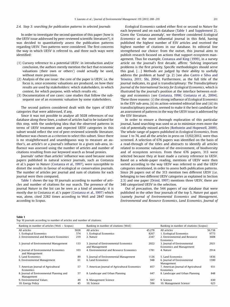
2.4. Step 3: searching for publication patterns in selected journals
In order to investigate the second question of this paper (how isthe UESV issue addressed by peer-reviewed scientific literature?), itwas decided to quantitatively assess the publication patternsregarding UESV. Two patterns were considered. The first concernsthe way in which UESV is referred to, and three such ways wereidentified:
(1) Cursory reference to a potential UESV: in introduction and/orconclusion, the authors merely mention the fact that economicvaluations (their own or others’) could actually be used,without more precision.
(2) Analysis of the use issue: the core of the paper is UESV, i.e. thefocus is, once economic valuations are produced, on how theirresults are used by stakeholders: which stakeholders, in whichcontext, for which purpose, with which results etc.
(3) Documentation of use cases: case studies that follow the sub-sequent use of an economic valuation by some stakeholders.
The second pattern considered dealt with the types of UESVcategories that were addressed, if any.
Since it was not possible to analyse all 5028 references of ourdatabase along these lines, a subset of articles had to be isolated forthis step, with the underlying idea that the observed patterns interms of UESV treatment and expected UESV categories in thissubset would reflect the rest of peer-reviewed scientific literature.Influence was chosen as a criterion to select this subset. Since thereis no straightforward and unambiguous way to measure an au-thor’s, an article’s or a journal’s influence in a given sub-area, in-fluence was assessed using the number of articles and number ofcitations resulting from our keyword search as broad proxies.
Journals’ rather than articles’ influence was used because somepapers published in natural science journals, such as Costanzaet al.’s paper in Nature (Costanza et al., 1997), were susceptible todistort the results in favour of ecological or conservation journals.The number of articles per journal and sum of citations for eachjournal were then compared.
Table 1 shows the top 10 journals according to number of arti-cles and number of citations for our search. The presence of thejournal Nature in the list can be seen as a kind of anomaly: it ismostly due to Costanza et al.’s paper (Costanza et al., 1997) whichwas, alone, cited 2282 times according to WoS and 2847 timesaccording to Scopus.
Ecological Economics ranked either first or second to Nature foreach keyword and on each database (Table 1 and Supplement 2).Given the ‘Costanza anomaly’, we therefore considered EcologicalEconomics as the most influential journal in this field, havingpublished the highest number of ESV articles and received thehighest number of citations in our database. Its editorial linestrengthened our choice: from the outset, this journal aims topublish research focused on actions that support ecosystem man-agement. Thus for example, Costanza and King (1999), in a surveyarticle on the journal’s first decade, affirm: ‘Solving importantproblems is the first priority. Specific methodologies should servethis goal. [.] Methods are judged by their ability to usefullyaddress the problem at hand’ (p. 2) (see also Castro e Silva andTeixeira, 2011; Shi, 2004). Furthermore, as the full title of thejournal indicates, its goal is transdisciplinary: The TransdisciplinaryJournal of the International Society for Ecological Economics, which isillustrated by the journal’s position at the interface between ecol-ogy and economics (see Costanza, 1996; Costanza et al., 2004).These three reasons: (i) the strong influence of Ecological Economicsin the ESV sub-area, (ii) its action-oriented editorial line and (iii) itstransdisciplinary position, seemed to make it the best candidate foran assessment of patterns in theway the UESV issue is addressed bythe ESV literature.
In order to ensure a thorough exploration of this particularjournal, hand searching was used so as to minimize even more therisk of potentially missed articles (Rothstein and Hopewell, 2009).The whole range of papers published in Ecological Economics, fromissue 1 to 74, and all the articles in press on 13/02/2012, were thusscreened. A selection of 676 papers was identified on the basis ofa read-through of the titles and abstracts to identify all articlesrelated to economic valuation of the environment, of biodiversityand of ecosystem services. From these 676 papers, 313 wereselected because they at least made a cursory reference to UESV.Based on a whole-paper reading, mentions of UESV were thensorted according to the way UESV was referred to and the UESVcategories mentioned, in order to assess both publication patterns.Since 26 papers out of the 313 mention two different UESV (i.e.belonging to two different UESV categories as explained in Section2.3) and one paper (Driml, 1997) mentions three UESV, there are340 categorized UESV in the selection.
Out of precaution, the 544 papers of our database that werepublished in the other four journals of the top 5, Nature put apart(namely Journal of Environmental Economics and Management,Environmental and Resource Economics, Land Economics, Journal of
Table 1Top 10 journals according to number of articles and number of citations.
Ranking in number of articles (WoS þ Scopus) Ranking in number of citations (WoS) Ranking in number of citations (Scopus)
All articles 5028 All articles 45,278 All articles 56,7381. Ecological Economics 574 1. Ecological Economics 8267 1. Ecological Economics 97732. Environmental and Resource Economics 219 2. Nature 2347 2. Environmental and Resource
Economics3608
3. Journal of Environmental Management 133 3. Journal of Environmental Economicsand Management
2022 3. Journal of EnvironmentalEconomics and Management
2921
4. Journal of Environmental Economicsand Management
103 4. Environmental and Resource Economics 1781 4. Nature 2914
5. Land Economics 89 5. Journal of Environmental Management 1126 5. Land Economics 18366. Environmental Management 61 6. Land Economics 948 6. Journal of Environmental
Management1590
7. American Journal of AgriculturalEconomics
57 7. American Journal of Agricultural Economics 857 7. American Journal of AgriculturalEconomics
931
8. Journal of Environmental Planning andManagement
57 8. Landscape and Urban Planning 647 8. Landscape and Urban Planning 848
9. Environmental Values 49 9. Management Science 597 9. Science 63010. Energy Policy 45 10. Science 596 10. Management Science 623
Y. Laurans et al. / Journal of Environmental Management 119 (2013) 208e219 211
Environmental Management) were screened (whole paper screen-ing) for a qualitative assessment of the first pattern (the way inwhich UESV is referred to). The result of this screening is brieflydiscussed as well in Section 3.2.
3. Results
3.1. Expected uses of ESV: a synthetic typology
As explained in Section 2.3, a first result is the construction ofcategories of UESV based on three peer-reviewed articles (Navrudand Pruckner, 1997; Pearce and Seccombe-Hett, 2000; Liu et al.,2010) and five references from the grey literature (Navrud, 2001;Pearce, 2001; an anonymous chapter in OECD, 2002; NRC, 2005;SCBD, 2007). This typology is synthetic in that it synthesizes het-erogeneous categories scattered in the literature. We distinguishbetween three main categories of UESV depending onwhether ESVis considered as being primarily decisive, technical, or informative,and eight sub-categories.
3.1.1. Decisive UESV (for a specific decision)This first category involves cases where the valuation is meant
to inform a specific decision. Here ESV can be seen as contributingto a process in which a given choice is to be made, ex ante, bya decision-maker facing alternatives. These options may involvea project or a policy, such as a regulatory proposal to be examined.It is then up to the ESV, when incorporated into a cost-benefitanalysis (CBA), to provide elements on the opportunity of theproject/policy and its economic consequences with regard to eco-system services, thus enabling an informed choice.
Within this category, three sub-categories of UESV can bedistinguished.
3.1.1.1. ESV for trade-offs. By proposing a monetary value for eco-system services, ESV can aim at helping to factor related concernsinto the CBA that are underpinning decision-makers’ trade-offs.The CBA process is formalized quite precisely: ‘CBA is charac-terized by a fairly strict decision making structure that includesdefining the project, identifying impacts that are economicallyrelevant, physically quantifying impacts as benefits or costs, andthen calculating a summary monetary valuation’ (Liu et al., 2010).This analysis may then be applied to all types of trade-offs about,for instance, programmes, laws and investment projects. In thisrespect, the purpose of the ESV is to enable the decision-maker tooptimize social well-being by making choices that balance outpreference criteria.
3.1.1.2. Participative ESV. Another approach considers economicanalysis as a ‘negotiation language’ (Henry, 1984, 1989). Here ESV isstill potentially ‘decisive’, and still intervenes ex ante as a decision-making tool. However, instead of providing a comprehensive rangeof choices that reflect a socially optimal decision, it is rather seen asa basis for discussion: through an open debate on ESV parametersand assumptions, stakeholders negotiate and define a project thatis adjusted and enhanced in terms of compromise and the sum ofinterests. OECD (2001) gives such an example with a disputedtransfer of ecosystem values in Oregon (see also Pearce andSeccombe-Hett, 2000; SCBD, 2007). Of course, this does meanthat such UESV is limited to ESVs based on benefit transfers.
3.1.1.3. ESV as a criterion for environmental management.Within limited budgets allocated to ecosystem services protection,ESV can also help prioritizing conservation efforts within an orga-nization, in an optimal way. It can facilitate the identification ofoptions most likely to maximize benefits, or of territories that
contribute most to ecosystem services. Investment priorities maythen be defined in accordance. ESV as a management criterion, or‘management tool’ (Pearce and Seccombe-Hett, 2000), differs fromthe ‘trade-off’ sub-category in that it concerns only a specificorganisation, and does not entail a choice among wide policy andsocial priorities.
3.1.2. “Technical” UESV (for the design of an instrument)This second category involves those cases where ESV is applied
after the choice of a policy or project, to adjust the economic in-strument that will implement the decision. It covers two possibletypes of UESV.
3.1.2.1. ESV for establishing levels of damage compensation.Agents responsible for ecosystem services degradation can beobliged to pay compensation for such damage. This compensationmay be a priori (i.e. compensating the anticipated effect of anoperation), or a posteriori (i.e. remediating damages caused by anaccident) (Burlington, 2004). In this case, ESV provides guidance foradministrative decisions or court rulings that determine theamounts to be paid out (see OECD, 2002).
3.1.2.2. ESV for price-setting. In cases where an economic instru-ment has been decided, ESV can be used to determine the amountspayable on the basis of a willingness-to-pay or willingness-to-receive logic: payments made by the beneficiaries of services inthe case of Payments for Ecosystem Services, entrance fees toprotected areas, etc. ESV can also help to set prices that allow ex-ternalities to be internalized, for example by factoring environ-mental costs into the price of a product (such as energy). This is therole discussed by Navrud and Pruckner (1997) when they mentionESV as ‘environmental costing’.
3.1.3. Informative UESV (for decision-making in general)Aside from its decisive and technical role, ESV can also be seen
as a means to provide information intended to have an indirectinfluence on decision-making, considered in a very broad sense. Forinstance, this is the type of UESV formulated by Fisher et al. (2008)when they report some of the responses given by ESV authorswhom they questioned on the expected uses of their works: ‘(1)distributing the research results to policy agents (.); (2) directlyinforming and engaging policy agents; (3) providing influentialsupport for current conservation initiatives’ (p. 2063). In this case,the expectation is not that ESV determine a choice with respect toa specific decision, but rather that it contribute to discussions,progressively modify viewpoints, demonstrate the interest of cer-tain policy directions or, in other words, have some sway. OECD(2001) defines this role in the following way: ‘Regardless of itsshortcomings, economic valuation plays an important role in edu-cating decision-makers about biodiversity benefits .’ (p. 20).
This category of UESV has three sub-categories.
3.1.3.1. ESV for awareness-raising. Informative ESV may be seen asthe vector for a broad message concerning the preferences thatshould be mainstreamed into society, particularly to ensure thatecosystem services considerations are integrated into public andprivate choices. Pearce (2001) and Daily et al. (2009), for example,basically consider that any ESV is a form of ‘advocacy’. Costanzaet al. (1997) launch the debate on their findings by stating that‘what this study makes abundantly clear is that ecosystem servicesprovide an important portion of the total contribution to humanwelfare on this planet. We must begin to give the natural capitalstock that produces these services adequate weight in the decision-making process, otherwise current and continued future humanwelfare may drastically suffer’ (p. 259). Gómez-Baggethun et al.
Y. Laurans et al. / Journal of Environmental Management 119 (2013) 208e219212
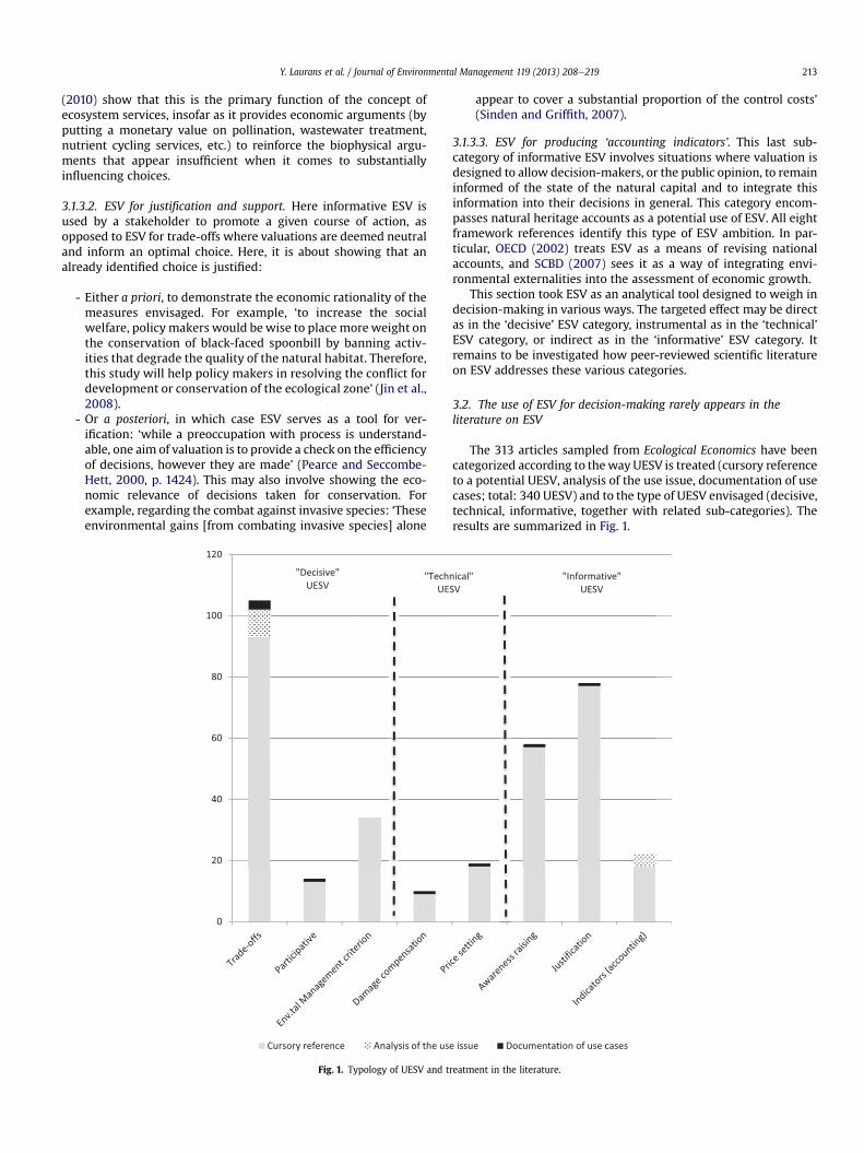
(2010) show that this is the primary function of the concept ofecosystem services, insofar as it provides economic arguments (byputting a monetary value on pollination, wastewater treatment,nutrient cycling services, etc.) to reinforce the biophysical argu-ments that appear insufficient when it comes to substantiallyinfluencing choices.
3.1.3.2. ESV for justification and support. Here informative ESV isused by a stakeholder to promote a given course of action, asopposed to ESV for trade-offs where valuations are deemed neutraland inform an optimal choice. Here, it is about showing that analready identified choice is justified:
- Either a priori, to demonstrate the economic rationality of themeasures envisaged. For example, ‘to increase the socialwelfare, policy makers would be wise to place moreweight onthe conservation of black-faced spoonbill by banning activ-ities that degrade the quality of the natural habitat. Therefore,this study will help policy makers in resolving the conflict fordevelopment or conservation of the ecological zone’ (Jin et al.,2008).
- Or a posteriori, in which case ESV serves as a tool for ver-ification: ‘while a preoccupation with process is understand-able, one aim of valuation is to provide a check on the efficiencyof decisions, however they are made’ (Pearce and Seccombe-Hett, 2000, p. 1424). This may also involve showing the eco-nomic relevance of decisions taken for conservation. Forexample, regarding the combat against invasive species: ‘Theseenvironmental gains [from combating invasive species] alone
appear to cover a substantial proportion of the control costs’(Sinden and Griffith, 2007).
3.1.3.3. ESV for producing ‘accounting indicators’. This last sub-category of informative ESV involves situations where valuation isdesigned to allow decision-makers, or the public opinion, to remaininformed of the state of the natural capital and to integrate thisinformation into their decisions in general. This category encom-passes natural heritage accounts as a potential use of ESV. All eightframework references identify this type of ESV ambition. In par-ticular, OECD (2002) treats ESV as a means of revising nationalaccounts, and SCBD (2007) sees it as a way of integrating envi-ronmental externalities into the assessment of economic growth.
This section took ESV as an analytical tool designed to weigh indecision-making in various ways. The targeted effect may be directas in the ‘decisive’ ESV category, instrumental as in the ‘technical’ESV category, or indirect as in the ‘informative’ ESV category. Itremains to be investigated how peer-reviewed scientific literatureon ESV addresses these various categories.
3.2. The use of ESV for decision-making rarely appears in theliterature on ESV
The 313 articles sampled from Ecological Economics have beencategorized according to theway UESV is treated (cursory referenceto a potential UESV, analysis of the use issue, documentation of usecases; total: 340 UESV) and to the type of UESV envisaged (decisive,technical, informative, together with related sub-categories). Theresults are summarized in Fig. 1.
Fig. 1. Typology of UESV and treatment in the literature.
Y. Laurans et al. / Journal of Environmental Management 119 (2013) 208e219 213

The main result of this analysis is the paucity of papers thatdescribe, through a case study, how a specific ESV has playeda role in a decision. Only eight such occurrences were identified,representing 2% of mentioned UESV in Ecological Economics(reported cases are numbered here, not papers). Among thoseeight occurrences of UESV, three are from papers specificallydevoted to analysing how ESV was used (the other five are frompapers that deal with the topic along with other subjects).Gowan et al. (2006) examine ‘the role and contribution of eco-nomic analysis, and specifically ecosystem valuation, in a prece-dent-setting dam removal case’ on the Elwha River in the stateof Washington. They conclude that ‘ecosystem valuation playeda minor role in the decision to remove the Elwha dams andparticipants in hydropower relicensing decisions in general donot rely on valuation studies to decide levels of ecosystem en-hancements’. Henry (1989) reports the case of a harbour exten-sion project in the Netherlands: after eliminating ‘from thebeginning ecologically unacceptable proposals without any needof further examination’, authorities ‘judged each ecologicallyacceptable plan on the basis of an economic assessment of all thecosts and benefits that could possibly be evaluated in monetaryterms e including those damages to the natural environmentwhich, without being drastic, should nevertheless be taken intoaccount’. The result was that none of the extension options thatdid not seriously harm the natural environment was econom-ically viable. Last, Rival (2010) explores the Ecuadorian Yasuni-ITT initiative and ‘the delight with which individuals andgroups with little prior knowledge of economics are ready tocrunch numbers. Such willingness to enter calculations usuallyassociated with experts may be related to the fact that the pro-posal has opened a democratic space in which the country’seconomic future may be debated and the calculations made byprofessional economists and government planners examined andchallenged.’
In addition, the results of our review indicate that, for themost part, UESV receives no more than a cursory reference in theform of an expected, proposed or desired use (e.g. Brander et al.,2007 is archetypical of this treatment of UESV). These simplementions of an expected use often envisage an informative use inthe form of general advocacy to protect biodiversity and eco-system services or to justify conservation choices (e.g. Amirnejadet al., 2006; Biao et al., 2010). Alternatively, they envisage thevaluation as enabling decision-makers to decide on generaltrade-offs (but in this case without identifying a specific decisionwith its related context and criteria) and, more particularly, togive the preservation of ecosystem services some weight, overall,alongside other economic and social objectives (e.g. Barbier,2000; Casey et al., 2006).
As indicated in Section 2.4, out of precaution we also screened(whole paper screening) the 544 ESV papers of our database thatwere published in the other four journals of the top 5, Nature putapart (namely Journal of Environmental Economics and Manage-ment, Environmental and Resource Economics, Land Economics,Journal of Environmental Management). Although a mere qual-itative assessment of the first pattern (the way in which UESV isreferred to), this screening confirms that the vast majority ofstudies that address UESV do so only in a cursory way. Based onthe representativeness of Ecological Economics for the ESV sub-area, and on this complementary screening, we suggest that thispattern is likely to be widespread in the entire peer-reviewedscientific literature.
The following section examines possible explanations for thediscrepancy between expectations and available information onUESV, and explores research avenues that such explanationsopen up.
4. Discussion: possible explanations to the literature patternsobserved and avenues for research
Three preliminary remarks on the limits of our review arenecessary:
- First, the keywords we used were unavoidably arbitrary. Theymatch the authors’ culture in economy, ecology, managementand political sciences, but it cannot be excluded that articles inother disciplines such as sociology, ethnology or psychologymay deal with similar concerns (i.e. UESV) with differentwords. The only assumption that can be made is that such ar-ticles, if they exist, are probably few.
- Second, we did not consider grey literature in our systematicreviewe only was it taken into account to help build categoriesof UESV. It would be intuitive to assume that grey literaturemust be the ideal tool to report ESV use cases or address the useissue. However, exploring grey literature systematically wasout of reach for our research. More importantly, the grey lit-erature that was explored based on the six websites inSupplement 3 did not confirm this intuition, with still few eand often the same e cases reported. In any case a more sys-tematic endeavour would be necessary here.
- Last, a literature review, however systematic, does not replacedifferent kinds of research involving thorough analyses ofspecific decision processes to get a complementary perspectiveon if and howESV are actually used (see e.g. Gowan et al., 2006;Laurans and Aoubid, 2012).
With this in mind, the results of our review still raise thequestion of why UESV issues are so rarely addressed by the ESVpeer-reviewed scientific literature. The purpose here is not toconjecture on the most probable explanation for this result, butrather to examine a wide range of possible explanations. This isnecessary to identify the different research avenues and lay theground for subsequent work that we consider necessary. To thisend, we divided the hypotheses into two main categories: eitherthe use of ESV is a common practice, but is absent from the liter-ature selected here (Section 4.1); or the use is effectively rare(Section 4.2).
4.1. A possible bias in the selected literature
Our observations mainly apply to peer-reviewed scientific lit-erature. A first set of four hypotheses can thus be formulated,bearing in mind the general idea that such literature only paintsa partial picture of actuality.
a. UESV may be difficult to observeIt is conceivable that UESV be seldom addressed by peer-
reviewed scientific literature because the actual contexts forits use go unnoticed by ESV researchers. This is what Fisheret al. (2008) suggest: they note that by applying a ‘filter’ thatselects ‘cases where ecosystem services analysis has been anintegral part of the policy process (ex ante)’, the result turns outto be very selective, ‘since few studies in the literature makeexplicit policy linkages’ (p. 2062). UESV would then be morewidely found in practice than peer-reviewed scientific liter-ature indicates; it would generally go unnoticed in the targetedcommunity of authors, and would not appear in the results ofa keyword search, even were it to produce a vast number oftitles. This could be reinforced by a potential time lag betweeneconomic valuations, their presentation in peer-reviewed sci-entific literature, and their use for decision making. Never-theless, the time lag is unlikely to be a major source of
Y. Laurans et al. / Journal of Environmental Management 119 (2013) 208e219214
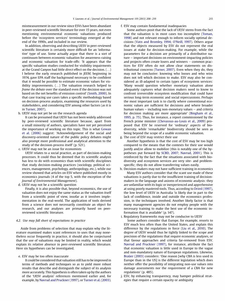
mismeasurement in our review since ESVs have been abundantin peer-reviewed scientific literature for over 15 years, not evenmentioning environmental economic valuations producedbefore the ‘ecosystem services’ terminology emerged at theend of the 1990s, and included in our review.In addition, observing and describing UESV in peer-reviewed
scientific literature is certainly more difficult for an ‘informa-tive’ type of use. Some actually argue that there is a sort ofcontinuum between economic valuation for awareness-raisingand economic valuation for trade-offs: ‘It appears that thespecific valuation studies conducted for visibility impairmentsat the Grand Canyon had little direct effect on the decision. (.)I believe the early research published in JEEM, beginning in1974, gave EPA staff the background necessary to be confidentthat it would be possible to estimate economic values for vis-ibility improvements. (.) The valuation research helped toframe the debate over the standard even if the decision was notbased on the net benefits of emission control’ (Smith, 2000). Inthat case tracing use cases takes a specific methodology basedon decision-process analysis, examining the resources used bystakeholders, and considering ESV among other factors (as it isin Turner, 2007).
b. UESV may not yet be on the research agendaIt can be presumed that UESV has not beenwidely addressed
by peer-reviewed scientific literature because, apart froma small minority of authors, specialists have not yet perceivedthe importance of working on this topic. This is what Gowanet al. (2006) suggest: ‘Acknowledgement of the social anddiscovery-oriented nature of the public policy debates mightalso prompt more professional and analytical attention to thestudy of the decision-process itself’ (p. 521).
c. UESV may not be an issue for economistsUESV relates to a social practice, as part of decision-making
processes. It could thus be deemed that its scientific analysishas less to do with economics than with scientific disciplinesthat study decision-making practices (sociology, political sci-ences, management, psychology, anthropology, etc.), while ourreview showed that articles on ESV where published mostly ineconomics journals (4 of the top 5, with the exception of theJournal of Environmental Management).
d. UESV may not be a scientific questionFinally, it is also possible that, beyond economics, the use of
valuation does not enjoy the same status as the valuation itselffrom a scientific point of view, insofar as it involves imple-mentation in the real-world. The application of tools derivedfrom a science does not necessarily constitute an object forresearch, and our analyses are primarily based on peer-reviewed scientific literature.
4.2. Use may fall short of expectations in practice
Aside from problems of selection that may explain why the lit-erature examined makes scant references to uses that may none-theless occur frequently in practice, it should also be conjecturedthat the use of valuations may be limited in reality, which wouldexplain its relative absence in peer-reviewed scientific literature.Here six hypotheses can be investigated.
e. ESV may be too often inaccurateIt couldbe considered that valuation still has to be improved in
terms of methods and techniques so as to yield more robustresults that describe and distinguish the subject of its analysismore accurately. This hypothesis is often takenupby the authorsof the ‘UESV analysis’ references mentioned earlier and, forexample, by Navrud and Pruckner (1997), or Turner et al. (2003).
f. ESV may contain fundamental inadequaciesSome authors posit that the lack of UESV stems from the fact
that the valuation is in most cases too incomplete (Toman,1998) and not relevant enough to inform socially optimal de-cisions (Vatn and Bromley, 1994; O’Neill, 1997). Others arguethat the objects measured by ESV do not represent the realissues at stake for decision-making. For example, while theparameters for a decision are primarily of a distributive na-ture e important decisions on environment-impacting policiesand projects often create losers and winners e common prac-tices for ESV often do not allow clear statements on dis-tributional concerns (Turner, 2007). Even when they do, theymay not be conclusive: knowing who looses and who winsdoes not tell which decision to make. ESV may also be con-sidered as ill-adapted to certain types of ecosystem services:‘Many would question whether monetary valuation aloneadequately captures what decision makers need to know toconfront irreversible ecosystem modification that could haveserious long-term economic and social repercussions. Perhapsthe most important task is to clarify where conventional eco-nomic values are sufficient for decisions and where broaderhuman values e including non-monetary values e and criteriafor decision making are more appropriate’ (Bingham et al.,1995, p. 75). Thus, for instance, a report commissioned by theFrench prime minister (Chevassus-au-Louis et al., 2009) pro-posed that ESV be reserved for ‘ordinary’ aspects of bio-diversity, while ‘remarkable’ biodiversity should be seen asbeing beyond the scope of a usable economic valuation.
g. The cost of ESV may restrict their useAnother hypothesis is that the cost of ESV may be too high
compared to the means that the contexts for their use wouldjustify and/or allow to mobilize (this is notably one of the hy-potheses put forward by SCBD, 2007; Navrud, 2001). This isreinforced by the fact that the situations associated with bio-diversity and ecosystem services are very site- and problem-specific; they do not allow transferring values easily.
h. Decision-makers may not have sufficient training in economicsMany ESV authors consider that the scant use made of these
valuations is partly due to the insufficient training of decision-makers in the language and axioms of economic analysis: theyare unfamiliar with its logic or inexperienced and apprehensiveat using poorly mastered tools. Thus, according to Driml (1997),the low level of UESV in Australia ‘is likely due in part to thelack of confidence, inside and outside the economics profes-sion, in the techniques involved. Another likely factor is thatmany management agencies do not employ people with thenecessary training to make the best use of the economic in-formation that is available’ (p. 147).
i. Regulatory frameworks may not be conducive to UESVSome authors consider that Europe, for example, resorts to
ESV much less often than the United States, and explain thisdifference by the regulations in force (Liu et al., 2010). Thedegree of UESV would thus be tightly linked to the scope andprecision of the regulations that require economic analyses, orthat favour approaches and criteria far-removed from ESV.Navrud and Pruckner (1997), for instance, attribute the factthat economic valuation is little used in Europe to the vagueand non-mandatory nature of European regulations. Likewise,Braüer (2003) considers: ‘One reason [why CBA is less used inEurope than in the US] is the different legislation which doesneither offer the possibility of integrating non-use values intodamage assessments nor the requirement of a CBA for newregulations’ (p. 485).
j. ESV, by enhancing transparency, may hamper political strat-egies that require a certain opacity or ambiguity
Y. Laurans et al. / Journal of Environmental Management 119 (2013) 208e219 215
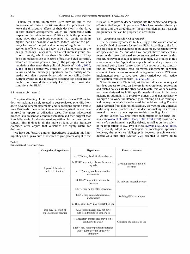
Finally for some, unintensive UESV may be due to thepreference of certain decision-makers for processes thatleave the distributive effects of their decisions in the dark,or that obscure arrangements which are indefensible withrespect to the public interest: ‘Politics affects the process inmany ways that can block outcomes that would result inhigher levels of economic welfare. Indeed, one of the pri-mary lessons of the political economy of regulation is thateconomic efficiency is not likely to be a key objective in thedesign of policy. Policy ideas can affect interest group po-sitions directly, which can then affect the positions of keydecision makers (such as elected officials and civil servants),who then structure policies through the passage of laws andregulations that meet their political objectives’ (Hahn, 2000,p. 18). In this perspective, limits on UESV mirrors politicalfailures, and are inversely proportional to the quality of theinstitutions that support democratic accountability. Socio-cultural evolution and increasing pressures for better use ofpublic funds would then slowly lead to more favourableconditions for UESV.
4.3. Avenues for research
The pivotal finding of this review is that the issue of ESV use fordecision-making is rarely treated in peer-reviewed scientific liter-ature beyond general statements and suggestions about possibleuses. This holds true whether it involves an analysis of the use issuein itself, or reports of utilization cases. The most widespreadpractice is to present an economic valuation and then suggest thatit could be useful for decision-making with no further precision orcontext. This finding is all the more striking as the literatureexamined often argues that valuations are highly useful fordecisions.
We have put forward different hypotheses to explain this find-ing. They open up avenues of research to give greater weight to the
issue of UESV, provide deeper insight into the subject and step upefforts to find ways to improve use. Table 2 summarises these hy-potheses and the three distinct though complementary researchprogrammes that can be proposed in accordance.
4.3.1. Creating a specific field of researchThe first three hypotheses (a, b, c) suggest the construction of
a specific field of research focused on UESV. According to the firstone, this field of research needs to be explored by researchers whoare specialized in ESV, but who have not yet shown sufficient in-terest in this area and need to be encouraged to do so. In thisrespect, however, it should be noted that many ESV studied in thisreview were in fact ‘applied’ to a specific site and a precise envi-ronmental policy issue (conservation of a species or area, combat-ting an invasive species, etc.). Moreover, experiments in whicheconomic tools for environmental management such as PES wereimplemented seem to have been often carried out with activeparticipation from economists (Liu et al., 2010).
Scientific work on ESV is not just theoretical or methodologicalbut does appear to show an interest in environmental protectionand related policies. On the other hand, to date, this work has oftennot been designed to fulfill specific needs of specific decision-makers. In addition, it is probably difficult, and not necessarilysynergetic, to work simultaneously on refining an ESV techniqueand on ways in which it can be used for decision-making. Encour-aging research from different disciplinary viewpoints and aimed ataddressing social practices such as decision-making in environ-mental matters may be a response to this stumbling block.
As per Section 3.2, only three publications of Ecological Eco-nomics (Gowan et al., 2006; Henry, 1989; Rival, 2010) focus on theterms of an environmental policy debate, as well as on the analysisof the implications of ESV. Two of these (Gowan et al., 2006; Rival,2010) mainly adopt an ethnological or sociological approach.However, the extensive bibliographic keyword search we con-ducted as a first step (Section 2.2), oriented us above all to
Table 2Hypotheses and research avenues.
Categories of hypotheses Hypotheses Research avenues
A possible bias in the selected literature
a. UESV may be difficult to observe
Creating a specific field of research
b. UESV may not yet be on the research agenda
c. UESV may not be an issue for economists
d. UESV may not be a scientific question No relevant research avenue
Use may fall short of expectations in practice
e. ESV may be too often inaccurate
Refining ESV techniquesf. ESV may contain fundamental inadequacies
g. The cost of ESV may restrict their use
h. Decision-makers may not have sufficient training in economics
Changing the context of usei. Regulatory frameworks may not be
conducive to UESV
j. ESV may hamper political strategies that require a certain opacity or
ambiguity
Y. Laurans et al. / Journal of Environmental Management 119 (2013) 208e219216
economics journals and did not provide any clues as to whether thesubject of UESV was substantially dealt with by other disciplinaryfields or types of journals. Thus economic ethnology, for example,which observes people’s economic behaviour, has not yet shownmuch interest in public decision-making, and even less in theenvironmental field (Weber, 2001; Strathern, 2000; Gudeman,2009). It is thus by calling for collaboration with disciplines suchas these that a deeper insight into UESV could be gained.
Hypothesisd (UESV isnota scientificquestion) is theonlyonethatdoes not open up an avenue for research. It is certainly consistentwith the scant attention given to the topic inpeer-reviewed scientificliterature, andwithaproposal thatwould limit thesubject to apurelyoperational and practical issue. Yet, it seems difficult to argue thata social practice could not be the subject of scientific investigation.
4.3.2. Refining ESV techniquesHypotheses e, f and g assume that future developments of ESV
methodology will help to substantially improve its use. In thisperspective, research can engage in two opposite directions. Onedirection can target a certain ‘standardization’ of ESV techniques soas to generalize valuations and reduce their costs. ‘Value transfer’ isone of the responses envisaged by ESV authors (Loomis andRosenberger, 2006). Yet value transfer renders the results lessrobust and less conclusive, as well as applicable only to issues thatare not overly site-specific, which limits its scope (Brouwer, 2000).In other words, it is highly unlikely that standardizing the dataunderpinning valuations will allow them to be more frequentlyused for decision-making, since their conclusiveness for specificdecisions would be impaired.
In the opposite direction, research could be oriented to broadenthe ESV field, or ensure more precise studies, particularly in view of‘decisive’ and ‘technical’ uses. It should however be noted that thefew UESV cases reported do not evidence a greater precision of ESVthan in other references. In all events, it is foreseeable that refiningESV studies would make the exercise more costly and thus moredifficult to extend for ‘decisive’ and ‘technical’ use, which are bothinherently topic- and scale-specific. We are thus faced with a ten-sion between two strategies: either standardize ESV to make themmore accessible, at the risk of also making them less usable fordecisive purposes; or seek to refine ESV for decisive or technicaluse, at the risk of raising their cost.
4.3.3. Changing the context of useThe last three hypotheses (h, i, j) involve targeting, or at least
hoping for, a change in users or in their operational context, ratherthan a change in valuations themselves. This implies for exampletraining decision-makers to use ESV more effectively, adjustinglaws and regulations to promote their use and reduce obstacles, orimproving decision-makers’ drive for transparency.
This prospect first seems at odds with one of the postulatesunderpinning the current enthusiasm for ESV, which assumes thatdecision-makers position themselves prioritarily on the basis ofeconomic criteria. As one author advocating concrete application ofESV writes: ‘Economics is there first, and all must speak its lan-guage seriously, at least some of the time, or be cut out of crucialparts of the debate’ (Herendeen, 1998, p. 30). Secondly, when reg-ulations provide for a CBA ahead of public decisions, as in the USA,the factoring in of ESV still seems to be far from satisfactory (Ruhlet al., 2007). Finally, it is indisputable that economic analysis canbe assigned the role of revealing the inadequacies of a political oradministrative decision-making process, as is shown in mostdemocratic countries by the use of ex-post economic valuationsconducted by auditing authorities. Yet, while auditing has existedfor many years, economists’ criticism of the reasoning behindpublic decisions has not abated (Hahn, 2000). All in all, changing
the context of use does not appear to be consistent with anapproach that, as Liu et al. (2010) suggest, would rather aim toadapt the tools to the problems.
5. Conclusion
ESV are abundantly produced and disseminated within thecurrent trend of a utilitarian view of the environment. Theseeconomic valuations are therefore promoted on the assumptionthat they respond to decision-makers’ needs and/or that they helpguiding decisions towards more and better conservation. Thepositive economic impacts of maintaining or increasing ecosystemservices is demonstrated and taken into account; as are, con-versely, the negative economic impacts of their degradation ordestruction.
Our research aimed to explore the theoretical assumptions andempirical bases that underlay this hypothesis, and to examine towhat extent there is evidence that UESV matches stated expecta-tions. Our systematic literature review shows that the issue of use isoverwhelmingly orphaned in peer-reviewed scientific literature onESV, with few exceptions. The common rule is to present an eco-nomic valuation, then suggest that it be used for decision-making,but without this use being either explicited or contextualized, andwithout concrete examples being provided nor analysed.
The next step was to develop hypotheses resulting from thisfinding. They suggest multiple avenues for research. These hy-potheses can be combined to explain the literature blindspot and/or the shortcomings of UESV to date. Evidence provided by theliterature review leads to the conclusion that: (1) the vast majorityof ESV are produced in a ‘supply-side logic’; (2) it is thus uncertainthat the type of tools offered to potential users are the best matchfor real decision-making needs; and (3) ESV is primarily gearedtowards an informative role for general influence and awareness-raising.
More broadly, and if all of the aforementioned hypotheses aretaken into account to explain the relative absence of UESV in peer-reviewed scientific literature, it seems vital that the problem ofusing economic valuations be made a priority issue for research.To achieve this, many barriers must be overcome, existingresearch on this issue must be stepped up and new avenues ofresearch opened up.
The paucity of UESV in peer-reviewed scientific literature is notonly a puzzle that needs clarifying through further research but alsoa major concern for biodiversity and ecosystem services. Certainly,if decision-making processes fail to use ESV, economic valuationcould lead to the type of disillusionment against which Redford andAdams (2009) give us due warning: ‘conservation has a history ofplacing great faith in new ideas and approaches that appear to offerdramatic solutions to humanity’s chronic disregard for nature ...only to become disillusionedwith them a few years later’ (p. 785). IfESV are supposed to be a decisive key for action, it hardly seemsreasonable to sideline for much longer the question of the use ofvaluations that occupy a central place in today’s discourse, thinkingand debate around conservation.
Acknowledgements
The authors would like to thank the Fondation d’EntrepriseHermès for supporting the project within which the presentresearch was conducted, as well as five interns for their preciouscontributions (Schéhérazade Aoubid, Joshua Berger, AlexandreHaddad, Benoît Othoniel, Marine Seilles) and Pierre Barthélemy forhis careful proofreading. Comments received from four anonymousreviewers were also immensely helpful.
Y. Laurans et al. / Journal of Environmental Management 119 (2013) 208e219 217
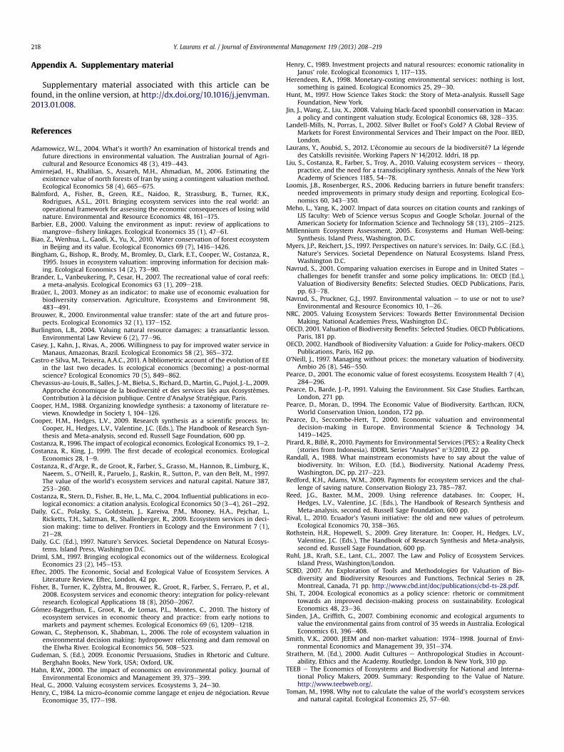
Appendix A. Supplementary material
Supplementary material associated with this article can befound, in the online version, at http://dx.doi.org/10.1016/j.jenvman.2013.01.008.
References
Adamowicz, W.L., 2004. What’s it worth? An examination of historical trends andfuture directions in environmental valuation. The Australian Journal of Agri-cultural and Resource Economics 48 (3), 419e443.
Amirnejad, H., Khalilian, S., Assareh, M.H., Ahmadian, M., 2006. Estimating theexistence value of north forests of Iran by using a contingent valuation method.Ecological Economics 58 (4), 665e675.
Balmford, A., Fisher, B., Green, R.E., Naidoo, R., Strassburg, B., Turner, R.K.,Rodrigues, A.S.L., 2011. Bringing ecosystem services into the real world: anoperational framework for assessing the economic consequences of losing wildnature. Environmental and Resource Economics 48, 161e175.
Barbier, E.B., 2000. Valuing the environment as input: review of applications tomangroveefishery linkages. Ecological Economics 35 (1), 47e61.
Biao, Z., Wenhua, L., Gaodi, X., Yu, X., 2010. Water conservation of forest ecosystemin Beijing and its value. Ecological Economics 69 (7), 1416e1426.
Bingham, G., Bishop, R., Brody, M., Bromley, D., Clark, E.T., Cooper, W., Costanza, R.,1995. Issues in ecosystem valuation: improving information for decision mak-ing. Ecological Economics 14 (2), 73e90.
Brander, L., Vanbeukering, P., Cesar, H., 2007. The recreational value of coral reefs:a meta-analysis. Ecological Economics 63 (1), 209e218.
Braüer, I., 2003. Money as an indicator: to make use of economic evaluation forbiodiversity conservation. Agriculture, Ecosystems and Environment 98,483e491.
Brouwer, R., 2000. Environmental value transfer: state of the art and future pros-pects. Ecological Economics 32 (1), 137e152.
Burlington, L.B., 2004. Valuing natural resource damages: a transatlantic lesson.Environmental Law Review 6 (2), 77e96.
Casey, J., Kahn, J., Rivas, A., 2006. Willingness to pay for improved water service inManaus, Amazonas, Brazil. Ecological Economics 58 (2), 365e372.
Castro e Silva, M., Teixeira, A.A.C., 2011. A bibliometric account of the evolution of EEin the last two decades. Is ecological economics (becoming) a post-normalscience? Ecological Economics 70 (5), 849e862.
Chevassus-au-Louis, B., Salles, J.-M., Bielsa, S., Richard, D., Martin, G., Pujol, J.-L., 2009.Approche économique de la biodiversité et des services liés aux écosystèmes.Contribution à la décision publique. Centre d’Analyse Stratégique, Paris.
Cooper, H.M., 1988. Organizing knowledge synthesis: a taxonomy of literature re-views. Knowledge in Society 1, 104e126.
Cooper, H.M., Hedges, L.V., 2009. Research synthesis as a scientific process. In:Cooper, H., Hedges, L.V., Valentine, J.C. (Eds.), The Handbook of Research Syn-thesis and Meta-analysis, second ed. Russell Sage Foundation, 600 pp.
Costanza, R., 1996. The impact of ecological economics. Ecological Economics 19, 1e2.Costanza, R., King, J., 1999. The first decade of ecological economics. Ecological
Economics 28, 1e9.Costanza, R., d’Arge, R., de Groot, R., Farber, S., Grasso, M., Hannon, B., Limburg, K.,
Naeem, S., O’Neill, R., Paruelo, J., Raskin, R., Sutton, P., van den Belt, M., 1997.The value of the world’s ecosystem services and natural capital. Nature 387,253e260.
Costanza, R., Stern, D., Fisher, B., He, L., Ma, C., 2004. Influential publications in eco-logical economics: a citation analysis. Ecological Economics 50 (3e4), 261e292.
Daily, G.C., Polasky, S., Goldstein, J., Kareiva, P.M., Mooney, H.A., Pejchar, L.,Ricketts, T.H., Salzman, R., Shallenberger, R., 2009. Ecosystem services in deci-sion making: time to deliver. Frontiers in Ecology and the Environment 7 (1),21e28.
Daily, G.C. (Ed.), 1997. Nature’s Services. Societal Dependence on Natural Ecosys-tems. Island Press, Washington D.C.
Driml, S.M., 1997. Bringing ecological economics out of the wilderness. EcologicalEconomics 23 (2), 145e153.
Eftec, 2005. The Economic, Social and Ecological Value of Ecosystem Services. ALiterature Review. Eftec, London, 42 pp.
Fisher, B., Turner, K., Zylstra, M., Brouwer, R., Groot, R., Farber, S., Ferraro, P., et al.,2008. Ecosystem services and economic theory: integration for policy-relevantresearch. Ecological Applications 18 (8), 2050e2067.
Gómez-Baggethun, E., Groot, R., de Lomas, P.L., Montes, C., 2010. The history ofecosystem services in economic theory and practice: from early notions tomarkets and payment schemes. Ecological Economics 69 (6), 1209e1218.
Gowan, C., Stephenson, K., Shabman, L., 2006. The role of ecosystem valuation inenvironmental decision making: hydropower relicensing and dam removal onthe Elwha River. Ecological Economics 56, 508e523.
Gudeman, S. (Ed.), 2009. Economic Persuasions, Studies in Rhetoric and Culture.Berghahn Books, New York, USA; Oxford, UK.
Hahn, R.W., 2000. The impact of economics on environmental policy. Journal ofEnvironmental Economics and Management 39, 375e399.
Heal, G., 2000. Valuing ecosystem services. Ecosystems 3, 24e30.Henry, C., 1984. La micro-économie comme langage et enjeu de négociation. Revue
Economique 35, 177e198.
Henry, C., 1989. Investment projects and natural resources: economic rationality inJanus’ role. Ecological Economics 1, 117e135.
Herendeen, R.A., 1998. Monetary-costing environmental services: nothing is lost,something is gained. Ecological Economics 25, 29e30.
Hunt, M., 1997. How Science Takes Stock: the Story of Meta-analysis. Russell SageFoundation, New York.
Jin, J., Wang, Z., Liu, X., 2008. Valuing black-faced spoonbill conservation in Macao:a policy and contingent valuation study. Ecological Economics 68, 328e335.
Landell-Mills, N., Porras, I., 2002. Silver Bullet or Fool’s Gold? A Global Review ofMarkets for Forest Environmental Services and Their Impact on the Poor. IIED,London.
Laurans, Y., Aoubid, S., 2012. L’économie au secours de la biodiversité? La légendedes Catskills revisitée. Working Papers N"14/2012. Iddri, 18 pp.
Liu, S., Costanza, R., Farber, S., Troy, A., 2010. Valuing ecosystem services e theory,practice, and the need for a transdisciplinary synthesis. Annals of the New YorkAcademy of Sciences 1185, 54e78.
Loomis, J.B., Rosenberger, R.S., 2006. Reducing barriers in future benefit transfers:needed improvements in primary study design and reporting. Ecological Eco-nomics 60, 343e350.
Meho, L., Yang, K., 2007. Impact of data sources on citation counts and rankings ofLIS faculty: Web of Science versus Scopus and Google Scholar. Journal of theAmerican Society for Information Science and Technology 58 (13), 2105e2125.
Millennium Ecosystem Assessment, 2005. Ecosystems and Human Well-being:Synthesis. Island Press, Washington, D.C.
Myers, J.P., Reichert, J.S., 1997. Perspectives on nature’s services. In: Daily, G.C. (Ed.),Nature’s Services. Societal Dependence on Natural Ecosystems. Island Press,Washington D.C.
Navrud, S., 2001. Comparing valuation exercises in Europe and in United States echallenges for benefit transfer and some policy implications. In: OECD (Ed.),Valuation of Biodiversity Benefits: Selected Studies. OECD Publications, Paris,pp. 63e78.
Navrud, S., Pruckner, G.J., 1997. Environmental valuation e to use or not to use?Environmental and Resource Economics 10, 1e26.
NRC, 2005. Valuing Ecosystem Services: Towards Better Environmental DecisionMaking. National Academies Press, Washington D.C.
OECD, 2001. Valuation of Biodiversity Benefits: Selected Studies. OECD Publications,Paris, 181 pp.
OECD, 2002. Handbook of Biodiversity Valuation: a Guide for Policy-makers. OECDPublications, Paris, 162 pp.
O’Neill, J., 1997. Managing without prices: the monetary valuation of biodiversity.Ambio 26 (8), 546e550.
Pearce, D., 2001. The economic value of forest ecosystems. Ecosystem Health 7 (4),284e296.
Pearce, D., Barde, J.-P., 1991. Valuing the Environment. Six Case Studies. Earthcan,London, 271 pp.
Pearce, D., Moran, D., 1994. The Economic Value of Biodiversity. Earthcan, IUCN,World Conservation Union, London, 172 pp.
Pearce, D., Seccombe-Hett, T., 2000. Economic valuation and environmentaldecision-making in Europe. Environmental Science & Technology 34,1419e1425.
Pirard, R., Billé, R., 2010. Payments for Environmental Services (PES): a Reality Check(stories from Indonesia). IDDRI, Series “Analyses” n"3/2010, 22 pp.
Randall, A., 1988. What mainstream economists have to say about the value ofbiodiversity. In: Wilson, E.O. (Ed.), Biodiversity. National Academy Press,Washington, DC, pp. 217e223.
Redford, K.H., Adams, W.M., 2009. Payments for ecosystem services and the chal-lenge of saving nature. Conservation Biology 23, 785e787.
Reed, J.G., Baxter, M.M., 2009. Using reference databases. In: Cooper, H.,Hedges, L.V., Valentine, J.C. (Eds.), The Handbook of Research Synthesis andMeta-analysis, second ed. Russell Sage Foundation, 600 pp.
Rival, L., 2010. Ecuador’s Yasuni initiative: the old and new values of petroleum.Ecological Economics 70, 358e365.
Rothstein, H.R., Hopewell, S., 2009. Grey literature. In: Cooper, H., Hedges, L.V.,Valentine, J.C. (Eds.), The Handbook of Research Synthesis and Meta-analysis,second ed. Russell Sage Foundation, 600 pp.
Ruhl, J.B., Kraft, S.E., Lant, C.L., 2007. The Law and Policy of Ecosystem Services.Island Press, Washington/London.
SCBD, 2007. An Exploration of Tools and Methodologies for Valuation of Bio-diversity and Biodiversity Resources and Functions, Technical Series n 28,Montreal, Canada, 71 pp. http://www.cbd.int/doc/publications/cbd-ts-28.pdf.
Shi, T., 2004. Ecological economics as a policy science: rhetoric or commitmenttowards an improved decision-making process on sustainability. EcologicalEconomics 48, 23e36.
Sinden, J.A., Griffith, G., 2007. Combining economic and ecological arguments tovalue the environmental gains from control of 35 weeds in Australia. EcologicalEconomics 61, 396e408.
Smith, V.K., 2000. JEEM and non-market valuation: 1974e1998. Journal of Envi-ronmental Economics and Management 39, 351e374.
Strathern, M. (Ed.), 2000. Audit Cultures e Anthropological Studies in Account-ability, Ethics and the Academy. Routledge, London & New York, 310 pp.
TEEB e The Economics of Ecosystems and Biodiversity for National and Interna-tional Policy Makers, 2009. Summary: Responding to the Value of Nature.http://www.teebweb.org/.
Toman, M., 1998. Why not to calculate the value of the world’s ecosystem servicesand natural capital. Ecological Economics 25, 57e60.
Y. Laurans et al. / Journal of Environmental Management 119 (2013) 208e219218

Turner, R.K., Paavola, J., Cooper, C., Farber, S., Jessamy, V., Georgiou, S., 2003. Valuingnature: lessons learned and future research directions. Ecological Economics46, 493e510.
Turner, R.K., 2007. Limits toCBA inUKandEuropeanenvironmental policy: retrospectsand future prospects. Environmental and Resource Economics 37, 253e269.
Van Campenhout, G., Van Caneghem, T., Van Uytbergen, S., 2008. A comparison ofoverall and sub-area journal influence: the case of the accounting literature.Scientometrics 77 (1), 61e90.
Vatn, A., Bromley, D.W., 1994. Choices without prices without apologies. Journal ofEnvironmental Economics and Management 26, 129e148.
Vihervaara, P., Rönkä, M., Walls, M., 2010. Trends in ecosystem service research:early steps and current drivers. Ambio 39 (4), 314e324.
Warner, A.M., 2010. Costebenefit Analysis in World Bank Projects. The World Bank,Washington DC.
Weber, F., 2001. Settings, interactions and things e a plea for a multi-integrativeethnography. Ethnography 2 (4), 475e499.
Y. Laurans et al. / Journal of Environmental Management 119 (2013) 208e219 219
! 211
Appendix 4
Rankovic & Billé (2013) !
!
Rankovic, A., Billé, R. (2013). Les utilisations de l’évaluation économique des services écosystémiques : un état des lieux. Études et documents, n°98. Commissariat général au développement durable, Ministère de l’Écologie, du Développement Durable et de l’Énergie.
!!

! 212
Études & documents | n°98 | Novembre 2013
8 | Commissariat général au développement durable – Service de l’économie, de l’évaluation et de l’intégration du développement durable
Aleksandar RANKOVIC et Raphaël BILLE – Les utilisations de l’évaluation économique des services écosystémiques : un état des lieux
Aleksandar RANKOVIC est diplômé en affaires internationales (IEP de Paris), en biologie et en sciences de l’environnement (Université Pierre et Marie Curie). Il réalise actuellement une thèse de doctorat en écologie au laboratoire Bioemco (unité mixte UPMC – CNRS – INRA – IRD – ENS – AgroParisTech – UPEC) dans l’équipe « Biodiversité et Fonctionnement des Écosystèmes » située à l’École Normale Supérieure. Ses travaux portent principalement sur les écosystèmes en milieu urbain et il s’intéresse également aux liens entre recherches en écologie et gestion environnementale.
Raphaël BILLE est diplômé en aménagement du territoire et en économie et est titulaire d’un doctorat de gestion de l’environnement (AgroParisTech). Il dirige depuis 2006 les programmes et équipes Biodiversité et Adaptation au changement climatique de l’Institut du Développement Durable et des Relations Internationales (IDDRI – Sciences Po). Ses domaines de prédilection concernent la gestion des zones côtières, l'économie et la gouvernance internationale de la biodiversité ainsi que l'analyse des processus de décision en matière d'environnement.
L’utilisation des évaluations économiques comme problématique centrale
De grands espoirs semblent placés dans la monétarisation pour améliorer les décisions relatives à la biodiversité et aux
écosystèmes, et ce de manière récurrente depuis de nombreuses années. Que ce soit par exemple chez l’économiste A.
Randall, qui affirmait en 1988 que « la meilleure façon de protéger la biodiversité [était] de lui affecter une valeur
économique » (Randall, 1988), chez les écologues J. Myers et J. Richert pour qui « l’on ne protège pas ce qu’on ne
valorise pas » (« we don’t protect what we don’t value », la valeur étant entendue comme économique chez les deux
auteurs ; Myers et Richert, 1997) ou plus récemment chez Pavan Sukhdev pour qui « l’économie des écosystèmes et de
la biodiversité peut contribuer de façon décisive à la sauvegarde de la biodiversité » (The Economics of Ecosystems and
Biodiversity, 2009), le constat semble unanime quant à l’utilité, voire l’obligation pragmatique, de recourir à l’étalon
monétaire pour parvenir à stopper la dégradation des écosystèmes et l’érosion de la biodiversité.
Pourtant, le caractère évident de cette intégration effective de la monétarisation et de sa contribution, prépondérante et
systématique, aux processus de décision suscite des réserves, notamment chez certains économistes. Claude Henry, par
exemple, a mis en évidence, dès les années 80, la dimension négociée des évaluations économiques environnementales
liées aux grands projets d’infrastructures (Henry, 1984, 1989). G. Heal, en 2000, souligne que « l’évaluation économique
n’est ni nécessaire ni suffisante pour la conservation. Nous conservons beaucoup de choses que nous n’évaluons pas, et
ne conservons pas de nombreuses choses que nous évaluons » (Heal, 2000). L’étude présentée ici, dont les résultats sont
regroupés dans Laurans et al. (2013), part ainsi de l’hypothèse que la monétarisation, en ce qui concerne les prises de
décision impactant les écosystèmes et la biodiversité, n’est pas suffisante en soi : pour apporter des « contributions
décisives », elle doit être effectivement utilisée dans la prise de décision.
L’approche choisie a été la réalisation d’un état de l’art structuré autour de deux grandes questions :
1. Quelles sont les utilisations attendues des évaluations économiques des services écosystémiques dans la
littérature ?
2. De quelle manière cette question est-elle traitée par la littérature ?
Le principal résultat a été la mise au jour d’un paradoxe : alors que de nombreuses utilisations sont attendues des
résultats des exercices de monétarisation, au point qu’elles constituent leur raison d’être, cette question précise de
l’utilisation est très peu abordée par la littérature : il semble exister un véritable point aveugle sur la question.

Commissariat général au développement durable – Service de l’économie, de l’évaluation et de l’intégration du développement durable | 9
Études & documents | n°98 | Novembre 2013
Une typologie synthétique des utilisations attendues par la littérature et un état des lieux
du traitement de l’utilisation
La revue de littérature a été construite en trois étapes. En premier lieu, une base de données d’articles publiés dans des
revues à comité de lecture a été constituée. Les articles ont été rassemblés à partir de recherches menées à l’aide d’une
sélection de mots-clés sur Web of Science (sur ses trois indexes de citation) ainsi que Scopus. Plus de 5 000 articles ont
été rassemblés au total. La seconde étape a consisté à rechercher, dans cette collection d’articles ainsi que dans une
sélection d’articles issus de la littérature grise, les articles proposant des typologies d’usages attendus pour la
monétarisation. Enfin, une analyse quantitative des tendances de la littérature concernant (i) la manière dont l’utilisation
est abordée et (ii) les catégories d’utilisation envisagées, a été menée sur un sous-échantillon de 313 articles.
Une typologie des utilisations attendues par la littérature a été constituée à partir de l’analyse d’un ensemble d’articles
de cadrage (Navrud et Pruckner, 1997 ; Pearce et Seccombe-Hett, 2000 ; OCDE, 2001 ; OCDE, 2002 ; NRC, 2005 ; SCBD,
2007 ; Liu et al., 2010). On y distingue trois grandes catégories d’utilisations.
L’évaluation décisive : cette première catégorie concerne les cas où l’évaluation permet une prise de décision en
particulier. Dans ce cas, on peut la voir comme participant à un processus par lequel un choix est opéré, ex ante, par un
décideur, qui fait face à des options alternatives. Ces options peuvent par exemple concerner une future infrastructure
dont on procède à l’analyse coûts-bénéfices, ou bien une politique, sous la forme d’une proposition de réglementation à
examiner.
L’évaluation technique : pour le réglage technique d’un instrument ou d’une politique (déjà décidée). Cette deuxième
catégorie concerne les cas où l’évaluation s’applique après un choix de politique ou de projet, pour permettre le réglage
de l’instrument économique qui mettra en œuvre la décision. Le cas des mécanismes de paiements pour services
environnementaux, par lesquels les bénéficiaires des services rémunèrent leurs fournisseurs, en est en principe
emblématique.
L’évaluation informative : l’évaluation peut aussi être considérée, non plus dans un rôle décisif, ni technique, mais
comme un moyen d’information destiné à influer de manière plus ou moins diffuse sur la décision, prise comme un
ensemble indéterminé. Dans ce cas, l’évaluation n’est pas attendue pour déterminer un choix dans le cadre d’une
décision particulière, mais pour alimenter la réflexion, modifier les points de vue, démontrer l’intérêt de certaines
options politiques générales. Les fameux travaux de Costanza et al. (1997) évaluant la valeur des services
écosystémiques à l’échelle de la planète illustrent parfaitement cette catégorie.
Ceci posé, comment la littérature traite-t-elle de la question de l’utilisation ? Nous avons distingué trois grands modes de
traitement de la question de l’utilisation par la littérature : la simple évocation de l’utilisation, où les auteurs se
contentent d’évoquer (souvent en introduction et/ou conclusion) que les évaluations monétaires (celles qu’ils présentent
ou en général) pourraient avoir tel ou tel usage ; l’analyse, où les auteurs s’intéressent principalement à la question de
l’utilisation des valeurs monétaires produites : par quelles parties prenantes, dans quels contextes, pour quel but et quels
résultats, etc. ? ; enfin, la documentation des cas d’utilisation, ou des études de cas suivant précisément la manière dont
les résultats d’évaluations monétaires sont utilisés par différentes parties prenantes. À partir des catégories d’utilisations
évoquées plus haut et de ces modes de traitement, nous avons quantifié dans notre sous-échantillon de 313 articles le
nombre d’articles pour chaque combinaison de catégorie et de traitement (Figure 1).
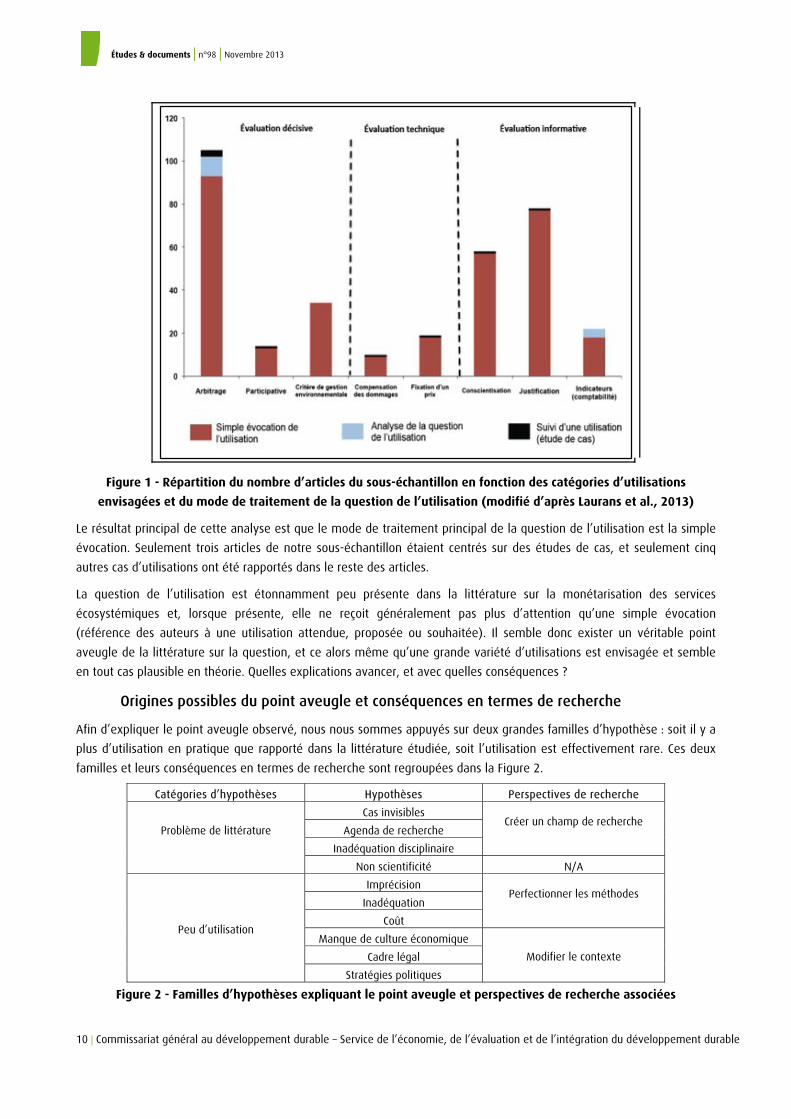
Études & documents | n°98 | Novembre 2013
10 | Commissariat général au développement durable – Service de l’économie, de l’évaluation et de l’intégration du développement durable
Figure 1 - Répartition du nombre d’articles du sous-échantillon en fonction des catégories d’utilisations
envisagées et du mode de traitement de la question de l’utilisation (modifié d’après Laurans et al., 2013)
Le résultat principal de cette analyse est que le mode de traitement principal de la question de l’utilisation est la simple
évocation. Seulement trois articles de notre sous-échantillon étaient centrés sur des études de cas, et seulement cinq
autres cas d’utilisations ont été rapportés dans le reste des articles.
La question de l’utilisation est étonnamment peu présente dans la littérature sur la monétarisation des services
écosystémiques et, lorsque présente, elle ne reçoit généralement pas plus d’attention qu’une simple évocation
(référence des auteurs à une utilisation attendue, proposée ou souhaitée). Il semble donc exister un véritable point
aveugle de la littérature sur la question, et ce alors même qu’une grande variété d’utilisations est envisagée et semble
en tout cas plausible en théorie. Quelles explications avancer, et avec quelles conséquences ?
Origines possibles du point aveugle et conséquences en termes de recherche
Afin d’expliquer le point aveugle observé, nous nous sommes appuyés sur deux grandes familles d’hypothèse : soit il y a
plus d’utilisation en pratique que rapporté dans la littérature étudiée, soit l’utilisation est effectivement rare. Ces deux
familles et leurs conséquences en termes de recherche sont regroupées dans la Figure 2.
Catégories d’hypothèses Hypothèses Perspectives de recherche
Cas invisibles
Agenda de recherche
Inadéquation disciplinaire
Créer un champ de recherche
Problème de littérature
Non scientificité N/A
Imprécision
Inadéquation
Coût
Perfectionner les méthodes
Manque de culture économique
Cadre légal
Peu d’utilisation
Stratégies politiques
Modifier le contexte
Figure 2 - Familles d’hypothèses expliquant le point aveugle et perspectives de recherche associées
Commissariat général au développement durable – Service de l’économie, de l’évaluation et de l’intégration du développement durable | 11
Études & documents | n°98 | Novembre 2013
Concernant la première famille d’hypothèses, une première possibilité concerne l’invisibilité potentielle des cas
d’utilisation. Par exemple, il peut y avoir un décalage temporel entre le moment où la monétarisation est réalisée et le
moment où son résultat est effectivement utilisé par des acteurs. Par ailleurs, dans le cas de l’utilisation informative,
celle-ci étant plus diffuse, les cas d’utilisation avérée sont plus difficilement observables. Toutefois, étant donné
l’ancienneté des pratiques de monétarisation dans le domaine de l’environnement (même dans le secteur des services
écosystémiques, qui paraît émergent mais qui a déjà au moins quinze ans d’ancienneté), il apparaît peu probable que
l’invisibilité aurait persisté si un effort de recherche s’y était consacré. Ceci amène au second point : il est fort
vraisemblable que la question de l’utilisation n’ait en fait que très peu été portée à l’agenda de recherche. La plupart des
travaux des économistes sur la question n’aborde que très peu la question de l’utilisation et il faut plutôt se tourner vers
d’autres sciences humaines et sociales (sciences de gestion, sciences politiques, sociologie, anthropologie, psychologie
etc.) qui étudient plus directement les processus de décision. Toutefois, même si nos références étaient majoritairement
composées de travaux d’économistes, de nombreuses autres disciplines étaient représentées mais nous n’avons malgré
tout pas trouvé plus de travaux traitant de la question de l’utilisation des évaluations économiques.
Concernant la seconde famille d’hypothèses, la littérature liste plusieurs facteurs qui pourraient expliquer qu’il y a moins
d’utilisations en pratique qu’attendu. D’une manière générale, il s’agirait d’une part de perfectionner les méthodes
d’évaluations, dont les imprécisions, l’inadéquation par rapport aux besoins des décideurs ou encore les coûts de
réalisation seraient autant d’obstacles à leur utilisation dans la décision. L’attention est ici portée à l’ajustement des
techniques d’évaluation : il s’agit de perfectionner l’outil et les méthodes. D’autre part, le manque de culture
économique des décideurs (qui ne comprendraient donc pas les évaluations monétaires), le manque d’obligations
légales à procéder à des évaluations économiques en matière d’environnement, ou encore un comportement stratégique
des décideurs qui auraient des réticences face à la transparence apportée par les évaluations économiques, sont
considérées comme des causes probables d’un déficit de prise en compte des évaluations économiques et invitent donc
à modifier, non pas l’outil, mais le contexte de son utilisation (former les décideurs, changer les lois, exiger la
transparence etc.).
Si une attention sur l’outil en lui-même et son contexte d’utilisation sont vraisemblablement souhaitables (et il existe,
sur le premier aspect, de très nombreux travaux), il nous semble toutefois important d’insister sur le fait qu’une
meilleure adéquation des évaluations économiques des services écosystémiques à ce à quoi elles sont censées servir en
pratique – aider à améliorer les décisions impactant les écosystèmes et la biodiversité – doit d’abord passer par un suivi,
sur les terrains où elle sont employées, de la manière dont elles s’intègrent dans les processus collectifs qui mènent à la
décision. Or, c’est justement le point aveugle que nous avons identifié, et il nous semble donc urgent de mettre cette
question encore trop ignorée au cœur de l’agenda de recherche.
Conclusion : Documenter, enfin, la vie sociale des évaluations économiques
Comme rappelé en introduction, beaucoup d’espoirs semblent placés dans les évaluations économiques pour ralentir la
dégradation des écosystèmes et l’érosion de la biodiversité. Néanmoins, pour qu’elles améliorent les décisions les
impactant, ces monétarisations doivent dans les faits être utilisées.
Or, la littérature traite très peu de cette question, pourtant clé, alors même qu’une grande diversité d’utilisations y est
envisagée. Que les évaluations soient véritablement utilisées ou non, qu’elles pèsent dans le sens de la conservation ou
non, nous n’en savons collectivement que peu de choses. Il semble en tous cas urgent d’objectiver ces questions et
d’insérer les retours du terrain dans les réflexions et débats. Cela passe par la multiplication des études de cas visant à
documenter la « vie sociale » des évaluations économiques des services écosystémiques : qui participe à leur
élaboration, par qui sont-elles utilisées, dans quel contexte, dans quel but et pour quels résultats ?
Études & documents | n°98 | Novembre 2013
12 | Commissariat général au développement durable – Service de l’économie, de l’évaluation et de l’intégration du développement durable
Références
Costanza, R., d’Arge, R., de Groot, R., Farber, S., Grasso, M., Hannon, B., Limburg, K., Naeem, S., O’Neill, R., Paruelo, J.,
Raskin, R., Sutton, P., van den Belt, M., 1997. The value of the world’s ecosystem services and natural capital. Nature
387, 253-260.
Heal, G., 2000. Valuing ecosystem services. Ecosystems 3, 24-30.
Henry, C., 1984. La micro-économie comme langage et enjeu de négociation. Revue Économique 35, 177-198.
Henry, C., 1989. Investment projects and natural resources: economic rationality in Janus’ role. Ecological Economics 1,
117-135.
Laurans, Y., Rankovic, A., Billé, R., Pirard, R., & Mermet, L., 2013. Use of ecosystem services economic valuation for decision making: Questioning a literature blindspot. Journal of Environmental Management 119, 208-219.
Liu, S., Costanza, R., Farber, S., Troy, A., 2010. Valuing ecosystem services e theory, practice, and the need for a transdisciplinary synthesis. Annals of the New York Academy of Sciences 1185, 54-78.
Myers, J.P., Reichert, J.S., 1997. Perspectives on nature’s services. In: Daily, G.C. (Ed.), Nature’s Services. Societal
Dependence on Natural Ecosystems. Island Press, Washington D.C.
Navrud, S., Pruckner, G.J., 1997. Environmental valuation – to use or not to use? Environmental and Resource Economics
10, 1-26.
NRC, 2005. Valuing Ecosystem Services: Towards Better Environmental Decision Making. National Academies Press,
Washington D.C.
OCDE, 2001. Valuation of Biodiversity Benefits: Selected Studies. OECD Publications, Paris, 181 pp.
OCDE, 2002. Handbook of Biodiversity Valuation: a Guide for Policy-makers. OECD Publications, Paris, 162 pp.
Pearce, D., Seccombe-Hett, T., 2000. Economic valuation and environmental decision-making in Europe. Environmental
Science & Technology 34, 1419-1425.
Randall, A., 1988. What mainstream economists have to say about the value of biodiversity. In: Wilson, E.O. (Ed.),
Biodiversity. National Academy Press, Washington, DC, pp. 217-223.
SCBD, 2007. An Exploration of Tools and Methodologies for Valuation of Biodiversity and Biodiversity Resources and Functions, Technical Series n 28, Montreal, Canada, 71 pp. http://www.cbd.int/doc/publications/cbd-ts-28.pdf
TEEB, 2009. The Economics of Ecosystems and Biodiversity for National and International Policy Makers. Summary:
Responding to the Value of Nature. http://www.teebweb.org/
! 213
Appendix 5
Rankovic et al. (2016) !!!
Rankovic, A., Aubert, P.-M., Lapeyre, R., Laurans, Y., Treyer, S. (2016). IPBES after Kuala Lumpur: Assessing knowledge on underlying causes of biodiversity loss is needed. Policy Brief n°05/16, Institute for Sustainable Development and International Relations (IDDRI-Sciences Po), Paris, 4 p.

! 214
Institut du dÈ veloppement durable et des relations internationales 27, rue Saint-Guillaume 75337 Paris cedex 07 France
POLICY BRIEFN°05/16 JUNE 2016 | BIODIVERSITY
www.
iddr
i.org
RECOMMENDATIONS1. While preparing the next IPBES work programme, governments should:a. Request and prioritize an ad hoc thematic assessment on existing policies and instru-
ments having an effect on biodiversity worldwide;b. Emphasize the focus on “indirect drivers” in all their other assessment requests;c. Ensure that “indirect drivers”, and particularly policies and existing solutions for their
implementation, are sufficiently covered in all scoping documents, with a dedicated chapter.
2. IPBES should actively reinforce the contribution of social sciences to its work:a. Works on biodiversity-impacting policies worldwide should not be considered as
policy prescriptive on the basis that they synthesize research on on-going or past governmental action; they are necessary to support effective implementation of biodi-versity policies;
b. Governments and stakeholder organizations should nominate a higher number of social scientists so that they can be in a capacity to contribute to, and also coordinate, such interdisciplinary works;
c. Similarly, the proportion of social scientists selected as IPBES experts and coordi-nating lead authors should be increased.
This article is based on research that has received a financial support from the French government in the framework of the programme ´ Investissements d' avenir ª, managed by ANR (French national agency for research) under the reference ANR-10-LABX-14-01.
IPBES after Kuala Lumpur: Assessing knowledge on underlying causes of biodiversity loss is neededAleksandar Rankovic, Pierre-Marie Aubert, Renaud Lapeyre, Yann Laurans, SÈ bastien Treyer (IDDRI)
The Intergovernmental Platform on Biodiversity and Ecosystem Services (IPBES) recently released its first assessments during its fourth plenary meeting in Kuala Lumpur, Malaysia. How
these first works will influence debates on biodiversity policies, and potentially support their implementation, will now be a point of atten-tion for the conservation community. Thanks to its original structure and its desire to mobilize a vast diversity of knowledge, IPBES is a historic opportunity to synthesize available knowledge on the causes, rooted in human collective action, that are behind biodiversity loss. The release of the pollination assessment provides the occasion to identify challenges and opportunities to better integrate knowledge on public policies, economic processes and other underlying factors in future IPBES works. The released assessment, albeit identifying a series of direct drivers to pollinator decline, does not actually cover ì indirect driversî or ì underlying causesî of biodiversity loss with the same depth of analysis. Addressing these topics will require the de-velopment of innovative interdisciplinary work among ecological and social sciences, and is crucial in order to find relevant policy options to halt biodiversity loss. There are several windows of opportunity, in the near future, to enhance the focus of IPBES on knowledge about the underlying causes of biodiversity loss.

POLICY BRIEF 05/20162 IDDRI
IPBES after Kuala Lumpur: Assessing knowledge on underlying causes of biodiversity loss is needed
1. IPBES AND THE IMPLEMENTATION CHALLENGEIPBES has the overall objective of ì strengthe-ning the science-policy interface for biodiver-sity and ecosystem services for the conservation and sustainable use of biodiversity, long-term human well-being and sustainable developmentî . Compared to previous international assessment mechanisms on biodiversity,1 IPBES innovates in its ambition to integrate a great diversity of academic and non-academic knowledge. Besides, its functions are not limited to producing assess-ments, as it possesses three other functions: knowledge generation catalysis, policy support and capacity building.2 Taken together, these charac-teristics make IPBES a useful and innovative tool to build the necessary knowledge base to address the challenge of implementing biodiversity poli-cies worldwide.
Indeed, almost twenty-five years after the Con-vention on Biological Diversity was signed, and with five other international conventions focusing on biodiversity issues,3 as well as numerous exper-tise mechanisms developed over the years, both the problem and the need to act seem well acknowl-edged internationally. The CBDí s Strategic Plan 2011-2020 and its Aichi Targets, are another exam-ple of international commitment. Why then, de-spite this recognition, is biodiversity still eroding?
Synthesizing knowledge on this precise ques-tion would, actually, be a major contribution from IPBES to biodiversity governance. Along-side research on the state of biodiversity and its direct drivers, what is critically needed now is to understand what hampers the implementation of conservation policies and why given policies fail or succeed in halting biodiversity loss worldwide. Examples of questions that need an international synthesis effort include: What is the net effect on biodiversity of often contradictory sectoral domes-tic policies? How much does spending for conser-vation weigh compared to environmentally harm-ful incentives? What do studies tell us about the conservation efficacy of different types of instru-ments (legal, economic, technical) in the field?
1. For instance : the Global Biodiversity Assessment, the Global Biodiversity Outlooks, the Millenium Ecosystem Assessment and its declinations, The Economics of Ecosys-tems and Biodiversity.
2. Decision UNEP/IPBES.MI/2/9, Appendix 1.3. Six international conventions focus on biodiversity
issues: the CBD, the Convention on Conservation of Migratory Species, the Convention on International Trade in Endangered Species of Wild Fauna and Flora, the International Treaty on Plant Genetic Resources for Food and Agriculture, the Ramsar Convention on Wet-lands, and the World Heritage Convention.
Answering such questions would require focus-ing on factors usually qualified as ì indirect driv-ersî or ì underlying causesî of biodiversity loss, which are typically the object of CBDí s Aichi Tar-gets 1-4. These underlying causes are linked to the functioning of human societies and refer to phe-nomena that are the traditional domains of inves-tigation of social scientific research. IPBES could represent a historical occasion to develop innova-tive interdisciplinary work to synthesize available knowledge on policies and instruments having an effect on biodiversity worldwide.
2. CRITICAL BLINDSPOTS AND DISCIPLINARY GAPS IN THE IPBES POLLINATION ASSESSMENTTo achieve this vision, a series of obstacles would need to be overcome first, as revealed by IPBESí first thematic assessment. The assessment on pollinators, pollination and food production provides a welcome synthesis on the state of world pollinators and what is known of their contribution to agriculture. It identifies a series of ì direct driversî threatening pollinators (land-use change, intensive agricultural manage-ment and pesticide use, environmental pollution, invasive alien species, pathogens and climate change), which is in itself an important prog-ress in current policy debates. It leaves aside, however, knowledge on important underlying causes such as agricultural trade and policies that are only cursorily addressed in four short paragraphs at the end of Chapter 2. Even though contradictions among sectoral public policies and associated phenomena such as environmentally harmful subsidies are increasingly recognized as major causes behind continuous biodiversity loss,4 knowledge thereof is barely mentioned throughout the pollination assessment. In the summary for policymakers (SPM), the word ì subsidyî does not even appear. International trade governance strongly influences the produc-tion of agricultural commodities, however evidence about this is neither mentioned. When it comes to the possible responses to halt polli-nators decline (e.g. Table SPM.1 in the SPM), even though the assessment identifies categories such as ì transforming agricultural landscapesî , it does not mention the contextual conditions that would enable such changes, nor the factors that are currently involved in blocking change.
4. James A. N., Kevin J., & Balmford A. (1999). Balan-cing the Earthí s accounts. Nature, 401, 323ñ 324; Centre dí analyse stratÈ gique (2012). Les aides publiques domma-geables ‡ la biodiversitÈ , rapport de la mission prÈ sidÈ e par Guillaume Sainteny, Paris, La Documentation fran-Áaise , 418 p.
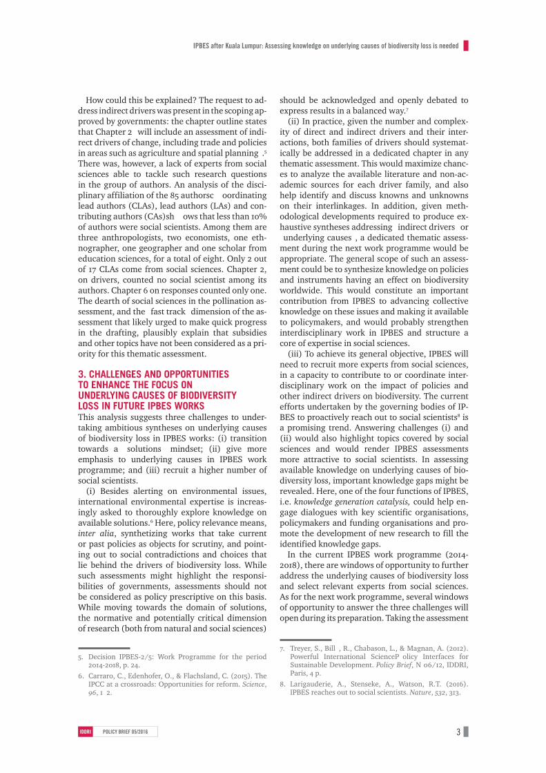
IPBES after Kuala Lumpur: Assessing knowledge on underlying causes of biodiversity loss is needed
POLICY BRIEF 05/2016 3IDDRI
How could this be explained? The request to ad-dress indirect drivers was present in the scoping ap-proved by governments: the chapter outline states that Chapter 2 ì will include an assessment of indi-rect drivers of change, including trade and policies in areas such as agriculture and spatial planningî .5 There was, however, a lack of experts from social sciences able to tackle such research questions in the group of authors. An analysis of the disci-plinary affiliation of the 85 authorsóc oordinating lead authors (CLAs), lead authors (LAs) and con-tributing authors (CAs)ósh ows that less than 10% of authors were social scientists. Among them are three anthropologists, two economists, one eth-nographer, one geographer and one scholar from education sciences, for a total of eight. Only 2 out of 17 CLAs come from social sciences. Chapter 2, on drivers, counted no social scientist among its authors. Chapter 6 on responses counted only one. The dearth of social sciences in the pollination as-sessment, and the ì fast trackî dimension of the as-sessment that likely urged to make quick progress in the drafting, plausibly explain that subsidies and other topics have not been considered as a pri-ority for this thematic assessment.
3. CHALLENGES AND OPPORTUNITIES TO ENHANCE THE FOCUS ON UNDERLYING CAUSES OF BIODIVERSITY LOSS IN FUTURE IPBES WORKSThis analysis suggests three challenges to under-taking ambitious syntheses on underlying causes of biodiversity loss in IPBES works: (i) transition towards a ì solutionsî mindset; (ii) give more emphasis to underlying causes in IPBES work programme; and (iii) recruit a higher number of social scientists.
(i) Besides alerting on environmental issues, international environmental expertise is increas-ingly asked to thoroughly explore knowledge on available solutions.6 Here, policy relevance means, inter alia, synthetizing works that take current or past policies as objects for scrutiny, and point-ing out to social contradictions and choices that lie behind the drivers of biodiversity loss. While such assessments might highlight the responsi-bilities of governments, assessments should not be considered as policy prescriptive on this basis. While moving towards the domain of solutions, the normative and potentially critical dimension of research (both from natural and social sciences)
5. Decision IPBES-2/5: Work Programme for the period 2014-2018, p. 24.
6. Carraro, C., Edenhofer, O., & Flachsland, C. (2015). The IPCC at a crossroads: Opportunities for reform. Science, 96, 1ñ 2.
should be acknowledged and openly debated to express results in a balanced way.7
(ii) In practice, given the number and complex-ity of direct and indirect drivers and their inter-actions, both families of drivers should systemat-ically be addressed in a dedicated chapter in any thematic assessment. This would maximize chanc-es to analyze the available literature and non-ac-ademic sources for each driver family, and also help identify and discuss knowns and unknowns on their interlinkages. In addition, given meth-odological developments required to produce ex-haustive syntheses addressing ì indirect driversî or ì underlying causesî , a dedicated thematic assess-ment during the next work programme would be appropriate. The general scope of such an assess-ment could be to synthesize knowledge on policies and instruments having an effect on biodiversity worldwide. This would constitute an important contribution from IPBES to advancing collective knowledge on these issues and making it available to policymakers, and would probably strengthen interdisciplinary work in IPBES and structure a core of expertise in social sciences.
(iii) To achieve its general objective, IPBES will need to recruit more experts from social sciences, in a capacity to contribute to or coordinate inter-disciplinary work on the impact of policies and other indirect drivers on biodiversity. The current efforts undertaken by the governing bodies of IP-BES to proactively reach out to social scientists8 is a promising trend. Answering challenges (i) and (ii) would also highlight topics covered by social sciences and would render IPBES assessments more attractive to social scientists. In assessing available knowledge on underlying causes of bio-diversity loss, important knowledge gaps might be revealed. Here, one of the four functions of IPBES, i.e. knowledge generation catalysis, could help en-gage dialogues with key scientific organisations, policymakers and funding organisations and pro-mote the development of new research to fill the identified knowledge gaps.
In the current IPBES work programme (2014-2018), there are windows of opportunity to further address the underlying causes of biodiversity loss and select relevant experts from social sciences. As for the next work programme, several windows of opportunity to answer the three challenges will open during its preparation. Taking the assessment
7. Treyer, S., BillÈ , R., Chabason, L., & Magnan, A. (2012). Powerful International ScienceñP olicy Interfaces for Sustainable Development. Policy Brief, N° 06/12, IDDRI, Paris, 4 p.
8. Larigauderie, A., Stenseke, A., Watson, R.T. (2016). IPBES reaches out to social scientists. Nature, 532, 313.
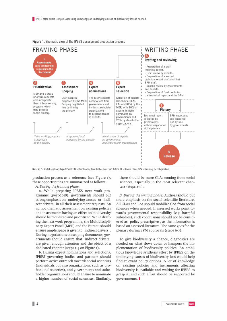
POLICY BRIEF 05/20164 IDDRI
IPBES after Kuala Lumpur: Assessing knowledge on underlying causes of biodiversity loss is needed
production process as a reference (see Figure 1), these opportunities are summarized as follows:
A. During the framing phase:a. While preparing IPBES next work pro-
gramme (post-2018), governments should put strong emphasis on ì underlying causesî or ì indi-rect driversî in all their assessment requests. An ad hoc thematic assessment on existing policies and instruments having an effect on biodiversity should be requested and prioritized. While draft-ing the next work programme, the Multidiscipli-nary Expert Panel (MEP) and the Bureau should ensure ample space is given to ì indirect driversî . During negotiations on scoping documents, gov-ernments should ensure that ì indirect driversî are given enough attention and the object of a dedicated chapter (steps 1-3 on Figure 1).
b. During expert nominations and selections, IPBES governing bodies and partners should perform active outreach towards social scientists (individuals but also organizations, such as pro-fessional societies), and governments and stake-holder organizations should ensure to nominate a higher number of social scientists. Similarly,
there should be more CLAs coming from social sciences, especially in the most relevant chap-ters (steps 4-5).
B. During the writing phase: Authors should put more emphasis on the social scientific literature. All CLAs and LAs should mobilize CAs from social sciences when needed. If assessed works point to-wards governmental responsibility (e.g. harmful subsidies), such conclusions should not be consid-ered as ì policy prescriptiveî , as the information is based on assessed literature. The same goes for the plenary during SPM approvals (steps 6-7).
To give biodiversity a chance, diagnostics are needed on what slows down or hampers the im-plementation of biodiversity policies. An ambi-tious knowledge synthesis effort by IPBES on the underlying causes of biodiversity loss would help find relevant policy options. A lot of knowledge on existing policies and instruments affecting biodiversity is available and waiting for IPBES to grasp it, and such effort should be supported by governments. |
Figure 1. Shematic view of the IPBES assessment production process
FRAMING PHASE WRITING PHASE
1.Governments
send assessment requests to the
Secretariat
2 Prioritization
MEP and Bureauprioritize requestsand incorporate them into a working program, whichthey propose to the plenary.
If the working programis approved by the plenary
If approved and budgeted by the plenary
Nomination of expertsby governments and stakeholder organizations
Technical report accepted bygovernments without negotiation at the plenary.
SPM negotiatedand approvedline by lineby governments.
8.Release
6Drafting and reviewing
- Preparation of a draft technical report.- First review by experts.- Preparation of a second technical report draft and first SPM draft.- Second review by governments and experts.- Preparation of final drafts for the technical report and the SPM.
7Plenary
3AssessmentScoping
Draft scoping proposed by the MEP.Scoping negotiatedline by line by the plenary.
4 Expertnominations
The MEP requests nominations fromgovernments andinvites stakeholder organizations to present namesof experts.
5Expertselection
Selection of experts (Co-chairs, CLAs, LAs and REs) by theMEP, with 80% of experts initially nominated by governments and20% by stakeholderorganizations.
Note: MEP - Multidisciplinary Expert Panel; CLA - Coordinating Lead Author; LA - Lead Author; RE - Review Editor; SPM - Summary for Policymakers

! 215
Appendix 6
Curriculum vitæ

! 216

October 2016
ALEKSANDAR RANKOVIC Born on 03.29.1986 in Paris, France French and Serbian citizenships Married
POSITIONS January 2015 - Institute for Sustainable Development and International Relations (IDDRI-Sciences Po) Present Research fellow on biodiversity and science-society interactions. January 2015 - Harvard University – John F. Kennedy School of Government May 2015 Fellow in the Program on Science, Technology and Society. January 2014 - Sorbonne Paris Cité program "Politics of the Earth in the Anthropocene" July 2014 Program led by Sciences Po (Prof. Bruno Latour). Scientific secretary, general
coordination of the program. December 2010 - Centre National de la Recherche Scientifique (CNRS) December 2013 PhD fellow at the Lab of Biogeochemistry and Ecology of Continental Environments
(BIOEMCO Lab – UMR 7618), Biodiversity and Ecosystem Functioning Team, Paris.
EDUCATION
January 2011 - PhD in Ecology November 2016 Université Pierre et Marie Curie-Paris VI, Doctoral School in "Sciences of Nature and (expected) Man: Ecology and Evolution" (ED 227)
Dissertation title: Living the street life: Long-term carbon and nitrogen dynamics in Parisian soil-tree systems. Supervised by Luc Abbadie, Sébastien Barot, Jean-Christophe Lata and Julie Leloup. IEES-Paris, Integrative Ecology Team, Paris, France.
2008-2010 Dual degree program in Environmental Science and Policy Master in International Affairs Paris Institute of Political Studies (Sciences Po Paris) Master in Environmental Sciences Université Pierre et Marie Curie-Paris VI 2004-2008 Bachelor in Life Sciences Université Pierre et Marie Curie-Paris VI
EXPERIENCES
1. RESEARCH AND TEACHING 1.1. Grants and research contracts 2016-17 IUCN Centre for Mediterranean Cooperation, “From nature-based solutions in INDCs
to consistent adaptation and mitigation policy planning in the Mediterranean” (co-investigator).
2016-17 French Ministry of the Environment, Energy and the Sea, "Integrating nature-based solutions into climate change adaptation policies – dialogue and good practices" (principal co-investigator, project submitted).
2015-17 Belmont Forum, "Impacts of Human Drivers on Biodiversity in Savannas (IHDBS)", (co-investigator, axis leader).
Professional contacts: IDDRI-Sciences Po
Postal address: 27 rue Saint-Guillaume, 75007, Paris, France Office: 41, rue du Four, 75006, Paris, France
+ 33 6 33 49 64 00 (mobile) [email protected]
2
2014-16 University Sorbonne Paris Cité, "Politics of the Earth in the Anthropocene" interdisciplinary programme (scientific secretary then co-investigator).
2014-16 City of Paris, Paris 2030, "Implication of mycorhizal communities in street tree reponse to trace metal pollution in urban environments (MycoPolis)" (co-investigator).
2014-15 Sorbonne Universités Alliance, "Densification policies, biodiveristy and quality of urban space: urban agriculture and greenways (Dens’City Project)" (co-investigator).
2011-13 GIS « Climat, Environnement, Société », "Climate change and urban greenways" (co-investigator, axis leader).
2010-11 PIR IngECOtech (CNRS-IRSTEA), "Ecological engineering of urban soils in a megalopolis" (co-investigator).
2010-13 Île-de-France region, R2DS, « Fonctionnement des sols urbains (SOLURB) » (PhD grant).
2009-12 Fondation d’entreprise Hermès - IDDRI, "Place and role of economic valuations of biodiversity and ecosystem services in decison-making processes" (co-investigator).
1.2. Organization of scientific and multistakeholder events November 2016 Side event at UNFCCC COP22 "From nature-based solutions in INDCs to consistent adaptation and mitigation policy
planning in the Mediterranean. Feedback and perspectives from Morocco and Tunisia". Convened by the IUCN Centre for Mediterranean Cooperation and IDDRI, in partnership with the Haut Commissariat aux Eaux et Forêts et à la Lutte Contre la Désertification of Morocco and the Ministry of Environment and Sustainable Development of Tunisia. Co-organizer. 8 November, Marrakech, Morocco.
October 2016 Journées FRB 2016 & Troisièmes rencontres GIEC-IPBES : "L'influence du GIEC et de
l'IPBES sur la prise de décision" (UNFCCC COP22 labeled event) Co-organized by FRB and IDDRI. Main organizer on the side of IDDRI. 13-14 October
2016, Paris, France. Website: http://www.fondationbiodiversite.fr/fr/fondation/evenements/evenements-
frb/journeesfrb2016.html June 2016 CSaP-IDDRI workshop: "The works of and on IPBES: What research for what
intervention?" Main co-organizer with Alice Vadrot. Academic workshop co-organized by IDDRI and
the Centre for Science and Policy, University of Cambridge. 27 June 2016, Cambridge, UK. Website:
http://www.iddri.org/Evenements/Ateliers/The-works-of-and-on-IPBES-What-research-for-what-intervention
April 2016 Séminaire FRB-Iddri : « IPBES : Kuala Lumpur, et après ? »
Main co-organizer with Agnès Hallosserie (FRB). Multistakeholder workshop on the outcomes of IPBES’ fourth plenary and how to address its influence on biodivserity policies. Institut des sciences de la communication, 28 avril 2016, Paris. Website: http://www.iddri.org/Evenements/Conferences/IPBES-Kuala-Lumpur,et-apres
October 2015 International conference « Des formes pour vivre l’environnement. Théorie,
expérience, esthétique et critique politique » Organized by the LADYSS (CNRS-Univ. Paris 1, 7, 8, 10) ! and the CRAL (CNRS-EHESS).
Member of the scientific commitee. 1-2 October 2015, Paris. Website : http://cral.ehess.fr/index.php?2046 September 2015 International conference "Ecology at the interface", symposium "Ecologists’ strategies
at science-policy interfaces: How can social sciences help?” Main organizer, with Audrey Coreau, Laurent Mermet and Yann Laurans. Held at
"Ecology at the interface", 13th European Ecological Federation (EEF) and 25th Italian Society of Ecology’s (SItE) joint conference, 21-25 September, Rome, Italy.
April 2015 Harvard STS workshop "Science and its Publics: Conversations on accountability" Organizer with Paulo Fonseca, Zara Mirmalek, Zoe Nyssa, Matthew Sample. Held on
28 April 2015 at Harvard University Center for the Environment. Website: http://sts.hks.harvard.edu/events/workshops/science-and-its-publics/

3
April 2015 Harvard STS special seminar on environmental migrations Organizer and discussant, seminar with François Gemenne on "Anthropocene and Its
Victims: How We Name Those Displaced by Environmental Changes", 24 April at the John F. Kennedy School of Government.
Website: http://sts.hks.harvard.edu/events/workshops/special-seminar-anthropocene-and-its-victims/
November 2014 École thématique « Transition écologique et environnement urbain : cas de
l’agglomération parisienne » of OSU Ecce Terra (UPMC-CNRS) Organizer and animator of the seminar «Vies de rue : Regards croisés sur les
plantations d’alignements parisiennes» with presentations from researchers and practitioners. Held on 6 November 2014 at the National Museum of Natural History, Paris.
January – Sorbonne Paris Cité "Politics of the Earth" programme July 2014 Organizer of four interdisciplinary workshops and one conference evaluated by an
international jury. Website: http://politiquesdelaterre.fr April 2012 – Seminar "History, Philosophy and Sociology of Ecology" April 2014 Founder and organizer, with Alix Sauve and Henri de Parseval. Bimestrial sessions with invited speakers, held at IEES-Paris. Program (in French): http://ieesparis.ufr918.upmc.fr/spip.php?article476 December 2012 Symposium "Vegetation, Cities and Climate: Scientific approaches, political issues", organized by the CCTV2 project and Paris 2030 program Member of the scientific committee. Held on 3 December 2012, Auditorium de l’Hôtel de Ville, Paris. December 2011 Sixth edition of the Regional Ecological Engineering Symposium, "Engineering the
water continuum" Member of the scientific committee and co-chair of the final round table. Held on 13-
14 December 2011, CIUP, Paris. December 2010 Fifth edition of the Regional Ecological Engineering Symposium, "Biodiversity and
ecological engineering: constraint or opportunity?", Member of the scientific committee. Held on 8-9 December 2010, CIUP, Paris. May 2010 Symposium "A diverse but common world: Biodiversity and Cooperation between
Peoples" Part of Sciences Po’s "Politics of the Earth" research axis (POLEARTH). Main organizer, with Émilie Hache and Béatrice Cointe. Held on 6 May 2010, Sciences Po, Paris.
Website: http://blogs.sciences-po.fr/recherche/files/2009/12/BiodiversityCooperation-Between-Peoples-2604.pdf
1.3. Teaching: September 2016 Summer school "Politics of the Earth" (Sciences Po & associate European universities)
One-week programme, 5-9 September 2016. Member of the organizing committee, in charge of the day on "Politics of Biodiversity" (personal involvement in 6 hours of teaching). Funded by EDGE project (H2020).
October 2012 École Normale Supérieure, Paris
Graduate program in biology, course unit "Insights in Life Sciences": Full development, teaching and evaluation of the course "Ecosystem ecology in urban environments: descriptive and practical challenges", three lectures of one hour.
September - Université Pierre et Marie Curie-Paris VI December 2011 Master "Sciences of the Universe, Environment, Ecology", course in "Great
environmental issues" (10h teaching). Co-responsible and member of the final evaluation jury.
1.4. Mentoring:
• 2015-2016
- Stefanie Chan, M2 "International Public Management", Sciences Po. Five months, co-advised with Yann Laurans.
4
- Rémy Ruat, M1 "Environmental Science and Policy", Université Pierre et Marie Curie - Paris VI and Sciences Po. Six months, co-advised with Sébastien Treyer.
• 2013-2014
- Iry Andrianjara, M2 "Ecology, Biodiversity, Evolution", Université Paris-Sud. Four months, co-advised with Katell Quenea and Jean-Christophe Lata.
- Anne Barbillon, M1 "Agronomic Engineering", SupAgro Montpellier. Five months, co-advised with Benoît Geslin, Éric Motard and Isabelle Dajoz.
• 2012-2013
- Víctor Cárdenas Ortega, M2 "Ecology, Biodiversity, Evolution", Université Pierre et Marie Curie - Paris VI. Four and a half months, co-advised with Sébastien Barot and Pierre Barré.
- Quentin Guignard, M2 "Ecology, Biodiversity, Evolution", AgroParisTech. Six months, co-advised with Sébastien Barot.
- Marie Fernandez, M2 "Molecular and Cell Biology", École Normale Supérieure. Six months, co-advised with Julie Leloup.
- Christelle Leterme, M1 in Geography, major in environment, Université Paris 1-Panthéon-Sorbonne. Four months, co-advised with Anne Sourdril.
• 2011-2012
- Ingrid Cheung Chin Tun, M2 "Environmental Science and Policy", Université Pierre et Marie Curie - Paris VI and Sciences Po. Six months, co-advised with Anne Sourdril.
- Anastasia Wolff, M2 "Ecology, Biodiversity, Evolution", École Normale Supérieure. Four months, co-advised with Julie Leloup.
- Zhanara Abikeyeva, dual degree in "Environmental Sciences", Université Paris-Sud and Tomsk Polytechnic University (Russia). Four months, co-advised with Jean-Christophe Lata.
- Anastasiya Stepanova, dual degree in "Environmental Sciences", Université Paris-Sud and Tomsk Polytechnic University (Russia), Four months, co-advised with Jean-Christophe Lata.
- Noémie Courtejoie, third year of the BSc in Biology, École Normale Supérieure. Two months, co-advised with Jean-Christophe Lata.
• 2010-2011
- Benjamin Izac, M1 "Ecology, Biodiversity, Evolution", Université Paris-Sud. One month.
• 2009-2010
- Ambre David, M1 "Ecology, Biodiversity, Evolution", Université Pierre et Marie Curie - Paris VI. Two months, co-advised with Luc Abbadie.
1.5. Service: April 2012 - BIOEMCO Lab council December 2013 PhD students representative. October 2011 - Scientific committee of the Doctoral School in Diversity of Living Organisms, December 2013 Université Pierre et Marie Curie-Paris VI PhD students representative. 2. PARTICIPATION TO POLICY PROCESSES November 2016 UNFCCC COP 22, 7 November-18 November 2016, Marrakech, Morocco. Accredited observer (Pacific Community – SPC). Organization of a side event,
interviews and observations. February 2016 Fourth plenary of IPBES, 22-28 February 2016, Kuala Lumpur, Malaysia. Accredited observer, representative of IDDRI. Observations and language proposal to
the French delegation. Accepted language includes the ending sentence of the pollination assessment’s summary for policymakers, as well as the ending sentence of its last key message.

5
December 2015 UNFCCC COP 21, 30 November-12 December 2015, Paris-Le Bourget, France. Accredited observer (IDDRI). Interviews and observations.
3. CONSULTING, EXPERTISE March 2014 Institut de conseil et d’études en développement durable (ICEDD – Namur, Belgium)
External reviewer for a study commissioned by the Walloon Region on the costs of climate change inaction. Chapter on biodiversity and ecosystem services.
March - Veolia Environnement Recherche et Innovation (VERI)
September 2010 Project officer for the study "Ecosystem services in urban environments" (final Master internship). Final report: Management of ecosystem services in urban environments: Research and application prospects, 131 p.
September - Chaire de Développement Durable de Sciences Po – European Commission October 2009 Contribution to the European Union Development Days 2009 : Redaction of a policy brief on the EU-Med cooperation for climate change adaptation,
for the plenary session “The road to Copenhagen and beyond” held on 24 October. Attending to the event and on-site diffusion of the paper to international actors (22-24 October 2009, Stockholm, Sweden).
January - Caisse des Dépôts et Consignations – Carbon Finance June 2009 Student group work (Sciences Po’s « projet collectif »):
Feasibility study for the implementation of an investment fund dedicated to "programmatic" joint implementation projects of greenhouse gas emissions reduction at the European level (Kyoto protocol framework). In charge of the methanization sector (agricultural and domestic waste).
OTHER EXPERIENCES September 2008 - Association Sciences Po Environnement (https://sciencespoenvironnement.fr) June 2010 Association member and President from July to December 2009. January 2005 - Häagen-Dazs Saint-Honoré & Häagen-Dazs Rosny 2 July 2008 Staff then store manager. Shops with respective annual turnovers of 700k€ and 450k€ in 2007. Staff
management (10 et 5 employees), supervising the application of standards (hygiene and service quality), stock management, cash management.
SKILLS j Languages • French: Native speaker • English: Fluent (TOEIC 990/990, TOEFL iBT 109/120) • Serbo-Croatian: Native speaker, Cyrillic and Latin alphabets • Spanish: Beginner • Japanese: Notions Analytical skills • Fieldwork and experimental design • Soil physico-chemistry (e.g. bulk density, texture, particle-size analysis, C and N contents, pH, etc.) • Stable isotope (15N, 13C) analysis in ecology • Microbial ecology (qPCR, T-RFLP, activity analysis by gas chromatography – CO2, N2O –, MicroRespTM-CLPP) • Univariate statistical modelling (R software) • Qualitative research methods for the social sciences (semi-structured interviews, participant observations, direct obvservations) • Research synthesis through systematic review methods
6
Soft skills • Conduct of interdisciplinary research • Research project development and management • Experience in teaching and course development • Mentoring students • Scientific animation • Outreach: oral communications and writings for local, national and European actors (City of Paris, French National Agency for Water and Aquatic Environments, French Ministry of the Environment, European Commission etc.) and the media (Le Monde, Le Figaro) Others • Black belt in karate (Shotokan-ryu)
PUBLICATIONS AND COMMUNICATIONS
1. EDITED VOLUMES 2016-2017. Principal guest editor for Environmental Science & Policy, special issue "A bridge for what? Discussing the politics of ecological sciences in biodiversity policy-making", co-edited with Audrey Coreau, Yann Laurans, Laurent Mermet and Sébastien Treyer. Forthcoming.
2. ARTICLES IN PEER-REVIEWED JOURNALS David, A. A. J., Boura, A., Lata, J.-C., Rankovic, A., Kraepiel, Y., Charlot, C., Barot, S., Abbadie, L., Ngao, J. (submitted). Street trees in Paris are sensitive to spring and autumn precipitation and recent climate changes.
Glatron, S., Blanc, N., Lamarche, T., Rankovic, A. (submitted). Urban vegetation as a means of mitigating the effects of global warming: what do city dwellers think?
Blanc, N., Glatron, S., Lamarche, T., Rankovic, A., Sourdril, A. (submitted). A new hybrid governance of urban nature: French case-studies.
Natali, M., Zanella, A., Rankovic, A., Banas, D., Cantaluppi, C., Abbadie, L., Lata, J.-C. (2016). Assessment of trace metal air pollution in the Paris area using TXRF-slurry analysis on cemetery mosses, Environmental Science and Pollution Research, doi:10.1007/s11356-016-7445-z
Gattuso, J.-P., Magnan, A., Billé, R., Cheung, W. W. L., Howes, E. L., Joos, F., Allemand, D., Bopp, L., Cooley, S., Eakin, C. M., Hoegh-Guldberg, O., Kelly, R. P., Pörtner, H.- O., Rogers, A.D., Baxter, J. M., Laffoley, D., Osborn, D., Rankovic, A., Rochette, J., Sumaila, U. R., Treyer, S., Turley, C. (2015). Contrasting futures for ocean and society from different CO2 emissions scenarios, Science, 349(6243), aac4722. DOI: 10.1126/science.aac4722
Laurans, Y., Rankovic, A., Billé, R., Pirard, R, Mermet, L. (2013). Use of ecosystem services economic valuation for decision making: Questioning a litterature blindspot, Journal of Environmental Management, 119, 208-219
Rankovic, A., Pacteau, C., Abbadie, L. (2012). Ecosystem services and cross-scale urban adaptation to climate change: An articulation essay, VertigO, Special Issue 12, http://vertigo.revues.org/11851 (in French)
3. BOOK CHAPTERS Chabason, L., Rankovic, A., Bonnel, A. (2016). De l’expertise à l’expérimentation collective ? Les liens entre sciences et politiques à l’heure de la mise en œuvre du développement durable. Regards sur la Terre 2016, forthcoming.
4. WORKING PAPERS, POLICY BRIEFS, OUTREACH Rankovic, A., Aubert, P.-M., Lapeyre, R., Laurans, Y., Treyer, S. (2016). IPBES after Kuala Lumpur: Assessing knowledge on underlying causes of biodiversity loss is needed. Policy Brief n°05/16, Institute for Sustainable Development and International Relations (IDDRI-Sciences Po), Paris, 4 p. http://www.iddri.org/Publications/IPBES-after-Kuala-Lumpur-Assessing-knowledge-on-underlying-causes-of-biodiversity-loss-is-needed
7
Aubert, P.-M., Ruat, R., Rankovic, A., Treyer, S. (2016). Which accountability framework and transformational potential of a multi-stakeholder initiative? The case of the 4‰ Initiative. Policy Brief n°01/16, Institute for Sustainable Development and International Relations (IDDRI-Sciences Po), Paris, 4 p. http://www.iddri.org/Publications/Cadre-de-redevabilite-et-potentiel-transformationnel-d-une-initiative-multi-acteurs-le-cas-du-4
Aubert, P.-M., Ruat, R., Rankovic, A., Treyer, S. (2016). Cadre de redevabilité et potentiel transformationnel d’une initiative multi-acteurs : le cas du 4 ‰. Policy Brief n°01/16, Institute for Sustainable Development and International Relations (IDDRI-Sciences Po), Paris, 4 p. http://www.iddri.org/Publications/Cadre-de-redevabilite-et-potentiel-transformationnel-d-une-initiative-multi-acteurs-le-cas-du-4
David, A., Boura, A., Rankovic, A., Kraepiel, Y., Barot, S., Abbadie, L., Lata, J.-C., Ngao, J. (2015). Long term impact of climate on tree-growth patterns in Paris street trees and its consequences on tree cooling potential: A dendroclimatic approach. Proceedings of ICUC9, 9th International Conference on Urban Climate jointly with the 12th Symposium on the Urban Environment (20-24 July, Toulouse, France), 5 p.
Rankovic, A., Billé, R. (2013). Les utilisations de l’évaluation économique des services écosystémiques : un état des lieux. Études et documents, n°98. Commissariat général au développement durable, Ministère de l’Écologie, du Développement Durable et de l’Énergie. http://www.developpement-durable.gouv.fr/IMG/pdf/E_D98_actes_seminaire_monetarisation_2012-2.pdf
Muller, Y., Nicolas, V., Rankovic, A., Genet, P., Lacroix, G., Hulot, F. (2012). Engineering the water continuum. ONEMA Meetings, n°16, August 2012. http://www.onema.fr/IMG/EV/meetings/Les-Rencontres-16UK.pdf
Muller, Y., Nicolas, V., Rankovic, A., Genet, P., Lacroix, G., Hulot, F. (2012). L’eau, ingénierie d’un continuum. Les rencontres de l’ONEMA, n°16, Août 2012. http://www.onema.fr/IMG/pdf/rencontres/Onema-Les-Rencontres-16.pdf
Billé, R., Laurans, Y., Mermet, L., Pirard, R., Rankovic, A. (2012). Valuation without action? On the use of economic valuations of ecosystem services. Policy Brief n°07/12, Institute for Sustainable Development and International Relations (IDDRI-Sciences Po), Paris, 6 p. http://www.iddri.org/Publications/Collections/Syntheses/Valuation-without-action-On-the-use-of-economic-valuations-of-ecosystem-services
Rankovic, A., Chancel, L., De Sahb, C. (2009). No-regret strategies in the Mediterranean: building sustainability through climate change adaptation. Reflexion paper for the European Union Development Days 2009, Stockholm, 22-24 October 2009, Stockholm, Sweden, 4 p.
5. OTHER ARTICLES, OPINIONS Rankovic, A., Silvain, J.-F., Abbadie, L., Barot, S., Bœuf, G., Chenu, C., Dajoz, I., Frascaria-Lacoste, N., van den Hove, S., Jouzel, J., Laurans, Y., Lavorel, S., Le Treut, H., Leroux, X., Sarrazin, F., Treyer, S., Tubiana, L. (2016). Climat et biodiversité : les experts doivent évaluer réussites et échecs des politiques publiques. Le Figaro, 14 October 2016 (print). http://www.lefigaro.fr/vox/societe/2016/10/13/31003-20161013ARTFIG00288-climat-les-experts-doivent-evaluer-reussites-et-echecs-des-politiques-publiques.php
Silvain, J.-F. & Rankovic, A. (2016). Les premières évaluations de l’IPBES sont-elles à la hauteur des attentes des chercheurs ? Fondation pour la Recherche sur la Biodiversité, 4 p. http://www.fondationbiodiversite.fr/fr/images/documents/IPBES/Article_FRB_Iddri_formaté.pdf
Laurans, Y., Rankovic, A., Lapeyre, R. (2016). L’IPBES pertinent politiquement : chiche ! Blog Iddri, http://www.blog-iddri.org/fr/2016/05/23/l-ipbes-pertinent-politiquement-chiche/
Rankovic, A. (2016). « Giec de la biodiversité » : l’étude globale sur la pollinisation fera-t-elle mouche ? Le Monde (web), 26 February 2016. http://www.lemonde.fr/idees/article/2016/02/26/giec-de-la-biodiversite-l-etude-globale-sur-la-pollinisation-fera-t-elle-mouche_4872468_3232.html
Collective (2015). Where Does France Go From Here? A Manifesto For Another Debate. Harvard Kennedy School Review, blog entry, 16 November 2015. http://harvardkennedyschoolreview.com/where-does-france-go-from-here-a-
manifesto-for-another-debate/. French version: Et maintenant ? Manifeste pour un autre débat. http://harvardkennedyschoolreview.com/et-maintenant-manifeste-pour-un-autre-debat/
Billé, R., Laurans, Y., Mermet, L., Pirard, R., Rankovic, A. (2011). À quoi servent les évaluations économiques de la biodiversité ? Ecorev’ - Revue critique d’écologie politique, n°32, 48-54
Rankovic, A. (2009). Chasse aux cétacés : coopération et conflits. The Paris Globalist Vol. III. n°2, p. 37 http://www.global21online.org/paris/pdf/Vol_III_Issue_2.pdf
6. ORAL COMMUNICATIONS AND POSTERS (*invited)
• Oral communications (O) and posters (P) presented at international scientific congresses

8
Rankovic, A. (2016). Long-term carbon and nitrogen dynamics in Parisian street soil-tree systems. First Open Science Meeting of the International Long-Term Ecological Research Network, 9-13 October, Kruger National Park, South Africa (P)
Aubert, P.-M., Lapeyre, R., Laurans, Y., Vignes, R., Rankovic, A. (2016). The global value chains of commodities and the future of savannas: First results on soybean and the Brazilian cerrado. First Open Science Meeting of the International Long-Term Ecological Research Network, 9-13 October, Kruger National Park, South Africa (O, presenter)
Charles-Dominique, T., Barot, S., Beckett, H., Blaum, N., Bond, W., Bustamante, M., Durigan, G., Kimuyu, D. M., Langan, L., Lata, J.-C., Laurans, Y., Murphy, B., Poux, X., Rankovic, A. (2016). Global and regional threats to savannas. First Open Science Meeting of the International Long-Term Ecological Research Network, 9-13 October, Kruger National Park, South Africa (O)
Poux, X., Rankovic, A., Bustamante, M., Coreau, A., Laurans, Y., Gignoux, J. (2016). How to ensure a long-term sustainability for world savannas? Insights from an international scenario-building initiative. First Open Science Meeting of the International Long-Term Ecological Research Network, 9-13 October, Kruger National Park, South Africa (O)
Gignoux, J., Barot, S., Beckett, H., Blaum, N., Bond, W., Bustamante, M., Charles-Dominique, T., Durigan, G., Langan, L., Lata, J.-C., Laurans, Y., Poux, X., Rankovic, A. (2016). The interest of heuristic conceptual models to predict the future of biodiversity in different ecosystems. Application to savannas worldwide. First Open Science Meeting of the International Long-Term Ecological Research Network, 9-13 October, Kruger National Park, South Africa (O)
Poux, X., Rankovic, A., Bustamante, M., Coreau, A., Laurans, Y., Gignoux, J. (2016). The future of world savannas: a burning issue. EcoSummit 2016 - Ecological Sustainability: Engineering Change, 29 August - 1 September 2016, Montpellier, France (O)
Rankovic, A. (2016). The place to be? Questioning the ocean’s quest for existence in the vast climate machine. Fifteenth Annual Meeting of the Science and Democracy Network, 23-25 June, London School of Economics and University College London, London, UK (O)
Rankovic, A., Coreau, A., Laurans, Y., Mermet, L., Treyer, S. (2015). Ecologists’ strategies at science-policy interfaces: How can social sciences help? Opening remarks. Symposium S25, "Ecologists’ strategies at science-policy interfaces: How can social sciences help?", at "Ecology at the interface": 13th European Ecological Federation (EEF) and 25th Italian Society of Ecology’s (SItE) joint conference, 21-25 September, Rome, Italy (O)
Rankovic, A., Geslin, B., Barbillon, A., Vaury, V., Abbadie, L., Dajoz, I. (2015). The δ15N signature of pollinating insects along an urbanization gradient in the Ile-de-France region. "Ecology at the interface": 13th European Ecological Federation (EEF) and 25th Italian Society of Ecology’s (SItE) joint conference, 21-25 September, Rome, Italy (O)
David, A., Boura, A., Rankovic, A., Kraepiel, Y., Barot, S., Abbadie, L., Lata, J.-C., Ngao, J. (2015). Long term impact of climate on tree-growth patterns in Paris street trees and its consequences on tree cooling potential: A dendroclimatic approach. ICUC9, 9th International Conference on Urban Climate jointly with the 12th Symposium on the Urban Environment, 20-24 July, Toulouse, France (O)
David, A., Rankovic, A., Bariac, T., Richard, P., Bagard, M., Lata, J.-C., Barot, S., Abbadie., L. (2014). Street Ecohydrology: A project to study street tree water use strategies and their consequences for managing tree cooling effects. 17th International Conference of the European Forum on Urban Forestry, 3-7 June 2014, Lausanne, Switzerland (P)
Blanc, N., Glatron, S., Lamarche, T., Rankovic, A., Sourdril, A. (2014). Interdisciplinary perspectives on urban green infrastructure and climate change adaptation: The stakes of a governance reconfiguration (Paris case-study). Second Global Land Project Open Science Meeting, "Land Transformations: Between Global Challenges and Local Realities", 19-21 March, Berlin, Germany (O)
Rankovic, A., Barot, S., Lata, J.-C., Leloup, J., Sebilo, M., Zanella, A., Abbadie, L. (2013). Urban ecosystem ecology at the soil-plant-atmosphere interface: Studies on a Parisian long-term chronosequence. INTECOL 2013, joint congress of the International Association for Ecology and the British Ecological Society, 18-23 August, London, United Kingdom (O)
Rankovic, A., Fernandez, M., Wolff, A., Lerch, T., Lata, J.-C., Barot, S., Abbadie, L., Leloup, J. (2013). Patterns in urban soil nitrogen cycling communities from a soil-tree chronosequence in Paris: A case of long-term microbial succession? INTECOL 2013, joint congress of the International Association for Ecology and the British Ecological Society, 18-23 August, London, United Kingdom (P)
9
Rankovic, A., Izac, B., Lata, J.-C., Leloup, J., Zanella, A., Barot, S., Abbadie, L. (2012). Differences in carbon and nitrogen stocks and isotopic compositions regarding the exposure time of soils to urban conditions: The case of street tree-pit soils from the city of Paris. EUROSOIL 2012, Fourth International Congress of the European Soil Science Societies, 2-6 July, Bari, Italy (O) • Oral communications (O) and posters (P) at scientific symposia
Rankovic, A. (2016). Helping the bug bite? Explicit and implicit conceptions of "policy relevance" in the IPBES pollination assessment. CSaP-IDDRI joint workshop, "The works of and on IPBES: What research for what intervention?", 27 June, University of Cambridge, UK (O)
Rankovic, A., Geslin, B., Barbillon, A., Vaury, V., Abbadie, L., Dajoz, I. (2016). Biodiversité urbaine et pollinisateurs. Colloque de bilan du programme interdisciplinaire « Politiques de la Terre à l’épreuve de l’Anthropocène », 14 juin, Sciences Po, Paris (O)
Rankovic, A. (2016). Les chaînes carbonées. Géopolitique du carbone dans la biosphère. Colloque de bilan du programme interdisciplinaire « Politiques de la Terre à l’épreuve de l’Anthropocène », 14 juin, Sciences Po, Paris (O)
*Rankovic, A. (2016). Trajectoires urbaines. Dynamiques de long terme du carbone et de l’azote dans les systèmes sol-arbre d’alignement parisiens. Journée scientifique « Matière organique des sols » de la Fédération Île-de-France de Recherche sur l’Environnement, 19 mai, Université Pierre et Marie Curie, Paris (O)
Rankovic, A. (2016). Savanna scenarios, the whys and hows. Second workshop of the Belmont Forum funded project "Impact of human drivers on biodiversity in savannas" (IHDBS), 25-29 January 2016, Universidade de Brasília, Brasilia, Brazil (O)
Rankovic, A. (2016). Answering the Belmont challenges – and beyond. Second workshop of the Belmont Forum funded project "Impact of human drivers on biodiversity in savannas" (IHDBS), 25-29 January 2016, Universidade de Brasília, Brasilia, Brazil (O)
Rankovic, A., Coreau, A., Treyer, S. (2015). Synthesis of answers to the preparatory survey. First workshop of the Belmont Forum funded project "Impact of human drivers on biodiversity in savannas" (IHDBS), 15-19 June 2015, Université Pierre et Marie Curie, Paris, France (O)
Rankovic, A. (2015). The public and urban regions – Conversation with Richard T. T. Forman. Workshop "Science and its Publics: Conversations on accountability", 28 April 2015, Harvard University Center for the Environment, Cambridge, MA, USA (O)
Rankovic, A. (2015). Discussant, with Claire Stockwell and Maximilian Mayer, of François Gemenne’s seminar: "Anthropocene and Its Victims: How We Name Those Displaced by Environmental Changes", John F. Kennedy School of Government, Harvard University, 24 April 2015, Cambridge, MA, USA (O)
Rankovic, A. (2015). Ecological entities in environmental policies: Making them count? Fellows Group Meeting, Program on Science, Technology and Society, John F. Kennedy School of Government, Harvard University, 3 March 2015, Cambridge, MA, USA (O)
Rankovic, A., David, A. (2014). Les écosystèmes haussmanniens : une approche écologique des plantations d’alignement parisiennes. Seminar « Vies de rue : regards croisés sur les plantations d’alignement parisiennes », École thématique « Transition écologique et environnement urbain » of OSU Ecce Terra and Dens’City project, 6 November 2014, National Museum of Natural History, Paris, France (O)
Barot, S., Abbadie, L., Blouin, M., Frascaria-Lacoste, N., Rankovic, A. (2014). Ecosystem services must tackle anthropized ecosystems and ecological engineering. Science days of the Paris Institute of Ecology and Environmental Sciences, 30 September-1 October 2014, INRA-Versailles, France (O)
Barbillon, A., Rankovic, A., Vaury, V., Dajoz, I., Geslin, B. (2014). The δ15N isotopic signature and morphological traits of pollinating insects along an urbanization gradient in the Ile-de-France region. Science days of the Paris Institute of Ecology and Environmental Sciences, 30 September-1 October 2014, INRA-Versailles, France (P)
David, A., Rankovic, A., Bariac, T., Richard, P., Bagard, M., Lata, J.-C., Barot, S., Abbadie., L. (2014). Street Ecohydrology: A project to study street tree water use strategies and their consequences for managing tree cooling effects. Science days of the Paris Institute of Ecology and Environmental Sciences, 30 September-1 October 2014, INRA-Versailles, France (P)
10
Barbillon, A., Rankovic, A., Vaury, V., Dajoz, I., Geslin, B. (2014). Étude de la signature isotopique δ15N d’insectes pollinisateurs le long d’un gradient d’urbanisation. Communication to the second « Journée d’Écologie Urbaine », 8 juillet 2014, National Museum of Natural History, Paris, France (O)
Rankovic, A. (2014). Carbone, nutriments et relations sols-plantes à l’anthropocène. Communication à la « Journée d’épreuve CO2 » du programme interdisciplinaire Sorbonne Paris Cité « Politiques de la Terre à l’épreuve de l’Anthropocène », 8 avril 2014, Université Paris Descartes, Paris (O)
*Rankovic, A. (2013). Round table « Cultures et fonctionnalités de l’environnement », study days «Gouvernance des natures urbaines» organized by LADYSS, 5-6 December, Paris (O)
Rankovic, A. (2013). Living the street life: Patterns and processes in urban ecosystems. Communication to the annual meeting of the Doctoral School in Diversity of Living Organisms (ED 392), 16-18 October, Station biologique de Roscoff, France (O)
*Rankovic, A. (2013). Dynamique de long terme du carbone et de l’azote dans les écosystèmes urbains : cas des plantations d’alignement parisiennes. Communication to the first « Journée d’Écologie Urbaine », 9 July Université Pierre et Marie Curie, Paris (O)
*Rankovic, A. (2013). Les services écosystémiques existent-ils ? Un essai d’écologie traductionniste. Communication to the study day « Services écosystémiques : de quel(s) service(s) parle-t-on ? Apports des sciences humaines et sociales », organized by the LADYSS, 30 May, Paris (O)
Blanc, N., Boudes, P., Glatron, S., Rankovic, A. & Sourdril, A. (2012). Greening, Climate and the City: the CCTV program. Communication to the Zones Ateliers - LTER meeting, 17 October, Paris (O)
Rankovic, A. (2012). Long-term carbon and nitrogen dynamics at the soil-plant-atmosphere interface in urban ecosystems: Studies on a Parisian soil-tree chronosequence. Communication to the annual meeting of the Graduate School in Diversity of Living Organisms (ED 392), 15-17 October, Station biologique de Roscoff, France (O)
Billé, R., Rankovic, A. (2012). Actual use of ecosystem services valuation for decision making: Questioning a literature blindspot. Communication to the regular seminar of the Biodiversity and Ecosystem Functioning team, Lab of Biogeochemistry and Ecology of Continental thes, 30 January, École Normale Supérieure, Paris, France (O)
• Communications at multistakeholder symposia Rankovic, A. (2016). Strategies of research, strategy for researchers: How can sciences be mobilized for biodiversity policies? Presentation to IDDRI’s Scientific Committee, 9 May, Paris
Rankovic. A. (2016). IPBES : quelle influence sur les politiques de biodiversité ?, Communication au séminaire FRB-Iddri « IPBES : Kuala Lumpur, et après ? » du 28 avril 2016, Institut des sciences de la communication, Paris, France
Rankovic, A. (2015). Opening the decision-making blackbox: Strategic reflections for the Oceans 2015 Initiative. Second workshop of the Oceans 2015 Initiative, 20-22 April, International Atomic Energy Agency, Monaco
Lata, J.-C., Rankovic, A., David, A., Dusza, Y., Kaisermann, A., Yusupov, D., Baranovskaya, N., Kim, J. (2014). Multifonctionnalité des écosystèmes urbains dans la lutte contre le changement climatique. Communication au colloque annuel du Groupe des Acteurs de l’Ingénierie Écologique, « L’ingénierie écologique : une option face au changement climatique ? », 15 December, Paris, France
Rankovic, A. (2014). Participation to round table « Services écosystémiques en milieu urbain », first meeting of « EFESE & Thèses » of the French National Assessment of Ecosystems and Ecosystem Services led by the French Ministry of Environment, Sustainable Development and Energy, 8 October, Paris, France
Andrianjara, I., Rankovic, A., Lata, J.-C., Castrec Rouelle, M., Quenea, K. (2014). Estimation des concentrations en éléments traces métalliques dans les sols et feuilles d’une chronoséquence de plantations d’alignement parisiennes : conséquences pour le recyclage des sols et l’utilisation du compost de feuilles en agriculture urbaine. Communication aux « Ateliers d’été de l’agriculture urbaine et de la biodiversité » de Natureparif, 30 juin-2 juillet 2014, Paris, France
*Rankovic, A. (2014). Débat « Les services écosystémiques – Évaluer les services : une aide ou un piège pour promouvoir la biodiversité ? » avec Philip Roche (IRSTEA), animé par Emmanuel Delannoy (Inspire Institut). Quatrièmes Assises Nationales de la Biodiversité, 23-25 juin, Montpellier, France
11
*Rankovic, A., Billé, R. (2012). Les utilisations de l’évaluation économique des services écosystémiques : un état des lieux. Communication to the symposium « Monétarisation des biens et services environnementaux : Quelles utilisations pour les politiques publiques et les décisions privées ? » of the French Ministry of Ecology, Sustainable Development and Energy, 13 December, Paris, France http://www.developpement-durable.gouv.fr/Monetarisation-des-biens-services,30483.html
*Rankovic, A. (2012). Round table «La prise en compte des services écologiques dans les projets d’architecture et d’urbanisme durables», international symposium « La nature, source d’innovation pour une métropole durable ? Bilan critique de la recherche scientifique et des politiques municipales - Chicago, New York, Montréal, Paris », organized by the GIS « Climat, Environnement, Société » and the City of Paris, 24 October, Paris http://www.gisclimat.fr/bilan-du-symposium-international-la-nature-source-dinnovation-pour-la-métropole-durable-chicago-new
*Rankovic, A. (2012). Recherche(s) et décision(s) relatives aux écosystèmes et à la biodiversité. Communication for the project « Questions de Sciences, Enjeux Citoyens » (www.qsec.fr), 24 February, Paris, France
7. AUDIOVISUAL AND OTHER PRODUCTIONS Garrigou, A.-S., Rankovic, A. (2014). Videos summarizing the first year of the programme Politics of the Earth in the Anthropocene: - Épreuve « Geopolitique des dioxydes de carbone » - Résumé des travaux 2013-2014. https://www.youtube.com/watch?v=zW3o-vq-cfA - Épreuve « Expertise des risques et médiatisation des catastrophes » - Résumé des travaux 2013-2014. https://www.youtube.com/watch?v=oj0m9zB2Fck - Épreuve « Dynamiques des zones critiques et conflits d’urbanisation » - Résumé des travaux 2013-2014. https://www.youtube.com/watch?v=T1wwrFLj0qQ - Géophysique, géographie, géopolitique : regards croisés. https://www.youtube.com/watch?v=5YwOHrXU4iY
8. MENTIONS IN THE PRESS Gueugneau, C. (2015). Le Foll veut embarquer l'agriculture mondiale dans la lutte contre le réchauffement. Médiapart, 3 décembre 2015. https://www.mediapart.fr/journal/france/031215/le-foll-veut-embarquer-lagriculture-mondiale-dans-la-lutte-contre-le-rechauffement Badin, É. & Zeitoun, C. (2012). Enquête : Ingénieuse écologie, CNRS Le journal, n°266 (mai-juin 2012). http://www.cnrs.fr/fr/pdf/jdc/JDC266.pdf

! 217

! 218
Related Documents


