lise.nscl.msu.edulise.nscl.msu.edu/download/other/documentation/lise++_6.doc · Web viewFor convenience, you can assign the value of the selected block to all further blocks. Fig.28.

THE CODE LISE++: version 6.1

Block structure: design your own spectrometer

www.nscl.msu.edu/lisednr080.jinr.ru/lise

East LansingNovember-2002

Contents:1. INTRODUCTION............................................................................................................................................................................................................................... 3

1.1. HOW TO DOWNLOAD LISE++.................................................................................................................................................... 31.2. NEW FILE FORMATS................................................................................................................................................................... 31.3. SUPPORT OF “CLASSIC” LISE FILES...........................................................................................................................................4

2. DESIGN YOUR OWN SPECTROMETER..................................................................................................................................................................................42.1. SET-UP DIALOG: NEW MAIN FEATURE.........................................................................................................................................52.2. SCHEME OF SPECTROMETER....................................................................................................................................................... 7

2.2.1. Settings of spectrometer scheme.......................................................................................................................................83. DESCRIPTION OF BLOCKS AND THEIR PROPERTIES....................................................................................................................................................8

3.1. OPTICAL BLOCK........................................................................................................................................................................ 83.1.1. Optical block: properties and methods.............................................................................................................................9

3.1.1.1. Optical matrix of LISE++ block............................................................................................................................................................................93.1.1.2. Acceptances and slits............................................................................................................................................................................................103.1.1.3. Momentum acceptance of spectrometer.............................................................................................................................................................12

3.1.2. Blocks from optical class................................................................................................................................................ 123.1.2.1. Drift block.............................................................................................................................................................................................................123.1.2.2. Rotation beam block.............................................................................................................................................................................................13

3.2. DISPERSIVE BLOCK.................................................................................................................................................................. 133.2.1. Properties and methods..................................................................................................................................................13

3.2.1.1. Computational values (fields)..............................................................................................................................................................................133.2.1.2. Calibration file......................................................................................................................................................................................................14

3.2.2. Dispersive block on the base of Magnetic dipole.............................................................................................................153.2.3. Wien velocity filter......................................................................................................................................................... 153.2.4. Compensating dipole after the Wien velocity filter..........................................................................................................16

3.3. MATERIAL BLOCKS.................................................................................................................................................................. 163.3.1. Material (detector) block: properties and methods.........................................................................................................18

3.4. DEGRADER IN THE DISPERSIVE FOCAL PLANE...........................................................................................................................193.4.1. Wedge angle calculation................................................................................................................................................. 203.4.2. Possible problems in wedge angle calculation................................................................................................................223.4.3. Curve profile degrader...................................................................................................................................................233.4.4. Use of two wedges..........................................................................................................................................................243.4.5. Double acceptance effect................................................................................................................................................ 24

4. TRANSMISSION AND FRAGMENT OUTPUT CALCULATIONS...................................................................................................................................264.1. TRANSMISSION CALCULATION IN A BLOCK...............................................................................................................................26

4.1.1. Transmission statistics.................................................................................................................................................... 274.2. CHARGE STATES...................................................................................................................................................................... 284.3. RESULTS FILE.......................................................................................................................................................................... 294.4. PREVIOUS ISOTOPE AREA RECTANGLE......................................................................................................................................29

5. IMPROVED MASS FORMULA WITH SHELL CROSSING CORRECTIONS...............................................................................................................295.1. SHELL CROSSING CORRECTIONS...............................................................................................................................................325.2. USE OF LDM PARAMETERIZATIONS IN LISE++........................................................................................................................335.3. LDM PARAMETERIZATIONS AND ACCURACY OF CROSS-SECTION CALCULATIONS......................................................................34

6. UPDATING AND NEW UTILITIES...........................................................................................................................................................................................356.1. EMITTANCE OF BEAM.............................................................................................................................................................. 356.2. PREFERENCES.......................................................................................................................................................................... 366.3. OPTIMUM TARGET................................................................................................................................................................... 366.4. DIALOGS GOODIES & PHYSICAL CALCULATOR.........................................................................................................................366.5. MATRIX CALCULATOR.............................................................................................................................................................376.6. RANGE OPTIMIZER – GAS CELL UTILITY...................................................................................................................................386.7. LISE FOR EXCEL..................................................................................................................................................................... 406.7. CYRILLIC AND HEX-STYLE CONVERTER....................................................................................................................................41

7. PLOTS............................................................................................................................................................................................................................................... 417.1. TRANSMISSION PLOTS..............................................................................................................................................................417.2. TWO-DIMENSIONAL PLOTS....................................................................................................................................................... 437.3. DEBUG DISTRIBUTIONS............................................................................................................................................................ 43

8. FUTURE DEVELOPMENTS OF LISE++.................................................................................................................................................................................45ACKNOWLEDGEMENTS...............................................................................................................................................................................................................45References:............................................................................................................................................................................................................................................. 45

- 2 -

1 Introduction

LISE++LISE++ is the new generation of the LISE code, which allows the creation of a spectrometerallows the creation of a spectrometer through the use of different “blocks”through the use of different “blocks”. A “block” can be a dipole (dispersive block), a material (i.e. a given thickness for a detector), a piece of beampipe, etc. The original LISE was restricted to a config-uration consisting of two dipoles, a wedge, and a velocity filter. The number of blocks used to create a spectrometer in LISE++ is limited by operating memory of your PC and your imagination. The code has an improved interface, new utilities were added, and the spectrometer scheme in the program al-lows quick editing of blocks.

2 How to download LISE++As with LISE, LISE++ is distributed freely and is accessible through ftp-servers in East Lansing (ftp://ftp.nscl.msu.edu/pub/lise/) and Dubna (ftp://dnr080.jinr.ru/lise/). Dubna ftp-server does not sup-port Netscape. Contents of the LISE ftp site and detailed information about downloadable files can be found in ftp://ftp.nscl.msu.edu/pub/lise/readme.

The new version LISE++ should be installed in the previous LISE directory as to not duplicate certain files (for example the mass database). The previous version will still work if this is done.

If you have already installed one of LISE++ (6.0.**) beta versions, it is strongly recommended to reinstall it with the newest version.

3 New file formatsThe LISE++ program has a new file format for all of the files it uses and creates. The extensions of these files were changed to avoid overlap with files of the LISE program. Three new types of files were added: a file containing a profile of a curved degrader, a file containing calibrations of dispersive optical blocks, and a matrix file. The new extensions are given in table 1.

Table 1. File extensions used by LISE and LISE++.

Type of file LISE LISE++ Default directoryRegular liz lpp /filesConfiguration (set-up) lcf lcn /configOption opt lopt /optionsDegrader - degra /degraderCalibration - cal /calibrationsMatrix - mat /files

Note: The regular LISE++ file (extension "lpp") consists of the Configuration file (lcn), the some sec-tions of the Option file (lopt), the experiment settings and calculation results:

LPP = LCN + LOPT + Experiment settings + Calculation results

File names of calibration and degrader files are saved in the configuration file.

Note: Upon starting, the code reads the LISE.INI file which contains the default configuration and op-tions file names, as well as the list of most recent files. The code loads the default configuration file and the default options files. If these files are absent the user is informed and the standard LISE set-tings are used. The user can set the default configuration and option files in the dialog "Preferences".

- 3 -

4 Support of “classic” LISE files

LISE++ can read all old-format files (regular, configuration, option), but it only saves just in its own format. If you choose old-format files (for example “liz” instead “lpp”) the code will propose to recal-culate transmissions of fragments and then ask if you want to save this file in the LISE++ format.

LISE++ also will show a message about a new mo-mentum acceptance. It is described in detail in the chapter 14

If you used a LISE++ (6.0.**) beta version, and the configuration files A1900-4dipoles.lcn and A1900-2dipoles.lcn are found in the directory “<LISE>\config”, then it is necessary to delete them. Corrected A1900’s configuration files are found in the directory “<LISE>\config\NSCL”.

5 Design your own spectrometer

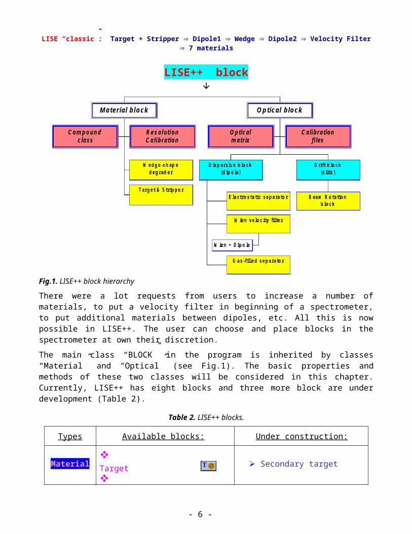
The “classic” LISE code uses only one configuration of a spectrometer consisting of two dipoles: LISE “classic”: Target + Stripper Dipole1 Wedge Dipole2 Velocity Filter 7 materials

LISE++ block

Fig.1. LISE++ block hierarchy

- 4 -

There were a lot requests from users to increase a number of materials, to put a velocity filter in begin-ning of a spectrometer, to put additional materials between dipoles, etc. All this is now possible in LISE++. The user can choose and place blocks in the spectrometer at own their discretion.

The main class “BLOCK” in the program is inherited by classes “Material” and “Optical” (see Fig.1). The basic properties and methods of these two classes will be considered in this chapter. Currently, LISE++ has eight blocks and three more block are under development (Table 2).

Table 2. LISE++ blocks.

Types Available blocks: Under construction:

Material Target

Stripper

Wedge-shape degrader Material (detector)

Secondary target

Optical Disper-sive (dipole) Wien velocity filter Drift block Beam rotation

Gas-filled separator Electrostatic separator

6 Set-up dialog: new main feature

Pressing on the button “Setup” in the toolbar (or through the menu “Settings Spec-trometer designing”) brings up a dialog “Spectrometer designing” (Fig.2) and allows you

to begin designing a fragment separator. This is the main new feature of LISE++.

The first two positions are occupied by the blocks “Target” and “Stripper”. There are fixed, it is im-possible to delete or move them.

Insert a new block: In the column “Block” of the window (“A” in Fig.2 - Spectrometer window) click on an exist-

ing block, which you want to insert a new block before or after; Choose an insert method “before” or “after” (“B” in Fig.2), In the frame “Insert block” (“C” in Fig.2) click on the icon of the block you wish to insert.

- 5 -

Delete block: Select a block you want to delete in the Spectrometer window,

Press on the button .

Move block: Select a block you want to move in the Spectrometer window, Press on a button “Up” or “Down” in the frame “Move element”.

Edit block: Select a block you want to edit in the Spectrometer window,

Press on the button .

or Double click, using the left mouse button, on the block you want to edit in the Spectrometer

window.

Fig.2. The dialog “Spectrometer designing” is the first step designing fragment separator.

It is possible to edit some properties of the selected block in the frame “Selected block” in the bottom left corner of the dialog.

Checkbox “Enable”: all new blocks are available automatically. It is impossible to disable the blocks “Target” and “Stripper”. If a block is set to disable, then this block is not shown in the Setup window and in the spectrometer scheme and the message “NO” will appear opposite this block in the column “Enable” of Spectrometer window of the dialog. A disabled block is not taken into account in trans-mission and spectrometer optic calculations. It is possible to change mode (“enable / disable”) of a block only in the dialog “Spectrometer designing”.

- 6 -

Checkbox “Let call automatically”: On: the block name is called automatically using the name of the block type and its order num-

ber in the spectrometer; Off: the block name may be entered manually. It is desired to input short names (less than 10

characters) to avoid a name truncation in the Setup window; All new blocks are called automatically.

Block name: The name of the block appears in all dialogs and menus connected with this block. If the option “Let call automatically” is set “Off”, then the user can input a new name for the block. It is rec-ommended to name the block so that it is clear from the name where the block is located. For example the name “Slits_Im2” is used to describe a drift block in the mode “slits” found in the location “Im -age2”.

Block length: the code uses a material block with zero length for the spectrometer length and time-of-flight calculations. Just optical blocks may have a length to determinate a spectrometer length and cal -culate time-of-flight. More on the length of optical blocks will be mentioned later in more detail.

Charge State (Z-Q): if the option “Charge states” (in the dialog “Preferences”) is set, and this is an optical dispersive block, then the cell “Charge state” is enabled and you can edit the charge state value for the setting fragment. More details about charge state calculations and their transmission is found in chapter 36

All operations in the dialog will be carried out without an opportunity to restore a former configuration. In other words the operation UNDO does not work in this dialogue. All changes will be shown in the “Setup win -dow” of the code and in the spectrometer scheme only after leaving this dialogue.

7 Scheme of spectrometer

The spectrometer scheme is a convenient innovation found in the new version (Fig.3). The program draws the spectrome-ter scheme on the basis of the blocks, en-tered by the user. The user can exclude or include this option in the dialog “Prefer-ence”.

Fig.3. The spectrometer scheme.

The number of dispersive block quadruples in your spectrometer can be changed in the dialog “General Block Settings” (see Fig.4) which is available through the dialog of block properties editing. Quadruples are properties of dispersive blocks (dipole, velocity filter). Quadruples are used just for the spectrometer scheme.

- 7 -

Fig.4. The “General block settings” dialog.

The user must be careful to set the correct length of dispersive block, which includes the quadruples and dipole(s). The dispersive block length should be always more than the dipole length, equal to the product of the radius of the dipole(s) and the angle (in radians). The difference between these lengths is the total length of the quadruples in that block.

The user can select a block on the spectrometer scheme by moving the mouse over it (turning the block dark blue), thus selecting it and allowing the user to click on it to bring up a dialog.

To Edit block properties: click on the selected block once using the left mouse button.

To Edit block acceptances and slits: click on the selected block once using the right mouse button.

Drift blocks in the mode “Slits” (block length is equal to 0) is shown by thin long line perpendicu-lar to the beam axis. In other words the length of the drawn block is proportional to its real length.

Materials with zero thickness are not shown in the scheme.

8 Settings of spectrometer scheme

It is possible to change properties of the spectrome-ter scheme using the dialog “Spectrometer scheme options” (see Fig.5) which can be loaded through the dialog “Preferences”.

The user can: Input an initial angle of the spectrometer, Set sizes of the scheme in units of the dimen-

sion of the isotope cells of the chart of nu-clides,

Change the background layout for the scheme,

Change colors.

To change a color it is necessary to select a block using the listbox in the frame “Block color in scheme” and then click on the window “Change”.

Fig.5. The “Spectrometer Scheme Options” dialog.

9 Description of Blocks and their properties10 Optical block

The hierarchy of optical blocks is shown in Table 3. Table 3. The hierarchy of optical blocks.

Class Derived from class New principal properties Blocks from this class

- 8 -

Optical block LISE++ block Optical matrix Slits & Acceptances

Drift Beam rotation

Dispersiveblock

Optical block Computational setting values Calibration file Setting charge state

Dipole Wien velocity filter

The description of classes is explained in the text. First the methods used in a class will be described for each class, then blocks used for constructing the spectrometer on the basis of a given class will be ex-plained.

11 Optical block: properties and methods

12 Optical matrix of LISE++ block

The “Optical matrix” class is based on a class “matrix” of constant, 66, dimension and has the capa-bility of transforming matrix elements of different units (mm  cm). LISE++ has two optical matrices for each optical block: “global “and “local”. The local matrix belongs just to one block and does not depend on other blocks. The program keeps all local matrices in configuration files. This is so the in-sert/removal of a new block in/from a spectrometer does not change the matrices of other blocks. The global matrix of the block is computed on the basis of ALL the previous blocks and the local matrix of this block. It is possible to present i global matrix calculations as recursive equation:

Gi = Li Gi-1 ,

Where G is the global matrix, and L is the local matrix. The global matrix of the first optical block is equal to its local matrix. The program uses elements from both matrices in fragment transmission cal-culations. The code automatically recalculates all global matrices if one of local matrices changed.

Clicking the button in the dialog of optical block properties allows the user

to load the dialog “Optical matrix” to edit block matrices (see Fig.6). The user can enter the data in different dimensions mm  cm, and into different matrices Local  Global. For this purpose using keys the user can choose mode, convenient for him. The matrix opposite to the one the user changed will be automatically recalculated on the basis of the just entered and previous matrices. If you enter the data in a global matrix, you should be sure, that the previous global matrix is computed correctly. If you input global matrices, start editing from the first matrix of a spectrometer.

- 9 -

Fig.6. The “Optical matrix” dialog.

In the LISE “classic” version the user could only edit local matrices. LISE++ not only allows you to edit local and global matrices by element as described above, but also allows to you input entire matri-ces using matrix files. Inserting matrices into the program LISE++ from the program TRANSPORT [Bro80] can be done using the following steps:

Choose a matrix corresponding to the block you want to change in the TRANSPORT result file and copy it to a new file.

Save the file with extension “mat”.

Create a new blank line in the file before the matrix elements. The first line of a file has to contain two numbers. The first shows matrix dimension (matrix is always supposed to be a square matrix). The second value is the dimen-sion. 0 corresponds to “mm”, 1 corresponds to “cm”. If the sec-ond number is missed, by de-fault it is supposed to be equal zero. The first line of the TRANSPORT matrix file should contain “6 1” (see Fig.7). The next six lines are matrix elements corresponding to the rows of the matrix. A separator between elements can be tabs, spaces, commas, or semicolons.

In the “Optic matrix” dialog click on “Global” to go to the mode of global matrix editing. Click on the button to load the file you just created. The default directory of matrix files is “<LISE++>\FILES”.

The dialogs of optical matrices depend on the block, and their features will be further explained in later sections. Reading of data in the matrix dialogs is not instantaneous, but is takes approximately 1 second in which you can see a blinking heart in the lower right corner of the dialog.

- 10 -

6 1-2.30374 0.00092 0.00000 0.00000 0.00000 2.8886310.75650 -0.43836 0.00000 0.00000 0.00000 0.0001100.00000 0.73813 0.00023 0.00000 0.00000 0.0000000.00000 37.30313 1.36628 0.00000 0.00000 0.0000003.10718 -0.12663 0.00000 0.00000 1.00000 -0.2422200.00000 0.00000 0.00000 0.00000 0.00000 1.00000

Fig.7. Example of matrix file (unit “cm”).

To save a matrix in a file it is necessary to press the button under the matrix. The program

saves the file as well as saving the units (mm/cm).

To get an inverse matrix press the button .

One way to check if the input values are corrected when then you are editing a matrix is to calculate the determinant. The determinant of an optical matrix should always be about 1. The determinant of a matrix is automatically calculated and displayed in the lower left, below the matrix.

13 Acceptances and slits

In the “classic” LISE program there was just one dialog for all the slits and acceptances of the spec-

trometer. In LISE++ each block (excluding “Rotation beam”, “ Stripper”, and “ Wedge” blocks) has

its own “Slits & Acceptance” dialog (see Fig.8), which is available by clicking in the dialog of the op-tical block properties through the button .

Fig.8. The “Slits & Acceptance” dialog.

The editing of slit sizes is more visual and convenient in the new version, as well as the use of slits is closer to the reality of an experiment. The maximum slit size is defined by the user. In LISE++ it is not possible to input a moment acceptance that frequently resulted in fallacy earlier. The momentum

- 11 -

acceptance is now determined by the slit size and dispersion (x/). Also, the program can calculate a momentum acceptance from the angular dispersion (/) and angular acceptance and takes that into ac-count in transmission calculations. It plays an important role in case of small dispersion (x/) and large angular dispersion (for example: block “Slits_S800BL” in the configuration file “A1900+S800_d0.lcn”).

If the checkbox “Use in calculations” is off then the program keeps the slits settings, but does not use in the calculations. The program shows the slit size in the “Set-up” window (see Fig.9 on the right) if the checkbox “Show in schematics” is set. Fig.9. The Set-up window fragment.

If the block has working slits then the Slits are found AFTER the optical block andBEFORE the material block (like support of detector)

Angular acceptance is applied on the BEGINNING of the block

14 Momentum acceptance of spectrometer

The program searches for the smallest acceptance in all the blocks and takes that for total momentum ac-ceptance of spectrometer (TMAS). The program shows the TMAS in the top right corner of the Infor-mation window . In reading in old (LISE)

files, where the slit size of slits was set using a mo-mentum acceptance, LISE++ will display the message indicating the former momentum acceptance value and new TMAS.

There are specific cases when the real TMAS actually will be more than shown by the program. The “double acceptance effect” is explained in chapter 32

15 Blocks from optical class

16 Drift block

A drift space is a field-free region through which the beam passes. There are three types of drift block classes (see Fig.10):

Standard drift block (as in the TRANSPORT code [Bro80]): Use this mode for a finite length detector in place of a detector with zero length in the spectrometer length calculation. The optical matrix is determined by the code on the base of block length.

Beam-line block: non-dispersive optical block. User can change the optical matrix values.

- 12 -

Slits mode: if the block length is equal to zero without dependence from a above-mentioned mode. The optical matrix of block in this mode is unitary.

It is possible to see the mode of a drift block in the Set-up window (see Fig.9). As well as in the spectrometer scheme “Slits” has different designa-tion from other modes of drift blocks. Some cells will be blocked from in-put in editing an optical matrix.

Increasing number blocks you de-crease transmission calculation speed. Despite that, it is recom-mended to use drift blocks in the mode Slits (more visual, fast access, is closer to a reality) instead of set-ting slits in the block “Dipole” for example.

Fig.10. The “Drift block” dialog.

17 Rotation beam block

The transverse coordinates x and y may be ro-tated through an angle 90,180, and 270 degrees about the z axis (the axis tangent to the central trajectory at the point of question) as done in the program TRANSPORT [Bro80]: type code 20.0. The “Rotate beam” block (see Fig.11) does not support slit properties. The “Rotation beam” block is shown by a circle on the spectrometer scheme. The code automatically recalculates the local optic matrix of the block. The user cannot edit matrix values.

Fig.11. The “Rotate beam” dialog.

The block is used at transitions of one plane to another. For example, the A1900 spectrometer is in a horizontal plane, and then the beam follows the S800 beam-line which is in a vertical plane.

18 Dispersive block

Optical dispersive blocks are electromagnetic separation devices. Only Dispersive optical blocks deter-mine the setting of the spectrometer on a certain fragment.

19 Properties and methods

20 Computational values (fields)

Classification of electromagnetic separation devices (LISE++ dispersive blocks) and their selection methods is given in Table 4. Magnetic (electrical) fields of dispersive blocks can be calculated by the

- 13 -

code, as well as the user can enter manually field values. The basic difference of dispersive blocks from optical blocks is that the adjustment of the fields of these blocks result in a change in the trajec-tory of particles and therefore their separation in space. When the spectrometer is “set” on a fragment, it means that the magnetic (electrical) rigidity of a particle coincides with magnetic (electrical) rigidity of electromagnetic devices in the central trajectory. The magnetic field (for a magnetic dipole) is cal -culated from the magnetic rigidity of the device using a dipole radius. If a calibration file (see the next chapter for a definition of the calibration file) is entered, then the electric current (I) is also taken into account.

Table 4. Electromagnetic separation devices.

Separation device Changeable field Strength Selection by

Magnetic dipole Magnetic (B[T]) Magnetic rigidity [Tm]

Electric dipole Electric (E [kV/m]) Electric rigidity [J/C]

E-cross-B filter Magnetic (B[T])Electric (E [kV/m])

Velocity

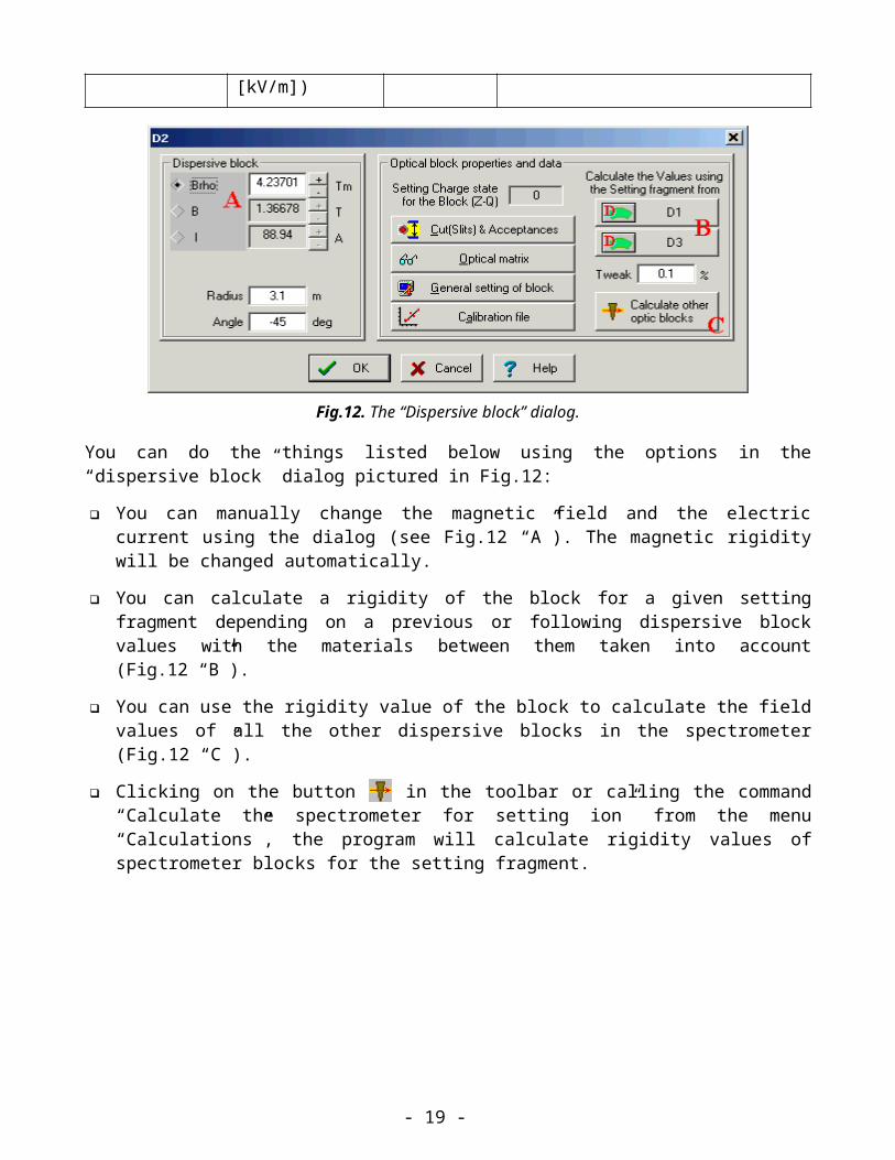
Fig.12. The “Dispersive block” dialog.

You can do the things listed below using the options in the “dispersive block” dialog pictured in Fig.12:

You can manually change the magnetic field and the electric current using the dialog (see Fig.12 “A”). The magnetic rigidity will be changed automatically.

You can calculate a rigidity of the block for a given setting fragment depending on a previous or fol-lowing dispersive block values with the materials between them taken into account (Fig.12 “B”).

You can use the rigidity value of the block to calculate the field values of all the other dispersive blocks in the spectrometer (Fig.12 “C”).

- 14 -

Clicking on the button in the toolbar or calling the command “Calculate the spectrometer for setting ion” from the menu “Calculations”, the program will calculate rigidity values of spectrom-eter blocks for the setting fragment.

21 Calibration file

The interrelation between a magnetic field and an electric current can be entered for the block through a calibration file. In actuality, experi-menters use electric currents to set a desirable magnetic field or in other words to establish de-sirable magnetic rigidity. Entering a value of the electric current in the Dispersive block dia-log, you can estimate expected magnetic rigid-ity.

Calibration dialogs were done in the LISE clas-sic version just for two defined spectrometers. Moreover the user could not change calibration values. LISE++ allows you to use calibration files for all of the dispersive blocks. Fig.13. The “Calibration file” dialog.

The format for the calibration file is rather simple. You can see the format description in The “Calibra-tion file” dialog (Fig.13). The program uses a cubic spline to get a value in region indicated in the file. The code uses a linear extrapolation if the searched value exceeds the determinate region.

Bread is a measured value from a electromagnetic device (for example a NMR probe).

Bset is established using the calibration. The program uses the Bread value to calculate a magnetic rigid-ity. If just one calibration between the magnetic field and electric current is entered, then B=Bread=Bset.

22 Dispersive block on the base of Magnetic dipole

The program uses the definition of a “Dispersive block” instead of simply a “Magnetic dipole” to un-derline that this block is a system with one optical matrix but consists of quadruples, drifts, and mag-netic dipoles. The “Dispersive block” dialog is presented in Fig.12. The basic characteristics and prop-erties were described above in the text.

The order of distribution and transmission calculations in the dispersive blocks is given in chapter 34

23 Wien velocity filter

LISE++ assumes the velocity filter is a standard dispersive block with the optical matrix and all other properties and methods. This redefinition in comparison with the “classical” version allows the use of the filter anywhere in the spectrometer. Velocity dispersion through the filter depends on the mass and charge of a particle and is function of the particles energy. The most important difference between the filter and a magnetic dipole is that dispersive elements of the local optical matrix are recalculated for each fragment and energy anew for the Wien velocity filter.

- 15 -

The filter operates with two fields. Therefore to adjust the filter on a one fragment, you should keep one field constant (see the frame ”Select constant field” in Fig.14) and change the other field. In a re-ality the electrical field is kept constant, while the magnetic field is changed.

Fig.14. The “Wien velocity filter” dialog.

The LISE code has three parameters to define the filter of velocity: o eElen - Effective electric length,o eMlen - Magnetic effective length,o rrf - Real/Read field.

There is just one parameter “Effective electric & magnetic length relation (EMLR)” in the LISE++ (see the frame ”Filter constants” in Fig.14), which is a combination of three of these LISE parameters using the formula: EMLR = eElen · rrf / eMlen.

24 Compensating dipole after the Wien velocity filter

It is planned to develop a dialog for a compensating dipole after the Wien velocity filter as in LISE (it was named dipole D6). The compensating dipole is a dispersive block assigned to compensate the ve-locity dispersion after the Wien velocity filter. Using the compensating dipole it is possible to get the A/Q dispersion. The main advantage of A/Q selection is absence of a momentum (velocity) dispersion which allows you to use the large momentum emittance of the secondary beam. However, you can simulate the compensating dipole in LISE++ already now. To do so, you have to put a dispersive block after the Wien velocity filter and manually input a dispersion of the block to compensate the fil-ter dispersion, such that after the compensating block the global dispersion is equal to zero. Fig.15 shows selections by the system “velocity filter dipole” for different values of the electric filed of the velocity filter. This example is accessible through the LISE web-site: http://groups.nscl.msu.edu/lise/6_1/examples/lise_wien_d6.lpp

- 16 -

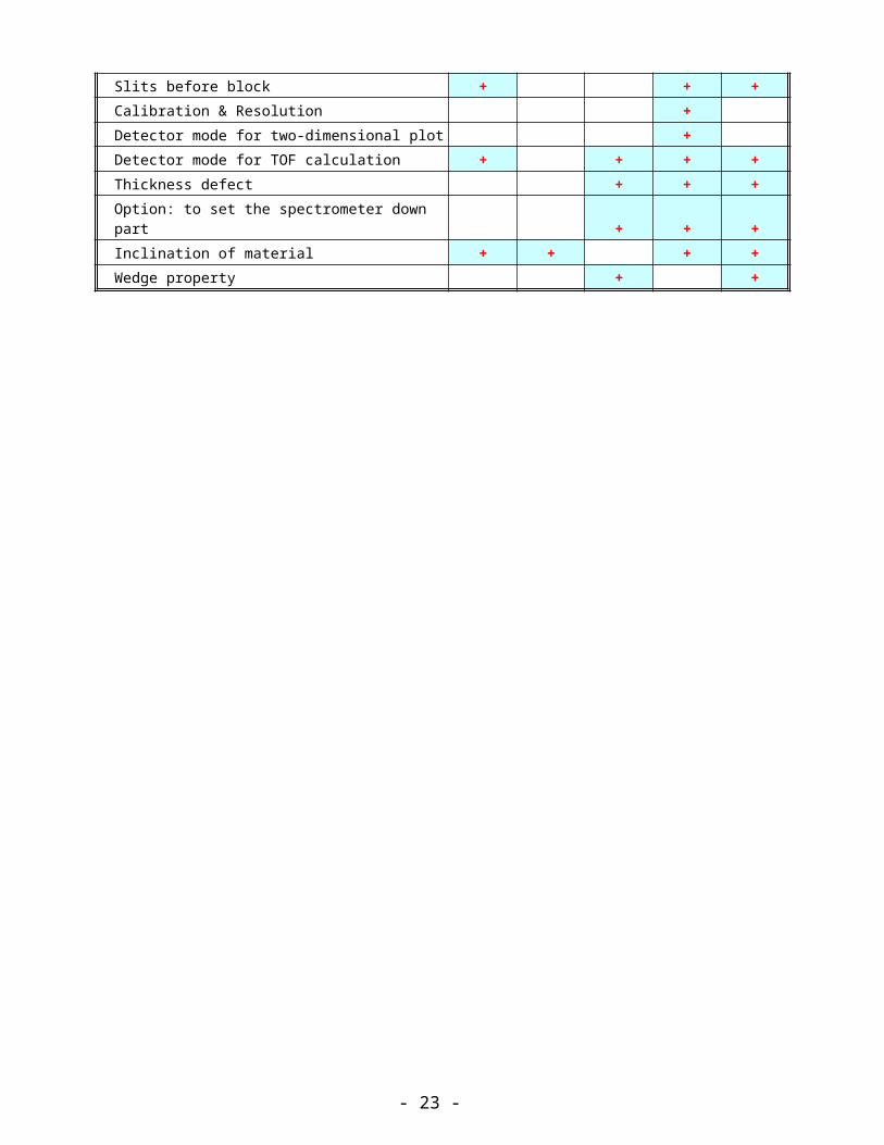
25 Material blocks

Material blocks were created on the basis of the LISE++ Block class and the LISE Compound class. There are four existing blocks (Target, Stripper, Material, Wedge) and one (Secondary target) still un-der development. Material blocks properties are given in Table 5.

Table 5. Properties of Material blocks.

Property / Block

Targ

et

Strip

per

Wed

ge

Mat

eria

l

Seco

ndar

y ta

rget

Calculation of primary fragments production + +     +Calculation of secondary reactions +        Attenuation due to reactions + + + + +General setting dialog     + + +Slits before block +     + +Calibration & Resolution       +  Detector mode for two-dimensional plot       +  Detector mode for TOF calculation +   + + +Thickness defect     + + +Option: to set the spectrometer down part     + + +Inclination of material + +   + +Wedge property     +   +

- 17 -

Fig.15. dE-Y simulation spectra for the reaction 40Ar + Be(500 m) with 32S as the setting frag-ment. The LISE spec-trometer (p/p=4.6%), Wien velocity filter and the compensating dipole were used in the calcu-lations. LISE velocity filter selects fragments in the vertical plane. En-ergy loss calculations were done through a 300 m silicon detector located behind the com-pensating dipole.

Upper plot shows the vertical selection of fragments after the ve-locity filter without the compensating dipole.

Middle and lower plots show the vertical selec-tion of fragments using the compensating dipole for different values of the electric field of the velocity filter.

- 18 -

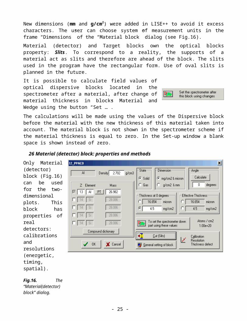
New dimensions (mm and g/cm2) were added in LISE++ to avoid it excess characters. The user can choose system of measurement units in the frame “Dimensions” of the “Material block” dialog (see Fig.16).

Material (detector) and Target blocks own the optical blocks property: Slits. To correspond to a real-ity, the supports of a material act as slits and therefore are ahead of the block. The slits used in the pro -gram have the rectangular form. Use of oval slits is planned in the future.

It is possible to calculate field values of optical dispersive blocks lo-cated in the spectrometer after a material, after change of material thickness in blocks Material and Wedge using the button “Set …”.

The calculations will be made using the values of the Dispersive block before the material with the new thickness of this material taken into account. The material block is not shown in the spectrometer scheme if the material thickness is equal to zero. In the Set-up window a blank space is shown instead of zero.

26 Material (detector) block: properties and methods

Only Material (detec-tor) block (Fig.16) can be used for the two-dimensional plots. This block has properties of real de-tectors: calibrations and resolutions (en-ergetic, timing, spa-tial).

Fig.16. The “Mate-rial(detector) block” dialog.

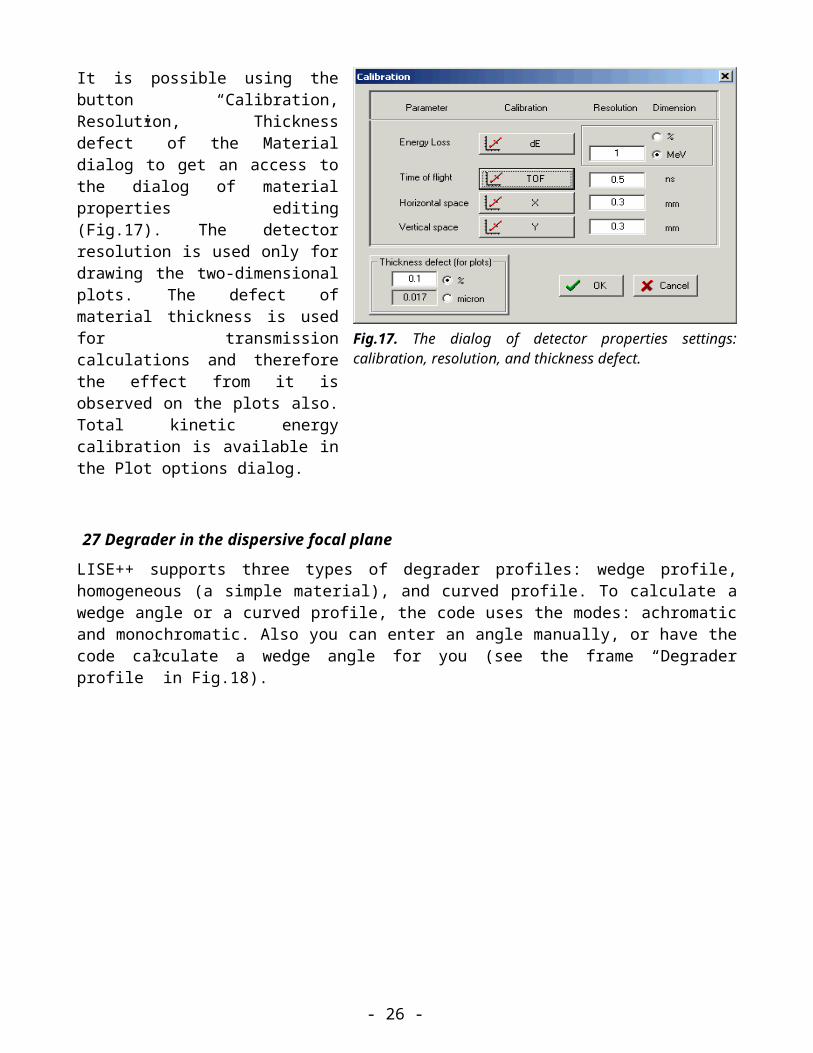
It is possible using the button “Calibra-tion, Resolution, Thickness defect” of the Material dialog to get an access to the di-alog of material properties editing (Fig.17). The detector resolution is used only for drawing the two-dimensional plots. The defect of material thickness is used for transmission calculations and therefore the effect from it is observed on the plots also. Total kinetic energy cali-bration is available in the Plot options di-alog.

Fig.17. The dialog of detector properties settings: calibration, resolution, and thickness defect.

- 19 -

27 Degrader in the dispersive focal plane

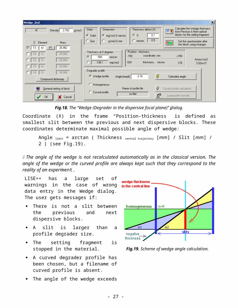
LISE++ supports three types of degrader profiles: wedge profile, homogeneous (a simple material), and curved profile. To calculate a wedge angle or a curved profile, the code uses the modes: achro-matic and monochromatic. Also you can enter an angle manually, or have the code calculate a wedge angle for you (see the frame “Degrader profile” in Fig.18).

Fig.18. The “Wedge (Degrader in the dispersive focal plane)” dialog.

Coordinate (X) in the frame “Position-thickness” is defined as smallest slit between the previous and next dispersive blocks. These coordinates determinate maximal possible angle of wedge:

Angle limit = arctan ( Thickness central trajectory [mm] / Slit [mm] / 2 ) (see Fig.19).

The angle of the wedge is not recalculated automatically as in the classical version. The angle of the wedge or the curved profile are always kept such that they correspond to the reality of an experiment.

LISE++ has a large set of warnings in the case of wrong data entry in the Wedge dialog. The user gets messages if:

There is not a slit between the previous and next dispersive blocks.

A slit is larger than a profile degrader size.

The setting fragment is stopped in the mate-rial.

A curved degrader profile has been chosen, but a filename of curved profile is absent.

The angle of the wedge exceeds the maxi-mum possible angle.

Fig.19. Scheme of wedge angle calculation.

- 20 -

28 Wedge angle calculationLISE++ can calculate a wedge angle from the conditions that the wedge must be achromatic or monochromatic after the block defined by the user. In the classical version the wedge is found between two dipoles and the angle is calculated for the focal plane after the second dipole. In LISE++ a wedge can be placed in anywhere.It is necessary in the frame “Mode” to choose the block after which conditions will be applied. If you press one of the keys “Fix” or enter a value into “Fixed in the code” cell manually (Fig.20) than the program uses one of calculated angles in the further calculations.

Fig.20. The wedge angle calculation dialog.

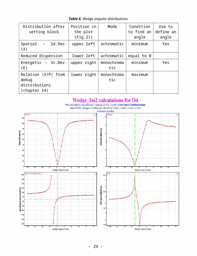
LISE++ calculates the wedge angle when this dialog is loading or when one of the parameters (block, number of points in distribution) changed. The code determinates the minimal (min) and maximal (max) values of angle (as well as Angle limit from the previous section). The program N+1 times calcu-lates a setting fragment transmission changing a wedge angle for the value (max - min) / N. As a result of these calculations the program fills four distributions which can be plotted by clicking “to plot a de-pendence from angle” in the frame “Mode”. The received wedge angular distributions are shown in Fig.21. A description the wedge angular distribution is shown in Table 6.

Table 6. Wedge angular distributions.

Distribution after setting block

Position in the plot (Fig.21)

Mode Condition to find an angle

Use to define an angle

Spatial – Sd.Dev.(X) upper left achromatic minimum YesReduced dispersion lower left achromatic equal to 0Energetic – St.Dev.(E) upper right monochro-

maticminimum Yes

- 21 -

Relation |X/P| from debugdistributions (chapter 54)

lower right monochro-matic

maximum

Fig.21. Wedge angular distributions.

The code seeks minimums in spatial and energetic distributions. The code defines angles using neigh-boring points of these minimal points by a simple expression. To get more precise wedge angles, it is necessary to increase the number of points in the wedge angular distributions. A default value of the distribution dimension is defined in the dialog “Preferences”.

Press the key “Escape” once if you want to break calculations.

If the code didn’t find a solution for one of a mode or you interrupted then you will see a string “???” instead of a calculated angle value.

Button “To plot a dependence from angle” will be inaccessible if

Calculations were interrupted

- 22 -

The transmission of the setting fragment after chosen block is equal to zero for all points of the wedge angular distributions.

29 Possible problems in wedge angle calculationWorking with the beta-version many users had questions and problems with wedge angle calculations. On the basis of their remarks, the program was modified to display messages indicating why a wedge angle was not is calculated. See Table 7 for messages problems, reasons then to correct the problem.

Table 7. Possible problems in wedge angle calculation and methods of their elimination.

LISE++ message Problem Reasons How to correct

Spectrometer is not set for the isotope of interest

Transmission of the isotope of interest after the setting block is equal to 0

The wedge thickness has been changed, but the user forgot to recalculate block values of the spectrometer after this block

Return to the wedge dialog, Click the button “to set the

spectrometer …”

Spectrometer has not been set on the isotope of interest

Leave the wedge dialog, Calculate spectrometer.

Wedge thickness is too thick Return to the wedge dialog, Decrease wedge thickness, Set the spectrometer.

Thickness of material located between wedge and the setting block is too thick

Leave the wedge dialog, Change material, Calculate spectrometer

try to increase maximum (min) angle by closing slits or making the wedge thicker

There is not mini-mum in the wedge spatial or energetic distributions(then see angle dis-tribution plots)

Achromatic or Monochromatic angles are bigger than the maxi-mum possible angle. This is a frequent problem.

try to increase the maximum possible angle by closing slits or making thicker the wedge

Slit size of one of the blocks af-ter the wedge up to the selected plane is smaller than the spatial distribution of fragment of in-terest

Leave the wedge dialog, Check all slits after the

wedge

Dispersion is wrong Check optical matrices; check that the correct dispersion plane direction was chosen

There is not a dispersive block after the wedge and the setting plane. In this case it is possible to calculate a wedge angle in monochromatic mode, but not in achromatic mode.

The wedge thick-ness is equal to 0!

No comments…it is clear

Input a positive value in the edit cell of wedge thickness, Click button “to set the spectrometer…” to calculate spec-

- 23 -

trometer down parts for new wedge thickness And try to calculate angle once more.

30 Curve profile degraderLISE ++ has a new profile of degrader that can be used for transmission calculations: a curved profile degrader. If in the classical version only a wedge shape degrader was applied to transmission calcula-tions, but in the new version a curved profile degrader also can be applied for transmission calcula-tions.

A curved degrader consists of a foil and a support for this foil. Having calculated a profile for the sup-port, the user can save it in a file and use it in further cal-culations.

In reality, a support for a curved degrader can hold many differ-ent thickness de-grader (foil). There-fore, LISE++ has the capability to let you use the same support for several different thickness degraders.

The support can be designed with use of the “Curve profile de-grader” dialog (Fig.22).

Fig.22. The “Curve profile degrader” dialog.

By analogy to the “Wedge angle calculation” dialog (Fig.20), the user should select a block and mode.

It is necessary to define support parameters X and L. A degrader length should be approximately the slits size.

Pressing on the button “Calculate & Plot”, the program will calculate a support of curved de-grader.

Save the calculated profile in a file.

The user can load already created structures from a disk. The parameters of a support from a file will be shown in the dialog and can be visualized in the plot. It is possible to see the corresponding wedge

- 24 -

angle from profile file in the dialog. This angle is calculated on the basis of the support and a material used at this moment in the wedge block. The files of supports have the extension “degra” and are by default in the directory “\degrader”.

31 Use of two wedgesThe new version has the opportunity to use multiple wedges at once. Examples of ways to use two wedges are:

1. Select an isotope of interest using an achromatic wedge to partially eliminate impurities. Then use a monochromatic wedge to get a monoenergetic secondary beam without impurities at the end of spectrometer.

2. To eliminate (by the second wedge) products of secondary reactions from the first wedge. This is very useful for particles at relativistic energies.

3. To increase the spectrometer momentum acceptance (see the next chapter).

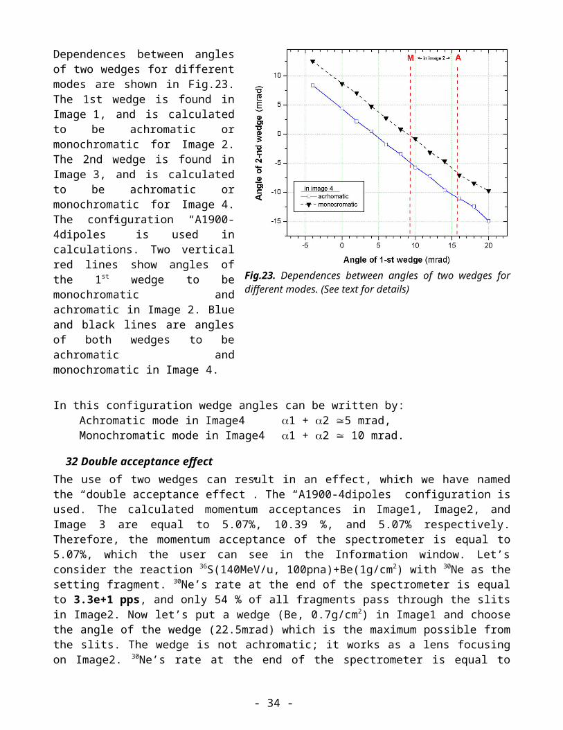
Dependences between angles of two wedges for different modes are shown in Fig.23. The 1st wedge is found in Im-age 1, and is calculated to be achromatic or monochromatic for Image 2. The 2nd wedge is found in Image 3, and is calcu-lated to be achromatic or monochro-matic for Image 4. The configuration “A1900-4dipoles” is used in calcula-tions. Two vertical red lines show angles of the 1st wedge to be monochromatic and achromatic in Image 2. Blue and black lines are angles of both wedges to be achromatic and monochromatic in Image 4. Fig.23. Dependences between angles of two wedges for different

modes. (See text for details)

In this configuration wedge angles can be written by:Achromatic mode in Image4 1 + 2 5 mrad,Monochromatic mode in Image4 1 + 2 10 mrad.

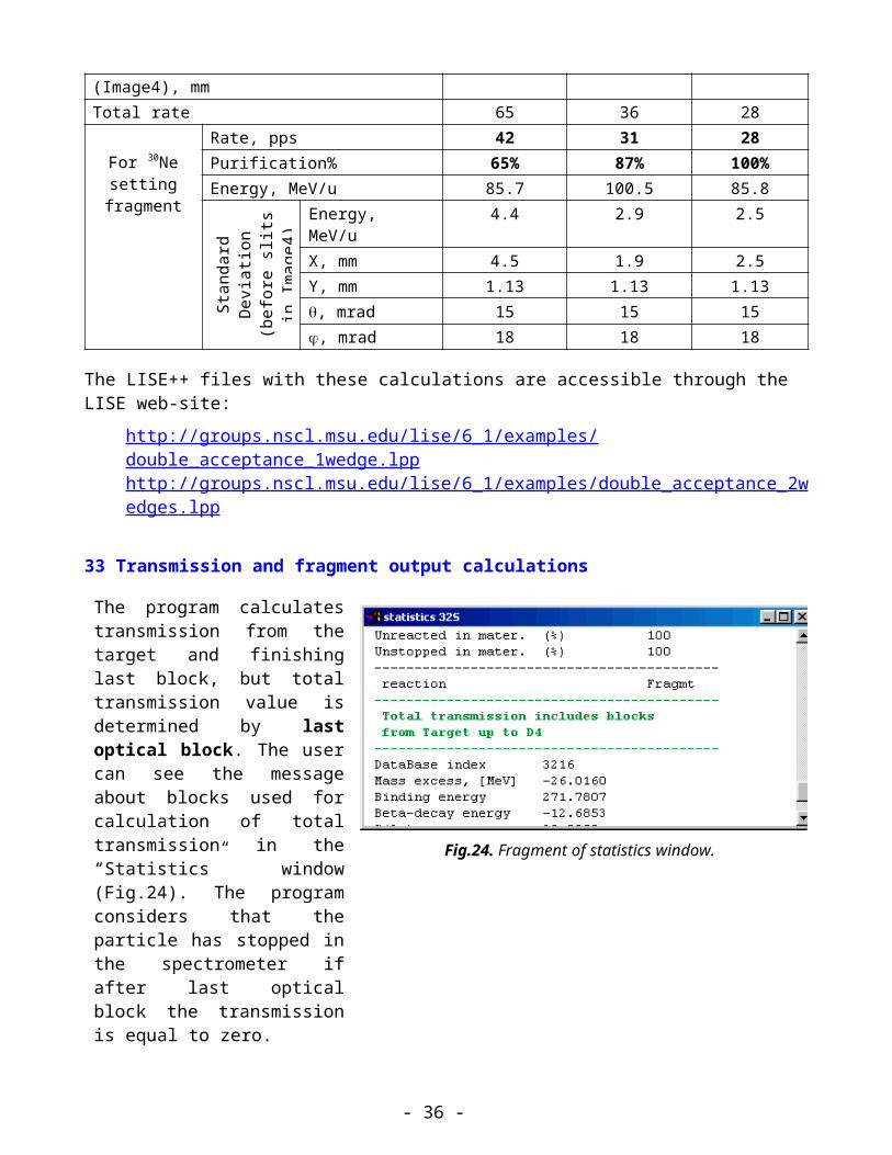
32 Double acceptance effectThe use of two wedges can result in an effect, which we have named the “double acceptance effect”. The “A1900-4dipoles” configuration is used. The calculated momentum acceptances in Image1, Im-age2, and Image 3 are equal to 5.07%, 10.39 %, and 5.07% respectively. Therefore, the momentum acceptance of the spectrometer is equal to 5.07%, which the user can see in the Information window. Let’s consider the reaction 36S(140MeV/u, 100pna)+Be(1g/cm2) with 30Ne as the setting fragment. 30Ne’s rate at the end of the spectrometer is equal to 3.3e+1 pps, and only 54 % of all fragments pass

- 25 -

through the slits in Image2. Now let’s put a wedge (Be, 0.7g/cm2) in Image1 and choose the angle of the wedge (22.5mrad) which is the maximum possible from the slits. The wedge is not achromatic; it works as a lens focusing on Image2. 30Ne’s rate at the end of the spectrometer is equal to 5.6e+1 pps, and 98% transmission through the slits in Image2. Now the momentum acceptance of the spectrometer is determined by the slits in Image1, instead of by the slits in Image2, and therefore the rate has doubled.

If a degrader is put in Image 3 that is identical to the wedge in Image1 and an angle is calculated to be achromatic for Image4 (angle = -14 mrad), it is possible to select 30Ne from the impurities which com-prise about 65% of the beam.

Calculation results for configurations with different numbers of wedges are shown in Table 8. From this table it follows that the best selection is reached when the wedge is found in a plane with maximal dispersion. But in this case the rate is lower, but the quality of a secondary beam (emittance, purifica-tion) is much better, than in the case of the use of two wedges. As always there is the balance between quantity and quality.

Table 8. Calculation results for configurations with different numbers of wedges.

Configuration 2 wedges 1 thin wedge 1 thick wedge

First WedgeLocation Image1 Image2 Image2

Thickness Be 0.7 g/cm2 Be 0.7 g/cm2 Be 1.4 g/cm2

Ang

le

(mra

d)

Achromatic 40.3 -2.05 -4.13Monochromatic 22.0 -10.85 -10.76abs.maximal 22.72 22.72 45.42fixed in the code 22.5 -2.1 -4.1628

Second wedgelocation Image3 - -

Thickness Be 0.7 g/cm2

Ang

le

(mra

d)

achromatic -13.7monochromatic -0.38Abs.maximal 22.72fixed in the code -13.7

30Ne transmission in Image2 slits 97.2% 54.2% 54.2%Silts in final focal plane (Image4), mm -4/+8 -6/+6 -9/+9Total rate 65 36 28

For 30Ne setting fragment

Rate, pps 42 31 28Purification% 65% 87% 100%Energy, MeV/u 85.7 100.5 85.8

Stan

dard

De-

viat

ion

(bef

ore

slits

in

Imag

e4)

Energy, MeV/u 4.4 2.9 2.5X, mm 4.5 1.9 2.5Y, mm 1.13 1.13 1.13, mrad 15 15 15, mrad 18 18 18

The LISE++ files with these calculations are accessible through the LISE web-site:

- 26 -

http://groups.nscl.msu.edu/lise/6_1/examples/double_acceptance_1wedge.lpphttp://groups.nscl.msu.edu/lise/6_1/examples/double_acceptance_ 2 wedge s .lpp

33 Transmission and fragment output calculations

The program calculates transmis-sion from the target and finishing last block, but total transmission value is determined by last optical block. The user can see the mes-sage about blocks used for calcula-tion of total transmission in the “Statistics” window (Fig.24). The program considers that the particle has stopped in the spectrometer if after last optical block the trans-mission is equal to zero.

Fig.24. Fragment of statistics window.

If a telescope, with certain slits in front of it, is placed in the end of the spectrometer, losses on the slits will not enter in the total transmission value. For example, FP_PIN detector after dipole 4 has its own slits of ± 25 mm in the configuration A1900-4dipoles. But the dipole D4 slits are equal to ± 150 mm. A loss of rate on FP_PIN slits is expected, but it will be not incorporated to the total trans-mission value.

Let’s suggest a scenario in which all secondary particles are stopped a telescope in the end of the spectrometer. If an optical block is put after the telescope then transmission of all particles will be equal to 0, and the code suggests no events were transmitted through the spectrometer.

34 Transmission calculation in a block

The orders of distribution transformation and transmission calculations in the dispersive and material blocks are given in Table 9.

Table 9. Transmission calculation order in block.

Optical block Material block

1. Angular acceptance: Transmission value calculation, Cutting of angular distributions.

2. Optical matrix application for spatial distributions.3. Spatial slits at the end of a block:

Transmission value calculation, Cutting of spatial, momentum and

angular distributions.

1. Spatial slits before a block:Transmission value calculation,Cutting of spatial, momentum and

angular distributions.2. Passing through the material.

Transformation of energetic distributions.3. Angular straggling application

for angular distributions.

- 27 -

4.Optical matrix application for angular distributions.

- 28 -

35 Transmission statisticsBy moving the mouse pointer to an isotope cell in the nuclide chart and pressing the right button of the mouse the user can calculate the transmission and rate of a selected isotope and its statistics window will pop up (Fig.25). Transmission re-sults are shown block by block in the new version. Lines divide the blocks. The total block transmission is shown in dark blue. In the new version the user can automatically see the block in which the particle has stopped (see the green oval in Fig.25), if the total transmission in that block is equal to zero.

The user can load the transmission dialog analysis (Fig.26), using the button “Analysis” from the statistics window or the command in the menu “Calculations Transmis-sion”. Fig.25. Fragment of statistics window.

Fig.26. The transmission analysis dialog.

- 29 -

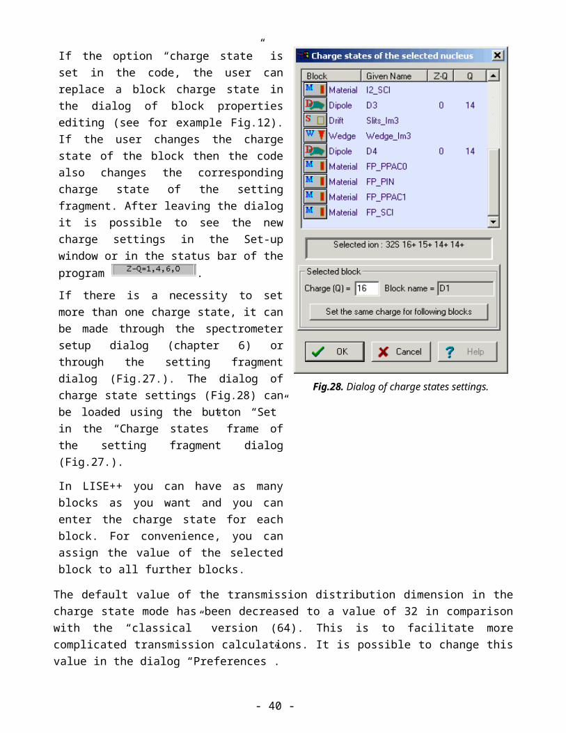
36 Charge states

The number of charge states of the setting fragment is equal to the num-ber of dispersive blocks. The n charge state of a block is defined in the code as Z-Q, where Q is the n charge state of setting fragment (see table on the right). The magnetic (electric) rigidity of the block is recalculated on the ba-sis of its charge state setting.

Dispersive block order 1 2 N

Charge state of setting fragment Q1 Q2 QN

Charge state of block Z-Q1 Z-Q2 Z-QN

Fig.27. The “Setting fragment” dialog.

If the option “charge state” is set in the code, the user can replace a block charge state in the dialog of block properties editing (see for example Fig.12). If the user changes the charge state of the block then the code also changes the corresponding charge state of the setting fragment. After leaving the dialog it is possible to see the new charge set-tings in the Set-up window or in the status bar of the program .

If there is a necessity to set more than one charge state, it can be made through the spectrometer setup dialog (chapter 6) or through the setting fragment dialog (Fig.27.). The dialog of charge state settings (Fig.28) can be loaded using the button “Set” in the “Charge states” frame of the setting fragment dialog (Fig.27.).

In LISE++ you can have as many blocks as you want and you can enter the charge state for each block. For convenience, you can assign the value of the selected block to all further blocks. Fig.28. Dialog of charge states settings.

The default value of the transmission distribution dimension in the charge state mode has been de-creased to a value of 32 in comparison with the “classical” version (64). This is to facilitate more com-plicated transmission calculations. It is possible to change this value in the dialog “Preferences”.

- 30 -

37 Results file

In connection with global reconstruction of the program, the result file also has undergone a number of serious changes. As before, the user can create, look and print a result file through the menu “File  Results”. The file will be saved with the same name as the name of the LISE++ file in the same directory, but with the extension “res”.

The result file contains calculations of energy losses and times of flight along with standard devia-tions. The same subroutine used to create the result file is used to calculate values (using the resolution of detectors) in the dialog “Goodies” and in the ellipse mode of two-dimensional plots.

Structure of the result file is:

Header: brief spectrometer configuration and basic options, Table 0: Transmission and Rate calculations, Table 1. Time of flight, Energy after stripper, Table 2. Energy after blocks, Table 3. Energy loss in materials.

Be careful when printing a result file. The width of the page depends proportionally on the quantity of blocks in the spectrometer. Print in landscape mode instead of portrait, or use a word-processor to prepare the file for printing.

38 Previous isotope area rectangle

It is possible just once to choose a rectangle of isotopes of interest to calculate their transmission by the button “Calculate area of nuclei” , and to repeat calculations with this rectangle again by click-ing the button “Previous calculated area” in the toolbar. The new version saves the previous iso-tope rectangle in the LISE++ file. After loading the file, the user can use the button “Previous calcu-lated area” without additional definition. If you want to change what isotopes are calculated, just click on “Calculate area of nuclei” again.

39 Improved mass formula with shell crossing corrections.

Accurate predictions of the production cross-sections of rare isotopes are important in the study of as-trophysical processes and in the location of drip-lines. Reaction models as the abrasion-ablation, statis-tical multifragmentation or fusion-evaporation models rely on parameterization of the nuclear masses. This may lead to large inaccuracies in the case of discrepancies between mass parameterization and the experimental masses.

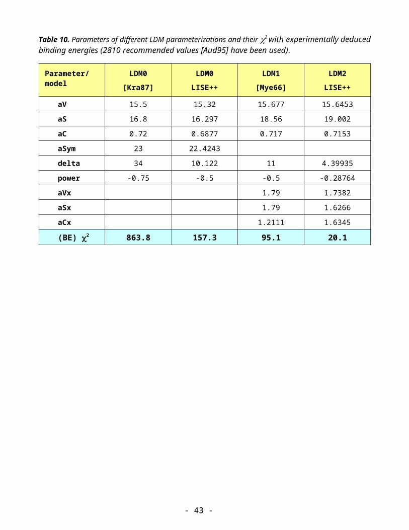
Representation of nuclei as liquid drops has been very successful in predicting their properties and masses, especially those along the valley of stability. However, a large discrepancy is observed for the classical Liquid Drop Mass formula and experimental values due to the shell structure. LISE++ uses a new mass formula with shell crossing corrections.

- 31 -

The most commonly used Liquid Drop Mass (LDM) formula (first developed by Von Weizsaecker) is where the nucleus binding energy is presented by sum of the terms shown in the table below:

Volume Surface Coulomb Symmetry PairingaVA -aS  A2/3 -aC  Z2 / A1/3 -aSym (2A-

Z)2/Adelta A-1/2

Where Z and A are the charge and mass number; aV, aS, aC, aSym, are coefficients; delta is equal to + for Z and N are even, and - for Z and N are odd, and zero for A is odd. Let’s name this formula by LDM0.

Meyers and Swiatecki [Mye66] have generalized this expression for the more general case of distorted nuclei:

Volume Surface Coulomb Coulomb_X PairingaVA(1-aVx  x) -aS  A2/3(1-aSx  x

)-aC  Z2 / A1/3 Acx  Z2 / A delta A-power

Where x is ((A-2Z)/A)2 ; aSx, aVx, aCx are the coefficients; the term Symmetry is equal to 0 in this formula, aSx and aVx suggested to be equal. Let’s name this formula by LDM1.

The formula LDM2 represents the formula LDM1 with shell crossing corrections, which are described in the next chapter. Table 10 shows parameters for all these models including a new fit of parameters using the LDM0 formula (LDM0 LISE++). Fig.29 shows differences between binding energies from experimental masses [Aud95] and different LDM parameterizations.

Table 10. Parameters of different LDM parameterizations and their 2 with experimentally deduced binding energies (2810 recommended values [Aud95] have been used).

Parameter/model LDM0

[Kra87]

LDM0

LISE++

LDM1

[Mye66]

LDM2

LISE++

aV 15.5 15.32 15.677 15.6453

aS 16.8 16.297 18.56 19.002

aC 0.72 0.6877 0.717 0.7153

aSym 23 22.4243

delta 34 10.122 11 4.39935

power -0.75 -0.5 -0.5 -0.28764

aVx 1.79 1.7382

aSx 1.79 1.6266

aCx 1.2111 1.6345

(BE) 2 863.8 157.3 95.1 20.1

- 32 -

Fig.29. Differences between binding energies from experimental masses [Aud95] and different LDM parame-terizations.

- 33 -

40 Shell crossing corrections

It is clearly visible from Fig.30, that the largest dif-ference between experimen-tal binding energies and cal-culated LDM1 parameteri-zation is observed on cross-ings of shells. Fig.29 shows (LDM0 LISE++ and LDM1 plots), that most of these de-viations for shells 28, 50 and 82 have the form close to Lorentz distribution. It is necessary to note, that these triangular deviations influ-ence fitting throughout the chart of nuclides. Attempts to smooth these “triangle” effects and then to make a new parameterization are undertaken with the use of “two-dimensional” Lorentz distribution. A finite area that is to be corrected is de-fined in the code. To avoid overshooting on the bound-ary of the area to be cor-rected the difference be-tween the Lorentz functions at this point and the bound-ary point are taken. The sec-tion of code used to calcu-late the shell correction is shown below Fig.30. Table11 contains parameters of shell corrections of the LDM2 model. It is possible to appreciate the contribu-tion of shell crossings cor-rections comparing 2 of dif-ferent models in Table 10.

Fig.30. Differences between binding energies of the inbuilt database and LDM1 parameterization.

//=================================================double ShellCorrect(int Z, int N, int Zshell, int Nshell, double Amp, double width, double length, double coef){double v = (fabs(N-Nshell)/coef + fabs(Z-Zshell))/width;double vl = length/width;

return( v < vl ? Amp * (1/(v*v + 1) - 1/(vl*vl + 1)) : 0);}//=================================================

Table 11. Parameters of LDM2 shell crossings corrections.

Z N Amp width length coef82 126 11.85 8.15 23.090 0.87850 82 12.84 8.21 21.382 0.87828 50 6.24 9.30 16.294 0.87820 28 2.13 6.89 12.165 0.87882 82 17.99 9.38 20.960 0.94250 50 12.26 8.91 21.841 0.94228 28 7.33 6.65 16.804 0.94220 20 5.40 2.02 3.332 0.94216 16 5.14 2.71 6.909 0.94214 14 4.88 2.39 11.253 0.9428 8 20.75 3.43 2.500 0.9426 6 18.57 3.04 2.500 0.9422 2 17.08 2.41 2.500 0.942

- 34 -

41 Use of LDM parameterizations in LISE++

The parameterizations LDM0 (LISE++), LDM1 and LDM2 are used in the code and named corre-spondingly Calculation 0, Calculation 1, and Calculation 2. Mass calculations are used:

To extrapolate mass of nuclei absent in the inbuilt database. These masses are kept in the operat-ing memory and used for calculations every time the code needs an isotope mass. The extrapo-lated mass of a nucleus is equal to:

,

where the nuclei (Ai,Zi) are the closest known nuclei ,in the database, to the unknown nuclei of interest.

To calculate widths of different channels of particle emissions in the Abrasion-Ablation or “LisFus” models if option “for separation energies use” is set to “semiempirical formula” in the “Setting of Prefragment and Evaporation calculations” dialog.

In the ”Production mechanism” dialog it is possible to choose one of LDM parameterizations in order to use it in calculations mentioned above. From the “Database” dialog it is possible to load the “Calculations” dialog (Fig.31), which with the user can see isotope characteristics calculated by various models. Using the “Data-base” dialog and LDM models plot options (Fig.32), the user can construct not only different model distributions, but also differences between distributions of various models (see for example Fig.30).

Fig.31. The mass calculations dialog. Fig.32. Database and LDM models plot options dialog

- 35 -

42 LDM parameterizations and accuracy of cross-section calculations

The dependences of minimum neu-tron separation energy (min{S1n,S2n}) and the production cross-sections of N=28 isotones versus the charge num-ber are plotted in Fig.33. Isotopes 40Mg and 41Al are unbound in calcula-tions using Calculation 0 and they are bound when using Calculation 2, as is visible from the figure. 41Al was ob-served in experiment [Not02], but 40Mg has not been observed, probably because of a small production cross section (see Fig.34). It is clear from the bottom plot of Fig.33 that the im-portance of accurate mass calculations becomes important close to the drip-line where the separation energy of a neutron or two neutrons close to zero. The plots indicate that it is possible to estimate the value of binding energy given experimental cross sections.

Experimental and calculated produc-tion cross-sections of N=28 isotones are shown in Fig.34. A difference of almost two-orders magnitude is ob-served between the abrasion-ablation model and EPAX parameterization in the 40Mg production cross-section. It is necessary to note, that it corre-sponds to the minimal separation en-ergy to 1 MeV (see Fig.33), calcu-lated by the LDM2. If the binding en-ergy is even less, the cross section will decrease.

Fig.33. Dependences of minimal neutron separation energy (min{S1n,S2n}) of N=28 isotones versus the charge number are shown in the top figure. Abbreviation “database (calculation x)” means that database values have been used for known masses and the LDMx parameterization was used to extrapolate unknown masses from the database. Calculated production cross-section of N=28 isotones in the reaction 48Ca+Ta are presented in the bottom plot. Parameters of the abrasion-ablation model used in calculations are shown in Table 12.

Table 12. Parameters of Abrasion-Ablation model were used in calculations in Fig.34.

Excitation energy method 2 Tunneling autoDistribution dimension (NP) 64 Option ”unbound” auto<E*> (MeV) 16.5 dA Decay modes All (8)E (MeV) 9.6 State density auto

- 36 -

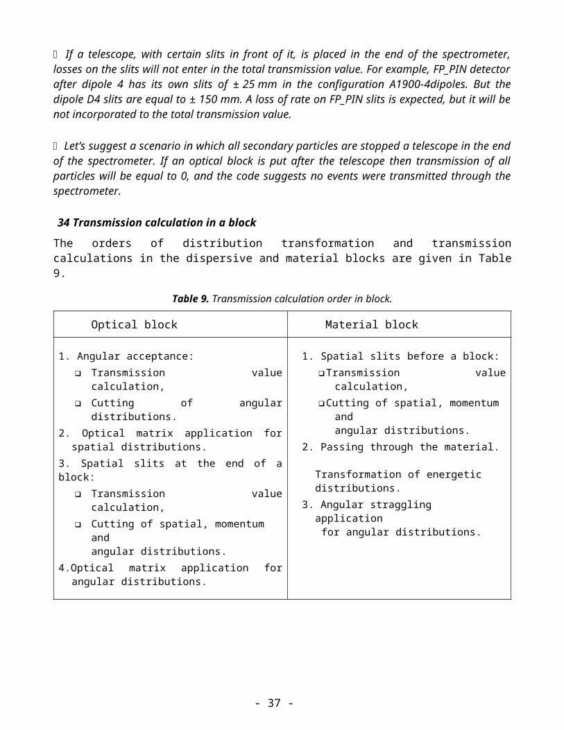
Fig.34. Experimental [Not02,Sak97], calculated by the LISE abrasion-ablation model (blue dash curve) and EPAX parameterization (red solid curve) production cross sections of neutron-rich isotopes in the reaction 48Ca+Ta versus neutron number. Binding energies from the database+LDM2 have been used for abrasion-ab-lation calculations.

More detailed description of improved mass parameterizations will be given in the upcoming paper [Sou02].

43 Updating and new utilities44 Emittance of beam

In LISE++ the beam emit-tance frame has been moved to the beam dialog (Fig.35). This location is more logical. In LISE the frame was lo-cated in the spectrometer op-tical matrices dialog.

In the new version the user can set an angle between the beam and the spectrometer not only in a horizontal plane, but also in the vertical plane.

Fig.35. The “Beam” dialog.

- 37 -

45 Preferences

In LISE++ the dialog “Preferences” has got a number of new options some of them already were de-scribed above. There are just some words about the new option “Calculate spectrometer setting using maximal or mean value of the momentum distribution”. The rigidity can be calculated using one of conditions (see Fig.36):

The maximum of momentum distribution corresponds to the central line of the spectrometer (left plot),

The average of momentum distribution is in the central line (right plot). This is the new feature of the code. The program LISE assumed only the first case for calculations.

Fig.36. Momentum distribution of a setting fragment in the dispersive focal plane. The block momentum ac-ceptance is shown by green color. The spectrometer is set on the maximal value of momentum distribution in the left figure and on the mean value correspondingly in the right plot.

46 Optimum target

In LISE++ the different modes of target thickness and angle inclination calcula-tions were joined to one dialog (see Fig.37). The user can keep constant a value of any dispersive blocks to calcu-late a target thickness corresponding to the block value.

Fig.37. The “Optimal target calculation mode” dialog.

47 Dialogs Goodies & Physical calculatorIn the dialog “Goodies” the code calculates standard deviations of times of flight and energy loss in materials. Momentum acceptance and detector (timing, energy) resolutions are taken into account.

- 38 -

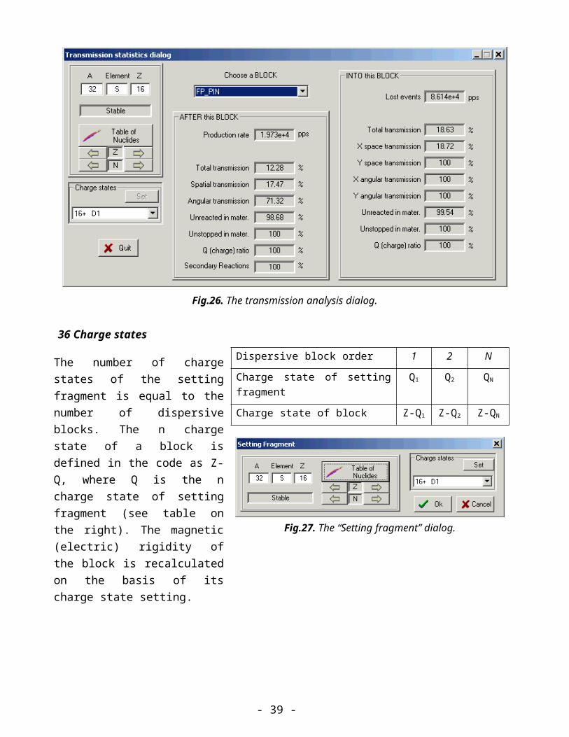
Fig.38. Physical calculator.

The Physical calculator of LISE++ can calculate energy loss throughout unlimited number of detectors (see Fig.38). The number of detectors in LISE was limited to seven. It is possible to edit materials without leaving the physical calculator dialog by clicking on an icon of a detector in the window of materials.

The window of material blocks contains only materials located after the last optical block.Lateral straggling through materials is included in the physical calculator, which is calculated on the basis of angular straggling and the detector length. The lateral straggling of fragments through a mate-rial is taken into account in fragment transmission calculations. The biggest effect of lateral straggling can been seen in for gas detectors.

48 Matrix calculator

The matrix calculator is new in LISE++. Using this new utility (Fig.39) it is possible to do the fol-lowing matrix computing operations with matrices:

One matrix operation Two matrix operationsInverse Product of two matricesTranspose Sum of two matricesTransform to Up triangularTransform to Down triangularProduct by constant value Determinant calculation

- 39 -

The calculator supports only square ma-trixes by dimensions from 2 up to 6. To do an operations with two matrixes, the sec-ond matrix should be stored in memory (M). The matrices can be read / saved from / in a matrix file. The format of the matrix file was given in the chapter 12

The calculator does not support optical matrix dimensions (mm/cm).

Fig.39. Matrix calculator

49 Range optimizer – Gas cell utilityThe ability to calculate the thick-ness (or inclination angle) of a de-grader used to slow beam particles to alter their stopping distance into a gas cell is developed in LISE++. Let us suppose, that a beam of ions after a dipole through a monochro-matic wedge, which is found in the dispersive plane, to make a mono-energetic beam. An adjustable de-grader is located behind the monochromatic wedge (Fig.40). The thickness of the adjustable de-grader can be changed to achieve a maximal ratio of particles stopped in the gas cell to the sum of parti-cles stopped before the gas cell and those that pass through it com-pletely. The thickness of the ad-justable degrader is varied by changing the angle of the de-grader. The utility can calculate an optimum inclination angle or thickness of a degrader, keeping the other fixed (see Fig.41).

Fig.40. Range optimizer block scheme.

Fig.41. The “Range optimizer” dialog.

- 40 -

The user has to choose, in the range optimizer dialog, the adjustable degrader material, the stopper ma-terial and the minimum and maximum thicknesses of the adjustable degrader. The code automatically suggests the minimum and maximum thicknesses of the adjustable degrader equal to zero and the range of the particle in the adjustable degrader respectively. The number of points used to calculate the optimal thickness (inclination angle) is equal to the number of points for the optimal thickness target calculation utility defined in the Preferences dialog.

The number of particles stopped in the gas cell versus the thickness of the adjustable degrader for two different wedges before the adjustable degrader are shown in Fig.42. It is visible from the figure that it is possible to set the adjustable degrader, using the monochromatic wedge, to stop 3.5 times more par-ticles in the gas cell if a homogeneous degrader is used.

Fig.42. Number of particles stopped in the gas cell versus the thickness of adjustable degrader for two different wedges before the adjustable degrader (see the scheme in Fig.40). The case of the monochromatic wedge is shown in top plot, the homogeneous degrader is given in the bottom plot.

- 41 -

50 LISE for Excel

The new version of LISE.xls allows you to make a fast identification of isotopes and a calibration of experimental registered parameters during an experiment. For calibration and identification LISE.xls uses the configuration:

Dipole Wedge Dipole dE-detector TKE-detector

Initially, it is necessary to input parameters of a set-up (lengths of dispersive blocks, dE-detector prop-erties, etc) and perform calibrations of time-of-flight and energy loss in the dE and TKE detectors.

You can use the new utility in two directions: Input parameters A, Z, Q1 and Q2 of the isotope of interest and input the Brho values to get

energy loss and time-of-flight data in channels (upper picture in Fig.43); Input experimental data in channels to get physical values (energy loss and time-of-flight) and

identification of the ion (lower picture in Fig.43).

You can only edit cells with a light grey background (see Fig.43). Other cells are write protected.

Fig.43. New identification tables of LISE.xls.

New transformation functions (Energy  Momentum, Brho  Momentum) and some new statistic functions (integration, etc) have been incorporated in the LISE.xls package. One improvement is that LISE.xls can handle unphysical inputs (i.e. a negative value for a material thickness).

- 42 -

6.7. Cyrillic and Hex-style converter

The new utility “Cyrillic converter” (Fig.44) has been developed to convert one Cyrillic character set to another. The Converter was made using the free distributed converter source (for MS-DOS) by Serge Bajin ([email protected]). The text converter supports for-mats: KOI8, Alternative 866, Windows-1251, ISO 8859-5 and can be loaded from the Units converter. This utility has been made in free time from work :)

This converter can be useful for people who are not burdened by problems of Cyrillic char-acter set conversion because the utility also al-lows converting Hex-style text (=EF=F0) and HTML symbols (and....;) to normal text.

Fig.44. Cyrillic and Hex-style converter.

51 Plots

The program can plot angular, spatial, energy and momentum distributions before and after every block, as well as inside a dispersive block. It permits to the user to look at how the dynamics of distri -butions change from block to block. Two-dimensional plots allow the user to see correlations between parameters (dE, TKE, TOF, X, Y) in detectors with the resolution of detectors taking into account.

52 Transmission plots

One-dimensional selection plots can be found through the menu “Plots” or the LISE++ toolbar. Table13 shows different types of selection plots. Momentum and Vertical special selection plots are avail-able only from the menu “Plots”. By clicking the icon of any of the plots (except for the Brho and Wedge selection plots) in the toolbar you get the menu of available blocks for which can be con-structed the plot. The Brho and Wedge selection plots are drawn immediately, without this menu, for blocks, which were set in the dialog “Plot options” (Fig.45). If the plot selection window has more than one plot then you can use the button inside the plot in which you want to zoom. A window with one selected plot will be created. It is possible to load the dialog “Plot options” using the button

in the toolbar or through the menu “Plot->Plot Options”.

- 43 -

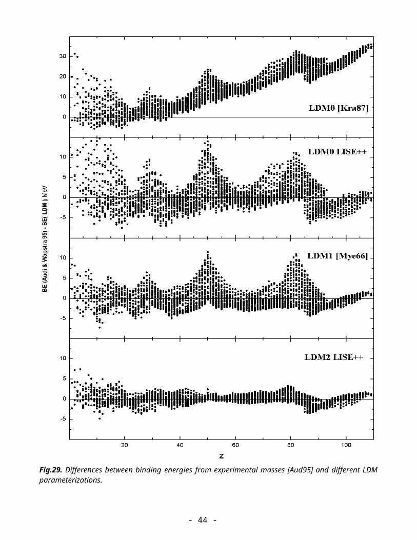
Table 13. Selection plots.

Plot name Number of distribution plots in window

note

Block selection 1. x’ angular (I)2. y’ angular (I)3. x spatial (OU)4. y spatial (OU)5. Momentum (OC)6. Energy (OC)

Designations in the plot:I - inputO - outputU - uncutC - cut

Angular 1. x’ angular (I)2. y’ angular (I)3. x’ angular (O)4. y’ angular (O)

Spatial (horizontal) 1. x spatial (I)2. x spatial (OU)3. x spatial (OC)

X spatial (OU) is not shown for materials and for dispersive blocks without slits.

Energy 1. Energy (I)2. Energy(OC)

Brho selection Momentum (OU) [Tm] You have to select a block for the plot in the “Plot options” dialog (Fig.45). Wedge selection X or Y spatial (OU) [mm]

Fig.45. The “Plot options” dialog.

- 44 -

53 Two-dimensional plots The use of experimental data from different detectors to build a two-dimensional plot is a large advan-tage of LISE++. For example, you can build a two-dimensional plot using the Х-coordinate from a PPAC located in Image2 and an energy loss value from a PIN-detector located after the last optical block. First you have to set in the "Plot options" dialog (Fig.45) “PPAC in Image2” as the X-detector and “PIN-detector” as the dE-detector. Then you click on plot "dE-X" from the menu "Plots" to create the plot. Material (detector) blocks only can be used to make two-dimensional plots.

The code uses a trigger for data acquisition taken from a detector. For "ellipse" mode drawing of two-dimensional plots, the first detector found in the beam line is used. For Monte Carlo simulations the last detector is used to start an acquisition.

Energy, time, and spatial resolutions of a detector are used when calculating standard deviations of measured values in two-dimensional plots. The defect (percent error) of a material thickness is used in two-dimensional plots as well as in fragment transmission calculations. You can see the increase in a peak width with a larger detector resolution or larger material thickness defect.

Be careful when you input the de-fect of a wedge thickness located in the dispersive plane. The effect on your fragment distribution can be large (see Fig.46).

Fig.46. “Wedge selection” distribu-tions in the focal plane of A1900 spec-trometer for different wedge thickness defects (0.1%, 1.5%, and 3.0%). Cal-culations were done with the reaction 40Ar(140 MeV/u)+Be(500 mg/cm2) for setting fragment 32S with an achro-matic wedge (Be 300 mg/cm2) located in Image 2.

54 Debug distributionsDebug distributions serve to check transmission calculations and transformations of distributions and represents an ideal transformation of the momentum to a coordinate. The given distribution (Px) is used in convolutions with spatial (x) and angular (x) components to get an output spatial distribu-tion after a block. Using debug distributions it is easy to see the dependence of distributions on wedge shape. Debug distributions also can be used for calculation of achromatic or monochromatic wedges (see the lower right plot in Fig.21).

Fig.47 shows two-dimensional spectra for the reaction 238U(1 GeV/u) + Be(3.5 g/cm2) 214Pb with a Al 1 g/cm2 wedge found between the 2nd and 3rd dipoles of the fragment separator FRS. The spectra are calculated for different wedge shapes. Fig.48 shows debug distributions after the 4th dipole for the same reaction as in Fig.47. Only calculations for isotopes 208Hg, 213,214Pb, 218Po are shown in the plots for illustration purposes. This example is available through the LISE web-site: http://groups.nscl.m-su.edu/lise/6_1/examples/214pb.lpp

- 45 -

The debug information window (the menu “PlotDebug information”) as well as debug distribution plots are only used for the developers of the program to control calculations of standard deviations of the main characteristics of debug distributions.

Fig.47. Monte Carlo method simulations for differ-ent shapes of wedge located between the second and third dipoles of the fragment-separator FRS (GSI). The position detector MW22 is found in the disper-sive focal plane between the 2nd and 3rd dipoles, the detectors MW41 and Music-P10 are located after the 4th dipole. See details in text.

Fig.48. Debug distributions (XP) after the fourth dipole of the fragment-separator FRS (GSI) for dif-ferent shapes of wedge located between the second and third dipoles. The wedge shapes are labeled on the plots. See details in text.

- 46 -

55 Future developments of LISE++

Develop new dispersive blocks: gas-filled, electrostatic separators, compensating dipole after the Wien velocity filter.

Create LISE++ configuration files for spectrometers in GANIL, Dubna, RIKEN, Texas A&M, etc. The authors hope to have help from experts of these laboratories for specific information (transport files, location and characteristics of detectors, emittance of primary beam, etc.).

Add a subroutine of fusion cross-section calculations below the Coulomb barrier in the PACE4 code and the LisFus model of LISE++.

Incorporate a new reaction mechanism: Fission (principal task for 2003 FY)

Develop a new material block: secondary target

Continue work under “Universal parameterization of momentum distribution of projectile frag-mentation products”.

Write a guide, “First steps” for beginners.

Write full LISE++ documentation.

Develop the “Beam analyzer” dialog to plot beam trajectories in dipoles.

Acknowledgements

LISE++ authors gratefully acknowledge Dr.Helmut Weik’s fruitful remarks, suggestions, and help with the development of LISE++. Special thanks to Helmut for continually checking the code.

LISE++ authors thank Heather Olliver for carefully proof reading this manual.

Fruitful discussions with Prof.Betty Tsang on the improved masss formula (chapter 39) and with Dr.Leo Weissman on the gas cell range optimizer (chapter 49) are gratefully acknowledged.

The authors are grateful to the entire National Superconducting Cyclotron Laboratory for fuitfull re-marks, comments and checking of preliminary versions of LISE++.

References:[Aud95] G.Audi and A.H.Wapstra, Atom.Data and Nucl.Data Tables (1995) 1.[Bro80] K.L.Brown et al. CERN 80-04 (1980);

PSI Graphic Transport Framework by U. Rohrer :http://people.web.psi.ch/rohrer_u/trans.htm[Kra87] ”Introductory nuclear physics”, K.S.Kraine, publ. By John Wiles & sons, New York, 1987.[Mye66] W.D.Myers and W.J.Swiatecki, Nuclear Physics 81(1966) 1-60.

[Not02] M.Notani et al., Phys.Lett.B, in press.

[Sak97] H.Sakurai et al., Nucl.Phys. A616 (1997) 311c.

[Sou02] “Improved mass parameterization in reaction models”, S.R.Souza et all. To be published.

- 47 -