Liquidity Matters: Addressing the Puzzle of Negative Bank ... · Liquidity Matters: Addressing the Puzzle of Negative Bank Output on Loans Bertrand Groslambert (Skema Business School,

Liquidity Matters: Addressing the Puzzle of

Negative Bank Output on Loans

Bertrand Groslambert (Skema Business School, France), Olivier Bruno (Université Nice Sophia

Antipolis, GREDEG-CNRS, SKEMA Business School and OFCE-DRIC, France), and Raphael

Chiappini (Université Nice Sophia Antipolis, GREDEG-CNRS, France))

Paper prepared for the 34

th IARIW General Conference

Dresden, Germany, August 21-27, 2016

Session 7A: Accounting for Finance in the Economy and the SNA I

Time: Friday, August 26, 2016 [Morning]

1

Liquidity matters: Addressing the puzzle of

negative bank output on loans1

Olivier BRUNOǂ, Raphael CHIAPPINI, Bertrand GROSLAMBERT*

Abstract: We develop a method for calculating bank output on loans that addresses the flaws of

the current System of National Account (SNA) approach. We build on Colangelo and Inklaar

(2012) and borrow from the literature on liquidity risk premium to determine some reference

rates that represent the pure credit risk premium and exclude the impact of liquidity risk from

these reference rates. Our method produces bank output estimates that are consistent with the

evolution of the economic activity and that remain always positive including in periods of

financial stress. In normal times, our results are similar to Colangelo and Inklaar (2012) and

confirm that the current SNA approach overestimates bank output.

Keywords: Bank output, FISIM, Credit risk premium, Liquidity risk premium

JEL: E43, G21

1. Introduction

Financial services comprise financial intermediation, financial risk management, liquidity

transformation and auxiliary financial activities. These activities create wealth and are generally

directly compensated through commissions and fees. However, part of those services is not

directly charged to bank customers. Instead, bank remuneration implicitly comes from the

spread between interest rates receivable on financial assets and interest rates payable on

financial liabilities. This is why evaluating the banking system output proves very challenging.

The key issue is to determine the relevant reference rate to be used for calculating the bank

value added. In the usual method retained by the System of National Accounts (SNA), this

reference rate is defined as the average interest rate at which banks lend money each other and

is used to measure the cost of funds for all types of activities (loans and deposits). Consequently,

it does not grapple with the difference in maturity and risk between the various types of loans

and deposits made by banks. It means that compensations for term and risk premiums are treated

as productive services offered by banks. On the contrary, according to Wang (2003) and Wang,

Basu and Fernald (2009), the value added by banks should be the residual net interest income

1 We thank Vincent Biausque, Antonio Colangelo, Satoru Hagino, Itsuo Sakuma, and participants to the 32nd GdRE symposium on Money, Banking and Finance for their help and comments on an earlier draft of the manuscript. ǂ Université Côte d'Azur, CNRS, GREDEG, SKEMA, OFCE-DRIC, France. Corresponding author. 250, rue Albert Einstein. 06560 Valbonne Sophia-Antipolis. [email protected] Université Cote d'Azur, CNRS, GREDEG, France. raphaë[email protected] * Université Côte d'Azur, SKEMA, France. [email protected]

2

after subtracting the required term and risk premium on loans and deposits. Consequently,

neither the loanable funds per se, nor the risk premium should be counted as bank value added.

The remuneration related to risk-taking does not fall within the productive activities of banks

since risk is ultimately supported by providers of capital. This remuneration should be recorded

as an allocation of income account as the System of National Accounts (SNA) recommends for

any property income. Only the portion of interest income related to the monitoring and

controlling of borrowers should be recorded in the Financial Intermediation Services Implicitly

Measured (FISIM).

The last 2008 version of the SNA tempted to clarify these issues and a consensus emerged in

favor of excluding the credit default risk premium from the calculation of bank value added on

loans. In that respect, new methods were developed to remove risk premium from the

calculation of bank value added for the United States (Basu, Inklaar and Wang, 2011) and for

the euro area (Colangelo and Inklaar, 2012). These methods suggest using for each type of

loans, the interest rate of a market debt security with the same risk profile and maturity but with

no service attached. This removes the credit risk premium as well as any term premium from

the calculation of FISIM on loans. However, the relevance of these new approaches is still in

question for at least two reasons: (1) they may lead to negative FISIM on loans in period of

financial stress and (2) they generate high volatility in FISIM measurement.

In this paper, we try to solve these puzzles by disentangling the credit and the liquidity risk

contained in credit spread used to measure FISIM on loans. The impact of illiquidity on the

price of bonds and on credit spread is well documented. For instance, using several alternative

liquidity measures proposed in the literature, Friewald, Jankowitsch and Subrahmanyam (2012)

find that liquidity proxies account for about 14% of the explained time-series variation of the

yield spread changes over time for individual bonds. They show also that the economic

significance of liquidity proxies increased by 50% during the subprime crisis compared to the

normal period. These results are confirmed by Bao, Pan and Wang (2011) that underline that in

times of financial stress, liquidity effects are the dominant driver of credit spread and take over

the credit risk component. According to us, these liquidity effects on the value of credit spread

do not reflect the fundamental level of credit risk. They are due to financial market

microstructure or to portfolio reallocation during period of stress. Consequently, it seems to be

necessary to take into account the share of illiquidity in the credit spread uses to compute FISIM

on loans in order to only remove the "pure" credit risk premium from the financial production

of bank.

Therefore, we propose a comprehensive measure of "pure" credit risk premium based on

parametric estimations, in line with the previous study of Tang and Yan (2010). We model the

variation of the credit spread on several macroeconomic and financial factors that are identified

as credit risk drivers in the empirical and theoretical literature. It allows us to extract the

evolution of the "illiquidity" premium which is calculated as the difference between the

evolution of the observed spread yield and the evolution of the estimated credit risk premium.

Finally, we use the estimated value of each variation of spreads to compute fitted spreads

needed for the computation of FISIM on loans.

We thus apply this new method to the case of the euro area in the spirit of Colangelo and Inklaar

(2012) focusing exclusively on FISIM on loans. For each institutional sector and each type of

loan, we identify two reference rates that respectively account for the corresponding risk profile

and the maturity. We first reproduce the Colangelo and Inklaar (2012) method and expand the

3

period under consideration to include the 2010-2013 European sovereign debt crisis period

when liquidity dried up dramatically on bonds market. This method generates very

heterogeneous annual results including some negative banking outputs on loans during episodes

of financial stress. Then, we modify the Colangelo and Inklaar (2012) approach and separate

pure credit risk from liquidity risk. We find that our approach produces coherent and stable

results even during periods of financial stress. It eliminates the occurrence of negative outputs

and generate reliable output estimates, including times of volatile movements in reference rates

and when liquidity markets dysfunction. This is the main contribution of our work. It provides

a method which delivers consistent results for calculating the value of financial services

production on loans. However, it does not address the issue of negative outputs on deposits (see

Groslambert, Chiappini, Bruno, 2015 for a comprehensive study on that point).

The organization of this article is as follows: section 2 presents the analytical framework for

the measurement of banking output and section 3 describes our database and methodology.

Section 4 presents our main results, and section 5 concludes.

2. Computing FISIM: the "old" and the "new" methods

2.1. The debate about credit risk in FISIM calculation

Debates about how estimating the level of bank production has existed as early as 1952 when

the very first standardized system of national accounts was implemented (OECD, 1998). The

1968 SNA and then the 1993 SNA tried to improve the method but have been inconclusive.2

First, as noted in the 2008 System of National Accounting (UN, 2008), “the way in which

financial institutions charge for the services they provide is not always as evident as the way in

which charges are made for most goods and services.” Banks do not explicitly charge for some

of their services. Instead, a significant part of their outcome is implicitly derived from the

interest rate margin between deposits and loans. The second challenge is to disentangle the part

of the spread that is due to the cost of funds and the one that corresponds to the services offered

by the bank.

Circumventing these difficulties for computing the amount of FISIM, the System of National

Accounts (SNA) 1993, 2008 and the European System of Accounts (ESA) 1995, 2010, suggests

using an arbitrary reference rate, such as the interbank rate. Under this rule of thumb, one can

calculate FISIM on deposits dY and FISIM on loans

lY . FISIM on deposits come from the

difference between the reference rate fr and the rate actually paid to depositors

dr times the

amount of deposits. FISIM on loans are given by the difference between the rate paid to banks

by borrowers lr and the reference rate

fr times the amounts of loans. We obtain

deposits

loans ( )

d f d

l l f

Y r r

Y r r

2 See OECD (1998) and Vanoli (2005) for a history of the calculation of the banking industry.

4

Adding explicitly charged services to the FISIM and deducting intermediate consumption gives

the value added of the banking industry.

FISIM + Explicitly charged services – Intermediate consumption = Value added

This method has been adopted since 1993. However, the 2008 financial crisis caused great

volatility in the FISIM output and has raised a series of questions about its relevance and

reliability. Results generated during this period have been found implausible (Davies, 2010). In

some occasions, negative FISIM occurred, whereas in other cases, FISIM output grew at

surprisingly high rate. The reason is that, paradoxically in times of rising risk, when banks

increase their rates to cover against possible default, the current method automatically generates

additional output for banks. That’s why, in the wake of the 2008 crisis, the widening of interest

rate spreads has mechanically inflated the FISIM, increasing significantly the contribution of

the banking sector to GDP (Mink, 2008). Referring to the Japanese economic situation, Sakuma

(2013) has made the same observation, especially during the years 2002-2004.3 In order to

address these questions, two working groups were created in 2010.4 Their final report was

published in May 2013 (ISWGNA, 2013). However, they have not been able to reach a

consensus on a method for calculating FISIM (Ahmad, 2013).

Mink (2010), Diewert et al. (2012) or Zieschang (2013) review the different approaches. The

main issue opposing researchers is whether the remuneration related to the management of

liquidity risk (for deposit) and the compensation related to the risk of default (for loans) must

be recorded in the production account. As Schreyer (2009) or Zieschang (2013) explains, the

key question is who bears the risk and consequently how should the financial risk management

activities be dealt with. Answering this question determines the choice of the reference rate

used for calculating the FISIM.

Some authors such as Ruggles (1983), argue that banks’ role is to directly provide finance to

borrowers as opposed to those who consider banks as providers of financial services. For these

researchers, banks bear the risk themselves and their output should include the compensation

for taking that risk. Their margin must include a risk premium and therefore the reference rate

should be a risk-free rate as explained in Fixler et al. (2010). For them, the reference rate

represents the opportunity cost of deposits, which is the return that the bank would get if it was

invested in assets liquid and stable enough for allowing fund withdrawal at any time.

Meanwhile, the reference rate also represents the opportunity cost of the bank’s loans. It is the

return that the bank foregoes by lending to its customers rather than investing into liquid assets

with no credit risk. This approach corresponds to the existing System of National Accounts

(SNA 1993, ESA 1995, SNA 2008, ESA 2010). It is currently implemented in the European

Union and in the United States, who respectively use an interbank rate and a government risk-

free rate as reference rate. Alternative ways to compute the reference rate exist. The Australian

Bureau of Statistics uses a midpoint of weighted average borrowing and lending rates (Cullen,

2011). Others such as Diewert, Fixler and Zieschang (2012), or Zieschang (2013) suggest taking

the cost of funds or the cost raising financial capital as reference rate. All these methods have a

3 Sakuma (2013) reviews the various methods that have been implemented to evaluate the production of the

financial sector since 1953. According to the author, the economic situation in Japan and its impact on the

estimation of the Japanese banking production revealed well before 2008, the shortcomings of the method used by

the System of National Accounting. 4 These are the "ISWGNA Task Force on FISIM" for the United Nations and the "European task Force on FISIM"

for the European Union.

5

common characteristic: they rely on a single reference rate which means that they incorporate

a certain amount of term and risk premium in the calculation of the FISIM.

Another stream of research made of Wang (2003), Wang, Basu and Fernald (2009), Basu,

Inklaar and Wang (2011), Wang and Basu (2011), Colangelo and Inklaar (2012) and Inklaar

and Wang (2013) considers that the output of banks does not depend on the amount of risk they

take. Those researchers, called the Wang camp by Diewert (2014), think that the compensation

for taking risk must be removed from the calculation of bank production. For these authors, as

for Schreyer and Stauffer (2011), banks are simply producers of financial services, whose role

and purpose is to reduce information asymmetry between investors and borrowers through

controlling and monitoring. For Wang (2003), the remuneration related to risk-taking does not

fall within the productive activities of banks since risk is ultimately supported by providers of

capital. This remuneration should be recorded as an allocation of income account as the system

of national accounting recommends for any property income. Only the portion of interest

income related to the monitoring and controlling of borrowers should be recorded in the FISIM.

To illustrate this point and highlight the shortcomings of the current method, Wang et al. (2009)

propose to consider the hypothetical case of a "bank that does nothing". This bank has the only

function to serve as a pipeline between savers and borrowers, without performing any

controlling or monitoring. This bank would finance on short-term market and would simply

record loans in its balance sheet. It would strictly do nothing, providing no service and not

creating any wealth. If the economic cycle is favorable, such a bank could generate substantial

profits by pocketing the term premium and the credit risk premium. Under the current system

of national accounting, this bank would also generate some value added, even though it has no

activity at all.

For Wang (2003), credit risk is not borne by banks but rather by the providers of capital. The

activity of financial intermediaries only consists in delivering financial services. Consequently,

their value added must not comprise any risk premium. Reference rates must be based on the

cost of funds and exclude those premiums. Therefore, when calculating FISIM generated by

lending activities, Basu, Fernald, Inklaar and Wang (BFIW)5 suggest using for each type of

loan, the interest rate mr of a market debt security with the same risk profile and maturity but

with no service attached. This removes the credit risk premium as well as any term premium

from the calculation of FISIM on loans.

The Inter-Secretariat Working Group on National Accounts (ISWGNA, 2013) has addressed

these issues, and investigated whether risk compensation for maturity and credit default risk

should be included in the calculation of the value of banks. Although the group could not reach

a consensus, a majority considered that the activity related to the maturity transformation should

remain in FISIM and therefore be included in the value added. Conversely, for the credit default

risk, a majority estimated that its remuneration should be excluded from the calculation of

FISIM. This could be done by using different reference rates which risk profiles would match

those of the various types of banking loans, effectively removing the risk premium. This is the

route followed by BFIW.

5 See Wang, Basu and Fernald (2009), Inklaar and Wang (2013), Basu, Inklaar and Wang (2011), Wang and Basu

(2011), and Colangelo and Inklaar (2012).

6

2.2. Credit risk and liquidity premium

The method proposed by BFIW to extract credit risk premium from bank value added is fairly

simple and can be compared to the current method used by the SNA. Let's define the following

variables:

LY : the nominal output of financial services implicitly measured to borrowers.

Lr : the average interest rate received on loans.

Fr : the single reference rate based on interbank rates.

L

ir : the interest rate received on loans of type i.

M

ir : the reference rate using rate of return on market securities with the same systematic risk

The current SNA method uses a single reference rate Fr for calculating the implicit margin

charged on borrowers —L Floans r r . The reference rate

Fr is the same for all types of

loans and consequently includes maturity and risk premiums in the estimation of the financial

services output. The alternative BFIW method uses instrument-specific reference rates M

ir for

each type of loan to account for their credit risk and maturity. This way of calculating the margin

excludes the maturity and risk premiums from the calculation.

Fig. 1. Comparison between the current SNA method and the BFIW method for estimating

financial services output. Both methods are based on loan balances times some interest rate

spreads. The difference between these methods comes from the use of different interest rate

spreads: L Fr r for the SNA method versus

L M

i ir r for the BFIW method.

The major challenge using the BFIW method lies in the choice of the specific reference rates M

ir that account for credit risk premium. In their paper, Colangelo and Inklaar (2012) retained

bond indices with different maturity compiled by Merrill Lynch. Credit risk premium is

measured by the spread between the yield of the risky bond indices of each maturity and the

Fr Fr

7

government bond yield of the same maturity. However, it is well recognized in the literature

that, in addition to credit risk, liquidity is one of the key determinants of the evolution of credit

spreads (Bao, Pan et Wang, 2011, Friewald, Jankowitsch and Subrahmanyam, 2012). The

problem is to quantify their relative effects and, particularly, how much they changed during

period of financial crisis. As both illiquidity and credit risk intensified at the same time during

crisis, it is not clear which factor is the dominating force in driving up bond spreads.

Nevertheless, a shrewd appraisal of the share of illiquidity in the credit spread uses to compute

FISIM on loans is necessary. From a theoretical point of view, the Wang and al. (2009) theory

implies that only the systematic part of the risk be removed from the FISIM calculation, and

not the illiquidity part resulting from the dysfunctioning of financial markets.

Two main path are followed by the literature to deal with the liquidity part contained in bonds

credit spreads. The first one tries to identify the level of "market illiquidity" contains in credit

spreads. This method is based on the elaboration of specific liquidity measures such as Amihud

(2002) or Roll (1984) measures, and requires to know the daily prices of bonds. This is the way

chosen by (Bao, Pan and Wang, 2011, Friewald, Jankowitsch and Subrahmanyam, 2012 or

Ericsson and Renault, 2006). The second method is founded on the extraction of the "pure"

credit risk premium contained in credit spread. It requires to identify some macroeconomic and

financial factors that are the main drivers of credit risk. This is the approach adopted by Tang

and Yan (2010).

Both methods lead to convergent outcome relative to the importance of illiquidity in the

variation of credit spread. Bao, Pan and Wang (2001) find that in aggregate, changes in market-

level illiquidity explain a substantial part of the time variation in yield spreads of high-rated

(AAA through A) bonds, overshadowing the credit risk component. In the cross-section, the

bond-level, they found that illiquidity measure explains individual bond yield spreads with large

economic significance. This result is in accordance with Friewald, Jankowitsch and

Subrahmanyam (2012) who find that liquidity proxies account for about 14% of the explained

time-series variation of the yield spread changes over time for individual bonds. The

explanatory share of illiquidity is even more important during period of financial stress. For

instance, Ericsson and Renault (2006) stress that, as default becomes more likely, the

components of bond yield spreads attributable to illiquidity increase.

These finding support the idea that a correct evaluation of the FISIM on loan must be based on

the use of a "pure" credit spread free of liquidity component. This is what we proposed in the

third part of the paper.

3. Data and methodology

This section presents the data used for computing FISIM on loans and the methodology retained

to extract the pure risk premium from credit spread.

3.1. Data description

In order to ensure consistency and continuity with the empirical studies initiated by Colangelo

and Inklaar (2012), we use mainly the ECB Statistical Data Warehouse for series on loans.

8

Interest rates on market debt security come from the ECB database, Bloomberg, Markit Iboxx,

and Merrill Lynch Bank of America.

For each type of loan, we must first define the quantity and the price of the financial

intermediation services. The quantity of financial intermediation generated by banks during the

period depends on the nature of the financial services provided. Some services, such as

screening, are performed only once at the initiation of the deal; other services occur regularly

until termination of the contract. This suggests using the outstanding amounts of loans and

deposits rather than the amounts of new business as a measure of quantity.

The price is represented by the spreads between some reference rates and the actual interest

rates on loans. For each type of loan, a corresponding reference rate is selected from the same

systematic risk and maturity profiles. For the actual interest rate, it is necessary to choose

between “new business” rates and “outstanding amount” rates.6 Because the spread between

the reference rate and the actual interest rate applies to the stock of loans in the relevant

instrument category, outstanding amount rates can be used. The current methodology proposed

by the SNA uses this option. However, Colangelo and Inklaar (2012) recommend using new

business rates because they are more consistent for comparison with maturity-matched

reference rates and we follow this recommendation.7

Consequently, to implement FISIM calculation on loan, for each institutional sector, for each

type of loan, and for each maturity, it is necessary to obtain the following series: outstanding

amounts, new business amounts, outstanding amount rates, new business rates, and matched

reference rates. Using the ECB database enables us to categorize the following statistical series

(Table 1). In our analysis, we focus on the two most important institutional sectors—namely,

non-financial corporations (S11) and households and non-profit institutions serving households

(S14+S15). These represent approximately 80% of the total outstanding amounts and constitute

approximately 90% of the banking output in the euro area (Colangelo and Inklaar, 2012).

Finally, our dataset covers the period 2003-2015 in order to include the 2010-2013 European

sovereign debt crisis period when liquidity dried up dramatically on bonds market.

Table 1: Characteristics of loans.

Loans

Sector Category Maturity

Non-financial corporations

(S11) Loans

Less than one year

Between one and five years

More than five years

Households and NPISH

(S14+S15)

Loans for house purchases

Less than one year

Between one and five years

Between five and ten years

More than ten years

Consumer credit

Less than one year

Between one and five years

More than five years

Less than one year

6 See the Manual on MFI (monetary flow index) interest rate statistics (ECB, 2003) for detailed definitions. 7 We alternatively tested outstanding amount and new business rate options and obtained similar results for both

approaches.

9

Other loans Between one and five years

More than five years

The method proposed by Colangelo and Inklaar (2012) consists in finding a new reference rate

that is adjusted for default risk premium and term premium. It requires to compute 1) the pure

risk premium part and 2) the term premium part. The term premium part is based on the risk

free rates determined by an error-correction model (ECM) pass-through equation. The pure risk

premium part is calculated as the spread between some matched market reference rates

corresponding to each financial product minus a risk free rate with the same duration.

Adjusted reference rate =

(matched credit risk market rate – risk free rate with the same duration) + ECM risk free rate

Colangelo and Inklaar (2012) use the Merril Lynch non-financial corporate bond index as

matched market rate for non-financial corporate bond index loans, and the Merril Lynch

covered bond index for household loans. However, the Merril Lynch indices are not split by

maturity. There is only one market rate for all non-financial corporate bonds and one market

rate for all household loans, no matter the maturity. In this paper, we take the Iboxx covered

bond indices. Our choice is motivated by the fact that contrary to the Merril Lynch indices, the

Iboxx indices are split by maturity. The maturity and the characteristic of each loan determine

the choice of the matched market reference rate to be used for calculating the credit spread with

the corresponding risk free rate. The risk free rate is given by the Euro government bond that

has the same duration as the matched market reference rate8. Table 2 details the construction of

the adjusted reference rates by product and maturity. Regarding the ECM risk free rates, we

simply take the same rates as determined by Colangelo and Inklaar (2012).

Table 2: Construction of credit risk and term premium adjusted reference rates.

Non-financial corporation loans

Less than one year (Iboxx cov. 1-3y – gvt bond 2y) + euribor 3m

Between one and five years (Iboxx cov. 1-5y – gvt bond 3y) + gvt bond 3y

More than five years (Iboxx cov. 5-10y – gvt bond 6y) + gvt bond 5y

Household housing loans

Less than one year (Iboxx cov. 1-3y – gvt bond 2y) + euribor 12m

Between one and five years (Iboxx cov. 1-5y – gvt bond 3y) + gvt bond 1y

Between five and ten years (Iboxx cov. 5-10y – gvt bond 6y) + gvt bond 5y

More than ten years (Iboxx cov. 10y+ – gvt bond 10y) + gvt bond 10y

Household consumer credit

Less than one year (Iboxx cov. 1-3y – gvt bond 2y) + euribor 6m

Between one and five years (Iboxx cov. 1-5y – gvt bond 3y) + gvt bond 5y

More than five years (Iboxx cov. 5y+ – gvt bond 8y) + gvt bond 10y

Household other credit

Less than one year (Iboxx cov. 1-3y – gvt bond 2y) + eonia

Between one and five years (Iboxx cov. 1-5y – gvt bond 3y) + gvt bond 5y

8 The euro area government bond rates are based on AAA-rated euro-denominated bonds issued by euro area central governments. They are calculated by the ECB.

10

More than five years (Iboxx cov. 5y+ – gvt bond 8y) + gvt bond 15y

3.2. Measuring “pure” risk premium

We introduce a novel econometric approach in order to deal with the problem of liquidity

premium when measuring FISIM on loans. The idea is to distinguish factors linked to credit

from those linked to liquidity risk and, therefore, estimate the “pure” credit risk premium. To

this end, following Tang and Yan (2010), we model the variation of the credit spread on several

macroeconomic and financial factor that are identified as credit risk drivers in the empirical and

theoretical literature. We consider first the economic growth rate since default probability and

credit spread should decrease with economic growth. We also takes into account the volatility

of the economic growth as Tang and Yan (2010) assess that the default probability and credit

spread increase with this volatility. The investment behavior is also important to assess credit

risk. The more risk adverse are the investors, the higher is the risk premium for holding risky

assets. As a consequence, we consider the economic sentiment of investors as a key determinant

of credit spread. Tang and Yan (2010) have shown that this variable is one of the main drivers

of spreads. Finally, we also consider the VIX as a proxy for overall equity market volatility

(Ericsson and Renault, 2006). Our model only consider variables explaining credit risk and we

assume that other variables influencing credit spreads are linked to liquidity risk. The model

takes the following form:

1 2 3 4ln ln ln

t t t t t ty VIX ESI IMP VolI (1)

With ty the variation of the credit spread,VIX , the VIX on Eurostoxx 50, ESI , the economic

sentiment index on the Eurozone developed by the European Commission, IMP , the index of

the manufacturing production in the Eurozone which proxy for GDP, VolI , the estimated

volatility of the manufacturing index of the Eurozone and t the error term. The volatility of

the manufacturing production index, which proxies for volatility of the economic growth of the

Eurozone is estimated following Mc Connell and Perez-Quiros (2000) and Stock and Watson

(2002) method which relies on the estimation of an AR(1) model as follows:

1t t tu (2)

Where t is the monthly growth rate of the manufacturing production index and evaluates

the persistence of the growth rate of the manufacturing production index. As suggested by Tang

and Yan (2010) following Mc Connell and Perez-Quiros (2000) / 2tu is an unbiased

estimate of the true volatility. As a consequence, following Tang and Yan (2010), we use tu

to proxy for growth volatility.

Eq. (1) has to be estimated for each category and maturity of spreads between the corresponding

Iboxx index and the reference risk free rate. In fact, for the computation of FISIM on loans, we

consider five different spreads depending on the maturity of the covered Iboxx index and risk

free rates. In a first step, we apply the augmented Dickey–Fuller (ADF) test to assess the order

of integration of each interest rate retained in the analysis. For robustness checks, we

complement this test with the stationarity test called KPSS developed by Kwiatkowski et al.

(1992). Using both tests is important because the ADF test has low power if the process is

stationary, but with a root close to the non-stationary boundary, and tends to reject the non-

11

stationarity hypothesis too often. The KPSS complements the ADF test because contrary to the

latter, which assesses the null hypothesis of the unit root, it tests the null hypothesis of

stationarity. It is a very powerful test, but it cannot catch non-stationarity due to a volatility

shift. As expected, both tests clearly indicate that all variables are stationary. Therefore, the

OLS estimator can be used as it is not biased by the existence of unit root in variables. However,

as all different matched market reference rates (Iboxx indices) are highly related, we cannot

assume that error terms estimated for each spreads are not correlated. As a consequence, we

rely on the methodology developed by Zellner (1962) and perform Seemingly Unrelated

Regression Equations (SURE), which allows the error terms to be correlated across the

equations.

Finally, we use the estimated value of each variation of spreads to compute fitted spreads

needed for the computation of FISIM on loans as follows:

1 1 1

1

ˆ ˆ

ˆ ˆ ˆ 1t t t

y y y

y y y if t

Where t̂y is the estimated variation of the spread derived from Eq. (1),

1y is the actual value

of the spread in January 2003 and t̂y is the constructed spread. This fitted spreads reflects only

the pure credit risk as the liquidity risk is captured in the error-term of Eq. (1).

We also apply this methodology for all the reference rates needed for the calculation of FISIM

and obtain reference risk free rates “cleaned” from liquidity risk by the estimation of the

following equation:

1 2 3 4ln( ) ln( ) ln( )

t t t t t tr VIX ESI IMP VolI (3)

Where r is the variation of the reference rate. As with Eq. (1), we estimate Eq. (3) for each

of the reference risk free rates needed for the computation of FISIM on loans using the SURE

method after testing the stationarity of each variable using both ADF and KPSS tests. Then, we

use the estimated variation of the reference risk free rate to construct the estimated reference

risk free rate used in the computation of FISIM on loans as follows:

1 1 1

1

ˆ ˆ

ˆ ˆ ˆ 1t t t

r r r

r r r if t

Where t̂r is the estimated variation of the reference risk free rate derived from Eq. (3),

1r is

the actual value of the risk free rate in January 2003 and t̂r is the constructed spread for the

computation of FISIM on loans.

Relying on this methodology allows us to obtain credit spread and reference risk free rates

cleaned from the liquidity risk and therefore estimate the value of FISIM on loans.

12

4. Results

4.1. Risk and liquidity premiums

Table 3 reports the estimation results of Eq. (1) for all the five spreads under scrutiny using the

SURE method.

Table 3 Spread specific results using SURE and OLS estimator

(1) (2) (3) (4) (5)

Ln (VIXt) 0.131***

(0.046)

0.122***

(0.045)

0.076*

(0.043)

0.078*

(0.044)

0.106**

(0.049)

Ln (ESIt) 0.439**

(0.218)

0.461**

(0.212)

0.282

(0.207)

0.306

(0.210)

0.268

(0.236)

Ln (IMPt) 0.202

(0.352)

0.099

(0.344)

0.167

(0.333)

0.123

(0.338)

0.194

(0.381)

VolIt 2.692

(1.713)

2.654

(1.674)

3.610**

(1.624)

3.347**

(1.648)

3.135*

(1.854)

Intercept -3.386***

(1.250)

-2.976**

(1.221)

-2.339**

(1.185)

-2.246*

(1.203)

-2.482*

(1.353)

Obs. 155 155 155 155 155 Note: Column (1) considers the variation of the difference between the covered Iboxx one to three years and the two years

Euro government bond. Column (2) considers the variation of the difference between the covered Iboxx one to five years and

the three years Euro government bond. Column (3) considers the variation of the difference between the covered Iboxx five to

ten years and the six years Euro government bond. Column (4) considers the variation between the covered Iboxx five to more

than ten years and the eight years Euro government bond. Column (5) considers the variation of the difference between the

covered Iboxx more than ten years and the ten years Euro government bond.

*, **, ***, denote significance at the 10 %, 5 % and 1 % level, respectively

We observe first that estimated coefficients are extremely similar between all different spreads.

However, the determinants of the variation of the different spreads seem quite different. We

find that the only common factor explaining the variation of the different spreads is the VIX.

This factor is significant at the 10 % level and positive in all regressions; confirming the fact

that the implied volatility is a key factor determining the evolution of credit spreads (Ericsson

and Renault, 2006). We also find that the economic sentiment index for the Eurozone is highly

significant and positive for spreads with lower maturities. It confirms results from Tang and

Yan (2010) which emphasis that investor behavior is a leading factor for the evolution of credit

spreads. Finally, we also show that macroeconomic variables such as the volatility of the

manufacturing production in the Euro area drive the evolution of the spreads with longer

maturities. All these specific factors proxy for credit risk. We assume that the liquidity risk is

contained in the error term of each equation. As a consequence, we use the estimated variation

of each of the five spreads to compute the “pure” credit risk spreads for the calculation of FISIM

on loans.

We also apply the same methodology for each of the nine reference risk free rates used for

FISIM computation. Table 4 displays the estimation results of Eq. (3) for all the nine reference

risk free rates considered in this analysis using the SURE method. Our results highlight the fact

that the increasing implied volatility reflected by the VIX has a negative and significant impact

on the variation of Euribor rates and Euro government bonds with a maturity lower than 5 years.

Moreover, the economic sentiment index has a strong significant and positive impact on shorter

maturity bonds.

13

We also find that the volatility of the growth of the manufacturing production in the Eurozone

is an important factor explaining the evolution of Euribor and government bonds rates.

However, our results also point out that for a maturity longer than 5 years, determinants of

credit risks do not seem to explain the variation of government bonds. Surprisingly, for these

bonds only the liquidity risk matters.

As for credit spreads, we use the estimated values of the variation of reference market rates to

construct all series of Euribor and government bond rates. This allows us to have rates cleaned

from liquidity risk.

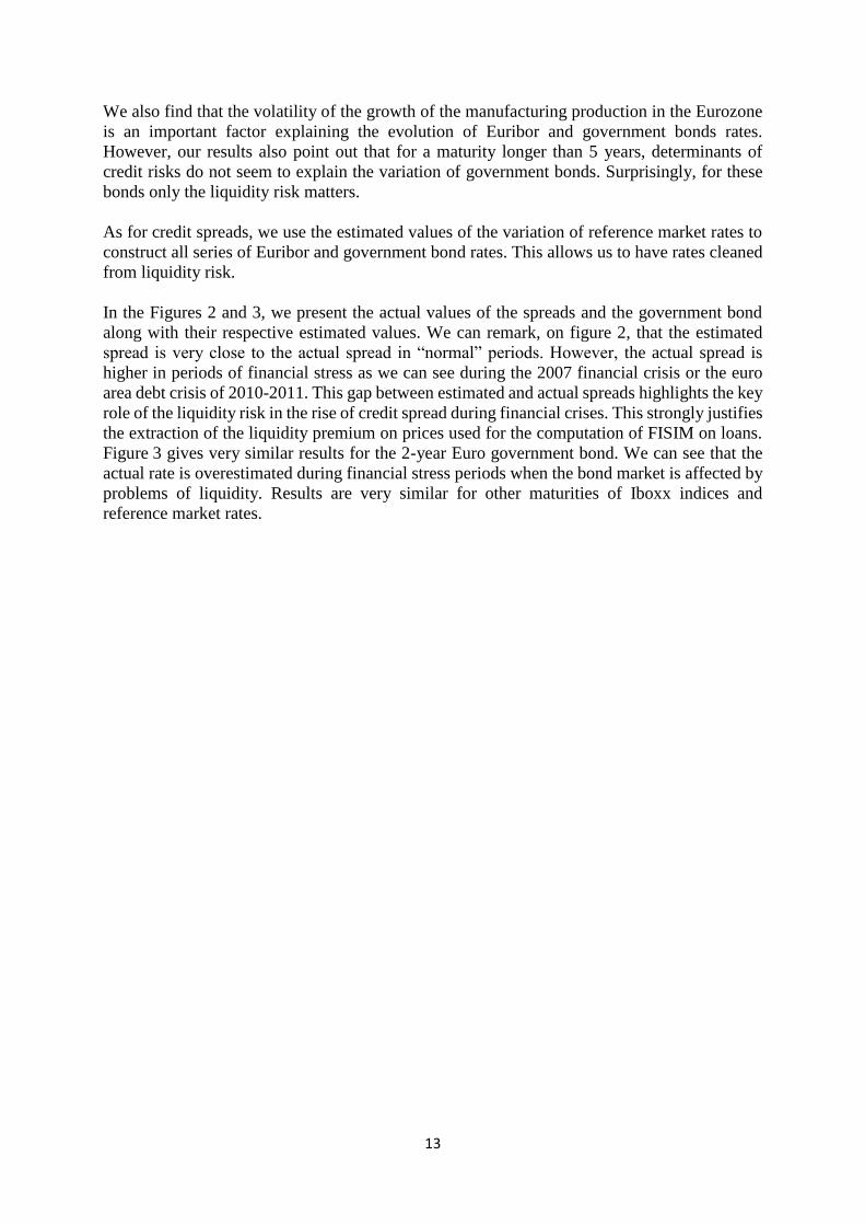
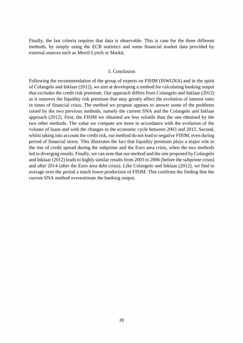
In the Figures 2 and 3, we present the actual values of the spreads and the government bond

along with their respective estimated values. We can remark, on figure 2, that the estimated

spread is very close to the actual spread in “normal” periods. However, the actual spread is

higher in periods of financial stress as we can see during the 2007 financial crisis or the euro

area debt crisis of 2010-2011. This gap between estimated and actual spreads highlights the key

role of the liquidity risk in the rise of credit spread during financial crises. This strongly justifies

the extraction of the liquidity premium on prices used for the computation of FISIM on loans.

Figure 3 gives very similar results for the 2-year Euro government bond. We can see that the

actual rate is overestimated during financial stress periods when the bond market is affected by

problems of liquidity. Results are very similar for other maturities of Iboxx indices and

reference market rates.

14

Table 4 Reference market rates specific results using SURE and OLS estimator

(1) (2) (3) (4) (5) (6) (7) (8) (9)

Ln (VIXt) -0.116***

(0.030)

-0.100***

(0.032)

-0.099***

(0.031)

-0.095***

(0.034)

-0.126***

(0.039)

-0.093*

(0.047)

-0.054

(0.047)

-0.019

(0.045)

-0.021

(0.044)

Ln (ESIt) 0.671***

(0.144)

0.736***

(0.152)

0.719***

(0.148)

0.743***

(0.163)

0.553***

(0.188)

0.447**

(0.226)

0.183

(0.223)

0.025

(0.216)

-0.061

(0.213)

Ln (IMPt) -0.226

(0.232)

0.012

(0.244)

-0.027

(0.240)

-0.121

(0.644)

-0.574*

(0.304)

-0.470

(0.366)

-0.064

(0.361)

0.200

(0.349)

0.274

(0.344)

VolIt -3.340***

(1.129)

-5.701***

(1.921)

-6.007***

(1.168)

-6.083***

(1.281)

-4.586***

(1.480)

-3.949**

(1.781)

-2.985*

(1.757)

-2.014

(1.700)

-1.362

(1.678)

Intercept -1.658**

(0.824)

-3.096***

(0.870)

-2.829***

(0.852)

-2.515***

(0.935)

0.535

(1.080)

0.435

(1.300)

-0.371

(1.282)

-0.988

(1.241)

-0.938

(1.225) Note: Colum (1) considers the variation of the eonia. Column (2) considers the variation of the 3-month euribor. Column (3) considers the variation of the 6-month euribor.

Column (4) considers the variation of the 12-month euribor. Column (5) considers the variation of the 1-year Euro Government bond. Column (6) considers the variation of

the 2-year Euro government bond. Column (7) considers the variation of the 5-year Euro government bond. Column (8) considers the variation of the 10-year Euro government

bond. Column (9) considers the variation of the 15-year Euro government bond. *, **, ***, denote significance at the 10 %, 5 % and 1 % level, respectively.

15

Figure 2: Actual and estimated spreads for the Iboxx covered 5 to 10 years and the 6-year Euro

government bond (%)

Figure 3: Actual and estimated rates for the 2-year Euro government bond (%)

0

0.5

1

1.5

2

2.5

3

20

03

m1

20

03

m7

20

04

m1

20

04

m7

20

05

m1

20

05

m7

20

06

m1

20

06

m7

20

07

m1

20

07

m7

20

08

m1

20

08

m7

20

09

m1

20

09

m7

20

10

m1

20

10

m7

20

11

m1

20

11

m7

20

12

m1

20

12

m7

20

13

m1

20

13

m7

20

14

m1

20

14

m7

20

15

m1

20

15

m7

Actual spread (Iboxx covered 5 to 10 years) Fitted spread (Iboxx covered 5 to 10 years)

-2

-1

0

1

2

3

4

5

20

03

m1

20

03

m7

20

04

m1

20

04

m7

20

05

m1

20

05

m7

20

06

m1

20

06

m7

20

07

m1

20

07

m7

20

08

m1

20

08

m7

20

09

m1

20

09

m7

20

10

m1

20

10

m7

20

11

m1

20

11

m7

20

12

m1

20

12

m7

20

13

m1

20

13

m7

20

14

m1

20

14

m7

20

15

m1

20

15

m7

ref_gb2y Fitted_gb2y

16

4.2. FISIM on loans

In Figures 4 and 5, we present the computation of FISIM on loans using respectively the actual

method retained by the SNA, the methodology proposed by Colangelo and Inklaar (2012) which

takes into account "gross" credit risk premium (that incorporate liquidity premium) and our

method which allows to focus on the "pure" credit risk premium cleaned from problems related

to liquidity. Figure 4 displays quarterly results whereas Figure 5 which presents yearly FISIM.

Figure 4: FISIM on loans by quarter

0

10

00

00

20

00

00

30

00

00

40

00

00

2002m1 2004m1 2006m1 2008m1 2010m1 2012m1 2014m1 2016m1

Current method C&I (2012) method

Our method

17

Figure 5: FISIM on loans by year

As expected, the current method leads to paradoxical results since FISIM on loans dramatically

increase during the financial crisis of 2008 and the Eurozone crisis of 2012 (in accordance with

the results of Sakuma (2013) for Japan). This rise is logically explained by the plummeting of

the reference rate used to compute the FISIM from 2008 due to very accommodating monetary

policy by the ECB.

FISIM computed using Colangelo and Inklaar (2012) methodology are lower than the ones

obtained by the current method and they do not increase during financial crisis of 2008.

However, the values of FISIM obtained using this method are extremely low from 2009 to 2012

and even negative in 2011, which raise issues of consistency of the method during period of

financial stress. Actually, it seems that the overestimation of credit spread and of the rate of

interest during period of financial stress lead to an underestimation of FISIM on loans. As

underlined by Colangelo and Inklaar (2012) : "This illustrates the unappealing choice for

statisticians in troubled financial times: one could either rely on government bond yields and

see a sharp widening of interest margins or use corporate bond yields and see a contracting

interest margin" (p. 151).

The ISWGNA (2013, p.20) has determined a list of criteria that should be met for producing

reasonable reference rates and sensible FISIM estimates. We compare the respective merits of

each method based on these criteria:

Strong connection to underlying economic conditions as measured by volatility,

No sustained periods of negative FISIM,

Sensible changes in FISIM near economic turning points,

0

10

00

00

20

00

00

30

00

00

mill

ion

s e

uro

2003 2004 2005 2006 2007 2008 2009 2010 2011 2012 2013 2014 2015

Current SNA method C&I (2012) method

Our method

18

Data is observable.

Regarding the first criteria, we measure the proportion of variation that is explained by the

underlying economic conditions by calculating the coefficient of determination (R²) between

the volume of outstanding loans and the FISIM on loans estimated by the three different

methods. R² are 0.20 for the current SNA method, 0.01 for the Colangelo and Inklaar (2012)

method and 0.72 for our liquidity risk corrected method. The latter is thus much more related

to the volatility of the underlying economic conditions than the first two methods. Figure 6

shows that the current SNA method or the Colangelo and Inklaar (2012) approach exhibit a

large volatility of FISIM during the whole period that is not in accordance with the evolution

of the volume of loans granted by financial institutions on the same period. On the contrary, the

FISIM on loans estimated with our method which is based on Colangelo and Inklaar (2012) but

corrected from the liquidity risk, follows closely the evolution of the outstanding amount of

loans over the period.

Figure 6: Volume of outstanding loans and estimates of FISIM on loans for the three different

methods

On the second criteria, the current SNA method and our liquidity risk adjusted method do no

generate any quarterly negative FISIM over the period. The Colangelo and Inklaar (2012)

method exhibits six quarters of negative FISIM mostly in 2011 at the height of the euro crisis.

For the third criteria, we investigate the behavior of FISIM around economic turning point. We

compute the coefficient of correlation between the year-on-year variations of the annual GDP

with the year-on-year variations of the annual FISIM. Again, over the whole period, our method

gives the highest coefficient of correlation at 0.07 versus 0.01 for the Colangelo and Inklaar

(2012) method and -0.63 for the current SNA method. These results are illustrated on Figure 7.

0

2000000

4000000

6000000

8000000

10000000

12000000

-100000

-50000

0

50000

100000

150000

200000

250000

300000

350000

03

/20

03

02

/20

04

01

/20

05

12

/20

05

11

/20

06

10

/20

07

09

/20

08

08

/20

09

07

/20

10

06

/20

11

05

/20

12

04

/20

13

03

/20

14

02

/20

15 Ou

tsta

nd

ing

amu

nt

of

loan

s (m

illio

ns

euro

)

FISI

M o

n lo

ans

(mill

ion

s eu

ro)

Our method liquidity risk adjusted C&I(2012) method

Current SNA method Outstanding amount of loans

19

Figure 7: Changes in annual GDP versus changes in annual FISIM (variations year on year)

-0.2

-0.1

0

0.1

0.2

0.3

0.4

0.5

0.6

-0.015

-0.01

-0.005

0

0.005

0.01

0.015

0.020

3/2

00

3

10

/20

03

05

/20

04

12

/20

04

07

/20

05

02

/20

06

09

/20

06

04

/20

07

11

/20

07

06

/20

08

01

/20

09

08

/20

09

03

/20

10

10

/20

10

05

/20

11

12

/20

11

07

/20

12

02

/20

13

09

/20

13

04

/20

14

11

/20

14

gdpvaryoy Current SNA method var. yoy

-4

-3

-2

-1

0

1

2

3

4

5

-0.015

-0.01

-0.005

0

0.005

0.01

0.015

0.02

03

/20

03

10

/20

03

05

/20

04

12

/20

04

07

/20

05

02

/20

06

09

/20

06

04

/20

07

11

/20

07

06

/20

08

01

/20

09

08

/20

09

03

/20

10

10

/20

10

05

/20

11

12

/20

11

07

/20

12

02

/20

13

09

/20

13

04

/20

14

11

/20

14

gdpvaryoy C&I(2012) method var. yoy

-0.1

-0.05

0

0.05

0.1

0.15

-0.015

-0.01

-0.005

0

0.005

0.01

0.015

0.02

03

/20

03

10

/20

03

05

/20

04

12

/20

04

07

/20

05

02

/20

06

09

/20

06

04

/20

07

11

/20

07

06

/20

08

01

/20

09

08

/20

09

03

/20

10

10

/20

10

05

/20

11

12

/20

11

07

/20

12

02

/20

13

09

/20

13

04

/20

14

11

/20

14

gdpvaryoy Our method liquidity risk adjusted var. yoy

20

Finally, the last criteria requires that data is observable. This is case for the three different

methods, by simply using the ECB statistics and some financial market data provided by

external sources such as Merril Lynch or Markit.

5. Conclusion

Following the recommendation of the group of experts on FISIM (ISWGNA) and in the spirit

of Colangelo and Inklaar (2012), we aim at developing a method for calculating banking output

that excludes the credit risk premium. Our approach differs from Colangelo and Inklaar (2012)

as it removes the liquidity risk premium that may greatly affect the evolution of interest rates

in times of financial crisis. The method we propose appears to answer some of the problems

raised by the two previous methods, namely the current SNA and the Colangelo and Inklaar

approach (2012). First, the FISIM we obtained are less volatile than the one obtained by the

two other methods. The value we compute are more in accordance with the evolution of the

volume of loans and with the changes in the economic cycle between 2003 and 2015. Second,

whilst taking into account the credit risk, our method do not lead to negative FISIM, even during

period of financial stress. This illustrates the fact that liquidity premium plays a major role in

the rise of credit spread during the subprime and the Euro area crisis, when the two methods

led to diverging results. Finally, we can note that our method and the one proposed by Colangelo

and Inklaar (2012) leads to highly similar results from 2003 to 2006 (before the subprime crisis)

and after 2014 (after the Euro area debt crisis). Like Colangelo and Inklaar (2012), we find in

average over the period a much lower production of FISIM. This confirms the finding that the

current SNA method overestimate the banking output.

21

References

Ahmad, N. 2013. FISIM. Document presented at presented at the 8th Meeting of the Advisory

Expert Group on National Accounts, Luxembourg.

Amihud, Y. 2002. Illiquidity and stock returns: cross-section and time-series effects. Journal

of Financial Markets, 5, 31-56.

Basu, S., Inklaar, R. and Wang, J. C. 2011. The value of risk: measuring the service output of

US commercial banks. Economic Inquiry, 49, 226-245.

Bao, J., Pan, J. and Wang, J. 2011. The illiquidity of corporate bonds. The Journal of Finance,

66, 911-946.

Colangelo, A., Inklaar, R. 2012. Bank output measurement in the Euro area: A modified

approach. Review of Income and Wealth, 58,142-165.

Davies, M. 2010. The measurement of financial services in the national accounts and the

financial crisis. IFC Bulletin chapters 33, 350-357.

Diewert, W. E. 2014. The treatment of financial transactions in the SNA: A user cost approach.

Eurostat Review on National Accounts and Macroeconomic Indicators, 1, 73-89.

Diewert, W. E., Fixler, D. and Zieschang, K. 2012. Problems with the Measurement of Banking

Services in a National Accounting Framework. UNSW Australian School of Business Research

Paper, No. 2012-25.

Ericsson, J., Renault, O. 2006. Liquidity and Credit Risk. Journal of Finance, 6, 2219-2250

European Central Bank 2003. Manual on MFI Interest Rate Statistics, Frankfurt

Fixler, D.J., Reinsdorf, M.B. and Villones S. 2010. Measuring the services of commercial banks

in the NIPA. Bank for International Settlements, IFC Bulletin, 33, July, 346-348.

Friewald, N., Jankowitsch R. and Subrahmanyam M.G. 2012. Illiquidity or Credit

Deterioration: A Study of Liquidity in the U.S. Corporate Bond Market during Financial Crises.

Journal of Financial Economics, 105, 18-36.

Groslambert, B., Chiappini, R. Bruno, O. 2015. Bank Output Calculation in the Case of France:

What Do New Methods Tell About the Financial Intermediation Services in the Aftermath of

the Crisis. GREDEG Working Paper, 2015-32.

Inklaar, R., Wang, J. C. 2013. Real Output of Bank Services: What Counts is What Banks Do,

Not What They Own. Economica, 80, 96–117.

Intersecretariat Working Group on National Accounts (ISWGNA) 2013. ISWGNA Task Force

on FISIM. Final report presented at the 8th Meeting of the Advisory Expert Group on National

Accounts, Luxembourg.

Mink, R. 2008. An Enhanced Methodology of Compiling Financial Intermediation Services

Indirectly Measured (FISIM). Paper presented at OECD Working Party on National Accounts,

Paris.

22

Mink, R. 2010. Mesure et enregistrement des services financiers. Document presented at

Colloque de l’Association de comptabilité nationale, Paris.

Organisation for Economic Cooperation and Development 1998. FISIM. In Joint

OECD/ESCAP Meeting on National Accounts.

Roll, R. 1984. A Simple Implicit Measure of the Effective Bid-Ask Spread in an Efficient

Market. The Journal of Finance, 39, 1127-1139.

Ruggles, R. 1983. The United States National Income Accounts, 1947-77: Their Conceptual

Basis and Evolution. In The U.S. National Income and Product Accounts: Selected Topics,

Murray F. Foss, ed., University of Chicago Press, Chicago and London, pp. 15-104.

Sakuma, I. 2013. A note on FISIM. Forthcoming in Price and Productivity Measurement:

Volume 3—Services, W. Erwin Diewert, Bert M. Balk, Dennis Fixler, Kevin J. Fox and Alice

O. Nakamura (eds.), Trafford Press .

Schreyer, P., Stauffer, P., 2011. Measuring the Production of Financial Corporations.

Forthcoming in Price and Productivity Measurement: Volume 3; Services, W.E. Diewert, B.M.

Balk, D. Fixler, K.J. Fox and A.O. Nakamura eds.

Tang, D.Y., Yan, H. 2010. Market conditions, default risk and credit spreads. Journal of

Banking and Finance, 34, 743-753.

United Nations, Eurostat, International Monetary Fund, Organization for Economic

Cooperation and Development and World Bank 2008. System of National Accounts 2008,

United Nations, New York.

United Nations 2015. Report of the Intersecretariat Working Group on National Accounts.

Vanoli A., 2005. A History of National Accounting, IOS Press: Amsterdam.

Wang, J. C. 2003. Loanable Funds, Risk, and Bank Service Output. Federal Reserve Bank of

Boston, Working Paper Series, No. 03-4.

Wang, J.C., Basu, S., 2011. Risk Bearing, Implicit Financial Services and Specialization in the

Financial Industry. Forthcoming in Price and Productivity Measurement: Volume 3; Services,

W.E. Diewert, B.M. Balk, D. Fixler, K.J. Fox and A.O. Nakamura eds., Trafford Press.

Wang, J.C., Basu S. and Fernald J.G. 2009. A General Equilibrium Asset-Pricing Approach to

the Measurement of Nominal and Real Bank Output. In Price Index Concepts and

Measurement, ed. by E. Diewert, J. Greenlees, and C. Hulten. Chicago: University of Chicago

Press for NBER, pp. 273–320.

Zieschang, K. 2013. “FISIM Accounting”. Forthcoming in Price and Productivity

Measurement: Volume 3—Services, W. Erwin Diewert, Bert M. Balk, Dennis Fixler, Kevin J.

Fox and Alice O. Nakamura (eds.), Trafford Press.