Liquidity effects on value-at-risk limits: construction of a new VaR model

Journal of Risk Model Validation 8(4), 1–28

Liquidity effects on value-at-risk limits:construction of a new VaR model

Sunny B. Walter MadorobaSchool of Business Leadership, University of South Africa, PO Box 392,UNISA 0003, South AfricaandC/O UWP Consulting Pty Ltd, Private Bag X66, Bryanston 2021, South Africa;email: [email protected]

Jan W. KrugerSchool of Business Leadership, University of South Africa, PO Box 392,UNISA 0003, South Africa; email: [email protected]

(Received ?; revised ?; accepted ?)

Changes to Madoroba addressOK? Please ensure full postaladdresses are given.

Value-at-risk (VaR) is a common tool applied by market makers to monitor therisk of any trading position. The conventional VaR model assumes a frictionlessmarket, which is seldom the case. The 2008 financial market crisis exposed theinadequacies of VaR limits, which do not factor in liquidity risk. Various liquidity-adjustedVaR models exist in an attempt to correct this anomaly. Our study presents “have been created”?

a newVaR model that incorporates intraday price movements on high–low spreadsand adjusts for a trade impact measure, �, a novel sensitivity measure of price New symbol chosen to denote

this term throughout – changeOK?movements due to trading volumes. The new VaR model returns violations that are

independent and identically distributed for 94% of the trading counters backtestedover a one-year period of trading on the Johannesburg Stock Exchange usingKupiec’s test of unconditional coverage. The Christoffersen test of independencereturns 96% of violations that are neither autocorrelated nor clustered, while theChristoffersen joint test of conditional coverage shows that the average numberof violations is correct 93% of the time at 99% significance levels. The new modelis valid and robust for the standard VaR backtests conducted.

1 INTRODUCTION

Liquidity risk is an idiosyncratic phenomenon that is often sidelined in mainstreamfinance practice and theory (Bhyat 2010, p. 32). However, liquidity risk manage-ment played a key role in the 2008 financial crisis (León 2012). The literature rec-ommends improving liquidity risk management by imposing and monitoring liq-uidity requirements on important banks and broker dealers (French et al 2010). The

1

Evelyn

Cross-Out

Evelyn

Cross-Out

Evelyn

Cross-Out

Evelyn

Typewritten text

2 S. B. W. Madoroba and J. W. Kruger

International Monetary Fund (2010) notes that although liquidity risk regulations and Not in References!

tools exist they are still in the early stages of development and discussion (Tucker2009). Regulators did not consider intraday liquidity risk until after the 2008 financialcrisis (Ball et al 2011). Liquidity risk is not formally monitored, and a recognizable Changes to sentence OK?

and readily accepted risk-metric measure does not exist (Dubil 2003).Value-at-risk (VaR) has become the standard criterion for assessing risk in the

financial industry. It is therefore necessary to study the effects of VaR-based riskmanagement on the prices of stocks and options (Berkelaar et al 2002).VaR calculatesthe worst expected loss over a given time horizon at a given confidence level undernormal market conditions (Orlova 2008, p. 13). It is the maximum value of losses thatcan occur with a certain probability in a given time period for any asset class undernormal market conditions. VaR estimates are derived for any type of risk exposure.These can be market, credit or operational risks. The conventional VaR model is basedon mid prices of the bid–ask spread, assuming that neither the size of transactionsnor the trading activity affects market prices. Nevertheless, the reality is that largetrading blocks and trading activities do impact prices. The effect of transaction sizesand trading activity, by impacting asset prices, indirectly influences the ease of tradeor market liquidity of the asset (Pastor and Stambaugh 2003).

A breach of VaR limits is a serious nonconformance that can attract severe penaltiesfrom the regulatory authorities. In extreme cases, the breach ofVaR limits can threatenthe capital-adequacy ratios of the bank, increasing the risk of possible bank failure.Standard VaR calculations do not take market liquidity or, conversely, the associated Changes to sentence OK?

liquidity risk into consideration. More than eighteen models of liquidity-adjusted VaRexist; however, there is no consensus as to which model captures all liquidity risks(Bhyat 2010, p. 71).

This study presents a liquidity-adjusted VaR composite model based on the addi-tion of a liquidity cost component to the standard VaR equation. The added cost ofliquidity incorporates intraday price movements on high–low spreads and adjusts forthe trade impact measure, �. This measure, introduced for the first time as a sensitiv- Changes to sentence OK?

ity measure, monitors the asset price movements due to trading volumes. The studybacktests the composite VaR model on random counters from the Johannesburg StockExchange (JSE) over a one-year period. The empirical results of our VaR model inthis study do not reject the null hypotheses of the three backtests (unconditional cov-erage, independence of exceptions and the joint test of independence and conditionalcoverage). This suggests that the composite VaR model constructed in this study isrobust and can be accepted as a novel contribution to the VaR literature.

The rest of this paper is set out as follows. Section 2 discusses existing VaR modelsand their shortcomings, while Section 3 shows how the new composite VaR modelwas constructed. Section 4 presents our empirical results from backtesting the model. Changes to sentence OK?

Section 5 discusses the results, and Section 6 concludes the paper.

Journal of Risk Model Validation 8(4)

Liquidity effects on value-at-risk limits 3

2 A REVIEW OF EXISTING VALUE-AT-RISK MODELS AND THEIRSHORTCOMINGS

In this paper, ten models that relate to the bid–ask spread as a proxy for measuringendogenous liquidity risk are reviewed.

2.1 Almgren and Chriss (1999, 2000) models

The Almgren and Chriss models of 1999 and 2000 derived optimal trading strate-gies that adopted both permanent and temporary market impact mechanisms fromHolthausen et al’s (1987) work. By externally setting a sales-completion period, themodel derives an optimal trading strategy defined as the strategy with the minimumvariance of transaction cost or shortfall for a given level of expected transactioncost. With the normal distribution, mean and variance of transaction cost, liquidity-adjusted VaR (L-adj VaR) can be determined and minimized to derive optimal tradingstrategies.

However, in practice, trading does not always follow the externally set time horizon Changes to this sentence andthe next OK?

for sales completion that is assumed in this model (Bhyat 2010, p. 104).

2.2 Jarrow and Subramanian (1997, 2001) models

The Jarrow and Subramanian models of 1997 and 2001 provided an instinctive Not in References!

approach, which introduced the concept of the liquidity discount into standard VaRcalculations for the first time. The liquidity discount approach requires that the trans-action completion period be given as an exogenous factor. The optimal trading strategyis then derived by maximizing an investor’s expected utility of consumption.

Both approaches require externally setting a fixed time horizon for liquidation,which might not be practical under abnormal market trading conditions (Bhyat 2000; Not in References!

Bhyat 2010, p. 97).

2.3 Hisata and Yamai (2000) model

Encouraged by a need to overcome the problem of fixing a time horizon for liquidation,Hisata andYamai (2000) extendedAlmgren and Chriss’s 1999 and 2000 approaches by Change OK?

assuming a constant speed of sales using continuous approximation. They successfullyderived a closed-form analytical solution for an optimal holding period. In this setting,the sales-completion time becomes an endogenous variable.

This model relies on the strong assumption of a constant speed of sales, which inour opinion is another way of fixing the time horizon for liquidation. Consequently,this model reduces to another form of Almgren and Chriss’s 1999 and 2000 modelswith their inherent shortcomings.

Research Paper www.risk.net/journal

Evelyn

Cross-Out


2.4 Krokhmal and Uryasev (2006) model

Krokhmal and Uryasev (2006) argued that the solutions offered by Almgren and Not in References!

Chriss (1999, 2000) and Jarrow and Subramanian (1997, 2001) were unable to dynam-ically respond to changes in market conditions. Therefore, they suggested a stochasticdynamic programming method and derived an optimal trading strategy by maximiz-ing the expected stream of cashflows. Under their framework, the optimal tradingstrategy becomes highly dynamic, as it can respond to market conditions at each timestep.

Although this model solves the issue of disregarding the setting of a time horizon forliquidation, its stochastic dynamic programming method ignores the nonparametricidiosyncrasy of liquidity risk effects.

2.5 Bertsimas and Lo (1998) model

Bertsimas and Lo (1998) incorporated asset price dynamics into an optimal tradingstrategy. They applied a dynamic programming approach to optimal liquidation prob- Changes to sentence OK?

lems and derived analytical expressions of the dynamic optimal execution strategiesby minimizing the expected trading cost over a fixed time horizon.

The model ignores the nonparametric idiosyncrasy of liquidity risk effects, andtherefore it tends to underestimate VaR numbers.

2.6 Berkowitz’s price-elasticity liquidity-adjusted VaR (2000) model

Bertsimas and Lo’s idea was picked up by Berkowitz (2000) in this model. Changes to this sentence andthe next OK?

Berkowitz (2000) formulated a liquidity-adjusted distribution of returns from whichliquidity-adjusted VaR could be extrapolated. The model is different from other para-metric adjustment models, as it is not based on an assumed liquidation schedule andfixed-price process. It is instead based on an optimal liquidation schedule derived Changes to sentence OK?

from the price process.The model attempts to migrate the price-change assumption of Bertsimas and Lo

directly into a parametric VaR equation. This approach is much less computationallyintensive. The model is relatively easy to implement, with all data required readilyavailable. The liquidity coefficient, � , measures the price impacts and spread volatility, Change OK?

and thus the model captures the essence of liquidity risk in the main.The model appears sound, but it is rather ad hoc with no strong theoretical basis to

its underlying assumptions.

2.7 Al Janabi (2008) model

The Al Janabi model is relatively uncomplicated to implement. It involves the scalingof the conventional parametric VaR by a factor that represents the weighted time toliquidation, time t , and the resultant VaR is expressed as an equation.



The main drawback of this model is that this input is not readily available, as most Word added – OK?

traders do not generally have a specific time by which they expect to have liquidatedall their positions. However, this is not the case with delta hedging, as by the time an Changes to sentence OK?

option expires or is exercised the corresponding stock holding needs to be sold.

2.8 Shamroukh’s covariance scaling (2000) model

Shamroukh’s (2000) covariance scaling model presents a similar, but more robust, Changes to sentence OK?

methodology to complement the Al Janabi (2008) model and account for liquidity Change OK?

risk in VaR. The model uses a scaling factor adjustment based on a model of a trader’sliquidation behavior. It analyzes a couple of situations, progressing from one assetand one risk factor through to nonuniform liquidation across multiple assets and riskfactors.

At each step of the analysis, the algebra tends to become more complicated,although, to the model’s credit, the underlying methodology remains the same andrelatively simple.

2.9 Bangia et al (1998) model

In 1998, Bangia et al proposed a simple but practical solution that is directly derivedfrom the conventional VaR model, in which an illiquidity factor is expressed as thehigh–low spread. It was indirectly based on the earlier model by Jarrow and Sub-ramanian (1997). It is considered a pioneering liquidity-adjusted VaR model thatattempts to incorporate spread-related risks and transaction costs. The model hingeson the idea that liquidity risk can be separated from price risk. Although Bangiaet al address the importance of both endogenous and exogenous liquidity risk, theychoose to focus solely on exogenous risk, as captured in the spread. They argue thatsince the spread can be easily accounted for with readily available data, doing somaintains their model’s simplicity and ease of use while providing sufficient accu-racy. More importantly, Bangia et al maintain that the spread is sufficiently importantto all market players to warrant proper specification. While they concede that priceimpacts become increasingly important when trade occurs outside the quoted depth,they point out that the loss in accuracy brought about by ignoring this makes up forthe contemptuous data gathering needed to model endogenous risk properly.

Although the Bangia et al approach avoids many complicated calculations, it failsto take into consideration endogenous illiquidity factors. Hence, liquidity risk andliquidity-adjusted VaR are almost always underestimated. However, the Bangia et almodel is considered the benchmark for VaR calculations (Bhyat 2010, p. 113).

While the Bangia et al (1998) model is relatively easy to implement, mostresearchers generally question its underlying assumptions.



(i) Le Sauté (1999) pointed out that extreme events in spreads and returns are not Should this be Le Saout(2002) here and below, as inrefs? Otherwise, please givepublication details for LeSauté (1999).

well-captured by the model. Hence, this model tends to underestimate risk.

(ii) Le Sauté further observed that the Bangia et al model ignores endogenousliquidity risk. He proceeded to propose a similar model of his own based onaverage-weighted spread (AWS). Using AWS, Le Sauté found that the propor-tion of VaR attributable to liquidity rises from 4% to 21%. This, in our view,is compelling evidence for the importance of price impacts. While the adjust-ment by Le Sauté seems plausible, calculating the AWS is relatively difficult,as it relies on order-book information based on the normal market size (NMS),which is not readily available on most exchanges.

(iii) Loebnitz (1999) argued that by neglecting price impacts on endogenous liquid- Not in References!

ity the model is rendered unrealistic. The assumption of a perfect correlationbetween spreads and returns could potentially underestimate the real risk, espe-cially in times of stress. According to Loebnitz, the liquidation value based onspread volatility should be modeled first, then a forecast applied to this spread-adjusted liquidation value. In this way, Loebnitz contends that the model is Changes to sentence OK?

more consistent with the price formation process, as it captures the effect ofthe spread on liquidation value and not on the forecast value.

2.10 Muranaga and Ohsawa (1999) model

Muranaga and Ohsawa’s findings brought new insight into high–low spread adjust-ments as a means of incorporating both exogenous and endogenous liquidity costs.Their study presents three different price paths that account for different liquidity riskelements. The first process accounts for intraday price movements, the second forintraday variability and the third for market price impacts.

Muranaga and Ohsawa’s model captures the essence of the shortcomings of the Ban- Changes to sentence OK?

gia et al model, as their spread calculations include both exogenous and endogenousrisk.

This aspect of Muranaga and Ohsawa’s findings is utilized in our study as the basisof introducing changes to improve the Bangia et al model. In the process, we construct Changes to this sentence and

the next OK?

our own unique composite VaR model.

3 CONSTRUCTING THE COMPOSITE VALUE-AT-RISK MODEL

Two improvements to the Bangia et al (1998) model are hypothesized in this paper. Change OK?

The first involves incorporating endogenous liquidity risk by introducing intraday Changes to sentence OK?

volatility pricing, as postulated by Muranaga and Ohsawa (1999). The second involvestaking into account the market impact of trading volumes on prices. We use the market



impact �, defined by Muranaga and Ohsawa (1999) as the sensitivity of bid or ask All mathematical notation hasbeen converted to LATEX orbeen rekeyed. Please checkall symbols and equationshave been typeset correctlythroughout your paper andmark any for amendment.

prices to trading volumes, in order to develop our own trade impact measure, �, anovel sensitivity measure of price movements due to trading volumes.

3.1 Building a new VaR composite model

The conventional VaR calculation is

VaR D Pt Œ1 � exp.�2:33�t /�; (3.1)

where

� Pt is the end-of-day closing price,

� �t is the return volatility of Pt ,

� 2.33 is a constant that represents a 99th percentile quantum of loss in the taildistribution.

Equation (3.1) is the standard parametric VaR model for calculating the worstexpected loss on any asset with a 99% probability of loss in a one-day period.

Bangia et al (1998) rightly argued that (3.1) has two shortcomings.

(i) It excludes tail events due to general market conditions.

(ii) It does not take liquidity risk into account.

In order to account for tail events and incorporate liquidity risk, Bangia et al (1998)proposed an adjustment for liquidity, which they called the “cost of liquidity” (CoL):

CoL D 12P 0

m.S C ˛s�s/; (3.2)

where

� P 0m is the mid price,

� S is the relative spread defined as [(high-minus-low)/mid price],

� ˛s is a scaling factor to achieve a 99% probability coverage of the distributionof P 0

m,

� �s is the return volatility of relative spread S .

Thus, the complete Bangia et al model is written as

L-adjVaR D Pt Œ1 � exp.�˛t��t /� C CoL; (3.3)

where



� Pt is the end-of-day closing price,

� ˛t is a scaling factor to achieve a 99% probability coverage of the distributionof Pt ,

� � is the correction factor for fat tails and is taken as 0.4,

� �t is the return volatility of Pt .

The Muranaga and Ohsawa (1999) model presents

(i) intraday variability of bid–ask spreads,

(ii) market impact, �-adjusted bid and ask prices,

where � measures the sensitivity of the price movement to trading volumes and is aproxy for endogenous liquidity.

The intraday variability of bid–ask spreads in the Muranaga and Ohsawa (1999)model is replaced with (3.4) and (3.5), which use the high–low spread, as the JSEis an order-driven market. Hence, instead of using the bid and ask prices, the quotedhigh or low price on the stock exchange board is incorporated in (3.4) and (3.5): Journal style is to use

centered dots only to denotescalar products and placeholders. I have assumed thedots here and later denotesimple multiplication andhave removed them. Pleasemark any that denote scalarproducts and should bereinstated. Please also checkall mathematical symbolsused, as these were unclearfrom the converted document.

Phigh D P 0m exp.�m"

p�/ C 1

2f .o/�; (3.4)

Plow D P 0m exp.�m"

p�/ C 1

2f .o/�; (3.5)

where

� Phigh is the high price,

� Plow is the low price,


� �m is the return volatility of P 0m,

� " are standard normal random numbers, which are fixed,

� � is the holding period (one day in this simulation),

� f .o/ is the probability density function of high–low spreads,

� � are uniform random numbers, which are fixed for each test run.

In this study, the price formation process is an important indicator of the waythe stock will eventually be valued by the market. Therefore, the history of trading,insofar as it reflects on the number of stocks traded, plays an important role in priceformation. The number of stocks traded in a day is taken as a proxy for liquidity. As



the volume of trade continues to increase, the price of the stock is expected to startto decease after a certain critical volume is traded. The study formulates �, a tradeimpact measure of price movements due to traded volumes, which will inform theprice-formation process. In formulating �, we consider the NMS as the minimumnumber of stocks for which a market maker must quote firm bid and ask prices. Onthe JSE, the NMS for each stock is calculated as 2.5% of the average daily turnoverof finalized trades in the preceding year and up to that particular day:

� D exp

��Vig.�/

NMS

�; (3.6)

where

� Vi is the volume of trade on the day,

� � is the sensitivity of price movement to trading volumes,

� g.�/ is the probability density function of �,

� NMS is the normal market size, taken as 2.5% of the average daily volume oftrades.

3.2 Synthesis of composite VaR model

Step 1

We used (3.4) and (3.5) of the Muranaga and Ohsawa model to recalculate S in order Changes to sentence OK?

to obtain Scomposite, the new relative spread measure.

Step 2

We used (3.6), a new parameter defined in this study as the trade impact measure �,to reconstruct the CoL in order to give CoLcomposite.

Hence, we have:

CoLcomposite D 12P 0

m.Scomposite C ˛composite�composite C �/; (3.7)

where


� Scomposite is the new relative spread from (3.4) and (3.5),

� ˛composite is a scaling factor to achieve a 99% probability coverage of thedistribution of Scomposite,

� �s is the volatility return of the relative spread,



� � is a new parameter defined in this study to represent the trade impact measure.

The new composite VaR model is then written as Equation 9 (here (3.9) waslabeled as 7 in the MS. Pleasecheck all cross-references arereferring to the correctequation.L-adjVaR D Pt Œ1 � exp.�˛t��t /� C CoLcomposite; (3.8)

where

CoLcomposite D 12Pt .Scomposite C ˛composite�composite C �/: (3.9)

4 EMPIRICAL RESULTS OF VALUE-AT-RISK MODEL APPLICATIONAND BACKTESTING

The data was obtained from the JSE through McGregor BFA, a financial servicesinformation provider. This study’s composite VaR model was backtested on 136 ran-dom counters of the JSE. At least ten counters were selected at random from the JSE’s Changes to sentence OK?

top forty counters, and the other ten were selected from the bottom forty of the JSE,ranked in terms of volume of trades. The empirical gain or loss for each successive dayover a period of one year consisting of 250 trading days was recorded. The empiricalobservation was restricted to the proceeding year’s 250 trading days only becausewe wanted to capture the most recent price formation processes that affect volatility. Changes to sentence OK?

The composite VaR-calculated expected loss was recorded and compared with theobserved loss for each risk evaluation day.

4.1 Basic statistics of asset returns

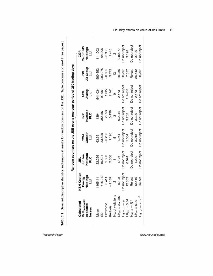
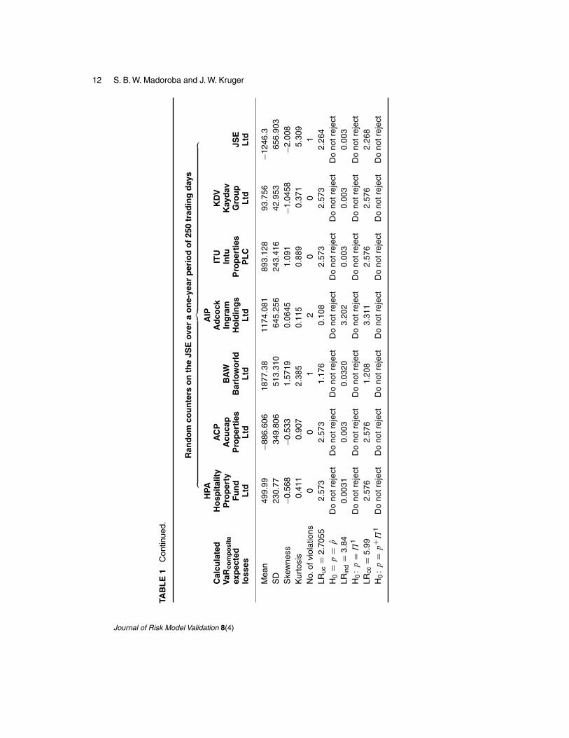
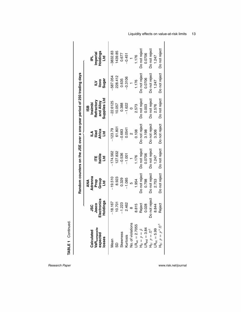
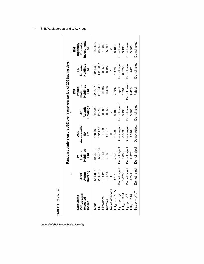
The mean, volatility, skewness and kurtosis of each of the asset counters’ percentagereturns were calculated. The volatility ranges from �25% to +50%, indicating thatthe counters exhibited a high degree of volatility. The symmetry of a distribution ismeasured by its skewness; it is a unitless measure. A symmetric distribution thereforehas a skewness of 0. While an asymmetrical distribution with a long tail to the right(higher values) has a positive skew, ie, greater than 0, an asymmetrical distributionwith a long tail to the left (lower values) has a negative skew, ie, less than 0. As ageneral rule of thumb, if the skewness is greater than 1.0 (or less than �1:0), theskewness is substantial and the distribution is far from symmetrical. In this study,there were no asset returns with a skewness of 0. The range of skewness values, asshown in Table 1 on the facing page, is �1:167 to 2.353.

Kurtosis, which has no units, quantifies whether the shape of the data distributionmatches a Gaussian or normal distribution. A Gaussian distribution has a kurtosis of0, while a flatter distribution has a negative kurtosis. If a distribution is more peakedthan a Gaussian distribution, it has a positive kurtosis. In this study, kurtosis valuesfrom �1:1167 to 7.548 were observed. The asset percentage return distributions are



TAB

LE

1S

elec

ted

desc

riptiv

est

atis

tics

and

empi

rical

resu

ltsfo

rra

ndom

coun

ters

onth

eJS

E.[

Tabl

eco

ntin

ues

onne

xtth

ree

page

s.]

Ran

do

mco

un

ters

on

the

JSE

over

ao

ne-

year

per

iod

of

250

trad

ing

day

s‚

…„ƒ

Cal

cula

ted

KE

HK

eato

nJB

LC

GR

VaR

com

po

site

En

erg

yJu

bile

eC

OM

INP

AE

GJD

GC

alg

roM

3ex

pec

ted

Ho

ldin

gs

Pla

tin

um

Co

mai

rIn

vest

ecA

ven

gJD

Gro

up

Ho

ldin

gs

loss

esL

tdP

LC

Ltd

PL

CL

tdL

tdL

td

Mea

n11

65.4

122

.266

63.5

913

9454

1.03

458

0.85

211

1.00

2S

D61

8.91

710

.501

33.6

2935

6.56

99.9

6129

3.07

564

.005

Ske

wne

ss0.

411

1.63

3�0

.206

2.35

31.

627

�0.0

35�0

.903

Kur

tosi

s�1

.167

2.30

61.

196

5.43

67.

141

3.74

21.

445

No.

ofvi

olat

ions

21

53

012

2LR

ucD

2.70

550.

108

1.17

61.

954

0.09

442.

573

18.9

850.

0007

7H

0D

pD

OpD

ono

trej

ect

Do

notr

ejec

tD

ono

trej

ect

Do

notr

ejec

tD

ono

trej

ect

Rej

ect

Do

notr

ejec

tLR

ind

D3.

8412

.302

0.02

41.

064

3.20

51.

1�E

87.

557

3.19

8H

0Wp

D˘

1R

ejec

tD

ono

trej

ect

Do

notr

ejec

tD

ono

trej

ect

Do

notr

ejec

tR

ejec

tD

ono

trej

ect

LRcc

D5.

9912

.410

1.20

03.

018

3.30

02.

573

26.5

423.

199

H0

WpD

pC ˘

1R

ejec

tD

ono

trej

ect

Do

notr

ejec

tD

ono

trej

ect

Do

notr

ejec

tR

ejec

tD

ono

trej

ect



TAB

LE

1C

ontin

ued.

Ran

do

mco

un

ters

on

the

JSE

over

ao

ne-

year

per

iod

of

250

trad

ing

day

s‚

…„ƒ

HPA

AIP

Cal

cula

ted

Ho

spit

alit

yA

CP

Ad

cock

ITU

KD

VV

aRco

mp

osi

teP

rop

erty

Acu

cap

BA

WIn

gra

mIn

tuK

ayd

avex

pec

ted

Fu

nd

Pro

per

ties

Bar

low

orl

dH

old

ing

sP

rop

erti

esG

rou

pJS

Elo

sses

Ltd

Ltd

Ltd

Ltd

PL

CL

tdL

td

Mea

n49

9.99

�886

.606

1877

.38

1174

.081

893.

128

93.7

56�1

246.

3S

D23

0.77

349.

806

513.

310

645.

256

243.

416

42.9

5365

6.90

3S

kew

ness

�0.5

68�0

.533

1.57

190.

0645

1.09

1�1

.045

8�2

.008

Kur

tosi

s0.

411

0.90

72.

385

0.11

50.

889

0.37

15.

309

No.

ofvi

olat

ions

00

12

00

1LR

ucD

2.70

552.

573

2.57

31.

176

0.10

82.

573

2.57

32.

264

H0

Dp

DOp

Do

notr

ejec

tD

ono

trej

ect

Do

notr

ejec

tD

ono

trej

ect

Do

notr

ejec

tD

ono

trej

ect

Do

notr

ejec

tLR

ind

D3.

840.

0031

0.00

30.

0320

3.20

20.

003

0.00

30.

003

H0

WpD

˘1

Do

notr

ejec

tD

ono

trej

ect

Do

notr

ejec

tD

ono

trej

ect

Do

notr

ejec

tD

ono

trej

ect

Do

notr

ejec

tLR

ccD

5.99

2.57

62.

576

1.20

83.

311

2.57

62.

576

2.26

8H

0Wp

Dp

C ˘1

Do

notr

ejec

tD

ono

trej

ect

Do

notr

ejec

tD

ono

trej

ect

Do

notr

ejec

tD

ono

trej

ect

Do

notr

ejec

t



TAB

LE

1C

ontin

ued.

Ran

do

mco

un

ters

on

the

JSE

over

ao

ne-

year

per

iod

of

250

trad

ing

day

s‚

…„ƒ

AN

AIS

BC

alcu

late

dJS

CA

dre

nn

aIL

AIn

sim

bi

IPL

VaR

com

po

site

Jasc

oP

rop

ITE

Iliad

Ref

ract

ory

ILV

Imp

eria

lex

pec

ted

Ele

ctro

nic

sG

rou

pIt

alti

leA

fric

aan

dA

lloy

Ilovo

Ho

ldin

gs

loss

esH

old

ing

sL

tdL

tdL

tdS

up

plie

sL

tdS

ug

arL

td

Mea

n�1

8.16

7�1

9.51

0�1

74.5

62�1

23.7

9�2

2.61

25�5

87.0

54�3

832.

83S

D10

.701

8.92

312

7.83

261

.801

10.0

5722

8.41

214

39.8

5S

kew

ness

�1.2

230.

329

�0.5

36�0

.683

0.38

80.

635

0.67

7K

urto

sis

2.46

2�1

.085

�1.0

010.

0541

�1.6

22�0

.310

6�0

.451

No.

ofvi

olat

ions

85

12

01

1LR

ucD

2.70

558.

815

1.95

41.

176

0.10

82.

573

1.17

61.

176

H0

Dp

DOp

Rej

ect

Do

notr

ejec

tD

ono

trej

ect

Do

notr

ejec

tD

ono

trej

ect

Do

notr

ejec

tD

ono

trej

ect

LRin

dD

3.84

0.02

80.

798

0.07

063.

198

0.00

30.

0706

0.07

06H

0Wp

D˘

1D

ono

trej

ect

Do

notr

ejec

tD

ono

trej

ect

Do

notr

ejec

tD

ono

trej

ect

Do

notr

ejec

tD

ono

trej

ect

LRcc

D5.

998.

844

2.75

31.

247

3.30

62.

576

1.24

71.

247

H0

WpD

pC ˘

1R

ejec

tD

ono

trej

ect

Do

notr

ejec

tD

ono

trej

ect

Do

notr

ejec

tD

ono

trej

ect

Do

notr

ejec

t



TAB

LE

1C

ontin

ued.

Ran

do

mco

un

ters

on

the

JSE

over

ao

ne-

year

per

iod

of

250

trad

ing

day

s‚

…„ƒ

IMP

ING

Cal

cula

ted

IVT

AC

LIm

pal

aIP

LIn

gen

uit

yV

aRco

mp

osi

teA

DR

Invi

cta

Arc

elo

rmit

tal

AD

IP

lati

nu

mIm

per

ial

Pro

per

tyex

pec

ted

Aco

rpH

old

ing

sS

AA

dap

tit

Ho

ldin

gs

Ho

ldin

gs

Inve

stm

ents

loss

esH

old

ing

Ltd

Ltd

Ho

ldin

gs

Ltd

Ltd

Ltd

Mea

n�5

61.8

25�1

995.

13�6

68.7

01�4

8.09

0�2

226.

14�3

844.

33�1

524.

29S

D22

4.71

366

5.16

417

2.17

928

.749

1183

.055

1442

.007

2359

6.6

Ske

wne

ss�0

.221

0.14

4�1

.539

�0.6

990.

296

0.65

9�1

5.84

3K

urto

sis

0.51

42.

160

11.9

57�0

.356

�0.4

76�0

.427

250.

999

No.

ofvi

olat

ions

10

02

81

2LR

ucD

2.70

551.

176

2.57

32.

573

0.10

87.

724

1.17

60.

108

H0

Dp

DOp

Do

notr

ejec

tD

ono

trej

ect

Do

notr

ejec

tD

ono

trej

ect

Rej

ect

Do

notr

ejec

tD

ono

trej

ect

LRin

dD

3.84

0.07

060.

003

0.00

33.

198

1.70

10.

0706

3.19

8H

0Wp

D˘

1D

ono

trej

ect

Do

notr

ejec

tD

ono

trej

ect

Do

notr

ejec

tD

ono

trej

ect

Do

notr

ejec

tD

ono

trej

ect

LRcc

D5.

991.

247

2.57

62.

576

3.30

69.

426

1.24

73.

306

H0

WpD

pC ˘

1D

ono

trej

ect

Do

notr

ejec

tD

ono

trej

ect

Do

notr

ejec

tR

ejec

tD

ono

trej

ect

Do

notr

ejec

t



far from normal. This is expected, as the asset counters considered are varied, withsome very liquid and others quite illiquid based on the number of trades made overthe 250 trading days considered.

However, it is important to note that the composite VaR model in this study disre-gards the statistical distribution of the asset price returns. Therefore, we did not modelthe lognormal returns, which might have given completely different observations inreturn distributions. The model is grounded in empirical observations of percentagereturns, which need not follow any particular distribution.

4.2 VaR model backtesting

4.2.1 Introduction to VaR model backtesting

Various studies in VaR methodologies have shown that any VaR model is only asgood as its backtest. The Basel Committee on Banking Supervision (1996) recom- Not in References!

mended that all financial risk model evaluations include a backtesting procedure. Ingeneral, backtesting compares the VaR expected loss of one day (ex ante) with theobserved loss of the following day (ex post). In this respect, a valid VaR model needsto comply with the so-called unconditional coverage characteristic. Unconditionalcoverage refers to the fact that the fraction of overshootings (ex post loss exceedsex ante VaR) obtained should be in line with the confidence level of the VaR. Fail-ure of unconditional coverage means that the calculated VaR does not measure therisk accurately. In addition to unconditional coverage, VaR models should satisfy theindependence property. The independence property refers to the clustering of viola-tions. In changing market conditions, the VaR model should adapt quickly to the newsituation. Therefore, observing a violation today should be independent of observ-ing an overshooting tomorrow. This aspect of VaR model performance is extremelyimportant, since a series of violations means that the risk is underestimated for longperiods during times of increased risk.

4.2.2 Regulatory framework of VaR model backtesting

According to CSSF Circular 07/308, Commission Directive 2010/43/EU and the Changes to sentence OK?Also, none of thesedocuments appear in thebibliography. Please givepublication details.

CESR Guidelines 10-788 (issued July 28, 2010), the Undertakings for CollectiveInvestments in Transferable Securities (UCITS) must monitor the reliability, validity,adequacy and effectiveness of the market-risk model using a backtesting program.The new CESR Guidelines 10-788 include the following.

� The backtesting must provide a comparison for each business day between theone-day 99% VaR results and the fluctuation over one day of the portfolio’svalue.

� The UCITS must undertake the backtesting program on at least a monthly basis.



� The UCITS should determine and monitor the violations. If the percentage ofviolations appears too high, the UCITS should review the VaR model.

� Violations are to be reported to senior management on a quarterly basis (and, ifapplicable, the UCITS competent authority should be informed on a semiannualbasis) if the number of violations for the most recent 250 business days exceedsfour (a 99% confidence interval).

It was against this background that the new composite VaR model of our study was Change OK?

subjected to backtesting using sample data from the JSE, as previously explained.

4.3 Statistical analysis

Figures provided are reflectedversions of those that appearin the MS. Also, the repeatedparagraph at the beginning ofthis subsection has beendeleted – change OK? Figures5 and 6 are identical. Pleaseprovide another version ofFigure 6. Finally, no figuresare referred to in the text:please add a brief mention ofthem somewhere in the text.

Three statistical tests for VaR model backtesting were applied to compare the com-posite VaR number with the empirically observed gain or loss for the 136 tradingcounters over 250 trading days from December 10, 2012, to December 10, 2013.

4.3.1 Kupiec’s unconditional coverage test

We construct a “hit” sequence that returns a 1 on a day .t C 1/ if the loss on that daywas larger than the VaR number calculated by our composite VaR model in advancefor that day. If the VaR number was not violated, then the hit sequence returns a0. The hit sequence of violations should be completely unpredictable and thereforedistributed independently over time as an independently and identically distributed(iid) Bernoulli variable.

The backtesting procedure is such that we tested whether the fractions ./ of the Changes to sentence OK?

violations obtained for a particular hit sequence were significantly different fromthe known VaR coverage fraction, p. We refer to this as the unconditional coveragehypothesis. In order to test it, we write the likelihood of an iid Bernoulli ./ hitsequence as Change to the Greek symbol

˘ here OK? This wasunclear from yourmanuscript. Please mark anythat denote the product

Qand

should be upright.

L./.˘/ D .1 � /T0./T1 ;

where T0 and T1 are the number of zeros and ones in the sample and T is the samplepopulation. We can easily estimate from O D T1=T , which denotes the empirically Changes to this sentence and

the next OK?

observed fractions of violations in the hit sequence.The optimized likelihood function becomes

L. O/.˘/ D�

1 � T1

T

�T0�

T1

T

�T1

under the unconditional coverage null hypothesis that D p, where p is the knownVaR coverage, which in our case is 99%. Hence the likelihood for p becomes

L.p/.˘/ D .1 � p/T0.p/T1 :



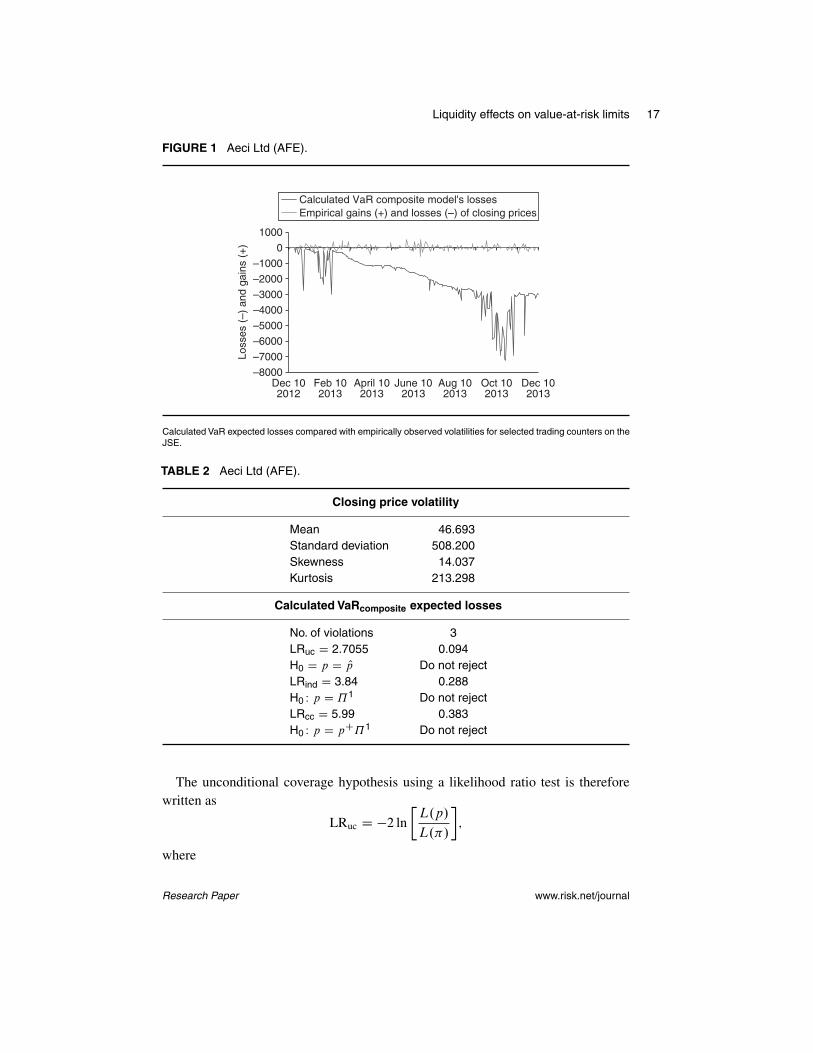
FIGURE 1 Aeci Ltd (AFE).

–8000

–7000

–6000

–5000

–4000

–3000

–2000

–1000

0

1000Lo

sses

(–)

and

gai

ns (

+)

Calculated VaR composite model's lossesEmpirical gains (+) and losses (–) of closing prices

Dec 102012

Feb 102013

April 102013

June 102013

Aug 102013

Oct 102013

Dec 102013

Calculated VaR expected losses compared with empirically observed volatilities for selected trading counters on theJSE.

TABLE 2 Aeci Ltd (AFE).

Closing price volatility

Mean 46.693Standard deviation 508.200Skewness 14.037Kurtosis 213.298

Calculated VaRcomposite expected losses

No. of violations 3LRuc D 2.7055 0.094H0 D p D Op Do not rejectLRind D 3.84 0.288H0 W p D ˘1 Do not rejectLRcc D 5.99 0.383H0 W p D pC˘1 Do not reject

The unconditional coverage hypothesis using a likelihood ratio test is thereforewritten as

LRuc D �2 ln

�L.p/

L./

�;

where



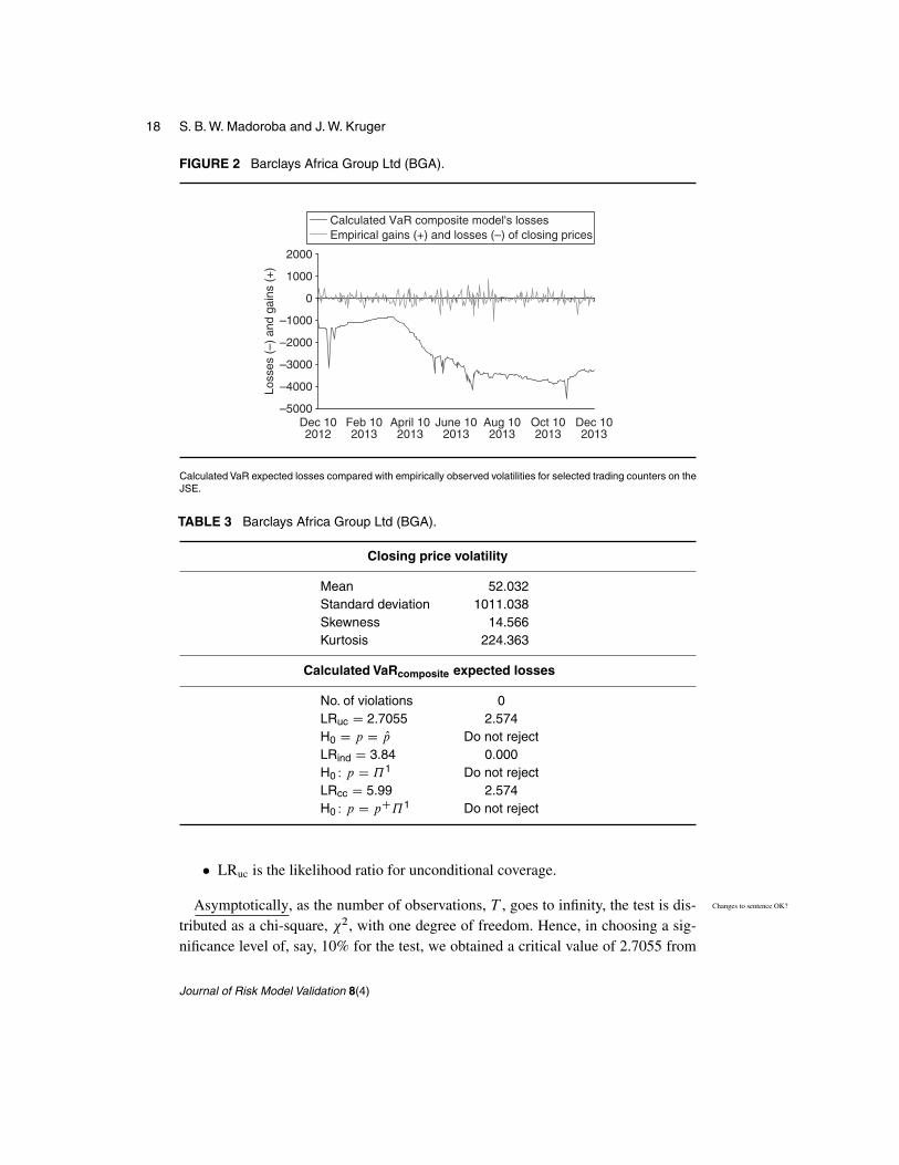
FIGURE 2 Barclays Africa Group Ltd (BGA).

Loss

es (

–) a

nd g

ains

(+

)


Dec 102012

Feb 102013

April 102013

June 102013

Aug 102013

Oct 102013

Dec 102013

2000

1000

0

–1000

–2000

–3000

–4000

–5000


TABLE 3 Barclays Africa Group Ltd (BGA).





� LRuc is the likelihood ratio for unconditional coverage.

Asymptotically, as the number of observations, T , goes to infinity, the test is dis- Changes to sentence OK?

tributed as a chi-square, 2, with one degree of freedom. Hence, in choosing a sig-nificance level of, say, 10% for the test, we obtained a critical value of 2.7055 from



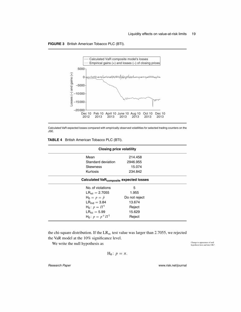
FIGURE 3 British American Tobacco PLC (BTI).

Loss

es (

–) a

nd g

ains

(+

)


Dec 102012

Feb 102013

April 102013

June 102013

Aug 102013

Oct 102013

Dec 102013

5000

0

–5000

–10 000

–15 000

–20 000


TABLE 4 British American Tobacco PLC (BTI).




No. of violations 5LRuc D 2.7055 1.955H0 D p D Op Do not rejectLRind D 3.84 13.674H0 W p D ˘1 RejectLRcc D 5.99 15.629H0 W p D pC˘1 Reject

the chi-square distribution. If the LRuc test value was larger than 2.7055, we rejectedthe VaR model at the 10% significance level.

We write the null hypothesis as Change to appearance of nullhypothesis here and later OK?

H0 W p D :



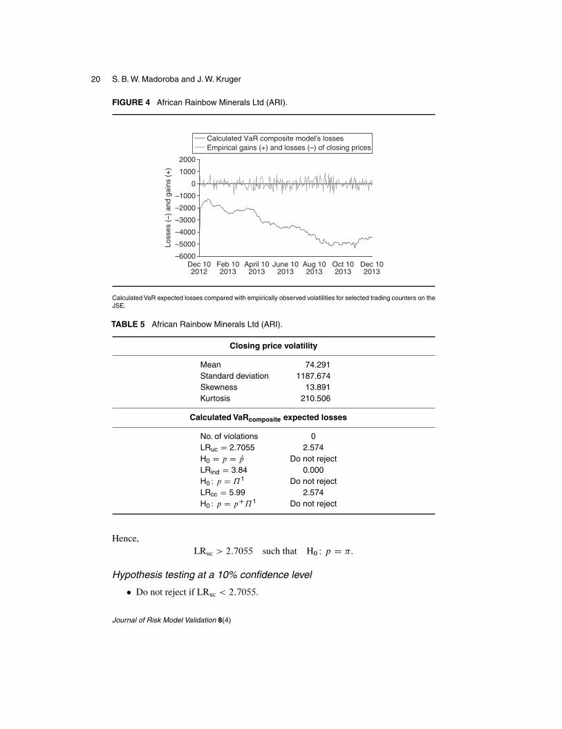
FIGURE 4 African Rainbow Minerals Ltd (ARI).

Loss

es (

–) a

nd g

ains

(+

)


Dec 102012

Feb 102013

April 102013

June 102013

Aug 102013

Oct 102013

Dec 102013

2000

1000

0

–1000

–2000

–3000

–4000

–5000

–6000


TABLE 5 African Rainbow Minerals Ltd (ARI).





Hence,LRuc > 2:7055 such that H0 W p D :

Hypothesis testing at a 10% confidence level

� Do not reject if LRuc < 2:7055.



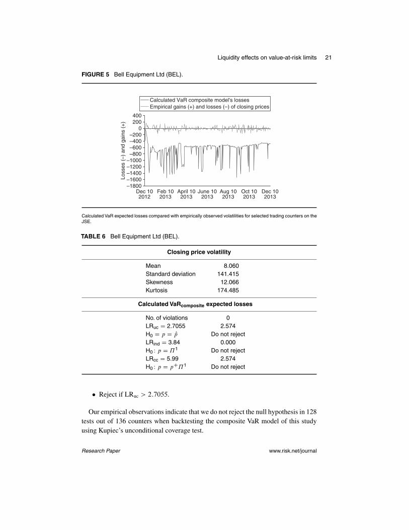
FIGURE 5 Bell Equipment Ltd (BEL).

Loss

es (

–) a

nd g

ains

(+

)


Dec 102012

Feb 102013

April 102013

June 102013

Aug 102013

Oct 102013

Dec 102013

400200

0–200–400–600–800

–1000–1200–1400–1600–1800


TABLE 6 Bell Equipment Ltd (BEL).





� Reject if LRuc > 2:7055.

Our empirical observations indicate that we do not reject the null hypothesis in 128tests out of 136 counters when backtesting the composite VaR model of this studyusing Kupiec’s unconditional coverage test.



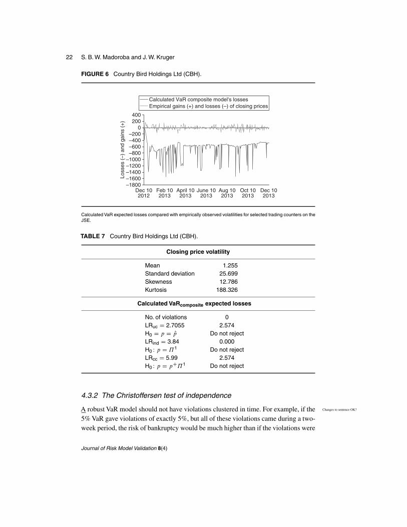
FIGURE 6 Country Bird Holdings Ltd (CBH).

Loss

es (

–) a

nd g

ains

(+

)


Dec 102012

Feb 102013

April 102013

June 102013

Aug 102013

Oct 102013

Dec 102013

400200

0–200–400–600–800

–1000–1200–1400–1600–1800


TABLE 7 Country Bird Holdings Ltd (CBH).





4.3.2 The Christoffersen test of independence

A robust VaR model should not have violations clustered in time. For example, if the Changes to sentence OK?

5% VaR gave violations of exactly 5%, but all of these violations came during a two-week period, the risk of bankruptcy would be much higher than if the violations were



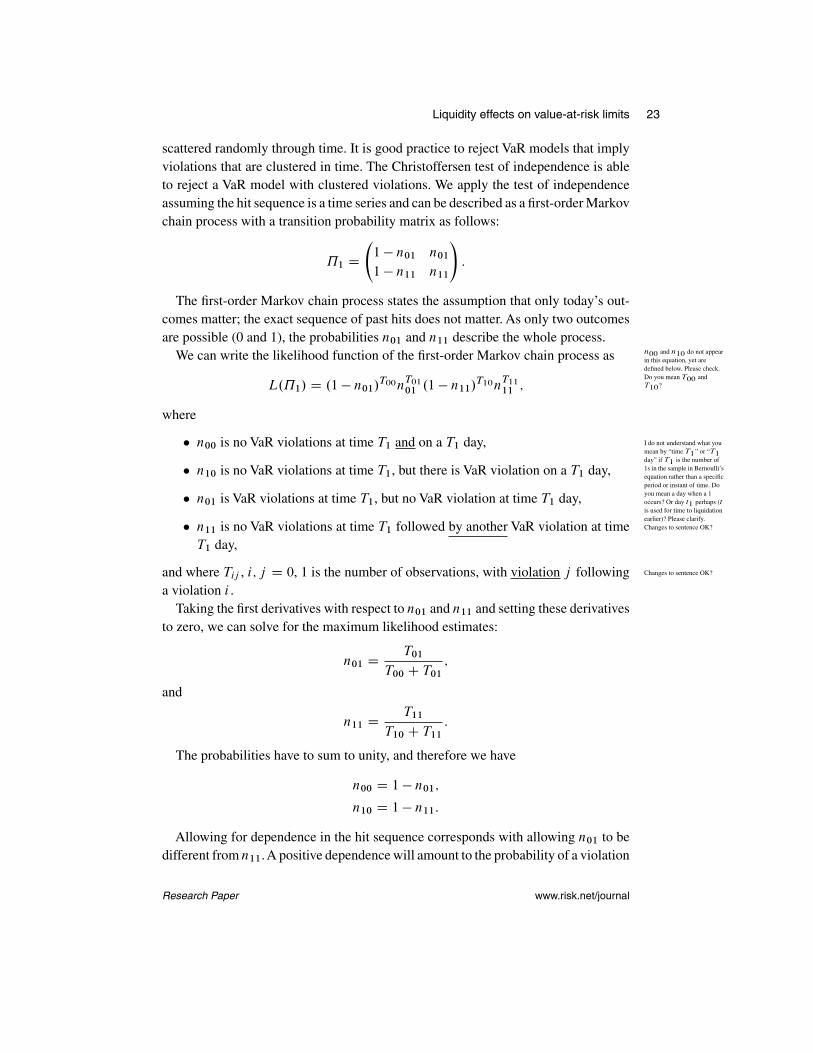
scattered randomly through time. It is good practice to reject VaR models that implyviolations that are clustered in time. The Christoffersen test of independence is ableto reject a VaR model with clustered violations. We apply the test of independenceassuming the hit sequence is a time series and can be described as a first-order Markovchain process with a transition probability matrix as follows:

˘1 D

1 � n01 n01

1 � n11 n11

!:

The first-order Markov chain process states the assumption that only today’s out-comes matter; the exact sequence of past hits does not matter. As only two outcomesare possible (0 and 1), the probabilities n01 and n11 describe the whole process.

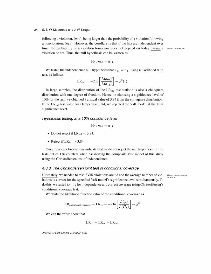
We can write the likelihood function of the first-order Markov chain process as n00 and n10 do not appearin this equation, yet aredefined below. Please check.Do you mean T00 andT10?L.˘1/ D .1 � n01/T00n

T01

01 .1 � n11/T10nT11

11 ;

where

� n00 is no VaR violations at time T1 and on a T1 day, I do not understand what youmean by “time T1” or “T1day” if T1 is the number of1s in the sample in Bernoulli’sequation rather than a specificperiod or instant of time. Doyou mean a day when a 1occurs? Or day t1 perhaps (tis used for time to liquidationearlier)? Please clarify.

� n10 is no VaR violations at time T1, but there is VaR violation on a T1 day,

� n01 is VaR violations at time T1, but no VaR violation at time T1 day,

� n11 is no VaR violations at time T1 followed by another VaR violation at time Changes to sentence OK?

T1 day,

and where Tij , i; j D 0, 1 is the number of observations, with violation j following Changes to sentence OK?

a violation i .Taking the first derivatives with respect to n01 and n11 and setting these derivatives

to zero, we can solve for the maximum likelihood estimates:

n01 D T01

T00 C T01

;

and

n11 D T11

T10 C T11

:

The probabilities have to sum to unity, and therefore we have

n00 D 1 � n01;

n10 D 1 � n11:

Allowing for dependence in the hit sequence corresponds with allowing n01 to bedifferent from n11.A positive dependence will amount to the probability of a violation



following a violation, .n11/, being larger than the probability of a violation followinga nonviolation, .n01/. However, the corollary is that if the hits are independent overtime, the probability of a violation tomorrow does not depend on today having a Changes to sentence OK?

violation or not. Thus, the null hypothesis can be written as

H0 W n01 D n11:

We tested the independence null hypothesis that n01 D n11 using a likelihood ratiotest, as follows:

LRind D �2 ln

�L.n01/

L.n11/

�� 2.1/:

In large samples, the distribution of the LRind test statistic is also a chi-squaredistribution with one degree of freedom. Hence, in choosing a significance level of10% for the test, we obtained a critical value of 3.84 from the chi-square distribution.If the LRind test value was larger than 3.84, we rejected the VaR model at the 10%significance level.

Hypothesis testing at a 10% confidence level

H0 W n01 D n11:

� Do not reject if LRind < 3:84.

� Reject if LRind > 3:84.

Our empirical observations indicate that we do not reject the null hypothesis in 130tests out of 136 counters when backtesting the composite VaR model of this studyusing the Christoffersen test of independence.

4.3.3 The Christoffersen joint test of conditional coverage

Ultimately, we needed to test if VaR violations are iid and the average number of vio- Changes to this sentence andthe next OK?

lations is correct for the specified VaR model’s significance level simultaneously. Todo this, we tested jointly for independence and correct coverage using Christoffersen’sconditional coverage test.

We write the likelihood function ratio of the conditional coverage as

LRconditional coverage D LRcc D �2 ln

�L.p/

L.˘1/

�� 2:

We can therefore show that

LRcc D LRuc C LRind:



It is important to note that the LRcc test takes the likelihood ratio from the nullhypothesis in the LRuc test and combines it with the likelihood ratio from thealternative hypothesis in the LRind test.

The null hypothesis for conditional coverage is then written as

H0 W p D ˘1 C ˘:

The Christoffersen test of conditional coverage test statistic LRcc also follows achi-square distribution with one degree of freedom and is asymptotically limited.Hence, in choosing a significance level of 10% for the test, we obtained a criticalvalue of 5.99 from the chi-square distribution. If the LRcc test value was larger than5.99, we rejected the VaR model at the 10% significance level.

Hypothesis testing at 10% confidence level

H0 W p D ˘1 C ˘:

� Do not reject if LRind < 5:99.

� Reject if LRind > 5:99.

Our empirical observations indicate that we do not reject the null hypothesis in128 tests out of 136 counters when backtesting the composite VaR model for theChristoffersen joint test of conditional coverage.

5 DISCUSSION OF THE RESULTS

Backtesting constituted the testing of three hypotheses regarding the “hit rate” of theVaR models. We defined the hit rate as the number of times the VaR model forecastunderestimated true loss. The empirical results showed that the null hypothesis wasnot rejected by Kupiec’s test of unconditional coverage for 179 tests out of the 180counters to which it was applied. The first hypothesis tested the unconditional cov-erage, which points out that an ˛% VaR should be breached close to .1�/˛% of the Change OK?

time by realized portfolio losses. The VaR model should therefore not systematicallyunder- or overestimate risk. This means that the number of predicted violations isless than our model’s specified coverage of 99%, indicating that our model does notunderestimate the quantum of loss.

The second was the independence hypothesis, which argues that violations of VaR Changes to sentence OK?

forecasts should be independent over time and not autocorrelated. The corollary isthat occurrence or nonoccurrence of a violation should bear no information on future “have no impact”?

violations. In this instance, the empirical results show that the null hypothesis wasnot rejected in 178 out of 180 of the cases for the Christoffersen test of independence.This indicates that our model consistently calculates iid predictions of violations. If Changes to sentence OK?


Evelyn

Cross-Out

Evelyn

Cross-Out


this is the case, then our VaR model should have no difficulty forecasting changesin profit and loss distribution. The composite VaR model is robust, as the number ofviolations follows a Markov chain process. These violations are also independent and Changes to sentence OK?

do not cluster. Such clustering is possible and common in stock exchange returns.Generally, if the underlying portfolio return has a clustered variance, as is common intime-varying asset returns such as stocks, clustering can occur, thereby impeding thetest of independence. The Christoffersen test of independence was devised specificallyto reject a VaR model with clustered violations.

The third hypothesis tested the conditional coverage of both independence andcorrect conditional coverage of violations by the model. Christoffersen’s joint test ofconditional coverage does not reject the null hypothesis in 126 out of 136 counters.This means that our model consistently returns a VaR number with violations that areiid, do not cluster and do not autocorrelate. At the same time, it provides the correct Changes to sentence OK?

coverage for the specified 99% probability of tail losses at all times.

6 CONCLUSION

The three standard backtesting statistical processes for VaR models did not rejectthe composite VaR model constructed in this study in 93% of cases. The VaR model Changes to sentence OK?

developed is therefore robust and valid, as it consistently returns the same results forthe most liquid and the most illiquid stocks on the JSE. Although the model appearsad hoc and random, this does not negate the fact that it actually works and passes therecommended backtests for all VaR models. In this study, the use of intraday high–low spreads instead of the traditional bid–ask spreads was preferable. They reflectactual trades that have taken place, while bid–ask spreads reflect only an intentionto trade at the bid or ask price. Therefore, the high–low spreads are considered abetter intraday price approximation path on the JSE when compared with bid–askspreads. The incorporation of �, a new trade impact measure of price movementsdue to traded volumes, makes this study’s VaR composite model unique. The modelis therefore an improvement when compared with the other models available forcalculating liquidity-adjusted VaR to stochastic asset returns.

It is important to note that future research can investigate the limits to solutionsfor (3.4), (3.5) and (3.7) in order to determine the boundary conditions for the ad hocmeasures in this model. This may provide useful insight into and help improve the Changes to sentence OK?

VaR literature currently available, as well as this study’s model.

REFERENCES

Al Janabi, M. A. M. (2008). Integrating liquidity risk factor into a parametric value at riskmethod. Journal of Trading 3(3), 76–87.


Evelyn

Cross-Out


Almgren, R., and Chriss, N. (1999). Value under liquidation. The Journal of Risk 2(4),16–32.

Almgren, R., and Chriss, N. (2000). Optimal execution of portfolio transactions.The Journalof Risk 3(2), 5–39.

Ball, A., Denbee, E., Manning, M., and Wetherilt, A. (2011). Intraday liquidity risk andregulation. Financial Stability Paper 11, Bank of England.

Bangia, A., Diebold, F., Schuermann, T., and Strughair, J. (1998). Modelling liquidity risk, Changes to sentence OK?

with implications for traditional market risk measurement and management. WorkingPaper 99-062, Leonard N. Stern School Finance Department Working Paper Series,New York University.

Berkelaar, T. A., Cumperayot, P., and Kouwenberg, R. (2002).The effect of VaR-based riskmanagement on asset prices and the volatility smile. European Financial Management8(2), 139–164.

Berkowitz, J. (2000). Breaking the silence. Risk 13(10), 105–108.Berkowitz, J., and O’Brien, J. (2001). How accurate are value-at-risk models at commercial

banks? Journal of Finance 57(3), 1093–1111.Bertsimas, D., and Lo, A.W. (1998). Optimal control of execution costs. Journal of Financial

Markets 1(1), 1–50.Bhyat, A. (2010). An examination of liquidity risk and liquidity risk measures. Master’s

Thesis, University of Cape Town.Christoffersen, P. (1998). Evaluating interval forecast. International Economic Review 39,

841–862.Dubil, R. (2003). How to include liquidity in a market VaR statistic? Journal of Applied

Finance 13(1), 19–28.French, K., Baily, M., Campbell, J. Y., Cochrane, J. H., Diamond, D. W., Duffie, D.,

Kashyap, A. K., Mishkin, F. S., Rajan, R. G., Scharfstein, D. S., Shiller, R. J., Shin, H. S.,Slaughter, M. J., Stein, J. C., and Stulz, R. M. (2010). The Squam Lake Report: Fixingthe Financial System. Princeton University Press.

Hisata, Y., and Yamai, Y. (2000). Research toward the practical application of liquidity risk Changes to sentence OK?

evaluation methods. Monetary and Economic Studies 18(2), 83–127.Holthausen, R. W., Leftwich, R. W., and Mayers, D. (1987). The effect of large block trans-

actions on security prices: a cross-sectional analysis. Journal of Financial Economics19, 237–267.

Jarrow, R. A. and Subramanian, A. (2001). The liquidity discount. Mathematical Finance.11(4), 447–474

León, C. (2012). Estimating the intraday liquidity risk of financial institutions: a Monte Carlosimulation approach. The Journal of Financial Market Infrastructures 1(1), 75–107.

Le Saout, E. (2002). Incorporating liquidity risk in VaR models. Working Paper, Paris IUniversity.

Muranaga, J., and Ohsawa, M. (1999).Measurement of liquidity risk in the context of marketrisk calculation. Research Paper, Institute for Monetary and Economic Studies, Bank ofJapan.

Orlova, E. (2008). Estimation of liquidity-adjusted VaR from historical data. Master’s Thesis,Centre for Applied Statistics and Economics, Humboldt-Universität zu Berlin.

Pastor, L., and Stambaugh, R. F. (2003). Liquidity risk and expected stock returns. Journalof Political Economy 111(3), 642–685.



Shamroukh, N. (2000). Modelling liquidity risk in VaR models.Working Paper, AlgorithmicsUK.

Tucker, P. (2009). The debate on financial system resilience: macroprudential instruments.Speech, Barclays Annual Lecture, London.


Liquidity effects on value-at-risk limits: construction of a new VaR model

Documents