Liquid Oxygen Magnetohydrodynamics - DigitalCommons ...

Utah State University Utah State University

DigitalCommons@USU DigitalCommons@USU

Space Dynamics Lab Publications Space Dynamics Lab

1-1-2010

Liquid Oxygen Magnetohydrodynamics Liquid Oxygen Magnetohydrodynamics

J. C. Boulware

H. Ban

S. Jensen

S. Wassom

Follow this and additional works at: https://digitalcommons.usu.edu/sdl_pubs

Recommended Citation Recommended Citation Boulware, J. C.; Ban, H.; Jensen, S.; and Wassom, S., "Liquid Oxygen Magnetohydrodynamics" (2010). Space Dynamics Lab Publications. Paper 23. https://digitalcommons.usu.edu/sdl_pubs/23

This Article is brought to you for free and open access by the Space Dynamics Lab at DigitalCommons@USU. It has been accepted for inclusion in Space Dynamics Lab Publications by an authorized administrator of DigitalCommons@USU. For more information, please contact [email protected].

Boulware, J. C., H. Ban, S. Jensen, and S. Wassom. "Liquid Oxygen Magnetohydrodynamics." Journal of Magnetohydrodynamics, Plasma and Space Research 15 (3-4). Abstract available at https://www.novapublishers.com/catalog/product_info.php?products_id=24460.

LIQUID OXYGEN MAGNETOHYDRODYNAMICS

J. C. Boulware, H. Ban, S. Jensen, S. Wassom

1. Abstract In the cryogenic realm, liquid oxygen (LOX) possesses a natural paramagnetic susceptibility and

does not require a colloidal suspension of particles for practical application as a magnetic

working fluid. Commercial ferrofluids have performed well in industrial applications, but

expanding their workable range to low temperatures requires a suitable selection of the carrier

fluid, such as LOX. In this chapter, the equation of motion for the pure fluid is derived and

applied to a slug of LOX being displaced by a pulsed magnetic field. Its theoretical performance

is compared to actual experimental data with discussion on empirical parameters, sensitivity to

measurement uncertainty, and geometric similarity. The 1.1 T pulse of magnetic flux density

produced oscillations in the slug of 6-8 Hz, generating up to 1.4 kPa of pressure change in a

closed section when the slug acted like a liquid piston. The experiments and theoretical model

demonstrate that LOX could be used as a magnetic working fluid in certain applications.

2. Introduction Elimination of moving parts and increased subsystem lifetime is a major benefit of actuator

systems with magnetically responsive fluids as opposed to those relying on a mechanical driver

to instigate flow. Space systems, in particular, could benefit from increased subsystem lifetime as

it would increase the overall mission length; however, unlike ground-based magnetic fluid

systems, use of magnetically responsive fluids in the low-temperature regime of space requires

verification of fundamental principles through basic research and experimentation, since it has

never been applied.

2.1 Magnetic Fluids

Magnetism occurs due to the atomic or molecular structure of a material and can be classified as

ferromagnetic, diamagnetic, or paramagnetic depending on the behavior of the poles.

Ferromagnetic solids have permanently aligned poles and generate their own magnetic fields.

Liquids, however, cannot maintain the alignment without a field and are either paramagnetic, in

which the poles align with the applied field, or diamagnetic, in which the poles align opposite the

applied field. The bulk effect of each is that paramagnetics are attracted to the field (towards an

increasing gradient), and that diamagnetics are repelled by it (away from an increasing

gradient)1•

In the 1960s, NASA developed "ferrofluids," which are a colloidal suspension of ferromagnetic

particles in a carrier fluid. A surfactant on the particles prevents their alignment without a field;

thus, ferrofluids actually exhibit superparamagnetism since they have an extremely high

susceptibility to an applied field. Ferrofluids have found many industrial applications, such as in

high-end audio speakers, digital data storage, and resonance imaging. As a working fluid,

ferrofluids have been proposed for pumps2•7

, valves8, actuators9

, heat pipes10"

11, and even optical

tuners12. The range of applicability of ferrofluids , however, is limited by the thermal

characteristics of the carrier fluid, typically water, oil, or a hydrocarbon. While much use has

been made of ferrofluids at ambient and high temperatures, freezing of the carrier fluid prevents

their use at low temperature. Furthermore, the presence of nanoparticles and surfactants in

ferrofluids complicates analyses, mainly due to agglomeration and nonhomogeneity. In the

cryogenic realm, liquid oxygen (LOX) presents a potential solution as it possesses a natural

paramagnetic susceptibility and does not require particles for practical application.

2.2 Liquid Oxygen

In all phases, the unpaired electrons in an 0 2 molecule lead to a bulk paramagnetic effect. At

room temperature, however, the thermal energy within the molecules may dominate the magnetic

alignment with an applied field; hence warm oxygen does not have an appreciable susceptibility.

As temperature decreases and thermal energy is reduced, the molecules are more able to align

and susceptibility increases. This phenomenon is known as Curie's Law, where, essentially,

paramagnetic susceptibility increases as temperature decreases. Furthermore, once oxygen

condenses (90 K, 1 atm), the volumetric susceptibility, x, significantly increases with the density

of the fluid. The relationship between volumetric susceptibility, mass susceptibility, Xmass, and

molar susceptibility, Xmolar, is defined through density, p, and molecular weight, MW, as

J J Xmo/ar X = p X mass = p MW · (1)

Throughout the remainder of the chapter, "susceptibility" will refer to volumetric susceptibility.

Although it is approximately 30 times weaker than a low-end ferrofluid, LOX has the highest

known paramagnetic susceptibility of pure fluids at about 0.0042. The lack of magnetic particles

eliminates risks such as corrosion and shock, and since LOX is already commonly used for life

support, thermal management, and propulsion systems, the integration process is simpler than for

a ferrofluid.

2.3 Previous Research

The basic properties of LOX have been measured under a variety of temperature and pressure

ranges13-15

, but unfortunately, very few experiments have studied the influence of a magnetic

field, perhaps due to the volatile nature of LOX. Surface tension16, surface instabilities17

, and

levitation phenomena18•

19 have all been studied under high magnetic fields, but none of these

experiments generated a bulk displacement of the liquid. Yerkes20 measured the wicking heights

of LOX heat pipes when augmented by a magnetic field and showed an increase ofup to 4 times

the capillary pressure for a magnetic flux density of 0.27 T. These experiments are useful in

understanding the nature of LOX magnetohydrodynamics as well as experimental research on

magnetic fluid pumps, magnetoviscosity, and magnetic fluid pipe flow.

2.3.1 Magnetic Fluid Pumps.

Regarding LOX, only one experimental study could be found which generated a high flow rate.

Youngquist21 ofthe Kennedy Space Center researched the dynamics of a column ofLOX in aU­

tube when a magnetic field was applied. He measured the displacement of one end of the column

when the other was pulsed with a magnetic field induced by a solenoid. Figure 1 shows the

experimental setup.

z

Tube Cross-Section A

z=O X

Figure 1. Experimental setup for LOX pumping, taken from Youngquist.

An electric current of 30 A was pulsed through the solenoid, generating a magnetic field with a

maximum flux density of 0.9 T. With the field applied, the height of the column oscillated about

a new mean, reaching a maximum displacement of 4-5 em. It is worthy of note that pulses of 100

A and 6 T were attempted, but yielded erratic results, often ripping off the top of the column. A

theoretical model was created to obtain a one-dimensional, finite-differenced solution, which

employed a second-order, velocity-based damping function relying upon empirical coefficients.

Again, this study was the only experimental research found on the magnetohydrodynamics of

LOX, but other ferrofluid pumps served well as bases for comparison.

Park and Seo2-4 of Pusan National University have developed a magnetic fluid linear pump for

use in infusion pumps and artificial hearts in the medical industry. Employing magnetic yokes to

propagate droplets of a magnetic fluid, the device uses surface shear to pump water as shown in

Figure 2.

Figure 2. Experimental setup for pumping water with a magnetic fluid, taken from Park and Seo.

Park and Seo report pumping heights equivalent to 2 kPa (0.29 psi) for a maximum flux density

of 0.036 T (360 G). While this seems like an extremely small field compared to Youngquist's

experiment, it is important to note the Park and Seo are using a ferrofluid and not LOX. The

research performed by Park and Seo is useful as a study on traveling waves and their effects on

the surface dynamics of a magnetic fluid droplet, but difficult to apply to LOX due to the

differences in susceptibility and surface tension. Nonetheless, the work serves as a good

benchmark for comparison.

Hatch5 of the University of Washington developed a ferrofluidic rotary micropump to enhance

lab-on-a-chip MEMS technology. The concept (shown in Figure 3) achieved 1.2 kPa of pressure

head using a rotating and stationary permanent magnet with a surface flux density of 0.35 T

(3500 G). As in the experimental arrangement of Park and Seo, the device pumps a separate,

immiscible fluid, but uses normal pressure instead of shear. The study reports operation at 4 and

8 rpm for 3 days at a time. It was found that the steady-state pressure gradient decreased over

time when the plugs were rotated both clockwise and counterclockwise. Pumping speeds greater

than 8 rpm generated too much pressure and disrupted the coupling between the permanent

magnet and the translating ferrofluidic plug. While Hatch's design is intuitive and effective, the

rotating permanent magnet is a mechanically moving component and, therefore, negates the goal

of creating a system for fluid actuation with no moving parts.

, l.!.:t ... ,ntlf'

ftntrfl tt·d [UJ • ~---

'

• fcrrotluid

pumped tluid

0 pcnnam:nt magnet

---- --r----r----- -

Figure 3. A rotating permanent magnet to propagate a ferrofluid plug, taken from Hatch.

Moghadarn6 also developed a microscale magnetic fluid pump and eliminated the moving parts.

He used a series of solenoids spaced along a tube to drive a magnetic fluid linearly, similar to the

method of Park and Seo. However, instead of wrapping the solenoids around the tube, they were

offset and orthogonally aligned so that their core could be filled with an iron rod and increase the

magnetic flux density. The setup produced 0.64 kPa of pressure head for flow rates of 1.1

cm3/min at 0.45 T. The study compared different working fluids and particles, but relied on the

viscous drag of the particles to create fluid motion.

Krauss 7 of the University of Bayreuth has used a two-coil system to pump a ferro fluid circularly.

The 90° phase difference of the two coils with orthogonal axes produced a net field able to rotate

the fluid through the magnetic stress on the fluid surface. The mean diameter of the duct was 100

mm and the system produced a maximum fluid velocity of 70 mrn!sec and a magnetic field of

800A/m.

Figure 4. Two-coil system for pumping a ferrofluid by magnetic surface stress, taken from Krauss.

Zahn and Greer22 of the Massachusetts Institute of Technology took a theoretical approach to

traveling waves, but without a free surface. He found that the magnetic fluid can actually be

pumped backwards if the wave moves too fast. Without the free surface, the field interacts with

the nanoparticles inside the ferrofluids, and motion is generated through the particle spin. He

studied the dynamics of a spatially steady field, which, however, varied sinusoidally in time. His

work was followed up by Mao and Koser23 ofYale University who were able to vary the field in

space as well. Their findings showed that a maximum flow velocity was achieved when the

product of the applied magnetic field frequency, the wave number, and the height of the channel

approached unity. In other words, pumping becomes more efficient as the magnetic field

frequency approaches the reciprocal of the relaxation time constant of the magnetic particles in

the fluid. Mao and Koser compared their experimental data with numerical results for a 2D

solution using FEMLAB and a lD solution using Matlab. They found that all 3 agreed well until

the magnetic field frequency reached about 30 kHz, when the Matlab solution began to diverge.

The aforementioned research illustrates the importance of fluctuating magnetic fields for

pumping. Without a gradient of the magnetic field, no net force is generated, just as with a

pressure gradient. However, as shown by Youngquist, stationary solenoids are still able to create

a magnetic field gradient, since their strength lessens with distance. By pulsing the stationary

solenoid, a time-varying gradient can also be induced and used for position control of the

magnetic fluid.

2.3.2 Magnetoviscosity

Viscosity is adherent to fluid motion and can be calculated through its stress and strain rates. The

normal and tangential surface force on a differential element due to thermodynamic pressure can

be found through a divergence of the stress tensor; likewise, magnetic force can be found

through the divergence of Maxwell stress tensor, but its associated viscosity is much more

complicated.

Molecular or microscale magnetic particles in a paramagnetic fluid align with the applied field

and can induce additional shear as a function of the strength of the field. When aligned, the

magnetic torque helps the particles resist rotation, thereby disrupting fluid flow. The

magnetoviscous effect is heavily studied in ferrofluids, but questions remain in the case of a

pure, paramagnetic fluid like LOX. For the purpose of the current research, LOX is considered as

a ferro fluid with angstrom-scale particles, a fill fraction, ¢, of 100%, and a carrier fluid with the

same viscosity as non-magnetized LOX. From equations given by Shliomis24, the full fill

fraction approximation leads to a vortex viscosity, [3, of 1.5 times the non-magnetized shear

viscosity, ry, but the small diameter and viscosity lead to a nearly infinitesimal Brownian

relaxation time, r. The ratio ultimately leads to a very small increase in the effective viscosity

from particle alignment, !Jry.

3 f3 =-ry¢ 2

r =3Vryl kT

t1 ry J1.0MH r I 4 f3 =

f3 l+J1.0MHr / 4f3

(2)

(3)

(4)

where V is the particle volume, k is the Boltzmann constant, T is temperature, Jl.o is the

permeability of free space, M is the magnetization, and H is the applied field. These equations,

however, were written for dilute solutions and may not be applicable for high concentrations.

Furthermore, experiments by McTague25 have shown that particle interactions may also affect

the overall viscosity, even in dilute solutions, and that the atomic interactions between particles

under a magnetic field generate an increase in the viscosity. The equations above assume

particles up to 10,000 times larger than a molecule of oxygen; thus, different forces may be at

play. Without an adequate theory, the magnetoviscous effect of LOX cannot be declared either

insignificant or significant until a physical experiment measures it.

Lastly, use of a high-frequency AC field in the magnetic field may actually induce a "negative

viscosity," as shown by Bacri26. As mentioned, a static or low-frequency field will retard flow

through particle alignment with the field. In the case of high frequencies, increased fluid motion

was observed, indicating a reduction in the viscosity. This effect may be desirable or undesirable

depending on the intended application.

2. 3. 3 Magnetic Fluid Pipe Flow

Aside from influencing the rotational viscosity and particle interactions, the field can have a

macroscopic effect on the flow of a magnetic fluid through a pipe. Cunha27 numerically studied

the laminar flow through a pipe within a magnetic field with a linear gradient. When the field

gradient was opposite the flow direction, the fluid was impeded as expected; however, Cunha

noted the drag reduction as the field gradient facilitated fluid flow. He characterized the flow by

a magnetic pressure coefficient, Cpm, representing the ratio of the magnetic to hydrodynamic

pressures in the flow. Cunha correlated his results to a non-magnetic friction factor relationship

off = 8/Re and found that, as the magnetic effects arise, f is reduced. The reduction is more

pronounced for higher Reynolds numbers, but the study is limited to an asymptotic value near Re

= 50. Nonetheless, Cunha showed that as an axial field in the direction of fluid flow increases,

drag on the walls decreases.

An axial field with a linear gradient is not simple to reproduce in a laboratory experiment;

instead, Chen28 applied a ring magnet and focused on the streamlines for magnetic fluid flow in a

tube as the field and magnetoviscous response varied. He characterized the system parameters

through a magnetic Reynolds number, Rem, and a viscosity parameter, R. Figure 5 shows the

difference in the streamlines as the system parameters vary.

2.5 2.5 2.5

2 2 2

1.5 1.5 1.5

1 1 1

0.5

"' 0

-2.5 -2.5 ............ _..._ ..... 0.5 0 0.5 0 0.5

(a) r r (c) r (d) r

Figure 5. Streamline patterns for magnetic fluid flow in a tube with (a) Rem = 103 and R = 0 (no viscosity variance with field); (b) Rem = 103 and R = 1; (c) Rem= 105 and R = 1; and (d) Rem= 1.225 * 106 and R = 3.5, taken from Chen.

The field was applied by a ring magnet at z = 0, but of undisclosed length or gradient. Study of

the axial velocity profiles at various locations shows that an adverse gradient occurs even

without a magnetoviscous influence. This indicates that even if the viscosity of LOX does not

increase with a magnetic field, fluid damping still increases due to flow circulation.

Schlichting29 gives the classical solution of oscillating flow through a pipe, but the presence of a

magnetic field and the finite slug length complicate the analysis for the current study. In the case

of an infinite slug without a magnetic field, the shear could be doubled during oscillations; it is

expected that the augmentation would be greater with the magnetic field and finite slug.

2.4 Current Test Parameters

To determine the viability of LOX as a working fluid in a magnetically driven actuator, the

authors conducted studies that were essentially an evolution of Youngquist's experiments, but

with test objectives focused on advancing the technology towards applied research instead of

basic; thus, the experimental principle was different as well.

The broad goal of the research was to support the notion that LOX could be used as a working

fluid in a magnetic fluid system due to its significant paramagnetic susceptibility. This goal was

to be achieved by performing controlled, quantitative experiments, correlating them to a

theoretical model, and determining predictable trends from the results. The theoretical model was

to limit empirical input (other than initial conditions) and be able to make predictions regardless

of system geometry. Most importantly, the final data should be useful to future, applied research.

For this purpose, the experiments used a slug of LOX rather than a long column, as in

Youngquist's experiments. Magnetic pressure on a slug is maximized when one edge is in the

center of the solenoid and the other is in a negligible field. While this is achievable with a long

column, a smaller slug is nearly as effective. Figure 6 shows that the magnetic flux density of a

0.6 em (0.25 in) solenoid drops to 5% of its maximum value of 1.1 T at a distance 1. 7 5 em from

the center of the solenoid (Youngquist's column of LOX totaled 36 em). This benchmark differs

depending on solenoid geometry, applied current, and wire spacing, but the example shows that a

slug can achieve nearly the same magnetic pressure for a much smaller mass and length.

Eliminating mass and length reduces inertia and shear, which would otherwise retard slug

motion.

1

i=' -.2:' 0.8 ' (i) c (I)

0 X 0.6 ::I rr: .g 0.4 . (I) c 0) ctl :2 0.2

..... .,._ 0 0 Q) Q) Ol Ol "0 "0 LU L.U o ·~~~~~--~~~L-~~~~~

-2.5 -2 -1.5 -1 -0.5 0 .5 1 1.5 2 2.5 Distance from Center of Solenoid (em)

Figure 6. Magnetic flux density along the axis of a solenoid.

The experiment was designed to displace a slug of LOX and correlate its dynamics to a

numerical model. In all, the research studied the viability of LOX in a magnetic fluid system

with the following objectives:

1) Displace a LOX slug using magnetic fields.

-Experimentally accomplishing this would quantify the potential of a LOX-based magnetic fluid system.

2) Detect the displacement through pressure.

- Innovative measuring techniques will be required to study how LOX behaves in a magnetic field.

3) Simulate the dynamics numerically.

- A verified numerical algorithm can quantify LOX performance outside the scope of laboratory testing.

4) Perform parametric studies to examine efficiency optimization methods.

-Information on the sensitivity to uncertainties and geometric variance will help to estimate the potential capability of an optimized system.

3. Theoretical Model The theoretical model was based on a simple force balance on the slug. The change in

momentum of the slug was a result of the net force from magnetism, pressure, and damping. The

equation of motion essentially becomes the Navier-Stokes equations with an additional term for

the magnetic force. Rosensweig1 provides a thorough description of the force due to magnetism,

also known as the Kelvin force. The Kelvin force density, f 111 , can be found through the

divergence of the Maxwell stress tensor as a function of the permeability of free space, f1o, the

magnetization vector, M, and magnetic field, H, as

(5)

The resultant magnetization from an applied field can be described by the Langevin function,

where the volumetric paramagnetic susceptibility xis the ratio of the magnetization vector to the

applied field vector, x = M I H. By substituting for M, using the vector identity, H· V'H =

V'(H·H)/2 - Hx(V'xH), and noting that Ampere's Law cancels out the curl of the applied field,

Eq. (5) can be derived to

fm = flo(XH · Y')H,

fm = floX(H · Y'H),

fm :::: ,U0 X(Y'(H ·H)/ 2- H x (\7 x H)) ,

(6)

(7)

(8)

fm = ,u0x(V(H · H)/ 2) ,

fm = JLoXV'Hz 12.

(9)

(10)

With a constant temperature, the relative permeability, f1, also remains constant. The relative

permeability is the ratio between the magnetic flux density, B, and applied magnetic fields, 11 =

B / H, which can also expressed in terms ofvolumetric susceptibility, ,u = Jlo{l +x) . Given these

relations, the Kelvin force density is derived as such:

!,, ~ l'oxv(: r /2' (11)

1 =/loX V'Bz Jm

2112 '

(12)

J: = /loX V'Bz m 2 ,u/ (1 + X/ ,

(13)

1 = - I- X V'Bz 1 111

2 fl o (1 + X/ ' (14)

and the force in the axial direction is

1 _I X dB 2 J m.x - 2 Jlo ( 1 + X/ dx x '

(15)

where the subscript x denotes the axial direction.

The differential term considers the ends of the slug, and when Eq. (15) is integrated over the

entire volume with a one-dimensional approximation, the force due to magnetism in the axial

direction, F M, is

(16)

2

F = _ 1_ X LfBX n:a 2 L M 2 flo (1 + X/ L1x '

(17)

2 2 F __ I _ X B x.US - B x .DS 2 L

M - 2 ,U0 (I + X/ L n:a ' (18)

2 F _n:a X (B 2_ B 2)

M - 2 Jlo ( 1 + X/ x.US x,DS ' (19)

where a is the tube radius, L is the slug length, and the subscripts US and DS denote the upstream

and downstream directions. The magnetic flux density generated by the solenoid is found by

summing the contribution of each loop. The magnetic flux density from an individual loop of

wire is derived from the Biot-Savart Law as,

2 J ( t) f.l oY!oop

B - -------'---x.!oop - ( 2 2 )-J/2 ·

2 rloop + dx (20)

Where r is the radius of a single loop of coil, l(t) is the applied current over time, the subscript

loop denotes a single loop of the coil, and dx is the axial distance from that loop.

The oscillatory motion, finite slug length, and unknown magnetoviscous effects complicated the

damping force on the one-dimensional analysis. These effects could be treated as having a

combined effect on the wall shear stress through an empirically found damping factor, S· The

classic relation for laminar wall shear stress in Hagen-Poiseuille flow as given by White30 and

the force due to damping, F D, was calculated as

r w = 4xl;ry I a ,

FD = 2Jra( L + Lilidde/1 )r w '

(21)

(22)

where rw is the wall shear stress, x is the velocity of the slug in the axial direction, 7J is the

nonmagnetized dynamic viscosity of LOX, L is the visible length of the slug, and Lhidden is the

hidden length of the slug in the steel sections. During filling, portions of LOX remained in the

plumbing and could not be directly measured, but could be calculated through the frequency of

the oscillations. The cause ofthe hidden slugs and calculation of their length will be discussed in

a later section.

The pressure force, F p, resulted from the differential pressure on either side of the slug as

Fp = 1ra2 L1p , (23)

where L1p denotes the pressure differential across the slug. The change in pressure resulted from

the compression and expansion of closed volumes on either side of the slug.

Thus, with the forces due to pressure, magnetism, and damping, the equation of motion for the

LOX slug becomes

2

mx=7ra 2 L1p + 7ra X 2

(B ,u/ -B, 0 / )+27rarJL + L,idden ), (24) 2 f.lo (I + X J · ·

where m is the mass of the visible and hidden slugs and x is the acceleration. This one-

dimensional force balance assumes that the finite length slug was an incompressible solid and

does not account for surface tension, cohesion, instabilities, or breakdown of the slug31•

Bashtovoi32 points out that capillary effects are reduced under the influence of a magnetic field

and are thus considered negligible during the pulse; however, they must be significant enough to

hold the slug in place when nonmagnetized. Gravity was also ignored, because the tube was

oriented horizontally.

The relationship between the initial magnetic pressure on the slug and its max1mum

displacement must be nondimensionalized to compare different geometries. The maximum

displacement can be nondimensionalized using the cross-sectional area of the tube and the

downstream volume as

Vol0 s (25)

where dxmax is the maximum displacement of the slug and Volos is the downstream volume. The

initial magnetic pressure on the slug, Pm.1, is defined as

- Jus M dH = _ I_ X (B 2 - B 2 ) Pm,i - Jlo DS 1 lJlo (I+ X/ us,; DS.i '

(26)

where the subscript i represents the initial value before the pulse. Because the initial magnetic

pressure is a function of the magnetic flux density at each of the edges, it can be found as a

function of the initial slug position. To nondimensionalize the initial magnetic pressure, the

Alfven velocity, Ua, could be used as,

Bmax ua = ~JloP,

so that the resulting nondimensional initial magnetic pressure is,

• Pm.i Pm = 5 2 '

. pua

(27)

(28)

where Bmax is the maximum magnetic flux density and pis the density of LOX, . It is also useful

to define an average initial velocity, u1, with the maximum displacement and the length of time

required to reach that maximum displacement, dt, which occurs during the first oscillation. The

average initial velocity is thus,

U = dxmax I dt

(29)

Then, the Mason number represents the ratio of damping to magnetic forces and is defined for

the current study as

Ma = FD = 81r( L + L,idden )slJUi F 2

M 1m P m,i

(30)

4. Experimental Apparatus The experiments were conducted on a small slug of LOX inside a circular tube, and

measurements were made that described the slug dynamics in a variety of test conditions. The

tube was oriented horizontally to mitigate the dominance of gravity, and was, therefore, small

enough so that the capillary forces allowed slug formation without inhibiting motion. Because

LOX is extremely volatile, helium was used as the surrounding gas, since it does not react with

oxygen. Also, with a melting point of 4 K at 1 atm, helium could be treated as an ideal gas at the

test conditions. Since the test section was part of a closed volume, the slug displacement could be

measured through pressure changes on either side of the slug as long as it did not break down.

PDS t LOX

Figure 7. Experimental principle of measuring slug displacement through pressure changes.

The slug dynamics were sensitive to the following parameters:

• slug length

• initial position

• solenoid geometry

• applied current

• system volume

• tube radius

• initial system pressure .

Experimentally, it was not feasible to vary the tube radius since it affected the capillarity of the

slug. Even marginal changes could significantly affect the dominance that surface tension would

play; thus, tube radius remained constant throughout the experiments. Likewise, the volatility of

LOX precludes high-pressure testing; thus, the initial system pressure remained as close to

atmospheric as possible throughout the experiments. The closed volume was placed in a liquid

nitrogen bath to prevent LOX boil-off, and test conditions and fluid properties were calculated at

77 K and 1 atm.

A photograph and CAD drawing of the experimental system can be seen in Figure 8. The closed

volumes on either side of the test section were dubbed the "upstream" and "downstream" sides

where the upstream side was the larger volume including the condenser, and the downstream

side was the smaller volume. Different geometric configurations required different system

volumes. Figure 8 shows a small downstream section of 1.8 cm3 and a small solenoid of 30

gauge wire. Another configuration used a downstream volume of 5.9 cm3, but maintained the

upstream volume constant at 337 cm3. Because the downstream volume was significantly less

than the upstream volume in both cases, the data from the downstream pressure sensor was used

for comparison. The operating pressure was maintained between 100-135 kPa for safety, and the

runtime was limited to 0.25 seconds to reduce resistance heating in the solenoids.

Condenser ------~

Test Section~ . - )

~ Quartz Tub'- " . / ". # ·

!0. (-.) ['! .d' ·'

Figure 8. Photograph and CAD drawing of experimental apparatus, from Boulware33•

Before the liquid slug could be precisely positioned in the quartz tube, gaseous oxygen had to be

introduced to the system at room temperature. Once the system was closed and submerged in

liquid nitrogen, the gas condensed into LOX droplets and fell from the heat exchanger into the

horizontal section of the plumbing. From there, a magnetic wand was used to drag portions of the

LOX into the transparent quartz tube. While the process allowed for precise measurement of the

slug length within 0.8 mm, an unknown amount of LOX remained in the steel sections. The mass

of LOX that could not be seen was dubbed the hidden slug length but could be precisely

calculated through the frequency of the pressure oscillations as will be shown later.

The quartz tube had an inner diameter of 1.9 mm, and the solenoids were powered by a Hewlett­

Packard 6268B 900 W DC power supply. The power supply had an upper limit of 30 V or 30 A;

therefore, an optimization process for the solenoid sizing could be developed. To maximize the

capability of the power supply, a resistance of 1 n was desired when the solenoid was in the

liquid nitrogen tub; thus, with a known coefficient of temperature resistance of 0.0039 for

copper, the corresponding resistance when at room temperature was 6.34 n. With a wire of

known gauge, the total wire length could be found, and then an iterative scheme using Matlab

and Excel could be used to determine the length and outer diameter of the solenoid that produced

the highest magnetic field for a constant voltage source. The optimal slug length for a particular

solenoid was determined as the length that generated the highest pressure change while

accounting for forces due to magnetism, pressure, and damping. The theoretical model was used

to create a numerical solution to find this length.

Kulite CT-375 analog pressure sensors located upstream and downstream of the slug in the test

section were sampled at 5kHz using a Measurement Computing PCIM-DAS1602/16 AID card

driven by Matlab with Simulink and xPC Target with a combined uncertainty of 0.17 kPa from

the effects of nonlinearity, hysteresis, 16-bit analog-to-digital conversion errors, and

repeatability. Because the changes in the upstream and downstream pressures were the desired

output, the absolute pressure and the measurement uncertainty were not influencing factors. The

noise in the raw data was reduced by a Chebyshev Type II lowpass filter, set to 0 db at 45 Hz and

-40 db at 50 Hz. The LOX slug formed a concave meniscus with edges measureable within 0.8

mm resolution via notches on the quartz tube.

5. Numerical Solution To apply the theoretical model to the experiment, a numerical simulation was written in Matlab

v7.6.0 (R2008a) on a 2.4GHz Pentium 4 processor with 2GB of RAM. The pulse dynamics were

typically solved in less than 2 seconds, allowing for a thorough optimization of system variables

through a regression analysis.

Fluid properties for LOX were taken from the CRC Handbook of Chemistry and Physics15, and

studies by Hilton14 indicated that the pressure fluctuations would not significantly affect those

values. Experimental measurements and observations were used to determine certain boundary

and initial conditions. The magnetic flux density is proportional to the applied current and

depends on the temperature of the solenoid over time. Eqs. (31-34) calculated the solenoid

temperature and current over time.

(31)

(32)

(33)

(34)

where R is the resistance of the solenoid, a is the coefficient of temperature resistance for

copper, Tis the temperature of the solenoid, P is the electrical power, the subscript i denotes the

time step, and the subscript 0 represents the initial value. Because the solenoids are only powered

for 0.25 seconds, convective cooling was shown not to be prevalent, despite being in direct

contact with the nitrogen. This is likely due to the nitrogen boil-off creating a vapor bubble

around the solenoid.

Using data from the previous time step, the position of the slug could then be found. Positive

displacement and velocity were considered as in the upstream direction, and the center of the

solenoid was considered the origin. Since the slug was initially at rest, the initial velocity and net

force were assigned values of zero. The displacement of the upstream edge of the solenoid was

found as,

• A Fr.i-1 A 2 (35) x i = x i-I + x i-I LJt + 2 LJt '

2 p;ra ( L + Lhidden }

where F r is the total force from the previous time step. Then, the magnetic flux density and force

due to magnetism could be found as,

I

B = f.J.1/ ; iii) l '{ (aso! + 2nb!Jr Y } (36)

x.us,; 2 m~-~rM , -IJ tz~o [(asot +2nb!JrY +(x,-2mbL1xfJ12

,

B = f.J.ol i " ~ a sot + 2nb!Jr 1( M ,- I) M-1{ ( )2 }

x,DS J 2 i..J i..J 2 2 /2 ' m~-1rM,- IJ n=O [(asol + 2nb!Jr) +(x, - L-2mb!Jx) y (37)

2

F - tra X (B 2 - B 2) MJ - 2/-Lo (f+x / x.US,i x.DS,i '

(38)

where Mx is the number of turns in the solenoid in the axial direction, Mr is the number of turns

in the radial direction, a sol is the radius of the solenoid, and b is the wire diameter. The force due

to pressure, was found as,

VDs,; = VDs,;-t +(xi - xi-1 )tra2

,

Vus,; = Vus ,;-1 - (x; - x,_I )tra 2,

P - P VDS,i~l DSJ - DS,i-1 V . '

DS,t

P. - P. VUS,i~/ US ,i - US,i-1 V, . '

US ,t

(39)

(40)

(41)

(42)

Fp,; = 7Ca2

( Pns,; - Pus,;)· ( 43)

Finally, the force due to damping was calculated along with the Reynolds number and wall shear

stress as,

16 px;_/ r .=--­

w,, Re. 2 1

F D; = 2tra( L + L hidden )r wi ' ' '

where Re is the Reynolds number.

(44)

(45)

(46)

Together, the pressure, magnetic, and damping forces formed the net force on the slug as

FT. = Fp +FM. -sgn(x _1)FD. , ,I ,I ,I I ,1 (47)

where damping was always opposite the direction of velocity. To begin the next time step, the

velocity was calculated as

FT +FT. 1 x = .~ .1- !Jt +x . I 2 2 (L L ) 1- 1 • pn:a + hidden

(48)

The small volume of the downstream volume amplified its pressure fluctuations, so it was used

for comparison. The time step of the simulation was chosen as 0.0002, so that it correlated with

the sampling frequency of the pressure sensor, and then the absolute residual, o, between the

experiment and simulation was calculated at each time step as

0; = P,xp,i - ~im.i ' (49)

where the subscripts exp and sim denote the experiment and simulation data. The simulation as a

whole was characterized by the root mean square deviation (RMSD) of the residuals during the

pulse period.

I N 2 oRMs = - l:o, , N ;;o

where N is the number of data points during the pulse.

6. Results and Discussion

(50)

The authors completed the aforementioned experimental and numerical research and published

the results in a series of articles33•35

• Key findings from the studies are the optimization of the

solenoid and slug combination, the maximum attainable pressure change in the downstream

section, uncertainty determination from the numerical model, and geometric variance of the test

parameters.

6.1 Solenoid I Slug Optimization

Using the process described before, two solenoids were constructed of24- and 30-gauge wire, as

shown in Table 1.

Table 1. Optimized solenoid specifications.

Solenoid A Solenoid B

Wire Gauge: 24 30

Radial Turns: 25 22

Axial Turns: 40 22

Length: 25.6 mm 6.8mm

Inner Diameter: 6.3mm 6.3mm

Outer Diameter: 35 .1 mm 21.3 mm

Mass: 128.4 g 11.1g

Bmax: 1.17 T @ 30 A 1.0 T@ 23.4 A

dB/dZmax: 89.7 T/m@ 30 A 128.5 Tim@ 23.4 A

The actual fabrication of Solenoid B led to a resistance of about 1.3 .Q in the liquid nitrogen;

hence, only 23.4 A of current could be drawn from the power supply. The reduced current draw

led to a lower total magnetic flux density, but its smaller size generated a higher flux density

gradient. The magnetic flux density along the axis affected the initial magnetic pressure for a

slug based on its length and initial position. Figure 9 and Figure 10 show the maximum pressure

change calculated by the numerical simulation for a variety of slug lengths and initial positions.

(a) (b)

Figure 9. Isometric (a) and side view (b) of a surface map generated to find optimal slug for Solenoid A35•

2 -·

j •.

Cen!er Pol11 (em)

(a)

···'

(b) 25

Slug Length(cm)

Figure 10. Isometric (a} and side view (b) of a surface map generated to find optimal slug for Solenoid B35•

A positive change in pressure represents a compression of the downstream section and a negative

change represents an expansion. The dashed lines in Figure 9b and Figure 1 Ob follow the

pressure change for various slug lengths regardless of its initial position. The peak of the lines

indicates the slug length that would induce the maximum pressure change for that solenoid. This

value was termed the optimal slug length and was 2. 7 em for Solenoid A and 1.3 em for Solenoid

B.

6.2 Maximum Attainable Pressure Change

Figure 11 shows an experimental run versus the numerical simulation and was the basis of the

analyses. A 0.25 sec pulse caused an oscillation of a 1.3 em slug that had one edge initially in the

center of the solenoid. The system pressure was about 131 .2 kPa when power was switched to

the solenoid at 0.01 sec. The downstream pressure fluctuated at approximately 7Hz, generating a

maximum pressure change of 1.2 kPa at about 0.06 sec after the pulse began. The regression

analysis found that a hidden slug length of 14.5 em and a damping factor of 6.08 resulted in the

lowest RMSD of the absolute error at 30.6 Pa. The solid line in Figure 11 shows the accuracy of

the Matlab simulation.

' •'

/ !~'

/.)' , ,

/ I

'

\ .;_ ·; ';;"' ----- . "":

-:,>' ·· -:--:-:_ , .·:. ......

·~ ,",;:.-'

\, .. .~ "': · . ......._~ --· ............. ,. .,.......;·· ":"'"'

0.1 0,15

Time (sec)

Figure 11. Experimental and simulated pressure oscillations for a 1.3 em slug34•

To perform the parametric studies mentioned in the third objective, several hundred runs similar

to Figure 11 were conducted. Each oscillated at about 6-8 Hz with amplitudes relative to the

initial conditions and applied current.

In Figure 11, the maximum pressure change was approximately 1.2 kPa at about 0.07 sec. One

edge of the 1.3 em slug in the center of the solenoid correlates to an initial center displacement of

0.65 em between the slug and solenoid. As the initial center displacement varied, a trend was

apparent in the maximum pressure change attainable in the downstream end. Increasing the

offset of the slug from the solenoid resulted in a higher pressure change symmetrically for

compression and expansion, as shown in Figure 12 for various slug lengths. Each of the tests in

Figure 12 used Solenoid B, which was calculated to have an optimal slug length of -1.3 em from

the regression analysis. In Figure 12, the 1.3 em slug length seemed to generate the highest

pressure change, thereby verifying the regression analysis.

liJ I a.. ~ a.. ' <l

~ -~ )(

n:l

::!:

- - - -- - --------- 1-.-5-;-- --1

Initial Position of Center of Slug (em)

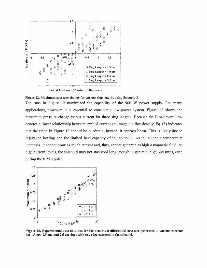
Figure 12. Maximum pressure change for various slug lengths using Solenoid B.

The runs in Figure 12 maximized the capability of the 900 W power supply. For many

applications, however, it is essential to consider a low-power system. Figure 13 shows the

maximum pressure change versus current for three slug lengths. Because the Biot-Savart Law

denotes a linear relationship between applied current and magnetic flux density, Eq. (5) indicates

that the trend in Figure 13 should be quadratic; instead, it appears linear. This is likely due to

resistance heating and the limited heat capacity of the solenoid. As the solenoid temperature

increases, it cannot draw as much current and, thus, cannot generate as high a magnetic field. At

high current levels, the solenoid may not stay cool long enough to generate high pressures, even

during the 0.25 s pulse.

1.5 -r----------------,

Iii 0.. ~ a.. <l

1.25

E 0.75 :s E ')( 0.5 n! ~

0.25 + L = 1.3 em

L = 1.9 em o L = 2.5 em

0~----~------~======~ 5 10 15

Current (A) 20

Figure 13. Experimental data obtained for the maximum differential pressure generated at various currents for 1.3 em, 1.9 em, and 2.5 em slugs with one edge centered in the solenoid.

6.3 Hydrodynamic Breakdown

Each of the data points in Figure 12 represents a run conducted in which the slug maintained its

form and remained intact. If the initial position was too far from the solenoid, the displacement

of the slug generated a pressure force greater than the magnetic force, and the slug broke down,

apparent in the data as well as physically in the experiment. Stationary experiments with a

ferro fluid by Perrt 1 verified the theoretical prediction that the pressure force could not exceed

the maximum magnetic capability of the solenoid. In Perry's case, the stationary experiments

induced a hydrostatic breakdown, whereas, in the current study, the breakdown took place during

dynamic motion and occurred slightly earlier than the static equations predicted.

With one edge of the slug centered in the solenoid and the other in a negligible field, Eq. (24)

predicted that the breakdown pressure should have been 1.95 kPa. Resistance heating in the

solenoid, however, limited the amount of current available at the time the maximum pressure

change occurred. Assuming 19.5 A of current at the peak of the curve, the breakdown pressure

should have been 1.45 kPa, which matches the experimental data much better, regardless of the

fact that it is a static prediction and does not consider fluid properties, such as surface tension,

cohesion, contact angle, and viscosity. Prediction of the hydrodynamic breakdown must also

consider the uneven force distribution along the slug, pressure differential about the slug, and

gravity, to be completely understood. The Reynolds number for the bulk slug motion remained

under 1500 for all of the runs, but a more aggressive study may have to consider slug velocity

and internal flow dynamics.

A probabilistic method to predict risk of failure should be used to predict hydrodynamic

breakdown, as it is likely due to a combination of the uneven force distribution along the slug,

pressure differential about the slug, gravity, and low surface tension of LOX. For higher-speed

tests, the rapid oscillations may also induce turbulent internal flow dynamics that cause the slug

to break down.

6. 4 Determining Uncertainty

By extracting the frequency and amplitude of the oscillations in the experimental data, the

Matlab model could be used to calculate the hidden slug length, damping factor, and precise

initial position of the slug. The authors performed detailed analyses on the uncertainties and

found a logarithmic correlation between frequency and hidden slug length and also between

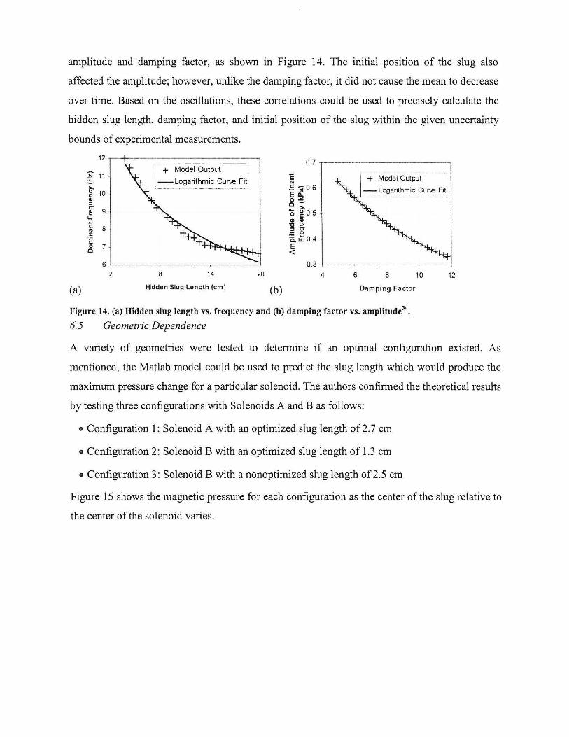
amplitude and damping factor, as shown in Figure 14. The initial position of the slug also

affected the amplitude; however, unlike the damping factor, it did not cause the mean to decrease

over time. Based on the oscillations, these correlations could be used to precisely calculate the

hidden slug length, damping factor, and initial position of the slug within the given uncertainty

bounds of experimental measurements.

(a)

'N 11 :s >. g 10 G>

"' w 9 u.

~ 6 c:: .E ~ 7

6'---------------' 2 8 14 20

Hidden Slug Length (em) (b)

0 .7 -.----------- ---,

'E ra .s -;G0.6 . Ell. 0-" c~

- ~05 0 c: . Ill II> '0 "' :::1 C' ;::: Ill a. u: 0.4 . E <1:

I +. M;t~!E~I -Output · . "]I - __ ~~~r!~.m~~-?u~-~i~J !

I l I I 0.3 +--~-------.------1

4 6 8 10 12

Damping Factor

Figure 14. (a) Hidden slug length vs. frequency and (b) damping factor vs. amplitude34•

6.5 Geometric Dependence

A variety of geometries were tested to determine if an optimal configuration existed. As

mentioned, the Matlab model could be used to predict the slug length which would produce the

maximum pressure change for a particular solenoid. The authors confirmed the theoretical results

by testing three configurations with Solenoids A and B as follows:

• Configuration 1: Solenoid A with an optimized slug length of 2. 7 em

• Configuration 2: Solenoid B with an optimized slug length of 1.3 em

• Configuration 3: Solenoid B with a nonoptimized slug length of 2.5 em

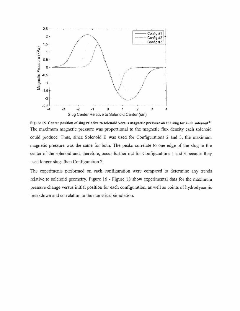
Figure 15 shows the magnetic pressure for each configuration as the center of the slug relative to

the center of the solenoid varies.

2.5 ,----.---r-----.---r-----.----;:::!:::::==::::::!::==:::::;-1

2

1.5

~ 0.5 1/l 1/l ~ 0

Q_

-~ -0.5 Q)

§, -1 !U

~ -1.5

-2

/ ='----··-···----- ----------

/

I I

I \ /-

/ I

J .

--Config#1 --- -·-· ·-·· Config #2

Config #3

.-~------------------

-2.5 '----'-----'-----'-----''-----'----'-----''------' -4 -3 -2 -1 0 2 3 4

Slug Center Relative to Solenoid Center (em)

Figure 15. Center position of slug relative to solenoid versus magnetic pressure on the slug for each solenoid35•

The maximum magnetic pressure was proportional to the magnetic flux density each solenoid

could produce. Thus, since Solenoid B was used for Configurations 2 and 3, the maximum

magnetic pressure was the same for both. The peaks correlate to one edge of the slug in the

center of the solenoid and, therefore, occur further out for Configurations 1 and 3 because they

used longer slugs than Configuration 2.

The experiments performed on each configuration were compared to determine any trends

relative to solenoid geometry. Figure 16 - Figure 18 show experimental data for the maximum

pressure change versus initial position for each configuration, as well as points of hydrodynamic

breakdown and correlation to the numerical simulation.

r- -2-,--- ---------, I

1.5 \ I ti

a.. I

~

\ I - ¢

Q) 0 Cl ~ c

"' 0.5 X ~ ~ .!:

~~ ()

~ X ::s

~ · 1/) 1/) -~ -~ ~ -2 -1 \ 2 3 ~ I X

$ ~.5 I a.. I

E I

::s I 8 -1 E I 0 Experimental Data I ')( I s 1'0 I

:E I i -1 .1_ X HydrostaticBreakdown , I

I -- Simulation L_ - ----------------

Center of Slug Relative to Solenoid (em)

Figure 16. Experimental and simulated data for the maximum pressure change in the downstream section as the initial position of the center of the slug varied for Configuration 135

•

ti a.. e. Q) Cl c

"' J: ()

~ ::s 1/)

~-.... 5 -10

a..

I E ::s I E ')(

l "' :E

1.5

)( -5 0 ls X

El -1 0

-1 .5

0

0

X

5 10

o Experimental Data

x Hydrostatic Breakdown

-- Numerical Simulation

Center of Slug Relative to Solenoid (mm)

1

Figure 17. Experimental and simulated data for the maximum pressure change in the downstream section as the initial position of the center of the slug varied for Configuration 235

•

r----··---· ,:r I

I - I CIS I

j Q. l

~

! Q)

Cl I c: I CIS .c: I * (.) I Q) ... :;, fl)

)( X >51.~ fl) 1.5 25 Q) ... * -0 .5 Q.

E X :;, X E -1

D. Experimental Data ')( CIS D. X Hydrostatic Breakdown :E -1 .5

--Numerical Simulation

Center of Slug Relative to Center of Solenoid (em)

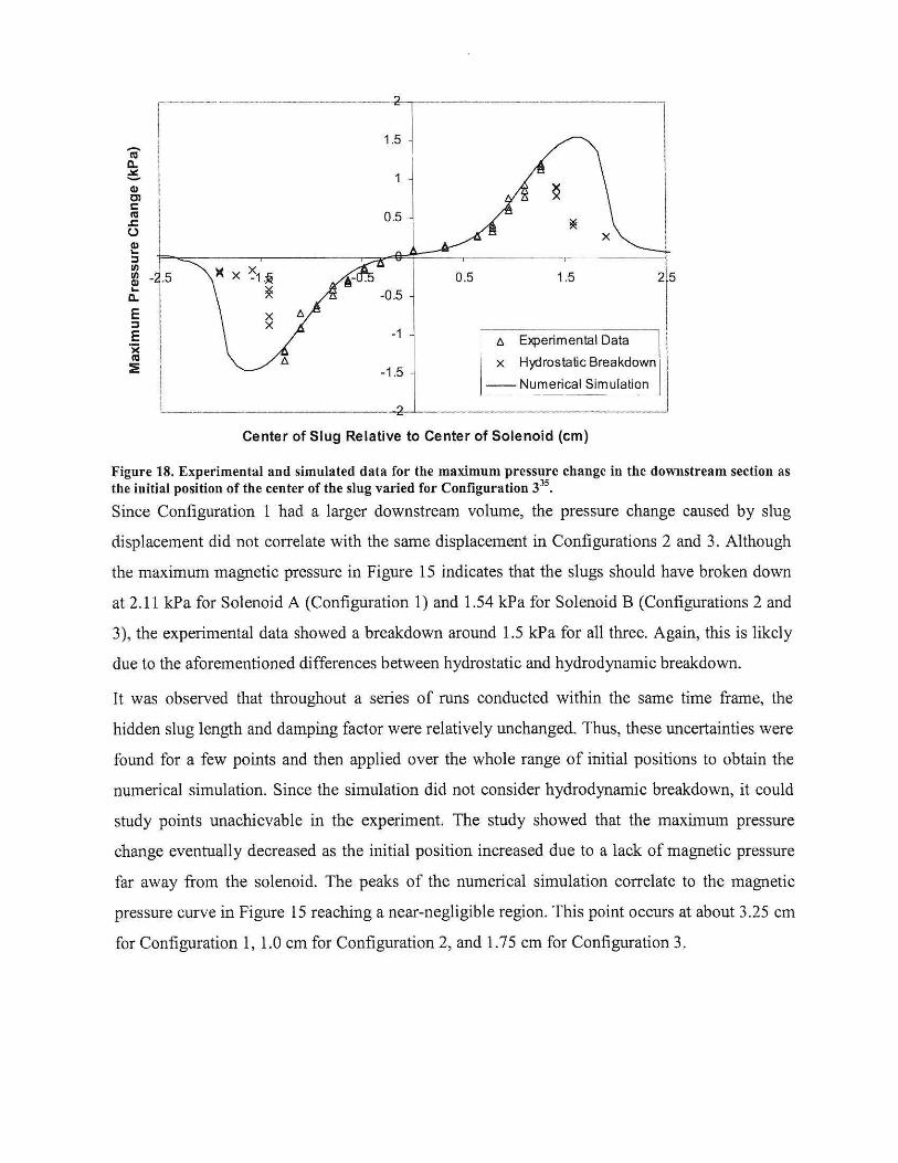
Figure 18. Experimental and simulated data for the maximum pressure change in the downstream section as the initial position of the center of the slug varied for Configuration 335

•

Since Configuration 1 had a larger downstream volume, the pressure change caused by slug

displacement did not correlate with the same displacement in Configurations 2 and 3. Although

the maximum magnetic pressure in Figure 15 indicates that the slugs should have broken down

at 2.11 kPa for Solenoid A (Configuration 1) and 1.54 kPa for Solenoid B (Configurations 2 and

3), the experimental data showed a breakdown around 1.5 kPa for all three. Again, this is likely

due to the aforementioned differences between hydrostatic and hydrodynamic breakdown.

It was observed that throughout a series of runs conducted within the same time frame, the

hidden slug length and damping factor were relatively unchanged. Thus, these uncertainties were

found for a few points and then applied over the whole range of initial positions to obtain the

numerical simulation. Since the simulation did not consider hydrodynamic breakdown, it could

study points unachievable in the experiment. The study showed that the maximum pressure

change eventually decreased as the initial position increased due to a lack of magnetic pressure

far away from the solenoid. The peaks of the numerical simulation correlate to the magnetic

pressure curve in Figure 15 reaching a near-negligible region. This point occurs at about 3.25 em

for Configuration 1, 1.0 em for Configuration 2, and 1.75 em for Configuration 3.

To apply the studies to other geometries, the findings must be nondimensionalized. Using Eq.

(1 1) and (14), the nondimensional maximum displacement and initial magnetic pressure were

seen to have a common trend, as seen in Figure 19.

.... 9915 1 ~ 8 r:::: (1)

E $J (1) (J

res 0.01

Q. i~<>c .!!! c 0.005 ti E a§~ ~ ::l 0 E t,.lll .><

" res ~·~16 ~j ~ -0. 04 -0.003 -0.002 0.001 0.002 0.003 0. 04

iV •lJ r::::

0 -0.005 Ill j fl. r:::: (1)

<>Config #1 E • <> c -0.01 D Config#2

I

r:::: $<> ¢ ll.Config #3 0 z 0

""'"

Non-Dimensional Initial Magnetic Pressure

Figure 19. Nondimensional maximum displacement versus nondimensional initial magnetic pressure35•

Each of the configurations held a nearly linear relationship regardless of their differences in

overall size. The average slope of a linear fit of the three data sets was 2.3 8 and could be applied

to other geometries with similar physical phenomena. For the current study, the capillary and

gravity forces were negligible compared to the pressure, damping, and magnetic forces; thus, the

results found could only be applied to systems of the same scale. Furthermore, a different

paramagnetic fluid would have a different susceptibility and fluid properties, resulting in a

different slope as well. Nonetheless, the correlation found is useful as a guideline during the

preliminary design state of a magnetic fluid actuator.

Each configuration used the same power source and generated approximately the same pressure

change. Treating the pressure change as an indicator of work performed by the fluid would entail

approximately the same output per power input for each configuration. However, since fluid

damping is detrimental to performance, it could be seen as a form of exergy destruction. Exergy

is the potential work of a system and is used to determine its second law efficiency. High

damping of the fluid reduces the potential work and, therefore, should be factored into a measure

of the system' s second law efficiency. This measure can be found through a nondimensional

number known as the Mason number, the ratio of damping to magnetic forces, and is shown in

Eq (30). Figure 20 shows P m.i versus ui for the three configurations. The slope of the linear trend

line for each set of data provides an important characteristic of each combination, as it is a

component of the Mason number. A lower Mason number indicates a more efficient system,

since less damping would exist for a given magnetic force (achievable through power input).

While it seems counterintuitive that a slower average initial velocity would imply a more

efficient system, Solenoid A was nearly 4 times longer than Solenoid B; thus, the magnitude of

velocity was relative. Instead, the Mason number is representative of exergy destruction and

should, ideally, be as low as possible.

~

..!!! E ~ >. ;t! (.)

.Q Ql -> Ill :E .E

(a)

~

..!!! E ~

"" - ----, s

20 .. 8 -~ ... ·a· g

" .o- ·

o.··· 0.5 1.5 2 .5 -~ ..--o.5

~~ .~· . . -20 I y = 1 0.923x - 0.31921 • <>

8 R2 = 0.9425

""

5

Initial Magnetic Pressure (kPa)

-1 ...

•; i

.-:·

-4

0

y = 4.0989x - 0.1066 R2 = 0.9817

(b) Initial Magnetic Pressure (kPa)

I 1-2-------

~ 6 .·6·· ··~

" ~,t,.A·~ ·

2 ~ · t{~ 1 -1 .

~-· .·~·· -6 y = 5.581 3x + 0.1124 6' R2 = 0.9822

1')

(c) Initial Magnetic Pressure (kPa)

Figure 20. Average initial velocity versus initial magnetic pressure for (a) Configuration 1, (b) 2, and (c) 335•

The near-linearity of the trend lines indicates that the Mason number is consistent for each

configuration. This implies that with a given slug length and profile of the magnetic flux density

along the axis of the solenoid, u i can be calculated through a proportionality constant of Pm.i·

When Eq. (9) is calculated for each run, the average Mason number for each configuration can

be found as shown in Table 2, assuming each configuration has an average damping factor of 6

and hidden slug length of 13 em.

Table 2, Average Mason number

Con fig. #of Runs Avg. Mason# Std. Dev.

1 41 0.247 6.62 * 1 o-2

2 26 0.091 2.03 * 10-2

3 37 0.143 3.54 * to-2

The correlations in Table 2 reveal two methods for improving system efficiency through

geometric measures. By optimizing the slug length for a solenoid and by minimizing the overall

geometry, damping can be lessened for a given magnetic force. While this seems particularly

beneficial for applications with MEMS technology, it is important to remember that capillarity

has not been introduced to the system. Nonetheless, the experiments and analyses performed

have verified the theoretical model and are therefore useful to future research and applications.

7. Conclusions The case for a LOX-based magnetic fluid system to replace mechanically moving parts in a

satellite system has been argued. The experiment alone satisfied the first two objectives by

confirming the potential of a LOX-based magnetic fluid system through innovative measuring

techniques. The experiment and numerical simulation also verified the theoretical model, thus

satisfying the third objective. The fourth objective was satisfied through the parametric studies

which examined the maximum pressure change attainable, effect of uncertainty, and geometric

variance. Accomplishing the objectives aided the overall goals by establishing the following

conclusions:

• an optimal slug size for a specific geometry exists that maximizes the attainable pressure

change for a given power source;

• a low-power system may perform more efficiently due to less resistance heating in the

solenoid;

• unknown portions of LOX in the fluid system and undetermined physical phenomena can be

empirically calculated through the theoretical model;

• an optimized slug and solenoid configuration will result in a more efficient system in terms

of work performed by the fluid with a minimal amount of damping;

• reducing the physical scale of the experiment increases its efficiency, as long as capillarity is

still negligible.

The conclusions of this research support the overall goals in aiding the design of a LOX-based

magnetic fluid system with no moving parts for small satellite applications.

8. References [1] Rosensweig R. E., Ferrohydrodynamics, Dover, New York, 1985.

[2] Park G. S., Seo K., "A Study on the Pumping Forces of the Magnetic Fluid Linear Pump," IEEE Transactions

on Magnetics, Vol. 39, No.3, 2003, pp. 1468-1471.

[3] Park G. S., Seo K., "New Design of the Magnetic Fluid Linear Pump to Reduce the Discontinuities of the

Pumping Forces," IEEE Transactions on Magnetics, Vol. 40, No.2, 2004, pp. 916-919.

[4] Seo K., Park G. S., "A Research on the Pumping Forces in the Magnetic Fluid Linear Pump," IEEE

Transactions on Magnetics , Vol. 41 , No. 5, 2005, pp. 1580-1583.

[5] Hatch A., Kamholz A. E., Holman G., Yager P., Bohringer K. F., "A Ferrofluidic Magnetic Micropump,"

Journal ofMicroelectromechanical Systems, Vol. 10,2001 , pp. 215-221.

[6] Moghadam M. E., Shafii M. B., Dehkordi E. A, "Hydromagnetic Micropump and Flow Controller. Part A:

Experiments with Nickel Particles Added to the Water," Experimental and Thermal Fluid Science, Vol. 33,

No.6, 2009, pp. 1021-1028.

[7] Krauss R., Liu M., Reimann B., Richter R. , Rehberg 1., "Pumping Fluid by Magnetic Surface Stress," New

Journal of Physics, Vol. 8, No. 18, 2006, pp. 1-11.

[8] Goldstein S. R., "Magnetic Fluid Actuated Control Valve, Relief Valve and Pump," U.S. Patent 4053952,

1977.

(9] Kamiyama S., "A Magnetic Fluid Actuator," Advanced Robotics, Vol. 1, No. 2, 1986, pp. 177-185.

[10] Ming Z., Zhongliang L., Guoyuan M., Shuiyuan C., "The Experimental Study on Flat Plate Heat Pipe of

Magnetic Working Fluid," Experimental and Thermal Fluid Science, Vol. 33, No.7, 2009, pp. 1100-1105.

(11 ] Jeyadevan B., Koganezawa H., Nakatsuka K., "Performance Evaluation of Citric Ion-Stabilized Magnetic

Fluid Heat Pipe," Journal of Magnetism and Magnetic Materials, Vol. 289, 2005, pp. 253-256.

[12] Liao W., Chen X., Chen Y. , PuS., Xia Y., Li Q., 'Tunable Optical Fibers with Magnetic Fluids," Applied

Physics Letters, Vol. 87, 2005, pp. 1-3.

[13] Celik D., Van Sciver, S. W., "Dielectric Coefficient and Density of Subcooled Liquid Oxygen," Cryogenics,

Vol. 45,2005, pp. 356-361.

[14] Hilton D. K., Van Sciver S. W., "Absolute Dynamic Viscosity Measurements of Subcooled Liquid Oxygen

from 0.15 MPa to 1.0 MPa," Cryogenics, Vol. 48, 2008, pp. 56-60.

[1 5] Lide D.R. (ed.), CRC Handbook of Chemistry and Physics, 89th Edition, CRC Pressfraylor and Francis, Boca

Raton, 2009.

[16] Takeda, M., and Nishigaki, K. , "Measurements of the Surface Tension of Liquid Oxygen in High Magnetic

Fields," Journal of the Physical Society of Japan , Vol. 61, No. 10, 1992, pp. 3631-3635.

[17] Catherall A. T., Benedict K. A., King P. J. , Eaves L., "Surface Instabilities on Liquid Oxygen m an

Inhomogeneous Magnetic Field," Physical Review E, Vol. 68,2003, pp. 1-3.

[18] Catherall A. T., L6pez-Aicaraz P., Benedict K. A., King P. J., Eaves L., "Cryogenically Enhanced Magneto­

Archimedes Levitation," New Journal o.f Physics, Vol. 7, No. 118, 2005, pp. 1-10.

[19] Hilton, D. K. , Celik, D., and VanSciver, S. W., "Subcooled Liquid Oxygen Cryostat for Magneto-Archimedes

Particle Separation by Density," Advances in Cryogenic Engineering, CP985, Vol. 53, AlP, 2008, pp. 1517-

1522.

(20] Yerkes, K. L., "Use ofMagnetic Fields to Augment Wicking of Oxygen Heat Pipes," Topics in Heat Transfer

HTD-ASME, Vol. 3, 1992, pp. 115-120.

[21] Youngquist R. C., Immer C. D., Lane J. E., Simpson J. C., "Dynamics of a Finite Liquid Oxygen Column in a

Pulsed Magnetic F ield," IEEE Transactions on Magnetics, Vol. 39, No.4, 2003, pp. 2068-2073.

[22] Zahn M., Greer D. R., "Ferrohydrodynamic Pumping in Spatially Uniform Sinusoidally Time-Varying

Magnetic Fields," Journal of Magnetism and Magnetic Materials, Vol. 149, 1995, pp. 165-173.

[23] Mao L., Koser H., "Ferrohydrodynamic Pumping in Spatially Traveling Sinusoidally Time-Varying Magnetic

Fields," Journal of Magnetism and Magnetic Materials, Vol. 289,2005, pp. 1999-2002.

[24] Shliomis, M. 1., "Effective Viscosity of Magnetic Suspensions," Soviet Journal of Experimental and

Theoretical Physics, Vol. 34, No.6, 1972, pp. 1291-1294.

[25] McTague, J.P., "Magnetoviscosity of Magnetic Colloids," Journal of Chemical Physics, Vol. 51, No. I, 1969,

pp. 133-136.

[26] Bacri, J. C., Perzynski, R. , and Shliomis, M. I., "Negative-Viscosity Effect in a Magnetic Fluid," Physical

ReviewLetters, Vol. 75,No. 11 , 1995,pp.2128-2 131.

[27] Cunha, F. R., and Sobral, Y. D., "Asymptotic Solution for Pressure-Driven Flows of Magnetic Fluids in

Pipes," Journal of Magnetism and Magnetic Materials, Vol. 289, pp. 314-317.

(28] Chen C. Y., Hong C. Y., Wang S. W., "Magnetic Flows in a Tube with the Effects of Viscosity Variation,"

Journal of Magnetism and Magnetic Materials, Vol. 252,2002, pp. 253-255.

[29] Schlicting, H. Boundmy-Layer Theory, 71h ed., McGraw-Hill, New York, 1979, pp. 436-438.

(30] White F. M., Viscous Fluid Flow, McGraw-Hill, New York, 1991 , pp. 116-118.

[31] Perry M. P., Jones T. B., "Hydrostatic Loading of Magnetic Liquid Seals," IEEE Transactions on Magnetics,

Vol. MAG-12, No.6, 1976, pp. 798-800.

[32] Bashtovoi V., Kuzhir P., Reks A., "Capillary Ascension of Magnetic Fluids," Journal of Magnetism and

Magnetic Materials, Vol. 252 , 2002, pp. 265-267.

[33] Boulware, J. C., Ban, H., Jensen, S., and Wassom, S., "Experimental Studies of the Pressures Generated by a

Liquid Oxygen Slug in a Magnetic Field," J Magn Magn Mater., Vol. 322,2010, pp. 1752-1757.

[34] Boulware, J. C., Ban, H., Jensen, S., and Wassom, S., "Modeling of the Dynamics of a Slug of Liquid Oxygen

in a Magnetic Field and Experimental Verification," Cryogenics, 2010, doi:10.1016/j.cryogenics.2010.03.004.

[35] Boulware, J. C., Ban, H., Jensen, S., and Wassom, S., "Geometric Influence on Liquid Oxygen

Magnetohydrodynamics," Article in Press, accepted for publication in Exp Therm Fluid Sci.