Liouville Equation-Based Stochastic Model for Shoreline Evolution

Liouville Equation-Based Stochastic Model for Shoreline 1 Evolution 2

Xing Zheng Wu1∗, Ping Dong2 3 1 Department of Applied Mathematics, School of Applied Science, University of Science and Technology Beijing, 30 Xueyuan Road, Haidan District, 4 Beijing, P. R. China. Post code: 100083. 5 2 Division of Civil Engineering, School of Engineering, Physics and Mathematics, University of Dundee, Dundee DD1 4HN, United Kingdom 6

Abstract 7

Long-term shoreline evolution due to longshore sediment transport is one of the key processes 8 that need to be addressed in coastal engineering design and management. To adequately represent 9 the inherent stochastic nature of the evolution processes, a probability density evolution model 10 based on the Liouville equation is proposed for predicting the shoreline changes. In this model, the 11 standard one-line beach evolution model that is widely used in coastal engineering design is 12 reformulated in terms of the probability density function of shoreline responses. A computational 13 algorithm involving a total variation diminishing scheme is employed to solve the resulting 14 equation. To check the accuracy and robustness of the model, the predictions of the model are 15 evaluated by comparing them with those from Monte Carlo simulations for two idealised shoreline 16 configurations involving a single long jetty perpendicular to a straight shoreline and a rectangular 17 beach nourishment case. The pertinent features of the predicted probabilistic shoreline responses are 18 identified and discussed. The influence of the density distributions of the input parameters on the 19 computed results is investigated. 20

Keywords: Shoreline evolution; Liouville equation; Probability density function; Total variation 21 diminishing 22

∗ Corresponding author. Tel.: +86 18611869118; Fax: +86 1082610539. E-mail address: [email protected]

1

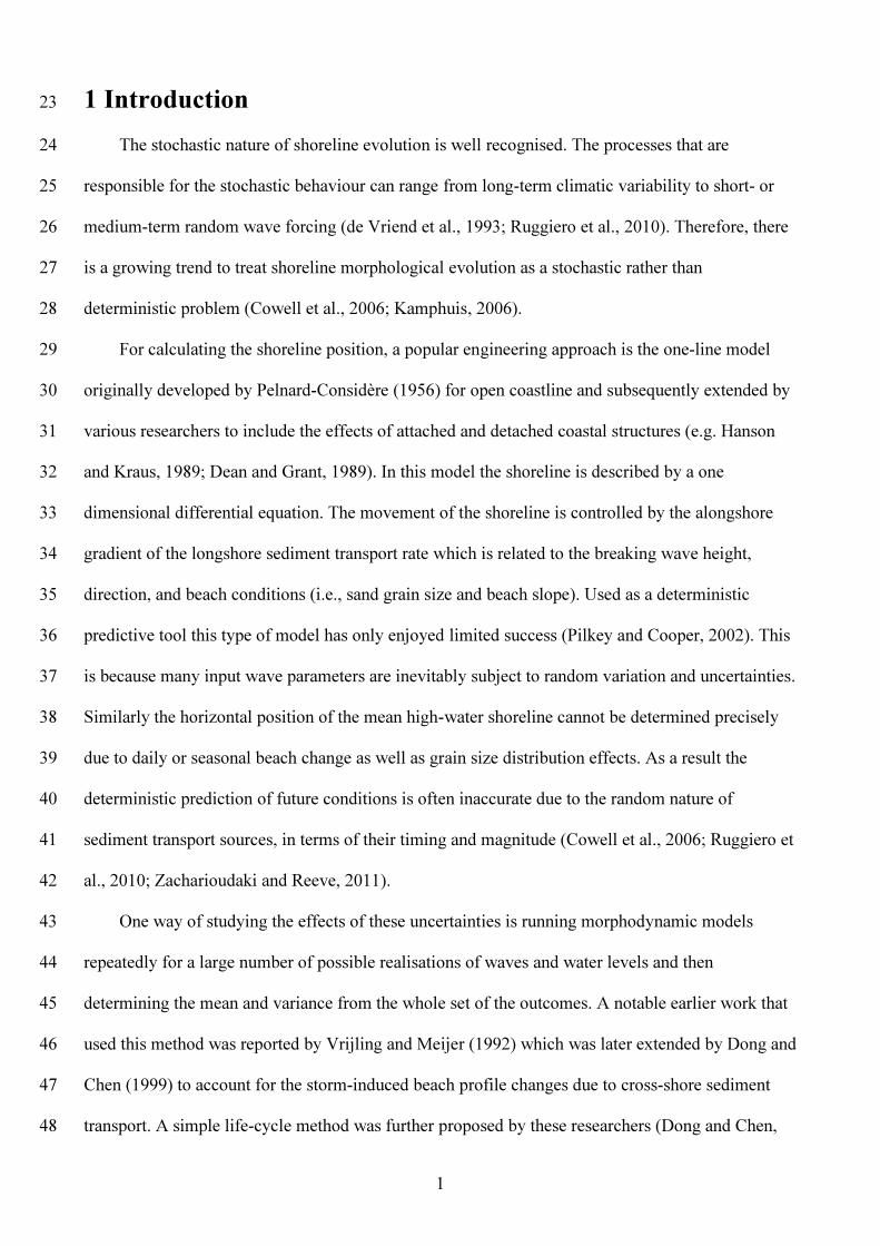
1 Introduction 23

The stochastic nature of shoreline evolution is well recognised. The processes that are 24 responsible for the stochastic behaviour can range from long-term climatic variability to short- or 25 medium-term random wave forcing (de Vriend et al., 1993; Ruggiero et al., 2010). Therefore, there 26 is a growing trend to treat shoreline morphological evolution as a stochastic rather than 27 deterministic problem (Cowell et al., 2006; Kamphuis, 2006). 28

For calculating the shoreline position, a popular engineering approach is the one-line model 29 originally developed by Pelnard-Considère (1956) for open coastline and subsequently extended by 30 various researchers to include the effects of attached and detached coastal structures (e.g. Hanson 31 and Kraus, 1989; Dean and Grant, 1989). In this model the shoreline is described by a one 32 dimensional differential equation. The movement of the shoreline is controlled by the alongshore 33 gradient of the longshore sediment transport rate which is related to the breaking wave height, 34 direction, and beach conditions (i.e., sand grain size and beach slope). Used as a deterministic 35 predictive tool this type of model has only enjoyed limited success (Pilkey and Cooper, 2002). This 36 is because many input wave parameters are inevitably subject to random variation and uncertainties. 37 Similarly the horizontal position of the mean high-water shoreline cannot be determined precisely 38 due to daily or seasonal beach change as well as grain size distribution effects. As a result the 39 deterministic prediction of future conditions is often inaccurate due to the random nature of 40 sediment transport sources, in terms of their timing and magnitude (Cowell et al., 2006; Ruggiero et 41 al., 2010; Zacharioudaki and Reeve, 2011). 42

One way of studying the effects of these uncertainties is running morphodynamic models 43 repeatedly for a large number of possible realisations of waves and water levels and then 44 determining the mean and variance from the whole set of the outcomes. A notable earlier work that 45 used this method was reported by Vrijling and Meijer (1992) which was later extended by Dong and 46 Chen (1999) to account for the storm-induced beach profile changes due to cross-shore sediment 47 transport. A simple life-cycle method was further proposed by these researchers (Dong and Chen, 48

2

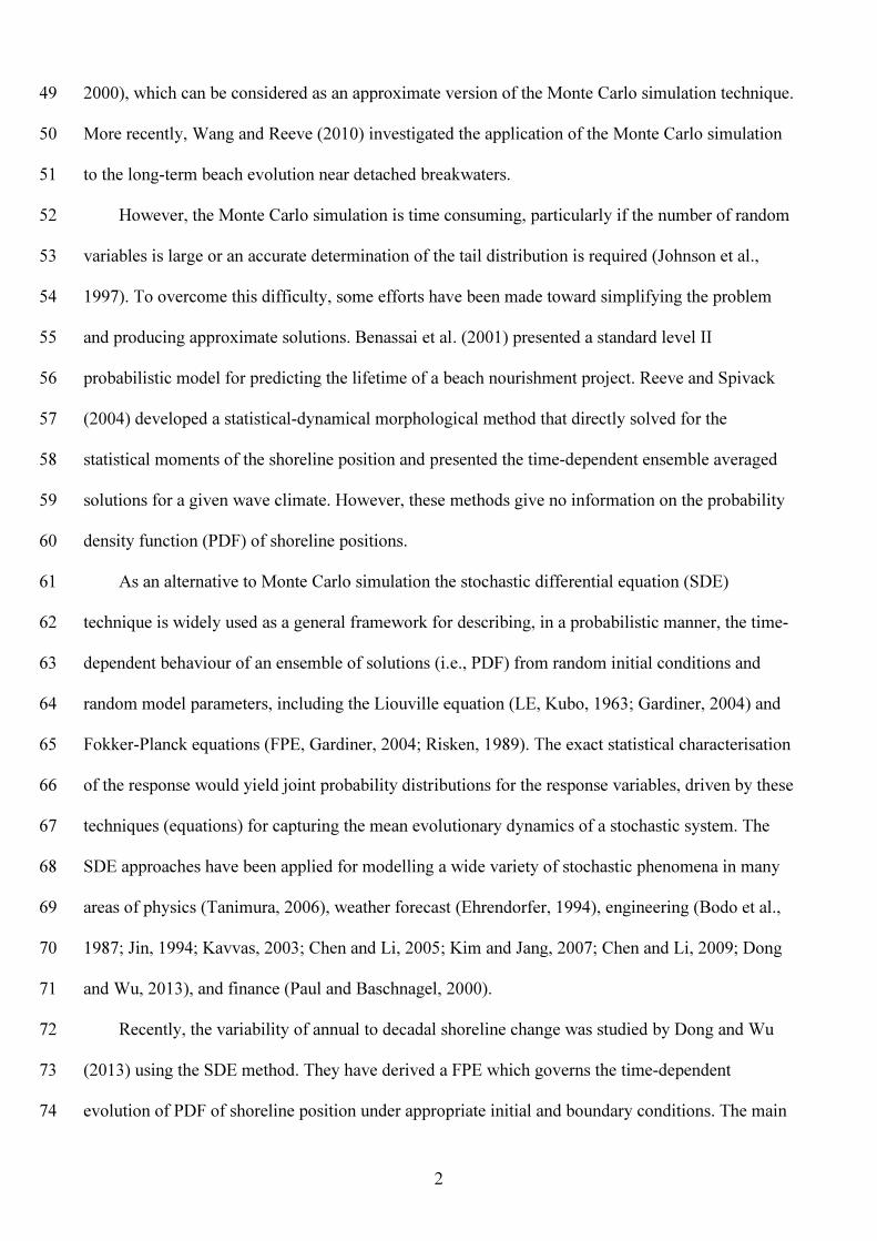
2000), which can be considered as an approximate version of the Monte Carlo simulation technique. 49 More recently, Wang and Reeve (2010) investigated the application of the Monte Carlo simulation 50 to the long-term beach evolution near detached breakwaters. 51

However, the Monte Carlo simulation is time consuming, particularly if the number of random 52 variables is large or an accurate determination of the tail distribution is required (Johnson et al., 53 1997). To overcome this difficulty, some efforts have been made toward simplifying the problem 54 and producing approximate solutions. Benassai et al. (2001) presented a standard level II 55 probabilistic model for predicting the lifetime of a beach nourishment project. Reeve and Spivack 56 (2004) developed a statistical-dynamical morphological method that directly solved for the 57 statistical moments of the shoreline position and presented the time-dependent ensemble averaged 58 solutions for a given wave climate. However, these methods give no information on the probability 59 density function (PDF) of shoreline positions. 60

As an alternative to Monte Carlo simulation the stochastic differential equation (SDE) 61 technique is widely used as a general framework for describing, in a probabilistic manner, the time-62 dependent behaviour of an ensemble of solutions (i.e., PDF) from random initial conditions and 63 random model parameters, including the Liouville equation (LE, Kubo, 1963; Gardiner, 2004) and 64 Fokker-Planck equations (FPE, Gardiner, 2004; Risken, 1989). The exact statistical characterisation 65 of the response would yield joint probability distributions for the response variables, driven by these 66 techniques (equations) for capturing the mean evolutionary dynamics of a stochastic system. The 67 SDE approaches have been applied for modelling a wide variety of stochastic phenomena in many 68 areas of physics (Tanimura, 2006), weather forecast (Ehrendorfer, 1994), engineering (Bodo et al., 69 1987; Jin, 1994; Kavvas, 2003; Chen and Li, 2005; Kim and Jang, 2007; Chen and Li, 2009; Dong 70 and Wu, 2013), and finance (Paul and Baschnagel, 2000). 71

Recently, the variability of annual to decadal shoreline change was studied by Dong and Wu 72 (2013) using the SDE method. They have derived a FPE which governs the time-dependent 73 evolution of PDF of shoreline position under appropriate initial and boundary conditions. The main 74

3

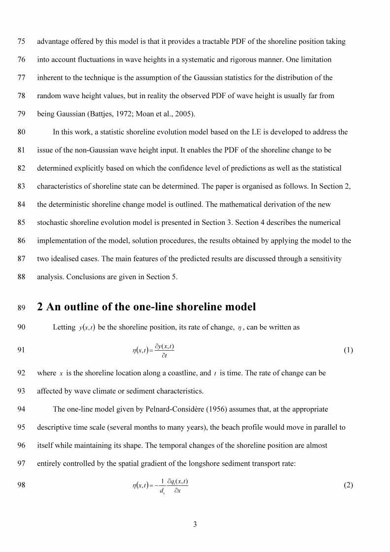
advantage offered by this model is that it provides a tractable PDF of the shoreline position taking 75 into account fluctuations in wave heights in a systematic and rigorous manner. One limitation 76 inherent to the technique is the assumption of the Gaussian statistics for the distribution of the 77 random wave height values, but in reality the observed PDF of wave height is usually far from 78 being Gaussian (Battjes, 1972; Moan et al., 2005). 79

In this work, a statistic shoreline evolution model based on the LE is developed to address the 80 issue of the non-Gaussian wave height input. It enables the PDF of the shoreline change to be 81 determined explicitly based on which the confidence level of predictions as well as the statistical 82 characteristics of shoreline state can be determined. The paper is organised as follows. In Section 2, 83 the deterministic shoreline change model is outlined. The mathematical derivation of the new 84 stochastic shoreline evolution model is presented in Section 3. Section 4 describes the numerical 85 implementation of the model, solution procedures, the results obtained by applying the model to the 86 two idealised cases. The main features of the predicted results are discussed through a sensitivity 87 analysis. Conclusions are given in Section 5. 88

2 An outline of the one-line shoreline model 89

Letting ( )txy , be the shoreline position, its rate of change, η , can be written as 90

( ) ttxytx

∂∂= ),(,η (1) 91

where x is the shoreline location along a coastline, and t is time. The rate of change can be 92 affected by wave climate or sediment characteristics. 93

The one-line model given by Pelnard-Considère (1956) assumes that, at the appropriate 94 descriptive time scale (several months to many years), the beach profile would move in parallel to 95 itself while maintaining its shape. The temporal changes of the shoreline position are almost 96 entirely controlled by the spatial gradient of the longshore sediment transport rate: 97

( ) xtxq

dtx∂

∂−= ),(1, l

c

η (2) 98

4

where lq is the alongshore sediment transport rate, and cd is the depth of closure representing the 99

seaward edge of the moving beach profile and is usually assumed as a constant for a given time 100 scale of analysis. The commonly-used predictive formula for lq takes the form of 101

[ ]),(2sin),(),( bl0l txtxqtxq α= (3) 102

where l0q is the amplitude of the alongshore transport rate, and bα is the breaking wave angle to the 103

local shoreline. For a fixed coordinate system with x defined broadly along the coastline and y 104

perpendicular to x , bα is given by 105

∂

∂−= xyxytxtx ),(arctan),(),( 0b αα (4) 106

where 0α is the incident breaking wave angle relative to x . In general, the variables l0q , 0α , and bα 107

all vary in time and along x . For a constant 0α , bα is only dependent on the local configuration of 108

the evolving shoreline. 109 For prediction purposes, an expression for l0q in terms of wave parameters and sediment 110

properties is required, and one of the most widely used expressions is the CERC formula developed 111 by the US Army Corps of Engineers (1984): 112

1gbbl0 )( aCEq = (5) 113

where 1a is a constant given by gnka )1)((2 sws

11 −−=

ρρ; bE and gbC are the wave energy and group 114

velocity evaluated at the breaking point, respectively; sρ is the density of the sand; wρ is the density 115

of water; sn is the void ratio of the sediments; and 1k is an empirical constant, commonly referred to 116

as the longshore sediment transport coefficient. The linear shallow water wave approximation gives 117

2bwb 8

1 ghE ρ= , in which g is the gravitational acceleration and bgb gdC = . Further assuming bb dh γ≈ , 118

where bd is the breaker depth and γ is the constant breaker index, Eq. (5) becomes 119

= −

12/12/3

w2/5

bl0 81 aghq γρ (6) 120

5

From Eqs. (2) and (6), it is clear that apart from the constant parameters 1k and cd , the 121

shoreline change rate is only dependent on the breaking wave parameters ( bh and 0α ) and shoreline 122

orientation. Both bh and 0α can be calculated from the offshore wave height, period, and angle 123

using an appropriate wave transformation model (Booij et al. 1999; Ris et al., 1999). Under certain 124 simplifying conditions, such as small angle of wave incidence, the one-line equation can be further 125

reduced to a simple diffusion equation in terms of the shoreline position y (Larson et al., 1997), 126

which was used as the basis for the stochastic shoreline evolution model by Reeve and Spivack 127 (2004). 128

3 Stochastic shoreline evolution model 129

Assuming that the evolutionary rate η is within a collection of admissible change rates η , the 130

stochastic shoreline evolution can be determined by running the deterministic one-line model using 131 a large number of randomly sampled hydrodynamic variables and model parameters as the inputs. 132 Both the true randomness and model uncertainties can be accounted for including random wave 133 parameters (breaking wave height, period, and angle) and uncertainties in the model parameters 134 (sediment transport coefficient 1k and closure depth cd ). Also can be included in this prediction 135

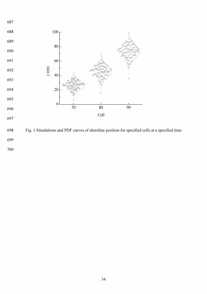
framework are the uncertainties in the boundary conditions and initial shoreline position both of 136 which could be subject to random short-term variations. The predicted admissible shoreline position 137 changes from a large number of random inputs will form a bundle of possible trajectories, as 138 depicted by the scattered points of a specified cell in Fig. 1. The statistical properties, including 139 mean and standard deviation, as well as PDF, can be calculated, as illustrated in Fig. 1. This Monte 140 Carlo sampling method is computationally demanding, especially when the number of input 141 parameters is large. The purpose of adopting a SDE approach is to determine directly and more 142 efficiently the PDF of the shoreline position at anytime and location alongshore. 143

As mentioned above, from a long-term perspective, the morphological response to storms is 144 analogous to ‘noise’ about the long-term trend, caused by the fluctuating morphological forces of 145

6

the waves, tides, and surges (Camfield and Morang, 1996; Medellín et al., 2008; Ruggiero et al., 146 2010). To account for the uncertainties caused by the short-term variations in either bed levels or 147 water levels in extracting the initial shoreline position from chart or survey data, the initial shoreline 148

position 0y is treated as a random variable (Ruggiero et al., 2003; Wang and Reeve, 2010).The 149

evolutionary shoreline position can thus be written in the form of differential equations with random 150 initial conditions (Soong, 1973; Gardiner, 2004): 151

==

0

b

)0,(),,(d

),(d

YxY

HxYttxY η (7) 152

where η is an operator of the stochastic shoreline position evolving in time subject to breaking 153

wave action and for a prescribed random initial shoreline position 0Y . Clearly the shoreline position 154

Y is now a stochastic process. It can be recognised that the dynamic system with the deterministic 155 operator η and random initial conditions is a probability preservative system. The reader should 156

consult Arimitsu (2009) and Chen and Li (2009) for more information on the principle of 157 probability preservation. 158

Substituting the one-line alongshore transport model into Eq. (7) yields 159

),,(d),(d 2/5

b txYHttxY ζ−= (8) 160

where ),,( txYζ is given by xdagtxY ∂∂= −

)2sin(181),,( b

c1

2/12/3w

αγρζ . 161

In the CERC formula, the wave breaking induced alongshore sediment transport rate is related 162 to wave height and direction and the relative angle of the shoreline at the point of breaking. To 163 obtain a simple LE-based model containing the least number of random variables, the empirical 164 coefficient 1k and the closure depth cd are treated as constants. To simplify the model further, the 165

incident wave angle 0α is also taken as a constant so that the alongshore transport rate is only 166

dependent on one random variable, i.e., the breaking wave height bH . 167

7

Following Soong (1973) and Gardiner (2004), by transferring the random coefficient (external 168 force, which is specified here as the breaking wave height) to a random initial condition Eq. (7) can 169 be recast in the following augmented form: 170

==

0

b

)0,(),,(d

),(d

ZxZ

HxYBttxZ

(9) 171

where 172

=b

),(),( HtxYtxZ ;

=0η

B ;

=b

00 H

YZ (10) 173

and ),,(),( 2/5b txyHty ζη −= . 174

Assuming that the joint PDF of 0Y and bH is known, the differential equation of the joint PDF 175

of Y and bH , ),,( bbthypYH , becomes a stochastic Liouville type equation (Soong, 1973; Gardiner, 176

2004; Dostupov and Pugachev, 1957; Syski, 1967): 177

0)],,(),([),,( bb bb =∂∂+∂

∂y

thyptyt

thyp YHYH η (11) 178

The probability density flow does not have any source terms, which means 0),( =∂

∂ytyη for any 179

specified bh (Shvidler and Karasaki, 2003; Chen and Li, 2005, 2009). Eq. (11) can be further 180

simplified as a one-dimensional advection equation by substituting the expression 181

),,(),( 2/5b txyHty ζη −= (Shvidler and Karasaki, 2003; Chen and Li, 2005; Li and Chen, 2008): 182

0),,(),(),,( bb

b bb =∂∂+∂

∂y

thypthYtthyp YHYH & (12) 183

where ),,(),( 2/5bb txyHthY ζ−=& is the ‘velocity’ of the response for a prescribed bh , called the 184

advection velocity coefficient. It represents the speed at which the PDF of a random shoreline 185 position moves alongshore. The initial condition required to solve Eq. (12) for ),,( bb

thypYH is the 186

joint PDF of bH and 0Y . It should be noted that the solution to Eq. (4) depends on both x and t , 187

that is, the PDF of the shoreline position will be a function of both time and position along the shore. 188 In essence, Eq. (12) is a conservative equation, which implies the principle of preservation of 189

8

probability, i.e., the total increment of probability in the state space is equal to the net ‘imported’ 190 probability transited through the boundary of the domain, as noticed by Chen and Li (2005). The 191 time-dependent PDF of a stochastic process is solved by imposing certain restrictions, such as the 192 non-negativity of the density function over the domain of the state variable and the normalisation 193 condition. 194

Upon solving Eq. (12), the PDF of Y is obtained by 195

∫Ω

=Z

z,ty,hptyp YHY d)(),( bb (13) 196

where ZΩ is the distribution domain of Z . The time dependent mean and standard deviation of Y 197

can then be obtained instead of a single deterministic value by 198

∫= max

min

d)(),(m

y

y Y yy,typtxy (14) 199

( )∫ −=max

min

d)(),( 2s

y

y Ym yy,tpyytxy (15) 200

where maxy and miny are the prescribe upper and lower limits of Y , respectively. 201

Supposing bH and 0Y are statistically independent (although this model is also valid for the 202

measured bH and 0Y which are dependent), the joint probability can be calculated from the marginal 203

PDFs of bH and 0Y : 204

0bb for),()(),,(bb

tthpypthyp HYYH == (16) 205

For a particular site, the joint or marginal distributions of the characteristic wave parameters 206 can be obtained in discrete form either from the measurements or from hindcast waves based on 207 wind data. Some distribution types have previously been applied to wave height: log-normal 208 distribution (Jasper, 1956; Guedes Soares and Viana, 1988; Moan et al., 2005), Weibull distribution 209 (Battjes, 1972; Guedes Soares and Henriques, 1996), and normal distribution (Kamphuis, 1999). 210

In the case of independent normal distributions, the initial joint PDF of 0Y and bH becomes 211

),(),()0;,( bbbs00m0b0bDKhNyyyNhypYH = (17) 212

9

where 2s0

2m0 2/)(

2s0

s00m0 21),( yyyey

yyyN −−

=

π and 2

b2

bb 2/)(2

bbbb 2

1),( DKheD

DKhN −−

=

π. 0my and s0y are the mean 213

and standard deviation of 0Y . bK and bD are the mean and standard deviation of bH . The time 214

dependent mean ),(m

txy and standard deviation ),(s txy of Y can be integrated by Eqs. (14) and Eq. 215

(15), respectively. It should be pointed out that the initial shoreline position is usually affected by 216 and thus correlated with the short-term wave and the sediment transport changes. However, over the 217 longer time scale storm-induced beach deformation is transient and its effects are often smoothened 218 out. Therefore, for the prediction of the long-term shoreline evolution, the assumption of statistical 219 independence is appropriate. 220

To ensure that the wave height is always positive, a truncated wave height distribution with the 221 height ranged from zero to a prescribed limit maxbH is used in the numerical simulations. The 222

parameters determining the normal distribution of bH are the mean value bK and standard deviation 223

bD , which is defined as bvb KCD = , where v

C is the coefficient of variance with 10v≤≤ C . Moan et al. 224

(2005) discussed the long-term variability of the wave climate in the northern North Sea, which 225 shows a large annual variation of the mean value of significant wave height sH and a coefficient of 226

variance of 0.26. When more data are used, the variation is reduced. Burcharth (1992) suggested 227 typical value of vC is 0.05-0.35. Kamphuis (1999) analysed hindcast wave heights and found

vC to 228

be 0.3 and 0.45 for waves in deep and shallow water, respectively. 229 Various forms of boundary conditions are described for the SDEs (Gardiner, 2004) depending 230

on the physics of the problem and the behaviour of the state variable under consideration. The 231 present problem has some unique features. Because the location of the shoreline at any given time 232 may be disturbed by the short term natural processes of erosion or deposition, there will be a finite 233

non-zero probability ),,( bbthypYH for any y , with the peak of the PDF being concentrated around my 234

for a specific cell at a certain time. my is the mean of the shoreline position and it may change 235

according to Eq. (14) over time at each cell. The solution of Eq. (12) would ordinarily lead to a 236 purely continuous distribution with a peak at myy = . In certain cases, the stronger boundary 237

10

conditions of probability density 0)0,,( bb=±∞ hpYH can be imposed, which is interpreted as having an 238

absorbing barrier placed at infinity for the flow of probability. Clearly, the boundary condition at 239

y = ±∞ , which will increase substantially the computational demand because of an increase in the 240

number of grid points, is neither practical nor necessary as the PDF is usually non-zero only over a 241 narrow range of shoreline position around its mean position. This seemingly anomalous situation 242

can be circumvented by placing the absorbing barriers symmetrically at ymyy y∆±=m

for each cell 243

0),,( bmaxb=thypYH (18a) 244

0),,( bminb=thypYH (18b) 245

where ymyy y∆+= mmax , ymyy y∆−= mmin , and y∆ is the size increment in the cross-shore direction. ym 246

is a positive integer that can be set in the range 60-500, depending on the resolution that describes 247 the discrete value of the PDF in the cross-shore direction. Therefore, maxy and miny actually vary 248

with the updated mean shoreline position over the cells and with time. The integer ym can be 249

roughly estimated from the upper limit for y predicted by a deterministic model in the range of 250

breaking wave height and beach parameters considered. 251

4 Numerical scheme and results 252

4.1 Numerical scheme 253 The partial differential equation (hyperbolic type) given by Eq. (12) under the initial condition 254

of Eq. (17) and the boundary condition of Eq. (18) can be solved numerically by incorporating a 255 mean shoreline response calculation from Eq. (14). Earlier studies have shown that the finite 256 difference schemes that are commonly used to solve hyperbolic type equations (Razi et al., 2013), 257 such as the Lax-Wendroff scheme (Lax and Wendroff, 1960) and the QUICKEST scheme (Leonard, 258 1979), are unable to either preserve the non-negative nature of the PDF or prevent high frequency 259 oscillations (Harten, 1983). Furthermore, to preserve the shape of the advected quantity, the 260 advection scheme should not cause spurious amplification of the existing extremes in an advected 261 quantity. To ensure numerical accuracy, the modified Lax-Wendroff scheme with an imposed flux 262

11

limiter, which is a total variation diminishing (TVD) scheme (Harten, 1983; Sweby, 1985), is 263 adopted in this work. 264

With the TVD scheme, for simplicity, let mjp , be a discrete approximation to ),,( bb mjYH thyp of 265

the j th node in the cross-shore direction to describe the PDF of the shoreline position 266

( y2,3,2,1 mj K= ) at time step m with mm tmt ∆= , and mt∆ is the time increment. The total variation (TV) 267

at time step m is defined by 268

∑ −= +j

mjmjm pp ,,1TV (19) 269

The inequality mm TVTV 1 ≤+ ensures the scheme to be TVD. Letting ),( b thYv &= and considering a 270

regular node size y∆ in the cross-shore direction, a conservative advection scheme can be written in 271

the form 272 [ ]mjmjCmjmj pprpp ,2/1,2/1,1, ˆˆ

−++ +−= (20) 273

where ytvr m

mC ∆∆= is the lattice ratio, [ ]),(),(2

1b1b mmmthYthYv && +=

−, and p ’s are the mixing ratios at the 274

grid edges. In the Lax-Wendroff scheme, the p ’s are defined by 275

[ ]mjmjCmjj pprpp ,,1,2/1 )1(21ˆ +−+= ++ (21) 276

To build a TVD scheme, the above advection scheme can be modified by introducing a factor, 277

φ , called the ‘flux limiter’: 278

[ ]mjmjCjmjj pprpp ,,1,2/1 )1(21ˆ +−+= ++ φ (22) 279

Substituting Eq. (22) into Eq. (20), then 280

−+−−+−= +−−+ 2/11,1,,1, /)1(21)1(2

11)( jjCjCmjmjCmjmj rrpprpp θφφ (23) 281

where )/()( ,,1,1,2/1 mjmjmjmjj pppp −−= +−+θ . For all j , the following conditions on jφ ensure the scheme is 282

the TVD (Harten, 1983): 283

2/020

2/1 ≤≤

≤≤

+jj

j

θφφ (24) 284

12

The van-Leer flux limiter (van Leer, 1974) with relatively small dissipation is adopted 285

)1/()( 2/12/12/1 +++ ++= jjjj θθθφ (25) 286

For a comprehensive discussion on TVD limiters, see Laney (1998). Additionally, the 287

Courant-Friedrichs-Lewy condition for Eq. (20) is imposed by 1≤Cr to ensure the convergence of 288

the numerical solution. 289

4.2 Solution procedures 290 For each time increment, the general calculation steps are as follows: 291 Step 1. Select discretised representative points in the domain of wave height to define the 292

initial distribution of )0,( bb iH hp , where ),3,2,1( bbbbb Nihih i K=∆= , bN is the total number of nodes in 293

the domain and bh∆ is the size increment. Prescribe )0,( jY yp , where yjy j ∆= , and )0,( jY yp is the 294

initial distribution of the shoreline position from which the mean position of the initial shoreline can 295 be obtained as )0,(

m ixy , where ix denotes the position of the thi cell ( K,2,1=i ). Then, a discredited 296

initial joint PDF can be obtained. 297 Step 2. Calculate the shoreline position ),( ki txy based on the one-line numerical scheme 298

(Komar, 1983) and the updated ),( 1m −ki txy by Eq. (14). kk tkt ∆= , where kt∆ is the time increment of 299

the thk step ( K,2,1,0=k ). The mean shoreline position ),(m ki txy is then obtained according to Eq. 300

(14), which is used to update the local breaking angle bα and the alongshore transport rate lq . 301

Step 3. Calculate the alongshore transport operator η and the advection velocity coefficient 302

),( b mthY& or mv . 303

Step 4. Solve the initial-boundary-value problem for the joint distribution ),,( bb mjYH thyp defined 304

by Eqs. (11), (16), and (17), where mm tmt ∆= ( K,2,1,0=m ), and mt∆ is the time increment for TVD. 305

mt∆ can be chosen as either km tt ∆=∆ or 1, >∆=∆ λλ km tt . Both time steps must satisfy the respective 306

Courant-Friedrichs-Lewy stability condition. The marginal distribution ),( mjY typ of Y can be 307

obtained by integrating the joint distribution. 308

13

Step 5. Update ),(m mi txy and ),(s mi txy using ),( mj typ according to Eqs. (13) and (14). 309

Repeat steps from 2 to 5 for the next time step. 310 In Steps 2 and 3, a routine deterministic shoreline analysis procedure is embedded in the 311

proposed model to compute the advection velocity coefficient in the evolutionary PDF equation 312 based on the updated ensemble averaged shoreline position. A separate finite difference method is 313 then employed to evaluate the PDF of the shoreline position (Step 4). 314

4.3 Numerical examples 315 To verify and validate the proposed stochastic model, two idealised shoreline configurations 316

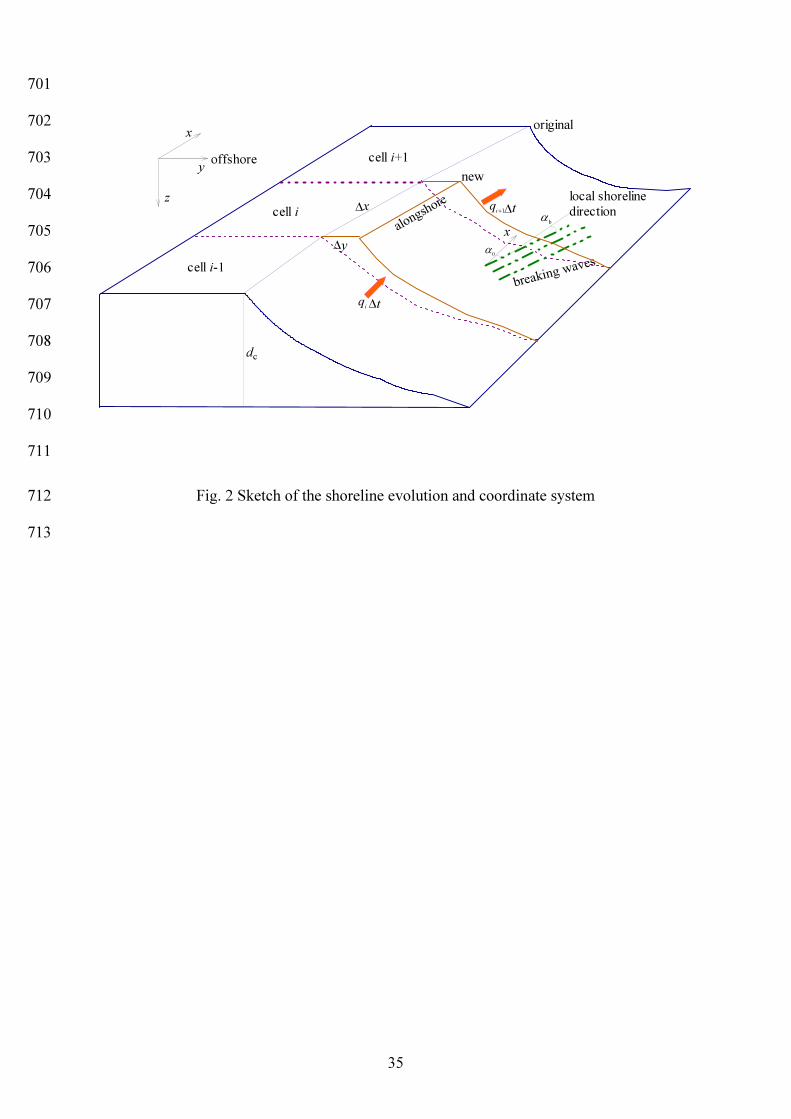
(as presented in Dong and Wu, 2013) are investigated. The first case is a single long jetty that 317 blocks littoral drift with different combinations of parameters. The jetty is located immediately to 318 the right of cell 100 with a littoral drift arriving from the far left at a rate determined from the given 319 wave conditions. Initially, the sandy shoreline is straight, corresponding to the x -axis ( )0(my =0). A 320

diagrammatic definition of the main variables is given in Fig. 2. The simulations are carried out 321 with cell width 25=∆x m and time increment 1.0=∆ kt day. A one-year simulation of shoreline 322

evolution is performed. For the initial boundary condition at 0=x , the spatial shoreline gradient 323 goes to zero because the beach is straight. For the boundary condition at 2500=x m, set 324

btan)(α=

∂∂

xty , which means that the shoreline has an orientation that allows for no sediment transport 325

because no material is allowed to pass the jetty, i.e., the shoreline normal is in the direction of the 326 waves. The values used for the constant input variables are given in Table 1. Considering the 327 maximum deposition distance and algorithm precision of the values of the PDF at the nodes, 328

5.0=∆y m, miny =-100 m, and maxy =650 m; ym =80 has been divided along the cross-shore direction. 329

Given maxbh =1.5 m and bN =200 points, the value of the wave height increment in its PDF 330

distribution is =∆ bh 0.0075 m. 331

If one examines Eq. (12), it can be seen that the numerical solution of this equation requires 332 knowledge of the mean and variance of the wave intensity and the initial shoreline position which 333

14

are normally distributed. In this example calculation, bK and vC are always assumed to be 0.675 m 334

and 0.15 (Burcharth, 1992), respectively, unless stated otherwise (as in sensitivity tests). The mean 335 of the initial shoreline 0y is zero with a standard deviation of 2.5 m. 336

The computed mean of the solution process my , compared with the deterministic numerical 337

solution at the final step using the algorithms given by Komar (1983) based on bK , is given in Fig. 3. 338

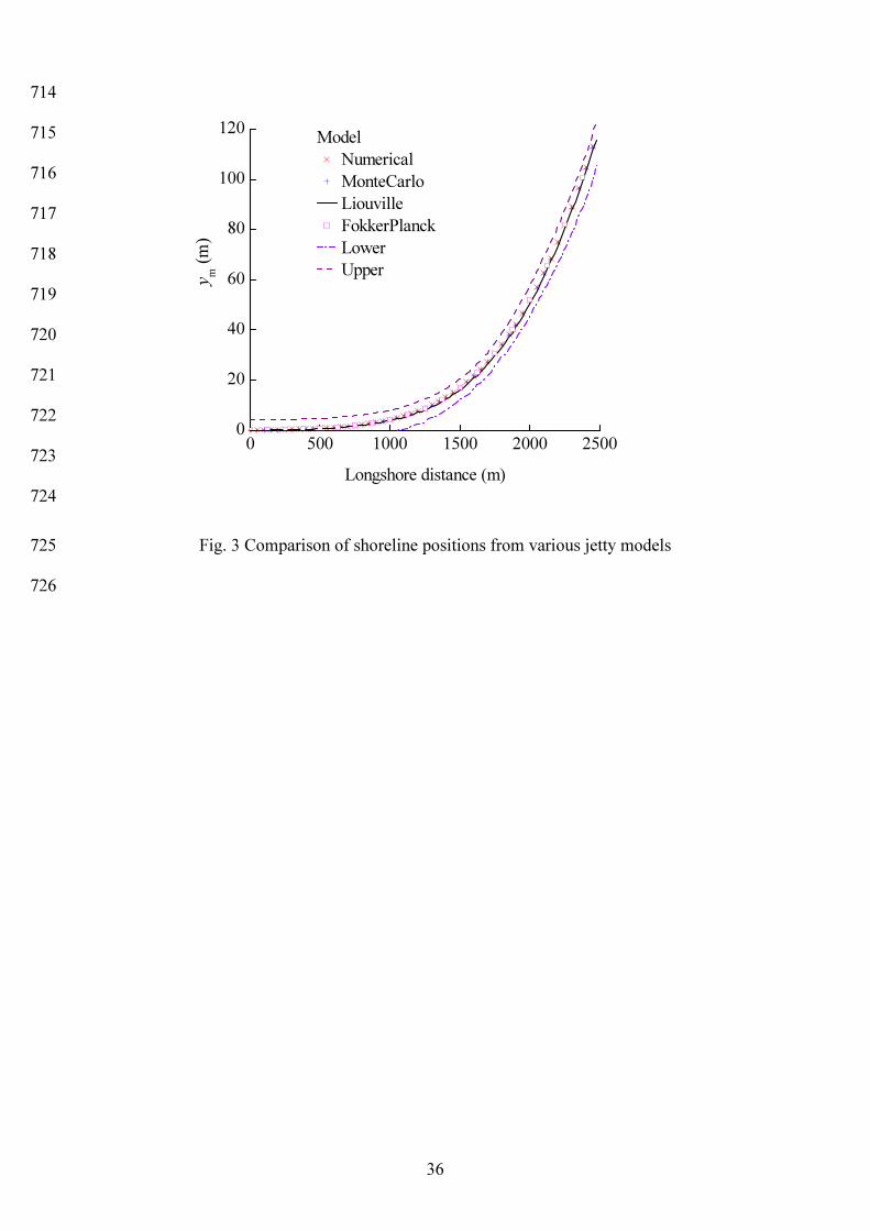
The table shows that the ensemble averaged shoreline position, with random wave height and 339 boundary condition taken into account, differs little from the one obtained using deterministic 340 procedures, where the parameters and boundary condition are first averaged. The results of the 341 mean shoreline position predicted using some other models, such as the direct Monte Carlo model 342 and the Fokker-Planck model (Dong and Wu, 2013), are also shown in Fig. 3. As expected, all 343 models predicted that the cells near the jetty have built outward as the result of accumulating sand, 344 with cell 100 immediately adjacent to the jetty building out the most. The accuracy of the proposed 345 model is confirmed because it not only matches the mean values predicted by the Monte Carlo 346 analysis but it also describes well the randomness and evolutionary process of the PDF, as 347 discussed below. Additionally, the proposed model can be conveniently used to provide the upper 348 and lower confidence limits corresponding to any required confidence level based on the predicted 349 PDFs. The results for this example at the 95% significance level are shown. 350

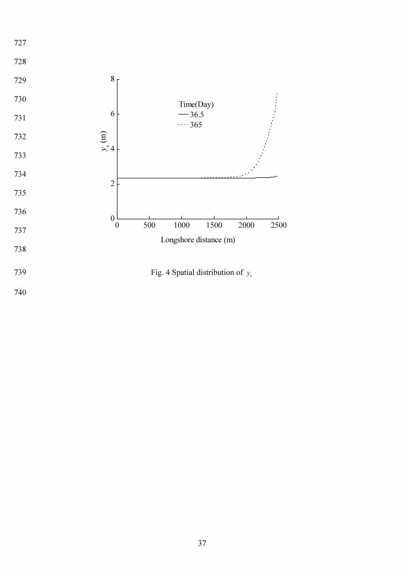
Fig. 4 shows the distributions of the standard deviation of the shoreline position sy at 36.5 351

days and 365 days for all cells. It can be seen that the randomness of the shoreline position 352 increases with the cumulative effects of alongshore transport over time and behaves in a nonlinear 353 way along the shoreline, with the standard deviation becoming larger adjacent to the jetty. 354

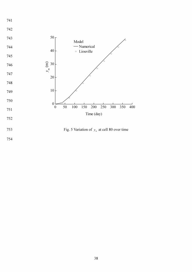
Fig. 5 shows the progressive increase of my with time at cell 80 ( x =2000 m). The shoreline 355

positions predicted by the LE-based stochastic model and the deterministic numerical model are 356 very similar, although the solution by the former is slightly smaller than the deterministic solution 357 due to the effects of randomness in the wave height and initial shoreline variables. 358

15

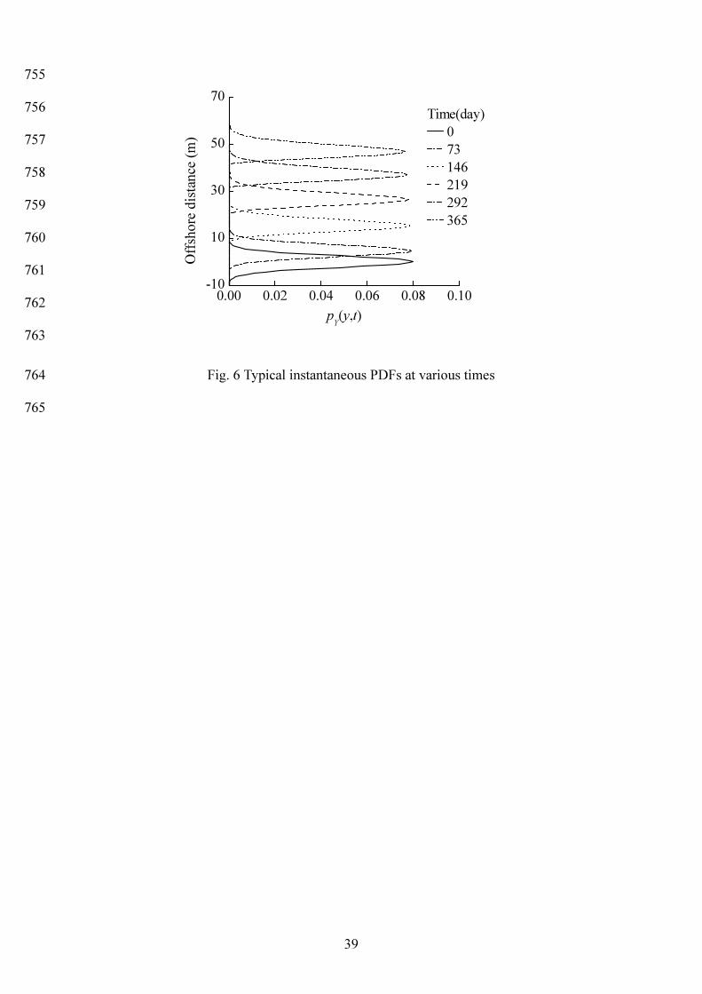
The variation of ),( typY with time is depicted in Fig. 6 at cell 80. It shows not only that the 359

expectation of the pdf curve shifts to a new position with time, due to the accumulation process in 360 the alongshore direction, but also becomes wider over time. This widening of the PDF of the 361 coastline position from the narrow PDFs of the input variables is due to the increase in the 362 advection velocity coefficient. 363

Above outputs are lacking on whether the new LE-based method brings a real improvement 364 over the existing approaches. To further highlight the advantages related to the use of different 365 distribution types and their impacts on the shoreline evolution, more modelling exercises are 366 undertaken. 367

The marginal distributions can also include the three-parameter log-normal distribution, the 368 three-parameter Weibull distribution, and some others. For the independent log-normal distribution, 369 the initial independent joint PDF of bH and 0Y is given by: 370

),,(),,()0;,( b0b0b LHLHLHLYLYLYYH HLYLhyp σµγσµγ= 371

where ( )22

0 2ln

00 )(2

1),,( LYLY

LYy

LYLYLYLYLY eyYL

σµγ

γσπσµγ

−−

−= and 372

( )22

b 2ln

bb )(2

1),,( LHLH

LHh

LHLHLHLHLH ehHL

σµγ

γσπσµγ

−−

−= . The location parameter LYγ =-84.552 m, the scale 373

parameter LYµ =4.437, the shape parameter LYσ =0.029, and LYy γ>0 for 0Y ; LHγ =0, LHµ =-0.404, 374

LHσ =0.155, and LHh γ>b for bH . 375

For the independent Weibull distribution, the initial joint PDF is given by: 376 ),,(),,()0;,( b0b0b WHWHWHWYWYWYYH HWYWhyp σµγσµγ= 377

where WY

WY

WYWY y

WY

WY

WY

WYWYWYWY eyYW

σ

µγσ

µγ

µσσµγ

−−−

−=

01

00 ),,( and 378

WH

WH

WHWY h

WH

WH

WH

WHWHWHWH ehHW

σ

µγσ

µγ

µσσµγ

−−−

−=

b1

bb ),,( . The location parameter WYγ =-7.262 m, the scale 379

16

parameter WYµ =8.069, the shape parameter WYσ = 3.12, and WYy γ≥0 , for 0Y ; WHγ =0, WHµ =0.718, 380

WHσ =7.234, and WHh γ≥b for bH . 381

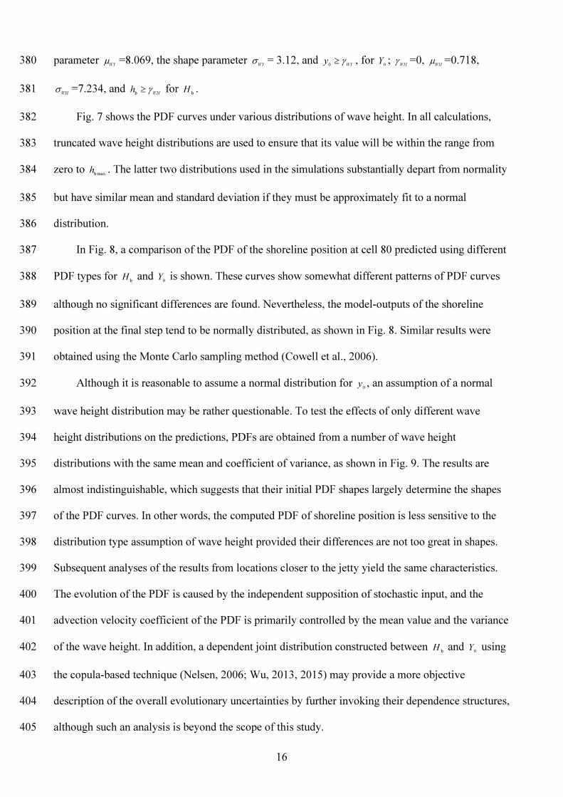
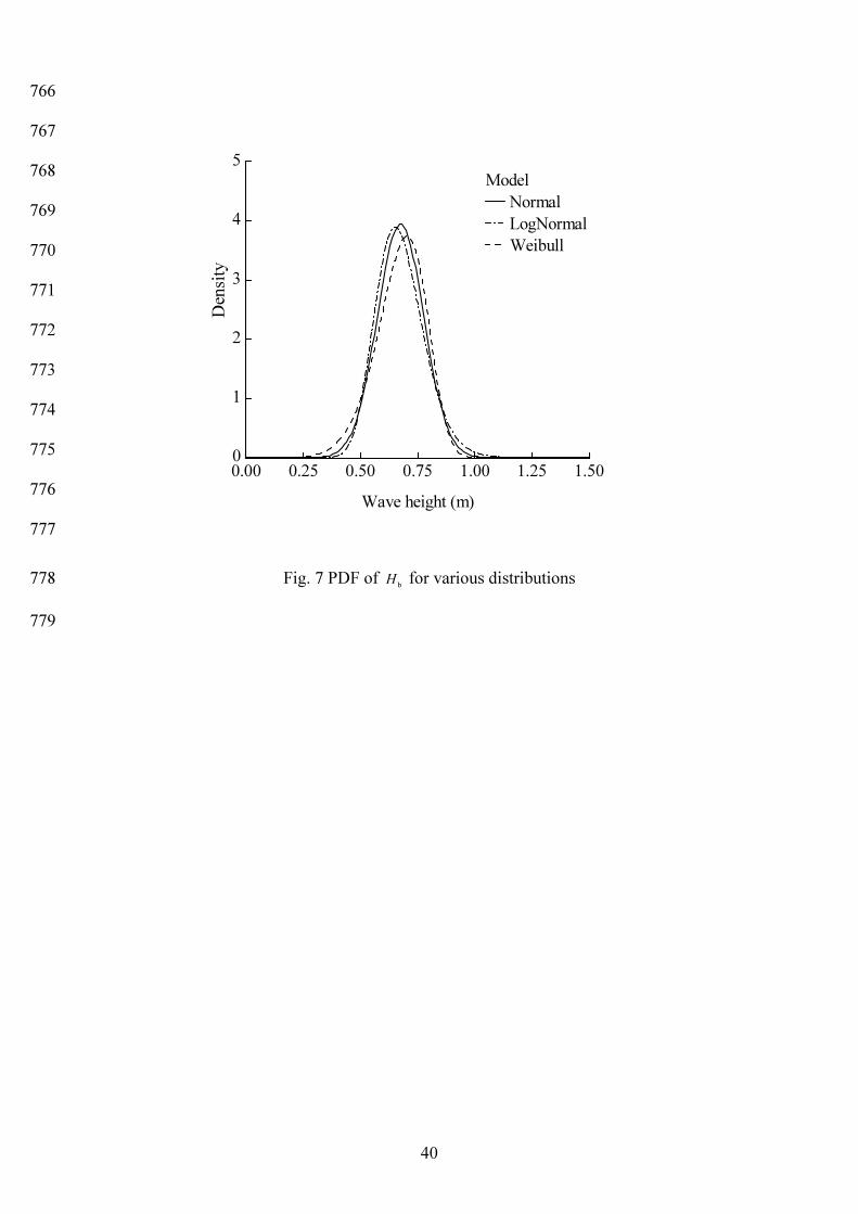
Fig. 7 shows the PDF curves under various distributions of wave height. In all calculations, 382 truncated wave height distributions are used to ensure that its value will be within the range from 383 zero to maxbh . The latter two distributions used in the simulations substantially depart from normality 384

but have similar mean and standard deviation if they must be approximately fit to a normal 385 distribution. 386

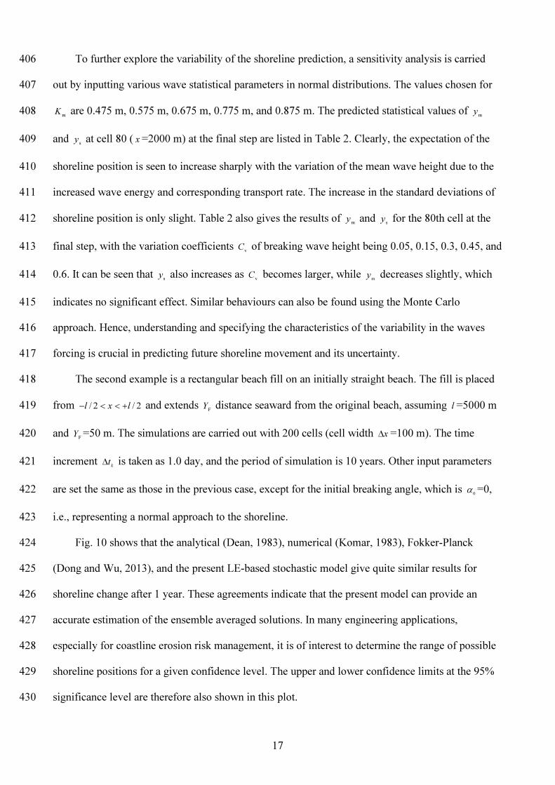
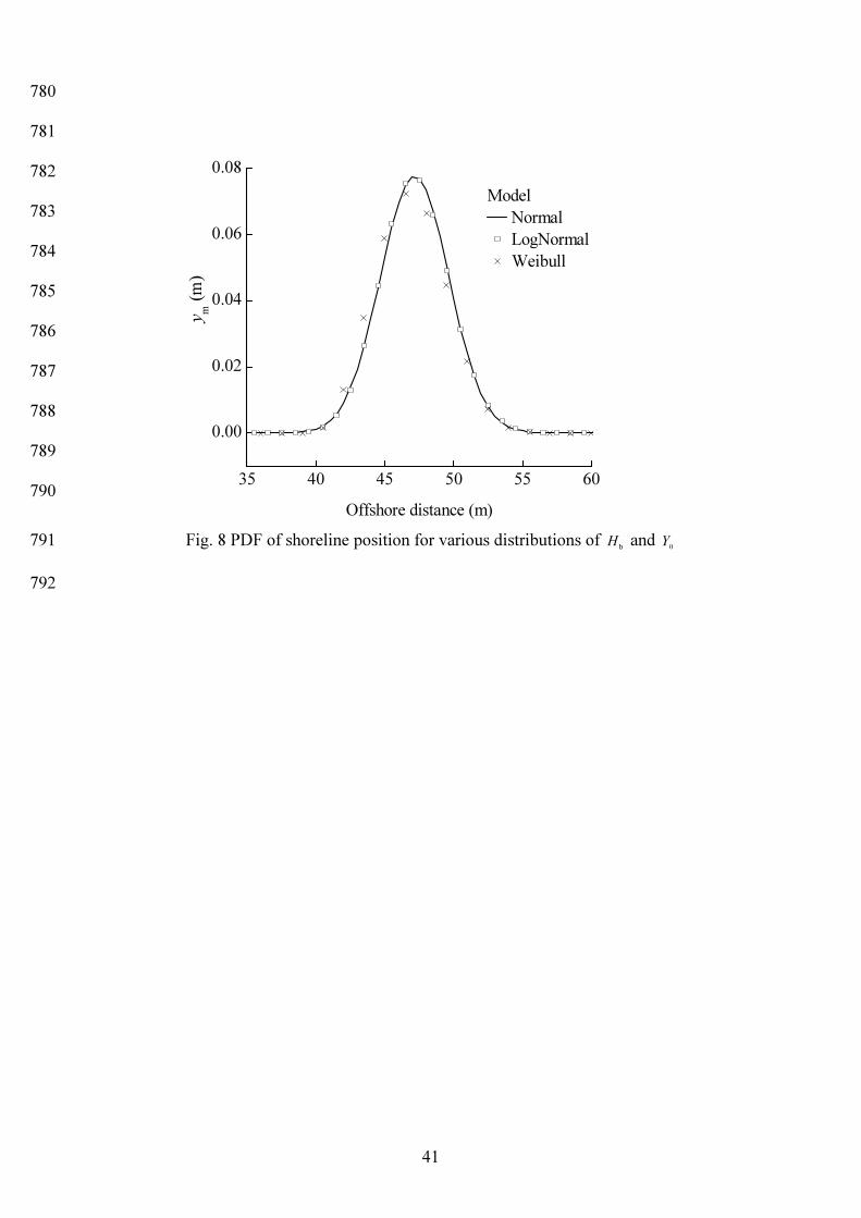
In Fig. 8, a comparison of the PDF of the shoreline position at cell 80 predicted using different 387

PDF types for bH and 0Y is shown. These curves show somewhat different patterns of PDF curves 388

although no significant differences are found. Nevertheless, the model-outputs of the shoreline 389 position at the final step tend to be normally distributed, as shown in Fig. 8. Similar results were 390 obtained using the Monte Carlo sampling method (Cowell et al., 2006). 391

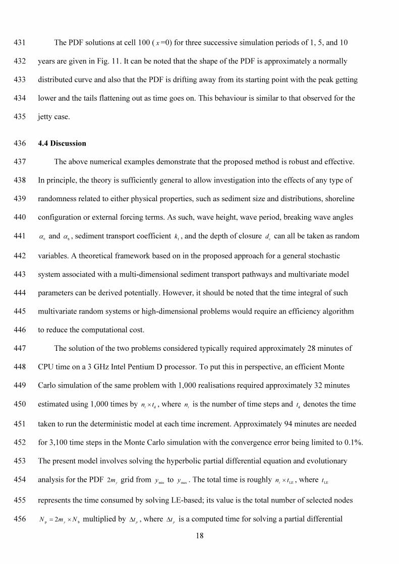
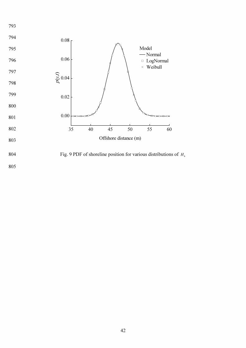
Although it is reasonable to assume a normal distribution for 0y , an assumption of a normal 392

wave height distribution may be rather questionable. To test the effects of only different wave 393 height distributions on the predictions, PDFs are obtained from a number of wave height 394 distributions with the same mean and coefficient of variance, as shown in Fig. 9. The results are 395 almost indistinguishable, which suggests that their initial PDF shapes largely determine the shapes 396 of the PDF curves. In other words, the computed PDF of shoreline position is less sensitive to the 397 distribution type assumption of wave height provided their differences are not too great in shapes. 398 Subsequent analyses of the results from locations closer to the jetty yield the same characteristics. 399 The evolution of the PDF is caused by the independent supposition of stochastic input, and the 400 advection velocity coefficient of the PDF is primarily controlled by the mean value and the variance 401

of the wave height. In addition, a dependent joint distribution constructed between bH and 0Y using 402

the copula-based technique (Nelsen, 2006; Wu, 2013, 2015) may provide a more objective 403 description of the overall evolutionary uncertainties by further invoking their dependence structures, 404 although such an analysis is beyond the scope of this study. 405

17

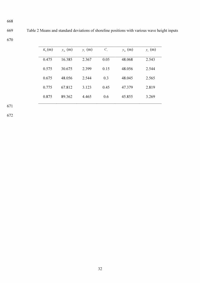
To further explore the variability of the shoreline prediction, a sensitivity analysis is carried 406 out by inputting various wave statistical parameters in normal distributions. The values chosen for 407

mK are 0.475 m, 0.575 m, 0.675 m, 0.775 m, and 0.875 m. The predicted statistical values of my 408

and sy at cell 80 ( x =2000 m) at the final step are listed in Table 2. Clearly, the expectation of the 409

shoreline position is seen to increase sharply with the variation of the mean wave height due to the 410 increased wave energy and corresponding transport rate. The increase in the standard deviations of 411

shoreline position is only slight. Table 2 also gives the results of my and sy for the 80th cell at the 412

final step, with the variation coefficients vC of breaking wave height being 0.05, 0.15, 0.3, 0.45, and 413

0.6. It can be seen that sy also increases as vC becomes larger, while m

y decreases slightly, which 414

indicates no significant effect. Similar behaviours can also be found using the Monte Carlo 415 approach. Hence, understanding and specifying the characteristics of the variability in the waves 416 forcing is crucial in predicting future shoreline movement and its uncertainty. 417

The second example is a rectangular beach fill on an initially straight beach. The fill is placed 418 from 2/2/ lxl +<<− and extends FY distance seaward from the original beach, assuming l =5000 m 419

and FY =50 m. The simulations are carried out with 200 cells (cell width x∆ =100 m). The time 420

increment kt∆ is taken as 1.0 day, and the period of simulation is 10 years. Other input parameters 421

are set the same as those in the previous case, except for the initial breaking angle, which is 0α =0, 422

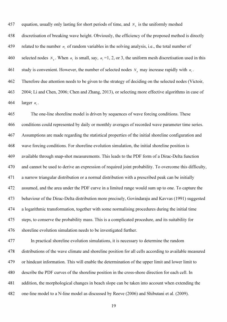
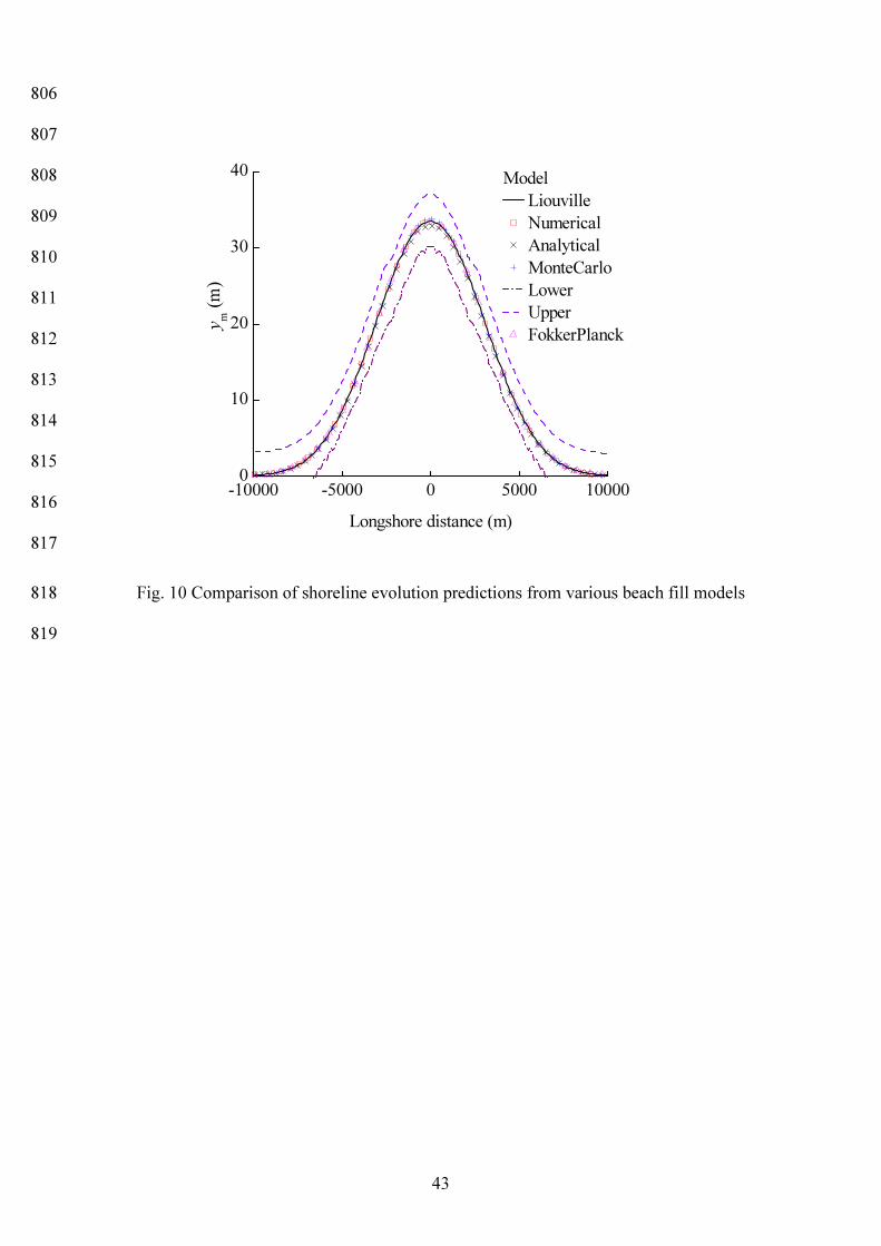
i.e., representing a normal approach to the shoreline. 423 Fig. 10 shows that the analytical (Dean, 1983), numerical (Komar, 1983), Fokker-Planck 424

(Dong and Wu, 2013), and the present LE-based stochastic model give quite similar results for 425 shoreline change after 1 year. These agreements indicate that the present model can provide an 426 accurate estimation of the ensemble averaged solutions. In many engineering applications, 427 especially for coastline erosion risk management, it is of interest to determine the range of possible 428 shoreline positions for a given confidence level. The upper and lower confidence limits at the 95% 429 significance level are therefore also shown in this plot. 430

18

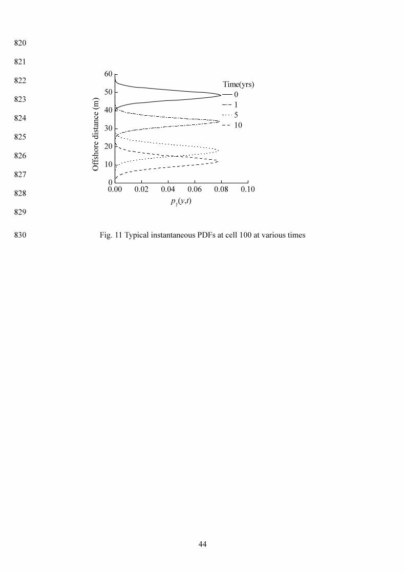
The PDF solutions at cell 100 ( x =0) for three successive simulation periods of 1, 5, and 10 431 years are given in Fig. 11. It can be noted that the shape of the PDF is approximately a normally 432 distributed curve and also that the PDF is drifting away from its starting point with the peak getting 433 lower and the tails flattening out as time goes on. This behaviour is similar to that observed for the 434 jetty case. 435

4.4 Discussion 436 The above numerical examples demonstrate that the proposed method is robust and effective. 437

In principle, the theory is sufficiently general to allow investigation into the effects of any type of 438 randomness related to either physical properties, such as sediment size and distributions, shoreline 439 configuration or external forcing terms. As such, wave height, wave period, breaking wave angles 440

0α and bα , sediment transport coefficient 1k , and the depth of closure cd can all be taken as random 441

variables. A theoretical framework based on in the proposed approach for a general stochastic 442 system associated with a multi-dimensional sediment transport pathways and multivariate model 443 parameters can be derived potentially. However, it should be noted that the time integral of such 444 multivariate random systems or high-dimensional problems would require an efficiency algorithm 445 to reduce the computational cost. 446

The solution of the two problems considered typically required approximately 28 minutes of 447 CPU time on a 3 GHz Intel Pentium D processor. To put this in perspective, an efficient Monte 448 Carlo simulation of the same problem with 1,000 realisations required approximately 32 minutes 449 estimated using 1,000 times by dtnt × , where tn is the number of time steps and dt denotes the time 450

taken to run the deterministic model at each time increment. Approximately 94 minutes are needed 451 for 3,100 time steps in the Monte Carlo simulation with the convergence error being limited to 0.1%. 452 The present model involves solving the hyperbolic partial differential equation and evolutionary 453 analysis for the PDF ym2 grid from miny to maxy . The total time is roughly LEtnt × , where LEt 454

represents the time consumed by solving LE-based; its value is the total number of selected nodes 455

bp 2 NmN y ×= multiplied by pt∆ , where pt∆ is a computed time for solving a partial differential 456

19

equation, usually only lasting for short periods of time, and bN is the uniformly meshed 457

discretisation of breaking wave height. Obviously, the efficiency of the proposed method is directly 458 related to the number rn of random variables in the solving analysis, i.e., the total number of 459

selected nodes pN . When rn is small, say, rn =1, 2, or 3, the uniform mesh discretisation used in this 460

study is convenient. However, the number of selected nodes pN may increase rapidly with rn . 461

Therefore due attention needs to be given to the strategy of deciding on the selected nodes (Victoir, 462 2004; Li and Chen, 2006; Chen and Zhang, 2013), or selecting more effective algorithms in case of 463

larger rn . 464

The one-line shoreline model is driven by sequences of wave forcing conditions. These 465 conditions could represented by daily or monthly averages of recorded wave parameter time series. 466 Assumptions are made regarding the statistical properties of the initial shoreline configuration and 467 wave forcing conditions. For shoreline evolution simulation, the initial shoreline position is 468 available through snap-shot measurements. This leads to the PDF form of a Dirac-Delta function 469 and cannot be used to derive an expression of required joint probability. To overcome this difficulty, 470 a narrow triangular distribution or a normal distribution with a prescribed peak can be initially 471 assumed, and the area under the PDF curve in a limited range would sum up to one. To capture the 472 behaviour of the Dirac-Delta distribution more precisely, Govindaraju and Kavvas (1991) suggested 473 a logarithmic transformation, together with some normalising procedures during the initial time 474 steps, to conserve the probability mass. This is a complicated procedure, and its suitability for 475 shoreline evolution simulation needs to be investigated further. 476

In practical shoreline evolution simulations, it is necessary to determine the random 477 distributions of the wave climate and shoreline position for all cells according to available measured 478 or hindcast information. This will enable the determination of the upper limit and lower limit to 479 describe the PDF curves of the shoreline position in the cross-shore direction for each cell. In 480 addition, the morphological changes in beach slope can be taken into account when extending the 481 one-line model to a N-line model as discussed by Reeve (2006) and Shibutani et al. (2009). 482

20

5 Conclusions 483

The long-term stochastic responses of a shoreline under random wave forcing and initial 484 shoreline position are formulated based on the Liouville type equation. The approach converts the 485 problem from a multivariate Monte Carlo simulation to one of solving an initial value problem 486 involving a first-order partial differential equation, which greatly simplifies the analysis, at least for 487 the forcing conditions considered. The one-dimensional governing evolutionary PDF equation is 488 solved by combining the deterministic nonlinear shoreline analysis to define the advection velocity 489 coefficient and the finite difference method with a TVD scheme to solve the advection equation for 490 joint PDF distributions. 491

Example calculations involving two idealised shoreline evolution cases and the use of different 492 probabilistic representations of the random breaking wave height show that the mean shoreline 493 predicted by the present model, and those resulting from the deterministic numerical scheme and 494 Monte Carlo simulations are comparable. It is found that the PDF of the shoreline position tends to 495 have a similar normally distributed form, although the PDF of the breaking wave height and initial 496 condition may assume various statistical distribution forms. This is because the PDF curves of 497 shoreline position are largely determined by its initial distribution shape, as the model calculations 498 mainly involve the independent supposition of a stochastic input and thus are largely controlled by 499 the mean value of the wave height parameter. The sensitivity analysis of the effects of the input 500 parameters on the predicted shoreline statistics further demonstrates that the proposed model is 501 capable of effectively predicting the complete stochastic characteristics of shoreline evolution 502 without requiring a Monte Carlo sampling. Comparing with the formulations based on the FPE, the 503 applicability of the SDE methods was extended through the formulating of the well-known LE, 504 which provides the ability of describing both Gaussian and non-Gaussian statistics of random inputs. 505

A simple CERC law is employed because it provides general, non-unique empirical fits to field 506 data sets and is popular in shoreline dynamic models. The ideas presented here are also tractable 507 with other forms of empirical laws, but these generalisations will not be pursued here. The present 508

21

model accounts for the effects of variability in both random wave parameters and the initial 509 shoreline position. The LE-based method is fairly general as it accepts any distribution type for the 510 random variables. Although the random breaking wave height parameter in the model is currently 511 assumed to be from a constant distribution, the spatial variation of the breaking wave height 512 parameter, depth of closure, and sediment transport coefficient can also be accounted for by 513 introducing additional random terms in the vector LE-based model. 514

Acknowledgements 515

The support of the UK Engineering and Physical Science Research Council as part of a 516 research project under Grant No. GR\L53953 is gratefully acknowledged. 517

Notations 518

1a constant in the expression for l0q [ kgsecm 22 ];

B operator; gbC wave group celerity [m/s]; vC coefficient of variance, 10

v≤≤ C , defined as the ratio of

the standard deviation to the mean; d difference operator;

bd breaker depth [m]; bD variance of bH , confirmed to a normal distribution [m]; cd closure depth [m]; bE wave energy evaluated at the breaking point [ kN ];

g acceleration of gravity [ 2sec/m ]; bh discrete wave height at breaking [m]; bH wave height at breaking [m]; sH significant wave height [m]; i cell number alongshore; bi node number in PDF of bH ; j node number in cross-shore; k time step of one-line model; 1k sediment transport coefficient, or, dimensionless empirical

coefficient; bK mean of bH ;

l distance alongshore [m]; m number of time steps in TVD scheme ;

ym number of the discrete distribution in cross-shore direction;

bN number of uniformly meshing discretisation for each time increment;

22

pN total number of the selected nodes, b2 Nmy ×= ; rn dimension of excitation vector; sn void ratio of sand, 4.0≈ ; tn number of time steps; p probability density function or PDF; p mixing ratio at the cell edges; lq volumetric long-shore sediment transport rate [ /secm3 ]; l0q amplitude of volumetric long-shore sediment transport rate

[ /secm3 ]; cr lattice ratio; t time [sec]; 0t initial time [sec]; dt time token for running the deterministic model [sec]; kt time in thk step of one-line shoreline model [sec]; mt time in thm step [sec] of TVD scheme; LEt time consumed by solving LE-based model [sec]; mTV total variation at time step m ;

v Y& ; mv mean of v ; x distance alongshore [m]; y shoreline position in cross-shore direction [m]; Y stochastic process or random variable of shoreline position

or random state (which is a component of state vector); 0Y initial random state or random variable of shoreline

position Y ; FY extension distance seaward from the rectangular beach; my expected value or mean value of y ; m0Y initial mean value of Y ; maxy maximum discrete shoreline position; miny minimum discrete shoreline position; sy standard deviation of y ; s0Y initial standard deviation of Y ;

Y& time derivate of Y , ),(2/5

b tyH ζ−= , or the ‘velocity’ of the response for a prescribed bh , called advection velocity coefficient;

Z random parameter with known PDFs; 0Z initial Z ; 0α incident angle of breaking waves relative to x [deg]; bα angle of breaking waves to the local shoreline [deg]; γ ratio of wave height to water depth at breaking,

b

bd

H= ; LHγ log-normal distribution location parameter of bH ; LYγ log-normal distribution location parameter of 0Y ; WHγ Weibull distribution location parameter of bH ; WYγ Weibull distribution location parameter of 0Y ; bh∆ size increment in bh [m]; kt∆ time increment of one-line shoreline model [sec]; mt∆ time increment of TVD [sec]; x∆ size increment in along-shore direction [m];

23

y∆ size increment in cross-shore direction [m]; ζ xdag

∂∂= −

))2(sin(181 b

c1

2/12/3w

αγρ ; η operator of shoreline position evolution, ),(5.2

b tyH ζ−= ;

η operator vector of determination of a dynamical state, may be determined by an appropriate deterministic shoreline evolution model;

θ ( )mjmj

mjmj

pppp

,,1

,1,

−

−=

+

− ;

λ ratio, k

m

tt

∆∆= 1> ;

LHµ log-normal distribution scale parameter of bH ; LYµ log-normal distribution scale parameter of 0Y ; WHµ Weibull distribution scale parameter of bH ; WYµ Weibull distribution scale parameter of 0Y ; s

ρ mass density of the sediment grains [ 3kg/m ]; w

ρ mass density of water [ 3kg/m ]; LHσ log-normal distribution shape parameter of bH ; LYσ log-normal distribution shape parameter of 0Y ; WHσ Weibull distribution shape parameter of bH ; WYσ Weibull distribution shape parameter of 0Y ;

φ flux limiter; zΩ distribution domain.

References 519

Arimitsu T (2009) Non-equlibrium thermo field dynamics and its application to error-correction for 520 spatially correlated quantum errors. Interdiscip Inform Sci 15(3):441–471 521

Battjes JA (1972) Long-term wave height distribution at seven stations around the British Isles. 522 Deutsche Hydrographische Zeitschrift J 25:179–189 523

Benassai E, Calabrese M, Uberti GSD (2001) A probabilistic prediction of beach nourishment 524 evolution. MEDCOAST01, The 5th Inter Conf on Mediterranean Coast Envir, 2001, Yasmine 525 Beach Resort, Hammamet, Tunisia 526

Bodo BA, Thompson ME, Unny TE (1987) A review on stochastic differential equations for 527 applications in hydrology. Stoch Hydrol Stoch Hydraul 2:81–100 528

Booij N, Ris RC, Holthuijsen LH (1999) A third-generation wave model for coastal regions, 1, 529 model description and validation. J Geophys Res 104(C4):7649–7666 530

24

Burcharth HF (1992) Uncertainty related to environmental data and estimated extreme events. Final 531 Report of PIANC Working Group 12, Group B 532

Camfield FE, Morang A (1996) Defining and interpreting shoreline change. Ocean Coast Manage 533 32:129–151 534

Chen JB, Li J (2005) Dynamic response and reliability analysis of nonlinear stochastic structures. 535 Probab Eng Mech 20(1):33–44 536

Chen JB, Li J (2009) A note on the principle of preservation of probability and probability density 537 evolution equation. Probab Eng Mech 24:51–59 538

Chen JB, Zhang SH (2013) Improving point selection in cubature by a new discrepancy. SIAM J 539 SCI COMPUT 35(5):A2121–A2149 540

Cowell PJ, Thom BG, Jones RA, Everts CH, Simanovic D (2006) Management of uncertainty in 541 predicting climate-change impacts on beaches. J Coastal Res 22(1):232–245 542

de Vriend HJ, Capobianco M, Chesher T, Swart HED, Latteaux B, Stive MJF (1993) Approaches to 543 long-term modelling of coastal morphology: a review. Coastal Eng 21:225–269 544

Dean RG (1983) Principles of beach nourishment. In: Komar PD, ed., CRC handbook of coastal 545 processes and erosion. CRC Press Boca Raton, Fla., 11, 217–232 546

Dean RG, Grant J (1989) Development of methodology for thirty-year shoreline projections in the 547 vicinity of beach nourishment projects. UFL/COEL-89/026. Gainesville, University of Florida 548

Dong P, Chen H (1999) Probabilistic predictions of time dependent long-term beach erosion risks. 549 Coast Eng 36:243–261 550

Dong P, Chen H (2000) A simple life-cycle method for predicting extreme shoreline erosion. Stoch 551 Environ Res Risk Assess 14:79–89 552

Dong P, Wu XZ (2013) Application of a stochastic differential equation to the prediction of 553 shoreline evolution. Stoch Environ Res Risk Assess 27(8):1799–1814 554

25

Dostupov BG, Pugachev VS (1957) The equation for the integral of a system of ordinary 555 differential equations containing random parameters. Automatika i Telemekhanika 18:620–556 630 557

Ehrendorfer M (1994) The Liouville equation and its potential usefulness for the prediction of 558 forecast skill. Part I: Theory. Monthly Weather Rev 122:703–713 559

Gardiner CW (2004) Handbook of stochastic methods for physics, chemistry, and the natural 560 sciences. Springer, Berlin 561

Govindaraju RS, Kavvas ML (1991) Stochastic overland flows. Part 2: Numerical solutions 562 evolutionary PDFs. Stoch Hydrol Hydraul 5:105–124 563

Guedes Soares C, Henriques AC (1996) Statistical uncertainty in long-term distributions of 564 significant wave height. J Offshore Mech Arctic Eng 11:284–291 565

Guedes Soares C, Viana PC (1988) Sensitivity of the response of marine structures to wave 566 climatology. In: Schrefer and Zienkiewicz (Editors), Computer Modelling in Ocean 567 Engineering 1988. pp 487–492. The Netherlands: A.A. Balkema Publishers 568

Hanson H, Kraus NC (1989) GENESIS: Generalized model for simulating shoreline change. Report 569 1, Technical Report CERC-89-19. Vicksburg, MS 570

Harten A (1983) High resolution schemes for hyperbolic conservation laws. J Comput Phys 49:357–571 393 572

Jasper NH (1956) Statistical distribution patterns of ocean waves and of wave-induced ship stresses 573 and motions with engineering applications. Transactions-Society of Naval Architects and 574 Marine Engineers 64:375–432 575

Jin M (1994) Random differential equation modelling for backwater profile computation. J Hydraul 576 Res 32(1):131–144 577

Johnson EA, Wojtkiewicz SF, Bergman LA, Spencer BF (1997) Observations with regards to 578

26

massively parallel computation for Monte Carlo simulation of stochastic dynamical systems. 579 Int J nonlinear Mech 32(4):721–734 580

Kamphuis JW (1999) Marketing Uncertainty. Proc. COPEDEC V., Cap Town, pp 2088–2099 581

Kamphuis JW (2006) Beyond the limits of coastal engineering. Proc. 30th ICCE, San Diego, pp 582 1938–1950 583

Kavvas ML (2003) Nonlinear hydrologic processes: Conservation equations for determining their 584 means and probability distributions. J Hydrologic Eng 8:44–53 585

Kim S, Jang SH (2007) Analytical derivation of steady state soil water probability distribution 586 function under rainfall forcing using cumulant expansion theory. KSCE J Civil Eng 11:227–587 232 588

Komar PD (1983) Computer models of shoreline changes. In: Komar PD, ed., CRC handbook of 589 coastal processes and erosion. CRC Press Boca Raton, Fla., 11, 205–216 590

Kubo R (1963) Stochastic liouville equations. J Math Phys 4(2):174–183 591

Larson M, Hanson H, Kraus NC (1997) Analytical solutions of one-line model for shoreline change 592 near coastal structures. J Waterway Port Coast Ocean Eng 123(4):180–191 593

Lax PD, Wendroff B (1960) Systems of conservation laws. Communications in Pure and Applied 594 Mathematics 13:217–237 595

Laney CB (1998) Computational gas dyanamics. Cambridge University Press 596

Leonard BP (1979) A stable and accurate convective modeling procedure based on quadratic 597 upstream interpolation. Comput Methods Appl Mech Eng 19:59–98 598

Li J, Chen JB (2006) The dimension-reduction strategy via mapping for probability density 599 evolution analysis of nonlinear stochastic systems. Probab Eng Mech 21(4):442–453 600

Li J, Chen JB (2008) The principle of preservation of probability and the generalized density 601 evolution equation. Struct Safety 30(1):65–77 602

27

Medellín G, Medina R, Falqués A, González M (2008) Coastline sand waves on a low-energy beach 603 at “El Puntal” spit, Spain. Mar Geol 250:143–156 604

Moan T, Gao Z, Ayala-Uraga E (2005) Uncertainty of wave-induced response of marine structures 605 due to long-term variation of extratropical wave conditions. Mar Struct 18:359–382 606

Nelsen RB (2006) An introduction to copulas, 2nd edition. Springer, New York 607

Paul W, Baschnagel J (2000) Stochastic processes. From physics to Finance. Springer 608

Pelnard-Considère (1956) Essai de theorie de l'evolution des formes de rivage enplages de sable et 609 de galets. Fourth Journess de I’Hydralique, les energies de la Mer Question III(1):289–298 610

Pilkey OH, Cooper JAG (2002) Longshore transport volumes: a critical view. J Coast Res ICS 611 Proceedings 2002. pp 572–580 612

Razi M, Attar PJ, Vedula P (2013) Uncertainty quantification for multidimensional dynamical 613 systems based on adaptive numerical solution of liouville equation. 54th 614 AIAA/ASME/ASCE/AHS/ASC Structures, Structural Dynamics, and Materials Conference. 615 pp 24 616

Reeve DE (2006) Explicit expression for beach response to non-stationary forcing near a groyne. J 617 Waterway Port Coast Ocean Eng 132(2):125–132 618

Reeve DE, Spivack M (2004) Evolution of shoreline position moments. Coast Eng 51(8-9):661–673 619

Ris RC, Holthuijsen LH, Booij N (1999) A third-generation wave model for coastal regions, 2, 620 verification. J Geophys Res 104(C4):7667–7681 621

Risken H (1989) The Fokker-Planck Equation, 2nd edn. Springer-Verlag, Berlin, Heidelberg 622

Ruggiero P, Buijsman M, Kaminsky GM, Gelfenbaum G (2010) Modeling the effects of wave 623 climate and sediment supply variability on large-scale shoreline change. Mar Geol 273:127–624 140 625

Ruggiero P, Kaminsky GM, Gelfenbaum G (2003) Linking proxy-based and datum-based 626

28

shorelines on a high-energy coastline: implications for shoreline change analyses. J Coast Res 627 38:57–82 628

Shibutani Y, Kuroiwa M, Matsubara Y, Kim M, Abualtaef M (2009) Development of N-line 629 numerical model considering the effects of beach nourishment. J Coastal Res SI56:554–558 630

Shvidler M, Karasaki K (2003) Probability density functions for solute transport in random field. 631 Transp Porous Media 50(3):243–266 632

Soong TT (1973) Random differential equations in science and engineering. New York: Academic 633 Press 634

Sweby PK (1985) High resolution TVD schemes using flux limiters. Lectures in Applied 635 Mathematics 22:289–309 636

Syski R (1967) Stochastic differential equations. In: Saaty TL Editors, Modern nonlinear equations, 637 McGraw-Hill, New York 638

Tanimura Y (2006) Stochastic Liouville, Langevin, Fokker–Planck, and Master equation 639 approaches to quantum dissipative systems. J Phys society of Japan 75(8):1–39 640

US Army Corps of Engineers (1984) Shore protection manual. Coastal Engineering Research 641 Center, Washington 642

van Leer B (1974) Towards the ultimate conservative difference scheme. II: Monotonicity and 643 conservation combined in a second order scheme. J Comput Phys 14:361–370 644

Victoir N (2004) Asymmetric cubature formulae with few points in high dimension for symmetric 645 measures. SIAM J Numer Anal 42(1):209–227 646

Vrijling JK, Meijer GJ (1992) Probabilistic coastline position computations. Coast Eng 17(1-2):1–647 23 648

Wang B, Reeve D (2010) Probabilistic modelling of long-term beach evolution near segmented 649 shore-parallel breakwaters. Coast Eng 57:732–744 650

29

Wu XZ (2013) Probabilistic slope stability analysis by a copula-based sampling method. Comput 651 Geosci 17(5):739–755 652

Wu XZ (2015) Assessing the correlated performance functions of an engineering system via 653 probabilistic analysis. Struct Safety 52, Part A: 10–19 654

Zacharioudaki A, Reeve DE (2011) Shoreline evolution under climate change wave scenarios. 655 Climatic Change 108:73–105 656

657

30

List of Tables: 658 Table 1 Input variables 659 Table 2 Means and standard deviations of shoreline positions with various wave height inputs 660 661

662

31

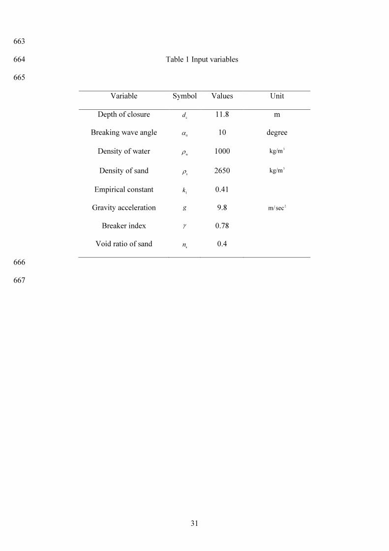
663 Table 1 Input variables 664

665

Variable Symbol Values Unit

Depth of closure cd 11.8 m Breaking wave angle 0α 10 degree

Density of water wρ 1000 3kg/m

Density of sand sρ 2650 3kg/m

Empirical constant 1k 0.41 Gravity acceleration g 9.8 2secm/

Breaker index γ 0.78

Void ratio of sand sn 0.4

666 667

32

668 Table 2 Means and standard deviations of shoreline positions with various wave height inputs 669

670

bK (m) my (m) sy (m) vC my (m) sy (m)

0.475 16.385 2.367 0.05 48.068 2.543 0.575 30.675 2.399 0.15 48.056 2.544 0.675 48.056 2.544 0.3 48.045 2.565 0.775 67.812 3.123 0.45 47.379 2.819 0.875 89.362 4.465 0.6 45.855 3.269

671 672

33

List of Figures: 673 Fig. 1 Simulations and PDF curves of shoreline position for specified cells at a specified time 674 Fig. 2 Sketch of the shoreline evolution and coordinate system 675 Fig. 3 Comparison of shoreline positions from various jetty models 676

Fig. 4 Spatial distribution of sy 677

Fig. 5 Variation of my at cell 80 over time 678

Fig. 6 Typical instantaneous PDFs at various times 679

Fig. 7 PDF of bH for various distributions 680

Fig. 8 PDF of shoreline position for various distributions of bH and 0Y 681

Fig. 9 PDF of shoreline position for various distributions of bH 682

Fig. 10 Comparison of shoreline evolution predictions from various beach fill models 683 Fig. 11 Typical instantaneous PDFs at cell 100 at various times 684 685

686

34

687 688 689 690 691 692 693 694 695 696 697

Fig. 1 Simulations and PDF curves of shoreline position for specified cells at a specified time 698 699

700

70 80 900

20

40

60

80

100

y (m)

Cell

35

701 702

703 704 705 706 707 708 709 710 711

Fig. 2 Sketch of the shoreline evolution and coordinate system 712 713

zy

xcell i+1

cell i

cell i-1

x

local shorelinedirection

0α

bα

b r e a k i n g wa v e sy∆

∆x

original

new

dc

∆tiq

∆t1+iqa l o n g

s h o r e

offshore

36

714 715 716 717 718 719 720 721 722 723 724

Fig. 3 Comparison of shoreline positions from various jetty models 725 726

0 500 1000 1500 2000 25000

20

40

60

80

100

120

y m (m

)

Longshore distance (m)

Model Numerical MonteCarlo Liouville FokkerPlanck Lower Upper

37

727 728 729 730 731 732 733 734 735 736 737 738

Fig. 4 Spatial distribution of sy 739

740

0 500 1000 1500 2000 25000

2

4

6

8

y s (m

)

Longshore distance (m)

Time(Day) 36.5 365

38

741 742 743 744 745 746 747 748 749 750 751 752

Fig. 5 Variation of my at cell 80 over time 753

754

0 50 100 150 200 250 300 350 4000

10

20

30

40

50

y m (m

)

Time (day)

Model Numerical Liouville

39

755 756 757 758 759 760 761 762 763

Fig. 6 Typical instantaneous PDFs at various times 764 765

0.00 0.02 0.04 0.06 0.08 0.10-10

10

30

50

70Time(day)

0 73 146 219 292 365

Offsh

ore di

stanc

e (m)

pY(y,t)

40

766 767 768 769 770 771 772 773 774 775 776 777

Fig. 7 PDF of bH for various distributions 778

779

0.00 0.25 0.50 0.75 1.00 1.25 1.500

1

2

3

4

5

Densi

ty

Wave height (m)

Model Normal LogNormal Weibull

41

780 781 782 783 784 785 786 787 788 789 790

Fig. 8 PDF of shoreline position for various distributions of bH and 0Y 791

792

35 40 45 50 55 60

0.00

0.02

0.04

0.06

0.08y m

(m)

Offshore distance (m)

Model Normal LogNormal Weibull

42

793 794 795 796 797 798 799 800 801 802 803

Fig. 9 PDF of shoreline position for various distributions of bH 804

805

35 40 45 50 55 60

0.00

0.02

0.04

0.06

0.08

p(y,t)

Offshore distance (m)

Model Normal LogNormal Weibull

43

806 807 808 809 810 811 812 813 814 815 816 817

Fig. 10 Comparison of shoreline evolution predictions from various beach fill models 818 819

-10000 -5000 0 5000 100000

10

20

30

40

y m (m

)

Longshore distance (m)

Model Liouville Numerical Analytical MonteCarlo Lower Upper FokkerPlanck

44

820 821 822 823 824 825 826 827 828 829

Fig. 11 Typical instantaneous PDFs at cell 100 at various times 830

0.00 0.02 0.04 0.06 0.08 0.100102030405060

Time(yrs) 0 1 5 10

Offsh

ore di

stanc

e (m)

pY(y,t)