Lingxiao Li Massachusetts Institute of Technology ...

Do Neural Optimal Transport Solvers Work?A Continuous Wasserstein-2 Benchmark

Alexander KorotinSkolkovo Institute of Science and Technology

Moscow, [email protected]

Lingxiao LiMassachusetts Institute of Technology

Cambridge, Massachusetts, [email protected]

Aude GenevayMassachusetts Institute of Technology

Cambridge, Massachusetts, [email protected]

Justin SolomonMassachusetts Institute of Technology

Cambridge, Massachusetts, [email protected]

Alexander FilippovHuawei Noah’s Ark Lab

Moscow, [email protected]

Evgeny BurnaevSkolkovo Institute of Science and Technology

Artificial Intelligence Research InstituteMoscow, Russia

[email protected]

Abstract

Despite the recent popularity of neural network-based solvers for optimal transport(OT), there is no standard quantitative way to evaluate their performance. In thispaper, we address this issue for quadratic-cost transport—specifically, computationof the Wasserstein-2 distance, a commonly-used formulation of optimal transport inmachine learning. To overcome the challenge of computing ground truth transportmaps between continuous measures needed to assess these solvers, we use input-convex neural networks (ICNN) to construct pairs of measures whose ground truthOT maps can be obtained analytically. This strategy yields pairs of continuousbenchmark measures in high-dimensional spaces such as spaces of images. Wethoroughly evaluate existing optimal transport solvers using these benchmarkmeasures. Even though these solvers perform well in downstream tasks, manydo not faithfully recover optimal transport maps. To investigate the cause of thisdiscrepancy, we further test the solvers in a setting of image generation. Our studyreveals crucial limitations of existing solvers and shows that increased OT accuracydoes not necessarily correlate to better results downstream.

Solving optimal transport (OT) with continuous methods has become widespread in machine learning,including methods for large-scale OT [11, 36] and the popular Wasserstein Generative AdversarialNetwork (W-GAN) [3, 12]. Rather than discretizing the problem [31], continuous OT algorithms useneural networks or kernel expansions to estimate transport maps or dual solutions. This helps scale OTto large-scale and higher-dimensional problems not handled by discrete methods. Notable successesof continuous OT are in generative modeling [42, 20, 19, 7] and domain adaptation [43, 37, 25].

In these applications, OT is typically incorporated as part of the loss terms for a neural networkmodel. For example, in W-GANs, the OT cost is used as a loss function for the generator; themodel incorporates a neural network-based OT solver to estimate the loss. Although recent W-GANsprovide state-of-the-art generative performance, however, it remains unclear to which extent thissuccess is connected to OT. For example, [28, 32, 38] show that popular solvers for the Wasserstein-1

Preprint.

arX

iv:2

106.

0195

4v2

[cs

.LG

] 2

5 O

ct 2

021

(W1) distance in GANs fail to estimate W1 accurately. While W-GANs were initially introducedwith W1 in [3], state-of-the art solvers now use both W1 and W2 (the Wasserstein-2 distance, i.e.,OT with the quadratic cost). While their experimental performance on GANs is similar, W2 solverstend to converge faster (see [19, Table 4]) with better theoretical guarantees [19, 26, 16].

Contributions. In this paper, we develop a generic methodology for evaluating continuous quadratic-cost OT solvers (W2). Our main contributions are as follows:

• We use input-convex neural networks (ICNNs [2]) to construct pairs of continuous measures thatwe use as a benchmark with analytically-known solutions for quadratic-cost OT (M3, M4.1).

• We use these benchmark measures to evaluate popular quadratic-cost OT solvers in high-dimensional spaces (M4.3), including the image space of 64ˆ 64 CelebA faces (M4.4).

• We evaluate the performance of these OT solvers as a loss in generative modeling of images (M4.5).

Our experiments show that some OT solvers exhibit moderate error even in small dimensions(M4.3), performing similarly to trivial baselines (M4.2). The most successful solvers are those usingparametrization via ICNNs. Surprisingly, however, solvers that faithfully recover W2 maps acrossdimensions struggle to achieve state-of-the-art performance in generative modeling.

Our benchmark measures can be used to evaluate future W2 solvers in high-dimensional spaces,a crucial step to improve the transparency and replicability of continuous OT research. Note thebenchmark from [35] does not fulfill this purpose, since it is designed to test discrete OT methodsand uses discrete low-dimensional measures with limited support.

Notation. We use P2pRDq to denote the set of Borel probability measures on RD with finite secondmoment and P2,acpRDq to denote its subset of absolutely continuous probability measures. Wedenote by ΠpP,Qq the set of the set of probability measures on RD ˆ RD with marginals P andQ. For some measurable map T : RD Ñ RD, we denote by T 7 the associated push-forwardoperator. For φ : RD Ñ R, we denote by φ its Legendre-Fenchel transform [10] defined byφpyq “ maxxPRD rxx, yy ´ φpxqs. Recall that φ is a convex function, even when φ is not.

1 Background on Optimal Transport

We start by stating the definition and some properties of optimal transport with quadratic cost. Werefer the reader to [34, Chapter 1] for formal statements and proofs.

Primal formulation. For P,Q P P2pRDq, Monge’s primal formulation of the squared Wasserstein-2distance, i.e., OT with quadratic cost, is given by

W22pP,Qq

def“ min

T 7P“Q

ż

RD

}x´ T pxq}2

2dPpxq, (1)

where the minimum is taken over measurable functions (transport maps) T : RD Ñ RD mapping Pto Q. The optimal T˚ is called the optimal transport map (OT map). Note that (1) is not symmetric,and this formulation does not allow for mass splitting, i.e., for some P,Q P P2pRDq, there is no mapT that satisfies T 7P “ Q. Thus, Kantorovich proposed the following relaxation [14]:

W22pP,Qq

def“ min

πPΠpP,Qq

ż

RDˆRD

}x´ y}2

2dπpx, yq, (2)

where the minimum is taken over all transport plans π, i.e., measures on RD ˆ RD whose marginalsare P and Q. The optimal π˚ P ΠpP,Qq is called the optimal transport plan (OT plan). If π˚ is ofthe form ridRD , T

˚s7P P ΠpP,Qq for some T˚, then T˚ is the minimizer of (1).

Dual formulation. For P,Q P P2pRDq, the dual formulation of W22 is given by [40]:

W22pP,Qq “ max

f‘gď 12 }¨}

2

„ż

RDfpxqdPpxq `

ż

RDgpyqdQpyq

, (3)

where the maximum is taken over all f P L1pP,RD Ñ Rq and g P L1pQ,RD Ñ Rq satisfyingfpxq ` gpyq ď 1

2}x´ y}2 for all x, y P RD. From the optimal dual potential f˚, we can recover the

optimal transport plan T˚pxq “ x´∇f˚pxq [34, Theorem 1.17].

2

The optimal f˚, g˚ satisfy pf˚qc “ g˚ and pg˚qc “ f˚, where uc : RD Ñ R is the c´transform ofu defined by ucpyq “ minxPRD

“

1{2}x´ y}2 ´ upxq‰

. We can rewrite (3) as

W22pP,Qq “ max

f

„ż

RDfpxqdPpxq `

ż

RDf cpyqdQpyq

, (4)

where the maximum is taken over all f P L1pP,RD Ñ Rq. Since f˚ and g˚ are each other’sc-transforms, they are both c-concave [34, M1.6], which is equivalent to saying that functionsψ˚ : x ÞÑ 1

2}x}2 ´ f˚pxq and φ˚ : x ÞÑ 1

2}x}2 ´ g˚pxq are convex [34, Proposition 1.21]. In par-

ticular, ψ˚ “ φ˚ and φ˚ “ ψ˚. Since

T˚pxq “ x´∇f˚pxq “ ∇ˆ

}x}2

2´ f˚pxq

˙

“ ∇ψ˚, (5)

we see that the OT maps are gradients of convex functions, a fact known as Brenier’s theorem [6].

“Solving” optimal transport problems. In applications, for given P,Q P P2pRDq, the W2 optimaltransport problem is typically considered in the following three similar but not equivalent tasks:

• Evaluating W22pP,Qq. The Wasserstein-2 distance is a geometrically meaningful way to compare

probability measures, providing a metric on P2pRDq.• Computing the optimal map T˚ or plan π˚. The map T˚ provides an intuitive way to interpolate

between measures. It is often used as a generative map between measures in problems like domainadaptation [36, 43] and image style transfer [16].

• Using the gradient BW22pPα,Qq{Bα to update generative models. Derivatives of W2

2 are usedimplicitly in generative modeling that incorporates W2 loss [19, 33], in which case P “ Pα is aparametric measure and Q is the data measure. Typically, Pα “ Gα7S is the measure generatedfrom a fixed latent measure S by a parameterized function Gα, e.g., a neural network. The goal isto find parameters α that minimize W2

2pPα,Qq via gradient descent.

In the generative model setting, by definition of the pushforward Pα “ Gα7S, we have

W22pPα,Qq “

ż

z

f˚pGαpzqqdSpzq `ż

RDg˚pyqdQpyq,

where f˚ and g˚ are the optimal dual potentials. At each generator training step, f˚ and g˚ are fixedso that when we take the gradient with respect to α, by applying the chain rule we have:

BW22pPα,QqBα

“

ż

z

JαGαpzqT∇f˚

`

Gαpzq˘

dSpzq, (6)

where JαGαpzqT is the transpose of the Jacobian matrix of Gαpzq w.r.t. parameters α. This result

still holds without assuming the potentials are fixed by the envelope theorem [29]. To capture thegradient, we need a good estimate of ∇f˚ “ idRD ´T

˚ by (5). This task is somewhat different fromcomputing the OT map T˚: since the estimate of ∇f˚ is only involved in the gradient update for thegenerator, it is allowed to differ while still resulting in a good generative model.

We will use the generic phrase OT solver to refer to a method for solving any of the tasks above.

Quantitative evaluation of OT solvers. For discrete OT methods, a benchmark dataset [35] existsbut the mechanism for producing the dataset does not extend to continuous OT. Existing continuoussolvers are typically evaluated on a set of self-generated examples or tested in generative modelswithout evaluating its actual OT performance. Two kinds of metrics are often used:

Direct metrics compare the computed transport map T̂ with the true one T˚, e.g., by using L2

Unexplained Variance Percentage (L2-UVP) metric [16, M5.1], [17, M5]. There are relatively fewdirect metrics available, since the number of examples of P,Q with known ground truth T˚ is small:it is known that T˚ can be analytically derived or explicitly computed in the discrete case [31, M3],1-dimensional case [31, M2.6], and Gaussian/location-scatter cases [1].

Indirect metrics use an OT solver as a component in a larger pipeline, using end-to-end performanceas a proxy for solver quality. For example, in generative modeling where OT is used as the generatorloss [19, 27], the quality of the generator can be assessed through metrics for GANs, such as theFréchet Inception distance (FID) [13]. Indirect metrics do not provide clear understanding about thequality of the solver itself, since they depend on components of the model that are not related to OT.

3

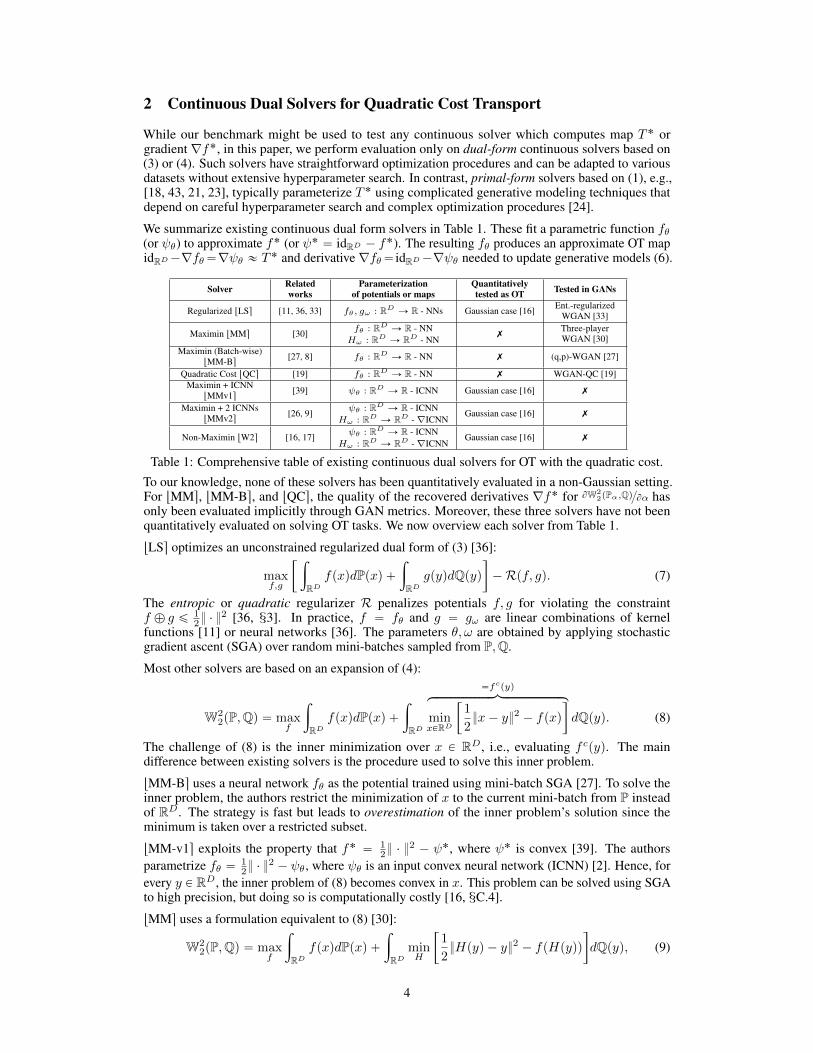
2 Continuous Dual Solvers for Quadratic Cost Transport

While our benchmark might be used to test any continuous solver which computes map T˚ orgradient ∇f˚, in this paper, we perform evaluation only on dual-form continuous solvers based on(3) or (4). Such solvers have straightforward optimization procedures and can be adapted to variousdatasets without extensive hyperparameter search. In contrast, primal-form solvers based on (1), e.g.,[18, 43, 21, 23], typically parameterize T˚ using complicated generative modeling techniques thatdepend on careful hyperparameter search and complex optimization procedures [24].

We summarize existing continuous dual form solvers in Table 1. These fit a parametric function fθ(or ψθ) to approximate f˚ (or ψ˚ “ idRD ´ f

˚). The resulting fθ produces an approximate OT mapidRD´∇fθ“∇ψθ « T˚ and derivative ∇fθ“ idRD´∇ψθ needed to update generative models (6).

Solver Relatedworks

Parameterizationof potentials or maps

Quantitativelytested as OT Tested in GANs

Regularized tLSs [11, 36, 33] fθ, gω : RD Ñ R - NNs Gaussian case [16] Ent.-regularizedWGAN [33]

Maximin tMMs [30] fθ : RD Ñ R - NNHω : RD Ñ RD - NN

7Three-playerWGAN [30]

Maximin (Batch-wise)tMM-Bs

[27, 8] fθ : RD Ñ R - NN 7 (q,p)-WGAN [27]

Quadratic Cost tQCs [19] fθ : RD Ñ R - NN 7 WGAN-QC [19]Maximin + ICNN

tMMv1s[39] ψθ : RD Ñ R - ICNN Gaussian case [16] 7

Maximin + 2 ICNNstMMv2s

[26, 9] ψθ : RD Ñ R - ICNNHω : RD Ñ RD - ∇ICNN

Gaussian case [16] 7

Non-Maximin tW2s [16, 17] ψθ : RD Ñ R - ICNNHω : RD Ñ RD - ∇ICNN

Gaussian case [16] 7

Table 1: Comprehensive table of existing continuous dual solvers for OT with the quadratic cost.

To our knowledge, none of these solvers has been quantitatively evaluated in a non-Gaussian setting.For tMMs, tMM-Bs, and tQCs, the quality of the recovered derivatives ∇f˚ for BW2

2pPα,Qq{Bα hasonly been evaluated implicitly through GAN metrics. Moreover, these three solvers have not beenquantitatively evaluated on solving OT tasks. We now overview each solver from Table 1.

tLSs optimizes an unconstrained regularized dual form of (3) [36]:

maxf,g

„ż

RDfpxqdPpxq `

ż

RDgpyqdQpyq

´Rpf, gq. (7)

The entropic or quadratic regularizer R penalizes potentials f, g for violating the constraintf ‘ g ď 1

2} ¨ }2 [36, M3]. In practice, f “ fθ and g “ gω are linear combinations of kernel

functions [11] or neural networks [36]. The parameters θ, ω are obtained by applying stochasticgradient ascent (SGA) over random mini-batches sampled from P,Q.

Most other solvers are based on an expansion of (4):

W22pP,Qq “ max

f

ż

RDfpxqdPpxq `

ż

RD

“fcpyqhkkkkkkkkkkkkkkkikkkkkkkkkkkkkkkj

minxPRD

„

1

2}x´ y}2 ´ fpxq

dQpyq. (8)

The challenge of (8) is the inner minimization over x P RD, i.e., evaluating f cpyq. The maindifference between existing solvers is the procedure used to solve this inner problem.

tMM-Bs uses a neural network fθ as the potential trained using mini-batch SGA [27]. To solve theinner problem, the authors restrict the minimization of x to the current mini-batch from P insteadof RD. The strategy is fast but leads to overestimation of the inner problem’s solution since theminimum is taken over a restricted subset.

tMM-v1s exploits the property that f˚ “ 12} ¨ }

2 ´ ψ˚, where ψ˚ is convex [39]. The authorsparametrize fθ “ 1

2} ¨ }2 ´ ψθ, where ψθ is an input convex neural network (ICNN) [2]. Hence, for

every y P RD, the inner problem of (8) becomes convex in x. This problem can be solved using SGAto high precision, but doing so is computationally costly [16, MC.4].

tMMs uses a formulation equivalent to (8) [30]:

W22pP,Qq “ max

f

ż

RDfpxqdPpxq `

ż

RDminH

„

1

2}Hpyq ´ y}2 ´ fpHpyqq

dQpyq, (9)

4

where the minimization is performed over functions H : RD Ñ RD. The authors use neuralnetworks fθ and Hω to parametrize the potential and the minimizer of the inner problem. To trainθ, ω, the authors apply stochastic gradient ascent/descent (SGAD) over mini-batches from P,Q.tMMs is generic and can be modified to compute arbitrary transport costs and derivatives, not justW2

2, although the authors have tested only on the Wasserstein-1 (W1) distance.

Similarly to tMMv1s, tMMv2s parametrizes fθ “ 12} ¨ }

2 ´ ψθ, where ψθ is an ICNN [26]. For afixed fθ, the optimal solution H is given by H “ p∇ψθq´1 which is an inverse gradient of a convexfunction, so it is also a gradient of a convex function. Hence, the authors parametrize Hω “ ∇φω,where φω is an ICNN, and use tMMs to fit θ, ω.

tW2s uses the same ICNN parametrization as [26] but introduces cycle-consistency regularization toavoid solving a maximin problem [16, M4].

Finally, we highlight the solver tQCs [19]. Similarly to tMM-Bs, a neural network fθ is used asthe potential. When each pair of mini-batches txnu, tynu from P,Q is sampled, the authors solve adiscrete OT problem to obtain dual variables tf˚n u, tg

˚nu, which are used to regress fθpxnq onto f˚n .

Gradient deviation. The solvers above optimize for potentials like fθ (or ψθ), but it is the gradientof fθ (or ψθ) that is used to recover the OT map via T “ x´∇fθ. Even if }f ´ f˚}2L2pPq is small,the difference }∇fθ ´∇f˚}2L2pPq may be arbitrarily large since ∇fθ is not directly involved inoptimization process. We call this issue gradient deviation. This issue is only addressed formally forICNN-based solvers tMMv1s, tMMv2s, tW2s [16, Theorem 4.1], [26, Theorem 3.6].

Reversed solvers. tMMs, tMMv2s, tW2s recover not only the forward OT map ∇ψθ « ∇ψ˚ “ T˚,but also the inverse, given by Hω « pT

˚q´1 “ p∇ψ˚q´1 “ ∇ψ˚, see [26, M3] or [16, M4.1]. Thesesolvers are asymmetric in P,Q and an alternative is to swap P and Q during training. We denote suchreversed solvers by tMM:Rs, tMMv2:Rs, tW2:Rs. In M4 we show that surprisingly tMM:Rs worksbetter in generative modeling than tMMs.

3 Benchmarking OT SolversIn this section, we develop a generic method to produce benchmark pairs, i.e., measures pP,Qq suchthat Q “ T 7P with sample access and an analytically known OT solution T˚ between them.

Key idea. Our method is based on the fact that for a differentiable convex function ψ : RD Ñ R,its gradient ∇ψ is an optimal transport map between any P P P2,acpRDq and its pushforward ∇ψ7Pby ∇ψ : RD Ñ RD. This follows from Brenier’s theorem [6], [41, Theorem 2.12]. Thus, for acontinuous measure P with sample access and a known convex ψ, pP,∇ψ7Pq can be used as abenchmark pair. We sample from ∇ψ7P by drawing samples from P and pushing forward by ∇ψ.

Arbitrary pairs pP,Qq. It is difficult to compute the exact continuous OT solution for an arbitrarypair pP,Qq. As a compromise, we compute an approximate transport map as the gradient of anICNN using tW2s. That is, we find ψθ parameterized as an ICNN such that ∇ψθ7P « Q. Then, themodified pair pP,∇ψθ7Pq can be used to benchmark OT solvers. We choose tW2s because it exhibitsgood performance in higher dimensions, but other solvers can also be used so long as ψθ is convex.Because of the choice of tW2s, subsequent evaluation might slightly favor ICNN-based methods.

Extensions. Convex functions can be modified to produce more benchmark pairs. If ψ1, . . . , ψN areconvex, then σpψ1, . . . , ψN q is convex when σ : RN Ñ R is convex and monotone. For example,c ¨ ψ1 (c ě 0q,

ř

n ψn, maxn

ψn are convex, and their gradients produce new benchmark pairs.

Inversion. If ∇ψθ is bijective, then the inverse transport map for pP,∇ψθ7Pq exists and is given byp∇ψθq´1. For each y P RD, the value p∇ψθq´1pyq can be obtained by solving a convex problem[39, M6], [16, M3]. All ICNNs ψθ we use have bijective gradients ∇ψθ, as detailed in Appendix B.1.

4 Benchmark Details and ResultsWe implement our benchmark in PyTorch and provide the pre-trained transport maps for all thebenchmark pairs. The code is publicly available at

https://github.com/iamalexkorotin/Wasserstein2BenchmarkThe experiments are conducted on 4 GTX 1080ti GPUs and require about 100 hours of computation(per GPU). We provide implementation details in Appendix B.

5

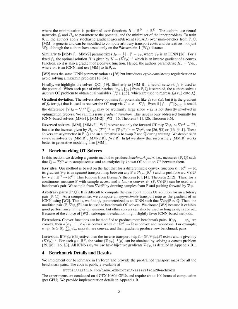
4.1 Datasets

High-dimensional measures. We develop benchmark pairs to test whether the OT solvers can redis-tribute mass among modes of measures. For this purpose, we use Gaussian mixtures in dimensionsD “ 21, 22, . . . , 28. In each dimension D, we consider a random mixture P of 3 Gaussians andtwo random mixtures Q1,Q2 of 10 Gaussians. We train approximate transport maps ∇ψi7P « Qi(i “ 1, 2) using the tW2s solver. Each potential is an ICNN with DenseICNN architecture [16, MB.2].We create a benchmark pair via the half-sum of computed potentials pP, 1

2 p∇ψ1 `∇ψ2q7Pq. Thefirst measure P is a mixture of 3 Gaussians and the second is obtained by averaging potentials, whichtransforms it to approximate mixtures of 10 Gaussians. See Appendix A.1 and Figure 1 for details.

Figure 1: An example of creation of a benchmark pair for dimension D “ 16. We first initialize3 random Gaussian Mixtures P and Q1,Q2 and fit 2 approximate OT maps ∇ψi7P « Qi, i “ 1, 2.We use the average of potentials to define the output measure: 1

2 p∇ψ1 `∇ψ2q7P. Each scatter plotcontains 512 random samples projected to 2 principle components of measure 1

2 p∇ψ1 `∇ψ2q7P.

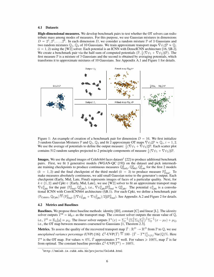
Images. We use the aligned images of CelebA64 faces dataset1 [22] to produce additional benchmarkpairs. First, we fit 3 generative models (WGAN-QC [19]) on the dataset and pick intermedi-ate training checkpoints to produce continuous measures QkEarly,QkMid,QkLate for the first 2 models(k “ 1, 2) and the final checkpoint of the third model (k “ 3) to produce measure P3

Final. Tomake measures absolutely continuous, we add small Gaussian noise to the generator’s output. Eachcheckpoint (Early, Mid, Late, Final) represents images of faces of a particular quality. Next, fork P t1, 2u and Cpkt P tEarly, Mid, Lateu, we use tW2s solver to fit an approximate transport map∇ψkCpkt for the pair pP3

Final,QkCpktq, i.e., ∇ψkCpkt7P3Final « QkCpkt. The potential ψkCpkt is a convolu-

tional ICNN with ConvICNN64 architecture (MB.1). For each Cpkt, we define a benchmark pairpPCelebA,QCpktq

def“pP3

Final, rp∇ψ1Cpkt `∇ψ2

Cpktq{2s7P3Finalq. See Appendix A.2 and Figure 2 for details.

4.2 Metrics and Baselines

Baselines. We propose three baseline methods: identity tIDs, constant tCs and linear tLs. The identitysolver outputs T id “ idRD as the transport map. The constant solver outputs the mean value of Q,

i.e., T 0 ” EQrys ” µQ. The linear solver outputs T 1pxq “ Σ´ 1

2

P`

Σ12

P ΣQΣ12

P˘

12 Σ

´ 12

P px´ µPq ` µQ,i.e., the OT map between measures coarsened to Gaussians [1, Theorem 2.3].

Metrics. To assess the quality of the recovered transport map T̂ : RD Ñ RD from P to Q, we useunexplained variance percentage (UVP) [16]: L2-UVPpT̂ q def

“ 100 ¨ }T̂ ´ T˚}2L2pPq{VarpQq%. Here

T˚ is the OT map. For values « 0%, T̂ approximates T˚ well. For values ě 100%, map T̂ is farfrom optimal. The constant baseline provides L2-UVPpT 0q “ 100%.

1http://mmlab.ie.cuhk.edu.hk/projects/CelebA.html

6

Figure 2: The pipeline of the image benchmark pair creation. We use 3 checkpoints of a generativemodel: P3

Final (well-fitted) and Q1Cpkt, Q2

Cpkt (under-fitted). For k “ 1, 2 we fit an approximateOT map P3

Final Ñ QkCpkt by ∇ψkCpkt, i.e. a gradient of ICNN. We define the benchmark pair by

pPCelebA,QCpktqdef“

`

P3Final,

12 p∇ψ

1Cpkt `∇ψ2

Cpktq7P3Final

˘

. In the visualization, Cpkt is Early.

To measure the quality of approximation of the derivative of the potential ridRD ´ T̂ s « ∇f˚ that isused to update generative models (6), we use cosine similarity (cos):

cospid´ T̂ , id´ T˚q def“

xT̂ ´ id,∇ψ˚ ´ idyL2pPq

}T˚ ´ id}L2pPq ¨ }T̂ ´ id}L2pPqP r´1, 1s.

To estimate L2-UVP and cos metrics, we use 214 random samples from P.

4.3 Evaluation of Solvers on High-dimensional Benchmark Pairs

We evaluate the solvers on the benchmark and report the computed metric values for the fittedtransport map. For fair comparison, in each method the potential f and the map H (where applicable)are parametrized as fθ “ 1

2} ¨ }2 ´ ψθ and Hω “ ∇φω respectively, where ψθ, φω use DenseICNN

architectures [16, MB.2]. In solvers tQCs, tLSs, tMM-Bs,tMMs we do not impose any restrictionson the weights θ, ω, i.e. ψθ, φω are usual fully connected nets with additional skip connections. Weprovide the computed metric values in Table 2 and visualize fitted maps (for D “ 64) in Figure 3.

All the solvers perform well (L2-UVP« 0, cos « 1) in dimensionD “ 2. In higher dimensions, onlytMMv1s, tMMs, tMMv2s, tW2s and their reversed versions produce reasonable results. However,tMMv1s solver is slow since each optimization step solves a hard subproblem for computing f c.Maximin solvers tMMs,tMMv2s,tMM:Rs are also hard to optimize: they either diverge from thestart (Û) or diverge after converging to nearly-optimal saddle point (í). This behavior is typical formaximin optimization and possibly can be avoided by a more careful choice of hyperparameters.

For tQCs, tLSs,tMM-Bs, as the dimension increases, the L2-UVP drastically grows. Only tMM-Bs

notably outperforms the trivial tLs baseline. The error of tMM-Bs is explained by the overestimationof the inner problem in (8), yielding biased optimal potentials. The error of tLSs comes from biasintroduced by regularization [36]. In tQCs, error arises because a discrete OT problem solved onsampled mini-batches, which is typically biased [5, Theorem 1], is used to update fθ. Interestingly,although tQCs, tLSs are imprecise in terms of L2-UVP, they provide a high cos metric.

Due to optimization issues and performance differences, wall-clock times for convergence arenot representative. All solvers except tMMv1s converged in several hours. Among solvers that

7

Dim 2 4 8 16 32 64 128 256tMMv1s 0.2 1.0 1.8 1.4 6.9 8.1 2.2 2.6tMMs 0.1 0.3 0.9 2.2 4.2 3.2 3.1í 4.1í

tMM:Rs 0.1 0.3 0.7 1.9 2.8 4.5 Û Û

tMMv2s 0.1 0.68 2.2 3.1 5.3 10.1í 3.2í 2.7í

tMMv2:Rs 0.1 0.7 4.4 7.7 5.8 6.8 2.1 2.8tW2s 0.1 0.7 2.6 3.3 6.0 7.2 2.0 2.7

tW2:Rs 0.2 0.9 4.0 5.3 5.2 7.0 2.0 2.7tMM-Bs 0.1 0.7 3.1 6.4 12.0 13.9 19.0 22.5

tLSs 5.0 11.6 21.5 31.7 42.1 40.1 46.8 54.7tLs 14.1 14.9 27.3 41.6 55.3 63.9 63.6 67.4

tQCs 1.5 14.5 28.6 47.2 64.0 75.2 80.5 88.2tCs 100 100 100 100 100 100 100 100tIDs 32.7 42.0 58.6 87 121 137 145 153

Dim 2 4 8 16 32 64 128 256tMMv1s 0.99 0.99 0.99 0.99 0.98 0.97 0.99 0.99

tMMs 0.99 0.99 0.99 0.99 0.99 0.99 0.99í 0.99í

tMM:Rs 0.99 1.00 1.00 0.99 1.00 0.98 Û Û

tMMv2s 0.99 0.99 0.99 0.99 0.99 0.96í 0.99í 0.99í

tMMv2:Rs 0.99 1.00 0.97 0.96 0.99 0.97 0.99 1.00tW2s 0.99 0.99 0.99 0.99 0.99 0.97 1.00 1.00

tW2:Rs 0.99 1.00 0.98 0.98 0.99 0.97 1.00 1.00tMM-Bs 0.99 1.00 0.98 0.96 0.96 0.94 0.93 0.93

tLSs 0.94 0.86 0.80 0.80 0.81 0.83 0.82 0.81tLs 0.75 0.80 0.73 0.73 0.76 0.75 0.77 0.77

tQCs 0.99 0.84 0.78 0.70 0.70 0.70 0.69 0.66tCs 0.29 0.32 0.38 0.46 0.55 0.58 0.60 0.62tIDs 0.00 0.00 0.00 0.00 0.00 0.00 0.00 0.00

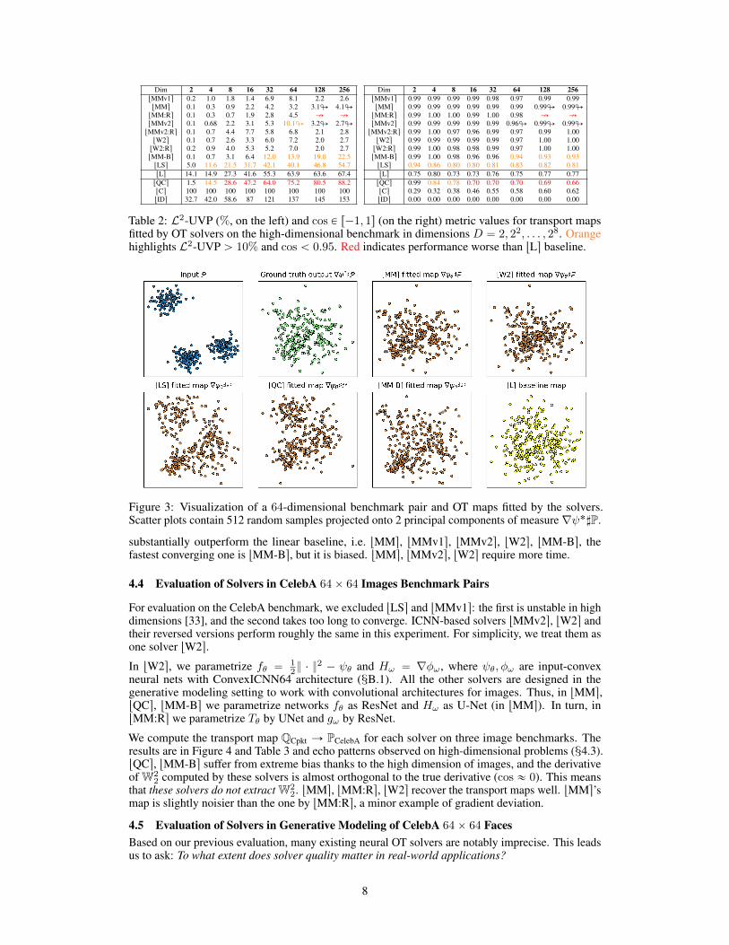
Table 2: L2-UVP (%, on the left) and cos P r´1, 1s (on the right) metric values for transport mapsfitted by OT solvers on the high-dimensional benchmark in dimensions D “ 2, 22, . . . , 28. Orangehighlights L2-UVP ą 10% and cos ă 0.95. Red indicates performance worse than tLs baseline.

Figure 3: Visualization of a 64-dimensional benchmark pair and OT maps fitted by the solvers.Scatter plots contain 512 random samples projected onto 2 principal components of measure ∇ψ˚7P.

substantially outperform the linear baseline, i.e. tMMs, tMMv1s, tMMv2s, tW2s, tMM-Bs, thefastest converging one is tMM-Bs, but it is biased. tMMs, tMMv2s, tW2s require more time.

4.4 Evaluation of Solvers in CelebA 64ˆ 64 Images Benchmark Pairs

For evaluation on the CelebA benchmark, we excluded tLSs and tMMv1s: the first is unstable in highdimensions [33], and the second takes too long to converge. ICNN-based solvers tMMv2s, tW2s andtheir reversed versions perform roughly the same in this experiment. For simplicity, we treat them asone solver tW2s.

In tW2s, we parametrize fθ “ 12} ¨ }

2 ´ ψθ and Hω “ ∇φω, where ψθ, φω are input-convexneural nets with ConvexICNN64 architecture (MB.1). All the other solvers are designed in thegenerative modeling setting to work with convolutional architectures for images. Thus, in tMMs,tQCs, tMM-Bs we parametrize networks fθ as ResNet and Hω as U-Net (in tMMs). In turn, intMM:Rs we parametrize Tθ by UNet and gω by ResNet.

We compute the transport map QCpkt Ñ PCelebA for each solver on three image benchmarks. Theresults are in Figure 4 and Table 3 and echo patterns observed on high-dimensional problems (M4.3).tQCs, tMM-Bs suffer from extreme bias thanks to the high dimension of images, and the derivativeof W2

2 computed by these solvers is almost orthogonal to the true derivative (cos « 0). This meansthat these solvers do not extract W2

2. tMMs, tMM:Rs, tW2s recover the transport maps well. tMMs’smap is slightly noisier than the one by tMM:Rs, a minor example of gradient deviation.

4.5 Evaluation of Solvers in Generative Modeling of CelebA 64ˆ 64 FacesBased on our previous evaluation, many existing neural OT solvers are notably imprecise. This leadsus to ask: To what extent does solver quality matter in real-world applications?

8

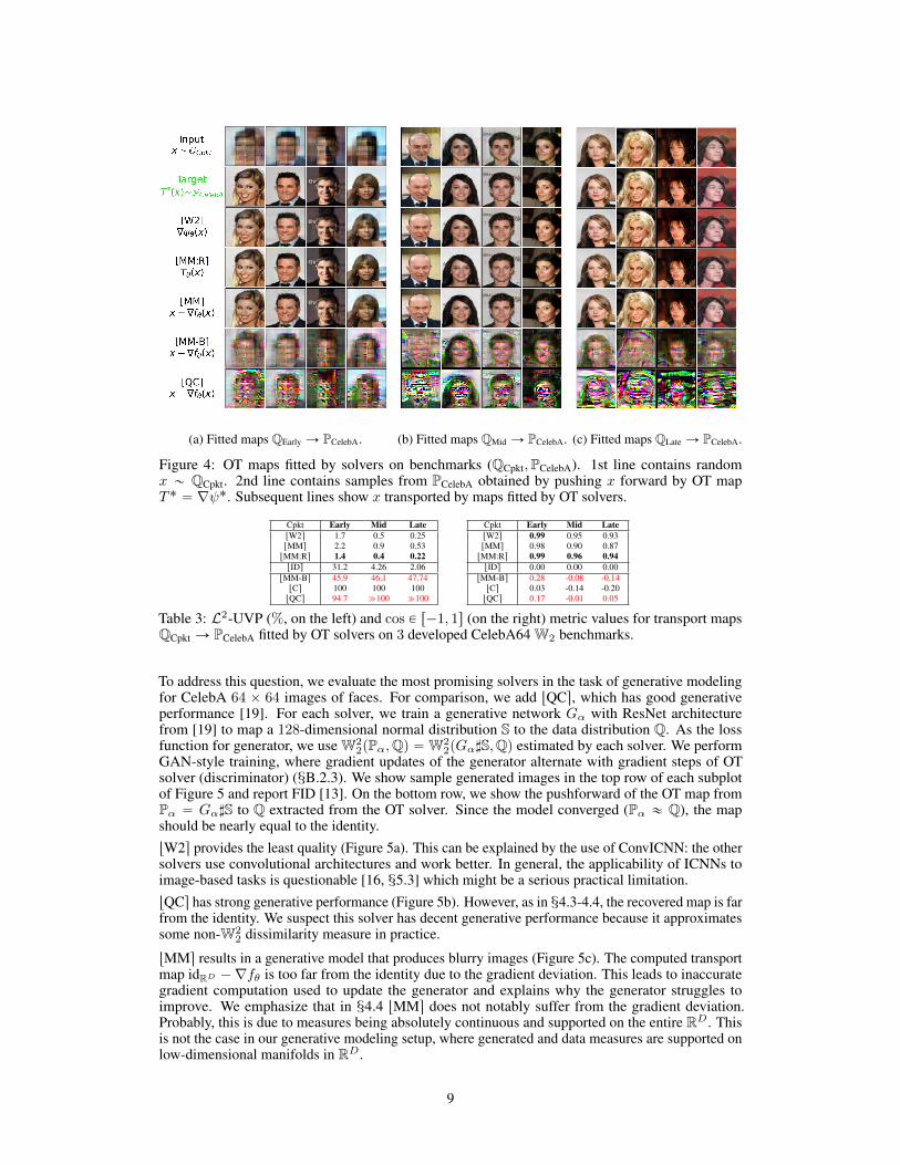
(a) Fitted maps QEarly Ñ PCelebA. (b) Fitted maps QMid Ñ PCelebA. (c) Fitted maps QLate Ñ PCelebA.

Figure 4: OT maps fitted by solvers on benchmarks (QCpkt,PCelebA). 1st line contains randomx „ QCpkt. 2nd line contains samples from PCelebA obtained by pushing x forward by OT mapT˚ “ ∇ψ˚. Subsequent lines show x transported by maps fitted by OT solvers.

Cpkt Early Mid LatetW2s 1.7 0.5 0.25tMMs 2.2 0.9 0.53

tMM:Rs 1.4 0.4 0.22tIDs 31.2 4.26 2.06

tMM-Bs 45.9 46.1 47.74tCs 100 100 100

tQCs 94.7 "100 "100

Cpkt Early Mid LatetW2s 0.99 0.95 0.93tMMs 0.98 0.90 0.87

tMM:Rs 0.99 0.96 0.94tIDs 0.00 0.00 0.00

tMM-Bs 0.28 -0.08 -0.14tCs 0.03 -0.14 -0.20

tQCs 0.17 -0.01 0.05

Table 3: L2-UVP (%, on the left) and cos P r´1, 1s (on the right) metric values for transport mapsQCpkt Ñ PCelebA fitted by OT solvers on 3 developed CelebA64 W2 benchmarks.

To address this question, we evaluate the most promising solvers in the task of generative modelingfor CelebA 64 ˆ 64 images of faces. For comparison, we add tQCs, which has good generativeperformance [19]. For each solver, we train a generative network Gα with ResNet architecturefrom [19] to map a 128-dimensional normal distribution S to the data distribution Q. As the lossfunction for generator, we use W2

2pPα,Qq “W22pGα7S,Qq estimated by each solver. We perform

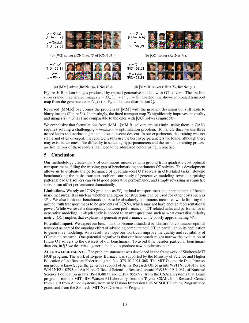
GAN-style training, where gradient updates of the generator alternate with gradient steps of OTsolver (discriminator) (MB.2.3). We show sample generated images in the top row of each subplotof Figure 5 and report FID [13]. On the bottom row, we show the pushforward of the OT map fromPα “ Gα7S to Q extracted from the OT solver. Since the model converged (Pα « Q), the mapshould be nearly equal to the identity.tW2s provides the least quality (Figure 5a). This can be explained by the use of ConvICNN: the othersolvers use convolutional architectures and work better. In general, the applicability of ICNNs toimage-based tasks is questionable [16, M5.3] which might be a serious practical limitation.tQCs has strong generative performance (Figure 5b). However, as in M4.3-4.4, the recovered map is farfrom the identity. We suspect this solver has decent generative performance because it approximatessome non-W2

2 dissimilarity measure in practice.

tMMs results in a generative model that produces blurry images (Figure 5c). The computed transportmap idRD ´∇fθ is too far from the identity due to the gradient deviation. This leads to inaccurategradient computation used to update the generator and explains why the generator struggles toimprove. We emphasize that in M4.4 tMMs does not notably suffer from the gradient deviation.Probably, this is due to measures being absolutely continuous and supported on the entire RD. Thisis not the case in our generative modeling setup, where generated and data measures are supported onlow-dimensional manifolds in RD.

9

(a) tW2s solver (ICNN ψθ , ∇ of ICNN Hω). (b) tQCs solver (ResNet fθ).

(c) tMMs solver (ResNet fθ , UNet Hω). (d) tMM:Rs solver (UNet Tθ , ResNet gω).

Figure 5: Random images produced by trained generative models with OT solvers. The 1st lineshows random generated images x “ Gαpzq „ Pα, z „ S. The 2nd line shows computed transportmap from the generated x “ Gαpzq „ Pα to the data distribution Q.

Reversed tMM:Rs overcomes the problem of tMMs with the gradient deviation but still leads toblurry images (Figure 5d). Interestingly, the fitted transport map Tθ significantly improves the qualityand images Tθ ˝Gαpzq are comparable to the ones with tQCs solver (Figure 5b).

We emphasize that formulations from tMMs, tMM:Rs solvers are maximin: using them in GANsrequires solving a challenging min-max-min optimization problem. To handle this, we use threenested loops and stochastic gradient descent-ascent-descent. In our experiments, the training was notstable and often diverged: the reported results use the best hyperparameters we found, although theremay exist better ones. The difficulty in selecting hyperparameters and the unstable training processare limitations of these solvers that need to be addressed before using in practice.

5 ConclusionOur methodology creates pairs of continuous measures with ground truth quadratic-cost optimaltransport maps, filling the missing gap of benchmarking continuous OT solvers. This developmentallows us to evaluate the performance of quadratic-cost OT solvers in OT-related tasks. Beyondbenchmarking the basic transport problem, our study of generative modeling reveals surprisingpatterns: bad OT solvers can yield good generative performance, and simply reversing asymmetricsolvers can affect performance dramatically.Limitations. We rely on ICNN gradients as W2 optimal transport maps to generate pairs of bench-mark measures. It is unclear whether analogous constructions can be used for other costs such asW1. We also limit our benchmark pairs to be absolutely continuous measures while limiting theground truth transport maps to be gradients of ICNNs, which may not have enough representationalpower. While we reveal a discrepancy between performance in OT-related tasks and performance ingenerative modeling, in-depth study is needed to answer questions such as what exact dissimilaritymetric tQCs implies that explains its generative performance while poorly approximating W2.Potential impact. We expect our benchmark to become a standard benchmark for continuous optimaltransport as part of the ongoing effort of advancing computational OT, in particular, in its applicationto generative modeling. As a result, we hope our work can improve the quality and reusability ofOT-related research. One potential negative is that our benchmark might narrow the evaluation offuture OT solvers to the datasets of our benchmark. To avoid this, besides particular benchmarkdatasets, in M3 we describe a generic method to produce new benchmark pairs.ACKNOWLEDGEMENTS. The problem statement was developed in the framework of Skoltech-MITNGP program. The work of Evgeny Burnaev was supported by the Ministry of Science and HigherEducation of the Russian Federation grant No. 075-10-2021-068. The MIT Geometric Data Process-ing group acknowledges the generous support of Army Research Office grants W911NF2010168 andW911NF2110293, of Air Force Office of Scientific Research award FA9550-19-1-031, of NationalScience Foundation grants IIS-1838071 and CHS-1955697, from the CSAIL Systems that Learnprogram, from the MIT–IBM Watson AI Laboratory, from the Toyota–CSAIL Joint Research Center,from a gift from Adobe Systems, from an MIT.nano Immersion Lab/NCSOFT Gaming Program seedgrant, and from the Skoltech–MIT Next Generation Program.

10

References[1] Pedro C Álvarez-Esteban, E Del Barrio, JA Cuesta-Albertos, and C Matrán. A fixed-point ap-

proach to barycenters in Wasserstein space. Journal of Mathematical Analysis and Applications,441(2):744–762, 2016.

[2] Brandon Amos, Lei Xu, and J Zico Kolter. Input convex neural networks. In Proceedings of the34th International Conference on Machine Learning-Volume 70, pages 146–155. JMLR. org,2017.

[3] Martin Arjovsky, Soumith Chintala, and Léon Bottou. Wasserstein GAN. arXiv preprintarXiv:1701.07875, 2017.

[4] Jonathan T Barron. Continuously differentiable exponential linear units. arXiv preprintarXiv:1704.07483, 2017.

[5] Marc G Bellemare, Ivo Danihelka, Will Dabney, Shakir Mohamed, Balaji Lakshminarayanan,Stephan Hoyer, and Rémi Munos. The cramer distance as a solution to biased Wassersteingradients. arXiv preprint arXiv:1705.10743, 2017.

[6] Yann Brenier. Polar factorization and monotone rearrangement of vector-valued functions.Communications on pure and applied mathematics, 44(4):375–417, 1991.

[7] Jiezhang Cao, Langyuan Mo, Yifan Zhang, Kui Jia, Chunhua Shen, and Mingkui Tan. Multi-marginal Wasserstein GAN. arXiv preprint arXiv:1911.00888, 2019.

[8] Yucheng Chen, Matus Telgarsky, Chao Zhang, Bolton Bailey, Daniel Hsu, and Jian Peng.A gradual, semi-discrete approach to generative network training via explicit Wassersteinminimization. In International Conference on Machine Learning, pages 1071–1080. PMLR,2019.

[9] Jiaojiao Fan, Amirhossein Taghvaei, and Yongxin Chen. Scalable computations of Wassersteinbarycenter via input convex neural networks. arXiv preprint arXiv:2007.04462, 2020.

[10] Werner Fenchel. On conjugate convex functions. Canadian Journal of Mathematics, 1(1):73–77,1949.

[11] Aude Genevay, Marco Cuturi, Gabriel Peyré, and Francis Bach. Stochastic optimization forlarge-scale optimal transport. In Advances in neural information processing systems, pages3440–3448, 2016.

[12] Ishaan Gulrajani, Faruk Ahmed, Martin Arjovsky, Vincent Dumoulin, and Aaron C Courville.Improved training of Wasserstein GANs. In Advances in Neural Information ProcessingSystems, pages 5767–5777, 2017.

[13] Martin Heusel, Hubert Ramsauer, Thomas Unterthiner, Bernhard Nessler, and Sepp Hochreiter.GANs trained by a two time-scale update rule converge to a local nash equilibrium. In Advancesin neural information processing systems, pages 6626–6637, 2017.

[14] Leonid Kantorovitch. On the translocation of masses. Management Science, 5(1):1–4, 1958.[15] Diederik P Kingma and Jimmy Ba. Adam: A method for stochastic optimization. arXiv preprint

arXiv:1412.6980, 2014.[16] Alexander Korotin, Vage Egiazarian, Arip Asadulaev, Alexander Safin, and Evgeny Burnaev.

Wasserstein-2 generative networks. In International Conference on Learning Representations,2021.

[17] Alexander Korotin, Lingxiao Li, Justin Solomon, and Evgeny Burnaev. Continuous wasserstein-2 barycenter estimation without minimax optimization. In International Conference on LearningRepresentations, 2021.

[18] Jacob Leygonie, Jennifer She, Amjad Almahairi, Sai Rajeswar, and Aaron Courville. Adversarialcomputation of optimal transport maps. arXiv preprint arXiv:1906.09691, 2019.

[19] Huidong Liu, Xianfeng Gu, and Dimitris Samaras. Wasserstein GAN with quadratic transportcost. In Proceedings of the IEEE International Conference on Computer Vision, pages 4832–4841, 2019.

[20] Huidong Liu, GU Xianfeng, and Dimitris Samaras. A two-step computation of the exact GANWasserstein distance. In International Conference on Machine Learning, pages 3159–3168.PMLR, 2018.

11

[21] Shu Liu, Shaojun Ma, Yongxin Chen, Hongyuan Zha, and Haomin Zhou. Learning highdimensional Wasserstein geodesics. arXiv preprint arXiv:2102.02992, 2021.

[22] Ziwei Liu, Ping Luo, Xiaogang Wang, and Xiaoou Tang. Deep learning face attributes in thewild. In Proceedings of International Conference on Computer Vision (ICCV), December 2015.

[23] Guansong Lu, Zhiming Zhou, Jian Shen, Cheng Chen, Weinan Zhang, and Yong Yu. Large-scale optimal transport via adversarial training with cycle-consistency. arXiv preprintarXiv:2003.06635, 2020.

[24] Mario Lucic, Karol Kurach, Marcin Michalski, Sylvain Gelly, and Olivier Bousquet. Are GANscreated equal? a large-scale study. In Advances in neural information processing systems, pages700–709, 2018.

[25] Yun Luo, Si-Yang Zhang, Wei-Long Zheng, and Bao-Liang Lu. WGAN domain adaptation foreeg-based emotion recognition. In International Conference on Neural Information Processing,pages 275–286. Springer, 2018.

[26] Ashok Vardhan Makkuva, Amirhossein Taghvaei, Sewoong Oh, and Jason D Lee. Optimaltransport mapping via input convex neural networks. arXiv preprint arXiv:1908.10962, 2019.

[27] Anton Mallasto, Jes Frellsen, Wouter Boomsma, and Aasa Feragen. (q, p)-Wasserstein GANs:Comparing ground metrics for Wasserstein GANs. arXiv preprint arXiv:1902.03642, 2019.

[28] Anton Mallasto, Guido Montúfar, and Augusto Gerolin. How well do WGANs estimate theWasserstein metric? arXiv preprint arXiv:1910.03875, 2019.

[29] Paul Milgrom and Ilya Segal. Envelope theorems for arbitrary choice sets. Econometrica,70(2):583–601, 2002.

[30] Quan Hoang Nhan Dam, Trung Le, Tu Dinh Nguyen, Hung Bui, and Dinh Phung. ThreeplayerWasserstein GAN via amortised duality. In Proc. of the 28th Int. Joint Conf. on ArtificialIntelligence (IJCAI), 2019.

[31] Gabriel Peyré, Marco Cuturi, et al. Computational optimal transport. Foundations and Trends®in Machine Learning, 11(5-6):355–607, 2019.

[32] Thomas Pinetz, Daniel Soukup, and Thomas Pock. On the estimation of the Wassersteindistance in generative models. In German Conference on Pattern Recognition, pages 156–170.Springer, 2019.

[33] Maziar Sanjabi, Jimmy Ba, Meisam Razaviyayn, and Jason D Lee. On the convergence and ro-bustness of training GANs with regularized optimal transport. arXiv preprint arXiv:1802.08249,2018.

[34] Filippo Santambrogio. Optimal transport for applied mathematicians. Birkäuser, NY, 55(58-63):94, 2015.

[35] Jörn Schrieber, Dominic Schuhmacher, and Carsten Gottschlich. Dotmark–a benchmark fordiscrete optimal transport. IEEE Access, 5:271–282, 2016.

[36] Vivien Seguy, Bharath Bhushan Damodaran, Rémi Flamary, Nicolas Courty, Antoine Rolet,and Mathieu Blondel. Large-scale optimal transport and mapping estimation. arXiv preprintarXiv:1711.02283, 2017.

[37] Jian Shen, Yanru Qu, Weinan Zhang, and Yong Yu. Wasserstein distance guided representationlearning for domain adaptation. In Proceedings of the AAAI Conference on Artificial Intelligence,volume 32, 2018.

[38] Jan Stanczuk, Christian Etmann, Lisa Maria Kreusser, and Carola-Bibiane Schonlieb. Wasser-stein GANs work because they fail (to approximate the Wasserstein distance). arXiv preprintarXiv:2103.01678, 2021.

[39] Amirhossein Taghvaei and Amin Jalali. 2-Wasserstein approximation via restricted convexpotentials with application to improved training for GANs. arXiv preprint arXiv:1902.07197,2019.

[40] Cédric Villani. Topics in optimal transportation. Number 58. American Mathematical Soc.,2003.

[41] Cédric Villani. Optimal transport: old and new, volume 338. Springer Science & BusinessMedia, 2008.

12

[42] Jiqing Wu, Zhiwu Huang, Janine Thoma, Dinesh Acharya, and Luc Van Gool. Wassersteindivergence for GANs. In Proceedings of the European Conference on Computer Vision (ECCV),pages 653–668, 2018.

[43] Yujia Xie, Minshuo Chen, Haoming Jiang, Tuo Zhao, and Hongyuan Zha. On scalable andefficient computation of large scale optimal transport. volume 97 of Proceedings of MachineLearning Research, pages 6882–6892, Long Beach, California, USA, 09–15 Jun 2019. PMLR.

13

A Benchmark Pairs Details

In Appendix A.1 we discuss the details of high-dimensional benchmark pairs. Appendix A.2 isdevoted to Celeba 64ˆ 64 images benchmark pairs.

A.1 High-dimensional Benchmark Pairs

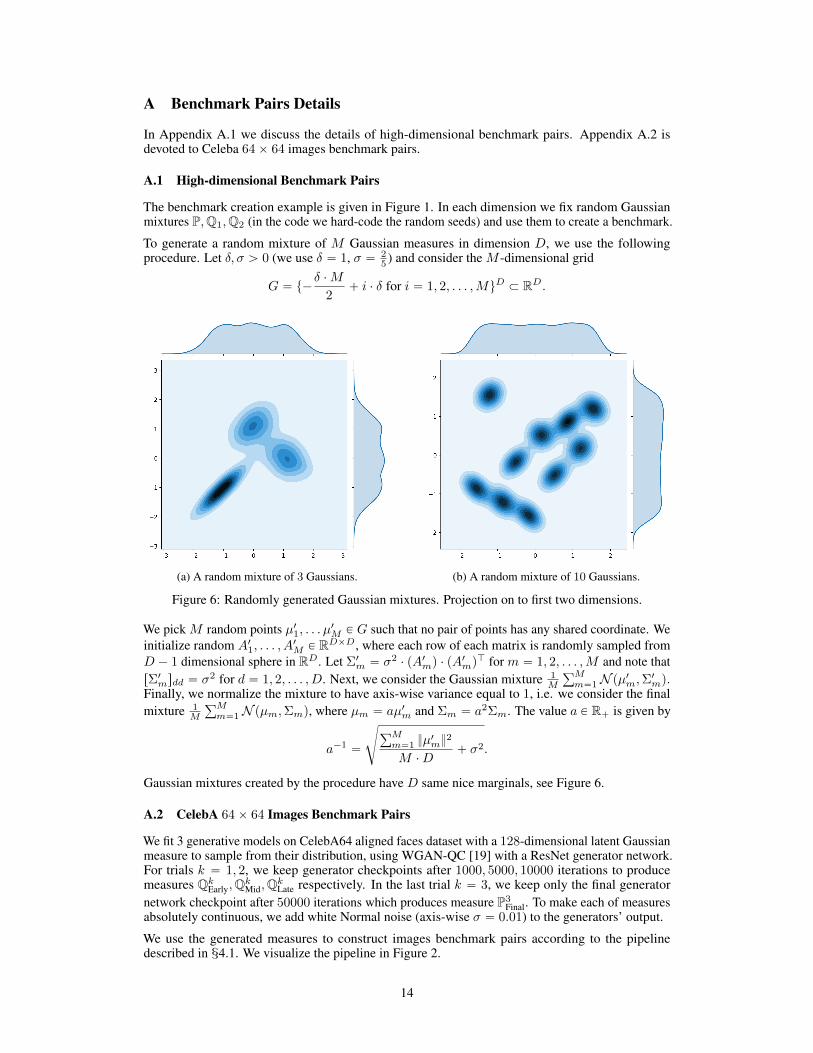
The benchmark creation example is given in Figure 1. In each dimension we fix random Gaussianmixtures P,Q1,Q2 (in the code we hard-code the random seeds) and use them to create a benchmark.

To generate a random mixture of M Gaussian measures in dimension D, we use the followingprocedure. Let δ, σ ą 0 (we use δ “ 1, σ “ 2

5 ) and consider the M -dimensional grid

G “ t´δ ¨M

2` i ¨ δ for i “ 1, 2, . . . ,MuD Ă RD.

(a) A random mixture of 3 Gaussians. (b) A random mixture of 10 Gaussians.

Figure 6: Randomly generated Gaussian mixtures. Projection on to first two dimensions.

We pick M random points µ11, . . . µ1M P G such that no pair of points has any shared coordinate. We

initialize random A11, . . . , A1M P RDˆD, where each row of each matrix is randomly sampled from

D ´ 1 dimensional sphere in RD. Let Σ1m “ σ2 ¨ pA1mq ¨ pA1mqJ for m “ 1, 2, . . . ,M and note that

rΣ1msdd “ σ2 for d “ 1, 2, . . . , D. Next, we consider the Gaussian mixture 1M

řMm“1 N pµ1m,Σ1mq.

Finally, we normalize the mixture to have axis-wise variance equal to 1, i.e. we consider the finalmixture 1

M

řMm“1 N pµm,Σmq, where µm “ aµ1m and Σm “ a2Σm. The value a P R` is given by

a´1 “

d

řMm“1 }µ

1m}

2

M ¨D` σ2.

Gaussian mixtures created by the procedure have D same nice marginals, see Figure 6.

A.2 CelebA 64ˆ 64 Images Benchmark Pairs

We fit 3 generative models on CelebA64 aligned faces dataset with a 128-dimensional latent Gaussianmeasure to sample from their distribution, using WGAN-QC [19] with a ResNet generator network.For trials k “ 1, 2, we keep generator checkpoints after 1000, 5000, 10000 iterations to producemeasures QkEarly,QkMid,QkLate respectively. In the last trial k “ 3, we keep only the final generatornetwork checkpoint after 50000 iterations which produces measure P3

Final. To make each of measuresabsolutely continuous, we add white Normal noise (axis-wise σ “ 0.01) to the generators’ output.

We use the generated measures to construct images benchmark pairs according to the pipelinedescribed in M4.1. We visualize the pipeline in Figure 2.

14

B Experimental Details

In Appendix B.1, we discuss the neural network architectures we used in experiments. All the othertraining hyperparameters are given in Appendix B.2.

B.1 Neural Network Architectures

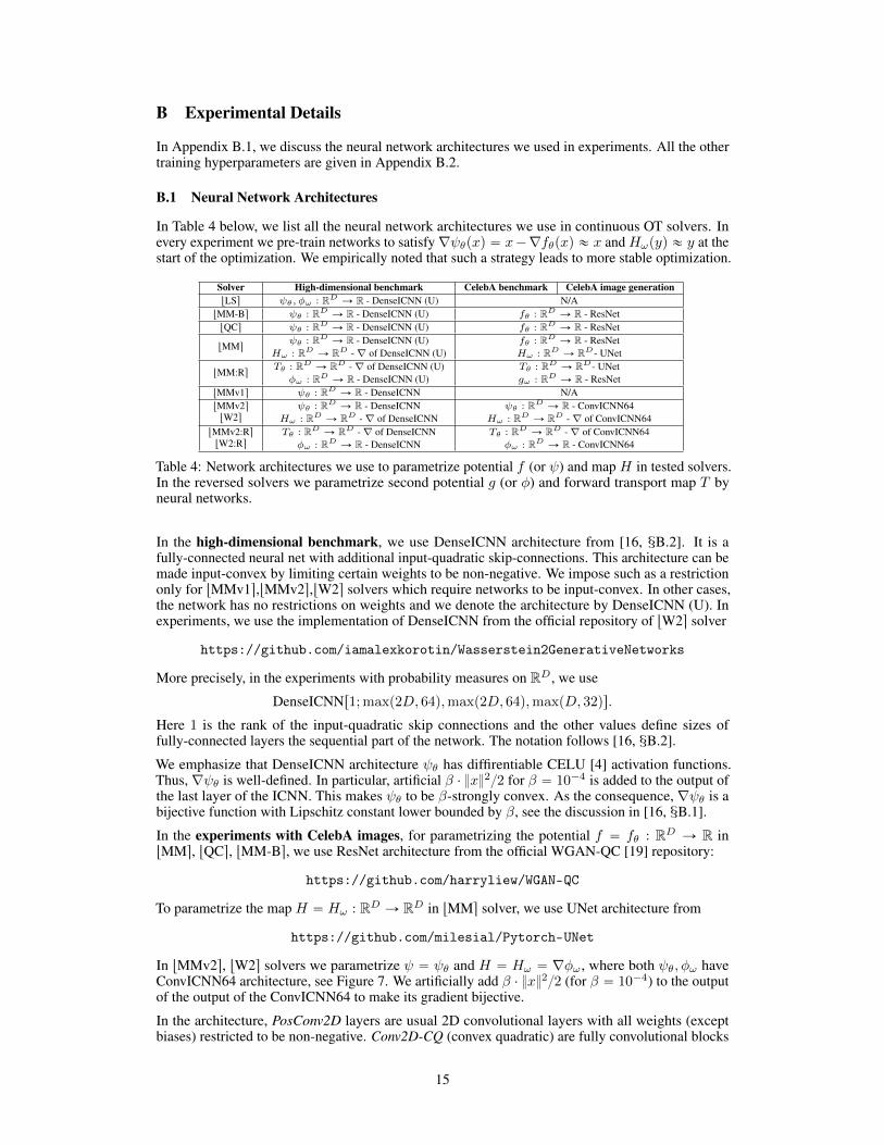
In Table 4 below, we list all the neural network architectures we use in continuous OT solvers. Inevery experiment we pre-train networks to satisfy ∇ψθpxq “ x´∇fθpxq « x and Hωpyq « y at thestart of the optimization. We empirically noted that such a strategy leads to more stable optimization.

Solver High-dimensional benchmark CelebA benchmark CelebA image generationtLSs ψθ, φω : RD Ñ R - DenseICNN (U) N/A

tMM-Bs ψθ : RD Ñ R - DenseICNN (U) fθ : RD Ñ R - ResNettQCs ψθ : RD Ñ R - DenseICNN (U) fθ : RD Ñ R - ResNet

tMMsψθ : RD Ñ R - DenseICNN (U)

Hω : RD Ñ RD - ∇ of DenseICNN (U)fθ : RD Ñ R - ResNetHω : RD Ñ RD- UNet

tMM:RsTθ : RD Ñ RD - ∇ of DenseICNN (U)φω : RD Ñ R - DenseICNN (U)

Tθ : RD Ñ RD- UNetgω : RD Ñ R - ResNet

tMMv1s ψθ : RD Ñ R - DenseICNN N/AtMMv2s

tW2s

ψθ : RD Ñ R - DenseICNNHω : RD Ñ RD - ∇ of DenseICNN

ψθ : RD Ñ R - ConvICNN64Hω : RD Ñ RD - ∇ of ConvICNN64

tMMv2:Rs

tW2:Rs

Tθ : RD Ñ RD - ∇ of DenseICNNφω : RD Ñ R - DenseICNN

Tθ : RD Ñ RD - ∇ of ConvICNN64φω : RD Ñ R - ConvICNN64

Table 4: Network architectures we use to parametrize potential f (or ψ) and map H in tested solvers.In the reversed solvers we parametrize second potential g (or φ) and forward transport map T byneural networks.

In the high-dimensional benchmark, we use DenseICNN architecture from [16, MB.2]. It is afully-connected neural net with additional input-quadratic skip-connections. This architecture can bemade input-convex by limiting certain weights to be non-negative. We impose such as a restrictiononly for tMMv1s,tMMv2s,tW2s solvers which require networks to be input-convex. In other cases,the network has no restrictions on weights and we denote the architecture by DenseICNN (U). Inexperiments, we use the implementation of DenseICNN from the official repository of tW2s solver

https://github.com/iamalexkorotin/Wasserstein2GenerativeNetworks

More precisely, in the experiments with probability measures on RD, we use

DenseICNNr1; maxp2D, 64q,maxp2D, 64q,maxpD, 32qs.

Here 1 is the rank of the input-quadratic skip connections and the other values define sizes offully-connected layers the sequential part of the network. The notation follows [16, MB.2].

We emphasize that DenseICNN architecture ψθ has diffirentiable CELU [4] activation functions.Thus, ∇ψθ is well-defined. In particular, artificial β ¨ }x}2{2 for β “ 10´4 is added to the output ofthe last layer of the ICNN. This makes ψθ to be β-strongly convex. As the consequence, ∇ψθ is abijective function with Lipschitz constant lower bounded by β, see the discussion in [16, MB.1].

In the experiments with CelebA images, for parametrizing the potential f “ fθ : RD Ñ R intMMs, tQCs, tMM-Bs, we use ResNet architecture from the official WGAN-QC [19] repository:

https://github.com/harryliew/WGAN-QC

To parametrize the map H “ Hω : RD Ñ RD in tMMs solver, we use UNet architecture from

https://github.com/milesial/Pytorch-UNet

In tMMv2s, tW2s solvers we parametrize ψ “ ψθ and H “ Hω “ ∇φω, where both ψθ, φω haveConvICNN64 architecture, see Figure 7. We artificially add β ¨ }x}2{2 (for β “ 10´4) to the outputof the output of the ConvICNN64 to make its gradient bijective.

In the architecture, PosConv2D layers are usual 2D convolutional layers with all weights (exceptbiases) restricted to be non-negative. Conv2D-CQ (convex quadratic) are fully convolutional blocks

15

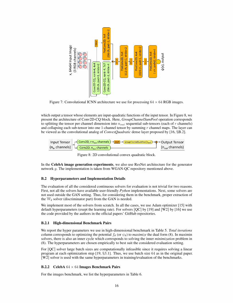
Figure 7: Convolutional ICNN architecture we use for processing 64ˆ 64 RGB images.

which output a tensor whose elements are input-quadratic functions of the input tensor. In Figure 8, wepresent the architecture of Conv2D-CQ block. Here, GroupChannelSumPool operation correspondsto splitting the tensor per channel dimension into nout sequential sub-tensors (each of r channels)and collapsing each sub-tensor into one 1-channel tensor by summing r channel maps. The layer canbe viewed as the convolutional analog of ConvexQuadratic dense layer proposed by [16, MB.2].

Figure 8: 2D convolutional convex quadratic block.

In the CelebA image generation experiments, we also use ResNet architecture for the generatornetwork g. The implementation is taken from WGAN-QC repository mentioned above.

B.2 Hyperparameters and Implementation Details

The evaluation of all the considered continuous solvers for evaluation is not trivial for two reasons.First, not all the solvers have available user-friendly Python implementations. Next, some solvers arenot used outside the GAN setting. Thus, for considering them in the benchmark, proper extraction ofthe W2 solver (discriminator part) from the GAN is needed.

We implement most of the solvers from scratch. In all the cases, we use Adam optimizer [15] withdefault hyperparameters (exept the learning rate). For solvers tQCs by [19] and tW2s by [16] we usethe code provided by the authors in the official papers’ GitHub repositories.

B.2.1 High-dimensional Benchmark Pairs

We report the hyper parameters we use in high-dimensional benchmark in Table 5. Total iterationscolumn corresponds to optimizing the potential fθ (or ψθ) to maximize the dual form (8). In maximinsolvers, there is also an inner cycle which corresponds to solving the inner minimization problem in(8). The hyperparameters are chosen empirically to best suit the considered evaluation setting.

For tQCs solver large batch sizes are computationally infeasible since it requires solving a linearprogram at each optimization step [19, M3.1]. Thus, we use batch size 64 as in the original paper.tW2s solver is used with the same hyperparameters in training/evaluation of the benchmarks.

B.2.2 CelebA 64ˆ 64 Images Benchmark Pairs

For the images benchmark, we list the hyperparameters in Table 6.

16

Solver Batch Size Total Iterations LR Note

tLSs 1024 100000 10´3 Quadratic regularizationwith ε “ 3 ¨ 10´2, see [36, Eq. (7)]

tMM-Bs 1024 100000 10´3 None

tQCs 64 100000 10´3 OT regularizationwithK “ 1, γ “ 0.1, see [19, Eq. (10)]

tMMv1s 1024 20000 10´31000 gradient iterations (lr “ 0.3)

to compute argmin in (8), see [39, M6].Early stop when gradient normă 10´3.

tMMs,tMMv2s 1024 50000 10´3 15 inner cycle iterations to updateHω ,(K “ 15 in the notation of [26, Algorithm 1])

tW2s 1024 250000 10´3 Cycle-consistency regularization,λ “ D, see [16, Algorithm 1]

Table 5: Hyperparameters of solvers we use in high-dimensional benchmark. Reversed are notpresdented in this table: they use the same hyperparameters as their original versions.

Solver Batch Size Total Iterations LR NotetMM-Bs 64 20000 3 ¨ 10´4 None

tQCs 64 20000 3 ¨ 10´4 OT regularizationwithK “ 1, γ “ 0.1, see [19, Eq. (10)]

tMMs 64 50000 3 ¨ 10´4 5 inner cycle iterations to updateHω ,(K “ 5 in the notation of [26, Algorithm 1])

tW2s 64 50000 3 ¨ 10´4 Cycle-consistency regularization,λ “ 104, see [16, Algorithm 1]

Table 6: Hyperparameters of solvers we use in CelebA images benchmark.

B.2.3 CelebA 64ˆ 64 Images Generation Experiment

To train a generative model, we use GAN-style training: generator networkGα updates are alternatingwith OT solver’s updates (discriminator’s update). The learning rate for the generator network is3 ¨ 10´4 and the total number of generator iterations is 50000.

In tQCs solver we use the code by the authors: there is one gradient update of OT solver per generatorupdate. In all the rest methods, we alternate 1 generator update with 10 updates of OT solver(iterations in notation of Table 6). All the rest hyperparameters match the previous experiment.

The generator’s gradient w.r.t. parameters α on a mini-batch z1, . . . , zN „ S is given by

BW22pPα,Qq{Bα “

ż

z

JαGαpzqT∇f˚

`

Gαpzq˘

dSpzq «1

N

Nÿ

n“1

JαGαpznqT∇fθ

`

Gαpznq˘

(10)

where S is the latent space measure and fθ is the current potential (discriminator) of OT solver. Notethat in tMM:Rs potential f is not computed but the forward OT map Tθ is parametrized instead. Inthis case, we estimate the gradient (10) on a mini-batch by 1

N

řNn“1 JαGαpznq

T pidRD ´ Tθq.

17