System F input u(t) output y(t) System F input u(t) System G output y(t) 2 LINEAR SYSTEMS 2 2 LINEAR SYSTEMS We will discuss what we mean by a linear time-invariant system, and then consider several useful transforms. 2.1 Definition of a System In short, a system is any process or entity that has one or more well-defined inputs and one or more well-defined outputs. Examples of systems include a simple physical object obeying Newtonian mechanics, and the US economy! Systems can be physical, or we may talk about a mathematical description of a system. The point of modeling is to capture in a mathematical representation the behavior of a physical system. As we will see, such representation lends itself to analysis and design, and certain restrictions such as linearity and time-invariance open a huge set of available tools. We often use a block diagram form to describe systems, and in particular their interconnec tions: In the second case shown, y(t) = G[F [u(t)]]. Looking at structure now and starting with the most abstracted and general case, we may write a system as a function relating the input to the output; as written these are both functions of time: y(t) = F [u(t)] The system captured in F can be a multiplication by some constant factor - an example of a static system, or a hopelessly complex set of differential equations - an example of a dynamic system. If we are talking about a dynamical system, then by definition the mapping from u(t) to y(t) is such that the current value of the output y(t) depends on the past history of u(t). Several examples are: t y(t) = u 2 (t 1 )dt 1 , t−3 N y(t) = u(t) + u(t − nδt). n=1 In the second case, δt is a constant time step, and hence y(t) has embedded in it the current input plus a set of N delayed versions of the input.

Welcome message from author
This document is posted to help you gain knowledge. Please leave a comment to let me know what you think about it! Share it to your friends and learn new things together.
Transcript
8202019 Linear Systems Review
httpslidepdfcomreaderfulllinear-systems-review 114
System Finput u(t) output y(t)
System Finput u(t)
System Goutput y(t)
2 LINEAR SYSTEMS 2
2 LINEAR SYSTEMS
We will discuss what we mean by a linear time-invariant system and then consider several
useful
transforms
21 Definition of a System
In short a system is any process or entity that has one or more well-defined inputs and one
or more well-defined outputs Examples of systems include a simple physical object obeying
Newtonian mechanics and the US economy
Systems can be physical or we may talk about a mathematical description of a system The
point of modeling is to capture in a mathematical representation the behavior of a physical
system
As
we
will
see
such
representation
lends
itself
to
analysis
and
design
and
certain restrictions such as linearity and time-invariance open a huge set of available tools
We often use a block diagram form to describe systems and in particular their interconnections
In
the
second
case
shown
y(t) =
G[F
[u(t)]]
Looking
at
structure
now
and
starting
with
the
most
abstracted
and
general
case
we
may
write a system as a function relating the input to the output as written these are both
functions of time
y(t) = F [u(t)]
The system captured in F can be a multiplication by some constant factor - an example of a
static system or a hopelessly complex set of differential equations - an example of a dynamic
system If we are talking about a dynamical system then by definition the mapping from
u(t) to y(t) is such that the current value of the output y(t) depends on the past history of
u(t)
Several
examples
are
t
y(t) = u
2(t1)dt1 tminus3
N
y(t) = u(t) +
u(t minus nδt) n=1
In the second case δt is a constant time step and hence y(t) has embedded in it the current
input plus a set of N delayed versions of the input
8202019 Linear Systems Review
httpslidepdfcomreaderfulllinear-systems-review 214
u(t)
y(t)
u(t-)
y(t-)
2 LINEAR SYSTEMS 3
22 Time-Invariant Systems
A dynamic system is time-invariant if shifting the input on the time axis leads to an equivalent
shifting
of
the
output
along
the
time
axis
with
no
other
changes
In
other
words
a
time-invariant system maps a given input trajectory u(t) no matter when it occurs
y(t minus τ ) = F [u(t minus τ )]
The formula above says specifically that if an input signal is delayed by some amount τ so
will be the output and with no other changes
An example of a physical time-varying system is the pitch response of a rocket y(t) when
the thrusters are being steered by an angle u(t) You can see first that this is an inverted
pendulum
problem
and
unstable
without
a
closed-loop
controller
It
is
time-varying
because
as the rocket burns fuel its mass is changing and so the pitch responds differently to various
inputs
throughout
its
flight
In
this
case
the
rdquoabsolute
timerdquo
coordinate
is
the
time
since
liftoff
To assess whether a system is time-varying or not follow these steps replace u(t) with
u(t minus τ ) on one side of the equation replace y(t) with y(t minus τ ) on the other side of the
equation and then check if they are equal Here are several examples
y(t) = u(t)32
This system is clearly time-invariant because it is a static map Next example
t
y(t) = u(t1)dt1
0
Replace u(t1) with u(t1
minus τ ) in the right hand side and carry it through t
u(t1
minus τ )dt1
=
tminusτ
u(t2)dt2 0 minusτ
The left hand side is simply
y(t minus τ ) =
tminusτ
u(t1)dt1
0
8202019 Linear Systems Review
httpslidepdfcomreaderfulllinear-systems-review 314
2 LINEAR SYSTEMS 4
Clearly the right and left hand sides are not equal (the limits of integration are different) and hence the system is not time-invariant As another example consider
t y(t) =
u
2
(t1)dt1 tminus5
The right-hand side becomes with the time shift t u
2(t1
minus τ )dt1
=
tminusτ
u
2(t2)dt2 tminus5 tminus5minusτ
whereas the left-hand side is
y(t minus τ ) =
tminusτ
u
2(t1)dt1 tminus5minusτ
the two sides of the defining equation are equal under a time shift τ and so this system is
time-invariant
A subtlety here is encountered when considering inputs that are zero before time zero - this is
the usual assumption in our work namely u(t) = 0 for t le 0 While linearity is not affected
by this condition time invariance is because the assumption is inconsistent with advancing
a signal in time Clearly part of the input would be truncated Restricting our discussion
to signal delays (the insertion of minusτ into the argument where strictly τ gt 0) resolves the
issue and preserves time invariance as needed
23 Linear Systems
Next we consider linearity Roughly speaking a system is linear if its behavior is scale-independent a result of this is the superposition principle More precisely suppose that
y1(t) = F [u1(t)]
and y2(t) =
F [u2(t)]
Then
linearity
means
that
for
any
two
constants α1
and α2
y(t) = α1y1(t) + α2y2(t) = F [α1u1(t) + α2u2(t)]
A simple special case is seen by setting α2
= 0
y(t) = α1y1(t) = F [α1u1(t)]
making clear the scale-invariance If the input is scaled by α1 then so is the output Here
are some examples of linear and nonlinear systems
du
y(t) = c (linear and time-invariant)
dt t
y(t) = u(t1)dt1
(linear but not time-invariant)
0
y(t) = 2u
2(t) (nonlinear but time-invariant)
y(t) = 6u(t) (linear and time-invariant)
8202019 Linear Systems Review
httpslidepdfcomreaderfulllinear-systems-review 414
width
height 1
t0 0
(t) = limit as
0
t
2 LINEAR SYSTEMS 5
Linear time-invariant (LTI) systems are of special interest because of the powerful tools we
can apply to them Systems described by sets of linear ordinary or differential differential equations having constant coefficients are LTI This is a large class Very useful examples
include
a
mass
m
on
a
spring
k
being
driven
by
a
force
u(t)
my(t) + ky(t) = u(t)
where the output y(t) is interpreted as a position A classic case of an LTI partial differential equation is transmission of lateral waves down a half-infinite string Let m be the mass per
unit length and T be the tension (constant on the length) If the motion of the end is u(t) then the lateral motion satisfies
part 2y(t x) part 2y(t x)
m = T partt2 partx2
with y(t x = 0) = u(t) Note that the system output y is not only a function of time but
also of space in this case
24 The Impulse Response and Convolution
A fundamental property of LTI systems is that they obey the convolution operator This
operator is defined by
infin
infin
y(t) = u(t1)h(t
minus t1)dt1
= u(t
minus t1)h(t1)dt1
minusinfin
minusinfin
The
function h(t)
above
is
a
particular
characterization
of
the
LTI
system
known
as
the
impulse response (see below) The equality between the two integrals should be clear since
the limits of integration are infinite The presence of the t1
and the
minust1
term inside the
integrations tells you that we have integrals of products - but that one of the signals is
turned around We will describe the meaning of the convolution more fully below
To understand the impulse response first we need the concept of the impulse itself also
known as the delta function δ (t) Think of a rectangular box centered at time zero of width
(time duration) 1048573 and height (magnitude) 11048573 the limit as 1048573
minusrarr 0 is the δ function The
area is clearly one in any case
8202019 Linear Systems Review
httpslidepdfcomreaderfulllinear-systems-review 514
2 LINEAR SYSTEMS 6
The inner product of the delta function with any function is the value of the function at zero
time
infin
f (t)δ (t)dt
=
2
f (t)δ (t)dt
=
f (t
=
0)
2
δ (t)dt
=
f (0)
minusinfin minus2 minus2
More
usefully
the
delta
function
can
pick
out
the
function
value
at
a
given
nonzero
time ξ
infin
f (t)δ (t minus ξ )dt = f (ξ ) minusinfin
Returning now to the impulse response function h(t) it is quite simply the output of the
LTI system when driven by the delta function as input that is u(t) = δ (t) or h(t) = F [δ (t)] In practical terms we can liken h(t) to the response of a mechanical system when it is struck
very hard by a hammer
Next we put the delta function and the convolution definition together to show explicitly
that the response of a system to arbitrary input u(t) is the convolution of the input and the
impulse response h(t) This is what is stated in the definition given at the beginning of this
section First we note that infin
u(t) = u(ξ )δ (ξ minus t)dξ minusinfin infin
= u(ξ )δ (t minus ξ )dξ (because the impulse is symmetric about zero time) minusinfin
Now
set
the
system
response
y(t) =
F
[u(t)]
where
F
is
an
LTI
system
- we
will
use
its
two properties below
infin
y(t) = F u(ξ )δ (t minus ξ )dξ infin
minusinfin
= u(ξ )F [δ (t minus ξ )]dξ (using linearity)
minusinfin infin
= u(ξ )h(t minus ξ )dξ (using time invariance) minusinfin
and this indeed is the definition of convolution often written as y(t) = h(t)
lowast u(t)
An
intuitive
understanding
of
convolution
can
be
gained
by
thinking
of
the
input
as
an infinite number of scaled delta functions placed very closely together on the time axis
Explaining the case with the integrand u(t minus ξ )h(ξ ) we see the convolution integral will call up all these virtual impulses referenced to time t and multiply them by the properly
shifted impulse responses Consider one impulse only that occurs at time t = 2 and we are
interested in the response at t = 5 Then u(t) = δ (t minus 2) or u(t minus ξ ) = δ (t minus 2
minus ξ ) The
integrand will thus be nonzero only when t minus 2
minus ξ is zero or ξ = t minus 2 Now h(ξ ) = h(t minus 2)
will be h(3) when t = 5 and hence it provides the impulse response three time units after the impulse occurs which is just what we wanted
8202019 Linear Systems Review
httpslidepdfcomreaderfulllinear-systems-review 614
2 LINEAR SYSTEMS 7
25 Causal Systems
All physical systems respond to input only after the input is applied In math terms this
means
h(t)
=
0
for
all
t lt
0
For
convenience
we
also
usually
consider
input
signals
to
be zero before time zero The convolution is adapted in a very reasonable way
infin
y(t) = u(ξ )h(t minus ξ )dξ minusinfin infin
= u(ξ )h(t minus ξ )dξ 0 t
= u(ξ )h(t minus ξ )dξ 0
The lower integration limit is set by the assumption that u(t) = 0 for t lt 0 and the upper
limit is set by the causality of the impulse response The complementary form with integrand
u(t
minus
ξ )h(ξ )
also
holds
26 An Example of Finding the Impulse Response
Letrsquos consider the differential equation mx(t) + bx(t) + cx(t) = δ (t) with the initial conditions of x(0) = x(0) = 0 We have
2
2
[mx + bx + cx]dt = δ (t)dt = 1 so that
minus2
minus2
m(x(0+)
minus x(0minus)) = 1
The + superscript indicates the instant just after zero time and the
minus superscript indicates
the instant just before zero time The given relation follows because at time zero the velocity
and position are zero so it must be the acceleration which is very large Now since x(0minus) =
0 we have x(0+) = 1m This is very useful - the initial velocity after the mass is hit
with a δ (t) input In fact this replaces our previous initial condition x(0) = 0 and we can
treat the differential equation as homogeneous from here on With x(t) = c1es1t + c2es2t the
governing equation becomes ms2
i + bsi
+ k = 0 so that
b
radic b2 minus
4km
s =
minus2m
plusmn
2m
Let σ = b2m and
k b2
= ωd
m
minus
4m2
and assuming that b2 lt 4km we find
1
h(t) = eminusσtsin(ωdt) t ge 0 mωd
8202019 Linear Systems Review
httpslidepdfcomreaderfulllinear-systems-review 714
Real(z)
Imag(z) z = 05 + i0866= cos( 3) + i sin( 3)= ei 3
= 1 3
1
1
-1
-1
0
1048573
2 LINEAR SYSTEMS 8
As noted above once the impulse response is known for an LTI system responses to all inputs can be found
t x(t) =
u(τ )h(t
minus
τ )dτ 0
In the case of LTI systems the impulse response is a complete definition of the system in
the
same
way
that
a
differential
equation
is
with
zero
initial
conditions
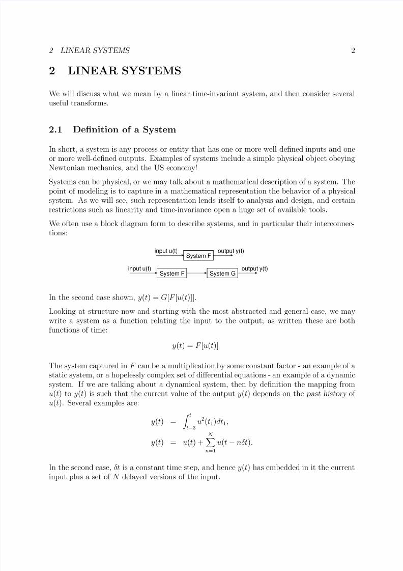
27 Complex Numbers
The complex number z = x + iy is interpreted as follows the real part is x the imaginary
part is y and i =
radic minus1 (imaginary) DeMoivrersquos theorem connects complex z with the
complex
exponential
It
states
that
cos
θ
+
i
sin
θ
=
eiθ
and
so
we
can
visualize
any
complex number in the two-plane where the axes are the real part and the imaginary part We say
that Re
eiθ
= cosθ and Im
eiθ
= sinθ to denote the real and imaginary parts of a
complex exponential More generally Re(z ) = x and Im(z ) = y
A complex number has a magnitude and an angle |z | =
radic x2 + y2 and arg(z ) = atan2(y x)
We can refer to the [x y] description of z as Cartesian coordinates whereas the [magnitude angle] description is called polar coordinates This latter is usually written as z = z 1048573 arg(z ) Arithmetic rules for two complex numbers z 1
and z 2
are as follows | |
z 1 +
z 2 = (x1 +
x2) +
i(y1 +
y2)
z 1
minus z 2
= (x1
minus x2) + i(y1
minus y2)
z 1
z 2
= arg(z 1) + arg(z 2)middot |z 1||z 2|1048573z 1z 2
=
|z 1| arg(z 1)
minus arg(z 2) |z 2|
Note that as given addition and subtraction are most naturally expressed in Cartesian
coordinates and multiplication and division are cleaner in polar coordinates
8202019 Linear Systems Review
httpslidepdfcomreaderfulllinear-systems-review 814
2 LINEAR SYSTEMS 9
28 Fourier Transform
The Fourier transform is the underlying principle for frequency-domain description of signals
We
begin
with
the
Fourier
series
Consider a signal f (t) continuous on the time interval [0 T ] which then repeats with period
T off to negative and positive infinity It can be shown that
infin
f (t) = Ao
+
[An
cos(nωot) + Bn
sin(nωot)] where
n=1
ωo
= 2πT 1
T
A0
= f (t)dtT 0
2
T
An
= f (t) cos(nωot)dt and
T 0
2
T
Bn
= f (t) sin(nωot)dt T 0
This says that the time-domain signal f (t) has an exact (if you carry all the infinity of terms) representation of a constant plus scaled cosines and sines As we will see later the impact of this second frequency-domain representation is profound as it allows an entirely new
set of tools for manipulation and analysis of signals and systems A compact form of these
expressions for the Fourier series can be written using complex exponentials infin
inωotf (t) =
C ne where
n=minusinfin
1
T
C n
=
f (t)eminusinωotdt
T 0
Of course C n
can be a complex number
In making these inner product calculations orthogonality of the harmonic functions is useful 2π
sin nt sin mt dt = 0 for n
ge 1 m
ge 1 n = m
0
1048573 2π
cos nt cos mt dt = 0 for n
ge 1 m
ge 1 n = m
0
1048573
2π
sin nt cos mt dt = 0 for n
ge 1 m
ge 1
0
Now letrsquos go to a different class of signal one that is not periodic but has a finite integral of absolute value Obviously such a signal has to approach zero at distances far from the
origin We can write a more elegant transformation
F (ω) =
infin
f (t)eminusiωtdt minusinfin
infin
iωτ dτ
1
f (t) = F (ω)e
2π minusinfin
8202019 Linear Systems Review
httpslidepdfcomreaderfulllinear-systems-review 914
8202019 Linear Systems Review
httpslidepdfcomreaderfulllinear-systems-review 1014
2 LINEAR SYSTEMS 11
parameters and of the frequency ω The Fourier Transform of the impulse response called
the system transfer function and we often refer to the transfer function as ldquothe systemrdquo
even though it is actually a (transformed) signal
By
way
of
summary
we
can
write
y(t) = h(t)
lowast u(t) and
Y (ω) = H (ω)U (ω)
29 The Angle of a Transfer Function
A particularly useful property of the Fourier (and Laplace) transform is that the magnitude
of the transfer function scales a sinusoidal input and the angle of the transfer function adds
to
the
angle
of
the
sinusoidal
input
In
other
words
u(t) = uo
cos(ωot + ψ)
minusrarr
y(t) = uo H (ωo) cos(ωot + ψ
+
arg(H (ωo))| |
To prove the above relations wersquoll use the complex exponential
u(t) = Re
uoe
i(ωot+ψ)
iψ = Re
uoe
iωot
making uoe = uo
complex then
y(t) = h(t)
lowast u(t) infin
=
h(τ )u(t
minus
τ )dτ
infin
iωo(tminusτ )
dτ =
minusinfin
h(τ )Re
uoe
minusinfin
= Re
infin
h(τ )eminusiωoτ dτ uoe
iωot
minusinfin
i(ωot+ψ)
= Re
H (ωo)uoe
= uo H (ωo) cos(ωot + ψ + arg(H (ωo)))| |
As an example let u(t) = 4 cos(3t +π4) and H (ω) = 2iω5 Then H (ωo) = H (3) = 6i5 =
121048573
π2
Thus
y(t) = 48
cos(3t
+ 3π4)
210 The Laplace Transform
The causal version of the Fourier transform is the Laplace transform the integral over time
includes only positive values and hence only deals with causal impulse response functions In
our
discussion
the
Laplace
transform
is
chiefly
used
in
control
system
analysis
and
design
8202019 Linear Systems Review
httpslidepdfcomreaderfulllinear-systems-review 1114
2 LINEAR SYSTEMS 12
2101
Definition
The Laplace transform projects time-domain signals into a complex frequency-domain equiv
alent
The
signal
y(t)
has
transform
Y
(s)
defined
as
follows
Y (s) = L(y(t)) =
infin
y(τ )eminussτ dτ 0
where s is a complex variable properly constrained within a region so that the integral converges Y (s) is a complex function as a result Note that the Laplace transform is linear and so it is distributive L(x(t) + y(t)) = L(x(t)) + L(y(t)) The following table gives a list
of some useful transform pairs and other properties for reference
The last two properties are of special importance for control system design the differentiation of a signal is equivalent to multiplication of its Laplace transform by s integration of a signal is equivalent to division by s The other terms that arise will cancel if y(0) = 0 or
if y(0) is finite
2102
Convergence
We
note
first
that
the
value
of s
affects
the
convergence
of
the
integral
For
instance
if
y(t) = et then the integral converges only for Re(s) gt 1 since the integrand is e1minuss in this
case
Although
the
integral
converges
within
a
well-defined
region
in
the
complex
plane
the
function Y (s) is defined for all s through analytic continuation This result from complex
analysis holds that if two complex functions are equal on some arc (or line) in the complex
plane then they are equivalent everywhere It should be noted however that the Laplace
transform is defined only within the region of convergence
2103
Convolution
Theorem
One of the main points of the Laplace transform is the ease of dealing with dynamic systems As with the Fourier transform the convolution of two signals in the time domain corresponds
with
the
multiplication
of
signals
in
the
frequency
domain
Consider
a
system
whose
impulse
response
is
g(t)
being
driven
by
an
input
signal
x(t)
the
output
is
y(t) =
g(t)
lowast
x(t)
The
Convolution Theorem is
t
y(t) = g(t minus τ )x(τ )dτ Y (s) = G(s)X (s) 0
lArrrArr
Herersquos the proof given by Siebert
8202019 Linear Systems Review
httpslidepdfcomreaderfulllinear-systems-review 1214
2 LINEAR SYSTEMS 13
y(t)
(Impulse) δ (t)
(Unit Step) 1(t)
(Unit Ramp) t
eminusαt
sin
ωt
cos ωt
eminusαt sin ωt
eminusαt cos ωt
1
b
minus a
(eminusat minus eminusbt)
1 1 1 +
ab
a
minus
b(be
minusat
minus
ae
minusbt
)
ωn radic 1
minus ζ 2
eminusζωnt sin ωn
1
minus ζ 2t
1
minus radic 1
1
minus ζ 2
eminusζωnt sin
ωn
1
minus ζ 2t + φ
radic
1
minus ζ 2
φ = tanminus1
ζ
(Pure
Delay)
y(t
minus
τ )1(t
minus
τ )
dy(t)(Time Derivative)
dt t
(Time Integral) y(τ )dτ 0
larrrarr
larrrarr
larrrarr
larrrarr
larrrarr
larrrarr
larrrarr
larrrarr
larrrarr
larrrarr
larrrarr
larrrarr
larrrarr
larrrarr
larrrarr
larrrarr
Y (s)
1
1
s
1
2s1
s + α
ω
s2 +
ω2
s
s2 + ω2
ω
(s + α)2 + ω2
s + α
(s + α)2 + ω2
1
(s + a)(s + b)
1
s(s
+
a)(s
+
b)
ω2
n
s2 + 2ζωns + ωn
2
ω2
n
s(s2 + 2ζωns + ωn2
)
Y
(s)e
minussτ
sY (s)
minus y(0)
0+Y (s)+
0minus
y(t)dt
s s
8202019 Linear Systems Review
httpslidepdfcomreaderfulllinear-systems-review 1314
2 LINEAR SYSTEMS 14
Y (s) = infin
y(t)eminusstdt
=
=
=
=
0 infin
0
t
0
g(t minus τ ) x(τ ) dτ
eminusst dt infin
0
infin
0
g(t minus τ ) h(t minus τ ) x(τ ) dτ
eminusstdt infin
0
x(τ )
infin
0
g(t minus τ ) h(t minus τ ) eminusst dt
dτ infin
x(τ ) G(s)eminussτ dτ 0
= G(s)X (s)
where h(t) is the unit step function When g(t) is the impulse response of a dynamic system then
y(t)
represents
the
output
of
this
system
when
it
is
driven
by
the
external
signal
x(t)
2104
Solution
of
Differential
Equations
by
Laplace
Transform
The Convolution Theorem allows one to solve (linear time-invariant) differential equations in the following way
1 Transform the system impulse response g(t) into G(s) and the input signal x(t) into
X (s) using the transform pairs
2
Perform
the
multiplication
in
the
Laplace
domain
to
find
Y
(s)
3 Ignoring the effects of pure time delays break Y (s) into partial fractions with no powers
of s greater than 2 in the denominator
4 Generate the time-domain response from the simple transform pairs Apply time delay
as necessary
Specific examples of this procedure are given in a later section on transfer functions
8202019 Linear Systems Review
httpslidepdfcomreaderfulllinear-systems-review 1414
MIT OpenCourseWarehttpocwmitedu
2017J Design of Electromechanical Robotic Systems
Fall 2009
For information about citing these materials or our Terms of Use visit httpocwmiteduterms

8202019 Linear Systems Review
httpslidepdfcomreaderfulllinear-systems-review 214
u(t)
y(t)
u(t-)
y(t-)
2 LINEAR SYSTEMS 3
22 Time-Invariant Systems
A dynamic system is time-invariant if shifting the input on the time axis leads to an equivalent
shifting
of
the
output
along
the
time
axis
with
no
other
changes
In
other
words
a
time-invariant system maps a given input trajectory u(t) no matter when it occurs
y(t minus τ ) = F [u(t minus τ )]
The formula above says specifically that if an input signal is delayed by some amount τ so
will be the output and with no other changes
An example of a physical time-varying system is the pitch response of a rocket y(t) when
the thrusters are being steered by an angle u(t) You can see first that this is an inverted
pendulum
problem
and
unstable
without
a
closed-loop
controller
It
is
time-varying
because
as the rocket burns fuel its mass is changing and so the pitch responds differently to various
inputs
throughout
its
flight
In
this
case
the
rdquoabsolute
timerdquo
coordinate
is
the
time
since
liftoff
To assess whether a system is time-varying or not follow these steps replace u(t) with
u(t minus τ ) on one side of the equation replace y(t) with y(t minus τ ) on the other side of the
equation and then check if they are equal Here are several examples
y(t) = u(t)32
This system is clearly time-invariant because it is a static map Next example
t
y(t) = u(t1)dt1
0
Replace u(t1) with u(t1
minus τ ) in the right hand side and carry it through t
u(t1
minus τ )dt1
=
tminusτ
u(t2)dt2 0 minusτ
The left hand side is simply
y(t minus τ ) =
tminusτ
u(t1)dt1
0
8202019 Linear Systems Review
httpslidepdfcomreaderfulllinear-systems-review 314
2 LINEAR SYSTEMS 4
Clearly the right and left hand sides are not equal (the limits of integration are different) and hence the system is not time-invariant As another example consider
t y(t) =
u
2
(t1)dt1 tminus5
The right-hand side becomes with the time shift t u
2(t1
minus τ )dt1
=
tminusτ
u
2(t2)dt2 tminus5 tminus5minusτ
whereas the left-hand side is
y(t minus τ ) =
tminusτ
u
2(t1)dt1 tminus5minusτ
the two sides of the defining equation are equal under a time shift τ and so this system is
time-invariant
A subtlety here is encountered when considering inputs that are zero before time zero - this is
the usual assumption in our work namely u(t) = 0 for t le 0 While linearity is not affected
by this condition time invariance is because the assumption is inconsistent with advancing
a signal in time Clearly part of the input would be truncated Restricting our discussion
to signal delays (the insertion of minusτ into the argument where strictly τ gt 0) resolves the
issue and preserves time invariance as needed
23 Linear Systems
Next we consider linearity Roughly speaking a system is linear if its behavior is scale-independent a result of this is the superposition principle More precisely suppose that
y1(t) = F [u1(t)]
and y2(t) =
F [u2(t)]
Then
linearity
means
that
for
any
two
constants α1
and α2
y(t) = α1y1(t) + α2y2(t) = F [α1u1(t) + α2u2(t)]
A simple special case is seen by setting α2
= 0
y(t) = α1y1(t) = F [α1u1(t)]
making clear the scale-invariance If the input is scaled by α1 then so is the output Here
are some examples of linear and nonlinear systems
du
y(t) = c (linear and time-invariant)
dt t
y(t) = u(t1)dt1
(linear but not time-invariant)
0
y(t) = 2u
2(t) (nonlinear but time-invariant)
y(t) = 6u(t) (linear and time-invariant)
8202019 Linear Systems Review
httpslidepdfcomreaderfulllinear-systems-review 414
width
height 1
t0 0
(t) = limit as
0
t
2 LINEAR SYSTEMS 5
Linear time-invariant (LTI) systems are of special interest because of the powerful tools we
can apply to them Systems described by sets of linear ordinary or differential differential equations having constant coefficients are LTI This is a large class Very useful examples
include
a
mass
m
on
a
spring
k
being
driven
by
a
force
u(t)
my(t) + ky(t) = u(t)
where the output y(t) is interpreted as a position A classic case of an LTI partial differential equation is transmission of lateral waves down a half-infinite string Let m be the mass per
unit length and T be the tension (constant on the length) If the motion of the end is u(t) then the lateral motion satisfies
part 2y(t x) part 2y(t x)
m = T partt2 partx2
with y(t x = 0) = u(t) Note that the system output y is not only a function of time but
also of space in this case
24 The Impulse Response and Convolution
A fundamental property of LTI systems is that they obey the convolution operator This
operator is defined by
infin
infin
y(t) = u(t1)h(t
minus t1)dt1
= u(t
minus t1)h(t1)dt1
minusinfin
minusinfin
The
function h(t)
above
is
a
particular
characterization
of
the
LTI
system
known
as
the
impulse response (see below) The equality between the two integrals should be clear since
the limits of integration are infinite The presence of the t1
and the
minust1
term inside the
integrations tells you that we have integrals of products - but that one of the signals is
turned around We will describe the meaning of the convolution more fully below
To understand the impulse response first we need the concept of the impulse itself also
known as the delta function δ (t) Think of a rectangular box centered at time zero of width
(time duration) 1048573 and height (magnitude) 11048573 the limit as 1048573
minusrarr 0 is the δ function The
area is clearly one in any case
8202019 Linear Systems Review
httpslidepdfcomreaderfulllinear-systems-review 514
2 LINEAR SYSTEMS 6
The inner product of the delta function with any function is the value of the function at zero
time
infin
f (t)δ (t)dt
=
2
f (t)δ (t)dt
=
f (t
=
0)
2
δ (t)dt
=
f (0)
minusinfin minus2 minus2
More
usefully
the
delta
function
can
pick
out
the
function
value
at
a
given
nonzero
time ξ
infin
f (t)δ (t minus ξ )dt = f (ξ ) minusinfin
Returning now to the impulse response function h(t) it is quite simply the output of the
LTI system when driven by the delta function as input that is u(t) = δ (t) or h(t) = F [δ (t)] In practical terms we can liken h(t) to the response of a mechanical system when it is struck
very hard by a hammer
Next we put the delta function and the convolution definition together to show explicitly
that the response of a system to arbitrary input u(t) is the convolution of the input and the
impulse response h(t) This is what is stated in the definition given at the beginning of this
section First we note that infin
u(t) = u(ξ )δ (ξ minus t)dξ minusinfin infin
= u(ξ )δ (t minus ξ )dξ (because the impulse is symmetric about zero time) minusinfin
Now
set
the
system
response
y(t) =
F
[u(t)]
where
F
is
an
LTI
system
- we
will
use
its
two properties below
infin
y(t) = F u(ξ )δ (t minus ξ )dξ infin
minusinfin
= u(ξ )F [δ (t minus ξ )]dξ (using linearity)
minusinfin infin
= u(ξ )h(t minus ξ )dξ (using time invariance) minusinfin
and this indeed is the definition of convolution often written as y(t) = h(t)
lowast u(t)
An
intuitive
understanding
of
convolution
can
be
gained
by
thinking
of
the
input
as
an infinite number of scaled delta functions placed very closely together on the time axis
Explaining the case with the integrand u(t minus ξ )h(ξ ) we see the convolution integral will call up all these virtual impulses referenced to time t and multiply them by the properly
shifted impulse responses Consider one impulse only that occurs at time t = 2 and we are
interested in the response at t = 5 Then u(t) = δ (t minus 2) or u(t minus ξ ) = δ (t minus 2
minus ξ ) The
integrand will thus be nonzero only when t minus 2
minus ξ is zero or ξ = t minus 2 Now h(ξ ) = h(t minus 2)
will be h(3) when t = 5 and hence it provides the impulse response three time units after the impulse occurs which is just what we wanted
8202019 Linear Systems Review
httpslidepdfcomreaderfulllinear-systems-review 614
2 LINEAR SYSTEMS 7
25 Causal Systems
All physical systems respond to input only after the input is applied In math terms this
means
h(t)
=
0
for
all
t lt
0
For
convenience
we
also
usually
consider
input
signals
to
be zero before time zero The convolution is adapted in a very reasonable way
infin
y(t) = u(ξ )h(t minus ξ )dξ minusinfin infin
= u(ξ )h(t minus ξ )dξ 0 t
= u(ξ )h(t minus ξ )dξ 0
The lower integration limit is set by the assumption that u(t) = 0 for t lt 0 and the upper
limit is set by the causality of the impulse response The complementary form with integrand
u(t
minus
ξ )h(ξ )
also
holds
26 An Example of Finding the Impulse Response
Letrsquos consider the differential equation mx(t) + bx(t) + cx(t) = δ (t) with the initial conditions of x(0) = x(0) = 0 We have
2
2
[mx + bx + cx]dt = δ (t)dt = 1 so that
minus2
minus2
m(x(0+)
minus x(0minus)) = 1
The + superscript indicates the instant just after zero time and the
minus superscript indicates
the instant just before zero time The given relation follows because at time zero the velocity
and position are zero so it must be the acceleration which is very large Now since x(0minus) =
0 we have x(0+) = 1m This is very useful - the initial velocity after the mass is hit
with a δ (t) input In fact this replaces our previous initial condition x(0) = 0 and we can
treat the differential equation as homogeneous from here on With x(t) = c1es1t + c2es2t the
governing equation becomes ms2
i + bsi
+ k = 0 so that
b
radic b2 minus
4km
s =
minus2m
plusmn
2m
Let σ = b2m and
k b2
= ωd
m
minus
4m2
and assuming that b2 lt 4km we find
1
h(t) = eminusσtsin(ωdt) t ge 0 mωd
8202019 Linear Systems Review
httpslidepdfcomreaderfulllinear-systems-review 714
Real(z)
Imag(z) z = 05 + i0866= cos( 3) + i sin( 3)= ei 3
= 1 3
1
1
-1
-1
0
1048573
2 LINEAR SYSTEMS 8
As noted above once the impulse response is known for an LTI system responses to all inputs can be found
t x(t) =
u(τ )h(t
minus
τ )dτ 0
In the case of LTI systems the impulse response is a complete definition of the system in
the
same
way
that
a
differential
equation
is
with
zero
initial
conditions
27 Complex Numbers
The complex number z = x + iy is interpreted as follows the real part is x the imaginary
part is y and i =
radic minus1 (imaginary) DeMoivrersquos theorem connects complex z with the
complex
exponential
It
states
that
cos
θ
+
i
sin
θ
=
eiθ
and
so
we
can
visualize
any
complex number in the two-plane where the axes are the real part and the imaginary part We say
that Re
eiθ
= cosθ and Im
eiθ
= sinθ to denote the real and imaginary parts of a
complex exponential More generally Re(z ) = x and Im(z ) = y
A complex number has a magnitude and an angle |z | =
radic x2 + y2 and arg(z ) = atan2(y x)
We can refer to the [x y] description of z as Cartesian coordinates whereas the [magnitude angle] description is called polar coordinates This latter is usually written as z = z 1048573 arg(z ) Arithmetic rules for two complex numbers z 1
and z 2
are as follows | |
z 1 +
z 2 = (x1 +
x2) +
i(y1 +
y2)
z 1
minus z 2
= (x1
minus x2) + i(y1
minus y2)
z 1
z 2
= arg(z 1) + arg(z 2)middot |z 1||z 2|1048573z 1z 2
=
|z 1| arg(z 1)
minus arg(z 2) |z 2|
Note that as given addition and subtraction are most naturally expressed in Cartesian
coordinates and multiplication and division are cleaner in polar coordinates
8202019 Linear Systems Review
httpslidepdfcomreaderfulllinear-systems-review 814
2 LINEAR SYSTEMS 9
28 Fourier Transform
The Fourier transform is the underlying principle for frequency-domain description of signals
We
begin
with
the
Fourier
series
Consider a signal f (t) continuous on the time interval [0 T ] which then repeats with period
T off to negative and positive infinity It can be shown that
infin
f (t) = Ao
+
[An
cos(nωot) + Bn
sin(nωot)] where
n=1
ωo
= 2πT 1
T
A0
= f (t)dtT 0
2
T
An
= f (t) cos(nωot)dt and
T 0
2
T
Bn
= f (t) sin(nωot)dt T 0
This says that the time-domain signal f (t) has an exact (if you carry all the infinity of terms) representation of a constant plus scaled cosines and sines As we will see later the impact of this second frequency-domain representation is profound as it allows an entirely new
set of tools for manipulation and analysis of signals and systems A compact form of these
expressions for the Fourier series can be written using complex exponentials infin
inωotf (t) =
C ne where
n=minusinfin
1
T
C n
=
f (t)eminusinωotdt
T 0
Of course C n
can be a complex number
In making these inner product calculations orthogonality of the harmonic functions is useful 2π
sin nt sin mt dt = 0 for n
ge 1 m
ge 1 n = m
0
1048573 2π
cos nt cos mt dt = 0 for n
ge 1 m
ge 1 n = m
0
1048573
2π
sin nt cos mt dt = 0 for n
ge 1 m
ge 1
0
Now letrsquos go to a different class of signal one that is not periodic but has a finite integral of absolute value Obviously such a signal has to approach zero at distances far from the
origin We can write a more elegant transformation
F (ω) =
infin
f (t)eminusiωtdt minusinfin
infin
iωτ dτ
1
f (t) = F (ω)e
2π minusinfin
8202019 Linear Systems Review
httpslidepdfcomreaderfulllinear-systems-review 914
8202019 Linear Systems Review
httpslidepdfcomreaderfulllinear-systems-review 1014
2 LINEAR SYSTEMS 11
parameters and of the frequency ω The Fourier Transform of the impulse response called
the system transfer function and we often refer to the transfer function as ldquothe systemrdquo
even though it is actually a (transformed) signal
By
way
of
summary
we
can
write
y(t) = h(t)
lowast u(t) and
Y (ω) = H (ω)U (ω)
29 The Angle of a Transfer Function
A particularly useful property of the Fourier (and Laplace) transform is that the magnitude
of the transfer function scales a sinusoidal input and the angle of the transfer function adds
to
the
angle
of
the
sinusoidal
input
In
other
words
u(t) = uo
cos(ωot + ψ)
minusrarr
y(t) = uo H (ωo) cos(ωot + ψ
+
arg(H (ωo))| |
To prove the above relations wersquoll use the complex exponential
u(t) = Re
uoe
i(ωot+ψ)
iψ = Re
uoe
iωot
making uoe = uo
complex then
y(t) = h(t)
lowast u(t) infin
=
h(τ )u(t
minus
τ )dτ
infin
iωo(tminusτ )
dτ =
minusinfin
h(τ )Re
uoe
minusinfin
= Re
infin
h(τ )eminusiωoτ dτ uoe
iωot
minusinfin
i(ωot+ψ)
= Re
H (ωo)uoe
= uo H (ωo) cos(ωot + ψ + arg(H (ωo)))| |
As an example let u(t) = 4 cos(3t +π4) and H (ω) = 2iω5 Then H (ωo) = H (3) = 6i5 =
121048573
π2
Thus
y(t) = 48
cos(3t
+ 3π4)
210 The Laplace Transform
The causal version of the Fourier transform is the Laplace transform the integral over time
includes only positive values and hence only deals with causal impulse response functions In
our
discussion
the
Laplace
transform
is
chiefly
used
in
control
system
analysis
and
design
8202019 Linear Systems Review
httpslidepdfcomreaderfulllinear-systems-review 1114
2 LINEAR SYSTEMS 12
2101
Definition
The Laplace transform projects time-domain signals into a complex frequency-domain equiv
alent
The
signal
y(t)
has
transform
Y
(s)
defined
as
follows
Y (s) = L(y(t)) =
infin
y(τ )eminussτ dτ 0
where s is a complex variable properly constrained within a region so that the integral converges Y (s) is a complex function as a result Note that the Laplace transform is linear and so it is distributive L(x(t) + y(t)) = L(x(t)) + L(y(t)) The following table gives a list
of some useful transform pairs and other properties for reference
The last two properties are of special importance for control system design the differentiation of a signal is equivalent to multiplication of its Laplace transform by s integration of a signal is equivalent to division by s The other terms that arise will cancel if y(0) = 0 or
if y(0) is finite
2102
Convergence
We
note
first
that
the
value
of s
affects
the
convergence
of
the
integral
For
instance
if
y(t) = et then the integral converges only for Re(s) gt 1 since the integrand is e1minuss in this
case
Although
the
integral
converges
within
a
well-defined
region
in
the
complex
plane
the
function Y (s) is defined for all s through analytic continuation This result from complex
analysis holds that if two complex functions are equal on some arc (or line) in the complex
plane then they are equivalent everywhere It should be noted however that the Laplace
transform is defined only within the region of convergence
2103
Convolution
Theorem
One of the main points of the Laplace transform is the ease of dealing with dynamic systems As with the Fourier transform the convolution of two signals in the time domain corresponds
with
the
multiplication
of
signals
in
the
frequency
domain
Consider
a
system
whose
impulse
response
is
g(t)
being
driven
by
an
input
signal
x(t)
the
output
is
y(t) =
g(t)
lowast
x(t)
The
Convolution Theorem is
t
y(t) = g(t minus τ )x(τ )dτ Y (s) = G(s)X (s) 0
lArrrArr
Herersquos the proof given by Siebert
8202019 Linear Systems Review
httpslidepdfcomreaderfulllinear-systems-review 1214
2 LINEAR SYSTEMS 13
y(t)
(Impulse) δ (t)
(Unit Step) 1(t)
(Unit Ramp) t
eminusαt
sin
ωt
cos ωt
eminusαt sin ωt
eminusαt cos ωt
1
b
minus a
(eminusat minus eminusbt)
1 1 1 +
ab
a
minus
b(be
minusat
minus
ae
minusbt
)
ωn radic 1
minus ζ 2
eminusζωnt sin ωn
1
minus ζ 2t
1
minus radic 1
1
minus ζ 2
eminusζωnt sin
ωn
1
minus ζ 2t + φ
radic
1
minus ζ 2
φ = tanminus1
ζ
(Pure
Delay)
y(t
minus
τ )1(t
minus
τ )
dy(t)(Time Derivative)
dt t
(Time Integral) y(τ )dτ 0
larrrarr
larrrarr
larrrarr
larrrarr
larrrarr
larrrarr
larrrarr
larrrarr
larrrarr
larrrarr
larrrarr
larrrarr
larrrarr
larrrarr
larrrarr
larrrarr
Y (s)
1
1
s
1
2s1
s + α
ω
s2 +
ω2
s
s2 + ω2
ω
(s + α)2 + ω2
s + α
(s + α)2 + ω2
1
(s + a)(s + b)
1
s(s
+
a)(s
+
b)
ω2
n
s2 + 2ζωns + ωn
2
ω2
n
s(s2 + 2ζωns + ωn2
)
Y
(s)e
minussτ
sY (s)
minus y(0)
0+Y (s)+
0minus
y(t)dt
s s
8202019 Linear Systems Review
httpslidepdfcomreaderfulllinear-systems-review 1314
2 LINEAR SYSTEMS 14
Y (s) = infin
y(t)eminusstdt
=
=
=
=
0 infin
0
t
0
g(t minus τ ) x(τ ) dτ
eminusst dt infin
0
infin
0
g(t minus τ ) h(t minus τ ) x(τ ) dτ
eminusstdt infin
0
x(τ )
infin
0
g(t minus τ ) h(t minus τ ) eminusst dt
dτ infin
x(τ ) G(s)eminussτ dτ 0
= G(s)X (s)
where h(t) is the unit step function When g(t) is the impulse response of a dynamic system then
y(t)
represents
the
output
of
this
system
when
it
is
driven
by
the
external
signal
x(t)
2104
Solution
of
Differential
Equations
by
Laplace
Transform
The Convolution Theorem allows one to solve (linear time-invariant) differential equations in the following way
1 Transform the system impulse response g(t) into G(s) and the input signal x(t) into
X (s) using the transform pairs
2
Perform
the
multiplication
in
the
Laplace
domain
to
find
Y
(s)
3 Ignoring the effects of pure time delays break Y (s) into partial fractions with no powers
of s greater than 2 in the denominator
4 Generate the time-domain response from the simple transform pairs Apply time delay
as necessary
Specific examples of this procedure are given in a later section on transfer functions
8202019 Linear Systems Review
httpslidepdfcomreaderfulllinear-systems-review 1414
MIT OpenCourseWarehttpocwmitedu
2017J Design of Electromechanical Robotic Systems
Fall 2009
For information about citing these materials or our Terms of Use visit httpocwmiteduterms

8202019 Linear Systems Review
httpslidepdfcomreaderfulllinear-systems-review 414
width
height 1
t0 0
(t) = limit as
0
t
2 LINEAR SYSTEMS 5
Linear time-invariant (LTI) systems are of special interest because of the powerful tools we
can apply to them Systems described by sets of linear ordinary or differential differential equations having constant coefficients are LTI This is a large class Very useful examples
include
a
mass
m
on
a
spring
k
being
driven
by
a
force
u(t)
my(t) + ky(t) = u(t)
where the output y(t) is interpreted as a position A classic case of an LTI partial differential equation is transmission of lateral waves down a half-infinite string Let m be the mass per
unit length and T be the tension (constant on the length) If the motion of the end is u(t) then the lateral motion satisfies
part 2y(t x) part 2y(t x)
m = T partt2 partx2
with y(t x = 0) = u(t) Note that the system output y is not only a function of time but
also of space in this case
24 The Impulse Response and Convolution
A fundamental property of LTI systems is that they obey the convolution operator This
operator is defined by
infin
infin
y(t) = u(t1)h(t
minus t1)dt1
= u(t
minus t1)h(t1)dt1
minusinfin
minusinfin
The
function h(t)
above
is
a
particular
characterization
of
the
LTI
system
known
as
the
impulse response (see below) The equality between the two integrals should be clear since
the limits of integration are infinite The presence of the t1
and the
minust1
term inside the
integrations tells you that we have integrals of products - but that one of the signals is
turned around We will describe the meaning of the convolution more fully below
To understand the impulse response first we need the concept of the impulse itself also
known as the delta function δ (t) Think of a rectangular box centered at time zero of width
(time duration) 1048573 and height (magnitude) 11048573 the limit as 1048573
minusrarr 0 is the δ function The
area is clearly one in any case
8202019 Linear Systems Review
httpslidepdfcomreaderfulllinear-systems-review 514
2 LINEAR SYSTEMS 6
The inner product of the delta function with any function is the value of the function at zero
time
infin
f (t)δ (t)dt
=
2
f (t)δ (t)dt
=
f (t
=
0)
2
δ (t)dt
=
f (0)
minusinfin minus2 minus2
More
usefully
the
delta
function
can
pick
out
the
function
value
at
a
given
nonzero
time ξ
infin
f (t)δ (t minus ξ )dt = f (ξ ) minusinfin
Returning now to the impulse response function h(t) it is quite simply the output of the
LTI system when driven by the delta function as input that is u(t) = δ (t) or h(t) = F [δ (t)] In practical terms we can liken h(t) to the response of a mechanical system when it is struck
very hard by a hammer
Next we put the delta function and the convolution definition together to show explicitly
that the response of a system to arbitrary input u(t) is the convolution of the input and the
impulse response h(t) This is what is stated in the definition given at the beginning of this
section First we note that infin
u(t) = u(ξ )δ (ξ minus t)dξ minusinfin infin
= u(ξ )δ (t minus ξ )dξ (because the impulse is symmetric about zero time) minusinfin
Now
set
the
system
response
y(t) =
F
[u(t)]
where
F
is
an
LTI
system
- we
will
use
its
two properties below
infin
y(t) = F u(ξ )δ (t minus ξ )dξ infin
minusinfin
= u(ξ )F [δ (t minus ξ )]dξ (using linearity)
minusinfin infin
= u(ξ )h(t minus ξ )dξ (using time invariance) minusinfin
and this indeed is the definition of convolution often written as y(t) = h(t)
lowast u(t)
An
intuitive
understanding
of
convolution
can
be
gained
by
thinking
of
the
input
as
an infinite number of scaled delta functions placed very closely together on the time axis
Explaining the case with the integrand u(t minus ξ )h(ξ ) we see the convolution integral will call up all these virtual impulses referenced to time t and multiply them by the properly
shifted impulse responses Consider one impulse only that occurs at time t = 2 and we are
interested in the response at t = 5 Then u(t) = δ (t minus 2) or u(t minus ξ ) = δ (t minus 2
minus ξ ) The
integrand will thus be nonzero only when t minus 2
minus ξ is zero or ξ = t minus 2 Now h(ξ ) = h(t minus 2)
will be h(3) when t = 5 and hence it provides the impulse response three time units after the impulse occurs which is just what we wanted
8202019 Linear Systems Review
httpslidepdfcomreaderfulllinear-systems-review 614
2 LINEAR SYSTEMS 7
25 Causal Systems
All physical systems respond to input only after the input is applied In math terms this
means
h(t)
=
0
for
all
t lt
0
For
convenience
we
also
usually
consider
input
signals
to
be zero before time zero The convolution is adapted in a very reasonable way
infin
y(t) = u(ξ )h(t minus ξ )dξ minusinfin infin
= u(ξ )h(t minus ξ )dξ 0 t
= u(ξ )h(t minus ξ )dξ 0
The lower integration limit is set by the assumption that u(t) = 0 for t lt 0 and the upper
limit is set by the causality of the impulse response The complementary form with integrand
u(t
minus
ξ )h(ξ )
also
holds
26 An Example of Finding the Impulse Response
Letrsquos consider the differential equation mx(t) + bx(t) + cx(t) = δ (t) with the initial conditions of x(0) = x(0) = 0 We have
2
2
[mx + bx + cx]dt = δ (t)dt = 1 so that
minus2
minus2
m(x(0+)
minus x(0minus)) = 1
The + superscript indicates the instant just after zero time and the
minus superscript indicates
the instant just before zero time The given relation follows because at time zero the velocity
and position are zero so it must be the acceleration which is very large Now since x(0minus) =
0 we have x(0+) = 1m This is very useful - the initial velocity after the mass is hit
with a δ (t) input In fact this replaces our previous initial condition x(0) = 0 and we can
treat the differential equation as homogeneous from here on With x(t) = c1es1t + c2es2t the
governing equation becomes ms2
i + bsi
+ k = 0 so that
b
radic b2 minus
4km
s =
minus2m
plusmn
2m
Let σ = b2m and
k b2
= ωd
m
minus
4m2
and assuming that b2 lt 4km we find
1
h(t) = eminusσtsin(ωdt) t ge 0 mωd
8202019 Linear Systems Review
httpslidepdfcomreaderfulllinear-systems-review 714
Real(z)
Imag(z) z = 05 + i0866= cos( 3) + i sin( 3)= ei 3
= 1 3
1
1
-1
-1
0
1048573
2 LINEAR SYSTEMS 8
As noted above once the impulse response is known for an LTI system responses to all inputs can be found
t x(t) =
u(τ )h(t
minus
τ )dτ 0
In the case of LTI systems the impulse response is a complete definition of the system in
the
same
way
that
a
differential
equation
is
with
zero
initial
conditions
27 Complex Numbers
The complex number z = x + iy is interpreted as follows the real part is x the imaginary
part is y and i =
radic minus1 (imaginary) DeMoivrersquos theorem connects complex z with the
complex
exponential
It
states
that
cos
θ
+
i
sin
θ
=
eiθ
and
so
we
can
visualize
any
complex number in the two-plane where the axes are the real part and the imaginary part We say
that Re
eiθ
= cosθ and Im
eiθ
= sinθ to denote the real and imaginary parts of a
complex exponential More generally Re(z ) = x and Im(z ) = y
A complex number has a magnitude and an angle |z | =
radic x2 + y2 and arg(z ) = atan2(y x)
We can refer to the [x y] description of z as Cartesian coordinates whereas the [magnitude angle] description is called polar coordinates This latter is usually written as z = z 1048573 arg(z ) Arithmetic rules for two complex numbers z 1
and z 2
are as follows | |
z 1 +
z 2 = (x1 +
x2) +
i(y1 +
y2)
z 1
minus z 2
= (x1
minus x2) + i(y1
minus y2)
z 1
z 2
= arg(z 1) + arg(z 2)middot |z 1||z 2|1048573z 1z 2
=
|z 1| arg(z 1)
minus arg(z 2) |z 2|
Note that as given addition and subtraction are most naturally expressed in Cartesian
coordinates and multiplication and division are cleaner in polar coordinates
8202019 Linear Systems Review
httpslidepdfcomreaderfulllinear-systems-review 814
2 LINEAR SYSTEMS 9
28 Fourier Transform
The Fourier transform is the underlying principle for frequency-domain description of signals
We
begin
with
the
Fourier
series
Consider a signal f (t) continuous on the time interval [0 T ] which then repeats with period
T off to negative and positive infinity It can be shown that
infin
f (t) = Ao
+
[An
cos(nωot) + Bn
sin(nωot)] where
n=1
ωo
= 2πT 1
T
A0
= f (t)dtT 0
2
T
An
= f (t) cos(nωot)dt and
T 0
2
T
Bn
= f (t) sin(nωot)dt T 0
This says that the time-domain signal f (t) has an exact (if you carry all the infinity of terms) representation of a constant plus scaled cosines and sines As we will see later the impact of this second frequency-domain representation is profound as it allows an entirely new
set of tools for manipulation and analysis of signals and systems A compact form of these
expressions for the Fourier series can be written using complex exponentials infin
inωotf (t) =
C ne where
n=minusinfin
1
T
C n
=
f (t)eminusinωotdt
T 0
Of course C n
can be a complex number
In making these inner product calculations orthogonality of the harmonic functions is useful 2π
sin nt sin mt dt = 0 for n
ge 1 m
ge 1 n = m
0
1048573 2π
cos nt cos mt dt = 0 for n
ge 1 m
ge 1 n = m
0
1048573
2π
sin nt cos mt dt = 0 for n
ge 1 m
ge 1
0
Now letrsquos go to a different class of signal one that is not periodic but has a finite integral of absolute value Obviously such a signal has to approach zero at distances far from the
origin We can write a more elegant transformation
F (ω) =
infin
f (t)eminusiωtdt minusinfin
infin
iωτ dτ
1
f (t) = F (ω)e
2π minusinfin
8202019 Linear Systems Review
httpslidepdfcomreaderfulllinear-systems-review 914
8202019 Linear Systems Review
httpslidepdfcomreaderfulllinear-systems-review 1014
2 LINEAR SYSTEMS 11
parameters and of the frequency ω The Fourier Transform of the impulse response called
the system transfer function and we often refer to the transfer function as ldquothe systemrdquo
even though it is actually a (transformed) signal
By
way
of
summary
we
can
write
y(t) = h(t)
lowast u(t) and
Y (ω) = H (ω)U (ω)
29 The Angle of a Transfer Function
A particularly useful property of the Fourier (and Laplace) transform is that the magnitude
of the transfer function scales a sinusoidal input and the angle of the transfer function adds
to
the
angle
of
the
sinusoidal
input
In
other
words
u(t) = uo
cos(ωot + ψ)
minusrarr
y(t) = uo H (ωo) cos(ωot + ψ
+
arg(H (ωo))| |
To prove the above relations wersquoll use the complex exponential
u(t) = Re
uoe
i(ωot+ψ)
iψ = Re
uoe
iωot
making uoe = uo
complex then
y(t) = h(t)
lowast u(t) infin
=
h(τ )u(t
minus
τ )dτ
infin
iωo(tminusτ )
dτ =
minusinfin
h(τ )Re
uoe
minusinfin
= Re
infin
h(τ )eminusiωoτ dτ uoe
iωot
minusinfin
i(ωot+ψ)
= Re
H (ωo)uoe
= uo H (ωo) cos(ωot + ψ + arg(H (ωo)))| |
As an example let u(t) = 4 cos(3t +π4) and H (ω) = 2iω5 Then H (ωo) = H (3) = 6i5 =
121048573
π2
Thus
y(t) = 48
cos(3t
+ 3π4)
210 The Laplace Transform
The causal version of the Fourier transform is the Laplace transform the integral over time
includes only positive values and hence only deals with causal impulse response functions In
our
discussion
the
Laplace
transform
is
chiefly
used
in
control
system
analysis
and
design
8202019 Linear Systems Review
httpslidepdfcomreaderfulllinear-systems-review 1114
2 LINEAR SYSTEMS 12
2101
Definition
The Laplace transform projects time-domain signals into a complex frequency-domain equiv
alent
The
signal
y(t)
has
transform
Y
(s)
defined
as
follows
Y (s) = L(y(t)) =
infin
y(τ )eminussτ dτ 0
where s is a complex variable properly constrained within a region so that the integral converges Y (s) is a complex function as a result Note that the Laplace transform is linear and so it is distributive L(x(t) + y(t)) = L(x(t)) + L(y(t)) The following table gives a list
of some useful transform pairs and other properties for reference
The last two properties are of special importance for control system design the differentiation of a signal is equivalent to multiplication of its Laplace transform by s integration of a signal is equivalent to division by s The other terms that arise will cancel if y(0) = 0 or
if y(0) is finite
2102
Convergence
We
note
first
that
the
value
of s
affects
the
convergence
of
the
integral
For
instance
if
y(t) = et then the integral converges only for Re(s) gt 1 since the integrand is e1minuss in this
case
Although
the
integral
converges
within
a
well-defined
region
in
the
complex
plane
the
function Y (s) is defined for all s through analytic continuation This result from complex
analysis holds that if two complex functions are equal on some arc (or line) in the complex
plane then they are equivalent everywhere It should be noted however that the Laplace
transform is defined only within the region of convergence
2103
Convolution
Theorem
One of the main points of the Laplace transform is the ease of dealing with dynamic systems As with the Fourier transform the convolution of two signals in the time domain corresponds
with
the
multiplication
of
signals
in
the
frequency
domain
Consider
a
system
whose
impulse
response
is
g(t)
being
driven
by
an
input
signal
x(t)
the
output
is
y(t) =
g(t)
lowast
x(t)
The
Convolution Theorem is
t
y(t) = g(t minus τ )x(τ )dτ Y (s) = G(s)X (s) 0
lArrrArr
Herersquos the proof given by Siebert
8202019 Linear Systems Review
httpslidepdfcomreaderfulllinear-systems-review 1214
2 LINEAR SYSTEMS 13
y(t)
(Impulse) δ (t)
(Unit Step) 1(t)
(Unit Ramp) t
eminusαt
sin
ωt
cos ωt
eminusαt sin ωt
eminusαt cos ωt
1
b
minus a
(eminusat minus eminusbt)
1 1 1 +
ab
a
minus
b(be
minusat
minus
ae
minusbt
)
ωn radic 1
minus ζ 2
eminusζωnt sin ωn
1
minus ζ 2t
1
minus radic 1
1
minus ζ 2
eminusζωnt sin
ωn
1
minus ζ 2t + φ
radic
1
minus ζ 2
φ = tanminus1
ζ
(Pure
Delay)
y(t
minus
τ )1(t
minus
τ )
dy(t)(Time Derivative)
dt t
(Time Integral) y(τ )dτ 0
larrrarr
larrrarr
larrrarr
larrrarr
larrrarr
larrrarr
larrrarr
larrrarr
larrrarr
larrrarr
larrrarr
larrrarr
larrrarr
larrrarr
larrrarr
larrrarr
Y (s)
1
1
s
1
2s1
s + α
ω
s2 +
ω2
s
s2 + ω2
ω
(s + α)2 + ω2
s + α
(s + α)2 + ω2
1
(s + a)(s + b)
1
s(s
+
a)(s
+
b)
ω2
n
s2 + 2ζωns + ωn
2
ω2
n
s(s2 + 2ζωns + ωn2
)
Y
(s)e
minussτ
sY (s)
minus y(0)
0+Y (s)+
0minus
y(t)dt
s s
8202019 Linear Systems Review
httpslidepdfcomreaderfulllinear-systems-review 1314
2 LINEAR SYSTEMS 14
Y (s) = infin
y(t)eminusstdt
=
=
=
=
0 infin
0
t
0
g(t minus τ ) x(τ ) dτ
eminusst dt infin
0
infin
0
g(t minus τ ) h(t minus τ ) x(τ ) dτ
eminusstdt infin
0
x(τ )
infin
0
g(t minus τ ) h(t minus τ ) eminusst dt
dτ infin
x(τ ) G(s)eminussτ dτ 0
= G(s)X (s)
where h(t) is the unit step function When g(t) is the impulse response of a dynamic system then
y(t)
represents
the
output
of
this
system
when
it
is
driven
by
the
external
signal
x(t)
2104
Solution
of
Differential
Equations
by
Laplace
Transform
The Convolution Theorem allows one to solve (linear time-invariant) differential equations in the following way
1 Transform the system impulse response g(t) into G(s) and the input signal x(t) into
X (s) using the transform pairs
2
Perform
the
multiplication
in
the
Laplace
domain
to
find
Y
(s)
3 Ignoring the effects of pure time delays break Y (s) into partial fractions with no powers
of s greater than 2 in the denominator
4 Generate the time-domain response from the simple transform pairs Apply time delay
as necessary
Specific examples of this procedure are given in a later section on transfer functions
8202019 Linear Systems Review
httpslidepdfcomreaderfulllinear-systems-review 1414
MIT OpenCourseWarehttpocwmitedu
2017J Design of Electromechanical Robotic Systems
Fall 2009
For information about citing these materials or our Terms of Use visit httpocwmiteduterms
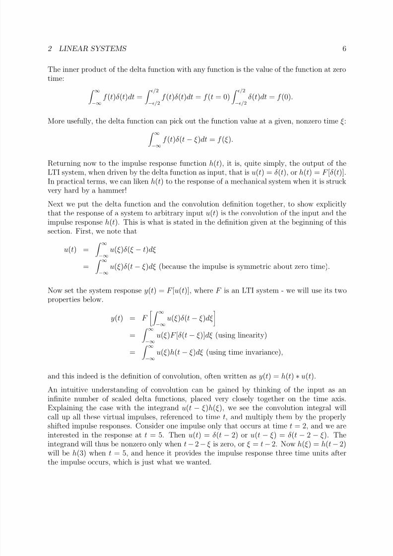
8202019 Linear Systems Review
httpslidepdfcomreaderfulllinear-systems-review 614
2 LINEAR SYSTEMS 7
25 Causal Systems
All physical systems respond to input only after the input is applied In math terms this
means
h(t)
=
0
for
all
t lt
0
For
convenience
we
also
usually
consider
input
signals
to
be zero before time zero The convolution is adapted in a very reasonable way
infin
y(t) = u(ξ )h(t minus ξ )dξ minusinfin infin
= u(ξ )h(t minus ξ )dξ 0 t
= u(ξ )h(t minus ξ )dξ 0
The lower integration limit is set by the assumption that u(t) = 0 for t lt 0 and the upper
limit is set by the causality of the impulse response The complementary form with integrand
u(t
minus
ξ )h(ξ )
also
holds
26 An Example of Finding the Impulse Response
Letrsquos consider the differential equation mx(t) + bx(t) + cx(t) = δ (t) with the initial conditions of x(0) = x(0) = 0 We have
2
2
[mx + bx + cx]dt = δ (t)dt = 1 so that
minus2
minus2
m(x(0+)
minus x(0minus)) = 1
The + superscript indicates the instant just after zero time and the
minus superscript indicates
the instant just before zero time The given relation follows because at time zero the velocity
and position are zero so it must be the acceleration which is very large Now since x(0minus) =
0 we have x(0+) = 1m This is very useful - the initial velocity after the mass is hit
with a δ (t) input In fact this replaces our previous initial condition x(0) = 0 and we can
treat the differential equation as homogeneous from here on With x(t) = c1es1t + c2es2t the
governing equation becomes ms2
i + bsi
+ k = 0 so that
b
radic b2 minus
4km
s =
minus2m
plusmn
2m
Let σ = b2m and
k b2
= ωd
m
minus
4m2
and assuming that b2 lt 4km we find
1
h(t) = eminusσtsin(ωdt) t ge 0 mωd
8202019 Linear Systems Review
httpslidepdfcomreaderfulllinear-systems-review 714
Real(z)
Imag(z) z = 05 + i0866= cos( 3) + i sin( 3)= ei 3
= 1 3
1
1
-1
-1
0
1048573
2 LINEAR SYSTEMS 8
As noted above once the impulse response is known for an LTI system responses to all inputs can be found
t x(t) =
u(τ )h(t
minus
τ )dτ 0
In the case of LTI systems the impulse response is a complete definition of the system in
the
same
way
that
a
differential
equation
is
with
zero
initial
conditions
27 Complex Numbers
The complex number z = x + iy is interpreted as follows the real part is x the imaginary
part is y and i =
radic minus1 (imaginary) DeMoivrersquos theorem connects complex z with the
complex
exponential
It
states
that
cos
θ
+
i
sin
θ
=
eiθ
and
so
we
can
visualize
any
complex number in the two-plane where the axes are the real part and the imaginary part We say
that Re
eiθ
= cosθ and Im
eiθ
= sinθ to denote the real and imaginary parts of a
complex exponential More generally Re(z ) = x and Im(z ) = y
A complex number has a magnitude and an angle |z | =
radic x2 + y2 and arg(z ) = atan2(y x)
We can refer to the [x y] description of z as Cartesian coordinates whereas the [magnitude angle] description is called polar coordinates This latter is usually written as z = z 1048573 arg(z ) Arithmetic rules for two complex numbers z 1
and z 2
are as follows | |
z 1 +
z 2 = (x1 +
x2) +
i(y1 +
y2)
z 1
minus z 2
= (x1
minus x2) + i(y1
minus y2)
z 1
z 2
= arg(z 1) + arg(z 2)middot |z 1||z 2|1048573z 1z 2
=
|z 1| arg(z 1)
minus arg(z 2) |z 2|
Note that as given addition and subtraction are most naturally expressed in Cartesian
coordinates and multiplication and division are cleaner in polar coordinates
8202019 Linear Systems Review
httpslidepdfcomreaderfulllinear-systems-review 814
2 LINEAR SYSTEMS 9
28 Fourier Transform
The Fourier transform is the underlying principle for frequency-domain description of signals
We
begin
with
the
Fourier
series
Consider a signal f (t) continuous on the time interval [0 T ] which then repeats with period
T off to negative and positive infinity It can be shown that
infin
f (t) = Ao
+
[An
cos(nωot) + Bn
sin(nωot)] where
n=1
ωo
= 2πT 1
T
A0
= f (t)dtT 0
2
T
An
= f (t) cos(nωot)dt and
T 0
2
T
Bn
= f (t) sin(nωot)dt T 0
This says that the time-domain signal f (t) has an exact (if you carry all the infinity of terms) representation of a constant plus scaled cosines and sines As we will see later the impact of this second frequency-domain representation is profound as it allows an entirely new
set of tools for manipulation and analysis of signals and systems A compact form of these
expressions for the Fourier series can be written using complex exponentials infin
inωotf (t) =
C ne where
n=minusinfin
1
T
C n
=
f (t)eminusinωotdt
T 0
Of course C n
can be a complex number
In making these inner product calculations orthogonality of the harmonic functions is useful 2π
sin nt sin mt dt = 0 for n
ge 1 m
ge 1 n = m
0
1048573 2π
cos nt cos mt dt = 0 for n
ge 1 m
ge 1 n = m
0
1048573
2π
sin nt cos mt dt = 0 for n
ge 1 m
ge 1
0
Now letrsquos go to a different class of signal one that is not periodic but has a finite integral of absolute value Obviously such a signal has to approach zero at distances far from the
origin We can write a more elegant transformation
F (ω) =
infin
f (t)eminusiωtdt minusinfin
infin
iωτ dτ
1
f (t) = F (ω)e
2π minusinfin
8202019 Linear Systems Review
httpslidepdfcomreaderfulllinear-systems-review 914
8202019 Linear Systems Review
httpslidepdfcomreaderfulllinear-systems-review 1014
2 LINEAR SYSTEMS 11
parameters and of the frequency ω The Fourier Transform of the impulse response called
the system transfer function and we often refer to the transfer function as ldquothe systemrdquo
even though it is actually a (transformed) signal
By
way
of
summary
we
can
write
y(t) = h(t)
lowast u(t) and
Y (ω) = H (ω)U (ω)
29 The Angle of a Transfer Function
A particularly useful property of the Fourier (and Laplace) transform is that the magnitude
of the transfer function scales a sinusoidal input and the angle of the transfer function adds
to
the
angle
of
the
sinusoidal
input
In
other
words
u(t) = uo
cos(ωot + ψ)
minusrarr
y(t) = uo H (ωo) cos(ωot + ψ
+
arg(H (ωo))| |
To prove the above relations wersquoll use the complex exponential
u(t) = Re
uoe
i(ωot+ψ)
iψ = Re
uoe
iωot
making uoe = uo
complex then
y(t) = h(t)
lowast u(t) infin
=
h(τ )u(t
minus
τ )dτ
infin
iωo(tminusτ )
dτ =
minusinfin
h(τ )Re
uoe
minusinfin
= Re
infin
h(τ )eminusiωoτ dτ uoe
iωot
minusinfin
i(ωot+ψ)
= Re
H (ωo)uoe
= uo H (ωo) cos(ωot + ψ + arg(H (ωo)))| |
As an example let u(t) = 4 cos(3t +π4) and H (ω) = 2iω5 Then H (ωo) = H (3) = 6i5 =
121048573
π2
Thus
y(t) = 48
cos(3t
+ 3π4)
210 The Laplace Transform
The causal version of the Fourier transform is the Laplace transform the integral over time
includes only positive values and hence only deals with causal impulse response functions In
our
discussion
the
Laplace
transform
is
chiefly
used
in
control
system
analysis
and
design
8202019 Linear Systems Review
httpslidepdfcomreaderfulllinear-systems-review 1114
2 LINEAR SYSTEMS 12
2101
Definition
The Laplace transform projects time-domain signals into a complex frequency-domain equiv
alent
The
signal
y(t)
has
transform
Y
(s)
defined
as
follows
Y (s) = L(y(t)) =
infin
y(τ )eminussτ dτ 0
where s is a complex variable properly constrained within a region so that the integral converges Y (s) is a complex function as a result Note that the Laplace transform is linear and so it is distributive L(x(t) + y(t)) = L(x(t)) + L(y(t)) The following table gives a list
of some useful transform pairs and other properties for reference
The last two properties are of special importance for control system design the differentiation of a signal is equivalent to multiplication of its Laplace transform by s integration of a signal is equivalent to division by s The other terms that arise will cancel if y(0) = 0 or
if y(0) is finite
2102
Convergence
We
note
first
that
the
value
of s
affects
the
convergence
of
the
integral
For
instance
if
y(t) = et then the integral converges only for Re(s) gt 1 since the integrand is e1minuss in this
case
Although
the
integral
converges
within
a
well-defined
region
in
the
complex
plane
the
function Y (s) is defined for all s through analytic continuation This result from complex
analysis holds that if two complex functions are equal on some arc (or line) in the complex
plane then they are equivalent everywhere It should be noted however that the Laplace
transform is defined only within the region of convergence
2103
Convolution
Theorem
One of the main points of the Laplace transform is the ease of dealing with dynamic systems As with the Fourier transform the convolution of two signals in the time domain corresponds
with
the
multiplication
of
signals
in
the
frequency
domain
Consider
a
system
whose
impulse
response
is
g(t)
being
driven
by
an
input
signal
x(t)
the
output
is
y(t) =
g(t)
lowast
x(t)
The
Convolution Theorem is
t
y(t) = g(t minus τ )x(τ )dτ Y (s) = G(s)X (s) 0
lArrrArr
Herersquos the proof given by Siebert
8202019 Linear Systems Review
httpslidepdfcomreaderfulllinear-systems-review 1214
2 LINEAR SYSTEMS 13
y(t)
(Impulse) δ (t)
(Unit Step) 1(t)
(Unit Ramp) t
eminusαt
sin
ωt
cos ωt
eminusαt sin ωt
eminusαt cos ωt
1
b
minus a
(eminusat minus eminusbt)
1 1 1 +
ab
a
minus
b(be
minusat
minus
ae
minusbt
)
ωn radic 1
minus ζ 2
eminusζωnt sin ωn
1
minus ζ 2t
1
minus radic 1
1
minus ζ 2
eminusζωnt sin
ωn
1
minus ζ 2t + φ
radic
1
minus ζ 2
φ = tanminus1
ζ
(Pure
Delay)
y(t
minus
τ )1(t
minus
τ )
dy(t)(Time Derivative)
dt t
(Time Integral) y(τ )dτ 0
larrrarr
larrrarr
larrrarr
larrrarr
larrrarr
larrrarr
larrrarr
larrrarr
larrrarr
larrrarr
larrrarr
larrrarr
larrrarr
larrrarr
larrrarr
larrrarr
Y (s)
1
1
s
1
2s1
s + α
ω
s2 +
ω2
s
s2 + ω2
ω
(s + α)2 + ω2
s + α
(s + α)2 + ω2
1
(s + a)(s + b)
1
s(s
+
a)(s
+
b)
ω2
n
s2 + 2ζωns + ωn
2
ω2
n
s(s2 + 2ζωns + ωn2
)
Y
(s)e
minussτ
sY (s)
minus y(0)
0+Y (s)+
0minus
y(t)dt
s s
8202019 Linear Systems Review
httpslidepdfcomreaderfulllinear-systems-review 1314
2 LINEAR SYSTEMS 14
Y (s) = infin
y(t)eminusstdt
=
=
=
=
0 infin
0
t
0
g(t minus τ ) x(τ ) dτ
eminusst dt infin
0
infin
0
g(t minus τ ) h(t minus τ ) x(τ ) dτ
eminusstdt infin
0
x(τ )
infin
0
g(t minus τ ) h(t minus τ ) eminusst dt
dτ infin
x(τ ) G(s)eminussτ dτ 0
= G(s)X (s)
where h(t) is the unit step function When g(t) is the impulse response of a dynamic system then
y(t)
represents
the
output
of
this
system
when
it
is
driven
by
the
external
signal
x(t)
2104
Solution
of
Differential
Equations
by
Laplace
Transform
The Convolution Theorem allows one to solve (linear time-invariant) differential equations in the following way
1 Transform the system impulse response g(t) into G(s) and the input signal x(t) into
X (s) using the transform pairs
2
Perform
the
multiplication
in
the
Laplace
domain
to
find
Y
(s)
3 Ignoring the effects of pure time delays break Y (s) into partial fractions with no powers
of s greater than 2 in the denominator
4 Generate the time-domain response from the simple transform pairs Apply time delay
as necessary
Specific examples of this procedure are given in a later section on transfer functions
8202019 Linear Systems Review
httpslidepdfcomreaderfulllinear-systems-review 1414
MIT OpenCourseWarehttpocwmitedu
2017J Design of Electromechanical Robotic Systems
Fall 2009
For information about citing these materials or our Terms of Use visit httpocwmiteduterms
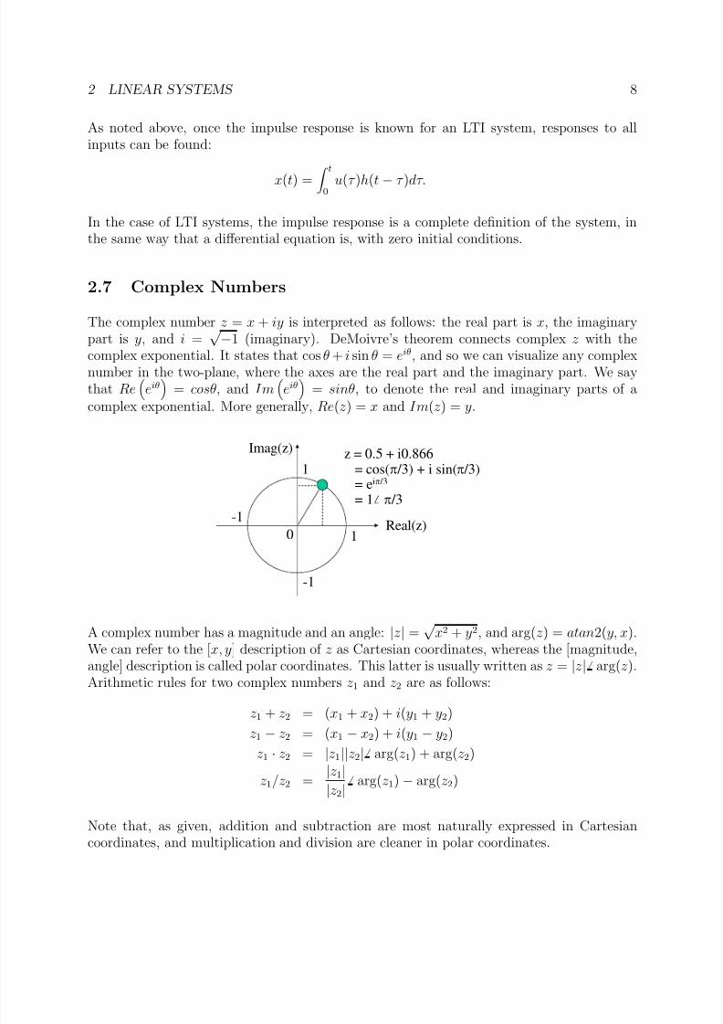
8202019 Linear Systems Review
httpslidepdfcomreaderfulllinear-systems-review 714
Real(z)
Imag(z) z = 05 + i0866= cos( 3) + i sin( 3)= ei 3
= 1 3
1
1
-1
-1
0
1048573
2 LINEAR SYSTEMS 8
As noted above once the impulse response is known for an LTI system responses to all inputs can be found
t x(t) =
u(τ )h(t
minus
τ )dτ 0
In the case of LTI systems the impulse response is a complete definition of the system in
the
same
way
that
a
differential
equation
is
with
zero
initial
conditions
27 Complex Numbers
The complex number z = x + iy is interpreted as follows the real part is x the imaginary
part is y and i =
radic minus1 (imaginary) DeMoivrersquos theorem connects complex z with the
complex
exponential
It
states
that
cos
θ
+
i
sin
θ
=
eiθ
and
so
we
can
visualize
any
complex number in the two-plane where the axes are the real part and the imaginary part We say
that Re
eiθ
= cosθ and Im
eiθ
= sinθ to denote the real and imaginary parts of a
complex exponential More generally Re(z ) = x and Im(z ) = y
A complex number has a magnitude and an angle |z | =
radic x2 + y2 and arg(z ) = atan2(y x)
We can refer to the [x y] description of z as Cartesian coordinates whereas the [magnitude angle] description is called polar coordinates This latter is usually written as z = z 1048573 arg(z ) Arithmetic rules for two complex numbers z 1
and z 2
are as follows | |
z 1 +
z 2 = (x1 +
x2) +
i(y1 +
y2)
z 1
minus z 2
= (x1
minus x2) + i(y1
minus y2)
z 1
z 2
= arg(z 1) + arg(z 2)middot |z 1||z 2|1048573z 1z 2
=
|z 1| arg(z 1)
minus arg(z 2) |z 2|
Note that as given addition and subtraction are most naturally expressed in Cartesian
coordinates and multiplication and division are cleaner in polar coordinates
8202019 Linear Systems Review
httpslidepdfcomreaderfulllinear-systems-review 814
2 LINEAR SYSTEMS 9
28 Fourier Transform
The Fourier transform is the underlying principle for frequency-domain description of signals
We
begin
with
the
Fourier
series
Consider a signal f (t) continuous on the time interval [0 T ] which then repeats with period
T off to negative and positive infinity It can be shown that
infin
f (t) = Ao
+
[An
cos(nωot) + Bn
sin(nωot)] where
n=1
ωo
= 2πT 1
T
A0
= f (t)dtT 0
2
T
An
= f (t) cos(nωot)dt and
T 0
2
T
Bn
= f (t) sin(nωot)dt T 0
This says that the time-domain signal f (t) has an exact (if you carry all the infinity of terms) representation of a constant plus scaled cosines and sines As we will see later the impact of this second frequency-domain representation is profound as it allows an entirely new
set of tools for manipulation and analysis of signals and systems A compact form of these
expressions for the Fourier series can be written using complex exponentials infin
inωotf (t) =
C ne where
n=minusinfin
1
T
C n
=
f (t)eminusinωotdt
T 0
Of course C n
can be a complex number
In making these inner product calculations orthogonality of the harmonic functions is useful 2π
sin nt sin mt dt = 0 for n
ge 1 m
ge 1 n = m
0
1048573 2π
cos nt cos mt dt = 0 for n
ge 1 m
ge 1 n = m
0
1048573
2π
sin nt cos mt dt = 0 for n
ge 1 m
ge 1
0
Now letrsquos go to a different class of signal one that is not periodic but has a finite integral of absolute value Obviously such a signal has to approach zero at distances far from the
origin We can write a more elegant transformation
F (ω) =
infin
f (t)eminusiωtdt minusinfin
infin
iωτ dτ
1
f (t) = F (ω)e
2π minusinfin
8202019 Linear Systems Review
httpslidepdfcomreaderfulllinear-systems-review 914
8202019 Linear Systems Review
httpslidepdfcomreaderfulllinear-systems-review 1014
2 LINEAR SYSTEMS 11
parameters and of the frequency ω The Fourier Transform of the impulse response called
the system transfer function and we often refer to the transfer function as ldquothe systemrdquo
even though it is actually a (transformed) signal
By
way
of
summary
we
can
write
y(t) = h(t)
lowast u(t) and
Y (ω) = H (ω)U (ω)
29 The Angle of a Transfer Function
A particularly useful property of the Fourier (and Laplace) transform is that the magnitude
of the transfer function scales a sinusoidal input and the angle of the transfer function adds
to
the
angle
of
the
sinusoidal
input
In
other
words
u(t) = uo
cos(ωot + ψ)
minusrarr
y(t) = uo H (ωo) cos(ωot + ψ
+
arg(H (ωo))| |
To prove the above relations wersquoll use the complex exponential
u(t) = Re
uoe
i(ωot+ψ)
iψ = Re
uoe
iωot
making uoe = uo
complex then
y(t) = h(t)
lowast u(t) infin
=
h(τ )u(t
minus
τ )dτ
infin
iωo(tminusτ )
dτ =
minusinfin
h(τ )Re
uoe
minusinfin
= Re
infin
h(τ )eminusiωoτ dτ uoe
iωot
minusinfin
i(ωot+ψ)
= Re
H (ωo)uoe
= uo H (ωo) cos(ωot + ψ + arg(H (ωo)))| |
As an example let u(t) = 4 cos(3t +π4) and H (ω) = 2iω5 Then H (ωo) = H (3) = 6i5 =
121048573
π2
Thus
y(t) = 48
cos(3t
+ 3π4)
210 The Laplace Transform
The causal version of the Fourier transform is the Laplace transform the integral over time
includes only positive values and hence only deals with causal impulse response functions In
our
discussion
the
Laplace
transform
is
chiefly
used
in
control
system
analysis
and
design
8202019 Linear Systems Review
httpslidepdfcomreaderfulllinear-systems-review 1114
2 LINEAR SYSTEMS 12
2101
Definition
The Laplace transform projects time-domain signals into a complex frequency-domain equiv
alent
The
signal
y(t)
has
transform
Y
(s)
defined
as
follows
Y (s) = L(y(t)) =
infin
y(τ )eminussτ dτ 0
where s is a complex variable properly constrained within a region so that the integral converges Y (s) is a complex function as a result Note that the Laplace transform is linear and so it is distributive L(x(t) + y(t)) = L(x(t)) + L(y(t)) The following table gives a list
of some useful transform pairs and other properties for reference
The last two properties are of special importance for control system design the differentiation of a signal is equivalent to multiplication of its Laplace transform by s integration of a signal is equivalent to division by s The other terms that arise will cancel if y(0) = 0 or
if y(0) is finite
2102
Convergence
We
note
first
that
the
value
of s
affects
the
convergence
of
the
integral
For
instance
if
y(t) = et then the integral converges only for Re(s) gt 1 since the integrand is e1minuss in this
case
Although
the
integral
converges
within
a
well-defined
region
in
the
complex
plane
the
function Y (s) is defined for all s through analytic continuation This result from complex
analysis holds that if two complex functions are equal on some arc (or line) in the complex
plane then they are equivalent everywhere It should be noted however that the Laplace
transform is defined only within the region of convergence
2103
Convolution
Theorem
One of the main points of the Laplace transform is the ease of dealing with dynamic systems As with the Fourier transform the convolution of two signals in the time domain corresponds
with
the
multiplication
of
signals
in
the
frequency
domain
Consider
a
system
whose
impulse
response
is
g(t)
being
driven
by
an
input
signal
x(t)
the
output
is
y(t) =
g(t)
lowast
x(t)
The
Convolution Theorem is
t
y(t) = g(t minus τ )x(τ )dτ Y (s) = G(s)X (s) 0
lArrrArr
Herersquos the proof given by Siebert
8202019 Linear Systems Review
httpslidepdfcomreaderfulllinear-systems-review 1214
2 LINEAR SYSTEMS 13
y(t)
(Impulse) δ (t)
(Unit Step) 1(t)
(Unit Ramp) t
eminusαt
sin
ωt
cos ωt
eminusαt sin ωt
eminusαt cos ωt
1
b
minus a
(eminusat minus eminusbt)
1 1 1 +
ab
a
minus
b(be
minusat
minus
ae
minusbt
)
ωn radic 1
minus ζ 2
eminusζωnt sin ωn
1
minus ζ 2t
1
minus radic 1
1
minus ζ 2
eminusζωnt sin
ωn
1
minus ζ 2t + φ
radic
1
minus ζ 2
φ = tanminus1
ζ
(Pure
Delay)
y(t
minus
τ )1(t
minus
τ )
dy(t)(Time Derivative)
dt t
(Time Integral) y(τ )dτ 0
larrrarr
larrrarr
larrrarr
larrrarr
larrrarr
larrrarr
larrrarr
larrrarr
larrrarr
larrrarr
larrrarr
larrrarr
larrrarr
larrrarr
larrrarr
larrrarr
Y (s)
1
1
s
1
2s1
s + α
ω
s2 +
ω2
s
s2 + ω2
ω
(s + α)2 + ω2
s + α
(s + α)2 + ω2
1
(s + a)(s + b)
1
s(s
+
a)(s
+
b)
ω2
n
s2 + 2ζωns + ωn
2
ω2
n
s(s2 + 2ζωns + ωn2
)
Y
(s)e
minussτ
sY (s)
minus y(0)
0+Y (s)+
0minus
y(t)dt
s s
8202019 Linear Systems Review
httpslidepdfcomreaderfulllinear-systems-review 1314
2 LINEAR SYSTEMS 14
Y (s) = infin
y(t)eminusstdt
=
=
=
=
0 infin
0
t
0
g(t minus τ ) x(τ ) dτ
eminusst dt infin
0
infin
0
g(t minus τ ) h(t minus τ ) x(τ ) dτ
eminusstdt infin
0
x(τ )
infin
0
g(t minus τ ) h(t minus τ ) eminusst dt
dτ infin
x(τ ) G(s)eminussτ dτ 0
= G(s)X (s)
where h(t) is the unit step function When g(t) is the impulse response of a dynamic system then
y(t)
represents
the
output
of
this
system
when
it
is
driven
by
the
external
signal
x(t)
2104
Solution
of
Differential
Equations
by
Laplace
Transform
The Convolution Theorem allows one to solve (linear time-invariant) differential equations in the following way
1 Transform the system impulse response g(t) into G(s) and the input signal x(t) into
X (s) using the transform pairs
2
Perform
the
multiplication
in
the
Laplace
domain
to
find
Y
(s)
3 Ignoring the effects of pure time delays break Y (s) into partial fractions with no powers
of s greater than 2 in the denominator
4 Generate the time-domain response from the simple transform pairs Apply time delay
as necessary
Specific examples of this procedure are given in a later section on transfer functions
8202019 Linear Systems Review
httpslidepdfcomreaderfulllinear-systems-review 1414
MIT OpenCourseWarehttpocwmitedu
2017J Design of Electromechanical Robotic Systems
Fall 2009
For information about citing these materials or our Terms of Use visit httpocwmiteduterms
8202019 Linear Systems Review
httpslidepdfcomreaderfulllinear-systems-review 814
2 LINEAR SYSTEMS 9
28 Fourier Transform
The Fourier transform is the underlying principle for frequency-domain description of signals
We
begin
with
the
Fourier
series
Consider a signal f (t) continuous on the time interval [0 T ] which then repeats with period
T off to negative and positive infinity It can be shown that
infin
f (t) = Ao
+
[An
cos(nωot) + Bn
sin(nωot)] where
n=1
ωo
= 2πT 1
T
A0
= f (t)dtT 0
2
T
An
= f (t) cos(nωot)dt and
T 0
2
T
Bn
= f (t) sin(nωot)dt T 0
This says that the time-domain signal f (t) has an exact (if you carry all the infinity of terms) representation of a constant plus scaled cosines and sines As we will see later the impact of this second frequency-domain representation is profound as it allows an entirely new
set of tools for manipulation and analysis of signals and systems A compact form of these
expressions for the Fourier series can be written using complex exponentials infin
inωotf (t) =
C ne where
n=minusinfin
1
T
C n
=
f (t)eminusinωotdt
T 0
Of course C n
can be a complex number
In making these inner product calculations orthogonality of the harmonic functions is useful 2π
sin nt sin mt dt = 0 for n
ge 1 m
ge 1 n = m
0
1048573 2π
cos nt cos mt dt = 0 for n
ge 1 m
ge 1 n = m
0
1048573
2π
sin nt cos mt dt = 0 for n
ge 1 m
ge 1
0
Now letrsquos go to a different class of signal one that is not periodic but has a finite integral of absolute value Obviously such a signal has to approach zero at distances far from the
origin We can write a more elegant transformation
F (ω) =
infin
f (t)eminusiωtdt minusinfin
infin
iωτ dτ
1
f (t) = F (ω)e
2π minusinfin
8202019 Linear Systems Review
httpslidepdfcomreaderfulllinear-systems-review 914
8202019 Linear Systems Review
httpslidepdfcomreaderfulllinear-systems-review 1014
2 LINEAR SYSTEMS 11
parameters and of the frequency ω The Fourier Transform of the impulse response called
the system transfer function and we often refer to the transfer function as ldquothe systemrdquo
even though it is actually a (transformed) signal
By
way
of
summary
we
can
write
y(t) = h(t)
lowast u(t) and
Y (ω) = H (ω)U (ω)
29 The Angle of a Transfer Function
A particularly useful property of the Fourier (and Laplace) transform is that the magnitude
of the transfer function scales a sinusoidal input and the angle of the transfer function adds
to
the
angle
of
the
sinusoidal
input
In
other
words
u(t) = uo
cos(ωot + ψ)
minusrarr
y(t) = uo H (ωo) cos(ωot + ψ
+
arg(H (ωo))| |
To prove the above relations wersquoll use the complex exponential
u(t) = Re
uoe
i(ωot+ψ)
iψ = Re
uoe
iωot
making uoe = uo
complex then
y(t) = h(t)
lowast u(t) infin
=
h(τ )u(t
minus
τ )dτ
infin
iωo(tminusτ )
dτ =
minusinfin
h(τ )Re
uoe
minusinfin
= Re
infin
h(τ )eminusiωoτ dτ uoe
iωot
minusinfin
i(ωot+ψ)
= Re
H (ωo)uoe
= uo H (ωo) cos(ωot + ψ + arg(H (ωo)))| |
As an example let u(t) = 4 cos(3t +π4) and H (ω) = 2iω5 Then H (ωo) = H (3) = 6i5 =
121048573
π2
Thus
y(t) = 48
cos(3t
+ 3π4)
210 The Laplace Transform
The causal version of the Fourier transform is the Laplace transform the integral over time
includes only positive values and hence only deals with causal impulse response functions In
our
discussion
the
Laplace
transform
is
chiefly
used
in
control
system
analysis
and
design
8202019 Linear Systems Review
httpslidepdfcomreaderfulllinear-systems-review 1114
2 LINEAR SYSTEMS 12
2101
Definition
The Laplace transform projects time-domain signals into a complex frequency-domain equiv
alent
The
signal
y(t)
has
transform
Y
(s)
defined
as
follows
Y (s) = L(y(t)) =
infin
y(τ )eminussτ dτ 0
where s is a complex variable properly constrained within a region so that the integral converges Y (s) is a complex function as a result Note that the Laplace transform is linear and so it is distributive L(x(t) + y(t)) = L(x(t)) + L(y(t)) The following table gives a list
of some useful transform pairs and other properties for reference
The last two properties are of special importance for control system design the differentiation of a signal is equivalent to multiplication of its Laplace transform by s integration of a signal is equivalent to division by s The other terms that arise will cancel if y(0) = 0 or
if y(0) is finite
2102
Convergence
We
note
first
that
the
value
of s
affects
the
convergence
of
the
integral
For
instance
if
y(t) = et then the integral converges only for Re(s) gt 1 since the integrand is e1minuss in this
case
Although
the
integral
converges
within
a
well-defined
region
in
the
complex
plane
the
function Y (s) is defined for all s through analytic continuation This result from complex
analysis holds that if two complex functions are equal on some arc (or line) in the complex
plane then they are equivalent everywhere It should be noted however that the Laplace
transform is defined only within the region of convergence
2103
Convolution
Theorem
One of the main points of the Laplace transform is the ease of dealing with dynamic systems As with the Fourier transform the convolution of two signals in the time domain corresponds
with
the
multiplication
of
signals
in
the
frequency
domain
Consider
a
system
whose
impulse
response
is
g(t)
being
driven
by
an
input
signal
x(t)
the
output
is
y(t) =
g(t)
lowast
x(t)
The
Convolution Theorem is
t
y(t) = g(t minus τ )x(τ )dτ Y (s) = G(s)X (s) 0
lArrrArr
Herersquos the proof given by Siebert
8202019 Linear Systems Review
httpslidepdfcomreaderfulllinear-systems-review 1214
2 LINEAR SYSTEMS 13
y(t)
(Impulse) δ (t)
(Unit Step) 1(t)
(Unit Ramp) t
eminusαt
sin
ωt
cos ωt
eminusαt sin ωt
eminusαt cos ωt
1
b
minus a
(eminusat minus eminusbt)
1 1 1 +
ab
a
minus
b(be
minusat
minus
ae
minusbt
)
ωn radic 1
minus ζ 2
eminusζωnt sin ωn
1
minus ζ 2t
1
minus radic 1
1
minus ζ 2
eminusζωnt sin
ωn
1
minus ζ 2t + φ
radic
1
minus ζ 2
φ = tanminus1
ζ
(Pure
Delay)
y(t
minus
τ )1(t
minus
τ )
dy(t)(Time Derivative)
dt t
(Time Integral) y(τ )dτ 0
larrrarr
larrrarr
larrrarr
larrrarr
larrrarr
larrrarr
larrrarr
larrrarr
larrrarr
larrrarr
larrrarr
larrrarr
larrrarr
larrrarr
larrrarr
larrrarr
Y (s)
1
1
s
1
2s1
s + α
ω
s2 +
ω2
s
s2 + ω2
ω
(s + α)2 + ω2
s + α
(s + α)2 + ω2
1
(s + a)(s + b)
1
s(s
+
a)(s
+
b)
ω2
n
s2 + 2ζωns + ωn
2
ω2
n
s(s2 + 2ζωns + ωn2
)
Y
(s)e
minussτ
sY (s)
minus y(0)
0+Y (s)+
0minus
y(t)dt
s s
8202019 Linear Systems Review
httpslidepdfcomreaderfulllinear-systems-review 1314
2 LINEAR SYSTEMS 14
Y (s) = infin
y(t)eminusstdt
=
=
=
=
0 infin
0
t
0
g(t minus τ ) x(τ ) dτ
eminusst dt infin
0
infin
0
g(t minus τ ) h(t minus τ ) x(τ ) dτ
eminusstdt infin
0
x(τ )
infin
0
g(t minus τ ) h(t minus τ ) eminusst dt
dτ infin
x(τ ) G(s)eminussτ dτ 0
= G(s)X (s)
where h(t) is the unit step function When g(t) is the impulse response of a dynamic system then
y(t)
represents
the
output
of
this
system
when
it
is
driven
by
the
external
signal
x(t)
2104
Solution
of
Differential
Equations
by
Laplace
Transform
The Convolution Theorem allows one to solve (linear time-invariant) differential equations in the following way
1 Transform the system impulse response g(t) into G(s) and the input signal x(t) into
X (s) using the transform pairs
2
Perform
the
multiplication
in
the
Laplace
domain
to
find
Y
(s)
3 Ignoring the effects of pure time delays break Y (s) into partial fractions with no powers
of s greater than 2 in the denominator
4 Generate the time-domain response from the simple transform pairs Apply time delay
as necessary
Specific examples of this procedure are given in a later section on transfer functions
8202019 Linear Systems Review
httpslidepdfcomreaderfulllinear-systems-review 1414
MIT OpenCourseWarehttpocwmitedu
2017J Design of Electromechanical Robotic Systems
Fall 2009
For information about citing these materials or our Terms of Use visit httpocwmiteduterms

8202019 Linear Systems Review
httpslidepdfcomreaderfulllinear-systems-review 1414
MIT OpenCourseWarehttpocwmitedu
2017J Design of Electromechanical Robotic Systems
Fall 2009
For information about citing these materials or our Terms of Use visit httpocwmiteduterms
Related Documents