Linear Systems Lecture 0 Some Math Background · LionSealWhite Lecture 0 Course Contents Vector spaces and mappings Matrix theory Norms Material: Lecture slides R.A. Horn and C.R.

LionSealWhite

LionSealGrey

Linear SystemsLecture 0

Some Math Background

Department Automatic ControlLund University

Linear Systems Lecture 0 Some Math Background

LionSealWhite

Lecture 0

Course Contents

Vector spaces and mappings

Matrix theory

Norms

Material:

Lecture slides

R.A. Horn and C.R. Johnson. Matrix Analysis. CambridgeUniversity Press, 2013.


LionSealWhite

Linear Systems I, 2016

Introduction

Multivariable Time-varying Systems

Transition Matrices

Controllability and Observability

Realization Theory

Stability Theory

Linear Feedback

Multivariable input/output descriptions

Some Bonus Material


LionSealWhite

Linear Systems I, 2016

Rugh, Linear System Theory, 2nd edition

Most of 1-7,9-12,13-14

Scan 15,20-23,25-29

Skip 8,16-19, 24

J. P. Hespanha, Linear Systems Theory. Princeton University Press.2009.Some more handouts


LionSealWhite

Course Contents

Credits: 9hp

9 Lectures (including this intro)

8 Exercise sessions (1st one on Wednesday, this week)

8 Handins (7 best counts). Strict deadlines!

24 hour take-home exam (date tbd: 8-th Dec or mid-January2017)


LionSealWhite

Vector spaces

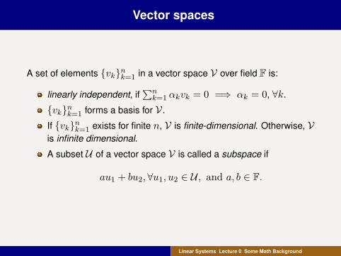
A set of elements {vk}nk=1 in a vector space V over field F is:

linearly independent, if∑nk=1 αkvk = 0 =⇒ αk = 0, ∀k.

{vk}nk=1 forms a basis for V .

If {vk}nk=1 exists for finite n, V is finite-dimensional. Otherwise, Vis infinite dimensional.

A subset U of a vector space V is called a subspace if

au1 + bu2,∀u1, u2 ∈ U , and a, b ∈ F.


LionSealWhite

Mappings

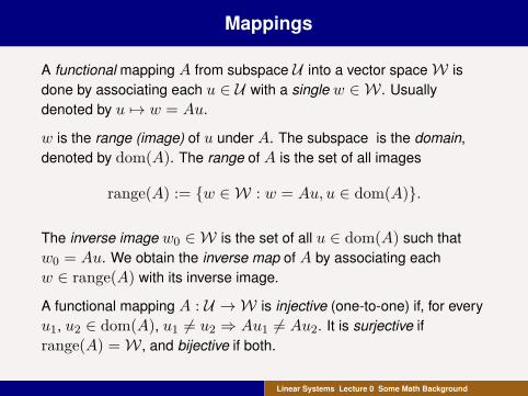
A functional mapping A from subspace U into a vector spaceW isdone by associating each u ∈ U with a single w ∈ W . Usuallydenoted by u 7→ w = Au.

w is the range (image) of u under A. The subspace is the domain,denoted by dom(A). The range of A is the set of all images

range(A) := {w ∈ W : w = Au, u ∈ dom(A)}.

The inverse image w0 ∈ W is the set of all u ∈ dom(A) such thatw0 = Au. We obtain the inverse map of A by associating eachw ∈ range(A) with its inverse image.

A functional mapping A : U → W is injective (one-to-one) if, for everyu1, u2 ∈ dom(A), u1 6= u2 ⇒ Au1 6= Au2. It is surjective ifrange(A) =W , and bijective if both.


LionSealWhite

Matrix representation of mappings

Given two vector spaces V andW over F, a mapping A : V → W islinear if

A(av + bu) = aAv + bAu, ∀u, v ∈ V, and a, b ∈ F.

Let {vk}nk=1 and {wk}mk=1 be bases for V andW , respectively. Foreach basis vector vk, let {a1k, a2k, . . . , amk} be the unique scalarssatisfying

Avk = a1kw1 + · · ·+ amkwm.

The mn scalars alk ∈ F completely characterises the map A. (why?)


LionSealWhite

Matrix representation of mappings

Let {vk}nk=1 and {wk}mk=1 be bases for V andW , respectively. Foreach basis vector vk, let {a1k, a2k, . . . , amk} be the unique scalarssatisfying

Avk = a1kw1 + · · ·+ amkwm.

The mn scalars alk ∈ F completely characterises the map A. Givenany v = α1v1 + · · ·+ αnvn and let w = Av = β1w1 + · · ·+ βnwn,by linearity we obtain β1

...βm

=

a11 . . . a1n...

. . ....

am1 . . . amn

α1

...αn

.

The matrix [ajk] ∈ Fm×n is the matrix representation of the linear mapA w.r.t. the input basis {vk}nk=1 and output basis {wk}mk=1.


LionSealWhite

Matrix Theory

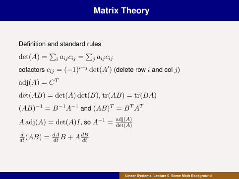
Definition and standard rules

det(A) =∑i aijcij =

∑j aijcij

cofactors cij = (−1)i+j det(A′) (delete row i and col j)

adj(A) = CT

det(AB) = det(A) det(B), tr(AB) = tr(BA)

(AB)−1 = B−1A−1 and (AB)T = BTAT

A adj(A) = det(A)I , so A−1 = adj(A)det(A)

ddt(AB) = dA

dt B +AdBdt


LionSealWhite

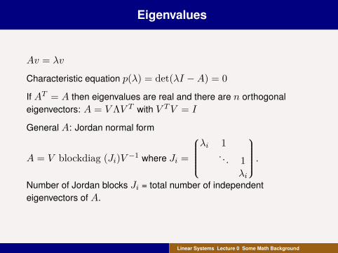
Eigenvalues

Av = λv

Characteristic equation p(λ) = det(λI −A) = 0

If AT = A then eigenvalues are real and there are n orthogonaleigenvectors: A = V ΛV T with V TV = I

General A: Jordan normal form

A = V blockdiag (Ji)V −1 where Ji =

λi 1

. . . 1λi

.

Number of Jordan blocks Ji = total number of independenteigenvectors of A.


LionSealWhite

Singular Value Decomposition etc

If A ∈ Rm×n then

A = U

Σ 00 0

V T

where U ∈ Rm×m, V ∈ Rn×n orthogonal (i.e. UUT = I andV V T = I) and

Σ = diag(σ1, . . . , σr) > 0, where σi is the square-root of aneigenvalue of AAT .

A symmetric =⇒ A = UΣUT .


LionSealWhite

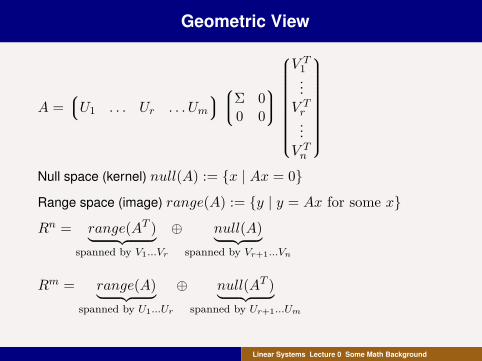
Geometric View

A =U1 . . . Ur . . . Um

Σ 00 0

V T1...V Tr...V Tn

Null space (kernel) null(A) := {x | Ax = 0}

Range space (image) range(A) := {y | y = Ax for some x}

Rn = range(AT )︸︷︷︸spanned by V1...Vr

⊕ null(A)︸︷︷︸spanned by Vr+1...Vn

Rm = range(A)︸︷︷︸spanned by U1...Ur

⊕ null(AT )︸︷︷︸spanned by Ur+1...Um


LionSealWhite

Computation of eAt

Definition: eAt =∞∑k=0

1k!(At)

k. Satisfies dXdt = AX .

ddte

At = AeAt = eAtA

If A = V ΛV T then eAt = V diag(eλit)V T

If A = V blockdiag (Ji)V −1 theneAt = V blockdiag (eJit)V −1

where eJit =

eλit teλit . . . tni−1

(ni−1)!eλit

. . . . . .eλit teλit

eλit

Laplace-transform L(eAt) = (sI −A)−1

e(A+B)t = eAteBt for all t⇔ AB = BA. Note: In general,eAteBt 6= e(A+B)t.


LionSealWhite

Quadratic Forms xTAx

Let’s assume AT = A (note that xTAx = xT (A+AT )x/2)

Positive definite: A ≥ 0 ⇔ xTAx ≥ 0, ∀x

Positive semi-definite: A > 0 ⇔ xTAx > 0,∀x 6= 0

We say that A ≥ B iff A−B ≥ 0.

Courant-Fisher formulas when AT = A:

λmax(A) = maxx 6=0

xTAxxT x

= maxxT x=1

xTAx

λmin(A) = minx 6=0

xTAxxT x

= minxT x=1

xTAx

λmin(A)I ≤ A ≤ λmax(A)I

A > 0⇔ λi(A) > 0,∀i


LionSealWhite

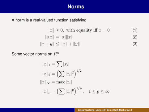
Norms

A norm is a real-valued function satisfying

‖x‖ ≥ 0, with equality iff x = 0 (1)

‖αx‖ = |α|‖x‖ (2)

‖x+ y‖ ≤ ‖x‖+ ‖y‖ (3)

Some vector norms on Rn

‖x‖1 =∑|xi|

‖x‖2 =(∑

|xi|2)1/2

‖x‖∞ = max |xi|

‖x‖p =(∑

|xi|p)1/p

, 1 ≤ p ≤ ∞


LionSealWhite

Norms: why are they useful?

A sequence {vk}nk=1 in a normed vector space V is said to converge,if ∃v ∈ V such that

‖v − vk‖V → 0, as k →∞.

If such a v exists, it is unique (why?).

Note that norms quantify the ‘closeness’ of two elements in a vectorspace, as we have seen above, i.e. converts convergence of {vk}∞k=0to a vector v to convergence of {‖v − vk‖}∞k=0 to 0!


LionSealWhite

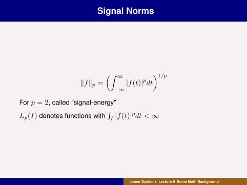
Signal Norms

‖f‖p =(∫ ∞−∞|f(t)|pdt

)1/p

For p = 2, called ”signal-energy”

Lp(I) denotes functions with∫I |f(t)|pdt <∞


LionSealWhite

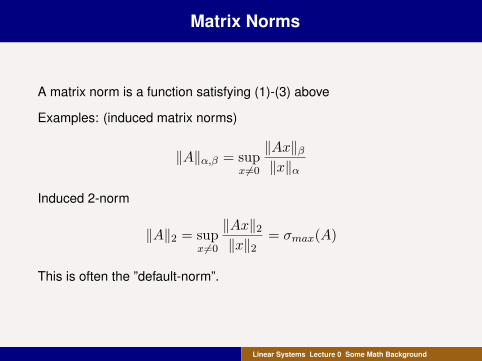
Matrix Norms

A matrix norm is a function satisfying (1)-(3) above

Examples: (induced matrix norms)

‖A‖α,β = supx 6=0

‖Ax‖β‖x‖α

Induced 2-norm

‖A‖2 = supx 6=0

‖Ax‖2‖x‖2

= σmax(A)

This is often the ”default-norm”.


LionSealWhite

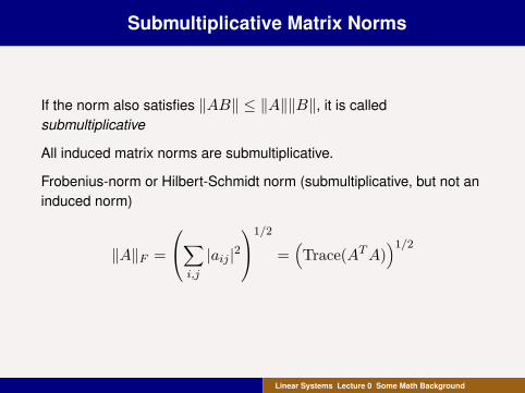
Submultiplicative Matrix Norms

If the norm also satisfies ‖AB‖ ≤ ‖A‖‖B‖, it is calledsubmultiplicative

All induced matrix norms are submultiplicative.

Frobenius-norm or Hilbert-Schmidt norm (submultiplicative, but not aninduced norm)

‖A‖F =

∑i,j

|aij |21/2

=(Trace(ATA)

)1/2


LionSealWhite

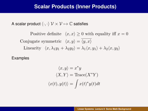
Scalar Products (Inner Products)

A scalar product 〈·, ·〉 V × V 7→ C satisfies

Positive definite 〈x, x〉 ≥ 0 with equality iff x = 0Conjugate symmetric 〈x, y〉 = 〈y, x〉

Linearity 〈x, λ1y1 + λ2y2〉 = λ1〈x, y1〉+ λ2〈x, y2〉

Examples

〈x, y〉 = x∗y

〈X,Y 〉 = Trace(X∗Y )

〈x(t), y(t)〉 =∫x(t)∗y(t)dt


LionSealWhite

Scalar Products (Inner Products)

A vector space V equipped with a scalar product is called a scalarproduct (inner product) space.

We say that x and y are orthogonal, denoted x ⊥ y if 〈x, y〉 = 0

For subspace: X ⊥ Y means that x ⊥ y,∀x ∈ X, y ∈ Y

Example: cos t is orthogonal to sin t in V = L2([−π, π])

Cauchy-Schwarz’ inequality:

n∑i=1|xiyi| = 〈x, y〉 ≤ ‖x‖2‖y‖2

(with equality if and only if x and y are proportional)


LionSealWhite

Why are these concepts useful?

In this course, we use vector spaces equipped with an inner productand corresponding norm. All these vector spaces have an additionalproperty which is useful in the study of sequence in the vector space(recall why a norm is useful).

A sequence {vk}∞k=0 in a normed vector space V is Cauchy, if for anyε > 0, there exists N(ε) such that

‖vk − vm‖V < ε, ∀k,m ≥ N(ε).

Note: Every convergent sequence is Cauchy, but not necessarily theconverse.


LionSealWhite

Why are these concepts useful?

A normed vector space + every Cauchy sequence is convergent iscalled complete and known as a Banach space.

A Banach space + scalar product is called a Hilbert space.

In a complete vector space, it is possible to check whether a sequenceis convergent by checking if it is Cauchy.

We can consider the modelling of a system in terms of mappingsbetween signal vector spaces. In this course, we deal with mappingsbetween Banach spaces.


LionSealWhite

Tools

Make sure you know how to simulate an ordinary differential system ine.g. Matlab/Simulink or Maple

You should also be familiar with using some symbolic manipulationprogram such as Maple

You should be able to use the Control System Toolbox (or similar)


LionSealWhite

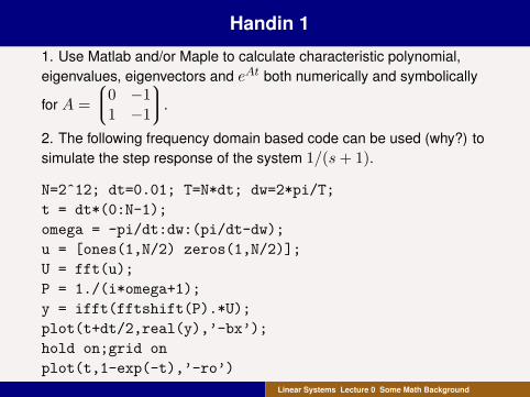
Handin 1

1. Use Matlab and/or Maple to calculate characteristic polynomial,eigenvalues, eigenvectors and eAt both numerically and symbolically

for A =0 −1

1 −1

.

2. The following frequency domain based code can be used (why?) tosimulate the step response of the system 1/(s+ 1).

N=2ˆ12; dt=0.01; T=N*dt; dw=2*pi/T;t = dt*(0:N-1);omega = -pi/dt:dw:(pi/dt-dw);u = [ones(1,N/2) zeros(1,N/2)];U = fft(u);P = 1./(i*omega+1);y = ifft(fftshift(P).*U);plot(t+dt/2,real(y),’-bx’);hold on;grid onplot(t,1-exp(-t),’-ro’)


LionSealWhite

Handin 1 - continued

Simulate the step response of the open loop systemP (s) = exp (−

√s) and of the closed loop system PC/(1 + PC)

under PI-control with C(s) = 1 + 1/s (you might want to tune N anddt).

Compare the rise time to 50% and the settling times to 99% of the finalvalue for open loop vs closed loop control.

3. See exercise session.


Linear Systems Lecture 0 Some Math Background · LionSealWhite Lecture 0 Course Contents Vector spaces and mappings Matrix theory Norms Material: Lecture slides R.A. Horn and C.R.

Documents