Linear-scaling implementation of molecular electronic self-consistent field theory

Linear-scaling implementation of molecular electronic self-consistentfield theory

Paweł SałekDepartment of Theoretical Chemistry, The Royal Institute of Technology, SE-10691 Stockholm, Sweden

Stinne Høst,a� Lea Thøgersen, Poul Jørgensen, Pekka Manninen,b�

Jeppe Olsen, and Branislav JansíkThe Lundbeck Foundation Center for Theoretical Chemistry, Department of Chemistry,University of Aarhus, DK-8000 Århus C, Denmark

Simen Reine,c� Filip Pawłowski,d� Erik Tellgren,e� and Trygve Helgakere�

Department of Chemistry, University of Oslo, P.O. Box 1033, Blindern N-0315, Norway

Sonia CorianiDipartimento di Scienze Chimiche, Università degli Studi di Trieste, Via Licio Giorgieri 1,I-34127 Trieste, Italy

�Received 4 October 2006; accepted 9 January 2007; published online 21 March 2007�

A linear-scaling implementation of Hartree-Fock and Kohn-Sham self-consistent field �SCF�theories is presented and illustrated with applications to molecules consisting of more than 1000atoms. The diagonalization bottleneck of traditional SCF methods is avoided by carrying out aminimization of the Roothaan-Hall �RH� energy function and solving the Newton equations usingthe preconditioned conjugate-gradient �PCG� method. For rapid PCG convergence, the Löwdinorthogonal atomic orbital basis is used. The resulting linear-scaling trust-region Roothaan-Hall�LS-TRRH� method works by the introduction of a level-shift parameter in the RH Newtonequations. A great advantage of the LS-TRRH method is that the optimal level shift can bedetermined at no extra cost, ensuring fast and robust convergence of both the SCF iterations and thelevel-shifted Newton equations. For density averaging, the authors use the trust-regiondensity-subspace minimization �TRDSM� method, which, unlike the traditional direct inversion inthe iterative subspace �DIIS� scheme, is firmly based on the principle of energy minimization. Whencombined with a linear-scaling evaluation of the Fock/Kohn-Sham matrix �including a boxed fittingof the electron density�, LS-TRRH and TRDSM methods constitute the linear-scaling trust-regionSCF �LS-TRSCF� method. The LS-TRSCF method compares favorably with the traditional SCF/DIIS scheme, converging smoothly and reliably in cases where the latter method fails. In one casewhere the LS-TRSCF method converges smoothly to a minimum, the SCF/DIIS method convergesto a saddle point. © 2007 American Institute of Physics. �DOI: 10.1063/1.2464111�

I. INTRODUCTION

During the last decade, much effort has been directedtowards the development and implementation of Hartree-Fock �HF� and Kohn-Sham �KS� self-consistent field �SCF�theories in such a manner that, for sufficiently large systems,the cost of the calculations scales linearly with system sizeO�N�, where N may be taken as the number of atoms in themolecule. To achieve linear scaling, two bottlenecks must beovercome: first, the construction of the Fock/KS matrix F in

the atomic-orbital �AO� basis, which conventionally scalesas O�N2�; second, the generation of a new density matrixfrom a given Fock/KS matrix, which is conventionallyachieved by an O�N3� diagonalization step FC=SC�, whereS is the AO overlap matrix. Over the years, many strategieshave been proposed to make the cost of these key steps scalelinearly with system size.

To remove the diagonalization bottleneck, many meth-ods have been suggested—see Refs. 1 and 2 for an overview.We focus here on the density-matrix methods,1 which may besubdivided into two categories:2 the Fermi-operator expan-sion �FOE� methods and the density-matrix minimization�DMM� methods. The FOE methods include rational-function, polynomial, or recursive-polynomial expansions tocompute the density matrix, of which the canonical-purification method of Palser and Manolopoulos,3 thepurification4,5 of McWeeny and the Chebyshev expansion6,7

of Baer and Head-Gordon serve as examples. Alternatively,the DMM methods use the fact that the density matrix ob-tained from a Fock/KS matrix diagonalization represents the

a�Author to whom correspondence should be addressed. Fax: �45 86196199. Electronic mail: [email protected]

b�Present address: Helsinki University of Technology, P.O. Box 1100 �Ota-kaari 1 M�, FI-02015 Hut, Finland.

c�Present address: The Lundbeck Foundation Center for Theoretical Chem-istry, Department of Chemistry, University of Aarhus, DK-8000 Århus C,Denmark.

d�Present address: Institute of Physics, Kazimierz Wielki University, PlacWeyssenhoffa 11, 85-072 Bydgoszcz, Poland.

e�Present address: Department of Chemistry, University of Durham, SouthRoad, Durham DH1 3LE, United Kingdom.

THE JOURNAL OF CHEMICAL PHYSICS 126, 114110 �2007�

0021-9606/2007/126�11�/114110/16/$23.00 © 2007 American Institute of Physics126, 114110-1

Downloaded 25 Mar 2007 to 129.240.250.48. Redistribution subject to AIP license or copyright, see http://jcp.aip.org/jcp/copyright.jsp

http://dx.doi.org/10.1063/1.2464111

http://dx.doi.org/10.1063/1.2464111

http://dx.doi.org/10.1063/1.2464111

global minimum of the Roothaan-Hall �RH� energy functionERH=Tr DF �with F fixed�,8,9 thereby replacing the diagonal-ization by a minimization, suitably constrained so as to sat-isfy the idempotency condition DSD=D. Li et al. proposedto deal with the idempotency constraint by replacing the den-sity matrix in the optimization by its McWeeny-purifiedcounterpart, noting that the variations are then idempotent tofirst order;10 their approach was further developed by Millamand Scuseria11 and by Challacombe.12 Alternatively, theidempotency condition may be incorporated into the param-etrization of the density matrix D�X�=exp�−XS�D exp�SX�with X antisymmetric, as described by Helgaker andco-workers.8,13,14 The first attempts to use this parametriza-tion to minimize ERH employed a sequence of Newton itera-tions but encountered difficulties in the solution of the New-ton linear equations.14 Subsequently, these difficulties weresolved by Shao et al.15 in their curvy-step method by trans-forming the Newton equations to the Cholesky basis, wherethe Hessian has a smaller condition number and is more di-agonally dominant than in the AO basis. We discuss hereimprovements to the algorithm of Shao et al.15 using theLöwdin or principal square-root basis rather than theCholesky basis for the following reasons. First, the conver-gence of the Newton equations is marginally better in theLöwdin basis than in the Cholesky basis; second, the Löwdinbasis is the orthogonal AO basis that resembles most closelythe original AO basis,16 ensuring that locality is preserved tothe greatest possible extent; and third, the transformation tothe Löwdin basis can be performed straightforwardly withina linear-scaling framework.17

In setting up the SCF iterations, we note that the RHenergy ERH�X�=Tr D�X�F constitutes a rather crude modelof the true SCF energy ESCF. In particular, at the expansionpoint X=0, ERH has the same gradient as ESCF but only anapproximate Hessian. A global minimization of ERH �as tra-ditionally accomplished by diagonalization of the Fock/KSmatrix� may therefore lead to steps that are too long andtherefore unreliable. To avoid such problems, we impose inthe trust-region RH �TRRH� method the condition that stepsshould not be taken outside the trust region, that is, outsidethe region where ERH is a good approximation to ESCF. Wehave previously implemented the TRRH method in conjunc-tion with the diagonalization of the Fock/KS matrix.18,19 Inthe present paper, we describe how the TRRH method maybe implemented without diagonalization, making it suitablefor linear-scaling SCF calculations. We denote the obtainedalgorithm the linear-scaling TRRH �LS-TRRH� method.

The information in the density and Fock/KS matrices�gradients� Di and Fi that have been generated during an SCFoptimization may be used to accelerate the convergence ofthe SCF iterations. Traditionally, this is accomplished by Pu-lay’s method of direct inversion in the iterative subspace�DIIS�,20 where an improved density matrix is obtained inthe subspace of the previous density matrices by minimizingthe norm of the gradient. As an alternative to DIIS, we re-cently introduced the trust-region density-subspace minimi-zation �TRDSM� algorithm,18,19 where a local energy modelEDSM is set up in the subspace of the previous density matri-ces Di. Disregarding the idempotency conditions, the

TRDSM algorithm reduces to the energy-DIIS �EDIIS� algo-rithm of Kudin et al.21 A disadvantage of the EDIIS algo-rithm is that, even at the expansion point, the EDIIS gradientis not equal to the SCF gradient. By contrast, the EDSM en-ergy of the TRDSM algorithm constitutes an accurate repre-sentation of the true energy ESCF in the subspace of previousdensity matrices Di; consequently, a trust-region optimiza-tion may be safely performed on EDSM to obtain the im-proved density matrix.

Combining the LS-TRRH and TRDSM algorithms, weobtain the linear-scaling trust-region SCF �LS-TRSCF�method. In the LS-TRSCF calculations, sparse-matrix alge-bra is used both in the LS-TRRH part and in the TRDSMpart of the optimization to achieve linear scaling. Samplecalculations are reported on polyalanine peptides containingup to 119 alanine residues to demonstrate linear scaling. TheLS-TRSCF convergence is also examined and comparedwith the convergence of conventional SCF/DIIS calculations,that is, diagonalization without level shifting, improved bythe DIIS algorithm. The calculations demonstrate that theLS-TRSCF algorithm constitutes an efficient and robust al-gorithm for optimizing SCF wave functions.

For the Fock/KS matrix evaluation to scale linearly, anumber of techniques have been introduced for the differentcontributions to F: the fast multipole method �FMM� for theCoulomb contribution;22–26 the order-N exchange methodand the linear exchange K �LinK� method for the exact HFexchange contribution,27–32 and efficient numerical-quadrature methods for the exchange-correlation �XC�contribution.33–35 Our SCF code uses FMM combined withboxed density fitting for the Coulomb contribution, LinK forthe exact-exchange contribution, and linear-scaling numeri-cal quadrature for the XC contribution.

The remainder of this paper contains three sections. Webegin by discussing the optimization of the RH energy inSec. II. Section III contains some illustrative calculations,whereas Sec. IV contains conclusions.

II. OPTIMIZATION OF THE ROOTHAAN-HALLENERGY

A. Parametrization of the density matrix

Let D be a valid KS density matrix of an N-electronsystem, which together with the AO overlap matrix S satis-fies the following relations:

DT = D , �1�

Tr DS = N , �2�

DSD = D . �3�

Introducing the projectors Po and Pv onto the occupied andvirtual orbital spaces

Po = DS , �4�

Pv = I − DS , �5�

we may, from the reference density matrix D, generate anyother valid density matrix by the transformation8

114110-2 Salek et al. J. Chem. Phys. 126, 114110 �2007�


D�X� = exp�− P�X�S�D exp�SP�X�� , �6�

where X is an antisymmetric matrix and where we have in-troduced the notation

P�X� = PoXPvT + PvXPo

T. �7�

The matrix exponential is evaluated as

exp�XS� = �n=0

��XS�n

n!. �8�

In an orthonormalized AO basis, such as will be discussed inSec. II E, simplifications and a typically faster convergencefollow from the fact that S=I.

The density matrix D�X� may be expanded in orders ofX as

D�X� = D + �D,P�X��S + 12 ��D,P�X��S,P�X��S + ¯ ,

�9�

where we have introduced the S commutator

�A,B�S = ASB − BSA . �10�

We shall here in particular be concerned with expansions ofthe type Tr�MD�X��, where M is symmetric. Inserting the Scommutator expansion of the density matrix D�X�, we obtain

Tr�MD�X�� = Tr�MD� + Tr�MPoXPvT − MPvXPo

T�

+ 12Tr�MPoXPv

TSPvXPoT

− 2MPvXPoTSPoXPv

T

+ MPoXPvTSPvXPo

T� + ¯ , �11�

where we have made repeated use of the idempotency rela-tions Po

2=Po and Pv2=Pv and of the orthogonality relations

PoPv=PvPo=0 and PoTSPv=Pv

TSPo=0. Introducing the short-hand notation

Mab = PaTMPb, �12�

this result may be written compactly as

Tr�MD�X�� = Tr�MD� + Tr�MvoX − MovX�

+ Tr�MooXSvvX − MvvXSooX� + ¯ .

�13�

Note that, whereas the off-diagonal blocks Mov and Mvo ofM contribute to the terms linear in X, the diagonal blocksMoo and Mvv contribute to the quadratic terms.

B. The Roothaan-Hall Newton equations

In an SCF optimization, diagonalization of the Fock/KSmatrix F is equivalent to minimization of the RH energy8,9

ERH�X� = Tr�FD�X�� 14�

in the sense that both approaches yield the same density ma-trix. However, ERH is only a crude model of the true SCFenergy function ESCF, having the correct gradient but an ap-proximate Hessian at the point of expansion; this can beunderstood from the observation that, whereas ERH dependslinearly on D�X�, the true energy ESCF depends nonlinearly

on D�X�. Therefore, a complete minimization of ERH �asachieved, for example, by diagonalization of the Fock/KSmatrix� may give steps that are too long to be trusted, in-creasing, for example, rather than decreasing the total SCFenergy. We therefore impose on the minimization the condi-tion that the new occupied space does not differ appreciablyfrom the old occupied space. Noting that D�X�S and DS areprojectors onto the new and old occupied spaces, respec-tively, we require that

�D�X� − D�S2 = Tr��D�X� − D�S�D�X� − D�S�

= 2N − 2 Tr�DSD�X�S� �15�

is equal to some real parameter � that characterizes the trustregion of ERH.

When the trust-region algorithm36 is used for ERH, theNewton step is taken only if the Hessian is positive definiteand the Newton step is inside the trust region; otherwise, theminimum is determined on the boundary of the trust regionof the second-order Taylor expansion of ERH�X�. This isachieved by setting up the Lagrangian where the step-sizeconstraint in Eq. �15� is added, multiplied by an undeter-mined multiplier �:

LRH�X� = Tr�FD�X�� − 2��N − Tr�DSD�X�S� − �� . �16�

Expanding this Lagrangian in orders of X, we obtain

LRH�X� = Tr�FD� + Tr�FvoX − FovX�

+ Tr�FooXSvvX − FvvXSooX�

+ 2��Tr�SooXSvvX� − �� + O�X3� . �17�

To obtain Eq. �17�, we have used Eq. �13� where M is re-placed by F and SDS, respectively, for the first and secondterms of Eq. �16�, recognizing that the only nonzero compo-nent of SDS is Po

TSDSPo=Soo. Differentiating this Lagrang-ian with respect to the elements X, we obtain

�LRH�X��X

= Fov − Fvo − SvvXFoo − FooXSvv + FvvXSoo

+ SooXFvv − 2��SvvXSoo + SooXSvv� + ¯ ,

�18�

where we have used the relation

�Tr�AX��X

= AT. �19�

Since XT=−X, the right-hand side of Eq. �18� is antisymmet-ric. Finally, setting the right-hand side equal to zero and ig-noring higher-order contributions, we obtain the matrix equa-tion

FvvXSoo − FooXSvv + SooXFvv − SvvXFoo − 2��SvvXSoo

+ SooXSvv� = Fvo − Fov �20�

for the stationary point of the RH energy function.We note that for each nonredundant solution X=P�X�,

Eq. �20� has redundant solutions X+XR, where XR containsonly redundant elements, that is, P�XR�=0. Restricting our-selves to the nonredundant solutions and introducing the no-tation

114110-3 Linear-scaling SCF theory J. Chem. Phys. 126, 114110 �2007�


G = Fov − Fvo, �21�

H�� = Fvv − Foo − �S �22�

for the RH gradient and level-shifted Hessian, we may writethese matrix equations more compactly as

H��XS + SXH�� = − G , �23�

where it is assumed that X is a pure matrix in the sense that

X=P�X�. These equations are solved iteratively, in a mannerto be discussed shortly, so as to minimize the RH energy �Eq.�14�� subject to the constraint �D�X�−D�S=�. In passing, wenote that the RH Newton equations �Eq. �23�� may be viewedas a special case of the generalized Lyapunov equation ofcontrol theory AXB+BXA=Q, where X is �anti�symmetricfor �anti�symmetric Q.

C. Vectorization transformation of the Roothaan-HallNewton equations

In discussing the solution of the RH Newton matrixequations �Eq. �23��, it is instructive to rewrite it in a differ-ent form. For this purpose, we introduce the vec operator,which vectorizes a matrix by stacking its columns, for ex-ample,

veca11 a12

a21 a22 =�

a11

a21

a12

a22

� . �24�

For three arbitrary, conformable matrices A, B, and C, wenote the relationship

vec�ABC� = �CT� A�vec B . �25�

Applying the vec operator to both sides of Eq. �23�, we ar-rive at the RH Newton linear equations

H��vec X = − vec G , �26�

with a level-shifted Hessian matrix given by

H�� = H�� S + S � H�� . �27�

The Newton matrix equations �Eq. �23�� for X are thus

equivalent to the Newton linear equations for vec X. We em-phasize, however, that in practice the more compact matrixform �Eq. �23�� is used rather than the linear equations �Eq.�26��.

D. The transformed preconditioned conjugate-gradientmethod

For large dimensions, linear equations such as Eq. �26�are typically solved iteratively using the conjugate-gradient�CG� method, the convergence depending critically on thecondition number of the level-shifted Hessian ��H��,where ��A� is the condition number of A. To accelerate con-vergence, the preconditioned CG �PCG� method is used, re-placing the linear equations �Eq. �26�� by the preconditionedequations

W−1H��vec X = − W−1 vec G , �28�

where W is a symmetric, positive-definite matrix that ap-proximates H�� but is easy to invert. We can now solve thelinear equations more quickly with the CG method providedthat ��W−1H��H��. A disadvantage of this ap-proach is that W−1H�� is, in general, neither symmetricnor positive definite, even for symmetric and positive-definite W and H��. To avoid this problem, we factorizethe preconditioner

W = VTV , �29�

where the positive-definite matrix V may or may not besymmetric. Inserting Eq. �29� into Eq. �28� and rearranging,we obtain the similarity-transformed linear equation

�V−TH��V−1��V vec X� = − V−T vec G , �30�

which constitutes the basis for the transformed PCG method.Returning to the matrix equations �Eq. �23��, we write

the preconditioner factor V in Eq. �29� as a Kronecker prod-uct

V = V � V �31�

and we find

V−T�A � B�V−1 = AV � BV, �32�

V vec A = vec AV, �33�

V−T vec A = vec AV, �34�

where we have used Eq. �25� and introduced the notation

AV = V−TAV−1, �35�

AV = VAVT. �36�

We may therefore write the preconditioned RH Newton ma-trix equations as

HV��XVSV + SVXVHV�� = − GV, �37�

where

GV = FVov − FV

vo, �38�

HV�� = FVvv − FV

oo − �SV. �39�

The application of the transformed PCG method for theNewton equations is thus equivalent to carrying out similar-ity transformations of the Fock/KS and overlap matrices withV−1. Our task now is to identify a useful preconditioner V.

E. Choice of preconditioner

For large values of the level-shift parameter �, the ma-

trix Newton equations �Eq. �37�� take the form �SVXVSV

=GV, suggesting that a suitable preconditioner V is obtainedby factorizing the �positive-definite� overlap matrix



S = VTV , �40�

since then SV=I in Eq. �37�. Such a factorization may beaccomplished in infinitely many ways, for example, by intro-ducing a Cholesky factorization37 �VC� or the Löwdindecomposition38 �Vs, also called the principal square root�

VC = U , �41�

Vs = S1/2, �42�

where U is an upper triangular nonsingular matrix and whereS1/2 is a positive-definite symmetric matrix. With these pre-conditioners, the RH Newton equations �Eq. �37�� take theform

HV��XV + XVHV�� = − GV, S = VTV , �43�

where

HV�� = FVvv − FV

oo − �I . �44�

These matrix equations, which are a special case of the con-tinuous Lyapunov equation AX+XAT=Q, are equivalent tothe following Newton linear equations:

HV��vec XV = − vec GV, �45�

HV�� = HV�� I + I � HV�� , �46�

which are the orthonormal counterpart of Eq. �26�. A furtherimprovement is possible by extracting the diagonal part ofthe similarity-transformed RH Hessian:

VH = diag��HV��111/2,�HV��22

1/2, . . . �V , �47�

which is trivially set up, requiring only the extraction of thediagonal elements of the Hessian

�HV��,�� = �FVvv − FV

oo�� + �FVvv − FV

oo�� − � , �48�

where we have assumed an orthonormal basis.The Cholesky and symmetric �square-root� precondition-

ers are equivalent in the sense that they yield the same con-dition number ��W−1H��. Indeed, since the structures ofF and S are broadly similar �with similar eigenvalues�, thesepreconditioners typically reduce the condition number byseveral orders of magnitude, greatly improving CG conver-gence and reducing the overall computational effort. In pass-ing, we note that, in any orthonormalized AO basis, the con-dition number of the RH Newton equations is the same as thecondition number in the canonical orbital basis, to which it isrelated by an �condition-number conserving� orthonormaltransformation.

An advantage of the Löwdin preconditioner over theCholesky preconditioner is that it is often more diagonallydominant, as we shall see in some of the examples in Sec.III. Moreover, among all possible orthogonal bases, the Löw-din basis is the one that most closely resembles the original�local� AO basis, ensuring that locality is preserved to thegreatest possible extent.16 A possible misgiving about theLöwdin preconditioner is the practicality of generating S1/2

and S−1/2 in linear time. However, in Ref. 17, we demonstrate

that S1/2 and S−1/2 can always be calculated at linear cost, inan iterative manner. Unless otherwise specified, we use theLöwdin basis in our calculations.

We conclude this section by noting that the use of anorthonormal Löwdin or Cholesky AO basis also simplifiesthe evaluation of the matrix exponential �Eq. �8�� to

exp�X� = �n=0

�Xn

n!. �49�

However, this series converges rapidly only for small X. Toaccelerate convergence for large arguments, we can use therelation

exp�X� = �exp�2−kX��2k, �50�

where on the right-hand side X is scaled by some suitablysmall parameter 2−k such that the Frobenius norm of X issmall enough for Eq. �49� to be rapidly convergent. In thisway, the transformed density matrix can be evaluated inabout ten matrix multiplications, regardless of the magnitudeof X. Furthermore, since X is antisymmetric, exp�−X� isgiven by �exp�X��T.

F. The level-shifted Newton equations in the canonicalmolecular-orbital basis

To gain insight into the convergence of the PCG algo-rithm and, in particular, to understand how the level-shiftparameter should be chosen, it is instructive to express Eq.�37� in the unoptimized canonical molecular-orbital �MO�basis. In this basis, the Fock/KS matrix has diagonaloccupied-occupied and virtual-virtual blocks with thepseudo-orbital energies P on the diagonal, whereas theoccupied-virtual and virtual-occupied blocks are nonzero.The level-shifted Hessian elements are then given by �usingindices A, B, C, and D for virtual MOs and I, J, K, and L foroccupied MOs�

HAIBJ�� = �AB�IJ�A − I − �� , �51�

and the virtual-occupied elements of Eq. �37� become

�A − I − ��XAI = FAI, �52�

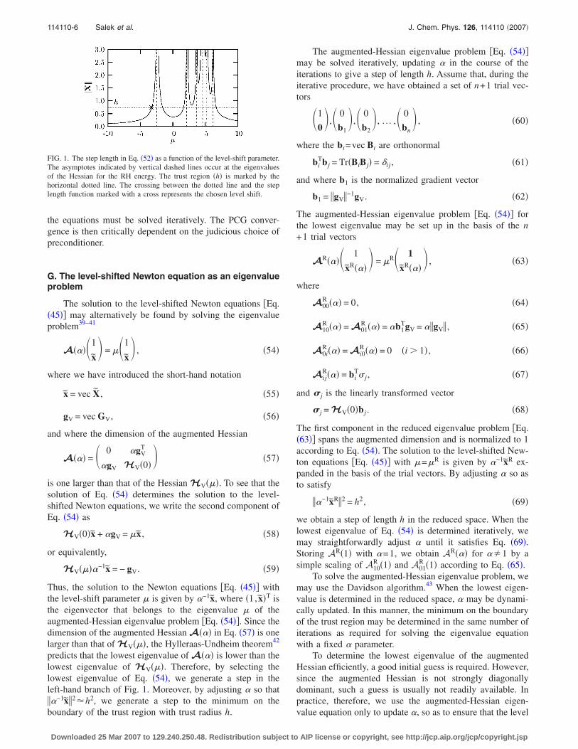
where XAI is the solution vector in the canonical MO basis.The step-length function

�X�S2 = �

AI

FAI2

�A − I − ��2 �53�

has k+1 branches, where k is the number of eigenvaluesA−I of the �unshifted� Hessian �see Fig. 1�. The function ispositive for all � with asymptotes at the eigenvalues. For�min�A−I�, the RH energy is lowered to both first andsecond orders.8,36 In the trust-region formalism, the steplength is taken to be the stationary point that corresponds tothe minimum on the boundary of the trust region. The sta-tionary point is therefore given by the intersection marked bya cross in Fig. 1.

In the canonical MO basis, the Hessian is diagonal andthe solution to the level-shifted Newton equations is trivial.In the AO basis, by contrast, the Hessian is not diagonal and



the equations must be solved iteratively. The PCG conver-gence is then critically dependent on the judicious choice ofpreconditioner.

G. The level-shifted Newton equation as an eigenvalueproblem

The solution to the level-shifted Newton equations �Eq.�45�� may alternatively be found by solving the eigenvalueproblem39–41

A��1

x = �1

x , �54�

where we have introduced the short-hand notation

x = vec X , �55�

gV = vec GV, �56�

and where the dimension of the augmented Hessian

A�� = 0 �gVT

�gV HV�0� �57�

is one larger than that of the Hessian HV��. To see that thesolution of Eq. �54� determines the solution to the level-shifted Newton equations, we write the second component ofEq. �54� as

HV�0�x + �gV = �x , �58�

or equivalently,

HV��−1x = − gV. �59�

Thus, the solution to the Newton equations �Eq. �45�� withthe level-shift parameter � is given by �−1x, where �1, x�T isthe eigenvector that belongs to the eigenvalue � of theaugmented-Hessian eigenvalue problem �Eq. �54��. Since thedimension of the augmented Hessian A�� in Eq. �57� is onelarger than that of HV��, the Hylleraas-Undheim theorem42

predicts that the lowest eigenvalue of A�� is lower than thelowest eigenvalue of HV��. Therefore, by selecting thelowest eigenvalue of Eq. �54�, we generate a step in theleft-hand branch of Fig. 1. Moreover, by adjusting � so that��−1x�2 h2, we generate a step to the minimum on theboundary of the trust region with trust radius h.

The augmented-Hessian eigenvalue problem �Eq. �54��may be solved iteratively, updating � in the course of theiterations to give a step of length h. Assume that, during theiterative procedure, we have obtained a set of n+1 trial vec-tors

1

0, 0

b1, 0

b2, . . . , 0

bn , �60�

where the bi=vec Bi are orthonormal

biTb j = Tr�BiB j� = �ij , �61�

and where b1 is the normalized gradient vector

b1 = �gV�−1gV. �62�

The augmented-Hessian eigenvalue problem �Eq. �54�� forthe lowest eigenvalue may be set up in the basis of the n+1 trial vectors

AR�� 1

xR�� = �R 1

xR�� , �63�

where

A00R �� = 0, �64�

A10R �� = A01

R �� = �b1TgV = ��gV� , �65�

A0iR �� = Ai0

R �� = 0 �i � 1� , �66�

AijR�� = bi

T� j , �67�

and � j is the linearly transformed vector

� j = HV�0�b j . �68�

The first component in the reduced eigenvalue problem �Eq.�63�� spans the augmented dimension and is normalized to 1according to Eq. �54�. The solution to the level-shifted New-ton equations �Eq. �45�� with �=�R is given by �−1xR ex-panded in the basis of the trial vectors. By adjusting � so asto satisfy

��−1xR�2 = h2, �69�

we obtain a step of length h in the reduced space. When thelowest eigenvalue of Eq. �54� is determined iteratively, wemay straightforwardly adjust � until it satisfies Eq. �69�.Storing AR�1� with �=1, we obtain AR�� for ��1 by asimple scaling of A10

R �1� and A01R �1� according to Eq. �65�.

To solve the augmented-Hessian eigenvalue problem, wemay use the Davidson algorithm.43 When the lowest eigen-value is determined in the reduced space, � may be dynami-cally updated. In this manner, the minimum on the boundaryof the trust region may be determined in the same number ofiterations as required for solving the eigenvalue equationwith a fixed � parameter.

To determine the lowest eigenvalue of the augmentedHessian efficiently, a good initial guess is required. However,since the augmented Hessian is not strongly diagonallydominant, such a guess is usually not readily available. Inpractice, therefore, we use the augmented-Hessian eigen-value equation only to update �, so as to ensure that the level

FIG. 1. The step length in Eq. �52� as a function of the level-shift parameter.The asymptotes indicated by vertical dashed lines occur at the eigenvaluesof the Hessian for the RH energy. The trust region �h� is marked by thehorizontal dotted line. The crossing between the dotted line and the steplength function marked with a cross represents the chosen level shift.



shift is in the proper interval and of the correct size. Theimproved trial vectors are themselves obtained by solvingthe level-shifted Newton equations in the same reducedspace �b1 ,b2 , . . . ,bn� as for the eigenvalue equation but withan updated level-shift parameter. Essentially, we perform asequence of PCG iterations, dynamically updating the level-shift parameter in the subspace generated by the PCG itera-tions.

In the PCG minimization, we first determine a solutionwith the step-size constraint �XV�=0.6, where �XV� is theFrobenius norm. Next, the subspace generated during thisminimization is utilized as the starting point for a subsequentminimization, now with the step-size constraint Xmax

V =0.35,where Xmax

V is the largest component of XV. Unlike the con-straint on �XV�, the constraint on Xmax

V is size-intensive. Thealgorithm is not sensitive to the choice of the �XV� param-eter, whereas Xmax

V should be chosen carefully. We havefound �XV�=0.6 and Xmax

V =0.35 to be suitable parameters.The first level shift is obtained by solving the

augmented-Hessian eigenvalue problem in a two-dimensional subspace, corresponding to a reduced spacecontaining only one trial vector, namely, the normalized gra-dient in Eq. �62�. The PCG iterations are terminated whenthe level shift has converged and when the residual has beenreduced by a factor of 100 relative to the residual in thetwo-dimensional reduced space.

The RH SCF iterations are continued until the gradientnorm �gV� is smaller than some preset threshold. However,just like �XV�, the norm �gV� is an extensive property. Indeedfor two noninteracting, identical systems, the total squarednorm is equal to twice the norm of each subsystem:

�gA+B�2 = �i

�giA�2 + �

i

�giB�2 = �gA�2 + �gB�2. �70�

A size-intensive requirement on the SCF convergence is thusto use the gradient norm divided by the square root of thenumber of electrons �gV� /�N.

H. Diagonalization of the level-shifted Fock/KS matrixby Newton’s method

The minimum of the RH energy subject to the step-sizeconstraint �Eq. �15�� may alternatively be determined by us-ing the MO coefficients as variational parameters. In thisparametrization, the density matrix may be expressed as

D�X� = CoccCoccT , �71�

where the coefficients of the occupied MOs Cocc satisfy theorthonormality constraint

CoccT SCocc = I . �72�

Imposing this orthonormality constraint simultaneously withthe step-size constraint �Eq. �15�� on the energy ERH, weobtain the Lagrangian

LRH�Cocc� = Tr�FD�X�� − ��2N − 2 Tr�DSD�X�S� − ��

− Tr ��CoccT SCocc − I� . �73�

Differentiation of this Lagrangian with respect to the MOcoefficients gives

�F − �SDS�Cocc�� = SCocc�� , �74�

where �� is chosen to be diagonal �� since the energyis invariant with respect to rotations among the occupiedMOs. The density matrix for the new RH iteration becomes

D�� = Cocc��CoccT �� , �75�

where Cocc�� are the eigenvectors of the generalized eigen-value problem �Eq. �74�� with the level-shifted Fock/KS ma-trix F−�SDS.

In the local part of the RH SCF optimization, where �=0 and X is small, the solution of the Newton matrix equa-tions �Eq. �23�� and the diagonalization of the Fock matrix�Eq. �74�� give essentially the same step and the same den-sity matrix. To first order in X, the solution of the Newtonequations then corresponds to a diagonalization of theFock/KS matrix. By contrast, in the global part of the RHSCF optimization, where X is larger, the steps obtained bydiagonalizing the Fock/KS matrix �Eq. �74�� and by solvingthe Newton equations �Eq. �23�� differ.

In our implementation, the Newton step is always takenin the local region, where �=0. In the global region, eachSCF iteration begins by solving the Newton eigenvalueequation �Eq. �54�� to determine the level-shift parameter�max by requiring that the largest step-length component isequal to Xmax

V . The minimization of

E�max

RH = Tr�F − �maxSDS�D�X� �76�

is represented by the solution of the Fock/KS eigenvalueequation �Eq. �74�� with �=�max. The solution of the level-shifted Newton equations with level-shift parameter �max

then represents a first-order diagonalization of the level-shifted Fock/KS matrix in Eq. �74�, whereas the full minimi-zation of E�max

RH requires a complete diagonalization and maybe accomplished by a sequence of level-shifted Newton it-erations with �=�max. In practice, a partial rather than exactminimization of E�max

RH is sufficient in the global region. Thus,in our implementation, no more than one or two level-shiftedNewton iterations �Eq. �23�� with �=�max are taken since,after two iterations, the Newton steps have become so smallthat they no longer affect the global SCF convergence. In-deed, our standard procedure is to take only one level-shiftedNewton step although we also report some calculationswhere two level-shifted Newton steps are taken at each SCFiteration.

I. Evaluation of the Coulomb contribution

The Coulomb contributions to the Fock/KS matrix andthe energy are given by

Jab = �ab� � , �77�

J = 12 � � � , �78�

in terms of the one-electron density



�r� = �cd

�c�r��d�r�Dcd. �79�

In density fitting,44,45 the computational cost is significantlyreduced by evaluating these contributions as

Jab = �ab� � , �80�

J = � � � − 12 � � � = J − 1

2 � − � − � �81�

from an approximate density expanded in an atom-centeredauxiliary basis:

�r� = ��

��r�c�. �82�

We determine the c� by minimizing the fitting error � − �w� − � with metric w subject to the charge-conservingconstraint � �r�dr=Ne, leading to the linear equation

��

��w��c� = ��w� � + �� , �83�

where the one-center overlaps are given by ��=��r�dr,and with

� =Ne − ��w��−1��

��w��−1��. �84�

From Eq. �81�, we see that the fitted Coulomb repulsionenergy is always lower than the regular repulsion energy. Thesmallest fitting error is obtained by an unconstrained mini-mization �=0 in the Coulomb metric w=r12

−1 in Eq. �83�. Theuse of constraints or of a non-Coulomb metric increases theerror, lowering the Coulomb energy.

With density fitting, large speedups are observed, butscaling becomes a problem for large systems—the inversion�Eq. �83�� scales cubically in time, whereas the memory re-quirements for the �� matrix scale quadratically. Toachieve linear scaling, there are two main strategies. One isto fit the density in a metric different from the long-rangeCoulomb metric, so that ��w�� of Eq. �83� becomes

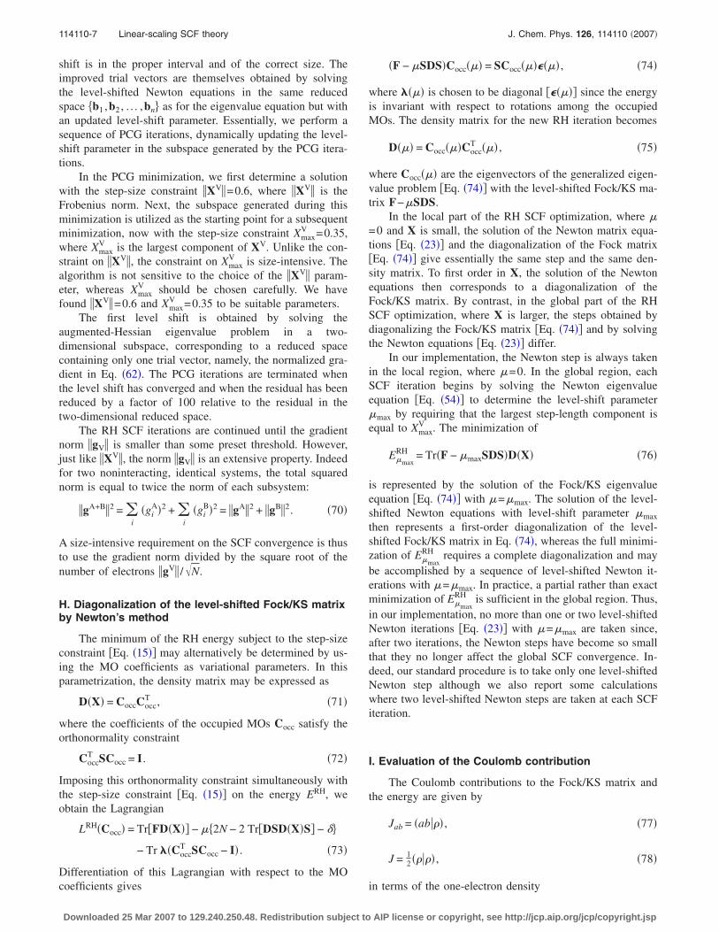
FIG. 2. The error in the energy in HF LS-TRSCF �top�and SCF/DIIS �bottom� optimizations.



sparse.45–47 Alternatively, the density is partitioned into lo-calized parts, which are fitted separately.48–50 We use an ap-proach similar to that of Ref. 48. The system is divided intolocalized parts i using the density partitioning51 of Yang andLee

�r� = �i

�i��r� = �i

�ab

�a�r��b�r�Dabxab�i� , �85�

where xab�i� =1 for both a and b in i, xab

�i� =1/2 for either a or bin i, and xab

�i� =0 otherwise. With this decomposition, some ofthe overlap distributions belonging to subsystem i may infact be centered outside this subsystem �by the Gaussianproduct rule�, but these decay exponentially with the squareof the separation between the two Gaussian functions.

Each subsystem density �i� is fitted using auxiliary func-tions located within an extended subsystem i, comprising theoriginal subsystem i padded with a buffer zone �i around thesubsystem

��i+�i

��c��i� = �

cd

��cd�Dcdxcd�i� − ��i�� . �86�

The multipliers are given by

��i� =Q�i� − ��i+�i

��−1�� i��

��i+�i��−1��

, �87�

with the subsystem charge

Q�i� =� �i��r�dr = �ab

SabDabxab�i� . �88�

The cost of solving Eq. �86� depends on the size of the sub-system rather than on the size of the full system. Given thatthe number of subsystems increases linearly with systemsize, the full density is fitted in linear time. In our calcula-tions, the total system is put in a rectangular box, which isrecursively bisected until no subbox contains more than 5000auxiliary basis functions. In the fitting, a buffer zone of width5 Bohr is used. In the applications presented here, we usedthe optimized basis set developed by Eichkorn et al.52,53 withno charge constraints imposed on the fitted density.

III. SAMPLE CALCULATIONS

In the HF and KS calculations reported here, we use theLS-TRSCF method, combining the LS-TRRH algorithm forthe RH iterations of Sec. II B with the TRDSM algorithm fordensity averaging �implemented in a local version of DALTON

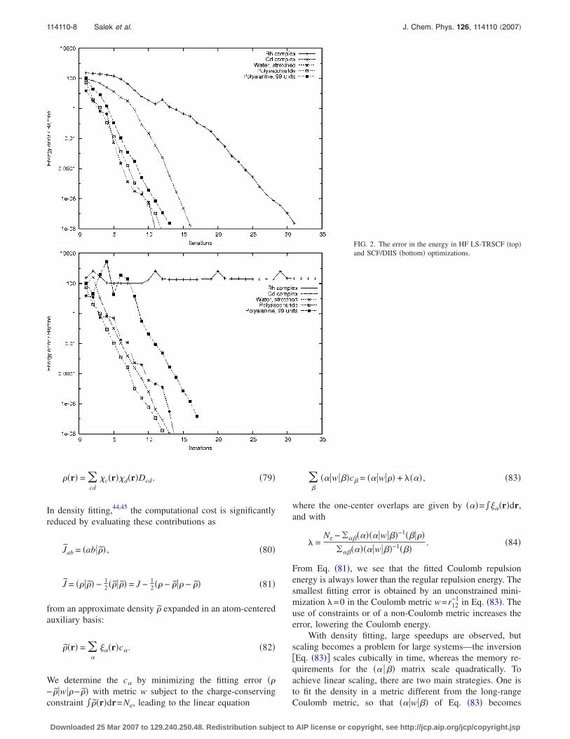
FIG. 3. The error in the energy in LDA KS optimizations using the one-step Newton LS-TRSCF �top left�, two-step Newton LS-TRSCF �top right�, andSCF/DIIS �bottom� methods.



�Ref. 54��. First, in Sec. III A, we compare the LS-TRSCFscheme with the traditional SCF/DIIS scheme. Next, in Sec.III B, we examine the CG solution of the RH Newton equa-tions �Eq. �45��. Finally, in Sec. III C, we consider the cost ofthe LS-TRRH optimization, demonstrating that linear scalingmay be obtained within this framework.

A. Convergence of the LS-TRSCF method

To compare the LS-TRSCF and SCF/DIIS methods, weuse the following five molecules which represent a variety ofbonding situations: the water molecule in the d-aug-pVTZbasis with the bonds stretched to twice their equilibriumvalue; the rhodium complex of Ref. 19, with the STO-3Gbasis for rhodium and the Ahlrichs VDZ basis for the otheratoms;55 the cadmium-imidazole complex of Ref. 18 in the3-21G basis; a 438-atom polysaccharide in the 6-31G basis;and a 992-atom polypeptide of 99 alanine residues in the6-31G basis. For all systems, we have carried out calcula-tions at the HF and KS levels of theory, using the localdensity approximation �LDA� and B3LYP functionals. As

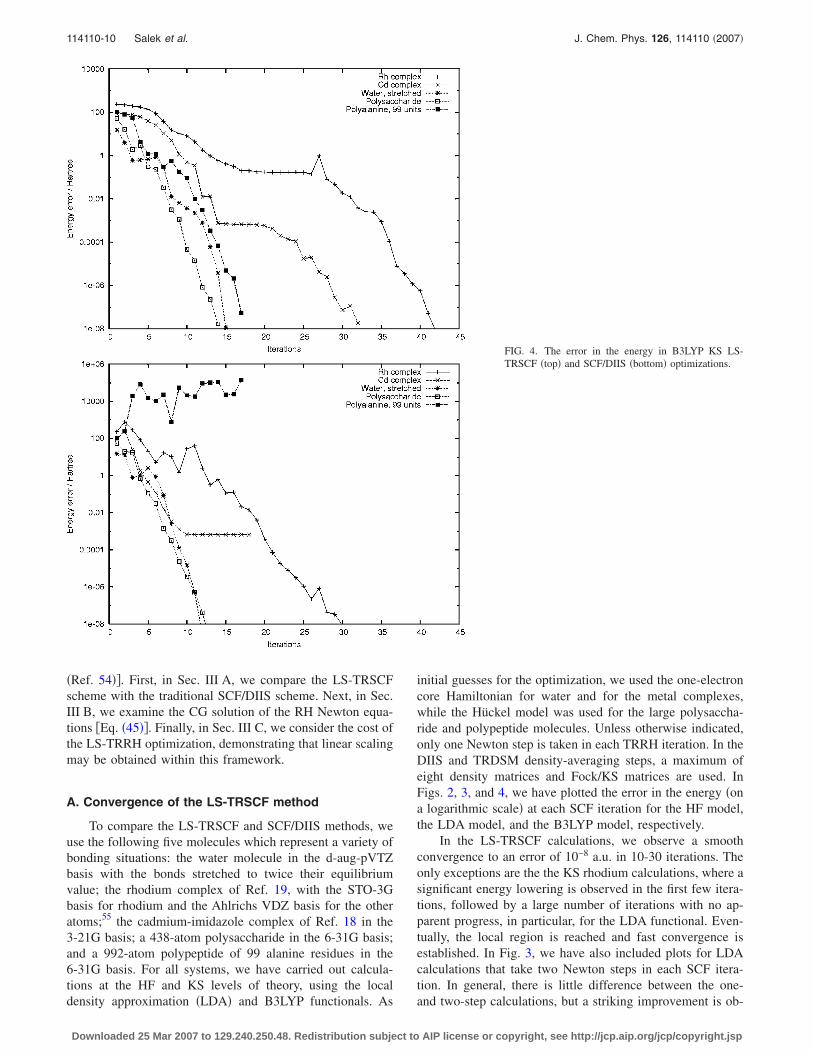
initial guesses for the optimization, we used the one-electroncore Hamiltonian for water and for the metal complexes,while the Hückel model was used for the large polysaccha-ride and polypeptide molecules. Unless otherwise indicated,only one Newton step is taken in each TRRH iteration. In theDIIS and TRDSM density-averaging steps, a maximum ofeight density matrices and Fock/KS matrices are used. InFigs. 2, 3, and 4, we have plotted the error in the energy �ona logarithmic scale� at each SCF iteration for the HF model,the LDA model, and the B3LYP model, respectively.

In the LS-TRSCF calculations, we observe a smoothconvergence to an error of 10−8 a.u. in 10-30 iterations. Theonly exceptions are the the KS rhodium calculations, where asignificant energy lowering is observed in the first few itera-tions, followed by a large number of iterations with no ap-parent progress, in particular, for the LDA functional. Even-tually, the local region is reached and fast convergence isestablished. In Fig. 3, we have also included plots for LDAcalculations that take two Newton steps in each SCF itera-tion. In general, there is little difference between the one-and two-step calculations, but a striking improvement is ob-

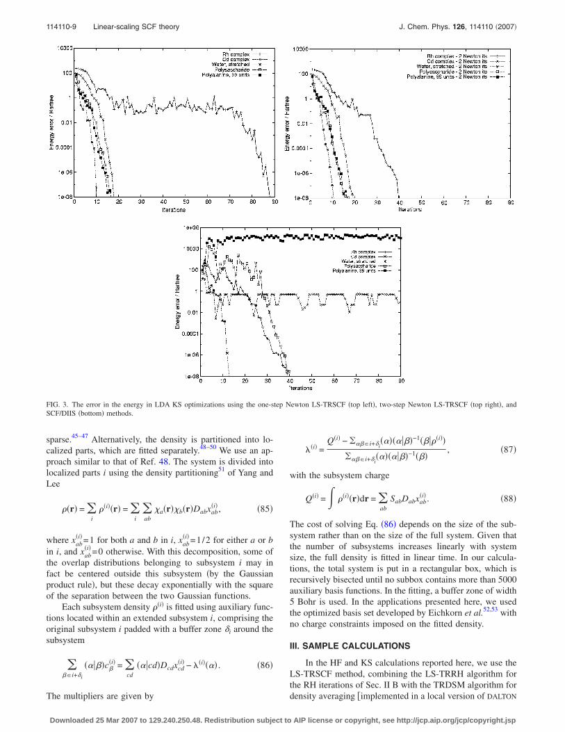
FIG. 4. The error in the energy in B3LYP KS LS-TRSCF �top� and SCF/DIIS �bottom� optimizations.



served for the rhodium complex. This improvement is not yetunderstood �it may be accidental�, and we continue to useone Newton iteration as the default in our optimizations.

A comparison of the SCF/DIIS plots with the LS-TRSCFplots in Figs. 2–4 clearly reveals the poorer SCF/DIIS per-formance, in particular, for the KS calculations. However,some differences are also observed in the HF calculations—unlike the LS-TRSCF method, the SCF/DIIS method di-verges for the rhodium complex and performs erratically inthe global part of the polyalanine optimization. In general,we note that the SCF/DIIS and LS-TRSCF differences arelargest in the global region, where the SCF/DIIS schemesuffers from the fact that it is not based on the principles ofenergy minimization and step-size control, sometimes lead-ing to an erratic behavior. In the local region, size constraintsbecome irrelevant, since both methods use the quasi-Newtoncondition to speed up the local convergence, which becomesvery similar for the two methods.

The SCF/DIIS LDA calculations in Fig. 3 show a strik-ingly erratic behavior. The cadmium and polyalanine calcu-

lations both diverge; for the polysaccharide, no convergenceis observed until iteration 25. Surprisingly, the LDA calcula-tion on the rhodium complex converges, unlike the Hartree-Fock calculation. Finally, concerning the B3LYP functionalin Fig. 4, we note that the SCF/DIIS polyalanine optimiza-tion diverges. Interestingly, for the cadmium complex, thehorizontal line that begins at iteration 10 indicates conver-gence to a stationary point of higher energy than that ob-tained with the LS-TRSCF algorithm. Indeed, a closer ex-amination of this stationary point reveals that it is a saddlepoint with the lowest Hessian eigenvalue of −0.0147 a.u.From an inspection of the corresponding LS-TRSCF curve, itappears that the LS-TRSCF approaches the same saddlepoint in iterations 15-20. At iteration 17, however, TRDSMdetects a negative Hessian eigenvalue, and from iteration 20,convergence is established towards the minimum �lowestHessian eigenvalue of 0.0275 a.u.�, which is reached in 32iterations.

B. The solution of the Roothaan-Hall Newton equations

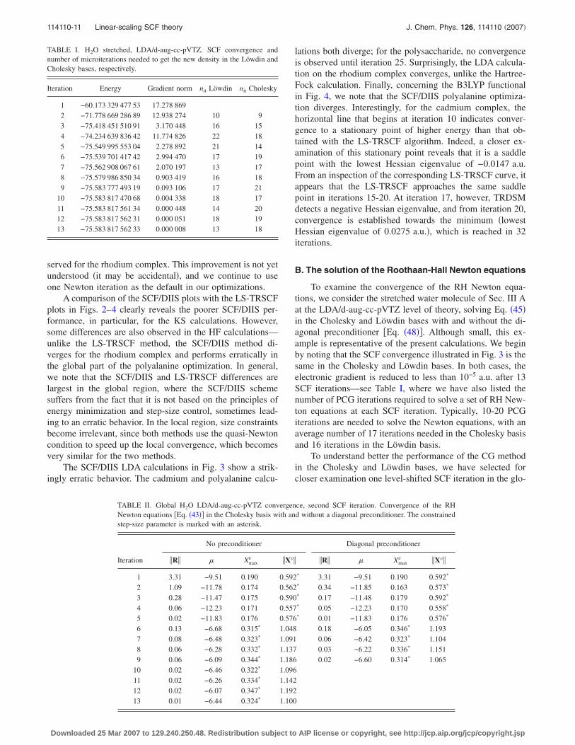
To examine the convergence of the RH Newton equa-tions, we consider the stretched water molecule of Sec. III Aat the LDA/d-aug-cc-pVTZ level of theory, solving Eq. �45�in the Cholesky and Löwdin bases with and without the di-agonal preconditioner �Eq. �48��. Although small, this ex-ample is representative of the present calculations. We beginby noting that the SCF convergence illustrated in Fig. 3 is thesame in the Cholesky and Löwdin bases. In both cases, theelectronic gradient is reduced to less than 10−5 a.u. after 13SCF iterations—see Table I, where we have also listed thenumber of PCG iterations required to solve a set of RH New-ton equations at each SCF iteration. Typically, 10-20 PCGiterations are needed to solve the Newton equations, with anaverage number of 17 iterations needed in the Cholesky basisand 16 iterations in the Löwdin basis.

To understand better the performance of the CG methodin the Cholesky and Löwdin bases, we have selected forcloser examination one level-shifted SCF iteration in the glo-

TABLE I. H2O stretched, LDA/d-aug-cc-pVTZ. SCF convergence andnumber of microiterations needed to get the new density in the Löwdin andCholesky bases, respectively.

Iteration Energy Gradient norm nit Löwdin nit Cholesky

1 −60.173 329 477 53 17.278 8692 −71.778 669 286 89 12.938 274 10 93 −75.418 451 510 91 3.170 448 16 154 −74.234 639 836 42 11.774 826 22 185 −75.549 995 553 04 2.278 892 21 146 −75.539 701 417 42 2.994 470 17 197 −75.562 908 067 61 2.070 197 13 178 −75.579 986 850 34 0.903 419 16 189 −75.583 777 493 19 0.093 106 17 21

10 −75.583 817 470 68 0.004 338 18 1711 −75.583 817 561 34 0.000 448 14 2012 −75.583 817 562 31 0.000 051 18 1913 −75.583 817 562 33 0.000 008 13 18

TABLE II. Global H2O LDA/d-aug-cc-pVTZ convergence, second SCF iteration. Convergence of the RHNewton equations �Eq. �43�� in the Cholesky basis with and without a diagonal preconditioner. The constrainedstep-size parameter is marked with an asterisk.

Iteration

No preconditioner Diagonal preconditioner

�R� � Xmaxv �Xv� �R� � Xmax

v �Xv�

1 3.31 −9.51 0.190 0.592* 3.31 −9.51 0.190 0.592*

2 1.09 −11.78 0.174 0.562* 0.34 −11.85 0.163 0.573*

3 0.28 −11.47 0.175 0.590* 0.17 −11.48 0.179 0.592*

4 0.06 −12.23 0.171 0.557* 0.05 −12.23 0.170 0.558*

5 0.02 −11.83 0.176 0.576* 0.01 −11.83 0.176 0.576*

6 0.13 −6.68 0.315* 1.048 0.18 −6.05 0.346* 1.1937 0.08 −6.48 0.323* 1.091 0.06 −6.42 0.323* 1.1048 0.06 −6.28 0.332* 1.137 0.03 −6.22 0.336* 1.1519 0.06 −6.09 0.344* 1.186 0.02 −6.60 0.314* 1.065

10 0.02 −6.46 0.322* 1.09611 0.02 −6.26 0.334* 1.14212 0.02 −6.07 0.347* 1.19213 0.01 −6.44 0.324* 1.100



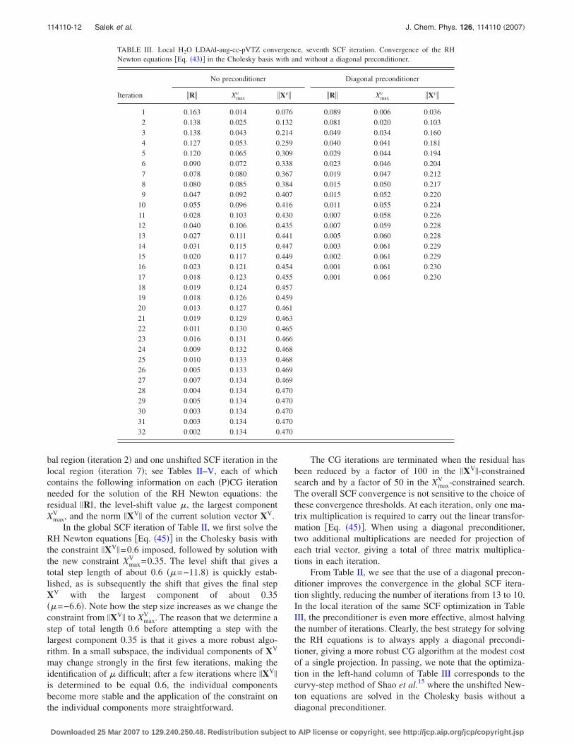
bal region �iteration 2� and one unshifted SCF iteration in thelocal region �iteration 7�; see Tables II–V, each of whichcontains the following information on each �P�CG iterationneeded for the solution of the RH Newton equations: theresidual �R�, the level-shift value �, the largest componentXmax

V , and the norm �XV� of the current solution vector XV.In the global SCF iteration of Table II, we first solve the

RH Newton equations �Eq. �45�� in the Cholesky basis withthe constraint �XV�=0.6 imposed, followed by solution withthe new constraint Xmax

V =0.35. The level shift that gives atotal step length of about 0.6 ��=−11.8� is quickly estab-lished, as is subsequently the shift that gives the final stepXV with the largest component of about 0.35��=−6.6�. Note how the step size increases as we change theconstraint from �XV� to Xmax

V . The reason that we determine astep of total length 0.6 before attempting a step with thelargest component 0.35 is that it gives a more robust algo-rithm. In a small subspace, the individual components of XV

may change strongly in the first few iterations, making theidentification of � difficult; after a few iterations where �XV�

is determined to be equal 0.6, the individual componentsbecome more stable and the application of the constraint onthe individual components more straightforward.

The CG iterations are terminated when the residual hasbeen reduced by a factor of 100 in the �XV�-constrainedsearch and by a factor of 50 in the Xmax

V -constrained search.The overall SCF convergence is not sensitive to the choice ofthese convergence thresholds. At each iteration, only one ma-trix multiplication is required to carry out the linear transfor-mation �Eq. �45��. When using a diagonal preconditioner,two additional multiplications are needed for projection ofeach trial vector, giving a total of three matrix multiplica-tions in each iteration.

From Table II, we see that the use of a diagonal precon-ditioner improves the convergence in the global SCF itera-tion slightly, reducing the number of iterations from 13 to 10.In the local iteration of the same SCF optimization in TableIII, the preconditioner is even more effective, almost halvingthe number of iterations. Clearly, the best strategy for solvingthe RH equations is to always apply a diagonal precondi-tioner, giving a more robust CG algorithm at the modest costof a single projection. In passing, we note that the optimiza-tion in the left-hand column of Table III corresponds to thecurvy-step method of Shao et al.15 where the unshifted New-ton equations are solved in the Cholesky basis without adiagonal preconditioner.

TABLE III. Local H2O LDA/d-aug-cc-pVTZ convergence, seventh SCF iteration. Convergence of the RHNewton equations �Eq. �43�� in the Cholesky basis with and without a diagonal preconditioner.

Iteration


�R� Xmaxv �Xv� �R� Xmax

v �Xv�

1 0.163 0.014 0.076 0.089 0.006 0.0362 0.138 0.025 0.132 0.081 0.020 0.1033 0.138 0.043 0.214 0.049 0.034 0.1604 0.127 0.053 0.259 0.040 0.041 0.1815 0.120 0.065 0.309 0.029 0.044 0.1946 0.090 0.072 0.338 0.023 0.046 0.2047 0.078 0.080 0.367 0.019 0.047 0.2128 0.080 0.085 0.384 0.015 0.050 0.2179 0.047 0.092 0.407 0.015 0.052 0.220

10 0.055 0.096 0.416 0.011 0.055 0.22411 0.028 0.103 0.430 0.007 0.058 0.22612 0.040 0.106 0.435 0.007 0.059 0.22813 0.027 0.111 0.441 0.005 0.060 0.22814 0.031 0.115 0.447 0.003 0.061 0.22915 0.020 0.117 0.449 0.002 0.061 0.22916 0.023 0.121 0.454 0.001 0.061 0.23017 0.018 0.123 0.455 0.001 0.061 0.23018 0.019 0.124 0.45719 0.018 0.126 0.45920 0.013 0.127 0.46121 0.019 0.129 0.46322 0.011 0.130 0.46523 0.016 0.131 0.46624 0.009 0.132 0.46825 0.010 0.133 0.46826 0.005 0.133 0.46927 0.007 0.134 0.46928 0.004 0.134 0.47029 0.005 0.134 0.47030 0.003 0.134 0.47031 0.003 0.134 0.47032 0.002 0.134 0.470



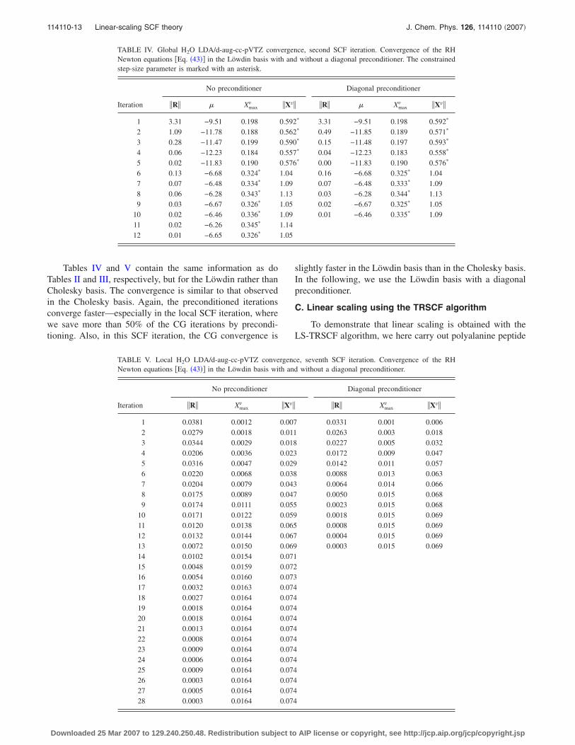
Tables IV and V contain the same information as doTables II and III, respectively, but for the Löwdin rather thanCholesky basis. The convergence is similar to that observedin the Cholesky basis. Again, the preconditioned iterationsconverge faster—especially in the local SCF iteration, wherewe save more than 50% of the CG iterations by precondi-tioning. Also, in this SCF iteration, the CG convergence is

slightly faster in the Löwdin basis than in the Cholesky basis.In the following, we use the Löwdin basis with a diagonalpreconditioner.

C. Linear scaling using the TRSCF algorithm

To demonstrate that linear scaling is obtained with theLS-TRSCF algorithm, we here carry out polyalanine peptide

TABLE IV. Global H2O LDA/d-aug-cc-pVTZ convergence, second SCF iteration. Convergence of the RHNewton equations �Eq. �43�� in the Löwdin basis with and without a diagonal preconditioner. The constrainedstep-size parameter is marked with an asterisk.

Iteration


�R� � Xmaxv �Xv� �R� � Xmax

v �Xv�

1 3.31 −9.51 0.198 0.592* 3.31 −9.51 0.198 0.592*

2 1.09 −11.78 0.188 0.562* 0.49 −11.85 0.189 0.571*

3 0.28 −11.47 0.199 0.590* 0.15 −11.48 0.197 0.593*

4 0.06 −12.23 0.184 0.557* 0.04 −12.23 0.183 0.558*

5 0.02 −11.83 0.190 0.576* 0.00 −11.83 0.190 0.576*

6 0.13 −6.68 0.324* 1.04 0.16 −6.68 0.325* 1.047 0.07 −6.48 0.334* 1.09 0.07 −6.48 0.333* 1.098 0.06 −6.28 0.343* 1.13 0.03 −6.28 0.344* 1.139 0.03 −6.67 0.326* 1.05 0.02 −6.67 0.325* 1.05

10 0.02 −6.46 0.336* 1.09 0.01 −6.46 0.335* 1.0911 0.02 −6.26 0.345* 1.1412 0.01 −6.65 0.326* 1.05

TABLE V. Local H2O LDA/d-aug-cc-pVTZ convergence, seventh SCF iteration. Convergence of the RHNewton equations �Eq. �43�� in the Löwdin basis with and without a diagonal preconditioner.

Iteration


�R� Xmaxv �Xv� �R� Xmax

v �Xv�

1 0.0381 0.0012 0.007 0.0331 0.001 0.0062 0.0279 0.0018 0.011 0.0263 0.003 0.0183 0.0344 0.0029 0.018 0.0227 0.005 0.0324 0.0206 0.0036 0.023 0.0172 0.009 0.0475 0.0316 0.0047 0.029 0.0142 0.011 0.0576 0.0220 0.0068 0.038 0.0088 0.013 0.0637 0.0204 0.0079 0.043 0.0064 0.014 0.0668 0.0175 0.0089 0.047 0.0050 0.015 0.0689 0.0174 0.0111 0.055 0.0023 0.015 0.068

10 0.0171 0.0122 0.059 0.0018 0.015 0.06911 0.0120 0.0138 0.065 0.0008 0.015 0.06912 0.0132 0.0144 0.067 0.0004 0.015 0.06913 0.0072 0.0150 0.069 0.0003 0.015 0.06914 0.0102 0.0154 0.07115 0.0048 0.0159 0.07216 0.0054 0.0160 0.07317 0.0032 0.0163 0.07418 0.0027 0.0164 0.07419 0.0018 0.0164 0.07420 0.0018 0.0164 0.07421 0.0013 0.0164 0.07422 0.0008 0.0164 0.07423 0.0009 0.0164 0.07424 0.0006 0.0164 0.07425 0.0009 0.0164 0.07426 0.0003 0.0164 0.07427 0.0005 0.0164 0.07428 0.0003 0.0164 0.074



calculations with up to 119 alanine residues �1192 atoms�using the HF and B3LYP models in the 6-31G basis. EachSCF optimization converges as the 99-residue calculations inFigs. 2 and 4.

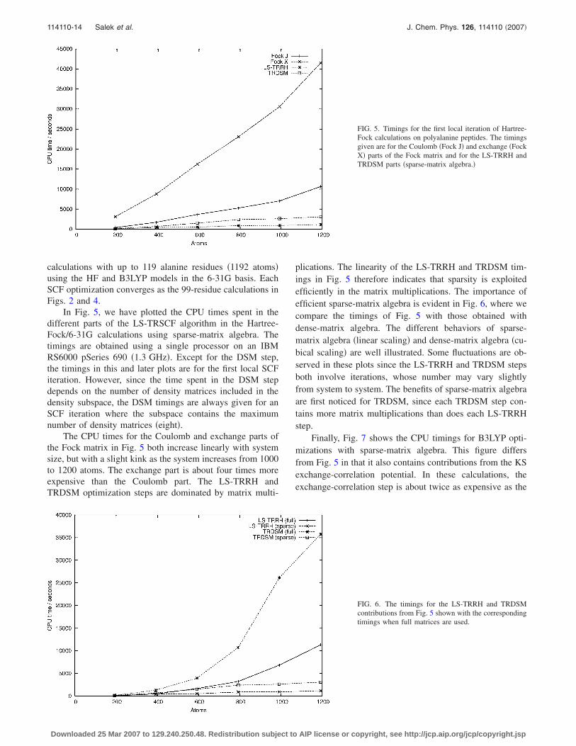
In Fig. 5, we have plotted the CPU times spent in thedifferent parts of the LS-TRSCF algorithm in the Hartree-Fock/6-31G calculations using sparse-matrix algebra. Thetimings are obtained using a single processor on an IBMRS6000 pSeries 690 �1.3 GHz�. Except for the DSM step,the timings in this and later plots are for the first local SCFiteration. However, since the time spent in the DSM stepdepends on the number of density matrices included in thedensity subspace, the DSM timings are always given for anSCF iteration where the subspace contains the maximumnumber of density matrices �eight�.

The CPU times for the Coulomb and exchange parts ofthe Fock matrix in Fig. 5 both increase linearly with systemsize, but with a slight kink as the system increases from 1000to 1200 atoms. The exchange part is about four times moreexpensive than the Coulomb part. The LS-TRRH andTRDSM optimization steps are dominated by matrix multi-

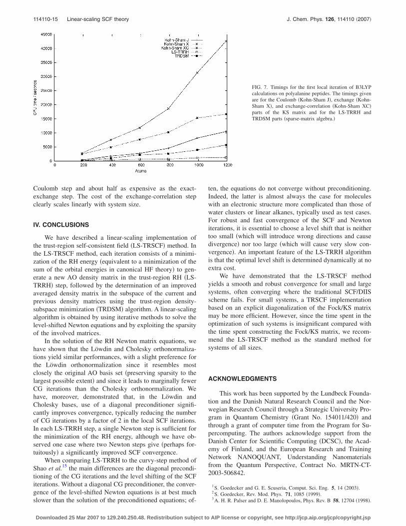
plications. The linearity of the LS-TRRH and TRDSM tim-ings in Fig. 5 therefore indicates that sparsity is exploitedefficiently in the matrix multiplications. The importance ofefficient sparse-matrix algebra is evident in Fig. 6, where wecompare the timings of Fig. 5 with those obtained withdense-matrix algebra. The different behaviors of sparse-matrix algebra �linear scaling� and dense-matrix algebra �cu-bical scaling� are well illustrated. Some fluctuations are ob-served in these plots since the LS-TRRH and TRDSM stepsboth involve iterations, whose number may vary slightlyfrom system to system. The benefits of sparse-matrix algebraare first noticed for TRDSM, since each TRDSM step con-tains more matrix multiplications than does each LS-TRRHstep.

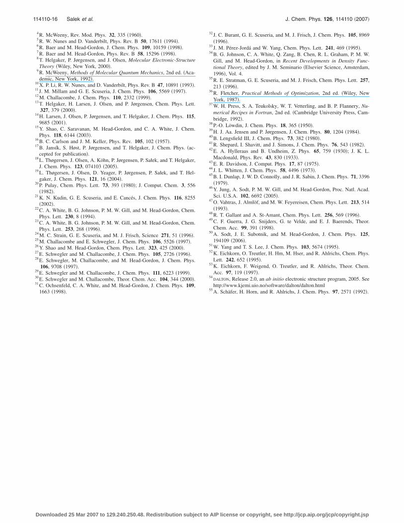
Finally, Fig. 7 shows the CPU timings for B3LYP opti-mizations with sparse-matrix algebra. This figure differsfrom Fig. 5 in that it also contains contributions from the KSexchange-correlation potential. In these calculations, theexchange-correlation step is about twice as expensive as the

FIG. 5. Timings for the first local iteration of Hartree-Fock calculations on polyalanine peptides. The timingsgiven are for the Coulomb �Fock J� and exchange �FockX� parts of the Fock matrix and for the LS-TRRH andTRDSM parts �sparse-matrix algebra.�

FIG. 6. The timings for the LS-TRRH and TRDSMcontributions from Fig. 5 shown with the correspondingtimings when full matrices are used.



Coulomb step and about half as expensive as the exact-exchange step. The cost of the exchange-correlation stepclearly scales linearly with system size.

IV. CONCLUSIONS

We have described a linear-scaling implementation ofthe trust-region self-consistent field �LS-TRSCF� method. Inthe LS-TRSCF method, each iteration consists of a minimi-zation of the RH energy �equivalent to a minimization of thesum of the orbital energies in canonical HF theory� to gen-erate a new AO density matrix in the trust-region RH �LS-TRRH� step, followed by the determination of an improvedaveraged density matrix in the subspace of the current andprevious density matrices using the trust-region density-subspace minimization �TRDSM� algorithm. A linear-scalingalgorithm is obtained by using iterative methods to solve thelevel-shifted Newton equations and by exploiting the sparsityof the involved matrices.

In the solution of the RH Newton matrix equations, wehave shown that the Löwdin and Cholesky orthonormaliza-tions yield similar performances, with a slight preference forthe Löwdin orthonormalization since it resembles mostclosely the original AO basis set �preserving sparsity to thelargest possible extent� and since it leads to marginally fewerCG iterations than the Cholesky orthonormalization. Wehave, moreover, demonstrated that, in the Löwdin andCholesky bases, use of a diagonal preconditioner signifi-cantly improves convergence, typically reducing the numberof CG iterations by a factor of 2 in the local SCF iterations.In each LS-TRRH step, a single Newton step is sufficient forthe minimization of the RH energy, although we have ob-served one case where two Newton steps give �perhaps for-tuitously� a significantly improved SCF convergence.

When comparing LS-TRRH to the curvy-step method ofShao et al.15 the main differences are the diagonal precondi-tioning of the CG iterations and the level shifting of the SCFiterations. Without a diagonal CG preconditioner, the conver-gence of the level-shifted Newton equations is at best muchslower than the solution of the preconditioned equations; of-

ten, the equations do not converge without preconditioning.Indeed, the latter is almost always the case for moleculeswith an electronic structure more complicated than those ofwater clusters or linear alkanes, typically used as test cases.For robust and fast convergence of the SCF and Newtoniterations, it is essential to choose a level shift that is neithertoo small �which will introduce wrong directions and causedivergence� nor too large �which will cause very slow con-vergence�. An important feature of the LS-TRRH algorithmis that the optimal level shift is determined dynamically at noextra cost.

We have demonstrated that the LS-TRSCF methodyields a smooth and robust convergence for small and largesystems, often converging where the traditional SCF/DIISscheme fails. For small systems, a TRSCF implementationbased on an explicit diagonalization of the Fock/KS matrixmay be more efficient. However, since the time spent in theoptimization of such systems is insignificant compared withthe time spent constructing the Fock/KS matrix, we recom-mend the LS-TRSCF method as the standard method forsystems of all sizes.

ACKNOWLEDGMENTS

This work has been supported by the Lundbeck Founda-tion and the Danish Natural Research Council and the Nor-wegian Research Council through a Strategic University Pro-gram in Quantum Chemistry �Grant No. 154011/420� andthrough a grant of computer time from the Program for Su-percomputing. The authors acknowledge support from theDanish Center for Scientific Computing �DCSC�, the Acad-emy of Finland, and the European Research and TrainingNetwork NANOQUANT, Understanding Nanomaterialsfrom the Quantum Perspective, Contract No. MRTN-CT-2003-506842.

1 S. Goedecker and G. E. Scuseria, Comput. Sci. Eng. 5, 14 �2003�.2 S. Goedecker, Rev. Mod. Phys. 71, 1085 �1999�.3 A. H. R. Palser and D. E. Manolopoulos, Phys. Rev. B 58, 12704 �1998�.

FIG. 7. Timings for the first local iteration of B3LYPcalculations on polyalanine peptides. The timings givenare for the Coulomb �Kohn-Sham J�, exchange �Kohn-Sham X�, and exchange-correlation �Kohn-Sham XC�parts of the KS matrix and for the LS-TRRH andTRDSM parts �sparse-matrix algebra.�



4 R. McWeeny, Rev. Mod. Phys. 32, 335 �1960�.5 R. W. Nunes and D. Vanderbilt, Phys. Rev. B 50, 17611 �1994�.6 R. Baer and M. Head-Gordon, J. Chem. Phys. 109, 10159 �1998�.7 R. Baer and M. Head-Gordon, Phys. Rev. B 58, 15296 �1998�.8 T. Helgaker, P. Jørgensen, and J. Olsen, Molecular Electronic-StructureTheory �Wiley, New York, 2000�.

9 R. McWeeny, Methods of Molecular Quantum Mechanics, 2nd ed. �Aca-demic, New York, 1992�.

10 X. P. Li, R. W. Nunes, and D. Vanderbilt, Phys. Rev. B 47, 10891 �1993�.11 J. M. Millam and G. E. Scuseria, J. Chem. Phys. 106, 5569 �1997�.12 M. Challacombe, J. Chem. Phys. 110, 2332 �1999�.13 T. Helgaker, H. Larsen, J. Olsen, and P. Jørgensen, Chem. Phys. Lett.

327, 379 �2000�.14 H. Larsen, J. Olsen, P. Jørgensen, and T. Helgaker, J. Chem. Phys. 115,

9685 �2001�.15 Y. Shao, C. Saravanan, M. Head-Gordon, and C. A. White, J. Chem.

Phys. 118, 6144 �2003�.16 B. C. Carlson and J. M. Keller, Phys. Rev. 105, 102 �1957�.17 B. Jansík, S. Høst, P. Jørgensen, and T. Helgaker, J. Chem. Phys. �ac-

cepted for publication�.18 L. Thøgersen, J. Olsen, A. Köhn, P. Jørgensen, P. Sałek, and T. Helgaker,

J. Chem. Phys. 123, 074103 �2005�.19 L. Thøgersen, J. Olsen, D. Yeager, P. Jørgensen, P. Sałek, and T. Hel-

gaker, J. Chem. Phys. 121, 16 �2004�.20 P. Pulay, Chem. Phys. Lett. 73, 393 �1980�; J. Comput. Chem. 3, 556

�1982�.21 K. N. Kudin, G. E. Scuseria, and E. Cancés, J. Chem. Phys. 116, 8255

�2002�.22 C. A. White, B. G. Johnson, P. M. W. Gill, and M. Head-Gordon, Chem.

Phys. Lett. 230, 8 �1994�.23 C. A. White, B. G. Johnson, P. M. W. Gill, and M. Head-Gordon, Chem.

Phys. Lett. 253, 268 �1996�.24 M. C. Strain, G. E. Scuseria, and M. J. Frisch, Science 271, 51 �1996�.25 M. Challacombe and E. Schwegler, J. Chem. Phys. 106, 5526 �1997�.26 Y. Shao and M. Head-Gordon, Chem. Phys. Lett. 323, 425 �2000�.27 E. Schwegler and M. Challacombe, J. Chem. Phys. 105, 2726 �1996�.28 E. Schwegler, M. Challacombe, and M. Head-Gordon, J. Chem. Phys.

106, 9708 �1997�.29 E. Schwegler and M. Challacombe, J. Chem. Phys. 111, 6223 �1999�.30 E. Schwegler and M. Challacombe, Theor. Chem. Acc. 104, 344 �2000�.31 C. Ochsenfeld, C. A. White, and M. Head-Gordon, J. Chem. Phys. 109,

1663 �1998�.

32 J. C. Burant, G. E. Scuseria, and M. J. Frisch, J. Chem. Phys. 105, 8969�1996�.

33 J. M. Pérez-Jordá and W. Yang, Chem. Phys. Lett. 241, 469 �1995�.34 B. G. Johnson, C. A. White, Q. Zang, B. Chen, R. L. Graham, P. M. W.

Gill, and M. Head-Gordon, in Recent Developments in Density Func-tional Theory, edited by J. M. Seminario �Elsevier Science, Amsterdam,1996�, Vol. 4.

35 R. E. Stratman, G. E. Scuseria, and M. J. Frisch, Chem. Phys. Lett. 257,213 �1996�.

36 R. Fletcher, Practical Methods of Optimization, 2nd ed. �Wiley, NewYork, 1987�.

37 W. H. Press, S. A. Teukolsky, W. T. Vetterling, and B. P. Flannery, Nu-merical Recipes in Fortran, 2nd ed. �Cambridge University Press, Cam-bridge, 1992�.

38 P.-O. Löwdin, J. Chem. Phys. 18, 365 �1950�.39 H. J. Aa. Jensen and P. Jørgensen, J. Chem. Phys. 80, 1204 �1984�.40 B. Lengsfield III, J. Chem. Phys. 73, 382 �1980�.41 R. Shepard, I. Shavitt, and J. Simons, J. Chem. Phys. 76, 543 �1982�.42 E. A. Hylleraas and B. Undheim, Z. Phys. 65, 759 �1930�; J. K. L.

Macdonald, Phys. Rev. 43, 830 �1933�.43 E. R. Davidson, J. Comput. Phys. 17, 87 �1975�.44 J. L. Whitten, J. Chem. Phys. 58, 4496 �1973�.45 B. I. Dunlap, J. W. D. Connolly, and J. R. Sabin, J. Chem. Phys. 71, 3396

�1979�.46 Y. Jung, A. Sodt, P. M. W. Gill, and M. Head-Gordon, Proc. Natl. Acad.

Sci. U.S.A. 102, 6692 �2005�.47 O. Vahtras, J. Almlöf, and M. W. Feyereisen, Chem. Phys. Lett. 213, 514

�1993�.48 R. T. Gallant and A. St-Amant, Chem. Phys. Lett. 256, 569 �1996�.49 C. F. Guerra, J. G. Snijders, G. te Velde, and E. J. Baerends, Theor.

Chem. Acc. 99, 391 �1998�.50 A. Sodt, J. E. Subotnik, and M. Head-Gordon, J. Chem. Phys. 125,

194109 �2006�.51 W. Yang and T. S. Lee, J. Chem. Phys. 103, 5674 �1995�.52 K. Eichkorn, O. Treutler, H. Hm, M. Hser, and R. Ahlrichs, Chem. Phys.

Lett. 242, 652 �1995�.53 K. Eichkorn, F. Weigend, O. Treutler, and R. Ahlrichs, Theor. Chem.

Acc. 97, 119 �1997�.54

DALTON, Release 2.0, an ab initio electronic structure program, 2005. Seehttp://www.kjemi.uio.no/software/dalton/dalton.html

55 A. Schäfer, H. Horn, and R. Ahlrichs, J. Chem. Phys. 97, 2571 �1992�.



https://www.researchgate.net/publication/216300613_Practical_Methods_of_Optimization?el=1_x_8&enrichId=rgreq-e04960ecdd942ae79503535a6786a02d-XXX&enrichSource=Y292ZXJQYWdlOzY0MjY1ODM7QVM6MTAyMTU5NTM4NDU4NjI5QDE0MDEzNjgxNDEyMTU=

https://www.researchgate.net/publication/216300613_Practical_Methods_of_Optimization?el=1_x_8&enrichId=rgreq-e04960ecdd942ae79503535a6786a02d-XXX&enrichSource=Y292ZXJQYWdlOzY0MjY1ODM7QVM6MTAyMTU5NTM4NDU4NjI5QDE0MDEzNjgxNDEyMTU=

https://www.researchgate.net/publication/252141690_An_Overview_of_Molecular_Quantum_Mechanics?el=1_x_8&enrichId=rgreq-e04960ecdd942ae79503535a6786a02d-XXX&enrichSource=Y292ZXJQYWdlOzY0MjY1ODM7QVM6MTAyMTU5NTM4NDU4NjI5QDE0MDEzNjgxNDEyMTU=

https://www.researchgate.net/publication/252141690_An_Overview_of_Molecular_Quantum_Mechanics?el=1_x_8&enrichId=rgreq-e04960ecdd942ae79503535a6786a02d-XXX&enrichSource=Y292ZXJQYWdlOzY0MjY1ODM7QVM6MTAyMTU5NTM4NDU4NjI5QDE0MDEzNjgxNDEyMTU=

Linear-scaling implementation of molecular electronic self-consistent field theory

Documents