Linear Precision for Toric Surface Patches

arX

iv:0

806.

3230

v2 [

mat

h.A

G]

29

Jun

2009

LINEAR PRECISION FOR TORIC SURFACE PATCHES

HANS-CHRISTIAN GRAF VON BOTHMER, KRISTIAN RANESTAD, AND FRANK SOTTILE

Abstract. We classify the homogeneous polynomials in three variables whose toricpolar linear system defines a Cremona transformation. This classification includes, asa proper subset, the classification of toric surface patches from geometric modelingwhich have linear precision. Besides the well-known tensor product patches andBezier triangles, we identify a family of toric patches with trapezoidal shape, each ofwhich has linear precision. Furthermore, Bezier triangles and tensor product patchesare special cases of trapezoidal patches.

Communicated by Wolfgang Dahmen and Herbert Edelsbrunner

Introduction

While the basic units in the geometric modeling of surfaces are Bezier trianglesand rectangular tensor product patches, some applications call for multi-sided C∞

patches (see [8] for a discussion). Krasauskas’s toric Bezier patches [10] are a flexibleand mathematically appealing system of such patches. These are based on real toricvarieties from algebraic geometry, may have shape any polytope ∆ with integer vertices,and they include the classical Bezier patches as special cases. For descriptions ofmultisided patches and toric patches, see [6].

More precisely, given a set of lattice points in Zn with convex hull ∆, Krasauskasdefined toric Bezier functions, which are polynomial blending functions associated toeach lattice point. This collection of lattice points and toric Bezier functions, togetherwith a positive weight associated to each lattice point is a toric patch. Choosing also acontrol point in Rd for each lattice point leads to a map Φ: ∆ → Rd whose image maybe used in modeling. If we choose the lattice points themselves as control points weobtain the tautological map τ : ∆ → ∆, which is a bijection. If the tautological maphas a rational inverse, then the toric patch has linear precision.

The lattice points and weights of a toric patch are encoded in a homogeneous multi-variate polynomial F (x0, . . . , xn) with positive coefficients, with every such polynomialcorresponding to a toric patch. In [5] it was shown that the toric patch given by F haslinear precision if and only if the associated toric polar linear system,

T (F ) =⟨x0∂F

∂x0

, x1∂F

∂x1

, . . . , xn

∂F

∂xn

⟩,

2000 Mathematics Subject Classification. 14M25, 65D17.Key words and phrases. Bezier patches, geometric modeling, linear precision, Cremona transfor-

mation, toric patch.Work of Sottile supported by NSF grants CAREER DMS-0538734 and DMS-0701050, the Institute

for Mathematics and its Applications, and Texas Advanced Research Program under Grant No.010366-0054-2007.

1

http://arxiv.org/abs/0806.3230v2

2 H-C. GRAF V. BOTHMER, K. RANESTAD, AND F. SOTTILE

defines a birational map ΦF : Pn −→ Pn. This follows from the existence of a rationalreparameterization transforming the tautological map into ΦF . The polar linear systemis toric because the derivations xi

∂∂xi

are vector fields on the torus (C×)n ⊂ Pn.

When T (F ) defines a birational map, we say that F defines a toric polar Cremona

transformation. We seek to classify all such homogeneous polynomials F withoutthe restriction that the coefficients are positive or even real. This is a variant ofthe classification of homogeneous polynomials F whose polar linear system (whichis generated by the partial derivatives ∂F

∂xi) defines a birational map. Dolgachev [4]

classified all such square free polynomials in 3 variables and those in 4 variables thatare products of linear forms.

Definition. Two polynomials F andG are called equivalent if they can be transformedinto each other by successive invertible monomial substitutions, multiplications withLaurent monomials, or scalings of the variables.

The property of defining a toric polar Cremona transformation is preserved underthis equivalence. Our main result is the classification (up to equivalence) of homoge-neous polynomials in three variables that define toric polar Cremona transformations.

Theorem 1. A homogeneous polynomial F in three variables that defines a toric polar

Cremona transformation is equivalent to one of the following

(1) (x+ z)a(y + z)b for a, b ≥ 1,

(2) (x+ z)a((x+ z)d + yzd−1

)bfor a ≥ 0 and b, d ≥ 1, or

(3)(x2 + y2 + z2 − 2(xy + xz + yz)

)d, for d ≥ 1.

When a = 0 and d = 1 in (2), we obtain the polynomial (x+y+z)b, which correspondsto a Bezier triangular patch of degree b used in geometric modeling. Similarly, thepolynomials F in (1) correspond to tensor product patches, which are also commonin geometric modeling. These are also recovered from the polynomials in (2) whend = 0, after multiplying by zb. Less-known in geometric modeling are trapezoidal

patches, which correspond to the polynomials of (2) for general parameters a, b, d.Their blending functions and weights are given in Example 1.13.

Corollary 2. The only toric surface patches possessing linear precision are tensor

product patches, Bezier triangles, and the trapezoidal patches of Example 1.13.

The polynomials of Theorem 1(3) cannot arise in geometric modeling, for they arenot equivalent to a polynomial with positive coefficients.

We remark that the notion of linear precision used here and in [5] is more restrictivethan typically used in geometric modeling. There, linear precision often means thatthere are control points in ∆ so that the resulting map ∆ → ∆ is the identity. Weinclude these control points in our definition of a patch to give a precise definitionthat enables the mathematical study of linear precision. Nevertheless, this restrictiveclassification will form the basis for a more thourough study of the general notion oflinear precision for toric patches.

In Section 1, we review definitions and results from [5] about linear precision fortoric patches, including Proposition 1.4 which asserts that a toric patch has linearprecision if and only if a polynomial associated to the patch defines a toric polarCremona transformation, showing that Corollary 2 follows from Theorem 1. We alsoshow directly that polynomials associated to Bezier triangles, tensor product patches,

LINEAR PRECISION FOR TORIC SURFACE PATCHES 3

and trapezoidal patches define toric polar Cremona transformations. In particular,this implies that trapezoidal patches have linear precision. In Section 2, we provethat the above equivalence preserves the property of defining a toric polar Cremonatransformation. Then we give our proof of Theorem 1. Three important ingredientsof this proof are established in the remaining sections. In Section 3, we show that ifall factors of F are contracted, then F has two such contracted factors and we identifythem. In Section 4, we classify the non contracted factors of F , and we conclude inSection 5 with an analysis of possible singularities of the curve defined by F .

Most of our proofs use elementary notions from algebraic geometry as developedin [2]. The only exceptions are in Section 4.2, where we blow up a binomial curve tocompute its arithmetic genus, and Section 5, which uses the resolution of base pointsof a linear series.

Notation. We shall use the term linear system on P2 both for a vector space of formsand for the projective space of curves that they define. More generally a linear systemon a surface defines a rational map to a projective space. A common factor in thelinear system can be removed without changing this map, so we shall say that twolinear systems are equivalent if they define the same rational map. For example,

〈F,G,H〉 ≡ 〈xF, xG, xH〉 .

1. Linear precision and toric surface patches

We review some definitions and results of [5]. See [3, 10, 13] for more on toricvarieties and their relation to geometric modeling.

Let ∆ ⊂ Rn be a lattice polytope (the vertices of ∆ lie in the integer lattice Zn).This may be defined by its facet inequalities

∆ = {s ∈ Rn : hi(s) ≥ 0 , i = 1, . . . , N} .Here, ∆ has N facets and for each i = 1, . . . , N , hi(s) := 〈vi, s〉 + ci is the linearfunction defining the ith facet, where vi ∈ Zn is the (inward oriented) primitive vectornormal to the facet and ci ∈ Z.

Let A ⊂ ∆∩Zn be any subset of the integer points of ∆ which includes its vertices.Let w = {wa : a ∈ A} ⊂ R> be a collection of positive weights. For each a ∈ A,Krasauskas defined the toric Bezier function

(1.1) βa(s) := wa · h1(s)h1(a)h2(s)

h2(a) · · ·hN(s)hN (a) .

Then (βa(s) : a ∈ A) are the blending functions for the toric Bezier patch of shape

(A, w).Given control points b = {ba : a ∈ A} ⊂ Rm we may define the map

(1.2)

Φ : ∆ −→ Rm ,

s 7−→∑

a∈A ba · βa(s)∑a∈A βa(s)

.

Precomposing the function βa(s) with a homeomorphism ψ : ∆ → ∆ gives a newfunction βa(ψ(s)). Using these new functions in place of the original functions βa

in (1.2) does not change the shape Φ(∆) but will alter the parameterization of thepatch.


The toric Bezier patch of shape (A, w) has linear precision if the tautological map

τ : ∆ −→ ∆

s 7−→∑

a∈A a · βa(s)∑a∈A βa(s)

is the identity. While this may not occur for the given blending functions, Theorem 1.11in [5] asserts that there is a unique reparameterization by a homeomorphism ψ : ∆ → ∆so that (βa(ψ(s)) : a ∈ A) has linear precision. Unfortunately, these new functionsβa(ψ(s)) may not be easy to compute. The toric patch of shape (A, w) has rational

linear precision if these new functions βa(ψ(s)) are rational functions or polynomials.This property has an appealing mathematical reformulation.

Given data (A, w) as above, suppose that d := max{|a| := a1 + · · ·+ an : a ∈ A} isthe maximum degree of a monomial xa for a ∈ A. Define the homogeneous polynomial

FA,w(x0, x1, . . . , xn) :=∑

a∈A

wa xd−|a|0 xa .

The toric polar linear system of FA,w is the linear system generated by its toric deriva-tives,

(1.3) T (FA,w) :=⟨x0∂FA,w

∂x0, x1

∂FA,w

∂x1, . . . , xn

∂FA,w

∂xn

⟩.

Proposition 1.4 (Corollary 3.13 of [5]). The toric patch of shape (A, w) has rational

linear precision if and only if its toric polar linear system (1.3) defines a birational

isomorphism Pn −→ Pn.

We illustrate Proposition 1.4 through some examples of patches with linear precision.

Example 1.5 (Bezier curves). Let A := {0, 1, . . . , d} ⊂ R. If we choose weightswi :=

(d

i

), then the toric Bezier functions are

(1.6) βi(s) :=(

d

i

)si(d− s)d−i , i = 0, 1, . . . , d .

The polynomial is

FA,w =

d∑

i=0

(d

i

)xiyd−i = (x+ y)d ,

and its associated toric polar linear system is

T (FA,w) =⟨xd(x+ y)d−1, yd(x+ y)d−1

⟩≡ 〈x, y〉 ,

which defines the identity map P1 → P1. Thus the toric patch with shape (A, w) hasrational linear precision.

Substituting s = d · t and removing the common factor of dd, the toric Bezierfunctions (1.6) become the univariate Bernstein polynomials, the blending functionsfor Bezier curves. Up to a coordinate change, this is the only toric patch in dimension1 which has rational linear precision [5, Example 3.15]. More precisely, the toricpolar linear system of a homogeneous polynomial F (x, y) that is prime to xy definesa birational isomorphism P1 → P1 if and only if F is the pure power of a linear formthat does not vanish at either coordinate point [0 : 1] and [1 : 0].


We specialize to the case n = 2 for the remainder of this paper. Our homogeneouscoordinates for P2 are [x : y : z] and the toric polar linear system defines the map

(1.7) [ x : y : z ] 7−→[x∂FA,w

∂x: y

∂FA,w

∂y: z

∂FA,w

∂z

].

Example 1.8 (Quadratic Cremona Transformation). Before giving examples of toricsurfaces patches with linear precision, we describe the classical quadratic Cremonatransformation, a birational map on the projective plane. This is defined by

ϕ : [ x : y : z ] 7−→ [ yz : zx : xy ] .

At points where xyz 6= 0, we have ϕ([x : y : z]) = [ 1x

: 1y

: 1z], which shows that ϕ

is an involution. The map ϕ is undefined at the three coordinate points [1 : 0 : 0],[0 : 1 : 0], and [0 : 0 : 1], which are its basepoints. For xy 6= 0 we have ϕ([x : y : 0]) =[0 : 0 : xy] = [0 : 0 : 1], and so the map ϕ contracts the coordinate line z = 0 to thepoint [0 : 0 : 1]. The other coordinate lines are also contracted by ϕ. Furthermore,as ϕ([1 : ty : tz]) = [t2yz : tz : ty] = [tyz : z : y], we see that if y, z are fixed but tapproaches zero, then ϕ([1 : ty : tz]) approaches [0 : z : y]. Thus the map ϕ blows upthe basepoint [1 : 0 : 0] into the line x = 0.

We call this map, or any map obtained from it by linear substitution, a standardquadratic Cremona transformation. There is a second, non standard, quadratic Cre-mona given by [x : y : z] 7→ [x2 : yz : xz]. We leave the computation of its contractedcurves and the resolution of its basepoints as an exercise for the reader.

Example 1.9 (Tensor product patches). Let a, b be positive integers. Let A be theinteger points in the a× b rectangle, {(i, j) : 0 ≤ i ≤ a, 0 ≤ j ≤ b}, and select weightswi,j :=

(i

a

)(j

b

). Then the corresponding toric Bezier functions are

(1.10) βi,j(s, t) :=(

i

a

)(j

b

)si(a− s)a−itj(b− t)b−j ,

and the homogeneous polynomial is

FA,w =

a∑

i=0

b∑

j=0

(i

a

)(j

b

)xiyjza+b−i−j = (x+ z)a(y + z)b .

Removing the common factor (x+ z)a−1(y+ z)b−1 from the partial derivatives of FA,w

shows that

T (FA,w) ≡ 〈ax(y + z), by(x+ z), z(a(y + z) + b(x+ z))〉= 〈(x+ z)(y + z), z(x + z), z(y + z)〉 ,

which defines a quadratic Cremona transformation with base points{[1 : 1 : −1], [1 : 0 : 0], [0 : 1 : 0]

}.

By Proposition 1.4, this patch (1.10) has rational linear precision. This is well-known,as after a change of coordinates, these blending functions define the tensor productpatch of bidegree (a, b), which has rational linear precision.


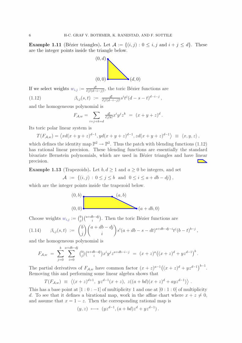
Example 1.11 (Bezier triangles). Let A := {(i, j) : 0 ≤ i, j and i + j ≤ d}. Theseare the integer points inside the triangle below.

(0, d)

(d, 0)(0, 0)

If we select weights wi,j := d!i!j!(d−i−j)!

, the toric Bezier functions are

(1.12) βi,j(s, t) := d!i!j!(d−i−j)!

sitj(d− s− t)d−i−j ,


FA,w =∑

i+j+k=d

d!i!j!k!

xiyjzk = (x+ y + z)d .

Its toric polar linear system is

T (FA,w) =⟨xd(x+ y + z)d−1, yd(x+ y + z)d−1, zd(x+ y + z)d−1

⟩≡ 〈x, y, z〉 ,

which defines the identity map P2 → P2. Thus the patch with blending functions (1.12)has rational linear precision. These blending functions are essentially the standardbivariate Bernstein polynomials, which are used in Bezier triangles and have linearprecision.

Example 1.13 (Trapezoids). Let b, d ≥ 1 and a ≥ 0 be integers, and set

A := {(i, j) : 0 ≤ j ≤ b and 0 ≤ i ≤ a+ db− dj} ,which are the integer points inside the trapezoid below.

(a, b)

(0, 0) (a + db, 0)

(0, b)

Choose weights wi,j :=(

b

j

)(a+db−dj

i

). Then the toric Bezier functions are

(1.14) βi,j(s, t) :=

(b

j

)(a + db− dj

i

)si(a+ db− s− dt)a+db−dj−itj(b− t)b−j ,


FA,w =b∑

j=0

a+db−dj∑

i=0

(b

j

)(a+db−dj

i

)xiyjza+db−i−j = (x+ z)a

((x+ z)d + yzd−1

)b.

The partial derivatives of FA,w have common factor (x + z)a−1((x + z)d + yzd−1

)b−1.

Removing this and performing some linear algebra shows that

T (FA,w) ≡⟨(x+ z)d+1, yzd−1(x+ z), z((a + bd)(x+ z)d + ayzd−1)

⟩.

This has a base point at [1 : 0 : −1] of multiplicity 1 and one at [0 : 1 : 0] of multiplicityd. To see that it defines a birational map, work in the affine chart where x + z 6= 0,and assume that x = 1 − z. Then the corresponding rational map is

(y, z) 7−→ (yzd−1, (a+ bd)zd + yzd−1) .


Changing coordinates, this is (y, z) 7→ (yzd−1, z), which is a bijection when z 6= 0.

Remark 1.15. The first three patches are widely used and implemented in CADsoftware. The trapezoid patch reduces to the Bezier triangle when a = 0 and d = 1,and to the tensor product patch when d = 0. While the trapezoid patch for generalparameters has not been used explicitly in modeling, special cases of it have appearedimplicitly. For example, a rational ruled surface in R3 of degree 2a+d with directrix ofminimal degree a and general one of degree a+d [12, §5.2] is the image of such a patch(here, b = 1). Bezier quad patches on a sphere bounded by circular arcs of minimaltype (2, 4) [11] are also trapezoidal. Some quad patches on rational canal surfaces [9]can be represented by trapezoidal patches with b = 2. The full possibilities for the useof the trapezid patch in modeling have yet to be developed.

2. Toric polar Cremona transformations

We classify toric surface (n = 2) patches with rational linear precision through the al-gebraic relaxation of classifying the homogeneous polynomials (forms) F = F (x, y, z) ∈C[x, y, z] whose toric polar linear system defines a birational map P2 −→ P2. Write Fx

for ∂∂xF , and the same for the other variables y and z. We will write F = 0 or simply

F for the reduced curve defined by F in P2.

Definition 2.1. Let F be a form. The vector space T (F ) := 〈xFx, yFy, zFz〉 definesthe toric polar linear system of curves on P2 and the toric polar map

ϕF : P2 −−→ P2

[ x : y : z ] 7−→ [ xFx : yFy : zFz ] ,

which maps curves in T (F ) into lines in the target P2. We say that F defines a toric

polar Cremona transformation if this map is birational.

We establish some elementary properties of such forms F and linear systems T (F ),and then give our classification of forms that define toric polar Cremona transforma-tions.

2.1. Equivalence of forms. There are some transformations which send one formdefining a toric polar Cremona transformation into another such form. Those whichare invertible define an equivalence relation on forms, and our classification is up tothis equivalence.

Lemma 2.2. A form F defines a toric polar Cremona transformation if and only if

every power F a for a > 0 defines a toric polar Cremona transformation.

Proof. The toric polar linear systems of F and F a are equivalent,⟨x∂F a

∂x, y ∂F a

∂y, z ∂F a

∂z

⟩= 〈axF a−1Fx, ayF

a−1Fy, azFa−1Fz〉 ≡ 〈xFx, yFy, zFz〉 .

The linearity of differentiation implies that F (x, y, z) defines a toric polar Cremonatransformation if and only if F (ax, by, cz) defines a toric polar Cremona transformation,for all non zero a, b, c ∈ C. Call this scaling the variables. Multiplication by a monomialalso preserves the property of defining a toric polar Cremona transformation.



xaybzcF defines a toric polar Cremona transformation, for any positive integers a, b, c.

Proof. It suffices to check that T (xF ) ≡ T (F ). Note that T (xF ) is⟨x ∂

∂xxF, y ∂

∂yxF, z ∂

∂zxF

⟩= 〈xF + x2Fx, yxFy, zxFz〉 ≡ 〈xFx, yFy, zFz〉 ,

which is T (F ). The last equivalence follows by removing the common factor x andapplying the Euler relation, which is xFx + yFy + zFz = deg(F )F .

The calculations in the proof of Lemma 2.3 hold when the exponents a, b, c are any

integers. Consequently, F may be any homogeneous Laurent polynomial. For example,

y−1z−1 + x−2yz−1 + x−2y−1z − 2(x−1z−1 + x−1y−1 + x−2)

is a Laurent form defining a toric polar Cremona transformation. (This is the form ofTheorem 1(3) with d = 1 multiplied by the monomial x−2y−1z−1.)

A third class of transformations are the invertible monomial transformations. Avector α = (α1, α2, α3) ∈ Z3 corresponds to a (Laurent) monomial tα := xα1yα2zα3 ofdegree |α| := α1 + α2 + α3. Let α, β, γ ∈ Z3 be three exponent vectors and considerthe map C3 → C3 defined by

(2.4) (x, y, z) 7−→ (tα, tβ, tγ) .

Lemma 2.5. The formula (2.4) defines a rational map P2 −→ P2 if and only if

|α| = |β| = |γ|. This map is invertible if and only if α− γ and β − γ form a basis for

{v ∈ Z3 : |v| = 0}.We prove Lemma 2.5 later. Suppose that A := {α, β, γ} ⊂ Z3 satisfies the hy-

potheses of Lemma 2.5 so that the map ϕA : P2 −→ P2 defined by (2.4) is a birationalisomorphism. It induces a map ϕ∗

A on monomials xaybzc by

(2.6) ϕ∗A(xaybzc) := tαa+βb+γc =: tAa ,

where a := (a, b, c)T and Aa is the multiplication of the vector a by the matrix A whosecolumns are α, β, γ. When A ∈ Mat3×3Q is invertible and satisfies the hypothesis ofLemma 2.5, we call ϕ∗

A an invertible monomial transformation. Under the hypothesesof Lemma 2.5, the condition that A is invertible is equivalent to |α| 6= 0.


ϕ∗A(F ) does for any invertible monomial transformation ϕ∗

A.

Proof. By (2.6), the toric derivative x ∂∂xϕ∗A(ta) is

(A1 · a)tAa = ϕ∗A((A1 · a)ta) = A1 · ϕ∗

A(x ∂∂xta, y ∂

∂yta, z ∂

∂zta)T ,

where A1 is the first row of the matrix A. Thus(x ∂

∂xϕ∗A(ta), y ∂

∂yϕ∗A(ta), z ∂

∂zϕ∗A(ta)

)T

= A(ϕ∗A(x ∂

∂xta, y ∂

∂yta, z ∂

∂zta)T

),

= ϕ∗A(x ∂

∂xta, y ∂

∂yta, z ∂

∂zta)T .

as A is invertible. Thus we have the relation between the toric polar linear systems

T (ϕ∗A(F )) = ϕ∗

A(T (F ))

for any homogeneous polynomial F . The lemma follows as ϕA is birational.


Definition 2.8. Let C[x±] := C[x, x−1, y, y−1, z, z−1] be the ring of Laurent polyno-mials, the coordinate ring of the torus (C∗)3. This is Z-graded by the total degree of amonomial. Forms F,G ∈ C[x±] are equivalent if G = ψ∗(F ), where ψ is a compositionof

(a) scaling variables, [x : y : z] 7→ [ax : by : cz], or(b) multiplication by a monomial, or(c) an invertible monomial transformation.

Our classification is up to this equivalence. By (b), it is no loss to assume that aLaurent form F is an ordinary form (in C[x, y, z]).

Proof of Lemma 2.5. The first statement is clear as a rational map C3 → C3 drops toa map P2 −→ P2 if and only if it is defined by homogeneous rational forms of the samedegree. For the second, consider the map (C∗)3 → P2 defined by

ϕ : t := (x, y, z) 7−→ [tα : tβ : tγ ] ,

and suppose that we have s, t ∈ (C∗)3 with ϕ(s) = ϕ(t). After rescaling in the source,we may assume that t = (1, 1, 1). In particular, s is a solution of

sα = λ , sβ = λ , and sγ = λ ,

for some λ ∈ C∗. But we also have

(2.9) sα−γ = 1 = sβ−γ .

Since |α| = |β| = |γ|, solutions to (2.9) include the diagonal torus ∆ := {(a, a, a) : a ∈C∗}, so we see again that ϕ is defined on the dense torus (C∗)3/∆ of P2. This map onthe dense torus is an isomorphism if and only if points of the diagonal torus are theonly solutions to (2.9), which is equivalent to the condition that the exponents α− γand β − γ are a basis for the free abelian group {v ∈ Z3 : |v| = 0}.

2.2. Proof of Theorem 1. Let F be a form defining a toric polar Cremona transfor-mation. We first classify the possible irreducible factors of F , and then determine whichfactors may occur together. The classification of the factors of F occupies Sections 3,4, and 5.

Under the rational map ϕF each component of each curve in the toric polar linearsystem is either contracted (mapped to a point) or mapped to a dense subset of acurve. As F ∈ T (F ), this in particular holds for the curve F = 0, whose componentscorrespond to the irreducible factors of F . (We always take the reduced structure onthis curve, that is, we consider the set of zeroes of F , not the scheme defined by F .) Anirreducible factor of F is contracted, respectively not contracted, if the correspondingcomponent of the curve F = 0 is contracted by the linear system T (F ), respectivelynot contracted. There are three possibilities for the factors of F .

(2.10)(1) F has no contracted factors, or(2) F has only contracted factors, or(3) F has both contracted and non contracted factors.

We get information about the factors of F from a simple, but useful restrictionlemma.

Lemma 2.11. Suppose that G is an irreducible factor of a form F . Then the restric-

tions of the toric polar linear systems of F and of G to the curve G = 0 are equivalent.


Proof. Write F = GnH with G and H coprime. Then

T (F ) = 〈nxGn−1GxH + xGnHx, nyGn−1GyH + yGnHy, nzG

n−1GzH + zGnHz〉 .After factoring out Gn−1, restricting to G = 0, and factoring out nH we obtain

T (F )|G ≡ 〈xGx, yGy, zGz〉|G = T (G)|G .A cornerstone of our classification is that there is a strong restriction on the singu-

larities of the curve F = 0. A singular point p of a curve is ordinary if locally near p,the curve consists of r > 1 smooth branches that meet transversally at p. In Section 5we prove the following theorem.

Theorem 2.12. If a form F coprime to xyz defines a toric polar Cremona transfor-

mation, then the curve F = 0 has at most one singular point outside the coordinate

lines, and if there is such a point, then all factors of F are contracted. Furthermore,

if this singular point is ordinary, then F has at most two distinct factors through the

singular point.

Since the toric polar map ϕF is birational, each component of a curve in the toricpolar linear system T (F ) is either contracted or mapped birationally onto a line, andat most one component of a curve is not contracted. This in particular holds for F .

Corollary 2.13. At most one factor of F is not contracted.

In Section 4 we classify the possible non contracted factors of F .

Theorem 2.14. If F is an irreducible form defining a curve with no singularities

outside the coordinate lines whose toric polar linear system maps this curve birationally

onto a line, then F is equivalent to one of the following forms,

(1) x2 + y2 + z2 − 2(xy + xz + yz), or

(2) (x+ z)d + yzd−1, for some integer d ≥ 1.

Example 1.13 with a = 0 and b = 1 shows that the second class of forms define toricpolar Cremona transformations, and the following example shows that the first classalso does.

Example 2.15. The form F of Theorem 2.14(1) has the toric polar linear system

T (F ) = 〈x2 − xy − xz, y2 − xy − yz, z2 − xz − yz〉= 〈(x−y−z)(y−x−z), (x−y−z)(z−x−y), (y−x−z)(z−x−y)〉 ,(2.16)

which defines a quadratic Cremona transformation with base points{[1 : 0 : 1], [0 : 1 : 1], [1 : 1 : 0]

}.

To help see the equality (2.16), note that −xFx − yFy + zFz = (x− y − z)(y − x− z).This example shows that the algebraic relaxation (seeking polynomials F with arbi-

trary coefficients whose toric polar linear system is birational) of the original problemfrom geometric modeling has solutions which do not come from geometric modeling,as the coefficients of F cannot simultaneously be made positive.

In Section 3, we study the possible contracted factors of F and prove the followinglemma.

Lemma 2.17. Suppose that G is a contracted factor of F . Then, up to a permutation

of variables, G = xa + αybza−b with a, b coprime and α 6= 0.


We now present a proof of Theorem 1, following the three cases of (2.10).

2.2.1. F has no contracted factors. In this case, Corollary 2.13 implies that F has asingle irreducible factor. Since this factor is not contracted it is equivalent to one ofthe forms described in Theorem 2.14. Since these forms define toric polar Cremonatransformations, Lemma 2.2 implies that any power of such a form defines a toric polarCremona transformation. In particular, F defines a toric polar Cremona transforma-tion. This establishes part (2) of Theorem 1(2) when a = 0 and also part (3).

2.2.2. F has only contracted factors. We outline the proof in this case, which is carriedout in Section 3. Suppose first that F defines a toric polar Cremona transformation.By Lemma 2.17, every contracted factor is a binomial. We first show that any twocontracted factors of F are simultaneously equivalent to

(z + x) and (z + y) ,

and in particular they meet outside the coordinate lines.Suppose that all factors of F are contracted, then we show that F has at least two

irreducible factors. We next show that if F has three or more factors, then we mayassume that they intersect transversally at [1 : 1 : −1]. Hence F = 0 has an ordinarysingularity of multiplicity at least 3, which contradicts the last part of Theorem 2.12.Therefore F is equivalent to

(2.18) (x+ z)a(y + z)b ,

with a, b > 0. By Example 1.9, any such form defines a toric polar Cremona transfor-mation, which completes the proof of Theorem 1(1).

2.2.3. F has both contracted and non contracted factors. By Corollary 2.13, F has aunique non contracted factor. It also has a unique contracted factor. Indeed, anytwo contracted factors meet outside the coordinate lines, and so the curve F = 0 issingular outside the coordinate lines. Then Theorem 2.12 implies that all factors of Fare contracted, a contradiction. All that remains is to examine the different possibilitiesfor the factors of F . We show that the non contracted factor cannot be equivalent tox2 + y2 + z2 − 2(xy + xz + yz). We then show that if the non contracted factor isequivalent to (x + z)d + yzd−1, then (after putting it into this form) the contractedfactor is x+ z. Example 1.13 shows that all possibilities

(x+ z)a((x+ z)d + yzd−1

)b

with a ≥ 0 and b > 0 define toric polar Cremona transformations, which completesthe proof of Theorem 1. These claims about the non contracted factors are proven inthe following two lemmas.

Lemma 2.19. If F has a non contracted factor equivalent to x2 + y2 + z2 − 2(xy +xz + yz), then it has no other factors.

Proof. Suppose that F has two factors, Q := x2 + y2 + z2 − 2(xy + xz + yz), and acontracted factor G. Since permuting the variables does not change Q, Lemma 2.17implies that G = xA + αyazA−a, with A, a ≥ 0 coprime and α non zero.

By Theorem 2.12, G and Q can meet only on the coordinate lines. If we substitutethe parameterization [x : y : z] = [(s+ t)2 : s2 : t2] of Q into G, we obtain

(2.20) (s+ t)2A + αs2at2A−2a .


The condition that Q and G meet only on the coordinate lines implies that the onlyfactors of (2.20) are s, t, or s + t. But this implies that A = a = 0, contradicting ourassumption that G was a non trivial factor of F .

Lemma 2.21. If F has the non contracted factor (x + z)d + yzd−1, then its other

irreducible factor must be x+ z.

Proof. Suppose that F has two factors, Q := (x + z)d + yzd−1 with d ≥ 1 and acontracted factor G, which is necessarily a binomial. Multiplying G by a monomialand scaling, we may assume it has the form α+ (−1)axAyaz−A−a with A ≥ 0 and A, acoprime. By Theorem 2.12, G and Q can meet only on the coordinate lines. We solveQ = 0 for y to obtain y = −(x+ z)d/zd−1 and then substitute this into G to obtain

α + (−1)axA(− (x+z)d

zd−1

)a

z−A−a = α + xA(x+ z)adz−A−ad .

If we multiply this by zA+ad if a ≥ 0 and by zA(x + z)−ad if a < 0 (and replace a by−a), this becomes either

αzA+ad + xA(x+ z)ad or αzA(x+ z)ad + xAzad .

Since G and Q can meet only on the coordinate lines, the only possible factors of thesepolynomials are x, z, and x + z. Neither x nor z can be a factor as A 6= ad and thecoefficients are non zero, so x + z is the only factor. But then we must have a = 0,α = 1, and A = 1, so that G = 1 + xz−1, or, clearing the denominator, G = x + z.

3. contracted factors

We study the contracted factors of a form F that defines a toric polar Cremonatransformation. We first prove Lemma 2.17, that any contracted factor of F is abinomial.

Proof of Lemma 2.17. By Lemma 2.11, the restrictions of the toric polar maps of Fand of G to the curve G = 0 coincide. Let T (G) be the toric polar linear system of G.Since it contracts G, T (G)|G = 〈xGx, yGy, zGz〉|G is one-dimensional, and so T (G) isonly two-dimensional. Thus there is a linear relationship among the toric derivativesof G,

q1xGx + q2yGy + q3zGz = 0 .

Writing G =∑

imi as a sum of terms mi = αixaiybizci , we see that q1ai + q2bi = q3ci

for all i. Thus we may assume that q1, q2, q3 ∈ Z and they are coprime. Permutingvariables, we may assume that the qj are non negative. Since G is homogeneous, sayof degree d, we have ai + bi + ci = d, and so

(q1 + q3)ai + (q2 + q3)bi = q3d .

Thus G(x, y, 1) is a weighted homogeneous polynomial of degree q3d. Since G is irre-ducible, the only possibilities are G(x, y, 1) = x or G(x, y, 1) = y (neither can occuras F is coprime to xyz), or G(x, y, 1) = xa + αyb with a and b coprime, α 6= 0 and(q1 + q3)a = (q2 + q3)b. Since G is irreducible, z does not divide G and G(x, y, 1) musthave degree d. Therefore after possibly interchanging x and y we see that G has theform claimed.


Any two contracted factors may be put into a standard form.

Lemma 3.1. If G and H are two contracted factors of F , then, up to equivalence

GH = (x+ z)(y + z).

In particular, any two contracted factors of F meet outside the coordinate lines.

Proof. Up to a permutation of the variables, each factor is a prime binomial of theform

xA + αyazA−a ,

where A, a ≥ 0 are coprime and α is non zero.By Theorem 2.12, F has at most one singularity outside the coordinate lines. Points

common to two factors of F are singular, so the factors G and H define curves thatmeet at most once outside the coordinate axes. To study such points, we dehomogenizeand set z = 1. Multiplying G and H by monomials, we may suppose that they havethe form

(3.2) G = α + xAya and H = β + xByb .

Since these are irreducible binomials, 1 = gcd{|A|, |a|} = gcd{|B|, |b|}, and since theyare coprime Ab−Ba 6= 0.

The points common to the two components are the solutions to G = H = 0. Thenumber of solutions to such a zero-dimensional binomial system is |Ab−Ba| [14, § 3.2].Since there can be at most one such point, |Ab − Ba| = 1. Interchanging the roles of(A, a) and (B, b) if necessary, we may assume that Ab−Ba = 1. Under the invertiblesubstitution x = xby−a and y = x−ByA, (3.2) becomes α+ x and β + y. Scaling x andy and rehomogenizing, we may assume that the binomials are x+ z and y + z.

Lemma 3.3. If F has only a single irreducible factor, then that factor is not contracted.

In particular a form with all factors contracted must have at least two factors.

Proof. LetG be the irreducible factor of F , then F = Ga for some a > 1. By Lemma 2.2the toric polar map ϕF of F coincides with the toric polar map ϕG of G. If G = 0 iscontracted, then, as in the proof of Lemma 2.17, T (G)|G is one-dimensional and thusT (G) is only two-dimensional so that xGx, yGy and zGz are dependent. But then ϕG,and hence ϕF , cannot be birational.

We classify forms F defining a toric polar Cremona transformation with all factorscontracted.

Theorem 3.4. If all factors of F are contracted, then F is equivalent to (x+z)a(y+z)b,

for some a, b > 0.

Proof. Suppose that all factors of F are contracted. By Lemma 3.1, we may assumethat two of the irreducible factors of F are x + z and y + z. We only need to showthat there are no further contracted factors of F . Suppose there is another contractedfactor. After multiplying by a monomial, this will have the form

γ + xCycz−C−c ,

with γ ∈ C∗ and C > 1. By Theorem 2.12, F has at most one singularity outside ofthe coordinate lines, and so this factor must meet the other factors only in the point[1 : 1 : −1] where they meet. It follows that γ = ±1 and C = |c| = 1.


We see that the only possible irreducible factors of F are

x+ z , y + z , z2 − xy , and y − x .

Since these four factors have distinct tangents at [1 : 1 : −1], the singularity of Fat this point is ordinary. By the last part of Theorem 2.12, F can have at most twodistinct factors through [1 : 1 : −1] so the theorem follows.

4. Irreducible polynomials

We classify irreducible factors of F which are not contracted by the toric polarCremona transformation. Specifically, we prove the following theorem.

Theorem 2.14. If F is an irreducible form defining a curve with no singularities

outside the coordinate lines whose toric polar linear system maps this curve birationally

onto a line, then F is equivalent to one of the following forms,

(1) x2 + y2 + z2 − 2(xy + xz + yz), or

(2) (x+ z)d + yzd−1, for some integer d ≥ 1.

Since the curve F = 0 is rational, it has a parameterization γ : P1 → P2 whichdetermines F up to a constant. The composition of γ with the toric polar Cremonatransformation of F is a map P1 → P2 of degree 1. We will deduce from this andthe location of the singularities of F that there are exactly three distinct irreduciblefactors appearing in γ.

Applying quadratic Cremona transformations puts γ into a standard form fromwhich the hypothesis on the singularities of F = 0 restricts F to be equivalent to oneof the forms of Theorem 2.14. An important technical part of this argument is the localcontribution to the arithmetic genus of a singular point of a binomial curve, which wecompute in Section 4.2.

4.1. Linear factors in γ. Suppose that F is a form of degree d that satisfies thehypotheses of Theorem 2.14 and let γ := [f : g : h] : P1 → P2 parameterize the curveF = 0. Then f , g, and h are are coprime forms of degree d on P1. Because the toricpolar map ϕF sends the image of γ (the curve F = 0) isomorphically onto a line, themap P1 → P2 with components

(4.1) fFx(γ), gFy(γ), and hFz(γ)

has degree 1, and thus these forms become linear after removing common factors. Westudy their syzygy module to show that there are only three distinct irreducible factorsin fgh.

Choose homogeneous coordinates [s, t] on P1 with st coprime to fgh. As γ parame-terizes F , we have F (γ) ≡ 0 on P1. Differentiating with respect to s and t gives

(4.2)

[fs gs hs

ft gt ht

]Fx(γ)Fy(γ)Fz(γ)

=

[00

].

Using the Euler relations sfs + tft = df (and the same for g and h) gives the syzygy

fFx(γ) + gFy(γ) + hFz(γ) = 0 .


Multiplying the first row of (4.2) by fgh gives a second syzygy, so we have

(4.3)

[fsgh fgsh fghs

1 1 1

]fFx(γ)gFy(γ)hFz(γ)

=

[00

].

An equivalent set of syzygies is given by the rows of the matrix

(4.4)

[fsgh− fghs fgsh− fghs 0

1 1 1

].

Since the three components (4.1) share a common factor whose removal yields linearforms (p, q, r) with the same syzygy matrix, r = −p − q and the removal of commonfactors from the first row of (4.4) gives the syzygy (−q, p, 0).

There are three sources for common factors of the first row of (4.4).

(1) Common factors of f and fs, of g and gs, or of h and hs,(2) common factors of some pair of f , g, or h, and(3) common factors of fsh− fhs and gsh− ghs.

A common factor of the third type that is not of type (1) or (2) vanishes at a pointp ∈ P1 where

rank

[fs gs hs

f g h

]≤ 1 .

The Euler relation implies that we also have

(4.5) rank

[fs gs hs

tft tgt tht

]≤ 1 ,

and so t is a common factor of the third type. Suppose now that t(p) 6= 0. Then (4.5)shows that the differential of γ does not have full rank at p, and so the the curve F = 0is singular at γ(p). But such a singular point must lie on a coordinate line of P2 andso one of f , g, or h vanishes at p. Without loss of generality, suppose that f(p) = 0.Then fs(p)h(p) = 0, as fsh−fhs vanishes at p, and so the common factor vanishing atp divides either fs or h, and is therefore a factor of type (1) or (2). Thus t is the onlyfactor of type (3) that is not of type (1) or (2). As fgh is coprime to t, the commonfactor t has multiplicity 1.

Now suppose that ℓ is a linear factor of fgh with ℓa, ℓb, and ℓc exactly dividing f ,g, and h, respectively. Then ℓa+b+c exactly divides fgh and ℓa+b+c−1 exactly dividesthe entries in the first row of (4.4). It follows that if the prime factorization of fgh isℓa1

1 · · · ℓak

k , then the common factor of the first row of (4.4) is

tℓa1−11 · · · ℓak−1

k .

This has degree 3d+1−k. Since the entries in the first row of (4.4) have degree 3d−1,and removing this common factor gives linear forms, we have that

3d− 1 = 1 + 3d+ 1 − k ,

or k = 3. Thus there are exactly three distinct linear factors dividing fgh.


4.2. Arithmetic genus of binomial germs. We compute δ(0,0), the contribution atthe origin to the arithmetic genus of a curve C with germ

(4.6) (xa − yb) u(x, y) = 0 ,

where u(0, 0) 6= 0. Write pa(C) for the arithmetic genus of a curve C.

Lemma 4.7. Let C be a curve on a smooth surface S with germ (4.6) given in local

coordinates (x, y) of a point p ∈ S. If C is obtained from C by a sequence of blowups

in p and points infinitely near p and is smooth at all points infinitely near p, then

(4.8) pa(C) = pa(C) − 12

((a− 1)(b− 1) + gcd(a, b) − 1

).

We call the difference pa(C) − pa(C) the δ-invariant of C at p.

Proof. Recall the formula [7, Cor V.3.7] for the arithmetic genus of the strict transformC ′ of a curve C obtained by blowing up a point of multiplicity a in C,

(4.9) pa(C′) = pa(C) − 1

2a(a− 1) .

Let C be defined near p by (4.6). Then C has multiplicity min{a, b} at p. If

min{a, b} = 1, then C = C and (4.8) becomes pa(C) = pa(C).If a = b, then C consists of a smooth branches meeting pairwise transversally at p.

Blowing up p separates these branches so that C ′ = C. By (4.9), we have

pa(C′) = pa(C) − 1

2a(a− 1) = pa(C) − 1

2

((a− 1)(a− 1) + a− 1

),

which establishes the lemma in this case.We complete the proof by induction on the maximum of the exponents of x and y.

Suppose that a < b. Then C is tangent to the curve y = 0 at p and so to compute theblowup C ′, we substitute x = xy in (4.6) to obtain

ya (xa − yb−a) · u(xy, y) .The exceptional divisor (y = 0) has multiplicity a, and the curve C ′ has local equation(xa − yb−a)u′, where u′(x, y) = u(xy, y) and so u′(0, 0) 6= 0. Since a, b − a < b =max{a, b}, our induction hypothesis applies to C ′ to give

pa(C) = pa(C′) − 1

2

((a− 1)(b− a− 1) + gcd(a, b− a) − 1

).

Using (4.9), this becomes

pa(C) = pa(C) − 12a(a− 1) − 1

2

((a− 1)(b− a− 1) + gcd(a, b− a) − 1

)

= pa(C) − 12

((a− 1)(b− 1) + gcd(a, b) − 1

),

which completes the proof.

4.3. Classification. Suppose that γ : P1 → P2 parameterizes the curve F = 0. Wemay assume that the three linear forms dividing components of γ are s, t, and ℓ :=−(s+ t). Since the components are relatively prime forms of degree d, there are sevenpossibilities for γ, up to permuting components and factors.

I [satd−a : tbℓd−b : sd−cℓc] II [satbℓd−a−b : sd−ctc : ℓd] III [satd−a : tbℓd−b : ℓd]IV [satd−a : sd−btb : ℓd] V [satbℓd−a−b : td : ℓd] VI [satd−a : td : ℓd]

VII [sd : td : ℓd]

We assume that all exponents appearing here are positive.


Theorem 4.10. Suppose that γ is a curve with parameterization one of the types

I—VII.

(1) If γ has type I and is smooth outside the coordinate lines, then γ is equivalent

to either

[s2t2 : t2ℓ2 : s2ℓ2] or [sd−1t : td−1ℓ : sd−1ℓ] .

(2) If γ does not have type I, then it may be transformed into a curve of type I via

quadratic Cremona transformations.

We deduce Theorem 2.14 from Theorem 4.10.

Proof of Theorem 2.14. Suppose that γ has the first form in Theorem 4.10(1). Applythe standard Cremona transformation [x : y : z] 7→ [yz : xz : xy] to γ and remove thecommon factor s2t2ℓ2 to obtain

[s2t2ℓ4 : s4t2ℓ2 : s2t4ℓ2] = [ℓ2 : s2 : t2] ,

which satisfies x2 + y2 + z2 − 2(xy + xz + yz) = 0, the curve in Theorem 2.14(1).Suppose that γ has the second form in Theorem 4.10(1). Set a := d − 1 to obtain

[sat : taℓ : saℓ]. If a = 0, this parameterizes the line x+ y + z = 0. If a > 0, apply thestandard Cremona transformation and multiply the y-coordinate by (−1)a to obtain

[sataℓ2 : (−1)as2atℓ : sata+1ℓ] = [ta−1ℓ : −(−s)a : ta] .

Since ℓ = −(s+ t), we have

(x+ z)a = (−sta−1)a = (−s)a(ta)a−1 = −yza−1 .

This gives all curves of the form in Theorem 2.14(2).

We prove Theorem 4.10 in the following subsections.

4.4. Curves of type I. Suppose that γ = [satd−a : tbℓd−b : sd−cℓc] is a rational curveof type I. If γ parameterizes a curve satisfying the hypotheses of Theorem 2.14, thenit can be singular only on the coordinate lines. Since all six exponents appearing inγ are positive, these singularities occur at the coordinate points. As γ is rational, itsarithmetic genus must equal the sum of its δ-invariants at these singular points.

In the neighborhood of the coordinate point [0 : 0 : 1], the curve has germ (xb −yd−a)u = 0, where u(0, 0) 6= 0. By Lemma 4.7 the δ-invariant is

12

((b− 1)(d− a− 1) + gcd(b, d− a) − 1

).

A similar formula holds at the other points [1 : 0 : 0] and [0 : 1 : 0]. Summing these,equating with pa(C) =

(d−12

), and multiplying by 2, we obtain

(4.11) (d− 1)(d− 2) = d(a+ b+ c− 3) − (ab+ ac + bc)

+ gcd(a, d− c) + gcd(b, d− a) + gcd(c, d− b) .

We may assume that the coordinates and forms s, t, ℓ have been chosen so that ais the maximum exponent and thus d − a is the minimum. We have a ≥ d − c andb ≥ d− a, and there are two cases to consider

(4.12) c ≥ d− b or d− b ≥ c .

We study each case separately, beginning with c ≥ d− b.


Proposition 4.13. The solutions to (4.11) in the polytope P defined by the inequalities

d− 1 ≥ a ≥ d− c

d− 1 ≥ b ≥ d− a(4.14)

d− 1 ≥ c ≥ d− b

are (d−1, d−1, 1), (d−1, 1, d−1), and (1, d−1, d−1), for any d ≥ 2, and (2, 2, 2) when

d = 4.

Proof. Since gcd(α, β) ≥ min(α, β), for positive integers α and β, we may simplify (4.11)to obtain the inequality

(d− 1)(d− 2) ≥ (d− 1)(a+ b+ c) − (ab+ ac + bc) .

Let Q = Q(a, b, c) be the symmetric quadratic form defined by the right hand side ofthis inequality. We find its maximum values on the polytope P . First, the Hessian ofQ is

hess(Q) =

0 −1 −1−1 0 −1−1 −1 0

.

This has negative eigenvalue −2 with eigenvector (1, 1, 1) and positive eigenvalue 1 withtwo-dimensional eigenspace a + b + c = 0. In particular, Q cannot take a maximumvalue in the interior of the polytope P or in any of its facets. It can only take amaximum value in an edge that is parallel to the negative eigenspace (1, 1, 1).

The polytope P is a symmetric bipyramid over the triangle whose vertices are

(4.15) (d−1, d−1, 1) , (d−1, 1, d−1) , (1, d−1, d−1) .

and with apices (d−1, d−1, d−1) and (d2, d

2, d

2). Since P has no edge parallel to the

negative eigenspace, Q takes its maximum value at vertices of P .The form Q takes value 0 at (d−1, d−1, d−1), 3

4d(d−2) at (d

2, d

2, d

2), and (d−1)(d−2)

at the vertices (4.15) of the triangle, and so the vertices of the triangle give solutions.When d = 2, P degenerates to a point (1, 1, 1), which is a solution to (4.11). The onlyremaining possibility is that the point (d

2, d

2, d

2) satisfies (4.11). But then

(d− 1)(d− 2) = 34d(d− 2) ,

in which case d = 4 and so (a, b, c) = (2, 2, 2) is the only other solution.

If we take the alternative inequality in (4.12), d− b ≥ c, then Q becomes

d(a+ b+ c− 1) − a− ab− ac− bc .

Replacing the third inequality in (4.14) by d−b ≥ c ≥ 1 defines a tetrahedron withvertices

(d−1, d−1, 1), (d−1, 1, d−1), (d−1, 1, 1), (d2, d

2, d

2) .

Similar arguments as in the proof of Proposition 4.13 give the additional solution(d−1, 1, 1) to (4.11). By symmetry, we also obtain solutions (1, d−1, 1) and (1, 1, d−1).

We write the curves γ corresponding to these solutions. The solution (a, b, c) =(2, 2, 2) gives the expression

[s2t2 : t2ℓ2 : s2ℓ2] ,


for γ and the solutions (a, b, c) = (d−1, d−1, 1) give the expressions

(4.16) [sd−1t : td−1ℓ : sd−1ℓ] .

The other two symmetric solutions give equivalent curves. Lastly, the solutions (a, b, c) =(d−1, 1, 1) give the expressions

[sd−1t : tℓd−1 : sd−1ℓ] ,

which become the expressions (4.16) under x↔ z and t↔ ℓ.

4.5. Reduction to curves of type I.

4.5.1. Quadratic Cremona transformations. We will show how curves of types II—VIIare equivalent to curves of type I through quadratic Cremona transformations. Wewill sometimes use the non standard quadratic Cremona transformation

[x : y : z] 7−→ [z2 : xz : xy] .

Permuting the variables gives five other non standard quadratic Cremona transforma-tions.

4.5.2. Curves of type II. Suppose that γ = [satbℓd−a−b : sd−ctc : ℓd] has type II. Weshow that this may be transformed into a curve of type I by induction on d. Wewill either transform γ into a curve of type I or one of type II of lower degree. Sincea + b < d = (d − c) + c, interchanging s and t if necessary, we may assume thatb < c. Applying the standard Cremona [xy : xz : yz] transformation and removing thecommon factor of tbℓd−a−b gives

[sa+d−ctb+cℓd−a−b : satbℓ2d−a−b : sd−ctcℓd] = [sa+d−ctc : saℓd : sd−ctc−bℓa+b] .

There remains a common power of s that we can remove. There are three cases toconsider.

(1) If a > d − c, then we remove the common factor of sd−c to obtain a curve oftype I.

(2) If a = d− c, then d = a+ c and we remove the common factor of sa = sd−c toobtain

[satc : ℓa+c : tc−bℓa+b] = [x : y : z] .

We now apply the non standard Cremona transformation [z2 : xz : xy] andremove the common factor tc−bℓa+b to obtain

(4.17) [t2c−2bℓ2a+2b : sat2c−bℓa+b : satcℓa+c] = [tc−bℓa+b : satc : satbℓc−b] .

If b < c− b, then we remove the common factor tb to obtain a curve of type I.If b = c− b, then we remove tb to get

[ℓa+b : satb : saℓb] = [x : y : z] .

Applying the non standard Cremona transformation [z2 : xy : yz] to get

[s2aℓ2b : satbℓa+b : s2atbℓb] = [saℓb : tbℓa : satb] ,

which has type I. Finally, if b > c − b, then we remove the common factor oftc−b from (4.17) to obtain

[ℓa+b : satb : sat2b−cℓc−b] ,

which has type II and degree a+ b < a+ c = d.


(3) If a < d− c, then we instead apply the non standard Cremona transformation[x2 : yz : xz] to γ and remove the common factor satbℓd−a−b to obtain

[satbℓd−a−b : sd−c−atc−bℓa+b : ℓd] .

Removing the final common factor ℓmin{d−a−b,a+b} gives another curve of typeII, but of lower degree.

4.5.3. Curves of type III. Suppose that γ = [satd−a : tbℓd−b : ℓd] has type III. We applythe standard Cremona transformation [xy : xz : yz] and remove the common factorℓd−b to obtain

[satb+d−a : satd−aℓb : tbℓd] .

There remains a common power of t that we can remove. There are three cases toconsider.

(1) If b > d− a, we factor out td−a to get the type I curve,

[satb : saℓb : ta+b−dℓd] .

(2) If b = d − a, we instead apply the non standard Cremona transformation[y2 : xy : xz] to γ and factor out tbℓa to get the type I curve,

[tbℓa : satb : saℓb] .

(3) If b < d− a, we factor out tb to obtain

[satd−a : satd−a−bℓb : ℓd] ,

which has type II, and we have already shown how to reduce a curve of type IIto a curve of type I.

4.5.4. Curves of type IV. Suppose that γ = [satd−a : sd−btb : ℓd] has type IV. Wemay assume that a > d − b and thus b > d − a. We apply the standard Cremonatransformation [yz : xz : xy] and remove the common factor of sd−btd−a, to get thetype I curve,

[ta+b−dℓd : sa+b−dℓd : satb] .

4.5.5. Curves of type V. Suppose that γ = [satbℓd−a−b : td : ℓd] has type V. If we applythe standard Cremona transformation [yz : xz : xy], we get the type I curve,

[tdℓd : satbℓ2d−a−b : satd+bℓd−a−b] = [td−bℓa+b : saℓd : satd] .

4.5.6. Curves of type VI. Suppose that γ = [satd−a : td : ℓd] has type VI. If we applythe standard Cremona transformation [yz : xz : xy], we get the type I curve,

[tdℓd : satd−aℓd : sat2d−a] = [taℓd : saℓd : satd] .

4.5.7. Curves of type VII. Suppose that γ = [sd : td : ℓd] has type VII. If we apply thestandard Cremona transformation, we get the type I curve,

[tdℓd : sdℓd : sdtd] .


5. Singularities of polynomials

Fix a form F with prime factorization F = F n1

1 F n2

2 · · ·F nk

k . Write√F = F1F2 · · ·Fr

for its square free part, the product of its prime factors. In the following theorem wedo not distinguish between the curves F = 0 and

√F = 0.

Theorem 2.12. If a form F coprime to xyz defines a toric polar Cremona transfor-

mation, then the curve F = 0 has at most one singular point outside the coordinate

lines, and if there is such a point, then all factors of F are contracted. Furthermore,

if this singular point is ordinary, then F has at most two distinct factors through the

singular point.

We prove Theorem 2.12 by studying the resolution of base points of the toric polarlinear system T (F ) at a singular point p on

√F = 0 not lying on the coordinate lines.

In the resolution, there is a tree of exceptional rational curves lying over p. We showthat the leaves of this tree are exceptional curves above p that are not contracted bythe lift of the toric polar map, but are components of the lift of

√F = 0. This implies

that there is at most one such leaf and its exceptional curve has multipicity 1, andthat all other components of this lift, including the strict transforms of the componentsof

√F = 0, are contracted by the toric polar map. Thus there is at most one such

singular point, and if it is ordinary, then F has two branches at this point.Any common factor in T (F ) = 〈xFx, yFy, zFz〉 is a multiple component of F . Indeed,

if F = F n1

1 F n2

2 · · ·F nrr is the prime factorization of F , then

G := gcd(xFx, yFy, zFz) = F n1−11 F n2−1

2 · · ·F nr−1

r .

is a common factor of xFx, yFy, zFz . Removing this factor we get the vector space

(5.1)√T (F ) := 〈F x, F y, F z〉 :=

⟨xFx

G,yFy

G,xFx

G

⟩,

where F x := n1xF1,x · · ·Fr + · · ·+ nrxF1 · · ·Fr,x, and the same for F y and F z. Noticethat

F x + F y + F z = (n1 deg(F1) + · · ·+ nr deg(Fr))F1 · · ·Fr = deg(F )√F .

In particular any common factor for form in√T (F ) is a factor of

√F and is thus one

of the Fi. But no Fi is a common factor, so forms in√T (F ) are coprime.

Let p be a multiple point of the curve√F = 0 outside the coordinate lines. It is a

common zero of the forms in F x, F y, F z, as well as all partial derivatives of√F , and

is therefore a base point for√T (F ). Resolving this base point and possibly infinitely

near base points gives a tree of exceptional rational curves lying over p. We are onlyconcerned with leaves of this tree so we assume that p = p0, p1, . . . , pr are successiveinfinitely near base points that we blow up to resolve the base locus of

√LF lying over

p. In particular we assume that p1 lies on the exceptional curve over p, the point p2 lieson the exceptional curve over p1, and etc. and that there are no base points infinitelynear to pr. Thus there is a unibranched curve that is smooth at pr and passes throughall these infinitely near points. These are some, but not necessarily all of the infinitelynear base points at p.

We denote by π1 : S1 → S0 = P2 the blow up of the point p0, and by E0 theexceptional curve of this map. Inductively we denote by πi : Si → Si−1 the blowup ofthe point pi−1 ∈ Si−1 and by Ei−1 the exceptional curve of this map. Write Ei also for


the total transform in Sk for k > i of the exceptional curve Ei of πi+1 : Si+1 → Si. Themap π : Sr+1 → P2 is then the composition of the blowups πi for i = 1, . . . , r + 1.

Let µ0(√T (F )) be the minimal multiplicity at p of a curve in

√T (F ). Then the

linear system√T (F )

(1)on S1 is generated by the strict transforms of curves in

√T (F )

having multiplicity µ0(√T (F )) at p. Set µ1(

√T (F )) to be the minimal multiplicity

at p1 of a curve in√T (F )

(1). Then the linear system

√T (F )

(2)on S2 is generated

by the strict transforms of curves in√T (F )

(1)having multiplicity µ1(

√T (F )) at p1.

Inductively, we obtain linear systems√T (F )

(i)with multiplicities µi(

√T (F )) at pi.

For any curve C in√T (F ), define the virtual transform C(i) in

√T (F )

(i)for i =

1, ..., r, to be unique member of this linear system that is mapped by π1 ◦ · · · ◦ πi to Cin P2. Thus the virtual transform C(i) of C on Si is the sum of the strict transform of

C(i−1) and(µi−1(C(i−1))−µi−1(

√T (F ))

)Ei−1, where µi−1(C(i−1)) is the multiplicity of

C(i−1) at pi−1.

We consider the virtual transform√F (r+1) in

√T (F )

(r+1), and claim that it contains

the leaf Er as a component. For this we follow the line of argument in [1], Section 8.5.We compare multiplicities and show that the inequality

µr

(√F (r)

)≥ µr

(√T (F )

)

is strict. We reduce this to a local calculation at p. First, let LP be the polar linearsystem of F defined by the partial derivatives 〈Fx, Fy, Fz〉. Let

√LP be the linear

system obtained by removing the fixed component of LP . By linearity, Fℓ = aFx +bFy + cFz is the partial derivative of F with respect to the linear form ℓ = ax+ by+ cz.In the Euler relation dF = xFx+yFy+zFz locally at p, the coordinates x, y, z are units.Therefore, locally at p, a general form in the toric polar linear system 〈xFx, yFy, zFz〉is a linear combination of F and its partial derivative Fℓ with respect to some linearform ℓ that vanishes at p. In particular, such a general form has the same multiplicitiesas Fℓ (compare [1] Section 7.2 and in particular Remark 7.2.4). So we may compute

µi(T (F )) and µi(√T (F )) locally at p, replacing F = 0 and

√F = 0 with their germs

f and√f at p, and considering their partials derivatives (polars) with respect to linear

forms that vanish at p. In particular µi(T (F )) = µi(fℓ) for a general polar fℓ withrespect to a linear form ℓ that vanishes at p. We also change coordinates so that x, yare local coordinates at p, and let fx, fy be the germs of the polars with respect to xand y.

We now analyze these germs. For any two germs g, γ of curves at p, we write [g, γ]pfor their local intersection multiplicity at p. If γ is unibranched, then this is simplythe order of vanishing of the pullback of g along a local parameterization of γ. Letf = fn1

1 fn2

2 · · · fnk

k be the irreducible factorization of the germ f of the curve F = 0 at

p. Set g = fn1−11 fn2−1

2 · · · fnk−1k and let

√f = f1f2 · · · fr = f

g, and fx = fx

gand fy = fy

g.

Lemma 5.2. Let f be the germ of the curve F = 0 at p, and let γ be any smooth germ

through p. Then we have [f, γ]p > min{[fx, γ]p, [fy, γ]p}. Furthermore,

[√f, γ]p > min{[fx, γ]p, [fy, γ]p} .


Proof. Let t 7→ (x(t), y(t)) be a local parameterization of γ. If [f, γ]p = n, thenf(x(t), y(t)) = tnu for some invertible series u. Taking the derivative, we have

ntn−1u+ tndu

dt= fx(x(t), y(t))

dx

dt+ fy(x(t), y(t))

dy

dt

so

n− 1 ≥ min{[fx, γ]p, [fy, γ]p} .Now, if mi = [fi, γ]p, then n =

∑ri=1mini and

fx(x(t), y(t)) = n1f1,xfn1−11 fn2

2 · · · fnk

k + · · ·+ nkfn1

1 fn2

2 · · · fnk−1k fk,x

= fn1−11 fn2−1

2 · · · fnk−1k (n1f1,xf2 · · · fk + · · ·+ nkf1f2 · · · fk,x) .

Similarly for fy, so

n− 1 ≥ min{[fx, γ]p, [fy, γ]p} =

k∑

i=1

mi(ni − 1) + min{[fx, γ]p, [fy, γ]p} .

Therefore the strict inequality [√f, γ]p > min{[fx, γ]p, [fy, γ]p} also holds at p.

Lemma 5.3. Let L = 〈g, h〉 be a linear system of germs of curves on a smooth surface

S and assume that p = p0, ..., pr is a sequence of infinitely near base points for the

linear system. Let f be a germ of a curve in L whose virtual transform f(i) in L(i) has

multiplicity µi(f(i)) at the point pi, and let µi(L) be the multiplicity of the linear system

L(i) at pi. Assume that for any smooth germ γ on S through p the local intersection

numbers satisfy:

[f, γ]p > min{[g, γ]p, [h, γ]p} .Then we have strict inequalities µi(f(i)) > µi(L) for each i = 0, 1, . . . , r.

Proof. The effective multiplicities at the points p = p0, p1, . . . , pr of the strict trans-forms of the polar germs coincide for all but a finite number of members in the pencil〈g, h〉. Changing variables if necessary, we may assume that the multiplicity sequencefor the germs g and h coincide and are equal to that of the linear system: µi := µi(L)for i = 0, . . . , r. These multiplicities are by definition the virtual multiplicities of fwith respect to the linear system L. At p = p0 the multiplicity µ0 differs from themultiplicity e0(f) of f . If γ is a smooth germ at p that avoids all tangent directions off , then [f, γ] = e0(f), and by assumption,

µ0(F ) = e0(f) = [f, γ] > min{[g, γ], [h, γ]} = µ0(L) .

Inductively, consider the virtual transform f(i) of f on Si and choose a unibranchedgerm γ through the sequence of points p0, . . . , pi that is smooth at pi and avoids allthe tangent directions of f(i) at pi. Let ej(γ) be the multiplicity of the strict transformγj of γ at the pj , for j = 0, . . . , i. Then, by assumption,

[f, γ] > min{[g, γ], [h, γ]} ≥i−1∑

i=0

µjej(γ) + µi .


On the other hand, if ej(f) is the multiplicity of the strict transform fj on Sj of f atpj and µi(f(i)) is the multiplicity of the virtual transform f(i) of f at pi, then

f(i) = fi −i−1∑

j=0

(µj − ej(f))Ej

while ej(γ) = [Ej , γj], so

[f, γ] =

i−1∑

j=0

ej(f)ej(γ) + [fi, γi]

=i−1∑

j=0

µjej(γ) +i−1∑

j=0

(ej(f) − µj)ej(γ) + [f(i), γi] +i−1∑

j=0

(µj − ej(f))[Ej, γj]

=i−1∑

j=0

µjej(γ) + µi(f(i)) .

In particular, µi(f(i)) > µi = µi(L).

Lemma 5.3 applied to the curve√F in the linear system

√T (F ) yields the following

corollary.

Corollary 5.4. Let p be a multiple point of√F outside the coordinate lines, and

let pr be a base point of√T (F ) infinitely near to p, such that

√T (F ) has no base

points infinitely near to pr. Then the virtual transform of√F = 0 in the linear system√

T (F )(r+1)

on the blowup of Sr at pr contains the exceptional curve Er as a component.

Furthermore, the restriction of the linear system√T (F )

(r+1)to the exceptional curve

Er has degree equal to µr

(√T (F )

), the multiplicity of

√T (F ) at pr.

Proof. Since the virtual multiplicity of√F at pr is strictly greater than the multiplicity

of the linear system by Lemmas 5.2 and 5.3, the first part follows. The multiplicityof

√T (F )

(r)at pr is precisely the number of intersection points between the general

member of√T (F )

(r+1)and the exceptional curve Er, so the second part also follows.

Proof of Theorem 2.12. The toric polar linear system T (F ) is equivalent to√T (F )

and√F = 0 belongs to the later system. Assume that p is a singular point of

√F = 0

outside the coordinate lines. The point p is then a base point of√T (F ). The set

of infinitely near base points of√T (F ) at p is finite, so it has at least one point pr

without further infinitely near base points. By Corollary 5.4, the exceptional curve Er

on Sr+1 of this point is a component of the virtual transform√F (r+1) on Sr+1. Since

the linear system√T (F ) defines a birational map, the restriction of its base point free

lift√T (F )

(r+1)to Er must have degree 0 or 1. But this degree is µr > 0, so µr = 1 and

Er must be mapped isomorphically to a line. Therefore all other components must becontracted and there can be no further multiple points of

√F outside the coordinate

lines. At an ordinary multiple point p of√F the multiplicity of

√T (F ) is one less

than the multiplicity of√F , so the last part follows.


References

[1] E. Casas-Alvero, Singularities of plane curves, London Mathematical Society Lecture Note Series,vol. 276, Cambridge University Press, 2000.

[2] D. Cox, J. Little, and D. O’Shea, Ideals, varieties, and algorithms, third ed., UndergraduateTexts in Mathematics, Springer, New York, 2007.

[3] D. Cox, What is a toric variety?, Topics in algebraic geometry and geometric modeling, Contemp.Math., vol. 334, Amer. Math. Soc., Providence, RI, 2003, pp. 203–223.

[4] I. V. Dolgachev, Polar Cremona transformations, Michigan Math. J. 48 (2000), 191–202, Dedi-cated to William Fulton on the occasion of his 60th birthday.

[5] L. Garcıa-Puente and F. Sottile, Linear precision for parametric patches, 2009, Advances inComputational Math., to appear.

[6] R. Goldman, Pyramid algorithms: A dynamic programming approach to curves and surfaces for

geometric modeling, Morgan Kaufmann Publishers, Academic Press, San Diego, 2002.[7] R. Hartshorne, Algebraic geometry, Springer-Verlag, New York, 1977, Graduate Texts in Math-

ematics, No. 52.[8] K. Karciauskas and R. Krasauskas, Comparison of different multisided patches using algebraic

geometry, Curve and Surface Design: Saint-Malo 1999 (P.-J. Laurent, P. Sablonniere, and L.L.Schumaker, eds.), Vanderbilt University Press, Nashville, 2000, pp. 163–172.

[9] R. Krasauskas, Minimal rational parametrizations of canal surfaces, Computing 79 (2007), no. 2-4, 281–290.

[10] R. Krasauskas, Toric surface patches, Adv. Comput. Math. 17 (2002), no. 1-2, 89–133, Advancesin geometrical algorithms and representations.

[11] , Bezier patches on almost toric surfaces, Algebraic geometry and geometric modeling,Math. Vis., Springer, Berlin, 2006, pp. 135–150.

[12] H. Pottmann and J. Wallner, Computational line geometry, Mathematics and Visualization,Springer-Verlag, Berlin, 2001.

[13] F. Sottile, Toric ideals, real toric varieties, and the moment map, Topics in algebraic geometryand geometric modeling, Contemp. Math., vol. 334, Amer. Math. Soc., Providence, RI, 2003,pp. 225–240.

[14] B. Sturmfels, Solving systems of polynomial equations, CBMS Regional Conference Series inMathematics, vol. 97, Amer. Math. Soc., 2002.

Mathematisches Institut, Georg-August-Universitiat Gttingen, Bunsenstr. 3-5, D-

37073 Gottingen Germany

E-mail address : [email protected]: http://www.crcg.de/wiki/index.php5?title=User:Bothmer

Matematisk institutt, Universitetet i Oslo, PO Box 1053, Blindern, NO-0316 Oslo,

Norway

E-mail address : [email protected]: http://www.math.uio.no/~ranestad

Department of Mathematics, Texas A&M University, College Station, TX 77843-

3368, USA

E-mail address : [email protected]: http://www.math.tamu.edu/~sottile

Linear Precision for Toric Surface Patches

Documents