Linear Mixed-Effects Modeling in SPSS: An Introduction to the MIXED Procedure Table of contents Introduction . . . . . . . . . . . . . . . . . . . . . . . . . . . . . . . . . . . . . . . . . . . . . . . . . . . . . . . . . . . . . . . . 1 Data preparation for MIXED . . . . . . . . . . . . . . . . . . . . . . . . . . . . . . . . . . . . . . . . . . . . . . . . . . . 1 Fitting fixed-effects models . . . . . . . . . . . . . . . . . . . . . . . . . . . . . . . . . . . . . . . . . . . . . . . . . . . 4 Fitting simple mixed-effects models . . . . . . . . . . . . . . . . . . . . . . . . . . . . . . . . . . . . . . . . . . . . 7 Fitting mixed-effects models . . . . . . . . . . . . . . . . . . . . . . . . . . . . . . . . . . . . . . . . . . . . . . . . . 13 Multilevel analysis . . . . . . . . . . . . . . . . . . . . . . . . . . . . . . . . . . . . . . . . . . . . . . . . . . . . . . . . . 16 Custom hypothesis tests . . . . . . . . . . . . . . . . . . . . . . . . . . . . . . . . . . . . . . . . . . . . . . . . . . . . 18 Covariance structure selection . . . . . . . . . . . . . . . . . . . . . . . . . . . . . . . . . . . . . . . . . . . . . . . . 19 Random coefficient models . . . . . . . . . . . . . . . . . . . . . . . . . . . . . . . . . . . . . . . . . . . . . . . . . . 20 Estimated marginal means . . . . . . . . . . . . . . . . . . . . . . . . . . . . . . . . . . . . . . . . . . . . . . . . . . . 25 References . . . . . . . . . . . . . . . . . . . . . . . . . . . . . . . . . . . . . . . . . . . . . . . . . . . . . . . . . . . . . . . . 28 About SPSS Inc. . . . . . . . . . . . . . . . . . . . . . . . . . . . . . . . . . . . . . . . . . . . . . . . . . . . . . . . . . . . 28 SPSS is a registered trademark and the other SPSS products named are trademarks of SPSS Inc. All other names are trademarks of their respective owners. © 2005 SPSS Inc. All rights reserved. LMEMWP-0305

Welcome message from author
This document is posted to help you gain knowledge. Please leave a comment to let me know what you think about it! Share it to your friends and learn new things together.
Transcript
Technical report
Linear Mixed-Effects Modeling in SPSS: An Introduction to the MIXED Procedure
Table of contents
Introduction. . . . . . . . . . . . . . . . . . . . . . . . . . . . . . . . . . . . . . . . . . . . . . . . . . . . . . . . . . . . . . . . 1
Data preparation for MIXED . . . . . . . . . . . . . . . . . . . . . . . . . . . . . . . . . . . . . . . . . . . . . . . . . . . 1
Fitting fixed-effects models . . . . . . . . . . . . . . . . . . . . . . . . . . . . . . . . . . . . . . . . . . . . . . . . . . . 4
Fitting simple mixed-effects models . . . . . . . . . . . . . . . . . . . . . . . . . . . . . . . . . . . . . . . . . . . . 7
Fitting mixed-effects models . . . . . . . . . . . . . . . . . . . . . . . . . . . . . . . . . . . . . . . . . . . . . . . . . 13
Multilevel analysis . . . . . . . . . . . . . . . . . . . . . . . . . . . . . . . . . . . . . . . . . . . . . . . . . . . . . . . . . 16
Custom hypothesis tests . . . . . . . . . . . . . . . . . . . . . . . . . . . . . . . . . . . . . . . . . . . . . . . . . . . . 18
Covariance structure selection. . . . . . . . . . . . . . . . . . . . . . . . . . . . . . . . . . . . . . . . . . . . . . . . 19
Random coefficient models . . . . . . . . . . . . . . . . . . . . . . . . . . . . . . . . . . . . . . . . . . . . . . . . . . 20
Estimated marginal means. . . . . . . . . . . . . . . . . . . . . . . . . . . . . . . . . . . . . . . . . . . . . . . . . . . 25
References . . . . . . . . . . . . . . . . . . . . . . . . . . . . . . . . . . . . . . . . . . . . . . . . . . . . . . . . . . . . . . . . 28
About SPSS Inc. . . . . . . . . . . . . . . . . . . . . . . . . . . . . . . . . . . . . . . . . . . . . . . . . . . . . . . . . . . . 28
SPSS is a registered trademark and the other SPSS products named are trademarks of SPSS Inc. All other names are trademarks of their respective owners. © 2005 SPSS Inc. All rights reserved. LMEMWP-0305

Introduction
The linear mixed-effects models (MIXED) procedure in SPSS enables you to fit linear mixed-effects models to data sampled
from normal distributions. Recent texts, such as those by McCulloch and Searle (2000) and Verbeke and Molenberghs
(2000), comprehensively review mixed-effects models. The MIXED procedure fits models more general than those of the
general linear model (GLM) procedure and it encompasses all models in the variance components (VARCOMP) procedure.
This report illustrates the types of models that MIXED handles. We begin with an explanation of simple models that can be
fitted using GLM and VARCOMP, to show how they are translated into MIXED. We then proceed to fit models that are unique
to MIXED.
The major capabilities that differentiate MIXED from GLM are that MIXED handles correlated data and unequal variances.
Correlated data are very common in such situations as repeated measurements of survey respondents or experimental
subjects. MIXED extends repeated measures models in GLM to allow an unequal number of repetitions. It also handles more
complex situations in which experimental units are nested in a hierarchy. MIXED can, for example, process data obtained
from a sample of students selected from a sample of schools in a district.
In a linear mixed-effects model, responses from a subject are thought to be the sum (linear) of so-called fixed and random
effects. If an effect, such as a medical treatment, affects the population mean, it is fixed. If an effect is associated with a
sampling procedure (e.g., subject effect), it is random. In a mixed-effects model, random effects contribute only to the
covariance structure of the data. The presence of random effects, however, often introduces correlations between cases as
well. Though the fixed effect is the primary interest in most studies or experiments, it is necessary to adjust for the covariance
structure of the data. The adjustment made in procedures like GLM-Univariate is often not appropriate because it assumes
independence of the data.
The MIXED procedure solves these problems by providing the tools necessary to estimate fixed and random effects in one
model. MIXED is based, furthermore, on maximum likelihood (ML) and restricted maximum likelihood (REML) methods, versus
the analysis of variance (ANOVA) methods in GLM. ANOVA methods produce an optimum estimator (minimum variance) for
balanced designs, whereas ML and REML yield asymptotically efficient estimators for balanced and unbalanced designs. ML
and REML thus present a clear advantage over ANOVA methods in modeling real data, since data are often unbalanced. The
asymptotic normality of ML and REML estimators, furthermore, conveniently allows us to make inferences on the covariance
parameters of the model, which is difficult to do in GLM.
Data preparation for MIXED
Many datasets store repeated observations on
a sample of subjects in “one subject per row”
format. MIXED, however, expects that
observations from a subject are encoded in
separate rows. To illustrate, we select a subset
of cases from the data that appear in Potthoff
and Roy (1964). The data shown in Figure 1
encode, in one row, three repeated measurements
of a dependent variable (“dist1” to “dist3”) from
a subject observed at different ages (“age1” to
“age3”).
Figure 1. MIXED, however, requires that measurements at different ages be collapsed into one variable, so that each subject has three cases. The Data Restructure Wizard in SPSS simplifies the tedious data conversion process. We choose “Data->Restructure” from the pull-down menu, and select the option “Restructure selected variables into cases.” We then click the “Next” button to reach the dialog shown in Figure 2.
1 Linear Mixed-Effects Modeling in SPSS
Linear Mixed-Effects Modeling in SPSS 2
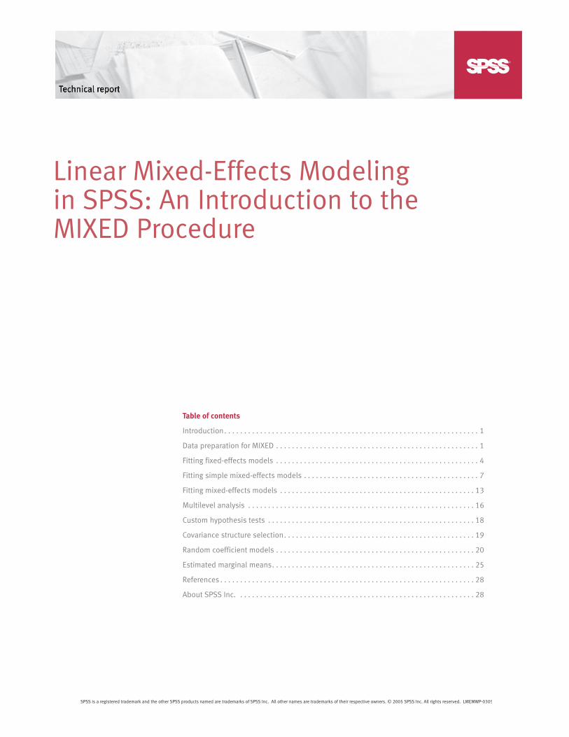
Figure 2. We need to convert two groups of variables (“age” and “dist”) into cases. We therefore enter “2” and click “Next.” This brings us to the “Select Variables” dialog box.
Figure 3. In the “Select Variables” dialog box, we first specify “Subject ID [subid]” as the case group identification. We then enter the names of new variables in the target variable drop-down list. For the target variable “age,” we drag “age1,” “age2,” and “age3” to the list box in the “Variables to be Transposed” group. We similarly associate variables “dist1,” “dist2,” and “dist3” with the target variable “distance.” We then drag variables that do not vary within a subject to the “Fixed Variable(s)” box. Clicking “Next” brings us to the “Create Index Variables” dialog box. We accept the default of one index variable, then click “Next” to arrive at the final dialog box.
3 Linear Mixed-Effects Modeling in SPSS
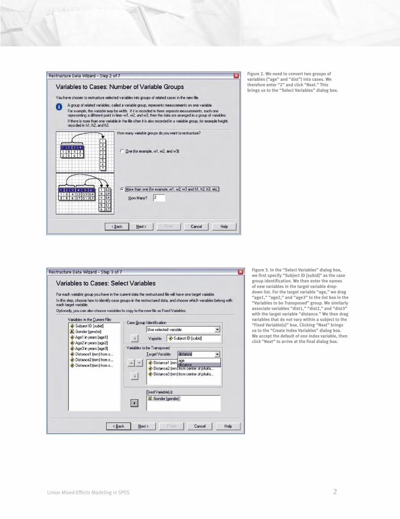
Figure 4. In the “Create One Index Variable” dialog box, we enter “visit” as the name of the indexing variable and click “Finish.”
Figure 5. We now have three cases for each subject.
We can also perform the conversion using the following command syntax:
VARSTOCASES
/MAKE age FROM age1 age2 age3
/MAKE distance FROM dist1 dist2 dist3
/INDEX = visit(3)
/KEEP = subid gender.
The command syntax is easy to interpret—it collapses the three age variables into “age” and the three response variables
into “distance.” At the same time, a new variable, “visit,” is created to index the three new cases within each subject. The
last subcommand means that the two variables that are constant within a subject should be kept.
Fitting fixed-effects models
With iid residual errors
A fitted model has the form , where is a vector of responses, is the fixed-effects design matrix, is a
vector of fixed-effects parameters and is a vector of residual errors. In this model, we assume that is distributed as
, where is an unknown covariance matrix. A common belief is that . We can use GLM or MIXED to
fit a model with this assumption. Using a subset of the growth study dataset, we illustrate how to use MIXED to fit a fixed-
effects model. The following command (Example 1) fits a fixed-effects model that investigates the effect of the variables
“gender” and “age” on “distance,” which is a measure of the growth rate.
Example 1: Fixed-effects model using MIXED
Command syntax:
MIXED DISTANCE BY GENDER WITH AGE
/FIXED = GENDER AGE | SSTYPE(3)
/PRINT = SOLUTION TESTCOV.
Output:
Linear Mixed-Effects Modeling in SPSS 4
Figure 6
Figure 7

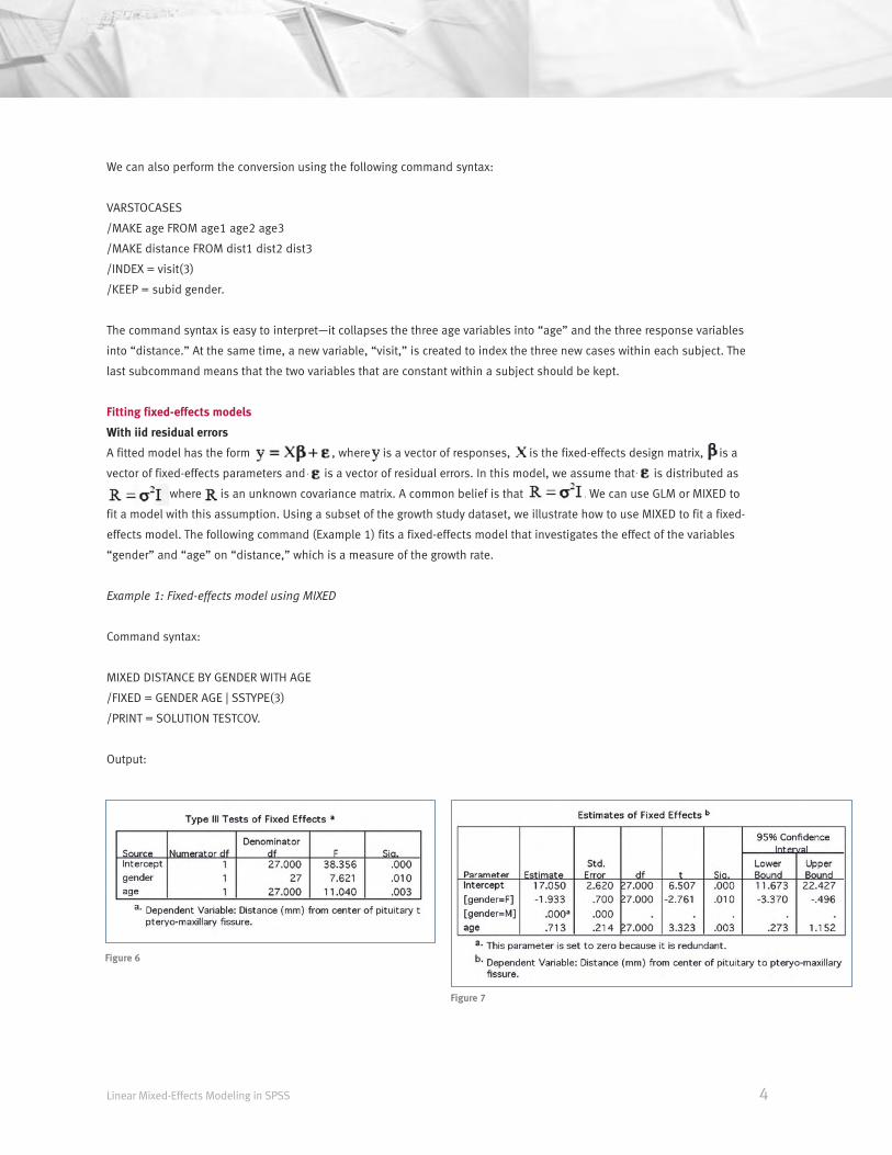
The command in Example 1 produces a “Type III Tests
of Fixed Effects” table (Figure 6). Both “gender” and
“age” are significant at the .05 level. This means
that “gender” and “age” are potentially impor-
tant predictors of the dependent variable. More
detailed information on fixed-effects parameters
may be obtained by using the subcommand /PRINT
SOLUTION. The “Estimates of Fixed Effects” table
(Figure 7) gives estimates of individual parameters,
as well as their standard errors and confidence intervals.
We can see that the mean distance for males is larger than that for females. Distance, moreover, increases with age. MIXED
also produces an estimate of the residual error variance and its standard error. The /PRINT TESTCOV option gives us the Wald
statistic and the confidence interval for the residual error variance estimate.
Example 1 is simple—users familiar with the GLM procedure can fit the same model using GLM.
Example 2: Fixed-effects model using GLM
Command syntax:
GLM DISTANCE BY GENDER WITH AGE
/METHOD = SSTYPE(3)
/PRINT = PARAMETER
/DESIGN = GENDER AGE.
Output:
5 Linear Mixed-Effects Modeling in SPSS
Figure 8
Figure 9

We see in Figure 9 that GLM and MIXED
produced the same Type III tests and
parameter estimates. Note, however,
that in the MIXED “Type III Tests of Fixed
Effects” table (Figure 6), there is no
column for the sum of squares. This is
because, for some complex models,
the test statistics in MIXED may not be
expressed as a ratio of two sums of
squares. They are thus omitted from the
ANOVA table.
With non-iid residual errors
The assumption may be violated in some situations. This often happens when repeated measurements are made on each
subject. In the growth study dataset, for example, the response variable of each subject is measured at various ages. We
may suspect that error terms within a subject are correlated. A reasonable choice of the residual error covariance will therefore
be a block diagonal matrix, where each block is a first-order autoregressive (AR1) covariance matrix.
Example 3: Fixed-effects model with correlated residual errors
Command syntax:
MIXED DISTANCE BY GENDER WITH AGE
/FIXED GENDER AGE
/REPEATED VISIT | SUBJECT(SUBID) COVTYPE(AR1)
/PRINT SOLUTION TESTCOV R.
Output:
Linear Mixed-Effects Modeling in SPSS 6
Figure 10
Figure 11
Figure 12
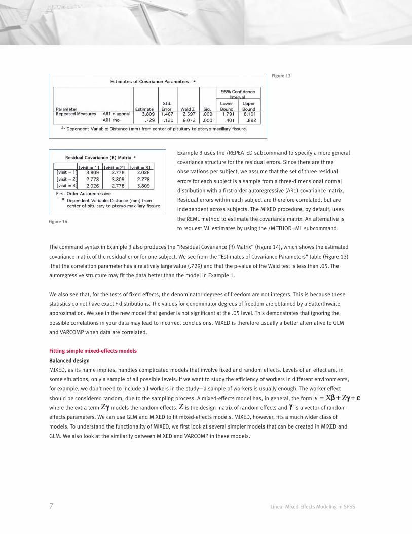
Example 3 uses the /REPEATED subcommand to specify a more general
covariance structure for the residual errors. Since there are three
observations per subject, we assume that the set of three residual
errors for each subject is a sample from a three-dimensional normal
distribution with a first-order autoregressive (AR1) covariance matrix.
Residual errors within each subject are therefore correlated, but are
independent across subjects. The MIXED procedure, by default, uses
the REML method to estimate the covariance matrix. An alternative is
to request ML estimates by using the /METHOD=ML subcommand.
The command syntax in Example 3 also produces the “Residual Covariance (R) Matrix” (Figure 14), which shows the estimated
covariance matrix of the residual error for one subject. We see from the “Estimates of Covariance Parameters” table (Figure 13)
that the correlation parameter has a relatively large value (.729) and that the p-value of the Wald test is less than .05. The
autoregressive structure may fit the data better than the model in Example 1.
We also see that, for the tests of fixed effects, the denominator degrees of freedom are not integers. This is because these
statistics do not have exact F distributions. The values for denominator degrees of freedom are obtained by a Satterthwaite
approximation. We see in the new model that gender is not significant at the .05 level. This demonstrates that ignoring the
possible correlations in your data may lead to incorrect conclusions. MIXED is therefore usually a better alternative to GLM
and VARCOMP when data are correlated.
Fitting simple mixed-effects models
Balanced design
MIXED, as its name implies, handles complicated models that involve fixed and random effects. Levels of an effect are, in
some situations, only a sample of all possible levels. If we want to study the efficiency of workers in different environments,
for example, we don’t need to include all workers in the study—a sample of workers is usually enough. The worker effect
should be considered random, due to the sampling process. A mixed-effects model has, in general, the form
where the extra term models the random effects. is the design matrix of random effects and is a vector of random-
effects parameters. We can use GLM and MIXED to fit mixed-effects models. MIXED, however, fits a much wider class of
models. To understand the functionality of MIXED, we first look at several simpler models that can be created in MIXED and
GLM. We also look at the similarity between MIXED and VARCOMP in these models.
7 Linear Mixed-Effects Modeling in SPSS
Figure 13
Figure 14
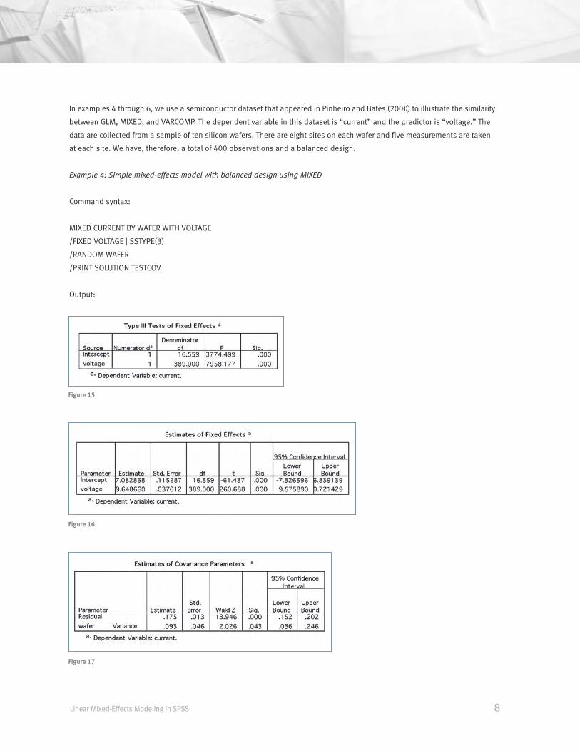
In examples 4 through 6, we use a semiconductor dataset that appeared in Pinheiro and Bates (2000) to illustrate the similarity
between GLM, MIXED, and VARCOMP. The dependent variable in this dataset is “current” and the predictor is “voltage.” The
data are collected from a sample of ten silicon wafers. There are eight sites on each wafer and five measurements are taken
at each site. We have, therefore, a total of 400 observations and a balanced design.
Example 4: Simple mixed-effects model with balanced design using MIXED
Command syntax:
MIXED CURRENT BY WAFER WITH VOLTAGE
/FIXED VOLTAGE | SSTYPE(3)
/RANDOM WAFER
/PRINT SOLUTION TESTCOV.
Output:
Linear Mixed-Effects Modeling in SPSS 8
Figure 15
Figure 16
Figure 17
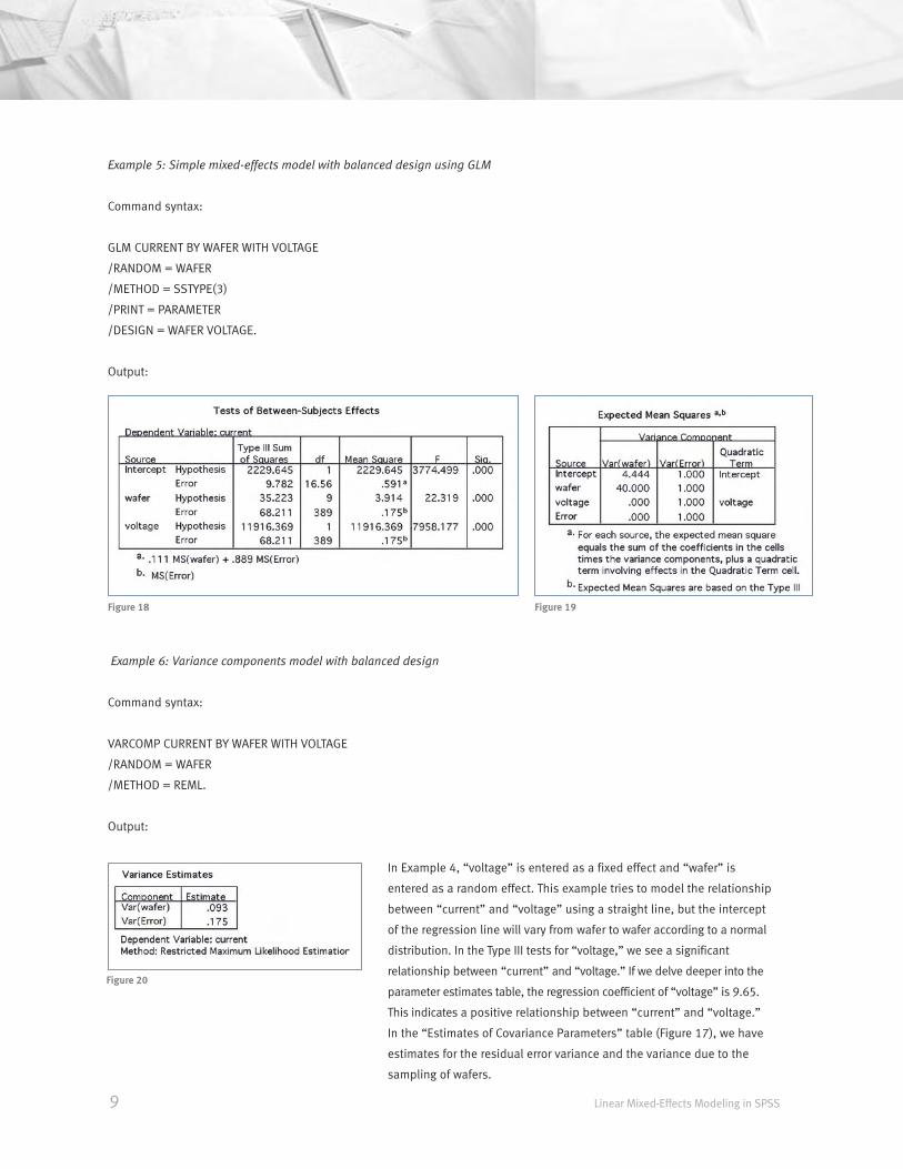
Example 5: Simple mixed-effects model with balanced design using GLM
Command syntax:
GLM CURRENT BY WAFER WITH VOLTAGE
/RANDOM = WAFER
/METHOD = SSTYPE(3)
/PRINT = PARAMETER
/DESIGN = WAFER VOLTAGE.
Output:
Example 6: Variance components model with balanced design
Command syntax:
VARCOMP CURRENT BY WAFER WITH VOLTAGE
/RANDOM = WAFER
/METHOD = REML.
Output:
In Example 4, “voltage” is entered as a fixed effect and “wafer” is
entered as a random effect. This example tries to model the relationship
between “current” and “voltage” using a straight line, but the intercept
of the regression line will vary from wafer to wafer according to a normal
distribution. In the Type III tests for “voltage,” we see a significant
relationship between “current” and “voltage.” If we delve deeper into the
parameter estimates table, the regression coefficient of “voltage” is 9.65.
This indicates a positive relationship between “current” and “voltage.”
In the “Estimates of Covariance Parameters” table (Figure 17), we have
estimates for the residual error variance and the variance due to the
sampling of wafers.
9 Linear Mixed-Effects Modeling in SPSS
Figure 18 Figure 19
Figure 20

We repeat the same model in Example 5 using GLM. Note that MIXED produces Type III tests for fixed effects only, but GLM
includes fixed and random effects. GLM treats all effects as fixed during computation and constructs F statistics by taking the
ratio of the appropriate sums of squares. Mean squares of random effects in GLM are estimates of functions of the variance
parameters of random and residual effects. These functions can be recovered from “Expected Mean Squares” (Figure 19). In
MIXED, the outputs are much simpler because the variance parameters are estimated directly using ML or REML. As a result,
there are no random-effect sums of squares.
When we have a balanced design, as in examples 4 through 6, the tests of fixed effects are the same for GLM and MIXED. We
can also recover the variance parameter estimates of MIXED by using the sum of squares in GLM. In MIXED, for example, the
estimate of the residual variance is 0.175, which is the same as the MS(Error) in GLM. The variance estimate of random effect
“wafer” is 0.093, which can be recovered in GLM using the “Expected Mean Squares” table (Figure 19) in Example 5:
Var(WAFER) = [MS(WAFER)-MS(Error)]/40 = 0.093
This is equal to MIXED’s estimate. One drawback of GLM, however, is that you cannot compute the standard error of the
variance estimates.
VARCOMP is, in fact, a subset of MIXED. These two procedures therefore always provide the same variance estimates, as seen
in examples 4 and 6. VARCOMP only fits relatively simple models. It can only handle random effects that are iid. No statistics
on fixed effects are produced. If your primary objective is to make inferences about fixed effects and your data are correlated,
MIXED is a better choice.
An important note: Due to the different estimation methods that are used, GLM and MIXED often do not produce the same
results. The next section gives an example of situations in which they produce different results.
Unbalanced design
One situation in which MIXED and GLM disagree is with an unbalanced design. To illustrate this, we removed some cases in
the semiconductor dataset, so that the design is no longer balanced.
Linear Mixed-Effects Modeling in SPSS 10
Figure 21

We then rerun examples 4 through 6 with this unbalanced dataset. The output is shown in examples 4a through 6a. We want
to see whether the three methods—GLM, MIXED and VARCOMP—still agree with each other.
Example 4a: Mixed-effects model with unbalanced design using MIXED
Command syntax:
MIXED CURRENT BY WAFER WITH VOLTAGE
/FIXED VOLTAGE | SSTYPE(3)
/RANDOM WAFER
/PRINT SOLUTION TESTCOV.
Output:
Example 5a: Mixed-effects model with unbalanced design using GLM
Command syntax:
GLM CURRENT BY WAFER WITH VOLTAGE
/RANDOM = WAFER
/METHOD = SSTYPE(3)
/PRINT = PARAMETER
/DESIGN = WAFER VOLTAGE.
11 Linear Mixed-Effects Modeling in SPSS
Figure 22
Figure 23
Figure 24

Output:
Example 6a: Variance components model with unbalanced design
Command syntax:
VARCOMP CURRENT BY WAFER WITH VOLTAGE
/RANDOM = WAFER
/METHOD = REML.
Output:
Since the data have changed, we expect examples 4a through 6a to differ
from examples 4 through 6. We will focus instead on whether examples 4a,
5a, and 6a agree with each other.
In Example 4a, the F statistic for the “voltage” effect is 67481.118, but
Example 5a gives an F statistic value of 67482.629. Apart from the test of
fixed effects, we also see a difference in covariance parameter estimates.
Examples 4a and 6a, however, show that VARCOMP and MIXED can produce the same variance estimates, even in an
unbalanced design. This is because MIXED and VARCOMP offer maximum likelihood or restricted maximum likelihood
methods in estimation, while GLM estimates are based on the method-of-moments approach.
MIXED is generally preferred because it is asymptotically efficient (minimum variance), whether or not the data are balanced.
GLM, however, only achieves its optimum behavior when the data are balanced.
Linear Mixed-Effects Modeling in SPSS 12
Figure 25
Figure 26
Figure 27
Fitting mixed-effects models
With subjects
In the semiconductor dataset, “current” is a dependent variable measured on a batch of wafers. These wafers are therefore
considered subjects in a study. An effect of interest (such as “site”) may often vary with subjects (“wafer”). One scenario is
that the (population) means of “current” at separate sites are different. When we look at the current measured at these sites
on individual wafers, however, they hover below or above the population mean according to some normal distribution. It is
therefore common to enter an “effect by subject” interaction term in a GLM or MIXED model to account for the subject variations.
In the dataset there are eight sites and ten wafers. The site*wafer effect, therefore, has 80 parameters, which can be denoted
by , i=1...10 and j=1...8. A common assumption is that ’s are assumed to be iid normal with zero mean and an
unknown variance. The mean is zero because ’s are used to model only the population variation. The mean of the
population is modeled by entering “site” as a fixed effect in GLM and MIXED. The results of this model for MIXED and GLM
are shown in examples 7 and 8.
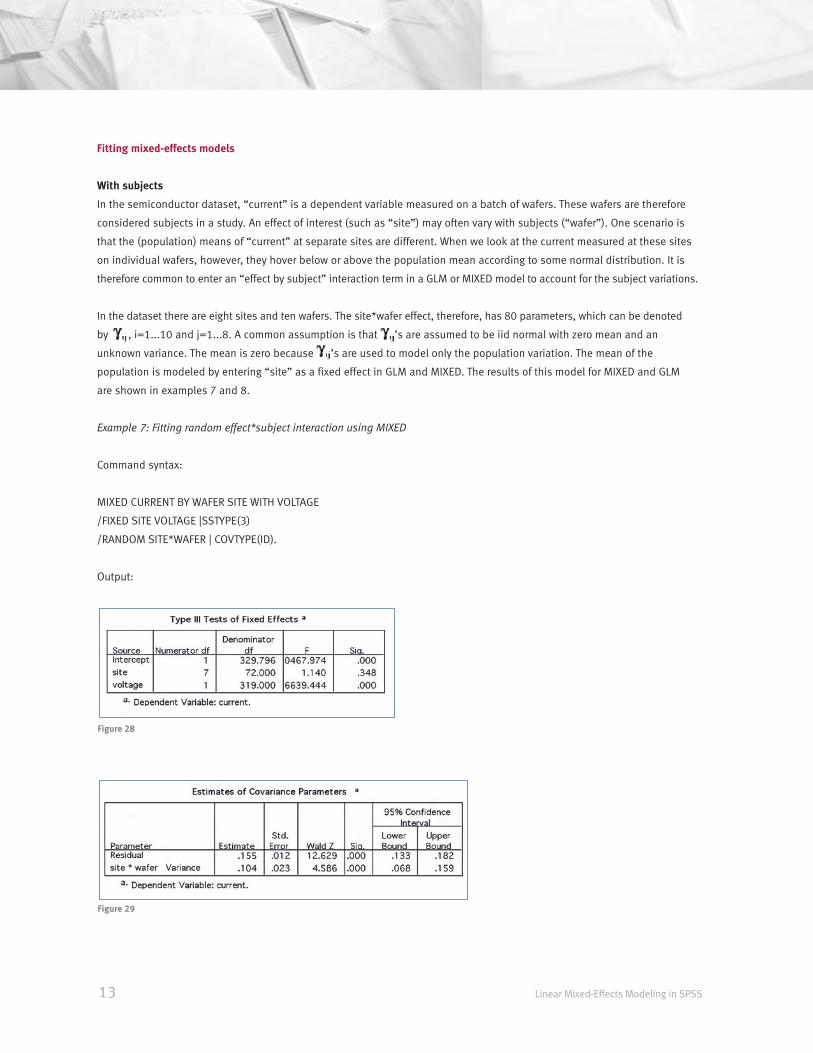
Example 7: Fitting random effect*subject interaction using MIXED
Command syntax:
MIXED CURRENT BY WAFER SITE WITH VOLTAGE
/FIXED SITE VOLTAGE |SSTYPE(3)
/RANDOM SITE*WAFER | COVTYPE(ID).
Output:
13 Linear Mixed-Effects Modeling in SPSS
Figure 28
Figure 29

Example 8: Fitting random effect*subject interaction using GLM
Command syntax:
GLM CURRENT BY WAFER SITE WITH VOLTAGE
/RANDOM = WAFER
/METHOD = SSTYPE(3)
/DESIGN = SITE SITE*WAFER VOLTAGE.
Output:
Since the design is balanced, the results of GLM and MIXED in examples 7 and 8 match. This is similar to examples 4 and 5.
We see from the results of Type III tests that “voltage” is still an important predictor of “current,” while “site” is not. The mean
currents at different sites are thus not significantly different from each other, so we can use a simpler model without the fixed
effect “site.” We should still, however, consider a random-effects model, because ignoring the subject variation may lead to
incorrect standard error estimates of fixed effects or false significant tests.
Up to this point, we examined primarily the similarities between GLM and MIXED. MIXED, in fact, has a much more flexible way
of modeling random effects. Using the SUBJECT and COVTYPE options, Example 9 presents an equivalent form of Example 7.
Example 9: Fitting random effect*subject interaction using SUBJECT specification
Command syntax:
MIXED CURRENT BY SITE WITH VOLTAGE
/FIXED SITE VOLTAGE |SSTYPE(3)
/RANDOM SITE | SUBJECT(WAFER) COVTYPE(ID).
Linear Mixed-Effects Modeling in SPSS 14
Figure 30 Figure 31

The SUBJECT option tells MIXED that each subject will have its own set of random parameters for the random effect “site.”
The COVTYPE option will specify the form of the variance covariance matrix of the random parameters within one subject.
The command syntax attempts to specify the distributional assumption in a multivariate form, which can be written as:
Under normality, this assumption is equivalent to that in Example 7. One advantage of the multivariate form is that you can easily
specify other covariance structures by using the COVTYPE option. The flexibility in specifying covariance structures helps us to
fit a model that better describes the data. If, for example, we believe that the variances of different sites are different, we can
specify a diagonal matrix as covariance type and the assumption becomes:
The result of fitting the same model using this assumption is given in Example 10.
Example 10: Using COVTYPE in a random-effects model
Command syntax:
MIXED CURRENT BY SITE WITH VOLTAGE
/FIXED SITE VOLTAGE |SSTYPE(3)
/RANDOM SITE | SUBJECT(WAFER) COVTYPE(DIAG)
/PRINT G TESTCOV.
Output:
15 Linear Mixed-Effects Modeling in SPSS
Figure 32
Figure 33
Figure 34

In Example 10, we request one extra table, the
estimated covariance matrix of the random
effect “site.” It is an eight-by-eight diagonal
matrix in this case. Note that changing the
covariance structure of a random effect also
changes the estimates and tests of fixed
effects. We want, in practice, an objective
method to select suitable covariance struc-
tures for our random effects. In the section
“Covariance Structure Selection,” we revisit
examples 9 and 10 to show how to select
covariance structures for random effects.
Multilevel analysis
The use of the SUBJECT and COVTYPE options
in /RANDOM and /REPEATED brings many
options for modeling the covariance structures
of random effects and residual errors. It is
particularly useful when modeling data
obtained from a hierarchy. Example 11
illustrates the simultaneous use of these
options in a multilevel model. We selected
data from six schools from the Junior School
Project of Mortimore, et al. (1988). We investi-
gate below how the socioeconomic status (SES)
of a student affects his or her math scores over
a three-year period.
Example 11: Multilevel mixed-effects model
Command syntax:
MIXED MATHTEST BY SCHOOL CLASS STUDENT GENDER SES SCHLYEAR
/FIXED GENDER SES SCHLYEAR SCHOOL
/RANDOM SES |SUBJECT(SCHOOL*CLASS) COVTYPE(ID)
/RANDOM SES |SUBJECT(SCHOOL*CLASS*STUDENT) COVTYPE(ID)
/REPEATED SCHLYEAR | SUBJECT(SCHOOL*CLASS*STUDENT) COVTYPE(AR1)
/PRINT SOLUTION TESTCOV.
Output:
Linear Mixed-Effects Modeling in SPSS 16
Figure 35
Figure 36
Figure 37
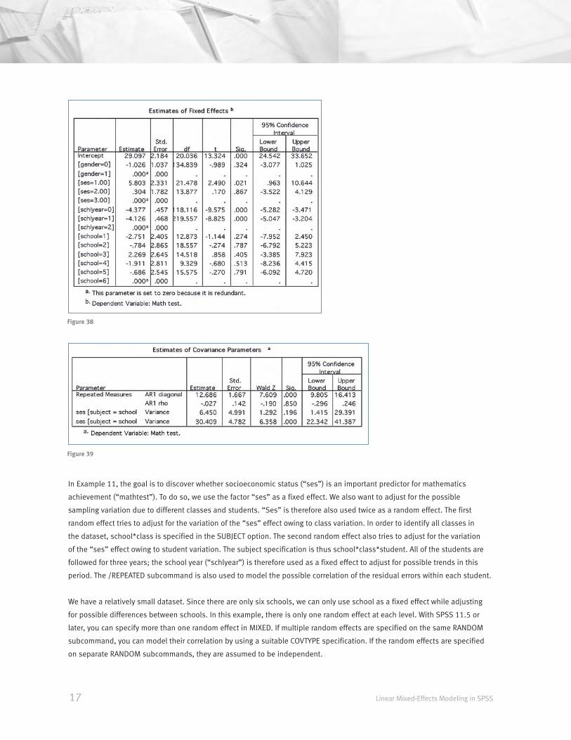
In Example 11, the goal is to discover whether socioeconomic status (“ses”) is an important predictor for mathematics
achievement (“mathtest”). To do so, we use the factor “ses” as a fixed effect. We also want to adjust for the possible
sampling variation due to different classes and students. “Ses” is therefore also used twice as a random effect. The first
random effect tries to adjust for the variation of the “ses” effect owing to class variation. In order to identify all classes in
the dataset, school*class is specified in the SUBJECT option. The second random effect also tries to adjust for the variation
of the “ses” effect owing to student variation. The subject specification is thus school*class*student. All of the students are
followed for three years; the school year (“schlyear”) is therefore used as a fixed effect to adjust for possible trends in this
period. The /REPEATED subcommand is also used to model the possible correlation of the residual errors within each student.
We have a relatively small dataset. Since there are only six schools, we can only use school as a fixed effect while adjusting
for possible differences between schools. In this example, there is only one random effect at each level. With SPSS 11.5 or
later, you can specify more than one random effect in MIXED. If multiple random effects are specified on the same RANDOM
subcommand, you can model their correlation by using a suitable COVTYPE specification. If the random effects are specified
on separate RANDOM subcommands, they are assumed to be independent.
17 Linear Mixed-Effects Modeling in SPSS
Figure 38
Figure 39
In the Type III tests of fixed effects, in Example 11, we see that socioeconomic status does impact student performance. The
parameter estimates of “ses” for students with “ses=1” (fathers have managerial or professional occupations) indicate that
these students perform better than students at other socioeconomic levels. The effect “schlyear” is also significant in the
model and the students’ performances increase with “schlyear.”
From “Estimates of Covariance Parameters” (Figure 39), we notice that the estimate of the “AR1 rho” parameter is not
significant, which means that a simple, scaled-identity structure may be used. For the variation of “ses” due to school*
class, the estimate is very small compared to other sources of variance and the Wald test indicates that it is not significant.
We can therefore consider removing the random effect from the model.
We see from this example that the major advantages of MIXED are that it is able to look at different aspects of a dataset
simultaneously and that all of the statistics are already adjusted for all effects in the model. Without MIXED, we must use
different tools to study different aspects of the models. An example of this is using GLM to study the fixed effects and
using VARCOMP to study the covariance structure. This is not only time consuming, but the assumptions behind the statistics
are usually violated.
Custom hypothesis tests
Apart from predefined statistics, MIXED allows users to construct custom hypotheses on fixed- and random-effects parameters
through the use of the /TEST subcommand. To illustrate, we use a dataset from Pinheiro and Bates (2000). The data consist
of a CT scan on a sample of ten dogs. The dogs’ left and right lymph nodes were scanned and the intensity of each scan was
recorded in the variable pixel. The following mixed-model command syntax tests whether there is a difference between the left
and right lymph nodes.
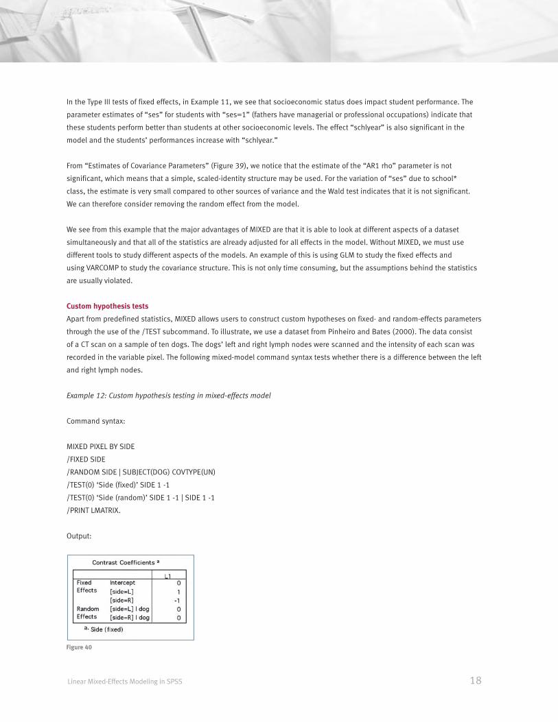
Example 12: Custom hypothesis testing in mixed-effects model
Command syntax:
MIXED PIXEL BY SIDE
/FIXED SIDE
/RANDOM SIDE | SUBJECT(DOG) COVTYPE(UN)
/TEST(0) ‘Side (fixed)’ SIDE 1 -1
/TEST(0) ‘Side (random)’ SIDE 1 -1 | SIDE 1 -1
/PRINT LMATRIX.
Output:
Linear Mixed-Effects Modeling in SPSS 18
Figure 40
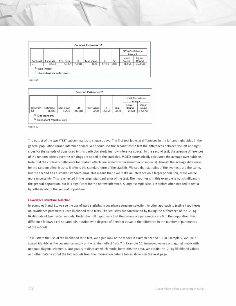
The output of the two /TEST subcommands is shown above. The first test looks at differences in the left and right sides in the
general population (broad inference space). We should use the second test to test the differences between the left and right
sides for the sample of dogs used in this particular study (narrow inference space). In the second test, the average differences
of the random effects over the ten dogs are added to the statistics. MIXED automatically calculates the average over subjects.
Note that the contrast coefficients for random effects are scaled by one/(number of subjects). Though the average difference
for the random effect is zero, it affects the standard error of the statistic. We see that statistics of the two tests are the same,
but the second has a smaller standard error. This means that if we make an inference on a larger population, there will be
more uncertainty. This is reflected in the larger standard error of the test. The hypothesis in this example is not significant in
the general population, but it is significant for the narrow inference. A larger sample size is therefore often needed to test a
hypothesis about the general population.
Covariance structure selection
In examples 3 and 11, we see the use of Wald statistics in covariance structure selection. Another approach to testing hypotheses
on covariance parameters uses likelihood ratio tests. The statistics are constructed by taking the differences of the -2 Log
likelihoods of two nested models. Under the null hypothesis that the covariance parameters are 0 in the population, this
difference follows a chi-squared distribution with degrees of freedom equal to the difference in the number of parameters
of the models.
To illustrate the use of the likelihood ratio test, we again look at the model in examples 9 and 10. In Example 9, we use a
scaled identity as the covariance matrix of the random effect “site.” In Example 10, however, we use a diagonal matrix with
unequal diagonal elements. Our goal is to discover which model better fits the data. We obtain the -2 Log likelihood values
and other criteria about the two models from the information criteria tables shown on the next page.
19 Linear Mixed-Effects Modeling in SPSS
Figure 41
Figure 42
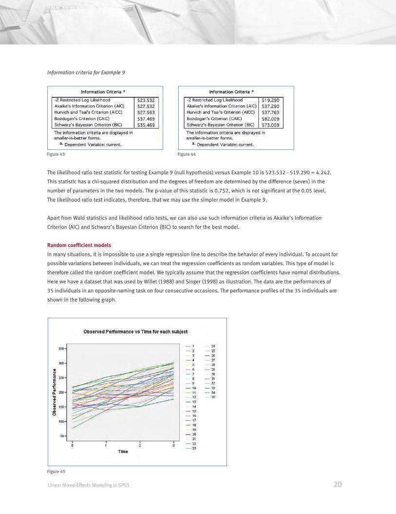
Information criteria for Example 9
The likelihood ratio test statistic for testing Example 9 (null hypothesis) versus Example 10 is 523.532 - 519.290 = 4.242.
This statistic has a chi-squared distribution and the degrees of freedom are determined by the difference (seven) in the
number of parameters in the two models. The p-value of this statistic is 0.752, which is not significant at the 0.05 level.
The likelihood ratio test indicates, therefore, that we may use the simpler model in Example 9.
Apart from Wald statistics and likelihood ratio tests, we can also use such information criteria as Akaike’s Information
Criterion (AIC) and Schwarz’s Bayesian Criterion (BIC) to search for the best model.
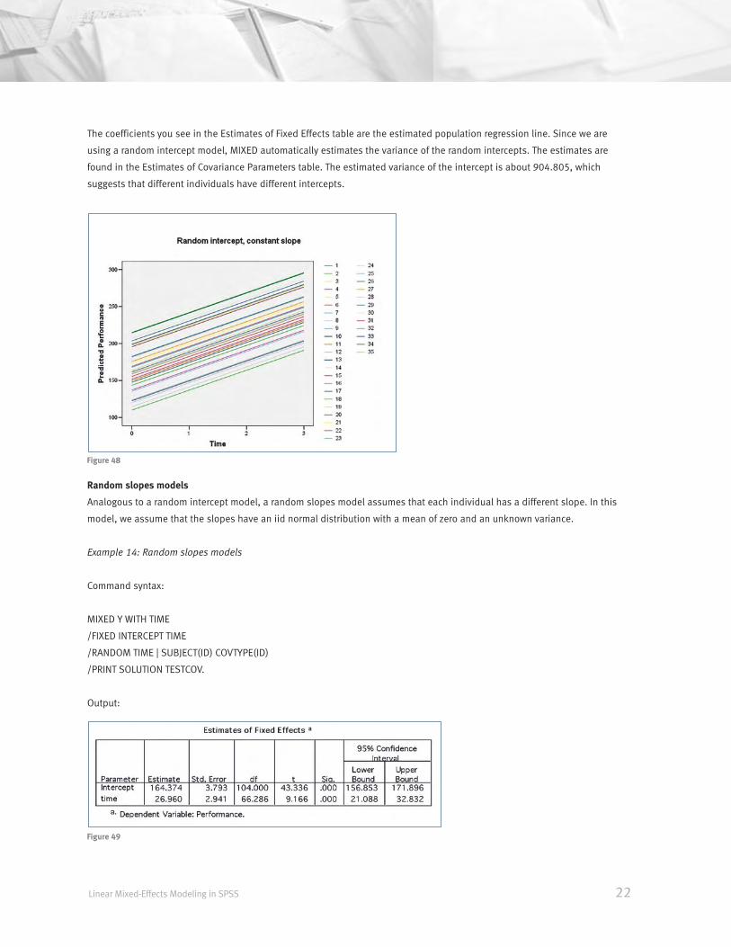
Random coefficient models
In many situations, it is impossible to use a single regression line to describe the behavior of every individual. To account for
possible variations between individuals, we can treat the regression coefficients as random variables. This type of model is
therefore called the random coefficient model. We typically assume that the regression coefficients have normal distributions.
Here we have a dataset that was used by Willet (1988) and Singer (1998) as illustration. The data are the performances of
35 individuals in an opposite-naming task on four consecutive occasions. The performance profiles of the 35 individuals are
shown in the following graph.
Linear Mixed-Effects Modeling in SPSS 20
Figure 43 Figure 44
Figure 45

We can see that most individuals exhibit an increasing trend over time. Since a single regression line will not fit all of them, it
makes sense to use a random coefficient model. If we restrict ourselves to linear models, there are three possible model types:
■ Random intercept
■ Random slopes
■ Random intercept and slopes
Random intercept models
As the name suggests, random intercept models assume that each individual has a different intercept. In this model, we
assume that the intercepts have an iid normal distribution with a mean of zero and some unknown variance.
Example 13: Random intercept models
Command syntax:
MIXED Y WITH TIME
/FIXED INTERCEPT TIME
/RANDOM INTERCEPT | SUBJECT(ID) COVTYPE(ID)
/PRINT SOLUTION TESTCOV.
Output:
21 Linear Mixed-Effects Modeling in SPSS
Figure 46
Figure 47
The coefficients you see in the Estimates of Fixed Effects table are the estimated population regression line. Since we are
using a random intercept model, MIXED automatically estimates the variance of the random intercepts. The estimates are
found in the Estimates of Covariance Parameters table. The estimated variance of the intercept is about 904.805, which
suggests that different individuals have different intercepts.
Random slopes models
Analogous to a random intercept model, a random slopes model assumes that each individual has a different slope. In this
model, we assume that the slopes have an iid normal distribution with a mean of zero and an unknown variance.
Example 14: Random slopes models
Command syntax:
MIXED Y WITH TIME
/FIXED INTERCEPT TIME
/RANDOM TIME | SUBJECT(ID) COVTYPE(ID)
/PRINT SOLUTION TESTCOV.
Output:
Linear Mixed-Effects Modeling in SPSS 22
Figure 48
Figure 49
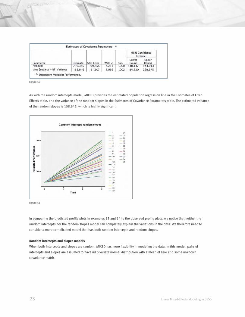
As with the random intercepts model, MIXED provides the estimated population regression line in the Estimates of Fixed
Effects table, and the variance of the random slopes in the Estimates of Covariance Parameters table. The estimated variance
of the random slopes is 158.946, which is highly significant.
In comparing the predicted profile plots in examples 13 and 14 to the observed profile plots, we notice that neither the
random intercepts nor the random slopes model can completely explain the variations in the data. We therefore need to
consider a more complicated model that has both random intercepts and random slopes.
Random intercepts and slopes models
When both intercepts and slopes are random, MIXED has more flexibility in modeling the data. In this model, pairs of
intercepts and slopes are assumed to have iid bivariate normal distribution with a mean of zero and some unknown
covariance matrix.
23 Linear Mixed-Effects Modeling in SPSS
Figure 50
Figure 51

Example 15: Random intercepts and slopes models
Command syntax:
MIXED Y WITH TIME
/FIXED INTERCEPT TIME
/RANDOM INTERCEPT TIME | SUBJECT(ID) COVTYPE(UN)
/PRINT SOLUTION TESTCOV.
Output:
In addition to estimating the population regression line, MIXED also estimates the variance of the intercepts, the variance of
the slopes, and the covariance between the intercepts and the slopes. All of the variance and covariance parameters in this
model are significant at the 0.05 level. We can see that the predicted profiles of the 35 individuals as shown below match
the observed profile much better than the profiles produced by the previous two models.
Linear Mixed-Effects Modeling in SPSS 24
Figure 52
Figure 53
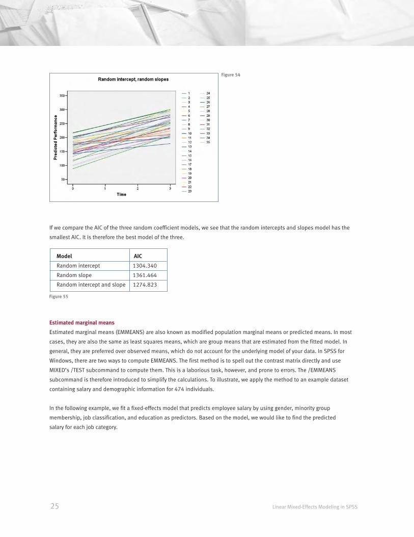
If we compare the AIC of the three random coefficient models, we see that the random intercepts and slopes model has the
smallest AIC. It is therefore the best model of the three.
Model AIC
Random intercept 1304.340
Random slope 1361.464
Random intercept and slope 1274.823
Estimated marginal means
Estimated marginal means (EMMEANS) are also known as modified population marginal means or predicted means. In most
cases, they are also the same as least squares means, which are group means that are estimated from the fitted model. In
general, they are preferred over observed means, which do not account for the underlying model of your data. In SPSS for
Windows, there are two ways to compute EMMEANS. The first method is to spell out the contrast matrix directly and use
MIXED’s /TEST subcommand to compute them. This is a laborious task, however, and prone to errors. The /EMMEANS
subcommand is therefore introduced to simplify the calculations. To illustrate, we apply the method to an example dataset
containing salary and demographic information for 474 individuals.
In the following example, we fit a fixed-effects model that predicts employee salary by using gender, minority group
membership, job classification, and education as predictors. Based on the model, we would like to find the predicted
salary for each job category.
25 Linear Mixed-Effects Modeling in SPSS
Figure 55
Figure 54
Example 16: EMMEANS
Command syntax:
MIXED SALARY BY GENDER MINORITY JOBCAT WITH EDUC
/FIXED GENDER MINORITY JOBCAT EDUC
/PRINT LMATRIX SOLUTION
/EMMEANS = TABLES(JOBCAT) COMPARE ADJ(SIDAK).
Output:
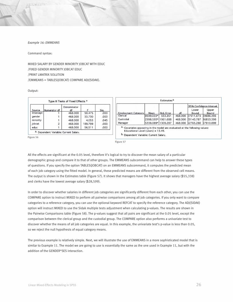
All the effects are significant at the 0.05 level, therefore it’s logical to try to discover the mean salary of a particular
demographic group and compare it to that of other groups. The EMMEANS subcommand can help to answer these types
of questions. If you specify the option TABLES(JOBCAT) on an EMMEANS subcommand, it computes the predicted mean
of each job category using the fitted model. In general, these predicted means are different from the observed cell means.
The output is shown in the Estimates table (Figure 57). It shows that managers have the highest average salary ($55,338)
and clerks have the lowest average salary ($28,599).
In order to discover whether salaries in different job categories are significantly different from each other, you can use the
COMPARE option to instruct MIXED to perform all pairwise comparisons among all job categories. If you only want to compare
categories to a reference category, you can use the optional keyword REFCAT to specify the reference category. The ADJ(SIDAK)
option will instruct MIXED to use the Sidak multiple tests adjustment when calculating p-values. The results are shown in
the Pairwise Comparisons table (Figure 58). The p-values suggest that all pairs are significant at the 0.05 level, except the
comparison between the clerical group and the custodial group. The COMPARE option also performs a univariate test to
discover whether the means of all job categories are equal. In this example, the univariate test’s p-value is less than 0.05,
so we reject the null hypothesis of equal category means.
The previous example is relatively simple. Next, we will illustrate the use of EMMEANS in a more sophisticated model that is
similar to Example 11. The model we are going to use is essentially the same as the one used in Example 11, but with the
addition of the GENDER*SES interaction.
Linear Mixed-Effects Modeling in SPSS 26
Figure 56
Figure 57

Example 17: EMMEANS
Command syntax:
MIXED MATHTEST BY SCHOOL CLASS STUDENT
GENDER SES SCHLYEAR
/FIXED GENDER SES GENDER*SES SCHLYEAR SCHOOL
/RANDOM SES |SUBJECT(SCHOOL*CLASS) COVTYPE(ID)
/RANDOM SES |SUBJECT(SCHOOL*CLASS*STUDENT) COVTYPE(ID)
/REPEATED SCHLYEAR | SUBJECT(SCHOOL*CLASS*STUDENT)
COVTYPE(AR1)
/PRINT SOLUTION TESTCOV
/EMMEAN TABLE(SES*GENDER) COMPARE(SES) ADJ(SIDAK).
Output:
27 Linear Mixed-Effects Modeling in SPSS
Figure 60
Figure 61
Figure 58Figure 59
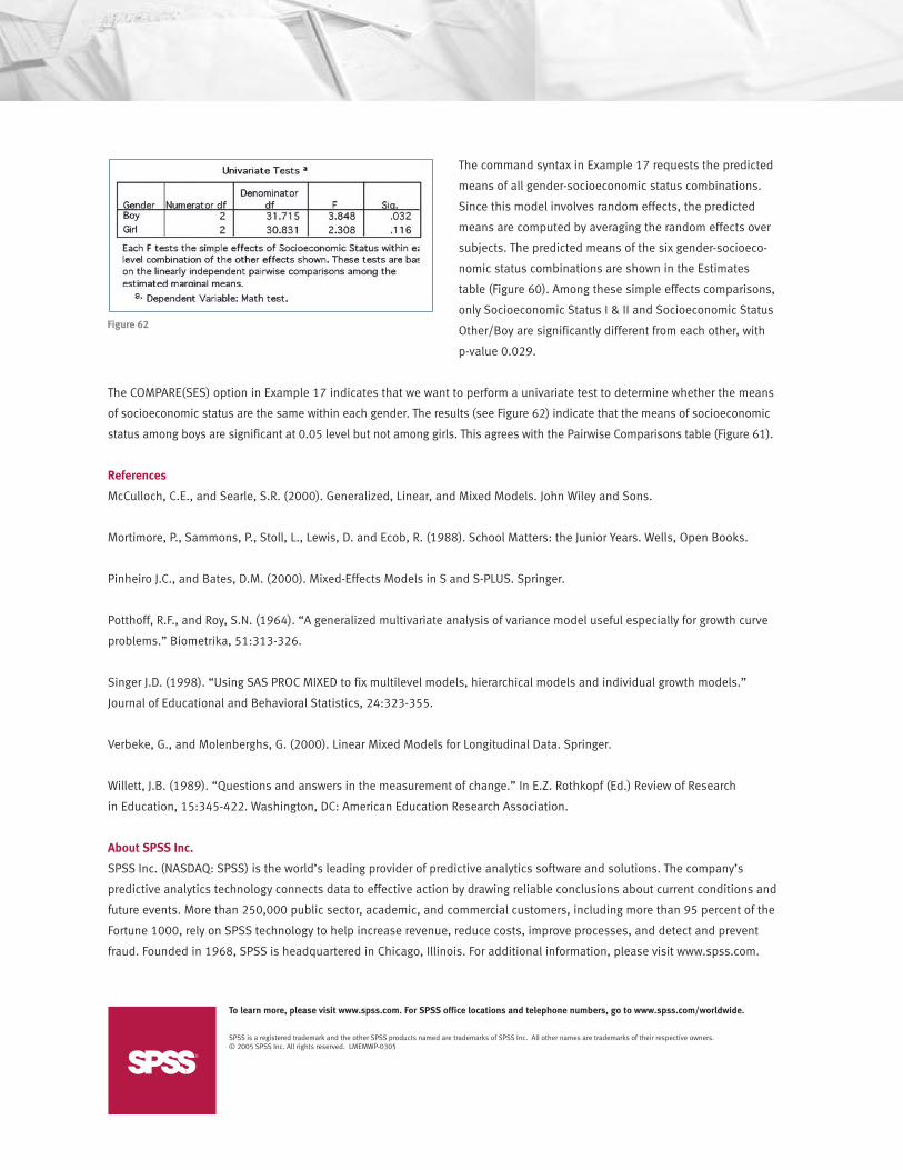
The command syntax in Example 17 requests the predicted
means of all gender-socioeconomic status combinations.
Since this model involves random effects, the predicted
means are computed by averaging the random effects over
subjects. The predicted means of the six gender-socioeco-
nomic status combinations are shown in the Estimates
table (Figure 60). Among these simple effects comparisons,
only Socioeconomic Status I & II and Socioeconomic Status
Other/Boy are significantly different from each other, with
p-value 0.029.
The COMPARE(SES) option in Example 17 indicates that we want to perform a univariate test to determine whether the means
of socioeconomic status are the same within each gender. The results (see Figure 62) indicate that the means of socioeconomic
status among boys are significant at 0.05 level but not among girls. This agrees with the Pairwise Comparisons table (Figure 61).
References
McCulloch, C.E., and Searle, S.R. (2000). Generalized, Linear, and Mixed Models. John Wiley and Sons.
Mortimore, P., Sammons, P., Stoll, L., Lewis, D. and Ecob, R. (1988). School Matters: the Junior Years. Wells, Open Books.
Pinheiro J.C., and Bates, D.M. (2000). Mixed-Effects Models in S and S-PLUS. Springer.
Potthoff, R.F., and Roy, S.N. (1964). “A generalized multivariate analysis of variance model useful especially for growth curve
problems.” Biometrika, 51:313-326.
Singer J.D. (1998). “Using SAS PROC MIXED to fix multilevel models, hierarchical models and individual growth models.”
Journal of Educational and Behavioral Statistics, 24:323-355.
Verbeke, G., and Molenberghs, G. (2000). Linear Mixed Models for Longitudinal Data. Springer.
Willett, J.B. (1989). “Questions and answers in the measurement of change.” In E.Z. Rothkopf (Ed.) Review of Research
in Education, 15:345-422. Washington, DC: American Education Research Association.
About SPSS Inc.
SPSS Inc. (NASDAQ: SPSS) is the world’s leading provider of predictive analytics software and solutions. The company’s
predictive analytics technology connects data to effective action by drawing reliable conclusions about current conditions and
future events. More than 250,000 public sector, academic, and commercial customers, including more than 95 percent of the
Fortune 1000, rely on SPSS technology to help increase revenue, reduce costs, improve processes, and detect and prevent
fraud. Founded in 1968, SPSS is headquartered in Chicago, Illinois. For additional information, please visit www.spss.com.
Figure 62
To learn more, please visit www.spss.com. For SPSS office locations and telephone numbers, go to www.spss.com/worldwide.
SPSS is a registered trademark and the other SPSS products named are trademarks of SPSS Inc. All other names are trademarks of their respective owners. © 2005 SPSS Inc. All rights reserved. LMEMWP-0305
Related Documents


![[ME] Multilevel Mixed Effects](https://static.cupdf.com/doc/110x72/587740121a28ab1c3a8babdd/me-multilevel-mixed-effects.jpg)