LINEAR AND NONLINEAR PROGRESSIVE ROSSBY WAVES ON A ROTATING SPHERE by Timothy G. Callaghan, B.A. B.Sc. ions (Qld) Submitted in fulfilment of the requirements for the Degree of Doctor of Philosophy Department of Mathematics " University of Tasmania January, 2005

Welcome message from author
This document is posted to help you gain knowledge. Please leave a comment to let me know what you think about it! Share it to your friends and learn new things together.
Transcript
LINEAR AND NONLINEAR PROGRESSIVE ROSSBY WAVES ON A ROTATING SPHERE
by
Timothy G. Callaghan, B.A. B.Sc. ions (Qld)
Submitted in fulfilment of the requirements for the Degree of Doctor of Philosophy
Department of Mathematics " University of Tasmania
January, 2005

I declare that this thesis contains no material which has been accepted for a degree or diploma by the University or any other institution, except by way of background information and duly acknowledged in the thesis, and that, to the best of my knowledge and belief, this thesis contains no material previously published or written by another person, except where due acknowledgement is made in the text of the thesis.
Signed. Timothy G. Callaghan
Date. i 3 /0 1 / Zocr

This thesis may be made available for loan and limited copying in ac-cordance with the Copyright Act 1968
Signed. /1— 611A—■
Timothy G. Callaghan
Date. 13 /61 / 200s'

ABSTRACT
We present an analysis of incompressible and compressible flow of a thin layer of
fluid with a free-surface on a rotating sphere. Our general aim is to investigate
the nature of progressive Rossby wave structures that are possible in this rotating
system, with the goal of expanding previous research by conducting an in-depth
analysis of wavespeed/amplitude relationships.
A linearized theory for the incompressible dynamics, closely related to the theory
developed by B. Haurwitz, is constructed, with good agreement observed between
the two separate models. This result is then extended to the numerical solution of
the full model, to obtain highly nonlinear large-amplitude progressive-wave solutions
in the form of Fourier series. A detailed picture is developed of how the progressive
wavespeed depends on the wave amplitude. This approach reveals the presence
of nonlinear resonance behaviour, with different disjoint solution branches existing
at different values of the amplitude. Additionally, we show that the formation of
localised low pressure systems is an inherent feature of the nonlinear dynamics, once
the forcing amplitude reaches a certain critical level.
We then derive a new free-surface model for compressible fluid dynamics and repeat
the above analysis by first constructing a linearized solution and then using this
to guide the computation of nonlinear solutions via a bootstrapping process. It is
shown that if the value of the pressure on the free-surface is assumed to be zero,
which is consistent with the concept of the atmosphere terminating, then the model
almost reduces to the incompressible dynamics with the only difference being a
slightly modified conservation of mass equation. By forcing wave amplitude in the
model we show that the resonant behaviour observed in the incompressible dynamics
is again encountered in the compressible model. The effect of the compressibility
is observed to become apparent through damped resonance behaviour in general,
so that in some instances two neighbouring disjoint solution branches from the
incompressible dynamics are seen to merge into one continuous solution branch when
compressible dynamics are incorporated. In closing, some conjectures are made as

to how these results might help explain certain observed atmospheric phenomena.
In particular it is conjectured that the process of atmospheric blocking is a direct
result of critically forced stationary Rossby waves.

ACKNOWLEDGEMENTS
I would like to sincerely thank my supervisor Professor Larry Forbes for his faithful
guidance and insight throughout all stages of this research. Having someone to look
up to and learn from is a great honour and privilege, and to him I will be eternally
indebted for his enthusiasm and encouragement.
I would also like to express deep gratitude to Dr Simon Wotherspoon for many
stimulating and illuminating discussions along the way. His advice, critical analysis
and wit have been most welcome and enjoyed immensely. A big thank you also to all
my mathematically minded friends both here at UTas and back at UQ for general
support and advice. In addition I wish to acknowledge the financial assistance of
the Australian government for an APA scholarship; this assistance has ultimately
afforded me the time and financial freedom to pursue this research.
Finally I would like to thank friends and family for continued emotional support. In
particular Mr Aaron Ryan has been a wonderful friend full of encouragement who I
will continue to value highly for his intelligence and like minded sense of humour. To
my parents and sisters I owe thanks not only for unconditional love and support but
also for believing in me and convincing me otherwise of my doubts in my own ability
at those, perhaps rather too frequent, precipitous times throughout this emotionally
taxing but highly rewarding period of my life.

TABLE OF CONTENTS
TABLE OF CONTENTS
LIST OF TABLES V
LIST OF FIGURES vi
1 INTRODUCTION
1
1.1 Brief Literature Review and Research Objective 1
1.2 Preliminaries 4
2 INCOMPRESSIBLE LINEARIZED SHALLOW ATMOSPHERE
MODEL 8
2.1 Derivation 8
2.2 Progressive-Wave Coordinate Transform 13
2.3 Non-dimensionalization of the Governing Equations 14
2.4 Linearization of the Equations 15
2.4.1 Base Zonal Flow Derivation 15
2.4.2 Linearization about the Base Zonal Flow 17
2.5 Numerical Solution of the Linearized Equations 19
2.5.1 Series Representation 19
2.5.2 Galerkin Method 21
2.5.3 Truncation and Generalised Eigenvalue Formulation 25 i

TABLE OF CONTENTS ii
2.6 Solution and Results 27
2.6.1 Parameters and Constants 27
2.6.2 Results for k = 3, 4 and 5 29
2.6.3 Comparison with Rossby-Haurwitz solution 35
3 INCOMPRESSIBLE NONLINEAR SHALLOW ATMOSPHERE
MODEL 40
3.1 Problem Specification 40
3.1.1 Conservation Equations 40
3.1.2 Series Representation 41
3.1.3 Volume Specification 43
3.2 Numerical Solution Method 44
3.2.1 Collocation 44
3.2.2 Newton-Raphson Technique 45
3.3 Code Highlights 48
3.3.1 Programming Language and Computational Environment 48
3.3.2 Truncation 48
3.3.3 Forcing the Solution 49
3.3.4 Collocation Points 50
3.3.5 Caching the Basis Functions 51
3.3.6 Calculation of the Jacobian Matrix 52
3.3.7 Adaptive Integration Method 54
3.3.8 Bootstrapping 54
3.4 Solution and Results 55
3.4.1 Measuring the Amplitude 55
3.4.2 Parameters and Constants 57
3.4.3 Results for tc = 4, w = 1.25 58

TABLE OF CONTENTS iii
3.4.4 Results for n = 4, w = 1.0 61
3.4.5 Results for ic = 5, w = 1.25 68
3.4.6 Results for K = 5, w = 1.0 71
3.5 Closing Remarks 73
4 COMPRESSIBLE LINEARIZED SHALLOW ATMOSPHERE MODEL 74
4.1 Derivation 74
4.2 Non-dimensionalization and Problem Simplification 82
4.2.1 Non-dimensionalization 82
4.2.2 Problem Simplification 83
4.3 Linearization of the Equations 84
4.4 Numerical Solution of the Linearized Equations 86
4.5 Solution and Results 87
4.5.1 Model Parameters 87
4.5.2 Zonal Flow Parameters and Mass Specification 88
4.5.3 Results for lc = 3,4 and 5 90
5 COMPRESSIBLE NONLINEAR SHALLOW ATMOSPHERE
MODEL 97
5.1 Problem Specification 97
5.1.1 Conservation Equations 97
5.1.2 Mass Specification 98
5.2 Numerical Solution Method 99
5.2.1 Series Solution and Algorithm 99
5.2.2 Amplitude Measurement 102
5.3 Solution and Results 103
5.3.1 Model parameters 103
TABLE OF CONTENTS iv
5.3.2 Results for tc = 4, w = 1.25 103
5.3.3 Results for K = 4, w = 1.0 106
5.3.4 Results for lc = 5, w = 1.25 108
5.3.5 Results for lc = 5, w = 1.0 109
5.4 Closing Remarks 111
6 CONCLUSION AND CLOSING REMARKS 112
6.1 Discussion and Application to Meteorology 112
6.2 Future work and Closing Remarks 114
A EVALUATION OF VOLUME SPECIFICATION JACOBIAN
ELEMENTS 116
B COMPRESSIBLE LINEARIZED SYSTEM DERIVATION 118
C 3D OPENGL ROSSBY WAVE VIEWER 121
BIBLIOGRAPHY AND SELECTED READING LIST 125
INDEX 130

LIST OF TABLES
2.1 Convergence of incompressible wavespeed and first three coefficients
in each series for increasing N, n = 3. 30
2.2 Convergence of incompressible wavespeed and first three coefficients
in each series for increasing N, it = 4. 30
2.3 Convergence of incompressible wavespeed and first three coefficients
in each series for increasing N, it = 5. 31
3.1 Damped Newton-Raphson algorithm. 47
4.1 Convergence of compressible wavespeed and first three coefficients in
each series for increasing N, it = 3. 90
4.2 Convergence of compressible wavespeed and first three coefficients in
each series for increasing N, it = 4. 91
4.3 Convergence of compressible wavespeed and first three coefficients in
each series for increasing N, it = 5. 91
V

LIST OF FIGURES
1.1 Spherical coordinate system with free-surface 5
2.1 Free-surface height parameters 8
2.2 Full eigen-spectrum for lc = 4 with N = 5 33
2.3 Zoomed eigen-spectrum for rc = 4 with N = 50 34
2.4 Comparison of incompressible linearized and Rossby-Haurwitz solu-
tions for n = 3,4 and 5 with N = 100. 36
2.5 Incompresible shallow atmosphere free-surface contours for it = 4
with N = 100. 37
2.6 Rossby—Haurwitz free-surface contours for n = 4 37
2.7 Incompressible shallow atmosphere free-surface contours with corre-
sponding velocity vector field for lc = 4 with N = 100 38
3.1 Various amplitude measurement methods 56
3.2 Incompressible wavespeed versus amplitude for Ic = 4 and w = 1.25 . 59
3.3 Incompressible shallow atmosphere free-surface contours for it = 4,
c4.) = 1.25 at limit of computation. The average amplitude is Aave
12.5104(deg.) and the wavespeed is c= 0.9580 60
3.4 Incompressible wavespeed versus amplitude for it = 4 and w = 1.0 62
3.5 Incompressible shallow atmosphere free-surface contours at end of
branch 1 for it = 4, w = 1.0. The average amplitude is Aave = 13.6732(deg.) and the wavespeed is c = 0.3978. 64
vi
LIST OF FIGURES vii
3.6 Incompressible shallow atmosphere free-surface contours at end of
branch 4 for tc = 4, w = 1.0. The average amplitude is Aave
17.11662(deg.) and the wavespeed is c = 0.3997 65
3.7 Incompressible shallow atmosphere free-surface contours at end of
branch 5 for n = 4, w = 1.0. The average amplitude is Aave
17.11662(deg.) and the wavespeed is c = 0.4016. 66
3.8 Incompressible shallow atmosphere free-surface contours with corre-
sponding velocity vector field at end of branch 5 for lc = 4, w = 1.0.
The average amplitude is ,Aave = 17.11662(deg.) and the wavespeed is c = 0.4016. 67
3.9 Incompressible wavespeed versus amplitude for n =- 5 and w = 1.25 68
3.10 Incompressible shallow atmosphere free-surface contours at end of
branch 1 for ic = 5, w = 1.25. The average amplitude is A —ave — 8.3678(deg.) and the wavespeed is c = 1.5812 70
3.11 Incompressible wavespeed versus amplitude for n = 5 and w = 1.0. 71
3.12 Incompressible shallow atmosphere free-surface contours at end of branch 1 for ic = 5, w = -1.0. The average amplitude is Aave =
9.3175(deg.) and the wavespeed is c = 0.9945 72
4.1 Free-surface height parameters 75
4.2 Comparison of compressible linearized and Rossby—Haurwitz solu-
tions for ic = 3,4 and 5 with N = 100 92
4.3 Compressible linearized free-surface contours for lc = 4 with N = 100. 93
4.4 Compressible linearized density contours for IC = 4 with N = 100. . . 94
4.5 Compressible linearized pressure contours for it = 4 with N = 100. . 95
4.6 Compressible linearized pressure contours with corresponding veloc- ity vector field for ic = 4 with N = 100 95
5.1 Compressible wavespeed versus Amplitude for n = 4 and w = 1.25 . 104
5.2 Compressible free-surface contours at end of branch 2 for /c = 4, w = 1.25. 105
5.3
LIST OF FIGURES
Compressible free-surface contours with velocity field at end of branch
viii
2 for n = 4, co = 1.25. 106
5.4 Compressible wavespeed versus amplitude for tz = 4 and co = 1.0 . . 107
5.5 Compressible wavespeed versus Amplitude for n = 5 and co = 1.25 . 108
5.6 Compressible wavespeed versus Amplitude for tc = 5 and co = 1.0 . . 110
C.1 Rossby-wave viewer output, Equatorial region 121
C.2 Rossby-wave viewer output, Antarctic polar region 122
C.3 Rossby-wave viewer output, Australian region 123
CHAPTER 1
INTRODUCTIO
1.1 Brief Literature Review and Research Objective
Since the classic paper by Rossby [69], proving the existence of large-scale planetary
waves in the atmosphere, there has been much interest and time devoted to un-
derstanding and describing these planetary waves, known throughout the scientific
community as Rossby waves. In particular, how Rossby waves influence the global
circulation of the atmosphere has been the focus of a wide body of research over
the past sixty years and it has been suggested by Lorenz [58], and later supported
by Lilly [50], that the dynamical stability of Rossby waves might impose a limit on
the overall numerical predictability of the global circulation.
Traditionally, almost all analytical and numerical analysis of planetary waves has
been carried out either on a localized tangent plane to a sphere, the 0-plane, or
else with a simplified set of governing equations for the full spherical geometry. The
benefits of these two approaches are that the recovery of closed form wave solutions
to the equations under consideration is often possible, of which the wave forms found
by Rossby [69], Haurwitz [32] and Longuet-Higgins [54, 55] are classic examples. In
this thesis, following work first introduced by Haurwitz [32], we make no tangent
plane simplifications and we use the shallow atmosphere equations for a thin layer
of fluid with a free-surface on a rotating sphere. The aim is to incorporate the exact
spherical geometry in the governing dynamics.
The shallow atmosphere equations, or shallow water equations if dealing with ocean-
ography, have been used extensively in dynamic meteorological modeling. The paper
by Williamson et al. [87] has subsequently generated a large literature of research 1
1.1. BRIEF LITERATURE REVIEW AND RESEARCH OBJECTIVE 2
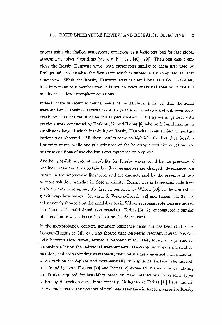
papers using the shallow atmosphere equations as a basic test bed for fast global
atmospheric solver algorithms (see, e.g. [9], [17], [40], [79]). Their test case 6 em-
ploys the Rossby-Haurwitz wave, with parameters similar to those first used by
Phillips [66], to initialise the flow state which is subsequently computed at later
time steps. While the Rossby-Haurwitz wave is useful here as a flow initialiser,
it is important to remember that it is not an exact analytical solution of the full
nonlinear shallow atmosphere equations.
Indeed, there is recent numerical evidence by Thuburn & Li [81] that the zonal
wavenumber 4 Rossby-Haurwitz wave is dynamically unstable and will eventually
break down as the result of an initial perturbation. This agrees in general with
previous work conducted by Hoskins [39] and Baines [6] who both found maximum
amplitudes beyond which instability of Rossby-Haurwitz waves subject to pertur-
bations was observed. All these results serve to highlight the fact that Rossby-
Haurwitz waves, while analytic solutions of the barotropic vorticity equation, are
not true solutions of the shallow water equations on a sphere.
Another possible source of instability for Rossby waves could be the presence of
nonlinear resonances, as certain key flow parameters are changed. Resonances are
known in the water-wave literature, and are characterised by the presence of two
or more solution branches in close proximity. Resonances in large-amplitude free-
surface waves were apparently first encountered by Wilton [88], in the context of
gravity-capillary waves. Schwartz & Vanden-Broeck [72] and Hogan [34, 35, 36]
subsequently showed that the small divisors in Wilton's resonant solutions are indeed
associated with multiple solution branches. Forbes [24, 25] encountered a similar
phenomenon in waves beneath a floating elastic ice sheet.
In the meteorological context, nonlinear resonance behaviour has been studied by
Longuet-Higgins & Gill [57], who showed that long-term resonant interactions can
exist between three waves, termed a resonant triad. They found an algebraic re-
lationship relating the individual wavenumbers, associated with each physical di-
mension, and corresponding wavespeeds; their results are concerned with planetary
waves both on the 0-plane and more generally on a spherical surface. The instabil-
ities found by both Hoskins [39] and Baines [6] extended this work by calculating
amplitudes required for instability based on triad interactions for specific types
of Rossby-Haurwitz waves. More recently, Callaghan & Forbes [11] have numeri-
cally demonstrated the presence of nonlinear resonance in forced progressive Rossby
1.1. BRIEF LITERATURE REVIEW AND RESEARCH OBJECTIVE 3
wave solutions of the shallow atmosphere equations, with different disjoint solution
branches existing at different values of the forcing amplitude. Thus, small pertur-
bations to a Rossby-Haurwitz wave which has been used to initialise a numerical
solution of the shallow atmosphere equations, could cause the wave to fluctuate be-
tween one solution branch and another in an unpredictable fashion, or break down
structurally altogether.
The main goal of this thesis is to extend the above literature by finding numeri-
cal solutions of the shallow water equations in the form of progressive Rossby waves
that propagate in time without change of shape. Additionally, we aim to explore the
relationship that exists between the nonlinear progressive wavespeed and wave am-
plitude. Two distinct models of the atmosphere are investigated; an incompressible
model is first considered and then, in the second half of the thesis, a compressible
model is analyzed. The approach is mainly through numerical methods so it must
be emphasized at the outset that the task of determining the nature of the exact
physical processes that produce some of the subsequently observed results is some-
what hard to discern; a separate analytical study, to which an entire thesis could
be devoted, would be needed in many instances. Our aim, therefore, is to uncover
key qualitative aspects of progressive Rossby wave solutions for the models under
examination.
In Chapter 2 we derive the incompressible shallow atmosphere equations for free-
surface fluid flow on a rotating sphere. After non-dimensionalizing, we construct a
linearization by first finding a base westerly zonal flow and then perturbing about
this state. Solutions are sought in the form of Fourier series with specific symmetry
conditions and a standard Galerkin method is used to integrate the linearized equa-
tions in closed form, leading to a generalised eigenvalue problem for the wavespeed
which is readily solved. Comparison is made to the equivalent Rossby-Haurwitz
solutions found in [32], with excellent agreement observed between the separate
theories.
In Chapter 3 we extend the linearized solutions computed in Chapter 2 to encom-
pass the full nonlinear equation set for the dynamical system. This allows for the
investigation of subtleties in the flow field, resulting from nonlinearity, which are
not possible to expose using linear theory alone. We again seek solutions in the
form of Fourier series, and a collocation method is used to solve for the unknown
Fourier coefficients and wavespeed. The solution is forced by parameterizing the

1.2. PRELIMINARIES 4
wave amplitude in terms of one of the unknown Fourier coefficients. A detailed pic-
ture is developed of how the progressive wavespeed depends on the wave amplitude,
revealing the presence of nonlinear resonances.
A compressible shallow atmosphere model is derived in Chapter 4. It is shown that
if the values of the pressure and density on the free-surface are assumed to be zero,
which is consistent with the concept of the atmosphere terminating there, then the
model almost reduces to the incompressible dynamics, with the only difference being
a slightly modified conservation of mass equation. Similar techniques to those used
in Chapter 2 are applied to the compressible equations, providing small amplitude >- linearized solutions of the model. CC
CC The solution of the full nonlinear dynamics of the compressible model is accom-
plished in Chapter 5. The linearized results of Chapter 4 are extended by comput-
ing nonlinear solutions via a bootstrapping process, providing detailed information
on how the nonlinear progressive wavespeed and amplitude are related. The effect
of compressibility is observed to manifest itself via damped resonance behaviour in
general. Cr)
A brief discussion in Chapter 6 concludes the thesis. In closing, some conjectures are CC u_i
made as to how the results obtained might help explain certain observed atmospheric
phenomena. In particular it is proposed that the process of atmospheric blocking is
a direct result of critically forced stationary Rossby waves. If this conjecture is true,
it would support the blocking theory of multiple equilibria that is popular amongst
many theoretical meteorologists. Lastly, a visualisation tool that was developed to
aid in interpreting the results, using the OpenGL three dimensional programming
interface, is briefly documented in Appendix C.
1.2 Preliminaries
In this section we introduce the coordinate frame and associated conservation equa-
tions to be used as the basis of the dynamics throughout the entirety of this thesis.
The derivation process is well represented and detailed in any one of a large number
of well respected texts on fluid dynamics (see, e.g. Batchelor [8] or Pedlosky [65]),
and as such will not be repeated in this work. However, the rotating spherical polar
coordinate reference frame system is less well known and requires a small amount
of development and clarification, which we present here.

1.2. PRELIMINARIES 5
We consider a spherical model Earth of radius a and rotating with constant angular
velocity Cl, enveloped by a model incompressible atmosphere, with a free-surface, of
depth h(A, 0, t). A spherical polar coordinate system (r, )., 0) is defined, in which
r measures the euclidean distance from the origin of the coordinate system and A is
the azimuthal (longitudinal) angle coordinate. An elevation (latitudinal) coordinate
0 is also defined as the angle above the equator, so that the North and South poles
are represented by 0 = 7/2 and 0 = — 7/2 respectively. This is not the standard
definition of polar angle 0 common in most instances (see, e.g. Kreyszig [44, pages
498-499]), although it is usual practice in meteorology (e.g. Dutton [21], Haltiner SL Williams [31], Holton [37]). A schematic diagram illustrating the coordinate system
and enveloping atmosphere is given in Figure 1.1.
Figure 1.1: Spherical coordinate system with free-surface.
The density and pressure in the atmosphere layer shown in Figure 1.1 are denoted
respectively as p and p, and g is the magnitude of the acceleration of gravity which is
directed radially inwards towards the centre of the sphere so that in vector notation
we have g = —g er . An atmospheric velocity vector q = are, + u),e ), + uck eo is introduced, with components Ur , u,„ uo in the coordinate directions given by unit vectors er , e), and eo.

1.2. PRELIMINARIES 6
In a reference frame rotating with angular velocity 11, conservation of mass for an
inviscid fluid is expressed through the continuity equation
Dp —Dt + PV = °
and conservation of momentum requires the usual Euler equation
Dq 1 —Dt + x q + -Vp = f, (1.2)
where f is the combined effect of all body forces per unit mass. The total (substan-
tial) derivative in (1.1) and (1.2) is defined as
D 0 Dt = at±q•v' (1.3)
and the gradient and divergence operators appearing in (1.1), (1.2) and (1.3) are
appropriately defined for the spherical polar coordinate system represented in Fig-
ure 1.1.
Conservation of energy, in the absence of viscous dissipation and thermal conduction,
is expressed through the first law of thermodynamics and is given mathematically
as DT pDp
Pcv Dt p Dt = Pqh. (1.4)
In (1.4), T is the temperature, ct, is the specific heat at constant volume, and qh is
the rate of heat addition per unit mass by internal heat sources. This study will
only be concerned with fluids that are either incompressible, so that the density p
is constant, or compressible and ideal, so that the ideal gas law of the form
p = pRT (1.5)
can be used to approximate the thermodynamic state relations. The symbol R in
(1.5) is the gas constant for dry air and will always take the value of
R = 287J kg' K'
in this work.
Because of the rotating reference frame and associated spherical coordinate system,
the component forms of (1.1), (1.2) and (1.4) are mathematically complicated and
need to be stated here for future reference. The complete set of governing equa-
tions in spherical component form is given by (see, e.g. Holton [37, pages 24-28],
Pedlosky [65, pages 314-317]),
1.2. PRELIMINARIES 7
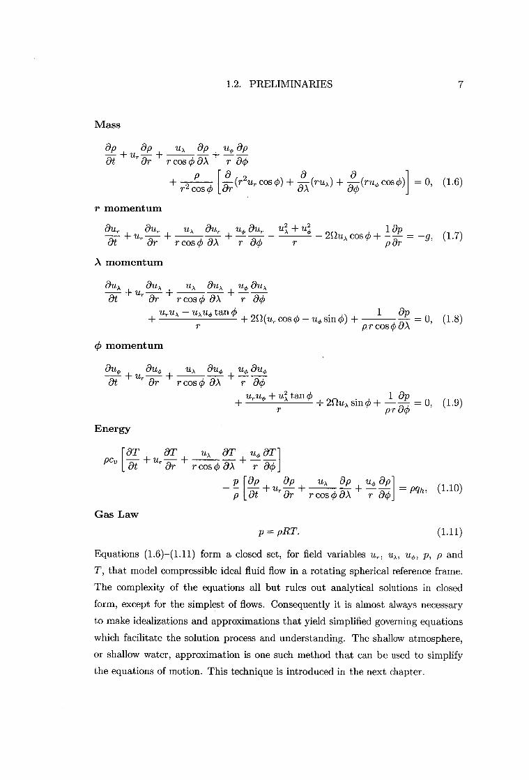
Mass
Op Op u,, Op nOp at Or ± r cos 0 aA ± r 00
a a P [ a (r2 u, cos 0) + — (ruA ) + — (ruo cos 0)] = 0, (1.6)
r2 cos 0 ar a), ao r momentum
aUr aUr U), aUr U4, aUr U 4- 2 U 1 Op 2
+ U r - + A CA 2/2ux cos 0 + = -g, (1.7) at Or r cos 0 OA r 00 p Or
A momentum
au„ au„ u, au, Ito au„ + U r Ot Or r cos 0 OA r ao
uru, — u„u, tan 0 1 Op + + 212 (u,. cos 4) no sin 0) + = 0, (1.8) r pr cos 0 aA 4) momentum
auo u„ + auo au4, + ur— at Or r cos 0 OA r 00 uruo + u2, tan 0 1 al, + 21-2uA sin 0 + —pr —a0
= 0, (1.9)
Energy
Pcv [— OT
Gas Law
OT u, OT u 4, aT1 Or r cos 0 a), r ao]
p [Op Op uA Op - - — + u — + p at r Or r cos 0 OA + —r —00 1 = Pqh, ( 1 . 10 )
p = pRT. (1.11)
Equations (1.6)-(1.11) form a closed set, for field variables Ur, u A , p, p and T, that model compressible ideal fluid flow in a rotating spherical reference frame. The complexity of the equations all but rules out analytical solutions in closed form, except for the simplest of flows. Consequently it is almost always necessary to make idealizations and approximations that yield simplified governing equations which facilitate the solution process and understanding. The shallow atmosphere, or shallow water, approximation is one such method that can be used to simplify the equations of motion. This technique is introduced in the next chapter.

CHAPTER 2
INCOMPRESSIBLE LINEARIZED SHALLOW ATMOSPHERE MODEL
2.1 Derivation
We consider here the basic derivation of the incompressible shallow atmosphere
equations following the general approach developed in Pedlosky[65, pages 57-63].
However, as opposed to the rotating cartesian form derived in [65],we initially start
in a rotating spherical coordinate system, thus allowing for the curved geometry of
the spherical Earth to be appropriately incorporated into the resulting equation set.
Figure 2.1: Free-surface height parameters
Commencing the derivation we define ft as the height of a free-surface surrounding
a rotating reference sphere of radius r = a as depicted in Figure 2.1. We measure ii,
8

2.1. DERIVATION 9
as the radial distance from the level surface r = a of the spherical coordinate system
to the free-surface. Additionally, define h and hb as the depth of the fluid and the
height of the underlying mountains respectively. The height of the free-surface h can be given in terms of the two parameters h and hb as
h=hb+h. (2.1)
Although the generality of this setup affords the representation of a much wider
class of problem we will restrict ourselves to the case when there is no underlying
mountain specification so that hb = 0, leading to
h = h. (2.2)
Because we are only concerned with incompressible flow in Chapters 2 and 3, the
equations of motion presented in Chapter 1 will reduce significantly. In particular,
since density p is constant the mass equation, (1.1), reduces to the form V • q = 0.
In addition, we can discard all thermodynamic behaviour, allowing us to remove the
energy and ideal gas_equations from the governing system. We also note that, due
to the nature of the spherical coordinate system, the vertical coordinate r appears
explicitly in the dynamical equations. Holton • [37, page 24] points out that these
curvature terms can be adequately approximated by r = a since the depth of the
atmosphere h is assumed to be much smaller than the radius of the earth. Adopting
the above approximations and simplifications we obtain the following form for the
incompressible dynamical equations.
Mass au, au, a
a cos 0-79-7--. + + (uo cos 0) = 0, (2.3)
r momentum
au, Our u, au, u,,, Our tt2A + 1 ap + u — + 2ou„ cos 0 + —p —ar = —g, (2.4) at r Or a cos cb a A a ao a
A momentum
au„ au, u„ au„ uo au, + + r uru, — uxuo tan 0
u — at Or a cos 0 OA a a0 a
1 Op 2S-2(ur cos cb — uo sin 0) +
ap cos a A = 0, (2.5)
2.1. DERIVATION 10
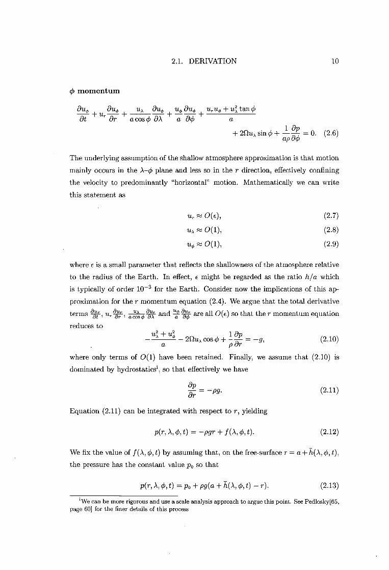
(/) momentum
Ouct, auo uA auo no Ono uruo + u2), tan 0 + ur — +
at ar a cos 0 aA a 00 a
+ 2QuA sin 0 + —1 p 0. (2.6) ap 00
The underlying assumption of the shallow atmosphere approximation is that motion mainly occurs in the A-0 plane and less so in the r direction, effectively confining the velocity to predominantly "horizontal" motion. Mathematically we can write this statement as
Ur
ux
0(c),
0(1),
(2.7)
(2.8)
0(1), (2.9)
where E is a small parameter that reflects the shallowness of the atmosphere relative to the radius of the Earth. In effect, E might be regarded as the ratio h I a which is typically of order 10 -3 for the Earth. Consider now the implications of this ap-proximation for the r momentum equation (2.4). We argue that the total derivative ternasu a aur and —aur are all 0(c) so that the r momentum equation at , r acosck aA a ao reduces to
U2 ± u2 ap (2.10) A a
ck 25-2uA cos 0 + -- p —ar = -g,
where only terms of 0(1) have been retained. Finally, we assume that (2.10) is dominated by hydrostatics', so that effectively we have
ap = -pg .
(2.11)
Equation (2.11) can be integrated with respect to r, yielding
p(r, A, 0, t) = - pgr + f (A, , t). (2.12)
We fix the value of f (A, 0, t) by assuming that, on the free-surface r = a + h(A, 0, t), the pressure has the constant value P o so that
P(r, A, 0, t) = Po pg(a + h(A, , t) - r). (2.13)
'We can be more rigorous and use a scale analysis approach to argue this point. See Pedlosky[65, page 60] for the finer details of this process

2.1. DERIVATION 11
From (2.13) we immediately obtain
OpOh _ OA – Pg OA' Op ah _
— Pg-a--;
(2.14)
(2.15)
implying that the horizontal pressure gradient components are independent of r,
which in turn implies that the horizontal accelerations must be r-independent also.
It is therefore consistent (see Pedlosky [65, page 61]) to assume that the horizontal
velocity components are also r-independent if they are initially so. Thus we must
have
(2.16)
(2.17)
so that, in conjunction with (2.7), the two remaining momentum equations, (2.5)
and (2.6), taken to 0(1) become
A momentum
au x ux aux uo aux uA uo tan 0 g Oh + 2/2/41, sin 0 + = 0, (2.18) at + a cos ch DA a 00 a ap cos 0 OA
(/) momentum
au cto uA aug, uo auo u2„, tan 0 g Oh 0t + a cos 0 aA + a 00 + a
+ 2QuA sin 0 + —ap —00 = O. (2.19)
We now turn our attention to the mass equation and note that since u A and u 4, are
r-independent we can integrate (2.3) with respect to r to give
Ou A a a cos 0 ur (r, A, 0, t) = –r [–a-5-k- + (no cos 0)] + it, (A, 0, t). (2.20)
To determine the nature of ft, we need to examine the boundary conditions on the
upper and lower boundaries r = a + h and r = a + hb respectively. On the lower
boundary we must have no normal flow, otherwise the fluid would penetrate the
surface and breach the conservation of mass requirement. Thus on r = a + hb we
must enforce the condition q • n = 0 where n is a normal to the surface r = a + hb. We can easily show that the normal to the lower boundary is given by
1 ahb 1 ahb n = er a cos
4,eA –
0 aA a Do (2.21)
2.1. DERIVATION 12
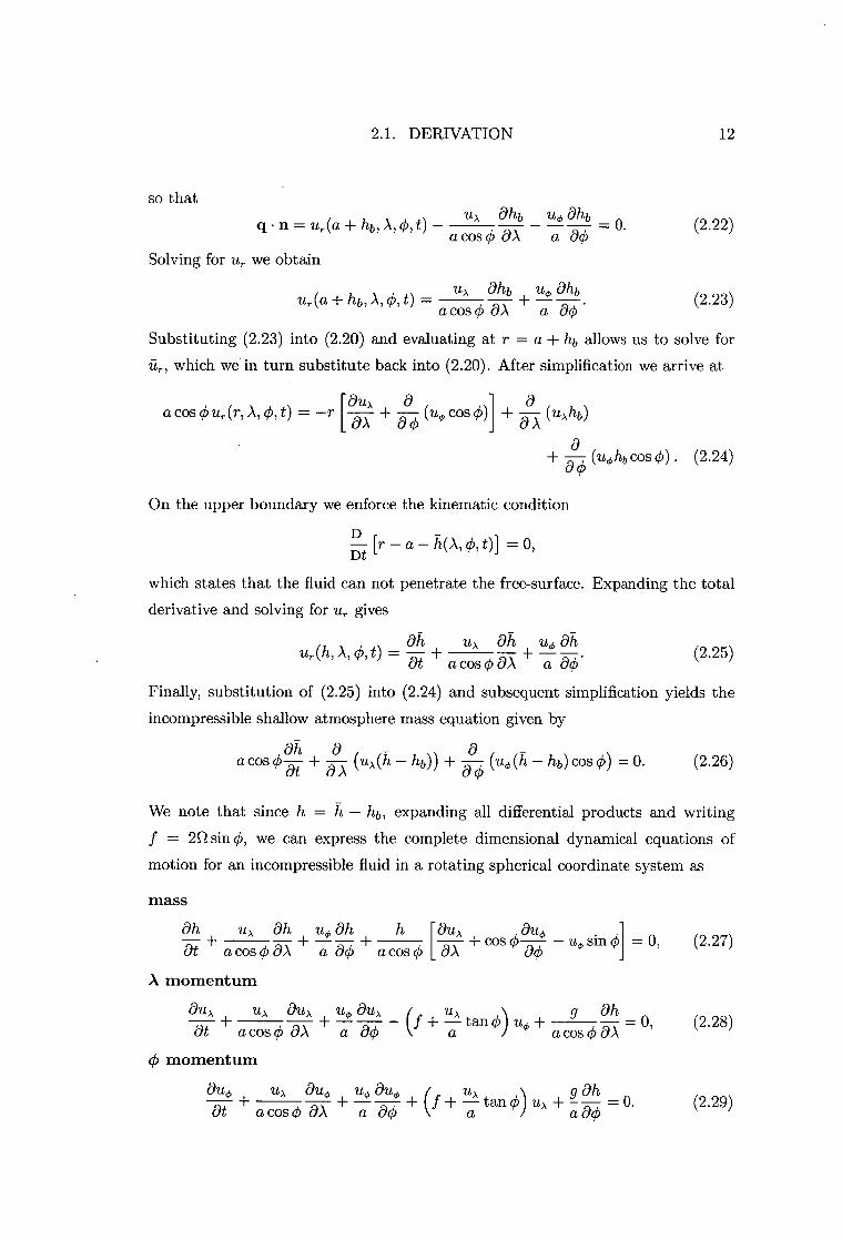
so that
q • n = ur (a hb, A, 0, t)
Solving for 'Ur we obtain
UA ahb uhb 0 a cos 0 aA a 80 —
(2.22)
u), ahb u4, ahb
ur (a + hb, A, 0, t) = •
(2.23) a cos 0 DA a± —
a0
Substituting (2.23) into (2.20) and evaluating at r = a ± lib allows us to solve for
fir , which we in turn substitute back into (2.20). After simplification we arrive at
au„ , , a
a cos 0 ur (r, A, 0, t) = -r [79-A- 014, cos 0)1 (uxhb)
a + — (uo hb cos 0) . (2.24) a
On the upper boundary we enforce the kinematic condition
Dt [r - a - h(A ' t)] =
which states that the fluid can not penetrate the free-surface. Expanding the total
derivative and solving for it,. gives
ur(h, 0,t) = —ah u, ah ucs ah
(2.25) at + a cos aA 4- a ao . Finally, substitution of (2.25) into (2.24) and subsequent simplification yields the
incompressible shallow atmosphere mass equation given by
ah a acos +
_ ,u,(h — hb)) + —a—a (uo(h- — hb) cos 0) = 0. 0 at a A
(2.26)
We note that since h = Ii - hb, expanding all differential products and writing
f = 2l sin 0, we can express the complete dimensional dynamical equations of
motion for an incompressible fluid in a rotating spherical coordinate system as
mass
ah ah Ito a h h a
[„u ), auo + a cos ± ± a cos + cos 0 - uo sin 01 = 0, (2.27) at 0 aA a 00 0 DA ao
A momentum
au„ uA auA u4, (9u), g ah = 0, (2.28) at + a cos °A a ao a a cos 0 aA
momentum
au,, UA aU4, auo g ah 0. (2.29) (k (f + tan 0) u + at + a cos 0 aA a Do
2.2. PROGRESSIVE-WAVE COORDINATE TRANSFORM 13
The above form is that given by Williamson et al.[87, page 213] as the advective
form of the shallow atmosphere equations and this is the form we shall subsequently
use for all analysis in this chapter.
2.2 Progressive-Wave Coordinate Transform
We are interested in solutions to equations (2.27), (2.28) and (2.29) that are of
the form of a progressive-wave with constant angular velocity. Defining c to be an
angular wavespeed we now construct a new moving coordinate frame that depends
on A and t in the form
n = A – ct. (2.30)
The effect of the –ct term is to translate any initial wave structure either towards
the west (c < 0) or towards the east (c > 0) with constant angular speed c. Since
we have defined a new coordinate system we need to establish how the equations of
motion are represented in this new reference frame. Applying the chain rule we can
easily show that, for some scalar field tIf (77 ,0), ow — ow
--= , A 0,\. a n (2.31)
ow &Ta n ow
= -- = –c . (2.32) at ail at ar, Using this transformation we can now write equations (2.27), (2.28) and (2.29) as
mass
(u, Oh u cos an 0 — – c cos ck)
4, h [a
11,, Ouo + – — + cos 0 – uo sin a a a
d = 0, an ao n ao A momentum
(2.33)
(
u), , au, u4, cos 0 au, (f cos 0 + sin 0) uo –g —Oh = 0, (2.34) — – c cos a a ao a an (j) momentum
(
u, auo uo cos 0 + (f cos 0 + ui sin 0) uA g cos q5 an — — ccos o = 0, (2.35) a a ao a a Do where we have multiplied each equation by cos q to remove apparent polar sin-
gularities that would otherwise adversely affect numerical computations, and we
have also retained the name "A momentum" to remind us of the fact that equation
(2.34) is essentially still the A component of conservation of momentum despite the
transformation to ?].
2.3. NON-DIMENSIONALIZATION OF THE GOVERNING EQUATIONS 14
2.3 Non-dimensionalization of the Governing Equations
In an attempt to generalise the analysis, it is desirable to express the governing
partial differential equations in a form that is independent of the specific units used
to measure the variables of the problem. For this reason we non-dimensionalize
each of the governing equations to expose the underlying qualitative behaviour.
The particular approach adopted here is similar to that used by Klein [42, page 766]
in that we reduce our dimensionless parameters to the set of familiar fluid dynamical
parameters comprised of Strouhal number, Froude number and Rossby number.
First we define the following characteristic values, for each reference scale contained in the problem, as
v„f characteristic speed,
href characteristic free-surface height,
c„f characteristic angular velocity.
Using these dimensional parameters we now rescale all the field variables to dimen-sionless form giving
fLA = - =
VUrief UA 7-4°114' Ito
114, = UA = Vreffickl
v rrr cee f = h h = hrefirt, h f
C ef
(2.36)
(2.37)
(2.38)
(2.39)
where the hat 0 denotes a dimensionless variable. Substituting equations (2.36)– (2.39) into (2.33), (2.34), (2.35) and manipulating, we obtain
mass
c„ f a all ail a ito u 0 — +no cos 0— +h — + cos 0 — /14, sin c cos 0 = 0, (2.40) vref jar1 ao A momentum
(fi x cref a , 0 , ft ), c cos op) — + u4, cos 0 ( 2C2a — cos 0 + fix) 'ri ck sin vref 0 77 0 0 vref ghref h
+2 0, (2.41) vref

2.4. LINEARIZATION OF THE EQUATIONS 15
4) momentum
Crof a C cos 0) a u a uo 2S2a
— + ito cos (P + — cos 0 + ft sin o an a (15 //ref
o
ghrof cos 0 a h v,?„ a o
= 0 ' (2.42)
where we have also replaced the Coriolis parameter f by its definition f = 21/ sin 0.
Three obvious dimensionless parameter groupings emerge from this process. These are just the familiar flow regime parameters from fluid dynamics given as
a Crcf Sr = Strouhal number, vref Vrcf Fr = Froude number,
VF1-t7c; vref
Ro = Rossby number. 2S.2a
Substitution of these parameters into our governing equations yields
mass
[a ?IA (fix — Sr c cos) — + u 0 o cos 0— + h + cos cb a 114) - ^ • an a o -a-71 a uo sm =0, (2.43)
A momentum
aUA , aux cos cb 1 alt (uA - Sr a cos 0) a + " ct, cos o — p - an ao (—R7-3. -"A ) 1166 sin ck 0, (2.44)
4, momentum
au au (uA - Sr cos 0) + cos + (cos 0
+) it, sin , cos 0 =
0, (2.45) ao Ro su "1- Fr2
which is the final form for the non-dimensional incompressible shallow atmosphere equations on a rotating sphere.
2.4 Linearization of the Equations
2.4.1 Base Zonal Flow Derivation
As previously discussed in Chapter 1 it is convenient to consider Rossby waves as
consisting of latitudinal perturbations about an underlying zonal flow structure.
Thus it is important to know the exact nature of the zonal flow in order to calculate
(14 Vref
2.4. LINEARIZATION OF THE EQUATIONS 16
the resulting perturbations. Following the work of Haurwitz[32, page 255] we choose
the simplest zonal flow in the form of a super rotation that only depends on latitude
and additionally has u 4, = O. The form for our zonal flow is then given by
zt,„ = w cos 0, (2.46)
uo, = 0, (2.47)
hz = (2.48)
where the parameter w is the non-dimensional representation of the base angular
speed of the flow and the subscript z is used to denote field variables belonging to
the zonal flow structure. The problem now reduces to finding the function H(0) that makes equations (2.46), (2.47) and (2.48) a solution of equations (2.43), (2.44)
and (2.45).
Direct substitution reveals that the only equation not identically satisfied by the
zonal flow structure is the 0 momentum equation, which yields the ordinary differ-
ential equation
dH = —wFr 2 ( -
1 + CV ) sin 0 c os 0. d0 Ro
This integrates easily to give
wFr2 1 H(0) = ho +
2(
Ro + w) cos2 0.
(2.49)
(2.50)
The constant of integration h, can be viewed as the base non-dimensional height
of the free-surface at the poles and typically we would choose h, = 1 so that the dimensional value of hz at 0 = +7/2 is href . The two parameters w and h, suffice
to specify uniquely any given super rotation and associated total mass, or volume
in the incompressible case, of the system. We note here that in order to make
comparison between results with differing values of w it is necessary to modify the
value of h, so that the total volume of fluid in a + hb <r <a + h remains constant. This amounts to solving a cubic equation for 110 once a fixed volume and value for w have been decided upon.
ii Although all variables are dimensionless, from now on, for the sake of brevity, we drop the hat 0 notation and all variables will be assumed dimensionless unless otherwise stated.
2.4. LINEARIZATION OF THE EQUATIONS 17
In summary, we have shown that a basic zonal flow structure is given by
ILA z = (i) cos 0,
uoz = 0, wFr2
hz = +
(2.51)
(2.52)
(2.53) 2 Ro
2.4.2 Linearization about the Base Zonal Flow
Given the base zonal flow we now consider 0(c) perturbations about this flow state
by constructing the perturbation expansions
ux (k) = nAz+ EU„ (71, 0) 4- 0(E2 ), (2.54)
U0(7/7 q5) = 0 + EUoi (71, + O(e2),
h(n, 0) = hz + Eh i (n,q5) + 0(c2 ).
(2.55)
(2.56)
The perturbation parameter E is a small quantity that represents the maximum
deviation about the zonal flow. It is instructive to think of c as a wave amplitude
in this case, although it must be emphasized that the linearization is only valid
for infinitely small amplitude and consequently our results will only be accurate as
—> 0. Nonetheless we can expect reasonable results for small values of E.
Substituting the perturbation expansions (2.54)-(2.56) into the governing equations
(2.43)-(2.45) leads to the set of partial differential equations given by
mass
Oh l (uAz - Sr c cos 0) + euoi co
d as:I
d hz
au / Ehz + COS Ic9 Uoi sin d + 0(e2 ) = 0, (2.57)
A momentum
, d uAz (
cos cb
E (11 A z — Sr C COS lp ) — ElLoi COS 19 E —d
IL A z ) Uoi Sill (1) ari ick Ro
1 ail,
+ (2.58)
cP momentum
( cos 0 cos 0 d hz alto + uAz u A z sin 0 + ,, + E (2/Az — Sr c cos 0) Ro Frz d 0 Dr)
(cos cos 0 oh, +c
cb + 220, z ) um sin 0 + 2 + 0(62 ) = 0. (2.59)
Ro R. ao
2.4. LINEARIZATION OF THE EQUATIONS 18
The 0(1) terms in (2.59) are satisfied identically by the base zonal flow. By putting
uAz = w cos 0 into the above equations we obtain the 0(€) equations that define the
first level of corrections in our perturbation expansions. These equations are
mass
ah i d h z [au m ttoi a (w - Sr c) cos— 0 + uo , cos ¢, + h — + cos 0 uo , sin 0] = 0, (2.60) an d 0 an 00 A momentum
aum Go — Sr c) cos0— (FL + 2w) uo , sin 0 cos 0 + — 1 ah, = ,,
an Fr2 an u, (2.61)
ck momentum
cos 0 ah, _„ (co — Sr c) cos o'L.--La + +2w) ux , sin 0 cos 0 + an (ITO F 2 ack — u. (2.62)
The solution of (2.60), (2.61) and (2.62) is facilitated by noting that we may write
each of the 0(c) perturbation terms as the product of a Fourier mode in n with a
function of 0. Thus we define
741 (i7 , 0) = cos(nn) A(0), (2.63)
u(n, 0) = sin(kn) st, (q5), (2.64)
= cos(kn) H(0), (2.65)
where the parity of the Fourier basis in ri in each term is chosen to preserve the
overall parity of each dynamical equation. Alternatively, it would be possible to
interchange the sin and cos terms in (2.63)-(2.65), with the effect of rotating the
solution at t= 0 by 71K. Also note that the parameter n has been introduced as a
way of specifying the wavenumber of the solution. This is a natural addition to the
model since intuitively we would expect that the wavespeed c will depend on the
number of equally spaced wavelengths around a latitude circle.
By defining our 0(c) terms according to (2.63)-(2.65) we can remove the n depen-
dence entirely from the partial differential equations, transforming them into a set
of ordinary differential and algebraic equations given by
mass
d h z k (w - Sr c) cos 0 H(0) + (I)(0) cos 0 d 0
d(0) + hz [-kA(0) + cos 0
413 (1. d (0) sin 01 = 0, (2.66) 0
2.5. NUMERICAL SOLUTION OF THE LINEARIZED EQUATIONS 19
A momentum
1 —tc (w — Sr c) cos0 A(0) — (—Ro
+ 2w) (I)(0) sin 0 cos 0 — = 0, (2.67) Fr2
0 momentum
1 ((V - Sr c) 4)(0) + (11 ±
2w) A(°) sin (k Fr2 d 1 d )
= °. (2.68)
2.5 Numerical Solution of the Linearized Equations
2.5.1 Series Representation
The numerical solution of (2.66), (2.67) and (2.68) can be accomplished by approx-
imating each of A(0), (DM and 7-00) with truncated series of basis functions. As
noted by Boyd[10, page 109], the particular choice of basis function is primarily
governed by the geometry involved in the problem. The inherent spherical geome-
try in the shallow atmosphere problem can be adequately described by using either
spherical harmonics or Fourier basis functions, which both cope well with periodic
boundary conditions. Although the generally accepted solution approach for prob-
lems in spherical geometry, in both meteorological and mathematical circles, is via
the spherical harmonics, the sheer simplicity and ease of use of Fourier series is an
attractive alternative that, as will be demonstrated shortly, allows for some further
analytical manipulation to be carried out, greatly reducing the computational time
for any given solution.
The particular form of the Fourier basis components needs careful consideration,
primarily because we can identify key symmetry and boundary conditions that each
of the field variables must satisfy. In this study we are only concerned with special
types of solutions that obey the following set of conditions:
• u ), and h are symmetric with respect to the equator (0 = 0),
• uo is anti-symmetric with respect to the equator,
• u ), and u,,, are zero at the poles (0 = ±7/2),
• h is constant at the poles.
From an analysis of the problem we can show that A(0) and 7-1(0) must be symmetric
with respect to the equator whilst 43(0) must be antisymmetric. This basically says
2.5. NUMERICAL SOLUTION OF THE LINEARIZED EQUATIONS 20
that a northward velocity deflection in the northern hemisphere is equivalent to a
southward velocity deflection in the southern hemisphere, whereas the free-surface
has the same height at points (no, ±00). From the above list of solution requirements
we can also deduce that the 0(i) field variables must all have zero value at the poles.
This is necessary because we have convergence of lines of longitude at 0 = ±7/2
and hence to avoid multi-valued functions for the field variables we require that the
perturbations are all zero at the polesiii .
Although the above list of solution requirements might seem, at first glance, to
be rather restrictive there is much to be gained by employing such an approach.
The main advantage of this formulation is that difficulties at the poles are avoided;
this can be a common source of numerical trouble in models that account for the
spherical geometry. The pole problem amounts to the previously mentioned dilemma
of having multi-valued functions defining the flow field and the apparent switching
of East to West (or North to South) as one traverses across a pole of the spherical
coordinate system. A common approach to navigate this troublesome numerical
stumbling block is to introduce new velocity components that are multiplied by
Fourier functions that correctly adjust for the parity change on either side of the
pole as detailed in Duran[20, page 207]. In our approach no such adjustments are
required since by forcing the flow to have stagnation points at each pole we will
never encounter a scenario in which flow with an eastward or northward component
suddenly switches to flow having a westward or southward component. Of course,
in all realistic global circulation models the handling of the pole problem becomes
an integral feature of any time integrating computation since in general stagnation
points are not situated at both poles. Nonetheless, the advantages to be had by
adopting our approach coupled with the motive of theoretical investigation justify
its use.
We are now in a position to construct the series approximations. For now we just
state the forms for the 0(i) linear terms, defering the statement of the series for
the full nonlinear terms until Chapter 3 when we approach the solution of the full
nonlinear system. The functions that meet our prescribed conditions above can be
mm general 7-40) need only be constant at the poles; however the allowed values for the parameter n effectively force 7-1 (±i) = 0.

2.5. NUMERICAL SOLUTION OF THE LINEARIZED EQUATIONS 21
given by
A(o) =>2 Pk ,fl cos((2n— 1)0), (2.69) n=i co
co) E Q sin(2n0), (2.70) n=i
co 7-00) E H,,,n (-1)n [cos(2n0) + cos(2(n — 1)0)] , (2.71)
n=1
where subscript n on each coefficient denotes the longitudinal wave number that we
are currently using as defined in equations (2.63)—(2.65).
It is also essential to point out that the particular form of (2.71) is due to the process
of basis recombination in which we have constructed new basis functions, which are
linear combinations of our underlying basis set, that satisfy the required boundary
conditions, as discussed in detail in Boyd[10, page 112]. Basis recombination is
needed here since the general representation of h(n, 0) need only be constant at the
poles, rather than zero as in the case of the two velocity components u,, and uo .
Thus the underlying basis set is centered around cos(2n0) which attains the value of
±1 at the poles. Since we require 7-1(0) to be zero at ±r/2 then it becomes the task
of basis recombination to satisfy this boundary condition; this is achieved through
the particular form of (2.71).
2.5.2 Galerkin Method
With the forms for each of our series defined we now tackle the problem of solving
for the wavespeed c and associated coefficients P - km , Q and 11,,n . To do this we
exploit the orthogonality properties of the trigonometric functions by requiring that
the residual equations, obtained after substituting (2.69)—(2.71) into (2.66)—(2.68),
be orthogonal to each of our expansion functions. This technique amounts to the
standard Galerkin method which has been used extensively to solve optimization
and root finding problems from all areas of mathematics. We now demonstrate the
particular application to our problem.
Substitution of (2.69)—(2.71) into (2.66) yields the algebraic version of the linearized

2.5. NUMERICAL SOLUTION OF THE LINEARIZED EQUATIONS 22
mass equation given by
–tc(co – Sr c) H,,n ( –1)n [cos(2m) cos ç5 + cos (2(n – 1)0) cos 0] n=1
oo
— WFT*2 (—Ro
+ co) E sin(2n) cos 2 0 sin 0 n=1
oo coFr2 ( 1 ± + 2 Ro
+ co) cos20) [–k E Pis,n COS((2n 1)0) n=1
0. 00 + E c2„,n2n cos (27/0) cos – E Q ,,n sin(2n0) sin 01 = 0. (2.72)
n=1 n=1
We can show that general terms of (2.72) take the form cos((21 – 1)0), for /
I, 2, ..., so these become our base expansion functions and the orthogonality con-
dition is now equivalent to multiplying (2.72) by cos((21 – 1)0), integrating from
–7r/2 < < 7r/2 and equating to zero. Performing these operations we have 00
–n(co – Sr c) E I 72' cos(2n0) cos 0 cos ((2/ – 1)0) c/0 n=1
oo
IC(W — Sr.c) E cos(2(n – 1)0) cos 0 cos ((2/ – 1)0) d0 n=1
– coFr2 + co) °E) Q,,,n sin(2n0) cos2 0 sin 0 cos ((2/ – 1)0) c/0 Ro n=1
_ hokE PK,n cos ((2n – 1)0) cos ((2/ – 1)) c/0 n=1 oo
\ 2 + 2h0 ,,n cos(2n0) cos 0 cos ((2/ – 1)0) d0
n=1 0 0
— ho Q,,nI
sin(2n0) sin 0 cos ((2/ – 1)0) c/0 n=1
ru,,Fr2 0. 2 Ro
+ w) E P,,,n I
cos ((2n – 1)0) cos2 0 coS ((2/ – 1)0) c/0 n=1
oo
+ wFr2 (-1
+ co) E nQ ,c , n cos(2n0) cos30 cos ((2/ – 1)0) d0 Ro
n=1
WFr2 2 Ro
W) Q n sin(2n0) sin 0 cos 20 cos ( (2/ – 1)) d = 0. n=1 2
(2.73)
All of the integrals in (2.73) can be rewritten by using trigonometric identities to
express the integrands in terms of products of two of the base expansion functions.

2.5. NUMERICAL SOLUTION OF THE LINEARIZED EQUATIONS 23
As an example, we consider the first integral in (2.73) and note that the integrand
may be written, with the aid of the identity cos(A -B)+cos(A+B) = 2 cos A cos B , as
1 cos(2n0) cos 0 cos ((2/ - 1)0) = [cos ((2n + 1)0) + cos ( (2n - 1)0)] cos ((2/ - 1)0)
1 cos((2n + 1)0) cos((21 - 1)0)
1 + -2
cos((2n - 1)0) cos((21 - 1)0). (2.74)
In addition we then, if required, shift the index on the resulting integrands so that
every integral in equation (2.73) is transformed to one of the form
/0 = f cos((2n - 1)0) cos((21 - 1)0) do, (2.75)
2 if n = /, (n 0 and / = 1) or (n = 1 and / = 0), (2.76)
0 otherwise,
where the o subscript denotes an integral obtained by using orthogonality.
Applying trigonometric identities, similar to that used in (2.74), to all the integrals
in (2.73) and then shifting the indices on those terms that require it we obtain
00 00
-(w - Sr c) E H,,,o+ ,(-1)n+1/0 — K(u) - Sr c) n=0 n=1
co wFr2 w\ — — (CV — Sr C) Elkn—i(-1)n-1/0
+
8 Ro ) 2 n=2
[ co E QK
' n-1-1-ro
n=0
+ E Q K,nio — E Q k,n—lio — E Q ic,n—go I — hoiC E Pn,nio n=1 n=2 n=3 j n=1
co oo , ho co , ho °° + ho E nqc,../-0 + ho E (n - ini,n—lio — tc,nlo + —2 E QK,n—l-to
n=1 n=2 n=1 n=2 oo kwFr2 /1 \ oo co
8 ii- ; + w) [E PK,n+lio + 2 Ptc,n-ro + E Ptc,n-14 n=0 n=1 n=2
coR2 1
oo oo oo oo 16 ( Ro +w E Qro + E Q tc,n.ro — E Q K,n—lIo — E C2k,n-2 10 )
n=L o n=1 n=2 n=3
wFr2 ( 1 w 00 00 + 8
+ ) [E(n + 1)(2K,n+11-0 + 3 E nQ/o Ro n=0 n=1
+ 3(n - 1 )qc,n-1-ro + (n - 2)Qn,n-2/0] = 0. n=2 n=3
(2.77) 00 00
± [110 [ 2 3K,Lo
3/cwFr 2 1 Kx.Rr 2 1 PK,/ + w)] 8 8 ( Ro
wFr2 ( 1 wR2 ( Ro
1
icSr --H
k ,2
+ 8 3,c) w)]
n ,
1 — (±) Hk 2 = C
± 16 3/cSr rj. [ — -- rc 2 Jan 1 -
w) Pit ' 2
1 (2.78)
2.5. NUMERICAL SOLUTION OF THE LINEARIZED EQUATIONS 24
Each integral lo in (2.77) is now in the standard form given by (2.75) allowing
us to use the orthogonality conditions given in (2.76) to extract a set of algebraic
equations for each value of the integer 1. Letting 1 = 1 and performing some algebraic
manipulations we arrive at
where we have taken the terms involving the wavespeed c to the right hand side in
preparation for the numerical solution method, to be discussed shortly. We also note
that letting 1 = 1 is equivalent to letting 1 = 0 since the nature of the orthogonality
of cos ((2n - 1)0) cos ((2/ - 1)0) is the same in both cases.
In a similar vein we now consider the case when 1 = 2, leading to
ts,wFr 2 /1 pk,1 + w) + [
+
rcwFr2 ( 1 Kho + w)] pk,2 )
co)] Qfro
+ w) Qtz 7 3
8 Ro ) ni.,;Fr2 ( 1
Pk
4 Ro 3h 9wFr2 (± [ 2 ° +
16 Ro +
±
8 Ro + w)
'3
[3h0 9wFr2 1 3wFr 2 1 [ 2 ± 16
( Ro + w)] Qk 7 2 + 16 Ro
(
tiw_ H k 2 ± _KA.4.) ri ...... _ [nSr , K2Sr +
lik,3] 2 k1
+ KwH ' 7 2 rik7 3 - (-; 2 llto - icSrlik,2 + — (2.79)
Finally, the cases for 1 > 3 are given by
IctoFr 2 ( 1 + w) ,.,,, [ , nu.;Fr2 ( 1 + )1 T., 8 Ro
r ,i_i + Kilo 4 Ro w r-K 7 1
nc.oFr2 ( 1 8 Ro Lo) PK 7/-Fi + w(21 -
1)Fr2 ( + w
1 +
16 —Ro ) Q tc,1-2
+ [(21 — 1)110 ± 3(21 - 1)wFr2 ( 1
2 16 Ro + w)] Qn 7/-1
[ (21 -2 1)1/0 + 3(21 - 1)wFr2 ( 1 + w)] c20 16 Ro )
w(21 - 1)Fr2 ( 1 16 Ro + co) Qi
+ nti.,(-1)/ + ica-p 2
H,,, i _ i -
nSr(-1) / icSr(-1)/ +
2 H„,1±1 = c [
2 H, ,1 1 IcSr (- 1) 1 Ho 2 + H tc,i+i]
(2.80)
2.5. NUMERICAL SOLUTION OF THE LINEARIZED EQUATIONS 25
Equations (2.78), (2.79) and (2.80) constitute an infinite set of algebraic relation-
ships representing mass conservation that must be satisfied for a solution to be valid.
In a similar manner we can derive equivalent algebraic relationships from both the
A and 0 momentum equations, (2.67) and (2.68), by substituting our series expres-
sions for the OW field variables and using orthogonality to generate the required
equations.
From the A momentum equation we have: For 1 = 0,
„ 1 —
( 1 r icSr
— I-pc 4.0) ts, - - 1 C[- 2 ' 1 — Q1 - 4 Ro Fr2 '
for 1 =1,
(2.81)
tc,CO IcCIJ 1 ( 1 ic 7. T - r-tc 1 w Q tc tc,2 — 2 ' 2 4 Ro Fr
= c [
icSr nSr - PK - Pic 2 (2.82)
2 2'
and for 1> 2,
tet,W K,CV 1 (1 (1 1 -
- -
2Pk,/ - —2 Ptc
'1+1 + -
4
—Ro +w - -4 —Ro + w Qn,c+i
k(-1)/ 7., n(-1) 1 , icSr nSr K,
H r2 1+1 = —2 1- ic
'I
2rtcp-i] Fr2 F
Similarly from the 0 momentum equation we have, for 1> 1,
1 ( 1 u) .13K 1 ( 1 ±
2 1,o ) ' 1 2 Uto w ichoWtc,1 21(-
Fr2 tc,
1)1+1 ± H
24-1) 1 + 1 2 HK,1+1 = C EKSrQn,/1 • Fr
(2.83)
(2.84)
2.5.3 Truncation and Generalised Eigenvalue Formulation
The set of algebraic equations (2.78)-(2.84) represent an infinite linear system in
the form of a generalised eigenvalue problem. In order to perform any numerical
work it is essential to truncate this system to some finite size. Let N E N define an
integer truncation level so that our infinite series (2.69)-(2.71) are now truncated
to sums over the finite domain 1 < n < N for n E N. Since we have three field
variables to solve for we will have a total of 3N unknown coefficients, requiring 3N
equations to close the system.

+ W) Pic,N-1 + [_ h0
-1- w(2N - 1)Fr2 ( 1 16 Ro + w) Qn,N-2
hu.oFr 2 ( 1 8 kRo
Fr2 1 (
2.5. NUMERICAL SOLUTION OF THE LINEARIZED EQUATIONS 26
Our choice of equations from the set (2.78)-(2.84) is rather intuitive and obvious in
that we use exactly N equations from each physical law. To elucidate this process
we note that the orthogonalised version of the mass equation consists of two base
equations, (2.78) and (2.79), and an infinite series of equations in the form of a
recurrence relation (2.80). To obtain exactly N equations from this set we retain
the first two equations along with N-2 from the recurrence relation so that the limit
on 1 in (2.80) is now 1 = 3, 4, 5, ... , N. Note that when 1 = N we make reference to
the coefficients P,,,N+1) QK,N+1 and Ilk ,N+1 but these and higher-order coefficients
are ignored in the truncation of the series (2.69)-(2.71). Thus when 1 = N we have
the modified version of (2.80) given by
-F [ (2N - 1)110 3(2N - 1)wFr2 ( 1
2 -E 16 Ro 4- (4)1 C2N ' iv-1
- 1)1z0 3(2N - 1)(h)Fr2 ( 1 2 -F
16 Ro + w)] Qic,N
± 21)N
II k,N-1 — liAl(- 1) N II tc ,N
pcSr(-1) N [ 2
Htc ,N_i — nSr(- 1) N HK,N] =c (2.85)
In a similar way we note that the orthogonalised version of the A momentum equa-
tion also consists of two base equations, (2.81) and (2.82), and an infinite recurrence
set (2.83). Again, to obtain exactly N equations from this set we retain the first
two equations and N - 2 equations from the recurrence relation so that the limit
on 1 in (2.83) is 1 = 2, 3, 4, ... , N - 1. Since the maximum coefficient index is N,
occuring when 1 = N - 1, we only index into coefficients that are members of the
truncated set so no special treatment, analogous to that used to obtain (2.85) above,
is required in this case.
The orthogonalised version of the cb momentum equation consists of one infinite
recurrence relation which we truncate to N equations by imposing the limit 1 =
1, 2, 3, ... , N on 1 in (2.84). When 1 = N it is again necessary to ignore Pk, N+1,
C2 k,N-Fi and Hfrc ,N-Fi and higher-order coefficients, giving a special form of (2.84) for
2.6. SOLUTION AND RESULTS 27
this case. The result is
2 RO Pic 'N trA-4)C2N ' N
1 ( 1 2N (-1)N+ 1 Fr2 Hic,N = C[ICSrQ,,N]. (2.86)
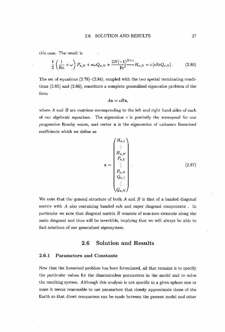
The set of equations (2.78)-(2.84), coupled with the two special terminating condi-
tions (2.85) and (2.86), constitute a complete generalised eigenvalue problem of the
form
Ax = cBx,
where A and B are matrices corresponding to the left and right hand sides of each
of our algebraic equations. The eigenvalue c is precisely the wavespeed for our
progressive Rossby waves, and vector x is the eigenvector of unknown linearized
coefficients which we define as
x =
I HK,1\
tc,N PIO
Prc,N C tc,1
(2.87)
\C2K,N/
We note that the general structure of both A and B is that of a banded diagonal
matrix with A also containing banded sub and super diagonal components . In
particular we note that diagonal matrix B consists of non-zero elements along the
main diagonal and thus will be invertible, implying that we will always be able to
find solutions of our generalised eigensystem.
2.6 Solution and Results
2.6.1 Parameters and Constants
Now that the linearized problem has been formulated, all that remains is to specify
the particular values for the dimensionless parameters in the model and to solve
the resulting system. Although this analysis is not specific to a given sphere size or
mass it seems reasonable to use parameters that closely approximate those of the
Earth so that direct comparison can be made between the present model and other
2.6. SOLUTION AND RESULTS 28
published results. With this in mind we adopt the following values for the sphere
specific parameters:
a = 6.37122 x 10⁶m, 27r
. 24 x 3600 7.272 x 10
-5 s-1 Q ,
g = 9.80616 m s -2 .
Additionally we define each characteristic reference scale as
(2.88)
(2.89)
(2.90)
vref = 40ms -1 , (2.91)
href = 8.0 x 10³ m, (2.92)
cref =—Si
.--:-., 2.4241 x 10 -6 s-1 . (2.93) 30
Note that whilst the values for h ref and cref seem "reasonable" with reference to the
Earth, one should not be surprised at the rather large value of v„f. Normally, to
compute velocities similar to those observed locally on the surface of the Earth one
must include the effects of friction and the planetary boundary layer in the problem.
Neglecting these terms, as we have done is this analysis, will always result in higher
than observed surface velocities, which accounts for the larger than normal choice
of vref.
With the specification of the above parameters we can now calculate estimates for
the Strouhal, Froude and Rossby numbers. These are given by
a cref Sr = — P--' 3.8611 x 10 -1 , (2.94)
Vref
Fr = Vref
'eZ:i 1.4281 x 10 -1 , (2.95) Virtr-c-f Ro = I-.. r-:_,
' . 4 3166 x 10 -2 . (2.96) 2SZa
The small value of Ro is in agreement with the definition of large-scale flow defined
by Pedlosky[65, pages 2-3] so that we can expect the Earth's rotation to be an
influential factor determining the nature of any calculated solution. This is precisely
the kind of behaviour we seek since we require flows in which the dominant driving
force sustaining any initial perturbation is highly dependent on the large scale nature
of the flow, as first demonstrated by Rossby[69].
For the dimensionless zonal flow parameters we choose values that are consistent
with those documented in the test set of Williamson et al. [87]. The equivalent
2.6. SOLUTION AND RESULTS 29
non-dimensional values for ho and co are
ho = 1, (2.97)
w 1.25. (2.98)
The value of 1 for It, is consistent with our previous statement about the dimensional
value of h at 0 = +7/2 being h„f , and the particular value of co above is obtained
by noting that Williamson et al. use a dimensional value for co of 7.848 x 10 -6 s-1 ,
a value first introduced by Phillips[66] in 1956 when he successfully integrated the
primitive equations of atmospheric flow. In order to convert this to a dimensionless
number it is necessary to multiply by the radius of the Earth and divide by the
reference velocity scale so that
7.848 x 10 -6a = 1.25.
ef (2.99)
Although (2.99) is only a single value of the dimensionless zonal flow angular speed,
the analysis presented here permits a wide variety of values for co. Nevertheless, the
value given by (2.99) facilitates comparison with other published literature, such as
Williamson et at [87]. In the next section we will consider the solution for values of co
over a wide range of allowable values including the specific value above, anticipating
the strong dependence of the nonlinear solution on w which will be discussed in
Chapter 3.
2.6.2 Results for K -= 3,4 and 5
The solution of the generalised eigenvalue problem was achieved by implementing a
MATLAB script that assembled the left and right hand side matrices and then solved
the resulting system by using the inbuilt routine eig (A, B) to find the eigenvalues
and corresponding eigenvectors. Various truncation levels were chosen to check
convergence of the algorithm and in all cases rapid convergence was observed for
increasing N. Typically a truncation value of N = 10 was all that was required to
establish the solution to 4 or 5 significant figures and a truncation level of N = 100
could almost be deemed excessive if not for the very small computational times
involved; approximately 3 seconds was required to compute all 300 eigenvalue-
eigenvector pairs when N = 100, on an AMD Athlon(tm) XP 1800+ processor
clocked at 1.54 GHz with 512 MB of physical memory clocked at 266 MHz.

2.6. SOLUTION AND RESULTS
30
Tables 2.1, 2.2 and 2.3 illustrate this rapid convergence for ic = 3, 4 and 5 respec-
tively. The final column in each table gives the order of the last coefficient in each
N 3 5 10 100 0 (Coeffloo) H3,1 -4.6628E-02 -4.4294E-02 -4.4505E-02 -4.4507E-02 H3, 2 -2.4242E-02 -2.2917E-02 -2.3022E-02 -2.3023E-02 1.0E-09 H3,3 9.3363E-03 1.1141E-02 1.1256E-02 1.1258E-02 P3,1 -1.7968E-01 -1.7071E-01 -1.7152E-01 -1.7153E-01 P3,2 -6.5140E-01 -6.1965E-01 -6.2262E-01 -6.2265E-01 1.0E-06 P3,3 -2.1733E-01 -1.7497E-01 -1.7495E-01 -1.7494E-01 Q3,1 -1.0157E+00 -9.6486E-01 -9.6945E-01 -9.6948E-01 Q3,2 -2.6718E-01 -2.5611E-01 -2.5740E-01 -2.5741E-01 1.0E-07 Q3 , 3 1.1171E-02 5.1071E-02 5.2422E-02 5.2437E-02
c -4.1957E-02 -4.1805E-02 -4.1805E-02 -4.1805E-02
Table 2.1: Convergence of incompressible wavespeed and first three coefficients in each series for increasing N, = 3.
series when N = 100 and provides evidence for the accuracy of the solution since in
each case the coefficients are observed to drop off reasonably fast and in the case of
= 4 we have accuracy to very high precision. The particular scaling for the coef-
ficients is arbitrary and has been chosen to match the equivalent Rossby-Haurwitz
wave as specified in [87], to be explained in the next section. Note also that conver-gence of the eigenvalue is obtained with smaller truncation than that required for corresponding accuracy in the coefficients, providing confidence in the accuracy of
the wavespeeds calculated.
N 3 5 10 100 0(COeff100) H4,1 -3.0905E-02 -2.9884E-02 -2.9888E-02 -2.9888E-02 H4 , 2 -1.2042E-02 -1.1779E-02 -1.1781E-02 -1.1781E-02 1.0E-17 H4,3 1.1248E-02 1.1718E-02 1.1719E-02 1.1719E-02 P4,1 -1.0749E-01 -1.0392E-01 -1.0393E-01 -1.0393E-01 P4,2 -5.0323E-01 -4.8531E-01 -4.8537E-01 -4.8537E-01 1.0E-15 P4,3 -2.5965E-01 -2.3376E-01 -2.3379E-01 -2.3379E-01 Q4,1 -9.1506E-01 -8.8487E-01 -8.8498E-01 -8.8498E-01 Q4,2 -4.0863E-01 -3.9154E-01 -3.9158E-01 -3.9158E-01 1.0E-15 Q4,3 6.5631E-03 3.0816E-02 3.0825E-02 3.0825E-02
c 9.5282E-01 9.5522E-01 9.5522E-01 9.5522E-01 -
Table 2.2: Convergence of incompressible wavespeed and first three coefficients in each series for increasing N, frc = 4.
As already stated, we need not only consider the value of ch) as used by Williamson
2.6. SOLUTION AND RESULTS
31
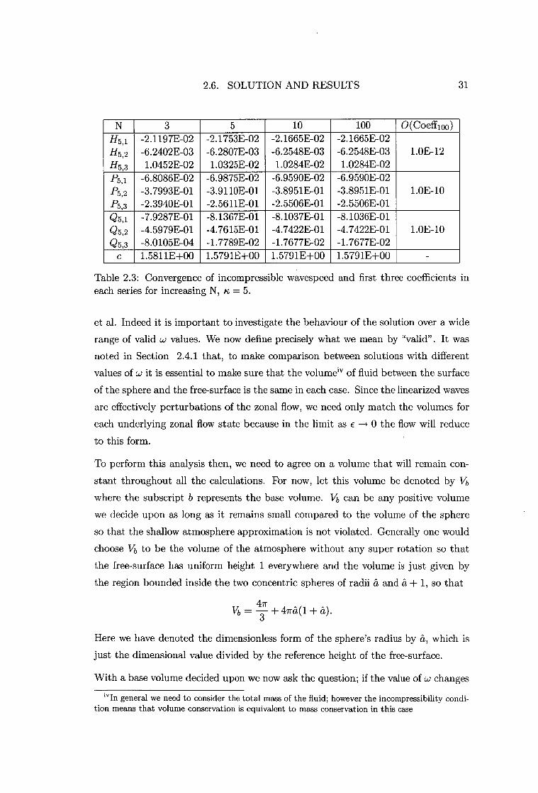
N 3 5 10 100 0 (Coeffico ) H5, 1 -2.1197E-02 -2.1753E-02 -2.1665E-02 -2.1665E-02 H5, 2 -6.2402E-03 -6.2807E-03 -6.2548E-03 -6.2548E-03 1.0E-12 H5,3 1.0452E-02 1.0325E-02 1.0284E-02 1.0284E-02 P5,1 -6.8086E-02 -6.9875E-02 -6.9590E-02 -6.9590E-02 P5,2 -3.7993E-01 -3.9110E-01 -3.8951E-01 -3.8951E-01 1.0E-10 P5,3 -2.3940E-01 -2.5611E-01 -2.5506E-01 -2.5506E-01 Q5,1 -7.9287E-01 -8.1367E-01 -8.1037E-01 -8.1036E-01 Q5,2 -4.5979E-01 -4.7615E-01 -4.7422E-01 -4.7422E-01 1.0E-10 Q5,3 -8.0105E-04 -1.7789E-02 -1.7677E-02 -1.7677E-02
c 1.5811E+00 1.5791E+00 1.5791E+00 1.5791E+00 -
Table 2.3: Convergence of incompressible wavespeed and first three coefficients in each series for increasing N, = 5.
et al. Indeed it is important to investigate the behaviour of the solution over a wide range of valid w values. We now define precisely what we mean by "valid". It was
noted in Section 2.4.1 that, to make comparison between solutions with different
values of w it is essential to make sure that the volume iv of fluid between the surface
of the sphere and the free-surface is the same in each case. Since the linearized waves
are effectively perturbations of the zonal flow, we need only match the volumes for
each underlying zonal flow state because in the limit as e -> 0 the flow will reduce
to this form.
To perform this analysis then, we need to agree on a volume that will remain con-
stant throughout all the calculations. For now, let this volume be denoted by 14
where the subscript b represents the base volume. Vb can be any positive volume
we decide upon as long as it remains small compared to the volume of the sphere
so that the shallow atmosphere approximation is not violated. Generally one would
choose Vb to be the volume of the atmosphere without any super rotation so that
the free-surface has uniform height 1 everywhere and the volume is just given by
the region bounded inside the two concentric spheres of radii et and et + 1, so that
47r Vb = -
3 + 4ret(1 + et).
Here we have denoted the dimensionless form of the sphere's radius by et, which is just the dimensional value divided by the reference height of the free-surface.
With a base volume decided upon we now ask the question; if the value of w changes
ivIn general we need to consider the total mass of the fluid; however the incompressibility condi-tion means that volume conservation is equivalent to mass conservation in this case

2.6. SOLUTION AND RESULTS 32
how must the value of ho change to ensure that the volume remains constant? To
answer this question we note that for the general zonal flow described in (2.53), the
volume is given by
27r 7r/2 al-h.(0)
v.=.1 I I r2 cos 0 dr dOchi 0 —7/2 a
7r/2 47r
= —3 f [14 + 3hza(hz + a)] cos 0 d0. (2.100)
The volume matching condition states that Vz – Vb = 0, thus substituting (2.53)
into (2.100) and performing algebraic manipulations leads to a cubic equation for
ho of the form
47r (87r-A 327rA2 167retA + 47'62) 110 — hrt3 + 47ra,) h20 3 „ 3 15 3
(647rA 3 327retA2 87ril2A Vb) = 0 (2.101)
105 15 3
where A = w). Once w is fixed, which in turn fixes the coefficients in
(2.101), we can solve for ho using any appropriate method we choose, be it analytical
or numerical. For the present purposes, the formula for the one real root of a cubic
equation was used to solve for 110 , as taken from Abramowitz & Stegun[1].
In general we may choose any value for w; however for (2.101) to have non-negative
solutions we can show that there is an upper limit on the value that w can take, since
the polar height ho must decrease as the super-rotation rate increases, when volume
remains fixed. The limiting upper value on w, denoted w u , will be encountered once
the solution of (2.101) returns ho = 0. Similarly we can also argue for a lower limit
of w = 0 since by definition of the linearization process we need to have a base zonal
flow to perturb about, which can only occur for non-zero w. In conclusion we must
restrict our investigation to the valid range of values from 0 < < wu.
With a volume matching method agreed upon we can now investigate the behaviour
of the eigenvalues for constant volume and varying w. For this analysis we present
results only for the case ic = 4 since similar behaviour is observed when ic = 3 or 5.
For a given truncation N we will have a total of 3N eigenvalues computed. Figure
2.2 shows the 15 calculated eigenvalues when N = 5 for valid values of parameter
w. Although the truncation level is quite low here it is useful to observe what is
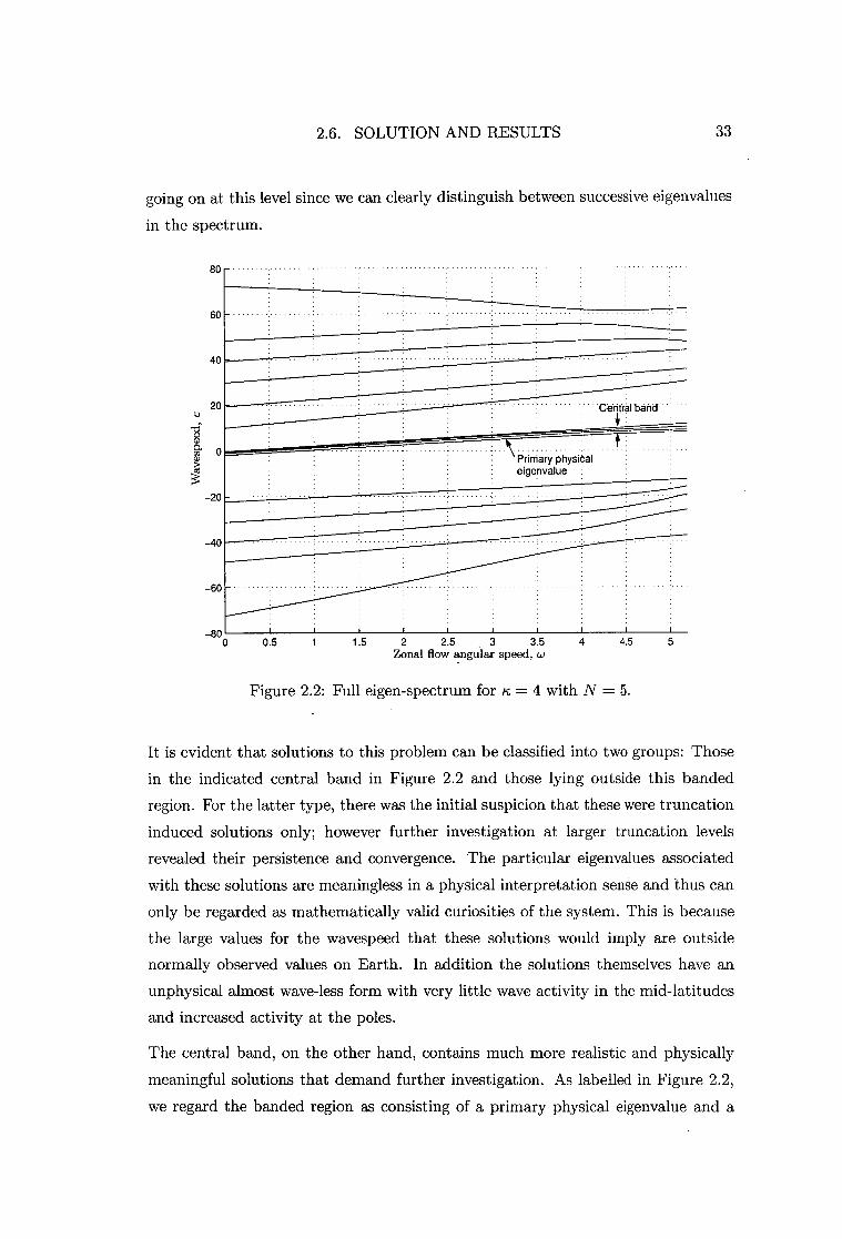
2.6. SOLUTION AND RESULTS 33
going on at this level since we can clearly distinguish between successive eigenvalues
in the spectrum.
80
60
40 -
Central band "
Primary physical eigenvalue
20
-20
-40
-60
-80 0
0.5 1 1.5 2 2.5 3 3.5 4 4.5 Zonal flow angular speed, w
Figure 2.2: Full eigen-spectrum for n = 4 with N = 5.
It is evident that solutions to this problem can be classified into two groups: Those
in the indicated central band in Figure 2.2 and those lying outside this banded
region. For the latter type, there was the initial suspicion that these were truncation
induced solutions only; however further investigation at larger truncation levels
revealed their persistence and convergence. The particular eigenvalues associated
with these solutions are meaningless in a physical interpretation sense and thus can
only be regarded as mathematically valid curiosities of the system. This is because
the large values for the wavespeed that these solutions would imply are outside
normally observed values on Earth. In addition the solutions themselves have an
unphysical almost wave-less form with very little wave activity in the mid-latitudes
and increased activity at the poles.
The central band, on the other hand, contains much more realistic and physically
meaningful solutions that demand further investigation. As labelled in Figure 2.2,
we regard the banded region as consisting of a primary physical eigenvalue and a
14
12
1 0
Limiting upper eigenvalue
Prtmary physical eigenvalue
2
0.5 1 1.5 2 2.5 3 3.5 4 4.5 5 Zonal flow angular speed, w
8
71- w a) 6 6
c) 4
2.6. SOLUTION AND RESULTS 34
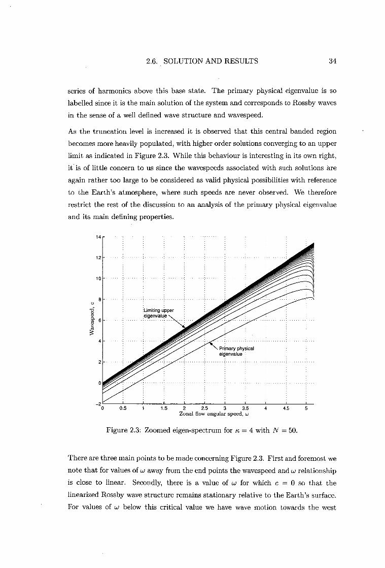
series of harmonics above this base state. The primary physical eigenvalue is so
labelled since it is the main solution of the system and corresponds to Rossby waves
in the sense of a well defined wave structure and wavespeed.
As the truncation level is increased it is observed that this central banded region
becomes more heavily populated, with higher order solutions converging to an upper
limit as indicated in Figure 2.3. While this behaviour is interesting in its own right,
it is of little concern to us since the wavespeeds associated with such solutions are
again rather too large to be considered as valid physical possibilities with reference
to the Earth's atmosphere, where such speeds are never observed. We therefore
restrict the rest of the discussion to an analysis of the primary physical eigenvalue
and its main defining properties.
Figure 2.3: Zoomed eigen-spectrum for ic = 4 with N = 50.
There are three main points to be made concerning Figure 2.3. First and foremost we
note that for values of w away from the end points the wavespeed and w relationship
is close to linear. Secondly, there is a value of w for which c = 0 so that the
linearized Rossby wave structure remains stationary relative to the Earth's surface.
For values of w below this critical value we have wave motion towards the west

2.6. SOLUTION AND RESULTS 35
whereas for values higher we have eastward wave motion, allowing for a wide variety
of atmospheric configurations. The final point concerns the behaviour at the upper
end of the graph, in which no real confidence can be placed. The bending over of
the solutions for large values of w is a consequence of the fact that the height at
the poles, h0 , is changing to conserve the total volume as previously discussed. At
the other end of the graph, when w = 0, we observe that the linearized solution
predicts that waves with non-zero wavespeed are possible when there is no zonal
flow structure. One way to interpret this behaviour is through the idea that the
perturbations themselves are valid solutions of the system and that no zonal flow is
required for them to exist; this idea is expanded by Pedlosky [65, pages 108-110].
Nonetheless, the solutions associated with values of w away from the end points are
physically reasonable, relevant and consistent with the Rossby-Haurwitz solutions,
to be discussed in the next section.
2.6.3 Comparison with Rossby-Haurwitz solution
To provide evidence supporting the accuracy of the linearized solutions computed,
it is useful to make a comparison between these solutions and the equivalent corre-
sponding Rossby-Haurwitz solutions. To do this we make use of the wavespeed for-
mula as presented in Haurwitz's classic paper [32] and later adopted by Williamson
et al. in their test set. The particular formula is given by
tc(3 + 'Ow - 212 c = (2.102) (1 + /0(2 + n)
which has been rewritten to reflect the naming conventions and variable names used
in this work. Note that this equation clearly shows a linear relationship between c
and w. Also, Haurwitz's work does not allow one to fix the volume for the calcu-
lation, since it does not use a free-surface formulation, so we should expect some
divergence from our solutions, which do take this into account.
To compare the two solution types we consider the primary physical eigenvalues for
= 3,4 and 5 with the equivalent Rossby-Haurwitz solutions over our valid w range.
Figure 2.4 shows the results of this comparison with the solid lines representing the
equivalent Rossby-Haurwitz solution for frc = 3 to 5 from bottom to top respectively.
In general one can conclude that the two models have good agreement, especially
so for values of w in the range 0 <w < 2 where the effect of the volume matching
is minimal. In fact better agreement is observed if one does not take the volume
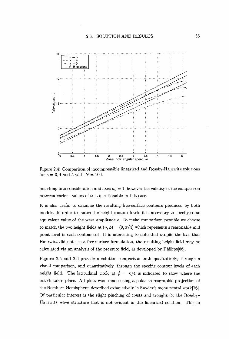
• — = 3 - - lc = 4
= 5 — R-H solutions
0.5 1 1.5 2 2.5 3 3.5 Zonal flow angular speed, (.,/
4.5
2.6. SOLUTION AND RESULTS 36
Figure 2.4: Comparison of incompressible linearized and Rossby-Haurwitz solutions for ic = 3,4 and 5 with N= 100.
matching into consideration and fixes h, = 1, however the validity of the comparison
between various values of co is questionable in this case.
It is also useful to examine the resulting free-surface contours produced by both
models. In order to match the height contour levels it it necessary to specify some
equivalent value of the wave amplitude e. To make comparison possible we choose
to match the two height fields at (77, cb) = (0,7r/4) which represents a reasonable mid
point level in each contour set. It is interesting to note that despite the fact that
Haurwitz did not use a free-surface formulation, the resulting height field may be
calculated via an analysis of the pressure field, as developed by Phillips[66].
Figures 2.5 and 2.6 provide a solution comparison both qualitatively, through a
visual comparison, and quantitatively, through the specific contour levels of each
height field. The latitudinal circle at 0 = 7r/4 is indicated to show where the
match takes place. All plots were made using a polar stereographic projection of
the Northern Hemisphere, described exhaustively in Snyder's monumental work[76].
Of particular interest is the slight pinching of crests and troughs for the Rossby-
Haurwitz wave structure that is not evident in the linearized solution. This in
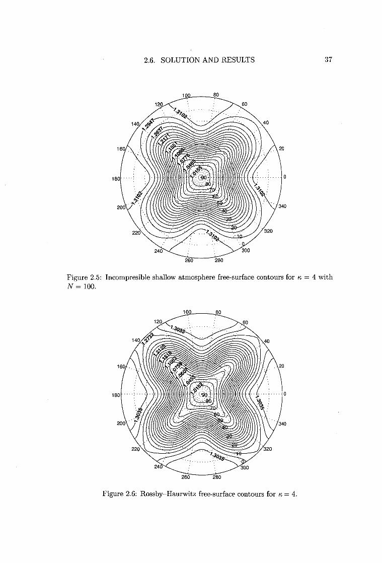
160 20
180
200
2.6. SOLUTION AND RESULTS 37
Figure 2.5: Incompresible shallow atmosphere free-surface contours for n = 4 with N = 100.
180
200 V 340
220 320
Figure 2.6: Rossby—Haurwitz free-surface contours for i = 4.

-.... ,
- -:"-- Z.- •Z` .‘ ‘̀ \ ,
— ... - , a, '6-- ■ , ‘...... \•
, ./ ...• ..\\ , -
- — . \' '
- , r• . 4\̀ ‘ . .
— , \ .\`1/4 - ,
, \\ .41/4'‘` -
- •1/4.,\
.- ••••• - — \\ t
... •••• ... tzs
.... , ‘l'
- ,‘‘
... ... - - -.., ‘' - - \
1,
..‘ ,1/4,
- 41 1 - 4 1
1t%
‘4% I lt Ill
1\ 1\
I% II I H I I 11 444
III II I I U U III
III II 111111 I I Ill111
ri •a il a 1 • II II il il i
iii ii
4111
tt
Ittt ,
It,
p.
7..
2.6. SOLUTION AND RESULTS 38
turn forces the lower heights, and hence pressures, near the poles to extend further
towards the equator in the Rossby-Haurwitz solution. However, overall there is
very close agreement between both types of solutions, encouraging one to assume
that these indeed are valid approximate solutions of the full non-linear governing
equations.
As a final supporting statement we investigate the nature of the corresponding
velocity vector field for the free-surface presented in Figure 2.5. From a geostrophic
point of view we would expect the fluid streamlines to be nearly parallel to the
pressure contours, something which is observed in Figure 2.7. Additionally we have
increasingly diminishing flow as we approach either pole, which converges to the
required stagnation point when 0 = ±7/2. Since the particular viewpoint of the
projection means that the sphere's rotation is counter clockwise when viewed from
above, we see that fluid flow is directed in the same direction as the underlying zonal
flow with the Rossby wave pattern moving relative to this mean fluid progression.
Figure 2.7: Incompressible shallow atmosphere free-surface contours with corre-sponding velocity vector field for lc = 4 with N = 100
In this chapter we have explored linearized solutions of the incompressible, non-

2.6. SOLUTION AND RESULTS 39
dimensional shallow atmosphere equations. The solutions that were obtained for
particular values of longitudinal wave number lc were found to be in close agree-
ment with the corresponding Rossby-Haurwitz solutions. Not only do the linearized
solutions provide helpful insight into this complex dynamical system, they can also
be used as a base starting point for a more thorough investigation of the complete
nonlinear system. This problem is addressed in the next chapter.

CHAPTER 3
INCOMPRESSIBLE NONLINEAR SHALLOW ATMOSPHERE MODEL
The goal of this chapter is two fold: Firstly we wish to extend the linearized so-
lutions computed in Chapter 2 to encompass the fully nonlinear equation set for
the dynamical system. This will allow for the investigation of subtleties in the flow
field, resulting from nonlinearity, which are not possible to expose using linear the-
ory alone. Secondly, and perhaps more importantly, we aim to conduct an in-depth
study of the relationship between the progressive wavespeed and corresponding am-
plitude. As will be shown, this type of analysis can reveal some interesting results
concerning Rossby wave behaviour. It will be demonstrated that solutions of the
system are highly dependent on the wavenumber n and the zonal flow angular speed
w.
3.1 Problem Specification
3.1.1 Conservation Equations
The equations of motion to be used in the present chapter are those derived in the
previous chapter for conservation of mass and momentum in the rotating shallow
atmosphere system. For ease of reference and completeness we restate these equa-
tions ((2.43), (2.44) and (2.45)) here for later use. Readers may consult the first
few sections of the previous chapter for their derivation. In dimensionless variables
we have:
40
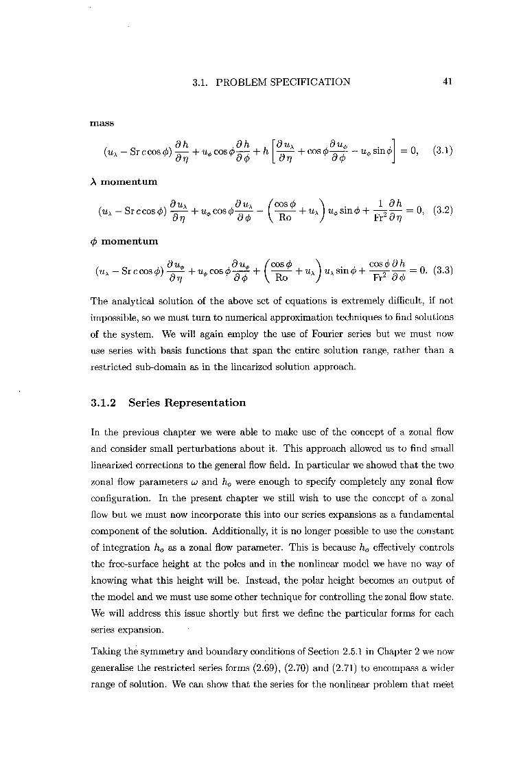
3.1. PROBLEM SPECIFICATION 41
mass
a h (ILA — Sr c cos (/)) + uo cos 0-hh + h[82LAd + cos o a 0 uo sin ] , 0, (3.1)
A momentum
au ), 0 A a = _ (3.2) a 0 — + 7./0 cos 0
(cos 1 h (uA — Sr c cos)
0 14) u s . m + m_ 77 a o Ro +
Fr id
momentum
au (cos 0 cosq5 ah au 9u + cos o + +u ,\ u sin + = 0. (3.3) (u, — Sr c cos a n a 0 Ro A Fr2 a o
The analytical solution of the above set of equations is extremely difficult, if not
impossible, so we must turn to numerical approximation techniques to find solutions
of the system. We will again employ the use of Fourier series but we must now
use series with basis functions that span the entire solution range, rather than a
restricted sub-domain as in the linearized solution approach.
3.1.2 Series Representation
In the previous chapter we were able to make use of the concept of a zonal flow
and consider small perturbations about it. This approach allowed us to find small
linearized corrections to the general flow field. In particular we showed that the two
zonal flow parameters ci.; and h, were enough to specify completely any zonal flow
configuration. In the present chapter we still wish to use the concept of a zonal
flow but we must now incorporate this into our series expansions as a fundamental
component of the solution. Additionally, it is no longer possible to use the constant
of integration Ito as a zonal flow parameter. This is because It, effectively controls
the free-surface height at the poles and in the nonlinear model we have no way of
knowing what this height will be. Instead, the polar height becomes an output of
the model and we must use some other technique for controlling the zonal flow state.
We will address this issue shortly but first we define the particular forms for each
series expansion.
Taking the symmetry and boundary conditions of Section 2.5.1 in Chapter 2 we now
generalise the restricted series forms (2.69), (2.70) and (2.71) to encompass a wider
range of solution. We can show that the series for the nonlinear problem that meet

3.1. PROBLEM SPECIFICATION 42
our conditions are given by:
00 O. 07, = cos + E E Pm ,n, cos(kmn) cos ((2n — 1)0) ,
m=1 n=1 00 00
.0 (7, 0) = E E Qm,„ sin(,m,) sin(27-0), m=1 n=1 oo
h(n , 0) = E Ho,„ cos(2n0) n=0
oo oo
+ E E Hm,n COS(KM,n) (-1)n [cos (20) + cos (2(n — 1)0) , (3.6) m=1 n=1
where (3.6) uses basis recombination to satisfy boundary conditions at the poles and
the series (3.4) for u, now contains the primary zonal flow velocity component. In-
stead of specifying the polar free-surface height we replace h, with the mindependent
series in (3.6) to allow for the polar height to be determined from the output of the
model, as discussed previously.
It is interesting to point out the absence of any n-independent terms in the series
(3.4) apart from the primary zonal flow term. One might well assume that to span
the solution space with a complete basis set one should use a series for u ›, of the
form
. 00 00 U,(,) = w cos o + po,r, cos ((2n — 1)0) + E E Prn ,„ cos(nmn) cos ( (2n — 1)0)
n=1 m=1 n=1
where we can think of the additional n-independent series term as modifying the base
zonal flow in a way that only depends on latitude. The problem with this approach
is that the zonal flow is no longer unique. Any numerical scheme that attempts
to solve the equations using this series representation will fail since the zonal flow
now becomes an output of the problem and the system has no way of knowing its
own base state. In hindsight this conclusion seems rather obvious; however it was
not discovered until analysis of the singular value decomposition of the Jacobian of
the truncated system revealed exactly N machine precision sized singular values in
the spectrum corresponding to the coefficients Poo . to Po,N. Removal of these terms
subsequently removed any associated ill-conditioning in the Jacobian, allowing the
solution to be computed.
(3.4)
(3.5)
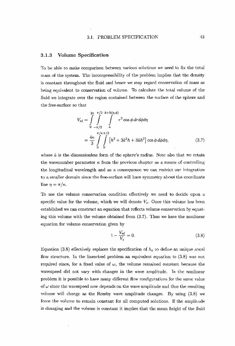
3.1. PROBLEM SPECIFICATION 43
3.1.3 Volume Specification
To be able to make comparison between various solutions we need to fix the total
mass of the system. The incompressibility of the problem implies that the density
is constant throughout the fluid and hence we may regard conservation of mass as
being equivalent to conservation of volume. To calculate the total volume of the
fluid we integrate over the region contained between the surface of the sphere and
the free-surface so that
27r 7r/2 et±h(71,0)
vni= I f I r2 COS drdOdn O-r/2 a
711K 7r/2
3 f f
[h3 3ã2h 3iih2 ] cos 0 d0c177, (3.7) 00
where et is the dimensionless form of the sphere's radius. Note also that we retain
the wavenumber parameter n from the previous chapter as a means of controlling
the longitudinal wavelength and as a consequence we can restrict our integration
to a smaller domain since the free-surface will have symmetry about the coordinate
line n =
To use the volume conservation condition effectively we need to decide upon a
specific value for the volume, which we will denote Vz . Once this volume has been
established we can construct an equation that reflects volume conservation by equat-
ing this volume with the volume obtained from (3.7). Thus we have the nonlinear
equation for volume conservation given by
1 — — = 0. Vni Vz (3.8)
Equation (3.8) effectively replaces the specification of h, to define an unique zonal
flow structure. In the linearized problem an equivalent equation to (3.8) was not
required since, for a fixed value of w, the volume remained constant because the
wavespeed did not vary with changes in the wave amplitude. In the nonlinear
problem it is possible to have many different flow configurations for the same value
of w since the wavespeed now depends on the wave amplitude and thus the resulting
volume will change as the Rossby wave amplitude changes. By using (3.8) we
force the volume to remain constant for all computed solutions. If the amplitude
is changing and the volume is constant it implies that the mean height of the fluid

3.2. NUMERICAL SOLUTION METHOD 44
must either increase or decrease. The mean height of the fluid is controlled via the
polar free-surface height h0 . It is now apparent that we have in fact parametrised
the polar height It, in terms of the conservation condition expressed in (3.8), and
this becomes the extra condition to close the problem.
3.2 Numerical Solution Method
3.2.1 Collocation
Equations (3.1), (3.2), (3.3) and (3.8) constitute a complete system for which the
solution gives nonlinear Rossby waves. The solution process consists of finding the
coefficients Hm,„, Pm,„, Q,,,,, and wavespeed c that make the series (3.4), (3.5)
and (3.6) a solution of the system. Various different techniques for doing this are
possible. The method chosen here is the pseudospectral technique of collocation in
which we require the residuals, obtained by substituting the series into the governing
equations, to be zero at every point on a mesh constructed from a finite number
of points in the flow field. This technique is in contrast to the spectral Galerkin
method of the previous chapter in which we required the residuals to be orthogonal
to the basis expansion functions over the entire domain. While we can use the same
basis functions for both the collocation and the Galerkin method, in the collocation
method we no longer have the residual orthogonality property of spectral methods
in general.
There are both advantages and disadvantages to using the collocation method
over other techniques such as the Galerkin method or finite-difference schemes.
Durran[20, pages 191-195] presents a detailed exposition of these key differences. In
summary, the main advantage of collocation over a finite-difference scheme is that
the collocation method will be more accurate provided the solution is smooth. This
is a direct result of using infinitely differentiable basis functions which allow for the
calculation of exact function derivatives at each point in the flow domain. The main
advantage of collocation over the Galerkin method is that the collocation method
is computationally less intensive because costly integrals need not be evaluated at
each step. In addition, since the grid points are fixed for a particular mesh, we can
cache the basis functions and their derivatives at all necessary points and use these
stored values to speed up the solution process by eliminating costly function calls
in the program. This technique will be explained later in the chapter.
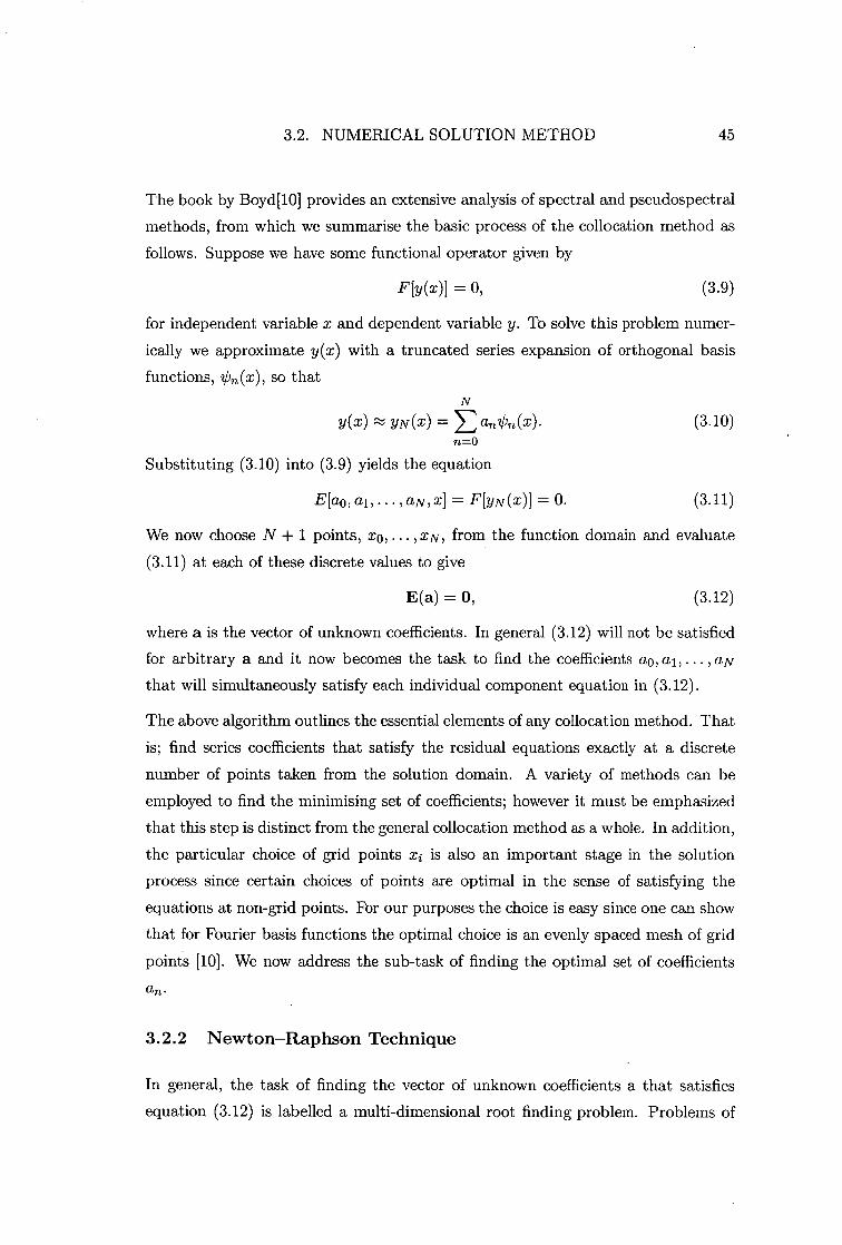
3.2. NUMERICAL SOLUTION METHOD 45
The book by Boyd[10] provides an extensive analysis of spectral and pseudospectral
methods, from which we summarise the basic process of the collocation method as
follows. Suppose we have some functional operator given by
Fly (x)] = 0, (3.9)
for independent variable x and dependent variable y. To solve this problem numer-
ically we approximate y(x) with a truncated series expansion of orthogonal basis
functions, //),,(x), so that
y(x) y N (x) = E an07,(x). (3.10) n=0
Substituting (3.10) into (3.9) yields the equation
E[ao, at, , a N , x] = Ffy N (x)] = 0. (3.11)
We now choose N + 1 points, xo, , xN, from the function domain and evaluate
(3.11) at each of these discrete values to give
E(a) = 0, (3.12)
where a is the vector of unknown coefficients. In general (3.12) will not be satisfied
for arbitrary a and it now becomes the task to find the coefficients a o , a l , , a N that will simultaneously satisfy each individual component equation in (3.12).
The above algorithm outlines the essential elements of any collocation method. That
is; find series coefficients that satisfy the residual equations exactly at a discrete
number of points taken from the solution domain. A variety of methods can be
employed to find the minimising set of coefficients; however it must be emphasized
that this step is distinct from the general collocation method as a whole. In addition,
the particular choice of grid points xi is also an important stage in the solution
process since certain choices of points are optimal in the sense of satisfying the
equations at non-grid points. For our purposes the choice is easy since one can show
that for Fourier basis functions the optimal choice is an evenly spaced mesh of grid
points [10]. We now address the sub-task of finding the optimal set of coefficients
an .
3.2.2 Newton—Raphson Technique
In general, the task of finding the vector of unknown coefficients a that satisfies
equation (3.12) is labelled a multi-dimensional root finding problem. Problems of
3.2. NUMERICAL SOLUTION METHOD 46
this type are notoriously difficult for a number of reasons, the main one being that
zeros of one residual component generally have nothing in common with zeros of
another distinct residual component, as described in Press et al.[68, pages 383-
386]. However, it is possible to solve problems of this type with careful analysis and
planning. One such method for accomplishing this task is an iterative technique
called the Newton-Raphson algorithm.
We present here an overview of the Newton-Raphson algorithm as detailed in [68,
pages 383-386]. Suppose we start with some initial guess for the vector of unknown
coefficients, defined to be a(k ) where the superscript denotes the current iterative
step. Each individual residual component in (3.12) can be expanded locally in a
Taylor series about the multi-dimensional point a(k) , leading to the vector equation
E(a(k) 6a(k)) E(a(k)) j(k)
where j (k ) is the Jacobian matrix of partial derivatives and is defined by
J2.7 = aaj a(k)
(3.13)
(3.14)
The goal of the root finding process is to make E(a(k) + 5a (k) ) = 0; thus equation
(3.13) provides a recipe for achieving this goal, since as a first approximation we
can neglect the higher order terms and set E(a(k) + oa(k) ) = 0, enabling us to solve
for the correction step a(k) that brings vector a(k) closer to satisfying (3.12). The
resulting linear system for the step direction is given by
j (k ) 6a(k) = _E(a(k)) , (3.15)
which can be solved for the vector 5a (k) using standard linear algebra techniques.
Once we have found the updating step, we update the solution to give the new
vector a(k+1) a(k) 6,(k)
a 7 (3.16)
which should be a better approximation to a root of (3.12). The above process is
then repeated, starting from the new point a(k+1) , until convergence is achieved.
While this algorithm is useful it is by no means robust in the sense that it will
always find a solution if one is known to exist. Specifically, the Newton-Raphson
method is known to converge to a root only if the starting guess is sufficiently close
to the root. Thus root finding using this technique requires both care and insight
into the expected nature of the solution, as described by Acton [2].
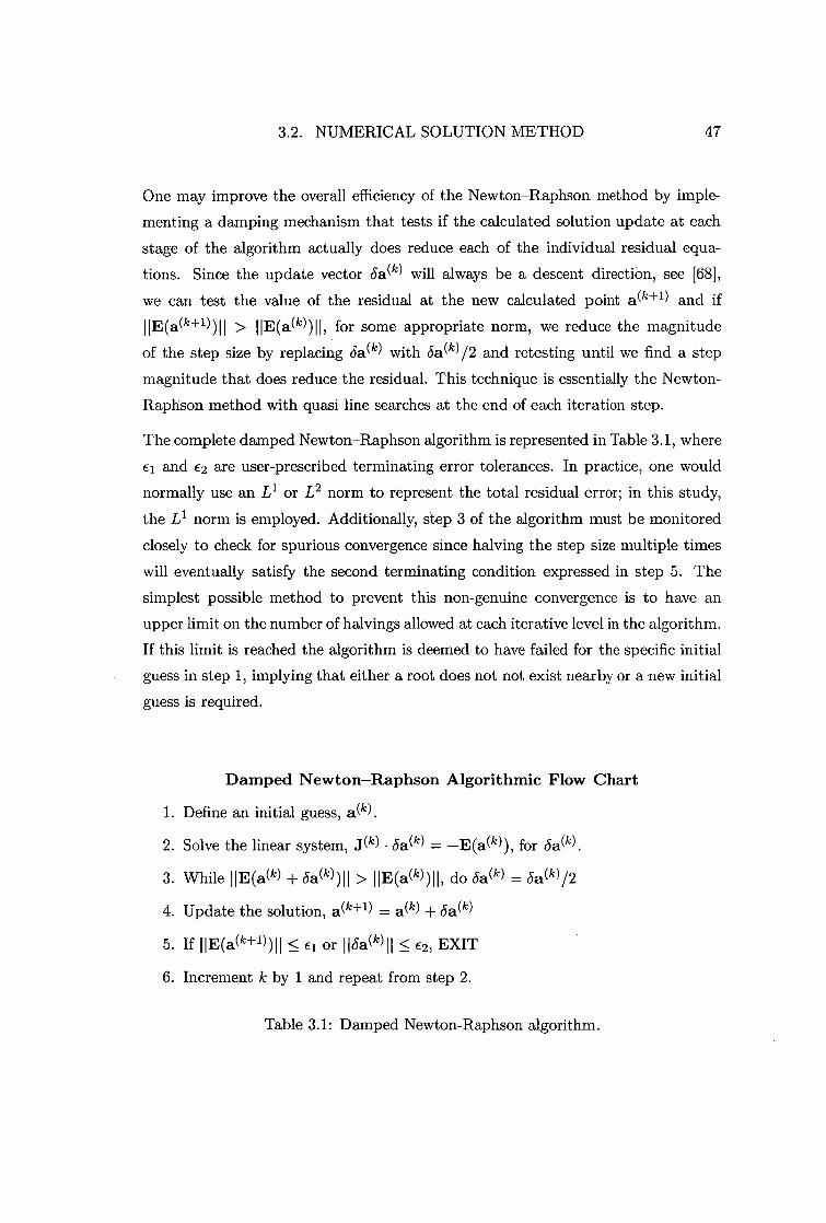
3.2. NUMERICAL SOLUTION METHOD 47
One may improve the overall efficiency of the Newton-Raphson method by imple-
menting a damping mechanism that tests if the calculated solution update at each
stage of the algorithm actually does reduce each of the individual residual equa-
tions. Since the update vector oa(k) will always be a descent direction, see [68],
we can test the value of the residual at the new calculated point a(k+ 1) and if
I 1E(a (k+1) )11 > IIE(a(k))11, for some appropriate norm, we reduce the magnitude
of the step size by replacing oa (k) with Sa (k) /2 and retesting until we find a step
magnitude that does reduce the residual. This technique is essentially the Newton-
Raphson method with quasi line searches at the end of each iteration step.
The complete damped Newton-Raphson algorithm is represented in Table 3.1, where
El and E2 are user-prescribed terminating error tolerances. In practice, one would
normally use an L l or L2 norm to represent the total residual error; in this study,
the L l norm is employed. Additionally, step 3 of the algorithm must be monitored
closely to check for spurious convergence since halving the step size multiple times
will eventually satisfy the second terminating condition expressed in step 5. The
simplest possible method to prevent this non-genuine convergence is to have an
upper limit on the number of halvings allowed at each iterative level in the algorithm.
If this limit is reached the algorithm is deemed to have failed for the specific initial
guess in step 1, implying that either a root does not not exist nearby or a new initial
guess is required.
Damped Newton-Raphson Algorithmic Flow Chart
1. Define an initial guess,
2. Solve the linear system, J(k) • 5a(k) = -E(a(k)), for 5a (k) .
3. While IIE(a(k) + Sa(k) )II > I IE(a(k))11, do 6a(k) =
4. Update the solution, a(k+1) a(k) (5a(k)
5. If IIE(a(k+1) )11 < El or IlOa (k) II < 62, EXIT
6. Increment k by 1 and repeat from step 2.
Table 3.1: Damped Newton-Raphson algorithm.

3.3. CODE HIGHLIGHTS 48
3.3 Code Highlights
In this section we present a brief overview of the key computer code components
used to assemble and solve the nonlinear problem, as well as some specific details
for particular techniques that were utilised.
3.3.1 Programming Language and Computational Environment
C++ was selected as the base programming language. In addition, various al-
gorithms, with appropriate modifications, from "Numerical Recipes in C++" by
Press et al.[68] were employed for common tasks, such as the solution of a linear
system. The feature rich abilities of the C++ programming language were exploited
where possible with much use being made of operator overloading to simplify and
improve the readability of code. The Microsoft Visual C++ 6.0 and GNU C++
compilers were used for compilation on Microsoft Windows XP(tm) and Red Hat
Linux 9.0(tm) respectively.
The majority of computations were performed on two separate computers, the first
being an AMD Athlon(tm) XP 1800+ processor clocked at 1.54 GHz with 512 MB
of physical memory clocked at 266 MHz, the second being an Athlon(tm) XP 2800+
processor clocked at 2.08 GHz with 1 GB of dual channel physical memory clocked at
333 MHz. Additionally, some computations were performed on an SGI Origin 3400
high performance computer (24 R14000 (500 MHz) CPUS, 24 GB main memory)
using OpenMP, a programming interface for writing high performance parallel com-
putations. Access to the super computer was generously provided by the Tasmanian
Partnership for Advanced Computing (TPAC).
3.3.2 Truncation
To accomplish the task of numerically solving for the coefficients Hm,„, P,,,, Q,,, and wavespeed c, we truncate the infinite series (3.4)-(3.6) with longitudinal trun-
3.3. CODE HIGHLIGHTS 49
cation M and latitudinal truncation N to give
MN
= CO COS 0 ± E E Pm , n, cos(nmq) cos ( (2n - 1 )0) , m=1 n=1
MN
u,,(7/, o) = E E Qm,n sin(nmq) sin(2ng5),
(3.17)
(3.18) m=1 n=1 N
h(n, 0) = Ho, COS(2n0) n=0
M-1 N
+ E E Hm,n cos(nmn)(-1)n [cos(2n0) + cos (2(n, - 1)0)] . (3.19) m=1 n=1
Series (3.17)-(3.19), along with the unknown wavespeed c, contain a total of 3M N + 2 unknown coefficients, so in order to close the system numerically we will need the
same number of residual equations to use in the collocation method.
We have already noted that the problem is governed by three dynamical equations,
(3.1)-(3.3), and a volume specification equation, (3.8). Since the volume specifica-
tion equation contains an integral it is not possible to evaluate this at individual
points in the domain. Rather, it represents the contribution from every point in
the domain. Consequently we can just evaluate this equation once for a given co-
efficient set and append the result to our residual vector obtained from collocating
at discrete points in the domain. This reduces the required number of collocation
points to 3M N + 1.
3.3.3 Forcing the Solution
It is necessary to be able to control the solution by stipulating either the wave
amplitude, denoted A, or the wavespeed, c, so that we may investigate the nonlinear
dependence of the wavespeed on amplitude. In the linearized theory this dependence
was not possible to expose because we only considered small amplitude waves. In
the nonlinear theory the wavespeed will be a function of amplitude so that c--= c(A). This behaviour has been demonstrated in a variety of situations, the most famous
being Stokes' [78] classic paper on finite amplitude gravity waves which has spawned
a plethora of additional papers (see the review article by Schwartz & Fenton [73]).
To force either the wavespeed or amplitude we must hold either of the two constant
throughout each root finding process. It is most helpful to hold the amplitude
constant and let the wavespeed be an output of the problem. To this end we need a

3.3. CODE HIGHLIGHTS 50
way of specifying the wave amplitude. This can be achieved by noting that we can
parameterise A in terms of one of our unknown coefficients. For example, we can
hold H1,1 fixed in the series for h(7-i, 0), thus removing one of the unknowns from the
problem. With this method we have no way of knowing exactly what the relationship
between A and H1,1 is, but it suffices to know that there is a relationship, through
which we can force A by specifying individual values for H1 , 1 .
By specifying either one of the coefficients or the wavespeed we again reduce by
one the total number of unknowns in the problem so that we must now construct
a total of 3MN residual equations. Since we have 3 separate dynamical equations
that govern the system we need a total of MN collocation mesh points. We choose
M points from the n domain and N points from the 0 domain, to be discussed in
the next section.
3.3.4 Collocation Points
For each orthogonal set of basis functions, there exists an optimal set of points
chosen, from the function domain, which will yield an optimal collocation method.
In general one can show that the optimal set of grid points consists of the abscissas
of a Gaussian quadrature associated with the specific basis set [10, page 88]. For
the trigonometric basis functions of a Fourier series, these points are evenly spaced
throughout the entire periodic function domain and thus are easily calculated for
any given truncation level.
For the collocation points in 0 we restrict ourselves to the Northern hemisphere
since our solution has specific symmetry relative to the equator. In addition we
choose strictly internal points from the domain since we have imposed boundary
conditions at both 0 = 0 and 4 = ±7r/2 through the specific choice of our basis
functions. Defining
A4) = ( 2(N + 1)
3.20)
to be the inter-grid point distance in the 0 direction, the N equally-spaced 0-grid
points are
çj =itXçt , for i = 1, 2, . . . , N. (3.21)
The collocation points in n can be obtained in a similar manner; however, since we
have stipulated a dependence on the wavenumber n, we need to consider the effect
this has on the linear independence of the individual residual equations. Specifically,
7r
3.3. CODE HIGHLIGHTS 51
if parity exists in the basis functions, and this parity is reflected directly in the
residual equations, then the collocation points must be modified to avoid redundancy
in the residual vector [10, pages 159-171]. By incorporating the wavenumber K
into our series expansions we effectively force K complete wavelengths around any
given latitude circle. In addition each individual wavelength will have symmetry
about its midpoint so that, for the first wavelength', the symmetry line is 17 =
7r/n. Consequently we must only choose collocation points from n c [0,7/k) to
avoid linearly dependent rows in the residual vector and resulting Jacobian matrix.
Defining
(3.22)
to be the inter-grid point distance in the 77 direction, the M equally spaced 17-grid
points are
(j — 1)/Xi, for j = 1, 2, ... , M. (3.23)
The set of points taken from all possible (77j, 0 i ) pairs constitutes what is known as
the collocation mesh. It is at precisely these points, and only these points, that we
will zero the individual residual equations by finding the optimising wavespeed and
associated set of coefficients.
3.3.5 Caching the Basis Functions
Unlike the spectral Galerkin method in which the residual values are considered at
every point in the function domain, the pseudospectral collocation method only ever
involves a finite number of points from the domain. We can use this to our advantage
because generally the most computationally intensive part of any computer program
is the evaluation of function calls. Since we know all the points at which we will need
to evaluate our basis functions for given truncation levels, we can evaluate these just
once and store the results in computer memory for later reference. The equations
governing the dynamics contain not only the field variables but their derivatives
with respect to ri and 0 as well, so we can also store this information in computer
memory.
To illustrate this concept, consider the general basis function cos(sTrig) which ap-
pears in the u ), and h series, (3.17) and (3.19) , as well as in the 77 derivative of
In the expression for n the —et term merely translates any initial wave configuration. We can therefore generalise by letting t = 0 so that effectively we have n = A.

3.3. CODE HIGHLIGHTS 52
the uo series (3.18). For a given truncation level M the collocation points in n are
defined uniquely by (3.23). We also know that the index m can take a value ranging
from 1 to M. We can thus evaluate the general basis function for all possible m and
n values and store this information in a matrix as
C71 =
(
cos (km) - • - cos(mim ) \
cos(2km.) • • • cos(krim )
cos(Mmii) • • • cos(M tmm)/
(3.24)
Similar matrices can be constructed and stored in computer memory for all the
other general basis functions contained in the series expansions, allowing for rapid
array access.
3.3.6 Calculation of the J acobian Matrix
The root finding process outlined in Section 3.2.2 requires the computation of the
Jacobian matrix of the residual vector at each iterative step. There are two main
methods usually employed to calculate the Jacobian matrix. The first method in-
volves the use of finite difference approximations to the derivatives of each residual
component relative to each member of the vector composed of the unknown coeffi-
cients and wavespeed. The second method employs the analytical evaluation of the
Jacobian terms prior to the computation stage, resulting in a simple evaluation for
each element of the Jacobian. The second method is to be prefered to the first when
the Jacobian elements are easily calculated because the resulting evaluations will
be accurate to machine precision. In this study the analytical method is employed
since the Jacobian elements are, in general, easily determined.
As an example we consider the evaluation of the derivative of the mass equation,
(3.1), with respect to each of our unknown coefficient elements. For the sake of
brevity we represent the mass equation at a particular collocation point as f i (a) = 0.
Let az be a general element of the vector of unknowns a and define the function
to be a generic placeholder for each of the dependent field variables uA , u , h and
the wavespeed c. We can represent the derivative of f i with respect to each element
of a as
ah afi .9 (X) af, a() = act, Oai a (21_p) Oa i r a ( ao) Oa • •
.877
(3.25)
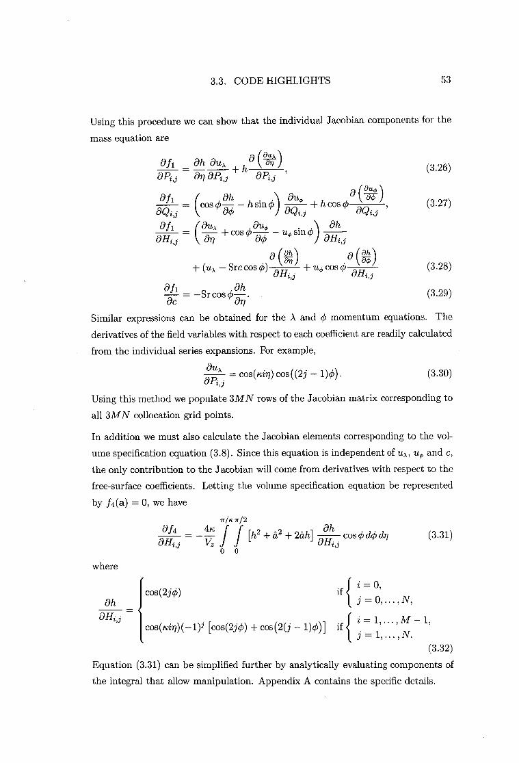
3.3. CODE HIGHLIGHTS 53
Using this procedure we can show that the individual Jacobian components for the
mass equation are
afi on au, + h a (#) aPio ail
(3.26) aPi,3 aP i,3
7
Oh 1 ( ah . No i au ■
= cos q5 h sin 0) + h cos 0 (3.27) aQi,i ao aQi,, ac2,,j ' afi. = (au >,
+ cos uo sin (i) 0 au4' aHi j an ao )
Oh ar-i,,,
a ( gh) a (gh) ± (2 1 x - Src cos 0) n u 77 ± t t 4, cos 0 (i5 (3.28)
ullid Oh = –Sr cos 0—
ah (3.29) Dc an • Similar expressions can be obtained for the A and 0 momentum equations. The
derivatives of the field variables with respect to each coefficient are readily calculated
from the individual series expansions. For example,
op = cos(Kiq) cos ((2j – 1).0) . (3.30)
Using this method we populate 3M N rows of the Jacobian matrix corresponding to
all 3M N collocation grid points.
In addition we must also calculate the Jacobian elements corresponding to the vol-
ume specification equation (3.8). Since this equation is independent of u, /t o and c,
the only contribution to the Jacobian will come from derivatives with respect to the
free-surface coefficients. Letting the volume specification equation be represented
by f4(a) = 0, we have
where
7r/k ir/2
[h + + 2ald af4 = 4n f 2 - a 2 - an
cos 0 chl)dn OH ij OH - ij
00 (3.31)
Oh cos(2j0) if {
cos(kiii)(-1) 3 [cos(2j0) + cos (2(j – 1))] if {
i = 0,
j = 0, , N ,
i = 1, , – 1,
j = 1, . . . , N.
aH1,,3
(3.32)
Equation (3.31) can be simplified further by analytically evaluating components of
the integral that allow manipulation. Appendix A contains the specific details.
au,,

3.3. CODE HIGHLIGHTS 54
3.3.7 Adaptive Integration Method
The integrals appearing in (3.7) and (3.31) are evaluated using numerical quadra-
ture. For the current study the technique of adaptive recursive quadrature is em-
ployed to evaluate the integrals, accurate to within a user defined relative tolerance
which can be as small as the machine precision of the computer on which the com-
putations are performed. The particular algorithm used is that of adaptive Lobatto
quadrature, with Kronrod extension of the Gauss-Lobatto formula, as detailed in
Gander & Gautschi [27] .
It is required to compute the volume integral (3.7) to high accuracy so that the
total volume of fluid is effectively conserved across separate runs of the program.
Using adaptive Lobatto quadrature we compute this integral to machine precision
with a relative tolerance of 1.0 x 10 -14 . In as far as the Jacobian is only used as
a means of finding an updating step direction, the machine accuracy employed in
calculating (3.7) is not required in the quadrature evaluation of (3.31). In fact,
computing (3.31) to high accuracy merely leads to significantly longer computation
times with little improvement in the overall direction of the updating step. For
this reason the accuracy of the Jacobian elements that are evaluated via quadrature
is sacrificed in favour of shorter computation times, with negligible difference in
algorithm efficiency in terms of producing a better estimate for the step direction.
3.3.8 Bootstrapping
In the present context we refer to bootstrapping as the process of taking a previous
solution and using this as the basis for an initial guess from which a new solution
is computed. The solution of the nonlinear problem requires three unique types of
bootstrapping.
The first type refers to the process of taking the coefficients and wavespeed computed
from the linearized model and computing an associated nonlinear solution. This
type of process can be used to compute nonlinear solutions when the corresponding
linearized solution is already known. This is only applicable when the amplitude is
small so that the nonlinear solution is approximated well by the linearized solution.
The second type of bootstrapping refers to the process of starting with a solution to
the nonlinear equations for a given truncation level and forcing one of the coefficients

3.4. SOLUTION AND RESULTS 55
in such a way as to produce another slightly different solution with the same trun-
cation level. This procedure forms the basis of mapping the wavespeed amplitude
relationship as it allows one to slowly increase either the wavespeed or amplitude
and incrementally trace out the underlying curve. It is this type of bootstrapping
that is employed most intensively in this study.
The third form of bootstrapping refers to taking a solution of the nonlinear system,
for a given truncation level, and increasing the truncation and computing the re-
sulting solution. This method can be used to verify numerically computed solutions
through a convergence argument. If the solution is shown to change little from
one truncation level to another we can be reasonably sure of the solution accuracy,
especially if a sizeable magnitude decrease is observed between the first and last
coefficient values in each series.
3.4 Solution and Results
3.4.1 Measuring the Amplitude
In order to investigate the relationship between the Rossby wavespeed and the am-
plitude, we require a means of measuring the amplitude, A, of a particular Rossby
wave. To elucidate this process, we first need to define what amplitude is. For a sim-
ple periodic wave pattern, the amplitude can be defined as the maximum deviation
of the wave as measured from the mean position to an extreme point. Fundamental
to this concept is the establishment of a universally agreed upon mean function
value. This mean value is usually chosen to be where the underlying medium would
reside if no wave pattern were present. For the case of one isolated periodic wave
structure, this position is intuitively obvious.
Now consider the problem of measuring Rossby wave amplitude horizontally on
a sphere, as depicted in the polar stereographic projection in Figure 3.1. To be
consistent we require just one mean state but due to the multitude of wave shapes
that are possible we see that there are an infinite number of mean states about
which we can measure wave deviation. We must therefore decide on exactly where
to measure amplitude from for any given wave. Because Rossby wave activity is
predominantly associated with the mid-latitude regions and also because 0 = +7r/4
represents the mid point between the equator and either pole, we choose the mean
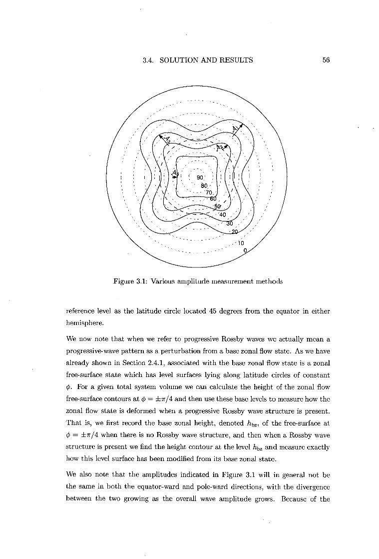
3.4. SOLUTION AND RESULTS 56
Figure 3.1: Various amplitude measurement methods
reference level as the latitude circle located 45 degrees from the equator in either
hemisphere.
We now note that when we refer to progressive Rossby waves we actually mean a
progressive-wave pattern as a perturbation from a base zonal flow state. As we have
already shown in Section 2.4.1, associated with the base zonal flow state is a zonal
free-surface state which has level surfaces lying along latitude circles of constant
(/). For a given total system volume we can calculate the height of the zonal flow
free-surface contours at 45 = ±7r/4 and then use these base levels to measure how the
zonal flow state is deformed when a progressive Rossby wave structure is present.
That is, we first record the base zonal height, denoted hbz , of the free-surface at
cb = ±774 when there is no Rossby wave structure, and then when a Rossby wave
structure is present we find the height contour at the level h b, and measure exactly
how this level surface has been modified from its base zonal state.
We also note that the amplitudes indicated in Figure 3.1 will in general not be
the same in both the equator-ward and pole-ward directions, with the divergence
between the two growing as the overall wave amplitude grows. Because of the
3.4. SOLUTION AND RESULTS 57
topology of the sphere it is possible for a Rossby wave to extend further towards
the equator than towards the pole where the lines of longitude converge. Thus to
record A effectively we will need to measure both the equator-ward and pole-ward
deflections, which we denote Ae and Ap respectively. Associated with these separate
but related amplitudes we define a simple averaged amplitude, the mean of the two
values, to be
A Ae + Ap ave • 2
(3.33)
In forthcoming sections when we present specific results we will plot the wavespeed
c versus each of the above defined amplitudes, namely Ae , Ap and Aave.
3.4.2 Parameters and Constants
Although this analysis is not specific to a given sphere size or mass it again seems
reasonable, as in the linearized model, to use parameters that closely approximate
those of the Earth so that direct comparison can be made between existing meteo-
rological models and observations. With this in mind we adopt the following values
for the sphere specific parameters:
a = 6.37122 x 10⁶ m, (3.34) 27r
Q = 24 x 3600
7.272 x 10⁻⁵s-1, (3.35)
g = 9.80616 m s -2 . (3.36)
Additionally we define each characteristic reference scale as
vref = 40ms-1 ,
href = 8.0 x 10³ m, ci
cref = —30
2.4241 x 10 -6 s-1 .
(3.37)
(3.38)
(3.39)
For the dimensionless zonal flow parameter w we will use two specific values. In
the linearized model we were afforded the luxury of being able to specify a broad
range of w values with little overhead incurred in terms of time taken to numerically
analyze the problem. Unfortunately, in the nonlinear model, we are no longer able to
investigate the solution dependency on w without incurring a significant increase in
the computation time. This is because at each value of w chosen we must compute a
complete solution curve for the c versus A relationship which involves many possible
3.4. SOLUTION AND RESULTS 58
values of the wavespeed, rather than the single value computed in the linearized
model. On average, to compute a complete solution curve for a fixed value of
w, many weeks of computational time is required for programs executing on the
previously documented hardware specifications in Section 3.3.1.
For this reason it was decided to restrict the investigation to two specific values of
the parameter w. The first value is consistent with the angular speed w used in the
test set proposed by Williamson et al. [87]. The second value, chosen to be 80% of
the first value, provides a slower and perhaps physically more realistic value for the
super rotation rate. In dimensionless form the two values are given by
Wi 1.25,
cv2 1.0.
The particular values above are obtained by noting that Williamson et al. use a
dimensional value for w of 7.848 x 10 -6 s-1- , a value first introduced by Phillips[66].
In order to convert this to a dimensionless number it is necessary to multiply by the
radius of the Earth and divide by the reference velocity scale so that
7.848 x 10⁻⁶a Wi = 1.25,
Vrof
W2 = 80%WlPs,' 1.0.
It is also necessary to specify a base volume 17, for the system, to be used in the
volume specification equation given by (3.8). For this study the value was chosen to
be the total volume contained between the surface of the sphere and the free-surface
shape defined by the zonal flow with parameters h, = 1 and w = 1.25. Thus the
base volume is simply the total volume of the atmosphere corresponding to purely
zonal flow with parameters equivalent to those used in Williamson et al. [87].
3.4.3 Results for i = 4, ce = 1.25
We now examine results obtained by solving the equations using the numerical
methods previously outlined. Because the process of root finding is quite sensitive
to the initial approximation to the root we use the first type of bootstrapping defined
in Section 3.3.8 to find an initial small-amplitude solution based on the linearized
result for equivalent parameter values in the model. Once we have obtained this
small amplitude nonlinear solution we then slowly force the wave amplitude by

Linearized solution
3.4. SOLUTION AND RESULTS 59
holding coefficient H1,1 fixed throughout the calculation and increasing its value
between successive runs of the program. Using this technique we build up a picture
of the overall relationship between the wavespeed and the amplitude.
Figure 3.2 shows the three solution curves when n = 4 and w = 1.25 for each of the
three measures of amplitude A, , Ap and Aa,ve defined previously in Section 3.4.1.
The truncation levels are M = 20 and N = 20 so that each series has a total of 400
coefficients, with a total of 1200 unknowns for the problem. Results were initially
computed at a lower truncation level of M = N = 10 to ascertain the general nature
of the relationship. Once the nature of the solution was established the truncation
was increased.
0.958
0.9575
0.956
0.9555
0.957
-6
I 0.9565
2
4
6 8 10 12
14
16 Amplitude (degrees)
Figure 3.2: Incompressible wavespeed versus amplitude for lc = 4 and w = 1.25
The error tolerance on the LI- norm of the residual vector was set at 10 -12 , leading
to average individual residual errors of the order of 10 -15 or less. The agreement
between the two levels of representation was found to be excellent with results at
the higher truncation level only differing marginally from those at the lower level,
providing evidence for the numerical convergence of the solutions calculated. In
particular, the third type of bootstrapping outlined in Section 3.3.8 was used to

3.4. SOLUTION AND RESULTS 60
increase the truncation level beyond M = N = 20 for a random sample of points
on the solution curve, and in all cases these higher resolution solutions were found
to differ negligibly from those for M = N = 20, and, at least for small amplitude,
from those of M = N = 10 as well.
The linearized solution is included and indicated in Figure 3.2, showing that for small
amplitude waves the linear and nonlinear solutions are essentially equivalent. As
the amplitude increases the wavespeed also increases, with the curve initially being
tangential to the linearized result for small A but diverging from the linearized result
and increasing more rapidly as A becomes larger. This behaviour is as expected
by analogy with other nonlinear wave calculations for gravitationally influenced
incompressible fluids, notably those of Stokes [78], Schwartz [71] and Cokelet [18].
These results, along with contributions from other key researchers in the field, are
summarised in the review article by Schwartz & Fenton [73].
160 I 20
180
200 Y4 340
220 320
240 300
Figure 3.3: Incompressible shallow atmosphere free-surface contours for k = 4, w = 1.25 at limit of computation. The average amplitude is Aave = 12.5104(deg.) and the wavespeed is c = 0.9580.
As the amplitude continues to increase the rate of wavespeed increase grows rapidly
until, ultimately, a limiting case is achieved numerically, where a slight curling over
of the curve is observed. The physical explanation of this limiting solution is not

3.4. SOLUTION AND RESULTS 61
clear from this example computation. It is possible, for example, that a sharp crest
might be formed somewhere in the flow field, as in the previously mentioned water-
wave case studied by Stokes and later by Schwartz. Alternatively, it may be the case
that the solution is topologically limited by enclosing bubbles, as found for the case
of gravity waves with surface tension by Schwartz & Vanden-Broeck [72], and Chen
Saffman [15]. However, an analysis of the free-surface contours at this limiting
wavespeed and amplitude combination, as shown in Figure 3.3, suggests that no
such behaviour is present.
We suggest, however, that some type of nonlinear resonance behaviour occurs, which
is not accessible to this numerical scheme because of the complexity of the solution
space and the implied sensitivity of Newton's method to the initial guess used.
Evidence supporting this statement is presented in the next section. Indeed, it
is suspected that the limiting wavespeed-amplitude combination indicated in Fig-
ure 3.2 is only really limited by the numerical solution method and that, in reality,
significantly faster and larger waves exist beyond the shown limit. Exhaustive at-
tempts to find such larger waves were made using numerous methods. In particular
the algorithm was changed so that the wavespeed became the forcing parameter in
an attempt to look for faster progressive waves; however convergence of the residual
vector was not obtained. In addition, the results obtained with the lower trunca-
tion level of M = N = 10 were found to converge for slightly larger amplitudes
and wavespeeds, although it was then found that subsequent bootstrapping of these
lower resolution solutions to ones at a higher resolution produced non-convergent
residuals. We must therefore reject these results at this point until further analytical
and numerical work can be done to investigate this behaviour.
3.4.4 Results for n = 4, ci.) = 1.0
The solution curves shown in Figure 3.4 represent results obtained with the values
= 4 and w = 1.0. The truncation levels were set at M = N = 15 with initial curves
mapped out using M = N = 10; little overall difference was observed between the
two resolutions. The error tolerance on the L 1 norm of the residual vector was set at
10 -12 , leading to average individual residual errors of the order of 10 -15 or less. Like
the previous example, the solution agrees well with the linearized result for small
amplitude waves and as A increases so does the wavespeed c. However, as opposed
to the previous case for w = 1.25, distinct discontinuous jumps are now evident,
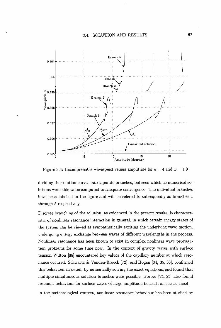
20 10 15 Amplitude (degrees)
Branch 5 0.401
Branch 4
Branch '1"(
'.0.399
Branch 2
0.398
Branch 1
0.397
ye
0.396
Linearized solution
Figure 3.4: Incompressible wavespeed versus amplitude for tc = 4 and co = 1.0
0.4
0.395o
3.4. SOLUTION AND RESULTS 62
dividing the solution curves into separate branches, between which no numerical so-
lutions were able to be computed to adequate convergence. The individual branches
have been labelled in the figure and will be refered to subsequently as branches 1
through 5 respectively.
Discrete branching of the solution, as evidenced in the present results, is character-
istic of nonlinear resonance interaction in general, in which certain energy states of
the system can be viewed as sympathetically exciting the underlying wave motion,
undergoing energy exchange between waves of different wavelengths in the process.
Nonlinear resonance has been known to exist in complex nonlinear wave propaga-
tion problems for some time now. In the context of gravity waves with surface
tension Wilton [88] encountered key values of the capillary number at which reso-
nance occured. Schwartz & Vanden-Broeck [72], and Hogan [34, 35, 36], confirmed
this behaviour in detail, by numerically solving the exact equations, and found that
multiple simultaneous solution branches were possible. Forbes [24, 25] also found
resonant behaviour for surface waves of large amplitude beneath an elastic sheet.
In the meteorological context, nonlinear resonance behaviour has been studied by
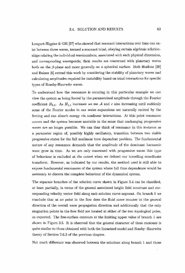
3.4. SOLUTION AND RESULTS 63
Longuet-Higgins & Gill [57] who showed that resonant interactions over time can ex-
ist between three waves, termed a resonant triad, obeying certain algebraic relation-
ships relating the individual wavenumbers, associated with each physical dimension,
and corresponding wavespeeds; their results are concerned with planetary waves
both on the 0-plane and more generally on a spherical surface. Both Hoskins [39]
and Baines [6] extend this work by considering the stability of planetary waves and
calculating amplitudes required for instability based on triad interactions for specific
types of Rossby-Haurwitz waves.
To understand how the resonance is occuring in this particular example we can
view the system as being forced by the parametrized amplitude through the Fourier
coefficient H1 , 1 . As H1 , 1 increases we see A and c also increasing until suddenly
some of the Fourier modes in our series expansions are naturally excited by the
forcing and can absorb energy via nonlinear interactions. At this point resonance
occurs and the system becomes unstable in the sense that unchanging progressive
waves are no longer possible. We can thus think of resonance in this instance as
a parameter region of, possibly highly oscillatory, transition between two stable
progressive states for the full nonlinear time dependent problem. The fundamental
nature of any resonance demands that the amplitude of the dominant harmonic
wave grow in time. As we are only concerned with progressive waves this type
of behaviour is excluded at the outset when we defined our travelling coordinate
transform. However, as indicated by our results, the method used is still able to
expose fundamental resonances of the system where full time dependence would be
necessary to discern the complete behaviour of the dynamical system.
The separate branches of the solution curve shown in Figure 3.4 can be classified,
at least partially, in terms of the general associated height field structure and cor-
responding velocity vector field along each solution curve segment. On branch 1 we
conclude that at no point in the flow does the fluid move counter to the general
direction of the overall wave propagation direction and additionally that the only
stagnation points in the flow field are located at either of the two topological poles,
as expected. The free-surface contours at the limiting upper value of branch 1 are
shown in Figure 3.5. It is observed that the general character of these contours is
quite similar to those obtained with both the linearized model and Rossby—Haurwitz
theory of Section 2.6.3 of the previous chapter.
Not much difference was observed between the solutions along branch 1 and those
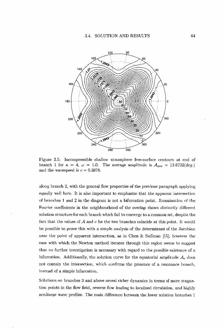
160 20
180
200
3.4. SOLUTION AND RESULTS 64
Figure 3.5: Incompressible shallow atmosphere free-surface contours at end of branch 1 for ic = 4, w = 1.0. The average amplitude is Aave = 13.6732(deg.) and the wavespeed is c = 0.3978.
along branch 2, with the general flow properties of the previous paragraph applying
equally well here. It is also important to emphasize that the apparent intersection
of branches 1 and 2 in the diagram is not a bifurcation point. Examination of the
Fourier coefficients in the neighbourhood of the overlap shows distinctly different
solution structure for each branch which fail to converge to a common set, despite the
fact that the values of A and c for the two branches coincide at this point. It would
be possible to prove this with a simple analysis of the determinant of the Jacobian
near the point of apparent intersection, as in Chen & Saffman [15]; however the
ease with which the Newton method iterates through this region seems to suggest
that no further investigation is necessary with regard to the possible existence of a
bifurcation. Additionally, the solution curve for the equatorial amplitude Ae does
not contain the intersection, which confirms the presence of a resonance branch,
instead of a simple bifurcation.
Solutions on branches 3 and above reveal richer dynamics in terms of more stagna-
tion points in the flow field, reverse flow leading to localised circulation, and highly
nonlinear wave profiles. The main difference between the lower solution branches 1
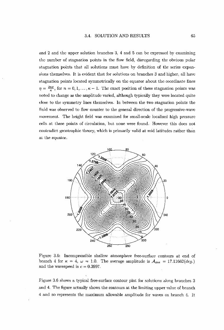
3.4. SOLUTION AND RESULTS 65
and 2 and the upper solution branches 3, 4 and 5 can be expressed by examining
the number of stagnation points in the flow field, disregarding the obvious polar
stagnation points that all solutions must have by definition of the series expan-
sions themselves. It is evident that for solutions on branches 3 and higher, all have
stagnation points located symmetrically on the equator about the coordinate lines = for ii = 0, 1, — 1. The exact position of these stagnation points was
noted to change as the amplitude varied, although typically they were located quite
close to the symmetry lines themselves. In between the two stagnation points the
fluid was observed to flow counter to the general direction of the progressive-wave
movement. The height field was examined for small-scale localised high pressure
cells at these points of circulation, but none were found. However this does not
contradict geostrophic theory, which is primarily valid at mid latitudes rather than
at the equator.
160 20
180
200 340
240 300
260 280
Figure 3.6: Incompressible shallow atmosphere free-surface contours at end of branch 4 for ic = 4, ci.) = 1.0. The average amplitude is Aave = 17.11662(deg.) and the wavespeed is c = 0.3997.
Figure 3.6 shows a typical free-surface contour plot for solutions along branches 3
and 4. The figure actually shows the contours at the limiting upper value of branch
4 and so represents the maximum allowable amplitude for waves on branch 4. It
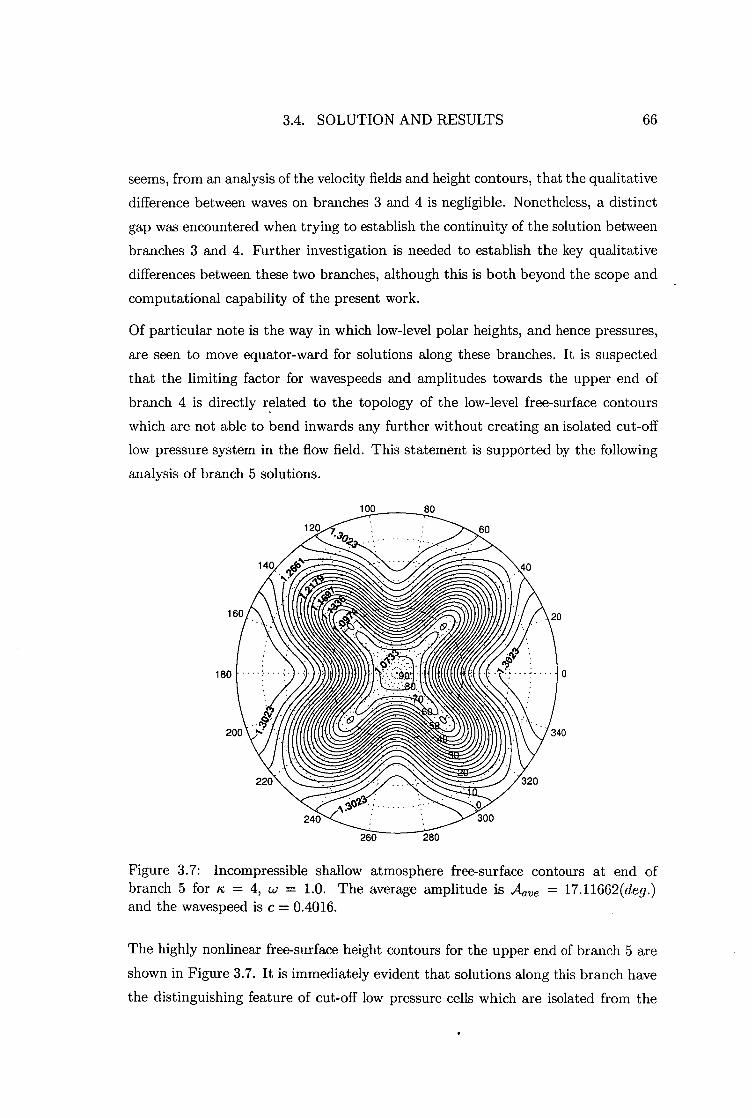
3.4. SOLUTION AND RESULTS 66
seems, from an analysis of the velocity fields and height contours, that the qualitative
difference between waves on branches 3 and 4 is negligible. Nonetheless, a distinct
gap was encountered when trying to establish the continuity of the solution between
branches 3 and 4. Further investigation is needed to establish the key qualitative
differences between these two branches, although this is both beyond the scope and
computational capability of the present work.
Of particular note is the way in which low-level polar heights, and hence pressures,
are seen to move equator-ward for solutions along these branches. It is suspected
that the limiting factor for wavespeeds and amplitudes towards the upper end of
branch 4 is directly related to the topology of the low-level free-surface contours
which are not able to bend inwards any further without creating an isolated cut-off
low pressure system in the flow field. This statement is supported by the following
analysis of branch 5 solutions.
180
200 340
220 320
240 300
Figure 3.7: Incompressible shallow atmosphere free-surface contours at end of branch 5 for lc = 4, w = 1.0. The average amplitude is A .—ave = 17.11662(deg.) and the wavespeed is c = 0.4016.
The highly nonlinear free-surface height contours for the upper end of branch 5 are
shown in Figure 3.7. It is immediately evident that solutions along this branch have
the distinguishing feature of cut-off low pressure cells which are isolated from the

Stagnation points Reverse flow
1/
t)
/I
I
3.4. SOLUTION AND RESULTS 67
general progressive-wave structure. In addition to the already mentioned stagnation
points in the flow field for waves on branches 3 and higher, more stagnation points
are introduced for waves on the fifth branch, this time occuring close to the poles
of the coordinate system rather than near the equator. It was initially suspected
that the centre of each cut-off low pressure cell must be a stagnation point; however
careful analysis of the velocity vector field did not confirm this. Nonetheless the
velocity in the vicinity of these cells is quite small compared to the rest of the flow
field and can almost be described as circulatory about the centre of each cell.
It is of interest to note that the stagnation points introduced for branch 5 solutions
occur immediately below each cut-off low pressure cell as indicated in figure 3.8.
Also shown are all previously mentioned stagnation points as well as regions of
circulation, labeled reverse flow. We can conclude that generally the flow is seen to
be geostrophic in the sense that the streamlines are nearly parallel to the isobars.
This is clearly true in the neighbourhood of the perturbed 0 = ±7/4 zonal flow
contour that forms the basis of the numerical analysis in this section.
Figure 3.8: Incompressible shallow atmosphere free-surface contours with corre-sponding velocity vector field at end of branch 5 for ic = 4, w = 1.0. The average amplitude is Aave = 17.11662(deg.) and the wavespeed is c = 0.4016.

10 2
4 6 8 Amplitude (degrees)
1.5815
Branch 2
1.581
c.) 1.5805
cna'
1.58
1.5795
Linearized solution
1.5790
3.4. SOLUTION AND RESULTS 68
The fate of the solution curves past the end of branch 5 is still uncertain. Attempts
were made to compute more points beyond the limits shown but in all cases conver-
gence was not achieved. It might be that our numerical method is not well suited
to computing past points where the slope of the curve is nearly infinite, in which
case improved techniques are required to investigate the behaviour past the limit
shown. Alternatively this may be close to the maximum allowable amplitude of the
system, imposed as a consequence of the finite size and topology of the sphere. An
analysis of the constraints of potential vorticity conservation of Rossby waves on a
0-plane by Lindzen & Schoeberl [52] revealed that there are finite limits to the size
of Rossby wave amplitudes. This reasoning should apply even more so to the sphere
where the finite size becomes an important attribute of the problem.
3.4.5 Results for K = 5, co = 1.25
Figure 3.9: Incompressible wavespeed versus amplitude for lc = 5 and w = 1.25
It is of interest to study how the dynamical system behaves with an alternative value
of the wave number n. We now present results obtained with n = 5, using the same
pair of values (w = 1.25 and w = 1.0) for the dimensionless zonal flow super rotation;

3.4. SOLUTION AND RESULTS 69
in this section we examine the case cv = 1.25. Figure 3.9 shows the computed
wavespeed versus amplitude relationship using a truncation of M = N = 20. The
error tolerance on the L1 norm of the residual vector was set at 10 -12 , leading to
average individual residual errors of the order of 10-15 or less.
The same general trend as for K = 4 is encountered here for Ic = 5, with the linearized
solution being a good approximation to the nonlinear solution for small A and the
wavespeed becoming increasingly greater as the amplitude is increased. It appears
that the use of K = 5 introduces a new phenomenon in the form of a localised cubic
structure located near c ,-z-, 1.5807. It was initially suspected that this was in fact
two distinct branches separated by a resonance; however it was possible to compute
continuously through this region, using a very small step size, without encountering
any non convergent solutions.
Therefore it seems that there are at least two explanations for this behaviour. The
first is that there is in fact a resonance occuring near the point of inflexion, but
existing on such a small scale that we were unable to detect it on any occasion.
This does not seem very likely given the nature of the previous nonlinear resonances
observed for the case K = 4, u.) = 1.0. The second explanation is that this is
a feature of the dynamics and forcing, in which energy exchange between certain
wavelengths is taking place in such a maner as to increase the overall amplitude
while at the same time reducing the wavespeed. If so, this would represent a type
of damped resonance, but careful analytical work, beyond the scope of this study,
would be needed to identify the physical nature of the damping mechanism. Despite
this localised reversal of the general trend of the graph, no obvious distinguishing
features are visible when we examine the free-surface contours and velocity vector
field in the vicinity of this solution region. This fact seems to support the conjecture
that separate resonance branches do not exist in this case.
Two separate solution branches were found to exist towards the upper end of the
curve when the limiting amplitude-wavespeed combination was approached. Be-
cause it is not entirely clear from the figure, it needs to be emphasized that the first
branch terminates in the vicinity of c ,--:: 1.5812; thus the highest possible wavespeed
indicated is at the right end of branch 2. It is again unlikely that the apparent in-
tersection of the two branches is a sign of a simple bifurcation, for reasons outlined
in the previous section.

3.4. SOLUTION AND RESULTS 70
For the left end of the second branch, numerical results have in fact been computed
well beyond the termination point shown in the figure. However, it appears that
they are of questionable validity due to increasing numerical error along that branch
and have therefore not been shown. The ultimate fate of this upper branch is not
clear and may perhaps require alternative numerical techniques to reveal. In any
event it is possible that this branch is physically unstable, the system preferring
the lower wavespeed over the higher one, and so would generally not be observed in
practice. It is even possible that a physical instability in this branch might produce
a numerical instability, since the numerical iteration process may be equivalent to
stepping forward in time, as has been shown in various applications of the Peaceman-
Rachford ADI method to the heat equation, documented in Ames [3, page 149].
100 80
120 60
160 20
180
200 340
220 320
240 300
Figure 3.10: Incompressible shallow atmosphere free-surface contours at end of branch 1 for = 5, w = 1.25. The average amplitude is A -ave = 8.3678(deg.) and the wavespeed is c = 1.5812.
Typical free-surface contours of the system are presented in Figure 3.10, showing
the nature of the solution at the end of branch 1. In contrast to the highly non-
linear structures computed at the end of the curve for ic = 4 and w = 1.0, these
contours exemplify the significantly smaller maximum amplitude for which a con-
vergent wavespeed was able to be calculated. In addition, no defining qualitative

2 4
6 8
10 Amplitude (degrees)
0.9946
0.9944
0.9942
0.994
Linearized solution
_1(
Figure 3.11: Incompressible wavespeed versus amplitude for ic = 5 and w = 1.0
0.993o 12
Aave 11" 0.9938
0.9936
0.9934
0.9932
3.4. SOLUTION AND RESULTS 71
features of the velocity field were found that could be used to distinguish easily
between the two solution branches. It is possible that more solution curves exist
beyond those that are indicated; however attempts to find such solutions were not
successful.
3.4.6 Results for ic = 5, w = 1.0
For completeness we present results in this final section for lc = 5 and w = 1.0.
Figure 3.11 shows the computed solution curves obtained with the truncation level
M = N = 15. The error tolerance on the L 1 norm of the residual vector was again
set at 10 -12 . The general features of this figure are less remarkable than those for
the preceding set of results obtained with w = 1.25, although there is some evidence
for a similar localised cubic structure, this time in the vicinity of c = 0.99395. The
severity of this local cubic behaviour, however, is significantly less noticeable and
does not substantially influence the general increase of c with A. As in all previous
solution curves presented, the results here agree well with the linearized value of the
wavespeed for small values of the amplitude.
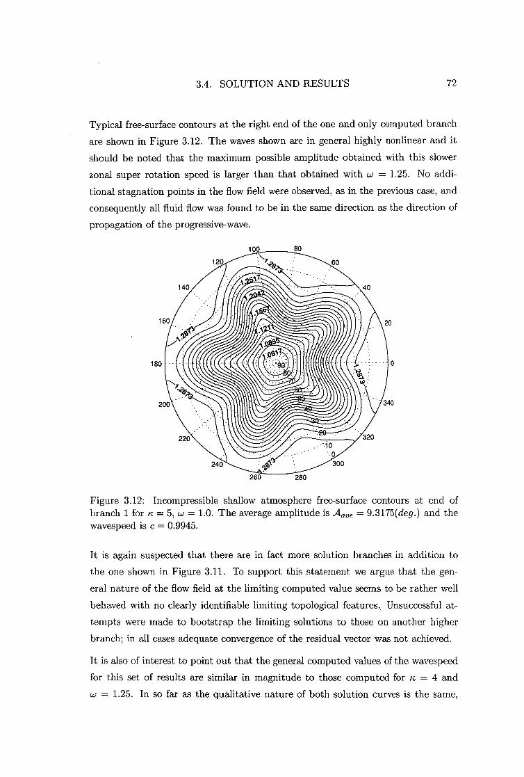
3.4. SOLUTION AND RESULTS 72
Typical free-surface contours at the right end of the one and only computed branch
are shown in Figure 3.12. The waves shown are in general highly nonlinear and it
should be noted that the maximum possible amplitude obtained with this slower
zonal super rotation speed is larger than that obtained with w = 1.25. No addi-
tional stagnation points in the flow field were observed, as in the previous case, and
consequently all fluid flow was found to be in the same direction as the direction of
propagation of the progressive-wave.
100 80
120 60
180
200 340
220 320
240 300
Figure 3.12: Incompressible shallow atmosphere free-surface contours at end of branch 1 for Ic = 5, w = 1.0. The average amplitude is Aa„, = 9.3175(deg.) and the wavespeed is c =- 0.9945.
It is again suspected that there are in fact more solution branches in addition to
the one shown in Figure 3.11. To support this statement we argue that the gen-
eral nature of the flow field at the limiting computed value seems to be rather well
behaved with no clearly identifiable limiting topological features. Unsuccessful at-
tempts were made to bootstrap the limiting solutions to those on another higher
branch; in all cases adequate convergence of the residual vector was not achieved.
It is also of interest to point out that the general computed values of the wavespeed
for this set of results are similar in magnitude to those computed for ic = 4 and
w = 1.25. In so far as the qualitative nature of both solution curves is the same,
3.5. CLOSING REMARKS 73
it seems reasonable to speculate that all solutions in the vicinity of this wavespeed
behave in a similar manner. That is to say that a general increase of c is seen with
increasing A for all values of K and appropriate value of w.
3.5 Closing Remarks
In this chapter we have successfully solved the complete nonlinear equations gov-
erning shallow atmosphere free-surface flow with embeded progressive Rossby wave
structures. Solutions in the form of finite Fourier series were obtained using a col-
location method with an associated Newton iterative scheme. By starting close to
the linearized solutions computed in the previous chapter and forcing the amplitude
to increasingly larger values we were able to successfully step along the wavespeed
versus amplitude solution curves for specific values of the parameters K and w.
Results obtained show that a relationship exists between increasing wave amplitude
and wavespeed; these are similar to the well know results for gravity influenced
free-surface waves. For the specific case of n = 4 and w = 1.0 we found substantial
evidence for nonlinear resonance in the system, with adjacent solution branches be-
ing separated by areas in which no solutions could be computed to within reasonable
convergence. At the limit of computability it was shown that highly nonlinear wave
profiles are possible with areas of cut off low pressure being a key feature of the
system at this critical limit. It is suspected that this behaviour exists in general, at
least to some extent, for all solutions that were investigated; however attempts to
confirm this have thus far been unsuccessful with questionable results. It is highly
unlikely that numerical methods alone can answer this existence question. Analyti-
cal techniques may be required to address this issue, however these are beyond the
scope of the present investigation.

CHAPTER 4
COMPRESSIBLE LINEARIZED SHALLOW ATMOSPHERE
MODEL
4.1 Derivation
We consider here the derivation of the compressible shallow atmosphere equations
in a rotating spherical coordinate system, again following the general approach de-
veloped in Pedlosky[65], with appropriate modifications for a compressible fluid.
For ease of reference and completeness we treat the derivation in this section as
distinct from that of the incompressible case derived in Section 2.1, although both
derivations share some similarities.
Refering to Figure 4.1, define h as the radial height above the level surface r = a of
a free-surface surrounding a rotating reference sphere of radius r = a. Additionally,
define h and hb as the depth of the fluid and the height of the underlying mountains
respectively. The height of the free-surface, h, can be given in terms of the two
parameters hb and h as
h = hb + h. (4.1)
Although the generality of this setup affords the representation of a much wider
class of problem we will restrict ourselves to the case when there is no underlying
mountain specification so that hb = 0, leading to
h = h. (4.2)
For this study we will be concerned with compressible, adiabatic fluid flow. Because
74
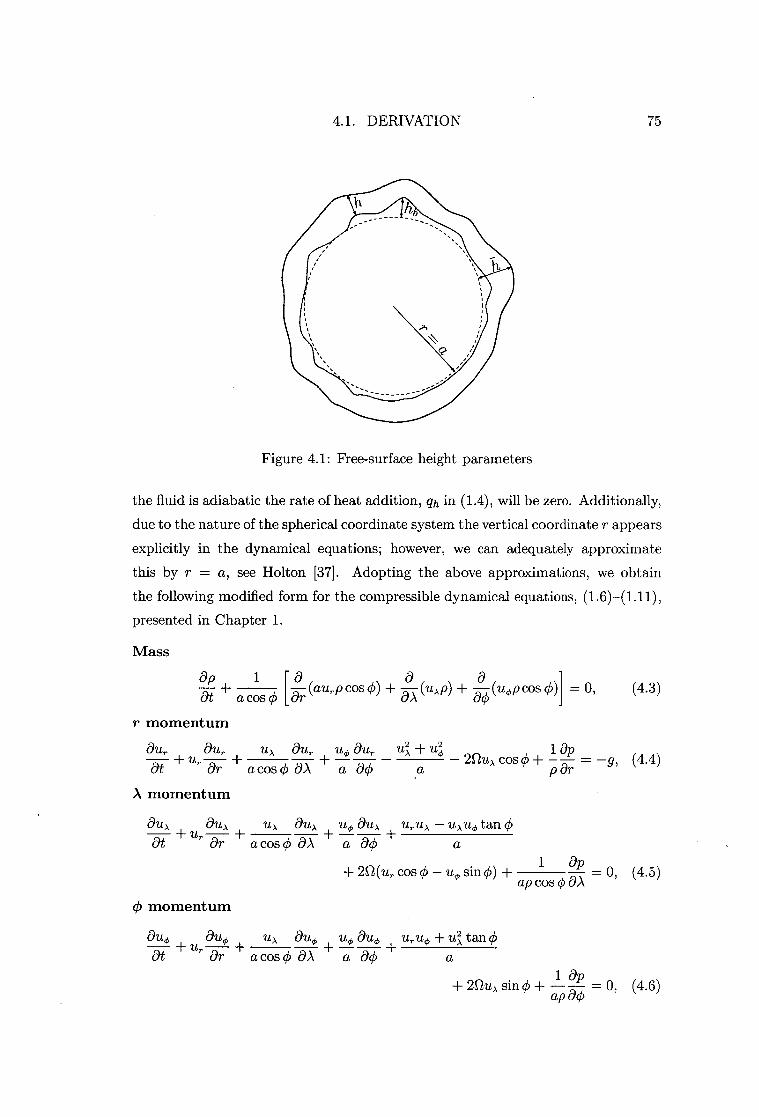
4.1. DERIVATION 75
Figure 4.1: Free-surface height parameters
the fluid is adiabatic the rate of heat addition, qh in (1.4), will be zero. Additionally,
due to the nature of the spherical coordinate system the vertical coordinate r appears
explicitly in the dynamical equations; however, we can adequately approximate
this by r = a, see Holton [37]. Adopting the above approximations, we obtain
the following modified form for the compressible dynamical equations, (1.6)-(1.11),
presented in Chapter 1.
Mass
Op 11 8 a a 4- a cos Or
(au r p cos 0) + Nt (u AP) + ,Tb (uop cos 0)1 = 0, Tai 0 (4.3)
r momentum
aUr aUr U), aU r Uo aUr2 2 ± -- = —g, (4.4) + Ur - + +
U), + U 1 aP o 2QUA COS o at Or a cos o aA a ao a p or
,
A momentum
+ Ur
14 au„ u,,, au, + uru„ — u,,u, tan 0 - + + at Or a cos 0 OA a ao a 1 Op ± 2Q(u r cos .0 - u ck sin 0) + ap cos 0 aA = 0 ' (4.5)
c/) momentum
auo Otto u >, alto uo auo uruo + u2,, tan 0 + ur — + + + Ot ar a cos 0 OA a ao a 1 Op + 2Qui sin 0 + —ap —(90
= 0, (4.6)
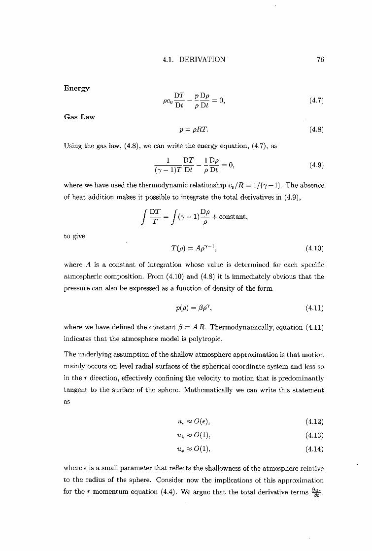
4.1. DERIVATION 76
Energy DT pDp _ 0
(Icy Dt - -19 Dt ' Gas Law
p = pRT.
Using the gas law, (4.8), we can write the energy equation, (4.7), as
1 DT 1 Dp _ 0 (-y - 1)T Dt pDt '
(4.7)
(4.8)
(4.9)
where we have used the thermodynamic relationship cvIR =11(y- 1). The absence
of heat addition makes it possible to integrate the total derivatives in (4.9),
f DT „Dp T - f (7 - 1 ) — + constant,
P
to give
T(p) = Ap7-1 , (4.10)
where A is a constant of integration whose value is determined for each specific
atmospheric composition. From (4.10) and (4.8) it is immediately obvious that the
pressure can also be expressed as a function of density of the form
P(p) = 13,07 , (4.11)
where we have defined the constant 0 = AR. Thermodynamically, equation (4.11)
indicates that the atmosphere model is polytropic.
The underlying assumption of the shallow atmosphere approximation is that motion
mainly occurs on level radial surfaces of the spherical coordinate system and less so
in the r direction, effectively confining the velocity to motion that is predominantly
tangent to the surface of the sphere. Mathematically we can write this statement
as
(4.12)
(4.13)
(4.14)
where E is a small parameter that reflects the shallowness of the atmosphere relative
to the radius of the sphere. Consider now the implications of this approximation
for the r momentum equation (4.4). We argue that the total derivative terms a*,

4.1. DERIVATION 77
, aUr t A_ au, a cos
um au, are all OW so that the r momentum equation reduces a
ar 5 ck and to
2 2 UA 1- U0 2Stux cos 0 +
= -g. (4.15)
a p ar
Additionally, we assume that (4.15) is dominated by hydrostatics' so that effectively
we have ap or = -Pg '
which in conjunction with (4.11), we arrive at
(4.16)
_ —9 v ar g-y •
Integration with respect to r yields
P7-1 (r, A, 0, t) = (A, 0, t) - 1)r
07 •
The value of fi (A, 0, t) is ascertained by assuming that on the free-surface, r =
a + h(A, 0, t), the density has the constant value Po , so that
p1-1 (r, A, 0, t) = P-0Y-1 + - 1) (a + h(A, 0, t) - r). (4.17)
Using (4.17) we can solve for p. With the addition of (4.10) and (4.11) we obtain
formulae for the thermodynamic variables in the problem. The results are
1 p(r, A,0, t) = [pr l + 1) (a + h(A,0, t) - 1 , (4.18)
- 1 p(r, A, 0, t) = [pY -1 + (a + h(A, 0, t) - r)] (4.19)
T (r , A, 0, t) = A [p-or + g(-y - 1) (a + h(A, 0, t) - r)] . (4.20)
From (4.18) and (4.19) we can show that
ap _ aA gP OA' ap an
g P TO'
(4.21)
(4.22)
'We can be more rigorous than this and use a scale analysis approach to argue this point. See Pedlosky[65, page 60] for the finer details of this process
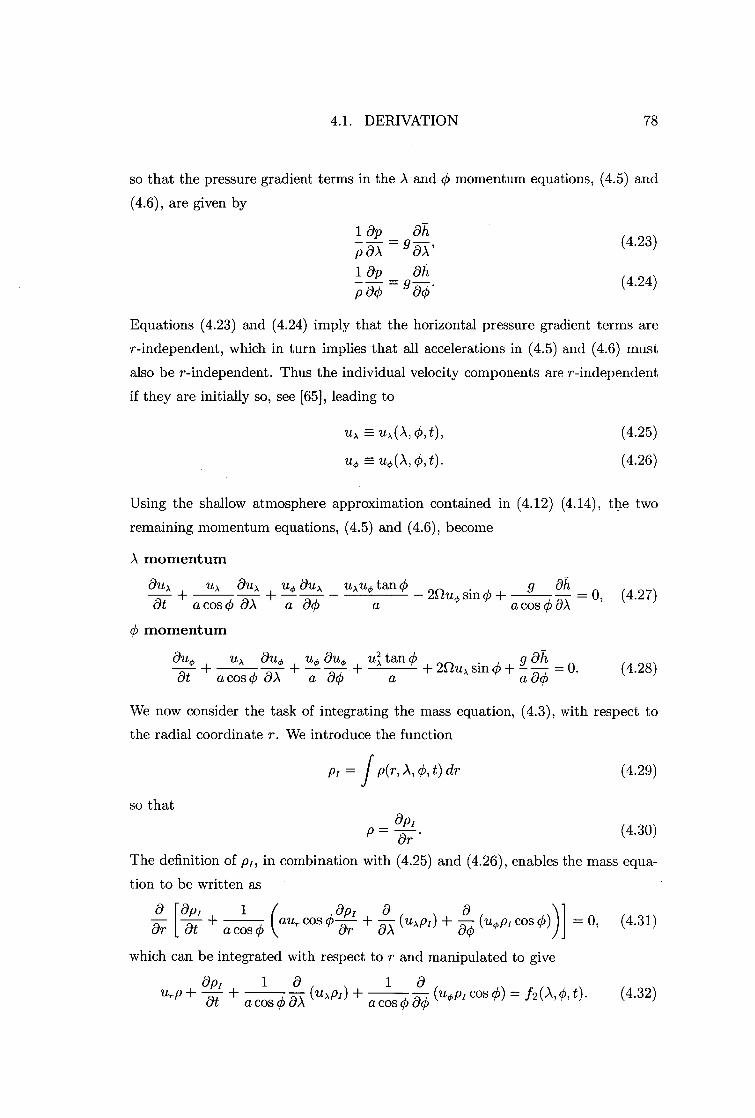
4.1. DERIVATION 78
so that the pressure gradient terms in the A and 0 momentum equations, (4.5) and
(4.6), are given by
1 Op Oh _ = g p OA DA lap_ ah P ad) 80
(4.23)
(4.24)
Equations (4.23) and (4.24) imply that the horizontal pressure gradient terms are
r-independent, which in turn implies that all accelerations in (4.5) and (4.6) must
also be r-independent. Thus the individual velocity components are r-independent
if they are initially so, see [65], leading to
(4.25)
no uo (A, 0, t). (4.26)
Using the shallow atmosphere approximation contained in (4.12)-(4.14), the two
remaining momentum equations, (4.5) and (4.6), become
A momentum
au), u), &ILA U4, aux u04, tan 0 Milo sin 0 + g ah = 0, (4.27) + + at a cos 0 OA a 00 a a cos 0 OA
0 momentum
auo ux No uct, Ouo u 2, tan 0 g ah =0. (4.28) + + Ot a cos 0 aA +
a ± 25-lux sin 0 + 00
We now consider the task of integrating the mass equation, (4.3), with respect to
the radial coordinate r. We introduce the function
Pi = I p(r, A, 0, t) dr (4.29)
so that api P = • (4.30) Or
The definition of p i , in combination with (4.25) and (4.26), enables the mass equa-
tion to be written as
a [ap, 1 ap, a a (au, cos 0 (u API) (uop cos 0))1= 0, (4.31) ar [ at + a cos 0
which can be integrated with respect to r and manipulated to give
Op/ 1 a 1 a ± (uAP/) ± a cos
(uopi cos 0) = f2 (A, 0, t). (4.32)
+ at a cos 0 OA 0 a0
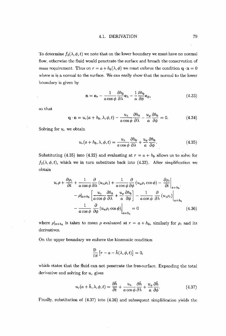
4.1. DERIVATION 79
To determine f2 (A, 0, t) we note that on the lower boundary we must have no normal
flow, otherwise the fluid would penetrate the surface and breach the conservation of
mass requirement. Thus on r = a+ hb(A, 0) we must enforce the condition q • n = 0
where n is a normal to the surface. We can easily show that the normal to the lower
boundary is given by
so that
n = er 1 ahb lDhb
a cos o aAeA aoe° ,. (4.33)
q • n = ur (a + hb, , 0, t)
uA ahb 214, ahb 0 acosq aA a ao (4.34)
Solving for Ur we obtain
/IA ahb u ahb
ur(a+ hb, A, , t) = + — . (4.35)
a cos 0 aA a ao
Substituting (4.35) into (4.32) and evaluating at r = a + hb allows us to solve for
f2(A, 0,0, which we in turn substitute back into (4.32). After simplification we
obtain
api 1 a, 1 a apI urp + + kuApi) + (no cos 0) — idt a cos0 aA a cos ao at a+hb
[a coA ahb u
s o aA a ao a cos aA u o ahb i 1 a „
Pla+hb ku xpo
1 a (uopi cos 0) = 0 a+hb a cos 0 ao
a+hb
(4.36)
where pl a+hb is taken to mean p evaluated at r = a + hb, similarly for Pi and its
derivatives.
On the upper boundary we enforce the kinematic condition
Dt [r — a— h(A, .0,0] = 0,
which states that the fluid can not penetrate the free-surface. Expanding the total
derivative and solving for up gives
ah uA 0h u ah + at a cos 0 aA a ao . (4.37)
Finally, substitution of (4.37) into (4.36) and subsequent simplification yields the
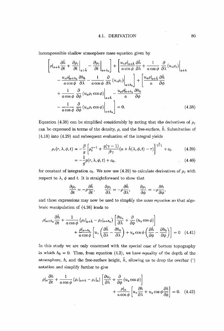
[
, an op' Pla-Fh at + at
aPI
a+h at ± [uola+h ah 1 a
a cos 0 8A a cos
4.1. DERIVATION 80
incompressible shallow atmosphere mass equation given by
1 a ,,,Api) uc Pia-Eh ah a cos ax' al-hb a ao
ItApla-Fh b ahb a cos 0 OA
1 a do
op, cos 0) a cos 0 p
1 a op, cos 0) a cos 0 aop
uoPla-Fhb anb a (90 ad-h
a-Fhb
0 (4.38)
Equation (4.38) can be simplified considerably by noting that the derivatives of p,
can be expressed in terms of the density, p, and the free-surface, h. Substitution of
(4.18) into (4.29) and subsequent evaluation of the integral yields
pi (r, ), 0, t) = [p-cr i + 9(7 1) (a + h(A, t) r)]
+ co (4.39)
1 = --P(r, A, 0, t) + CO , (4.40)
for constant of integration co. We now use (4.39) to calculate derivatives of pi with
respect to A, 0 and t. It is straightforward to show that
Op, an ap,an ap, an at P —-ä' P a A' ao ark'
and these expressions may now be used to simplify the mass equation so that alge-
braic manipulation of (4.38) leads to
, an 1 attA + (u0 cos 0)1 Pla+hb ± a cos kPlIa+h P Ila-f-hb [—OA aq5
+ pla+hbrujahohb) +uocoso (ah ahb)1
a cos 0 1_ aA aA = 0 (4.41)
In this study we are only concerned with the special case of bottom topography in which hb = 0. Thus, from equation (4.2), we have equality of the depth of the
atmosphere, h, and the free-surface height, h, allowing us to drop the overbar (-) notation and simplify further to give
Oh 1 , au ), a , Pia a cos WI la+h P r la ) [ -5)T y 24, COS 0)]
a cPoi: [u), Nah + cos 0--,97k1 = 0. (4.42)

4.1. DERIVATION 81
Note that from (4.40) we can replace all occurances of pi with equivalent pressure
terms so that we can also write (4.42) as
1 [ 0a e
g t, (pia
pla+h) u, cos 0
at cb A PlaLh + a cos ) +
(90 g (Pia — Pla+h))] = O. (4.43)
As a check of the validity of this equation we note that if the fluid is incompressible,
that is p is constant, then p = po + pg(a + h – r) so that
Pla Pla+h = PO,
and thus (4.43) becomes
Oh 1 a (u ),h) 4(u,hcosc,))]=0, at ± 0 a cos LaA
which is identical to (2.27) from the incompressible derivation.
To the extent that the aim of this study is to investigate progressive Rossby wave
structures, we again introduce a coordinate frame involving the progressive angular
wavespeed c and longitudinal and time coordinates, A and t, as in Section 2.2 of
Chapter 2. We define
= A – ct
as the new travelling coordinate system, with the effect of the –ct term being to
translate any initial wave structure either towards the west (c < 0) or towards the
east (c > 0) with constant angular speed c.
Applying the coordinate transformation to the governing equations and writing
f = 2S2 sin ck, we can express the complete dimensional dynamical equations of
motion for a thin layer of compressible fluid with a free-surface in a rotating spherical
coordinate system as
mass
, Oh [0 „ a —cga cos OPlax-7 + 571 (u), Pla+h )) —ack (11,0 COS 0 (Pia Pla+h))] = 0, (4.44)
A momentum
(u ), ILA u 4, cos 4) au, (f cos ck + —u:
+ —g
—Oh
= 0, (4.45) — – c cos q5) (
a 07/ a 00 a 07/
ci) momentum
+ – c cos ) Otto uo cos ck auo sin
cos Oh = 0, (4.46)
(,f cos + sm qS) u ), a a 00 a a 00
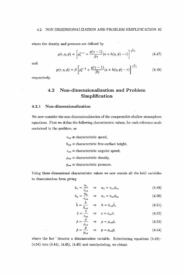
4.2. NON-DIMENSIONALIZATION AND PROBLEM SIMPLIFICATION 82
where the density and pressure are defined by 1
P(r, n, 0) = [Pj -1 + g(7 - 1)(a + h(n,46) —
^y — 1
(4.47)
and
respectively.
—1 r Pfr,n, 0) = 0 ge - 1 ) [p-i; + (a + 07, Cb) (4.48)
4.2 Non-dimensionalization and Problem Simplification
4.2.1 Non-dimensionalization
We now consider the non-dimensionalization of the compressible shallow atmosphere
equations. First we define the following characteristic values, for each reference scale
contained in the problem, as
vrof H characteristic speed,
hrof H characteristic free-surface height,
c„f H. characteristic angular speed,
Prof H characteristic density,
Prof a- characteristic pressure.
Using these dimensional characteristic values we now rescale all the field variables
to dimensionless form giving
u), = — = vreffi,„ (4.49)
Vref U4,
7:10 = = Vre ffL4,, (4.50) vref h
n = — h — (4.51) h ref
e =C crofe, (4.52) cref
P P = P = Prod', (4.53) Prof P
P P (4.54) Prof
where the hat " denotes a dimensionless variable. Substituting equations (4.49)—
(4.54) into (4.44), (4.45), (4.46) and manipulating, we obtain

4.2. NON-DIMENSIONALIZATION AND PROBLEM SIMPLIFICATION 83
mass
, ail (Fry [a „ a „ —sra,o la Cos + (f, Pla+h)) ± 0,0 cos A' lPla Pla-Fhd= 0,
(4.55)
A momentum
(14 — Sr e cos 0) —afiA cos09ux (coso Ro
c/) momentum
1 aii = 0 , (4.56) + fto sin (k F72
(cos 0 cos 0 = 0, (4.57) ack Ro Sin Cb Fr2 (90
where the four dimensionless flow regime parameters are defined as
a Cref Sr = Vmf
Fr= vref N/ghref
Vref Ro =
2/2a Vmf
M= Pref
Strouhal number, (4.58)
Froude number, (4.59)
Rossby number, (4.60)
Mach number. (4.61)
In addition to the above set of equations, we also need to find the dimensionless
forms of (4.47) and (4.48). Recall that the thermodynamic relationship between
density and pressure is given by equation (4.11), for some constant [3. We stipulate
that when p is at its reference value, so is p. Thus the value of 3 is given as
= pref/p7ref , for appropriate characteristic values of the density and pressure. Using
this definition we can write (4.47) as
160'1 71)0) =[(°)-Y + (7 —1) 04) 2 ( a Pref -y Fr) + n(71,0) —
ef
Similarly, from (4.48), we obtain
r 1 7 1 href) (4.62)
13(r,MO) = [(±1)7 -1 (7-1) (M )2 ( a Prof +
7 Fr + h(7/ 95 ) — (4.63)
4.2.2 Problem Simplification
In the thermodynamic variable derivation process we assumed that the density on
the free-surface was given by the constant value po . It is entirely reasonable to

4.3. LINEARIZATION OF THE EQUATIONS 84
stipulate that this constant value is zero, so that the atmosphere ranges in density
and pressure from high values on the surface of the sphere to increasingly lower
values as we approach the free-surface, on which the values drop to zero. This idea
is consistent with the concept of the atmosphere ending and is more plausible than
arbitrarily ascribing a value to the free-surface density. For this reason we will adopt
the value Po = 0 for all subsequent work in the remainder of this thesis. In doing so
we significantly simplify the governing dynamical equations.
Putting Po = 0 into (4.62) and (4.63) gives 1
)
r Y ; 1) (FACI. ) 2 ( h7 -a + 11( r )] ref 717 0) — IZ 7 (4.65)
^y-1
5(r, n, cb) =
and
- 1) (A4) 2 ( a r -Y Fr ) href h(11 ' `e) href
A\ (4.64)
so that 151 a±h = 0. Substituting (4.64) and (4.65) into (4.55), expanding the deriva-
tives, and subsequent algebraic manipulation yields a modified continuity equation
of the form
(itx — Sr e cos 0) —a + cos cb —a
n a (y — l) 9 u1 ), + cos o a — 7:to sin 01 = 0. (4.66)
7 a n a Note that (4.66) is similar in form to its incompressible equivalent given by (2.43),
the only difference coming from the (-y — 1)/-y factor multiplying the divergence
terms. This simplified form is a direct consequence of stipulating that the atmo-
spheric density and pressure on the upper boundary of the atmosphere is zero. The
equations to be used throughout the rest of this chapter are the set formed from
conservation of mass (4.66), the two horizontal components of the conservation of
momentum (4.56) and (4.57), and the thermodynamic descriptors (4.64) and (4.65).
For the sake of brevity, we now dispense with the hat 0 notation and all variables
will be assumed dimensionless unless otherwise stated.
4.3 Linearization of the Equations
We again construct a purely zonal base flow that only depends on latitude and
has no uo component. In a similar manner to Section 2.4.1 we can show that a zonal
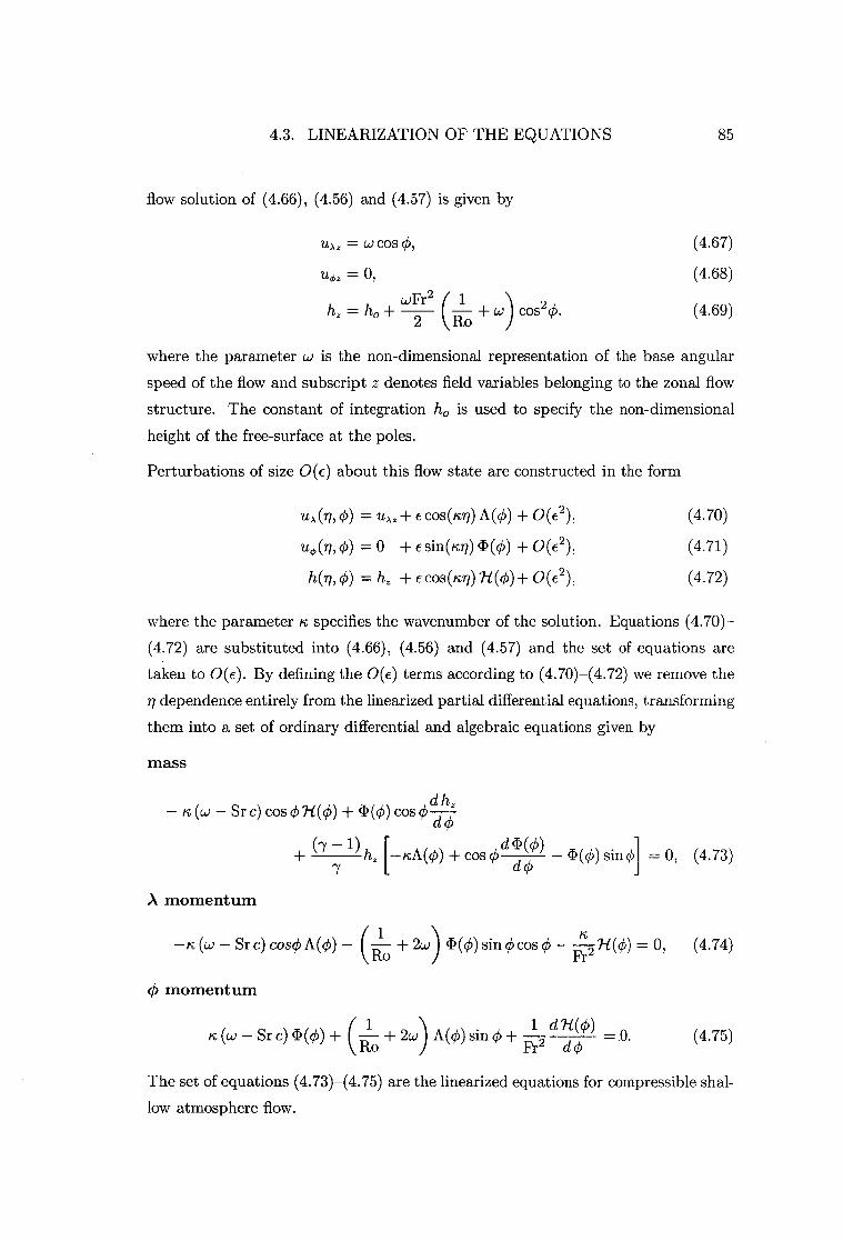
4.3. LINEARIZATION OF THE EQUATIONS 85
flow solution of (4.66), (4.56) and (4.57) is given by
uAz = w cos 0,
uoz = 0,
hz = + car2 (-1 +w) cos2 0. 2 Ro
(4.67)
(4.68)
(4.69)
where the parameter w is the non-dimensional representation of the base angular
speed of the flow and subscript z denotes field variables belonging to the zonal flow
structure. The constant of integration h, is used to specify the non-dimensional
height of the free-surface at the poles.
Perturbations of size OW about this flow state are constructed in the form
11, ),(71 , = u,,z + COS(1c1J) A(0) + O(€), (4.70)
uo (ri , = 0 + E sin(rui) 41.(0) + 0 (€2 ), (4.71)
h(i) = hz + cos(k7i) 7-i (0) + 0 (€2 ), (4.72)
where the parameter n specifies the wavenumber of the solution. Equations (4.7O)-
(4.72) are substituted into (4.66), (4.56) and (4.57) and the set of equations are
taken to OW. By defining the OW terms according to (4.70)—(4.72) we remove the
77 dependence entirely from the linearized partial differential equations, transforming
them into a set of ordinary differential and algebraic equations given by
mass
(w – Sr c) cos 071(0) + <I.(0)
(7 – 1) h 0,
= 0,
(4.73)
(4.74)
(4.75)
cos cb ddhoz
1. (0) (I) [ nA(0) + cos cb d (0) sin ] 0, + z 7
A momentum
(C.J — Sr c) cos 0 A(0) – (—Ro
4) momentum
1 (w – Sr c) (1.(0) + (
d
2w) + (0) sin cos .0 – Fc--;N(0)
1 dR(0) O. 2w) A + (0) sin + d =
The set of equations (4.73)—(4.75) are the linearized equations for compressible shal-
low atmosphere flow.

4.4. NUMERICAL SOLUTION OF THE LINEARIZED EQUATIONS 86
4.4 Numerical Solution of the Linearized Equations
Solutions of (4.73)-(4.75) are sought in the form of truncated Fourier series with
specific symmetry conditions. We restrict the set of possible solutions to those
that have u), and h symmetric and uo anti-symmetric with respect to the equator
(0 = 0). Additionally we require that uA and u ch, are zero at the poles, while h needs
to be constant at the poles (0 = +7r/2). The functions that meet these prescribed
conditions can be given by
N A(0) = E p„ cos((2n - 1)0), (4.76)
n=1 N
CO) = E Q,,, n sin(2n0), (4.77) n=1 N
n(0) = E ii"(-1)n [cos(2n0) + cos(2(n, - 1)0)] , (4.78) n=1
where subscript K on each coefficient denotes the longitudinal wavenumber and N
is a positive integer truncation level. The particular form of (4.78) is due to the
process of basis recombination, as discussed in Section 2.5.1 of Chapter 2.
To solve for the wavespeed c and associated coefficients P", Q,,„ and H„,n we
exploit the orthogonality properties of the trigonometric functions by requiring that
the residual equations, obtained after substituting (4.76)-(4.78) into (4.73)-(4.75),
be orthogonal to each of our expansion functions. This technique amounts to the
standard Galerkin method in which each residual equation is multiplied by each
basis function in turn and integrated over the domain -7r/2 < 0 < 7r/2. After
considerable algebra", in which the integrals are evaluated in closed form in a manner
similar to Section 2.5.2, a generalized eigenvalue problem is constructed of the form
Ax = cBx, (4.79)
where A and B are matrices corresponding to the left and right-hand sides of each
of the algebraic equations obtained from orthogonality. The eigenvalue c is the
wavespeed for the progressive Rossby wave, and vector x is the eigenvector of un-
known linearized coefficients which is defined as
x = [H,o, . . . , Hk,N, P_ K,I, • • • , Pic,N7 QK,1, • - - , Qk,N1 T • (4.80)
il See Appendix B for the individual component equation derivations.
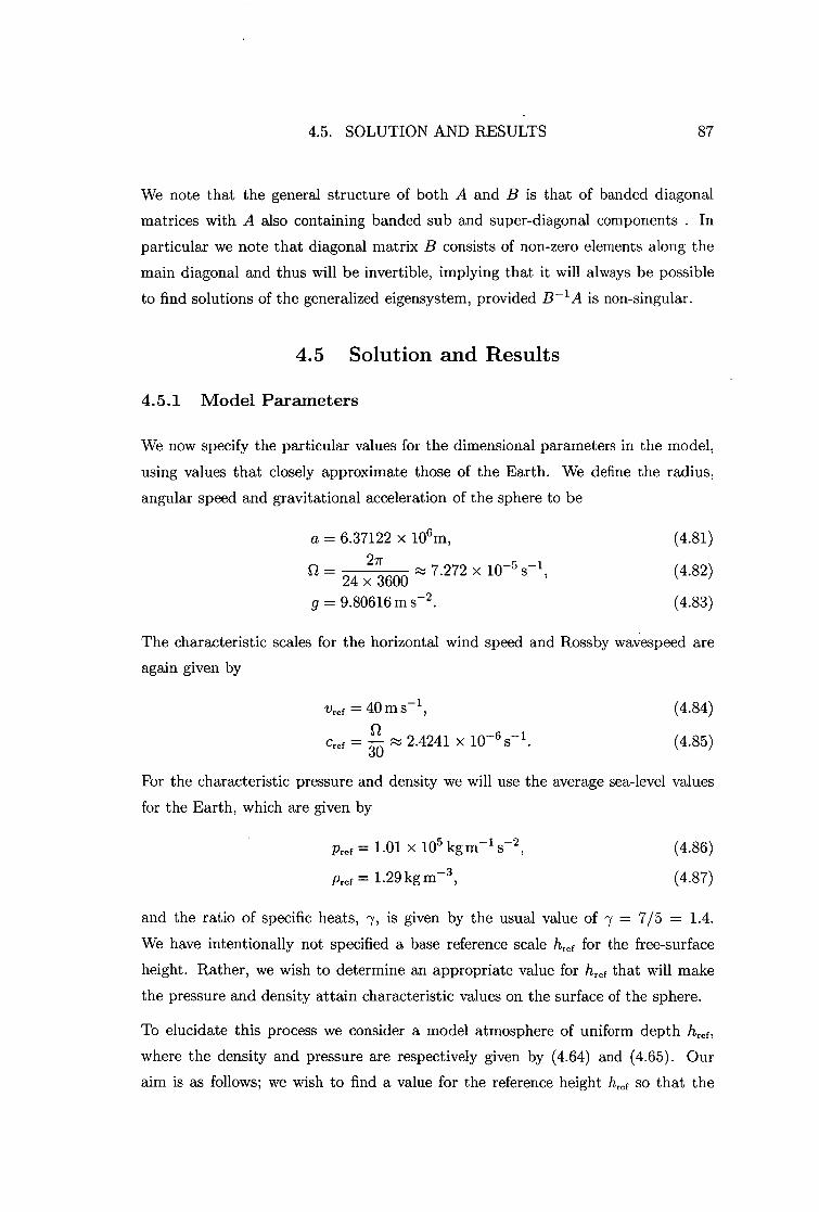
4.5. SOLUTION AND RESULTS 87
We note that the general structure of both A and B is that of banded diagonal
matrices with A also containing banded sub and super-diagonal components . In
particular we note that diagonal matrix B consists of non-zero elements along the
main diagonal and thus will be invertible, implying that it will always be possible
to find solutions of the generalized eigensystem, provided B -1 A is non-singular.
4.5 Solution and Results
4.5.1 Model Parameters
We now specify the particular values for the dimensional parameters in the model,
using values that closely approximate those of the Earth. We define the radius,
angular speed and gravitational acceleration of the sphere to be
a = 6.37122 x 10⁶ m, (4.81) 27r
Q = 24 x 3600
Ps--' 7.272 x 10⁻⁵s-1, (4.82)
g = 9.80616m s -2 . (4.83)
The characteristic scales for the horizontal wind speed and Rossby wavespeed are
again given by
vref = 40 m s-1 , (4.84)
cref =—C2
R.,- 2.4241 x 10 -6 s-1 . (4.85) 30
For the characteristic pressure and density we will use the average sea-level values
for the Earth, which are given by
Prof = 1.01 x 10⁵ kg m-1 s-2 , (4.86)
Prof = 1.29kg m-3 , (4.87)
and the ratio of specific heats, 7, is given by the usual value of 7 = 7/5 = 1.4.
We have intentionally not specified a base reference scale h„f for the free-surface
height. Rather, we wish to determine an appropriate value for h ref that will make
the pressure and density attain characteristic values on the surface of the sphere.
To elucidate this process we consider a model atmosphere of uniform depth h rof ,
where the density and pressure are respectively given by (4.64) and (4.65). Our
aim is as follows; we wish to find a value for the reference height h ref so that the

4.5. SOLUTION AND RESULTS 88
non-dimensional density and pressure at sea level are equal to unity. That is, the
dimensional density and pressure at sea-level take their characteristic values. Since
the free-surface has height everywhere given by the constant h ref , the value of 'km 0)
in (4.64) and (4.65) will be the constant 11, = 1. Additionally, because we are
evaluating on the surface of the sphere, we will have r = a so that the density at
sea-level is given by
,o(a) r( ry — 1) (M) 2]
'Y (4.88)
By substituting the dimensionless parameters M and Fr, given by (4.61) and (4.59),
into (4.88) and setting ga) = 1 we can solve for h ref to obtain
Wiref
1 )gPref •
(4.89)
Using this value of h ref ensures that the sea-level density and pressure are consistent
with that observed on the Earth. For the particular reference and parameter values
defined above we have
h„f r-z,- 27.944 x 10³ m.
Note that this is considerably larger than the value of 8.0 x 10 3 m used in the
incompressible model in Chapters 2 and 3.
4.5.2 Zonal Flow Parameters and Mass Specification
So that we can compare solutions for different values of the zonal flow angular speed
(4., it is necessary to derive a mass specification condition, similar to the volume
specification condition of Section 2.6.2. To perform this analysis we define a base
system mass denoted by Mb. We choose Mb to be the mass of the atmosphere
without any super rotation so that the free-surface has a uniform non-dimensional
height of 1 everywhere and the total mass is just given by the contribution of mass
elements in the region bounded inside the two concentric spheres of radii a and
a + 1. The dimensionless form of the sphere's radius is the constant a, which is just
the dimensional value divided by the reference height of the free-surface. Using this
notation we can rewrite the expression for the density, (4.64), in the form
p(r , 71, sb) = I l) ( 1\4 ) 2 + 0) - 1.)] 7 \ (4.90)
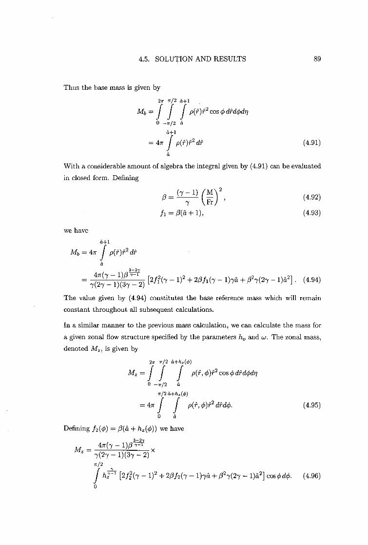
4.5. SOLUTION AND RESULTS 89
Thus the base mass is given by
27r 7r/2 ei-F1
M& = f f f p 2 cos 0 di 'd0dn 0 —7r/2 a
a+1 = 47r f (4.91)
a
With a considerable amount of algebra the integral given by (4.91) can be evaluated
in closed form. Defining
we have a+1
Mb = 47r f p( 2 a
= (7 — 1 ) (I \ 4 ) 2 Fr/
fi =8(a+ 1),
(4.92)
(4.93)
— 1) 2 + 2,3fi — ± 027 (27 1)a2] (4.94)
The value given by (4.94) constitutes the base reference mass which will remain
constant throughout all subsequent calculations.
In a similar manner to the previous mass calculation, we can calculate the mass for
a given zonal flow structure specified by the parameters ho and w. The zonal mass,
denoted /14.z , is given by
27r 7r/2 a±hz (0)
f I
0)1'2 cos 0 d1-d0c/71 0 —7r/2 a
7r/2 a-f-hz (0)
= 47r I f p(I , 0) f'2 CifT/O. 0 a
Defining f2(0) = 0(et + 11,(0)) we have
(4.95)
Mz = — 1)(37 — 2) x 7r/2
f h ' 1 ) 2 + 20f2(Y 1 )7e1 02-Y(27 — 1)â2} cos d. (4.96)
47r(-y — 1)0 7-1
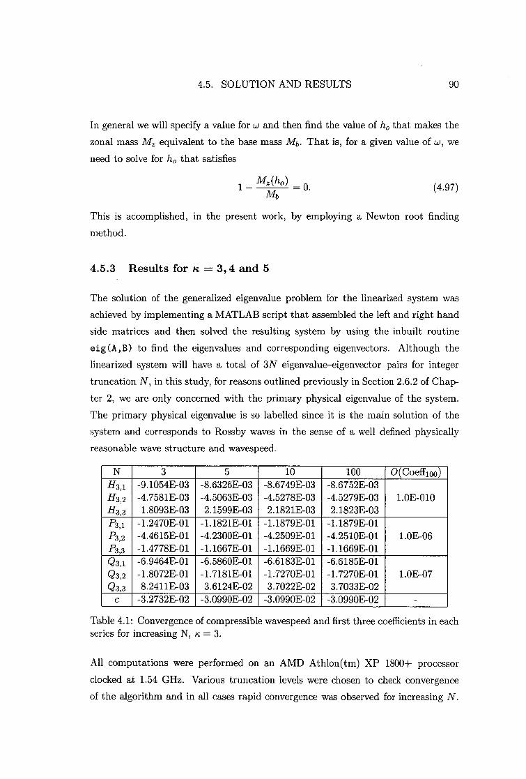
4.5. SOLUTION AND RESULTS 90
In general we will specify a value for w and then find the value of h, that makes the
zonal mass M, equivalent to the base mass Mb. That is, for a given value of w, we
need to solve for h, that satisfies
1 M(h0 ) = O. Mb
(4.97)
This is accomplished, in the present work, by employing a Newton root finding
method.
4.5.3 Results for lc = 3,4 and 5
The solution of the generalized eigenvalue problem for the linearized system was
achieved by implementing a MATLAB script that assembled the left and right hand
side matrices and then solved the resulting system by using the inbuilt routine
eig (A, B) to find the eigenvalues and corresponding eigenvectors. Although the
linearized system will have a total of 3N eigenvalue-eigenvector pairs for integer
truncation N, in this study, for reasons outlined previously in Section 2.6.2 of Chap-
ter 2, we are only concerned with the primary physical eigenvalue of the system.
The primary physical eigenvalue is so labelled since it is the main solution of the
system and corresponds to Rossby waves in the sense of a well defined physically
reasonable wave structure and wavespeed.
N 3 5 10 100 0 (Coeffico ) H3,1 -9.1054E-03 -8.6326E-03 -8.6749E-03 -8.6752E-03 H3,2 -4.7581E-03 -4.5063E-03 -4.5278E-03 -4.5279E-03 1.0E-010 H3 , 3 1.8093E-03 2.1599E-03 2.1821E-03 2.1823E-03 P3 , 1 -1.2470E-01 -1.1821E-01 -1.1879E-01 -1.1879E-01 P3 , 2 -4.4615E-01 -4.2300E-01 -4.2509E-01 -4.2510E-01 1.0E-06 P3,3 -1.4778E-01 -1.1667E-01 -1.1669E-01 -1.1669E-01 Q3,1 -6.9464E-01 -6.5860E-01 -6.6183E-01 -6.6185E-01 Q3,2 -1.8072E-01 -1.7181E-01 -1.7270E-01 -1.7270E-01 1.0E-07 Q3,3 8.2411E-03 3.6124E-02 3.7022E-02 3.7033E-02
c -3.2732E-02 -3.0990E-02 -3.0990E-02 -3.0990E-02
Table 4.1: Convergence of compressible wavespeed and first three coefficients in each series for increasing N, tc = 3.
All computations were performed on an AMD Athlon(tm) XP 1800+ processor
clocked at 1.54 GHz. Various truncation levels were chosen to check convergence
of the algorithm and in all cases rapid convergence was observed for increasing N.

4.5. SOLUTION AND RESULTS 91
Tables 4.1, 4.2 and 4.3 illustrate this rapid convergence for ic = 3, 4 and 5 respec-
tively. The final column in each table gives the order of the last coefficient in each
series when N = 100 and provides evidence for the accuracy of the solution since
in each case the coefficients are observed to drop off reasonably fast. Convergence
of the eigenvalue was obtained with smaller truncation than that required for cor-
responding accuracy in the coefficients, providing confidence in the accuracy of the
wavespeeds calculated.
N 3 5 10 100 0 (Coeffioo ) H4,1 -8.9296E-03 -8.5877E-03 -8.5884E-03 -8.5884E-03 H4,2 -3.5334E-03 -3.4524E-03 -3.4527E-03 -3.4527E-03 1.0E-17 H4,3 3.2098E-03 3.3605E-03 3.3608E-03 3.3608E-03 P4,1 -1.0787E-01 -1.0371E-01 -1.0372E-01 -1.0372E-01 P4,2 -5.0855E-01 -4.8726E-01 -4.8729E-01 -4.8729E-01 1.0E-14 P4,3 -2.6010E-01 -2.2920E-01 -2.2922E-01 -2.2922E-01 Q4,1 -9.2662E-01 -8.9120E-01 -8.9126E-01 -8.9126E-01 Q4,2 -4.0757E-01 -3.8689E-01 -3.8692E-01 -3.8692E-01 1.0E-14 Q4,3 8.1376E-03 3.6334E-02 3.6339E-02 3.6339E-02
c 9.4027E-01 9.4351E-01 9.4351E-01 9.4351E-01
Table 4.2: Convergence of compressible wavespeed and first three coefficients in each series for increasing N, = 4.
N 3 5 10 100 0 (COeff100)
H5,1 -8.7573E-03 -8.8926E-03 -8.8539E-03 -8.8539E-03 H5,2 -2.6638E-03 -2.6678E-03 -2.6562E-03 -2.6562E-03 1.0E-13 H5,3 4.2517E-03 4.2289E-03 4.2113E-03 4.2112E-03 P5,1 -9.5624E-02 -9.7098E-02 -9.6676E-02 -9.6676E-02 P5,2 -5.4770E-01 -5.5740E-01 -5.5498E-01 -5.5498E-01 1.0E-9 P5 , 3 -3.4186E-01 -3.5640E-01 -3.5482E-01 -3.5482E-01 Q5,1 -1.1484E+00 -1.1662E+00 -1.1611E+00 -1.1611E+00 Q5,2 -6.5400E-01 -6.6863E-01 -6.6572E-01 -6.6572E-01 1.0E-10 Q5,3 1.2470E-03 -1.2695E-02 -1.2554E-02 -1.2554E-02 c 1.5653E+00 1.5638E+00 1.5638E+00 1.5638E+00 -
Table 4.3: Convergence of compressible wavespeed and first three coefficients in each series for increasing N, = 5.
It is of interest to note that although we are now modelling a compressible atmo-sphere, the results obtained are generally quite similar to those from the incom-
pressible model of Chapter 2. However, it is quite remarkable that the wavespeeds
computed between the two models are consistently similar despite the fact that

— = 3 — — ,c=4
= 5 — R—H solutions
4.5. SOLUTION AND RESULTS 92
the incompressible and compressible models have average free-surface heights that
are quite different; the reference height in the compressible model is approximately
three and a half times larger than that used in the incompressible model. There-
fore it seems highly likely that when Phillips [66] first prescribed the value of
href = 8.0 x 10³ m for the incompressible dynamics, some consideration must have
been given to the compressibility of the atmosphere.
To provide evidence supporting the accuracy of the linearized solutions computed,
it is again useful to make a comparison between these solutions and the equivalent
corresponding Rossby—Haurwitz solutions. To do this we make use of the wavespeed
formula derived by Haurwitz [32]. The particular formula, restated here for refer-
ence, is given by #c(3 n)co —2Q
(4.98) c = (1 + k)(2 + n)
which has been rewritten to reflect the naming conventions and variable names used
in this work. To compare the two solution types we consider the primary physical
0 0.5 1 1.5 2 2.5 3 3.5 4 4.5 5 Zonal flow angular speed, co
Figure 4.2: Comparison of compressible linearized and Rossby—Haurwitz solutions for ic = 3,4 and 5 with N = 100.
eigenvalues for n = 3,4 and 5 with the equivalent Rossby—Haurwitz solutions over
a reasonable range of allowable co values. Figure 4.2 shows the results of this corn-

4.5. SOLUTION AND RESULTS 93
parison, with the solid lines representing the equivalent Rossby—Haurwitz solution
for it = 3 to 5 from bottom to top respectively. In general one can conclude that
the two models are in good broad agreement and we see that the behaviour of the
compressible linearized solutions in not dissimilar to that of the incompressible lin-
earized solutions, as shown in Figure 2.4 of Chapter 2. We also note that because the
Haurwitz model has no provision for fixing the total mass Mb of the atmosphere,
differences are to be expected between that model and the work presented here.
The discrepancies are most noticeable for larger values of the parameter co where
the effect of the mass matching condition has greater influence on the solution.
Figures 4.3-4.5 present polar stereographic projections of the free-surface, density
and pressure contours respectively. The scaling of the amplitude, via the lineariza-
tion parameter E, was chosen so that the free-surface height matched the non-
dimensional height of the Rossby—Haurwitz wave at (n , 0) = (0, 7/4). This is similar
to the technique that was used to match the incompressible and Rossby—Haurwitz
solutions in Section 2.6.3 of Chapter 2. The scaling is arbitrary and is only used
here so that visual confirmation of the general wave structure can be made.
160 20
180
200 340
Figure 4.3: Compressible linearized free-surface contours for n = 4 with N-- 100.
It is evident that the compressible free-surface contours of Figure 4.3 are quite similar
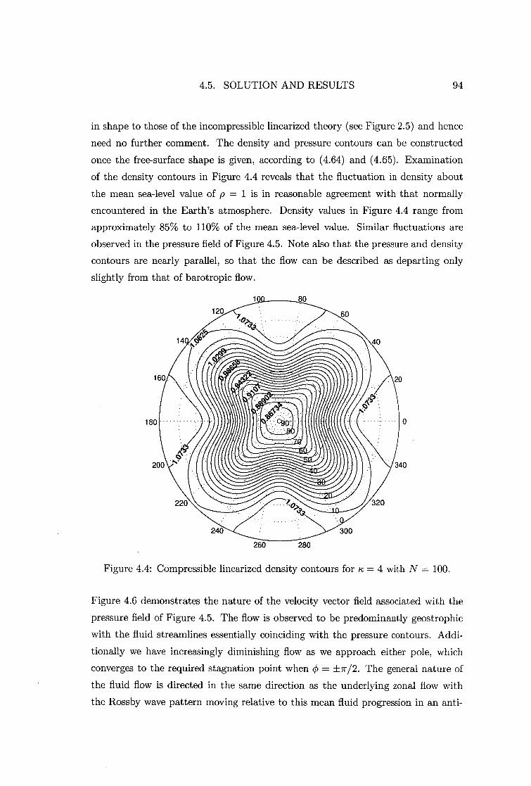
4.5. SOLUTION AND RESULTS 94
in shape to those of the incompressible linearized theory (see Figure 2.5) and hence
need no further comment. The density and pressure contours can be constructed
once the free-surface shape is given, according to (4.64) and (4.65). Examination
of the density contours in Figure 4.4 reveals that the fluctuation in density about
the mean sea-level value of p = 1 is in reasonable agreement with that normally
encountered in the Earth's atmosphere. Density values in Figure 4.4 range from
approximately 85% to 110% of the mean sea-level value. Similar fluctuations are
observed in the pressure field of Figure 4.5. Note also that the pressure and density
contours are nearly parallel, so that the flow can be described as departing only
slightly from that of barotropic flow.
Figure 4.4: Compressible linearized density contours for n = 4 with N = 100.
Figure 4.6 demonstrates the nature of the velocity vector field associated with the
pressure field of Figure 4.5. The flow is observed to be predominantly geostrophic
with the fluid streamlines essentially coinciding with the pressure contours. Addi-
tionally we have increasingly diminishing flow as we approach either pole, which
converges to the required stagnation point when 4 = ±7/2. The general nature of
the fluid flow is directed in the same direction as the underlying zonal flow with
the Rossby wave pattern moving relative to this mean fluid progression in an anti-

.... . • ..., • \ •
, „,... ,..., - ..- ..., ,. --, N
. s■-` \ -.- \ \\ ... . — \ -- — . .
.--- -- . --- . \
.: - . ..-
de .... . — . \ ‘ . . ‘. . ._ ..- ..- — . , ‘‘\
-- .'-- -- \■ -... -.• %
1 1 '
---
0 / • ..
•
. /./ / / /
/ 0/ / / /// /1 /
Vt, 11%
4.5. SOLUTION AND RESULTS 95
140 40
160 20
180
260
280
Figure 4.5: Compressible linearized pressure contours for ic = 4 with N = 100.
Figure 4.6: Compressible linearized pressure contours with corresponding velocity vector field for rc = 4 with N = 100

4.5. SOLUTION AND RESULTS 96
clockwise manner, as expected for this particular map projection of the Northern
Hemisphere.

CHAPTER 5
COMPRESSIBLE NONLINEAR SHALLOW ATMOSPHERE MODEL
In this chapter we consider the solution of the full nonlinear dynamical problem for
compressible flow on a rotating sphere with a free-surface. The linearized results
of Chapter 4 are extended, providing detailed information on how the nonlinear
progressive wavespeed and amplitude are related. The techniques used to solve the
mathematical problem are similar to those used to solve the nonlinear incompressible
dynamics problem in Chapter 3, and as such an abridged version is presented here
with the main focus being on the results, which are shown to differ in some key
ways.
5.1 Problem Specification
5.1.1 Conservation Equations
The equations of motion to be used are those derived in Chapter 4 for conservation
of mass and momentum in the rotating compressible shallow atmosphere system.
In dimensionless variables the three conservation equations are given as:
mass
(uA — Sr c cos 0) —0 h + u 4, cos 0-
0 h 0 0
u [0 + cos 0 u sin 0] =0. (5.1)
'Y an 00 97
5.1. PROBLEM SPECIFICATION 98
A momentum
au, (u,— Sr c cos ck) + no cos oau, (cos0 + u,) uo sin + 1- -Lh = 0, (5.2) ao Ro Fr2
4 momentum
au, au, (cos o ) A 0 cos 0 0 h (u - Sr c cos 0) -b--+ u4, cos— + uA usin+ 0 + = 0. (5.3)
Ro Fr2
The particular form of (5.1) is the result of specifying that the density and pressure
on the free-surface are zero, as in Section 4.2.2 of the previous chapter. The specific
forms for the thermodynamic variables of density and pressure are given by
PV, 71, = 1) ( M 2
\ Fr / (a + ii(n) 0) 71)] '7 1
(5.4)
[ - 1) ( A4\ 2 (Fr) + he 1 7, -
where et is the dimensionless form of the sphere's radius.
5.1.2 Mass Specification
To enable comparison between solutions of the dynamical system given by (5.1)-
(5.3) we again use a mass Specification condition, so that the total mass of the
atmosphere is held constant for all solutions calculated. We define a base system
mass denoted Mb, which is given by (4.94) of Section 4.5.2. For a general progressive
Rossby wave of arbitrary free-surface height h(n, 0), the total mass of fluid contained
between the surface of the sphere and the free-surface is given by
ir/2
114,1 = f f .0-' 2 COS cb &Mr, . (5.6) 0 -7r/2 a
Defining
and
= (5.5)
= (7 - 1 ) (A71 ) 2 Fr)
f3(97, 0) = 13(et + 0)),
(5.7)
(5.8)
5.2. NUMERICAL SOLUTION METHOD 99
we can write the integral given by (5.6) in the form
M1 = 7(27 X - 1)(37 - 2) 7r/k 7r/2
f f h 77-7 [2gb —1) 2 + 20 f3(7 + 02-y(2-y — 1)a2] cos dodri.
The nonlinear equation for mass conservation is then given by
Mn1 — — — 0.
Mb (5.10)
The complete specification of a nonlinear atmospheric progressive Rossby wave in
this compressible model consists of solving (5.1)-(5.3) and (5.10) subject to some
condition defining the amplitude of the wave.
5.2 Numerical Solution Method
5.2.1 Series Solution and Algorithm
Solutions of the full nonlinear dynamics given in the previous section are sought
using Fourier series with similar symmetry conditions imposed on the field variables
as in Section 4.4 of Chapter 4. Taking these symmetry and boundary conditions
into account, the series for the nonlinear problem, using longitudinal truncation M and latitudinal truncation N, are given by:
1,22 4k(-y - 1)0 -1-1
uA (n, 0) =
uo(n, 0) =
h(77,0) =
M N
W COS + E E cos(nrrvq) cos ( (2n - 1)0) , m=1 n=1
(5.11)
MN
E E m,n sin(Km,n) sin(24), (5.12) m=1 n=1
E I/0, 72 cos(20) n=0
M-1 N + E E Hn" cos(kinn)(-1) 72 [cos(2n0) + cos(2(n - 1)0)] . (5.13) m=1 n=1
Here, (5.13) again uses basis recombination to satisfy boundary conditions at the
poles. The nonlinear series (5.11) for to, now contains the primary zonal flow velocity
component. Instead of specifying the polar free-surface height we replace h, with

5.2. NUMERICAL SOLUTION METHOD 100
the single summation term in (5.13) to allow the polar height to be determined from
the output of the model.
The solution is forced by either parameterizing the amplitude, denoted A, in terms
of one of the unknown coefficients, or specifying the wavespeed c. To this end H1 , 1 ,
in the series for h(71, 0), or the wavespeed c is fixed prior to computation, thus re-
moving one of the unknowns from the problem. The majority of computations were
performed by specifying H 1 ,1, and the second technique of specifying c was reserved
for cases where two or more solutions were possible with the same amplitude.
The general solution process consists of finding the set of coefficients
Q,,,„ and wavespeed c that make the series (5.11)-(5.13) a solution of the dynamical
system described by (5.1)-(5.3) and (5.10). The technique chosen to accomplish
this task for the current work was the pseudospectral technique of collocation in
which we require the residuals, obtained by substituting the series into the governing
equations, to be zero at every point on a mesh constructed from a finite number
of collocation points in the flow field. This is exactly the same technique that was
used to solve the incompressible nonlinear dynamics problem of Chapter 3 and will
not be further expanded upon here.
For the collocation points in 0 we restrict computation to the Northern hemisphere
since the solution has specific symmetry relative to the equator. In addition, strictly
internal points from the domain are chosen, since the specific choice of the basis
functions for each series imposes boundary conditions at both 0 = 0 and 0 = ±7r/2.
Defining
AO = ( 2(N + 1)
5.14)
to be the inter-grid point distance in the 0 direction, the N equally-spaced 0-grid
points are given by
0i = iA0, for i = 1, 2, . , N. (5.15)
The collocation points in ri can be obtained in a similar manner; however, since
we have stipulated a dependence on the wavenumber n we are only free to choose
collocation points from n E [0, 7r/K) to avoid linearly dependent rows in the resulting
Jacobian matrix. This also accounts for the fact that the Rossby wave is symmetric
about its mid-line n = 7/K. Defining
7r
7r = Mtc
(5.16)
5.2. NUMERICAL SOLUTION METHOD 101
to be the inter-grid point distance in the ri direction, the M equally spaced 71-grid
points are given by
Tlj = (j — 1) n , for j = 1, 2, .. , M. (5.17)
The set of points taken from all possible (nj , 00 pairs constitutes the collocation
mesh to be used in the numerical solution.
Evaluating each of the three governing dynamical equations (5.1)-(5.3) at each of
the collocation mesh points and computing the mass specification condition (5.10)
yields a vector of residuals, denoted E(a), of length 3MN + 1, where a is a vector
comprised of the wavespeed (if it is not the forcing term) and set of unknown
coefficients. A damped Newton-Raphson method, as in Section 3.2.2 of Chapter 3,
is then used to solve the resulting algebraic system, which has the general form
E(a) = 0. (5.18)
The Jacobian matrix, which is required to compute the updating vector in the
Newton-Raphson method, is calculated analytically since the Jacobian elements
are, in general, easily determined. Additionally, the total residual error, which is
used in assessing the convergence of a solution, is computed using the norm.
The starting guess at the set of unknowns a in the Newton-Raphson method is
initially determined from the equivalent small amplitude linearized solution given in
Section 4.4 of the previous chapter. Once a small amplitude nonlinear solution has
been determined it is then used as the basis for the next solution to be computed
but with a slightly modified value of either c or H1,1, depending on the type of
forcing. This bootstrapping procedure forms the basis of mapping the wavespeed
versus amplitude relationship incrementally.
Computational efficiency is achieved by caching each of the basis functions and
their derivatives with respect to i and 0 at each of the collocation mesh points; this
approach reduces the computational overhead incurred by repeated function calls
to the trigonometric functions. The integral appearing in (5.9) is evaluated using
numerical quadrature. The particular algorithm used is that of adaptive Lobatto
quadrature, with Kronrod extension of the Gauss-Lobatto formula, as detailed in
Gander Sz Gautschi [27]. The majority of computations were performed on two
separate computers, the first being an AMD Athlon(tm) XP 1800+ processor clocked
at 1.54 GHz with 512 MB of physical memory clocked at 266 MHz, the second being

5.2. NUMERICAL SOLUTION METHOD 102
an Athlon(tm) XP 2800+ processor clocked at 2.08 GHz with 1 GB of dual channel
physical memory clocked at 333 MHz.
5.2.2 Amplitude Measurement
In order to investigate the relationship between the progressive Rossby wavespeed
and amplitude, we require a means of defining the amplitude A of a particular
Rossby wave. For a simple periodic wave, the amplitude can be defined as the
maximum deviation from the mean position to an extreme point. The problem
of measuring Rossby wave amplitude horizontally on a sphere is somewhat more
complicated and arbitrary, however. Due to the multitude of wave shapes that are
possible there are an infinite number of mean states about which we can measure
wave deviation. We must therefore decide which one is appropriate to use. Because
Rossby wave activity is predominantly associated with the mid-latitude regions and
also because 0 = +7r/4 represents the mid-point between the equator and either
pole, we choose the mean reference level as the latitude circle located 45° from the
equator in either hemisphere.
In this context, progressive Rossby waves are perturbations from a base zonal West-
erly flow, for which the height contours are simply circles of constant 0. The unper-
turbed free-surface height contours at 0 = +7r/4 are taken here as the base level,
against which Rossby wave amplitudes are measured. This is identical with the
definition of amplitude given in Section 3.4.1 of Chapter 3.
We again observe that the amplitude will not be the same in both the equator-
ward and pole-ward directions, and the difference between the two will increase as
the overall wave amplitude grows. Thus to record A effectively we measure both
the equator-ward and pole-ward deflections, again denoted A, and Ap respectively.
Associated with these separate amplitudes we define a simple averaged amplitude,
the mean of the two values, to be
A, + Ap Aave - .
2, (5.19)
It is important to emphasize that these definitions of amplitude are somewhat ar-
bitrary, although they are a useful way of quantifying transverse amplitudes on a
spherical surface.
5.3. SOLUTION AND RESULTS 103
5.3 Solution and Results
5.3.1 Model parameters
The parameters and constants for the model are again chosen to approximate those
of the Earth, as in Section 4.5.1 of the previous chapter. Specifically, the parameters
a, II and g, as well as the four reference scales v„ f , cref , p„f and p„f are given by
(4.81)—(4.87) respectively. Additionally, the reference height level is defined by
(4.89) and the ratio of specific heats is given as -y = 1.4.
For the dimensionless zonal flow parameter co we use two specific values; these are
the same values used in the incompressible nonlinear model of Section 3.4.2. The
first value is consistent with the angular speed co used in the test set proposed by
Williamson et al. [87]. The second value, chosen to be 80% of the first value, provides
a slower value for the super rotation rate. In dimensionless form they are given by
wi = 1.25, (5.20)
cuz = 1.0. (5.21)
5.3.2 Results for lc = 4, c," = 1.25
Figure 5.1 shows the wavespeed c computed for n = 4 and co = 1.25, for each
of the three measures of amplitude Ae , Ap and Aa,. The truncation levels are
M = 15 and N = 15 and the error tolerance on the L 1 norm of the residual vector
was set at 10 -12 . The solution curves are comprised of a total of 147 converged
results; however, the majority of computations were performed for larger values of
the amplitude so as to ascertain the detailed behaviour towards the right end of the
graph.
The general characteristics of the solution are quite similar to those of the equivalent
incompressible model with similar parameters (see Section 3.4.3). For small ampli-
tude the value of the wavespeed c is appropriately approximated by the linearized
solution, which is indicated in the figure. Additionally, as the amplitude increases
so does the wavespeed, which is to be expected.
The main new feature of these results, as opposed to the incompressible results
refered to previously, is the addition of a new branch, labeled branch 2 in Figure 5.1.
The small hook-shaped branch 2 was found by first calculating the solution curve

5.3. SOLUTION AND RESULTS 104
at a lower truncation level of M = N = 10 and then bootstrapping these results to
solutions with more coefficients at a higher truncation level. Only a narrow region
of convergence was found; however, the solutions contained along this small branch
were all found to converge within the required error tolerance norm of 10 -12 .
0.951
0.95
0.949
0.948
Branch 2
Branch 1 0.947
0.946
0.945
0.944
0.943o
Linearized solution
6 8 10 12 14 16 18 20 Amplitude (degrees)
Figure 5.1: Compressible wavespeed versus Amplitude for n = 4 and co = 1.25
The separation of the solution curve into two branches again indicates the presence
of a resonant interaction. Attempts were made to find solutions for values of the
wavespeed inside the gap between branches 1 and 2 but results indicated that no
such solutions exist, or at least are not possible to find using our numerical method.
A slight bending-over of the curve at the right end of branch 1 is observed. Identical
behaviour was encountered in the incompressible model. Thus it seems likely that
the incompressible model Might also harbour an additional branch, beyond branch
1, with higher wavespeeds and larger amplitudes, as was conjectured previously in
Section 3.4.3.
The free-surface contours at the limiting upper end of branch 2 are show in Fig-
ure 5.2. To the extent that the difference in the amplitude of solutions lying on
the right end of branch 1 and those lying on all of branch 2 is only slight, min-
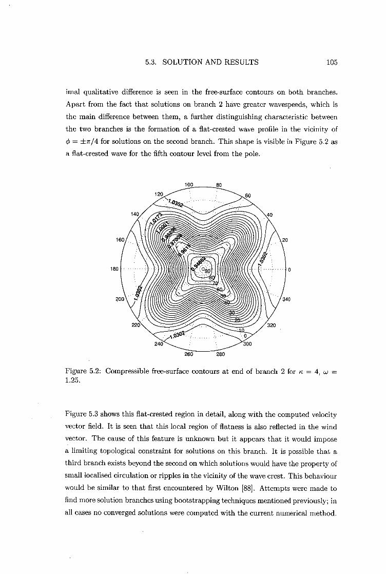
100
5.3. SOLUTION AND RESULTS 105
imal qualitative difference is seen in the free-surface contours on both branches.
Apart from the fact that solutions on branch 2 have greater wavespeeds, which is
the main difference between them, a further distinguishing characteristic between
the two branches is the formation of a flat-crested wave profile in the vicinity of
= ±7/4 for solutions on the second branch. This shape is visible in Figure 5.2 as
a flat-crested wave for the fifth contour level from the pole.
160 20
180
200 340
260
280
Figure 5.2: Compressible free-surface contours at end of branch 2 for ic = 4, w = 1.25.
Figure 5.3 shows this flat-crested region in detail, along with the computed velocity
vector field. It is seen that this local region of flatness is also reflected in the wind
vector. The cause of this feature is unknown but it appears that it would impose
a limiting topological constraint for solutions on this branch. It is possible that a
third branch exists beyond the second on which solutions would have the property of
small localised circulation or ripples in the vicinity of the wave crest. This behaviour
would be similar to that first encountered by Wilton [88]. Attempts were made to
find more solution branches using bootstrapping techniques mentioned previously; in
all cases no converged solutions were computed with the current numerical method.

5.3. SOLUTION AND RESULTS 106
Figure 5.3: Compressible free-surface contours with velocity field at end of branch 2 for lc = 4, w = 1.25.
5.3.3 Results for 11. = 4, w = 1.0
Figure 5.4 gives the computed wavespeeds from 197 individual computations using
= 4 and w = 1.0. Results were obtained by requiring the L 1 norm of the residual
vector to be less than 10 -12 . The truncation levels were again set at M = N = 15
with little difference observed between solutions obtained with a truncation level of
M = N = 10. Agreement between the nonlinear solution for small amplitude and
the linearized result is again observed to be excellent, with the linearization only
failing to provide a good estimate of the wavespeed as the amplitude is increased.
A distinct discontinuous jump is observed in the solution curve, indicating nonlinear
resonance. Of particular note is the peaked, pinched region in the middle of branch 2,
which is not present in the equivalent incompressible solution curve (see Figure 3.4).
It is interesting to observe, however, that the incompressible model has a resonance
located between branches 2 and 3 and that the qualitative difference between these
two branches was minimal. Thus the peaked region in the middle of branch 2 for
the compressible model could be seen as a similar phenomenon, except that for the

5.3. SOLUTION AND RESULTS
107
0.3965
0.396
0.3955
0.395
0.3945
I. 0.394
0.3935
0.393
0.3925
0.392
0.3915 0
Branch 1
Branch 2
ave
10 15 Amplitude (degrees)
Linearized solution
20
Figure 5.4: Compressible wavespeed versus amplitude for lc = 4 and u.; = 1.0
compressible dynamics the behaviour is damped, so that the effect of the resonance
on the solution curve is limited locally.
It is also possible that the segment of the solution curve that has been labelled here
as branch 2 is in fact two separate branches. To test whether this claim could be true,
the solutions on branch 2 were calculated using a very small amplitude increase each
time; in total, over 70 points comprise the computed branch 2 solution. Although
the local peaked region was encountered, no break in the continuity of the numerical
solution occured, in contrast to the similar case for the incompressible dynamics in
which a distinct gap was detected. It therefore seems reasonable to conclude that
Branch 2 really is a continuous branch containing a damped resonance, on the basis
of the careful numerical solution.
The main distinguishing difference between solutions on branches 1 and 2 can again
be exposed by examining the associated velocity vector fields. As in the equivalent
incompressible case of Section 3.4.4, it is observed that at no point on branch 1 does
the solution contain any stagnation points other than at the poles. For solutions on
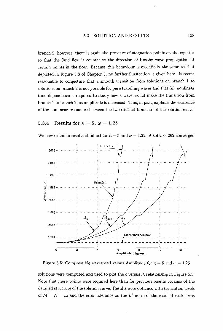
5.3. SOLUTION AND RESULTS 108
branch 2, however, there is again the presence of stagnation points on the equator
so that the fluid flow is counter to the direction of Rossby wave propagation at
certain points in the flow. Because this behaviour is essentially the same as that
depicted in Figure 3.8 of Chapter 3, no further illustration is given here. It seems
reasonable to conjecture that a smooth transition from solutions on branch 1 to
solutions on branch 2 is not possible for pure travelling waves and that full nonlinear
time dependence is required to study how a wave would make the transition from
branch 1 to branch 2, as amplitude is increased. This, in part, explains the existence
of the nonlinear resonance between the two distinct branches of the solution curve.
5.3.4 Results for k = 5, cv = 1.25
We now examine results obtained for n = 5 and w = 1.25. A total of 262 converged
1.5675
1.567
1.5665
1.566
1.5655
1.565
1.5645
1.564
2
4
6 8
10
12
Amplitude (degrees)
Figure 5.5: Compressible wavespeed versus Amplitude for n = 5 and (.,.) = 1.25
solutions were computed and used to plot the c versus A relationship in Figure 5.5.
Note that more points were required here than for previous results because of the
detailed structure of the solution curve. Results were obtained with truncation levels
of M = N = 15 and the error tolerance on the LI. norm of the residual vector was
5.3. SOLUTION AND RESULTS 109
set at 10 -12 .
The general nature of the graph is seen to be quite similar to that of the incom-
pressible equivalent given in Figure 3.9, with the linearized solution being a good
approximation for small amplitude. However, note the existence of two localised
cubic structures on branch 1, as opposed to the single isolated structure for the
incompressible case. It was proposed in Section 3.4.5 that this behaviour was repre-
sentative of a type of damped resonance in which energy exchange between certain
wavelengths is taking place in such a maner as to increase the overall amplitude
while at the same time reducing the wavespeed. To understand the exact mecha-
nism behind this damping would require, at the very least, careful analytical work
beyond the scope of this numerical study.
Despite this localised reversal of the general trend of the graph, no obvious dis-
tinguishing features are visible when the free-surface contours and velocity vector
field are examined in the vicinity of these solution regions. Two separate solution
branches were again found to exist towards the upper end of the curve when the
limiting amplitude-wavespeed combination was approached. However, the qualita-
tive difference between the two branches is minimal and it may be that this second
branch is physically unstable, as discussed in Section 3.4.5 of Chapter 2, or that
a greater truncation level is required to resolve the nature of this branch owing to
slow convergence of the Fourier series.
5.3.5 Results for K. = 5, csi = 1.0
In this final section we present results for the computed wavespeeds with parameter
values given by ic = 5 and co = 1.0, as represented in Figure 5.6. The truncation
levels were again set at M = N = 15 and the error tolerance on the L 1 norm of the
residual vector was set at 10 -12 , leading to average individual residual errors of the
order of 10-15 or less. A total of 155 points comprise the makeup of the solution
curves. For small amplitudes, the wavespeed is aptly given by the linearized result,
as indicated in the figure.
One of the localised cubic structures, seen in the previous set of results, is evident
here also, albeit on a much smaller scale, in the vicinity of c = 0.9852. This be-
haviour is similar in general to the incompressible results of Section 3.4.6. The
main new feature is the introduction of another solution branch as a result of the
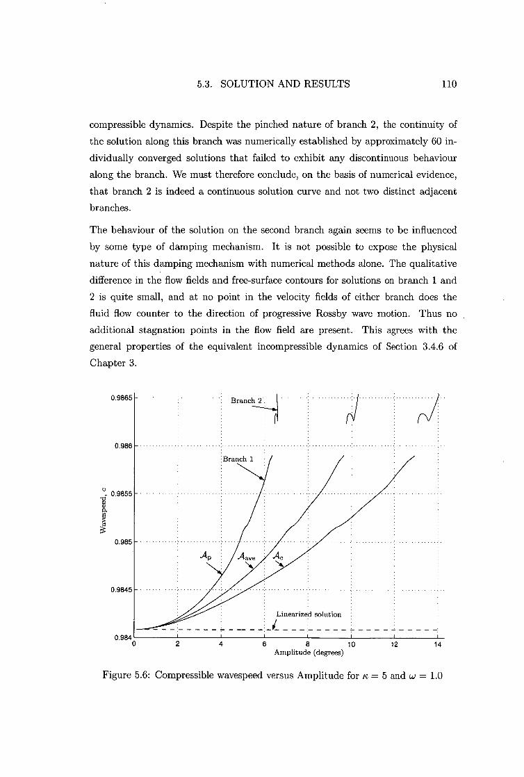
0.9865 Branch 2
0.986
Branch 1
u, 0.9855
a)
0.985
0.9845
Linearized solution
14 0.984
2
4
6 8 10
12 14 Amplitude (degrees)
5.3. SOLUTION AND RESULTS 110
compressible dynamics. Despite the pinched nature of branch 2, the continuity of
the solution along this branch was numerically established by approximately 60 in-
dividually converged solutions that failed to exhibit any discontinuous behaviour
along the branch. We must therefore conclude, on the basis of numerical evidence,
that branch 2 is indeed a continuous solution curve and not two distinct adjacent
branches.
The behaviour of the solution on the second branch again seems to be influenced
by some type of damping mechanism. It is not possible to expose the physical
nature of this damping mechanism with numerical methods alone. The qualitative
difference in the flow fields and free-surface contours for solutions on branch 1 and
2 is quite small, and at no point in the velocity fields of either branch does the
fluid flow counter to the direction of progressive Rossby wave motion. Thus no
additional stagnation points in the flow field are present. This agrees with the
general properties of the equivalent incompressible dynamics of Section 3.4.6 of
Chapter 3.
Figure 5.6: Compressible wavespeed versus Amplitude for lc = 5 and w = 1.0

5.4. CLOSING REMARKS 111
5.4 Closing Remarks
In this chapter we solved the complete nonlinear equations governing compressible
shallow atmosphere free-surface flow. The results obtained were similar to those
from the incompressible model with similar parameters; however, small key differ-
ences were observed that are attributable to the compressibility of the dynamics.
Specifically, it was shown that for all four cases examined, at least two distinct so-
lution branches were found in each instance. The presence of compressibility was
observed to damp some instances of resonant behaviour that were encountered in
the incompressible model. The cut-off low pressure cells that were computed for
= 4 and w = 1.0 in the incompressible case were not observed in the compressible
model. However, it is suspected that they do still exist and that our numerical
scheme was not capable of finding them due to the sensitivity of Newton's method.
Attempts to confirm the existence of these cells have thus far been unsuccessful.
It is again highly unlikely that numerical methods alone can answer this existence
question, and that additional analytical methods may have to be employed. Such
an analysis is beyond the scope of the present investigation.

CHAPTER 6
CONCLUSION AND CLOSING REMARKS
6.1 Discussion and Application to Meteorology
In this thesis we have presented a detailed picture of how the effects of nonlinearity
influence the relationship existing between wavespeed and amplitude for progres-
sive Rossby waves. The techniques utilised have uncovered feature-rich dynamical
properties of solutions of the shallow atmosphere equations on a rotating sphere. In
particular it was shown that nonlinear resonance plays an important and dominant
role for waves with large amplitudes. The effect of resonance was observed to sepa-
rate solutions of the system into disjoint regions, with similar solutions lying on the
same solution branch in wavespeed—amplitude space.
Two specific models of the atmosphere were used: an incompressible and a com-
pressible model. For the incompressible dynamics it was shown that, for slowly
propagating progressive waves with longitudinal wavenumber n = 4, if the ampli-
tude forcing became large enough it was possible for the flow to develop localised
low-pressure cells in the mid-latitude regions. These types of extreme amplitude
solutions were accompanied by stagnation points in the flow field at locations other
than the poles. In general it was observed that for these highly nonlinear waveforms
the lower polar free-surface heights, and hence pressures, and also the higher equa-
torial free-surface elevations, tended to be grossly distorted so that it was common
for contours originating near the equator or pole to be deformed towards regions
well in excess of the mid-latitudes.
112

6.1. DISCUSSION AND APPLICATION TO METEOROLOGY 113
In the Earth's atmosphere, Rossby waves are frequently observed by filtering out
localised small scale effects and concentrating on the 500 mb height field contours,
so that the effects of the planetary boundary layer, and hence friction, are mini-
mal. Using this technique it is possible to expose the large-scale structure of the
atmosphere. Since the late 1970's there has been considerable effort expended by
meteorologists in an attempt to explain the large-scale process of atmospheric block-
ing (see the critical review article by Lindzen [51]). In its simplest form, blocking
is either the existence of a stationary high pressure cell that persists in the mid-
latitudes where westerly flow would normally be observed, or a ridge of high pressure
that extends polewards from the tropics and influences the mid-latitude flow char-
acteristics. Usually the formation of a block tends to be associated with stationary
planetary waves.
In the investigation conducted in this thesis, it was found that the most extreme case
of large amplitude waves was for slowly moving progressive Rossby waves with the
parameters tc = 4 and w = 1.0. The linearized wavespeed associated with this spe-
cific parameter configuration was c 0.395. Thus for only a slightly smaller value
of the zonal flow parameter w, the linearized and associated nonlinear wavespeeds
would be very close to zero, so that the Rossby wave would be approximately station-
ary with respect to the the surface of the Earth. We conjecture that the particular
nature of the wavespeed—amplitude relationship for stationary Rossby waves would
not be dissimilar to that computed for the case ic = 4 and w = 1.0. If this is
so it would imply the existence of highly distorted nearly stationary Rossby waves
containing high pressure ridges extending polewards from the equator, with cut-off
low pressure cells in the the mid-latitudes. This type of atmospheric configuration
could be seen as being crucial to the instigation of a blocking event, with subse-
quent development of cut-off high-pressure cells near the mid-latitudes when full
time dependence is included in the model.
This argument is, in general, supported by the work of Austin [5] who found that the
splitting of westerly winds by blocking is attributable to interference, or resonance,
between planetary waves with very large amplitudes. In this conjecture, however,
nothing is implied as to how the dynamical system moves from one solution branch to
the next. Nor is it expected that all the solution branches would be physically stable.
Charney & DeVore [13] and Charney, Shukla & Mo [14] have conducted studies in
an attempt to ascertain the effect of topography and thermal forcing on blocking in
6.2. FUTURE WORK AND CLOSING REMARKS 114
the atmosphere and have shown the existence of multiple equilibrium states, some of
which exhibit blocking phenomena. It is thus possible that through various forcing
mechanisms, such as the effects of topography and thermal heating/cooling, the
atmosphere can pass from one equilibrium state to another. If this proves to be
true then the highly nonlinear feature-rich solutions calculated in this work would
support the idea that blocking is primarily a dynamical state which is accessible
through appropriate forcing of the atmospheric system.
6.2 Future work and Closing Remarks
The aim of this thesis was to investigate numerically nonlinear progressive Rossby
wave behaviour. The analysis techniques utilised have uncovered some of the defin-
ing features of shallow atmosphere free-surface flow with progressive Rossby waves;
however, many questions still remain unanswered. Because of the complexity of
the governing equations, and the associated sensitivity of Newton's method, it is
highly possible that our numerical solution method did not find all possible solution
branches for the particular parameter configurations used. It would thus be desir-
able to conduct analytical research in an attempt to support the numerical findings
contained in this thesis. Additionally, an analytical study would provide insight
into the proposed existence of additional solution branches that were conjectured
at various stages throughout this thesis. However, because of the sheer complexity
of the dynamical equations involved, it is more than likely that such an analytical
approach would be severely limited in scope unless significant approximations and
idealizations were made.
In this work nothing has been said of the stability of the solutions computed. It
seems highly likely that solutions along the first branch of each wavespeed—amplitude
curve would be stable, and for small amplitude waves an analysis of the linearized
system would more than likely suffice to ascertain the Lyapunov stability of the
system. The reasoning behind this statement stems from the fact that Rossby
waves are frequently observed in the atmosphere and so must form an integral part
of its stable composition. The stability of the highly nonlinear waves computed with
very large amplitudes would require special attention again. It would be desirable
to know whether or not the largest flow computed for ic = 4 and ci.) = 1, the
flow containing cut-off low-pressure cells, is stable, as this would have consequences

6.2. FUTURE WORK AND CLOSING REMARKS 115
for the stability of blocking formations, as discussed previously. Additionally, the
inclusion of topography and temperature forcing in this analysis would be of great
benefit.
This work has shown the sensitive dependence of progressive Rossby-wave solutions
upon the zonal flow speed co. Ideally, a complete study of the entire parameter region
0 < (.,) < wii would reveal the complete dynamical behaviour of large amplitude
progressive Rossby waves, where w u is the maximum permissible angular speed,
limited by the requirement that the atmosphere have some positive depth. Of
course, such a massive numerical study is not achievable. It may be the case that
analytical techniques might reveal further dynamical behaviour, although that is
beyond the scope of the present work.
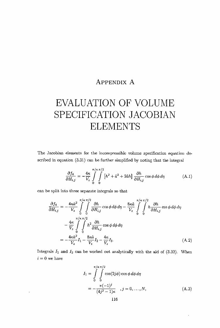
APPENDIX A
EVALUATION OF VOLUME SPECIFICATION JACOBIA\
ELEMENTS
The Jacobian elements for the incompressible volume specification equation de-
scribed in equation (3.31) can be further simplified by noting that the integral
7r/k 7r/2 ah ah = 4' I [112 +a2 + 2ah] cos 0 do di, axi ,3 vz
00 (A.1)
can be split into three separate integrals so that
7r/k 7r/2 ah 7r/k 7r/2 ah ka 2 (914 j
cos 0 dO 8/th r h an
cosodoth,• 4vz vz
0 0 00 7r/k 7r/2
ff h2 ,90ll.h.,i cos4 dq dij 4K
00
4Ica2 r 8Ka r 4K r (A.2)
V, V,
Integrals 1). and 12 can be worked out analytically with the aid of (3.32). When i = 0 we have
7r/K 7r/2
11 = f cos(2j0) cos cb cick dri 0 o
7r(-1)3 (4j2 i)tc ,j — 0, • • • ,N, (A.3)
— V,
116
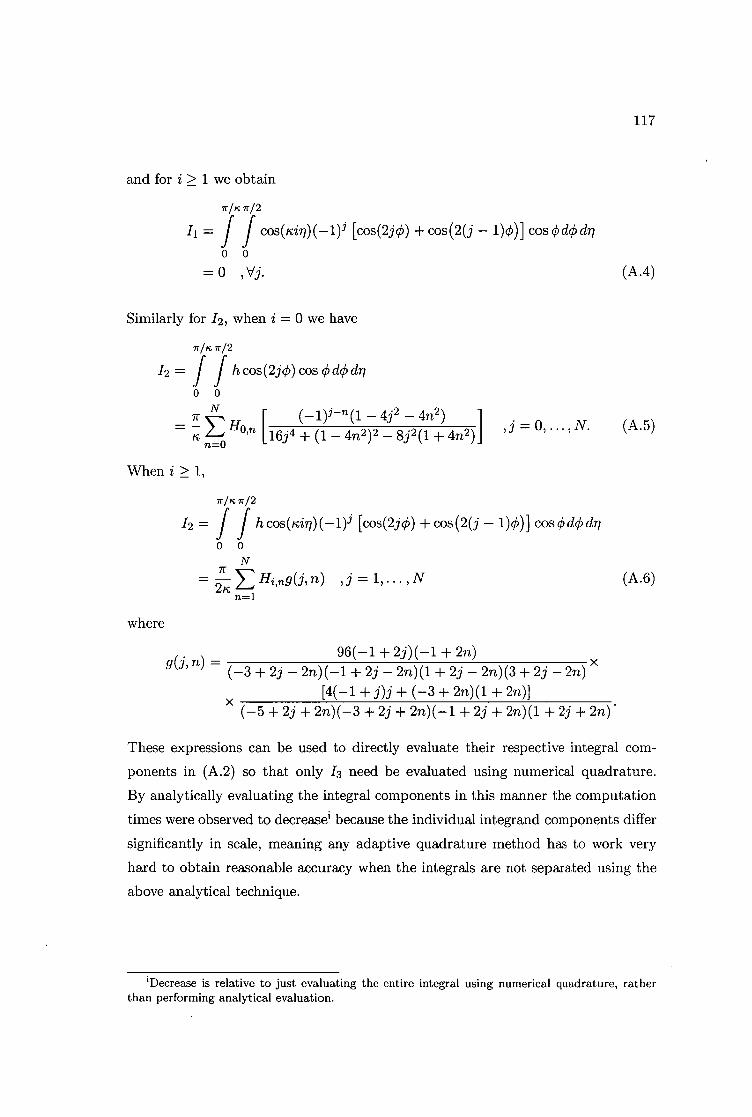
117
and for i > 1 we obtain
7r/is 7r/2
= f COS(Kin)(-1) 3 COS(2j0) COS(2(j — 1.)0)] cos dck dn
0 0 =0 ,V j. (A.4)
Similarly for 12, when i = 0 we have
7r/k 7r/2
/2 = f h coS(2j0) COS 40 Cin 00
(-1)i —rt (1 — 4j 2 — 471,2 ) = 7 110 16j4 nE , = 0, . , N. (A.5) + (1 _ 4n2)2 — 8j2 (1 + 4n2 ) n=0
When i > 1,
7r/n 7r/2
12 = f f h COS(Kin)(-1) 3 [cos(2j0) + cos (2(j — 1)0)] COS d4i 0 0
7T E Himg(j,n) ,j = 1, . . . ,N
2k
where
96(-1 + 2j)(-1 + 2n) g(j,n) =
(-3 + 2j — 2n)(-1 + 2j — 2n)(1 + 2j — 2n)(3 + 2j — 2n) x [4(-1 + j)j + (-3 + 2n)(1 + 2n)]
(-5 + 2j + 2n)(-3 + 2j + 2n)(-1 + 2j + 2n)(1 + 2j + 2n)
These expressions can be used to directly evaluate their respective integral com-
ponents in (A.2) so that only 13 need be evaluated using numerical quadrature.
By analytically evaluating the integral components in this manner the computation
times were observed to decrease i because the individual integrand components differ
significantly in scale, meaning any adaptive quadrature method has to work very
hard to obtain reasonable accuracy when the integrals are not separated using the
above analytical technique.
(A.6) n=1
'Decrease is relative to just evaluating the entire integral using numerical quadrature, rather than performing analytical evaluation.
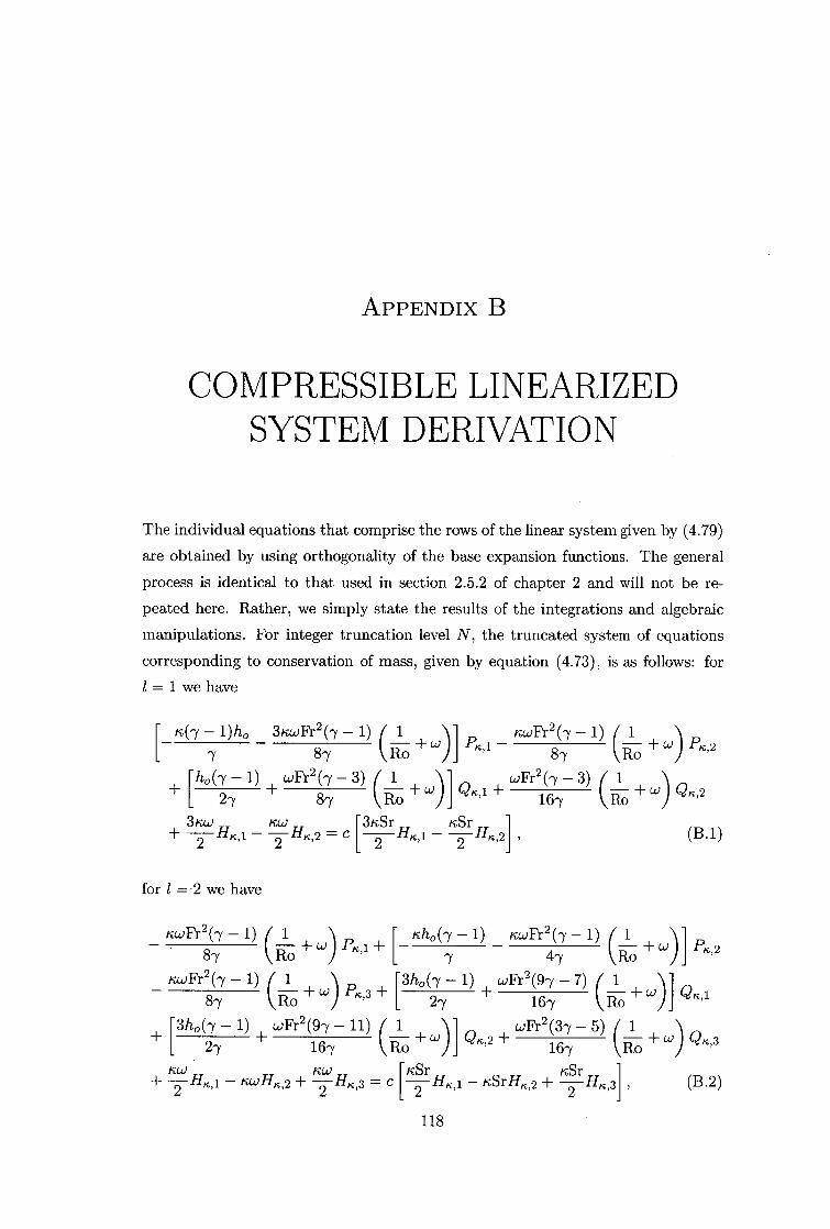
KwFr 2 (7 – 1) ( 1 Ro + w) Ptc,i
tauFr2 (7 – 1) ( 1 Ro +
Pio
[3h0 (7 - 1) wFr2 (97 – 11) 27 167
– nw1-42+
+[ K
'Y
ho ey – 1) kt4)Fr 2 (-y – 1) ( 1 47 Ro )
+[ 314) (7 – 1) ± wFr2 (9-y – 7) ( 1
) ± ci .) I Q,,,i
27 167 Ro
( 1 +\1 (2K,2 + coFr2 (37 –5) ( 1
Ro ) 167 Ro )
= c 1 -
2 H – KSr II K 2 -I- — n K 31 7 ' 2 ' KSr kSr ,
(B.2)
APPENDIX B
CO PRESSIBLE LINEARIZED SYSTEM DERIVATION
The individual equations that comprise the rows of the linear system given by (4.79)
are obtained by using orthogonality of the base expansion functions. The general
process is identical to that used in section 2.5.2 of chapter 2 and will not be re-
peated here. Rather, we simply state the results of the integrations and algebraic
manipulations. For integer truncation level N, the truncated system of equations
corresponding to conservation of mass, given by equation (4.73), is as follows: for
1=1 we have
[ rc(-y – 1)h0 3titar2 (-y – 1) / 1 + w)] mvn.2(7 1) (R1o + 8-y Ro 8-y
iho (-y – 1) ± wFr2 (7 –3) ( 1 + w)] coFr2 (-y – 3) ( 1 I_ 2-y 87 Ro ) 167 + w) QK' 2
2 C [3tcSr icSr
+ Hki - — 11K 2 2 2 = ' 2 ' 2 ' (B.1)
for 1 = 2 we have
118
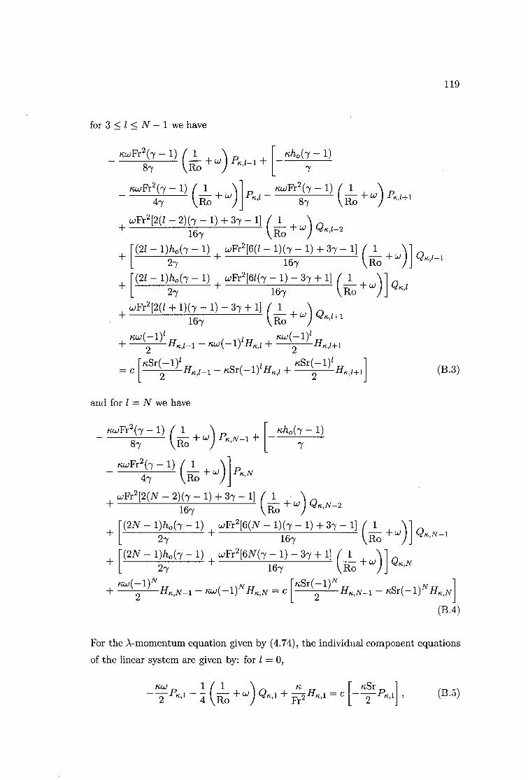
119
for 3 < 1 < N - 1 we have
kwFr2(; - 1) (: 8 ,0 + w) Pk,/ 1. + [ lth°(7),- 1)
nwFr 2 (7 - 1) ( 1 + )] , ruoFr 2 (7 - 1) ( 1 4'y Ro w ix/
87 Ro + w) Ptc,c+i
+wa2 [2(/ - 2)(7 - 1) + 37 - 1] ( 1 ± w)
167 Ro
+[(21- 1)h0 (7 - 1) wFr2 [6(/ - 1)(7 - 1)
27 + 167 [(21- 1)110 (7 - 1) + wFr2 [6/(7 - 1) - 37
+ 27 167
+ wFr2 [2(/ + 1)(7 - 1) - 37 + 11 (J_ + w)
167 Ro nw(-1) 1
+ -1/K,i-i. kid-( -1 ) 11/o + 2 2 r
2 r(-1)/ nSr(-1) 1
= c nSr( 1) / 1/0 + 2 litc,t+11 (B.3)
and for 1= N we have
tcwFr2 (7 - 1) ( 1 + cv) p,,,Ar_1 + [ tchc,(7 - 1) 87 Ro ) 7
kwFr2 (7 - 1) ( 1 + col pk,N 47 Ro )
wFr2 [2(N - 2)(7 - 1) + 37 - 1] (± • ,, + 167 Ro + w) L' ic ' 1'1-2
[(2N - 1)1/0 (7 - 1) + wFr 2 [6(N - 1)(7 - + 27 167 1) + 37 - 1} ( 1 Ro
+ [(2N - 1)1/0 (7 - 1) + coFr2 [6Ney - 1) - 37 ± 1] ( 1 + u.)1
) Qic,N
27 167 Ro sw(-1) N
2 rr(-1)N ,
± HK,N_i KW( i)N H,c ,N = C 2
II, N_i — kSr( - 1) N I I k,N1
(B.4)
For the )-momentum equation given by (4.74), the individual component equations
of the linear system are given by: for 1 = 0,
(B.5)
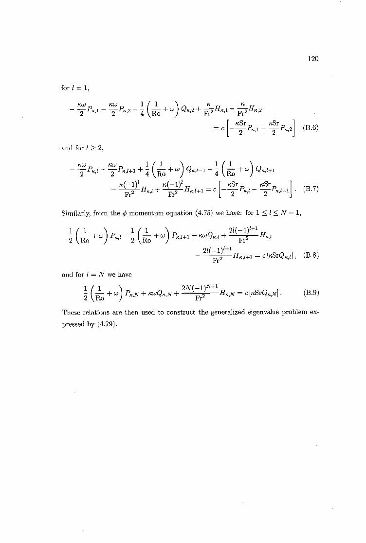
120
for 1 = 1,
ruCV 1/1 rr
C
1
7_3 (B.6)
(B.7)
— 1,
, (B.8)
(B.9)
- -- I-, 2 — Qtc,2 2 k ' 2 6 4 Ro Fr
=
and for 1 > 2,
tc/i.) T.) 1 ( i fi
/ /-F1 w) k,1-1 - -4
tc(-1) 1
— Fr2 ilic,2
tcSr nSr
w) tc,1+1
icSr KSr
2
rk,/-1-1
< N
H H tc,1+1 = C Fr2 Fr2
Similarly, from the momentum equation (4.75) we
1 1 (-1 Ro
24-1) 1 + 1
—
2
— 2
have: for 1 < 1
2(-1) 1 + 1 Frz
= c R.2
and for 1 = N we have
1 ( 1 +
Kto(2,,,N +2N(_1)N -Fi
H„,/+1
Htc,N = C[KSTQ Pk ,N 2 Ro co) Fr2
These relations are then used to construct the generalized eigenvalue problem ex-
pressed by (4.79).

Wave speed = 3 19327969-001 Ap =884degrees &Ivo = 997 Pecirs99 As = 11,39 dooms Penal = TS 70 0999 Curry* tex_NA = 29
APPENDIX C
3D OPENGL ROSSBY WAVE VIEWER
Figure C.1: Rossby-wave viewer output, Equatorial region
A three-dimensional (3D) visualisation tool was developed to aid in interpreting the
results, using the OpenGL 3D programming interface. The basic idea and aim was
to be able to view progressive-wave free-surface contours superimposed on a rotat-
ing sphere in full 3D and real time. Additionally, it was required to translate these
contours with respect to the rotating sphere so as to illustrate visually the prop- 121

Wave speed = 3.984142e-001 Ap = 6.06 degrees Aave =9.56 degrees A. = 12.23 degrees Period = 760 days Current tesjd= 32
122
agation of the waves. OpenGL provides a convenient interface for accomplishing
such a task, with built-in functions to handle the majority of the complex 3D cal-
culations. We present here a brief overview of the processes utilised to implement
this program (see, e.g., Hill [33] for an explanation of terms used in this discus-
sion). The basic framework for the 3D program is loosely based around a tutorial
on Jeff Molofee's OpenGL related website (see, http://nehe.gamedev.net ); however
substantial changes were required to implement the full program. Additionally, arc-
ball camera movement in the program was implemented using Terence J. Grant's
tutorial as a guide. This tutorial is also freely available on Jeff Molofee's website
(see, http: / /nehe.gamedev.net /data/lessons/lesson.asp?lesson= 48) .
Figure C.2: Rossby-wave viewer output, Antarctic polar region
Full-colour free-surface contours were generated in MATLAB, for every point on
each wavespeed-amplitude curve computed. These 2D images were then exported
as encapsulated postscript files so they could be scaled without corruption. The
images were then clipped and resized so as to be compatible with OpenGL texture
loading. Because it was desirable to have a full-colour map of the Earth wrapped
around the sphere, it was necessary to make only the contours in each image opaque,
with the rest of the image being transparent so that the map of the Earth could

Wave speed =4 013473e-001 Ap = 12 7A dogrees Rave = 17.19 degrees Re = 22.14 degrees Period = 74 71 days Current tex_od = 139
123
be seen beneath the contours. For this reason, an alpha channel (transparency
channel) was added to each image in order to let OpenGL know which parts of each
contour image were visible; the alpha channel algorithm was written in MATLAB.
The pictures were then saved using the PNG format, which supports the addition
of an alpha channel.
Texture mapping (the process of mapping a 2D image onto a 3D surface) was used
to load images of the Earth and free-surface contours, and then wrap each image
around the surface of a sphere. Various rotations, which are standard functions of
the OpenGL language, were then employed to translate the free-surface contours
relative to the underlying image of the Earth. This gives the desired effect of the
progressive waves moving relative to the fixed land beneath them. Readouts of
the current progressive wavespeed, amplitude and period were placed in the upper
left-hand corner of the screen, providing easy visual reference.
Figure C.3: Rossby-wave viewer output, Australian region
Additionally, a control mechanism was implemented to let a user step easily along
the various computed solutions on each wavespeed—amplitude curve. In this manner,
the transition and qualitative difference of solutions lying on different resonance
branches is readily observed. Complete control over the viewing angle and zoom
124
level were also implemented, providing visual access to any point on the globe with
a simple click and drag or wheel scroll of the mouse.
Figures C.1-C.3, which are screen shots of the running program, illustrate the gen-
eral output of the viewer, although it must be emphasised that the real program
runs in full 3D and is interactive. The viewer has been designed to run on Windows
98/NT/2000/Me/XP operating systems, although a port to Linux would be possi-
ble, and requires a system with an OpenGL compliant graphics card with at least
32Mb of memory. The program and source code are freely available upon request
to the author.

BIBLIOGRAPHY AND SELECTED READING LIST
[1] M. Abromowitz and I. A. Stegun. Handbook of Mathematical Functions with Formulas, Graphs, and Mathematical Tables. Dover, 1972.
[2] F. S. Acton. Numerical Methods that Work. Harper and Row, 1970.
[3] W. F. Ames. Numerical Methods for partial differential equations. Academic Press, second edition, 1977.
[4] G. Arfken. Mathematical Methods for Physicists. Academic Press, 3rd edition, 1985.
[5] J. F. Austin. The blocking of middle latitude westerly waves by planetary waves. Q.J.R. Meteorol. Soc., 106:327-350,1980.
[6] P. G. Baines. The stability of planetary waves on a sphere. J. Fluid Mech., 73(part 2):193-213,1976.
[7] J. J. Barton and L. R. Nackman. Scientific and Engineering C++: An introduction with advanced techniques and examples. Adison-Wesley Publishing Company, Inc., 1994.
[8] G. K. Batchelor. Introduction to Fluid Dynamics. Cambridge University Press, 1967.
[9] J. R. Bates, Y. Li, A. Brandt, S. F. McCormick, and J. Ruge. A global shallow-water numerical model based on the semi-lagrangian advection of potential vorticity. Q.J.R. Meteorol. Soc., 121:1981-2005,1995.
[10] John P. Boyd. Chebyshev and Fourier Spectral Methods. Dover Publications, 2nd edition, 2000.
[11] T. G. Callaghan and L. K. Forbes. Nonlinear progressive Rossby waves for incompress-ible flow on a rotating sphere, Submitted for publication. J. Fluid Mech., 2004.
[12] C. Canuto. Spectral Methods in Fluid Dynamics. Springer Series in Computational Physics. Springer-Verlag, 1988.
[13] J. G. Charney and J. G. DeVore. Multiple flow equilibria in the atmosphere and blocking. J. Atmos. Sci., 36:1205-1216,1979.
[14] J. G. Charney, J. Shukla, and K. C. Mo. Comparison of a barotropic blocking theory with observation. J. Atmos. Sci., 38:762-779,1981.
[15] B. Chen and P.G. Saffman. Steady gravity-capillary waves on deep water II. Numerical results for finite amplitude. Studies in Appl. Math., 62:95-111,1980b.
[16] H.-B. Cheong. Application of double fourier series to the shallow-water equations on a sphere. J. Comput. Phys., 165:261-287,2000.
125
BIBLIOGRAPHY AND SELECTED READING LIST 126
[17] H.-B. Cheong. Double fourier series on a sphere: Applications to elliptic and vorticity equations. J. Comput. Phys., 157:327-349, 2000.
[18] E. D. Cokelet. Steep gravity waves in water of arbitrary uniform depth. Philos. Trans. R. Soc. London Ser. A, 286:183-230, 1977.
[19] H. M. Deitel and P. J. Deitel. C-i-± How to Program. Prentice Hall, 1994.
[20] D. R. Durran. Numerical Methods for Wave Equations in Geophysical Fluid Dynamics, volume 32 of Texts in applied mathematics. Springer-Verlag, 1998.
[21] J. A. Dutton. The Ceaseless Wind: An introduction to the theory of atmospheric motion. McGraw-Hill, 1976.
[22] P. N. Edwards. A brief history of atmospheric general circulation modeling. In D. A. Randall, editor, General Circulation Development, Past Present and Future: The Pro-ceedings of a Symposium in Honor of Akio Arakawa, pages 67-90. New York: Academic Press, 2000.
[23] L. K. Forbes and S. R. Belward. Atmospheric interfacial waves in the presence of two moving fluid layers. Phys. Fluids, 6(10):3306-3316, October 1994.
[24] L.K. Forbes. Surface waves of large amplitude beneath an elastic sheet. Part 1. High-order series solution. J. Fluid Mech., 169:409-428, 1986.
[25] L.K. Forbes. Surface waves of large amplitude beneath an elastic sheet. Part 2. Galerkin solution. J. Fluid Mech., 188:491-508, 1988.
[26] L. Fox and I. B. Parker. Chebyshev Polynomials in Numerical Analysis. Oxford Uni-versity Press, 1968.
[27] W. Gander and W. Gautschi. Adaptive quadrature - revisited. BIT, 40(1):84-101, March 2000.
[28] G. H. Golub and C. F. Van Loan. Matrix Computations. John Hopkins Series in the Mathematical Sciences. John Hopkins University Press, 1989.
[29] D. Gottlieb and S. A. Orszag. Numerical Analysis of Spectral Methods: Theory and applications. Regional Conference Series in Applied Mathematics. SIAM, 1977.
[30] G. J. Haltiner. Numerical Weather Prediction. John Wiley and Sons, Inc., 1971.
[31] G. J. Haltiner and R. T. Williams. Numerical Prediction and Dynamic Meteorology. Wiley, second edition, 1980.
[32] B. Haurwitz. The motion of atmospheric disturbances on the spherical earth. J. Mar. Res., 3:254-267, 1940.
[33] F. S. Hill. Computer Graphics Using OpenGL. Prentice Hall, second edition, 2001.
[34] S. J. Hogan. Some effects of surface tension on steep water waves. J. Fluid Mech., 91:167-180, 1979.
[35] S. J. Hogan. Some effects of surface tension on steep water waves. Part 2. J. Fluid Mech., 96:417-445, 1980.
[36] S. J. Hogan. Some effects of surface tension on steep water waves. Part 3. J. Fluid Mech., 110:381-410, 1981.
[37] James R. Holton. An Introduction to Dynamic Meteorology. Academic Press, 1972.
[38] I. Horton. Beginning Visual C++ 5. Wrox Press Ltd., 1997.

BIBLIOGRAPHY AND SELECTED READING LIST 127
[39] B. J. Hoskins. Stability of the Rossby-Haurwitz wave. Q.J.R. Meteorol. Soc., 99:723- 745,1973.
[40] R. Jakob-Chien, J J. Hack, and D. L. Williamson. Spectral transform solutions to the shallow water test set. J. Comput. Phys., 119:164-187,1995.
[41] I. N. James. Introduction to Circulating Atmospheres. Cambridge Atmospheric and Space Science Series. Cambridge University Press, 1995.
[42] R. Klein. Asymptotic analyses for atmospheric flows and the construction of asymp-totically adaptive numerical methods. ZAMM, 80:765-777,2000.
[43] H.-0. Kreiss and J. Oliger. Comparison of accurate methods for the integration of hyperbolic equations. Tellus, 24:199-215,1972.
[44] E. Kreyszig. Advanced Engineering Mathematics. Wiley, sixth edition, 1988.
[45] T. N. Krishnamurti and L. Bounoua. An Introduction to Numerical Weather Prediction Techniques. CRC Press, 1996.
[46] Sir H. Lamb. Hydrodynamics. Dover Publications, 6th edition, 1945.
[47] D. Lanser, J. G. Blom, and J. G. Verwer. Time integration of the shallow water equations in spherical geometry. J. Comput. Phys., 171:373-393,2001.
[48] A. T. Layton. Cubic spline collocation method for the shallow water equations on the sphere. J. Comput. Phys., 179:578-592,2002.
[49] A. T. Layton and W. F. Spotz. A semi-lagrangian double fourier method for the shallow water equations on the sphere. J. Comput. Phys., 189:180-196,2003.
[50] D. K. Lilly. A note on barotropic instability and predictability. J. Atmos. Sci., 30(4145-146, January 1973.
[51] R. S. Lindzen. Stationary planetary waves, blocking, and interannual variability. Adv. Geophys., 29:251-273,1986.
[52] R. S. Lindzen and M. R. Schoeberl. A note on the limits of rossby wave amplitudes. J. Atmos. Sci., 39(5):1171-1174, May 1982.
[53] A. Z. Loesch. Finite-amplitude stability or Rossby wave flow. J. Atmos. Sci., 35(6):929- 939, June 1978.
[54] M. S. Longuet-Higgins. Planetary waves on a rotating sphere. Proc. Roy. Soc. London A, 279:446-473,1964.
[55] M. S. Longuet-Higgins. Planetary waves on a rotating sphere. II. Proc. Roy. Soc. London A, 284:40-68,1965.
[56] M. S. Longuet-Higgins. New integral relations for gravity waves of finite amplitude. J. Fluid Mech., 149:205-215,1984.
[57] M.S. Longuet-Higgins and A.E. Gill. Resonant interactions between planetary waves. Proc. R. Soc. Lond. A, 299:120-140,1967.
[58] E. Lorenz. Barotropic instability of Rossby wave motion. J. Atmos. Sci., 29(2):258-265, February 1972.
[59] E. N. Lorenz. The Nature and Theory of the General Circulation of the Atmosphere. WMO(Series). World Meteorological Organisation, 1967.
[60] J. C. McWilliams, L. P. Graves, and M. T. Montgomery. A formal theory for vortex rossby waves and vortex evolution. Geophys. Astro. Fluid Dyn., 97(5):275-309, Aug 2003.

BIBLIOGRAPHY AND SELECTED READING LIST 128
[61] P. Neittaanmaki, M. Rudnicki, and A. Savini. Inverse Problems and Optimal Design in Electricity and Magnetism, volume 35 of Monographs in Electrical and Electronic Engineering. Oxford Science Publications, 1996.
[62] A. Neumaier. Solving ill-conditioned and singular linear systems: A tutorial on regu-larization. SIAM Rev., 40:636-666, 1998.
[63] T. Nihei and K. Ishii. A fast solver of the shallow water equations on a sphere using a combined compact difference scheme. J. Comput. Phys., 187:639-659, 2003.
[64] J. M. Ortega and W. C. Rheinboldt. Iterative Solution of Nonlinear Equations in Several Variables. Computer Science and Applied Mathematics. Academic Press, 1970.
[65] J. Pedlosky. Geophysical Fluid Dynamics. Springer-Verlag, 1982.
[66] N. A. Phillips. Numerical integration of the primitive equations on the hemisphere. Mon. Wea. Rev., 87:333-345, 1959.
[67] V. Pope and T. Davies. Testing and evaluating atmospheric climate models. Comp. Sci. Eng., 4(5):64-69, Sep-Oct 2002.
[68] W. H. Press, S. A. Teukolsky, W. T. Vetterling, and B. P Flannery. Numerical Recipes in C++: The art of scientific computing. Cambridge University Press, 2nd edition, 2002.
[69] C.-G. Rossby and collaborators. Relation between variations in the intensity of the zonal circulation of the atmosphere and the displacements of the semi-permanent cen-ters of action. J. Mar. Res., 2:38-55, 1939.
[70] R. Salmon. Lectures on Geophysical Fluid Dynamics. Oxford University Press, 1998.
[71] L. W. Schwartz. Computer extension and analytic continuation of stokes' expansion for gravity waves. J. Fluid Mech., 62:553-578, 1974.
[72] L. W. Schwartz and J.-M. Vanden-Broeck. Numerical solution of the exact equations for capillary-gravity waves. J. Fluid Mech., 95:119-139, 1979.
[73] L.W. Schwartz and J.D. Fenton. Strongly nonlinear waves. Ann. Rev. Fluid Mech., 14:39-60, 1982.
[74] J. Shen. Efficient spectral-Galerkin methods III: Polar and cylindrical geometries. SIAM J. SCI. COMPUT., 18(6):1583-1604, November 1997.
[75] I. Silberman. Planetary waves in the atmosphere. J. Met., 11:27-34, 1954.
[76] John P. Snyder. Map projections-A Working Manual. U.S. Geological Survey profes-sional paper ; 1395, 1987.
[77] M. A. Snyder. Chebyshev Methods in Numerical Approximation. Prentice Hall Series in Automatic Computation. Prentice Hall, 1966.
[78] G. G. Stokes. On the theory of oscillatory waves. Camb. Trans., viii:441-473, 1847.
[79] P. N. Swarztrauber. Spectral transform methods for solving the shallow-water equations on the sphere. Mon. Wea. Rev., 124:730-744, 1996.
[80] M. Taylor, J. Tribbia, and M. Iskandarani. The spectral element method for the shallow water equations on the sphere. J. Comput. Phys., 130:92-108, 1997.
[81] J. Thuburn and Y. Li. Numerical simulations of rossby-haurwitz waves. Tellus A, 52:181-189, 2000.

BIBLIOGRAPHY AND SELECTED READING LIST 129
[82] M. A. Tolstykh. Vorticity-divergence semi-lagrangian shallow-water model of the sphere based on compact finite differences. J. Comput. Phys., 179:180-200,2002.
[83] H. Tomita, M. Tsugawa, M. Satoh, and K. Goto. Shallow water model on a modified icosahedral geodesic grid by using spring dynamics. J. Comput. Phys., 174:579-613, 2001.
[84] K. Trulsen and C. C. Mei. Modulations of three resonating gravity-capillary waves by a long gravity wave. J. Fluid Mech., 290:345-376,1995.
[85] K. Trulsen and C. C. Mei. Effects of weak wind damping on wilton's ripples. J. Fluid Mech., 335:141-163,1997.
[86] A. Wfin-Nielsen and H. Marshall. On the structure of transient atmospheric waves. Part III. Atmosfera, 3:73-109,1990.
[87] D. L. Williamson, J. B. Drake, J. J. Hack, R. Jakob, and P. N. Swarztrauber. A stan-dard test set for numerical approximations to the shallow water equations in spherical geometry. J. Comput. Phys., 102:211-224,1992.
[88] J.R. Wilton. On ripples. Philos. Mag., 29(6):688-700,1915.

INDEX
Mb, base system mass, 89 Mz, zonal flow mass, 90 T, temperature, 6 Vb, base volume, 31
zonal flow volume, 32, 43, 58 S-2, angular velocity, 6 h, free-surface height, 8, 74 0-plane, 1 K, longitudinal wavenumber, 18, 43 co, zonal angular speed, 16, 85 u A , 5 u0 , 5
5 c, angular wavespeed, 13 h, free-surface depth, 9, 74 ho , polar free-surface height, 16, 85
adiabatic flow, 74 Amplitude
Aave, 57 Ae, 57 Ap , 57 maximum allowable, 68 measurement method, 56, 102 measurement of, 55
atmospheric blocking, 113
barotropic flow, 94 basis function, 19
caching, 44, 51, 101 caching example, 51 Fourier, 19 spherical harmonics, 19
basis recombination, 21, 86, 99 bifurcation, 69 bifurcation point, 64 bootstrapping, 54, 101
type 1, 54 type 2, 54 type 3, 55
boundary conditions, 19, 21
characteristic scales, 14 collocation, 100 collocation mesh, 50, 101
definition, 51 optimal choice, 45
collocation method, 44 advantages, 44 algorithm, 45
computer specifications, 48, 101 conservation equations
dimensional compressible, 81 dimensional incompressible, 12 incompressible advective form, 13 spherical component form, 6
continuity equation, 6 convergence, 29 convergence of longitude, 20 Coriolis parameter, 15 curvature terms, 9
density, 5 free-surface value, 84 sea-level, 88
diagonal matrix, 27, 87
eigenspectrum incompressible, 33
eigenvalue, 27, 86 primary physical, 33, 90
eigenvalues central band, 33
eigenvector, 27, 86 energy conservation, 6, 9 Euler equation, 6
finite-difference scheme, 44 flat-crested wave, 105, 106 forcing, 49
amplitude, 49, 58, 112 compressible model, 100 thermal, 114 topographical, 114
130
INDEX 131
wavespeed, 49, 61 Fourier coefficients, 21 Fourier mode, 18 Fourier series, 19, 41, 99
truncated, 86 truncation, 25, 48
free-surface, 5 Froude number, 15, 28, 83
Galerkin method, 21, 44, 86 generalised eigenvalue problem, 25, 86
solution of, 29, 90 truncated, 27
geostrophic approximation, 38, 94 gravitaitonal acceleration, 5
height field matching, 36, 93 horizontal
acceleration, 11, 78 pressure gradient, 11, 78
hydrostatic approximation, 10, 77
ideal fluid, 6 ideal gas law, 6, 9 index shifting, 23
Jacobian matrix, 46, 101 calculation of, 52 linear dependence, 51
kinematic condition, 12, 79
large-scale flow, 28 latitude, 5 latitude circle, 51 linear system
infinite, 25 Linearization
compressible, 85 incompressible, 17
localised circulation, 64 longitude, 5
Mach number, 83 mass conservation, 6 mass specification, 88, 98 momentum conservation, 6
Newton-Raphson method, 45, 101 algorithm, 46 algorithmic flow chart, 47 damped, 47 shortcomings, 46
non-dimensionalization incompressible equations, 14
normal flow, 11 North pole, 5 numerical quadrature
adaptive recursive, 54 Lobatto, 54
orthogonality, 21, 22 algebraic equations, 24
parameter specification, 28, 57, 87, 103 parity, 18, 51 planetary wave, 1 polar height parametrisation, 44 polar stereographic projection, 36, 93 pole problem, 20 polytropic atmosphere, 76 pressure, 5
cut-off low, 66 free-surface value, 84 incompressible, 10 sea-level, 88
progressive-wave, 13 pseudospectral method, 45
radial coordinate, 5 recurrence relation, 26 residual equation, 21, 49
redundancy, 51 residual vector, 101 resonance
branch, 61 damped, 69, 107, 109 discrete branching, 62 nonlinear, 61, 104, 106, 112 parameter region, 63 planetary wave, 63
reverse flow, 64 root finding, 90
multi-dimensional, 45 Rossby number, 15, 28, 83 Rossby wave, 1, 15
observational method, 113 stationary, 34, 113
Rossby-Haurwitz comparison with compressible
linearized solution, 92 comparison with incompressible
linearized solution, 35 formula, 35, 92 free-surface contours, 37

INDEX 132
scale analysis, 10 series representation, 41 shallow atmosphere
compressible, 74 incompressible, 8
shallow atmosphere approximation, 10, 76 shallow atmosphere equations
non-dimensional compressible, 83, 97 non-dimensional compressible
linearized, 85 non-dimensional incompressible, 15, 40 non-dimensional incompressible
linearized, 17, 18 singular value decomposition, 42 South pole, 5 spherical polar coordinate system, 5 stability
planetary wave, 63 stagnation point, 20, 63, 65, 107
symmetrical location, 65 Strouhal number, 15, 28, 83 super rotation, 16 symmetry conditions, 19, 43, 86, 99
unit vector, 5
valid zonal flow value, 31, 32 velocity vector, 5 volume conservation, 31 volume matching condition, 32 volume specification, 43
zonal flow, 15, 84
Related Documents