Linear and nonlinear dynamics of pulsatile channel flow - Spiral

This draft was prepared using the LaTeX style file belonging to the Journal of Fluid Mechanics 1

Linear and nonlinear dynamicsof pulsatile channel flow

Benoıt P IER1† and Peter J. SCHMID2

1Laboratoire de mecanique des fluides et d’acoustique,CNRS—Ecole centrale de Lyon—Universite de Lyon 1—INSA Lyon,

36 avenue Guy-de-Collongue, 69134 Ecully, France.2Department of Mathematics, Imperial College,

South Kensington Campus, London SW7 2AZ, United Kingdom.

(Accepted for publication in Journal of Fluid Mechanics)

The dynamics of small-amplitude perturbations as well as the regime of fully devel-oped nonlinear propagating waves is investigated for pulsatile channel flows. The time-periodic base flows are known analytically and completely determined by the Reynoldsnumber Re (based on the mean flowrate), the Womersley number Wo (a dimensionlessexpression of the frequency) and the flowrate waveform. This paper considers pulsatileflows with a single oscillating component and hence only three non-dimensional controlparameters are present. Linear stability characteristics are obtained both by Floquetanalyses and by linearized direct numerical simulations. In particular, the long-termgrowth or decay rates and the intracyclic modulation amplitudes are systematicallycomputed. At large frequencies (mainly Wo > 14), increasing the amplitude of theoscillating component is found to have a stabilizing effect, while it is destabilizing at lowerfrequencies; strongest destabilization is found for Wo ≃ 7. Whether stable or unstable,perturbations may undergo large-amplitude intracyclic modulations; these intracyclicmodulation amplitudes reach huge values at low pulsation frequencies. For linearlyunstable configurations, the resulting saturated fully developed finite-amplitude solutionsare computed by direct numerical simulations of the complete Navier–Stokes equations.Essentially two types of nonlinear dynamics have been identified: “cruising” regimesfor which nonlinearities are sustained throughout the entire pulsation cycle and whichmay be interpreted as modulated Tollmien–Schlichting waves, and “ballistic” regimesthat are propelled into a nonlinear phase before subsiding again to small amplitudeswithin every pulsation cycle. Cruising regimes are found to prevail for weak baseflowpulsation amplitudes, while ballistic regimes are selected at larger pulsation amplitudes;at larger pulsation frequencies, however, the ballistic regime may be bypassed due to thestabilizing effect of the base-flow pulsating component. By investigating extended regionsof a multi-dimensional parameter space and considering both two-dimensional and three-dimensional perturbations, the linear and nonlinear dynamics are systematically exploredand characterized.

1. Introduction

Pulsatile flows occur in a variety of engineering applications as well as in the humanbody. Over the past fifty years many studies have addressed the linear dynamics ofoscillating flows over a flat plate or through channels or pipes, but surprisingly few

† Email address for correspondence: [email protected]

2 B. Pier and P. J. Schmid

recent investigations have considered pulsatile flows, and the development of finite-amplitude traveling waves has hardly ever been addressed. While purely oscillatory flowsare governed by a single characteristic time, based on the oscillation period, pulsatileflows also depend on a second characteristic time scale, related to the mean flow velocity.Another essential difference is that oscillating configurations undergo global flow reversaland therefore the absolute value of the flow speed increases and decreases twice perperiod, while pulsating flows generally maintain the same flow direction and display onlyone phase of increasing flow speed and one phase of decreasing flow speed in each cycle.Hence, the presence of a non-vanishing mean flow component leads to behaviour distinctfrom purely oscillating situations. Using the classical channel geometry, the purpose of thepresent work is to systematically establish both linear and fully nonlinear flow featuresprevailing for fundamental pulsatile flow configurations.Among the few known exact solutions of the Navier–Stokes equations (Drazin & Riley

2006), those which are time-periodic and parallel are of particular interest (Davis 1976).The Stokes (1851) layer, i.e. the flow induced in a semi-infinite volume of fluid by aninfinite flat plate harmonically oscillating in its own plane, has served as the archetypalconfiguration for the study of time-periodic flows near a solid boundary. Similar velocityprofiles prevail if the fluid is in contact with a fixed plate and is brought into motionby an oscillating pressure gradient parallel to the plate. If the flow is confined betweentwo parallel plates, the exact base flow profiles are still obtained in terms of exponentialfunctions, while periodic flows through a circular pipe are known as Womersley (1955)solutions and may be expanded in terms of Bessel functions.All these time-periodic flows develop an oscillating boundary layer of characteristic

thickness

δ =√

ν/Ω, (1.1)

where ν is the kinematic viscosity of the fluid and Ω the pulsation frequency. For channelsor pipes, the time-periodic flow profiles significantly depend on the ratio of the diameterto the oscillating-boundary-layer thickness, known as the Womersley number Wo. Thus,for large values of Wo, confinement or curvature effects are expected to be negligible andthe dynamics similar to that of a semi-infinite Stokes layer. In contrast, at low valuesof Wo, pulsatile flows may be seen as slowly-modulated parabolic Poiseuille profiles. Inphysiological situations (Ku 1997; Pedley 2000), typical Womersley numbers prevailingin the main blood vessels are in the range 5–15 which is neither small nor very large. Ourrecent study of flow through model abdominal aortic aneurysms (Gopalakrishnan et al.

2014b,a) has revealed the need to investigate in detail the dynamics of physiological flowconditions even for simple parallel geometries. As will be shown in the present paper, itis precisely in the range 5 < Wo < 20 that pulsatile channel flow undergoes transitionsbetween different characteristic regimes, both for small-amplitude perturbations as wellas fully developed nonlinear propagating waves.

1.1. Literature review

Early theoretical and numerical work is mainly focused on the linear stability ofStokes layers or the equivalent channel and pipe flows. For obvious reasons, experimentalinvestigations almost exclusively consider the flow through circular pipes, but are ableto address the fully developed dynamics prevailing in unstable configurations. Morerecently, the linear stability of a range of time-periodic flows has been revisited, usingthe now available numerical methods and facilities. Surprisingly, apart from a few recentcomputations of turbulent periodic flows, the nonlinear regime has not yet attractedmuch theoretical or numerical attention.

Linear and nonlinear dynamics of pulsatile channel flow 3

Grosch & Salwen (1968) were among the first to address the linear stability of time-dependent plane Poiseuille flow, by expanding the disturbance streamfunction on a smallset of basis functions. They found that for weak pressure gradient modulations, theresulting modulated flow was more stable than the steady flow, while a rather drasticdestabilization was observed at higher velocity modulations.von Kerczek & Davis (1974) study the linear stability of oscillatory Stokes layers,

using quasi-static theories and integration of the linearized time-dependent equations.They were unable to find any unstable modes for the configurations considered. Usingsemi-analytic methods, Hall (1978) also found this flow to be stable in the parameterrange investigated.Yang & Yih (1977) consider axisymmetric perturbations to harmonic oscillating pipe

flow. All configurations for which calculations have been carried out are found to bestable. Later, Fedele et al. (2005) also claim that axisymmetric modes in pulsatile pipeflow are stable, while, more recently, Thomas et al. (2011) were able to obtain unstableaxisymmetric modes and to establish critical conditions for this flow.In a landmark study of pulsating plane channel flow, von Kerczek (1982) considers

configurations with moderate pulsation amplitudes, mostly near the critical Reynoldsnumber for steady flow, and computes Floquet exponents by a series expansion, using aperturbation analysis in the amplitude of the oscillating base velocity. It is found thatthe sinusoidally pulsating flow is more stable than the steady plane Poiseuille flow fora range of frequencies greater than about Wo = 12. Lower or much higher frequencieswere found to make the flow unstable, in contrast with the results of Grosch & Salwen(1968). The perturbation analysis also confirms the result obtained by Hall (1975) thatthe growth rate depends quadratically on small pulsating amplitudes.Using numerical simulations, Singer et al. (1989) find that the effect of oscillation is

generally stabilizing. However, at low frequencies, the perturbation energy may vary byseveral orders of magnitude within each cycle. These authors confirm findings by vonKerczek (1982) and suspect that those by Grosch & Salwen (1968) are underresolved.They are also probably the first to attempt a nonlinear simulation.Rozhdestvenskii et al. (1989) appear to be the first to implement a complete Floquet

analysis, based on temporal integration of matrices. They were also able to confirm resultsby von Kerczek (1982).Using mainly analytical methods, Cowley (1987) and, more recently, Hall (2003)

suggest that the Stokes layers do not sustain linearly unstable modes in the limit ofvery large Reynolds numbers.In an experimental study, Merkli & Thomann (1975) investigate transition in oscillating

pipe flow and show that turbulence occurs in the form of periodic bursts which arefollowed by relaminarization in the same cycle and do not necessarily lead to turbulentflow during the whole cycle.Using a similar experimental setup, Hino et al. (1976) identify three types of regimes:

weakly turbulent, conditionally turbulent and fully turbulent. Decelerating phases arefound to promote turbulence while the laminar flow may recover during acceleratingphases.Adopting a physiological approach,Winter & Nerem (1984) report similar experimental

observations and note that fully turbulent flow is only found when a mean flow is present.Stettler & Hussain (1986) further investigate the transition occurring in a pulsatile

pipe flow experiment and document the passage frequency of “turbulent plugs” for a widerange of control parameters and delineate the conditions when plugs occur randomly orphase-locked with the pulsation.Considering oscillatory pipe flow, Akhavan et al. (1991a,b) establish experimentally


and numerically that turbulence appears explosively towards the end of the accelerationphase and is sustained throughout the deceleration phase while being restricted to thewall region. Using a quasi-steady transient growth analysis, it is suggested that transitionmay be the result of a secondary instability mechanism.Straatman et al. (2002) derive by a linear stability analysis that pulsating a plane

Poiseuille flow is always destabilizing. However, they seem to associate stability withdecay throughout the cycle and it is therefore difficult to interpret the marginal curvesshown in that paper.More recently, in a series of theoretical and numerical papers, Blennerhassett and

Bassom, with Thomas and Davies, have used Floquet analysis and linear simulationto address the stability of a range of related time-periodic flows due to an oscillatingplate (Blennerhassett & Bassom 2002; Thomas et al. 2010, 2014, 2015), a streamwiseoscillating channel (Blennerhassett & Bassom 2006; Thomas et al. 2011) or pipe (Blenner-hassett & Bassom 2006; Thomas et al. 2011, 2012), as well as a torsionally oscillatingpipe (Blennerhassett & Bassom 2007; Thomas et al. 2012), thereby resolving some ofthe inconsistencies of previous linear stability analyses and establishing, among others,curves of marginal linear instability for this family of flows. The spatio-temporal impulseresponse of the Stokes layer is studied by Thomas et al. (2014), and the fate of somedisturbances when they become nonlinear is also considered.Luo & Wu (2010) revisit the linear instability of finite Stokes layers, comparing results

obtained by instantaneous instability theory in a quasi-steady approach with those fromFloquet analysis. It is shown that during its amplification phase, a Floquet mode closelyfollows the instantaneous unstable mode, and the results by Blennerhassett & Bassom(2002) are confirmed.Transition to turbulence has been investigated by direct numerical simulations of

the Stokes boundary layer by Vittori & Verzicco (1998), Costamagna et al. (2003)and Ozdemir et al. (2014). Tuzi & Blondeaux (2008) have addressed the intermittentturbulent regime observed in a pulsating pipe. These studies consider flow in wavywalled channels or pipes and it is observed that turbulence generally appears aroundflow reversal, and that it displays statistical properties similar to those prevailing in thesteady case.

1.2. Objectives and organization of the paper

By considering the fundamental configuration of pulsatile channel flow, the aim of thepresent study is to systematically document the temporal dynamics of small-amplitudeperturbations and, in unstable situations, to characterize the resulting finite-amplituderegime of traveling nonlinear modulated waves.Revisiting the linear regime, using both Floquet analyses and linearized numerical

simulations, we confirm the earlier findings and analyze in full detail three-dimensionalperturbations over large parameter ranges.The so-far neglected finite-amplitude traveling-wave solutions prevailing for linearly

unstable base flows are computed by direct numerical simulations of the complete Navier–Stokes equations, at prescribed total pulsating flow rates. Again, the purpose is to identifyand analyze the characteristic regimes and to systematically explore a wide parameterspace.To this end, after introducing the governing equations and the geometry in §2, the

base flow and non-dimensional parameters are specified in §3. The different mathematicalapproaches used in this work are formulated in §4, while the associated numerical solutionmethods and relevant validation steps are discussed in the appendix §A. The main bodyof the paper consists of the results pertaining to the linear (§5) and nonlinear (§6)


dynamics. In both cases, we start by discussing the features of characteristic examples,before progressively taking into account variations of more parameters in order to explorehow the dynamics unfolds over the complete parameter space. The paper finishes (§7)with a summary and some suggestions for future work.

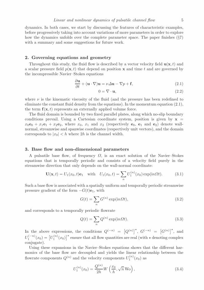
2. Governing equations and geometry

Throughout this study, the fluid flow is described by a vector velocity field u(x, t) anda scalar pressure field p(x, t) that depend on position x and time t and are governed bythe incompressible Navier–Stokes equations

∂u

∂t+ (u · ∇)u = ν∆u−∇p+ f , (2.1)

0 = ∇ · u, (2.2)

where ν is the kinematic viscosity of the fluid (and the pressure has been redefined toeliminate the constant fluid density from the equations). In the momentum equation (2.1),the term f(x, t) represents an externally applied volume force.The fluid domain is bounded by two fixed parallel plates, along which no-slip boundary

conditions prevail. Using a Cartesian coordinate system, position is given by x =x0e0 + x1e1 + x2e2, where x0, x1 and x2 (respectively e0, e1 and e2) denote wall-normal, streamwise and spanwise coordinates (respectively unit vectors), and the domaincorresponds to |x0| < h where 2h is the channel width.

3. Base flow and non-dimensional parameters

A pulsatile base flow, of frequency Ω, is an exact solution of the Navier–Stokesequations that is temporally periodic and consists of a velocity field purely in thestreamwise direction that only depends on the wall-normal coordinate:

U(x, t) = U1(x0, t)e1 with U1(x0, t) =∑

n

U(n)1 (x0) exp(inΩt). (3.1)

Such a base flow is associated with a spatially uniform and temporally periodic streamwisepressure gradient of the form −G(t)e1, with

G(t) =∑

n

G(n) exp(inΩt), (3.2)

and corresponds to a temporally periodic flowrate

Q(t) =∑

n

Q(n) exp(inΩt). (3.3)

In the above expressions, the conditions Q(−n) =[

Q(n)]⋆, G(−n) =

[

G(n)]⋆, and

U(−n)1 (x0) =

[

U(n)1 (x0)

]⋆ensure that all flow quantities are real (with ⋆ denoting complex

conjugate).Using these expansions in the Navier–Stokes equations shows that the different har-

monics of the base flow are decoupled and yields the linear relationship between the

flowrate components Q(n) and the velocity components U(n)1 (x0) as

U(n)1 (x0) =

Q(n)

2hW(x0

h,√nWo

)

, (3.4)


where the Womersley number Wo is defined as

Wo ≡ h√

Ω/ν, (3.5)

and the function W determines the profiles of the different velocity components and isdefined as

W (ξ, w) ≡

(

cosh(√iξw)

cosh(√iw)

− 1

)/(

tanh(√iw)√

iw− 1

)

if w 6= 0

3

2

(

1− ξ2)

. if w = 0,

(3.6)

for |ξ| 6 1, using√i ≡ (1 + i)/

√2. These profiles (3.6) are normalized to unit cross-

sectionally averaged velocity.Furthermore, the pressure and flowrate components are related as

Q(n)

G(n)= 2

h3

ν

i

nWo2

(

tanh(√inWo)√

inWo− 1

)

if n 6= 0 andQ(0)

G(0)=

2

3

h3

ν. (3.7)

Hence it is obvious that the pulsatile base flow is entirely determined by its frequency Ωand the Fourier components Q(n) of the flowrate (or the components G(n) of the associ-ated pressure gradient).The mathematical and numerical methods implemented in the present study can

handle flowrates of the form (3.3) with an arbitrary number of Fourier components,but this would correspond to a tremendously large multi-dimensional parameter space,impossible to explore exhaustively. Since, the aim here is to systematically analyze thebehaviour of fundamental pulsating-flow configurations, the control-parameter space isrestricted by investigating only base flowrates with a single oscillating component, i.e.,for which Q(n) = 0 as |n| > 2. Without loss of generality, Q(1) may then be restrictedto real values. As only flows with a non-vanishing mean flow component Q(0) will beconsidered, it is then convenient to write

Q(t) = Q(0)(1 + Q cosΩt), (3.8)

where the relative amplitude Q of the oscillating flowrate component is defined as

Q ≡ 2Q(1)/Q(0). (3.9)

After defining a Reynolds number

Re ≡ Q(0)/ν, (3.10)

based on the mean velocity Q(0)/2h, the channel width 2h and the viscosity ν, the baseflow is entirely specified by three non-dimensional control parameters: the Womersleynumber Wo (3.5), the Reynolds number Re (3.10), and the relative amplitude of theoscillating flowrate component Q (3.9).Snapshots of typical base flow profiles are given in figure 1. Remember that the

oscillating profiles develop a boundary layer near the walls of thickness δ =√

ν/Ω.The relative thickness of this boundary layer is governed by the Womersley numbersince Wo = h/δ. Throughout this paper, reference is often made to acceleration (resp.deceleration) phases of the base flow, here defined as phases during which the flowrateQ(t) increases (resp. decreases). Note that since the boundary layers near the walls areout of phase with the bulk flow, the actual fluid accelerations or decelerations at differentpositions in the channel cross-section do not coincide exactly with such a global definitionbased on the sign of dQ/dt.


= +

Figure 1. Snapshots of typical base flow profile associated with a flowrate of the formQ(t)/Q(0) = 1 + Q cosΩt. In this example, Wo = 10 and Q = 0.6.

4. Mathematical formulation

In this entire study, the total instantaneous flow fields are separated into basic andperturbation quantities as

utot(x, t) = U1(x0, t)e1 + u(x, t), (4.1)

ptot(x, t) = −G(t)x1 + p(x, t), (4.2)

whether the perturbation is of small amplitude (for linear stability analyses) or not (forinvestigating the fully developed nonlinear dynamics). The momentum and continuityequations for the perturbation quantities u(x, t) ≡ u0(x, t)e0 + u1(x, t)e1 + u2(x, t)e2and p(x, t) then read, in dimensional form,

∂u

∂t+ U1

∂u

∂x1+ u0

∂U1

∂x0e1 + (u · ∇)u = ν∆u−∇p+ f , (4.3)

0 = ∇ · u. (4.4)

The external volume force f(x, t) is mainly used in nonlinear evolution problems formaintaining the prescribed total pulsatile flowrate; it will be specified and discussed be-low (§4.3). Also, the initial perturbation in both linear and nonlinear evolution problemsis triggered by a small-amplitude impulsive f , and it has been checked that the resultingdynamics does not depend on the details of this initial impulse.

4.1. Linear temporal evolution problem

When carrying out a linear stability analysis for small-amplitude perturbations, thequadratic terms (u · ∇)u in the previous equation (4.3) may be neglected. Since thebase flow is homogeneous in directions parallel to the channel walls, infinitesimally smallvelocity and pressure disturbances may then be written by resorting to spatial normalmodes of the form

u(x, t) = ul(x0, t) exp i(α1x1 + α2x2), (4.5)

p(x, t) = pl(x0, t) exp i(α1x1 + α2x2), (4.6)

where α1 and α2 are the streamwise and spanwise wave numbers, respectively. Substitu-tion of (4.5,4.6) into the linearized version of the governing equations (4.3,4.4) yields

∂tu0 + iα1U1u0 = ν(

∂00 − α21 − α2

2

)

u0 − ∂0p, (4.7)

∂tu1 + iα1U1u1 + (∂0U1)u0 = ν(

∂00 − α21 − α2

2

)

u1 − iα1p, (4.8)

∂tu2 + iα1U1u2 = ν(

∂00 − α21 − α2

2

)

u2 − iα2p, (4.9)


0 = ∂0u0 + iα1u1 + iα2u2, (4.10)

with the notation ∂t ≡ ∂∂t, ∂0 ≡ ∂

∂x0

and ∂00 ≡ ∂2

∂x2

0

. Together with no-slip boundary

conditions along the channel walls, this system of partial differential equations consistsof a temporal evolution problem for the complex-valued functions u0, u1, u2 and p thatdepend on a single spatial coordinate, x0, and is numerically solved using the methodoutlined in section §A.3 of the appendix.

4.2. Floquet analysis

Instead of integrating the previous linear temporal evolution problem by starting witha given initial condition, the linear stability of pulsating channel flow can also be studiedby solving the eigenproblems arising from a Floquet analysis, thus obtaining the completespectrum and the associated eigenfunctions.Since the base flow is time-periodic with pulsation Ω, perturbations are sought in

normal-mode form as

u(x, t) =

[

∑

n

u(n)(x0) exp inΩt

]

exp i(α1x1 + α2x2 − ωt), (4.11)

p(x, t) =

[

∑

n

p(n)(x0) exp inΩt

]

exp i(α1x1 + α2x2 − ωt), (4.12)

where the complex frequency ω is the eigenvalue, and the eigenfunctions

u(x0, t) ≡∑

n

u(n)(x0) exp inΩt and p(x0, t) ≡∑

n

p(n)(x0) exp inΩt (4.13)

have the same temporal periodicity as the base flow.

Substitution of these expansions, with u(n)(x0) ≡ u(n)0 (x0)e0+ u

(n)1 (x0)e1+ u

(n)2 (x0)e2,

into equations (4.7–4.10) yields the Floquet eigenvalue problem. This system of linearcoupled ordinary differential equations in the x0-coordinate may be written, for eachinteger n, as

ωu(n)0 = nΩu

(n)0 + α1

∑

k

U(k)1 u

(n−k)0 + iν

(

∂00 − α21 − α2

2

)

u(n)0 − i∂0p

(n), (4.14)

ωu(n)1 = nΩu

(n)1 + α1

∑

k

U(k)1 u

(n−k)1 − i

∑

k

∂0U(k)1 u

(n−k)0

+ iν(

∂00 − α21 − α2

2

)

u(n)1 + α1p

(n), (4.15)

ωu(n)2 = nΩu

(n)2 + α1

∑

k

U(k)1 u

(n−k)2 + iν

(

∂00 − α21 − α2

2

)

u(n)2 + α2p

(n), (4.16)

0 = −i∂0u(n)0 + α1u

(n)1 + α2u

(n)2 , (4.17)

together with no-slip boundary conditions along the channel walls

u(n)0 = u

(n)1 = u

(n)2 = 0 for x0 = ±h. (4.18)

In the above momentum equations (4.14–4.16), the coupling of the different Fourier com-ponents of the velocity eigenfunctions occurs through the base-flow velocity components.

Note that, since U(k)1 = 0 for |k| > 2 in the configurations under investigation (3.8), the

coupling of the eigenvelocities through the base flow only occurs between n and n − 1,n or n+ 1. The numerical solution of this generalized eigenvalue problem (4.14–4.18) isoutlined in section §A.2 of the appendix.


The long-term evolution of a given mode is dictated by the complex frequency ω, orequivalently by the Floquet multiplier µ ≡ exp(−iωT ) which accounts for the gain afterone complete pulsation period. The complex frequency of the most unstable or leaststable mode depends on all parameters through a linear dispersion relation as

ω = ωlin(α1, α2; Re,Wo, Q). (4.19)

Whenever ωi > 0, or equivalently |µ| > 1, the perturbation is unstable and growsexponentially over a large number of pulsation periods. Note, however, that within apulsation period the dynamics differs from such an exponential behaviour due to thebase-flow pulsation.

4.3. Nonlinear temporal evolution problem

In unstable situations, an initial small-amplitude perturbation of wave vector α1e1 +α2e2 may be amplified and eventually reach finite amplitudes so that the nonlinear termin (4.3) can no longer be neglected. Expanding the finite-amplitude disturbance as

u(x, t) =∑

n

u(n)(x0, t) exp in(α1x1 + α2x2), (4.20)

p(x, t) =∑

n

p(n)(x0, t) exp in(α1x1 + α2x2), (4.21)

and replacing these expansions with u(n)(x0, t) ≡ u(n)0 (x0, t)e0 + u

(n)1 (x0, t)e1 +

u(n)2 (x0, t)e2 into (4.3,4.4) results in a nonlinear temporal evolution problem consisting

of a system of coupled partial differential equations for the different flow components

∂tu(n)0 + inα1U1u

(n)0 +

∑

k

N (n,k)u(k)0 = ν∆(n)u

(n)0 − ∂0p

(n), (4.22)


(n)1 + (∂0U1)u

(n)0 +

∑

k

N (n,k)u(k)1 = ν∆(n)u

(n)1 − inα1p

(n), (4.23)


(n)2 +

∑

k

N (n,k)u(k)2 = ν∆(n)u

(n)2 − inα2p

(n), (4.24)

0 = ∂0u(n)0 + inα1u

(n)1 + inα2u

(n)2 , (4.25)

where the operators N (n,k) and ∆(n) are defined as

N (n,k) ≡ u(n−k)0 ∂0 + u

(n−k)1 ikα1 + u

(n−k)2 ikα2 and ∆(n) ≡ ∂00 − n2α2

1 − n2α22. (4.26)

This is akin to performing a direct numerical simulation in a finite domain with periodicboundary conditions in the wall-parallel coordinates. The initial-value problem of interesthere is the temporal development of a streamwise and spanwise periodic small-amplitudeperturbation, characterized by real values α1 and α2. The initial evolution is dictated bythe linear temporal growth rate ωi, obtained from a linear stability analysis. Wheneverωi > 0, modulated exponential temporal growth takes place until nonlinear effects comeinto play. The quadratic nonlinear terms of the Navier–Stokes equations then promotehigher spatial harmonics of the form u(n)(x0, t) exp in(α1x1+α2x2) as well as a spatiallyhomogeneous flow correction u(0)(x0, t). Terms of the form exp i(nα1x1 +mα2x2) withm 6= n would only be generated by secondary instabilities; therefore, finite-amplitude flowfields may be expanded here as a single spatial Fourier series (4.20,4.21) since the aim isto obtain finite-amplitude primary solutions. A complete secondary stability analysis ofthese primary nonlinear waves is beyond the scope of the present investigation.


The development, through nonlinear interactions, of a spatially homogeneous flowcorrection u(0)(x0, t) results in a modification of the streamwise total flowrate by

q1(t) =

∫ +h

−h

u(0)1 (x0, t) dx0, (4.27)

and three-dimensional oblique waves may also give rise to a non-vanishing spanwiseflowrate

q2(t) =

∫ +h

−h

u(0)2 (x0, t) dx0. (4.28)

Since there is no mean pressure gradient associated with a perturbation of the form (4.21),the governing equations (4.3,4.4) for perturbations of the form (4.20,4.21) without anexternal volume force f correspond to a temporal evolution problem at prescribed totalpressure gradient. In order to simulate a temporal evolution at prescribed total flowrate,the assumed form of the pressure (4.21) is not sufficiently general: one must allow forthe development of a spatially homogeneous pressure gradient, which is equivalent toan external volume force of the form f = −g1(t)e1 −g2(t)e2 and entails the additionalterms −g1(t) and −g2(t) on the r.h.s. of equations (4.23) and (4.24) when n = 0. Thisadditional force, or pressure gradient, in the streamwise and spanwise directions may betuned so that disturbances develop without modifying the base flowrate, which is purelyin the streamwise direction. The numerical computation of the required g1(t) and g2(t)will be discussed in the appendix §A.3.

5. Linear dynamics

The configurations under investigation are completely determined by three non-dimensional control parameters: the Womersley number Wo (3.5), the Reynolds numberRe (3.10) and the relative amplitude of the oscillating flowrate component Q (3.9).Numerical results, however, depend on the choice of units for space and time. In thesequel, distances are measured in units of the channel diameter (here 2h) and velocitiesin units of mean base flow velocity (here Q(0)/2h). The associated time scale of 4h2/Q(0)

then leads to a non-dimensional frequency of Ω = 4Wo2 /Re, which corresponds to apulsation period of T = πRe

2Wo2.

With the non-dimensionalization adopted in this work, the steady Poiseuille flow isknown to become linearly unstable for Re > Rec with Rec ≃ 7696, and the marginalperturbation at criticality is two-dimensional with a streamwise wavenumber of α1,c ≃2.041 and a frequency of ωc ≃ 0.808 (see e.g. page 73 of Schmid & Henningson (2001)and references therein).The approach used here is to investigate how the instability features are influenced by

the presence of an additional pulsatile component. Starting from Poiseuille flow, the in-stability characteristics are monitored as the amplitude Q of the oscillating base flowratecomponent is increased. For most results presented below, the reference configurationis the steady Poiseuille flow at Re = 10000, which is linearly unstable. Depending onthe pulsation frequency, measured by the Womersley number, the aim is to work outwhether the pulsating component promotes or reduces the instability and how the lineardynamics are affected within a pulsation period and in the long term.

The linear stability analysis is introduced with typical temporal evolution problems,increasing only Q while all other parameters are kept constant. Subsequently, moregeneral situations are considered, varying the Womersley number Wo, streamwise and


(a)u

1 2 3 4 tT

(b)u

1 2 3 4 tT

(c)u

1 2 3 4 tT

(d)u

1 2 3 4 tT

(e)u

1 2 3 4 tT

(f)u

1 2 3 4 tT

Figure 2. Temporal evolution of a small-amplitude perturbation with α1 = 2 at Re = 10000and Wo = 10. Perturbation velocity time series for base flow with (a) Q = 0 (Poiseuille flow),

(b) Q = 0.02, (c) Q = 0.04, (d) Q = 0.06, (e) Q = 0.08 and (f) Q = 0.10 over 4 base-flowpulsation cycles. In this linear dynamics, the velocity scale is arbitrary but identical for all casesshown, and the same initial perturbation has been used throughout to trigger the perturbation.

spanwise wavenumbers α1 and α2, and eventually the Reynolds number Re to obtain thecritical conditions for onset of linear instability in the most general case.

5.1. Typical temporal evolution problems

To illustrate the temporal dynamics of small-amplitude perturbations developing inpulsatile channel flow, we first consider perturbations of streamwise wavenumber α1 = 2at Re = 10000.Figure 2(a) shows the temporal evolution of a perturbation developing in steady

Poiseuille flow (with Q = 0), computed by time-marching of (4.7–4.10). An exponentiallygrowing linear travelling wave is seen to develop, where ul(x0, t) ∼ exp(−iωt) with acomplex frequency of ω = 0.7497+ 0.0067i. This frequency is numerically determined bycomputing e.g. i(∂tu0)/u0, and its value is also confirmed by solving the correspondingeigenvalue problem (4.14–4.18). The energy contained in the perturbation grows expo-


100

102

104

106

108

E

0 1 2 3 4 t/T

Q = 0.10

0.08

0.06

0.04

0.02

0.00

Figure 3. Temporal evolution of perturbation energy for Q = 0.00, 0.02, . . . , 0.08, 0.10 atα1 = 2, Re = 10000 and Wo = 10 (same configurations as figure 2). Intracyclic modulation

amplitude rapidly increases with the pulsation amplitude Q, and it is observed that intracyclicgrowth (resp. decay) approximately coincides with base flow deceleration (resp. acceleration)phases, as indicated by solid sinusoidal line representing Q(t) (not to scale).

nentially as E ∼ exp(2ωit), see figure 3. Throughout this section on linear dynamics, theinstantaneous energy E(t) of a perturbation is defined as the spatially averaged value of|u(x, t)|2 per unit volume.Adding to this base flow a pulsatile component of different magnitudes Q = 0.02, 0.04,

. . . , 0.10, at Wo = 10, the perturbation is observed to undergo a modulated exponentialgrowth (figure 2b–f), where the modulations occur at the frequency of the base flow.The temporal evolution of the corresponding fluctuating energy is shown in figure 3.The long-term growth of the perturbation is governed by the Floquet multiplier µ ≡exp(−iωT ) and may be derived in the direct numerical simulations by monitoring e.g.

u0(x0, t+T )/u0(x0, t) (see §A.3 for more details on the numerical implementation). Here,for Q = 0.02, 0.04, 0.06, 0.08 and 0.10, the perturbation grows exponentially according toa complex frequency of ω = 0.7495+0.0068i, ω = 0.7490+0.0072i, ω = 0.7481+0.0077i,ω = 0.7468 + 0.0085i and ω = 0.7852 + 0.0095i respectively. Again, these values areconfirmed by solving the corresponding Floquet eigenproblems. Thus, the weak periodiccomponent of the base flow is here responsible for a slight increase in growth rate (ωi).In these examples, the pulsatile component of the base flow only weakly affects the

long-term perturbation growth: all energy curves in figure 3 display a similar mean slopein these logarithmic plots. However, the dynamics within each cycle significantly changeswith increasing values of Q. Indeed, the amplitude of the intracyclic modulations increasesby about three orders of magnitude as Q is increased from 0.02 to 0.1.Comparison of the energy curves with the base flowrate (solid grey curve in figure 3)

shows that enhanced growth occurs in the deceleration phase of the base flow, while decayoccurs during the acceleration phase. Although time dependent, this behaviour is similarto what is known for steady boundary layers developing along a flat plate, for which anadverse pressure gradient promotes transition while a favourable pressure gradient delays


it (Kachanov 1994). The importance of this intracyclic growth and decay rapidly increaseswith Q, while the net growth over an entire base-flow cycle in these examples is of thesame order as the growth prevailing for the equivalent steady Poiseuille configuration.In order to characterize the intracyclic dynamics, it is convenient to compensate the

computed quantities by removing the asymptotic long-term exponential growth, i.e., toconsider

u(x0, t) ≡ u(x0, t) exp(−ωit) and E(t) ≡ E(t) exp(−2ωit). (5.1)

Note that the compensated flow fields u, obtained by processing data from directnumerical simulations, differ from the Floquet eigenfunctions only by a phase velocityterm exp(iωrt). The ratio

Emaxmin ≡ maxt E(t)

mint E(t)(5.2)

is then a direct measure of the amplitude of the intracyclic modulations. While Emaxmin = 1

for steady Poiseuille flow, it rapidly grows with the pulsatile component and reachesEmax

min = 8042 for Q = 0.10 in the above example. More results for Emaxmin over a large

parameter space are presented below.The velocity time series shown in Figure 2 illustrate that the dynamics is governed

by two distinct time-scales: fast oscillations (associated with ωr) are due to the spatiallytravelling wave, while the slower modulations are tuned to the frequency Ω of the baseflow. In these examples, ωr/Ω ≃ 19 as Ω = 4Wo2 /Re = 0.04. This discrepancyof frequencies explains why a stability analysis in terms of Floquet eigenmodes (4.13)requires a large number of Fourier components to be successful, and the required numberof modes rapidly increases with Q. In theory, a Floquet analysis is preferable to alinearized direct numerical simulation since it yields the entire spectrum and not only thedominant mode. In practice, however, the size of the associated eigenproblems becomesrapidly unmanageable as Q is increased, while the numerical resolution requirements fora DNS are largely independent of Q.The number of Floquet harmonics that is required for a sufficient resolution of the

modes may be estimated from DNS data. Indeed, a Fourier analysis of the compensatedflow fields u yields the spectra shown in figure 4. These spectra are centered aroundthe dominant frequency in the signal, which corresponds to −ωr, and their width (e.g.the number of modes above the dashed line at 1/20 of the maximum) is directly relatedto the number of Fourier modes required to approximate the intracyclic dynamics. Therapid broadening of the spectra in figure 4 with Q is associated with the increase of theintracyclic modulation amplitude, and highlights the sensitivity of the dynamics on thepulsating component of the base flow.

5.2. Temporal instability at α1 = 2 and Re = 10000

The influence of the base-flow pulsating magnitude and frequency on disturbancegrowth has been systematically investigated at Re = 10000 and (α1, α2) = (2, 0) for5 6 Wo 6 25 and 0 6 Q 6 0.6. The temporal growth rate ωi has been computed bothby direct numerical simulations of the linearized evolution equations and by solving theFloquet eigenproblems. For each value of the Womersley number Wo = 5, 6, . . . , 25, thepulsating magnitude Q has been increased from 0 to 0.6 (in steps of 0.002) to illustratethe effect of an increasing oscillating component, starting with a Poiseuille flow, which isunstable in this configuration. For small values of Q, the growth rate is seen to dependquadratically on the pulsating magnitude (figure 5a), and the instability is enhanced atlow frequencies (Wo = 5, . . . , 13) while it is reduced at higher frequencies (Wo = 14, . . . ,25); strongest destabilization occurs for Wo = 9. Note that the quadratic dependence


−100 −75 −50 −25 0 25 50 ω/Ω

100

10−4

10−8

10−12

Q = 0.10

0.08

0.06

0.04

0.02

0.00

Figure 4. Spectra of compensated velocity time series for Q = 0.00, 0.02, . . . , 0.08, 0.10 atα1 = 2, Wo = 10 and Re = 10000. The peak in these spectra near ω/Ω = −19 is associated withthe dominant frequency −ωr of the travelling fluctuations. The width is related to the numberof Fourier modes that are required in a Floquet analysis and is seen to rapidly increase with thebase-flow pulsating amplitude Q.

in small values of Q has been analytically established by Hall (1975) and von Kerczek(1982). At larger values of Q, perturbations are found to decay (ωi < 0) for Womersleynumbers beyond Wo = 14, and the decay rate may display a non-monotonic dependenceon Q (figure 5b).The intracyclic modulation amplitudes Emax

min computed for the same parameter rangesare given in figure 6. Whatever the Womersley number Wo, the ratio Emax

min increasesalmost exponentially with Q starting from Poiseuille flow (Q = 0). At larger pulsationamplitudes Q, the growth of Emax

min is seen to saturate; however, at low Womersleynumbers, the exponential growth of Emax

min continues to astronomical values as Q increases.Since the intracyclic amplification Emax

min is related to the deceleration and accelerationphases of the base flow, its growth may be understood in the following manner. Increas-ing Q at constant Wo, corresponds to stronger deceleration and acceleration of the baseflow without modifying their durations and therefore enhances the ratio Emax

min that isreached within each pulsation cycle. Moreover, reducing Wo corresponds to increasingthe pulsation period as Wo−2, and therefore stretching the duration of both decelerationand acceleration phases. Hence, Emax

min grows much faster with Q at smaller values of Wo.As discussed previously, in situations where significant intracyclic modulations take

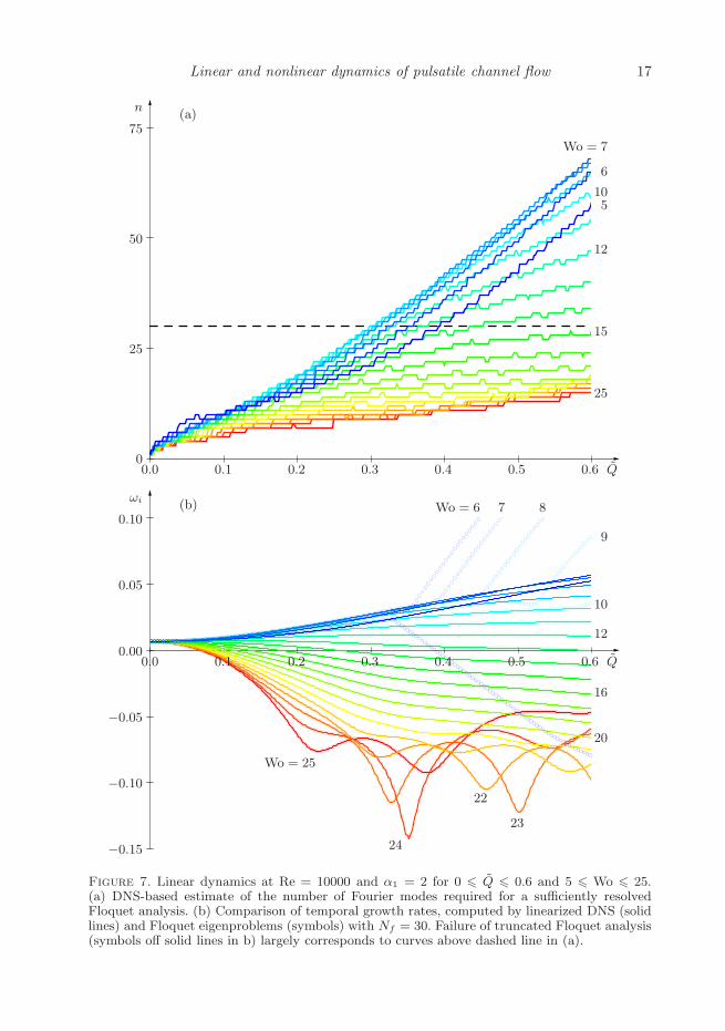
place, a large number of Fourier components is required when carrying out a stabil-ity analysis based on Floquet eigenproblems. From the DNS results, after computingFourier spectra of the compensated velocity fields, the approximate number of Fouriermodes required in a Floquet analysis can be determined: the data plotted in figure 7(a)correspond to the number of modes in the compensated spectrum with energy above 1/20of the maximum (above dashed line in figure 4). This plot may be used as a guidelinefor estimating the parameter region amenable to Floquet analysis. The relevance of thiscriterion is demonstrated in figure 7(b), comparing temporal growth rates computedboth by linearized DNS (lines) and Floquet analysis (symbols) retaining Nf = 30Fourier components to expand the eigenmodes (4.13). As expected, both methods yieldindistinguishable results up to Q = 0.6 for moderate to large values of Wo. It is only at


(a)

0.05 0.10 Q

−0.005

0.000

0.005

0.010

ωi

Wo = 97

5

13

15

17

20

25

(b)

0.1 0.2 0.3 0.4 0.5 0.6 Q

−0.15

−0.10

−0.05

0.00

0.05

ωi

Wo = 65

10

12

16

20

22

2324

Wo = 25

Figure 5. Linear temporal growth rate at Re = 10000 and α1 = 2 for 0 6 Q 6 0.6 andWo = 5, 6, . . . , 25.

lower pulsation frequencies, i.e. lower Wo, that a truncated Floquet method is seen tofail beyond some value of Q.

5.3. Two-dimensional instability analysis at Re = 10000

A complete two-dimensional instability analysis has been performed by exploring arange of streamwise wavenumbers, 0.5 6 α1 6 4.0, for each configuration. This rangehas been chosen so as to encompass all unstable wavenumbers for 5 6 Wo 6 25 and0 6 Q 6 0.6 at Re = 10000.Figure 8 shows isolines of positive temporal growth rate for (a) Wo = 6, (b) Wo = 10,

(c) Wo = 12 and (d) Wo = 15, computed via linearized DNS. For Poiseuille flow (Q = 0),unstable wavenumbers range from α1 ≃ 1.75 to α1 ≃ 2.19, and, as the amplitude Q of thepulsating base-flow component is increased, this range evolves as well as the maximumgrowth rate that is achieved for each Q.As already observed, the instability is enhanced with increasing Q for low to moderate

Womersley numbers. Figure 8(a–c), corresponding to Wo = 6, 10 and 12 respectively,shows how the upper bound of the unstable wavenumber range increases almost linearly


0.0 0.1 0.2 0.3 0.4 0.5 0.6 Q100

104

108

1012

1016

1020

1024

Emaxmin

Wo = 5 6 7 8

9

10

11

12

13

1415

2025

Figure 6. Amplitude of intracyclic modulation Emaxmin at Re = 10000 and α1 = 2 for

0 6 Q 6 0.6 and 5 6 Wo 6 25.

with Q, while the lower bound depends much less on Q. The most unstable wavenumberoccurs roughly in the center of the unstable range, and it is therefore observed that anincreasing pulsation amplitude Q favours instabilities at smaller wavelengths (larger α1).Thus, for these configurations, the maximum temporal growth rate is significantly largerthan the values shown in figure 5 corresponding to a fixed α1 = 2.

At larger Womersley numbers (see figure 8d corresponding to Wo = 15), the pulsatingcomponent has a stabilizing effect and the range of unstable α1 disappears as Q isincreased.

5.4. Three-dimensional instability analysis at Re = 10000

According to Squire’s theorem, which remains valid for pulsating flows (Conrad &Criminale 1965), a two-dimensional analysis is sufficient to study onset of instability.Nonetheless, it is worth to investigate the dynamics of three-dimensional perturbationsdeveloping in pulsatile channel flow. Figure 9 shows the temporal growth rate in the(α1, α2)-wavevector plane for a range of pulsating amplitudes Q and Womersley num-bers Wo, at Re = 10000.

At a high pulsation frequency of Wo = 15 (figure 9c), the pulsating component reducesthe growth rates and base flows are stable at Q = 0.2 and beyond. In contrast, atlower Womersley numbers, the base-flow pulsation enhances the instability and increasesthe range of unstable wavenumbers. At Wo = 5 (figure 9a), the maximum growth rateincreases slightly faster with Q than at Wo = 10 (figure 9b). While the maximum growthrate follows very similar trends at Wo = 5 and Wo = 10, the evolution with Q of theentire unstable region in the (α1, α2)-wavevector plane shows some differences. Indeed,at Wo = 5 (figure 9a), the pulsation promotes spanwise modes associated with a finite α2

and small α1. At Wo = 10 (figure 9b), the pulsation rather favours streamwise modes: asQ is increased, the unstable region further extends in the direction of large values of α1.


(a)

0.0 0.1 0.2 0.3 0.4 0.5 0.6 Q0

25

50

75

n

Wo = 7

6

510

12

15

25

(b)

0.0 0.1 0.2 0.3 0.4 0.5 0.6 Q

−0.15

−0.10

−0.05

0.00

0.05

0.10

ωiWo = 6 7 8

9

10

12

16

20

22

23

24

Wo = 25

Figure 7. Linear dynamics at Re = 10000 and α1 = 2 for 0 6 Q 6 0.6 and 5 6 Wo 6 25.(a) DNS-based estimate of the number of Fourier modes required for a sufficiently resolvedFloquet analysis. (b) Comparison of temporal growth rates, computed by linearized DNS (solidlines) and Floquet eigenproblems (symbols) with Nf = 30. Failure of truncated Floquet analysis(symbols off solid lines in b) largely corresponds to curves above dashed line in (a).


(a)

0.0 0.2 0.4 0.6 Q1.5

2.0

2.5

3.0

3.5

α1 (b)

0.0 0.2 0.4 0.6 Q1.5

2.0

2.5

3.0

3.5

α1

(c)

0.0 0.2 0.4 0.6 Q1.5

2.0

2.5

3.0

3.5

α1 (d)

0.0 0.2 0.4 0.6 Q1.5

2.0

2.5

3.0

3.5

α1

Figure 8. Isolines of linear temporal growth rate for two-dimensional perturbations in(α1, Q)-plane at Re = 10000 and (a) Wo = 6, (b) Wo = 10, (c) Wo = 12, (d) Wo = 15.Thick black lines correspond to the marginal curve ωi = 0 and thin coloured lines to positivegrowth rates ωi = 0.005, 0.010, 0.015, . . .

5.5. Critical Reynolds number

Whether a given base flow, characterized by the non-dimensional parameters Re, Woand Q, is linearly unstable or not depends on the growth rate of its most unstable orleast stable mode:

ωmaxi (Re,Wo, Q) ≡ max

α1,α2Imωlin(α1, α2;Re,Wo, Q). (5.3)

In accordance with Squire’s theorem, it is observed that the maximum growth rate alwaysoccurs for α2 = 0. Then, the critical Reynolds number Rec(Wo, Q) for onset of instabilityat given values of Wo and Q is obtained by the condition of vanishing ωmax

i . The evolutionof Rec with Q for a range of Wo is shown in figure 10. Poiseuille flow (Q = 0) correspondsto a critical Reynolds number of Rec = 7696. For the configurations investigated here, thepulsating base flow component is seen to have a stabilizing effect for Womersley numbersbeyond 13. This stabilizing effect is very strong for Wo > 18: when increasing Q, thecritical Reynolds number more than doubles when Q = 0.2 is reached. On the otherhand, for lower frequencies, the pulsating component has a destabilizing effect, whichappears to be strongest around Wo = 7.

6. Nonlinear dynamics

In this section the aim is to analyze the fully developed dynamics sustained in linearlyunstable base flows, in order to identify and characterize the different regimes thatprevail in this configuration. Since fully developed perturbations naturally arise from the


(a) Wo = 5

Q = 0.0Q = 0.1

Q = 0.2Q = 0.3

Q = 0.4Q = 0.5

Q = 0.6

0.0

0.5

1.0

1.5

2.0

2.5

3.0α2

0.51.0

1.52.0

2.53.0

3.54.0α1

(b) Wo = 10

Q = 0.0Q = 0.1

Q = 0.2Q = 0.3

Q = 0.4Q = 0.5

Q = 0.6

0.0

0.5

1.0

1.5

2.0

2.5

3.0α2

0.51.0

1.52.0

2.53.0

3.54.0α1

(c) Wo = 15

Q = 0.0Q = 0.1

Q = 0.2

0.0

0.5

1.0

1.5

2.0

2.5

3.0α2

0.51.0

1.52.0

2.53.0

3.54.0α1

Figure 9. Isolines of temporal growth rate ωi in the (α1, α2)-wavevector plane for Q = 0.0, 0.1,. . . , 0.6 at (a) Wo = 5, (b) Wo = 10, (c) Wo = 15. Thick black lines correspond to the marginalcurve ωi = 0 and thin coloured lines to positive growth rates ωi = 0.005, 0.010, 0.015, . . . .


0.0 0.1 0.2 0.3 0.4 Q5000

7500

10000

12500

15000

Rec Wo = 25 22 20 19 18 17

16

15

14

13

12

11

10

Figure 10. Critical Reynolds number for onset of temporal instability as a function of thebase-flow pulsation amplitude Q for a range of Womersley numbers: Wo = 5, 6, . . . , 25.

temporal development of a small-amplitude initial disturbance, the present approach isbased on temporal evolution problems investigated by direct numerical simulations of thecomplete Navier–Stokes equations. The initial evolution is dictated by linear dynamics, asdiscussed in the previous section. Whenever the linear temporal growth rate is positive,the perturbation necessarily reaches finite-amplitude levels and nonlinear effects comeinto play. In the absence of secondary instabilities, a fully developed regime is thenreached with spatial periodicity imposed by the prescribed values of streamwise andspanwise wavenumbers α1 and α2.Subcritical behaviour has been documented for plane Poiseuille flow (Ehrenstein &

Koch 1991) and is expected to exist also for pulsatile channel flow. However, it is beyondthe scope of the present paper to investigate finite-amplitude regimes that may existbeyond the linearly unstable regions in parameter space.

6.1. Two characteristic examples of fully developed regimes

While carrying out direct numerical simulations over large regions of a multi-dimensional parameter space, essentially two types of fully developed regimes have beenobserved: “cruising” regimes for which nonlinearities are sustained throughout the entirepulsation cycle and “ballistic” regimes that are propelled into a nonlinear phase beforesubsiding again to small amplitudes within every cycle.These two distinct regimes may be illustrated by analyzing perturbations with α1 = 2

developing in a base flow at Re = 10000 and Wo = 10 with two different pulsationamplitudes Q = 0.08 and 0.20.

6.1.1. “Cruising” nonlinear regime

For a pulsatile base flow at Re = 10000, Wo = 10 and Q = 0.08, a small-amplitudeperturbation of streamwise wavenumber α1 = 2 is linearly unstable and therefore leadsto a fully developed regime. Figure 11(a) gives the temporal evolution of the total


(a)

0 5 10 15 20 25 30 tT

0.00

0.02

0.04

0.06

0.08

0.10

0.12

E

28 29 30 tT

0.00

0.02

0.04

0.06

0.08

0.10

0.12

E

(b)

0 5 10 15 20 25 30 tT

10−35

10−30

10−25

10−20

10−15

10−10

10−5

100E

28 29 30 tT

10−6

10−5

10−4

10−3

10−2

10−1

100E

E(1)

E(0)

E(2)

E(3)

E(4)

E(5)

(c)

0 5 10 15 20 25 30 tT

−0.5

0.0

0.5

1.0

1.5

2.0

2.5

28 29 30 tT

−0.5

0.0

0.5

1.0

1.5

2.0

2.5

Figure 11. “Cruising” nonlinear regime resulting from modulated exponential growth ofsmall-amplitude initial perturbation with α1 = 2 at Re = 10000, Wo = 10 and Q = 0.08.(a) Total perturbation energy. (b) Energy of each spatial Fourier component. (c) Spatiallyaveraged wall shear stress of perturbation (black solid), total (red dashed) and base (grey dotted)fields relative to steady Poiseuille flow value.

perturbation energy on a linear scale, while figure 11(b) shows the energy of the differentspatial Fourier components on a logarithmic scale. Here, the instantaneous energy E(n)(t)of the n-th Fourier component of the perturbation is defined as the spatially averagedvalue of |u(n)(x0, t)|2 per unit volume.Instantaneous spatially averaged wall shear stress values are plotted in figure 11(c).During the early stages of the temporal evolution (here approximately 0 < t/T < 10),

a linear regime prevails with a complex frequency of ω = 0.7468 + 0.0085i and anintracyclic modulation amplitude of Emax

min = 1.35 × 103. In this regime, the differentFourier components are classically slaved to the fundamental as E(n) ∝ (E(1))n forn > 2, and E(0) ∝ (E(1))2. The mean slopes of the energy curves are seen to follow thesescalings in figure 11(b), and the intracyclic modulations around these mean slopes do


the same. It is only the mean-flow correction E(0) that is found to decay more slowlythan (E(1))2 during the intracyclic decay phases. This slower decay of the spatiallyhomogeneous component E(0) corresponds to viscous dissipation that is less efficientthan the stabilization of the E(1) component during the base-flow acceleration phase.Indeed, for the same base flow, the decay of a spatially homogeneous perturbation withα1 = α2 = 0 follows the dashed line in figure 11(b), which displays a similar slope as themean-flow correction E(0) here in its phases of slow decay.As finite amplitude levels are reached (here beyond t/T = 10), a fully developed regime

is entered consisting of a travelling nonlinear wave that is modulated by the pulsating baseflow. In this regime, the modulation amplitude is no larger than the average values so thatthe regime remains fully nonlinear throughout the pulsation cycle and is characterizedby a ratio of intracyclic modulation amplitudes of order unity, here Emax

min = 2.51.From figure 11(b) it is observed that the total perturbation energy is largely dominated

by the fundamental component E(1), even in the nonlinear regime. Higher harmonicsare well below the fundamental and follow the same pattern of intracyclic modulation.It is only the mean flow correction E(0) that displays a different trend: two intracyclicmaxima, coinciding with the extrema of the fundamental (or the total) energy. The secondmaximum of E(0) that occurs when the perturbation is near its lowest is probably dueto the continuing transfer of energy from the fundamental to the spatially homogeneouscomponent and due to the fact that this energy is only slowly dissipated so that E(0)

continues to build up while E(1) decreases. Monitoring the energy associated with thedifferent Fourier components shows that this fully developed regime may be accuratelycomputed by using only a limited number of components. All of the computations of thepresent study have been carried out with Nh = 9, and for most cases the fully developeddynamics were already well resolved with Nh = 5.The instantaneous spatially averaged wall shear stress (WSS) is plotted in figure 11(c),

relative to the value prevailing for a steady Poiseuille flow at the same Reynolds number.The wall shear stress component due to the perturbation (solid black curve) follows asimilar evolution to the fluctuating energy (figure 11a), which results in a significantincrease of the total WSS (dashed red curve) and departure from the WSS prevailing forthe base flow (dotted grey curve). The growth (resp. decay) of the perturbation WSSduring the deceleration (resp. acceleration) phases of the base flow, results in a totalspatially averaged WSS modulation out of phase with the base flow by approximately aquarter period, similar to what is observed for Stokes layers.This regime consists of a travelling nonlinear wave that propagates downstream with

a temporally modulated amplitude. Snapshots of the flow fields over two wavelengthsare shown in figure 12, near maximum energy at t/T = 29.5 (a,b) and minimum energyat t/T = 30.0 (c,d). The total flow fields (a,c) display the sinuous structure of thesenonlinear travelling waves, while the perturbation velocity fields (b,d) give an idea of theassociated propagating vortices.These modulated travelling nonlinear waves are associated with the spatio-temporal

WSS pattern shown in figure 13(a) over one streamwise wavelength for one pulsationperiod. The characteristic oblique lines in this plot are associated with the nonlinearwaves travelling at a nearly constant phase velocity. Their amplitude is modulated overthe pulsation period, similarly to what has already been observed in figure 11. However,the wave-like nature of the flow structure is associated with local WSS values well aboveand below their spatial average shown in figure 11(c). The temporal evolution of thelocal maximum and minimum WSS values are shown in figure 13(b) together with theinstantaneous spatial average. While the spatially averaged perturbation WSS values areof the same order as the base flow contribution, the local extrema are significantly larger.


(a)

(b)

(c)

(d)

Figure 12. Snapshots of velocity fields in cruising nonlinear regime over two wavelengths withα1 = 2 at Re = 10000, Wo = 10 and Q = 0.08: (a) total velocity at t/T = 29.5, (b) perturbationvelocity at t/T = 29.5, (c) total velocity at t/T = 30.0, (d) perturbation velocity at t/T = 30.0.Solid curves to the right of (a) and (c) indicate base-flow profile prevailing at same instant.

Also, the modulation of these nonlinear propagating waves results in larger modulationamplitudes for the local extrema than for the spatially averaged values. Thus, this fullydeveloped regime is associated with strong localized stresses in alternating directionstravelling along the channel walls.

6.1.2. “Ballistic” nonlinear regime

The temporal evolution of an initial small-amplitude perturbation for a base flow ata larger pulsating amplitude of Q = 0.20 is depicted in figure 14. In this example, thesmall-amplitude regime prevails approximately for 0 < t/T < 5, and, in that stage,the perturbation exponentially grows according to a complex frequency of ω = 0.8119+0.0156i with a significantly larger intracyclic modulation amplitude of Emax

min = 4.61×107.Once finite amplitudes are reached, the essential difference with the previous config-

uration is that the nonlinear regime does not prevail throughout the entire pulsationcycle: the fully developed regime consists of regular nonlinear bursts separated by phasesof nearly unperturbed base flow. Thus, the ratio of intracyclic modulation amplitudesis here much larger than unity, Emax

min = 391, since the perturbation drops to very smalllevels during the linear phase of the cycle (figure 14a).Monitoring the temporal evolution of the energy contained in the different spatial

Fourier components (figure 14b), shows that the observations of the previous configura-tion still hold: during the linear phases, higher harmonics are slaved to the fundamentalas E(n) ∝ (E(1))n; a few Fourier components are enough to fully resolve the dynamics;during stabilization phases, the mean flow correction E(0) decays on a slow time scale andtherefore becomes un-slaved from the fundamental. Here the un-slaving of the mean-flowcorrection from the fundamental also occurs in the linear phases of the fully developedregime: the slow decay rate of the mean-flow correction is dictated by viscosity and isequivalent to that of a spatially homogeneous perturbation with α1 = α2 = 0 indicatedby a dashed line in figure 14(b). Again, the total perturbation energy is dominated by thefundamental component, except during the linear phases of the fully developed regime


(a)

0.0

0.5

1.0

x1

λ

29 29.5 30 tT

(b)WSS

29 29.5 30 tT

−8

−6

−4

−2

0

2

4

6

8

Figure 13. (a) Spatio-temporal pattern of the perturbation WSS in cruising regime over onestreamwise wavelength λ = 2π/α1 and one pulsation period. WSS values are relative to asteady Poiseuille flow at the same Reynolds number, and thick solid black isoline correspondingto WSS = 0 separates thin dashed red (resp. blue) isolines corresponding to levels WSS = 2,4, 6 (resp. WSS = −2, −4, −6). (b) Instantaneous spatially averaged (solid black), minimum(dashed blue) and maximum (dashed red) values of WSS.

where the fundamental drops to negligible levels while the mean flow correction lagsbehind. Note also that due to these alternating linear and nonlinear phases, the energylevels in the ballistic regime are significantly lower than those of the cruising regime.The temporal evolution of the associated WSS is shown in figure 14(c). Obviously the

WSS associated with the perturbation (solid black curve) is only significant during thenonlinear phases. These nonlinear phases are relatively short compared with the pulsationperiod, therefore the total WSS (dashed red curve) in the fully developed regime onlyweakly departs from the WSS prevailing for the base flow (dotted grey curve).This fully developed regime consists of periodic nonlinear bursts that are identically

regenerated during every pulsation cycle. Snapshots of the flow fields over two wave-lenghts are shown in figure 15. Near maximum energy at t/T = 29.6, the total flow fields(figure 15a) exhibit the sinuous structure of the finite-amplitude travelling perturbation;this sinuosity is, however, less pronounced than in figure 12(a) since the perturbationis less energetic here. The associated perturbed fields at t/T = 29.6 are represented infigure 15(b). In the linear phase, at t/T = 30.0, the total flow fields (figure 15c) areindistinguishable from the base flow since the perturbation has negligible amplitude.These nonlinear bursting travelling waves are associated with the spatio-temporal WSS


(a)

0 5 10 15 20 25 30 tT

0.000

0.005

0.010

0.015

0.020

0.025

E

28 29 30 tT

0.000

0.005

0.010

0.015

0.020

0.025

E

(b)

0 5 10 15 20 25 30 tT

10−35

10−30

10−25

10−20

10−15

10−10

10−5

100E

28 29 30 tT

10−20

10−15

10−10

10−5

100E

E(1)

E(0)

E(1)

E(2)

(c)

0 5 10 15 20 25 30 tT

−0.5

0.0

0.5

1.0

1.5

2.0

28 29 30 tT

−0.5

0.0

0.5

1.0

1.5

2.0

Figure 14. “Ballistic” nonlinear regime resulting from modulated exponential growth ofsmall-amplitude initial perturbation with α1 = 2 at Re = 10000, Wo = 10 and Q = 0.2. (a) Totalperturbation energy. (b) Energy of each spatial Fourier component. (c) Spatially averaged wallshear stress of perturbation (black solid), total (red dashed) and base (grey dotted) fields relativeto steady Poiseuille flow value.

pattern shown in figure 16(a). As already noted, the perturbation WSS is only significantduring the nonlinear phases of the dynamics, here approximately for 29.4 < t/T < 29.8.While the spatially averaged perturbation WSS (solid black curve in figure 16b) doesnot exceed half the mean value prevailing for the base flow, the local extrema due thetravelling wave structure reach values that are an order of magnitude larger. Thus theballistic regime is still associated with intense spatially localized WSS events, while thespatially averaged values remain rather weak (see also figure 14c).

6.1.3. Terminology

These two markedly different fully developed dynamics exemplified by the configu-rations discussed in this section have motivated the terms “cruising” and “ballistic”


(a)

(b)

(c)

Figure 15. Snapshots of velocity fields in ballistic nonlinear regime over two wavelengths withα1 = 2 at Re = 10000, Wo = 10 and Q = 0.2: (a) total velocity at t/T = 29.6, (b) perturbationvelocity at t/T = 29.6, (c) total velocity at t/T = 30.0 when the perturbation is negligible. Solidcurves to the right of (a) and (c) indicate base-flow profile prevailing at same instant.

(a)

0.0

0.5

1.0

x1

λ

29 29.5 30 tT

(b)WSS

29 29.5 30 tT

−4

−2

0

2

4

Figure 16. (a) Spatio-temporal pattern of the perturbation WSS in ballistic regime over onestreamwise wavelength λ = 2π/α1 and one pulsation period. WSS values are relative to asteady Poiseuille flow at the same Reynolds number, and thick solid black isoline correspondingto WSS = 0 separates thin dashed red (resp. blue) isolines corresponding to levels WSS = 1,2, 3 (resp. WSS = −1, −2, −3). (b) Instantaneous spatially averaged (solid black), minimum(dashed blue) and maximum (dashed red) values of WSS.


(a)

0.00

0.05

0.10E

50 51 52 tT

(b)

0.05

0.10E

50 51 52 tT

(c)

0.00

0.05

0.10E

50 51 52 tT

(d)

0.05

0.10E

50 51 52 tT

Figure 17. Temporal evolution of perturbation energy in fully developed regime at (a) Wo = 7,

(b) Wo = 10, (c) Wo = 15, (d) Wo = 20, for Q = 0.00 (horizontal line), 0.02, 0.04, . . . , 0.20 andα1 = 2, Re = 10000.

regimes by analogy with cruising and ballistic flight: the “cruising” perturbations arecontinuously driven by nonlinearities while the “ballistic” state is characterized by “take-off” and “landing” of the perturbation energy level. More precisely, in the cruising regime,nonlinearities are sustained throughout the pulsation cycle, resulting in a fully developedregime with a modulated amplitude, that may be interpreted as saturated Tollmien–Schlichting waves undergoing modulations caused by the pulsation of the underlyingbase flow. In contrast, the ballistic regime consists of linear and nonlinear phases thatalternate within every pulsation cycle: from a small-amplitude minimum reached nearthe middle of the linear phase, strong linear growth thrusts the system into a nonlinearregime that culminates after saturation at finite amplitude, before collapsing again andsubsiding towards the next minimum.

6.2. Nonlinear dynamics at α1 = 2 and Re = 10000

The fully developed regime that prevails after perturbations reach finite amplitudeshas been systematically investigated at α1 = 2 and Re = 10000 for Womersley numbersin the range 5 6 Wo 6 25 and increasing pulsation amplitudes Q. Figure 17 shows thetemporal evolution of the perturbation energy in the final regime over two base-flowpulsation periods for 0 6 Q 6 0.2.For Poiseuille flow, i.e. Q = 0, finite-amplitude Tollmien–Schlichting waves with

constant energy are selected (dark blue horizontal lines in figure 17).As the base-flow pulsation amplitude Q is increased, these nonlinear travelling waves

display energy modulations around a mean value: in this cruising regime the temporallyaveraged perturbation energy remains very close to the value prevailing for Q = 0.As for the linear dynamics (see figure 3), energy builds up during base flow deceleration(n < t/T < n+0.5 for integer n) while it declines during base flow acceleration (n+0.5 <


t/T < n+ 1); recall that the definition of base flow acceleration and deceleration phasesis based on the sign of dQ/dt.The amplitude of these perturbation energy modulations grows as Q is increased.

Eventually the minimum energy value reached near t/T = n drops to a low level,and the flow behaviour switches then to a ballistic regime, characterized by linearphases of negligible perturbation amplitudes alternating with finite-amplitude bursts.This transition from cruising to ballistic regimes appears to be rather sudden: curves infigure 17 correspond to constant steps in Q of 0.02, and they display a gap at the transitionbetween these two nonlinear regimes. At larger pulsation frequencies, see figure 17(d) atWo = 20, the base-flow modulation has a stabilizing effect so that the ballistic regime isnever selected: as Q is increased, the critical value for stability is reached while the flowis still in a cruising regime. The fully developed modulated Tollmien–Schlichting wavesthat prevail at the lower values of Q could probably be interpreted as inviscid vorticitywaves and described by a Korteweg–de Vries equation, following a similar approach thanthat proposed by Tutty & Pedley (1994). In that context, the transition from cruising toballistic regimes may be governed by a similar mechanism than that leading to cnoidalwaves in a KdV model.Note also that when the critical value of Q for transition from cruising to ballistic

regimes is approached, the energy curves display small-scale irregular fluctuations thatbreak the overall periodicity of the flow from one pulsation period to the next andare believed to be the sign of secondary instabilities rather than numerical instabilitiessince this same behaviour is observed after changing spatial and temporal resolutionsof the simulations. These secondary instabilities certainly play a role in the precisetransition scenario between the two nonlinear regimes. However, the present numericalimplementation was designed to investigate the structure of nonlinear travelling waves ofgiven spatial wavenumbers and does not take into account sufficient degrees of freedomfor a full secondary stability analysis, which is left for future investigations.At larger base-flow modulation amplitudes, the maximum energy reached during the

nonlinear bursts in the ballistic regime increases again with Q, as illustrated in figure 18for 0.2 6 Q 6 0.4 and Wo = 7 and 10. Eventually, the nonlinear bursts occurring at everybase-flow pulsation period display some variation from one period to the next. Dependingon the control parameters, the fluctuations that affect the regular pattern associated withthe ballistic regime result either in period-doubling or more irregular behaviour. A moredetailed characterization of the fully developed regimes prevailing beyond these periodicnonlinear waves has not been attempted.The phase diagram in figure 19 indicates the nature of the selected regime over the

whole range of investigated Womersley numbers: 5 6 Wo 6 25. The cruising regimeprevails at low base-flow modulation amplitudes, starting from Poiseuille flow at Q = 0.At larger values of Q, to the right of the dashed curve, transition to a ballistic regimeoccurs. The pulsating base flow is linearly stable above the black curve. The critical valueof Q where the transition between the two nonlinear regimes occurs is seen to weaklydepend on the Womersley number. It is only at low values of Wo that the cruising regimesurvives significantly beyond Q ≃ 0.1. At larger pulsation frequencies (i.e. larger Wo),the stabilizing effect of the base-flow pulsation competes with its enhancing effect on theperturbation energy modulation. Thus, as already observed in figure 17(d) for Wo = 20,the ballistic regime is suppressed and the cruising regime prevails over the entire rangeof unstable Q, here for Wo > 17.The criterion used to distinguish between cruising and ballistic regimes is based on

the ratio Emaxmin of the energy perturbation in the fully developed regime. This ratio is

of order 1 for cruising regimes and increases more than tenfold in the ballistic regime,


(a)

0.00

0.05

E

50 51 52 53 54 tT

(b)

0.00

0.05

E

50 51 52 53 54 tT

Figure 18. Temporal evolution of perturbation energy in fully developed regime at (a) Wo = 7,

(b) Wo = 10, for Q = 0.20 (blue), 0.22, . . . , 0.38, 0.40 (red) and α1 = 2, Re = 10000. The

maximum energy of the nonlinear bursts increases with Q and, at larger values of Q, successivepeaks culminate at slightly different levels.

0.0 0.1 0.2 0.3 0.4 Q5

10

15

20

25

Wo

stable

cruising

ballistic

Figure 19. Phase diagram of the flow dynamics for Re = 10000 and α1 = 2. A cruising regimeprevails at low base-flow modulation amplitudes Q. At larger Q, to the right of the dashed curve,a ballistic regime takes over. Above the black curve, the pulsating base flow is linearly stable.

characterized by vanishing energy levels in its linear phases. Since the transition betweenboth nonlinear regimes occurs rather suddenly, the boundary between both regimes islargely independent of the precise value of the critical ratio Emax

min used.


(a1)

0.0 0.1 0.2 0.3 0.4 0.5 Q1.5

2.0

2.5

3.0

α1 (a2)

0.0 0.1 0.2 0.3 0.4 0.5 Q

2.0

2.5

3.0

α1 (a3)

0.0 0.1 0.2 0.3 0.4 0.5 Q

2.0

2.5

3.0

α1

(b1)

0.0 0.1 0.2 0.3 0.4 0.5 Q1.5

2.0

2.5

3.0

α1 (b2)

0.0 0.1 0.2 0.3 0.4 0.5 Q

2.0

2.5

3.0

α1 (b3)

0.0 0.1 0.2 0.3 0.4 0.5 Q

2.0

2.5

3.0

α1

(c1)

0.0 0.1 0.2 0.3 0.4 0.5 Q1.5

2.0

2.5

3.0

α1 (c2)

0.0 0.1 0.2 0.3 0.4 0.5 Q

2.0

2.5

3.0

α1 (c3)

0.0 0.1 0.2 0.3 0.4 0.5 Q

2.0

2.5

3.0

α1

(d1)

0.0 0.1 0.2 0.3 0.4 0.5 Q1.5

2.0

2.5

3.0

α1 (d2)

0.0 0.1 0.2 0.3 0.4 0.5 Q

2.0

2.5

3.0

α1 (d3)

0.0 0.1 0.2 0.3 0.4 0.5 Q

2.0

2.5

3.0

α1

Figure 20. Isolines of perturbation energy levels for two-dimensional fully developed nonlinearregimes in (α1, Q)-plane at Re = 10000 and (a) Wo = 6, (b) Wo = 10, (c) Wo = 12, (d) Wo = 15.Plots (1) represent temporally averaged energy, while (2) and (3) give maximum and minimumvalues respectively. Color isolines correspond to E = 0.01, 0.02, 0.03, . . . , and the thick blackcurve represents the neutral boundary.

6.3. Two-dimensional nonlinear dynamics at Re = 10000

The complete two-dimensional nonlinear travelling wave solutions have been computedby exploring the whole range of linearly unstable wavenumbers α1 for 0 6 Q 6 0.5 and5 6 Wo 6 25 at Re = 10000.Figure 20 shows characteristic features of perturbation energy for selected configura-

tions. Plots of the first column (a1–d1) in this figure illustrate the temporally averagedenergy of the fully developed regime prevailing in the linearly unstable domain of the(α1, Q)-plane for (a1) Wo = 6, (b1) Wo = 10, (c1) Wo = 12 and (d1) Wo = 15. Plots inthe second (a2–d2) and third (a3–d3) columns correspond respectively to maximum andminimum energy values in the same regimes.


For Poiseuille flow, constant-amplitude Tollmien–Schlichting waves are obtained, sothat all plots correspond to the same values along the line Q = 0.Increasing the base-flow pulsation amplitude Q results in modulated nonlinear trav-

elling waves with increasing modulation amplitude. For example, considering the caseWo = 6 (plots a1, a2 and a3) and concentrating on α1 = 2 for 0 6 Q 6 0.1, it is seen thatthe average energy (plot a1) remains almost constant while the maximum energy (plota2) increases with Q and the minimum energy (plot a3) decreases. The same observationholds for different values of α1 and Wo: for 0 6 Q 6 0.1, the discrepancy betweenmaximum energy (plots a2–d2) and the corresponding minimum energy (plots a3–d3)increases with Q, while the average energy (plots a1–d1) remains almost constant in Q.It is found that this cruising regime prevails over all unstable wavenumbers α1, and thatthe modulation amplitude is more pronounced at smaller wave lengths (larger α1). Notealso that the nonlinear regime displays finite-amplitude energy levels up to the uppermarginal wavenumber (near α1 ≃ 2.2): it is expected that these nonlinear solutionscontinue to exist in the linearly stable region for larger values of α1, but the investigationof such sub-critical nonlinear modulated solutions by continuation methods has not yetbeen attempted.The cruising regime, characterized by energy modulations around a mean value that

is rather independent of Q, extends over the entire range of linearly unstable α1 fromQ = 0 to Q ≃ 0.15 at Wo = 6 and to Q ≃ 0.11 at Wo = 10, 12 and 15. Thus, the phasediagram of figure 19 remains valid after taking into account the whole range of unstablewavenumbers α1.As already observed, the cruising regime ends rather suddenly when Q is increased. The

ballistic regime, that takes over at larger base-flow pulsation amplitudes, is characterizedby much lower values of the temporally averaged energy (plots a1–c1) and vanishingvalues of minimum energy levels (plots a3–c3). The maximum energy (plots a2–c2)prevailing in the ballistic regime displays low values at onset of this regime (nearQ ≃ 0.15) and increases with Q. The irregular shape of isolines in the ballistic regimeis due to the loss of exact periodicity of the nonlinear solutions already observed in theprevious section: when the successive nonlinear bursts are not perfectly identical, somescatter results while recording peak values in different realizations. At larger pulsationfrequencies, the instabilities are suppressed as Q is increased (plots d1–d3), thus avoidingthe ballistic regime.

6.4. Three-dimensional nonlinear dynamics at Re = 10000

For given pulsating base flows, three-dimensional finite-amplitude modulated propa-gating waves have been computed over the entire linearly unstable region of the (α1, α2)-wavevector plane. The linear temporal growth rate of three-dimensional perturbationshas been discussed in section §5.4 and illustrated in figure 9.The task of systematically investigating these fully developed nonlinear solutions has

been carried out for 5 6 Wo 6 25 and 0 6 Q 6 0.6 at Re = 10000. For a each base flow,characterized by the non-dimensional control parameters Q, Wo and Re, the nonlineartemporal evolution problem has been simulated for those values of (α1, α2) that areassociated with a positive linear temporal growth rate. In this process, the (α1, α2)-wavevector plane has been covered using steps of 0.05 in both α1 and α2 and, for eachrun, characteristic quantities are derived from the fully developed nonlinear regime.Figure 21 shows levels of temporally averaged perturbation energy while peak energy

levels are plotted in figure 22. In these figures, color isolines correspond to energy levelsE = 0.01, 0.02, . . . , and the thick black curve represents the neutral boundary.At low base-flow modulation amplitudes, Q = 0.0 and 0.1, the fully developed flow is in


(a) Wo = 5

Q = 0.0Q = 0.1

Q = 0.2Q = 0.3

Q = 0.4Q = 0.5

0.0

0.5

1.0

1.5

2.0

2.5α2

0.51.0

1.52.0

2.53.0

3.54.0α1

(b) Wo = 10

Q = 0.0Q = 0.1

Q = 0.2Q = 0.3

Q = 0.4Q = 0.5

0.0

0.5

1.0

1.5

2.0

2.5α2

0.51.0

1.52.0

2.53.0

3.54.0α1

(c) Wo = 15

Q = 0.0Q = 0.1

Q = 0.2

0.0

0.5

1.0

1.5

2.0

2.5α2

0.51.0

1.52.0

2.53.0

3.54.0α1

Figure 21. Isolines of average energy levels for three-dimensional nonlinear solutions in the(α1, α2)-wavevector plane for Q = 0.0, 0.1, . . . , 0.5 at (a) Wo = 5, (b) Wo = 10, (c) Wo = 15and Re = 10000. Color isolines correspond to E = 0.01, 0.02, 0.03, . . . , and the thick blackcurve represents the neutral boundary.


(a) Wo = 5

Q = 0.0Q = 0.1

Q = 0.2Q = 0.3

Q = 0.4Q = 0.5

0.0

0.5

1.0

1.5

2.0

2.5α2

0.51.0

1.52.0

2.53.0

3.54.0α1

(b) Wo = 10

Q = 0.0Q = 0.1

Q = 0.2Q = 0.3

Q = 0.4Q = 0.5

0.0

0.5

1.0

1.5

2.0

2.5α2

0.51.0

1.52.0

2.53.0

3.54.0α1

(c) Wo = 15

Q = 0.0Q = 0.1

Q = 0.2

0.0

0.5

1.0

1.5

2.0

2.5α2

0.51.0

1.52.0

2.53.0

3.54.0α1

Figure 22. Isolines of maximum energy levels for three-dimensional nonlinear solutions in the(α1, α2)-wavevector plane for Q = 0.0, 0.1, . . . , 0.5 at (a) Wo = 5, (b) Wo = 10, (c) Wo = 15and Re = 10000. Color isolines correspond to E = 0.01, 0.02, 0.03, . . . , and the thick blackcurve represents the neutral boundary.


the cruising regime, characterized by a significant average perturbation energy (figure 21)and slightly larger maximum energy levels (figure 22). In this regime, average and peakenergy levels significantly increase with α1, starting at low values near the small-α1

neutral boundary and reaching finite values at the large-α1 neutral boundary. The energylevels depend more weakly on α2, so that the iso-levels remain roughly parallel to theneutral boundaries as α2 is increased from 0.Between Q = 0.1 and Q = 0.2, the flow switches to ballistic regimes, and this transition

is accompanied by a sharp drop in energy levels. Beyond Q = 0.2, for low to moderatepulsation frequencies, the perturbation energy levels increase again with Q, very weaklyon average (figure 21a,b) but significantly for peak values (figure 22a,b). In contrast, athigher Womersley numbers, base-flow pulsation has a stabilizing effect, see figure 21(c)and 22(c) at Wo = 15. In the ballistic regime, the energy isolines are more irregular for thesame reasons as those mentioned in the previous sub-section, but the general trend of thepeak energy levels remains the same, except that the largest values are reached withinthe linearly unstable region and not near the large-α1 neutral boundary. Therefore itwould be expected that the cruising nonlinear regime is more likely to display subcriticalbehaviour, i.e., to continue to exist beyond the large-α1 neutral boundary, than theballistic regime.At a given value of Q, the same regime is seen to prevail over the entire linearly unstable

region of the (α1, α2)-plane. Thus it appears that the phase diagram of figure 19 stillremains valid after taking into account all linearly unstable three-dimensional waves.The maximum localized WSS occurring in the nonlinear regimes is shown in figure 23.

In this figure, color isolines correspond to WSS levels of 0.5, 1.0, 1.5, . . . , relative toPoiseuille flow values. These plots follow a similar trend as the peak energy levels shownin figure 22, except that the regime change between Q = 0.1 and 0.2 is associated witha less-pronounced drop in WSS.

6.5. Nonlinear dynamics at other Reynolds numbers

In order to systematically investigate the nonlinear dynamics prevailing after onsetof linear instability, i.e., for Reynolds numbers above the marginal curves plotted infigure 10, two-dimensional nonlinear travelling wave solutions have been computed forlinearly unstable configurations in the range 8000 6 Re 6 15000.The main findings are summarized in figure 24, extending the phase diagram of

figure 19 and showing the nature of the selected flow regime in the (Q,Wo)-plane forRe = 8000, 10000, 12000 and 15000. As in figure 19, these curves correspond to a fixedstreamwise wavenumber of α1 = 2. In the preceding sections it has been shown, forRe = 10000, that this approach yields a good approximation of the boundary betweencruising and ballistic regimes without exploring the whole region of linearly unstablethree-dimensional waves in the (α1, α2)-plane for each base flow. A systematic coverageof the five-dimensional parameter space (Re, Wo, Q, α1, α2) would require of the orderof 106 runs for each value of Re. Nonetheless, it has been checked that the curves offigure 24 are a faithful representation of the dominant flow dynamics prevailing for anylinearly unstable wavenumbers.In agreement with the linear results of section 5, the stable region of the (Q,Wo)-

plane shrinks as the Reynolds number is increased: the stability boundary (solid curvesin figure 24) moves toward larger values of Q and Wo with increasing Re. In contrast,the boundary between cruising and ballisitic regimes remains almost unchanged over theentire range from Re = 8000 to Re = 15000. For all the base flows considered in thisinvestigation, the transition from cruising to ballistic regimes is found to occur when thebase-flow oscillation amplitude exceeds about 10–15% of the steady flow component.


(a) Wo = 5

Q = 0.0Q = 0.1

Q = 0.2Q = 0.3

Q = 0.4Q = 0.5

0.0

0.5

1.0

1.5

2.0

2.5α2

0.51.0

1.52.0

2.53.0

3.54.0α1

(b) Wo = 10

Q = 0.0Q = 0.1

Q = 0.2Q = 0.3

Q = 0.4Q = 0.5

0.0

0.5

1.0

1.5

2.0

2.5α2

0.51.0

1.52.0

2.53.0

3.54.0α1

Figure 23. Isolines of maximum local WSS levels for three-dimensional nonlinear solutionsin the (α1, α2)-wavevector plane for Q = 0.0, 0.1, . . ., 0.5 at (a) Wo = 5, (b) Wo = 10 andRe = 10000. Color isolines correspond to WSS = 0.5, 1.0, 1.5, . . . , relative to Poiseuille value,and the thick black curve represents the neutral boundary.

7. Summary and future work

In this paper, we have systematically investigated the rich dynamics resulting from per-turbations developing in harmonically pulsating channel flows, for Womersley numbersin the range 5 6 Wo 6 25.

The temporal dynamics of small-amplitude perturbations consists of travelling wavesthat grow or decay exponentially in the long term while displaying intra-cyclic mod-ulations tuned to the base-flow pulsations. Starting from steady Poiseuille flow andincreasing the amplitude of the oscillating base flow component Q at constant Womersleynumber, it is found that the oscillating component reduces instability for Wo & 13 whileit has a destabilizing effect at lower frequencies. Strongest destabilization occurs nearWo = 7. Using Floquet analysis and linearized simulations, the present investigationconfirms that growth rates depend quadratically on small values of Q, a result analyticallyobtained by Hall (1975).


0.0 0.1 0.2 0.3 0.4 Q5

10

15

20

25

Wo

stable

cruising

ballistic

800010000

12000

Re = 15000

Figure 24. Maps in (Q,Wo)-plane indicating nature of the flow dynamics prevailing for arange of Reynolds numbers: Re = 8000, 10000, 12000 and 15000. Dashed curves correspondto boundary between cruising and ballistic regimes. Above the solid curves the base flows arelinearly stable.

While instability (resp. stability) is determined by the net growth (resp. decay) offluctuations over one complete pulsation cycle, strong transient growth and decay occurwithin each cycle. At small values of Q, the intracyclic growth and decay phases almostbalance so that the long-term growth remains similar to the Poiseuille value despiteintracyclic modulation amplitudes that may reach several orders of magnitude. Intracyclicgrowth and decay mainly occur during baseflow deceleration and acceleration phasesrespectively, and intracyclic modulation is enhanced at low pulsation frequencies, i.e.,for long durations of deceleration and acceleration phases. A side-effect of these strongintracyclic modulations is the requirement of a large number of Fourier modes for areasonably resolved Floquet analysis. This also probably explains why earlier attemptsat linear stability analyses by solving Floquet eigenproblems were fraught with difficulties,and only Thomas et al. (2011) were able to locate neutral conditions.Exploring the whole range of three-dimensional perturbations does not change the

general picture derived from two-dimensional stability analysis since Squire’s theoremremains valid for pulsating flows (Conrad & Criminale 1965). Nonetheless, it is foundthat oblique perturbations at finite spanwise and small streamwise mode numbers aremore strongly destabilized by low-frequency base-flow pulsation, e.g. at Wo = 5, than atfrequencies around Wo = 10.Using direct numerical simulations to compute the temporal evolution of fully de-

veloped nonlinear propagating waves resulting from linearly unstable situations hasshown that there exist two distinct regimes of finite-amplitude dynamics. In the cruisingregime, the perturbation evolves nonlinearly throughout the pulsation cycle, while theballistic regime consists of linear and nonlinear phases that alternate, locked-in withthe base flow pulsation. Nonlinear solutions in the cruising regime may be interpretedas saturated Tollmien–Schlichting waves that are modulated by the base-flow pulsation.These cruising waves are selected for weak base-flow pulsation amplitudes Q and theirintracyclic modulation amplitudes increase with Q, albeit not as drastically as in thelinear regime. For stronger base-flow pulsations, the intracyclic modulation amplitude


eventually becomes of the same order as the mean perturbation level. When suchstrongly modulated waves are no longer able to keep up with the nonlinear regimethroughout the cycle, transition to the ballistic regime occurs. In the ballistic regime, thetemporal evolution is then governed by the following sequence of steps: during base-flowdeceleration phases, small-amplitude fluctuations grow fast, as in a purely linear setting,thus propelling the system into a nonlinear regime where the amplitude saturates at finitelevel; during subsequent base-flow acceleration, the perturbation amplitude declines untilthe flow falls back to the linear regime; the fluctuation amplitude then rapidly dropsto reach a minimum near the maximum of the basic flowrate, and grows again in thesubsequent base-flow deceleration phase. Thus, the ballistic regime follows part of a lineardynamics with high intra-cyclic modulation amplitude, while nonlinear saturation capsits growth and limits the perturbation level in the high-amplitude phase. These linearand nonlinear mechanisms adjust so that the nonlinear bursts are identically regenerated,resulting in a regime with no net growth or decay over one pulsation cycle. For largerbase-flow pulsation amplitudes, these nonlinear bursts prevailing in the ballistic regimedisplay some fluctuations from cycle to cycle, which is the sign of secondary instabilities,beyond the scope of the present investigation.Computation of spatio-temporal wall shear stress patterns has revealed that both

cruising and ballistic regimes are associated with intense spatially localized WSS values,much stronger than the spatially averaged values as well as the base-flow values.Working out the nonlinear dynamics for the entire parameter space in the range 5 6

Wo 6 25, shows that a cruising regime prevails at low base-flowmodulation amplitudes Q,and that transition to a ballistic regime occurs between Q = 0.1 and Q = 0.2, unlessthe ballistic regime is bypassed because the neutral boundary is crossed while still in thecruising regime.The present investigation uses a single spatial Fourier series (4.20,4.21) to compute

the saturated wavetrains. This approach yields nonlinear solutions of the Navier–Stokesequations and prevents the development of secondary instabilities that would break theimposed spatial periodicity. Secondary instabilities may play an important part in thefully developed dynamics, and in particular near the transition between cruising andballistic regimes. Secondary stability properties could be investigated by implementinga technique similar to that used for the rotating-disk flow (Pier 2007), and the resultingdynamics could be computed by simulations allowing for more degrees of freedom, e.g.,using a double Fourier expansion in both wall-parallel directions for the flow fields.The nonlinear travelling waves found in the present investigation display a structure

that is reminiscent of solutions to the Korteweg–de Vries equation. Therefore one mightexpect that an approach similar to that implemented by Tutty & Pedley (1994) couldaccount for the dynamics, and possibly explain the ballistic regime in terms of cnoidalwaves. Another line of thought would be to analyze the pulsating channel flow in termsof a Mathieu equation (McLachlan 1964), also known to give rise to similar solutions asthe amplitude of the oscillatory term becomes larger.Having established the existence of nonlinear modulated travelling wave solutions

for linearly unstable pulsating channel flows, it would now be worth to investigate theexistence of subcritical solutions, i.e., finite-amplitude solutions that prevail in linearlystable base flows. Such subcritical solutions are known to exist for steady Poiseuille flow(Ehrenstein & Koch 1991) and are therefore also expected in its pulsating counter-part.These subcritical solutions may be sought by continuously varying control parametersin a DNS or by generalizing the continuation technique of Ehrenstein & Koch (1991) totake into account the modulation of these solutions. The findings of the present papersuggest that the cruising regime probably displays such a subcritical behaviour, while it


is less likely for the ballistic regime. And indeed, since the ballistic regime continuouslyregenerates nonlinear pulses on its own, it presumably does not depend on a finite-amplitude perturbation to be selected.

In the context of small-amplitude fluctuations, a question that has not yet beenaddressed is the nature of pulsating channel flow instability, i.e., convective or absolute(Huerre & Monkewitz 1990). For purely oscillating boundary layers, as investigated byBlennerhassett & Bassom (2002, 2006) and Thomas et al. (2014), the onset of instabilityis expected to coincide with absolute instability, while steady plane Poiseuille flow isat most convectively unstable. Therefore, transition between convective and absoluteinstability is likely to occur when the pulsating base-flow component is increased orequivalently the steady component reduced; this could be investigated using the theorydiscussed by Brevdo & Bridges (1997).

The observation of linear modes exhibiting strong intracyclic growth phases, raises thequestion of the possibility for even larger transient growth resulting from an optimalinitial condition. Current investigations address the computation of transient energyamplifications using nonmodal stability theory (see Schmid 2007) applied to time-periodicflows.

In a physiological context, the blood flowrates resulting from the cardiac pulse cannotbe described by a single oscillating harmonic component but require a Fourier expansionof the form (3.3) with more modes. All the mathematical methods and numerical toolsdeveloped in the present investigation can handle flowrates with an arbitrary number ofbase-flow Fourier components. Current collaboration with Service de chirurgie vasculaire(Hopital Edouard-Herriot, Lyon) and Service de Radiologie (Hopital de la Croix-Rousse,Lyon) aims at obtaining relevant flowrate wave-forms for studying their fluid dynamicalproperties.

For bioengineering applications as well as for fundamental reasons, the present ap-proach needs to be generalized from plane channel to circular pipe configurations. Thiswork is in progress and requires minor adjustments to take into account the extraterms due to a formulation in cylindrical coordinates. However, the main difficulty arisesfrom the fact that Hagen–Poiseuille flow through a circular pipe is linearly stable at allReynolds numbers, therefore an approach based on temporally modulating the steadybase flow is inappropriate for comprehending a regime of nonlinear waves travellingthrough a circular pipe. Thomas et al. (2011) have found neutrally stable conditionsfor pulsating pipe flow that could be used as starting points for nonlinear simulations;these conditions, however, correspond to essentially oscillating flow with a weak steadycomponent, thus complicating their continuation toward physiological conditions. Fur-thermore, pulsatile flow through curved pipes (Siggers & Waters 2008) probably sustainseven more complex dynamics.

This work was partially supported by a grant “PEPS Ecoulements biologiques”,Institut des sciences de l’ingenierie et des systemes (INSIS-CNRS).

Part of this work was carried out while BP was enjoying a French Governmentfellowship at Churchill College, Cambridge University.

Institut national de physique nucleaire et de physique des particules (IN2P3-CNRS)is gratefully acknowledged for very generously providing computing resources. Withoutaccess to its Centre de calcul allowing to continuously run hundreds of independentsingle-processor jobs it would not have been possible to carry out the present researchrequiring the systematic investigation of a multi-dimensional parameter space in greatdetail and at multiple resolutions.


Appendix A. Numerical solution methods and validation

Following the mathematical formulation of §4, the governing equations yield systems ofcoupled partial differential equations of first order in time with spatial derivatives only inthe wall-normal coordinate x0. The numerical implementation of these one-dimensionalmulti-component problems is based on the home-spun PackstaB library in C++; it involvesa Chebyshev collocation technique for spatial discretization and a predictor–correctorfractional-step method for temporal integration. The essential features used in the presentinvestigation are presented below, more details of the general method may be foundin (Pier 2015, §A.6).

A.1. Spatial discretization

The differential problems in the wall-normal coordinate x0 are solved via a Chebyshevcollocation method (Boyd 2001) where the collocation points ξi ≡ −h cos(iπ/(N0 − 1))for 0 6 i < N0 span the diameter of the channel.No-slip boundary conditions apply to the velocity components while there are no

boundary conditions for the pressure. Thus the velocity components are discretized usingall N0 collocation points including boundary points, while the pressure components maybe discretized using only the N0−2 interior points. This amounts to approximating veloc-ity components by polynomials of order N0− 1 and pressure components by polynomialsof order N0 − 3. In this collocation technique, approximations of the x0-derivatives arethen computed by using N0 ×N0 or (N0 − 2)× (N0 − 2) matrices, respectively.Taking into account symmetry/antisymmetry of the different flow fields and using the

associated discretized differential operators in the x0-coordinate, computations may berestricted to half the channel width and the numerical effort reduced by using only theN⋆

0 collocation points from the centerline to the boundary instead of the complete set ofN0 = 2N⋆

0 − 1 points covering the entire channel diameter.

A.2. Eigenvalue problems

The Floquet analysis discussed in §4.2 yields an infinite system of linear coupledordinary differential equations involving the Fourier components of the velocity andpressure eigenfunctions (4.14–4.17).Truncating the Fourier expansions of the eigenfunctions (4.13) at |n| 6 Nf then yields

an algebraic generalized eigenvalue problem of size (4N0 − 2)(2Nf + 1), since there areN0 values for each of the three velocity components and N0 − 2 values for the pressurecomponents. This generalized eigenvalue problem may be reduced to a regular eigenvalueproblem of size 2(N0 − 2)(2Nf + 1) by eliminating the pressure (taking the divergenceof the momentum equations) and one of the velocity components (using the continuityequation) as well as the (homogeneous) velocity boundary conditions. This may be furtherreduced to 2(N⋆

0 − 1)(2Nf +1), with N0 = 2N⋆0 − 1, by separately solving for sinuous or

varicose modes.Note that for all configurations considered in this study, it has been found that the

most unstable or least stable perturbation is a sinuous mode, a confirmation of what wasalready observed by von Kerczek (1982).

A.3. Temporal evolution problems

In a linear analysis, the equations (4.7–4.10) involve three scalar velocity componentsand one pressure field. In a nonlinear analysis, after truncating the Fourier expan-sions (4.20,4.21) at |n| 6 Nh, the equations (4.22–4.25) involve 3(2Nh + 1) velocitycomponents and 2Nh + 1 pressure components; note that the condition of real fields


implies that 2Nh+1 complex components are completely described by 2Nh+1 indepen-dent real components. Time-marching of these incompressible Navier–Stokes equationsis carried out by a second-order accurate predictor–corrector fractional-step method,derived from the implementations of Goda (1979) and Raspo et al. (2002), where thevelocity components are obtained at the intermediate time-step by solving Helmholtz-type problems, and Poisson-type problems yield the pressure predictions and correctionsrequired to enforce divergence-free velocity fields. Complete details of the numericalmethod are given in (Pier 2015, §A.6.3).For each simulation, the numerical values of the Floquet multiplier µ and of the

associated frequency ω are derived by computing the ratios ui(x0,j , t + T )/ui(x0,j , t),where i = 0, 1 or 2 and x0,j is any of the collocation points. It is then checked that allthese ratios converge to the same constant value and do not depend on the phase withrespect to the base-flow pulsation, with at least five significant digits. Since the precisionof these ratios is degraded when both the numerator and the denominator approach verysmall values, a threshold has been set on the magnitude of the denominator (typically10−5) below which the ratio is not computed. The same strategy has been adopted toproduce Table 1, but using longer time-series than for the rest of the paper in order toobtain the required highly converged numbers.As mentioned in §4.3, an external volume force f = −g1(t)e1 −g2(t)e2 is used in the

nonlinear governing equations in order to simulate evolution problems at the prescribedinstantaneous total flow rate of the base flow. The purpose of this time-dependentspatially homogeneous body force, or pressure gradient, in the wall-parallel directionsis to ensure that the spatially invariant flow corrections u(0)(x0, t) due to non-linearitiesdevelop without modifying the base flowrate. In the numerical implementation, thestreamwise and spanwise flowrate corrections q1(t) and q2(t), defined in (4.27,4.28), aredriven to vanishing values by applying pressure gradient values governed by

∂tg1 = q1

(

G(0)

τQ(0)

)

and ∂tg2 = q2

(

G(0)

τQ(0)

)

. (A 1)

Using sufficiently small values of the relaxation time τ and solving equations (A 1)while time-marching (4.22–4.25) guarantees that the pressure gradients g1(t) and g2(t)constantly adjust so as to suppress any departure from the base flowrate.

A.4. Validation

The accuracy of our numerical schemes has been assessed by comparison with knownresults and by extensive resolution tests.For steady Poiseuille configurations, the eigenvalues given by Schmid & Henningson

(2001, p. 504) have been reproduced to 8 significant digits both by solving the corre-sponding eigenvalue problem and by linearized direct numerical simulations (DNS); notethat in these tables (Schmid & Henningson 2001, p. 504) the third column correspondsto α = 0.25 and β = 2 instead of the mistakenly given β = 3. The nonlinear time-marching procedure has been checked by reproducing the Tollmien–Schlichting wavesobtained by Ehrenstein & Koch (1991).For pulsating base flows, we have reproduced the growth rates shown in figure 1 of (von

Kerczek 1982) by computing data similar to those shown in our figure 5(b). By modifyingour codes to take into account oscillating boundaries, we have also reproduced the datagiven in table 1 of (Blennerhassett & Bassom 2006), albeit not to 6 significant digits forall of them, and those more recently presented in figure 2b of (Thomas et al. 2011).The validation of our numerical methods is further based on thorough resolution-


Floquet N⋆0 = 16 24

Nf = 4 0.77226176 + 0.01194734i 0.77241812 + 0.01208715i8 0.78504147 + 0.00935444i 0.78521143 + 0.00945091i

12 0.78504178 + 0.00935423i 0.78521176 + 0.00945071i16 0.78504178 + 0.00935423i 0.78521176 + 0.00945071i20 0.78504178 + 0.00935423i 0.78521176 + 0.00945071i

N⋆0 = 32 40

Nf = 4 0.77241825 + 0.01208730i 0.77241825 + 0.01208730i8 0.78521144 + 0.00945111i 0.78521144 + 0.00945111i

12 0.78521178 + 0.00945092i 0.78521178 + 0.00945092i16 0.78521178 + 0.00945092i 0.78521178 + 0.00945092i20 0.78521178 + 0.00945092i 0.78521178 + 0.00945092i

DNS N⋆0 = 16 24

Nt = 2× 103 0.78591123 + 0.00945731i 0.78604254 + 0.00954315i5× 103 0.78520420 + 0.00933115i 0.78534476 + 0.00946264i

104 0.78508394 + 0.00929745i 0.78524509 + 0.00945350i2× 104 0.78504068 + 0.00928410i 0.78522016 + 0.00945137i5× 104 0.78501960 + 0.00927863i 0.78521309 + 0.00945070i

105 0.78501341 + 0.00927741i 0.78521196 + 0.00945057i2× 105 0.78501048 + 0.00927694i 0.78521160 + 0.00945057i5× 105 0.78500878 + 0.00927670i 0.78521146 + 0.00945061i

N⋆0 = 32 40

Nt = 2× 103 0.78604246 + 0.00954325i 0.78604246 + 0.00954326i5× 103 0.78534469 + 0.00946274i 0.78534468 + 0.00946274i

104 0.78524501 + 0.00945363i 0.78524501 + 0.00945363i2× 104 0.78522009 + 0.00945157i 0.78522009 + 0.00945157i5× 104 0.78521311 + 0.00945102i 0.78521311 + 0.00945102i

105 0.78521211 + 0.00945094i 0.78521211 + 0.00945094i2× 105 0.78521186 + 0.00945092i 0.78521186 + 0.00945092i5× 105 0.78521179 + 0.00945092i 0.78521179 + 0.00945092i

Table 1. Complex frequency ω of most unstable linear perturbation at Re = 10000, Wo = 10,Q = 0.1 and α1 = 2. Values computed by solving Floquet eigenproblem (truncated at Nf Fouriercomponents) and linearized DNS (with Nt time steps per pulsation period) for different spatialresolutions.

independence studies and, for the linear results, on the consistency beween Floquetanalysis and linearized DNS.Table 1 gives values of the complex frequency ω for the most unstable linear perturba-

tion at Re = 10000, Wo = 10, Q = 0.1 and α1 = 2. For a range of spatial discretizationsN⋆

0 = 16, 24, 32 and 40, the value of ω is computed by solving Floquet eigenproblemsusing an increasing number Nf of Fourier modes for the eigenfunctions and by linearizedDNS using an increasing number Nt of time steps per base-flow pulsation period. Withboth methods, it is found that eight significant digits are achieved for N⋆

0 > 32. Inthis example, the eigenproblem is already very accurately resolved with Nf > 12, andthe temporal simulations reach the same precision with Nt > 5×105. Note that thesecorrespond to approximately Nt/20 time steps per perturbation period since ωr/Ω ≃ 20with Ω = 4Wo2 /Re = 0.04. Figure 25(a) plots the error of the values computed byDNS with respect to the converged Floquet results and demonstrates the second-orderconvergence of the temporal integration scheme; forN⋆

0 > 32, curves are indistinguishablein this log-log plot. In practice, linearized simulations with Nt = 104 and N⋆

0 = 32 yield


(a)

103 104 105 106 Nt

10−9

10−8

10−7

10−6

10−5

10−4

10−3

ωerr

N⋆0 = 16

24

> 32

(b)

104 105 106 Nt

10−9

10−8

10−7

10−6

10−5

Eerr

Nh = 2

35

10

Figure 25. (a) Error in ω computed by linearized DNS with increasing number Nt of time stepsper pulsation period and N⋆

0 = 16, 24, 32, 40, 48. (b) Error in perturbation energy computedby nonlinear DNS with increasing Nt and Nh = 2 (blue), 3, 4, . . . , 10 (red) at N⋆

0 = 56.

Nh = 4 N⋆0 = 32 40 48 56

Nt = 2×104 0.0035969556 0.0035969659 0.0035969656 0.00359696565×104 0.0035965369 0.0035965454 0.0035965451 0.0035965451

105 0.0035964768 0.0035964830 0.0035964826 0.00359648262×105 0.0035964555 0.0035964615 0.0035964612 0.00359646125×105 0.0035964290 0.0035964511 0.0035964508 0.0035964508

106 0.0035964198 0.0035964480 0.0035964477 0.0035964477

Nh = 9 N⋆0 = 32 40 48 56

Nt = 2×104 0.0035947566 0.0035945442 0.0035945398 0.00359453975×104 0.0035941373 0.0035938778 0.0035938737 0.0035938737

105 0.0035941337 0.0035937882 0.0035937844 0.00359378472×105 0.0035942881 0.0035937632 0.0035937600 0.00359376005×105 0.0035948005 0.0035937528 0.0035937513 0.0035937512

106 0.0035953686 0.0035937481 0.0035937493 0.0035937492

Table 2. Energy of fully developed nonlinear fluctuation at Re = 10000, Wo = 10, Q = 0.2and α1 = 2. Values computed by DNS with Nt time steps per pulsation period, spatial Fourierexpansions truncated at |n| 6 Nh and using a range of resolutions in x0 coordinate.

results of sufficient accuracy over the entire parameter space considered here. In contrast,the number Nf of Fourier modes required for convergence depends on Wo and increases

significantly with Q as discussed in §5.2.Table 2 gives values of the average perturbation energy in the fully developed regime

at Re = 10000, Wo = 10, Q = 0.2 and α1 = 2, obtained by DNS with up to Nt = 106

time-steps per pulsation period and different settings of Nh and N⋆0 . This configuration

is discussed in detail in §6.1.2. For nonlinear temporal evolution problems, the resolutionrequirements to achieve a precision of 8 significant digits are more difficult to meet sinceincreasing the number Nh of spatial Fourier modes also requires larger values of N⋆

0 tofully resolve these higher modes. Nonetheless, figure 25(b), which plots the error withrespect to the value computed at highest resolution, shows that second-order convergenceis still achieved for the nonlinear simulations. For the parameter ranges considered in thispaper, it has been found that nonlinear simulations with Nt = 105, Nh = 7 and N⋆

0 = 48are generally more than enough to obtain reliable results and plots that do not changeat higher resolutions.


REFERENCES

Akhavan, R., Kamm, R. D. & Shapiro, A. H. 1991a An investigation of transition toturbulence in bounded oscillatory Stokes flows. Part 1. Experiments. J. Fluid Mech. 225,395–422.

Akhavan, R., Kamm, R. D. & Shapiro, A. H. 1991b An investigation of transition toturbulence in bounded oscillatory Stokes flows. Part 2. Numerical simulations. J. FluidMech. 225, 423–444.

Blennerhassett, P. J. & Bassom, A. P. 2002 The linear stability of flat Stokes layers. J. FluidMech. 464, 393–410.

Blennerhassett, P. J. & Bassom, A. P. 2006 The linear stability of high-frequency oscillatoryflow in a channel. J. Fluid Mech. 556, 1–25.

Blennerhassett, P. J. & Bassom, A. P. 2007 The linear stability of high-frequency oscillatoryflow in a torsionally oscillating cylinder. J. Fluid Mech. 576, 491–505.

Boyd, J. P. 2001 Chebyshev and Fourier spectral methods. New York: Dover.Brevdo, L. & Bridges, T. J. 1997 Absolute and convective instabilities of temporally

oscillating flows. Z. angew. Math. Phys. 48, 290–309.Conrad, P. W. & Criminale, W. O. 1965 The stability of time-dependent laminar flow:

parallel flows. Z. angew. Math. Phys. 16, 233–254.Costamagna, P., Vittori, G. & Blondeaux, P. 2003 Coherent structures in oscillatory

boundary layers. J. Fluid Mech. 474, 1–33.Cowley, S. J. 1987 High frequency Rayleigh instability of Stokes layers. In Stability of time

dependent and spatially varying flows (ed. D. L. Dwoyer & M. Y. Hussaini), pp. 261–275.Springer.

Davis, S. H. 1976 The stability of time-periodic flows. Annu. Rev. Fluid Mech. 8, 57–74.Drazin, P. & Riley, N. 2006 The Navier–Stokes equations. A classification of flows and exact

solutions. Cambridge: Cambridge University Press.Ehrenstein, U. & Koch, W. 1991 Three-dimensional wavelike equilibrium states in plane

Poiseuille flow. J. Fluid Mech. 228, 111–148.Fedele, F., Hitt, D. L. & Prabhu, R. D. 2005 Revisiting the stability of pulsatile pipe flow.

Eur. J. Mech. B/Fluids 24, 237–254.Goda, K. 1979 A multistep technique with implicit difference schemes for calculating two- or

three-dimensional cavity flows. J. Comp. Phys. 30, 76–95.Gopalakrishnan, S. S., Pier, B. & Biesheuvel, A. 2014a Dynamics of pulsatile flow through

model abdominal aortic aneurysms. J. Fluid Mech. 758, 150–179.Gopalakrishnan, S. S., Pier, B. & Biesheuvel, A. 2014b Global stability analysis of flow

through a fusiform aneurysm: steady flows. J. Fluid Mech. 752, 90–106.Grosch, C. E. & Salwen, H. 1968 The stability of steady and time-dependent plane Poiseuille

flow. J. Fluid Mech. 34, 177–205.Hall, P. 1975 The stability of Poiseuille flow modulated at high frequencies. Proc. R. Soc.

Lond. A 344, 453–464.Hall, P. 1978 The linear stability of flat Stokes layers. Proc. R. Soc. Lond. A 359, 151–166.Hall, P. 2003 On the instability of Stokes layers at high Reynolds numbers. J. Fluid Mech.

482, 1–15.Hino, M., Sawamoto, M. & Takasu, S. 1976 Experiments on transition to turbulence in an

oscillatory pipe flow. J. Fluid Mech. 75, 193–207.Huerre, P. & Monkewitz, P. A. 1990 Local and global instabilities in spatially developing

flows. Ann. Rev. Fluid Mech. 22, 473–537.Kachanov, Y. S. 1994 Physical mechanisms of laminar-boundary-layer transition. Ann. Rev.

Fluid Mech. 26, 411–482.von Kerczek, C. & Davis, S. H. 1974 Linear stability of oscillatory Stokes layers. J. Fluid

Mech. 62, 753–773.von Kerczek, C. H. 1982 The instability of oscillatory plane Poiseuille flow. J. Fluid Mech.

116, 91–114.Ku, D. N. 1997 Blood flow in arteries. Annu. Rev. Fluid Mech. 29, 399–434.Luo, J. & Wu, X. 2010 On the linear instability of a finite Stokes layer: Instantaneous versus

Floquet modes. Phys. Fluids 22, 054106.


McLachlan, M. W. 1964 Theory and Application of Mathieu functions. Dover.Merkli, P. & Thomann, H. 1975 Transition to turbulence in oscillating pipe flow. J. Fluid

Mech. 68, 567–575.Ozdemir, C. E., Hsu, T.-J. & Balachandar, S. 2014 Direct numerical simulations of

transition and turbulence in smooth-walled Stokes boundary layer. Phys. Fluids 26,045108.

Pedley, T. J. 2000 Blood flow in arteries and veins. In Perspectives in Fluid Dynamics (ed.G. K. Batchelor, H. K. Moffatt & M. G. Worster), pp. 105–158. Cambridge: CambridgeUniversity Press.

Pier, B. 2007 Primary crossflow vortices, secondary absolute instabilities and their control inthe rotating-disk boundary layer. J. Eng. Math. 57, 237–251.

Pier, B. 2015 Dynamique des ecoulements ouverts : instabilites et transition, courbure etrotation. Habilitation a diriger des recherches, Ecole centrale de Lyon & Universite deLyon.

Raspo, I., Hugues, S., Serre, E., Randriamampianina, A. & Bontoux, P. 2002 Aspectral projection method for the simulation of complex three-dimensional rotating flows.Computers and Fluids 31, 745–767.

Rozhdestvenskii, B. L., Simakin, I. N. & Stoinov, M. I. 1989 Investigation of the stabilityof a pulsating Poiseuille flow in a planar channel. U.S.S.R. Comput. Maths. Math. Phys.29, 65–73.

Schmid, P. J. 2007 Nonmodal stability theory. Annu. Rev. Fluid Mech. 39, 129–162.Schmid, P. J. & Henningson, D. S. 2001 Stability and transition in shear flows. New York:

Springer.Siggers, J. H. & Waters, S. L. 2008 Unsteady flows in pipes with finite curvature. J. Fluid

Mech. 600, 133–165.Singer, B. A., Ferziger, J. H. & Reed, H. L. 1989 Numerical simulations of transition in

oscillatory plane channel flow. J. Fluid Mech. 208, 45–66.Stettler, J. C. & Hussain, A. K. M. F. 1986 On transition of the pulsatile pipe flow. J. Fluid

Mech. 170, 169–197.Stokes, G. G. 1851 On the effect of the internal friction of fluids on the motion of pendulums.

Trans. Cambridge Philos. Soc. 9 (2), 8–106.Straatman, A. G., Khayat, R. E., Haj-Qasem, E. & Steinman, D. A. 2002 On the

hydrodynamic stability of pulsatile flow in a plane channel. Phys. Fluids 14, 1938–1944.Thomas, C., Bassom, A. P. & Blennerhassett, P. J. 2012 The linear stability of oscillating

pipe flow. Phys. Fluids 24, 014106.Thomas, C., Bassom, A. P., Blennerhassett, P. J. & Davies, C. 2010 Direct numerical

simulations of small disturbances in the classical Stokes layer. J. Eng. Math. 68, 327–338.Thomas, C., Bassom, A. P., Blennerhassett, P. J. & Davies, C. 2011 The linear stability

of oscillatory Poiseuille flow in channels and pipes. Proc. R. Soc. Lond. A 467, 2643–2662.Thomas, C., Blennerhassett, P. J., Bassom, A. P. & Davies, C. 2015 The linear stability

of a Stokes layer subjected to high-frequency perturbations. J. Fluid Mech. 764, 193–218.Thomas, C., Davies, C., Bassom, A. P. & Blennerhassett, P. J. 2014 Evolution of

disturbance wavepackets in an oscillatory Stokes layer. J. Fluid Mech. 752, 543–571.Tutty, O. R. & Pedley, T. J. 1994 Unsteady flow in a nonuniform channel: A model for

wave generation. Phys. Fluids 6, 199–208.Tuzi, R. & Blondeaux, P. 2008 Intermittent turbulence in a pulsating pipe flow. J. Fluid

Mech. 599, 51–79.Vittori, G. & Verzicco, R. 1998 Direct simulation of transition in an oscillatory boundary

layer. J. Fluid Mech. 371, 207–232.Winter, D. C. & Nerem, R. M. 1984 Turbulence in pulsatile flows. Ann. Biomed. Eng. 12,

357–369.Womersley, J. R. 1955 Method for the calculation of velocity, rate of flow and viscous drag

in arteries when pressure gradient is known. J. Physiol. 127, 553–563.Yang, W. H. & Yih, C.-S. 1977 Stability of time-periodic flows in a circular pipe. J. Fluid

Mech. 82, 497–505.

Linear and nonlinear dynamics of pulsatile channel flow - Spiral

Documents