Linear Algebra Meets Lie Algebra

Linear Algebra Meets Lie AlgebraThe Kostant-Wallach Theory

Noam ShomronBeresford Parlett

University of California, Berkeley

June, 2010

ILAS Meeting, Pisa, Italy

Gelfand-Zeitlin theory from the perspective of classical mechanics,I and IIStudies in Lie Theory, 2006.

Linear Algebra Meets Lie AlgebraThe Kostant-Wallach Theory

Noam ShomronBeresford Parlett

University of California, Berkeley

June, 2010

ILAS Meeting, Pisa, Italy

Gelfand-Zeitlin theory from the perspective of classical mechanics,I and IIStudies in Lie Theory, 2006.

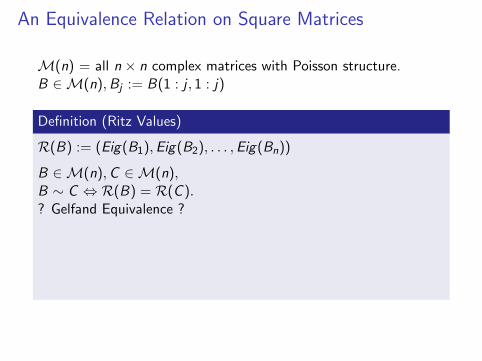
An Equivalence Relation on Square Matrices

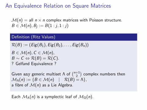
M(n) = all n × n complex matrices with Poisson structure.B ∈M(n),Bj := B(1 : j , 1 : j)

Definition (Ritz Values)

R(B) := (Eig(B1),Eig(B2), . . . ,Eig(Bn))

B ∈M(n),C ∈M(n),B ∼ C ⇔ R(B) = R(C ).? Gelfand Equivalence ?

Given any generic multiset Λ of(n+1

2

)complex numbers then

MΛ(n) := B ∈M(n) | R(B) = Λ,a fibre ofM(n) as a Lie Algebra.

EachMΛ(n) is a symplectic leaf ofMΩ(n).

An Equivalence Relation on Square Matrices

M(n) = all n × n complex matrices with Poisson structure.B ∈M(n),Bj := B(1 : j , 1 : j)

Definition (Ritz Values)

R(B) := (Eig(B1),Eig(B2), . . . ,Eig(Bn))

B ∈M(n),C ∈M(n),B ∼ C ⇔ R(B) = R(C ).? Gelfand Equivalence ?

Given any generic multiset Λ of(n+1

2

)complex numbers then

MΛ(n) := B ∈M(n) | R(B) = Λ,a fibre ofM(n) as a Lie Algebra.

EachMΛ(n) is a symplectic leaf ofMΩ(n).

Why study ∼ ?

Gil Strang

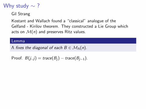
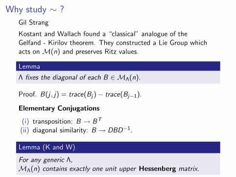
Kostant and Wallach found a “classical” analogue of theGelfand - Kirilov theorem. They constructed a Lie Group whichacts onM(n) and preserves Ritz values.

Lemma

Λ fixes the diagonal of each B ∈MΛ(n).

Proof. B(j , j) = trace(Bj)− trace(Bj−1).

Elementary Conjugations

(i) transposition: B → BT

(ii) diagonal similarity: B → DBD−1.

Lemma (K and W)

For any generic Λ,MΛ(n) contains exactly one unit upper Hessenberg matrix.

Why study ∼ ?

Gil Strang

Kostant and Wallach found a “classical” analogue of theGelfand - Kirilov theorem. They constructed a Lie Group whichacts onM(n) and preserves Ritz values.

Lemma

Λ fixes the diagonal of each B ∈MΛ(n).

Proof. B(j , j) = trace(Bj)− trace(Bj−1).

Elementary Conjugations

(i) transposition: B → BT

(ii) diagonal similarity: B → DBD−1.

Lemma (K and W)

For any generic Λ,MΛ(n) contains exactly one unit upper Hessenberg matrix.

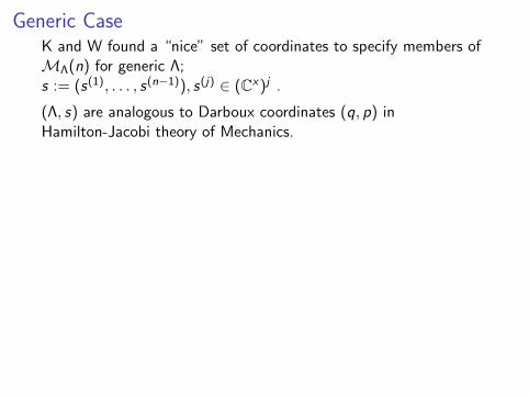
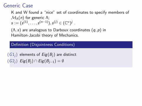
Generic CaseK and W found a “nice” set of coordinates to specify members ofMΛ(n) for generic Λ;s := (s(1), . . . , s(n−1)), s(j) ∈ (Cx)j .

(Λ, s) are analogous to Darboux coordinates (q, p) inHamilton-Jacobi theory of Mechanics.

Definition (Disjointness Conditions)

(G1j) elements of Eig(Bj) are distinct

(G2j) Eig(Bj) ∩ Eig(Bj−1) = ∅

Definition

Λ := (Λ1,Λ2, . . . ,Λn)Λj := either j × j invertible diagonal matrix orits diagonal entries in some fixed order .

MΩ(n) = the generic fibres inM(n).






Definition








Definition



The Dual CoordinatesB ∈MΛ(n) ⊂MΩ(n).(G1m)⇒ Bm = GmΛm(Gm)−1, Gm ∈ GL(m).Gm unique if last row is ones, by (G2m).

Definition

bm and cm ∈ Cm, given by

Bm+1 =

(Gm 00T 1

) (Λm cm

bmT δm+1

) (Gm

−1 00T 1

)=

(Bm Gmcm

bmTGm

−1 δm+1

).

Theorem (BNP)

s = (1, b2T , b3

T , . . . , bn−1T ) determines B.

What is Gm ?

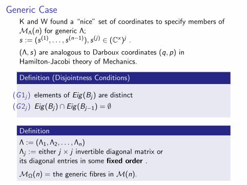
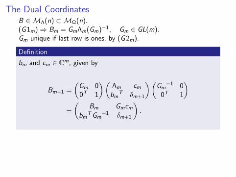
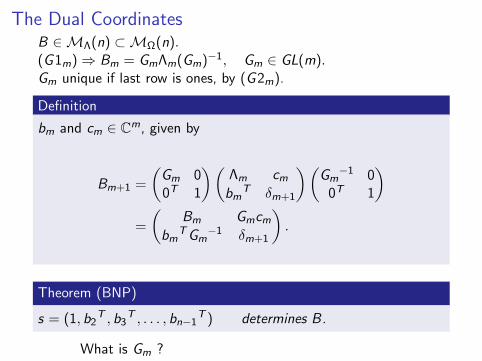
The Dual CoordinatesB ∈MΛ(n) ⊂MΩ(n).(G1m)⇒ Bm = GmΛm(Gm)−1, Gm ∈ GL(m).Gm unique if last row is ones, by (G2m).

Definition

bm and cm ∈ Cm, given by

Bm+1 =

(Gm 00T 1

) (Λm cm

bmT δm+1

) (Gm

−1 00T 1

)=

(Bm Gmcm

bmTGm

−1 δm+1

).

Theorem (BNP)

s = (1, b2T , b3

T , . . . , bn−1T ) determines B.

What is Gm ?

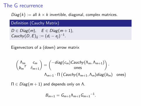
The G recurrence

Diag(k) := all k × k invertible, diagonal, complex matrices.

Definition (Cauchy Matrix)

D ∈ Diag(m), E ∈ Diag(m + 1),Cauchy(D,E )ij := (di − ej)

−1.

Eigenvectors of a (down) arrow matrix

(Λm cm

bmT δm+1

)=

(−diag(cm)Cauchy(Λm,Λm+1)

ones

)·

Λm+1 · Π(Cauchy(Λm+1,Λm)diag(bm) ones

)Π ∈ Diag(m + 1) and depends only on Λ.

Bm+1 = Gm+1Λm+1Gm+1−1.

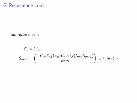
G Recurrence cont.

So, recurrence is

G1 = (1),

Gm+1 =

(−Gmdiag(cm)Cauchy(Λm,Λm+1)

ones

), 1 ≤ m < n.

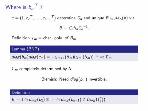
Where is bmT ?

c = (1, c2T , . . . , cn−1

T ) determine Gn and unique B ∈MΛ(n) via

B = GnΛnGn−1.

Definition χm = char. poly. of Bm.

Lemma (BNP)

diag(bm)diag(cm) = −χm+1(Λm)(χm′(Λm))−1 =: Σm.

Σm completely determined by Λ.

Blemish: Need diag(bm) invertible.

Definition

b := 1⊕ diag(b2)⊕ · · · ⊕ diag(bn−1) ∈ Diag((n2

))

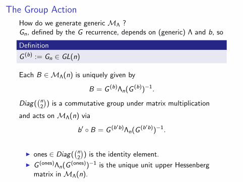
The Group Action

How do we generate generic MΛ ?Gn, defined by the G recurrence, depends on (generic) Λ and b, so

Definition

G (b) := Gn ∈ GL(n)

Each B ∈MΛ(n) is uniquely given by

B = G (b)Λn(G(b))−1.

Diag((n2

)) is a commutative group under matrix multiplication

and acts onMΛ(n) via

b′ B = G (b′b)Λn(G(b′b))−1.

I ones ∈ Diag((n2

)) is the identity element.

I G (ones)Λn(G(ones))−1 is the unique unit upper Hessenberg

matrix inMΛ(n).

Regularity

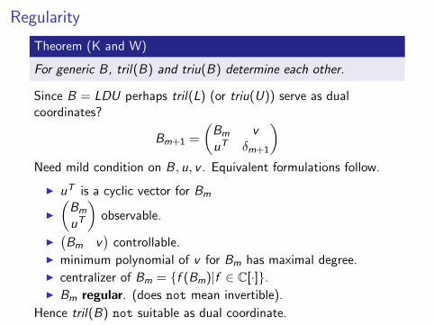
Theorem (K and W)

For generic B, tril(B) and triu(B) determine each other.

Since B = LDU perhaps tril(L) (or triu(U)) serve as dualcoordinates?

Bm+1 =

(Bm vuT δm+1

)Need mild condition on B, u, v . Equivalent formulations follow.

I uT is a cyclic vector for Bm

I

(Bm

uT

)observable.

I(Bm v

)controllable.

I minimum polynomial of v for Bm has maximal degree.I centralizer of Bm = f (Bm)|f ∈ C[·].I Bm regular. (does not mean invertible).

Hence tril(B) not suitable as dual coordinate.

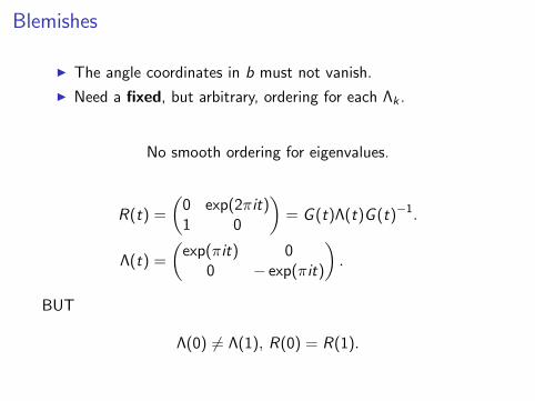
Blemishes

I The angle coordinates in b must not vanish.

I Need a fixed, but arbitrary, ordering for each Λk .

No smooth ordering for eigenvalues.

R(t) =

(0 exp(2πit)1 0

)= G (t)Λ(t)G (t)−1.

Λ(t) =

(exp(πit) 0

0 − exp(πit)

).

BUT

Λ(0) 6= Λ(1), R(0) = R(1).

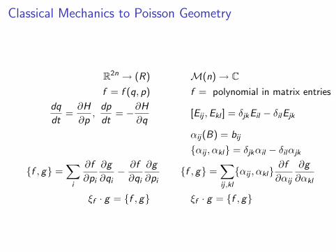
Classical Mechanics to Poisson Geometry

R2n → (R) M(n)→ Cf = f (q, p) f = polynomial in matrix entries

dq

dt=

∂H

∂p,

dp

dt= −∂H

∂q[Eij ,Ekl ] = δjkEil − δilEjk

αij(B) = bij

αij , αkl = δjkαil − δilαjk

f , g =∑

i

∂f

∂pi

∂g

∂qi− ∂f

∂qi

∂g

∂pif , g =

∑ij ,kl

αij , αkl∂f

∂αij

∂g

∂αkl

ξf · g = f , g ξf · g = f , g

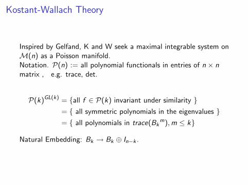
Kostant-Wallach Theory

Inspired by Gelfand, K and W seek a maximal integrable system onM(n) as a Poisson manifold.Notation. P(n) := all polynomial functionals in entries of n × nmatrix , e.g. trace, det.

P(k)GL(k) = all f ∈ P(k) invariant under similarity = all symmetric polynomials in the eigenvalues = all polynomials in trace(Bk

m),m ≤ k

Natural Embedding: Bk → Bk ⊕ In−k .

K-W theory (cont.)

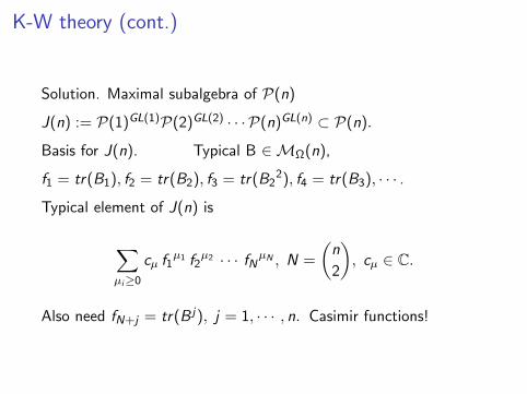
Solution. Maximal subalgebra of P(n)

J(n) := P(1)GL(1)P(2)GL(2) · · · P(n)GL(n) ⊂ P(n).

Basis for J(n). Typical B ∈MΩ(n),

f1 = tr(B1), f2 = tr(B2), f3 = tr(B22), f4 = tr(B3), · · · .

Typical element of J(n) is

∑µi≥0

cµ f1µ1 f2

µ2 · · · fNµN , N =

(n

2

), cµ ∈ C.

Also need fN+j = tr(B j), j = 1, · · · , n. Casimir functions!

K-W Theory (cont.)

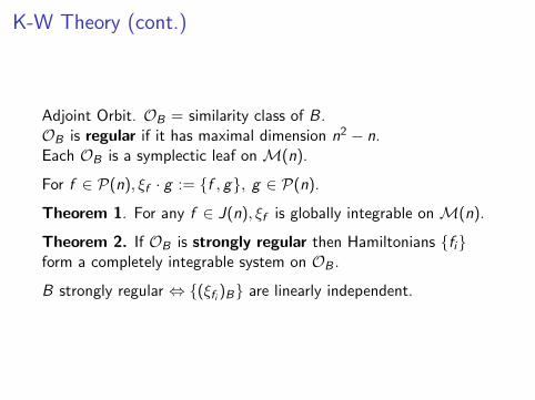
Adjoint Orbit. OB = similarity class of B.OB is regular if it has maximal dimension n2 − n.Each OB is a symplectic leaf on M(n).

For f ∈ P(n), ξf · g := f , g, g ∈ P(n).

Theorem 1. For any f ∈ J(n), ξf is globally integrable onM(n).

Theorem 2. If OB is strongly regular then Hamiltonians fiform a completely integrable system on OB .

B strongly regular ⇔ (ξfi )B are linearly independent.

The Gelfand-Zeitlin Group Action

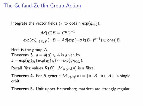
Integrate the vector fields ξfi to obtain exp(qiξfi ).

Ad(G )B = GBG−1

exp(q ξtr(Bm)k ) · B = Ad [exp(−q k(Bm)k−1)⊕ ones]B

Here is the group A.Theorem 3. a = a(q) ∈ A is given bya = exp(q1ξf1) exp(q2ξf2) · · · exp(qNξfN ).

Recall Ritz values R(B). MR(B)(n) is a fibre.

Theorem 4. For B generic MR(B)(n) = a · B | a ∈ A, a singleorbit.

Theorem 5. Unit upper Hessenberg matrices are strongly regular.

Reconciliation

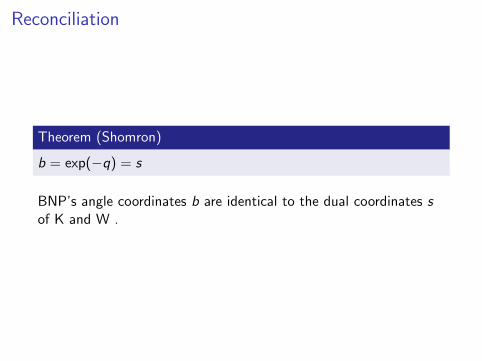
Theorem (Shomron)

b = exp(−q) = s

BNP’s angle coordinates b are identical to the dual coordinates sof K and W .

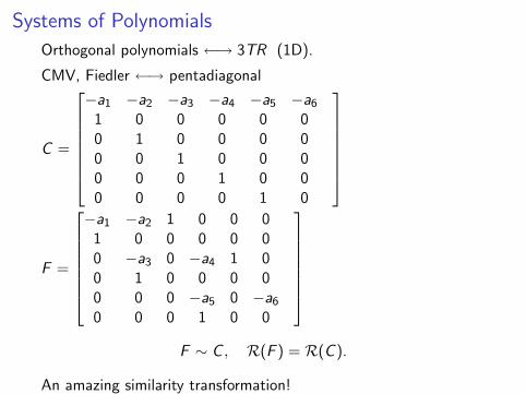
Systems of Polynomials

Orthogonal polynomials ←→ 3TR (1D).

CMV, Fiedler ←→ pentadiagonal

C =

−a1 −a2 −a3 −a4 −a5 −a6

1 0 0 0 0 00 1 0 0 0 00 0 1 0 0 00 0 0 1 0 00 0 0 0 1 0

F =

−a1 −a2 1 0 0 01 0 0 0 0 00 −a3 0 −a4 1 00 1 0 0 0 00 0 0 −a5 0 −a6

0 0 0 1 0 0

F ∼ C , R(F ) = R(C ).

An amazing similarity transformation!

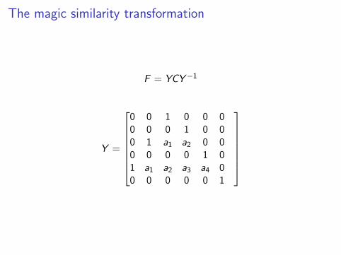
The magic similarity transformation

F = YCY−1

Y =

0 0 1 0 0 00 0 0 1 0 00 1 a1 a2 0 00 0 0 0 1 01 a1 a2 a3 a4 00 0 0 0 0 1

Linear Algebra Meets Lie Algebra

Documents