Linear Algebra for data science Session 1

Welcome message from author
This document is posted to help you gain knowledge. Please leave a comment to let me know what you think about it! Share it to your friends and learn new things together.
Transcript
Linear Algebra for data science
Session 1
Warm Up
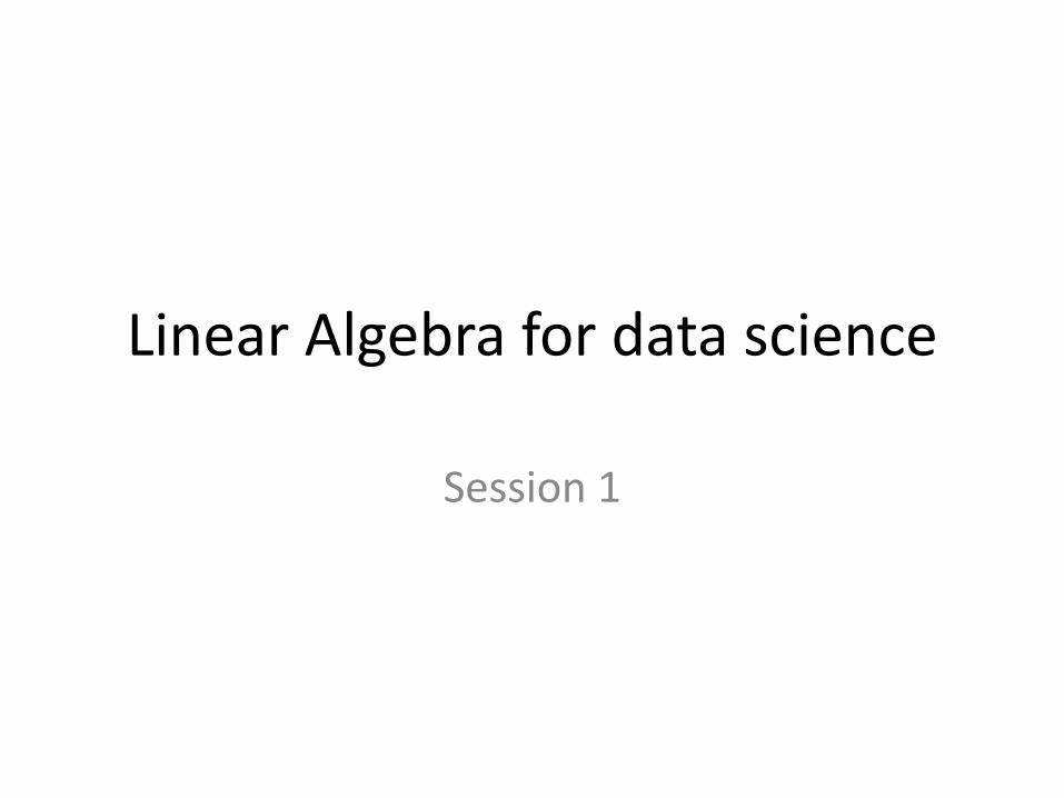
• What do you know about:– Artificial Intelligence (AI).– Soft computing (SC).– Machine learning (ML).– Deep learning (DL).
2
AI Layers
What is AI?
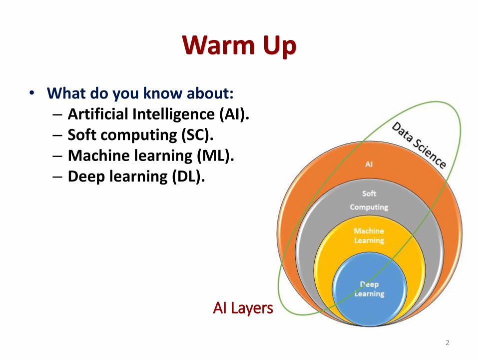
• Artificial intelligence enablescomputers and machines to mimicthe perception, learning, problem-solving, and decision-makingcapabilities of the human mind. [IBM]
• Artificial intelligence is thesystem's ability to correctly interpretexternal data, to learn from suchdata, and to use those learnings toachieve specific goals and tasksthrough flexible adaptation. [Kaplan et. al.,
Business Horizons]
3
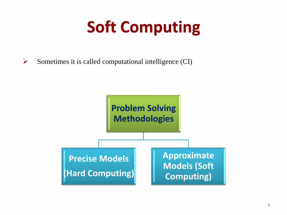
Soft Computing
➢ Sometimes it is called computational intelligence (CI)
4
Problem Solving Methodologies
Precise Models
(Hard Computing)
Approximate Models (Soft Computing)
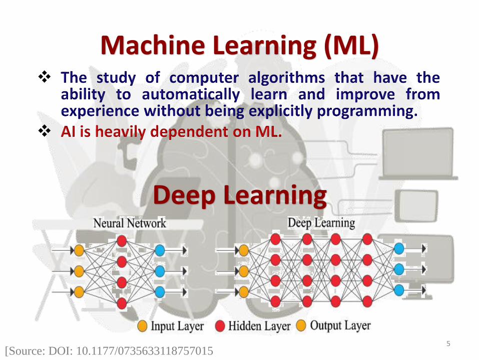
Machine Learning (ML)
5
Deep Learning
[Source: DOI: 10.1177/0735633118757015
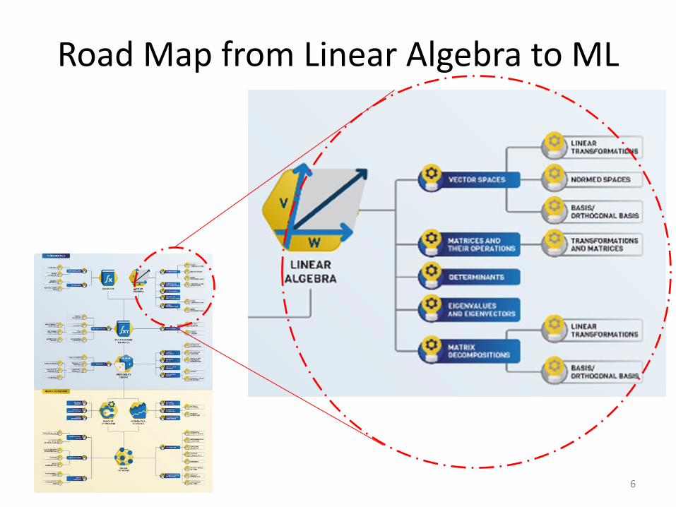
Road Map from Linear Algebra to ML
6
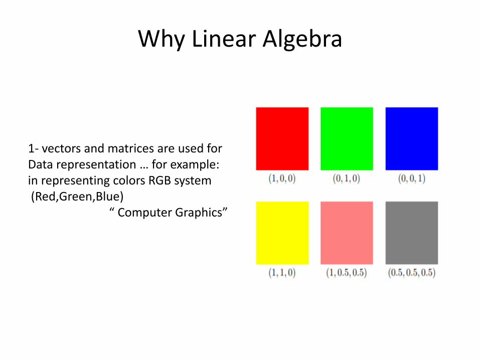
1- vectors and matrices are used forData representation … for example:in representing colors RGB system(Red,Green,Blue)
“ Computer Graphics”
Why Linear Algebra
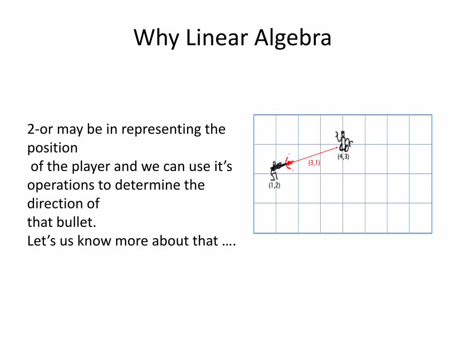
2-or may be in representing the positionof the player and we can use it’s operations to determine the direction ofthat bullet.Let’s us know more about that ….
Why Linear Algebra
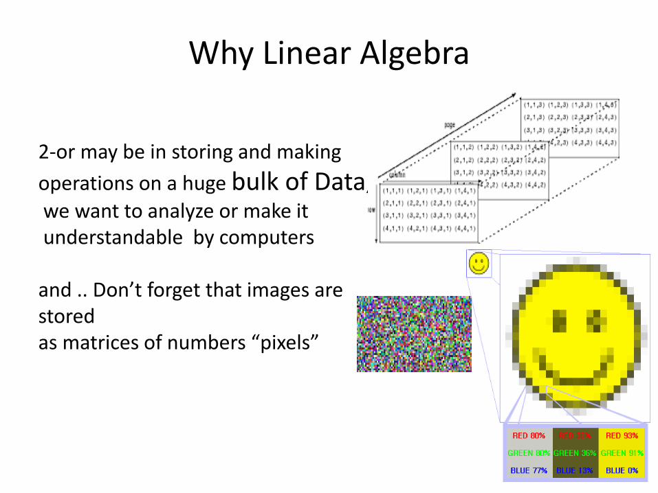
2-or may be in storing and making
operations on a huge bulk of Data,
we want to analyze or make itunderstandable by computers
and .. Don’t forget that images are storedas matrices of numbers “pixels”
Why Linear Algebra
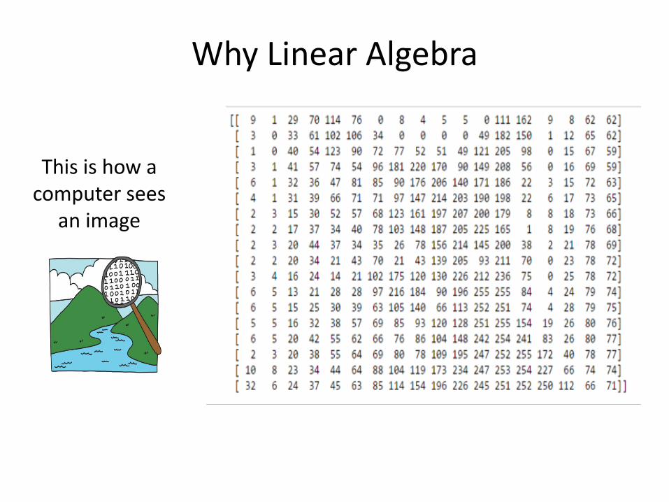
This is how a computer sees
an image
Why Linear Algebra
So… Linear Algebra is definitely every where
Profiling
• How much do you know about the fundamentals of linear algebra?
Rate yourself from 1 (min knowledge) to 10
OR
Take this quick quiz (Kahoot link)
12
Contents
• Basics of linear algebra
– Vectors, vector space, norms
– dot product,
– Matrices,
– Operations on matrices
13
• Linear Programming with applications in a wide range of domains
• Planning• Decision Engineering• Financial forecasting• Technological trend forecasting• Natural Language processing
Applications for solving linear systems of equation
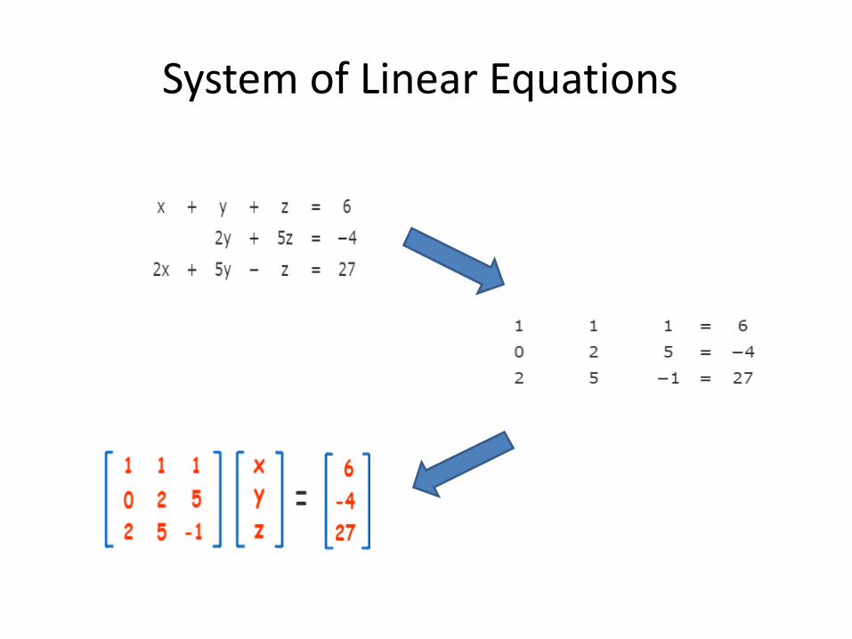
System of Linear Equations
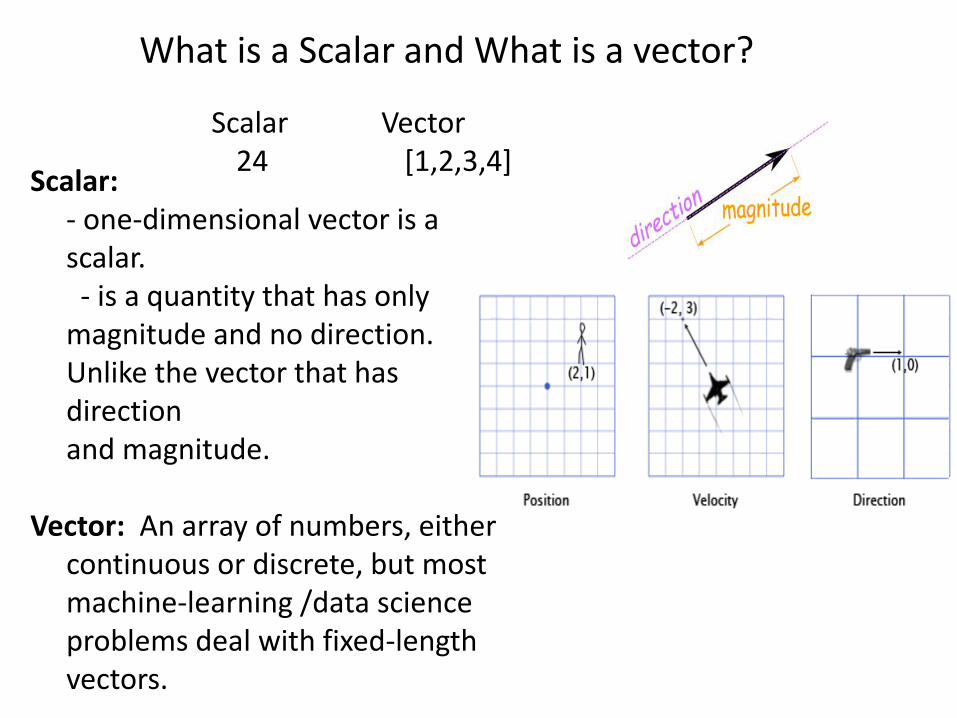
Scalar Vector24 [1,2,3,4]
What is a Scalar and What is a vector?
Scalar:- one-dimensional vector is a scalar. - is a quantity that has only
magnitude and no direction.Unlike the vector that has direction and magnitude.
Vector: An array of numbers, either continuous or discrete, but most machine-learning /data science problems deal with fixed-length vectors.
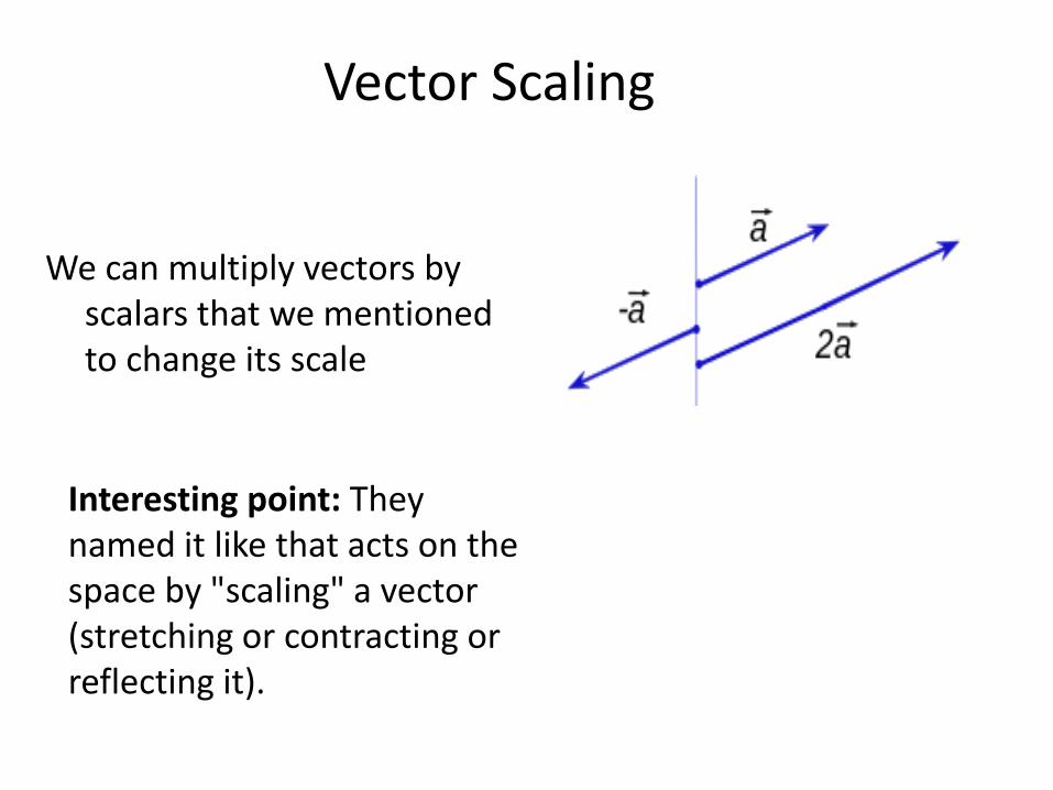
Vector Scaling
We can multiply vectors by scalars that we mentioned to change its scale
Interesting point: They named it like that acts on the space by "scaling" a vector (stretching or contracting or reflecting it).
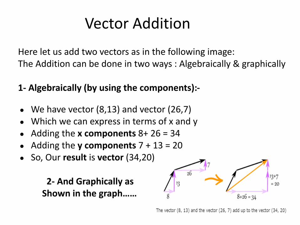
● We have vector (8,13) and vector (26,7)● Which we can express in terms of x and y● Adding the x components 8+ 26 = 34 ● Adding the y components 7 + 13 = 20● So, Our result is vector (34,20)
2- And Graphically as Shown in the graph……
Vector Addition
Here let us add two vectors as in the following image:The Addition can be done in two ways : Algebraically & graphically
1- Algebraically (by using the components):-
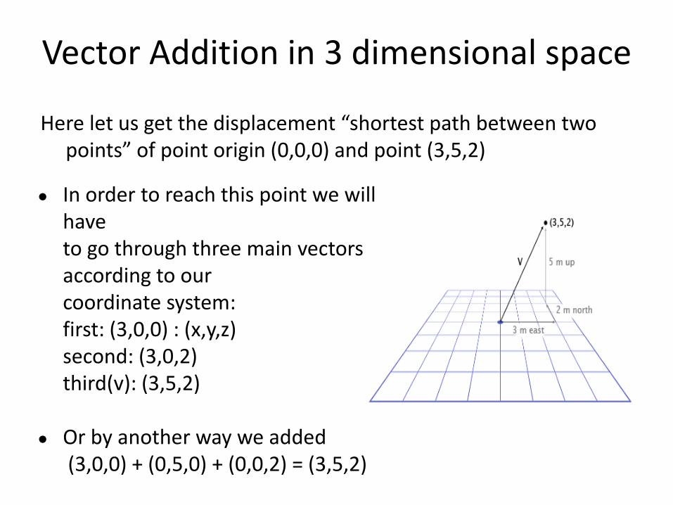
● In order to reach this point we will have to go through three main vectors according to ourcoordinate system:first: (3,0,0) : (x,y,z)second: (3,0,2)third(v): (3,5,2)
● Or by another way we added(3,0,0) + (0,5,0) + (0,0,2) = (3,5,2)
Vector Addition in 3 dimensional space
Here let us get the displacement “shortest path between two points” of point origin (0,0,0) and point (3,5,2)
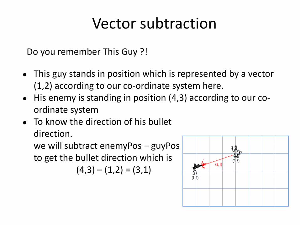
● This guy stands in position which is represented by a vector (1,2) according to our co-ordinate system here.
● His enemy is standing in position (4,3) according to our co-ordinate system
● To know the direction of his bullet direction. we will subtract enemyPos – guyPosto get the bullet direction which is
(4,3) – (1,2) = (3,1)
Vector subtraction
Do you remember This Guy ?!
Vector Multiplication
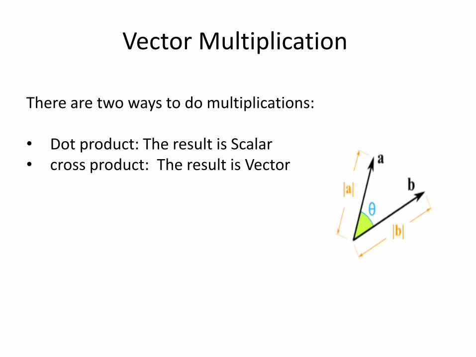
There are two ways to do multiplications:
• Dot product: The result is Scalar• cross product: The result is Vector
Vectors: Cross product
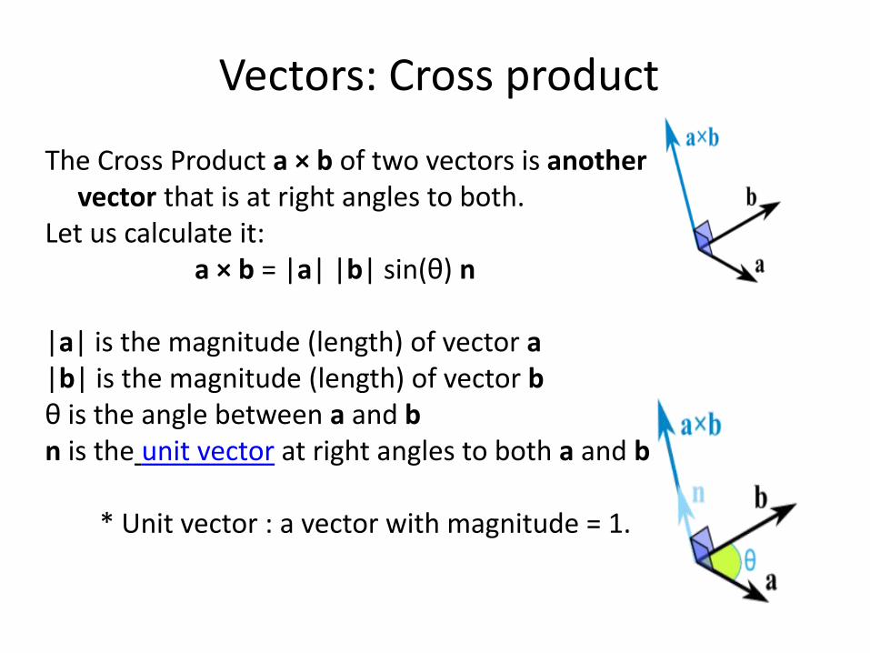
The Cross Product a × b of two vectors is another vector that is at right angles to both.
Let us calculate it:a × b = |a| |b| sin(θ) n
|a| is the magnitude (length) of vector a|b| is the magnitude (length) of vector bθ is the angle between a and bn is the unit vector at right angles to both a and b
* Unit vector : a vector with magnitude = 1.

Vectors : dot/Inner product
Any vector of dimension n can be represented as a matrix 𝑣 ∈ 𝑅𝑛×1. Let us denote two n dimensional vectors 𝑣1 ∈ 𝑅𝑛×1and 𝑣2 ∈ 𝑅𝑛×1
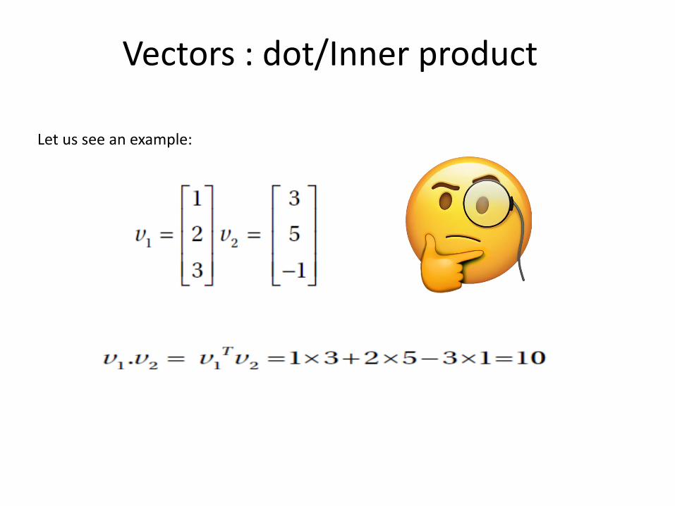
The dot product of two vectors is the sum of the product of corresponding components—i.e., components along the same dimension—and can be expressed as
Vectors : dot/Inner product
Let us see an example:
Matrices
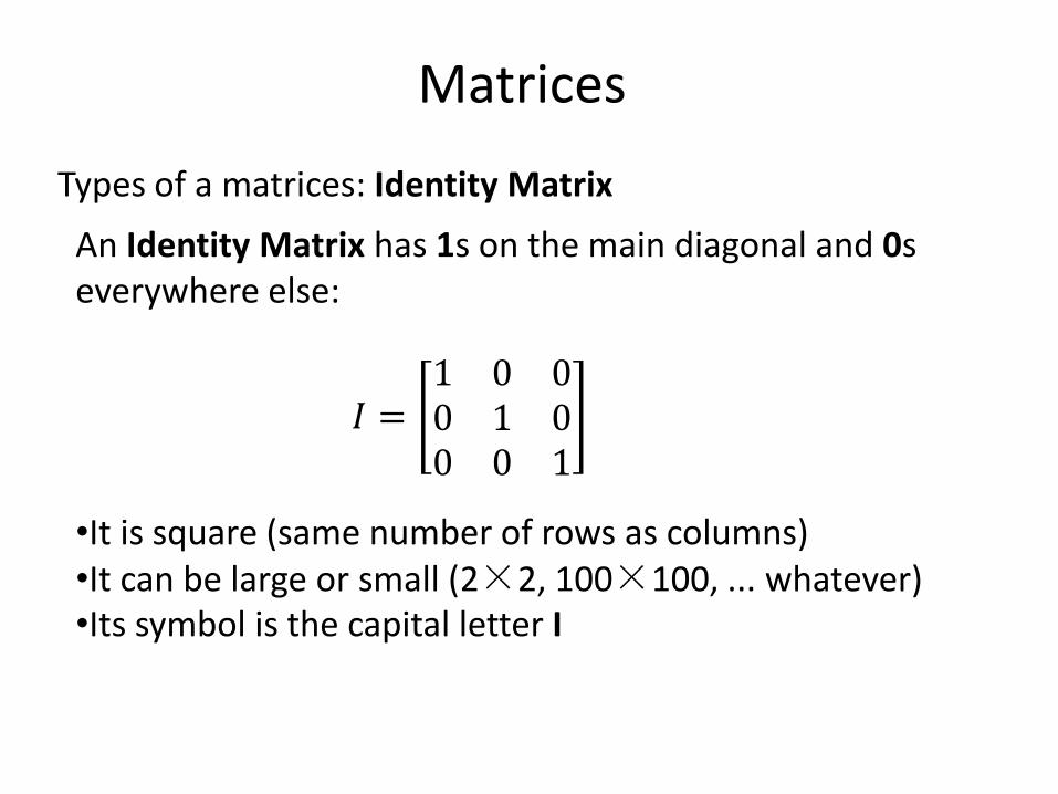
Types of a matrices: Identity Matrix
An Identity Matrix has 1s on the main diagonal and 0s everywhere else:
𝐼 =1 0 00 1 00 0 1
•It is square (same number of rows as columns)•It can be large or small (2×2, 100×100, ... whatever)•Its symbol is the capital letter I
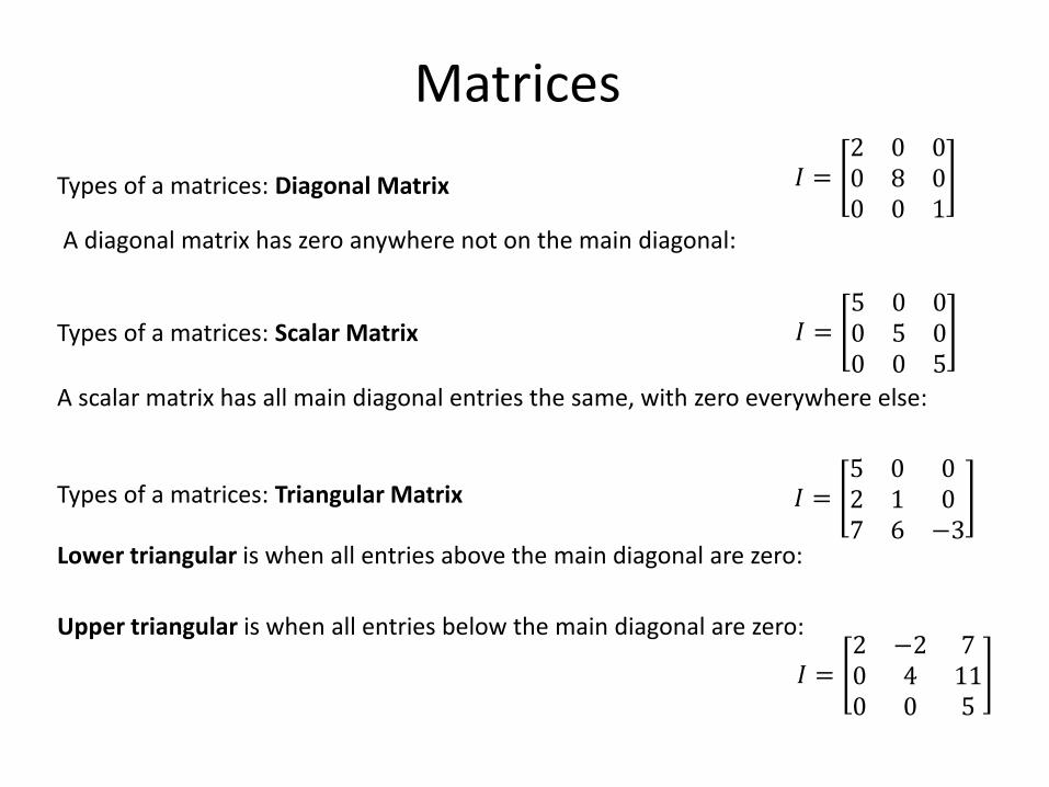
Types of a matrices: Diagonal Matrix
A diagonal matrix has zero anywhere not on the main diagonal:
𝐼 =2 0 00 8 00 0 1
Matrices
Types of a matrices: Scalar Matrix
A scalar matrix has all main diagonal entries the same, with zero everywhere else:
𝐼 =5 0 00 5 00 0 5
Types of a matrices: Triangular Matrix
Lower triangular is when all entries above the main diagonal are zero:
𝐼 =5 0 02 1 07 6 −3
Upper triangular is when all entries below the main diagonal are zero:
𝐼 =2 −2 70 4 110 0 5
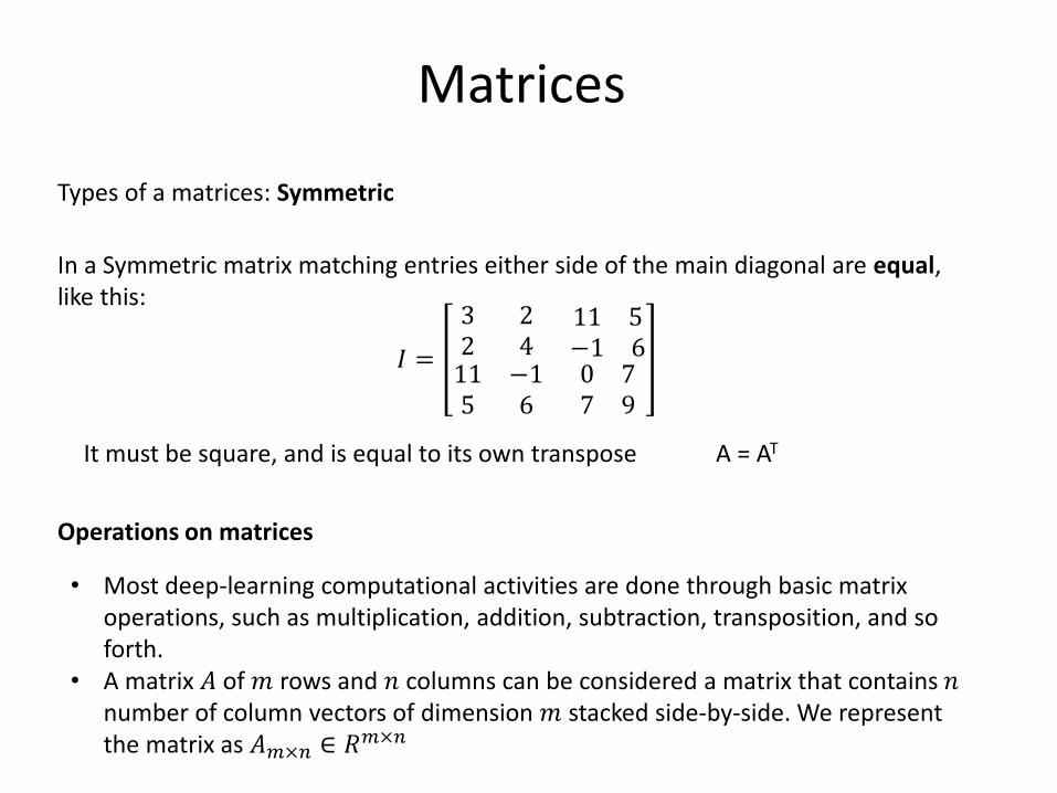
Types of a matrices: Symmetric
In a Symmetric matrix matching entries either side of the main diagonal are equal, like this:
𝐼 =
3 2 11 52 4 −1 6115
−16
0 77 9
It must be square, and is equal to its own transpose A = AT
Matrices
Operations on matrices
• Most deep-learning computational activities are done through basic matrix operations, such as multiplication, addition, subtraction, transposition, and so forth.
• A matrix 𝐴 of 𝑚 rows and 𝑛 columns can be considered a matrix that contains 𝑛number of column vectors of dimension 𝑚 stacked side-by-side. We represent the matrix as 𝐴𝑚×𝑛 ∈ 𝑅𝑚×𝑛
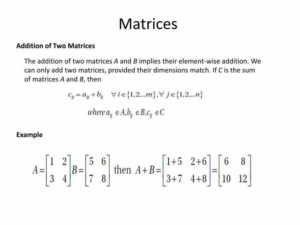
Addition of Two Matrices
The addition of two matrices A and B implies their element-wise addition. We can only add two matrices, provided their dimensions match. If C is the sum of matrices A and B, then
Matrices
Example
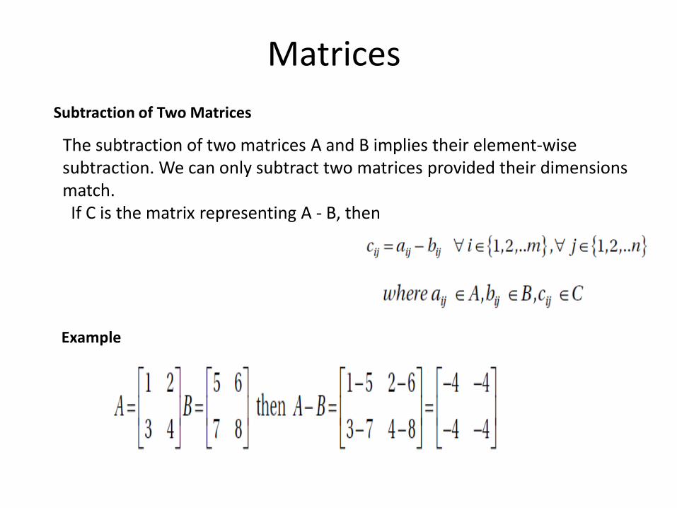
Subtraction of Two Matrices
The subtraction of two matrices A and B implies their element-wise subtraction. We can only subtract two matrices provided their dimensions match.If C is the matrix representing A - B, then
Matrices
Example
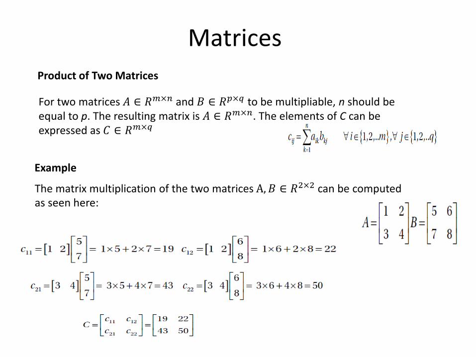
Product of Two Matrices
For two matrices 𝐴 ∈ 𝑅𝑚×𝑛 and 𝐵 ∈ 𝑅𝑝×𝑞 to be multipliable, n should be equal to p. The resulting matrix is 𝐴 ∈ 𝑅𝑚×𝑛. The elements of C can be expressed as 𝐶 ∈ 𝑅𝑚×𝑞
Matrices
Example
The matrix multiplication of the two matrices A, 𝐵 ∈ 𝑅2×2 can be computed as seen here:
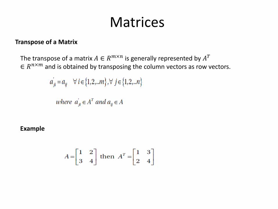
Transpose of a Matrix
The transpose of a matrix 𝐴 ∈ 𝑅𝑚×𝑛 is generally represented by 𝐴𝑇
∈ 𝑅𝑛×𝑚 and is obtained by transposing the column vectors as row vectors.
Matrices
Example

Example:
The transpose of the product of two matrices A and B is the product of the transposes of matrices A and B in the reverse order; i.e., (𝐴𝐵)𝑇= 𝐵𝑇𝐴𝑇
For example, if we take two matrices then
Hence, the equality (𝐴𝐵)𝑇= 𝐵𝑇𝐴𝑇 holds.
Matrices
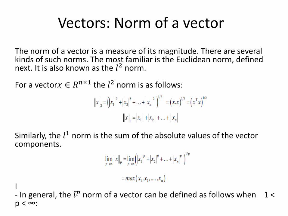
Vectors: Norm of a vector
The norm of a vector is a measure of its magnitude. There are several kinds of such norms. The most familiar is the Euclidean norm, defined next. It is also known as the 𝑙2 norm.
For a vector𝑥 ∈ 𝑅𝑛×1 the 𝑙2 norm is as follows:
Similarly, the 𝑙1 norm is the sum of the absolute values of the vector components.
I - In general, the 𝑙𝑝 norm of a vector can be defined as follows when 1 < p < ∞:
Vectors
Norm of a vector
• Generally, for machine learning we use both l2 and l1 norms forseveral purposes. For instance,
1.the least square cost function that we use in linear regression isthe l2 norm of the error vector; i.e., the difference between theactual target-value vector and the predicted target-value vector.
2.Similarly, very often we would have to use regularization for ourmodel, with the result that the model doesn’t fit the trainingdata very well and fails to generalize to new data. To achieveregularization, we generally add the square of either the l2 normor the l1 norm of the parameter vector for the model as apenalty in the cost function for the model. When the l2 norm ofthe parameter vector is used for regularization, it is generallyknown as Ridge Regularization, whereas when the l1 norm isused instead it is known as Lasso Regularization.
Vectors
Vectors
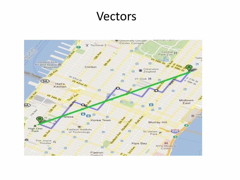
Norm of a vectorFor example, if you are building an application for taxi drivers in Manhattan that needs the minimal distance between two places, then using the ℓ1 norm (purple) would make more sense than ℓ2 (green). Because the ℓ2ℓ2 distance “is not accessible” to a taxi driver, as s/he can only navigate through the purple roads.
But if the same app was meant to be used by helicopter pilots, then the green line would serve them better. Here I’m mixing the notions of norm (“length” or “size”) and metric (“distance”), but you get the idea.

Exercise 1
Vector Space
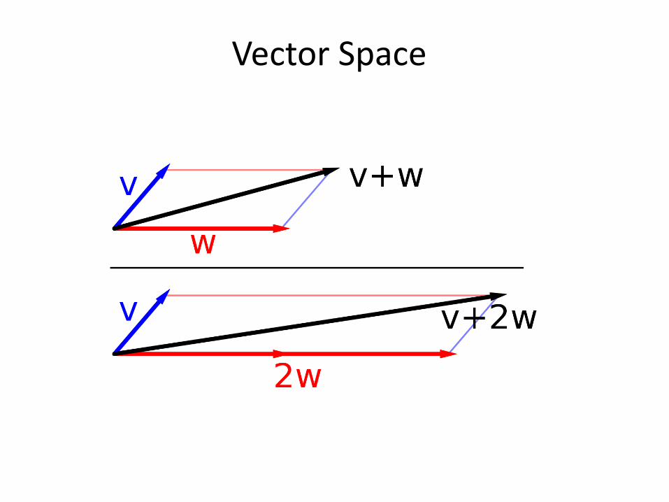
Vector Space
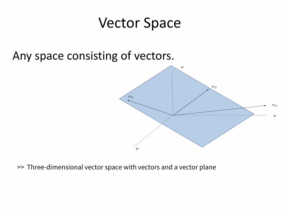
Vector Space
Any space consisting of vectors.
>> Three-dimensional vector space with vectors and a vector plane
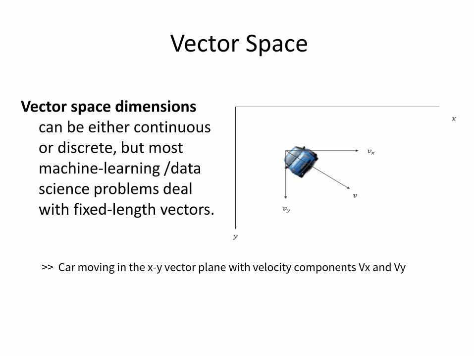
Vector Space
Vector space dimensionscan be either continuous or discrete, but most machine-learning /data science problems deal with fixed-length vectors.
>> Car moving in the x-y vector plane with velocity components Vx and Vy
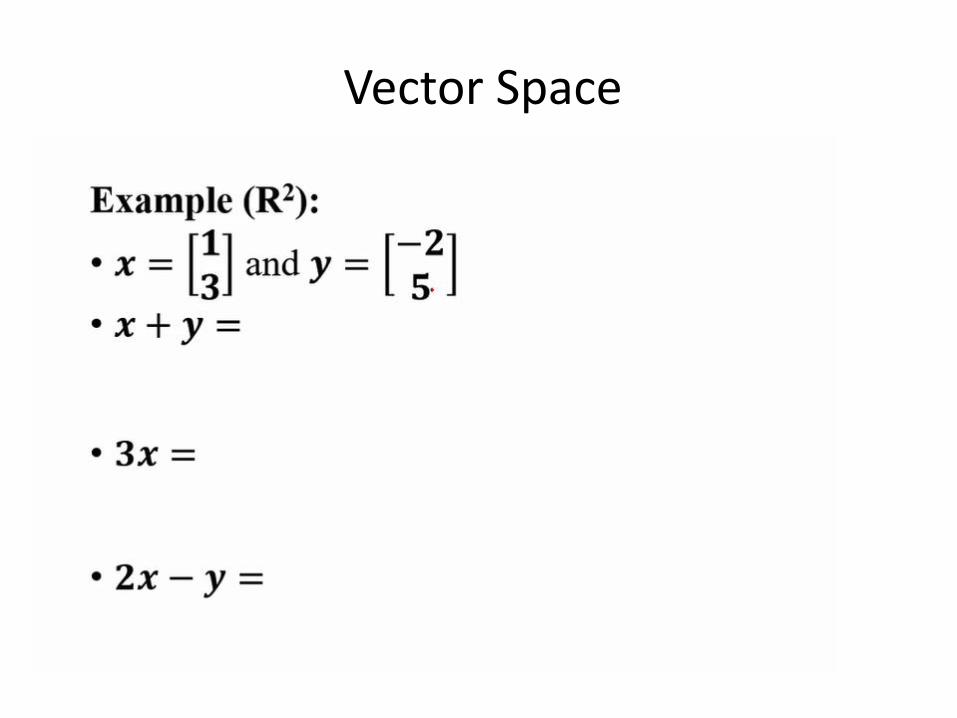
Vector Space

43

Linear Algebra for data science
Session 2
Contents
• Vector Spaces, basis and dimension
– linear combination of vectors
– vector space
– linear transformation using matrices
45
Linear Combination of Vectors
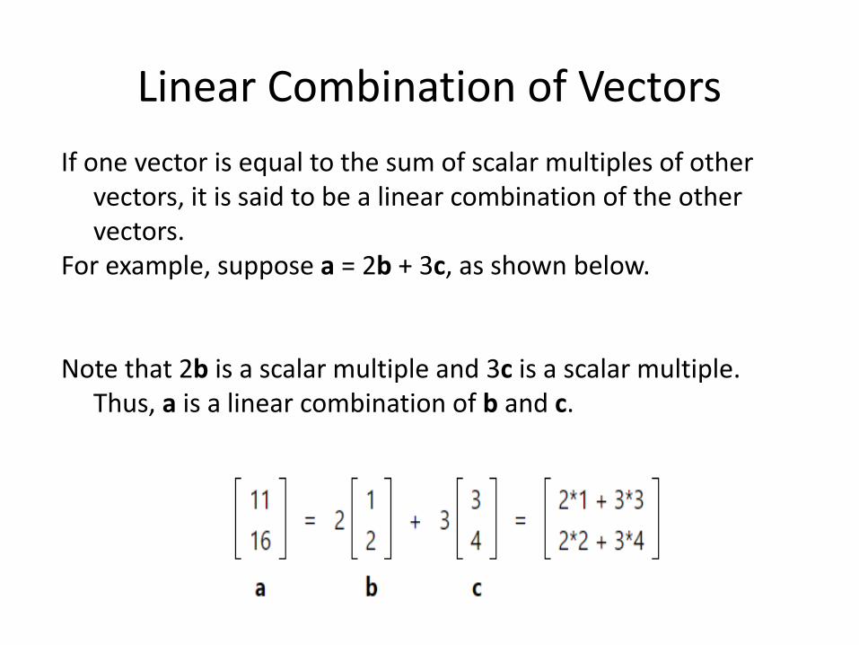
If one vector is equal to the sum of scalar multiples of other vectors, it is said to be a linear combination of the other vectors.
For example, suppose a = 2b + 3c, as shown below.
Note that 2b is a scalar multiple and 3c is a scalar multiple. Thus, a is a linear combination of b and c.
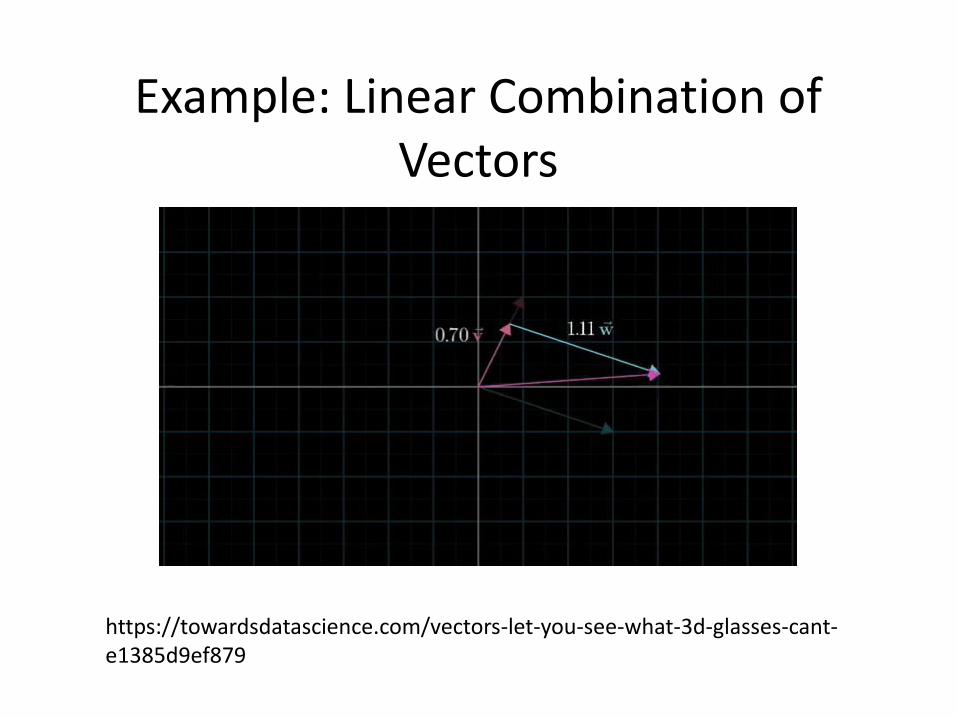
Example: Linear Combination of Vectors
https://towardsdatascience.com/vectors-let-you-see-what-3d-glasses-cant-e1385d9ef879
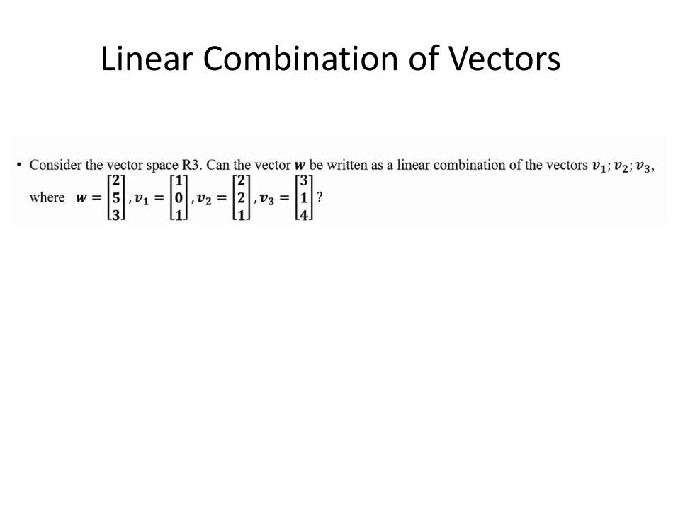
Linear Combination of Vectors
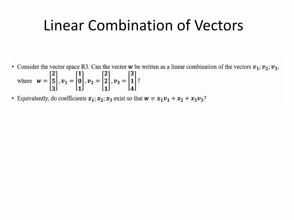
Linear Combination of Vectors
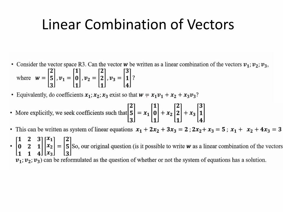
Linear Combination of Vectors
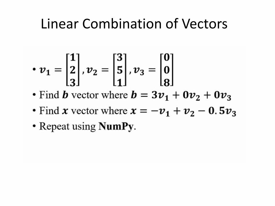
Linear Combination of Vectors
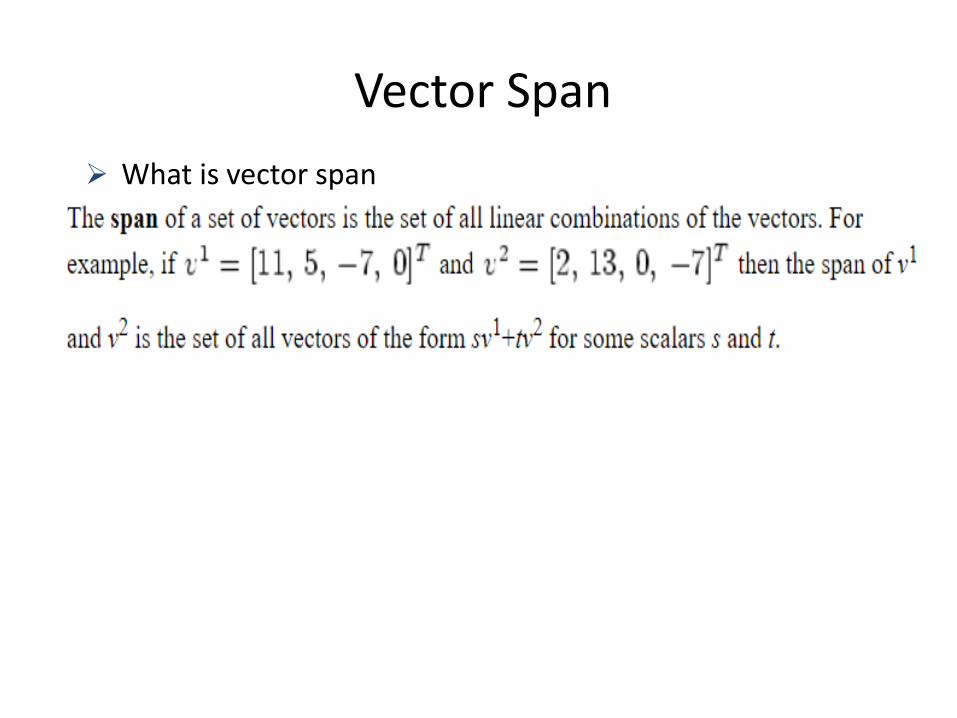
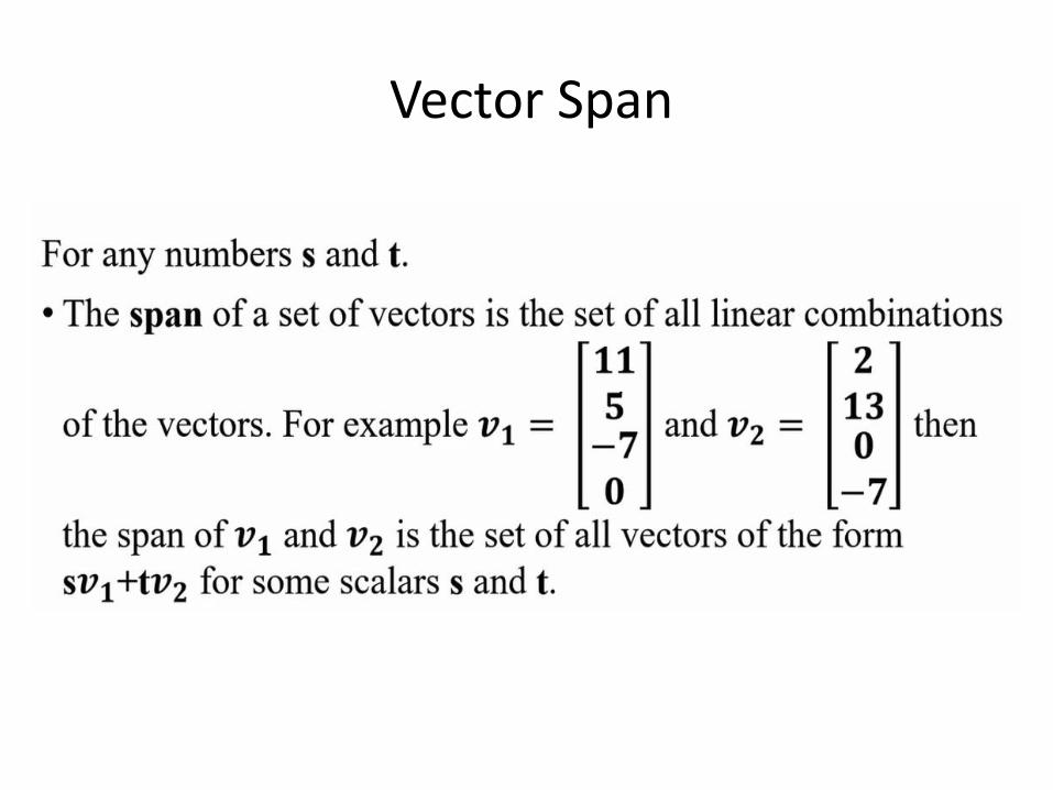
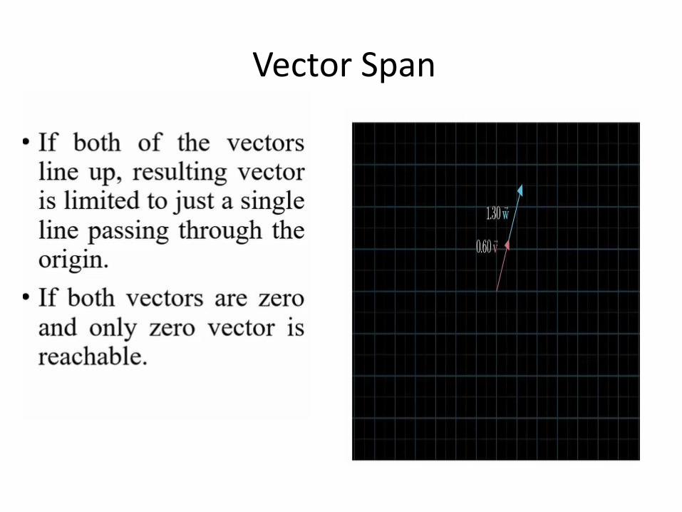
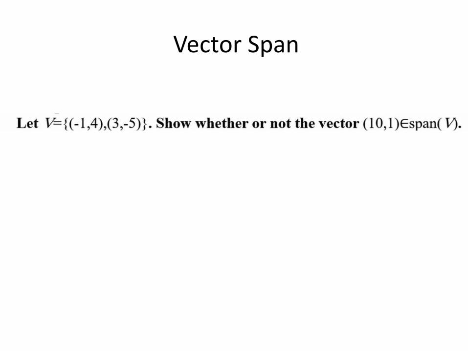
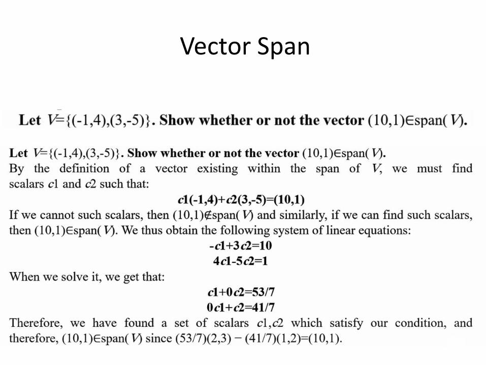
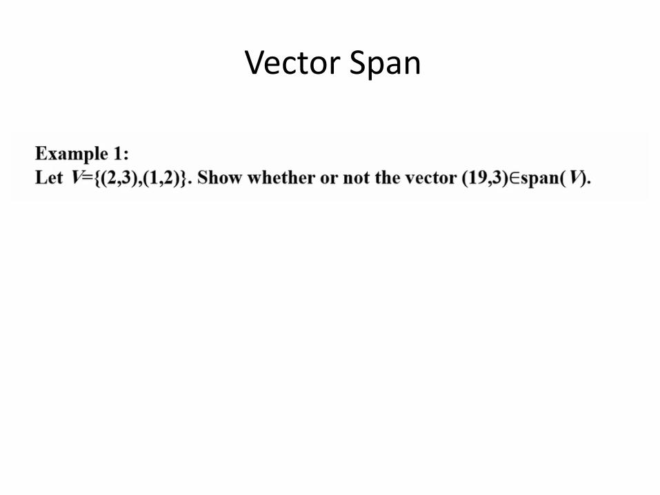
Vector Span
➢ What is vector span

Vector Span
Vector Span
Vector Span
Vector Span
Vector Span
Vector Span

Linear Independence of Vectors
• A vector is said to be linearly dependent on other vectors if it can be expressed as the linear combination of other vectors.
• If 𝑣1 = 5𝑣2 + 7𝑣3 , then 𝑣1, 𝑣2 and 𝑣3 are not linearly independent since at least one of them can be expressed as the sum of other vectors. In general, a set of 𝑛 vectors 𝑣1, 𝑣2, … , 𝑣𝑛 ∈ 𝑅𝑛×1 is said to be linearly independent if and only if 𝑎1𝑣1 + 𝑎2𝑣2 +⋯+ 𝑎𝑛𝑣𝑛 = 0 implies each of 𝑎𝑖 = 0 ∀𝑖∈ {1,2,… , 𝑛}.
• If 𝑎1𝑣1 + 𝑎2𝑣2 +⋯+ 𝑎𝑛𝑣𝑛 = 0 and not all 𝑎𝑖 = 0, then the vectors are not linearly independent.
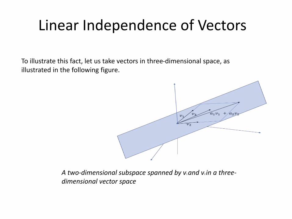
To illustrate this fact, let us take vectors in three-dimensional space, as illustrated in the following figure.
A two-dimensional subspace spanned by v1 and v2 in a three-dimensional vector space
Linear Independence of Vectors
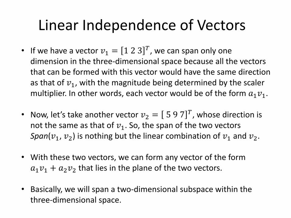
• If we have a vector 𝑣1 = 1 2 3 𝑇, we can span only one dimension in the three-dimensional space because all the vectors that can be formed with this vector would have the same direction as that of 𝑣1, with the magnitude being determined by the scaler multiplier. In other words, each vector would be of the form 𝑎1𝑣1.
• Now, let’s take another vector 𝑣2 = 5 9 7 𝑇, whose direction is not the same as that of 𝑣1. So, the span of the two vectors Span(𝑣1, 𝑣2) is nothing but the linear combination of 𝑣1 and 𝑣2.
• With these two vectors, we can form any vector of the form 𝑎1𝑣1 + 𝑎2𝑣2 that lies in the plane of the two vectors.
• Basically, we will span a two-dimensional subspace within the three-dimensional space.
Linear Independence of Vectors
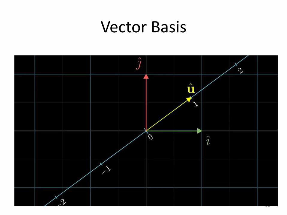
Vector Basis
62
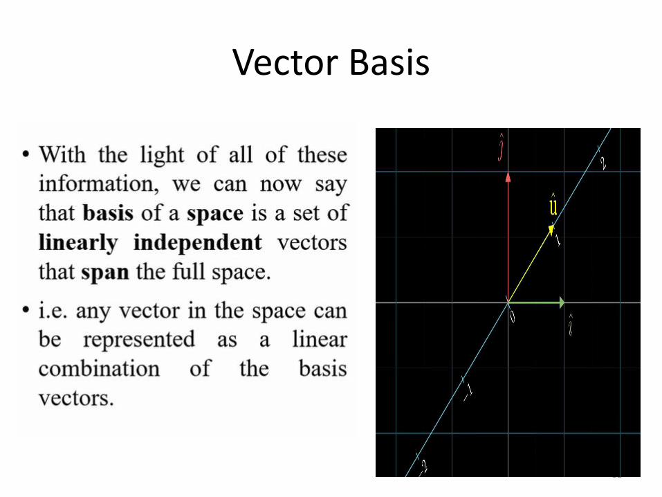
Vector Basis
63
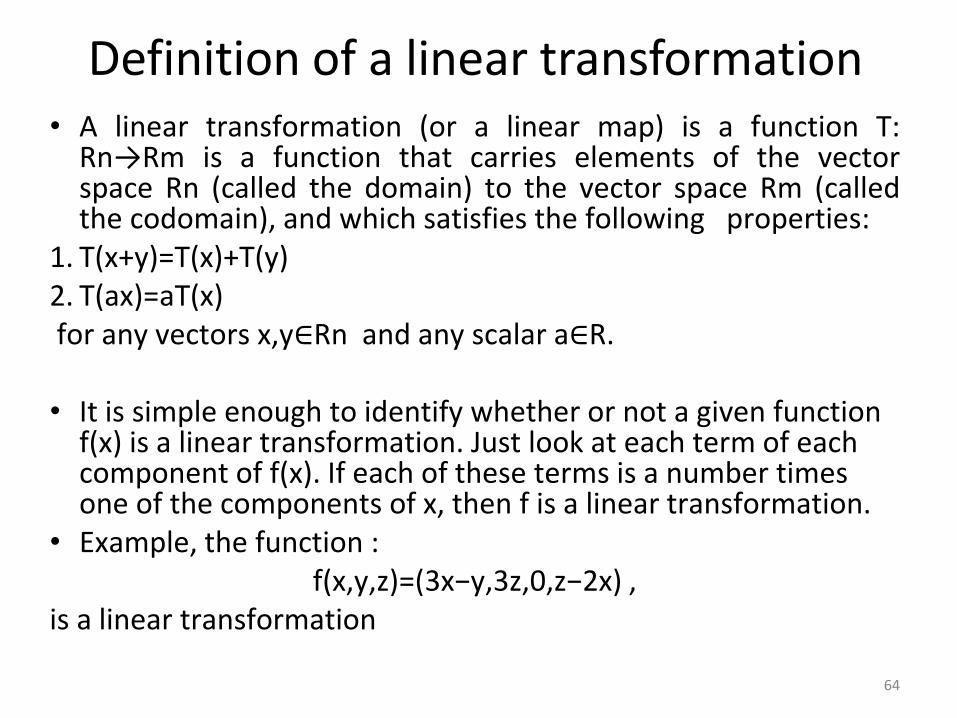
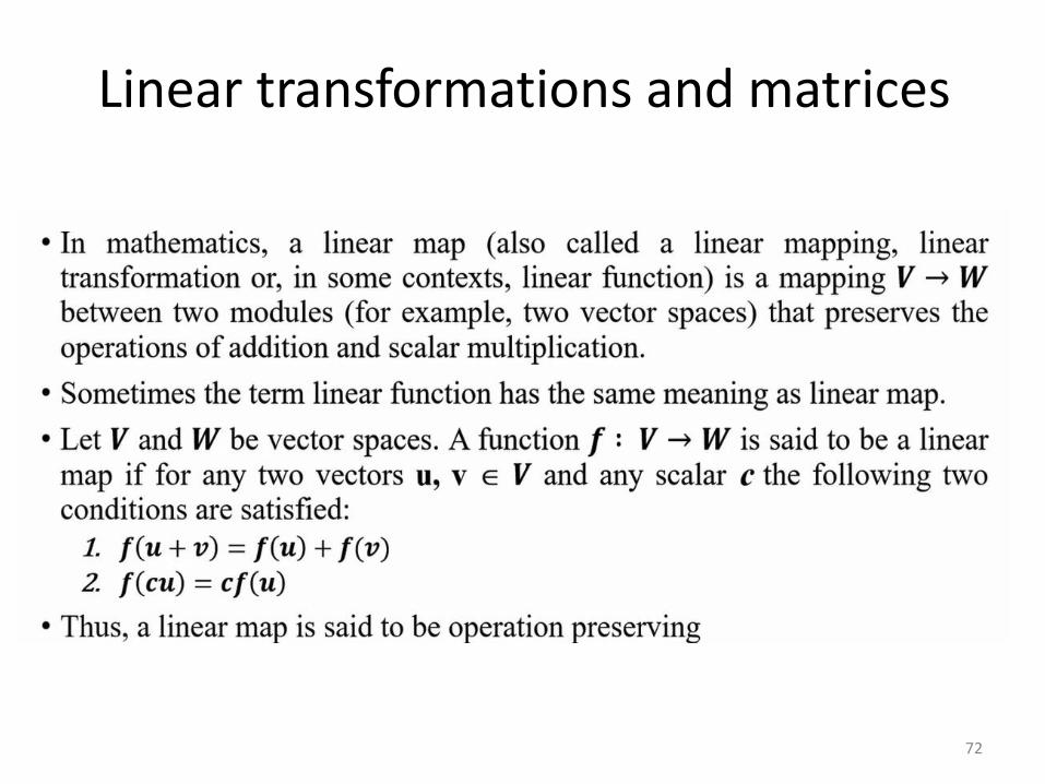
Definition of a linear transformation • A linear transformation (or a linear map) is a function T:
Rn→Rm is a function that carries elements of the vectorspace Rn (called the domain) to the vector space Rm (calledthe codomain), and which satisfies the following properties:
1. T(x+y)=T(x)+T(y)2. T(ax)=aT(x)for any vectors x,y∈Rn and any scalar a∈R.
• It is simple enough to identify whether or not a given function f(x) is a linear transformation. Just look at each term of each component of f(x). If each of these terms is a number times one of the components of x, then f is a linear transformation.
• Example, the function : f(x,y,z)=(3x−y,3z,0,z−2x) ,
is a linear transformation
64
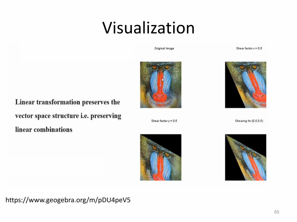
Visualization
65
https://www.geogebra.org/m/pDU4peV5
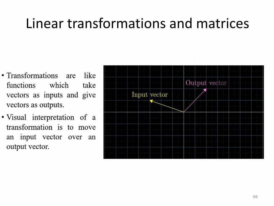
Linear transformations and matrices
66
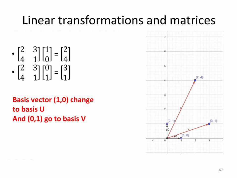
Linear transformations and matrices
67
Basis vector (1,0) change to basis UAnd (0,1) go to basis V

Linear transformation (note)
Why linear transformation
When you start thinking in Matrix as a linear transformation on the space, you will find all linear algebra topics reiles on the concept of linear transformation
68
Linear transformation (note)
Why linear transformation
Matrix will tell us where the vector basis go
We can think in matrix in terms of what it does in the vector space
69
Linear transformation
70
Linear transformation
71
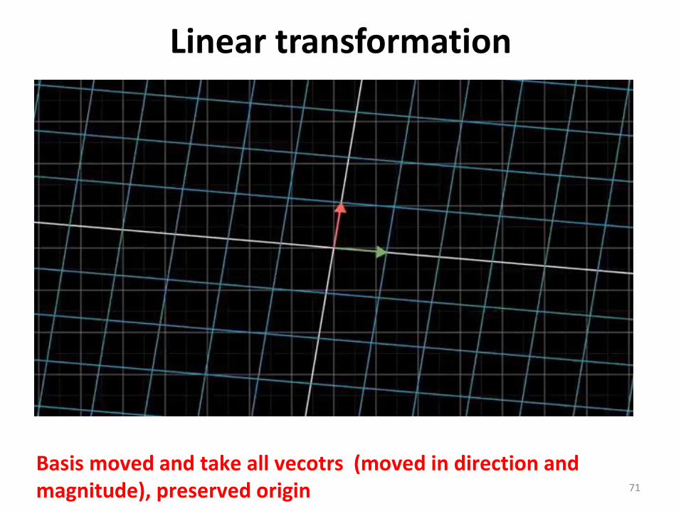
Basis moved and take all vecotrs (moved in direction and magnitude), preserved origin
Linear transformations and matrices
72
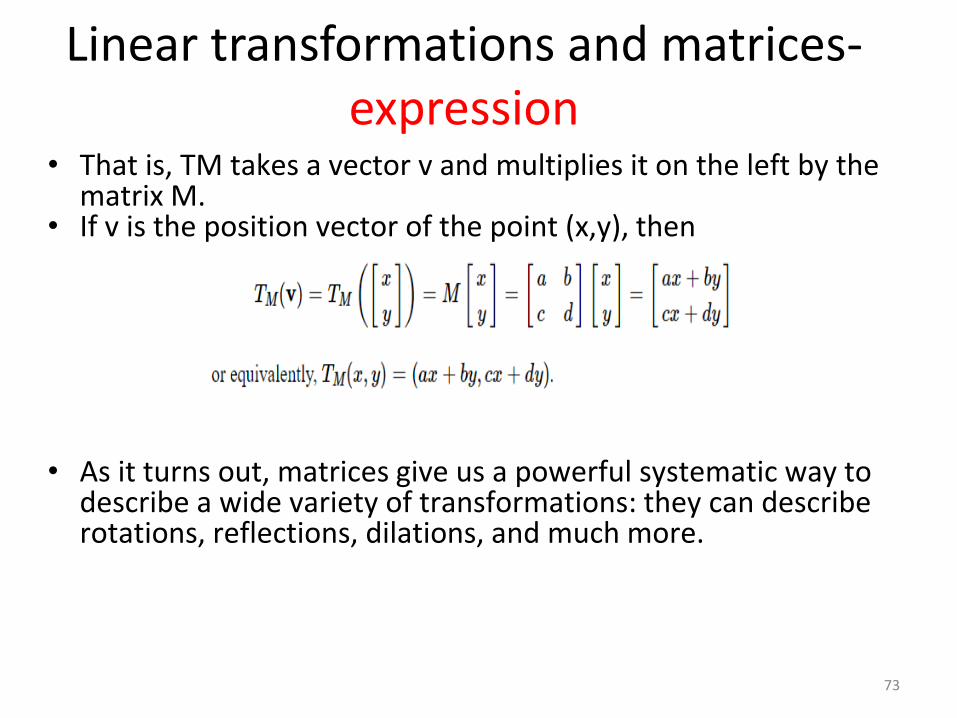
• That is, TM takes a vector v and multiplies it on the left by the matrix M.
• If v is the position vector of the point (x,y), then
• As it turns out, matrices give us a powerful systematic way to describe a wide variety of transformations: they can describe rotations, reflections, dilations, and much more.
Linear transformations and matrices-expression
73
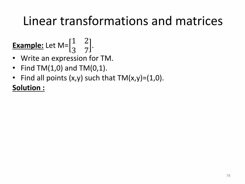
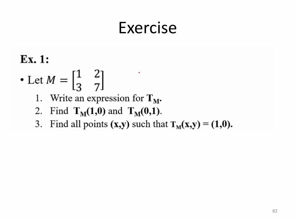
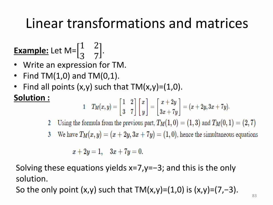
Example: Let M=1 23 7
.
• Write an expression for TM.• Find TM(1,0) and TM(0,1).• Find all points (x,y) such that TM(x,y)=(1,0).Solution :
Linear transformations and matrices
74

Example: Let M=1 23 7
.
• Write an expression for TM.• Find TM(1,0) and TM(0,1).• Find all points (x,y) such that TM(x,y)=(1,0).Solution :
Solving these equations yields x=7,y=−3; and this is the only solution. So the only point (x,y) such that TM(x,y)=(1,0) is (x,y)=(7,−3).
Linear transformations and matrices
75
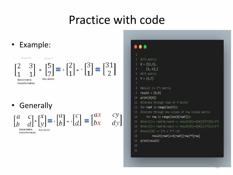
• Example:
• Generally
Practice with code
76
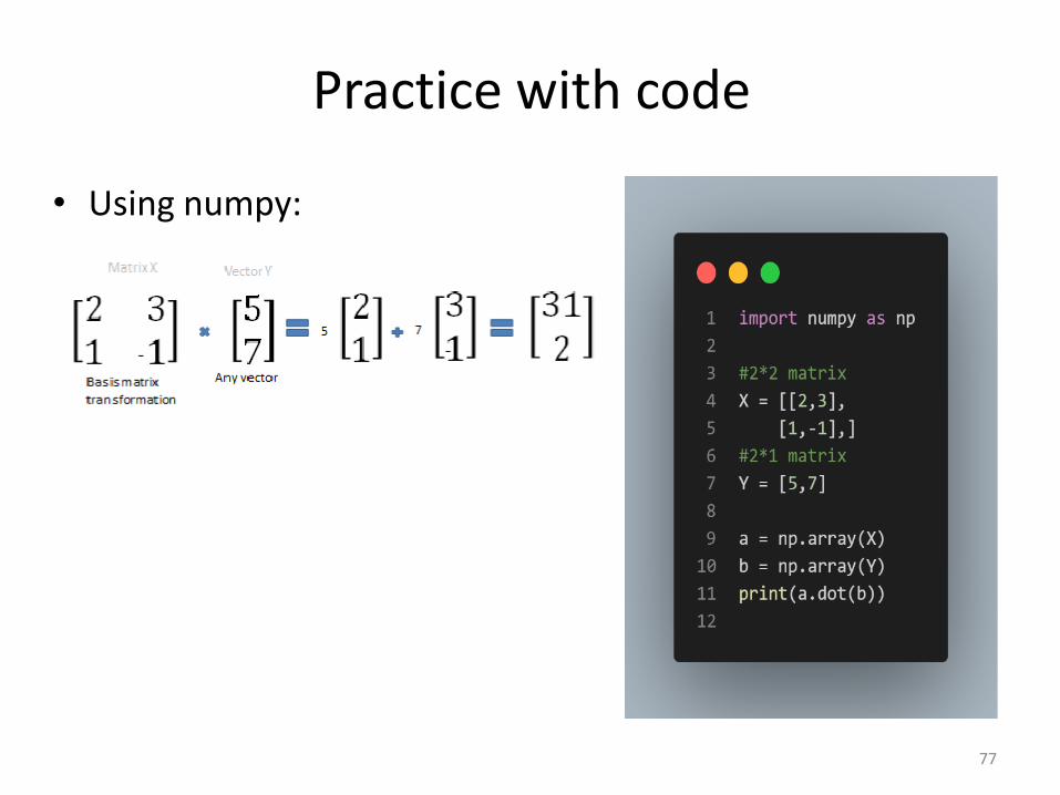
• Using numpy:
Practice with code
77

Practice
78
https://www.geogebra.org/m/pDU4peV5
79
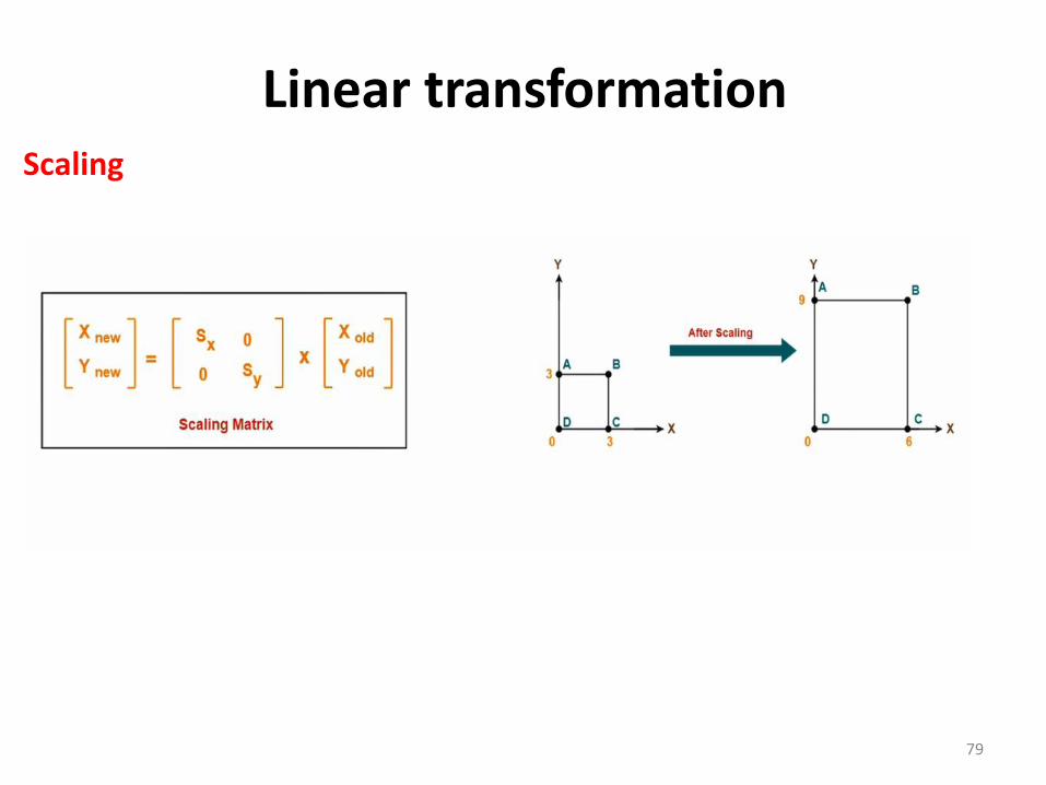
Scaling
Linear transformation
80
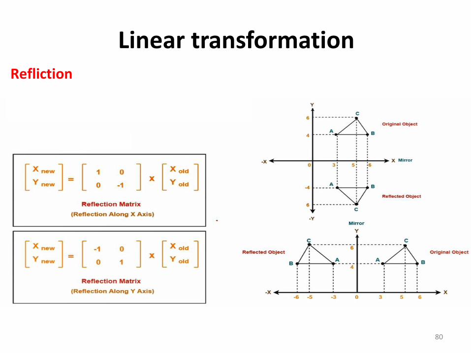
Refliction
Linear transformation
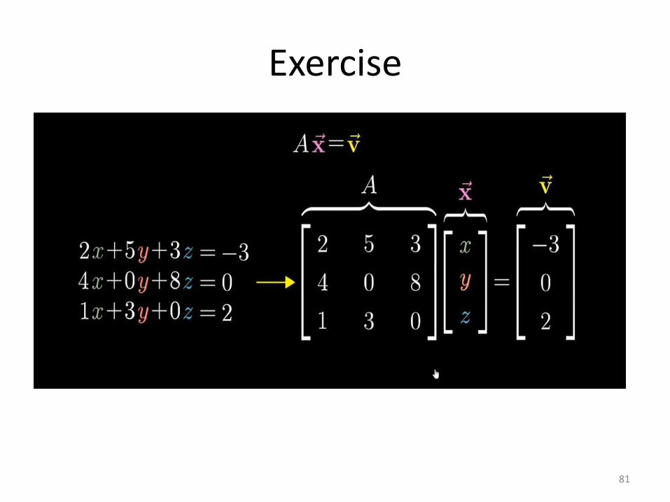
Exercise
81
Exercise
82
Example: Let M=1 23 7
.
• Write an expression for TM.• Find TM(1,0) and TM(0,1).• Find all points (x,y) such that TM(x,y)=(1,0).Solution :
Solving these equations yields x=7,y=−3; and this is the only solution. So the only point (x,y) such that TM(x,y)=(1,0) is (x,y)=(7,−3).
Linear transformations and matrices
83
84
85

86

87

Linear Algebra for data science
Session 3
contents
• Rank of a matrix
• Determinant of matrix,
• Inverse of matrix,
• Gauss Jordan method
89
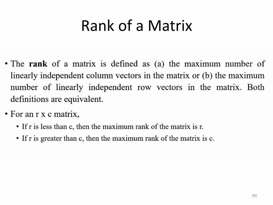
Rank of a Matrix
90

Rank of a Matrix
91
2. Heating and cooling the materials
Standards
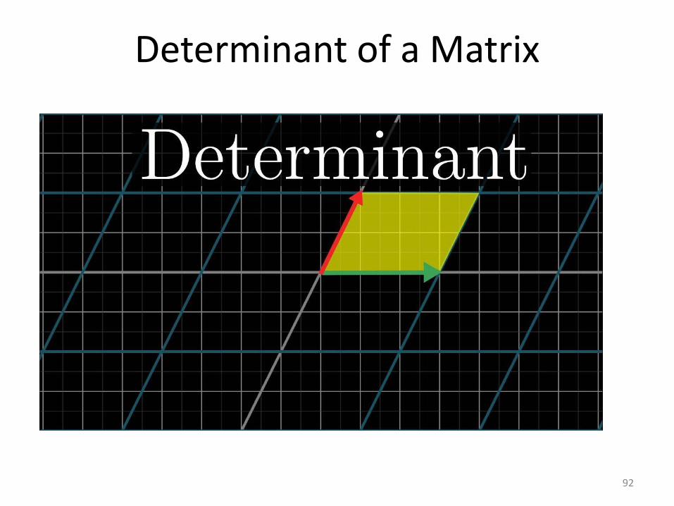
Determinant of a Matrix
92
Standards
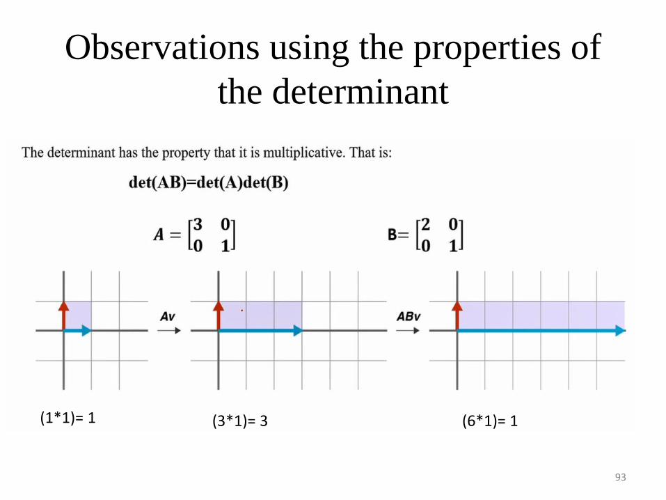
Observations using the properties of
the determinant
93
(1*1)= 1 (3*1)= 3 (6*1)= 1
2. Heating and cooling the materials
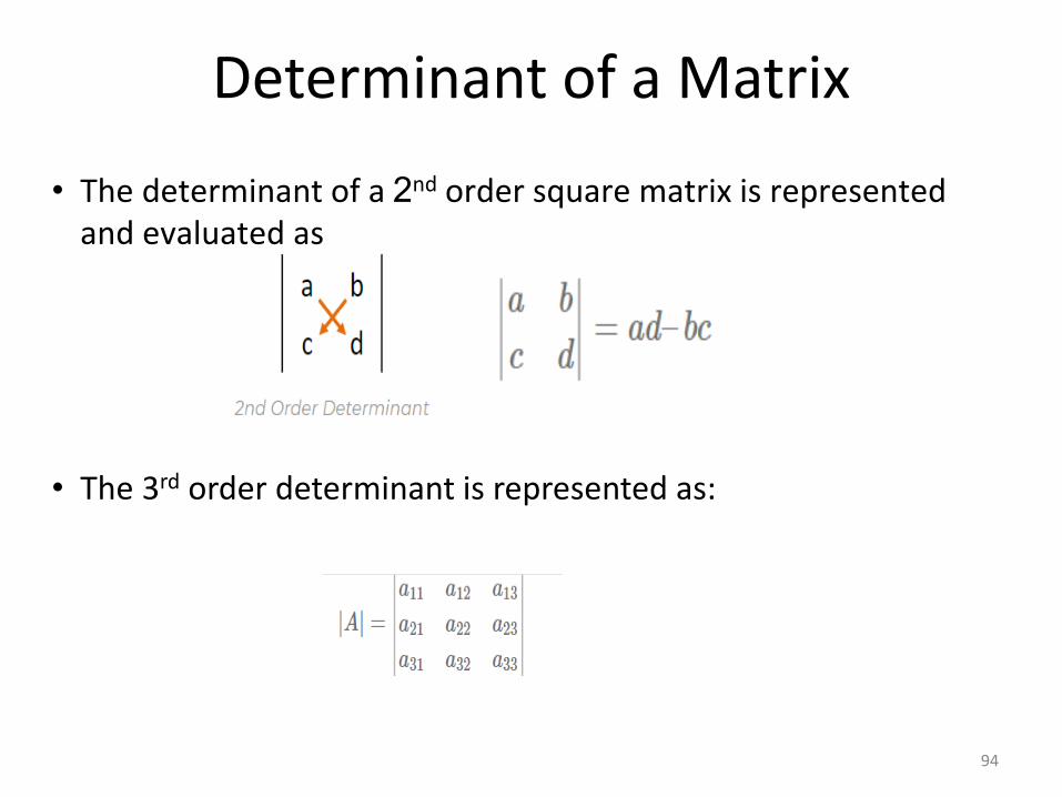
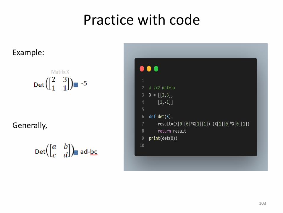
Standards• The determinant of a 2nd order square matrix is represented and evaluated as
• The 3rd order determinant is represented as:
Determinant of a Matrix
94
2. Heating and cooling the materials
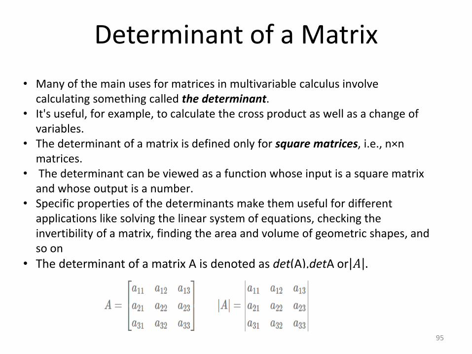
Standards• Many of the main uses for matrices in multivariable calculus involve calculating something called the determinant.
• It's useful, for example, to calculate the cross product as well as a change of variables.
• The determinant of a matrix is defined only for square matrices, i.e., n×nmatrices.
• The determinant can be viewed as a function whose input is a square matrix and whose output is a number.
• Specific properties of the determinants make them useful for different applications like solving the linear system of equations, checking the invertibility of a matrix, finding the area and volume of geometric shapes, and so on
• The determinant of a matrix A is denoted as det(A),detA orȁ ȁ𝐴 .
Determinant of a Matrix
95

2. Heating and cooling the materials
Standards• The expansion of determinant |A| in terms of the first row is:
• Similarly, we can expand the determinant |A| in terms of the second column as:
Determinant of a Matrix
96
2. Heating and cooling the materials
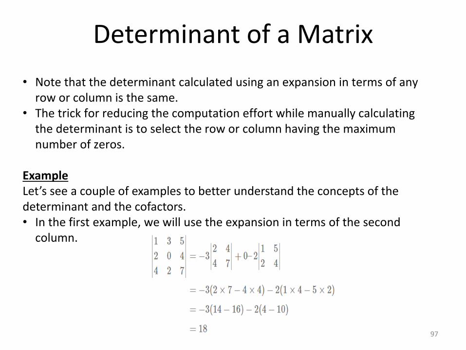
Standards• Note that the determinant calculated using an expansion in terms of any row or column is the same.
• The trick for reducing the computation effort while manually calculating the determinant is to select the row or column having the maximum number of zeros.
ExampleLet’s see a couple of examples to better understand the concepts of the determinant and the cofactors. • In the first example, we will use the expansion in terms of the second
column.
Example
Determinant of a Matrix
97
2. Heating and cooling the materials
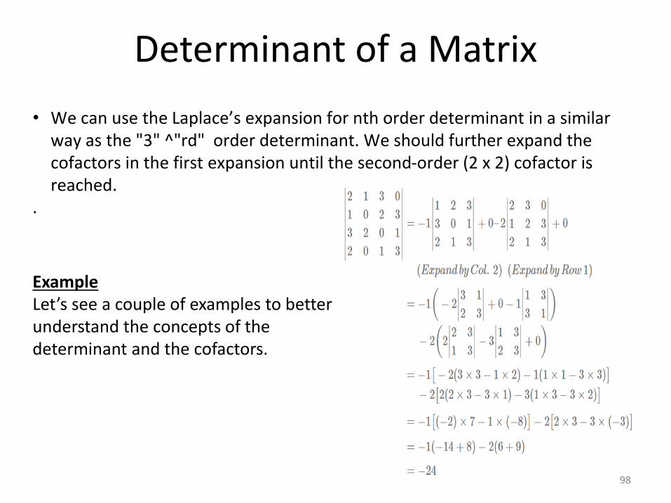
Standards• We can use the Laplace’s expansion for nth order determinant in a similar way as the "3" ^"rd" order determinant. We should further expand the cofactors in the first expansion until the second-order (2 x 2) cofactor is reached.
.
ExampleLet’s see a couple of examples to better understand the concepts of the determinant and the cofactors.
Example
Determinant of a Matrix
98
2. Heating and cooling the materials
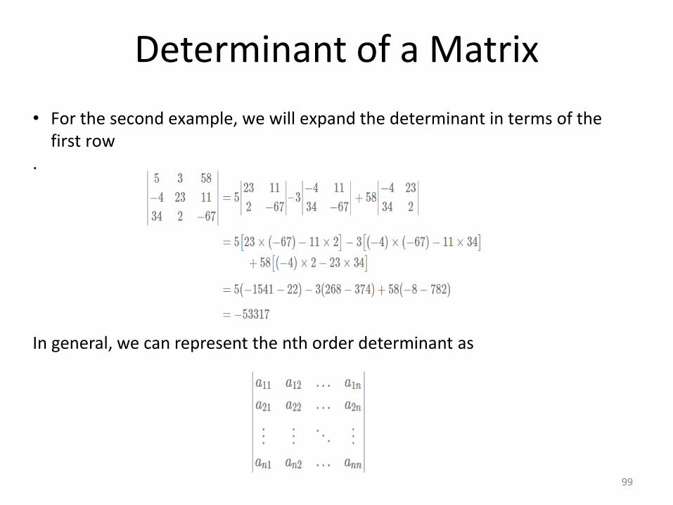
Standards• For the second example, we will expand the determinant in terms of the first row
.
In general, we can represent the nth order determinant as
Determinant of a Matrix
99
2. Heating and cooling the materials
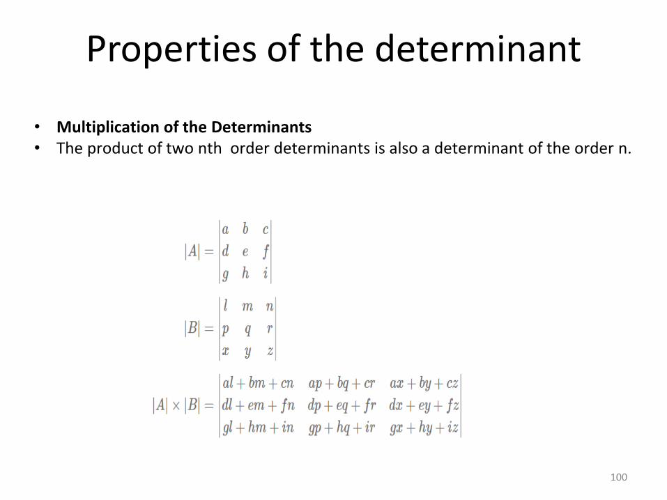
Standards• Multiplication of the Determinants• The product of two nth order determinants is also a determinant of the order n.
Properties of the determinant
100
Standards
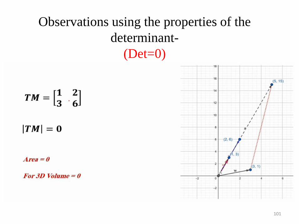
Observations using the properties of the
determinant-
(Det=0)
101
Standards
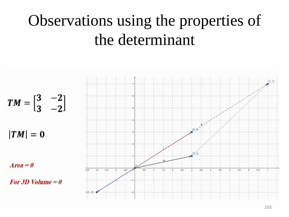
Observations using the properties of
the determinant
102
Standards
Observations Using the Properties of the Determinant
Practice with code
Example:
Generally,
103
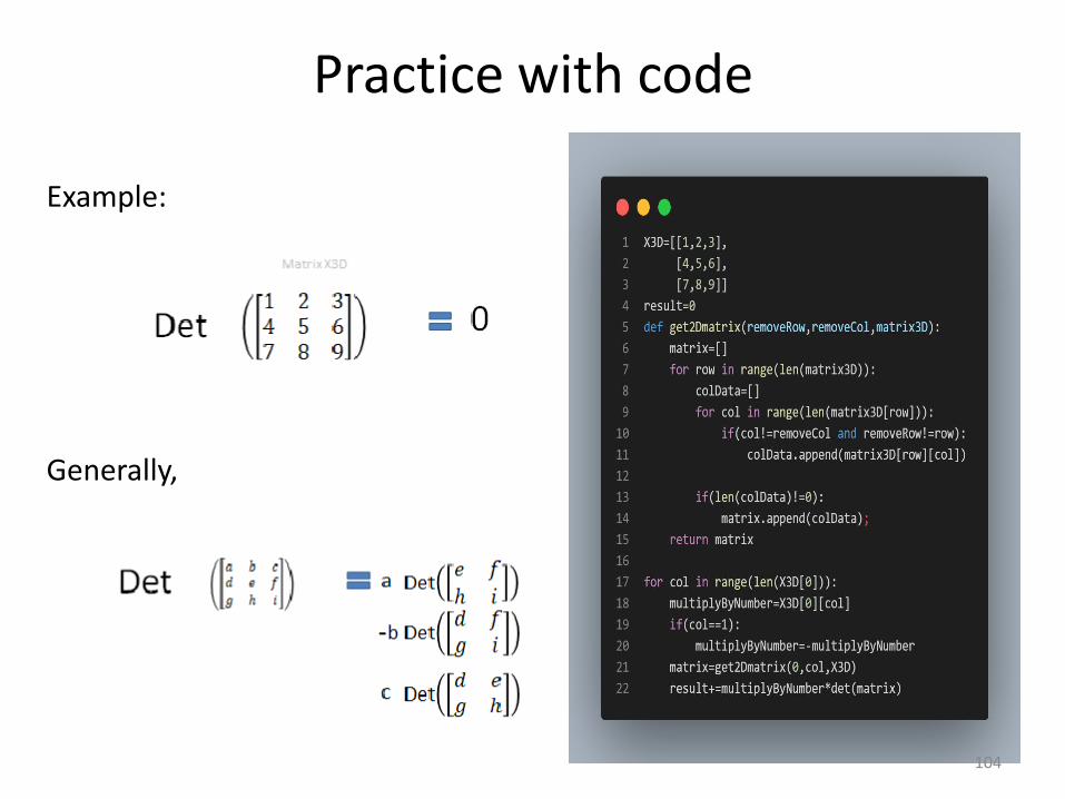
Practice with code
Example:
Generally,
104
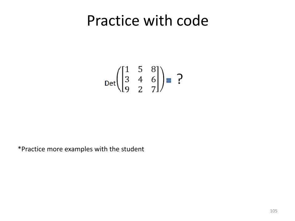
Practice with code
*Practice more examples with the student
105
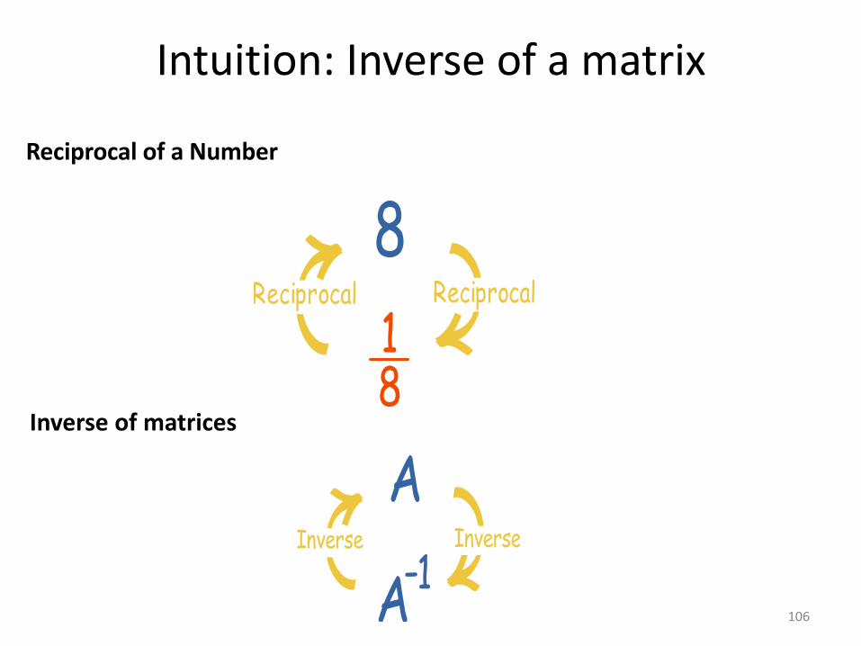
Intuition: Inverse of a matrix
Inverse of matrices
Reciprocal of a Number
106
2. Heating and cooling the materials
Standards
If the Matrix determinant equal zero , thematrix does not have an inverse( singularmatrix ). Collapse space
Collapsed stored cannot be restored
Important Note
107
2. Heating and cooling the materials
Standards
Singular Matrix
• When the determinant of a matrix is zero, i.e., |A|=0, then that matrix is called as a Singular Matrix.
• The matrix with a non-zero determinant is called the Non-singular Matrix.
• All the singular matrices are Non-invertible Matrices, i.e., it is not possible to take an inverse of a matrix
Singular Matrix
108
Inverse of a Matrix
109
Inverse 110
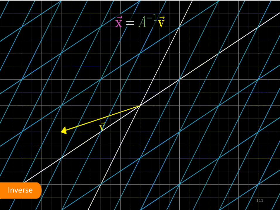
Inverse 111
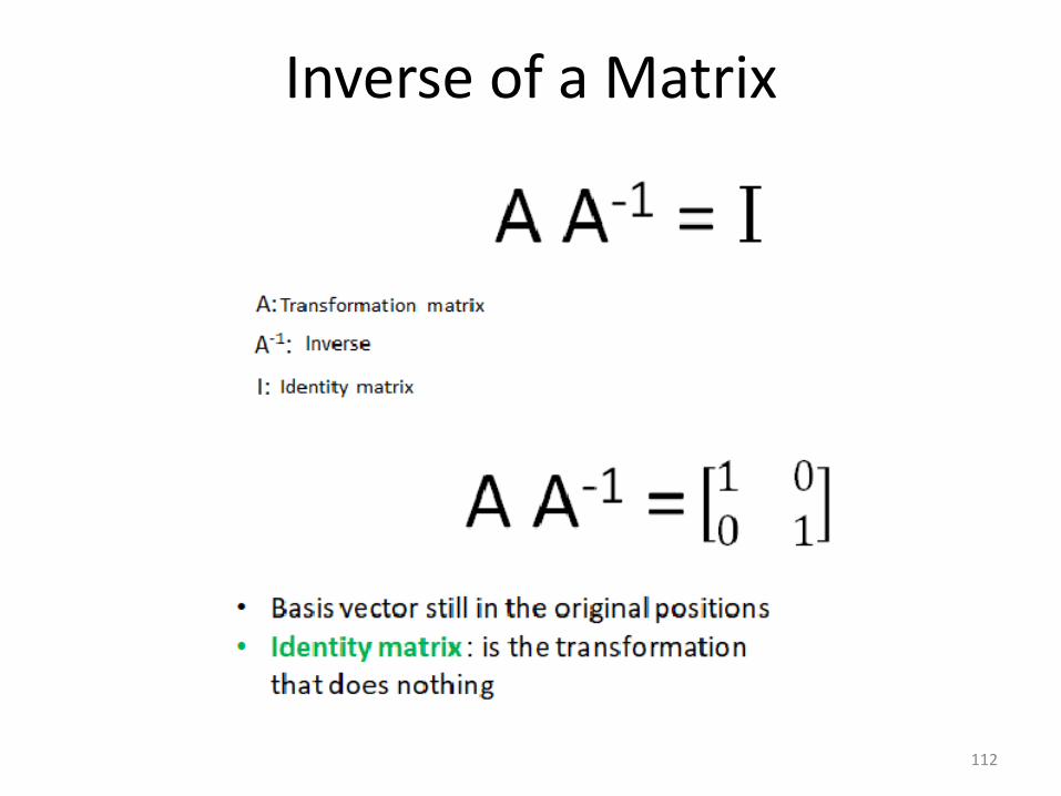
Inverse of a Matrix
112

113

114

Linear Algebra for data science
Session 4
contents
• Solving a system of linear equations
• Eigenvalues and Eigen vectors
• Principal Component Analysis (PCA)
116
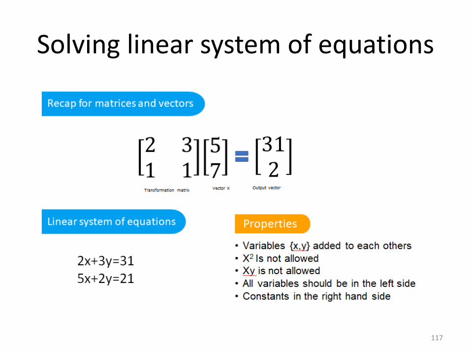
Solving linear system of equations
117

Solving linear system of equations
118
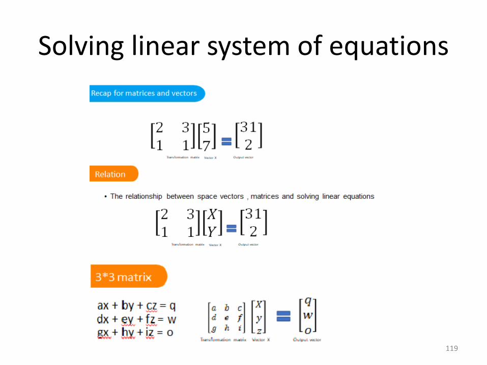
Solving linear system of equations
119
Solving linear system of equations
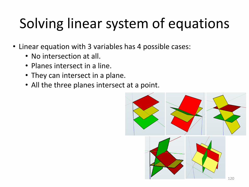
• Linear equation with 3 variables has 4 possible cases:• No intersection at all.• Planes intersect in a line.• They can intersect in a plane.• All the three planes intersect at a point.
120
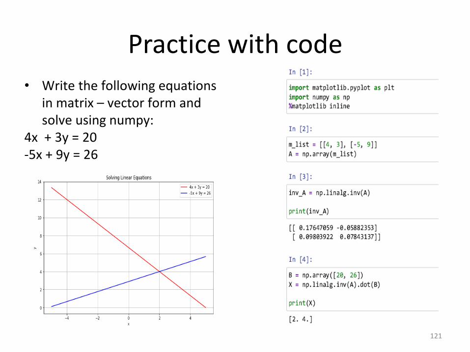
Practice with code
• Write the following equations in matrix – vector form and solve using numpy:
4x + 3y = 20-5x + 9y = 26
121
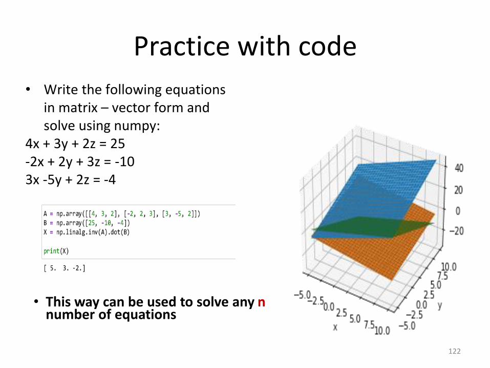
Practice with code
• Write the following equations in matrix – vector form and solve using numpy:
4x + 3y + 2z = 25-2x + 2y + 3z = -103x -5y + 2z = -4
• This way can be used to solve any nnumber of equations
122
Eigenvalues and Eigen vectors of a matrix
123
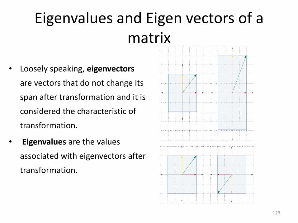
• Loosely speaking, eigenvectors
are vectors that do not change its
span after transformation and it is
considered the characteristic of
transformation.
• Eigenvalues are the values
associated with eigenvectors after
transformation.
Eigenvalues and Eigen vectors of a matrix
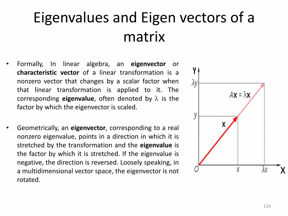
• Formally, In linear algebra, an eigenvector orcharacteristic vector of a linear transformation is anonzero vector that changes by a scalar factor whenthat linear transformation is applied to it. Thecorresponding eigenvalue, often denoted by is thefactor by which the eigenvector is scaled.
• Geometrically, an eigenvector, corresponding to a realnonzero eigenvalue, points in a direction in which it isstretched by the transformation and the eigenvalue isthe factor by which it is stretched. If the eigenvalue isnegative, the direction is reversed. Loosely speaking, ina multidimensional vector space, the eigenvector is notrotated.
124
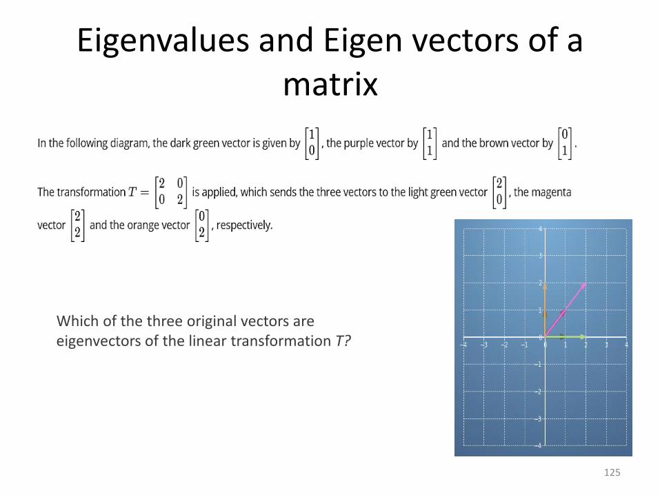
Eigenvalues and Eigen vectors of a matrix
125
Which of the three original vectors are eigenvectors of the linear transformation T?
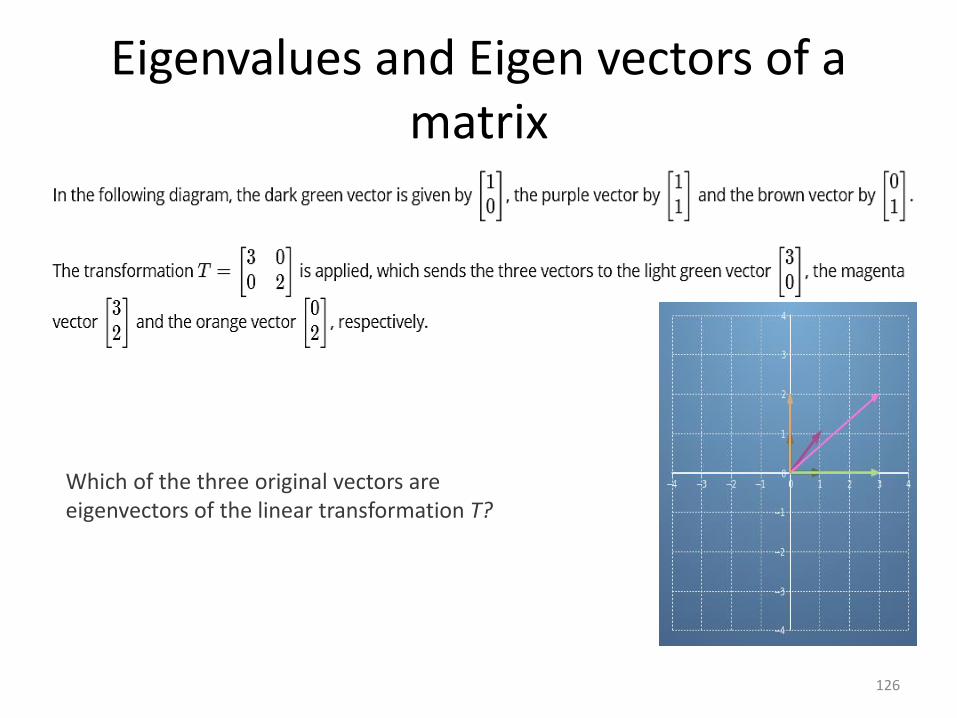
Eigenvalues and Eigen vectors of a matrix
126
Which of the three original vectors are eigenvectors of the linear transformation T?
Eigenvalues and Eigen vectors of a matrix
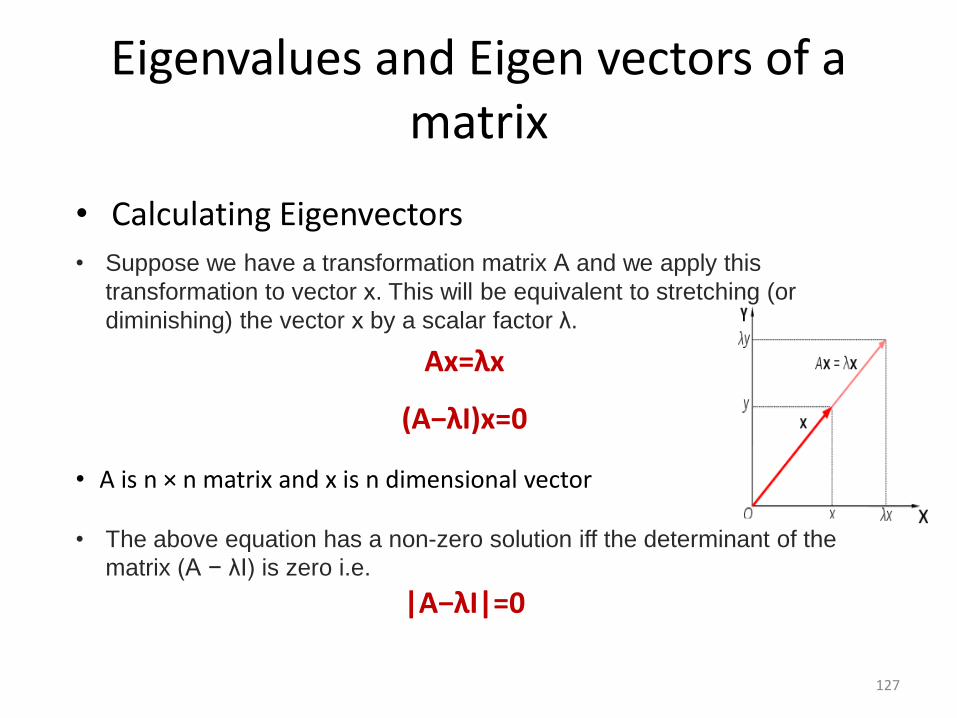
• Calculating Eigenvectors
127
• Suppose we have a transformation matrix A and we apply this
transformation to vector x. This will be equivalent to stretching (or
diminishing) the vector x by a scalar factor λ.
Ax=λx
(A−λI)x=0
• A is n × n matrix and x is n dimensional vector
• The above equation has a non-zero solution iff the determinant of the
matrix (A − λI) is zero i.e.
|A−λI|=0
Eigenvalues and Eigen vectors of a matrix
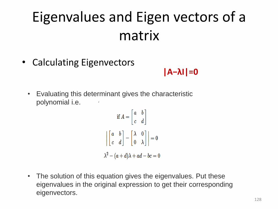
• Calculating Eigenvectors
128
• Evaluating this determinant gives the characteristic
polynomial i.e.
|A−λI|=0
• The solution of this equation gives the eigenvalues. Put these
eigenvalues in the original expression to get their corresponding
eigenvectors.
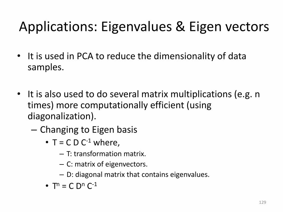
Applications: Eigenvalues & Eigen vectors
• It is used in PCA to reduce the dimensionality of data samples.
• It is also used to do several matrix multiplications (e.g. n times) more computationally efficient (using diagonalization).
– Changing to Eigen basis• T = C D C-1 where,
– T: transformation matrix.
– C: matrix of eigenvectors.
– D: diagonal matrix that contains eigenvalues.
• Tn = C Dn C-1
129
Principal Component Analysis (PCA)
• Dimensionality reduction method.
• Transform a large set of variables into a smaller one that still contains most of the information in the large set.
• Used in– Data compression:
• Save data.
• Speed up learning algorithm.
– Data visualization (Reduce high dimension data to 3D or 2D).
130
Principal Component Analysis (PCA)
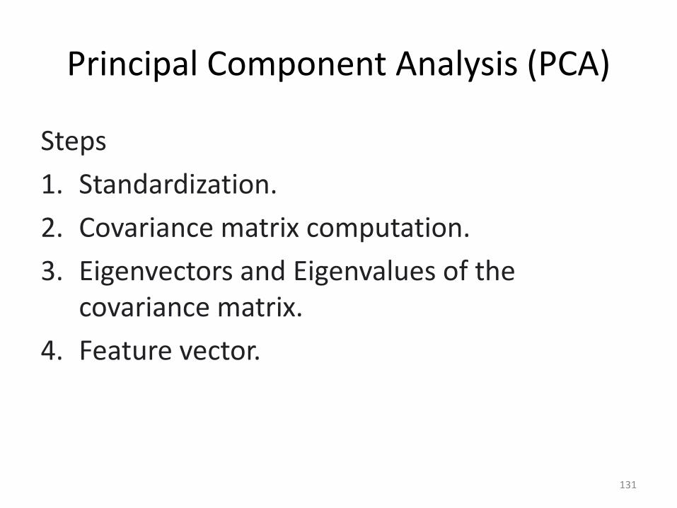
Steps
1. Standardization.
2. Covariance matrix computation.
3. Eigenvectors and Eigenvalues of the covariance matrix.
4. Feature vector.
131
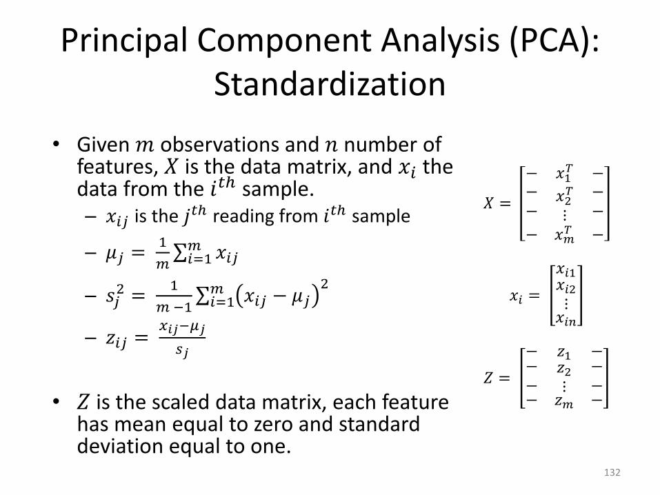
Principal Component Analysis (PCA): Standardization
• Given 𝑚 observations and 𝑛 number of features, 𝑋 is the data matrix, and 𝑥𝑖 the data from the 𝑖𝑡ℎ sample.– 𝑥𝑖𝑗 is the 𝑗𝑡ℎ reading from 𝑖𝑡ℎ sample
– 𝜇𝑗 =1
𝑚σ𝑖=1𝑚 𝑥𝑖𝑗
– 𝑠𝑗2 =
1
𝑚 −1σ𝑖=1𝑚 𝑥𝑖𝑗 − 𝜇𝑗
2
– 𝑧𝑖𝑗 =𝑥𝑖𝑗−𝜇𝑗
𝑠𝑗
• 𝑍 is the scaled data matrix, each feature has mean equal to zero and standard deviation equal to one.
𝑋 =
− 𝑥1𝑇 −
−−
𝑥2𝑇
⋮
−−
− 𝑥𝑚𝑇 −
𝑥𝑖 =
𝑥𝑖1𝑥𝑖2⋮𝑥𝑖𝑛
𝑍 =
− 𝑧1 −−−
𝑧2⋮
−−
− 𝑧𝑚 −
132
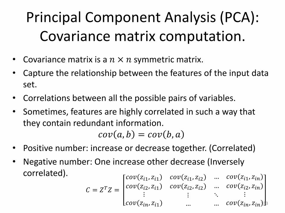
Principal Component Analysis (PCA): Covariance matrix computation.
• Covariance matrix is a 𝑛 × 𝑛 symmetric matrix.
• Capture the relationship between the features of the input data set.
• Correlations between all the possible pairs of variables.
• Sometimes, features are highly correlated in such a way that they contain redundant information.
𝑐𝑜𝑣 𝑎, 𝑏 = 𝑐𝑜𝑣 𝑏, 𝑎
• Positive number: increase or decrease together. (Correlated)
• Negative number: One increase other decrease (Inversely correlated).
𝐶 = 𝑍𝑇𝑍 =
𝑐𝑜𝑣(𝑧𝑖1, 𝑧𝑖1) 𝑐𝑜𝑣(𝑧𝑖1, 𝑧𝑖2) … 𝑐𝑜𝑣(𝑧𝑖1, 𝑧𝑖𝑛)
𝑐𝑜𝑣(𝑧𝑖2, 𝑧𝑖1) 𝑐𝑜𝑣(𝑧𝑖2, 𝑧𝑖2) … 𝑐𝑜𝑣(𝑧𝑖2, 𝑧𝑖𝑛)⋮
𝑐𝑜𝑣(𝑧𝑖𝑛, 𝑧𝑖1)⋮…
⋱…
⋮𝑐𝑜𝑣(𝑧𝑖𝑛, 𝑧𝑖𝑛)133
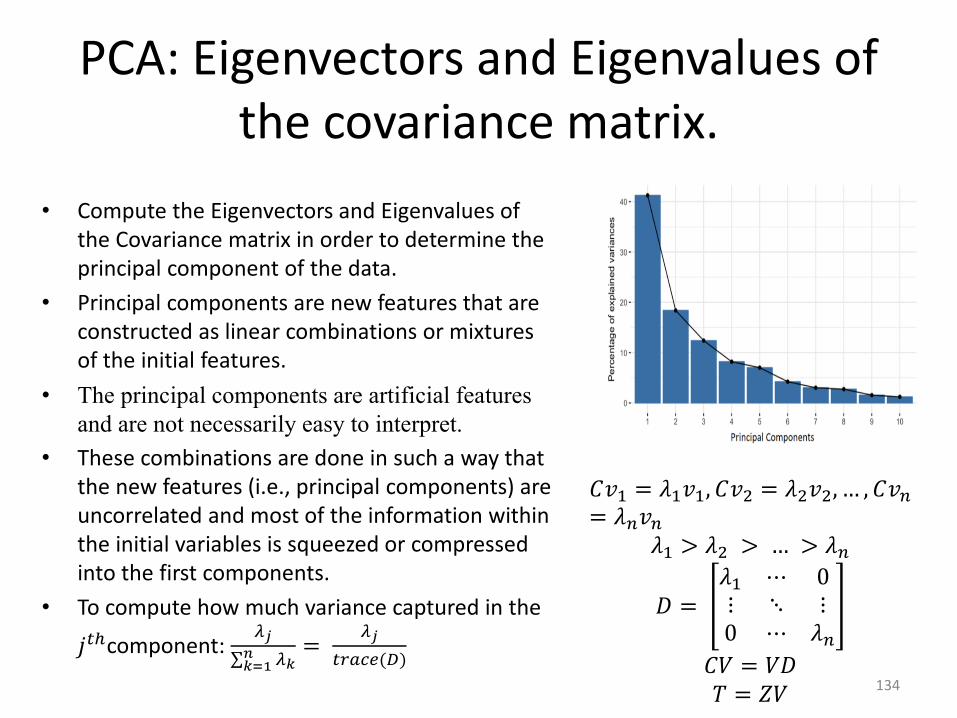
PCA: Eigenvectors and Eigenvalues of the covariance matrix.
• Compute the Eigenvectors and Eigenvalues of the Covariance matrix in order to determine the principal component of the data.
• Principal components are new features that are constructed as linear combinations or mixtures of the initial features.
• The principal components are artificial features
and are not necessarily easy to interpret.
• These combinations are done in such a way that the new features (i.e., principal components) are uncorrelated and most of the information within the initial variables is squeezed or compressed into the first components.
• To compute how much variance captured in the
𝑗𝑡ℎcomponent: 𝜆𝑗
σ𝑘=1𝑛 𝜆𝑘
=𝜆𝑗
𝑡𝑟𝑎𝑐𝑒(𝐷)
𝐶𝑣1 = 𝜆1𝑣1, 𝐶𝑣2 = 𝜆2𝑣2, … , 𝐶𝑣𝑛= 𝜆𝑛𝑣𝑛
𝜆1 > 𝜆2 > … > 𝜆𝑛
𝐷 =𝜆1 ⋯ 0⋮ ⋱ ⋮0 ⋯ 𝜆𝑛
𝐶𝑉 = 𝑉𝐷𝑇 = 𝑍𝑉 134
Principal Component Analysis (PCA): Feature vector
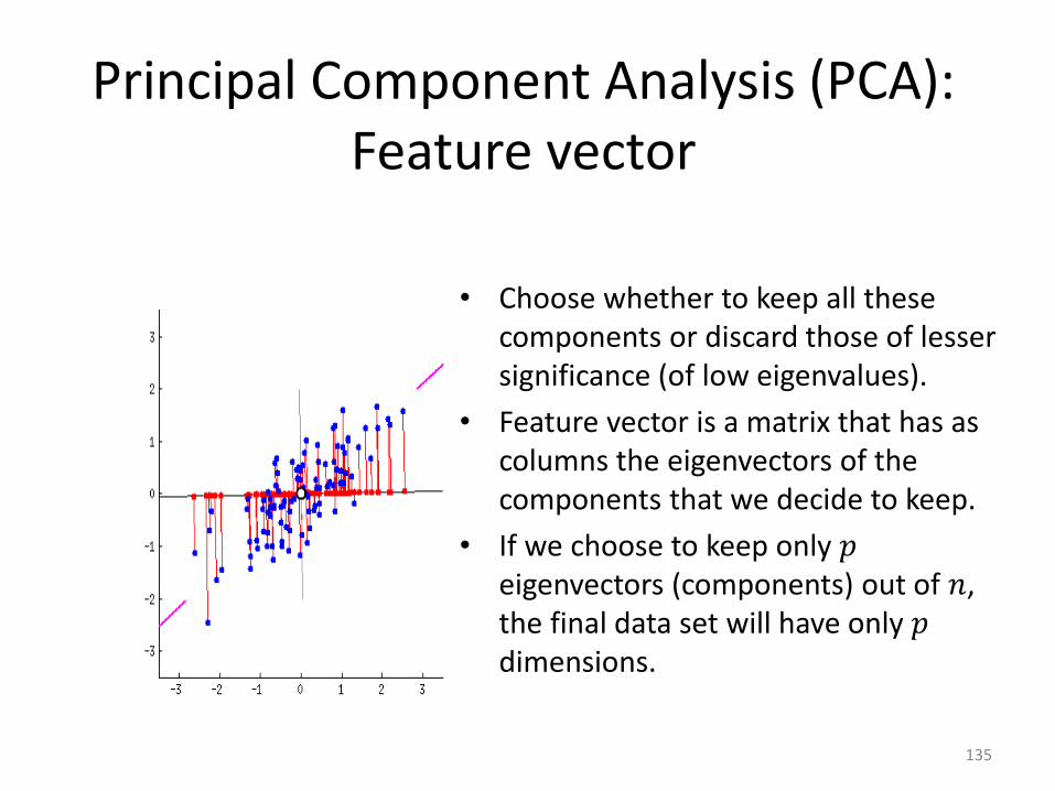
• Choose whether to keep all these components or discard those of lesser significance (of low eigenvalues).
• Feature vector is a matrix that has as columns the eigenvectors of the components that we decide to keep.
• If we choose to keep only 𝑝eigenvectors (components) out of 𝑛, the final data set will have only 𝑝dimensions.
135
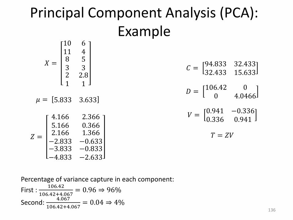
Principal Component Analysis (PCA): Example
𝑋 =
10 611 48321
532.81
𝜇 = 5.833 3.633
𝑍 =
4.166 2.3665.166 0.3662.166−2.833−3.833−4.833
1.366−0.633−0.833−2.633
𝐶 =94.833 32.43332.433 15.633
𝐷 =106.42 0
0 4.0466
𝑉 =0.941 −0.3360.336 0.941
𝑇 = 𝑍𝑉
Percentage of variance capture in each component:
First : 106.42
106.42+4.067= 0.96 ⇒ 96%
Second: 4.067
106.42+4.067= 0.04 ⇒ 4%
136
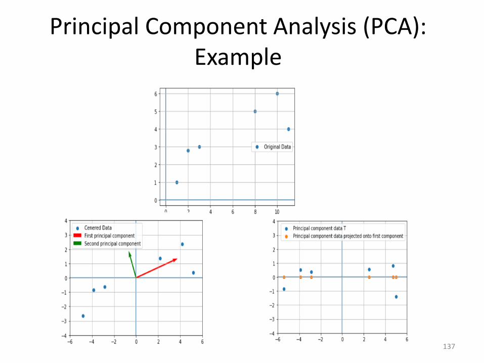
Principal Component Analysis (PCA): Example
137
Principal Component Analysis (PCA): Comments
• Principal components are used to reduce large-dimensional data sets to data sets
with a few dimensions that still retain most of the information in the original data.
• Each principal component is a linear combination of the scaled variables.
• Any two principal components are uncorrelated.
• The first few principal components account for a large percentage of the total
variance.
• The principal components are artificial variables and are not necessarily easy to
interpret.
138

139

140
Linear Algebra for data science
Practical Session
Related Documents