LINEAMENT ANALYSIS FROM SATELLITE IMAGES, NORTH-WEST OF ANKARA A THESIS SUBMITTED TO THE GRADUATE SCHOOL OF NATURAL AND APPLIED SCIENCES OF MIDDLE EAST TECHNICAL UNIVERSITY BY GÜLCAN SARP IN PARTIAL FULFILLMENT OF THE REQUIREMENTS FOR THE DEGREE OF MASTER OF SCIENCE IN GEODETIC AND GEOGRAPHIC INFORMATION TECHNOLOGIES SEPTEMBER 2005

Welcome message from author
This document is posted to help you gain knowledge. Please leave a comment to let me know what you think about it! Share it to your friends and learn new things together.
Transcript
LINEAMENT ANALYSIS FROM SATELLITE IMAGES, NORTH-WEST OF ANKARA
A THESIS SUBMITTED TO THE GRADUATE SCHOOL OF NATURAL AND APPLIED SCIENCES
OF MIDDLE EAST TECHNICAL UNIVERSITY
BY
GÜLCAN SARP
IN PARTIAL FULFILLMENT OF THE REQUIREMENTS FOR
THE DEGREE OF MASTER OF SCIENCE IN
GEODETIC AND GEOGRAPHIC INFORMATION TECHNOLOGIES
SEPTEMBER 2005

Approval of the Graduate School of Natural and Applied Sciences
________________________________ Prof. Dr. Canan ÖZGEN
Director
I certify that this thesis satisfies all the requirements as a thesis for the degree of Master of Science.
________________________________ Assist. Prof. Dr. Zuhal AKYÜREK Head of Department
This is to certify that we have read this thesis and that in our opinion it is fully adequate, in scope and quality, as a thesis for the degree of Master of Science.
________________________________ Prof. Dr. Vedat TOPRAK
Supervisor Examining Committee Members Assoc. Prof. Dr. Nurünnisa USUL (METU, CE) ______________________
Prof. Dr. Vedat TOPRAK (METU, GEOE) ______________________
Assoc. Prof. Dr. Oğuz IŞIK (METU, CP) ______________________
Assist Prof. Dr. Zuhal AKYÜREK (METU, GGIT) ______________________
Dr. Arda ARCASOY (Arcasoy Consulting) ______________________

I hereby declare that all information in this document has been obtained and presented in accordance with academic rules and ethical conduct. I also declare that, as required by these rules and conduct, I have fully cited and referenced all material and results that are not original to this work. Name, Last name: Gülcan SARP
Signature :
iii

ABSTRACT
LINEAMENT ANALYSIS FROM SATELLITE IMAGES, NORTH-WEST OF ANKARA
SARP, Gülcan
M.Sc., Department of Geodetic and Geographic Information Technologies
Supervisor: Prof. Dr. Vedat TOPRAK
September 2005, 76 pages
The purposes of this study are to extract lineaments from satellite images in order to
contribute to the understanding of the faults. Landsat image is used for the analysis
which is processed for both automated and manual extraction. During manual extraction
four methods (filtering, PCA, band rationing and color composites) are used.
Comparison of the two output maps indicated that manual extraction produced better
results.
Manually extracted lineament map is tested with the fault map of the area compiled from
eight studies. The accuracy of the lineament map for the whole area is 38.69 % which
increases to 50.28 % in the vicinity of North Anatolian Fault Zone (NAFZ).
Evaluation of the length, density and orientation of the lineaments indicated that: a)
there are fault zones in the area other than the NAFZ, b) Several fault segments are
iv

identified in the region which are absent in the fault map due the difficulty in mapping
during the field studies; c) the dominant lineament trend is NE-SW (parallel to the
NAFZ), however, a second trend is obvious in NW-SE direction.
Keywords: Lineament analysis, automated extraction, manual extraction, Turkey
v

ÖZ
UYDU GÖRÜNTÜLERİNDEN ÇİZGİSELLİK ANALİZİ, ANKARA KUZEY-BATI’SI
SARP, Gülcan
Yüksek Lisans, Jeodezi ve Cografi Bilgi Teknolojileri E.A.B.D.
Tez Yöneticisi: Prof. Dr. Vedat TOPRAK
Eylül 2005, 76 sayfa
Bu çalışmanın amacı fayların daha iyi anlaşılmasına katkı sağlamak amacı ile uydu
görüntülerinden çizgiselliklerin çıkarılmasıdır. Bu çalışmada çizgisellikler otomatik ve
otomatik olmayan yöntemler kullanılarak Landsat uydu görüntüsünden çıkarılmıştır.
Otomatik olmayan yöntemler için dört metot kullanılmıştır. (Filitreler, Temel Bileşenler
Analizi, bantların bölünmesi ve renk bileşenleri). Otomatik ve otomatik olmayan
yöntemler kullanılarak belirlenen çizgiselliklerin karşılaştırılması sonucunda otomatik
olmayan yöntemin daha iyi sonuçlar verdiği belirlenmiştir.
Otomatik olmayan yöntemler kullanılarak elde edilen çizgisellik haritası bölgede daha
önceden yapılmış sekiz farklı çalışmadan derlenen fay haritası ile karşılaştırılmıştır.
Yapılan çalışmanın doğruluğu tüm alan için %38,69 olup kuzey anadolu fay zonu (KAF)
civarında %50,28’e yükselmektedir.
vi

Çizgiselliklerin uzunluklarına, yoğunluklarına ve yönelimlerine göre değerlendirilmesi
sonucunda: a) bölgede KAF’dan başka fay zonlarının olduğu belirlenmiştir, b) saha
çalışmaları ile yapılan fay haritalarında belirlenememiş birçok fay parçası belirlenmiştir,
c) çizgiselliklerin başlıca yönelimlerinin KD-GB (KAF’a paralel) olmasına rağmen KB-
GD eğilimli ikinci bir yönelim gösterdikleri belirlenmiştir.
Anahtar Kelimeler: Çizgisellik analizi, otomatik çizgisellik çıkarımı, manuel yöntemle
çizgisellik çıkarımı, Türkiye
vii

To My Family
viii

ACKNOWLEDGMENTS
I would like to express my sincere thanks to my supervisor Prof. Dr. Vedat Toprak, for
his continuous support, guidance and motivation during my study.
I would like to express my special thanks to Professors in GGIT and Geology
Department for their valuable comments and support.
Thanks to my examining committee, Assoc. Prof. Dr. Nurünnisa Usul, Assoc. Prof.
Oğuz Işık, Assist. Prof. Dr. Zuhal Akyürek, Dr. Arda Arcasoy for their valuable
suggestions.
I would also like to thank Research Assistants in GGIT and Geology Department, all my
friends and colleagues for their encouragements and support.
Finally, I would like to thank my family for their support and patience during my study.
ix

TABLE OF CONTENTS
PLAGIARISM ............................................................................................................... iii
ABSTRACT................................................................................................................... iv
ÖZ .................................................................................................................................. vi
DEDICATION ............................................................................................................... viii
ACKNOWLEDGMENTS ............................................................................................. ix
TABLE OF CONTENTS............................................................................................... x
LIST OF TABLES ......................................................................................................... xii
LIST OF FIGURES ....................................................................................................... xiii
CHAPTER
1. INTRODUCTION ............................................................................................. 1
1.1. Purpose and Scope ...................................................................................... 1
1.2. Method of Study ......................................................................................... 2
1.3. Organization of Thesis................................................................................ 3
2. BACKGROUND STUDIES .............................................................................. 4
2.1. Lineament analysis by using digital image enhancement and
Filtering techniques..................................................................................... 4
2.2. Lineament analysis by using automated extraction techniques .................. 8
3. STUDY AREA AND THE DATA.................................................................... 12
3.1. Study Area .................................................................................................. 12
3.2. Data ............................................................................................................. 14
3.2.1. Satellite Image.................................................................................. 14
3.2.2. Fault Map of the Area ...................................................................... 15
3.2.3. Road Map......................................................................................... 18
x

4. METHOD AND APPLICATION...................................................................... 20
4.1. Input Data.................................................................................................... 20
4.2. Lineament Extraction.................................................................................. 22
4.2.1. Manual Lineament Extraction.......................................................... 22
4.2.1.1. Filtering operations .............................................................. 23
4.2.1.2. Principal Component Analysis (PCA) ................................. 31
4.2.1.3. Spectral Rationing................................................................ 34
4.2.1.4. Color Composite .................................................................. 38
4.2.2. Final Map Generation ...................................................................... 40
4.2.3. Automated Lineament Extraction .................................................... 44
4.2.4. Evaluation of the automatically extracted lineaments ..................... 48
5. TESTING AND EVALUATION OF LINEAMENT MAP .............................. 50
5.1. Testing Lineament Map with Fault Map .................................................... 51
5.2. Evaluation of Lineament Map .................................................................... 56
5.2.1. Density Analysis .............................................................................. 56
5.2.2. Intersection Density Analysis .......................................................... 59
5.2.3. Length Analysis ............................................................................... 61
5.2.4. Orientation Analysis ........................................................................ 63
6. DISCUSSION AND CONCLUSION................................................................ 64
6.1. Discussion................................................................................................... 64
6.1.1. Problems of Manual lineament extraction ....................................... 64
6.1.2. Comparison of manual and automated lineament extraction........... 66
6.1.3. Accuracy of the resultant map.......................................................... 67
6.1.4. Implications of the results produced ................................................ 69
6.2. Conclusion .................................................................................................. 70
6.3. Recommendations....................................................................................... 71
REFERENCES......................................................................................................... 72
xi

LIST OF TABLES
Table 3.1. Area covered by previous works for the preparation of fault map.
Each color represents a study listed in the table below. Labels
indicate topographic sheet numbers. ........................................................... 16
Table 4.1. Sobel and Prewitt filters in four main directions applied in this study ...... 26
Table 4.2. (a) Variance / Covariance Matrix (b) Eigen vectors and Eigen values
of the Principal Component Analysis of the Landsat ETM data................ 32
Table 4.3. Comparison of basic statistics of the final map with other maps
produced by different methods.................................................................... 43
Table 5.1. Length and ratio of the matching lineaments for the whole area ............... 55
Table 5.2. Length and ratio of the matching lineaments for the area mapped by
Öztürk et al. (1985). ................................................................................... 55
xii
LIST OF FIGURES
Figure 3.1. A) Location map of the study area, B) Elevation map of the area .......... 13
Figure 3.2. True color composite Landsat ETM image of the study area.................. 15
Figure 3.3. The fault map of the study area ............................................................... 18
Figure 3.4. A) TM3/TM7 ratio used to extract the roads in the area.
B) A close up view (zoom) of the image to show the visible details of
the roads. .................................................................................................. 19
Figure 3.5. The digitized road map of the study area................................................. 19
Figure 4.1. Flowchart of the method applied in this study......................................... 21
Figure 4.2. Generation of a new image file by filtering operation.
A) A window is selected that moves both row-wise and column-wise,
B) For each window a new value (R) is calculated.................................. 24
Figure 4.3. Filtered images of the study area:
A) Normal contrast-stretched image, B) Low pass filtered image,
C) High pass filtered image, D) Directional filtered image ..................... 25
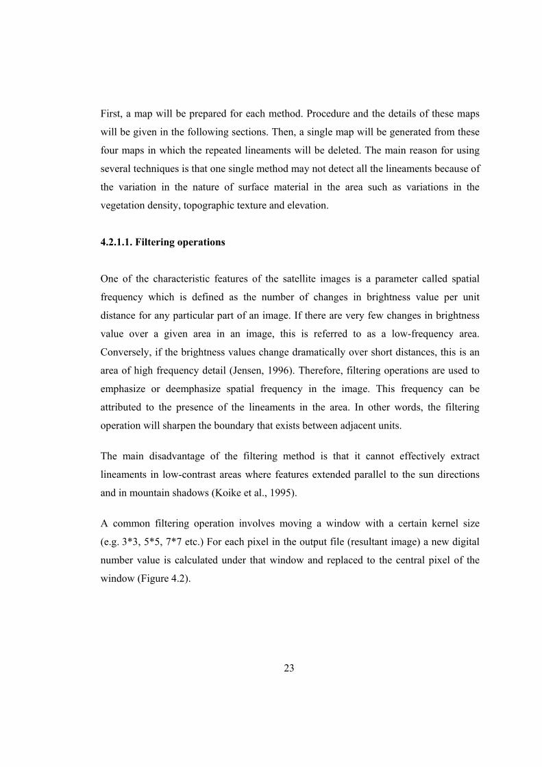
Figure 4.4. Sobel filtered image in E-W, NE-SW, NW-SE, NS directions. .............. 27
Figure 4.5. Prewitt filtered image in E-W, NE-SW, NW-SE, NS directions............. 28
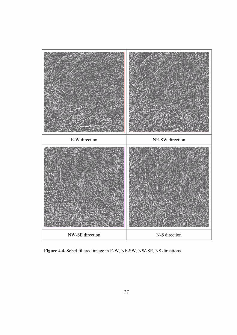
Figure 4.6. Lineament map generated after Gradient-Sobel filtering operation ........ 29
Figure 4.7. Frequency distribution of Gradient-Sobel filtering operation ................. 29
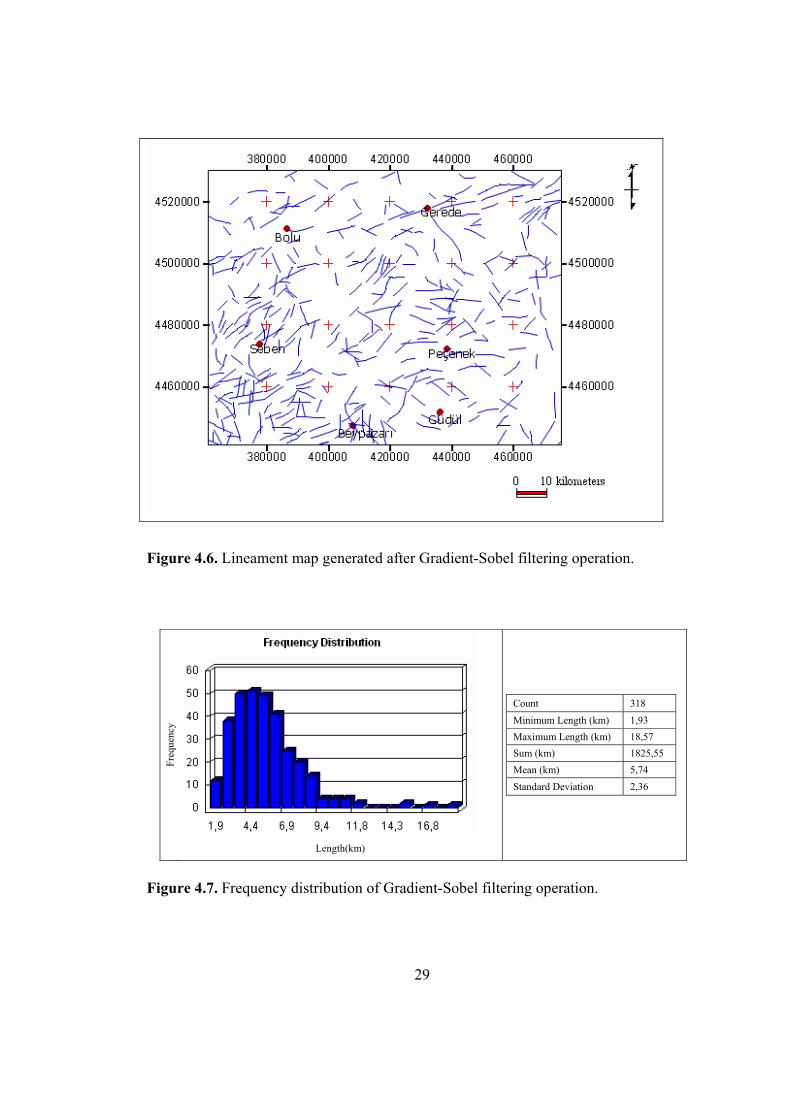
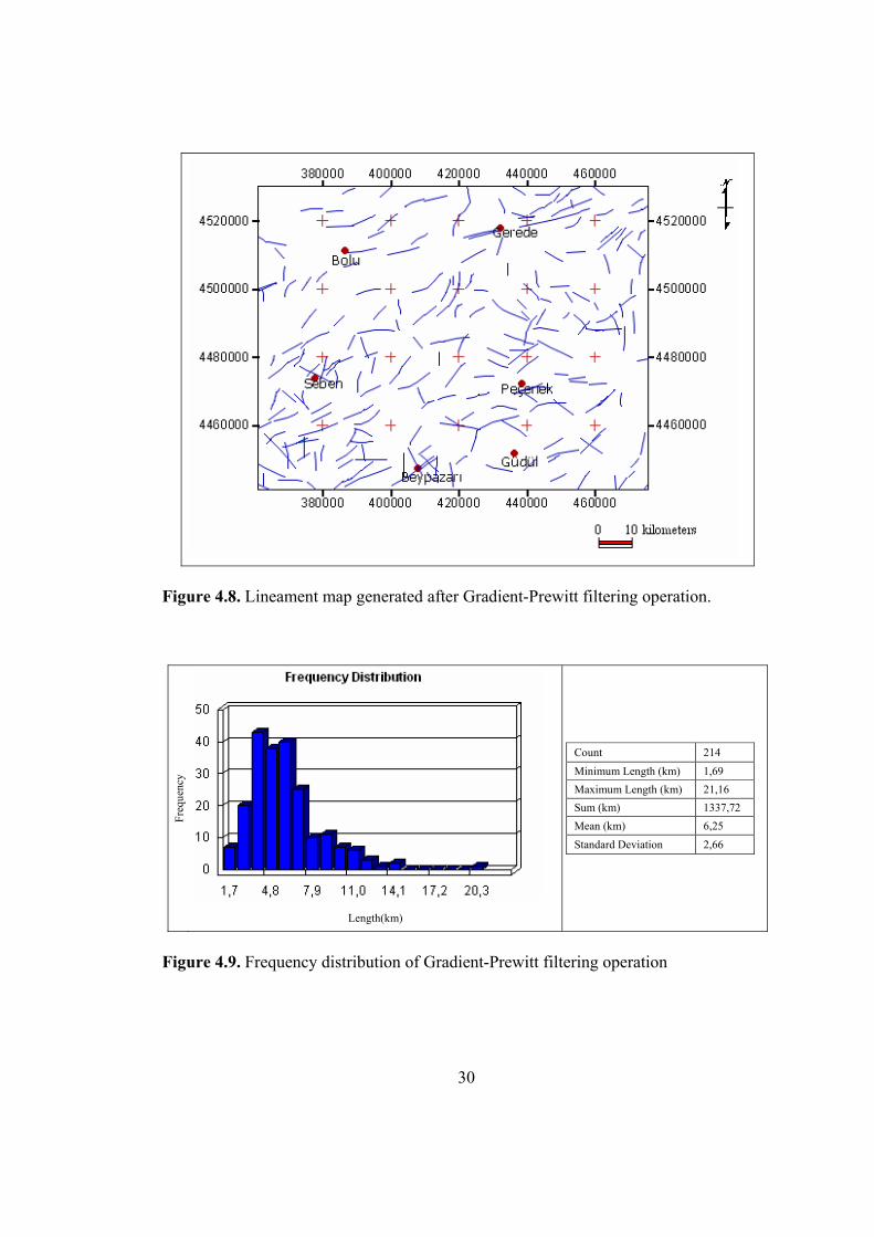
Figure 4.8. Lineament map generated after Gradient-Prewitt filtering operation...... 30
Figure 4.9. Frequency distribution of Gradient-Prewitt filtering operation............... 30
Figure 4.10. False color composite of PCA 1 (Red), 2 (Green), and 3 (blue) ............. 33
Figure 4.11. Lineaments extracted from PCA.............................................................. 33
Figure 4.12. Frequency distribution of Lineaments result of PCA .............................. 34
xiii

Figure 4.13. Rationed image derived from the Band5/Band7.
A) Original image for Band 7; B) Ratio of 5/7.
The image at the bottom is the zoom to green rectangular area............... 35
Figure 4.14. Color composite image of the area consisting of
5/7, 2/3 and 4/5 ratios............................................................................... 36
Figure 4.15. Lineament map extracted from band rationing........................................ 37
Figure 4.16. Frequency distribution lineaments result of band rationing .................... 37
Figure 4.17. Color composite of the band 2 (Blue), 3 (Green), 4 (Red) ...................... 39
Figure 4.18. Lineament map extracted from color composite of the band 2, 3, 4 ....... 39
Figure 4.19. Histogram of the lineaments for color composite of
the bands 2, 3 and 4.................................................................................. 40
Figure 4.20. Steps of combining the lineament maps generated by different
Methods.................................................................................................... 41
Figure 4.21. Final lineament map generated by the combination manual extracted
lineaments. ............................................................................................... 42
Figure 4.22. Histogram and basic statistics of the final lineament map....................... 42
Figure 4.23. Lineament map and basic statistics of the automatically extracted
(left column) and manually extracted lineaments. ................................... 48
Figure 4.24. Rose diagrams prepared from automatically and manually extracted
lineaments. ............................................................................................... 50
Figure 5.1. Illustration of the matching fault lines and lineaments to compute
the accuracy of the manually extracted lineament map.. ......................... 52
Figure 5.2. Lineaments (blue lines) identified by the manual extraction and
the faults (red lines) compiled from the literature.................................... 53
Figure 5.3. Matching line segments of lineaments and fault lines determined by
the intersection of two sets....................................................................... 54
Figure 5.4. Procedure to calculate density of lineaments........................................... 57
Figure 5.5. Density of lineaments with different search radius (A) 1 km, (B) 3 km,
(C) 6 km, and (D) 8 km............................................................................ 58
xiv

Figure 5.6. An example of lineament intersection. .................................................... 60
Figure 5.7. Lineament intersection density map with a search radius of 8 km.......... 61
Figure 5.8. Illustration of lineament-length density analysis ..................................... 62
Figure 5.9. Lineament length density map of the area. .............................................. 63
xv
1
CHAPTER 1
INTRODUCTION
1.1. Purpose and Scope
Lineaments are defined as mapable linear surface features, which differ distinctly from
the patterns of adjacent features and presumably reflect subsurface phenomena (O’Leary
et al., 1976). The subsurface effect is valid if the origin of the lineament is controlled by
geological structures such as faults and fractures. Other types of lineaments resulted
from morphological effects (stream channels or drainage divides) or human effects
(roads, field boundaries) can also exist in the region.
Lineament mapping is considered as a very important issue in different disciplines to
solve certain problems in the area. For example, in site selection for construction a dams,
bridges, roads, etc., for seismic and landslide risk assessment (Stefouli et al., 1996), for
mineral exploration (Rowan and Lathram, 1980), for hot spring detection and
hydrogeological research (Sabins, 1996) the nature and the pattern of the lineaments
should be known.
Satellite images and aerial photographs are extensively used to extract lineaments for
different purposes. Since satellite images are obtained from varying wavelength intervals
of the electromagnetic spectrum, they are considered to be a better tool to discriminate
the lineaments and to produce better information than conventional aerial photographs.
(Casas et al, 2000)

2
A comprehensive study of the satellite images and/or aerial photographs is a
complicated study that comprises several steps. For example, extraction of lineaments
from images or photos and generation of a final lineament map is task that involves
several enhancement techniques or manual interpretation. Examples of other steps are
analysis of the derived lineaments according to their density, direction, length,
orientation, intersection etc. and the final interpretation of the lineaments for different
disciplines such as agriculture or geology.
The purpose of this study is to apply the remote sensing techniques for lineament
analysis to the North-West of Ankara. The scope includes the preparation of lineament
map (both by visual image interpretation and automated extraction techniques), the
comparison of the lineament map with published geological maps and carrying out
performing certain evaluation techniques such as density and orientation for extraction
further information about the lineaments.
1.2. Method of Study
This study is completed in two major stages. The first stage is the compilation of
literature related to various aspects of the lineament analysis. The second stage involves
a set of processes performed to achieve the purpose of the study. All the studies are
office work and no fieldwork is made during the study.
During this study three different software packages are used since there is not single
software that will process all steps in the analyses. These are TNT Mips (version 6.8),
PCI Geomatica (version 8.2), ArcGIS (version 9). All manual lineament extraction
including Filtering operations, Principal Component Analysis (PCA), Spectral
Rationing, Color Composite are carried out using TNT Mips software. The automated
lineament extraction is carried out using the Line option of PCI Geomatica software.
ArcGıs is used for analysis operations of the extracted lineaments.

3
1.3. Organization of Thesis
This thesis is composed of eight chapters.
Chapter 2 contains the literature survey and reviews necessary information about
lineament analysis.
Chapter 3 introduces the study area and the data used in this thesis.
Chapter 4 presents the method of the study and application of the methodology on the
selected study area.
Chapter 5 presents the testing extracted lineaments with previous studies in the area and
the evaluation of the lineaments according to their density intersection density, length
and orientation.
Chapter 6 contains the discussion part; result obtained from all the study and
recommendations for the future studies.

4
CHAPTER 2
BACKGROUND STUDIES
In this chapter, the previous studies on lineament extraction and their analysis are
explained. Studies related with the subject of this thesis can be grouped into two
categories.
(1) Lineament analysis by using digital image enhancement and filtering techniques.
(2) Lineament analysis by using automated extraction techniques.
Studies related to these categories are explained below in chronological order.
2.1 Lineament analysis by using digital image enhancement and filtering techniques
Qari (1991) analyzed Landsat TM image using various image processing techniques
including principal component analysis, decorrolation stretching, and edge enhancement
techniques. These techniques were used for mapping different lithologies and for the
structural analysis of rugged terrain located in Al-Khabt area, Southern Arabia. The
result of the study shows that the remote sensing technique helps to understand complex
evaluation of the Arabian Shield.
Kumar and Reddy (1991) suggested a procedure for analyzing digitized linear features.
Analysis of lineaments is composed of two stages. The first stage involves interpretation
of lineaments from a source map or image and generation of a lineament map. The
second stage involves the actual analysis of the derived lineament map. In the analysis of
lineaments location, direction, length, and curvature from primary attributes of
lineaments. The analyzed linear features can be classified into three main areas as
follows: (1) analysis using a cellular approach, (2) development of an experimental

5
lineament database; and (3) development of computer aided analysis techniques. The
procedure is tested in an area in South India.
Mah et al. (1995) extracted lineaments by using digital image enhancements techniques
in Northern Territory, Australia. To highlight the lineaments, TM bands 4, 5, and 7 were
edge-enhanced by 3*3 asymmetric filter kernels with different illumination directions.
TM 7 was filtered with a NS-SW trending illuminated filter; TM 5 was filtered with a
NW-SE trending illuminated filter, and TM 4 was filtered with E-W and N-S trending
illuminated filters. The interpreted lineaments were statistically analyzed using LINPAC
software developed by the authors (Balia and Taylor) at the University of New South
Wales, Sydney, Australia.
Chang et al. (1998) extracted the lineaments from satellite images by using digital
enhancement and filtering techniques. They claimed that automatic extraction of
lineaments has not been widely accepted and the task of line drawing should be done
manually. The main reason for this is that the human interpreter can consider data trends
within a wide spatial range more effectively than most automatic algorithms suggested.
They suggested an algorithm based on the profile recognition and polygon-breaking to
extract automatically ridge and valley axes. The program is applied to the area in Taiwan
and is claimed to be successful in extracting the ridge and valley system.
Süzen and Toprak (1998) extracted lineaments by using different lineament extraction
techniques including single band, multiband enhancements and spatial domain filtering
techniques. A new algorithm that consist of a combination of large smoothing filters and
gradient filters was developed, in order to get rid of the artificial lineaments which are
out of interest and to determine discontinuous and/or closely spaced regional lineaments.
They tested the alignments found after analysis with the drainage network in the area
which is north of Ankara.
Arlegui and Soriano (1998) used different band combinations of Landsat 5 TM to extract
lineaments in central Ebro basin (NE Spain). The best visual quality was obtained with a
false colour image utilizing bands 2, 4 and 7 (in blue, green and red respectively). Visual

6
quality was improved by a linear contrast stretch in which the lower 1% of the pixels
was assigned to black and the upper 1% was assigned to white (digital numbers 0 and
255 respectively). The remaining pixel values were distributed linearly between these
values. Finally, the area is analyzed in more detail using print copies at a scale of
1/100.000. A visual analysis of the resulting images was made and more than 6.000
lineaments were mapped by this method.
Zakir et al. (1999) developed a new type of fractal plot based on the fractal nature of
lineaments. This plot displays the effect of varying in the counting cell dimension on
two counted aspects, which are the total frequency of segmented lineaments and the total
lineament to cell intersections. The two candidate lines on the plot intersect at a point
which defines the Optimal Cell Dimension (OCD) necessary for preparing an optimized
lineament density map.
Leech et al. (2003) attempted to identify the lineaments in Coastal Cordillera of northern
Chile. They digitally enhanced the geo-corrected data using band-rationing techniques,
linear and Gaussian nonlinear stretching, and principal component analysis. A series of
directional edge filters were applied to enhance the lineaments contained in the image. A
vector map was produced by manually digitizing the enhanced data. Orientation,
magnitude and degree of spread of lineament populations are measured and analysed
with the aim of identifying distinct lineament sets.
Won-In and Charusiri (2003) attempted to map geology of Cho Dien area (Northern
Vietnam) using satellite images. The main enhancement techniques include high-pass
filtering, albedo correction, image classification, principal component analysis (PCA)
and band ratios in order to discriminate the rock types and extract lineaments. High-pass
filtering was considered to be the most suitable approach for lineament analysis. Albedo
was good for differentiating lithology, and image classification was also successfully
used for lineament interpretation and discrimination of lithologies. The result shows that
the geological map obtained from the visual interpretation is more accurate than earlier
works in the same area.

7
Cortes et al. (2003) made a visual analysis of the whole region (Duero Basin - north
Spain) directly on the computer screen (with the help of conventional drawing
programs) at different scales to avoid as much as possible loss of information. More than
10.000 lineaments were hand-drawn and mapped. In most cases, the identification of
lineaments is based on geomorphological criteria since fractures favour the development
of different landforms and these facilitate at present the identification of lineaments. In
other cases, the presence of a tonal contrast helps to differentiate lineaments. Directional
filtering was not used due to the great variability of lineament directions observed from
a previous analysis. These filters identified orientations, thus concealing some
lineaments with different trends.
Nama (2004) used the Landsat 7 (ETM) imagery to detect and map the extent of the
faults and lineaments formed during 1999 volcanic eruptions of Mount Cameroon.
Various image processing techniques were tested and compared in order to detect most
effective output. Principal Component Analysis was found to be useful to determine the
extent of deformation caused by volcanic eruption.
The summary of the above mentioned references in relation to the thesis is that:
- Nine of these studies aim to extract lineaments manually from the satellite
images. Other two (Kumar and Reddy, 1991 and Zakir et al. 1999) analyzed the
lineaments derived from the images.
- All studies with no exception used Landsat satellite image during the analyses,
- Following remote sensing techniques are used for extracting the lineaments:
filtering in six studies, Principal Component Analysis in five, stretching in four,
color composite in one, band ratio in one and classification in one.
- Following aspects of the lineaments are analyzed after the lineament map is
generated: length, density, orientation, curvature and spatial distribution.

8
2.2 Lineament analysis by using automated extraction techniques
Wang et al. (1990) applied the Hough transform to automatically detect the straight lines
that represent geologic lineaments on the satellite images. The main advantages of this
method are that it is relatively unaffected by gaps in lines and by noise. The method
involves transforming each of the figure points into a straight line in parameter space.
The method is applied to a Landsat TM image of Sudbury (Ontario - Canada) The result
of this study shows that automated interpretation identifies more of the faults than visual
interpretation.
Zlatopolsky (1992) introduced a new program for the extraction of automated linear
image features. He named the program as LESSA (Lineament Extraction and Stripe
Statistical Analysis). In this study, the main experimental results of LESSA testing and
of its application to aerial and satellite imagery processing are discussed. It is shown that
the description of texture orientation properties obtained reflects the image pattern and
scarcely depends on applied procedures and their parameters.
Koike et al. (1995) proposed a new method to identify the lineaments from the satellite
image. They called this method as “Segment Tracing Algorithm (STA)”. The method is
applied to a mountainous area in southwestern Japan. The principle of the STA is to
detect a line of pixels as a vector element by examining local variance of the gray level
in the digital image, and to connect retained line elements along their expected
directions. The threshold values for the extraction and the linkage of line elements are
direction dependent. The advantages of the proposed method over usual filtering
methods are its capability to trace only continuous valleys and extract more lineaments
that parallel the sun's azimuth and those located in shadow areas.
Zlatopolsky (1997) used the program LESSA (Lineament Extraction and Stripe
Statistical Analysis) introduced by Zlatopolsky (1992) for extracting and analyzing
linear features. The methods developed for texture orientation can be applied to different
types of image data such as grey tone images, binary schemes, and digital terrain maps.

9
Texture orientation properties are characterized by rose diagrams, vector fields, and
digital fields.
Koike et al. (1998) proposed a new method to calculate the azimuth (strike and dip
angles) of “fracture” planes through a combination of lineaments maps and digital
elevation models (DEM’s). In this study, a segment tracing algorithm (STA) was used to
automatically interpret lineaments from satellite images, extracted lineaments are
concatenated into “fractures” by examining the difference of orientation angle and the
distance between the neighboring lineaments. The method is applied to three regions in
Japan with different rock associations. Lineaments are extracted using Landsat TM and
SPOT pan images.
Majumdar and Bhattacharya (1998) proposed a method for extraction of linear and
anomalous patterns by application of Haar transform. The Haar transform is claimed to
be useful in extraction of subtle features with finer details from an image. This method is
applied to pat of Cambay Basin in India. The results show that the major drainage
pattern as well as lineament patterns is extracted by digital filtering techniques.
Casas et al. (2000) introduced a computer program, LINDENS (designed in Fortran 77
for Macintosh and PC), that analyze lineament length and density. The program also
provides a tool for classifying the lineaments contained in different cells, so that their
orientation can be represented in frequency histograms and/or rose diagrams. The
density analysis is done by creating a network of square cells, and counting the number
of lineaments that are contained within each cell, that have one of their ends within the
cell or that cross-cut the cell boundary. The lengths of lineaments are then calculated.
The program is tested in Duero Basin in Northern Spain particularly for the reliability of
density analysis.
Costa and Starkey (2001) introduced a computer program, PhotoLin, written for an
IBM-PC-compatible microcomputer which detects linear features in aerial photographs,
satellite images and topographic maps. The image to be analyzed is prepared as a
computer-readable input file in PCX format. The image file is binarized and segmented

10
using a threshold to identify features of interest. The median axes of the features are
located using a thinning algorithm and they are represented as a lineament map. For
orientation analysis, linear features are isolated by breaking branches which are broken
into segments of constant length. The mean orientations of the segments are determined
and used to prepare a rose diagram.
Vassilas et al. (2002) presented an automated lineament detection method based on a
modified Hough transform. The method first performs an efficient data clustering then
binarizes the classification result and finally applies the modified Hough transform in
order to identify lineaments. The capabilities of method are described using Landsat TM
satellite data from the Vermion area in Greece. The results of the automated analysis
show major geological faults in the selected area.
Mostafa and Bishta (2004) emphasized importance of the rock types on the lineament
patterns existing in the area. They extracted lineaments from Landsat ETM image data
using GeoAnallst PCI EASI/PACE software. The digitally extracted lineaments were
compared with the visually interpreted lineaments to detect and count true/false
lineaments. The extracted lineaments were counted as frequency, length, lineament to
cell intersection using square counter. Correlating lineament density maps with
radiometric contour maps show that rock units with high radioactivity are also
characterized by high lineament density and lineament intersection density.
A summary of the above mentioned references in relation to the thesis is that:
- Except one reference (Casas et al, 2000) in all studies the lineaments are extracted
from the satellite image using automated algorithms. Casas et al. (2000)
introduced a computer program that evaluates the lineaments extracted from
satellite images.
- Six of the studies used Landsat image to extract the lineaments. Two use digital
terrain model and one uses ISRO (Indian Space Research Organization)
multispectral image.

11
- For the extraction of the lineaments following algorithms/softwares are used:
LESSA (Lineament Extraction and Stripe Statistical Analysis) by two, Segment
Tracing Algorithm (STA) by two, Haar transform by one, PhotoLin by one,
Hough transform by one and PCI Geomatica by one.
- After the lineament map is extracted the orientation, length, frequence and density
of the lineaments are evaluated.
12
CHAPTER 3
STUDY AREA AND THE DATA
3.1. Study Area
Study area used for the application of the algorithm described in this thesis is located to
the northwest of Ankara province. The area is within Zone 36 of Universal Transverse
Mercator projection system. The upper left and lower right coordinates of the study area
are 4529790N-357703E and 4426164N-471475E, respectively (Figure 3.1-A). The total
area covered is 11786 km2. Major cities within the area are Bolu, Gerede, Çamlıdere,
Kızılcahamam, Beypazarı, Seben and Güdül.
Morphologically the area is a mountainous region. The minimum and maximum
elevation in the study area is 351 and 2367 m, respectively. The area is characterized by
NEE-SWW trending topographic ridges particularly in the northern and southern parts.
Deeply dissected valleys in the northern part corresponds to the trace of the North
Anatolian Fault Zone (Figure 3.1-B). The circular topographic mass between Bolu,
Seben and Peçenek is the Köroğlu mountain.
The main highway in the area is the Trans European Motorway (TEM) that connects
Ankara to Istanbul. In the northern part of the area (between Gerede and Bolu) the TEM
is approximately parallel to the North Anatolian fault zone.

13
A
B
Figure 3.1. A) Location map of the study area, B) Elevation map of the area.

14
3.2. Data
Three data sets are used in this study:
1. The satellite image of the area to extract the lineaments,
2. The fault map of the area compiled from the literature, and
3. The road map of the area extracted from the satellite image.
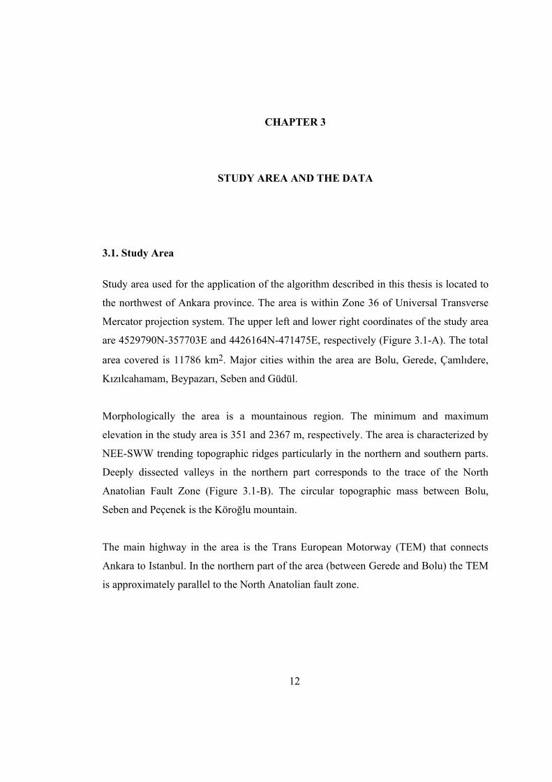
3.2.1. Satellite Image
Satellite image of the area is the main data used in this study. It is used for the extraction
of lineaments. Considering spatial resolution of the available satellite images and the
size of the study area, Landsat ETM image is selected for this study. This image has a
resolution of 30 m which can easily detect the lineaments. Most of the applications in
the literature are performed using this image (Qari, 1991; Kumar and Reddy, 1991; Mah
et al., 1995; Süzen and Toprak, 1998; Arlegui and Soriano, 1998; Nama, 2004). Lower
resolution satellite image (e.g. 80 m and larger cell size) may not be suitable to detect
the lineaments. Higher resolution images, on the other hand, may complicate the process
and can detect minor lineaments not interested in.
The subset of the Landsat ETM acquired on 2000-07-04, Path 178 and row 032 Earth
Sat Ortho, GeoCover is used in this study. The image is provided from RS-GIS
Laboratory, Geological Eng. Dept., METU. The image is composed of 3123 rows and
4018 columns. It has eight bands sensitive to different wavelengths. Six of these bands
detect visible (1, 2, 3), near infrared “NIR” (4), short wave infrared “SWIR” (5, 7), one
thermal and one panchromatic. The Landsat ETM image of the study area is shown
Figure 3.2.
15
Figure 3.2. True color composite Landsat ETM image of the study area
3.2.2. Fault Map of the Area
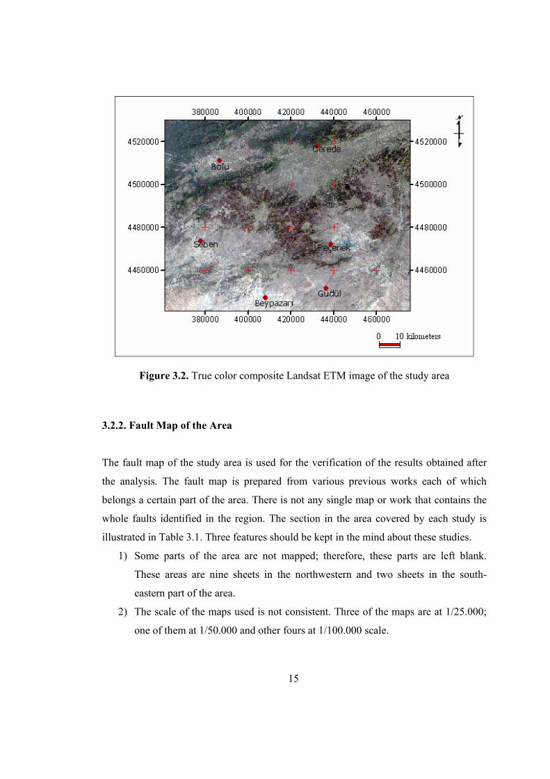
The fault map of the study area is used for the verification of the results obtained after
the analysis. The fault map is prepared from various previous works each of which
belongs a certain part of the area. There is not any single map or work that contains the
whole faults identified in the region. The section in the area covered by each study is
illustrated in Table 3.1. Three features should be kept in the mind about these studies.
1) Some parts of the area are not mapped; therefore, these parts are left blank.
These areas are nine sheets in the northwestern and two sheets in the south-
eastern part of the area.
2) The scale of the maps used is not consistent. Three of the maps are at 1/25.000;
one of them at 1/50.000 and other fours at 1/100.000 scale.

16
Table 3.1. Area covered by previous works for the preparation of fault map. Each color represents a study listed in the table below. Labels indicate topographic sheet numbers.
Color Reference Scale
No map in this area Öztürk et al.(1985) 1/ 25000 Rondot (1956) 1/100000 Türkecan et al. (1991) 1/ 25000 Demirci (2000) 1/100000 Öngür (1976) 1/ 50000 Ürgün (1972) 1/ 25000 Erol (1954) 1/100000 Şaroğlu et al. (1995) 1/100000
17
3) The purpose of these studies is different that effects the reliability of the result
map generated:
-Öztürk et al. (1985) aims to map the faults within the North Anatolian fault zone
region and is directly focused on the detection of the faults existing in the
area.
-Rondot (1956) studied geology of the Seben-Nallıhan-Beypazarı region with a
main emphasis given on the volcanic rocks.
-Türkecan et al. (1991) studied the geology and properties of volcanic rocks
between the Seben-Gerede-Güdül-Beypazarı-Çerkeş-Orta Kurşunlu region.
-Demirci (2000) studied geology of the area between Beypazarı and Kazan to
outline the Neogene tectonic deformation northwest of Ankara.
-Öngür (1976) aims to define geothermal resources within the volcanic rocks in
Kızılcahamam region.
-Ürgün (1972) studied geology and hydrogeology of the Yeniçağa and Dörtdivan
region.
-Erol (1954) studied the geology of the Köroğlu-Işık volcanic mountains and
Neogene basin between Beypazarı and Ayaş.
-Şaroğlu et al. (1995) studied ages and tectonic properties of the Nort Anatolian
Fault Zone between Yeniçağa and Eskipazar.
All these features should be considered as factors that will negatively affect the quality
of the fault map compiled in this study.
To prepare the fault map, first of all the eight maps are converted individually to digital
format by the use of the scanner. Then the maps are geometrically corrected and
combined to get a single map. The faults on the resultant map are digitized to generate
the fault map to be used in this study (Figure 3.3).
The map suggests that two regions are characterized by the presence of faults these are
the northern parts of the area between Bolu and Gerede that corresponds to the North
Anatolian Fault Zone and the southeastern parts of the area around Peçenek and Güdül.

18
Other regions such as south of Gerede and vicinity of Seben have a lower frequency of
the faults. This difference might be due to the actual case in the field or due to the
inconsistent details on the faults mapped by different researchers.
Figure 3.3. The fault map of the study area.
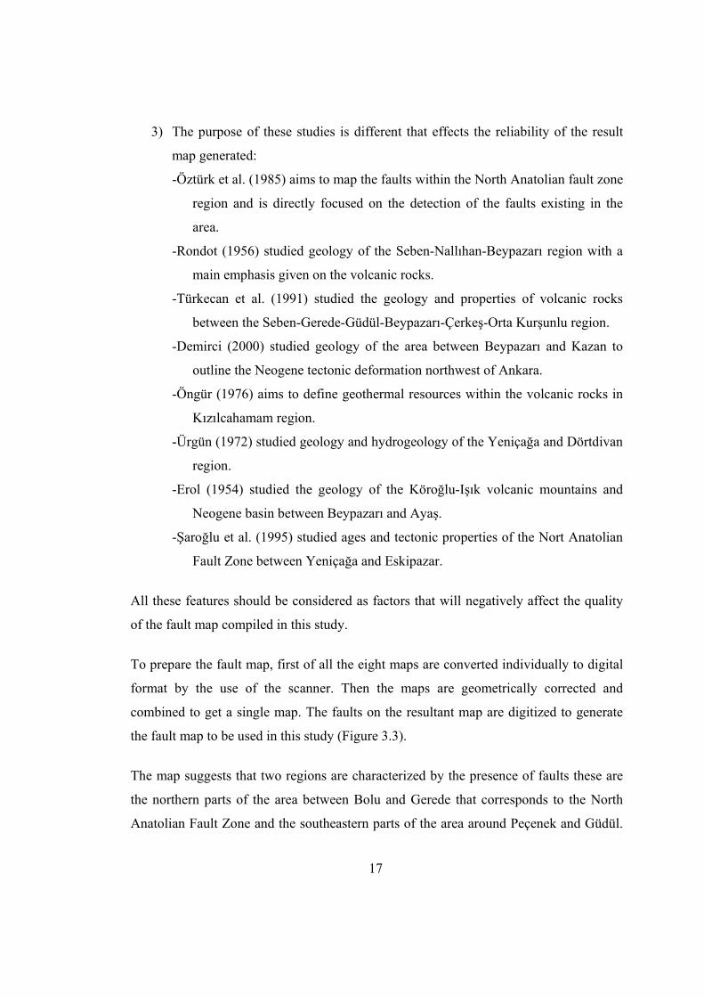
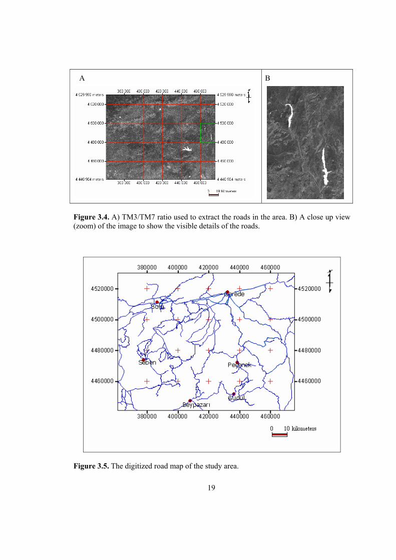
3.2.3. Road Map
The purpose of the generating a road map is to avoid to identify the roads as lineaments
in the area because some roads, particularly the straight ones, might be confused and
classified as lineament. The road map of the area is digitized from the true color
composite of the image (Figure 3.2) and ratio of TM3/TM7 (Figure 3.4) in this image
roads appear in lighter tone due to their relatively high reflectance in the red band (TM3)
and low reflectance in mid infrared band (TM7) (Lillesand, 1999). Figure 3.5 shows the
digitized road map of the area.
19
A
B
Figure 3.4. A) TM3/TM7 ratio used to extract the roads in the area. B) A close up view (zoom) of the image to show the visible details of the roads.
Figure 3.5. The digitized road map of the study area.

20
CHAPTER 4
METHOD AND APPLICATION
This chapter describes the method used in this study and its application in the selected
area. The flowchart of the method is given in Figure 4.1.
The method is composed of four successive steps:
1) The first step is the selection of input data for analysis.
2) The second step is lineament extraction by using manual and automated
lineament extraction techniques and the comparison between them.
3) The third step includes the testing of final map with available fault map of the
area.
4) The last step is the evaluation of lineament map and includes density, direction,
intersection length, and orientation analysis.
4.1. Input Data
The first step of the methodology is selection of initial input data for lineament
extraction. Although the lineaments can be extracted from several data such as aerial
photographs, geophysical data etc, in this study the satellite image is preferred for the
application.

21
“
Figure 4.1 Flowchart of the method applied in this study.
INPUT DATA Satellite Image
LINEAMENT EXTRACTION
AUTOMATED LINEAMENT EXTRACTION
• Line option of PCI Geomatica
MANUAL LINEAMENT EXTRACTION • Filtering operations
• Principal Component Analysis (PCA)
• Spectral Rationing
• Color Composite
FINAL LINEAMENT MAP
EVALUATION OF LINEAMENT MAP • Density • Length • Direction • Orientation
TESTING FINAL MAP WITH FAULT MAP
STEP
1
STEP
2
STEP
3
STEP
4
LINEAMENT MAP
MAP VERIFICATION

22
4.2. Lineament Extraction
The second step of the methodology is extraction of lineaments from satellite images
and final map generation. This is the main step in the application. Lineament extraction
in this study is performed in two ways:
Manual lineament extraction
Automated lineament extraction
4.2.1. Manual Lineament Extraction
In manual extraction method, the lineaments are extracted from satellite image by using
visual interpretation. The lineaments usually appear as straight lines or “edges” on the
satellite images which in all cases contributed by the tonal differences within the surface
material. The knowledge and the experience of the user is the key point in the
identification of the lineaments particularly to connect broken segments into a longer
lineament (Wang et al., 1990). Some general features, however, help to identify the
lineaments can be listed as follows as already described in the literature:
- Topographic features such as straight valleys, continuous scarps,
- Straight rock boundaries,
- Systematic offset of rivers,
- Sudden tonal variations,
- Alignment of vegetation.
According to Koike et al. (1995) a continuous straight valley is the most helpful feature
as a primary identification criterion in image processing for lineaments because a
satellite image has no direct information on the topography of the area.
There are several image enhancement techniques that can contribute to manual
lineament extraction. In this study four of commonly known techniques will be used in
the preparation of the final lineament map. These are filtering operations, Principal
Component Analysis (PCA), spectral rationing and the color composites.
23
First, a map will be prepared for each method. Procedure and the details of these maps
will be given in the following sections. Then, a single map will be generated from these
four maps in which the repeated lineaments will be deleted. The main reason for using
several techniques is that one single method may not detect all the lineaments because of
the variation in the nature of surface material in the area such as variations in the
vegetation density, topographic texture and elevation.
4.2.1.1. Filtering operations
One of the characteristic features of the satellite images is a parameter called spatial
frequency which is defined as the number of changes in brightness value per unit
distance for any particular part of an image. If there are very few changes in brightness
value over a given area in an image, this is referred to as a low-frequency area.
Conversely, if the brightness values change dramatically over short distances, this is an
area of high frequency detail (Jensen, 1996). Therefore, filtering operations are used to
emphasize or deemphasize spatial frequency in the image. This frequency can be
attributed to the presence of the lineaments in the area. In other words, the filtering
operation will sharpen the boundary that exists between adjacent units.
The main disadvantage of the filtering method is that it cannot effectively extract
lineaments in low-contrast areas where features extended parallel to the sun directions
and in mountain shadows (Koike et al., 1995).
A common filtering operation involves moving a window with a certain kernel size
(e.g. 3*3, 5*5, 7*7 etc.) For each pixel in the output file (resultant image) a new digital
number value is calculated under that window and replaced to the central pixel of the
window (Figure 4.2).

24
A
B
Figure 4.2 Generation of a new image file by filtering operation. A) A window is selected that moves both row-wise and column-wise, B) For each window a new value (R) is calculated.
The High Pass filter selectively enhances the small scale features of an image (high-
frequency spatial components) while maintaining the larger-scale features (low-
frequency components) that constitute most of the information in the image.
Directional filters (edge detection filters) are designed to enhance linear features such as
roads, streams, faults, etc. The filters can be designed to enhance features which are
oriented in specific directions. Commonly used edge detection filters are Gradient-
Sobel, Gradient-Roberts, and Gradient-Prewitt. Examples of filtered images that applied
in the study area are shown in Figure 4.3.

25
A B
C D
Figure 4.3 Filtered images of the study area:
A) Normal contrast-stretched image, B) Low pass filtered image, C) High pass filtered image, D) Directional filtered image.

26
Directional Gradient-Sobel and Gradient-Prewitt filters are applied to the Landsat ETM
band 7 in N-S, E-W, NE-SW and NW-SE directions to increase frequency and contrast
in the image. The directional filters in four principal directions are given in Table 4.1.
Table 4.1. Sobel and Prewitt filters in four main directions applied in this study.
The results of the Sobel and Prewitt filters are given in Figures 4.4 and 4.5 for four main
directions. These figures belong to a small section in the study area to show the details
of the results obtained.
Two maps are prepared from these images; one for Sobel and the other for Prewitt. The
result lineament map for Sobel filters and its frequency histogram is shown in Figures
4.6 and 4.7, respectively. The map and histogram for the Prewitt filters, on the other
hand, are shown in Figures 4.8 and 4.9, respectively.
The number of the lineaments identified in these two filters is considerably different.
The number is 318 for Sobel and 214 for Prewitt. Visual comparison of the two maps
suggests that most of the additional lines in Sobel filters are homogeneously distributed
over the area except close vicinity of Seben.
The average length of the lineaments is 5.7 km for Sobel and 5.5 km for Prewitt. The
longest lineament is about 21 km east of Gerede (Figure 4.8). This maximum value,
however, is less than the expected value because the presence of North Anatolian Fault
Zone is already known in the area that passes through Bolu and Gerede.
N-S NE-SW E-W NW-SE SOBEL
-1 0 1 -2 0 2 -1 0 1
-2 -1 0 -1 0 1 0 1 2
-1 -2 -1 0 0 0 1 2 1
0 1 2 -1 0 1 -2 -1 0
PREWITT
-1 0 1 -1 0 1 -1 0 1
-1 -1 0 -1 0 1 0 1 1
-1 -1 -1 0 0 0 1 1 1
0 1 1
-1 0 1
-1 -1 0
27
E-W direction NE-SW direction
NW-SE direction N-S direction
Figure 4.4. Sobel filtered image in E-W, NE-SW, NW-SE, NS directions.

28
E-W direction NE-SW direction
NW-SE direction N-S direction
Figure 4.5. Prewitt filtered image in E-W, NE-SW, NW-SE, NS directions.
29
Figure 4.6. Lineament map generated after Gradient-Sobel filtering operation.
Freq
uenc
y
Length(km)
Count 318 Minimum Length (km) 1,93 Maximum Length (km) 18,57 Sum (km) 1825,55 Mean (km) 5,74 Standard Deviation 2,36
Figure 4.7. Frequency distribution of Gradient-Sobel filtering operation.
30
Figure 4.8. Lineament map generated after Gradient-Prewitt filtering operation.
Freq
uenc
y
Length(km)
Count 214 Minimum Length (km) 1,69 Maximum Length (km) 21,16 Sum (km) 1337,72 Mean (km) 6,25 Standard Deviation 2,66
Figure 4.9. Frequency distribution of Gradient-Prewitt filtering operation
31
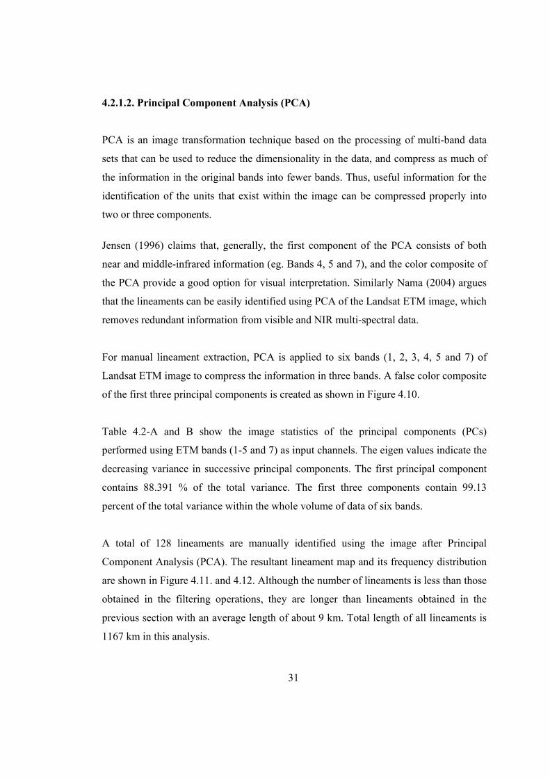
4.2.1.2. Principal Component Analysis (PCA)
PCA is an image transformation technique based on the processing of multi-band data
sets that can be used to reduce the dimensionality in the data, and compress as much of
the information in the original bands into fewer bands. Thus, useful information for the
identification of the units that exist within the image can be compressed properly into
two or three components.
Jensen (1996) claims that, generally, the first component of the PCA consists of both
near and middle-infrared information (eg. Bands 4, 5 and 7), and the color composite of
the PCA provide a good option for visual interpretation. Similarly Nama (2004) argues
that the lineaments can be easily identified using PCA of the Landsat ETM image, which
removes redundant information from visible and NIR multi-spectral data.
For manual lineament extraction, PCA is applied to six bands (1, 2, 3, 4, 5 and 7) of
Landsat ETM image to compress the information in three bands. A false color composite
of the first three principal components is created as shown in Figure 4.10.
Table 4.2-A and B show the image statistics of the principal components (PCs)
performed using ETM bands (1-5 and 7) as input channels. The eigen values indicate the
decreasing variance in successive principal components. The first principal component
contains 88.391 % of the total variance. The first three components contain 99.13
percent of the total variance within the whole volume of data of six bands.
A total of 128 lineaments are manually identified using the image after Principal
Component Analysis (PCA). The resultant lineament map and its frequency distribution
are shown in Figure 4.11. and 4.12. Although the number of lineaments is less than those
obtained in the filtering operations, they are longer than lineaments obtained in the
previous section with an average length of about 9 km. Total length of all lineaments is
1167 km in this analysis.

32
Table 4.2. (a) Variance / Covariance Matrix (b) Eigen vectors and Eigen values of the Principal Component Analysis of the Landsat ETM data.
(A)
Raster ETM1 ETM2 ETM3 ETM4 ETM5 ETM7
ETM1 472.5143 553.5380 799.7514 132.1839 636.5963 697.0007
ETM2 553.5380 665.8568 964.0897 185.3828 768.0187 856.8937
ETM3 799.7514 964.0897 1456.0673 222.7589 1158.0626 1279.7290
ETM4 132.1839 185.3828 222.7589 387.5988 204.9344 390.6032
ETM5 636.5963 768.0187 1158.0626 204.9344 1051.1056 1179.0247
ETM7 697.0007 856.8937 1279.7290 390.6032 1179.0247 1443.7166
(B)
ETM1 ETM2 ETM3 ETM4 ETM5 ETM7 EigenValues %
PC1 0.2971 0.3595 0.5346 0.1175 0.5247 0.4557 88.3910
PC2 -0.1833 -0.1450 -0.3170 0.8280 0.3944 -0.0619 7.5107
PC3 -0.3276 -0.3823 -0.3163 -0.4604 0.4887 0.4423 3.2334
PC4 0.5922 0.3023 -0.6867 -0.0183 -0.0829 0.2812 0.5161
PC5 -0.2388 -0.1187 0.0962 0.2875 -0.5685 0.7168 0.2650
PC6 -0.6025 0.7734 -0.1812 -0.0756 0.0168 -0.0047 0.0839
Pattern of the lineament map (Figure 4.11) suggest that some faults that belong to the
North Anatolian Faults Zone are not properly identified particularly around Bolu.
Lineaments in other parts especially in the southern section between Seben, Peçenek and
Beypazarı display a typical pattern of the faults as already reported in the literature.

33
Figure 4.10. False color composite of PCA 1 (Red), 2 (Green), and 3 (Blue).
Figure 4.11. Lineaments extracted from PCA

34
Freq
uenc
y
Length(km)
Count 128
Minimum Length (km) 1,37 Maximum Length (km) 50,17 Sum (km) 1167,44 Mean (km) 9,12 Standard Deviation 6,32
Figure 4.12. Frequency distribution of Lineaments result of PCA.
4.2.1.3. Spectral Rationing
Rationed images are useful usually for discriminating spectral variations in an image
that are masked by the brightness variations. This enhanced discrimination is due to the
fact that rationed images clearly display the variations in slopes of the spectral
reflectance curves between the two bands involved, regardless of the absolute
reflectance values observed in the bands (Lillesand, 1999). By rationing the data from
two different spectral bands the variations in the slopes of the spectral reflectance curves
between the two different spectral ranges are enhanced and the variations in scene
illumination as a result of topographic effects are reduced. According to Sabins (1996),
ratio images combined in RGB offer greater contrast between the units in the image than
do individual TM band false color images.
An example of band rationing is shown in Figure 4.13 applied to a part of the study area.
In this example the band 5 is divided by band 7 to remove the effect of shadows. By the
help of the band rationing most of the scene illumination effect are removed from the
image and linear features more easily identified from the rationed image.

35
Band 7 of the Landsat ETM Band 5/Band7 of the Landsat ETM
Zoom in the box
A B
C
Figure 4.13. Rationed image derived from the Band5/Band7. A) Original image for Band 7; B) Ratio of 5/7. The image at the bottom is the zoom to green rectangular area.
Spectral rationing is used for manual lineament extraction in order to visually improve
the interpretability of the image and to help the extraction of geomorphologic lineaments
which is affected by topography. Ratios of bands 5/7, 2/3, and 4/5 are selected for
manual lineament extraction:
- TM 5/7 discriminate materials containing hydroxyl bearing minerals. These
minerals can be used as good indicator for the water effects along fractures
(Crippen, 1988).
- TM 2/3 shows contrast between the dense vegetation areas and sparse vegetation
areas, band 4/5 displays the disturbed areas in dark or black tone. (Won-In and
Charusiri, 2003).

36
These bands are used to produce a false color composite (RGB: 5/7, 2/3, 4/5) for manual
lineament extraction. The resultant image used for the extraction of lineaments is shown
in Figure 4.14. The lineament map and its frequency distribution are shown in Figures
4.15 and 4.16, respectively.
Total length of lineaments is 972.6 which is the lowest value in all methods. Number of
lineaments is 146 and the maximum length is 44.23 km. One distinguishing feature of
this fault map is that, the North Anatolian Fault is best identified between Bolu and
Gerede. Frequency of the lineaments is higher around Peçenek and Güdül. South of
Gerede is the area with the least lineaments.
Figure 4.14. Color composite image of the area consisting of 5/7, 2/3 and 4/5 ratios.

37
Figure 4.15. Lineament map extracted from band rationing.
Freq
uenc
y
Length(km)
Count 146 Minimum Length (km) 1,36 Maximum Length (km) 44,23 Sum (km) 972,61 Mean (km) 6,66 Standard Deviation 5,96
Figure 4.16. Frequency distribution lineaments result of band rationing.

38
4.2.1.4. Color Composite
The human eye can only distinguish between certain numbers of shades of gray in an
image (e.g. 16 shades); however, it is able to distinguish between much more colors (e.g.
a few hundred different colors). Therefore, a common image enhancement technique is
to assign specific digital number (DN) values (or ranges of DN values) to specific colors
to increase the contrast of particular DN values with the surrounding pixels in an image.
An entire image can be converted from a gray scale to a color image, or portions of an
image that represent the DN values of interest can be colored. Color images, especially
digital ones, are superior for many applications, especially if they are "false-color".
False color images are produced for manual lineament extraction because they increase
the interpretability of the data. Different combinations of three bands are examined and
the best visual quality is obtained with a false color image utilizing three near-IR bands
2, 3 and 4 (in blue, green and red respectively). This false color combination made it
easier to identify linear patterns of vegetation, geologic formation boundaries, river
channels, geological weakness zones. The result of the process is shown in Figure 4.17.
From the visual interpretation of the false color composite 128 lineaments are extracted
(Figure 4.18). The length and frequency distribution of manually extracted lineaments
are illustrated in Figure 4.19.
Maximum length of the lineament is 54.12 km which is the longest line identified in all
methods. Similar to the previous method (rationing) the North Anatolian Fault is well
identified in this method. Frequency of the lineaments is high around Seben, Peçenek
and Güdül which is consistent with other methods. Almost similar to other methods the
least lineaments are identified south of Gerede and northeast of Seben.

39
Figure 4.17. Color composite of the band 2 (Blue), 3 (Green), 4 (Red).
Figure 4.18. Lineament map extracted from color composite of the band 2, 3, 4

40
Freq
uenc
y
Length(km)
Count 128 Minimum Length (km) 2,02 Maximum Length (km) 54,13 Sum (km) 1112,89 Mean (km) 8,69 Standard Deviation 6,80
Figure 4.19. Histogram of the lineaments for color composite of the bands 2, 3 and 4.
4.2.2. Final Map Generation
The above mentioned techniques are used to extract lineaments from the satellite
images. There is not a commonly accepted method to prepare the final lineament map.
Although any of these techniques (or combination of more than one) can be used to
extract lineaments, four different techniques are applied here in order to be sure that no
lineament is missed in the area. The reason for this is that the area is not homogenous in
terms of the surface characteristics, and it is believed that each method may enhance one
aspect of the surface.
Each process will generate a GIS layer that can be linked to other layers easily. Presence
of multiple lineament maps, however, may result in confusion and complexity. To
overcome this problem a single lineament map should be generated from the results of
all these methods. The procedure for combining the lineaments obtained from all
methods into one map is shown in Figure 4.20. Accordingly, here is always one output
file which is overlaid every time on a different processed image (red lines are new
lineaments extracted from corresponding process; black lines are those transferred from
previous one). In this study, four methods produced five outputs (two for filtering)
suggesting five overlay analyses. Following steps are applied for the generation of final
map:

41
Figure 4.20. Steps of combining the lineament maps generated by different methods.
- Manually extracted lineaments are overlaid onto the same map, one map at a
time. The order of the overlay analysis is not important during this process. The
order used in this study is applied for this step.
- Duplicated lineaments are erased from the map every time a new layer is added.
Erasing of duplicated elements is performed by manual interpretation. In case of
different lengths, the shorter lineaments are deleted.
- The road map is integrated with the lineament map. 87 lineaments that exactly
match the roads are erased.
The final map generated after adding all lineaments are combined and those that
correspond to the roads are erased (Figure 4.21). The histogram and basic statistics of
this map are illustrated in Figure 4.22. Comparison of this map with individual maps
produced by above mentioned methods is given in Table 4.3. Following observations
can be made on the final map:
- Total number of lineaments in generated by different methods is 934. The total
number in the final map, 584, suggests that 350 lineaments are deleted that
correspond to duplicated lineaments including those that match the roads.

42
Figure 4.21 Final lineament map generated by the combination manual extracted lineaments.
Freq
uenc
y
Length(km)
Count 584
Minimum Length (km) 0,86 Maximum Length (km) 68,61 Sum (km) 4154,53 Mean (km) 7,11 Standard Deviation 5,60
Figure 4.22. Histogram and basic statistics of the final lineament map.

43
- The maximum frequency of lineaments is 318 in Sobel filtering which is about
54 % of the final map. This value decreases to 22 % in rationing and color
composite processes. All these suggest that none of the single method is enough
to detect the lineaments existing in the area.
- Total length of the lineaments in final map is 4154.5 km which is 3 or 4 times
greater than any map produced by individual methods. Two reasons for this
difference are that: 1) Only smaller lineaments are deleted during the
combination of maps, and 2) each method had produced considerable amount of
lineaments which are spatially different from each other.
- The maximum length of the lineaments is increased to 68.61 km suggesting that
during generating of final map, some segments are combined to yield longer
lineaments.
- Although the distribution of the frequency of the lineaments identified is
different in different parts of the area, certain parts are lacking lineaments. Two
of these regions are northwestern part of the area and south of Gerede (Figure
4.21).
- The lineaments along the North Anatolian Fault Zone (along Bolu-Gerede) are
overemphasized in the final map which is not observed in any single map of five
processes.
Table 4.3. Comparison of basic statistics of the final map with other maps produced by different methods.
Filtering
Sobel PrewittPCA Rationing Color
composite FINAL MAP
Count (frequency) 318 214 128 128 146 584
Maximum Length (km) 18.57 21.15 50.17 54.12 44.23 68.61
Total Length (km) 1825.5 1337.7 1167.4 1112.9 972.6 4154.5
Mean length (km) 5.74 6.25 9.12 8.69 6.66 7.11

44
4.2.3. Automated Lineament Extraction
Lineaments are extracted from satellite images using automated extraction techniques in
order to compare with the manually extracted lineaments. The main advantages of
automated lineament extraction over the manual lineament extraction are its ability to
uniform approach to different images; processing operations are performed in a short
time and its ability to extract lineaments which are not recognized by the human eyes.
Available software’s provide different algorithms for automated extraction. Three
common algorithms are Hough transform, Haar transform and Segment Tracing
Algorithm (STA) (Koçal, 2004).
The Hough transform is a technique which can be used to separate features of specific
shape within an image. It is required that the specific feature must be defined in some
parametric form. The Hough transform is most commonly used for the detection of lines,
circles, ellipses, etc. The main advantages of the Hough transform are that it is relatively
unaffected by gaps in lines and by noise (Wang et. al. 1990).
Haar transform used by Majumdar and Bahattacharya (1988) for extraction of linear and
anomalous patterns in the image. This method provides a domain in which a type of
differential energy is concentrated in local regions. The transform has both low and high
frequency components and therefore can be used for image enhancement (Koçal, 2004).
The Segment Tracing Algorithm (STA), which is developed by Koike et al. (1995), is a
method to automatically detect a line of pixels as a vector element by examining local
variance of the gray level in a digital image.
The automated lineament extraction in this study is performed by the LINE module of
Geomatica software. The logic of this method is similar to STA. A brief explanation of
the algorithm of this module will be given here. This information is provided from the
Geomatica users’ manual (2001).

45
Algorithm of Automated Lineament Extraction by Geomatica: LINE module of
Geomatica extracts linear features from an image and records the polylines in vector
segments by using six parameters. These parameters will be mentioned explained below.
The algorithm of the LINE consists of three stages: edge detection, thresholding, and
curve extraction.
In the first stage, the “Canny edge detection algorithm” is applied to produce an edge
strength image. The Canny edge detection algorithm has three substeps. First, the input
image is filtered with a Gaussian function whose radius is given by the RADI parameter.
Then gradient is computed from the filtered image. Finally, those pixels whose gradient
are not local maximum are suppressed (by setting the edge strength to 0).
In the second stage, a threshold is applied for the edge strength image to obtain a binary
image. Each ON pixel of the binary image represents an edge element. The threshold
value is given by the GTHR parameter.
In the third stage, curves are extracted from the binary edge image. This step consists of
several substeps. First, a thinning algorithm is applied to the binary edge image to
produce pixel-wide skeleton curves. Then a sequence of pixels for each curve is
extracted from the image. Any curve with the number of pixels less than the parameter
value LTHR is discarded from further processing. An extracted pixel curve is converted
to vector form by fitting piecewise line segments to it. The resulting polyline is an
approximation to the original pixel curve where the maximum fitting error (distance
between the two) is specified by the FTHR parameter. Finally, the algorithm links pairs
of polylines which satisfy the following criteria: (1) two end-segments of the two
polylines face each other and have similar orientation (the angle between the two
segments is less than the parameter ATHR); (2) the two end-segments are close to each
other (the distance between the end points is less than the parameter DTHR).

46
Description of six parameters used in the algorithm is as follows:
RADI (Filter radius): This parameter is used in the first step of the first stage of the
process for the “Canny edge detection”. It specifies the radius of the edge
detection filter (in pixels). It roughly determines the smallest-detail level in the
input image to be detected. The data range for this parameter is between 0 and
8192.
GTHR (Gradient threshold): This parameter is used in the second stage of the process
for the “Canny edge detection”. It specifies the threshold for the minimum
gradient level for an edge pixel to obtain a binary image. The data range for this
parameter is between 0 and 255.
LTHR (Length threshold): This parameter is used in the third stage of the process. It
specifies the minimum length of curve (in pixels) to be considered as lineament or
for further consideration (e.g., linking with other curves). The data range for this
parameter is between 0 and 8192.
FTHR (Line fitting error threshold): This parameter is used in the second step of the
third stage. It specifies the maximum error (in pixels) allowed in fitting a polyline
to a pixel curve. Low FTHR values give better fitting but also shorter segments in
polyline. The data range for this parameter is between 0 and 8192.
ATHR (Angular difference threshold): This parameter is used in the last step of the
third stage of the process. It specifies the maximum angle (in degrees) between
segments of a polyline. Otherwise, it is segmented into two or more vectors. It is
also the maximum angle between two vectors for them to be linked. The data
range for this parameter is between 0 and 90.
DTHR (Linking distance threshold): This parameter is used in the last step of the third
stage of the process. It specifies the minimum distance (in pixels) between the end
points of two vectors for them to be linked. The data range for this parameter is
between 0 and 8192.

47
The automated lineament extraction operations are applied on Landsat ETM scene by
using PCI EASI/PACE software line option. Band 7 of the image with a spatial
resolution 30*30 meter is selected for automated lineament extraction considering the
purpose of this study; since this band is useful for discrimination of lineaments and other
geological features such as mineral and rock types and is also sensitive to vegetation
moisture content (Sabins, 1996).
The extraction process is manipulated changing the six parameters. Several lineament
maps are generated using different threshold values. The most suitable threshold values
are selected (below) considering these lineaments as fault lines. General properties of
faults are taken into consideration such as the length, curvature, segmentation,
separation and so on in order to determine the threshold values. The parameters in this
application are selected as follows:
RADI=10
GTHR=75
LTHR=30
FTHR=3
ATHR=1
DTHR=40
According to these threshold values:
- The size of Gaussian kernel which is used as a filter during edge detection 10
(RADI),
- Spectral difference at the edge is about 30 % (GTHR),
- Threshold for curvature is 30 pixels suggesting almost straight lines (LTHR),
- Line fitting error is (FTHR) 3 pixels that does not let identification of closely
spaced lineaments within 90 meters,
- Angular difference threshold (ATHR) is 1 degrees used for segmentation,
- Linking distance threshold (DTHR) is 40 pixels (1200 m) that corresponds to the
distance used to link two segments.

48
4.2.4. Evaluation of the automatically extracted lineaments
The automatically extracted lineament map and its basic statistics are illustrated in
Figure 4.23. The results of the manual extraction are also given in this figure to compare
the two maps.
Automatically Extracted Lineaments Manually Extracted Lineaments
Count 3191 Minimum Length (km) 0,86 Maximum Length (km) 4,33 Sum (km) 3882,25 Mean (km) 1,22 Standard Deviation 0,37
Count 584 Minimum Length (km) 0,86 Maximum Length (km) 68,61 Sum (km) 4154,53 Mean (km) 7,11 Standard Deviation 5,60
Freq
uenc
y
Length(km)
Freq
uenc
y
Length(km)
Figure 4.23. Lineament map and basic statistics of the automatically extracted (left column) and manually extracted lineaments.
49
Comparison of two maps can yield following observations:
- Frequency of automatically extracted lineaments is greater more than 5 times of
the manually extracted ones (3191 versus 584). The most important factor for
this is that the lineaments in automated one are shorter in length so that a few of
them could be combined to form one line in manually extracted map. Although
the linking distance threshold is assigned as 1200 m (40 pixels), the program
could not combine segmented lines.
- Automatically extracted map is not made a correction for the map road that
might be a secondary reason for this high frequency.
- Although the frequency of the lineaments is higher in automated one, the total
length of all lineaments is still less than the lineaments (3882.25 km versus
4154.53 km) identified by manual methods. This feature is best illustrated by the
mean lengths of automatic and manual lineaments which are 1.21 km and 7.11
km, respectively.
- Spatial distribution of the lineaments in both maps is considerably different. In
the automated one the frequency of the lines seems to be higher in the
southwestern part of the area, particularly in the close vicinity of Beypazarı. In
the manual one, on the other hand, lineament frequency is higher along the line
between Bolu and Gerede (that fits the North Anatolian Fault Zone).
- The pattern of the two maps although in general look similar, there are some
minor (but important) differences among them. For examples about 10 km south
of Bolu is totally different in both maps. This is lacking lineaments in the
automated one but is full of lines in the second. Other examples of such areas are
southeastern part of the area, close vicinity of Peçenek, south of Beypazarı, and
south and southeast of Seben.
- Length of the maximum lineament detected by automated one is 4.3 km which is
not a proper length for the faults in the area. This length, however, is 68.6 km for
manual one which is quite reasonable.

50
- Orientation of the lineaments for both lineament maps are compared using the
rose diagrams (Figure 4.24). The diagrams are prepared using the frequencies of
the lineaments and therefore are not length-weighted. Two diagrams show great
similarities as being concentrated in NE-SW direction. They differ, however, in
two minor aspects: 1) automated ones cover a wide range whereas the manual
ones are confined to a narrow interval in N45E to N75E; 2) a second minor
direction is identified in manual one in NW-SE direction which is missed in the
automated one.
Automatically Extracted Lineaments Manually Extracted Lineaments
Figure 4.24. Rose diagrams prepared from automatically and manually extracted lineaments.
Comparison of two maps indicates that the manually extracted lineament map is more
reliable in terms of length of the lineaments, their segmentation, their spatial distribution
and their orientation. Although, the extraction of the automated ones is performed with
different threshold values, the one presented here is the best output considering these
lineaments as fault lines. Therefore, the manual extraction produces better results most
probably due to the experience of the user involved in the processes. For this reason the
output of the automated one will not be considered in the rest of the thesis.

51
CHAPTER 5
TESTING AND EVALUATION OF LINEAMENT MAP
5.1. Testing Lineament Map with Fault Map
Manually extracted lineaments are tested for their accuracy by the help of the fault data
compiled from the literature. The lineament map used is the result of the manual
extraction generated in previous chapter (Figure 4.21). The fault map, on the other hand,
is the one introduced in DATA chapter (Figure 3.3) which was a compilation from 8
studies.
The accuracy of lineament map is computed by using GIS overlay technique that
determines where the lineaments and faults are matched. For this operation a buffer zone
of 150 m is assigned to the extracted lineaments that test the matching segments of the
lineaments and the faults (Figure 5.1). The output of this operation produces three types
of lines:
1) Non-matching lineaments: These are the lineaments that do not match to any
fault line (shown as purple lines in the figure),
2) Non-matching fault lines: These are the fault lines that do not match to any
lineament (shown as red lines), and
3) Matching lineaments and fault lines: These are the segments in the buffer
where both lineaments and faults exist (shown as green lines).
The matching segments are stored in the database. The ratio of total length of recorded
elements to the total length of the fault lines is calculated to yield the accuracy of the
lineament map.
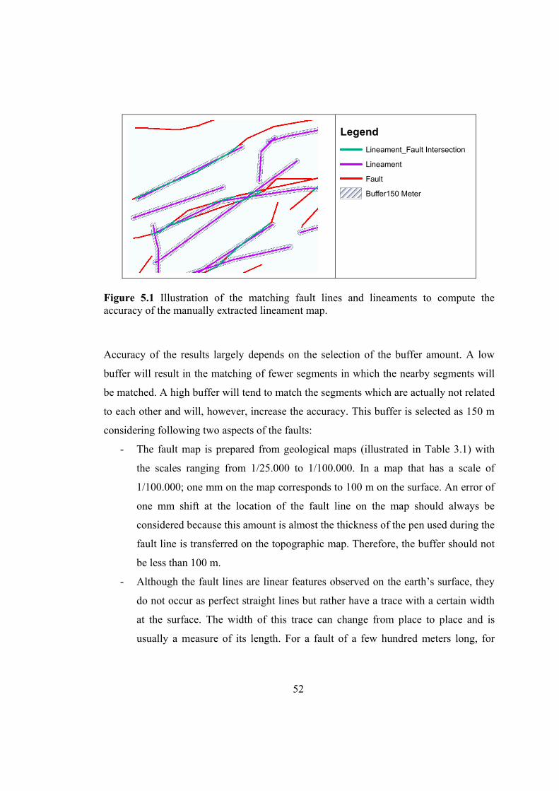
52
LegendLineament_Fault Intersection
Lineament
Fault
Buffer150 Meter
Figure 5.1 Illustration of the matching fault lines and lineaments to compute the accuracy of the manually extracted lineament map.
Accuracy of the results largely depends on the selection of the buffer amount. A low
buffer will result in the matching of fewer segments in which the nearby segments will
be matched. A high buffer will tend to match the segments which are actually not related
to each other and will, however, increase the accuracy. This buffer is selected as 150 m
considering following two aspects of the faults:
- The fault map is prepared from geological maps (illustrated in Table 3.1) with
the scales ranging from 1/25.000 to 1/100.000. In a map that has a scale of
1/100.000; one mm on the map corresponds to 100 m on the surface. An error of
one mm shift at the location of the fault line on the map should always be
considered because this amount is almost the thickness of the pen used during the
fault line is transferred on the topographic map. Therefore, the buffer should not
be less than 100 m.
- Although the fault lines are linear features observed on the earth’s surface, they
do not occur as perfect straight lines but rather have a trace with a certain width
at the surface. The width of this trace can change from place to place and is
usually a measure of its length. For a fault of a few hundred meters long, for

53
example, a width of a few meters can be expected. The average length of the
faults in this study is 3.34 km.
Selection of 150 m for the buffer is, therefore, very close to the minimum tolerable
width of the buffer. Although a wider buffer would increase the accuracy of the result,
this minimum value is selected in this study. It should be kept in the mind that, the
lineament map is generated from satellite image of 30 m spatial resolution. Therefore,
the buffer corresponds to 5 pixels in the satellite image.
Lineaments and the fault lines are shown together in Figure 5.2 by blue and red lines,
respectively. Blue lines are dominating in the figure because the total length of
lineaments (4154 km) is almost twice of the fault lines (2098 km).
These two sets are intersected as mentioned above to find the common line segments.
The resultant map is shown in Figure 5.3.
Legend
Lineament
Fault
Figure 5.2. Lineaments (blue lines) identified by the manual extraction and the faults (red lines) compiled from the literature.

54
Legend Matching line segments (km)
(Lineaments and Fault lines)
Figure 5.3. Matching line segments of lineaments and fault lines determined by the intersection of two sets.
According to the final map produced by intersecting lineaments and the fault lines, in
some parts of the area a dense population of matching segments is observed. These areas
are obvious along the North Anatolian Fault Zone (Bolu-Gerede line), around Peçenek
and Güdül, west of Beypazarı, and the area between Seben and Peçenek. In some other
parts of the area, however, such as between Gerede and Peçenek, between Beypazarı and
Güdül, and south of Seben no matching segments are detected. The main reason for this
is that the fault lines are already not mapped in these areas (Figure 5.2).
Total length of intersection is calculated to be 811.79 km (Table 5.1). This is 38.7 % of
the faults identified in the area which also defines the accuracy of the lineament map
prepared in this study for the whole area. Since the fault map is composed of several
maps at different scales prepared by different groups, it is natural that the reliability of
the fault map can be questioned. For this reason it is decided to test accuracy of the
lineament map for one of these studies which aims to map the faults. The work
performed by Öztürk et al. (1985) is such a study carried out along the North Anatolian
Fault Zone.

55
Table 5.1. Length and ratio of the matching lineaments for the whole area.
Total lineament length (km) 4154.53
Total fault length (km) 2098.05
Total matching length (km) 811.79
Matching length/Fault length (%) 38.69
The map prepared by Öztürk et al. (1985) contains 10 topographic sheets at 1/25.000
scale between Bolu and Gerede (Table 3.1). This area is cropped from both lineament
map and fault map. The same process (mentioned above) is applied to this sub-map to
compute the accuracy for this area. The length and the ratio of the matching lineaments
are given in Table 5.2. Accordingly, the accuracy of the lineament map increases to
50.28 %.
Table 5.2. Length and ratio of the matching lineaments for the area mapped by Öztürk et al. (1985).
Total lineament length (km) 725.88
Total fault length (km) 637.35
Total matching length (km) 320.49
Matching length/Fault length (%) 50.28
56
5.2. Evaluation of Lineament Map
The lineaments extracted manually will be evaluated in this section in order to extract
further information on the distribution and nature of the lineaments. There is not in the
literature a definite way to evaluate the lineaments; and in most cases this is left to the
user based on the purpose of the study. These analyses, in most cases, are processes that
use GIS with other ancillary data. Ancillary data such as topography, geology map,
geophysical data etc. are not used in this study. Therefore, conventional techniques
commonly applied to lineaments such as frequency or length against azimuth histograms
(Mostafa and Zakir, 1996), rose-diagrams (Nalbant and Alptekin, 1995), and or
lineament density maps (Zakir et. al.1999) will be used here. Lineament density and
intersection density of lineaments are also useful for characterizing the spatial patterns
of lineaments (Kumar and Reddy, 1991).
In this study four processes of evaluation are applied. These are: 1) density analysis, 2)
intersection density analysis, 3) length analysis, and 4) orientation analysis.
5.2.1. Density Analysis
The purpose of the lineament density analysis is to calculate frequency of the lineaments
per unit area. This is also known as lineament-frequency (Greenbaum, 1985). This
analysis will produce a map showing concentrations of the lineaments over the area. The
procedure of density analysis is shown in Figure 5.4. First a unit area (a circular area
with a search radius) is defined by the user. Then this area is shifted laterally and
vertically over the area with a defined grid distance. Every time, the frequency of the
lineaments is counted and the number is recorded in an ASCII file for the center of
corresponding unit area. The resultant text file that contains X, Y and Z values (Easting,
Northing and frequency, respectively) and is stored to be processed for preparing density
(contour) map of the area.

57
Lineaments within the unit area Grid pattern applied in calculations
Unit area (with certain search radius and grid distance)
Figure 5.4. Procedure to calculate density of lineaments
Analysis of lineament density is performed by counting number of lineaments contained
in specified unit area. To calculate lineament density, several search radiuses were tested
(1, 3, 6 and 8 km). The results of these analyses are shown in Figure 5.5. As the search
radius increases, frequency of high density areas increases. If the purpose is to see the
details of certain fault sets in local scale then smaller search radius should be selected. If
the purpose is to have an idea on the distribution of the faults at regional scale, then
larger radius should be selected.
The density map generated for 1 km search radius (Figure 5.5-A) does not show any
concentration in particular areas but rather a homogenous distribution. That means the
search radius is not appropriate because the width of the area is more than 100 km (in E-
W direction). The maps prepared with the radius equal to or greater than 3 km, on the
other hand, produces certain patterns that display some information on the distribution of
the faults.

58
A B
C D
Figure 5.5. Density of lineaments with different search radius (A) 1 km, (B) 3 km, (C) 6 km, and (D) 8 km.
Other three maps (Figure 5.5-B, C and D) suggest that there are several fault zones in
the area. Although in general the faults are exposed in the form of an ellipse that extends
in NE-SW direction, several sub-zones (or fault sets) can be distinguished in the area.
North Anatolian Fault Zone (NAFZ), which is the well known zone in the region, is just
one the zones and there are several others scattered in the area. The NAFZ is visible as a

59
linear zone extending in NE-SW direction that passes through Bolu and Gerede. Other
fault zones visible in the area are as follows:
- A relatively shorter fault zone is observed parallel to the trend of the NAFZ to
the north of Bolu.
- One fault zone is obvious in the close vicinity of Güdül in NW-SE direction that
extends to Bolu and joins the NAFZ.
- In the eastern part of the area a fault zone is observed in almost N-S direction.
- In the vicinity of Peçenek a fault zone extends from south of Gerede towards
south in N-S direction and joins other fault zones near Güdül.
- In the southwestern part of the area there is a cluster of faults with an irregular
pattern. The map with 3 km search radius (Figure 5.5-B) imply that this cluster is
composed several fault sets trending in almost E-W direction.
The presence of the NAFZ is known from the literature. Other fault zones, however, are
not described that in the previous studies. Therefore, lineament map prepared in this
study can lead to reclassify the faults existing in the region.
5.2.2. Intersection Density Analysis
Lineament intersection density is a map showing the frequency of intersections that
occur in a unit cell. The procedure is the same as the previous density map. An example
of unit area is shown in Figure 5.6. where two intersections are detected. The purpose of
using intersection density map is to estimate the areas of diverse lineament orientations.
If the lineaments do not intersect in an area, the resultant map will be represented by a
plain map with almost no density contours. That means the lineaments are almost
parallel to sub-parallel in this area if they are not short in length.

60
Figure 5.6. An example of lineament intersection.
The density of lineaments intersection is produced by counting the number of lineament
intersections per unit area. The search radius is taken as 8 km. The result of the analysis
is shown in Figure 5.7.
Visual comparison of density and intersection density maps indicates that both maps
show only a small as indicated in certain parts of the area. In most of the area the
intersection density is different than density map. For example, along the North
Anatolian Fault Zone (between) Bolu and Gerede, although the density is very high, the
intersection density about 3 to 6 %. That means in spite of the abundance of the faults in
this section, because most of the faults are parallel to each other they do not intersect and
therefore the intersection density is low.
The regions characterized by high intersection densities are the southwestern parts
between Beypazarı and Seben, northeastern parts (East of Gerede) and some local
regions around Güdül and Peçenek.

61
Legend
Intersection Point
Lineament
Density of Intersection Points (%)0 - 0,03
0,03 - 0,06
0,06 - 0,10
0,10 - 0,13
0,13 - 0,17
0,17 - 0,20
0,20 - 0,23
0,23 - 0,27
0,27 - 0,30
Figure 5.7. Lineament intersection density map with a search radius of 8 km.
5.2.3. Length Analysis
Analysis of the lineament length density is useful guide for interpreting the lineament
map. Calculating lengths of lineaments more accurately gives the image of lineament
density, since the total length per unit area depends on the lines or segment of lines
completely contained within the cell. This analysis is also known as “lineament-length
density” (Greenbaum, 1985) and is defined as the total length of all recorded lineaments
divided by the area under consideration. A grid of cells is constructed over the area
(Figure 5.8.) and the total length is calculated within this unit area. The rest of the
analysis is similar to the previous two analyses.

62
L1
L2
L3
Length over the unit area: L1 + L2 + L3
Unit area
Figure 5.8. Illustration of lineament-length density analysis.
The length of the lineaments are measured and plotted into selected grid size to prepare
the length density map (Figure 5.9.). The most distinguishing feature of this map is that
the highest concentration is observed along the North Anatolian Fault Zone (NAFZ).
This zone in the map extends from west of Bolu to the east of Gerede. That means the
longest fault segments are observed along the NAFZ.
Other concentrations observed in the area are: a) in the middle of Gerede and Peçenek
that extends in NE-SW direction and joins the NAFZ at a certain angle and relatively in
a narrow belt, b) between Beypazarı and Seben as a wide belt that extends in almost E-
W direction that bifurcates into two branches further east, c) a relatively shorter but well
defined zone in the central part between Bolu, Seben and Peçenek that extends NW-SE
direction.
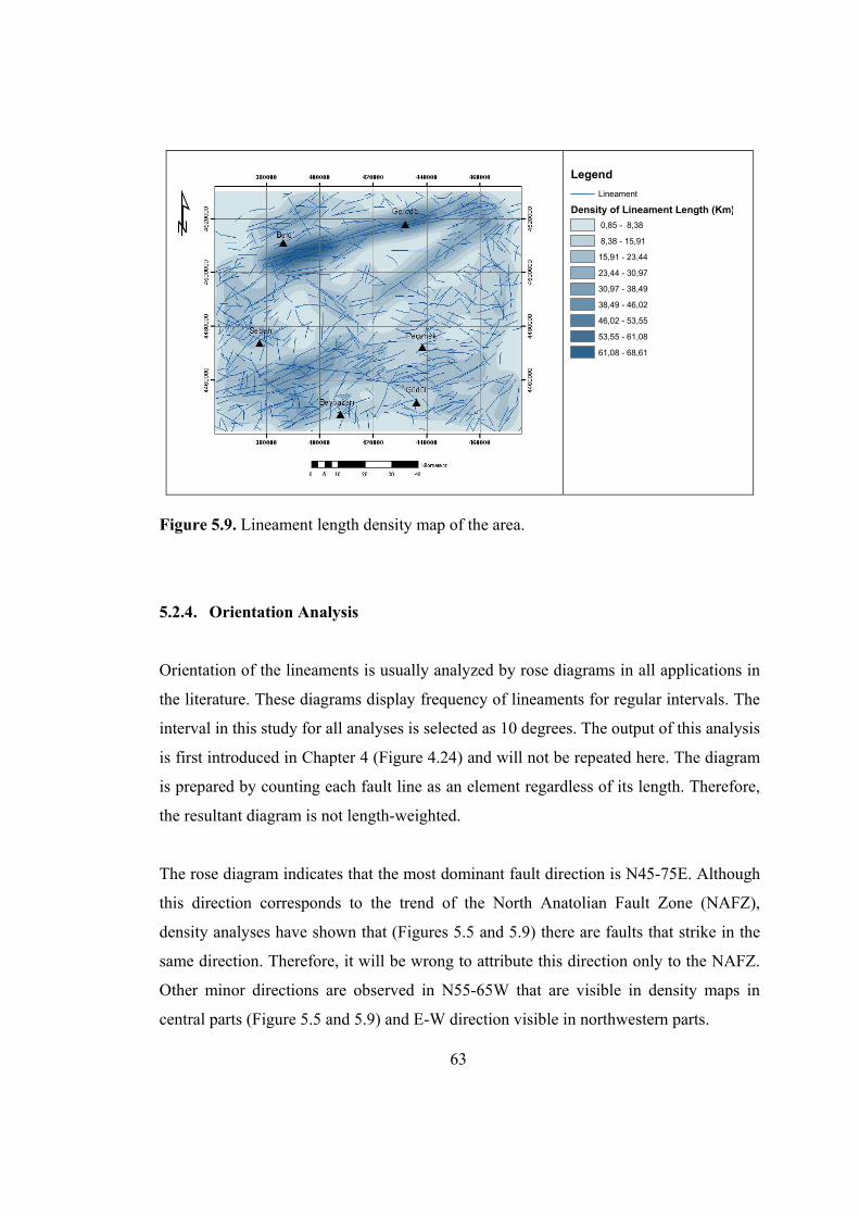
63
LegendLineament
Density of Lineament Length (Km) 0,85 - 8,38
8,38 - 15,91
15,91 - 23,44
23,44 - 30,97
30,97 - 38,49
38,49 - 46,02
46,02 - 53,55
53,55 - 61,08
61,08 - 68,61
Figure 5.9. Lineament length density map of the area.
5.2.4. Orientation Analysis
Orientation of the lineaments is usually analyzed by rose diagrams in all applications in
the literature. These diagrams display frequency of lineaments for regular intervals. The
interval in this study for all analyses is selected as 10 degrees. The output of this analysis
is first introduced in Chapter 4 (Figure 4.24) and will not be repeated here. The diagram
is prepared by counting each fault line as an element regardless of its length. Therefore,
the resultant diagram is not length-weighted.
The rose diagram indicates that the most dominant fault direction is N45-75E. Although
this direction corresponds to the trend of the North Anatolian Fault Zone (NAFZ),
density analyses have shown that (Figures 5.5 and 5.9) there are faults that strike in the
same direction. Therefore, it will be wrong to attribute this direction only to the NAFZ.
Other minor directions are observed in N55-65W that are visible in density maps in
central parts (Figure 5.5 and 5.9) and E-W direction visible in northwestern parts.

64
CHAPTER 6
DISCUSSION AND CONCLUSION
6.1. Discussion
Several aspects of the study will be discussed in this section. These are classified into
four as follows:
1. Problems of the manual lineament extraction,
2. Comparison of manual and automated lineament extraction,
3. Accuracy of the resultant lineament map, and
4. Implications of the results obtained.
6.1.1. Problems of Manual lineament extraction
Selection of satellite image: The first problem in the manual lineament extraction is the
selection of the most suitable satellite image. Landsat images (MSS, TM or ETM) are
the most commonly used images in the literature. The main reason for this selection is
the spatial resolution of the image (30*30 m) which is convenient for lineament analysis.
Lineament in this study and in most of the previous works refers to fault existing on the
earth’s surface. Therefore, the nature of the lineaments should also be considered during
this selection. If a lineament analysis is carried out to identify, for example, field
boundaries in agricultural areas, then Landsat may not be a good choice because certain
fields might have small dimensions that can not be detected at this resolution. The faults,
however, as mentioned before, are relatively longer structures with certain widths that
can be distinguished at this scale. The minimum and the mean lengths of the lineaments

65
measured in this study are 0.85 and 7.11 km. These lineaments can be easily illustrated
in the maps at a scale of 1:50.000, which is easily identified on a Landsat image.
Selection of method: The lineament map is generated in this study by combining the
maps produced from four methods. These are filtering operations, principal component
analysis, spectral rationing and color composite process. The main reason for several
processes to be involved is that none of the single methods may detect all the lineaments
existing in the area because of the diverse nature of the surface. In the study area it is
known that some sections are densely vegetated (e.g. north of Kızılcahamam) while
some other parts are barren (east of Beypazarı). Similarly topographic texture and
drainage density is different in different parts of the area. Since the purpose of these
operations is to make the image visually more representative to identify the lineaments,
several methods applied in the application may reduce the problem in the identification
of the lineaments. The results obtained for each method confirm this argument.
Comparison of the maps (Figures 4.6, 4.8, 4.11 and 4.15) and their basic statistics
(Figures 4.7, 4.9, 4.12 and 4.16) indicate that there are considerable differences in the
lineaments in terms of their length and spatial distribution. Repetition of the lineaments
among different techniques is not a problem, because such lineaments are deleted during
the combination of the maps. Therefore, multiple process of the manual lineament map
seems to be a correct decision and is applied in this study.
Digitization of the lineaments: The most critical aspect of manual extraction is the
process of the digitization of the lineaments. This step is totally user-dependent and is
subjective. General attitude in the literature is that, the accuracy of the final map is
directly related to the experience of the user. Although it is usually accepted that, two
users may produce different outputs or even the same user can digitize different
lineaments from the same source in different times, there no way to avoid these
problems. The advantage in the extraction processes in this study is that the lineaments
are considered as faults and the author of this thesis is geologist, who knows the basic
criteria in the identification of faults, and is familiar to the shape and pattern of the

66
faults. The accuracy of the final map, however, can only be tested with ground truth
studies or a reliable fault map of the area published.
6.1.2. Comparison of manual and automated lineament extraction
Automated extraction of the lineaments is performed using one of the available software.
There are different approaches (e.g. Hough transform, Haar transform, Segment Tracing
Algorithm) in the literature with different algorithms to achieve the purpose. The
software used in this thesis (LINE module of Geomatica) use an algorithm that has a
similar approach to the Segment Tracing Algorithm. This software first converts the
image into a binary data and detects lines from this map using six threshold parameters.
These parameters are designed to determine several aspects of the lineaments such as
curvature, linking distance, angular difference etc. For each parameter there is a wide
range of input data for threshold.
Automated lineament map is prepared for several threshold values and one of them is
selected which meets the requirements that these lineaments are fault lines. The map
generated by this method, however, has considerable differences from the manual one.
The basic differences are in their lengths, frequencies and spatial distribution (Figure
4.23). For example, the mean length of the automated lineaments is 1.2 km which is 7.1
km for manual one. Total number of the lineaments, on the other hand is 3191 in the first
and 584 in the second one. Therefore, automated method produced almost 6 times
shorter but 5 times more segments than manual method.
The difference in the spatial distribution of the two maps is overemphasized in three
regions (Figure 4.23):
1- The area around the North Anatolian Fault Zone (northern part of the area
between Bolu and Gerede) is not clear in the automated one and certain gap are
observed south of Bolu whereas the longest lineaments are identified in the
manual method.

67
2- In manual method few lineaments are identified in the area between south of
Gerede and north of Peçenek. In automated method, however, numerous faults
are identified in this section particularly north of Peçenek.
3- Automated method identified faults between Seben and Beypazarı which is the
most populated area of this method. This area, on the other hand, is represented
by manual method by fewer amounts of the faults.
All these differences indicate that quality and reliability of the outputs produced by two
methods are not the same. Based on the following two arguments, it is decided that the
manual method worked better than the automated and produced a more reliable outputs:
1- The pattern of the lineament including the length, linking characteristics and
spatial relationships extracted by automated one do not resemble a fault system
in the area. This pattern is rather similar to a drainage system dominated with
short tributaries such as gullies. Topography might be the main reason for this
problem which was eliminated in the manual extraction by band rationing,
2- Automated method could not detect details of the well-known fault zone (North
Anatolian) which is the most prominent structure in the area. This zone,
particularly, between Bolu and Gerede is well known by its long and straight
fault segments.
For these reasons, the automatically extracted lineaments were not considered in the rest
of the study and evaluation of the lineaments was performed for the manually extracted
ones.
6.1.3. Accuracy of the resultant map
Accuracy of the manually extracted lineament map is tested by the fault map compiled
from the literature. This compilation is based on the eight maps that have scales ranging
68
from 1/25.000 to 1/100.000. Since purposes of the maps prepared are different,
reliability of the faults existing in these maps are different. Two of these maps are
prepared at 1950’s (Erol 1954; and Rondot, 1956) and are expected to miss some of the
faults in the area. Some of other maps (Ürgün 1972; Öngür, 1976 and Türkecan et al.,
1991) are prepared for mapping volcanic terrain and it is probable that some faults are
identified in the area. Dense vegetation and rough topography are the main factors for
missing certain fault segments during the mapping. For all these reasons the reliability of
the fault map compiled can be questioned. There is, however, not any other way to test
the accuracy of the lineaments. A ground truth study during this study was not possible
which might be the most suitable way for accuracy assessment.
Accuracy is computed by overlaying lineament map and fault map to investigate how
much of two maps match. A buffer of 150 m is assigned to lineaments and the lengths of
matching segments are recorded (Figure 5.1). Visual interpretation and the results of the
overlay analysis suggest that the lineaments match with the faults in the northern and
southeastern parts of the area (Figures 5.2 and 5.3). In the central, eastern and
southwestern parts of the area, on the other hand, there is great difference in two maps.
The main characteristic of these regions is that there is more alignments identified than
the faults mapped.
Total length of the matched lineaments is divided by the total length of the faults in the
region to find the accuracy of the lineament map. This division yielded a value of
38.69 % indicating that only about one-third of the faults in the whole area are identified
by manual extraction. Considering the variety of the maps that contribute to final fault
map, it is decided to test the accuracy using only one of these that aims to map faults in
the area. The study performed by Öztürk et al. (1985) is believed to be one of the most
sensitive one. Computation made for this map yielded a value of 50.28 % which is quite
above the average of the area.

69
6.1.4. Implications of the results produced
Four procedures are applied in this study to evaluate the nature and distribution of the
lineaments. These are: density, intersection density, length, and orientation analyses. The
first three analyses are illustrated as maps and the last one as rose diagram. The
evaluation of the lineaments can imply following conclusions:
- There are major fault zones in the area other than North Anatolian Fault Zone
(NAFZ). The presence of these zones is not known from literature. These zones
are located to the southern, eastern and southwestern parts of the area (Figure
5.5).
- Intersection density analysis indicates the density is low along the NAFZ. In the
other parts such as southwestern and northeastern parts the density is high. This
observation suggests that the NAFZ consists of parallel to sub-parallel faults,
whereas other fault zones are composed of fault segments in different directions.
The reason for this diversity might be explained by the tectonic phases in the
area. That means, the NAFZ may consist of faults formed during one phase;
other faults, on the other hand, belong to different phases.
- The faults developed in NW-SE direction are observed in the lineament maps
(Figure 5.5) which are not clear in the fault map of the area (Figure 3.3) except
some small segment around Seben and Peçenek. These faults are also
emphasized in the rose diagram of the lineament maps as the second dominant
direction (Figure 4.24).
- In the central parts of the area (e.g. east of Seben and North of Peçenek)
lineaments are identified which are missed in the fault map of the area. These
alignments are good examples of the faults that could not be mapped during the
field studies.

70
- It is difficult to claim that all the lineaments identified in this study correspond to
fault lines. Any linear surface feature, natural or artificial, that has a difference in
the tonality might easily be confused with faults. The length and the pattern of
these features can be used to differentiate them as in the case of crop boundaries.
Roads are other features can be confused in the alignment analysis. These
features are deleted in this study using the data derived from the satellite image.
There might be, however, other elements still existing in the database that are
actually not faults. Ground truth studies are the best way to avoid such erratic
identification.
6.2. Conclusion
The main conclusions derived in this study are:
- Automated lineament extraction does not work properly to identify the faults or
fault zones existing in the area. The problem faced in this study is related to the
length and the pattern of the faults. For this reason, it is decided to use the
manually extracted lineaments for further analyses.
- Manual method is believed to extract the lineaments successfully in the area.
Resultant lineament map is tested with the fault map of the area compiled from
literature. The map compiled can be questioned for is reliability because in most
parts the purpose of the mapping is not to identify the faults. Therefore, the
overall accuracy of the lineament map is 38.69 %. This accuracy increases to
50.28 when tested for the section around the North Anatolian Fault Zone
(NAFZ).
- The contributions of the lineaments maps in introducing the faults in the area are:
1) there are several other fault zones in the area with equal densities of the
NAFZ. These zones are observed in the southwestern, northeastern and southern

71
parts of the area, 2) central parts of the area contain more faults than indicated by
fault map of the area. Most probably these faults could not be mapped due to
dense vegetation and rough topography, 3) a second trend of the fault other than
the NE-SW direction (trend of the NAFZ) is emphasized in the area. This trend is
NW-SE and is commonly observed in the central parts of the area.
6.3. Recommendations
The recommendation for feature studies can be listed as follows.
• Accuracy assessment in this study is based on the published fault data which
have different purposes and mapping scales. These differences, however, had
a negative effect on the accuracy of the resultant map. For this reason field
studies (ground truth studies) are suggested to be the best way to test the
accuracy of the extracted lineaments.
• There is no standard on selection of the optimum band for manual lineament
extraction. Therefore, it is recommended that the geologic, topographic
properties and vegetation cover of the selected area should be taken in the
consideration.
• Manual Lineament extraction is a user dependent process. The study made by
the expert increases the reliability of the resultant map.

72
REFERENCES
Arlegui, L.E., Soriano, M.A., 1998, “Characterizing lineaments from satellite images
and field studies in the central Ebro basin (NE Spain)”, International Journal of
Remote Sensing, Vol.19, No.16, 3169-3185.
Casas, A. M., Cortes, Angel L., Maestro, A., Soriano, M.A.,Riaguas, A., Bernal, J.,
2000, “A program for lineament length and density analysis”, Computers and
Geosciences, Vol. 26, No. 9/10, 1011-1022.
Chang, Y.,Song, G., HSU, S., 1998, “Automatic Extraction of Ridge and Valley Axes
Using the Profile Recognition and Polygon-Breaking Algorithm”, Computers and
Geosciences, Vol. 24, No.1, 83-93.
Cortes, A.L., Soriano, M.A., Maestro, A., Casas, A.M., 2003, “The role of tectonic
inheritance in the development of recent fracture systems, Duero Basin, Spain”,
International Journal of Remote Sensing, Vol. 24, No. 22, 4325-4345.
Costa, R.D., Starkey, J., 2001, “Photo Lin: a program to identfy and analyze linear
structures in aerial photographs, satellite images and maps”, Computers and
Geosciences, Vol.27, No. 5, 527-534.
Crippen, R. E., 1988, “The dangers of underestimating the importance of data
adjustments in band ratioing”, Int. J. Remote Sensing, 9, 767-776.
Demirci, C.Y., 2000, “Structural analysis in Beypazarı-Ayaş-Kazan-Peçenek area NW
of Ankara (Turkey)”, Ph.D. thesis, Middle East Technical University, 178 p.
Erol, O., 1954, “Köroğlu-Işık Dağları Volkanik Kütlesinin Orta Bölümleri ile
Beypazarı-Ayaş Arasındaki Neojen Havzasının Jeolojisi Hakkında rapor”, M.T.A.
Report No.2279.
Geomatica 8.2 User’s Manual, 2001.
Greenbaum, D.,1985, “Review of remote sensing applications to groundwater
exploration in basement and regolith”, Brit Geol Surv Rep OD 85/8, 36 pp.

73
Jensen, J. R., 1996, “Introductory Digital Image Processing”, Prentice Hall Series in
Geographic Information Science, New Jersey, 316 pages.
Koçal, A., 2004, “A Methodology for Detection and Evaluation of Lineaments from
Satellite Imagery”, Ms. thesis, Middle East Technical University, 121 p.
Koike, K., Nagano, S. And Kawaba,K., 1998, “Constraction and Analysis of Interpreted
Fracture Planes Through Combination of Satellite-Image Derived Lineaments and
Digital Elevation Model Data”, Computers and Geosciences, Vol. 24, No.6,
pp.573-583.
Koike, K., Nagano, S. And Ohmi, M., 1995, “Lineament Analysis of Satellite Images
Using A Segment Tracing Algorithm (STA)”, Computers and Geosciences, Vol.
21, No. 9, 1091-1104.
Kumar, R., Reddy, T., 1991, “Digital Analysis of Lineaments- A Test Study on South
India”, Computers and Geosciences, Vol. 17, No. 4, 549-559.
Leech, D.P., Treloar, P.J., Lucas, N.S., Grocott, J., 2003, “Landsat TM analysis of
fracture patterns: a case study from the Coastal Cordillera of northern Chile”,
International Journal of Remote Sensing, Vol. 24, No. 19, 3709-3726.
Lillesand, T.M. and Keifer, R.W., 1999, “Remote Sensing and Image Interpretation”,
4th Edition.
Mah, A., Taylor, G.R., Lennox, P. and Balia, L., 1995, “Lineament Analysis of Landsat
Thematic Mapper Images, Northern Territory, Australia”, Photogrammetric
Engineering and Remote Sensing, Vol. 61, No. 6, 761-773.
Majumdar, T.J., Bhattacharya, B.B., 1988, “Application of the Haar transform
forextraction of linear and anomalous over part of Cambay Basin, India”,
International Journal of Remote Sensing, Vol, 9, No. 12, 1937-1942.
Microimages Online Reference Manual, 2002. http://www.microimages.com/refman;
Last visited on 10.8.2005
Mostafa, M.E. and Bıshta A.Z., 2004, “Significiance of lineament patterns in rock unit
classification and designation: A plot study on the Gharib-Dara area, northern
Estern Desert, Egypt” International Journal of Remote Sensing”, Vol.26, No.7,
1463-1475.
74
Mostafa, M. E, Zakir, F. A. 1996, “New enhancement techniques for azimuthal analysis
of lineaments for detecting tectonic trends in and around the Afro-Arabian Shield.
International Journal of Remote Sensing”, Vol.17, No.15, 2923-2943.
Nalbant, S., and Alptekin, Ö., 1995, “The use of Landsat Mapper imagery for analysing
lithology and structure of Korucu-Dugla area in western Turkey”, International
Journal of Remote Sensing, Vol.16, No.13, 2357-2374.
Nama, E.E., 2004, “Lineament detection on Mount Cameroon during the 1999 volcanic
eruptions using Landsat ETM”, International Journal of Remote Sensing, Vol, 25,
No.3, pp.501-510.
O’Leary, D. W. Friedman, J. D., Pohn, H. A., 1976, “Lineament, linear, lineation: Some
proposed new standards for old terms”, Geological Society America Bulletin,
Vol.87, 1463-1469.
Öngür, T.,1976, “Kızılcahamam, Çamlıdere, Çeltikçi, Kazan Dolayının Jeoloji Durumu
ve Jeotermal Enerji Olanakları”, M.T.A. Derleme. Report No.3273.
Öztürk, A., İnan, S., Tutkun, S.Z., 1985, “Abant-Yeniçaga (Bolu) Bölgesinin
Tektoniği”, C.Ü. Mühendislik Fakültesi Yer Bilimleri Derg. C.2, S.1.
Qari, M.Y.H.T., 1991, “Application of Landsat TM Data to Geological Studies, Al-
Khabt Area, Southern Arabian”, Photogrammetric Engineering and Remote
Sensing, Vol.57, No.4, 421-429.
Reddy, R. K. T., 1991, “Digital Analtsis of Lineaments- A Test Study on South India”,
Computers and Geosciences, Vol. 17, No.4, 549-559.
Rondot, J., 1956, “1/100000 lik 39/2 (güney kısım) ve 39/4 nolu paftaların jeolojisi
Seben-Nallıhan-Beypazarı ilçeleri”, M.T.A. Report No.2517.
Rowan, L. C. and E. H. Lathram, 1980, Mineral Exploration. Chapter 17, in Remote
Sensing in Geology (B. S. Siegal and A. R. Gillespie, editors), John Wiley and
sons, New York, pp. 553- 605.
Sabins, F. F., 1996, “Remote Sensing: Principles and Interpretation, 3rd Ed.: W. H.
Freeman and Company”, New York, 494 pages.

75
Süzen, M.L., and Toprak, V., 1998, “Filtering of Satellite Images in Geological
Lineament Analyses: An Application to a Fault Zone in Central Turkey”,
International Journal of Remote Sensing, Vol. 19, No. 6, 1101-1114.
Stefouli, M., A. Angellopoulos, S. Perantonis, N. Vassilas, N. Ambazis, E. Charou,
1996, “Integrated Analysis and Use of Remotely Sensed Data for the Seismic Risk
assessment of the southwest Peloponessus Greece”. First Congress of the Balkan
Geophysical Society, 23-27 September, Athens Greece.
Şaroğlu, F., Herence, E., Sarıaslan, M., Emre, Ö.,1995, “Yenicağa-Gerede-Eskipazar
arasının jeolojisi ve Kuzey Anadolu Fayının genel özellikleri”, M.T.A. Report
No.9873.
Türkecan, A., Hepşen, N., Papak, I., Akbaş, B., Dinçel, A., Karataş, S., Özgür, İ., Akay,
E., Bedi, Y., Sevin, M., Mutlu, G., Sevin, D.,Ünay, E., and Saraç, G., 1991,
“Seben-Gerede (Bolu), Güdül-Beypazarı (Ankara) ve Çerkeş-Orta-Kurşunlu
(Çankırı) Yörelerinin (Köroğlu Dağları) jeolojisi ve volkanik kayaçların
petrolojisi”, M.T.A. Report No.9193.
Ürgün, S., 1972, “Bolu-Gerede kazasının Yeniçağa-Dörtdivan bucakları arasında kalan
bir kısım sahanın jeolojisi ve jeotermik enerji yönünden incelenmesi”, M.T.A.
Report No.3073.
Vassilas, N., Perantonis, S., Charou, E., Tsenoglou T., Stefouli, M., Varoufakis, S.,
2002, “Delineation of Lineaments from Satellite Data Based on Efficient Neural
Network and Pattern Recognition Techniques” 2nd Hellenic Conf. on AI, SETN-
2002, 11-12 April 2002, Thessaloniki, Greece, Proceedings, Companion Volume,
355-366.
Wang, Jinfei, Member, IEEE, Howarth, Philip J., 1990, “Use of the Hough Transform in
Automated Lineament Detection”, IEEE Transactions on Geoscience and Remote
Sensing, Vol. 28, No. 4, 561-566.
Won-In, K., Charusiri, P., 2003, “Enhancement of thematic mapper satellite images for
geological mapping of the Cho Dien area, Northern Vietnam”, International
Journal of Applied Earth Observation and Geoinformation, Vol. 15, 1-11.
76
Zakir, F. A., Quari, M.H.T., Mostafa, M.E.,1999, “A new optimizing technique for
preparing lineament density maps”, International Journal of Remote Sensing, Vol.
20, No. 6,1073-1085.
Zlatopolsky, A.A., 1992, “Program LESSA (Lineament Extraction and Stripe Statistical
Analysis) automated linear image features analysis—experimental results”,
Computers and Geosciences, Vol.18, No.9, 1121-1126.
Zlatopolsky, A.A.,1997, “Description of Texture Orientation in Remote Sensing Data
Using Computer Program LESSA”, Computers and Geosciences, Vol.23, No.1,
45-62.
Related Documents


![Pal_et_al[1] SAR FFT Lineament IJRS](https://static.cupdf.com/doc/110x72/577d205d1a28ab4e1e92a9c1/paletal1-sar-fft-lineament-ijrs.jpg)