Welcome message from author
This document is posted to help you gain knowledge. Please leave a comment to let me know what you think about it! Share it to your friends and learn new things together.
Transcript
LIMNOLOGYInland Water Ecosystems
JACOB KALFFMcGill University
PrenticeHall
Prentice HallUpper Saddle River, New Jersey 07458
Contents
CHAPTER 1Inland Waters and Their Catchments:An Introduction and Setting 11.1 Introduction 1
1.2 The Setting 8
1.3 Organization of the Text 10
Acknowledgments 12
CHAPTER 2The Development of Limnology 132.1 Limnology and Its Roots 13
2.2 Limnology Between World War I and WorldWar II 18
2.3 The Development of Ideas: Europe 19
2.4 The Development of Ideas: NorthAmerica 21
2.5 Limnology after World War II 24
2.6 Scales and Patterns: A ConceptualExploration 2 7
CHAPTER 3Water: A Unique and ImportantSubstance 3 5
3.1 Introduction 3 5
3.2 Characteristics of Water 35
CHAPTER 4Water Resources, Water Pollution,and Lakes 414.1 Introduction 41
4.2 Water Resources 42
4.3 Lakes, Rivers, Wetlands, and Their GlobalDistribution 46
4.4 A Look at "Typical" Lakesand Streams 48
CHAPTER 5Hydrology and Climate 535.1 Introduction 53
5.2 Water Movement in Catchments
5.3 Humans and the Hydrologic Cycle
5.4 Global Patterns in Precipitationand Runoff 59
5.5 Runoff and the Presenceof Waterbodies 63
64
53
57
5.6
5.7 -
5.8
Water Inputs ancThe Aral Sea
The Caspian Sea
CHAPTER 6
1 Outputs68
70
Origin and Age of Lakes 726.1
6.2
6.3
6.4
6.5
6.6
6.7
6.8
Introduction
Glacial Lakes
Tectonic Lakes
Coastal Lakes
Riverine Lakes
Volcanic Lakes
Solution or Karst
Manmade Lakes
72
73
76
78 '"
78
81
: Lakes 82
or Reservoirs 82
CHAPTER 7Lake and Catchment Morphometry 857.1 Introduction 85
7.2 The Bathymetric Map 85
7.3 Lake Surface Area 86
7.4 Lake Depth 87
VII
viii CONTENTS
7.5 Lake Shape 90
7.6 Underwater and Catchment Slopes 91
CHAPTER 8Rivers and the Export of Materials fromDrainage Basins and the Atmosphere 948.1 Introduction 94
8.2 Flowing Water Systems 95
8.3 Rivers and Their Ecotones 103
8.4 Rivers, Their Banks, and HumanActivity 106
8.5 Drainage-Basin Export of Nitrogenand Phosphorus 108
8.6 Atmospheric Deposition of Nutrients 113
8.7 Nutrient Export, Catchment Size, LakeMorphometry, and the Biota:A Conceptualization 116
8.8 Organic Carbon Export from DrainageBasins 117
CHAPTER 9Aquatic Systems and their Catchments 1229.1 Catchment Size" 122
9.2 Catchment Form 122
9.3 Catchment Soils and Vegetation 123
9.4 Water Residence Time 124
9.5 Nutrient Concentrations, Trophic State,andWRT 127
9.6 Retention of Dissolved and ParticulateMaterials by Lakes and Reservoirs 131
9.7 Sediment Loading to AquaticSystems 133
CHAPTER 10Light 13610.1 Introduction 136
10.2 Detectors 137
10.3 Light Above and Below the WaterSurface ••• 139
10.4 Absorption, Transmission, and Scatteringof Light in Water 140
10.5 Ultraviolet Radiation and Its Effects 143
10.6 Light Attenuation 144
10.7 Light Attenuationand Photosynthesis 145
10.8 Light Attenuation and LakeStratification 146
10.9 The Secchi Disc and Its Utility 148
10.10 Limitations of the Secchi Disc 148
10.11 Light and Primary Production 149
10.12 Underwater Vision 153
CHAPTER 11Temperature Cycles, Lake Stratification,and Heat Budgets 15411.1 Introduction 154
11.2 Types of Stratification and Mixing 155
11.3 Morphometry and Stratification 159
11.4 Seasonal Temperature Cyclesand Stratification 160
11.5 Stability of Stratification 164
11.6 Stability of Temperate vs TropicalLakes 165
11.7 Thermocline Depth 166
11.8 Thermocline Shape 167
11.9 Meromictic Lakes 168
11.10 Development of Meromixis 169
11.11 Heat Budgets 172
11.12 Climatic Change and AquaticSystems 174
C H A P T E R 12Water Movements 179
12.1 Introduction 179
12.2 Laminar vs Turbulent Flow 179
12.3 Surface Gravity Waves 181
12.4 Turbulent Flow and Measuresof Stability 183
12.5 Coefficient of Vertical Eddy 186
12.6 Coefficient of Horizontal EddyDiffusion 187
CONTENTS IX
12.7 Horizontal Currents 188
12.8 Long-term Surface CurrentPatterns 192
12.9 Langmuir Currents 192
12.10 Standing Surface Waves 194
12.11 Internal or Thermocline Seiches 194
12.12 Internal Seiches, Hypolimnetic Currents,and Sediment Resuspension 198
12.13 Turbulent Mixing and the Biota 199
CHAPTER 13Salinity and Major Ion Compositionof Lakes and Rivers 20213.1 Introduction 202
13.2 Salinity and Its Origins 202
13.3 Total Salinity and Its Determination 205
13.4 Major Ion Composition 206
13.5 Human Activity, Climate, and IonComposition 209
Saline Lakes and Their Distribution 21213.6
13.7 Ionic Composition of Inland Saline Lakesand Wetlands" 212
13.8 The Salinity Spectrum and the Biota 214
CHAPTER 14Inorganic Carbon and pH 21814.1 Introduction 218,
14.2 Carbon Dioxide in Water 218
14.3 pH and Its Range in AquaticSystems 219
14.4 Alkalinity of Inland Waters 220
14.5 pH, Extreme Environmental Conditions,and Species Richness 221
14.6 Carbonates: Precipitationand Solubilization 222
CHAPTER 15Dissolved Oxygen 226
15.1 Introduction 226
15.2 Solubility of Oxygen in Water 226
15.3
15.4
15.5
Sources and Sinks of Oxygen
Photosynthesis, Respiration,and DOC 231
228
Dissolved Oxygen Consumption and LakeProductivity 233
15.6 Oxygen Depletion in Ice-coveredWaters 236
15.7 Dissolved Oxygen and the Biota 236
CHAPTER 16Oxidation-Reduction Potential16.1 Introduction 239
16.2 Redox Reactions and NutrientCycling 239
CHAPTER 17Phosphorus Concentrationsand Cycling 24717.1 Introduction 247
17.2 The Classical Model of Phosphorus• Cycling 247
17.3 The Modern Model and Aerobic PhosphorusRelease 249
17.4 The MassVBalance Equation and PhosphorusCycling ' 252
17.5 Sediment Phosphorus Releaseand Phytoplankton Production 255
17.6 Phosphorus Control, Internal Loading,and Lake Management 256
17.7 The Empirical Modelingof Phosphorus 261
17.8 The Dynamic Modelingof Phosphorus 265
CHAPTER 18Nitrogen Cycling 27018.1 Introduction: The Atmosphere, the Land,
and the Water 270
18.2 Nitrogen Transformation Processes 272
18.3 Nitrification 273
18.4 Denitrification 275
CONTENTS
18.5 Nitrogen Fixation: Ratesand Process 277
18.6 Nitrogen Fixation Rates: Planktonvs Littoral Zone 279
18.7 Forms and Quantities of Nitrogenin Inland Waters 280
CHAPTER 19Iron, Manganese, and Sulfur 28419.1 Introduction 284
19.2 Iron Cycling 284
19.3 Iron and Sulfur 287
19.4 Iron and Organic Matter 288
19.5 The Manganese Cycle 288
19.6 Iron, Manganese, and Trace Metals 289
CHAPTER 20Particle Sedimentation and Sediments 29220.1 Introduction 292
20.2 Origin and Distributionof Sediments 292
20.3 Sedimentation and Sediment Traps 296
20.4 Sinking Velocities and SedimentationRates 299
20.5 The Sediment Record -302
20.6 Dating Sediments 305
20.7 Profundal Sediment Characteristics 307
CHAPTER 21The Phytoplankton 30921.1 Introduction 309
21.2 Species Composition and PhylogeneticGeneralities 311
21.3 Phytoplankton Size and Activity: Small Cellsvs Large Cells 319
21.4 Seasonal Biomass Cycles: A ConceptualModel 322
21.5 The Composition of PhytoplanktonCells 327 •-'•'•
21.6 Algal Sedimentation and BuoyancyControl 329
21.7 Parasitism and Disease 331
21.8 Photosynthesis, Light,and Temperature 333
21.9 Photosynthesis, Respiration,and Growth 333
21.10 Primary Production in Nature 334
21.11 Production: Biomass (P:B) Ratiosand Specific Growth Rates in Nature 338
21.12 Limiting Nutrientsand Eutrophication 341
21.13 Nitrogen vs Phosphorus 343
21.14 Empirical Nutrient-PhytoplanktonRelationships 345
21.15 The Maximum PhytoplanktonBiomass 346
CHAPTER 22The Bacteria 34922.1 Introduction 349
22.2 From Past to Present 350
22.3 Bacterial Size, Form,and Metabolism 351
22.4 Abundance, Biomass,and Distribution 353
22.5 Heterotrophic Bacterial Abundanceand Environmental Factors 355
22.6 Resource Limitation vs Grazing Controlof Bacterial Abundance 3 60
22.7 Heterotrophic Bacteria: Production, Losses,and System Contribution 361
22.8 Viruses 362
22.9 The Microbial Food Web 363
22.10 Photosynthetic Bacteria 368
22.11 Heterotrophic Sediment Bacteria 373
CHAPTER 23Zooplankton 37623.1 Introduction 376
23.2 Zooplankton Sampling 377
23.3 Protozoa, Rotifers, and Crustaceans 379
2 3.4 Species Richness and Its Prediction 3 84
CONTENTS XI
23.5 Seasonal Cycles 386
2 3.6 Long-term Variation in ZooplanktonAbundance 389
23.7 Top-down Control of Zooplankton 391
23.8 Biomanipulation and LakeManagement 393
23.9 Chaoborus: The Phantom Midge 3 96
23.10 Zooplankton Feeding 398
23.11 Nutrient Cycling and Zooplankton 399
23.12 Resource Availability and ZooplanktonBiomass 400
23.13 Zooplankton Production 401
23.14 Diel Migration andCyclomorphosis 404
CHAPTER 24Benthic Plants 408
24.1 Introduction 408
24.2 Wetlands and Their Utilization 410
24.3 Macrophyte Distribution and SpeciesRichness ? 412
24.4 Macrophyte Biomass and ItsDeterminants -- 414
24.5 Submerged Macrophyte Distribution: Lightand Lake Morphometry 417
24.6 Submerged Macrophyte Distributionsand Plant Nutrients 42 0
24.7 Submerged Macrophyte Distribution andDissolved Inorganic Carbon (DIC): APhysiological Exploration 421
24.8 Plant Size, Community Structure,and Function 422
24.9 Attached Algae 424
24.10 Eutrophication and Benthic Plants 427
24.11 Lake Management and Macrophytes 43 0
CHAPTER 25Zoobenthos 43 525.1 Introduction 435
25.2 Taxonomic Distribution, Species Richness,and Abundance 436
25.3 Life-History Aspects 437
25.4 Lake Morphometry, Substrate Characteristics,and the Zoobenthos 43 8
25.5 Resource and Predation Control 444
25.6 The Zebra Mussel: A KeystoneSpecies 446
25.7 The Zoobenthos and Energy Flowin Lakes 448
CHAPTER 26Fish and Water Birds 45126.1 Introduction 451
26.2 Fish Species and Species Richness 452
26.3 Life-History Attributes and PopulationDynamics of Age-0 Fish 455
26.4 Fish Growth: Determinantsand Measurement 458
26.5 Fisheries and FisheriesManagement 463
26.6 The Biology of a Temperate Zone Fishand a Tropical Fish: Perch and Tilapia 465
26.7 Predicting Fish Biomass, Production,- and Yield 468
26.8 Aquaculture and Water Quality 472
26.9 Water Birds 475
CHAPTER 27Acidification of Waterways 47827.1 Introduction 478
27.2 Sources and Distributions 478
27.3 Acid-Sensitive Waters 481
27.4 Characteristics of Acid-Sensitive Watersand Catchments 483
27.5 Catchments and Lake Acidification: Wetand Dry Deposition 484
27.6 Neutralization and Buffering Processesin Catchments 484
27.7 Buffering Capacity of Lakes, Rivers,and Wetlands 486
27.8 Aluminum and Other Toxic Metals 487
27.9 Effects of Acidification on the AquaticBiota 488
27.10 Modeling the Acidification Process i 493
Xll CONTENTS
27.11 Lake Management: Recovering from. Acidification 496
27.12 The Future 497
CHAPTER 28Contaminants 500
28.1 Introduction 500
28.2 Toxic Substances 504
28.3 Sources of Contaminants 506
28.4 The Fate of Contaminants 508
28.5 The Sediment Record 511
28.6 Physical and Chemical Characteristicsof Contaminants and Their Distributionin Nature 512
28.7 Toxicity and Its Prediction 513
28.8 Bioaccumulationand Biomagnification 517
28.9 Mercury and the Mercury Cycle 519
28.10 Toxic Chemicals, Environmental Health,and Lake Management 522
CHAPTER 29Reservoirs 523
29.2
29.3
29.4
29.5
29.6
29.7
29.8
Natural Lakes and Reservoirs
The River-Lake-ReservoirContinuum 529
524
Water Residence Time and PlanktonGrowth Rates 530
Reservoir Zonation: A ConceptualView 531
Drawdowns 532
Reservoir Aging and the TrophicUpsurge 533
Large Reservoirs and Their Impacts
APPENDIX 1International Organization forStandardization of Country Codes
535
537
APPENDIX 2Conversion Factors for Selected Elementsand Reported Species 538 .
BIBLIOGRAPHY 5 3 9
29.1 Introduction 523 INDEX 573
H R
l
Inland Waters and TheirCatchments: An Introduction
and Setting1.1 Introduction
Limnology, the studyof lakes, rivers, andwetlands assystems, maywell be the most successful of the ecological sciences. The distinct borders of lakes in particular have always suggested the possibility ofstudying them as units. Limnology has, as a result,attracted a disproportionately largenumberofecolo-gists interested in the behavior of whole systems(Wetzel 1983) and has provided a disproportionatenumber ofguiding concepts in ecology. More specifically, limnology has long been preeminent in workon energyand material flow, in the manipulation oflargeenclosures andwholesystems, aswell as in theuse of experimental stream channels and ecosystemmodeling. Increasingly, the lake, wetland, or river isseen and examined as a component of an integratedland-water system.The aesthetic appeal oflakes andtheapparent ease
of sampling the small organisms of the open waterhave longdrawn awide variety of outstanding ecolo-gists, including those interested in questions posed atthe population and community level of biological organization and their experimental testing. Consequently, limnology has contributedmuch to ecology atthose two scales of biological organization. It is,however, onlypartially anecological science. Lakes, rivers,and wetlands have drawn scientists with backgroundsin chemistry, physics, andgeology, andlimnology haslong been anexciting multidisciplinary science. In addition to being intellectually stimulating, limnology isofgreat practical importance in thatthelimited supplyoffresh water must beshared bya burgeoning human
population, thus becoming increasingly subject topollution anddepletion. The fairly recent development ofan applied limnology, preoccupied with the remediation of polluted waters and the preservation andwiseexploitation ofaquatic resources, has added anapplieddimension to the science—one that is exceptional inecology. The roots ofapplied limnology are, however,much older anddateback at least150 years to researchon the sewage pollution of waterways, depleted fishstocks, and fish culture that had not been consideredpart of limnology.The substantial funding for research with a more
or less direct application has led to heated debateamong limnologists aboutthe goals ofscience, the relative merits of fundamental versus applied science, andthe importance (inmanagement) of work carried outon whole systems over often many years versus thecommonly short-term basic research on specific components undersimplified conditions. The extentof debate isunprecedented in ecology, but thereisnodoubtthatlimnology has been stimulated and enriched byitsapplied component. In addition, funding for appliedresearch has frequently allowed for work that contributed to the advancement of fundamental science.1Applied limnology haspermitted manymorescientists
1• "As pure science becomes harder to justify and fund we mustmake every effort to derive general principles from thestudy of applied problems. Ecologists should notbeafraid ofapplied problems,theycan tellusmuchabout general principles." (Harris 1994)• "Resource management efforts oftenconstitute veryinterestinglarge-scale and long-term manipulations of communities andecosystems thatcould beexploited byresearch-oriented ecologists."(Lodge et al. 1998)
1
CHAPTER 1 Inland Waters and Their Catchments:AnIntroduction andSetting
to be involved with limnology than would have beenthe case if it had remained an overwhelmingly academic discipline. The management of polluted lakes,rivers, and wetlands and the managing of freshwaterrecreation (above all, for sportfishing) have becomemultibillion-dollar enterprises ofgreatpublic interestWhile the importance and success of limnology
may justify reading a textbook on the subject, it certainly does not facilitate writing one. I quickly discovered six problems that must be faced byall authors ofscience textbooks and that are highly relevant to thestudents experiencing them. I therefore urge the student readernot to skipthe rest of thischapter; youwillfind it useful in interpreting not only this book butalso other science courses.The first issue is the problemof howmuch detail
to present. The science of limnology is incomplete, asis evident from the large number of new findingsbeingmade everyyear. Thesefindings often provide anew twist to previous interpretations and sometimescompletely change existing ideas about how aquaticsystems or components of the biota function. An introductory textbook cannot, and should not, presentthe lastword or last interpretationof the field; that isthe jobof reviews produced by specialists for specialists.However, there is alsothe oppositedangerof presentinglimnology as if the results and interpretationsdiscussed are the finalword on the subject. Takingthelatter approach enables a textbook author to soundmore authoritative, thereby comforting you, the student, by making the subject seem relatively simple,rendering this a temptingroute for an author to take.In addition, it makes the writing, and therefore thesubject, easier to comprehend. Such authoritative textbooks presentwhat are, at best, partial truths as factsand would not sufficiently sensitize the reader thatlimnology, like any vital science, is a field in flux.Today's "truth"isnextyear's "halftruth"andwill likelybeforgotten asirrelevant 10or 20years fromnow. It isimportant, evenat the undergraduatelevel, to appreciate this flux. The recognition of the incompleteness ofany science makes it possible for undergraduates tolook at textbooks and scientific articles with a criticaleyerather than thinkof themasaseries ofunquestionable truths. Some undergraduate readers of the present text may even become sufficiently excited andchallenged by the incompleteness of the field to consider a career in limnology or aquatic management.The authorof an introductory textmustremember
Einstein's advice: "Eveiything should be as simple aspossible but no simpler." If I have frequently erred on
the sideofoversimplification, a commonandnecessarylimitation of textbooks, I trust that this will be recognized assuchbymoreexperienced limnologists. I havetried to reduce the problem by providing more information than can be reasonably assigned in a one-quarter or a one-semester course by indicating whichsections or portion of sections—marked with an A—could be skipped in short introductory courses. Thiswill also serve to makethe bookuseful for longer, moreadvanced courses. The A designation allows professorsof a shorter course the option of dealing with certaintopics andnot others, or to disregard themaltogether.The manyreferences provided serveassources to statementsmade and conclusions drawn.They alsoserveasa possible starting point for termpapers and researchprojects. If the reader is using the book as a text in ashort introductory course s(he) maynowelectto turnto Section 1.2.A I recommend that all tables and figures in sectionsnot assigned in a particular course be glanced overnevertheless. Anability to scan, to extractthe nuggetsofgold, isanimportant skill thatneeds tobe acquiredby all beginning scientists. There are simply far toomany papers in limnology, or even in anyof its majorsubspecialties, to be able to read every one. I suggestthat the footnotes presented be similarly scanned.These sometimes provide additional information thatis less central than the text itself. The quotations,whichreflect the sometimes strong opinionsof scientists, will hopefully offera view of the opinions scientists hold. These viewpoints help reveal scientists ashumanbeings withstrongemotions andcommitmentsrather than as totallydispassionate observers presenting the unassailable and absolute truth at all times.Not all quotations or all research quoted in the textwill be referenced in order to limit their number. Theinitials of authors indicate that the publication is notreferenced. However, the initialsplus the year of publicationallowmost of the non-referencedpapers to bereadilylocated in databases.The secondmajorproblemI havehad to confront,
oneundergraduates are rarely aware of,is howto balance opinions andinterpretations withfacts. The conclusions scientists draw from a particular data set aregreatly influenced bytheirbackgrounds andscientificperspectives. Even if particular facts (the data) standthe test of time, their interpretation continues tochange in lightofnew findings. The general ideas thatguide individual limnologists (andall other scientists)in their research are conceptual rather than strictlybased on data and are the product of their particular
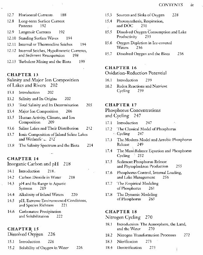
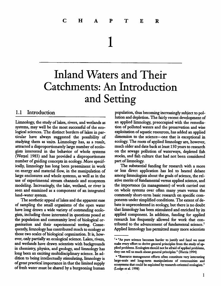
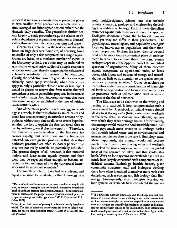
Figure 1-1 Log-log scatterplot of experimental duration versus area of anindividual unit of experiments in limnology. Each circle represents one experiment For loticstudies, experimental unitarea was estimated as mean stream widthmultiplied by the length of reach understudy. For plotting, volumes (V) wereconverted to areas (A) byA = V2^. Notethat a large majority of experiments arecarried out over a period of less than 10months and cover a unit area of less than10 m2, probably less than 1 m2. (AfterLodge etal. 1998.)
10=
102_
£ 10McoE
Bc<0E•cCOa
8
10°-
10-1-
10-2-|
10"
1.1 Introduction
o o•o o
o
oo
o0 o o• °° ° ocamapo o oo00 SJjCD CD
o•
o
o 8•P °oo o
o •c
° o oo
0°°
» *0 °0
•
oo
O COHcd» o
0 »°«cPo <%
ogc?c$« Oo°^)»oacox) coco 0 o
o <D»
0 0 o
o o
o lentic• lotic
~i—i-^—i—i—i—i—i—i—i—i—i—i—i—r10"510-410-310~2 10_1 10° 101 102 103 104 105 106 107 10B 109 10101011
Experimental unitarea (m2)
education, outlook, background, and professional experience.2 Not surprisingly, each scientist workswithin a framework of ideas and beliefs that help de-terrnine not only the kind of research considered interesting but alsothe specific research questions to beposed. This shouldbe recognized and is further developedin Chapter 2, outlining the historyand development of limnology.
Textbooks tend to minimize the different viewpoints held to reduce possible confusion engenderedby disagreements. Limnology textbooks therefore,commonly present specific examples asif theyaregeneralities. This contributes to a desirable simplicity, butat the cost of preventing an appreciation of ongoingarguments in the literature often stemming from thetendency to drawbroader conclusions thanarestrictly
allowed by the data.3 Thus, a problem for anyoneusing the literature, and particularly for studentsperusing books and conference proceedings that havenot benefited from the critical editing done by first-rate journals, is to decide where the facts end and theopinionsbegin.However, the abovecommentsshouldnot be interpreted to mean that scientific conclusionsare simply a matter of opinion. Science as an enterpriseismerciless in weedingout earlyconclusions thatare not well supported by follow-up research and,therefore, do not withstand the test of time.Third, the vastmajority of limnological (and eco
logical) studies are carried out over an area less than10 m2, over a period ofless than ayear (Fig. 1-1), andfrequently only over a few months. This leaves thequestionopen as to how general or applicable the results and interpretations are to the system as a whole
2"It has often been observed thatdifferent scientists may draw entirelydifferent, sometimes dramatically opposed conclusions fromthe same facts. How can this be? Evidently, suchdivergence of interpretationis die result of a drasticdifference in the ideologies ofthe respective scientists." (E. Mayr 1982. The Growth ofBiologicalThought)
}uIn no less than74of a sample of 149 articles selected from tenhighlyregardedmedicaljournalsconclusionswere drawn that werenot justified by the results presented." (S. Schor and I. Karsten1966) Strongly held viewssupported by weaklysubstantiated conclusions aresimilarlywidespread in limnology.
4 CHAPTER 1 Inland Waters and Their Catchments:AnIntroduction and Setting
10,000Size of experimental unit (I)
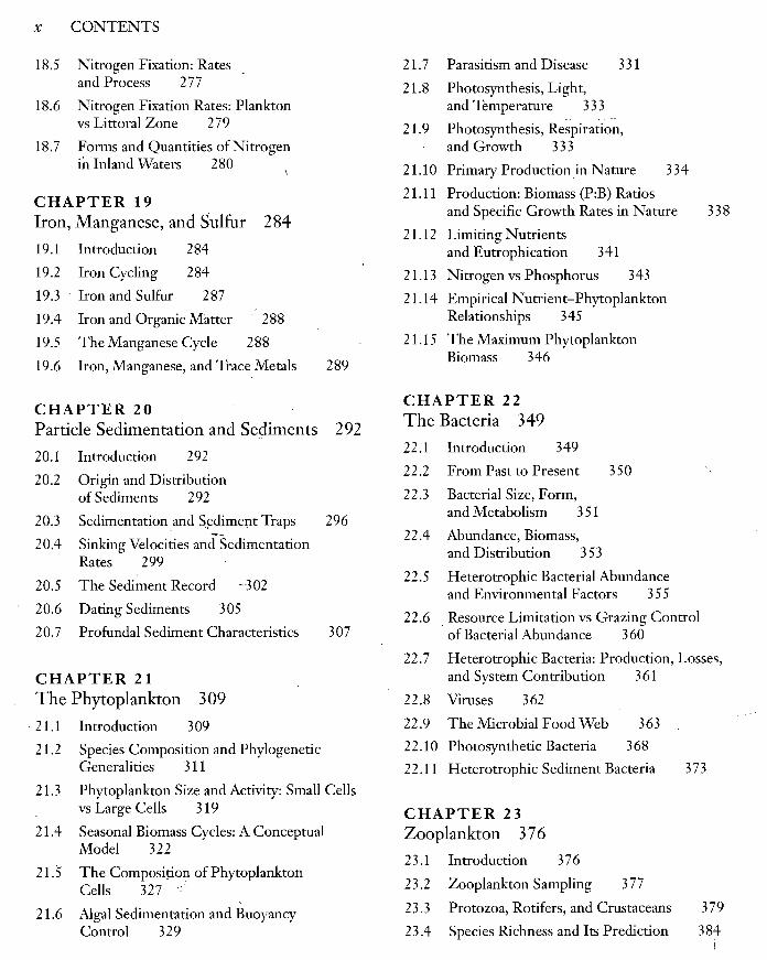
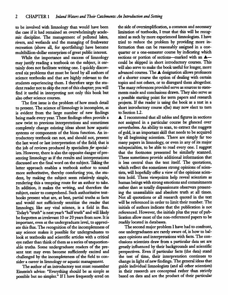
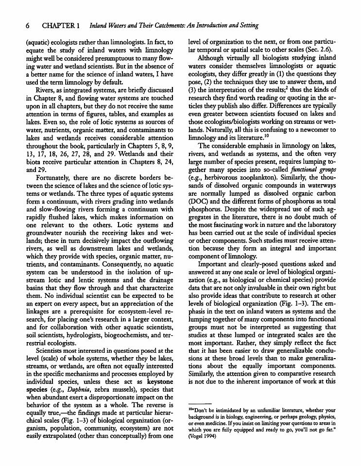
Figure 1-2 The relationship between the sizeanddurationof experiments published in papers on marine microbialecology between 1990 and 1995. The results are equally applicable to equivalent workin inland waters where identicaltechniques are used. (Modified after Duarte etal. 1997.)
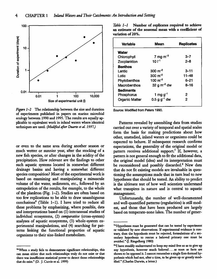
or even to the same area during another season ormuch wetter or sunnier year, after the stocking of anewfish species, or after changes in the acidity of theprecipitation. How relevant are the findings to othersuch aquatic systems located in somewhat differentdrainage basins and having a somewhat differentspecies composition? Most of the experimentalworkisbased on examining and manipulating a minusculevolume of the water, sediments, etc., followed by anextrapolation of the results, for example, to the wholeof the plankton (Fig. 1-2). Studies are often based ontoo few replications to be able to draw unambiguousconclusions4 (Table 1-1). I have tried to reduce allthese problems by emphasizing, where possible, dataand interpretations based on (1) interannual studiesofindividual ecosystems, (2) comparative (cross-system)analyses of aquatic ecosystems, (3) whole-system experimental manipulations, and (4) searching for patterns linking the functional properties of aquaticorganisms to their size-linked metabolism.
4"When a study fails to demonstrate significant relationships, thiscanmean either that such relationships truly do not exist or thattherewas insufficient statistical powerto detectthose relationshipsthat do exist" (D. J. Currie et al. 1999)
Table 1-1 Number of replicates required to achievean estimate of the seasonal mean with a coefficient ofvariation of20%.
Variable Mean Replicates
WaterChlorophyll Zmgnr3 3-7
Zooplankton 10 r1 2-8
BenthosLentic 300 nr2 3-11
Lotic 300 nrr2 11-48
Phytobenthos 100 m"2 6-21
Macrobenthos 32 g nr2 dw 8-16
SedimentsPhosphorus 1 mg g_1 2
Organic Matter 0.5 g g"1 dw 2
Source; Modified from Peters 1990.
Patterns revealed by assembling data from studiescarried out overavariety of temporal andspatial scalesform the basis for making predictions about howother, unstudied, inlandwatersor organisms couldbeexpected to behave. If subsequent research confirmsexpectations, the generality of the original model orpattern receives additional support.5 If, however, apattern isnot generalenough to fit the additional data,the original model (idea) and its interpretation mustbe reconsidered and possibly discarded.6 New datathat do not fit existing models are invaluable in questioningthe assumptions madethat in turn leadto newhypotheses that should be tested. Anability to predictis the ultimate test of how well scientists understandwhat transpires in nature and is central to aquaticmanagement.Unfortunately, the number of well-documented
andwell-quantified patterns(regularities) is stillmodest, and those that have been produced are largelybased on temperate-zone lakes. The number of gener-
5"Hypotheses mustbe generated that can be tested by experimentor validated by new observations. If experimental evidence is contrary, then the hypothesis mustbe rejected, formulations of a secondary hypothesis to rescue a beloved primary one must beavoided."Q.Ringelberg 1980)6"I have steadily endeavoured to keepmymind free soasto give upany hypothesis, however much beloved... as soon as facts areshown to beopposed it. I cannot remember asingle first-formed hypothesis which had not,after atime, tobegiven uporgreatly modified." (Charles Darwin, a letter.)
alities thatarestrongenough tohave predictive poweris even smaller. Most generalities available deal withtime-averaged conditions (year, season) rather than thedynamic daily actuality. The generalities further pertainlargely to static properties (e.g., the relative or absolute abundance oforganisms or community biomass)rather than with theirdynamics over time and space.Generalities presented in the textcannot always be
based on large data sets. Some are, of necessity, basedon studies ofonly a few ecosystems in a single region.Others are based on a moderate number of species inthe laboratory or field, yetothers may be anchored onquantitative or qualitative studies of a single ecosystemor species overtime,therebysuggesting theexistence ofa broader regularity that remains to be confirmed.Clearly, thepredictive power ofgeneralities varies considerably, some apply worldwide, while others mayapply to only a particular climatic zone or lake type. Iwouldbe pleased to receive data from readers that willstrengthen or refute generalities proposed in the text, aswell asinformation aboutimportantpatterns thatwereoverlooked or notyetpublished at the time [email protected] themajorproblems in limnology, andecol
ogyas a whole, is that it is obviously mucheasier andmuch less timeconsuming to articulate notions or hypotheses without anydata at all, or to create hypothesesafter the fact to explain the data collected, than totesthypotheses to see if they have merit5,7 Therefore,the number of available ideas in the literature increases rapidly, but with their merits frequentlyuntested. An even greater problem is that ideas (hypotheses) presented are often so loosely phrased thatthey are not really testable or potentially refutable.The greatest danger of all, however, is that untestednotions and ideas about aquatic systems and theirbiota may be repeated often enough to become acceptedas fact and entered into the conceptual framework used byindividual scientists.8The fourth problem I have had to confront, and
equally an issue for students, is that limnology is a
7"The verification ofideas may bethemost treacherous trap inscience, as counter examples are overlooked, alternative hypothesesbrushed aside and existing paradigms manicured. The successful advance of science and the proper useof experimentation depends ona rigorous attempt to falsify hypotheses." (P. K Dayton and R. L.Oliver 1979)^Oneofthe chief causes ofpoverty inscience isusually imaginarywealth. The aimof science is not to open the door to infinitewisdom,but to set alimit to infiniteerror." (Galileo in B. Brecht's play,LifeofGalileo)
1.1 Introduction
truly multidisciplinary science—one that includesphysics, chemistry, geology, andengineering (hydrology), in addition to biology. Each of thesedisciplinesexamines aquatic systems from a different perspective.Ecologists dominate among the biological limnologists, yet they too differ in their perspectives. Thephysiologists, autecologists, andpopulation ecologistsfocus on individuals or populations and their functional properties. To them the lake, river, or wetlandneed not bemore thana convenient place or environment in which to examine these functions. Systemecologists operate at theopposite endof thesimplifiedspectrum of organization. Many of them conceiveaquatic ecosystems as operational units, or blackboxes, with inputs and outputs of energy andmaterials, butpay little ornoattention to thespecies components or processes involved.9 Other researchers setthemselves aside from any consideration of hierarchical levels oforganization andfocus instead on particular processes, such as sedimentation rates in aquaticsystemsor the fluxof nutrients.The fifth issue to be dealt with in thewriting and
reading of a textbook is how comprehensive such abook should be. A textbook on inland waters shouldideally treatflowing water (lotic) systems andwedandsin the same detail as standing water (lentic) systemswithwhich theysharedrainage basins. Unfortunately,the attemptwould make the bookunwieldy since it already pays much more attention to drainage basinsthat nourish inland water and to environmental andmanagement issues than is the rule in limnology texts.More importantly, the attempt would fail becausemuch of the literature on flowing waterandwetlandshas lacked thesame ecosystem context thathas guidedmost of the research on lakes, and that guides thisbook.Workon lotic systems andwetlands hasuntil recently been largely concerned with components of individual systems (hydrology, benthic insects, plantcommunity structure, etc.) and biologists workingthere have often identified themselves more with coredisciplines, such asecology andfish biology, thanlimnology. Consequently, most biologists working onlotic systemsor wetlands have considered themselves
'"The difference between limnology and the disciplines thatcontribute to it isoneofmotivation andintegration rather thancontext.An invertebrate zoologist canmeasure respiration in aquatic crustaceans, achemist can quantify the speciation ofmetals, andaphysicist can producenew equations for fluid motion. Such informationisnot limnological unless it is castin a form that sheds lighton thefunctioningofaquaticsystems." (Lewis et al. 1995)
6 CHAPTER 1 Inland Waters and Their Catchments: AnIntroduction andSetting
(aquatic) ecologists rather thanlimnologists. In fact, toequate the study of inland waters with limnologymightwell beconsidered presumptuous tomany flowingwaterandwetland scientists. But in the absence ofa better name for the science of inland waters, I haveusedthe term limnology by default.Rivers, as integrated systems, are brieflydiscussed
in Chapter 8, and flowing water systems are touchedupon in all chapters, but they do not receive the sameattention in terms of figures, tables, and examples aslakes. Even so, the role of lotic systems as sources ofwater,nutrients, organicmatter, and contaminants tolakes and wetlands receives considerable attentionthroughoutthe book, particularly in Chapters 5, 8,9,13, 17, 18, 26, 27, 28, and 29. Wetlands and theirbiota receive particular attention in Chapters 8, 24,and 29.Fortunately, there are no discrete borders be
tween the scienceof lakesand the scienceof lotic systems or wetlands.The three types of aquatic systemsform a continuum, with rivers grading into wetlandsand slow-flowing rivers forming a continuum withrapidly flushed lakes, which makes information onone relevant to the others. Lotic systems andgroundwater nourish the receiving lakes and wetlands; these in turn decisively impact the outflowingrivers, as well as downstream lakes and wetlands,which they providewith species,organic matter, nutrients, and contaminants. Consequently, no aquaticsystem can be understood in the isolation of upstream lotic and lentic systems and the drainagebasins that they flow through and that characterizethem. No individual scientist can be expected to bean expert on every aspect, but an appreciation of thelinkages are a prerequisite for ecosystem-level research, for placing one's research in a larger context,and for collaboration with other aquatic scientists,soil scientists, hydrologists, biogeochemists, and terrestrial ecologists.
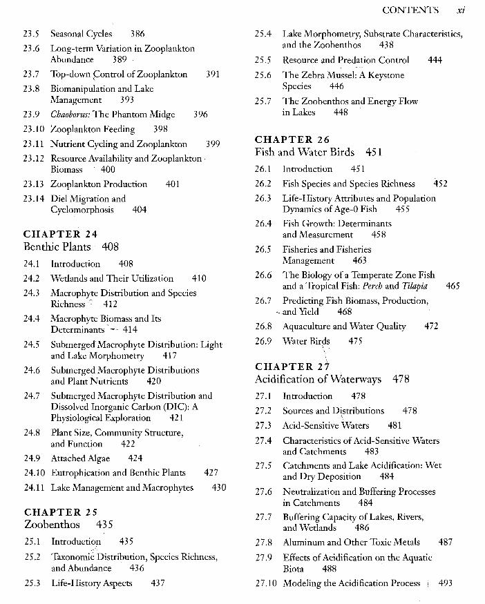
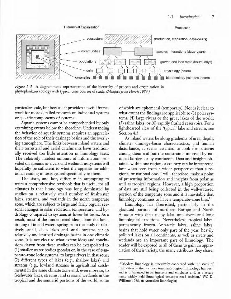
Scientists most interested in questions posed at thelevel (scale) of whole systems, whether they be lakes,streams, or wedands, are often not equally interestedin the specificmechanisms and processesemployed byindividual species, unless these act as keystonespecies (e.g., Dapbnia, zebra mussels), species thatwhen abundant exert a disproportionate impact on thebehavior of the system as a whole. The reverse isequally true,—the findings made at particular hierarchical scales (Fig. 1-3) of biological organization (organism, population, community, ecosystem) are noteasilyextrapolated (other than conceptually) from one
level of organization to the next,or fromone particular temporal or spatial scale to other scales (Sec. 2.6).Although virtually all biologists studying inland
waters consider themselves limnologists or aquaticecologists, theydiffer greatly in (1) the questions theypose, (2) the techniques they use to answer them, and(3) the interpretation of the results;2 thus the kinds ofresearch they findworth reading or quotingin the articles theypublish also differ. Differences are typicallyeven greater between scientists focused on lakes andthoseecologists/biologists working on streams orwetlands.Naturally, all this is confusingto a newcomertolimnology and itsliterature.10The considerable emphasis in limnology on lakes,
rivers, and wetlands as systems, and the often verylargenumber of species present, requireslumping together many species into so-called functional groups(e.g., herbivorous zooplankton). Similarly, the thousands of dissolved organic compounds in waterwaysare normally lumped as dissolved organic carbon(DOC) and the different forms of phosphorusas totalphosphorus. Despite the widespread use of such aggregates in the literature, there is no doubt much ofthe most fascinating workin nature and the laboratoryhas been carried out at the scale of individual speciesor other components. Such studiesmust receiveattention because they form an integral and importantcomponent of limnology.Important and clearly-posed questions asked and
answered at anyone scale or level of biological organization (e.g., as biological or chemical species) providedata that are not onlyinvaluable in their ownright butalsoprovide ideas that contribute to research at otherlevels of biological organization (Fig. 1-3). The emphasis in the text on inlandwaters as systems and thelumpingtogether ofmanycomponentsinto functionalgroups must not be interpreted as suggesting thatstudies at these lumped or integrated scales are themost important. Rather, they simply reflect the factthat it has been easier to draw generalizable conclusions at these broad levels than to make generalizations about the equally important components.Similarly, the attention given to comparative researchis not due to the inherent importance of work at this
,0"Don't be intimidated by an unfamiliar literature, whether yourbackground is in biology, engineering, or perhaps geology, physics,or evenmedicine. If youinsiston limitingyourquestions to areasinwhich you are fully equipped and ready to go, you'll not go far."(Vogel 1994)
Hierarchial Organization
ecosystem
communities
populations
1.1 Int?-oduction "
Processes
production, respiration (days-years)
species interactions (days-years)
growth and loss rates (hours-days)/ \
CID|CZD: CD|CZ3
cells | |—1~| r~l-f~r-| r-f~H I physiology (hours)organelles •' • •- • • • • •-• • • '• biochemistry (minutes-hours)
Figure 1-3 A diagrammatic representation of the hierarchy of process and organization inphytoplankton ecology with typical time courses of study. (Modifiedfront Hairis 1986.)
particularscale, but becauseit providesa useful framework for more detailed research on individual systemsor specificcomponents of systems.Aquatic systems cannot be comprehended by only
examining events below the shoreline. Understandingthe behavior of aquatic systems requires an appreciation of the role of their drainagebasins and the overlying atmosphere. The links between inland waters andtheir terrestrial and aerial catchments have traditionally received too little attention in limnology texts.The relatively modest amount of information providedon streams or riversand wedands as systems willhopefully be sufficient to whet the appetite for additional readingin texts gearedspecifically to them.The sixth, and last, difficulty in attempting to
write a comprehensive textbook that is useful for allclimates is that limnology was long dominated bystudies on a relatively small number of freshwaterlakes, streams, and wedands in the north temperatezone, which are subjectto largeand fairly regular seasonal changes in solar radiation, temperature, and hydrology compared to systems at lower latitudes. As aresult, most of the fundamental ideas about the functioning of inlandwaters spring from the study of relatively small, deep lakes and small streams set inrelatively undisturbed drainage basins in one climaticzone. It is not clear to what extent ideas and conclusions drawn from these studies can be extrapolated to(1) smaller water bodies (ponds) or, in the caseof temperate-zone lotic systems, to larger rivers in that zone;(2) different types of lakes (e.g., shallow lakes) andstreams (e.g., lowland streams in agricultural catchments) in the same climate zone and, even more so, tofreshwater lakes, streams, and seasonal wedands in thetropical and the semiarid portions of the world, some
of which are ephemeral (temporary). Nor is it clear towhat extent the findings are applicable to (3) polar systems; (4) large rivers or the great lakes of the world;(5) saline lakes; or (6) rapidly flushed reservoirs. For alighthearted viewof the 'typical' lake and stream, seeSection 4.3.
As inlandwaters lie along gradients of area, depth,climate, drainage-basin characteristics, and humandisturbance, it seems essential to look for patternsamong them without the constraints imposed by national borders or by continents.Data and insights obtainedwithin one region or country can be interpretedbest when seen from a wider perspective than a regional or national one. I will, therefore, make a pointof presenting information and insights from polar aswell as tropical regions. However, a high proportionof data are still being collected in the well-wateredportion of the temperate zone and it is inevitable thatlimnology continues to have a temperate-zone bias.11Limnology has flourished, particularly in the
glaciated portions of northern Europe and NorthAmerica with their many lakes and rivers and longlimnological traditions. Nevertheless, tropical lakes,permanently frozen Antarctic lakes, saline lakes,basins that hold water only part of the year, heavilypolluted lakes on all continents, as well as rivers andwedands are an important part of limnology. Thereader will be exposed to all of them to gain an appreciation of their variety, the manyattributes they share,
""Modern limnology is excessively concerned with the study offreshwaters in the northern temperate region. Limnology hasbeenand is unbalanced in its interests and emphases and, as a result,many widely held limnological concepts need revision." (W. D.Williams 1988, an Australian limnologist)
8 CHAPTER 1 Inland Waters and Their Catchments:AnIntroduction andSetting
and the differences ultimately imposed byclimate, geology, and time.Because large lakes andrivers often form the bor
der between two or more countries, and spelling outcountry names is space consuming, I frequently usethe International Standards Organization countrycode abbreviations [e.g., FR for France, RU for theRussianFederation, BR for Brazil, and CA for Canada(rather than California, as those from the US mightthink)] given inAppendix 1,with the countries alwayspresented in alphabetical order. Occasional referenceis made to marine work, either because good datafrom inland waters are lackingor because a comparison with marine work is appropriate. Furthermore,references to marine literature serve as a reminder ofthe close linksbetweenlimnology and oceanography.Human impacts on inland waters and their
drainage basins are increasing rapidly andhave startedto affect bodies of water everywhere. The ability topredict the effects of human impacts and their mitigation is of great importance to the progress of limnology as a science and is also a matter of urgency inenvironmental management. The contribution of inland waters to human welfare is enormous, but itsvalue has been captured only to a minor extent inmonetary terms. A recent and courageous attempt(Costanza et al., 1997) shows—regardless of assumptions made to generate figures—the enormousvalueof aquaticsystems. Services provided globally by lakesand rivers total about US $8,000 ha"1 of water surface(1 ha = 0.01 km2 or 10,000 m2). The single largest"service" provided is the regulation of discharge andsupply of water for agriculture and industry (~US$5,000 ha"1), but the role of catchments, reservoirs,and aquifers in the storage and supplyof water is important aswell (-US $2,000 ha-1). The overall contribution of wetlands is estimated to be even greater(~US $15,000 ha"1). The largestwetland contributionsare in the regulation and dampening of fluctuations(flood control, storm protection, etc.) (-US $5,000ha-1), water supply (storage andretention) (-US$4,000ha-1), andwaste treatment (wastewater treatment, pollution control, detoxification) (-US $4,000ha*1).Well-trained limnologistswill have to play a much
larger role in the managementof preciousaquaticresources if their future is to be safeguarded. Aquaticmanagement depends on an underpinning of appropriate science and there will have to be an increasedemphasis on fundamental long-term research, aboveall at the whole-system level at which most environmental problems are largely recognized. As environ
mental degradation progresses relentlessly on a globalscale, the appropriate science will require, more thanever, anability to provide useable data, pose clear andrealistic questions, analyze data appropriately, and reporttheresults not only to peers butalso to awider publicAsthe behavior of aquatic systems can't be under
stoodin isolation fromthe drainage basins and atmosphere that nourish them, both greatly influenced byhuman activities, I paymore attention than has beenthe rulein limnology textbooks to drainage basins andhuman impacts. Indeed, the effect of humans on theenvironment isbecoming sopervasive that it would beinappropriate not to includea specific chapteron acidification (Chapter 27), another on contaminants(Chapter 28), and a third on the man-made lakes wecallreservoirs (Chapter 29). In many chapters, I touchbriefly upon the implications of findings for aquaticmanagement in order to link fundamental (pure) sciencewith applied researchand resourcemanagement
1.2 The Setting
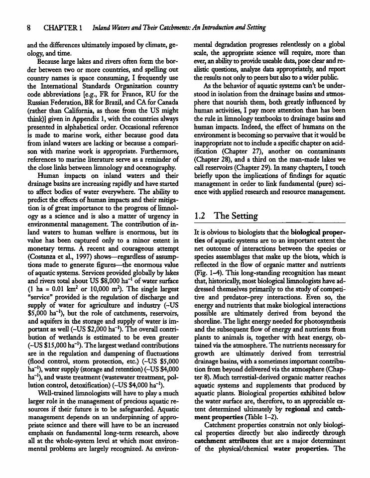
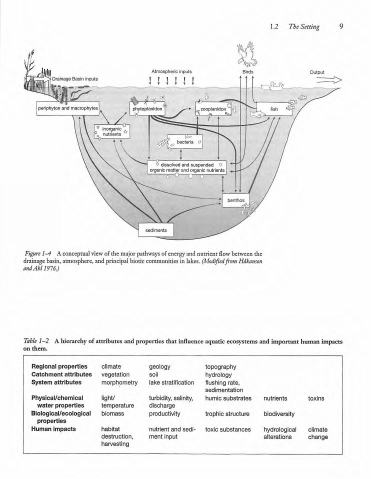
It is obvious to biologists that the biological properties of aquaticsystems are to an important extent thenet outcome of interactions between the species orspecies assemblages that makeup the biota,which isreflected in the flow of organicmatter and nutrients(Fig. 1-4). This long-standing recognition has meantthat, historically, most biological limnologists haveaddressed themselves primarilyto the studyof competitive and predator-prey interactions. Even so, theenergyand nutrients that makebiological interactionspossible are ultimately derived from beyond theshoreline.The light energyneeded for photosynthesisand the subsequentflow of energyand nutrients fromplants to animals is, together with heat energy, obtainedviathe atmosphere. The nutrients necessary forgrowth are ultimately derived from terrestrialdrainage basins,with a sometimes important contribution frombeyonddelivered viathe atmosphere(Chapter 8).Much terrestial-derived organic matter reachesaquatic systems and supplements that produced byaquatic plants. Biological properties exhibited belowthe water surfaceare, therefore, to an appreciable extent determined ultimately by regional and catchment properties (Table 1-2).Catchment properties constrain not only biologi
cal properties directly but also indirectly throughcatchment attributes that are a major determinantof the physical/chemical water properties. The
Drainage Basin inputs
IPperiphyton and macrophytes
Atmospheric inputs
J ! J ! J !Birds
Figure 1-4 Aconceptual viewof the major pathways of energyand nutrient flowbetween thedrainage basin, atmosphere, and principal biotic communities in lakes. (Modifiedfront HdkansonandAhl 1976.)
1.2 The Setting
Output
Table 1-2 A hierarchy of attributesand properties that influence aquatic ecosystemsand important human impactson them.
Regional properties climate geology topographyCatchment attributes vegetation soil hydrologySystem attributes morphometry lake stratification flushing rate,
sedimentation
Physical/chemical light/ turbidity, salinity, humic substrates nutrients toxinswater properties temperature discharge
Biological/ecological biomass productivity trophic structure biodiversityproperties
Human impacts habitat nutrient and sedi toxic substances hydrological climatedestruction, ment input alterations changeharvesting
10 CHAPTER 1 Inland Waters and Their Catchments: AnIntroduction andSetting
biological/ecological properties are consequendythe resultnot onlyofbiological interactions below thewaterline but by properties and attributes at higherlevels in the hierarchy(Table 1-2), whichare increasinglymodified by human impacts.Avarietyof regional and localized properties and
attributes together create the 'stage' upon which thebiological 'actors' play out the drama; modifyingthe shapeand sizeof the original stageand changingthe play as it evolves. Human activities increasinglyimpactboth the stageand the actors themselves. Fundamental research on largelypristine systems providean important baselineagainstwhichmajor human impactscan be measured.Both fundamentaland appliedresearchcomplement this by measuringthe impactofvarious degreesof human activity on aquaticsystemsthat provides the basis for environmental management.
1.3 Organization of the Text
No field can be understood without reference to itshistory and tradition and Chapter 2 is devoted to thedevelopmentof limnology and major ideas that haveguided its development. A few relatively short chapters then describe the characteristics of water, waterresource distribution, and hydrology. In Chapters 6and 7, the book turns to the origin and form (morphometry) of lakes and rivers, followed by a chapteron riversand the export of materials from the land andatmosphere to the water (Chapter 8),and another thatlinks drainage basin attributes to inland water functioning(Chapter 9).The second, informal, section (Chapters 10-20)
addresses primarily the physical and chemical properties of aquaticsystems, but points out the role of thebiotatherein. There arechapters on light inputanditsdistribution, lake stratification, water movements, thedistribution of salts and dissolvedoxygen,aswell as onthe cyclingof important nutrients in the water,whoserole in lakes is largely relevant to lotic systems andwedands. Organisms are not only affected by theirphysical/chemical environment, they greatly modifytheir environment.The section endswith a chapter onthe sedimentation of particles, sediment characteristics, and what dated sediments can reveal about thepast The stage has now been set for a more explicitconsideration of the biota (Chapters 21-26) that, aspointed out, not only act on the stage but alsomodifyit by their activities.
The third portioncontains chapters devoted to thephytoplankton, the bacterioplankton, the zooplankton, the benthic plants, the animals associated withsubstrates, and endswith a chapter on fishand aquaticbirds (Chapter 26).The fourth, and last, informal divisionof the book
addresses major human (anthropogenic) impacts onaquatic systems and consists of three chapters. It begins withChapter27 on the effects of acidifying precipitation on aquatic systems. The next deals withcontaminants (other than nutrients), their sources,distribution, and roles in inland waters (Chapter 28).The last, Chapter 29, evaluates similarities and differences between natural and man-made lakes to integrate research on reservoirs more firmly intolimnology and remind the reader that rapidly flushedreservoirs have asmanyloticas lenticattributes.Terminology will be kept to a rmnimum, as it is
often more a hindrance than a help to newcomers to afield and discourages communication between disciplines. Older, but important references will be usedwhen newer ones do not materially add to the information already available. This is done both to acknowledge important early work and to remind thereader that "Rome (or Cairo) was not built in a day."Particular attention has been paid to publications thatattempt to quantitatively integrate new findings intothe existing literature, thereby contributing to a synthesis. However, the literature is so vast that only atiny fractionof it could be cited and the work ofmanyexcellent scientists couldnot be acknowledged.Afewbasicterms and conceptsfollow immediately
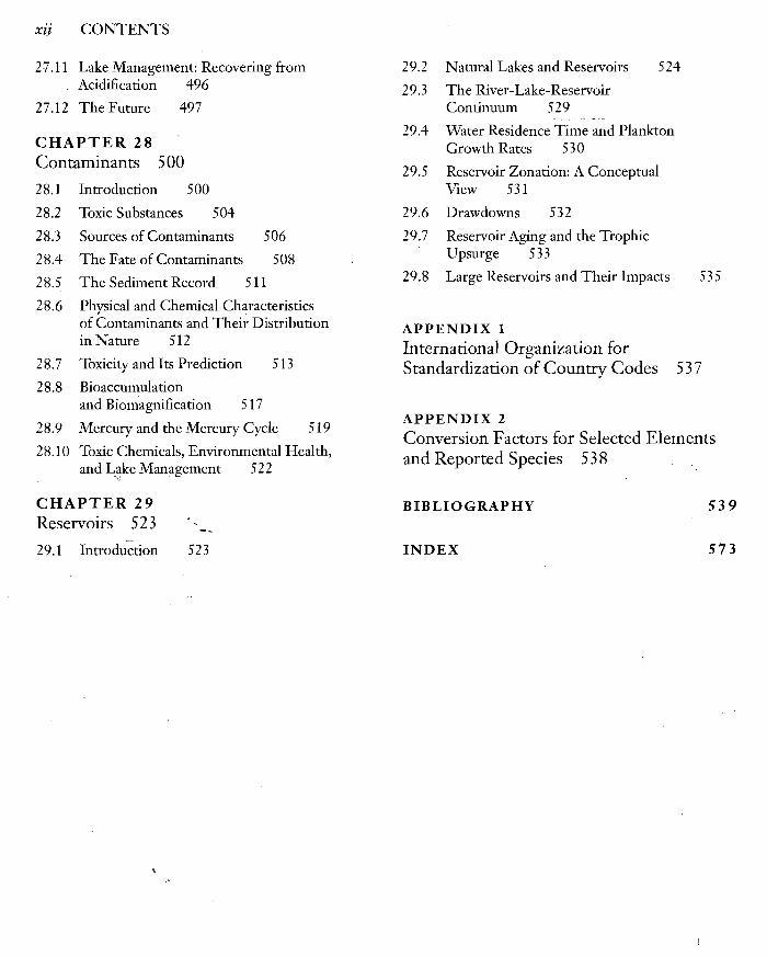
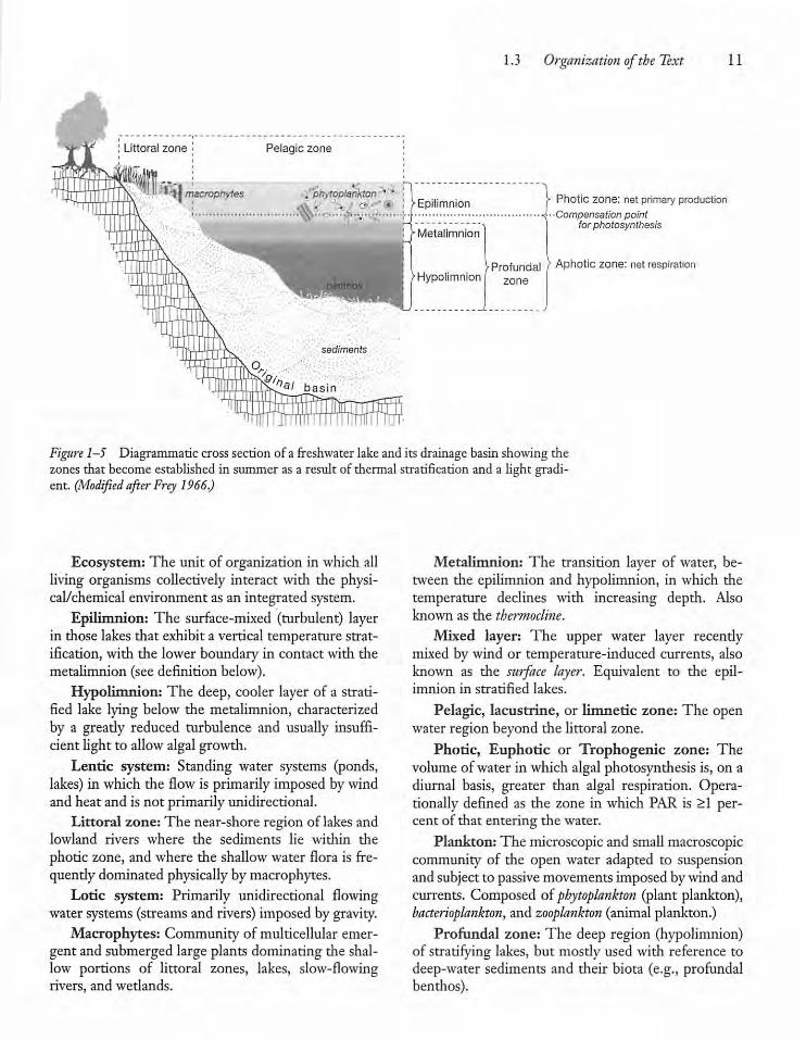
below so that, even before they are specifically discussed in subsequent chapters, they will be understood.The "Highlights" presentedat the end of eachchapter serve as reminders of important issues examined in the text. Their memorization in conjunctionwith Figure 1-5 will greatlyaid in the appreciation ofthe chapters to follow:
Aphotic or tropholytic zone: The volume ofwater or the area of sediments where the photosyn-thetically available radiation (PAR) is <1 percent ofthat entering the water and where plant respirationislarger than plant photosynthesis.
Benthos: The communityassociated with the bottom—refers most commonlyto the animalcommunity.
Catchment, drainage basin, or (in North America) watershed: The area of land that drains towardsan aquatic system. The termparalimnion hasbeenusedoccasionally.
Epilimnion
Metalimnion
1.3 Organization ofthe Text 11
Photic zone: net primary production•Compensation point
for photosynthesis
'Profundal ( Aphotic zone: net respirationHypolimnion f zone
Figure 1-5 Diagrammaticcross section of a freshwater lakeand its drainagebasinshowing thezones that become established in summer as a result of thermal stratificationand a light gradient. (Modified afterFrey 1966.)
Ecosystem: The unit of organization in which allliving organisms collectively interact with the physical/chemical environment as an integrated system.
Epilimnion: The surface-mixed (turbulent) layerin those lakes that exhibit a vertical temperature stratification, with the lower boundary in contact with themetalimnion (see definition below).
Hypolimnion: The deep, cooler layer of a stratified lake lying below the metalimnion, characterizedby a gready reduced turbulence and usually insufficient light to allowalgal growth.
Lentic system: Standing water systems (ponds,lakes) in which the flow is primarily imposed bywindand heat and is not primarily unidirectional.
Littoral zone: The near-shore region of lakesandlowland rivers where the sediments lie within thephotic zone, and where the shallowwater flora is fre-quendy dominated physically bymacrophytes.
Lotic system: Primarily unidirectional flowingwater systems (streams and rivers) imposed bygravity.
Macrophytes: Community of multicellular emergent and submerged large plants dominating the shallow portions of littoral zones, lakes, slow-flowingrivers, and wedands.
Metalimnion: The transition layer of water, between the epilimnion and hypolimnion, in which thetemperature declines with increasing depth. Alsoknown as the thermocline.
Mixed layer: The upper water layer recendymixed by wind or temperature-induced currents, alsoknown as the surface layer. Equivalent to the epilimnion in stratified lakes.
Pelagic, lacustrine, or limnetic zone: The openwater region beyond the littoral zone.
Photic, Euphoric or Trophogenic zone: Thevolume of water in which algal photosynthesis is, on adiurnal basis, greater than algal respiration. Operationally defined as the zone in which PAR is >1 percent of that entering the water.
Plankton: The microscopic and small macroscopiccommunity of the open water adapted to suspensionand subject to passive movements imposed bywind andcurrents. Composed of phytoplankton (plant plankton),bacteiioplankton, and zooplankton (animal plankton.)
Profundal zone: The deep region (hypolimnion)of stratifying lakes, but mosdy used with reference todeep-water sediments and their biota (e.g., profundalbenthos).
12 CHAPTER 1 Inland Waters and Their Catchments: AnIntroduction andSetting
Wetlands: Transition zones between terrestrialandaquatic systemswherethe soils arewaterlogged forat least part of the year or covered by shallow water,and which are typically occupied by rooted aquaticvegetation (macrophytes); not all wetlands are physically connected to lakes or lotic systems. The littoralzone of lakes and rivers forms a continum with wetlands. Wetlands can have both lotic and lentic attributesand, at times, maylackstandingwaterentirely.
AcknowledgmentsThis book is dedicated to the memory of two exceptionally fine scientists and friends, Rob Peters and FrankRigler. They kept reminding me of the importance ofphrasingscientific questionsas testablehypotheses ratherthan as somewhat vague, but interesting, notions. Theyalsosensitized me to the artificiality of trying to distinguish between fundamental (basic) science and a moreapplied science. I am very grateful to my closest colleagues, the late Robert Peters,WilliamLeggett,JosephRasmussen, andNeil Price, for their insights, advice, andfor the scientific stimulation they have provided meoverthe years. I acknowledge myMSc and PhD supervisors,Drs. H. R McCrimmon (University ofToronto and Universityof Guelph, Canada and D. G. Frey (IndianaUniversity, US), for their support and confidence in me. Dr.Henri Decampsandhisstaffat the Centre d'Ecologie desSystemes Aquatiques (CNRS) in Toulouse, France, aswellasDr. CarlosDuarte andcolleagues at the Centra deEstudios Avanzados de Blanes (CSIC) in Blanes, Spain;are thankedfor their hospitality and support during sabbaticalyearsofwriting and research.I am grateful, aboveall, to my present and past graduate students, as well aspost-doctoral fellows, for their stimulationand their repeated demonstration that ideas and notions that I helddearwere, in the final analysis, either wrongor lesssimple than I had thought Special thanks go to ElenaRoman,Daina Brumelis, Michael Ditor, Grace Cheong,Anton Pitts, Anouk Bertner, Jason Derouin, and to various other technicians and student assistants for data collecting and graphics over the years of writing. The bookwould never have been written without them and the secretarial help with word processing provided during theearly stages bythe Department ofBiology, McGill "University. In addition, I acknowledge C. H. Fernando, University of Waterloo, D. Jeffries, Canada Centre ForInland Waters, K. Murphy, Hydro-Quebec, V G.Richardson, Canada Centre For Inland Waters, W. D.Williams,University ofAdelaide, andM. Braun, Interna
tional Commission for the protection of the Rhine, fordata and/or advice. I further acknowledge, with admiration, the professionalism and dedication of the followingPrentice Hall editors: Teresa Ryu, acquisitions editor,Joanne Hakim, production editor, andJocelyn Phillips,copy editor. Most of the following people provided commentson Chapter 1.Anumber of peoplereviewed individual chapters and I thank the following for theirinsights andsuggestions, although I alone bear responsibilityfor errors andomissions.
G. and I. Ahlgren, (ch.21), Uppsala UniversityJ. Bloesch,(ch. 20),EAWAG, SwitzerlandA.S.Brooks, (chs. 8,22, and 28) University ofWisconsinW R DeMott, (chs.8, 22 and 28)Indiana UniversityP. J. Dillon, (chs. 5 and27),Ontario Ministry ofThe Environment andTrent University
J. A.Downing, (chs. 8, 9, and 18),Iowa State UniversityC. M. Duarte, (chs. 2 and 24), Instituto Mediterraneo de
EstudiosAvanzados, (CSIC), SpainJ. Fresco,(ch. 3),McGill UniversityJ. M. Gasol, (ch. 22), Institut de Ciencies delMar, (CSIC),
SpainE. Gorham, (chs.2 and 13),University ofMinnesotaL. HSkanson, (ch. 7), Uppsala UniversityS. K. Hamilton, (ch. 15),Michigan State UniversityR. W Kortmann, (chs. 16 and 19),Ecosystem Consulting
Service, Inc., Coventry, USA.W M. Lewis, Jr., (ch. 11),University ofColoradoO.Lind (chs.8, 22, and 28)Baylor UniversityS. C. Maberly, (ch. 14), Centre fir Ecology andHydrology,
UKS.Maclntyre, (ch. 12),University ofCalifornia, Santa Bar
baraJ. Melack, (chs. 4 and 6), University of California, Santa
BarbaraM.L.Ostrofsky, (chs. 8,22, and28)Allegheny CollegeM. L. Pace, (ch. 23), Institute ofEcosystem Studies, USAR H. Peters, (ch.2),McGill UniversityY. T. Prairie, (ch. 17), University of Quebec at Montreal
(UQUAM)J. B.Rasmussen, (chs. 26 and 28),McGill UniversityH. Regier, (ch. 26), University ofTorontoC. S. Reynolds, (ch. 21) Institute ofFreshwater Ecology, UKD. Roeder, (chs. 8,22, and 28)SimonsRock College ofBardK. Sand-Jensen, (chs. 10 and 24), Freshwater Biological
Laboratory, DenmarkJ. P. Smol, (ch. 20),Queens University, CanadaM. Straskraba, (ch. 29),Academy of Sciences of The Czech
RepublicD. Strayer, (ch. 25), Institute ofEcosystem Studies, USA
H R
2
The DevelopmentofLimnology
2.1 Limnology and Its Roots
Limnology1 came of age in 1901 when FrancoisAlphonse Forel (1841-1912) published the first textbookon the subject. In the book Forel, whowasProfessor of Physiology at the University of Lausanne(CH), presented the results of more than 30 years ofresearch on Lac Leman (Lake of Geneva), drawingalsoon measurements made on other lakes byhimselfand other scientists. The textbook was the outgrowthof his 1869 book on deep-water-sediment fauna andincluded a synthesis of his three volume Le Leman:Monographie Limnologique, published between 1892and 1904. The first two volumes described the geology, physics, and chemistry of the lake; the last dealtwith the lake's biology. Forelwas not just the founderof limnology and creator of its name,hewasalsoa firstrate early ecologist who recognized the relationshipbetween organisms and their climatic, hydrological,geological, physical, and chemical environments. Inotherwords, he sawlakes asintegratednaturalunitsorecosystems, as had StephenAlfred Forbes in America(1887), and as anticipatedbyThoreau, whowasnot ascientist, while making observationson Walden Pondin the 1840s and 1850s. Forel was not, however, thefirst person to do what is now called limnology, andhis definition of limnology as the "oceanography oflakes" acknowledges the influence of preceeding developments in marinescience. Earlier limnological re-
'From Greek limne =lake, pool, or swamp, + logos =discourse orstudy-
search ofthelate 18th and early 19th centuries had beenprimarily concerned with the physical attributes oflakes and river discharge (Table 2-1), followed by aflood of biological papers starting around the timethat Forel (1869) published his firstworkon the bottom fauna ofLac Leman.Starting in 1888, a number of biological stations
for limnological research were, within a few years ofeach other, established in both Europe and NorthAmerica. The first systematic comparisons of differentlakes and rivers, and early measurements of phytoplankton and zooplankton population dynamics, weremade before the turn of the century (Table 2-1). Atabout the same time, the first limnological measurements were being made in remote tropical Africanlakes and rivers; the development of sampling equipment and chemical techniques for water analysis wasnot far behind.Prior to the FirstWorldWar, nearlyall hrnnolo-
gists were interested in descriptions of physical,chemical, and biological aspects of (usually) singlelakes, therebylayingthe groundwork for subsequentattempts to organize the growing mass of information into logical schemes of lake and river classification. Probably the most influential Europeanlimnologist during the first decade of the 20th century wasC. Wesenberg-Lund (DK, 1867-1955).Hewasfar aheadof his time, recognizing the importanceof experimentationand manipulation to obtain clear-cut answers, and he saw the need for comparative(among-system) analysis of aquatic systemsinvolvingnot one but a number of lakes (C.Wesenberg-Lund1905). In 1910 he wrote an impressive synthesis, in
13
14 CHAPTER 2 The Development ofLimnology
Table 2-1 Milestones in the development of limnology.
Year Development
1650 Acategorizationof four lake types based on the presence/absence of stream inflows (B. Varenius,DE/NL).
1674 Descriptionof a filamentous green alga (Spirogyra) from a Dutch lake and an early recognition ofseasonal differences in algal populations as well as descriptions of rotifers (A. van Leeuwenhoek).
1779-1796 Using a heavily insulated thermometer, H. B. de Saussure (CH) noted that deep waters in someSwiss lakes were much colder than surface waters and were also near the point of maximum density (4°C).
1787 Depth determination of some English lakes (J. Clark).1800-1810 First systematic measures of river discharge (Rhone, CH; Gota, SE).1819 Discovery of what is now called the metalimnion (thermocline) in Lake Geneva [Lac Leman] by
H. T. de la Beche (GB).1826 First scientific description of an algal bloom, in Lac de Morat, by L de Candolle (CH).1833 Recognition of the importance of the water balance in determining lake size, salinity, and sediment
retention (J. P. Jackson, GB).1841 Diurnal oxygen cycle; linking low dissolved oxygen levels with fish kills, and high concentrations of
oxygen linked with high algal concentrations (A. Morren and C. Morren, BE).1850 Measurement of the turbidity of Lake Superior with a tin cup, which disappeared from view at 12.8
m (L.Agassiz, US).1852 Acid rain is linked to coal burning in England (R.A. Smith), 100 years before acid rain was recog
nized as a widespread problem in Europe and eastern North America.1865 Development of the Secchi disc for measuring water transparency by Commander Cialdi and Pro
fessor P.A. Secchi, priest/scientist on the SS ImmacolataConcezione, a steam corvet of the papalnavy traveling in the Adriatic Sea.
1867 Distribution and ecology of crustacean zooplankton in Danish lakes (E. Muller).1869 Publication of a paper on the bottom fauna of Lac Leman (F. A. Forel, CH).1871 Establishment of the U.S. Commission of Fish and Fisheries in response to the decline of com
mercial fish stocks in the Laurentian Great Lakes.1877 Classification of river zones on the basis of dominant fish species present by, among others,
V. D. M. Borne (DE). Beginning of detailed study of the Illinois River and the development of biological indicators of water quality (S. A. Forbes, US).
1887 Recognition of lakes as functioning units or "microcosms" (S. A. Forbes, US) and independently in1892 by F.A. Forel (CH). The development of nets for quantitative capture of marine plankton plusthe rudimentary statistics to analyze data by V. Hensen (DE). Description of the vertical migrationof zooplankton by A. Weismann (DE).
1888 Development of the (still) widely used Winkler technique for dissolved oxygen determination (L.W.Winkler, DE)and used in 1895 by R Hoppe-Seyler (DE) to explore the relationship between dissolved oxygen and the biota.
1888 Establishment in Bohemia (CZ) of the first freshwater laboratory followed in 1891 by laboratoriesat L Glubokoe (RU), and Plon (DE), and at Lake St. Clair (US) in 1893.
1891 Description of what we now call thermoclines and how they are formed, by E. Richter (DE), and independently by E. A. Birge (US).
1892 Quantitative phytoplankton studies by C. Apstetn in Germany following upon the largely qualitativeplankton (and benthic) studies of plant and animal species distribution, which flourished during the1870-1910 period in Europe and eastern North America. In the following year G. N. Calkins (US),reported a regular recurring spring and fall algal bloom in Massachusetts lakes. Scientists recognize the importance of competitive interactions to the distribution of some stream invertebrates(W. Voigt, DE).
1892-1904 Publication of F.A. Forel's three-volume monograph, entitled Le L6man:Monographie Umnologie,based upon work done on Lake of Geneva (Lac Leman), CH.
2.1 Limnology andItsRoots 15
Table 2-1 (continued)
Year Development
1895 Depthdistribution of submerged macrophytecommunitiesby E.Warming (DK).1896 Firstuse of the mark-recapture technique to estimate the size of fish stocks in the sea (S.G. J.
Peterson, DK), followed by the use of fish scalesto determine age of mature fish (C. Hoffbauer,DE, 1898). Experimental in-situwork on the relationship between light and the growth of diatoms(G.C. Whipple, US). C. Apstein (DE) proposed a relationship between nitrogen availability andblooms of cyanobacteria.
1897 Zooplankton population cycles in Lake Mendota (US) by E. A. Birge; a visionary recognition of theimportance of small algae (nanoplankton) not caught well with the coarse plankton nets that wereavailable by C. A. Kofoid (US), and a similar important recognition by G. C. Whipple (US)of the importance of wind-driven mixing of lakes to the development of algal blooms.
1897-1909 Inter-lake comparisons in Scotland (J. Murray and L Pullar)followed in 1904 by a comparativeanalysis of Scottish and Danish lakes by C. Wesenberg-Lund (DK).
1898 Recognition of the importance of lake morphometry (lake depth) by showing that shallow lakeshave greater plankton abundance than deep ones (H. Huitfeldt-Kaas, NO), a concept elaboratedupon by D. Rawson (CA) between the 1930s and 1960s. First evidence, presented by A. Dele-becque (FR), that the chemical characteristics of lakes are importantly determined by the geologyof their catchments, reported in a book entitled Les Lacs Francais.
1901 Publication of the first limnology text, Handbuch der Seenkunde. Allgemeine Umnologie, by F. A.Forel (CH),followed 25 years later by a successor text written by A. Thienemann (DE), and in 1935by the first text written in English with the word limnology in its title (P. S. Welch, US).
1902 Seasonal cycles of planktonic bacteria (A. Pfenniger, CH) in Lake Zurich by means of plate counts,followed in 1930 by quantitatively more correct microscopical counts (S. S. Kusnetsov and G. S.Karzinkin, USSR), and in the 1970s by a superior counting procedure based on fluorescent staining of bacteria.
1903 First comprehensive studies of river plankton and associated physical/chemical conditions byC. A. Kofoid (US),following 1893 work on zooplankton (rotifers) in the Rhine River by R. Lauter-born (DE).
1904 Description of internal waves or thermocline seiches in Loch Ness (E. E.Watson, GB), followingpioneering work in 1897 "On gravitational oscillations of rotating water," by Lord Kelvin (GB).
1905 Experimental demonstration that submerged aquatic angiosperms take up substances via theirroots, and that herbivorous invertebrates feed primarily not on the macrophytes but on the associated algae, bacteria, and detritus (R. H. Pond, US).
1908 Establishment of the first limnological journal, Internationale revue der gesamten Hydrobiofogieund Hydrographie, encompassing limnology and hydrology. A first systematic attempt to use acomponent of the biota (diatoms) as indicators of (stream) water quality. R. Kolkwitz and M. Mars-son (DE).
1910 The linkingof sewage inputs to algal blooms (R. Lauterborn, DE). A. Steuer (DE), while working onfish culture, reported the effect of fish predation on the zooplankton community, something notrecognized in fundamental limnology until 1958.
1911 Development of the Ekmandredge for quantitative sampling of lake sediments and their fauna(S. Ekman, SE) and later modified to its present form by E.A. Birge (US); demonstration of theabundance of the small phytoplankton that had been largely overlooked (H. Lohmann, DE).
1912 Developmentof an instrument for measuring the underwater solar energy in lakes (E. A. Birge,US). Work on the longitudinal distribution of particular invertebrates in streams as a function oftemperature and competitive interactions (A. Thienemann, DE).Development of "standards" forsewage effluents entering rivers (GB).
1915 Recognition of lakes as open systems with inputs and outputs, when E.A. Birge (US)and W.Schmidt (DE) independently developed lake heat budgets. Use of glass slides to study the attaching organisms in nature by E. Naumann (SE), and independently in 1916, E. Hentschel (GE).
{continued)
16 CHAPTER 2 The Development ofLimnology
Table 2-1 (continued)
Year Development
1920 The recognitionof distinct, annually deposited sediment layers in LakeZurichby F. Nipkow (CH),followed thirty years later by the development of paleolimnologyas a subdiscipline.
1921 Development of an air-bubble system to destratify lakes and Improveoxygen concentrations andwater quality (W. Scott and A. L Foley,US); seldom used until the 1970s.
1922 Establishment of the International Association for Theoretical and Applied Limnology (SIL) with401 founding members from nearly all continents; quantification of links between the flora of lakesand the morphometry and geology of their drainage basins by W.H. Pearsall (GB).
1923 Experimental proof of the importance of phosphorus in determining algal growth in lakes and seas(W. R. G. Atkins, GB).
1925 Development of the first mathematical model to predict water quality: an equation that predictshow much the dissolved oxygen concentration in rivers will decline at given points downstream ofa waste discharge (H.W. Streeter and E. B. Phelps, US).
1926 Publication of important research on the relationship between distributions of sediment-dwellinginvertebrates and environmental factors by J. Lundbeck (DE).
1927 Publication of the dissolved oxygen method for determination of phytoplankton production(T. Gaarder and H. Gran, NO)and anticipated by A. Putter (1924) in Germany. Recognition of theimportance of dissolved oxygen in the distribution of stream invertebrates (E. Hubault, FR),followed in 1937 by the identification of the importance of water-velocity determined substrate characteristics to stream invertebrates (G. Nietzke, DE).
1927-1929 Development of tropical limnologywith the British Fisheries and Limnological survey of Lake Victoria and other RiftValley lakes (in East Africa) by M. Graham, P. M. Jenkins and E. B. Worthington(GB)and the German-Austrian Sunda (Indonesia) expedition led by A.Thienemann (DE) and F.Ruttner (AT). Development of an accoustic method for detection of fish by K. Kimura (JP) in 1929.
1930 Use of artificial streams to study effect of nutrients and other pollutants on the biota (H.W.Streeter, US), and again in 1957 for ecological purposes (H.T. Odum and L M. Hoskin, US). Estimation of epiiimnetic primary production by the measurement of hypolimnetic oxygen consumption rates (K.M. Strom, NO). Elaboration of the notion that the concentration of nitrogen andphosphorus (and silica in diatoms as well)determine phytoplankton species composition andabundance in lakes (W.H. Pearsall, GB).
1932 Use of inorganic N:P ratios as indicators of nitrogen versus phosphorus limitation in lakes (W. H.Pearsall, GB). His ideas were quantified in 1966 by M. Sakamoto (JP).
1934 Direct measurements of planktonic primary production and respiration rates in lakes, usingchanges in dissolved oxygen concentration in plankton samples placed in suspended glass bottles (G. G. Vinberg, USSR), and independently developed by J. T. Curtis (US) in 1935.
1936 Studies on control of the concentrations and cycling of elements (iron and phosphorus) in lakes byW. Einsele (DE), followed in 1941 by equally important studies on the biogeochemistry of a number of elements by C. H. Mortimer (GB).
1938 The first manipulation of a whole lake through the addition of fertilizers to study the effects onplankton and fish by C. Juday and C. L. Schloemer (US), followed 10 years later by recognition ofthe need for reference (control) lakes (R. R. Langford, CA), and for more controlled experiments byA. Hasler and associates (US) in the 1950s.
1939 The use of sediment traps to estimate plankton loss rates from the zone of primary production inlakes (J. Grim, DE).
1941 Addition of phosphorus to a lake and the study of its transformation and cycling (W.Einsele, DE);a mass balance (input-output) model of phosphorus in Unsley Pond (G. E. Hutchinson, US). Massbalance modeling is now used extensively in lake management, but apparently was first used forthis purpose in 1957 (F. Baldinger, CH).
1942 The view of lakes as functioning units organized along trophic lines (R. L. Lindeman, US), and partially anticipated by A. Thienemann (DE), and in 1939 by V. S. Ivlev (USSR).
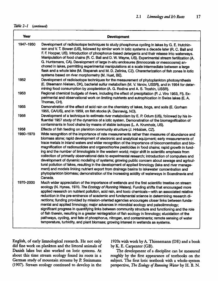
2.1 Limnology andIts Roots 17
Table 2-1 (continued)
Year Development
1947-1950 Development of radioisotope techniques to studyphosphorus cycling inlakesbyG. E. Hutchinson and V. T. Bowen (US), followed bysimilar work in lotic systems a decade later (R. C. Ball andF. F. Hooper, US). Introduction ofphosphorus-based detergents and theirreleaseinto waterways.Manipulation offood chains(R. C. Ball and D. W. Wayne, US). Experimental streamfertilization (A.G. Huntsmans, CA). Development of largein-situ enclosures (limnocorals or mesocosms)anchored in lakes, permitting experimental manipulations at a scale intermediatebetween a largeflask and a whole lake (M. Stepanek and M.D.Zelinka,CZ).Characterization of fish zones in loticsystems based on river morphometry (M.Huet, BE).
1952 Development of radioisotopetechniques for the measurementof phytoplankton photosynthesis(E. Steemann Nielsen, DK), bacterialsulfurmetabolism(M. V. Vanov, USSR), and in 1954 for determining food consumption by zooplankton (A. G. Rodinaand A.S. Troshin, USSR).
1953 Regional chemical budgets of rivers, including the effect of precipitation (P. J. Vlro 1953, Fl). Experimental and observational workon limiting nutrients and eutrophication inSwiss lakes (E. A.Thomas, CH).
1955 Demonstration of the effect of acid rainon the chemistry of lakes, bogs, and soils (E.Gorham1955, CA/US), and in 1959, on fish stocks (A. Dannevig, NO).
1956 Development of a technique to estimate river metabolism by E. P. Odum(US), followed by his Influential 1957 study of the dynamics of a loticsystem. Demonstration of the biomagnification ofcontaminants in food chains by means of stable isotopes (L A.Krumholz, US).
1958 Effectsof fish feeding on plankton communitystructure (J. Hrbacek, CZ).1960-1970 Wide recognition of the importance of rate measurements rather than measures of abundance and
biomass alone; rapid development of electronic and analytical equipment; early measurements oftrace metals in inland waters and wider recognition of the importance of bioconcentration and biomagnification of radionuclides and organochlorinepesticides in food chains; rapid growth infunding and the number of limnologists in the western world; majorshift in scientificemphasis fromcollection of primarily observational data to experimental research; introduction of computers anddevelopment of dynamicmodeling of systems; growing publicconcern about sewage and agricultural pollution of lakes, resulting in the development of applied limnology (lakeand rivermanagement) and models linking nutrient export fromdrainage basins to lakewater concentration andphytoplankton biomass; demonstration of the increasing acidity of waterways inScandinavia andCanada.
1970-2000 Much wider appreciation of the importance of wetlands and the first scientific treatise on streamecology (N. Hynes, 1970. The EcologyofRunning Waters). Fundingshifts that encouraged moreapplied research on nutrient pollution, acid rain, and toxic chemicals—with an associated relativereduction in the pre-eminence of academic and fundamental science in determining research directions; funding provided by mission-oriented agencies encourages closer links between fundamental and applied limnology; majoradvances inmicrobial ecology and paleolimnology;significant progress inquantifying links between communitystructure and functioning and the roleof fish therein, resulting in a greater reintegration of fish ecology in limnology; elucidation of thepathways, cycling, and fate of phosphorus, nitrogen,and contaminants; remote sensing of watertemperature, turbidity, and plant biomass; growing interest in wetlands as systems.
English, of earlylimnological research. He not onlydid finework on plankton and the littoral animals ofDanish lakes but also worked on lotic systems. Atabout this time stream ecology found its roots in aGerman study of mountain streams by P. Steinmann(1907). Stream ecology continued to develop in the
1920swith work byA.Thienemann (DE) and a bookbyK. E. Carpenter (GB).The development of a discipline can be measured
roughly by the first appearance of textbooks on thesubject. The first lotic textbook with a whole-systemperspective, The Ecology ofRunning Water by H. B. N.
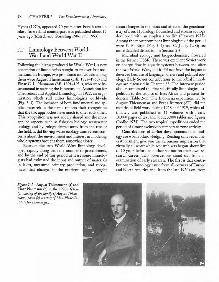
18 CHAPTER 2 The Development ofLimnology
Hynes (1970), appeared 70 years after Forel's text onlakes. Its wedand counterpart was publishedabout 15yearsago (Mitsch and Gosseling 1986, rev. 1993).
2.2 Limnology Between WorldWar I and World Warn
Following the hiatus produced byWorld War I, a newgeneration of limnologists sought to recover lost momentum. In Europe, two prominent individualsamongthem were August Thienemann (DE, 1882-1960) andEinar C. L. Naumann (SE, 1891-1934), who were instrumental in starting the International Association forTheoretical and Applied Limnology in 1922, an organization which still unites limnologists worldwide(Fig. 2-1). The inclusion of both fundamental and applied research in the name reflects their recognitionthat the two approaches havemuch to offer each other.This recognition was not widely shared and the moreapplied aspects, such as fisheries biology, wastewaterbiology, and hydrology drifted away from the rest ofthe field, asdidflowing waterecology until recentconcerns about the environment and interest in modelingwholesystems brought them somewhatcloser.Between the two World Wars limnology devel
oped rapidly along with the number of practitioners,and by the end of this period at least some limnologists had estimated the input and output of materialsin lakes, measured primary production, and recognized that changes in the nutrient supply brought
Figure 2-1 August Thienemann (a) andEinar Naumann (b) in the 1920s. [Photo(a) courtesy of the family ofAugust Thienemann; photo (b) courtesy ofMax-Plank-In-stitutefiir Limnologie.]
about changes in die biota and affected the geochemistryof iron. Hydrology flourishedand stream ecologydeveloped with an emphasis on fish (Hawkes 1975).Among the most prominent limnologists of the periodwere E. A. Birge (Fig. 2-2) and C. Juday (US); seemore detailed discussion in Section 2.4.Microbial ecology and biogeochemistry flowered
in the former USSR. There was excellent Soviet workon energy flow in aquatic systems between and afterthe two World Wars, but it did not have the impact itdeserved becauseof language barriers and political ideology. Early Soviet contributions to microbial limnology are discussed in Chapter 22. The interwar periodalsoencompassed the first specifically limnological expedition to die tropics of East Africa and present Indonesia (Table 2-1). The Indonesia expedition, led byAugust Thienneman and Franz Ruttner (AT), did tenmonths of field work during 1928 and 1929,which ultimately was published in 11 volumes with nearly10,000pages of text and about 3,000 tables and figures(Rodhe 1974).The two tropical expeditions ended theperiod of almost exclusively temperate-zone activity.Contributions of earlier developments in limnol
ogyareworth acknowledging. Readingonly recent literature might give you the erroneous impression thatvirtuallyall worthwhile researchwas begun about fiveto 10 years before an author set out on their own research career. Two observations stand out from anexamination of early research. The first is that contributions to limnology came from all cornersof Europeand North America and, from the late 1920s on, from
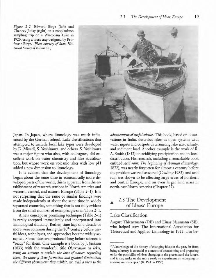
Figure 2-2 Edward Birge (left) andChancey Juday (right) on a zooplanktonsampling trip on a Wisconsin Lake in1920, using a brass trap designed by Professor Birge. (Photo courtesy of State Historical Society ofWisconsin.)
Japan. In Japan, where limnology was much influencedby the German school. Lake classifications thatattempted to include local lake types were developedbyD. Miyadi, S. Yoshimura, and others. S. Yoshimurawas a major figure who also, with colleagues, did excellent work on water chemistry and lake stratification, but whose work on volcanic lakeswith low pHadded a newdimension to limnology.It is evident that the development of limnology
began about the same time in economically more developed parts of the world; this is apparent from the establishment of research stations in North America andwestern, central, and eastern Europe (Table 2-1). It isnot surprising that the same or similar findings weremade independendy at about the same time in widelyseparatedcountries,something that is not fully evidentfrom the smallnumber of examples givenin Table2-1.Anew concept or promising technique (Table 2-1)
is rarely accepted immediately and incorporated intolimnological thinking. Rather, time lags of a decade ormore were common during the20th century before useful ideas, techniques, and approaches becamewidelyaccepted. Some ideas are produced long before science is"ready" for them. One example is a book byJ. Jackson(1833) with the wonderful tide Observation on lakes,being an attempt to explain the laws of nature regardingthem; the cause oftheirformation and gradual diminution;the differentphenomena they exhibit, etc. with a view to the
2.3 The Develop?nent ofIdeas: Europe 19
adva?ice?nent ofuseful science. This book, based on observations in India, describes lakes as open systems withwater inputsand outputs determining lakesize, salinity,and sediment load. Another example is the work of R.A. Smith (1852) on acidifying precipitationand its localdistribution. His research, includinga remarkable bookentidedAcid rain: The beginning ofchemical climatology,1872), was nearly forgotten for almosta century beforethe problemwasrediscovered (Cowling1982), and acidrain was shown to be affecting large areas of northernand central Europe, and an even larger land mass innorth-east North America (Chapter 27).
2.3 The Developmentof Ideas:2 Europe
Lake Classification
AugustThienemann (DE) and Einar Naumann (SE),who helped start The International Association forTheoretical and AppliedLimnology in 1922, also be-
2"A knowledge of thehistory ofchanging ideas in thepast, far frombeing a luxury, is essentialas a means of accustomingand preparingus for the possibility of ideaschanging in the present and the future,and it may make us the more ready to experiment on enlarging orrevising our concepts." (K. Picken 1960)
20 CHAPTER 2 The Development ofLimnology
came the intellectual leaders ofamovement to providestructurefor the understanding of lakes. Duringa 30-year period between the two World Wars and justafter, theyand their associates in Europeattempted toclassify lakes (Seetypen Lehre or Lake Typology) virtuallyas if lakes were functioning units or superorganis-mal units that should be identifiable with taxonomickeys. AsA.Thienemann(1925) put it, "If one investigates a lake typologically, one cannot expect the impossible from nature who, if she is ever to bescientifically comprehended to any degree at all, herpeculiarities, patterns and processes, must be categorized." Their preoccupationwithclassification of lakesinto fixed categories wasunderstandable because mostlimnologists were taxonomists by training, and theneed for categorizing the rapidly accumulating massof limnological informationwas becoming acute. Inaddition, scientists were, and sometimes still arerooted in the19* century notion ofscience as apurelyautomatic revelation of the realities of the world following the accumulation of facts. Lake classification(typology) and the characterization of rivers, based onfishor invertebrateassemblages, were assumed to leadto important advances. That science progressed mostrapidlyby posing and testing clearlyarticulatedquestions (hypotheses) was not widely appreciated. Nor,with the exception of visionarywork byW. H. Pearsallin England,wasit wellrecognized that aquaticsystemsand their biota fie along a large number of physical,chemical, and biological gradients, and that the position of any body of water into this multidimensionalspace dependson the climate, geology, land use of thedrainagebasin, systemmorphometry, and species present. In hindsight, it is not surprising that the lakesstudieddidnot fitwellin the simpleand idealized classification schemes proposed. Initially, Thienemannbasedhis schemeon the presenceor absenceof particular chironomid larvae (Diptera, Insecta) in the sediments, which served as indicators of environmentalconditions and, especially, dissolved oxygen levels.The problemwith the classification schemes grad
ually became apparent to Thienemann, Naumann,and others because newly investigated lakeswould inevitably differ from the relatively few on which theoriginalclassificationwasbased.This led to the development of increasingly complex schemes, ones thatmight include dissolved oxygencontent, other organisms,water color, lakemorphometry, sediment quality,and even"maturity" of the lakes. These schemesfailedwhen more lakes and lakes in different lake districtswere examined. In other words, the schemes lacked
sufficient generality to have predictive power.3 Furthermore, the fact that classifications were largelyqualitative meant that different users of any onescheme might come to different conclusions. Theseproblems were compounded because tests for deter-miningstatistically significant differences were eithernonexistent or not readily available. Equivalent attempts by E. Naumann and others to characterizelotic systems were evenlesssuccessful (Hawkes 1975).Although forgotten today, complex lakeclassifica
tion schemes were a milestone in limnology becausethey helped draw thedifferent subdisciplines together,provided an important stimulus for among-lake studies, and showed that limnologists had developed awell-defined approach to the field. The associated notion of lakes as superorganisms or integrated units didnot disappear completely and is held in a modifiedform today by those who examine inland waters asunits characterized by inputs and outputs, and thoseinterested in whole-system metabolism.
Thienemann
The urbaneThienemann wasan outstandingecologistand the prime force in the development of researchnot only on individual insect species (autecology) butalso on functional groupings (producers, consumers,and reducers) which,as earlyas 1914,laid the groundwork for later research on energy flowin aquatic systems (Vollenweider andKerekes 1980)and anticipatedthe ecosystem concept (Rodhe 1979). His personalresearchcontributions to the developmentof limnologyhad largely ended by the mid-1920s, when he beganworkingprimarilyon the autecology, distribution, andtaxonomy of a group of aquaticinsect species (chirono-mids) in lotic and lentic systems. The goal of his researchon the ecologyof particular lentic chironomidspecies was to use them as indicators to characterizeaquatic systems, not simply because the specieswerefascinatingor might be used to appreciate the ecologyof all insect species.Thienemann's influential ideas on nutrient cycling
within lakes and food-web structure (A. Thienemann1925) were acknowledged by Lindeman (1942) in hisinfluential paper on trophic levels and energyflow inaquatic systems (Sec. 2.4).
'"No scienti6c theory isworthanythinguntilit enables ustopredictsomething that is goingon. Until that is done theories are a meregameofwords."0. B. S.Haldane 1937)
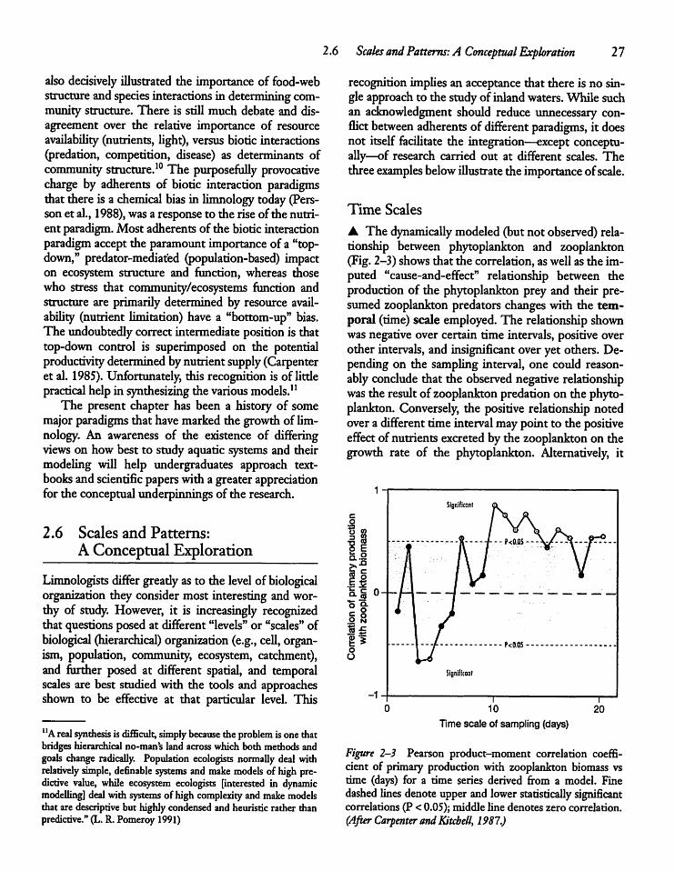
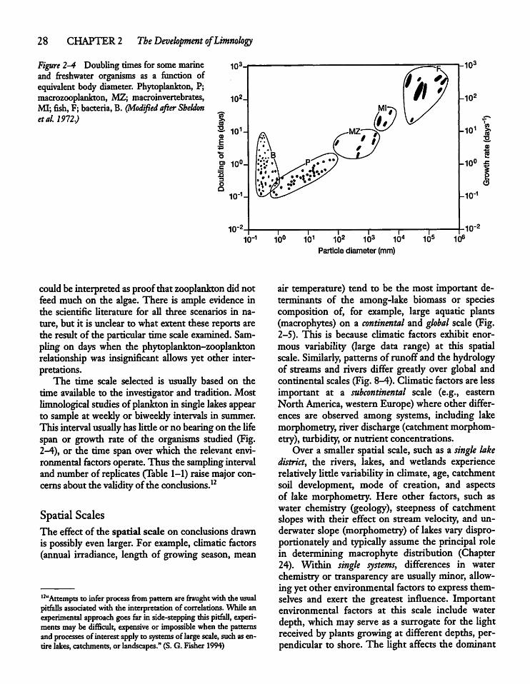
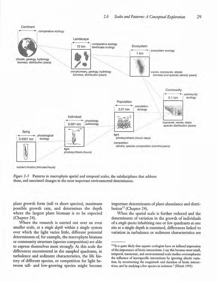
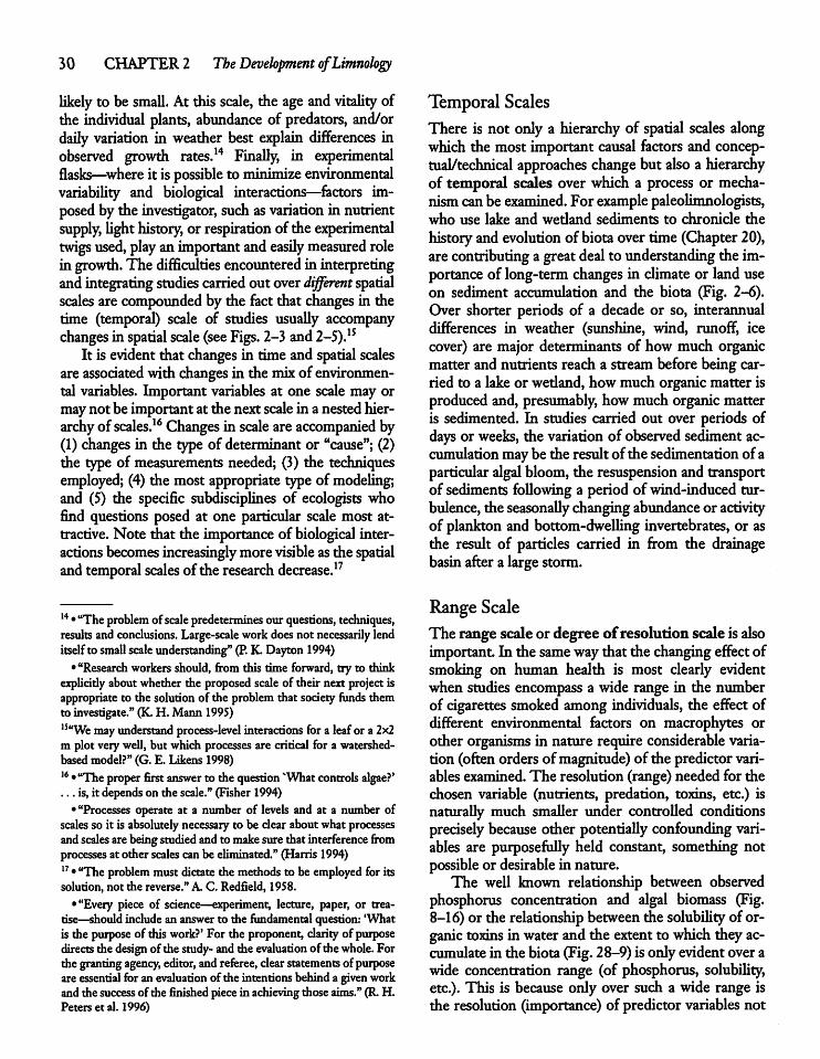
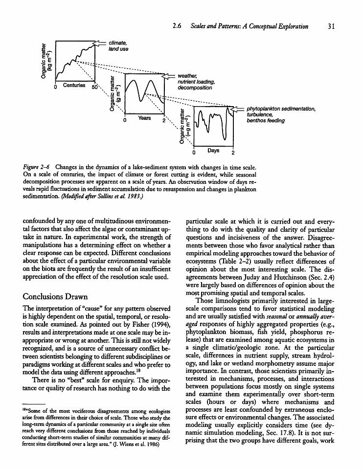

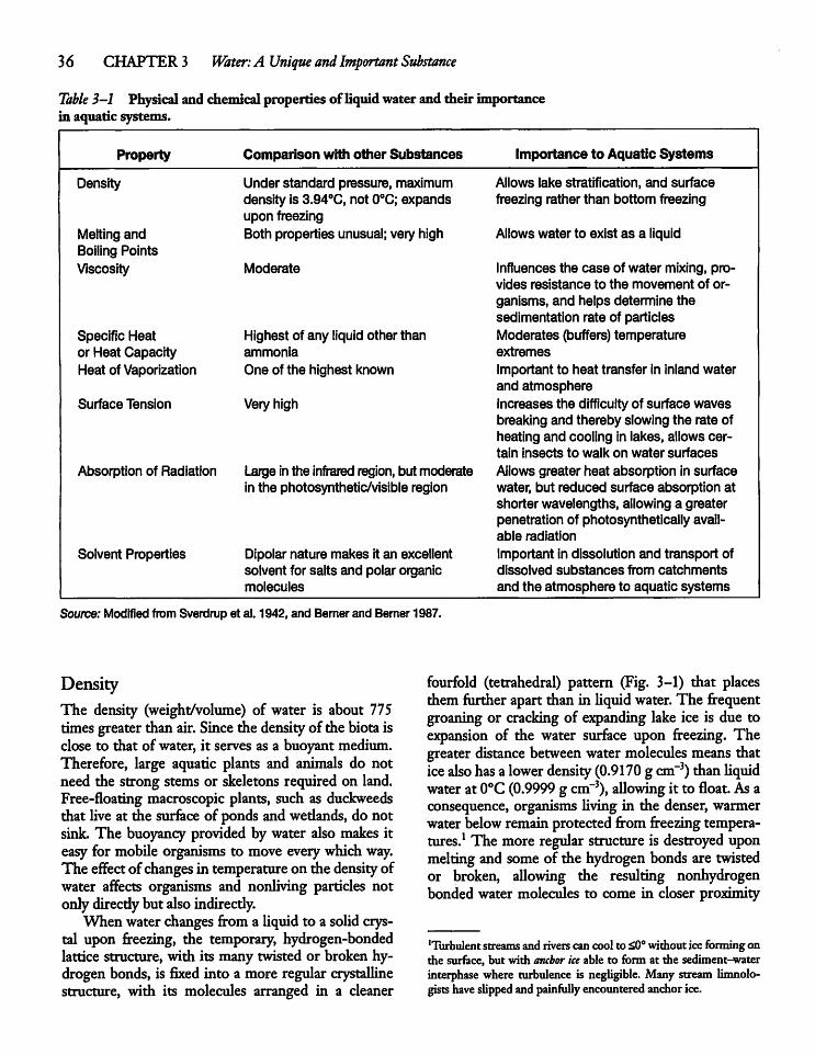
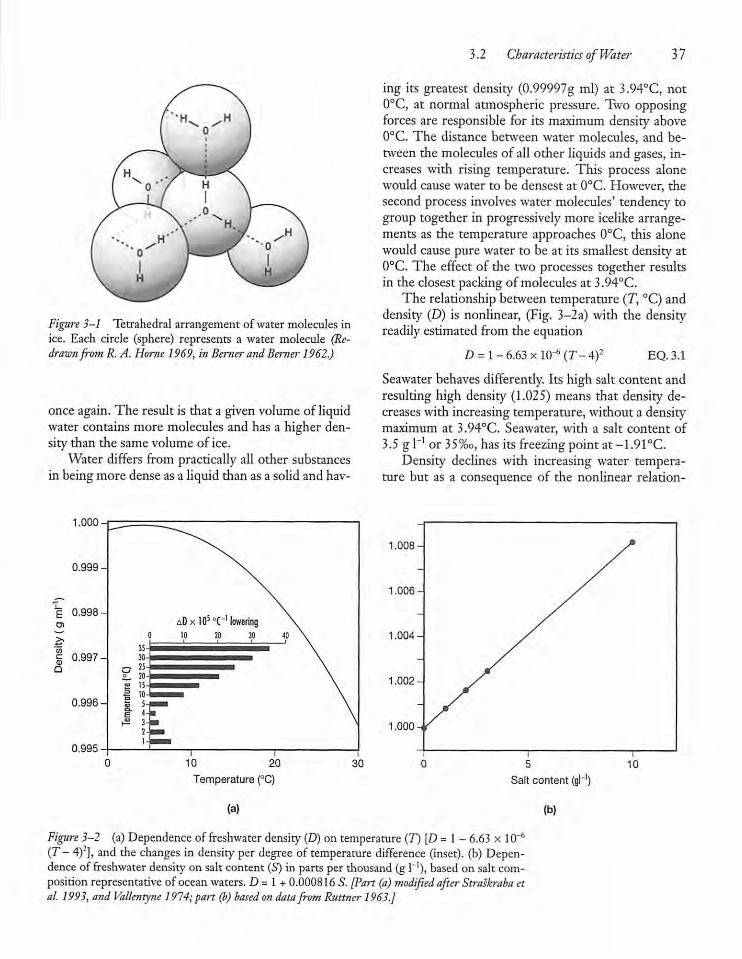
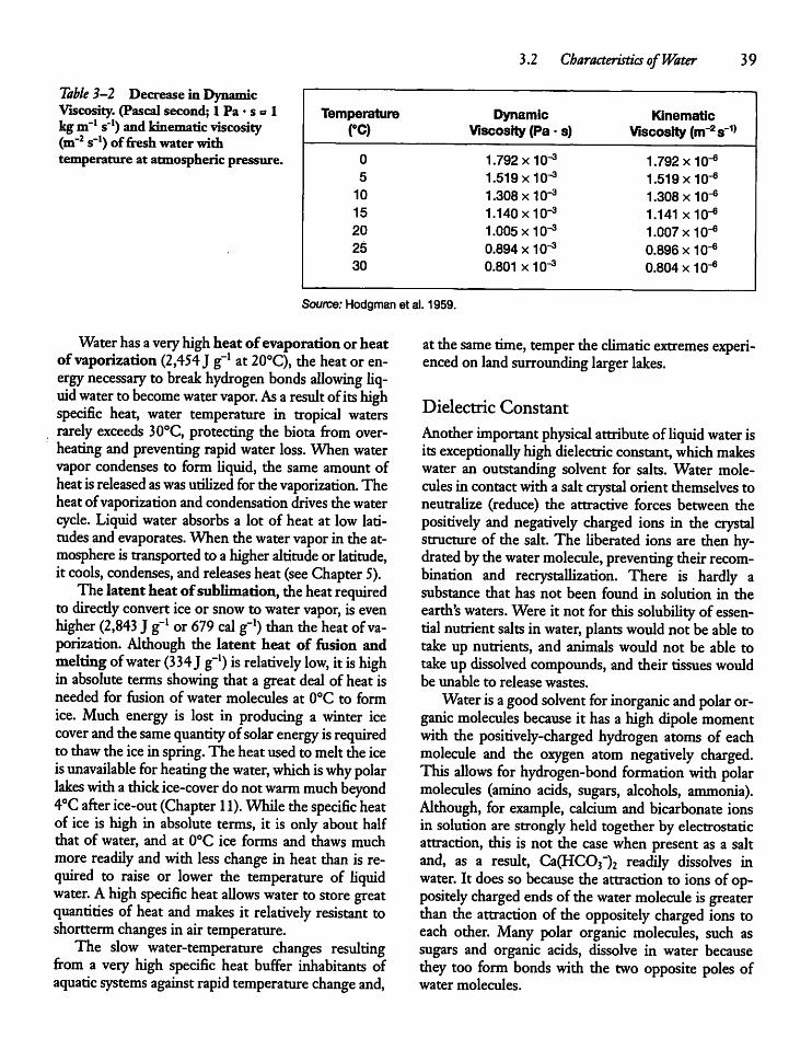
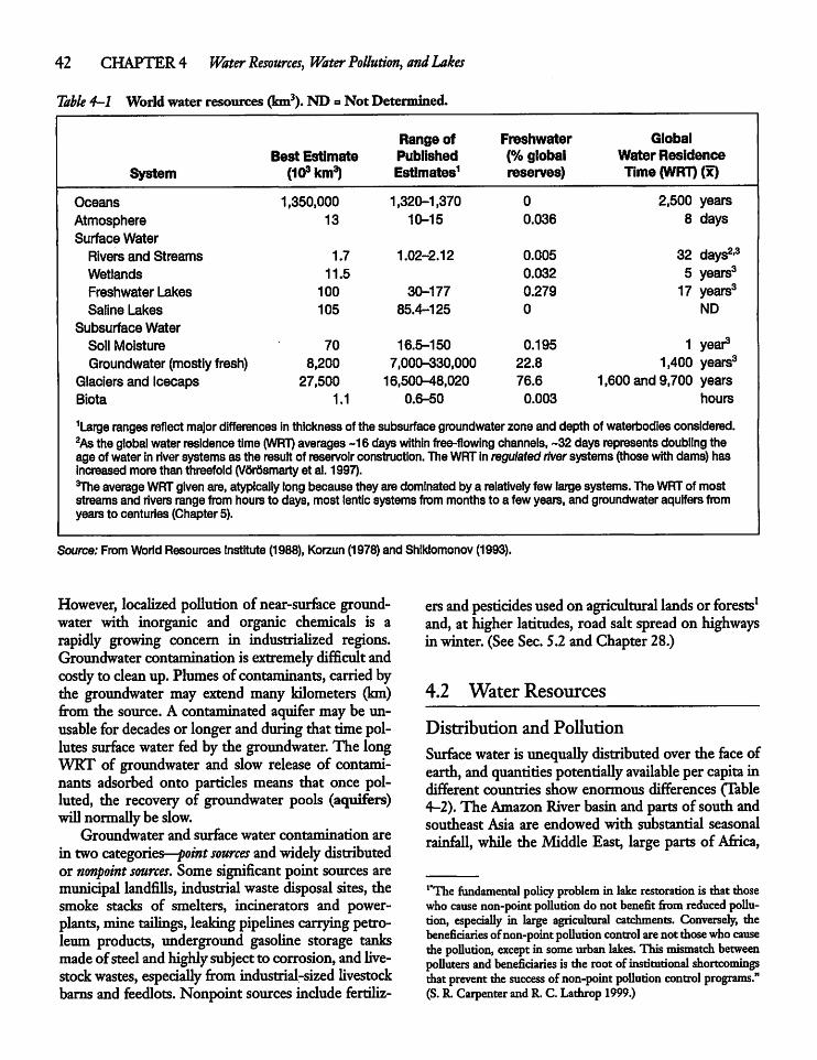
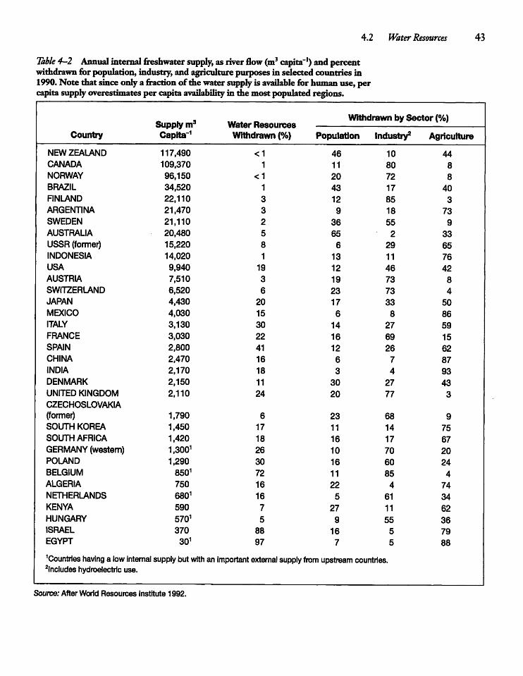
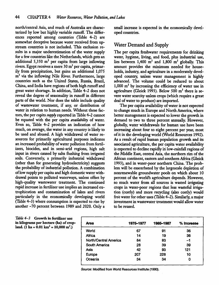
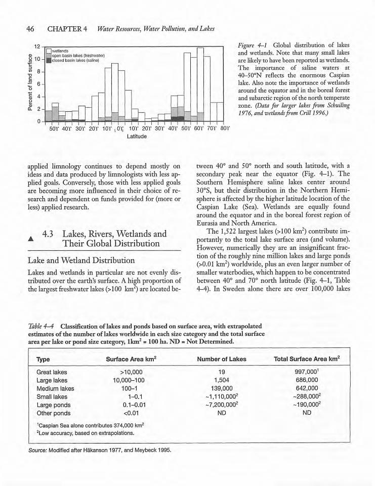
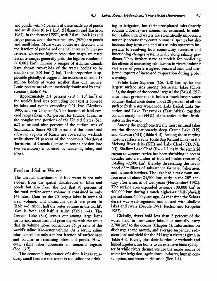
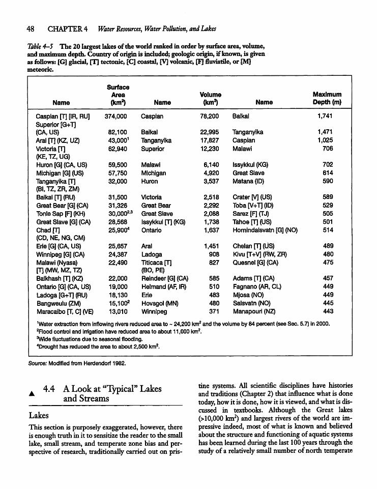
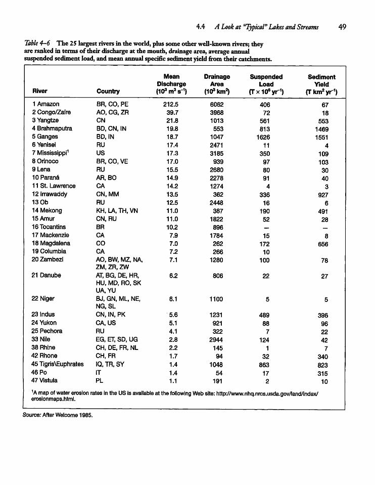
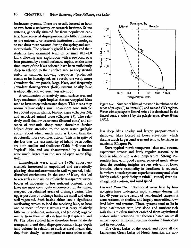
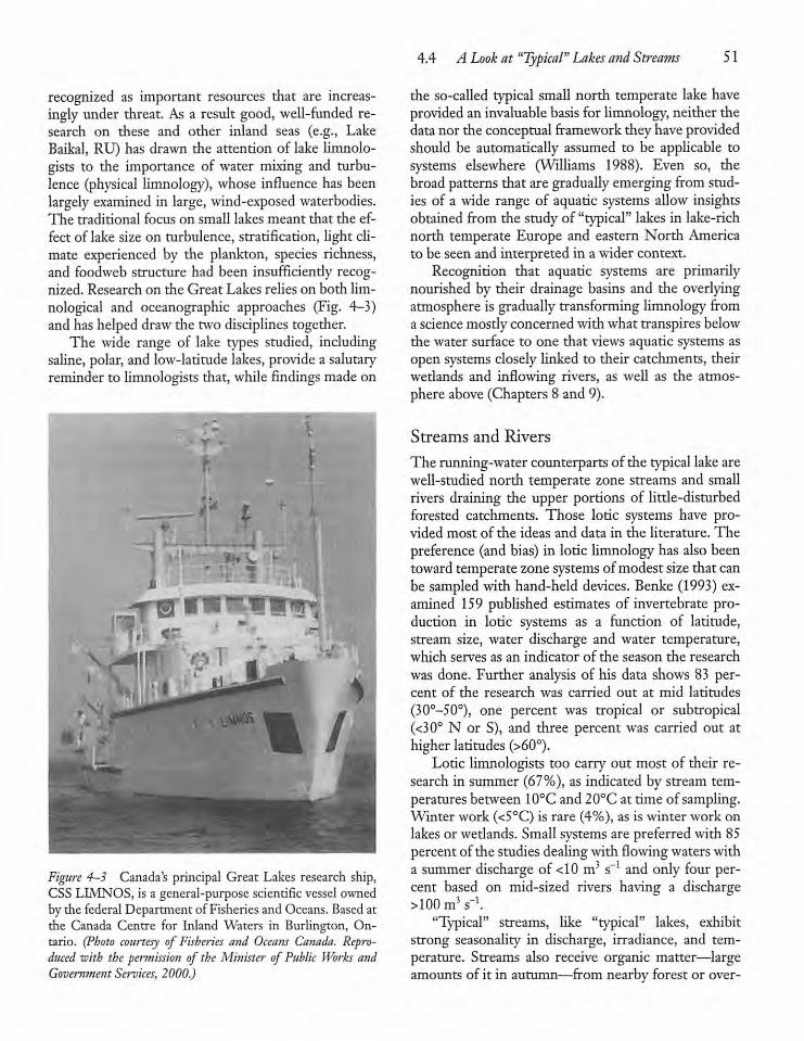
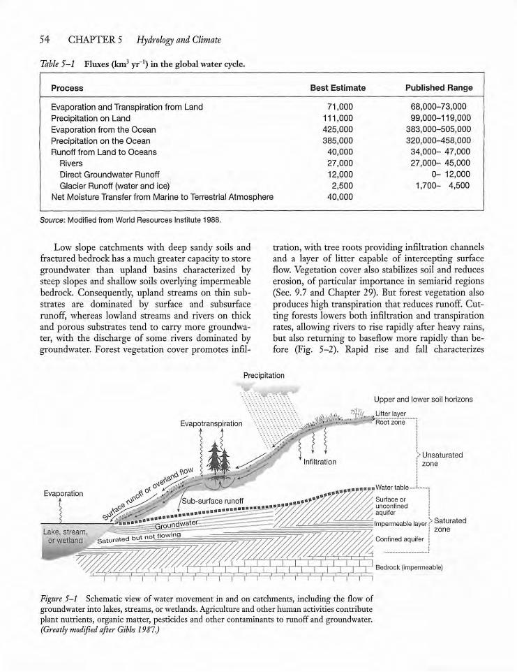
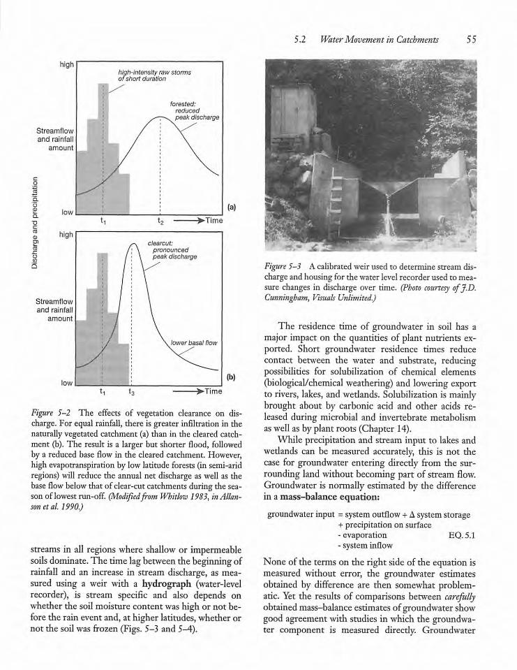
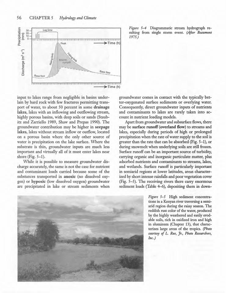
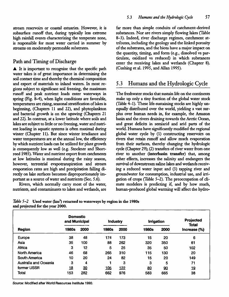
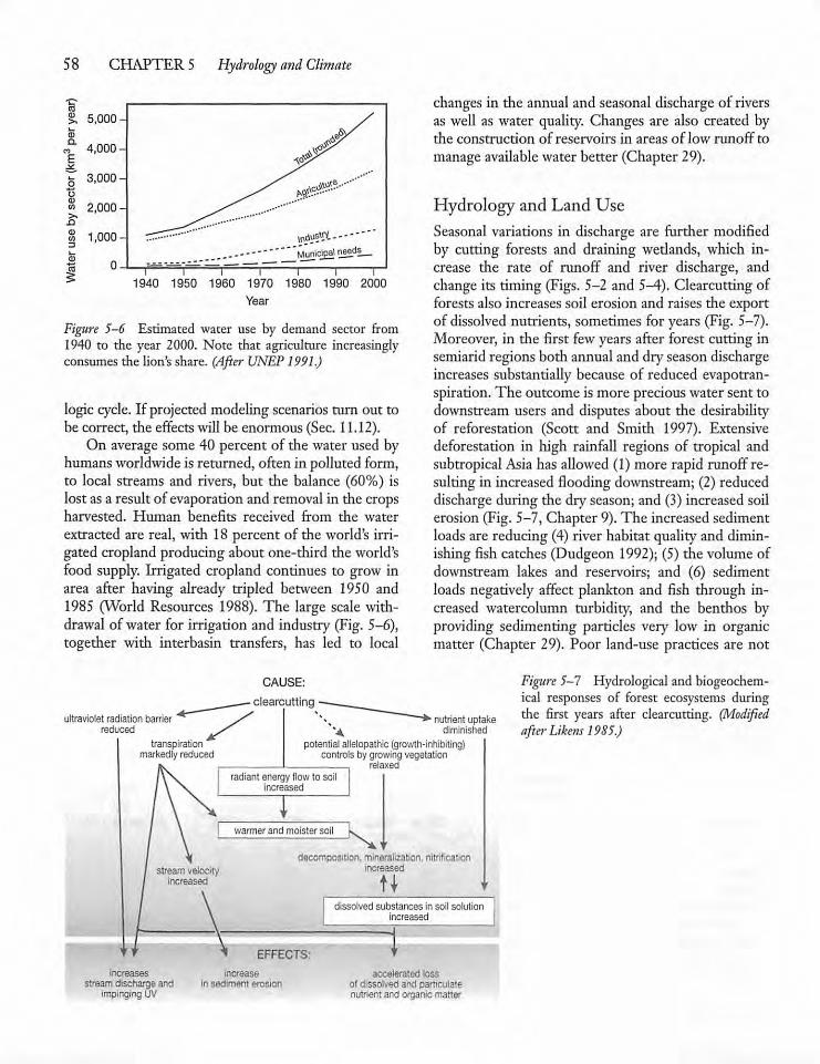
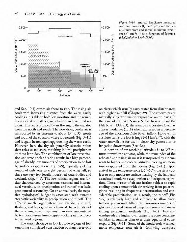
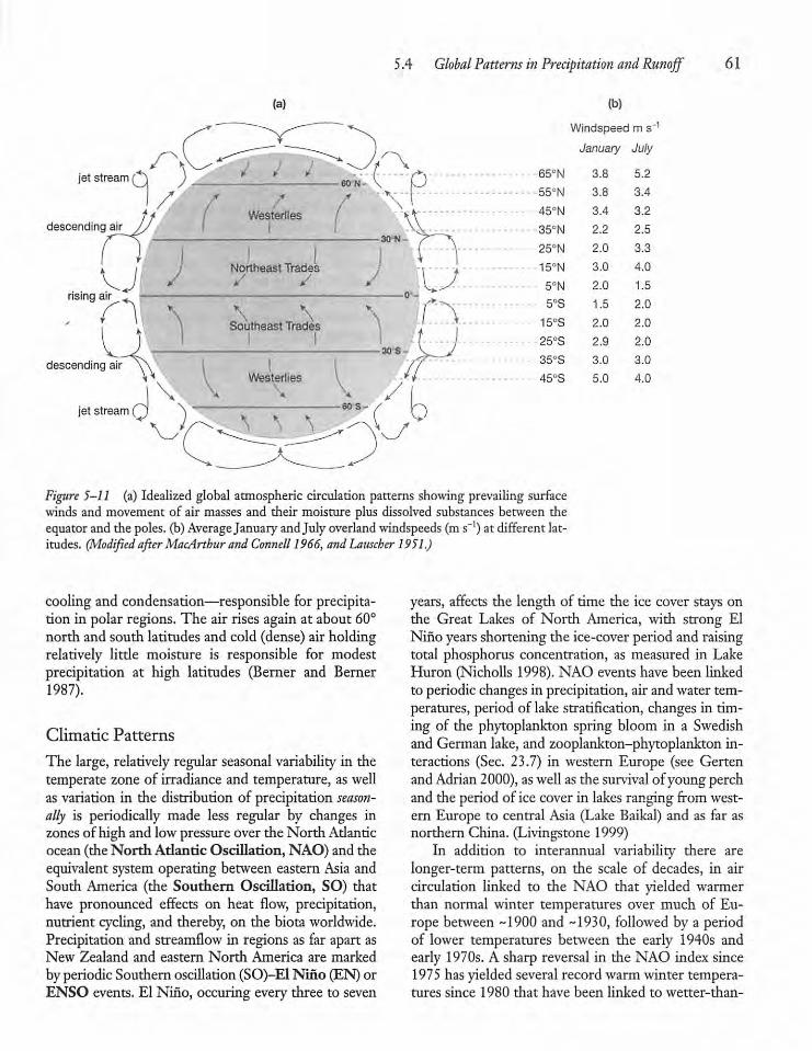
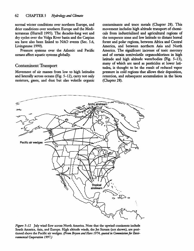
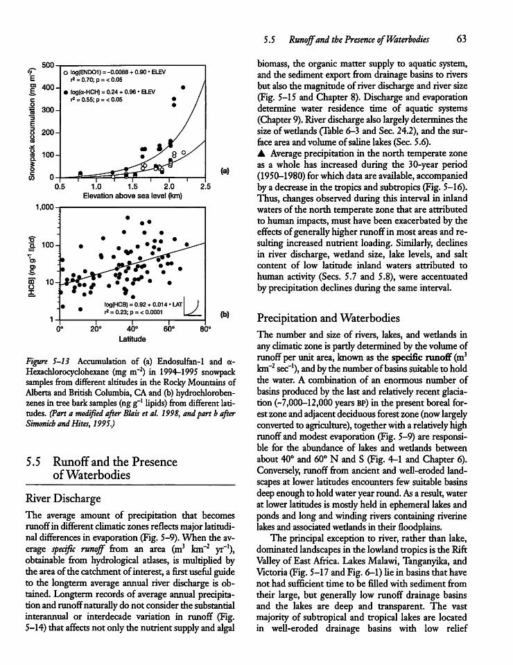
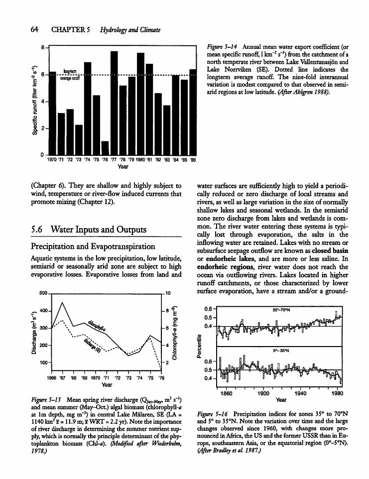
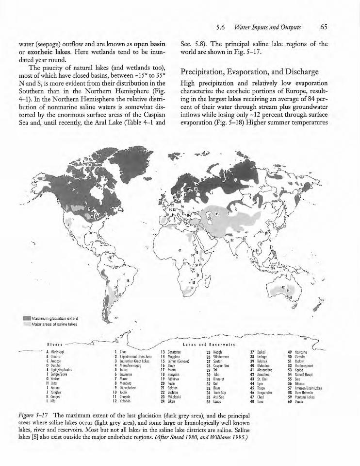
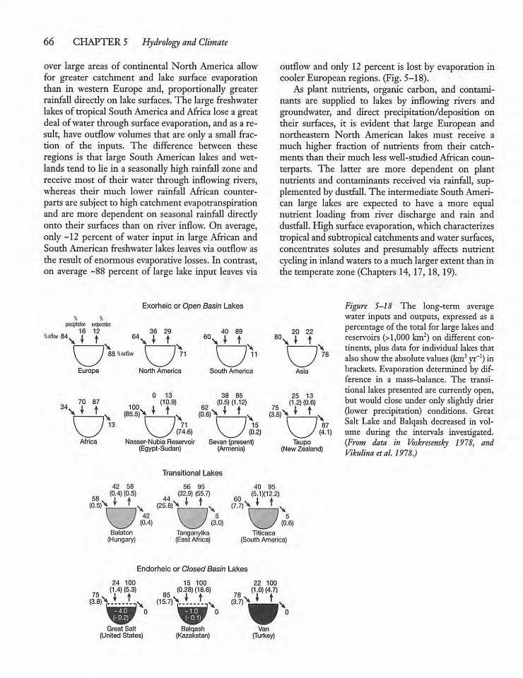
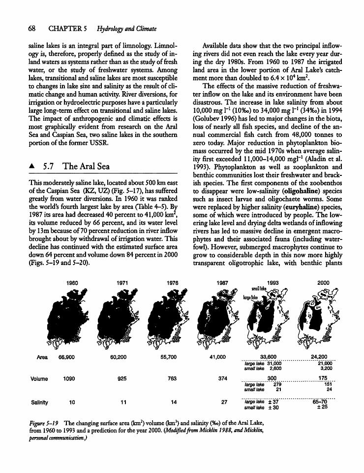
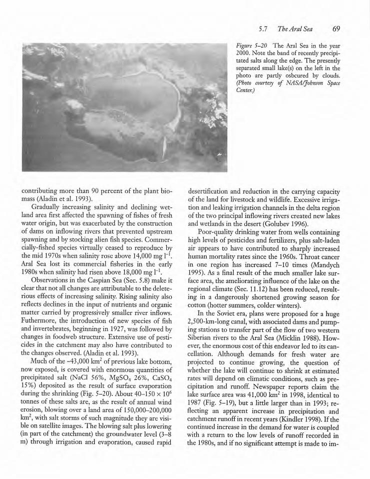
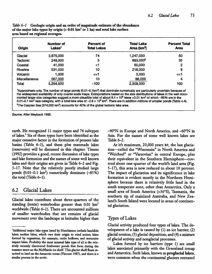
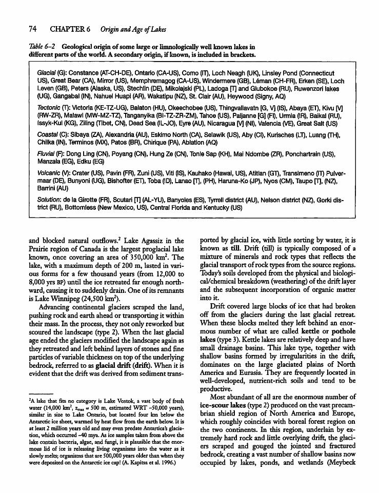
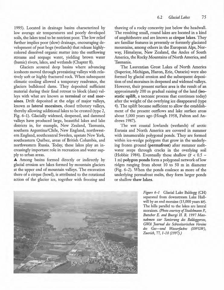
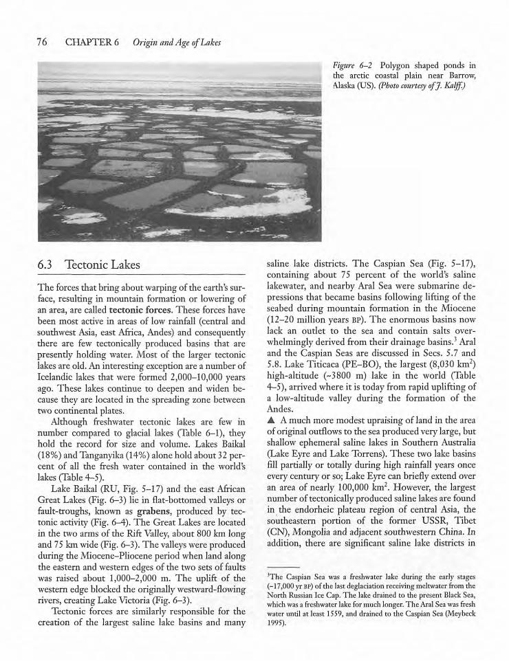
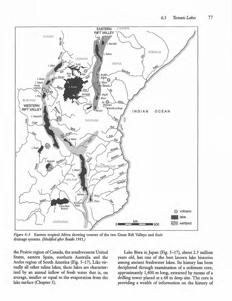
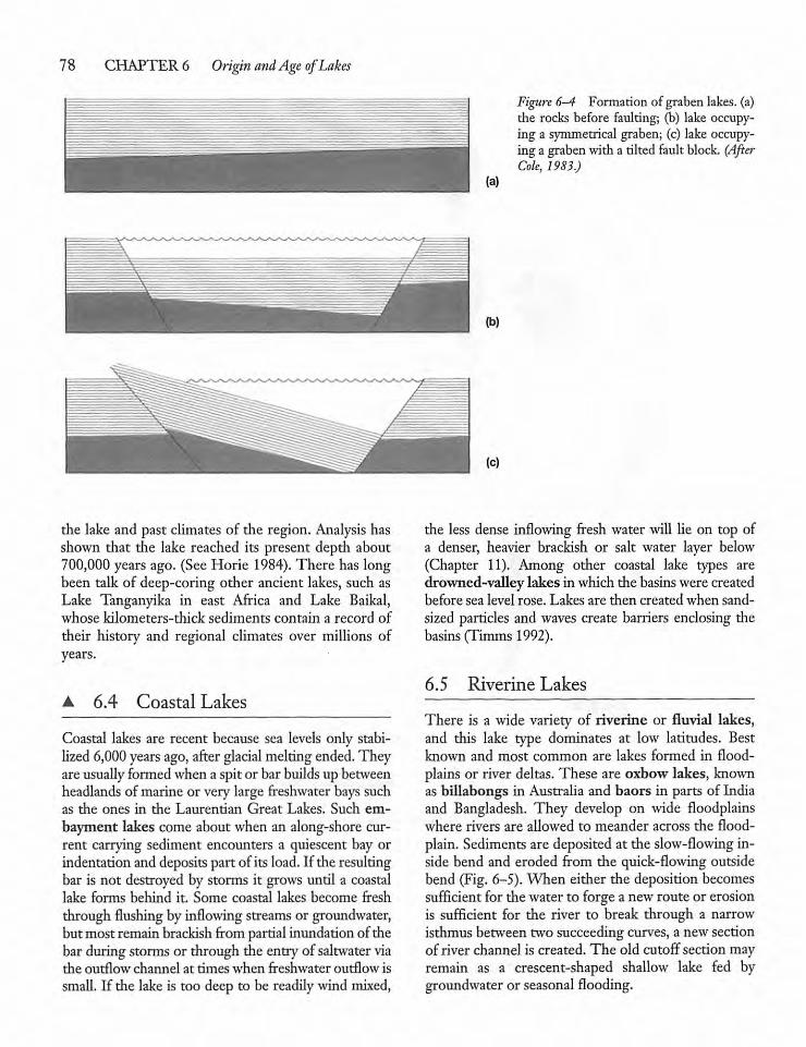
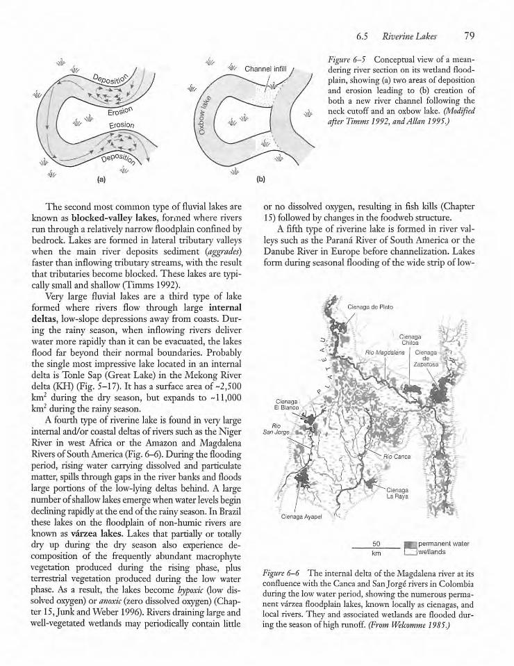
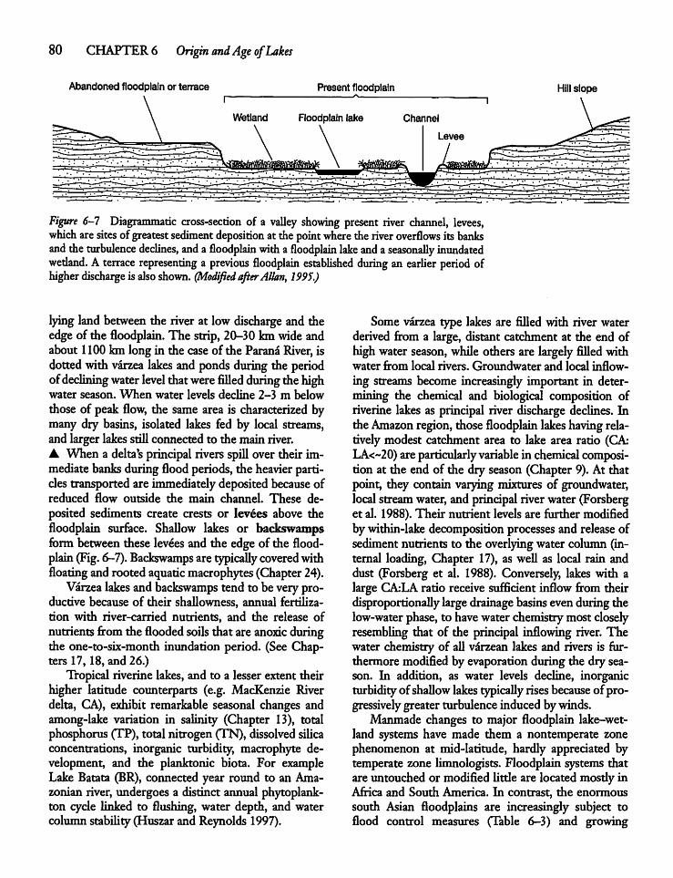
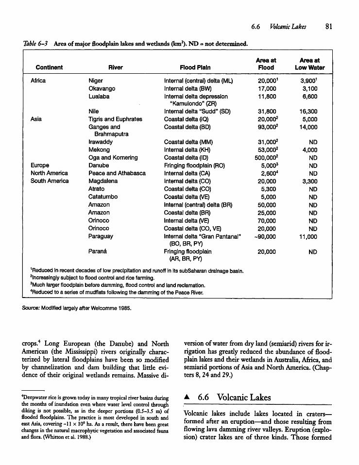
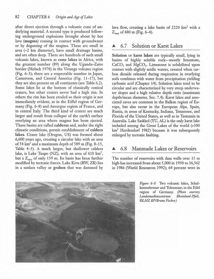
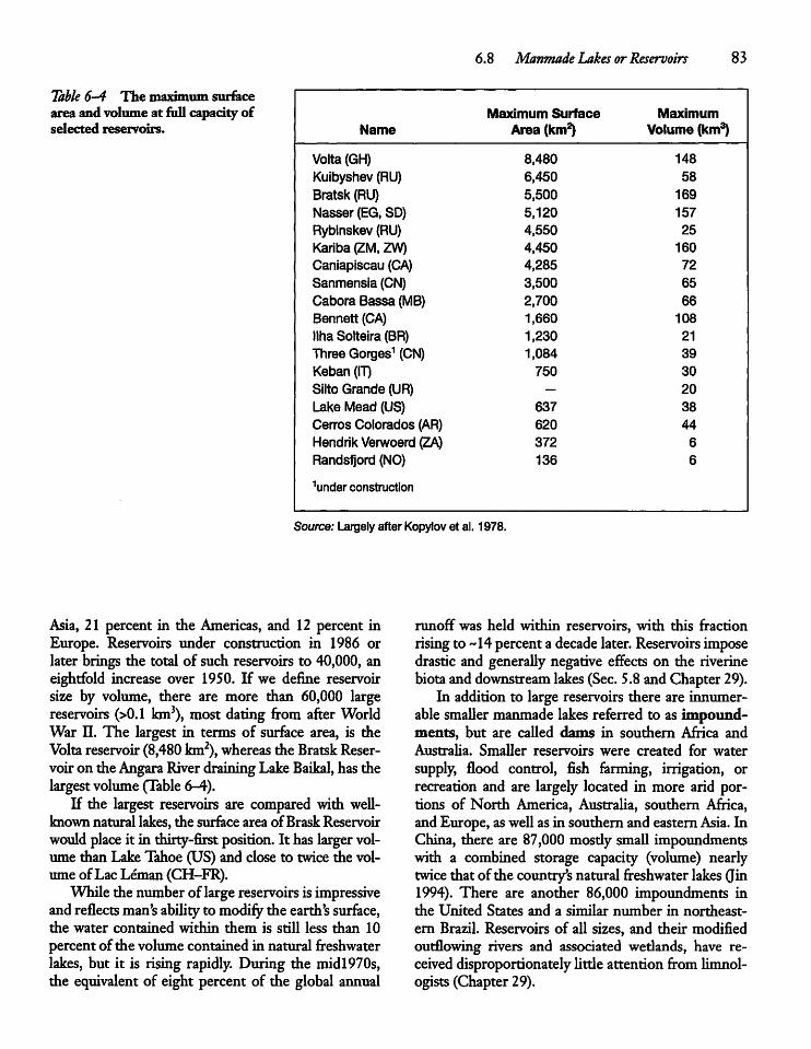
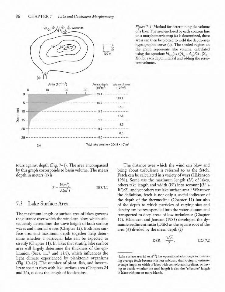
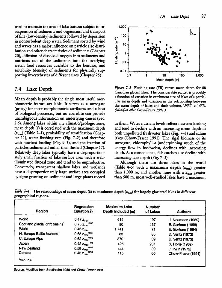
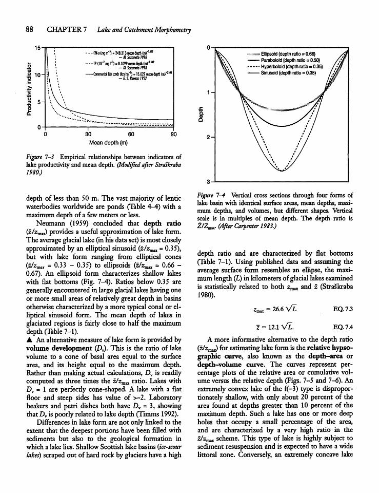
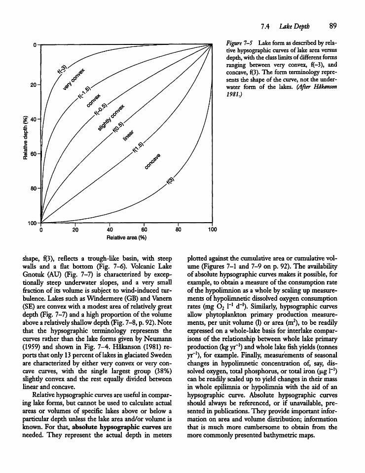
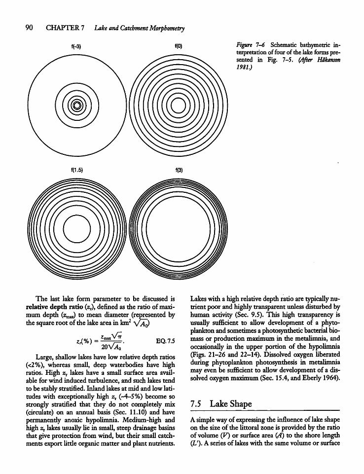
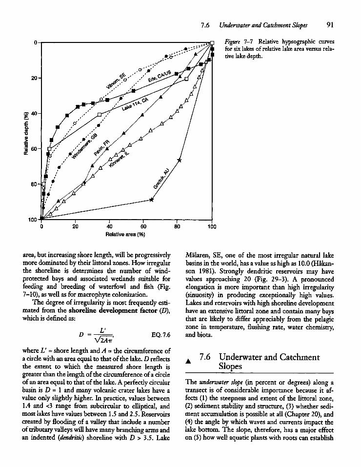
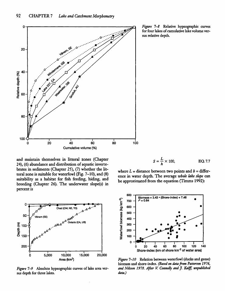
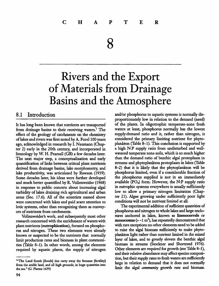
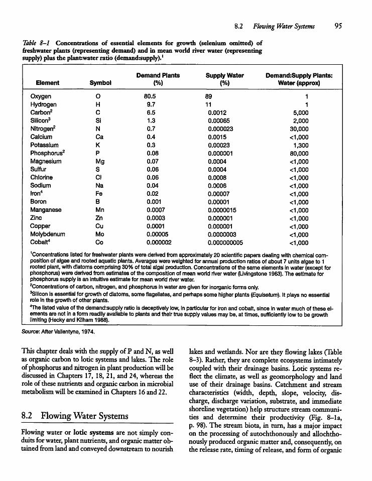
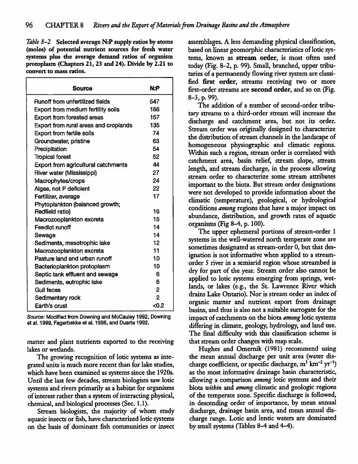
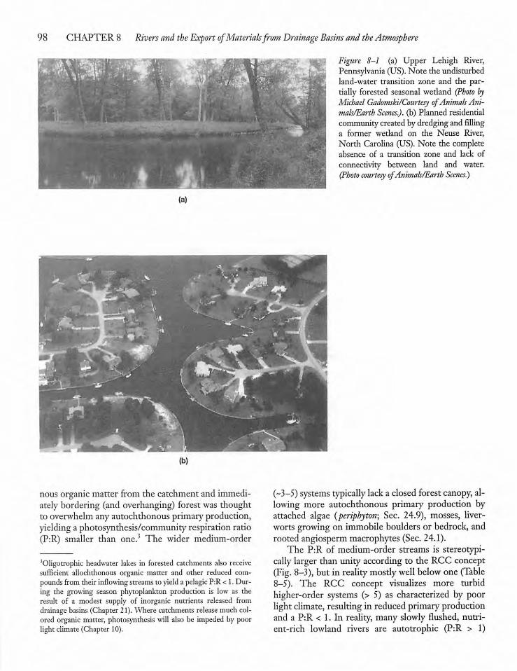
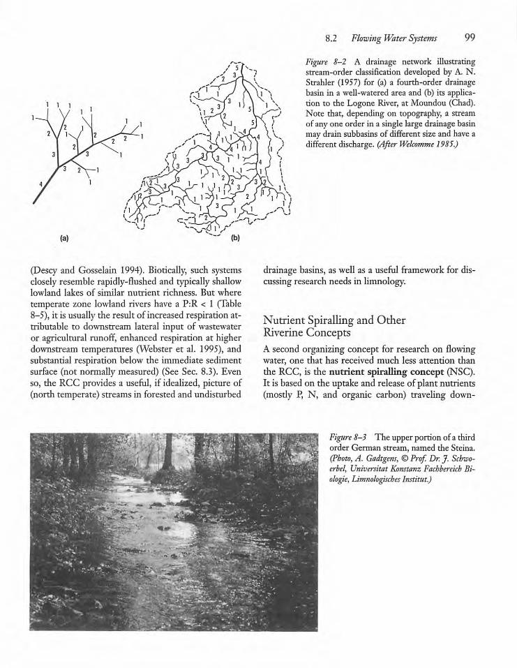
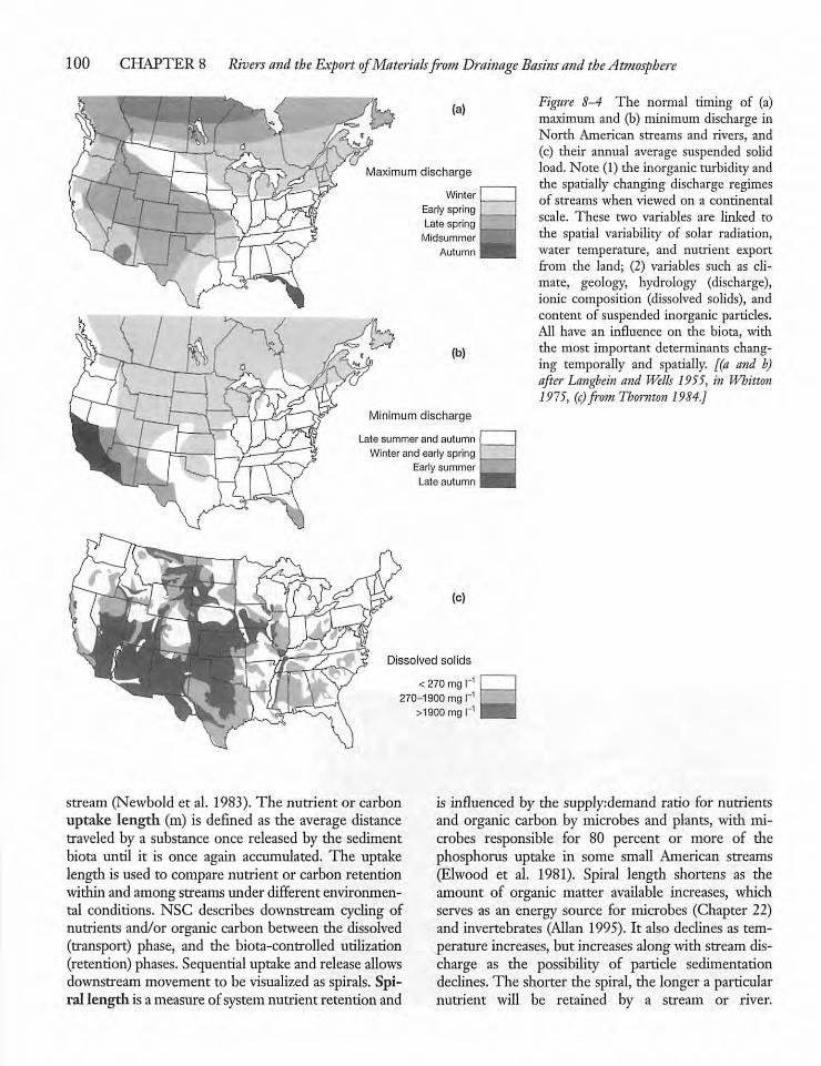
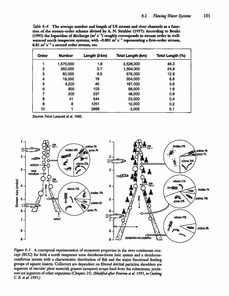
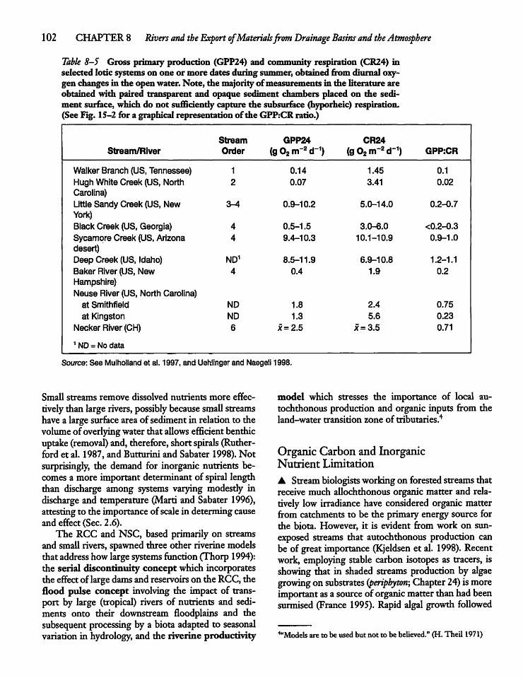
by equally rapid removal by grazerswill leave a smalland barely visible algal biomass (Huryn 1996, andKjeldsenetal. 1998).5The rapid response of periphytic algae to experi
mental fertilization in a number of pristine lotic systems has shown low-order systems to be primarilynutrient rather than light limited, and to have loticfoodwebs that can readilyshift from heterotrophic toautotrophic mode upon nutrient addition (Petersonet al. 1985). The systems further exhibit increasedorganic matter decomposition upon addition of inorganic nutrients, and then have enhanced fish production (Johnston et al. 1990). But lotic research isstill dominated by work in the water-rich north temperate zone, characterized by relatively predictablebiological responses to fairly regularhydrological seasonality, (Fig. 8-4) and there is little appreciation ofimpacts on the biota of exceptionally large inter-yearvariation in river discharge and intra-yearvariabiUtyin seasonal timing of peak and minimumwater flows(Fig. 8-6) occurring over much of the globe (Puck-ridgeet al. 1998).
8.3 Rivers and Their Ecotones
The transition zones between adjacent ecologicalsystems are known as ecotones. These encompasssharp gradients in environmental factors, dominatingprocesses, and species composition. The transitionzonebetweenan aquaticsystem and the adjacent land,is known as the riparian zone. Riparian zones havemajor, but poorly quantified, effects on inlandwaters.The transition zone between lentic or lotic systemsand adjacent wetlands form a second important eco-tone. Deltas formed at themouthof rivers where theyenter lakes or reservoirs are a third typeof interphasebetween loticand lenticecosystems.The fourth important ecotone type is the transi
tion zone in the vertical plane between the stream-channel water and the groundwater, known as thehyporheic zone or hyporheos (Fig. 8-7). This zone,an important habitat for the biota, contains a variablemixture of surface water and groundwater characterizedby strong gradients in flushing, dissolved oxygen
5Incorrect conclusions drawn about community energy and nutrientflow on die basis of the (relatively easyto measure) biomass {standing stock) rather than on growth and loss rates (more difficult tomeasure and interpret) have long held back the development ofecology.
8.3 Rivers and Their Ecotones 103
concentration, and chemistry. The lower boundary hasbeen defined operationally asthedepth towhich 10percentormorechannel water (< 90% groundwater) ispresent (Triska et al. 1993). The hyporheic zone not onlyextends vertically below thestream bottom but,depending on hydrological conditions and the definition used,mayeven extend beyond thestream or rivermargins intothegroundwater zone of the floodplain when substratepermeability (porosity) allows the passage of (oxygenated) water, organicmatter, andorganisms (Fig. 8-7).The difficult to sample hyporheic and floodplain
zones are home to communities of aquatic microbesand invertebrates, including someendemicmacroinver-tebrates (species found nowhere else). Strayer et al.(1997) reported an average of nearly 600 species perthree-liter pump sample taken in the hyporheic zone.The species were numerically dominated bycopepods,nematodes, andmicroannelid worms, but included typically larger insects and molluscs.6 Hyporheic organisms, including microbes, apparentlyplaya major (butlittle assessed) role in retention and transformation oforganic matter and the cycling of nutrients and gasesbetween land,water, and the atmosphere. Work on asixth orderprealpine Swiss riverallowed the conclusionthat the gravel-dominated hyporheic zone and its microbes contributed farmore(76-96%) ofwhole systemrespiration than the typically better-investigated surfi-cial sediments of the stream bed (Naegeli andUehlinger 1997).Larval aquatic insects (stoneflies, Fig. 25-3) have
been collected in groundwater monitoringwells up totwo kilometers from a lowland river bordered by athicksubstrate ofhighporosity, showing howextensivethe floodplain ecotone can be (Stanford and Ward1993). Stoneflies use the aquifer (groundwater) to return to the river, there emerging from the water asadults forbreeding andeggdeposition. The fraction ofmacroinvertebrate production associated with the immediate channel bottom, rather than with the hyporheic zoneor floodplain, is determined by substratecharacteristics and is further affected by the degree ofconnection (connectivity) of compartments which inturn are affected by discharge through the hyporheiczone and the water residence time there. North tem-
*"One ofthemost sensational zoological discoveries ofthelate 19thand early 20th century was that groundwaters contain a diversefauna of endemic,morphologically distinctive invertebrates. Thousands of specialized groundwater animals, "stygobionts," includingcrustaceans, worms, mollusks, and other invertebrates are nowknown... " (D. L. Strayeret al. 1995)
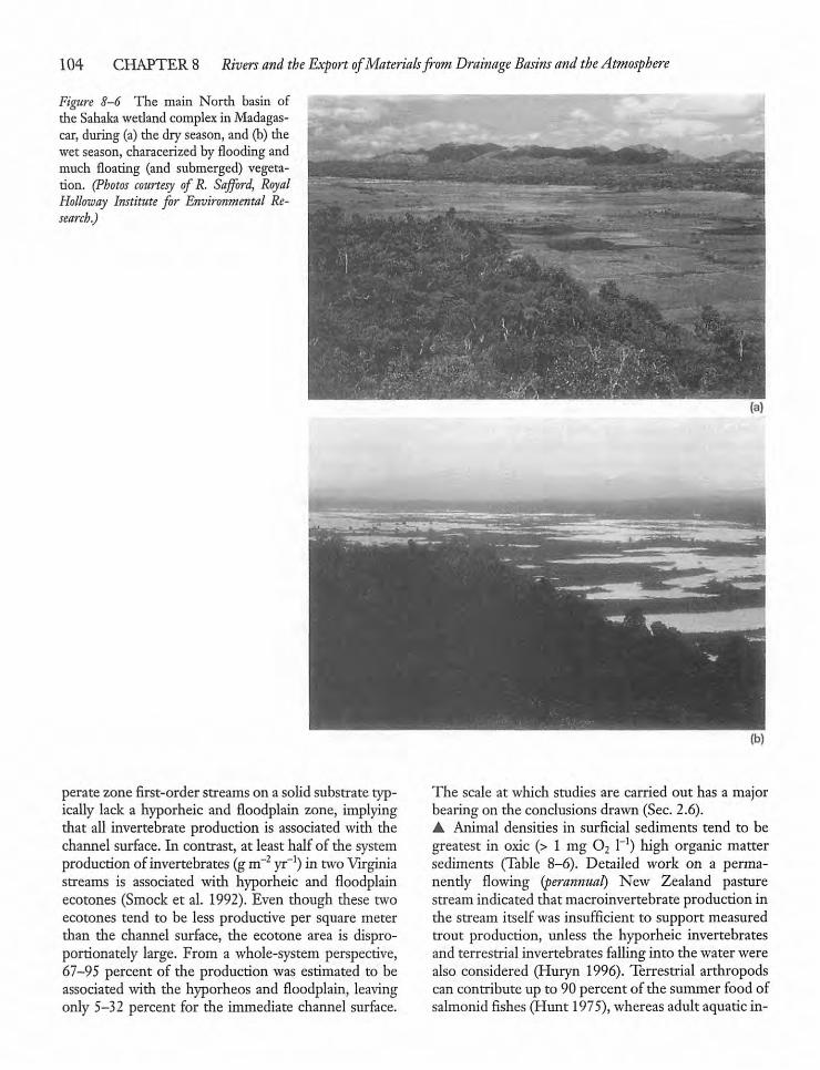
104 CHAPTER 8 Rivers and the Export ofMaterialsfrom Drainage Basins and the Atmosphere
Figure 8-6 The main North basin ofthe Sahaka wetland complex inMadagascar, during (a) the dry season, and (b) thewet season, characerized by flooding andmuch floating (and submerged) vegetation. (Photos courtesy of R. Safford, RoyalHolloway Institute for Environmental Re-scarch.)
perate zone first-order streams on a solid substrate typically lack a hyporheic and floodplain zone, implyingthat all invertebrate production is associated with thechannel surface. In contrast, at least half of the systemproduction of invertebrates (gm~2 yr"1) in two Virginiastreams is associated with hyporheic and floodplainecotones (Smock et al. 1992). Even though these twoecotones tend to be less productive per square meterthan the channel surface, the ecotone area is disproportionately large. From a whole-system perspective,67-95 percent of the production was estimated to beassociated with the hyporheos and floodplain, leavingonly 5-32 percent for the immediate channel surface.
The scale at which studies are carried out has a majorbearing on the conclusions drawn (Sec. 2.6).• Animal densities in surficial sediments tend to begreatest in oxic (> 1 mg 02 1_1) high organic mattersediments (Table 8-6). Detailed work on a permanently flowing (perannual) New Zealand pasturestream indicated that macroinvertebrate production inthe stream itself was insufficient to support measuredtrout production, unless the hyporheic invertebratesand terrestrial invertebrates fallinginto the waterwerealso considered (Huryn 1996). Terrestrial arthropodscan contribute up to 90 percent of the summer food ofsalmonid fishes (Hunt 1975),whereas adult aquatic in-
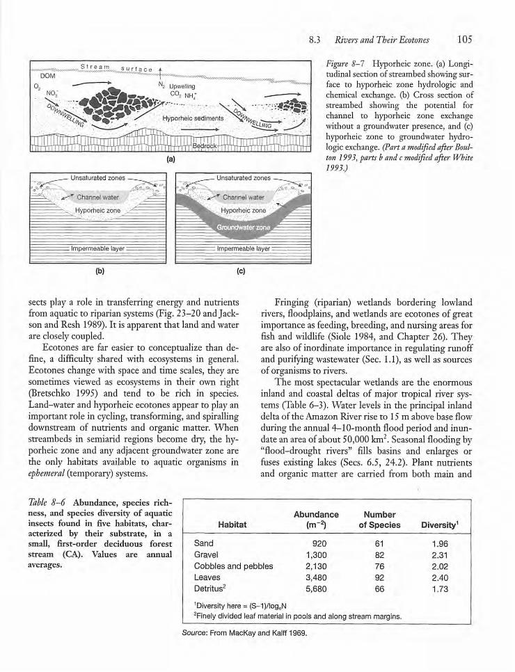
Impermeable layer:
8.3 Rivers and Their Ecotones 105
Figure 8-1 Hyporheic zone, (a) Longitudinal sectionof streambedshowing surface to hyporheic zone hydrologic andchemical exchange, (b) Cross section ofstreambed showing the potential forchannel to hyporheic zone exchangewithout a groundwater presence, and (c)hyporheic zone to groundwater hydro-logic exchange. (Part amodified after Boul-ton 1993, parts bandcmodified after White1993.)
sects play a role in transferring energy and nutrientsfrom aquatic to riparian systems (Fig. 23-20 andJackson and Resh 1989). It is apparent that land and waterare closelycoupled.Ecotones are far easier to conceptualize than de
fine, a difficulty shared with ecosystems in general.Ecotones change with space and time scales, they aresometimes viewed as ecosystems in their own right(Bretschko 1995) and tend to be rich in species.Land-waterand hyporheic ecotones appear to playanimportant role in cycling, transforming, and spirallingdownstream of nutrients and organic matter. Whenstreambeds in semiarid regions become dry, the hyporheic zone and any adjacent groundwater zone arethe only habitats available to aquatic organisms inephemeral (temporary) systems.
Fringing (riparian) wetlands bordering lowlandrivers, floodplains, and wetlands are ecotones of greatimportance asfeeding, breeding, and nursingareas forfish and wildlife (Siole 1984, and Chapter 26). Theyare also of inordinate importance in regulating runoffand purifyingwastewater (Sec. 1.1), as well as sourcesof organisms to rivers.The most spectacular wetlands are the enormous
inland and coastal deltas of major tropical river systems (Table 6-3). Water levels in the principal inlanddelta of the Amazon River rise to 15 m above base flowduring the annual 4-10-month flood period and inundate an area ofabout 50,000 km2. Seasonal flooding by"flood-drought rivers" fills basins and enlarges orfuses existing lakes (Sees. 6.5, 24.2). Plant nutrientsand organic matter are carried from both main and
Table 8—6 Abundance, species richness, and species diversity of aquaticinsects found in five habitats, characterized by their substrate, in asmall, first-order deciduous foreststream (CA). Values are annualaverages.
Abundance NumberHabitat (rrr2) of Species Diversity1
Sand 920 61 1.96Gravel 1,300 82 2.31
Cobbles and pebbles 2,130 76 2.02Leaves 3,480 92 2.40Detritus2 5,680 66 1.73
1Diversity here = (S-1)/logeN2Finely divided leaf material ir pools and along stream margins.
Source: From MacKay and Kalff 1969.
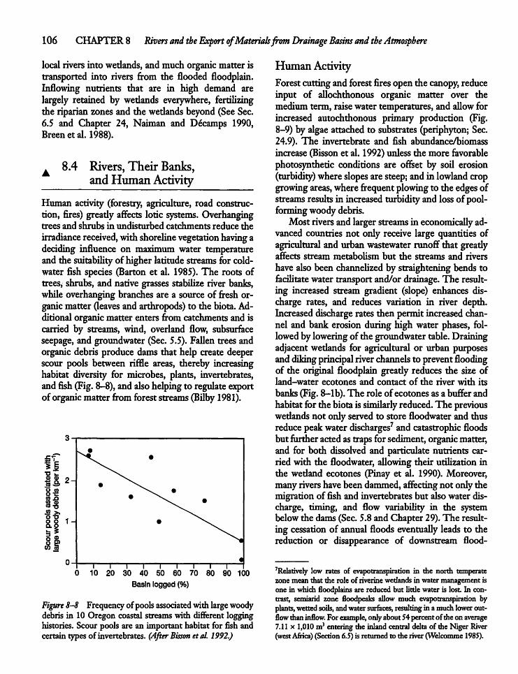
106 CHAPTER8 Rivers and the Export ofMaterialsfrom Drainage Basins and theAtmosphere
local riversinto wetlands, and much organicmatter istransported into rivers from the flooded floodplain.Inflowing nutrients that are in high demand arelargely retained by wetlands everywhere, fertilizingthe riparian zonesand the wetlands beyond (SeeSec.6.5 and Chapter 24, Naiman and Decamps 1990,Breenetal. 1988).
A 8.4 Rivers, Their Banks,andHuman Activity
Human activity (forestry, agriculture, road construction, fires) greatlyaffects lotic systems. Overhangingtrees and shrubs in undisturbed catchments reduce theirradiance received, withshoreline vegetation having adeciding influence on maximum water temperatureand the suitability of higher latitude streams for cold-water fish species (Barton et al. 1985). The roots oftrees, shrubs, and native grasses stabilize river banks,while overhanging branchesare a sourceof fresh organic matter (leaves andarthropods) to the biota. Additional organicmatter enters from catchments and iscarried by streams, wind, overland flow, subsurfaceseepage, and groundwater (Sec. 5.5). Fallen trees andorganic debris produce dams that help create deeperscour pools between riffle areas, thereby increasinghabitat diversity for microbes, plants, invertebrates,andfish (Fig. 8-8),andalso helping to regulate exportof organic matter from foreststreams(Bilby 1981).
i i i i i i i i r10 20 30 40 50 60 70 80 90 100
Basin logged (%)
Figure 8-8 Frequencyofpoolsassociatedwithlargewoodydebris in 10 Oregon coastal streamswith differentlogginghistories. Scour pools are an important habitat for fish andcertain types of invertebrates. (After Bisson etal. 1992.)
Human ActivityForestcuttingandforestfires open the canopy, reduceinput of allochthonous organic matter over themediumterm, raisewater temperatures, and allow forincreased autochthonous primary production (Fig.8-9) by algae attached to substrates (periphyton; Sec.24.9). The invertebrate and fish abundance/biomassincrease (Bissonet al. 1992)unless the more favorablephotosynthetic conditions are offset by soil erosion(turbidity) whereslopes are steep; and in lowland cropgrowing areas, where frequent plowing to the edges ofstreamsresults in increased turbidity and lossof pool-formingwoodydebris.Most rivers and largerstreamsin economically ad
vanced countries not only receive large quantities ofagricultural and urbanwastewater runoff that greatlyaffects stream metabolism but the streams and rivershave also been channelized by straightening bends tofacilitate water transportand/or drainage. The resulting increased stream gradient (slope) enhances discharge rates, and reduces variation in river depth.Increased discharge rates then permit increased channel and bank erosion during high water phases, followed bylowering of the groundwater table. Drainingadjacent wetlands for agricultural or urban purposesanddiking principal riverchannels to preventfloodingof the original floodplain greatly reduces the size ofland-water ecotones and contact of the river with itsbanks (Fig. 8—lb). The roleof ecotones asa bufferandhabitatfor the biotais similarly reduced. The previouswetlands not only served to store floodwater and thusreduce peak water discharges7 and catastrophic floodsbut furtheractedas trapsforsediment, organicmatter,and for both dissolved and particulate nutrients carried with the floodwater, allowing their utilization inthe wetland ecotones (Pinay et al. 1990). Moreover,manyrivers havebeen dammed, affecting not onlythemigration offish and invertebrates but alsowater discharge, timing, and flow variability in the systembelowthe dams (Sec. 5.8 and Chapter 29).The resulting cessation of annual floods eventually leads to thereduction or disappearance of downstream flood-
7Relatively low rates of evapotranspirarion in die north temperatezonemean that the role of riverine wetlands in watermanagement isone in which floodplains are reducedbut litde water is lost In contrast, semiarid zone floodpeaks allow much evapotranspirarion byplants, wettedsoils, andwater surfaces, resulting in amuchlower outflow thaninflow. Forexample, onlyabout54percent of theon average7.11 x 1,010 m3 entering the inland central delta of dieNigerRiver(westAfrica)(Section6.5) is returned to the river(Welcomme 1985).
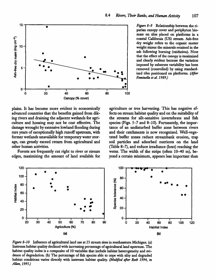
Canopy (% cover)
plains. It has become more evident in economicallyadvanced countries that the benefits gained fromdiking rivers and draining the adjacent wetlands for agriculture and housing may not be cost effective. Thedamage wroughtby extensive lowland flooding duringrare years of exceptionally high runoff upstream, withformer wetlands unavailable for temporarywaterstorage, can greatly exceed return from agricultural andother human activities.
Forests are frequently cut right to river or streamedges, maximizing the amount of land available for
120
100-
x 80-^
H
I 40H
20-j
0
20 30 40 50 60 70
Agriculture (%)
(a)
80
8.4 Rivers, Their Banks, andHuman Activity 107
90
Figure 8-9 Relationshipbetween the riparian canopy cover and periphyton biomass on riles placed on platforms in acoastal California (US) stream. Ash-freedry weight refers to the organic matterweight minus the mineralsretainedin theash following burning (oxidation). Notethat the effect of the canopyis maximizedand clearly evident because the variationimposed by substrate variability has beenremoved (controlled) by using standardized tiles positioned on platforms. (AfterFeminella et al. 1989.)
agriculture or tree harvesting. This has negative effects on stream habitatqualityandon the suitability ofthe streams for silt-sensitive invertebrate and fishspecies (Figs. 5-7 and 8-10). Fortunately, the importance of an undisturbed buffer zone between riversand their catchments is now recognized. Well-vegetated buffer zones reduce streambank erosion, trapsoil particles and adsorbed nutrients on the land(Table 8-7), andreduce irradiance (heat) reaching thewater. The width of the strips (often 10-40 m), beyond acertain minimum, appears less important than
iuu- —••
•T* •
•
2O
80-
60-
•
• ••• • •
23
ICO
40-
20-
0-
• •
i i i i i20 40 60
Habitat index
(b)
80 100 120
Figure 8-10 Influence of agricultural land useat23stream sites in southeastern Michigan, (a)Instream habitat quality declined with increasing percentage ofagricultural land upstream. Thehabitat quality index is a composite of 10variables thatinclude habitat heterogeneity and evidence of degradation, (b) The percentage of fish species able to cope with siltyand degradedhabitat conditions varies directly with instream habitat quality. (Modified after Roth 1994, inAllan, 1995.)
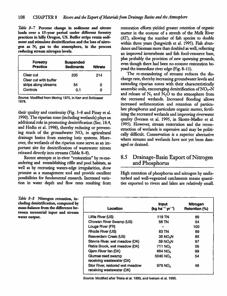
108 CHAPTER 8 Rivers and the Export ofMaterialsfrom Drainage Basinsand theAtmosphere
Table 8-7 Percent change in sediment and nitrateloads over a 15-year period under different forestrypractices in hilly Oregon, US. Buffer strips retain sediment and stimulate denitrification and the loss ofnitrogen as N2 gas to the atmosphere, in the processreducing stream nitrogen levels.
restoration efforts yielded greater retention of organicmatter in the ecotone of a stretch of the Melk River(AT), allowing the number of fish species to doublewithin three years Gungwirth et al. 1995). Fish abundance andbiomass morethandoubled aswell, reflectingan improved invertebrate and fish food-resource base,plus probably the provision of newspawning grounds,eventhough there had beenno ecotonerestorationbeyondthe immediate riveredge(Fig. 8-11).The re-meandering of streams reduces the dis
charge rate, therebyincreasing groundwater levels andextending riparian zones with their characteristicallyanaerobic soils, encouraging denitrification ofN03-Nand release ofN2 and N26 to the atmosphere fromthe recreated wetlands. Increased flooding allowsincreased sedimentation and retention of particulatephosphorus andparticulate organic matter, fertilizing the recreated wetlands andimproving riverwaterquality (Iversen et al. 1995, in Skotte-Moller et al.1995). However, stream restoration and the reconstruction of wetlands is expensive andmay be politically difficult. Conservation is a superior alternativewhere streams andwetlands have not yet been damagedor drained.
8.5 Drainage-Basin Export ofNitrogenand Phosphorus
High retentionof phosphorus andnitrogenbyundisturbed and well-vegetated catchments means quantities exported to rivers and lakes are relatively small.
ForestryPractice
SuspendedSediments Nitrate
Clear cut 205 214Clear cut with bufferstrips along streams 54 0Controls 0.1 0
Source: Modified from Moring 1975, in Karr and Schlosser1978.
their quality and continuity (Fig. 5-8 andPinay et al.1990). The riparian zone (includingwedands) plays anadditional rolein promoting denitrification (Sec. 18.4,and Hedin et al. 1998), thereby reducing or preventing much of the groundwater N03 in agriculturaldrainage basins from entering lotic systems. Moreover, thewetlands of the riparian zoneserve asan important site for denitrification of wastewater nitratereleased direcdy into streams(Table 8-8).Recent attempts at in-river "restoration" by re-me
andering and reestablishing riffle and poolhabitats, aswell as by recreating waters-edge irregularities, showpromise as a management tool and provide excellentpossibilities for fundamental research. Increased variation in water depth and flow rates resulting from
Table 8-8 Nitrogen retention, includingdenitrification, computed bymass-balance from die difference between terrestrial input and streamwater output.
Input NitrogenLocation (kg ha"1 yr1) Retention (%)
Little River (US) 119TN 89Chowan River Swamp (US) 58 TN 64Louge River (FR) - 100
Rhode River (US) 83 TN 89
Beaverdam Creek (US) 35 N03N 85Stevns River, wet meadow (DK) 59 NO3N 97
Rabis Brook, wet meadow (DK) 711 N03 56
Gjern River fen (DK) 884 N03 99
Glumso reed swamp 5046 N03 54receiving wastewater (DK)Stor River, restored wet meadow 979 N03 48receiving wastewater (DK)
Source: Modified after Triska et al. 1993, and Iversen et al. 1995.
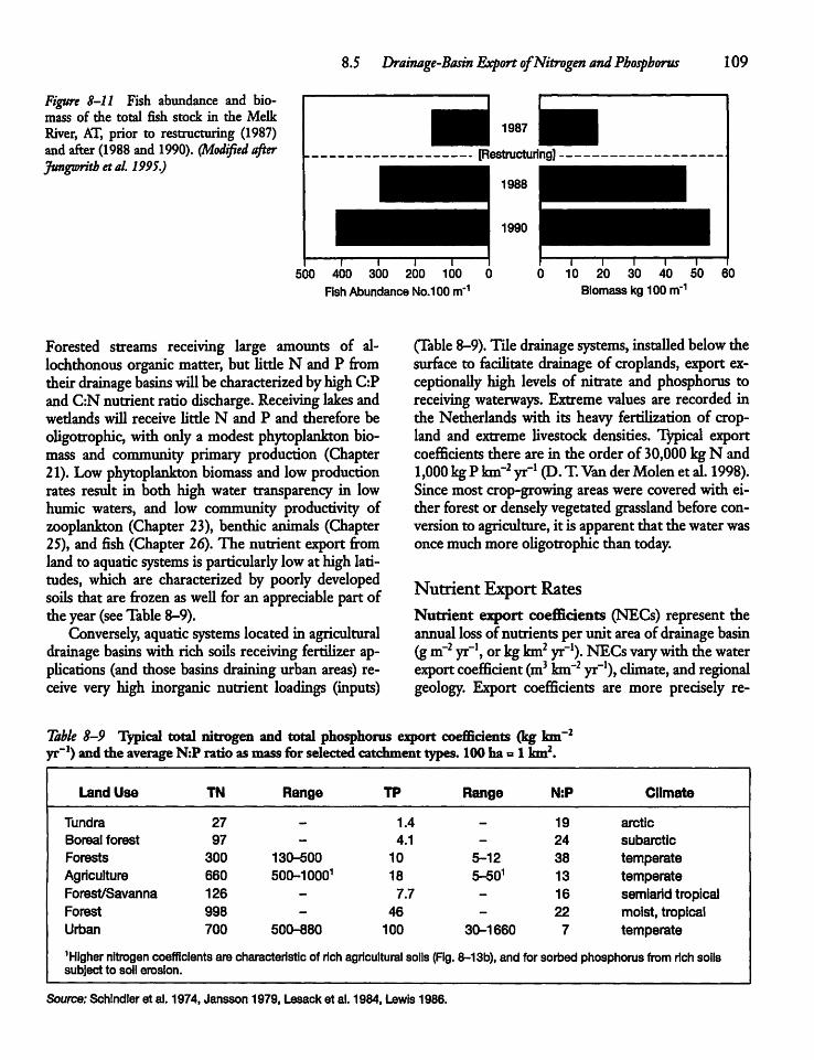
8.5 Drainage-Basin Export ofNitrogen andPhosphorus 109
Figure 8-11 Fish abundance and biomass of the total fish stock in the MelkRiver, AT, prior to restructuring (1987)and after (1988and 1990). (Modified afterJungumtb etal. 1995.)
r20 30 40 50
Biomasskg 100m"1500 400 300 200 100 0
Fish Abundance No.100 m*160
Forested streams receiving large amounts of al-lochthonous organic matter, but little N and P fromtheirdrainage basins will becharacterized byhighC:PandC:N nutrient ratio discharge. Receiving lakes andwetlands will receive little N and P and therefore beoligotrophia with only a modestphytoplankton biomass and community primary production (Chapter21). Low phytoplankton biomass and lowproductionrates result in both high water transparency in lowhumic waters, and low community productivity ofzooplankton (Chapter 23), benthic animals (Chapter25), and fish (Chapter 26).The nutrient export fromland to aquatic systems is particularly lowat high latitudes, which are characterized by poorly developedsoils that are frozen as well for an appreciable part ofthe year (seeTable8-9).Conversely, aquaticsystems locatedin agricultural
drainage basins with rich soils receiving fertilizer applications (and those basins draining urban areas) receive very high inorganic nutrient loadings (inputs)
(Table 8-9).Tile drainage systems, installed below thesurface to facilitate drainage of croplands, export exceptionally high levels of nitrate and phosphorus toreceiving waterways. Extreme values are recorded inthe Netherlands with its heavy fertilization of cropland and extreme livestock densities. Typical exportcoefficients there are in the order of 30,000kg N and1,000 kgP km-2 yr"1 (D.T.Van derMolen et al. 1998).Since most crop-growingareaswere covered with either forestor densely vegetatedgrassland before conversion to agriculture, it is apparent that thewaterwasoncemuchmore oligotrophic than today.
Nutrient Export RatesNutrient export coefficients (NECs) represent theannuallossof nutrients per unit area of drainagebasin(gm~2 yr-1, orkgkm2 yr-1). NECs varywith thewaterexport coefficient (m3 km"2 yr-1), climate, and regionalgeology. Export coefficients are more precisely re-
Table 8-9 Typical total nitrogen and total phosphorus export coefficients (kg km-2yr'1) and the average N:P ratio asmassfor selectedcatchmenttypes.100ha =1 km2.
Land Use TN Range TP Range N:P Climate
Tundra 27 _ 1.4 _ 19 arcticBoreal forest 97 - 4.1 - 24 subarcticForests 300 130-600 10 5-12 38 temperateAgriculture 660 500-10001 18 5-501 13 temperateForest/Savanna 126 - 7.7 - 16 semiarid tropicalForest 998 - 46 - 22 moist, tropicalUrban 700 500-880 100 30-1660 7 temperate
'Higher nitrogen coefficients aresubject to soil erosion.
characteristic of rich agricultural soils (Fig. 8-13b), and for sorbed phosphorus from rich soils
Source: Schindler et al. 1974, Jansson 1979, Lesack et al. 1984, Lewis 1986.
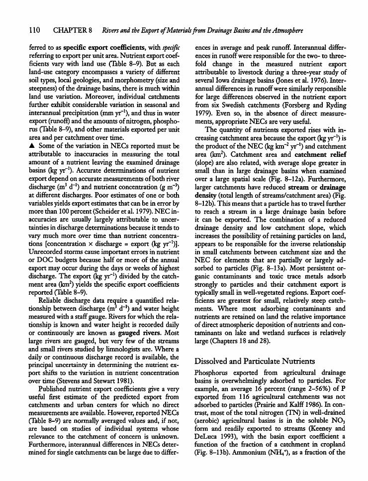
110 CHAPTER8 Rivers and the Export ofMaterialsfrom Drainage Basins and theAtmosphere
ferred to as specific export coefficients, with specificreferringto exportper unit area.Nutrient exportcoefficients vary with land use (Table 8-9). But as eachland-use category encompasses a variety of differentsoil types, local geologies, andmorphometry (size andsteepness) of the drainage basins, there ismuchwithinland use variation. Moreover, individual catchmentsfurther exhibit considerable variation in seasonal andinterannual precipitation (mm yr"1), andthus inwaterexport (runoff) andthe amounts ofnitrogen, phosphorus (Table 8-9), andother materials exported per unitareaandper catchment over time.A Some of the variation in NECs reportedmust beattributable to inaccuracies in measuring the totalamount of a nutrient leaving the examined drainagebasins (kg yr-1). Accurate determinations of nutrientexportdependon accuratemeasurements of both riverdischarge (m3 d"1) and nutrient concentration (gm"})at different discharges. Poor estimates of one or bothvariables yields exportestimates that canbe in errorbymore than 100percent (Scheideret al. 1979). NEC inaccuracies are usually largely attributable to uncertaintiesin discharge determinationsbecause it tendstovary much more over time than nutrient concentrations [concentration x discharge = export (kg yr"1)].Unrecorded storms cause important errors in nutrientor DOC budgets because half or more of the annualexportmayoccur during the days or weeks of highestdischarge. The export (kgyr"1) divided by the catchmentarea (km2) yields the specific export coefficientsreported (Table8-9).Reliable discharge data require a quantified rela
tionship between discharge (m3 d"1) and water heightmeasured with a staffgauge. Rivers forwhich the relationship is known and water height is recorded dailyor continuously are known as gauged rivers. Mostlarge rivers are gauged, but very few of the streamsand small rivers studied by limnologists are. Where adaily or continuous discharge record is available, theprincipal uncertainty in determining the nutrient export shifts to the variation in nutrient concentrationover time (Stevens and Stewart 1981).Published nutrient export coefficients give a very
useful first estimate of the predicted export fromcatchments and urban centers for which no directmeasurementsare available. However,reported NECs(Table 8-9) are normally averaged values and, if not,are based on studies of individual systems whoserelevance to the catchment of concern is unknown.Furthermore, interannual differences in NECs determined for singlecatchments can be large due to differ
ences in average and peak runoff. Interannual differencesin runoffwere responsible for the two- to threefold change in the measured nutrient exportattributable to livestock during a three-year study ofseveral Iowadrainage basins (Jones et al. 1976). Interannual differences in runoffweresimilarly responsiblefor large differences observed in the nutrient exportfrom six Swedish catchments (Forsberg and Ryding1979). Even so, in the absence of direct measurements, appropriateNECs are veryuseful.The quantity of nutrients exported rises with in
creasing catchment area because theexport (kg yr"1) istheproduct oftheNEC(kg km"2 yr"1) and catchmentarea (km2). Catchment area and catchment relief(slope) are also related, with average slope greater insmall than in large drainage basins when examinedover a large spatial scale (Fig. 8-12a). Furthermore,larger catchments have reduced stream or drainagedensity (total length of streams/catchment area) (Fig.8—12b). This meansthat a particlehas to travelfurtherto reach a stream in a large drainage basin beforeit can be exported. The combination of a reduceddrainage density and low catchment slope, whichincreases the possibility of retaining particleson land,appears to be responsible for the inverse relationshipin small catchments between catchment size and theNEC for elements that are partially or largely adsorbed to particles (Fig. 8-13a). Most persistent organic contaminants and toxic trace metals adsorbstrongly to particles and their catchment export istypically small in well-vegetated regions. Export coefficients are greatest for small, relatively steep catchments. Where most adsorbing contaminants andnutrients are retained on land the relativeimportanceof direct atmosphericdepositionof nutrients and contaminants on lake and wetland surfaces is relativelylarge (Chapters 18and 28).
Dissolved and Particulate Nutrients
Phosphorus exported from agricultural drainagebasins is overwhelmingly adsorbed to particles. Forexample, an average 16 percent (range 2-56%) of Pexported from 116 agricultural catchments was notadsorbed to particles(Prairie and Kalff1986). In contrast, most of the total nitrogen (TN) in well-drained(aerobic) agricultural basins is in the soluble N03form and readily exported to streams (Keeney andDeLuca 1993), with the basin export coefficient afunction of the fraction of a catchment in cropland(Fig. 8-13b). Ammonium(NH^), as a fraction of the
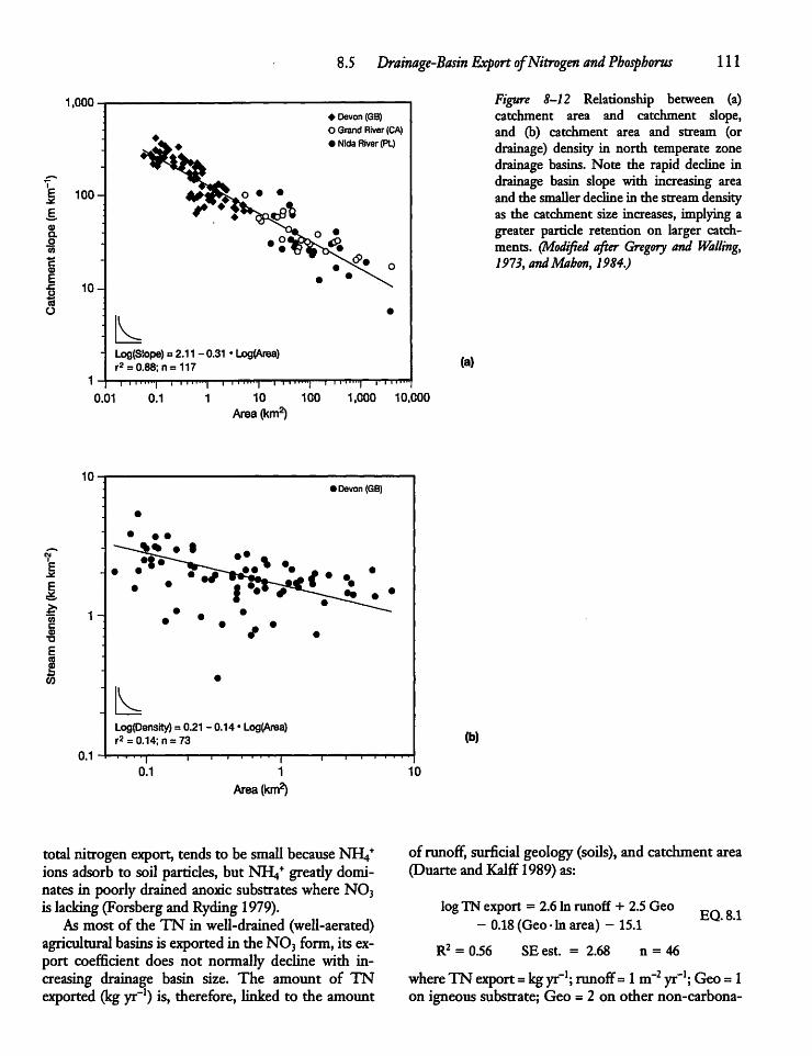
8.5 Drainage-Basin Export ofNitrogen and Phosphorus 111
1,000Devon (GB)
O Grand River (CA)• Nida River (PL)
Figure 8-12 Relationship between (a)catchment area and catchment slope,and (b) catchment area and stream (ordrainage) density in north temperate zonedrainage basins. Note the rapid decline indrainage basin slope with increasing areaand the smallerdeclinein the streamdensityas the catchment size increases, implying agreater particle retention on larger catchments. (Modified after Gregory and Walling,1973, andMabon, 1984.)
CDao0)
CD
E.eo
COO
100-
10-
Log(Slope) = 2.11 - 0.31 • Log(Area)r2 = 0.88; n = 117T I """| 1 I l"i"| TT I iii >""| i 11 "|M|—nr
10
Area(km2)
(a)
0.01 0.1 100 1,000 10,000
10
1-
co
0.1
Log(Density) = 0.21 - 0.14 • Log(Area)r* = 0.14; n = 73
0.1
Area (km2)
• Devon (GB)
total nitrogen export, tends to be smallbecause NH^*ions adsorb to soil particles, but NH^* greatly dominates in poorly drained anoxic substrateswhere N03is lacking (Forsbergand Ryding1979).As most of the TN in well-drained (well-aerated)
agriculturalbasinsis exported in the N03 form, its export coefficient does not normally decline with increasing drainage basin size. The amount of TNexported (kg yr"1) is, therefore, linked to the amount
(b)
10
of runoff,surficial geology(soils), and catchment area(Duarte and Kalff 1989) as:
log TN export = 2.6 In runoff + 2.5 Geo- 0.18 (Geo •In area) - 15.1
R2 = 0.56 SE est. = 2.68 n = 46
EQ.8.1
where TNexport =kgyr *; runoff=1m 2yr"1; Geo=1on igneous substrate; Geo = 2 on other non-carbona-
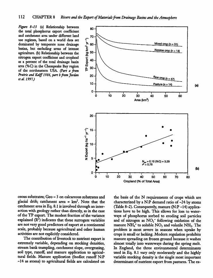
112 CHAPTER 8 Rivers and the Export ofMaterialsfrom Drainage Basins and theAtmosphere
Figure 8-13 (a) Relationship betweenthe total phosphorus export coefficientand catchment area under different landuse regimes, based on a world data setdominated by temperate zone drainagebasins, but excluding areas of intenseagriculture, (b)Relationship between thenitrogen export coefficient and croplandas a percent of the total drainage basinarea (%C)in the Chesapeake Bay regionof the northeastern USA (Part a fromPrairie and Kaljfl986, part bfrom Jordanetal. 1997.)
30 40Area(km2)
20-
•
r 15- •
£ • ^*^CO-C ^^^"^ •110"t
8£ •
Z 5- m _^"-"•p Nw=0.15 (%C)+3.29
r* = 0.78»•>
' I I I l l I
10 20 30 40 50 60 70Cropland (% of Total Area)
80
(a)
(b)
ceous substrates; Geo = 3 on calcareous substrates andglacial drift; catchment area = km2. Note that thecatchment areainEq. 8.1 isinvolved throughaninteractionwith geologyrather than direcdy, as in the caseof the TP export. The modest fraction of the varianceexplained (R2) indicates thatthese surrogate variablesarenot verygoodpredictors of exportat a continentalscale, probably because agricultural and other humanactivities are not explicitly considered.The contribution of livestock to nutrientexport is
extremely variable, depending on stocking densities,stream banktrampling, catchment slope, overgrazing,soil type, runoff, and manure application to agricultural fields. Manure application (feedlot runoff N:P~14 as atoms) to agricultural fields are calculated on
the basis of the N requirements of crops which arecharacterized by aN:P demand ratioof ~24 byatoms(Table 8-2).Consequently, manure (N:P~14) applications have to be high. This allows for loss to waterways of phosphorus sorbed to eroding soil particlesand of nitrogen as N03~ following oxidation of themanure NrV to soluble N03 and volatile NH3. Theproblem is most severe in seasons when uptake bycrops is smallor lacking. Modern regulationprohibitsmanure spreading on frozen ground because it washesalmost totallyinto waterways during the springmelt.In England, the three environmental determinantsused in Eq. 8.1 vary only moderately and the highlyvariable stocking densityis the singlemost importantdeterminant of nutrient export from pastures. The ex-
perience there suggests thatone hectare (0.01 km2) oftypically low-slope pasture land there can efficiendyabsorb the waste of 2.5 milking cows, 25 pigs, or 250laying hens,with eachgroupexcretingabout400kgNyr"1 (Cooke and Williams 1973).It is not surprising that water pollution can be a
majorproblemwherelivestock is kept at exceptionallyhigh densities in barns or feedlots (Jones et al. 1976)or where, as in the Netherlands, high densities requireimporting much feed (organic matter and nutrientstherein), with the wastes overwhelming the absorptivecapacity of soils (Table 8-9).When abundant, migrating or residentgeese, swans, and ducks excrete sufficient nutrients obtained from fields and waterwayselsewhere to significandy enhance the local nutrientloading of lakes andwedands (Manny et al. 1994), butthewaterfowl contribution is typically small comparedto livestock.
Sewage WastewaterSewagewastewater is byfar the most importantsourceof nutrients to rivers and lakesnear large urban centers.Humans release -12 gN and -1.5 g P per personper day, plus additional phosphorus contained in detergents and food particles. Where populations arelargeandwastewater treatment is nonexistentor poor,nearly all of the nutrients released by urban humans,their animals, and garden fertilizers enter waterwaysviasewers. However, in economically advanced countries usinggood sewage treatment, the nutrient contribution of agriculturedominates.In countries with advanced wastewater treatment,
chemicals [usually A1(S04)3, FeCl3 or Ca(OH)2] arecommonly added during primary sewage treatmentto flocculate and precipitate more nutrients, organicmatter, and adsorbed contaminants than would be thecase without them (Fig. 8-14).The precipitated material is collected before the treated wastewater isreleased. More advanced (and more expensive) treatment systems (secondary treatment) allow micro-bially-induced flocculation and sedimentation of theorganic matter, the nutrients contained therein, andthe adsorbed contaminants (Fig. 8-14). The sedi-mented solids must be buried in landfills that do notleak, or theyhave to be incinerated, with the attendantrelease ofmetals andorganicmatter to the atmosphere.Wastewater lagoons andwetlands serving asnutri
ent traps for wastewater from villages and livestockfarms can be a less expensive alternative to sewagetreatment plants (Sec. 24.2). They are most effective
8.6 Atmospheric Deposition ofNutrients 113
at lowerlatitudeswhere light and temperature are suf-ficiendy high to allow a year-round growing seasonandmuchdenitrification, wheresedimentshavea highadsorbing capacity, and quantities of wastewater arenot so high as to overwhelm the retention capacityofthe systems. Typically shallow wetlands allow readytrapping of particlesby the sediments and nutrient uptakeby the aquaticvegetation and sedimentmicrobes.(Sec. 24.2.)
8.6 AtmosphericDepositionofNutrients
Not all the nutrients that nourish inland waters arederived from their terrestrial catchments. Someenter as difficult-to-measure micron-sized aerosolparticles (dryfall) and gases, complementing the quantitiesmeasured in precipitation(wetfall) from the overlying atmosphere or aerial catchment (Chapter 27).Aquatic systems are therefore not only products oftheir terrestrial drainage basins but, to varying degrees, the product of events far away. The role of theaerial catchment is probably bestunderstood with reference to highlyacidic wetfail and dryfall that maybeproduced locally aswellashundreds, if not thousands,of kilometers from the system upon which it falls,whose fate it helps determine (Chapter 27). Even so,mostaquatic systemswitha substantial catchment thatare remote from urban, industrial, or agricultural regions are overwhelmingly dependent for nutrients onthe more easily defined terrestrialcatchmentTerrestrial catchments serve as receptors of aeri
ally-derived materials fromelsewhere, some ofwhichis subsequendy reexported to receiving waterways.Schindler et al. (1976) argue that all of the catchmentphosphorus carried to remote Rawson Lake (CA) byits streams must have been derived from the atmospherebecause no phosphate containing rockhasbeenfound in the drainage basin. There is long-rangetransport in the upper atmosphere of gases and thedust containing nutrients from the Saharan desert tothe Amazon basin of South America, and from centralAsia to the Hawaiian Islands and North America;there is alsotransport of pollutants from the industrialized temperate zone to polar regions (Fig. 5-13 andChapter 28).Nitrogen and phosphorusentering aquaticsystems
via the atmosphere (kg km"2 yr"1) rise from lowquantities in polar regions to a broadmaximum in agricultural regions of the temperate zone, characterized by
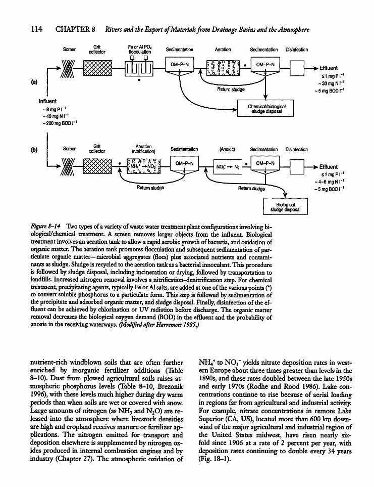
114 CHAPTER8 Rivers and the Export ofMaterialsfrom Drainage Basins and the Atmosphere
Screen
(a)
Influent
~8mgpr1-40mgNr1~200mgBODr1
(b) Screen
Gritcollector
Gritcollector
FeorAIP04flocculaticn
0 D
Aeration(nitrification)
NrV-»NOa
Sedimentation Aeration
OM-P-N "STY17*
Sedimentation Disinfection
Chemical/biologicalsludge disposal
Sedimentation (Anoxic) Sedimentation Disinfection
Figure 8-14 Two types ofavariety ofwaste water treatment plant configurations involving biological/chemical treatment. A screen removes larger objects from the influent. Biologicaltreatment involves anaeration tankto allow arapid aerobic growth ofbacteria, andoxidation oforganic matter. The aeration tank promotes flocculation and subsequent sedimentation ofparticulate organic matter—microbial aggregates (floes) plus associated nutrients and contaminants as sludge. Sludge isrecycled totheaeration tank as abacterial innoculant. Thisprocedureis followed bysludge disposal, including incineration or drying, followed bytransportation tolandfills. Increased nitrogen removal involves a nitrification-denitrification step. For chemicaltreatment, precipitatingagents, typically FeorAlsalts, areadded atoneofthevarious points (*)to convert soluble phosphorus to a particulate form. Thisstep is followed bysedimentation oftheprecipitate and adsorbed organic matter, and sludge disposal. Finally, disinfection oftheeffluent can beachieved bychlorination orUVradiation before discharge. The organic matterremoval decreases thebiological oxygen demand (BOD) in theeffluent and theprobability ofanoxia in the receivingwaterways. (Modified afterHarremoes 1985.)
^ EffluentSlmgPl"1~30mgNr1
~5mgBOD|-1
>• EffluentSlmgPr1
-4-6mgNr1-SmgBODI"1
nutrient-rich windblown soils that are often furtherenriched by inorganic fertilizer additions (Table8-10). Dust from plowed agricultural soils raises atmospheric phosphorus levels (Table 8-10, Brezonik1996), withthese levels muchhigherduringdrywarmperiods than when soilsare wet or coveredwith snow.Large amounts of nitrogen (asNH3 and N20) are released into the atmosphere where livestock densitiesarehighandcropland receives manure or fertilizer applications. The nitrogen emitted for transport anddeposition elsewhere is supplemented bynitrogenoxides produced in internal combustion engines and byindustry (Chapter 27). The atmospheric oxidation of
NHj* to N03" yieldsnitrate deposition rates in western Europe about three timesgreater than levels in the1890s, and these rates doubled between the late 1950sand early 1970s (Rodhe and Rood 1986). Lake concentrations continue to rise because of aerial loadingin regions far fromagricultural and industrial activity.For example, nitrate concentrations in remote LakeSuperior (CA, US), located more than 600 km downwindof the majoragricultural and industrialregionofthe United States midwest, have risen nearly sixfold since 1906 at a rate of 2 percent per year, withdeposition rates continuing to double every 34 years(Fig. 18-1).
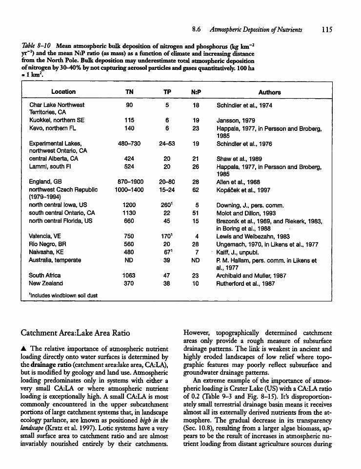
8.6 Atmospheric Deposition ofNutrients 115
Table 8-10 Mean atmospheric bulk deposition of nitrogen and phosphorus (kg km-2yr-1) and themean N:P ratio (as mass) asa function ofclimate and increasing distancefromthe North Pole. Bulkdeposition mayunderestimate total atmospheric depositionofnitrogenby30-40% bynot capturingaerosolparticles andgases quantitatively. 100ha= lkm2.
Location TN TP N:P Authors
Char Lake Northwest 90 5 18 Schindler et al., 1974Territories, CAKuokkel, northern SE 115 6 19 Jansson, 1979Kevo, northern FL 140 6 23 Happala, 1977, in Persson and Broberg,
1985Experimental Lakes, 480-730 24-53 19 Schindler etal., 1976northwest Ontario, CAcentral Alberta, CA 424 20 21 Shawetal., 1989Lammi, south Fl 524 20 26 Happala, 1977, in Persson and Broberg,
1985England, GB 870-1900 20-80 28 Allen etal., 1968northwest Czech Republic 1000-1400 15-24 62 Kopa5ek etal., 1997(1979-1994)north central Iowa, US 1200 2601 5 Downing, J., pers. comm.south central Ontario, CA 1130 22 51 Molot and Dillon, 1993north central Florida, US 660 45 15 Brezonik et al., 1969, and Riekerk, 1983,
in Boring etal., 1988Valencia, VE 750 1701 4 Lewis and Weibezahn, 1983Rio Negro, BR 560 20 28 Ungemach, 1970, in Likens et al., 1977Naivasha, KE 480 671 7 Kalff, J., unpubl.Australia, temperate ND 39 ND P. M. Hallam, pers. comm. in Likens et
al., 1977South Africa 1063 47 23 Archibald and Muller, 1987New Zealand 370 38 10 Rutherford et al., 1987
'Includes windblown soil dust
Catchment Area:Lake Area Ratio
A The relative importance of atmospheric nutrientloading direcdyonto water surfaces is determined bythe drainage ratio (catchmentareadake area,CAjLA),but is modified by geologyand land use.Atmosphericloading predominates only in systems with either avery small CA:LA or where atmospheric nutrientloading is exceptionally high.A small CA:LA is mostcommonly encountered in the upper subcatchmentportions of large catchment systems that, in landscapeecology parlance, are known aspositioned high in thelandscape (Kratzet al. 1997). Lotic systems have a verysmall surface area to catchment ratio and are almostinvariably nourished entirely by their catchments.
However, topographically determined catchmentareas only provide a rough measure of subsurfacedrainage patterns. The link is weakest in ancient andhighly eroded landscapes of low relief where topographic features may poorly reflect subsurface andgroundwaterdrainagepatterns.An extreme example of the importance of atmos
phericloadingisCrater Lake (US)with a CA:LA ratioof 0.2 (Table 9-3 and Fig. 8-15). It's disproportionatelysmall terrestrial drainage basinmeansit receivesalmostall its externally derived nutrients from the atmosphere. The gradual decrease in its transparency(Sec. 10.8), resulting from a larger algaebiomass, appears to be the result of increases in atmospheric nutrient loadingfrom distant agriculture sourcesduring
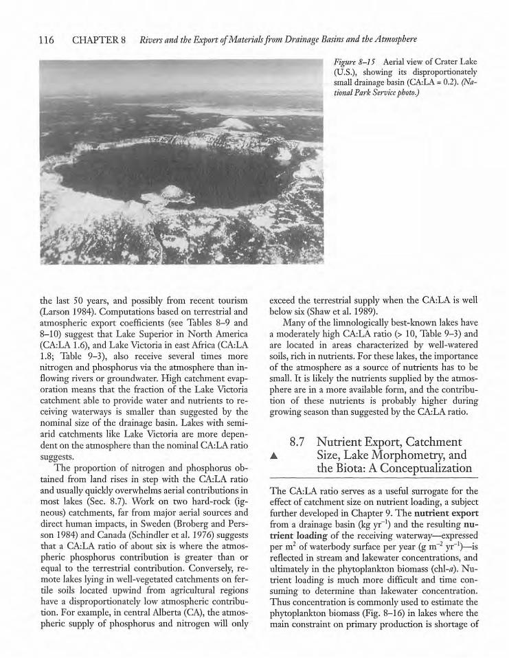
116 CHAPTER 8 Rivers and the Export ofMaterialsfrom Drainage Basins and the Atmosphere
the last 50 years, and possibly from recent tourism(Larson 1984). Computations based on terrestrial andatmospheric export coefficients (see Tables 8-9 and8-10) suggest that Lake Superior in North America(CA:LA 1.6), and Lake Victoria in east Africa (CA:LA1.8; Table 9-3), also receive several times morenitrogen and phosphorus via the atmosphere than inflowing rivers or groundwater. High catchment evaporation means that the fraction of the Lake Victoriacatchment able to provide water and nutrients to receiving waterways is smaller than suggested by thenominal size of the drainage basin. Lakes with semi-arid catchments like Lake Victoria are more dependent on the atmosphere than the nominalCA:LAratiosuggests.The proportion of nitrogen and phosphorus ob
tained from land rises in step with the CA:LA ratioand usuallyquicklyoverwhelms aerial contributions inmost lakes (Sec. 8.7). Work on two hard-rock (igneous) catchments, far from major aerial sources anddirect human impacts, in Sweden (Broberg and Persson 1984) and Canada (Schindler et al. 1976) suggeststhat a CA:LA ratio of about six is where the atmospheric phosphorus contribution is greater than orequal to die terrestrial contribution. Conversely, remote lakes lying in well-vegetated catchments on fertile soils located upwind from agricultural regionshave a disproportionately low atmospheric contribution. For example, in central Alberta (CA), the atmospheric supply of phosphorus and nitrogen will only
Figure 8-15 Aerial view of Crater Lake(U.S.), showing its disproportionatelysmall drainage basin (CA:LA = 0.2). (National Park Service photo.)
exceed the terrestrial supply when the CA:LA is wellbelow six (Shaw et al. 1989).Many of the limnologically best-known lakes have
a moderately high CA:LAratio (> 10,Table 9-3) andare located in areas characterized by well-wateredsoils, rich in nutrients. For these lakes, the importanceof the atmosphere as a source of nutrients has to besmall. It is likely the nutrients supplied by the atmosphere are in a more available form, and the contribution of these nutrients is probably higher duringgrowingseason than suggestedby the CA:LAratio.
8.7 Nutrient Export, Catchment• Size, Lake Morphometry, and
the Biota:A Conceptualization
The CA:LA ratio serves as a useful surrogate for theeffect of catchment size on nutrient loading, a subjectfurther developed in Chapter 9. The nutrient exportfrom a drainage basin (kg yr-1) and the resulting nutrient loading of the receiving waterway—expressedperm2 ofwaterbody surface per year (g m~2 yr-1)—isreflected in stream and lakewater concentrations, andultimately in the phytoplankton biomass (chl-tf). Nutrient loading is much more difficult and time consuming to determine than lakewater concentration.Thus concentration is commonlyused to estimate thephytoplankton biomass (Fig. 8-16) in lakeswhere themain constraint on primary production is shortage of
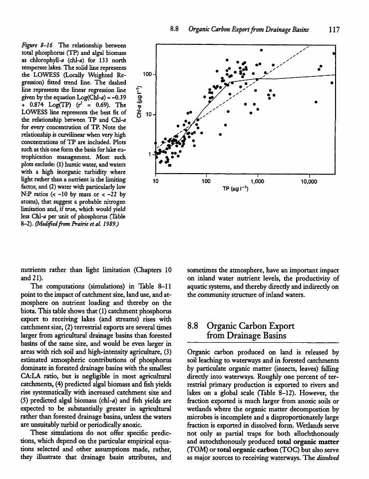
8.8 Organic Carbon Exportfrom Drainage Basins 117
Figure 8-16 The relationship betweentotal phosphorus (TP) and algal biomassas chlorophyll-* (chl-tf) for 133 northtemperate lakes. The solid line representsthe LOWESS (Locally Weighted Regression) fitted trend line. The dashedline represents the linear regression linegiven bythe equation Log(Chl-*) =-0.39+ 0.874 Log(TP) (r2 = 0.69). TheLOWESS line represents the best fit ofthe relationship between TP and Chl-tffor every concentration of TP. Note therelationship is curvilinear whenveryhighconcentrations of TP are included. Plotssuch as this one form the basis for lake eu-trophication management. Most suchplots exclude: (1)humicwater,andwaterswith a high inorganic turbidity wherelightratherthana nutrientis the limitingfactor, and (2)waterwith particularlylowN:P ratios (< ~10 by mass or < -22 byatoms), that suggest a probable nitrogenlimitationand, if true, whichwouldyieldlessChi-* per unit of phosphorus (Table8-2). (Modifiedfrom Prairie etal. 1989.)
O
100-
•s
•&£^-•
•
•
•
10-
•c*r%y. •& y
•
•
(
•
1-
m
i i
10 100
nutrients rather than light limitation (Chapters 10and 21).The computations (simulations) in Table 8-11
point to the impactof catchmentsize,landuse,and atmosphere on nutrient loading and thereby on thebiota.This tableshows that (1)catchment phosphorusexport to receiving lakes (and streams) rises withcatchment size, (2) terrestrial exports are several timeslargerfromagricultural drainage basins than forestedbasins of the same size, and would be even larger inareas with rich soil and high-intensityagriculture, (3)estimated atmospheric contributions of phosphorusdominate in forested drainage basins with the smallestCA:LA ratio, but is negligible in most agriculturalcatchments, (4) predicted algal biomass and fish yieldsrise systematically with increased catchment size and(5) predicted algal biomass (chl-tf) and fish yields areexpected to be substantially greater in agriculturalrather than forested drainage basins, unless the watersareunsuitably turbidor periodically anoxic.These simulations do not offer specific predic
tions, which depend on the particular empirical equations selected and other assumptions made, rather,they illustrate that drainage basin attributes, and
1,000
TPOigr1)10,000
sometimes the atmosphere, havean important impacton inland water nutrient levels, the productivity ofaquatic systems, and therebydirecdyand indirecdyonthe community structure of inlandwaters.
8.8 Organic Carbon Exportfrom DrainageBasins
Organic carbon produced on land is released bysoil leaching to waterways and in forested catchmentsby particulate organic matter (insects, leaves) fallingdirecdy into waterways. Roughly one percent of terrestrial primary production is exported to rivers andlakes on a global scale (Table 8-12). However, thefraction exported is much larger from anoxic soils orwedands where the organic matter decompostion bymicrobes is incomplete and a disproportionately largefractionis exported in dissolved form.Wedands servenot only as partial traps for both allochthonouslyand autochthonously produced total organic matter(TOM) or total organic carbon (TOC) but also serveas major sources to receiving waterways. The dissolved
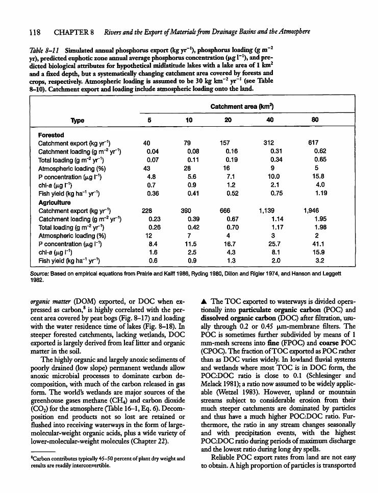
118 CHAPTER 8 Rivers and the Export ofMaterialsfrom Drainage Basins and the Atmosphere
Table 8-11 Simulated annual phosphorus export (kg yr"1), phosphorus loading (gm"2yr), predicted euphoric zone annual average phosphorus concentration (ng1"!), and predicted biological attributes for hypothetical midlatitude lakes with a lake area of1km2anda fixed depth, but a systematically changing catchment areacovered byforests andcrops, respectively. Atmospheric loading is assumed to be 30 kg km"2 yr"1 (see Table8-10).Catchmentexportand loading include atmospheric loading onto the land.
Type
Catchment area (km2)
5 10 20 40 80
Forested
Catchment export (kgyr1) 40 79 157 312 617
Catchment loading (g nrr2 yr1) 0.04 0.08 0.16 0.31 0.62
Total loading (g nrr2 yr1) 0.07 0.11 0.19 0.34 0.65
Atmospheric loading (%) 43 28 16 9 5
P concentration (u.g I"1) 4.8 5.6 7.1 10.0 15.8
chl-a (u.g I"1) 0.7 0.9 1.2 2.1 4.0
Fish yield (kg ha-1 yr1) 0.36 0.41 0.52 0.75 1.19
AgricultureCatchment export (kgyr1) 228 390 666 1,139 1,946Catchment loading (g nrr2 yr1) 0.23 0.39 0.67 1.14 1.95
Total loading(g nrr2 yr1) 0.26 0.42 0.70 1.17 1.98
Atmospheric loading (%) 12 7 4 3 2
P concentration (u.g I"1) 8.4 11.5 16.7 25.7 41.1
chl-a (fig I"1) 1.6 2.5 4.3 8.1 15.9
Fishyield (kg ha-1 yr1) 0.6 0.9 1.3 2.0 3.2
Source: Based on empirical equations from Prairie and Kalff1986, Ryding 1980, Dillon and Rigler 1974, and Hanson and Leggett1982.
organic matter (DOM) exported, or DOC when expressed as carbon,8 is highly correlated with the percent area coveredbypeat bogs (Fig.8-17) and loadingwith the water residence time of lakes (Fig. 8-18). Insteeper forested catchments, lackingwedands, DOCexportedis largelyderived from leafUtterand organicmatter in the soil.The highlyorganicand largelyanoxic sediments of
poorly drained (low slope) permanent wedands allowanoxic microbial processes to dominate carbon decomposition, with much of the carbon released in gasform. The world's wedands are major sources of thegreenhouse gases methane (CH4) and carbon dioxide(C02) for the atmosphere (Table 16-1, Eq. 6).Decomposition end products not so lost are retained orflushed into receiving waterways in the form of large-molecular-weight organic acids, plus a widevarietyoflower-molecular-weight molecules (Chapter 22).
8Carbon contributes typically 45-50 percent of plant dryweightandresultsarereadilyinterconvertible.
• The TOC exported to waterways is divided operationally into particulate organic carbon (POC) anddissolved organic carbon (DOC) after nitration, usually through 0.2 or 0.45 u,m-membrane filters. ThePOC is sometimes further subdivided by means of 1mm-mesh screens into fine (EPOC) and coarse POC(CPOC).The fractionofTOC exportedasPOC ratherthan as DOC varieswidely. In lowland fluvial systemsand wedands where most TOC is in DOC form, thePOGDOC ratio is close to 0.1 (Schlesinger andMelack1981); a ratio now assumed to bewidelyapplicable (Wetzel 1983). However, upland or mountainstreams subject to considerable erosion from theirmuch steeper catchments are dominated by particlesand thus have a much higher POGDOC ratio. Furthermore, the ratio in any stream changes seasonallyand with precipitation events, with the highestPOGDOC ratioduringperiods ofmaximum dischargeand the lowest ratio during longdry spells.Reliable POC export rates from land are not easy
to obtain.Ahighproportion of particles is transported
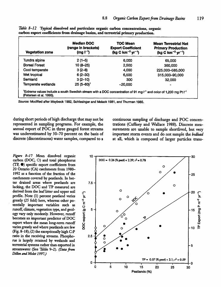
8.8 Organic Carbon Exportfrom Drainage Basins 119
Table 8—12 Typical dissolved and particulate organic carbon concentrations, organiccarbon export coefficients from drainage basins, and terrestrial primary production.
Median DOC TOC Mean Mean Terrestrial Net(range in brackets) Export Coefficient Primary Production
Vegetation zone (mgl-1) (kgCkm-2yr1) (kgCknrV"1)
Tundra alpine 2(1-5) 6,000 65,000Boreal Forest 10 (8-25) 2,500 360,000Cool temperate 3(2-8) 4,000 225,000-585,000Wet tropical 6 (2-30) 6,500 315,000-90,000Semiarid 3 (2-10) 300 32,000Temperate wetlands 25 (5-60)1 -20,000 -
'Extreme values include •a south Swedish stream with a DOCconcentration of 91 mg I_1 and color of 1,200 mg Pt I-1(Petersen etal. 1995).
Source: Modified after Meybeck 1982, Schlesinger and Melack 1981, and Thurman 1985.
during shortperiods ofhighdischarge thatmay not berepresented in sampling programs. For example, theannual export of POC in three gaugedforest streamswas underestimated by 30-70 percent on the basis ofdiscrete (discontinuous) watersamples, compared to a
Figure 8-17 Mean dissolved organiccarbon (DOC, O) and total phosphorus(TP, •) specific export coefficients from20 Ontario (CA) catchments from 1980-1992 as a function of the fraction of thecatchments covered by peadands. In better drained areas where peadands arelacking, the DOC and TP measured arederived from the leaflitteranduppersoilprofile. Note (1) percent peadand variesgready (25 fold) here,whereas other potentially important variables such asrunoff, climate, vegetation type, andgeologyvaryonlymodesdy. However, runoffbecomes an importantpredictorof DOCexport where the mean long-term runoffvaries greadyandwherepeadandsare few(Fig. 8-18); (2)the exceptionally highC:Pratio in the receiving streams. Phosphorus is largely retained by wedands andterrestrial systems rather thanexported instreamwater (See Table 9-2). (Data fromDillon andMolot 1997.)
EOB•coaxa>
O
continuous sampling of discharge and POC concentrations (Cufmey and Wallace 1988). Discrete measurements are unable to sample shortlived, but veryimportantstorm events and do not sample the bedloadat all, which is composed of larger particles trans-
T10 15 20
Peatlands (%)
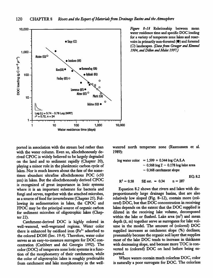
120 CHAPTER 8 Rivers and the Export ofMaterialsfrom Drainage Basins and theAtmosphere
Eo
CDc'i5COo
OOO
• Slapy(G)
000- •
Marion (CA)°n. • Ivankovo (HR)
Bev(UM# Vv •Kremenchug(UA)100- N.* Rybinsk (RU)
Rndtey(US)o \\ 0
X-oLawrence (US)* h.
10- M1° fc*^k Balotoa (KU) • °
i
Log (L)= 3.74r2 = 0.72, n =
-0.78 Log (WRT)24
| I i ' '-"•10 100 1,000
Water residence time (days)10,000
Figure 8-18 Relationship between meanwater residence timeand specific DOC loadingfor a variety of temperate zonelakes and reservoirs in primarily non-forested (•) andforested(O) landscapes. (Datafrom Groeger and Khrnnel1984, andDillonandMolot1997.)
ported in association with the stream bed rather thanwith the water column. Even so, allochthonously derived CPOC iswidely believed to be largely degradedon the land and to sediment rapidly (Chapter 20),playing aminor role in the planktonic carbon cycle oflakes. Nor is much known about the fate of the sometimes abundant ultrafine allochthonous POC (<50pm) in lakes. But the allochthonously derived CPOCis recognized of great importance in lotic systemswhere it is an important substrate for bacteria andfungi andserves, togetherwith the attached microbes,asa source offoodfor invertebrates (Chapter25). Following its sedimentation in lakes, the CPOC andFPOC maybe the principal sourceof organiccarbonfor sediment microbes of oligotrophic lakes (Chapter 22).Catchment-derived DOC is highly colored in
well-watered, well-vegetated regions. Water colorthere is enhanced byoxidized iron (Fe3+ adsorbed tothe colored DOM (Sec. 19.4).Therefore, water colorserves as an easy-to-measure surrogatefor DOC concentration (Cuthbert and del Georgio 1992). Thecolor(DOC) of temperatezoneloticsystems isa function of the morphometry of their catchments, whilethe color of oligotrophic lakes is roughly predictablefrom catchment and lakemorphometry in the well-
watered north temperate zone (Rasmussen et al.1989):
logwater color = 1.599 + 0.344log CA:LA- 0.568 log z - 0.178 log lake area- 0.368 catchment slope
EQ.8.2R2 = 0.58 SE est. = 0.34 n = 287
Equation 8.2 shows that rivers and lakes withdisproportionately large drainage basins, that are alsorelatively low sloped (Fig. 8-12), contain more (colored)DOC, but that DOC concentration in receivinglakes depends on the extent that the DOC supplied isdiluted in the receiving lake volume, decomposedwithin the lake or flushed. Lake area (m2) and meandepth (z, m)together serve assurrogates for lake volume in the model. The amount of (colored) DOCsupplied increases as catchment slope (%) declines;presumably because theorganic soil layer thatsuppliesmost of the lake DOC tends to increase in thicknesswithdecreasing slope, andbecause moreTOC is converted to (colored) DOC on land before being exported.Where waters contain much colorless DOC, color
is naturally a poor surrogate for DOC. The colorless
8.8 Organic Carbon Exportfrom Drainage Basins 121
portion of DOC normallyincreases as total DOC declines in well-watered and well-vegetated regions ofnorthern Europe and northeastern North America.Conversely, in slowly flushed, and in closed salinelakes in the prairie region of North America, the colorless fraction increases with increasing DOC (Curtisand Adams 1995). This is probablythe result of longwater retention (slow flushing), allowing evaporativeconcentration of DOC, particle formation and sedimentation, respiration, and photobleaching (Chapter10)of the entering organicmatter.Not all allochthonous TOC (and inorganic plant
nutrients) is received via inflowing streams or rivers.Some is receivedvia groundwater,DOC deposition inprecipitation, and as POC in the atmosphere deposited on the water surface (-0.1 g m~2 yr-1) (Sec.22.6).
Highlights• Lotic (flowing-water) systems are complete ecosystems intimately coupled to their drainage basins.They are more than conduits of organicmatter andnutrientsfromcatchments to receiving lakes andwetlands.
• A widely used and easily determined surrogate forstreamsizeis streamorder,a lineargeomorphic characteristicof lotic systems.
• The river continuum concept is a useful frameworkforviewing loticsystems as longitudinally integratedsystems, linking stream size (order), energy input,and the processing of organic matter by the biotafrom headwater to mouth.
• The land-water transition zone(ecotone, or riparianzone)is characterized by sharp gradients in environmental factors, species composition, anddominatingspecies. The riparian zone isimportant in cycling andtransformingnutrients andorganic matter. Well-vegetated riparian zones are of great importance, reducing streambank erosion, trapping soil particles and
absorbed nutrients on landand, in agriculture, stimulating denitrification (N03 —» N2). All of these helpmaintain water quality and the traditional biota, including fish.The hyporheic zone is the transition zone in the vertical plane between the stream channel and subsurface sediments. It is an important habitat for the biotaand contains a mixture of surface waterand groundwater. This zone may extend laterally beyond theriver margin into the floodplain.A Rivers and their associated wedands receive, withincreasingly fewer exceptions, large quantities ofwastewater and agricultural runoff that impact thebiota. Superimposed is widespread channelization(straightening bends, resulting in more rapid discharge), channel deepening, bank erosion, aswell asseparation of rivers from their floodplains throughdike construction. Rivers are often dammed, reducing maximum discharge and its timing, the size ofdownstream wedands, and riverine biota. Promisingattempts at "river restoration," including reconnec-tionwithformer(drained) wetlands, are underway.The export of nutrients from catchments (kg yr"1)increases with increasing catchment size, slope, andrunoff. It is further affected by surficial geology (soilstructure) and land use. Nutrient exports per unitarea (km2) are low from well-vegetated catchmentsand exceptionally high from fields with seasonalcrops,high livestock densities, and in urban areas.Additional nutrients (and contaminants) enter waterways via the atmosphere.Atmospheric nutrient loading(kg km-2 yr"1) is low at high latitudes and rises totypically veryhigh downwind from rich agriculturaland urban areas. Lakes with small catchments, in relation to the surface area ofwater, areparticularly dependenton atmospheric inputs.The exportof organic matter fromland to the receivingwaterincreases withcatchmentareaand isparticularly high from wedands. Dissolved organic matter(DOM) from well-watered, vegetated regions is typicallycolored.
H R
9
Aquatic Systemsand their Catchments
9.1 Catchment Size
Inlandwater functioning is tighdy linked to the characteristics of their drainage basins and the ecoregionsin which they fie.1 The average slope (relief) ofdrainage basinsdecreases as the areaof catchments increases (Fig. 8-12a) resulting in large basins within aregion having the lowest slopes,whereas small catchments tend to be relatively steep. Similarly, drainagedensity (the total stream length per unit area) normally declines as catchment size increases (Fig.8-12b). Therefore, particulate matter with adsorbedplant nutrients or contaminantsleaves landat a higherrate per unit area, in a small catchment (Sec. 8.4),eventhough the total amount ofwater andparticulatematter exported (tonnes yr-1) will be smaller. At thesame time, more rapid runoff in smaller, steeperdrainage basins means reduced contact time betweenwater and the substrate, permitting less biological/chemical breakdown of substrate (weathering). Soilsare expected to be thinner because the rapid runofferodes and transports particles toward less steepportions of the catchment for at least partial storagethere. The net result is typically lower nutrient export
1*Ecoregions describe ecological zonation across the landscape,with an ecoregion commonlybased on similarityof climate, geology, land surface form, soil formation, primary production, terrestrialvegetation, and energyflow. (Landers et al. 1998)• "The ecosystem, consideredbymanyto be the fundamental ecological unit, is not definable in a wayto allow nutrient processes tobe assessed. The watershedis a muchmore realisticecological unit."(D.W. Schindler et al. 1976)
122
(kg yr-1) (Sec. 8.5) and lower dissolved salt content(Chapter 13) in lotic systems draining small, ratherthan large, catchmentswithin a particular climaticallyand geologically homogeneous region. Low-slopedrainage basins may also have areas of impededdrainage, forming wedands that release much dissolved and colored organic matter in higher rainfallzones (Fig. 8-18).
A 9.2 Catchment Form
The topography (geomorphology) of the landscapehelpsdetermine streammorphology aswell as the surface shapeand sizeof lakes, their underwater formanddepth (Sec 7.4), and the abundance of wedands (ifany). The system attributesaffect a variety of physicaland chemical characteristics of water that, togetherwith the system morphology, havea deciding effectonthe productivity and the typesof organisms present.Catchment topography (slope) is a function of
catchment size. Within any climatic/geologic regionthe steepness and total length of river channels typically decline as drainage basin size increases. Catchment area and lake area are also highly correlated(with the correlation coefficient r = 0.82), as shown ina study of 215 North American lakes (Table 9-1).Other correlations include those between lake depthand catchment area, depth and nutrient concentrations, phosphorusand nitrogen, and nutrient concentrations and algal biomass (chl-a). However, lake areais not only a function of catchment area but also ofcatchment geology because lakes on dense igneous
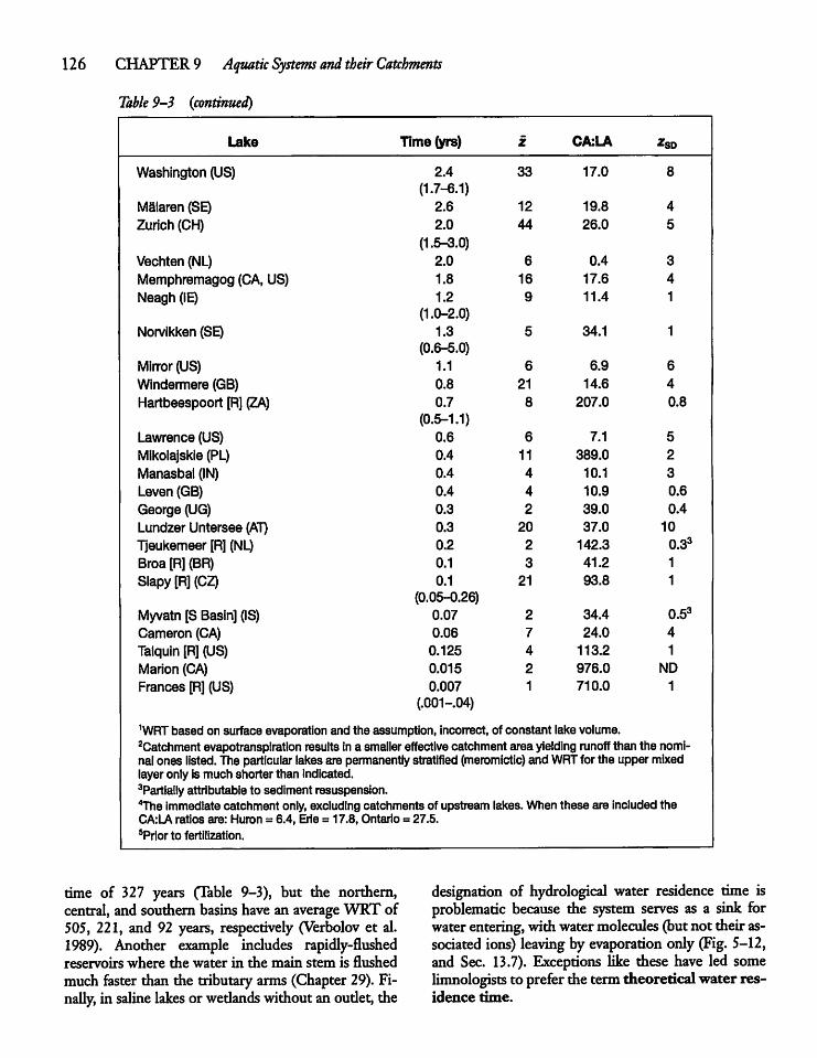
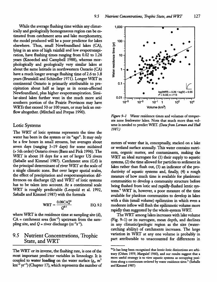
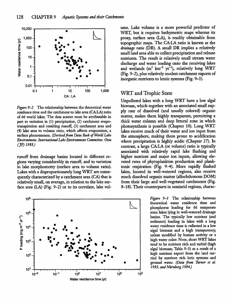
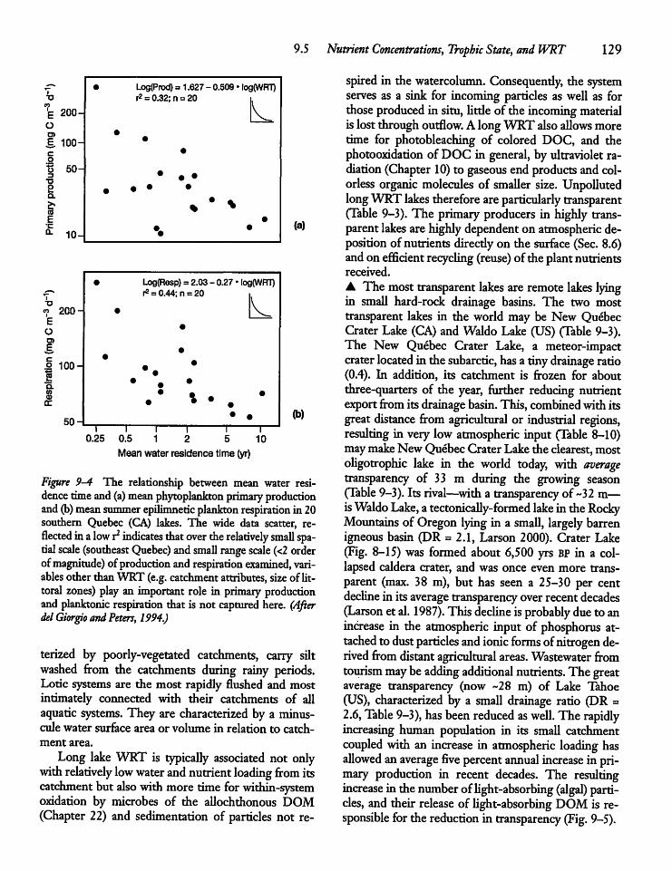
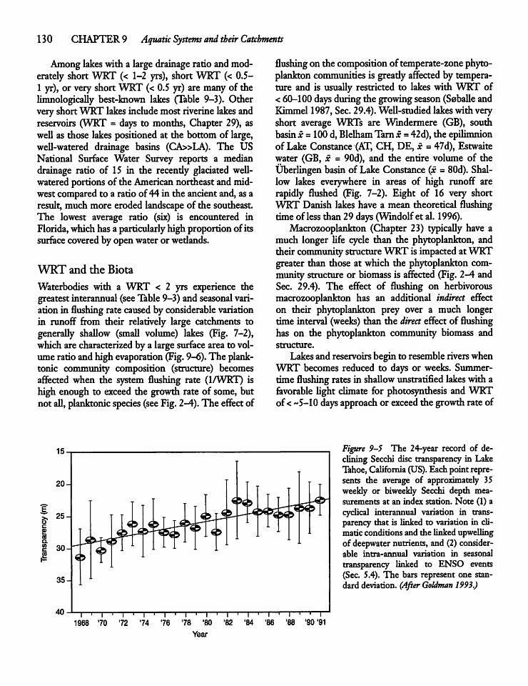
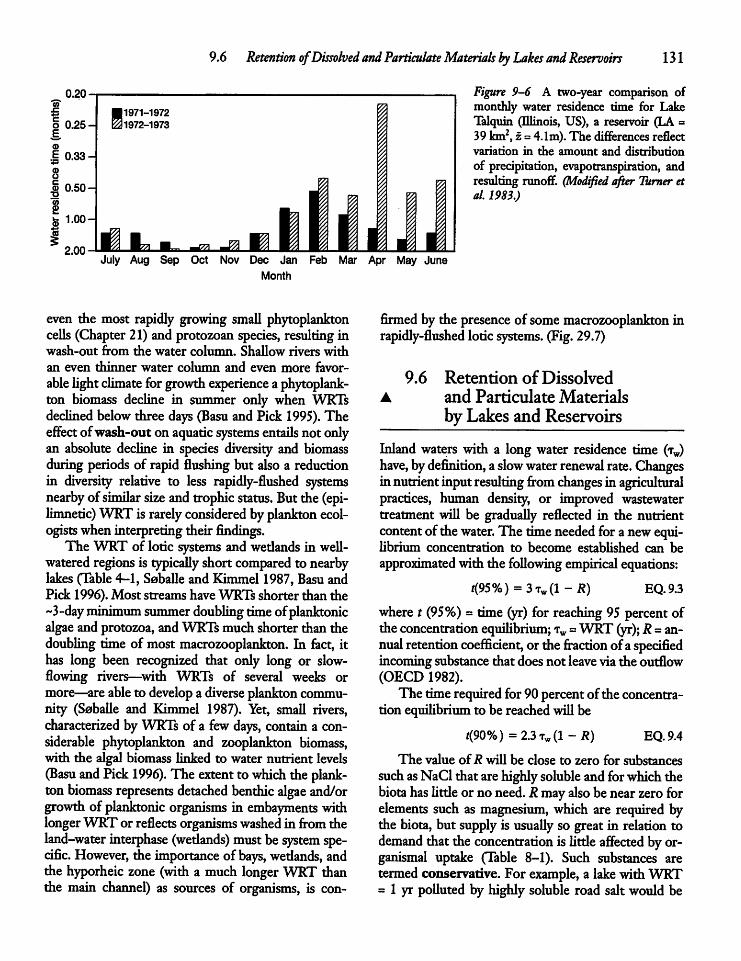
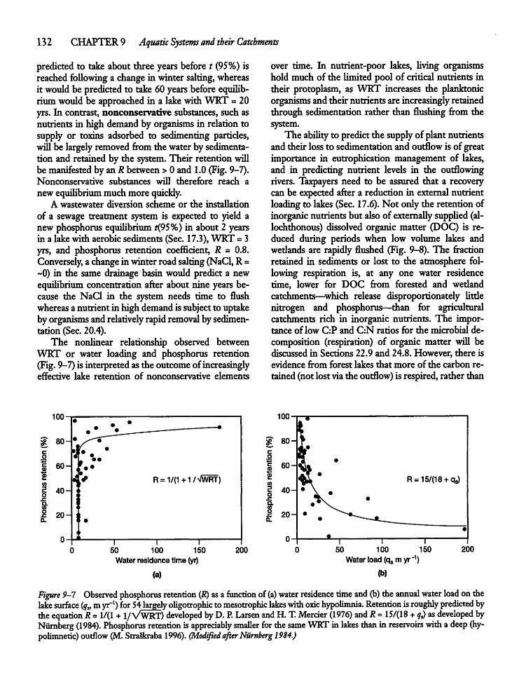
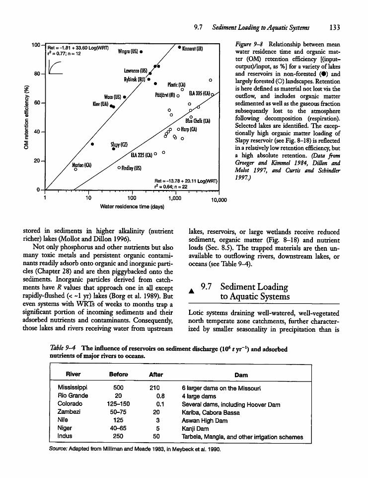
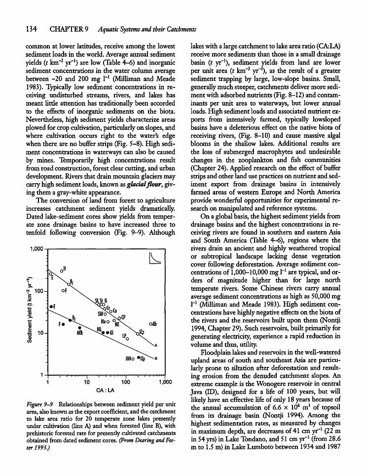
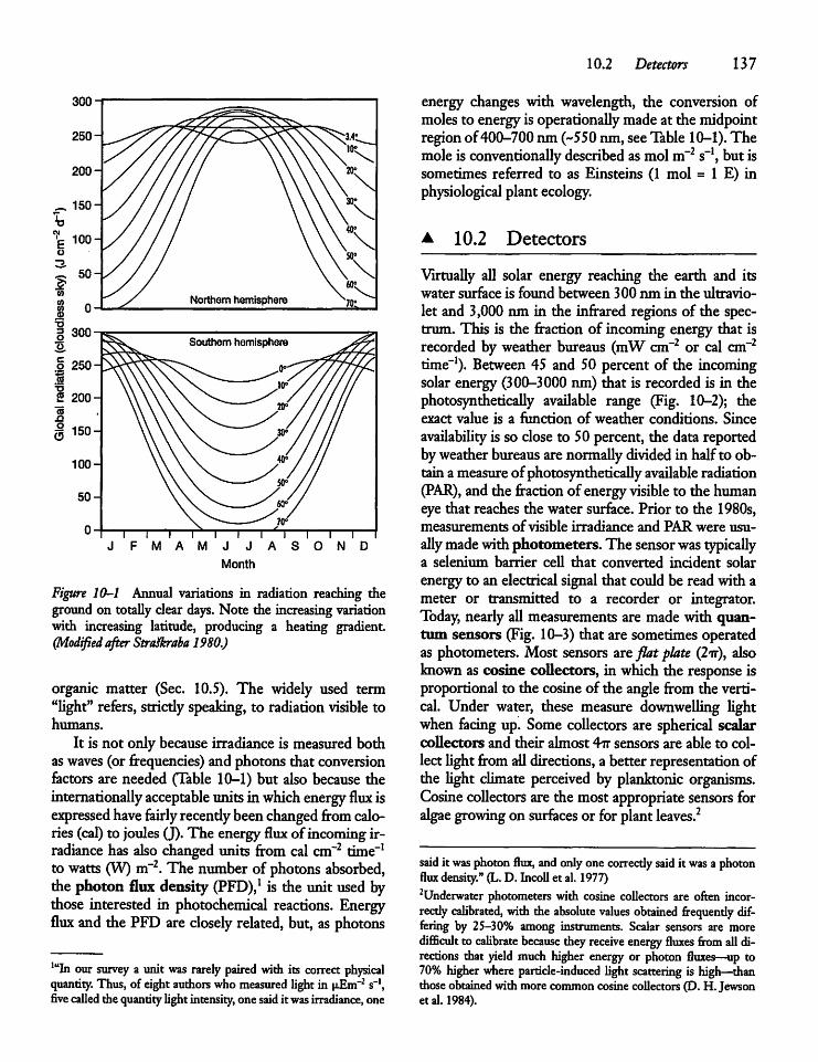
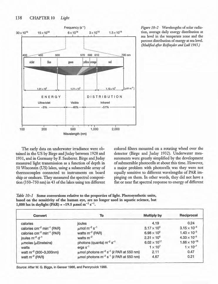
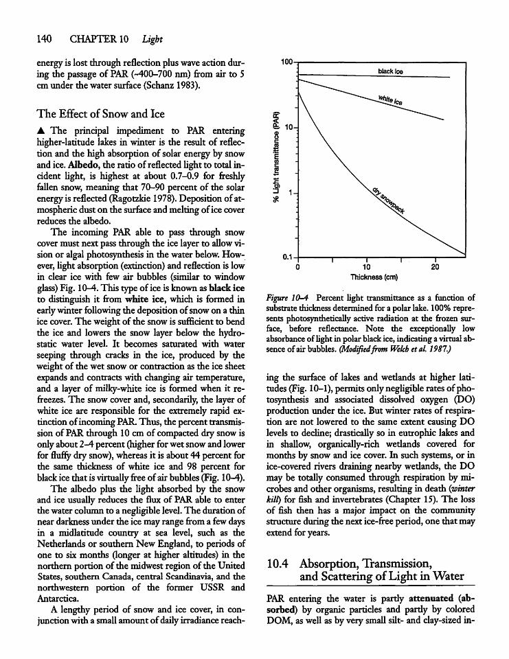
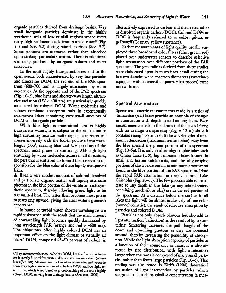
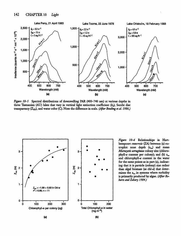
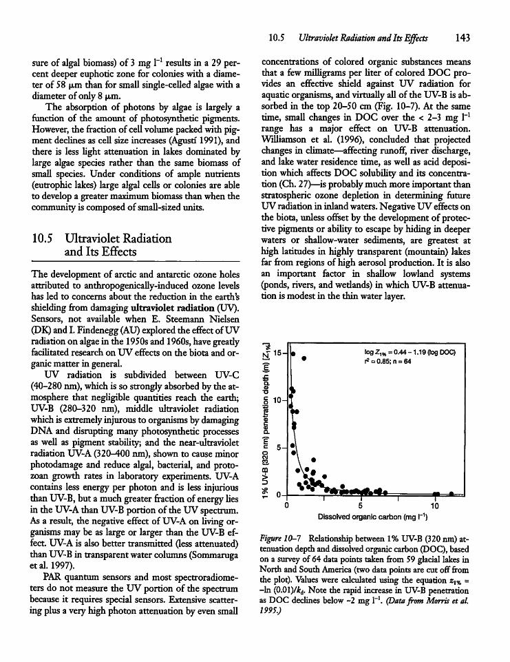
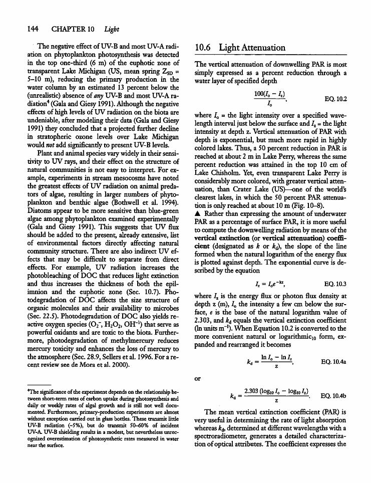
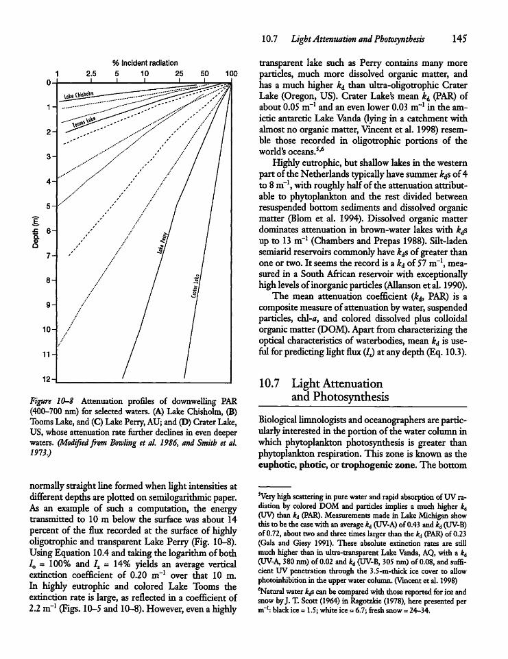
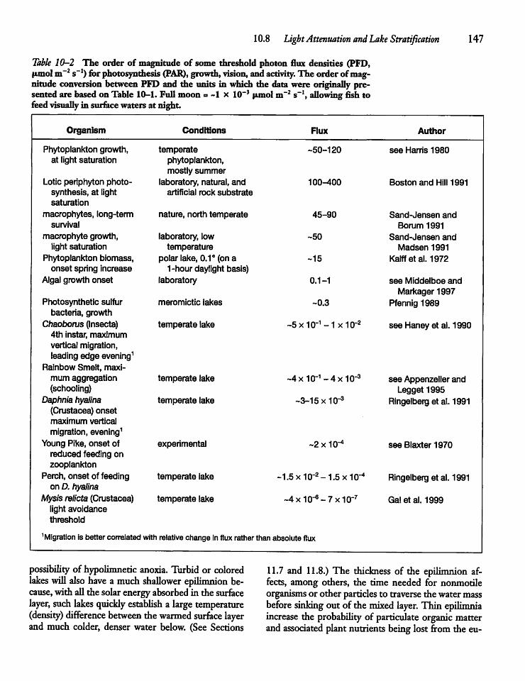
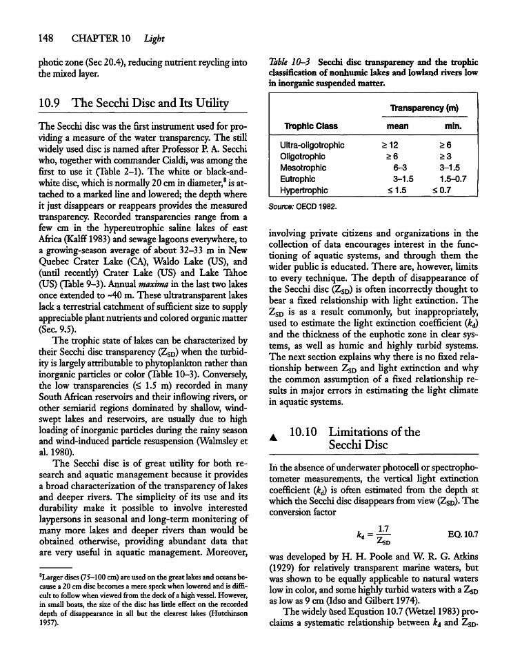
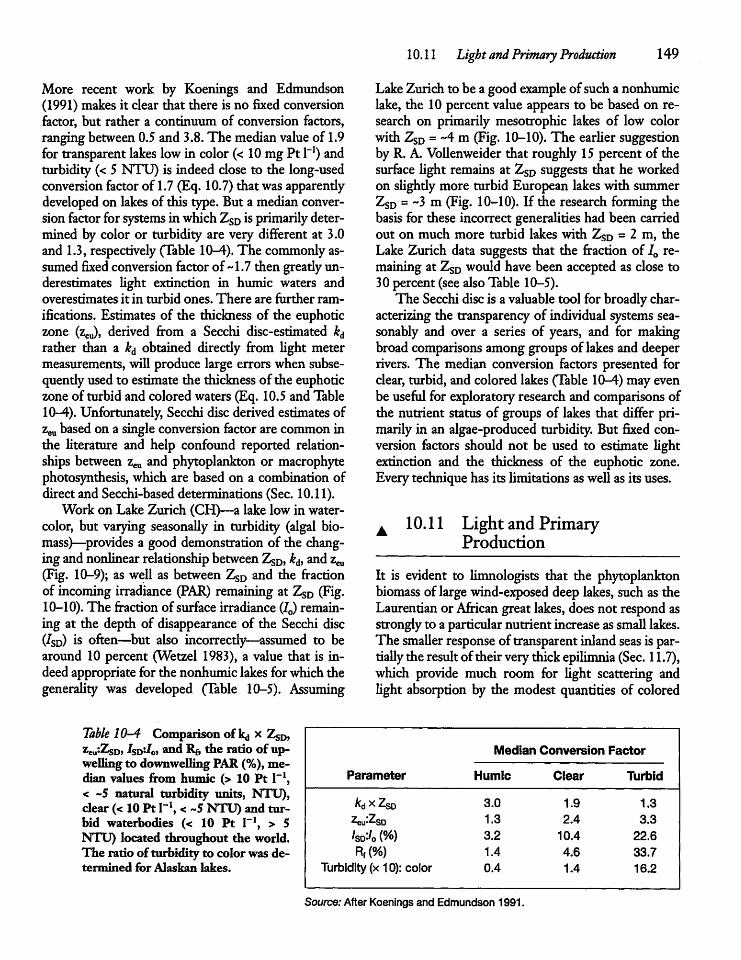
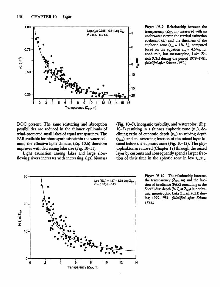
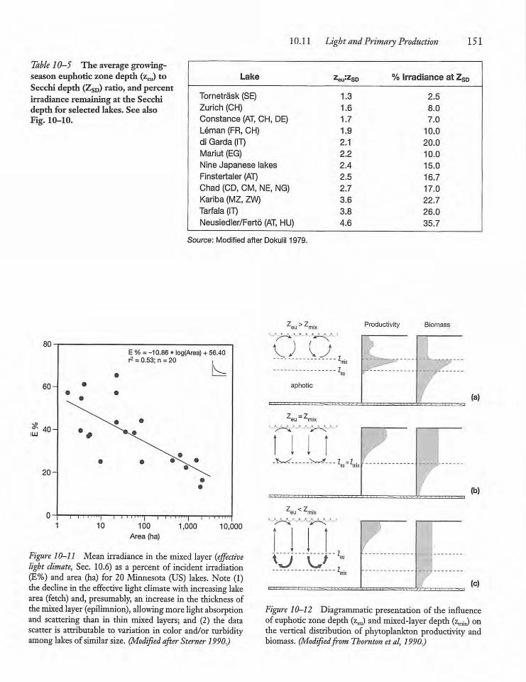
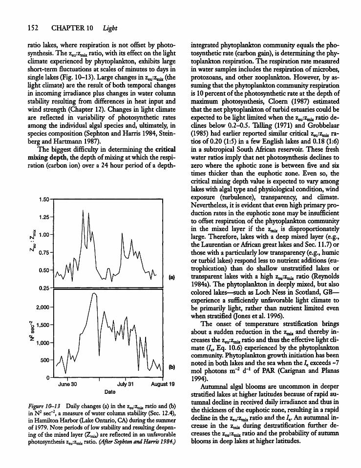
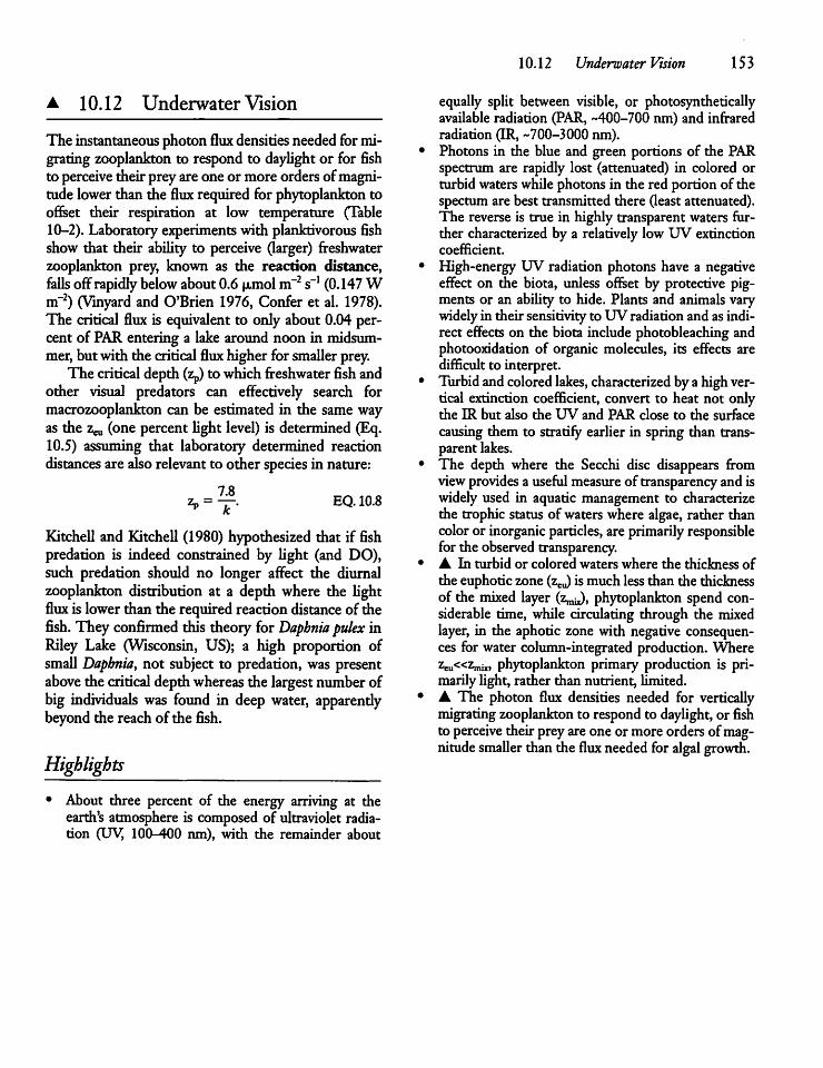
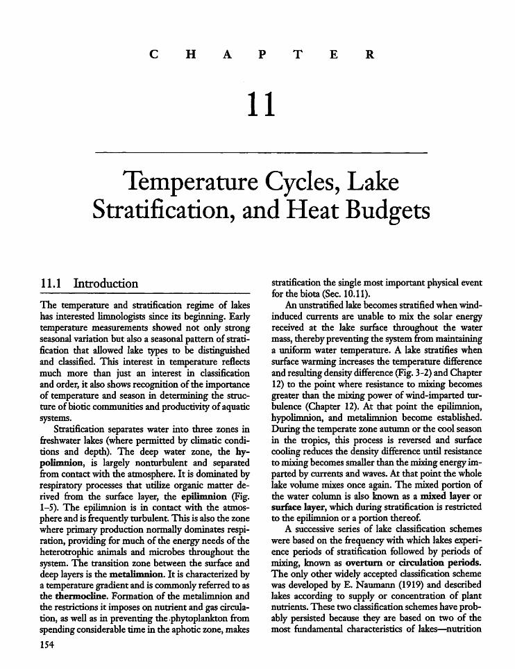
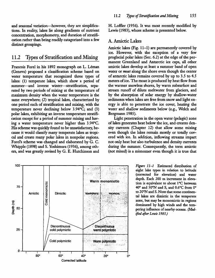
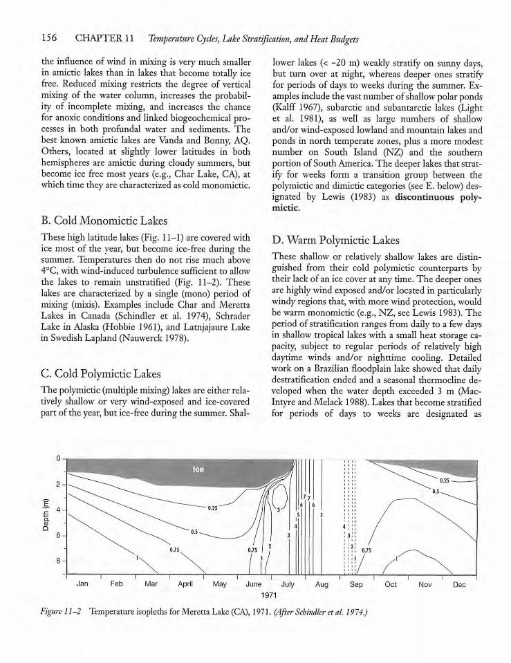
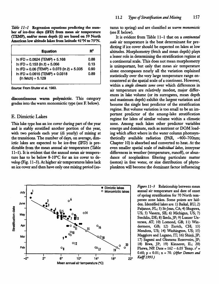
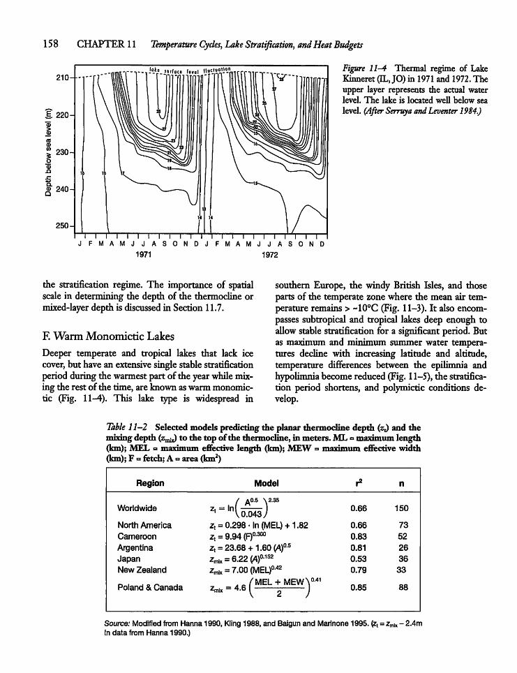
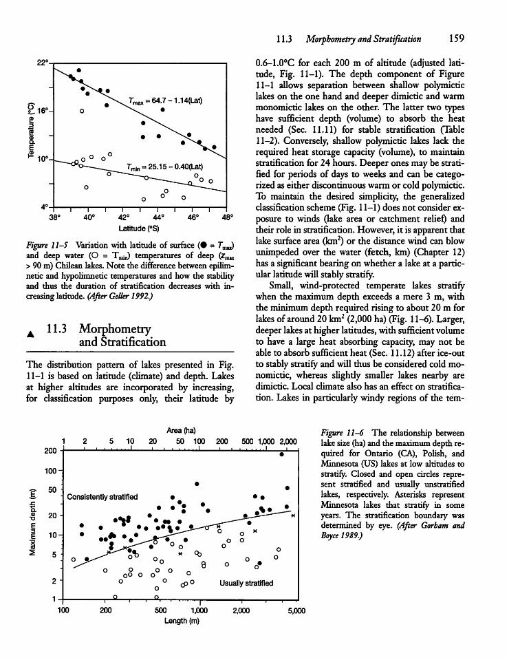
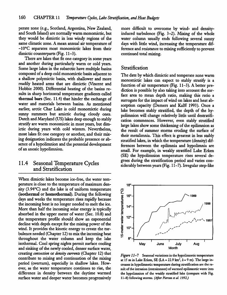
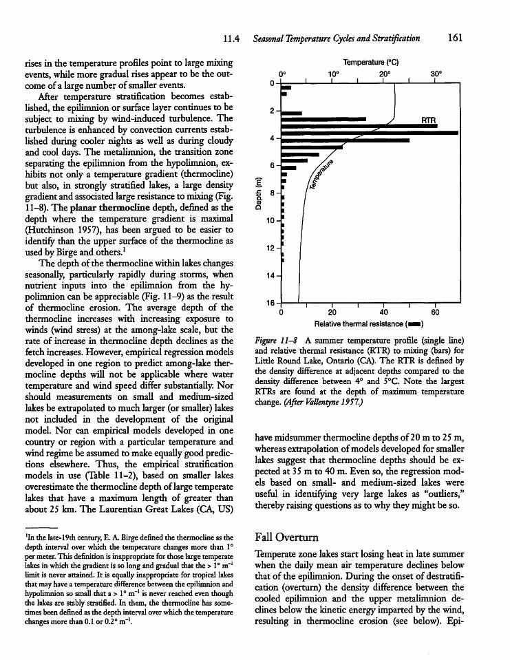
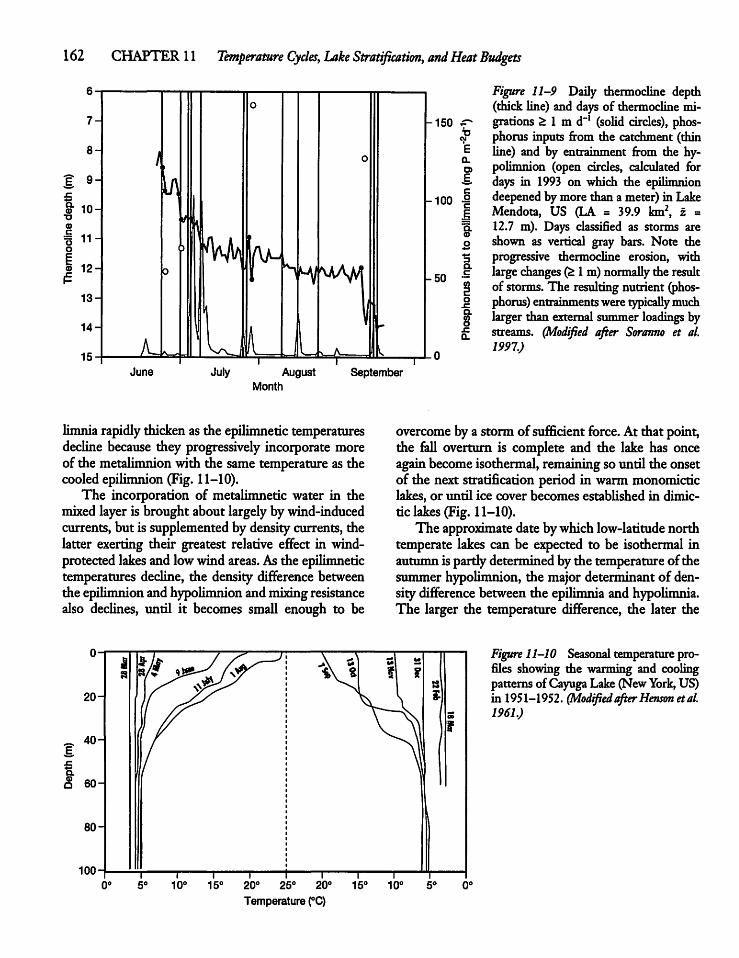
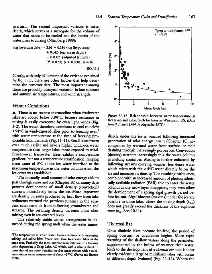
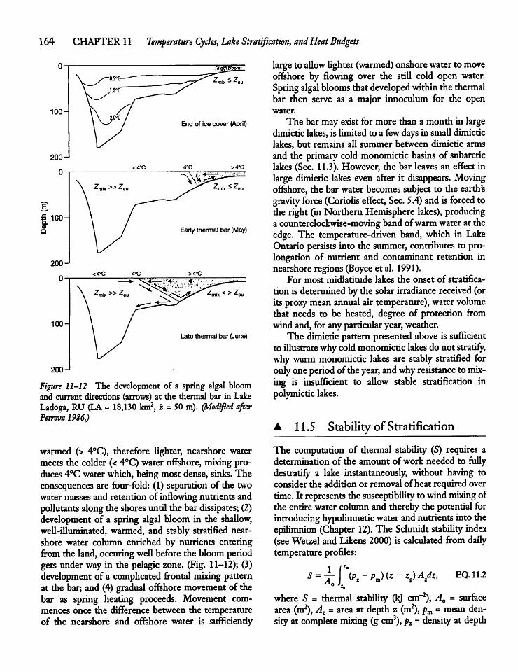
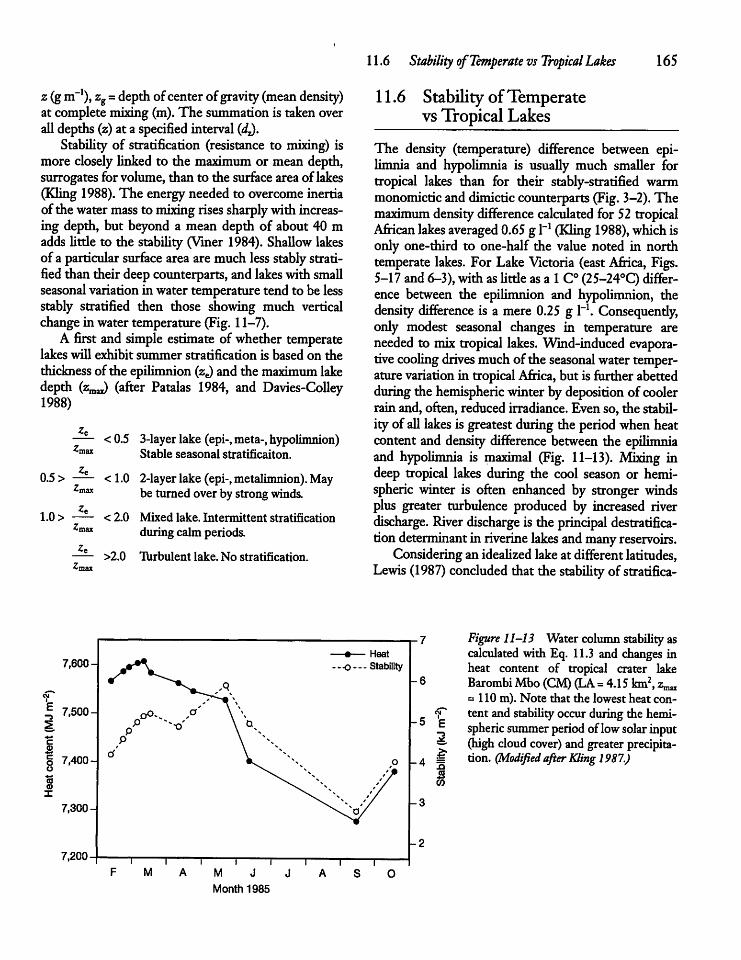
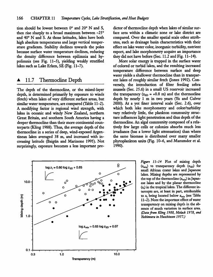
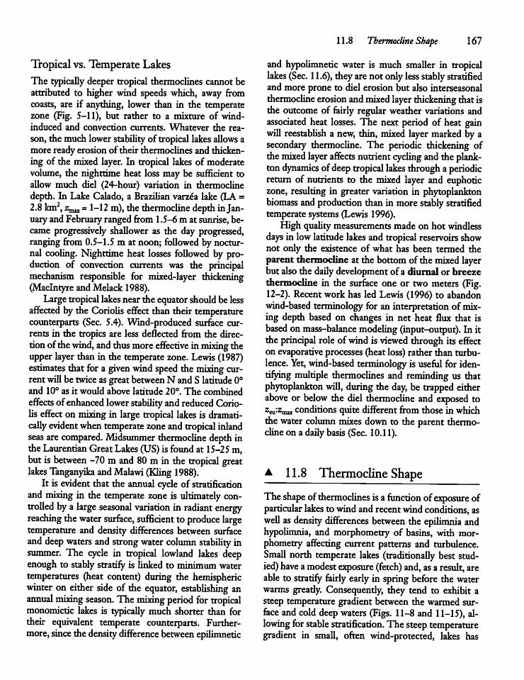
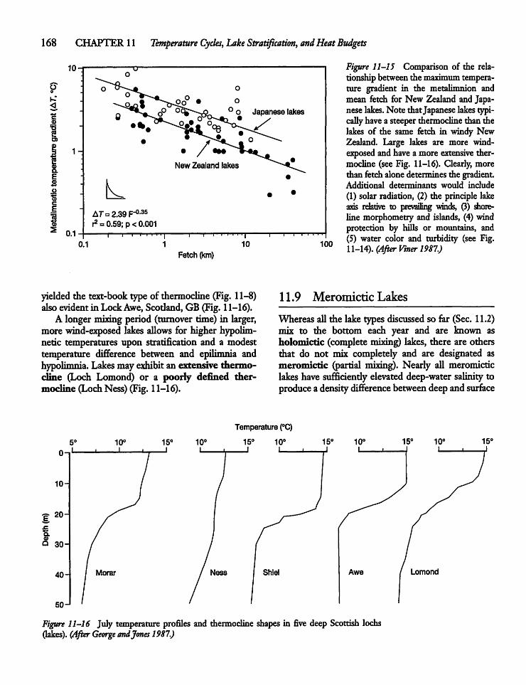
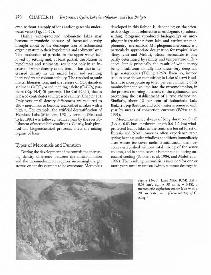
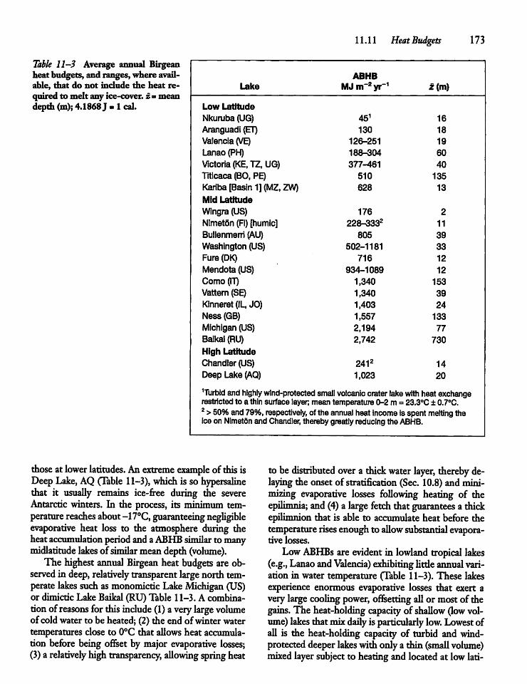
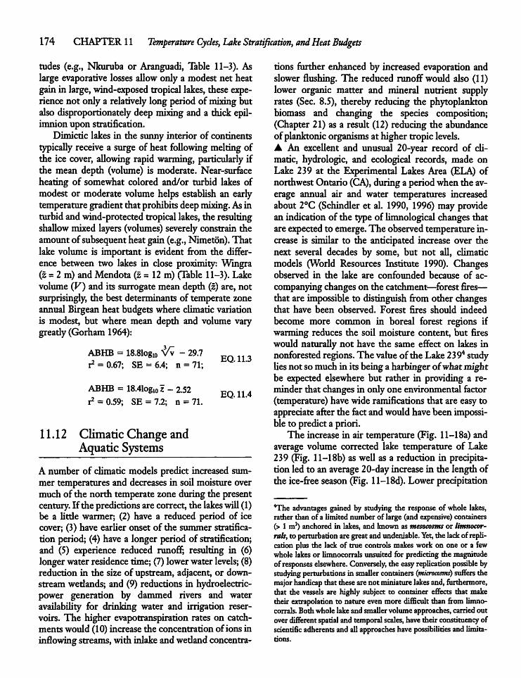
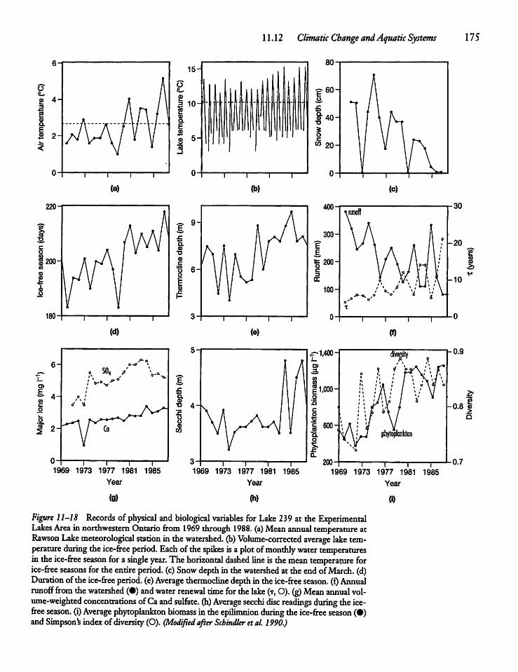
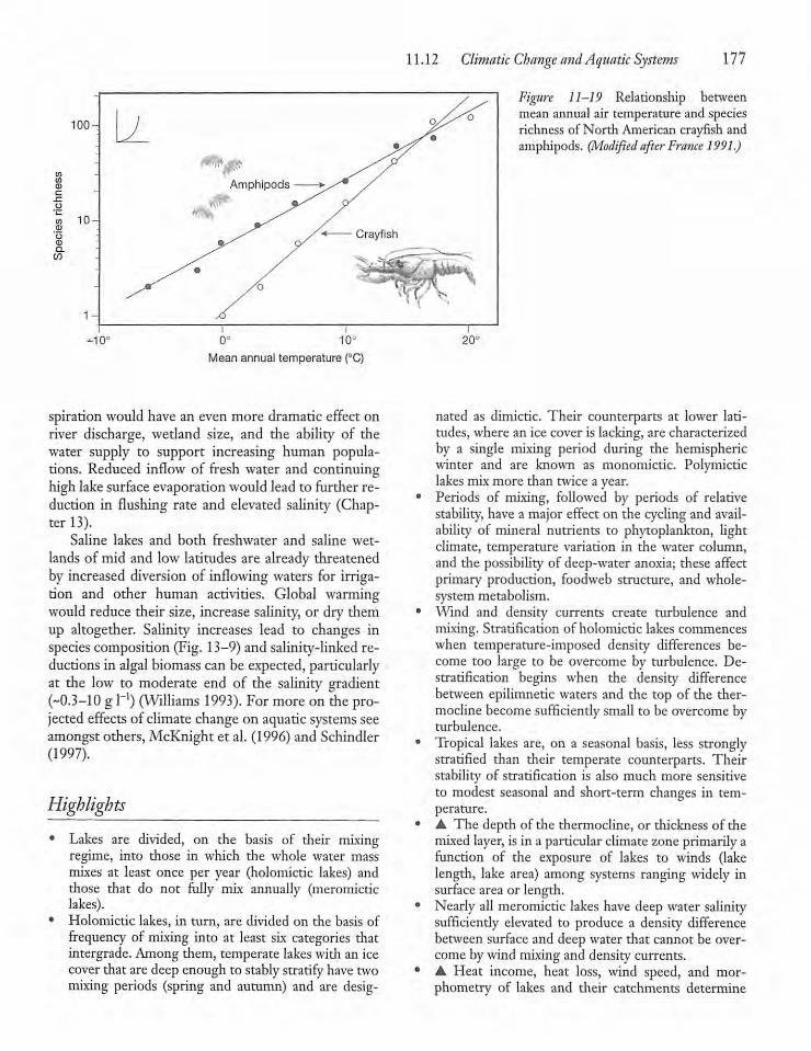

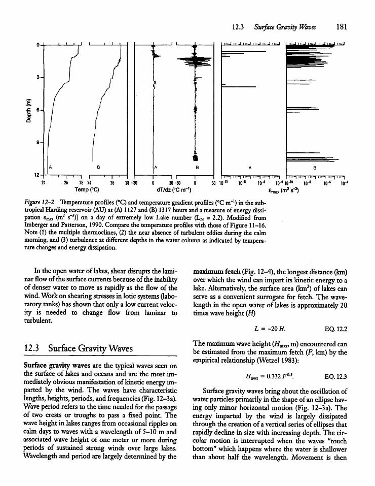
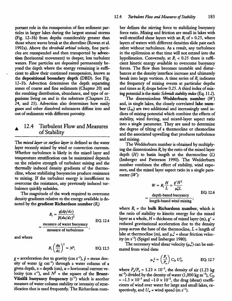
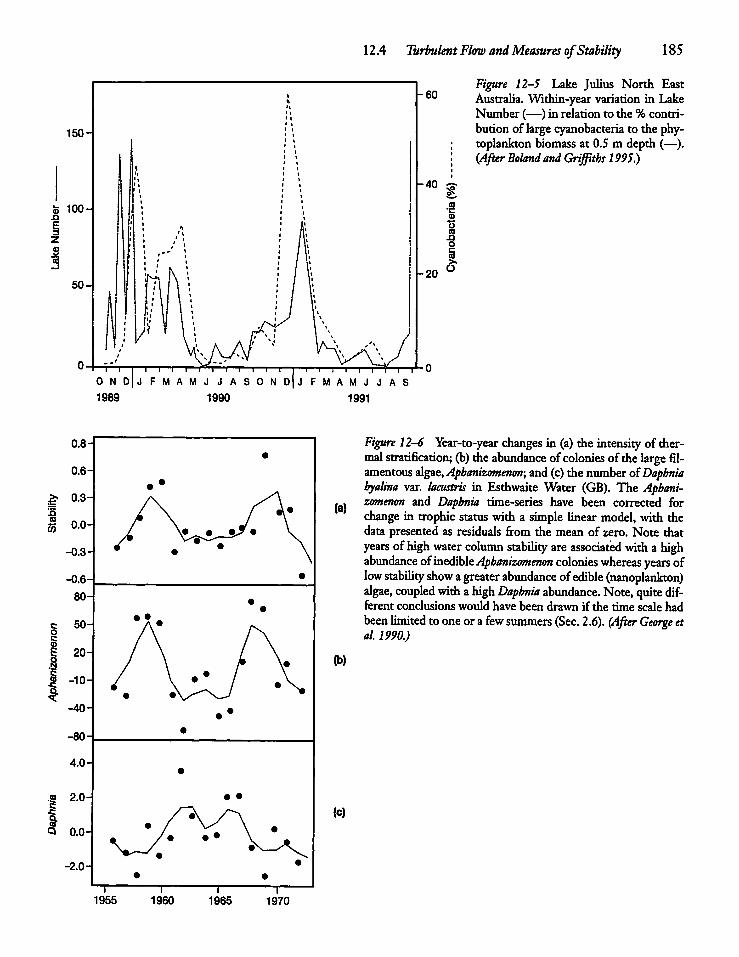
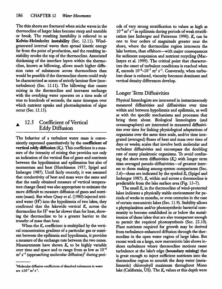
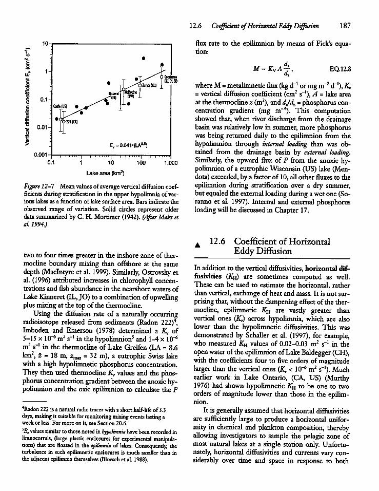
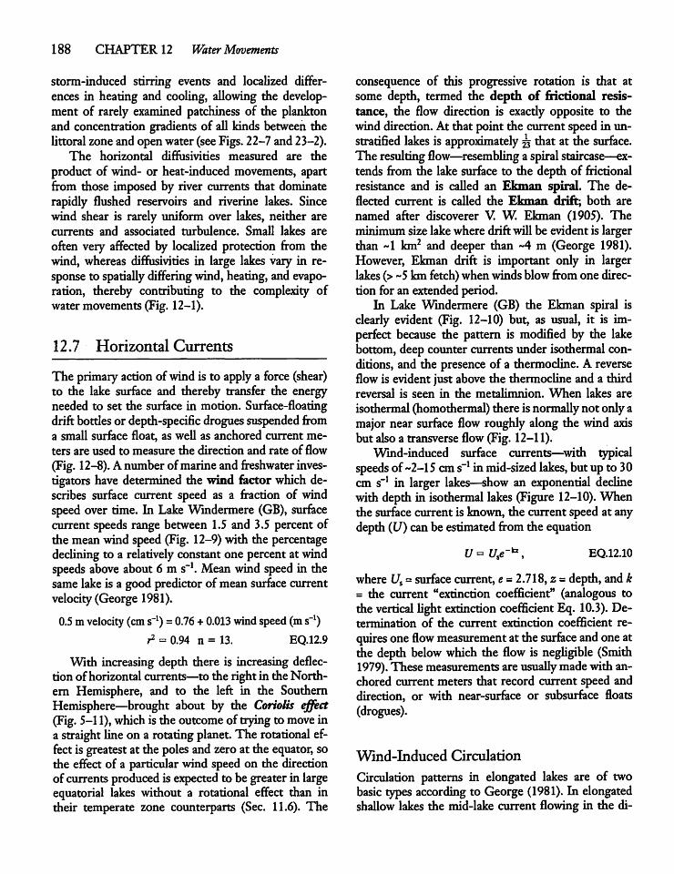
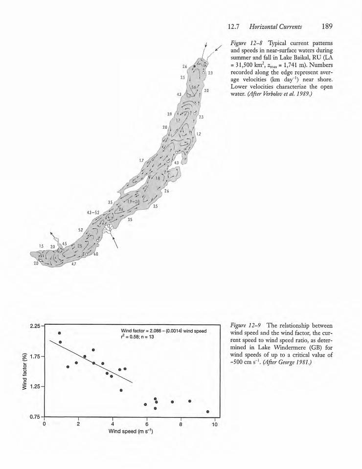
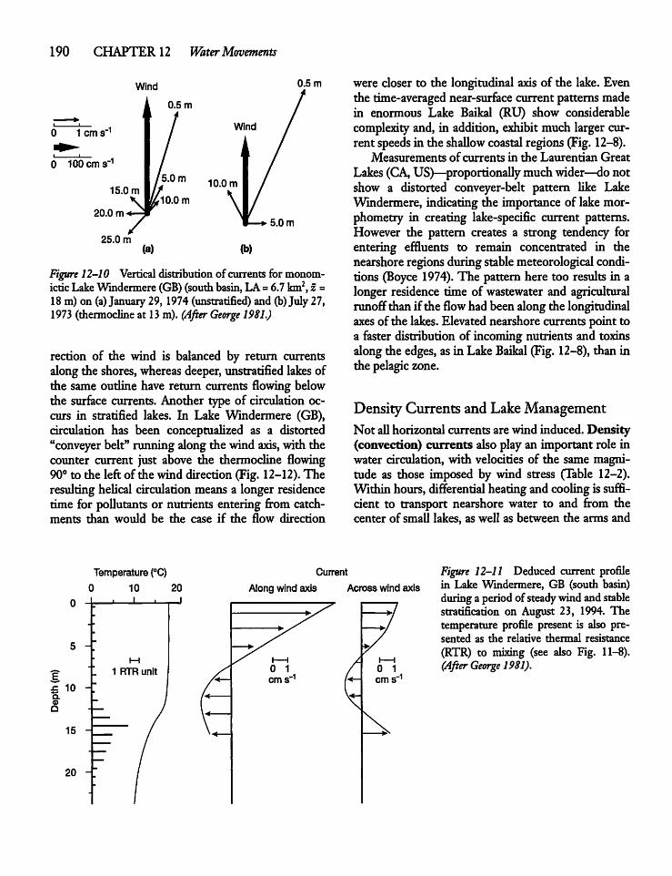
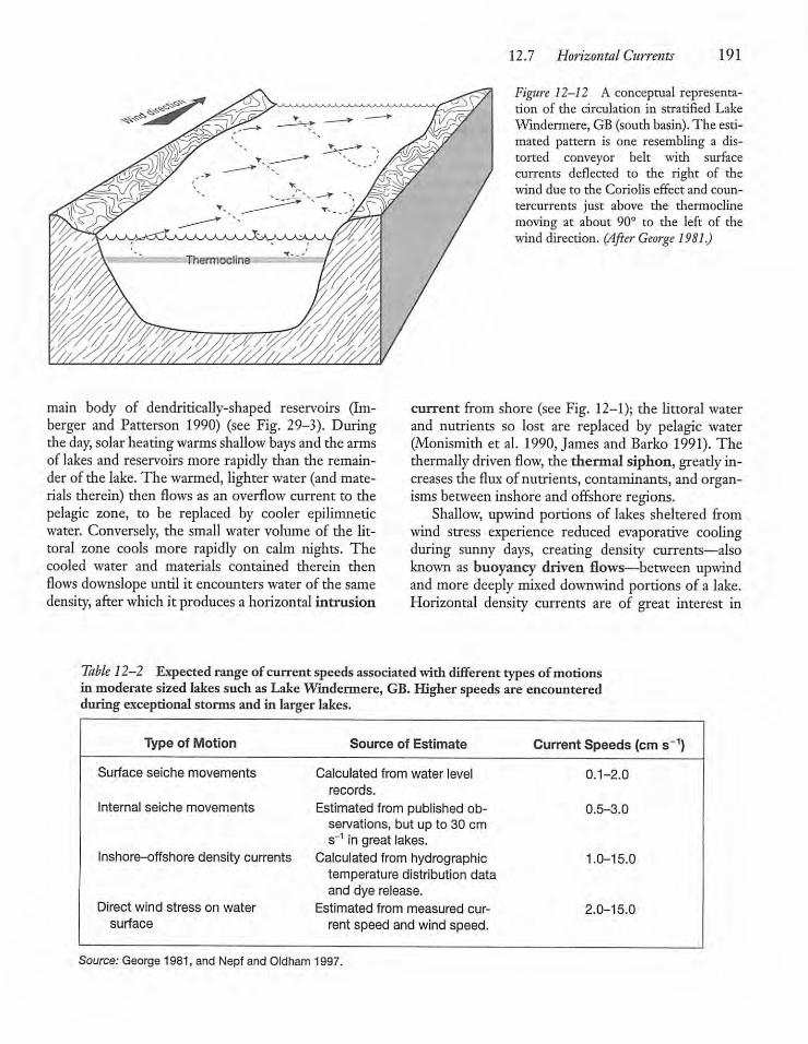
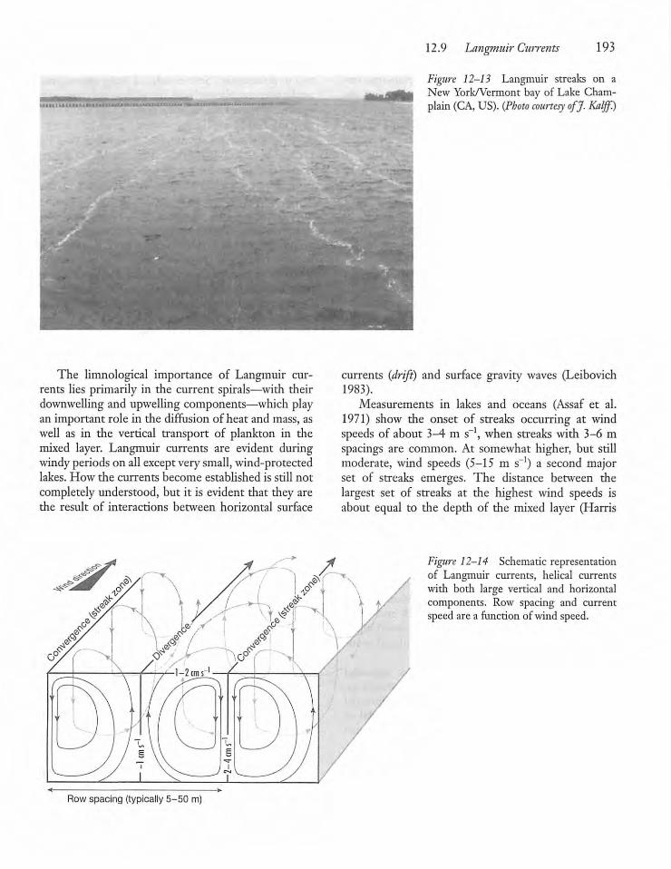
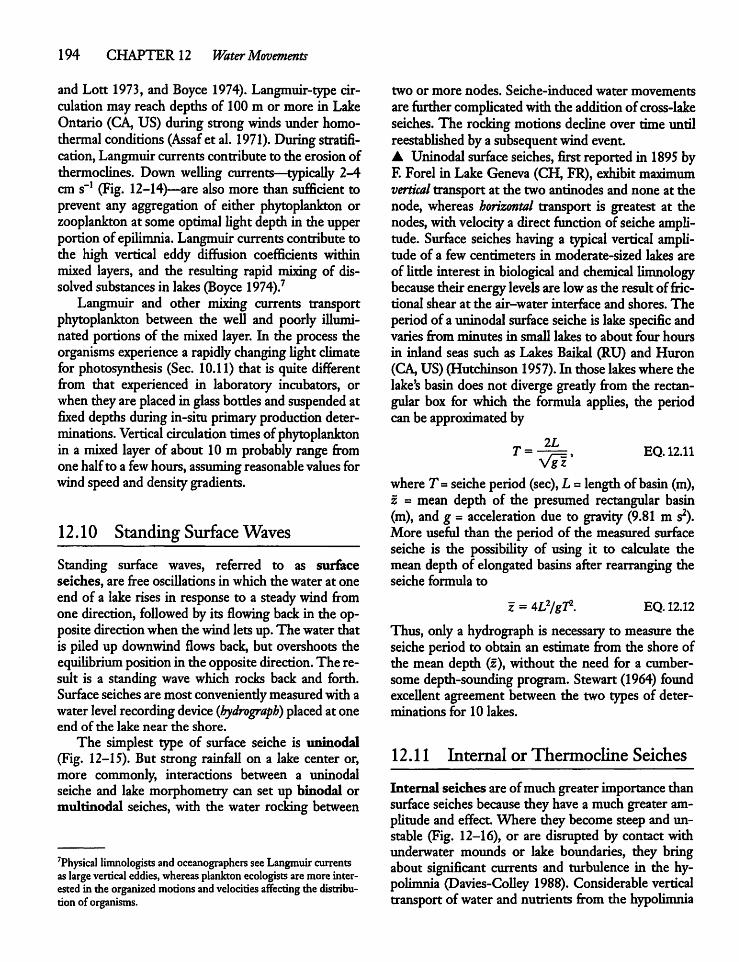
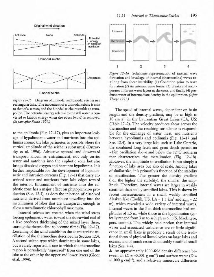
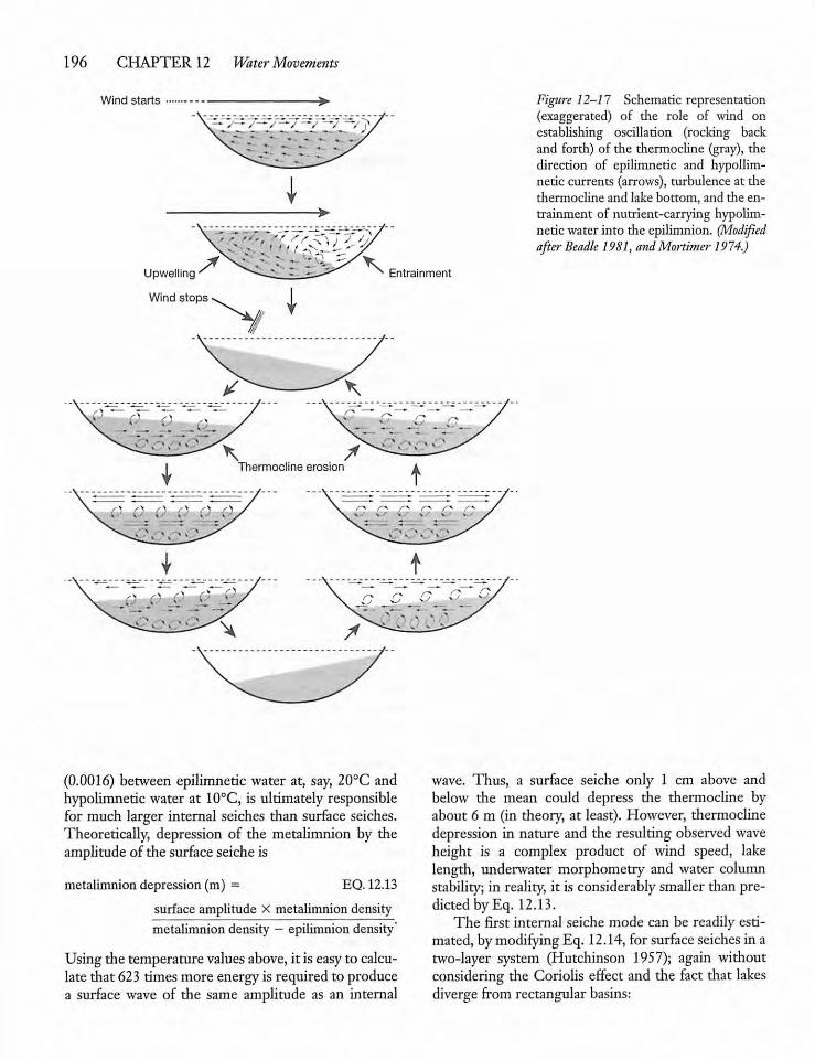
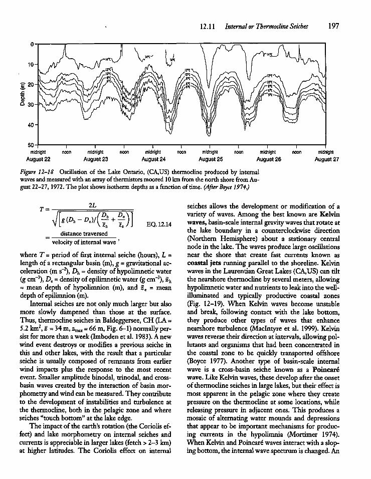
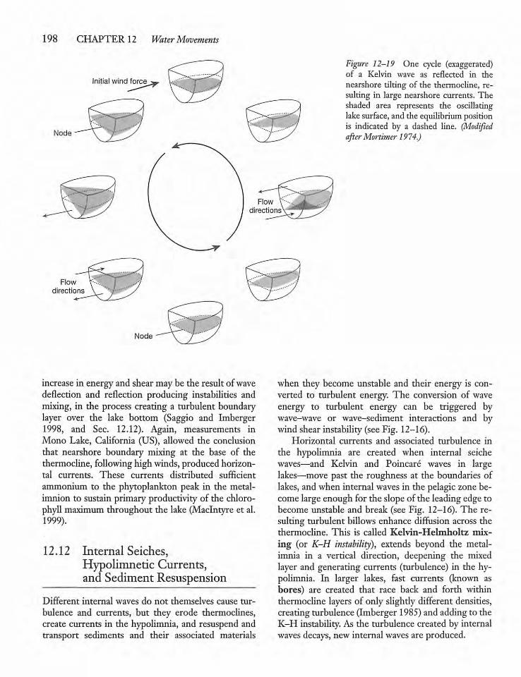
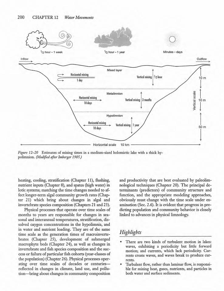
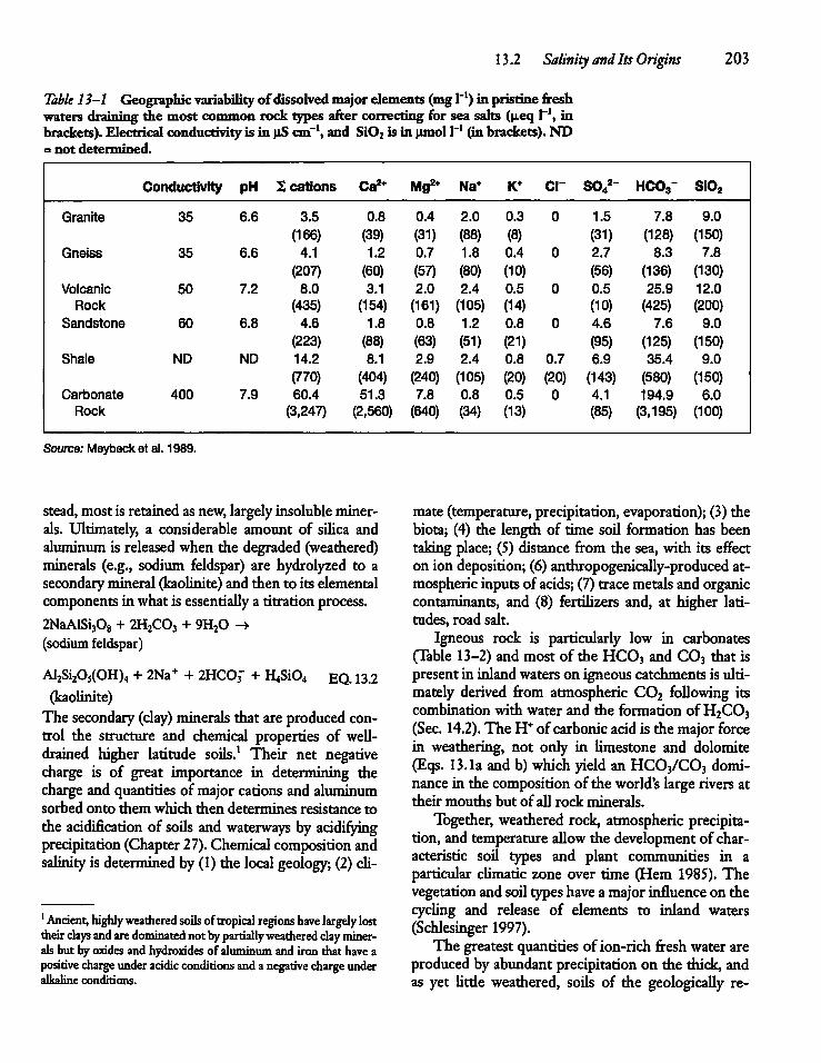
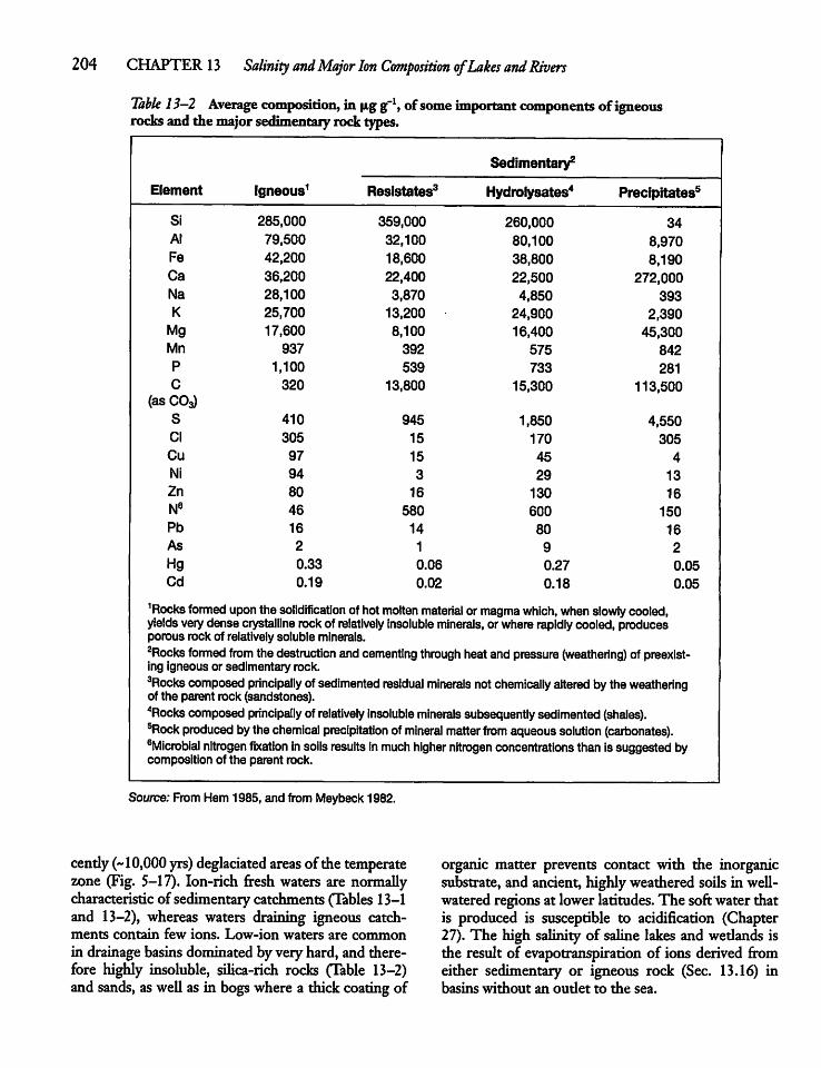
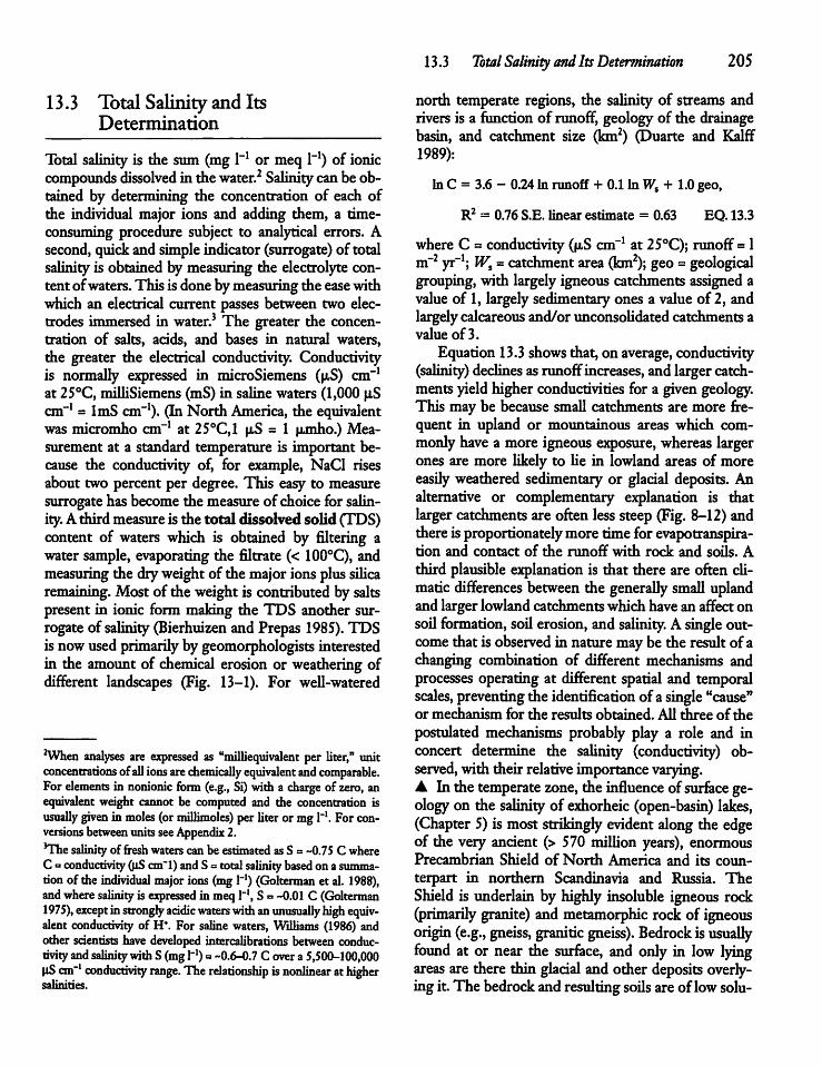
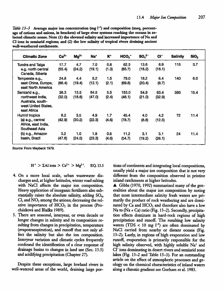
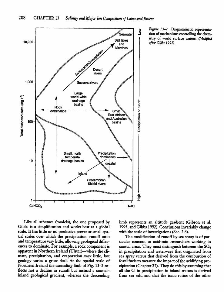
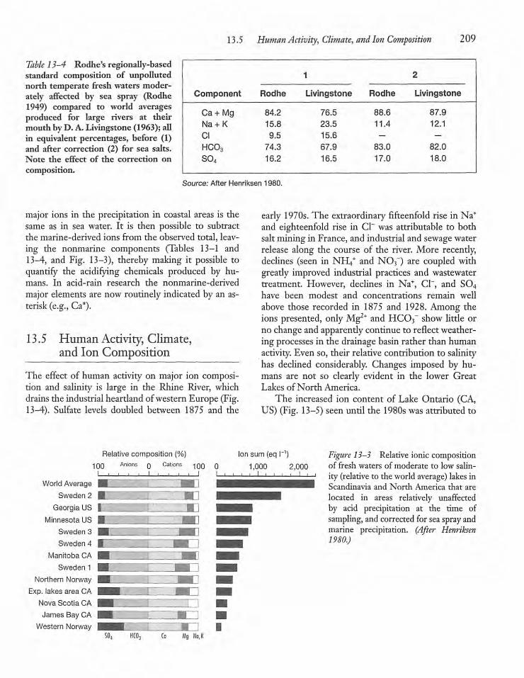
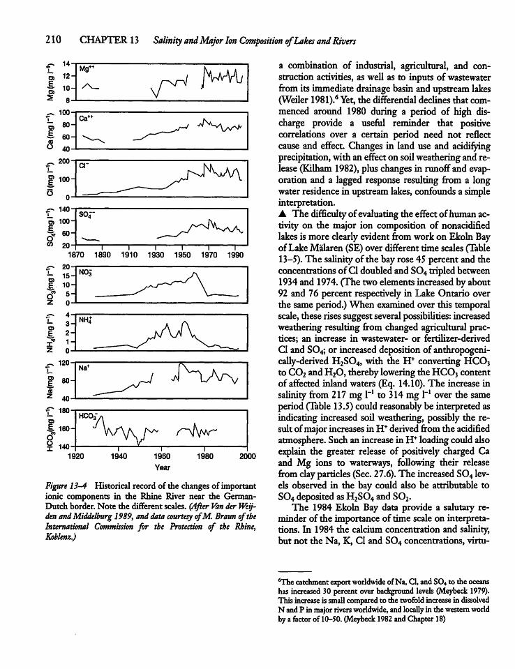
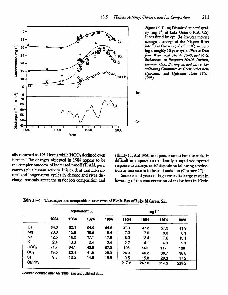
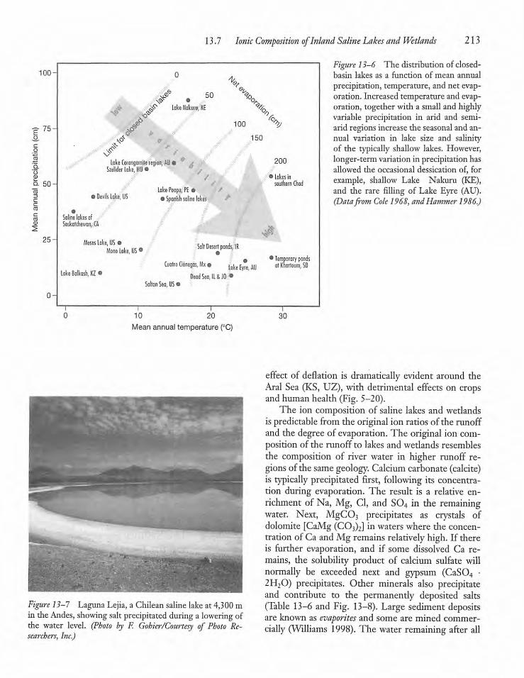

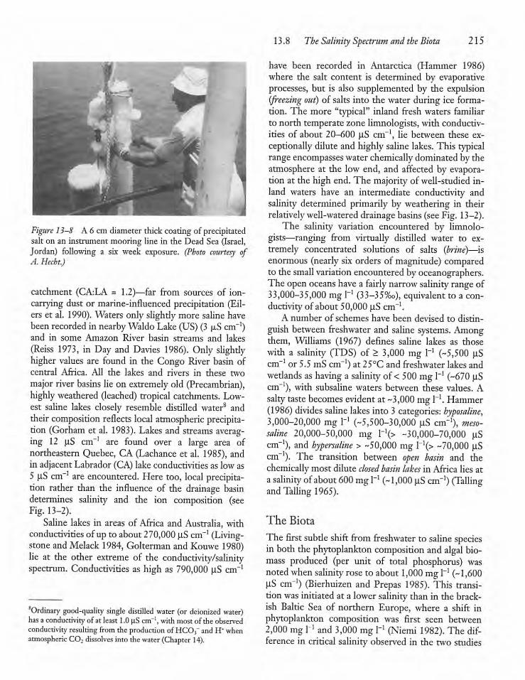
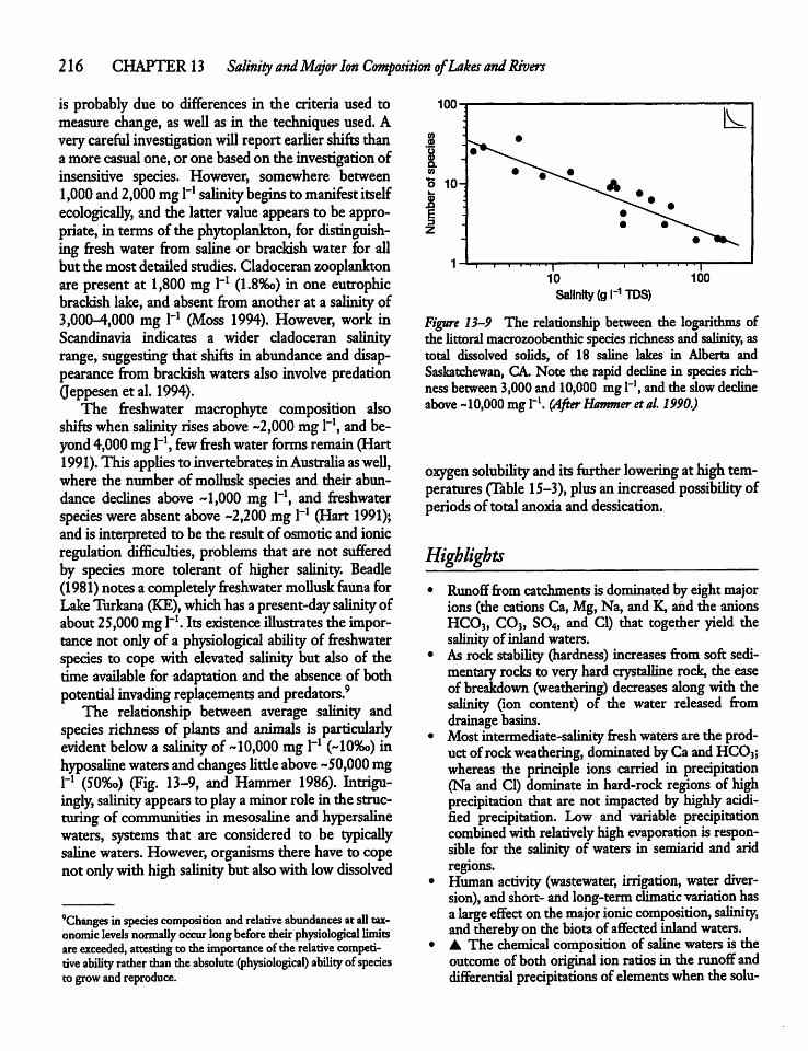

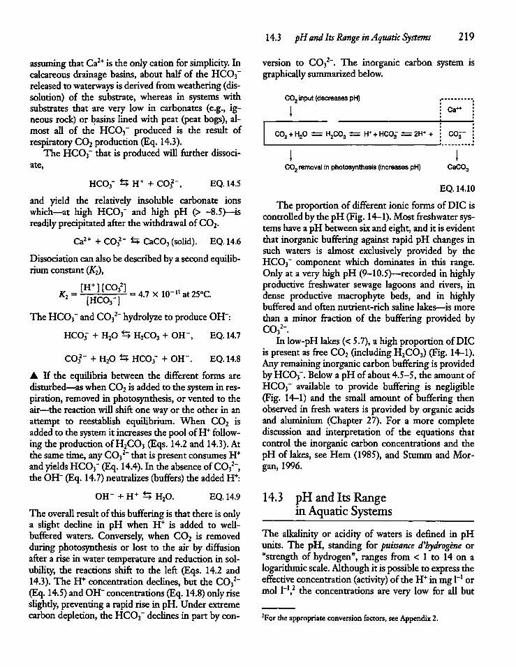
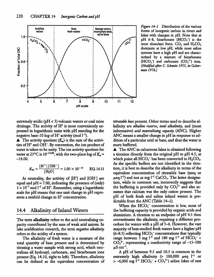
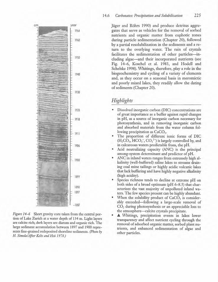
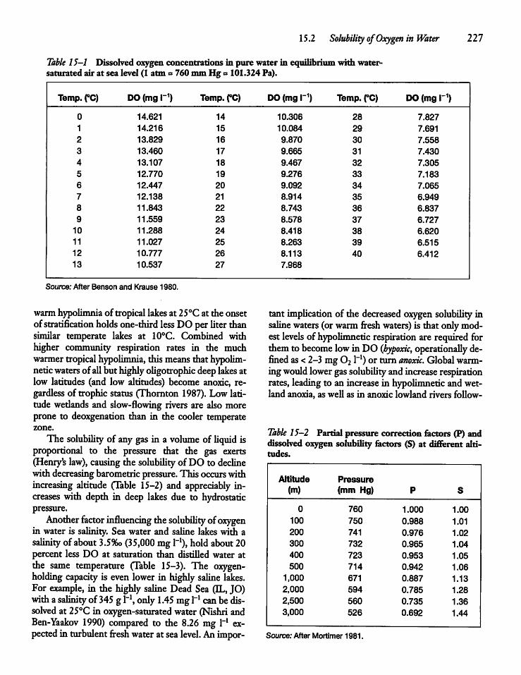
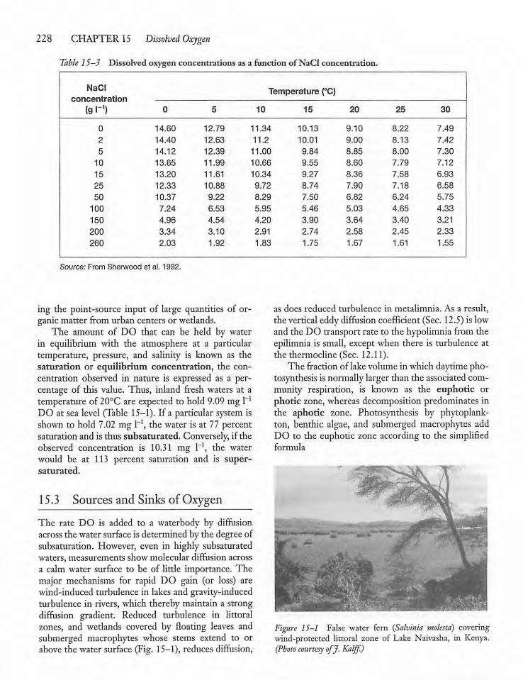
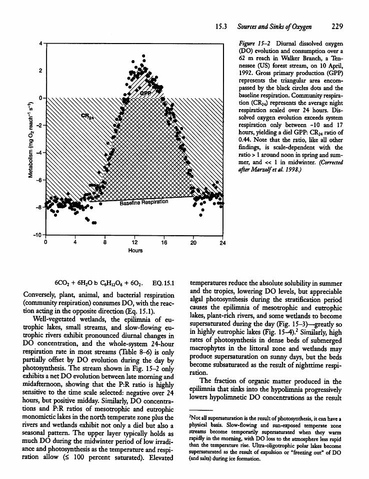
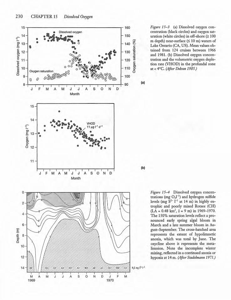
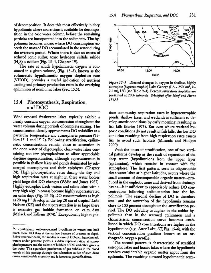
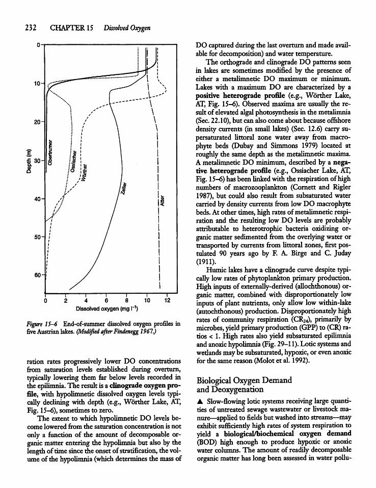
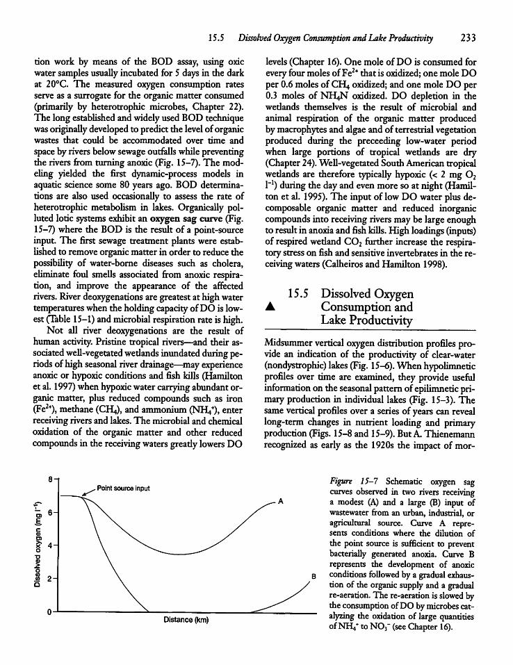
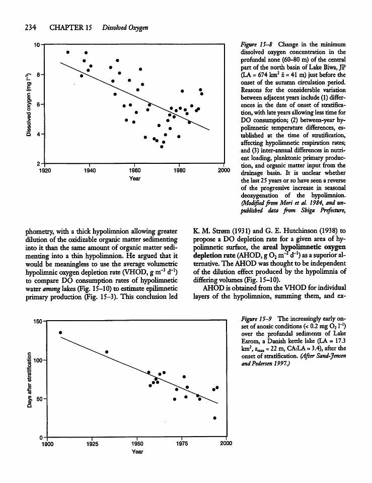
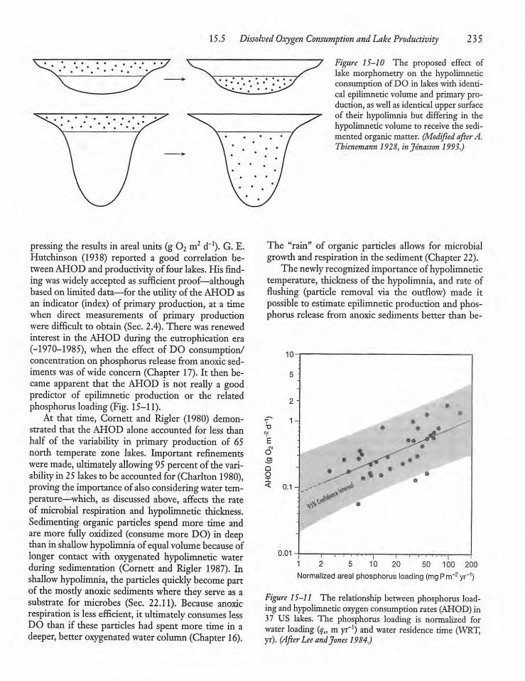
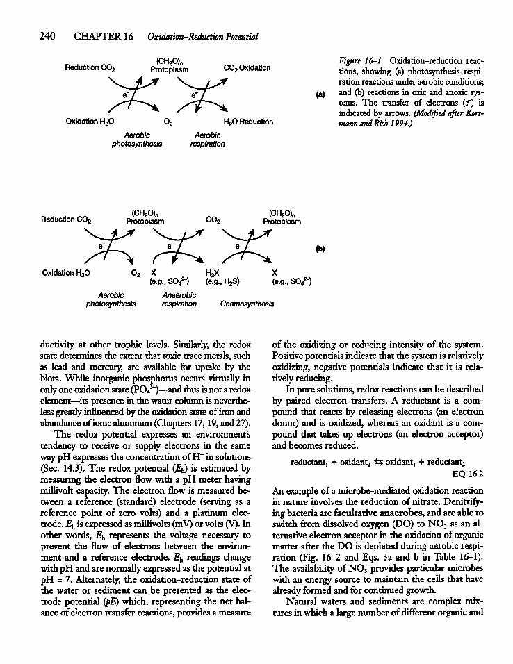
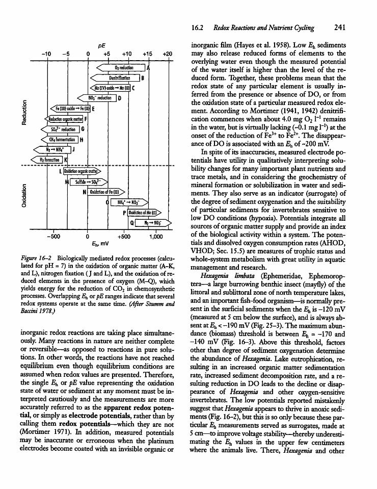
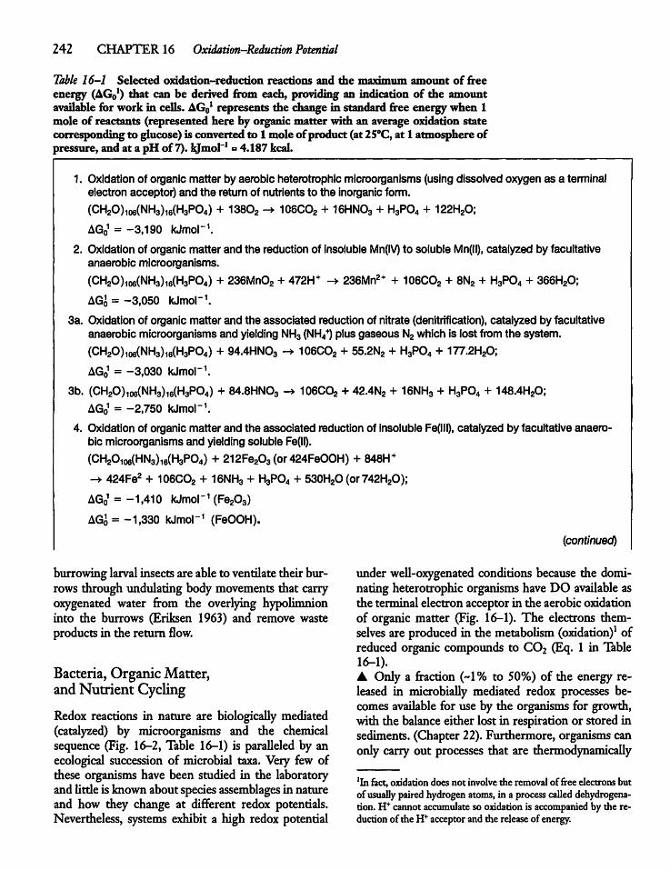
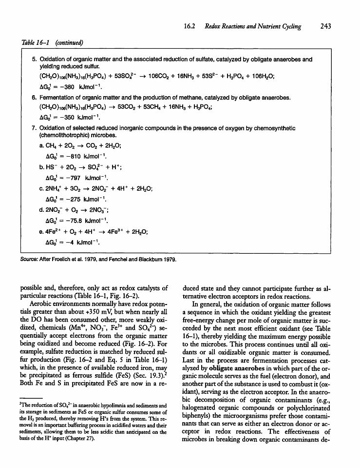
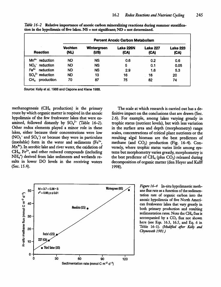
16.2 Redox Reactions and Nutrient Cycling 245
Table 16—2 Relative importance ofanoxic carbon mineralizing reactions duringsummerstratification in the hypolimnia offive lakes. NS « not significant; ND <=> not determined.
Percent Anoxic Carbon Metabolism
Vechten Wintergreen Lake226N Lake 227 Lake 223Reaction (NL) (US) (CA) (CA) (CA)
Mn4* reduction ND NS 0.6 0.2 0.6N03" reduction ND NS 5 0.1 0.05Fe3* reduction ND NS 2.9 1.6 5.3S042" reduction ND 13 16 16 20CH4 production 70 87 75 82 74
Source: Kellyet al. 1988 and Capone and Kiene 1988.
methanogenesis (CH4 production) is the primaryroute bywhichorganicmatter is respiredin the anoxichypolimnia of the few freshwater lakes that were examined, followed distantly by S042~ (Table 16-2).Other redox elements played a minor role in theselakes, either because their concentrations were low(N03~ and S04") or because they were in particulate(insoluble) form in the water and sediments (Fe3+,Mn4*). In aerobic lake andriverwater, the oxidation ofCH,, Fe2+, and other reduced compounds (includingNH,+) derived from lake sediments and wetlands results in lower DO levels in the receiving waters(Sec. 15.4).
The scale at which research is carried out has a definitive impacton the conclusions that are drawn(Sec.2.6). For example, among lakes varying greatly introphic status (nutrient levels), but with lessvariationin the surface area and depth (morphometry) rangescales, concentrations of critical plant nutrients or theresulting algal biomass are the best predictors ofmethane (and C02) production (Fig. 16-4). Conversely, where trophic status varies little among systems butmorphometry varies greatly, morphometry isthe best predictor of CH4 (plus C02) released duringdecomposition oforganic matter(den HeyerandKalff1998).
50-M = 3.7 + 0.38»S Winfergreen (US) /^r2=0.95; p£ 0.01
TJ
7E 40-O Mem!ota(US)# y^E
& 30-3(D
1 20-"35E Frain'stUSU^2^ 10- 227«fl*/5
0-c
/•Third Sister (US)
I) 30
i 1 160 90 120
Sedimentation rate(mmol C m"2 d"1)
Figure 16-4 In-situ hypolimnetic methane flux rate as a function ofthe sedimentation rate of organic carbon into theanoxichypolimnia of five North American freshwater lakes that vary greatly inboth primary production and resultingsedimentation rates.Note theCH4flux isaccompanied by a C02 flux not shownhere (see Eqs. 16.3, 16.5, and Eq. 6 inTable 16-1). (Modified after Kelly andChynmvetb 1981.)
246 CHAPTER 16 Oxidation-ReductionPotential
Highlights• Oxidation-reduction reactions, or redox reactions,are largely mediated (catalyzed) in nature by microorganisms.
• Redox reactionsare directlyor indirectlyresponsiblefor most organic-matter oxidation, nutrient recycling, and energy flow from microbes to highertrophic levels.
• In contrast to reactions in pure solutions, in naturemany redox reactions are neither complete nor reversible and redox potentials must be interpretedcautiously.
• Dissolved oxygen (DO) is the electron acceptor ofchoice in aerobic systems, resulting in lowerlevels of
DO in the hypolimnia andsediments duringmetabolism (oxidation) of sedimenting and sedimented organic matter. • When DO is exhausted, otherelectron acceptors (e.g., NO3", S042~, organic matter) are reduced sequentially. The reduced compounds that are produced then serve as electrondonors upon the return of DO, providing energytoyet other types ofmicroorganisms.
• A While the apparent redox potentials are usuallyinferred from the presenceor absence of DO, measured potentials provide an indication of the oxidation state of elements and the types of microbes andother organisms that are dominant Potentials arealsousefulfor inferringthe suitability of the sedimentenvironment for aerobic invertebrates.
H R
17
Phosphorus Concentrationsand Cycling
17.1 Introduction
It is nowwidelyrecognized that the eutrophicationoffreshwater can be controlled by reducing the input ofplant nutrients, especially phosphorus and nitrogen.Of these two elements, phosphorus is generally considered in shortest supply for algal growth in oligo-trophic waters at midlatitude, characterized by a highN:P ratio (Sec. 8.1). Therefore, most nutrient-controlprograms have focused on it. The N:P ratio of theprotoplasm of rapidly growing algal assemblagesvaries only moderately around the idealized Redfieldratio (Table 8-2); substantially lowering the phosphorus supply raises the N:P supply ratio above the element demand ratio and usually reduces the algalbiomass. Another reason for the focus on phosphorushasbeen that the fixation of atmospheric nitrogen bycyanobacteria makes control of nitrogen more difficult (Chapter 18). Finally, phosphorus removal fromwastewater throughbiological andchemical precipitation (Fig. 8-14) is readily feasible and less expensivethanremoval ofnitrogen.Phosphorus enters aquatic systems from the land
and by direct atmospheric deposition on water surfaces (Tables 8-9 and 8-10). Catchment contributionsare normally dominant, except where the catchmentareaisverysmalland alsocomposedof a substratelowin phosphorus (Sees. 9.1-9.3). Phosphorus is typicallyhighin demand relative to supply andphosphorus retention is highwithlittle released to receiving waterways in well-watered andvegetated drainage basins inthe temperate zone. The phosphorus that is released isprimarily in the dissolved organic form, supplemented
by organic phosphorus contained in particleswashedfrom the land with additional dissolved phosphorusfrom the atmosphere. In poorly vegetated basins—including crop-growing areas—phosphorus is usuallyreleased to waterways while sorbed to soil particles,particularly duringperiodsof storm runoff" (Sec. 8.5).
17.2 The Classical ModelofPhosphorus Cycling
According to the classical view ofphosphorus cycling,based on very important research done before andafter World War II by W. Einsele and W. Ohle inGermany, and C. H. Mortimer in England, P043" isstrongly sorbedto iron oxyhydroxides (e.g., FeOOH)or precipitated as FeP04 under aerobic conditions.Over time much of theP043" entering lakes and wetlands isremoved from thewatercolumn aftersorptionto oxidized and highly insoluble FeOOH aggregates(floes) and sedimenting organic particles, includingalgal cells. The aggregates continue to serve as effective sorption surfaces at the oxidized sediment surfaceandthusasan effective barrier to phosphate diffusion.The aggregates not only trap phosphate that is released following sediment decomposition of sedi-mented organic particles but, more importantly, serveas abarrier toP043~ diffusing upward from theanoxicsediments below, preventing its return to the watercolumn (see also Chapter 19). Mortimer (1941)determined that a sediment redox potential of~200 mVseparates the oxidizing (Fe3+ andassociated
247
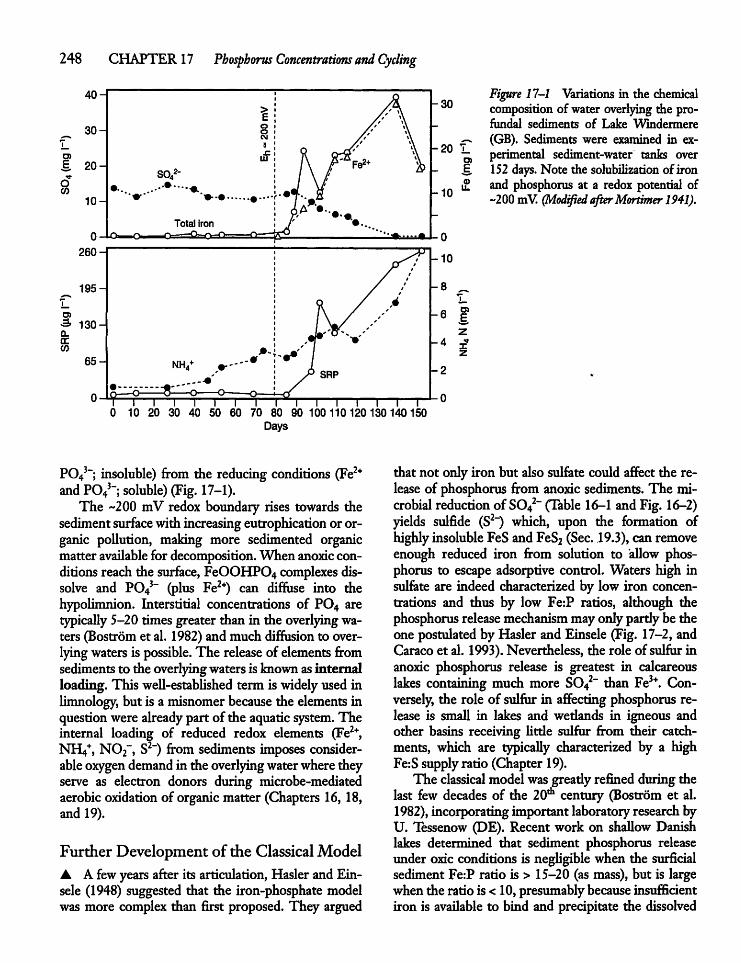
248 CHAPTER17 Phosphorus Concentrations and Cycling
-30
-20 I.
-10
-10
enE
Figure 17-1 Variations in the chemicalcomposition of water overlyingthe pro-fundal sediments of Lake Windermere(GB). Sediments were examined in experimental sediment-water tanks over152days. Note the solubilization of ironand phosphorus at a redox potential of-200 mV (ModifiedafterMortimer 1941).
i—i—i—i—i—i—i—i—r70 80 90 100 110120130140150
Days
P043"; insoluble) from the reducing conditions (Fe2+and P043"; soluble) (Fig. 17-1).The -200 mV redox boundary rises towards the
sedimentsurfacewith increasing eutrophication or organic pollution, making more sedimented organicmatter available for decomposition.When anoxicconditions reach the surface, FeOOHP04 complexes dissolve and P043" (plus Fe2+) can diffuse into thehypolimnion. Interstitial concentrations of P04 aretypically 5-20 times greater than in the overlying waters (Bostrom et al. 1982) and much diffusion to overlying waters is possible. The release of elements fromsediments to the overlyingwatersis knownasinternalloading. This well-established term is widely used inlimnology, but is a misnomerbecause the elements inquestion were already part of the aquatic system.Theinternal loading of reduced redox elements (Fe2+,NH4+, N02~, S2") from sediments imposes considerableoxygen demandin the overlyingwaterwhere theyserve as electron donors during microbe-mediatedaerobicoxidation of organicmatter (Chapters 16, 18,and 19).
Further Development of the ClassicalModel• A fewyears after its articulation, Hasler and Ein-sele (1948) suggested that the iron-phosphate modelwasmore complex than first proposed. They argued
that not only iron but also sulfate could affectthe release of phosphorus from anoxic sediments. The microbial reduction ofS042~ (Table 16-1 and Fig. 16-2)yields sulfide (S2~) which, upon the formation ofhighlyinsolubleFeS and FeS2 (Sec. 19.3), can removeenough reduced iron from solution to allow phosphorus to escape adsorptive control. Waters high insulfate are indeed characterized by low iron concentrations and thus by low Fe:P ratios, although thephosphorus releasemechanismmay only partly be theone postulated by Hasler and Einsele (Fig. 17-2, andCaraco et al. 1993).Nevertheless, the role of sulfur inanoxic phosphorus release is greatest in calcareouslakes containing much more S042~ than Fe3+. Conversely, the role of sulfur in affecting phosphorus release is small in lakes and wetlands in igneous andother basins receiving little sulfur from their catchments, which are typically characterized by a highFe:Ssupplyratio (Chapter 19).The classical modelwasgreatly refinedduring the
last few decades of the 20th century (Bostrom et al.1982), incorporatingimportant laboratoryresearch byU. Tessenow (DE). Recent work on shallow Danishlakes determined that sediment phosphorus releaseunder oxic conditions is negligiblewhen the surficialsediment Fe:P ratio is > 15-20 (as mass), but is largewhen the ratio is < 10,presumablybecause insufficientiron is available to bind and precipitate the dissolved
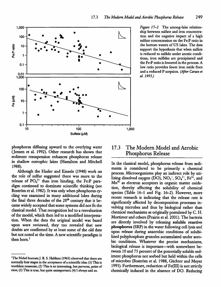
17.3 The Modern Model andAerobic Phosphorus Release 249
1,000-
100-
<3. 10-
1-
0.110 100
Sulfate (nM)
phosphorus diffusing upward to the overlying water(Jensen et al. 1992). Other research has shown thatsediment resuspension enhances phosphorus releasein shallow eutrophic lakes (Hamilton and Mitchell1988).Although the Hasler and Einsele (1948) work on
the role of sulfur suggested there was more to therelease of P043" than iron binding, the Fe:P paradigm continued to dominate scientific thinking (seeBostrom et al. 1982). It was onlywhenphosphorus cyclingwas examined in many additional lakes duringthe final three decades of the 20th century thatit became widely accepted that somesystems didnot fit theclassical model. That recognition led to a reevaluationofthemodel, which thenledto amodified interpretation. When the data the original model was basedupon were reviewed, they too revealed that newdoubts are confirmedby at least some of the old databutnotnoted at the time. Anew scientific paradigm isthen born.1
'TheNobel laureateJ. B.S.Haldane (1963) observed thattherearenormally fourstages in the acceptance ofa scientific idea: (1)This isworthless nonsense; (2) This is aninteresting, butperverse, pointofview; (3)This is true, but quiteunimportant; (4)I always saidso.
1,000
Figure 11-2 The among-lake relationship between sulfate and iron concentration and the negative impact of a highsulfate concentration on the Fe:P ratio inthe bottom waters of US lakes. The datasupport the hypothesis that when sulfateis reduced to sulfide under anoxic conditions, iron sulfides are precipitated andthe Fe:P ratio is lowered in the process.Alow ratio provides fewer iron oxide floesand a reduced P sorption. (After Caraco etal. 1993.)
17.3 The Modern Model and AerobicPhosphorus Release
In the classical model, phosphorus release from sediments is considered to be primarily a chemicalprocess. Microorganisms play an indirect role by utilizing dissolved oxygen (DO), N03", S042-, Fe3+, andMn4* as electron acceptors in organic matter oxidation, thereby affecting the solubility of chemicalspecies (Table 16-1 and Fig. 16-2). However, morerecent research is indicating that the release rate issignificantly affected by decomposition processes involving microbes and thus by biological rather thanchemical mechanisms asoriginally postulated byC.H.Mortimer and others (Prairie et al. 2001).The bacteriaare directly involved by releasing soluble reactivephosphorus (SRP) in the waterfollowing celllysis andupon release during anaerobic conditions of solubi-lized polyphosphate granules accumulated under aerobic conditions. Whatever the precise mechanisms,biological release is important—with somewhere between 10and75percentof the potentially soluble sediment phosphorus not sorbed but heldwithin the cellsofmicrobes (Bostrom et al. 1988, Gachter andMeyer1993). Furthermore, reduction ofFe(EI)isnot strictlychemically induced in the absence of DO. Reducing
250 CHAPTER 17 Phosphorus Concentrations and Cycling
conditions alone are not enough to reduce Fe(IQ) toFe(II), in part because the aggregates arestabilized bya coating of organic matter. Iron-reducing bacteriausing Fe(m) as an electron acceptor in the oxidationoforganicmatter, arenecessary (Lovley 1991, Eq.4inTable 16-1, andChapter19).If the classical model were applicable, Fe(H)
and P043~ should be released simultaneously uponthe chemical reduction of the Fe(flT) complex. ButGachter et al. (1988) has shown that release patternsare out of phase. They also observed that sedimentsare less able to take up dissolved phosphorus uponsterilization with antibiotics—this would not be thecase if theprocesses werestrictlyphysical or chemical.Reexamination of the data collected by Mortimer(1942) in Estwaite Water (GB) showed that thePoland Fe2+ release patterns had also been out ofphase.Recently, Prairie etal. (2001) found theclassical theoryinadequatewhen they reported thatno relationship existed between iron and phosphorus release in theanoxic hypolimnia of a series of Quebec (CA) lakes,and also showed thatmany oligotrophic lakes can goanoxic withoutphosphorus release. Release appears todepend not so muchon hypolimnetic DO concentrations asonthebalance between thesupplyofphosphorus in sedimenting particles and the—still poorlyunderstood—retention capacity imposed bybiologicaland chemical means. In practice, it does notreallymatterwhether the released phosphorus hadbeenpart ofan Fe complex or held bymicroorganisms. However,understanding how the phosphorus is held is crucialfor consideration of underlying mechanisms that arenot onlyinteresting in themselves butmay also lead tobetter predictive models.• The recent reevaluation of the classical theory isimportant for severalreasons:
1. It provides a useful reminder that correlations donot provide proof of a mechanistic link, eventhough a particularly mechanistic interpretationseems to be the most plausible explanation at thetime.
2. It allows consideration of alternative hypotheses,explaining why some lakes withanoxic hypolimniarelease little or no phosphorus (Caracoet al. 1991).It alsoallows the possibility of an improvedexplanation (prediction)—even in lakes that appear tofit the classical model.
3. The . phosphorus released from inorganicFeOOHP04 (andA100HP04) complexes is inor
ganic P043", whereas phosphorus directly releasedbymicrobes is organic or colloidal polyphosphatephosphorus. Unfortunately, the standard colori-metricmolybdate technique that is usedfor determination of P043", uses reagents that hydrolyze(break down) labile organic phosphorus causing itto be measured as P043~. Yet, only one to 10 percent ofthe P043~ may have been inthis form priorto the chemical analyses (Rigler 1973). Consequently, hypolimnetic increases in dissolved phosphorus following the development of anoxia hadalways been thought to be in the P043" form, andthus in accord with the classical model—eventhough it may have been organic phosphorus released bymicrobes. Such analyses arenow routinelyreported assoluble reactive phosphorus (SRP).
4. The classical model pertains to the behavior ofphosphorus in the hypolimnia rather than lakes asa whole. Large increases observed in the well-oxygenated mixed layer of shallow (unstratified)but productive lakes that cannot be attributed toexternal loadingare not explained by the classicalmodel. Nor is the classical model appropriate toexplain why phosphorus release from well aeratedand turbulent littoral zones is dependent on thephosphorus concentration gradient across thesediment-water interface (Bostrom et al. 1982).
Aerobic Phosphorus ReleaseManymechanisms are responsible in varying degreesfor aerobic phosphorus release. They range fromthosewithphysical causes to thosewithunderlying biological causes. Their relative importance varies overtimeandspace. Increases in internal loading in highlyproductive shallow lakes with an oxicsedimentsurfacelayerhave been experimentally linked to increases intemperature (Sandergaard 1989)—suggesting thatbiological processes are probably involved—and toincreases in pH resultingfromhigh rates of photosynthesis (Fig. 17-3). Elevated pH appears to allow someof the phosphorus adsorbed to FeOOH floes to be replaced by OH", with the phosphate released to thewater. Microbial respiration and decay also releasephosphorus and other elements into the interstitialwater where it is subject to diffusion to the overlyingwater. Conversely, microbes play an indirect role inreducing phosphorus release by maintaining a sediment redoxpotential high enough to inhibit or reducerelease from sediments. They do so by using elevated
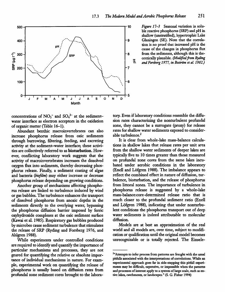
17.3 TheModernModel andAerobic Phosphorus Release 251
Month
concentrations of N03" and S042" at the sediment-water interface as electron acceptors in the oxidationof organicmatter (Table 16-1).
Abundant benthic macroinvertebrates can alsoincrease phosphorus release from oxic sedimentsthrough burrowing, filtering, feeding, and excretingactivity at the sediment-water interface; these activitiesare collectively referred to asbioturbation. However, conflicting laboratory work suggests that theactivity of macroinvertebrates increases the dissolvedoxygen flux into sediments, thereby decreasing phosphorus release. Finally, a sediment coating of algaeand bacteria (biofilm) may either increase or decreasephosphorus release dependingon growingconditions.Another group of mechanisms affecting phospho
rus release are linked to turbulence induced by windor gasbubbles. The turbulenceenhances the transportof dissolved phosphorus from anoxic depths in thesediments directly to the overlying water, bypassingthe phosphorus diffusion barrier imposed by ferricoxyhydroxide complexes at the oxic sediment surface(Kawai et al. 1985). Respiratory gasbubbles producedbymicrobescausesediment turbulence that stimulatesthe release of SRP (Ryding and Forsberg 1976, andAhlgren1988).While experiments under controlled conditions
are requiredto identifyandquantifythe importance ofparticular mechanisms and processes, they are notgeared for quantifying the relative or absolute importance of individual mechanisms in nature. For example, experimental work on quantifying the release ofphosphorus is usually based on diffusion rates fromprofundal zone sediment cores brought to the labora
Figure 11-3 Seasonal variation in soluble reactivephosphorus (SRP)and pH inshallow (unstratified), hypertrophicLakeGlaningen (SE). Note that the correlation is no proof that increased pH is thecause of the changes in phosphorus fluxfrom the sediments, although this is theoreticallyplausible. (Modifiedfrom RydingandForsberg 1911, inBostrom etal. 1982.)
tory. Evenif laboratory conditions resemble the diffusion rates characterizing the nonturbulent profundalzone, they cannot be a surrogate (proxy) for releaserates for shallowwater sedimentsexposed to considerable turbulence.2It is clear from whole-lake mass-balance calcula
tions in shallow lakes that release rates per unit areafrom the shallow water sediments of deeper lakes aretypically five to 10 times greater than thosemeasuredon profundal zone cores from the same lakes incubated under aerobic conditions in the laboratory(Enell and Lofgren 1988). The imbalance appears toreflect the combined effect in nature of diffusion, turbulence, bioturbation, and the release of phosphorusfrom littoral zones. The importance of turbulence inphosphorus release is suggested by a whole-lakemass-balance:core-determined release ratio that ismuch closer to the profundal sediment ratio (Enelland Lofgren 1988), indicating that under nonturbulent conditions the phosphorus transport out of deepwater sediments is indeed attributable to moleculardiffusion.Models are at best an approximation of the real
world and all models are, over time, subject to modificationor qualification until the originalmodelbecomesunrecognizable or is totally rejected. The Einsele-
2"Attempts to infer process from patterns arefraught with theusualpitfalls associated with the interpretations of correlations.While anexperimental approachgoes far in side-stepping this pitfallexperiments maybe difficult, expensive, or impossiblewhen the patternsandprocesses of interest applyto a systemof largescale,suchasentire lakes, catchments, or landscapes." (S. G. Fisher 1994)
252 CHAPTER 17 Phosphorus Concentrations and Cycling
Ohle-Mortimer phosphorus-iron model is no exception to thisrule.It hascontinued to provide an important framework for ideas and data on phosphoruscycling andits linkto the Fecycle, but is less completethan its authors were able to surmise 60 years ago.Models are to beused, not unquestioningly believed.
a 17.4 The Mass-Balance Equationand Phosphorus Cycling
Aquatic systems are open systems with inputs andoutputs. If one assumes that the input of substanceM isconstant and the input is instantly and completelymixed throughoutthewaterbody, then the steady stateor equilibrium version of the relationship between inputs, losses, outputs, and the concentration ofM canbe expressed with a simple mass-balance model:
AM
Af= I-0-(SffOSS-R). EQ.17.1
Where AM/Ar = storage gain or loss of substanceMover time t\ I= external load; O=outflow loss; S^^=loss to sediments; R= internal load; and (Sg^ - R) =net sedimentation (5net).Inland waters are subject to seasonal and diurnal
changes in the absolute and relative importance ofphotosynthesis and respiration, as well as to changesin weather and climatic conditions and it is evidentthat theycannotbe in a steady state,for anylengthoftime.3 But, since seasonal patterns repeat themselvesmoreor lesseachyear or growingseason, equilibrium(AM/Af = 0) is assumed in steady state mass-balancemodeling, whichis usually donewith a seasonal or annual perspective rather than with the hourly or dailydynamic reality.The many phosphorus budgets now available,
based on input-output modeling, have demonstratedboth seasonal and annual variability in the rate of netphosphorus sedimentation. Mass-balance budgets for
}The assumption thatnatural systems normally reach andmaintainequilibriumhas its roots in a world-view derivedfrom Greekmetaphysics, which proposes that nature must ultimatelyexpress an ordered reality. While most scientists now recognize that naturalsystems are not in a state of true equilibrium, systemsare often assumed to be in equilibriumover the courseof short-term or annualstudies. Assuming equilibrium conditions simplifies experiments,and is also encouraged by the simplicity of equilibrium mathematics.
phosphorus (and nitrogen)—made with applied goalsin mind—pointed out the importance of sediments asa phosphorus source andhasencouraged fundamentalresearch on nutrient cycling; this in turn influencesthe interpretations madein more applied research.
Lakes with OxicHypolimniaTemperate lakes with oxic hypolimnia are considerablydifferentfrom thosewith anoxic ones.Lakeswithoxic hypolimnia are generally deep and havethickhypolimnia ableto hold a largemass of dissolved oxygenfollowing overturn (Sec. 15.5). Their drainage ratios(CA:LAor CAV) arenormally relatively small, implying small water loading (Chapter 8), and thus a longwater residence time (WRT), as well as small catchment-nutrient loading (seeTable 17-1 and Chapter 8)compared to most lakes with anoxic hypolimnia.
Mass-balance measurements have shown that thefraction of the external phosphorus loadsupplied on anannual basis that is retained (R)and stored in the sedimentsrather than flushed out is about twice as largeasfor those with anoxic hypolimnia (Table 17-1). Thefraction of phosphorus retained by lakes and wetlandsdeclines exponentially with increasing water loading(m yr-1) and increases with theWRT (yr) (Fig. 9-7)
R =(1 + VWRT)'
and the phosphorus concentration in the water (notlost to sediments or outflow) is
p =* water
Inflow
1 + VWRT
EQ. 17.2
EQ. 17.3
assuming that Pi^ = Poutflow This equation indicatesthat, among lakes, the P concentration of inflowingwater rather than the actual P loading (kgyr-1) is thesingle best indicatorof the water concentration.Deep lakes with a longWRT (>10yr) typically re
tain 70-90 percent of the incoming phosphorus. Progressively less of the incoming phosphorus is storedpermanently in the sediments asWRT declines (Fig.9-7). ShortWRT systems are alsousuallyshallow andlesswell-stratified or completely unstratified. Consequently, a greater fraction of the phosphorus input isretained in the epilimnia, whereit is potentially available to primaryproducers and microbes, before beingflushed out A combination of larger nutrient loadingto short WRT lakes and higher nutrient retention inthe water column (Fig. 9-3 and Table 17-1) explainsthe typically highernutrient concentrations, algal tur-
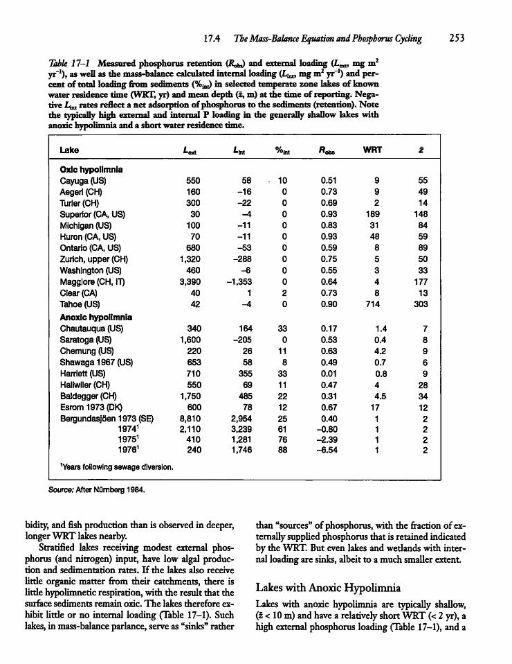
17.4 The Mass-Balance Equation and Phosphorus Cycling 253
Table 17-1 Measured phosphorus retention (Robd and external loading (L^ mg m2yr-1), as well as the mass-balance calculated internal loading (L^ mgm2 yr-1) and percent of total loading from sediments (%fnt) in selected temperate zone lakes of knownwater residence time (WRT, yr) and mean depth (z, m) at the time ofreporting. Negative Lint rates reflect a net adsorption of phosphorus to the sediments (retention). Notethe typicallyhigh external and internal P loading in the generally shallow lakes withanoxichypolimnia and a short water residence time.
Lake ^ext '•Int %w "obs WRT z
Oxic hypolimniaCayuga (US) 550 58 - 10 0.51 9 55
Aegeri (CH) 160 -16 0 0.73 9 49
Turler(CH) 300 -22 0 0.69 2 14
Superior (CA, US) 30 -4 0 0.93 189 148
Michigan (US) 100 -11 0 0.83 31 84
Huron (CA,US) 70 -11 0 0.93 48 59
Ontario (CA, US) 680 -53 0 0.59 8 89
Zurich, upper (CH) 1,320 -288 0 0.75 5 50
Washington (US) 460 -6 0 0.55 3 33Maggiore (CH, IT) 3,390 -1,353 0 0.64 4 177Clear (CA) 40 1 2 0.73 8 13
Tahoe (US) 42 -4 0 0.90 714 303
Anoxic hypolimniaChautauqua (US) 340 164 33 0.17 1.4 7
Saratoga (US) 1,600 -205 0 0.53 0.4 8Chemung (US) 220 26 11 0.63 4.2 9Shawaga 1967 (US) 653 58 8 0.49 0.7 6
Harriett (US) 710 355 33 0.01 0.8 9Haiiwiler (CH) 550 69 11 0.47 4 28Baldegger (CH) 1,750 485 22 0.31 4.5 34Esrom 1973 (DK) 600 78 12 0.67 17 12
Bergundasjden 1973 (SE) 8,810 2,954 25 0.40 1 219741 2,110 3,239 61 -0.80 1 219751 410 1,281 76 -2.39 1 219761 240 1,746 88 -6.54 1 2
'Yearsfollowing sewage diversion.
Source: After NQrnberg 1984.
bidity, and fish production than is observedin deeper,longerWRT lakes nearby.
Stratified lakes receiving modest external phosphorus (and nitrogen) input, have low algal production and sedimentation rates. If the lakes also receivelittle organic matter from their catchments, there istittlehypolimneticrespiration, with the resultthat thesurface sediments remain oxic. The lakes therefore exhibit little or no internal loading (Table 17-1). Suchlakes, in mass-balance parlance, serve as"sinks" rather
than "sources" of phosphorus,with the fraction of externally supplied phosphorus that is retained indicatedby the WRT. But even lakes andwetlands with internalloading aresinks,albeitto amuch smaller extent.
Lakeswith AnoxicHypolimniaLakes with anoxic hypolimnia are typically shallow,(z <10m) andhavea relatively shortWRT (< 2 yr), ahigh external phosphorus loading (Table 17-1), and a
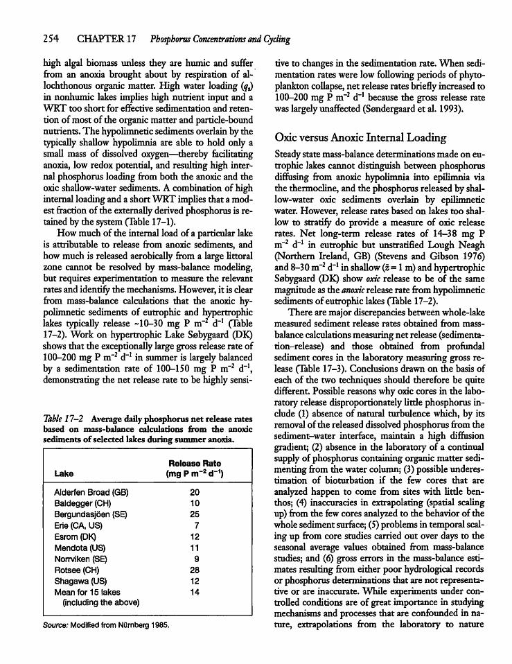
254 CHAPTER17 Phosphorus Concentrations and Cycling
high algal biomass unless they are humic and sufferfrom an anoxia brought about by respiration of al-lochthonous organic matter. High water loading (&)in nonhumic lakes implies high nutrient input and aWRT too short for effective sedimentation and retention ofmostof the organic matter and particle-boundnutrients.The hypolimnetic sedimentsoverlain by thetypically shallow hypolimnia are able to hold only asmall mass of dissolved oxygen—thereby facilitatinganoxia, low redox potential, and resulting high internal phosphorus loadingfrom both the anoxic and theoxic shallow-water sediments. A combination of highinternal loadingand a shortWRT implies that a modest fraction of the externally derived phosphorus is retainedby the system (Table 17-1).Howmuch of the internal load of a particularlake
is attributable to release from anoxic sediments, andhowmuchis released aerobically froma large littoralzone cannot be resolved by mass-balance modeling,but requires experimentation to measure the relevantratesand identifythe mechanisms. However, it is clearfrom mass-balance calculations that the anoxic hypolimnetic sediments of eutrophic and hypertrophiclakes typically release ~10-30 mg P m~2 d-1 (Table17-2). Work on hypertrophic Lake Sobygaard (DK)shows that the exceptionally large gross release rate of100-200 mgP m~2 d"1 in summer is largely balancedby a sedimentation rate of 100-150 mg P m~2 d"1,demonstrating the net release rate to be highlysensi-
Table 17-2 Average dailyphosphorus net release ratesbased on mass-balance calculations from the anoxicsediments of selected lakes during summer anoxia.
Release RateLake (mg P m~2d"1)
Alderfen Broad (GB) 20Baldegger (CH) 10
Bergundasjoen (SE) 25
Erie (CA, US) 7
Esrom (DK) 12
Mendota (US) 11
Norrviken (SE) 9
Rotsee (CH) 28
Shagawa (US) 12
Mean for 15 lakes 14(including the above)
Source: Modified from NOrnberg 1985.
rive to changesin the sedimentation rate. When sedimentation rateswere lowfollowing periodsof phyto-plankton collapse, net release ratesbriefly increased to100-200 mgP m~2 d"1 because the gross release ratewaslargelyunaffected (Sondergaard et al. 1993).
Oxic versusAnoxic Internal LoadingSteady statemass-balance determinations madeon eutrophic lakes cannot distinguish between phosphorusdiffusing from anoxic hypolimnia into epilimnia viathe thermocline, and the phosphorusreleased byshallow-water oxic sediments overlain by epilimneticwater. However, release rates based on lakes too shallow to stratify do provide a measure of oxic releaserates. Net long-term release rates of 14-38 mg Pm~2 d-1 in eutrophic but unstratified Lough Neagh(Northern Ireland, GB) (Stevens and Gibson 1976)and 8-30 m~2 d"1 inshallow (z=lm) and hypertrophicSabygaard (DK) show oxic release to be of the samemagnitudeas the anoxic releaserate fromhypolimneticsediments of eutrophic lakes (Table 17-2).There are major discrepancies betweenwhole-lake
measured sediment release rates obtained from mass-balance calculations measuring net release (sedimentation-release) and those obtained from profundalsediment cores in the laboratory measuring gross release (Table 17-3). Conclusions drawn on the basis ofeach of the two techniques should therefore be quitedifferent. Possiblereasonswhy oxiccores in the laboratory release disproportionatelylittle phosphorus include (1) absence of natural turbulence which, by itsremoval of the released dissolved phosphorusfrom thesediment-water interface, maintain a high diffusiongradient; (2) absence in the laboratoryof a continualsupplyof phosphorus containingorganicmatter sedi-menting from the water column;(3)possible underestimation of bioturbation if the few cores that areanalyzed happen to come from sites with little benthos; (4) inaccuracies in extrapolating (spatial scalingup)fromthe few coresanalyzed to the behavior of thewholesedimentsurface; (5)problemsin temporal scaling up from core studies carried out over days to theseasonal average values obtained from mass-balancestudies; and (6) gross errors in the mass-balance estimatesresulting from either poor hydrological recordsor phosphorus determinations that are not representative or are inaccurate. While experiments under controlled conditions are of great importance in studyingmechanisms and processes that are confounded in nature, extrapolations from the laboratory to nature
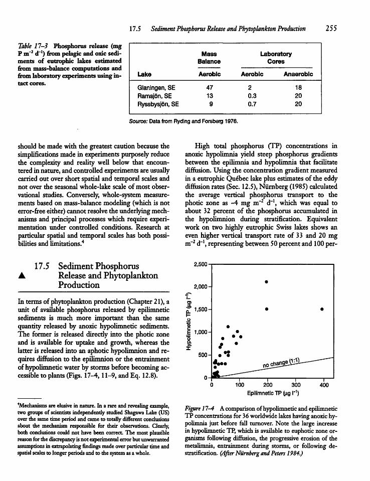
17.5 Sediment Phosphorus Release and Phytoplankton Production 255
Table 17-3 Phosphorus release (mgP m"2 d~!) from pelagic andoxic sediments of eutrophic lakes estimatedfrom mass-balance computations andfrom laboratory experiments using intact cores.
Lake
MassBalance
LaboratoryCores
Aerobic Aerobic Anaerobic
Glaningen, SERamsjdn, SERyssbysjdn, SE
47
13
9
2 18
0.3 200.7 20
Source: Data from Ryding and Forsberg 1976.
should be madewith the greatest cautionbecause thesimplifications made in experiments purposely reducethe complexity and reality well below that encountered in nature, and controlled experiments areusuallycarriedout over short spatial and temporal scales andnot over the seasonal whole-lake scale of most observational studies. Conversely, whole-system measurements based on mass-balance modeling (which is noterror-freeeither) cannot resolve the underlyingmechanisms and principal processes which require experimentation under controlled conditions. Research atparticular spatialand temporal scales has both possibilities and limitations.4
17.5 Sediment Phosphorus• Release and Phytoplankton
Production
In termsof phytoplankton production (Chapter 21),aunit of available phosphorus released by epilimneticsediments is much more important than the samequantity released by anoxic hypolimnetic sediments.The former is released directly into the photic zoneand is available for uptake and growth, whereas thelatter is released into an aphotichypolimnion and requires diffusion to the epilimnion or the entrainmentofhypolimnetic waterbystorms before becoming accessibleto plants (Figs. 17-4, 11-9, and Eq. 12.8).
"•Mechanisms areelusive in nature. In a rare and revealing example,two groupsof scientists independently studied Shagawa Lake (US)over the same time period and came to totallydifferent conclusionsabout the mechanism responsible for their observations. Clearly,bom conclusions couldnot havebeen correct. The most plausiblereason forthediscrepancy isnot experimental errorbutunwarrantedassumptions in extrapolating findingsmadeover particulartime andspatial scales to longerperiodsand to the system asawhole.
High total phosphorus (TP) concentrations inanoxic hypolimnia yield steep phosphorus gradientsbetween the epilimnia and hypolimnia that facilitatediffusion. Using the concentration gradient measuredin a eutrophicQuebec lakeplus estimates of the eddydiffusion rates (Sec. 12.5),Nurnberg (1985)calculatedthe average vertical phosphorus transport to thephotic zone as ~4 mg m~2 d-1, which was equal toabout 32 percent of the phosphorus accumulated inthe hypolimnion during stratification. Equivalentwork on two highly eutrophic Swiss lakes shows aneven higher vertical transport rate of 33 and 20 mgm"2 d"1, representing between 50percent and 100 per-
2,500
100 200 300
Epilimnetic TP fag I"1)400
Figure 17-4 Acomparisonof hypolimneticand epilimneticTP concentrationsfor 36worldwidelakeshavinganoxichypolimnia just before fall turnover. Note the large increasein hypolimnetic TP, which is available to euphoriczone organisms following diffusion, the progressive erosion of themetalimnia, entrainment during storms, or following de-stratification. (After Nurnberg andPeters 1984.)
256 CHAPTER 17 Phosphorus Concentrations and Cycling
centof thephosphorus accumulated in theanoxic hypolimnion of one of the two lakes (Bloesch et al.1977).The vast majority of low mimic lakes in largely
undisturbed catchments in the temperate zone lackanoxic hypolimnia and typically experience little hypolimnetic sediment phosphorus release and thephosphorussupplied to the phytoplankton mustbederivedfrom the oxic shallow-water sediments and externalinputs. Caraco et al. (1992) estimate that the euphoriczone phosphorus pool of oligotrophic Mirror Lake(US) would be totally exhausted in less than onemonth in summer without fresh inputs from shallow-water sediments, supplemented by phosphorusobtained via the atmosphere. But, as summer phosphorus concentrations in the open water of oligotrophic to mesotrophic lakes do not change verymuch, inputs must largely balance losses (Guy et al.1994).5Internal loading from sediments, nutrient recy
cling in thewater column, and atmospheric input become progressively more important among lakes asthe catchment to lake area (CA:LA) ratio declines andcatchment derived nutrientloading also declines (Sec.9.4). Anextreme case isLakeMichigan (US, CAjLA=1.6), which released about837 mgP m-2 (27 mmol Pm~2) from its nearshore aerobic sediments following alarge storm during spring turnover, a quantity 10times greater than the annual input from all externalsources (Brooks and Edgington 1994, and see Sec.12.12). The inputs stimulate bacterial production before the onset of the spring algal bloom (Cottner2000).
17.6 Phosphorus Control, InternalLoading, and LakeManagement
Highly eutrophic lakes are unsightly, with lowwatertransparency resultingfromaverylargealgal biomass.Thisunsightly appearance ismagnified when thephytoplankton community isdominated byscum-formingcyanobacteria (Sec. 21.6). If they are deep enough tostratify, the hypolimnia of such lakes are thin (Fig.15-10),causing them to become readilyanoxic as theresult of high algal sedimentation and decomposition
5"Just how . . . lakes areable to support a crop ofphytoplanktonfromMay toJuly or Augustwithout anyappreciable decrease in thesoluble phosphorus of the upperwateror onlya slightone, is notknown." (C.Juday et al. 1927)
rates. High diffusion rates plus entrainments duringwindy periods allow considerable internal loading tothe euphoric zone (Fig. 11-9), supplemented by internal loading from oxic shallow-water sediments.Summer fish kills occur when the epilimnia turn temporarilyanoxic during destratification events and largequantities of highly reduced inorganic and organic(oxygen-consuming) compounds enterthemixed layer(see Sees. 15.4 and 16.2).Highly eutrophic lakes and slow-flowing lowland
rivers rich in nutrients are turbid and are further characterized byabundant and unsightly algal and bacterial mats on stones and sediments in shallow water.Equally unsightly mats characterize nutrient-pollutedshallow rivers. In response to public complaints majorefforts have been made to reduce the external nutrientloading.
Phosphorus RemediationThe mostwidely used remediation techniques used torestore andmanage lakes and rivers include (1) phosphorus, and sometimes nitrogen, removal (abatement)in sewage treatment plants before releasing treatedwastewater into receiving rivers or lakes (Fig. 8-14);(2) diverting wastewater; (3) using natural or constructed wetlands to trap incoming phosphorus andenhance denitrification, therebylowering the nutrientrelease into receiving rivers and lakes (Sec. 18.4); and(4) constructingwell-vegetated buffer stripsalongwaterways to trap particulate and dissolved phosphorus(andnitrogen) released by agriculture and deforested(clear cut) drainage basins (Chapter 18). Other lesswidely usedand still experimental approaches include(5) controlling sediment phosphorus release (phosphorus inactivation) following the addition of aluminum sulfate (alum) or ferric chloride and itssubsequent precipitation and storage in aerobic lakesediments asA1P04,FeP04, or as Fe(OOH)P04 floes(Fig. 17-5); (6) oxidizing phosphorus-rich organicsedimentsin lakeswith lime (Ca(OH)2) and the resulting precipitation of the insoluble mineral apatite[Ca10(PO4)5(OH)2], or injecting liquid calcium nitrateinto sedimentsor the hypolimnia. Adding lime raisesthe pH and the resulting increased iron flocculationprovides a sorptivesurface for the phosphorusas longas the sediment surface remains aerobic. The proposed NO3" additions stimulate denitrification whichraises the redox potential of the sediments or water(Chapter 18 and Sec. 16.2), allowing the Fe(DI) floes
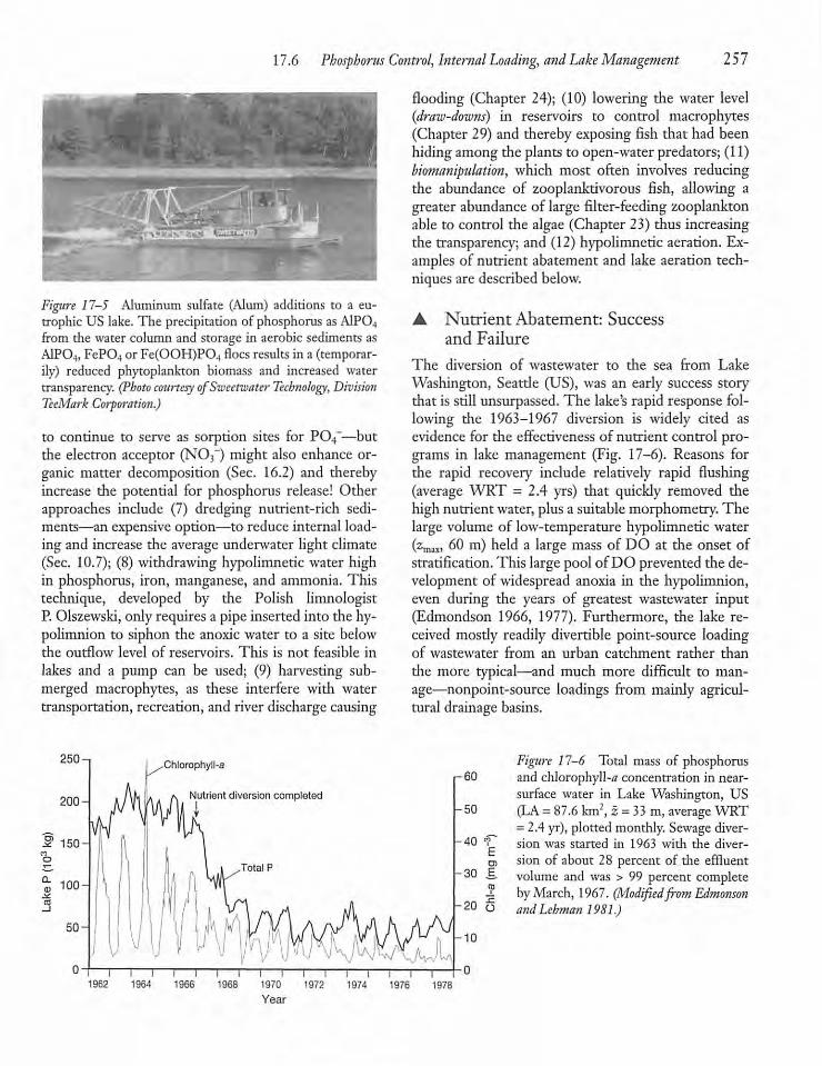
17.6 Phosphorus Control, Internal Loading, and Lake Management 257
Figure 11-5 Aluminum sulfate (Alum) additions to a eutrophic US lake.The precipitation of phosphorus asA1P04from the water column and storage in aerobic sediments asA1P04) FeP04 or Fe(OOH)P04 floes results in a (temporarily) reduced phytoplankton biomass and increased watertransparency. (Photo courtesy ofSweetwater Technology, DivisionTeeMark Corporation.)
to continue to serve as sorption sites for P04"—butthe electron acceptor (N03_) might also enhance organic matter decomposition (Sec. 16.2) and therebyincrease the potential for phosphorus release! Otherapproaches include (7) dredging nutrient-rich sediments—an expensiveoption—to reduce internal loading and increase the average underwater light climate(Sec. 10.7); (8) withdrawing hypolimnetic water highin phosphorus, iron, manganese, and ammonia. Thistechnique, developed by the Polish limnologistP.Olszewski, only requires a pipe inserted into the hypolimnion to siphon the anoxic water to a site belowthe outflow level of reservoirs. This is not feasible inlakes and a pump can be used; (9) harvesting submerged macrophytes, as these interfere with watertransportation, recreation, and river discharge causing
250-,
1962 19641 I
1966 19681 I I I T1970 1972 1974
Year
flooding (Chapter 24); (10) lowering the water level{draw-downs) in reservoirs to control macrophytes(Chapter 29) and thereby exposing fish that had beenhiding among the plants to open-water predators; (11)biomanipulation, which most often involves reducingthe abundance of zooplanktivorous fish, allowing agreater abundance of large filter-feeding zooplanktonable to control the algae (Chapter 23) thus increasingthe transparency; and (12) hypolimnetic aeration. Examples of nutrient abatement and lake aeration techniques are described below.
• Nutrient Abatement: Successand Failure
The diversion of wastewater to the sea from LakeWashington, Seatde (US), was an early success storythat is still unsurpassed. The lake's rapid response following the 1963-1967 diversion is widely cited asevidence for the effectiveness of nutrient control programs in lake management (Fig. 17-6). Reasons forthe rapid recovery include relatively rapid flushing(average WRT = 2.4 yrs) that quickly removed thehigh nutrient water, plus a suitable morphometry. Thelarge volume of low-temperature hypolimnetic water(zmax) 60 m) held a large mass of DO at the onset ofstratification. This large pool of DO prevented the development of widespread anoxia in the hypolimnion,even during the years of greatest wastewater input(Edmondson 1966, 1977). Furthermore, the lake received mosdy readily divertible point-source loadingof wastewater from an urban catchment rather thanthe more typical—and much more difficult to manage—nonpoint-source loadings from mainly agricultural drainage basins.
1976 1978
Figure 11-6 Total mass of phosphorusand chlorophyll-^ concentration in near-surface water in Lake Washington, US(LA = 87.6 km2, z = 33 m, average WRT= 2.4 yr), plotted monthly. Sewage diversion was started in 1963 with the diversion of about 28 percent of the effluentvolume and was > 99 percent completebyMarch, 1967. (Modifiedfrom'Edmonsonand Lehman 1981.)
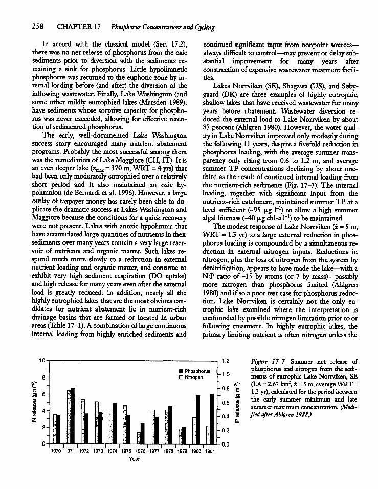
258 CHAPTER 17 Phosphorus Concentrations and Cycling
In accord with the classical model (Sec. 17.2),there was no net release of phosphorus from the oxicsediments prior to diversion with the sediments remaining a sink for phosphorus. Little hypolimneticphosphorus was returned to the euphoric zone byinternal loadingbefore (and after) the diversion of theinflowing wastewater. Finally, Lake Washington (andsome other mildly eutrophied lakes (Marsden 1989),have sediments whose sorptive capacity for phosphorus was never exceeded, allowing for effective retention of sedimentedphosphorus.The early, well-documented Lake Washington
success story encouraged many nutrient abatementprograms. Probably the most successful among themwas the remediation of LakeMaggiore(CH, IT). It isan even deeperlake(£„,„ = 370m,WRT = 4 yrs)thathadbeenonlymoderately eutrophied overa relativelyshort period and it also maintained an oxic hypolimnion (deBernardi et al. 1996). However, a largeoutlay of taxpayer moneyhas rarelybeen able to duplicate the dramatic success at Lakes Washington andMaggiore because the conditions for a quick recoverywere not present. Lakeswith anoxic hypolimnia thathave accumulated largequantities ofnutrientsin theirsediments over many years contain averylarge reservoir of nutrients and organic matter. Such lakes respond much more slowly to a reduction in externalnutrient loadingand organic matter, and continue toexhibit very high sediment respiration (DO uptake)andhighrelease formanyyears even after the externalload is greatly reduced. In addition, nearly all thehighlyeutrophied lakes that are the most obvious candidates for nutrient abatement He in nutrient-richdrainage basins that are farmed or located in urbanareas (Table 17-1).Acombination of largecontinuousinternal loading from highly enriched sediments and
10-
continued significant input from nonpoint sources—always difficult to control—may preventor delay substantial improvement for many years afterconstructionof expensive wastewater treatment facilities.Lakes Norrviken (SE), Shagawa (US), and Soby-
gaard (DK) are three examples of highly eutrophic,shallow lakes that have received wastewater formanyyears before abatement. Wastewater diversion reduced the external load to LakeNorrviken by about87 percent (Ahlgren 1980). However, the water quality in LakeNorrviken improved onlymodesdyduringthe following 11years, despite a fivefold reduction inphosphorus loading, with the average summer transparency only rising from 0.6 to 1.2 m, and averagesummer TP concentrations declining by about one-third as the result of continued internal loading fromthe nutrient-rich sediments (Fig. 17-7).The internalloading, together with significant input from thenutrient-rich catchment, maintained summer TP at alevel sufficient ("95 |xg l"1) to allow a high summeralgal biomass (-40 figchl-tf l"1) to bemaintained.The modest responseof LakeNorrviken (z= 5m,
WRT = 1.3 yr) to a large external reduction in phosphorus loading is compounded by a simultaneous reduction in external nitrogen inputs. Reductions innitrogen, plus the lossof nitrogen from the system bydenitrification, appears to havemade the lake—with aN:P ratio of ~15 by atoms (or 7 by mass)—possiblymore nitrogen than phosphorus limited (Ahlgren1980) and if so a poor test case for phosphorus reduction. Lake Norrviken is certainly not the only eutrophic lake examined where the interpretation isconfounded bypossible nitrogenlimitation prior to orfollowing treatment In highly eutrophic lakes, theprimarylimitingnutrient is often nitrogen unless the
1.2
\3 6-<D
£0
£ 4H
• Phosphorus• Nitrogen -1.0
Figure 17-7 Summer net release ofphosphorus and nitrogen from the sediments of eutrophic Lake Norrviken, SE(LA=2.67 km2, z =5m,averageWRT=1.3yr), calculated for the period betweenthe early summer minimum and latesummer maximum concentration. (ModifiedafterAhlgren 1988.)
ii i i i i i i i i r1970 1971 1972 1973 1974 1975 1976 1977 1978 1979 1980 1981
Year
-0.8
-0.6
-0.2
•0.0
%
h0.4 2
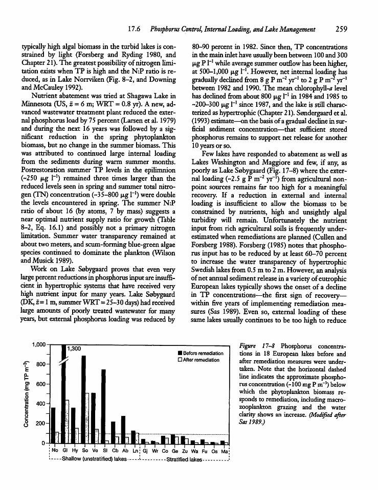
17.6 Phosphorus Control^ InternalLoading, andLakeManagement 259
typically high algal biomassin the turbid lakes is constrained by light (Forsberg and Ryding 1980, andChapter21). The greatestpossibility ofnitrogenlimitation exists whenTP is high and the N:P ratio is reduced, as in LakeNorrviken (Fig. 8-2, and DowningandMcCauley1992).Nutrient abatement was tried at Shagawa Lake in
Minnesota (US, z = 6m; WRT = 0.8 yr). A new, advanced wastewater treatment plant reduced the externalphosphorusloadby 75percent (Larsenet al. 1979)and during the next 16 years was followed by a significant reduction in the spring phytoplanktonbiomass, but no change in the summer biomass. Thiswas attributed to continued large internal loadingfrom the sediments during warm summer months.Postrestoration summer TP levels in the epilimnion(~250 u.g I"1) remained three times larger than thereduced levels seen in spring and summer total nitrogen(TN) concentration (~35-800 \xg l"1) were doublethe levels encountered in spring. The summer N:Pratio of about 16 (by atoms, 7 by mass) suggests anear optimal nutrient supply ratio for growth CTable8-2, Eq. 16.1) and possibly not a primary nitrogenlimitation. Summer water transparency remained atabout two meters, andscum-forming blue-green algaespecies continued to dominate the plankton (WilsonandMusick 1989).Work on Lake Sebygaard proves that even very
large percent reductions inphosphorus inputareinsufficient in hypertrophic systems that have received veryhigh nutrient input for many years. Lake Sabygaard(DK, z= 1m,summerWRT=25-30 days) hadreceivedlarge amounts of poorly treated wastewater for manyyears, but external phosphorus loading was reduced by
1,000-i
80-90 percent in 1982. Since then, TP concentrationsin themaininlethaveusually beenbetween 100and300|xg P l"1 while average summer outflow has been higher,at 500-1,000 pug l"1. However, net internal loading hasgradually declined from 8gP m"2 yr-1 to 2 gP m"2 yr-1between 1982 and 1990. The meanchlorophyll-/? levelhas declined from about 800 p,g l"1 in 1984 and1985 to~200-300 p,g l"1 since 1987, andthe lake is still characterized ashypertrophic (Chapter 21). Sendergaard et al.(1993) estimate—on the basis ofa gradual decline in sur-ficial sediment concentration—that sufficient storedphosphorus remains to support net release for another10years or so.Few lakes have responded to abatement aswell as
Lakes Washington andMaggiore and few, if any, aspoorlyasLakeSobygaard (Fig. 17-8)where the external loading (~2.5 g P m~2 yr-1) from agricultural non-point sources remains far too high for a meaningfulrecovery. If a reduction in external and internalloading is insufficient to allow the biomass to beconstrained by nutrients, high and unsightly algalturbidity will remain. Unfortunately the nutrientinput from richagricultural soils is frequently underestimated whenremediations are planned (Cullen andForsberg 1988). Forsberg (1985) notes that phosphorus input has to be reduced by at least 60-70 percentto increase the water transparency of hypertrophicSwedish lakes from 0.5 mto 2m.However, ananalysisofnetannual sediment release in avariety ofeutrophicEuropean lakes typically shows the onset of a declinein TP concentrations—the first sign of recovery—within five years of implementing remediation measures (Sas 1989). Even so, external loading of thesesame lakes usually continues to be too highto reduce
7 800-E
|> 600-
1,300• Before remediation• After remediation
Figure 17-8 Phosphorus concentrations in 18 European lakes before andafter remediation measures were undertaken. Note that the horizontal dashedline indicates the approximate phosphorusconcentration (-100mgP m~3) belowwhich the phytoplankton biomass responds to remediation, including macro-zooplankton grazing and the waterclarity shows an increase. (Modified afterSas1989.)
2 400-
oo 200-
i I TNo Gl Hy So Ve
q-^T^SI Cb Ab Ln; Gj Wr Co Ge Zu Wa Fu Os Ma;
Shallow (unstratified) lakes '- Stratified lakes •
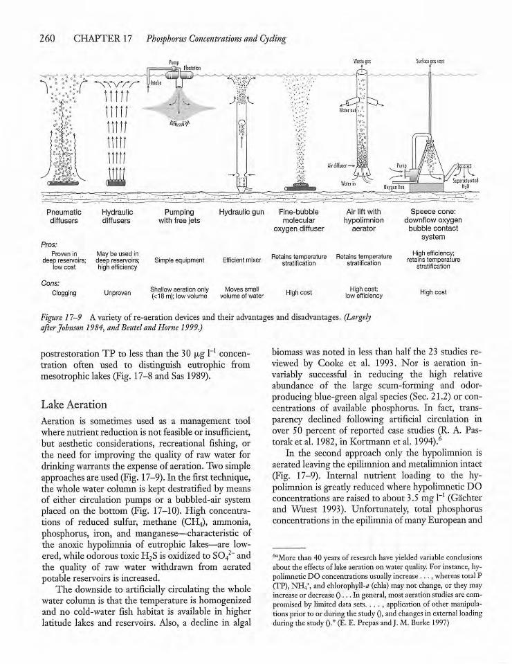
260 CHAPTER 17 Phosphorus Concentrations and Cycling
Pump Surface gos vent
>i--r
Pneumaticdiffusers
Hydraulicdiffusers
Pumpingwith free jets
Hydraulic gun Fine-bubblemolecular
oxygen diffuser
Air lift withhypolimnionaerator
Pros:Proven in May be used in
deep reservoirs; deep reservoirs;low cost high efficiency
Simple equipment r«i-:««» m;„„. Retains temperature Retains temperatureEfficient mixer stratifica^ion stratification
Speece cone:downflow oxygenbubble contact
system
High efficiency;retains temperature
stratification
Cons:Clogging Unproven Shallow aeration only
(<18m); low volumeMoves small
volume of water High cost High cost;low efficiency High cost
Figure 11-9 Avariety of re-aerationdevices and their advantages and disadvantages. (LargelyafterJohnson 1984, andBeutel andHome 1999.)
postrestoration TP to less than the 30 \xg 1 concentration often used to distinguish eutrophic frommesotrophic lakes (Fig. 17-8 and Sas 1989).
Lake Aeration
Aeration is sometimes used as a management toolwhere nutrient reduction is not feasible or insufficient,but aesthetic considerations, recreational fishing, orthe need for improving the quality of raw water fordrinking warrants the expense of aeration. Two simpleapproaches are used(Fig. 17-9). In the first technique,the whole water column is kept destratified by meansof either circulation pumps or a bubbled-air systemplaced on the bottom (Fig. 17-10). High concentrations of reduced sulfur, methane (CH4), ammonia,phosphorus, iron, and manganese—characteristic ofthe anoxic hypolimnia of eutrophic lakes—are lowered,while odorous toxic H2S isoxidized to S042- andthe quality of raw water withdrawn from aeratedpotable reservoirs is increased.The downside to artificially circulating the whole
water column is that the temperature is homogenizedand no cold-water fish habitat is available in higherlatitude lakes and reservoirs. Also, a decline in algal
biomass was noted in less than half the 23 studies reviewed by Cooke et al. 1993. Nor is aeration invariably successful in reducing the high relativeabundance of the large scum-forming and odor-producing blue-green algal species (Sec. 21.2) or concentrations of available phosphorus. In fact, transparency declined following artificial circulation inover 50 percent of reported case studies (R. A. Pas-toraket al. 1982, in Kortmann et al. 1994).6In the second approach only the hypolimnion is
aerated leavingthe epilimnion and metalimnion intact(Fig. 17-9). Internal nutrient loading to the hypolimnion is greatlyreducedwherehypolimnetic DOconcentrations are raised to about 3.5 mg1_1 (Gachterand Wuest 1993). Unfortunately, total phosphorusconcentrations in the epilimniaofmanyEuropean and
6"More than 40 years of research have yielded variable conclusionsabout the effects of lakeaerationonwater quality. For instance, hypolimnetic DO concentrations usually increase .. . , whereas total P(TP), NH4+, and chlorophyll-^ (chla) maynot change, or theymayincrease or decrease 0 •••In general, mostaerationstudiesarecompromised by limited datasets. . . . , application of odier manipulations priorto or duringthestudy 0, andchanges in external loadingduring the studyQ." (E. E. Prepas andJ. M. Burke 1997)
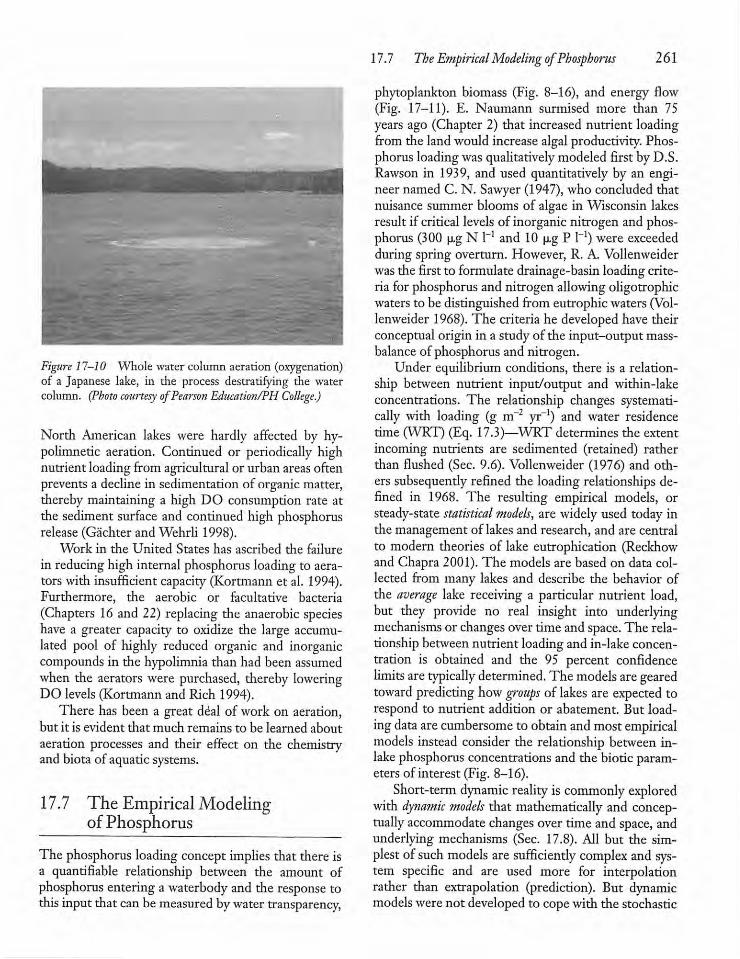
Figure 11-10 Whole water column aeration (oxygenation)of a Japanese lake, in the process destratifying the watercolumn. (Photo courtesy ofPearson Education/PH College.)
North American lakes were hardly affected by hypolimnetic aeration. Continued or periodically highnutrient loading from agricultural or urban areas oftenprevents a decline in sedimentation of organic matter,thereby maintaining a high DO consumption rate atthe sediment surface and continued high phosphorusrelease (Gachter and Wehrli 1998).Work in the United States has ascribed the failure
in reducing high internal phosphorus loading to aerators with insufficient capacity(Kortmann et al. 1994).Furthermore, the aerobic or facultative bacteria(Chapters 16 and 22) replacing the anaerobic specieshave a greater capacity to oxidize the large accumulated pool of highly reduced organic and inorganiccompounds in the hypolimnia than had been assumedwhen the aerators were purchased, thereby loweringDO levels (Kortmann and Rich 1994).There has been a great deal of work on aeration,
but it is evident that much remains to be learned aboutaeration processes and their effect on the chemistryand biota of aquatic systems.
17.7 The Empirical Modelingof Phosphorus
The phosphorus loadingconcept implies that there isa quantifiable relationship between the amount ofphosphorus enteringa waterbody and die response tothis input that canbemeasured bywater transparency,
17.7 The EmpiricalModeling ofPhosphorus 261
phytoplankton biomass (Fig. 8-16), and energy flow(Fig. 17-11). E. Naumann surmised more than 75years ago (Chapter 2) that increased nutrient loadingfrom the land would increase algal productivity. Phosphorus loadingwasqualitatively modeled first by D.S.Rawson in 1939, and used quantitatively by an engineer named C. N. Sawyer (1947), who concluded thatnuisance summer blooms of algae in Wisconsin lakesresult if critical levels of inorganic nitrogen and phosphorus (300 ^g N I and 10 jxg P l-1) were exceededduring spring overturn. However, R. A.Vollenweiderwasthe first to formulate drainage-basin loadingcriteria for phosphorus and nitrogen allowingoligotrophicwaters to be distinguished from eutrophic waters (Vollenweider 1968). The criteria he developed have theirconceptualorigin in a study of the input-output mass-balance of phosphorus and nitrogen.Under equilibrium conditions, there is a relation
ship between nutrient input/output and within-lakeconcentrations. The relationship changes systematically with loading (g m~2 yr-1) and water residencetime (WRT) (Eq. 17.3)—WRT determines the extentincoming nutrients are sedimented (retained) ratherthan flushed (Sec. 9.6). Vollenweider (1976) and others subsequently refined the loadingrelationships defined in 1968. The resulting empirical models, orsteady-state statistical models, are widely used today inthe management of lakes and research, and are centralto modern theories of lake eutrophication (Reckhowand Chapra 2001). The models are based on data collected from many lakes and describe the behavior ofthe average lake receiving a particular nutrient load,but they provide no real insight into underlyingmechanisms or changes overtime and space. The relationship between nutrient loadingand in-lakeconcentration is obtained and the 95 percent confidencelimits are typically determined. The models are gearedtoward predicting how groups of lakes are expected torespond to nutrient addition or abatement. But loadingdata arecumbersome to obtain andmostempiricalmodels instead consider the relationship between in-lake phosphorus concentrations and the biotic parameters of interest (Fig. 8-16).Short-term dynamic reality is commonly explored
with dynamic models that mathematically and conceptually accommodate changes over time and space, andunderlying mechanisms (Sec. 17.8). All but the simplest ofsuch models are sufficiently complex and system specific and are used more for interpolationrather than extrapolation (prediction). But dynamicmodels werenot developed to copewith the stochastic
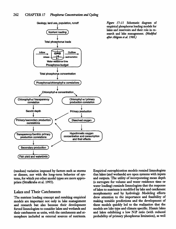
262 CHAPTER 17 Phosphorus Concentrations and Cycling
Geology, land use, population, runoff
T(Nutrient loading J
1Total phosphorus loads
Inflow
Water residence time
Phosphorus budget
Outflow
sedimentation
ITotal phosphorus concentration
*^Phosphorus/chlorophyil-a correlationsJ
1Chlorophyll-a concentration
/ \
Figure 17-11 Schematic diagram ofempirical phosphorus loadingmodels forlakes and reservoirs and their role in research and lake management. (ModifiedafterAhlgren etal 1988.)
( Chlorophyll-a/transparencycorrelation ) C Chlorophyll-a/primary
production correlation D
z
ISecchi depth
i1
Primary production
IQDissolved oxygen 3Primary/secondary production
correlations
Transparency/benthlc primaryproduction correlationsc
Hypolimnetic oxygenconcentration and consumption
and their effects
1( Secondary production )
(Fish yield and waterblrds)
(random)variation imposed by factors such as stormsor disease, nor with the long-term behavior of systems,forwhichyet other model typesaremore appropriate(Straskraba et al. 1993).
Lakes and Their Catchments
The nutrient loading concept and resulting empiricalmodels are important not only in lake managementand research but also because their developmentforced limnologists to consider lakes andwedands andtheir catchments as units, with the catchments and atmosphere included as external sources of nutrients.
Empirical eutrophication models remindlimnologiststhat lakes(andwedands) are open systemswith inputsand outputs. The utilityof incorporating meandepth(a surrogate for volume and water residence time orwaterloading) reminds limnologists that the responseof lakes to nutrients ismodified by lakeand catchmentmorphometry and by hydrology. Modeling effortsdrew attention to the importance and feasibility ofmaking testable predictions and the development ofthese models quickly led to the realization that themodels arelake type andclimate specific. Humic lakesand lakes exhibiting a low N:P ratio (with reducedprobability of primary phosphorus limitation), aswell
as lakes having high inorganic turbidity (light limitation) are often excluded as they do not fit the laketypeof greatestinterest.Nor are the most commonly usedempirical models applicable to eutrophic lakes withanoxic hypolimnia, which—in addition to external inputs—often experience internal phosphorus loading(Sec. 17.4).The following equation developmentwas derived
fromAhlgren et al. 1988.Readers not concernedwithmodelderivations shouldskip to Section 17.8.A The basic mass-balance model for total phosphorus can be written as:
®= MQPV-^-S. EQ. 17.4
SeeTable 17-4 for symbols and units. Byconsideringa lake to be in equilibrium on an annual basis[A(PV/Ar) = 0], the amount of phosphorus retained(equals inputminusoutput)is equalto the mass in thewater minus the net sedimentation (S).However, Vollenweider concluded that it would bemore logical toconsider retention as a function of the in-lake mass orconcentration:
©=«- PQ " <rP, EQ.17.5
where the sedimentation coefficient a is the fractionofthein-lake mass ofP removed annuallybysedimentationviaall processes other than outflow.
17.7 The EmpiricalModeling ofPhosphorus 263
Atsteadystate,Eq. 17.5 is reducedto
*=(m^)- EQ17-6and substituting the flushing rate pw for Q/v:
PV=(——Y EQ.17.7VPw + oV
lb yield the within-lake concentration, the mass inEq. 17.7 is divided by lakevolume(v):
= /_M/V_\\pw + o-/
EQ.17.8
M/Visequivalent toLp/z, andsubstitution inEq. 17.8produces
EQ. 17.9
which is the basic equation underlying mostphosphorus loading models. This equation is important inboththeoretical andapplied limnology because it provides a quantitative basis forunderstandingwhysomelakes areoligotrophic andotherseutrophic. Equation17.9 also provides a partial explanation for the tendency ofdeep lakes to bemoreoligotrophic thanshallow ones, and that rapidly flushed lakes retain lessphosphorus and fewer particles of all kinds because ahigher fraction of them leave via the outflowthan inlakes that flush moreslowly. When both the numera-
Table 17-4 Symbols and units usedin die phosphorus mass-balancemodels.
p =TP= in-lake total phosphorusconcentration (mgm-3)Pi = inflow mean total phosphorusconcentration (mg nr3)Lp = annual P loading (mg m~2 yr1)V = lakevolume(m3)PV= total mass of phosphorus in lake (mg)f = time
M = annual inputmass of phosphorus (mgyr1)O = annual outflow mass of phosphorus (mgyr1)Q = dischargeof the outletof lake (m3 yr1)qB = water discharge height (myr1)S = annual net sedimentation of phosphorus (mg yr1)a = sedimentation coefficient (yr1)v = apparent P settling velocity(myr1)z = lake mean depth (m)pw = Q/V = flushing rate (yr1)tw sl/fvO/VRT, yr)orWRTRa = P retention coefficient
Source: AfterAhlgren et al. 1988.
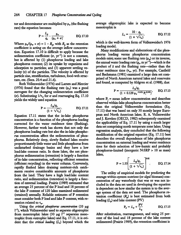
264 CHAPTER17 Phosphorus Concentrations and Cycling
tor anddenominatoraremultiplied by pw (the flushingrate) the equation becomes
P =Pw
9s (Pw + Or)'EQ. 17.10
Where pw/(pw +a) = 1 - I2p, with Rp as the retentioncoefficient is actingon the average inflow concentration. Equation 17.10 is difficult to applybecause thesedimentation coefficient (a, yr-1) is not a constant,but is affected by (1) phosphorus loading and lakephosphorus content; (2) its uptake by organisms andadsorption to particles; and (3) apparent settling velocity (v) of the particles. The velocity is affected byparticlesize,stratification, turbulence,food-web structure, etc. (Sees. 20.4 and 21.6).Both Vollenweider (1976) and Larsen and Mercier
(1976) found that the flushing rate (pw) was a goodsurrogate for the changing sedimentation coefficient(a). Substituting1/twfor a and rearrangingEq. 17.10yields thewidely used equation
V*«P =(1 +V£)'
Equation 17.11 states that the in-lake phosphorusconcentration is a functionof the phosphorus loadingcorrected for the water residence time (flushing).However, further work has shown that not only thephosphorus loading rate but alsothe in-lake phosphorus concentration affect the sedimentation of phosphorus. Relatively deep, slowly flushed lakes receiveproportionatelylittlewater and little phosphorusfromundisturbed drainage basins and they have a lowloaddake content ratio. In these lakes, the net phosphorussedimentation (retention) is largely a functionof in-lake concentration, reflectingefficientretention(efficient recycling) in the water column. Conversely,rapidly flushed lakes draining nutrient-rich catchments receive considerable amounts of phosphorusfrom the land. They have a high loaddake contentratio, and sedimentation (retention) is largely a function of external loading. Prairie (1989) estimatedthatan average 25 percent of the P loadand 18percentofthe lake P content of 120 lakes examined sedimented(retained) annually. Reliable estimates of P retentionmust consider both P load and lake P content, with retention related to tw.Using the critical phosphorus concentration (10 fig
l"1), which Vollenweider usedto separate oligotrophicfrom mesotrophic lakes (30 p,g l"1 separates meso-trophic from eutrophic lakes) and Eq. 17.11, it is evident that the critical loading (L^ beyond which the
EQ. 17.11
average oligotrophic lake is expected to becomemesotrophic is
10-ftLP =
(1 +V*w)'which is the well-known form ofVollenweider's 1976loadingmodel.Manymodifications and elaborationsof the phos
phorus loading versus phosphorus concentrationmodelsexist; someuse flushingrate (pw) or its inverse,theannualwater loading rate(q„myr-1)—which istheproduct of z and the flushing rate—rather than thewater residence time (tot yr). For example, Canfieldand Bachmann (1981) examined a large data set comprisedof North Americannatural lakesand reservoirsand found, as computedbyAhlgren et al. (1988), that
Lp/q*P =
(1 + 0.129 pw-0.4511> 0.549 )'
EQ. 17.12
EQ. 17.13
where Pj = mean inflow concentration and describesobserved within-lakephosphorusconcentration betterthan the original Vollenweider formulation (Eq.17.11) that was based on only30mosdy largerEuropean and North American lakes. R. A. VollenweiderandJ. Kerekes (OECD, 1982) subsequently examinedthe applicability of Eq. 17.11 by using a much largerdataset comprisingnorth temperatezonelakes. Usingregression analysis, they concluded that the followingmodification of the originalequation(Eq. 17.11) bestdescribes the overall dependence of lake phosphorusconcentrationon externalloadingandwater residencetime for their selection of low-humic and probablyphosphorus-limited (inorganic N:SRP > 10 as mass)lakes,
P = 1.55Lp/qs
(1 +Vo
0.82
EQ. 17.14
The utility of empirical models for predicting theaverage within-system nutrient (or algalbiomass) concentration of any waterbody that was or was not included in the data set used in developing the equationis dependent on howsimilar the system is to the average system of the data set used. The phosphorus retention coefficient (Rp) is best estimated from bothloading (Lp) and lake content (PV)
PV EQ. 17.15
After substitution, rearrangement, and using 25 percent of the load and 18 percent of the lake contentsedimented (Prairie 1989), the retention coefficient is
= 0.25 + 0.18tp 1 + 0.18t '
EQ. 17.16
This equation states that the dependence of Rp onWRT (t) is attributable to sedimentation of both theload and lake content.Equations 17.11 and 17.14are easily rearrangedto
estimate the phosphorus loading. Such a rearrangement is useful for confirming the reliability of estimated phosphorus loadings that are based on directmeasurements or export coefficients (Table 8-8). Theutilityof this exercise rests upon having measured theparametersof the equationswith little error.For most limnologists, the prediction of phospho
rus loading or in-lake phosphorus concentration isonlya steppingstone towardspredicting,for example,aspects of phosphorus dynamics, algal biomass or primaryproduction, dissolved oxygen consumption rates,secondary production, or fish yields (Fig. 17-11).Equivalent work on small lotic systems suggests thatwhen in-stream total phosphorus concentration iskept below 30u,g PI"1, and total nitrogen concentration iskept below 350 u,g N l"1, thebenthic algal biomass is not likely to exceed nuisance levels of 100 mgchl-tf nT2 (Dodds et al. 1997).
17.8 The DynamicModelingof Phosphorus
There mustbe a trade-off between the simplicity andgenerality ofmodels, andtheprecision ofpredictions.7Empirical statistical models suchas those described byEqs. 17.11,17.13, and 17.15 have the desired simplicity and considerable generality. However, the best-known models are not trulygeneral, instead theyarerestricted to a particular set of nonhumic freshwaterlakes in the temperate zone with typically oxic hypolimnia where the N:P ratio suggests a primaryphosphorus limitation. Furthermore, models makestatements about theaverage behavior of large "populations" of waters, and their application to individualsystemsmay result in large errors.In empirical models, the natural complexity is re
duced to annual or seasonal averages of loading andconcentration. Steady-state empirical models also saynothing aboutthe effect of phosphorus over time andspace within particular lakes ofinterest. Butthe largest
7"Any model remains an intellectual plaything oflimited impact...unless it can betested byand verified byexperiment, orbyfield observation, or both." (C. H. Mortimer 1975)
17.8 The DynamicModeling ofPhosphorus 265
shortcoming of empirical modeling is that without acause and effect structure, it can only reliably forecastunder conditions similar to those reflected in the dataset thatwas used to construct themodels. The problemofmultiple causes and effects—which can be plausiblyexplained by differentmechanisms or combinations ofmechanisms—retard progress in ecology andlimnology,andsets limits uponthe utility ofempirical anddynamicmodeling. Furthermore, individual scientists with rootsin different paradigms tend to hold strongviews aboutwhich mechanisms or processes are believed most important8There is a need for more flexible, powerful mod
els. The desired models should not only be able topredict future states but also provide explanationsabout why the system of interest behaves as it doesbased on both the mechanisms and processes that areemployed bybiological or chemical species or groupsof species. Lake specific answers would be obtained.This need has beenpartially met by the developmentof dynamic simulation models with varying complexity(Sec. 2.6), complementing the empirical models discussed above. But the dynamicmodelshave their limitations. In the case of phosphorus modeling, little isknown about the processes and mechanisms to bemodeled, some necessary data are lacking, and it isunknown which environmental factors exert thestrongest influence on different phosphorus compartmentsover time and space. Three dynamic modelsarediscussed below.
A EAWAGModel
Dynamic eutrophication models available today differgready incomplexity depending on thegoals (generality versus precision) and interest and background ofthe creators. An example of a simple dynamic phosphorus model is the EAWAG model, developed at theSwiss Federal Institute for Environmental Science andTechnology [EAWAG] (Fig. 17-12). This model issimple because it uses only soluble reactive phosphorus(SRP), particulate phosphorus (PP), anddissolved oxygen concentration as the state or predictor variablesevaluated over time. Fixed rateconstants (modelparameters) for photosynthesis, respiration, mineralization,
'Individual bias was first recognized in 1897 by T.C. Chamberlinwhen hewrote, "There is the thenimminent danger of an unconscious selection and of a magnifying of phenomena that fall intoharmonywith thetheory and support it and anunconscious neglectof phenomenathat fail that coincidence."
CHAPTER 17 Phosphorus Concentrations and Cycling
[SRP]Mineralization
[PP] + [02]
sedimentation, sediment oxygen consumption, sediment phosphorus release, flushing, and in-lake transport between the epilimnia, metalimnia, andhypolimnia were either measured or obtained frompublished data. The experimentally determined rateconstants were obtained in one region of Switzerland—characterized by a particular climate, geology,and lake morphometry—and the resulting model istherefore a regional model, but it can be "recalibrated"for work elsewhere.The EAWAG model is simple from a dynamic
modeling perspective; it employs many fixed (nondynamic) constants, some of which are obtained fromsteady-state statistical (empirical) models. However,data requirements for predicting phosphorus concentrations are much larger for the EAWAG dynamicmodel than for empiricalmodels. This particular disadvantage isacceptable to thosewhovalue the insightsto be gained by considering aspects of the dynamicsthat are based on a mechanistic underpinning. Thisunderpinning allows simple (simplistic) dynamic models to be seen as a stepping stone toward more comprehensive models. Whether EAWAG or anothersimplified dynamic model with empirical aspects willallow for better predictions than is possible withequivalentregionallydeveloped but far simpler empirical models is not well resolved (Ahlgren 1988).It is important to keep in mind that simplicity,
generality, and predictivepowerare not the onlycriteria considered to be important in modeling. Whilepredictive power is certainly a long-termgoalof most
Figure 11-12 Schematic diagram of asimple dynamic model. The EAWAGmodel is based on a limited number ofrequired measurements. (Modified afterR. Gdchter et al. 1983, in Ahlgren et al.1988.)
scientists favoring dynamic simulation modeling, theprimary short-term goal is usually an exploration todiscover gaps that can form the basis for researchand more comprehensive models. Indeed, simulationspoint to outcomes that are rarely imaginable on thebasis of common sense and they provide new explanations for events observed in nature (Scheffer and Beets1994).
Lake Glumsoe Model
The EAWAG model is interesting becauseit explicitlyexplores the possibilities of embedding empirical aspectswithina simple dynamic model, therebybenefitting from an explicit consideration of processes andmechanisms. Much more complex than the EAWAGmodelfor phosphorus, but of onlymoderatecomplexity, is the ecosystem model originally developed forthe highly eutrophicLakeGlumsoein Denmark(Fig.17-13). It describes the behavior of three trophic levels (phytoplankton, zooplankton, and fish) as a function of the phosphorus supply. Instead of the twophosphorus state variables used in the EAWAGmodel, the Glumsoe model uses a large number of simultaneous equations that include eight phosphorusvariables, another nine nonphosphorus state variables,plus 19 parameters describing the lake, and 28 fixedrate constants to define the phosphorus, nitrogen, andenergy fluxes between compartments. The 28 fixedrate constants have to be determined—an enormousand almostimpossible task—or drawnfrom the litera-
SEDIMENT
17.8 The DynamicModeling ofPhosphorus 267
Figure 17-13 Schematic diagramof theGlumsoe model of phophorus cycling.Note its complexity relative to Fig.17-12, and its simplicity relative to Fig.17-14. (Modified after Jargensen et al.1986.)
in interstitial water exchange fraction NonexchangeP
turewith their relevance to the system in question uncertain. The relatively complex Glumsoe model andother such models are abstractions and a simplification of reality. Some of the particular constants selected from the laboratory andfield literature requireadjustment (calibration, tuning) tomake themodel results fit observed lake behavior. Sophisticated techniques are available for thispurpose andgoodfits canbe obtained, but since adjusted constants have noknown biological reality themodels arenotveryusefulfor predicting the behavior of the same lake after achange in nutrient loading or fish introduction, or forpredicting the behavior of other lakes that inevitablydiffer physically, chemically, andbiologically from thelake onwhich themodel was originally based. Moreover, the samegoodfit betweenobserved andmodeleddata can beproduced bymanipulating different sets ofconstants or state variables.
PCLOOS Model
A final, more recent example of an interesting,but considerably more complex, dynamic simulationmodel is the PCLOOSmodel developed byJanse etal. (1992). It attemptsto dealwithbothwaterandsediment processes and addresses not only phosphorusbut also carbon fluxes (Fig. 17-14). This model hasbeen partly calibrated and used to simulate (interpolate) what should happen in a Dutch lake following areduction in external phosphorus loading.
Recent DevelopmentsMost of the dynamic modeling done today has lessgrandiose goals than the ecosystem-level modelingdiscussed above. The limitations ofmodeling complexsystems is better understood and most current dy-
268 CHAPTER 17 Phosphorus Concentrations and Cycling
BenthosEgesfionand death
namic modeling exercises focus on more readilytestable components ofthe earlier ecosystem models.9The complexity of evenrelatively simple dynamic
modelsis sufficiendy large that consideration of theirunderlying assumptions is beyond the scope of a general limnology text. However, the importance of developing both simple empirical and more complexsimulation models is without question. Empiricalandsimulation modelscombinedwith other modelingapproaches complement one another. They make it possible to develop relatively simple hybrid models thatcombine empirical modeling based on field surveydatawith dynamic modeling of population responsesto changesin environmental factors, basedon laboratory experiments, to produce population level forecasts (Shuter and Regier 1989). But even hybridmodels are not easy to present (explain) in a general
'"Science canbeviewed astheprocess ofbuilding successively "better" descriptive and predictivemodels of the world. But how doesone define "better?" In the past, scientists have tended to narrowtheir questions in order to achieve higher accuracy. This leads to[dynamic] modelswith lowarticulation [fewcomponents] but highdescriptive accuracy. They saymuchabout little.More recendyscientistshavebegunto takea "systems view" that looksat phenomenamore comprehensively. This strategy leads to highly articulated[manycomponent]modelswith lowaccuracy. These modelssaylittle about much." (R. Costanza and F.H. Sklar 1985)
Outflow
Inflow
Figure 17-14 Overview of thePCLOOS model of phosphorus and carbon flow in aquatic systems. Compartments modeled in two units are indicatedby two boxes, one behind the other. Thephytoplankton compartment is composed of three functional groups: cyano-bacteria, diatoms, and green algae. Thearrowsdenote both carbon and phosphorus fluxes. (Modified from Janse et al.1992.)
textbook. For all their limitations, simple empiricalmodels provide a much needed pattern (generality)and are an important starting point in research. Theyalsoplaya crucially important role in aquaticmanagement, not because they make precise predictions butbecause the rate of environmental degradation is solarge that there is no alternative to making management decisions based on imprecise empirical models.See Schefferand Beets 1994for an excellentand easy-to-understand discussion of the possibilities and limitationsofmodeling approaches.
Highlights• Phosphorus is the element usuallyin shortest supplyfor algalgrowth in oligotrophic and mesotrophicwaters characterized by a N:P supply ratio that is muchhigher than the demandratio of algalprotoplasm.
• According to the classical FeP04 model,sedimentingand sedimented iron oxyhydroxide floes (aggregates)strongly sorbP043". Sedimented aggregates serve asan effective phosphate diffusion barrier to sedimentsolublereactivephosphorus (SRP) as long as the aggregates remainintactunder oxic conditions.
• When DO concentration approaches zero and thesediment surface redox potential declines to below~200 mV, the aggregates dissolve and the elementsdiffuse into the overlyingwater.
• Microbes play a major direct and indirect role inphosphorus release from sediment, modifying theclassical viewofsedimentrelease asa primarily chemical process. Phosphorus is not always released followingthe dissolution of iron aggregates.
• • In shallow eutrophiclakes, physical disturbance ofthe oxic sediments allows dissolved phosphorus to escape to the overlying water, bypassing the diffusionbarrier.
• A The fraction of incoming phosphorus that is retained by lakes and wetlands and stored in the sediments increases with water residence time.
• A As the catchment area to lake area ratio declines,sedimentrelease, nutrient recycling in the water columnandthe atmosphere become increasingly important as sources of phosphorus for algaland microbialgrowth.
• The principal phosphorus (and nitrogen) remediation (abatement) techniques involve (1) nutrient removal fromwastewater in sewage treatmentplants or
17.8 The DynamicModeling ofPhosphorus 269
wedands before release; (2) diversion of wastewaterfrom rivers and lakes; and (3) the maintenance orconstruction ofwell-vegetated buffer stripsalongwaterways to trap dissolved and particulate phosphorusreleased asthe resultofparticular land-use practices.
• A The recovery of lakes following phosphorusabatement is quickest in rapidly flushed lakes wherethe nutrient and organicmatter inputshad beensmallenough to allow an oxic hypolimnion to be maintained. Recovery is slowest in those shallow lakeswith an anoxic hypolimnion that had received andstored large quantities of nutrients and organic matter in theirsediment overmanyyears, allowing themto serve as an ongoing source of phosphorus to theoverlyingwater. Recovery is impossible where catchment exportsremain high.
• There isno "best" modeling approach. The mostappropriate models change with the temporal and spatialscales atwhich questions areposed.
H A P T E R
18
Nitrogen Cycling
18.1 Introduction: The Atmosphere,the Land, and the Water
Nitrogenplays a central role in inland waters. Nitrogen and phosphorus are commonly the elements ingreatest demand by plants and the heterotrophic microbes relative to supply (Table 8-1). The nitrogensupply is thereforeofgreatimportance in determiningthe primary productivity of aquatic systems and microbial recycling of organicmatter.Nitrogen, in contrastto phosphorus, exists in ava
rietyof oxidized and reduced forms (oxidation states)that allow it to serve as an electron donor and receiverin a host of oxidation-reduction reactions (Table16-1) of central importance in nutrient cycling andbiogeochemistry.Ionicand organic nitrogen are supplied to aquatic
systems from drainage basins and the atmosphere.Total nitrogen (TN) in precipitation ranges from alow of-100kgkm-2 yr-1 in polar regions to over 2,000kgkm-2 yr-1 inor downwind from industrial and agricultural regions in the north temperate zone (Table8-10). Boring et al. (1988) reported a similar rangeover primarily forested regions of the United Statesalso indicating longdistance transportfromregions ofemission.Atmospheric nitrogen inputs to the land have ap
proximately doubled globally—and even more locally—as the result of human activity, withairmassescarrying the emitted nitrogen over longdistances be
270
fore deposition (Vitousek et al. 1997). In the northeastern US,theatmospheric deposition ofnitrogen onthe landscape, primarily originating from fossil fuelcombustion, currently exceeds all other individual nitrogen inputs from fertilizer, imported food andfeed,andnitrogenfixation bycropsQaworski et al. 1997). A12-year record of TN deposition in Ontario (CA),downwind from major US source regions, showedthat about half the bulk precipitation—precipitationcollected in open containers (Chapter 27)—to be inthe form of N03", a third asNfV, and the balance astotal organic nitrogen (TON) (Molot and Dillon1993). More limited data suggest that a similarN03:NH4+ ratio characterizes the wet tropics (Downinget al. 1999) whereas measurements in central Europe indicate a slighdy greater deposition of NIVthan N03", mosdy in summer (Kopacek et al. 1997).The ratio is further skewed toward NH** in westernEurope as the result of enormous emisions from livestockwastes (Chapter 27).
Long-term Increasein Nitrogen DepositionAn indication of the widely reported long-term increase in nitrogendeposition from the atmosphere isprovided by nitrate measurements made in remoteLake Superior (CA, US). The lake is characterized byan unusually small catchment area to lake area(CA:LA) ratio(1.6) andthin,nutrient-poorborealfor-
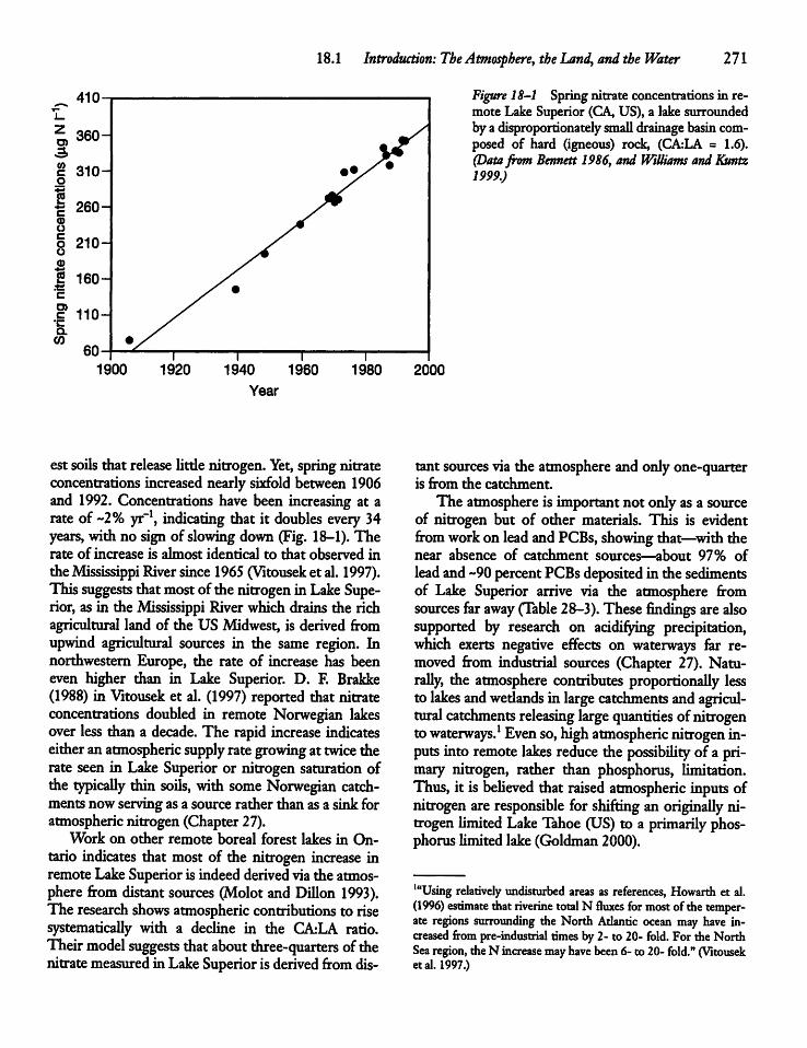
18.1 Introduction: TheAtmosphere, the Land, and the Water 271
410
1900 1920 1940 1960
Year
1980
est soils that release little nitrogen.Yet, springnitrateconcentrations increased nearly sixfold between 1906and 1992. Concentrations have been increasing at arate of ~2% yr"1, indicating that it doubles every 34years, with no sign of slowing down (Fig. 18-1).Therate of increase is almost identical to that observed intheMississippi Riversince1965(Vitousek et al. 1997).This suggests thatmostofthe nitrogen in Lake Superior, as in the Mississippi Riverwhich drains the richagricultural land of the US Midwest, is derived fromupwind agricultural sources in the same region. Innorthwestern Europe, the rate of increase has beeneven higher than in Lake Superior. D. F. Brakke(1988) in Vitouseket al. (1997) reported that nitrateconcentrations doubled in remote Norwegian lakesover less than a decade. The rapid increase indicateseither an atmospheric supply rategrowing at twice therate seen in Lake Superior or nitrogen saturation ofthe typically thin soils, with some Norwegian catchments now servingas a source rather than as a sink foratmospheric nitrogen (Chapter 27).Work on other remote boreal forest lakes in On
tario indicates that most of the nitrogen increase inremote LakeSuperior is indeed derived via the atmosphere from distantsources (Molot and Dillon 1993).The research shows atmospheric contributions to risesystematically with a decline in the CArLA ratio.Theirmodel suggests that aboutthree-quarters ofthenitratemeasuredin LakeSuperior is derivedfrom dis
2000
Figure 18-1 Spring nitrate concentrations in remote Lake Superior (CA, US), a lake surroundedby adisproportionately small drainage basin composed of hard (igneous) rock, (CArLA = 1.6).(Datafrom Bennett 1986, and Williams andKuntz1999.)
tant sourcesvia the atmosphere and only one-quarteris from the catchment.The atmosphere is importantnot onlyas a source
of nitrogen but of other materials. This is evidentfrom workon leadandPCBs, showing that—with thenear absence of catchment sources—about 97% oflead and~90 percentPCBsdeposited in the sedimentsof Lake Superior arrive via the atmosphere fromsources far away (Table 28-3). These findings arealsosupported by research on acidifying precipitation,which exerts negative effects on waterways for removed from industrial sources (Chapter 27). Naturally, the atmosphere contributes proportionally lessto lakes andwedands in large catchments andagricultural catchments releasing large quantities ofnitrogentowaterways.1 Even so, high atmospheric nitrogen inputsinto remote lakes reduce the possibility of a primary nitrogen, rather than phosphorus, limitation.Thus, it is believed that raised atmospheric inputs ofnitrogen are responsible for shifting an originally nitrogen limited LakeTahoe (US) to a primarily phosphorus limited lake (Goldman2000).
'"Using relatively undisturbed areas as references, Howarth et al.(1996) estimate thatriverine total N fluxes for mostofthe temperate regions surrounding the North Atlantic ocean may have increased from pre-industrial timesby 2- to 20- fold. Fordie NorthSea region, the N increase mayhavebeen6- to 20- fold." (Vitouseketal. 1997.)
272 CHAPTER 18 Nitrogen Cycling
A Nitrogen Retention on the LandWell-vegetated remote catchments effectively retainmost of the nitrogen (and phosphorus) deposited onthe land from the atmosphere (Table 9-2), exportingonlya modestfraction of the two elements to waterways. Vitousek and Howarth (1991) argue for a primary nitrogen limitation in undisturbed temperatezone forested ecosystems. Their conclusion is supported bynitrogenmass-balances for the oligotrophicforest lakes mentioned above (Molot and Dillon1993),which show that about two-thirds (67%) oftheatmospheric TN deposited is stored or denitrified onland, 12 percent is denitrifiedwithin lakes, four percentis storedin lake sediments, andonly17percentisexported from lakes by outflowing rivers. Moreover,the N:P ratio in streams draining the basins is generally lower than it is in precipitation, pointingto preferential retention of N on land unless the nitrogen isreleased to the atmosphere as a gas. Conversely, N:Pratiosin lakeoutflows is slightlyhigher than input ratios,pointingto preferential P retention bylakes. Thetwo differentN:P ratios support the idea that P-lim-ited temperate zone lakes can coexist with N-limitedforest drainage basins in relatively pristine regions(Molot and Dillon 1993).The N:P ratio in streamsleavingforesteddrainage
basins ismuchhigher than the equivalentratio inmoststreamsdrainingnutrient-rich agricultural catchmentsin the temperatezone (Table 8-9). These lowerratiossupport experimental evidence for reduced phosphorus limitation in most nutrient-rich lakes (Chapter21). There alsoappear to be climaticdifferences in theretention of nitrogen; limitedevidence points to muchlowernitrogen retention by tropicalmoist forests thanby temperate counterparts, with high nitrogen-fluxrivers drainingmost tropicalcatchments (Downing etal. 1999). Conversely, arid-zone lakes appear to receive exceptionally little nitrogen from their poorlyvegetated drainage basins via inflowing rivers (Galatand Verdin 1988).
18.2 Nitrogen TransformationProcesses
Nitrogen fixed by photosynthetic or heterotrophicmicrobes becomes part of the particulate organic nitrogen (PON) pool, as does the dissolved N03~ takenup by photosynthetic organisms in a process called
assimilative nitrate reduction (Fig. 18-2). In thisprocess, energycapturedphotosynthetically is used toreduce oxidizedN03~ or N02~ to the reduced nitrogenofthe protoplasm.In the absence of dissolved oxygen (DO), oxidized
nitrogen (N03~ and N02") serves as a final electronacceptor in the oxidation of organicmatter byfacultative heterotrophic microorganisms at the oxic-anoxicinterface, the sediment surface, and at the oxyclinepresentin somemetalimnia. The oxidized forms ofnitrogen are reduced in a denitrification or dissimila-tive nitrate reduction sequence, yieldinggaseous N2,aswell as gaseous N20, an important greenhouse gasemittedinto the globalatmosphere.Another fraction of N03~ is reduced to NH^ in
dissimilative ammonia production (Fig. 18-2, andEq. 3b in Table 16-1).However, the largest source ofNH4+ results from the breakdown and mineralizationof organicmatter byboth aerobicand anaerobic bacteria in a process called ammonification (Fig.18-2).2 Ammonification commences with detritalparticles in the photic zone and continues during sedimentation and after particles arrive at thesediment surface. Large quantities of total inorganicnitrogen (TIN) are releasedinto the water column from the sediments in eutrophic lakes andwedands (Table 8.8). For example, Hohener andGachter (1994) estimated a sediment release rateranging 16-31 mgN m~2 d"1 duringan eleven-summer study of the effects of hypolimnetic aeration onthe water qualityof a eutrophic Swiss lake.A Large quantities of hypolimnetic NfV and othernutrients can be returned to epilimniaduring entrainment of hypolimneticwater during storms (Fig. 11-9and Chapter 12). Two summer days of strong windsassociated with a cold front resulted in a 1.2 m lowering (erosion) of the thermocline of Lake Mendota(US) and theentrainment ofabout 0.33 gm"2 ofNrVfromthe anaerobic hypolimnion plusabout one-thirdasmuch total phosphorus.The internal loadingof theepilimnion was followed within six days by about athreefold increase in the algal biomass (Stauffer andLee 1973). Much of the nitrogen supplied was presumably taken up as NIV during assimilative ammonium reduction. However, in the presenceof DO
2Under highpHconditions inwarm (hyper) eutrophic waters therecan bearapid shiftfromNIV to toxic NH3, leading to decreases infish culture trout growth, andpossibly severe damage to fish stocks.
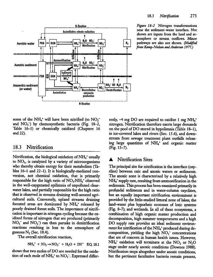
IponUAerobic water
Aerobic sediment
Anaerobic sediment(orwater)
PON
N-fixalion
Assimilativenitrate reduction
DONC
Ammonification
DONSedimentadsorbedNH4+
Assimilation
NH4
NHi
NHi
tN20 N02"Nilrification
tN20 N02-Nitrification
Dissimilativeammoniaproduction
N-fixation
MOr
NO,
NOr
some of the NFV will have been nitrified (to N02~and N03") by chemosynthetic bacteria (Fig. 18-2,Table 16-1) or chemically oxidized (Chapters 16and 22).
18.3 Nitrification
Nitrification, thebiological oxidation ofNJV usuallyto N03, is catalyzed by a variety of microorganismswho therebyobtain energyfor their metabolism (Tables 16-1 and 22-1). It is biologically-mediated conversion, not chemical oxidation, that is primarilyresponsible for the high ratio of N03:NH4+ observedin thewell-oxygenated epilimnia of unpolluted clear-water lakes, andpartially responsible for thehighratiothatisobserved in streams draining well-aerated agricultural soils. Conversely, upland streams drainingforested areas are dominated by NIV released bypoorly drained forest soils. The importance ofnitrification isimportantin nitrogencycling because the oxidized forms of nitrogen that are produced (primarilyN03" and N02") can then partake in denitrificationreactions resulting in loss to the atmosphere ofgaseous N2 (Sec. 18.4).The overallnitrification reaction,
NH/ + 2O2-+NO3- + H20 + 2H+ EQ.18.1
shows that two moles ofDO are needed for the oxidationofeach mole ofNIV to N03". Expressed differ-
t tNOf NO N20Denitrification
18.3 Nitrification 273
Figure 18-2 Nitrogen transformationsnear the sediment-water interface. Notshown are inputs from the land and atmosphere or stream outflows. Minorpathways are also not shown. (ModifiedfromKamp-Nielson andAnderson 1977.)
endy, ~4mg DO are required to oxidize 1 mg NIVnitrogen.Nitrification therefore exertslarge demandson the poolofDO stored in hypolimnia (Table 18-1),in ice-covered lakes and rivers (Sec. 15.6), and downstream from sewage treatment plant outfalls releasing large quantities of NIV and organic matter(Fig. 15-7).
A Nitrification Sites
The principal site fornitrification istheinterface (oxy-cline) between oxic and anoxic waters or sediments.The anoxic zone is characterized by a relatively highNIV supply rate,resulting from ammonification in thesediments. Thisprocess has been examined primarily inprofundal sediments and in water-column oxyclines,but an equally important nitrification environment isprovided by the little-studied littoralzoneof lakes; theland-water plus hyporheic ecotones of lotic systems(Fig. 8-7); and wedands. In all of these ecosystems, acombination of high organic matter production anddecomposition, high summer temperatures and a highDO supply rate provides an ideal sediment environment for nitrification oftheNIV produced during decomposition, yielding the high N03~ concentrationsthat are of concern in humanhealth issues. However,NrV oxidation will terminate at the N02 or NzOstage under nearly anoxic conditions (Downes 1988).Nitrification stopsaltogetherunder anoxic conditions,but the pertinent facultative bacteria remain present,
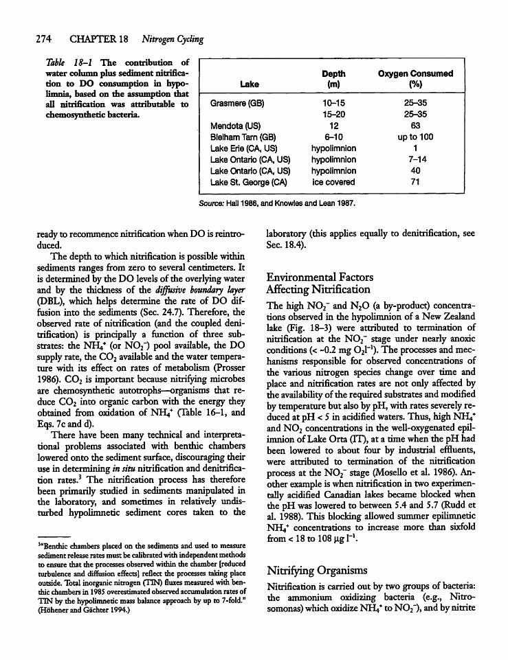
274 CHAPTER 18 Nitrogen Cycling
Table 18-1 The contribution ofwater column plus sediment nitrification to DO consumption in hypolimnia, based on the assumption matall nitrification was attributable tochemosynthetic bacteria.
Depth Oxygen ConsumedLake (m) (%)
Grasmere (GB) 10-15 25-35
15-20 25-35
Mendota (US) 12 63
BlelhamTarn (GB) 6-10 up to 100Lake Erie (CA, US) hypolimnion 1
Lake Ontario (CA,US) hypolimnion 7-14
Lake Ontario (CA, US) hypolimnion 40
Lake St. George (CA) ice covered 71
Source: Hall 1986, and Knowles and Lean 1987.
readyto recommence nitrificationwhenDO isreintroduced.The depth to which nitrification is possible within
sediments ranges from zero to several centimeters. Itis determined by the DO levels of the overlying waterand by the thickness of the diffusive boundary layer(DBL), which helps determine the rate of DO diffusion into the sediments (Sec. 24.7). Therefore, theobserved rate of nitrification (and the coupled denitrification) is principally a function of three substrates: the NIV (or N02~) pool available, the DOsupply rate, the C02 available and the water temperature with its effect on rates of metabolism (Prosser1986). C02 is important because nitrifying microbesare chemosynthetic autotrophs—organisms that reduce C02 into organic carbonwith the energy theyobtained from oxidation of NIV (Table 16-1, andEqs.7candd).There have been many technical and interpreta-
tional problems associated with benthic chamberslowered onto the sediment surface, discouraging theiruse in determining insitu nitrification anddenitrification rates.3 The nitrification process has thereforebeen primarily studied in sediments manipulated inthe laboratory, and sometimes in relatively undisturbed hypolimnetic sediment cores taken to the
'"Benthic chambers placed on the sediments and used to measuresedimentrelease rates mustbe calibratedwith independentmethodsto ensure that the processes observed withinthe chamber [reducedturbulence and diffusion effects] reflect the processes taking placeoutside. Total inorganic nitrogen (TIN) fluxes measured withbenthic chambers in 1985 overestimated observed accumulation rates ofTIN by the hypolimnetic mass balance approach by up to 7-fold."(Hohener and Gachter 1994.)
laboratory (this applies equally to denitrification, seeSec. 18.4).
Environmental FactorsAffecting NitrificationThe high N02" and N20 (a by-product) concentrations observed in the hypolimnion of a New Zealandlake (Fig. 18-3) were attributed to termination ofnitrification at the N02" stage under nearly anoxicconditions (< -0.2 mg021_1). The processes andmechanisms responsible for observed concentrations ofthe various nitrogen species change over time andplace and nitrification rates are not only affected bythe availability ofthe required substrates andmodifiedbytemperature but also bypH,withrates severely reduced at pH <5 in acidified waters. Thus, highNIVandN02 concentrations in the well-oxygenated epil-imnion of Lake Orta (IT), at a time when the pH hadbeen lowered to about four by industrial effluents,were attributed to termination of the nitrificationprocess at theN02" stage (Mosello et al. 1986). Another example iswhennitrification in twoexperimentally acidified Canadian lakes became blocked whenthe pH was lowered to between 5.4and 5.7 (Rudd etal. 1988). This blocking allowed summerepilimneticNIV concentrations to increase more than sixfoldfrom <18to 108 ugr1.
Nitrifying OrganismsNitrification is carried out by two groups of bacteria:the ammonium oxidizing bacteria (e.g., Nitro-somonas) which oxidize NIV to N02"), and bynitrite
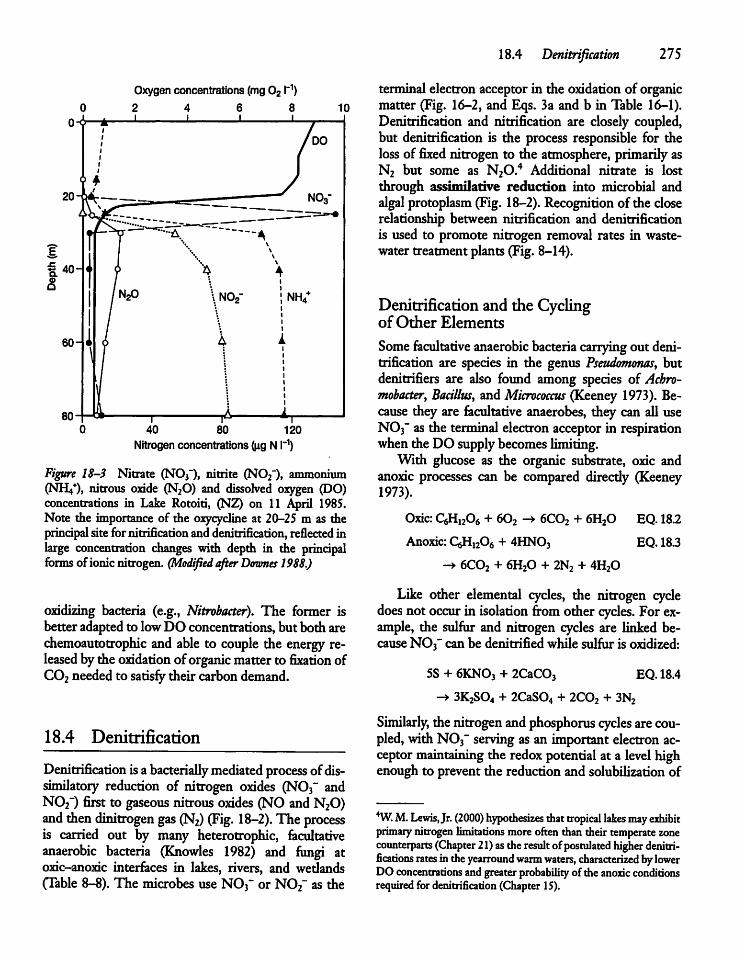
Oxygen concentrations (mg 021-1)4 6 8 10
80 120
Nitrogen concentrations dig N l~1)
Figure 18-3 Nitrate (N03~), nitrite (N02~), ammonium(NIV). nitrous oxide (N20) and dissolved oxygen (DO)concentrations in Lake Rotoiti, (NZ) on 11 April 1985.Note the importance of the oxycycline at 20-25 m as theprincipalsite for nitrificationand denitrification, reflectedinlarge concentration changes with depth in the principalforms ofionicnitrogen. (Modifiedafter Downes 1988.)
oxidizing bacteria (e.g., Nitrobacter). The former isbetter adaptedto lowDO concentrations,but both arechemoautotrophic and able to couple the energy released bythe oxidation oforganic matter to fixation ofC02 neededto satisfy their carbondemand.
18.4 Denitrification
Denitrification isa bacteriallymediated process ofdis-similatory reduction of nitrogen oxides (N03~ andN02") first to gaseous nitrous oxides (NO and N20)and thendinitrogen gas (N2) (Fig. 18-2). The processis carried out by many heterotrophic, facultativeanaerobic bacteria (Knowles 1982) and fungi atoxic-anoxic interfaces in lakes, rivers, and wetlands(Table 8-8). The microbes use N03~ or N02" as the
18.4 Denitrification 275
terminal electron acceptor in the oxidationof organicmatter (Fig. 16-2, and Eqs. 3a and b in Table 16-1).Denitrification and nitrification are closely coupled,but denitrification is the process responsible for theloss of fixed nitrogen to the atmosphere, primarilyasN2 but some as N20.4 Additional nitrate is lostthrough assimilative reduction into microbial andalgal protoplasm (Fig. 18-2).Recognition ofthe closerelationship between nitrification and denitrificationis used to promote nitrogen removal rates in wastewater treatment plants (Fig. 8-14).
Denitrification and the CyclingofOther Elements
Some facultative anaerobic bacteriacarryingout denitrification are species in the genus Pseudomonas, butdenitrifiers are also found among species of Achro-mobacter, Bacillus, andMicrococcus (Keeney 1973). Because they are facultative anaerobes, they can all useN03" as the terminal electronacceptor in respirationwhentheDO supply becomes limiting.With glucose as the organic substrate, oxic and
anoxic processes can be compared directly (Keeney1973).
Oxic: QiHuOfi + 602 -> 6COz + 6H20 EQ. 18.2
Anoxic: OH^Oe + 4HN03 EQ. 18.3
-> 6C02 + 6H20 + 2N2 + 4H20
Like other elemental cycles, the nitrogen cycledoes not occur in isolation from other cycles. For example, the sulfur and nitrogen cycles are linked because N03" can be denitrified while sulfur is oxidized:
5S + 6KNO3 + 2CaC03 EQ. 18.4
-> 3K2S04 + 2CaS04 + 2C02 + 3N2
Similarly, thenitrogen andphosphorus cycles arecoupled, with N03" serving as an important electron acceptormaintaining the redoxpotentialat a level highenough to prevent the reduction and solubiUzation of
4W. M. Lewis, Jr. (2000) hypothesizes that tropical lakes may exhibitprimary nitrogen limitations moreoften thantheir temperate zonecounterparts (Chapter 21)asthe result of postulated higher denitri-fications rates in theyearround warmwaters, characterized bylowerDO concentrations andgreater probability ofthe anoxic conditionsrequired fordenitrification (Chapter15).
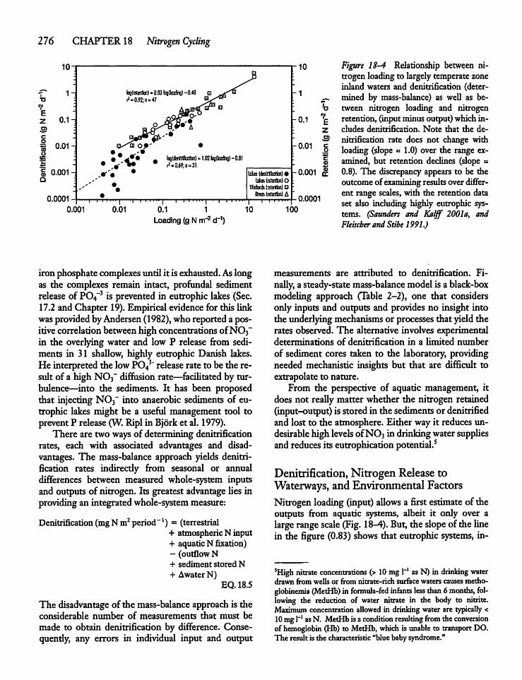
276 CHAPTER 18 Nitrogen Cycling
Ez
10
1-
0.1-
« 0.01 -
bg(retettHon) ° 0.83^=0.92:11=47
iCdenftifftcatkxO =1.02 logtafcj) -0.81>0.«?;n=31
10
-0.1
0.01
§ 0.001Q
0.0001
Lies(deniti&Btfa(i)«Likas (retention) O
Welfands {retention) •Bwrs(retention) A
i i i in
-0.001
Ez
co
o
0.0001
F/gwr* i£-4 Relationship between nitrogen loadingto largelytemperatezoneinland waters and denitrification (determined by mass-balance) as well as between nitrogen loading and nitrogenretention, (inputminusoutput)whichincludes denitrification. Note that the denitrification rate does not change withloading (slope = 1.0) over the range examined, but retention declines (slope =0.8). The discrepancy appears to be theoutcomeof examiningresultsoverdifferent range scales, with the retention dataset also including highly eutrophic systems. (Saunders and Kalff 2001a, andFleischer and Stibe 1991.)
0.001 0.01
-T^J- I11 I III I I I
0.1 1
Loading (gNm~2 d"1)10
iron phosphatecomplexes until it is exhausted. Aslongas the complexes remain intact, profundal sedimentrelease of P04~3 is prevented in eutrophic lakes (Sec.17.2 and Chapter 19). Empiricalevidence for this linkwasprovided byAndersen(1982), who reported a positivecorrelationbetweenhigh concentrationsofN03"in the overlying water and low P release from sediments in 31 shallow, highly eutrophic Danish lakes.He interpreted thelow P043" release rate tobetheresult of a high N03" diffusion rate—facilitated by turbulence—into the sediments. It has been proposedthat injectingNO3" into anaerobic sediments of eutrophic lakes might be a useful management tool topreventP release (W.Ripl in Bjorket al. 1979).There are twowaysof determining denitrification
rates, each with associated advantages and disadvantages. The mass-balance approach yields denitrification rates indirectly from seasonal or annualdifferences between measured whole-system inputsand outputs of nitrogen. Its greatest advantage lies inproviding an integratedwhole-system measure:
Denitrification (mgNm2 period l) = (terrestrial+ atmospheric N input+ aquatic N fixation)- (outflow N+ sediment stored N+ Awater N)
EQ. 18.5
The disadvantage ofthe mass-balance approach is theconsiderable number of measurements that must bemade to obtain denitrification by difference. Conse-quendy, any errors in individual input and output
100
measurements are attributed to denitrification. Finally, a steady-state mass-balance modelis a black-boxmodeling approach (Table 2-2), one that considersonly inputs and outputs and provides no insight intothe underlying mechanisms or processes that yieldtherates observed.The alternative involves experimentaldeterminations of denitrification in a limited numberof sediment cores taken to the laboratory, providingneeded mechanistic insights but that are difficult toextrapolate to nature.From the perspective of aquatic management, it
does not really matter whether the nitrogen retained(input-output) isstored in thesediments or denitrifiedand lost to the atmosphere. Either way it reducesundesirable high levels ofNO3in drinkingwatersuppliesand reduces itseutrophication potential.5
Denitrification, Nitrogen Release toWaterways, andEnvironmental FactorsNitrogenloading (input) allows a first estimate of theoutputs from aquatic systems, albeit it only over alarge range scale (Fig. 18-4). But, the slope ofthe linein the figure (0.83) shows that eutrophicsystems, in-
5High nitrate concentrations (> 10 mg l"1 as N) in drinking waterdrawn from wells or from nitrate-rich surface waters causes metho-globinemia (MetHb) in formula-fed infants less than6months, following the reduction of water nitrate in the body to nitrite.Maximumconcentration allowed in drinkingwater are typically <10mgl"1 asN. MetHbisacondition resulting from the conversionof hemoglobin (Hb) to MetHb, which is unable to transport DO.The result is the characteristic "blue baby syndrome."
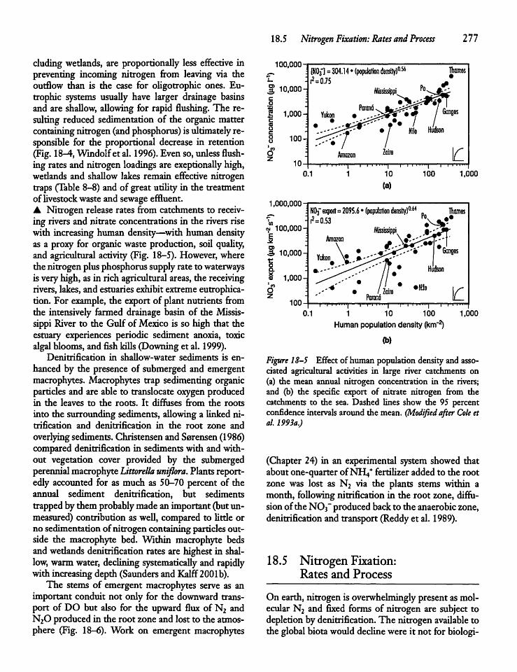
eludingwedands, are proportionally less effective inpreventing incoming nitrogen from leaving via theoutflow than is the case for oligotrophic ones. Eutrophic systems usually have larger drainage basinsand are shallow, allowing for rapid flushing. The resulting reduced sedimentation of the organic mattercontaining nitrogen (andphosphorus) is ultimately responsible for the proportional decrease in retention(Fig.18-4,Windolf et al. 1996). Even so,unless flushing rates and nitrogen loadings are exeptionally high,wedands and shallow lakes remain effective nitrogentraps (Table 8-8) and of great utility in the treatmentof livestockwasteand sewage effluent.• Nitrogen release rates from catchments to receiving rivers and nitrate concentrations in the rivers risewith increasing human density—with human densityas a proxy for organic waste production, soil quality,and agricultural activity (Fig. 18-5). However, wherethe nitrogen plusphosphorussupplyrate to waterwaysisveryhigh, as in rich agricultural areas, the receivingrivers, lakes, and estuariesexhibit extremeeutrophication. For example, the export of plant nutrients fromthe intensively farmed drainage basin of the Mississippi River to the Gulf of Mexico is so high that theestuary experiences periodic sediment anoxia, toxicalgalblooms, and fish kills (Downing et al. 1999).
Denitrification in shallow-water sediments is enhanced by die presence of submerged and emergentmacrophytes. Macrophytes trap sedimenting organicparticles and are able to translocate oxygen producedin the leaves to the roots. It diffuses from the rootsinto the surrounding sediments, allowinga linked nitrification and denitrification in the root zone andoverlying sediments. ChristensenandSarensen (1986)compared denitrification in sediments with and without vegetation cover provided by the submergedperennialmacrophyteLittorella uniflora. Plants reportedly accounted for as much as 50-70 percent of theannual sediment denitrification, but sedimentstrapped bythemprobablymadeanimportant(butunmeasured) contribution as well, compared to little orno sedimentation of nitrogen containing particlesoutside the macrophyte bed. Within macrophyte bedsandwetlands denitrification rates are highest in shallow, warm water, declining systematically and rapidlywithincreasing depth (Saunders andKalff2001b).The stems of emergent macrophytes serve as an
important conduit not only for the downward transport of DO but also for the upward flux of N2 andN20 produced in the root zone and lost to the atmosphere (Fig. 18-6). Work on emergent macrophytes
18.5 Nitrogen Fixation: Rates and Process 277
100,000-
% 10,000-;
P31=304.14 • (population density)0-56r2=0.75
£ 1.000- Yukon
8 100-
oz
10
1,000,000-
?W 100,000-E
M 10,000-•coa
8 1,000-
100
mi Nile Hudson
Zaire |/~AmazonIM l l i i 11">| 1 i i i "i.j—f—r
0.1 1 10 100
(a)1,000
N03~export=2095.6•(populationdensity)0-44 . ThamesM.53 VV*
Amazon
Yukon
I I i | I I i i ""| | I i i"'i| r-T-r0.1 1 10 100 1,000
Human population density (km-2)
(b)
Figure 18-5 Effectof human populationdensityand associated agricultural activities in large river catchments on(a) the mean annual nitrogen concentration in the rivers;and (b) the specific export of nitrate nitrogen from thecatchments to the sea. Dashed lines show the 95 percentconfidence intervals around the mean. (Modified after Cole etal. 1993a.)
(Chapter 24) in an experimental system showed thatabout one-quarter of NH^ fertilizer added to the rootzone was lost as N2 via the plants stems within amonth, following nitrification in the root zone, diffusionofthe N03" produced backto the anaerobic zone,denitrification and transport (Reddyet al. 1989).
18.5 Nitrogen Fixation:Rates and Process
On earth, nitrogen is overwhelmingly present asmolecular N2 and fixed forms of nitrogen are subject todepletion by denitrification. The nitrogen available tothe global biotawould decline were it not for biologi-
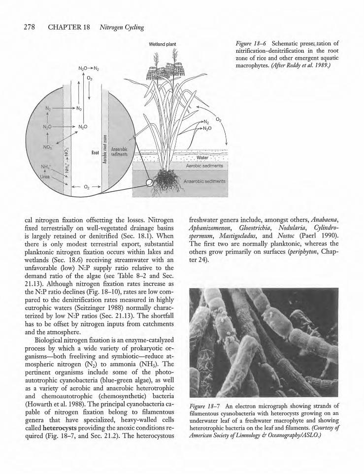
278 CHAPTER 18 Nitrogen Cycling
Wetland plant
cal nitrogen fixation offsetting the losses. Nitrogenfixed terrestrially on well-vegetated drainage basinsis largely retained or denitrified (Sec. 18.1). Whenthere is only modest terrestrial export, substantialplanktonic nitrogen fixation occurs within lakes andwetlands (Sec. 18.6) receiving streamwater with anunfavorable (low) N:P supply ratio relative to thedemand ratio of the algae (see Table 8-2 and Sec.21.13). Although nitrogen fixation rates increase asthe N:P ratio declines(Fig. 18-10), rates are lowcompared to the denitrification rates measured in highlyeutrophic waters (Seitzinger 1988) normally characterized by low N:P ratios (Sec. 21.13). The shortfallhas to be offset by nitrogen inputs from catchmentsand the atmosphere.Biological nitrogen fixation is an enzyme-catalyzed
process by which a wide variety of prokaryotic organisms—both freeliving and symbiotic—reduce atmospheric nitrogen (N2) to ammonia (NH3). Thepertinent organisms include some of the photo-autotrophic cyanobacteria (blue-green algae), as wellas a variety of aerobic and anaerobic heterotrophicand chemoautotrophic (chemosynthetic) bacteria(Howarth et al. 1988). The principalcyanobacteria capable of nitrogen fixation belong to filamentousgenera that have specialized, heavy-walled cellscalled heterocysts providingthe anoxic conditionsrequired (Fig. 18—7, and Sec. 21.2). The heterocystous
.'.'. Water .•. : .
Aerobic sediments
—-
Anaerobic sediments
Figure 18-6 Schematic prese; .tation ofnitrification-denitrification in the rootzone of rice and other emergent aquaticmacrophytes. (After Reddy etal. 1989.)
freshwater genera include, amongst others, Anahaena,Apbanizomenon, Gloeotrichia, Nodularia, Cylmdro-spermum, Mastigocladus, and Nostoc (Paerl 1990).The first two are normally planktonic, whereas theothers grow primarily on surfaces (peripbyton, Chapter 24).
Figure 18-1 An electron micrograph showing strands offilamentous cyanobacteria with heterocysts growing on anunderwater leaf of a freshwater macrophyte and showingheterotrophic bacteria on the leafand filaments. (Courtesy ofAmerican Society ofLimnology &Oceanography/'ASLO.)
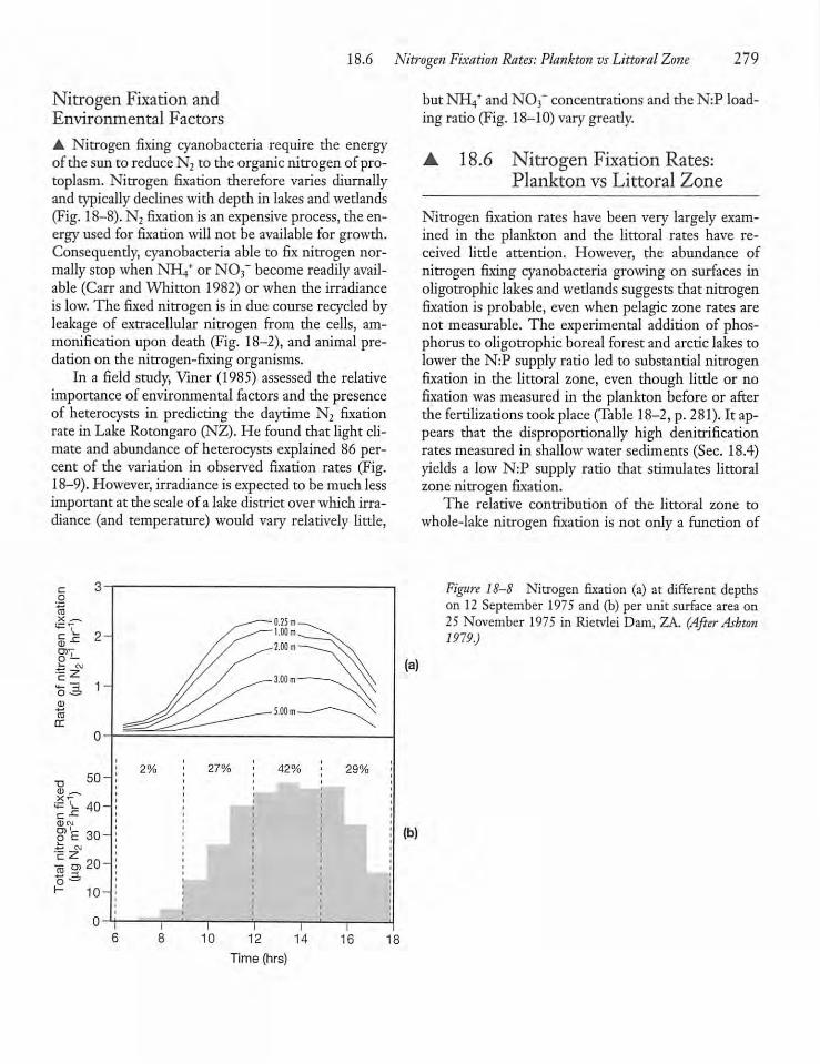
18.6 Nitrogen Fixation Rates: Plankton vsLittoral Zone 279
Nitrogen Fixation andEnvironmental Factors
• Nitrogen fixing cyanobacteria require the energyofthe sun to reduce N2 to the organic nitrogen of protoplasm. Nitrogen fixation therefore varies diurnallyand typicallydeclines with depth in lakes and wetlands(Fig. 18-8). N2 fixation is an expensive process, the energy used for fixationwill not be available for growth.Consequently, cyanobacteria able to fix nitrogen normally stop when NH4+ or N03~ become readily available (Carr and Whitton 1982) or when the irradianceis low.The fixed nitrogen is in due course recycled byleakage of extracellular nitrogen from the cells, ammonification upon death (Fig. 18-2), and animal pre-dation on the nitrogen-fixingorganisms.In a field study, Viner (1985) assessed the relative
importance of environmental factors and the presenceof heterocysts in predicting the daytime N2 fixationrate in Lake Rotongaro (NZ). He found that light climate and abundance of heterocysts explained 86 percent of the variation in observed fixation rates (Fig.18-9).However, irradiance is expected to bemuch lessimportant at the scale of a lake district over which irradiance (and temperature) would vary relatively little,
10 12 14
Time (hrs)16
but NH4+and N03 concentrations and the N:P loading ratio (Fig. 18-10) vary greatly.
A 18.6 Nitrogen Fixation Rates:Plankton vs Littoral Zone
Nitrogen fixation rates have been very largely examined in the plankton and the littoral rates have received little attention. However, the abundance ofnitrogen fixing cyanobacteria growing on surfaces inoligotrophic lakes andwetlands suggests that nitrogenfixation is probable, even when pelagic zone rates arenot measurable. The experimental addition of phosphorus to oligotrophic boreal forest and arctic lakes tolower the N:P supply ratio led to substantial nitrogenfixation in the littoral zone, even though little or nofixation wasmeasured in the plankton before or afterthe fertilizations took place(Table 18-2, p. 281). It appears that the disproportionally high denitrificationrates measured in shallow water sediments (Sec. 18.4)yields a low N:P supply ratio that stimulates littoralzone nitrogen fixation.The relative contribution of the littoral zone to
whole-lake nitrogen fixation is not only a function of
Figure 18-8 Nitrogen fixation (a) at different depthson 12 September 1975 and (b) per unit surface area on25 November 1975 in Rietvlei Dam, ZA. (After Ashton1919.)
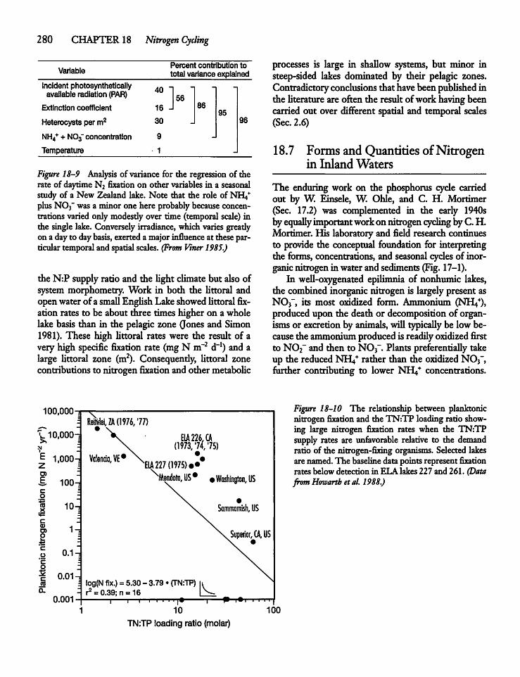
280 CHAPTER18 Nitrogen Cycling
VariablePercent contribution tototal variance explained
Incident photosyntheticallyavailable radiation (PAR) 40 "1 1
56Extinction coefficient 16 J 86
95Heterocysts perm2 30 96
NH4+ +N03"concentration 9 JTemperature • 1 J
Figure 18-9 Analysis of variance for the regression of therate of daytimeN2 fixation on other variables in a seasonalstudy of a New Zealand lake. Note that the role of NH^*plusNO3" wasa minor one here probablybecause concentrationsvariedonly modesdyover time (temporal scale) inthe single lake. Conversely irradiance, whichvaries greadyon a dayto daybasis, exerted a majorinfluence at theseparticulartemporaland spatial scales. (From Viner 1985.)
the N:P supplyratio and the light climate but alsoofsystemmorphometry. Work in both the littoral andopenwaterof a small English Lakeshowed littoralfixation rates to be about three timeshigher on a wholelake basis than in the pelagic zone (Jones and Simon1981). These high littoral rates were the result of avery high specific fixation rate (mg N m~2 d"1) and alarge littoral zone (m2). Consequently, littoral zonecontributions to nitrogen fixation and other metabolic
100,000-j
\. 10,000-
E 1,000-zO)
Ǥ. 100-co
10-
EIA226,CA(1973/7(75)
•
ElA 227 (1975) ••*XMendoto,US# *Washington, US
Sammomish, US
processes is large in shallow systems, but minor insteep-sided lakes dominated by their pelagic zones.Contradictoryconclusions that havebeenpublished inthe literature are often the resultofworkhaving beencarried out over different spatial and temporal scales(Sec. 2.6)
18.7 Forms and Quantities ofNitrogenin Inland Waters
The enduringwork on the phosphorus cycle carriedout by W. Einsele, W. Ohle, and C. H. Mortimer(Sec. 17.2) was complemented in the early 1940sbyequally importantworkon nitrogencycling byC.H.Mortimer. His laboratory and field research continuesto provide the conceptual foundation for interpretingthe forms, concentrations, and seasonal cycles of inorganic nitrogeninwaterand sediments (Fig. 17-1).In well-oxygenated epilimnia of nonhumic lakes,
the combined inorganic nitrogen is largely present asN03", its most oxidized form. Ammonium (NH4+),producedupon the death or decomposition of organismsor excretionby animals, will typically be low because the ammonium producedis readilyoxidized firstto N02" and then to NO3".Plants preferentiallytakeup the reduced NH^ rather than the oxidized NO3",further contributing to lower NH^ concentrations.
Figure 18-10 Hie relationship between planktonicnitrogen fixation and the TN:TP loading ratio showing large nitrogen fixation rates when the TN:TPsupply rates are unfavorable relative to the demandratio of the nitrogen-fixing organisms. Selected lakesare named.The baselinedata points represent fixationrates below detection in ELA lakes 227 and 261. (Datafrom Howarth etal. 1988.)
COX
c<DO)
2C
oco
Superior, CA, US
0.1
0.01
0.001
I log(N fix.) =5.30- 3.79• (TN:TP)r2 =0.39;n =16
T—r—r
10
TN:TP loading ratio (molar)100
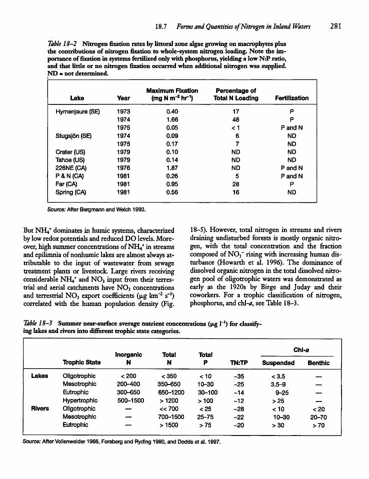
18.7 Forms and Quantities ofNitrogen in Inland Waters 281
Table 18-2 Nitrogen fixation rates by littoral zone algaegrowingon macrophytes plusthe contributions of nitrogen fixation to whole-system nitrogen loading. Note the importance offixation in systems fertilized only with phosphorus, yielding a low N:P ratio,and that litde or no nitrogen fixation occurred when additional nitrogen was supplied.ND b not determined.
Maximum Fixation Percentage ofLake Year (mg N m~2 hr1) Total N Loading Fertilization
Hymenjaure (SE) 1973 0.40 17 P
1974 1.66 48 P
1975 0.05 <1 PandNStugsjon (SE) 1974 0.09 6 ND
1975 0.17 7 ND
Crater (US) 1979 0.10 ND NDTahoe (US) 1979 0.14 ND ND226NE (CA) 1976 1.87 ND PandNP &N (CA) 1981 0.26 5 PandNFar(CA) 1981 0.95 28 P
Spring (CA) 1981 0.56 16 ND
Source: After Bergmann and Welch 1990.
But NH4* dominates in humic systems, characterizedby lowredoxpotentials and reduced DO levels. Moreover, high summer concentrationsof NHL** in streamsandepilimnia of nonhumiclakes are almostalways attributable to the input of wastewater from sewagetreatment plants or livestock. Large rivers receivingconsiderable NrV and NO3 input from their terrestrial and aerial catchments have NO3 concentrationsand terrestrial NO3 export coefficients (p,g km"2 s"1)correlated with the human population density (Fig.
18-5). However, total nitrogen in streams and riversdraining undisturbed forests is mosdy organic nitrogen, with the total concentration and the fractioncomposed of NO3" risingwith increasing humandisturbance (Howarth et al. 1996). The dominance ofdissolved organic nitrogen in the total dissolved nitrogen pool of oligotrophic waters was demonstrated asearly as the 1920s by Birge and Juday and theircoworkers. For a trophic classification of nitrogen,phosphorus, and cbl-a, seeTable 18-3.
Table 18-3 Summer near-surface average nutrientconcentrations (|tg l"1) for classifying lakesand rivers into different trophic state categories.
Chi •aInorganic
NTotal Total
Trophic State N P TN:TP Suspended Benthic
Lakes Oligotrophic <200 <350 <10 -35 <3.5Mesotrophic 200-400 350-650 10-30 -25 3.5-9 —
Eutrophic 300-650 650-1200 30-100 -14 9-25 —
Hypertrophic 500-1500 >1200 >100 -12 >25 —
Rivers Oligotrophic — «700 <25 -28 <10 <20Mesotrophic — 700-1500 25-75 -22 10-30 20-70Eutrophic — >1500 >75 -20 >30 >70
Source:AfterVollenweider1968, Forsberg and Ryding 1980, and Dodds et al. 1997.
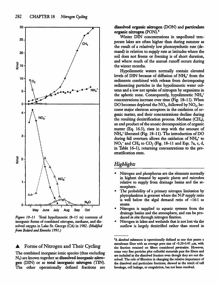
282 CHAPTER 18 Nitrogen Cycling
30
25-
20-
15-
10-
oE
*'*' NH/
May June July Aug Sep
Figure 18-11 Total hypolimnetic (8-15 m) contents ofinorganic forms of combinednitrogen,methane,anddissolvedoxygen in Lake St. George (CA) in 1982. (Modifiedfrom BedardandKnowles 1991.)
A FormsofNitrogen andTheir CyclingThe combinedinorganicionic species (thus excludingN2)are known together asdissolved inorganic nitrogen (DIN) or as total inorganic nitrogen (TIN).The other operationally defined fractions are
dissolved organic nitrogen (DON) and particulateorganic nitrogen (PON).6Winter DIN concentrations in unpolluted tem
perate lakes are often higher than during summer asthe result of a relatively lowphotosynthetic rate (demand) in relation to supplyrate at latitudeswhere thesoil does not freeze or freezing is of short duration,and where much of the annual runoff occurs duringthe winter months.Hypolimnetic waters normally contain elevated
levels of DIN because of diffusion of NIV fr°m thesediments combined with release from decomposingsedimentingparticles in the hypolimneticwater column and a lownet uptake of nitrogen by organisms inthe aphotic zone. Consequently, hypolimnetic NIVconcentrations increase over time (Fig. 18-11).WhenDO becomes depleted the N03, followed byN02, becomemajor electron acceptors in the oxidation of organicmatter, and their concentrations decline duringthe resulting denitrification process. Methane (CH4),anendproductofthe anoxic decomposition of organicmatter (Eq. 16.3), rises in step with the amount ofNIV liberated(Fig. 18-11).The introductionof DOduring fall overturn allows the oxidation of NIV toNOj" and CH4 to COz (Fig. 18-11 and Eqs. 7a, c, d,in Table 16-1), returning concentrations to the pre-stratification state.
Highlights• Nitrogen and phosphorus are the elements normallyin highest demand by aquatic plants and microbesrelative to supply from drainage basins and the atmosphere.
• The probability of a primarynitrogen limitation byphytoplanktonis greatestwhere the N:P supplyratiois well below the algal demand ratio of -16:1 asatoms.
• Nitrogen is supplied to aquatic systems from thedrainagebasinsand the atmosphere, and can be produced insituthrough nitrogen fixation.
• Nitrogen in lakes andwedandsthat is not lostvia theoutflow is largely denitrified rather than stored in
6Adissolved substance is operationally defined asone that passes amembrane filter with an average poresize of ~0.20-0.45 \ixa, withthe fraction retained on filters considered particulate. However,somevery fine particles pluscolloidal materials pass the filters andareincludedin the dissolved fraction even though they arenot dissolved. The roleof filtration in changingthe relativeimportanceofthe dissolved and particulate fractions, skewed as the result of cellbreakage, cell leakage, orcoagulation, has not beenresolved.
18.7 Forms and Quantities ofNitrogen inInland Waters 283
sediments. The relative importance ofdenitrification • Nitrogen cycling affects other nutrient cycles (e.g.,rises with increasing water residence time and de- phosphorus and sulfur).creasing water depth. Nitrogen lost to the atmos- • Humanactivity hasraised—and continues to raise—phere through denitrification isno longer available to the export of nitrogen from the land to waterwaysthebiota, makingwedands and shallow lakes particu- and, via the atmosphere to aquatic systems far fromlarly useful fortreating wastewater. regions ofindustrial and agricultural activity.
H E R
19
Iron, Manganese, and Sulfur
19.1 Introduction
Iron and manganese are essential micronutrients forplantsand iron mayoccasionally control algalproduction in inland waters. Reduced inorganic sulfur concentrations, together with irradiance, determine theproduction rates of photosynthetic sulfur bacteriabelowthe oxycline in transparent lakes (Sec. 22.10).The solubilityof Fe andMn in the ionic (not com-
plexed) form is very low in pure solutions. The calculated solubility of ionic iron in well-oxygenated watersthat are not exceptionally acidic is less than 10 jig I"1(Mill 1980).1 Yet total iron concentrations measured infiltered riverwater are about 1,000 timeshigher, indicatinga sorptionor complexation withorganiccolloidsand other forms of dissolved organicmatter in lakes,rivers, and wedands, gready affecting metal behaviorand concentration. Since there is little iron in ionicform, it canoccasionally limit algal growth (Sec. 21.13).The physical, chemical, and biological interactions
of iron and manganese with other elements and organic matter are well-recognized. Iron plays a particularlyimportant role in determining the concentration,solubility, and flux rates of phosphate, sulfur, tracemetals, and dissolved organic carbon (DOC) in waterways. Furthermore, alkalinity is generated in acidifiedlakes upon the microbial reduction of oxidized ironand sulfate, thereby buffering aquatic sediments
'The solubility of Feandmost othermetalsunderoxicconditions isparticularly elevated undertheverylowpH conditions encounteredin highlyacidic volcanic lakes andacidified streams draining acidiccoalmine effluents (Sec. 14.5andChapter 27).
284
against acidification (Tables 27-1 and 16-1). In lakes,bufferingis permanent if the reducedelementsare notreoxidized during the next period of destratificationand reoxygenation. The iron and manganese inaquatic systems is derived from drainage basins, primarilyas oxides.
19.2 Iron Cycling
The classic work of C. H. Mortimer (1941-1942) oniron (and phosphorus, see Chapter 17) cycling inEsthwaite Water (GB)providesthe basisfor our present understandingof the iron cycle in lowmimic (lowDOC) nonacidified waters.In the presence of dissolved oxygen (DO) and the
absence of much dissolved organicmatter, ferric iron[Fe3+ or Fe(EQ)] forms a number of insoluble oxidesand oxyhydroxides (FeOOH). The aggregates (floes)that are formed settle onto the sediments,also the primary reason why well-oxygenated stream sedimentsare frequendycovered by a rusty brown layer of sedimented Fe(OH)3 carried in as reduced iron (Fe2+) ingroundwater.2 Ferric iron becomes subject to micro-bially andchemicallymediated reduction in lakes, wetlands, andthe hyporheic zoneofloticsystems oncetheDO, oxidized manganese (Mn4*), and nitrate have been
2Fe (and Mn) oxides havea large surface area perunit weight andtheirsurface hydroxyl groups have ahighaffinity (adsorption capacity) for avariety of trace elements and dissolved organic matter. Oxidized surfaces also facilitate oxidation of sorbed elements throughredox reactions.
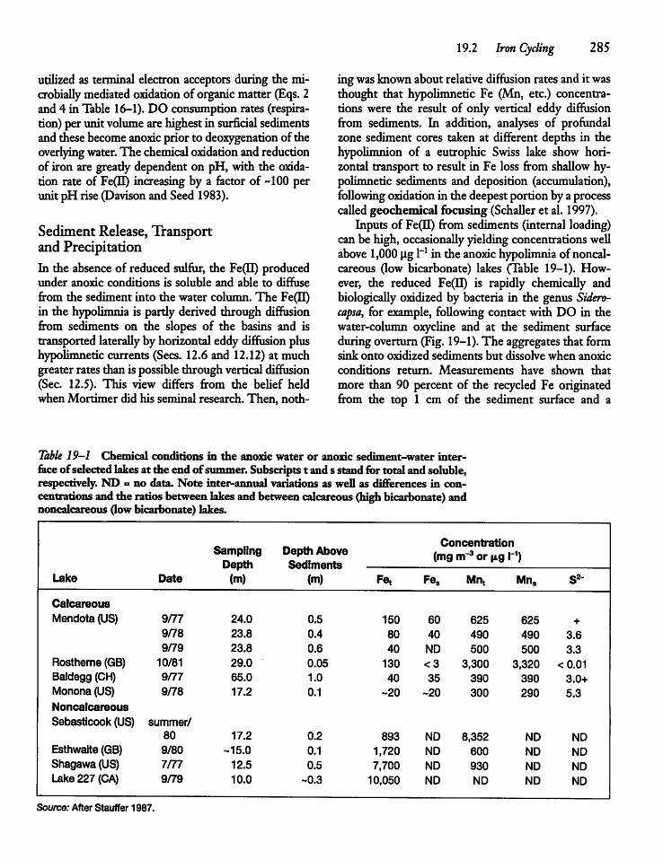
utilized as terminal electron acceptors during the mi-crobially mediated oxidation of organic matter (Eqs. 2and 4 in Table 16-1). DO consumption rates (respiration)per unit volume are highest in surficial sedimentsand thesebecome anoxic prior to deoxygenation oftheoverlyingwater. The chemical oxidation and reductionof iron are gready dependent on pH, with the oxidation rate of Fe(H) increasingby a factor of -100 perunit pH rise(Davison and Seed1983).
Sediment Release, TransportandPrecipitationLi the absenceof reduced sulfur, the Fe(H) producedunder anoxic conditions is soluble and able to diffusefrom the sediment into the water column. The Fe(H)in the hypolimnia is partly derived through diffusionfrom sediments on the slopes of the basins and istransported laterallyby horizontal eddy diffusion plushypolimnetic currents (Sees. 12.6 and 12.12) at muchgreater rates than is possible through verticaldiffusion(Sec. 12.5). This view differs from the belief heldwhen Mortimer did his seminal research. Then, noth
19.2 Iron Cycling 285
ingwas knownabout relative diffusion ratesand it wasthought that hypolimnetic Fe (Mn, etc.) concentrations were the result of only vertical eddy diffusionfrom sediments. In addition, analyses of profundalzone sediment cores taken at different depths in thehypolimnion of a eutrophic Swiss lake show horizontal transport to result in Fe loss from shallowhypolimnetic sediments and deposition (accumulation),following oxidation in the deepestportion bya processcalled geochemical focusing (Schaller et al. 1997).Inputs of Fe(H) from sediments (internal loading)
can be high, occasionally yieldingconcentrationswellabove 1,000 ug l"1 in the anoxic hypolimnia ofnoncal-careous (low bicarbonate) lakes (Table 19-1). However, the reduced Fe(H) is rapidly chemically andbiologically oxidized by bacteria in the genus Sidero-capsa, for example, following contact with DO in thewater-column oxycline and at the sediment surfaceduringoverturn(Fig. 19-1).The aggregates that formsink onto oxidized sediments but dissolve when anoxicconditions return. Measurements have shown thatmore than 90 percent of the recycled Fe originatedfrom the top 1 cm of the sediment surface and a
Table 19-1 Chemical conditions in die anoxic water or anoxic sediment-water interfaceof selected lakes at the end ofsummer. Subscripts t and s stand for total and soluble,respectively. ND a no data. Note inter-annual variations as well as differences in concentrations and the ratios between lakes and between calcareous(highbicarbonate) andnoncalcareous (low bicarbonate) lakes.
SamplingDepth
Depth AboveSediments
Concentration(mg m-3or |ig I"1)
Lake Date (m) (m) Fe, Fe8 Mn, Mn8 s2-
CalcareousMendota (US) 9/77 24.0 0.5 150 60 625 625 +
9/78 23.8 0.4 80 40 490 490 3.69/79 23.8 0.6 40 ND 500 500 3.3
Rostherne (GB) 10/81 29.0 0.05 130 <3 3,300 3,320 <0.01Baldegg (CH) 9/77 65.0 1.0 40 35 390 390 3.0+Monona (US) 9/78 17.2 0.1 -20 -20 300 290 5.3NoncalcareousSebasticook (US) summer/
80 17.2 0.2 893 ND 8,352 ND NDEsthwaite (GB) 9/80 -15.0 0.1 1,720 ND 600 ND NDShagawa (US) 7/77 12.5 0.5 7,700 ND 930 ND NDLake 227 (CA) 9/79 10.0 -0.3 10,050 ND ND ND ND
Source: After Stauffer 1987.
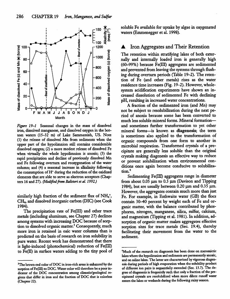
286 CHAPTER 19 Iron, Manganese, and Sulfur
]f 100-ic
&S eoHc5T3cos
"8>o
r-150 rvr
F M A M J JASONDJ
Month
Figure 19-1 Seasonal changes in the mass of dissolvediron, dissolved manganese, and dissolved oxygen in the bottom waters (15-32 m) of Lake Sammamish, US. Note(1) the release of dissolvedMn from sediments when theupper part of the hypolimnion still contains considerabledissolved oxygen; (2) a moremodest release of dissolved Fewhen virtually the whole hypolimnion is anoxic; (3) therapid precipitation and decline of previously dissolved Mnand Fe following overturn and reoxygenation of the watercolumn; and (4) a seasonal increase in alkalinity followingthe consumption ofH*during the reductionofthe oxidizedelementsthat are able to serveas electron acceptors (Chapters 16and27). (Modifiedfrom Balisteri etal. 1992.)
similarly high fraction of the sediment flux of NrV,CH4, anddissolved inorganic carbon (DIC)(see Cook1984).The precipitation rate of Fe(IH) and other trace
metals (including aluminum, seeChapter 27)declinesamong systems with increasing DOCbecause ofsorptionto dissolved organic matter.3 Consequendy, muchmore iron is retained in oxic water columns than ispredicted on the basis of research on ironsolubility inpure water. Recent work has demonstrated that thereis light-induced photochemical) reduction of FeQH)to Fe(H) in surface waters adding to the tiny pool of
3Thebrown-redcolor of DOC in iron-rich areasis enhancedby thesorption ofFe(m)toDOC.Water color will therefore beapoorindicator of the DOC concentration among climatic/geological regions thatdiffer in ironanddie fraction ofDOCthat is colorless(Chapter 22).
solubleFe available for uptake by algaein oxygenatedwaters (Emmenegger et al. 1998).
A IronAggregates andTheir RetentionThe retention within stratifying lakes of both externally and internally loaded iron is generally high(60-99%) because Fe(IH) aggregates are sedimentedandprevented fromleaving the systems throughflushing duringoverturn periods (Table 19-2).The retention of Fe (and other metals) rises as the waterresidence timeincreases (Fig. 19-2).However, whole-system acidification experiments have shown an increased dissolution of sedimented Fe with decliningpH, resulting in increased waterconcentrations.A fraction of the sedimented iron (and Mn) may
not be subject to resolubilization during the next period of anoxia because some has been converted tomuch less soluble mineral forms. Mineral formation—and sometimes further transformation to yet othermineral forms—is known as diagenesis; the termis sometimes also applied to the transformation oforganic compounds from one form to another inmicrobial respiration. Transformed crystals of a precipitate are generally less soluble than the originalcrystals making diagenesis an effective way to reduceor prevent solubilization when environmental conditions once again become conducive to solubiUzation.4Sedimenting Fe(m) aggregates range in diameter
fromabout 0.05 pm to 0.5 urn (Davison andTipping1984), but are usually between0.20 urn and 0.35 (im.However, the aggregates contain muchmore than justFe. For example, in Esthwaite water (GB) the floescontain 30-40 percent byweight each of Fe and organic matter, with the balance contributed by phosphorus, nitrogen, manganese, silica, sulfur, calcium,and magnesium (Tipping et al. 1981). In addition, adsorption oforganic matter makes aggregates effectivesorption sites for trace metals (Sec. 19.4), therebyfacilitating their movement from the water to thesediment.
4Much of die research on diagenesis hasbeendoneon meromicdclakeswhere thehypolimnion andsediments arepermanendy anoxic,and on salinelakes. The latter are characterizedbyvigorousdiagenesis during periods ofhigh evaporation when thesolubility productofdifferent ionpairs is sequentially exceeded (Sec. 13.7). The degree ofdiagenesis isfrequendy such thatonly a fraction oftheprecipitated crystals are resolubilized when more dilute runoff waterentersthe lakes or wedands duringthe following rainyseason.
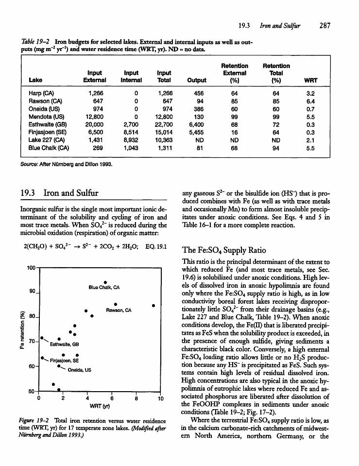
19.3 Iron and Sulfur 287
Table 19-2 Iron budgetsfor selectedlakes. External andinternalinputsaswellas outputs (mgm~2 yr-1) andwater residence time (WRT, yr).ND =no data.
Retention RetentionInput Input Input External Total
Lake External Internal Total Output (%) (%) WRT
Harp (CA) 1,266 0 1,266 456 64 64 3.2Rawson (CA) 647 0 647 94 85 85 6.4
Oneida (US) 974 0 974 386 60 60 0.7Mendota (US) 12,800 0 12,800 130 99 99 5.5Esthwaite (GB) 20,000 2,700 22,700 6,400 68 72 0.3Finjasjoen (SE) 6,500 8,514 15,014 5,455 16 64 0.3Lake 227 (CA) 1,431 8,932 10,363 ND ND ND 2.1Blue Chalk (CA) 269 1,043 1,311 81 68 94 5.5
Source: After NOrnberg and Dillon 1993.
19.3 Iron and Sulfur
Inorganicsulfuris the singlemost important ionic determinant of the solubility and cycling of iron andmost trace metals. When S042~ is reduced during themicrobial oxidation (respiration) of organicmatter:
2-2(CH20) + S04 S2_ + 2C02 + 2H20; EQ. 19.1
100
90.Blue Chalk, CA
£ 80_Rawson, CA
Esthwaite, GB
-»Finjasjoen, SE
^ Oneida, US
70-
60-
50-
WRT(yr)10
Figure 19-2 Total iron retention versus water residencetime (WRT, yr) for 17 temperate zone lakes. (Modified afterNumberg andDillon 1993.)
any gaseous S2" or the bisulfide ion (HS~) that isproduced combines with Fe (as well as with trace metalsandoccasionallyMn) to form almostinsoluble precipitates under anoxic conditions. See Eqs. 4 and 5 inTable16-1 for a more complete reaction.
The Fe:S04Supply RatioThis ratio is the principaldeterminant ofthe extent towhich reduced Fe (and most trace metals, see Sec.19.6) issolubilized under anoxic conditions. High levels of dissolved iron in anoxic hypolimnia are foundonlywhere the Fe:S04supply ratio is high, as in lowconductivity boreal forest lakes receiving disproportionately little S042" from their drainage basins (e.g.,Lake 227 and Blue Chalk, Table 19-2). When anoxicconditions develop, the Fe(II) that is liberated precipitates asFeSwhenthe solubilityproduct is exceeded, inthe presence of enough sulfide, giving sediments acharacteristic black color. Conversely, a highexternalFe:S04 loading ratio allows little or no H2S productionbecause anyHS"is precipitated asFeS. Such systems contain high levels of residual dissolved iron.High concentrations are also typical in the anoxic hypolimnia of eutrophic lakes where reduced Fe and associated phosphorus are liberated after dissolution ofthe FeOOHP complexes in sediments under anoxicconditions (Table 19-2;Fig.17-2).Where the terrestrial Fe:S04supply ratio is low, as
in the calcium carbonate-rich catchments ofmidwest-ern North America, northern Germany, or the
288 CHAPTER19 Iron, Manganese, and Sulfur
Ukraine, virtually all Fe is precipitated as FeS andanoxic hypolimnia typically contain littleFe (e.g., LakeMendota, Table 19-1) but considerable H2S. Wherethe lakes are also sufficiendy transparent, a layer ofphotosynthetic sulfur bacteria develops just belowtheoxycline, utilizing the reduced sulfur(Sec. 22.10). Calcareous lakes retain not onlymost Fe but alsoretain asubstantial fraction ofthe Mn supply (Sec. 19.5), primarily as insoluble MnC03. Outflowing rivers fromsuch lakes consequendy carry little Fe and Mn, anddownstream lakes and wedands are characterized byexceptionally lowFe:SandMn:Ssupplyratios.
A SulfurDiagenesisWhere the climate and morphometry allow an extended period of lakeor wetland anoxiaand much diagenesis, sediments acquire a more stable, less solubleprecipitate in the form of ferrous disulfide (FeS2),known as the mineral pyrite (Capone and Kiene1988). There is growingevidence that pyrite can formmuchmore quickly than once thought feasible. Evenso, much of the reduced sulfur is not stored perma-nendy as FeS or FeS2 minerals but rather as organicsulfur compounds, which are less readily reoxidizedfollowing reoxygenation than inorganic forms. Theorganic sulfur is formed direcdy during microbiallymediated reduction of S042", andabiotically by reactions of reduced sulfur with sediment organic matter(Rudd et al. 1986, Urban 1994). In some saline systems, most of the sulfur may be stored as gypsum(CaS04) or anhydride.
A 19.4 Iron and OrganicMatter
Iron and most other metals become adsorbed to sedi-menting inorganic aggregates (Sec. 19.2) and alsobond with colloidal5 and dissolved organic moleculesknown as organic ligands. Many ligands are humic-acid polymers that release H+ ions (protons) and arenegatively-charged hydrophobic ("water fearing")molecules (Sec. 8.8). The molecules form metal-
5Intermediate-sized colloids falling between the operationally defined "particulate" (retained by 0.2 or 0.45 |im membrane filters)and"soluble"phasehavebeen disregarded by aquatic scientists because they aredifficultto separate andanalyze (Allan 1986). In somelakescolloidcarbonlevels aremuch higher than concentrations ofparticulate organiccarbon(BurnisonandLeppard 1983).
organic complexes by ion exchange, surface adsorption, or chelation and the small colloidal Fe(HI) particles that are formed aresubjectto little sedimentation.The existence of Fe(ffl) aggregates in anoxic hypolimnia has been attributed to their stabilization byorganic matter and to insufficient reducing conditionsat the sediment-water interface during the stratification period(Sigget al. 1991). It is the bondingofmetals to organicligands that most confounds our abilityto base an interpretation of metal behavior in inlandwaters on either measured redox potentials in natureor on the behavior ofmetalsin pure inorganicsolutionin the laboratory. The bonding of Fe (andmost tracemetals) to dissolved organic matter (DOM) allowshighermetal levels in both oxidized waters(redox potential Eh > -200 mV) at nearly neutral pH and inacidic waters than is expected from thermodynamicconsiderations(Urban et al. 1990,Nurnberg and Dillon 1993). The increased solubility of oxidized iron(and aluminium) in acidified waters at pH < 5 allowsthe additional bondingwith DOM and floe formation(sedimentation) responsible for the characteristicallyincreased clarity of lakes following acidification(Chapter 27).
19.5 The Manganese Cycle
Manganese oxides [Mn(IQ), Mn(IV)] becomereducedat higher redox potentials than Fe3+ and S042~ (Fig.16-2), with the result that appreciable levels of dissolved Mn(II) appear in the hypolimnia or in hypoxicgroundwaterat a timewhen Fe remainsin the insoluble hydroxideform. Conversely, manganeseoxidationand precipitation commence when Fe remains dissolved (Fig. 19-1).Manganeseis precipitatedprimarily as relatively large (1-5 Jim) Mn oxide aggregates,but also asMnC03 in calcareouswaters low in DOC.In comparison to Fe(EH), little oxidized Mn is boundto organic matter (Urban et al. 1990). Inorganic floesmaycontain largeamounts ofCa, butMg, Si,P,S,CI,K, and Ba have been found as well (Tipping et al.1984). Following microbially mediated oxidation,most Mn(H) is precipitated asMn(m) or Mn(IV) oxy-hydroxide floes and not asMnS because little reducedsulfuris normallyavailable at the relatively high £h atwhichMn(H) is formed (Table19-1). A larger fractionof precipitatedMn oxidefloes than precipitatedFe (asFeSor FeS2) is solubiUzed in the anoxic hypolimnia ofcalcareous lakes. SolubiUzed Mn (or Fe) is also subject
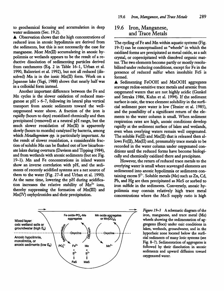
to geochemical focusing and accumulation in deepwater sediments (Sec. 19.2).• Observationshowsthat the high concentrations ofreduced iron in anoxic hypolimnia are derived fromthe sediments, but this is not necessarily the case formanganese. Most Mn(H) accumulating in anoxic hypolimnia or wetlands appears to be the result of a reductive dissolution of sedimenting particles derivedfrom catchments (Eq. 2 in Table 16-1, Urban et al.1990, Balistrieri et al. 1992), but not all reduced (dissolved) Mn is in the ionic Mn(H) form. Work on aJapanese lake (Yagi, 1988) shows that nearlyhalfwasin a colloidal form instead.Another important difference between the Fe and
Mn cycles is the slower oxidation of reduced manganese at pH > 6-7, foUowing its lateral plus verticaltransport from anoxic sediments toward the well-oxygenated water above. A fraction of the iron israpidly(hours to days) reoxidized chemically and thenprecipitated (removed) at a neutral pH range, but themuch slower reoxidation of Mn(II) is apparendyslowly (hours to months) catalyzed bybacteria, amongwhichMetallogenium spp. is particularly important Asthe result of slower reoxidation, a considerable fraction ofsolubleMn can be flushed out of low bicarbonate lakes duringoverturn (Davison andTipping 1984),andfromwedands withanoxic sediments (but seeFig.19-1). Mn and Fe concentrations in inland watersshow an inverse correlation with pH, and the sediments of recendy acidifiedsystemsare a net source ofthem to the water (Fig. 27-8 and Urban et al. 1990).At the same time, lowering the pH during acidification increases the relative stability of Mn2+ ions,thereby suppressing the formation of Mn(H[) andMn(TV) oxyhydroxides and their precipitation.
Mixed layeroxic wetland soils orgroundwater (high E^
Anoxic hypolimnia,monolimnia, oranoxic sediments (lowE^
19.6 Iron, Manganese, and TraceMetals 289
19.6 Iron, Manganese,and Trace Metals
The cycling of Fe andMn within aquaticsystems (Fig.19-3) can be conceptualized as "wheels" in which theoxidized formsare precipitated asmetal oxide,as a saltcrystal, or coprecipitated with dissolved organic matter.The twoelementsbecomepartlyor mosdy resolu-bilizedunder reducing conditions, except for Fe in thepresence of reduced sulfur when insoluble FeS isformed.• Sedimenting FeOOH and MnOOH aggregatesscavenge redox-sensitive tracemetals and arsenic fromoxygenated waters that are not highly acidic (Gunkeland Sztraka 1986, Kuhn et al. 1994). If the sedimentsurfaceis oxic,the trace element solubilityin the surfi-cial sediment pore water is low Clessier et al. 1985),and the possibility of a significant return of the elements to the water column is small. When sedimentrespiration rates are high, anoxic conditions developrapidly at the sediment surface of lakes and wedands,evenwhen overlying waters remain well oxygenated.The soluble Fe(II) and Mn(II) that is released then allows Fe(II),Mn(II) and, presumably trace metals to berecorded in the water columnunder oxygenated conditions until the reduced forms have become biologi-cally and chemically oxidized there and precipitate.
However, the return of reduced trace metals to theoverlying water is smallwhere scavenged elementsaresedimented into anoxic hypolimnia or sedimentscontaining excess S2". Soluble metals (Me) such asZn,Cd,Pb, andHg are then precipitatedasMeS or sorbed toiron sulfide in the sediments. Conversely, anoxic hypolimnia may contain relatively high trace metalconcentrations where the Me:S supply ratio is high
Figure 19-3 Aschematic diagram of theiron, manganese, and trace metal (Me)wheels showing the sedimentation of aggregates (floes) under oxic conditions inlakes, wedands, groundwater, and in thehyporheic zone located below the surfi-cialsediments of manyloricsystems (seeFig. 8-7). Sedimentationof aggregates isfollowed by their dissolution in anoxicsediments and upward diffusion towardoxygenatedwater.
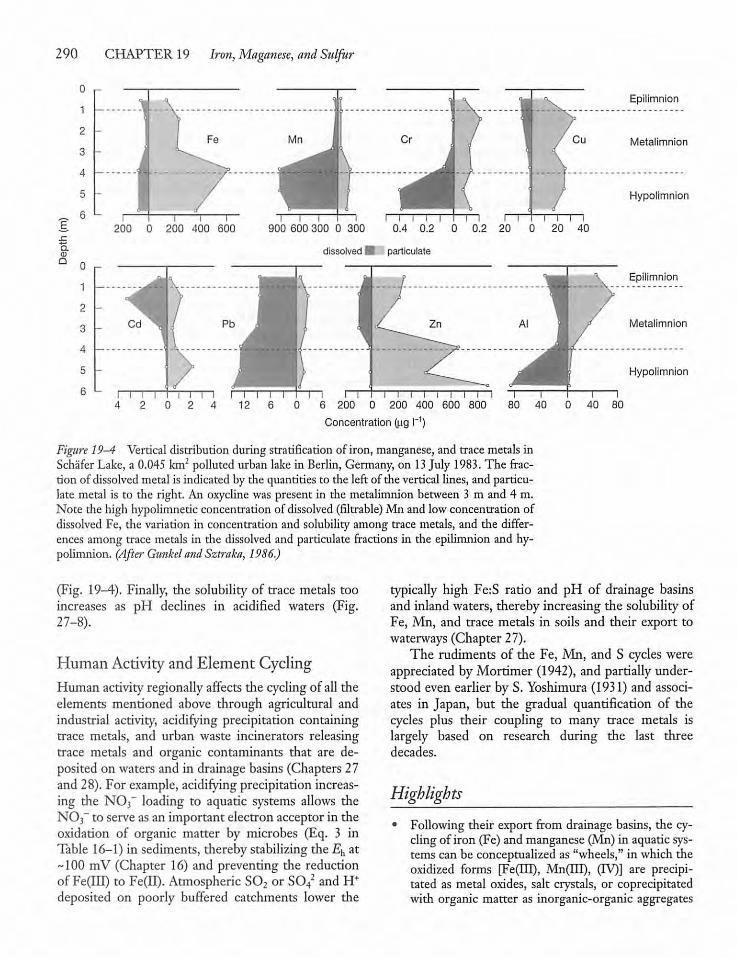
290 CHAPTER 19 Iron, Maganese, and Sulfur
i r200 0 200 400 600 900 600 300 0 300
Epilimnion
Hypolimnion
0.4 0.2 0 0.2 20 0 20 40-a
Boa
dissolved h*. particulate
Epilimnion
Hypolimnion
4 2 0 2 4 12 6 0 6 200 0 200 400 600 800 80 40 0 40 80
Concentration (jag I"1)
Figure 19-4 Vertical distribution during stratification of iron, manganese, and tracemetals inSchafer Lake, a 0.045 km2 polluted urban lake in Berlin, Germany, on 13 July 1983. The fraction of dissolvedmetal is indicated by the quantities to the left of the vertical lines, and particulate metal is to the right. An oxycline was present in the metalimnion between 3 m and 4 m.Note the high hypolimnetic concentration of dissolved (filtrable) Mn and lowconcentration ofdissolved Fe, the variation in concentration and solubility among trace metals, and the differences among trace metals in die dissolved and particulate fractions in the epilimnion and hypolimnion. (After Gunkcl andSztraka, 1986.)
(Fig. 19-4). Finally, the solubility of trace metals tooincreases as pH declines in acidified waters (Fig.27-8).
Human Activityand Element CyclingHuman activityregionallyaffects the cycling of all theelements mentioned above through agricultural andindustrial activity, acidifying precipitation containingtrace metals, and urban waste incinerators releasingtrace metals and organic contaminants that are deposited on waters and in drainage basins (Chapters 27and 28). For example,acidifying precipitation increasing the N03~ loading to aquatic systems allows theN03~ to serve as an important electron acceptor in theoxidation of organic matter by microbes (Eq. 3 inTable 16-1) in sediments, thereby stabilizing the Eh at-100 mV (Chapter 16) and preventing the reductionof Fe(IH) to Fe(H). Atmospheric S02 or S042 and H+deposited on poorly buffered catchments lower the
typically high Fe:S ratio and pH of drainage basinsand inland waters, thereby increasing the solubilityofFe, Mn, and trace metals in soils and their export towaterways (Chapter 27).The rudiments of the Fe, Mn, and S cycles were
appreciated by Mortimer (1942), and partiallyunderstood even earlier by S. Yoshimura (1931) and associates in Japan, but the gradual quantification of thecycles plus their coupling to many trace metals islargely based on research during the last threedecades.
Highlights• Following their export from drainage basins, the cyclingof iron (Fe) and manganese (Mn) in aquatic systemscan be conceptualized as "wheels," in which theoxidized forms [Fe(Hl), Mn(ITI), (Tv7)] are precipitated as metal oxides, salt crystals, or coprecipitatedwith organic matter as inorganic-organic aggregates
(floes). The elements are partly solubilized as Fe(IQ)andMn(U) under reducing conditions in anoxic hypolimnia, anoxic wedands, and in the anoxic portionofthe hyporheiczone oflotic systems.
• The resolubilization of reduced iron (Fe(II)], mosttrace metals (Me), and occasionally Mn(H) underanoxic conditions is lowwherereducedinorganic sulfur (S2~, HS~) concentrations are high and insolubleFeS, FeS2,MnS, and MeS is formed.
• Fe and Mn cycling in aquatic systems is no longerseen as only the outcome of chemical oxidation andreductions. There has been recent recognitionof theimportant direct and indirect roles microbes play inredox reactions.
• A Fe andMn are of great importance through theirphysical, chemical, and biological interactions withsulfur, other elements, and organic matter affectingthe concentrations of phosphate, nitrate, and mosttracemetalsavailable to the biota.The verylowsolu
19.6 Iron, Manganese, andTrace Metals 291
bilityof Fe under well-oxygenated conditionsin euphoriczonesoccasionally limitsalgal growth.
• The onset ofanoxic conditions and the removal of anFe oxide diffusion barrier at the oxic-anoxic sedimentinterface results in high concentrations of soluble Feand Mn in anoxic hypolimnia and slowly flushedanoxic wedands.
• Sulfurplays an important role in Fe, tracemetal, andsometimes Mn cycling with reduced ionic sulfurforming insoluble precipitates under anoxic conditions, preventing their release into the overlyingwater.
• • Humans affect the regional cycling of elementsthrough agricultural andindustrial activity; bygreadyincreasingthe nitrate, sulfate, phosphate, trace metal,and hydrogen ions deposition on water and theirdrainage basins; and by allowing increased dissolvedoxygen consumption rates in organically enrichedwaterways.
H R
20
Particle Sedimentationand Sediments
20.1 Introduction
Amajor determinant of the sediments suitability as aphysical and nutrient substrate for the biota is itsphysical and chemical structure. In shallow water,algae growon sediments and the rooted macrophytesobtain nutrients from them (Chapter 24). Heterotrophic bacteria and invertebrates live on andwithin the spaces between sediment particles, whilefish use sediments for feeding and nesting (Chapter 26).Sedimentrespiration, dominated bymicrobes(Sec. 25.7), largely determineswhether the sedimentsurface will be oxicor anoxic and whether the apparent redox potential is high or low (Chapter 16). Thishas a major impact on the suitability of the sedimentsfor invertebrates requiring dissolved oxygen (Chapter 25), and the extent that the sediments can serve asa source or sink of nutrients and trace metals (Chapters 15 to 19, and 28) to the water column.The likelihood of sedimented particles plus ad
sorbed nutrients and contaminants remaining at thesite of sedimentation, resuspending and then transportinganddepositing elsewhere, or flushing fromthesystem is a function of system morphometry (size,shape, anddepth)whichdetermines exposure towindsand wind-induced turbulence (Chapter 12). Lakemorphometry (depth) also influences the length oftime available for organic particles to decompose inthe water column rather than become sedimented.The sediment texture and chemicalcompositionin allinlandwaters is modified by the sediment biota. However, usingthe samemetaphorasbefore,the sedimentbiota operate and interact on a "stage" whose size,292
shape, and suitability for the "actors" is determinedbeyond the shoreline and, in lakes, is also gready affected by decomposition in the water column abovethe sediments. The preserved remains of some of the"actors" are increasingly providing insights into thehistoryof lakes, quiescentbaysof rivers, and wedandsas well as their response over time to changes in climate and human disturbance.
20.2 Origin and Distributionof Sediments
Lake and wedand sediments are usually overwhelmingly derived via inflowing rivers from drainagebasins. The soils, the vegetation cover, the drainageratio (CALA ratio), and the catchment slope determinenot onlythe particle supply rate but also the extent to which the supply to aquatic systems iscomposed of inorganic particles rather than organicmatter (Chapter 8).An important fraction of catchment-derived phos
phorus, iron, manganese, and inorganic nitrogen exported to aquatic systems asNH^ travels adsorbed toorganic and inorganic particles (Likens 1984, PrairieandKalff1988 and Chapters 8, and 17 to 19). Thereis, therefore, a correlation between the quantities ofparticulate matter exported from the land and thequantities of phosphorus, nitrogen, iron, and otherplantnutrients received by inlandwaters.In anyclimatic or geologic zone, the shape andsize
of an aquatic system is a function of catchment morphometry (Chapter 7). The water residence time of
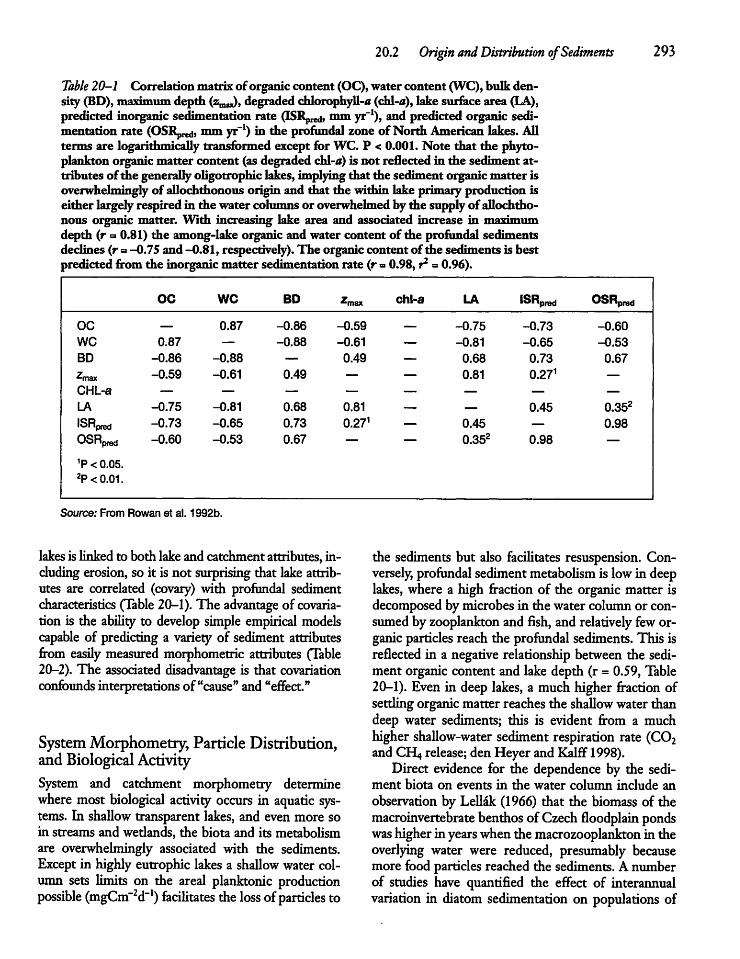
20.2 Origin and Distribution ofSediments 293
Table 20-1 Correlationmatrix oforganic content (OC),water content (WC), bulk density (BD), maximum depth (Zmw)* degraded chlorophyll-a (chl-a), lake surface area (LA),predicted inorganic sedimentation rate (ISKprd, mm yr-1), andpredicted organic sedimentation rate (OSR^, mm yr-1) in the profundal zone ofNorth American lakes. Allterms are logarithmically transformed except for WC. P < 0.001. Note that the phytoplankton organic matter content (as degraded chl-0) is not reflected in the sediment attributes ofthe generally oligotrophic lakes, implying that the sediment organic matter isoverwhelmingly of allochthonous origin and that the within lake primary production iseither largely respired in die water columns or overwhelmed by die supply ofallochthonous organic matter. With increasing lake area and associated increase in i?iflT"""i"idepth (r = 0.81) the among-lake organic and water content of the profundal sedimentsdeclines (r =-0.75 and -0.81, respectively). The organic content ofthe sediments is bestpredictedfrom the inorganicmatter sedimentation rate (r =0.98,r2 «= 0.96).
OC WC BD *max chl-a LA ISRpred OSRpred
OC — 0.87 -0.86 -0.59 — -0.75 -0.73 -0.60
WC 0.87 — -0.88 -0.61 — -0.81 -0.65 -0.53
BD -0.86 -0.88 — 0.49 — 0.68 0.73 0.67
*max -0.59 -0.61 0.49 — — 0.81 0.271 —
CHL-a — — — — — — — —
LA -0.75 -0.81 0.68 0.81 — — 0.45 0.352ISRpred -0.73 -0.65 0.73 0.271 — 0.45 — 0.98
OSRpred -0.60 -0.53 0.67 — — 0.352 0.98 —
1P < 0.05.2P<0.01.
Source: From Rowan et al. 1992b.
lakesis linked to both lake and catchment attributes, including erosion, so it is not surprising that lakeattributes are correlated (covary) with profundal sedimentcharacteristics (Table 20-1).The advantage of covariation is the ability to develop simple empirical modelscapable of predicting a variety of sediment attributesfrom easily measured morphometric attributes (Table20-2). The associated disadvantage is that covariationconfounds interpretations of "cause" and "effect."
SystemMorphometry, Particle Distribution,andBiological ActivitySystem and catchment morphometry determinewhere most biological activity occurs in aquatic systems. In shallowtransparent lakes, and evenmore soin streams and wedands, the biota and its metabolismare overwhelmingly associated with the sediments.Except in highly eutrophic lakes a shallowwater column sets limits on the areal planktonic productionpossible (mgCm"zd_1) facilitates theloss ofparticles to
the sediments but also facilitates resuspension. Conversely, profundal sedimentmetabolism is lowin deeplakes, where a high fraction of the organic matter isdecomposed bymicrobesin the water column or consumedby zooplanktonand fish, and relatively feworganicparticles reach the profundal sediments.This isreflected in a negative relationship between the sediment organic content and lake depth (r = 0.59, Table20-1). Even in deep lakes, a much higher fraction ofsettlingorganicmatter reaches the shallowwater thandeep water sediments; this is evident from a muchhigher shallow-water sediment respiration rate (C02and CH4 release; den Heyer and Kalff 1998).Direct evidence for the dependence by the sedi
ment biota on events in the water column include anobservation by Lellak(1966) that the biomass of themacroinvertebrate benthosof Czechfloodplain pondswas higherinyears whenthemacrozooplankton in theoverlying water were reduced, presumably becausemore food particles reached the sediments. A numberof studies have quantified the effect of interannualvariation in diatom sedimentation on populations of
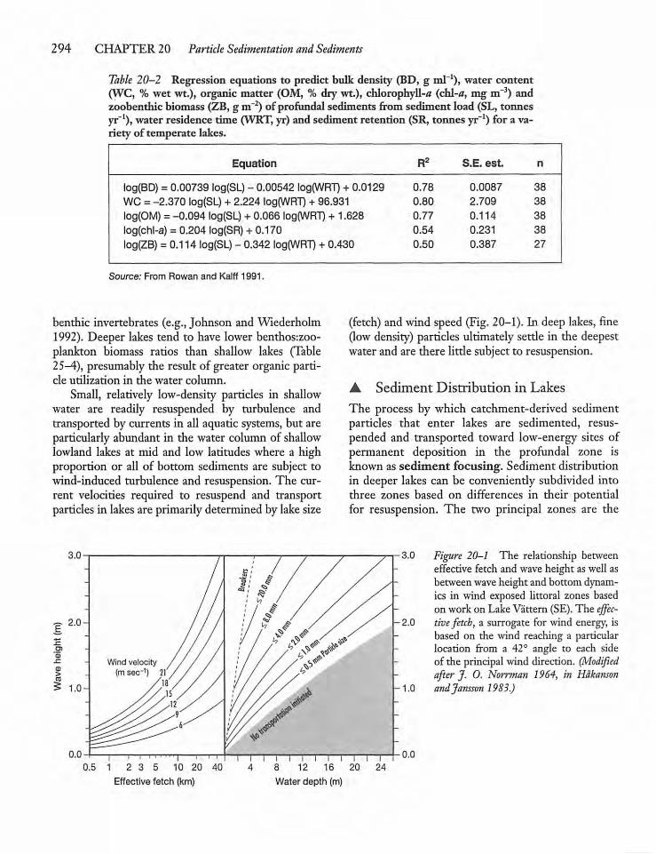
294 CHAPTER 20 Particle Sedimentation and Sediments
Table 20-2 Regression equations to predict bulk density (BD, g ml-1), water content(WC, % wet wt.), organicmatter (OM, % drywt.), chlorophyll-a (chl-#, mg m~3) andzoobenthic biomass (ZB, g m~2) of profundal sediments from sediment load (SL, tonnesyr-1), water residence time (WRT, yr) and sedimentretention (SR, tonnes yr-1) for a variety of temperate lakes.
Equation
log(BD) = 0.00739 log(SL) - 0.00542 log(WRT) + 0.0129WC = -2.370 log(SL) + 2.224 log(WRT) + 96.931log(OM) = -0.094 log(SL) + 0.066 log(WRT) + 1.628log(chl-a) = 0.204 log(SR) + 0.170log(ZB) = 0.114 log(SL) - 0.342 log(WRT) + 0.430
R* S.E. est. n
0.78 0.0087 38
0.80 2.709 38
0.77 0.114 38
0.54 0.231 38
0.50 0.387 27
Source: From Rowan and Kalff 1991.
benthic invertebrates (e.g.,Johnson and Wiederholm1992). Deeper lakes tend to have lower benthostzoo-plankton biomass ratios than shallow lakes (Table25-4), presumably the result of greater organic particle utilization in the water column.Small, relatively low-density particles in shallow
water are readily resuspended by turbulence andtransported by currents in all aquatic systems, but areparticularly abundant in the water column of shallowlowland lakes at mid and low latitudes where a highproportion or all of bottom sediments are subject towind-induced turbulence and resuspension. The current velocities required to resuspend and transportparticles in lakesare primarilydetermined by lake size
i
1 2 3 5 10 20
Effective fetch (km)
(fetch) and wind speed (Fig. 20-1). In deep lakes, fine(lowdensity) particles ultimately settle in the deepestwater and are there little subject to resuspension.
• Sediment Distribution in Lakes
The process by which catchment-derived sedimentparticles that enter lakes are sedimented, resuspended and transported toward low-energy sites ofpermanent deposition in the profundal zone isknown as sediment focusing. Sediment distributionin deeper lakes can be conveniently subdivided intothree zones based on differences in their potentialfor resuspension. The two principal zones are the
Figure 20-1 The relationship betweeneffective fetch and wave height aswell asbetweenwaveheight and bottom dynamics in wind exposed littoral zones basedon work on LakeVattern (SE).The effective fetch, a surrogate for wind energy, isbased on the wind reaching a particularlocation from a 42° angle to each sideofthe principal wind direction. (Modifiedafter J. O. Norrman 1964, in Hakansonandjansson 1983.)
16 20
Water depth (m)
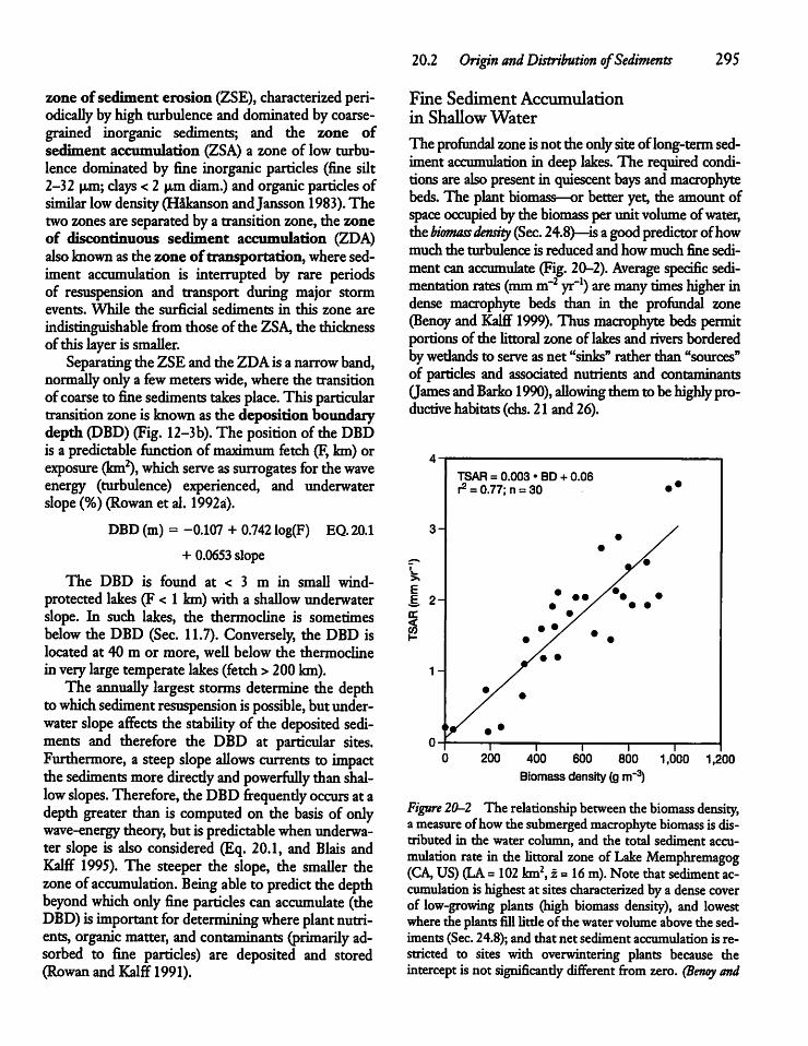
zone of sediment erosion (ZSE), characterized periodically byhigh turbulenceand dominatedby coarsegrained inorganic sediments; and the zone ofsediment accumulation (ZSA) a zone of low turbulence dominated by fine inorganic particles (fine silt2-32 pjn; clays < 2 u,mdiam.)and organic particlesofsimilarlowdensity(HakansonandJansson 1983). Thetwozonesare separatedby a transition zone, the zoneof discontinuous sediment accumulation (ZDA)alsoknownas the zone oftransportation, wheresediment accumulation is interrupted by rare periodsof resuspension and transport during major stormevents. While the surficial sediments in this zone areindistinguishable from those ofthe ZSA,the thicknessof this layer is smaller.Separatingthe ZSE and the ZDA is a narrowband,
normally only a fewmeters wide, where the transitionof coarse to finesediments takes place. This particulartransition zone is knownas the deposition boundarydepth (DBD) (Fig. 12-3b).The position of the DBDis a predictable function of maximumfetch (F, km) orexposure (km2), which serve as surrogates for thewaveenergy (turbulence) experienced, and underwaterslope(%) (Rowan et al. 1992a).
DBD (m) = -0.107 + 0.742log(F) EQ. 20.1
+ 0.0653slope
The DBD is found at < 3 m in small wind-protected lakes (F < 1 km) with a shallow underwaterslope. In such lakes, the thermocline is sometimesbelow the DBD (Sec. 11.7). Conversely, the DBD islocated at 40 m or more, well below the thermoclinein verylargetemperate lakes (fetch >200km).The annually largest storms determine the depth
towhich sediment resuspension ispossible, butunderwater slope affects the stability of the deposited sediments and therefore the DBD at particular sites.Furthermore, a steep slope allows currents to impactthe sediments moredirectly andpowerfully thanshallow slopes. Therefore, theDBDfrequendy occurs at adepth greater than is computed on the basis of onlywave-energy theory,but is predictablewhenunderwater slope is also considered (Eq. 20.1, and Blais andKalff 1995). The steeper the slope, the smaller thezone ofaccumulation. Being able to predict thedepthbeyond which only fine particles can accumulate (theDBD) is important fordeterminingwhere plantnutrients,organic matter, and contaminants (primarily adsorbed to fine particles) are deposited and stored(Rowanand Kalff 1991).
20.2 Origin and Distribution ofSediments 295
Fine Sediment Accumulationin ShallowWater
The profundal zoneisnot theonlysiteof long-term sediment accumulation in deep lakes. The required conditionsare also presentin quiescent bays andmacrophytebeds. The plant biomass—or better yet, the amount ofspace occupied by the biomass per unit volume ofwater,thebiomassdensity (Sec. 24.8)—is agoodpredictor ofhowmuch the turbulence is reduced and howmuch fine sediment can accumulate (Fig. 20-2). Average specific sedimentation rates (mm m"2 yr-1) are many times higher indense macrophyte beds than in the profundal zone(Benoy andKalff 1999). Thus macrophyte beds permitportionsofthe littoral zone of lakes and riversborderedbywetlands to serveas net "sinks'' rather than "sources"of particles and associated nutrients and contaminants(James andBarko 1990), allowing themtobehighlyproductivehabitats (chs. 21 and 26).
TSAR = 0.003 • BD + 0.06r2= 0.77; n = 30
400 600 800
Biomassdensity (gm"3)1,000 1,200
Figure 20-2 The relationship between the biomass density,a measureof how the submergedmacrophytebiomass is distributed in the water column, and the total sediment accumulation rate in the littoral zone of Lake Memphremagog(CA, US) (LA= 102 km2, z = 16m).Note that sedimentaccumulation is highestat sitescharacterized bya densecoverof low-growing plants (high biomass density), and lowestwhere the plants fill litde ofthewater volume above the sediments (Sec. 24.8); and that net sediment accumulation is restricted to sites with overwintering plants because theinterceptis not significantiy different fromzero. (Benoy and
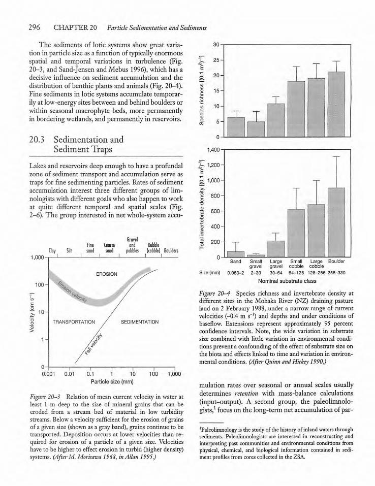
296 CHAPTER 20 Particle Sedimentation and Sediments
The sediments of lotic systems show great variation in particle sizeas a function of typically enormousspatial and temporal variations in turbulence (Fig.20-3, and Sand-Jensen and Mebus 1996), which has adecisive influence on sediment accumulation and thedistribution of benthic plants and animals (Fig. 20-4).Fine sediments in lotic systems accumulate temporarilyat low-energysites betweenand behind bouldersorwithin seasonal macrophyte beds, more permanendyin bordering wedands, and permanendy in reservoirs.
20.3 Sedimentation andSediment Traps
Lakes and reservoirs deep enough to have a profundalzone of sediment transport and accumulation serveastraps for fine sedimenting particles. Rates of sedimentaccumulation interest three different groups of limnologistswith different goalswho alsohappen to workat quite different temporal and spatial scales (Fig.2-6). The group interested in net whole-system accu-
1,000
GravelFine Coarse and Rubble
Clay Silt sand sand pebbles (cobble) BouldersI I I I I
EROSION
100-
10-
1
0-
0.001 0.01
TRANSPORTATION SEDIMENTATION
0.1 1 10
Particle size (mm)100 1,000
Figure 20-3 Relation ofmean current velocity in water atleast 1 m deep to the size of mineral grains that can beeroded from a stream bed of material in low turbiditystreams. Below a velocity sufficient for the erosion of grainsof a given size (shown as a gray band), grains continue to betransported. Deposition occurs at lower velocities than required for erosion of a particle of a given size. Velocitieshave to be higher to effect erosion in turbid (higher density)systems. (AfterM.Morisawa 1968, inAllan1995.)
0)Q.CO
30
25
20
15—1
10-
5-
-
T
T Tr1]
Sand
Size (mm) 0.063-2
Smallgravel2-30
Largegravel30-64
Small Large Bouldercobble cobble
64-128 128-256 256-330
Nominal substrate class
Figure 20-4 Species richness and invertebrate density atdifferent sites in the Mohaka River (NZ) draining pastureland on 2 February 1988, under a narrow range of currentvelocities (~0.4 m s_1) and depths and under conditions ofbaseflow. Extensions represent approximately 95 percentconfidence intervals. Note, the wide variation in substratesize combined with little variation in environmental conditionspreventa confounding of the effectof substrate size onthe biota and effects linked to time and variation in environmental conditions. (After Quinn andHickey 1990.)
mulation rates over seasonal or annual scales usuallydetermines retention with mass-balance calculations(input-output). A second group, the paleolimnolo-gists,1 focus on thelong-term netaccumulation ofpar-
'Paleolimnology is thestudy ofthe history ofinland waters throughsediments. Paleolimnologists are interested in reconstructing andinterpreting past communities and environmental conditions fromphysical, chemical, and biological information contained in sediment profilesfrom cores collectedin the ZSA.
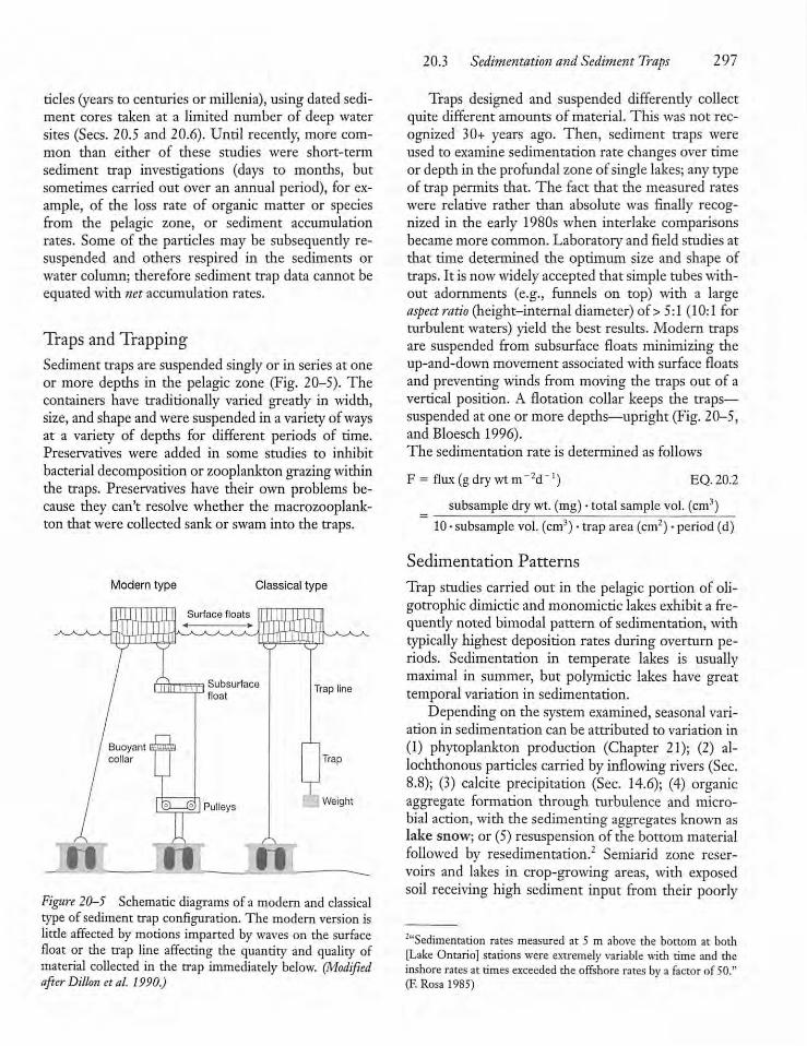
tides (years to centuries or millenia), using dated sediment cores taken at a limited number of deep watersites (Sees. 20.5 and 20.6). Until recently, more common than either of these studies were short-termsediment trap investigations (days to months, butsometimes carried out over an annual period), for example, of the loss rate of organic matter or speciesfrom the pelagic zone, or sediment accumulationrates. Some of the particles may be subsequendy re-suspended and others respired in the sediments orwater column; therefore sediment trap data cannot beequated with netaccumulation rates.
Traps and TrappingSediment traps are suspended singly or in series at oneor more depths in the pelagic zone (Fig. 20-5). Thecontainers have traditionally varied greatly in width,size, and shapeandwere suspendedin a varietyofwaysat a variety of depths for different periods of time.Preservatives were added in some studies to inhibitbacterial decomposition or zooplankton grazingwithinthe traps. Preservatives have their own problems because they can't resolve whether the macrozooplank-ton that were collected sank or swam into the traps.
Modern type Classical type
Figure 20-5 Schematic diagrams of a modern and classicaltype of sediment trap configuration. The modern version islittle affected bymotions imparted bywaves on the surfacefloat or the trap line affecting the quantity and quality ofmaterial collected in the trap immediately below. (NlodifiedafterDillon et al. 1990.)
20.3 Sedimentation andSediment Traps 291
Traps designed and suspended differently collectquite different amounts of material. This was not recognized 30+ years ago. Then, sediment traps wereused to examine sedimentation rate changes over timeor depth in the profundal zone of single lakes;any typeof trap permits that. The fact that the measured rateswere relative rather than absolute was finally recognized in the early 1980s when interlake comparisonsbecamemore common. Laboratory and field studies atthat time determined the optimum size and shape oftraps. It is nowwidely accepted that simple tubes without adornments (e.g., funnels on top) with a largeaspect ratio (height-internal diameter) of > 5:1 (10:1 forturbulent waters) yield the best results. Modern trapsare suspended from subsurface floats minimizing theup-and-down movement associated with surface floatsand preventing winds from moving the traps out of avertical position. A flotation collar keeps the traps—suspendedat one or more depths—upright (Fig. 20-5,and Bloesch 1996).The sedimentation rate is determined as follows
F = flux (gdrywtm~2d_1) EQ.20.2
subsample drywt. (mg) •total samplevol. (cm3)10•subsample vol. (cm3) •trap area (cm2) •period (d)
Sedimentation Patterns
Trap studies carried out in the pelagic portion of oligotrophic dimictic and monomictic lakes exhibit a frequently noted bimodal pattern of sedimentation, withtypically highest deposition rates during overturn periods. Sedimentation in temperate lakes is usuallymaximal in summer, but polymictic lakes have greattemporal variation in sedimentation.Depending on the systemexamined, seasonal vari
ation in sedimentation can be attributed to variation in(1) phytoplankton production (Chapter 21); (2) al-lochthonous particles carried byinflowing rivers (Sec.8.8); (3) calcite precipitation (Sec. 14.6); (4) organicaggregate formation through turbulence and microbial action,with the sedimenting aggregates known aslake snow; or (5)resuspension of the bottommaterialfollowed by resedimentation.' Semiarid zone reservoirs and lakes in crop-growing areas, with exposedsoil receiving high sediment input from their poorly
""Sedimentation rates measured at 5 m above the bottom at both[Lake Ontario] stationswere extremely variable with time and theinshore rates at times exceeded the offshore rates bya factor of 50."(F. Rosa 1985)
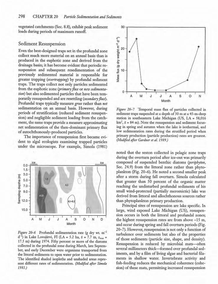
298 CHAPTER 20 Particle Sedimentation andSediments
vegetated catchments (Sec. 8.8), exhibitpeaksedimentloads during periods of maximum runoff.
Sediment ResuspensionEven the best-designedtraps set in the profundal zonecollect much more material on an annual basis than isproduced in the euphoric zone and derived from thedrainage basin; it hasbecome evidentthat periodic resuspension and subsequent resedimentation of thepreviously sedimented material is responsible forgreater trapping (overtrapping) by profundal sedimenttraps. The traps collect not only particles sedimentedfrom the euphoric zone (primaryflux or new sedimentation) but alsosedimented particles that havebeen temporarily resuspended andare resettling(secondaiyflux).Profundal traps typically measure gross rather thannetsedimentation on an annual basis. However, duringperiods of stratification (reduced sediment resuspension) and negligible sediment loading from the catchment, the same trapsprovide ameasure approximatingnet sedimentation of the then-dominant primary fluxof autochthonously-produced particles.The importance of resuspension first became evi
dent to algal ecologists examining trapped particlesunder the microscope. For example, Simola (1981)
J A S
Month
Figure 20-6 Profundal sedimentation rate (g dry wt. m"2d"1) in Lake Lovojarvi, FI (LA = 5.2 ha, z = 7.7 m, z,^ =17.5m) during 1974. Fifty percent or more of the diatomscollected in the profundal zone during March, lateSeptember, and earlyDecemberwere organisms transported fromthe littoral sediments to open water prior to sedimentation.The identified shaded isopleths and unshaded areas represent different rates of sedimentation. (Modified after Simola1981.)
Month
Figure 20-1 Temporal mass flux of particles collected insedimenttrapssuspended at a depth of 30m at a 45-m-deepstation in southeastern Lake Michigan (US, LA = 58,016km2, z = 84m). Note the resuspension and sediment focusing in spring and autumn when the lake is isothermal, andlow sedimentation rates during the stratified period whenprimary production (particle production) rates are greatest.(Modified afterGardner etal. 1989.)
noted that the seston collected in pelagic zone trapsduring the overturn period after ice-out was primarilycomposed of suspended benthic diatoms (periphyton,Sec. 24.9) from the littoral zone rather than phytoplankton (Fig. 20-6). He noted a secondsmaller peakafter a storm during fall overturn. Simola calculatedthat greater than 50 percent of the organic matterreaching the undisturbed profundal sediments of hissmall wind-protected (partially meromictic) lake wasderived from littoral and allochthonous sources ratherthan phytoplankton primaryproduction.Principal sites of resuspension are lake specific. In
large, wind exposed Lake Michigan (US), resuspension occurs in both the littoral and profundal zones;the highest resuspension rates are from above ~15 m,and occur during spring and fall overturn periods (Fig.20-7). However, resuspension is not only a function ofturbulence over sediments but also of the propertiesof those sediments (particle size, shape, and density).Resuspension is reduced by microbial mats—oftenseveral millimeters thick—formed over profundal sediments, and by a film of livingalgaeand bacterial filaments in shallow water. Invertebrate activity andfish-feeding reduces the mechanical coherence (cohesion) of diese mats, permitting increased resuspension
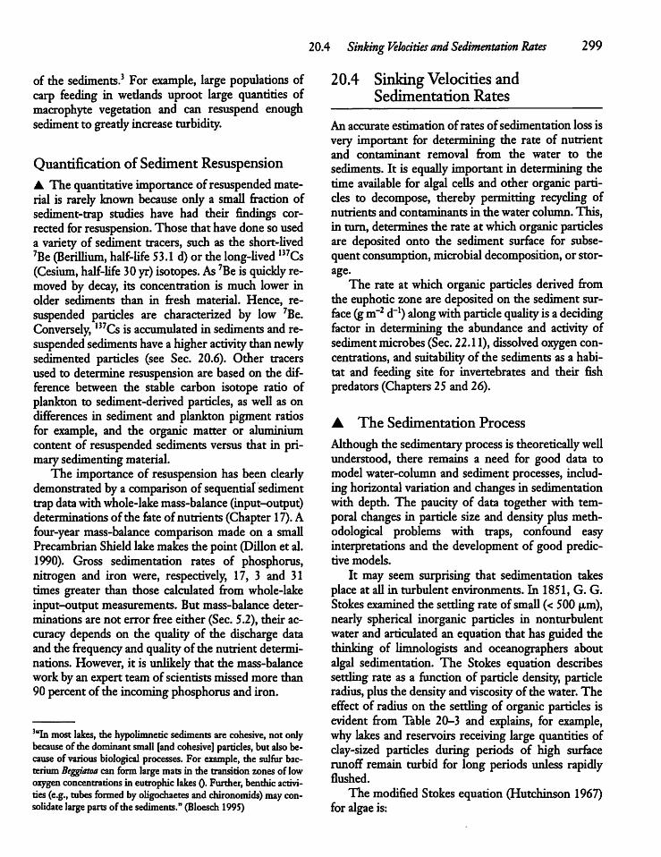
20.4 Sinking Velocities and Sedimentation Rates 299
of the sediments.3 For example, large populations ofcarp feeding in wedands uproot large quantities ofmacrophyte vegetation and can resuspend enoughsediment to greadyincrease turbidity.
Quantification of Sediment Resuspension• The quantitative importance of resuspended material is rarely known because only a small fraction ofsediment-trap studies have had their findings corrected for resuspension. Those that have donesouseda variety of sediment tracers, such as the short-lived7Be (BeriUium, half-Ufe 53.1 d) or thelong-Uved ,37Cs(Cesium, half-Ufe 30yr) isotopes. As 7Be isquickly removed by decay, its concentration is much lower inolder sediments than in fresh material. Hence, re-suspended particles are characterized by low 7Be.Conversely, 137Cs isaccumulated in sediments and re-suspended sediments have a higheractivity thannewlysedimented particles (see Sec. 20.6). Other tracersused to determine resuspension are based on the difference between the stable carbon isotope ratio ofplankton to sediment-derived particles, as weU as ondifferences in sediment and plankton pigment ratiosfor example, and the organic matter or aluminiumcontent of resuspended sediments versus that in primarysedimentingmaterial.The importance of resuspension has been clearly
demonstrated by a comparison of sequential sedimenttrap datawithwhole-lakemass-balance (input-output)determinations ofthe fateof nutrients (Chapter 17). Afour-year mass-balance comparisonmade on a smaUPrecambrian Shieldlakemakesthe point (DiUon et al.1990). Gross sedimentation rates of phosphorus,nitrogen and iron were, respectively, 17, 3 and 31times greater than those calculated from whole-lakeinput-output measurements. But mass-balance determinations are not error free either (Sec. 5.2), their accuracy depends on the quaUty of the discharge dataand the frequency and qualityofthe nutrient determinations.However, it is unlikely that the mass-balancework by an expert team of scientists missedmore than90 percent ofthe incomingphosphorusand iron.
3"In most lakes, die hypolimnetic sediments are cohesive, notonlybecause ofthe dominant small [and cohesive] particles, but also because of various biological processes. Forexample, the sulfurbacteriumBeggiatoa can form large mats in the transition zonesof lowoxygen concentrations in eutrophiclakes 0- Further, benthicactivities(e.g., tubes formed by oligochaetes andchironomids) mayconsolidate largepartsofthe sediments." (Bloesch 1995)
20.4 SinkingVelocities andSedimentation Rates
An accurate estimation ofrates ofsedimentation loss isvery important for determining the rate of nutrientand contaminant removal from the water to thesediments. It is equaUy important in determining thetime available for algal ceUs and other organic particles to decompose, thereby permitting recycling ofnutrients and contaminants in the water column. This,in turn, determinesthe rate at which organic particlesare deposited onto the sediment surface for subsequent consumption, microbialdecomposition, or storage.The rate at which organic particles derived from
the euphoric zoneare deposited on the sediment surface (gm~2 d"1) alongwith particle quaUty isadecidingfactor in determining the abundance and activity ofsedimentmicrobes(Sec. 22.11), dissolved oxygen concentrations, and suitabiUty ofthe sediments as a habitat and feeding site for invertebrates and their fishpredators (Chapters 25 and 26).
A The Sedimentation Process
Althoughthe sedimentaryprocessis theoreticaUy wellunderstood, there remains a need for good data tomodel water-column and sediment processes, including horizontalvariation and changesin sedimentationwith depth. The paucity of data together with temporal changes in particle size and density plus methodological problems with traps, confound easyinterpretations and the development of good predictive models.It may seem surprising that sedimentation takes
placeat aU in turbulent environments. In 1851,G. G.Stokes examined the settling rate of smaU (<500 u,m),nearly spherical inorganic particles in nonturbulentwaterand articulated an equation that has guided thethinking of limnologists and oceanographers aboutalgal sedimentation. The Stokes equation describessettling rate as a function of particle density, particleradius, plus the densityand viscosity ofthe water.Theeffect of radius on the settling of organic particles isevident from Table 20-3 and explains, for example,why lakes and reservoirs receiving large quantities ofclay-sized particles during periods of high surfacerunoff remain turbid for long periods unless rapidlyflushed.The modified Stokes equation(Hutchinson 1967)
for algaeis:
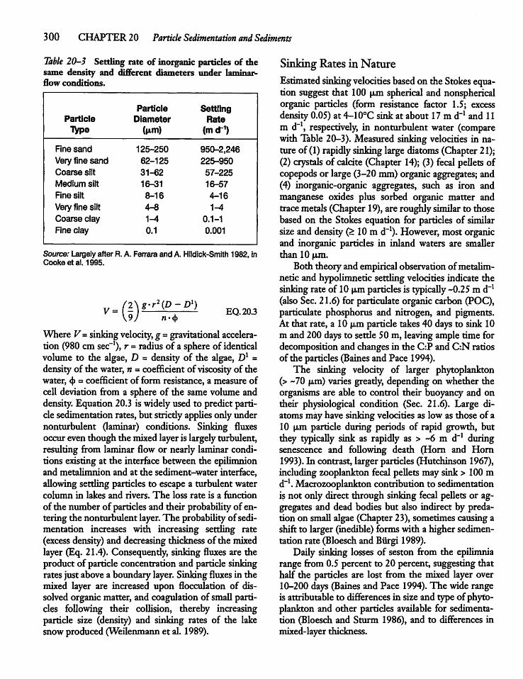
300 CHAPTER 20 ParticleSedimentation and Sediments
Table 20-3 Settling rate of inorganic particles of thesame density and different diameters under laminar-flow conditions.
Particle SettlingParticle Diameter RateType (lim) (md1)
Fine sand 125-250 950-2,246Very fine sand 62-125 225-950Coarse silt 31-62 57-225Medium silt 16-31 16-57Fine silt 8-16 4-16Veryfine silt 4-8 1^1Coarse clay 1-4 0.1-1
Fine clay 0.1 0.001
Source: Largely after R. A. Ferrara and A. Hildick-Smith 1982, inCooke etal. 1995.
(D - Dl)(!)^ EQ.20.3
Where V= sinking velocity, g =gravitational acceleration (980 cmsec-1), r = radius of a sphere of identicalvolume to the algae, D = density of the algae, D1 =densityofthe water, n =coefficient of viscosity ofthewater, <j> = coefficient of form resistance, a measure ofceU deviation from a sphere of the samevolume anddensity. Equation 20.3 is widely used to predict particle sedimentationrates, but stricdy appUes onlyundernonturbulent (laminar) conditions. Sinking fluxesoccureventhough the mixed layeris largelyturbulent,resulting from laminar flow or nearly laminar conditions existing at the interface between the epilimnionand metalimnion and at the sediment-water interface,aUowing settling particles to escape a turbulent watercolumn in lakes and rivers. The loss rate is a functionofthe number of particlesand their probabilityof entering the nonturbulent layer.The probabiUtyof sedimentation increases with increasing settling rate(excess density) and decreasing thickness ofthe mixedlayer (Eq. 21.4). Consequendy, sinking fluxes are theproduct of particle concentration and particle sinkingrates just abovea boundarylayer. Sinkingfluxes in themixed layer are increased upon flocculation of dissolvedorganic matter, and coagulation of smaU particles foUowing their collision, thereby increasingparticle size (density) and sinking rates of the lakesnowproduced (Weilenmannet al. 1989).
Sinking Ratesin NatureEstimated sinkingvelocities based on theStokes equation suggest that 100 pjn spherical and nonsphericalorganic particles (form resistance factor 1.5; excessdensity 0.05) at 4-10°C sinkat about 17m d_1 and 11m d"1, respectively, in nonturbulent water (comparewithTable 20-3).Measured sinking velocities in nature of (1) rapidly sinking largediatoms (Chapter21);(2) crystals of calcite (Chapter 14); (3) fecal pellets ofcopepods or large (3-20mm)organic aggregates; and(4) inorganic-organic aggregates, such as iron andmanganese oxides plus sorbed organic matter andtracemetals (Chapter19), are roughlysimilar to thosebased on the Stokes equation for particles of similarsize and density (^ 10 m d"1). However, most organicand inorganic particles in inland waters are smaUerthan 10 u,m.Both theory and empiricalobservationofmetalim-
netic and hypolimneticsettling velocities indicate thesinking rateof 10pjn particles is typicaUy ~0.25 m d"1(also Sec. 21.6) for particulate organic carbon (POC),particulate phosphorus and nitrogen, and pigments.At that rate, a 10 jxm particle takes40 days to sink 10m and 200 days to settle 50 m, leavingample time fordecomposition and changesin the C:P and C:N ratiosofthe particles (Baines and Pace 1994).The sinking velocity of larger phytoplankton
(> ~70 u>m) varies gready, depending on whether theorganisms are able to control their buoyancy and ontheir physiological condition (Sec. 21.6). Large diatomsmayhave sinkingvelocities as low as those of a10 u,m particle during periods of rapid growth, butthey typicaUy sink as rapidly as > ~6 m d-1 duringsenescence and foUowing death (Horn and Horn1993). In contrast, larger particles(Hutchinson 1967),including zooplankton fecal peUets may sink > 100md-1. Macrozooplankton contribution to sedimentationis not only direct through sinking fecal peUets or aggregates and dead bodies but also indirect by preda-tion on smaU algae (Chapter 23), sometimes causing ashift to larger (inedible)formswith a higher sedimentation rate (Bloesch and Biirgi 1989).Daily sinking losses of seston from the epilimnia
range from 0.5 percent to 20 percent, suggesting thathalf the particles are lost from the mixed layer over10-200 days (Baines and Pace 1994). The wide rangeis attributable to differences in size and type of phytoplankton and other particles available for sedimentation (Bloesch and Sturm 1986), and to differences inmixed-layerthickness.
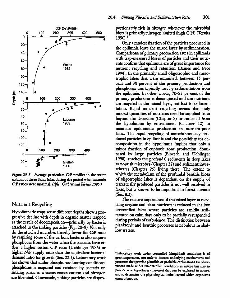
20.4 Sinking Velocities andSedimentation Rates 301
n£
cn-l
I 100I
C:P (by atoms]200 300 400
i
500
20-
40-
^r- •
60-
80- I • Walen1982
100-
120-•/
140- |«
Grelfen1983
• •
Figure 20-8 Average particulate C:P profiles in the watercolumnofthree Swisslakesduringthe periodwhen sestonicC:Pratios weremaximal. (After Gacbter andBloesch 1985.)
Nutrient RecyclingHypolimnetic traps setat different depths show a progressive decline withdepthin organic mattertrappedas the result of decomposition—primarily bybacteriaattached to thesinking particles (Fig. 20-8). Not onlydo the attached microbes therebylower the C:P ratiobyrespiring some of the carbon, bacteria also acquirephosphorus from thewater when theparticles have either a higher seston C:P ratio (Uehlinger 1986) orhigherN:P supply ratio than the equivalent bacterialdemand ratio forgrowth (Sec. 22.5). Laboratory workhas shown that underphosphorus-limiting conditions,phosphorus is acquired and retained by bacteria onsinking particles whereas excess carbon and nitrogenareUberated. Conversely, sinking particles aredispro
portionately rich in nitrogen whenever the microbialbiota isprimarilynitrogen limited (highC:N) (Tezuka1990).4Onlyamodestfractionofthe particlesproducedin
the epilimnia leave the mixed layer by sedimentation.Comparisons of primaryproduction rates in epilimniawith trap-measured losses of particles and their nutrientsconfirmthat epilimnia areof great importancefornutrient recycling and retention (Baines and Pace1994). In the primarilysmaU oUgotrophic and mesotrophic lakes that were examined, between 15 percent and 30 percent of the primary production andphosphorus was typicaUy lost by sedimentation fromthe epilimnia. In other words, 70-85 percent of theprimary production is decomposed and the nutrientsare recycled in the mixed layer, not lost to sedimentation. Rapid nutrient recycling means that onlymodest quantities of nutrients need be supplied frombeyond the shoreline (Chapter 8) or returned fromthe hypolimnia by entrainment (Chapter 12) tomaintain epilimnetic production in nutrient-poorlakes. The rapid recycling of autochthonously produced particles in epilimnia and the possibility for decomposition in the hypolimnia impUes that only aminor fraction of euphoric zone production, dominated by large particles (Bloesch and Uehlinger1990), reaches the profundal sediments in deep lakesto nourish microbes (Chapter22)andsedimentinvertebrates (Chapter 25) living there. The extent towhich die metabolism of the profundal benthic biotaof oUgotrophic lakes is dependent on the supply ofterrestriaUy produced particles is not weU resolved inlakes, but is known to be important in forest streams(Sec. 8.2).The relative importance ofthe mixed layer inrecy
cling organic andplantnutrientsis reduced in shallowunstratified lakes where particles are rapidly sedimented on calm days onlyto be partiahy resuspendedduringperiods of turbulence. The distinction betweenplanktonic and benthic processes is nebulous in shallow waters.
laboratory work under controlled (simplified) conditions is ofgreat importance, not only to discern underlying mechanisms andprocesses thatprovide plausible or probable explanations forobservations made under uncontrolled conditions in nature but also toprovide new hypotheses (theories) that canbe explored in nature,and to determine thephysiological limits beyond which organismscannot function.

302 CHAPTER 20 Particle Sedimentation and Sediments
20.5 The Sediment Record
Profundal sediments in the zone of sediment accumulation (Sec. 20.2) contain an invaluable record of pastconditions. Lakes, wetlands, quiescent bays and flood-plains of rivers, and the sediments of former—dessi-cated or infilled lake basins (paleolakes)—contain asystemhistory. Paleolimnologists can infer a great dealabout the past when sediments collected with coringdevices are examined and dated.
Coring DevicesMost coring devices are either gravity corers or pistoncorers. Gravity corers, widely used for collecting coresin soft, relatively recent sediments, consist of aweighted tube with a valve mechanism that closes atthe upper end once the core is taken, preventing lossof the core when the device is hauled to the surface(Fig. 20-9). Piston corers are designed to take rela-
Figure 20-9 Asediment gravitycorer with a core visible inthe transparent core tube. (Photo courtesy off. Smol.)
tively long cores (several meters)when the core tube isdriven into the sediments. A sliding piston inside thetube moves up, eliminating the hydrostatic pressurecreated while the core tube is filled, and offsetting thetendency of sediment to be pushed down as the coretube is driven in. A third device, used to collect sediments with a high water content, is not a tube. It is aprobe filled with dry ice and alcohol (—70°C) thatfreezes the adjacent sediment before thefreeze sampler(with adhering sediment) is pulled to the surface forsubsampling. Cores and freeze samples are subsam-pled—usually by slicing them into layers—to isolatespecific time periods (Smol and Glew 1992). Deep-coring ancient lakes involves an offshore drilling platform and coring device similar to those used to drillfor oil in the sea. A 1,400m-long core taken in LakeBiwa (JP) has brought three million years of the history ofthe lakeand region to light (Horie 1987).
Transfer Functions and HindcastingThe single greatest advance made by paleolimnologists in recent decades—and one of the most important advances in limnology as a whole during thatperiod—was the development of transfer functions allowing the fossil record to be quantified and interpreted in terms of important environmental variablessuch as pH, total phosphorus, salinity, DOC, aluminium, trace elements, temperature (climate), andprofundal zone DO. To accomplish this, a calibrationdata set, also known as a training or reference data set, iscreated for a series of waters (usually > 40) in a particular geographic region. This is done by first quantifying the biological indicators under study (e.g.,diatoms, chrysophytes, invertebrates, or fish scales) inrecently deposited sediments (usually the top 1 cm)and statistically linking the abundance of organismalremains to the present-day chemical or physical variable (Fig. 20-10). In the second step, equations basedon the quantitative relationships currently observedare used to infer past conditions (hindcasting) basedupon abundance of the same species in dated cores. Itis assumed that the relationship between species composition and environmental conditions in the calibration data set is constant over time and relevant toconditions when the fossils were deposited.A Hindcasting saw major progress during the 1980swhen the ability to distinguish between lakes and wetlands that had been acidified as the result of upwind
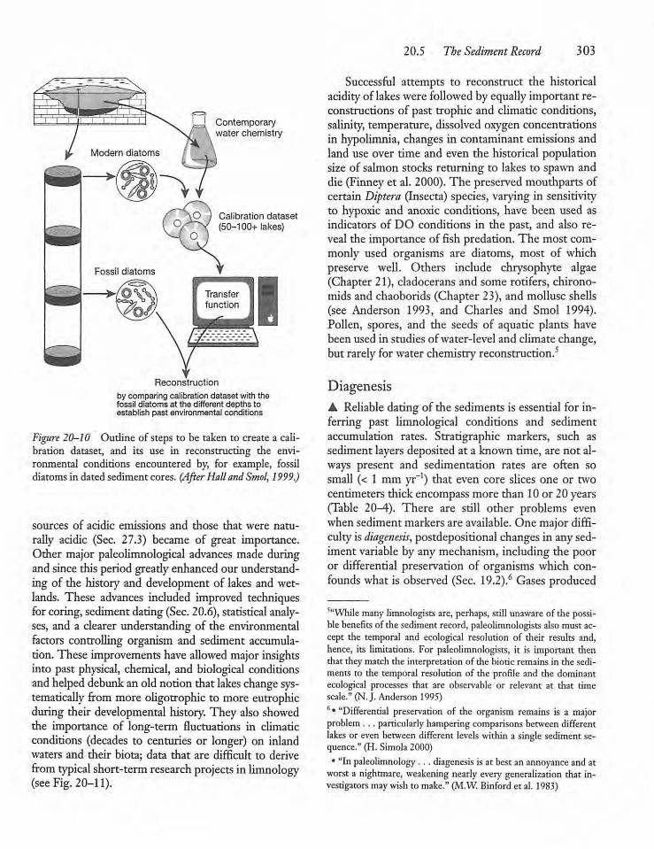
Contemporarywater chemistry
(D ) Calibration datasets^( (50-100+lakes)
Reconstruction
by comparing calibration dataset with thefossil diatoms at the different depths toestablish past environmental conditions
Figure 20-10 Oudine of steps to be taken to create a calibration dataset, and its use in reconstructing the environmental conditions encountered by, for example, fossildiatomsin dated sediment cores. (AfterHalland Smol, 1999.)
sources of acidic emissions and those that were naturally acidic (Sec. 27.3) became of great importance.Other major paleolimnological advances made duringand since this period gready enhanced our understanding of the history and developmentof lakes and wetlands. These advances included improved techniquesfor coring,sedimentdating (Sec. 20.6), statistical analyses, and a clearer understanding of the environmentalfactors controlling organism and sediment accumulation. These improvements have allowed major insightsinto past physical, chemical, and biological conditionsand helped debunk anoldnotion that lakes change systematically from more oUgotrophic to more eutrophicduring their developmental history. They also showedthe importance of long-term fluctuations in climaticconditions (decades to centuries or longer) on inlandwaters and their biota; data that are difficult to derivefrom typical short-term research projects in limnology(see Fig. 20-11).
20.5 The Sediment Record 303
Successful attempts to reconstruct the historicalacidityof lakeswere followed by equallyimportant reconstructions of past trophic and climatic conditions,salinity, temperature, dissolved oxygen concentrationsin hypolimnia, changes in contaminant emissions andland use over time and even the historical populationsize of salmon stocks returning to lakes to spawn anddie (Finney et al. 2000). The preserved mouthparts ofcertain Diptera (Insecta) species, varying in sensitivityto hypoxic and anoxic conditions, have been used asindicators of DO conditions in the past, and also reveal the importance of fish predation. The most commonly used organisms are diatoms, most of whichpreserve well. Others include chrysophyte algae(Chapter 21), cladocerans and some rotifers, chirono-mids and chaoborids (Chapter 23), and mollusc shells(see Anderson 1993, and Charles and Smol 1994).Pollen, spores, and the seeds of aquatic plants havebeen used in studies of water-level and climate change,butrarely for water chemistry reconstruction.5
Diagenesis• Reliable dating of the sediments is essential for inferring past limnological conditions and sedimentaccumulation rates. Stratigraphic markers, such assediment layers deposited at a known time, are not always present and sedimentation rates are often sosmall (< 1 mm yr-1) that even core slices one or twocentimeters thick encompass more than 10 or 20 years(Table 20-4). There are still other problems evenwhen sedimentmarkers are available. One major difficulty isdiagenesis, postdepositional changes in anysediment variable by anymechanism, including the pooror differential preservation of organisms which confounds what is observed (Sec. 19.2).6 Gases produced
5"While many limnologists are, perhaps, still unaware ofthe possiblebenefits ofthe sediment record, paleolimnologists also mustaccept the temporal and ecological resolution of their results and,hence, its limitations. For paleolimnologists, it is important thenthat they match the interpretation ofthe biotic remains in the sediments to the temporal resolution of the profile and the dominantecological processes that are observable or relevant at that timescale." (N.J. Anderson 1995)6• "Differential preservation of the organism remains is a majorproblem . . . particularly hampering comparisons between differentlakes or even between different levels within a single sediment sequence." (H. Simola 2000)• "In paleolimnology . . . diagenesis is at bestan annoyance andatworst a nightmare, weakening nearly every generalization that investigators may wish to make." (M.W. Binford et al. 1983)
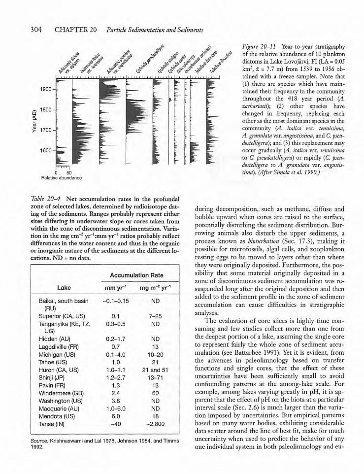
304 CHAPTER 20 Particle Sedimentation and Sediments
1900- =
1800--
> 1700-^
1600-a
50iabundance
Table 20-4 Net accumulation rates in the profundalzone of selected lakes, determined by radioisotope dating of the sediments. Ranges probably represent eithersites differing in underwater slope or cores taken fromwidiin the zone of discontinuous sedimentation. Variation in the mg cm-2 yr_I:mm yr-1 ratios probably reflectdifferences in the water content and thus in the organicor inorganic nature ofthe sediments at the different locations. ND = no data.
Lake
Accumulation Rate
mm yr1 mg m-2yr1
Baikal, south basin ~0.1-0.15 ND(RU)
Superior (CA, US) 0.1 7-25Tanganyika (KE, TZ, 0.3-0.5 NDUG)
Hidden (AU) 0.2-1.7 ND
Lagodiville (FR) 0.7 13
Michigan (US) 0.1-4.0 10-20Tahoe (US) 1.0 21
Huron (CA, US) 1.0-1.1 21 and 51Shinji (JP) 1.2-2.7 13-71
Pavin (FR) 1.3 13
Windermere (GB) 2.4 60Washington (US) 3.8 NDMacquarie (AU) 1.0-6.0 ND
Mendota (US) 6.0 18
Tansa (IN) -40 -2,800
Source: Krishnaswami and Lai 1978, Johnson 1984, and Timms1992.
Figure 20-11 Year-to-year stratigraphyofthe relative abundance of 10 planktondiatoms in Lake Lovojarvi, FI (LA=0.05km2, z = 7.7 m) from 1539 to 1956 obtained with a freeze sampler. Note that(1) there are species which have maintained their frequency in the communitythroughout the 418 year period (A.zachariasii); (2) other species havechanged in frequency, replacing eachother as the most dominant speciesin thecommunity {A. italica var. tenuissinia,A. granulata var.angustisshna, and C. pseu-dostelligera); and (3) this replacementmayoccur gradually (A. italica var. tenuissi?nato C.pseudostelligera) or rapidly (C. pseu-dostelligera to A. granulata var. angustisshna). (After Simola etal. 1990.)
during decomposition, such as methane, diffuse andbubble upward when cores are raised to the surface,potentially disturbing the sediment distribution. Burrowing animals also disturb the upper sediments, aprocess known as bioturbation (Sec. 17.3), making itpossible for microfossils, algal cells, and zooplanktonresting eggs to be moved to layers other than wherethey were originally deposited. Furthermore, the possibility that some material originally deposited in azone of discontinuous sediment accumulation was resuspended long after the original deposition and thenadded to the sediment profile in the zone of sedimentaccumulation can cause difficulties in stratigraphicanalyses.The evaluation of core slices is highly time con
suming and few studies collect more than one fromthe deepest portion of a lake,assumingthe singlecoreto represent fairly the whole zone of sediment accumulation (see Battarbee 1991). Yet it is evident, fromthe advances in paleolimnology based on transferfunctions and single cores, that the effect of theseuncertainties have been sufficiently small to avoidconfounding patterns at the among-lake scale. Forexample, among lakes varying greatly in pH, it is apparent diat the effectof pH on the biota at a particularinterval scale (Sec. 2.6) is much larger than the variation imposed by uncertainties. But empirical patternsbased on many water bodies, exhibiting considerabledata scatter around the line of best fit, make for muchuncertainty when used to predict the behavior of anyone individual system in both paleolimnology and eu-
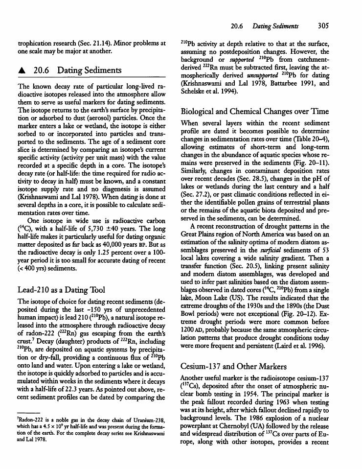
trophication research(Sec. 21.14). Minor problems atone scalemay be major at another.
A 20.6 Dating Sediments
The known decay rate of particular long-lived radioactive isotopes released into the atmosphere allowthem to serveas usefulmarkers for dating sediments.The isotopereturns to the earth'ssurfacebyprecipitation or adsorbed to dust (aerosol) particles. Once themarker enters a lake or wedand, the isotope is eithersorbed to or incorporated into particles and transported to the sediments. The age of a sediment coreslice is determined by comparing an isotope's currentspecific activity (activity per unit mass) with the valuerecorded at a specific depth in a core. The isotope'sdecay rate (or half-Ufe: the time required for radio activity to decay in half) must be known, and a constantisotope supply rate and no diagenesis is assumed(Krishnaswami andLai 1978).When dating is done atseveral depths in a core, it is possibleto calculatesedimentation rates over time.One isotope in wide use is radioactive carbon
(14C), with a half-life of 5,730 ±40 years. The longhalf-Ufe makes it particularly useful for datingorganicmatter deposited as far backas40,000yearsBP. But asthe radioactive decayis only 1.25percent over a 100-yearperiodit is too smallfor accurate datingof recent(<400yrs) sediments.
Lead-210 as aDatingToolThe isotopeof choicefor dating recent sediments(deposited during the last -150 yrs of unprecedentedhuman impact) islead 210 (210Pb), anatural isotope released into the atmosphere through radioactive decayof radon-222 (222Rn) gas escaping from the earth'scrust.7 Decay (daughter) products of222Rn, including210Pb, are deposited on aquatic systems by precipitation or dry-fall, providing a continuous flux of 210Pbonto landandwater. Upon enteringa lakeor wedand,theisotope isquickly adsorbed to particles andis accumulated within weeks in thesediments where it decayswitha half-Ufe of 22.3 years. As pointedout above, recentsediment profiles canbe dated bycomparing the
7Radon-222 is a noble gas in the decay chain of Uranium-238,which has a4.5 x 109 yrhalf-Ufe and was present during the formation of the earth. For the complete decay series see Krishnaswamiand Lai 1978.
20.6 Dating Sediments 305
210Pb activity at depth relative to that at the surface,assuming no postdeposition changes. However, thebackground or supported 210Pb from catchment-derived 222Rn mustbe subtracted first, leaving the at-mosphericaUy derived unsupported 2I0Pb for dating(Krishnaswami and Lai 1978, Battarbee 1991, andSchelskeetal. 1994).
Biological and Chemical Changes over TimeWhen several layers within the recent sedimentprofile are dated it becomes possible to determinechanges in sedimentation ratesover time (Table 20-4),allowing estimates of short-term and long-termchanges in the abundanceof aquaticspecies whoseremainswere preserved in the sediments (Fig. 20-11).Similarly, changes in contaminant deposition ratesover recent decades (Sec. 28.5), changes in the pH oflakes or wedands during the last century and a half(Sec. 27.2), or past climatic conditions reflected in either the identifiable pollen grains of terrestrial plantsor the remains ofthe aquaticbiota deposited and preserved in the sediments, can be determined.A recent reconstruction of drought patterns in the
GreatPlains region ofNorth America was based on anestimationofthe salinityoptima of modern diatom assemblages preserved in the surficial sediments of 53local lakes covering a wide salinity gradient. Then atransfer function (Sec. 20.5), linking present salinityand modern diatom assemblages, was developed andusedto inferpast salinities basedon the diatomassemblages observed indated cores (14C, 210Pb) from asinglelake, Moon Lake (US). The results indicated that dieextreme droughtsofthe 1930s and the 1890s (theDustBowl periods) were not exceptional (Fig. 20-12). Extreme drought periods were more common before1200 AD, probably because the same atmospheric circulation patterns that produce drought conditions todayweremore frequent and persistent(Lairdet al. 1996).
Cesium-137 and Other Markers
Anotheruseful marker is the radioisotope cesium-137(137Cs), deposited after the onset of atmospheric nuclear bomb testing in 1954. The principal marker isthe peak fallout recorded during 1963 when testingwas at itsheight, afterwhichfallout declined rapidly tobackground levels. The 1986 explosion of a nuclearpowerplant at Chernobyl(UA) foUowed by the releaseand widespread distribution of 137Cs over parts ofEurope, along with other isotopes, provides a recent
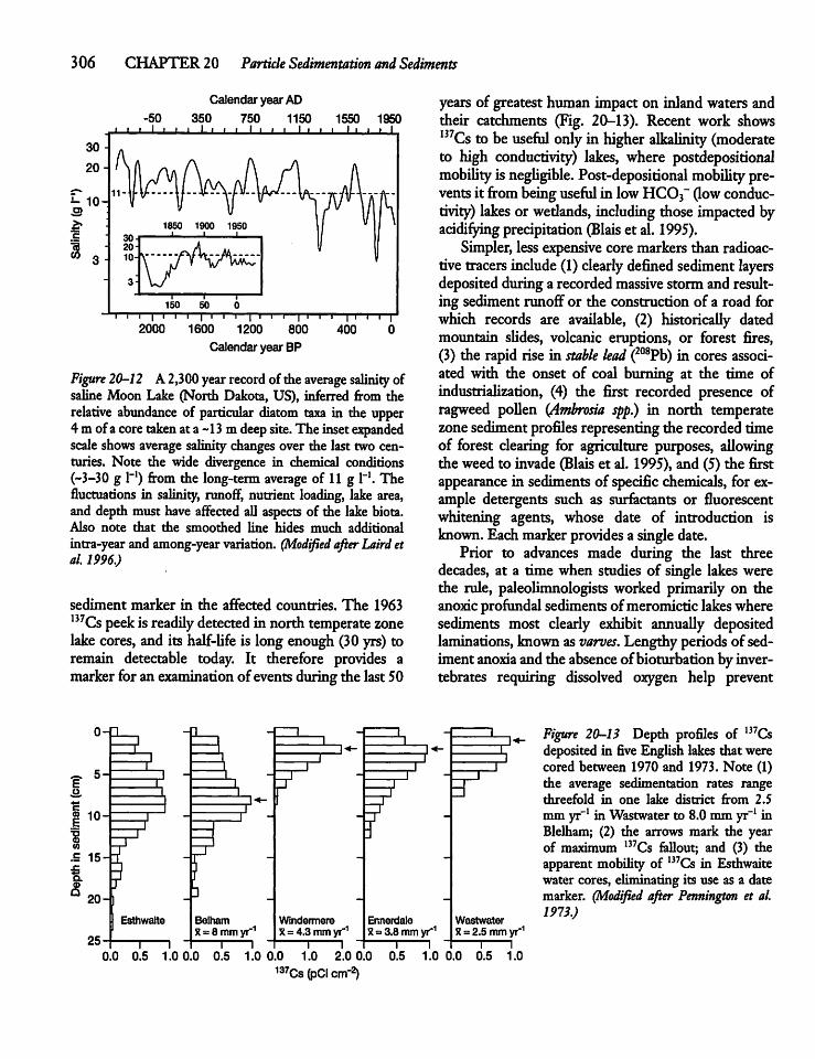
306 CHAPTER 20 Particle Sedimentation and Sediments
-50
Calendar year AD350 750 1150 1550 1950
i I i i i I i t i I i i i ' • • • Li_
' I ' ' i I '2000 1600 1200
Calendar year BP
Figure 20-12 A2,300 yearrecordof the average salinity ofsaline Moon Lake (North Dakota, US), inferred from therelative abundance of particular diatom taxa in the upper4mofa coretakenat a ~13 mdeepsite.The insetexpandedscale shows average salinity changes over the last twocenturies. Note the wide divergence in chemical conditions(~3—30 g l"1) from the long-term average of 11 g l"1. Thefluctuations in salinity, runoff, nutrient loading, lake area,and depth must have affected all aspects of the lakebiota.Also note that the smoothed line hides much additionalintra-year and among-year variation. (Modified after Laird etal. 1996.)
years of greatest human impact on inlandwaters andtheir catchments (Fig. 20-13). Recent work showsI37Cs to be useful only in higher alkalinity (moderateto high conductivity) lakes, where postdepositionalmobility is negligible. Post-depositional mobiUty preventsit frombeingusefulin lowHC03~ (lowconductivity) lakes or wedands, including those impacted byacidifying precipitation (Blais et al. 1995).Simpler, lessexpensive coremarkers than radioac
tive tracersinclude (1) clearly defined sedimentlayersdeposited duringa recorded massive stormand resulting sediment runoff or the construction of a road forwhich records are available, (2) historically datedmountain sUdes, volcanic eruptions, or forest fires,(3) the rapid rise in stable lead (208Pb) in cores associated with the onset of coal burning at the time ofindustrialization, (4) the first recorded presence ofragweed poUen (Ambrosia spp.) in north temperatezonesediment profiles representing the recorded timeof forest clearing for agriculture purposes, allowingthe weed to invade (Blaiset al. 1995), and (5) the firstappearance in sedimentsof specific chemicals, for example detergents such as surfactants or fluorescentwhitening agents, whose date of introduction isknown. Eachmarker providesa singledate.Prior to advances made during the last three
decades, at a time when studies of single lakes werethe rule, paleolimnologists worked primarily on theanoxic profundal sediments ofmeromictic lakeswheresediments most clearly exhibit annually depositedlaminations, knownas varves. Lengthy periods of sediment anoxia and the absenceof bioturbation by invertebrates requiring dissolved oxygen help prevent
sediment marker in the affected countries. The 1963137Cs peek isreadily detected innorth temperate zonelake cores, and its half-Ufe is long enough (30yrs) toremain detectable today. It therefore provides amarkerfor an examination of events duringthe last50
OH
t 5^
10-
£ 15-
f* 20-1
25
J -
Esthwaite Belhamx = 8 mmyr1
r
WindermereX=4.3 mm yr1
I II i
l"«- iI i
I II 3"
Wastwater5? = 2.5 mm y
r "i
—i
r •
Ermerdalex =3.8mmyr1
I I0.0 0.5 1.0 0.0 0.5 1.0 0.0 1.0 2.0 0.0
137Cs (pCi cm"2)0.5 1.0 0.0 0.5 1.0
Figure 20-13 Depth profiles of 137Csdeposited in five English lakes that werecored between 1970 and 1973. Note (1)the average sedimentation rates rangethreefold in one lake district from 2.5mmyr-1 inWastwater to 8.0mmyr-1 inBlelham; (2) the arrows mark the yearof maximum l37Cs fallout; and (3) theapparent mobility of 137Cs in Esthwaitewater cores, eliminating its use as a datemarker. (Modified after Pennington et al.1973.)
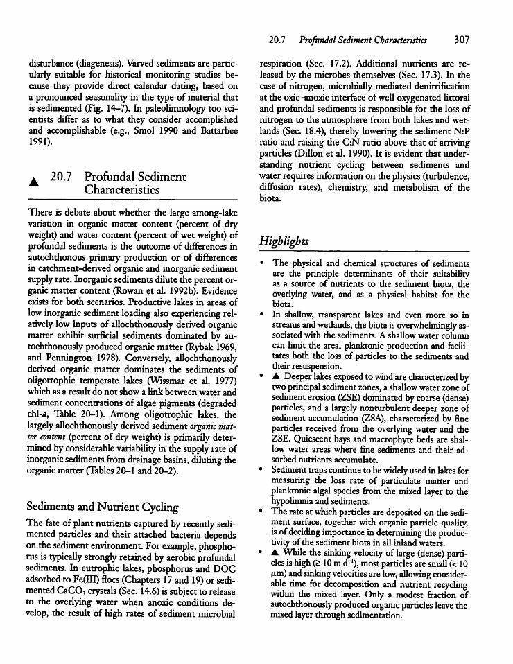
disturbance (diagenesis). Varved sediments are particularly suitable for historical monitoring studies because they provide direct calendar dating, based ona pronounced seasonality in the type of material thatis sedimented (Fig. 14-7). In paleolimnology too scientists differ as to what they consider accompUshedand accompUshable (e.g., Smol 1990 and Battarbee1991).
a 20.7 Profundal SedimentCharacteristics
There is debate aboutwhether the large among-lakevariation in organic matter content (percent of dryweight) and water content (percentof wetweight) ofprofundal sediments is the outcome of differences inautochthonous primary production or of differencesin catchment-derived organicand inorganic sedimentsupply rate.Inorganic sediments dilutethe percentorganic matter content (Rowan et al. 1992b). Evidenceexists for both scenarios. Productive lakes in areas oflow inorganic sediment loading also experiencing relatively low inputs of allochthonously derived organicmatter exhibit surficial sediments dominated by au-tochthonously produced organic matter (Rybak 1969,and Pennington 1978). Conversely, aUochthonouslyderived organic matter dominates the sediments ofoUgotrophic temperate lakes (Wissmar et al. 1977)which as a result do not show a link between water andsediment concentrations of algae pigments (degradedchl-tf, Table 20-1). Among oligotrophic lakes, thelargely aUochthonously derived sediment organic matter content (percent of dryweight) is primarily determined byconsiderable variabiUty in the supply rateofinorganic sediments from drainage basins, diluting theorganicmatter (Tables20-1 and 20-2).
Sediments and Nutrient CyclingThe fate of plantnutrients captured byrecendy sedimented particles and their attached bacteria dependsonthesediment environment Forexample, phosphorusis typicaUy strongly retained byaerobic profundalsediments. In eutrophic lakes, phosphorus and DOCadsorbed to Fe(HI) floes (Chapters 17and19) or sedimented CaC03 crystals (Sec. 14.6) issubject to releaseto the overlying water when anoxic conditions develop, the result of high rates of sediment microbial
20.7 Profundal Sediment Characteristics 307
respiration (Sec. 17.2). Additional nutrients are released by the microbes themselves (Sec. 17.3). In thecase of nitrogen, microbially mediated denitrificationat the oxic-anoxic interface ofweU oxygenated Uttoraland profundal sediments is responsible for the loss ofnitrogen to the atmosphere from both lakes and wetlands (Sec. 18.4), thereby lowering the sediment N:Pratio and raising the C:N ratio above that of arrivingparticles (DiUon et al. 1990). It is evident that understanding nutrient cycUng between sediments andwaterrequiresinformationon the physics (turbulence,diffusion rates), chemistry, and metaboUsm of thebiota.
Highlights• The physical and chemical structures of sedimentsare the principle determinants of their suitabiUtyas a source of nutrients to the sediment biota, theoverlying water, and as a physical habitat for thebiota.
• In shaUow, transparent lakes and even more so instreams andwedands, the biotaisoverwhelmingly associated with the sediments. A shaUow water columncan limit the areal planktonic production and faciU-tates both the loss of particles to the sediments andtheir resuspension.
• • Deeper lakes exposed towind arecharacterized bytwo principal sediment zones, a shaUow water zone ofsediment erosion (ZSE) dominated bycoarse (dense)particles, and a largely nonturbulent deeper zone ofsediment accumulation (ZSA), characterized by fineparticles received from the overlying water and theZSE. Quiescent bays and macrophyte beds are shallow water areas where fine sediments and their adsorbed nutrients accumulate.
• Sediment traps continue to bewidely used in lakes formeasuring the loss rate of particulate matter andplanktonic algal species from themixed layer to thehypolimnia and sediments.
• The rate atwhich particles are deposited on thesediment surface, together with organic particle quaUty,isofdeciding importance in determining theproductivityofthe sediment biota in aU inland waters.
• • While the sinking velocity of large (dense) particles ishigh (£10md"1), most particles aresmall (< 10|im)and sinkingvelocities arelow, aUowing considerable time for decomposition and nutrient recyclingwithin the mixed layer. Only a modest fraction ofautochthonously produced organic particles leave themixed layerthrough sedimentation.

308 CHAPTER 20 Particle Sedimentation and Sediments
A Avarietyof radioisotopes are avaUable for datingsediment cores, with 210Pb the isotope of choice fordatingsediments deposited duringthe last-150yearsofunprecedented humanimpact Simpler, less expensive core markers—providing only a single date—include the deposition of an identifiable sedimentlayer or a poUutant whose date of introduction isknown.
• PaleoUmnological advances duringrecent decadesaUow the sedimentfossil record to be quantified andinterpretedin terms of environmental variables suchaspH, total phosphorus, salinity, DOC, temperature,hydrology, and profundal dissolved oxygen concentration.
CHAPTER
21
The Phytoplankton
21.1 Introduction
The algae in the openwateroflakes andlarge rivers—die phytoplankton—are by far the best-studiedof aUbiotic groupings in inlandwaters and oceans. Tens ofthousands of papers have beenpubUshed on the physiological ecology and physiology of phytoplanktonspecies in the laboratory and field, the seasonal dynamics of individual species, and the apparent causesoftheirwaxing andwaning. The community structureand the productivity of phytoplankton assemblages inrelation to environmental factors andbiological interactions have also received a greatdealof attention. Anenormous amount is now known about phytoplankton, and for a modestnumber of species some broadgeneraUties are possible at the species level in nature.Yet, predictions at the species level are hampered bythe hundreds of species present in individual waters,mostofwhom have received Utde study, and the hostof possible interactions among them. Predictions arefurther hampered byinteractions between species andthechanging physical/ chemical environment, and byinteractions between the phytoplankton and theirtemporaUy and spatiaUy changing predators. Evenso,weU-studied temperate zone lakes tend to haveboth arecurring and characteristic assemblage of dominantspecies at particular times of the year. Such seasonalregularities continue to stimulate phytoplankton ecol-ogists to examine the mechanisms, processes, and environmental factors determining the composition ofthe communities observed (Fig. 21-1). However, theapparent regularity ofthe biomass cycle anddominant
species in individual systems is confounded in someyears bylarge shifts in bothcomposition andtiming ofbiomass peaks, providing a reminderofthe difficultiesthat must be surmounted before predictions can bemadeaboutindividual species.
AlgalClassificationThe phytoplankton community is composed ofseveralgroups of algae and one major group of photosynthetic bacteria, the cyanobacteria. The latter wereknown andclassified asthe Cyanophyta or blue-greenalgae byalgal systematists before it was widely appreciated that the group ismuchmore closely related tothe bacteria. But, since photosynthetic cyanobacteriafunctionaUy resemble the remaining phytoplanktongroups, theyare typicaUy discussed asa component ofthe phytoplanktonrather than ofthe true bacteria.The traditional classification of major groups of
aerobic (oxygenic) andphotosynthetic plants based onmorphology or pigmentation is increasingly givingway to one based on evolutionary (molecular-based)relationships.1 This began with the recognitionthat blue-green algae, Division Cyanophyta, belong tothe EmpireBacteria (Prokaryota) and not to the Empire Eukaryota. The prokaryotic cyanobacteria lack,
'The hierarchy of biological classification is basically as follows:Domain, Kingdom, Subkingdom, Phylum (animals andbacteria) orDivision (plants), Subdivision, Class, Order, Family, Genus, Species,Subspecies (variety).
309
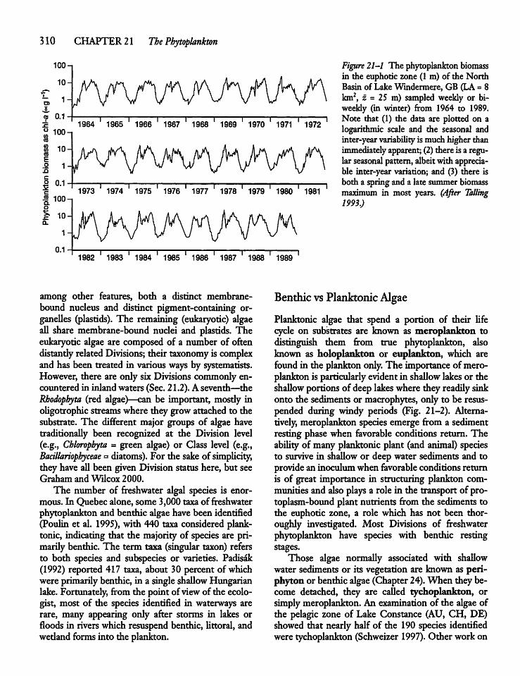
310 CHAPTER21 The Phytoplankton
100-1
x
2 °-1° 100wCO
8 10COE
! 1J 0.1I 100Q.o
j? 10Q.
1964 ' 1965 " 1966 T1967 1968 ' 1969 ' 1970 ' 1971 ' 1972
Figure 21-1 The phytoplankton biomassin the euphoric zone (1 m) of the NorthBasin of Lake Windermere, GB (LA = 8km2, z = 25 m) sampled weekly or biweekly (in winter) from 1964 to 1989.Note that (1) the data are plotted on alogarithmic scale and the seasonal andinter-year variabiUty is much higher thanimmediately apparent; (2)there is a regular seasonal pattern,albeitwithappreciable inter-year variation; and (3) there isboth a spring and a late summer biomassmaximum in most years. (After Tailing1993.)
1973 1974 1975 ' 1976 ' 1977 ' 1978 ' 1979 ' 1980 ' 1981
0.11982 ' 1983 T 1984 ' 1985 ' 1986 ' 1987 ' 1988 ' 1989 '
among other features, both a distinct membrane-bound nucleus and distinct pigment-containing or-ganeUes (plastids). The remaining (eukaryotic) algaeaU share membrane-bound nuclei and plastids. Theeukaryotic algae are composed of a number of oftendistandy related Divisions; their taxonomy is complexand has been treated in various ways by systematists.However, there are only sixDivisions commonly encountered in inland waters (Sec. 21.2). A seventh—theRhodophyta (red algae)—can be important, mosdy inoUgotrophic streamswhere they growattached to thesubstrate. The different major groups of algae havetraditionaUy been recognized at the Division level(e.g., Chlorophyta = green algae) or Class level (e.g.,Bacillariophyceae = diatoms). For the sakeof simpUcity,they haveall been givenDivision status here, but seeGraham and Wilcox 2000.The number of freshwater algal species is enor
mous. In Quebec alone, some 3,000 taxa of freshwaterphytoplankton and benthic algae have been identified(Poulin et al. 1995),with 440 taxa considered planktonic, indicating that the majority of species are primarily benthic. The term taxa (singular taxon) refersto both species and subspecies or varieties. Padisak(1992) reported 417 taxa, about 30 percent of whichwere primarilybenthic, in a singleshaUowHungarianlake. Fortunately, from the point of viewofthe ecolo-gist, most of the species identified in waterways arerare, many appearing only after storms in lakes orfloods in riverswhich resuspend benthic, Uttoral, andwedand forms into the plankton.
Benthicvs Planktonic Algae
Planktonic algae that spend a portion of their Ufecycle on substrates are known as meroplankton todistinguish them from true phytoplankton, alsoknown as holoplankton or euplankton, which arefound in the plankton only. The importance of meroplankton is particularlyevident in shaUow lakes or theshaUow portions of deep lakeswhere they readilysinkonto the sedimentsor macrophytes, only to be resuspended during windy periods (Fig. 21-2). Alternatively, meroplankton species emerge from a sedimentresting phase when favorable conditions return. TheabiUty of many planktonic plant (and animal) speciesto survive in shaUow or deep water sediments and toprovidean inoculumwhen favorable conditions returnis of great importance in stracturing plankton communitiesand alsoplays a role in the transport of protoplasm-bound plant nutrients from the sediments tothe euphoric zone, a role which has not been thoroughly investigated. Most Divisions of freshwaterphytoplankton have species with benthic restingstages.Those algae normally associated with shaUow
water sediments or its vegetation are known as peri-phyton or benthic algae (Chapter24).When they become detached, they are caUed tychoplankton, orsimplymeroplankton. An examination of the algaeofthe pelagic zone of Lake Constance (AU, CH, DE)showed that nearly half of the 190 species identifiedwere tychoplankton (Schweizer 1997). Other work on
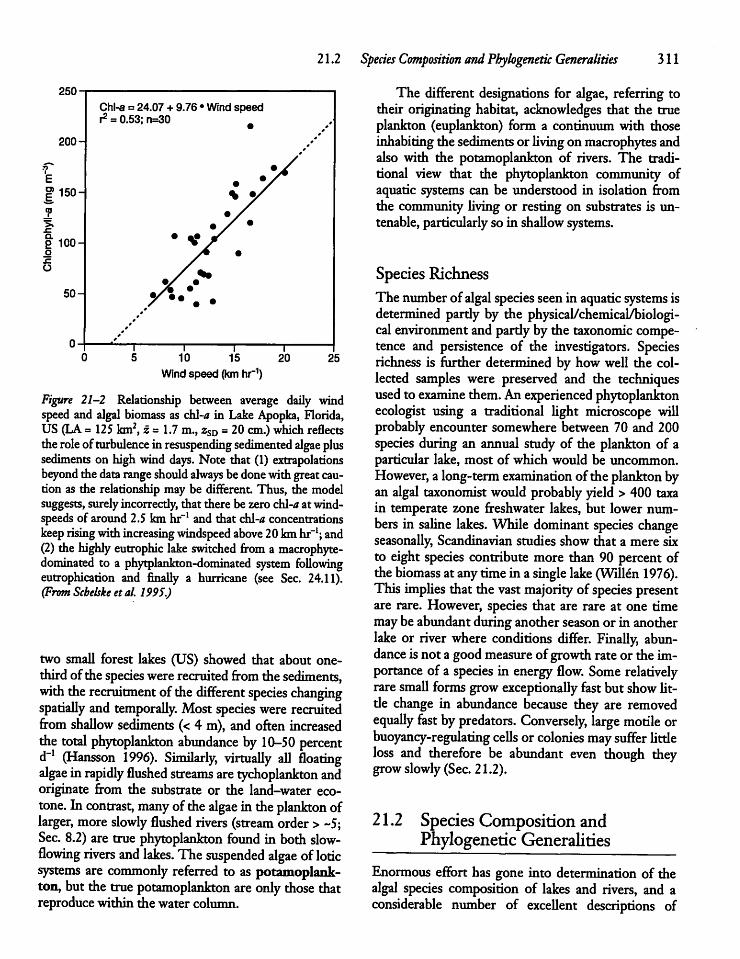
21.2 Species Composition andPhylogenetic Generalities 311
250
200-
E|» 150J>»SZ
S 100-oszO
50-
Chl-a = 24.07 + 9.76 • Wind speedr2= 0.53; n=30
10T15
Wind speed (km hr1)20 25
Figure 21-2 Relationship between average daily windspeed and algal biomass as chl-a in Lake Apopka, Florida,US (LA = 125 km2, z = 1.7 m.,ZsD =20cm.) which reflectstheroleofturbulence in resuspending sedimented algae plussediments on high wind days. Note that (1) extrapolationsbeyond the datarangeshould always bedonewithgreatcaution as the relationshipmay be different. Thus, the modelsuggests, surelyincorrecdy,that there be rero chl-tf at wind-speeds of around 2.5 km hr"1 and that chl-/? concentrationskeep risingwithincreasingwindspeed above 20kmhr-1; and(2) the highly eutrophic lake switched from a macrophyte-dominated to a phymlankton-dominated system foUowingeutrophication and finaUy a hurricane (see Sec. 24.11).(From Scbelske etal. 1995.)
two smaU forest lakes (US) showed that about one-thirdofthe species wererecruitedfromthe sediments,with therecruitment ofthe different species changingspatiaUy and temporaUy. Most species were recruitedfrom shaUow sediments (< 4 m), and often increasedthe total phytoplankton abundance by10-50 percentd"1 (Hansson 1996). Similarly, virtuaUy aU floatingalgae in rapidly flushed streams aretychoplankton andoriginate from the substrate or the land-water eco-tone. In contrast, many ofthe algae in theplankton oflarger, more slowly flushed rivers (stream order> ~5;Sec. 8.2) are true phytoplankton found in both slow-flowing rivers and lakes. The suspended algae ofloticsystems are commonly referred to as potamoplank-ton, butthe truepotamoplankton are only those thatreproduce within the water column.
The different designations for algae, referring totheir originating habitat, acknowledges that the trueplankton (euplankton) form a continuum with thoseinhabitingthe sedimentsor Uving on macrophytes andalso with the potamoplankton of rivers. The traditional view that the phytoplankton community ofaquatic systems can be understood in isolation fromthe community Uving or resting on substrates is untenable, particularly so in shaUow systems.
Species RichnessThe numberof algal species seenin aquatic systems isdetermined partly by the physical/chemical/biologicalenvironment and partlyby the taxonomic competence and persistence of the investigators. Speciesrichness is further determined by how weU the collected samples were preserved and the techniquesused to examine them.Anexperienced phytoplanktonecologist using a traditional Ught microscope wiUprobably encounter somewhere between 70 and 200species during an annual study of the plankton of aparticular lake, most of which would be uncommon.However, a long-term examination ofthe planktonbyan algal taxonomist would probablyyield > 400 taxain temperate zone freshwater lakes, but lower numbers in saUne lakes. While dominant species changeseasonally, Scandinavian studies show that a mere sixto eight species contribute more than 90 percent ofthe biomass at anytimein a single lake (Willen 1976).This impUes that the vastmajority of species presentare rare. However, species that are rare at one timemaybeabundantduringanotherseason or in anotherlake or river where conditions differ. FinaUy, abundance isnot a goodmeasure ofgrowth rateor the importance of a species in energy flow. Some relativelyraresmaU forms grow exceptionaUy fast but show Utde change in abundance because they are removedequaUy fast bypredators. Conversely, large motile orbuoyancy-regulating ceUs or colonies may suffer Utdeloss and therefore be abundant even though theygrowslowly (Sec. 21.2).
21.2 SpeciesComposition andPhylogenetic Generalities
Enormous effort has gone into determination of thealgal species composition of lakes and rivers, and aconsiderable number of exceUent descriptions of
312 CHAPTER21 The Phytoplankton
species distribution overtimein individual systems areavailable. Yet, the extensive and impressive amountofinformation collected over the last 80-100 years hasnot enabled the development of models able to predict,even roughly, the species composition of individual systems over time and space.2 The difficultiesencountered have long encouraged research on moreaggregated scales (Genus, Division), yielding the gen-eralities outlined below.However, these are too broadto be considered interesting(useful) research bymanylimnologists working at less aggregated scales. Whatat first glance might seem to be modest accomplishments is not attributableto a lackof thoughtful, high-quality research but rather to the large numbers ofspecies and the daily, seasonally, and spatially changingphysical, chemical, and biological environmentdetermininggrowthand lossratesin individual species. It isthe imbalance between the magnitude of the relativegrowth and loss rates of individual species which determinestheir contribution to the communitybiomassover time.While a priori predictionof species composition is
a goal, individual lakes exhibit sufficiendy large seasonal and interyear repetition in the abundance ofdominant species and genera (Fig. 21-1) to have encouraged the development of schemes describing typical seasonal or midsummer patterns for particularlake types. The among-lake patternsarenearlyalwaysdescribed as a function ofnutrient richness. However,growing recognition that the stability ofthe watercolumn exerts a major influence on the Ught climate experienced (Figs. 10-12and 12-5),and therebyon therelative growth rates and abundance of the differentspecies, has in recent years encouraged the development of promising schemes whichinclude watercolumn stability (Ught climate), nutrient richness, andflushing time (Reynolds 1997).
The Intermediate Disturbance HypothesisThe phytoplankton of any waterbody are composedof many species, indicating that interactions for resources are usuaUy insufficient to aUow large-scaleelimination through competitive exclusions. Thisshows that species are not in an equiUbrium {steadystate). It is clear that externaUy produced disturbances
2"The forces controlling species composition, diversity, dynamics,andstability of anecosystem remain one ofthe major mysteries ofmodern science." (D. Tilman 1996)
are sufficiendy common to interrupt or reverseprogress towards a steady state. Frequent disturbances exclude aU but a few rapidly growing pioneerspecies. Maximum diversityis therefore hypothesizedto be the result of intermediate levels of disturbance.The Intermediate Disturbance Hypothesis (IDH)ofJ. H. ConneU (1978) is an attempt to reconcile themore recent nonequilibrium view with the earUerequiUbriumviewbyarguingthat the observed organizational state of communities is the outcome ofprogress toward equiUbrium since the last disturbance. Figure 21-3 shows conceptuaUy how thetimescale of disturbanceexertsan impact on the communitystructure of differenttypes of lakes (Reynolds1993). When the timespan between disturbanceslengthens, a successional sequence of dominantspecies develops. The intermediate disturbance hypothesis is one of a series of conceptual schemes topredict and understand changes that have been observed at the species or genus level of phylogeneticorganization. A number of better quantified broadgeneralities have emerged at the Division level, themost aggregatedscaleof algal systematics.
Division Cyanophyta: cyanobacteria, ~1,350freshwater speciesLargecolonies, clusters of intertwined cells, or singlefilaments (Figs. 21-4 and 18-7) of cyanobacteria frequently dominate the algal biomass of nutrient-rich(high biomass) temperate lakes (Fig. 21-5) andslowlyflowing rivers in summer. They also dominate in icecovered polar lakes and polarmeltwater streams thatfreeze soUd in winter. At lower latitudes the largecyanobacteria may dominate slow-flowing rivers andlakes for much of the year, or evenyear-round (Fig.21-6).Moreover, the large cyanobacteria predominate
among the benthic algaeof hot springs and antarcticpools. In addition, tiny cyanobacteria (< 2 pm): (Sec.21.3) commonly dominate the algal biomass inoUgotrophic lakes, andyet other cyanobacteria dominate the algal biomass in poorly iUuminated metalim-nia. All this variation is a tribute to an extraordinarystructural and functional heterogeneity among thecyanobacteria. They are proof that many factors(light, nutrients, C02, pH, temperature, turbulence,competition, selective grazing by predators) determine the dominance of particular species in aU Divi-
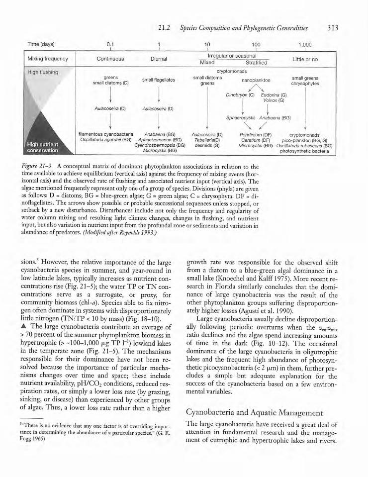
Time (days) 0.1
21.2 Species Composition and Phylogenetic Generalities
1 10 100 1,000
313
Mixing frequency
High flushing
Continuous
greenssmall diatoms (D)
Aulacoseira (D)
Diurnal
small flagellates
Aulacoseira (D)
Irregular or seasonalMixed Stratified
cryptomonadssmall diatoms
greensnanoplankton
Dinobryon (C) Eudorina (G)Volvox (G)
Little or no
small greenschrysophytes
Sphaerocystis Anabaena (BG)
High nutrientconservation
filamentous cyanobacteria Anabaena (BG)Oscillatoria agardhii (BG) Aphanizomenon (BG)
Cylindrospermopsis (BG)Microcystis (BG)
Aulacoseira (D)Tabellaria(D)desmids (G)
Peridinium (DF) cryptomonadsCeratium (DF) pico-plankton (BG, G)Microcystis (BG) Oscillatoria rubescens (BG)
photosynthetic bacteria
Figure 21-3 A conceptual matrix of dominant phytoplankton associations in relation to therime available toachieve equilibrium (vertical axis) against thefrequency ofmixing events (horizontal axis) and the observed rate of flushing and associated nutrientinput (vertical axis). Thealgae mentioned frequently represent only one ofagroup ofspecies. Divisions (phyla) are givenas follows: D =diatoms; BG=blue-green algae; G =green algae; C =chrysophyta; DF =di-noflagellates. The arrows show possible or probable successional sequences unless stopped, orsetback by a new disturbance. Disturbances include not only the frequency and regularity ofwater column mixing and resulting light climate changes, changes in flushing, and nutrientinput, but also variation in nutrient input from the profundal zone or sediments andvariation inabundance ofpredators. (Modified after Reynolds 1993.)
sions. However, the relative importance of the largecyanobacteria species in summer, and year-round inlow latitude lakes, typically increases as nutrient concentrations rise (Fig. 21-5); the water TP or TN concentrations serve as a surrogate, or proxy, forcommunity biomass (chW/). Species able to fix nitrogen often dominate insystems with disproportionatelylittle nitrogen (TN:TP < 10 bymass) (Fig. 18-10).• The large cyanobacteria contribute an average of>70percentof the summerphytoplankton biomass inhypertrophic (> -100-1,000 p,g TP V) lowland lakesin the temperate zone (Fig. 21-5). The mechanismsresponsible for their dominance have not been resolved because the importance of particular mechanisms changes over time and space; these includenutrient availability, pH/C02 conditions, reduced respiration rates, or simply a lower loss rate (by grazing,sinking, or disease) than experienced by other groupsofalgae. Thus, a lower loss rate rather than a higher
'"There is no evidence that any one factor is of overriding importance indetermining die abundance ofa particular species." (G. E.Fogg 1965)
growth rate was responsible for the observed shiftfrom a diatom to a blue-green algal dominance in asmall lake (Knoechel and Kalff 1975).More recent research in Florida similarly concludes that the dominance of large cyanobacteria was the result of theother phytoplankton groups suffering disproportionatelyhigher losses (Agustf et al. 1990).Large cyanobacteria usually decline disproportion-
ally following periodic overturns when the z^a^ratio declines and die algae spend increasing amountsof time in the dark (Fig. 10-12). The occasionaldominance of the large cyanobacteria in oligotrophiclakes and the frequent high abundance of photosynthetic picocyanobacteria (< 2 |xm) in them, further precludes a simple but adequate explanation for thesuccess of the cyanobacteria based on a few environmental variables.
Cyanobacteria andAquatic ManagementThe large cyanobacteria have received a great deal ofattention in fundamental research and the management of eutrophic and hypertrophic lakes and rivers.
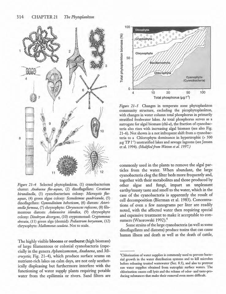
314 CHAPTER 21 The Phytoplankton
Figure 21-4 Selected phytoplankton. (1) cyanobacteriumcluster: Anabaena flos-aquae, (2) dinoflagellate: Ceratiumhirundinella, (3) cyanobacterium colony: Microcystis flos-aquae, (4) green algae colony: Scenedesmus quadricauda, (5)dinoflagellate: Gymnodinium helveticum, (6) diatom: Asteri-onellafonnosa, (7) chrysophyte: Cbrysococcus nifescens, (8) filamentous diatom: Aulacoseira islandica, (9) chrysophytecolony: Dinobiyon divergens, (10) cryptomonad: Ciyptomonasobovata, (11) green alga (desmid): Pediastrum boiyanum, (12)chrysophyte: Mallomonas caudata. Not to scale.
The highly visible blooms or outburst (high biomass)of large filamentous or colonial cyanobacteria (especially in die genera Aphanizomenon, Anabaena, andMicrocystis; Fig. 21-4), which produce surface scums onnutrient-rich lakes on calmdays, are not only aesthetically displeasing but furthermore interfere with thefunctioning of water supply plants requiring potablewater from the epilimnia or rivers. Sand filters are
100
%Eo!oco
cra
D-o
50-
10 20 50
Totalphosphorus (ug I"1)
Figure 21-5 Changes in temperate zone phytoplanktoncommunity structure, excluding the picophytoplankton,with changes inwater column total phosphorus in primarilystratified freshwater lakes. As total phosphorus serves as asurrogate for algal biomass (chl-a), thefraction ofcyanobacteria also rises with increasing algal biomass (see also Fig.21-6).Not shown is a not infrequentshift froma cyanobacteria to a Chlorophyta dominance in hypertrophic (> 500u,gTP I"1) unstratified lakes and sewage lagoons (see Jensenetal. 1994). (Modifiedfiv?n Watson etal. 1997.)
commonly used in the plants to remove the algal particles from the water. When abundant, the largecyanobacteria clog thefilter beds more frequently and,together with their metabolites and those produced byother algae and fungi, impart an unpleasantearthy/musty taste and smell to thewater, which in thecase of the cyanobacteria is apparently the result ofcell decomposition (Bierman et al. 1983). Concentrations of even a few nanograms per liter are readilynoted, with the affected water then requiring specialand expensive treatment tomake it acceptable to consumers (Wnorowski 1992).4
Some strains ofthe large cyanobacteria (as well as somedinoflagellates and diatoms) produce toxins thatcan causehuman illness and death as well as the death of cattle,
4Chlorination ofwater supplies is commonly used to prevent bacterial growdi in die water distribution systems and to kill microbesbefore releasing treated wastewater (Sec. 8.5), and also to pretreatraw water supplies obtained from eutrophic surface waters. Thechlorination causes cell lysis and the release of odor- and taste-producing substances diatmake dieirremoval even more difficult.
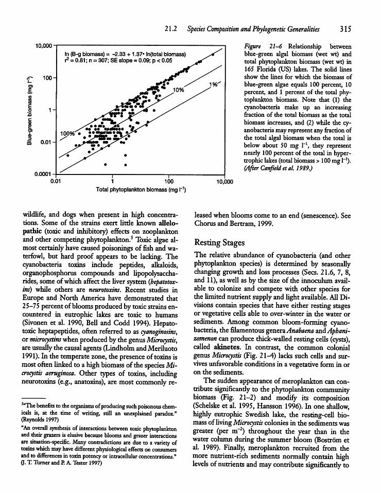
21.2 Species Composition and Phylogenetic Generalities 315
10,000
^ 100HD)E
|ne
£
S 0.01 -
0.00010.01
In (B-g biomass) = -2.33 + 1.37* ln(total biomass)r2 = 0.81;n = 307;SEslope = 0.09; p < 0.05
1 100
Totalphytoplankton biomass (mg I"1)
wildlife, and dogs when present in high concentrations. Some of the strains exert Utde known allelo-pathic (toxic and inhibitory) effects on zooplanktonand other competing phytoplankton.5 Toxic algae almostcertainly have caused poisonings of fish andwaterfowl, but hard proof appears to be lacking. Thecyanobacteria toxins include peptides, alkaloids,organophosphorus compounds and lipopolysaccha-rides, some ofwhich affect the liversystem (hepatotox-ins) while others are neurotoxins. Recent studies inEurope and North America have demonstrated that25-75percentofblooms produced bytoxic strains encountered in eutrophic lakes are toxic to humans(Sivonen et al. 1990, Bell and Codd 1994). Hepato-toxic heptapeptides, often referred to as cyanoginosins,ormicrocystinswhen produced bythegenusMicrocystis,areusually the causal agents (Lindholm andMeriluoto1991). In the temperate zone, the presence of toxins ismost often linked toahigh biomass ofthe speciesMicrocystis aeruginosa. Other types of toxins, includingneurotoxins (e.g., anatoxins), are most commonly re-
5aThe benefits to the organisms ofproducing such poisonous chemicals is, at the time of writing, still an unexplained paradox."(Reynolds 1997)"An overall synthesis of interactions between toxic phytoplanktonand their grazers iselusive because blooms and grazer interactionsare situation-specific. Many contradictions are due to a variety oftoxins which may have different physiological effects onconsumersandto differences in toxin potency or intracellular concentrations."Q.T.Turner and P.A.Tester 1997)
10,000
Figure 21-6 Relationship betweenblue-green algal biomass (wet wt) andtotal phytoplankton biomass (wet wt) in165 Florida (US) lakes. The solid linesshow the lines for which the biomass ofblue-green algae equals 100 percent, 10percent, and 1 percent of the total phytoplankton biomass. Note that (1) thecyanobacteria make up an increasingfraction of the total biomass as the totalbiomass increases, and (2)while the cyanobacteria mayrepresentanyfraction ofthe total algal biomass when the total isbelow about 50 mg I"1, they representnearly 100 percent of the total in hypertrophiclakes (totalbiomass > 100 mgl"1).(After Canfield etal. 1989.)
leased whenblooms come to an end (senescence). SeeChorus and Bertram, 1999.
Resting StagesThe relative abundance of cyanobacteria (and otherphytoplankton species) is determined by seasonallychanging growth and loss processes (Sees. 21.6, 7, 8,and 11), aswellas by the sizeofthe innoculumavailable to colonize and compete with other species forthe limited nutrientsupply andlightavailable. All Divisions contain species that have either resting stagesor vegetative cells able to over-winter in the water orsediments. Among common bloom-forming cyanobacteria, the filamentous generaAnabaena andAphanizomenon canproduce thick-walled resting cells (cysts),called akinetes. In contrast, the common colonialgenus Microcystis (Fig. 21-4) lacks such cells and survives unfavorable conditions in avegetative form in oron the sediments.The sudden appearance ofmeroplankton can con
tribute significantly to thephytoplankton communitybiomass (Fig. 21-2) and modify its composition(Schelske et al. 1995, Hansson 1996). In oneshallow,highly eutrophic Swedish lake, the resting-cell biomass of livingMicrocystis colonies in the sediments wasgreater (per m~2) throughout the year than in thewatercolumn during the summerbloom(Bostrom etal. 1989). Finally, meroplankton recruited from themore nutrient-rich sediments normally contain highlevels ofnutrients and may contribute significantiy to
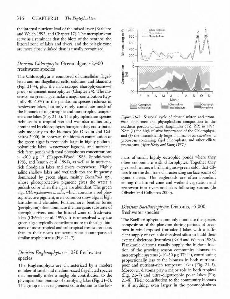
316 CHAPTER 21 The Phytoplankton
the internal nutrient load of the mixed layer (Barbieroand Welch 1992, and Chapter 17).The meroplanktonserve as a reminder that the biota of the benthos, thelittoral zone of lakes and rivers, and the pelagic zoneare more closely linkeddian is usually recognized.
Division Chlorophyta: Green algae, -2,400freshwater speciesThe Chlorophyta is composed of unicellular flagellated and nonflagellated cells, colonies, and filaments(Fig. 21-4), plus the macroscopic charophyceans—agroup of ancient macrophytes (Chapter 24). The microscopic green algaemakea major contribution (typically 40-60%) to the planktonic species richness infreshwater lakes, but only rarely contribute much ofthe biomass of oligotrophic and mesotrophic temperate zone lakes (Fig. 21-5). The phytoplankton speciesrichness in a tropical wedand was also numericallydominated bychlorophytes but again theycontributedonly modesdy to the biomass (de Oliveira and Cal-heiros 2000). In contrast, the biomass contribution ofthe green algae is frequently large in highly pollutedpolymictic lakes, wastewater lagoons, and nutrient-rich farm ponds with total phosphorus concentrations> -500 (jug 1_I (Happey-Wood 1988, Spodniewska1983, and Jensen et al. 1994), as well as in nutrient-rich floodplain lakes and rivers everywhere. Highlysaline shallow lakes and wedands too are frequentlydominated by green algae, mainly Dunaliella spp.,whose photoprotective pigment gives the water apinkish colorwhen the algae are abundant. The greenalga Chlamydomonas nivalis, whichcontains a red photoprotectivepigment, are a common snowalga at highlatitudes and altitudes. Furdiermore, benthic forms(periphyton) often dominate the inorganic substrate ofeutrophic rivers and the littoral zone of freshwaterlakes (Chetelat et al. 1999). It is unresolved why thegreenalgae typically contributemore to the algal biomass of most tropical and subtropical freshwater lakesthan to their north temperate zone counterparts ofsimilar trophic status (Fig. 21-7).
Division Euglenopbyta: -1,020 freshwaterspeciesThe Euglenophyta are characterized by a modestnumber of small and medium-sized flagellated speciesthat normally make a negligible contribution to thephytoplankton biomass of stratifying lakes (Fig. 21-5).The group makes its greatest contribution to the bio-
1,000-1
800-
600-
400-
200-
0-T
50-
100
Other protozoaSlrombidiumPhyloplonkton
CyanophytaChlorophyta
J JMonth
IChrysophytaIBacillariophyta
ICryplophytaIPyrrophyta
Figure 21-7 Seasonal cycle of phytoplankton and protozoan abundance and phytoplankton composition in dienorthern portion of Lake Tanganyika (TZ, ZR) in 1975.Note (1) the high relative importance of the Chlorophyta,and (2) die intermittently large biomass of Strombidium, aprotozoan containing algal chloroplasts, and other ciliateprotozoans. (After Hecky andKling 1987.)
mass of small, highly eutrophic ponds where theyoften codominate with chlorophytes. Together theygive such waters a brilliant grass-green color that differs from the dull tone characterizing surface scums ofcyanobacteria. The euglenoids are often abundantamong the littoral zone and wedand vegetation andare swept into rivers and lakes following storms (deOliveira and Calheiros 2000).
Division Bacillariophyta: Diatoms, -5,000freshwater speciesThe Bacillariophyta commonly dominate the speciescomposition of the plankton during periods of overturn in wind-exposed (turbulent) lakes with a sufficientsupply of available dissolved silica to build theirexternal skeletons (frustules) (Kalff and Watson 1986).Planktonic diatoms usually supply the highest fraction of the growing season community biomass inmesotrophic systems (-10-30 p-gTP I"1), contributingproportionally less to the biomass in both nutrient-poor and nutrient-rich temperate lakes (Fig. 21-5).Moreover, diatoms play a major role in both tropical(Fig. 21-7) and ultra-oligotrophic polar lakes (Fig.21-8). Their contribution to the community biomassis, if anything, even larger in the potamoplankton
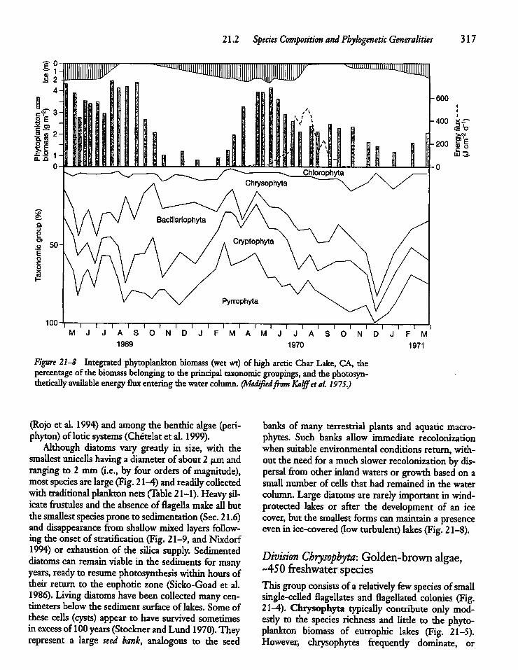
21.2 Species Composition and Phylogenetic Generalities 317
-s-o
Figure 21-8 Integrated phytoplankton biomass (wet wt) of high arctic Char Lake, CA, thepercentage ofthe biomass belonging to theprincipal taxonomic groupings, and thephotosyn-thetically available energy flux entering thewater column. (Modifiedfrom Kalffet al. 1915.)
(Rojo et al. 1994) and among the benthic algae (periphyton)of loticsystems (Chetelatet al. 1999).Although diatoms vary gready in size, with the
smallest unicells having a diameterof about2 pin andranging to 2 mm (i.e., by four orders of magnitude),mostspecies arelarge (Fig. 21-4)andreadily collectedwith traditional plankton nets (Table 21-1). Heavy silicate frustules and the absence of flagella make all butthesmallest species prone to sedimentation (Sec. 21.6)anddisappearance from shallow mixed layers following the onsetof stratification (Fig. 21-9, andNixdorf1994) or exhaustion of the silica supply. Sedimenteddiatoms can remain viable in the sediments for manyyears, readyto resume photosynthesis withinhoursoftheir return to the euphoric zone (Sicko-Goad et al.1986). Living diatoms have beencollected many centimeters below the sediment surface of lakes. Some ofthese cells (cysts) appear to have survived sometimesinexcess of100 years (Stockner and Lund 1970). Theyrepresent a large seed bank, analogous to the seed
banks of many terrestrial plants and aquatic macrophytes. Such banks allow immediate recolonizationwhensuitable environmental conditions return, withouttheneed for amuch slower recolonization by dispersal from other inland waters or growth based on asmall number of cells that had remained in the watercolumn. Large diatoms are rarely important in wind-protected lakes or after the development of an icecover, but the smallest forms can maintain a presenceeven in ice-covered (low turbulent)lakes (Fig. 21-8).
Division Chrysophyta: Golden-brown algae,~450 freshwater speciesThisgroup consists ofa relatively few species ofsmallsingle-celled flagellates and flagellated colonies (Fig.21-4). Chrysophyta typically contribute only mod-esdy to the species richness and Utde to the phytoplankton biomass of eutrophic lakes (Fig. 21-5).However, chrysophytes frequendy dominate, or
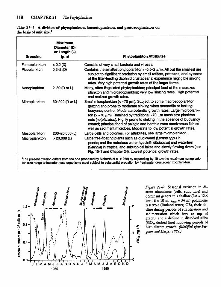
318 CHAPTER 21 The Phytoplankton
Table 21-1 A division of phytoplankton, bacterioplankton, and protozooplankton onthe basis ofunit size.1
Grouping
MaximumDiameter (D)or Length (L)
(jim)
Femtoplankton < 0.2 (D)Picoplankton 0.2-2 (D)
Nanoplankton 2-30 (Dor L)
Microplankton 30-200 (Dor L)
Mesoplankton 200-20,000 (L)Macroplankton > 20,000 (L)
Phytoplankton Attributes
Consists of very small bacteria and viruses.Contains the smallest phytoplankton (-0.5-2 fim). All but the smallest aresubject to significant predation by small rotifers, protozoa, and by someof the filter-feedingdaphnid crustaceans; experience negligible sinkingrates. Very high potential growth rates of the larger forms.
Many, often flagellated phytoplankton; principal food of the macrozooplankton and microzooplankton; very low sinking rates. High potentialand realized growth rates.
Small microplankton (< -70 u,m). Subject to some macrozooplanktongrazing and prone to moderate sinking when nonmotile or lackingbuoyancy control. Moderate potential growth rates. Large microplankton (> -70 u.m). Retained by traditional -70 u.mmesh size planktonnets (netplankton). Highlyprone to sinking in the absence of buoyancycontrol; principal food of pelagic and benthic zone omnivorous fish aswell as sediment microbes. Moderate to low potential growth rates.
Large cells and colonies. For attributes, see large microplankton.Large free-floating plants such as duckweed {Lemna spp.) inponds; and the notorious water hyacinth (Eichornia) and waterfern(Salvinia) in tropical and subtropical lakes and slowlyflowingrivers (seeFig. 15-1 and Chapter 24). Lowest potential growth rates.
1The presentdivision differs from the one proposedbySieburth et al. (1978) byexpanding by10 fimthe maximum nanoplankton size range to includethose organismsmost subject to substantialpredationbyfreshwatercrustacean zooplankton.
1979
I I 1 I l l l i IMAMJ JASOND
1980
Figure 21-9 Seasonal variation in diatom abundance (cells, solid line) anddominant genera in a shallow (LA =12.6km2, z = 10 m, z^ = 34 m) polymicticreservoir (Rudand water, GB), their declineduringperiods of stratification andsedimentation (thick bars at top ofgraph), and a decline in dissolved silica(Si03, dashed line) following periods ofhigh diatom growth. (Modified after Ferguson andHarper 1982.)
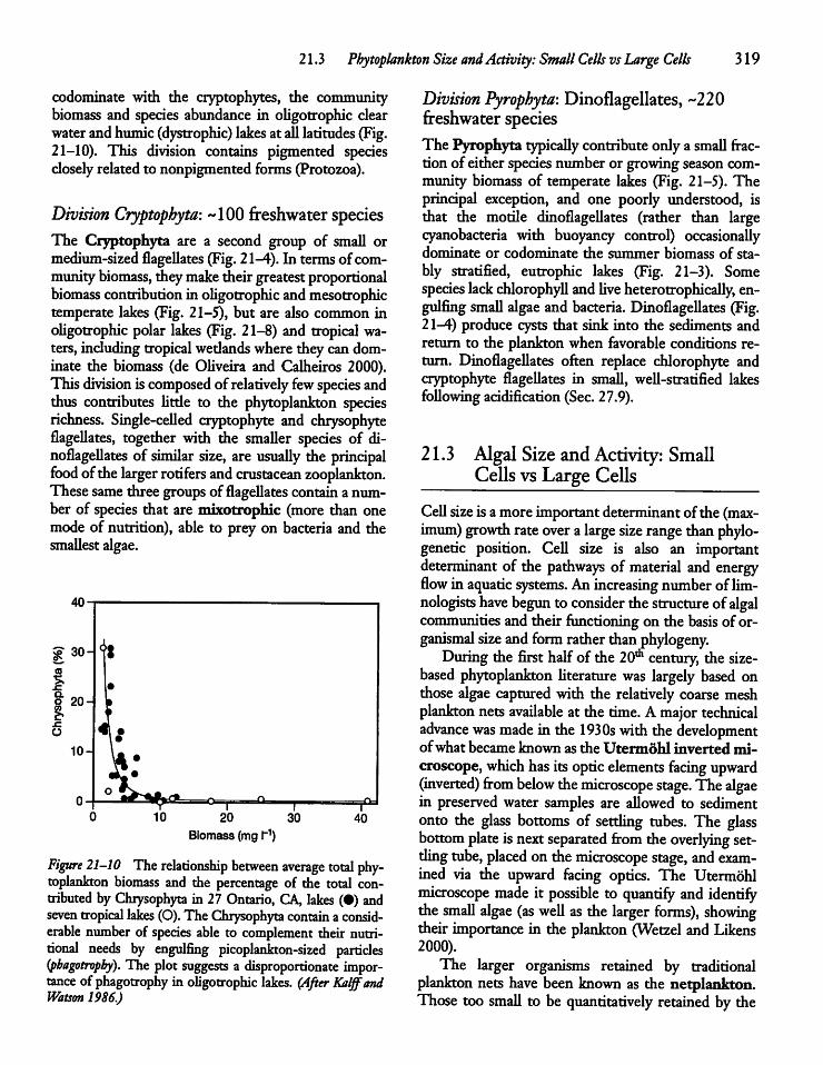
21.3 Phytoplankton SizeandActivity: SmallCells vsLarge Cells 319
codominate with the cryptophytes, the communitybiomass and species abundance in oligotrophic clearwaterandhumic (dystrophic) lakes at alllatitudes (Fig.21-10). This division contains pigmented speciesclosely related to nonpigmented forms (Protozoa).
Division Cryptophyta: -100 freshwater speciesThe Cryptophyta are a second group of small ormedium-sized flagellates (Fig. 21-4). In termsof communitybiomass, theymaketheir greatestproportionalbiomass contributionin oligotrophicandmesotrophictemperate lakes (Fig. 21-5), but are also common inoligotrophic polar lakes (Fig. 21-8) and tropical waters, including tropicalwedandswhere they candominate the biomass (de Oliveira and Calheiros 2000).This division is composed of relatively few species andthus contributes little to the phytoplankton speciesrichness. Single-celled cryptophyte and chrysophyteflagellates, together with the smaller species of dinoflagellates of similar size, are usually the principalfood ofthe larger rotifers andcrustacean zooplankton.These same three groups of flagellates contain anumber of species that are auxotrophic (more than onemode of nutrition), able to prey on bacteria and thesmallest algae.
10 20 30
Biomass(mgl~1)
Figure 21-10 Therelationship between average total phytoplankton biomass and the percentage of the total contributed byChrysophyta in 27 Ontario, CA, lakes (•) andseven tropical lakes (O). The Chrysophyta contain a considerable number of species able to complement their nutritional needs by engulfing picoplankton-sized particles(pbagotropby). The plot suggests a disproportionate importance ofphagotrophy in oligotrophic lakes. (After KalffandWatson 1986.)
Division Pyrophyta: Dinoflagellates, -220freshwater speciesThe Pyrophyta typically contribute only a smallfraction of either species number or growingseasoncommunity biomass of temperate lakes (Fig. 21-5). Theprincipal exception, and one poorly understood, isthat the motile dinoflagellates (rather than largecyanobacteria with buoyancy control) occasionallydominate or codominate the summer biomass of stably stratified, eutrophic lakes (Fig. 21-3). Somespecies lackchlorophyll and five heterotrophically, engulfing small algae and bacteria. Dinoflagellates (Fig.21-4) produce cysts that sink into the sediments andreturn to the plankton when favorable conditions return. Dinoflagellates often replace chlorophyte andcryptophyte flagellates in small, well-stratified lakesfollowing acidification (Sec. 27.9).
21.3 AlgalSize andActivity: SmallCellsvs Large Cells
Cellsizeis a more important determinantofthe (maximum) growth rate overa large size range thanphylogenetic position. Cell size is also an importantdeterminant of the pathways of material and energyflow in aquatic systems. Anincreasing number oflimnologists have begun to consider thestructure ofalgalcommunities and their functioning on the basis of or-ganismal size and form ratherthanphylogeny.During the first half of the 20th century, the size-
based phytoplankton literature was largely based onthose algae captured with the relatively coarse meshplankton nets available at the time. Amajor technicaladvance was made in the 1930s with the developmentofwhat became known as theUtermohl inverted microscope, which hasits optic elements facing upward(inverted) from below themicroscope stage. The algaein preserved water samples are allowed to sedimentonto the glass bottoms of settling tubes. The glassbottom plate isnext separated from theoverlying settling tube, placed on themicroscope stage, and examined via the upward facing optics. The Utermohlmicroscope made it possible to quantify and identifythe small algae (as well as the larger forms), showingtheir importance in the plankton (Wetzel andLikens2000).The larger organisms retained by traditional
plankton nets have been known as the netplankton.Those too small to be quantitatively retained by the
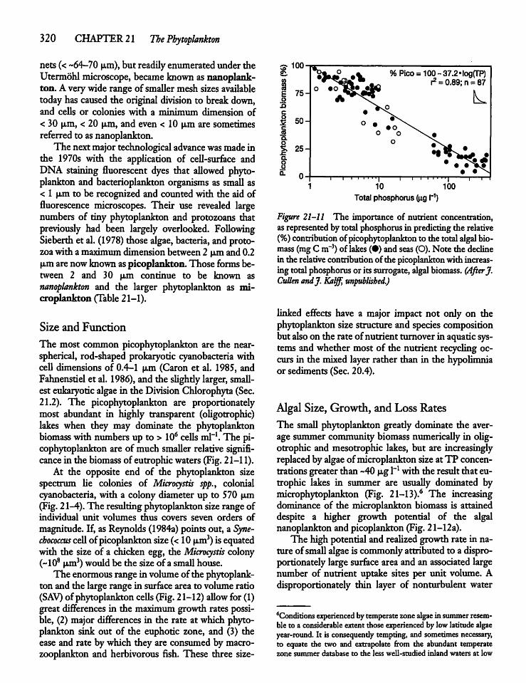
320 CHAPTER 21 The Phytoplankton
nets (<~64-70 u,m), but readilyenumeratedunder theUtermohl microscope, became known asnanoplank-ton. Averywiderange of smallermeshsizes availabletodayhas caused the original division to break down,and cells or colonies with a minimum dimension of< 30 p,m, < 20 u,m, and even < 10 p,mare sometimesreferred to asnanoplankton.The nextmajortechnological advance was made in
the 1970s with the application of cell-surface andDNA staining fluorescent dyes that allowed phytoplankton and bacterioplankton organisms as small as< 1 p,m to be recognizedand counted with the aid offluorescence microscopes. Their use revealed largenumbers of tiny phytoplankton and protozoans thatpreviously had been largely overlooked. FollowingSieberth et al. (1978) thosealgae, bacteria, andprotozoawith amaximumdimensionbetween2 p,mand 0.2p,m arenowknown aspicoplankton. Those forms between 2 and 30 p,m continue to be known asnanoplankton and the larger phytoplankton as microplankton (Table 21-1).
Size and Function
The most common picophytoplankton are the near-spherical, rod-shaped prokaryotic cyanobacteria withcell dimensions of 0.4-1 pin (Caron et al. 1985, andFahnenstiel et al. 1986), and the slighdylarger, smallest eukaryotic algae in the Division Chlorophyta (Sec.21.2). The picophytoplankton are proportionatelymost abundant in highly transparent (oUgotrophic)lakes when they may dominate the phytoplanktonbiomass withnumbers up to > 106 cells ml"1. The picophytoplankton are of much smaller relative significancein the biomass of eutrophicwaters(Fig. 21-11).At the opposite end of the phytoplankton size
spectrum lie colonies of Microcystis spp., colonialcyanobacteria, with a colony diameter up to 570 u,m(Fig.21-4). The resultingphytoplanktonsizerangeofindividual unit volumes thus covers seven orders ofmagnitude. If, as Reynolds (1984a) points out, a Syne-chococcus cell ofpicoplankton size (< 10u,m3) isequatedwith the size of a chicken egg, the Microcystis colony(~108 p-m3) wouldbe the sizeof a smallhouse.The enormous range in volumeofthe phytoplank
ton and the large range in surface area to volumeratio(SAV) of phytoplankton cells(Fig. 21-12) allowfor (1)great differences in the maximum growth rates possible, (2) major differences in the rate at which phytoplankton sink out of the euphoric zone, and (3) theease and rate by which they are consumed by macrozooplankton and herbivorous fish. These three size-
,c % Pico =100-37.2Mog(TP)• ^ =0.89:11 =87
100
Total phosphorus (ug l~1)
Figure 21-11 The importance of nutrient concentration,as represented by total phosphorus in predictingthe relative(%)contribution ofpicophytoplankton to the totalalgal biomass (mg Cm"3) of lakes (•) andseas (O). Note the declinein the relativecontribution ofthe picoplanktonwith increasing totalphosphorus or its surrogate,algal biomass. (AfterJ.Cullen andJ. Kalff, unpublished.)
linked effects have a major impact not only on thephytoplankton size structureand species compositionbut alsoon the rate ofnutrient turnover in aquaticsystems and whether most of the nutrient recycling occurs in the mixed layer rather than in the hypolimniaor sediments (Sec. 20.4).
AlgalSize, Growth, and Loss RatesThe small phytoplankton gready dominate the average summer community biomassnumerically in oligotrophic and mesotrophic lakes, but are increasinglyreplaced byalgae ofmicroplankton sizeatTP concentrations greater than~40 p,g I"1 with theresult thateutrophic lakes in summer are usually dominated bymicrophytoplankton (Fig. 21-13).6 The increasingdominance of the microplankton biomass is attaineddespite a higher growth potential of the algalnanoplankton and picoplankton (Fig. 21-12a).The high potential and realized growth rate in na
ture of smallalgaeis commonlyattributed to a disproportionately large surface area and an associated largenumber of nutrient uptake sites per unit volume. Adisproportionately thin layer of nonturbulent water
Conditionsexperienced bytemperate zonealgae in summer resemble to a considerable extent those experienced by low latitude algaeyear-round. It is consequently tempting, and sometimes necessary,to equate the two and extrapolate from the abundant temperatezone summer database to the less well-studied inland waters at low
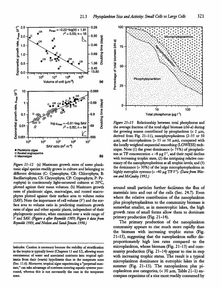
21.3 Phytoplankton Size andActivity: Small Cells vsLarge Cells 321
^-" 2.5&iffI 2.0
©
s 1.5j=
?y 1.0o
<n
2«0.5
con
fi 0.0
10^
fi 0.001
_CRutnax=-0.22-log(V) + 1.91
1^= 0.53:0 = 16
.« CP»B#B
liu^ lllli^ lllliu^ lllllllj llllllj llllll^ IIIIIUj lllliu) |Tin102 104 106 108Volume of unit(urn-3)
0.28
(a)
-0.069
log 1W = -0.61-log SAVr2= 0.82; n = 64
\c:--693I I i i""| l l i nii'i—| i i imu| | |
103 104 105 106SAV ratio (rrr^rrr3)
• Planktonic algaeo Rooted angiosperms• Macroatgae
107
(b)
Figure 21-12 (a) Maximum growth rates of some planktonicalgalspecies readilygrownin culture and belongingtodifferent divisions (C: Cyanophyta; CR: Chlorophyta; B:Bacillariophyta; CS: Chrysophyta; CP: Cryptophyta;P: Pyrophyta) in continuously light-saturated cultures at 20°C,plotted against their mean volumes, (b) Maximum growthrates of planktonic algae, macroalgae, and rooted macrophytes plotted against their surface area to volume ratios(SAV). Note the importance of cell volume (V) and the surface area to volume ratio in predicting maximum growthrates of algae and other aquaticplants, independentof theirphylogenetic position, when examined overa widerange ofFand SAV (Figure a after Reynolds 1989; Figure b data fromReynolds 1989,andNielsen andSand-Jensen 1990.)
latitudes. Caution is necessary because the stability of stratificationin the tropics is typically lower(Chapters 11 and12), allowing moreentrainment of water and associated nutrients into tropical epilimnia from their (warm) hypolimnia than in the temperate zone(Sec. 11.6).Moreover, tropical algae experiencing a "perpetual summer," cantakeadvantage ofnutrientsenteringaquatic systems year-round, whereas this is not necessarily the case in the temperatezone.
10 100
Totalphosphorus (ug I"1)
Figure 21-13 Relationship between total phosphorus andthe averagefraction ofthe total algal biomass (chl-*) duringthe growing season contributed by picoplankton (< 2 u.m,derived from Fig. 21-11), nanophytoplankton (2-35 or 50lira), and microplankton (> 35 or 50 u,m), computed withthe locallyweightedsequentialsmoothing (LOWESS) technique.Note (1) the great dominance (>75%) of picoplanktonat TP concentration <~8u,g l"1, and their rapiddeclinewith increasingtrophic state, (2) the intriguing relativeconstancyofthe nanophytoplanktonat all trophic levels; and (3)the dominance (> 50%) ofthe large microphytoplankton inhighly eutrophic systems (> ~40 u,g TP l~l). (Datafrom Watson andMcCauley 1992.)
around small particles further facilitates the flux ofmaterials into and out of the cells (Sec. 24.7). Evenwhere the relative contribution of the nanoplanktonplus picophytoplankton to the community biomass issomewhat smaller, as in mesotrophic lakes, the highgrowth rates of small forms allow them to dominateprimaryproduction (Fig. 21-14).The primary production of the nanoplankton
community appears to rise much more rapidly thanthe biomass with increasing trophic status (Fig.21-15), suggesting that the nanoplankton suffer disproportionately high loss rates compared to themicroplankton, whosebiomass (Fig.21-13) and community production (Fig. 21-14) appear to rise in stepwith increasing trophic status. The result is a typicalmicroplankton dominance in eutrophic lakes in thesummer (Fig. 21-13). The nanoplankton plus picoplanktonsize categories, (< 30 p,m, Table 21-1) encompass organisms of a sizemost readilyconsumedby
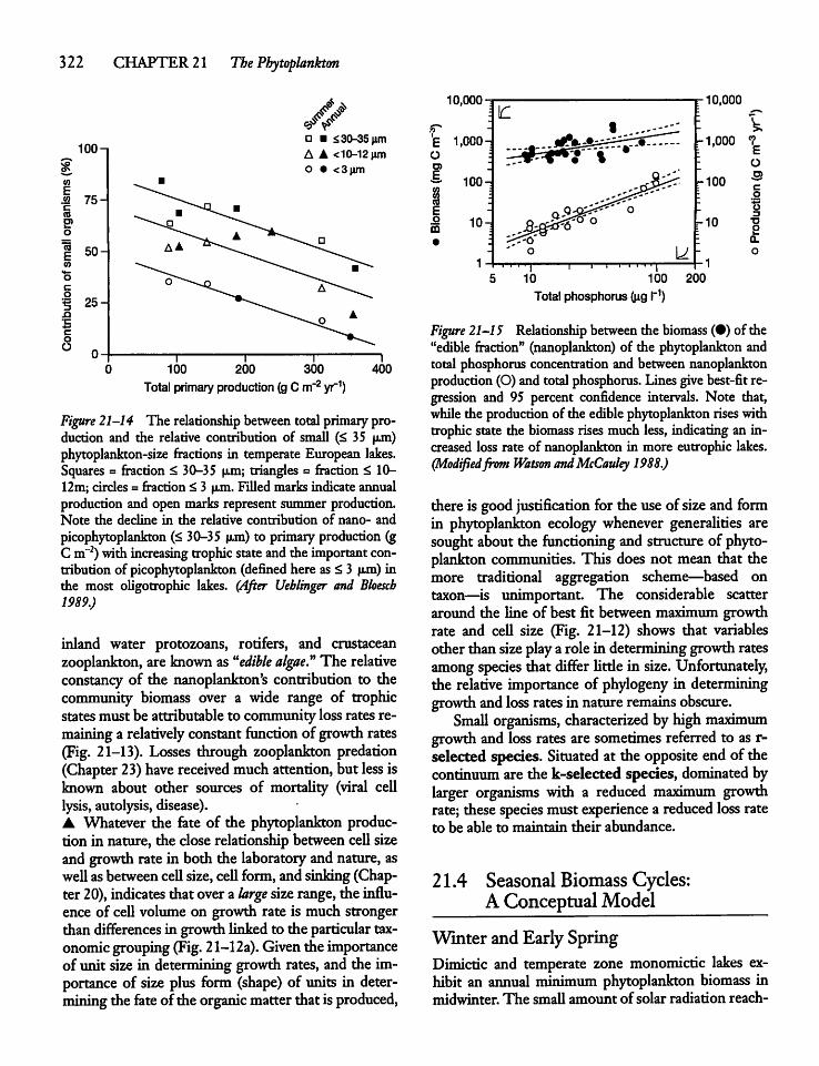
322 CHAPTER 21 The Phytoplankton
100-1
CO
1 75 HcCO
50-
25-
//• • 530-35 urn
A A <10-12umO • <3um
100 200 300
Total primary production (gCm~2 yr1)400
Figure 21-14 The relationship between total primary production and the relative contribution of small (< 35 u,m)phytoplankton-size fractions in temperate European lakes.Squares = fraction < 30-35 um; triangles = fraction £ 10-12m; circles = fraction < 3 u.m.Filled marks indicate annualproduction and open marks represent summerproduction.Note the decline in the relative contribution of nano- andpicophytoplankton (< 30-35 u>m) to primaryproduction (gC m~2) withincreasing trophicstateand the important contribution of picophytoplankton (defined here as £ 3 ujn) inthe most oUgotrophic lakes. (After Uehlinger and Bloesch1989.)
inland water protozoans, rotifers, and crustaceanzooplankton, are known as uedible algae." The relativeconstancy of the nanoplankton's contribution to thecommunity biomass over a wide range of trophicstatesmust be attributable to community loss rates remaining a relatively constant function of growth rates(Fig. 21-13). Losses through zooplankton predation(Chapter 23) have received much attention, but less isknown about other sources of mortality (viral celllysis, autolysis,disease).• Whatever the fate of the phytoplankton production in nature, the closerelationshipbetweencellsizeand growthrate in both the laboratory and nature, aswellas between cell size, cell form, and sinking (Chapter 20), indicates that overa large size range, the influence of cell volume on growth rate is much strongerthan differences in growthlinkedto the particular tax-onomic grouping (Fig. 21-12a). Giventhe importanceof unit size in determininggrowth rates, and the importance of size plus form (shape) of units in determining the fate ofthe organic matterthat isproduced,
10,000- 10,000
10 100 200
Total phosphorus (ug I"1)
Figure 21-15 Relationship between the biomass (•) of the"edible fraction" (nanoplankton) of the phytoplankton andtotal phosphorus concentration and between nanoplanktonproduction (O)and totalphosphorus. Lines give best-fit regression and 95 percent confidence intervals. Note that,while the productionof the ediblephytoplankton riseswithtrophic state the biomass rises much less, indicating an increased loss rate of nanoplankton in more eutrophic lakes.(Modifiedfrom Watson andMcCauley 1988.)
there is goodjustification for the use of sizeand formin phytoplankton ecology whenever generalities aresought about the functioning and structure of phytoplankton communities. This does not mean that themore traditional aggregation scheme—based ontaxon—is unimportant. The considerable scatteraround the line of best fit between maximumgrowthrate and cell size (Fig. 21-12) shows that variablesother than size playa role in detennininggrowthratesamong species that differ littlein size. Unfortunately,the relative importance of phylogeny in determininggrowth andloss rates in natureremains obscure.Small organisms, characterized by highmaximum
growth and loss rates are sometimes referred to as r-selected species. Situated at the opposite end of thecontinuumare the k-selected species, dominated bylarger organisms with a reduced maximum growthrate; thesespecies must experience a reduced lossrateto be able to maintain their abundance.
21.4 Seasonal Biomass Cycles:A ConceptualModel
Winter and Early SpringDimictic and temperate zone monomictic lakes exhibit an annual nMnimum phytoplankton biomass inmidwinter. The small amount ofsolar radiation reach-
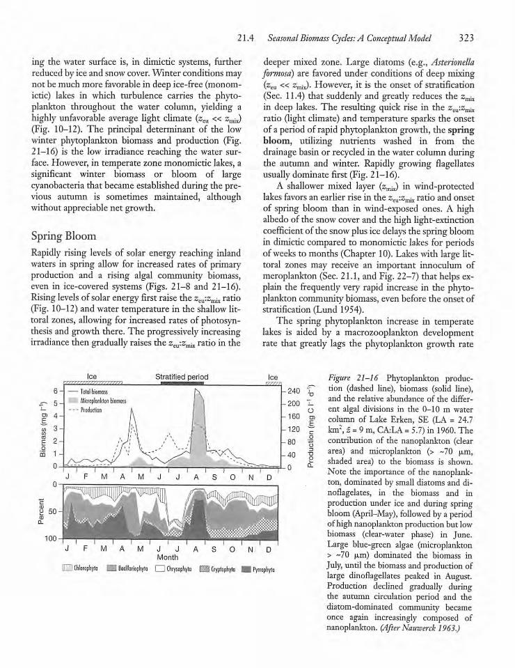
21.4 Seasonal Biomass Cycles: A ConceptualModel 323
ing the water surface is, in dimictic systems, furtherreduced by ice and snow cover.Winter conditions maynot be much more favorable in deep ice-free (monom-ictic) lakes in which turbulence carries the phytoplankton throughout the water column, yielding ahighly unfavorable average light climate (zeu « z^J(Fig. 10-12). The principal determinant of the lowwinter phytoplankton biomass and production (Fig.21-16) is the low irradiance reaching the water surface. However, in temperate zonemonomictic lakes, asignificant winter biomass or bloom of largecyanobacteria that becameestablishedduring the previous autumn is sometimes maintained, althoughwithout appreciable net growth.
Spring BloomRapidly rising levels of solar energy reaching inlandwaters in spring allow for increased rates of primaryproduction and a rising algal community biomass,even in ice-covered systems (Figs. 21-8 and 21-16).Risinglevels of solar energy first raise the z^-.z^ ratio(Fig. 10-12) and water temperature in the shallow littoral zones, allowing for increased rates of photosynthesis and growth there. The progressively increasingirradiance then graduallyraises the z^iz^ ratio in the
P 50-
100
J JMonth
deeper mixed zone. Large diatoms (e.g., Asterionellaformosa) are favored under conditions of deep mixing(zeu « ZnuJ. However, it is the onset of stratification(Sec. 11.4) that suddenly and gready reduces the zmixin deep lakes. The resulting quick rise in the zcu:zmixratio (light climate) and temperature sparks the onsetof a period of rapid phytoplankton growth, the springbloom, utilizing nutrients washed in from thedrainage basin or recycled in the water columnduringthe autumn and winter. Rapidly growing flagellatesusually dominate first (Fig. 21-16).A shallower mixed layer (zmix) in wind-protected
lakes favors an earlier rise in the z^-.z^ ratio and onsetof spring bloom than in wind-exposed ones. A highalbedo of the snowcover and the high light-extinctioncoefficient ofthe snow plus ice delays thespring bloomin dimictic compared to monomictic lakes for periodsofweeks to months (Chapter 10). Lakes with large littoral zones may receive an important innoculum ofmeroplankton (Sec. 21.1, and Fig. 22-7) that helps explain the frequendy very rapid increase in the phytoplanktoncommunitybiomass, evenbefore the onset ofstratification (Lund 1954).The spring phytoplankton increase in temperate
lakes is aided by a macrozooplankton developmentrate that gready lags the phytoplankton growth rate
-240 TJ
-200 j_
O-160
F-120
ct)
-80 o-i
-40 0o
n LL
[illl; Chlorophyta [_] Bacillariophyta •Chrysophyta EttSl: Cryptophyta 90 Pyrrophyla
Figure 21-16 Phytoplankton production (dashed line), biomass (solid line),and the relative abundance of the different algal divisions in the 0-10 m watercolumn of Lake Erken, SE (LA = 24.7km2, z =9 m,CALA=5.7) in 1960. Thecontribution of the nanoplankton (cleararea) and microplankton (> -70 u.m,shaded area) to the biomass is shown.Note the importance of the nanoplankton, dominated by small diatoms and di-noflagelates, in the biomass and inproduction under ice and during springbloom (April-May), followed by a periodof high nanoplankton production but lowbiomass (clear-water phase) in June.Large blue-green algae (microplankton> -70 u,m) dominated the biomass inJuly, until the biomass and production oflarge dinoflagellates peaked in August.Production declined gradually duringthe autumn circulation period and thediatom-dominated community becameonce again increasingly composed ofnanoplankton. (After Nauwerck 1963.)
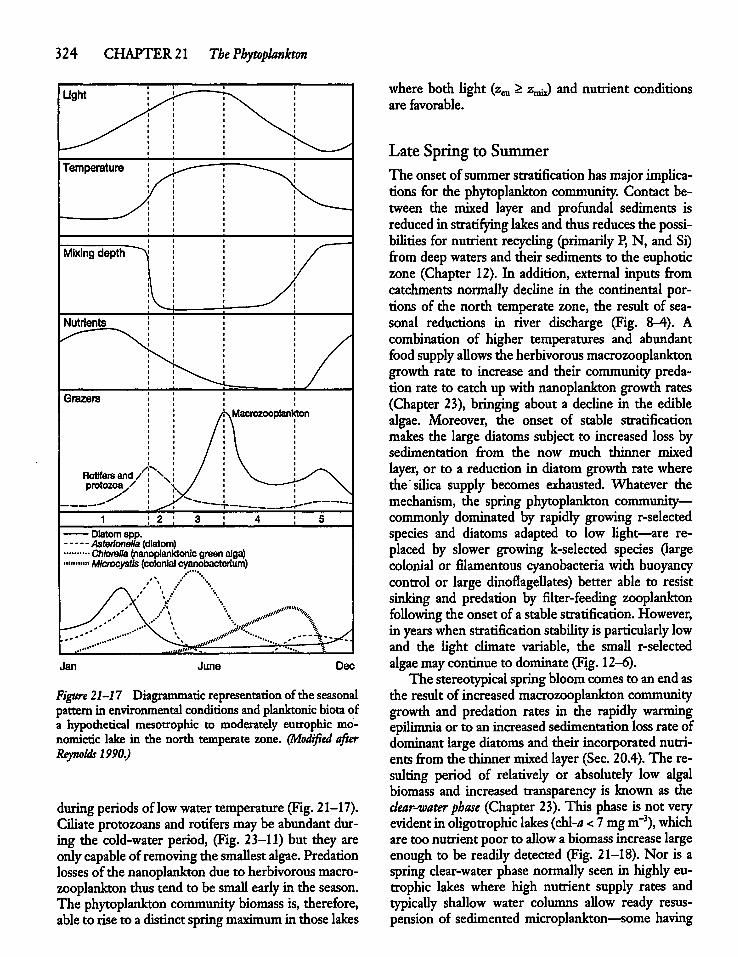
324 CHAPTER21 The Phytoplankton
Jan
Diatom 8pp.Asterlonella (diatom)Chlorella (nanoplanktonic green alga)Microcystis (colonial cyanobacterium)
Stw412
June
^,m'%
Dec
Figure 21-17 Diagrammatic representation of the seasonalpatternin environmental conditions andplanktonic biotaofa hypothetical mesotrophic to moderately eutrophic monomictic lake in the north temperate zone. (Modified afterReynolds 1990.)
duringperiodsof lowwater temperature(Fig. 21-17).Ciliateprotozoans and rotifersmaybe abundantduring the cold-water period, (Fig. 23-11) but they areonlycapable of removing the smallest algae. Predationlosses ofthe nanoplanktondue to herbivorous macrozooplankton thus tend to be small earlyin the season.The phytoplankton community biomass is, therefore,able to riseto a distinct springmaximum in thoselakes
where both fight (zeare favorable.
> z^ and nutrient conditions
Late Spring to SummerThe onset of summer stratificationhasmajor implications for the phytoplankton community. Contact between the mixed layer and profundal sediments isreduced in stratifying lakes and thus reduces the possibilities for nutrient recycling (primarily P, N, and Si)from deepwaters and their sediments to the euphoriczone (Chapter 12). In addition, external inputs fromcatchments normally decline in the continental portions of the north temperate zone, the result of seasonal reductions in river discharge (Fig. 8-4). Acombination of higher temperatures and abundantfoodsupplyallows die herbivorousmacrozooplanktongrowth rate to increase and their community predation rate to catch up with nanoplankton growth rates(Chapter 23), bringing about a decline in the ediblealgae. Moreover, the onset of stable stratificationmakes the large diatoms subject to increased loss bysedimentation from the now much thinner mixedlayer, or to a reduction in diatom growth rate wherethe silica supply becomes exhausted. Whatever themechanism, the spring phytoplankton community—commonly dominated by rapidly growing r-selectedspecies and diatoms adapted to low Ught—are replaced by slower growing k-selected species (largecolonial or filamentous cyanobacteria with buoyancycontrol or large dinoflagellates) better able to resistsinking and predation by filter-feeding zooplanktonfollowing the onsetof a stable stratification. However,in years whenstratification stability is particularly lowand the Ught climate variable, the smaU r-selectedalgaemaycontinue to dominate (Fig. 12-6).The stereotypical springbloom comes to anendas
the result of increased macrozooplankton communitygrowth and predation rates in the rapidly warmingepilimnia or to an increased sedimentation lossrate ofdominant largediatoms and their incorporated nutrients fromthe thinner mixed layer(Sec 20.4). The resulting period of relatively or absolutely low algalbiomass and increased transparency is known as theclear-water phase (Chapter 23). This phase is not veryevident inoUgotrophic lakes (cbl-a <7mg m~3), whichare too nutrient poor to allow a biomass increase largeenough to be readily detected (Fig. 21-18). Nor is aspring clear-water phase normally seen in highly eutrophic lakes where high nutrient supply rates andtypicaUy shallow water columns aUow ready resuspension of sedimented microplankton—some having
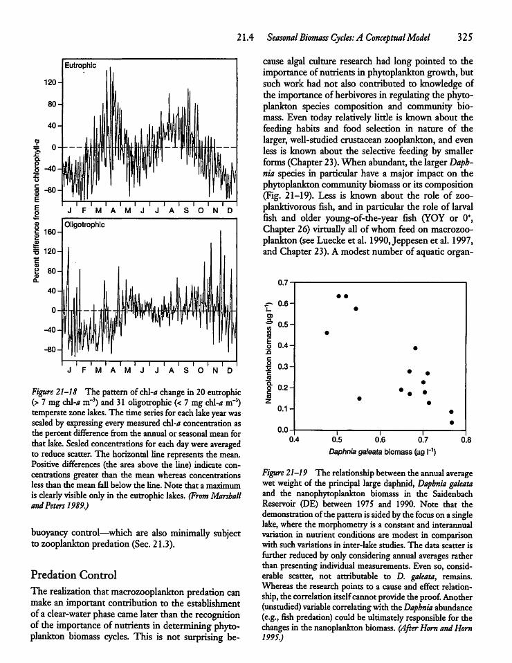
21.4 Seasonal Biomass Cycles: A ConceptualModel 325
Eutrophic
120-
"I 1 1 1 1 1 1 1—J FMAMJ JASOND
Figure 21-18 The patternof chl-achange in 20 eutrophic(> 7mg chl-a m"3) and 31 oUgotrophic (< 7 mg chl-* m"3)temperate zonelakes. The timeseries for eachlake yearwasscaledby expressing everymeasuredcbl-aconcentration asthe percent difference from the annual or seasonal mean forthatlake. Scaled concentrations foreach day were averagedto reduce scatter. The horizontal line represents the mean.Positive differences (the area above the line) indicate concentrations greater than the mean whereas concentrationsless than the mean faU below the line. Note that a maximumis clearly visible onlyin the eutrophic lakes. (From MarshallandPeters 1989.)
buoyancy control—which are also minimally subjectto zooplankton predation (Sec. 21.3).
Predation Control
The realization thatmacrozooplankton predation canmake an important contribution to the establishmentofa clear-water phase came later than therecognitionof the importance ofnutrients in determining phytoplankton biomass cycles. This is not surprising be
cause algal culture research had long pointed to theimportance of nutrients in phytoplankton growth, butsuch work had not also contributed to knowledge ofthe importanceof herbivores in regulating the phytoplankton species composition and community biomass. Even today relatively little is known about thefeeding habits and food selection in nature of thelarger,weU-studied crustacean zooplankton, and evenless is known about the selective feeding by smallerforms (Chapter 23).When abundant, the largerDapb-nia species in particular have a major impact on thephytoplankton communitybiomass or its composition(Fig. 21-19). Less is known about the role of zoo-planktivorous fish, and in particular the role of larvalfish and older young-of-the-year fish (YOY or 0+,Chapter 26) virtuaUy aU of whom feed on macrozooplankton(seeLueckeet al. 1990,Jeppesen et al. 1997,and Chapter 23).Amodest number of aquatic organ-
v.t -
• •
~ 0.6-i •
? °-5"•
o 0.4- •
J 0.3-§• 0.2-Z
0.1-
•
• ••
•• ••
•
•
I I0.4 0.5 0.6 0.7
Daphnia galeata biomass (ug I'1)0.8
Figure 21-19 The relationship between the annualaveragewetweight of the principal large daphnid, Daphnia galeataand the nanophytoplankton biomass in the SaidenbachReservoir (DE) between 1975 and 1990. Note that thedemonstration ofthe patternisaided bythe focus onasinglelake, where the morphometry is a constant and interannualvariation in nutrient conditions are modest in comparisonwith such variations in inter-lake studies. The data scatter isfurther reduced byonlyconsidering annual averages ratherthan presenting individual measurements. Even so, considerable scatter, not attributable to D. galeata, remains.Whereas the research points to a causeand effect relationship, thecorrelation itselfcannotprovide theproof. Another(unstudied) variable correlatingwiththeDaphnia abundance(e.g., fish predation) could beultimately responsible for thechanges in the nanoplankton biomass. (AfterHorn andHorn1995.)
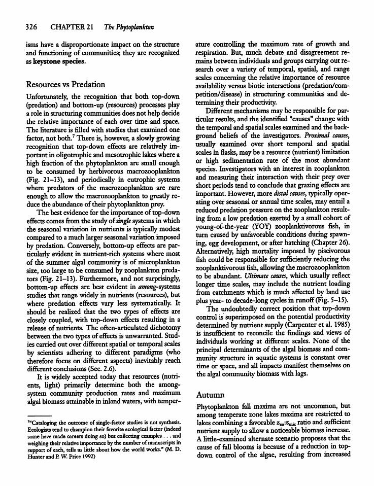
326 CHAPTER 21 The Phytoplankton
isms have a disproportionate impacton the structureand functioning of communities; they are recognizedaskeystone species.
Resources vs Predation
Unfortunately, the recognition that both top-down(predation) and bottom-up (resources) processes playa rolein structuringcommunities doesnot helpdecidethe relative importance of each over time and space.The literature is filled with studies that examined onefactor, not both.7 There is, however, a slowly growingrecognition that top-down effects are relatively importantin oUgotrophic andmesotrophic lakes where ahigh fraction of the phytoplankton are smaU enoughto be consumed by herbivorous macrozooplankton(Fig. 21-13), and periodicaUy in eutrophic systemswhere predators of the macrozooplankton are rareenough to allow the macrozooplankton to greadyreduce the abundanceof their phytoplanktonprey.The bestevidence for the importance of top-down
effects comes from thestudy oisingle systems inwhichthe seasonal variation in nutrients is typicaUy modestcompared to amuch larger seasonal variation imposedby predation. Conversely, bottom-up effects are particularly evident in nutrient-rich systems where mostof the summer algal community is of microplanktonsize, too large to be consumed byzooplankton predators (Fig. 21-13). Furthermore, and not surprisingly,bottom-up effects are best evident in among-systemsstudies that range widely in nutrients (resources), butwhere predation effects vary less systematicaUy. Itshould be realized that the two types of effects areclosely coupled, with top-down effects resulting in arelease of nutrients. The often-articulated dichotomybetween the two types ofeffects isunwarranted. Studiescarried out overdifferent spatial or temporal scalesby scientists adhering to different paradigms (whotherefore focus on different aspects) inevitably reachdifferent conclusions (Sec. 2.6).It is widely accepted today that resources (nutri
ents, Ught) primarily determine both the among-system community production rates and maximumalgal biomass attainable in inlandwaters, withtemper-
7uCataloging the outcome of single-factor studies is not synthesis.Ecologists tend to champion their favorite ecological factor (indeedsome have made careers doing so)but collecting examples ... andweighing their relative importance bydienumber ofmanuscripts insupport of each, tells us little about howtheworld works." (M. D.Hunter and P.W. Price 1992)
ature controlling the maximum rate of growth andrespiration. But, much debate and disagreement remainsbetweenindividuals and groups carryingout research over a variety of temporal, spatial, and rangescales concerning the relative importance of resourceavailabiUty versus biotic interactions (predation/com-petition/disease) in structuring communities and determining their productivity.Different mechanisms maybe responsible for par
ticular results, and the identified "causes"changewiththe temporal andspatial scales examined andthe background beliefs of the investigators. Proximal causes,usuaUy examined over short temporal and spatialscales in flasks, maybe a resource (nutrient) limitationor high sedimentation rate of the most abundantspecies. Investigators with an interest in zooplanktonandmeasuring their interaction with their prey overshortperiods tend to conclude that grazing effects areimportant. However, moredistal causes, typicaUy operating over seasonal or annual time scales, may entail areduced predation pressure on thezooplankton resultingfrom a low predation exerted bya smaU cohort ofyoung-of-the-year (YOY) zooplanktivorous fish, inturn caused byunfavorable conditions duringspawning, eggdevelopment, or after hatching (Chapter 26).Alternatively, high mortaUty imposed by piscivorousfish could be responsible for sufficiendy reducing thezooplanktivorous fish, aUowing themacrozooplanktonto be abundant Ultimate causes, which usuaUy reflectlonger time scales, may include the nutrient loadingfrom catchments which is much affected by land useplus year- to decade-long cycles in runoff (Fig. 5-15).The undoubtedly correct position that top-down
control is superimposed on the potential productivitydetermined bynutrientsupply (Carpenter et al. 1985)is insufficient to reconcile the findings and views ofindividuals working at different scales. None of theprincipal determinants of thealgal biomass and community structure in aquatic systems is constant overtime or space, and aU impacts manifest themselves onthe algal community biomass withlags.
Autumn
Phytoplankton faU maxima are not uncommon, butamong temperate zone lakes maxima are restricted tolakes combining a favorable z^jz^^ ratio andsufficientnutrientsupply to aUow a noticeable biomass increase.AUtde-examined alternate scenario proposes that thecause of faU blooms is because of a reduction in top-down control of the algae, resulting from increased
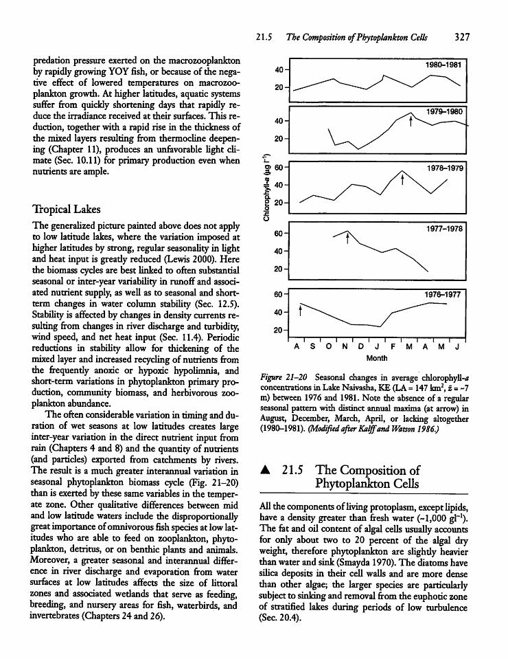
predation pressure exerted on the macrozooplanktonby rapidlygrowingYOYfish, or because of the negative effect of lowered temperatures on macrozooplanktongrowth. At higher latitudes, aquatic systemssuffer from quickly shortening days that rapidly reduce the irradiance received at their surfaces. This reduction, together with a rapid rise in the thickness ofthe mixed layers resulting from thermocline deepening (Chapter 11), produces an unfavorable Ught cU-mate (Sec. 10.11) for primary production even whennutrients are ample.
Tropical LakesThe generaUzed picturepaintedabove doesnot applyto low latitude lakes, where the variation imposed athigher latitudes bystrong, regular seasonality in Ughtand heat input is greatly reduced (Lewis 2000). Herethe biomass cycles are best linked to often substantialseasonal or inter-yearvariabiUty in runoff and associated nutrient supply, asweU as to seasonal and short-term changes in water column stabiUty (Sec. 12.5).Stability is affected bychanges in density currents resulting from changes in river discharge and turbidity,wind speed, and net heat input (Sec. 11.4). Periodicreductions in stabiUty allow for thickening of themixed layerand increased recycling of nutrients fromthe frequently anoxic or hypoxic hypolimnia, andshort-term variations in phytoplankton primary production, community biomass, and herbivorous zooplankton abundance.The often considerable variation in timing and du
ration of wet seasons at low latitudes creates largeinter-year variation in the direct nutrient input fromrain (Chapters 4 and 8)and the quantity of nutrients(and particles) exported from catchments by rivers.The result is a much greater interannual variation inseasonal phytoplankton biomass cycle (Fig. 21-20)than isexerted by these same variables in the temperate zone. Other qualitative differences between midand low latitude waters include the disproportionaUygreatimportance ofomnivorous fish species at low latitudes who are able to feed on zooplankton, phytoplankton, detritus, or on benthic plants and animals.Moreover, a greater seasonal and interannual difference in river discharge and evaporation from watersurfaces at low latitudes affects the size of littoralzones and associated wedands that serve as feeding,breeding, and nursery areas for fish, waterbirds, andinvertebrates (Chapters24 and 26).
21.5 The Composition ofPhytoplankton Cells 327
2
60-
^40sza.
8 20-o
1978-1979
O
60-1977-1978
40-
20-
60- 1976-1977
40- f^20-
IA S O N D J F M
i i
A M J
Month
Figure 21-20 Seasonal changes in average chlorophyll-^concentrations in Lake Naivasha,KE (LA= 147km2, z = ~7m) between 1976 and 1981. Note the absence of a regularseasonal pattern with distinct annual maxima (at arrow) inAugust, December, March, April, or lacking altogether(1980-1981). (Modified afterKalffand Watson 1986.)
A 21.5 The Composition ofPhytoplankton Cells
AU thecomponents ofUving protoplasm, except Upids,have a density greater than fresh water (-1,000 gl"1).The fatand oilcontent of algal cells usuaUy accountsfor only about two to 20 percent of the algal dryweight, therefore phytoplankton are sUghdy heavierthanwaterandsink(Smayda 1970). The diatoms havesiUca deposits in their ceU walls and are more densethan other algae; the larger species are particularlysubject to sinking and removal from theeuphoric zoneof stratified lakes during periods of low turbulence(Sec. 20.4).
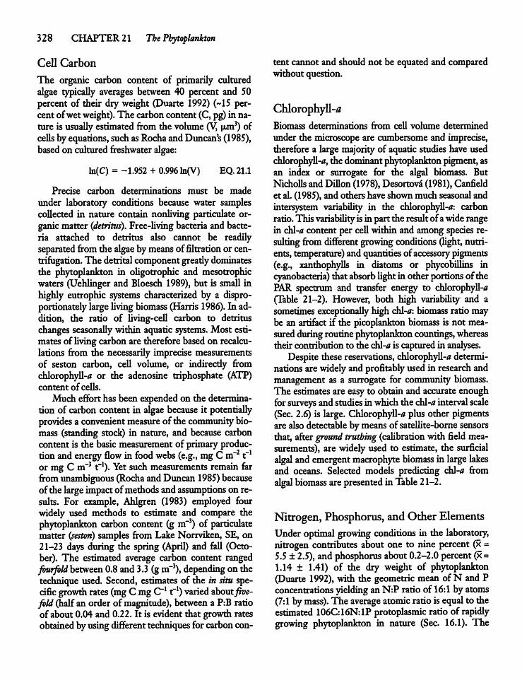
328 CHAPTER 21 The Phytoplankton
Cell Carbon
The organic carbon content of primarily culturedalgae typicaUy averages between 40 percent and 50percent of their dry weight (Duarte 1992) (-15 percent ofwetweight). The carboncontent (C, pg)in nature isusuaUy estimated from thevolume (V, ujn3) ofceUs byequations, suchasRocha andDuncan's (1985),based on culturedfreshwater algae:
ln(C) = -1.952 + 0.996ln(V) EQ. 21.1
Precise carbon determinations must be madeunder laboratory conditions because water samplescollected in nature contain nonliving particulate organic matter (detritus). Free-Uving bacteria and bacteria attached to detritus also cannot be readilyseparated fromthe algae bymeans of filtration or cen-trifugation. The detritalcomponentgreadydominatesthe phytoplankton in oUgotrophic and mesotrophicwaters (Uehlinger and Bloesch 1989), but is small inhighly eutrophic systems characterized by a disproportionately largeliving biomass (Harris1986). In addition, the ratio of Uving-ceU carbon to detrituschanges seasonaUy within aquaticsystems. Most estimates of Uving carbonare therefore based on recalculations from the necessarily imprecise measurementsof seston carbon, ceU volume, or indirecdy fromchlorophyU-0 or the adenosine triphosphate (ATP)content of ceUs.Much effort has been expended on the determina
tion of carbon content in algae because it potentiaUyprovides a convenient measure of the community biomass (standing stock) in nature, and because carboncontent is the basic measurement of primaryproduction and energy flow in food webs (e.g., mg C m~21-1or mgC m~3 t"1). Yet such measurements remain farfrom unambiguous (Rocha andDuncan1985) becauseofthe large impact ofmethods andassumptions on results. For example, Ahlgren (1983) employed fourwidely used methods to estimate and compare thephytoplankton carbon content (g m"3) of particulatematter (seston) samples from Lake Norrviken, SE, on21-23 days during the spring (April) and faU (October). The estimated average carbon content rangedfburfbld between 0.8 and 3.3 (gm~3), depending onthetechnique used. Second, estimates of the in situ specific growth rates (mg CmgC"11"1) varied aboutfivefold(halfan order of magnitude), between a P:B ratioof about 0.04 and 0.22. It is evident that growth ratesobtained byusingdifferent techniques for carbon con
tent cannot and should not be equated and comparedwithoutquestion.
Chlorophyll-/?Biomass determinations from ceU volume determinedunder the microscope are cumbersome and imprecise,therefore a largemajority of aquatic studies have usedchlorophyll-a, the dominantphytoplankton pigment, asan index or surrogate for the algal biomass. ButNicholls and DiUon(1978), Desortova (1981), Canfieldet al. (1985), and others have shownmuch seasonalandintersystem variabiUty in the chlorophyU-fl: carbonratio. This variabiUty isin part theresultofawide rangein chl-a content per ceU within and among species resulting fromdifferent growing conditions (light, nutrients, temperature) andquantities ofaccessory pigments(e.g., xanthophylls in diatoms or phycobilUns incyanobacteria) that absorbUght in other portionsofthePAR spectrum and transfer energy to chlorophyU-/*(Table 21-2). However, both high variabiUty and asometimes exceptionaUy high chl-a: biomass ratio maybe an artifact if the picoplankton biomass is not measured duringroutinephytoplankton countings, whereastheir contribution to the chl-ais captured in analyses.Despite thesereservations, chlorophyU-* determi
nations arewidely and profitably usedin research andmanagement as a surrogate for community biomass.The estimates are easy to obtainand accurate enoughforsurveys andstudies inwhich the chl-a interval scale(Sec. 2.6) is large. ChlorophyU-/* plus other pigmentsare alsodetectable bymeansof sateUite-borne sensorsthat, after ground truthing (caUbration with field measurements), are widely used to estimate, the surficialalgal andemergent macrophyte biomass in large lakesand oceans. Selected models predicting chl-tf fromalgal biomass arepresented inTable 21-2.
Nitrogen, Phosphorus, and Other ElementsUnder optimal growing conditions in the laboratory,nitrogen contributes about one to nine percent (x =5.5± 2.5), and phosphorusabout 0.2-2.0 percent (x=1.14 ± 1.41) of the dry weight of phytoplankton(Duarte 1992), with the geometric mean of N and Pconcentrations yieldingan N:P ratio of 16:1 by atoms(7:1 bymass). The average atomic ratioisequal to theestimated 106C:16N:1P protoplasmic ratio of rapidlygrowing phytoplankton in nature (Sec. 16.1). The
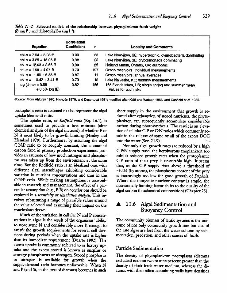
21.6 Algal Sedimentation and Buoyancy Control 329
Table 21-2 Selectedmodels of the relationship betweenphytoplankton fresh weight(Bmg I1') and chlorophyll-^(|tg l"1).
CorrelationEquation Coefficient n Locality and Comments
china = 7.94 + 8.03-B 0.93 63 Lake Norrviken, SE; hypertrophic, cyanobacteria dominatingchina = 3.25 + 15.06-B 0.98 23 Lake Norrviken, SE; cryptomonads dominatingchl-a = 12.63+ 3.55-B 0.90 25 Holland Marsh, Ontario, CA; eutrophicchl-a = 1.58+ 4.97-B 0.79 197 Czech reservoirs; individual measurementschina = -1.69+ 6.38-B 0.87 11 Czech reservoirs; annual averageschl-a = -10.42 +3.41-B 0.79 13 Lake Naivasha, KE; monthly measurementslog (chl-a) = 0.55 0.82 165 165 Florida lakes, US; single spring and summer mean
+ 0.50- log (B) values for each lake
Source: FromAhlgren 1970, Nicholls 1976, and Desortova 1981; modified after Kalff and Watson 1986, and Canfield et al. 1985.
protoplasm ratio is assumed to also representthe algaluptake (demand)ratio.The uptake ratio, or Redfield ratio (Eq. 16.1), is
sometimes used to provide a first estimate (afterchemical analysis ofthe algal material) ofwhetherP orN is most likely to be growth limiting (Healey andHendzel 1979). Furthermore, by assuming the algalC:N:P ratio to be roughly constant, the amount ofcarbon fixed in primary production experiments provides anestimate ofhowmuch nitrogen andphosphorus was taken up from the environment at the sametime. But the Redfield ratio is an idealized one, withdifferent algal assemblages exhibiting considerablevariation in nutrient concentrations and thus in theC:N:P ratio. While making assumptions is unavoidable in research and management, the effect ofa particular assumption (e.g., P:B) on conclusions should beexplored in a sensitivity or simulation analysis. This involves substituting a range of plausible values aroundthevalue selected and examining theirimpact on theconclusions drawn.Much of the variation in ceUular N and P concen
trations in algae is the result of the organisms' abiUtyto store some N and considerably more P, enough tosatisfy the growth requirements for several ceU divisions during periods when the uptake rate is higherthan its immediate requirement (Duarte 1992). Theexcess uptake is commonly referred to as luxuryuptake and the excess stored is known as surplus orstoragephosphorus ornitrogen.Stored phosphorusor nitrogen is available for growth when thesupply:demand ratio becomes unfavorable. When NandP (andSi,in the case of diatoms) becomes in such
short supply in the environment that growth is reduced after exhaustion of storednutrients, the phytoplankton can subsequendy accumulate considerablecarbon during photosynthesis. The result is an elevationofcellular C:Por C:N ratios which commonly result in the release of some or all of the excess DOCinto the water (Sec. 21.9).Not only algal growth rates are reduced bya high
C:P:Nsupply ratio; the herbivorous zooplankton tooexhibit reduced growth rates when the protoplasmicC:P ratio of their prey is unsuitably high. It seemsthat, as the C:P supply rises above a threshold of-300:1 (by atoms), thephosphorus content ofthe preyis increasingly too low for good growth of Daphnia.Where the inorganic nutrient content is ample, thenutritionaUy limiting factor shifts to the quaUty ofthealgal carbon (biochemical composition) (Chapter 23).
A 21.6 Algal Sedimentation andBuoyancyControl
The community biomass of lentic systems is the outcome of not only community growth rate but also oftherate algae arelostfrom thewater column bysedimentation, predation, and other causesof death.
Particle Sedimentation
The density of phytoplankton protoplasm (diatomsexcluded) isabout two tonine percent greater than thedensity of their freshwater medium, whereas the diatoms with their silica-containing walls have densities
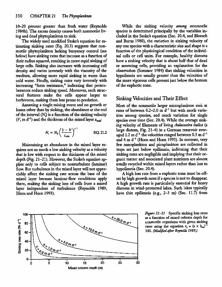
330 CHAPTER 21 The Phytoplankton
10-20 percent greater than fresh water (Reynolds1984b). The excess density causes both nonmotile Uvinganddeadphytoplankton to sink.The widely usedmodified Stoke's equation for es
timating sinking rates (Eq. 20.3) suggests that non-motile phytoplankton lacking buoyancy control (seebelow) have sinking ratesthat increase asa function oftheir radius squared, resultinginmore rapidsinking oflarge ceUs. Sinking also increases with increasing ceUdensity and varies inversely with the viscosity of themedium, aUowing more rapid sinking in warm thancold water. FinaUy, sinking rates vary inversely withincreasing "form resistance," indicating that protru-berances reduce sinkingspeed.Moreover, such structural features make the cells appear larger toherbivores, makingthem lessprone to predation.Assuming a singlemixing event and no growth or
losses other than bysinking, the abundance at the endofthe interval (AQ is a function ofthe sinkingvelocity(y,md"1) andthe thickness ofthe mixed layer z^.
Nt =No(^—^-} EQ.21.2\ *mix /
Maintaining an abundance in the mixed layer requires not somucha lowsinking velocity asa velocitythat is lowwith respect to the thickness of the mixeddepth(Fig. 21-21). However, the Stoke's equation ap-pUes only to ceUs subject to nonturbulent (laminar)flow. But turbulence in the mixedlayerwiU not appreciably affect the sinking rate across the base of themixed layer because laminar-flow conditions applythere, making the sinking loss of cells from a mixedlayer independent of turbulence (Reynolds 1989,Horn and Horn 1993).
15 20
Mixed column depth (m)
While the sinking velocity among nonmotilespecies is determined principaUy by the variables included in the Stoke's equation(Sec. 20.4, and Bloeschand Burns 1980), the variation in sinking velocity ofanyonespecies witha characteristic size andshape isafunction ofthe physiological conditionofthe individual ceUs or ceU units. For example, healthy diatomshave a sinking velocity that is about half that of deador senescing cells, providing an explanation for theobservation (Sommer 1984) that sinking velocities inhypolimnia are usuaUy greater than the velocities ofthemorevigorous ceUs present justbelow the bottomofthe euphoriczone.
SinkingVelocities andTheir EffectMost of the nonmotile larger microplankton sink atrates of between 0.2-2.0 m d"1 but with much variation among species, and much variation for singlespecies over time(Sec. 20.4). While the average sinking velocity of filaments of Uving Aulacoseira italica (alarge diatom, Fig. 21-4) in a German reservoir averaged 1.2 md"1 thevelocities ranged between 0.5 md-1and 4 m d-1 (Horn andHorn 1993). In contrast, veryfew nanoplankton and picoplankton are coUected intraps set just below epilimnia, indicating that theirsinking ratesarenegUgible and implying that their organic matter and associated plantnutrientsare almosttotaUy recycled within mixed layers ratherthan losttohypolimnia (Sec. 20.4).Ahighloss rate froma euphoric zonemustbeoff
setbyhighgrowthratesif a species isnot to disappear.Ahigh growth rate is particularly essential for heavydiatoms in wind-protected lakes. Such lakes typicaUyhave thin epilimnia (e.g., 2-3 m) (Sec. 11.7) from
30
Figure 21-21 Specific sinking loss ratesas a function of mixed column depth fornonmotile organisms with given sinkingrates using the equation rs = (s x hj-1100. (Modified afterReynolds 1989.)
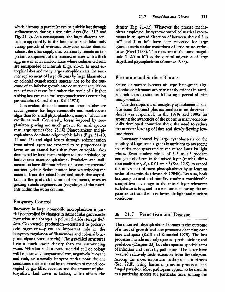
which diatoms in particular canbe quickly lost throughsedimentation during a few calm days (Eq. 21.2 andFig. 21-9). As a consequence, the large diatoms contribute appreciably to the biomass of such lakes onlyduring periods of overturn. However, unless diatomsexhaust the siUca supplythey commonlyremain an important componentof the biomass in lakes with a thick2^, as weU as in shaUow lakeswhere sedimented cellsare resuspended at intervals (Figs. 21-2). In most eutrophic lakes andmany largeeutrophic rivers, the summer replacement of large diatoms by large filamentousor colonial cyanobacteria appears not to be the outcomeof an inferiorgrowthrate or nutrient acquisitionrate of the diatoms but rather the result of a highersinking loss rate thanforlargecyanobacteria containinggasvacuoles (Knoechel andKalff1975).It is evident that sedimentation losses in lakes are
much greater for large nonmotile and nonbuoyantalgae than for smaU phytoplankton, manyofwhicharemotile as weU. Conversely, losses imposed by zooplankton grazing are much greater for smaU speciesthan largespecies (Sec. 23.10). Nanoplankton and picoplankton dominate oUgotrophic lakes (Figs. 21-10,11 and 13) and algal losses through sedimentationfrom mixed layers are expected to be proportionaUylower on an annual basis than from eutrophic lakesdominated bylarge forms subject to Utde predation byherbivorous macrozooplankton. Predation and sedimentation have different effects on organicmatterandnutrient cycling. Sedimentation involves stripping thematerial from the mixed layerand much decomposition in the profundal zone and sediments, whereasgrazing entails regeneration (recycling) of the nutrients within the water column.
BuoyancyControlBuoyancy in large nonmotile microplankton is par-tiaUy controlled bychanges in intracellular gas vacuoleformation and changes in polysaccharide storage (ballast). Gas vacuole production—restricted to prokary-otic organisms—plays an important role in thebuoyancy regulationof filamentous and colonial blue-green algae (cyanobacteria). The gas-filled structureshave a much lower density than the surroundingwater. Whether such a cyanobacterial ceU or colonywiU bepositively buoyant and rise, negatively buoyantand sink, or neutraUy buoyant under nonturbulentconditions isdeterminedby the fractionofthe ceU occupied bygas-filled vacuoles and the amount of pho-tosynthate laid down as ballast, which affects the
21.7 Parasitism and Disease 331
density (Fig. 21-22). Whatever the precise mechanisms employed, buoyancy-controUed vertical movements in an upward direction of between about 0.5 mhr"1 and 3 m hr-1 have been recorded for largecyanobacteria under conditions of Utde or no turbulence (Paerl 1988). The rates are ofthe same magnitude (1-2.5 m h"1) as the vertical migration of largeflageUated phytoplankton(Sommer 1988).
Floatation and Surface Blooms
Scums or surface blooms of large blue-green algalcolonies or filaments are particularlyevident in nutrient-rich lakes in summer following a period of calmsunnyweather.The development of unsighdycyanobacterial sur
face scum (blooms) plus accumulation on downwindshores was responsible in the 1970s and 1980s forarousing the awareness ofthe pubUc in manyeconom-icaUy developed countries about the need to reducethe nutrient loading of lakes and slowly flowing lowland rivers.Buoyancy control by large cyanobacteria or the
motiUty of flageUated algae is insufficient to overcomethe turbulence generated in the mixed layer byUghtwinds. Even modest winds of 3-5 m s"1 produceenough turbulence in the mixed layer (vertical diffusioncoefficient,K\>0.01 cms"1 (Sec. 12.5), to exceedthe movement of most phytoplankton by at least anorder of magnitude (Reynolds 1984b). Even so, bothbuoyancy control and motiUty confer a considerablecompetitive advantage in the mixed layer wheneverturbulence is low, and in metalimnia, aUowing the organisms to trackthe most favorable Ught and nutrientconditions.
A 21.7 Parasitism and Disease
The observed phytoplankton biomass is the outcomeof a hostof growth and loss processes changing overtime and space (Kalff and Knoechel 1978). The lossprocesses include not only species-specific sinking andpredation (Chapter 23) but also species-specific ratesof infection and death by pathogens. The latter havereceived relatively Utde attention from limnologists.Among the most important pathogens are viruses(Sec. 22.8), lysing bacteria, parasitic protozoa, andfungal parasites. Mostpathogens appear to bespecificto a particular species at a particular time. Among the
332 CHAPTER 21 The Phytoplankton
surface scum
tmcy
talp
t
buoyancy control lost
tminimal photosynthesis
increased nutrients
inhibiting light intensity near optimiumor light intensity
C02 limitation and C02
gas vacuoles dilutedby increased cell growth
buoyancy lost ^ a|gaesink
excess photosynthate
excess density rises(polysaccharide "ballast" increases)
< vesiclepressure rises
collapse ofgas vesicles
algae float up ifturbulence is low
buoyancy gained reduced-< excess
density
ballastconsumed(C02 production)
low vesiclegas pressure
\o>w n°1
low light intensityand little growth
Figure 21-22 Concepmal model of the relationship between environmental factors, biosynthesis, and buoyancy in large cyanobacteria. More recent studies paygreater attention to theroleof polysaccharide baUast than turgor pressure in buoyancy control. (Modified after Reynoldsand Walsby 1915.)
protozoans, thosespecies that extractthe cellcontentsof their host are recognized as parasites; while othersat the oppositeend of the pathogen-predator continuum engulf their prey and are considered to be truemicrozooplankton predators.Best-studied are the uniflageUate Chytridiales
(Chytridomycetes)—known as chytrids—and their parasitic interaction with diatoms. These parasitic fungihavea life-cycle stage in which largenumbers of free-swimming flagellated bodies, known as zoospores,are formed and releasedfrom the parent body or sporangium. The zoospores settle on phytoplanktonceUs, penetrate the ceU with their flagellum and transfer host protoplasm to the externally attachedzoospores. The zoospores growand become sporangiwhich in turn form new zoospores (van Donk 1989).In the courseof an epidemic there is an increase firstof recendy encysted zoospores, foUowed by a rise insporangia and the death of the algal cells that bearthem. Infection is Ught-dependent and related to the
photosynthetic conditions experienced by the host,the effect of temperature on the parasite, aswell asbythe host's density (Bruning 1991). Detailed workon aJapanese lake (Lake Suwa) suggests that high chytrid-induced diatommortalityis uncommonthere becauseit requires not only an infrequendy observed highdiatom infection rate (> 30%) but also temperatureshigh enough to permit a high chytrid growth rate(Kudoh and Takahashi 1990). The difficulty in converting the percentage of parasitized cells into deathrates is that the time between infection and cell deathis generaUy unknown in nature.Evenso, parasitism isan important loss mechanism which requires moreinvestigation.8
'"Although parasitism is likely to be just as important as other lossprocesses, many of the dynamic models of phytoplankton-biomasschanges have incorporated factors for therate of removal byherbivoresand for sedimentation, but losses due to parasite attacks havenot been considered." (van Donk 1989)
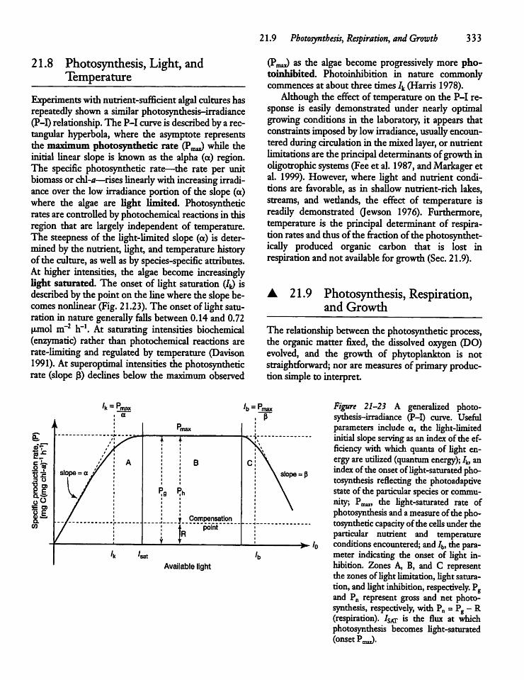
21.9 Photosynthesis, Respiration, andGrowth 333
21.8 Photosynthesis, Light, andTemperature
Experiments withnutrient-sufficientalgalcultureshasrepeatedly shown a similar photosynthesis-irradiance(P-I) relationship. The P-I curveis described bya rectangular hyperbola, where the asymptote representsthe maximum photosynthetic rate (Pmai) while theinitial linear slope is known as the alpha (a) region.The specific photosynthetic rate—the rate per unitbiomass or chl-a—rises linearlywithincreasing irradiance over the low irradiance portion of the slope (a)where the algae are light limited. Photosyntheticratesare controlledbyphotochemicalreactionsin thisregion that are largely independent of temperature.The steepness of the light-limited slope (a) is determined by the nutrient, Ught, and temperature historyofthe culture, asweU as byspecies-specific attributes.At higher intensities, the algae become increasinglylight saturated. The onset of Ught saturation (4) isdescribed bythepointon theUne where the slope becomes nonlinear (Fig. 21.23). The onsetofUght saturation in nature generaUy falls between 0.14 and 0.72pinol m~2 h"1. At saturating intensities biochemical(enzymatic) rather than photochemical reactions arerate-Umiting and regulated by temperature (Davison1991). At superoptimal intensities the photosyntheticrate (slope 3) declines below the maximumobserved
(Pmai) as the algae become progressively more pho-toinhibited. Photoinhibition in nature commonlycommences at about three times 7^ (Harris 1978).Although the effect of temperature on the P-I re
sponse is easily demonstrated under nearly optimalgrowing conditions in the laboratory, it appears thatconstraints imposed by lowirradiance, usually encounteredduringcirculation in themixed layer, or nutrientlimitations are the principal determinants of growthinoUgotrophic systems (Feeet al. 1987, andMarkager etal. 1999). However, where Ught and nutrient conditions are favorable, as in shaUow nutrient-rich lakes,streams, and wedands, the effect of temperature isreadily demonstrated Qewson 1976). Furthermore,temperature is the principal determinant of respirationrates andthusofthe fraction ofthe photosynthet-icaUy produced organic carbon that is lost inrespiration andnot available for growth (Sec. 21.9).
• 21.9 Photosynthesis, Respiration,and Growth
The relationship between thephotosynthetic process,the organic matter fixed, the dissolved oxygen (DO)evolved, and the growth of phytoplankton is notstraightforward; nor aremeasures ofprimary production simple to interpret.
'k = "max 'b- •max• a , P
i k p•max
& /! .^^^^ i i®T / Jr ^0«
%? ''/' !\o « ,/ i a : : b c: \*fi slope = a i ! \ slope =p3 O
w Pg Ph | \oO ; \£ o> i \
I* j j CompensationCO ; | point
Y T
'k /satAvailable light
'b
Figure 21-23 A generalized photo-sythesis-irradiance (P-I) curve. Usefulparameters include a, the Ught-limitedinitial slopeservingas an indexofthe efficiency with which quanta of Ught energyare utiUzed (quantum energy); 7banindex ofthe onsetofUght-saturated photosynthesis reflecting the photoadaptivestate ofthe particular species or community; PmiU, the Ught-saturated rate ofphotosynthesis and ameasure ofthephotosynthetic capacity ofthe cells under theparticular nutrient and temperatureconditions encountered; and/b, the parameter indicating the onset of Ught inhibition. Zones A, B, and C representthezones ofUght limitation, Ught saturation, and Ught inhibition, respectively. Pgand Pn represent gross and net photosynthesis, respectively, with Pn = Pg - R(respiration). ISKr is the flux at whichphotosynthesis becomes Ught-saturated(onset P,^.
334 CHAPTER 21 The Phytoplankton
The overaU and gready simplified photosyntheticequation:
6C02 +12H20^>QH1206 +6H20 +602EQ.21.3
shows that if only simple carbohydrates were produced,eachmole of C02 takenup would result in therelease ofonemoleof oxygen. In that case, the photosynthetic quotient (PQ)—defined as +02/-C02 byvolume—is 1.0 and the respiratory quotient (RQ =+C02/-02) would be unity as weU. However, mostrecordedPQs rangebetweenone and two (commonly~1.2). APQ higher than 1.0tellsus that algae typicaUysynthesize a mixture of carbohydrates, fats, and proteins rather than only carbohydrates.
Excess carbon is excreted when the rate of carbonfixation temporarily exceeds the rate atwhichit canbeeither converted to protoplasm or stored as carbohydrates in the limited physical space available—whengrowth rates and photosynthetic rates are not balanced. An analysis of marine and fresh water studiesshows that an average of -13 percent ofthe photosyn-thate is excreted, but that the extracellular release(ECR - p.g C l"1 hr"1) varies widely between three and41 percent among systems (Baines and Pace 1991).The carbonlost by ECR is naturaUy not available foralgal growth andmeasures of carbonuptake thereforeoverestimate the amount of carbon that is assimilatedand converted to protoplasm. While the released carbon is not available to the plants that produced it, itplays animportant role in thenutrition ofaquatic bacteria (Chapter 22). A second means bywhich photo-synthate becomes unavailable for growth is throughphotorespiration, a significant loss process when thephotosynthetic system is Ught saturated (atP^ orphotoinhibited (Harris 1978, Raven and BeardaU1981). The terms"carbonfixation," "production," and"photosynthesis" are here, and commonly elsewhere,used interchangeably but they do not have the samemeaning. Photosynthesis refers to the process only, grossproduction to the rateofcarbon fixation before respiration is taken into account, and netproduction refers tothe gross production rateminus respiration. Productionmakes nostatementastowhethergross or net production is measured. Carbon fixation refers simply to therate carbon is fixed per period, usuaUy measured bytheuptake of 14C02 during photosynthesis, butwithout claims as to its fate. The term primary productionrefers to the rate at which energy is stored by photosynthetic activity in the form of organic substances
which can be used as food (E. P. Odum 1959). It isused interchangeably withprimary productivity, whichonce referred to yield rather than rate. For techniquesused to measure primary production from dissolvedoxygen (DO) evolution or the uptake of radiocarbon(HI4C03) seeWetzel andLikens 2000.
CarbonAssimilation and RespirationWhile the ratio of carbon assimilation to respirationhas been shown to be greatest at low temperatures,respiration becomes increasingly more significant asthe temperature increases (Jewson 1976). The impU-cation is that a considerably higher photosyntheticrate is needed for a specified amount of growth (netproduction) at high temperatures. This conclusion isof considerable significance in interpreting phytoplankton growthunder poor Ught conditions in coolmetalimnia and in snow and ice-covered lakes. Thesame low Ught flux would be insufficient in warmerwater to compensate for a much higher respirationrate there.The gross carbon-fixation rateat the depthofmaxi
mumphotosynthesis (Pn^,Figs. 21-23and21-24)nor-mally greadyexceeds the algal respiration rate,but anappreciable fraction of the phytoplankton spend timeunderUght-limited conditions in the deeperportionsof the mixed layer. Thus, the phytoplankton community in Lunzer Lake, AT, was Ught-limited duringincubation below about 2 m, whereas it wasUght-limited at aU depths (except possibly at the verysurface) in highly eutrophic ZeUer Lake (AT, Fig.21-24). At some depth in the mixed layer, the grosscarbon-fixation rate (P) of the average ceU is reducedor even declines to zero. However, respiration (R) isunaffected and the depth-integrated net production(growth) for themixed layer asawhole may bemodest, even though the rates of net carbon fixation arehigh at the depth where photosynthesis is maximal(P,™,). Furthermore, for growth the carbon that isfixed during the day has to exceed the sum total ofdaytime andnighttime respiration.
21.10 PrimaryProductionin Nature
Production Patterns andTheir ModelingThe photosynthesis-irradiance relationship (P-I) observed for a particular species in the laboratory (Fig.
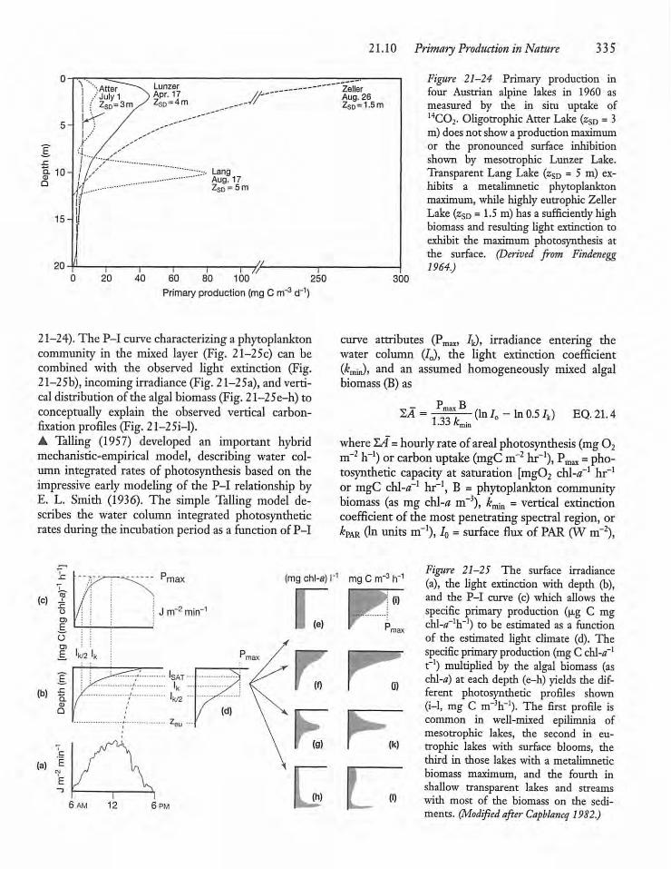
Lunzer/July 1 ) Apr. 17I ZSD=3m/ ZSD =4m .-J/-
LangAug. 17ZSd = 5 m
JL.i 7r100 250
-3 w-hPrimary production (mg C m"3 d
21-24).The P-I curve characterizinga phytoplanktoncommunity in the mixed layer (Fig. 21—25c) can becombined with the observed light extinction (Fig.21—25b), incoming irradiance (Fig. 21—25a), and verticaldistribution ofthe algalbiomass (Fig.21-25e-h) toconceptually explain the observed vertical carbon-fixation profiles(Fig. 21-25i-l).A Tailing (1957) developed an important hybridmechanistic-empirical model, describing water column integrated rates of photosynthesis based on theimpressive earlymodeling of the P-I relationship byE. L. Smith (1936). The simple Tailing model describes the water column integrated photosyntheticrates during the incubation period as a function ofP-I
21.10 Primary Production inNature 335
ZellerAug. 26ZSd= 1.5 m
300
Figure 21-24 Primary production infour Austrian alpine lakes in 1960 asmeasured by the in situ uptake of14C02. Oligotrophic Atter Lake (zSD = 3m) does not show a production maximumor the pronounced surface inhibitionshown by mesotrophic Lunzer Lake.Transparent Lang Lake (zSD = 5 m) exhibits a metalimnetic phytoplanktonmaximum, while highly eutrophic ZellerLake (zSD = 1.5 m) has a sufficientlyhighbiomass and resulting light extinction toexhibit the maximum photosynthesis atthe surface. (Derived from Findenegg1964.)
curve attributes (Pmax, 4), irradiance entering thewater column (I0), the Ught extinction coefficient(^min)> ana" an assumed homogeneously mixed algalbiomass (B) as
2A =B
1.33 k„(In 70 - In 0.5/k) EQ.21.4
where IA =hourlyrate ofareal photosynthesis (mg02m~2 fr1) or carbon uptake (mgC m-2 hr-1), Pmax =photosynthetic capacity at saturation [mg02 chl-a'1 hr"1or mgC chl-0"1 hr-1, B = phytoplankton communitybiomass (as mg ch\-a m~3), k^ = vertical extinctioncoefficient of the mostpenetrating spectral region, orkPAR (In unitsm"1), I0 = surface flux of PAR (VV m~2),
maxSZ --^--^_T__^<. PT-
(C Io
E.oO)
J
'k/2 Ik^ J""-""""^?E =IS^"^ /
Depth
X i
f
(mg chl-a) I"1 mgC rrf3 h"Figure 21-25 The surface irradiance(a), the light extinction with depth (b),and the P-I curve (c) which allows thespecific primary production (u.g C mgchl-^r'h"1) to be estimated as a functionof the estimated Ught climate (d). Thespecific primary production (mgC chl-a'1t"1) multiplied by the algal biomass (aschl-tf) at each depth (e-h) yields the different photosynthetic profiles shown(i-1, mg C m~3h-1). The first profile iscommon in well-mixed epilimnia ofmesotrophic lakes, the second in eutrophic lakes with surface blooms, thethird in those lakes with a metalimneticbiomass maximum, and the fourth inshallow transparent lakes and streamswith most of the biomass on the sediments. (Modified afterCapblancq 1982.)
J m 2 mirf
6 pm
r r^r i
(f) I 0)
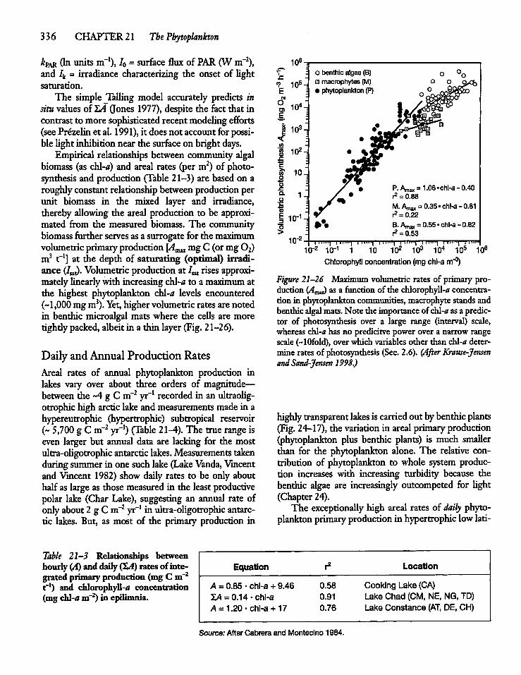
336 CHAPTER 21 The Phytoplankton
kPAR (In units m-1), 70 = surface flux of PAR (W m~2),and 4 = irradiance characterizing the onset of Ughtsaturation.The simple Jelling model accurately predicts in
situ values of YA (Jones 1977), despite the fact that incontrast to more sophisticated recent modelingefforts(seePrezelin et al. 1991), it doesnot account for possible Ught inhibitionnear the surfaceon bright days.Empirical relationships between community algal
biomass (as chl-a) and areal rates (per m2) of photosynthesis and production (Table 21-3) are based on aroughlyconstant relationshipbetweenproductionperunit biomass in the mixed layer and irradiance,therebyaUowing the areal production to be approximated from the measured biomass. The communitybiomass further serves asa surrogatefor the maximumvolumetricprimaryproduction [A^^mgC (ormg02)m3 f1] at the depth of saturating (optimal) irradiance (4at)- Volumetricproduction at 4>t rises approximatelylinearlywith increasingchl-a to a maximum atthe highest phytoplankton chl-a levels encountered(~1,000 mgm3). Yet, higher volumetric rates arenotedin benthic microalgal mats where the ceUs are moretighdy packed, albeit in a thin layer (Fig.21-26).
DailyandAnnual Production RatesAreal rates of annual phytoplankton production inlakes vary over about three orders of magnitude—between the ~4 g C m~2 yr"1 recorded in anultraoUg-otrophichigh arcticlakeandmeasurements madein ahypereutrophic (hypertrophic) subtropical reservoir(~ 5,700 g C m-2 yr-1) (Table 21-A). The truerange iseven larger but annual data are lacking for the mostultra-oUgotrophic antarctic lakes. Measurements takenduringsummer in one suchlake (Lake Vanda, Vincentand 'Vincent 1982) show daily rates to be only abouthalfas large as those measured in the least productivepolar lake (Char Lake), suggesting an annual rate ofonly about 2 g C m~2 yr-1 in ultra-oligotrophic antarctic lakes. But, as most of the primary production in
Equation
106-
105-
104-
103-
102.
10.
1.
10"1-
io-2-
o benthic algae (B)a macrophytes (M)• phytoplankton (P)
P-Amax= 1-06 'China -0.40r2= 0.88M-Amax= 0.35'chl-a-0.81^ = 0.22B. Amax =0.55 • chl-a - 0.82r2= 0.53
l in'"] 11mn] i in""] iiimn 11in'"! iiii»"| Mimm inib"2 io-1 1 10 102 103 104 io5 io6
Chlorophyll concentration (mg chl-am"3)
Figure 21-26 Maximum volumetric rates of primary production (AmJ) as a function of the chlorophyU-* concentration in phytoplankton communities, macrophyte standsandbenthicalgalmats.Note the importanceofchl-aasapredictor of photosynthesis over a large range (interval) scale,whereas chl-a has no predicitve power over a narrow rangescale (~10fold), over which variables other than chl-a determine rates of photosynthesis (Sec. 2.6). (After Krause-JensenandSand-Jensen 1998.)
highly transparent lakes iscarried out bybenthic plants(Fig. 24-17), thevariation in areal primary production(phytoplankton plus benthic plants) is much smaUerthan for the phytoplankton alone. The relative contribution of phytoplankton to whole system production increases with increasing turbidity because thebenthic algae are increasingly outcompeted for Ught(Chapter 24).The exceptionally high areal rates of daily phyto
plankton primary production in hypertrophic low lati-
LocationTable 21-3 Relationships betweenhourly (A) and daily(ZA) rates of integrated primary production (mgC m~2t"1) and chlorophyU-tf concentration(mgchl-am~2) in epilimnia.
A = 0.85 • chl-a + 9.46 0.58
2>4 = 0.14-chl-a 0.91
A = 1.20 -chl-a + 17 0.76
Cooking Lake (CA)Lake Chad (CM, NE, NG, TD)Lake Constance (AT, DE, CH)
Source: After Cabrera and Montecino 1984.
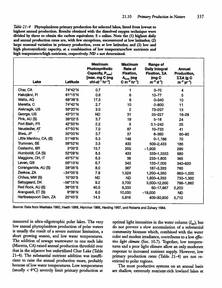
21.10 Primary Production inNature 337
Table 21-4 Phytoplankton primaryproduction for selected lakes, listed from lowest tohighest annual production. Results obtained with the dissolved oxygen technique weredivided by three to obtain the carbon equivalent.S => saline.Note the (1) highest dailyand annual production rates are, with few exceptions, encountered at low latitudes; (2)large seasonal variation in primary production, even at low latitudes; and (3) low andhigh photosynthetic capacity, at a combination of low temperature/low nutrients andhigh temperature/high nutrients, respectively.ND a not determined.
Maximum Maximum Range ofPhotosynthetic Rate of Daily Integral AnnualCapacity, Pmax; Fixation, Fixation, 2A Production,[max. mg C (mg AmaxOng (mgC 22A(gC
Lake Latitude chl-a)1 hr1] C nr3 hr1) nr2 d"1) nr2yr1)
Char, CA 74°42'N 0.7 1 0-70 4Hakojarvi, Fl 61°15'N 0.6 6 10-77 5Watts, AQ 68°36'S 17.3 6 0-340 10Meretta, C 74°42'N 2.7 10 0-800 11Aleknagik, US 59°20'N 3.0 2 73-207 13George, US 43°31'N ND 31 25-227 16-28Pink, AU (S) 38°02'S 3.7 19 5-18 24Port Bielh, FR 42°50'N 2.2 5 0.1-242 25Neusiedler, AT 47°50'N 7.0 87 10-733 41Biwa, JP 35°00'N 3.7 37 6-390 60-90LittleManitou, CA, (S) 51°48'N 5.3 146 0-1,188 70Trummen, SE 56°52'N 3.3 433 500-2,433 180Castanho, BR 3°00'S 15.7 200 -1,900 290Humboldt, CA (S) 52°09'N 8.5 433 333-1,3333 680Maggiore, CH, IT 45°57'N 6.3 38 233-1,800 365Leven, GB 56°10'N 6.7 343 133-7,000 340-620Corangamite, AU(S) 38°05'S 8.0 367 187-3,333 760Zeekoe, ZA ~34°05'S 7.9 1,524 1,200-4,350 860-1,000Chilwa, MW(S) 15°30'S ND ND 1,800-4,333 730-1,300Sobygaard, DK ~56°15'N 9.2 3,700 3,000-12,000 766-1,862Red Rock, AU (S) 38°05'S 40.0 6,333 60-17,667 2,200Aranguadi, ET (S) 9°39'N 6.0 10,000 -19,000 NDHartbeespoort Dam, ZA 25°45'S 14.3 5,916 400-30,900 5,712
Source: Data from Westlake 1980, Heath 1988, Hammer 1986, Harding 1997, and Robarts and Zohary 1984.
measured in ultra-oUgotrophic polar lakes. The verylow annual phytoplankton production of polarwatersis usuaUy the result of a severe nutrient limitation, ashort growing season, and low water temperatures.The addition of sewage wastewater to one such lake(Meretta, CA) raised annual productionthreefold overthat in the adjacent but unfertiUzed CharLake (Table21-4). The substantial nutrient addition was insufficient to raise the annual production more, probablybecause oflowwater temperatures. Low temperatures(usuaUy < 4°C) severely limit primary production at
optimal Ught intensities in thewatercolumn (4„), butdo not prevent a slow accumulation of a substantialcommunity biomasswhich, combined with the watercolor and modest irradiance, contributes toalow effective light climate (Sec. 10.7). Together, low temperatures anda poorUght climate aUow an onlymoderateresponse to increased nutrient supply. However, lowprimary production rates (Table 21-4) are not restrictedto polar regions.The most productive systems on an annual basis
are shaUow, extremely nutrient-rich lowland lakes at
338 CHAPTER 21 The Phytoplankton
lowlatitudes.The combinationof a variable but year-round high irradiance and shaUow water column'syields a high effective Ught cUmate. This, combinedwithhighwatertemperatures andhighnutrient levels,yields a very high biomass and results in high arealproduction rates. The highest production ratesrecorded at the depth of optimal irradiance (1^,)are the product of a high photosynthetic capacity—also known as the assimilation number [mgC (mgchl-tf)"1 hr-1]—and an exceptionaUy high biomass(Table 21-4).
Hypertrophic LakesCertain shaUow saline lakes are among the most productive lakes globaUy, but Hartbeespoort, a SouthAfrican freshwater reservoir, appears to be the mostproductive lake on record (Table 21-4). A combination ofhighyear-roundirradiance, high temperatures,largewastewater loading into a shallow mixed layerpermit the extraordinarily high depth-integrated production rates observed.High water temperatures in inland waters at low
latitudes aUow a high rate ofmicrobial decompositionand recycling of nutrients contained within the organic matter respired, making them quickly availablefor uptake and growthby the algae. In the temperatezone, the ideal growing conditions are most closelyapproached in shallow but hypertrophic lakes (e.g.,LakeSobygaard, DK) in summer (Table 21-4). Evenso, lower water temperatures and a resulting lowerPmax appear to be responsible for distincdy smaUerdaily rates(Table 21-4) than for their tropical counterparts(Osborne1991,Jeppesenet al. 1997a). On anannual basis, the lower annual depth-integratedproduction rates in hypertrophic temperate zoneandhighlatitudelakes are primarily attributable to a combination of a longwinterperiod of lowirradiance andlowwater temperatures.
Photosynthetic EfficiencyThe efficiency (%)of light utiUzation, the photosynthetic efficiency, of aquatic plants in whole systemscan be obtained by dividing the photosyntheticaUystored energy on an areal basis (g C m"2 d-1) by thephotosyntheticaUy available energy (PAR, u.mol m~2d"1) after converting to comparable energy units.Computed phytoplankton efficiencies are typicaUyweU below one percent, but reach to between one andfour percent in shallow eutrophic systems (Harding
1997). The one percent valuebasedon phytoplanktonisa largeunderestimate ofwholesystem efficiencies inclearoUgotrophic lakes wheremost ofthe productionis contributed bybenthicplants(Fig. 24-17).Evenso,Ught scattering and absorption in water columns islarge enough to reduce the photosynthetic efficiencyof highly productive aquatic systems to well belowthat encountered on land.
21.11 Production:Biomass (P:B) Ratiosand Specific Growth Rates inNature
The P:B ratio is defined as the ratio ofcarbon fixed (P)to phytoplankton biomass, expressed ascarbon(B) perunit time. It provides a useful measure of the rate atwhich algal carbonturns over. The P:Bcomplementsthe photosynthetic capacitywhichexpresses the abiUtyor potential to fix carbon per unit of chlorophyU-tf[mg C (mg chl-a)~l t"1]. From summer measurementsofthe P:BandP:chl-a ratios in mixed layerssomeimportantgeneraUties have emerged:
1. The average P:B ratio in mixed layers is high intransparent oUgotrophic systems (Fig. 21-27), andis lowwithin and amongaquaticsystems when thecommunity biomass is high (eutrophic waters).Low ratios in eutrophic waters imply a low productivity per unit biomass or chlorophyll-^(Tereshenkova 1985). Lowaverage specific growthratesfurther implythat lossratesmust also be lowto allow the highbiomass to bemaintained.
2. The normaUy high P:Bobserved in nutrient-poortransparent waters commonly dominated by smaUspecies (Fig. 21-27) impUes a rapid recycling ofbothorganic matter and the nutrients in high demand. Rapid recycling further requires an efficientcoupUng between the phytoplankton, their zooplankton grazers, andassociated microbes.
3. A reduced community P:B under conditions ofhighphytoplankton biomass is primarily attributable to a poor effective Ught climate, which is theresultof self shading. Light limits the growth rateof the individuals and the community, not nutrients. Superimposed is the reduced growth potential of the typicaUy large-sized phytoplanktonspecies dominating most eutrophic lakes andslowly flowing rivers (see Fig. 21-13). While thecommunity P:B declines withincreasing selfshad-
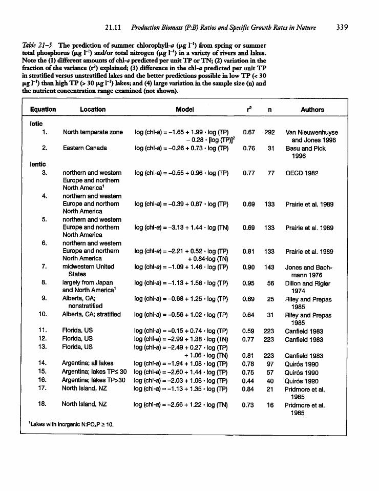
21.11 Production Biomass (P:B) Ratios andSpecific Growth Rates inNature
Table 21-5 The prediction of summer chlorophyU-a (pg l"1) from springor summertotal phosphorus (p.g l"1) and/ortotal nitrogen (p.g \~l) in a variety of rivers and lakes.Note the (1) different amounts ofchl-a predicted per unitTP or TN; (2) variation in thefraction of the variance (r2) explained; (3) difference in the chl-a predicted per unit TPin stratified versus unstratified lakes and the better predictions possible in low IT (< 30|tg l-1) thanhighTP (> 30 u-g I"1) lakes; and(4) large variation in the sample size (n) andthe nutrient concentration range examined (not shown).
339
Equation Location Model r2 n Authors
lotic
1. North temperate zone log (chl-a) = -1.65+ 1.99-log (TP)- 0.28 • [log (TP)]2
0.67 292 Van Nieuwenhuyseand Jones 1996
2. Eastern Canada log (chl-a) = -0.26 + 0.73 • log (TP) 0.76 31 Basu and Pick1996
lentic
3. northern and westernEurope and northernNorth America1
log (chl-a) = -0.55 + 0.96 • log (TP) 0.77 77 OECD 1982
4. northern and westernEurope and northern log (chl-a) = -0.39 + 0.87 • log (TP) 0.69 133 Prairie etal. 1989North America
5. northern and westernEurope and northern log (chl-a) = -3.13+ 1.44-log (TN) 0.69 133 Prairie etal. 1989North America
6. northern and westernEurope and northern log (chl-a) = -2.21 + 0.52 • log (TP) 0.81 133 Prairie etal. 1989North America + 0.84-log (TN)
7. midwestern UnitedStates
log (chl-a) = -1.09 + 1.46- log (TP) 0.90 143 Jones and Bach-mann 1976
8. largely from Japanand North America1
log (chl-a) = -1.13 + 1.58- log (TP) 0.95 56 Dillonand Rigler1974
9. Alberta, CA;nonstratified
log (chl-a) = -0.68 + 1.25- log (TP) 0.69 25 Riley and Prepas1985
10. Alberta, CA; stratified log (chl-a) = -0.56 + 1.02- log (TP) 0.64 31 Riley and Prepas1985
11. Florida, US log (chl-a) = -0.15+ 0.74-log (TP) 0.59 223 Canfield 198312. Florida, US log (chl-a) = -2.99+ 1.38-log (TN) 0.77 223 Canfield 198313. Florida, US log (chl-a) = -2.49 + 0.27 • log (IP)
+ 1.06-log (TN) 0.81 223 Canfield 198314. Argentina; all lakes log (chl-a) = -1.94 + 1.08- log (TP) 0.78 97 Quiros 199015. Argentina; lakes TP< 30 log (chl-a) = -2.60+ 1.44-log (TP) 0.75 57 Quiros 199016. Argentina; lakes TP>30 log (chl-a) = -2.03+ 1.06-log (TP) 0.44 40 Quiros 199017. North Island, NZ log (chl-a) = -1.13 + 1.35- log (TP) 0.84 21 Pridmore et al.
198518. North Island, NZ log (chl-a) = -2.56+ 1.22-log (TN) 0.73 16 Pridmore et al.
1985
1Lakes with inorganic N:P04P £ 10.
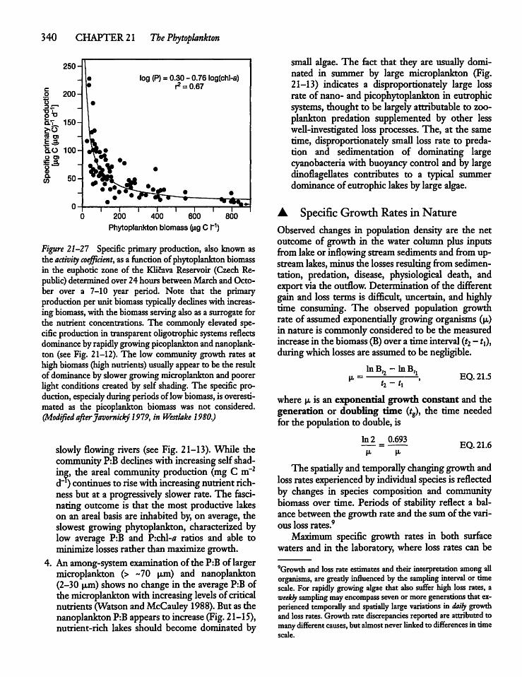
340 CHAPTER 21 Tfo Phytoplankton
250-
!• log (P) = 0.30 - 0.76 log(chl-a)c r2 = 0.67o 200-
S" I •"OUOTJ
Q.T 150-
2 O) -
I"3, •\Q.O 100- «(!••
Specificeno
•
n•~ v-« %*v^
(i i
) 200i i i i i i
400 600 800
Phytoplankton biomass fag C l~1)
Figure 21-27 Specific primaryproduction, also known asthe activity coefficient, asa function of phytoplankton biomassin the euphoric zone of the KUcava Reservoir (Czech Re-pubUc) determinedover24hours betweenMarch andOctober over a 7-10 year period. Note that the primaryproductionper unit biomass typicaUy declines with increasing biomass, with the biomass serving also asa surrogate forthe nutrient concentrations. The commonly elevated specificproduction in transparent oUgotrophic systems reflectsdominance byrapidlygrowingpicoplankton andnanoplankton (see Fig. 21-12). The low community growth rates athigh biomass (highnutrients)usually appearto be the resultof dominance byslowergrowingmicroplankton and poorerUght conditions created by self shading. The specific production,especialy during periodsof lowbiomass, is overestimated as the picoplankton biomass was not considered.(Modified afterJavornicky1979, in Westlake 1980.)
slowly flowing rivers (see Fig. 21-13). Wrule thecommunity P:B declines with increasing selfshad-
-2ing, the areal community production (mg C id-') continues to risewithincreasing nutrientrichness but at a progressively slower rate. The fascinating outcome is that the most productive lakeson an areal basis are inhabited by, on average, theslowest growing phytoplankton, characterized bylow average P:B and P:chl-a ratios and able tominimizelosses rather than maximize growth.Anamong-system examination ofthe P:Bof largermicroplankton (> ~70 u.m) and nanoplankton(2-30 p,m) shows no change in the average P:B ofthe microplankton with increasing levels of criticalnutrients (WatsonandMcCauley 1988). But as thenanoplankton P:Bappearsto increase(Fig.21-15),nutrient-rich lakes should become dominated by
m
smaU algae. The fact that they are usuaUy dominated in summer by large microplankton (Fig.21-13) indicates a disproportionately large lossrate of nano- and picophytoplankton in eutrophicsystems, thought to be largely attributable to zooplankton predation supplemented by other lessweU-investigated loss processes. The, at the sametime, disproportionately small loss rate to predation and sedimentation of dominating largecyanobacteria with buoyancy control and by largedinoflageUates contributes to a typical summerdominance of eutrophic lakesby large algae.
A SpecificGrowth Rates in NatureObserved changes in population density are the netoutcome of growth in the water column plus inputsfromlakeor inflowingstream sedimentsand fromupstreamlakes, minus the losses resultingfromsedimentation, predation, disease, physiological death, andexportvia the outflow. Determinationof the differentgain and loss terms is difficult, uncertain, and highlytime consuming. The observed population growthrate of assumed exponentiaUy growing organisms (u,)in nature is commonlyconsideredto be the measuredincrease in the biomass (B) over a time interval (r2 -1{),duringwhichlosses are assumed to be negUgible.
u.=
lnBfr-lnBtlEQ. 21.5
where p, is an exponential growth constant and thegeneration or doubling time (fg), the time neededfor the population to double, is
ln2 0.693EQ.21.6
The spatially and temporally changing growthandloss ratesexperienced byindividual species is reflectedby changes in species composition and communitybiomass over time. Periods of stabiUty reflect a balance between the growth rate and the sum ofthe various loss rates.9Maximum specific growth rates in both surface
waters and in the laboratory, where loss rates can be
'Growth and lossrate estimates and their interpretation amongallorganisms, are greatly influenced by the sampling interval or timescale. For rapidly growing algae that also sufferhigh loss rates, aweekly sampling mayencompass seven ormoregenerations thatexperienced temporally and spatially large variations in daily growthand loss rates. Growthrate discrepancies reported are attributed tomanydifferent causes, butalmost never linked to differences in timescale.
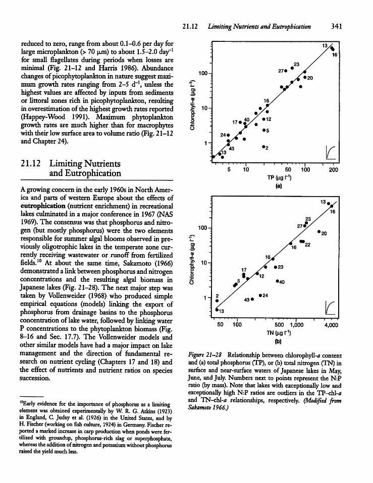
reducedto zero, range from about 0.1-0.6 per dayforlarge microplankton (> 70 pjn) to about1.5-2.0 day-1for smaU flageUates during periods when losses areminimal (Fig. 21-12 and Harris 1986). Abundancechanges of picophytoplankton in nature suggestmaximum growth rates ranging from 2-5 d"1, unless thehighest values are affected by inputs from sedimentsor Uttoral zones rich in picophytoplankton, resultingin overestimation ofthe highestgrowth ratesreported(Happey-Wood 1991). Maximum phytoplanktongrowth rates are much higher than for macrophyteswiththeir lowsurface areato volume ratio (Fig. 21-12and Chapter 24).
21.12 Limiting Nutrientsand Eutrophication
Agrowingconcern in the early 1960sin North America and parts of western Europe about the effects ofeutrophication (nutrient enrichment) in recreationallakes culminated in a majorconference in 1967 (NAS1969). The consensus was that phosphorus and nitrogen (but mosdy phosphorus) were the two elementsresponsible forsummer algal blooms observed in previously oUgotrophic lakes in the temperate zone cur-rendy receiving wastewater or runoff from fertilizedfields.10 At about the same time, Sakamoto (1966)demonstrated a link between phosphorus and nitrogenconcentrations and the resulting algal biomass inJapanese lakes (Fig. 21-28). The nextmajor stepwastaken byVoUenweider (1968) who produced simpleempirical equations (models) Unking the export ofphosphorus from drainage basins to the phosphorusconcentration of lake water, followed byUnking waterP concentrations to the phytoplankton biomass (Fig.8-16 and Sec. 17.7). The Vollenweider models andothersimilar models have hadamajor impact on lakemanagement and the direction of fundamental research on nutrient cycling (Chapters 17 and 18) andthe effect of nutrients and nutrient ratios on speciessuccession.
l0Early evidence for the importance of phosphorus as alimitingelement was obtained experimentally by W. R. G. Atkins (1923)in England, C. Juday et al. (1926) in the United States, and byH. Fischer (working on fish culture, 1924) in Germany. Fischer reported amarked increase in carp production when ponds were fertilized with groundup, phosphorus-rich slag or superphosphate,whereas theaddition ofnitrogen and potassiumwithout phosphorusraised the yieldmuch less.
21.12 LimitingNutrients andEutrophication 341
100-
1
a8o
o
2
a.
8oJCO
10r
T 1—i i • • ' ' | 1 r50 100 200
TP (ug I"1)(a)
; 13 v- /16
100-
23
2ll/•20
- ^e"2210-
#;17
164
•12• 23
•40
1- 2 y• /
•13™-
43*
r
• 24
• 'i 1—I—f50 100 500 1,000 4,000
TN (ug I"1)(b)
Figure 21-28 Relationship between chlorophyU-* contentand (a) total phosphorus (TP), or (b) total nitrogen (TN)insurface and near-surface waters ofJapanese lakes in May,June, andJuly. Numbers next to points represent the N:Pratio (bymass). Note that lakes withexceptionaUy lowandexceptionaUy high N:P ratios are oudiers in the TP-chl-*and TN-chl-tf relationships, respectively. (Modified fromSakamoto 1966.)
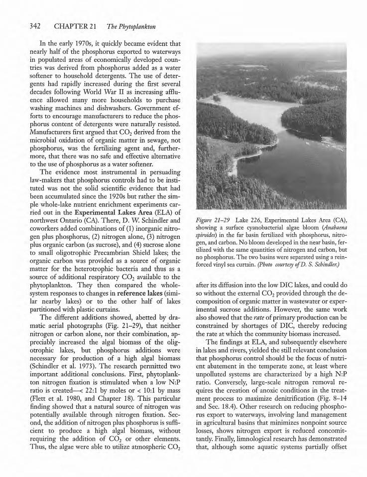
342 CHAPTER 21 The Phytoplankton
In the early 1970s, it quickly became evident thatnearly half of the phosphorus exported to waterwaysin populated areas of economically developed countries was derived from phosphorus added as a watersoftener to household detergents. The use of detergents had rapidly increased during the first severaldecades following World War II as increasing affluence allowed many more households to purchasewashing machines and dishwashers. Government efforts to encourage manufacturers to reduce the phosphorus content of detergents were naturally resisted.Manufacturers first argued that C02 derived from themicrobial oxidation of organic matter in sewage, notphosphorus, was the fertilizing agent and, furthermore, that there was no safe and effective alternativeto the use of phosphorus as a water softener.The evidence most instrumental in persuading
law-makers that phosphorus controls had to be instituted was not the solid scientific evidence that hadbeen accumulated since the 1920s but rather the simple whole-lake nutrient enrichment experiments carried out in the Experimental Lakes Area (ELA) ofnorthwest Ontario (CA). There, D. W. Schindler andcoworkers added combinations of (1) inorganic nitrogen plus phosphorus, (2) nitrogen alone, (3) nitrogenplusorganic carbon (assucrose), and (4) sucrosealoneto small oligotrophic Precambrian Shield lakes; theorganic carbon was provided as a source of organicmatter for the heterotrophic bacteria and thus as asource of additional respiratory C02 available to thephytoplankton. They then compared the whole-system responses to changes in reference lakes (similar nearby lakes) or to the other half of lakespartitioned with plastic curtains.The different additions showed, abetted by dra
matic aerial photographs (Fig. 21-29), that neithernitrogen or carbon alone, nor their combination, appreciably increased the algal biomass of the oligotrophic lakes, but phosphorus additions werenecessary for production of a high algal biomass(Schindler et al. 1973). The research permitted twoimportant additional conclusions. First, phytoplankton nitrogen fixation is stimulated when a low N:Pratio is created—< 22:1 by moles or < 10:1 by mass(Flett et al. 1980, and Chapter 18). This particularfinding showed that a natural source of nitrogen waspotentially available through nitrogen fixation. Second, the addition of nitrogen plus phosphorus is sufficient to produce a high algal biomass, withoutrequiring the addition of C02 or other elements.Thus, the algae were able to utilize atmospheric C02
Figure 21-29 Lake 226, Experimental Lakes Area (CA),showing a surface cyanobacterial algae bloom {Anabaenaspiroides) in die far basin fertilized with phosphorus, nitrogen, and carbon. No bloom developedin the near basin, fertilized with the same quantities of nitrogen and carbon, butno phosphorus. The two basins were separated using a reinforced vinyl sea curtain. (Photo courtesy ofD. S. Schindler.)
after its diffusion into the low DIC lakes, and could doso without the external C02 provided through the decomposition of organic matter in wastewater or experimental sucrose additions. However, the same workalsoshowed that die rate of primary production can beconstrained by shortages of DIC, thereby reducingthe rate at which the community biomass increased.The findings at ELA, and subsequently elsewhere
in lakes and rivers, yielded the still relevant conclusionthat phosphorus control should be the focus of nutrient abatement in the temperate zone, at least whereunpolluted systems are characterized by a high N:Pratio. Conversely, large-scale nitrogen removal requires the creation of anoxic conditions in the treatment process to maximize denitrification (Fig. 8-14and Sec. 18.4). Other research on reducing phosphorus export to waterways, involving land managementin agricultural basins that minimizes nonpoint sourcelosses, shows nitrogen export is reduced concomit-tandy. Finally, limnological research has demonstratedthat, although some aquatic systems partially offset
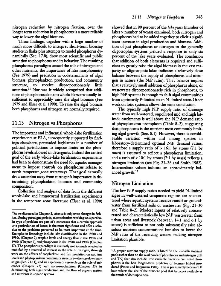
nitrogen reduction by nitrogen fixation, over thelonger term reduction in phosphorus is a more reUablewayto lower the algal biomass.These findings, together with a large number of
much more difficult to interpret short-term bioassaystudies in flasks plusattempts to modelphosphorus dynamically (Sec. 17.8), drewmost scientific and publicattentionto phosphorus and its behavior. The resultingphosphorus paradigm causedthe role of nitrogen andother nutrients, the importance of lakemorphometry(Fee 1979) and predation as codeterminants of algalbiomass, phytoplankton production, and communitystructure, to receive disproportionately Utdeattention.11 Nor was it widely recognized that additionsofphosphorusalone towhole lakesare usuaUy insufficient to appreciably raise the algal biomass (Fee1979 and Elser et al. 1990). To raise the algal biomassboth phosphorus andnitrogenare normaUy required.
21.13 Nitrogen vs Phosphorus
The important and influential whole-lake fertilizationexperiments at ELA, subsequently supported by findings elsewhere, persuaded legislators in a number ofpoUtical jurisdictions to impose limits on the phosphorus levels aUowed in detergents. Indeedthe centralgoal of the early whole-lake fertihzation experimentshadbeen todemonstrate theneed foraquatic management to impose controls on phosphorus release tonorth temperate zonewaterways. That goalnaturallydrew attentionaway fromnitrogen's importance in de-tennining phytoplankton biomass and communitycomposition.CoUection and analysis of data from the different
whole-lake and limnocorral fertilization experimentsin the temperate zone Uterature (Elser et al. 1990)
"Aswediscussed inChapter 2,science issubject tochanges in fashion. During paradigm periods, mostscientists working onaparticular typeof problem are part of a consensus thata certain approachor a particular set of issues, is the most significant andoffer a solution to the problems perceived to be most important at the time.Examples in limnologyinclude lake classification in the 1920s and1930s, (Chapter 2), trophic levels andenergy flow in the 1950s and1960s (Chapter 2), and phosphorus inthe 1970s and 1980s (Chapter17). The phosphorus paradigm iscurrendy not somuch rejected asmodified by a renewal of interest in the role of nitrogen, throughwork on theeffects of zooplankton and fish predation onnutrientlevels and phytoplankton community structure—the top-down paradigm (Sec. 23.11), andanexplosion of research on the roleof microbes (Chapter 22) and microzooplankton (Chapter 23) indetermining bothalgal production and the flow of organic matterandnutrientsin aquatic systems.
21.13 Nitrogen vsPhosphorus 343
showed that in 80 percent ofthe lakeyears (number oflakes x number of years) examined, both nitrogen andphosphorus had to be addedtogether to eUcit a significant increase in algal production and biomass. Addition of just phosphorus or nitrogen to the generallyoUgotrophic systems yielded a response in only sixpercent of the lake years evaluated. The conclusionthat addition of both elements is required and sufficient to gready raise the algal biomass in the vast majority of oUgotrophic lakes indicates a relatively closebalance between the supply of phosphorus and nitrorgen in nature (the N:P ratio). That balance impUesthat a relatively smaU additionof phosphorusalone, orwastewater disproportionately rich in phosphorus, tohighN:P systems is enough to shift algal communitiesfromaprimarilyP-Umited to anN-limited state.Otherwork on lotic systemsaUows the same conclusion.The typicaUy high N:P supply ratio of drainage
waterfromweU-watered, unpollutedmid andhigh latitude catchments is weU above the N:P demand ratioof phytoplankton protoplasm (Table 8-2), suggestingthat phosphorus is the nutrientmostcommonly limiting algal growth (Sec. 8.1).However, there is considerable variation within and among species inlaboratory-determined optimal N:P demand ratios,therefore a supply ratio of > 16:1 by atoms (7:1 bymass) is assumed to reflect a phosphorus limitation,anda ratioof < 10:1 by atoms (7:1 bymass) reflects anitrogen limitation (see Fig. 21-28 and Smith 1982).Intermediate values indicate an approximately balanced growth.12
Nitrogen LimitationThe low N:P supply ratios needed to yield N-limitedalgae in weU-watered temperate regions are encountered where aquatic systems receive runoffor groundwater from fertiUzed soils or wastewater (Fig. 21-30and Table 8-2). Modest inputs of relatively concentratedand characteristicaUy lowN:P wastewater fromurban areas and Uvestock (between 14:1 and 6:1 byatoms) is sufficient to not only substantiaUy raise absolute nutrient concentrations but also to lower theN:P ratio of the receiving waters, making nitrogenlimitation plausible.
12A proper nutrient supply ratio is based on theavailable nutrientpools rather than onthe total pools of phosphorus and nitrogen (TPand TN) thatalso include Utde available fractions. Yet, total phosphorus is the best longer-term predictor of biomass (chl-a) produced (Peters and Bergmann 1982). This ispresumably becauseTPbestreflects the sizeof the nutrientpool that becomes available asthe result of decomposition.
344 CHAPTER 21 The Phytoplankton
N:P (by mass)250 75 25 9 5
100
Total phosphorus fag l~1)1,000
Figure 21-30 Relationship betweenmeansummerTNandTP concentrationsin epilimneticwaters of largelytemperate zonewaters. The average trend in the data (soUd Une)was estimated using a LOcaUy WEighted SequentialSmoothing (LOWESS) technique. The thin black linesshowN:P ratios of selectedpotential nutrient sources to thelakes. Multiply by 2.21 to obtain molar (atomic) N:P ratios.Note the typicaUy highN:P ratio in runofffromunfertiUzedfields and forests and the progressive decline in the N:Pratio towards highlyeutrophic(highTP) systems, wheretheratio increasingly resembles manure seepage and wastewater. (After Downing andMcCauley 1992.)
• The slopeofthe relationshipbetweenTN andTPconcentrations is typicaUy smaUer than unity (Fig.21-30) and it is evident that the TN:TP ratio declinesamong aquatic systems as TP levels rise. The UkeU-hoodof anN:P supply ratiounable to satisfy the algaldemand ratio for nitrogen is greatest for eutrophicsystems (TP > -30-100 u,g l"1) (Downing and McCauley 1992) and for oUgotrophic semiarid zone systems that receive exceptionally Utde fixed nitrogenfromtheir poorlyvegetated catchments or the atmosphere (Sec. 18.1).The importance ofTN in predicting algal biomass
in highly eutrophic systems was demonstrated byPrairie et al. (1989)who showed the correlation betweenTP and chl-aconcentrationsto be greadyinfluenced by TN at high phosphorus concentrations(> -60 u,g P l"1), suggesting a primary nitrogen limitation. The effect of nitrogen was insignificant at lowTP concentrations (oUgotrophic systems). Although
nitrogen Umitation becomes more probable in highlyeutrophic systems (Fig. 21-30), the self shadingproduced bya highalgal biomass increases the possibiUtyof Ught limitation, not nutrient Umitation, in turbidwaters. Finally, theN:P ratio decUnes sharplywith increasing salinity in North American lakes, suggestingthat TN is the limitingnutrient in more highlysaline(semi-arid zone) waters (Chow-Frazer 1991).The Uterature shows that the possibiUty of a pri
mary nitrogen Umitation is higherin oUgotrophic waters at lower latitudes than in the temperate zone.LowN:P districts are found in subtropical Florida (US),wheremany lakes and streams are locatedon marinesediments high in phosphorus(Canfield 1983). Semi-arid zone tropicaland temperate reservoirs (Sec. 29.6)and streams, as weU as a variety of tropical SouthAmerican lakes (Setaro and Melack 1984) have N:Psupply ratios suggesting primary nitrogen Umitation.Lebo et al. (1994) and Lewis (2000) hypothesize thatlowlatitudelakes maybemore prone to nitrogen limitationas the resultofyear-roundhighwater temperatures and a resulting high denitrification at theoxic-anoxic interfaceof the typicaUy anoxic hypolimnia of tropical lakes (Sees. 15.2 and 18.4). However,other low latitude lakes appear to be either phosphorus limited or have an N:P supply ratio close to thealgae demand ratio (Tailing andLemoalle 1998).
Other Limiting FactorsPhosphorus and nitrogenwere the only twonutrientsnecessary to gready increase growth rates and community biomass in -80 percent of the oUgotrophicfreshwater lake fertiUzation experiments in whichboth elementswere added (Elser et al. 1990), but therewas no growth response in the remaining 20 percentofthe lake years examined. This lackof response mayhave been attributable to a nutrient limitation by elements other than nitrogen and phosphorus. Short-term bioassays in flasks have variously pointed to Fe,Co, Mn, Mo, or S as the most probable candidates. AUmitation by one or more of these elements is mostplausible where the N:P supply ratio approaches thedemand ratio of the plants (Forsberg and Ryding1980, Healeyand Hendzel 1980). An iron Umitationhas been demonstrated in the central Pacific Oceanand an occasional iron Umitation in Lake Erie (CA,US) is suggested bybioassay experiments (Twiss et al.2000). Other possible reasons for the lack of responseto the additionofN and P includeprimaryUght limitation in humic or turbid lakes, or an abundance of
21.14 EmpiricalNutrient-Phytoplankton Relationships 345
large herbivores able to prevent an algal biomass response. Even so, algal species differ somewhat in theirN:P demand ratio and diatoms are further dependenton a siUca availabiUty. Consequendy,changes in nutrient ratios in nature can be expected to affect thespecies composition even when the community biomass is constrained by phosphorus and nitrogen.
• 21.14 EmpiricalNutrient-PhytoplanktonRelationships
The external nutrient supply which plays sucha central role in predicting the growing-season algalcommunity biomass and production of inland watersis usuaUy overwhelmingly obtained from drainagebasins via streams and rivers (Fig. 5-15). Exceptionsinclude lakes and wedands with a particularly lowdrainage ratio (CA:LA) receiving most nutrients viathe atmosphere, or low latitude lakes with higherratios but subject to so much catchment and streamevapotranspiration that the receiving lakes andwetlands are primarily dependent on directprecipitation on the water surface(Chapter 8 and Sec.9.5).FinaUy, wedands andthose lakes located in exceptionaUydeep, porous drainage basins receive most of theirwater anda significant portionof theirnutrientsupplyfrom groundwater rather than from inflowingstreams.
The importance ofdrainage basins was recognizedby E.Naumann (SE) at thebeginning ofthe20th century (Chapter2); quaUfied by Pearson (GB); and for-maUzed by D. S. Rawson (CA), whose findingsstimulated R.VoUenweider andothersto develop simple quantitative models linking the phytoplanktonbiomass to theexternalsupply oftotal phosphorus (Sec.17.7). Butmostempirical models onlylinkaverage TPorTN concentrations in streams or lakes to theaveragealgal biomass {chl-a) because concentrationmeasurements aremuch simpler thanobtaining nutrientloading estimates from the land and atmosphere (Fig.21-28). See Table 21-5 fora small sample ofthe manyempiricalnutrient-biomass models.The equations and plots in Table 21-5 predict
widely varying amounts of chlorophyll-^ per unit ofnutrient. Differences in the regression slopes, theintercepts, and the data scatter have received considerable attention, but remain poorly resolved. However, it is evident that lakes and rivers differ toomuch among regions for thereto bea single empirical
model characterizing the relationship everywhere.Considerable among-systemvariation in the relationship between the total phosphorus concentration(or its covariate, total nitrogen concentration, Table9-1) and the algal biomass (aschl-a) is partiaUy the result of differences in temporal, spatial, and range(interval) scales. Differences in cUmate, lake morphometry, nutrient supply, and biological interactionsaddmuch additional variation. This is particularly evident fromArgentinean workin which groups of lakesdiffering in their trophic status, animal biota, and sediment respiration yieldeda varietyof lake type specificmodels (Tables 21-5 and 21-6). Some models (Table21-5) are based on individual data points, otherson summer data only, while yet others representannual averages.13 PossibiUties and limitations ofsteady-state regression modelssuch as those in Tables21-5 and 21-6 are discussed in Sec. 17.7.
The TP-chl-0 RelationshipandAquaticManagementEmpirical total phosphorus-chlorophyll-^ relationships arewidely used in research andaquatic management, but several precautions should be noted:
1. The relationships are onlyappUcable to primarilyphosphorus-deficient systems and should not beused if the phytoplankton yield is largely constrained bysome other factor (e.g., light, nitrogen,flushing).
2. The relationships are not precise, as is evidentfrom the scatter around the regression slopes(Figs. 8-16 and 21-28).The empirical models reflect theaverage behavior of the systems examinedand cannot be used to predict how changes inphosphorus loading or phosphorus concentrationwill change the algal biomass in particular water-bodies. If individual waterbodies are to be managed, available system-specific information should
''Laboratory and among-system field studies have long appreciatedthepower of resolution gained byallowing thevariable(s) of interest, whether it is lake or river size, nutrient supply in chemostats,fish predation in limnocorrals, or nutrient concentrations amonglakes or rivers, to vary gready while holding other environmentalvariables relatively or absolutelyconstant. Studies further differ inspatial andtemporal scale andit isnot at allsurprising that thereisalotofdisagreement about thegenerality ofinterpretations made andconclusions drawn.
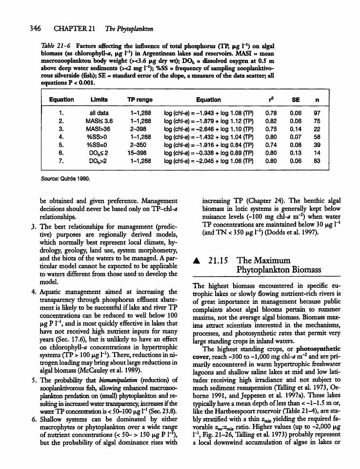
346 CHAPTER 21 The Phytoplankton
Table 21-6 Factors affecting the influence of total phosphorus (TP, p.g l"1) on algalbiomass (as chlorophyU-tf, iig I"1) in Argentinean lakes and reservoirs. MASI = meanmacrozooplankton body weight (><3.6 p.g dry wt); DOb ° dissolved oxygen at 0.5 mabove deepwater sediments (><2 mg l"1); %SS =frequency of sampling zooplanktivorous silverside (fish); SE =» standard error ofthe slope, a measure ofthe data scatter; aUequations P < 0.001.
Equation Limits TP range Equation r2 SE n
1. all data 1-1,288 log (chl-a) = -1.943 + log 1.08 (TP) 0.78 0.06 97
2. MASI< 3.6 1-1,288 log (chl-a) = -1.879 + log 1.12 (TP) 0.82 0.06 75
3. MASI>36 2-398 log (china) = -2.646 + log 1.10 (TP) 0.75 0.14 22
4. %SS>0 1-1,288 log (chl-a) = -1.432 + log 1.04 (TP) 0.80 0.07 58
5. %ss=o 2-350 log (china) = -1.916 + log 0.84 fTP) 0.74 0.08 39
6. DOb£2 15-398 log (chl-a) = -0.338 + log 0.89 (TP) 0.80 0.13 14
7. D0b>2 1-1,288 log (china) = -2.045 + log 1.06 (TP) 0.80 0.06 83
Source: Quirds 1990.
be obtained and given preference. Managementdecisions should never be basedonly on TP-chl-tfrelationships.
3. The best relationships for management (predictive) purposes are regionaUy derived models,which normaUy best represent local climate, hydrology, geology, land use, system morphometry,and the biota of the waters to be managed.A particularmodel cannot be expected to be appUcableto waters different from those used to developthemodel.
4. Aquatic management aimed at increasing thetransparency through phosphorus effluent abatement is likelyto be successful if lakeand riverTPconcentrations can be reduced to weU below 100p,g PI"1, and ismost quickly effective in lakes thathave not received high nutrient inputs for manyyears (Sec. 17.6), but is unlikely to have an effecton chlorophyll-/? concentrations in hypertrophicsystems (TP>100 p,g l"1). There,reductions innitrogen loadingmaybring about largereductions inalgal biomass (McCauley et al. 1989).
5. The probabiUty that biomanipulation (reduction) ofzooplanktivorous fish, aUowing enhanced macrozooplankton predation on (smaU) phytoplankton andresultinginincreasedwater transparency, increases ifthewaterTP concentration is<50-100 pgl"1 (Sec. 23.8).
6. ShaUow systems can be dominated by eithermacrophytes or phytoplankton over a wide rangeof nutrient concentrations (< 50- > 150 u.g PI"1),but the probabiUty of algal dominance rises with
increasing TP (Chapter 24). The benthic algalbiomass in lotic systems is generaUy kept belownuisance levels (-100 mg chl-a m~2) when waterTP concentrations aremaintained below 30p,g l"1(and TN <350 p,g l"1) (Dodds et al. 1997).
• 21.15 The MaximumPhytoplankton Biomass
The highest biomass encountered in specific eutrophic lakes or slowly flowing nutrient-rich rivers isof great importance in management because pubUccomplaints about algal blooms pertain to summermaxima, not the average algalbiomass. Biomass maxima attract scientists interested in the mechanisms,processes, and photosynthetic rates that permit verylarge standing crops in inland waters.The highest standing crops, or photosynthetic
cover, reach -300 to -1,000 mgchl-a m~2 andareprimarily encountered in warm hypertrophic freshwaterlagoons and shaUow saline lakes at mid and lowlatitudes receiving high irradiance and not subject tomuch sediment resuspension (Tailing et al. 1973, Osborne 1991, and Jeppesen et al. 1997a). These lakestypicaUyhave amean depthofless than<-1-1.5mor,liketheHartbeespoortreservoir (Table 21-4), are stablystratified with a thinZa^ yielding the required favorableZeuiZmix ratio. Higher values (up to -2,000 u,gl"1, Fig.21-26,Tailing et al. 1973) probably representa local downwind accumulation of algae in lakes or
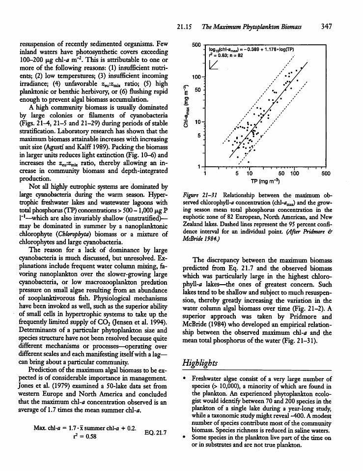
resuspension of recendy sedimented organisms. Fewinland waters have photosynthetic covers exceeding100-200 \ig chl-a m"2. This is attributable to oneormore of the following reasons: (1) insufficient nutrients; (2) low temperatures; (3) insufficient incomingirradiance; (4) unfavorable 2eu:2mix ratio; (5) highplanktonic or benthic herbivory, or (6) flushing rapidenough to prevent algalbiomass accumulation.A high community biomass is usuaUy dominated
by large colonies or filaments of cyanobacteria(Figs. 21-4, 21-5 and 21-29) during periods of stablestratification. Laboratory research has shown that themaximum biomassattainable increaseswith increasingunit size (Agustf and Kalff1989). Packingthe biomassin larger units reducesUghtextinction (Fig. 10-6) andincreases the 2eu:2mix ratio, thereby aUowing an increase in community biomass and depth-integratedproduction.Not aU highly eutrophic systems are dominated by
large cyanobacteria during the warm season. Hypertrophic freshwater lakes and wastewater lagoons withtotalphosphorus (TP)concentrations >500-1,000 p.g Pl"1—which are also invariably shaUow (unstratified)—may be dominated in summer by a nanoplanktonicchlorophyte (Chlorophyta) biomass or a mixture ofchlorophytes and large cyanobacteria.The reason for a lack of dominance by large
cyanobacteria is much discussed, but unresolved. Explanations include frequentwater columnmixing, favoring nanoplankton over the slower-growing largecyanobacteria, or low macrozooplankton predationpressure on smaU algae resulting from an abundanceof zooplanktivorous fish. Physiological mechanismshave been invoked asweU, such as the superior abiUtyof smaU ceUs in hypertrophic systems to take up thefrequendy limited supply of C02 (Jensen et al. 1994).Determinants of a particular phytoplankton size andspecies structure have not beenresolved because quitedifferent mechanisms or processes—operating overdifferent scales and each manifesting itselfwith alag—can bringabouta particular community.Predictionofthe maximum algal biomass to be ex
pected is of considerable importance in management.Jones et al. (1979) examined a 50-lake data set fromwestern Europe and North America and concludedthat the maximum chl-a concentration observed is anaverageof 1.7 times the mean summer chl-a.
Max. chl-a = 1.7 • x summer chl-a + 0.2.r2 = 0.58
EQ.21.7
21.15 TheMaximum Phytoplankton Biomass 347
E
3E
1
log^chl-aroaJ =-0.389 + 1.178«log(TP)r2= 0.83; n = 82
V- /.//' •• /
100- / ** // .*/'/50 :
/ ** / '
- / ' \a'_ '' * • / /' •/• /
/ • ,w* /10- *' • /* /' •• y 1
I '•••• • /• /' • /V* '
5 :. /• ' '/•. .»'•/ *%/ •/
' * /
1f *
• 5 10 50 100 5C
TP (mgm"3)
Figure 21-31 Relationship between the maximum observed chlorophyU-tf concentration (cYA-a^ and the growing season mean total phosphorus concentration in theeuphotic zone of 82 European, North American, and NewZealand lakes. Dashed lines represent the 95 percentconfidence interval for an individual point (After Pridmore &McBride 1984.)
The discrepancy between the maximum biomasspredicted from Eq. 21.7 and the observed biomasswhich was particularly large in the highest chloro-phyU-tf lakes^—the ones of greatest concern. Suchlakes tendto beshaUow andsubject tomuchresuspension, thereby gready increasing the variation in thewater column algal biomass over time (Fig. 21-2). Asuperior approach was taken by Pridmore andMcBride (1984) whodeveloped an empirical relationship between the observed maximum chl-a and themean totalphosphorus ofthe water(Fig. 21-31).
Highlights
Freshwater algae consist of a very large number ofspecies (> 10,000), a minority of which are found inthe plankton. An experienced phytoplankton ecolo-gistwould identify between 70and200species in theplankton of a single lake during a year-long study,while a taxonomic studymightreveal -400.Amodestnumber ofspecies contribute most ofthe communitybiomass. Species richness is reduced in salinewaters.Somespecies in the planktonUve part ofthe time onor in substrates and are not true plankton.
348 CHAPTER21 The Phytoplankton
• The phytoplankton range in sizefromas smaU as< 1u.m indiameter, withorganisms <2 |xm defined aspicophytoplankton. The algal picophytoplankton, together with those in the next size category, thenanophytoplankton (2-30 u.m), have the highestmaximum growth rates, are of a size readily eaten bya variety of freshwater invertebrates, and have a density lowenough to make them little subject to sedimentation. Large phytoplankton, the microplankton,range in size from > 30 u,mto coloniesof-600 u,m indiameter. They arecharacterized bylower maximumgrowth rates and, when lacking flageUa (motiUty) orbuoyancy control, are most subjectto sedimentation.
• Growth rate and community biomass in temperateandpolarwaters isprimarily constrained byUght Umitation in winter, while nutrient Umitation usuaUylimits communityproduction and biomass in aU buthighlyturbid watersat the same latitudesin summer,andyear-round at lowerlatitudes. Superimposed arebiomass oscillations and species fluctuations produced by predation, sedimentation, disease, or flushing that helpstructurethe community.
• A The specific growth rate [mg C g C~l (or mgchl-a) d-1] in the laboratory and communities in nature, is Ught-limited under low irradiance. Growthrates increase to a maximum at an intermediate intensity encountered somewherein the upper water column or shaUow-water sediments, and becomephotoinhibitedyet closerto the surface.
• A The annual depth-integrated phytoplanktonrates of primary production ranges about three orders ofmagnitude from a low of<4 g C m~2 yr-1 inultra-oUogotrophic polar lakes to a high of 6000 gCm~2 yr"T inahypertrophic low latitude lake. Ultra-oUgotrophic lakes experience a very short growingseason, low temperatures, and very low nutrient inputs from their drainage basins. Annual productionrates (gC m~2 yr"1) are lower than thehighest daUyratesmeasured in highlynutrient-rich (hypertrophic)tropical lakes that alsoexperience high temperaturesand high irradianceyear-round.
• A The primary production (P) to phytoplanktonbiomass(B) ratio (P:B), expressedas carbon, is a use
fulmeasure of specific growth rates.The P:B ratio inthe mixed layer of lakes and slowly flowing lowlandrivers tends to be lowwhen the algal biomass ishigh,yielding a poor effective Ught cUmate for photosynthesis. Loworganismal growthratesdemand lowlossrates if a species is not to disappear. The typicallyhigh P:B ratios seen in nutrient-poor water, characterized by a low community biomass of typicaUysmaU algae and high water transparency, imply arapid individual growth rate, a high loss rate, andrapidrecycUng oforganic matter and the nutrientsinhighest demand.
• A The two nutrients in highest demandrelative totheir supply are phosphorus and nitrogen. Experimentaladditions to oUgotrophic freshwater lakes andstreams showthat onlycombined shortages of P andN constrain the community biomass in virtuaUy aUenvironments that are not Ught-limited, but the rateofbiomass accumulation canbeconstrained byaDICshortage,especially in lowDIC lakes. Other elements(e.g., siUca for diatoms) also affect algal speciescomposition.
• A primaryphosphorus limitation is common in well-watered temperate regions, characterized by an N:Psupplyratio (>~16:1 byatoms)weU abovethe demandratio of the algae. A primary nitrogen limitation ismost probable in agricultural and urban areaswherethe runoff is both rich in nutrients and characterizedby a lowN:P supplyratio (belowthe demandratio ofthe algae). A primary nitrogen Umitation outside thetemperate zone is most likely in regions where thesurface geology is rich in phosphorus, in low latitudesemiarid catchments where the soils release disproportionaUy UtdeN, and in someother tropical lakes.
• A PubUc complaints about algalbloomsin the temperate zone pertain largely to the summer maximarather than the average biomass. Highest standingcrops or community biomass, typically dominatedby large cyanobacteriareaching -300-1,000 u.g chl-am~2 are encountered in shaUow (z< 1.5m) nutrient-rich waters during periods of high irradiance plushigh temperature.
CHAPTER
22
The Bacteria
22.1 Introduction
The smaU size(mostly < 1 pin diameter) andmorphological diversity—much less than the protozoa oralgae—has greadyaffected the developmentof aquaticmicrobiology. Most of the heterotrophic prokaryotesare too smaU to be seen or identified under the Ughtmicroscope and earlywork had to be basedon cultur-ing of microbes. That work, started during the lastdecade or soofthe 19th century, was anoutgrowth ofconcern about the importance of disease-causingsewage bacteria in lakes and rivers from which townsdrewtheir drinkingwater.The earlyemphasis on cultureworkwasmost use
ful in the development of culture media that enabledresearchers to detect and count wastewater bacteria indrinking water, and identify a variety of sewage andother pathogenic species that couldbe culturedon themedia developed. The emphasis on culturing bacterialed directly to importantwork in microbial physiology, workthat then contributed muchto the development of conceptual ideas about the roles of microbesin nutrient cycling. All of these accomplishmentswere, from an ecological perspective, somewhat offsetby the associated emphasis on laboratory rather thanfield research, and a disregard for thevast majority ofheterotrophicbacteria that couldnot, and stiU cannot,begrownon available culturemedia. Those forms thatcan be cultured frequently change size, shape, andphysiology under different growing conditions, indicating that traditional systematic and physiologicalcharacteristics ofspecies arenotveryuseful in describing planktonicbacteria (Hobbie 1988).
Difficulties in enumerating the abundance ofaquatic bacteria in nature—a prerequisite for workontheir distribution and dynamics—have been graduaUyovercome. Major technical breakthroughs during thelast two decades or so make it possible to obtain reasonablyreUable bacterialabundance and biomassmeasurements—measurements that reveal the bacterialabundance in fresh water to be about three orders ofmagnitude greater (BirdandKalff1984) than had beenbelieved on the basis ofthe traditional culture studies.The much higher abundances revealed by the recentadvances in technique have shown that the bacterialbiomass contributes between aboutfive and 15 percentof the total planktonic biomass in fresh water (delGiorgio and Gasol 1995). All this gready stimulatedfairly successful efforts tomeasure bacterial productionratesand to assess the importance of planktonic bacteria in nutrient cyclingand foodwebs.The outcomehasbeen a veritable explosion of papers on different aspects ofmicrobial ecology duringthe lasttwodecades.The new counting techniques not only showed thatplanktonic bacteria areunexpectedly abundant but alsothat theyaremuch smaUer than those typicaUy seen inculture. Genetic-fingerprinting techniques, based onsequences of ribosomal RNA, have begun to make itpossible to distinguish between phylogenetic groups ofmicrobes (Subclasses, phylotypes) in naturalcommunities on the basis ofnucleic-acid sequences. It is evidentfrom the many new rRNA sequences that have beenfound that the vast majority of bacterioplanktonspeciesare notrepresented in cultures.The techniques used in microbial ecology con
tinue to evolve very rapidly and too Utde time has349
3 50 CHAPTER 22 The Bacteria
passed to be certain whether some of the emerginggeneraUties are fact, artifact, or a mixture of the two.As a consequence, the present chapter is much morespeculative than any ofthe others.Many ofthe recentfindings and ecological interpretations made wiUprobably not stand the test of time because experimentsare stiU overwhelmingly restrictedto laboratoryand field studies carried out in small containers(« 11), over short periods (< 1 day) on singlefactors,making it difficult to extrapolate the findings to nature(see Fig. 1-2).While the role of heterotrophic bacteriain theuti-
Uzation and decomposition (Uberation) of organicmatter haslong been recognized in a quaUtative sense,the more recent work is starting to allowsome quantificationas weU. Much of the work is being done inoceansand estuaries and this chapter wiU, more thanany other, draw from the marine Uterature. lb do soassumes that the principal constraints on bacterialgrowth do not differ materiaUy between marine andfreshwaters. While this conclusion appearsto be generallytrue, twomajor differences havebecomeapparent. First, planktonic freshwater bacteria encounter asubstantial supply of organic carbon produced ondrainagebasins and littoral zones (allochthonousproduction), while oceanic bacteria are overwhelmingly dependent on carbon produced in situ (autochthonousproduction). Second, and probably as a consequence,lake plankton contains more heterotrophic biomassper unit autotrophic biomass (Sec. 22.7).Recent developments in microbial ecology are
havingramifications elsewhere in the aquaticsciences.The fluorescent-staining techniques that have revolutionized the enumeration of heterotrophic bacteria(Hobbie et al. 1977) now also permit the picophytoplankton (< 2 p,m) to be readily seen (Chapter 21).Their previously unrecognizedabundance has led to asmall revolution in phytoplankton ecology, raisingquestions about some ofthe interpretations made during the last 70 years in studies when researchers wereunaware of either their existence or their abundance.Moreover, the recent developments in microbialecology have pointed to the important role the heterotrophic bacteria play in detenriining phytoplankton abundances and production, resulting from theabilityofthe bacteria to competesuccessfullywith thephytoplankton for inorganicnutrients that are in shortsupply. Recentresearch on bacterial biomass and production has also raisedmany questions about the fateof aU this production, leading to much experimentalwork on the consumersof heterotrophic bacteria.The
identification ofthe protozoans(mosdyflageUates andciUates) asmajorpredators hasaUowed an explosion ofresearch on protozoan ecology(Chapter 23). The research has demonstrated that the traditional divisionbetween botany and zoology is unwarranted—certainprotozoa are able to both photosynthesize and grazeon bacteria. In addition to the heterotrophic bacteria,there are two other groups of aquatic bacteria. Thefirst group—the cyanobacteria (blue-green algae)—were discussed in Chapter 21, the second group—thegreen and purple photosynthetic bacteria of anoxicenvironments—wiU be dealt with in Sec. 22.10.
A 22.2 From Past to Present
The early microbiological studies, starting in 1889and usingorganic-richgrowth (culture)media that wenowknowgreadyunderestimatethe varietyand abundance of microbes present, laid the groundwork forthe secondphaseof development. This occurredwhenL. M. Snow and E. B. Fred, working with Birge andJuday, in Wisconsin, developed the first microscopetechnique aUowing enumeration of (larger) bacteriaunder the Ught microscope (after concentrating andstaining them). The new microscope method, inde-pendendy developed in the former USSR a fewyearslater, showed the bacterial abundance in unpoUutedwater to be roughly ten thousand times greater thanthe numbers obtained by traditional culture methods(A. S. Razumov 1932, in Kuznetsov 1970).The new microscope techniques were perfected
and employed in the former USSR between the twoWorldWars, when interest in aquaticmicrobial ecologylanguished somewhat in the rest of Europe and inNorth America. The isolation ofthe former USSR, asa result of language and poUtics, meant that the abundant and excellentwork carried out over a 30-40 yearperiod in both aquatic and soil microbiology waslargely unappreciated or hidden from the view ofWestern scientists.FollowingWorldWar II, Sovietscientists not only
developed radioisotopic techniques in an attempt tomeasure heterotrophic bacterial respiration but alsoexplored the use of fluorescent dyes to stain bacteria(Gorlenko et al. 1983). Starting in the 1960s and1970s, renewed interest by western scientists in theplanktonic microbes led to the development of convenient fluorescent-staining techniques that now aUowroutine determination of bacterial abundances. In themodern technique, the bacteria are first coUected on
filters, then stained with a fluorescent dye, and finallyobserved using an epifluorescent microscope (Francisco et al. 1973, Hobbie et al. 1977). The stainingtechniques have revealed that the vast majority ofplanktonic bacteria are too smaU (0.1-1.0 p,m diameter) to have been visible with the old stainingtechniques employing nonfluorescent dyes. Countsobtained with the earUerdyes appear to have yieldedabundances that are twofold lower in oUgotrophiclakes and sevenfold lower in mesotrophic lakes thanthose obtained by fluorescence microscopy. The underestimates in more eutrophic lakes were muchlarger (-twentyfold; Bird and Kalff 1984). Unfortunately, there is no simple conversion factor to reconcile old and new data, primarily because the sizedistribution—and thus the visibiUty—of bacteriaunder the Ught microscope greadyvaries betweensystems. The reconciUation of data collectedin the past,usingdifferent techniques,with modern data is not restricted to microbial ecology, but is common whenevermajor technical advances are made. For example,muchofthe older (pre-1960)phytoplanktonUteraturedid not take the nanoplankton into account, whereasthe more recent Uterature has largely overlooked thepicophytoplanktonin analyses and interpretations. Inanother example, nearly all ofthe pre-1960 determinationsof pH weremadewith dyes, and the resultsarenot easily convertible into modern measurementsmadewith pH meters. As a result, it has been difficultto compare present levels of acidification with pre-acidification dye data (Chapter 27). A last example isthe major improvement in technique and laboratoryprocedures that have madethe earUer (pre-1980) Uterature on trace-metal levels in waters impossible to interpret (Chapter 28).
22.3 Bacterial Size, Form,and Metabolism
Until the development of easily performed epifluo-rence techniques for counting, most aquatic bacteriawere thought to be > 1 p,m short rods (cylinders), andthe average bacterial cell in aerobic waters was be-Ueved to have a volume about an order of magnitudegreater than the -0.03 p,m3 volume (range 0.01-0.2p.m3) determined with fluorescence techniques by, forexample, Cole et al. (1993). It isnowevidentthat cocci(spheres or near-spheres), rangingfrom0.1-0.6 p,m indiameter, dominate most waters but with a variablefraction of vibrio (curved ceUs), rod, colony, and fila
22.3 BacterialSize, Form, andMetabolism 351
mentous forms (5—55 p-m); rods arranged in chains(5-100 p,m) are also present. While it makes physiological sensefor smaUer organisms with a more favorable surface to volume ratio (Sec. 21.3) to be favoredunder conditions when substrates are limiting, there isno systematic relationship between bacterial size andtrophic status (Cole et al. 1993).A The observed size distribution of planktonic bacteria may be principaUy due to selectivepredation ofthe larger bacteria by filter feeding zooplankton and,when abundant, mussels, rather than substrate availability. For example,experimental manipulation of enclosures (mesocosms) led to the development of acommunityof smaU cocciand rods that were typicalofthe lake itselfwhen the large water fleaDaphnia dominated. Grazing byDaphnia on large bacteria and protozoans prevented the latter from restricting theabundance of smaU bacteria (-80% of biomass < 1u,m). Conversely, when the protozoans (protists)wereaUowed to dominate, their grazing led to rapid reduction of smaUer cells, and an increase of the large filamentous bacteria that were resistant to protozoangrazing (-90% of biomass > 3 p,m) (Jiirgens et al.1994).When abundant, grazers can structure bacterialcommunities and bring about changes in the growthrate and taxonomic composition of the assemblagesfavoring rapidlyreproducing and/or grazing-resistantspecies (Jiirgens et al. 1999).
MetabolicTypesThe impossibility of identifying often superficiallysimilar species by Ught microscopy, and the impossi-biUty ofculturingmorethanaminiscule percentage (<1%)ofthe organisms has long led microbiologists toemphasize metaboUc type (Table 22-1) rather than thetaxonomy of the organisms coUected. The principlemetaboUc division is between autotrophic bacteriawhoobtain aU or virtuaUy aU ceU carbon required forbiosynthesis by reducing C02, and heterotrophicbacteria who obtain aU such carbon from reduced organic substances. A second division, based on thesource of energy used, distinguishes betweenchemosynthetic bacteria (chemoautotrophs)—autotrophic forms that utiUze energyobtained fromenergy-yielding (exergonic) chemical reactions to reduceC02 to organic matter—and the photosynthetic bacteria (phototrophs). Thesebacteria uselight energy forthe reduction of C02 to organiccarbon(Table 22-1).Athird division is based on the source of electrons forgrowth. Organisms can be either organotrophs
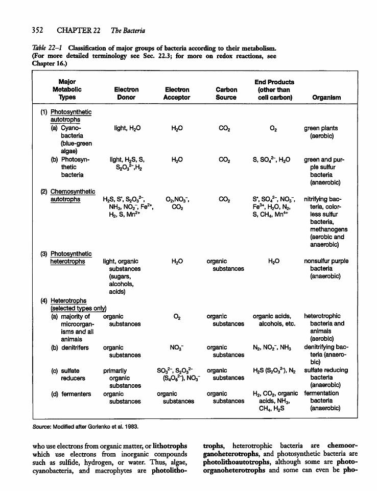
352 CHAPTER 22 The Bacteria
Table 22-1 Classification of major groups of bacteria according to their metabolism.(For more detailed terminology see Sec. 22.3; for more on redox reactions, seeChapter 16.)
Major End ProductsMetabolic Electron Electron Carbon (other thanTypes Donor Acceptor Source cell carbon) Organism
(1) Photosyntheticautotrophs(a) Cyano light, H20 H20 C02 02 green plants
bacteria (aerobic)(blue-greenalgae)
(b) Photosyn light, H2S, S, H20 C02 S, S042~, H20 green and purthetic S2O3 ,n2 ple sulfurbacteria bacteria
(anaerobic)(2) Chemosynthetic
autotrophs H2S, S, S2O3 , 02,N03-, co2 s°, so42-, NO3-, nitrifying bacNH3, N02-, Fe2+, C02 Fe3*, H20, N2, teria, colorH2, S, Mn2+ S, CH4, Mn4* less sulfur
bacteria,methanogens(aerobic andanaerobic)
(3) Photosyntheticheterotrophs light, organic H20 organic H20 nonsulfur purple
substances substances bacteria(sugars, (anaerobic)alcohols,acids)
(4) Heterotrophs(selected types only)(a) majority of organic 02 organic organic acids, heterotrophic
microorgan substances substances alcohols, etc. bacteria andisms and all animalsanimals (aerobic)
(b) denitrifers organic NO3- organic N2, N02", NH3 denitrifying bacsubstances substances teria (anaero
bic)(c) sulfate primarily 0O3 , S2O3 organic H2S(S2032-).N2 sulfate reducing
reducers organicsubstances
(S4062-), NO3- substances bacteria(anaerobic)
(d) fermenters organic organic organic H2,C02, organic fermentation
substances substances substances acids, NH3,CH4, H2S
bacteria(anaerobic)
Source: Modified after Gorlenko et al. 1983.
whouse electrons from organicmatter, or lithotrophswhich use electrons from inorganic compoundssuch as sulfide, hydrogen, or water. Thus, algae,cyanobacteria, and macrophytes are photolitho-
trophs, heterotrophic bacteria are chemoor-ganoheterotrophs, and photosynthetic bacteria arephotoUthoautotrophs, although some are photo-organoheterotrophs and some can even be pho-
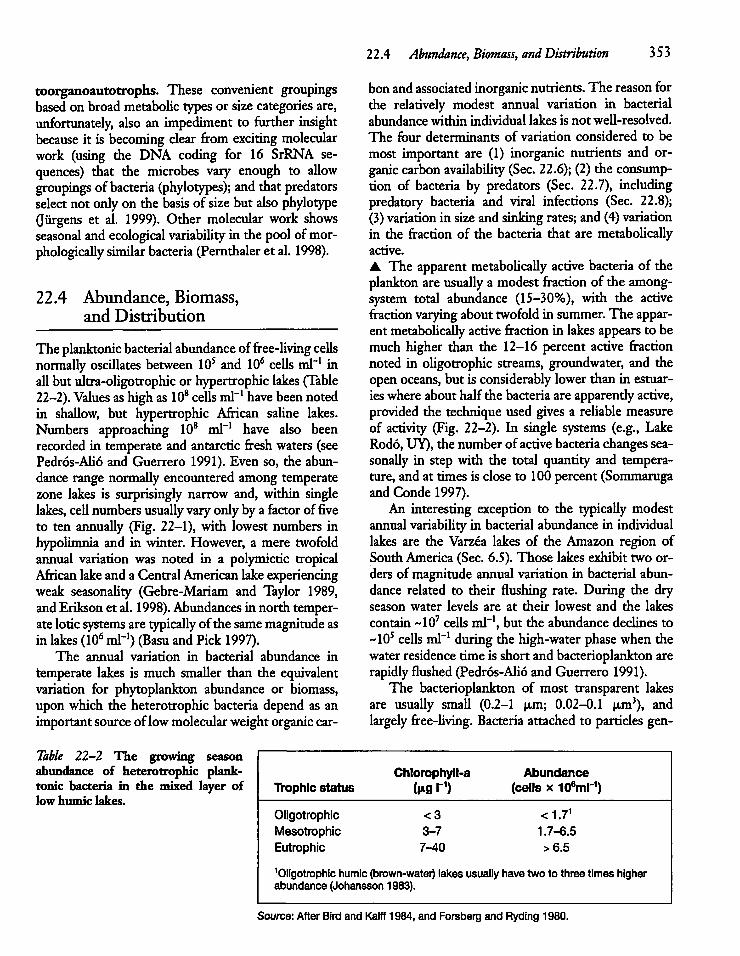
toorganoautotrophs. These convenient groupingsbased on broadmetaboUc typesor sizecategories are,unfortunately, also an impediment to further insightbecause it is becoming clear from exciting molecularwork (using the DNA coding for 16 SrRNA sequences) that the microbes vary enough to aUowgroupings of bacteria (phylotypes); andthatpredatorsselect not onlyon the basis of size but also phylotype(Jiirgens et al. 1999). Other molecular work showsseasonal and ecological variabiUty in the pool ofmor-phologicaUy similar bacteria (Pernthaler et al. 1998).
22.4 Abundance, Biomass,and Distribution
The planktonic bacterial abundance offree-Uving ceUsnormaUy oscillates between IO5 and IO6 cells ml"1 inallbut ultra-oUgotrophic or hypertrophic lakes (Table22-2). Values ashigh as IO8 ceUs ml"1 have been notedin shaUow, but hypertrophic African saline lakes.Numbers approaching IO8 ml"1 have also beenrecorded in temperate and antarctic fresh waters (seePedros-AU6 and Guerrero 1991). Even so, the abundance range normaUy encountered among temperatezone lakes is surprisingly narrow and, within singlelakes, ceU numbers usually varyonlyby a factorof fiveto ten annuaUy (Fig. 22-1), with lowest numbers inhypolimnia and in winter. However, a mere twofoldannual variation was noted in a polymictic tropicalAfrican lakeand a Central American lakeexperiencingweak seasonaUty (Gebre-Mariam and Taylor 1989,and Erikson et al. 1998).Abundances in north temperate loticsystems are typicaUy ofthe samemagnitude asin lakes (IO6 ml"1) (Basu andPick 1997).The annual variation in bacterial abundance in
temperate lakes is much smaUer than the equivalentvariation for phytoplankton abundance or biomass,upon which the heterotrophic bacteria depend as animportant source of lowmolecularweight organiccar
Table 22-2 The growing seasonabundance of heterotrophic planktonic bacteria in the mixed layer oflow mimic lakes.
Trophic status
OligotrophicMesotrophicEutrophic
22.4 Abundance, Biomass, andDistribution 353
bonandassociated inorganic nutrients. The reason forthe relatively modest annual variation in bacterialabundance within individual lakes is not weU-resolved.The four determinants of variation considered to bemost important are (1) inorganic nutrients and organic carbon avaflabiUty (Sec. 22.6); (2) the consumption of bacteria by predators (Sec. 22.7), includingpredatory bacteria and viral infections (Sec. 22.8);(3)variation in sizeand sinkingrates;and (4)variationin the fraction of the bacteria that are metaboUcaUyactive.A The apparentmetaboUcaUy active bacteria of theplankton are usually a modest fraction of the among-system total abundance (15-30%), with the activefraction varying about twofold in summer. The apparent metaboUcaUy active fraction in lakes appears to bemuch higher than the 12-16 percent active fractionnoted in oUgotrophic streams, groundwater, and theopenoceans, but is considerably lowerthan in estuarieswhere about half the bacteria are apparendy active,provided the technique used gives a reUable measureof activity (Fig. 22-2). In single systems (e.g., LakeRodo,UY), the number of activebacteria changesseasonally in step with the total quantity and temperature, and at times is close to 100 percent (Sommarugaand Conde 1997).An interesting exception to the typicaUy modest
annual variability in bacterial abundance in individuallakes are the Varzea lakes of the Amazon region ofSouth America (Sec. 6.5). Those lakes exhibit two orders of magnitude annual variation in bacterial abundance related to their flushing rate. During the dryseason water levels are at their lowest and the lakescontain -107 ceUs ml"1, but the abundance declines to-105 cells ml"1 during the high-water phase when thewater residencetime is short and bacterioplankton arerapidlyflushed (Pedros-AUo and Guerrero 1991).The bacterioplankton of most transparent lakes
are usually smaU (0.2-1 p,m; 0.02-0.1 u,m3), andlargely free-Uving. Bacteriaattached to particles gen-
Chlorophyll-a0*91"1)
<3
3-7
7-40
Abundance(cells x I06mr1)
<1.711.7-6.5
>6.5
Oligotrophic humic(brown-water) lakes usuallyhave two to three times higherabundance (Johansson 1983).
Source: After Bird and Kalff 1984, and Forsberg and Ryding 1980.
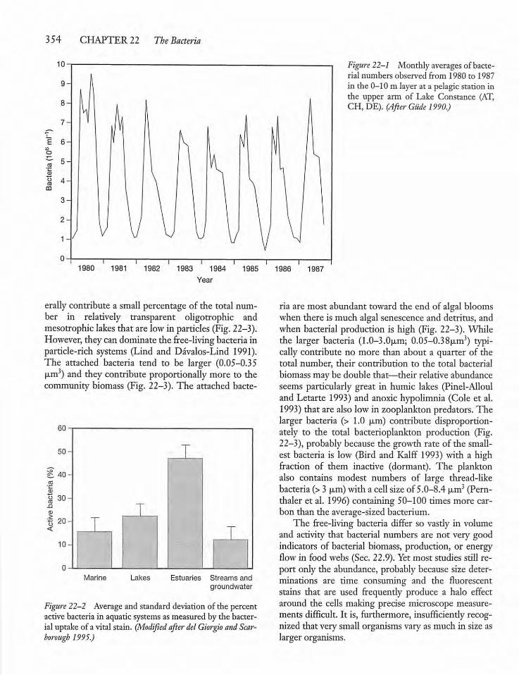
354 CHAPTER 22 The Bacteria
10
9-1
8-
7-
£ 6-O
« 5O A -
3
2-|
1-
01980 1981 1982 1983 1984
Year
1985
erallycontribute a small percentage of the total number in relatively transparent oligotrophic andmesotrophic lakes that are lowin particles (Fig. 22-3).However, they candominate the free-living bacteriainparticle-rich systems (Lind and Davalos-Lind 1991).The attached bacteria tend to be larger (0.05-0.35p-m3) and they contribute proportionally more to thecommunity biomass (Fig. 22-3). The attached bacte-
60
50-
- TT
T
T
^40-.55q3
I 30
20-
10
Marine Lakes Estuaries Streams andgroundwater
Figure 22-2 Average and standard deviationof the percentactivebacteria in aquatic systems asmeasuredbydie bacterial uptake of a vital stain. (Modified after del Giorgio and Scarborough 1995.)
1986 1987
Figure 22-1 Mondily averages of bacterial numbers observed from 1980 to 1987in die 0-10 m layer at a pelagicstation inthe upper arm of Lake Constance (AT,CH, DE). (After Glide 1990.)
ria are most abundant toward the end of algal bloomswhen there is much algal senescence and detritus, andwhen bacterial production is high (Fig. 22-3). Whilethe larger bacteria (1.0-3.Opan; 0.05-0.38u,m3) typically contribute no more than about a quarter of thetotal number, their contribution to the total bacterialbiomassmay be double that—their relative abundanceseems particularly great in humic lakes (Pinel-Allouland Letarte 1993) and anoxic hypolimnia (Cole et al.1993) that are also low in zooplankton predators. Thelarger bacteria (> 1.0 p.m) contribute disproportionately to the total bacterioplankton production (Fig.22-3), probably because the growth rate ofthe smallest bacteria is low (Bird and Kalff 1993) with a highfraction of them inactive (dormant). The planktonalso contains modest numbers of large thread-likebacteria(>3 p,m) with a cellsizeof 5.0-8.4 p-m3 (Pern-thaler et al. 1996) containing50-100 times more carbon than the average-sized bacterium.The free-living bacteria differ so vasdy in volume
and activity that bacterial numbers are not very goodindicators of bacterial biomass, production, or energyflow in food webs (Sec. 22.9). Yet most studies still report only the abundance, probably because size determinations are time consuming and the fluorescentstains that are used frequendy produce a halo effectaround the cells making precise microscope measurements difficult. It is, furthermore, insufficiendy recognized that very small organisms vary as much in size aslarger organisms.
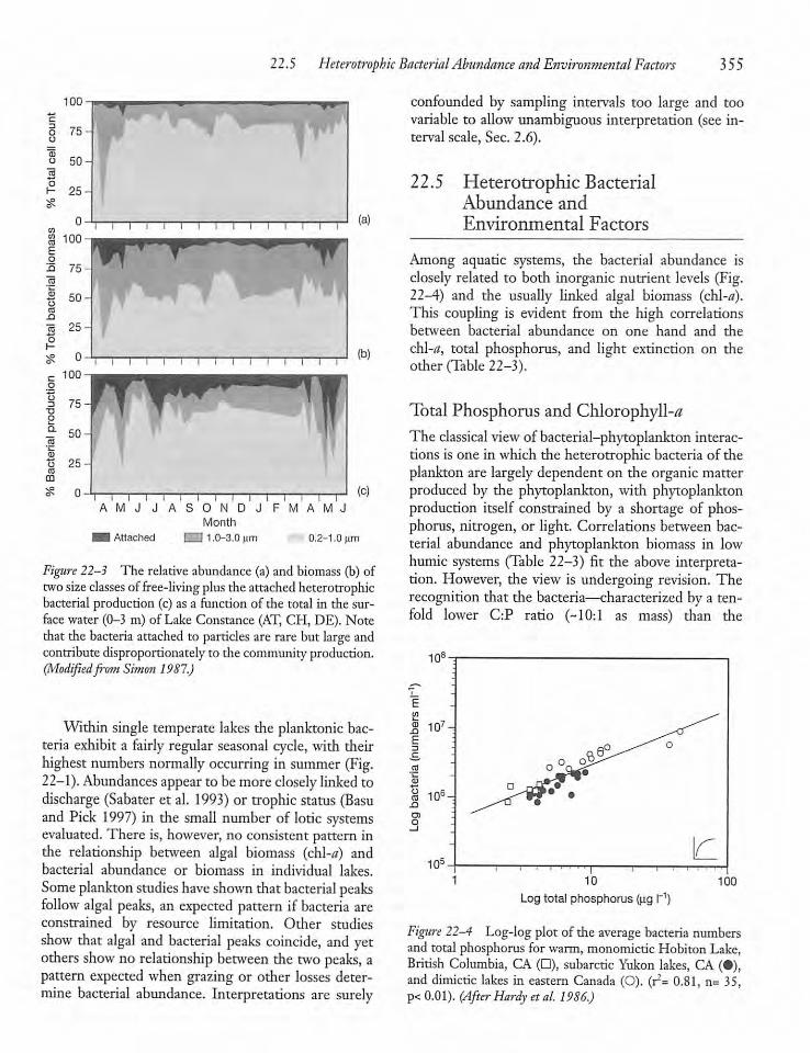
22.5 Heterotrophic BacterialAbundance andEnvironmental Factors 355
>s
75-
50 ->
"^f
~~V'25-
0- 1 1 1 1
100-
s?100
o
aZJ"OO
Q.
IB
£o(0m
i—i—i—i—i—i—i—i—rAMJJASONDJF
Month• Attached H 1.0-3.0 urn
i rA M J
(b)
0.2-1 .Ofim
Figure 22-3 The relative abundance (a) and biomass (b) oftwosize classes of free-living plusdie attached heterotrophicbacterialproduction (c)as a function of the total in the surface water (0-3 m) of Lake Constance (AT, CH, DE). Notethat the bacteria attached to particles are rare but large andcontribute disproportionately to the community production.(Modifiedfront Simon 1987.)
Within single temperate lakes the planktonic bacteria exhibit a fairly regular seasonal cycle, with theirhighest numbers normally occurring in summer (Fig.22-1).Abundances appearto bemore closely linked todischarge (Sabater et al. 1993) or trophic status (Basuand Pick 1997) in the small number of lotic systemsevaluated. There is, however, no consistent pattern inthe relationship between algal biomass (ch\-a) andbacterial abundance or biomass in individual lakes.Someplankton studies have shown that bacterial peaksfollow algal peaks, an expected pattern if bacteria areconstrained by resource limitation. Other studiesshow that algal and bacterial peaks coincide, and yetothers show no relationship between the two peaks, apattern expected when grazing or other losses determine bacterial abundance. Interpretations are surely
confounded by sampling intervals too large and toovariable to allowunambiguous interpretation (see interval scale, Sec. 2.6).
22.5 Heterotrophic BacterialAbundance andEnvironmental Factors
Among aquatic systems, the bacterial abundance isclosely related to both inorganic nutrient levels (Fig.22-4) and the usually linked algal biomass (chl-tf).This coupling is evident from the high correlationsbetween bacterial abundance on one hand and thechl-tf, total phosphorus, and light extinction on theother (Table 22-3).
Total Phosphorus and Chlorophyll-^The classical viewof bacterial-phytoplankton interactions is one in which the heterotrophic bacteria of theplankton are largely dependent on the organic matterproduced by the phytoplankton, with phytoplanktonproduction itself constrained by a shortage of phosphorus, nitrogen, or light. Correlations between bacterial abundance and phytoplankton biomass in lowhumic systems (Table 22-3) fit the above interpretation. However, the view is undergoing revision. Therecognition that the bacteria—characterized by a tenfold lower C:P ratio (-10:1 as mass) than the
100
Log total phosphorus (ug
Figwe 22-4 Log-log plot of the average bacteria numbersand total phosphorus for warm, monomictic Hobiton Lake,British Columbia, CA (•), subarctic Yukon lakes, CA (•),and dimictic lakes in eastern Canada (O). (r= 0.81, n= 35,p<0.01). (After Hardy etal. 1986.)
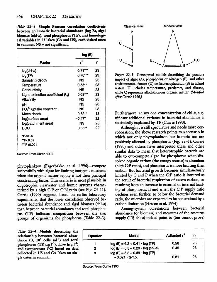
356 CHAPTER 22 The Bacteria
Table 22-3 Simple Pearson correlation coefficientsbetween epilimnetic bacterial abundance (log B), algalbiomass (ch\-a), total phosphorus (TP), and limnologi-cal variables in 23 lakes (CA and US), each visited oncein summer. NS =» not significant.
Factor
log(B)
r2 n
log(chl-a) 0.71*** 23
logfJP) 0.76*** 23
Sampling depth NS 23
Temperature 0.55** 23
Conductivity NS 23
Light extinction coefficient {kjj 0.68*** 23
Alkalinity NS 23
PH NS 23
PO43* uptake constant NS 23
Mean depth -0.62** 18
log(surface area) -0.47* 22
log(catchment area) NS 23
DOC 0.55** 22
*P<0.05
**P<0.01
***P<0.001
Source: From Currie 1990.
phytoplankton (Fagerbakke et al. 1996)—competesuccessfullywith algae for limitinginorganic nutrientswhen the organic matter supply is not their principalconstraining factor. This scenario ismost plausible inoligotrophic clearwater and mimic systems characterized by a high C:P or C:N ratio (see Fig. 24-11).Currie (1990) suggests, based on earlier laboratoryexperiments, that the lower correlation observed between bacterial abundance and algal biomass (chl-tf)than between bacterial abundance and total phosphorus (TP) indicates competition between the twogroups of organisms for phosphorus (Table 22-3).
Equation
Classical view
P
kB
Modern view
P
Figure 22-5 Conceptual models describing the possibleimpact of algae (A), phosphorus or nitrogen (P), andotherenvironmental factors (U) on bacterioplankton (B)in inlandwaters. U includes temperature, predators, and disease,whileC represents allochthonous organic matter. (ModifiedafterCurrie 1990.)
Furthermore, at any one concentration of chl-tf, significant additional variance in bacterial abundance isstatistically explained by TP (Currie 1990).
Although it is still speculative and needs morecorroboration, the above research points to a scenario inwhich not only phytoplankton but bacteria too arepositively affected by phosphorus (Fig. 22-5). Currie(1990) and others have interpreted these and othersimilar data to mean that heterotrophic bacteria areable to out-compete algae for phosphorus when dissolved organic carbon (the energy source) isabundant(high C:P ratio), and phosphorus ismore limiting thancarbon. But bacterial growth becomes simultaneouslylimited by C and P when the C:P ratio is lowered asthe result of bacterial respiration of excess carbon, orresulting from an increase in external orinternal loading of phosphorus. If and when the C:P supply ratiodeclines even further, to below the bacterial demandratio, the microbes are expected to be constrained by acarbon limitation (Hessen et al. 1994).
Among-system correlations between bacterialabundance (or biomass) and measures of the resourcesupply (TP, chl-tf) indeed point to (but cannot prove)
Model Adjusted r2Table 22-4 Models describing dierelationship between bacterial abundance (B, 106 cells ml-1) and totalphosphorus (TP, |*g I"1), cbl-a (|ig l"1)and temperature (°C) based on datacollected in US and CA lakes on single dates in summer.
1 log (B) = 6.2 + 0.41 • log (TP) 0.562 log (B) = 6.5 + 0.29 • log (chl^a) 0.453 log (B) = 5.8 + 0.39 • log (TP)
+ 0.021 • temp. 0.81
23
23
23
Source: From Currie 1990.
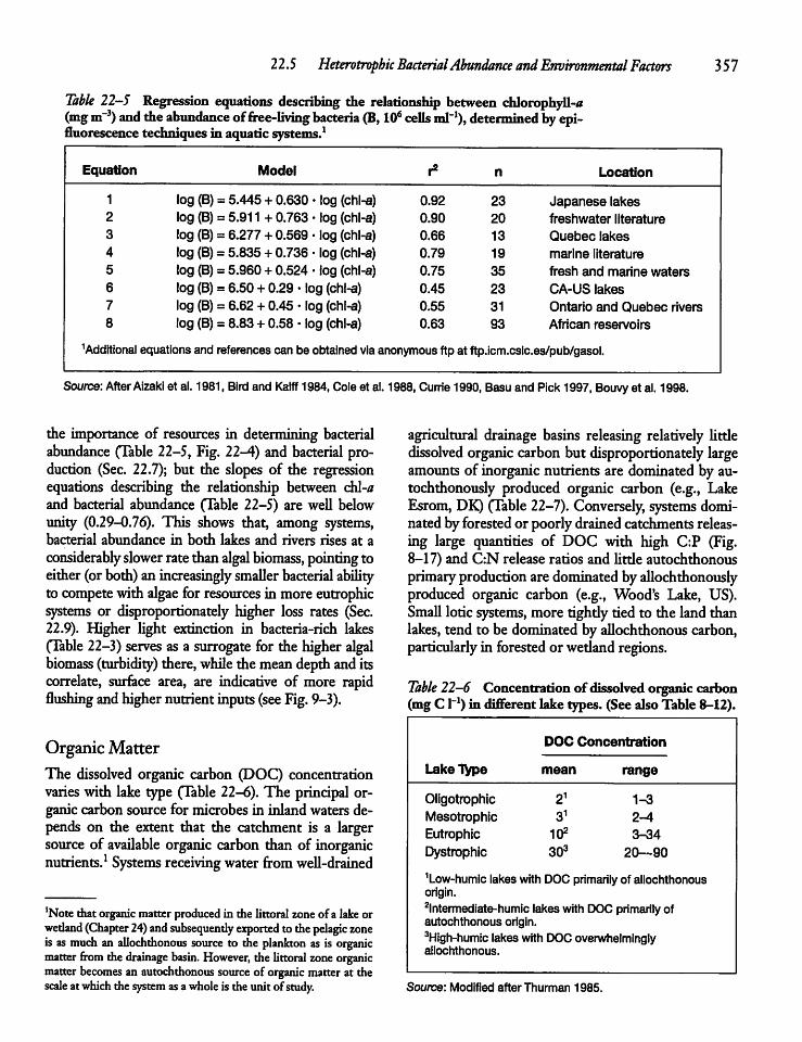
22.5 Heterotrophic BacterialAbundance and Environmental Factors 357
Table 22-5 Regression equations describing the relationship between chlorophyll-/*(mgm~3) and theabundance offree-living bacteria (B, 106 cells ml-1), determined byepi-fluorescence techniquesin aquaticsystems.1
Equation Model r2 n Location
1 log (B)= 5.445 + 0.630 • log (chl-a) 0.92 23 Japanese lakes2 log (B) = 5.911 + 0.763 • log (chl-a) 0.90 20 freshwater literature3 log (B) = 6.277 + 0.569 • log (chl-a) 0.66 13 Quebec lakes4 log (B) = 5.835 + 0.736 • log (chl-a) 0.79 19 marine literature5 log (B) = 5.960 + 0.524 • log (china) 0.75 35 fresh and marine waters6 log (B) = 6.50 + 0.29 • log (chl-a) 0.45 23 CA-US lakes7 log (B) = 6.62 + 0.45 • log (chl-a) 0.55 31 Ontario and Quebec rivers8 log (B)= 8.83 + 0.58 • log (chl-a) 0.63 93 African reservoirs
Additional equationsand references can be obtainedviaanonymous ftp at ftp.icm.csic.es/pub/gasol.
Source:AfterAizaki et al. 1981, Bird and Kalff 1984,Coleet al. 1988,Currie 1990, Basu and Pick 1997, Bouvy et al. 1998.
the importance of resources in determining bacterialabundance (Table 22-5, Fig. 22-4) and bacterial production (Sec. 22.7); but the slopes of the regressionequations describing the relationship between chl-0and bacterial abundance (Table 22-5) are well belowunity (0.29-0.76). This shows that, among systems,bacterial abundance in both lakes and rivers rises at aconsiderably slower rate thanalgal biomass, pointing toeither(orboth) an increasingly smaller bacterial abilityto compete withalgae for resources in moreeutrophicsystems or disproportionately higher loss rates (Sec.22.9). Higher light extinction in bacteria-rich lakes(Table 22-3) serves as a surrogate for the higheralgalbiomass (turbidity) there,while themeandepthanditscorrelate, surface area, are indicative of more rapidflushing andhighernutrientinputs(see Fig. 9-3).
Organic MatterThe dissolved organic carbon (DOC) concentrationvaries with lake type (Table 22-6). The principal organic carbon source for microbes in inland waters depends on the extent that the catchment is a largersource of available organic carbon than of inorganicnutrients.1 Systems receiving water from well-drained
'Note thatorganic matter produced in the littoral zoneof alake orwetland (Chapter 24)and subsequently exported to thepelagic zoneis as muchan aUochthonous source to the plankton as is organicmatter from the drainage basin. However, the littoral zoneorganicmatter becomes an autochthonous source of organic matterat thescale atwhich the system as awhole is theunitof study.
agricultural drainage basins releasing relatively littledissolved organic carbonbut disproportionately largeamounts of inorganic nutrients are dominated by au-tochthonously produced organic carbon (e.g., LakeEsrom, DK) (Table 22-7). Conversely, systems dominated byforestedor poorly drainedcatchmentsreleasing large quantities of DOC with high C:P (Fig.8-17) and C:N release ratios and little autochthonousprimary production are dominated byallochthonouslyproduced organic carbon (e.g., Wood's Lake, US).Small lotic systems, more tightly tied to the land thanlakes, tend to be dominatedby aUochthonous carbon,particularly in forested or wetland regions.
Table 22-6 Concentrationof dissolved organiccarbon(mgC r1) in differentlaketypes.(SeealsoTable8-12).
DOC Concentration
Lake Type
OligotrophyMesotrophicEutrophicDystrophic
mean
2131102303
range
1-3
2-4
3-34
20—90
1Low-humic lakeswith DOC primarily of aUochthonousorigin.2lntermediate-humic lakeswith DOC primarily ofautochthonous origin.3High-humic lakeswith DOC overwhelminglyaUochthonous.
Source: Modified after Thurman 1985.

358 CHAPTER 22 The Bacteria
Table 22-1 Sources of organic carbon, as a percentage of the total input for selectedtemperate zone lakes, values are rounded offand therefore do not total 100percent.Note the relative importance of autochthonous carbonsources in die low-humic freshwaterandabove allinPyramidLakeandin eutrophicLakeEsrom, both ofwhichreceivedisproportionately little organic carbon from their catchments. Highly dystrophic(humic)Wood'sLake is an exampleof a system receivingmuch aUochthonous carbon.The relative availability of aUochthonous organic carbon is poorly understood. Thetrophic designations are: oligotrophy (O),mesotrophic (M), eutrophic (£), dystrophic(D), saline (S).
Paajarvi Lawrence Mirror Wood's Pyramid EsromLake Fl US US CA US DK
Autochthonous
phytoplankton 59 19 65 — 96 88
periphyton 2 18 2 6 — 5
macrophytes 7 39 2 3 0 5
Subtotal 68 76 69 9 96 98
AUochthonous
fluvial — 11 15 90 4 2
atmospheric (leaf fall) — — 10 1 0 0
Subtotal 33 11 25 91 4 2
Mean depth (m) 14 6 6 1 59 12
Tropic status D M 0 D S E
Source: From Galat 1986.
• DissolvedOrganicCarbonand Its Availability
Dissolved organiccarbon (DOC) is a mixtureof compounds with more than 50 percent present as largemolecular-weight humic and fulvic acids coUectivelyreferred to as humic substances. The remainder consistsof neutral acids and compounds of smallermolecularweight, such asmono- and polysaccharides aswell asamino acids, that are much more available to microbes. The terrestrialDOM exportedby streamsandgroundwater can be operationally divided into twopools: an old (» 40 years) soil-water pool of extensively catchment-recycled organic matter carried tostreams by groundwater, and a pool of more recentand probablymoremicrobiaUy labile(available) DOCderived from leaf Utter or the surficial soil layer thatis exported as surface and subsurface runoff duringperiods of high runoff (Schiff et al. 1997). The oldsoil-water pool contains considerable amounts ofhgnin-like substances, phenolic polymers unique tovascular plants, that are widely believed to be rela
tively resistant (refractory, recalcitrant, nonlabile) tofurther decomposition. The recent DOC pool contains more smaller molecular weight sugars, aminoacids, peptides, and other simple compounds leachedfrom recently produced plant detritus. In all inlandwaters, the aUochthonous pool is supplemented byboth simple and more complex recently producedcompounds of algalandmacrophyteorigin.There areveryfew weU-quantified generalizations
about the composition of natural DOC and its availabilityto microbes. The number of compoundsisvastand the composition of DOC changes over time andspace. The techniques usedto measure DOC fractionsand microbial metabolism are not always easy to interpret and continue to evolve in ways that make it difficult to compare the results of differing techniques,makingdifferent assumptions.
Both DOC and POC fractions (the latter after solubilization by extraceUular enzymes deployed on bacterial ceU surfaces, ectoenzymes) are utilized to someextent by the heterotrophic bacteria. Ultraviolet radiation also degrades high molecular-weight organic
22.5 Heterotrophic BacterialAbundance andEnvironmental Factors 359
compounds (humic substances) into lower molecular-weight molecules that appear to bedisproportionatelyavailable ascarbon and energysources. In the process,nutrientsare released (MoranandZepp 1997).The efficiency by which the organic carbon sub
strate is converted to biomass is reflected in the fraction of the substrate that is used for growth ratherthan for respiration. Phrased alternatively, the conversion efficiency or growth efficiency (yield) is thebacterial biomass produced per unit organic carbonutilized (Table 22-8, and del Giorgio and Cole 1998).There ismuch variation in thegrowthefficiency of
different substrates (Table 22-8), in part because thesubstrates differ in the fraction of carbonreadily available.2 Growth efficiency isfurther affected by the C:NandC:P ratio of the organic matter. When a limitinginorganic nutrient is experimentally added—and theC:N or C:P ratio is thereby lowered—moreof the formerly unavailable POC or DOC becomes availableand the conversion efficiency increases (Table 22-8).Growth efficiency rises as phytoplankton productionrises, reflecting an increased supply of high qualitycarbon with relatively low C:P and C:N ratios (delGiorgioand Cole 1998).
AUochthonous vs Autochthonous Carbonin Microbial Metabolism
Even low-humic systems receive considerableamounts of organic carbon, mosdy as dissolved organiccarbon (DOC) from their drainage basins (Sec.8.8) with additional amounts from littoral zones. TheaUochthonous input of decomposable organic matteris sufficient to lowerthe photosynthesis to respiration(P:R) ratio of most streams (Table 8-5) and the epil-imnia of many low-humic oligotrophic lakes to wellbelowunity (delGiorgio and Peters 1993). Planktonicbacteria in high-humic lakes, characterized by highlight extinction, lowdissolved nutrient levels, anda re-
2The quantity and quality ofDOC isnotonly ofgreat importancein limnology butalso inenvironmental toxicology (Chapter 28) andpublic health. ChJorination of drinking water and treated sewagewastewater prior to its release to waterways serves to killintestinalbacteria. Unfortunately, the chlorine, together withthewastewaterDOCandnatural DOC,allows the bacteria in the receiving waterways to synthesizehaloacetic acids of concern and trihalomethaneprecursors. The subsequent conversion of precursors to trihalo-methanes (e.g., trichloromethane or chloroform) withcarcinogenic,and possibly mutagenic, properties provides a health risk whereconcentrations are elevated and the water is a source of drinkingwater. (Palmstrom et al. 1988)
Table 22-8 Estimates of growthefficiency (conversionefficiency, BCE) of bacteria in utilizing particulate anddissolved organic substrates. (See alsoTable 22-3.)
Substrate Yield (%)
DOC from a humic lake 4-5DOC fromAmazon River(BR) 3-46DOCfrom Ogeechee River, Georgia(US) 31
DOC from leaf leachate 10POC from Spartina (emergentmacrophyte) 10
POC from Juncus leaves (emergentmacrophyte) 2.5
POC from natural seston 9POC from phytoplankton 14-24POC from phytoplankton 58
lignocellulose from Carex (emergentmacrophyte) 29
lignocellulose from same Carex plusadded NH4+ 54
Excreted organic carbon (freshwater literature) 31-75
Source: From Pomeroy and Wiebe 1988, Tranvik and HSfle1987, and del Giogio and Cole 1998.
suiting low autotrophic primary production, are overwhelmingly nourished by aUochthonous carbon, withthe supply rate linked to highperiods of streaminflow(Table 22-7, and Bergstrom and Jansson 2000). Inshallow clearwater lakes dominated by lake and wetland macrophytes, some of the required organic carbon is derived from littoral zones (Table 22-7, andCoveney andWetzel, 1995). Evenso, a high fractionof the DOC received from well-vegetated drainagebasins is thought to be quite resistant (recalcitrant) tofurther microbial decomposition in aquatic systemsbecause of a typically lengthy exposure to microbialdegradation and transformation on land or in wetlands. But even if only a very small fraction of thelarge pool of allochthonously DOC supplied is available to aquatic microbes, the quantities substantiallyadd to the pool of presumably more recently synthesizedand more readilyavailable autochthonous DOCprovided by the phytoplankton and benthicplants.Anotherexplanation for the apparentrecalcitrance
ofmuchof the aUochthonous organic matter involves,as mentioned, not so much the molecular structure ofthe DOC itself as the C:P or C:N ratio. Streams and
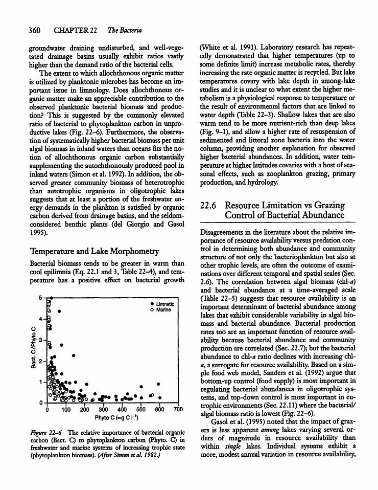
360 CHAPTER 22 The Bacteria
groundwater draining undisturbed, and weU-vege-tated drainage basins usually exhibit ratios vasdyhigher thanthedemand ratio ofthebacterial cells.The extent to whichaUochthonous organicmatter
is utilized by planktonic microbes hasbecome an important issue in limnology. Does aUochthonous organic mattermake an appreciable contribution to theobserved planktonic bacterial biomass and production? This is suggested by the commonly elevatedratio of bacterial to phytoplankton carbon in unproductive lakes (Fig. 22-6). Furthermore, the observation ofsystematicaUy higherbacterial biomass perunitalgal biomass in inland waters thanoceans fits thenotion of aUochthonous organic carbon substantiallysupplementing the autochthonously produced poolininlandwaters (Simon et al. 1992). In addition, the observed greater community biomass of heterotrophicthan autotrophic organisms in oligotrophia lakessuggests that at least a portion of the freshwater energy demands in the plankton is satisfied by organiccarbon derived from drainage basins, and the seldom-considered benthic plants (del Giorgio and Gasol1995).
Temperature andLakeMorphometryBacterial biomass tends to be greater in warm thancoolepilimnia (Eq. 22.1 and 3,Table 22-4), and temperature has a positive effect on bacterial growth
3 • Limnetico Marine
n i i i0 100 200 300 400 500 600 700
Phyto C (ocg CI"1)
Figure 22-6 The relative importance of bacterial organiccarbon (Bact. C) to phytoplankton carbon (Phyto. Q infreshwater and marine systems of increasing trophic state(phytoplankton biomass). (After Simon etal. 1982.)
(White et al. 1991). Laboratory research has repeatedly demonstrated that higher temperatures (up tosomedefinite limit) increase metabolic rates, therebyincreasing the rateorganic matteris recycled. Butlaketemperatures covary with lake depth in among-lakestudies and it is unclear to what extent the highermetabolism is a physiological response to temperature orthe result of environmental factors that are linked towater depth (Table 22-3). ShaUow lakes that are alsowarm tend to be more nutrient-rich than deep lakes(Fig. 9-1), and aUow a higher rate of resuspension ofsedimented and Uttoral zone bacteria into the watercolumn, providing another explanation for observedhigher bacterial abundances. In addition, water temperature at higherlatitudes covaries witha hostofseasonal effects, such as zooplankton grazing, primaryproduction, and hydrology.
22.6 Resource Limitation vs GrazingControl of Bacterial Abundance
Disagreements in the Uterature about the relative importanceof resourceavailabUity versuspredationcontrol in determining both abundance and communitystructure of not only the bacterioplankton but also atother trophic levels, are often the outcome of examinationsover different temporal and spatialscales (Sec.2.6). The correlation between algal biomass (chl-«)and bacterial abundance at a time-averaged scale(Table 22-5) suggests that resource availability is animportantdeterminantof bacterial abundance amonglakes that exhibitconsiderable variability in algal biomass and bacterial abundance. Bacterial productionrates too are an important function of resource avaU-ability because bacterial abundance and communityproduction are correlated (Sec. 22.7); but the bacterialabundance to chl-0 ratio declines with increasingchl-a, a surrogate for resourceavailability. Based on a simple food webmodel, Sanders et al. (1992) argue thatbottom-up control (food supply) is most important inregulating bacterial abundances in oligotrophic systems, and top-down control is most important in eutrophic environments (Sec. 22.11) where the bacterial/algal biomass ratio is lowest(Fig. 22-6).Gasol et al. (1995)noted that the impact of graz
ers is less apparent among lakes varying several orders of magnitude in resource avaUability thanwithin single lakes. Individual systems exhibit amore,modestannualvariation in resource avaUability,
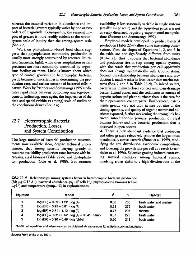
22.7 Heterotrophic Bacteria: Production, Losses, and System Contribution 361
whereas the seasonal variation in abundance and impactof bacterial grazers typically varies byone or twoorders of magnitude. Consequently, the seasonal impact of grazers is more readilyevident at the within-system scale of inquiry than the among-system scale(Sec. 2.6).Work on phytoplankton-based food chains sug
gests that phytoplankton community production isusuaUy most stronglyconstrained by resource limitation (nutrients, light),whUe their zooplankton or fishpredators are most commonly controUed by organisms feeding on them. Little is known about whichtype of control governs the heterotrophic bacteria,partlybecause of uncertainies in determiningthe production rates and carbon content of bacterial ceUs innature.Work byPsenner and Sommaruga (1992) indicates rapid shifts between bottom-up and top-downcontrol, indicating, once again, the importance of thetime and spatial (withinvs among) scaleof studiesonthe conclusions drawn (Sec. 2.6).
22.7 Heterotrophic Bacteria:Production, Losses,and SystemContribution
The large number of bacterial production measurements now available show, despite technical uncertainties, that among systems varying greatly inresource availability production rates increase with increasing algal biomass (Table 22-9) and phytoplankton production (Cole et al. 1988). But resource
avaUability is less seasonally variable in single systems(smaUer range scale) and the equivalent pattern is notas easUy discerned, requiring experimental manipulations (Psenner and Sommaruga 1992).Empirical models developed to predict bacterial
production (Table 22-9) aUow someinteresting observations. First, the slopes of Equations 1,2, and 3 inthe table are not significantly different from unity(0.81-1.22), thus it appears that bacterial abundanceand production rise in step among aquatic systems,with the result that production per ceU apparentlydoes not change systematicaUy with trophic status.Second, the relationshipbetweenabundanceand production ismuchweaker in freshwater thanmarine systems (Eqs. 2 and 3 in Table 22-9). In inland waters,bacteria are inmuchcloser contactwiththeirdrainagebasins, littoral zones, and the sediments as sources oforganic carbon and plant nutrients than is the case fortheir open-ocean counterparts. Furthermore, catchments gready vary not only in size but also in thetiming,quantity, and qualityof organicmatter and nutrients exported, further weakening the strong linkbetween autochthonous primary production or algalbiomass (chl-tf) and the bacterial production that isobserved in open oceans.• There is now abundant evidence that protozoanand other grazers selectively remove the larger, mostmetabolically active bacteria (Simek et al. 1999), modifying the size distribution, taxonomic composition,andlowering the growthrate per ceU asa result(Pern-thaler et al. 1996). Selective grazinginducescontrasting survival strategies among bacterial strains,involving either shifts to a high division rate of the
Table 22-9 Relationships amongsystems betweenheterotrophic bacterial production(BP, |tg C T1 d"1), bacterial abundance (A, 109 cells l"1), phytoplankton biomass (chl-a,|ig I-1) and temperature(temp.,°C)in euphoric zones.
Equation Model r2 n Habitat
1 log (BP) = 0.89 + 1.22 -log (A) 0.68 700 fresh water and marine2 log (BP)= 0.95 + 0.81 • log (A) 0.21 275 fresh water3 log(BP) = 0.71 + 1.12 -log(A) 0.77 207 marine4 log (BP)= 0.52 + 0.52 • log (A) + 0.041 • temp. 0.37 275 fresh water5 log (BP) = 0.90 + 0.49 • log (chl-a) 0.20 219 freshwater
'Additional equations and references can be obtained via anonymous ftp at ftp.icm.csic.es/pub/gasol.
Source: From White et al. 1991.
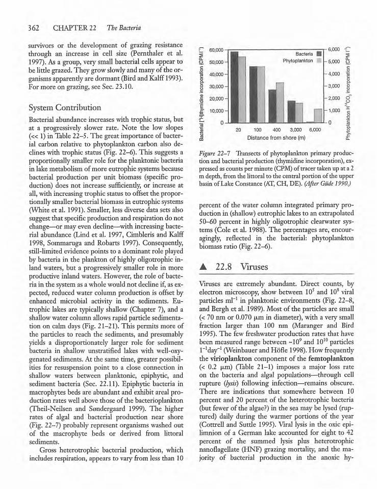
362 CHAPTER 22 The Bacteria
survivors or the development of grazing resistancethrough an increase in cell size (Pernthaler et al.1997). As a group, very small bacterial cells appear tobe little grazed. They grow slowly andmany of the organisms apparently aredormant (Bird andKalff 1993).For more on grazing, see Sec. 23.10.
System ContributionBacterial abundance increases with trophic status, butat a progressively slower rate. Note the low slopes(« 1) in Table 22-5. The great importance of bacterial carbon relative to phytoplankton carbon also declineswith trophic status (Fig. 22-6). This suggests aproportionally smaller role for the planktonic bacteriain lakemetabolismofmore eutrophic systems becausebacterial production per unit biomass (specific production) does not increase sufficiently, or increase atall,with increasing trophic status to offset the proportionallysmallerbacterialbiomass in eutrophic systems(White et al. 1991). Smaller, less diverse data sets alsosuggestthat specific production and respiration do notchange—ormay even decline—with increasingbacterial abundance (Lind et al. 1997, Cimbleris and Kalff1998, Sommaruga and Robarts 1997). Consequendy,still-limited evidence points to a dominant role playedby bacteria in the plankton of highly oligotrophic inland waters, but a progressively smaller role in moreproductive inland waters. However, the role of bacteria in the systemasa wholewould not declineif, as expected, reduced water column production is offset byenhanced microbial activity in the sediments. Eutrophic lakes are typically shallow (Chapter 7), and ashallowwater column allows rapid particle sedimentation on calm days (Fig. 21-21). This permits more ofthe particles to reach the sediments, and presumablyyields a disproportionately larger role for sedimentbacteria in shallow unstratified lakes with well-oxygenated sediments. At the same time, greater possibilities for resuspension point to a close connection inshallow waters between planktonic, epiphytic, andsediment bacteria (Sec. 22.11). Epiphytic bacteria inmacrophytes beds are abundant and exhibit areal production rates well above those of the bacterioplankton(Theil-Neilsen and Sondergaard 1999). The higherrates of algal and bacterial production near shore(Fig. 22-7) probably represent organisms washed outof the macrophyte beds or derived from littoralsediments.
Gross heterotrophic bacterial production, whichincludes respiration, appears to vary from less than 10
T_ 60,000 -i2 Bacteria •
p 6,000 t_2
Q. 50,000 - Phytoplankton - 5,000 o
'•§ 40,000 - nc
- 4.000 |8 30,000 - J- - 3,000 §
| 20,000 -J" 10,000- r r—j
- 2,000 OT
-1,000 co2
'S 20 100 400 3,000 6,000o
,S Distance from shore (m)
Q.O
1
Figure 22-7 Transects of phytoplankton primary production and bacterial production (thymidineincorporation), expressed ascountsper minute (CPM)of tracer takenup at a 2m depth, from the littoral to the central portion of the upperbasinof Lake Constance (AT, CH, DE). (After Glide 1990.)
percent of the water column integrated primary production in (shallow) eutrophic lakes to an extrapolated50-60 percent in highly oligotrophic clearwater systems (Cole et al. 1988).The percentages are, encouragingly, reflected in the bacterial: phytoplanktonbiomass ratio (Fig. 22-6).
A 22.8 Viruses
Viruses are extremely abundant. Direct counts, byelectron microscopy, show between 10' and 108 viralparticles ml-1 in planktonic environments (Fig. 22-8,and Berghet al. 1989). Most of the particles are small(< 70 nm or 0.070 p.m in diameter), with a very smallfraction larger than 100 nm (Maranger and Bird1995).The few freshwater production rates that havebeen measured range between ~109 and 1010 particlesl_1day_1 (Weinbauer andHofle 1998). Howfrequendythe virioplankton component of the femtoplankton(< 0.2 fim) (Table 21-1) imposes a major loss rateon the bacteria and algal populations—through cellrupture (lysis) following infection—remains obscure.There are indications that somewhere between 10percent and 20 percent of the heterotrophic bacteria(but fewer of the algae?) in the seamay be lysed (ruptured) daily during the warmer portions of the year(Cottrell and Suttle 1995). Viral lysis in the oxic epi-limnion of a German lake accounted for eight to 42percent of the summed lysis plus heterotrophicnanoflagellate (HNF) grazing mortality, and the majority of bacterial production in the anoxic hy-
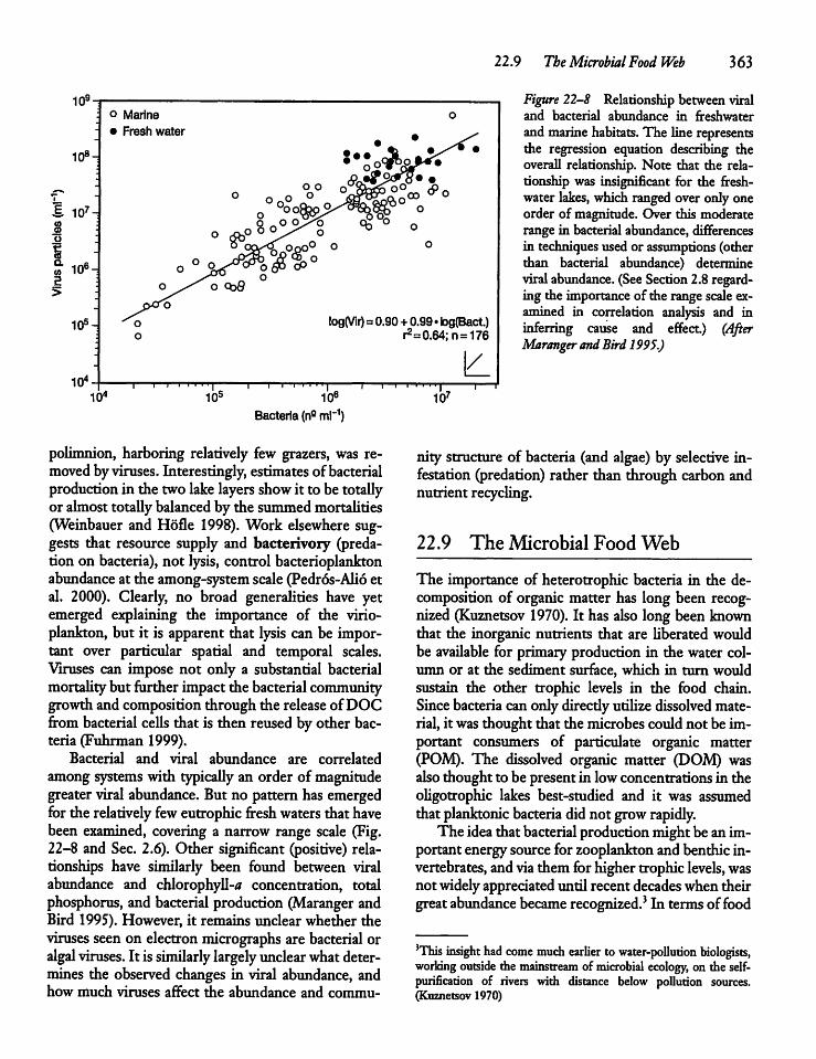
io9-r
108-
M, 107-Jo
JioH55
o Marine
• Fresh water
22.9 The Microbial Food Web 363
105- log(Vir)=0.90+0.99 • bg(Bact.)r2=0.64; n=176
Figure 22-8 Relationship between viraland bacterial abundance in freshwaterandmarine habitats. The line representsthe regression equation describing theovendl relationship. Note that the relationship was insignificant for the freshwater lakes, which rangedover onlyoneorder of magnitude. Over this moderaterange in bacterial abundance, differencesin techniquesused or assumptions (otherthan bacterial abundance) determineviralabundance. (SeeSection2.8 regarding the importanceof the range scale examined in correlation analysis and ininferring cause and effect.) (AfterMaranger andBird 1995.)
104104
i i i i i i
10s 106Bacteria (n°ml-1)
polimnion, harboring relatively few grazers, was removed byviruses.Interestingly, estimatesof bacterialproduction in the two lakelayers showit to be totaUyor almost totaUy balancedby the summedmortalities(Weinbauer and Hofle 1998). Work elsewhere suggests that resource supply and bacterivory (preda-tion on bacteria), not lysis, control bacterioplanktonabundance at the among-system scale(Pedros-Alio etal. 2000). Clearly, no broad generalities have yetemerged explaining the importance of the virio-plankton, but it is apparent that lysis can be important over particular spatial and temporal scales.Viruses can impose not only a substantial bacterialmortalitybut further impactthe bacterial communitygrowthand composition through the release ofDOCfrombacterial cellsthat is then reused by other bacteria (Fuhrman 1999).
Bacterial and viral abundance are correlatedamongsystems with typicaUy an order of magnitudegreater viral abundance. Butno pattern has emergedfor the relatively few eutrophicfreshwaters that havebeen examined, covering a narrow range scale (Fig.22-8 and Sec. 2.6). Other significant (positive) relationships have similarly been found between viralabundance and chlorophyU-* concentration, totalphosphorus, and bacterial production (Maranger andBird 1995).However, it remains unclear whether theviruses seen on electronmicrographs are bacterial oralgal viruses. It is similarly largely unclear whatdetermines the observed changes in viral abundance, andhow much viruses affect the abundance and commu
\LT 1 1107
nity structure of bacteria (and algae) by selective infestation (predation) rather than through carbonandnutrient recycling.
22.9 The Microbial Food Web
The importance of heterotrophic bacteria in the decomposition of organic matter has long been recognized (Kuznetsov 1970). It has also long been knownthat the inorganic nutrients that are liberated wouldbe available for primaryproduction in the water column or at the sediment surface, which in turn wouldsustain the other trophic levels in the food chain.Since bacteria canonlydirectly utilize dissolved material, it was thought that the microbes couldnot be important consumers of particulate organic matter(POM). The dissolved organic matter (DOM) wasalsothought to be present in lowconcentrationsin theoligotrophic lakes best-studied and it was assumedthatplanktonic bacteria didnot grow rapidly.The ideathat bacterial productionmightbe an im
portant energy source for zooplankton and benthic invertebrates, andvia themforhighertrophiclevels, wasnot widely appreciateduntil recent decades when theirgreatabundance became recognized.3 In terms offood
'This insight had come much earlier towater-pollution biologists,working outside the mainstream of microbial ecology, on the self-purification of rivers with distance below pollution sources.(Kuznetsov 1970)
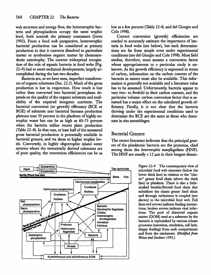
364 CHAPTER 22 The Bacteria
webstructure and energyflow, the heterotrophicbacteria and phytoplankton occupy the same trophiclevel, both nourish the primary consumers (Jones1992). From a food web perspective, heterotrophicbacterial production can be considered as primaryproduction in that it converts dissolved to particulatematter or synthesizes organic matter by chemosyn-thetic autotrophy. The current widespread recognition of the role of aquatic bacteria in foodwebs (Fig.22-9) had to awaittechnicaldevelopments, largelyaccomplished during the last two decades.Bacteria are, aswehaveseen, imperfecttransform
ers of organicsubstrates(Sec. 22.5). Much of the grossproduction is lost in respiration. How much is lostrather than converted into bacterial protoplasm dependson the qualityof the organicsubstrate andavailability of the required inorganic nutrients. Thebacterial conversion (or growth) efficiency (BCE orBGE) of substrate into bacterial biomass productionplateaus near 50percentin the plankton of highly eutrophic water but can be as high as 60-75 percentwhen the bacteria utilize recent plant production(Table 22-8). In that case, at least half of the measuredgross bacterial production is potentiaUy avadable tobacterial grazers, and via them to higher trophic levels. Conversely, in highly oligotrophic inland watersystems where the terrestrially derived substrates areof poor quality, the conversion efficiencies can be as
- ^ Zoobenthos
Viruses
Autochthonous and aUochthonous DOM "*"
lowasa few percent (Table 22-8, and del Giorgio andCole 1998).Correct conversion (growth) efficiencies are
needed to accuratelyestimate the importance of bacteria in food webs (see below), but such determinations are far from simple even under experimentalconditions (seedel Giorgio and Cole 1998).Most fieldstudies, therefore, must assume a conversion factorwhose appropriateness to a particular study is unknown. As the growth efficiency is expressed in termsof carbon, information on the carbon content of thebacteria in nature must also be available. This informationis generaUy not available and a Uterature valuehas to be assumed. Unfortunately, bacteria appear tovary two- to fivefold in their carbon content, and theparticularvolume: carbon conversion factor that is assumedhas a major effecton the calculated growth efficiency. Finally, it is not clear that the bacteriathriving under the experimental conditions used todetermine the BCE are the same as those who dominate in situ assemblages.
Bacterial Grazers
The recent Uterature indicatesthat the principalgrazers of the planktonic bacteria are the protozoa, chiefamong them the heterotrophic nanoflagellates (HNF).The HNF are usuaUy < 12 u-m in their longestdimen-
Top carnivoresFigure 22—9 The contemporaryviewofmicrobial food web structure (below thelower thick line) in relation to the "classic" grazer food chain (above the thickline) in plankton. There is also a little-studied benthic/littoral food chain thatsubsidizes the classic grazer food chainand through turbulence is coupled (notshown) to the microbial food web. FuUlines and arrows indicate feeding interactions, broken arrows indicate viral infections. The pool of dissolved organicmatter (DOM) used as a substrate by thebacteria is replenished by various releaseprocesses(excretion,exudation,ceU lysis,sloppy feeding) from each compartmentand from the catchment. (Modified fromWeisse and Stockner 1993.)
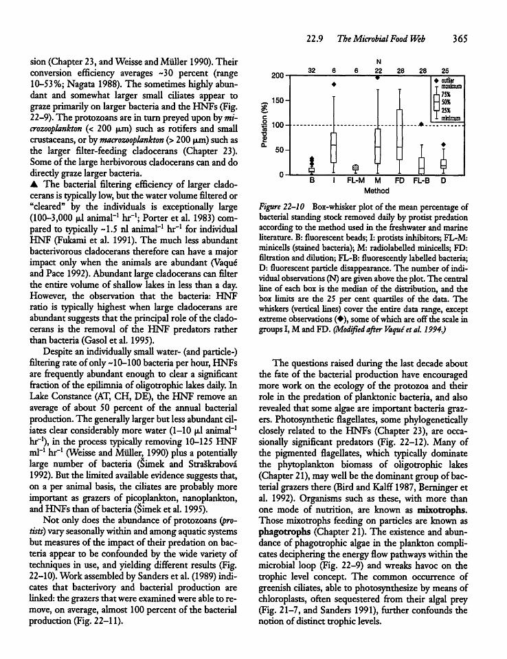
sion (Chapter 23, andWeisse andMuller 1990).Theirconversion efficiency averages ~30 percent (range10-53%; Nagata 1988). The sometimes highly abundant and somewhat larger smaU ciliates appear tograzeprimarilyon larger bacteriaand the HNFs (Fig.22-9). The protozoans are in turn preyed upon bymi-crozooplankton (< 200 u,m) such as rotifers and smaUcrustaceans, or bymacrozooplankton (>200 u,m) suchasthe larger filter-feeding cladocerans (Chapter 23).Some of the largeherbivorous cladocerans canand dodirectlygraze larger bacteria.• The bacterial filtering efficiency of larger cladocerans is typicaUy low,but the water volume filtered or"cleared" by the individuals is exceptionaUy large(100-3,000 ul animal-1 hr-1; Porter et al. 1983) compared to typicaUy -1.5 nl animal-1 hr-1 for individualHNF (Fukami et al. 1991). The much less abundantbacterivorous cladocerans therefore can havea majorimpact only when the animals are abundant (Vaqueand Pace 1992). Abundant large cladocerans can filterthe entirevolume of shaUow lakes in less than a day.However, the observation that the bacteria: HNFratio is typically highest when large cladocerans areabundantsuggests that the principal role of the cladocerans is the removal of the HNF predators ratherthan bacteria (Gasol et al. 1995).Despitean individuaUy smaU water- (andparticle-)
filtering rate of only~10-100bacteria per hour,HNFsare frequently abundant enough to cleara significantfraction of the epilimnia of oUgotrophic lakes dady. InLake Constance (AT, CH, DE), the HNF remove anaverage of about 50 percent of the annual bacterialproduction. The generally larger but lessabundantciliates clear considerably more water (1-10 u,l animal-1hr-1), in the process typicaUy removing 10-125 HNFml-1 hr-1 (Weisse and MuUer, 1990) plus a potentiaUylarge number of bacteria (Simek and Straskrabova1992). But the limitedavailable evidence suggests that,on a per animal basis, the cifiates are probably moreimportant as grazers of picoplankton, nanoplankton,and HNFs than ofbacteria (Simek et al. 1995).Not only does the abundance of protozoans (pro
tests) varyseasonaUywithin and amongaquaticsystemsbut measures of the impactof their predation on bacteria appear to be confounded by the wide variety oftechniques in use, and yielding different results (Fig.22-10).Work assembled by Sanderset al. (1989) indicates that bacterivory and bacterial production arelinked: the grazers that wereexamined wereableto remove, on average, almost 100percent of the bacterialproduction (Fig. 22-11).
200
~ 150-
£ 100CD
1Q.
50-
22.9 The Microbial Food Web 365
32 6 6 22 28 28 25
T f T
outliermaximum75X50%25Xminimum
B I FL-M M FD FL-B DMethod
Figure 22-10 Box-whisker plot of the mean percentage ofbacterial standing stockremoved daily by protist predationaccordingto the method used in the freshwaterand marineliterature. B: fluorescent beads; I: protistsinhibitors; FL-M:minicells (stained bacteria); M: radiolabeled miniceUs; FD:filtration and dilution; FL-B: fluorescendy labeUed bacteria;D: fluorescent particle disappearance. The number of individual observations (N)aregiven above theplot.The centralline of each box is the median of the distribution, and thebox limits are the 25 per cent quartiles of the data. Thewhiskers (vertical lines) cover the entire data range, exceptextreme observations some of which are off the scale ingroupsI, M and FD. (Modified after Vaque etal. 1994.)
The questions raised during the last decade aboutthe fete of the bacterial production have encouragedmore work on the ecologyof the protozoa and theirrole in the predation of planktonic bacteria, and alsorevealed that some algae are importantbacteria grazers. Photosynthetic flagellates, somephylogeneticallyclosely related to the HNFs (Chapter 23), are occa-sionally significant predators (Fig. 22-12). Many ofthe pigmented flageUates, which typicaUy dominatethe phytoplankton biomass of oUgotrophic lakes(Chapter 21), mayweU be the dominant groupofbacterial grazers there (Bird andKalff 1987, Berninger etal. 1992). Organisms such as these, with more thanone mode of nutrition, are known as mixotrophs.Those mixotrophs feeding on particles are known asphagotrophs (Chapter 21). The existence and abundance of phagotrophic algae in the planktoncompU-cates deciphering the energyflow pathways withinthemicrobial loop (Fig. 22-9) and wreaks havoc on thetrophic level concept. The common occurrence ofgreenish cifiates, able to photosynthesize by meansofchloroplasts, often sequestered from their algal prey(Fig. 21-7, and Sanders 1991), further confounds thenotion of distinct trophic levels.
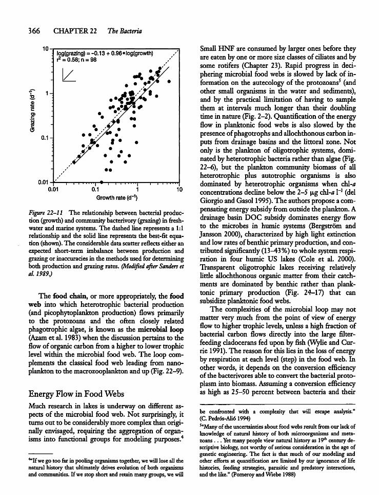
366 CHAPTER 22 The Bacteria
10
1-
CD
0.1-
0.01
log(grazing)= -0.13 +0.96«log(growth)r2 =0.58; n =98
T—r-r
0.01 0.1
Growth rate(d_1)
i i 111 "| i i i 111 ii1 10
Figure 22-11 The relationship betweenbacterial production (growth) andcommunity bacterivory (grazing) in freshwaterandmarinesystems. The dashedline represents a 1:1relationship and the solid line represents the best-fitequation (shown). The considerable data scatter reflects either anexpected short-term imbalance between production andgrazingor inaccuracies in the methodsusedfor determiningboth productionand grazingrates. (Modified after Sanders etal. 1989.)
The food chain, or more appropriately, the foodweb into which heterotrophic bacterial production(and picophytoplankton production) flows primarilyto the protozoans and the often closely relatedphagotrophic algae, is known as the microbial loop(Azam et al. 1983) when the discussion pertainsto theflow of organic carbonfroma higher to lowertrophiclevel within the microbial food web. The loop complements the classical food web leading from nano-plankton to the macrozooplanktonand up (Fig. 22-9).
Energy Flowin FoodWebsMuch research in lakes is underway on different aspects of the microbial food web. Not surprisingly, itturns out to be considerablymore complex than origi-nally envisaged, requiring the aggregation of organisms into functional groups for modeling purposes.4
^Ifwegotoo far in pooling organisms together, wewill lose all dienatural history that ultimately drives evolution of both organismsandcommunities. If we stop short andretainmany groups, wewill
SmaU HNF are consumedby larger ones before theyare eatenbyone or more sizeclasses of ciliates and bysome rotifers (Chapter 23). Rapid progress in decipheringmicrobial food webs is slowed by lackof information on the autecology of the protozoans5 (andother small organisms in the water and sediments),and by the practical limitation of having to samplethem at intervals much longer than their doublingtimein nature (Fig. 2-2). Quantification of the energyflow in planktonic food webs is also slowed by thepresenceofphagotrophsand aUochthonous carboninputs from drainage basins and the littoral zone. Notonly is the plankton of oUgotrophic systems, dominated by heterotrophic bacteriarather than algae(Fig.22-6), but the plankton community biomass of aUheterotrophic plus autotrophic organisms is alsodominated by heterotrophic organisms when cbl-aconcentrations decline below the 2-5 p,g chl-/* I"1 (delGiorgioandGasol 1995). The authorsproposea compensating energysubsidyfromoutsidethe plankton.Adrainage basin DOC subsidy dominates energy flowto the microbes in humic systems (Bergstrom andJansson 2000), characterized by high Ught extinctionand lowrates of benthic primaryproduction, and contributed significantly (13-43%) to wholesystemrespiration in four humic US lakes (Cole et al. 2000).Transparent oUgotrophic lakes receiving relativelylittle aUochthonous organic matter from their catchments are dominated by benthic rather than planktonic primary production (Fig. 24-17) that cansubsidize planktonicfoodwebs.The complexities of the microbial loop may not
matter very much from the point of view of energyflow to higher trophic levels, unless a high fractionofbacterial carbon flows directly into the large filter-feedingcladocerans fed upon by fish (WyUe and Currie 1991). The reason for this Ues in the lossof energyby respirationat each level (step) in the foodweb. Inother words, it depends on the conversion efficiencyof the bacterivores able to convert the bacterial protoplasminto biomass. Assuming a conversion efficiencyas high as 25-50 percent between bacteria and their
be confronted with a complexity that will escape analysis."(C. Pedros-Ali6 1994)5uMany of theuncertainties about food webs result from ourlack ofknowledge of natural history of both microorganisms and meta-zoans ... Yetmany people view natural history as 19* century descriptivebiology, not worthy of seriousconsideration in the ageofgenetic engineering. The fact is that much of our modeling andother efforts at quantification are limited by our ignorance of lifehistories, feeding strategies, parasitic and predatory interactions,and the like." (Pomeroy andWiebe 1988)
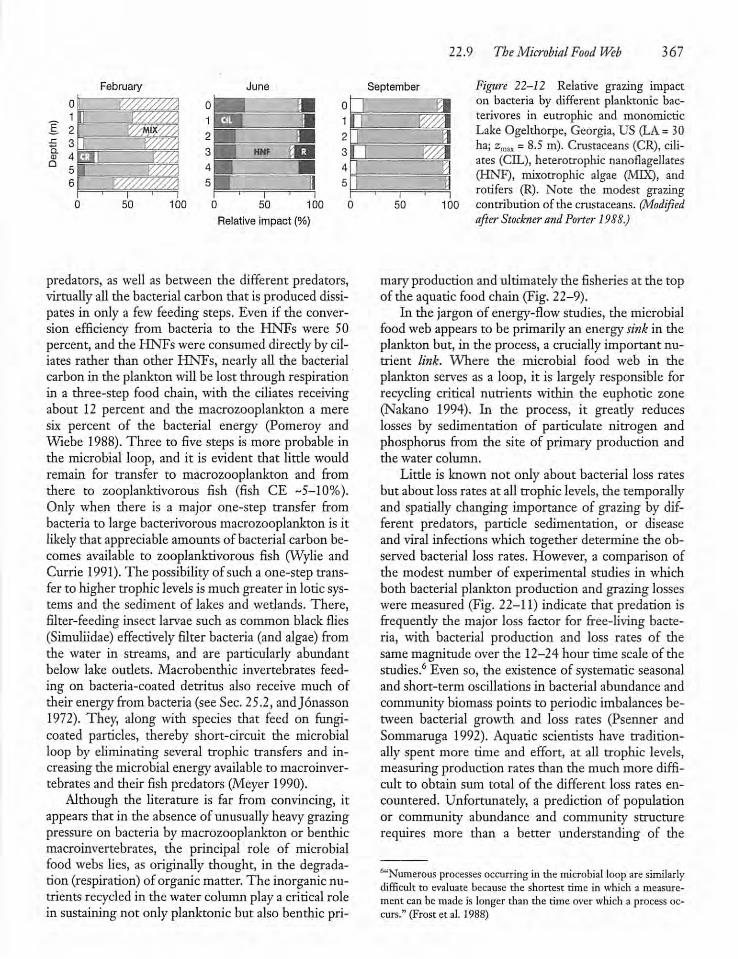
22.9 The Microbial Food Web 367
February
0 ... ::.vi1I V/////A2I MIX
3 I T/77A4j II V//A5| ! Y////,6
i
June
0 •1p II2 •3 HNF
4 •5 j 1
1 1 1 1
ftSeptember
^
Figure 22-12 Relative grazing impacton bacteria by different planktonic bac-terivores in eutrophic and monomicticLake Ogelthorpe, Georgia, US (LA=30ha; zm3X = 8.5 m). Crustaceans (CR), abates (CIL), heterotrophic nanoflagellates(HNF), mixotrophic algae (MIX), androtifers (R). Note the modest grazingcontribution of the crustaceans. (ModifiedafterStockner andPorter 1988.)
Q.o
D
50 100 0 50 100
Relative impact (%)
2
3:
4
predators, as well as between the different predators,virtually all the bacterial carbon that is produced dissipates in only a few feeding steps. Even if the conversion efficiency from bacteria to the HNFs were 50percent, and the HNFs were consumed direcdy by cil-iates rather than other HNFs, nearly all the bacterialcarbon in the plankton will be lost through respirationin a three-step food chain, with the ciliates receivingabout 12 percent and the macrozooplankton a meresix percent of the bacterial energy (Pomeroy andWiebe 1988). Three to five steps is more probable inthe microbial loop, and it is evident that little wouldremain for transfer to macrozooplankton and fromthere to zooplanktivorous fish (fish CE -5-10%).Only when there is a major one-step transfer frombacteria to large bacterivorous macrozooplankton is itlikelythat appreciable amounts of bacterial carbon becomes available to zooplanktivorous fish (Wylie andCurrie 1991).The possibility of such a one-step transfer to higher trophic levels is much greater in lotic systems and the sediment of lakes and wedands. There,filter-feeding insect larvae such as common black flies(Simuliidae) effectively filter bacteria (and algae) fromthe water in streams, and are particularly abundantbelow lake oudets. Macrobenthic invertebrates feeding on bacteria-coated detritus also receive much oftheir energy from bacteria (seeSec.25.2, andJonasson1972). They, along with species that feed on fungi-coated particles, thereby short-circuit the microbialloop by eliminating several trophic transfers and increasing the microbial energy available to macroinver-tebrates and their fish predators (Meyer 1990).Although die literature is far from convincing, it
appears that in the absence of unusually heavy grazingpressure on bacteria by macrozooplankton or benthicmacroinvertebrates, the principal role of microbialfood webs lies, as originally thought, in the degradation (respiration) of organicmatter. The inorganicnutrients recycled in the water column play a critical rolein sustaining not only planktonic but also benthic pri
J
3
50 100
mary production and ultimately the fisheries at the topof the aquatic food chain (Fig. 22-9).
In the jargon of energy-flow studies, the microbialfood web appears to be primarily an energy sink in theplankton but, in the process, a crucially important nutrient link. Where the microbial food web in theplankton serves as a loop, it is largely responsible forrecycling critical nutrients within the euphoric zone(Nakano 1994). In the process, it gready reduceslosses by sedimentation of particulate nitrogen andphosphorus from the site of primary production andthe water column.Little is known not only about bacterial loss rates
but about loss rates at all trophic levels, the temporallyand spatially changing importance of grazing by different predators, particle sedimentation, or diseaseand viral infectionswhich together determine the observed bacterial loss rates. However, a comparison ofthe modest number of experimental studies in whichboth bacterial plankton production and grazing losseswere measured (Fig. 22-11) indicate that predation isfrequendy the major loss factor for free-living bacteria, with bacterial production and loss rates of thesamemagnitude over the 12-24 hour time scaleof thestudies.6 Even so, the existence of systematic seasonaland short-term oscillations in bacterial abundance andcommunity biomass points to periodic imbalances between bacterial growth and loss rates (Psenner andSommaruga 1992). Aquatic scientists have traditionally spent more time and effort, at all trophic levels,measuring production rates than the much more difficult to obtain sum total of the different loss rates encountered. Unfortunately, a prediction of populationor community abundance and community structurerequires more than a better understanding of the
'"Numerous processes occurring in themicrobial loop aresimilarlydifficult to evaluate because the shortest time in which a measurement can be made is longer than the time over which a processoccurs." (Frost et al. 1988)
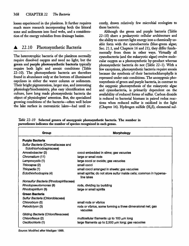
368 CHAPTER 22 The Bacteria
losses experienced in the plankton. It further requiresmuch more research incorporating both the littoralzone and sediments into food webs, and a consideration of the energysubsidies from drainagebasins.
A 22.10 Photosynthetic Bacteria
The heterotrophic bacteria of the plankton normallyrequire dissolved oxygen and need no light, but thegreen and purple photosynthetic bacteria typicallyrequire both Ught and anoxic conditions (Table22-10). The photosynthetic bacteria are thereforefound in abundanceonly at the bottom of illuminatedoxyclines in either the water column or sediments.Their bright pigmentation,larger size,and interestingphysiology/biochemistry, plus easy identification andculture, have long made photosynthetic bacteria theobjectof physiologists' attention. But, the specializedgrowing conditions of the bacteria—often well belowthe lake surface in meromictic lakes—had until re-
cendy, drawn relatively few microbial ecologists tothese bacteria.Although the green and purple bacteria (Table
22-10) share a prokaryotic cellular architecture andtheability to convert Ught energy intoa chemicaUyusable form with the cyanobacteria (blue-green algae;Sec. 21.1, and Chapters 16and 21), theydiffer fundamentally from them in other ways. Virtually aUcyanobacteria (and the eukaryotic algae) evolve molecular oxygen as a photosyntheticby-productwhereasphotosynthetic bacteria do not (Table 22-1). With afew exceptions, photosynthetic bacteria requireanoxiabecause the synthesis of their bacteriochlorophyUs isrepressed under oxicconditions.The anoxygenic photosynthesis of green and purple bacteria,in contrast tothe oxygenic photosynthesis of the eukaryotic algaeand cyanobacteria, is primarily dependent on theavailabiUty of reduced forms of sulfur. Carbon dioxideis reduced to bacterial biomass in paired redox reactions when reduced sulfur is oxidized in the Ught(Chapter 16).Hydrogen sulfide (H2S), elemental sul-
Table 22-10 Selected genera of anoxygenic photosynthetic bacteria. The number inparentheses indicates the number ofspecies recognized in each genus.
Group Morphology
Purple BacteriaSulfurBacteria (Chromatiaceae andEctothiorhodospiraceae)
Amoebobacter (2) cocci embedded in slime; gas vacuolesChromatium(11) large or small rodsLamprocystis (1) large cocci or ovoids; gas vacuolesThiocapsa (2) small cocciThiopedia (1) small cocci arranged in sheets; gas vacuolesEctothiorhodospira (4) small spirilla; do not store sulfur inside cells; common in hypersa-
line lakesNonsulfurBacteria (Rhodospirillaceae)Rhodopseudomonas (8) rods, dividing by buddingRhodospirillum (6) large or small spirillaGreen BacteriaSulfurBacteria (Chlorobiaceae)Chlorobium (5) small rods or vibriosPelodictyon (3) rods or vibrios, some forming a three dimensional net; gas
vacuoles
Gliding Bacteria (Chloroflexaceae)Chloroflexus (2) multicellular filaments up to 100 u,m longOscillochloris (1) large filaments up to 2,500 fxm long; gas vacuoles
Source: Modified after Madigan 1988.
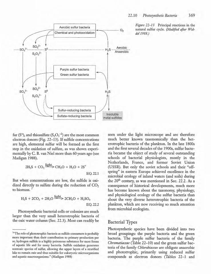
Aerobic sulfur bacteria
Chemical and photooxidation
Purple sulfur bacteria
Green sulfur bacteria
Sulfur-reducing bacteria
Sulfate-reducing bacteria
fur (S°), and thiosulfate (S203~2) are the mostcommonelectron donors (Fig. 22-13). If sulfide concentrationsare high, elemental sulfur will be formed as the firststep in the oxidation of sulfate, as was shown experimentally byC.B.vanNiel more than 60years ago(seeMadigan 1988).
2H,S + CO,ligh^CH20 + H20 + 2SC
EQ. 22.1
But when concentrations are low, the sulfide is oxidized direcdy to sulfate during the reduction of C02to biomass.7
H7S + 2CO, + 2H70light
> 2CH20 + H2S04
EQ.22.2
Photosynthetic bacterial cells or colonies are muchlarger than the very small heterotrophic bacteria ofthe oxic water column (Sec. 22.3). Most can readilybe
"The roleofphototrophic bacteria assulfide consumers isprobablymore important than their contribution to primaryproductionperse;hydrogen sulfide is a highlypoisonous substance formost formsof aquatic life and for many bacteria. Sulfide oxidation generatesnontoxic species of sulfur, allowing the upper layers of a stratifiedlake to remainoxicand thus suitable for eukaryotic microorganismsand aquaticmacroorganisms." (Madigan 1988)
H2SAnaerobic
HoS
22.10 Photosynthetic Bacteria 369
Figure 22-13 Principal reactions in the02 natural sulfur cycle. (Modified after Wid-
dell988.)
Aerobic
Insolublemetal sulfides
seen under the light microscope and are thereforemuch better known taxonomically than the heterotrophic bacteria of the plankton. In the late 1800sand the first several decades of the 1900s, sulfur bacteria became the object of study of several outstandingschools of bacterial physiologists, mostly in theNetherlands, France, and former Soviet Union(USSR). But only the soviet schools and their "offspring" in eastern Europe achieved excellence in themicrobial ecology of inland waters (and soils) duringdie 20th century, as was mentioned in Sec. 22.2. As aconsequence of historical developments, much morehas become known about the taxonomy, physiology,and physiological ecology of the sulfur bacteria thanabout the very diverse heterotrophic bacteria of theplankton, whichare now receiving so much attentionfrom microbial ecologists.
BacterialTypesPhotosynthetic species have been divided into twobroad groupings: the purple bacteria and the greenbacteria. The purple sulfur bacteria of the familyChroitiatiaceae (Table 22-10) and the green sulfur bacteria of the family Chlorobiaceae are obligate anaerobicand phototrophic, primarily using reduced sulfurcompounds as electron donors (Tables 22-1 and
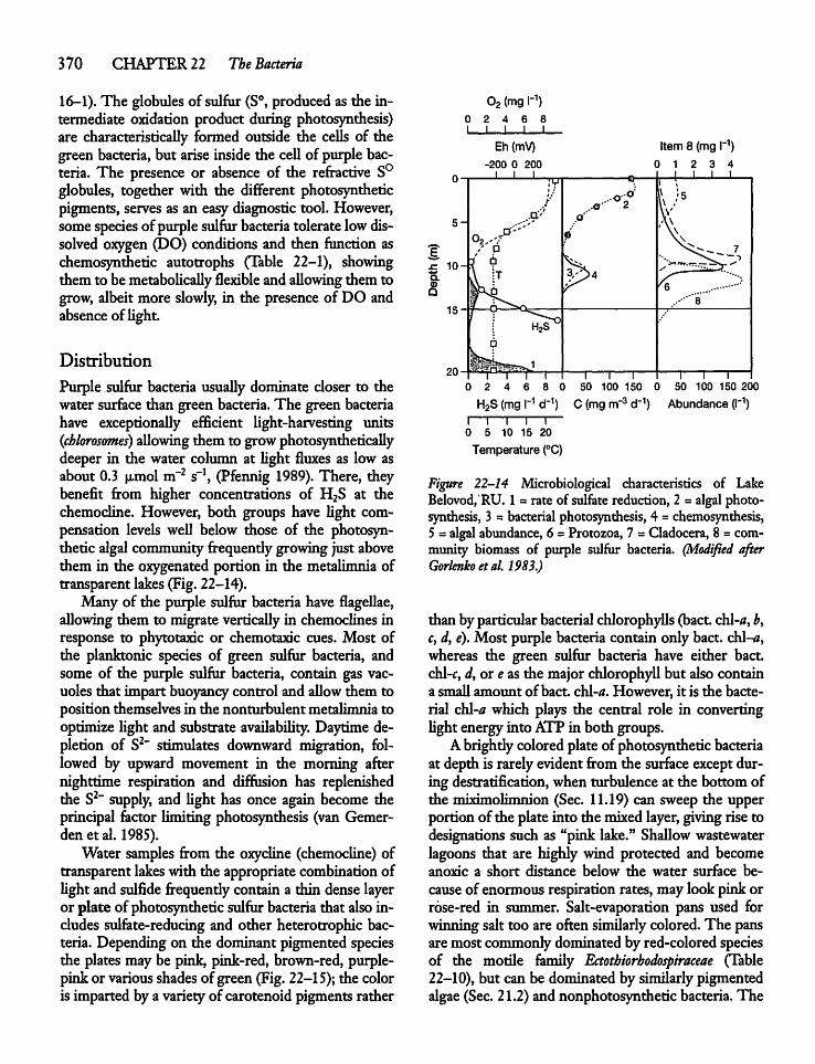
370 CHAPTER 22 The Bacteria
16-1). The globules of sulfur (S°, produced as the intermediate oxidation product during photosynthesis)are characteristicaUy formed outside the cells of thegreen bacteria, but arise inside the ceU of purple bacteria. The presence or absence of the refractive S°globules, together with the different photosyntheticpigments, serves as an easy diagnostic tool. However,somespecies of purple sulfurbacteria tolerate lowdissolved oxygen (DO) conditions and then function aschemosynthetic autotrophs (Table 22-1), showingthem to bemetabolically flexible and aUowing them togrow, albeit more slowly, in the presence of DO andabsenceof Ught.
Distribution
Purple sulfur bacteria usuaUy dominate closer to thewater surface than green bacteria.The green bacteriahave exceptionaUy efficient light-harvesting units(chlorosomes) allowing them to growphotosyntheticaUydeeper in the water column at Ught fluxes as low asabout 0.3 fxmol m~2 s"1, (Pfennig 1989). There, theybenefit from higher concentrations of H2S at thechemocline. However, both groups have Ught compensation levels weU below those of the photosynthetic algal communityfrequendygrowingjust abovethem in the oxygenated portion in the metalimnia oftransparent lakes (Fig. 22-14).Many of the purple sulfur bacteriahave flageUae,
aUowing them to migrate vertically in chemoclines inresponse to phytotaxic or chemotaxic cues. Most ofthe planktonic species of green sulfur bacteria, andsome of the purple sulfur bacteria, contain gas vacuoles that impart buoyancycontrol and allowthem topositionthemselves in the nonturbulent metalimnia tooptimize Ught and substrate availability. Daytimedepletion of S2" stimulates downward migration, followed by upward movement in the morning afternighttime respiration and diffusion has replenishedthe S2" supply, and Ught has once again become theprincipal factor limiting photosynthesis (van Gemer-den et al. 1985).Water samples from the oxycline (chemocline) of
transparent lakes with the appropriate combinationofUght and sulfide frequendycontain a thin denselayeror plate of photosynthetic sulfur bacteria that also includes sulfate-reducing and other heterotrophic bacteria. Depending on the dominant pigmented speciesthe platesmay be pink, pink-red, brown-red, purple-pinkor various shades of green (Fig. 22-15);the coloris imparted by a varietyof carotenoid pigmentsrather
a
02 (mg I"1)0 2 4 6 8I I I I L
Eh(mV)-200 0 200
I I l
Item 8 (mgI"1)0 12 3 4
a I 1 I 1
5-
10-
•T1f
.0/'
°2..-/°'""/ 0
\ JT
.O'
Vj>4
..<1 \
V5
.-'" 815-
HgS0
,UT| -p j1 1 1 1 1 1
0 2 4 6 8 0 50 100 150 0 50 100 150 200
H2S (mg I"1 d"1) C (mg rrr3 d"1) Abundance (I"1)I—I—I—I—I—0 5 10 15 20
Temperature (°C)
Figure 22-14 Microbiological characteristics of LakeBelovod/RU. 1 = rate of sulfatereduction, 2 = algal photosynthesis, 3 = bacterial photosynthesis, 4 = chemosynthesis,5 = algalabundance,6 = Protozoa, 7 = Cladocera,8 = community biomass of purple sulfur bacteria. (Modified afterGorlenko etal. 1983.)
than byparticular bacterialchlorophyUs (bact. chl-tf, b,ct d, e). Most purple bacteria contain only bact. chl-a,whereas the green sulfur bacteria have either bact.chl-c, d,or e as the major chlorophyll but also containa small amount ofbact. cbl-a. However, it is the bacterial chl-awhich plays the central role in convertingUght energyinto ATP in both groups.Abrighdy coloredplate of photosyntheticbacteria
at depth is rarelyevidentfrom the surface except during destratification, when turbulence at the bottom ofthe miximolimnion (Sec. 11.19) can sweep the upperportion of the plate into the mixed layer,givingrise todesignations such as "pink lake." Shallow wastewaterlagoons that are highly wind protected and becomeanoxic a short distance below the water surface because of enormous respiration rates,maylookpinkorrose-red in summer. Salt-evaporation pans used forwinningsalt too are often similarlycolored.The pansaremost commonlydominatedby red-coloredspeciesof the motile family Ectothiorhodospiraceae (Table22-10), but can be dominated by similarly pigmentedalgae (Sec. 21.2) and nonphotosynthetic bacteria. The
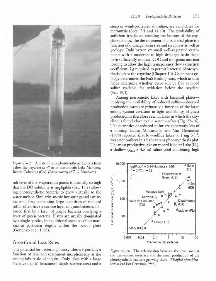
Figure 22-15 A plate of pink photosyndietic bacteria frombelow die oxycline at ~7 m in meromictic Lake Mahoney,British Columbia (CA). (Photo courtesy ofT. G. Noithcote.)
salt level of the evaporation ponds is normallyso highthat the DO solubility is negligible (Sec. 15.2) allowing photosynthetic bacteria to grow virtually to thewatersurface. Similarly, anoxic hot springsand estuar-ine mud flats containing large quantities of reducedsulfur often have a surface layer of cyanobacteria, followed first by a layer of purple bacteria overlying alayer of green bacteria. Plates are usually dominatedby a single species, but additional species exhibit maxima at particular depths within the overall plate(Gorlenko et al. 1983).
Growth and Loss Rates
The potential for bacterial photosynthesis ispartially afunction of lake and catchment morphometry at dieamong-lake scale of inquiry. Only lakes with a large"relative depth" (maximum depth-surface area) and a
22.10 Photosynthetic Bacteria 371
steep or wind-protected shoreline, are candidates formeromixis (Sees. 7.4 and 11.10). The probability ofsufficient irradiance reaching the bottom of the oxy-cline to allow the development of a bacterial plate is afunction of drainage basin size and steepness as well asgeology. Only barren or small well-vegetated catchments with a moderate to high drainage basin slopehave sufficiendy modest DOC and inorganic nutrientloading to allow the high transparency (low extinctioncoefficient, kd) required to permit bacterial photosyn-diesis below the oxycline (Chapter 10).Catchment geology determines the Fe:S loading ratio, which in turnhelps determine whether there will be free reducedsulfur available for oxidation below the oxycline(Sec. 19.3).Among meromictic lakes with bacterial plates—
implying the availability of reduced sulfur—observedproduction rates are primarily a function of the largeamong-system variation in light availability. Highestproduction is therefore seen in lakes in which the oxycline is found close to the water surface (Fig. 22-16).The quantities of reduced sulfur are apparently lessofa limiting factor; Montesinos and Van Gemerden(1986) reported that low-sulfide lakes (< 1 mg S 1_1)were not oudiers in a light versus photosynthesis plot.The most productive lake on record is Solar Lake (IL),a shallow (zmax = 4.5 m) saline pool combining high
10,000
EoO)
E
1,000-
100-
10-
1
0.001 0.01 0.1 1 10 100
Irradiance {% surface)
Figure 22-16 The relationship between the irradiance atdie oxic-anoxic interface and the areal production of diephotosyndietic bacteria growing there. (Modified after Montesinos and Van Gemerden 1986.)
log(Prod.) = 0.84«log(lrr.) + 1.95r2 = 0.77; n = 29I^ Fayetteville\f Green (US)
Veisovo (UA)
Mirror (US)Valle de San Juan
(CU)
• Solar(IL)
Ciso(ES)
Deadmoose••*/ *\(CA)
Wadolek (PL)
1Hiruga (JP)
Mary (US)
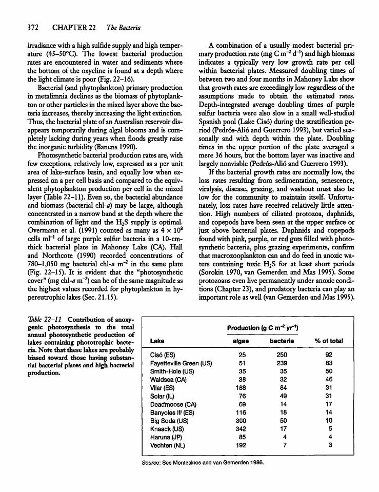
372 CHAPTER 22 The Bacteria
irradiance with a high sulfide supplyandhigh temperature (45-50°C). The lowest bacterial productionrates are encountered in water and sediments wherethe bottom of the oxycUne is found at a depth wherethe Ught climateis poor (Fig. 22-16).Bacterial (and phytoplankton) primaryproduction
in metalimnia declines as the biomass of phytoplankton or other particles in themixed layerabove die bacteriaincreases, therebyincreasing the Ught extinction.Thus, the bacterial plateofanAustraUan reservoir disappears temporarily during algal blooms and is completelylacking during yearswhen floods gready raisethe inorganic turbidity(Banens 1990).Photosyntheticbacterialproduction rates are,with
few exceptions, relatively low, expressed as a per unitarea of lake-surface basin, and equaUy low when expressed on a per ceU basis and comparedto the equivalent phytoplanktonproduction per ceU in the mixedlayer (Table 22-11). Even so, the bacterial abundanceand biomass (bacterial chl-a) may be large, althoughconcentratedin a narrow band at the depth where thecombination of Ught and the H2S supply is optimal.Overmann et al. (1991) counted as many as 4 x 10⁸cells ml-1 of large purple sulfur bacteria in a 10-cm-thick bacterial plate in Mahoney Lake (CA). Halland Northcote (1990) recorded concentrations of780-1,050 mg bacterial chl-a m"2 in the same plate(Fig. 22-15). It is evident that the "photosyntheticcover" (mg chl-a m'2) can beofthesame magnitude asthe highest values recorded for phytoplankton in hy-pereutrophic lakes (Sec. 21.15).
A combination of a usuaUy modest bacterial primary production rate(mg Cm"2 d"1) andhighbiomassindicates a typicaUy very low growth rate per ceUwithin bacterial plates. Measured doubling times ofbetweentwo and fourmonths inMahoney Lake showthat growth ratesareexceedingly lowregardless of theassumptions made to obtain the estimated rates.Depth-integrated average doubling times of purplesulfur bacteria were also slow in a smaU weU-studiedSpanish pool (Lake Ciso) during the stratification period (Pedr6s-AU6 and Guerrero 1993), but varied sea-sonaUy and with depth within the plate. Doublingtimes in the upper portion of the plate averaged amere 36 hours, but the bottom layerwas inactive andlargely nonviable (Pedr6s-AU6 and Guerrero 1993).If the bacterial growth rates are normaUy low, the
loss rates resulting from sedimentation, senescence,viralysis, disease, grazing, and washout must also below for the community to maintain itself. Unfortunately, loss rates have received relativelyUttle attention. High numbers of ciUated protozoa, daphnids,and copepods have been seen at die upper surfaceorjust above bacterial plates. Daphnids and copepodsfoundwith pink,purple, or red guts fiUed with photosynthetic bacteria, plus grazing experiments, confirmthat macrozooplankton can and do feed in anoxic waters containing toxic H2S for at least short periods(Sorokin 1970, van Gemerden and Mas 1995). Someprotozoans evenUve permanendyunder anoxic conditions (Chapter 23), and predatory bacteria can playanimportant role asweU (van Gemerden andMas 1995).
Table 22-11 Contribution of anoxygenic photosynthesis to the totalannual photosynthetic production oflakes containing phototrophic bacteria. Note that these lakes are probablybiased toward those having substantial bacterial plates and high bacterialproduction.
Production (g C m"2 yr~1)
Lake algae bacteria % of total
Cis6 (ES) 25 250 92
Fayetteville Green (US) 51 239 83
Smith-Hole (US) 35 35 50
Waldsea (CA) 38 32 46
Vilar(ES) 188 84 31
Solar (IL) 76 49 31
Deadmoose (CA) 69 14 17
Banyoles III (ES) 116 18 14
Big Soda (US) 300 50 10
Knaack (US) 342 17 5
Haruna (JP) 85 4 4
Vechten (NL) 192 7 3
Source: See Montesinos and van Gemerden 1986.
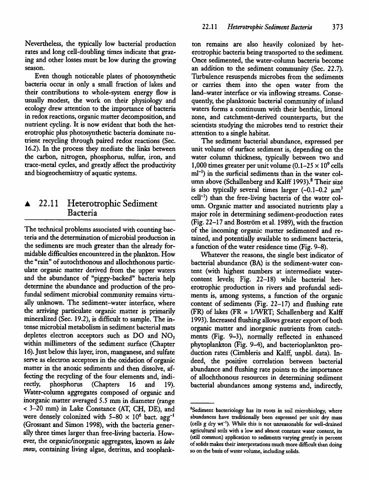
Nevertheless, the typicaUy low bacterial productionrates and long ceU-doubling times indicate that grazing and other losses must be lowduring the growingseason.
Even though noticeable plates of photosyntheticbacteria occur in only a smaU fraction of lakes andtheir contributions to whole-system energy flow isusually modest, the work on their physiology andecology drew attention to the importance of bacteriain redox reactions, organic matter decomposition, andnutrient cycUng. It is now evident that both the heterotrophic plus photosynthetic bacteria dominate nutrient recycling through paired redox reactions (Sec.16.2). In the process they mediate the links betweenthe carbon, nitrogen, phosphorus, sulfur, iron, andtrace-metal cycles, and greadyaffect the productivityand biogeochemistry of aquaticsystems.
A 22.11 Heterotrophic SedimentBacteria
The technical problems associated withcounting bacteriaandthe determination ofmicrobial production inthe sediments are muchgreater than the already formidable difficulties encountered in the plankton. Howthe "rain"of autochthonous andaUochthonous particulate organic matter derived from the upper watersand the abundance of "piggy-backed" bacteria helpdetermine the abundance and production of the pro-fundal sediment microbial community remains virtually unknown. The sediment-water interface, wherethe arriving particulate organic matter is primarilymineraUzed (Sec. 19.2), is difficult to sample. The intense microbial metaboUsm in sediment bacterial matsdepletes electron acceptors such as DO and N03within millimeters of the sediment surface (Chapter16). Just below this layer, iron,manganese, andsulfateserve aselectron acceptors in the oxidation of organicmatter in the anoxic sediments and then dissolve, affecting the recycling of the four elements and, indi-recdy, phosphorus (Chapters 16 and 19).Water-column aggregates composed of organic andinorganic matteraveraged 5.5 mmin diameter (range< 3-20 mm) in Lake Constance (AT, CH, DE), andwere densely colonized with 5-80 x 106 bact. agg-1(Grossant and Simon 1998), with the bacteria gener-aUy three times largerthan free-Uving bacteria. However, the organic/inorganic aggregates, known as lakesnow, containing Uving algae, detritus, and zooplank-
22.11 Heterotrophic Sediment Bacteria 373
ton remains are also heavily colonized by heterotrophicbacteriabeing transported to the sediment.Once sedimented, the water-column bacteria becomean addition to the sediment community (Sec. 22.7).Turbulence resuspends microbes from the sedimentsor carries them into the open water from theland-water interface or via inflowing streams. Conse-quendy, the planktonicbacterialcommunityof inlandwaters forms a continuum with their benthic, Uttoralzone, and catchment-derived counterparts, but thescientists studying the microbes tend to restrict theirattention to a single habitat.The sediment bacterial abundance, expressed per
unit volume of surface sediment is, depending on thewater column thickness, typicaUy between two and1,000 times greaterperunitvolume (0.1-25 x 109 cellsml-1) in the surficial sediments than in the water columnabove (SchaUenberg andKalff 1993).8 Their sizeis also typicaUy several times larger (~0.1-0.2 urn3ceU-1) than the free-Uving bacteria of the water column. Organicmatter and associated nutrients play amajor role in determining sediment-production rates(Fig. 22-17 and Bostrom et al. 1989),with the fractionof the incoming organic matter sedimented and retained, and potentiaUy available to sediment bacteria,a function of thewaterresidence time (Fig. 9-8).Whatever the reasons, the single best indicator of
bacterial abundance (BA) is the sediment-water content (with highest numbers at intermediate water-content levels; Fig. 22-18) while bacterial heterotrophic production in rivers and profundal sediments is, among systems, a function of the organiccontent of sediments (Fig. 22-17) and flushing rate(FR) of lakes (FR = 1/WRT; Schallenberg and Kalff1993). Increased flushing aUows greater export ofbothorganic matter and inorganic nutrients from catchments (Fig. 9-3), normally reflected in enhancedphytoplankton (Fig. 9-4), and bacterioplankton production rates (Cimbleris and Kalff, unpbl. data). Indeed, the positive correlation between bacterialabundance and flushing rate points to the importanceof aUochthonous resources in determining sedimentbacterial abundances among systems and, indirecdy,
8Sediment bacteriology has its roots in soil microbiology, whereabundances have traditionally been expressed per unit dry mass(cells g drywt"1). While this is not unreasonable for well-drainedagricultural soilswith a low and almost constant water content, its(still common) application to sediments varying greatly in percentofsolids makes their interpretations much more difficult than doingsoondiebasis ofwater volume, including solids.
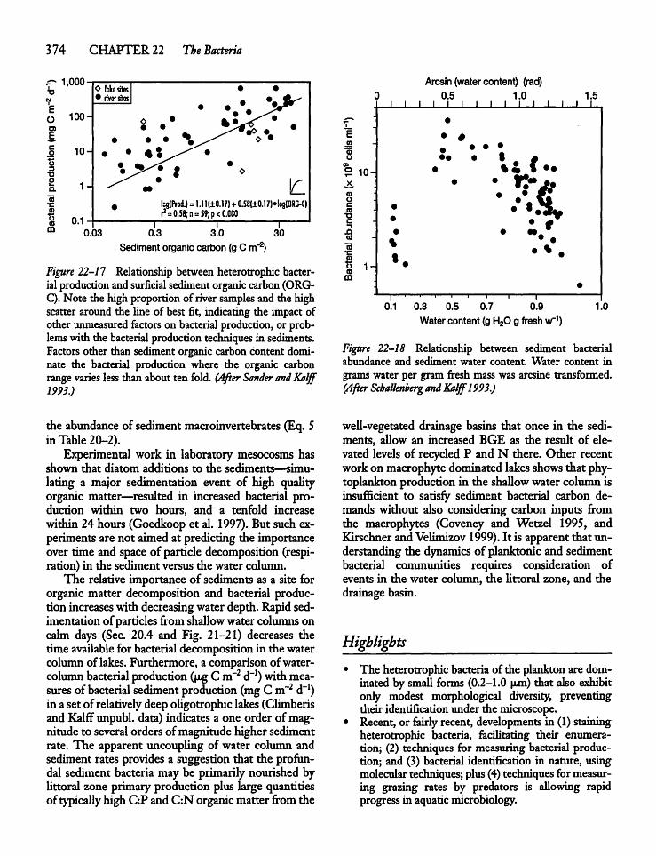
374 CHAPTER 22 The Bacteria
r* 1,000
=rEOO)E
O lakesites• river sites
• •
100-
•
% •* ***** •• • •^^ °
10- • • %\^^ •
1-
n 1
# bg(Prod.) =l.ll(±0.l7)+0.53(±0.l7)»!o;(0RG-C)r2=0.58; n=59; p< 0.000
0. )3I I I
0.3 3.0 30
Sedimentorganic carbon (gC m-2)
Figure 22-17 Relationship between heterotrophic bacterial productionand surficial sediment organiccarbon (ORG-C). Note the high proportion of river samples and the highscatter around the line of best fit, indicating the impact ofother unmeasured factors on bacterial production, or problemswith the bacterial production techniques in sediments.Factorsother than sedimentorganiccarbon content dominate the bacterial production where the organic carbonrangevariesless than about ten fold. (After Sander andKalff1993.)
the abundance of sedimentmacroinvertebrates (Eq. 5in Table 20-2).Experimental work in laboratorymesocosms has
shown that diatom additions to the sediments—simulating a major sedimentation event of high quaUtyorganic matter—resulted in increased bacterial production within two hours, and a tenfold increasewithin 24 hours (Goedkoop et al. 1997).But such experimentsare not aimedat predicting the importanceover time and space of particle decomposition (respiration) in the sediment versus the water column.The relative importance of sediments as a site for
organic matter decomposition and bacterial production increases with decreasingwater depth. Rapidsedimentationof particles fromshallowwater columns oncalm days (Sec. 20.4 and Fig. 21-21) decreases thetime available for bacterial decomposition in the watercolumn of lakes.Furthermore, a comparison of water-column bacterial production (u.g Cm"2 d-1) with measures ofbacterial sediment production (mg C m~2 d"1)in a set of relatively deepoUgotrophic lakes (Climberisand Kalffunpubl. data) indicates a one order of magnitude to severalorders of magnitude higher sedimentrate. The apparent uncoupling of water column andsediment rates provides a suggestion that the profun-dal sediment bacteriamay be primarily nourished bylittoral zone primary production plus large quantitiesof typicaUy highC:P and C:N organicmatter from the
? 10-
OCCOTJC3X>03
To
I0Q
Arcsin (water content) (rad)0.5 1.0
I I I I I I I I I
0.1 0.3 0.5 0.7 0.9
Watercontent(gH20g freshw~1)
Figure 22-18 Relationship between sediment bacterialabundance and sediment water content. Water content ingramswater per gram fresh masswas arcsine transformed.(After Schallenberg andKalff1993.)
weU-vegetated drainage basins that once in the sediments, aUow an increased BGE as the result of elevated levels of recycled P and N there. Other recentworkon macrophytedominatedlakesshowsthat phytoplanktonproduction in the shaUow water column isinsufficient to satisfy sediment bacterial carbon demands without also considering carbon inputs fromthe macrophytes (Coveney and Wetzel 1995, andKirschner andVelimizov 1999).It is apparent that understanding the dynamics of planktonicand sedimentbacterial communities requires consideration ofevents in the water column, the Uttoral zone, and thedrainagebasin.
Highlights• The heterotrophic bacteriaof the plankton are dominated by small forms (0.2-1.0 |im) that also exhibitonly modest morphological diversity, preventingtheir identification under the microscope.
• Recent, or fairlyrecent, developments in (1) stainingheterotrophic bacteria, faciUtating their enumeration; (2) techniques for measuringbacterial production; and (3) bacterial identification in nature, usingmoleculartechniques;plus (4) techniques for measuring grazing rates by predators is aUowing rapidprogressin aquaticmicrobiology.
The abundance of free-Uving bacteria in watercolumns usuaUy osciUates between 10s and 106 ceUsper ml-1, except in ultra-oUgotrophic and hypertrophic waters.Bacterial abundance and production increase amongsystemsas the resource availability increases, but at aprogressively slowerrate, pointing to disproportion-aUy higher lossrates in eutrophicsystems.Heterotrophic bacteriacompetewith algaefor limiting nutrients (e.g.,phosphorusand nitrogen).The principal bacterial predators are the typicaUyabundant heterotrophic nanoflageUates (HNFs),smaU ciUates, and phagotrophic algal flageUates, butcertain macrozooplankton and macrobenthic invertebrates are major consumerswhen abundant.• TypicaUy highbacteria:phytoplankton biomass ratios and autotrophicheterotrophic biomass ratios inthe plankton of oUgotrophic lakes points to energy(organic matter) subsidies from the littoral zone anddrainagebasins.
22.11 Heterotrophic Sediment Bacteria 375
A The C:P and C:N ratios of organic matter are animportantdeterminantof organic matter availabilityto microbes and their conversion (growth) efficiency.• Veryrecent studieson aquaticvirusesindicate thatthey can be important as a source of microbial mor-taUty, but also release microbe-derived organic matter to the microbial community.• The organic matter utilized in microbial foodwebs is often largely respired within the microbialloop,rather than available asmicrobial production tohigher trophic levels. In the process plant nutrients inhigh demandare recycled.• Communitiesof purple and green photosyntheticbacteria commonly form a denselayerat the bottomof the oxycline in lakes and sediments receiving botha sufficient irradiance and a supply of reduced sulfur.A The sediment bacterial community in the surficialsediments is, depending on water column thickness,typicaUy between twoand 1,000 timesgreaterthan inthe water column above.
CHAPTER
23
Zooplankton
23.1 Introduction
The inland water zooplankton, or animal plankton,range in sizefromsmallprotozoanflageUates lessthan2 |xm in their longest dimension to large crustaceansof several centimeters. The macrozooplankton,larger than 200 u,m and comprised principaUy of crustaceans, have been the subject of many Umnologicalstudiesduring the last 100years.Microzooplankton,those animal organisms smaUer than 200 u,m includethe rotifers, the smallestinstars (larval stages) of copepods, aswell as the protozoans. In practice, the microzooplankton designation is frequendy appUed to therotifers alone, a large group of animals that rank second to crustaceans in the amount of attention accorded them by biologists concerned with thezooplankton. For both taxonomic and analytical reasons protozoans or protozooplankton are usually, asin this text, considered separately from the other animal plankton.Crustacean zooplankton and all but the smaUest
rotifers can be quantitatively sampledwith traditionalplankton nets and traps. Rotifers are also easily preserved and can be readilyexamined with Ught microscopes under low magnification. This is not the casefor the much smaller ciUated and flagellated protozoans that must be collected, preserved, and examinedwith techniques that are generallyforeign to those interested in larger organisms. The techniquesrequiredfor the deUcate protozoans are more similar to techniques needed for the study of phytoplankton and arequite differentfrom those employed to examine larger376
zooplankton. As a consequence, the protozoans havereceived Utde attention from aquatic scientists untilrecendy, although in 1920, H. Lohmann (DE) proposed an important role for colorless flageUates inpelagic food webs. The neglect the protozoans havesuffered has been aUeviated with a surge of interest inthe ecologyof these organisms when their abundanceand importanceas predators of heterotrophic bacteriawasrecognized (Chapter22).The recent attention accorded to protozoans has led to a near revolution inideasabout the role of the zooplankton in aquatic systems. It has similarly becomewidelyrecognized during the last 30 years or so that planktivorous fish andother invertebrate predators, when abundant, havemajordirect and indirect effects (top-downeffects) onzooplankton abundance and community structure.This recognition changed earUer beUefs based uponthe idea that the availabiUty of resources (bottom-upeffects) and competition for these resources amongzooplankton species were the principal determinantsof abundance, distribution and community structureof animalplankton in nature.Apart from the zooplankton groups mentioned
above, there are a few species of insect larvae (e.g.,Chaoborus species and other midges, Chironomidae),jeUyfish, and larval clams (e.g., Dreissena, the zebramussels) that may at times be an important component of the animal plankton. Recendy hatchedlarval fish can also be consideredpart of the planktonfor the first weeks of their Ufe—until they becomestrong enough swimmers to determine their positionin the water columnregardless of turbulence,at which
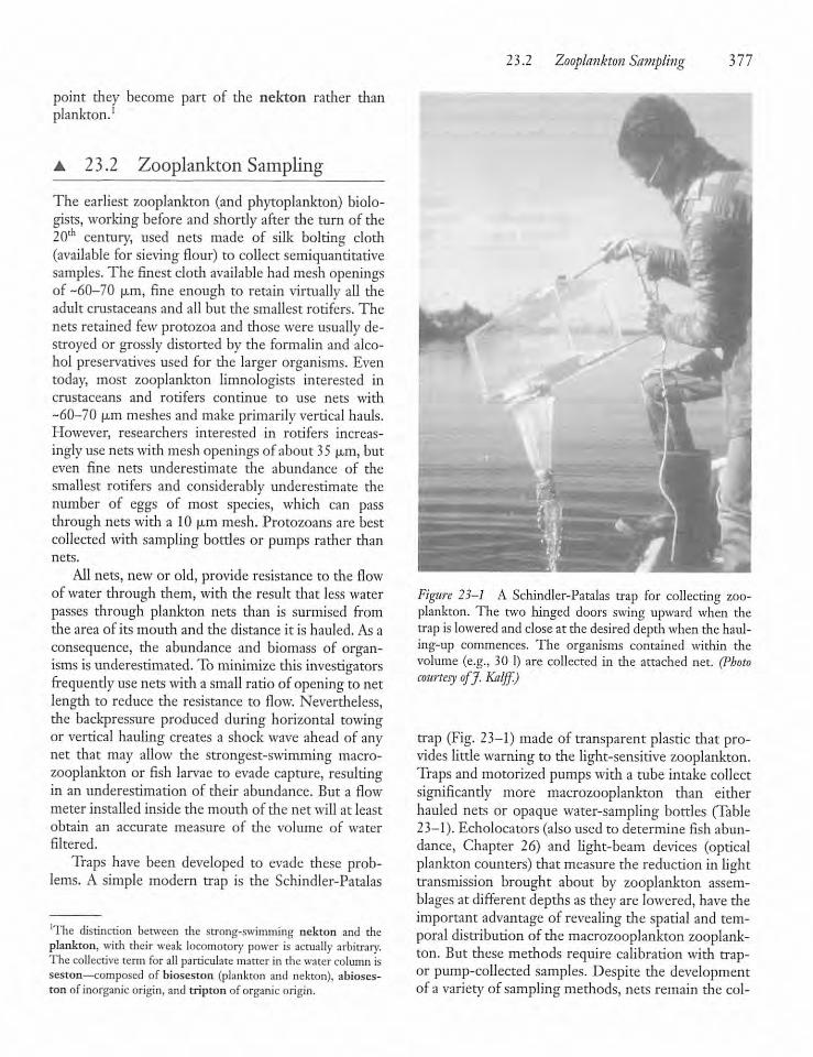
point they become part of the nekton rather thanplankton.1
• 23.2 Zooplankton Sampling
The earliest zooplankton (and phytoplankton) biologists, working before and shortly after the turn of the20 century, used nets made of silk bolting cloth(available for sieving flour) to collect semiquantitativesamples. The finest cloth available had mesh openingsof -60-70 |xm, fine enough to retain virtually all theadult crustaceans and all but the smallest rotifers. Thenets retained few protozoa and those were usually destroyed or grossly distorted by the formalin and alcohol preservatives used for the larger organisms. Eventoday, most zooplankton limnologists interested incrustaceans and rotifers continue to use nets with-60-70 (xm meshesand make primarilyvertical hauls.However, researchers interested in rotifers increasinglyuse nets with mesh openings of about 35 u,m, buteven fine nets underestimate the abundance of thesmallest rotifers and considerably underestimate thenumber of eggs of most species, which can passthrough nets with a 10 u,m mesh. Protozoans are bestcollected with sampling bottles or pumps rather thannets.
All nets, new or old, provide resistance to the flowof water through them, with die result that lesswaterpasses through plankton nets than is surmised fromthe area of its mouth and the distance it is hauled. As aconsequence, the abundance and biomass of organisms is underestimated. Tominimize diis investigatorsfrequently use nets with a small ratioof opening to netlength to reduce the resistance to flow. Nevertheless,the backpressure produced during horizontal towingor vertical hauling creates a shock wave ahead of anynet that may allow the strongest-swimming macrozooplankton or fish larvae to evade capture, resultingin an underestimation of their abundance. But a flowmeter installed inside the mouth of the net will at leastobtain an accurate measure of the volume of waterfiltered.Traps have been developed to evade these prob
lems. A simple modern trap is the Schindler-Patalas
'The distinction between the strong-swimming nekton and theplankton, with their weak locomotory power is actually arbitrary.The collective term for all particulate matter in the water column isseston—composed of bioseston (plankton and nekton), abioses-ton of inorganic origin,and tripton of organicorigin.
23.2 Zooplankton Sampling 377
Figure 23-1 A Schindler-Patalas trap for collecting zooplankton. The two hinged doors swing upward when dietrap is lowered andclose at the desired depth when thehaul-ing-up commences. The organisms contained within thevolume (e.g., 30 1) are collected in the attached net. (Photocourtesy ofJ. Kalff.)
trap (Fig. 23-1) made of transparent plastic that provides littlewarning to the light-sensitive zooplankton.Trapsandmotorized pumpswith a tube intakecollectsignificantly more macrozooplankton than eitherhauled nets or opaque water-sampling bottles (Table23-1). Echolocators (also used to determine fish abundance, Chapter 26) and light-beam devices (opticalplankton counters) thatmeasure the reduction in lighttransmission brought about by zooplankton assemblages at different depths as they are lowered, have theimportant advantage of revealing the spatial and temporal distribution of the macrozooplankton zooplankton. But thesemethods require calibration with trap-or pump-collected samples. Despite the developmentof a varietyof samplingmethods, nets remain the col-
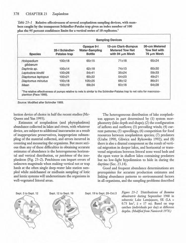
378 CHAPTER 23 Zooplankton
Table 23-1 Relative effectiveness of several zooplankton sampling devices, widi numbers caught by the transparent Schindler-Patalas trap given an index number of 100plus the 95percent confidence limitsfor a vertical seriesof 10 replicates.1
Sampling Devices
Opaque 9-1 13-cm Clark-Bumpus 30-cm Metered
28-I Schindler- Water-Sampling Metered Tow Net Tow Net with
Species Patalas trap Bottle with 94 u.m Mesh 76 u.m Mesh
Holopedium 100+18 65±15 71*18 65±24
gibberumDaphnia sp. 100±14 62+18 74±13 60±30
Leptodora kindtii 100±26 54±41 35+24 59+33
Diaptomus leptopus 100±21 60±22 54+23 49+21
Diaptomus minutus 100±18 105±25 68±12 86±31
Mean 100±19 69±24 60+18 64±28
The relative effectiveness of pumps relative to nets is similar to the Schindler-Patales trap to net ratio for macrozoo-plankton (Pace 1986).
Source: Modified after Schindler 1969.
lection device of choice in half the recent studies (McQueen and Yan 1993).Estimates of zooplankton (and phytoplankton)
abundance collected in lakes and rivers, with whateverdevice, are subject to additional inaccuracies as a resultof inappropriate preservatives, inappropriate subsam-pling of the material collected, and errors incurred incounting and measuring the organisms. But more serious than any of these difficulties in obtaining accurateestimates of abundance is the heterogeneous horizontal and vertical distribution, or patchiness of the zooplankton (Fig. 23-2). Patchiness can impart errors ofunknownmagnitudewhen makingvertical net or traphauls at the often single deep-water lake station sampled while midchannel or midbasin sampling of loticand lentic systems willunderestimate the organisms inwell-vegetated littoral areas.
The heterogeneous distribution of lake zooplankton appears in part determined by (1) system morphometry(lake depth and shape); (2)the configurationof inflows and outflows; (3) prevailingwinds; (4) current patterns; (5) upwellings; (6) competition for foodresources between zooplankton species; (7) predators(Urabe 1990, Gliwicz and Rykowska 1992); and (8)there is alsoa diurnal component as the result of verticalmigration in deeper lakes, and horizontal or transversal migrations between littoral zone weed beds andthe open water in shallow lakes containing predatorsbut no low-light hypolimnion to hide in during thedaytime(Sec. 23.14).Good and frequent abundance determinations are
prerequisites for accurate production estimates andlinking abundance patterns to environmental factorsin allorganisms, and the sampling problems described
Sept. 3 to Sept. 12 Sept. 12 to Sept. 19 Sept. 19 to Sept. 28-Oct.3 Figure 23-2 Distributions of Bosmhiaobtusirostris during September 1968 insubarctic Lake Latnjajaure, SE (LA =0.73 km2, z = 17 m). Based on trapcatches (individuals per day) at differentdepths. (Modifiedfrom Nauwerck 1918.)
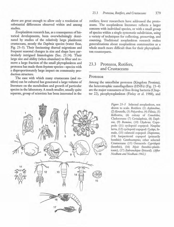
above are great enough to allow onlya resolution ofsubstantial differences observed within and amongstudies.Zooplankton research has, asa consequence ofhis
torical developments, been overwhelmingly dominated by studies of the relatively large planktoniccrustaceans, mosdy the Daphnia species (water fleas,Fig. 23-3). Their fascinating diurnal migrations andfrequent seasonal changes in sizeand shape have particularly intrigued limnologists (Sec. 23.14). Theirlarge size and ability (when abundant) to filter and remove a large fraction of the small phytoplankton andprotozoa hasmade them keystone species—species witha disproportionately large impact on community production structure.The ease with which many crustaceans (and ro
tifers) can be cultured has generated a largevolume ofliterature on the metabolism and growth of particularspecies in the laboratory. Amuchsmaller, usually quiteseparate, group of scientists has been interested in the
23.3 Protozoa, Rotifers, andCrustaceans 379
rotifers; fewer researchers have addressed the protozoans. The zooplankton literature reflects a largerconcern widi individual species, or with a small groupofspecies within a single systematic subdivision, usinga variety of techniques for collecting, preserving, andcounting. Traditional zooplankton research makesgeneralizations about zooplankton communities as awhole much more difficult than for their phytoplankton counterparts.
23.3 Protozoa, Rotifers,and Crustaceans
Protozoa
Among die unicellular protozoa (Kingdom Protista),the heterotrophic nanoflagellates (HNFs) (Fig. 23-4)are the major consumers of free-living bacteria (Chapter 22), picophytoplankton (Finlay et al. 1988), and
Figure 23-3 Selected zooplankton, notdrawn to scale. Rotifers: (1) Asplanchna,(2)Keratella, (3)Polyaithra, (4)Filinia, (5)Kellicottia, (6) colony of Conochilus;Cladocerans: (7) Ceriodaphnia, (8) Daphnia, (9) Bosmina, (10) Chydorus; Copepods: (11) cyclopoid copepod: Naupliuslarva, (12) cyclopoid copepod: Cyclops, female, (13) calanoid copepod: Diaptomus,(14) harpacticoid copepod (primarilybenthic): Canthocamptus; other selectedCrustaceans: (15) Ostracods: Cypridopsis(bendiic), (16) Mysis (benthic-plank-tonic), (17) Eubranchipus (littoral). (AfterNeedha?ti andNccdbam 1962.)
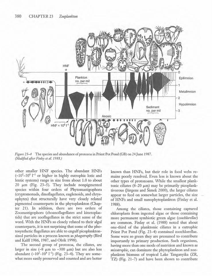
380 CHAPTER 23 Zooplankton
Epilimnion
Metalimnion
Hypolimnion
Figure 23-4 The speciesand abundanceof protozoa in Priest Pot Pond (GB)on 24June 1987.(Modified afterFinley etal. 1988.)
other smaller HNF species. The abundant HNFs(-lO'-lO8 l-1 or higher in highly eutrophic lotic andlentic systems) range in size from about 1.0 to about20 fim (Fig. 23-5). They include nonpigmentedspecies within four orders of Phytomastigophora(cryptomonads, dinoflagellates, euglcnoids, and chrys-ophytes) that structurally have very closely relatedpigmented counterparts in the phytoplankton (Chapter 21). In addition, there are two orders ofZoomastigophora (choanoflagellates and kinetoplas-tids) that are zooflagellates in the strict sense of dieword. With the HNFs so closely related to their algalcounterparts, it is not surprising that some of the photosynthetic flagellates are able to engulf picoplankton-sized particles in a process known asphagotrophy (Birdand Kalff 1986, 1987, and Olrik 1998).The second group of protozoa, die ciliates, are
larger in size (~8 u.m to ~300 u,m) but are also lessabundant (~102-104 T1) (Fig. 23-4). They are somewhat more easilypreserved and counted and are better
known than HNFs, but their role in food webs remains poorly resolved. Even less is known about theother types of protozoans. While the smallest planktonic ciliates (8-20 u,m) may be primarily picoplank-tivorous (Jiirgens and Simek 2000), the larger ciliatesappear to feed on somewhat larger particles, the sizeof HNFs and small nanophytoplankton (Finlay et al.1988).Among die ciliates, those containing captured
chloroplasts from ingested algae or those containingmore permanent symbiotic green algae (zoochlorellae)are common. Finlay et al. (1988) noted that aboutone-third of the planktonic ciliates in a eutrophicPriest Pot Pond (Fig. 23-4) contained zoochlorellae.Somewere so green they are presumed to contributeimportantly to primary production. Such organisms,havingmore than one mode of nutrition and known asauxotrophic, can dominate the phytoplankton and zooplankton biomass of tropical Lake Tanganyika (ZR,TZ) (Fig. 21-7) and have been shown to contribute
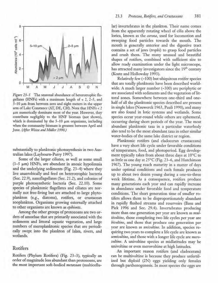
Figure 23-5 The seasonalabundance of heterotrophic flagellates (HNFs) with a maximum length of < 2, 2-5, and5-10 u.m from between zero and eight meters in the upperarm of Lake Constance (AT, DE, CH). Note that HNFs < 2u.m numerically dominate most of the year. However, theycontribute negligibly to the HNF biomass (not shown),which is dominated by the 5-10 u,m organisms, includingwhen the community biomass is greatest betweenApril andJune. (After Weisse andMtiller 1990.)
substantially to planktonic photosynthesis in twoAustralian lakes (Laybourn-Parry 1997).
Some of the larger ciliates, as well as some small(1-5 u.m) HNFs, are abundant in anoxic hypolimniaand the underlying sediments (Fig. 23-4) where theylive anaerobically and feed on heterotrophic bacteria(Sec. 22.9), nanoflagellates (Sec. 21.2), and colonies ofpurple photosynthetic bacteria (Sec. 22.10). Somespecies of planktonic flagellates and ciliates are normally not free-living but are attached to large phytoplankton (e.g., diatoms), rotifers, or crustaceanzooplankton. Organisms growing externally attachedto other organisms are known as epibionts.Among the other groups of protozoans are two or
ders of amoebae that are primarily associated with thesediments and littoral aquatic vegetation, and largenumbers of meroplanktonic species that are periodically swept into the plankton of lakes, rivers, andwetlands.
Rotifers
Rotifers (Phylum Rotifera) (Fig. 23-3), typically anorder ofmagnitude less abundantthan protozoans, arethe most important soft-bodied ?netazoan (multicellu
23.3 Protozoa, Rotifers, andCnistaceans 381
lar) invertebrates in the plankton. Their name comesfrom the apparently rotating wheel of cilia above thelorica, known as the corona, used for locomotion andsweeping food particles towards the mouth. Themouth is generally anterior and the digestive tractcontains a set of jaws (trophi) to grasp food particlesand crush diem. The many unusual and beautifulshapes of rotifers, combined with sufficient size toallow ready examination under the light microscope,has attracted many investigators since the 19th century(Koste and Hollowday 1993).Relatively few(-100) but ubiquitous rotifer species
that are totally planktonic have been described worldwide. A much larger number (-300) are periphytic orare associated with sediments and the vegetationof littoral zones. Somewhere between one-third and one-half of all the planktonic species described are presentin singlelakes (Nauwerck1963,Pauli 1990), and manyare also found in lotic systems and wetlands. Somespecies occur year-round while others are ephemeral,occurring during short periods of the year. The mostabundant planktonic taxa in a particular waterbodyalso tend to be the most abundant taxa in other similarwater-bodies of the same lakedistrict or region.
Planktonic rotifers (and cladoceran crustaceans)have a very short life cycle under favorable conditionsof temperature, food, and photoperiod. Egg development typically takes from about three days at 10°C toas little asone dayat 25°C (Fig. 23-6, and Hutchinson1967). The young reach maturity in a matter of daysunder optimal conditions and each female producesup to about two dozen young during a one-to-threeweek lifetime. As a consequence, rotifers producemany generations each year and can rapidly increasein abundance under favorable food and temperatureconditions. The short generation time of smaller rotifers allows them to be disproportionately abundantin rapidly flushed streams and reservoirs (Basu andPick 1996 and Sec. 29.4). Invertebrates producingmore than one generation per year are known asmul-tivoltine, those completing two life cycles per year arebivoltine, and those that produce one generation peryear are known as univoltine. In addition, species requiring twoyears to complete a lifecycle are known assemivoltine, and thosewith a longer life cycle aremero-voltine. A univoltine species at midlatitudes may beunivoltine or even merovoltine at high latitudes.An important reason rotifers (and cladocerans)
can be multivoltine is because they produce unfertilized but diploid (2N) eggs yielding only femalesthrough pardienogenesis. In mostspecies the eggs are
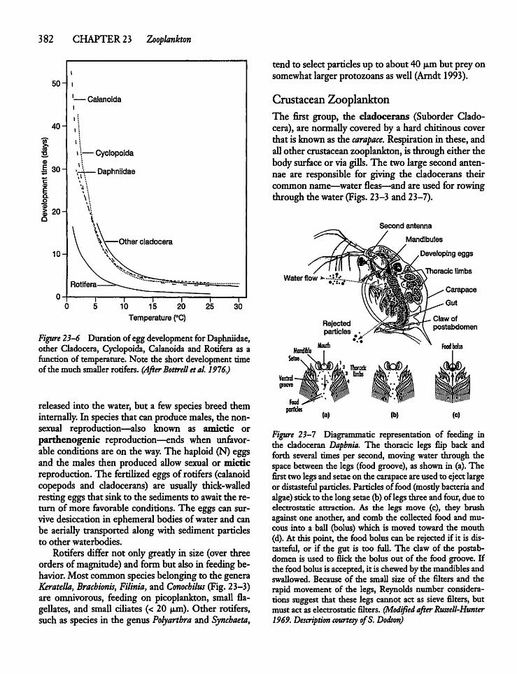
382 CHAPTER 23 Zooplankton
50-
40-
I©
.§ 30-
©
Eao©§ 20-Q
10-
Calanoida
— Cyclopoida
- Daphniidae
10 15
Temperature (°C)
Figure 23-6 Duration of eggdevelopment for Daphniidae,other Cladocera, Cyclopoida, Calanoida and Rotifera as afunction of temperature. Note the short developmenttimeof the much smallerrotifers. (After Bottrell etal. 1976.)
released into the water, but a fewspecies breed theminternally. In species that can producemales, the nonsexual reproduction—also known as amictic orparthenogenic reproduction—ends when unfavorable conditions are on the way. The haploid (N) eggsand the males then produced allow sexual or micticreproduction.The fertilized eggs of rotifers (calanoidcopepods and cladocerans) are usually thick-walledrestingeggsthat sink to the sedimentsto awaitthe return of more favorable conditions. The eggs can survive desiccation in ephemeral bodies ofwater and canbe aerially transported along with sediment particlesto other waterbodies.Rotifers differnot only gready in size (over three
orders of magnitude) and form but also in feedingbehavior. Most common speciesbelonging to the generaKeratella, Brachionis, Filinia, and Conochilus (Fig. 23-3)are omnivorous, feeding on picoplankton, small flagellates, and small cifiates (< 20 (xm). Other rotifers,such as species in the genus Polyarthra and Synchaeta,
tend to selectparticlesup to about 40 u,m but prey onsomewhat largerprotozoans aswell (Arndt 1993).
Crustacean ZooplanktonThe first group, the cladocerans (Suborder Cladocera), are normallycovered by a hard chitinouscoverthat is knownas the carapace. Respirationin these, andallother crustacean zooplankton, is througheither thebodysurface or viagills. The two largesecond antennae are responsible for giving the cladocerans theircommon name—waterfleas—and are used for rowingthrough the water (Figs. 23-3 and 23-7).
Second antenna
Mandibules
Developing eggs
Thoracic limbsWater flow
Ventralgroove
Carapace
Gut
Claw ofpostabdomen
Figure 23-7 Diagrammatic representation of feeding inthe cladoceran Dapbnia. The thoracic legs flip back andforth several times per second, movingwater through thespace between the legs (foodgroove), as shownin (a). Thefirst two legsand setaeon the carapaceareused to ejectlargeor distasteful particles. Particlesof food(mosdybacteria andalgae) stickto the longsetae(b)of legsthree and four, due toelectrostatic attraction. As the legs move (c), they brushagainst one another, and comb the collected food and mucous into a ball (bolus) which is moved toward the mouth(d). At this point, the food boluscan be rejectedif it is distasteful, or if the gut is too full. The claw of the postabdomen is used to flick the bolus out of the food groove. Ifthe foodbolusisaccepted, it ischewed by the mandibles andswallowed. Because of the small size of the filters and therapid movement of the legs, Reynolds number considerations suggest that these legs cannot act as sieve filters, butmust act as electrostatic filters. (Modified afterRussell-Hunter1969. Description courtesy ofS. Dodson)
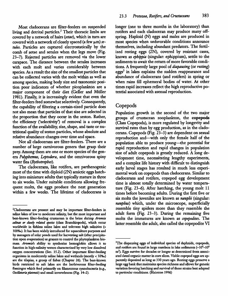
Most cladocerans are filter-feeders on suspendedliving and detrital particles.2 Their thoracic limbs arecovered bya network ofhairs (setae)y which in turnarecoveredwithanetworkofclosely spaced (afew u,m) seniles. Particles are captured electrostatically by thecomb of setae and setules when the legs move (Fig.23-7). Rejected particles are removed via the lowercarapace. The distance between the setules increaseswith each molt and varies considerably betweenspecies. As a resultthe size of thesmallest particles thatcan be collected varies with the molt within as well asamongspecies, makingbodysizeand taxonomic position poor indicators of whether picoplankton are amajor component of their diet (Geller and Muller1981). Finally, it is increasingly evident that even thefilter-feeders feedsomewhatselectively. Consequendy,the capabihty of filtering a certain-sized particle doesnot alsomeanthat particles of that sizeare selected inthe proportion that they occur in the seston. Rather,the efficiency ('selectivity') of removal is a complexfunction of the availability, size,shape, and tasteor nutritional quality ofsestonparticles, whose absolute andrelative abundance changes overtimeandspace.Not all cladocerans are filter-feeders. There are a
number of large carnivorous genera that grasp theirprey. Amongthem are one or more species of the genera Polyphemus, Leptodora, and the omnivorous spinywater flea (Bythotrephes).The cladocerans, like rotifers, are parthenogenic
mostof the timewith diploid(2N) amicticeggshatching into miniatureadults that typicallymature in threeto sixweeks. Under suitable conditions allowing frequent molts, the eggs produce the next generationwithin a few weeks. The lifetime of cladocerans is
2Cladocerans are present and may be important filter-feeders insaline lakes of lowto moderate salinity, but the most important andbest-known filter-feeding crustacean is the brine shrimp Anemiasalinas or closely related species (class Branchiopoda), which occurworldwide in Ashless saline lakes and tolerates high salinities (>300%o). It hasbeen widely introduced for aquaculture purposes andby managers of solar pondsused for harvestingsalt(afterprecipitationupon evaporation) asgrazers to controlthe phytoplankton biomass. Anemia's ability to synthesize hemoglobin allows it tofunction in high-salinitywaterscharacterized by very low dissolvedoxygen concentrations (Sec. 15.2). Other important filter-feedingorganisms in moderately saline lakesandwetlands(mosdy <30%o)are the tilapias, a group of fishes (Chapter 26). The best-knownbirds restricted to salt lakes are the herbivorous filter-feedingflamingos which feed primarilyon filamentous cyanobacteria (e.g.,Oscillatoria platensis) and smallinvertebrates (Fig. 14-2).
23.3 Protozoa, Rotifers, and Crustaceans 383
longer (one to three months in the laboratory) thanrotifers and each cladoceranmay produce many offspring. Haploid (N) eggs and males are produced inmost species when unfavorable conditions announcethemselves, including abundant predators. The fertilized resting eggs (2N), covered by resistant cases,known as epbippia (singular: ephippium), settle to thesediments to await the return ofmore favorable conditions. A frequendy large pool oidiapausing (or resting)eggs3 in lakes explains the sudden reappearance andabundance of cladocerans (and rotifers) in spring orwhen rains fill ephemeral bodies of water. At othertimes rapid increases reflect the high reproductive potential associatedwith asexual reproduction.
CopepodsPopulation growth in the second of the two majorgroups of crustacean zooplankton, the copepods(Class Copepoda), is more regulated by longevityandsurvival rates than by egg production,as in the cladocerans. Copepods(Fig. 23-3) are dependent on sexualreproduction and—with only the female half of thepopulation able to produce young—the potential forrapid reproduction and rapid changes in populationsize of adult copepods is gready reduced. A long development time, necessitating lengthy experiments,and a complex life historywith difficult to distinguishearly larval stages has resulted in much less experimentalworkon copepodsthan cladocerans. Similartocladocerans and rotifers, copepod egg developmenttime is almost totally determined by water temperature (Fig. 23-6). After hatching, the young molt 11timesbeforebecoming adults. During the first five orsixmolts the juveniles are knownas nauplii (singular:nauplius) which, under the microscope, superficiallyresemble tiny spiders more than they resemble theadult form (Fig. 23-3). During the remaining fivemolts the immatures are known as copepodites. Thelatter resemble the adult,alsocalled the copepodite VI
'The diapausing eggs of individual species of daphnids, copepods,and rotifers are found in large numbers in lake sediments (~104-106m2). Eggs survive for decades or longer as determined from associateddatedorganicmatter in coreslices. Viable copepodeggsareap-parendydepositedaslong as330 yearsago.Resting eggs preserve alarge eggbankthatmaintains species richness and allows forgenericvariation favoring hatchingand survival ofthose strainsbest adaptedto particular conditions. (Hairston 1996)
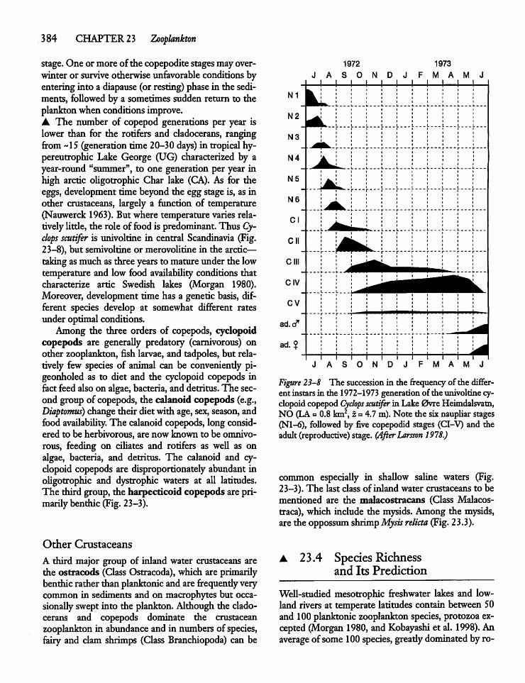
384 CHAPTER 23 Zooplankton
stage. One ormoreof the copepodite stages mayoverwinter or survive otherwise unfavorable conditions byenteringinto a diapause (or resting) phase in the sediments, followed by a sometimessudden return to theplanktonwhen conditions improve.A The number of copepod generations per year islower than for the rotifers and cladocerans, rangingfrom -15 (generationtime 20-30 days) in tropicalhy-pereutrophic Lake George (UG) characterized by ayear-round "summer", to one generation per year inhigh arctic oUgotrophic Char lake (CA). As for theeggs, development time beyond the egg stage is, as inother crustaceans, largely a function of temperature(Nauwerck 1963).But where temperature varies relatively Utde, the role of food is predominant.Thus Cyclops scutifer is univoltine in central Scandinavia (Fig.23-8), but semivoltine or merovolitine in the arctic—takingasmuch as three years to mature under the lowtemperature and low food availability conditions thatcharacterize artic Swedish lakes (Morgan 1980).Moreover, development time has a genetic basis, different species develop at somewhat different ratesunder optimal conditions.Among the three orders of copepods, cyclopoid
copepods are generaUy predatory (carnivorous) onother zooplankton, fish larvae, and tadpoles, but relatively few species of animal can be conveniendy pigeonholed as to diet and the cyclopoid copepods infact feedalsoon algae, bacteria,and detritus.The second group of copepods, the calanoid copepods (e.g.,Diaptomus) changetheir dietwith age, sex, season, andfood availabiUty. The calanoidcopepods, long considered to be herbivorous, are now known to be omnivorous, feeding on cifiates and rotifers as weU as onalgae, bacteria, and detritus. The calanoid and cyclopoid copepods are disproportionately abundant inoUgotrophic and dystrophic waters at aU latitudes.The third group, the harpecticoid copepods are primarilybenthic (Fig.23-3).
Other Crustaceans
A third major group of inland water crustaceans arethe ostracods (ClassOstracoda),which are primarilybenthic rather than planktonicand are frequendyverycommon in sediments and on macrophytes but occa-sionaUy sweptinto the plankton. Although the cladocerans and copepods dominate the crustaceanzooplankton in abundance and in numbersof species,fairy and clam shrimps (Class Branchiopoda) can be
1972 1973
JASONDJ FMAMJ
Figure 23-8 The succession in the frequency of the different instarsin the 1972-1973 generationof the univoltinecyclopoid copepod Cyclops scutifer in Lake0vre Heimdalsvatn,NO (LA=0.8 km2, z = 4.7 m).Note the sixnaupUar stages(Nl-6), followed by five copepodid stages (CI-V) and theadult (reproductive) stage. (After Larsson 1978.)
common especially in shallow saline waters (Fig.23-3). The last classof inland water crustaceans to bementioned are the malacostracans (Class Malacos-traca), which include the mysids. Among the mysids,are the oppossumshrimpMysis relicta (Fig. 23.3).
A 23.4 Species Richnessand Its Prediction
Well-studied mesotrophic freshwater lakes and lowland rivers at temperate latitudes contain between50and 100planktoniczooplanktonspecies, protozoa excepted (Morgan 1980, andKobayashi et al. 1998). Anaverage of some100species, greadydominated by ro-
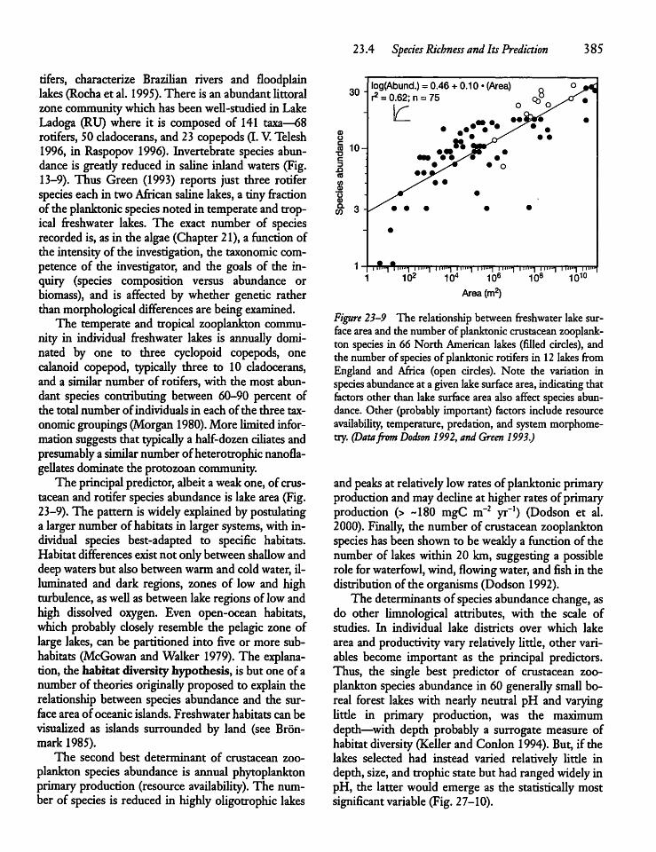
tifers, characterize Brazilian rivers and floodplainlakes (Rocha et al. 1995).There is an abundant Uttoralzone communitywhich has been wefi-studied in LakeLadoga (RU) where it is composed of 141 taxa—68rotifers, 50 cladocerans, and 23 copepods (I. V.Telesh1996, in Raspopov 1996). Invertebrate species abundance is gready reduced in saline inland waters (Fig.13-9). Thus Green (1993) reports just three rotiferspecies each in twoAfricansaline lakes,a tiny fractionof the planktonicspeciesnoted in temperate and tropical freshwater lakes. The exact number of speciesrecorded is, as in the algae (Chapter 21), a function ofthe intensityof the investigation, the taxonomic competence of the investigator, and the goals of the inquiry (species composition versus abundance orbiomass), and is affected by whether genetic ratherthanmorphological differences are being examined.The temperate and tropical zooplankton commu
nity in individual freshwater lakes is annually dominated by one to three cyclopoid copepods, onecalanoid copepod, typicaUy three to 10 cladocerans,and a similar number of rotifers, with the most abundant species contributing between 60-90 percent ofthe total number ofindividuals in each of the three taxonomicgroupings(Morgan 1980). More limitedinformationsuggests that typicaUy a half-dozen cifiates andpresumably a similar numberofheterotrophicnanofla-geUates dominate the protozoancommunity.The principalpredictor, albeit aweakone, of crus
taceanand rotifer species abundanceis lakearea (Fig.23-9). The pattern is widelyexplained by postulatinga larger number of habitats in larger systems, with individual species best-adapted to specific habitats.Habitatdifferences existnot onlybetween shaUow anddeepwatersbut alsobetweenwarmand coldwater, il-luminated and dark regions, zones of low and highturbulence, asweU asbetween lake regions of lowandhigh dissolved oxygen. Even open-ocean habitats,which probably closely resemble the pelagic zone oflarge lakes, can be partitioned into five or more sub-habitats (McGowan andWalker 1979). The explanation, the habitat diversity hypothesis, is but one of anumberof theoriesoriginaUy proposedto explain therelationship between species abundance and the surface area ofoceanic islands. Freshwater habitats can bevisualized as islands surrounded by land (see Bron-mark 1985).The second best determinant of crustacean zoo
plankton species abundance is annual phytoplanktonprimaryproduction (resourceavailabiUty). The number of species is reduced in highly oligotrophic lakes
23.4 Species Richness and Its Prediction 385
30 -log(Abund.) = 0.46 + 0.10 • (Area)r2 =0.62; n =75 *8D
O 0*
<D••••• •x
9/•
O «I • r< • •
| 10~ •-*Jr*c tm ••/•^ •3 • s* • oa •••^
$ s^% *o j«r •©a. oCO 3 - • • • • •
H •
•
•UTTW"pin^ i in'"] iin"T niu»| iu»"i iini'T ii ""1 1 """1
• 102 104 106 108 1010Area (m2)
Figure 23-9 The relationship between freshwater lakesurfacearea and the number of planktoniccrustaceanzooplankton species in 66 North American lakes (filled circles), andthe number of species of planktonicrotifers in 12 lakes fromEngland and Africa (open circles). Note the variation inspecies abundanceat a given lakesurfacearea, indicatingthatfactors other than lakesurface area also affect species abundance. Other (probablyimportant) factors include resourceavailabiUty, temperature, predation, and systemmorphometry. (Datafrom Dodson 1992,andGreen 1993.)
and peaks at relatively low rates of planktonicprimaryproductionandmaydecUne at higher rates of primaryproduction (> ~180 mgC m~2 yr"1) (Dodson et al.2000). Finally, the number of crustacean zooplanktonspecies has been shown to be weakly a function of thenumber of lakes within 20 km, suggesting a possiblerole forwaterfowl, wind, flowing water,and fishin thedistributionof the organisms(Dodson 1992).The determinants of species abundance change, as
do other Umnological attributes, with the scale ofstudies. In individual lake districts over which lakearea and productivity vary relatively Utde, other variables become important as the principal predictors.Thus, the single best predictor of crustacean zooplankton species abundance in 60 generaUy small boreal forest lakes with nearly neutral pH and varyinglittle in primary production, was the maximumdepth—with depth probably a surrogate measure ofhabitat diversity (Keller and Conlon 1994). But, if thelakes selected had instead varied relatively Utde indepth,size, and trophic state but had rangedwidely inpH, the latter would emerge as the statistically mostsignificant variable (Fig. 27-10).
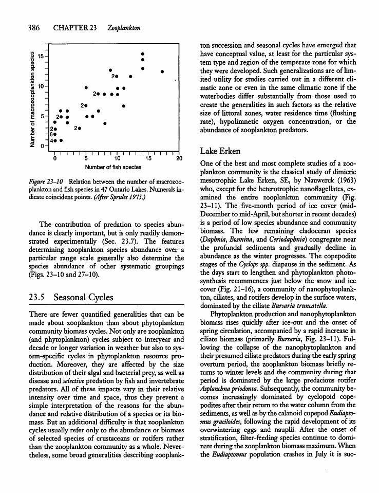
386 CHAPTER 23 Zooplankton
Number of fish species
Figure 23-10 Relation between the number of macrozooplanktonand fishspecies in 47 Ontario Lakes. Numerals indicatecoincidentpoints. (After Sprules 1975.)
The contribution of predation to species abundance is clearly important, but is only readily demonstrated experimentally (Sec. 23.7). The featuresdetermining zooplankton species abundance over aparticular range scale generally also determine thespecies abundance of other systematic groupings(Figs. 23-10 and 27-10).
23.5 SeasonalCycles
There are fewer quantified generalities that can bemade about zooplankton than about phytoplanktoncommunity biomasscycles. Not only are zooplankton(and phytoplankton) cycles subject to interyear anddecadeor longer variation in weather but also to system-specific cycles in phytoplankton resource production. Moreover, they are affected by the sizedistribution of their algal and bacterial prey, asweU asdiseaseand selective predation by fish and invertebratepredators. All of these impacts vary in their relativeintensity over time and space, thus they prevent asimple interpretation of die reasons for die abundance and relative distribution of a speciesor its biomass. But an additional difficulty is that zooplanktoncycles usually refer only to the abundance or biomassof selected species of crustaceans or rotifers ratherthan the zooplankton community as a whole. Nevertheless, some broad generaUties describing zooplank
ton succession and seasonal cycles have emerged thathave conceptual value, at least for the particular system type and region of the temperate zone for whichtheyweredeveloped. SuchgeneraUzations are of Um-ited utility for studies carried out in a different climatic zone or even in the same climatic zone if thewaterbodies differ substantiaUy from those used tocreate the generaUties in such factors as the relativesize of Uttoral zones, water residence time (flushingrate), hypoUmnetic oxygen concentration, or theabundance of zooplankton predators.
Lake Erken
One of the best and most complete studies of a zooplankton community is the classical study of dimicticmesotrophic Lake Erken, SE, by Nauwerck (1963)who, except for the heterotrophic nanoflagellates, examined die entire zooplankton community (Fig.23-11). The five-month period of ice cover (mid-Decemberto mid-April, but shorter in recent decades)is a period of low species abundance and communitybiomass. The few remaining cladoceran species(Daphnia, Bosmina, and Ceriodaphnia) congregate nearthe profundal sediments and gradually decUne inabundance as the winter progresses. The copepoditestages of the Cyclops spp. diapause in the sediment. Asthe days start to lengthen and phytoplankton photosynthesis recommences just below the snow and icecover (Fig. 21-16), a community of nanophytoplank-ton, ciUates, and rotifers developin the surfacewaters,dominatedby the ciUate Bursaria truncatella.Phytoplanktonproductionand nanophytoplankton
biomass rises quickly after ice-out and the onset ofspring circulation, accompanied by a rapid increase inciUate biomass (primarily Bursaria, Fig. 23-11). Following the collapse of the nanophytoplankton andtheir presumedciUate predatorsduring the earlyspringoverturn period, the zooplankton biomass briefly returns to winter levels and the community during thatperiod is dominated by the large predacious rotiferAsplanchnapriodonta. Subsequendy, the communitybecomes increasingly dominated by cyclopoid cope-podites after their return to thewatercolumnfromthesediments, asweU asby the calanoid copepodEudiapto-mus graciloides, following the rapid development of itsoverwintering eggs and nauplu. After the onset ofstratification, filter-feeding species continue to dominateduringthe zooplankton biomass maximum.Whenthe Eudiaptomus population crashes in July it is sue-
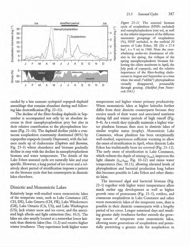
23.5 Seasonal Cycles 387
aooN
ice stratified period ice
35- ;\ Nanophytoplankton30-
25-
20-
: ri Zooplankton-4
3
15- -2
10-
5--1
I I I i i I I I I i iM O N
ClO
>,
Q.o
Figure 23-11 The seasonal biomasscycle of zooplankton (HNFs excluded)and nanophytoplankton (wet wt), as wellas the relative importance of the differenttaxonomic groupings of zooplankton(%), HNF excluded, in the surficial 20meters of Lake Erken, SE (SA = 27.4km2, z = 9 m) in 1960. Note the overwhelming under-ice dominance of ciliates in the spring, the collapse of thespring nanophytoplankton biomass following the ciliate maximum in April, theJuly peak of copepods, and the relativeimportance of the filter-feeding cladocerans in August and September at a timewhen the small ("edible") phytoplanktonvirtually disappeared, presumablythrough grazing. (Modified from Nauw-erckl963.)
cladocerans
o 100O N
ceeded by a late summer cyclopoid copepod-daphnidassemblage that remains abundant during and following lake destratification (Fig. 23-11).The decline of the filter-feeding daphnids in Sep
tember is accompanied not only by an absolute increase in their nanophytoplankton prey but also intheir relative contribution to the phytoplankton biomass (Fig. 21-16). The daphnid decline yields a crustacean zooplankton community dominated (80%) bycopepodite copepods (mostlyDiaptomus), with the balance made up of cladocerans (Daphnia and Bosmina,Fig. 23-3) whose abundance and biomass graduallydecline in step with the decline in nanophytoplanktonbiomass and water temperature. The details of theLake Erken seasonal cycle are naturally lake and yearspecific. However, a long period of ice cover and a relatively short period of stratification imposes a patternon the biomass cycle that has counterparts in dimicticlakes elsewhere.
Dimictic and Monomictic Lakes
Relatively large well-studied warm monomictic lakesof the temperate zone, such as Lake Constance (AT,CH, DE), Lake Geneva (CH, FR), Lake Windermere(GB), Lake Ontario (CA, US), and LakeWashington(US), lack winter snow and ice cover, and the associated high albedo and light extinction (Sec. 10.3). Thelakes are alsousually located at a somewhat lower latitude than dimictic lakes (Sec. 11.2) and receive higherwinter irradiance. They experience both higherwater
temperature and higher winter primary productivity.Warm monomictic lakes at higher latitudes furtherdiffer from their dimictic counterparts because theyreceive much of their water and associated nutrientsduring fall and winter periods of high runoff (Fig.8-4). As a result they typically maintain a higher winter plankton biomass than seen in dimictic lakes ofsimilar trophic status (trophy). Monomictic LakeConstance, whose plankton has been exceptionallywell-studied, experiences sufficient warming to allowthe onset of stratification in April, when dimictic LakeErken has traditionally been ice covered (Fig. 23-11).The early onset of stratification in Lake Constance,which reduces the depth of mixing(zmix), improves thelight climate (z^-.z^x, Fig. 10-12) and raises watertemperatures (Sec. 10.11), allowing elevated levels ofphytoplankton and bacterial production long beforethis becomes possible in Lake Erken and other dimictic lakes.The increased algal and bacterial biomass (Fig.
22-1) together with higher water temperatures allowmuch earlier egg development as well as highergrowth rates of protozoans (Fig. 23-5), rotifers, andcrustacean zooplankton in Lake Constance and otherwarm monomictic lakes of the temperate zone, than ispossible in their dimictic counterparts with a lengthyperiod of ice cover. Longer autumnal days and resulting greater daily irradiance further extends the growing season of temperate zone monomictic lakes,allowing more generations of zooplankton and potentially permitting a greater role for zooplankton in
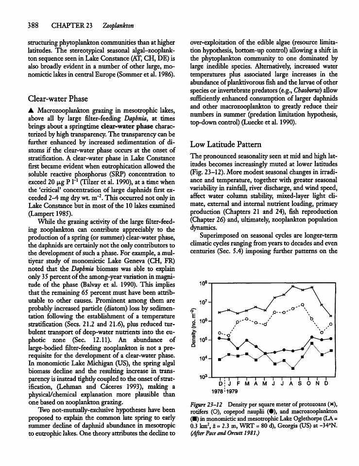
388 CHAPTER 23 Zooplankton
stnicturingphytoplankton communities thanat higherlatitudes. The stereotypical seasonal algal-zooplank-ton sequenceseen in Lake Constance (AT, CH, DE) isalso broadly evident in a number of other large, monomicticlakes in centralEurope (Sommeret al. 1986).
Clear-water Phase
• Macrozooplankton grazing in mesotrophic lakes,above aU by large filter-feeding Daphnia, at timesbrings about a springtime clear-water phase characterizedbyhigh transparency. The transparency canbefurther enhanced by increased sedimentation of diatoms if the clear-water phase occurs at the onset ofstratification. A clear-water phase in Lake Constancefirst became evidentwhen eutrophication allowed thesoluble reactive phosphorus (SRP) concentration toexceed 20 u,g P l"1 (Tilzer et al. 1990), at a time whenthe 'critical' concentration of large daphnids first exceeded 2-4mgdrywt. m~2. Thisoccurred notonly inLake Constance but in most of the 10 lakes examined(Lampert 1985).While the grazing activity of the large filter-feed
ing zooplankton can contribute appreciably to theproductionof a spring (or summer)clear-water phase,the daphnids are certainly not the only contributors tothe development of such a phase.For example, a mul-tiyear study of monomictic Lake Geneva (CH, FR)noted that the Daphnia biomass was able to explainonly35percentof the among-year variation in magnitude of the phase (Balvay et al. 1990). This impUesthat the remaining 65 percent must have been attributable to other causes. Prominent among them areprobably increased particle (diatom) lossby sedimentation following the estabUshment of a temperaturestratification (Sees. 21.2 and 21.6), plus reduced turbulent transport of deep-water nutrients into the euphoric zone (Sec. 12.11). An abundance oflarge-bodied filter-feeding zooplankton is not a prerequisite for the development of a clear-water phase.In monomictic LakeMichigan (US), the spring algalbiomass decline and the resulting increase in transparency is insteadtightlycoupledto the onsetofstratification, (Lehman and Caceres 1993), making aphysical/chemical explanation more plausible thanone based on zooplankton grazing.Twonot-mutuaUy-exclusive hypotheses have been
proposed to explain the common late spring to earlysummer decline of daphnid abundance in mesotropicto eutrophic lakes. One theoryattributes the decline to
over-exploitation of the edible algae (resource limitationhypothesis, bottom-upcontrol) aUowing a shiftinthe phytoplankton community to one dominated bylarge inedible species. Alternatively, increased watertemperatures plus associated large increases in theabundance ofplanktivorous fishand the larvae of otherspecies or invertebrate predators (e.g., Chaoborus) aUowsufficiendy enhanced consumption of larger daphnidsand other macrozooplankton to gready reduce theirnumbers in summer (predation limitation hypothesis,top-downcontrol) (Luecke et al. 1990).
Low Latitude Pattern
The pronouncedseasonality seen at mid and high latitudes becomes increasingly muted at lower latitudes(Fig. 23-12).More modest seasonal changes in irradiance and temperature, together with greater seasonalvariabiUty in rainfaU, river discharge, andwind speed,affect water column stabihty, mixed-layer light cU-mate, external and internal nutrient loading, primaryproduction (Chapters 21 and 24), fish reproduction(Chapter 26) and, ultimately, zooplankton populationdynamics.Superimposed on seasonal cycles are longer-term
climatic cycles rangingfromyearsto decades andevencenturies (Sec. 5.4) imposing further patterns on the
-rri—i—i—i—i—i—i—i—rD;J FMAMJ JASOND
1978:1979
Figure 23-12 Density per square meterof protozoans (X),rotifers (O), copepod nauplii (•), and macrozooplankton(•) in monomictic and mesotrophic Lake Oglethorpe (LA=0.3 km2, z = 2.3m, WRT = 80 d), Georgia (US) at ~34°N.(After Pace andOrcutt 1981.)
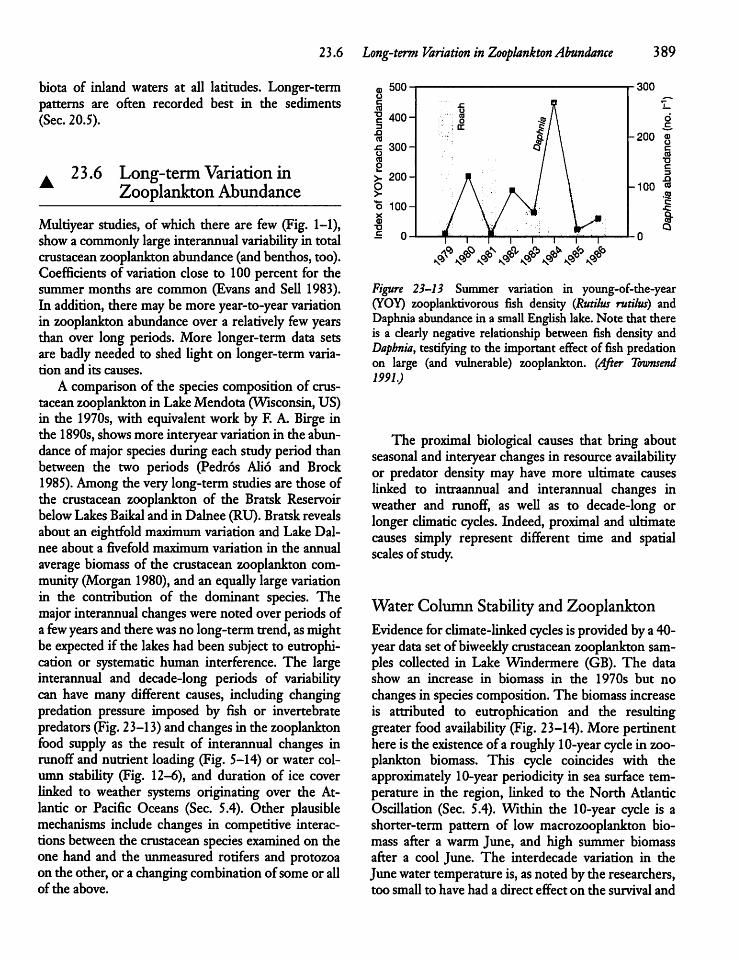
23.6 Long-term Variation inZooplanktonAbundance 389
biota of inland waters at all latitudes. Longer-termpatterns are often recorded best in the sediments(Sec. 20.5).
a 23.6 Long-term Variation inZooplankton Abundance
Multiyear studies, of which there are few (Fig. 1-1),showa commonly large interannualvariabiUty in totalcrustaceanzooplankton abundance (and benthos, too).Coefficients of variation close to 100 percent for thesummer months are common (Evans and SeU 1983).In addition, there maybe more year-to-yearvariationin zooplankton abundance over a relatively few yearsthan over long periods. More longer-term data setsare badlyneeded to shed Ught on longer-term variation and its causes.A comparison of the species compositionof crus
tacean zooplankton in LakeMendota (Wisconsin,US)in the 1970s, with equivalent work by F. A. Birge inthe 1890s, showsmore interyear variation in the abundance of major species during each study period thanbetween the two periods (Pedros Alio and Brock1985). Among the very long-term studies are those ofthe crustacean zooplankton of the Bratsk Reservoirbelow Lakes Baikal and in Dalnee (RU). Bratsk revealsabout an eightfold maximum variation and LakeDalnee about a fivefold maximum variation in the annualaverage biomass of the crustacean zooplankton community(Morgan 1980), and an equallylarge variationin the contribution of the dominant species. Themajorinterannualchanges were noted over periodsofa fewyears and therewas no long-term trend, asmightbe expected if the lakes had been subject to eutrophi-cation or systematic human interference. The largeinterannual and decade-long periods of variabiUtycan have many different causes, including changingpredation pressure imposed by fish or invertebratepredators (Fig. 23-13)andchanges in the zooplanktonfood supply as the result of interannual changes inrunoff and nutrient loading (Fig. 5-14) or water column stabiUty (Fig. 12-6), and duration of ice coverlinked to weather systems originating over the Atlantic or Pacific Oceans (Sec. 5.4). Other plausiblemechanisms include changes in competitive interactions between the crustacean species examined on theone hand and the unmeasured rotifers and protozoaon the other, or a changingcombinationof someor allof the above.
Figure 23-13 Summer variation in young-of-the-year(YOY) zooplanktivorous fish density (Rutilus rutilus) andDaphnia abundance in a small English lake. Note that thereis a clearly negative relationship between fish density andDaphnia, testifyingto the important effect of fish predationon large (and vulnerable) zooplankton. (After Townsend1991.)
The proximal biological causes that bring aboutseasonal and interyear changesin resource availabiUtyor predator density may have more ultimate causeslinked to intraannual and interannual changes inweather and runoff, as weU as to decade-long orlonger climatic cycles. Indeed, proximal and ultimatecauses simply represent different time and spatialscales of study.
Water Column Stability and ZooplanktonEvidence for climate-linked cycles is provided bya 40-year data set of biweekly crustacean zooplanktonsamples coUected in Lake Windermere (GB). The datashow an increase in biomass in the 1970s but nochangesin speciescomposition. The biomassincreaseis attributed to eutrophication and the resultinggreater food availabiUty (Fig. 23-14).More pertinenthere is the existence of a roughly 10-yearcycle in zooplankton biomass. This cycle coincides with theapproximately 10-year periodicity in sea surface temperature in the region, linked to the North AdanticOscillation (Sec. 5.4). Within the 10-year cycle is ashorter-term pattern of low macrozooplankton biomass after a warm June, and high summer biomassafter a cool June. The interdecade variation in theJune water temperature is, asnoted by the researchers,too small to have had a direct effect on the survival and
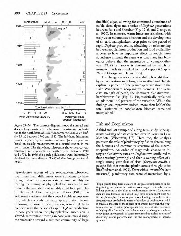
390 CHAPTER 23 Zooplankton
Temperature MJ JASONDJ I l_J I I I I
1940-1
1950-
1960-
1970-
1980-
Perch
12 14 16 18 20
Mean June temperature (°C) Perch year-classstrength (thousands)
Figure 23-14 The contour diagram shows the annual anddecadal longvariationin the biomassof crustaceanzooplankton in the north basinofLakeWindermere, GB (LA=8 km2;2= 25 m) between 1940and 1980.The left-hand histogramshows the year-to-year variations in meanJune temperaturebased on weekly measurements at a central station in thenorth basin. The right-hand histogram shows year-to-yearvariations in the year-class strength of perch between 1940and 1976. In 1976 the perch polulations were dramaticallydepleted by fungal disease. (Modified after George and Han-is1985.)
reproductive success of the zooplankton. However,the interannual differences were sufficient to havebrought about changes in water column stability affecting the timing of phytoplankton succession andthereby the availabiUty of suitably sized food particlesfor the zooplankton. George and Harris (1985) provide someevidence that the crop of edible nanoplankton, which succeeds the early spring diatom bloomfollowing the onset of stratification, is more likely tocoincidewith the period of rapid Daphnia productionin cool years when the phytoplankton succession isslowed. Intermittant mixing in cool years may disruptthe succession toward a summer community of large
(inedible) algae, allowing for continued abundance ofedible-sized algae and a series of Daphnia generationsbetweenJune and October (Fig. 12-6, and George etal. 1990). In contrast, warm Junes are associated withearlywater column stratification and the developmentof an early nanoplankton crop prior to the period ofrapid Daphnia production. Matching or mismatchingbetween zooplankton production and food availabilityappears to have an important effect on zooplanktonabundance in much the sameway that many fish biologists believe that the magnitude of young-of-the-year (YOY) fish stocks is determined by match ormismatch with its zooplankton food supply (Chapter26, and George and Harris 1985).The changes in resource availability brought about
by eutrophication and changes in weather and climateexplain 35 percent of the year-to-year variation in theLake Windermere zooplankton biomass. The year-class strength of perch, the dominant planktivorous-benthivorous fish (Fig. 23-14), statistically explainedan additional 6.5 percent of the variation. While thefindings are impressive indeed, more than half of thetotal variation in zooplankton biomass remainedunexplained.4
Fish and ZooplanktonA third and last example of a long-term study is the dynamic modeling of data collectedover 14years, in LakeMendota (Wisconsin, US). Here too, the analysispoints to the role of planktivory by fish in determiningthe biomass and community structure of the macrozooplankton. An order of magnitude change in interyear planktivory rates on Daphnia was attributed tofirst a waxing (growing) and then a waning effect of asingle strong year-class of cisco (Coregonus aztedi), apelagic fish that remains planktivorous throughout itslife (Rudstam et al. 1993). Yearswith a lowmodeled (notmeasured) planktivory rate were characterized by a
4High-quality long-term data are of the greatest importance in distinguishing short-term fluctuations from long-term trends, and inlinking patterns in the biota to environmental factors. Long-termdata are rare because the needed long-term commitment does notfit the philosophy of most organizations funding research and it isfrequendy not profitable in termsof the flow of publications whichis used as a measure of the success of scientists. However, the long-term collection of either poor-quality data, data of little relevance,or high-quality datawith poorlydocumented or changing methodologyis not onlywastefulof scarceresources but useless in terms ofdiscerning useful patterns, and for the management of aquaticsystems.
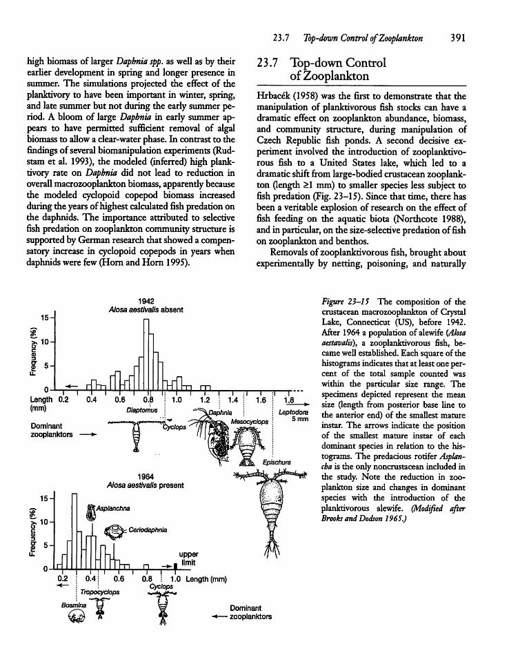
high biomass of larger Daphnia spp. as weU as by theirearUer development in spring and longer presence insummer. The simulations projected the effect of theplanktivory to have been important in winter, spring,and late summerbut not during the earlysummerperiod. A bloom of large Daphnia in early summer appears to have permitted sufficient removal of algalbiomass to aUow a clear-water phase. In contrast to thefindings of several biomanipulationexperiments (Rud-stam et al. 1993), the modeled (inferred) high planktivory rate on Daphnia did not lead to reduction inoveraU macrozooplankton biomass, apparendybecausethe modeled cyclopoid copepod biomass increasedduringthe yearsof highestcalculated fishpredationonthe daphnids. The importance attributed to selectivefish predation on zooplankton community structure issupported byGermanresearch that showed a compensatory increase in cyclopoid copepods in years whendaphnidswere few(Horn and Horn 1995).
15-
* 10
y
15H
t
t—rLength 0.2 0.4(mm)
Dominantzooplanktors —•
0.2
1942Alosa aestivalis absent
1964Alosa aestivalis present
JjfoAsptanchna
_. d^^ Ceriodaphnla
0.4
Tropocyclops
Bosmlna
upperlimit1"V1! I?
0.6 O.f0.8 I 1.0 Length (mm)Cyclops
23.7 Top-down Control ofZooplankton
23.7 Top-down Controlof Zooplankton
391
Hrbacek (1958) was the first to demonstrate that themanipulation of planktivorous fish stocks can have adramatic effect on zooplankton abundance, biomass,and community structure, during manipulation ofCzech RepubUc fish ponds. A second decisive experiment involved the introduction of zooplanktivorous fish to a United States lake, which led to adramatic shiftfromlarge-bodied crustacean zooplankton (length £1 mm) to smaUer species less subject tofish predation (Fig. 23-15). Since that time, there hasbeen a veritable explosion of researchon the effectoffish feeding on the aquatic biota (Northcote 1988),andin particular, on the size-selective predationoffishon zooplankton and benthos.Removals of zooplanktivorous fish, brought about
experimentaUy by netting, poisoning, and naturally
Figure 23-15 The composition of thecrustacean macrozooplankton of CrystalLake, Connecticut (US), before 1942.After 1964 a population of alewife (Alosaaestivalis), a zooplanktivorous fish, becameweU established. Each square of thehistogramsindicatesthat at least one percent of the total sample counted waswithin the particular size range. Thespecimens depicted represent the meansize (length from posterior base line tothe anterior end) of the smallest matureinstar. The arrows indicate the positionof the smallest mature instar of eachdominant species in relation to the histograms. The predacious rotifer Asplan-cha is the only noncrustaceanincludedinthe study. Note the reduction in zooplankton size and changes in dominantspecies with the introduction of theplanktivorous alewife. (Modified afterBrooks and Dodson 1965.)
Dominantzooplanktors
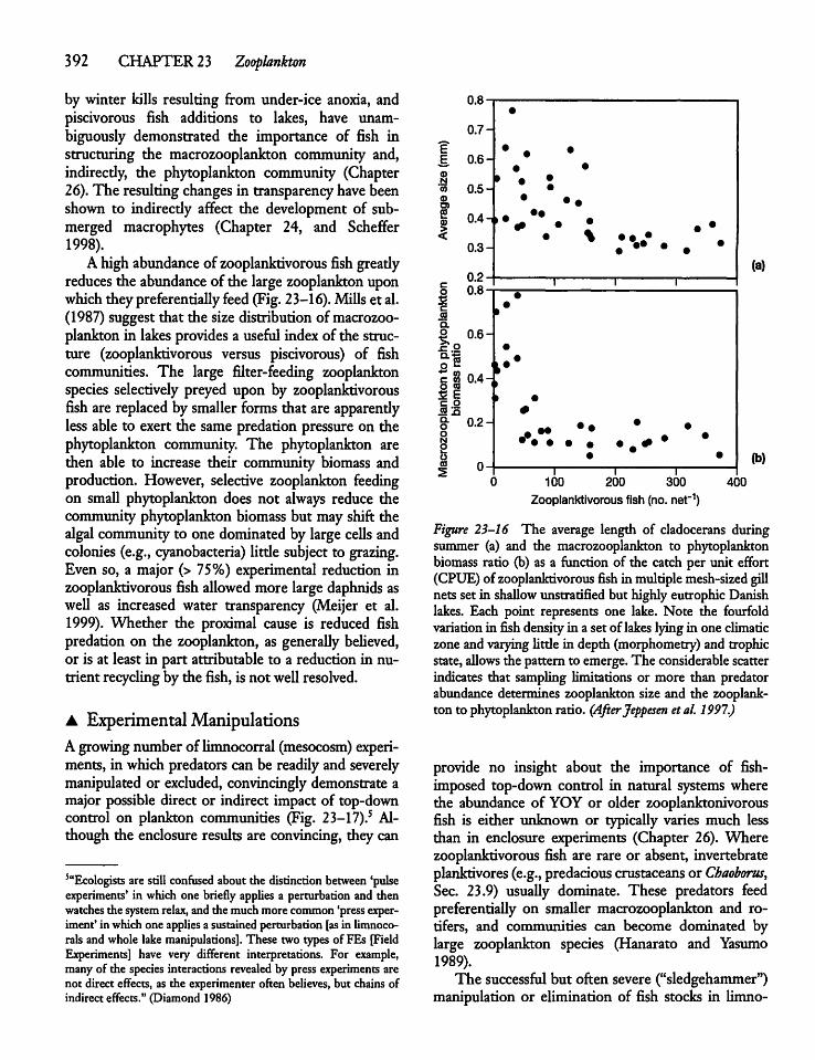
392 CHAPTER 23 Zooplankton
by winter kills resulting from under-ice anoxia, andpiscivorous fish additions to lakes, have unambiguously demonstrated the importance of fish instructuring the macrozooplankton community and,indirecdy, the phytoplankton community (Chapter26). The resultingchanges in transparency have beenshown to indirecdy affect the development of submerged macrophytes (Chapter 24, and Scheffer1998).Ahighabundance of zooplanktivorous fish gready
reduces the abundance of the large zooplankton uponwhichthey preferentiaUy feed(Fig.23-16).MiUs et al.(1987) suggest that the size distribution of macrozooplankton in lakes provides a useful indexof the structure (zooplanktivorous versus piscivorous) of fishcommunities. The large filter-feeding zooplanktonspecies selectively preyed upon by zooplanktivorousfish are replaced bysmaller forms that are apparendyless able to exert the same predation pressure on thephytoplankton community. The phytoplankton arethen able to increase their community biomass andproduction. However, selective zooplankton feedingon small phytoplankton does not always reduce thecommunity phytoplankton biomass but may shift thealgal community to one dominated by large ceUs andcolonies (e.g., cyanobacteria) little subject to grazing.Even so, a major (> 75%) experimental reduction inzooplanktivorous fish allowed more large daphnids asweU as increased water transparency (Meijer et al.1999). Whether the proximal cause is reduced fishpredation on the zooplankton, as generaUy beUeved,or is at least in part attributable to a reduction in nutrient recycling by the fish, is not well resolved.
A ExperimentalManipulationsAgrowing number of limnocorral (mesocosm) experiments, in which predators can be readily and severelymanipulated or excluded, convincingly demonstrate amajor possible direct or indirect impact of top-downcontrol on plankton communities (Fig. 23-17).5 Although the enclosure results are convincing, they can
5ttEcologists are still confused about thedistinction between 'pulseexperiments' in which one briefly applies a perturbation and thenwatches the system relax, and the muchmore common'pressexperiment' in which one appliesa sustainedperturbation [asin limnoco-rals and whole lake manipulations]. These two types of FEs [FieldExperiments] have very different interpretations. For example,many of the species interactions revealed by press experiments arenot direct effects, as the experimenter often believes, but chains ofindirect effects." (Diamond 1986)
EE.©N0)<DO)
2
I
CoScaQ.
o.-so2
11is .QQ.OO
OCO
5
0.8
0.7-
0.6-
0.5
0.4
0.3 H
"!>•
• :• ••
• •
0.20.8-
0.6-
0.4-
0.2-
# •#
% ;*•
• •• *•• • • • • • . # #1 1 1
0 100 200 300 400
Zooplanktivorous fish (no. net"1)
(a)
(b)
Figure 23-16 The average length of cladocerans duringsummer (a) and the macrozooplankton to phytoplanktonbiomass ratio (b) as a function of the catch per unit effort(CPUE) of zooplanktivorous fishin multiplemesh-sized gillnets set in shaUow unstratified but highly eutrophic Danishlakes. Each point represents one lake. Note die fourfoldvariation in fish density in a set of lakeslying in one climaticzone andvarying Utdein depth (morphometry) and trophicstate, allows the pattern to emerge.The considerable scatterindicates that sampling limitations or more than predatorabundance determines zooplankton size and the zooplankton to phytoplankton ratio. (AfterJeppesen etal. 1997.)
provide no insight about the importance of fish-imposed top-down control in natural systems wherethe abundance of YOY or older zooplanktonivorousfish is either unknown or typically varies much lessthan in enclosure experiments (Chapter 26). Wherezooplanktivorous fish are rare or absent, invertebrateplanktivores (e.g.,predaciouscrustaceans or Chaoborus,Sec. 23.9) usuaUy dominate. These predators feedpreferentiaUy on smaUer macrozooplankton and rotifers, and communities can become dominated bylarge zooplankton species (Hanarato and Yasumo1989).The successful but often severe ("sledgehammer")
manipulation or elimination of fish stocks in Umno-
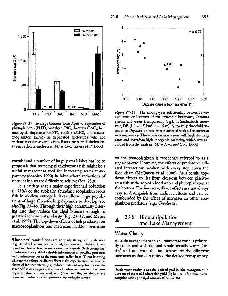
1,500-
O 1,000-
500-
' PHY" PIC " BAC ' HNF ' MIC " MAZ
Figure 23-17 Average biomass fromAprilto Septemberofphytoplankton (PHY),picoalgae (PIC), bacteria(BAC), heterotrophic flageUates (HNF), rotifers (MIC), and macrozooplankton (MAZ) in duplicated enclosures with andwithout zooplanktivorous fish. Bars represent deviation betweenrephcate enclosures. (After Christoffersen etal. 1993.)
corrals6 anda number of largely smaU lakes has led toproposals that reducing planktivorous fish might be auseful management tool for increasing water transparency (Shapiro 1990) in lakeswhere reductions ofnutrient inputs are difficultto achieve (Sec. 23.8).It is evident that a major experimental reduction
(> 75%) of the typicaUy abundant zooplanktivorousfish in shaUow eutrophic lakes aUows large populations of large filter-feeding daphnids to develop (seealso Fig.23-16.Through theirhighcommunity filtering rate they reduce the algal biomass enough togready increase waterclarity (Fig. 23-18, andMeijeret al. 1999). The top-down effects offish predation onmacrozooplankton and macrozooplankton predation
6Limnocorral manipulations are normally strong and qualitiative(e.g., fertilized versus not fertilized, fish versus no fish) and sustained to allow a clear response overdie controls. Such strong manipulations have yielded valuable information onpossible processesand mechanisms but at the same timesuffer from (1) not knowingwhether theeffects aredirect effects astheexperimenter believes, orchains ofindirect effects (e.g. reduced nutrient recycling in theabsenceoffish or changesin the flowof carbon and nutrients betweenphytoplankton and bacteria); and (2) an inability to identify thedominant mechanisms andprocesses operating innature.
23.8 Biomanipulation andLakeManagement 393
r2 = 0.77
4-•
••
5-•
•*
6-• •••
•
7-•
•
•
p1 1 1 i 1
0.05 0.10 0.15 0.20 0.25 0.30
Daphnia galeata biomass (mm31~1)0.35
Figure 23-18 The among-year relationship between average summer biomass of the principle herbivore, Daphniagaleata and water transparency (zSD), in Saidenbach reservoir, DE (LA =1.5 km2; z = 15 m). Aroughly threefold increasein Daphnia biomasswasassociatedwith a 3m increasein transparency. The asteriskmarksayearwithhigh flushingrates and therefore high inorganic turbidity, which was excluded from the analysis. (AfterHorn andHorn 1995.)
on the phytoplankton is frequendy referred to as atrophic cascade. However, the effectsof predator-mediated interactions weaken with every step down thefood chain (McQueen et al. 1986). As a result, top-down effects are far from clear-cut between piscivorousfish at the topofa foodwebandphytoplankton atthe bottom. Furthermore, directeffects arenot alwayseasy to distinguish from indirect effects and can beconfounded by the effect of increases in other zooplankton predators (e.g., Chaoborus).
a 23.8 BiomanipulationandLakeManagement
Water ClarityAquatic managementin the temperate zone is primarily concerned with the end result, usually water clarity,7 and not with the importance of the differentmechanisms that determined the desired transparency.
7High water clarity is not thedesired goal in lake management inportions of theworldwherefish yield(kgha-1 yr"1) for humanconsumptionis the principal concern(Chapter 26).
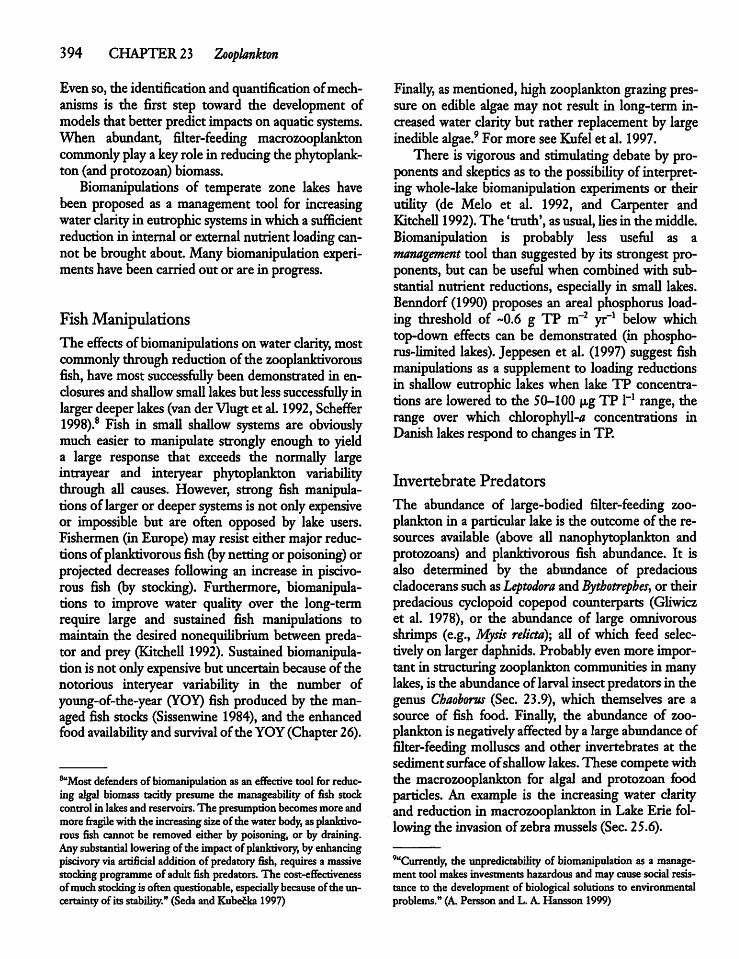
394 CHAPTER 23 Zooplankton
Evenso,the identification andquantification ofmechanisms is the first step toward the development ofmodels that better predictimpacts on aquatic systems.When abundant, filter-feeding macrozooplanktoncommonly playakeyrole in reducing the phytoplankton (and protozoan)biomass.Biomanipulations of temperate zone lakes have
been proposed as a management tool for increasingwaterclarityin eutrophic systems inwhicha sufficientreduction in internal or external nutrientloading cannot be brought about.Many biomanipulation experiments have beencarried out or are in progress.
FishManipulationsThe effects of biomanipulations on water clarity, mostcommonlythrough reduction of the zooplanktivorousfish, have most successfuUy beendemonstrated in enclosures andshaUow small lakes but less successfuUy inlargerdeeperlakes (van derVlugtet al. 1992, Scheffer1998).8 Fish in smaU shaUow systems are obviouslymuch easier to manipulate strongly enough to yielda large response that exceeds the normaUy largeintrayear and interyear phytoplankton variabiUtythrough aU causes. However, strong fish manipulationsof largeror deepersystems is not onlyexpensiveor impossible but are often opposed by lake users.Fishermen (in Europe) may resist either major reductionsofplanktivorous fish(bynettingor poisoning) orprojected decreases foUowing an increase in piscivorous fish (by stocking). Furthermore, biomanipulations to improve water quaUty over the long-termrequire large and sustained fish manipulations tomaintain the desired nonequiUbrium between predator and prey (Kitchell 1992). Sustained biomanipulation is not onlyexpensive but uncertain because of thenotorious interyear variabiUty in the number ofyoung-of-the-year (YOY) fish produced by the managed fish stocks (Sissenwine 1984), and the enhancedfood availabiUty and survivalof the YOY(Chapter 26).
8aMost defenders of biomanipulation asaneffective tool forreducing algal biomass tacitly presume the manageability of fish stockcontrolin lakesandreservoirs. Hie presumptionbecomesmore andmore fragile with the increasing sizeof the waterbody,asplanktivorous fish cannot be removed either by poisoning, or by draining.Any substantial loweringof the impact of planktivory, by enhancingpiscivoryvia artificial addition of predatory fish, requiresamassivestocking programmeof adult fish predators. The cost-effectivenessof much stocking is often questionable,especially becauseofthe uncertaintyofits stability." (Sedaand Kubecka 1997)
Finally, asmentioned, high zooplankton grazing pressure on edible algae maynot result in long-term increased water clarity but rather replacement by largeinedible algae.9 Formore see Kufel et al. 1997.There is vigorous and stimulating debate by pro
ponents and skeptics as to the possibility of interpreting whole-lake biomanipulation experiments or theirutiUty (de Melo et al. 1992, and Carpenter andKitchell 1992).The 'truth', as usual, Ues in the middle.Biomanipulation is probably less useful as amanagement tool than suggested by its strongest proponents, but can be usefulwhen combinedwith substantial nutrient reductions, especiaUy in smaU lakes.Benndorf(1990) proposes an areal phosphorus loading threshold of ~0.6 g TP m~2 yr-1 below whichtop-down effects can be demonstrated (in phosphorus-limited lakes). Jeppesen et al. (1997) suggest fishmanipulations as a supplement to loading reductionsin shaUow eutrophic lakeswhen lake TP concentrations are lowered to the 50-100p,g TP l"1 range, therange over which chlorophyU-/* concentrations inDanish lakes respond to changesin TP.
Invertebrate Predators
The abundance of large-bodied filter-feeding zooplankton in a particular lake is the outcome of the resources available (above aU nanophytoplankton andprotozoans) and planktivorous fish abundance. It isalso determined by the abundance of predaciouscladocerans suchasLeptodora and Bythotrephes, or theirpredacious cyclopoid copepod counterparts (GUwiczet al. 1978), or the abundance of large omnivorousshrimps (e.g., Mysis relicta); aU of which feed selectively on larger daphnids. Probablyevenmore important in structuring zooplanktoncommunities in manylakes, is the abundanceof larval insect predators in thegenus Chaoborus (Sec. 23.9), which themselves are asource of fish food. Finally, the abundance of zooplanktonisnegatively affectedbya largeabundanceoffilter-feeding molluscs and other invertebrates at thesediment surfaceof shaUow lakes.These compete withthe macrozooplankton for algal and protozoan foodparticles. An example is the increasing water clarityand reduction in macrozooplankton in LakeErie followingthe invasion of zebramussels (Sec. 25.6).
'"Currently, the unpredictability of biomanipulation asa management tool makes investments hazardousandmay causesocialresistance to the development of biological solutions to environmentalproblems." (A Persson andL. A. Hansson 1999)
While the debate about the practical utilityof biomanipulation experiments in lake management continues, the experiments have been invaluable inexploring the mechanisms and processes involved intop-down impacts on the structuring of planktonicand Uttoral communities. Furthermore, the experiments are raisingimportant questions about nutrientcycling, food-web structure, and the role of microbialfoodwebs (Sec. 22.9).
Increasing Fish Food:IntroducingMysis relictaFisheries biologists have introduced the opossumshrimpMysis relicta to many north temperate lakeswhere it did not previously exist in an attempt to increase the food available to salmonids (lake trout andsalmon). This attempt at lake management has hadmajor unforeseen consequences. Predation by Mysison larger cladocerans has led to a virtual disappearance of large daphnids,10 resulting in a major modification of the macrozooplankton community and anincrease in the abundance of smaller less or nonpre-dated zooplankton (Langeland 1988). Declines inlarge herbivorious zooplankton typicaUy result in increased phytoplankton biomass.Fish communities havealsobeen affected byMysis
introductions. Its introduction in Lake Tahoe (US) ledto a rapid and unexpected decline of the kokaneesalmon (Oncorhynchus nerka), which fed primarily onthe previously abundant large cladocerans. Furthermore, the expected increase in the catch of lake trout(Salvelinus namaycush) did not materiaUze eventhoughthe latter fed increasingly on Mysis (Goldman 1981).Similarly, a decUne in the char and whitefish fisheriesin Scandinavian lakes is at least partly attributable tothe effectofMysis introductions (Lasenbyet al. 1986).The introductions increase the length of the foodchain byone step,with the macrozooplankton energynowmainly flowing to the fishvia the mysids. With azooplankton growth efficiency (food intake/growth x100) of only -15-50 percent (Sec.23.10) the introduction ofMysis resulted in a decrease rather than the expected increase in the yieldof planktivorous fish. Thelengtheningof foodchainshas the further unfortunate
10Mysids are omnivorous and exhibit two distinct feeding modes:Large food itemsarepicked up usingdie thoracic appendages, whilealgae andother suspended particles are filtered from the incomingwatercurrentproducedby the sameappendages.
23.8 Biomanipulation andLakeManagement 395
result of elevating the levels of persistent contaminants in fish, suchassalmonor laketrout, at the top ofthe food chain (Sec. 28.8).
The Great Lakes ofNorth America:A Natural Biomanipulation ExperimentThe Great Lakes of North America are particularlyweU-studied large-scale natural (unintended) biomanipulation experiments. Long-term phytoplanktonrecords and fishcatchstatistics together with some30years of crustacean zooplankton data place LakeMichigan and the other Laurentian Great Lakesamong the best-studied lakesworldwide. Major perturbation of the food-web structure were first notedfoUowing the introduction of the sea lamprey eel(Petromyzon marinus) in the 1830s, with the predatorfeeding on large piscivorous fish (Fig. 23-19). Thenext major change in the food-web structure of thelakes was the introduction of pacific salmon speciesand the invasion of the alewife (Alosapseudoharengus), azooplanktivorous fish, foUowed during the last decadeor so by the introduction of two predacious cladocerans, the spinywater flea (Bythotrephes longimanus), filter-feeding zebra mussels (Dreissena spp., Sec. 25.6);plus several fish species, a New Zealand moUusc, andthe fishhook water flea (Cercopagispengoi) in 1998.Manyof the recent invaders originaUy came from
the Caspian Searegion of the formerUSSR(Sec. 5.8)and 'escaped' after canals were constructedlinkingtheregionwith central and western Europe, or as the result of transplants into newly created reservoirs elsewhere in the former USSR. However, invasions of diesomewhat salinity-tolerant species into western Europe (Ketelaars et al. 1998) and the Laurentian GreatLakes is attributedprimarily to ships releasing baUastwaterswith their stowaways, taken on elsewhere. Butnot all invaders arrive in baUast water. Otherwise introduced species include the common carp (Cyprinuscarpio), eurasian water milfoil (Myriophyllum spicatum,a submerged macrophytein the Uttoral zone and wetlands, seeChapter 24),and purple loosestrife (Lythrumsalicaria, anemergent macrophyte inwedands).11Investigations into the effects of these introduc
tions have aUowed a number of somewhat uncertainconclusions as to their individual effects on plankton
"In subtropical regions (e.g. Florida, US) many tropical plants andanimals originally imported for the aquarium trade or to decoratepondshaveescaped andthrived,with some amajorthreat to the native biota.
396 CHAPTER23 Zooplankton
1990-]
1970-
1950-
1930-
1910-
1890-
1870-
1850-
1830-
1810-
Ruffe(fish)1986
Zebra mussel1988
Spiny water flea1988
Round- and tubenosegobies (fish)1990
Figure 23-19 A timeline of those of the140nonindigenous species introductionsconsidered to havesubstantial impacts onthe Great Lakes. (Modified after Mills etal. 1993.)
Eurasian watermilfoil(submerged macrophyte) 1952
White Perch1950s
Gulgeahertwlgl(protozoan fish parasite)
1960
Coho salmon1933
Furunculosis(fish bacterium) 1902Brown trout1883 Commoncarp
1879 Chinook salmon1873
Alewife1873 Purple loosestrife
(emergent macrophyte)1869
Sea lamprey(piscivorous fish predator) 1830s
and lake function. The effect of introductions to theLaurentian Great Lakes is inconclusive not becausethe research has been deficient but because the effectof each introduction has cascaded through the foodweb of the lakes, in turn settingup newcascades, withthe time scales over which these indirect effects operate are poorly known. This, togetherwith the impos-sibiUty of clearly distinguishing direct from indirecteffects, the effect of one introduction from the next,effects from longer-term climatic cycles, as weU asfrom chemical and shoreline changes brought aboutbyhumanactivity. AU this,andexacerbated bythe absence of controls, has largely confounded unambiguous interpretations of the effect of the introductionson the zooplanktonand other componentsof the foodweb (Mills et al. 1987, and Lehman and Caceres1993).An exception to the difficultyof linking cause and
effectis the 'sledgehammer' effectof the recent introduction of zebramussels(Sec. 25.6)on the crustaceanzooplankton of shaUow LakeErie. Huge populationsof the benthic mussels rapidly filter and remove thesmall algae and bacteriaalsoconsumed by filter-feedingmacrozooplankton. They further consume the rotifers, ciliates, and naupUi that werenormaUy eatenbyomnivorous copepods. The contribution of themacrozooplankton to whole-lake secondary production has declined in step with the increase in benthicproduction (Johannson et al. 2000).
Even though the effects of introductions are typicallydifficult to resolve, the abundant research in theNorth American Great Lakes, western Europe,Florida, NewZealand, andelsewhere has gready contributed to anappreciation of the complexity ofplanktonicandUttoral food webs, and the importantroleofthe zooplankton therein.
23.9 Chaoborus: The PhantomMidgeFish, predacious zooplankton, and filter-feeding zebramussels arenot the onlypredatorsof zooplankton, norare they necessarily the most important. In mesotrophicand eutrophic lakes and ponds, nonbitingfliesin the genus Chaoborus (Family Chaoboridae, OrderDiptera) are often present in sufficient numbers tohave a major impact, primarily on intermediate-sizedspecies of macrozooplankton (HiUbricht-Ilkowskaetal. 1975).The phantom midges are known as such because
of their transparentlarval stages (Fig.25-3).The two-pigmentedgasbladderschange their densityupon expansionand contraction, aUowing the larvae to moveup and down the water column.The bladdersserveasthe targets for echolocators,making it possibleto follow their dailymigrations. Four aquatic stages coverover 98 percent of the duration of their Ufe cycle.Bodylength increases about fourfold betweenthe first
and fourth instar stages. In highly oligotrophic, food-limited temperate zone lakes there may only be onegeneration of Chaoborus produced in two years. Conversely, developmentcan be completed in six to sevenweeks at summer temperatures in warm food-richlakes (Muttkowski 1918).Following pupation, the motile pupa rises to the
surface to metamorphose and emerges from the watersurface as a nonbiting mosquito-like fly. The fertilizedfemales deposit their eggs over a brief period(<6 days). Alarge number of eggsare laid in rafts nearthe shore (~500 eggs female-1). This, together with ahigh abundance of midges, particularly in lakes lackingmuch fish predation, mayresult in the emergenceof-100,000 first instar larvae per square meter (Neill1985). Although these suffer from enormous mortality, the maximum densities of all instar stages combined often range between about 5,000 m~2 and arecord 130,000 m~2 in a fish-free system (Xie et al.1998). In Lake Victoria (KE, TZ, UG), Chaoborus larvaeappear to be the most common insect larvae in thelake,12 followed by the chironomids (Chapter 25, andMacDonald 1956); together they produce enormousmating swarms (Fig. 23-20).The first and second instar larvae, typically < 200
u,m in width, inhabit the lower depths of the epil-imnion, preying on nanoplankton, large protozoans,verysmall crustaceans, and noncolonial rotifers (Neill1988).In contrast, the much longer (13-18 mm) diirdand fourth instars exhibit pronounced diel verticalmigrations but are benthic during the dayand hide in hypoxic or anoxic sediments in lakeswith fish predators.At night they feed on plankton, acting as ambushpredators on large rotifers, intermediate-sized Daphnia in the epilimnion, and other similar-sized macrozooplankton (Moore 1988). During this period they
12"The periodic appearances of lake-fly swarms [involving synchronous pupation and adult emergence] is well known on many[African] lakes. What appear to be gigantic clouds of smoke, sometimes of over fifty meters in height and occasionally more than akilometre in length, rise from the surface of the lake. The majorityof the swarms on LakeVictoria appear a few days after the newmoons. They are mainly composed of chaoborids, especiallyChaoborus anomalus, with a lessernumber of chironomidsof the genera Chironomiis, Tanypus and Prodadius. The water seemsto boilwithstruggling fish devouring the pupae as they rise to the surface toemerge; the swarms are often followed by flocks of white-wingedblack tern, kites and other birds taking advantage of the abundantfeast . . . The swarms are often blown onto the land by onshorewinds. . . whether this is a significantdrain on the lake's productivity remains to be determined." (Beadle 1981).
23.9 Chaoborus: ThePhantomMidge 397
Figure 23-20 Amating swarm of lake flies (chaoborids andchironomids) on Lake Victoria (KE, TZ, UG). (Photo courtesy ofG. Kling)
also replenish their dissolved oxygen supply. Theirpreference for intermediate-sized zooplankton (including earlymolts of larger species) has been postulated as a trade-off between an increased encounterrate of the more rapidly swimming large cladoceransand reduced handling efficiency of large prey (Pas-torak 1981), but maybe more simplya function of thegape width (mouth diameter) setting limits on the sizeof ingestible particles. While the earlyinstars (I and II)are too small to be eaten by fish, they are consumed byinvertebrate predators such as predatory copepods(Fischer and Frost 1996). However, the abundance ofthe larger instars ILT and IV is strongly constrained byfish predation and chaoborids may be absent fromlakes with high fish predation pressure (Lamontagneand Schindler 1994).When abundant, Chaoborus competes with zooplanktivorous fish for prey. A reductionin fish predators during lake acidification, commonlyresults in an increase in Chaoborus abundance (Chapter27 and Locke and Sprules 1993).
Chaobonis instarsHI and IV typicaUy exhibit no diurnalmigration in lakesand ponds that lackzooplanktivorous fish, but will commence migrations following the
398 CHAPTER23 Zooplankton
introduction offish (Dawidowiczet al. 1990).Verticalmigrations may be extensive. The fourth instar larvaemigrate up to 200 m between the deep hypoxic (lowoxygen) layer and the upper waters of LakeMalawi(MM,MZ, TZ) at a calculated rate of about 25m h"1upward and 40 m h"1 downward (Sec. 23.14, andIrvine 1997).
Chaoborus predation has a direct impact not onlyon the mid-sized macrozooplankton and earliermoltsof larger species but indirecdy on the size and foodweb structure of zooplankton and fish communities.This wasdemonstrated when large daphnids wereexperimentally removed from enclosures in a Ashlesslake. The resulting reduced competition for food resources allowed a large increase in the abundance ofsmall rotifers and small cladoceran species. The increased abundanceof the small zooplankton providedsuchanabundance of foodparticles that manymoreofthe early Chaoborus instars survived and reached thefourth instar stage (Neill 1984). This particularexperiment is mentioned for two reasons. First, as a reminder that the role of competition for resourcesshould not be overlooked despite recent emphasis inthe literature on predation as the major force in structuring zooplankton communities, (Neill 1984,Yan etal. 1985). Second, despite the emphasis in the literature on adult forms or late developmental stages ofparticular zooplankton species, the abundance of zooplankton (insects, fish, etc.) will not be predictablewithout sufficient information on the survival andgrowth of the early developmental stages.
A 23.10 Zooplankton Feeding
The recognitionthat growthof a zooplankton population or community requires both enough food of sufficient quality and appropriate size range to be readilyeaten has led to important research, mosdy in thelaboratory, on different aspects of the filtering,assimilation, and respiration rates of primarily macrozooplankton. This work has made a major contribution to appreciation of the physiological andbehavioral ecology of zooplankton and their energyrequirements for growth and reproduction. Thefiltering rate (F) or clearance rate (ml animal-1 d"1) is calculated from the volume of water cleansed by theaverage individual per unit of time:
In(C0) - ln(Ct) wWt N
EQ.23.1
Where C0 = initial concentrations of food organisms(no. ml"1), Ct =thefinal concentration of food organisms (no.ml-1), W=watervolume (ml), iV= numberofanimals, and t =duration of experiment.The amount of food consumed, the grazing rate
(G) or ingestion rate per animal per unit of time, is theproduct of the filtering rate (F) and the mean foodconcentration (Q:
G = FxC0+ Ct
EQ.23.2
normally expressed in terms of the energy content,wet or dryweight, or carbon content.Russian researchers report that the gross growth
efficiency (food intake/growth x 100) of macrozooplanktonvaries between 15percent and 32 percent innature (Winberg 1972). But the gross efficiency willnaturally range beyondthesevalues when foodqualityis either very high or very low (Richman and Dodson1983). While the grossgrowth efficiency of both protozoans and metazoan animals commonly varieswidely around amean of 20-30 percent (Straile1997),the growth efficiency is a function of the C:P ratio ofthe particles consumed (Elser et al. 2000), which isnormallyunknown in nature. Consequendy, a particular reported valuemust be assumed, leavingmuch uncertainty as to the fraction of the seston consumed,assimilated, and used for growth rather than respired.
FilteringRates and Particle SizeLaboratorymeasurements show a systematic increasein daphnid filtering rate with temperature to an optimum range beyond which the filtering rate declinesrapidly (Horn 1981), and a similar increase with increasing body size (Knoechel and Holtby 1986, andJiirgens et al. 1996). Although larger zooplanktonhavea higher filteringrate than smallones (Sec. 22.9),the filtering rate per unit biomass (themass-specificfiltering rate) declines with increasingorganismal size—regardless of taxonomic position—when examinedover a wide body-size range (Peters and Downing1984). Filtering and grazingrates alsodepend on foodconcentration (Horn 1981)and quality.Most direct measures of filtering (grazing) have
been determined in beakers, either by adding unla-belled algae or other food particles and measuringtheir decline some hours later or, byadding 32P or 14Clabelled food particles and allowing the zooplanktonto graze for a few minutes before collecting the animals and determining their radioactivity, lb facilitate
the analysis, the numbersof animals usedialaboratoryexperiments are usually considerably higher than observed in nature. This may result in (unrecognized)grazing rate reductions to less than half those measured under more natural densities (Fig. 23-21).Probablythe most elegant and least artificial graz
ing studies are those using the Haney in situ grazingchamber (Haney1973), based on a device developed byZ.M. GUwicz (PL).The clearplasticchamber(resembling a Schindler-Patalas trap, Fig. 23-1), is loweredandwhen closed entrapsa knownvolumeofwater andits organisms. Closing the doors opens a smallpistonwhich releases radio-labelled cells (bacteria, algae, oryeast) of a suitable size. Aftera fewminutesof feeding,but before radio-labelled food particles are defecated,the chamber ishauled to the surfaceand the zooplankton are collected. From the calculated radioactivityper unit volumeof chamber at the outset, the feedingtime, and the radioactivity of the zooplankton afterfeeding, the grazing rate of individual zooplanktonspecies or the community as a whole can be determined (Knoechel and Holtby 1986). Feeding studiesbased on providing highlypalatable particles of an optimal size (-5—10 pin) in Haney chambers or in thelaboratorywillnaturallyyielda higher grazingrate onthose particles than on the wholenatural spectrum of
0.08
& 0.02
0.00-
Grazing rate = 0.078• (Biomass)"0264
25 50 75
Zooplankton biomass (mm31"1)
"1100
Figure 23-21 A laboratory-determined relationship between macrozooplankton biomass (Daphnia byalina) andthespecies-specific grazingrate, showing a pronounced declinein grazingwith increased crowding. (AfterHorn 1981.)
23.11 Nutrient Cycling and Zooplankton 399
nanoplankton (2-30 p,m) present in nature, and willfurther yield a rate that even more gready overestimates the grazing on natural assemblages, composednot only of picoplankton and nanoplankton but alsoon the little (if at all) consumed larger microplankton(> ~30 |xm) (fames and Forsyth 1990, and Cyr andPace 1993).
Grazing Impactson the PreyThe frequendymodest whole-system grazing rates innature (ml animal-1 d"1 x no. of animals) measured,evenon edible-sizedparticles (< -30 u,m), suggest thatmost of the time the principal role of macrozooplankton is to structure the prey community rather than actas the principaldeterminant of the biomass of phytoplankton, protozooplankton, and bacterioplanktoncommunities (Fig. 23—22).In both terrestrial and aquatic communities, the
lossrates imposedby herbivores is primarily imposedon the most rapidly growing prey organisms ratherthan being experienced equally by all potential foodparticles (Fig. 24-10). This is probably because thehigh-quality food, rich in the minerals, nutrients, proteins, and fatty acids required for rapid growth, isdisproportionately present in fast-growing prey organisms (see Fig. 24-11). Recognition of the importanceof selective feedinghasprovidedsupport for thehypothesis that the abundance ofmicrophytoplanktonin aquatic systems is partlyattributable to largerphytoplankton beinglittle subjectto zooplankton grazing.
a 23.11 Nutrient Cyclingand Zooplankton
Zooplankton affect the phytoplankton communitybiomass andstructure direcdy by selective grazing aswell as indirecdy through the release (recycling) ofcritically needed mineral nutrients. The selective effect of each mechanism and the effect of the twoprocesses combined on the phytoplankton communitystructure and abundance remains poorlyknown. Fieldmanipulations of grazers yield changes in the phytoplankton community that at times arebetterexplainedby changes observed in algal growth rates linked tomineral nutrients than by grazer-induced mortality(Sterner 1989). Predators exert not only a top-downbutalso a bottom-up effect on theirpreybecause theyrecycle nutrients, making them available to the primary producers. These complexities are increased
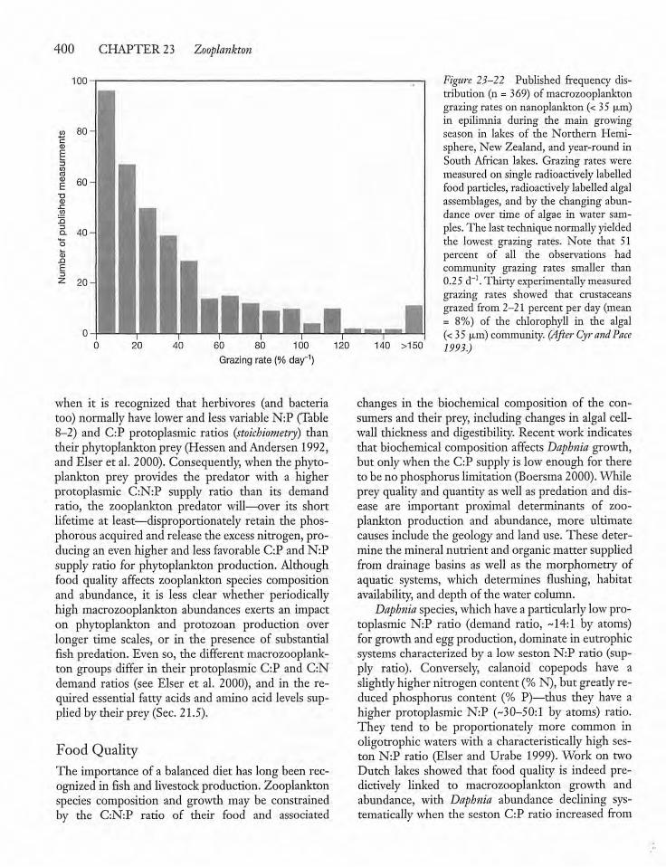
400 CHAPTER 23 Zooplankton
100
60 80 100
Grazingrate (% day"1)
when it is recognized that herbivores (and bacteriatoo) normally have lower and lessvariable N:P (Table8-2) and C:P protoplasmic ratios (stoichiometiy) thantheir phytoplankton prey (Hessenand Andersen 1992,and Elser et al. 2000). Consequendy, when the phytoplankton prey provides the predator with a higherprotoplasmic C:N:P supply ratio than its demandratio, the zooplankton predator will—over its shortlifetime at least—disproportionately retain the phosphorous acquiredand release the excess nitrogen, producing an even higher and less favorable C:P and N:Psupply ratio for phytoplankton production. Althoughfood quality affects zooplankton species compositionand abundance, it is less clear whether periodicallyhigh macrozooplankton abundances exerts an impacton phytoplankton and protozoan production overlonger time scales, or in the presence of substantialfish predation. Even so, the different macrozooplankton groups differ in their protoplasmic C:P and C:Ndemand ratios (see Elser et al. 2000), and in the required essential fatty acids and amino acid levels supplied by their prey (Sec. 21.5).
Food QualityThe importance of a balanced diet has long been recognized in fish and livestock production. Zooplanktonspecies composition and growth may be constrainedby the C:N:P ratio of their food and associated
140 >150
Figure 23-22 Published frequency distribution (n = 369) of macrozooplanktongrazing rates on nanoplankton (< 35 fim)in epilimnia during the main growingseason in lakes of the Northern Hemisphere, New Zealand, and year-round inSoudi African lakes. Grazing rates weremeasured on single radioactively labelledfood particles, radioactively labelledalgalassemblages, and by the changing abundance over time of algae in water samples.The last technique normallyyieldeddie lowest grazing rates. Note that 51percent of all the observations hadcommunity grazing rates smaller than0.25d"1. Thirty experimentally measuredgrazing rates showed that crustaceansgrazed from 2-21 percent per day (mean= 8%) of the chlorophyll in the algal(<35 u.m) community. (After Cyr andPace1993.)
changes in the biochemical composition of the consumers and their prey, including changes in algal cell-wall thickness and digestibility. Recent work indicatesthat biochemical composition affectsDaphnia growth,but onlywhen the C:P supply is low enough for thereto be no phosphorus limitation (Boersma 2000). Whileprey qualityand quantity as well as predation and disease are important proximal determinants of zooplankton production and abundance, more ultimatecauses include the geology and land use. These determine the mineral nutrient and organicmatter suppliedfrom drainage basins as well as the morphometry ofaquatic systems, which determines flushing, habitatavailability, and depth of the water column.Daphnia species, which have a particularly lowpro
toplasmic N:P ratio (demand ratio, -14:1 by atoms)forgrowthandeggproduction, dominate in eutrophicsystems characterized by a low seston N:P ratio (supply ratio). Conversely, calanoid copepods have aslightly higher nitrogen content(% N), but greadyreduced phosphorus content (% P)—thus they have ahigher protoplasmic N:P (~30—50:1 by atoms) ratio.They tend to be proportionately more common inoligotrophic waters with a characteristically high seston N:P ratio (Elser and Urabe 1999). Work on twoDutch lakes showed that food quality is indeed pre-dictively linked to macrozooplankton growth andabundance, with Daphnia abundance declining systematically when the seston C:P ratio increased from
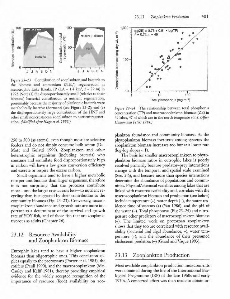
100
I I IJ JASON
Figure 23-23 Contribution of zooplankton and bacteria tothe biomass and ammonium (NH4+) regeneration inmesotrophic Lake Kizaki, JP (LA = 1.4 km2, z = 29 m) in1992. Note (1) the disproportionately small (relative to theirbiomass) bacterial contribution to nutrient regeneration,presumably because diemajority ofplanktonic bacteria weremetabolically inactive (dormant) (see Figure 22-2); and (2)the disproportionately large contribution of the HNF andother small noncrustaccan zooplankton to nutrient regeneration. (Modified after Haga etal. 1995.)
250 to 500 (as atoms), even though most are selectivefeeders and do not simply consume bulk seston (De-Mott and Gulatti 1999). Zooplankton and otherheterotrophic organisms (including bacteria) whoconsume and assimilate food disproportionately highin carbon will have a low gross conversion efficiencyand excrete or respire the excess carbon.Small organisms tend to have a higher metabolic
rate per unit biomass than largerorganisms, thereforeit is not surprising that the protozoa contributemore—and the larger crustaceans less—to nutrient recycling than is suggested by their contribution to thecommunity biomass (Fig. 23-23). Conversely, macrozooplankton abundance and growth rate are more important as a determinant of the survival and growthrate of YOY fish, and of those fish that are zooplanktivorous as adults (Chapter 26).
23.12 Resource Availabilityand Zooplankton Biomass
Eutrophic lakes tend to have a higher zooplanktonbiomass than oligotrophic ones. This conclusion applies equally to the protozoans (Porter et al. 1985), therotifers (Pauli 1990), and the macrozooplankton (Mc-Cauley and Kalff 1981), thereby providing empiricalevidence for the widely accepted recognition of theimportance of resource (food) availability on zoo
1,000
OlE.
i 100-1E03
raaooN
10
23.13 Zooplankton Production
log(ZB) = 0.76 + 0.91 • logfTP)r2 = 0.72; n = 49
401
100
Total phosphorus (mg m~3)
Figure 23-24 The relationship between total phosphorusconcentration (TP) and macrozooplankton biomass (ZB) in49 lakes, 47 of which are in the north temperate zone. (AfterHansonand Peters1984.)
plankton abundance and community biomass. As thephytoplankton biomass increases among systems thezooplankton biomass increases too but at a lower rate(log-logslopes< 1).The basis for smallermacrozooplankton to phyto
plankton biomass ratios in eutrophic lakes is poorlyresolved primarily becausepredator-prey interactionschange with the temporal and spatial scale examined(Sec. 2.6), and because more than species interactionsdetermine the abundance of populations and communities. Physical/chemical variables amonglakes that arelinked withresource availability and,correlate with themacrozooplankton biomass and production (see below)include temperature (+), waterdepth (-), thewaterresidence time of systems (+) (Yan 1986), and the pH ofthe water (-). Total phosphorus (Fig 23-24) and nitrogen areotherpredictors ofmacrozooplankton biomass(+). The limited work on protozoan zooplanktonshows that they too are correlated with resource availability (bacterial and algal abundance, +), water temperature (+), and the abundance of their presumedcladoceran predators (-) (GasolandVaque 1993).
23.13 Zooplankton Production
Most available zooplankton production measurementswere obtained during the life of the International Biological Programme (IBP) of the late 1960s and early1970s. A concerted effort was then made to obtain in-
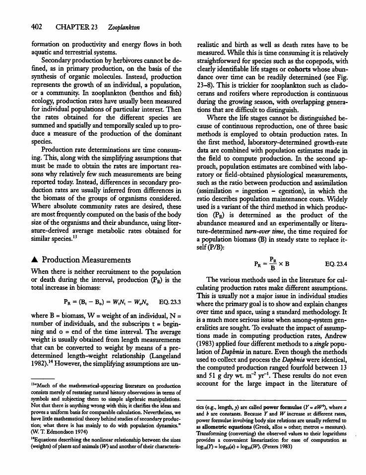
402 CHAPTER23 Zooplankton
formation on productivity and energy flows in bothaquatic and terrestrial systems.Secondary production byherbivores cannotbede
fined, as in primary production, on the basis of thesynthesis of organic molecules. Instead, productionrepresents the growth of an individual, a population,or a community. In zooplankton (benthos and fish)ecology, production rates have usually been measuredfor individual populations of particular interest. Thenthe rates obtained for the different species aresummed andspatially andtemporally scaled up to produce a measure of the production of the dominantspecies.
Production rate determinations are time consuming. This, along with the simplifying assumptions thatmust be made to obtain the rates are important reasons why relatively few such measurements are beingreported today. Instead, differences in secondary production rates are usually inferred from differences inthe biomass of the groups of organisms considered.Where absolute community rates are desired, thesearemostfrequendy computed on the basis of thebodysize of the organisms andtheirabundance, using literature-derived average metabolic rates obtained forsimilar species.13
• Production Measurements
When there is neither recruitment to the populationor death during the interval, production (Pr) is thetotal increase in biomass:
PR = (Bt - B0) = WtNt - WoN0 EQ. 23.3
whereB = biomass, W =weightof an individual, N =number of individuals, and the subscripts t = beginning and o = end of the time interval. The averageweightis usually obtained from length measurementsthat can be converted to weight by means of a predetermined length-weight relationship (Langeland1982).14However, thesimplifying assumptions are un-
13"Much of the mathematical-appearing literature on productionconsists merelyof restatingnaturalhistoryobservations in termsofsymbols and subjecting them to simple algebraic manipulations.Not that there is anythingwrongwith this; it clarifies the ideasandprovesa uniform basisfor comparablecalculation. Nevertheless, wehave littlemathematical theorybehindstudies ofsecondary production; what there is has mainly to do with population dynamics."(W. T. Edmondson 1974)"Equations describing thenonlinear relationship between thesizes(weights) of plants and animals(W)and another of their characteris-
realistic and birth as well as death rates have to bemeasured. Whilethisis timeconsuming it is relativelystraightforward for species suchas the copepods, withclearly identifiable lifestages or cohorts whose abundance over time can be readily determined (see Fig.23-8). This is trickier for zooplankton such as cladocerans and rotifers where reproduction is continuousduring the growing season, with overlapping generationsthat are difficult to distinguish.Where the life stages cannot be distinguished be
cause of continuous reproduction, one of three basicmethods is employed to obtain production rates. Inthe first method, laboratory-determined growth-ratedata are combined with population estimates made inthe field to compute production. In the second approach,population estimatesare combinedwith laboratory or field-obtained physiological measurements,such as the ratio between productionand assimilation(assimilation = ingestion - egestion), in which theratio describes population maintenance costs. Widelyused is a variantof the thirdmethod inwhichproduction (Pr) is determined as the product of theabundance measured and an experimentally or literature-determined turn-over time, the time required fora population biomass (B) in steadystate to replace itself (P/B):
PrPr =~iX B EQ.23.4
The various methods used in the Uterature for calculating production ratesmake different assumptions.This is usually not a major issue in individual studieswhere the primary goalis to show andexplain changesovertimeand space, usinga standard methodology. Itis amuchmore seriousissuewhenamong-system generalities are sought,lb evaluate the impactof assumptions made in computing production rates, Andrew(1983) applied fourdifferent methods to a single populationofDaphnia in nature. Even though the methodsused to collect and process the Daphniawere identical,the computedproduction ranged fourfold between 13and 51 g drywt. m~2 yr-1. These results do not evenaccount for die large impact in the Uterature of
tics (e.g., length, j*) arecalled power formulae (KoaW\ where aand b are constants. Because Y and W increase at different rates,powerformulae involving bodysizerelationsare usually referredtoas allometric equations (Greek, alios = other; metros = measure).Transforming (converting) the observedvalues to their logarithmsprovides a convenient linearization for ease of computation aslogioW= log,0(«) + log.oW- (Peters 1983)
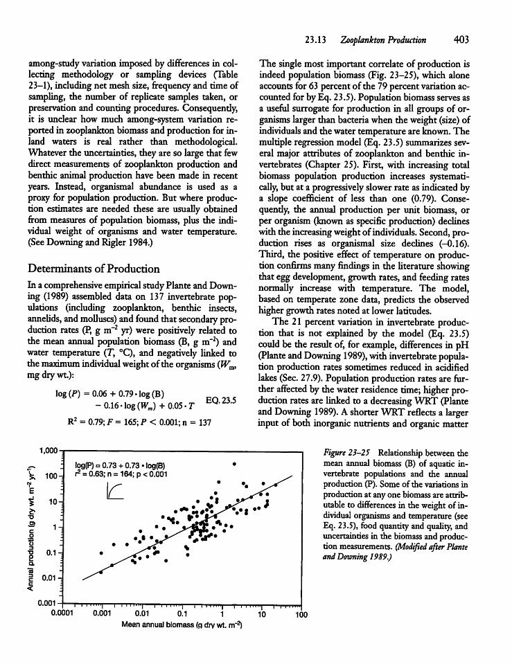
among-study variation imposed by differences in collecting methodology or sampling devices (Table23-1), including net mesh size, frequencyand time ofsampling, the number of repUcate samples taken, orpreservation and counting procedures. Consequendy,it is unclear how much among-system variation reported in zooplanktonbiomassand production for inland waters is real rather than methodological.Whatever the uncertainties, they are so largethat fewdirect measurements of zooplankton production andbenthic animal production have been made in recentyears. Instead, organismal abundance is used as aproxyfor population production. But where production estimates are needed these are usuaUy obtainedfrom measures of population biomass, plus the individual weight of organisms and water temperature.(See DowningandRigler 1984.)
Determinants of Production
In a comprehensive empirical studyPlante andDowning (1989) assembled data on 137 invertebrate populations (including zooplankton, benthic insects,anneUds, andmolluscs) andfound that secondary production rates (P, g m~2 yr) were positively related tothe mean annual population biomass (B, g m-2) andwater temperature (T, °C), and negatively linked tothemaximum individual weight of theorganisms (Wm,mg drywt.):
log(P) =0.06+ 0.79-log (B)-0.16-log(Wm)+0.05-r
R2 = 0.79; F = 165; P < 0.001; n = 137
1,000
\ 100-E
TS3
Sa
2 o.oi
10-
0.1-
log(P) = 0.73 + 0.73 -log(B)r2 =0.63; n = 164; p< 0.001
EQ.23.5
23.13 Zooplankton Production 403
The single most important correlateof production isindeed population biomass (Fig. 23-25), which aloneaccounts for 63 percentof the 79percentvariationaccountedfor byEq. 23.5). Populationbiomass serves asa useful surrogate for production in aU groups of organisms larger than bacteria when the weight(size) ofindividuals and thewater temperatureare known. Themultiple regression model (Eq. 23.5) summarizes several major attributes of zooplankton and benthic invertebrates (Chapter 25). First, with increasing totalbiomass population production increases systemati-caUy, but at a progressively slowerrate as indicated bya slope coefficient of less than one (0.79). Consequently, the annual production per unit biomass, orper organism (known as specific production) declineswiththe increasingweightof individuals. Second, production rises as organismal size declines (-0.16).Third, the positive effect of temperature on productionconfirms many findings in the Uterature showingthat eggdevelopment, growth rates, and feeding ratesnormally increase with temperature. The model,based on temperate zone data, predicts the observedhighergrowthratesnoted at lower latitudes.The 21 percent variation in invertebrate produc
tion that is not explained by the model (Eq. 23.5)could be the result of, for example, differences in pH(Plante and Downing 1989), with invertebrate population production rates sometimes reduced in acidifiedlakes (Sec. 27.9). Population productionrates are furtheraffected bythewater residence time; higher production rates are linked to a decreasing WRT (Planteand Downing 1989). Ashorter WRT reflects a largerinput of both inorganic nutrients and organic matter
Figure 23-25 Relationship between themean annual biomass (B) of aquatic invertebrate populations and the annualproduction (P). Some of the variationsinproductionat anyone biomass are attributable to differences in theweight of individual organisms and temperature (seeEq. 23.5), food quantityand quality, anduncertainties in the biomass and productionmeasurements. (Modified after PlanteandDowning 1989.)
0.001 i—p
0.0001 0.001 0.01r-r i mi
0.11—r
1i i " "ni|
10I I Mill
100
Mean annual biomass (g dry wt. m"2)
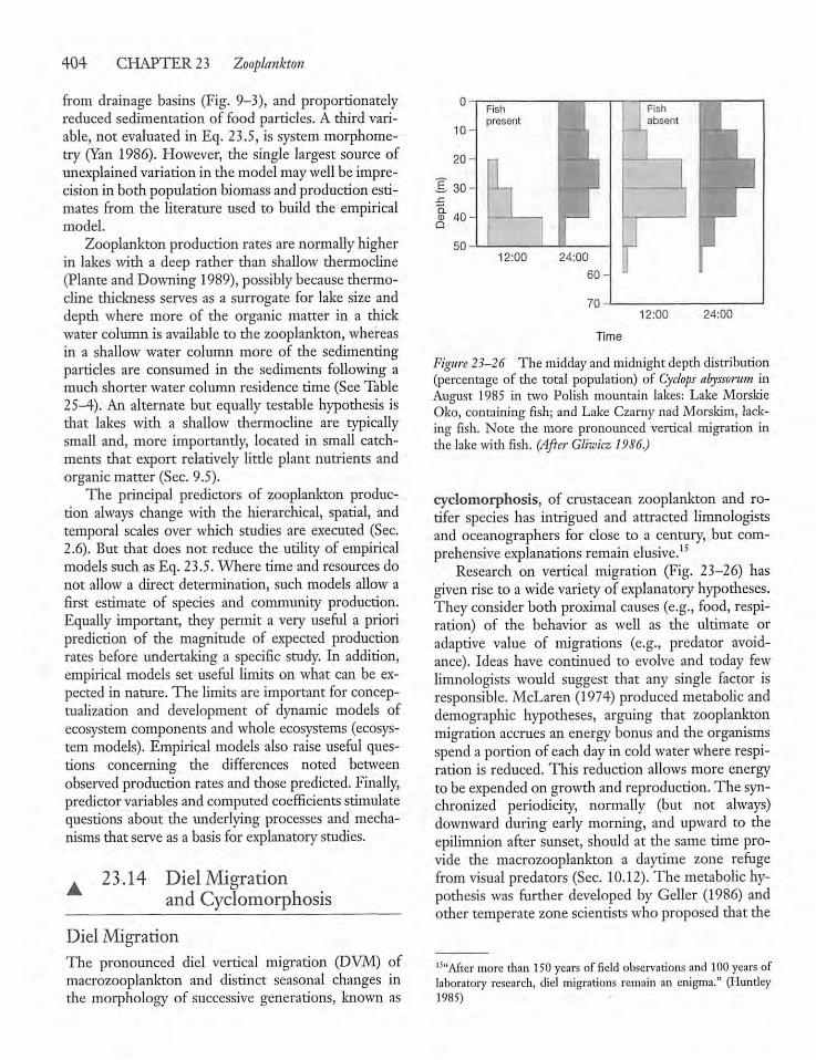
404 CHAPTER 23 Zooplankton
from drainage basins (Fig. 9-3), and proportionatelyreduced sedimentation of food particles. A third variable, not evaluated in Eq. 23.5, is systemmorphometry (Yan 1986). However, the single largestsource ofunexplainedvariation in die model maywell be imprecision in both population biomass and production estimates from the literature used to build the empiricalmodel.Zooplankton production rates are normallyhigher
in lakes with a deep rather than shallow thermocline(Plante and Downing 1989), possibly becausethermocline thickness serves as a surrogate for lake size anddepth where more of the organic matter in a thickwater column is available to the zooplankton,whereasin a shallow water column more of the sedimentingparticles are consumed in the sediments following amuch shorter water column residence time (See Table25-4). An alternate but equally testable hypothesis isthat lakes with a shallow thermocline are typicallysmall and, more importantly, located in small catchments that export relatively little plant nutrients andorganic matter (Sec. 9.5).The principal predictors of zooplankton produc
tion always change widi die hierarchical, spatial, andtemporal scales over which studies are executed (Sec.2.6). But that does not reduce die utility of empiricalmodels suchasEq. 23.5. Where timeand resources donot allow a direct determination, such models allow afirst estimate of species and community production.Equally important, they permit a very useful a prioriprediction of the magnitude of expected productionrates before undertaking a specific study. In addition,empirical models set useful limits on what can be expected in nature. The limits are important for conceptualization and development of dynamic models ofecosystem components and whole ecosystems (ecosystem models). Empirical models also raise useful questions concerning the differences noted betweenobserved production rates and thosepredicted. Finally,predictor variables and computed coefficients stimulatequestions about the underlying processes and mechanisms that serve as a basis for explanatorystudies.
. 23.14 Diel Migrationand Cyclomorphosis
Diel MigrationThe pronounced diel vertical migration (DVM) ofmacrozooplankton and distinct seasonal changes inthe morphology of successive generations, known as
12:00 24:00
Time
Figure 23-26 The midday and midnight depthdistribution(percentage of the total population) of Cyclops abyssorum inAugust 1985 in two Polish mountain lakes: Lake MorskieOko, containing fish; and Lake Czarny nad Morskim, lacking fish. Note the more pronounced vertical migration indie lake with fish. (After GUwicz 1986.)
cyclomorphosis, of crustacean zooplankton and rotifer species has intrigued and attracted limnologistsand oceanographers for close to a century, but comprehensive explanations remain elusive.1Research on vertical migration (Fig. 23-26) has
given rise to a wide variety of explanatory hypotheses.They consider both proximal causes (e.g., food, respiration) of the behavior as well as the ultimate oradaptive value of migrations (e.g., predator avoidance). Ideas have continued to evolve and today fewlimnologists would suggest that any single factor isresponsible. McLaren (1974) produced metabolic anddemographic hypotheses, arguing that zooplanktonmigration accrues an energybonus and the organismsspenda portion of eachdayin coldwaterwhererespiration is reduced. This reduction allows more energyto be expended on growthand reproduction. The synchronized periodicity, normally (but not always)downward during early morning, and upward to theepilimnion after sunset, should at the same time provide the macrozooplankton a daytime zone refugefrom visual predators (Sec. 10.12). The metabolic hypothesis was further developed by Geller (1986) andother temperatezonescientists who proposed that the
15,1After moredian 150 years of field observations and 100 years oflaboratory research, diel migrations remain an enigma." (Huntley1985)
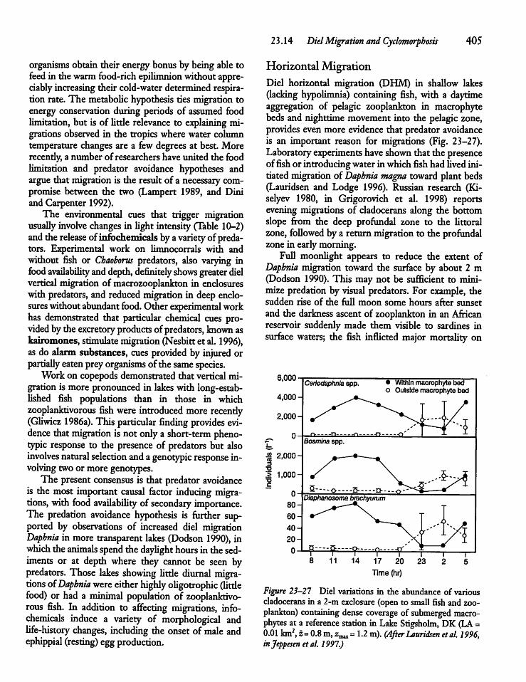
organisms obtain their energy bonus by being able tofeed in the warmfood-rich epilimnionwithout appreciably increasing their cold-water determinedrespiration rate. The metabolic hypothesis ties migration toenergy conservation during periods of assumed foodlimitation, but is of Utde relevance to explaining migrations observed in the tropics where water columntemperature changes are a few degrees at best.Morerecendy, a number of researchers have united the foodlimitation and predator avoidance hypotheses andargue that migration is the result of a necessary compromise between the two (Lampert 1989, and Diniand Carpenter 1992).The environmental cues that trigger migration
usually involve changes in light intensity(Table 10-2)and therelease ofinfbchemicals byavariety ofpredators. Experimental work on limnocorrals with andwithout fish or Chaoborus predators, also varying infood availability anddepth, definitely shows greater dielvertical migration of macrozooplankton in enclosureswith predators, and reduced migration in deep enclosures without abundant food. Otherexperimental workhas demonstrated that particular chemical cues provided bytheexcretory products ofpredators, known askairomones, stimulate migration (Nesbitt et al. 1996),as do alarm substances, cues provided by injured orpartially eaten preyorganisms ofthesame species.Work on copepods demonstrated that vertical mi
grationis more pronounced in lakes with long-established fish populations than in those in whichzooplanktivorous fish were introduced more recendy(GUwicz 1986a). This particular finding provides evidence thatmigration is not only a short-term pheno-typic response to the presence of predators but alsoinvolves natural selection and agenotypic response involving twoor moregenotypes.The present consensus is that predator avoidance
is the most important causal factor inducing migrations, with food availabiUty of secondary importance.The predation avoidance hypothesis is further supported by observations of increased diel migrationDaphnia in more transparent lakes (Dodson 1990), inwhich theanimals spend the dayUght hours in thesediments or at depth where they cannot be seen bypredators. Those lakes showing Utde diurnal migrations ofDaphniawere either highly oUgotrophic (Utdefood) or had a minimal population of zooplanktivorous fish. In addition to affecting migrations, info-chemicals induce a variety of morphological andfife-history changes, including the onset of male andephippial (resting) eggproduction.
23.14 DielMigration and Cyclomorphosis 405
HorizontalMigrationDiel horizontal migration (DHM) in shaUow lakes(lacking hypolimnia) containing fish, with a daytimeaggregation of pelagic zooplankton in macrophytebeds and nighttime movement into the pelagic zone,provides evenmore evidence that predator avoidanceis an important reason for migrations (Fig. 23-27).Laboratory experiments have shown that the presenceoffish or introducingwaterinwhich fish hadUved initiated migration of Daphnia magna toward plant beds(Lauridsen and Lodge 1996). Russian research (Ki-selyev 1980, in Grigorovich et al. 1998) reportsevening migrations of cladocerans along the bottomslope from the deep profundal zone to the Uttoralzone, foUowed bya return migration to the profundalzonein earlymorning.
FuU moonUght appears to reduce the extent ofDaphnia migration toward the surface by about 2 m(Dodson 1990). This may not be sufficient to minimize predation byvisual predators. For example, thesudden rise of the fuU moon some hours after sunsetand the darkness ascent of zooplankton in an Africanreservoir suddenly made them visible to sardines insurface waters; the fish inflicted major mortaUty on
6,000Ceriodaphnia spp.
4,000-
• Within macrophyte bedo Outside macrophyte bed
17 20
Time (hr)
Figure 23-27 Diel variations in the abundance of variouscladocerans in a 2-mexclosure (open to small fish andzooplankton) containing dense coverage of submerged macro-phytes at a reference station in Lake Stigsholm, DK(LA =0.01 km2,z= 0.8m,zmax=1.2 m). (AfterLauridsenetal. 1996,injeppesenetal. 1997.)
406 CHAPTER 23 Zooplankton
the crustaceans (GUwicz 1986b). The extentofmigration is furthermore a function of organismal size(Peters et al. 1994). The large opposum shrimp (Mysisrelicta, Fig. 23-3) in ultra-oUgotrophic Lake Tahoemay move 900-1,000 m verticaUy during 24 hours,possibly a record for a freshwater zooplankton(Goldman, 1981).
CyclomorphosisThis term, describing seasonal changes in generationalmorphology, wascoinedbyR. Lauterborn (DE)in 1904. Cyclomorphosis has been observed in phytoplankton (dinoflagellates, and colony formation inunicellular green algae), zooplankton (rotifers, copepods, and cladocerans) and fish, but has been investigatedbest in daphnids. These express it most stronglyas seasonal changes in head shape (helmet size) andthe length of the carapace spineor dorsalcrest (Jacobs1987). In rotifers it is expressed primarilyby changesin spine length. Stricdy speaking, cyclomorphosis entails the production of different phenotypes by thesame genotype. However, genetic studies have revealed that there isa genetic component to cyclomorphosis (Black 1980). Even morphologicaUy verysimilar plankton organismsmay seasonaUy show distinct changes in genotype, thereby confounding theinterpretation of cyclomorphism.There are abundant laboratory studies (Havel
1987) Unking cyclomorphism to temperature, food,light,turbulence, andwatersoluble organic substancesthat serve as infochemicals released by potentialpredators. Intriguingly, experimentaUy induced or enhanced morphological changes seen during the various developmental (ontogenetic) stages in thelaboratory are usuaUy less extreme than what is observed in nature. This impUes that either laboratoryconditions reducethe numberor strengthof identifiedinducing factors or the existence in nature of yetunidentified inducing factors (Jacobs1987).Many adaptive explanations for cyclomorphosis
have been proposed over the last century. One of theearUest theories was that sinking rate is reduced as aresult of increased surface area or enhancement ofoxygen diffusion during periods of low oxygen concentration. More modern explanations include decreased visibiUty to predators or the increaseddifficulty experienced by predators in handling zooplanktonwith longerspines or an unusual bodyshape.For example, posterior spine development in laboratory clones of the rotifer Keratella cochlearis is en
hanced by a water-soluble factor released by two different species of cyclopoid copepods and a predatoryrotifer (Stemberger and Gilbert 1984). The spinedform of this rotifer is less susceptible to predation bythe inducing species. A difficulty confounding adaptive interpretations of cyclomorphosis on growth andsurvival is that morphological changes are accompanied by changes in physiology and behavior.Probably the most widely accepted hypothesis
today is that seasonaUy changing selective predationby temporarily abundant predators act as a selectiveforce for the subsequent cyclomorphosis that is observed. This is supported by observations of clonecultures showing muchvariation in morphology even intheabsence ofpredators.16
Highlights• Inland-water zooplankton range in size from smaUprotozoan flageUates less than 2 u.m in their longestdimension to large crustaceans several centimetersinlength.
• Inland-water zooplankton consistprimarilyof protozoans, rotifers, and crustaceans. Abundance and individual growth rates are highest among smaUprotozoansand lowestamong large crustaceans.
• WeU-studied freshwater lakes and rivers contain50-100 planktonic zooplankton (protozoans included), plus a roughly equal number of Uttoralspecies. Species abundance declines with increasingsalinity. Species richness increases with systemsize,attributable to increased habitat variation. Thetrophic status serves as an indicator of resourceavailabiUty.
• • Long-term studies of crustacean zooplankton inunpolluted lakes reveal largeinterannual anddecade-long variabiUty in zooplankton abundance, speciescomposition, andcommunity biomass. The variationhas been primarily attributed to changing predationpressure imposed by fish or invertebrates, and indirecdy to changes in nutrient loading, flushing rates,water column stabiUty, or the duration ofan ice cover
16Broad generalizations in biological limnology reflect thebehaviorof many species. No such general interpretations have emergedfrom the studies on vertical migration andcyclomorphosis of individual zooplankton species. This failure appears, the result of continuing attempts to draw broad generalities from diestudy of singlerather thanmanyspecies. In otherwords, the failure appears to stemfrom attempts to extrapolate from the specific to the general without the identification of a broad generality that unites the diverseobservations made.
which can be linked to interannual variations inweatherand decades-long climatic cycles.
• Ahighabundance of zooplanktivorous fish, includingyoung-of-the-year, gready reduces the abundance oflarge zooplankton on which they preferentiaUy feed.The reduction in large filter-feeding herbivorouszooplankton typicaUy allows an increase in phytoplankton biomass or a shift to an algal communitydominated by large ceUs and colonies Utdesubjecttopredation.
9 • Biomanipulations, primarily through reductionsof zooplanktivorous fish, have been proposed as amanagement tool in temperate zone lakesfor increasingwater clarity throughenhanced removal ofphytoplankton by the resulting abundance of largefilter-feeding zooplankton.
• Eutrophic waters have a higher protozoan, rotifer,and crustacean biomass and production than oUgotrophicwaters, providingempirical evidence for thewidely accepted recognition of the importance of resource (food) availabiUty on zooplankton abundanceand community biomass.
• • Predators exert both top-down and bottom-upeffects on their prey because they also recycle nutri
23.14 DielMigration and Cyclomorphosis 407
ents and thus affect the C:N:P supply ratio of thephytoplankton.
• Secondary production by invertebrates represents thegrowth ofanindividual, apopulation, or a community.
• Secondary production ratesofzooplankton (and benthicinsects) is, among populations, bestpredicted onthe basis of the population biomass (+), individualweight of organisms (-), andwater temperature (+).
• A The frequendy modest whole-system grazingrates in nature suggest that the principal role ofmacrozooplankton is to structure the prey community rather than determine its biomass.
• A The present consensus is that predator avoidanceis themostimportant causal factor inducing diel migrations, with food availabiUty of secondary importance.
• • While comprehensive explanations remain elusive, themostwidely accepted hypothesis for seasonalchanges in zooplankton morphology (cyclomorphosis) is that seasonaUy changing predation by temporarilyabundantpredators superimposes a selectiveforce on the already substantial variation inmorphologypresent in the absence of predators.
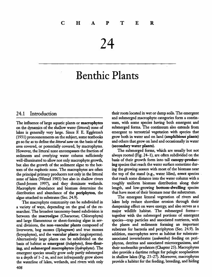
CHAPTER
24
Benthic Plants
24.1 Introduction
The influence of largeaquaticplantsor macrophyteson the dynamics of the shaUowwater(Uttoral) zoneoflakes is generaUy very large. Since E E. Eggleton's(1931) pronouncements on the subject, sometextbooksgoso far as to definethe littoral zone on the basis of thearea covered, or potentiaUy covered, by macrophytes.However, the Uttoral zone encompasses the fraction ofsediments and overlying water column sufficiendyweU-iUuminated to aUow not onlymacrophyte growth,but also die growth of the sediment algae to the bottom of the euphoric zone.The macrophytes are oftenthe principal primaryproducersnot onlyin the Uttoralzone of lakes (Wetzel 1983) but also in shaUowrivers(Sand-Jensen 1997), and they dominate wedands.Macrophyte abundance and biomass determine thedistribution and abundance of the periphyton, thealgae attached to substrates (Sec. 24.9).The macrophyte community canbe subdivided in
a variety of ways, depending on the goal of the researcher. The broadest taxonomy-based subdivision isbetween the macroalgae (Characeae; Chlorophyta)and large filamentous or sheet-forming algae in several divisions, the non-vascular plants composed ofUverworts, bog mosses (Sphagnum) and true mosses(bryophytes), and the vascular plants (angiosperms).Alternatively large plants can be subdivided on thebasis of habitat as emergent (helophytes), free-floating, and submerged macrophytes (hydrophytes). Theemergentspecies usually growonlypartlysubmergedto a depth of 1-2 m, and not infrequendygrowabovethe waterUne of lakes, wedands, and rivers with only408
their roots locatedinwet or dampsoils. The emergentand submerged macrophyte categories forma continuum, with some species having both emergent andsubmerged forms. The continuum also extends fromemergent to terrestrial vegetation with species thatgrowboth in water and on land (amphibious plants)andothersthat growon landandoccasionaUy inwater(secondary water plants).The submerged forms, which are usually but not
always rooted (Fig. 24-1), are often subdivided on thebasis of their growth form into taU canopy-producing species that reachthewatersurface sometime during the growing season withmostof the biomass nearthe top of the stand (e.g., water UUes), erect speciesthat reach some distance into the water column with aroughly uniform biomass distribution along theirlength, and low-growing bottom-dwelling speciesthat have most of their biomass near the substratum.The emergent Uttoral vegetation of rivers and
lakes help reduce shoreline erosion through theirdampening effecton wave energy, and alsoserves as amajor wildUfe habitat. The submerged forms—together with the submerged portions of emergentspecies—trap particles and associated nutrients, withthe plants and sediments forming an importantsubstrate for bacteria and periphyton (Sec. 24.9). Inaddition, macrophytes serve as habitat for substrate-associated invertebrates (zoobenthos) feeding on periphyton, detritus and associated microorganisms, andtheirzoobenthic predators (Chapter25). Macrophytesalso provide a daytime refuge for pelagic zooplanktonin shaUow lakes (Fig. 23-27).Moreover, macrophytesprovide a habitatfor the feeding, breeding, andhiding
24.1 Introduction 409
Figure 24-1 Some species of free-floating, submerged, and emergentmacrophytes. Not to scale. (From a variety ofsources.)
(a) Eichhornia crassipes(free-floating)
(b) Pistia stratiotes(free-floating)
(c) Potamogeton pectinatus(submerged rooted)
(d) Ceratophyllum demersum(submerged nonrooted)
(e) Elodea canadensis(submerged rooted)
(f)Myriophyllum spicatum(submerged rooted)
(g) Typha latifolia(emergent)
(h) Phragmites australis(emergent)
(i)Cyperus papyrus(emergent)
of littoral fish and for pelagic or riverine fish speciesfeeding in shallow water. Finally, the macrophyte-dominated littoral zone provides a habitat for waterfowl, songbirds, amphibians, reptiles, andmammals.Where abundant, the submerged macrophytes are
important suppliersof organicmatter to inlandwaters,and their decomposition can have a major effect ondissolved oxygen concentrations and the cycling ofnutrients and contaminants. The canopy-forming sub
merged macrophytes of lakes interfere with fishing,boating, andswimming when dense and are often considered visually unattractive by property owners,prompting demands for their removal (Sec. 24.11).Dense beds ofsubmerged macrophytes in lotic systemsimpair discharge and thereby increase the potential forflooding and interferewith boat transportation.Among free-floating macrophytes, the small duck
weeds (e.g., Lemna spp.) are probably the best known.
410 CHAPTER 24 Benthic Plants
They cover the surface of nutrient-rich wind-protectedponds and ditchesin temperateand tropicalregions. More important from a management perspective are larger species, such as the water hyacinth(Eichhornia crassipes) (Fig. 24-1a), the nile cabbage(Pistia stratiotes) (Fig. 24-lb), and aquatic ferns (e.g.,Salvinia molesta) which sometimes cover part or eventhe whole surface ofnutrient-rich lakes and reservoirs(See Fig. 15-1), slowly flowing rivers, or wedands atlower latitudes. They interfere with water transportand reduce the underwaterUght cUmate, negatively affecting the phytoplankton and submerged macrophytes. Free-floating macrophyte species competewith phytoplankton for nutrients because their rootsare suspended in the water; and onlymanage this successfully in nutrient-richwaters sufficiendy protectedfrom the wind to prevent the plants from beingwashed ashore.
24.2 Wetlands and Their Utilization
Wedandsare waterlogged landscapes that coverabout8.6 million km2 or 6.4 percent of Earth's land area(Mitsch and Gosselink 1993); this is about three timesthe area of lakes. The greatest extent of wedands isfound in the boreal forest regions of North Americaand Eurasia, and around the equator (seeFig. 4-1).A definition of wedands that satisfies everyonehas
not been developed because the suitabiUty of a definition depends on the goaland the field of interest of itscreators. Some focus on soil development, others onaspects of the hydrology, andyet othersemphasize thevegetation or biotain general. Here wetlands are defined asa placesufficiendy saturatedwithwater to enable plants characteristic of wet soils to grow (P. E.Greeson et al. 1978, in Howard-WilUams 1983).Wetlands and lakes form part of a continuum, with thedeeperportionsof largewedands considered as lakeswith a large littoral zone.There is no universal classification scheme for
wedands. The available schemeswere created for particular purposes and address higher latitude wedandscharacterized by their particular climatic, hydrologi-cal, geological, and vegetation conditions (Morant1983). Selective terms and types of wedands derivedfor the north temperate zone are presented in Table24-1. Workable definitions of wedands and wedandtypes are important to wedand scientists and areequaUy important to assist managers and regulators inwedand management. They need clear and legaUy
bindingdefinitions to prevent or control the drainingof wedands for agriculture or urban development, asweU as preventing the large-scale cutting of forestedwedands. The channelization (straightening) of windinglowland rivers separates rivers fromthewedands ontheir floodplains, encouraging drainage for agriculture(Sec. 4.3). The conversion of deepwater wedands insouthern and southeast Asia to a monoculture of rice,and the conversion ofwedands(shallow lakes) for aqua-culture are the major threats to wedands in that area.The valueof wedands for flood control, water storage,and water purification has been estimated at US-$15,000 ha"1 yr_1 (Sec. 1.1). This does not even consider their value as a habitat for fish and wildUfe, recreation, or maintaining biodiversity. In less economicaUydeveloped countries at low latitudes, wedands are thehomeofmiUions ofpeopledependenton themfor theirUveUhood and for mamtaining theirculture.1A About half the wedand area in the contiguousUnited States has disappeared since 1780, mosdybecause theyweredrained foragricultural purposes. Theimpact has been greatestin die lowerMississippi valley and the prairie pothole (slough) region—a majorwaterfowl breeding area in the northern portions ofthe prairie region of the United States and adjacentCanada (Mitsch and Gosselink 1993). In some statessuch as CaUfornia, Ohio, and Iowa, less than 10 percent of the original wedands remain; virtually allfreshwater wedands have been lost near major urbancenters worldwide. The losses are even greater inwestern Europe where wedands have been drainedsince the Middle Ages. Of those remaining in theNetherlands and Germany in 1950, more than halfwere drained by 1980 (Gleick 1993). Not only thewedands are lost, the birds, mammals, and fish disappearwith them.Population growthin South and EastAsia stimu
lates dam building and draining or converting wetlands for agricultural or aquacultural purposes. By1988about half the originalwedand area in a numberof southeast Asian countries had been drained orgready modified (Gleick 1993)—in populated Java(ED) onlysome 6 percent remained—and conversionshave probably been accelerating. The diversion of in-
lwThe principle forces driving government policies such as those onland use, on agricultural subsidies and on water pricing, are economic. There is therefore anurgentneedto effectdetailed analyseswhichcandemonstrate the multiplepublic benefitsof wetland conservation, as opposed to the public cost andmore limited privatebenefits of wetland conversion." P.J. Dugan 1994.
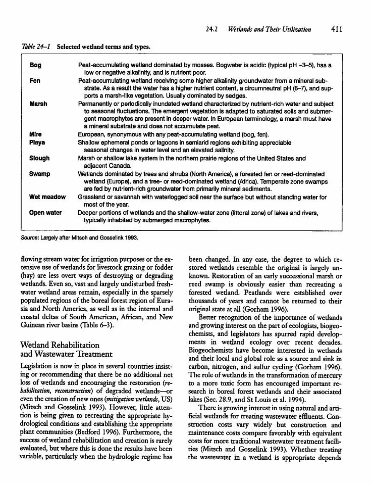
24.2 Wetlands and Their Utilization 411
Table 24-1 Selected wedand terms and types.
Bog Peat-accumulating wetland dominated by mosses. Bogwater is acidic (typical pH -3-5), has alow or negative alkalinity, and is nutrient poor.
Fen Peat-accumulating wetland receiving some higher alkalinity groundwater from a mineral substrate. As a result the water has a higher nutrient content, a circumneutral pH (6-7), and supports a marsh-like vegetation. Usually dominated by sedges.
Marsh Permanently or periodically inundated wetland characterized by nutrient-rich water and subjectto seasonal fluctuations. The emergent vegetation is adapted to saturated soils and submerged macrophytes are present in deeper water. In European terminology, a marsh must havea mineral substrate and does not accumulate peat.
Mire European, synonymous with any peat-accumulating wetland (bog, fen).Playa Shallow ephemeral ponds or lagoons in semiarid regions exhibiting appreciable
seasonal changes in water level and an elevated salinity.Slough Marsh or shallow lake system in the northern prairie regions of the United States and
adjacent Canada.Swamp Wetlands dominated by trees and shrubs (NorthAmerica), a forested fen or reed-dominated
wetland (Europe), and a tree- or reed-dominated wetland (Africa). Temperate zone swampsare fed by nutrient-rich groundwater from primarily mineral sediments.
Wet meadow Grassland or savannah with waterlogged soil near the surface but without standing water formost of the year.
Open water Deeper portions of wetlands and the shallow-water zone (littoral zone) of lakes and rivers,typically inhabited by submerged macrophytes.
Source: Largely after Mitsch and Gosselink 1993.
flowing streamwater for irrigation purposesor the extensive use ofwedands for Uvestock grazingor fodder(hay) are less overt ways of destroying or degradingwedands. Evenso,vastand largely undisturbed freshwater wedand areas remain, especially in the sparselypopulated regions of the boreal forest regionof Eurasia and North America, as weU as in the internal andcoastal deltas of South American, African, and NewGuinean river basins (Table 6-3).
Wetland Rehabilitationand Wastewater Treatment
Legislation is nowin place in several countries insisting or recommendingthat there be no additional netloss of wedands and encouraging the restoration (rehabilitation, reconstruction) of degraded wedands—oreven the creation ofnewones(mitigation wetlands, US)(Mitsch and Gosselink 1993). However, little attention is being given to recreating the appropriate hy-drological conditions andestablishing the appropriateplant communities (Bedford 1996). Furthermore, thesuccess ofwedand rehabiUtation andcreation israrelyevaluated, but where this is done the results have beenvariable, particularly when the hydrologic regime has
been changed. In any case, the degree to which restored wedands resemble the original is largely unknown. Restoration of an earlysuccessional marshorreed swamp is obviously easier than recreating aforested wedand. Peadands were estabUshed overthousands of years and cannot be returned to theiroriginal state at aU (Gorham 1996).Better recognition of the importance of wedands
andgrowing intereston the part of ecologists, biogeo-chemists, and legislators has spurred rapid developments in wedand ecology over recent decades.Biogeochemists have become interested in wedandsand their local and global role as a source and sink incarbon, nitrogen, and sulfur cycling (Gorham 1996).The role ofwedands in the transformation ofmercuryto a more toxic form has encouraged important research in boreal forest wedands and their associatedlakes(Sec. 28.9, and St Louis et al. 1994).There isgrowing interest in usingnaturalandarti
ficial wedands for treatingwastewater effluents. Construction costs vary widely but construction andmaintenance costs compare favorably with equivalentcosts for more traditional wastewater treatment faculties (Mitsch and Gosselink 1993). Whether treatingthe wastewater in a wedand is appropriate depends
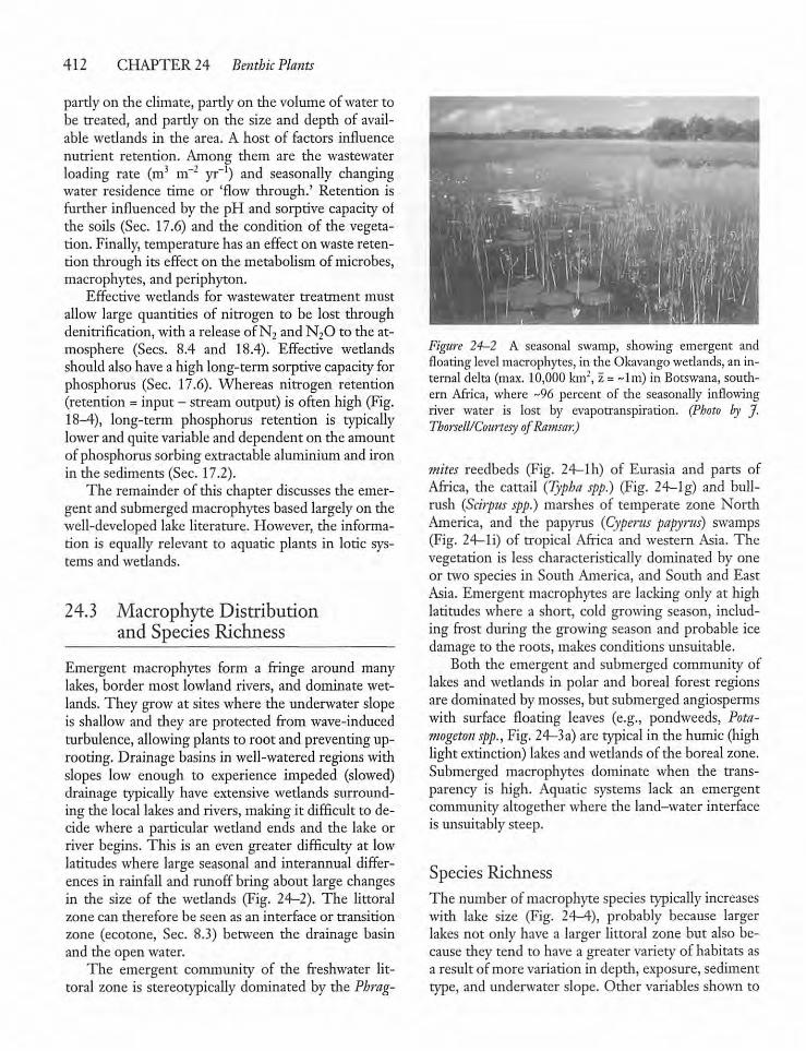
412 CHAPTER 24 Benthic Plants
partly on the climate, partly on the volume of water tobe treated, and pardy on the size and depth of available wetlands in the area. A host of factors influencenutrient retention. Among them are the wastewaterloading rate (m3 m-2 yr"1) and seasonally changingwater residence time or 'flow through.' Retention isfurther influenced by the pH and sorptive capacity ofthe soils (Sec. 17.6) and the condition of the vegetation. Finally, temperature hasan effecton wasteretention through its effect on the metabolism of microbes,macrophytes, and periphyton.
Effective wetlands for wastewater treatment mustallow large quantities of nitrogen to be lost throughdenitrification, with a release of N2 and N20 to the atmosphere (Sees. 8.4 and 18.4). Effective wedandsshould alsohavea high long-term sorptivecapacity forphosphorus (Sec. 17.6). Whereas nitrogen retention(retention = input - stream output) is often high (Fig.18-4), long-term phosphorus retention is typicallylower and quite variable and dependent on the amountof phosphorus sorbing extractable aluminium and ironin the sediments (Sec. 17.2).The remainder of this chapter discusses the emer
gent and submerged macrophytes based largely on thewell-developed lake literature. However, the information is equally relevant to aquatic plants in lotic systems and wetlands.
24.3 Macrophyte Distributionand Species Richness
Emergent macrophytes form a fringe around manylakes, border most lowland rivers, and dominate wetlands. They growat siteswhere the underwater slopeis shallow and they are protected from wave-inducedturbulence, allowingplants to root and preventinguprooting. Drainage basins in well-watered regionswithslopes low enough to experience impeded (slowed)drainage typically have extensive wedands surrounding the local lakes and rivers, making it difficult to decide where a particular wetland ends and the lake orriver begins. This is an even greater difficulty at lowlatitudes where large seasonal and interannual differences in rainfall and runoff bring about large changesin the size of the wetlands (Fig. 24—2). The littoralzone can therefore be seen as an interface or transitionzone (ecotone, Sec. 8.3) between the drainage basinand the open water.The emergent community of the freshwater lit
toral zone is stereotypically dominated by the Phrag-
Figure 24-2 A seasonal swamp, showing emergent andfloatinglevel macrophytes,in die Okavangowetlands, an internal delta (max. 10,000km2, z = ~lm) in Botswana, soudi-ern Africa, where ~96 percent of the seasonally inflowingriver water is lost by evapotranspiration. (Photo by J.Thorsell/Courtesy ofRamsar.)
mites reedbeds (Fig. 24-1h) of Eurasia and parts ofAfrica, the cattail (Typha spp.) (Fig. 24-1g) and bull-rush (Scirpus spp.) marshes of temperate zone NorthAmerica, and the papyrus (Cypertts papynis) swamps(Fig. 24—li) of tropical Africa and western Asia. Thevegetation is less characteristically dominated by oneor two species in South America, and South and EastAsia. Emergent macrophytes are lacking only at highlatitudes where a short, cold growing season, including frost during the growing season and probable icedamage to die roots, makes conditions unsuitable.
Both the emergent and submerged community oflakes and wetlands in polar and boreal forest regionsare dominated bymosses, but submerged angiospermswith surface floating leaves (e.g., pondweeds, Pota-mogeton spp., Fig. 24—3a) are typical in the humic (highlight extinction) lakes and wetlandsof the boreal zone.Submerged macrophytes dominate when the transparency is high. Aquatic systems lack an emergentcommunity altogether where the land-water interfaceis unsuitably steep.
Species RichnessThe number of macrophyte species typically increaseswith lake size (Fig. 24-4), probably because largerlakes not only have a larger littoral zone but also because they tend to have a greater variety of habitats asa result of more variation in depth, exposure, sedimenttype, and underwater slope. Other variables shown to
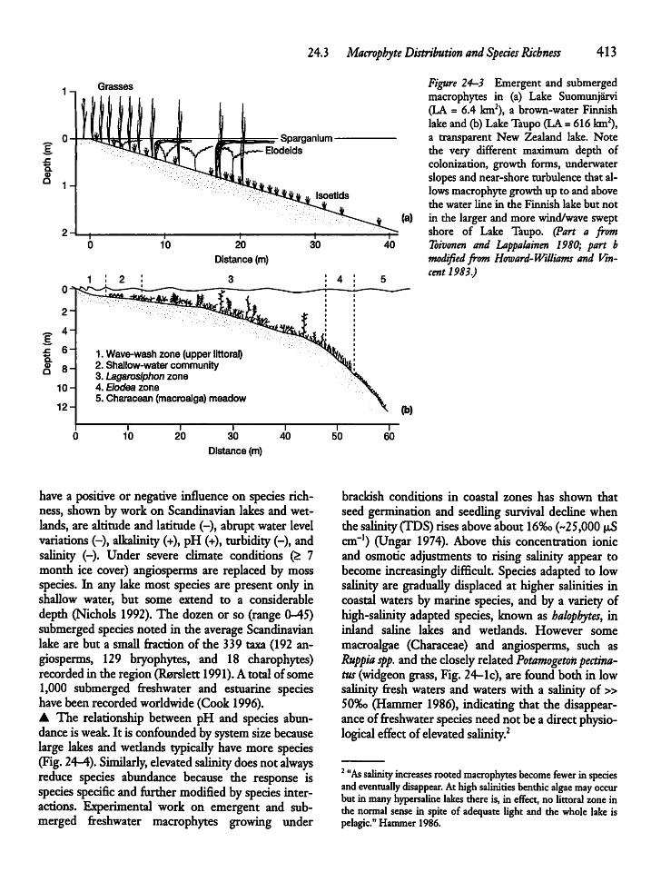
24.3 Macrophyte Distribution and Species Richness 413
a.COQ
~ 4HE
"5.(D Q I
10-
12-
Grasses
0 10 20
Distance (m)
1 2 3
Wave-wash zone (upper littoral)Shallow-water communityLagarosiphon zoneElodea zoneCharacean (macroalga) meadow
10 20 30
Distance (m)40
have a positive or negative influence on species richness, shown by work on Scandinavian lakes and wetlands, are altitudeand latitude (-), abruptwater levelvariations (-), alkalinity (+), pH (+), turbidity (-), andsalinity (-). Under severe climate conditions (£ 7month ice cover) angiosperms are replaced by mossspecies. In any lake most species are present only inshaUow water, but some extend to a considerabledepth (Nichols 1992). The dozen or so (range 0-45)submerged species noted in the average Scandinavianlake are but a smaU fraction of the 339 taxa (192 angiosperms, 129 bryophytes, and 18 charophytes)recordedin the region (Rarslett 1991). A total of some1,000 submerged freshwater and estuarine specieshavebeen recordedworldwide (Cook 1996).A The relationship between pH and species abundance isweak. It is confounded bysystem size becauselarge lakes andwedands typicaUy have more species(Fig. 24-4). Similarly, elevated salinity does not alwaysreduce species abundance because the response isspecies specific and furthermodified by species interactions. Experimental work on emergent and submerged freshwater macrophytes growing under
50 60
Figure 24-3 Emergent and submergedmacrophytes in (a) Lake Suomunjarvi(LA= 6.4 km2), a brown-water Finnishlake and(b) Lake Taupo (LA =616km2),a transparent New Zealand lake. Notethe very different maximum depth ofcolonization, growth forms, underwaterslopes and near-shore turbulencethat allowsmacrophyte growth up to and abovethe water line in the Finnish lake but notin the larger and more wind/wave sweptshore of Lake Taupo. (Part a fromToivonen and Lappalainen 1980; part bmodified from Howard-Williams and Vincent1983.)
brackish conditions in coastal zones has shown thatseed germination and seedling survival decline whenthe salinity(TDS) risesaboveabout 16%o (-25,000 u.Scm-1) (Ungar 1974). Above this concentration ionicand osmotic adjustments to rising salinity appear tobecome increasingly difficult. Species adapted to lowsalinity are graduaUy displaced at higher salinities incoastal waters bymarine species, and by a variety ofhigh-salinity adapted species, known as halophytes, ininland saline lakes and wedands. However somemacroalgae (Characeae) and angiosperms, such asRuppia spp. andthe closely related Potamogeton pectina-tus (widgeon grass, Fig. 24-1c), are found both in lowsalinity fresh waters and waters with a salinity of »50%o (Hammer 1986), indicating that the disappearance of freshwater species neednot be a directphysiological effect ofelevated salinity.2
2"As salinity increases rooted macrophytes become fewer inspeciesandeventually disappear. Athighsalinities benthic algae may occurbut in manyhypersaline lakes there is, in effect, no littoralzoneinthe normal sense in spiteof adequate light and the whole lake ispelagic." Hammer 1986.
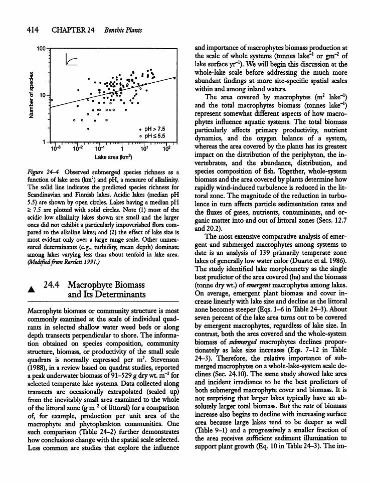
414 CHAPTER 24 Benthic Plants
100-
5 10-
XIE3Z
• •• : t *
• ao ooo
. pH>7.5o pH£5.5
I i iiin'i i i iii»i| i i inn') i i iiiiit| i i iiim'i—r1CT3 10"2 10"1 1 101 102
Lakearea (km2)
Figure 24-4 Observed submerged species richness as afunction of lake area (km2) and pH, ameasure ofalkalinity.The soUd line indicates the predicted species richness forScandinavian and Finnish lakes. Acidic lakes (median pH5.5)are shownby open circles. Lakes havinga medianpH> 7.5 are plotted with soUd circles. Note (1) most of dieacidic low alkalinity lakes shown are smaU and the largerones did not exhibit a particularly impoverished flora compared to the alkaline lakes; and (2) the effect of lake size ismost evident only over a large range scale. Other unmeasured determinants (e.g., turbidity, mean depth) dominateamong lakes varying less than about tenfold in lake area.(Modifiedfrom Rurslett 1991.)
. 24.4 Macrophyte Biomassand Its Determinants
Macrophyte biomass or communitystructure is mostcommonly examined at the scale of individual quadrants in selected shaUow water weed beds or alongdepth transects perpendicular to shore.The information obtained on species composition, communitystructure, biomass, or productivity of the smaU scalequadrats is normaUy expressed per m2. Stevenson(1988), in a reviewbased on quadrat studies, reportedapeakunderwater biomass of91-529 gdrywt. m~2 forselected temperate lake systems. Data coUected alongtransects are occasionaUy extrapolated (scaled up)from the inevitably small area examined to the wholeoftheUttoral zone (gm~2 ofUttoral) fora comparisonof, for example, production per unit area of themacrophyte and phytoplankton communities. Onesuch comparison (Table 24-2) further demonstrateshowconclusions changewith the spatialscaleselected.Less common are studies that explore the influence
andimportance ofmacrophytes biomass productionatthe scale of whole systems (tonnes lake-1 or gm~2 oflake surface yr"1). We will begin this discussion at thewhole-lake scale before addressing the much moreabundant findings at more site-specific spatial scaleswithin and among inlandwaters.The area covered by macrophytes (m2 lake-1)
and the total macrophytes biomass (tonnes lake"1)represent somewhat different aspects of how macrophytes influence aquatic systems. The total biomassparticularly affects primary productivity, nutrientdynamics, and the oxygen balance of a system,whereas the areacovered by the plantshasits greatestimpact on the distribution of the periphyton, the invertebrates, and the abundance, distribution, andspecies composition of fish. Together, whole-systembiomass and the areacoveredbyplants determinehowrapidlywind-induced turbulence is reduced in the Uttoral zone. The magnitude of the reduction in turbulence in turn affects particle sedimentation rates andthe fluxes of gases, nutrients, contaminants, and organic matter into and out of Uttoral zones (Sees. 12.7and 20.2).The most extensive comparative analysis of emer
gent and submerged macrophytes among systems todate is an analysis of 139 primarily temperate zonelakes of generaUy lowwater color (Duarte et al. 1986).The study identified lakemorphometry as the singlebestpredictorof the areacovered (ha)and the biomass(tonnedrywt.)of emergentmacrophytes amonglakes.On average, emergent plant biomass and cover increase linearlywith lakesizeand decline as the Uttoralzone becomes steeper (Eqs. 1-6 in Table24-3). Aboutseven percentof the lake area turns out to be coveredby emergent macrophytes, regardless of lake size. Incontrast, both the area covered and the whole-systembiomass of submerged macrophytes declines proportionately as lake size increases (Eqs. 7-12 in Table24-3). Therefore, the relative importance of submergedmacrophytes on awhole-lake-system scale declines (Sec. 24.10). The same study showed lake areaand incident irradiance to be the best predictors ofboth submerged macrophyte cover and biomass. It isnot surprising that larger lakes typicaUy have an absolutely larger total biomass. But the rate of biomassincrease also begins to decline with increasing surfacearea because large lakes tend to be deeper as weU(Table 9-1) and a progressively a smaller fraction ofthe area receives sufficient sediment illumination tosupportplant growth (Eq. 10in Table 24-3).The im-
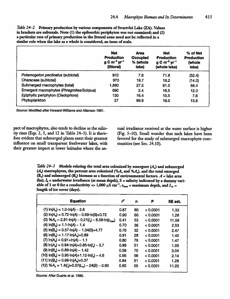
24.4 Macrophyte Biomass andItsDeterminants 415
Table 24-2 Primaryproduction by variouscomponents ofSwartvlei Lake (ZA). Valuesin brackets are subtotals. Note (1) the epibentfaic periphyton was not examined; and (2)a particularrate ofprimary production in the Uttoral zone need not be reflected in asimilar role when the lake as a whole is considered, an issue ofscale.
Net Area Net % of NetProduction Occupied Production Productiong C m~2 yr1 % (whole g C m~2 yr1 (whole(littoral) lake) (whole lake) lake)
Potamogeton pectinatus (subtotal) 910 7.8 71.8 (52.4)Characeae (subtotal) 970 19.7 19.2 (14.0)Submerged macrophytes (total) 1,880 27.5 91.0 66.4Emergent macrophytes (Phragmites/Scirpus) 690 2.4 16.5 12.0Epiphytic periphyton {Cladophora) 130 16.4 10.5 7.6Phytoplankton 27 69.9 19.0 13.8
Source: Modified after Howard-Williams and Allanson 1981.
pactofmacrophytes, also tends to decline asthe salinity rises (Eqs. 2, 5, and 12 in Table 24-3). It is therefore evident that submerged plants exerttheirgreatestinfluence on smaU transparent freshwater lakes, withtheir greatest impactat lower latitudes where the an
nual irradiance received at the water surface is higher(Fig. 5-10). SmaU wonder that such lakes have beenfavored for the study of submerged macrophyte communities (see Sec. 24.10).
Table 24-3 Models relating the total area colonized byemergent (4^ and submerged(AJmacrophytes, the percentarea colonized (%Ae and %AJ, andthe totalemerged(B^ and submerged (BJ biomass as a function of environmental factors.A =lake area(ha), lt e underwater irradiance (at mean depth), S=salinity indicated byadummy variable of 1or0 foraconductivity <> 1,000 |iS cm"1, z^a»mflxinnirn depth,andLic =length ofice cover (days).
Equation r2 n P SEest.
(1)ln(Ae) = 1.0-ln(/l)-2.6 0.87 60 < 0.0001 1.33(2) ln(/g = 0.72-ln(A) - 0.69-ln(S)+0.72 0.90 60 < 0.0001 1.28(3) %Ae = 2.81-ln(A) - 0.21(/J - 6.58-^(2^ 0.41 53 < 0.0001 11.59(4)ln(Be) = 1.1-ln(A)-1.4 0.70 36 < 0.0001 2.53(5)ln(Be) = 0.57-ln(A) - 1.34(S)+4.77 0.76 32 < 0.0001 2.47(6)ln(Be) = 1.17-Wa)+0.89 0.91 28 < 0.0001 1.45(7)ln(As) = 0.91+ln(A)-1.1 0.80 76 < 0.0001 1.47(8) ln(/U= 0M-\n{A)+0.85MQ - 3.7 0.89 51 < 0.0001 1.05(9) ^ = 0.89-^) -1.42 0.59 70 < 0.0001 3.04(10) In(Ba) = 0.95-ln(A)+1.12-1^/3) - 4.6 0.66 56 < 0.0001 2.14(11) InfBg) = o.gg-int/u+o^ 0.84 51 < 0.0001 1.26(12)%Aa = 1.4(^+0.07(1^ - 24(S)- 0.90 0.60 55 < 0.0001 11.20
Source: After Duarte et al. 1986.
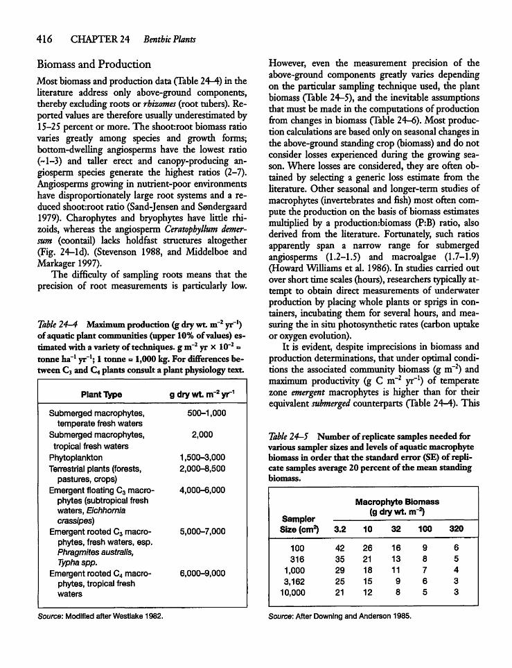
416 CHAPTER 24 Benthic Plants
Biomass and Production
Most biomass and production data (Table 24-4) in theUterature address only above-ground components,thereby excluding roots or rhizomes (root tubers). Reported values are therefore usually underestimated by15-25 percent or more. The shoofcroot biomass ratiovaries gready among species and growth forms;bottom-dwelling angiosperms have the lowest ratio(-1-3) and taUer erect and canopy-producing an-giosperm species generate the highest ratios (2-7).Angiosperms growing in nutrient-poor environmentshave disproportionately large root systems and a reducedshoot:root ratio (Sand-Jensen and Sendergaard1979). Charophytes and bryophytes have Utde rhi-zoids, whereas the angiosperm Ceratophyllum demer-sum (coontail) lacks holdfast structures altogether(Fig. 24-ld). (Stevenson 1988, and Middelboe andMarkager 1997).The difficulty of sampling roots means that the
precision of root measurements is particularly low.
Table 24-4 Maximum production(gdrywt. m~2 yr"1)ofaquatic plant communities (upper 10% ofvalues) estimatedwith a varietyof techniques, g m"2 yr x 10"2 otonne ha"1 yr"1; 1 tonne =1,000kg.For differences between C3and C4plants consult a plant physiology text.
Plant Type g drywt. m"2 yr1
Submerged macrophytes, 500-1,000temperate fresh waters
Submerged macrophytes, 2,000tropical fresh watersPhytoplankton 1,500-3,000Terrestrial plants (forests, 2,000-8,500pastures, crops)
Emergent floating C3macro 4,000-6,000phytes (subtropical freshwaters, Eichhorniacrassipes)
Emergent rooted C3macro 5,000-7,000phytes, fresh waters, esp.Phragmites australis,Typhaspp.
Emergent rooted C4macro 6,000-9,000phytes, tropical freshwaters
Source: Modified afterWestlake 1982.
However, even the measurement precision of theabove-ground components gready varies dependingon the particular sampling technique used, the plantbiomass (Table 24-5), and the inevitable assumptionsthat must be made in the computations of productionfrom changes in biomass (Table 24-6). Most productioncalculations are based onlyon seasonal changes inthe above-ground standingcrop (biomass) and do notconsider losses experienced during the growing season.Where losses are considered, they are often obtained by selecting a generic loss estimate from theUterature. Other seasonal and longer-term studies ofmacrophytes (invertebrates and fish) mostoftencompute the production on the basis of biomass estimatesmultiplied by a productiombiomass (P:B) ratio, alsoderived from the Uterature. Fortunately, such ratiosapparendy span a narrow range for submergedangiosperms (1.2-1.5) and macroalgae (1.7-1.9)(HowardWiUiams et al. 1986). In studies carried outover short time scales(hours), researchers typicaUy attempt to obtain direct measurements of underwaterproduction by placingwhole plants or sprigs in containers, incubating them for several hours, and measuring the in situ photosynthetic rates (carbonuptakeor oxygen evolution).It is evident, despite imprecisions in biomass and
production determinations, that under optimal conditions the associated community biomass (g m-2) andmaximum productivity (g C m"2 yr-1) of temperatezone emergent macrophytes is higher than for theirequivalent submerged counterparts (Table 24-4). This
Table 24-5 Number of repUcatesamples needed forvarioussampler sizes and levelsof aquaticmacrophytebiomass in order that the standard error (SE) of repUcate samplesaverage20 percent of the mean standingbiomass.
SamplerSize (cm2)
Macrophyte Biomass(g dry wt. m-2)
3.2 10 32 100 320
100 42 26 16 9 6
316 35 21 13 8 5
1,000 29 18 11 7 4
3,162 25 15 9 6 3
10,000 21 12 8 5 3
Source: After Downing and Anderson 1985.
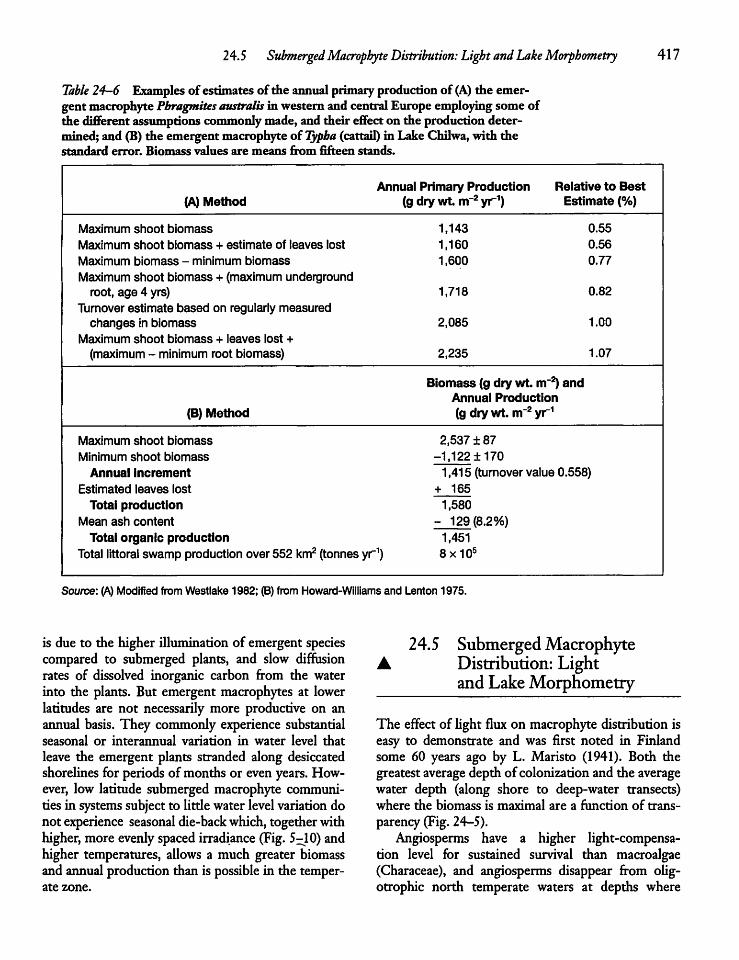
24.5 SubmergedMacrophyte Distribution: Light and LakeMorphometry 417
Table 24-6 Examplesof estimates of the annual primaryproduction of (A) the emergent macrophytePbragmites australis in western and central Europe employingsome ofthe different assumptions commonlymade, and their effect on the production determined; and (B)the emergent macrophyte of Typba (cattail)in LakeChilwa,with thestandard error. Biomass values are means from fifteen stands.
Annual Primary Production Relative to Best(A) Method (g dry wt. m-2 yr1) Estimate (%)
Maximum shoot biomass 1,143 0.55
Maximum shoot biomass + estimate of leaves lost 1,160 0.56
Maximum biomass - minimum biomass 1,600 0.77
Maximum shoot biomass + (maximum undergroundroot, age 4 yrs) 1,718 0.82
Turnover estimate based on regularly measuredchanges in biomass 2,085 1.00
Maximum shoot biomass + leaves lost +(maximum - minimum root biomass) 2,235 1.07
Biomass (g dry wt. m"2) andAnnual Production
(B) Method (g dry wt. m-2yr1
Maximum shoot biomass 2,537 ±87Minimum shoot biomass -1,122 ±170Annual increment 1,415 (turnover value 0.558)
Estimated leaves lost + 165
Total production 1,580Mean ash content - 129(8.2%)Total organic production 1,451
Total littoral swamp production over552 km2 (tonnesyr1) 8x10⁵
Source: (A) Modified from Westlake 1982; (B) from Howard-Williams and Lenton 1975.
is due to the higher illumination of emergent speciescompared to submerged plants, and slow diffusionrates of dissolved inorganic carbon from the waterinto the plants. But emergent macrophytes at lowerlatitudes are not necessarily more productive on anannual basis. They commonly experience substantialseasonal or interannual variation in water level thatleave the emergent plants stranded along desiccatedshorelines for periods of months or evenyears. However, low latitude submerged macrophyte communities in systems subject to little water levelvariationdonot experience seasonal die-backwhich, togetherwithhigher,more evenlyspaced irradiance (Fig. 5-10) andhigher temperatures, allows a much greater biomassand annualproduction than is possible in the temperate zone.
24.5 SubmergedMacrophyte• Distribution: Light
and LakeMorphometry
The effectof Ught flux on macrophyte distribution iseasy to demonstrate and was first noted in Finlandsome 60 years ago by L. Maristo (1941). Both thegreatestaverage depth of colonizationand the averagewater depth (along shore to deep-water transects)where the biomass is maximal are a function of transparency (Fig. 24—5).Angiosperms have a higher light-compensa
tion level for sustained survival than macroalgae(Characeae), and angiosperms disappear from oUgotrophic north temperate waters at depths where
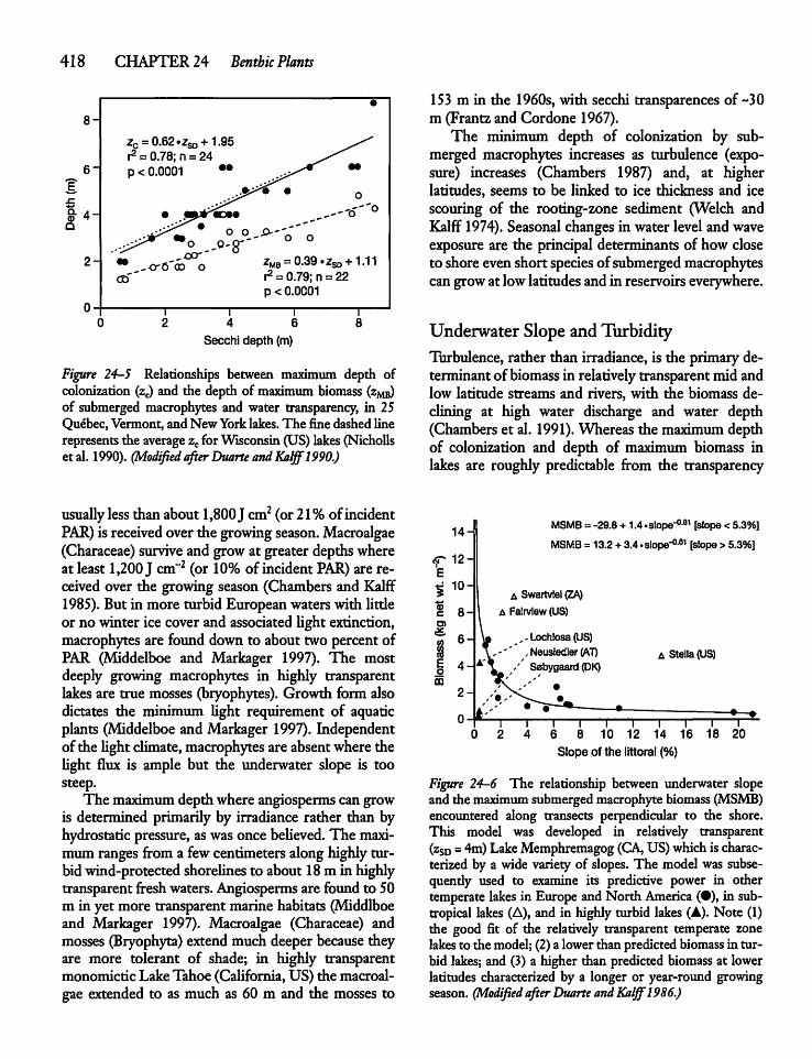
418 CHAPTER 24 Benthic Plants
•
8-
zc = 0.62.zSD + 1.95 ^r2= 0.78; n = 24 ^^
6"
g..c
9- 4-o
p < 0.0001
* O O S>~'~' -
2- • .o-o'c^o 2MB =0.39.2S0 +1.11oo'' r2= 0.79;n = 22
p < 0.0001ft-
CI
) 2I I I4 6 8
Secchi depth (m)
Figure 24-5 Relationships between maximum depth ofcolonization (zj and the depth of maximum biomass (zMB)of submerged macrophytes and water transparency, in 25Quebec, Vermont, and NewYork lakes. The fine dashed linerepresents the averagezcforWisconsin (US) lakes(NichoUset al. 1990). (Modified afterDuarte andKalff1990.)
usuaUy less thanabout1,800J cm2 (or21%ofincidentPAR) is received over the growing season. Macroalgae(Characeae) survive and growat greater depthswhereat least 1,200J cm-2 (or 10% of incidentPAR) are received over the growing season (Chambers and Kalff1985).But in more turbid European waters with Utdeor no winter ice cover and associated Ught extinction,macrophytes are found down to about two percent ofPAR (Middelboe and Markager 1997). The mostdeeply growing macrophytes in highly transparentlakes are true mosses (bryophytes). Growth form alsodictates the ininimum Ught requirement of aquaticplants (Middelboe and Markager 1997). Independentof the Ught climate, macrophytes are absentwhere theUght flux is ample but the underwater slope is toosteep.The maximumdepth where angiosperms can grow
is determined primarily by irradiance rather than byhydrostatic pressure, aswasonce beUeved. The maximumranges from a fewcentimeters alonghighlyturbidwind-protectedshorelinesto about 18m in highlytransparent freshwaters. Angiosperms are found to 50m in yet more transparent marine habitats (Middlboeand Markager 1997). Macroalgae (Characeae) andmosses (Bryophyta) extendmuch deeper because theyare more tolerant of shade; in highly transparentmonomictic Lake Tahoe (California, US) the macroalgae extended to as much as 60 m and the mosses to
153 m in the 1960s, with secchi transparences of ~30m (Frantz and Cordone 1967).The minimum depth of colonization by sub
merged macrophytes increases as turbulence (exposure) increases (Chambers 1987) and, at higherlatitudes, seems to be Unked to ice thickness and icescouring of the rooting-zone sediment (Welch andKalff 1974). Seasonal changesin water leveland waveexposure are the principal determinants of how closeto shore evenshort species of submergedmacrophytescangrowat lowlatitudesand in reservoirs everywhere.
Underwater Slope andTurbidityTurbulence, rather than irradiance, is the primary determinant of biomass in relatively transparentmid andlow latitude streams and rivers, with the biomass declining at high water discharge and water depth(Chamberset al. 1991). Whereas the maximum depthof colonization and depth of maximum biomass inlakes are roughly predictable from the transparency
14H
<jT 12-E^ 10-
«6-
I 4"03
2
0-
MSMB =-29.8+1.4.slope"081 [slope <5.3%]MSMB =13.2+3.4 .slope"081 [slope >5.3%]
A Swartvlei (ZA)A Falrview (US)
,-Lochlosa(US), Neusledler (AT)'' Sabygaard (DK)
10 12
A Stella (US)
14~i—i—r16 18 20
Slope of the littoral (%)
Figure 24-6 The relationship between underwater slopeand the maximum submerged macrophyte biomass (MSMB)encountered along transects perpendicular to the shore.This model was developed in relatively transparent(zsd=4m)LakeMemphremagog (CA, US)whichis characterized by a wide variety of slopes. The model was subse-quendy used to examine its predictive power in othertemperate lakes in Europe and North America (•), in subtropical lakes (A), and in highly turbid lakes (A). Note (1)the good fit of the relatively transparent temperate zonelakesto the model; (2)a lower than predicted biomassin turbid lakes; and (3) a higher than predicted biomass at lowerlatitudes characterized by a longer or year-round growingseason. (Modified afterDuarte andKalff1986.)
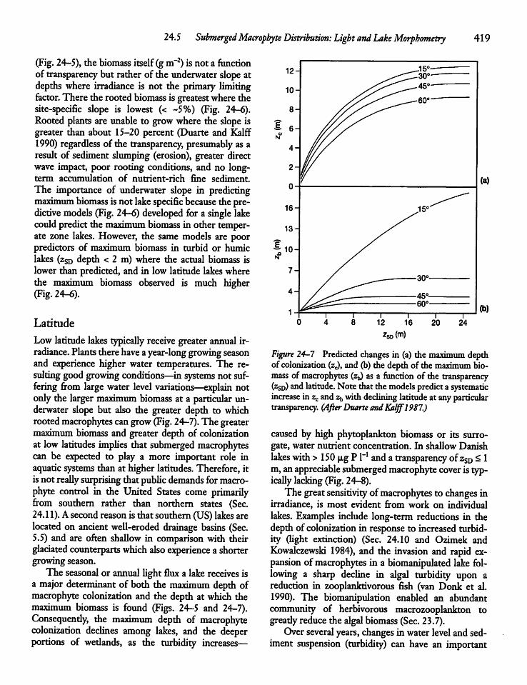
24.5 SubmergedMacrophyte Distribution: Light andLakeMorphometry 419
(Fig. 24-5), the biomass itself(gm"2) isnot a functionof transparency but rather of the underwater slope atdepths where irradiance is not the primary limitingfactor. There the rootedbiomass is greatestwhere thesite-specific slope is lowest (< -5%) (Fig. 24-6).Rooted plants are unable to growwhere the slope isgreater than about 15-20 percent (Duarte and Kalff1990) regardless of the transparency, presumably as aresult of sediment slumping (erosion), greater directwave impact, poor rooting conditions, and no long-term accumulation of nutrient-rich fine sediment.The importance of underwater slope in predictingmaximum biomass isnot lakespecific because the predictive models (Fig. 24-6) developed for a single lakecould predict themaximum biomass in other temperate zone lakes. However, the same models are poorpredictors of maximum biomass in turbid or humiclakes (zSD depth < 2 m) where the actual biomass islower than predicted, and in low latitude lakes wherethe maximum biomass observed is much higher(Fig. 24-6).
Latitude
Lowlatitude lakes typically receive greaterannual irradiance. Plants therehave ayear-long growing seasonand experience higher water temperatures. The resultinggoodgrowing conditions—in systems not suffering from large water level variations—explain notonly the larger maximum biomass at a particular underwater slope but also the greater depth to whichrootedmacrophytes cangrow (Fig. 24-7).The greatermaximum biomass and greater depth of colonizationat low latitudes implies that submerged macrophytescan be expected to play a more important role inaquatic systems than at higher latitudes. Therefore, itisnot reaUy surprisingthat pubUc demands formacrophyte control in the United States come primarilyfrom southern rather than northern states (Sec.24.11). Asecondreasonis that southern (US)lakes arelocated on ancient weU-eroded drainage basins (Sec.5.5) and are often shaUow in comparison with theirglaciated counterparts which also experience a shortergrowing season.The seasonal or annual Ught flux a lake receives is
a major determinant of both the maximum depth ofmacrophyte colonization and the depth at which themaximum biomass is found (Figs. 24-5 and 24-7).Consequendy, the maximum depth of macrophytecolonization declines among lakes, and the deeperportions of wedands, as the turbidity increases—
Figure 24-1 Predicted changes in (a) the maximum depthof colonization (zj, and (b) the depthof the maximum biomass ofmacrophytes (z^ as a function of the transparency(zSD) andlatitude. Note that themodels predict a systematicincrease in zc andzb withdeclining latitude at anyparticulartransparency. (After Duarte andKalff1987.)
caused by high phytoplankton biomass or its surrogate, water nutrient concentration. In shaUowDanishlakes with >150 u,g P l"1 and a transparency ofzSD <1m,anappreciable submerged macrophyte cover istypicaUy lacking (Fig. 24-8).The great sensitivity ofmacrophytes to changes in
irradiance, is most evident from work on individuallakes. Examples include long-term reductions in thedepth of colonization in response to increased turbidity (Ught extinction) (Sec. 24.10 and Ozimek andKowalczewski 1984), and the invasion and rapid expansion ofmacrophytes in a biomanipulated lake following a sharp decline in algal turbidity upon areduction in zooplanktivorous fish (van Donk et al.1990). The biomanipulation enabled an abundantcommunity of herbivorous macrozooplankton togreadyreduce the algal biomass (Sec. 23.7).Overseveral years, changes inwater level and sed
iment suspension (turbidity) can have an important
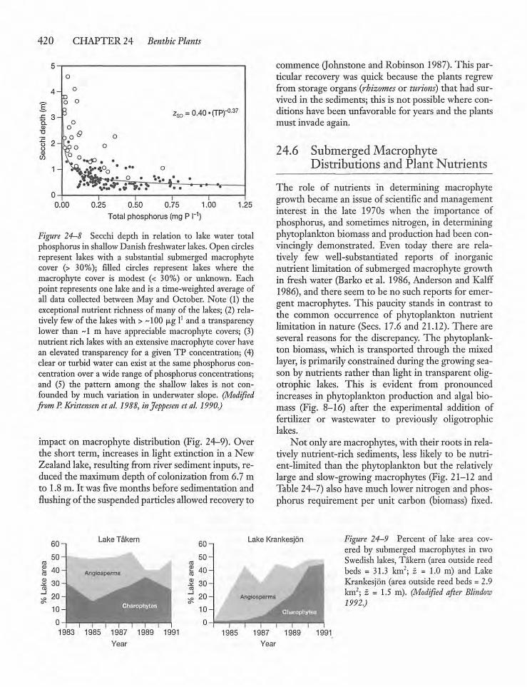
420 CHAPTER 24 Benthic Plants
0.00 0.25 0.50 0.75 1.00
Total phosphorus (mgP I"1)1.25
Figure 24-8 Secchi depth in relation to lake water totalphosphorus in shallowDanish freshwater lakes.Open circlesrepresent lakes with a substantial submerged macrophytecover (> 30%); filled circles represent lakes where themacrophyte cover is modest (< 30%) or unknown. Eachpoint represents one lake and is a time-weighted averageofall data collected between May and October. Note (1) theexceptional nutrient richness of many of die lakes; (2) relatively few of the lakes widi> ~100 u,g 1' and a transparencylower than ~1 m have appreciable macrophyte covers; (3)nutrient rich lakeswith an extensive macrophyte cover havean elevated transparency for a givenTP concentration; (4)clear or turbid water can exist at the same phosphorus concentration over a wide range of phosphorus concentrations;and (5) the pattern among the shallow lakes is not confounded by much variation in underwater slope. (Modifiedfrom P. Kristensen etal. 1988, injeppesen etal. 1990.)
impact on macrophyte distribution (Fig. 24—9). Overthe short term, increases in light extinction in a NewZealand lake, resulting from river sediment inputs, reduced the maximum depth of colonizationfrom 6.7mto 1.8 m. It was five months before sedimentation andflushing of the suspendedparticlesallowed recoveryto
commence (Johnstone and Robinson 1987). This particular recovery was quick because the plants regrewfrom storage organs (rhizomes or furious) that had survived in the sediments; this is not possible where conditions have been unfavorable for years and the plantsmust invade again.
24.6 Submerged MacrophyteDistributions and Plant Nutrients
The role of nutrients in determining macrophytegrowth becamean issue of scientificand managementinterest in the late 1970s when the importance ofphosphorus, and sometimes nitrogen, in determiningphytoplankton biomass and production had been convincingly demonstrated. Even today there are relatively few well-substantiated reports of inorganicnutrient limitation of submerged macrophyte growthin fresh water (Barko et al. 1986, Anderson and Kalff1986), and there seem to be no such reports for emergent macrophytes. This paucity stands in contrast tothe common occurrence of phytoplankton nutrientlimitation in nature (Sees. 17.6 and 21.12). There areseveral reasons for the discrepancy. The phytoplankton biomass, which is transported through the mixedlayer, is primarily constrained during the growingseason by nutrients rather than light in transparent oligotrophic lakes. This is evident from pronouncedincreases in phytoplankton production and algal biomass (Fig. 8-16) after the experimental addition offertilizer or wastewater to previously oligotrophiclakes.Not only are macrophytes,with their roots in rela
tivelynutrient-rich sediments, less likely to be nutrient-limited than the phytoplankton but the relativelylarge and slow-growing macrophytes (Fig. 21-12 andTable 24-7) also havemuch lower nitrogen and phosphorus requirement per unit carbon (biomass) fixed.
Lake Takern Lake Krankesjon Figure 24-9 Percent of lake area covered by submerged macrophytes in twoSwedish lakes, Takern (area outside reedbeds = 31.3 km2; z = 1.0 m) and LakeKrankesjon (area outside reed beds = 2.9km2; z = 1.5 m). (Nlodified after Blindoiv1992.)
1983 1985 1987 1989 1991
Year
1985 1987 1989
Year
1991
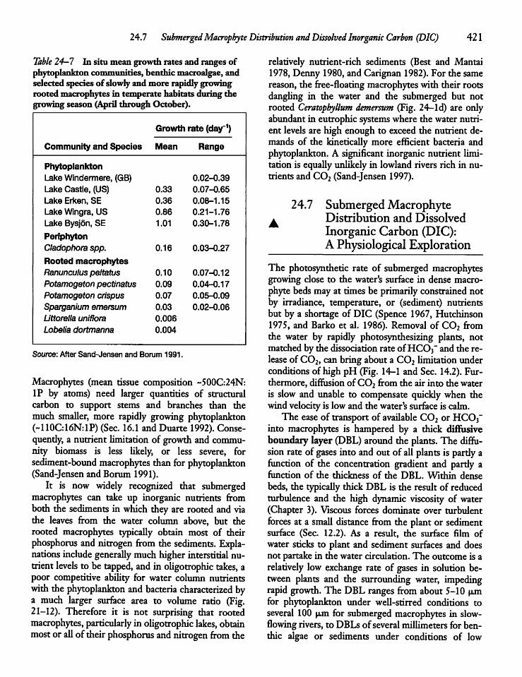
24.7 SubmergedMacrophyte Distribution and Dissolved Inorganic Carbon (DIC) 421
Table 24-1 In situ mean growth rates and rangesofphytoplankton communities, benthic macroalgae, andselected species ofslowly and more rapidly growingrooted macrophytes in temperate habitats during thegrowing season (April through October).
Growth rate (day-1)
Community and Species Mean Range
PhytoplanktonLake Windermere, (GB) 0.02-0.39
Lake Castle, (US) 0.33 0.07-0.65
Lake Erken, SE 0.36 0.08-1.15
Lake Wingra, US 0.86 0.21-1.76Lake Bysjon, SE 1.01 0.30-1.78
PeriphytonCladophora spp. 0.16 0.03-0.27
Rooted macrophytesRanunculus peltatus 0.10 0.07-0.12
Potamogeton pectinatus 0.09 0.04-0.17Potamogeton crispus 0.07 0.05-0.09
Sparganium emersum 0.03 0.02-O.06Littorella uniflora 0.006
Lobelia dortmanna 0.004
Source: After Sand-Jensen and Borum 1991.
Macrophytes (mean tissue composition -500G24N:IP by atoms) need larger quantities of structuralcarbon to support stems and branches than themuch smaller, more rapidly growing phytoplankton(~110C:16N:1P)(Sec. 16.1 and Duarte 1992).Conse-quendy, a nutrient limitation of growth and community biomass is less likely, or less severe, forsediment-bound macrophytes than for phytoplankton(Sand-Jensen and Borum 1991).It is now widely recognized that submerged
macrophytes can take up inorganic nutrients fromboth the sediments in which theyare rooted and viathe leaves from the water column above, but therooted macrophytes typically obtain most of theirphosphorus and nitrogen from the sediments. Explanations include generally muchhigherinterstitial nutrientlevels to be tapped, andin oUgotrophic takes, apoor competitive ability for water column nutrientswith thephytoplankton and bacteria characterized bya much larger surface area to volume ratio (Fig.21-12). Therefore it is not surprising that rootedmacrophytes, particularly in oUgotrophic lakes, obtainmost or all of theirphosphorus and nitrogen from the
relatively nutrient-rich sediments (Best and Mantai1978, Denny 1980, and Carignan 1982). For the samereason, the free-floating macrophytes with their rootsdangling in the water and the submerged but notrooted Ceratophyllum demersum (Fig. 24-1d) are onlyabundant in eutrophic systems where the water nutrient levels are high enough to exceed the nutrient demands of the kineticaUy more efficient bacteria andphytoplankton. A significant inorganic nutrient limitation is equaUy unlikely in lowland rivers rich in nutrients and C02 (Sand-Jensen 1997).
24.7 Submerged Macrophytea Distribution and Dissolved
Inorganic Carbon (DIC):A Physiological Exploration
The photosynthetic rate of submerged macrophytesgrowing close to the water's surface in dense macrophyte bedsmayat times be primarilyconstrained notby irradiance, temperature, or (sediment) nutrientsbut by a shortage of DIC (Spence 1967, Hutchinson1975, and Barko et al. 1986). Removal of C02 fromthe water by rapidly photosynthesizing plants, notmatched by the dissociationrate of HC03" and the release of C02, can bring about a C02 Umitation underconditions of high pH (Fig. 14-1 and Sec. 14.2). Furthermore, diffusionof C02 from the air into the wateris slow and unable to compensate quickly when thewindvelocity is lowand the water'ssurfaceis calm.The easeof transport of available C02 or HC03"
into macrophytes is hampered by a thick diffusiveboundary layer (DBL) around the plants. The diffusion rate of gases into and out of all plants is partly afunction of the concentration gradient and partly afunction of the thickness of the DBL. Within densebeds, the typicaUy thick DBL is the result of reducedturbulence and the high dynamic viscosity of water(Chapter 3). Viscous forces dominate over turbulentforces at a small distance from the plantor sedimentsurface (Sec. 12.2). As a result, the surface film ofwater sticks to plant and sediment surfaces and doesnot partake in the water circulation.The outcome is arelatively low exchange rate of gases in solution between plants and the surrounding water, impedingrapid growth. The DBL ranges from about 5-10 urnfor phytoplankton under weU-stirred conditions toseveral 100 p,m for submerged macrophytes in slow-flowing rivers, to DBLsofseveral millimeters for benthic algae or sediments under conditions of low
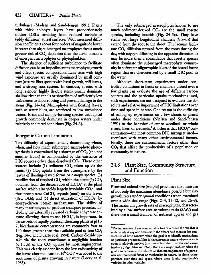
422 CHAPTER 24 Benthic Plants
turbulence (Madsen and Sand-Jensen 1991). Plantswith thick epiphyte layers have proportionatelythicker DBLs resulting from reduced turbulence(eddydiffusion) at leafsurfaces. With measured diffusioncoefficients aboutfourordersofmagnitude lowerinwater than air,submergedmacrophytes face amuchgreater risk of C02 depletion than the aerialportionsof emergentmacrophytes or phytoplankton.The absence of sufficient turbulence to facilitate
diffusion canbean impedimentto macrophyte growthand affect species composition. Lake sites with highwind exposure are usuaUy dominated by smaU compact(rosette-like) specieswithbasal growth, stiffleaves,and a strong root system. In contrast, species withlong, slender, highly flexible stems usually dominateshaUow river channelsor shorelinesof sufficiendylowturbulenceto aUow rooting andprevent damage to thestems (Fig. 24-3a).Macrophytes with floating leaves,such as water UUes, are restricted to low turbulencewaters. Erect and canopy-forming species with apicalgrowth commonly dominate in deeper waters underrelatively shelteredconditions (Fig.24-3).
Inorganic CarbonLimitationThe difficulty of experimentaUy determining where,when, and howmuch submerged macrophyte photosynthesis is constrained bya shortage ofC02 (and notanother factor) is compounded by the existence ofDIC sources other than dissolved C02. These othersources include (1) sediment C02 taken up via theroots; (2) C02 uptake from the atmosphere by theleaves of floating-leaved forms or canopyspecies; (3)reutiUzation of respiredC02 within the plant;(4)C02obtained from the dissociation of HC03" at the plantsurface which also yields largely insoluble C032~ andthus precipitates CaC03 crystals (marl) on the leaves(Sec. 14.6); and (5) direct utiUzation of HCOf byenergy-driven uptake mechanisms. The abiUty ofmany macrophytes to produce transport proteins, includingthe externaUy released carbonicanhydrase enzyme aUowing them to use HC03~, is important. Indensebedsof rapidlyphotosynthesizing plantsat pH >7, bicarbonate concentrations are commonly four to140 timesgreater than the available pool of free C02(Fig. 14-1andDuarteet al. 1994). Carbondioxide uptake via the roots contributes a negligible fraction(< 1.5%) of the C02 uptake by most angiosperms.This was clearly evident from the low radioactivity ofthe leaves after radiocarbon H14C03~wasaddedto theroot zone of plants growing in nature (Loczy et al.1983).
The only submerged macrophytes known to usemuch sediment-derived C02 are the small rosettespecies, including isoetids (Fig. 24-3a). They havestems with large longitudinal channels (lacunae) thatextend from the root to the shoot The lacunae faciU-tate C02 diffusion upward from the roots during theday, with oxygen diffusing in the oppositedirection. Itmay be more than a coincidence that rosette speciesoften dominate the submerged macrophyte community in softwateroUgotrophic lakesof the boreal forestregion that are characterized by a smaU DIC pool inthe water.Although short-term experiments under con-
troUed conditions in flasks or chambersplacedover afew plants can evaluate the use of different carbonsources and the particular uptake mechanisms used,suchexperiments are not designed to evaluate the absoluteand relative importanceofDIC limitations overtime and space in nature. One reason is the difficultyof scaling up experiments on a few shoots or plantsunder these conditions (Nielsen and Sand-Jensen1991) to the behavior of entire weedbeds or wholerivers, lakes, or wedands.3 Anotheris thatHC03" concentration—the most common DIC surrogate used—correlates with many other environmental factors.Finally, there are environmental factors other thanC02 that affect the productivity of a population orcommunity in nature.
24.8 Plant Size, Community Structure,and Function
Plant Size
Plant and animalsize(weight) provides a firstmeasureofnot onlythemaximum abundance possible but alsogrowth rates underoptimal conditions when examinedover a wide size range (Figs. 2-4, 21-12, and 26-8).The maximum growthrate ofmacrophytes, characterizedby a lowsurface area to volume ratio (SA:V) andtherefore a small number of nutrient uptake and gas
'The importance of environmental factors otherthantheonethatisunder studyatany onetime—with theothers held more orless constant—is of little concern when the goal is to identifymechanismsorparticular processes. Nor is it aconcern in nature whenever variation is relatively modestin allvariables other than the one examined (e.g., Figs. 24-6and 24-8). Butit isamajor problem when thegoal istodetermine therelative orabsolute importance ofaparticular environmental factor or mechanism in nature, let alone its importance over time and space, where there is also considerablevariation in other variables.
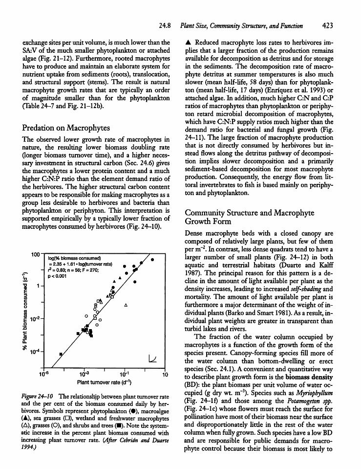
24.8 Plant Size, Community Structure, and Function 423
exchange sitesper unit volume, ismuchlowerthan theSA;V of the much smaUer phytoplanktonor attachedalgae (Fig. 21-12). Furthermore, rooted macrophyteshave to produce and maintain an elaborate systemfornutrient uptake from sediments (roots), translocation,and structural support (stems). The result is naturalmacrophyte growth rates that are typicaUy an orderof magnitude smaUer than for the phytoplankton(Table 24-7 and Fig. 21-12b).
Predationon MacrophytesThe observed lower growth rate of macrophytes innature, the resulting lower biomass doubling rate(longer biomass turnover time), and a higher necessary investment in structural carbon (Sec. 24.6) givesthe macrophytes a lower protein content and a muchhigher C:N:P ratio than the element demand ratio ofthe herbivores. The higher structural carbon contentappears to be responsible formakingmacrophytes asagroup less desirable to herbivores and bacteria thanphytoplankton or periphyton. This interpretation issupported empirically by a typically lower fraction ofmacrophytes consumed byherbivores (Fig. 24-10).
"8E
100"
1-
10-2-
10-4-
log(% biomass consumed)=2.35 +1.61 • log(turnover rate) # #r2= 0.83;n = 56;F = 270;p< 0.001
KT6 10"3 10"1Plant turnoverrate(d~1)
U
10
Figure 24-10 The relationship between plant turnover rateand the per cent of the biomass consumed daily by herbivores. Symbols represent phytoplankton (•), macroalgae(A), sea grasses (•), wedand and freshwater macrophytes(A), grasses (O),andshrubs and trees(•). Note the systematic increase in the percent plant biomass consumed withincreasing plant turnover rate. (After Cebridn and Duarte1994.)
• Reduced macrophyte loss rates to herbivores im-pUes that a larger fraction of the production remainsavailable for decomposition as detritus and for storagein the sediments. The decomposition rate of macrophyte detritus at summer temperatures is also muchslower (mean half-life, 58 days) than for phytoplankton (mean half-Ufe, 17 days) (Enriquez et al. 1993) orattached algae. In addition, muchhigher C:N andC:Pratiosofmacrophytes than phytoplanktonor periphyton retard microbial decomposition of macrophytes,whichhaveC:N:P supply ratios much higher than thedemand ratio for bacterial and fungal growth (Fig.24-11). The large fraction of macrophyte productionthat is not direcdy consumed by herbivores but instead flows along the detritus pathway of decomposition implies slower decomposition and a primarilysediment-based decomposition for most macrophyteproduction. Consequendy, the energy flow from Uttoral invertebrates to fish is basedmainlyon periphyton and phytoplankton.
Community Structure andMacrophyteGrowth Form
Dense macrophyte beds with a closed canopy arecomposed of relatively large plants, but few of themperm"2. In contrast, less dense quadrats tendto have alarger number of smaU plants (Fig. 24—12) in bothaquatic and terrestrial habitats (Duarte and Kalff1987). The principal reason for this pattern is a decline in the amount of Ught available per plant as thedensity increases, leading to increased self-shading andmortaUty. The amount of Ught available per plant isfurthermore a majordeterminantof the weightof individual plants(Barko and Smart 1981). Asa result, individual plantweights are greater in transparent thanturbid lakes and rivers.The fraction of the water column occupied by
macrophytes is a function of the growth form of thespecies present. Canopy-forming species fiU more ofthe water column than bottom-dwelling or erectspecies (Sec. 24.1). A convenientand quantitative wayto describe plant growth form is the biomass density(BD): the plant biomass per unit volume of water occupied (gdry wt. m"3). Species such as Myriophyllum(Fig. 24-1f) and those among the Potamogeton spp.(Fig. 24-1c) whose flowersmust reach the surface forpollination havemost of their biomassnear the surfaceand disproportionately Utde in the rest of the watercolumnwhen fuUy grown. Suchspecies have a lowBDand are responsible for public demands for macrophyte control because their biomass is mostUkely to
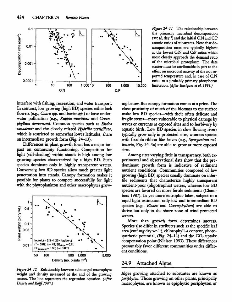
424 CHAPTER 24 Benthic Plants
0.0001
C:N
interfere withfishing, recreation, andwater transport.In contrast, lowgrowing (highBD)species either lackflowers (e.g., Chara spp. and Isoetesspp.) or have underwater pollination (e.g., Ruppia maritima and Cerato-pbyllum demersum). Common species such as Elodeacanadensis and the closely relatedHydrilla verticillata,whichis restricted to somewhatlower latitudes, sharean intermediate growthform(Fig. 24-13).Differences in plant growthformhas a majorim
pact on community functioning. Competition forUght (self-shading) within stands is high among lowgrowing species characterized by a high BD. Suchspecies dominate only in highly transparent waters.Conversely, lowBD species aUow muchgreater Ughtpenetration into stands. Canopy formation makes itpossible for plants to compete successfuUy for Ughtwith the phytoplankton andothermacrophytes grow-
1^ L% °-5 : :x- •£• • X .•o • \« •3 Ny# •
£ 0.1 r •:o> ^ •| 0.05 \ ^sw •
c • «N* •
OS •
Q. log(wt.) = 2.3 -1.25 • log(den.) .. •*1 •
0.01- r2 =0.67; n=43; SE^=0.11;SEirtercept =0-30; P<0.001 •
50 100 500 1,0001 1
5,0Density (no. plants m"2)
Figure 24-12 Relationship between submergedmacrophyteweight and density measured at the end of the growingseason. The line represents the regression equation. (AfterDuarte andKalff1981.)
1,000 10,000C:P
Figure 24-11 The relationship betweenthe primarily microbial decompositionrate(k, day-1) and theinitial C:Nand C:Patomic ratios of substrates. Note that decomposition rates are typicaUy highestat the lowest C:N and C:P ratios whichmost closely approach the demand ratioof the microbial protoplasm. The datascattermust be attributablein part to theeffect on microbial activity of the not reported temperature and, in case of C:Nratio, to a probablyprimaryphosphoruslimitation. (After Enriquez etal. 1993.)
ingbelow. Butcanopy formation comes at aprice. Theclose proximity ofmuch of the biomass to the surfacemake low BD species—with their often delicate andfragile stems—more vulnerable to physical damage bywaves or currentsat exposed sitesand to herbivory byaquatic birds. LowBDspecies in slow flowing riverstypicaUy grow onlyin protected sites, whereas specieswith flexible ribbon-like leaves (e.g., Sparganium val-lisneria, Fig. 24-3a) are able to grow at more exposedsites.Amongsitesvarying Utde in transparency, both ex
perimental and observational data showthat the predominant growth form is indicative of sedimentnutrient conditions. Communities composed of lowgrowing (high BD) speciesusuaUy dominate on infertile sediments that characterize highly transparentnutrient-poor (oUgotrophic) waters, whereas low BDspecies are favored on more fertile sediments (Chambers 1987). In yet more eutrophic lakes, subject to arapid Ught extinction, only low and intermediate BDspecies (e.g., Elodea and Ceratophyllum) are able tothrive but only in the shore zone of wind-protectedwaters.
More than growth form determines success.Speciesalso differ in attributes such as the specificleafarea (cm2 mgdrywt.-1), chlorophyU-/? content, photosynthetic potential, (Fig. 24-14) and the C02 uptakecompensationpoint (Nielsen 1993).These differencespresumablyfavor different communities under different conditions.
24.9 Attached Algae
Algae growing attached to substrates are known asperiphyton. Those growingon other plants, principaUymacrophytes, are known as epiphytic periphyton or
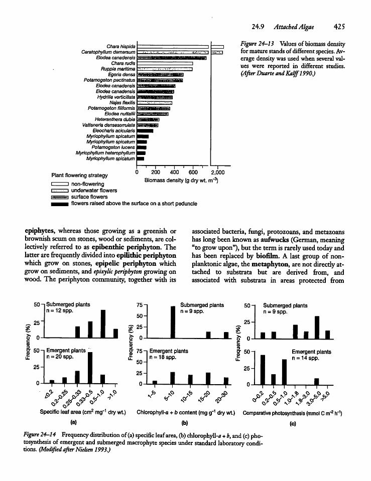
Chara hispidaCeratophyllum demersum
Elodea canadensisChara mdis
Ruppia maritimaEgeria densa
Potamogeton pectinatusElodea canadensisElodea canadensisHydrillaverticillata
Najas flexilisPotamogeton filifonmis
Elodea nuttalliiHeteranthera dubia
Vallisneria densesenvlataEleocharis acicularis
MyriophyllumspicatumMyriophyllumspicatumPotamogeton lucens
MyriophyllumheterophyllumMyriophyllum spicatum
.,*-..,- --. - •*,•.>.:•-T.il
• • ' • •'•• "•• m*-t~m
^a
"t—r
^•'
Plant flowering strategy' i non-flowering
200 400 600 2,000Biomassdensity (gdrywt. m"3)
c 3 underwater flowersei surface flowers• flowers raised above the surface on a short peduncle
24.9 AttachedAlgae 425
Figure 24-13 Values of biomass densityformaturestandsofdifferentspecies. Average densitywasused when several values were reported in different studies.(After Duarte andKalff1990.)
epiphytes, whereas those growing as a greenish orbrownish scum on stones, wood or sediments, are collectively referred to as epibentfaic periphyton. Thelatter arefrequendy divided intoepihthicperiphytonwhich grow on stones, epipelic periphyton whichgrowon sediments, and epixylicperiphyton growing onwood. The periphyton community, together with its
associated bacteria, fungi, protozoans, and metazoanshas longbeenknown asaufwucks (German, meaning"to grow upon"), but the term is rarelyused today andhas been replaced by biofilm. A last group of non-planktonic algae, the metaphyton, are not direcdy attached to substrata but are derived from, andassociated with substrata in areas protected from
50 -i Submerged plantsn = 12spp.
~ 25'
o 0
3
u§• 50-| Emergent plants
n = 20 spp.
L25-
*-+\u3J & o- v- v*VW
Specific leafarea (cm2 mg"1 drywt.)(a)
75-
50-
25-
fr 0cCD
g- 75-| Emergent plants50-
25-
0
Submerged plantsn = 9 spp.
1 L
n = 18spp.
I M i> F F $? J
c
|50U.
25-1
0
50- Submerged plantsn = 9 spp.
25-
II IIII
n- 1
uEmergent plantsn = 14spp.
i—r
Q* Q* V V **>•
*
Chlorophylls +b content (mg g-1 dry wt.) Comparative photosynthesis (mmol Cm'2 h"1)(b) (c)
Figure 24-14 Frequencydistribution of(a) specific leafarea, (b) chlorophyU-* +b, and (c) photosynthesis ofemergent and submerged macrophyte species under standard laboratory conditions. (ModifiedafterNielsen 1993.)
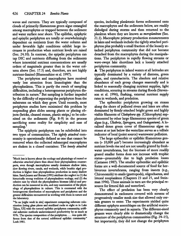
426 CHAPTER 24 Benthic Plants
waves and currents. They are typically composed ofclouds of primarily filamentous greenalgae entangledamong macrophytes or trapped between the sedimentandwater surface near shore.The epiUthic, epiphyticandepixyUc periphyton are totaUy or overwhelminglydependent on nutrients from the water column andunder favorable Ught conditions exhibit large increases in production when nutrient levels are raised(Sec. 24.10). In contrast, the epipeUc periphyton cantap DIC and nutrients diffusing from the sedimentswhere interstitial nutrient concentrations are usuaUyorders of magnitude greater than in the water column above (Sec. 17.5) and, therefore, are not highlynutrient-limited (Blumenshine et al. 1997).The periphyton and macrophytes have received
vasdy less attention from limnologists than thephytoplankton. This is partly the result of samplingdifficulties, including a heterogeneous periphyton distribution in nature.4 Butsampling is further impededbythe difficulty ofseparating the periphyton from thesubstrates on which they grow. Until recendy, mostperiphyton studies have minimized this problem bysuspending glass sUdes among plants or placing objects (bricks, cleaned stones, plastic strips,) to be colonized on the sediments (Fig. 8-9) in the processsacrificing some reaUty for simpUcity and ease ofsampling.5The epiphytic periphyton can be subdivided into
two types of communities. The tightly attached community is operationally defined as one that cannotberemoved when the coUected submergedmacrophytesare shaken in a closed container. The loosely attached
4Much less is knownaboutthe ecology andphysiology of rooted orotherwise attached plants than about their phytoplankton counterparts, even though macrophytes usually dominate shallow lakes,slow flowing rivers, canals, andwetlands, whilebenthic algal production is higher thanphytoplankton production in manyshallowlakes. Sand-Jensen andBorum(1991) attributethe neglectto (1)thehistorically strong tradition of phytoplankton ecology, and (2) therelative ease by which the phytoplankton biomass (chl-a) and productioncanbe measuredin situ, andeasyexamination of the physiology of phytoplankton in culture. This is contrasted with theheterogenous distribution of macrophytes and periphyton and thegreater difficulties encountered inworkingwiththemin nature andthe laboratory.5"In an [eight weekin situ] experiment comparing substrate colonization [using glass plates and sterilized rocksat eight m in LakeTahoe, US]with the natural epilithic periphyton community, artificial substratemethods underestimated productivityby asmuch as95%. The species composition of die periphyton was quite different from that of the natural sublittoral epilithic community."Loeb 1981.
species, including planktonic forms sedimented ontothemacrophytes and the sediments below, are readilydislodged during storms and then returned to theplankton where they are known asmeroplankton (Sec.21.1). Macrophyte primaryproduction measurementsin lakes andwetlands include the tighdyattached periphyton plus probably a small fraction ofthe loosely attached periphyton community that did not becomedetachedfrom the macrophytes during the manipulations. The periphyton in rapidly flowing streams orwave-swept lake shorelines lack a loosely attachedperiphytoncommunity.• The periphyton in inlandwaters at all latitudes aretypicaUy dominated by a variety of diatoms, greenalgae, and cyanobacteria. The absolute and relativeabundance of each group changes seasonaUy and islinked to seasonaUy changing nutrient supplies, Ughtconditions, scouring in streams duringfloods (Stevenson et al. 1996), flushing, external nutrient supplyrates in wedands,and predation.The epibenthic periphyton growing on stones
along the shore of poUuted rivers and lakes are oftendominated by firmlyattachedbright green and highlyvisible filaments of Cladophora spp. (Chlorophyta) supplemented byother largefilamentous species of greenalgae (e.g., Ulothrix, Spirogyra, andOedogonium). Alo-caUzed dense green cover of filamentous algae onstones at or justbelow thewaterline serves asa teUtaleindicatorof local (point source)wastewater pollution.The largeepibenthic or epiUthic filamentous gen
era (> 10,000 u.m3) become increasingly abundant asnutrient levels riseandare not usuaUy grazedbyfreshwater invertebrates, but the biomass of more readilygrazed smaUer forms does not increase with trophicstatus—presumably due to high predation losses(Cattaneo 1987). The smaUer epibenthic and epiUthicforms are a weU-documented source of food for herbivorous invertebrates, ranging from insects (e.g.,Chironomids) to snails (gastropods), oUgochaetes, andUttoral zooplankton (Chapters 23 and 25, and Stein-man 1996). These animalsin turn are the principal resource for Uttoral fish and waterfowl.The effect of predation has been very clearly
demonstrated in exclosures covered with screens ofprogressively smaUer meshsizethat aUowed onlycertain grazers to enter. The experiments yielded quitedifferent epiphyte assemblages on the artificial macrophytes commonly used in aquaria. The different-sizedgrazers were clearly able to dramaticaUy change thestructureof the periphyton communities (Fig. 24-15),but importandy, they did not change the periphyton
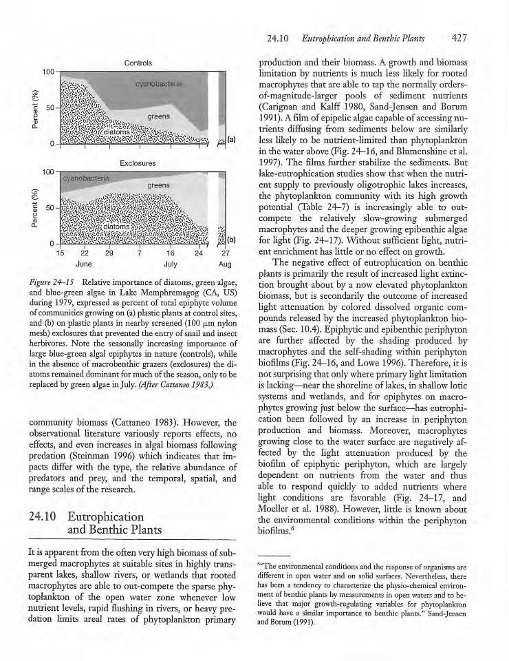
Controls100
W&SX& cyanobacteria
%
- vO~
greens
¥ p (a)
Figure 24—15 Relative importance of diatoms, green algae,and blue-green algae in Lake Memphremagog (CA, US)during 1979, expressed as percent of total epiphyte volumeof communitiesgrowing on (a)plastic plants at control sites,and (b) on plastic plants in nearby screened (100 \xm nylonmesh) exclosures that prevented the entry of snail and insectherbivores. Note the seasonally increasing importance oflarge blue-green algal epiphytes in nature (controls), whilein the absence of macrobenthic grazers (exclosures) the diatomsremained dominant for much of the season, only to bereplacedbygreen algae inJuly. (After Cattaneo 1983.)
community biomass (Cattaneo 1983). However, theobservational literature variously reports effects, noeffects, and even increases in algal biomass followingpredation (Steinman 1996) which indicates that impacts differ with the type, the relative abundance ofpredators and prey, and the temporal, spatial, andrange scalesof the research.
24.10 Eutrophicationand Benthic Plants
It is apparentfromthe oftenveryhigh biomass of submerged macrophytes at suitable sites in highly transparent lakes, shallow rivers, or wedands that rootedmacrophytes are able to out-compete the sparse phytoplankton of the open water zone whenever lownutrient levels, rapid flushing in rivers, or heavy predation limits areal rates of phytoplankton primary
24.10 Eutrophkation and Benthic Plants 427
production and their biomass. A growth and biomasslimitation by nutrients is much less likely for rootedmacrophytes that are able to tap the normally orders-of-magnitude-larger pools of sediment nutrients(Carignan and Kalff 1980, Sand-Jensen and Borum1991). A filmof epipelicalgaecapableof accessing nutrients diffusing from sediments below are similarlyless likely to be nutrient-limited than phytoplanktonin the water above (Fig. 24-16, and Blumenshine et al.1997). The films further stabilize the sediments. Butlake-eutrophicationstudies show that when the nutrient supply to previously oUgotrophic lakes increases,the phytoplankton community with its high growthpotential (Table 24-7) is increasingly able to out-compete the relatively slow-growing submergedmacrophytes and the deeper growing epibenthic algaefor light (Fig. 24-17).Without sufficient light, nutrient enrichment has little or no effect on growth.The negative effect of eutrophication on benthic
plants is primarily the result of increased light extinction brought about by a now elevated phytoplanktonbiomass, but is secondarily the outcome of increasedlight attenuation by colored dissolved organic compounds released by the increased phytoplankton biomass (Sec. 10.4). Epiphytic and epibenthic periphytonare further affected by the shading produced bymacrophytes and the self-shading within periphytonbiofilms (Fig. 24-16, and Lowe 1996).Therefore, it isnot surprising that onlywhereprimarylight limitationis lacking—near the shoreline of lakes, in shallow loticsystems and wedands, and for epiphytes on macrophytes growing just below the surface—has eutrophication been followed by an increase in periphytonproduction and biomass. Moreover, macrophytesgrowing close to the water surface are negatively affected by the light attenuation produced by thebiofilm of epiphytic periphyton, which are largelydependent on nutrients from the water and thusable to respond quickly to added nutrients wherelight conditions are favorable (Fig. 24-17, andMoeller et al. 1988). However, little is known aboutthe environmental conditions within the periphytonbiofilms.6
"The environmental conditions and the response of organisms aredifferent in open waterand on solid surfaces. Nevertheless, therehas been a tendency to characterize the physio-chemical environmentof benthic plants bymeasurements in openwaters andto believe that major growth-regulating variables for phytoplanktonwould have a similar importance to benthic plants." Sand-Jensenand Borum (1991).
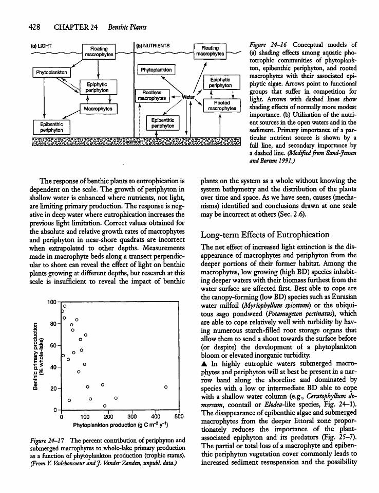
428 CHAPTER 24 Benthic Plants
(a) LIGHT
The responseofbenthicplants to eutrophicationisdependent on the scale. The growth of periphyton inshaUow water is enhancedwhere nutrients, not Ught,are limitingprimaryproduction. The response is negative in deepwaterwhereeutrophication increases theprevious Ught limitation. Correct values obtained forthe absolute and relative growth rates of macrophytesand periphyton in near-shore quadrats are incorrectwhen extrapolated to other depths. Measurementsmade in macrophyte bedsalong a transect perpendicular to shore can reveal the effectof Ught on benthicplants growing at different depths, but research at thisscale is insufficient to reveal the impact of benthic
100 200 300 400
Phytoplankton production (g C m"2 y"1)500
Figure 24-17 The percent contribution ofperiphyton andsubmerged macrophytes to whole-lake primary productionas a function of phytoplankton production (trophicstatus).(From Y. Vadeboncoeur andJ. Vander Zanden, unpubl. data.)
Figure 24-16 Conceptual models of(a) shading effects among aquatic phototrophic communities of phytoplankton, epibenthic periphyton, and rootedmacrophytes with their associated epiphytic algae. Arrows point to functionalgroups that suffer in competition forUght Arrows with dashed lines showshadingeffects of normallymore modestimportance, (b) Utilization of the nutrient sourcesin the openwatersand in thesediment. Primary importance of a particular nutrient source is shown by afull line, and secondary importance bya dashedUne. (Modifiedfrom Sand-Jensenand Borum1991.)
plants on the system as a whole without knowing thesystem bathymetry and the distribution of the plantsover time and space. As we have seen, causes (mechanisms) identified and conclusions drawn at one scalemaybe incorrect at others (Sec. 2.6).
Long-term Effects ofEutrophicationThe net effectof increased Ught extinction is the disappearance of macrophytes and periphyton from thedeeper portions of their former habitat. Among themacrophytes, lowgrowing (highBD)species inhabitingdeeper waters withtheir biomass furthest from thewater surface are affected first. Best able to cope arethecanopy-forming (low BD) species suchasEurasianwater milfoil (Myriophyllum spicatum) or the ubiquitous sago pondweed (Potamogeton pectinatus), whichare able to cope relatively weU with turbiditybyhaving numerous starch-filled root storage organs thatallow them to send a shoot towards the surface before(or despite) the development of a phytoplanktonbloomor elevated inorganic turbidity.• In highly eutrophic waters submerged macrophytes andperiphyton will at best be presentin a narrow band along the shoreline and dominated byspecies with a low or intermediate BD able to copewith a shallow water column (e.g., Ceratophyllum de-mersum, coontail or Ehdea-hke species, Fig. 24-1).The disappearance of epibenthic algae andsubmergedmacrophytes from the deeper littoral zone proportionately reduces the importance of the plant-associated epiphyton and its predators (Fig. 25-7).The partial or total loss of a macrophyte andepibenthic periphyton vegetation cover commonly leads toincreased sediment resuspension and the possibiUty
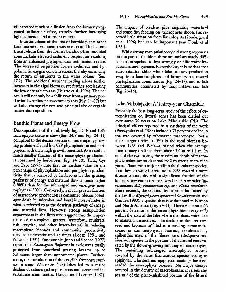
of increased nutrient diffusion fromthe formerly vegetated sediment surface, thereby further increasingUghtextinctionand nutrient release.Indirect effects of the loss of benthic plants other
than increased sediment resuspension and linked nutrient release from the former benthic plant-occupiedzone include elevated sediment respiration resultingfrom an enhanced phytoplankton sedimentation rate.The increased respiration lowers sediment and hy-polimnetic oxygen concentrations, therebyenhancingthe return of nutrients to the water column (Sec.17.2). The additional nutrient loading allows furtherincreases in the algal biomass, yet further acceleratingthe lossof benthic plants (Duarte et al. 1994). The netresultwiU not onlybe ashiftaway fromaprimary production bysediment-associated plants(Fig. 24-17) butwiU also change the rate and principal site of organicmatter decomposition.
BenthicPlants andEnergy FlowDecomposition of the relatively high C:P and C:Nmacrophyte tissue is slow (Sec. 24.8 and Fig. 24-11)compared to thedecomposition ofmorerapidly growingprotein-rich andlowC:Pphytoplankton andperiphyton with their highgrowthpotential. Asa result, amuch smaUer fraction of the macrophyte productionis consumed by herbivores (Fig. 24-10). Thus, Cyrand Pace (1993) note that the median value for thepercentage of phytoplankton and periphyton productivity that is removed by herbivores in the grazingpathway of energy andmaterial flow is much higher(~80%) than for the submerged and emergentmacrophytes (~30%). Conversely, a muchgreaterfractionofmacrophyte production is consumed (decomposed)after death by microbes and benthic invertebrates inwhatis referred to as the detritus pathwayof energyand material flow. However, strong manipulationexperiments in the Uterature suggest that the importance of macrophyte grazers (waterfowl, muskrats,fish, crayfish, and other invertebrates) in reducingmacrophyte biomass and community productivitymay be underestimated at times (Lodge 1991, andNewman 1991). For example, Jupp andSpence (1977)report thatPotamogeton filifbrmes in exclosures totaUyprotected from waterfowl grazing became up to5.3 times larger than unprotected plants. Furthermore, the introduction of the crayfish Orconectes rusti-cus in some Wisconsin (US) lakes led to a majordecline of submerged angiosperms and associated invertebrate communities (Lodge and Lorman 1987).
24.10 Eutrophication andBenthic Plants 429
The impact of resident plus migrating waterfowland some fish feeding on macrophyte shoots has received Utde attention from limnologists (Sendergaardet al. 1996) but can be important (van Donk et al1994).WhUe strongmanipulations yield strongresponses
on the part of the biota these are unfortunately difficult to extrapolate to less strongly or differendy impactednatural systems. Nevertheless, it is evidentthateutrophication shifts whole-lake primary productionaway from benthic plants and Uttoral zones towardphytoplankton communities (Fig. 24-17), and to fishcommunities dominated by zooplanktivorous fish(Fig. 26-16).
LakeMikolajskie: A Thirty-year ChronicleProbablythe best long-term studyof the effectof eutrophication on Uttoral zones has been carried outover some 30 years on Lake Mikolajskie (PL). Theprincipal effects reported in a synthesis of the work(Pieczyriska et al. 1988) include a 37percentdecline inthe area covered by submerged macrophytes, but amuch larger decline (90%) in the total biomass between 1963 and 1980—a period when the averagetransparency declined from about 3.0 m to 1.1 m. Inone of the twobasins, the maximum depth of macrophyte colonization declined by 2 m over a mere nineyears. There was amajor shiftin the dominant species,from low-growing Characeae in 1963 toward a morediverse community with a significant fraction of thebiomass nowcomposed of several species of taUer (intermediate BD)Potamogeton spp. andElodea canadensis.More recendy, the community became dominated bythe lowBDMyriophyllum spicatum (Kowalczewski andOzimek 1993), a species that iswidespread in Europeand North America (Fig. 24-1f). There wasalsoa 66percent decrease in the macrophyte biomass (g m~2)within the area of the lakewhere the plantswereableto maintain themselves. The decline in the area covered and biomass m~2 led to a striking summer increase in the periphyton biomass, dominated byepibenthic mats of the filamentous Cladophora andVaucheria species in the portion of the Uttoral zonevacated bytheslower-growing submerged macrophytes.The remaining submerged macrophytes becamecovered by the same filamentous species acting asepiphytes. The summer epiphyton coatings have exceeded the macrophyte biomass. No major changeoccured in the density of macrobenthic invertebratesper m~2 of the plant-inhabited portion of the littoral
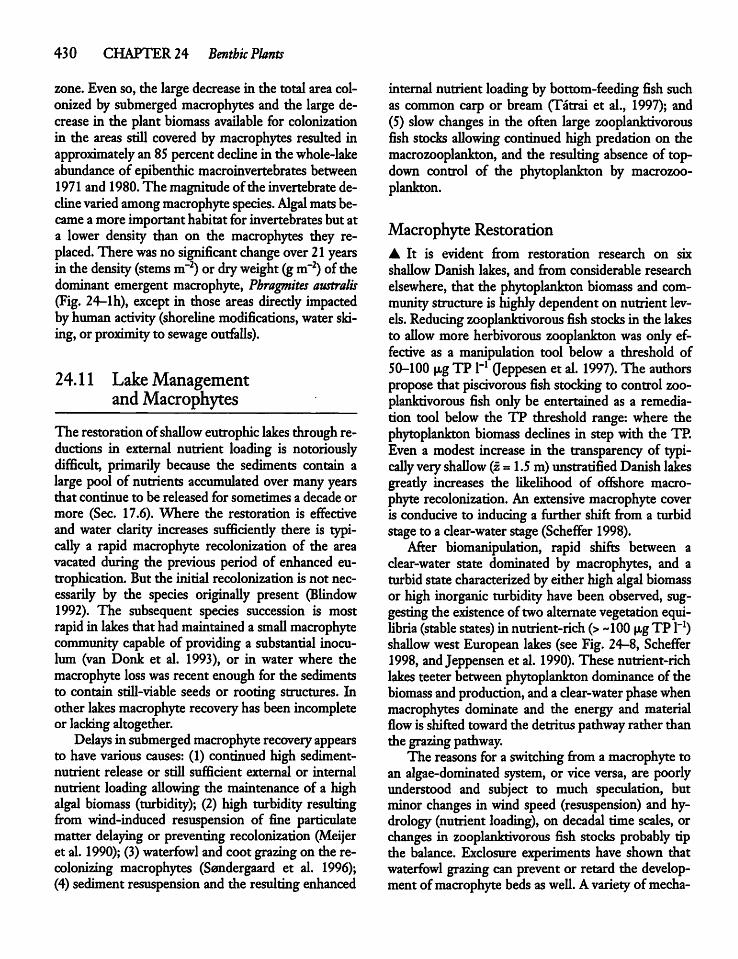
430 CHAPTER 24 Benthic Plants
zone.Even so, the large decrease in the total area colonized by submerged macrophytes and the large decrease in the plant biomass available for colonizationin the areas still covered by macrophytes resulted inapproximately an 85 percent declinein the whole-lakeabundance of epibenthicmacroinvertebrates between1971 and 1980.The magnitudeof the invertebratedeclinevariedamongmacrophyte species. Algal matsbecameamore important habitat for invertebratesbut ata lower density than on the macrophytes they replaced. There wasno significant changeover21yearsin thedensity (stems m~2) or dryweight (gm~2) ofthedominant emergent macrophyte, Pbragmites australis(Fig. 24-lh), except in those areas direcdy impactedby human activity(shoreline modifications, water skiing, or proximityto sewage outfalls).
24.11 LakeManagementandMacrophytes
The restoration ofshaUow eutrophic lakes throughreductions in external nutrient loading is notoriouslydifficult, primarily because the sediments contain alarge pool of nutrients accumulated over manyyearsthat continue to be released for sometimes a decade ormore (Sec. 17.6). Where the restoration is effectiveand water clarity increases sufficiendy there is typicaUy a rapid macrophyte recolonization of the areavacated during the previous period of enhanced eutrophication. But the initial recolonization is not necessarily by the species originaUy present (Blindow1992). The subsequent species succession is mostrapidin lakes that hadmaintained a small macrophytecommunitycapable of providing a substantial inoculum (van Donk et al. 1993), or in water where themacrophyte losswas recent enough for the sedimentsto contain stiU-viable seeds or rooting structures. Inother lakes macrophyterecoveryhas been incompleteor lackingaltogether.Delaysin submergedmacrophyte recoveryappears
to havevarious causes: (1) continued high sediment-nutrient release or still sufficient external or internalnutrient loading aUowing the maintenance of a highalgal biomass (turbidity); (2) high turbidity resultingfrom wind-induced resuspension of fine particulatematter delaying or preventing recolonization (Meijeret al. 1990); (3)waterfowl and coot grazing on the re-colonizing macrophytes (Sondergaard et al. 1996);(4) sediment resuspension and the resulting enhanced
internal nutrient loadingby bottom-feedingfish suchas common carp or bream (Tatrai et al., 1997); and(5) slow changes in the often large zooplanktivorousfish stocks aUowing continued high predation on themacrozooplankton, and the resulting absence of top-down control of the phytoplankton by macrozooplankton.
Macrophyte Restoration• It is evident from restoration research on sixshaUowDanish lakes, and from considerable researchelsewhere, that the phytoplankton biomass and communitystructure is highlydependent on nutrient levels.Reducingzooplanktivorous fish stocksin the lakesto aUow more herbivorous zooplankton was only effective as a manipulation tool below a threshold of50-100 p,g TP 1_1 Qeppesen et al. 1997). The authorspropose that piscivorous fish stocking to control zooplanktivorous fish only be entertained as a remediation tool below the TP threshold range: where thephytoplankton biomass declines in step with the TP.Even a modest increase in the transparency of typicaUy veryshaUow (z= 1.5m) unstratified Danishlakesgready increases the likelihood of offshore macrophyte recolonization. An extensive macrophyte coveris conducive to inducing a further shift from a turbidstageto a clear-water stage (Scheffer 1998).After biomanipulation, rapid shifts between a
clear-water state dominated by macrophytes, and aturbid state characterized by either high algalbiomassor high inorganic turbidity have been observed, suggestingthe existence of two alternatevegetationequi-Ubria (stable states) innutrient-rich (> "100u,gTP l-1)shaUow west European lakes (see Fig. 24-8, Scheffer1998, andJeppensen et al. 1990). These nutrient-richlakes teeter betweenphytoplankton dominance of thebiomass and production,and a clear-water phasewhenmacrophytes dominate and the energy and materialflowis shifted toward the detritus pathwayrather thanthe grazingpathway.The reasonsfor a switchingfrom a macrophyte to
an algae-dominated system, or vice versa, are poorlyunderstood and subject to much speculation, butminor changes in wind speed (resuspension) and hydrology (nutrient loading), on decadal time scales, orchanges in zooplanktivorous fish stocks probably tipthe balance. Exclosure experiments have shown thatwaterfowl grazingcan prevent or retard the development of macrophytebeds asweU. Avarietyof media-
nisms have been postulated as being responsible forenhanced waterclarityfoUowing the estabUshment ofmacrophytes (Sondergaard and Moss 1999). Amongthem are (1) increased sedimentation and lowered resuspension as the result of reduced turbulence inmacrophyte beds; (2) macrophyte shading of phytoplankton; (3) macrophyte release of compounds thatreduce phytoplankton growth (allelopathic compounds)',(4) sufficient uptake of nutrients by macrophytes andepiphytes to reducenutrient availabiUty to the phytoplankton; and (5) increased grazing by large pelagiczooplankton who use the macrophyte beds as a daytime refuge from fish predators (Fig. 23-27), supplemented by plant-associated Uttoral zooplankton (e.g.,chydorids). Enclosure experiments have shown thatthe projectedhigh zooplanktongrazingrates aremostplausible when the zooplanktivorous fishabundance ismodest (< 3m"2) and more than 20 percent of thewater volume is occupied (infested) by macrophyteswhichprovide a refuge for fish (Fig. 24-18). Howeverthe most plausible cause inevitably changes with thetimeand spatial scaleinvestigated (Sec. 2.6).The replacementof dense blooms of phytoplank
ton bydensebedsof canopy-formingmacrophytes is amixed blessing in aquatic management becausemacrophytes interfere with swimming, boating, andfishing. The particular trade-off is consideredworthexploring intensively in countries such as the Netherlands, Denmark, Poland, and parts of England where
-a
II
IOQ+
-Sc
4
1,800
1,200
600
20 40
Macrophytes (PVI) (%)60
24.11 LakeManagement andMacrophytes 431
the nonpointnutrient supply from agriculture is highenough that evenwhereurbanwastewater treatment isgood, shaUow lakesremain turbid. But the trade-off isnot acceptable in, for example, the south central andsouthern United States where hypertrophy is lesscommon, where the growing season is much longer(Fig.24-7), the plant biomass accumulation large andwhere there is Utde or no winter die-back. The plantcover in the typicaUy shaUow waterways there is sohigh to engenderdemands for macrophyte control. Incooler higher latitude western Europe, caUs formacrophyte control (byweedcutting)are primarilytoprevent die flooding that results when dense beds ofmacrophytes impede drainage in slowly flowing lowland streams and rivers, and to faciUtate water transport in canalsand rivers.
Macrophyte ControlThere are three basic approaches used, singly or incombination, for managing (controlling) aquaticweedproblems: mechanical harvesting and removal of submerged macrophytes, herbicide treatment, and biological control. A fourth method, used routinely insteep-sided fish ponds everywhere, is to add enoughfertilizers to maintainphytoplanktonbloomsthat produce a sufficiently high Ught extinction to preventmacrophyte development. However, the fertilizationapproach to macrophyte control is unsuitable in the
Figure 24-18 Biomass of the dominantpelagic cladocerans (Daphnia + Bosmina)versus the catch per unit effort (CPUE)of 0+ and 1+ roach and three-spinedsticklebacks, and fraction of water volume infested by macrophytes (PVI) inLake Stigsholm (SE, LA = 0.01 km2,z = 0.8 m). Enclosure experiments involved manipulation of plants (mainlyPotamogeton spp.) and fish density. Notethat a high macrozooplankton biomassoccured at an intermediate (> ~20%) tohigh PVI, but onlywhen the zooplanktivorous fish abundance was modest(AfterJeppesen etal. 1997.)
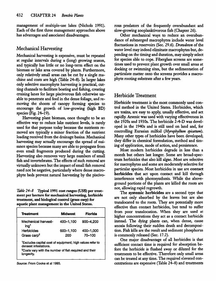
432 CHAPTER 24 Benthic Plants
management of multiple-use lakes (Nichols 1991).Eachof the first threemanagement approaches abovehasadvantages and associated disadvantages.
Mechanical HarvestingMechanical harvesting is expensive, must be repeatedat regular intervals during a (long) growing season,and typicaUy has Utde or no long-term effect on thebiomass or lake area covered by plants. Furthermore,onlyrelatively small areas can be cut by a single machineand costs are high (Table 24-8). In larger lakesonlyselective macrophyte harvesting is practical, cuttingchannels to facilitate boatingandfishing, creatingcruising lanes for largepiscivorous fish otherwise unableto penetrateandfeed in the dense foUage, andremoving the shoots of canopy forming species toencourage the growth of low-growing (high BD)species (Fig.24-19).Harvesting plant biomass, once thought to be an
effective way to reduce lake nutrient levels, is rarelyused for that purpose today because the nutrients removed are typicaUy a minor fraction of the nutrientloadingreceived from the drainage basins. Mechanicalharvesting may actuaUy encourage the spread of nuisancespecies because manyare ableto propagate fromeven small fragments produced during the cutting.Harvesting also removes very large numbers of smaUfish and invertebrates. The effects of such removal arevirtuaUyunknownbut the impactof smaU fish removalneed not be negative, particularlywhere densemacrophyte beds prevent natural harvestingby the piscivo-
Table 24-8 Typical 1991 cost ranges (US$)per treatment per hectare for mechanical harvesting, herbicidetreatment, and biological control (grass carp) foraquatic plant management in the United States.
Treatment Midwest Florida
Mechanical harvest- 400-1,100 900-4,200ing1
HerbicidesGrass carp2
600-1,100 400-1,000200 70-100
1Excludes capital cost of equipment; high values refer todensest infestations.
2Costs varywiththe number of fish required and theirlongevity.
Source: From Cooke et al 1993.
rous predators of the frequendy overabundant andslow-growing zooplanktivorous fish (Chapter26).Other mechanical ways to reduce an overabun
dance of submerged macrophytes include water levelfluctuations in reservoirs (Sec. 29.6).Drawdown of thewaterlevel mayindeedeliminate macrophytes but, dependingon the timingandduration,maysimplyselectfor species able to cope. Fiberglass screens are sometimesused to prevent plant growthoversmallareas atdocking or swimming sites, but the sedimentation ofparticulatematter onto the screensprovidesa macrophyte rooting substrateafter a fewyears.
Herbicide Treatment
Herbicide treatment is the most commonly used control method in the United States. Herbicides, whichare toxins, are easy to apply, usuaUy effective, and actrapidly. Arsenic wasusedwith varyingeffectiveness inthe 1920s and 1930s. The herbicide 2-4-D was developed in the 1940s and is stiU used on land and, forcontrolling Eurasian milfoil (Myrophyllum spicatum).Many other types of herbicideshave been developed;they differ in chemical formulation, method and timing of application, mode of action, and persistence.Most modern herbicides degrade in less than a
month but others last longer. Some are broad-spectrum herbicides that also kill algae.Most are selectiveformacrophytes and somearemoderatelyselective forparticular species. Most herbicides in use are contactherbicides that act upon contact and kill throughinterference with photosynthesis. While the above-ground portions of the plants are killed the roots arenot, aUowing rapid regrowth.The systemic herbicides are a second type that
are not only absorbed by the leaves but are alsotranslocated to the roots. They are potentiaUy moreeffective than contact herbicides, but tend to sufferfrom poor translocation. When they are used athigher concentrations they act as a contact herbicideinstead. The dying plants can, when dense, causeanoxia foUowing their sudden death and decomposition. Fish kills are the result and sediment phosphorusis commonly released (Sec. 17.2).One major disadvantage of aU herbicides is that
sufficient contact time is required for absorption before the herbicide is flushed away or diluted for thetreatments to be effective. Therefore only smaU areascanbe treated at any time.The required elevated concentrationsare expensive (Table 24-8) and treatments
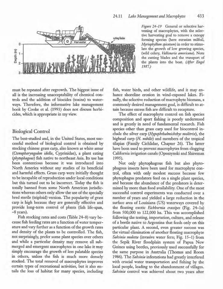
must be repeated after regrowth. The biggest issue ofall is the increasing unacceptability of chemical controls and the addition of biocides (toxins) to waterways. Therefore, the informative lake managementbook by Cooke et al. (1993) does not discuss herbicides, which is appropriate in my view.
Biological ControlThe best-studied and, in the United States, most successful method of biological control is obtained bystockingchinesegrasscarp, also known aswhite amur(Ctenopharyngodon idella, Cyprinidae), a plant eating(phytophagous) fish native to northeast Asia. Its use hasbeen contentious because it was introduced intoNorth America without any studies of its beneficialand harmful effects. Grass carp were initially thoughtto be incapable of reproduction under local conditionsbut this turned out to be incorrect. Today the fish istotally banned from some North American jurisdictionswhereas othersonlyallow the use of the speciallybred sterile (triploid) version. The popularity of grasscarp is high because they are generally effective andprovide long-term control of plants (fish life-span,~8years).Fishstocking rates andcosts (Table 24-8) vary be
cause fish feeding rates area function ofwater temperature and varyfurther as a function of the growth ratesand density of the plants to be controlled. The fish,not surprisingly, prefer some plant species over othersand while a particular density may remove all submerged and emergentmacrophytes in one lake it maysimply encourage the growth of less palatable speciesin others, unless the fish is much more denselystocked. The total removal of macrophytes improvescertain types of recreational activities, but it also entails the loss of habitat for many species, including
24.11 Lake Management andMacrophytes 433
Figure 24-19 General or selective harvesting of macrophytes, with the selective harvesting goal to remove a canopyforming species (here eurasian milfoil,Myriophyllum spicatum) in order to stimulate the growth of low growing species,(wild celery, Vallisneria americana). Notethe cutting blades and the transport ofthe plants into the boat. (After Engel1987.)
fish, water birds, and other wildlife, and it may enhance shoreline erosion in wind-exposed lakes. Finally, the selective reduction ofmacrophyte biomass, acommonly desired management goal, is difficult to attain because excess fish are difficult to recapture.The effect of macrophyte control on fish species
composition and sport fishing is poorly understoodand is gready in need of fundamental research. Fishspecies other than grass carp used for biocontrol include the silver carp (Hypophthalmichthys molitrix), thebighead carp (H. nobilis) and members of the tropicaltilapias (Family Cichlidae, Chapter 26). The latterhave been used to prevent macrophytes from cloggingCalifornia irrigation canals(Opuszynski and Shireman1995).Not only phytophagous fish but also phyto
phagous insects have been used for macrophyte control, often with only modest success because fewphytophagus predators feed on a single plant species,and because the abundance of the predators is determined bymore than food availability. One of the mostsuccessful control experiments was conducted over anumber of years and yielded a large reduction in thesurface area of Louisiana (US) waterways covered bythe floating exotic Eichhornia crassipes (Fig. 24—la)from 500,000 to 122,000 ha. This was accomplishedfollowing the testing, importation, culture, and releaseof a beedenative to Argentina that feeds onlyon thisparticular plant. A second, even greater success wasthe virtual elimination of another floating macrophyteSalvinia molesta (invasive water fern; Fig. 15-1) fromthe Sepik River floodplain system of Papua NewGuinea using beedes, previously used successfully forthe same purpose in Australia (Thomas and Room1986). The Salvinia infestations had gready interferedwith crucial water transportation and fishing by thelocal people, leading to the abandonment of villages.Salvinia control was achieved about two years after
434 CHAPTER 24 Benthic Plants
introduction of the beetle, which as adults feed onSalvinia buds whereas the larvae attack both buds andrhizomes.
Highlights• Large aquatic plants can be subdivided on the basisof habitat between the amphibious, emergent, free-floating, and submerged forms.
• Periphytonincludethe benthic algae associated withmacrophytesand those growing on sediment or rocksubstrates.
• A Emergent macrophytes extend from above theshoreline to a depth of roughly1-2 m,whilethe sub-mergent angiosperms extend down to a depth where~2-10 percent of the incoming irradiance (PAR) penetrates, unless the underwater slope is unsuitablysteep or the turbulence too great. Macroalgae andmosses extendmuchdeeper.
• Macrophytes and periphyton dominate the phytoplanktonin shaUow transparentwaterways where therooted macrophytes plus the periphyton growingonfine nutrient-rich sedimentsare able to tap sedimentnutrient concentrations much higher than thoseavailable to the phytoplankton. But in nutrient-richwaters the phytoplankton outcompete (shade) thebottom-Uving plants for Ught.
• GlobaUy, wedands cover an area about three timesthat of lakesand include the fringingUttoral zones ofrivers and lakes. The historicaUy extensive wedandshavebeen largelydrained for agriculturalpurposes indensely populated agricultural areas and thus are lostas (1) a cruciaUy important feeding, breeding, and
hiding area for fish and wildUfe and thus the maintenanceof high biodiversity, (2)for water purification;(3) waterstorageand flow regulation; and (4)a homefor fishermen and seasonal farmers, particularly inthe economicaUy developing world.• During periods of high photosynthesis, the photosynthetic rate of macrophytes may be constrainedby a slowdiffusion rate of dissolved inorganiccarbonfrom thewater into the plants.Macrophyte growth rates under optimal conditionsare typicaUy an order of magnitudesmaUer than forthe muchsmaUer phytoplankton and periphyton.A Macrophytes have a much higher structural carbon content for stems and therefore a lower proteinand nutrient (especiaUy P and N) content and lowerdesirabiUty to most herbivores and heterotrophicbacteriathan the phytoplanktonand periphyton.Eutrophication shifts whole lake primary productionaway from benthic plant and Uttoral zones towardphytoplankton communities and zooplanktivorousfish.A Macrophyte beds are an important refuge frompiscivorous fish for both young-of-the-year fish andsmaU fish species, and a partial refuge for macrozooplankton and benthic invertebrates from their fishpredators.A Dense beds of macrophytes interfere with riverdischarge, water transport, boating, and fishing, andalso prevent piscivorousfish from feeding efficiendyin the dense foUage. Three management approachesare mechanical harvesting, herbicide treatment, andbiological control using macrophyte-eating fish orinsect predators.
CHAPTER
25
Zoobenthos
25.1 Introduction
The zoobenthos is the animal community Uving inassociation with the substrate-water interface. Thefauna of the sedimentsurface, the epifauna, and thoseof the surficial sediments, the infauna, have been investigated best. In addition, there is diverse fauna associated with themacrophytic vegetation, the epiphyticfauna, and a second one, the hyporheic fauna, UvingweU below the substrate surface in the permeablegravel of rivers. The hyporheic fauna is part of a continuum that ranges from the fauna of the sediment-surface of lakes to the floodplain fauna of thegroundwater adjacent to manyloticsystems (Sec. 8.3).The zoobenthic community contains organisms
ranging in size from the poorly investigated protozoans to largeclams and crayfish. Nearly aU investigators have routinely used relatively coarse sieves (poresize 400-1,000 p,m, but mostcommonly 400-500 p,m)to separate the larger forms—the macrobenthos, includingmost insects—from soft sediment substrates.Theyuse a similar mesh size to coUect stream organisms removed from the substrate. The use of coarsesieves and nets faciUtates samplingand quantificationbut at the cost of gready underestimating themeiobenthos (< -400-100 p,m) which is composedprimarily of rotifers, copepods, young chironomids,smaU oUgochaetes, and nematodes. The microben-thos (< 100 urn)—composed of smaU species including protozoans and juveniles of larger forms—arecompletely overlooked. The oversight is not seriouswhen the biomass ofmacrobenthic animals consumedby fish and water birds is at issue (Sec. 25.5), but it is
very serious when density or species estimates areneeded (Fig. 25-1). Researchers working on MirrorLake(NewHampshire, US) noted that ofmore than amilUon individuals m~2, >98percent oftheindividualsand two-thirds of the typically smaU species wouldhave been overlooked if only the macrobenthos andmeiobenthos (there > 250 p,m) had been investigated(Strayer 1985).About half the animals were found inthe top centimeter. Unfortunately, the Uterature islargely based on themacrobenthos which hinders synthesis.1 Sieves are unsuitable for sampling the mega-benthos (> 1000 u,m), which includes crayfish andlarge bivalve moUuscs, that require different samplingtechniques.
Size and Energy FlowNormaUzed size spectra indicate that, similar toplankton, the biomass of unicellular (algae, protozoa)and multicellular (metazoan) benthic organisms areroughly equal in all the logarithmic sizeclasses examined (Fig. 25-2). This impUes that the metaboUsm ofthe benthos is gready underestimated by consideringonly organisms ofmacrobenthic size andweight. But
'"Iwould like tomake a plea for limnologists to choose their sievemesh sizes more carefully. Historically, the mesh sizes used havebeenhighlyvariable ... The reason... is that the 'ideal' meshsize(i.e.,one that retains the most animalsand the leastsediment)varieswiththe sediment type and the objectives of the study. Whilethisapproachhas been useful for individualscientists,it has also left thefield oflimnology with a body of'quantitative' data thatisvery difficultto interpret." (Strayer1985.)
435
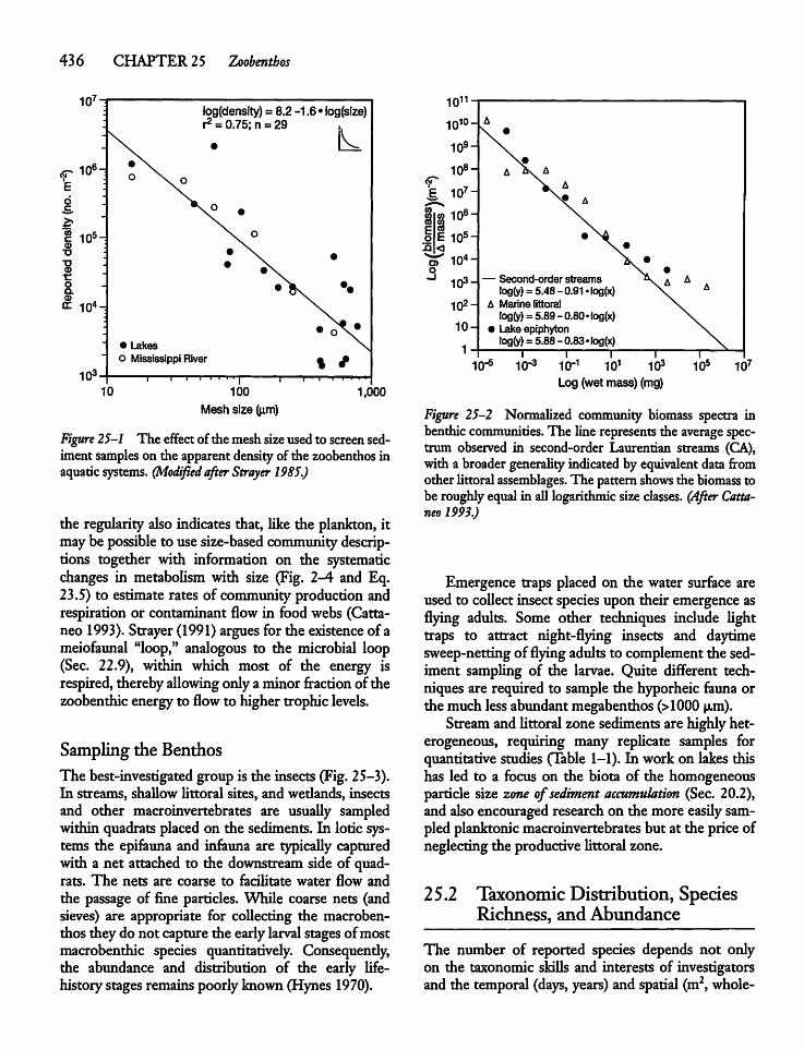
436 CHAPTER 25 Zoobenthos
107-
E
CDT3•aCD
oQ.CD
10<h
105-
104-
103-
log(denslty) = 8.2 -1.6 • log(size)r2= 0.75; n = 29 .
• LakesO Mississippi River % /
10I r
100
Mesh size (urn)1,000
F/gwre 25-1 The effect of themeshsizeusedto screensediment samples on the apparentdensityof the zoobenthos inaquaticsystems. (Modifiedafter Strayer 1985.)
the regularityalso indicates that, Uke the plankton, itmay be possible to usesize-based community descriptions together with information on the systematicchanges in metaboUsm with size (Fig. 2-4 and Eq.23.5) to estimate rates of communityproduction andrespiration or contaminant flow in food webs (Cattaneo 1993). Strayer (1991)argues for the existence of ameiofaunal "loop," analogous to the microbial loop(Sec. 22.9), within which most of the energy isrespired, therebyallowing onlyaminor fraction of thezoobenthic energyto flow to higher trophic levels.
Samplingthe BenthosThe best-investigated groupis the insects (Fig. 25-3).In streams, shaUow Uttoral sites, and wedands, insectsand other macroinvertebrates are usuaUy sampledwithin quadrats placedon the sediments. In lotic systems the epifauna and infauna are typicaUy capturedwith a net attached to the downstream side of quadrats. The nets are coarse to faciUtate water flow andthe passage of fine particles. WhUe coarse nets (andsieves) are appropriate for coUecting the macrobenthos they do not capture the early larvalstagesofmostmacrobenthic species quantitatively. Consequendy,the abundance and distribution of the early Ufe-history stages remainspoorly known (Hynes 1970).
10"1Log (wet mass) (mg)
Figure 25-2 Normalized community biomass spectra inbenthiccommunities. The line represents the average spectrum observed in second-order Laurentian streams (CA),with a broader generaUty indicatedby equivalent data fromother Uttoralassemblages. The pattern showsthe biomasstobe roughlyequalin all logarithmic sizeclasses. (After Cattaneo1993.)
Emergence traps placed on the water surface areused to coUect insect species upon their emergenceasflying adults. Some other techniques include Ughttraps to attract night-flying insects and daytimesweep-nettingof flyingadults to complement the sediment sampling of the larvae. Quite different techniques are required to sample the hyporheic fauna orthe much lessabundant megabenthos (>1000 u,m).Stream and Uttoralzone sediments are highly het
erogeneous, requiring many repUcate samples forquantitative studies (Table 1-1). In work on lakes thishas led to a focus on the biota of the homogeneousparticle size zone of sediment accumulation (Sec. 20.2),and also encouraged research on the more easUy sampledplanktonic macroinvertebrates but at the priceofneglectingthe productiveUttoral zone.
25.2 Taxonomic Distribution, SpeciesRichness, and Abundance
The number of reported species depends not onlyon the taxonomic skiUs and interests of investigatorsand the temporal (days, years) andspatial (m2, whole-
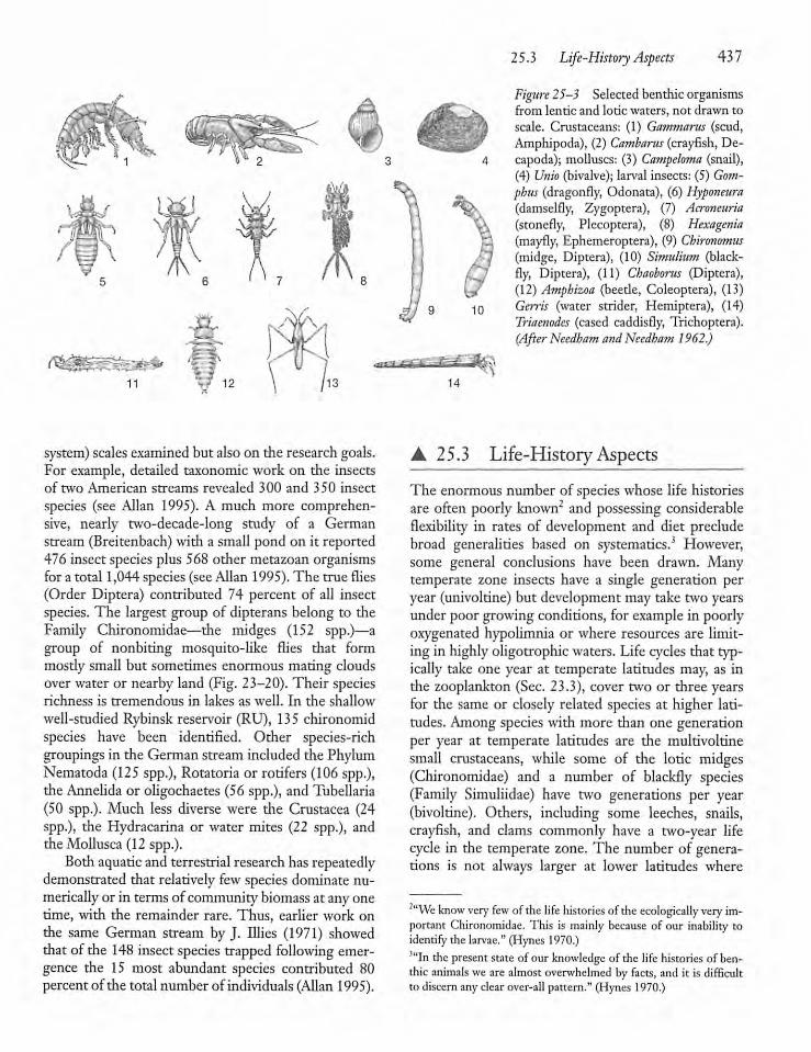
system) scales examined but alsoon the researchgoals.For example, detailed taxonomicwork on the insectsof two American streams revealed 300 and 350 insectspecies (see Allan 1995). A much more comprehensive, nearly two-decade-long study of a Germanstream (Breitenbach) with a small pond on it reported476 insect species plus 568 other metazoan organismsfor a total 1,044species (seeAllan 1995).The true flies(Order Diptera) contributed 74 percent of all insectspecies.The largest group of dipterans belong to theFamily Chironomidae—the midges (152 spp.)—agroup of nonbiting mosquito-like flies that formmosdy small but sometimes enormous mating cloudsover water or nearby land (Fig. 23-20). Their speciesrichness is tremendous in lakes as well. In the shallowwell-studied Rybinsk reservoir (RU), 135 chironomidspecies have been identified. Other species-richgroupingsin the German stream included the PhylumNematoda (125 spp.), Rotatoria or rotifers (106 spp.),the Annelida or oligochaetes (56 spp.), and Tubellaria(50 spp.). Much less diverse were the Crustacea (24spp.), the Hydracarina or water mites (22 spp.), andthe Mollusca (12 spp.).Bothaquatic and terrestrial research has repeatedly
demonstrated that relatively few species dominate numerically or in termsofcommunity biomass at anyonetime, with the remainder rare. Thus, earlier work onthe same German stream by J. lilies (1971) showedthat of the 148 insectspecies trapped following emergence the 15 most abundant species contributed 80percent of the total number of individuals(Allan1995).
25.3 Life-History Aspects 437
Figure 25-3 Selectedbenthic organismsfrom lentic and lotic waters, not drawn toscale. Crustaceans: (1) Gaitimarus (scud,Amphipoda), (2)Cambarus (crayfish, De-capoda);molluscs: (3) Campelama (snail),(4) Unto (bivalve); larval insects: (5) Gom-phus (dragonfly, Odonata), (6) Hyponeura(damselfly, Zygoptera), (7) Acroneuria(stonefly, Plecoptera), (8) Hexagenia(mayfly, Ephemeroptera), (9) Chironomus(midge, Diptera), (10) Simulium (black-fly, Diptera), (11) Chaoborus (Diptera),(12) Amphizoa (beede, Coleoptera), (13)Gerris (water strider, Hemiptera), (14)Triaenodes (cased caddisfly, Trichoptera).(After Needham andNeedham 1962.)
• 25.3 Life-History Aspects
The enormous number of species whose life historiesare often poorly known2 and possessing considerableflexibility in rates of development and diet precludebroad generalities based on systematics.3 However,some general conclusions have been drawn. Manytemperate zone insects have a single generation peryear (univoltine) but development may take two yearsunder poor growing conditions, for example in poorlyoxygenated hypolimnia or where resources are limiting in highlyoligotrophic waters. Life cycles that typically take one year at temperate latitudes may, as inthe zooplankton (Sec. 23.3), cover two or three yearsfor the same or closely related species at higher latitudes. Among species with more than one generationper year at temperate latitudes are the multivoltinesmall crustaceans, while some of the lotic midges(Chironomidae) and a number of blackfly species(Family Simuliidae) have two generations per year(bivoltine). Others, including some leeches, snails,crayfish, and clams commonly have a two-year lifecycle in the temperate zone. The number of generations is not always larger at lower latitudes where
2"We know very few ofthelife histories ofthe ecologically very important Chironomidae. This is mainly because of our inability toidentifydie larvae."(Hynes 1970.)'"In thepresent state ofourknowledge ofdie life histories of benthic animals we are almostoverwhelmed by facts, and it is difficultto discern anyclear over-allpattern." (Hynes 1970.)
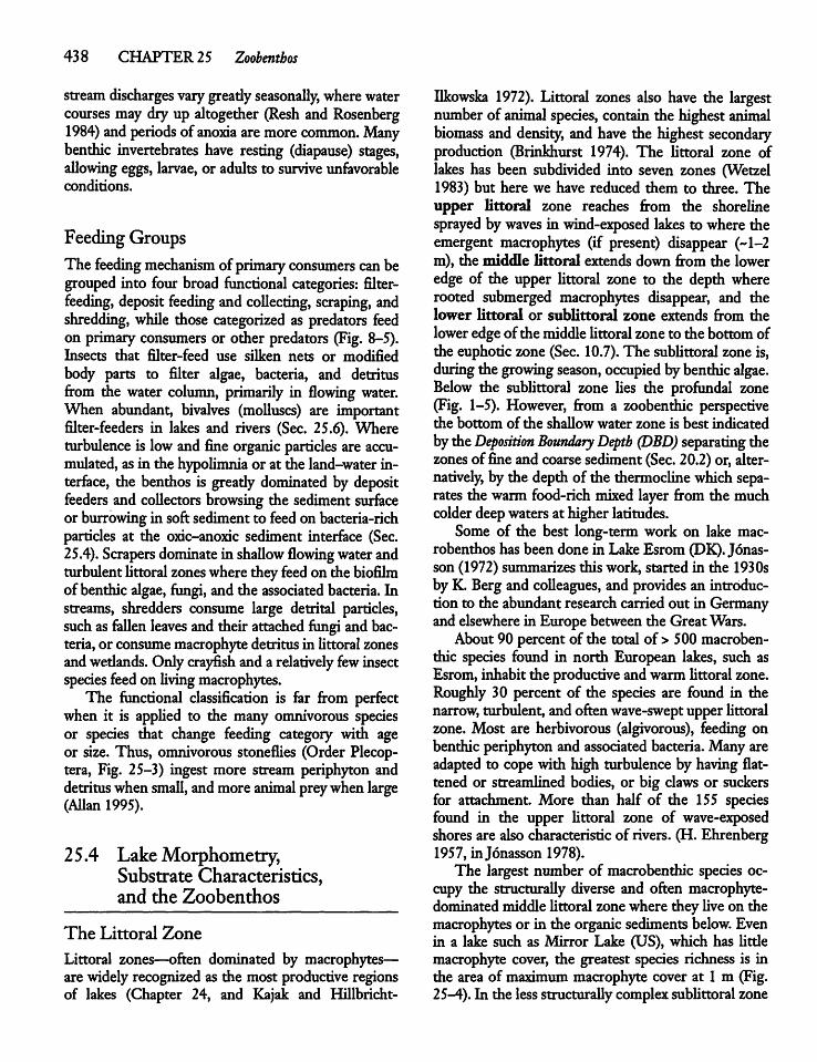
438 CHAPTER 25 Zoobenthos
streamdischarges varygreadyseasonaUy, wherewatercourses may dry up altogether (Resh and Rosenberg1984) andperiods of anoxia aremore common. Manybenthic invertebrates have resting (diapause) stages,aUowing eggs, larvae, or adults to survive unfavorableconditions.
Feeding GroupsThe feeding mechanism ofprimary consumers can begrouped into four broad functional categories: filter-feeding, deposit feeding and coUecting, scraping, andshredding, whUe those categorized as predators feedon primaryconsumers or other predators (Fig. 8-5).Insects that filter-feed use silken nets or modifiedbody parts to filter algae, bacteria, and detritusfrom the water column, primarily in flowing water.When abundant, bivalves (molluscs) are importantfilter-feeders in lakes and rivers (Sec. 25.6). Whereturbulence is lowand fine organic particles are accumulated,as in the hypoUmnia or at the land-water interface, the benthos is gready dominated by depositfeeders and coUectors browsing the sediment surfaceor burrowingin soft sediment to feedon bacteria-richparticles at the oxic-anoxic sediment interface (Sec.25.4). Scrapers dominate in shallow flowing waterandturbulentUttoral zones where theyfeedon the biofilmof benthic algae, fungi, and the associated bacteria. Instreams, shredders consume large detrital particles,suchas fallen leaves and their attached fungi and bacteria,or consumemacrophytedetritus in Uttoral zonesandwedands. Only crayfish and a relatively few insectspecies feedon Uving macrophytes.The functional classification is far from perfect
when it is appUed to the many omnivorous speciesor species that change feeding category with ageor size. Thus, omnivorous stonefUes (Order Plecop-tera, Fig. 25-3) ingest more stream periphyton anddetrituswhen smaU, andmore animalpreywhen large(AUan1995).
25.4 LakeMorphometry,Substrate Characteristics,and the Zoobenthos
The Littoral Zone
Littoral zones—often dominated by macrophytes—are widely recognized as the most productive regionsof lakes (Chapter 24, and Kajak and Hillbricht-
Ilkowska 1972). Littoral zones also have the largestnumber of animal species, contain the highest animalbiomass and density, andhave the highest secondaryproduction (Brinkhurst 1974). The Uttoral zone oflakes has been subdivided into seven zones (Wetzel1983) but here we have reduced them to three. Theupper littoral zone reaches from the shorelinesprayed bywaves in wind-exposed lakes to where theemergent macrophytes (if present) disappear (-1-2m), the middle littoral extends down from the loweredge of the upper Uttoral zone to the depth whererooted submerged macrophytes disappear, and thelower littoral or subUttoral zone extends from thelower edgeof themiddle Uttoral zoneto the bottomofthe euphoriczone (Sec. 10.7). The subUttoral zone is,during the growing season, occupied bybenthic algae.Below the subUttoral zone Ues the profundal zone(Fig. 1-5). However, from a zoobenthic perspectivethe bottom of the shaUow water zone is best indicatedbytheDeposition Boundary Depth (DBD) separating thezones of fine and coarse sediment (Sec. 20.2) or, alternatively, by the depth of the thermocline which separates the warm food-richmixed layer from the muchcolderdeepwatersat higher latitudes.Some of the best long-term work on lake mac
robenthos has been done in Lake Esrom (DK).Jonas-son (1972) summarizes this work, started in the 1930sbyK. Bergand coUeagues, and provides an introduction to the abundant researchcarried out in Germanyandelsewhere in Europe betweenthe GreatWars.About 90 percent of the total of > 500macroben
thic species found in north European lakes, such asEsrom, inhabit the productive and warm Uttoralzone.Roughly 30 percent of the species are found in thenarrow, turbulent, and oftenwave-swept upper Uttoralzone. Most are herbivorous (algivorous), feeding onbenthic periphyton and associated bacteria.Many areadapted to cope with high turbulence by having flattened or streamlined bodies, or big claws or suckersfor attachment. More than half of the 155 speciesfound in the upper Uttoral zone of wave-exposedshores are also characteristic of rivers. (H. Ehrenberg1957, in Jonasson 1978).The largest number of macrobenthic species oc
cupy the structuraUy diverse and often macrophyte-dominatedmiddle Uttoralzonewhere they Uve on themacrophytesor in the organic sediments below. Evenin a lake such as Mirror Lake (US), which has Utdemacrophyte cover, the greatest species richness is inthe area of maximum macrophyte cover at 1 m (Fig.25-4). In the less structuraUycomplexsubUttoralzone
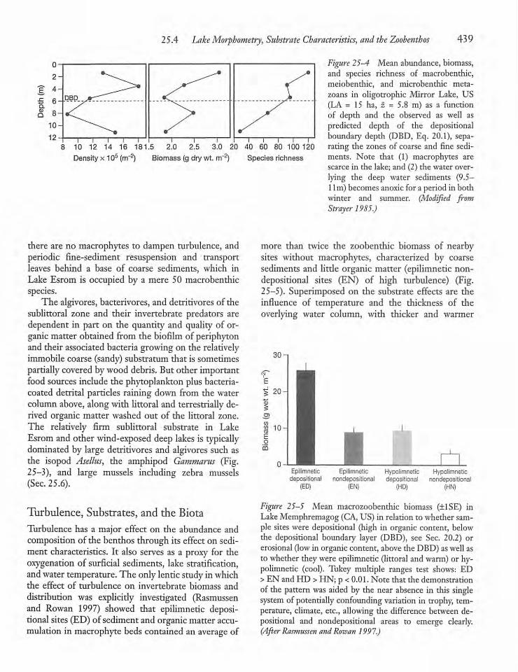
25.4 Lake Morphometry, Substrate Characteristics, andthe Zoobenthos 439
•5.01
Q
0
2
4-
6-
8-
10
12-
DBD
T"1610 12 14 16 181.5 2.0 2.5 3.0
Density x 105(rrf2) Biomass(gdrywt. rrf2
there are no macrophytes to dampen turbulence, andperiodic fine-sediment resuspension and transportleaves behind a base of coarse sediments, which inLake Esrom is occupied by a mere 50 macrobenthicspecies.The algivores, bacterivores, and detritivores of the
subUttoral zone and their invertebrate predators aredependent in part on the quantity and quality of organic matter obtained from the biofilm of periphytonand their associated bacteria growingon the relativelyimmobile coarse (sandy) substratum that is sometimespartially covered bywood debris. Butother importantfood sources include the phytoplankton plus bacteria-coated detrital particles raining down from the watercolumn above, alongwith littoral and terrestrially derived organic matter washed out of the littoral zone.The relatively firm sublittoral substrate in LakeEsromand other wind-exposed deep lakes is typicallydominated by large detritivores and algivores such asthe isopod Asellus, the amphipod Gammanis (Fig.25-3), and large mussels including zebra mussels(Sec. 25.6).
Turbulence, Substrates, and the BiotaTurbulence has a major effect on the abundance andcomposition of the benthos through its effecton sediment characteristics. It also serves as a proxy for theoxygenation of surficial sediments, lake stratification,and water temperature. The onlylentic study inwhichthe effect of turbulence on invertebrate biomass anddistribution was expUcidy investigated (Rasmussenand Rowan 1997) showed that epilimnetic depositional sites (ED)of sedimentand organicmatter accumulation in macrophyte beds contained an average of
t I r20 40 60 80 100 120
Species richness
Figure 25-4 Meanabundance, biomass,and species richness of macrobenthic,meiobendiic, and microbendiic meta-zoans in oligotrophic Mirror Lake, US(LA = 15 ha, 2 = 5.8 m) as a functionof depdi and the observed as well aspredicted depth of the depositionalboundary depth (DBD, Eq. 20.1), separating the zones of coarse and fine sediments. Note that (1) macrophytes arescarce in the lake; and (2) die water overlying the deep water sediments (9.5-1lm) becomesanoxicfor a period in bothwinter and summer. (Modified fromStrayer 1985.)
more than twice the zoobenthic biomass of nearbysites without macrophytes, characterized by coarsesediments and little organic matter (epilimnetic non-depositional sites (EN) of high turbulence) (Fig.25-5). Superimposed on the substrate effects are theinfluence of temperature and the thickness of theoverlying water column, with thicker and warmer
30-,
% 20-
8 10-
Epilimnetic Epilimnetic Hypolimnetic Hypolimneticdepositional nondepositional depositional nondepositional
(ED) (EN) (HD) (HN)
Figure 25-5 Mean macrozoobenthic biomass (±1SE) inLakeMemphremagog (CA,US) in relation to whether sample sites were depositional (high in organic content, belowthe depositional boundary layer (DBD), see Sec. 20.2) orerosional (low in organic content, above the DBD) as well asto whether theywere epilimnetic (littoral andwarm) or hypolimnetic (cool). Tukey multiple ranges test shows: ED>EN and HD >HN; p < 0.01. Note that the demonstrationof the patternwas aided by the near absence in this singlesystem of potentially confounding variation in trophy, temperature, climate, etc., allowing the difference between depositional and nondepositional areas to emerge clearly.(After Rasmussen andRowan 1997.)
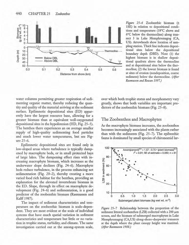
440 CHAPTER 25 Zoobenthos
0.1 0.2 0.3 0.4
Distance from shore (km)
water columns permitting greater respiration of sedi-menting organic matter, thereby reducing the quantity and qualityof the materialarrivingat the sedimentsurface. Epilimnetic depositional sites (ED) apparently have the largest resource base, allowing for agreater biomass than at equivalent well-oxygenateddepositional sites in die hypolimnion(HD, Fig. 25-5).The benthos there experiences an on average smallersupply of high-quality sedimenting food particlesand much lower water temperatures, but see Figure 25-6.Epilimnetic depositional sites are found only in
low-sloped areas where turbulence is typically dampened by macrophyte beds, or in small protected baysof large lakes. The dampening effect rises with increasing macrophyte biomass, which increases as theunderwater slope declines (Fig. 24—6). Macrophytebeds reduce turbulence, in the process enhancing netsedimentation (Fig. 20-2), diereby creating a morevaried food rich habitat for the bendios, providing anexplanation for the elevated invertebrate biomass inthe ED. Slope, through its effect on macrophyte development (Fig. 24-6) and sedimentation, is a goodpredictor of the zoobenthic biomass (Rasmussen andKalff 1987).The impact of sediment characteristics and tem
perature on the zoobenthic biomass is scale-dependent. They are most evident at the scale of individualsystems that have much spatial variation in sedimentcharacteristics and temperature but little or no variation in trophic status, turbidity, and climate. The sameinvestigation carried out at the among-system scale,
0.5 0.6
Figure 25-6 Zoobenthic biomass (±1SE) in relation to depositional conditions and temperature (18°C above and6°C below the thermocline) along transect 3 in Lake Memphremagog (CA,US). Arrowheads show location of samplingstation. Thicklineindicates depositional sites below the depositionalboundary depth (DBD). Note (1) thehighest biomass is in shallow depositional quadrats above the thermoclineand at depositional sites below the thermocline; (2) the lowest biomass is foundat sites of erosion (nondeposition, coarsesediment) below the thermocline. (AfterRasmussen andRowan 1997.)
overwhich both trophic status and morphometry varygready, shows that both variables are important predictors of the zoobenthic biomass (Fig. 25-8).
The Zoobenthos andMacrophytesAs the macrophyte biomass increases, the zoobenthosbecomes increasingly associatedwith the plants ratherthan with the sediments (Fig. 25-7). The epibenthicfauna is dominated by smallspecies of chironomid lar-
100-
10-
# Arcsin(percent) = 1.57 - 0.75 • (plant biomass)r2 = 0.91; SE of estimate = 0.082; n = 61
0.5 1.0 1.5 2.0 2.5 3.0
Submerged plant biomass (kg wet wt. rrf
Figure 25-7 Relationship between the proportion of thesediment littoral zoobenthos (LZB) collected with a 200 u,mscreen, and the biomass of submerged macrophytes in LakeMemphremagog (CA,US) along-shore-deepwater transectsat the depth where the plant canopy height was maximal.(After Rasmussen 1988.)
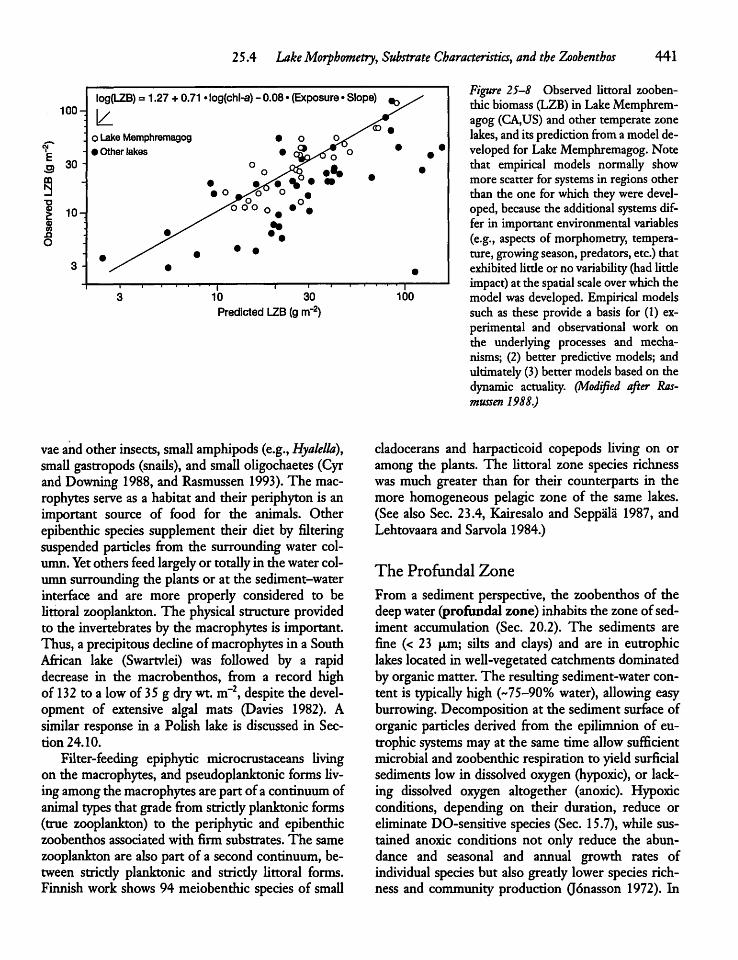
25.4 LakeMorphometry, Substrate Characteristics, andthe Zoobenthos 441
log(LZB)= 1.27 + 0.71 • log(chl-a) - 0.08 • (Exposure • Slope) ^/100- \^ s^d •
O Lake Memphremagog • o Of
% '• • Other lakes • SL"Oo o• •
•3 30-
9 "O QfT
• o «x^O o #
•J. ••
I io-^o oy^OO 0# • •
<DV) ^^ >nO
%s^ ••• s/' • # •
3 - • •
3' ' ' | I l
10 30
Predicted LZB (g rrf2)
' ' I100
Figure 25-8 Observed littoral zoobenthic biomass (LZB)in LakeMemphremagog (CA,US) and other temperate zonelakes, and itsprediction fromamodeldeveloped for LakeMemphremagog.Notethat empirical models normally showmore scatter for systems in regions otherthan the one for which they were developed, because the additional systems differ in important environmentalvariables(e.g., aspects of morphometry, temperature, growingseason,predators, etc.) thatexhibitedlittle or no variability (hadUtdeimpact)at the spatialscaleoverwhichthemodel was developed. Empiricalmodelssuch as these provide a basis for (1) experimental and observational work onthe underlying processes and mechanisms; (2) better predictive models; andultimately (3)better models based on thedynamic actuality. (Modified after Rasmussen 1988.)
vaeand other insects, smallamphipods (e.g., Hyalella),small gastropods (snails), and small oligochaetes (CyrandDowning 1988, and Rasmussen 1993). The macrophytes serve as a habitat and their periphyton is animportant source of food for the animals. Otherepibenthic species supplement their diet by filteringsuspended particles from the surroundingwater column. Yet othersfeed largely or totallyin thewatercolumn surroundingthe plants or at the sediment-waterinterface and are more properly considered to belittoral zooplankton. The physical structure providedto the invertebrates by the macrophytes is important.Thus, a precipitousdeclineof macrophytes in a SouthAfrican lake (Swartvlei) was followed by a rapiddecrease in the macrobenthos, from a record highof 132 to a low of 35 g drywt. m~2, despite the development of extensive algal mats (Davies 1982). Asimilar response in a Polish lake is discussed in Section 24.10.Filter-feeding epiphytic microcrustaceans Uving
on the macrophytes, and pseudoplanktonic forms Uving amongthe macrophytes are part of a continuumofanimal typesthat grade from stricdy planktonic forms(true zooplankton) to the periphytic and epibenthiczoobenthos associated with firm substrates. The samezooplankton are alsopart of a second continuum, between stricdy planktonic and stricdy Uttoral forms.Finnish work shows 94 meiobenthic species of smaU
cladocerans and harpacticoid copepods Uving on oramong the plants. The Uttoral zone species richnesswas much greater than for their counterparts in themore homogeneous pelagic zone of the same lakes.(See also Sec. 23.4, Kairesalo and Seppala 1987, andLehtovaara and Sarvola 1984.)
The Profundal Zone
From a sedimentperspective, the zoobenthos of thedeepwater (profundal zone) inhabits the zoneof sediment accumulation (Sec. 20.2). The sediments arefine (< 23 u-m; silts and clays) and are in eutrophiclakes located in well-vegetated catchments dominatedby organicmatter.The resulting sediment-watercontent is typicaUy high (~75-90% water), allowing easyburrowing. Decomposition at the sediment surface oforganic particles derived from the epilimnion of eutrophic systems mayat the same time allow sufficientmicrobialand zoobenthic respiration to yield surficialsediments low in dissolved oxygen (hypoxic), or lacking dissolved oxygen altogether (anoxic). Hypoxicconditions, depending on their duration, reduce oreliminate DO-sensitive species (Sec. 15.7),while sustained anoxic conditions not only reduce the abundance and seasonal and annual growth rates ofindividual species but also gready lower species richness and community production (Jonasson 1972). In
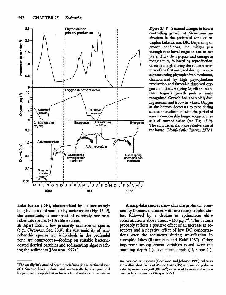
442 CHAPTER 25 Zoobenthos
1960 1961
I l l l l l l I I I I I I I I I I IMJJSONDJ FMAMJJASONDJFMAMJ
Lake Esrom (DK), characterized by an increasinglylengthy period ofsummer hypoxia/anoxia (Fig. 15-9),the community is composed of relatively few macrobenthic species (-20) able to cope.A Apart from a few primarily carnivorous species(e.g., Chaoborus, Sec. 23.9), the vast majority of macrobenthic species and individuals in the profundalzone are omnivorous—feeding on suitable bacteria-coated detrital particles and sedimentingalgaereaching the sediments (Jonasson 1972).4
*The usually little-studied benthicmeiofauna (intheprofundal zoneof a Swedish lake) is dominated numerically by cyclopoid andharpacticoid copepodsbut includesa fair abundanceof nematodes
1962
Figure 25-9 Seasonal changes in factorscontrolling growth of Cbironomus an-thracinus in the profundal zone of eutrophicLakeEsrom,DK. Dependingongrowth conditions, the midges passthrough four larval stages in one or twoyears. They then pupate and emerge asflying adults, foUowed by reproduction.Growth is high during the autumnoverturn of the firstyear, andduringthe subsequentspringphytoplankton maximum,characterized by high phytoplanktonproductionand favorable dissolved oxygen conditions.Aspring (April) and summer (August) growth peak is easilyrecognized. Growthdeclines rapidlyduring autumnand is lowin winter.Oxygenat the bottom decreases to zero duringsummerstratification, with the periodofanoxia considerably longer todayas a result of eutrophication (see Fig. 15-9).The silhouettes show the relative size ofthe larvae. (Modified afterJonasson 1978.)
Among-lake studiesshow that the profundalcommunity biomass increases with increasing trophic status, foUowed by a decline at epilimnetic chl-aconcentrations above about ~120 p,g l"1. The patternprobably reflects a positive effect of an increase in resources and a negative effect of low DO concentrations over the sediments during stratification ineutrophic lakes (Rasmussen and Kalff 1987). Otherimportant among-system variables noted were thesampling depth (-), lake mean depth (-), slope (-),
and ostracod crustaceans (Goedkoop and Johnson 1996),whereasthe well-studied fauna of Mirror Lake (US) is numericallydominated bynematodes (-680,000 m~2) in terms ofbiomass, andinproduction by chironomids (Strayer 1985.)
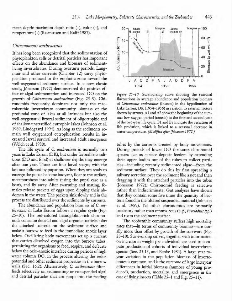
25.4 Lake Morphometry, Substrate Characteristics, and theZoobenthos 443
mean depth: maximum depth ratio (+), color (-), andtemperature (+) (Rasmussen and Kalff 1987).
Chironomous anthracinus
It has long been recognized that the sedimentation ofphytoplankton cellsor detrital particles has importanteffects on the abundance and biomass of sediment-living invertebrates. During overturn periods, Lang-muir and other currents (Chapter 12) carry phytoplankton produced in the euphotic zone toward thewell-oxygenated sediment surface. In a now classicstudy, Jonasson (1972) demonstrated the positive effect of algal sedimentation and increased DO on thegrowth of Chironomus anthracinus (Fig. 25-9). Chironomids frequendy dominate not only the macrobenthic invertebrate community biomass of theprofundal zone of lakes at all latitudes but also thewell-oxygenated littoral sediment of oligotrophic andof shallow unstratified eutrophic lakes (Johnson et al.1989, Lindegaard 1994). As long as the sediments remain well oxygenated eutrophication results in increased larval survival and increased adult emergence(Welch etal. 1988).The life cycle of C. anthracinus is normally two
years in Lake Esrom (DK), but under favorable conditions (DO and food) at shallower depths they emergeafter one year. There are four larval stages, with thelastone followed bypupation. When they are ready toemergethe pupaebecomebuoyant, float to the surface,metamorphose into adults (using the pupal case as aboat), and fly away. After swarming and mating, females release packets of eggs upon dipping their abdomenin the water. The packets sinkslowly and in theprocess are distributedover the sedimentsby currents.The abundance and population biomass of C. an
thracinus in Lake Esrom follows a regular cycle (Fig.25-10). The red-colored hemoglobin-rich chironomids consume detrital and algal organic particles plusthe attached bacteria on the sediment surface andmake a burrow to feed in the immediate anoxic layerbelow. Oscillating body movements set up a currentthat carries dissolved oxygen into the burrow tubes,permitting the organismsto feed, respire, and defecatebelow theoxic-anoxic interface during periods ofhighwater column DO, in the process altering the redoxpotential and other sediment properties in the burrowwalls (Sec. 16.2). Alternatively, C. anthracinus filter-feeds selectively on sedimenting or resuspended algaland detrital particles that are swept into the feeding
20 -i Autumn Emergence Autumn Emergence p100Al overturn Bl A2 overturn B2
>j~* j ,. '•—x • -80 ce'E 15" "&\
i
E
o
c6>
-60 tS-io- a5Q) 5O -40 mCO•D I5 5- N. co3.Q -20 E< Biomass o
CD
n nI I I I I i i i i i i i i i i i i I iiii
J A 0 D F A J A 0 D F A
1954 1955 1956
Figure 25-10 Survivorship curve showing the seasonalfluctuations in average abundance and population biomassof Chironomus anthracinus (Insecta) in the hypolimnion ofLake Esrom, DK (1954-1956) in relation to external factorsshownbyarrows.Al and A2show the beginning of the summer low-oxygen period (anoxia) in the first and second yearof the two-yearlife cycle. Bl and B2indicate the cessationoffish predation, which is linked to a seasonal decrease inwater temperature. (Modified afterJonasson 1972.)
tubes by the currents created by body movements.During periods of lower DO the same chironomidspecies acts as surface-deposit feeders by extendingtheir upper bodies out of the tubes to collect particles—including recendy sedimented algae—from thesediment surface. They do this by first spreading asalivarysecretion over the sediment like a net and thendragging it with the attached particles into the tubes(Jonasson 1972). Chironomid feeding is selectiverather than indiscriminate. Gut analyses have shownthat they contain some five times the quantity of bacteria found in the filtered suspendedmaterial (Johnsonet al. 1989). Yet other chironomids are primarilypredatoryrather than omnivorous (e.g., Procladius spp.)and roam the sediment surface.The zoobenthic community suffers high mortality
rates that—in terms of community biomass—are usually more than offset by growth of the survivors (Fig.25-10). Survivorship curves, together with informationon increase in weight per individual, are used to compute production of cohorts of individual invertebratespecies (Sec. 23.13, and Benke 1984). A largeyear-to-year variation in the population biomass of invertebrates iscommon, and istheoutcome oflarge interyeardifferences in initial biomass (number of young produced), production, mortality, and emergence in thecase offlying insects (Table 25-1 andFig.25-11).
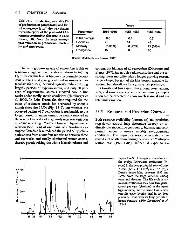
444 CHAPTER 25 Zoobenthos
Table 25-1 Production,mortality (%of production in parentheses) and larval emergence (gm~2 drywt.) duringthree life cycles of the profundal Chironomusanthracinus (Insecta) in LakeEsrom, DK. Note the large among-year variation in production, mortality, and emergence.
Parameter
Years
1954-1956 1956-1958 1958-1960
Initial biomassProductionMortalityEmergence
0.6
217 (33%)15
0.4
14
8 (57%)6
0.74122 (54%)20
Source: Modified from J6nasson 1972.
The hemoglobin-carrying C. anthracinus is able tomaintain a high aerobic metaboUsm down to 2-3 mg021"1, below this level it becomes increasingly dependent on the storedglycogen utilized in anaerobic metaboUsm (Sec. 15.7). Survival isgreatly reduced duringlengthyperiods of hypoxia/anoxia, and only 50 percent of experimental animals survived two to fiveweeks under totaUy anoxic conditions (Hamburger etal. 2000). In Lake Esrom the time required for theonset of sediment anoxia has decreased by about amonth since the 1950s (Fig. 15-9), but whether theobserved decline ofC. anthracinus is attributable to thelonger period of anoxia cannot be clearly resolved asthe resultof an order ofmagnitude interyearvariationin abundance (Fig. 25-11). However, hypolimneticaeration (Sec. 17.6) of one basin of a two-basin eutrophic Canadian lakereducedthe period of hypolimnetic anoxia from about four months to between threeand six weeks and totaUy eliminated winter anoxia,therebygready raisingthe whole-lake abundance and
community biomass of C. anthracinus (Dinsmore andPrepas 1997).An aerobic sediment surfaceand the resulting lower mortaUty, plus a longergrowing season,madea larger fraction of the lake bottom avaUable forfeeding, but alsoallows for a greaterfishpredation.Growth and loss rates differ amongyears, among
sites, and among species, and the community composition can be expected to showmuch seasonal and interannual variation.
25.5 Resource and Predation Control
Both resource avadabiUty (bottom-up) and predation(top-down) control help determine direcdy or indirecdythe zoobenthiccommunitybiomass and composition under otherwise suitable environmentalconditions. The impact of resource availabiUty received a lot ofattentionduringthe so-caUed "eutrophication era" (1970-1985). Influential experimental
'33 '35 '54
Figure 25-11 Changes in abundanceofthe midge Chironomus anthracinus (Insecta)in the deepprofundalzoneof LakeEsrom (LA = 17.3 km2, z = 13.5 m), aDanish ketde lake, between 1932 and1995. Note the large variation amongyears and decades. The life cycle is annual (univoltine) or mayhave two generations per year (bivoltine) in the upperhypolimnion, but the larvaehave a two-year life cycle (hemivoltine) in the deepprofundal zone with its long periods ofhypoxia/anoxia. (After Lindegaard et al.1997.)
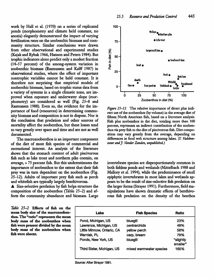
work by HaU et al. (1970) on a series of repUcatedponds (morphometry and climate held constant, noanoxia) elegandydemonstrated the impact of varyingfertilization rates on the zoobenthic biomass and community structure. Similar conclusions were drawnfrom other observational and experimental studies(Kajak andRybak 1966, Hanson and Peters 1984). Buttrophicindicators alonepredictonlyamodestfraction(14-57 percent) of the among-system variation inzoobenthic biomass (Rasmussen and Kalff 1987) inobservational studies, where the effect of importantnontrophic variables cannot be held constant. It istherefore not surprising that empirical models ofzoobenthicbiomass, basedon trophic status data froma variety of systems in a singleclimatic zone, are improved when exposure and underwater slope (morphometry) are considered as weU (Fig. 25-8 andRasmussen 1988). Even so, the evidence for the importance of food (resources) in determining community biomass and compositionis not in dispute. Nor isthe conclusion that predation and other sources ofmortalityaffect the zoobenthos, but these losses tendto varygreadyoverspaceand time and are not asweUdocumented.The macrozoobenthos is an important component
of the diet of most fish species of commercial andrecreational interest. An analysis of the Uteratureshows that the stomach content of adult piscivorousfish such as lake trout and northern pike contain, onaverage, > 75percentfish. But thisunderestimates theimportance of zoobenthos to the extent that their fishpreywas in turn dependent on the zoobenthos (Fig.25-12). Adults of important prey fish such as perchandwhitefish are typicaUy largelybenthivorous.A Size-selective predationby fishhelpsstructure thecomposition of the zoobenthos (Table 25-2) and affects the community abundance and biomass. Large
25.5 Resource and Predation Control 445
iuu-
Walleye,• Northern pike
75-• take trout
8 Lorgemoulti bass«
5 50-T3C • SmoBmouth bass.C0) Smeh •u.
25-
Rode bass
0- Gsco
Alnrifa•
•
•
Trout perch* Stickleback* • • 'KKnSculpin
T25
T7550 100
Zoobenthos in diet (%)
Figure 25-12 The relative importanceof direct plus indirect use of the zoobenthos (byvolume) in the averagediet offifteenNorth American fish, based on a Uterature analysis.Fish plus zoobenthos in die diet, totaling more than 100percent, represents an indirect contribution of the zoobenthos viaprey fish to the diet of piscivorousfish.Diet composition may vary gready from the average, depending ondifferences in foodweb structure among lakes. (Y. Vadebon-coeurandj. Vander Zanden, unpublished.)
invertebrate species are disproportionately commoninboth Ashless pondsandwedands(Mittelbach 1988 andMaUory et al. 1994), whUe the predominance of smaUepiphytic invertebrates in most lakes and wedands appears to be the result of size-selective fishpredation onthe largerforms (Strayer 1991). Furthermore, field manipulations have shown dramatic effects of benthivorous fish predation on the density of the benthos
Table 25-2 Effects of fish on themean body size of the macrozoobenthos. The "ratio" represents the meanbody mass of the zoobenthos whenfish were present divided by the meanbody mass of the zoobenthos whenfish were absent.
Lake Fish Species Ratio
Pond, Michigan, US bluegill 23%
Lawrence, Michigan, US centrarchids 49%Little Minnow, Ontario, CA yellow perch 58%Warniak, PL carp, bream 79%Ponds, New York, US bluegill "slightly
smaller"
Third Sister, Michigan, US mixed warmwater species 165%
Source: After Strayer 1991.
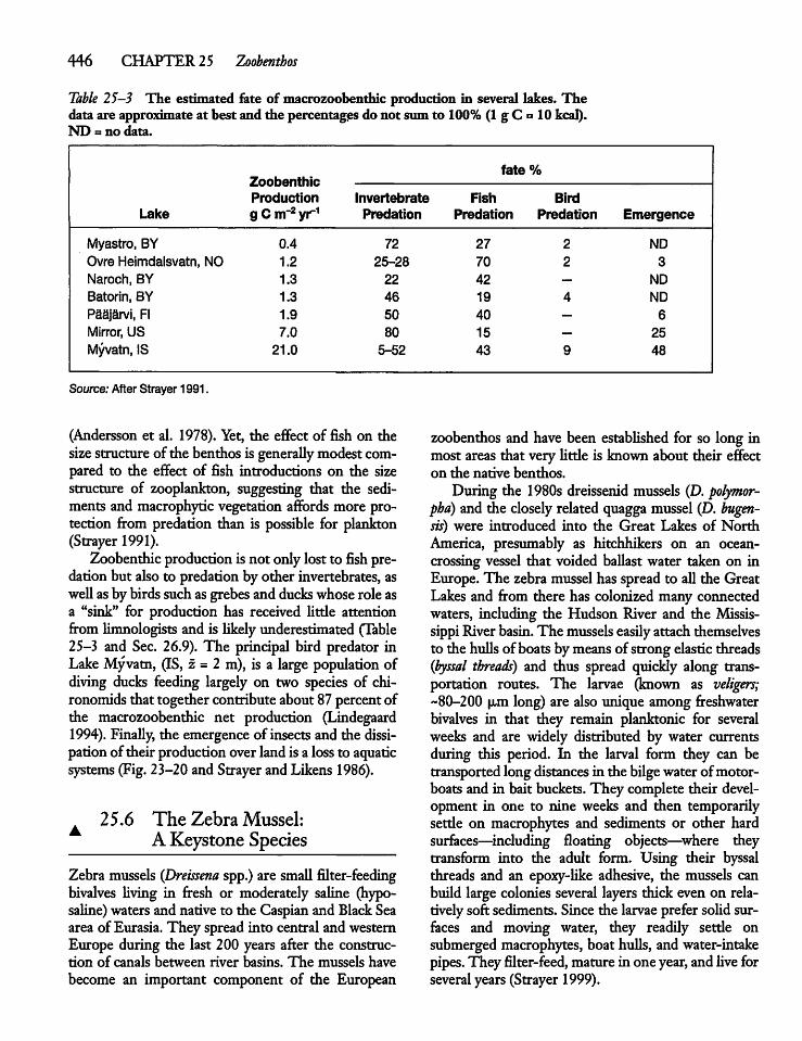
446 CHAPTER 25 Zoobenthos
Table 25-3 The estimated fate of macrozoobenthic production in several lakes. Thedata are approximate at best and the percentages do not sum to 100% (1 g C ° 10 kcal).ND = no data.
fate %Zoob&nthic
Production Invertebrate Fish BirdLake g C m"2yr1 Predation Predation Predation Emergence
Myastro, BY 0.4 72 27 2 ND
Ovre Heimdalsvatn, NO 1.2 25-28 70 2 3
Naroch, BY 1.3 22 42 — ND
Batorin, BY 1.3 46 19 4 ND
Paajarvi, Fl 1.9 50 40 — 6Mirror, US 7.0 80 15 — 25Myvatn, IS 21.0 5-52 43 9 48
Source: After Strayer 1991.
(Andersson et al. 1978). Yet, the effect of fish on thesize structure of the benthos is generaUymodestcompared to the effect of fish introductions on the sizestructure of zooplankton, suggesting that the sediments and macrophytic vegetation affords more protection from predation than is possible for plankton(Strayer 1991).Zoobenthic production is not onlylost to fish pre
dation but also to predation by other invertebrates, asweU asbybirdssuchasgrebesand ducks whoserole asa "sink" for production has received little attentionfrom Umnologists and is likelyunderestimated (Table25-3 and Sec. 26.9). The principal bird predator inLakeMyvatn, (IS, z = 2 m), is a large population ofdiving ducks feeding largely on two species of chironomids that together contributeabout 87percentofthe macrozoobenthic net production (Lindegaard1994). FinaUy, the emergence of insects and the dissipationof their productionoverlandis a lossto aquaticsystems (Fig.23-20 and Strayerand Likens 1986).
25.6 The Zebra Mussel:A Keystone Species
Zebra mussels (Dreissena spp.) are smaU filter-feedingbivalves Uving in fresh or moderately saline (hypo-saUne) waters and native to the Caspian and BlackSeaarea of Eurasia. They spread into central and westernEurope during the last 200 years after the construction of canals between river basins. The mussels havebecome an important component of the European
zoobenthos and have been estabUshed for so long inmost areas that very Utde is known about their effecton the native benthos.During the 1980s dreissenid mussels (D. polymor-
pba) and the closely related quagga mussel (D. bugen-sis)were introduced into the Great Lakes of NorthAmerica, presumably as hitchhikers on an ocean-crossing vessel that voided ballast water taken on inEurope. The zebramusselhas spread to aU the GreatLakes and from there has colonizedmany connectedwaters, including the Hudson River and the MississippiRiverbasin.The mussels easily attach themselvesto the huUs of boats bymeansof strong elasticthreads(byssal threads) and thus spread quickly along transportation routes. The larvae (known as veligers;~80-200 p,m long) are also unique among freshwaterbivalves in that they remain planktonic for severalweeks and are widely distributed by water currentsduring this period. In the larval form they can betransportedlong distances in the bilgewaterofmotor-boats and in bait buckets. They complete their development in one to nine weeks and then temporarilysettle on macrophytes and sediments or other hardsurfaces—including floating objects—where theytransform into the adult form. Using their byssalthreads and an epoxy-Uke adhesive, the mussels canbuild large colonies several layers thick even on relativelysoft sediments. Since the larvaeprefer solidsurfaces and moving water, they readily settle onsubmerged macrophytes, boat huUs, and water-intakepipes. They filter-feed, mature in oneyear,andUve forseveral years (Strayer1999).
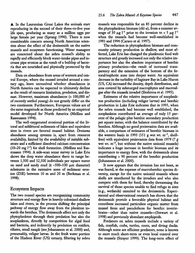
A In the Laurentian Great Lakes the animals startreproducing in the second of their three-to-five yearUfe span, producing as many as a miUion eggs perlarge female per year (Sprung 1990). There is nowconsiderable concern among North American scientists about the effect of the dreissenids on the nativemussels and ecosystem functioning. Water managersare concerned about the zebra mussel's abiUty torapidly and efficiendy blockwater-intake pipesand increase pipeerosion as the resultof a buildup of bacteria that are nourished and physically protected by themussels.
Data on abundance from areas ofwestern and central Europe, where the mussel invaded around a century ago, leave unresolved whether abundances inNorth America can be expected to ultimately declineasthe result of resourceUmitation, predation, and disease. However, maximum abundances (> 100,000 m2of recendysettled young)do not gready differon thetwo continents. Furthermore, European values are ofthe samemagnitudeas thosepredictedbyan empiricalmodel developed for North America (Mellina andRasmussen 1994).The well-oxygenated erosional portion of the Ut
toral and subUttoral sediments of lakesand equivalentsites in rivers are favored mussel habitat. Dreissenaabundance among systems is, apart from resourceavailabiUty, limited by the availability of suitable substrate and a sufficient dissolved calcium concentration(10-20 mg l"1) for shell formation. (Mellina and Rasmussen 1994).A side-scan sonar survey in Lake Erieshows the deep water abundance there to range between 1,500 and 32,500 individuals per square meteron sand and sandy mud (x -500-100 p,m diameter)substrates in the extensive zone of sediment erosion (ZSE) between 10 m and 20 m (Berkman et al.1998).
Ecosystem ImpactsThe twomussel species are reorganizing communitystructure and energy flowin heavilycolonizedshaUowlakes and rivers, in the process shifting the principalpathway of energy flow away from the plankton towards the benthos. The dreissenids affect not onlythephytoplankton through their predation but also thezooplankton, direcdy by competition for algal foodand bacteria, and indirecdyby predation on rotifers,ciliates, smallnaupU (seeJohannsson et al. 2000) and,presumably, veliger larvae. In the fresh water portionof the Hudson River (US) estuary, filtering by zebra
25.6 The ZebraMussel: A Keystone Species 447
mussels was responsible for an 85 percent decline inthe phytoplanktonbiomass (chl-a), from a summeraverage of 30 u,g l"1 prior to the invasion to < 5 p,g I"1when the mussels had become weU-established in1993 and 1994 (Caraco et al. 1997).The reductionin phytoplanktonbiomass and com
munity primary production in shaUow, and most affected, LakeErie has changedthe planktonic foodwebstructureandgreadyincreased not onlythe relative importance but also the absolute importance of benthicprimary production—the result of increased transparency and the extension of the bottom of the Ut-toral/euphotic zone into deeper water. An equivalentdecrease in the turbidityofSaginawBayin LakeHuron(US, CA)increased the density, depth distribution, andarea covered by submerged macrophytes and macroalgaeafter the mussels invaded (Skubinna et al. 1995).Estimates of the relative importance of zooplank
ton production (including veUger larvae) and benthicproduction in Lake Erie indicates that in 1993,whenthe zebra mussels had become weU established, thezooplankton contributed an average of only 15 percent of the pelagic plus benthic secondaryproductionper square meter, with the balance contributed by thebenthos.Althoughno good preinvasion data are avad-able, a comparison of estimates of benthic biomass inthe western basin in 1993 (351 g wet wt. m~2, sheU-free) with equivalent preinvasion data from 1979(7 gwet wt. m~2, but without the native unionid mussels)indicates a huge increase in benthic biomass and itsimportance to energy flow, with the dreissenids alonecontributing > 90 percent of the benthic production(Johannsson et al. 2000).It now appears that the invasion has not been, as
was feared, at the expense ofmacrobenthic species diversity, except for the native unionid mussels whosesheUs are smothered by the invaders and who alsocompete with them for food, thereby threatening thesurvival of those species unable to find refuge in sites(e.g., wedands) unsuited to the dreissenids. Experimental and observational research has shown that thedreissenids provide a favorable physical habitat andcontribute increased particulate organic matter frommussel feces and pseudofeces for benthic invertebrates—other than native mussels—(Stewart et al.1998) and previously abundant amphipods.Predators on zebra mussels include a variety of
fish, crayfish, crabs, turtles, coots, and diving ducks.Although some are efficientpredators, none is knownto exert much short-term or even local control overthe mussels (Strayer 1999). The long-term effect of
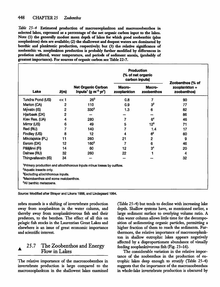
448 CHAPTER 25 Zoobenthos
Table 25-4 Estimated production of macrozooplankton and macrozoobenthos inselected lakes, expressed as a percentage of the net organic carbon input to the lakes.Note (1) the generallymodest mean depth of lakes for which good zoobenthic (pluszooplankton) dataare available; (2) the shaUowest anddeepestwatersare dominated bybenthic and planktonic production, respectively; but (3) the relative significance ofzoobenthicvs. zooplankton production is probablyfurther modified by differences inpredation suffered, water temperature, and periods of sediment anoxia, (probably ofgreatest importance). For sources oforganic carbon see Table 22-7.
Production(% of net organiccarbon inputs)
Zoobenthos (% ofNet Organic Carbon Macro Macro zooplankton +
Lake *(m) Inputs1 (g m~2yr1) zooplankton zoobenthos zoobenthos)
Tundra Pond (US) «1 263 0.8 7 90Marion (CA) 2 110 0.9 32 77Myvatn (IS) 2 3303 1.3 6 82
Hjarbaek (DK) 2 — — — 86Kiev Res. (UA) 4 280 7 64 46Mirror (US) 6 49 5 125 71Red (RU) 7 140 7 1.4 17Findley (US) 8 12 4 62 60Mikolajskie (PL) 11 260 21 2 9Esrom (DK) 12 1603 7 6 46Paajarvi (Fl) 14 60 12 34 20Dalnee (RU) 32 260 22 1 4Thingvallavatn (IS) 34 — — — 32
1Primary production and aUochthonous inputsminuslosses by outflow.2Aquatic insects only.3Excluding aUochthonous inputs."Macrobenthos and some meiobenthos.5AII benthic metazoans.
Source: Modified after Strayer and Likens 1986, and Lindegaard 1994.
zebramussels is a shifting of invertebrate productionaway from zooplankton in the water column, andthereby away from zooplanktivorous fish and theirpredators, to the benthos. The effect of aU this onpelagicfish stocks in the Laurentian Great Lakes andelsewhere is an issue of great economic importanceand scientific interest.
25.7 The Zoobenthos and EnergyFlow in Lakes
The relative importance of the macrozoobenthos ininvertebrate production is large compared to themacrozooplankton in the shallowest lakes examined
(Table 25-4) but tends to decline with increasing lakedepth. ShaUow systems have, as mentioned earlier, alarge sediment surface to overlying volume ratio. Athin water column aUows Utde time for the decomposition of sedimenting organic particles, permitting ahigher fraction of them to reach the sediments. Furthermore, the relative importance of macrozooplankton in shaUow eutrophic lakes appears negativelyaffected by a disproportionate abundance of visuaUyfeeding zooplanktivorous fish (Fig. 23-16).The considerable variation in the relative impor
tance of the zoobenthos in the production of eutrophic lakes deep enough to stratify (Table 25-4)suggests that the importanceof the macrozoobenthosin whole-lake invertebrate production is obscured by
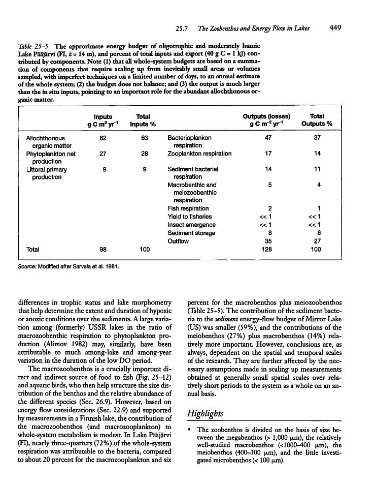
25.7 The Zoobenthos and Energy Flow inLakes 449
Table 25-5 The approximate energy budget of oUgotrophic and moderately humicLake Paajarvi (FI,z a 14m),and percent of total inputsand export(40g C =1kj) contributedbycomponents. Note (1)that aU whole-system budgets are based on a summation of components that require scaling up from inevitably smaU areas or volumessampled, with imperfecttechniqueson a limitednumber of days, to an annual estimateof the wholesystem; (2)the budget does not balance; and (3)die output is much largerthan the in situ inputs, pointing to an important role for die abundantaUochthonous organic matter.
Inputs Total Outputs (losses) Totalg C m2yr1 Inputs % g C m-2yr1 Outputs %
AUochthonous 62 63 Bacterioplankon 47 37
organic matter respirationPhytoplankton net 27 28 Zooplankton respiration 17 14
productionLittoral primary 9 9 Sediment bacterial 14 11
production respirationMacrobenthic and 5 4
meiozoobenthicrespiration
Fish respiration 2 1
Yield to fisheries «1 «1
Insect emergence «1 «1
Sediment storage 8 6
Outflow 35 27
Total 98 100 128 100
Source: Modified after Sarvala et al. 1981.
differences in trophic status and lake morphometrythat helpdeterminethe extentand duration of hypoxicor anoxic conditionsover thesediments. A largevariation among (formerly) USSR lakes in the ratio ofmacrozoobenthic respiration to phytoplankton production (Alimov 1982) may, similarly, have beenattributable to much among-lake and among-yearvariation in the duration of the lowDO period.The macrozoobenthos is a cruciaUy important di
rect and indirect source of food to fish (Fig. 25-12)and aquatic birds, who then help structure the size distribution of the benthos and the relative abundance ofthe different species (Sec. 26.9). However, based onenergy flow considerations (Sec. 22.9) and supportedbymeasurements in a Finnish lake, the contribution ofthe macrozoobenthos (and macrozooplankton) towhole-system metaboUsm is modest. In LakePaajarvi(FT), nearly three-quarters (72%) of the whole-systemrespiration was attributable to the bacteria, comparedto about 20 percent for the macrozooplankton and six
percent for the macrobenthos plus meiozoobenthos(Table 25-5). The contribution of the sediment bacteria to the sediment energy-flow budget ofMirror Lake(US) was smaUer (59%), and the contributions of themeiobenthos (27%) plus macrobenthos (14%) relatively more important. However, conclusions are, asalways, dependent on the spatial and temporal scalesof the research. They are further affected by the necessary assumptions made in scalingup measurementsobtained at generally smaU spatial scales over relativelyshort periods to the system as a whole on an annual basis.
Highlights
• The zoobenthos is divided on the basis of size between the megabenthos (> 1,000 u,m), the relativelyweU-studied macrobenthos (<1000-400 u,m), themeiobenthos (400-100 u,m), and the Utde investigated microbenthos (< 100 u,m).
450 CHAPTER 25 Zoobenthos
• The zoobenthos is numericaUy dominated by smaUspecies and is species-rich compared to the invertebrates of the openwater(zooplankton).
• Species richness, abundance, community biomass,and production is highest in the Uttoral zone—therichest in resources, best-oxygenated, and warmestportion ofaquatic systems—and is lowest in the profundal sediments ofdeeplakes.
• The structuraUy diverse macrophyte beds of wetlands, lakes, and rivers are important sites oforganicmatteraccumulation andprovide a largesurface areafor colonization by the zoobenthos and their prey;they also provide some protection from fish predators, and as a result they are characterized by thehighest zoobenthic biomass perunitarea and greatestspecies richness.
• Invertebrate and fish production (Ch. 26) is roughlypredictable from abundance data, weight per individual, and temperature; biomass serves as a relativelyeasily obtained indicator of population and community production.
• The among-system zoobenthic biomass andproduction increases with resource supply (trophic status),
butisreduced inwaters experiencing lengthy periodsof hypoxia/anoxia.
• • Macrozoobenthic net production is lost throughmortaUty, insect emergence, and predation by invertebrates, fish, and birds.
• • Zebra mussels, when abundant in rivers and shallow lakes, shiftwhole-system invertebrate productiontoward the sediments.
• A There is a tendency for the macrozoobenthos todominate themacrozoobenthos plus macrozooplankton biomass andproduction in shaUow systems, characterized bya smaUwatervolume to sedimentsurfacearea, and for macrozooplankton to dominate deepsystems. The pattern is weakened by variations inpredation, sediment anoxia, andinsectemergence.
• A The macrozoobenthos (and macrozooplankton)playa cruciaUy important direct and indirect role inthe production of fish and aquatic birds, which inturn help structure the macrozoobenthicsizedistribution and relative species abundance.
CHAPTER
26
Fish and Water Birds
26.1 Introduction
Fishplaya major role in aquatic systems and are alsoof great economic importance. They have receivedmuch attention, albeit largelyat the species level andtherefore independent of other fish species and theecosystem of which they are a component. There aretwo important reasons for the traditional isolation ofresearch on fishes from the rest of Umnology. First,the greater economic importanceof some fish has encouraged more research on the life history andpopulation dynamics of commerciaUy important species inisolation from their noncommercial counterparts andthe rest of limnology. The second reason is thevasdylarger size ofmostfishes relative to theplanktonic andbenthic animals of interest to other aquatic scientists.The greatersizeofmost fishes is associated withmuchgreater longevity, slower biomass doubling time (Fig.2-4), andmuchhigher mobiUty andrequires not onlydifferent sampling techniques but also study over different temporal scales (years to decades) and largerspatial scales (whole lakes plus their wedands and inflowing rivers) thanthe equivalent scales ofconcern tomostbiological Umnologists.The lackof attention given to water birdsismore
understandable because birds are not exclusivelyaquatic even if most or aU of their nutrition is obtainedfrom aquatic systems; they exert an important effecton the abundance and community structure ofmacroinvertebrates and fish.
Fish Research andLimnology
The earUest workon the taxonomy of fishes and theirdistribution evolved in thefirst halfofthe 19th centuryinto a broader-based studyof fishes and their biology.This form ofstudycame to beknown as ichthyology.It began with descriptive studies by zoologists of themorphology and Ufe historyof individual species, including their early development, growth, and feedinghabits. This focus graduaUy expanded to encompassresearch on fish physiology, diseases, culture, behavior,andpopulation biology. The earlyfundamental research by ichthyologists formed the basis for moreappUed research after evidence ofoverfishing of commercially important stocks in both inland and marinewaters became apparent in the late 19th and early 20thcenturies. The appUed research led to the development of a fisheries science that is concerned with themanagement of commerciaUy important stocks, defined asgroups of randomly mating individuals occupying the same spatial habitat. More specificaUy, it isconcerned with the impact of fishing on exploitedpopulations, the steps required to achieve and maintainoptimumyield, and the replenishment of depletedstocks through fish culture. Fisheries science is practiced primarily in government-sponsored agencies. InNorth America, it was long taughtin Schools or Departments of Fish and Game and Natural Resourcesprograms thatwere physicaUy and often conceptuaUyisolated from the fundamental science departments
451
452 CHAPTER 26 Fish and WaterBirds
(zoology and botany) that housed the limnologists(Magnuson 1991). With the development of ecology,including fish ecology, during the first 30or 40yearsof the 20th century, zoology departments sometimessupported a modest number offish ecologists.
Communication and coUaboration between thesethree groups of scientists has often been limited because the groups adhere to different scientific paradigms and typicaUy workat different temporal, spatial,andhierarchical scales (Sec. 2.6). Fishecologists tend toworkat the hierarchical scale of populations, focusingon population structure and interactions betweenspecies, primarily from an evolutionary perspective.Fisheries scientists emphasize organizationat the population level from an appUed rather than fundamentalperspective. FinaUy, biological limnologists studysmaUorganisms with doubling times ranging from hours toweeks; these organisms have typicaUy been examinedfrom a fundamental perspective over smaU spatial (ml,1, m2) and temporal (hours, days) scales (Figs. 1-1 and1-2).Nevertheless, most limnologists have—conceptually at least—placed their small-scale studies into alarger scale (ecosystem) perspective. AU three groupshave paid muchmoreattention to themoreeasUy sampledpelagic zone(open water) than the Uttoral zone oflakes, rivers, or wedands. The traditional separationbetween fishecology and fisheries science is becomingblurred now that an increasing number of ecologistsareworking on appUed problems. Yet someof the long-estabUshed isolation between fundamental and appUedaquatic science remains.A The International Association for Theoretical andAppUed Limnology (SIL) established in 1922 (Sec. 2.2)purposefuUy included the word "appUed" in its tide,but relatively few appUed scientists founda home in anorganization dominated bythosewithfundamental interests. Most hydrologists, water poUution biologists,fish ecologists, and virtuaUy aU fisheries scientistsjoined organizations that better represented their interests. Asa result,only10percent to 15percent of thepapers presented at the SDL congresses in the half-centuryfollowingWorldWarII have beenon fish (North-cote 1988). Anevenlowerfraction of articles pubUshedin the pre-eminentinternational journalLimnology andOceanography have been devoted to fish, and virtuaUyaU of those have addressed only one aspect—the top-downeffectoffish on lower trophic levels.Fish production and community structure are af
fected by the nutrient supply, something appreciatedfor centuriesby those involved with aquaculture. Duringthe last50years or so thishasalso beenrecognized
by fisheries scientists and those limnologists interestedin the effects of plant nutrients (resources) on fishyields (catches) and community production. Fish inturn directly affect the structure and energy flow atother trophic levels through their selective feeding onplants, invertebrates, andother fish. Fish indirecdyinfluence the abundance and composition of algal andbacterial communities through their predation onmacrozooplankton and benthic invertebrates, as weUas through nutrient recycling and transformation oforganicmatter (Sees. 23.7 and 25.5).
25.6 Fish Species andSpecies Richness
Fish SpeciesThe inlandwaters of the world contain nearly 11,000fish species. These can be divided into two groups orclasses: those with and those without jaws (a tiny fractionofthe species). The jawed fishes arefurtherdividedintospecieswithacartilaginous skeleton (thesharks andrays) andthose witha bonyskeleton (thevast majority).Among the bony fishes two subclasses are relevant tolimnologists: the lungfishes (Dipnoi) comprising onlyafew species, and the ray-finned fishes (Actinopterygii).The ray-finned fishes in turn aredominated bythe evo-lutionaiily advanced bony fishes, the (Teleostet) (Figs.26-1 and 26-2). The teleost fishes, which have a symmetrical tail and a gasbladder usedprimarily for buoyancy control, make up -94 percent of aU inland waterspecies. Among themthe carps (Order Cypriniformes)dominate with -3,000 species, foUowed by the catfishes(Order Siluriformes) with -1,950 species, and theperch-like species (Order Perciformes) with -950species. The latterinclude temperate zone perch asweUasthemanyspecies of lowlatitude richUds.The air-breathing lungfishes Uve in high tempera
ture, low latitude wedands that are likely to becomeperiodicaUy hypoxic or anoxic (Sec. 15.7). Some canevensurvive out of water in damphabitatswhileotherssurvive droughts byburrowing in damp sediments(Lowe-McConneU 1982). In contrast, many of theteleost fish respond behavioraUy to lowdissolved oxygen concentrations (< -4-7 mg l"1) by migration orlocal movements and die when DO declines belowspecies-specific minima (Sec. 15.7). However, a widevarietyof lowaltitude fishes havedeveloped anatomical and physiological adaptations that aUow them toutiUze (gulp) the air above the surface or use the thin(often only a few miUimeters thick) weU-oxygenated
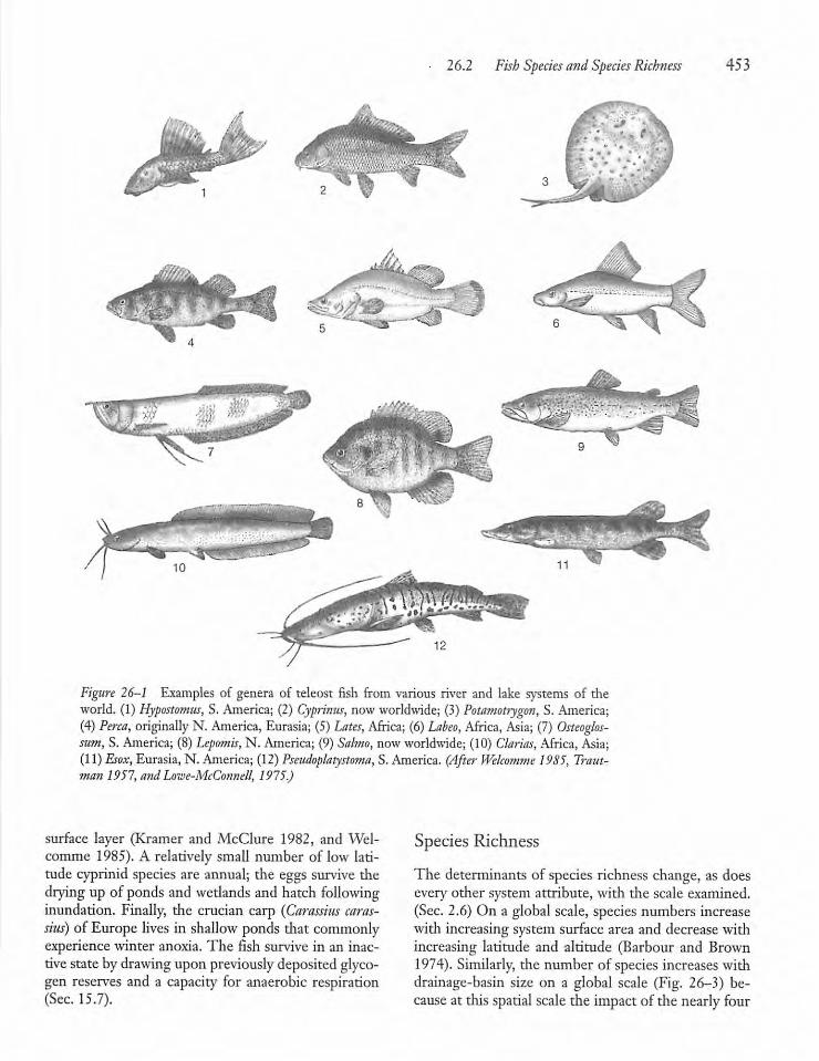
26.2 Fish Species and Species Rich?iess 453
Figure 26-1 Examples of genera of teleost fish from various river and lake systems of theworld. (1) Hypostomus, S.America; (2) Cyprinus, now worldwide; (3) Potamotiygon, S. America;(4) Perca, originally N. America, Eurasia; (5) hates, Africa; (6) Labeo, Africa, Asia; (7) Osteoglos-sum, S. America; (8) Lepomis, N. America; (9) Sahno, now worldwide; (10) Clarias, Africa, Asia;(11)Esox, Eurasia, N. America; (12)Pseudoplatystoma, S. America. (After Welcomme 1985, Trainman 1957, and Lowe-McConnell, 1975.)
surface layer (Kramer and McClure 1982, and Welcomme 1985). A relatively small number of low latitude cyprinid species are annual; the eggs survive diedrying up of ponds and wetlands and hatch followinginundation. Finally, the crucian carp (Carassius carassius) of Europe lives in shallow ponds that commonlyexperience winter anoxia. The fish survive in an inactive statebydrawing upon previously deposited glycogen reserves and a capacity for anaerobic respiration(Sec. 15.7).
Species Richness
The determinants of species richness change, as doesevery other system attribute, with the scale examined.(Sec. 2.6) On a global scale, species numbers increasewith increasingsystem surface area and decrease withincreasing latitude and altitude (Barbour and Brown1974). Similarly, the number of species increases withdrainage-basin size on a global scale (Fig. 26-3) because at this spatial scale the impactof the nearlyfour
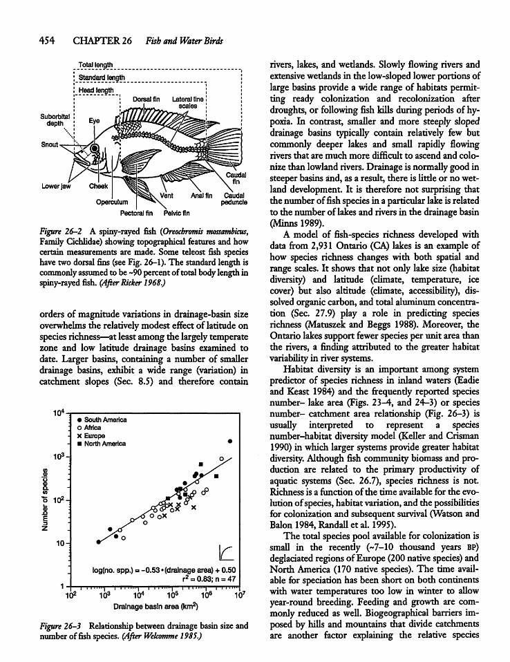
454 CHAPTER 26 Fish and Water Birds
Suborbitaldepth
Snout-
Lower jaw
TbtajlengthStandard length
Head length
Operculum
Pectoral fin Pelvic fin
Caudal
Anal fin Caudalpeduncle
Figure 26-2 A spiny-rayed fish (Oreocbromis mossambicus,FamilyCichlidae) showingtopographical features and howcertain measurements are made. Some teleost fish specieshave two dorsalfins (seeFig. 26-1). The standardlength iscommonly assumed to be -90 percentof total bodylengthinspiny-rayed fish. (AfterRicker 1968.)
orders of magnitudevariations in drainage-basin sizeoverwhelms the relatively modest effectof latitudeonspecies richness—at leastamongthe largelytemperatezone and low latitude drainage basins examined todate. Larger basins, containing a number of smaUerdrainage basins, exhibit a wide range (variation) incatchment slopes (Sec. 8.5) and therefore contain
104
103-
(0
"B 102_|
E3Z
icH
• South Americao AfricaX Europe• North America
tlog(no. spp.) = -0.53 • (drainage area) + 0.50
r2=0.83;n =47I i | i i i iiii'i—i i i iini| | i i iinij | i 11
162 103 104 io5 io6 ib7Drainage basinarea(km2)
Figure 26-3 Relationship between drainage basin size andnumber offish species. (After Welcomme 1985.)
rivers, lakes, and wedands. Slowly flowing rivers andextensive wedands in the low-sloped lowerportions oflargebasins provide a wide range of habitats permitting ready colonization and recolonization afterdroughts, or following fish kills during periods of hypoxia. In contrast, smaller and more steeply slopeddrainage basins typicaUy contain relatively few butcommonly deeper lakes and smaU rapidly flowingrivers that are much more difficult to ascend and colonize than lowland rivers. Drainageis normaUy good insteeper basinsand, as a result, there is Utdeor no wetland development. It is therefore not surprising thatthe number offish species in a particular lakeis relatedto the number of lakes and riversin thedrainagebasin(Minns 1989).A model of fish-species richness developed with
data from 2,931 Ontario (CA) lakes is an example ofhow species richness changes with both spatial andrange scales. It shows that not only lake size (habitatdiversity) and latitude (cUmate, temperature, icecover) but also altitude (climate, accessibiUty), dissolved organiccarbon, and total aluminumconcentration (Sec. 27.9) play a role in predicting speciesrichness (Matuszek and Beggs 1988). Moreover, theOntario lakessupport fewerspecies per unit area thanthe rivers, a finding attributed to the greater habitatvariabiUty in river systems.Habitat diversity is an important among system
predictor of species richness in inland waters (Eadieand Keast 1984) and the frequendy reported speciesnumber- lake area (Figs. 23-4, and 24-3) or speciesnumber- catchment area relationship (Fig. 26-3) isusuaUy interpreted to represent a speciesnumber-habitat diversity model (KeUer and Crisman1990) in which larger systems providegreater habitatdiversity. Althoughfish communitybiomass and production are related to the primary productivity ofaquatic systems (Sec. 26.7), species richness is not.Richness is a function of the time available for the evolution of species, habitat variation,and the possibiUtiesfor colonization and subsequent survival (WatsonandBalon 1984, RandaU et al. 1995).The total species pool available for colonization is
smaU in the recently (~7—10 thousand years BP)deglaciated regions ofEurope (200 native species) andNorth America (170 native species). The time available for speciation has been short on both continentswith water temperatures too low in winter to aUowyear-round breeding. Feeding and growth are commonly reduced as well. Biogeographical barriers imposed by hiUs and mountains that divide catchmentsare another factor explaining the relative species
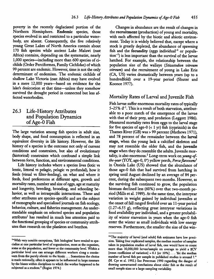
26.3 Life-HistoryAttributes and Population Dynamics ofAge-0 Fish 455
poverty in the recendy deglaciated portion of theNorthern Hemisphere. Endemic species, thosespecies evolved in and restricted to a particularwater-body, are absent. Consequendy, the five relativelyyoung Great Lakes of North America contain about170 fish species while ancient Lake Malawi (eastAfrica) contains, depending on the systematise nearly1,000 species—including more than 600 species of ci-chUds (OrderPerciformes, Family CichUdae) ofwhich99percentare endemic. However, timeisnot the onlydeterminant of endemism. The endemic cichUds ofshaUow LakeVictoria (eastAfrica) may have evolvedin a mere 12,000 years—based on evidence for thelake's desiccation at that time—unless they somehowsurvived the drought period in connected but less affected waterbodies.
26.3 Life-HistoryAttributesand Population DynamicsofAge-0Fish
The large variation among fish species in adult size,body shape, and food consumption is reflected in anequivalent diversity in Ufe history. However, the Ufehistory of a species is the outcome not onlyof currentconditions and constraints, but also of evolutionary(historical) constraints which confound a simple linkbetween form, function, and environmental conditions.Life historyincludes where a species Uves (lotic vs
lentic, Uttoral vs pelagic, pelagic vs profundal), howitfeeds (visual vs filter-feeding), on what and where itfeeds, food preferences at different ages, growth andmortaUty rates, number and size ofeggs, age atmaturityand longevity, breeding, brooding, and schooling behavior, as weU as intraspecific interactions. These andother attributes are species-specific and are thesubjectofmonographs and speciaUzed journals onfish ecology,behavior, culture, andfisheries management. Anunderstandable emphasis on selected species and populationattributes1 has resulted in much less attention paid tothefunctional grouping ofspecies or community attributes thanresearch on theplankton andbenthos.
'"With very notable exceptions, 'fish biologists' have tended tospecialize atoneparticular level of organisation, mostattheorganism,some atthe population, and fewer at thecommunity level. Withinaparticular level one can arrange different workers along a continuum from the purelyabiotic to the biotic... Sometimes the choiceismade rationally, often it appears tobeinfluenced inlarge measurebythebiases within disciplines towhich theworker happened tobesubjected asastudent." (Regier 1974.)
Changes in abundance arethe result of changes intherecruitment (production) ofyoung andmortaUty,with eachaffected by the biotic and abiotic environment.Today it is widely beUeved that, except whereastock is gready depleted, the abundance of spawningfish and the fecundity (eggs individual-1 or population"1) is less important thanthe survival of the larvaehatched. For example, the relationship between thepopulation size of the walleye (Stizostedion vitreumvitreum) and the recruitment of young in Lake Erie(CA, US) varies dramatically between years (up to ahundredfold) over a 19-year period (Shuter andKoonce 1977).
Mortality Rates of Larval and Juvenile FishFish larvae suffer enormous mortaUty rates oftypicaUy5-25% d"1. This isa resultofboth starvation, attributable to a poor match of the emergence of the larvaewith that of their prey, andpredation (Leggett 1986).Measured mortaUty rates from eggs to the larval stagefor five species of age-0 (< 1yr) fish (cyprinids) in theThamesRiver (GB) was >99percent(Mathews 1971),and 78 percent of the remainder between the larvalstage, when the young lack a calcified skeleton andmay not resemble the older fish, and the juvenilestagewhen they do resemblethe adults.JuvenilemortaUty, isalso enormous.2 Long-termwork onyoung-of-the-year (YOY, age-0,0+) yeUow perch, Percaflavescens3in Oneida Lake (US) showed that the abundance ofthose age-0 fish that had survived from hatching inspring untilAugust declined by an average of 84 percent, during the subsequenttwomonths. However, asthe surviving fish continued to grow, the populationbiomass declined less (60%) over that two-month period (MiUs et al. 1989). Atthesame time, theinteryearvariation in weight gained by individual juveniles attheonset offall ranged fivefold over an 11-year period(1.27-6.55 g), reflecting great interyear variations infood availabiUty perindividual, and agreater probability of winter starvation in years when the age-0 fishenter thewinter as smaU individuals with low energyreserves. Furthermore, the smaller the size of the win-
2"The majority of larval [and adult] fish estimates have low precision. Taking four replicated samples, themedian number ofsamplestaken in population studies of larval fish, one would have to countmore than 30,000,000 larvae/sample on average to yield a fCV[mean coefficient of variation] =0.1 [or 10%] ... Yet the mediannumberof larval fish per sample in published studies is around 7."(H. Cyr et al. 1992.) See Peterman 1990 regarding the danger ofdrawing unwarranted conclusions about older fish as the result ofsmall sample sizes oralarge sampling variability.
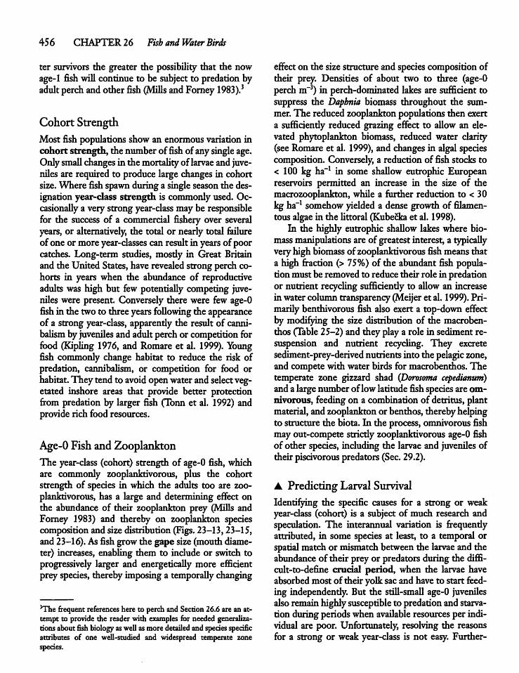
456 CHAPTER 26 Fish and Water Birds
ter survivors the greater the possibUity that the nowage-1 fishwiU continue to be subject to predation byadult perch and other fish (MiUs and Forney 1983).3
Cohort StrengthMost fish populations showan enormousvariation incohort strength, the numberoffish ofanysingle age.Onlysmall changes in the mortaUty of larvae and juve-niles are required to produce large changes in cohortsize. Where fishspawn duringa single seasonthe designation year-class strength is commonlyused. Oc-casionaUy a very strong year-class may be responsiblefor the success of a commercial fishery over severalyears, or alternatively, the total or nearly total failureof one or more year-classes can result in yearsof poorcatches. Long-term studies, mosdy in Great Britainand the United States,have revealed strong perch cohorts in years when the abundance of reproductiveadults was high but few potentiaUy competing juveniles were present. Conversely there were few age-0fish in the twoto threeyears foUowing the appearanceof a strong year-class, apparendy the result of cannibalism byjuveniles andadult perch or competition forfood (Kipling 1976, and Romare et al. 1999). Youngfish commonly change habitat to reduce the risk ofpredation, cannibalism, or competition for food orhabitat. They tend to avoid openwaterandselectvegetated inshore areas that provide better protectionfrom predation by larger fish Clbnn et al. 1992) andproviderich food resources.
Age-0 Fishand ZooplanktonThe year-class (cohort) strength of age-0 fish, whichare commonly zooplanktivorous, plus the cohortstrength of species in which the adults too are zooplanktivorous, has a large and determining effect onthe abundance of their zooplankton prey (MiUs andForney 1983) and thereby on zooplankton speciescompositionand sizedistribution (Figs. 23-13,23-15,and 23-16). Asfish grow the gape size (mouth diameter) increases, enabling them to include or switch toprogressively larger and energeticaUy more efficientprey species, thereby imposinga temporaUy changing
3The frequent references here to perch and Section 26.6 are anattempt to provide the reader with examples for needed generalizationsabout fish biologyaswell asmore detailed andspecies specificattributes of one well-studied and widespread temperate zonespecies.
effecton the sizestructure and species compositionoftheir prey. Densities of about two to three (age-0perch m"3) in perch-dominated lakes are sufficient tosuppress the Daphnia biomass throughout the summer. The reduced zooplankton populations then exerta sufficiendy reduced grazing effect to aUow an elevated phytoplankton biomass, reduced water clarity(see Romare et al. 1999), and changes in algal speciescomposition. Conversely, a reduction of fish stocks to< 100 kg ha'1 in some shaUow eutrophic Europeanreservoirs permitted an increase in the size of themacrozooplankton, while a further reduction to < 30kgha-1 somehow yielded a dense growth of filamentous algaein the Uttoral (Kubecka et al. 1998).In the highly eutrophic shaUow lakes where bio
mass manipulations are of greatest interest, a typicaUyveryhigh biomass of zooplanktivorous fishmeansthata high fraction (> 75%) of the abundant fish populationmust be removed to reducetheir role in predationor nutrient recycling sufficiently to aUow an increaseinwatercolumntransparency (Meijeret al. 1999). Primarilybenthivorous fish also exert a top-down effectby modifying the size distribution of the macrobenthos (Table 25-2) and they playa role in sedimentresuspension and nutrient recycling. They excretesediment-prey-derived nutrients into the pelagic zone,and compete with water birds for macrobenthos. Thetemperate zone gizzard shad (Dorosoma cepedianum)anda largenumber of lowlatitude fishspecies areomnivorous, feedingon a combinationof detritus, plantmaterial, and zooplankton or benthos, therebyhelpingto structure the biota. In the process, omnivorous fishmayout-compete strictly zooplanktivorous age-0 fishof other species, including the larvae and juveniles oftheir piscivorous predators (Sec. 29.2).
A Predicting LarvalSurvivalIdentifying the specific causes for a strong or weakyear-class (cohort) is a subject of much research andspeculation. The interannual variation is frequendyattributed, in some species at least, to a temporal orspatialmatch or mismatchbetween the larvae and theabundance of their prey or predators during the diffi-cult-to-define crucial period, when the larvae haveabsorbed most of their yolk sac and have to start feeding independently. But the stiU-smaU age-0 juvenilesalsoremainhighlysusceptible to predation and starvation during periodswhen available resources per individual are poor. Unfortunately, resolving the reasonsfor a strong or weak year-class is not easy. Further-
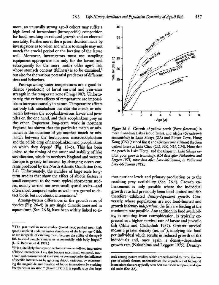
26.3 Life-HistoryAttributes and Population Dynamics ofAge-0 Fish 457
more, an unusually strong age-0 cohort may suffer ahigh level of intracohort (intraspecific) competitionfor food, resultingin reducedgrowth and an elevatedmortaUty. Furthermore, the a priori decision madebyinvestigators as to when and where to samplemaynotmatch the crucial period or the location of the larvaeweU. Moreover, investigators must use samplingequipment appropriate not only for the larvae, andsubsequendy for the more motile older age-0 fishwhose stomach content (fullness) is to be examined,4but alsofor the various potentialpredatorsof differentsizes and behaviors.Post-spawning water temperatures are a good in
dicator (predictor) of larval survival and year-classstrength in the temperate zone (Craig 1987). Unfortunately, the various effects of temperature are impossible to interpret causally in nature. Temperatureaffectsnot only fish metaboUsm but also the match or mismatch between the zooplanktivorous larvae and juve-mles on the one hand, and their zooplankton preyonthe other. Important long-term work in northernEngland has shown that the particularmatch or mismatch is the outcome of yet another match or mismatch between the herbivorous macrozooplanktonandtheedible cropofnanoplankton andpicoplanktonon which they depend (Fig. 12-6). This has beenlinked to the timing of the onsetand stability of lakestratification, which in northernEngland andwesternEurope is gready influenced by changing ocean currents produced by the North Atlantic Oscillation (Sec.5.4). Unfortunately, the number of large scale long-term studies that show the effect of abiotic factors issmall compared to the more typical short-term studies, usually carried out over small spatial scales—andoften short temporal scales as well—are geared to detect biotic but not abiotic interactions.5Among-system differences in the growth rates of
species (Fig. 26-4) in any single cUmatic zone and inaquaculture (Sec. 26.8), have beenwidely linked to ei-
''"The gear used in most studies (towed nets, pushed nets, highspeed samplers) underestimates abundance of thelarger age-0 fish,or are incapable ofcatching them, because theability of the age-0fish to avoid samplers increases exponentially with body length."(L. G. Rudstam et al. 1995.)5"It isquite likely that aquatic ecologists have an inflated impressionofbiotic interactions. I say this because most small, temporal, taxonomic andenvironmental scale studies overemphasise the influenceofspecific interactions byignoring abiotic variation, byaccentuatingthemagnitude and duration of biotic interactions bystudyingfew species inisolation." (Hinch 1991.) It isequally true that large
40-i
Age(yr)
Figure 26-4 Growth of yeUow perch (Perca flavescens) inthree Canadian Lakes (soUd lines), and tilapia (Oreocbromismossambicus) in Lake Sibaya (ZA) and Plover Cove, HongKong (CN) (dashedlines) and (Oreocbromis niloticus) (brokendashedhues) in Lake Chad (CD, NE, NG, CM). Note thattheperch in Lake Herteland the tilapia in Lake Sibaya exhibitpoorgrowth (stunting). (CA data after Nakashima andLeggett 1975, other data after Lowe-McConnell, in Pullin andLowe-McConnell 1982.)
ther nutrient levels and primaryproductionor to theresulting prey availabiUty (Sec. 26.4). Growth enhancement is only possible where the individualgrowthrate had previously been food-limited and fishtherefore exhibited density-dependent growth. Conversely, where populations are not food-limited andgrowth isdensity independent, the fish arefeeding at themaximum rate possible. Anyaddition in foodavailability, as resulting from eutrophication, is typically expressed asa higher survival rateof larvae andjuvenilefish (Mills and Chalanhuk 1987). Greater survivalmeans a greater density (no. m~2), implying less foodper individual which results in reduced growth of theindividuals and, once again, a density-dependentgrowth rate (Nakashima andLeggett 1975). Density-
scaleamong-system studies,which are well-suitedto revealthe impact ofabiotic factors, underestimate the importance ofbiologicalinteractions thataretypically seen bestover shorttemporal and spatial scales(Sec.2.6).
458 CHAPTER 26 Fish and Water Birds
Low water (growth arrested)Flood (growth, reproduction)Poor flood (poor growth, no reproduction)
Figure 26-5 Growth of Citharinuscitharus in the Senegal river floodplainsystem ofsubtropical westAfrica (~16°N).(Modified after C. Reizer 1974, in Wel-comme 1985.)
1966 1967 1968 1969 1970
dependent growth usually reflects a shortage of suitable (high quality) prey but may also be the outcomeof higheractivity levels and a resultinghighermetabolism in certain waters, leaving less food energy forgrowth. A higher activity level results in greater in-traspecific or interspecific interactions among fishes,thereby affecting growth independent from foodavailability (Boisclair and Leggett 1989).
Predation and Survival
Survival is enhanced where food resources are abundant and where predation is low. But studies of foodavailabiUty to a population must also consider thecompetition by juveniles andadults of other vertebrateand invertebrate species. For example, the phantommidge (Chaoborus spp., Insecta) is another importantpredator of macrozooplankton as well as being preyfor larger fish (Sec. 23.9). But most fish species areable, at all life stages, to shift to alternatetypes of preyand habitat when necessary.6 Low predation rates andhighsurvival ratesare commonly seeninweedy waterways where young fish are able to hide from fish and
6"A survey of 33lakes located on the Canadian Shield indicated thatjuvenile and adult brook charr Salvelinus fontinaks (Mitchell) shifttheir food habits fromzoobenthos to zooplankton and their spatialdistribution from littoral to pelagic zone,whenliving sympatrically[sharing habitat] with white sucker Catastomiis commersoni(Lacepede). (H. Venne and P.Magnan 1995.)
other vertebrate predators. A high survival rate mayallow the development of very large populations ofstunted (poorly growing) adult fish that mature at asmall size.Fish are considered to be stunted when theyare substantially smaller than equivalent adults fromother populations in the same climatic region (Fig.26-4).
26.4 Fish Growth:Determinants and Measurement
The strong seasonality in environmental conditionsthat is imposed at higher latitudes by a great seasonalvariation in temperature, irradiance, and resourceavailability is reflected in seasonally changing growthrates, including a lengthywinter period of little or nogrowth and the possibility of experiencing under-iceoxygen depletion (Sec. 15.7). Seasonality at lowlatitudes is linked to seasonal floods and droughts affecting the habitat, resource availability, and deoxy-genation ofmid to low latitude river systems and theirassociated wetlands (Sees. 15.2, and 15.7), as well asthe hypolimnia (Sec. 15.4). Both hydrology and temperature impose the observed seasonality at intermediate (subtropical) latitudes. Growth will be poor andreproduction nonexistent in tropical rivers and theirassociated wedands if hydrological conditions are unfavorable during the breeding season (Fig. 26-5).
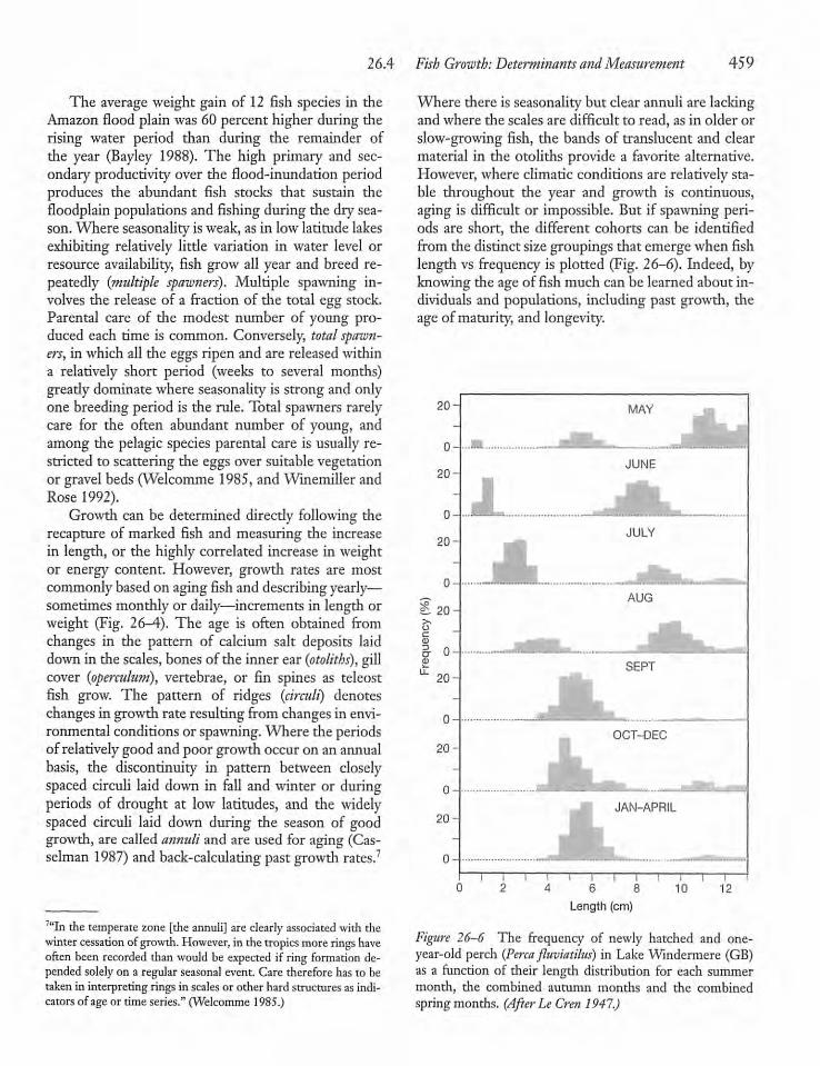
26.4 Fish Growth: Determinants andMeasurement 459
The average weight gain of 12 fish species in theAmazon flood plain was60 percent higher during therising water period than during the remainder ofthe year (Bayley 1988). The high primary and secondary productivity over the flood-inundation periodproduces the abundant fish stocks that sustain thefloodplain populationsand fishing during the dry season.Where seasonality isweak, as in low latitude lakesexhibiting relatively little variation in water level orresource availability, fish grow all year and breed repeatedly {multiple spawners). Multiple spawning involves the release of a fraction of the total egg stock.Parental care of the modest number of young produced each time is common. Conversely, total spawners, in which all the eggs ripen and are released withina relatively short period (weeks to several months)greatly dominate where seasonality is strong and onlyone breeding period is the rule. Total spawners rarelycare for the often abundant number of young, andamong the pelagic species parental care is usually restricted to scattering the eggsover suitablevegetationor gravel beds (Welcomme 1985,and Winemiller andRose 1992).Growth can be determined directly following the
recapture of marked fish and measuring the increasein length, or the highly correlated increase in weightor energy content. However, growth rates are mostcommonlybasedon aging fish and describingyearly—sometimesmonthly or daily—increments in length orweight (Fig. 26-4). The age is often obtained fromchanges in the pattern of calcium salt deposits laiddownin the scales, bones of the inner ear {otoliths), gillcover {operculum), vertebrae, or fin spines as teleostfish grow. The pattern of ridges {circuit) denoteschangesin growth rate resulting from changesin environmental conditions or spawning.Where the periodsof relatively good and poor growth occur on an annualbasis, the discontinuity in pattern between closelyspaced circuli laid down in fall and winter or duringperiods of drought at low latitudes, and the widelyspaced circuli laid down during the season of goodgrowth, are called annuli and are used for aging (Cas-selman 1987) and back-calculating pastgrowth rates.7
7"In the temperate zone [the annuli] areclearly associated with thewintercessation of growth. However, in the tropicsmore ringshaveoften been recorded than would be expected if ring formation depended solelyon a regular seasonal event. Care therefore has to betaken in interpreting rings in scales or other hard structures as indicators of age or time series." (Welcomme 1985.)
Where there is seasonality but clear annuli are lackingand where the scales are difficult to read, as in older orslow-growing fish, the bands of translucent and clearmaterial in the otoliths provide a favorite alternative.However, where climatic conditions are relatively stable throughout the year and growth is continuous,aging is difficult or impossible. But if spawning periods are short, the different cohorts can be identifiedfrom the distinct sizegroupings that emergewhen fishlength vs frequency is plotted (Fig. 26-6). Indeed, byknowing the age of fish much can be learned about individuals and populations, including past growth, theage of maturity, and longevity.
20-
0
20
0
20
0-
2^ 20-
03
cr 00)
"" 20-
0
20-
0
20-1
0-
J.
X
i—i—r
MAY
JUNE
JULY
AUG
i—i—i—r6 8
Length (cm)
1 ~10
T12
Figure 26-6 The frequency of newly hatched and one-year-old perch {Perca fluviatilus) in Lake Windermere (GB)as a function of their length distribution for each summermonth, the combined autumn months and the combinedspring months. (After LeCren 1947.)
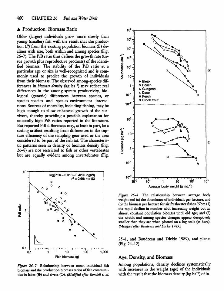
460 CHAPTER 26 Fish and Water Birds
A Production: Biomass Ratio
Older (larger) individuals grow more slowly thanyoung (smaller) fish with the result that the production (P) from the existingpopulation biomass (B) declines with size, both within and among species (Fig.26-7).The P:Bratio thus defines the growthrate (tissue growth plus reproductiveproducts)of the identified biomass. The stability of the P:B ratio at aparticular age or size is well-recognized and is commonly used to predict the growth of individualsfrom their biomass. The observedamong-species differences in biomass density (kg ha-1) may reflect realdifferences in the among-system productivity, biological (genetic) differences between species, orspecies-species and species-environment interactions. Sources of mortality, includingfishing, maybehigh enough to allow enhanced growth of the survivors, thereby providing a possible explanation forunusually high P:B ratios reported in the literature.But reported P:B differencesmay,at least in part, be ascaling artifact resulting from differences in the cap-ture efficiency of the sLpling gear used or the areaconsidered to be part of the habitat. The characteristic patterns seen in density or biomass density (Fig.26-8) are not restricted to fish or other vertebratesbut are equally evident among invertebrates (Fig.
10-
0.1
log(P:B)= 0.313 - 0.420 • log(W)r2 = 0.60; n =53
o
o
1 1 I I Hll| 1 1 | | III I'll) | | I I Mil
0.1 1 10 100 1,000Fish biomass (g)
Figure 26-7 Relationship between mean individual fishbiomass and the productionrbiomass ratiosoffish communities in lakes (•) and rivers (O). (Modified after Randall etal.
106
105-]
104
j" io3^
1 *H•oc
I 10-J1n
1CT1n
10"2
102-
o>10-
1":
1(T1-
10-2
• Bleako Roacha Gudgeona Dace• Perchd Brook trout
i i1(T2 10"1
I I I H'l'l | I I ll>>102 1b31 10
Average bodyweight (g ind."1)
Figure 26-8 The relationship between average bodyweight and (a)the abundance of individuals per hectare, and(b)the biomass per hectarefor sixfreshwater fishes. Note (1)the rapid decline in number with increasing weightbut analmost constant population biomass until old age; and (2)the within and among species changes appear deceptivelysmaller than they are when plotted on a log scale (as here).(Modified after Boudreau andDickie 1989.)
(a
(b
25-1, and Boudreau and Dickie 1989), and plants(Fig. 24-12).
Age, Density, and BiomassAmong populations, density declines systematicallywith increases in the weight (age) of the individualswiththe resultthat the biomass density (kgha"1) of in-
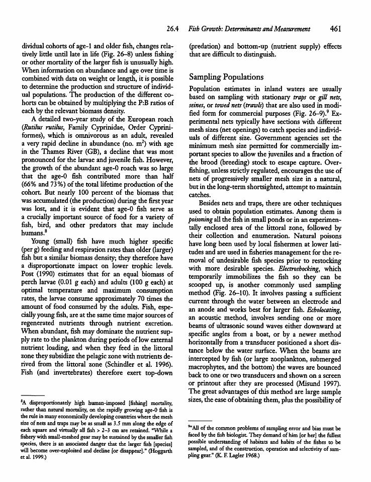
26.4 Fish Growth: Determinants andMeasurement 461
dividual cohorts of age-1 and older fish, changes relativelylittle until late in life (Fig. 26-8) unless fishingor other mortalityof the larger fish is unusually high.When informationon abundance and ageover time iscombined with data on weightor length, it is possibleto determine the production and structure of individual populations. The production of the different cohorts can be obtained bymultiplyingthe P:B ratios ofeachby the relevantbiomass density.A detailed two-year study of the European roach
(Rutilus rutilus, Family Cyprinidae, Order Cyprini-formes), which is omnivorous as an adult, revealeda very rapid decline in abundance (no. m2) with agein the Thames River (GB), a decline that was mostpronounced for the larvaeand juvenilefish.However,the growth of the abundant age-0 roachwas so largethat the age-0 fish contributed more than half(66% and 73%) of the total lifetime production of thecohort But nearly 100 percent of the biomass thatwasaccumulated (the production) during the firstyearwas lost, and it is evident that age-0 fish serve asa crucially important source of food for a variety offish, bird, and other predators that may includehumans.8Young (small) fish have much higher specific
(perg) feeding andrespiration ratesthanolder(larger)fish but a similar biomass density; they thereforehavea disproportionate impact on lower trophic levels.Post (1990) estimates that for an equal biomass ofperch larvae (0.01 g each) and adults (100 g each) atoptimal temperature and maximum consumptionrates, the larvae consume approximately 70 times theamount of food consumed by the adults. Fish, especiallyyoungfish, areat the same timemajorsources ofregenerated nutrients through nutrient excretion.Whenabundant, fish may dominate the nutrientsupplyrate to the plankton duringperiods of lowexternalnutrient loading, and when they feed in the littoralzonetheysubsidize the pelagic zonewithnutrientsderived from the littoral zone (Schindler et al. 1996).Fish (and invertebrates) therefore exert top-down
8A disproportionately high human-imposed [fishing] mortality,rather than natural mortality, on the rapidly growing age-0 fish istherule inmanyeconomically developing countries where themeshsize of netsand traps maybe as small as 3.5mm along the edge ofeach square and virtually all fish>2-3 cm are retained. "While afishery withsmall-meshed gear maybesustained by thesmaller fishspecies, there is an associated danger that the larger fish [species]will become over-exploited and decline [or disappear]." (Hoggarthetal. 1999.)
(predation) and bottom-up (nutrient supply) effectsthat are difficult to distinguish.
SamplingPopulationsPopulation estimates in inland waters are usuallybased on sampling with stationary traps or gill nets,seines, or towed nets (trawls) that are also used in modified form for commercial purposes (Fig. 26-9).9 Experimental nets typically have sectionswith differentmeshsizes (net openings) to catchspecies and individuals of different size. Government agencies set theminimummesh size permitted for commercially important species to allowthe juveniles and a fractionofthe brood (breeding) stock to escape capture. Overfishing, unless strictlyregulated, encourages the useofnets of progressively smaller mesh size in a natural,but in the long-termshortsighted, attempt to maintaincatches.Besides nets and traps, there are other techniques
used to obtain population estimates. Among them ispoisoning allthe fishin small pondsor in an experimentally enclosed area of the littoral zone, followed bytheir collection and enumeration. Natural poisonshave long beenused by local fishermen at lower latitudes andareusedin fisheries management for the removal of undesirable fish species prior to restockingwith more desirable species. Electroshocking, whichtemporarily immobilizes the fish so they can bescooped up, is another commonly used samplingmethod (Fig. 26-10). It involves passing a sufficientcurrent through the water between an electrode andan anode and works best for larger fish. Echolocating,an acoustic method, involves sending one or morebeams of ultrasonic sound waves either downward atspecific angles from a boat, or by a newer methodhorizontally from a transducer positioned a short distance below the water surface. When the beams areintercepted by fish (or large zooplankton, submergedmacrophytes, and the bottom) the waves are bouncedback to one or two transducers and shown on a screenor printout after they are processed (Misund 1997).The greatadvantages of thismethod are large samplesizes, theease ofobtaining them, plus thepossibility of
'"All of the common problems of sampling error and bias must befaced by the fish biologist. They demandof him [or her] the fullestpossible understanding of habitats and habits of the fishes to besampled, and of theconstruction, operation and selectivity of samplinggear." (K. F. Lagler1968.)
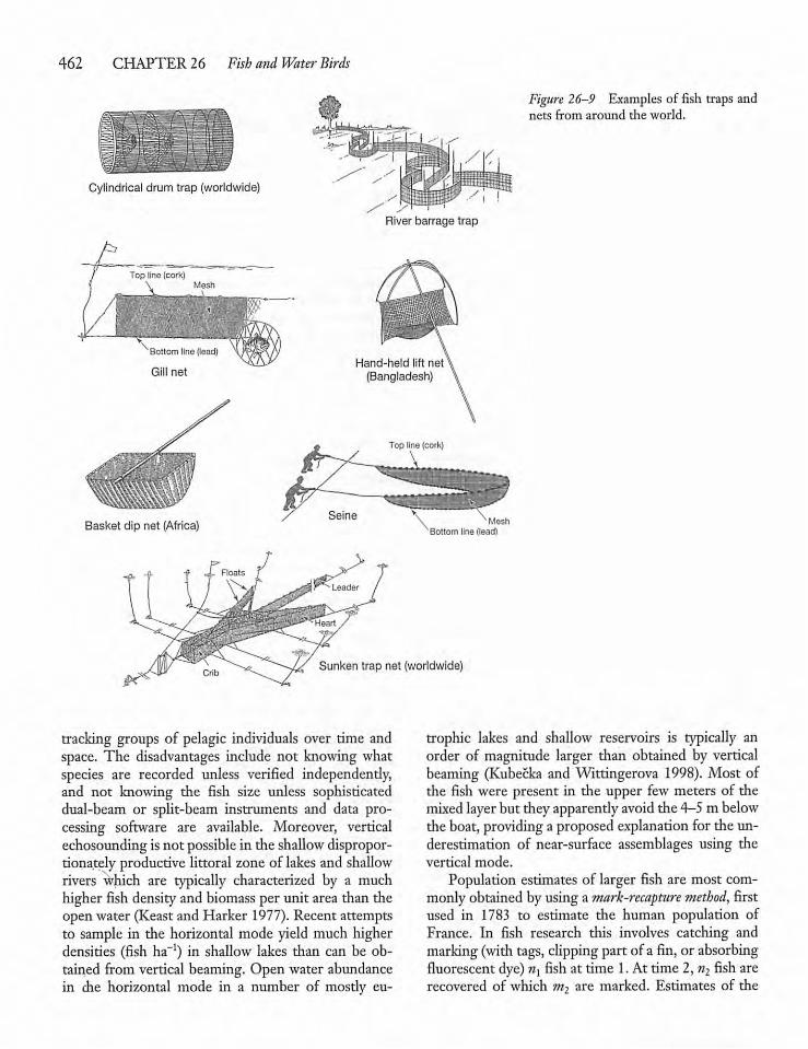
462 CHAPTER 26 Fish and Water Birds
Cylindrical drum trap (worldwide)
River barrage trap
Figure 26-9 Examples of fish traps andnets from around the world.
Sunken trap net (worldwide)
tracking groups of pelagic individuals over time andspace. The disadvantages include not knowing whatspecies are recorded unless verified independently,and not knowing the fish size unless sophisticateddual-beam or split-beam instruments and data processing software are available. Moreover, verticalechosoundingis not possible in the shallowdisproportionately productive littoral zone of lakes and shallowrivers which are typically characterized by a muchhigher fish density and biomass per unit area than theopen water (Keastand Harker 1977). Recent attemptsto sample in the horizontal mode yield much higherdensities (fish ha-1) in shallow lakes than can be obtained from vertical beaming. Open water abundancein the horizontal mode in a number of mostly eu-
trophic lakes and shallow reservoirs is typically anorder of magnitude larger than obtained by verticalbeaming (Kubecka and Witringerova 1998). Most ofthe fish were present in the upper few meters of themixed layerbut theyapparently avoid the 4—5 mbelowthe boat, providing a proposed explanation for the underestimation of near-surface assemblages using thevertical mode.Population estimates of larger fish are most com
monlyobtained byusingamark-recapture method, firstused in 1783 to estimate the human population ofFrance. In fish research this involves catching andmarking (with tags, clipping part of a fin, or absorbingfluorescent dye) nl fish at time 1.At time 2, n2 fish arerecovered of which m2 are marked. Estimates of the
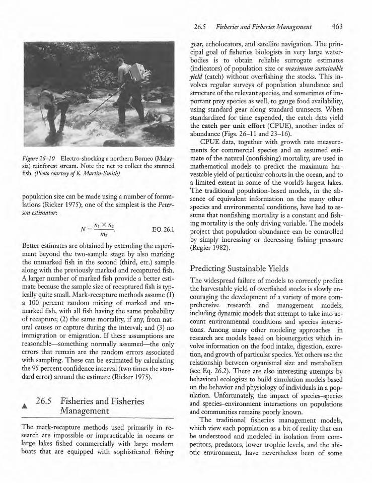
1
Figure 26-10 Electro-shocking a northern Borneo (Malaysia) rainforest stream. Note the net to collect the stunnedfish. (Photo courtesy ofK.Martin-Smith)
population size can be made using a number of formulations (Ricker 1975); one of the simplest is the Peterson estimator:
N =nx X n2
m2EQ. 26.1
Better estimatesare obtained by extending the experiment beyond the two-sample stage by also markingthe unmarked fish in the second (third, etc.) samplealong with the previously marked and recaptured fish.A larger number of marked fish provide a better estimate because the sample sizeof recaptured fish is typically quite small. Mark-recapture methods assume (1)a 100 percent random mixing of marked and unmarked fish, with all fish having the same probabilityof recapture; (2) the same mortality, if any, from natural causes or capture during the interval; and (3) noimmigration or emigration. If these assumptions arereasonable—something normally assumed—the onlyerrors that remain are the random errors associatedwith sampling. These can be estimated by calculatingthe 95percent confidence interval (two times the standard error) around the estimate (Ricker 1975).
26.5 Fisheries and FisheriesManagement
The mark-recapture methods used primarily in research are impossible or impracticable in oceans orlarge lakes fished commercially with large modernboats that are equipped with sophisticated fishing
26.5 Fisheries andFisheriesManagement 463
gear, echolocators, and satellite navigation. The principal goal of fisheries biologists in very large water-bodies is to obtain reliable surrogate estimates(indicators) of population size or maximum sustainableyield (catch) without overfishing the stocks. This involves regular surveys of population abundance andstructure of the relevant species, and sometimes of important prey species aswell, to gauge food availability,using standard gear along standard transects. Whenstandardized for time expended, the catch data yieldthe catch per unit effort (CPUE), another index ofabundance (Figs. 26-11 and 23-16).CPUE data, together with growth rate measure
ments for commercial species and an assumed estimate of the natural (nonfishing) mortality, are used inmathematical models to predict the maximum har-vestableyield of particular cohorts in the ocean, and toa limited extent in some of the world's largest lakes.The traditional population-based models, in the absence of equivalent information on the many otherspecies and environmental conditions, have had to assume that nonfishing mortality is a constant and fishing mortality is the only driving variable. The modelsproject that population abundance can be controlledby simply increasing or decreasing fishing pressure(Regier 1982).
Predicting Sustainable YieldsThe widespread failure of models to correctly predictthe harvestable yield of overfished stocks is slowly encouraging the developmentof a variety of more comprehensive research and management models,including dynamic models that attempt to take into account environmental conditions and species interactions. Among many other modeling approaches inresearch are models based on bioenergetics which involve information on the food intake, digestion, excretion, and growthof particularspecies. Yet others use therelationship between organismal size and metabolism(see Eq. 26.2). There are also interesting attempts bybehavioral ecologists to build simulation models basedon thebehavior andphysiology of individuals in a population. Unfortunately, the impact of species-speciesand species-environment interactions on populationsand communities remainspoorly known.The traditional fisheries management models,
which view each population as a bit of reality that canbe understood and modeled in isolation from competitors, predators, lower trophic levels, and the abiotic environment, have nevertheless been of some
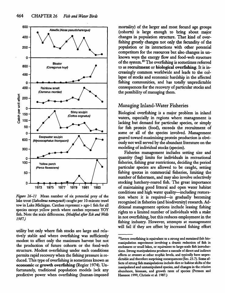
464 CHAPTER 26 Fish and WaterBirds
600
400-
200-
800-
400-
0-
400-
£ 200-0)ac
S o-0)a_ 150-1Q 100-
50 H
0
600-
300-
Alewife (Alosapseudohamngus)
Bloater(Coregonus hoyi)
Rainbow smelt(Osmerus mordax)
Slimy sculpin(Coitus cognatus)
Deepwater sculpin(Myoxocephalus thompsoni)
1973 1975 1977 1979 1981 1983
Figure 26-11 Mean number of six potential prey of thelaketrout (Salvelinus namaycusb) caught per 10-minutetrawltowin LakeMichigan. Catches represent>age-1 fish for allspecies except yellow perch where catches represent YOYfish. Note the scale differences. (Modified after Eck and Wells1987.)
utility but only where fish stocks are large and relatively stable and where overfishing was sufficientlymodest to affect only the maximum harvest but notthe production of future cohorts or the food-webstructure. Modest overfishing under such conditionspermits rapid recoverywhen the fishingpressure is reduced.This type of overfishingis sometimesknownaseconomic or growth overfishing (Regier 1974). Unfortunately, traditional population models lack anypredictive power when overfishing (human-imposed
mortality) of the larger and most fecund age groups(cohorts) is large enough to bring about majorchanges in population structure. That kind of overfishing greatly changes not only the fecundity of thepopulation or its interactions with other potentialcompetitors for the resources but also changes in unknown ways the energy flow and food-web structureofthe system.10 Theoverfishing issometimes referredto as recruitment or biological overfishing. It is increasingly common worldwide and leads to the collapse of stocks and economic hardship in the affectedfishing communities, and has totally unpredictableconsequences for the recovery of particularstocks andthe possibility of managing them.
Managing Inland-Water FisheriesBiological overfishing is a major problem in inlandwaters, especially in regions where management islacking but demand for particular species, or simplyfor fish protein (food), exceeds the recruitment ofsome or all of the species involved. Managementgearedtowardmaximizing protein productionis obviouslynot wellservedby the abundant literature on themodelingof individual stocks(species).Fisheries management includes setting size and
quantity (bag) limits for individuals in recreationalfisheries, fishinggear restrictions,deciding the periodparticular species are allowed to be caught, settingfishing quotas in commercial fisheries, limiting thenumberof fishermen, andmayalsoinvolve selectivelystocking hatchery-reared fish. The great importanceof maintaining good littoral and open water habitatconditions and high water quality—including restoration where it is required—is gradually becomingrecognised in fisheries (andbiodiversity) research. Additional management options include leasing fishingrights to a limited number of individuals with a stakeinnot overfishing, but this reduces employment in thefishing industry. However, attempts at managementwill foil if they are offset by increased fishing effort
10Severe overfishing is equivalent to astrongandsustained fish bio-manipulation experiment involving a drastic reduction of fish inenclosures or smalllakes, or equivalent to large-scale fish introductions. Strongmanipulations produce acascade of directandindirecteffects or stressors at other trophic levels, and typicallyhaveunpredictable andtherefore surprising consequences (Sec. 23.7). Someeffects of strongfish manipulations include dietorhabitat shiftsof themanipulated andunmanipulated species, andchanges in the relativeabundance, biomass, and growth rates of species (Persson andHansson 1999, Christie et al. 1987.)
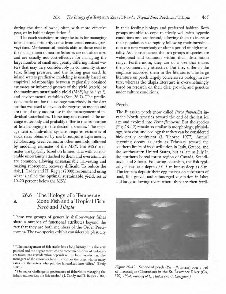
26.6 The Biology ofa Temperate Zone Fish and a Tropical Fish: Perch and Tilapia 465
during the time allowed, often with more effectivegear, or byhabitatdegradation.11The catch statistics forming the basis for managing
inland stocks primarily come from creel census (survey) data. Mathematical models akin to those used inthe management ofmarine fisheries are not often usedand are usually not cost-effective for managing thelarge number of smalland greatly differing inlandwaters that may vary considerably in community structure, fishing pressure, and the fishing gear used. Ininland waters predictive modeling is usually based onempirical relationships between regionally obtainedestimates or informed guesses of the yield (catch), orthe maximum sustainable yield (MSY, kg ha"1 yr_1),and environmental variables (Sec. 26.7). The predictions made are for the average waterbody in the dataset that wasused to develop the regression models andare thus of only modest use in the management of individualwaterbodies. These may not resemble the averagewaterbodyand probably differ in the proportionof fish belonging to the desirable species. The management of individual systems requires estimates ofstock sizes obtained by mark-recapture experiments,echolocating, creel census, or other methods, followedby modeling estimates of the MSY. But MSY estimates are typically based on limited data with considerable uncertainty attached to them and overestimatesare common, allowing unsustainable harvesting andmaking subsequent recovery difficult. To reduce therisk, J. Caddy andH. Regier (2000) recommend usingwhat is called the optimal sustainable yield, set at10-20 percent below the MSY.
26.6 The Biology of a Temperate• Zone Fish and a Tropical Fish:
Perch and Tilapia
These two groups of generally shallow-water fishesshare a number of functional attributes beyond thefact that they are both members of the Order Perci-formes. The two species exhibit considerable plasticity
"'The management offish stocks has a long history. It is also verypolitical and the degree towhich the recommendations ofbiologistsare taken into consideration depends on the local jurisdiction. Themanagers of the resources have to consider the users who inmanycases are the voters who put die lawmakers into office." (Craig1987.)"The major challenge in governance of fisheries ismanaging thefishers and not just thefish stocks." (J. Caddy and H. Regier 2000.)
in their feeding biology and preferred habitat. Bothgroups are able to cope relatively well with hypoxicconditions and are fecund, allowing them to increasetheir population size rapidly following their introduction to a newwaterbody or after a period of high mortality. As a consequence, the two groups of species arewidespread and common within their distributionrange. Furthermore, they are of a size that makesthem commercially attractive. But they differ in theemphasis accorded them in the literature. The largeliterature on perch largely concerns its biology in nature, whereas the tilapia literature is overwhelminglybased on research on their diet, growth, and geneticsunder culture conditions.
Perch
The Eurasian perch (now called Perca fluviatilis) invaded North America toward the end of the last iceage and evolved into Perca flavescens. But the species(Fig. 26-12) remain so similar in morphology, physiology, behavior, and ecologythat they can be consideredbiologically equivalent (J. Thorpe 1977). Annualspawning occurs as early as February toward thesouthern limits of its distribution in Italy, Greece, andthe southeastern United States, but as late asJuly inthe northern boreal forest region of Canada, Scandinavia, and Siberia. Following courtship, the fish typically spawn at a depth of 0-3 m but as deep as 6 m.The females deposit their eggmasses on substrates ofsand, fine gravel, and submerged vegetation in lakesand large inflowing rivers where they are then fertil-
Figure 26-12 School of perch (Perca flavescens) over a bedof macroalgae (Characeae) in the St. Lawrence River (CA,US). (Photo courtesy ofC. Hudon and C. Carignan.)
466 CHAPTER 26 Fish and Water Birds
ized. Egg production in fish is proportional to bodyweightand in perch this averages 15,000 eggs per 100grams ofbodyweight; largefemales canproduce morethan 100,000 eggs. In the centralportionof its rangeittakes two to three yearsfor malesand two to five yearsfor females to become part of the spawning populationbut ranges from two years in the southern UnitedStates to 10years at its northern limits in Canada.Egg mortality is high if eggs become coated with
silt (siltation), exposed to anoxic conditions, subjectedto fungal infection, or where predation by fish andcrayfish is important. Egg mortality in acidified lakesincreases when the pH declines below5.5 during thespawning period,but it is onlyat pH 4 that hatchingisreduced to about 60 percent.Mortality is completeatpH 3.5 in highly acidified waterways (Sec. 27.9). Theability of perch to reproduce successfully in acidifiedlakes is virtually unsurpassed and helps explain theirabundance in such waters that, furthermore, now lacktheir traditionalpredators.
Age-0 FishEgg development is a function of water temperature,andin perchtakes about40days at 8°but onlyten daysat 15° (Duarte and Alcaraz 1989). Newlyhatched larvae (5-6 mm) are weak swimmers and currents carrythem from the littoral to the limnetic (pelagic) zonewhere, at midlatitudes, they remain for four to eightweeks until fin development is sufficient to allow themto return to the littoralzone.In the limnetic zonetheyfeed visually duringthe daytime andon moonlitnightson copepod nauplii, small copepodites, as well as onsmall cladocerans (Chapter 23) and even small fishlarvae. With increasing size and gape the young areable to feed on progressively larger prey, includingbenthic invertebrates and fish (Mehner et al. 1998).In the littoral zone, the young form shoals
(schools) and feed and hide from predators withinmacrophyte beds. Alternatively, they become demersal (bottom living), in particular in shallow unstrati-fied lakes. Cannibalism by age-1 perch commencedwhen the perch in a German reservoir reached 12-15mm, a time when the gape size of the age-0 fishwaslarge enough for them to be able to feed on largedaphnids. Older perch contributed to the predation(cannibalism) when the age-0 cohort reached about 30mm in mid June (Doerner et al. 1999).Daily offshore migration of the shoals of larger
larvae and juveniles toward dusk is followed by onshore migration at dawn but ends when the juveniles
reachabout 30mm, afterwhichthey remain in the littoralor demersal zone for the remainder of the growing season. There is ongoing debate about whetheroffshore migrations at duskallow for pelagic feedingat a timewhen they are not as subjectto visually feeding predators, and the return at dawn is a response togreater prey abundancein the littoral zone or warmerinshorewatersduring the daytime, or whether the migrations have a (genetic) evolutionary basis instead.Mortality of the larvae and age-0 juveniles is, as inother fish, enormous (Sec. 26.3), averaging ~ 6% d"1(range 2-9%) and 2% d-1 in two shallow Scottishlakes. The age-0 perch, including the egg stage, contributed88-96 percent of the total annual perch production in the lakes (Treasurer 1989). However, thecontributionof age-0 (andoften age-1) fish to annualfishproduction is not normallyconsideredin work onproduction, (Sec. 26.7)which dealswith older, largeranimals caught in gill nets or traps with relativelycoarse meshes.The size at which surviving juveniles enter the
winter seasonvaries greatly among years and amonglakes. The maximum range reported is 48-159 mmtotal length, but is more typically 50-100 mm, withthe juveniles weighing 1-3 g wet wt. (Post and McQueen 1994). Interyear variation in cohort size andpreyabundanceappearsto haveamajor impact on theresources available per individual and the resulting(density-dependent) growthof the young.Winter mortality is typically high. In Oneida Lake
(US) the mortality for cohorts of age-0 perch rangedfrom72-99 percent of those fish that had survived thesummer and autumn, with higher mortalities in yearswhen the juveniles enteredwinter at a smallsize(Niel-son 1980). More recent work has shown that wintermortalitywithin a cohort is higher for smallindividuals and is further linked to the length of the ice-coverperiod (Post andEvans 1989). The northernlimits ofperch distributionare similarlybelieved to be set by agrowingseason too short to acquire the size and energy reserves needed to survive the long winters(Shuter and Post 1990).
Age-1 andOlder FishThe age-1 and olderfish tend to be primarily littoral,feeding largely onbenthic invertebrates supplementedbylargezooplankton but there is considerable among-system variationin the extent that the limneticzone isutilized; this is attributed to the relative food availability and predationpressurein the twozones. The den-
26.6 The Biology ofa Temperate Zone Fish and a Tropical Fish: PerchandTilapia 467
sity and structure of macrophyte beds (habitat complexity, plant growth form and density, degree ofpatchiness, dissolved oxygen concentration) has a bigimpact on the abundance and distribution of perch(and other species), their prey, and their predators(Eklov 1977), with reduced fish abundances in thedensest beds where mobility is much reduced (Fig.24-18) and in unvegetated exposedareas.Large perch (7-15 cm) have a sufficientgape size
to become piscivorous on smallerfishaswellascannibalistic on age-0 and smallage-1 juveniles in both thelittoral and limnetic zones (Persson et al 1988). Butthe shift to a fish diet in adult perch is naturally contingent on a sufficient supply of invertebrates earlierin life, enablingthem to grow to the sizenecessary tomakethe diet shiftpossible.Perch feed at low water temperatures, including
under ice, if the visibility and prey presence permitsthis. The species is alsowell-adapted to surviving hypoxic conditions (> 0.25-0.5 mg 021"1) in cold (< 4°)ice-covered waters. The lower survival limit in fishrises with temperature and the associated increasedmetabolism. In perchit rises to about 1.2 mg021"1 at16° and 2mg021-1 at 26°. Even so, growth andreproduction in fish continues to be negatively affected atdissolved oxygen (DO) levels wellabovesurvival limits(Sec. 15.7and Craig 1987).
TilapiaTilapia is the common nameapplied to what are nowrecognized as a group ofAfrican fish (one species extends into the Middle East) and South American fishonceclassified in the genus Tilapia (Family Cichlidae).The tilapias are low latitude fish characterized notonly by a similar morphology but also by a flexibleomnivorous diet. Most of their food is obtained at thebase of the food chain, making them energeticallyhighly efficient. Mostspecies share a common feedingand breeding biology based primarily on the littoralzone. Following the most recent reclassification, theseveral hundred species were split into three genera.The species most widely used in aquaculture are themouth-brooding tilapias, now placed in the genusOreochromis (Fig. 26-2). They include O. mossambicus(mozambique tilapia), originally restricted to thesoutheastern coastal region of Africa, and 0. aureus(blue tilapia) originally limited to theChad and NigerRiver basins ofwest Africa. 0. niloticus, the nile tilapia,originated in theNile andRiftValleys of northeasternAfrica but then naturally extended its range to the
Niger River and Lake Chad basins of western Africa.The three mouth-brooding species, now extensivelyused in low latitude aquacultureworldwide,havebeenwidely introduced to waterways outside their naturalrange to increasefishyields, aswell as for macrophyteor mosquitocontrol.The species are so closely relatedthat theycanhybridizein culture and shareaverysimilar life history.
Environmental Conditions
The desirability of tilapias in aquaculture stems fromrapid year-round growth to a commercial size (Fig.26-4) and the plasticity of their diet. In addition, theirshoaling behavior permits high-density culture, whilethe ease of hybridization in captivity allows for an increased bodysizeof hybrids and the productionof unisex individuals to prevent crowding and stunting.Finally, their ability to thrive in fresh as well as salinewaters is desirable in culture. 0. mossambicus is the mosteurybaline (salt tolerant; > 40%o), but the other speciescan be grown in only moderately less saline ponds.Their salinity toleranceis an adaptation for survival inthe shallow waters they naturally occupy. These aresubject to substantial seasonal anddecade or longerperiods of droughts and high evaporation resulting in avariable and periodically high salinity. Tilapia alsocopes well withhigh turbidity, a condition commonlyencountered in their naturalhabitatwhere rivers carryhigh sediment loads to the lakes andwedands duringthe rainy season. Tilapias are capable of coping withlow dissolved oxygen levels, allowing them to surviveperiods of hypoxia in littoral zones and wedands. Butmassive tilapia kills have been recorded in stratifiedlakes with anoxic hypolimnia when, during overturn,the whole water mass becomes anoxic. One such overturnin Lake George (Uganda) killed -1.3 x 10⁶ fish ina few hours (Pullinand Lowe-McConnell 1982).
Breeding BiologyThe single most detailed life-history study has beenon a stuntedpopulation of 0. mossambicus in subtropical Lake Sibaya, a South African coastal lake at thesouthern and most temperate portion of its range(Bruton and Bolt 1975).Adult males move into the littoral zone in spring (September) to establish territories and dig nests, preferentially between sparselyspaced stems of emergent and submerged macro-phytes at a depthof0.5-5m, but nestsare found downto ~6mamongthe stemsoiMyriophyllum spicatum and
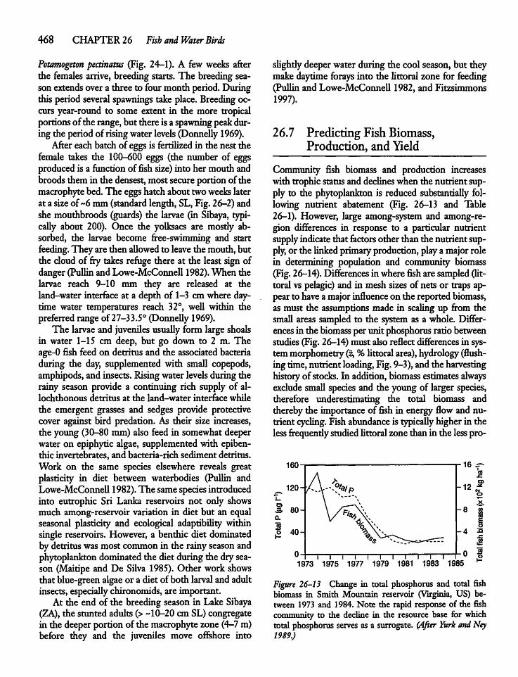
468 CHAPTER 26 Fish and Water Birds
Potamogeton pectinatus (Fig. 24-1). A few weeks afterthe females arrive, breeding starts. The breeding seasonextends overa three to fourmonth period.Duringthis period several spawnings takeplace. Breeding occurs year-round to some extent in the more tropicalportionsof the range,but there is a spawning peakduring the period of risingwaterlevels (Donnelly 1969).Aftereachbatchof eggs is fertilized in the nest the
female takes the 100-600 eggs (the number of eggsproducedis a functionoffish size) into her mouth andbroodsthem in the densest, most secureportion of themacrophyte bed. The eggs hatchabouttwoweeks laterat a size of-6 mm(standard length, SL,Fig.26-2)andshe mouthbroods (guards) the larvae (in Sibaya, typically about 200). Once the yolksacs are mosdy absorbed, the larvae become free-swimming and startfeeding. They are then allowed to leavethe mouth, butthe cloud of fry takesrefuge there at the least sign ofdanger(Pullin andLowe-McConnell 1982).When thelarvae reach 9-10 mm they are released at theland-water interface at a depth of 1-3 cm where daytime water temperatures reach 32°, well within thepreferred range of 27-33.5° (Donnelly 1969).The larvae and juveniles usually form large shoals
in water 1-15 cm deep, but go down to 2 m. Theage-0 fish feed on detritus and the associated bacteriaduring the day, supplemented with small copepods,amphipods, andinsects. Risingwaterlevels duringtherainy season provide a continuing rich supply of al-lochthonous detritus at the land-water interface whilethe emergent grasses and sedges provide protectivecover against bird predation. As their size increases,the young (30-80 mm) also feed in somewhatdeeperwater on epiphytic algae, supplemented with epiben-thic invertebrates, and bacteria-rich sediment detritus.Work on the same species elsewhere reveals greatplasticity in diet between waterbodies (Pullin andLowe-McConnell 1982). The samespecies introducedinto eutrophic Sri Lanka reservoirs not only showsmuch among-reservoir variation in diet but an equalseasonal plasticity and ecological adaptability withinsingle reservoirs. However, a benthic diet dominatedbydetritus was most common in the rainyseason andphytoplankton dominated the diet duringthe dryseason (Maitipe and De Silva 1985). Other work showsthat blue-green algae or a diet ofboth larval and adultinsects, especially chironomids, are important.At the end of the breeding season in Lake Sibaya
(ZA), the stunted adults (> -10-20 cm SL) congregatein the deeper portion of the macrophytezone (4-7 m)before they and the juveniles move offshore into
slighdydeeperwater during the cool season, but theymake daytime forays into the littoral zone for feeding(Pullin and Lowe-McConnell 1982, and Fitzsimmons1997).
26.7 PredictingFishBiomass,Production, and Yield
Community fish biomass and production increaseswith trophicstatusand declines when the nutrient supply to the phytoplankton is reduced substantially following nutrient abatement (Fig. 26-13 and Table26-1). However, large among-system and among-re-gion differences in response to a particular nutrientsupply indicate that factors other than the nutrient supply, or the linkedprimaryproduction,playa majorrolein determining population and community biomass(Fig. 26-14). Differences inwherefishare sampled (littoral vs pelagic) and in mesh sizes of nets or traps appear to haveamajor influenceon the reported biomass,as must the assumptions made in scaling up from thesmall areas sampled to the system as a whole. Differences in the biomass per unit phosphorus ratio betweenstudies(Fig.26-14)must alsoreflect differences in systemmorphometry(z, %littoralarea), hydrology(flushingtime, nutrientloading, Fig.9-3),andthe harvestinghistoryof stocks. Li addition, biomass estimates alwaysexclude small species and the young of larger species,therefore underestimating the total biomass andtherebythe importance of fish in energy flow and nutrient cycling. Fishabundance is typically higher in theless frequendy studied littoralzonethan in the lesspro-
1 1 1 1 1 1 1 1 1 1 T" P1973 1975 1977 1979 1981 1983 1985 H
Figure 26-13 Change in total phosphorus and total fishbiomass in Smith Mountain reservoir (Virginia, US) between 1973 and 1984. Note the rapid response of the fishcommunity to the decline in the resource base for whichtotal phosphorus serves as a surrogate. (After Yurk and Ney1989.)
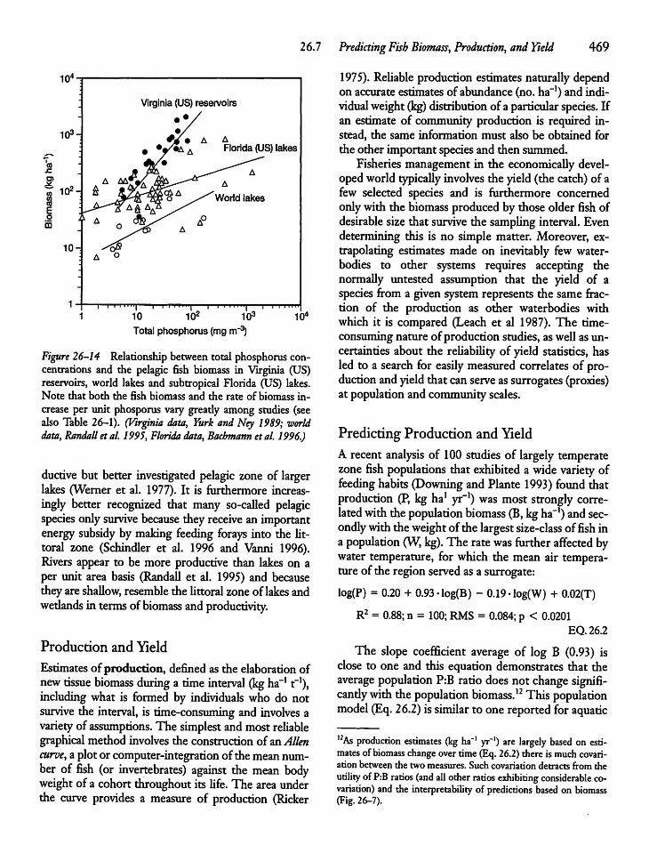
26.7 Predicting Fish Biomass, Production, andYield 469
104^
Virginia (US) reservoirs
• •/
9 ••^•a A Florida (US) lakes
A
A
World lakes
10i 11i"n—
102'"I | l l I mi
103 104Total phosphorus (mg rrf3)
Figure 26-14 Relationship betweentotal phosphorus concentrations and the pelagic fish biomass in Virginia (US)reservoirs, world lakes and subtropical Florida (US) lakes.Note that both the fish biomass and the rate of biomass increase per unit phosporus vary gready among studies (seealso Table 26-1). (Virginia data, Yurk and Ney 1989; worlddata, Randall etal. 1995, Florida data, Bachmann etal. 1996.)
ductive but better investigated pelagic zone of largerlakes (Werner et al. 1977). It is furthermore increasingly better recognized that many so-called pelagicspecies only survive because theyreceive an importantenergy subsidy by making feeding forays into the littoral zone (Schindler et al. 1996 and Vanni 1996).Rivers appear to be more productive than lakes on aper unit area basis (Randall et al. 1995) and becausetheyare shallow, resemble the littoral zoneof lakes andwedands in terms ofbiomass andproductivity.
Production and YieldEstimates of production, defined as the elaboration ofnew tissue biomass during a time interval (kg ha-11"1),including what is formed by individuals who do notsurvive the interval, is time-consuming and involves avariety of assumptions. The simplest andmost reliablegraphical method involves the construction of anAllencurve, aplotor computer-integration of themean number of fish (or invertebrates) against the mean bodyweight of a cohort throughout its life. The area underthe curve provides a measure of production (Ricker
1975). Reliable production estimatesnaturally dependon accurateestimatesof abundance(no. ha-1) and individual weight(kg) distribution of a particular species. Ifan estimate of community production is required instead, the same information must also be obtained forthe other importantspecies and then summed.Fisheries management in the economically devel
opedworld typically involves the yield (the catch)of afew selected species and is furthermore concernedonlywith the biomassproduced by those older fish ofdesirable size that survive the sampling interval. Evendetermining this is no simple matter. Moreover, extrapolating estimates made on inevitably few water-bodies to other systems requires accepting thenormally untested assumption that the yield of aspecies from a given system represents the same fraction of the production as other waterbodies withwhich it is compared (Leach et al 1987). The time-consuming nature of production studies, aswell as uncertainties about the reliability of yield statistics, hasled to a search for easily measured correlates of production andyield that canserve assurrogates (proxies)at populationand communityscales.
Predicting Production and YieldA recent analysis of 100 studies of largely temperatezone fish populations that exhibited a wide variety offeeding habits (Downing andPlante 1993) found thatproduction (P, kg ha1 yr"1) was most strongly correlated with thepopulation biomass (B, kgha-1) andsecondlywiththeweight of the largest size-class offish ina population (W, kg). The ratewas further affected bywater temperature, for which the mean air temperature of the regionserved asa surrogate:log(P) = 0.20 + 0.93-log(B) - 0.19-log(W) + 0.02(T)
R2 = 0.88; n = 100; RMS = 0.084; p < 0.0201EQ.26.2
The slope coefficient average of log B (0.93) isclose to one and this equation demonstrates that theaverage population P:B ratio does not change signifi-candywith thepopulation biomass.12 Thispopulationmodel (Eq. 26.2) issimilar to one reported for aquatic
12As production estimates (kg ha-1 yr"1) are largely based on estimates ofbiomass change over time(Eq. 26.2) thereismuch covariation between the two measures. Such covariation detracts from theutility ofP:B ratios (and allotherratios exhibiting considerable covariation) and the interpretability of predictions based on biomass(Fig. 26-7).
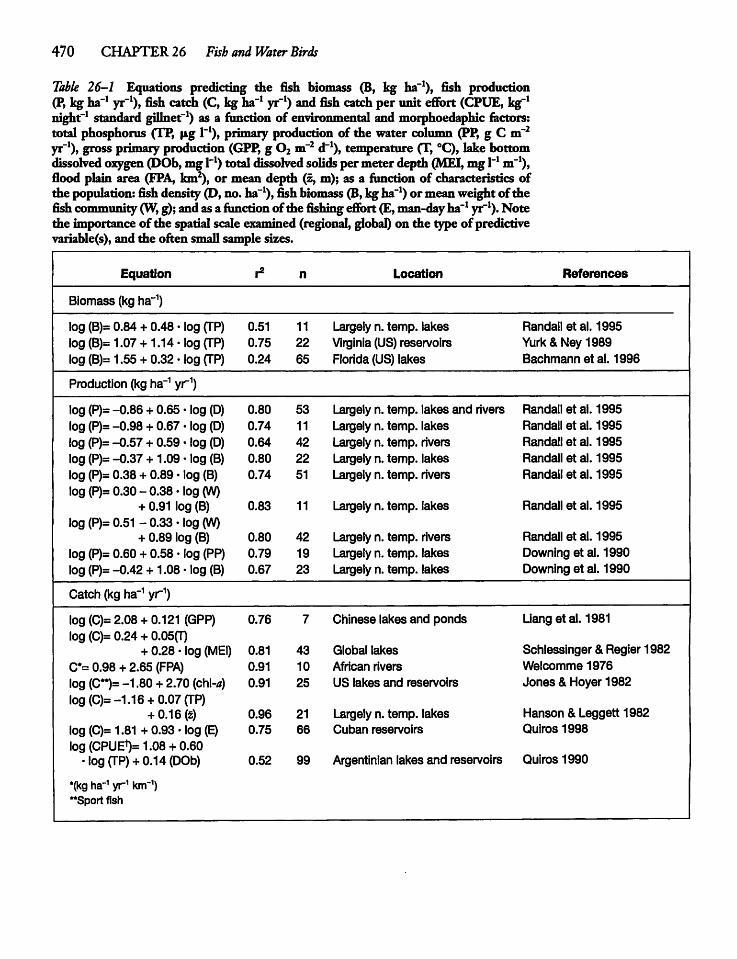
470 CHAPTER 26 Fish and Water Birds
Table 26-1 Equations predicting die fish biomass (B, kg ha-1), fish production(P, kg ha-1 yr-1), fish catch (C, kg ha-1 yr-1) and fish catch perunit effort (CPUE, kg"1night-1 standard gillnet-1) as a function of environmental andmorphoedaphic factors:total phosphorus (TP, |ig l-1), primary production of the water column (PP, g C m"2yr-1), gross primary production (GPP, g 02 m-2 d-1), temperature (T, °C), lakebottomdissolved oxygen (DOb, mg l-1) totaldissolved solids permeterdepth(MEI, mg l"1 m-1),flood plain area (FPA, km2), or mean depth (z, m); as a function of characteristics ofthe population: fish density(D,no. ha-1), fish biomass (B,kg ha-1) ormeanweightofdiefish community(W, g); andasa function ofthe fishing effort(E,man-day ha-1 yr-1). Notethe importance of the spatial scale examined (regional, global) on the type of predictivevariable(s), and the often small sample sizes.
Equation r2 n Location References
Biomass (kgha-1)
log (B)=0.84 + 0.48 • log (TP) 0.51 11 Largely n. temp, lakes Randall et al. 1995
log (B)=1.07+ 1.14-log (TP) 0.75 22 Virginia (US) reservoirs Yurk&Ney1989log (B)=1.55+ 0.32-log (TP) 0.24 65 Florida (US)lakes Bachmann et al. 1996
Production (kg ha-1 yr1)
log (P)=-0.86+ 0.65-log (D) 0.80 53 Largely n. temp, lakes and rivers Randall et al. 1995
log (P)=-0.98+ 0.67-log (D) 0.74 11 Largely n. temp, lakes Randall etal. 1995
log (P)= -0.57 + 0.59 • log (D) 0.64 42 Largely n. temp, rivers Randall etal. 1995
log (P)= -0.37 + 1.09- log (B) 0.80 22 Largely n. temp, lakes Randall etal. 1995
log (P)=0.38 + 0.89 • log (B) 0.74 51 Largely n. temp, rivers Randall etal. 1995
log (P)= 0.30-0.38-log (W)+ 0.91 log (B) 0.83 11 Largely n. temp, lakes Randall etal. 1995
log (P)= 0.51 - 0.33 • log (W)+ 0.89 log (B) 0.80 42 Largely n. temp, rivers Randall et al. 1995
log (P)= 0.60 + 0.58 • log (PP) 0.79 19 Largely n. temp, lakes Downing etal. 1990log (P)=-0.42+ 1.08-log (B) 0.67 23 Largely n. temp, lakes Downing et al. 1990
Catch (kgha-1 yr1)
log (C)=2.08 + 0.121 (GPP) 0.76 7 Chinese lakes and ponds Liang etal. 1981log (C)=0.24 + 0.05fJ)
+ 0.28 • log (MEI) 0.81 43 Global lakes Schiessinger &Regier 1982C*= 0.98 + 2.65 (FPA) 0.91 10 African rivers Welcomme 1976
log (C*> -1.80 + 2.70 (chl-a) 0.91 25 US lakes and reservoirs Jones &Hoyer 1982log (C)=-1.16 + 0.07 (TP)
+ 0.16(2) 0.96 21 Largely n. temp, lakes Hanson &Leggett 1982log (C)= 1.81+0.93-log (E) 0.75 66 Cuban reservoirs Quiros 1998
log (CPUEV 1.08 + 0.60• log (TP)+ 0.14 (DOb) 0.52 99 Argentinian lakes and reservoirs Quiros 1990
*(kg ha-1 yr1 km-1)"Sport fish
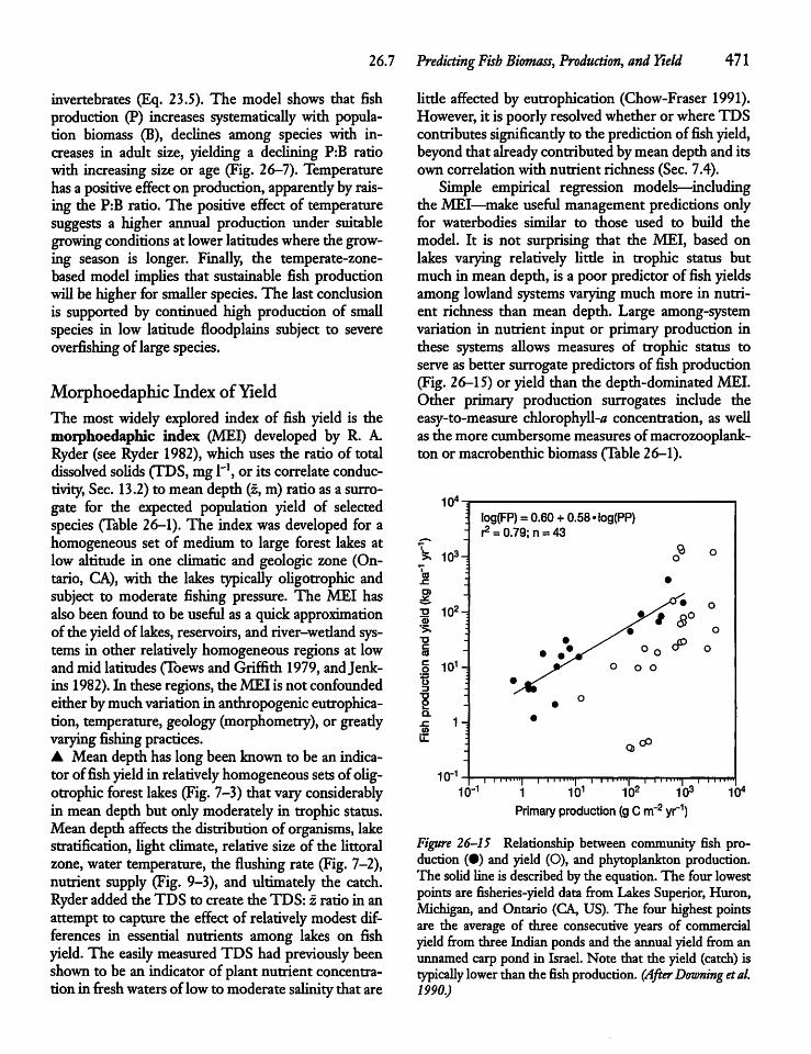
26.7 Predicting Fish Biomass, Production, and Yield 471
invertebrates (Eq. 23.5). The model shows that fishproduction (P) increases systematically with population biomass (B), declines among species with increases in adult size, yielding a declining P:B ratiowith increasing size or age (Fig. 26-7). Temperaturehas a positive effecton production, apparentlyby raising the P:B ratio. The positive effect of temperaturesuggests a higher annual production under suitablegrowing conditions at lower latitudes wherethe growing season is longer. Finally, the temperate-zone-based model implies that sustainable fish productionwillbe higher for smallerspecies. The last conclusionis supported by continued high production of smallspecies in low latitude floodplains subject to severeoverfishing of largespecies.
Morphoedaphic Index ofYieldThe most widely explored index of fish yield is themorphoedaphic index (MEI) developed by R. A.Ryder (seeRyder 1982), which uses the ratio of totaldissolved solids (TDS, mgl"1, or its correlate conductivity, Sec. 13.2) to mean depth (z,m) ratio as a surrogate for the expected population yield of selectedspecies (Table 26-1). The index was developed for ahomogeneous set of medium to large forest lakes atlow altitude in one climatic and geologic zone (Ontario, CA), with the lakes typically oligotrophic andsubject to moderate fishing pressure. The MEI hasalsobeen found to be usefulas a quickapproximationof the yieldof lakes, reservoirs, and river-wetland systems in other relatively homogeneous regions at lowand mid latitudes (Tbews and Griffith 1979, and Jenkins 1982). In these regions,theMEI isnot confoundedeither bymuchvariation in anthropogenic eutrophica-tion, temperature, geology(morphometry), or greadyvarying fishingpractices.A Mean depth has long been known to be an indicator offishyieldin relatively homogeneous setsofoligotrophic forest lakes (Fig. 7-3) that vary considerablyin meandepth but onlymoderately in trophic status.Mean depth affects the distribution of organisms, lakestratification, light climate, relativesize of the littoralzone,water temperature, the flushing rate (Fig. 7-2),nutrient supply (Fig. 9-3), and ultimately the catch.Ryderaddedthe TDS to create the TDS: z ratio in anattempt to capture the effectof relatively modest differences in essential nutrients among lakes on fishyield. The easily measuredTDS had previously beenshown to be an indicator of plant nutrient concentration in freshwatersof lowto moderatesalinity that are
little affected by eutrophication (Chow-Fraser 1991).However, it is poorly resolved whether or whereTDScontributessignificandy to the predictionoffish yield,beyondthat already contributedbymeandepth and itsown correlation with nutrient richness (Sec. 7.4).Simple empirical regression models—including
the MEI—make useful management predictions onlyfor waterbodies similar to those used to build themodel. It is not surprising that the MEI, based onlakes varying relatively little in trophic status butmuch in mean depth, is a poor predictor offish yieldsamong lowland systems varying much more in nutrient richness than mean depth. Large among-systemvariation in nutrient input or primary production inthese systems allows measures of trophic status toserve as better surrogate predictorsof fishproduction(Fig. 26-15) or yield than the depth-dominated MEI.Other primary production surrogates include theeasy-to-measure chlorophyll-^ concentration, as wellas the more cumbersomemeasuresofmacrozooplank-ton or macrobenthic biomass (Table 26-1).
104
V 103-
2 102-
101-
1^
10"
log(FP) = 0.60 + 0.58«log(PP)r2= 0.79; n = 43
Q>CO
o9 °
I I ITIIH| 1 I I 1'H'I | | | |llll| | | | ||lll| | | I I
lb-1 1 io1 102 103 ib4Primary production (gC rrf2yr1)
Figure 26-15 Relationship between community fish production (•) and yield (O), and phytoplankton production.The solidline is describedby the equation.The four lowestpointsare fisheries-yield data fromLakes Superior, Huron,Michigan, and Ontario (CA, US). The four highest pointsare the average of three consecutive years of commercialyieldfrom three Indian pondsand the annualyieldfromanunnamed carp pond in Israel. Note that the yield (catch) istypically lowerthan the fishproduction. (AfterDowning etal.1990.)
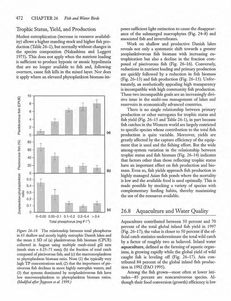
472 CHAPTER 26 Fish and Water Birds
Trophic Status, Yield, and ProductionModest eutrophication (increase in resource availability) allowsa higher standing stock and higher fishproduction (Table 26-1), but normallywithout changes inthe species composition (Nakashima and Leggett1975).This does not apply when the nutrient loadingis sufficient to produce hypoxic or anoxic hypolimniathat are no longer available to fish and, followingoverturn, cause fish kills in the mixed layer. Nor doesit applywhere an elevated phytoplankton biomass im-
-0.05 0.05-0.1 0.1-0.2 0.2-0.4
Total phosphorus (mgP I"1)
Figure 26-16 The relationship between total phosphorusin 65 shallow and mostly highly eutrophic Danish lakes andthe mean ± SD of (a) planktivorous fish biomass (CPUE)collected in August using multiple mesh-sized gill nets(mesh sizes = 6.25-75 mm); (b) die fraction of total catchcomposed of piscivorous fish; and (c) the macrozooplanktonto phytoplankton biomass ratio. Note (1) the typically veryhigh TP concentrations and; (2) that the importance of piscivorous fish declines in more highly eutrophic waters; and(3) that systems dominated by zooplanktivorous fish havelow macrozooplankton to phytoplankton biomass ratios.(Modified afterJeppesen etal. 1999.)
posessufficient light extinction to cause the disappearance of the submerged macrophytes (Fig. 24-8) andassociated fish and invertebrates.Work on shallow and productive Danish lakes
reveals not only a systematic shift towards a greaterzooplanktivorous fish biomass with increasing eutrophication but also a decline in the fraction composed of piscivorous fish (Fig. 26-16). Conversely,reductions in nutrient loading and primary productionare quickly followed by a reduction in fish biomass(Fig. 26-13) and fish production (Fig. 26-15). Unfortunately, an aesthetically appealing high transparencyis incompatiblewith high community fish production.These two incompatiblegoalsare an increasinglydivisive issue in the multi-use management of lakes andreservoirs in economically advanced countries.There is no single relationship between primary
production or other surrogates for trophic status andfish yield (Fig. 26-15 and Table 26-1), in part becausefish catches in the Western world are largely restrictedto specific specieswhose contribution to the total fishproduction is quite variable. Moreover, yields aregready affected by the capture efficiency of the equipment that is used and the fishing effort. But the wideamong-system variation in the relationship betweentrophic status and fish biomass (Fig. 26-14) indicatesthat factors other than those reflecting trophic statushave an important effect on fish production and biomass. Even so, fish yields approach fish production inhighlymanagedAsian fish ponds where the mortalityis low and the available food is used optimally. This ismade possible by stocking a variety of species withcomplementary feeding habits, thereby maximizingthe use of the resources available.
26.8 Aquaculture and Water Quality
Aquaculture contributed between 50 percent and 70percent of the total global inland fish yield in 1997(Fig. 26-17); the value is closer to 50 percent if the official catch statistics underestimate the total wild catchby a factor of roughly two as believed. Inland wateraquaculture, defined as the farmingof aquatic organisms, is growing rapidly while the global yield of wildcaught fish is leveling off (Fig. 26-17). Asia contributed 84 percent of the global inland fish production in 1992 (FAO 1995).Among the fish grown—most often at lower lati
tudes—85 percent are noncarnivorous species. Although their food conversion (growth) efficiency is low
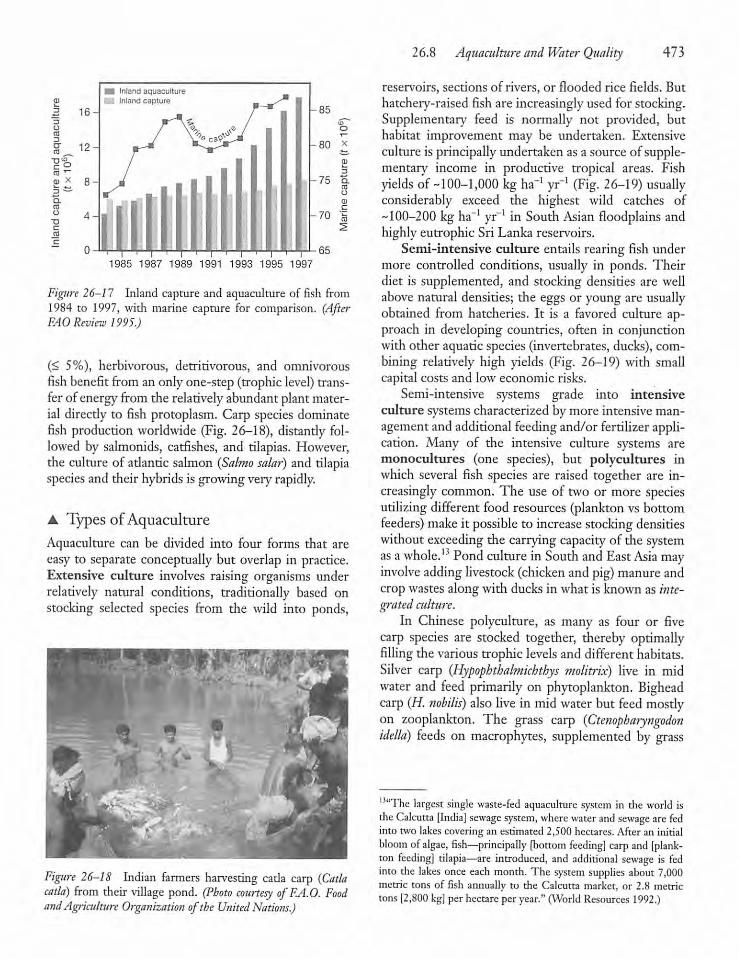
3 16-
ni x
Q,EQO
"OCCO
12-
8
4
01985 1987 1989 1991 1993 1995 1997
Figure 26-17 Inland capture and aquaculture of fish from1984 to 1997, with marine capture for comparison. (AfterFAOReview 1995.)
(< 5%), herbivorous, detritivorous, and omnivorousfish benefit from an only one-step (trophic level) transferof energy from the relatively abundant plantmaterial direcdy to fish protoplasm. Carp species dominatefish production worldwide (Fig. 26—18), distantly followed by salmonids, catfishes, and tilapias. However,the culture of atlantic salmon (Salmo salar) and tilapiaspecies and their hybrids is growingvery rapidly.
A Types of AquacultureAquaculture can be divided into four forms that areeasy to separate conceptually but overlap in practice.Extensive culture involves raising organisms underrelatively natural conditions, traditionally based onstocking selected species from the wild into ponds,
Figure 26-1S Indian farmers harvesting cada carp (Catlacatla) from their village pond. (Photo courtesy ofF.A.O. FoodandAgriculture Organization ofthe United Nations.)
26.8 Aquaculture andWater Quality 473
reservoirs, sections of rivers, or flooded rice fields. Buthatchery-raised fish are increasingly used for stocking.Supplementary feed is normally not provided, buthabitat improvement may be undertaken. Extensiveculture is principallyundertaken as a source of supplementary income in productive tropical areas. Fishyields of-100-1,000 kg ha-1 yr"1 (Fig. 26-19) usuallyconsiderably exceed the highest wild catches of-100-200 kg ha-1 yr-1 in South Asian floodplains andhighlyeutrophic Sri Lanka reservoirs.
Semi-intensive culture entails rearing fish undermore controlled conditions, usually in ponds. Theirdiet is supplemented, and stocking densities are wellabove natural densities; the eggs or young are usuallyobtained from hatcheries. It is a favored culture approach in developing countries, often in conjunctionwith other aquatic species (invertebrates, ducks), combining relatively high yields (Fig. 26-19) with smallcapital costs and low economic risks.Semi-intensive systems grade into intensive
culture systems characterized by more intensive management and additional feedingand/or fertilizer application. Many of the intensive culture systems aremonocultures (one species), but polycultures inwhich several fish species are raised together are increasingly common. The use of two or more speciesutilizing different food resources (plankton vs bottomfeeders) make it possible to increase stocking densitieswithoutexceeding the carryingcapacity of the systemas awhole.13 Pond culture inSouth and East Asia mayinvolve addinglivestock (chicken and pig) manureandcrop wastes along with ducks in what is known as integrated culture.
In Chinese polyculture, as many as four or fivecarp species are stocked together, thereby optimallyfilling the various trophic levels and different habitats.Silver carp (Hypophthalmichthys molitrix) live in midwater and feed primarily on phytoplankton. Bigheadcarp (H. nobilis) also live in midwater but feed mostlyon zooplankton. The grass carp (Ctenopharyngodonidella) feeds on macrophytes, supplemented by grass
"The largest single waste-fed aquaculture system in die world isdieCalcutta [India] sewage system, where water and sewage arefedinto two lakes covering an estimated 2,500hectares. After an initialbloom ofalgae, fish—principally [bottom feeding] carp and [plankton feeding] tilapia—are introduced, and additional sewage is fedinto die lakes onceeach month. The system supplies about 7,000metric tons of fish annually to the Calcutta market, or 2.8 metrictons [2,800kg]per hectare per year." (World Resources 1992.)
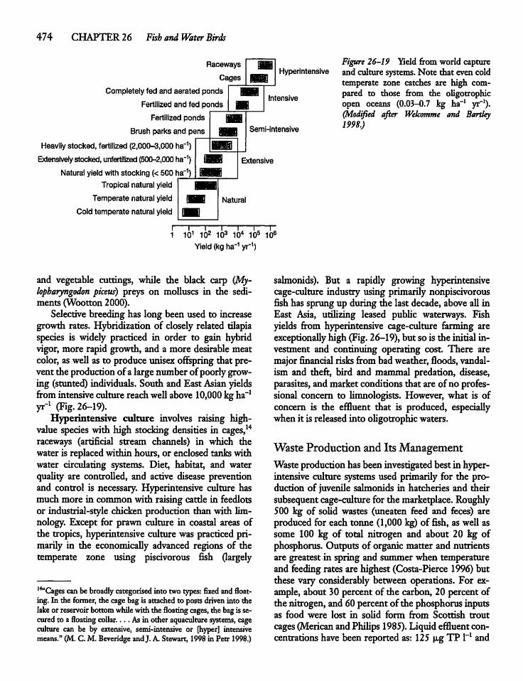
474 CHAPTER 26 Fish and WaterBirds
Raceways
Cages
Completely fed and aerated ponds
Fertilized and fed ponds
Fertilized ponds
Brush parks and pens
Heavily stocked, fertilized (2,000-3,000 ha-1)Extensively stocked, unfertilized (500-2,000 ha"1)
Natural yield with stocking(<500 ha-1)Tropical natural yield
Temperate natural yield
Cold temperate natural yield
Hyperintensive
Intensive
Semi-intensive
Figure 26-19 Yield from world captureand culture systems.Note that even coldtemperate zone catches are high compared to those from the oligotrophicopen oceans (0.03-0.7 kg ha-1 yr-1).(Modified after Welcomme and Bartley1998.)
Extensive
Natural
1—n—I, I, L L L1 101 102 103 104 105 106
Yield (kg ha"1 yr"1)
and vegetable cuttings, while the black carp (My-lopharyngodon piceus) preys on molluscs in the sediments (Wootton 2000).Selective breeding has long been used to increase
growth rates. Hybridization of closely related tilapiaspecies is widely practiced in order to gain hybridvigor, more rapid growth, and a more desirable meatcolor, aswell as to produce unisex offspring that prevent the productionof a largenumberof poorlygrowing (stunted) individuals. South and East Asian yieldsfrom intensive culture reachwell above 10,000 kgha"1yr"1 (Fig. 26-19).
Hyperintensive culture involves raising high-value species with high stocking densities in cages,14raceways (artificial stream channels) in which thewater is replacedwithin hours, or enclosed tankswithwater circulating systems. Diet, habitat, and waterquality are controlled, and active disease preventionand control is necessary. Hyperintensive culture hasmuchmore in common with raising cattle in feedlotsor industrial-style chicken production than with limnology. Except for prawn culture in coastal areas ofthe tropics, hyperintensive culture was practiced primarily in the economically advanced regions of thetemperate zone using piscivorous fish (largely
1''"Cages can bebroadly categorised intotwo types: fixed and floating.In the former, the cagebagis attached to postsdriven into thelake or reservoir bottomwhile withthe floating cages, the bagissecuredto a floating collar.... Asin other aquaculture systems, cageculture can be by extensive, semi-intensive or [hyper] intensivemeans." (M. C. M. Beveridge and J. A. Stewart, 1998 in Petr 1998.)
salmonids). But a rapidly growing hyperintensivecage-culture industry using primarilynonpiscivorousfish has sprung up during the last decade, above all inEast Asia, utilizing leased public waterways. Fishyields from hyperintensive cage-culture farming areexceptionally high (Fig.26-19), but so is the initial investment and continuing operating cost. There aremajor financial risks from badweather, floods,vandalism and theft, bird and mammal predation, disease,parasites, andmarket conditions that are of no professional concern to Umnologists. However, what is ofconcern is the effluent that is produced, especiallywhen it is releasedinto oligotrophicwaters.
Waste Productionand Its ManagementWasteproductionhasbeen investigated best in hyperintensive culture systems used primarilyfor the production of juvenile salmonids in hatcheries and then-subsequent cage-culture for the marketplace. Roughly500 kg of solid wastes (uneaten feed and feces) areproduced for each tonne (1,000kg) of fish, as well assome 100 kg of total nitrogen and about 20 kg ofphosphorus. Outputs of organicmatter and nutrientsare greatest in spring and summerwhen temperatureand feedingrates are highest (Costa-Pierce 1996) butthese vary considerably between operations. For example, about 30 percent of the carbon, 20 percent ofthe nitrogen, and 60 percent of the phosphorusinputsas food were lost in solid form from Scottish troutcages (MericanandPhilips 1985). Liquid effluentconcentrations have beenreported as: 125 \igTP l"1 and
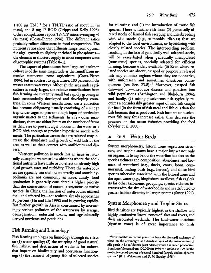
1,400 [igTN 1_1 for a TN:TP ratio of about 11 (asmass), and 8 mg 1_1 BOD (Cripps and Kelly 1996).Other compilations reportTN:TP ratiosaveraging ~5(as mass) (Costa-Pierce 1996). The different ratiosprobably reflectdifferences in food composition. Thenutrient ratiosshowthat effluents range fromoptimalfor algal growth to slightly enriched in phosphorus—the elementin shortestsupplyin most temperatezoneoligotrophicsystems (Table 8-1).The export ofphosphorus fromlarge-scale salmon
culture is of the samemagnitude as the runoff from intensive temperate zone agriculture (Costa-Pierce1996), but in contrastto agriculture, 100percentof thewastes enterswaterways. Although the areaunderagriculture is vasdylarger, the relative contributions fromfish forming arecurrendy small but rapidly growing inboth economically developed and developing countries. In some Western jurisdictions, waste collectionhas become obligatory, usually consisting of a sludgetrapundercages to prevent a highinput of particulateorganic matter to the sediments. In a few other jurisdictions, mere are either limits on the number of farmsor their size to prevent algal blooms in the water or aBODhigh enough to produce hypoxic or anoxic sediments. The particulate wastes that arereleased may increase the abundance and growth of wild fish in thearea as well as their contact with antibiotics and disease.
Nutrient pollution is much less an issue in naturallyeutrophicwatersat lowaltitudeswhere the additional nutrients have little or no effect onalready highalgal growth rates and turbidity. There thewaterbod-ies are typically too shallow to stratify and anoxic hy-polimnia are not commonly an issue. Lasdy, foodproduction is generally considered a higher prioritythan the conservation of natural ecosystems or nativespecies. In China, the fraction of waterbodies utilizedfor—and affected by—aquaculture already approaches30percent (Hu and Liu 1998) andis growing rapidly.But further growth in Asia is constrained by increasingly serious pollution of the waterways by sewage,deoxygenation, industrial toxins, and agriculturallyderived nutrients andpesticides.
Fish Farming and LimnologyFish farming impinges onlimnology through itseffecton (1) water quality; (2) the usurping of good naturalfish habitat and destruction of wedands for culturethat impact on biodiversity and ecosystem functioning; (3) the removal of young fish of selected species
26.9 Water Birds 475
for culturing; and (4) the introduction of exotic fishspecies. There is further risk from (5) genetically alteredstocks of farmed fish escaping andinterbreedingwith wild stocks (e.g., salmonids, tilapias) that areadapted to the local environment, or hybridizing withclosely related species. The interbreeding problem,resulting in the lossof geneticallywell-adapted stocks,will be exacerbated when genetically manipulated(transgenic) species, specially adapted for efficientfarming, becomewidelyavailable. (6) Evenwhere relatedspecies are absent, escaped or purposely releasedfish may colonize regions where they are nonnative,with unforeseen and sometimes disastrous consequences (see Sec. 23.8).15 Moreover, escaped fishcan—and do—introduce disease and parasites intowild populations (Arthington and Blundorn 1996);and finally, (7) raising piscivorous fish typically requires a considerably greaterinput ofwild fish caughtfor feed (in the form offish mealand fishoil) than thefish biomass thatis produced. Fish farmers ofpiscivorous fish may thus increase rather than decrease thepressure on the ocean fisheries providing the feed(Naylor et al. 2000).
A 26.9 Water BirdsSystem morphometry, littoral zone vegetation structure, and trophic status have a major impact not onlyon organisms livingbelowthe waterlinebut alsoon thespecies richness and composition, abundance, and biomass of waterfowl (e.g., ducks, coots, loons, com-morants), wading birds (e.g., herons), and those birdspecies otherwise associated with the httoral zone andthe open water (e.g., kingfishers, swallows, fish eagles).As for other taxonomic groupings, species richness increases with the size ofwaterbodies and is attributed togreater habitat diversity in larger systems (Suter 1994).
System Morphometry and Trophic StatusBird densities are typically highest in the shallow andhighlyproductivehttoral zonesoflakes and rivers, andtheir associated wedands. The land-water interface(riparian zone) is of great importance to birds
1SaMost notable in recent years has been the [heated] exchange ofviews on the advantages and disadvantages of die introduction ofnile perch inLakeVictoria [east Africa] which has raised productionfrom LakeVictoria from 100,000t in 1980 to 450,000t in 1990 attheprobable cost oftheloss ofseveral hundred [largely endemic] nativespecies." (R. I.Welcomme and D.M. Bardey 1998.)
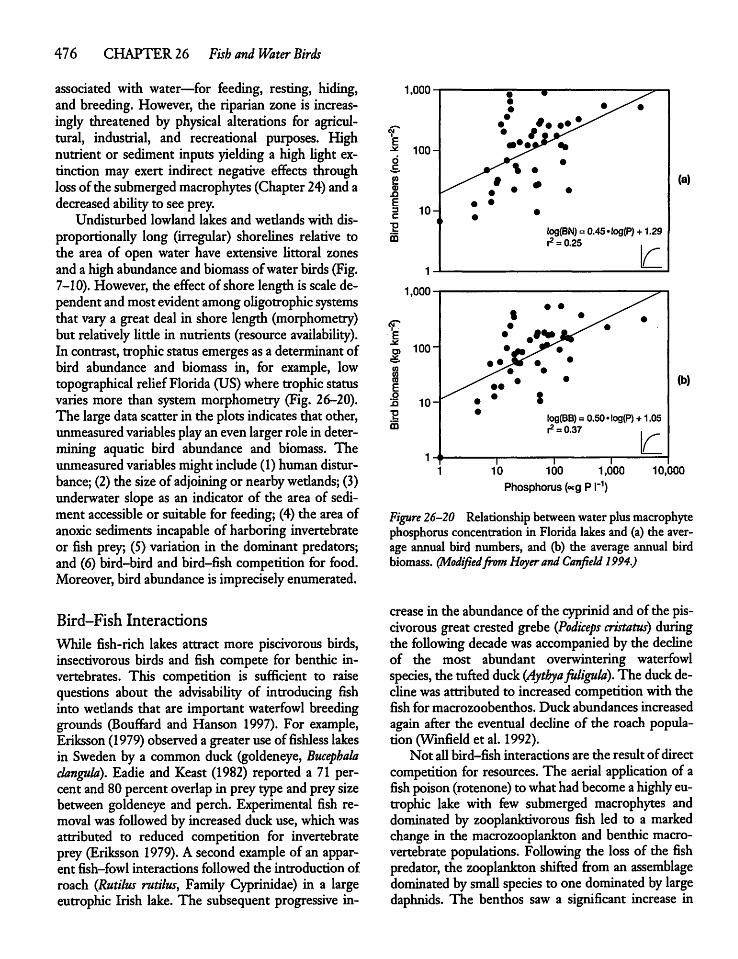
476 CHAPTER 26 Fish and Water Birds
associated with water—for feeding, resting, hiding,and breeding. However, the riparian zone is increasingly threatened by physical alterations for agricultural, industrial, and recreational purposes. Highnutrient or sediment inputs yielding a high light extinction may exert indirect negative effects throughlossof the submergedmacrophytes (Chapter 24)and adecreased ability to see prey.
Undisturbed lowland lakes and wedands with dis-proportionally long (irregular) shorelines relative tothe area of open water have extensive Httoral zonesand a high abundance and biomass ofwater birds (Fig.7-10). However, the effectof shore length is scale dependent andmost evidentamongoligotrophicsystemsthat vary a great deal in shore length (morphometry)but relatively little in nutrients (resource availability).In contrast, trophic status emergesasa determinantofbird abundance and biomass in, for example, lowtopographical reliefFlorida (US)where trophic statusvaries more than system morphometry (Fig. 26-20).The largedata scatterin the plots indicates that other,unmeasured variables playan evenlarger role in determining aquatic bird abundance and biomass. Theunmeasured variables might include (1)humandisturbance; (2)the sizeof adjoining or nearbywedands; (3)underwater slope as an indicator of the area of sediment accessible or suitable for feeding; (4) the area ofanoxic sediments incapable of harboring invertebrateor fish prey; (5) variation in the dominant predators;and (6) bird-bird and bird-fish competition for food.Moreover, bird abundance is imprecisely enumerated.
Bird-Fish Interactions
While fish-rich lakes attract more piscivorous birds,insectivorous birds and fish compete for benthic invertebrates. This competition is sufficient to raisequestions about the advisability of introducing fishinto wedands that are important waterfowl breedinggrounds (Bouffard and Hanson 1997). For example,Eriksson (1979) observed a greater useof fishless lakesin Sweden by a common duck (goldeneye, Bucephalaclangula). Eadie and Keast (1982) reported a 71 percent and 80 percent overlapin prey type and preysizebetween goldeneye and perch. Experimental fish removalwas followed by increased duck use, whichwasattributed to reduced competition for invertebrateprey (Eriksson 1979). A second example of an apparent fish-fowl interactions followed the introduction ofroach (Rutilus rutilus, Family Cyprinidae) in a largeeutrophic Irish lake. The subsequent progressive in
o
<D
E3C
m
• • ^: i^<•• •. ••^^• **v^
100- •••V**jS\. *
^^ * . •^ • • •• •
10- •o •
log(BN)= 0.45»tog(P) +1.29r2= 0.25
1 _\r
,uuu-
• • ^^t *^^ •<F • ^y^ •
E • •**Mo> 100" *4M j*»i • •JC • •0)0) ^^m •CO • •E ••o15 10- •
• X? •
!og(BB)= 0.50»!og(P) + 1.05m
1 ."a3r \r
1i10
i i100 1,000 10,(
(a)
(b)
Phosphorus («g P I"1)
Figure 26-20 Relationship between waterplusmacrophytephosphorus concentrationin Florida lakes and (a) the average annual bird numbers, and (b) the average annual birdbiomass. (Modifiedfrom Hoyerand Canfield 1994.)
crease in the abundanceof the cyprinidand of the piscivorous great crested grebe (Podiceps cristatus) duringthe following decade was accompanied by the declineof the most abundant overwintering waterfowlspecies, the tuftedduck(Aythyafuligula). The duckdeclinewas attributed to increased competitionwith thefish for macrozoobenthos. Duck abundances increasedagain after the eventual decline of the roach population (Winfield et al. 1992).Not all bird-fish interactions are the result ofdirect
competition for resources. The aerial application of afish poison (rotenone) towhathadbecome ahighly eutrophic lake with few submerged macrophytes anddominated by zooplanktivorous fish led to a markedchange in the macrozooplankton and benthic macro-vertebrate populations. Following the loss of the fishpredator, the zooplankton shifted from an assemblagedominated bysmall species to one dominated by largedaphnids. The benthos saw a significant increase in
Hyalella, a benthic amphipod resembling Gammarus(Fig. 25-3) and a favorite fish and duckprey (Hansonand Buder 1994).The associatedlarge increase in migrating waterbirdsin theMinnesota (US) lake was attributednot onlyto amore abundantbenthosresultingfrom gready reduced fish predation but also to zoo-plankton-induced greater water clarity, (zSd 0.3-0.4 mto 1.2-1.5 m). The greater transparency allowed themacrophytes to recolonize, especially Potanogeton pecti-natus, (Fig. 24-1), and Vallisneria americana, whose desirable seeds, tubers, and leaves helped draw largenumbers of migrating birds in early autumn.The rolewater birds playin structuring the aquatic
biota has received little attention—apart from somelargely qualitative data such as those describedabove—on relatively few waterbodies. Anexception issomeworkon whole-system energy flow in limnolog-ically well-characterized Lake Esrom (DK) (Chapter25).Water birds there consumed20 percent of the annual aboveground macrophyte production, but only~4percent of the annual zoobenthicproduction in therelatively steep-sloped lake (seealsoTable 25-3). Thebirds were estimated to be significantcompetitors ofpiscivorous fish, consuming roughly a quarter of thequantity of fish taken by the piscivorous fish (Wooll-head, 1994).
Land-Water Interactions
It has become increasingly recognized that aquaticsystems cannot be understood in isolation from theirincreasingly human-impacted drainage basins and theinput ofmaterials from the atmosphere. Water-associatedbirds (andother vertebrates suchasfrogs, turtles,andmuskrats) straddle the terrestrial and aquatic domains, cycling organic matter and nutrients betweenthem. Byfeeding on aquatic organisms, both fish andbirds influence the abundance and community structure of the biota at the land-water interface and belowthe waterline.16 Limnologists can make an importantcontribution to research on the management ofwaterbirds.
I6"When plankdvorous fish densities were low [in the eutrophicponds, and macrozooplankton densities and transparency werehigh] mallards and muskrats made heavy use of theresulting abundant macrophytes and periphyton. Replacement ofthemacrophytesand periphyton by dense algal blooms associated with control ofzooplankton byan abundance of plankdvorous fish resulted in decreased use bymuskrats and ducks andincreased use byfish-eatingbirds including kingfishers, herons and egrets." (C. N. Spencer andD. L. King 1984.)
26.9 Water Birds 477
HighlightsFish speciesrichness declineswith increasing latitudeand altitude but increases with drainage basin sizeand the sizeofwaterbodies. Asfor other groupsoforganisms, the determinants of species richness andother fish attributes change with the temporal andspatial scale examined.Fish populations are characterized by orders ofmagnitude interannual variation in the survival ofyoung, linked primarily to variation in food availability and predation. Small changes in mortality ofage-0 fish lead to large changes in the abundance ofcohorts.Age-0 fish typicallyyield more than half the lifetimeproductionof a cohort. But nearly 100percent of thebiomass accumulated in the first year is lost to predation or starvation.Fish have an important and temporally changingeffect on the size structure, abundance, and speciescomposition of their prey. Age-0 fish, which commonlyfeed on zooplankton, thereby exertan indirecteffecton the phytoplanktoncommunitystructure.A The age of age-1 and older fish is commonly determined through examination of the pattern of calcium deposits laid down in scales, bones, and finswhich, together with sizemeasurements, are used toobtaingrowthrates.Eutrophication results in an enhanced communityfish production, but if severe, results in changes infishspeciescomposition and fish kills.Fish density (n° ha"1) and biomass density (kg ha"1)tendsto be greatestnear-shorein systems withawell-developed Uttoral zoneand in the near-surface layer,and tendsto decline withdepth in lakes.Overfishing of commercially important stocks iswidespread and globally increasing, with unpredictable effects on the energy flow and food-webstructureof the affected systems.The fraction of the global inland fish yield (catch)contributed by aquaculture is around 50 percent ofthe total and is rising.• In culture, the highest fish yields are obtainedfrom noncarnivorous species that benefitfroma one-step (trophic level) transfer of energyfrom the relatively abundant plantmaterial to fish protoplasm.A Aquaculture can have important negative effectson aquatic systems.A The biomass ofwaterbirdsis greaterin eutrophicthan oligotrophic waters, but as for most freshwaterfish, it is also gready dependent on the presence ofwell-vegetated littoral zones and adjacent areas forbreeding, hiding, andoftenfor feeding.
CHAPTER
27
Acidification ofWaterways
27.1 Introduction
Acidification of the environment by the depositionofstrong acids or compounds that subsequendy formstrong acids (acid precursors), has a major effect onthe chemistryand biota of tens of thousandsoflakes,rivers, wedands, and drainage basins in northern Europe, northeastern North America (Fig. 27-1), partsof east Asia, and elsewhere on a smaller spatial scale.Aquatic acidification is defined by a decrease of theacid neutralizing capacity (ANC) of waterways (Sec.14-4).Acidified watersundergo chemicaland biological changes, and experience species losses or changesin the relative abundance of species. These changesare the combined outcome of hydrogen ions (H+) deposited direcdyon water surfaces and the indirect effects ofhighH+concentrations on catchmentsoilsandvegetation. High H+ concentrations lead to the releaseof metals from soils and their subsequent streamtransportto the receiving lakes andwedands. HighH+levels in waterways also releasemetals, including toxicmetals, from the sediments direcdy into the overlyingwater. Humans and wildlife can be affected by drinkingwater high in toxicmetals that is at the sametimelow in carbonates. People are indirectly affected bythe demise of natural resources—through the loss ofdesirable fish or invertebrate species, forests, or irreparable damage to our architectural heritage whenH+ in precipitation dissolves the limestone and sandstone of ancient buildingsand publicmonuments.Not all lakes, rivers, and wetlands receiving acidic
precipitation are affected. Some have sufficiendy478
buffered drainagebasinsto resist acidification. Othersare naturally acidic as the result of organic acids andare thus little changedby the additionof highlyacidicprecipitation.Many waterbodies worldwide are acidified by in
dustrial or mining effluents. A quarter of all acidicstreams in acid-sensitive areas of the United States arethe result of acidicmine drainage resulting from theoxidation of sulfur in the waste rock or "tailings''(Baker et al. 1991). However, the geology of drainagebasins largelydetermines the acidneutralizingcapacity (ANC) of inlandwater and howwellwaterways—and the soils in their drainage basins—will beprotectedagainstatmospheric acidification.
27.2 Sources and Distributions
The principal sources of acid precipitation are sulfurdioxide (S02)andnitrogenoxides (NO andN02), collectively denotedasNOx,released during the combustion of coal, oil, gasoline, and the smelting of orescontaining sulfur. Globally, between two and threetimes more S02 and NOx are released into the atmosphereasanthropogenic emissions thannaturally asinorganic elements (forexample, sulfurfromvolcanoes)or organic compounds from soils, wedands, and marine systems (Galloway1995).The emitted S02, NOx, and their oxidationprod
ucts, S042" andN03", have typical meanatmosphericresidence times of one to three days. With a mediantransportvelocity of about 400 kmper day, the mean
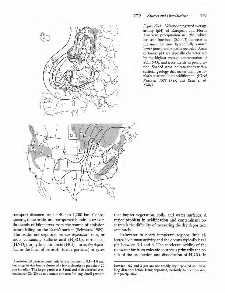
5.1 4.9
transport distance can be 400 to 1,200 km. Conse-quendy, theseoxides are transportedhundredsor eventhousands of kilometers from the source of emissionbefore falling on the Earth's surface (Schwartz 1989).The oxides are deposited as wet deposition—rain, orsnow containing sulfuric acid (H2S04), nitric acid(HNO3), or hydrochloric acid(HO)—or asdry deposition in the form of aerosols1 (oxide particles) or gases
'Aerosol-sized particles commonly have adiameter of0.1—1.0 u,m,but range in size froma clusterof a few molecules to particles > 20u.m in radius.The larger particles(>5 u.m) and their adsorbed contaminants (Ch. 28)do not remainairborne for long. Small particles
27.2 Sources a?id Distributions 479
Figure 27-1 Volume-integrated averageacidity (pH) of European and NorthAmerican precipitation in 1985, whichhas seen fractional (0.2-0.3) increases inpH since that time. Episodically, a muchlower precipitation pH is recorded. Areasof lowest pH are typically characterizedby the highest average concentration ofS04, N03, and trace metals in precipitation. Shaded areas indicate zones with asurficial geology that makes them particularly susceptible to acidification. (WorldResources 1988-1989, and Reuss et al.1986.)
that impact vegetation, soils, and water surfaces. Amajor problem in acidification and contaminant research is the difficulty ofmeasuring the dry depositionaccurately.Rainwater in north temperate regions little af
fected byhuman activityand the oceans typically hasapH between 5.5 and 6. The moderate acidity of therainwater far from volcanic sources is primarily the result of the production and dissociation of H2C03 in
between -0.2 and 2 u.m are not readily dry-deposited and travellong distances before being deposited, probably by incorporationinto precipitation.
480 CHAPTER27 Acidificatin of'Waterways
the atmosphere (Sec. 14.2). The presentacidity ofprecipitation in heavily industrialized regions of theNorthern Hemisphere (Fig. 27-1), including centralJapan and southernKorea, has increased ten to fifty-fold (decreased by 1-1.5 pH unit) from an estimatedpreindustrialbackgroundpH of 5.5-6.A The loading of atmospheric acids is not a goodmeasure of the acidifying powerof the precipitation inportions of western and centralEurope or the northeast and midwest United Stateswhere there is an appreciable release of NH3 into the atmosphere fromanimal manure, sewage treatmentplants, fertilizer, industrial processes and vehicle emisions. The NHj released produces OH", which neutralizes atmosphericH+.
NH3(gas) + H2O^NH4+ + OH". EQ.27.1Ammonia also reacts with sulfuric and nitric acids andforms aerosols. The reaction consumes H+ and thusserves as a source of alkalinity, yielding a more nearlyneutralprecipitation than predictedfromatmosphericS04 and N03 levels alone.
HN03 + H2S04 + 3NH3^NH4N03 + (NH^SCV
EQ.27.2
ButwhereNH3 levels are disproportionately high, thepH of the precipitation appreciably underestimatesthe acidifying potential of NHj*. This is because thechemically and biologically mediated oxidation (nitrification, Sec. 18.3)of NHj* in soils and waters releasesH+ and ultimately contributes to acidification, withone mole of NH^ yielding two moles of hydrogenions and one mole ofnitrate:
NH,+ + 202->2H+ + NO3- + H20 EQ.27.3
(Eq. 11 in Table 27-1), unless the N03" that is produced is taken up by the biota or denitrified by themicrobes (Sees. 18.4and Eq. 7, Table 27-1) in catchments, lake sediments, or at the land-water interfaceof rivers and wedands (Sec. 8.4).
Sulfur and Nitrogen Oxide EmissionsThe rapid increase in fossil-fuel consumption afterWorldWar II not onlygready raisedthe levels of S02and NOx in the atmosphere of industrialized countriesbut also the toxic trace-metal levels (Chapter 28). Inboth eastern North America and in Europe sulfuremissions more than doubled between 1900 and 1980(Husar 1986, Dovland and Semb 1980), primarily as
the result of power plants burning coal and fuel oil togenerate electricity(Fig. 27-2). Emissioncontrols areresponsible for the subsequent decline (averaging>40%bythe year2000) in S02 emissions in the original group of OECD countries (United States,Canada,westernEurope, andJapan).Anthropogenic emissions of NOx are derived pri
marilyfrom the oxidation(fixation) of atmosphericN2gas in internal combustion engines rather than fromthe fuel itself. Asa result, hydrogen ions derivedfromHN03 are particularly prevalent near urban areas.The magnitude ofnitrogen emissions ismuchlesscertain than that of sulfur because it is much more difficult to quantify the many individual sources of NO,emission (including cars and agricultural activities)than the relativelyfewmajor S02 emitters. Even so, afairly recent estimate suggests an increase in NOxemissions of 12-20 times in the eastern United Statessince 1900 (Husar 1986). While S02 emissions havedeclined gready, NOxemissions haverisenslighdybetween 1980 and 1996 in the OECD countries as awhole. Increases in NOx are reflected in measured increases in the absolute and relativeimportance of theN03 concentrations of the precipitation in highlypopulatedregions.At present, S02 andNOxemissionseach contribute roughly half of the anthropogenicallyproduced hydrogen ions in economically developedcountries. Chloride production resulting from industrial activity and particularly from garbage incinerators can be a third locallyimportant source of H+.In both eastern North America and northwestern
Europe prevailing winds tend to be from the southwest. As a result,winds carrying high concentrations ofH+blowfrom the heavily industrialized regionsof bothcontinents toward poorly buffered igneous drainagebasins—the Canadian Shield in northeastern CanadaandnorthernNewEngland, and the Shield Region ofFinno-Scandinavia—dotted with an enormous numberof low salinity lakes that are readily acidified. Thesesame winds carry heavy metals, organic compoundsliberated duringincompletecombustionprocesses, andparticulates. Winds from the south, and in Europefrom the southeast aswell, are sufficiendy common onboth continents to allow the eastern seaboard of theUnited Statesand easternEurope to serveasimportantadditional source regions of H+.Depositionlevels declinewith distancefrommajor
sources, but a precipitation pH averaging less than4.6-4.7 is sufficient to allow the acidification of sensitive catchments over large areas of igneous outcrop-pingson both continents (Sec. 27.10).
27.3 Acid-Sensitive Waters 481
Table 27-1 Selected processes affecting the add neutralizing capadty (ANC) of aquaticsystems and drainage basins, expressed per mole of CH20 (reduction) or 02 (oxidation)consumed (A ANC, organic) and per mole of inorganic substrate reduced (A ANC,inorganic).
In-lake and wetlandA ANC A ANC Mechanism for
Processes Reaction (organic) (inorganic) Permanent Change
Reduction Processes
Weathering (1) CaC03 + 2H+ <± Ca2+ +C02+ H20
— +2
(2) CaAI2Si208 + 2H+& Ca2+ — +2
+ H20 + AI2Si205 (OH)4(3) Al203 +3H20 + 6H+& 2AI3+ — +6
+ 6H20Ion exchange (4) 2ROH +S042"& R2S04
+ 20H"— +2
5)NaR + H+& HR + Na+ — +1Denitrification 6) 2CH20 + N03" + 2H+
<=* 2C02+ NH4+ + H20+1 +2 export of NH4+ via
outflowDenitrification (7) 5CH20 + 4N03" + 4H+
<± 5C02 +2N2 +7H20+0.8 +1 release of N2to
atmosphereManganese (8) CH20 +2Mn02 + 4H+ <± C02 +4 +2 Mn2+ export viareduction + 2Mn2+ + 3H20 outflowIron reduction (9)CH20 + 4FeO(OH)+ 8H+
<* C02 +4Fe2+ +7H20+8 +2 sediment burial as
FeS2Sulfate reduction (10)2CH2O + SO42- + 2H+
& C02 + H2S +2H20+1 +2 sediment burial as
FeS, FeS^ organicsulfur, or H2S gasrelease to atmosphere
Oxidation ProcessesNitrification (11)NH4+ +202^N03- +2H+
+ H20-1 -2
Manganese (12)2Mn2+ + 02 + 3H20 -4 -2oxidation <± 2Mn02 +4H+ +H20Iron oxidation (13)4Fe2+ + 02 + 6H20
& 4FeO(OH) + 8H+-8 -2
Sulfide oxidation (14)H2S + 202^S042" +2H+ -1 -2
Pyrite oxidation (15)FeS2 +3f02+3jH20^Fe(OH3) +2S042- +4H+
-1.1 -4
Source: After Schnoor and Stumm 1985, and Davison 1987.
27.3 Acid-Sensitive Waters
The inland waters that are most sensitive to acidification are transparent with a very lowsalinity (conductivity < -50 |xS cm"1), a correspondingly low HC03"concentration, and a small add neutralizing capacity
(ANC)or alkalinity of < 50 u.eq/1. Humic lakes in thesame areacommonly have a lowalkalinity but are naturally acidic from the release of organic acids. Highlystained (rich in organic acid) lotic systems in theAmazon and Congo River basins(centralAfrica) havea pH of ~3.5-4.5 although far from sources of
482 CHAPTER 27 Acidification ofWaterways
1955 1960 1965 1970 1975 1980
anthropogenic H+ inputs. The most acid-sensitivetransparent waters are characterized by a backgroundpH between 5 and 7. Chemical sensitivity to acidification implies that small increments of added acid produce relatively large declines in pH. From anecological rather than a chemical perspective, a sensitive waterbody is one in which additional inputs ofacid are likely to result in biological changes prior torapid lowering of the pH. Although the first changesto be noted are usually biological, these are subtle andoften difficult to detect—therefore a chemical definition is usually required.
Kelso et al. (1986) estimated that there are morethan 350,000 lakes in eastern Canada with an ANC< 50 u.eq/1, of which more than 14,000 are acidified(pH <4.7)with an ANC of S 0 u,eq/l. There are alsoa much more modest number of acidified lakes in thenortheastern United States, primarily in the Adirondack region of New York. Sweden, with a muchsmaller landmass than eastern Canada, has about85,000 lakes larger than 1 ha of which about 20,000were acidified, plus around 90,000 km of acidifiedstreams (Dickson 1985). In Norway, lakes and streamsin an area of more than 33,000km2 have lost, or werelosing, their fish stocks and seven major rivers havelost their salmonpopulations.• In response to lackof information on the preacidi-fication pH of lakes, paleolimnologists havesucceededin developing quantitative relationships (models) betweenthe species compositionof algalcommunitiesinsurface sedimentsand the pH of overlyingwaters. Thecalibration data sets are dien used to infer the lake-water pH at different times in die past on the basis ofthe species composition found in slices of dated cores(Sec. 20.5). Measurements show that most of the lakesin the AdirondackMountains (US)had a pH close to 6
1,000o —.•iz in
£tE <u=J COw >
Figure 27-2 Weighted yearly mean FTconcentrations in precipitation at Lista,in southernmost Norway, and yearly energy consumption in Europe for theperiod 1955-1985. Emission of S02has continued to decline, resulting in a~ forty percent reduction in the mean H*concentration of the precipitation. (AfterHenriksen 1987.)
800
c o
-600
co oCD *-Q.IOo o
1985
around 1900. Today the pH has declined between 1(tenfold) and 2 (a hundredfold) units in the majority oflakes, with the greatest acidification occurring between 1920and 1950(Cumming etal. 1994). Asimilardecline is seen in Swedish west coast (Fig. 27-3) andsouth coast lakes (Wright and Gjessing 1976).The extent of pH decline in affected regions is a
function of both local geology (soils that determinethe available bufferingcapacity) and the sulfur plus nitrogen oxide deposition rates, which decrease withdistance from major source regions (Fig. 27-4). Aspointed out above, not all acidic lakes in acid-sensitiveareas are acidic because of acid precipitation. For example, about one-quarter of 1,180 lakes sampled inacid-sensitive areas of the United States were acidifiedby organic acids derived from their drainage basins
60
8 40-
aJ 20-Q.
West coast of Sweden, 15 lakes
1930s
H1971
6
PH
Figure 27-3 Changes in die fraction of lakes of differentpH on the west coast of Sweden between the 1930s and1971. (After Wright andGjessing 1976.)
27.4 Characteristics ofAcid-Sensitive Waters and Catchments 483
150-
S 100-
CO
0
_300-
^ 200H= 100H
< 0
7.0 H
I 6.5 H
6.0
5.5
S042" =-12+334• (D) -163. (D)2r2= 0.96
A =244-168.p)r2n 0.97
pH =7.33-1.15 • (D)r2= 0.96
~I 1 1 1 10.4 0.8
Total sulphur deposition (gm"2 yr-1)1.2
Figure 27-4 Relation between sulfur deposition (D) andthemean S042~ concentration in lake waters, the alkalinity(A), and the pH of Ontario lakes on the Canadian Shieldwith increasing distance from the major source region.Error bars correspond to one standard deviation. (AfterNeary andDillon 1988.)
(Baker et al. 1991). CanadaandFinlandalsohavelargenumbersof highlycoloredacidiclakes (pH <5.3)containing very low levels of S042" that are naturallyacidic as the result of a high input of organic acids(Kamari et al. 1991). It is evident that in regionsdominated by brown-water systems (humic, dystrophic),the role of organic acidsmust be evaluated before theeffect of industrial acids can be determined.
27.4 Characteristics ofAcid-SensitiveWaters and Catchments
Susceptibility to acidification is affected by:
1. the abilityof catchmentsoilsand rock to neutralizeincoming acids;
2. lake morphometry and catchment attributes;3. organic acids in runoff; and4. neutralizing agents and processes within aquaticsystems.
The abilityof the catchment soilsand rock to neutralizethe incomingacidsis the singlemost importantfactor distinguishing acidified from nonacidified lakedistricts in regions with low pH precipitation. Thelarger the fraction of a catchment that is covered byeasily weathered carbonate-rich rocks and soils, thehigher the ANC and salinity (conductivity) (Tables13-1 and 13-2). Susceptible areas, denoted by a lowANC, are found in glaciated areas on igneous (e.g.,quartzite, granite,basalt, or gneiss) or other highlyinsoluble bedrock rich in silicate minerals (e.g., sandstone), where the surface material is derived frommaterial of similargeology. Rivers, lakes, andwetlandsare readily protected where the insoluble bedrock iswithin the catchment overlainby a modest amount ofcalcareous drift (Sec. 13.2) brought in from otherareasby glaciers.Geologically susceptible regions impactedby acid
ification include much of northern Canada and Scandinavia, mountainous areas of central and westernEurope, and the AdirondackMountains of the northeastern United States (Fig. 27-1). Other major regions covered with soils containing little bufferincludethe RockyMountains ofwesternNorth America, large parts of central and eastern China, all ofKorea, and portions of Japan, New Zealand, northeastern Brazil, and South Africa.In lakedistrictswhere surficial soils are of igneous
origin, the extent of susceptibility is determined bylakemorphometry, catchment attributes, and the absence of atmospheric dust rich in CaCOj.2 Streamsand lakes positioned at the head of drainage basins{headwater lakes) are most at risk because the catchment areas feeding the inflowingstreams or groundwater are small, the soils are thin, and most of theprecipitationreaches the lake surfaces directly ratherthan asrunoffcarryingalkalinity (ANC)releasedfromthe soil and rock. Similarly, small, high latitude lakebasins are frequently lined with peat in locationswhere catchment slopes areverylowandbogsdevelop(Sec. 8.8), preventing the underlying soil and rock
2The near-neutral precipitation pH recorded in heavily industrialized regions of south-central China is attributed to atmosphericneutralization with CaCOj-rich dust carried from upwind regions(H. B. Xue and J. L. Schnoor 1994). The Sahara desert is also a richsource of wind-blown alkaline material and of phosphorus. InNorth America, significantlevels of acid-neutralizingdust are seenin precipitationin the semiaridplains east of the RockyMountainsand in the midwest, which are characterizedby exposedcalcareoussoilssubject to wind erosion.
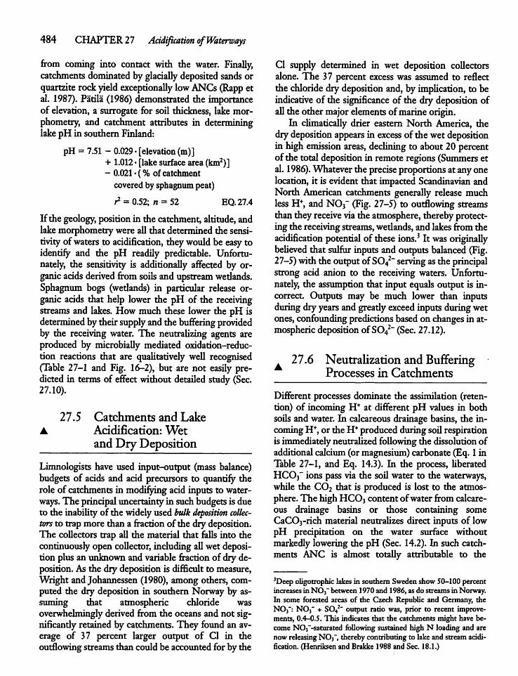
484 CHAPTER 27 Acidification ofWaterways
from coming into contact with the water. Finally,catchments dominated byglacially deposited sands orquartzite rockyield exceptionally lowANCs(Rapp etal. 1987). Patila (1986) demonstrated the importanceof elevation, a surrogate for soil thickness, lake morphometry, and catchment attributes in determininglakepH in southern Finland:
pH = 7.51 - 0.029 •[elevation(m)]+ 1.012 •[lakesurface area (km2)]- 0.021 •(% of catchmentcovered by sphagnum peat)
r2 = 0.52;n = 52 EQ.27.4
If the geology, position in the catchment, altitude, andlakemorphometrywereall that determinedthe sensitivity ofwaters to acidification, theywould be easy toidentify and the pH readily predictable. Unfortunately, the sensitivity is additionally affected by organic acids derived from soils and upstream wetlands.Sphagnum bogs (wetlands) in particular release organic acids that help lower the pH of the receivingstreams and lakes. How much these lower the pH isdetermined bytheirsupply andthe buffering providedby the receiving water. The neutralizing agents areproduced by microbially mediated oxidation-reduction reactions that are qualitatively well recognised(Table 27-1 and Fig. 16—2), but are not easily predicted in terms of effect without detailed study(Sec.27.10).
27.5 Catchments and Lake• Acidification: Wet
and Dry Deposition
Limnologists have used input-output (mass balance)budgets of acids and acid precursors to quantify therole of catchments in modifying acid inputs to waterways. The principal uncertaintyin suchbudgetsis dueto the inability of the widely used bulk deposition collectors to trap more than a fraction of the dry deposition.The collectors trap all the material that falls into thecontinuously open collector, includingallwet deposition plus an unknownand variable fractionof dry deposition.As the dry deposition is difficult to measure,Wright and Johannessen (1980), among others, computed the dry deposition in southern Norway by assuming that atmospheric chloride wasoveiwhelminglyderived from the oceans and not significantly retained by catchments. They found an average of 37 percent larger output of CI in theoutflowingstreams than could be accounted for by the
CI supply determined in wet deposition collectorsalone. The 37 percent excess was assumed to reflectthe chloride drydeposition and, by implication, to beindicative of the significance of the drydeposition ofallthe othermajor elements ofmarine origin.In climatically drier eastern North America, the
drydeposition appears in excess of thewetdepositionin high emission areas, declining to about 20 percentof the totaldeposition in remote regions (Summers etal. 1986).Whatever theprecise proportions at anyonelocation, it is evident that impacted Scandinavian andNorth American catchments generally release muchless H+, andN03" (Fig. 27-5) to outflowing streamsthantheyreceive via theatmosphere, thereby protecting the receiving streams, wetlands, and lakes from theacidification potential of these ions.3 It was originallybelieved that sulfur inputs andoutputs balanced (Fig.27-5) with theoutput ofS042" serving as theprincipalstrong acid anion to the receiving waters. Unfortunately, the assumption that input equals output is incorrect Outputs may be much lower than inputsduring dryyears andgreatly exceed inputs during wetones, confounding predictions based on changes in atmospheric deposition ofS042~ (Sec. 27.12).
27.6 Neutralization andBufferingProcesses in Catchments
Different processes dominate the assimilation (retention) of incomingH+ at different pH values in bothsoils and water. In calcareous drainage basins, the incomingH+, or the H+produced during soil respirationis immediately neutrahzedfollowing the dissolution ofadditional calcium (ormagnesium) carbonate(Eq. 1inTable 27-1, and Eq. 14.3). In the process, liberatedHC03~ ions passvia the soil water to the waterways,while the C02 that is produced is lost to the atmosphere.The highHC03 content ofwater from calcareous drainage basins or those containing someCaC03-rich material neutralizes direct inputs of lowpH precipitation on the water surface withoutmarkedly lowering the pH (Sec. 14.2). In such catchments ANC is almost totally attributable to the
JDeep oligotrophic lakes in southern Sweden show50-100 percentincreases in NO3" between 1970and 1986, asdo streams in Norway.In some forested areas of the Czech Republic and Germany, theNO3": N03" + S042" output ratio was, prior to recent improvements, 0.4-0.5. This indicates that the catchments might have become N03"-saturated following sustained high N loading and arenow releasing NOj", therebycontributingto lakeandstreamacidification. (Henriksen and Brakke 1988 and Sec. 18.1.)
27.6 Neutralization and Buffering Processes inCatchments 485
100-
40 60
Input(keqkm"2 yr1)
C03/HC03 system. If the H+inputs are large and theaccessible CaC03 deposits in the catchment are limited, a progressively increasing fraction of the HC03"released is lost as C02 to the atmosphere and theHC03 of the outflowing streams and the pH of receiving lakes declinesover time.
Sensitive Catchments
Sensitive igneous catchments that lack calcareous deposits and also lack bogs releasing organic acid typically havewater with a pH of 5-6 when nonacidified.The C02 producedin respirationby the soilbiota andplant roots combineswith water to form H2C03 (Sec.14.2). Following the dissociation of the H2C03, theH+ produced isneutrahzedbythe weathering ofNa orK feldspar minerals—the principal component of igneous rock—and the HC03" released. Slowweathering yields clay minerals composed primarily ofinsoluble aluminium silicates, but also releasesmoderate amounts of HC03", cations, and dissolvedsilica towaterways (Eq. 13.2, and Eq. 2 in Table 27-1).The HC03" released during weathering of hard
igneous rockissufficiently small to make the receivinglakes and rivers extremely sensitive to acidification.The H+ in nonacidifying precipitation is primarilyconsumed (and retained) in the catchment soils by acation exchange neutralization (Eqs. 4 and 5 in Table27-1,) and little is released to the runoff (see Fig.27-5). More specifically, some of the H+ is taken upand removed in the process of dissolving the aluminiumhydroxides, oxides, and Si02 contained in the
100
Figure 27-5 Specific inputs versus specificoutputs of ions for each of fiveyears(1973-1978) in an acidified Norwegiancatchment, with the dry deposition fraction determined by the chloride correction method (see Sec. 27.5). The 1:1 linerepresents an equal input and output.Note (1) the retention of hydrogen ionsand nitrate; (2) the net export of calciumand magnesium; and (3) an input-outputratio close to one for sulfate, chloride,and sodium. (After Wright and Johan-nessen 1980.)
clay minerals produced during the breakdown ofweathered silicates (Eq. 3 in Table 27-1). Other H+may be exchanged for cations on the soil particles.The Al ions that are released replace Ca, Mg, andother basecations on the negatively chargedcolloidalclay and humus particles of the soil matrix, with thereleased cations enteringwaterways.The extent to which soils produced from igneous
rockcan serve as a buffer and protect the outflowingrivers and the receiving lakes and wetlands is a function of (1) the abundance of silicate and claymineralsto be weathered; (2) the extent to which negativelycharged clayparticles in soil and sediment are associated with base cations such as Ca2+, Mg24, orNrV andAl}+ available to exchange places with the incomingH+; and (3) the thickness of the soilor,more correctly,the overburden and flowpath contact time that thewaterhaswith the soil. The leaching (release) of basecations is consequently a function of the supply rate ofthe H+ and water movement.4When the supply of strong acid anions (primarily
S04 and N03) is increasedduring acidification, theremust be an equivalent increase in cation release tomaintain the ionic charge balance. Initially the required cations come from exchangeable bases in the
4In acid-rain research, themajor cations are, forhistorical reasons,referred toasbase cations. Theyform thecation ofstrongbases [e.g.,Ca (OH)2, K (OH)] whereas those anions associated with strongacids (S042~, CI", and N03") are referred to as the (strong) acidanions.
486 CHAPTER27 Acidification ofWaterways
soil or sediments, thereby protecting the receivingwaters from acidification. Butwhen the base cation supplydeclines over time, theyarereplaced bythecationsAl3+ and H+ to maintain the ionic charge balance onthe soil particles. A further H+ input allows excess Al(plus other tracemetals) andexcess H+ to be exported,raising their levels in streams, wetlands, and lakes. Asthewater pH declines to about4.5^4.7, organic acidsthat hadpreviously actedasnatural sources ofH+ startbuffering against further acidification. Similarly, Aloxides released to the water start to dissolve or dissociate and begin to serve as additional buffers againstacidification.
Al (OH)3 + 3H+ <=* Al3+ + 3H20 EQ. 27.5
27.7 BufferingCapacity of Lakes,Rivers and Wetlands
The acid neutralizing capacity ofwateris of the greatest importance in determining the pH and assessingthe buffering capacity of fresh water. It can be expressedmost simplyas:
ANC= [HC03-] + 2[C032- ] EQ.27.6+ [OH-]±[AT] - [H+] - 2[A1+]
Where S[AT] = 3[A13+] +2[A10H2+] + [AL(OH)2+]...C032" and OH" are essentially absent from the
generally lowANC oligotrophic watersof acid-sensitive areas (Fig. 14-1) and organic anion concentrations are negligible in clear water lakes, thereforeEquation27.6can be simplified to:
ANC = [HCO3-] - H+ - [AT ] EQ.27.7
and in aquaticsystems with a pH >~5.5 to:ANC = [HC03] - H+ EQ.27.8
The sum of the charge of all strong basecationsmustbalance the sum of their strong acid anion counterparts; the ANC can then be expressedas the differencebetweenthe sumof the basecationand the strongacidanions (unit: p,eq l"1)ANC= [Ca2+] + [Mg2"1- ] + [Na+ ] EQ.27.9
+ [K+] + [NH4+] - [S042]" + [CI"]" + [NO3-]This definition of ANC overlooks ionic aluminiumand organic anions (A-), whose role remains to becompletely defined. When the supply of acid anionsexceeds the base cations available, the ANC is < 0
fieq 1_1 and thewaterways will bestrongly acidic withapHof<5.5.
Microbes and ANC
Complex chemical processes are far from the onlydeterminants ofANC in drainage basins and aquatic systems. Microbes also playa centralrole in increasing orreducing theANC. For example, a microbe-mediatedoxidation of reduced inorganic sulfur and nitrogencompounds results in the production of H+, S042~,NOf, Fe3+, Mn4* and areduction inANC (Eqs. 11-15in Table 27-1). Conversely, acid deposition on bogs(peatlands) is normally largelyneutrahzed by a NOfuptake byplantsand through the microbial reductionofS042_, NOf, Fe3+, and Mn4* at oxyclines (Eqs. 6 -10inTable27-1).The role ofmicrobes ascatalysts forthe redoxreactions that bring about a reduction in H+(increase in pH) is reversed when waterlogged soilsare aerated, wetlands are drained, or when a series ofdryyears produce a lowerwatertable.The aerationofpreviously anoxic soil and sediment permits micro-biallymediatedoxidationof the reducedsulfurminerals and the release of H+ (acidification) followingrewetting (Eqs. 14 and 15in Table27-1).
Changesin AlkalinityA seasonal reduction in base cation inputs to waterways from still-frozen soils during the spring melt ofacidic snow has a short-term negative effect on pHand alkalinity (Molot et al. 1989). Conversely, a periodicpattern of summer anoxia in lakesor wetlands hasa short-term positiveeffecton the ANC (inFig. 19-1),but the alkalinity gainedis temporaryand is lostwhenoxic conditions return (Eqs. 11-15 in Table 27-1).Muchmore important is the permanentgain in alkalinity (ANC) obtained through burial of reducedredox elements or their loss to the outflow or atmosphere, or when the S042- or NOf are taken up andstored in the forest vegetation; for example:
106CO2 + 138H2Q + 16NCV EQ. 27.10
^(CH2O)106(NH3)i6 + 160H" + 13802The in situ production of permanent alkalinity is ofgreat importance in buffering (protecting) acidifiedwaters from further acidification and aids in their recovery following a reduction in the deposition of acidprecursors.With the reduction (removalofH+) occurring justbelow the oxycline in the surficial sediments,
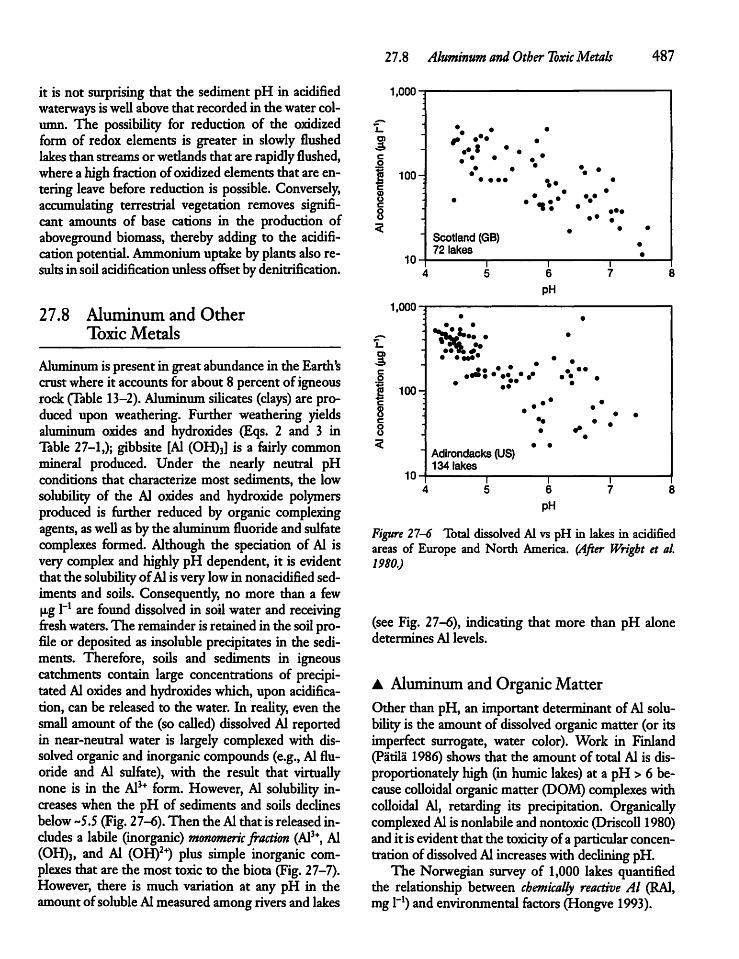
it is not surprising that the sediment pH in acidifiedwaterways iswell above that recorded in thewatercolumn. The possibility for reduction of the oxidizedform of redox elements is greater in slowly flushedlakes than streamsor wetlands that are rapidlyflushed,wherea high fraction ofoxidized elements that are entering leave before reduction is possible. Conversely,accumulating terrestrial vegetation removes significant amounts of base cations in the production ofaboveground biomass, thereby adding to the acidificationpotential. Ammonium uptake byplantsalsoresultsin soilacidification unlessoffsetbydenitrification.
27.8 Aluminum and OtherToxic Metals
Aluminum is present in great abundance in the Earth'scrustwhere it accountsfor about 8 percent of igneousrock (Table 13-2). Aluminum silicates (clays) are produced upon weathering. Further weathering yieldsaluminum oxides and hydroxides (Eqs. 2 and 3 inTable 27-1,); gibbsite [Al (OH)3] is a fairly commonmineral produced. Under the nearly neutral pHconditions that characterize most sediments, the lowsolubility of the Al oxides and hydroxide polymersproduced is further reduced by organic complexingagents, aswellas by the aluminumfluorideand sulfatecomplexes formed. Although the speciation of Al isvery complex and highly pH dependent, it is evidentthat the solubilityofAlisverylowin nonacidified sediments and soils. Consequently, no more than a few|xg l-1 are found dissolved in soil water and receivingfresh waters. The remainder isretainedin the soilprofile or deposited as insoluble precipitates in the sediments. Therefore, soils and sediments in igneouscatchments contain large concentrations of precipitatedAloxides and hydroxides which, upon acidification, can be released to the water. In reality, even thesmall amount of the (socalled) dissolved Al reportedin near-neutral water is largely complexed with dissolved organicand inorganic compounds (e.g., Al fluoride and Al sulfate), with the result that virtuallynone is in the Al3+ form. However, Al solubility increases when the pH of sediments and soils declinesbelow ~5.5 (Fig. 27-6).Then theAlthat isreleased includes a labile (inorganic) monomelicfraction (Al3+, Al(OH)3, and Al (OH)24) plus simple inorganic complexes that are the most toxic to the biota(Fig. 27-7).However, there is much variation at any pH in theamountofsolubleAlmeasured amongrivers and lakes
27.8 Aluminum and Other ToxicMetals 487
1,000-
co
| 100-c<DUc
10
1,000
| 100-:
10
••I
Scotland (GB)72 lakes
!*•**•• •>Sfe•• • •
Adlrondacks (US)134 lakes
%•
T"6
PH
• • •
6
pH
Figure 27-6 Total dissolved Al vs pH in lakes in acidifiedareas of Europe and North America. (After Wright et al.1980.)
(see Fig. 27-6), indicating that more than pH alonedetermines Al levels.
A Aluminum andOrganic MatterOther than pH, an important determinant of Al solubility is the amountof dissolved organic matter (or itsimperfect surrogate, water color). Work in Finland(Patila 1986) shows that the amount of total Al is disproportionately high (in humic lakes) at a pH > 6 because colloidal organic matter (DOM)complexes withcolloidal Al, retarding its precipitation. Organicallycomplexed Alis nonlabileand nontoxic (Driscoll 1980)andit is evidentthat the toxicity of a particular concentrationof dissolved Alincreases withdeclining pH.The Norwegian survey of 1,000 lakes quantified
the relationship between chemically reactive Al (RA1,mg l"1) and environmental factors (Hongve 1993).
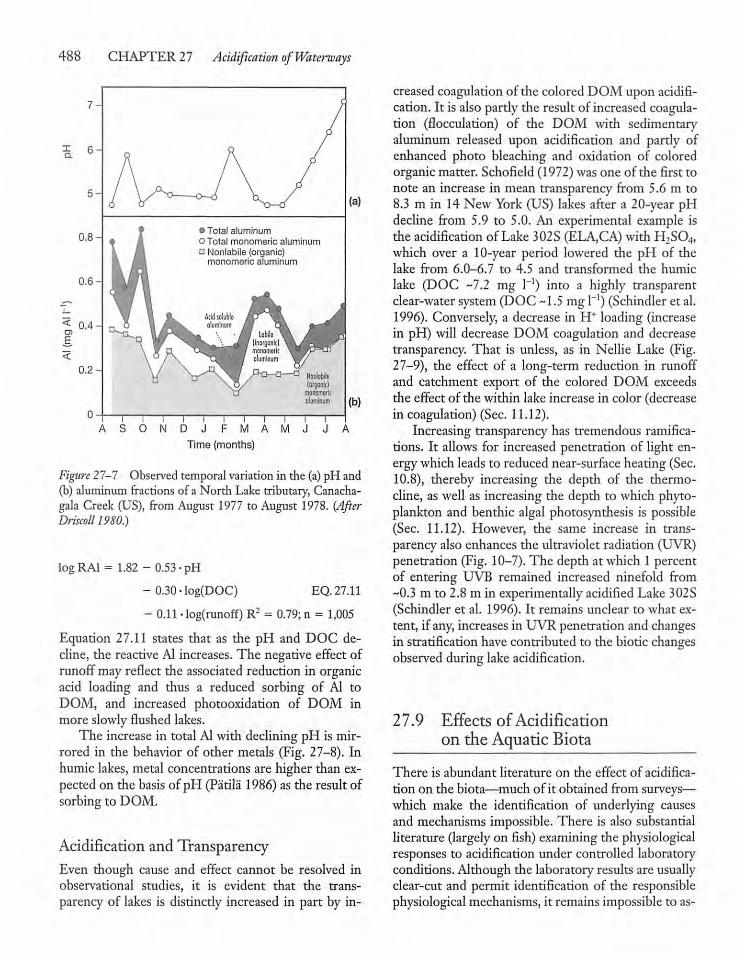
488 CHAPTER 27 Acidification ofWaterways
Xo.
• Total aluminumo Total monomeric aluminum- Nonlabile (organic)monomeric aluminum
ASONDJ FMA
Time (months)
Figure 27-7 Observed temporal variation in die (a)pH and(b) aluminum fractions of a North Lake tributary, Canacha-gala Creek (US), from August 1977 to August 1978. (AfterDriscoll1980.)
log RA1 = 1.82 - 0.53 •pH
- 0.30 • log(DOC) EQ. 27.11
- 0.11 •log(runoff) R2 = 0.79; n = 1,005
Equation 27.11 states that as the pH and DOC decline, the reactive Al increases. The negative effect ofrunoffmay reflect the associated reduction in organicacid loading and thus a reduced sorbing of Al toDOM, and increased photooxidation of DOM inmore slowly flushed lakes.The increase in total Alwith declining pH is mir
rored in the behavior of other metals (Fig. 27-8). Inhumic lakes, metal concentrations are higher than expected on the basis of pH (Patila 1986) as the result ofsorbing to DOM.
Acidification and TransparencyEven though cause and effect cannot be resolved inobservational studies, it is evident that the transparency of lakes is distinctly increased in part by in
creased coagulation of the colored DOM upon acidification. It is also partly the result of increased coagulation (flocculation) of the DOM with sedimentaryaluminum released upon acidification and pardy ofenhanced photo bleaching and oxidation of coloredorganic matter. Schofield (1972)was one of the first tonote an increase in mean transparency from 5.6 m to8.3 m in 14 New York (US) lakes after a 20-year pHdecline from 5.9 to 5.0. An experimental example isthe acidification of Lake 302S (ELA,CA) with H2S04,which over a 10-year period lowered the pH of thelake from 6.0-6.7 to 4.5 and transformed the humiclake (DOC -7.2 mg 1_1) into a highly transparentclear-water system (DOC~1.5 mg1_1) (Schindler et al.1996). Conversely, a decrease in H+ loading (increasein pH) will decrease DOM coagulation and decreasetransparency. That is unless, as in Nellie Lake (Fig.27-9), the effect of a long-term reduction in runoffand catchment export of the colored DOM exceedsthe effect of the within lake increase in color (decreasein coagulation) (Sec. 11.12).Increasing transparency has tremendous ramifica
tions. It allows for increased penetration of light energywhich leads to reduced near-surface heating (Sec.10.8), thereby increasing the depth of the thermo-cline, as well as increasing the depth to which phytoplankton and benthic algal photosyndiesis is possible(Sec. 11.12). However, the same increase in transparency also enhances the ultraviolet radiation (UVR)penetration (Fig. 10-7). The depth at which 1 percentof entering UVB remained increased ninefold from~0.3 m to 2.8 m in experimentally acidified Lake 302S(Schindler et al. 1996). It remains unclear to what extent, if any, increasesin UVR penetration and changesin stratification have contributed to the biotic changesobserved during lake acidification.
27.9 Effects ofAcidificationon the Aquatic Biota
There is abundant literature on the effect of acidification on the biota—muchof it obtained from surveys—which make the identification of underlying causesand mechanisms impossible. There is also substantialliterature (largely on fish) examining the physiologicalresponses to acidification under controlled laboratoryconditions. Although the laboratory results are usuallyclear-cut and permit identification of the responsiblephysiological mechanisms, it remains impossible to as-
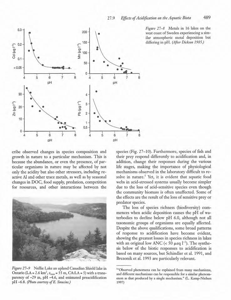
0.3-1
0.2-
' 0.1-
< 0.05 -
27.9 Effects ofAcidification on the Aquatic Biota 489
200-\ °
_ 150-
«- 100-c
2
• \
o
50-•
•
,**«I \ I
Figure 27-8 Metals in 16 lakes on thewest coast of Sweden experiencing a similar atmospheric metal deposition butdiffering in pH. (After Dickson 1985.)
cribe observed changes in species composition andgrowth in nature to a particular mechanism. This isbecause the abundance, or even the presence, of particular organisms in nature may be affected by notonly the acidity but also other stressors, including reactiveAl and other trace metals, as well as by seasonalchanges in DOC, food supply, predation, competitionfor resources, and other interactions between the
species (Fig. 27-10). Furthermore, species offish andtheir prey respond differendy to acidification and, inaddition, change their responses during the variouslife stages, making the importance of physiologicalmechanisms observed in the laboratory difficult to resolve in nature.' Yet, it is evident that aquatic foodwebs in acid-stressed systems usually become simplerdue to the loss of acid-sensitive species even thoughthe community biomass is often unaffected. Some ofthe effects are the result of the loss of sensitive prey orpredator species.The loss of species richness (biodiversity) com
mences when acidic deposition causes the pH of waterbodies to decline below pH 6.0, although not alltaxonomic groups of organisms are equally affected.Despite the above qualifications, some broad patternsof response to acidification have become evident,showing the greatest losses in species richness in lakeswith an original low ANC (< 50 jxeq l-1). The synthesis below of the biotic responses to acidification isbased on many sources, but Schindler et al. 1991, andBrezoniket al. 1993 are particularly relevant.
Figure 27-9 Nellie Lake an upland CanadianShield lakeinOntario (LA=2.6 km2, zmax = 55m, CA:LA= 5)with a transparency of ~29 m, pH ~4.6, and estimated preacidificationpH ~6.8. (Photo courtesy ofE. Snucins.)
5"Observed phenomena can be explained from many mechanisms,and different mechanisms can be responsible for a similarphenomenon as that produced by a single mechanism." (L. Kamp-Nielsen1997)
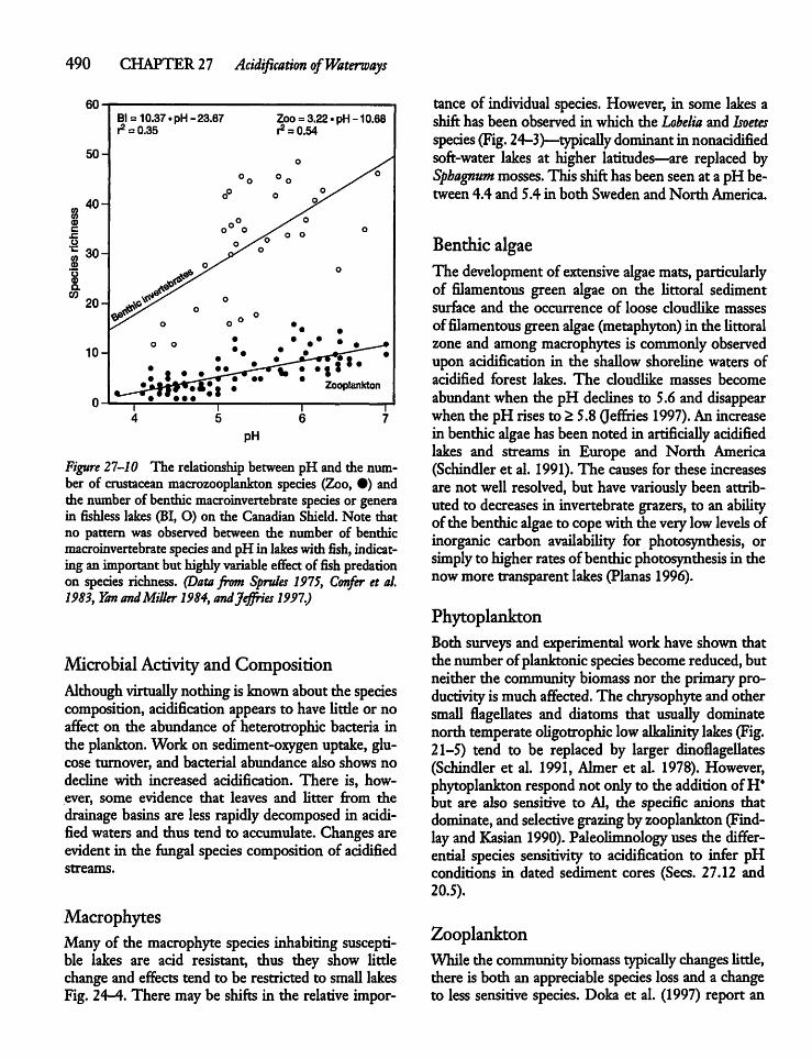
490 CHAPTER 27 Acidification ofWaterways
60-
50-
40-
30-
o©a
20-
10-
Bl = 10.37. pH-23.67^ =0.35
Zoo o 3.22 .pH-10.68^ = 0.54
Figure 27-10 The relationship between pH and the number of crustacean macrozooplankton species (Zoo, •) andthe number of benthic macroinvertebrate species or generain fishless lakes (BI, O) on the Canadian Shield. Note thatno pattern was observed between the number of benthicmacroinvertebrate species and pH in lakes withfish, indicating an important but highlyvariableeffectof fishpredationon species richness. (Data from Sprules 1975, Confer et al.1983, Yon andMiller 1984,andJeffries 1997.)
Microbial Activity andCompositionAlthough virtually nothing is knownabout the speciescomposition, acidification appears to have little or noaffect on the abundance of heterotrophic bacteria inthe plankton. Work on sediment-oxygen uptake, glucose turnover, and bacterial abundance also shows nodecline with increased acidification. There is, however, some evidence that leaves and Utter from thedrainage basins are less rapidly decomposed in acidifiedwaters and thus tend to accumulate. Changesareevident in the fungal species composition of acidifiedstreams.
MacrophytesMany of the macrophyte species inhabiting susceptible lakes are acid resistant, thus they show littlechangeand effects tend to be restricted to smalllakesFig. 24-4. There may be shifts in the relative impor
tance of individual species. However, in some lakes ashift has been observed in which the Lobelia and Isoetesspecies (Fig.24-3)—typically dominantin nonacidifiedsoft-water lakes at higher latitudes—are replaced bySphagnum mosses. This shifthasbeenseenat a pH between 4.4 and 5.4 in both Sweden and North America.
Benthic algaeThe development of extensive algae mats, particularlyof filamentous green algae on the Httoral sedimentsurface and the occurrence of loose cloudlike massesof filamentous green algae(metaphyton) in the littoralzone and amongmacrophytes is commonly observedupon acidification in the shallow shoreline waters ofacidified forest lakes. The cloudlike masses becomeabundant when the pH declines to 5.6 and disappearwhen the pH rises to > 5.8 (Jeffries 1997). An increasein benthicalgae hasbeennoted in artificially acidifiedlakes and streams in Europe and North America(Schindler et al. 1991). The causes for these increasesare not well resolved, but havevariously been attributed to decreases in invertebrate grazers, to an abilityof the benthic algaeto copewith the very lowlevels ofinorganic carbon availability for photosynthesis, orsimplyto higher rates of benthic photosynthesis in thenowmore transparent lakes(Planas1996).
PhytoplanktonBoth surveys and experimental work have shown thatthe numberof planktonic species becomereduced,butneither the communitybiomass nor the primary productivity is much affected. The chrysophyte and othersmall flagellates and diatoms that usually dominatenorth temperateoligotrophiclowalkalinity lakes (Fig.21-5) tend to be replaced by larger dinoflagellates(Schindler et al. 1991, Aimer et al. 1978). However,phytoplankton respondnot only to the additionof H+but are also sensitive to Al, the specific anions thatdominate,and selective grazingbyzooplankton(Find-layandKasian 1990). Paleolimnology uses the differential species sensitivity to acidification to infer pHconditions in dated sediment cores (Sees. 27.12 and20.5).
ZooplanktonWhile the communitybiomass typically changeslittle,there is both an appreciable species loss and a changeto less sensitive species. Doka et al. (1997) report an
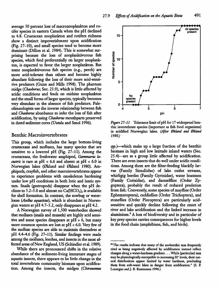
27.9 Effects ofAcidification on theAquatic Biota 491
average 50percent loss ofmacrozooplankton and rotiferspecies in eastern Canada when the pH declinedto 4.8. Crustacean zooplankton and rotifers richnessshow a distinct impoverishment upon acidification(Fig. 27-10), and small species tend to become moredominant (Dillon et al. 1984). This is somewhat surprising because the loss of zooplanktivorous fishspecies, which feed preferentially on larger zooplankton, is expected to favor the larger zooplankton. Butsome zooplanktivorous fish species (e.g., perch) aremore acid-tolerant than others and become highlyabundant following the loss of their more acid-sensitive predators (Gunn and Mills 1998). The phantommidge {Chaoborus-, Sec. 23.9), whichis littleaffected byacidic conditions and feeds on midsize zooplanktonand the smallformsof largerspecies, typically becomesvery abundant in the absence of fish predators. Pale-olimnologists use the inverse relationship between fishand Chaoborus abunbance to infer the loss of fish afteracidification, byusingChaoborusmouthparts preservedin dated sediment cores (Uutala and Smol 1996).
Benthic Macroinvertebrates
This group, which includes the large bottom-livingcrustaceans and molluscs, has many species that aresensitive to a lowered pH (Fig. 27-11). Among thecrustaceans, the freshwater amphipod, Gammarus la-custris is rare at pH < 6.6 and absent at pH < 6.0 inNorwegian lakes (0kland and 0kland 1980). Am-phipods, crayfish, andothermacroinvertebrates appearto experience problems with exoskeleton hardeningunder low pH conditions in both lotic and lentic system. Snails (gastropods) disappear when the pH declinesto 5.2-5.0 and almost no Ca(HC03)2 is availablefor shell formation. In contrast, the sowbug or water-louse (Asellus aquaticus), which is abundant in Norwegianwatersat pH 4.7-5.2, onlydisappears at pH 4.2.A Norwegian surveyof 1,500waterbodies showed
thatmolluscs (snails andmussels) are highly acid sensitive and some species disappears at pH > 6, but manymore commonspecies are lost at pH < 6.0.Veryfewofthe mollusc species are able to maintain themselves atpH 4.4-4.6 (Fig. 27-11). Similar findings were madeamongthe molluscs, leeches, and insectsin the most affected areas ofNewEngland, US(Schindler et al. 1989).While there are pronounced shifts in the relative
abundance of the sediment-living immature stages ofaquaticinsects, there appearsto be little changein thetotal invertebrate communitybiomass upon acidification. Among the insects, the midges (Chironomus
Figure 27-11 Tolerance limitofpH for 17widespread benthic invertebrate species (important as fish food organisms)in acidified Norwegian lakes. (After Okland and Qkland1980.)
spp.)—which make up a large fraction of the benthicbiomass in high and low latitude inlandwaters (Sec.25.4)—are as a group little affected by acidification.There are even insects that do well under acidic conditions.Amongthem are the filter-feeding blackfly larvae (Family Simuliidae) of lake outlet streams,whirligig beetles (Family Gyrinidae), water boatmen(Family Corixidae), and damselflies (Order Zy-goptera), probably the result of reduced predationfromfish. Conversely, somespecies ofmayflies (OrderEphemeroptera),caddisflies (Order Trichoptera), andstoneflies (Order Plecoptera) are particularly acid-sensitive and quickly decline following the onset ofriver and lake acidification and the linked increase inaluminium.6 Aloss ofbiodiversity and in particular ofkeypreyspecies carriesconsequences for higher levelsin the food chain (amphibians, fish, and birds).
'"The results indicate thatmany of the zoobenthic taxa frequentlycited as being negatively affected by acidification instead reflectchanges alongawater-hardness gradient... While [particular] taxamaybe physiologically susceptibleto increasingH*levels,their natural distributions appear limited by water hardness, precludingthem from soft-water lakes in danger from acidification." (S. P.LonerganandJ. B. Rasmussen 1996.)
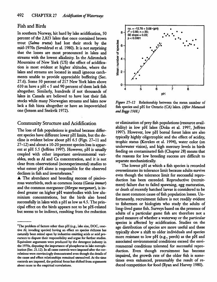
492 CHAPTER 27 Acidification ofWaterways
Fish and Birds
In southernNorway, hit hard by lake acidification, 50percent of the 2,823 lakes that once contained browntrout {Salmo trutta) had lost their stock by themid-1970s (Sevaldrud et al. 1980). It isnot surprisingthat the losses are most pronounced in lakes andstreams with the lowest alkalinity. In the AdirondackMountains of New York (US) the effect of acidification is most evident at higher altitudes, where thelakes and streams are located in small igneous catchments unable to provide appreciable buffering (Sec.27.6). Some 50 percent of 217 New Yorklakes above610m have a pH <5 and 90 percentof themlackfishaltogether. Similarly, hundreds if not thousands oflakes in Canada are believed to have lost their fishstocks while manyNorwegian streams and lakes nowlacka fish biota altogether or have an impoverishedone (Jensen and Snekvik 1972).
Community Structure andAcidificationThe loss of fish populations is gradual because different species havedifferentlowerpH limits, but the decline is evident below aboutpH 6.5 (Figs. 27-11 and27-12)andabouta 10-20 percentspecies loss isapparent at pH 5.5 (Jeffries 1997). However, pH is usuallycoupled with other important environmental variables, such as Al and Ca concentration, and it is notclearfromobservational (nonexperimental) studies towhat extent pH alone is responsible for the observeddeclines in fish and invertebrates.7A The abundance and breeding success of piscivorous waterbirds, such as common loons {Gavia immer)and the common merganser {Mergusmerganser), is indeed greater on higher pH waterbodies with lowaluminium concentrations, but the birds also breedsuccessfully in lakeswith a pH as lowas4.5.The principaleffecton the birds appearsnot to be pH-relatedbut seems to be indirect, resulting from the reduction
7The problem of factors other than pH(e.g., lake size, DOC, reactive Al, invading species) having an effect on species richness hasnaturally been seizedupon by industriesemitting acids or acidprecursors to dispute their responsibilityand argue for further studies.Equivalentargumentswere producedby the detergent industry inthe 1970s, disputing the importance of phosphorusin lakeeutroph-ication(Sec. 21.12). In allcases controlswere imposedafterthe correlations wereconvincingly demonstrated eventhoughthe details ofthe cause and effect relationships remainedunresolved.At the timecontrolsareimposed, the political focus hasshifted fromargumentsaboutcause to the empirical correlations.
8-
8 6-Q.w
% 4-E3C
C
| 2-
no. =-12.76 +3.08 »(pH) •r2 =0.92;n =20;SEslope=0.22; V. "p<0.0001 *
pH
Figure 27-12 Relationship between the mean number offish species and pH for Ontario (CA) lakes. (AfterMatuszekandBeggs 1988.)
or eliminationof prey fishpopulations(resourceavailability) in low pH lakes (Doka et al. 1997, Jeffries1997). However, low pH boreal forest lakes are alsotypically highlyoligotrophic and the effectof acidity,trophic status (Kerekes et al. 1994), water color (onunderwater vision), and high mercury levels in birdsfeeding on contaminated fish (Chapter28)means thatthe reasons for low breeding success are difficult toseparatemechanistically. .The lowestpH at which a fish species is recorded
overestimates its tolerance limit because adults surviveeven though the tolerance limit for successful reproduction has been exceeded. Reproductive (recruitment) failure due to failed spawning, eggmaturation,or death of recently hatched larvaeis considered to bethe most common causeoffish population losses. Unfortunately, recruitment failure is not readily evidentto fishermen or biologists who study the adults oflong-lived gamefish. Surveys basedon the presenceofadults of a particular game fish are therefore not agoodmeasure of whether a waterwayor the particularspecies is affected by acidification. Studies on theage distribution of species are more useful and thesetypically show a shift to older individuals and speciesmore resistant to low pH (e.g., perch) as the pH andassociated environmental conditions exceed the environmental conditions tolerated for successful reproduction. Even though recruitment has becomeimpaired, the growth rate of the older fish is sometimes even enhanced, presumably the result of reducedcompetition for food (RyanandHarvey 1980).
Interpretations of species losses are further confounded bysummer pH levels highenoughto suggestthat factors other than acidification are responsible forthe observed changes, whereas the possibility ofepisodic (periodic) acidification during the springmeltof highlyacidicsnow, or much lowerpH during periodic heavy summer rains is overlooked (Fig. 27-7).Short-term exposure to a sharply lowered pH duringthe snow-melt period may expose eggs and larvae toacutely toxic concentrations of H+or metals at a timewhenlittle or no sampling is beingdone.Low pH watersnormallyhave high Al concentra
tions (Fig. 27-6), of which the reactive monomericfractions are particularly toxic. Much of the aluminumis derived from the catchments, but additional Al is released by sediments. Thus, the experimental acidification of streams (but not their catchments) with H2S04to apH ofabout4 isfollowed bya substantial release ofAlto die water (Henriksenet al. 1988). Unfortunately,the toxiceffectofAl (and other metals)observedin thelaboratory(Parkhurstet al. 1990) is confounded in nature byits correlation withH+, the availability and uptake of calcium, and the normal lack of informationabout the extent that the measured elevated levels ofdissolved Al were in a labile and toxic monomericform, rather than sorbed to DOC and nonlabile.
A 27.10 Modeling the AcidificationProcess
A variety of models have been developed, rangingfrom simple empirical onesto complex dynamic models that consider catchmentweatheringprocesses andthe chemical equilibria determining the ANC of receiving waters. Elaborate process-orientedmodelsareappropriate for well-studied catchments and aquaticsystems forwhich mostof thenecessary information isavailable (Reusset al. 1986).
Mechanistic andEmpirical ModelsProbably themostinfluential of the process-based analytical models usedtodayisMAGIC (Model ofAcidification of Groundwater In Catchments). It is asimple mechanistic simulation model based on amathematical representation of a small number ofwhat are considered to be keyphysical and chemicalprocesses controlling the equilibrium between majordissolved and adsorbed ions in soils andwaterquality.The moderate datarequirements make it easy to apply
27.10 Modeling theAcidification Process 493
in comparison with more complex (comprehensive)models, but at the inevitable risk of overlooking important processes. Simulationmodelingis used to predict changes in the surface-water quality responsetime to changes in atmosphere precipitation. Impressively, predictions made by Cosby et al. (1985) concerning the time required for acidification and therecovery of different soil types in well-characterizedcatchments are qualitatively closeto what is being observed 20yearslater.Unfortunately, the processes dominating particu
lar catchments are generally unknown and the mostuseful predictive model is a semiempirical model developed by Henriksen (1980). It focuses on measuredalkalinity changes below the waterline rather than, asin MAGIC and other process models, on the catchment and sediment processes that produce the observed alkalinity. The Henriksen model has beenrefined (Wright 1983a, Henriksen and Brakke 1988),but as the model's underlying ideas and its utility areequally evident from the simpler original version itwillbe brieflydiscussed.Henriksen (1980) visualized the acidification
process asone in whichthe alkalinity of awaterbodyistitrated by strong acid (H2S04) deposited on the surface. He used alkalinity (ANC) as an integrator andindicator of the unexamined catchment processesthat are responsible for most of the observed buffercapacity of inlandwaters.The titration with acid of awholeaquatic system in nature resembles the titrationof a Ca(HC03)2 solutionin a beaker, a procedure usedto determine the alkalinity of inland waters (Fig.27-13 and Sec. 14.4).The Henriksen model uses the term acidification
in a special sense bydefining it by the change in alkalinity (ANC).
acidification= preacidification alkalinity (ANQ)- present alkalinity (ANC).
Very few preacidification alkalinities are availableand it is assumed that there is an electron neutrality(ion balance). Simplifying the most critical componentsof the cation-anion balance, it is possible to conclude that:
2[Ca2+]* + 2[Mg2]* = [HC03"] - [H+] EQ. 27.12
the units are in u,eq l"1 and the asterisk (*) indicatesthe nonmarine derived concentrations. Therefore:
ANCq = [Ca2+ + Mg*+]* EQ.27.13
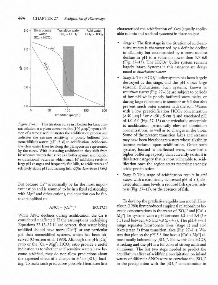
494 CHAPTER 27 Acidification ofWaterways
8.0 Bicarbonate Transition water Acid waterwater S04»HC03 S04 > HC03
S04 < HC03
50 100 150
H+ added (ueq I"1)200
Figure 27-13 This titration curve in a beaker for bicarbonate solution at a givenconcentration (100 u.eq/1) upon addition of a strong acid illustrates the acidification process andindicates the extreme sensitivity of poorly buffered (butnonacidified) waters (pH -5-6) to acidification. Acid-sensitive clear-water lakes lie alongthe pH spectrum representedby the curve. With increasing acidification they shift frombicarbonatewaters that serveas a bufferagainst acidificationto transitional waters in which small H+ additions result inlargepH changesand frequendy fish kills, to acidicwatersofrelatively stable pH and lacking fish. (After Henriksen 1980.)
But because Ca2+ is normally by far the most important cation and is assumed to be in a fixed relationshipwith Mg2* and other cations, the equation can be further simplified to:
ANC0 = [Ca2+]* EQ. 27.14
While ANC declines during acidification the Ca isconsidered unaffected. If the assumptions underlyingEquations 27.12-27.14 are correct, then water beingacidified should have more [Ca2+]* at any particularpH than nonacidified systems, which has been observed (Overrein et al. 1980). Although the pH: [Ca]'ratio or the [Ca +Mg]": HCO3 ratio provide a usefulindication as to whether acid sensitive waters have become acidified, they do not allow predictions aboutthe expected effect of a change in H+ or [S04]' loading. Tomakesuch predictions possible Henriksen first
characterized the acidification oflakes (equally applicable to lotic andwedand systems) in three stages:
• Stage 1:The first stage in the titration of acid-sensitivewaters is characterized by a definite declinein alkalinity but accompanied by a more modestdecline in pH to a value no lower than 5.5-6.0(Fig. 27-13). The HCO3- buffer system remainslargely intact. Systems in this category are designated as bicarbonate waters.
• Stage 2:The HC03~ buffersystemhasbeen largelydestroyed at this stage, and the pH shows largeseasonal fluctuations. Such systems, known astransition waters (Fig. 27-13) are subject to periodsof low pH while poorly buffered snow melts, orduring large rainstorms in summer or fall that alsoprevent much water contact with the soil. Waterswith a low preacidification HCO3 concentration(< 50 u,eq l"1 or <-50 p-S cm-1) and associated pHof 5.0-6.0 (Fig. 27-13) are particularly susceptibleto acidification, periodically elevated aluminiumconcentrations, as well as to changes in the biota.Some of the present transition lakes and streamsmayhave beenbicarbonate waters whose alkalinitybecame reduced upon acidification. Other suchsystems, located in unaffected areas, never had ahigher bufferingcapacitythan currently exists; it isthis latter category that is most vulnerable to acidification once the region starts receiving stronglyacidicprecipitation.
• Stage 3: This stage of acidification results in acidwaterswith a chronically depressed pH of < 5, elevatedaluminium levels, a reduced fishspecies richness (Fig. 27-12), or the absenceoffish.
To develop the predictiveequilibriummodelHenriksen(1980) firstproduced empirical relationships between concentrations in the water of [SO4]* and [Ca* +Mg*] for systems with a pH between 5.2 and 5.4 (x=5.3)and between4.6 and 4.8 (x=4.7).The pH 4.7-5.3range separates bicarbonate lakes (stage 1) and acidlakes (stage 3) from transition lakes (Fig. 27-14). Waters that plot on the pH 5.3 line have a [Ca* +Mg*] almost totally balanced by [S04]*. Below this line HC03is lacking and the pH is a function of strong acids andaluminum. The last two steps needed to predict theequilibrium effect of acidifyingprecipitation on inlandwaters of different ANCs were to correlate the [S04]*in the precipitation with the [S04]* concentration in
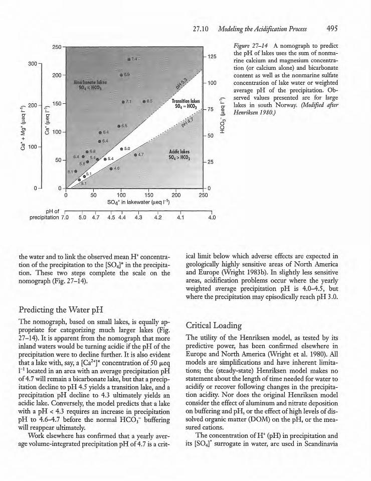
300-i
200-
D)
+
Q 100-
o-
250
100 150 200
SO4* in lakewater (ueq I"1)
27.10 Modeling the Acidification Process 495
-125
-100
. — 75
-50
-25
crID3,'«OOX
Figure 27-14 A nomograph to predictthe pH of lakes uses the sum of nonma-rine calcium and magnesium concentration (or calcium alone) and bicarbonatecontent as well as the nonmarine sulfateconcentration of lake water or weightedaverage pH of the precipitation. Observed values presented are for largelakes in south Norway. (Modified afterHenriksen 1980.)
pHof —i 1 1—i r~precipitation 7.0 5.0 4.7 4.5 4.4 4.3 4.2 4.1 4.0
the water and to link the observed mean H+ concentration of the precipitation to the [SO4]* in the precipitation. These two steps complete the scale on thenomograph (Fig. 27-14).
Predicting the Water pHThe nomograph, based on small lakes, is equally appropriate for categorizing much larger lakes (Fig.27-14). It is apparent from the nomograph that moreinlandwaterswould be turning acidic if the pH of theprecipitation were to decline further. It is also evidentthat a lake with, say, a [Ca2+]* concentration of50 u,eq1_1 located inan area with an average precipitation pHof4.7will remain a bicarbonate lake,but that a precipitation decline to pH 4.5 yields a transition lake, and aprecipitation pH decline to 4.3 ultimately yields anacidic lake. Conversely, the model predicts that a lakewith a pH < 4.3 requires an increase in precipitationpH to 4.6-4.7 before the normal HC03~ bufferingwillreappear ultimately.Work elsewhere has confirmed that a yearly aver
agevolume-integrated precipitation pH of4.7 is a crit
ical limit belowwhich adverse effects are expected ingeologically highly sensitive areas of North Americaand Europe (Wright 1983b). In slighdy less sensitiveareas, acidification problems occur where the yearlyweighted average precipitation pH is 4.0-4.5, butwhere the precipitationmayepisodically reach pH 3.0.
Critical LoadingThe utility of the Henriksen model, as tested by itspredictive power, has been confirmed elsewhere inEurope and North America (Wright et al. 1980). Allmodels are simplifications and have inherent limitations; the (steady-state) Henriksen model makes nostatement about the length of time needed for water toacidify or recover following changes in the precipitation acidity. Nor does the original Henriksen modelconsider the effect of aluminum and nitrate depositionon buffering and pH, or the effectof high levels of dissolved organicmatter (DOM) on the pH, or the measured cations.The concentration ofH+ (pH) in precipitation and
its [S04]* surrogate in water, are used in Scandinavia
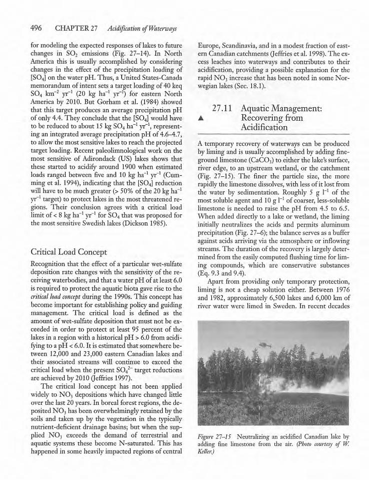
496 CHAPTER 27 Acidification ofWaterways
for modeling the expected responses of lakes to futurechanges in S02 emissions (Fig. 27-14). In NorthAmerica this is usually accomplished by consideringchanges in the effect of the precipitation loading of[S04] on the water pH. Thus, a United States-Canadamemorandum of intent sets a target loading of 40 keqS04 km-2 yr-1 (20 kg ha-1 yr-1) for eastern NorthAmerica by 2010. But Gorham et al. (1984) showedthat this target produces an average precipitation pHof only 4.4. They conclude that the [S04] would haveto be reduced to about 15 kgS04 ha"1 yr-1, representing an integrated average precipitation pH of 4.6-4.7,to allowthe most sensitive lakes to reach the projectedtarget loading. Recent paleolimnological work on themost sensitive of Adirondack (US) lakes shows thatthese started to acidify around 1900 when estimatedloads ranged between five and 10 kg ha-1 yr-1 (Cum-ming et al. 1994), indicating that the [SO4] reductionwill have to bemuch greater (> 50% of the 20kgha-1yr-1 target) to protectlakes in the most threatened regions. Their conclusion agrees with a critical loadlimit of<8 kg ha-1 yr-1 for S04 thatwas proposed forthe most sensitive Swedish lakes (Dickson 1985).
Critical Load ConceptRecognition that the effect of a particular wet-sulfatedeposition rate changes with the sensitivity of the receiving waterbodies, and that awater pH of at least6.0is required to protect the aquatic biota gaverise to thecritical load concept during the 1990s. This concept hasbecome important for establishing policy and guidingmanagement. The critical load is defined as theamount of wet-sulfate deposition that must not be exceeded in order to protect at least 95 percent of thelakes in a regionwith a historicalpH > 6.0 from acidifying to a pH <6.0. It is estimated that somewhere between 12,000 and 23,000 eastern Canadian lakes andtheir associated streams will continue to exceed thecritical load when the present S042" target reductionsare achieved by 2010 Qeffries 1997).The critical load concept has not been applied
widely to N03 depositions which have changed littleover the last 20 years. In boreal forest regions, the deposited N03 has been overwhelmingly retained by thesoils and taken up by the vegetation in the typicallynutrient-deficient drainage basins; but when the supplied N03 exceeds the demand of terrestrial andaquatic systems these become N-saturated. This hashappened in some heavily impacted regions of central
Europe, Scandinavia, and in a modest fraction of eastern Canadian catchments (Jeffries et al. 1998). The excess leaches into waterways and contributes to theiracidification, providing a possible explanation for therapid N03 increase that has been noted in someNorwegian lakes(Sec. 18.1).
27.11 AquaticManagement:A Recovering from
Acidification
A temporary recovery of waterways can be producedby limingand is usually accomplished by adding fine-ground limestone (CaC03) to either the lake'ssurface,river edge, to an upstream wedand, or the catchment(Fig. 27-15). The finer the particle size, the morerapidly the limestone dissolves, with lessof it lost fromthe water by sedimentation. Roughly 5 g 1 of themost soluble agent and 10g 1 of coarser, less-solublelimestone is needed to raise the pH from 4.5 to 6.5.When added directly to a lake or wedand, the liminginitially neutralizes the acids and permits aluminumprecipitation (Fig. 27-6); the balance serves as a bufferagainst acids arrivingvia the atmosphere or inflowingstreams.The duration of the recoveryis largelydetermined from the easily computed flushingtime for liming compounds, which are conservative substances(Eq. 9.3 and 9.4).Apart from providing only temporary protection,
liming is not a cheap solution either. Between 1976and 1982, approximately 6,500 lakes and 6,000 km ofriver water were limed in Sweden. In recent decades
Figure 27-15 Neutralizing an acidified Canadian lake byadding fine limestone from die air. (Photo courtesy of W.Keller.)
about 200,000 tonneshavebeen appliedeachyear at acost of $25 million (US). Although the cost is toogreat and the results too temporary—particularly inareas of high runoff (flushing)—to encourage widespread use, it isevident thatliming yields dramatic effects through a rapid rise in pH and decline ofaluminum, mercury, and othermetals following theirprecipitation from thewatercolumn (SMA 1982).
Liming and the BiotaThe effect of liming on the biota is less well-understood. The reasons for this include the generationtime oftheorganisms. Algae have a generation time ofdays and should beable to respond more rapidly to thechanged conditions than some macrozooplanktonwhich have generation times of weeks to a year ormore,or the benthic insectswith typically one generation per year at higher latitudes. Indeed, the numberof algal species increases relatively quickly upon limingandshifts fromacid-tolerant dinoflagellate species(Fig. 21-10) to a chrysophyte flagellate communitysimilar to that found in oligotrophic but nonacidifiedlakes (Fig. 21-10, Eriksson et al. 1983). Yet the rateofalgal change is less rapid than might be expected,whichmaybe the result of an overridingnutrient limitation, similar to that observed in nonacidified oligotrophic lakes. Furthermore, liming raises the pH andthe ANC beyondthe levels encountered in other sensitive but nonacidified lakes and therefore does notrepresent a return to the original conditions.The absence of a rapid and clear-cut community
response to liming is not onlythe resultof generationtime and nutrient considerations but is also attributable to other environmental changes that follow bothliming and a reduction in acidifying precipitation.These changes typically include reducedwater clarity(more color) (Sec. 27.8) resulting in a reducedmixingdepth (Sec. 11.7), therefore a reduction in the size ofthe euphoric zone, and a resulting reduction in benthic algae production. Another factor influencing thepostneutralization community composition is thechange in food-web structure following the renewedsuccessful reproduction of surviving piscivorous fishspecies. Their offspring directly and indirectly affectthe zooplankton and benthos (Gunn andMills 1998).The rate of recoveryafter limingor amajor reduc
tion in acidifying precipitation is a function of the dispersal ability and reproductive strategyofspecies. Therecovery is most rapid for algae, followed by zoo
27.12 The Future 497
plankton and most benthic invertebrates characterizedby a short (<, 1 yr) generation time. Yan et al. (1996)noted a full zooplankton recovery within 10 years inlimedlakes that hadbeen acidified to pH 5.7,but lakesthatwere strongly acidified (pH <, 4.5) andmetal-contaminated remained impoverished even after 15years.Finally, the recovery of large aquatic species (e.g.,molluscs, fish) that were extirpated is impossible unless a species innoculum survived elsewhere in thedrainage basin or theyarestocked. Afull biological recoverywill therefore greatly laga chemical recovery. Afinal factor influencing community recovery is thetimerequired for species thatwerelost duringacidification to invade a particular lakeor stream from outsidethe drainage basin (Henrikson andBrodin1995).A few experimental studies have explored the use
of inorganic fertilizer additions as an alternative toliming. The resulting increased removal of C02(H2C03) in photosynthesis raises the pH (Sec. 14.2)and the ANC. Davison et al. (1995) propose modestfertilization instead of limingfor producingneededalkalinity. Fertilization, theyargue, hasminimal effectson the community plus the advantage of moderatelyincreasing theproductivity of the typically highly oligotrophic lakes.
27.12 The Future
The long-termsolution to acidification is a major reduction in emissions of S02 and NOx; the magnitudeof this reduction in SOz can be predicted using theHenriksenmodel (Fig. 27-14).While much remains to be learned about the re
sponse of inland waters and their catchments to acidification, it has become abundandy clear that areduction in acid precursor emissions reduces the aciddeposition on drainage basins in much the same waythat a reductionin externalnutrient loadingultimatelyreduces lake eutrophication (Sec. 17.6). Direct evidence for the effect of emission controls on lakes hasbeen obtained by monitoring at Sudbury, Canada.The mining-smelting complex located there wasoncethe single-largest point sourceofS02 emissions in theworld; it has reduced its emissions in recent decadesbyabout 80percent to about 5 x 10s tons S02 yr-1.The local lakes haverecovered in stepwith this reduction (Keller andGunn 1995). For example, SwanLakehad a measured pH of 4.0 in 1977 which rose to 5.6within10years, whilethe water transparency declinedas the lake became more colored. The pH inferred
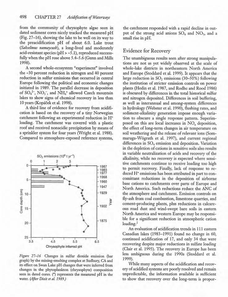
498 CHAPTER27 Acidification ofWaterways
from the community of chrysophyte algae seen indated sedimentcoresnicelytracked the measured pH(Fig.27-16), showing the lake to be well on its waytothe preacidification pH of about 6.0. Lake trout(Salvelinus namaycush), a long-lived and moderatelyacid-resistant species (pH > -5.1), reproduced successfully when the pH rose above5.4-5.6 (Gunn andMills1998).A second whole-ecosystem "experiment" involved
the ~30 percent reduction in nitrogen and 40 percentreduction in sulfur emissions that occurred in centralEurope following the political and economic changesinitiated in 1989.The parallel decrease in depositionof S042-, N03~, and NH4+ allowed Czech mountainlakes to show signs of chemical recovery in less than10years (Kopacek et al. 1998).A third line of evidence for recovery from acidifi
cation is based on the recovery of a tiny Norwegiancatchment following an experimental reduction in H+loading. The catchment was covered with a plasticroofand received nonacidic precipitation bymeans ofa sprinkler system for four years (Wright et al. 1988).Compared to atmosphere-exposed reference systems,
S02 emissions (106tyr1)0 12 3
4.5 5.5
Chrysophyte inferred pH6.5
Figure 27-16 Changes in sulfur dioxide emission (bargraph) bythe mining-smelting complex at Sudbury, CAandits effect on SwanLake pH changes that were inferred fromchanges in the phytoplankton (chrysophyte) compositionseen in dated cores. (*) represents the measured pH in thewater. (After Dixit etal. 1989.)
the catchment responded with a rapid decline in output of the strong acid anions S04 and N03, and asmall rise in pH.
Evidence for RecoveryThe unambiguous results seen after strong manipulations are not as yet widely observed at the scale ofwhole-lake districts in northeastern North Americaand Europe (Stoddard et al. 1999). It appears that thelarge reduction in S02 emissions (30-50%) followingthe institution of stricter emission controls on powerplants (Hedin et al. 1987, and Rodhe and Rood 1986)is obscured by differences in the total historical sulfurand nitrogen deposited. Differences in soil buffering,as well as interannual and among-system differencesin hydrology (Websteret al. 1990), flushing rates,andsediment-alkalinity generation impose enough variation to obscure a single response pattern. Superimposed on this are local increases in NOx deposition,the effectof long-term changes in air temperature onsoil weathering and the releaseof relevant ions (Som-maruga-Wograth et al. 1997), and current regionaldifferences in S04 emission and deposition.Variationin the depletion of cations in sensitive soils also resultsin variable neutralization of acids and recovery of thealkalinity, while no recovery is expected where sensitive catchments continue to receive loading too highto permit recovery. Finally, lack of response to reduced H+ emissions hasbeenattributed in part to concomittant reductions in the deposition of airbornebase cations to catchments over parts of Europe andNorth America. Such reductions reduce the ANC ofthe atmosphere and catchment. Emission controls onfly-ash from coal combustion, limestone quarries, andcement-producing plants, plus reductions in calcareous road dust and wind-swept bare soils in easternNorth America andwesternEurope maybe responsible for a significant reduction in atmospheric cationloading.2
An evaluation of acidification trends in 111 easternCanadian lakes (1983-1991) found no change in 60,continued acidification of 17, and only 34 that wererecovering despite major reductions in sulfate loading(Clair et al. 1995). The recovery in Europe has beenless ambiguous during the 1990s (Stoddard et al.1999).While manyaspectsof the acidification and recov
ery of acidified systemsare poorly resolvedand remainunpredictable, the information available is sufficientto show that recovery over the long-term is propor-
tionalto the reductionin emissions of acidprecursors.Unfortunately, there has been insufficient long-termfollow-up and acidification research funding has beenseverely reduced in most jurisdictions as prioritieshaveshifted to concern about the effects of projectedclimate change and toxic chemicals (Chapter 28)onhumans and the biota.8
Highlights• Acidification of the environmentby the deposition ofstrong acids or their precursors (S02, N03, N02) isdefined bya decrease ofthe acid neutralizing capacity(ANC) whichgready affects the chemistry and biotaof aquatic systems over large areas of northeasternNorth America, northern and central Europe, andelsewhere on a smallerspatialscale.
• The precipitationpH in industrialized nationsof Europe, North America andJapan has declined tenfoldto thirtyfoldduring the last century from a volume-integratedprecipitation pH of 5-6 to 4.1-4.7, but isnow slowly increasing in response to reduced S02emissions.
• Acid precursors emitted into the atmosphere aretransportedlongdistances beforedeposition.
• Inlandwaters mostsensitive to anthropogenic acidification have a lowANC(<50 u,eq I"1) andare locatedin smalldrainage basins underlainby (1)high insoluble bedrock and surface material derived from the
'"Research ontheeffect ofacid rain onwater quality isbeset bytwosevere problems: first is thepaucity ofdataandthe timeandmoneyrequired to obtain additional data; the second is the long, [years todecade] time scale of the responses that interest us." (B. J. Cosby etal. 1985)
27.12 The Future 499
same geology; (2) siliceous sand; or (3) a peat layerseparating the water from contact with the underlying soils.Aquaticsystems locatedin calcareous drainagebasinsand those containing some calcareous deposits areusuallywell-protected from acidifying precipitation.A fraction of acidified waters in affected areas is theresult of organic acids released from sphagnumbogsand organic-rich soils rather than anthropogenicemissions.The solubility of aluminum and trace metals in soilsand sediments increases systematically as the pH declines below ~5.5, with certain labile forms of aluminum most toxic to the biota.The biota varies in its sensitivity to acidification andlinked increases in reactive and toxic aluminum, butspecies richness declines predictably with a decliningpH below 6.0. Among the most sensitive groups arethe large bottom-living crustaceans and molluscs, aswellas certain fish species.While a temporaryrecoveryfromacidification canbeproduced by liming (CaC03 addition)—thereby increasing the ANC and pH—a long-term recovery iscontingentupon a reductionin emissions of acidprecursors, a reduction now underway in Europe andNorth America.Recovery over the long-term will be proportional toreductions in emission of acidprecursors, but the rateisa complex function ofmanyfactors, including catchment geology, soil buffering, the extent and durationof acidification, hydrology, temperature, microbial alkalinity-generation in the sediments, the generationtime oforganisms, andthe dispersal ability ofspecies.• Present loadingtargets in North America andEuropewould have to be reduced further to permit therecovery of thousands of the most sensitive lakes andassociated streams.
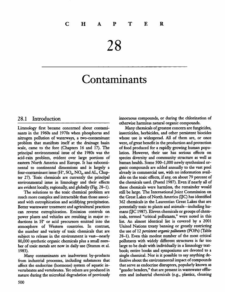
CHAPTER
28
Contaminants
28.1 Introduction
Limnology first became concerned about contaminants in the 1960s and 1970s when phosphorus andnitrogen pollution of waterways, a two-contaminantproblem that manifests itself at the drainage basinscale, came to the fore (Chapters 16 and 17). Theprincipal environmental issue of the 1980s was theacid-rain problem, evident over large portions ofeastern North America and Europe. It has subcontinental to continental dimensions and is largely afour-contaminant issue(H+, SO„ NOx,andAL,Chapter 27). Toxic chemicals are currently the principalenvironmental issue in limnology and their effectsare evidentlocally, regionally, and globally (Fig.28-1).The solutions to the toxic chemical problem are
much more complexand intractable than those associated with eutrophication and acidifying precipitation.Betterwastewater treatment and agricultural practicescan reverse eutrophication. Emission controls onpower plants and vehicles are resulting in major reductions in H+ or acid precursors emitted into theatmosphere of Western countries. In contrast,the number and variety of toxic chemicals that aresubject to release in the environment is vast—nearly80,000 syntheticorganicchemicals plus a small number of toxicmetals are now in dailyuse (Stumm et al.1983).Many contaminants are inadvertent by-products
from industrial processes, including substances thataffect the endocrine (hormone) system of aquatic invertebrates and vertebrates. Yetothers are produced innatureduringthe microbial degradation of previously500
innocuous compounds, or during the chlorination ofotherwise harmless natural organiccompounds.Manychemicals ofgreatestconcernare fungicides,
insecticides, herbicides, and other persistent biocideswhose use is widespread. All of them are, or oncewere, ofgreatbenefit in theproduction andprotectionof food produced for a rapidly growing humanpopulation. However, their use has serious effects onspecies diversity and community structure as well ashumanhealth. Some 500-1,000newlysynthesized organic compounds are added annually to the vast poolalready in commercial use,with no information availableon the toxiceffects, if any, on about 79percent ofthe chemicals used. (Postel 1987). Even if nearly all ofthese chemicals were harmless, the remainder wouldstill be large. The InternationalJoint Commission onthe Great Lakes of North America (TJC) has identified362 chemicals in the Laurentian Great Lakes that arepotentially toxic to plants and animals—including humans(IJC 1987). Elevenchemicals or groupsof chemicals, termed "critical pollutants," were noted in thislist. An almost identical list is covered by a 2001United Nations treaty banning or greatly restrictingtheuse of 12 persistent organicpollutants (POPs) (Table28-1). Even this modest number of the most criticalpollutants with widely different structures is far toolarge to be dealt withindividually in a limnology textbook; entire books and symposiums are devoted to asingle chemical. Nor is it possible to say anything definitive about the environmental impactof compoundsthat serveas endocrine disrupters, popularlyknown as"gender benders," thatarepresent inwastewater effluents and industrial chemicals (e.g., plastics, cleaning
SCALE TIME LAG
MillenniaGlobal
Continental Centuries
Regional
Local
1850 1950 1960 1970 1980 1990 2000
28.1 Introduction 501
Figure 28-1 Increasing speed of appearance and extent of new water quality problems. (Modified from Somlyody1995.)
Table 28-1 The 12 persistent organic pollutants to be banned or stricdy controlledworldwideby aUnited Nations treaty to be signed in 2001(*) and the 11"critical pollutants" on the International Joint Commission for the Laurentian Great Lakes "primarytrack," (A) selected on the basisoftheir chemical stabilityandresulting persistence, thequantityand type ofuse, the tendency to accumulate in organisms, andtheir toxicity.
Chemical
Dioxins (* A)
Furans (*A)
Benzo (a) pyrene (A)
DDT and itsbreakdownproducts, including DDE(* A)
Aldrin/Dieldrin (* A)
Productionand Release
Unintentional
Unintentional
Unintentional
Intentional
Intentional
Hexachlorobenzene (* A) Unintentional
Source
Polychlorinated dibenzo-dioxins (PCDDs; 75 congeners) andpolychlorinateddibenzo-furans (PCDFs; 135 congeners) arecreated in the manufacture of herbicides used in agricultureand forest management. Also produced as by-products duringthe combustion of chlorinated additives in fossil fuels and chlorine-containing medical and municipalwastes such as plastics,through production of pentachlorophenol (PCP)wood preservative, and in pulp and paper production processes that usechlorine to bleach wood and pulp. Some congeners are highlytoxic (see Fig.28-2); most have low acute toxicity.
Product of the incomplete combustion of fossil fuels and wood,including forest fires, auto exhaust, and waste incineration.One of a large family of polycyclic aromatic hydrocarbons(PAHs).
Insecticide used primarily for mosquito control in tropical areas.Sedimenthalf-life of DDT is -10-15 years at temperate latitudes.
Insecticide used extensively,especially on fruit and for termitecontrol.Half-life in soil is about fiveyears. Aldrin rapidlydegrades to dieldrin.
HCB is a by-product of the combustion of fuels that containchlorinated additives, incineration of wastes that contain chlorinated substances, and inmanufacturing processes using chlorine. Foundas a contaminantinchlorinatedpesticides (half-lifein nature -3-6 yrs).
(continued)
502 CHAPTER 28 Contaminants
Table 28-1 (continued)
ProductionChemical and Release Source
Alkylated lead (A) Intentional Used as a fuel additive and in solder, pipes, and paint.Unintentional Released through combustion of leaded fuel, wastes, cigarettes,
as well as from pipes, paint cans, and paint chips.Mirex (* A) Intentional Fire retardant and pesticide used to control fire ants. Breaks
down to a more toxic form, photomirex, in the presence of sunlight. Present sources are residuals from manufacturing sites,spills, and disposal in landfills. Highly persistent with a half-lifeup to 10 years.
Mercury (A) Intentional Used in metallurgy.Unintentional By-product locallyand regionally of chlor-alkali, paint, electrical
equipment manufacturing processes, refuse incineration, andcoal combustion.
Polychlorinated Intentional PCBs used as insulating fluids in electrical capacitors and transbiphenyls (* A) formers, and in the production of hydraulic fluids and lubri
cants. Additives in paint, carbon-copy paper, and plastics.Once used as a vehicle for pesticide dispersal; 209 congenersvarying greatly in toxicity. Half-life is from weeks to years.
Unintentional Primarily released to the environment through leakage, spills, andwaste storage and disposal.
Toxaphene (* A) Intentional Insecticide used mostly on cotton, but also on cereal grain, fruits,nuts, and vegetables. Soil half-lifefrom a year to 14 years. Themost important congeners have 6-10 CIs. Substitute for DDT.Relatively volatile with global distribution.
Heptachlor (*) Intentional Used to control soil insects, termites, mosquitoes, and croppests.
Chlordane (*) Intentional Insecticide used primarily for termite control. Soil half-life ~1 year.Endrin (*) Intentional Insecticide and rodenticide used on cotton, rice, and corn. Soil
half-life up to 12 years.
Source: After T.E. Colborn et al. 1990 in Anon 1991 and various sources.
products, spermicides, andpesticides area few). Thesealteror blockthe hormonesystem of individual vertebrates (fish, crocodiles) and their offspring and canproduce developmental (sexual) immune systemchanges, and possibly carcinogenic effects. The present chapter focuses on aspects of behavior in a smallnumber of groups of organic chemicals and a few selected metals. Fortunately, the toxicity of these andother potentially toxic compounds is generally relatedto their physiochemical structure. Structure, therefore, gives a first estimate of the probable toxicity ofexisting chemicals, aswell as those being consideredfor commercial use. The relationship between thestructureand functioning ofcontaminants provides animportant basis for this chapter. The physiochemical
structure of chemicals provide the limnologist withsome badly needed generalities anda foundation forafurtherexploration of the literature.Most of the chemicals of concern are individually
found in lake water in extremely low concentrations,often at the picogram per liter (10"12 g l"1) orparts pertrillion (ppt) level. The technology to make measurements at such low concentrations is both recent andexpensive, and requires extreme precautions againstcontamination during fieldcollection, storage, extraction, digestion, and analysis of the samples. An evengreater problem isthevariation over time and space ofthese chemicals in both water and the atmosphere.In contrast to previous chapters, the present one
draws mostheavily on research carried out in a single
region, the Laurentian Great Lakes basin of NorthAmerica. This is not because there are fewgood studies elsewhere but because work in the Great Lakes region is unsurpassed in the variety and duration ofinvestigations and has been carried out with largelystandardized methods on both sides of the UnitedStates- Canadian border. The two federal governments have provided most of the large financial resources necessary, and the adjoining states andprovinces have also collaborated to an unprecedenteddegree.The Laurentian Great Lakesvary considerably in
the amount of pollution that is experienced—remoteLake Superior is generally most pristine and downstream Lake Ontario is most polluted. The latter receives water from the NiagaraRiver, whichconnectsitto upstream LakeErie. The Niagara River basin hasbeen home to a large chemical industry dependent onits hydropower and as a result now holds some 1.2million tonnes ofcontaminated materials stored in the66 largest of a much largr number of chemical dumpsites. A considerable number of these sites either leakor have the potential to leak chemicals into LakeOntario.
Contaminants ofGreatest Concern
Manyof the chemicals of greatestconcern worldwideare highly chlorinated organic molecules, known asorganochlorines (OCs). These, together with someother groups of persistent organic chemicals, are
(a)
28.1 Introduction 503
known as persistent organic pollutants (POPs),which are defined as those with a half-life in water orsediments of greater than eightweeks. In other words,their activity decays to less than half the original concentration during this time period. While they havediverse chemical structures, mosthave a lowsolubilityin water, high accumulation potential in fat, and resistance to degradation (high recalcitrance). The recalcitrant chemicals are either purposely synthesized asbiocides (e.g., insecticides and herbicides) or inadver-tendy created in industrial processes and released.One example are the PCBs, a group ofpolychlorinatedhydrocarbons (PCHs) produced commercially by thechlorination of biphenyl primarily for industrial use(Table 28-1). The mixtures ofpolychlorinated biphenyls(PCBs) that are produced varygreadyin compositionandphysical properties, depending importandy on theratio of chlorine to biphenyl usedand the productiontemperature (Fig. 28-2). The number of chlorinemolecules and their positioning on the rings influences their properties and biological activity. Thecommercial mixtures also contain some inadvertendyproduced and exceptionally toxic polychlorinateddibenzo-p-dioxins and polychlorinated dibenzo-p-furans (PCDDs, PCDFs).Some of the POPs of greatest concern are not
themselves highly toxic at theconcentrations normallyencountered in nature.They are,however, highlypersistent (resistant to microbial and chemical breakdown) and tend to accumulate in the biota (Sec. 28.8).Some of the POPs have become widely distributed
3" r 3 ?
S' 6' 6 5
Numbering in thebiphenyl ring structure
3,3', 4,4', 5 Pentacholorobiphenyl (PSCB)
a a
3,3'. 4,4', 5,5' Hexacholorobiphenyl(P6CB)
Figure 28-2 (a) The biphenyl ringstructure chemical makeup of selectedPCBs; (b) two closely related and themost toxic polychlorinated dioxins andfurans; and (c) DDT, dieldrin, and heptachlor (seeTable 28-1)
(b)
(c)
2,3,7, 8 Tetracholorodibenzo-p-dioxin 2,3,4,7,8 Pentacholorodibenzo-p-furanfT4CDD) (P5CDF)
1,1,1-Trichloro-2I2-bis(p-chlorophenyOethane (DDT) Dieldrin Heptachlor
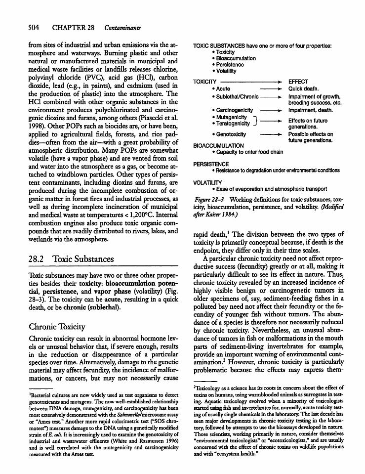
504 CHAPTER 28 Contaminants
from sites of industrial and urban emissions via the atmosphere and waterways. Burning plastic and othernatural or manufactured materials in municipal andmedical waste facilities or landfills releases chlorine,polyvinyl chloride (PVC), acid gas (HC1), carbondioxide, lead (e.g., in paints), and cadmium (used inthe production of plastic) into the atmosphere. TheHC1 combined with other organic substances in theenvironment produces polychlorinated and carcinogenicdioxins and furans, amongothers (PiasecM et al.1998).Other POPs such as biocides are, or have been,applied to agricultural fields, forests, and rice paddies—often from the air—with a great probability ofatmospheric distribution. Many POPs are somewhatvolatile (have a vapor phase) and are vented from soilandwater into the atmosphere as a gas,or become attached to windblown particles. Other typesof persistent contaminants, including dioxins and furans, areproduced during the incomplete combustion of organicmatter in forest fires and industrial processes, aswell as during incomplete incineration of municipalandmedical wasteat temperatures< 1,200°C. Internalcombustion engines also produce toxic organic compounds that are readily distributed to rivers, lakes, andwedandsvia the atmosphere.
28.2 Toxic Substances
Toxic substances mayhave twoor three other properties besides their toxicity: bioaccumulation potential, persistence, and vapor phase (volatility) (Fig.28-3).The toxicity can be acute, resultingin a quickdeath, or be chronic (sublethal).
Chronic ToxicityChronictoxicity can result in abnormal hormone levels or unusual behavior that, if severe enough, resultsin the reduction or disappearance of a particularspecies over time.Alternatively, damage to the geneticmaterial mayaffect fecundity, the incidence ofmalformations, or cancers, but may not necessarily cause
'Bacterial cultures are nowwidelyusedastest organisms to detectgenotoxicants andmutagens. The nowwell-established relationshipbetween DNA damage, mutagenicity, andcarcinogenicity hasbeenmost extensively demonstrated with the Sahmmella/microsome assayor "Ames test."Anothermore rapid colorimetric test ("SOSchro-motest") measures damage to theDNA usingagenetically modifiedstrain ofE. colt. It is increasingly usedto examine the genotoxicity ofindustrial and wastewater effluents (White and Rasmussen 1996)and is well correlated with the mutagenicity and carcinogenicitymeasured with the Ames test.
TOXIC SUBSTANCES have one or more of four properties:• Toxicity• Bioaccumulation• Persistence• Volatility
TOXICITY• Acute
• Sublethal/Chronic
• Carcinogenicity• Mutagenicity ->• Teratogenicity J
• Genotoxicity
BIOACCUMULATION
-*- EFFECT-»- Quick death.
-»- Impairment of growth,breeding success, etc.
•+- Impairment, death.
-*~ Effects on futuregenerations.
-*~ Possible effects onfuture generations.
• Capacity to enter food chain
PERSISTENCE• Resistance to degradation under environmental conditions
VOLATILITY• Ease of evaporation and atmospheric transport
Figure 28-3 Working definitions for toxic substances, toxicity, bioaccumulation, persistence, and volatility. QAodifiedafterKaiser 1984.)
rapid death,1 The division between the two types oftoxicity is primarily conceptual because, if deathis theendpoint, theydiffer onlyin their timescales.Aparticular chronictoxicity neednot affect repro
ductive success (fecundity) gready or at all, makingitparticularly difficult to see its effect in nature. Thus,chronic toxicity revealed byan increased incidence ofhighly visible benign or carcinogenetic tumors inolder specimens of, say, sediment-feeding fishes in apolluted bayneed not affect their fecundity or the fecundity of younger fish without tumors. The abundance of a species is therefore not necessarily reducedby chronic toxicity. Nevertheless, an unusual abundance of tumors in fish or malformations in the mouthparts of sediment-living invertebrates for example,provide an importantwarning of environmental contamination.2 However, chronic toxicity is particularlyproblematic because the effects may express them-
2Toxicology as ascience has itsroots in concern about theeffect oftoxins onhumans, usingwarmblooded animals assurrogates in testing. Aquatic toxicology evolved when a minority of toxicologistsstarted usingfish andinvertebrates for, normally, acute toxicity testingofusually single chemicals in thelaboratory. The last decade hasseen major developments in chronic toxicity testing in the laboratory, followed by attempts to usediebioassays developed in nature.Those scientists, working primarily in nature, consider themselves"environmental toxicologists" or"ecotoxicologists," andare usuallyconcernedwith the effect of chronic toxins on wildlife populationsandwith "ecosystemhealth."
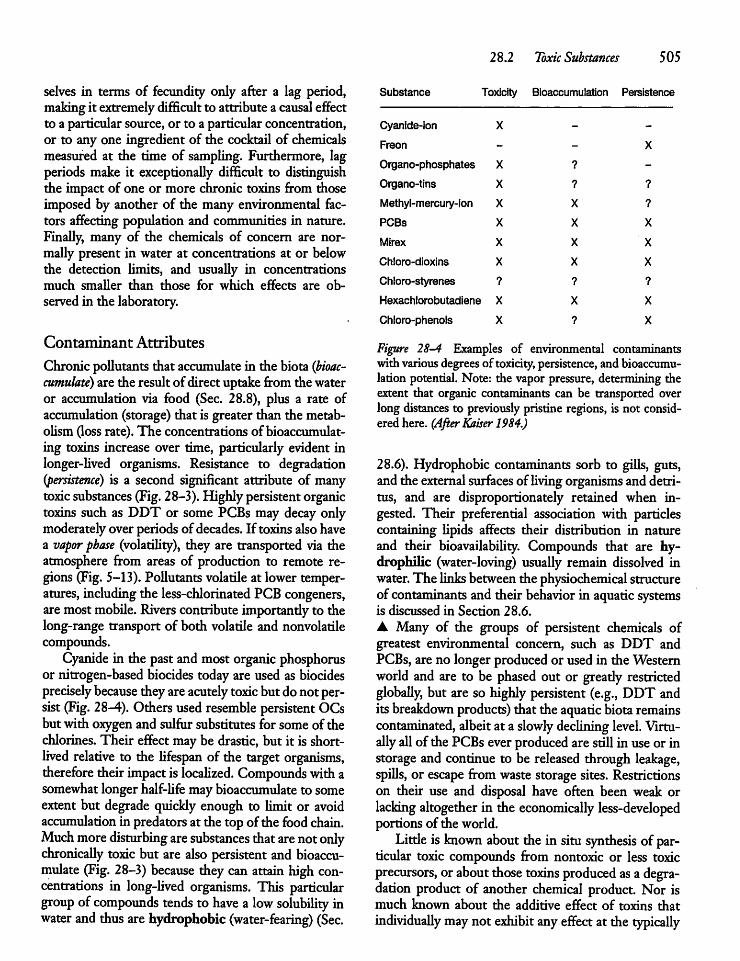
selves in terms of fecundity only after a lag period,makingit extremelydifficultto attribute a causaleffectto a particular source, or to a particular concentration,or to any one ingredient of the cocktail of chemicalsmeasured at the time of sampling. Furthermore, lagperiods make it exceptionally difficult to distinguishthe impact of one or more chronic toxins from thoseimposed by another of the many environmental factors affecting population and communities in nature.Finally, many of the chemicals of concern are normally present in water at concentrations at or belowthe detection limits, and usually in concentrationsmuch smaller than those for which effects are observedin the laboratory.
Contaminant Attributes
Chronic pollutants that accumulate in the biota (bioac-cumulate) are the result of direct uptake from the wateror accumulation via food (Sec. 28.8), plus a rate ofaccumulation (storage) that is greater than themetabolism (loss rate). The concentrations of bioaccumulat-ing toxins increase over time, particularly evident inlonger-lived organisms. Resistance to degradation(persistence) is a second significant attribute of manytoxic substances (Fig. 28-3). Highlypersistent organictoxins such as DDT or some PCBs may decay onlymoderatelyoverperiodsof decades. If toxins alsohavea vapor phase (volatility), they are transported via theatmosphere from areas of production to remote regions (Fig. 5-13). Pollutantsvolatile at lower temperatures, including the less-chlorinated PCBcongeners,aremostmobile. Rivers contributeimportandyto thelong-range transport of both volatile and nonvolatilecompounds.Cyanide in the past andmost organic phosphorus
or nitrogen-based biocides todayare used as biocidesprecisely because theyareacutely toxic butdonot persist (Fig. 28-4). Others usedresemble persistent OCsbutwithoxygen and sulfursubstitutes for someof thechlorines. Their effect maybe drastic, but it is shortlived relative to the lifespan of the target organisms,therefore theirimpact is localized. Compounds with asomewhat longerhalf-life maybioaccumulate to someextent but degrade quickly enough to limit or avoidaccumulation in predatorsat the top of the food chain.Much more disturbing aresubstances thatarenotonlychronically toxic but are also persistent and bioaccumulate (Fig. 28-3) because they can attain high concentrations in long-lived organisms. This particulargroup of compounds tends to have a low solubility inwater andthusarehydrophobic (water-fearing) (Sec.
28.2 Toxic Substances 505
Substance Toxicity Bioaccumulation F'ersistence
Cyanide-ion X - -
Freon - - X
Organo-phosphates X ?-
Organo-tins X ? ?
Methyl-mercury-ion X X ?
PCBs X X X
Mirex X X X
Chloro-dioxins X X X
Chloro-styrenes ? ? ?
Hexachlorobutadiene X X X
Chloro-phenols X ? X
Figure 28-4 Examples of environmental contaminantswithvariousdegreesof toxicity, persistence, and bioaccumulation potential. Note: the vapor pressure, determining theextent that organic contaminants can be transported overlong distances to previously pristineregions, is not considered here. (AfterKaiser 1984.)
28.6). Hydrophobic contaminants sorb to gills, guts,and the external surfaces of livingorganisms anddetritus, and are disproportionately retained when ingested. Their preferential association with particlescontaining lipids affects their distribution in natureand their bioavailability. Compounds that are hy-drophilic (water-loving) usually remain dissolved inwater. The linksbetweenthe physiochemical structureof contaminants and their behavior in aquatic systemsis discussed in Section 28.6.A Many of the groups of persistent chemicals ofgreatest environmental concern, such as DDT andPCBs, are no longer produced or used in the Westernworld and are to be phased out or gready restrictedglobally, but are so highly persistent (e.g., DDT anditsbreakdown products) that theaquatic biota remainscontaminated, albeitat a slowly declining level. Virtuallyallof the PCBseverproduced are still in useor instorage and continue to be released through leakage,spills, or escape fromwaste storage sites. Restrictionson their use and disposal have often been weak orlacking altogether in the economically less-developedportions of the world.Little is known about the in situsynthesis of par
ticular toxic compounds from nontoxic or less toxicprecursors, or aboutthose toxins produced asa degradation product of another chemical product. Nor ismuch biown about the additive effect of toxins thatindividually may not exhibit any effect at the typically
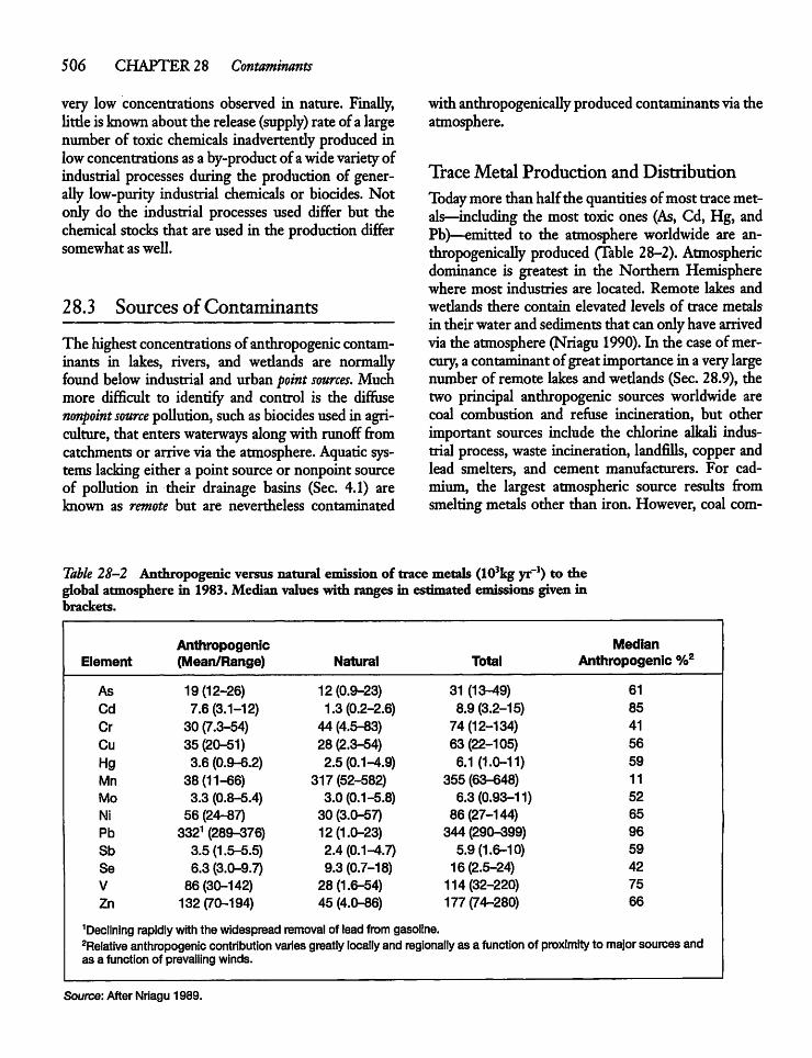
506 CHAPTER 28 Contaminants
very low concentrations observed in nature. Finally,little is knownabout the release (supply) rate ofa largenumber of toxic chemicals inadvertendyproducedinlowconcentrations asa by-productof awidevarietyofindustrial processes during the production of generally low-purity industrial chemicals or biocides. Notonly do the industrial processes used differ but thechemical stocks that are used in the productiondiffersomewhat as well.
28.3 Sources ofContaminants
The highestconcentrationsof anthropogeniccontaminants in lakes, rivers, and wedands are normallyfound below industrial and urban point sources. Muchmore difficult to identify and control is the diffusenonpoint source pollution, such asbiocides used in agriculture, that enters waterways alongwith runoff fromcatchments or arrivevia the atmosphere.Aquatic systems lacking either a point source or nonpoint sourceof pollution in their drainage basins (Sec. 4.1) areknown as remote but are nevertheless contaminated
with anthropogenically producedcontaminantsviatheatmosphere.
Trace Metal Production and Distribution
Todaymore than halfthe quantitiesofmost tracemetals—^including the most toxic ones (As, Cd, Hg, andPb)—emitted to the atmosphere worldwide are anthropogenically produced (Table 28-2). Atmosphericdominance is greatest in the Northern Hemispherewhere most industries are located. Remote lakes andwedands there contain elevated levels of trace metalsin theirwaterandsediments that canonlyhave arrivedviathe atmosphere (Nriagu1990). In the case ofmercury, a contaminant ofgreatimportance in averylargenumber of remote lakes and wedands (Sec. 28.9), thetwo principal anthropogenic sources worldwide arecoal combustion and refuse incineration, but otherimportant sources include the chlorine alkali industrial process, waste incineration, landfills, copper andlead smelters, and cement manufacturers. For cadmium, the largest atmospheric source results fromsmeltingmetals other than iron. However, coal com-
Table 28-2 Anthropogenic versus natural emission of tracemetals (103kg yr-1) to theglobal atmosphere in 1983. Median values with ranges in estimated emissions given inbrackets.
Anthropogenic MedianElement (Mean/Range) Natural Total Anthropogenic %2
As 19(12-26) 12(0.9-23) 31 (13-49) 61
Cd 7.6(3.1-12) 1.3(0.2-2.6) 8.9 (3.2-15) 85
Cr 30 (7.3-54) 44 (4.5-83) 74(12-134) 41
Cu 35 (20-51) 28 (2.3-54) 63(22-105) 56
Hg 3.6 (0.9-6.2) 2.5 (0.1-4.9) 6.1 (1.0-11) 59
Mn 38(11-66) 317(52-582) 355 (63-648) 11
Mo 3.3 (0.8-5.4) 3.0 (0.1-5.8) 6.3(0.93-11) 52
Ni 56 (24-87) 30 (3.0-57) 86(27-144) 65
Pb 3321 (289-376) 12(1.0-23) 344 (290-399) 96
Sb 3.5(1.5-5.5) 2.4 (0.1-^.7) 5.9(1.6-10) 59
Se 6.3 (3.0-9.7) 9.3(0.7-18) 16(2.5-24) 42
V 86 (30-142) 28(1.6-54) 114(32-220) 75
Zn 132(70-194) 45 (4.0-86) 177(74-280) 66
declining rapidly with the widespread removal of lead from gasoline2Relative anthropogenic contribution varies greatly locally and regionally as a function of proximity to major sources andas a function of prevailing winds.
Source: After Nriagu 1989.
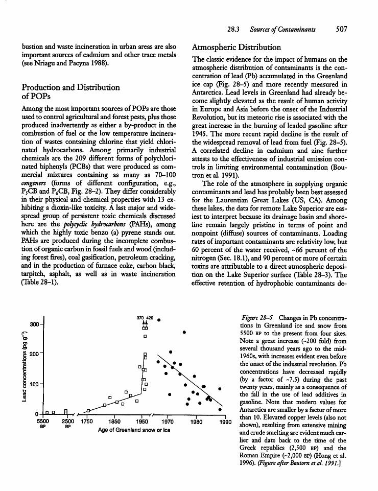
bustion and waste incineration in urban areas are alsoimportant sourcesof cadmiumand other trace metals(seeNriagu and Pacyna 1988).
Production and Distributionof POPs
Amongthe most important sourcesof POPs are thoseused to control agriculturaland forest pests,plus thoseproduced inadvertendy as either a by-product in thecombustion of fuel or the low temperature incineration of wastes containing chlorine that yield chlorinated hydrocarbons. Among primarily industrialchemicals are the 209 different forms of polychlorinated biphenyls (PCBs) that were produced as commercial mixtures containing as many as 70-100congeners (forms of different configuration, e.g.,PSCB and P6CB, Fig. 28-2). They differconsiderablyin their physical and chemical properties with 13 exhibiting a dioxin-like toxicity. A last major and widespread group of persistent toxic chemicals discussedhere are the polycyclic hydrocarbons (PAHs), amongwhich the highly toxic benzo (a) pyrene stands out.PAHs are produced during the incomplete combustion of organic carbon in fossil fuelsandwood (includingforest fires), coalgasification, petroleum cracking,and in the production of furnace coke, carbon black,tarpitch, asphalt, as well as in waste incineration(Table28-1).
300-
O)
200
i<DOCoo•D8
100-
370 420
MtJD
Age of Greenland snow or ice
28.3 Sources ofContaminants 507
Atmospheric DistributionThe classic evidencefor the impact of humans on theatmospheric distribution of contaminants is the concentration of lead (Pb) accumulated in the Greenlandice cap (Fig. 28-5) and more recendy measured inAntarctica. Lead levels in Greenland had already become slighdy elevated as the result of human activityin Europe and Asia before the onset of the IndustrialRevolution, but its meteoric rise is associated with thegreat increase in the burning of leaded gasoline after1945. The more recent rapid decline is the result ofthe widespread removal of leadfrom fuel (Fig. 28-5).A correlated decline in cadmium and zinc furtherattests to the effectiveness of industrial emission controls in limiting environmental contamination (Bou-tron et al. 1991).The role of the atmosphere in supplyingorganic
contaminants and leadhasprobablybeen best assessedfor the Laurentian Great Lakes (US, CA). Amongtheselakes, the datafor remote LakeSuperiorare easiest to interpret because its drainage basin and shoreline remain largely pristine in terms of point andnonpoint (diffuse) sources of contaminants. Loadingratesof important contaminants are relativity low, but60 percent of the water received, "66 percent of thenitrogen (Sec. 18.1), and 90 percent or more of certaintoxins are attributable to a direct atmospheric deposition on the Lake Superior surface (Table 28-3). Theeffective retention of hydrophobic contaminants de-
1990
Figure 28-5 Changes in Pb concentrations in Greenland ice and snow from5500 BP to the present from four sites.Note a great increase (~200 fold) fromseveral thousand years ago to the mid-1960s, with increases evident even beforethe onset of the industrial revolution. Pbconcentrations have decreased rapidly(by a factor of ~7.5) during the pasttwenty years, mainly as a consequence ofthe fall in the use of lead additives ingasoline. Note that modem values forAntarctica are smaller by a factor ofmorethan 10.Elevated copper levels (also notshown), resulting from extensive miningand crude smeltingare evidentmuch earlier and date back to the time of dieGreek republics (2,500 BP) and theRoman Empire (~2,000 BP) (Hong et al.1996). (FigureafterBoutorn etal. 1991.]
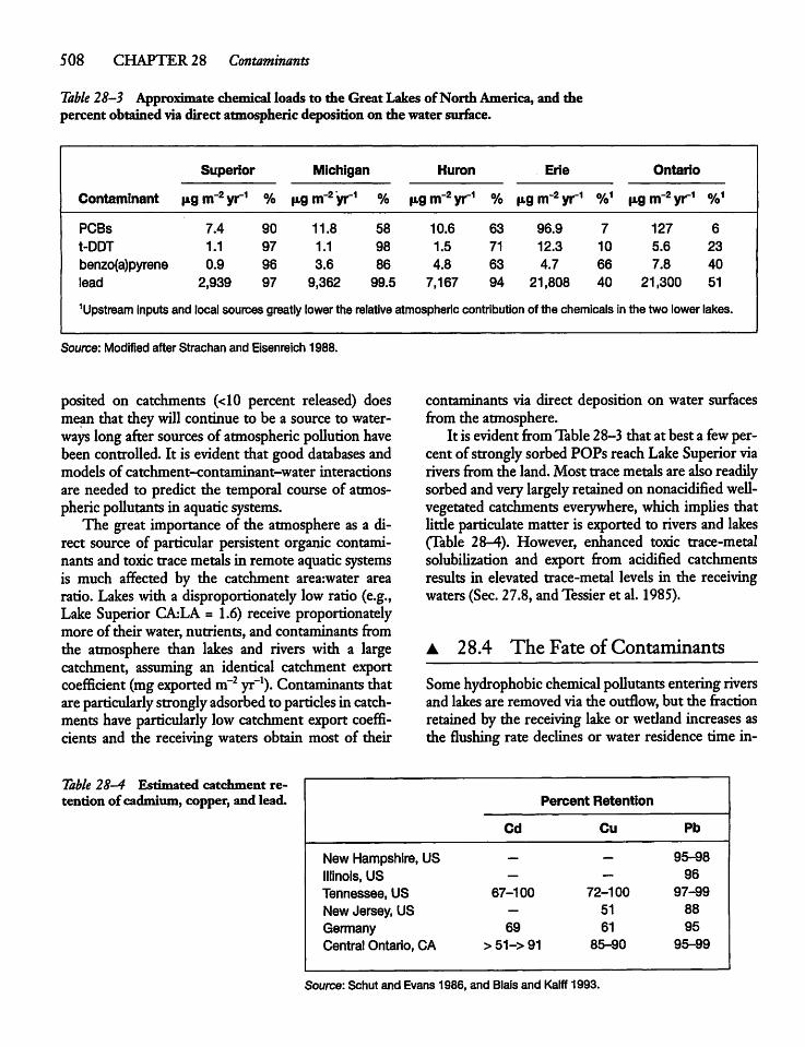
508 CHAPTER 28 Contaminants
Table 28-3 Approximate chemical loads to the Great Lakes of North America, and thepercent obtained via direct atmospheric deposition on die water surface.
Contaminant
Superior Michigan Huron Erie Ontario
|igm"2yr1 % ugm~2yr1 % fjtg nr2 yr1 % ingnr2yr1 %1 l«.gm"2yr1 %1
PCBs 7.4 90 11.8 58 10.6 63 96.9 7 127 6
t-DDT 1.1 97 1.1 98 1.5 71 12.3 10 5.6 23
benzo(a)pyrene 0.9 96 3.6 86 4.8 63 4.7 66 7.8 40
lead 2,939 97 9,362 99.5 7,167 94 21,808 40 21,300 51
1Upstream inputs and local sources greatly lower the relativeatmospheric contribution of the chemicals in the two lower lakes.
Source: Modified after Strachan and Eisenreich 1988.
posited on catchments (<10 percent released) doesmean that they will continue to be a source to waterways long after sources of atmospheric pollutionhavebeen controlled. It is evident that good databases andmodels of catchment-<:ontaminant-water interactionsare needed to predict the temporal course of atmospheric pollutantsin aquaticsystems.The great importance of the atmosphere as a di
rect source of particular persistent organic contaminants and toxictracemetals in remote aquaticsystemsis much affected by the catchment arearwater arearatio. Lakeswith a disproportionately low ratio (e.g.,Lake Superior CA:LA = 1.6) receive proportionatelymore of their water, nutrients, and contaminants fromthe atmosphere than lakes and rivers with a largecatchment, assuming an identical catchment exportcoefficient (mg exported m~2 yr-1). Contaminants thatare particularly stronglyadsorbedto particlesin catchments have particularly low catchment export coefficients and the receiving waters obtain most of their
contaminants via direct deposition on water surfacesfrom the atmosphere.It is evidentfromTable28-3 that at best a fewper
cent of stronglysorbedPOPs reachLakeSuperiorviariversfrom the land.Most tracemetalsare alsoreadilysorbed andverylargely retainedon nonacidified well-vegetated catchments everywhere, which implies thatlittle particulate matter is exported to rivers and lakes(Table 28-4). However, enhanced toxic trace-metalsolubilization and export from acidified catchmentsresults in elevated trace-metal levels in the receivingwaters (Sec. 27.8, and Tessier et al. 1985).
• 28.4 The Fate of Contaminants
Somehydrophobic chemical pollutantsentering riversand lakes are removed via the outflow, but the fractionretained by the receiving lakeor wedand increases asthe flushing rate declines or water residence time in-
Table 28-4 Estimated catchment retention ofcadmium, copper, and lead. Percent Retention
Cd Cu Pb
New Hampshire, US — — 95-98
Illinois, US _ _ 96
Tennessee, US 67-100 72-100 97-99
New Jersey, US 51 88
Germany 69 61 95
Central Ontario, CA > 51-> 91 85-90 95-99
Source: Schut and Evans 1986, and Blais and Kalff 1993.
creases (Chapter 8).Those chemicals most subject toadsorption are most readily removed from the watercolumn bysedimentation and thus are leastreadily exported via the outflow.
Long-rangeTransportMost organochlorines and organic mercury (methylmercury) havea sufficiendy highvaporpressure that afraction of the persistent contaminants are lost fromboth the land and water to the atmosphere byvolatilization; this route is particularly important insummerwhenwaterandsoiltemperatures arehighestButon an annual basis volatilization is expected to bemost important from warm tropical lakes, wedands,and their catchments. Volatile organic compounds(VOCs) are carriedaloft by rising air masses andmaybe transported in the gas phase or adsorbed toparticles for hundreds if not thousands of kms atthe latitude of emission. They are also carried tohigher latitudes and altitudes (see Fig. 5-13), eitherdirecdy or following a temperature-driven transport-deposition-partial revolatization-transport sequence(Sec. 5.4). Deposition is enhanced when airbornePOPs—in the gas phase and as aerosols—reach theircondensation temperature at highlatitudes, or in highmountain regions at a lowerlatitude. Deposition thenprevails overrevolatilization (degassing), whereas it isthe reverse at lowlatitudes. Lowtemperatures furtherreduce rates of VOC degradation and increase theprobability of a long-term storage. POPs accumulatedin thesnowpack or on plantandsoil surfaces may become buried, revolatdized, or are transported toaquatic systems during periods of snow melt wherethey become subject to uptake and bioaccumulation(Sec. 28.8).Sediments, lake ice, and the biota of arctic waters
contain elevated levels of a wide variety of POPs,mercury, and radionuclides that resulted from atomicbomb testing or nuclear accidents (Lockhart et al.1992). In winter, the North American arctic air oftencontains a haze of small aerosol particles (primarily"soot" or carbon black and sulfates) and gases derived from Eurasia and midlatitude North America.Desert dust particles (< 1 u,m) from central Asiahave been noted in Alaskan snow (Lockhart et al.1992). "Brown snow" in the Canadian Arctic includesclay andsoot particles plus adsorbed POPs that havebeen traced to Siberian and western China regions ofAsia (Welch et al. 1991). However, with increasingdistance from the North Pole, the contaminants in
28.4 The Fate ofContaminants 509
boreal forest lakes are increasingly derived fromlower latitude industrial or agricultural regions (seeFig. 5-12).The extent that POPs in waterways are primarily
lost by biodegradation by microbes, chemically orphotochemically, is highlydependent on environmental conditions and the specific physiochemical characteristicsof the particular chemical (Sec. 28.7).
Contaminant Concentrations over Time
Roughmass-balance calculations for the sum total ofthe most common PCB congeners and for lead showthat the two contaminant types differ greadyin theirprincipal loss processes in LakeSuperior. The atmosphere is ultimately the principal sink (92%) of themore volatile PCBs.3 As a consequence, only 13 percent (170 kg yr"1) of total PCBs entering Lake Superior is permanendy buried in the sediments or lost viathe outflow, with the balance (87%, -1,900 kg yr"1)lost by volatilization (Strachan and Eisenreich 1988).The roughly 20 percentdecline per yearin thewhole-water concentration of PCBs between 1980 and 1992isattributed to a systematic decline in atmospheric inputs to Lake Superior. The lake is now serving as asource rather than as a sink of PCBs (Jeremiason et al.1994). In contrast, the sediments rather than the atmosphere are the principal sinkfor lead, which is bothstrongly particle sorbing and not very volatile (Strachan and Eisenreich 1988).The encouraging decline in concentration of
themost abundant PCB congeners in Lake Superioris also evident for other POPs, measured in fish fromNorth American lakes not subject to point-sourcecontamination (Schmitt et al. 1985) as well as in sediments (Fig. 28-6). Consequendy, thereisencouragingevidence that contaminant levels will decline whereregional or continent wide controls on emissions areinstituted. The declines are most evident from analyses of the biota over time, and from concentrationprofiles in dated sediments. The declines are not asobvious from the much more variable and typically
JLow chlorinated (1-3 chlorine atoms) biphenyls are not only morevolatile butalso more readily degraded bychemical, photochemical,and metabolic processes. They consequendy have a much shorterhalf-life (months) than thehighly chlorinated (4-10 chlorine atoms)biphenyl congeners, with themosthighly chlorinated congeners almost totally persistent and dominant in long-lived organisms andsediments close to sources.
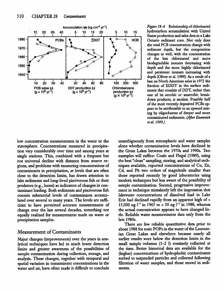
510 CHAPTER 28 Contaminants
t r10 20 30 40
PCB sales (o)(gx106yr1)
Accumulation (•) (ng cm"2 yr1)20
t r20 40 60 80
DDTproduction (o)(gx109yr1)
low concentration measurements in the water or theatmosphere. Concentrations measured in precipitation vary considerably over time and amongyears atsingle stations. This, combined with a frequent butnot universal decline with distance from source regions, andproblems withmeasuring concentrations ofcontaminants in precipitation, at levels that are oftenclose to the detection limits, has drawn attention tolake sediments and long-lived piscivorous fish or theirpredators (e.g., loons) as indicators of changes in contaminant loading. Bothsediments andpiscivorous fishcontain substantial levels of contaminants accumulatedover several to manyyears. The levels are sufficient to have permitted accurate measurements ofchange over the last several decades, something notequally realized for measurements made on water orprecipitation samples.
Measurement ofContaminants
Major changes (improvements) over the years in analytical techniques have led to much lower detectionlimits and greater awareness of the possibiUties ofsample contamination during collection, storage, andanalysis. These changes, together with temporal andspatial variation in contaminant concentrations in thewater and air, have often made it difficult to conclude
10_L
15±
100 200 300
Chlorobenzeneproduction (o)(gX109yr1)
Figure 28-6 Relationship ofchlorinatedhydrocarbon accumulation with UnitedStatesproduction and salesdata in a LakeOntario sediment core. Not only doesthe total PCBconcentrationchangewithsediment depth, but the compositionchanges as well, with the concentrationof the less chlorinated and morebiodegradable isomers decreasing withdepth and the more highly chlorinatedand persistent isomers increasing withdepth (Oliveret al. 1989). Asa result of aban on North American sales in 1972 thefraction of 2DDT in the surface sediments that consists of DDT, rather thanone of its aerobic or anaerobic breakdown products, is modest Possibly halfof the most recendy deposited PCBsappear to be attributableto an upwardmixing by oligochaetes of deeper and morecontaminatedsediments. (AfterEisenreichetal. 1989.)
unambiguously from atmospheric and water samplesalone whether contamination levels have declined inthe Great Lakes between the 1970s and 1990s. Twoexamples will suffice: Coale and Flegal (1989), usingthe best"clean" sampling, storing, andanalytical techniques available, reported concentrations of Cu, Zn,Cd, and Pb two orders of magnitude smaller thanthose reported recendy by good laboratories usingmodern techniques but less aware of the possibility ofsample contamination. Second, progressive improvement in technique mistakenly left the impression thatlakewater concentrations of dissolved lead in LakeErie haddeclined rapidly from an apparent highof <15,000 ng 1_1 in 1965 to < 30 ngH in 1988, whereasthe actual concentration appears to have changed lit-de. Reliable water measurements date only from thelate 1980s.There are few reliable quantitative data prior to
about 1988 for toxic POPs in the water ofthe Laurentian Great Lakes and elsewhere because nearly allearlier results were below the detection limits in thesmall sample volumes (1-2 1) routinely collected atthe time. Better historical data are available for the(higher) concentrations of hydrophobic contaminantssorbed to suspended particles and collected followingfiltration of water samples, and those stored in sediments.
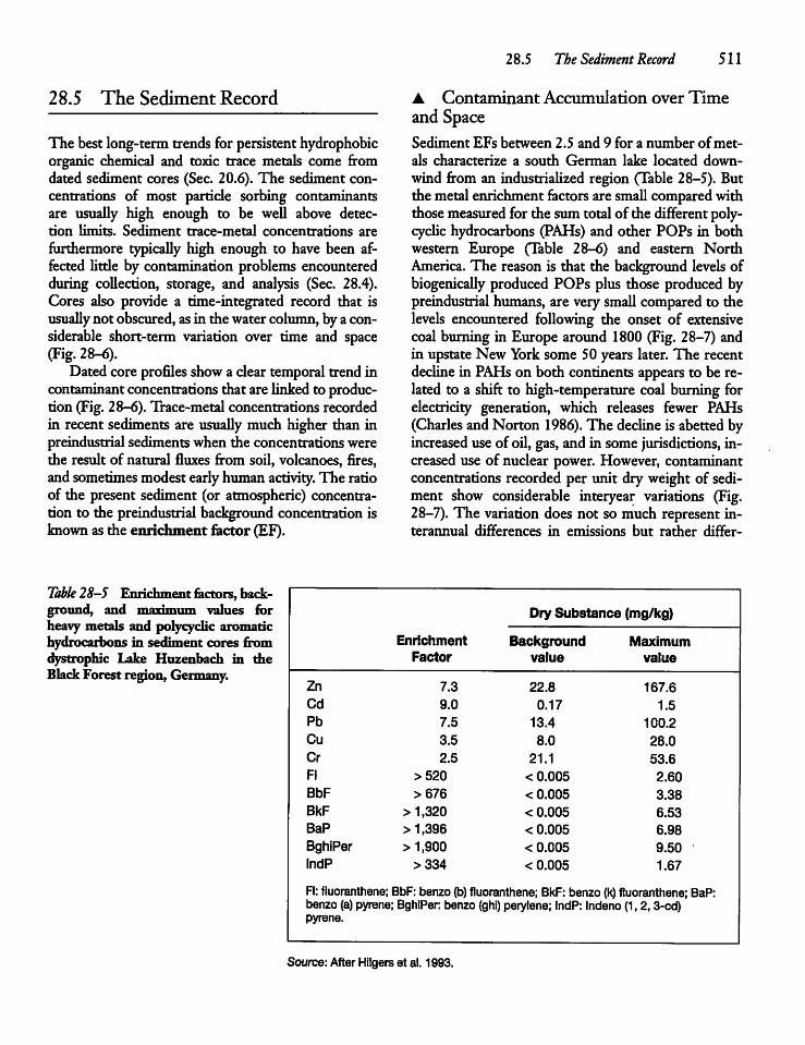
28.5 The Sediment Record 511
28.5 The Sediment Record
The best long-term trends for persistent hydrophobicorganic chemical and toxic trace metals come fromdated sediment cores (Sec. 20.6). The sediment concentrations of most particle sorbing contaminantsare usually high enough to be well above detection limits. Sediment trace-metal concentrations arefurthermore typically high enough to have been affected little by contamination problems encounteredduring collection, storage, and analysis (Sec. 28.4).Cores also provide a time-integrated record that isusually not obscured, asin thewatercolumn, bya considerable short-term variation over time and space(Fig. 28-6).Dated core profiles show a clear temporal trend in
contaminantconcentrationsthat are linkedto production (Fig. 28-6). Trace-metal concentrations recordedin recent sediments are usually much higher than inpreindustrial sediments when the concentrations weredie result of natural fluxes from soil, volcanoes, fires,andsometimes modestearlyhumanactivity. The ratioof the present sediment (or atmospheric) concentration to the preindustrial backgroundconcentration isknown as the enrichment factor (EF).
• Contaminant Accumulation over Timeand SpaceSediment EFs between 2.5 and 9 for a number ofmetals characterize a south German lake located downwind from an industrialized region (Table 28-5). Butthe metalenrichment factors are smallcompared withthosemeasured for the sum total of the differentpoly-cyclic hydrocarbons (PAHs) and other POPs in bothwestern Europe (Table 28-6) and eastern NorthAmerica. The reason is that the background levels ofbiogenically produced POPs plus those produced bypreindustrialhumans, are very small compared to thelevels encountered following the onset of extensivecoal burning in Europe around 1800 (Fig. 28-7) andin upstate New York some 50 years later. The recentdecline in PAHson both continents appears to be related to a shift to high-temperature coal burning forelectricity generation, which releases fewer PAHs(Charles andNorton 1986). The decline is abettedbyincreased use of oil, gas, and in some jurisdictions, increased use of nuclear power. However, contaminantconcentrations recorded per unit dry weight of sediment show considerable interyear variations (Fig.28-7). The variation does not so much represent in-terannual differences in emissions but rather differ-
Table 28-5 Enrichment factors, background, and mflvimum values forheavymetals and polycyclic aromatichydrocarbons in sediment cores fromdystrophic Lake Huzenbach in theBlackForest region, Germany.
EnrichmentFactor
Dry Substance (mg/kg)
Backgroundvalue
Maximumvalue
Zn 7.3 22.8 167.6Cd 9.0 0.17 1.5Pb 7.5 13.4 100.2Cu 3.5 8.0 28.0Cr 2.5 21.1 53.6Fl > 520 < 0.005 2.60BbF > 676 < 0.005 3.38BkF > 1,320 < 0.005 6.53BaP > 1,396 < 0.005 6.98BghiPer > 1,900 < 0.005 9.50IndP > 334 < 0.005 1.67
Fl: fluoranthene; BbF:benzo (b)fluoranthene; BkF:benzo (k) fluoranthene; BaP:benzo (a) pyrene; BghiPen benzo (ghi) perylene; IndP: Indeno(1,2,3-cd)pyrene.
Source: After Hilgers et al. 1993.
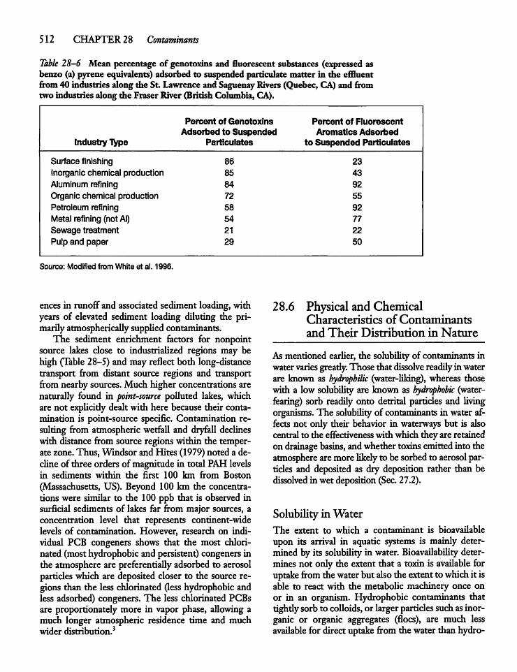
512 CHAPTER 28 Contaminants
Table 28-6 Mean percentageof genotoxins and fluorescent substances (expressed asbenzo (a) pyrene equivalents) adsorbed to suspended particulate matter in the effluentfrom 40 industries along the St. Lawrence and SaguenayRivers (Quebec, CA)and fromtwo industries along the Fraser River (British Columbia, CA).
Percent of Genotoxins Percent of FluorescentAdsorbed to Suspended Aromatics Adsorbed
Industry Type Particulates to Suspended Particulates
Surface finishing 86 23
Inorganic chemical production 85 43
Aluminum refining 84 92
Organic chemical production 72 55
Petroleum refining 58 92
Metal refining (not Al) 54 77
Sewage treatment 21 22
Pulp and paper 29 50
Source: Modified from White et al. 1996.
ences in runoff and associated sediment loading, withyears of elevated sediment loading diluting the primarilyatmosphericallysuppliedcontaminants.The sediment enrichment factors for nonpoint
source lakes close to industrialized regions may behigh (Table 28-5) and may reflect both long-distancetransport from distant source regions and transportfromnearby sources. Much higher concentrationsarenaturally found in point-source polluted lakes, whichare not explicidydealt with here because their contamination is point-source specific. Contamination resulting from atmosphericwetfall and dryfall declineswith distance from source regionswithin the temperate zone. Thus, Windsor and Hites (1979) noted a declineof three orders of magnitude in total PAHlevelsin sediments within the first 100 km from Boston(Massachusetts, US). Beyond 100 km the concentrations were similar to the 100 ppb that is observed insurficial sediments of lakes far from major sources, aconcentration level that represents continent-widelevels of contamination. However, research on individual PCB congeners shows that the most chlorinated (mosthydrophobicand persistent)congeners inthe atmosphere are preferentially adsorbed to aerosolparticles which are deposited closer to the source regions than the less chlorinated (less hydrophobic andless adsorbed) congeners. The less chlorinated PCBsare proportionately more in vapor phase, allowing amuch longer atmospheric residence time and muchwider distribution.3
28.6 Physical andChemicalCharacteristics ofContaminantsand Their Distribution in Nature
Asmentioned earlier, the solubilityof contaminants inwatervaries gready. Those that dissolve readily inwaterare known as hydrophilic (water-liking), whereas thosewith a lowsolubility are known as hydrophobic (water-fearing) sorb readily onto detrital particles and livingorganisms. The solubility of contaminants in water affects not only their behavior in waterways but is alsocentralto the effectiveness withwhich they are retainedon drainage basins, andwhethertoxins emittedinto theatmosphere aremorelikely to besorbed to aerosol particles and deposited as dry deposition rather than bedissolved in wet deposition (Sec. 27.2).
Solubility in WaterThe extent to which a contaminant is bioavailableupon its arrival in aquatic systems is mainly determined by its solubility in water. Bioavailability determines not only the extent that a toxinis available foruptake from thewaterbutalso the extent towhich it isable to react with the metabolic machinery once onor in an organism. Hydrophobic contaminants thattighdysorb to colloids, or largerparticles suchasinorganic or organic aggregates (floes), are much lessavailable for directuptakefrom thewater than hydro-
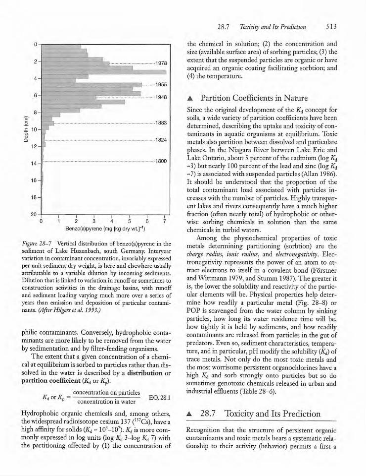
T12 3 4 5 6
Benzo(a)pyrene (mg[kg drywt.]"1)
Figure 28-7 Vertical distribution of benzo(a)pyrene in thesediment of Lake Huzenbach, south Germany. Interyearvariationin contaminant concentration, invariably expressedper unit sedimentdryweight, is here and elsewhere usuallyattributable to a variable dilution by incoming sediments.Dilution that is linked to variation in runoff or sometimes toconstruction activities in the drainage basins, with runoffand sediment loading varying much more over a series ofyears than emission and deposition of particular contaminants. (AfterHilgers etal. 1993.)
philic contaminants. Conversely, hydrophobic contaminants are more likely to be removed from the waterbysedimentation andbyfilter-feeding organisms.The extent that a given concentration of a chemi
calat equilibrium issorbed to particles rather than dissolved in the water is described by a distribution orpartition coefficient (Kd orKp).
concentration on particlesKd orKp = ; r^ EQ. 28.1concentration m water
Hydrophobic organic chemicals and, among others,thewidespread radioisotope cesium 137 (137Cs), have ahigh affinity forsolids (Kd ~ 103—107). Kd ismorecommonly expressed in log units (logKd 3-log Kd 7)withthe partitioning affected by (1) the concentration of
28.7 Toxicity andItsPrediction 513
the chemical in solution; (2) the concentration andsize(available surfacearea) of sorbing particles;(3) theextent that the suspended particles are organic or haveacquired an organic coating facilitating sorbtion; and(4) the temperature.
A Partition Coefficients in Nature
Since the original development of the K^ concept forsoils, a wide variety of partition coefficients have beendetermined, describing the uptake and toxicity of contaminants in aquatic organisms at equilibrium. Toxicmetals alsopartition between dissolvedand particulatephases. In the Niagara River between Lake Erie andLakeOntario, about 5 percent of the cadmium(logKd~3) but nearly 100 percent of the lead and zinc (log Kd~7)is associatedwith suspended particles (Allan 1986).It should be understood that the proportion of thetotal contaminant load associated with particles increaseswith the number of particles. Highly transparent lakes and rivers consequently have a much higherfraction (often nearly total) of hydrophobic or otherwise sorbing chemicals in solution than the samechemicals in turbid waters.Among the physiochemical properties of toxic
metals determining partitioning (sorbtion) are thecharge radius, ionic radius, and electrojiegativity. Electronegativity represents the power of an atom to attract electrons to itself in a covalent bond (ForstnerandWittmann 1979, and Stumm1987). The greater itis, the lower the solubility and reactivity of the particular elements will be. Physical properties help determine how readily a particular metal (Fig. 28-8) orPOP is scavenged from the water column by sinkingparticles, how long its water residence time will be,how tightly it is held by sediments, and how readilycontaminants are released from particles in the gut ofpredators. Even so, sediment characteristics, temperature, and in particular,pH modify the solubility(K^ oftrace metals. Not only do the most toxic metals andthe mostworrisome persistentorganochlorines have ahigh K^ and sorb strongly onto particles but so dosometimes genotoxic chemicals released in urban andindustrial effluents (Table 28-6).
• 28.7 Toxicity and Its Prediction
Recognition that the structure of persistent organiccontaminants and toxic metals bears a systematic relationship to their activity (behavior) permits a first a
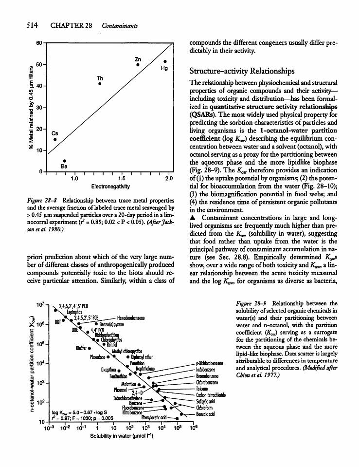
514 CHAPTER 28 Contaminants
140-
50-
Th
Zn
Hg
40- •
30-
20- Cs /10-
fi-
•
Ba
i i i i
1.0i i i i
1.5i i i i i
2.0
10
d
Electronegativity
Figure 28-8 Relationship between trace metal propertiesand the average fraction of labeled tracemetalscavenged by>0.45 \im suspendedparticlesover a 20-dayperiod in a lim-nocorral experiment (r2 =0.85; 0.02 <P <0.05). (AfterJackson et al. 1980.)
priori prediction about which of the very large number of differentclasses of anthropogenically producedcompounds potentially toxic to the biota should receive particular attention. Similarly, within a class of
107-,
&106-
o
fio4onQ.u.
<D
« 103-i
Oc
o 10Mo
2,4,5,2,,4,/5,PCBLepfoptios
U5,2*,5'PCB• Benzo(a)pyrane
v«M'KBf L\ Dicnbrofenmioi
' • Chlorophyrifos
logr2 =
compounds the different congenersusuallydifferpredictably in their activity.
Structure-activity RelationshipsThe relationship between physiochemical andstructuralproperties of organic compounds and their activity—including toxicity and distribution—has been formalized in quantitative structure activity relationships(QSARs). The most widelyused physical property forpredicting the sorbtion characteristics of particlesandliving organisms is the 1-octanol-water partitioncoefficient (logKqJ) describing the equihbrium concentration between water and a solvent (octanol), withoctanolservingas a proxyfor the partitioningbetweenthe aqueous phase and the more lipidlike biophase(Fig. 28-9). The K^ therefore provides an indicationof (1)the uptakepotentialbyorganisms; (2)the potential for bioaccumulation from the water (Fig. 28-10);(3) the biomagnification potential in food webs; and(4) the residence time ofpersistent organic pollutantsin the environment.A Contaminant concentrations in large and long-lived organisms are frequendymuch higher than predicted from the .KoW (solubility in water), suggestingthat food rather than uptake from the water is theprincipal pathway of contaminantaccumulation in nature (see Sec. 28.8). Empirically determined li^sshow, overawide rangeof both toxicity andK^,, a linear relationship between the acute toxicity measuredand the log K^,, for organisms as diverse as bacteria,
Figure 28-9 Relationship between thesolubility ofselectedorganicchemicals inwater(s) and their partitioning betweenwater and n-octanol, with the partitioncoefficient (K^,) serving as a surrogatefor the partitioning of the chemicals between the aqueous phase and the morelipid-likebiophase. Data scatter is largelyattributable to differences in temperatureand analytical procedures. (Modified afterCbiouetal. 1977.)
KoW = 5.0-0.67'logS0.97; F = 1030; p = 0.005
1010"3 10"2 10"1 1 10 102 103
Solubility inwater (umol I"1)
t—n;—•«104 105 106
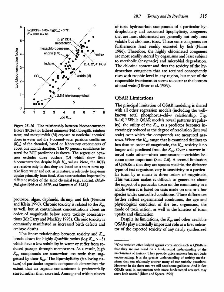
6-i
5-
o
,2 4-
£ 3-
oon 2O)Q
1-
log(BCF) =0.85. log(Kow) - 0.72^ =0.90:0 =66
P, P' DDT,heptachlors
hexachlorobenzene, ,y _\' •? ft. • ^endrin(FM) /\J» •V''^'
lindane, y •*
CCI,U /' t £m /' endrin(M)
C-2,5,6 trichloropyridinol
o
"I 1—3 4
LogK0
Figure 28-10 The relationship between bioconcentrationfactors (BCFs) for fatheadminnows(FM),bluegills, rainbowtrout, and mosquitofish (M) exposed to nonlethal chemicaldosesin water and the 1-octanol-waterpartition coefficient(KoJ) of the chemical, based on laboratory experiments ofabout one month duration. The 95 percent confidence interval for BCF predictions is shown.The regressionequation excludes three outliers (O) which show litdebioconcentration despite high K^ values. Note, the BCFsare relative onlyin that they are based on a short-termuptake from waterandnot, asin nature, a relatively long-termuptake primarily fromfood. Also note variation imparted bydifferent studies of the samechemical (e.g., endrin). (Modifiedafter Veitb etal. 1979, andStuntm etal. 1983.)
protozoa, algae, daphnids, shrimp, and fish (NendzaandKlein1990). Chronictoxicity is related to theK^as well, but at contaminant concentrations about anorder of magnitude below acute toxicity concentrations (McCarty andMacKay 1993). Chronictoxicity iscommonly manifested as increased birth defects andembryo deaths.The linear relationship between toxicity and K^,
breaks down for highly lipophilic toxins (log K^w > -5)which have a lowsolubility in wateror suffer fromreduced passage through membranes. As a result, high•KqW compounds are somewhat less toxic than suggested bytheir .K^. The lipophylicity (fat-loving nature) of particular organiccompounds determines theextent that an organic contaminant is preferentiallystored rather than excreted. Amongandwithin classes
28.7 Toxicity andItsPrediction 515
of toxic hydrocarbon compounds of a particular hy-drophobicity and associated lipophylicity, congenersthat are most chlorinatedare generally not only leastvolatile but alsomost toxic. These samecongeners arefurthermore least readily excreted by fish (Niimi1986). Therefore, the highly chlorinated congenersare most readily stored by organismsand least subjectto metabolic (enzymatic) and microbial degradation.The chlorinecontent and thus the toxicity of the hydrocarbon congeners that are retained consequentlyrises with trophic level in any region, but most of theresponsible fractionation seems to occur at the bottomof food webs (Oliver et al. 1989).
QSAR LimitationsThe principal limitationof QSARmodelingis sharedwith all other regressionmodels (including the well-known total phosphorus-chl-0 relationship, Fig.8-16).4 While QSAR models reveal patterns (regularity), the utility of the K&, as a predictor becomes increasingly reduced as the degree of resolution (intervalscale) over which the compounds are measured narrows.When the A^w range that is examineddeclinestoless than an order of magnitude, theK^ toxicity is nolongerwell-predictedfrom the K^,. Over a narrow interval scale other—often unmeasured—variables become more important (Sec. 2.6). A second limitationofQSARs is that theyare species specific, the differenttypes of test organisms vary in sensitivity to a particular toxin by as much as three orders of magnitude.This variation makes it difficult to generahze aboutthe impact ofa particular toxin on the community asawhole when it is based on tests made on one or a fewspeciesunder controlled conditions. These differencesfurther reflect experimental conditions, the age andphysiological condition of the test organisms, themode of toxic action, as well as the kinetics of toxinuptake and elimination.Despite its limitations, the K^ and other available
QSARs playa crucially important role asa first indicator of the expected toxicity of any newlysynthesized
^One criticism often lodged against correlations such as QSARs isthat they are not based on a fundamental understanding of themechanisms of toxicity. They provide quickanswers but not basicunderstanding. It is the greater understanding of toxicity mechanisms that can ultimately answer manyof our toxicity questions.However, in the shortrun,we stillneedsomeguidance. And in factQSARs used in conjunction with more fundamental research mayserveboth needs." (BlumandSpeece1990)
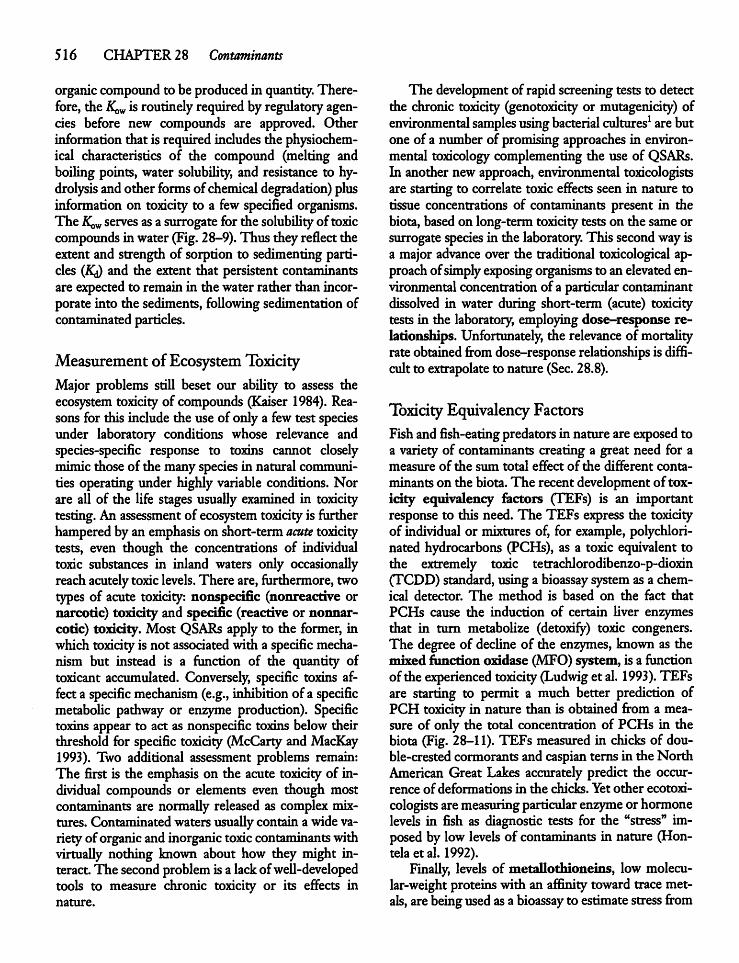
516 CHAPTER 28 Contaminants
organic compound to be producedin quantity. Therefore, theK^ is routinely required by regulatory agencies before new compounds are approved. Otherinformation that is required includesthe physiochemical characteristics of the compound (melting andboiling points, water solubility, and resistance to hydrolysis andother forms of chemical degradation) plusinformation on toxicity to a few specified organisms.The K&, serves asa surrogate for the solubilityof toxiccompounds in water (Fig. 28-9). Thus they reflect theextentand strength of sorption to sedimenting particles (IQ and the extent that persistent contaminantsare expected to remain in the water rather than incorporate into the sediments, following sedimentation ofcontaminated particles.
Measurement ofEcosystemToxicityMajor problems still beset our ability to assess theecosystem toxicity of compounds (Kaiser 1984). Reasonsfor this include the use of only a few test speciesunder laboratory conditions whose relevance andspecies-specific response to toxins cannot closelymimic those of the manyspecies in natural communities operating under highly variable conditions. Norare all of the life stages usually examined in toxicitytesting. Anassessment of ecosystem toxicity is furtherhamperedby an emphasis on short-term acute toxicitytests, even though the concentrations of individualtoxic substances in inland waters only occasionallyreach acutelytoxiclevels. There are, furthermore, twotypes of acute toxicity: nonspecific (nonreactive ornarcotic) toxicity and specific (reactive or nonnarcotic) toxicity. Most QSARs apply to the former, inwhichtoxicity is not associated with a specific mechanism but instead is a function of the quantity oftoxicant accumulated. Conversely, specific toxins affecta specific mechanism (e.g., inhibitionof a specificmetabolic pathway or enzyme production). Specifictoxins appear to act as nonspecific toxins below theirthreshold for specific toxicity (McCarty and MacKay1993). Two additional assessment problems remain:The first is the emphasis on the acute toxicity of individual compounds or elements even though mostcontaminants are normally released as complex mixtures. Contaminatedwatersusuallycontain a widevarietyoforganic andinorganic toxic contaminants withvirtually nothing known about how they might interact. The secondproblem is a lackofwell-developedtools to measure chronic toxicity or its effects innature.
The development of rapid screeningtests to detectthe chronic toxicity (genotoxicity or mutagenicity) ofenvironmental samples using bacterial cultures1 arebutone of a number of promisingapproaches in environmental toxicology complementing the use of QSARs.In another new approach, environmental toxicologistsare starting to correlate toxiceffects seen in nature totissue concentrations of contaminants present in thebiota, basedon long-term toxicitytests on the sameorsurrogatespecies in the laboratory. This secondwayisa major advance over the traditional toxicologic^ approachofsimply exposing organisms to an elevated environmental concentrationof a particularcontaminantdissolved in water during short-term (acute) toxicitytests in the laboratory, employingdose-response relationships. Unfortunately, the relevance of mortalityrate obtainedfromdose-response relationships is difficult to extrapolate to nature (Sec. 28.8).
Toxicity Equivalency FactorsFish and fish-eating predators in nature are exposed toa variety of contaminants creating a great need for ameasure of the sum total effect of the different contaminantson the biota.The recent developmentof toxicity equivalency factors (TEFs) is an importantresponse to this need. The TEFs express the toxicityof individual or mixtures of, for example, polychlorinated hydrocarbons (PCHs), as a toxic equivalent tothe extremely toxic tetrachlorodibenzo-p-dioxin(TCDD) standard, usinga bioassay systemas a chemical detector. The method is based on the fact thatPCHs cause the induction of certain fiver enzymesthat in turn metabolize (detoxify) toxic congeners.The degree of decline of the enzymes, known as themixed function oxidase (MFO) system, is a functionof the experienced toxicity (Ludwig et al. 1993). TEFsare starting to permit a much better prediction ofPCH toxicity in nature than is obtained from a measure of only the total concentration of PCHs in thebiota (Fig. 28-11). TEFs measured in chicks of double-crestedcormorantsand Caspian terns in the NorthAmerican Great Lakes accurately predict the occurrence ofdeformations in the chicks. Yet other ecotoxi-cologists aremeasuring particular enzyme or hormonelevels in fish as diagnostic tests for the "stress" imposed by low levels of contaminants in nature (Hon-tela etal. 1992).Finally, levels of metallothioneins, low molecu
lar-weight proteins with an affinity toward tracemetals, arebeingusedasa bioassay to estimate stress from
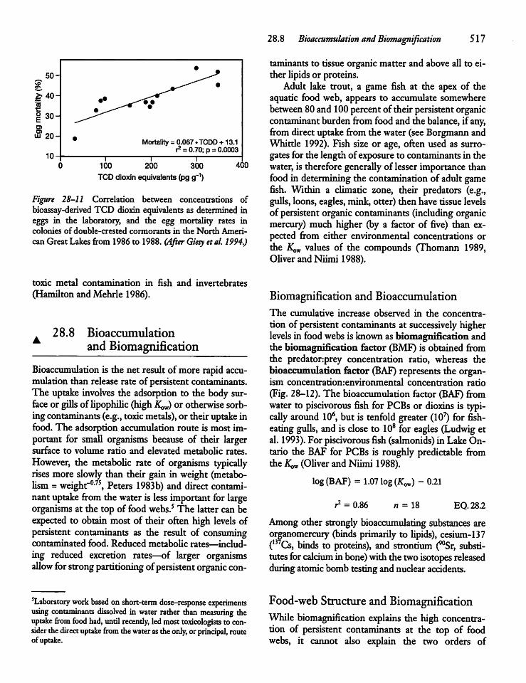
•
mortality(%)W*kenooo11I••
O)
uj 20- • Mortality = 0.067 .TCDD +13.1r2= 0.70;p = 0.0003
1 I I100 200 300
TCD dloxin equivalents(pgg"1)400
Figure 28-11 Correlation between concentrations ofbioassay-derived TCD dioxin equivalents as determined ineggs in the laboratory, and the tgg mortality rates incolonies of double-crested cormorants in the North AmericanGreat Lakesfrom 1986to 1988. (After Giesy etal. 1994.)
toxic metal contamination in fish and invertebrates(Hamilton and Mehrle 1986).
28.8 Bioaccumulationand Biomagnification
Bioaccumulation is the net resultofmore rapid accumulation than release rate of persistent contaminants.The uptake involves the adsorption to the bodysurface or gills of lipophilic (highK^)or otherwise sorbing contaminants (e.g.,toxicmetals), or their uptakeinfood. The adsorptionaccumulation route is most important for small organisms because of their largersurface to volume ratio and elevated metabolic rates.However, the metabolic rate of organisms typicallyrises more slowly than their gain in weight (metabolism =weight-075, Peters 1983b) and direct contaminantuptake from thewater is less important for largeorganisms at the top of food webs.5 The lattercanbeexpected to obtain most of their often high levels ofpersistent contaminants as the result of consumingcontaminated food. Reduced metabolic rates—including reduced excretion rates—of larger organismsallow forstrong partitioning ofpersistent organic con
laboratory work based onshort-term dose-response experimentsusing contaminants dissolved in water rather than measuring theuptake from food had, until recendy, ledmost toxicologists to consider thedirect uptake from thewater astheonly, orprincipal, routeof uptake.
28.8 Bioaccumulation and Biomagnification 517
taminants to tissueorganicmatter and above all to either lipids or proteins.Adult lake trout, a game fish at the apex of the
aquatic food web, appears to accumulate somewherebetween80and 100percent of their persistentorganiccontaminant burden fromfoodand the balance, if any,fromdirect uptake from the water (seeBorgmannandWhittle 1992). Fish size or age, often used as surrogatesfor the length of exposure to contaminantsin thewater, is therefore generally of lesserimportance thanfood in determining the contamination of adult gamefish. Within a climatic zone, their predators (e.g.,gulls, loons,eagles, mink, otter) then havetissuelevelsof persistentorganiccontaminants (including organicmercury) much higher (by a factor of five) than expected from either environmental concentrations orthe KoW values of the compounds (Thomann 1989,Oliver and Niimi 1988).
Biomagnification and BioaccumulationThe cumulative increase observed in the concentration of persistent contaminants at successively higherlevels in food webs is known asbiomagnification andthe biomagnification factor (BMF) is obtained fromthe predator:prey concentration ratio, whereas thebioaccumulation factor (BAF) represents the organism concentratiomenvironmental concentration ratio(Fig. 28-12). The bioaccumulation factor (BAF) fromwater to piscivorous fish for PCBs or dioxins is typically around 106, but is tenfold greater (107) for fish-eating gulls, and is close to 108 for eagles (Ludwig etal. 1993). For piscivorous fish(salmonids) in LakeOntario the BAF for PCBs is roughly predictable fromthe #oW (Oliverand Niimi 1988).
log (BAF) = 1.07 log (Kow) - 0.21
r2 = 0.86 n = 18 EQ.28.2
Among otherstrongly bioaccumulating substances areorganomercury (binds primarily to lipids), cesium-137(I37Cs, binds to proteins), and strontium (^Sr, substitutes forcalcium inbone) with thetwo isotopes releasedduring atomic bombtesting andnuclear accidents.
Food-web Structure andBiomagnificationWhile biomagnification explains the high concentration of persistent contaminants at the top of foodwebs, it cannot also explain the two orders of
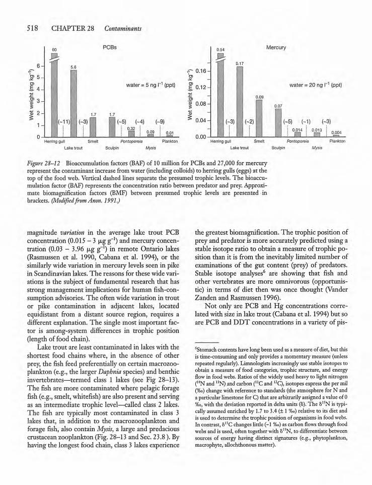
518 CHAPTER 28 Contaminants
6-T
x. °
I 4-
I
1-1
PCBs
water = 5 ng I"1 (ppt)
~5) (-4) (-9)0.32
n 0.01
Herring gull Smelt Pontoporeia Plankton
Lake trout Sculpin Mysis
0.16-
D)E 0.12-1
| 0.08 -I
0.04-
0.00
0.54
0.17
(-3) (~2)
Mercury
water = 20 ng I"1 (ppt)
0.07
(-5) (-1) (~3)0.014 0.013
0.004
Herring gull Smelt Pontoporeia PlanktonLake trout Sculpin Mysis
Figure 28-12 Bioaccumulation factors (BAF) of 10million for PCBsand 27,000 for mercuryrepresent the contaminant increasefromwater (includingcolloids) to herring gulls (eggs) at thetop of the food web. Vertical dashed lines separate the presumed trophic levels. The bioaccumulation factor (BAF) represents the concentration ratio betweenpredator and prey.Approximate biomagnification factors (BMF) between presumed trophic levels are presented inbrackets. (ModifiedfromAnon. 1991.)
magnitude variation in the average lake trout PCBconcentration (0.015 - 3 fxg g-1) andmercury concentration (0.03 - 3.96 \xg g~l) in remote Ontario lakes(Rasmussen et al. 1990, Cabana et al. 1994), or thesimilarly widevariation in mercury levels seen in pikein Scandinavian lakes. The reasons for these wide variations is the subject of fundamental research that hasstrong management implications for human fish-consumption advisories. The often widevariation in troutor pike contamination in adjacent lakes, locatedequidistant from a distant source region, requires adifferent explanation. The single most important factor is among-system differences in trophic position(length of food chain).
Lake trout are least contaminated in lakes with theshortest food chains where, in the absence of otherprey, the fish feed preferentially on certain macrozooplankton (e.g., the larger Daphnia species) and benthicinvertebrates—termed class 1 lakes (see Fig 28-13).The fish are more contaminated where pelagicforagefish (e.g., smelt, whitefish) are alsopresentand servingas an intermediate trophic level—called class 2 lakes.The fish are typically most contaminated in class 3lakes that, in addition to the macrozooplankton andforage fish, also containMysis, a large and predaciouscrustacean zooplankton (Fig. 28-13 and Sec. 23.8). Byhaving the longest food chain, class 3 lakes experience
the greatestbiomagnification. The trophic positionofprey and predator is more accuratelypredicted using astableisotope ratio to obtain ameasure of trophic position than it is from the inevitablylimited number ofexaminations of the gut content (prey) of predators.Stable isotope analyses6 are showing that fish andother vertebrates are more omnivorous (opportunistic) in terms of diet then was once thought (VanderZanden and Rasmussen 1996).Not only are PCB and Hg concentrations corre
lated with size in lake trout (Cabana et al. 1994) but soare PCB and DDT concentrations in a variety of pis-
6Stomach contents have longbeenused asameasure ofdiet,but thisis time-consuming and onlyprovides a momentary measure (unlessrepeated regularly). Limnologists increasingly usestable isotopes toobtain a measure of food categories, trophic structure, and energyflowin foodwebs.Ratios of the widelyused heavyto light nitrogen(l4N and13N) andcarbon (13C and 12C), isotopes express thepermil(%o) change withreference to standards (the atmosphere forN andaparticular limestone forC) thatarearbitrarily assigned avalue of0%o, with thedeviation reported in delta units (8). The 8I5N is typically assumed enriched by 1.7 to 3.4(± 1%o) relative to its dietandisused to determine the trophic positionof organismsin foodwebs.Incontrast, 8nC changes little(~1 %o) ascarbon flows through foodwebs and isused, often together with 815N, to differentiate betweensources of energy having distinct signatures (e.g., phytoplankton,macrophyte,allochthonousmatter).
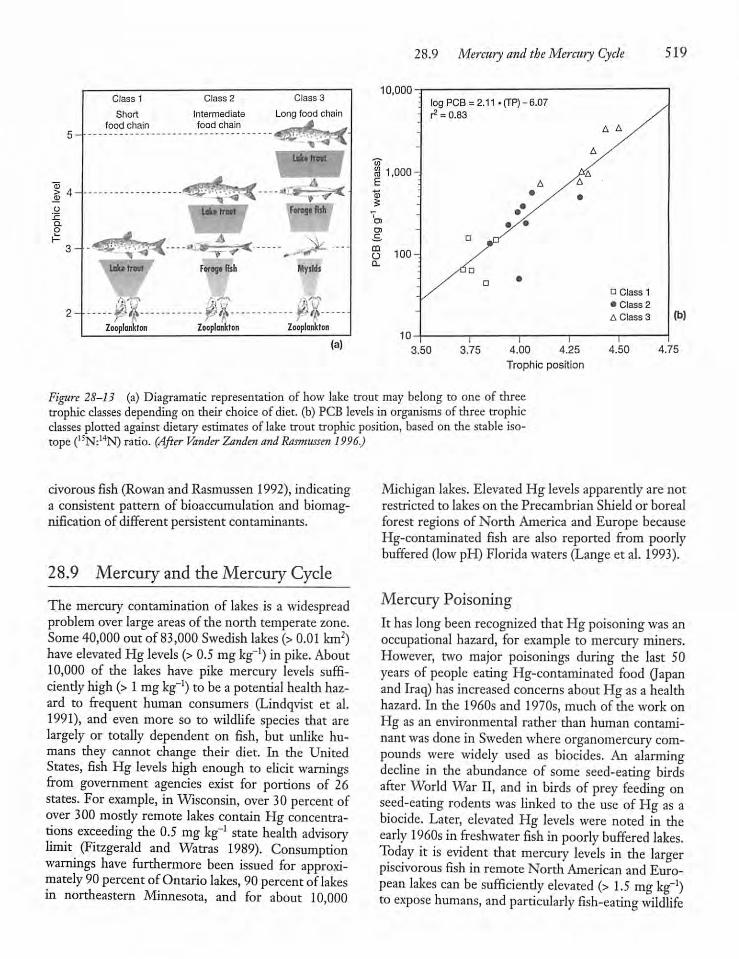
5--
> 4-
ox:
3- -
Class 1
Loke trout
Zooplankton
Class 2 Class 3
Long food chain
Forage fish Myslds
Zooplankton Zooplankton
28.9 Mercury and the Mercury Cycle
10,000
3 i,oooE
; logPCB = 2.11.(TP)-6.07• ^ = 0.83
100-
10
3.50 3.751 1
4.00 4.25
Trophic position
A A
• Class 1
• Class 2
A Class 3
4.50
519
(b)
4.75
Figure 28-13 (a) Diagramatic representation of how lake trout may belong to one of threetrophicclasses depending on their choice of diet, (b)PCB levels in organisms of three trophicclasses plotted against dietary estimates of lake trout trophic position, based on the stable isotope (15N:14N) ratio. (After Vander Zanderi and Rasmussen 1996.)
civorous fish (Rowan and Rasmussen 1992), indicatinga consistent pattern of bioaccumulation and biomagnification of different persistent contaminants.
28.9 Mercury and the Mercury Cycle
The mercury contamination of lakes is a widespreadproblemover large areas of the north temperate zone.Some 40,000 out of 83,000 Swedish lakes (> 0.01 km2)have elevated Hg levels (> 0.5 mgkg-1) in pike. About10,000 of the lakes have pike mercury levels suffi-ciendy high (> 1mgkg-1) to bea potential health hazard to frequent human consumers (Lindqvist et al.1991), and even more so to wildlife species that arelargely or totally dependent on fish, but unlike humans they cannot change their diet. In the UnitedStates, fish Hg levels high enough to elicit warningsfrom government agencies exist for portions of 26states. For example, inWisconsin, over 30 percent ofover 300 mosdy remote lakes contain Hg concentrations exceeding the 0.5 mg kg-1 state health advisorylimit (Fitzgerald and Watras 1989). Consumptionwarnings have furthermore been issued for approximately 90percent ofOntario lakes, 90percent oflakesin northeastern Minnesota, and for about 10,000
Michigan lakes. Elevated Hg levels apparently are notrestricted to lakes on the Precambrian Shield or borealforest regions of North America and Europe becauseHg-contaminated fish are also reported from poorlybuffered (lowpH) Florida waters (Lange et al. 1993).
Mercury PoisoningIt has longbeen recognized that Hg poisoning was anoccupational hazard, for example to mercury miners.However, two major poisonings during the last 50years of people eating Hg-contaminated food (Japanand Iraq) has increased concerns about Hg as a healthhazard. In the 1960s and 1970s, much of the work onHg as an environmental rather than human contaminant was done in Sweden where organomercury compounds were widely used as biocides. An alarmingdecline in the abundance of some seed-eating birdsafter World War II, and in birds of prey feeding onseed-eating rodents was linked to the use ofHg as abiocide. Later, elevated Hg levels were noted in theearly 1960s in freshwater fish in poorly buffered lakes.Today it is evident that mercury levels in the largerpiscivorous fish in remote North American and European lakes can be sufficiendy elevated (> 1.5 mg kg-1)toexpose humans, and particularly fish-eating wildlife
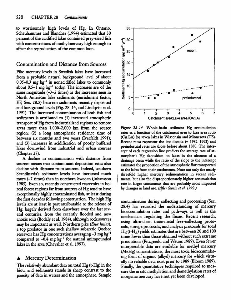
520 CHAPTER 28 Contaminants
to worrisomely high levels of Hg. In Ontario,Scheuhammer and Blancher (1994) estimated that 30percentof the acidified lakes containedprey-sized fishwithconcentrations ofmethylmercury highenoughtoaffect the reproduction of the common loon.
Contamination and Distance from Sources
Pike mercury levels in Swedish lakes have increasedfrom a probable natural background level of about0.05-0.3 mg kg-1 in nonacidified lakes to commonlyabout 0.5-1 mg kg-1 today. The increases are of thesamemagnitude (~3-5 times) as the increases seen inNorth American lake sediments (enrichment factor,EF, Sec. 28.5) between sediments recendy depositedandbackground levels (Fig. 28-14,andLindqvist et al.1991).The increased contamination of both fish andsediments is attributed to (1) increased atmospherictransport of Hg from industrialized regions to remoteareas more than 1,000-2,000 km from the sourceregion: (2) a long atmospheric residence time ofbetween six months and two years (Iverfeldt 1991);and (3) increases in acidification of poorly bufferedlakes downwind from industrial and urban sources(Chapter 27).
A decline in contamination with distance fromsourcesmeans that contaminant deposition rates alsodecline with distance from sources. Indeed, southernScandinavia's sediment levels have increased muchmore (~7 times) than in northern Sweden (Johansson1985). Even so, recently constructed reservoirs in boreal forest regions far fromsources ofHg tend to haveexceptionally highlycontaminated fish, at leastduringthe first decades following construction. The highHglevels are at least in part attributable to the release ofHg, largelyderived from elsewhere over the last several centuries, from the recently flooded and nowanoxic soils(Bodaly et al. 1984), althoughrocksourcesmaybe important aswell.Northern pike (Esox lucius),a top predator in one such shallowsubarcticQuebecreservoir has Hgconcentrations averaging "3mg kg-1compared to ~0.4 mg kg"1 for natural unimpoundedlakes in the area (Chevalier et al. 1997).
• Mercury DeterminationThe relatively abundantdataon totalHg (t-Hg) in thebiota and sediments stands in sharp contrast to thepaucity of data in waters and the atmosphere. Sample
12 3 4 5
Catchment area:Lake area (CA:1_A)
Figure 28-14 Whole-basin sediment Hg accumulationrates as a function of the catchment area to lake area ratio(CALA) for seven lakes in Wisconsin and Minnesota (US).Recent rates represent the last decade (= 1982-1992) andpreindustrial rates are those beforeabout 1850. The intercept of each regression line predicts the average rate of atmospheric Hg deposition on lakes in the absence of adrainage basinwhile the ratio of the slope to the interceptestimates the proportionof the atmospheric flux transportedto the lakesfrom their catchments.Note not only the nearlythreefold higher mercury sedimentation in recent sediments, but also the disproportionately higher accumulationrate in larger catchments that are probably most impactedby changesin land use. (After Swain etal. 1992.)
contamination during collecting and processing (Sec.28.4) has retarded the understanding of mercurybioaccumulation rates and pathways as well as themechanisms regulating the fluxes. Recent research,using ultra-clean trace-metal free-collecting protocols, storageprotocols,and analysis protocols for totalHg (t-Hg) yields estimates thatarebetween 20and100times lower than those obtained without such extremeprecautions (Fitzgerald andWatras 1989). Even fewerinterpretable data are available for methyl mercury(MeHg) concentrations, themosttoxic bioaccumulat-ing form of organic (alkyd) mercury forwhich virtually no reliable dataexist prior to 1989 (Bloom 1989).Finally, the quantitative techniques required to measurethe in situmethylation anddemethylation ratesofinorganic mercury have notyetbeendeveloped.
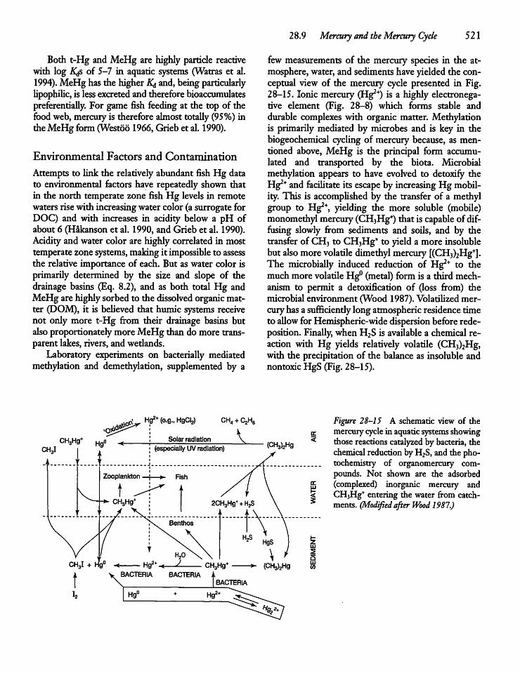
Both t-Hg and MeHg are highly particle reactivewith log Ajs of 5-7 in aquatic systems (Watras et al.1994). MeHg has the higher K& and, beingparticularlylipophilic, is less excreted and thereforebioaccumulatespreferentially. For game fish feeding at the top of thefoodweb, mercury is therefore almost totally (95%) intheMeHg form(Westdo 1966, Grieb et al. 1990).
Environmental Factors and Contamination
Attempts to link the relatively abundant fishHg datato environmental factors have repeatedly shown thatin the north temperate zone fish Hg levels in remotewaters risewith increasingwater color (asurrogateforDOC) and with increases in acidity below a pH ofabout 6 (Hakanson et al. 1990, and Grieb et al. 1990).Acidity and water color are highly correlated in mosttemperatezonesystems, makingit impossible to assessthe relative importance of each. But aswater color isprimarily determined by the size and slope of thedrainage basins (Eq. 8.2), and as both total Hg andMeHg are highlysorbed to the dissolved organicmatter (DOM), it is believed that humic systems receivenot only more t-Hg from their drainage basins butalsoproportionatelymoreMeHg than do more transparent lakes, rivers, and wetlands.Laboratory experiments on bacterially mediated
methylation and demethylation, supplemented by a
Hg2* (e.g., HgCI2) CH4 +C2H6
CH,I
28.9 Mercury andthe Mercury Cycle 521
few measurements of the mercury species in the atmosphere, water, and sediments haveyielded the conceptual view of the mercury cycle presented in Fig.28-15. Ionic mercury (Hg2*) is a highly electronegative element (Fig. 28-8) which forms stable anddurable complexes with organic matter. Methylationis primarily mediated by microbes and is key in thebiogeochemical cycling of mercury because, as mentioned above, MeHg is the principal form accumulated and transported by the biota. Microbialmethylation appears to have evolved to detoxify theHg2* and faciHtate its escape byincreasing Hgmobility. This is accomplished by the transfer of a methylgroup to Hg2*, yielding the more soluble (mobile)monomethylmercury(CH3Hg+) that is capable of diffusing slowly from sediments and soils, and by thetransferof CH3 to CH3Hg* to yield a more insolublebut also morevolatile dimethyl mercury[(CH3)2Hg+].The microbially induced reduction of Hg2* to themuch more volatile Hg°(metal) form isa thirdmechanism to permit a detoxification of (loss from) themicrobial environment (Wood 1987).Volatilized mercuryhasa sufficiently long atmosphericresidencetimeto allow forHemispheric-wide dispersionbeforerede-position. Finally, when H2S is available a chemical reaction with Hg yields relatively volatile (CH3)2Hg,with the precipitation of the balance as insoluble andnontoxic HgS (Fig. 28-15).
Figure 28-15 A schematic view of themercurycyclein aquaticsystems showingthose reactions catalyzed by bacteria, thechemical reduction byH2S, and the photochemistry of organomercury compounds. Not shown are the adsorbed(complexed) inorganic mercury andCH3Hg+ entering the water from catchments. (Modifiedafter Wood 1987.)
CH3I +Hg° m. Hg2+-« 1 CH3Hg* •- (CH3)zHg1 V BACTERIA BACTERIA AJ \^ [BACTERIA
Hgu Hg'
522 CHAPTER 28 Contaminants
28.10 Toxic Chemicals, EnvironmentalHealth, andAquaticManagement
The only effective way to reduce the supplyof toxicchemicals to the environment is to prevent their release to the atmosphere and waterways. Toxic chemicals that are persistent and also bioaccumulate are ofparticular concern because of their potential for biomagnification in foodwebs. The humanconsumptionofcontaminated fish andwildlife isan importantissue,particularly for subsistence fishermen and isolatedcommunities of native people with a traditional diethigh in piscivorous fishwho have to balancecontamination risks againsta nutritious diet. However, piscivorous fish and fish-eating wildHfe (e.g., loons,kingfishers, gulls, eagles, mink, otter), cannot changetheir fish diet and are far more at risk.There is considerable debate as to the seriousness of
die contaminationof piscivorous fish and their predators in terms of health but there is enoughevidence toshowthat certainwildlife species are at least subdy affected in the more polluted portionsof the LaurentianGreat Lakes. The increases in the frequency of deformities andreproductive failures in aquatic birds, including embryosurvival (Giesyet al. 1994), that havebeenobserved are similarto those seen in laboratorystudiesof the same or a surrogate species exposed to PCBs andother POPs (Ludwig etal. 1993).7
Highlights• Among the chemicals of greatest concern are highlychlorinatedorganicmolecules, knownasorganochlo-rines, that are persistent (degrade slowly) and accumulatein the biota.Those persistent organicpollutants(POPs) that are somewhat volatile or sorbed to airborne particlesare carried for hundreds if not thou
7"This studyindicates thatthe protection ofwildlife species willrequiremuchmore stringentregulations than those currentlyrecommended to protect the human population from cancer. Theprotection of wildlife populations and humans from subtle effectsshould be given equal priority to thatof protecting humanpopulations from cancer." (Ludwig et al. 1993)
sands of kilometers from areas of production to remote regions.Toxicity can be acute, resultingin quickdeath.Morecommonis chronic (sublethal) toxicity, whoseeffectsare much more difficult to quantify and, because itexpresses its effects with lags,makesit difficultto linkchronic toxicityto particular sources.More than half of the quantitiesof most tracemetals(including toxicAs, Cd, Hg, and Pb) globally emittedto the atmosphereare anthropogenically produced.The relative importanceof the atmosphereasa directsource of particular POPs and toxic trace metals inremote aquatic systems is gready affected by thecatchment areaiwater area ratio.Contaminants that dissolve readily in water areknownashydrophilic, whilethosewith a lowsolubility are known ashydrophobic. The latter sorb readilyonto detrital particles and living organisms, are lessbioavailable for directuptakefromthewater than hydrophiliccontaminants, and are more likelyto be removed from the water by sedimentation andfilter-feeding organisms.A systematic relationship between the structure ofpersistent organic contaminants and toxic metals andtheir activity—including their toxicity, uptake, andbioaccumulation potential—and distribution hasbeen formalized in quantitative structure and activityrelationships (QSARs) that havepredictivepower.• The recent developmentof toxicity equivalencyfactors (TEFs) allows the sum total effect of differentcontaminants in nature to be compared.• Important differences between adjacent remotewaterways in the contamination of particular piscivorous fish specieswith, for example, PCBs or mercury,are linked in part to differences in the number ofsteps in the respective food chains (food-web structure), allowing for differentdegrees of biomagnification.The onlyeffective wayto reducethe supply of toxinsto aquaticsystems is to prevent their release to waterways and the atmosphere.
CHAPTER
29
Reservoirs
29.1 Introduction
The vastmajorityof reservoirs in existence todayarerelatively small (volume < ~106 m3)—they are calledimpoundments, or dams in southernAfricaandAustralia(see Sec. 6.8)—and are used primarily for irrigation,water supply, and also for fish farming. The smallestones are usually constructed for domesticuse, watering livestock, irrigation, or fish production.However,about948 large-volume reservoirs, thosewithdamsatleast 15 m high, were under construction in 1994(Anon. 1997) contributing to the about 50,000 suchdams worldwide in 2000.Most reservoirs are constructedbydamming rivers
in regions where evaporation approaches or exceedsprecipitation (Fig 5-9), with the water typically derived from local rivers during rainy periods. Permanent lakes are uncommon as the result of low localrunoff and normally few basins deep enough to holdwater yearround. River discharge into semiarid andarid zone (dryland) reservoirs shows large seasonal andinteryearvariation. Large reservoirs in the lowrunoffportions of the world are built principally for irrigation, flood control, andwater supply to urban areas,but at times also for improved navigation (as on theVolga River, Sec. 5.8), fish culture, or recreation.Large-volume reservoirs, built primarily for hydroelectric power generation, are constructed in regionsof low as well as high precipitation, where landscapetopography andriver discharge make damming possible and economically attractive (Fig. 29-1).
The fraction of the world's runoff temporarily retained behind dams has been growing rapidly, withlarge-volume reservoirs (> 0.5 km3) holding some 20percent (~8,400 km3) of the global mean runoff.Reservoirwater storage has risen to about seven timesthe volume ofwater in rivers(Vorosmarty et al. 1997).Water retention by reservoirs has major ramifica
tions for river discharge and its timing, for sedimentand nutrient retention behind dams (Sec.9.6), for thebiota of the extensively modified rivers and wetlandsupstream and downstream from the reservoirs, and forthe affected people.The negative environmental consequences and social impacts of large reservoirs arebecoming gradually better appreciated and a prioriEnvironmental Impact Assessments (EIAs) are requiredandaremorerigorous than in thepast.Western Umnologists have traditionally paid little
attention to reservoirs; the firstlimnology textbook ontheminEnglish was onlypublished in 1990 (Thorntonet al. 1990). Until recendy, possibly the single mosthistorically important set of publications in awestEuropean language are the three slim volumes reportingthe long-term careful studyof a number of Czechhy-droele(^(^drinkingwater reservoirs (Hrbacek 1966,Hrbacek and Straskraba 1973a and b). These (dated)volumes remain useful for introducing Western readers to a vastRussian and east European literature thathas been largely inaccessible to theWesternworld. Asearly as 1963,613 papers hadbeenwrittenon the shallow eutrophic Rybinsk Reservoir on the Volga River(RU)(Straskraba and Straskrabova 1969).
523
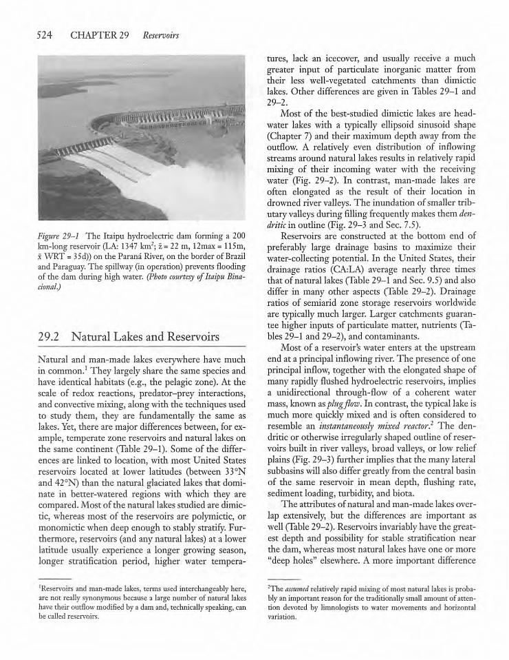
524 CHAPTER 29 Reservoirs
Figure 29-1 The Itaipu hydroelectric dam forming a 200km-long reservoir (LA: 1347 km2; z= 22 m, 12max = 115m,x WRT = 35d)) on the Parana River, on die border of Braziland Paraguay. The spillway (in operation) prevents floodingof the dam during high water. (Photo courtesy of Itaipu Bina-cional.)
29.2 Natural Lakes and Reservoirs
Natural and man-made lakes everywhere have muchin common.1 They largely share the same species andhave identical habitats (e.g., the pelagic zone). At thescale of redox reactions, predator-prey interactions,and convective mixing, alongwith the techniquesusedto study them, they are fundamentally the same aslakes. Yet, there are major differences between, for example, temperate zone reservoirs and natural lakes onthe same continent (Table 29-1). Some of the differences are linked to location, with most United Statesreservoirs located at lower latitudes (between 33°Nand 42°N) than the natural glaciated lakes that dominate in better-watered regions with which they arecompared. Most of the natural lakesstudied are dimic-tic, whereas most of the reservoirs are polymictic, ormonomicticwhen deep enough to stablystratify. Furthermore, reservoirs (and any natural lakes) at a lowerlatitude usually experience a longer growing season,longer stratification period, higher water tempera
'Reservoirs and man-made lakes, terms used interchangeably here,are not really synonymousbecause a large number of natural lakeshavedieir outflowmodifiedby a dam and, technicallyspeaking, canbe called reservoirs.
tures, lack an icecover, and usually receive a muchgreater input of particulate inorganic matter fromtheir less well-vegetated catchments than dimicticlakes. Other differences are given in Tables 29-1 and29-2.Most of the best-studied dimictic lakes are head
water lakes with a typically ellipsoid sinusoid shape(Chapter 7) and dieir maximum depth away from theoutflow. A relatively even distribution of inflowingstreams around natural lakes results in relatively rapidmixing of their incoming water with the receivingwater (Fig. 29-2). In contrast, man-made lakes areoften elongated as the result of their location indrowned river valleys. The inundation of smaller tributary valleys during filling frequentlymakes them dendritic in outline (Fig. 29-3 and Sec. 7.5).
Reservoirs are constructed at die bottom end ofpreferably large drainage basins to maximize theirwater-collecting potential. In the United States, theirdrainage ratios (CA:LA) average nearly three timesthat of natural lakes (Table 29-1 and Sec. 9.5) and alsodiffer in many other aspects (Table 29-2). Drainageratios of semiarid zone storage reservoirs worldwideare typically much larger. Larger catchments guarantee higher inputs of particulate matter, nutrients (Tables 29-1 and 29-2), and contaminants.Most of a reservoir's water enters at the upstream
end at a principal inflowing river. The presenceof oneprincipal inflow, together with the elongated shape ofmany rapidly flushed hydroelectric reservoirs, impliesa unidirectional through-flow of a coherent watermass, known asplugflow. In contrast, the typical lake ismuch more quickly mixed and is often considered toresemble an instantaneously mixed reactor? The dendritic or otherwise irregularly shaped outline of reservoirs built in river valleys, broad valleys, or low reliefplains(Fig. 29-3) further implies that the many lateralsubbasins willalsodiffer gready from the central basinof the same reservoir in mean depth, flushing rate,sediment loading, turbidity, and biota.The attributes of natural and man-made lakes over
lap extensively, but the differences are important aswell (Table29-2). Reservoirs invariablyhave the greatest depth and possibility for stable stratification nearthe dam, whereas most natural lakes have one or more"deep holes" elsewhere. A more important difference
"The assumed relatively rapid mixingof most natural lakesis probablyan important reason for the traditionallysmall amount of attention devoted by limnologists to water movements and horizontalvariation.
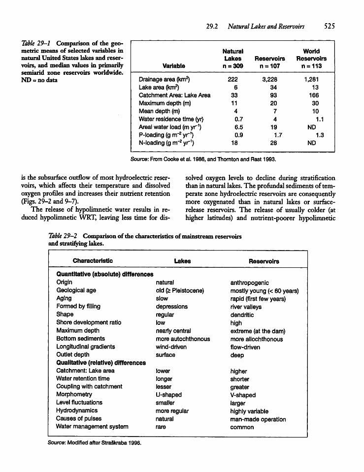
29.2 Natural Lakes and Reservoirs 525
Table 29-1 Comparison of the geometric means of selected variables innatural United States lakes and reservoirs, and median values in primarilysemiarid zone reservoirs worldwide.ND = no data
Natural WorldLakes Reservoirs Reservoirs
Variable n = 309 n = 107 n = 113
Drainage area (km2) 222 3,228 1,281Lakearea (km2) 6 34 13
Catchment Area: Lake Area 33 93 166Maximum depth (m) 11 20 30Mean depth (m) 4 7 10Water residence time (yr) 0.7 4 1.1
Areal water load (myr1) 6.5 19 ND
P-loading (gm~2 yr1) 0.9 1.7 1.3
N-loading (gm~2 yr1) 18 28 ND
Source: From Cooke et al. 1986, and Thornton and Rast 1993.
is the subsurface outflow of most hydroelectric reservoirs, which affects their temperature and dissolvedoxygen profiles and increases their nutrient retention(Figs. 29-2 and 9-7).The release of hypolimnetic water results in re
duced hypolimnetic WET, leaving less time for dis
solved oxygen levels to decline during stratificationthan in natural lakes. The profundalsedimentsof temperate zone hydroelectric reservoirs are consequendymore oxygenated than in natural lakes or surface-release reservoirs. The release of usually colder (athigher latitudes) and nutrient-poorer hypolimnetic
Table 29—2 Comparisonof the characteristicsofmainstreamreservoirsand stratifying lakes.
Characteristic Lakes Reservoirs
Quantitative (absolute) differencesOrigin natural anthropogenicGeological age old (>Pleistocene) mostly young (< 60 years)Aging slow rapid (first few years)Formed by filling depressions river valleysShape regular dendriticShore development ratio low highMaximum depth nearly central extreme (at the dam)Bottom sediments more autochthonous more allochthonousLongitudinal gradients wind-driven flow-drivenOutlet depth surface deepQualitative (relative) differencesCatchment: Lake area lower higherWater retention time longer shorterCoupling with catchment lesser greaterMorphometry U-shaped V-shapedLevel fluctuations smaller largerHydrodynamics more regular highly variableCauses of pulses natural man-made operationWater management system rare common
Source: Modified after StraSkraba 1996.
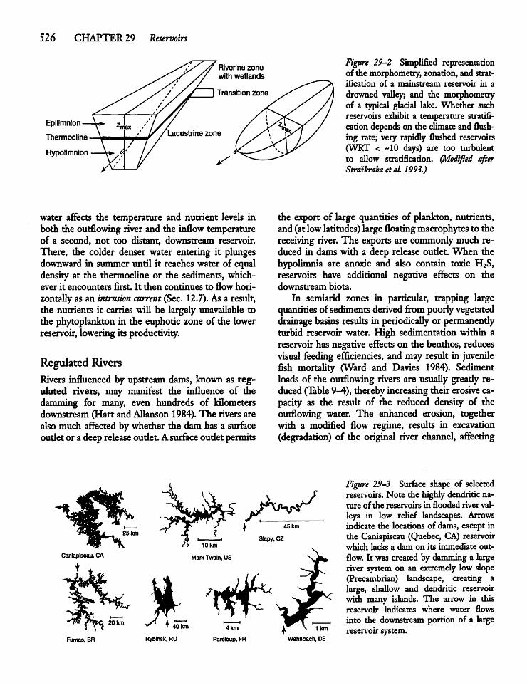
526 CHAPTER 29 Reservoirs
Epllimnion—\+- zlThermocline
Hypolimnion —W *
water affects the temperature and nutrient levels inboth the outflowing river and the inflowtemperatureof a second, not too distant, downstream reservoir.There, the colder denser water entering it plungesdownward in summer until it reaches water of equaldensity at the thermocline or the sediments, whichever it encounters first. It then continues to flow horizontallyas an intrusion current (Sec. 12.7). Asa result,the nutrients it carrieswill be largely unavailable tothe phytoplankton in the euphoric zone of the lowerreservoir, loweringits productivity.
Regulated RiversRivers influenced by upstream dams, known as regulated rivers, may manifest the influence of thedamming for many, even hundreds of kilometersdownstream(Hart and Allanson 1984). The rivers arealso much affected by whether die dam has a surfaceoudet or a deep releaseoudet. Asurfaceoudet permits
Fumas, BR Rybinsk, RU Pareloup, FR
Figure 29-2 Simplified representationof the morphometry, zonation, and stratification of a mainstream reservoir in adrowned valley; and the morphometryof a typical glacial lake. Whether suchreservoirs exhibit a temperature stratification depends on the climate and flushing rate; very rapidly flushed reservoirs(WRT < ~10 days) are too turbulentto allow stratification. (Modified afterStraskraba etal. 1993.)
the export of large quantities of plankton, nutrients,and(at lowlatitudes) largefloatingmacrophytes to thereceiving river. The exports are commonlymuch reduced in damswith a deep release oudet. When thehypolimnia are anoxic and also contain toxic H2S,reservoirs have additional negative effects on thedownstream biota.In semiarid zones in particular, trapping large
quantities of sediments derived frompoorlyvegetateddrainage basins results in periodically or permanentlyturbid reservoir water. High sedimentation within areservoir hasnegative effects on the benthos, reducesvisual feeding efficiencies, andmayresult in juvenilefish mortality (Ward and Davies 1984). Sedimentloads of the outflowing rivers are usually gready reduced(Table 9-4), thereby increasing their erosive capacity as the result of the reduced density of theoutflowing water. The enhanced erosion, togetherwith a modified flow regime, results in excavation(degradation) of the original river channel, affecting
Wahnbach, DE
Figure 29-3 Surface shape of selectedreservoirs. Note the highly dendritic nature of the reservoirs in flooded river valleys in low relief landscapes. Arrowsindicate the locations of dams, except inthe Caniapiscau (Quebec, CA) reservoirwhich lacks a dam on its immediate outflow. It wascreated by damming a largeriver system on an extremely low slope(Precambrian) landscape, creating alarge, shallow and dendritic reservoirwith many islands. The arrow in thisreservoir indicates where water flowsinto the downstream portion of a largereservoir system.
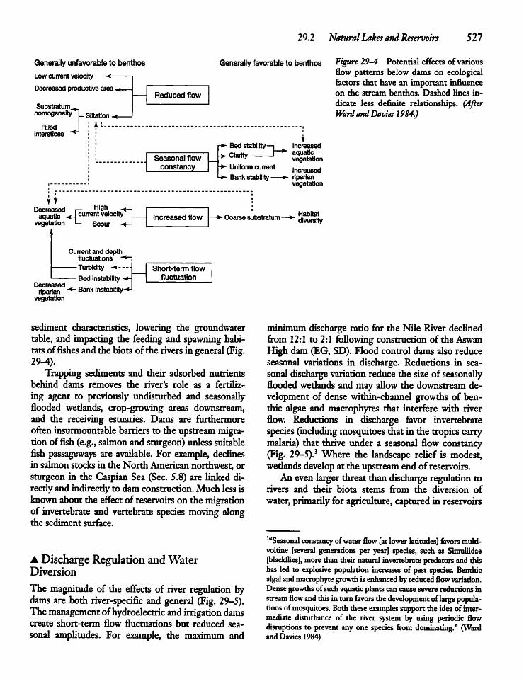
29.2 Natural Lakes and Reservoirs 527
Generally unfavorable to benthosLow current velocity -<
Decreased productive area -*-
Generally favorable to benthos Figure 29-4 Potential effectsof variousflow patterns belowdams on ecologicalfactors that have an important influenceon the stream benthos. Dashed lines indicate less definite relationships. (AfterWard andDavies1984.)
Substratum <homogeneity|_ siltation -«-
ALRiled Iinterstices "*~^
Reduced flow
Bed stabilityClarity _J *" aquatic
vegetation
YIncreased
Seasonal flowconstancy Uniform current
Bank stability —Increasedriparianvegetation
YtDecreasedaquatic '̂ currentvelocityHigh
vegetation Scour OH Increased flow -Coarse substratum - Habitatdiversity
Current and depthfluctuations "*
— Turbidity •<--
Bed instability -Bank instability-
Decreasedriparian
vegetation
Short-term flowfluctuation
sediment characteristics, lowering the groundwatertable, and impacting the feeding and spawning habitatsoffishes andthe biotaof the rivers in general (Fig.29-4).Trapping sediments and their adsorbed nutrients
behind dams removes the river's role as a fertilizing agent to previously undisturbed and seasonallyflooded wedands, crop-growing areas downstream,and the receiving estuaries. Dams are furthermoreofteninsurmountable barriers to the upstream migration offish (e.g., salmon and sturgeon) unless suitablefish passageways are available. For example, declinesin salmon stocks in the North American northwest, orsturgeon in the CaspianSea (Sec. 5.8) are linked directlyand indirectlyto damconstruction. Much less isknown about the effect of reservoirs on themigrationof invertebrate and vertebrate species moving alongthe sediment surface.
A Discharge Regulation andWaterDiversion
The magnitude of the effects of river regulation bydams are both river-specific and general (Fig. 29-5).Themanagement ofhydroelectric andirrigation damscreate short-term flow fluctuations but reduced seasonal amplitudes. For example, the maximum and
minimum discharge ratio for the Nile River declinedfrom 12:1 to 2:1 following construction of the AswanHigh dam (EG, SD). Flood control dams also reduceseasonal variations in discharge. Reductions in seasonal discharge variation reducethe sizeof seasonallyflooded wedands and mayallow the downstream development of dense within-channel growths of benthic algae and macrophytes that interfere with riverflow. Reductions in discharge favor invertebratespecies (including mosquitoes that in the tropicscarrymalaria) that thrive under a seasonal flow constancy(Fig. 29-5).3 Where die landscape relief is modest,wedands develop at the upstream endof reservoirs.Aneven larger threat than discharge regulation to
rivers and their biota stems from the diversion ofwater, primarily for agriculture, captured in reservoirs
3aSeasonal constancy ofwater flow [at lower latitudes] favors multi-voltine [several generations per year] species, such as Simuliidae[blackflies], morethantheirnatural invertebrate predators and thishas led to explosive population increases of pest species. Benthicalgal andmacrophyte growth is enhanced by reduced flow variation.Densegrowths of suchaquatic plants cancause severe reductions instream flow and thisin turnfavors thedevelopment of large populations of mosquitoes. Boththese examples support the idea of intermediate disturbance of the river system by using periodic flowdisruptions to prevent any one species from dominating." (WardandDavies 1984)
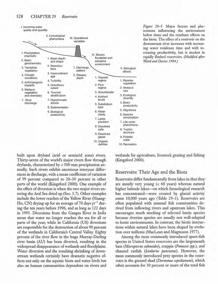
528 CHAPTER 29 Reservoirs
Incoming waterquality and quantity
I. Limnological
^^phenomena III.Operational
variables
1. Precipitationchemistry
1. Basin depth-L-Ji^-v IV. Stream
floodplain and2. Basin and shape estuarinegeochemistry environment
3. Terrestrial2. Retentiontime 1. Discharge V. Biological
vegetation pattern effects4. Climatic
3. Impoundmentage 2. Release
depthconditions 1. Thermal
5. Anthropogenicimpacts
4. Turbidity
5. Drawdown
regime
2. Flow
1. Riparianvegetation
6. Wetlandextent regime 2. Wetland
sizevegetation 6. Thermal 3. Groundwaterand chemistry stratification 4. Nutrient 3. Ecological
diversity7. River 7. Hypolimnetic levels
discharge anoxia
8. Sedimentation5. Substratumtype
4. Bioticproductivity
9. Biological 6. Water5. Migrations
productivity clarity
7. Lenticplankton
8. Dissolvedsalts
9. Dissolvedgases
10. Organicdetritus
6. Speciescomposition
7. Life-cyclephenomena
8. Trophicstructure
9. Potablewater
10. Recreation
Figure 29-5 Major factors and phenomena influencing the environmentbelow dams and die resultant effects onthe biota. The effect of a reservoir on thedownstream river increases with increasing water residence time and with increasing productivity, but is modest inrapidly flushed reservoirs. (Modified afterWard andDavies 1984.)
built upon dryland (arid or semiarid zone) rivers.Thirty-seven of the world's major rivers flow throughdrylands, characterized by < 500 mm precipitation annually. Such rivers exhibit enormous interyear differencesin discharge, with amean coefficientof variationof 99 percent compared to 20-30 percent in otherparts of the world (Kingsford 2000). One example ofthe effectof diversioniswhen the twomajor riversentering the AralSeadried up (Sec. 5.7).Other examplesinclude the lower reachesof the Yellow River(Huang-Ho, CN) drying up foran average of 70days yr-1 during the ten years before 1996,and as long as 122 daysin 1995. Diversions from the Ganges River in Indiamean that water no longer reaches the sea for all orparts of the year, while in California (US) diversionsare responsible for the destruction of about 90 percentof the wedands in California's Central Valley. Eightypercent of the river flow in the huge Murray-Darlingriver basin (AU) has been diverted, resulting in thewidespread disappearance of wedands and floodplains.Water diversion and the resulting shrinking of downstream wedands certainly have dramatic negative effectsnot only on the aquatic biota and water birds butalso on human communities dependent on rivers and
wedands for agriculture, livestock grazing and fishing(Kingsford 2000).
Reservoirs: Their Age and the BiotaReservoirs differ fundamentally from lakesin that theyare mostly very young (< 60 years) whereas naturalhigher latitudelakes—on which limnological researchhas concentrated—were created by glacial activitysome 10,000 years ago (Table 29-1). Reservoirs areoften populated with unusual fish communities derived from inflowing rivers and upstream lakes. Thisencourages much stocking of selected lentic speciesbecause riverine species are usually not well-adaptedto lentic environments. In contrast, the biotic interactions within natural lakes have been shaped by evolution over millenia (MacLean and Magnuson 1977).Among the most commonly introduced sport-fish
species in United States reservoirs are the largemouthbass (Microptcrus salmoides), crappie {Pomoxis spp.), andchannel catfish (Ictalurus punctatus). However, themost commonly introduced prey species in the reservoirs is the gizzard shad (Doroso?na cepedianum), whichoften accounts for 30 percent or more of the total fish
biomass(Stein et al. 1995).The adult shad is herbivorousaswellaszooplanktivorous and feeds bypumpingwater through its gillswhile swimming. The young-of-the-year(YOY or age 0+)shad influencethe structure of fish communities by reducing the growth,survival, and abundance of coexisting species. Theshadlarvae feedon protozoansand rotifers, shiftingtocrustacean zooplankton when somewhat bigger, andfeeding on phytoplankton, protozoa, rotifers,and sediment detritus (including bacteria and algae) whenlarger than about 3 cm. Where abundant, shad andother such omnivorous fish compete successfully formacrozooplanktonwith the larvaeof piscivorous gamefish. Omnivorous species therefore indirecdy affectthe piscivorous species by influencing the abundanceof their zooplanktivorous prey who, as visual feeders,are handicapped under turbid conditions (O'Brian1990). Shad and other sediment-feeding fish canplaya significant role in recycling nutrients to the phytoplankton following excretion (Vanni 1996).North temperate zone food-chain models are
based on top-down control of plankdvorous fish bypiscivorous species and are unlikely to be useful inpredicting the impact of gizzard shador other omnivorousfish species that are typically dominant in lowerand low latitude lakes and reservoirs. The abiHty ofomnivorous fish, such as tilapia (Sec. 26.6), to feedonphytoplankton, zooplankton, and detritus allowsthemto exert a still not well understood influence on thestructureof food webs and energyflow, differing fundamentally fromthe widely discussed patternsseeninhigher latitude waters (Vanni 1996).
29.3 The River-Lake-ReservoirContinuum
Both artificial and natural lakes lie along gradients ofclimate, geology, morphometry, flushing, chemistry,and biology that preclude a clear separation betweenlakes and reservoirs. The single most useful continuum along which to conceptualize and model thefunctioning of reservoirs is to envision them as intermediates between lakes and rivers (Fig. 29-6) interms of their water residence time (yr) or flushingrate (yr'1).Large reservoirs are of three basic types (Fig.
29-6). Mainstream or nin-of-the-river reservoirsare most riverlike (WRT = days to weeks) and aremost often constructed to generate electricity. Mainstream reservoirs experience little or no temperature
29.3 The River-Lake-Reservoir Continuum 529
RiversContinuum
Lakes
Reservoirs
Mainstream"run-of-the-river"
reservoirs
Tributarystoragereservoirs
Mainstreamstoragereservoirs
Days Weeks Months Years
Increasing average residence time
Figure 29-6 Reservoirs occupy an intermediate positionbetween rivers andnatural lakes on a continuum of aquaticecosystems. The extent of riverine influence and the hydraulic retention time determine the relative positionsof impoundment types (e.g., mainstream run-of-the-river,mainstreamstorage, tributary storage) along the river-lakecontinuum. (Modified after Kimmel and Groeger 1984.)
stratification if the water residence time is < —10 days(Straskraba et al. 1993), no seasonal lowering of thewater level, and the least modification of the riverinebiota within and below the reservoir. As a group,mainstream reservoirs have received the least attention from limnologists. Exceptions include certainreservoir cascades or chains of reservoirs (e.g., Volga,Colorado, and Vltava Rivers). Tributary storagereservoirsbuilt on small rivers have the longestwaterresidence time(WRT, typically fromamonthto ayearor more) and the greatest possibility of temperaturestratification where morphometry and climate allowthis. These reservoirs have a surface outflow and areusually built for flood control andirrigation. Theyperiodically experience a drawdown (water-level lowering, Sec. 29.6) when much more water is removedthan enters. However, drawdowns are not restricted toreservoirs. Natural drawdowns, a result of evaporationduring the dry season, are experienced most severelybynatural lakes in semiarid andaridregions. The tributary storage reservoir is the most common typeworldwide andhasreceived the mostlimnological attention among reservoir types, precisely because theymostresemble natural lakes in flushing (OECD 1982)andotherattributes. Mainstream storagereservoirshold an intermediate position (WRT=typically a fewmonths), butbecome more riverine (lotic) during high
5 30 CHAPTER 29 Reservoirs
runoff periods and more lacustrine (lentic) at othertimes.The WRT of both reservoirs and rapidly flushed
lakes is highly sensitive to seasonal variation in runoffand evaporation. The effectof this is once againmostevident in low runoff regions. An example is the LakeMcllwaine reservoir (ZW). It has an averageWRT ofabout one year, but varies from a calculated theoreticalmaximum of 12 years during months of severedroughts to an observed four months during exceptionallyhigh rainfallyears (Ballinger andThornton 1982).
29.4 Water Residence Timeand Plankton Growth Rates
The plankton diversity of rapidly flushed reservoirsand lakes declines when the flushing(dilution) rate exceeds the growth rate (doubling time) of the mostrapidly growing species at a particular temperatureand they experience washout. First to be affected arethe freshwater copepods whose development time(egg to egg) under optimal conditions is about 30daysat 10°, 14 daysat 20°, and 7.5 daysat 25°.Their development time is about 25 percent slower than cladocer-ans at the same temperature. Development time of thetypically much smaller rotifers is around 1.5 days at25° under otherwise optimal conditions (Allan 1976),explaining the dominance of rotifers (Basu and Pick1996) and fast-growing protozoa in rapidly flushedlotic systems and reservoirs. The sequential washout
2,000
1994
of the different zooplanktonwith increased flushing isexpected to havean effecton the community structureof their phytoplankton and protozoan prey beforethese more rapidly growing prey organisms themselves become directly affected by flushing. Macrozooplankton encountered in rapidly flushed systemsmust be derived from embayments characterized by alonger WRT, or from adjacent wetlands (see Fig.29-7). The first macrozooplankton to appear as theflushing rate declines are small rapidly reproducing,parthenogenic cladocerans (Sec. 23.3)—a large Daph-niaspeciesmade its appearance in a cool Scottish lakewhen the WRT consistendy exceeded about 18 days.The number of individuals became unrelated to flushing when the WRT exceeded about four weeks (Brookand Woodward 1956), reflecting the importance offactors other than WRT (e.g., predation and food)over longer time scales.Washout of phytoplankton commences at lower
WRT in turbid, deeply mixed, or cold reservoirswhere conditions for photosynthesis are much less favorable than in shallow systems of low turbidity atsummer temperatures. As the WRT declines withinand among systems, the flushing rate progressively exceeds the growdi rates of more of the species until thecommunity becomes restricted to a few small specieswith very high growth potential (Fig. 21-12). Underfavorable conditions of light, temperature, and nutrients, the minimum WRT required to allow the mostrapidly growing species to reach a biomass maximumis around 5-7 days in the relatively few temperate
400
-300
-200
-100
CD
3>
J2Q.OoN
Figure 29-7 Seasonal changes in waterresidence time (WRT), total phytoplankton, and total macrozooplankton biomassand transparency in polymictic Glen-more Reservoir (Alberta, CA; LA = 4.6km2, z = 6.1m). Note that the macrozooplankton abundance tends to be low during periods of most rapid flushing,whereas the phytoplankton biomass inthe particular reservoir tends to be greatest during the periods of highest irradi-ance and lowest turbidity (zcu > zmix) andmost rapid (~ 10 days) flushing (greatestnutrient loading, and wash-out of slowergrowing plankton). (After Watson et al.1996.)
zone lakes and reservoirs that have been investigated(Fig. 29-7, Straskraba and Javornicky 1973, andSoballe and Threlkeld 1985).
Field observations show that the effect of washouton the summer composition of phytoplankton communities becomes evident first when the WRT declines to below 60-100 days in temperate zonewaterbodies (Kimmel et al. 1990). The wide range isattributable to differences in irradiance received atthe water surface, the transparency, the thickness ofthe mixed layer subject to flushing, the zeu:zmix ratio(Sec. 10.11), and the temperature, which together determine the doubling time of phytoplankton (Sec.21.11) and direcdy or indirecdy affect the growth oftheir predators.
29.5 Reservoir Zonation:A Conceptual View
Mainstream reservoirs exhibit pronounced longitudinal zonation that is largely absent from the typicallyshallow and windswept storage reservoirs that do notoccupya well-defined river valley. The same zonation
29.5 Reservoir Zonation: A Conceptual View 531
is also lacking in well-mixed tributary storage reservoirs exhibitingmuch longer WRTs and therefore enhanced possibilities for water mixing. Mainstreamreservoirs without many arms (bays) exhibit pronounced longitudinal gradients in flowvelocity, waterresidence time, suspended solids, mixed-layer light climate, nutrient concentration, and the compositionand productivityof the biota.The three zones presentin an idealized mainstream storage reservoir are: ariverine zone, a transition zone, and a lacustrine zone(Fig. 29-8).
Riverine Zone
In semiaridregions and crop-growing areas characterizedbymuchbare soil, the shallowriverinezone is particularly turbid during periods of high river dischargewhen much inorganic matter is washed in from theland. Inorganic nutrient levels are also typically maximal in the riverine zone, but the light climate is unfavorable during high discharge and production is low.The zoobenthos and fish community of the riverinezone resemble that of the inflowingrivers.
Riverine Zone
Harrow, channelized basinRelatively high flow arid rapidwater HushingHigh suspended solids; turbid; lowlignt availability; i^<2^,Nutrient supply by advedion;relatively high nutrientsLight limited planktonic primary production;relatively high benthic primary production
Algal cell losses primarily bysedimentation andadvedion
Very low macrozooplankton;growth rate <flushing rateOrganic matter supply primarilyollochthonous; P<RCoarse sediments (low watercontent) andassociated benthos
Dissolved oxygen high oversediments
Transitional Zone
Broader, deeper basinReduced flow and flushing
Reduced suspended solids: less turbid;light availability increasedAdvedive nutrient supply reduced
Planktonic primary production (m-3) relatively high;relatively low benthic primary production
Algal cell losses bysedimentation ana grazingVariable macrozooplankton;growth rote <to >flushing roteOrganic matter supplyallochlhonous to autochthonous
Fine inorganic andorganicsediments andassociated biota
Oissolved oxygen high whenunslratilied, low when stratified(thin hypalimnion)
Lacustrine Zone
Broad, deep, lakelike basinLittle flow ond slowest water flushing
Relatively clear; more light atdepth;eu> zmi
Nutrient supply by internalrecycling; relatively low nutiienlsNutrient-limited planktonic primary production;relatively high planktonic primary production (m"'l;relatively low benthic primary productionAlgal cell losses oftenprimarily by grazingIntermediate macrozooplankton;growth rate >Hushing raleOrganic mailer supply mostautochthonous; P>to<RFinest sediments (high watercontent) ondassociated biota
Dissolved oxygen variable;thick hypolimnion but onoxic intropics
Figure 29-8 Longitudinal zonation inenvironmental factors controlling lightand nutrient availability for phytoplankton production, algal productivity, standing crop, organic matter supply, andtrophic status in an idealized temperatereservoir. During low water phases thetransitional zone may be lacustrine andthe riverine zone awedand,while duringperiods of rapid flushing the transitionalzone may extend to the dam. (Modifiedafter Kimmel and Groeger 1984.)
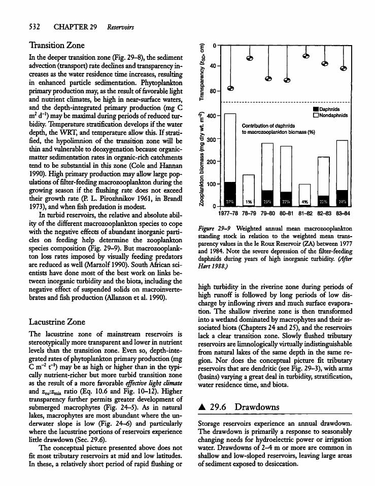
532 CHAPTER 29 Reservoirs
Transition Zone
In the deepertransitionzone (Fig. 29-8), the sedimentadvection (transport) ratedeclines andtransparency increases asthewater residence time increases, resultingin enhanced particle sedimentation. Phytoplanktonprimary production may, asthe resultoffavorable fightand nutrient climates, be high in near-surface waters,and the depth-integrated primary production (mg Cm2 d-1) may be maximal during periods ofreduced turbidity. Temperature stratification develops if the waterdepth, theWRT, and temperature allow this. If stratified, the hypolimnion of the transition zone will bethin andvulnerable to deoxygenation because organic-matter sedimentation rates in organic-rich catchmentstend to be substantial in this zone (Cole and Hannan1990). High primaryproductionmayallow largepopulations of filter-feeding macrozooplankton duringthegrowing season if the flushing rate does not exceedtheir growth rate (P. L. Pirozhnikov 1961, in Brandl1973), andwhenfish predationismodestIn turbid reservoirs, the relative and absolute abil
ity of the different macrozooplankton species to copewith the negative effects of abundant inorganic particles on feeding help determine the zooplanktonspeciescomposition (Fig. 29-9). But macrozooplankton loss rates imposed by visually feeding predatorsare reduced as well (Marzolf 1990). South African scientists have done most of the best work on links between inorganic turbidity and the biota, includingthenegative effect of suspended solids on macroinvertebrates and fishproduction (Allanson et al. 1990).
Lacustrine Zone
The lacustrine zone of mainstream reservoirs isstereotypicallymore transparentand lowerin nutrientlevels than the transition zone. Even so, depth-integrated rates of phytoplanktonprimaryproduction (mgC m~21"1) may be as highor higher than in the typicallynutrient-richer but more turbid transition zoneas the result of a more favorable effective light climateand zCu:zmix ratio (Eq. 10.6 and Fig. 10-12). Highertransparency further permits greater development ofsubmerged macrophytes (Fig. 24-5). As in naturallakes,macrophytes are most abundant where the underwater slope is low (Fig. 24-6) and particularlywhere the lacustrine portions of reservoirs experiencelittle drawdown (Sec. 29.6).The conceptual picture presented above does not
fit most tributary reservoirs at mid and low latitudes.In these, a relatively short period of rapid flushing or
Eo
a
c
ia
40-
80-
<L 400 H
t•o 3001o>E,
1200HoXI
c
£ 100HJaoqN 0
•Daphnids•Nondaphnids
Contribution of daphnidsto macrozooplankton biomass {%)
^Q 1% ^^m ^^M 4% ^Q ^Q1977-78 78-79 79-80 80-81 81-82 82-83 83-84
Figure 29-9 Weighted annual mean macrozooplanktonstanding stock in relation to the weighted mean transparencyvaluesin the le RouxReservoir (ZA) between 1977and 1984.Note the severe depression of the filter-feedingdaphnids during years of high inorganic turbidity. (AfterHart 1988.)
high turbidity in the riverine zone during periods ofhigh runoff is followed by long periods of low discharge by inflowing rivers and much surface evaporation. The shallow riverine zone is then transformedinto awedand dominated bymacrophytesand their associated biota (Chapters 24 and 25), and the reservoirslack a clear transition zone. Slowly flushed tributaryreservoirs are limnologicallyvirtuallyindistinguishablefrom natural lakes of the same depth in the same region. Nor does the conceptual picture fit tributaryreservoirs that are dendritic (seeFig. 29-3), with arms(basins) varyinga great deal in turbidity,stratification,water residence time, and biota.
• 29.6 Drawdowns
Storage reservoirs experience an annual drawdown.The drawdown is primarilya response to seasonablychangingneeds for hydroelectric power or irrigationwater. Drawdowns of 2-4 m or more are common inshallow and low-sloped reservoirs, leavinglarge areasof sedimentexposed to desiccation.
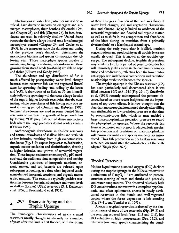
Fluctuations in water level, whether natural or artificial, have dramatic impacts on emergent and submerged macrophytes, their benthos (Palomald 1994,and Chapter 25), and fish (Chapter 26). In fact, drawdowns are used in relatively shallow United Statesreservoirs that havea largehttoral zone for submergedmacrophyte control (Chapter 24, and Cooke et al.1993). In the temperate zone the duration and timingof the previous year's drawdown determines themacrophyte biomass and species composition the following year. Those macrophyte species capable ofmaintaining living roots during a drawdown and thosegrowing from stored seeds (seedbanks) are able to copeand thrive (Nilsson and Keddy 1988).The abundance and age distribution of fish is
much affected by postspawning water level changesbecause most reservoir fish use the vegetated httoralzone for spawning, feeding, and hiding by the larvaeand YOY. A drawdown of as little as 50 cm immediately following spawningwill desiccate a largefractionof the eggsin higher latitudereservoirs, therebyeliminatingwholeyear-classes of fish havingonly one annual spawning period (Duncan and Kubecka, 1995).Summer drawdowns are used in some United Statesreservoirs to increase the growth of largemouth bassby forcing YOY prey fish out of dense macrophytebeds where the large predators do not readily venture(O'Brian 1990).Anthropogenic drawdowns in shallow reservoirs
and natural drawdowns of shallow lakes and wedandsat low latitudes, resulting from high evapotranspira-tion losses (Fig.5-9), expose largeareasto desiccation,organic-matter oxidation and denitrification, freezingat higher latitudes, and growth of terrestrial vegetation. Theseimpact sediment chemistry (Eh, pH, nutrients) and the sediment biotacomposition andactivity.Considerable quantities of inorganic nutrients, organic matter, and soil bacteria are released uponsubsequent reflooding, at a timewheninputsofcatchment-derived inorganic nutrients and organic matteris also maximal. The result is a typically positive relationship between bacterial abundance and water levelsin shallow (former) USSR reservoirs (S. I. Kuznetsovet al. 1966, in Prochazkova et al. 1973).
29.7 Reservoir Aging and theTrophic Upsurge
The limnological characteristics of newly createdreservoirs usually changes significandy for a numberof years after the land is first flooded, with the extent
29.7 ReservoirAging and the Trophic Upsurge 533
of these changes a function of the land area flooded,water level changes, soil and vegetation characteristics, and climate. Aging is linked to oxidation of theterrestrial vegetation and flooded soil organic matter,aswell as to shifts in the compositionand abundanceof the biota during its transition from a primarilyriverine(lotic)to a lake(lentic) assemblage.During the early years after it is filled, nutrient
concentrations and productivity at all trophic levels areusually elevated. This is known as the trophic upsurge. The subsequent decline, trophic depression,may similarly last for a period of years to decades butwillultimately yielda more stablecommunitycompositionandproductivity, reflecting both the lowernutrient-supply rate and the newcompetitionand predationrelationships established betweenthe species.The trophic upsurge in the Klicavareservoir (CZ)
has been particularly well documented since it wasfilled between 1952 and 1955 (Fig. 29-10). Straskrabaet al. (1993) recendy reinterpreted the patterns observed based onmore recent insightsabout the importance of top-down effects. It is now thought that theabundantmacrozooplankton notedshordyafterfillingwas attributable to lowpredationpressure at that timeby zooplanktivorous fish, which in turn enabled alarge macrozooplankton predation pressure to retardthe phytoplankton upsurge. Where the reservoir fishfauna iscomposed onlyofpoorlyadapted loticspecies,fish production and predation on macrozooplanktonwillremainlowuntil lenticspecies invadeor are introduced. Thus fish production in Sri Lankan reservoirsremained low until after the introduction of the well-adapted Tilapia (Sec. 26.6).
Tropical ReservoirsModesthypolimnetic dissolved oxygen (DO) declinesduringthe trophicupsurge in the Kh'cava reservoir toa minimum of 5 mg02 l"1 are attributed to precon-struction clearing of trees and shrubs and generallycool water temperatures. The observed relatively highDO concentrations contrastwitha complete hypolimnetic, and often epilimnetic, anoxia in newly established reservoirs in the humid and well-vegetatedtropics where the forest vegetation is left standing(Fig. 29-11, and Tundisi et al. 1993).Anoxia in tropicalreservoirs is abetted by the den
dritic nature ofmostof the reservoirs (Fig. 29-3)andthe resulting reduced fetch (Sees. 11.3 and 11.6), lowDO solubility at high temperatures (Sec. 15.2), andrelatively low wind speeds characterizing the conti-
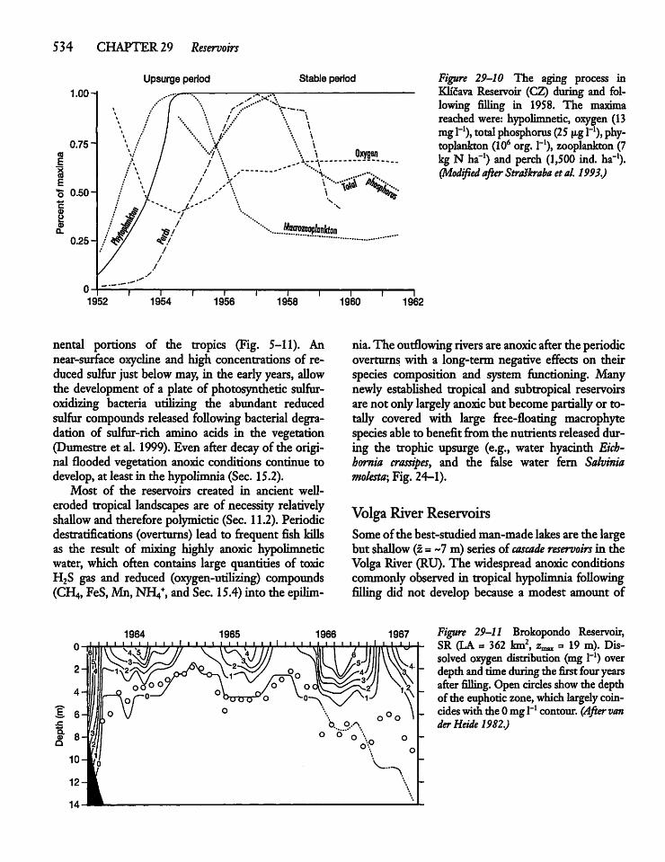
534 CHAPTER 29 Reservoirs
Upsurge period Stable period Figure 29-10 The aging process inKlicava Reservoir (CZ) during and following filling in 1958. The maximareachedwere: hypolimnetic, oxygen (13mgl-1), total phosphorus (25 p.g l-1), phytoplankton (106 org. I"1), zooplankton (7kgN ha~l) and perch (1,500 ind. ha-1).(Modified after Straskraba etal. 1993.)
1.00-1
\ \ Oxygen•x-~.~y
'''%. •..Ao\<
Motroaopfankfon
—I 1 r—1958 1960 1962
nental portions of the tropics (Fig. 5-11). Annear-surface oxycline and high concentrations of reduced sulfurjust below may, in the earlyyears, allowthe development of a plate of photosynthetic sulfur-oxidizing bacteria utilizing the abundant reducedsulfur compounds released following bacterial degradation of sulfur-rich amino acids in the vegetation(Dumestre et al. 1999). Even after decayof the original flooded vegetation anoxic conditions continue todevelop, at least in the hypolimnia (Sec. 15.2).Most of the reservoirs created in ancient well-
eroded tropical landscapes are of necessity relativelyshallow and therefore polymictic (Sec. 11.2). Periodicdestratifications (overturns) lead to frequent fish killsas the result of mixing highly anoxic hypolimneticwater, which often contains large quantities of toxicH2S gas and reduced (oxygen-utilizing) compounds(CH4, FeS,Mn, NJV, and Sec. 15.4)into the epilim-
nia.The outflowingriversare anoxic after the periodicoverturns with a long-term negative effects on theirspecies composition and system functioning. Manynewly established tropical and subtropical reservoirsare not only largelyanoxic but becomepartiallyor totally covered with large free-floating macrophytespecies ableto benefitfrom the nutrients released during the trophic upsurge (e.g., water hyacinth Eich-hornia crassipes, and die false water fern Salviniamolesta; Fig. 24-1).
VolgaRiver ReservoirsSomeof the best-studiedman-madelakesare the largebut shallow (z = ~7 m) series of cascade reservoirs in theVolga River (RU). The widespread anoxic conditionscommonlyobserved in tropical hypolimnia followingfilling did not develop because a modest amount of
Figure 29-11 Brokopondo Reservoir,SR (LA = 362 km2, z^ = 19 m). Dissolved oxygen distribution (mg l-1) overdepthand timeduringthe firstfouryearsafter filling. Open circles showthe depthof the euphotic zone,whichlargelycoincides withthe0mgl"1 contour. (After vanderHeide1982.)
and due to generally rapid flushing and cooler watertemperatures. The sediments remained generally welloxygenated, making the developmentof an abundantmacrobenthic community possible during the trophicupsurge. The macrobenthos permitted a particularlyproductive fishery at the time. The shallow reservoirsdeveloped large submerged macrophyte beds in theextensive Httoral and wedand zones created(Straskraba et al. 1993). The reservoirs did not develop the extensive floating rafts of water hyacinth orfalse water fern so common at lower latitudes. However, rich soils and agricultural activity have guaranteed eutrophic conditions even after the end of theupsurge period (summer zSD =~1.5 m,TN =~1 mgT1,TP =~110 p,g 1_1; Litvinov andMineeva 1994).
Boreal Reservoirs
The last group of reservoirs to be mentioned are thelarge but generally shallow hydroelectric reservoirsconstructed in recent decades in the low relief borealforest regions of North America and Eurasia. Thetrophic upsurge is small in these regions of thinnutrient-poor soils overlying hard igneous rock.Windswept cool waters have maintained high DOconcentrations in summer, but permit localized de-oxygenation under the winter ice cover in shallowareas wherebogswith a thick layer of organic matterare flooded.An unpleasant and unexpected side effect of con
struction has been gready elevated levels of mercuryin long-lived piscivorous fish, such as lake trout andpike, duringthe firstseveral decades (Sec. 28.9). Workon some Canadian reservoirs showed the onset of adecline in themercury content of their principal prey,the shorter-lived zooplanktivoFeus lake whitefish,seven yearsafter flooding; a decline that is attributedto gradual depletion of the available soil mercury butnot yet seen in the piscivorous fish (Chevalier et al.1997). Even so, elevated sedimentmercury levels innatural lakes nearby indicate that mercury levels arelikely to remain high, especially in piscivorous fish atthe top of the foodchain.
29.8 Large ReservoirsandTheir Impacts
The construction of bigdams has beenamixed benefit, particularly at low latitudes in the economicallyless-developed portions of the world.The benefits of
29.8 Large Reservoirs and Their Impacts 535
hydroelectric power are large but go primarily tourban areas for downstream from the dams. Between30 and 40 percent of the world's271million irrigatedhectares—which play a major role in global food production—rely on dams for water, but their benefitscome at a large environmental cost that has receiveddisproportionately little attention. The cost includesthe disruption of river flow, the loss of vast areas ofwedands and their biota following the termination ofthe large seasonal floods, and the desiccation of dryland rivers downstream as a result of water diversionfor irrigation. Furthermore, the dams interfere withthe migration of fish and invertebrates, causing reduced biodiversity, while reduced discharge to theoceans results in salinization of coastal wedands.Other losers have been politically weak indigenouspeople—dependent on the rivers, wedands, and landflooded by reservoirs, for hunting, fishing, farming,livestock raising and for mamtaining their culture.Limnologists working for consulting firms contributetheir technical expertise to the Environmental ImpactAssessments that are required before internationallenders provide the necessary funds for construction.Two principal difficulties bedevil reservoir construction: The benefits and costs tend to go to differentgroups of people, and the typically unanticipated butmajor environmental costs have received far too littleattention (Straskraba et al. 1993). Whether a growinginternational pressure for the development of agreater number of smaller, individually less intrusivedams is on balance less environmentally (and socially)destructive must be region- and site-specific. Whateverthe case, limnologists with a broadenvironmentalperspective, andanability to collaborate andarguetheimpacts with economists, sociologists, and engineers,will be in demand.
Highlights
• Reservoirs are variously constructed for irrigation,electricity generation, flood control, watersupply tourban areas, improved navigation, fishculture, recreation, or some combination of the above.
• Most reservoirs are small and built for irrigation bydamming rivers in lowrainfall (low runoff) regions.
• Reservoirs and natural lakes have much in common,but reservoirs tend to have larger drainage basinsthan natural lakes of similar size in the same region.They further differ in that reservoirs are usually recently constructed and have their greatest depth atthe dam.
536 CHAPTER 29 Reservoirs
• Large reservoirs are of three basic types. Mainstreamor run-of-the-river reservoirs areconstructed to generate electricity and are characterized by rapidflushing, little or no stratification, no drawdown, waterrelease viaa deepoudet, andaremost riverlike. Tributary storage reservoirsare built on smallerriversandare used principally for irrigation and flood control.They experience slower flushing, maybe stratified ifdeepenough,experience periodicdrawdowns, haveasurface oudet, and most resemble natural lakes in thearea.Mainstreamstorage reservoirs havean intermediateposition, becomingmore loticduringperiods ofhigh runoff andmore lentic at other times.
• • Mainstream storage reservoirs, lying in well-defined river valleys, exhibit pronounced longitudinalzonationwith gradients in flow velocity, water residence time, suspended solids, mixed layer fight climate, and the biota.
• A Flushing rates greater than the doubling time ofplanktonicorganisms results in washout.
* Rivers and their biota are gready affected by the insertion of a lentic systemwhich follows dam construction, and dams also interfere with migrations.Modifications in the timing and volume of the discharge regime, plus trappingmaterials behind damsaffects the biota downstream. However, the singlelargest threat to rivers, their biota, and downstreamwetlands stem from the large-scale water diversionfor agriculture, resulting in a gready reduced discharge or zerodischarge in dryland rivers andthe lossofdownstream wedands, and their biota.
* A Exposureand desiccation of the Httoral zone following drawdowns has pronounced effects on thebiota.
* The constructionof bigdamshasbeen amixed blessing, particularly in the economically less-developedportions of the world.
Related Documents