Welcome message from author
This document is posted to help you gain knowledge. Please leave a comment to let me know what you think about it! Share it to your friends and learn new things together.
Transcript

LIMITS OF TRANSLATES OF PLANE CURVES |
ON A PAPER OF ALDO GHIZZETTI
PAOLO ALUFFI, CAREL FABER
Abstract. We study the limits of PGL(3) translates of an arbitrary plane curve,
giving a description of all possible limits of a given curve and computing the mul-
tiplicities of corresponding components in the normal cone to the base scheme of
a related linear system. This information is a key step in the computation of the
degree of the closure of the linear orbit of an arbitrary plane curve.
Our analysis recovers and extends results obtained by Aldo Ghizzetti in the
1930's.
1. Introduction
Let C be an arbitrary complex plane curve of degree d. Consider C together withall its translates: the orbit of C for the natural action of PGL(3) on the projectivespace Pn of all plane curves of degree d. Which plane curves appear in the orbitclosure of C? Or in other words, what are the limits of translates of C? In this article
we answer a re�ned form of this question.Harris and Morrison ([HM98], p.138) de�ne the at completion problem for embed-
ded families of curves as the determination of all curves in Pn that can arise as atlimits of a family of embedded stable curves over the punctured disc. The problem
mentioned in the �rst paragraph contains the isotrivial case of the at completionproblem for plane curves, and a solution to it can in fact be found in the marvelous ar-ticle [Ghi36b] by the Italian mathematician Aldo Ghizzetti (a summary of the resultsis contained in [Ghi36a]). However, as we will explain below, our main application
requires a more re�ned type of information; thus our aim is somewhat di�erent thanGhizzetti's, and we cannot simply lift his results. Consequently, our work in thispaper is independent of [Ghi36b]. In any case, Ghizzetti's approach has substantiallyin uenced ours; see x3.26 for a description of his work and a comparison with ours.The enumerative geometry of families of plane curves with prescribed singularities
presents a notoriously diÆcult problem. Spectacular progress was made in the lastdecade in several special cases; we mention the work of Kontsevich [Kon95] and ofCaporaso-Harris [CH98]. Consider the special case where the family consists of acompletely arbitrary plane curve and all its translates. In our paper [AF00a] we
explained how the degree of this family, in other words, the number of curves in thefamily passing through the appropriate number of general points in the plane, can becomputed. For example, for a nonsingular curve C this family is the set of all possibleembeddings of C in P2; our motivation in [AF93], [AF00b], [AF00c], [AF00a], and the
present article is the study of this set, and of its natural generalization for arbitraryplane curves.
1

2 PAOLO ALUFFI, CAREL FABER
The starting point of our method is to view the action map on C as a rational map cfrom the P8 of 3�3 matrices to the Pn of plane curves of degree d. We require a precisedescription of the closure of the graph of c, speci�cally of the scheme-theoretic inverseimage of the locus of indeterminacy. This is the exceptional divisor of the blow-up
of P8 along the base scheme of c, the projective normal cone (PNC). A set-theoreticdescription of the components of the PNC amounts to a solution of the (isotrivial) at completion problem, together with careful bookkeeping of the di�erent arcs inP8 used to obtain each limit. The PNC can be viewed as an arc space associated to
the rational map c; it is probably possible to recast our analysis in x3 in the light ofrecent work on arc spaces (cf. for example [DL01]), and it would be interesting to doso.In fact a set-theoretic description of the PNC does not suÆce for our enumerative
application in [AF00a]. This requires the full knowledge of the PNC as a cycle, that is,the determination of the multiplicity of its di�erent components. Thus, we determinenot only the limits of one-dimensional families of translates of C, but we also classifysuch families up to a natural notion of equivalence and we keep track of the behaviorof a family near the limit. The determination of the limits and the classi�cation are
contained in x3. As may be expected, the determination of the multiplicities is quitedelicate; this is worked out in x4. Preliminaries, and a more detailed introduction,can be found in x2.The �nal result of our analysis is stated in x2 of [AF00a], in the form of �ve
`Facts'. The proofs of these facts are spread over the present text; we recommendcomparing loc.cit. with x3.2 and x4.2 to establish a connection between the moredetailed statements proved here and the summary in [AF00a].Caporaso and Sernesi use our determination of the limits in [CS03] (Theorem 5.2.1).
Hassett [Has99] and Hacking [Hac03] study the limits of the family of nonsingularplane curves of a given degree, by methods di�erent from ours: they allow the planeto degenerate together with the curve. It would be interesting to compare their resultsto ours.
Acknowledgments. We thank an anonymous referee of our �rst article on the topic
of linear orbits of plane curves, [AF93], for bringing the paper of Aldo Ghizzetti toour attention. A substantial part of the work leading to the results in this paperwas performed while we enjoyed the peaceful atmosphere at Oberwolfach during a`Research in Pairs' stay, and thanks are due to the Volkswagen Stiftung for supportingthe R.i.P. program.
The �rst author thanks the Max-Planck-Institut f�ur Mathematik in Bonn, Ger-many, for the hospitality and support, and Florida State University for granting asabbatical leave in 2001-2. The second author thanks Princeton University for hos-pitality and support during the spring of 2003. The �rst author's visit to Stockholm
in May 2002 was made possible by support from the G�oran Gustafsson foundation.The second author's visit to Bonn in July 2002 was made possible by support fromthe Max-Planck-Institut f�ur Mathematik.

LIMITS OF TRANSLATES OF PLANE CURVES | ON A PAPER OF ALDO GHIZZETTI 3
2. Preliminaries
2.1. We work over C . Roughly speaking, the question we (and Ghizzetti) addressis the following: given a plane curve C, what plane curves can be obtained as limits
of translates of C? By a translate we mean the action on C of an invertible lineartransformation of P2, that is, an element of PGL(3). We view PGL(3) as an openset in the space P8 parametrizing 3� 3 matrices �; if F (x; y; z) is a generator of thehomogeneous ideal of C, � acts on C by composition: we denote by C Æ � the curvewith ideal (F Æ �) = (F (�(x; y; z))), and we call the set of all translates C Æ � the
linear orbit of C. Our guiding question here concerns the limits of families C Æ g(a),for g : A ! P8 any map from a smooth curve A to P8, centered at a point mappingto a singular transformation.Since the at limit is determined by the completion of the local ring of A at the
center, we may replace A with Spec C [[t]]. Thus, a `curve germ in P8' (germ for short)in this article will simply be a C [[t]]-valued point �(t) of P8. Our `germs' are oftencalled `arcs' in the literature.The limit of C Æ �(t) as t! 0:
limt!0
C Æ �(t)
is the at limit over the punctured t-disk; concretely, this is obtained by clearing
common powers of t in the expanded expression F (�(t)) and then setting t = 0.It will always be assumed that the center � = �(0) of a germ �(t) is a singular
transformation. Further, we may and will assume that �(t) is invertible for somet 6= 0: indeed, this condition may be achieved by perturbing every �(t) achieving a
limit, using terms of high enough power in t so as not to a�ect the limit.We note that, by the same token, every limit attained by one of our `germs' can
conversely be realized as the at limit of a family parametrized by a curve A mappingto P8, as above; and in fact we can even assume A = A 1 . Indeed, truncating �(t) ata high enough power does not a�ect limt!0 C Æ �(t), and a polynomial �(t) describes
a map A 1 ! P8.
2.2. Here is one example showing that rather interesting limits may occur: let C bethe 7-ic curve with equation
x3z4 � 2x2y3z2 + xy6 � 4xy5z � y7 = 0
and the family
�(t) =
0@ 1 0 0
t8 t9 0t12 3
2t13 t14
1A ;
then
F Æ �(t) = �1
16t52(x3(8x2 + 3y2 � 8xz)(8x2 � 3y2 + 8xz)) + higher order terms.
That is,
limt!0
F Æ �(t) = �1
16x3(8x2 + 3y2 � 8xz)(8x2 � 3y2 + 8xz) ;

4 PAOLO ALUFFI, CAREL FABER
a pair of quadritangent conics (see [AF00b], x4.1), union the distinguished tangentline taken with multiplicity 3. Note that the connected component of the identity inthe stabilizer of this curve is the additive group.
2.3. Our primary objective is essentially to describe the possible limits of a planecurve C, starting from a description of certain features of C. We now state this goal
more precisely.In the process of computing the degree of the closure of the linear orbit of an
arbitrary curve, [AF00a], we are led to studying the closure of the graph of therational map
P8 9 9 KPN
mapping an invertible � to C Æ �, viewed as a point of the space PN parametrizingplane curves of degree deg C. This graph may be identi�ed with the blow-up of P8
along the base scheme S of this rational map. Much of the enumerative information
we seek is then encoded in the exceptional divisor E of this blow-up, that is, in theprojective normal cone of S in P8. In fact, the information can be obtained from adescription of the components of E (viewed as 7-dimensional subsets of P8�PN ) andfrom the multiplicities with which these components appear in E. A more thoroughdiscussion of the relation between this information and the enumerative results, as
well as of the general context underlying our study of linear orbits of plane curves,may be found in x1 of [AF00a].Our goal in this paper is the description of the components of the projective normal
cone of S, and the computation of the multiplicities with which the components
appear in the projective normal cone.
2.4. This goal relates to the one stated more informally in x2.1 in the sense that thecomponents of the projective normal cone dominate subsets of the boundary of thelinear orbit of C. Our technique will consist of studying an arbitrary �(t), aiming todetermine whether the limit (�(0); limt!0 C �(t)) is a general point of the support of
a component of the normal cone; we will thus obtain a description of all componentsof the normal cone. We should warn the reader that we will often abuse the languageand refer to the point (�(0); limt!0 C �(t)) (in P
8�PN ) by the typographically moreconvenient limt!0 C Æ �(t) (which is a point of PN ).We should also point out that our analysis will not exhaust the boundary of a
linear orbit: one component of this boundary may arise as the closure of the set oftranslates C � with � a rank-2 transformation, and a general such � does not belongto S. Indeed, the rational map mentioned above is de�ned at the general � of rank 2.To be more precise, if � is a rank-2 matrix whose image is not contained in C (for
example, if C has no linear components), then C Æ � may be described as a `star' oflines through ker�, reproducing projectively the tuple of points cut out by C on theimage of �. It would be interesting to provide a precise description of the set of starsarising in this manner. As this set does not contribute components to E, this study
is not within the scope of this paper.
2.5. One of our main tools in the set-theoretic determination of the componentsof E will rely precisely on the fact that limits along rank-2 transformations do not

LIMITS OF TRANSLATES OF PLANE CURVES | ON A PAPER OF ALDO GHIZZETTI 5
contribute components to E. We will argue that if a limit obtained by a germ �(t)can also be obtained as a limit by a germ �(t) contained in the rank-2 locus, thenwe can `discard' �(t). Indeed, such limits will have to lie in the exceptional divisor ofthe blow-up of the rank-2 locus; as the rank-2 locus has dimension 7, such limits will
span loci of dimension at most 6. We will call such limits `rank-2 limits' for short.The form in which this observation will be applied is given in Lemma 3.1.Incidentally, germs �(t) centered at a rank-2 transformation whose image is con-
tained in C do contribute a component to E (cf. x3.6); by the argument given in the
previous paragraph, however, contributing �(t) will necessarily be invertible for t 6= 0.
2.6. In x3 we will determine the components of E set-theoretically, as subsets ofP8 � PN . As a preliminary observation (cf. [AF00a], p. 8) we can describe the wholeof E set-theoretically in terms of limits, as follows. Recall that S denotes the base
locus of the rational map c : P8 9 9 KPN de�ned by � 7! C Æ �.
Lemma 2.1. As a subset of P8 � PN , the support of E is
jEj = f(�;X) 2 P8 � PN : X is a limit of c(�(t))
for some curve germ �(t) � P8 centered at � 2 S and not contained in Sg :
Proof. Let eP8 be the closure of the graph of the rational map c de�ned above. Thisis an 8-dimensional irreducible variety, mapping to P8 by the restriction � of theprojection on the �rst factor of P8 � PN , and identi�ed with the blow-up of P8 along
the base scheme S of c. The set E is the inverse image ��1(S) in eP8.Any curve germ �(t) in P8 centered at � 2 S and not contained in S lifts to a germ
in P8 centered at a point of E; this yields the � inclusion.For the other inclusion, let ~�(t) be a germ centered at a point ~� of E, and such that
~�(t0) 62 E for t0 near 0; such a germ may be obtained (for example) by successively
intersecting eP8 with general divisors of type (1; 1) through ~�. As � is 1-to-1 in thecomplement of E, ~�(t) is the lift of a (unique) curve germ �(t) in P8, giving the other
inclusion.
2.7. As mentioned in x1, our application in [AF00a] requires the knowledge of Eas a cycle, that is, the computation of the multiplicities of the components of E.This information is obtained in x4. Our method will essentially consist of a local
study of the families determined in x3: the multiplicity of a component will be com-puted by analyzing certain numerical information carried by germs �(t) `marking'that component (cf. De�nition 4.4).
We will in fact study the inverse image E of E in the normalization P of eP8:roughly speaking, the multiplicity of the components of E is determined by the orderof vanishing of C�(t) for corresponding germs �(t). The number of components of E
dominating a given component D of E is computed by distinguishing the contributionof di�erent marking germs.Finally, the last key numerical information consists of the degree of the components
of E over the corresponding components of E; this will be obtained by studying
the PGL(3) action on eP8, and in particular the stabilizer of a general point of each

6 PAOLO ALUFFI, CAREL FABER
component D of E. Given a component D of E dominatingD, we identify a subgroupof this stabilizer (the inessential subgroup, cf. x4.6), determined by the interactionbetween di�erent parametrizations of a corresponding marking germ; the degree ofD over D is the index of this subgroup in the stabilizer (Proposition 4.12).
3. Set-theoretic description of the normal cone
3.1. In this section we determine the di�erent components of the projective normalcone (PNC for short) E described in Lemma 2.1, for a given, arbitrary plane curve
C with homogeneous ideal (F ), where F 2 C [x; y; z] is a homogeneous polynomial ofdegree d.The PNC can be embedded in P8 � PN , where PN parametrizes all plane curves of
degree d. A typical point of a component of the PNC is in the form
(�(0); limt!0
C Æ �(t))
where �(t) is a curve germ centered at a point �(0) such that im�(0) is containedin C. We will determine the components of the PNC by determining a list of germs�(t) which exhaust the possibilities for pairs (�(0); limt!0 C Æ �(t)) for a given curve.Roughly speaking, we will say that two germs are equivalent if they determine the
same data (�(0); limt!0 C Æ �(t)) (see De�nition 3.2 for the precise notion). Fora given curve C and a given germ �(t), we will construct an equivalent germ ina standardized form; we will determine which germs �(t) in these standard forms`contribute' components of the PNC, in the sense that (�(0); limt!0 C Æ �(t)) belongs
to exactly one component (and that a suÆciently general such �(t) yields a generalpoint of that component), and describe that component.
3.2. The end-result of the analysis can be stated without reference to speci�c germs�(t). We will do so in this subsection, by listing general points (�;X ) on the compo-
nents of the PNC, for a given C.We will �nd �ve types of components: the �rst two will depend on global features
of C, while the latter three will depend on features of special points of C (in ectionpoints and singularities of the support of C). The terminology employed here matches
the one in x2 of [AF00a]. In four of the �ve components � is a rank-1 matrix, andthe line ker� plays an important role; we will call this `the kernel line'.
� Type I.
{ �: a rank-2 matrix whose image is a linear component ` of C;{ X : a fan consisting of a star of lines through the kernel of � and cutting outon the residual line `0 a tuple of points projectively equivalent to the tuplecut out on ` by the residual to ` in C. The multiplicity of `0 in the fan is the
same as the multiplicity of ` in C.Fans and stars are studied in [AF00c]; they are items (3) and (5) in the classi�-cation of curves with small linear orbits, in x1 of loc. cit.
� Type II.
{ �: a rank-1 matrix whose image is a nonsingular point of the support C 0 ofa nonlinear component of C;

LIMITS OF TRANSLATES OF PLANE CURVES | ON A PAPER OF ALDO GHIZZETTI 7
{ X : a nonsingular conic tangent to the kernel line, union (possibly) a multipleof the kernel line. The multiplicity of the conic component in X equals themultiplicity of C 0 in C.
Such curves are items (6) and (7) in the classi�cation of curves with small or-
bit. The extra kernel line is present precisely when C is not itself a multiplenonsingular conic.
� Type III.{ �: a rank-1 matrix whose image is a point p at which the tangent cone to C
is supported on at least three lines;{ X : a fan with star reproducing projectively the tangent cone to C at p, anda multiple residual kernel line.
These limit curves are also fans, as in type I components; but note that type I
and type III components are di�erent, since for the typical (�;X ) in type Icomponents � has rank 2, while it has rank 1 for type III components.
� Type IV.{ �: a rank-1 matrix whose image is a singular or in ection point p of thesupport of C.
{ X : a curve determined by the choice of a line in the tangent cone to C atp, and by the choice of a side of a corresponding Newton polygon. Thisprocedure is explained more in detail below.
The curves X arising in this way are items (7) through (11) in the classi�cation
in [AF00c], and are studied enumeratively in [AF00b].� Type V.
{ �: a rank-1 matrix whose image is a singular point p of the support of C.{ X : a curve determined by the choice of a line ` in the tangent cone to C at
p, the choice of a formal branch for C at p tangent to `, and the choice ofa certain `characteristic' rational number. This procedure is explained morein detail below.
The curves X arising in this way are item (12) in the classi�cation in [AF00c],and are studied enumeratively in [AF00b], x4.1.
Here are the details of the determination of the limit curves X for components oftype IV and V.Type IV: Let p = im� be a singular or in ection point of the support of C; choose
a line in the tangent cone to C at p, and choose coordinates (x : y : z) so that x = 0is the line ker�, p = (1 : 0 : 0), and that the selected line in the tangent cone has
equation z = 0. The Newton polygon for C in the chosen coordinates is the boundaryof the convex hull of the union of the positive quadrants with origin at the points(j; k) for which the coeÆcient of xiyjzk in the generator F for the ideal of C in thechosen coordinates is nonzero (see [BK86], p.380). The part of the Newton polygon
consisting of line segments with slope strictly between �1 and 0 does not depend onthe choice of coordinates �xing the ag z = 0, p = (1 : 0 : 0).The possible limit curves X determining components of type IV are then obtained
by choosing a side of the polygon with slope strictly between �1 and 0, and setting
to 0 the coeÆcients of the monomials in F not on that side. These curves are studiedin [AF00b]; typically, they consist of a union of cuspidal curves. The kernel line is

8 PAOLO ALUFFI, CAREL FABER
part of the distinguished triangle of such a curve, and in fact it must be one of thedistinguished tangents.This procedure determines a component of the PNC, unless the limit curve X is
supported on a conic union (possibly) the kernel line.
Type V: Let p = im� be a singular point of the support of C, and let m be themultiplicity of C at p. Again choose a line in the tangent cone to C at p, and choosecoordinates (x : y : z) so that x = 0 is the kernel line, p = (1 : 0 : 0), and z = 0 is theselected line in the tangent cone.
We may describe C near p as the union of m `formal branches'; those that aretangent to z = 0 may be written
z = f(y) =Xi�0
�iy�i
with �i 2 Q , 1 < �0 < �1 < : : : , and �i 6= 0.The choices made above determine a �nite set of rational numbers, which we call
the `characteristics' for C (w.r.t. the line z = 0): these are the numbers C such thatat least two of the branches tangent to z = 0 agree modulo yC , di�er at yC, and have
�0 < C.For a characteristic C, the initial exponents �0 and the coeÆcients �0 , C+�0
2
for
the corresponding branches must agree. Let (1)C ; : : : ;
(S)C be the coeÆcients of yC in
these S branches (so that at least two of these numbers are distinct, by the choice
of C). Then X is de�ned by
xd�2SSYi=1
�zx�
�0(�0 � 1)
2 �0y
2 ��0 + C
2 �0+C
2
yx� (i)C x
2
�:
This is a union of `quadritangent' conics|that is, nonsingular conics meeting atexactly one point|with (possibly) a multiple of the distinguished tangent, whichmust be supported on the kernel line.
3.3. The following simple example illustrates the components described in x3.2: all�ve types are present for the curve
y((y2 + xz)2 � 4xyz2) = 0 :
We will list �ve germs �(t), and the corresponding limits. (This is not an exhaustivelist of all the components of the PNC for this curve.) The speci�c germs used herewere obtained by applying the procedures explained in the rest of the section.
� Type I. A germ �(t) centered at a rank-2 matrix with image the linear componentof the curve:
�(t) =
0@1 0 0
0 t 00 0 1
1A
This yields the limit
y x2z2 ;
a fan consisting of the line y = 0 and a star through the point (0 : 1 : 0), thatis, the kernel of �(0).

LIMITS OF TRANSLATES OF PLANE CURVES | ON A PAPER OF ALDO GHIZZETTI 9
� Type II.We `aim' a one-parameter subgroup with weights (1; 2) at a nonsingularpoint of the curve and its tangent line:
�(t) =
0@1 0 01 1 01 1 1
1A0@1 0 00 t 00 0 t2
1A0@ 1 0 0�1 1 00 �1 1
1A =
0@ 1 0 01� t t 01� t t� t2 t2
1A :
(The curve is nonsingular at (1 : 1 : 1) = im�(0), and tangent to the line y = z.)This germ yields a limit
x3((x + y)2 � 4xz) ;
that is, a nonsingular conic union a (multiple) tangent line supported on thekernel line ker�(0).
� Type III. We aim a one-parameter subgroup with weights (1; 1) at (0 : 0 : 1):
�(t) =
0@t 0 00 t 00 0 1
1A
obtaining a limit of
xy(x� 4y)z2 :
a fan consisting of the tangent cone to C at p, union a multiple kernel line.� Type IV. Considering now C at p = (1 : 0 : 0), here is the Newton polygonw.r.t. the line z = 0:
2y z3
−4y z 2 2
yz2
y5
It has one side with slope between �1 and 0. The corresponding germ will be aone-parameter subgroup with weights (1; 2):
�(t) =
0@1 0 0
0 t 00 0 t2
1A
yielding as limit the monomials of F situated on the selected side:
x2yz2 + 2xy3z + y5 = y(y2 + xz)2 :
This is a double nonsingular conic, union a transversal line.� Type V. Finally, write formal branches for C at p:8><
>:y = 0
z = �y2 � 2y5=2 � : : :
z = �y2 + 2y5=2 � : : :

10 PAOLO ALUFFI, CAREL FABER
We �nd one characteristic C = 52, corresponding to the second and third branch.
These branches truncate to �y2; as will be explained in x3.24, this information
determines the germ
�(t) =
0@ 1 0 0t4 t5 0
�t8 �2t9 t10
1A
yielding the limit
x(zx + y2 + 2x2)(zx + y2 � 2x2)
prescribed by the formula given in x3.2. This is a pair of quadritangent conicsunion a distinguished tangent supported on the kernel line.
3.4. The rest of the section consists of the detailed analysis yielding the list given inx3.2. Our approach will be in the spirit of Ghizzetti's paper, and indeed was inspiredby reading it. The general strategy consists of an elimination process: starting froman arbitrary germ �(t), we determine the possible components that arise unless �(t)
is of some special kind, and keep restricting the possibilities for �(t) until none is left.Here is a guided tour of the successive reductions. First of all, we will determine
germs leading to type I components (x3.7); this will account for all germs centeredat a rank-2 matrix, so we will then be able to assume that �(0) has rank 1. Next,
we will show (Proposition 3.7, x3.8{x3.11) that every � centered at a rank-1 matrixis equivalent, in suitable coordinates, to one in the form
�(t) =
0@ 1 0 0
q(t) tb 0
r(t) s(t)tb tc
1A
with 1 � b � c and q, r, and s polynomials satisfying certain conditions. Considering
the case q � r � s � 0 (that is, when � is a `one-parameter subgroup') leads tocomponents of type II, III, and IV; this is done in x3.13{x3.15. The subtlest case,leading to type V components, takes the remaining x3.16{x3.24. The key step hereconsists of showing that germs leading to new components are equivalent to germs in
the form 0@ 1 0 0
ta tb 0
f(ta) f 0(ta)tb tc
1A
where C = cais one of the characteristics considered in x3.2, f is a corresponding
branch, b is determined by the other data, and : : : stands for the truncation modulotc. This key reduction is accomplished in Proposition 3.15, after substantial prepara-tory work. A re�nement of the reduction, given in Proposition 3.20, leads to the
de�nition of `characteristics' and to the description of components of type V givenabove (cf. Proposition 3.26).As the process accounts for all possible germs, this will show that the list of com-
ponents given in x3.2 is exhaustive, concluding our description of the PNC.

LIMITS OF TRANSLATES OF PLANE CURVES | ON A PAPER OF ALDO GHIZZETTI 11
3.5. Before starting on the path traced above, we discuss three results that willbe applied at several places in the discussion. The �rst two are discussed in thissubsection, and the third one in the subsection which follows.The �rst concerns a recurrent tool in establishing that a germ �(t) does not con-
tribute a component to the PNC. As we discussed in x2.5, this is the case for `rank-2limits', that is, limits that can also be obtained by germs entirely contained withinthe locus of rank-2 transformations in P8. Since we are looking for germs determiningcomponents of E, we may ignore such `rank-2 limits' and the germs that lead to them.
Lemma 3.1. Assume that �(0) has rank 1. If limt!0 C Æ �(t) is a star with centeron ker�(0), then it is a rank-2 limit.
Proof. Assume X = limt!0 C Æ �(t) is a star with center on ker�(0). We may choosecoordinates so that x = 0 is the kernel line and the generator for the ideal of X is apolynomial in x; y only. If
�(t) =
0@a00(t) a01(t) a02(t)a10(t) a11(t) a12(t)a20(t) a21(t) a22(t)
1A ;
then X = limt!0 C Æ �(t) for
�(t) =
0@a00(t) a01(t) 0
a10(t) a11(t) 0a20(t) a21(t) 0
1A :
Since �(0) has rank 1 and kernel line x = 0,
�(0) =
0@a00(0) 0 0a10(0) 0 0
a20(0) 0 0
1A = �(0) :
Now �(t) is contained in the rank-2 locus, verifying the assertion.
A limit limt!0 C Æ �(t) as in the lemma will be called a `kernel star'.A second tool will be at the root of our reduction process: we will replace a given
germ �(t) with a di�erent one in a more manageable form, but leading to the samecomponent of the PNC in a very strong sense.
De�nition 3.2. Two germs are `equivalent' with respect to C if they are (possibly
up to an invertible change of parameter) �bers of a family of germs with constantcenter and limit. More precisely, two germs �0(t), �1(t) are equivalent if there existsa connected curve H, a regular map A : H � Spec C [[t]] ! P8, two points h0, h1 ofH, and a unit �(t) 2 C [[t]] such that:
� A(h0; t) = �0(t);� A(h1; t) = �1(t�(t));
� A( ; 0) : H ! P8 is constant;� If A : H� Spec C [[t]] ! C 9 is a lift of A, then F ÆA(h; t) � �(h)Gtw mod tw+1
for some w, with � : H ! C � a nowhere vanishing function and G a nonzeropolynomial in x; y; z independent of h.

12 PAOLO ALUFFI, CAREL FABER
It is clear that De�nition 3.2 gives an equivalence relation on the set of germs:re exivity and symmetry are immediate, and transitivity is obtained by joining twofamilies along a common �ber (note that the limitG and the weight w are determinedby any of the �bers of a family, hence they are the same for any two families extending
a given germ).Note the possible parameter change in the second condition: this guarantees that
a germ �(t) is equivalent to any of its reparametrizations �(t�(t)). This exibilitywill play an important role in part of our discussion, especially in x4.6 and �.
By Lemma 2.1, the third and fourth conditions amount to the statement that all
germs �h(t) = A(h; t) lift to germs in eP8, the closure of the graph of c, centered atthe same point. If �0, �1 are centered at a point of S, then �0 and �1 (and in fact allthe intermediate �h) determine the same point in the projective normal cone. Thus,
equivalent germs can be `continuously deformed' one into the other while holding thecenter of their lift in P8 � PN �xed.Typically, the curve H will simply be a chain of aÆne lines, minus some points.Given an arbitrary germ �(t), we will want to produce an equivalent and `simpler'
germ. Our basic tool to produce an equivalent germ will be the following.
Lemma 3.3. Assume �(t) � �(t) Æm(t), and that M = m(0) is invertible. Then �
is equivalent to � ÆM (w.r.t. any curve C).
Proof. Write m(t) =M + tm1(t), and take H = A 1 , �(t) = 1. Let
�h(t) = A(h; t) := �(t) Æ (M + htm1(t)) :
Then
� �0 = � ÆM ,� �1 = �, and� �h(0) = �(0) ÆM does not depend on h.
For any given F ,
F Æ �(t) = twG + tw+1G1(t)
with G = limt!0 F Æ �(t). Then
F Æ�h(t) = F Æ�(t)Æ(M+htm1(t)) = tw(G+tG1(t))Æ(M+htm1(t)) = twGÆM+h.o.t.
The term G ÆM is not 0, since M is invertible, and does not depend on h.Thus � = �1 is equivalent to �ÆM = �0 according to De�nition 3.2, as needed.
3.6. The third preliminary item concerns formal branches of C at a point p, cf. [BK86]
and [Fis01], Chapter 6 and 7. Choose aÆne coordinates (y; z) = (1 : y : z) so thatp = (0; 0), and let �(y; z) = F (1 : y : z) be the generator for the ideal of C in thesecoordinates. Decompose �(y; z) in C [[y; z]]:
�(y; z) = �1(y; z) � � � � � �r(y; z)
with �i(y; z) irreducible power series. These de�ne the irreducible branches of C at p.Each �i has a unique tangent line at p; if this tangent line is not y = 0, by theWeierstrass preparation theorem we may write (up to a unit in C [[y; z]]) �i as a
monic polynomial in z with coeÆcients in C [[y]], of degree equal to the multiplicitymi of the branch at p (cf. for example [Fis01], x6.7). If �i is tangent to y = 0, we may

LIMITS OF TRANSLATES OF PLANE CURVES | ON A PAPER OF ALDO GHIZZETTI 13
likewise write it as a polynomial in y with coeÆcients in C [[z]]; mutatis mutandis, thediscussion which follows applies to this case as well.Concentrating on the �rst case, let
�i(y; z) 2 C [[y]][z]
be a monic polynomial of degree mi, de�ning an irreducible branch of C at p, nottangent to y = 0. Then �i splits (uniquely) as a product of linear factors over thering C [[y� ]] of power series with rational nonnegative exponents:
�i(y; z) =
miYj=1
(z � fij(y)) ;
with each fij(y) in the form
f(y) =Xk�0
�ky�k
with �k 2 Q , 1 � �0 < �1 < : : : , and �k 6= 0. We call each such z = f(y) a formalbranch of C at p. The branch is tangent to z = 0 if the dominating exponent �0 is > 1.The terms z � fij(y) in this decomposition are the Puiseux series for C at p.
Summarizing: if C has multiplicity m at p then C splits into m formal branchesat p. In x3.16 and �. we will want to determine limt!0 C Æ �(t) as a union of `limits'of the individual formal branches at p. The diÆculty here resides in the fact thatwe cannot perform an arbitrary `change of variable' in a power series with fractional
exponents. In the case in which we will need to do this, however, �(t) will have thefollowing special form:
�(t) =
0@ 1 0 0
ta tb 0
r(t) s(t)tb tc
1A
with a < b � c positive integers and r(t), s(t) polynomials (satisfying certain restric-tions, which are immaterial here). We will circumvent the diÆculty we mentioned by
the following ad hoc de�nition.
De�nition 3.4. The limit of a formal branch z = f(y), along a germ �(t) as above,is de�ned by the dominant term in
(r(t) + s(t)tby + tcz)� f(ta)� f 0(ta)tby � f 00(ta)t2by2
2� � � �
where f 0(y) =P k�ky
�k�1 etc.
By `dominant term' we mean the coeÆcient of the lowest power of t after cancel-lations. This coeÆcient is a polynomial in y and z, giving the limit of the branchaccording to our de�nition.Of course we need to verify that this de�nition behaves as expected, that is, that
the limit of C is the union of the limits of its individual branches. We do so in thefollowing lemma.

14 PAOLO ALUFFI, CAREL FABER
Lemma 3.5. Let �(y; z) 2 C [[y]][z] be a monic polynomial,
�(y; z) =Yi
(z � fi(y))
a decomposition over C [[y� ]], and let �(t) be as above. Then the dominant term in� Æ �(t) is the product of the limits of the branches z = fi(y) along �, de�ned as inDe�nition 3.4.
Proof. We can `clear the denominators' in the exponents in fi, by writing
�(Tm; z) =Yi
(z � 'i(T ))
where 'i(T ) 2 C [[T ]] and 'i(T ) = fi(Tm). For an integer ` such that `a=m is integer,
we may write
t = S` ; Tm = T (S)m = S`a + S`by = S`a(1 + S`(b�a)y)
with T (S) 2 C [[S; y]]: explicitly,
T (S) = S`am
�1 +
1
mS`(b�a)y +
1
m
�1
m� 1
�S`2(b�a)
y2
2+ � � �
�
The dominant term (w.r.t. t) in
� Æ �(t) = �(ta + tby; r(t) + s(t)tby + tcz)
equals the dominant term (w.r.t. S) in
�(S`a + S`by; r(S`) + s(S`)S`by + S`cz) = �(T (S)m; r(S`) + s(S`)S`by + S`cz)
=Yi
�(r(S`) + s(S`)S`by + S`cz)� 'i(T (S))
�Thus the dominant term in � Æ �(t) is the product of the dominant terms in thefactors
(r(S`) + s(S`)S`by + S`cz)� 'i(T (S))
and we have to verify that the dominant term here agrees with the one in De�ni-
tion 3.4.For this, we use a `Taylor expansion' of 'i. Write
'i(T (S)) =Xk�0
@k'i(T (S))
@ykjy=0
yk
k!:
We claim that@k'i(T (S))
@ykjy=0 = f
(k)i (S`a)S`bk :
indeed, this is immediately checked for fi(y) = y�, hence holds for any fi.
Therefore we have
'i(T (S)) =Xk�0
f(k)i (S`a)
S`bkyk
k!

LIMITS OF TRANSLATES OF PLANE CURVES | ON A PAPER OF ALDO GHIZZETTI 15
or, recalling t = S`:
'i(T (S)) = fi(ta) + f 0i(t
a)tby + f 00i (ta)t2b
y2
2+ : : :
This shows that
(r(S`) + s(S`)S`by + S`cz)� 'i(T (S))
is in fact given by
(r(t) + s(t)tby + tcz)�
�fi(t
a) + f 0i(ta)tby + f 00i (t
a)t2by2
2+ : : :
�;
and in particular the dominant terms in the two expressions must match, as needed.
The gist of this subsection is that we may use formal branches for C at p in order
to compute the limit of C along germs �(t) of the type used above, provided thatthe limit of a branch is computed by using the formal Taylor expansion given inDe�nition 3.4. This fact will be used several times in x3.16 and �.
3.7. We are �nally ready to begin the discussion leading to the list of componentsgiven in x3.2.Applying Lemma 2.1 amounts to studying germs �(t) in P8, centered at matrices �
with image contained in C|these are precisely the matrices in the base locus S of therational map c introduced in x2. The corresponding component of E is determinedby the center of the germ, and the limit.As we may assume that �(0) is contained in C, we may assume that rk�(0) = 1
or 2. We �rst consider the case of germs centered at a rank-2 matrix �, hence withimage equal to a linear component of C. We will show that any germ centered at sucha matrix leads to a point in the component of type I listed in x3.2.Write
�(t) = �(0) + t�(t) ;
where �(0) has rank 2 and image de�ned by the linear polynomial L; thus, we may
write the generator of the ideal of C as
F (x; y; z) = L(x; y; z)mG(x; y; z)
with L not a factor of G. The curve de�ned by G is the `residual of L in C'.
Proposition 3.6. The limit limt!0 C Æ �(t) is a fan consisting of an m-fold line `,supported on limt!0 L Æ �(t), and a star of lines through the point ker�. This star
reproduces projectively the tuple cut out on L by the residual of L in C.
The terminology of stars and fans was introduced in [AF00c], x2.1. Here the m-foldline ` may contain the point ker�, in which case the fan degenerates to a star.
Proof. Write
�(t) = �(0) + t�(t) ;
then the ideal of C Æ �(t) is generated by
L(�(t))mG(�(t)) = tmL(�(t))mG(�(0) + t�(t)) ;

16 PAOLO ALUFFI, CAREL FABER
since L is linear and vanishes along the image of �(0). As t approaches 0, L(�(t))m
converges to an m-fold line, while the other factor converges to G(�(0)), yielding thestatement.
A simple dimension count shows that the limits arising as in Proposition 3.6 doproduce components of the projective normal cone. Indeed, matrices with image con-
tained in a given line form a P5; for any given such matrix, the limits obtained consistof a �xed star through the kernel, plus a (multiple) line varying freely, accountingfor 2 extra dimensions. These components are the components of type I described inx3.2 (also cf. [AF00a], x2, Fact 2(i)).
3.8. Having taken into account the case in which the center �(0) may be a rank-2matrix, we are reduced to considering germs �(t) with �(0) of rank 1. Proposition 3.7
below will allow us to further assume that �(t) has a particularly simple (and poly-nomial) expression.We de�ne the degree of the zero polynomial to be �1. We denote by v the
`valuation' of a power series or polynomial, that is, its order of vanishing at 0; wede�ne v(0) to be +1.
Proposition 3.7. With a suitable choice of coordinates, any germ � is equivalent toa product 0
@1 0 0q 1 0r s 1
1A �
0@ta 0 0
0 tb 00 0 tc
1A
with
� a � b � c integers, q; r; s polynomials;
� deg(q) < b� a, deg(r) < c� a, deg(s) < c� b;� q(0) = r(0) = s(0) = 0.
If further b = c and q, r are not both zero, then we may assume that v(q) < v(r).
The proof of this proposition requires a few preliminary considerations.
3.9. The space P8 of 3 � 3 matrices considered above is, more intrinsically, theprojective space PHom(V;W ), where V and W are vector spaces of dimension 3.The generator F of the ideal of a plane curve of degree d is then an element ofSymdW �; for ' 2 Hom(V;W ), the composition F Æ ' (if nonzero) is the element of
SymdV � generating the ideal of C Æ '. We denote by PGL(V;W ) the Zariski opensubset of PHom(V;W ) consisting of invertible transformations, and write PGL(V )for PGL(V; V ) (which is a group under composition).Homomorphisms � of C � to PGL(V ) will be called `1-PS' (as in: `1-parameter
subgroups'), as will be called their extensions C ! PHom(V; V ). Recall that every
1-PS can be written as
t 7!
0@ta 0 0
0 tb 00 0 tc
1A
after a suitable choice of coordinates in V , where a � b � c are integers (and a mayin fact be chosen to equal 0). Thus we may view a 1-PS as a C ((t))-valued point

LIMITS OF TRANSLATES OF PLANE CURVES | ON A PAPER OF ALDO GHIZZETTI 17
of PGL(V ) � PHom(V; V ). The following lemma shows that these are the basicconstituents of every germ �(t).
Lemma 3.8. Every germ �(t) in PHom(V;W ) is equivalent to a germ
H Æ h1 Æ � ;
where:
� H is a constant invertible linear transformation V !W ;� h1 is a C [[t]]-valued point of PGL(V ) with h1(0) = IdV ; and� � is a 1-PS.
Proof. Every germ � can be written (cf. [MF82], p.53) as a composition:
V
�
44k // U
�0 // Uh0 // W
where k and h0 are C [[t]]-valued points of PGL(V; U), PGL(U;W ) respectively and �0
is a 1-PS. In particular,K = k(0) is an invertible linear transformation; by Lemma 3.3,the composition is equivalent to the composition
VK // U
�0 // Uh0 // W ;
which can be written as
V
�
44K // U
�0 // UK�1
// VK // U
h0 // W :
Here � is again a 1-PS, as a conjugate of a 1-PS by a constant transformation. Thestatement follows by writing h0 ÆK = H Æ h1 as prescribed.
Now we choose coordinates in V so that � is diagonal:
� =
0@ta 0 0
0 tb 00 0 tc
1A
with a � b � c integers; thus we may view h1 and � as matrices, and we are interestedin putting h1 in a `standard' form.
Lemma 3.9. Let
h1 =
0@u1 b1 c1a2 u2 c2a3 b3 u3
1A
be a C [[t]]-valued point of PGL(V ), such that h1(0) = I3. Then h1 can be written asa product h1 = h � j with
h =
0@1 0 0
q 1 0r s 1
1A ; j =
0@v1 e1 f1d2 v2 f2d3 e3 v3
1A
with q, r, s polynomials, satisfying
1. h(0) = j(0) = I3;

18 PAOLO ALUFFI, CAREL FABER
2. deg(q) < b� a, deg(r) < c� a, deg(s) < c� b;3. d2 � 0 (mod tb�a), d3 � 0 (mod tc�a), e3 � 0 (mod tc�b).
Proof. Obviously v1 = u1; e1 = b1 and f1 = c1. Use division with remainder to write
v�11 a2 = D2tb�a + q
with deg(q) < b � a, and let d2 = v1D2tb�a (so that qv1 + d2 = a2). This de�nes q
and d2, and uniquely determines v2 and f2. (Note that q(0) = d2(0) = f2(0) = 0 and
that v2(0) = 1.)Similarly, we let r be the remainder of
(v1v2 � e1d2)�1(v2a3 � d2b3)
under division by tc�a; and s be the remainder of
(v1v2 � e1d2)�1(v1b3 � e1a3)
under division by tc�b.
Then deg(r) < c� a, deg(s) < c� b and r(0) = s(0) = 0; moreover, we have
v1r + d2s � a3 (mod tc�a); e1r + v2s � b3 (mod tc�b);
so we take d3 = a3 � v1r � d2s, e3 = b3 � e1r � v2s. This de�nes r, s, d3 and e3, anduniquely determines v3.
3.10. We are now ready to prove Proposition 3.7. We have written a germ equivalentto � as
H � h � j � �
with notations as above. Now, by (3) in Lemma 3.9 we have j � � = � � ` for `with entries in C [[t]], and L = `(0) lower triangular, with 1's on the diagonal. By
Lemma 3.3 this germ is equivalent to
H � h � � � L = (H � L) � L�1 � (h � �) � L :
We change coordinates in V by L�1, so that L�1 � (h ��) �L has matrix representation
h � �. Finally, we choose coordinates in W so that H � L = I3, completing the proofof the �rst part of Proposition 3.7.If b = c, then the condition that deg s < c� b = 0 forces s = 0. Conjugating by0
@1 0 00 0 1
0 1 0
1A
interchanges q and r; so we may assume v(q) � v(r) if q and r are not both 0.Conjugating by 0
@1 0 0
0 1 00 u 1
1A
replaces r by uq + r, allowing us to force v(q) < v(r), and completing the proof ofProposition 3.7.

LIMITS OF TRANSLATES OF PLANE CURVES | ON A PAPER OF ALDO GHIZZETTI 19
3.11. By Proposition 3.7, and scaling the entries in the 1-PS so that a = 0, anarbitrary germ � is equivalent to one that, with a suitable choice of coordinates, canbe written as
�(t) =
0@ 1 0 0
q(t) tb 0
r(t) s(t)tb tc
1A
with 0 � b � c and q, r, and s polynomials satisfying certain conditions. We may infact assume that b > 0, since we are already reduced to the case in which �(0) is arank-1 matrix. If b > 0, then the center �(0) is the matrix
�(0) =
0@1 0 00 0 00 0 0
1A
with image the point (1 : 0 : 0) and kernel the line x = 0.Further, if (1 : 0 : 0) is not a point of the curve C then limt!0 C Æ �(t) is simply a
multiple kernel line with ideal (xdeg C). Thus we may assume that p = (1 : 0 : 0) isa point of C. In what follows, we will assume that � is a germ in the standard formgiven above, and all these conditions are satis�ed.One last remark will be needed later in the section: if the polynomial q(t) is known
to be nonzero, then Proposition 3.7 admits the following re�nement.
Lemma 3.10. If q 6� 0 in �(t), then �(t) is equivalent to a germ0@ 1 0 0
ta tb 0
r1(t) s1(t)tb tc
1A �
0@1 0 00 u 0r s v
1A ;
with
� a < b � c positive integers;� r1(t) and s1(t) polynomials of degree < c, < (c� b) respectively and vanishing att = 0; and
� u; r; s; v 2 C , with uv 6= 0.
If further b = c, then we may assume a < v(r1).
Proof. As q 6� 0, we may write q(t) = �(t)a for a = v(q) (so 0 < a < b) and with
�(t) 2 C [[t]], such that �(t)=t is a unit in C [[t]]. Expressing t in terms of � , we canset
�(�) =
0@ 1 0 0
�a u(�)� b 0
r(�) s(�)u(�)� b v(�)� c
1A
so that �(t) = �(�(t)), for suitable r(�), s(�), and invertible u(�), v(�) in C [[� ]].Since �(t) and �(t) only di�er by a change of parameter, they are equivalent in the
sense of De�nition 3.2.
Next, de�ne �(t); �(t) 2 C [[t]] so that
r(t) = r(t) + �(t)tc ; s(t)tb = s(t)tb + �(t)tc

20 PAOLO ALUFFI, CAREL FABER
with r(t), s(t)tb polynomials of degree less than c, and observe that then
�(t) =
0@ 1 0 0
ta u(t)tb 0
r(t) s(t)u(t)tb v(t)tc
1A =
0@ 1 0 0
ta tb 0
r(t) s(t)tb tc
1A �
0@ 1 0 0
0 u(t) 0�(t) �(t)u(t) v(t)
1A :
The rightmost matrix is invertible at 0, so by Lemma 3.3 �(t) (and hence �(t)) isequivalent to 0
@ 1 0 0
ta tb 0
r(t) s(t)tb tc
1A �
0@1 0 00 u 0r s v
1A
where u = u(0), r = �(0), s = �(0)u(0), and v = v(0). We have uv 6= 0 as both u(t)and v(t) are invertible.
To obtain the stated form, let r1(t) = r(t) and s1(t) so that s1(t)tb = s(t)tb.
Then r1(t) and s1(t) are polynomials of degree < c, < (c � b) respectively, and
r1(0) = s1(0) = 0 as an immediate consequence of r(0) = s(0) = 0.Finally, note that a = v(q) and v(r1) = v(r); if b = c, then we may assume
v(q) < v(r) by Proposition 3.7, and hence a < v(r1) as needed.
The form obtained in Lemma 3.10 will be needed in a key reduction (Proposi-
tion 3.15) later in the section. The e�ect of the constant factor on the right in thegerm appearing in the statement of Lemma 3.10 is simply to translate the limit (byan invertible transformation �xing the ag consisting of the line x = 0 and the point(0 : 0 : 1)). Thus this factor will essentially be immaterial in the considerations in
this section.
3.12. In the following, it will be convenient to switch to aÆne coordinates centeredat the point (1 : 0 : 0): we will denote by (y; z) the point (1 : y : z); as we just argued,we may assume that the curve C contains the origin p = (0; 0). We write
F (1 : y : z) = Fm(y; z) + Fm+1(y; z) + � � �+ Fd(y; z) ;
with d = deg C, Fi homogeneous of degree i, and Fm 6= 0. Thus, Fm(y; z) generatesthe ideal of the tangent cone of C at p.
3.13. In the next three subsections we consider the case in which q = r = s = 0,that is, in which �(t) is itself a 1-PS:
�(t) =
0@1 0 0
0 tb 00 0 tc
1A
with 1 � b � c. Also, we may assume that b and c are coprime: this only amountsto a reparametrization of the germ by t 7! t1=d, with d = gcd(b; c); the new germ isnot equivalent to the old one in terms of De�nition 3.2, but clearly achieves the same
limit.Germs with b = c(= 1) lead to components of type III:

LIMITS OF TRANSLATES OF PLANE CURVES | ON A PAPER OF ALDO GHIZZETTI 21
Proposition 3.11. If q = r = s = 0 and b = c, then limt!0 C Æ �(t) is a fanconsisting of a star projectively equivalent to the tangent cone to C at p, and of aresidual (d�m)-fold line supported on ker�.
Proof. The composition F Æ �(t) is
F (x : tby : tbz) = tbmxd�mFm(y; z) + tb(m+1)xd�(m+1)Fm+1(y; z) + � � �+ tdmFd(y; z) :
By de�nition of limit, limt!0 C �(t) has ideal (xd�mFm(y; z)), proving the assertion.
A dimension count (analogous to the one in x3.7) shows that the limits found inProposition 3.11 contribute a component to the projective normal cone when the staris supported on three or more lines. These are the components `of type III' in the
terminology of x3.2; also cf. [AF00a], x2, Fact 4(i).
3.14. More components may arise due to 1-PS with b < c, but only if C is in aparticularly special position relative to �.
Lemma 3.12. If q = r = s = 0 and b < c, and z = 0 is not contained in the tangentcone to C at p, then limt!0 C Æ �(t) is supported on a pair of lines.
Proof. The condition regarding z = 0 translates into Fm(1; 0) 6= 0. Applying �(t)to F , we �nd:
F (x : tby : tcz) = tbmxd�mFm(y; tc�bz) + tb(m+1)xd�(m+1)Fm+1(y; t
c�bz) + � � �
Since Fm(1; 0) 6= 0, the dominant term on the right-hand-side is xd�mym, proving theassertion.
By Lemma 3.1, these limits do not contribute components to the projective normal
cone.Components that do arise due to 1-PS with b < c may be described in terms of the
Newton polygon for C at (0; 0), relative to the line z = 0, which we may now assume(by the preceding lemma) is part of the tangent cone to C at p. The Newton polygonfor C in the chosen coordinates is the boundary of the convex hull of the union of the
positive quadrants with origin at the points (j; k) for which the coeÆcient of xiyjzk
in the equation for C is nonzero (see [BK86], p.380). The part of the Newton polygonconsisting of line segments with slope strictly between �1 and 0 does not depend onthe choice of coordinates �xing the ag z = 0, p = (0; 0).
Proposition 3.13. Assume q = r = s = 0 and b < c.
� If �b=c is not a slope of the Newton polygon for C, then the limit limt!0 C �(t)is supported on (at most) three lines. Such limits do not contribute componentsto the projective normal cone.
� If �b=c is a slope of a side of the Newton polygon for C, then the ideal of the
limit limt!0 C Æ �(t) is generated by the polynomial obtained by setting to 0 thecoeÆcients of the monomials in F not on that side. Such polynomials are in theform
G = xqyrzqSYj=1
(yc + �jxc�bzb)

22 PAOLO ALUFFI, CAREL FABER
Proof. For the �rst assertion, simply note that under the stated hypotheses only onemonomial in F is dominant in F Æ �(t); hence, the limit is supported on the unionof the coordinate axes. A simple dimension count shows that such limits may onlyspan a 6-dimensional locus in P8 � PN , so they do not determine a component of the
projective normal cone.The second assertion is analogous: the dominant terms in F Æ �(t) are precisely
those on the side of the Newton polygon with slope equal to �b=c. It is immediatethat the resulting polynomial can be factored as stated.
Limits arising as in the second part of Proposition 3.13 are the curves studied in[AF00b], and appear as items (6) through (11) in the classi�cation in x1 of [AF00c].
The number S of `cuspidal' factors in G is the number of segments cut out by theinteger lattice on the selected side of the Newton polygon.Assume the point p = (1 : 0 : 0) is a singular or an in ection point of the support
of C. If b=c 6= 1=2, then the corresponding limit will contribute a component tothe PNC: indeed, the orbit of the corresponding limit curve has dimension 7. If
b=c = 1=2, then a dimension count shows that the corresponding limit will contributea component to the PNC unless it is supported on a conic union (possibly) the kernelline.These are the components of type IV in x3.2, also cf. [AF00a], x2, Fact 4(ii).
3.15. If p is a nonsingular, non-in ectional point of the support of C, then theNewton polygon consists of a single side with slope �1=2, and the polynomial G in
the statement of Proposition 3.13 reduces to
xd�2S(y2 + �xz)S ;
that is, a (multiple) conic union a (multiple) tangent line supported on ker�; here Sis the multiplicity of the corresponding component of C. The orbit of this limit curvehas dimension 6; but as there is one such limit at almost all points of the support ofevery nonlinear component of C, the collection of these limits span one component
of the projective normal cone for each nonlinear component of C. These componentsare the components of type II in x3.2, also cf. [AF00a], Fact 2(ii).
Example 3.14. Consider the `double cubic' with (aÆne) ideal generated by
(y2 + z3 + z)2 = y4 + 2y2z3 + 2y2z + z6 + 2z4 + z2 :

LIMITS OF TRANSLATES OF PLANE CURVES | ON A PAPER OF ALDO GHIZZETTI 23
Its Newton polygon consists of one side, with slope �1=2:
z2
z6
2y 2z
y 4
2z4
2 y 2z 3
The limit by the 1-PS 0@1 0 00 t 00 0 t2
1A
consists, according to the preceding discussion, of the part of the above polynomial
supported on the side. This may be checked directly:
(x(ty)2 + (t2z)3 + x2(t2z))2 = x2t4(y4 + 2xy2z + x2z2) + xt8(2y2z3 + 2xz4) + t12z6
the dominant terms in this expression are x2y4 + 2x3y2z + x4z2 = x2(y2 + xz)2. Thesupport of the limit is a conic union a tangent kernel line, as promised.
3.16. Having dealt with the 1-PS case in the previous sections, we may now assume
that
�(t) =
0@ 1 0 0
q(t) tb 0
r(t) s(t)tb tc
1A
with the conditions listed in Proposition 3.7, and further such that q; r, and s do notall vanish identically. As four of the �ve types of components listed in x3.2 have beenidenti�ed, we are left with the task of showing that the only remaining components
of the PNC to which such germs may lead are the ones `of type V'. This will take therest of the section.The key to the argument will be a further restriction on the germs we need to
consider. We are going to argue that the curve has a rank-2 limit unless �(t) and
certain formal branches of the curve are closely related.Work in aÆne coordinates (y; z) = (1 : y : z). If C has multiplicity m at p = (0; 0),
then we can write the generator F for the ideal of C as a product of formal branches(cf. x3.6)
F = f1 � � � � � fm
where each fi is expressed as a power series with fractional exponents. Among thesebranches, we will especially focus on the ones that are tangent to the line z = 0,

24 PAOLO ALUFFI, CAREL FABER
which may be written explicitly as
z = f(y) =Xi�0
�iy�i
with �i 2 Q , 1 < �0 < �1 < : : : , and �i 6= 0.
Notation. For C 2 Q , we will denote by f(C)(y) the �nite sum (`truncation')
f(C)(y) =X�i<C
�iy�i :
For c 2 Z, we will also write g(t) for the truncation of g(t) to tc, so that f(ta) = f(C)(ta)
when C = ca. Note that for all b > a the truncation f 0(ta)tb is determined by b and
f(ta) (and hence by f(C)(y) and a, b).
Proposition 3.15. Let �(t) be as above, and assume that limt!0 C Æ �(t) is not arank-2 limit. Then C has a formal branch z = f(y), tangent to z = 0, such that � isequivalent to a germ 0
@ 1 0 0
ta tb 0
f(ta) f 0(ta)tb tc
1A �
0@1 0 00 u 0r s v
1A ;
with a < b < c positive integers, u; r; s; v 2 C , and uv 6= 0.Further, it is necessary that c
a� �0 + 2( b
a� 1).
The proof of this key reduction requires the study of several distinct cases. We will�rst show that under the hypothesis that limt!0 C �(t) is not a rank-2 limit we may
assume that q(t) 6= 0, and this will allow us to replace it with a power of t; next, wewill deal with the b = c case; and �nally we will see that if b < c and �(t) is not in thestated form, then the limit of every branch of C is a (0 : 0 : 1)-star. This will implythat the limit of C is a kernel star in this case, proving the assertion by Lemma 3.1.
3.17. The �rst remark is that, under the assumptions that q, r, and s do not vanish,we may in fact assume that q(t) is not zero.
Lemma 3.16. If �(t) is as above, and q � 0, then limt!0 C Æ �(t) is a rank-2 limit.
Proof. This is a case-by-case analysis. Assume q � 0; thus r and s are not both zero.For F the generator of the ideal of C, consider the fate of an individual monomialxAyBzC under �(t):
mABC = xAyB(r(t)x+ s(t)tby + tcz)CtbB
If r � 0 and s 6� 0, note that v(s) � deg s < c� b: Therefore, the dominating termin mABC is
xAyB+CtbB+(b+v(s))C :
Since v(s) > 0, the weights with which a �xed limit monomial xAyB+C arises are mu-tually distinct, hence the limit monomial with minimum weight cannot be cancelled.
Thus limt!0 F Æ �(t) is the sum of all the limit monomials xAyB+C with minimumweight. Thus limt!0 C Æ�(t) is a kernel star, and hence a rank-2 limit by Lemma 3.1.

LIMITS OF TRANSLATES OF PLANE CURVES | ON A PAPER OF ALDO GHIZZETTI 25
If r 6� 0 and s 6� 0, but v(r) > b+ v(s), the same discussion applies, with the sameconclusion.If r 6� 0, and s � 0 or v(r) < b+ v(s)(< c), then the dominating term in mABC is
xA+CyBtbB+v(r)C ;
as v(r) > 0 these limit monomials again have di�erent weights, so limt!0 C Æ �(t) isagain a kernel star.Finally, assume r 6� 0, s 6� 0, and v(r) = b + v(s) (in particular, v(r) 6= b). The
dominating terms are then those
xAyB(r0x+ s0y)C = rC0 x
A+CyB + � � �+ sC0 xAyB+C
with minimal bB+v(r)C, where r0, s0 are the leading coeÆcients in r(t), s(t). These
terms cannot all cancel: as b 6= v(r), there must be exactly one term with maximumB + C, and the corresponding term xAyB+C cannot be cancelled by other terms. Asthe limit is again a kernel star, hence a rank-2 limit, the assertion is proved.
3.18. By Lemma 3.16 we may now assume that q(t) 6= 0. By Lemma 3.10 we may
then replace �(t) with an equivalent germ0@ 1 0 0
ta tb 0
r1(t) s1(t)tb tc
1A �
0@1 0 00 u 0r s v
1A
with a < b � c, r1(t), s1(t) polynomials, and an invertible constant factor on the right.This constant factor is the factor appearing in the statement of Proposition 3.15. Thelimit of any curve under this germ is a rank-2 limit if and only if the limit by0
@ 1 0 0
ta tb 0
r1(t) s1(t)tb tc
1A
is a rank-2 limit, so we may ignore the constant matrix on the right in the rest of theproof of Proposition 3.15.Renaming r1(t), s1(t) by r(t), s(t) respectively, we are reduced to studying germs
�(t) =
0@ 1 0 0
ta tb 0
r(t) s(t)tb tc
1A
with a < b � c positive integers and r(t), s(t) polynomials of degree < c, < (c � b)respectively and vanishing at t = 0.
In order to complete the proof of Proposition 3.15, we have to show that if limt!0 CÆ
�(t) is not a rank-2 limit then b < c and r(t), s(t) are as stated.
3.19. We �rst deal with the case b = c.
Lemma 3.17. Let �(t) be as above. If b = c, then limt!0 C Æ �(t) is a rank-2 limit.

26 PAOLO ALUFFI, CAREL FABER
Proof. If b = c, then s = 0 necessarily:
�(t) =
0@ 1 0 0
ta tb 0
r(t) 0 tb
1A ;
and further a < v(r) (by Lemma 3.10).
Decompose F (1 : y : z) in C [[y; z]]: F (1 : y : z) = G(y; z) �H(y; z), where G(y; z)collects the branches that are not tangent to z = 0. Writing G(y; z) as a sum ofhomogeneous terms in y; z:
G(y; z) = Gm0(y; z) + higher order terms
with Gm0(1; 0) 6= 0, and applying �(t) gives
Gm0(tax+ tby; r(t)x+ tbz) + higher order terms :
As a < v(r) and a < b, the dominant term in this expression is tm0axm
0
: that is, thelimit of these branches is supported on the kernel line x = 0.The (formal) branches collected in H(y; z) are tangent to z = 0, and we can write
such branches as power series with fractional coeÆcients (cf. x3.6):
z = f(y) =Xi�0
�iy�i
with �i 2 Q , 1 < �0 < �1 < : : : , and �i 6= 0. We will be done if we show that thelimit of such a branch (in the sense of De�nition 3.4) is given by an equation in x
and z: the limit limt!0 C Æ �(t) will then (cf. Lemma 3.5) be a (0 : 1 : 0)-star, hencea rank-2 limit by Lemma 3.1.The aÆne equation of the limit of z = f(y) is given by the dominant terms in
r(t) + tbz = f(ta) + f 0(ta)tby + � � �
we observe that y appears on the right-hand-side with weight larger than b (as �0 > 1).On the other hand, z only appears on the left-hand-side, so it cannot be cancelledby other parts in the expression. It follows that the weight of the dominant terms is
� b, and in particular that y does not appear in these dominant terms. This showsthat the equation of the limit does not depend on y, and we are done.
3.20. Next, assume that � is parametrized by
�(t) =
0@ 1 0 0
ta tb 0
r(t) s(t)tb tc
1A
with the usual conditions on r(t) and s(t), and further b < c.We want to study the limits of individual branches of C under such a germ. We
�rst deal with branches that are not tangent to z = 0:
Lemma 3.18. Under these assumptions on �, the limits of branches that are nottangent to the line z = 0 are necessarily (0 : 0 : 1)-stars. Further, if a < v(r) thenthe limit of such branches is the kernel line x = 0.
LIMITS OF TRANSLATES OF PLANE CURVES | ON A PAPER OF ALDO GHIZZETTI 27
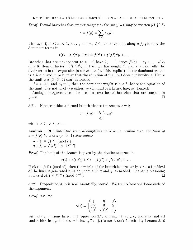
Proof. Formal branches that are not tangent to the line y = 0 may be written (cf. x3.6)
z = f(y) =Xi�0
�iy�i
with �i 2 Q , 1 � �0 < �1 < : : : , and �i 6= 0, and have limit along �(t) given by thedominant terms in
r(t) + s(t)tby + tcz = f(ta) + f 0(ta)tby + : : : :
Branches that are not tangent to z = 0 have �0 = 1, hence f 0(y) = 1 + : : : with
1 6= 0. Hence, the term f 0(ta)tby on the right has weight tb, and is not cancelled byother terms in the expression (since v(s) > 0). This implies that the dominant weightis � b < c, and in particular that the equation of the limit does not involve z. Hencethe limit is a (0 : 0 : 1) star, as needed.
If a < v(r) and �0 = 1, then the dominant weight is a < b, hence the equation ofthe limit does not involve y either, so the limit is a kernel line, as claimed.Analogous arguments can be used to treat formal branches that are tangent to
y = 0.
3.21. Next, consider a formal branch that is tangent to z = 0:
z = f(y) =Xi�0
�iy�i
with 1 < �0 < �1 < : : :
Lemma 3.19. Under the same assumptions on � as in Lemma 3.18, the limit of
z = f(y) by � is a (0 : 0 : 1)-star unless
� r(t) � f(ta) (mod tc);
� s(t) � f 0(ta) (mod tc�b).
Proof. The limit of the branch is given by the dominant terms in
r(t) + s(t)tby + tcz = f(ta) + f 0(ta)tby + : : :
If r(t) 6� f(ta) (mod tc), then the weight of the branch is necessarily < c, so the idealof the limit is generated by a polynomial in x and y, as needed. The same reasoningapplies if s(t) 6� f 0(ta) (mod tc�b).
3.22. Proposition 3.15 is now essentially proved. We tie up here the loose ends ofthe argument.
Proof. Assume
�(t) =
0@ 1 0 0
q(t) tb 0
r(t) s(t)tb tc
1A
with the conditions listed in Proposition 3.7, and such that q; r, and s do not allvanish identically, and assume limt!0 C Æ �(t) is not a rank-2 limit. By Lemma 3.16

28 PAOLO ALUFFI, CAREL FABER
we may assume q(t) 6= 0; hence by Lemma 3.10 �(t) is equivalent to a germ0@ 1 0 0
ta tb 0
r1(t) s1(t)tb tc
1A �
0@1 0 00 u 0r s v
1A ;
with a < b � c, r1(t), s1(t) polynomials, and u; r; s; v 2 C with uv 6= 0. The limit
along this germ is not a rank-2 limit if and only if the limit along0@ 1 0 0
ta tb 0
r1(t) s1(t)tb tc
1A
is not a rank-2 limit. Assuming this is the case, necessarily b < c by Lemma 3.17.
Further, by Lemma 3.18 the limits of all branches that are not tangent to z = 0 are(0 : 0 : 1)-stars, hence rank-2 limits (by Lemma 3.1); the same holds for all formalbranches z = f(y) tangent to z = 0 unless r1(t) = f(ta) and s1(t)t
b = f 0(ta)tb,
by Lemma 3.19. Hence, if limt!0 C Æ �(t) is not a rank-2 limit then �(t) must beequivalent to one in the form given in the statement of the proposition, for someformal branch z = f(y) tangent to z = 0.
Finally, to see that the stated condition on camust hold, look again at the limit of
the formal branch z = f(y), that is, the dominant term in
r(t) + s(t)tby + tcz = f(ta) + f 0(ta)tby +f 00(ta)t2by2
2+ � � � :
the dominant weight will be less than c (causing the limit to be a (0 : 0 : 1)-star) ifc > 2b + v(f 00(ta)) = 2b + a(�0 � 2). The stated condition follows at once.
The e�ect of the constant factor on the right in the germ appearing in the statementof Proposition 3.15 is simply to translate the limit (by an invertible transformation�xing the ag consisting of the line x = 0 and the point (0 : 0 : 1)). Hence, for theremaining considerations in this section we may and will ignore this factor.
Also, we will replace t by t1=d in the germ obtained in Proposition 3.15 to ensurethat the exponents appearing in its expression are relatively prime; the resulting germdetermines the same component of the PNC.
3.23. The next reduction concerns the possible triples a < b < c determining limitscontributing to components of the PNC. This is best expressed in terms of B = b
a
and C = ca. Let
z = f(y) =Xi�0
�iy�i
with �i 2 Q , 1 < �0 < �1 < : : : , and �i 6= 0, be a formal branch tangent to z = 0.Every choice of such a branch and of a rational number C = c
a> 1 determines a
truncation
f(C)(y) =X�i<C
�iy�i :
With this notation, the truncation f(ta) equals f(C)(ta).

LIMITS OF TRANSLATES OF PLANE CURVES | ON A PAPER OF ALDO GHIZZETTI 29
The choice of a rational number B = basatisfying 1 < B < C determines now a
germ as prescribed by Proposition 3.15:
�(t) =
0@ 1 0 0
ta tb 0
f(ta) f 0(ta)tb tc
1A
(choosing the smallest positive integer a for which the entries of this matrix haveinteger exponents). Observe that the truncation f(ta) = f(C)(t
a) is identically 0 if
and only if C � �0. Also observe that f 0(ta)tb is determined by f(C)(ta), as it equals
the truncation to tc of (f(C))0(ta)tb.
Proposition 3.20. If C � �0 or B 6= C��02
+1, then limt!0 C �(t) is a rank-2 limit.
We deal with the di�erent cases separately.
Lemma 3.21. If C � �0, then limt!0 C Æ �(t) is a (0 : 1 : 0)-star.
Proof. If C = ca� �0, then f(C)(y) = 0, so
�(t) =
0@ 1 0 0
ta tb 00 0 tc
1A :
Collect the branches that are not tangent to z = 0 into �(y; z) 2 C [[y; z]], with initialform �m(y; z). Applying �(t) to these branches gives
�m(tax + tby; tcz) + : : :
with limit a kernel line since a < c and �m(1 : 0) 6= 0.As for the branches that are tangent to z = 0, let z = f(y) be such a formal branch.
The limit along �(t) is given by the dominant terms in
tcz = f(ta) + f 0(ta)tby + : : :
All terms on the right except the �rst one have weight larger than a�0 � aC = c,hence the dominant term does not involve y, concluding the proof.
By Lemma 3.1, the limits obtained in Lemma 3.21 are rank-2 limits, so the �rstpart of Proposition 3.20 is proved. As for the second part, if B < C��0
2+ 1 then C >
�0+2(B�1), and the limit is a rank-2 limit by the last assertion in Proposition 3.15.
For B � C��02
+ 1, the limit of a branch tangent to z = 0 depends on whether the
branch truncates to f(C)(y) or not. These cases are studied in the next two lemmas.
Lemma 3.22. Assume C > �0 and B � C��02
+ 1, and let z = g(y) be a formal
branch tangent to z = 0, such that g(C)(y) 6= f(C)(y). Then the limit of the branch issupported on a kernel line.
Proof. The limit of the branch is determined by the dominant terms in
f(ta) + f 0(ta)tby + tcz = g(ta) + g0(ta)tby + : : :

30 PAOLO ALUFFI, CAREL FABER
Assume the truncations g(C) and f(C) do not agree. If the �rst term at which theydisagree has weight lower than B + �0 � 1, then the dominant terms in the expan-sion have weight lower than the weight of f 0(ta)tby, and it follows that the limit is
supported on x = 0. So we may assume that
g(C)(y) = f(C)(y) + yB+�0�1�(y)
for some �(y). We claim that then the terms f 0(ta)tby and g0(ta)tby agree modulo tc:
this implies that the dominant term is independent of y. As the dominant term is alsoindependent of z (since the truncations g(C) and f(C) do not agree), the statementwill follow from our claim.In order to prove the claim, observe that
(g(C))0(y) = (f(C))
0(y) + (B + �0 � 1)yB+�0�2�(y) + yB+�0�1�0(y) :
thus, (g(C))0(y)yB and (f(C))
0(y)yB must agree modulo y2B+�0�2. Since B � C��02
+1,we have
2B + �0 � 2 � (C � �0) + 2 + �0 � 2 = C ;
hence (g(C))0(ta)tb and (f(C))
0(ta)tb must agree modulo taC = tc. It follows that
f 0(ta)tby and g0(ta)tby agree modulo tc, and we are done.
Lemma 3.23. Assume C > �0 and B � C��02
+ 1, and let z = g(y) be a formal
branch tangent to z = 0, such that g(C)(y) = f(C)(y). Denote by (g)C the coeÆcient of
yC in g(y).
� If B > C��02
+ 1, then the limit of the branch z = g(y) by �(t) is the line
z = (C � B + 1) C�B+1y + (g)C :
� If B = C��02
+ 1, then the limit of the branch z = g(y) by �(t) is the conic
z =�0(�0 � 1)
2 �0y
2 +�0 + C
2 �0+C
2
y + (g)C :
Proof. Rewrite the expansion whose dominant terms give the limit of the branch as:
tcz = (g(ta)� f(ta)) + (g0(ta)tb � f 0(ta)tb)y +g00(ta)
2t2by2 + : : :
The dominant term has weight c = Ca by our choices; if B > C��02
+ 1 then the
weight of the coeÆcient of y2 exceeds c, so it does not survive the limiting process,and the limit is a line. If B = C��0
2+ 1, the term in y2 is dominant, and the limit is
a conic.
The explicit expressions given in the statement are obtained by reading the coeÆ-cients of the dominant terms.
We can now complete the proof of Proposition 3.20:
Lemma 3.24. If B > C��02
+ 1, then the limit limt!0 C Æ �(t) is a rank-2 limit.

LIMITS OF TRANSLATES OF PLANE CURVES | ON A PAPER OF ALDO GHIZZETTI 31
Proof. We will show that the limit is necessarily a kernel star, which gives the state-ment by Lemma 3.1.As B > 1, the coeÆcient C�B+1 is determined by the truncation f(C), and in
particular it is the same for all formal branches with that truncation. If B > C��02
+1,
by Lemma 3.23 the branches contributes a line through the �xed point (0 : 1 :(C � B + 1) C�B+1). We are done if we check that all other branches contribute a
kernel line x = 0: and this is implied by Lemma 3.18 for branches that are not tangentto z = 0 (note a < v(r) for the germs we are considering), and by Lemma 3.22 forformal branches z = g(y) tangent to z = 0 but whose truncation g(C) does not agreewith f(C).
3.24. Finally we are ready to complete the description of the components given inx3.2. By Propositions 3.15 and 3.20, germs leading to components of the PNC thathave not yet been accounted for must be (up to a constant translation, and up to
replacing t by t1=d) in the form
�(t) =
0@ 1 0 0
ta tb 0
f(ta) f 0(ta)tb tc
1A
for some branch z = f(y) = �0y�0 + : : : of C tangent to z = 0 at p = (0; 0), and
further satisfying C > �0 and B = C��02
+ 1 for B = ba, C = c
a. New components of
the PNC will arise depending on the limit limt!0 C Æ �(t), which we now determine.
Lemma 3.25. If C > �0 and B = C��02
+ 1, then the limit limt!0 C Æ �(t) consistsof a union of quadritangent conics, with distinguished tangent equal to the kernel linex = 0, and of a multiple of the distinguished tangent line.
Proof. Both �0 and �0+C
2
are determined by the truncation f(C) (since C > �0);
hence the equations of the conics
z =�0(�0 � 1)
2 �0y
2 +�0 + C
2 �0+C
2
y + C
contributed (according to Lemma 3.23) by di�erent branches with truncation f(C)may only di�er in the C coeÆcient.It is immediately veri�ed that all such conics are tangent to the kernel line x = 0,
at the point (0 : 0 : 1), and that any two such conics meet only at the point (0 : 0 : 1);thus they are necessarily quadritangent.
Finally, the branches that do not truncate to f(C)(y) must contribute kernel lines,by Lemmas 3.18 and 3.22.
The type of curves arising as the limits described in Lemma 3.25 are studied in[AF00b], x4.1; also see item (12) in the classi�cation of curves with small orbit in[AF00c], x1. The degenerate case in which only one conic appears does not lead to acomponent of the projective normal cone, by the usual dimension considerations. A
component is present as soon as there are two or more conics, that is, as soon as twobranches contribute distinct conics to the limit.

32 PAOLO ALUFFI, CAREL FABER
This leads to the description given in x3.2. We say that a rational number C is`characteristic' for C (with respect to z = 0) if at least two formal branches of C(tangent to z = 0) have the same nonzero truncation, but di�erent coeÆcients for yC.
Proposition 3.26. The set of characteristic rationals is �nite.The limit limt!0 C Æ �(t) obtained in Lemma 3.25 determines a component of the
projective normal cone precisely when C is characteristic.
Proof. If C � 0, then branches with the same truncation must in fact be identical,
hence they cannot di�er at yC , hence C is not characteristic. Since the set of exponentsof any branch is discrete, the �rst assertion follows.The second assertion follows from Lemma 3.25: if C > �0 and B = C��0
2+ 1, then
the limit is a union of a multiple kernel line and conics with equation
z =�0(�0 � 1)
2 �0y
2 +�0 + C
2 �0+C
2
y + C :
these conics are di�erent precisely when the coeÆcients C are di�erent, and thestatement follows.
Proposition 3.26 leads to the procedure giving components of type V explainedin x3.2 (also cf. [AF00a], x2, Fact 5), concluding the set-theoretic description of theprojective normal cone given there.
3.25. Rather than reproducing from x3.2 the procedure leading to components oftype V, we o�er another explicit example by applying it to the curve consideredin x2.2.
Example 3.27. We obtain the components of type V due to the singularity at thepoint p = (1 : 0 : 0) on the curve
x3z4 � 2x2y3z2 + xy6 � 4xy5z � y7 = 0
The ideal of the tangent cone at p is (z4), so that this curve has four formal branches,all tangent to the line z = 0. These can be computed with ease:8>>>><
>>>>:
z = y3=2 � y7=4
z = y3=2 + y7=4
z = �y3=2 + iy7=4
z = �y3=2 � iy7=4
:
We �nd a single characteristic C = 74, and two truncations y3=2, �y3=2. In both cases
�0 =32, so B =
7
4� 3
2
2+1 = 9
8. The lowest integer a clearing all denominators is 8, and
we �nd the two germs
�1(t) =
0@ 1 0 0t8 t9 0
t12 32t13 t14
1A ; �2(t) =
0@ 1 0 0
t8 t9 0
�t12 �32t13 t14
1A :
As in each case there are two branches (with di�erent y7=4-coeÆcients), the limitsmust in both cases be pairs of quadritangent conics, union a triple kernel line. The

LIMITS OF TRANSLATES OF PLANE CURVES | ON A PAPER OF ALDO GHIZZETTI 33
limit along �1 is listed in x2.2; the limit along �2 must be, according to the formulagiven above,
x3
zx�
32 �
12
2(�1)y2 �
32 +
74
2� 0 � yx� ix2
! zx�
32 �
12
2(�1)y2 �
32 + 7
4
2� 0 � yx+ ix2
!
that is (up to a constant factor),
x3�64x2z2 + 48xy2z + 9y4 + 64x4
�;
as may also be checked directly.
3.26. In this subsection we brie y describe the contents of Aldo Ghizzetti's �rst pa-per [Ghi36b]. Following this paper, Ghizzetti turned to analysis under the mentorshipof Guido Fubini and Mauro Picone. His 50 year career was crowned by the electioninto the Accademia Nazionale dei Lincei . See [Fic94].
In [Ghi36b], Ghizzetti reports the results of his 1930 thesis under Alessandro Ter-racini. He determines here the limits of one-parameter families of `homographic' planecurves (that is, of curves in the same orbit under the PGL(3) action).A main feature of loc. cit. is the classi�cation of one-dimensional systems of `homo-
graphies' approaching a degenerate homography. Let t = (aik(t)) be such a system,
where the coeÆcients aik(t) are power series in t in a neighborhood of t = 0; we as-sume that det(aik(t)) vanishes at t = 0 but is not identically zero. The t are viewedas transformations from a projective plane � to another plane �0:
x0i =
3Xk=1
aik(t)xk ; (i = 1; 2; 3):
A plane curve C 0 of degree d in �0 with equation F (x01; x02; x
03) = 0 is given; transform-
ing it by t gives a curve Ct in � and the goal is to determine the limiting curve C0.The coordinates xk may be modi�ed by a system of non-degenerate homographies of� to reduce t to a simpler form.When 0 has rank 2, it de�nes a kernel point S in � and an image line s0 in �0.
When C 0 does not contain s0, it is easy to see that C0 consists of d lines through S,the d-tuple being projectively equivalent to the d points that C 0 cuts out on s0. Let s0be the limiting position of the line st that results from transforming s0 by t. WhenC 0 contains s0 with multiplicity m, the limiting curve C0 consists of a (d�m)-tupleof lines through S (projectively equivalent to the (d � m)-tuple of points that the
residual of C 0 cuts out on s0) and the line s0 with multiplicity m. These are the limitcurves of type I.When 0 has rank 1, it de�nes a kernel line s in � and an image point S 0 in �0.
When C 0 doesn't pass through S 0, the limiting curve C0 consists of the line s with
multiplicity d. Assume from now on that C 0 passes through S 0. For t 6= 0, let St bethe inverse image point under t of S
0 and let S0 be the limiting point. The authorconsiders two cases: S0 is not contained in s (case I) or it is (case II). (We reservethe word `cases' for Ghizzetti's classi�cation and continue to use `types' for ours.)
After a change of coordinates in � it may be assumed that St is �xed and coincideswith S0. Then t induces a linear map !t on the pencils through S0 and S
0 and one

34 PAOLO ALUFFI, CAREL FABER
obtains a limiting transformation !0, which is either non-degenerate (cases I1 and II1)or degenerate (cases I2 and II2).Case I1 yields one-parameter subgroups with two equal weights; this gives the limit
curves of type III, the fans of Proposition 3.11. In case II1 the kernel line s contains
S0 and the limit curves become kernel stars. Ghizzetti explicitly shows that they arerank-2 limits.In cases I2 and II2, the degenerate map !0 de�nes a kernel line s through S0 and an
image line s0 through S 0. Let s0 be the limiting position of the line st that results from
transforming s0 by !t. The author distinguishes two subcases: s and s0 are distinct(cases I21 and II21) or they coincide (cases I22 and II22). Moreover, in case II22 it isnecessary to distinguish whether s di�ers from s = s0 (case II
022) or coincides with it
(case II0022).
Case I21 yields one-parameter subgroups with three distinct weights: in the notationof x3.13 (with b < c), s is x = 0, s is y = 0, and s0 is z = 0. This gives the limitcurves of types II and IV, cf. xx3.14 and 3.15.Each of the cases I22, II21, and II022 leads to limit curves that are kernel stars; again,
Ghizzetti shows explicitly that they are rank-2 limits.
The case II0022 remains: s = s = s0. Assume that C 0 is tangent to s0 in S 0; if not,C0 consists of the line s with multiplicity d. After a change of coordinates in � and achange of parameter (similar to the one in Lemma 3.10), the matrix of t has threezero entries, one entry equal to 1, and one entry a positive power of t; each of the
remaining entries vanishes at t = 0 but is not identically zero. (The matrix is notin triangular form.) The vanishing orders of two of the entries (m and m + n inGhizzetti's notation) arose naturally in the classi�cation leading to the present case.The other three vanishing orders are called m + p, q, and r, and it is necessary to
analyze the various possibilities for the triple p, q, and r. (In the last section ofloc. cit. the author remarks that m and n are the degree and class of the curve ofimage points under t of a �xed point in � and that p, q, and r are similarly relatedto the curve of inverse image points of a �xed point in �0.)Ghizzetti distinguishes �ve cases in his analysis of the triple p, q, and r. After
simplifying coordinate changes, the t are applied to the branches of C 0 at S 0 thatare tangent to s0. The �rst four cases lead to limit curves that are kernel stars. Inthe study of the �fth case, it is necessary to distinguish �ve subcases. The �rst threelead to limit curves that are kernel stars. The fourth case is not worked out in detail.
The limit curve consists of lines; in general, not all of these lines belong to the samepencil, according to Ghizzetti, but in fact they form a kernel star (cf. Lemma 3.24).The �fth and �nal case leads to a union of quadritangent conics and a multiple ofthe kernel line, as in Lemma 3.25. These are the limit curves of type V; with them,
Ghizzetti concludes his analysis of the possible limit curves arising from a system ofnon-degenerate homographies approaching a degenerate homography.One of the consequences of Ghizzetti's work is that the irreducible components of
limit curves are very special from the projective standpoint; for example, they arenecessarily isomorphic to their own dual. It is clear that such curves have `small'
linear orbit; Ghizzetti's characterization was extended to curves with small orbit in

LIMITS OF TRANSLATES OF PLANE CURVES | ON A PAPER OF ALDO GHIZZETTI 35
projective spaces of arbitrary dimension in one of Ciro Ciliberto's �rst papers, [Cil77].Plane curves with small linear orbits are classi�ed in [AF00c].It will be obvious from the above that Ghizzetti's approach and ours are quite
similar. Let us then conclude this section by indicating some of the di�erences. From
a technical viewpoint, Proposition 3.7 and its re�nement Lemma 3.10 lead us to thekey reduction of Proposition 3.15; this result allows us to restrict our attention togerms that are essentially determined by a branch of C. Although this reductionis perhaps not as geometrically meaningful as Ghizzetti's approach, it appears to
lead to a considerable simpli�cation. Also, the fact that the limit curves necessarilyhave in�nite stabilizer plays a less prominent role in [Ghi36b]. Most importantly,Ghizzetti's goal was essentially the set-theoretic description of the boundary compo-nents of the linear orbit of a curve, while our enumerative applications in [AF00a]
require the more re�ned information carried by the projective normal cone dominat-ing the boundary. This forces us to be more explicit concerning equivalence of germs,and leads us to a rather di�erent classi�cation than the one considered by Ghizzetti.In fact, the set-theoretic description alone of (even) the projective normal cone doesnot suÆce for our broader goals, so that we need to re�ne our analysis considerably
in order to determine the projective normal cone as a cycle, in the next section. Forthis, the notion of equivalence introduced in De�nition 3.2 will play a crucial role,cf. Proposition 4.5 and Lemma 4.10.In any case, Ghizzetti's contribution remains outstanding for its technical prowess,
and it is an excellent example of concreteness and concision in the exposition of verychallenging material. The fact that this is his �rst paper makes our admiration of itonly stronger.
4. The projective normal cone as a cycle
4.1. As mentioned in x1 and x2, the enumerative computations in [AF00a] requirethe knowledge of the cycle supported on the projective normal cone; that is, we needto compute the multiplicities with which the components identi�ed in x3 appear in
the PNC. This is what we do in this section.Our general strategy will be the following. By normalizing the graph of the basic
rational map P8 9 9 KPN , we will distinguish di�erent `ways' in which a componentmay arise, and compute a contribution to the multiplicity due to each way. This
contribution will be obtained by carefully evaluating di�erent ingredients: the orderof contact of certain germs with the base scheme of the rational map, the number ofcomponents in the normalization dominating a given component of the PNC, and thedegree of the restriction of the normalization map to these components.
4.2. Here is the result. The `multiplicities' in the following list are contributionsto the multiplicity of each individual component from the possibly di�erent ways toobtain it. This list should be compared with [AF00a], x2, Facts 1 through 5.
� Type I. The multiplicity of the component determined by a line ` � C equals themultiplicity of ` in C.
� Type II.The multiplicity of the component determined by a nonlinear componentC 0 of C equals 2m, where m is the multiplicity of C 0 in C.

36 PAOLO ALUFFI, CAREL FABER
� Type III. The multiplicity of the component determined by a singular point pof C such that the tangent cone � to C at p is supported on three or more linesequals mA, where m is the multiplicity of C at p and A equals the number ofautomorphisms of � as a tuple in the pencil of lines through p.
� Type IV. The multiplicity of the component determined by one side of a Newtonpolygon for C, with vertices (j0; k0), (j1; k1) (where j0 < j1) and limit
xqyrzqSYj=1
�yc + �jx
c�bzb�
;
(with b and c relatively prime) equals
j1k0 � j0k1
SA ;
where A is the number of automorphisms A 1 ! A 1 , � 7! u� (with u a root of
unity) preserving the S-tuple f�1; : : : ; �Sg.1
� Type V. The multiplicity of the component corresponding to the choice of acharacteristic C and a truncation f(C)(y) at a point p, with limit
xd�2SSYi=1
�zx �
�0(�0 � 1)
2 �0y
2 ��0 + C
2 �0+C
2
yx� (i)C x
2
�
is `WA, where:
{ ` is the least positive integer � such that f(C)(y�) has integer exponents.
{ W is de�ned as follows. For each formal branch � of C at p, let v� be the�rst exponent at which � and f(C)(y) di�er, and let w� be the minimum ofC and v�. Then W is the sum
Pw�.
{ A is twice the number of automorphisms ! u + v preserving the S-tuple
f (1)C ; : : : ;
(S)C g.
Concerning the `di�erent ways' in which a component may be obtained (each pro-ducing a multiplicity computed by the above recipe), no subtleties are involved forcomponents of type I, II, or III: there is only one contribution for each of the speci�eddata|that is, exactly one contribution of type I from each line contained in C, onecontribution of type II from each nonlinear component of C, and one of type III from
each singular point of C at which the tangent cone is supported on three or moredistinct lines.As usual, the situation is a little more complex for components of type IV and V.Components of type IV correspond to sides of Newton polygons; one polygon is
obtained for each line in the tangent cone at a �xed singular point p of C, and each ofthese polygons provides a set of sides (with slope strictly between �1 and 0). Exactlyone contribution has to be counted for each side obtained in this fashion. Note thatsides of di�erent Newton polygons may lead to the same limits, hence to the same
component of the PNC.
Example 4.1. The curve(y � z3)(z � y3) = 0
1Note: the number A given here is denoted A=Æ in [AF00a].

LIMITS OF TRANSLATES OF PLANE CURVES | ON A PAPER OF ALDO GHIZZETTI 37
has a node at the origin p: (y; z) = (0; 0); the two lines in the tangent cone both givethe Newton polygon
each with one side with slope�1=3. The corresponding limits, obtained (as prescribedin x3.14) via the germs 0
@1 0 0
0 t 00 0 t3
1A ;
0@1 0 0
0 t3 00 0 t
1A
are respectivelyy(z � y3) ; z(y � z3) :
These limits belong to the same PGL(3) orbit; thus the two sides determine the samecomponent of the PNC. According to the result given above, the multiplicity of thiscomponent receives a contribution of 4 from each of the sides, so the componentappears with multiplicity 8 in the PNC.
Components of type V are determined by a choice of a singular point p of C, aline L in the tangent cone to C at p, a characteristic C and a truncation f(C)(y) of aformal branch of C tangent to L. Recall that this data determines a triple of positiveintegers a < b < c with C = c=a: the number C and the truncation f(C)(y) determine
B as in the beginning of x3.24, and a is the smallest integer clearing denominatorsof all exponents in the corresponding germ �(t). Again, di�erent choices may leadto the same component of the PNC, and we have to specify when choices should becounted as giving separate contributions. Of course di�erent points p or di�erent lines
in the tangent cone at p give separate contributions; the question is when two sets ofdata (C; f(C)(y)) for the same point, with respect to the same tangent line, should becounted separately.To state the result, we say that (C; f(C)(y)), (C
0; g(C0)(y)) (or the truncations f(C),
g(C0) for short) are sibling data if C = C 0 and f(C)(ta) = g(C)((�t)
a) for an a-th root� of 1.
Example 4.2. If z = f(y), z = g(y) are formal branches belonging to the same ir-reducible branch of C at p, then the corresponding truncations f(C)(y), g(C)(y) are
siblings for all C.Indeed, if the branch has multiplicitym at p then f(�m) = '(�) and g(�m) = (�),
with (�) = '(��) for an m-th root � of 1 ([Fis01], x7.10). That is,
if f(y) =X
�iy�i ; then g(y) =
X�m�i �iy
�i
for � an m-th root of 1. Note that the positive integer a determined by C is suchthat a�i is integer for all the exponents �i lower than C.

38 PAOLO ALUFFI, CAREL FABER
Now let � be an (am)-th root of 1 such that �a = �, and set � = �m; since theexponents a�i in the truncations are integers, as well as all exponents m�i, we have
�m�i = �ma�i = �a�i
for all exponents �i < C, and this shows that the truncations are siblings.
With this notion, we can state precisely when two truncations (C; f(C)(y)) at thesame point, with respect to the same tangent line, yield separate contributions: theydo if and only if they are not siblings.
The proof that the formulas presented above hold occupies the rest of this paper.
Rather direct arguments can be given for the `global' components, of type I andtype II, cf. xx4.8 and 4.9. The `local' types III, IV, and V require some preliminaries,covered in the next several sections.
4.3. The main character in the story will be the normalization P of the closure eP8of the graph of the basic rational map P8 9 9 KPN introduced in x2. We denote by
n : P! eP8the normalization map, and by n the composition P! eP8 ! P8.
In x2, Lemma 2.1 we have realized the PNC as a subset of eP8 � P8 � PN . Recall
that the PNC is in fact the exceptional divisor E in eP8, where the latter is viewed asthe blow-up of P8 along the base scheme S of the basic rational map. If F 2 C [x; y; z]generates the ideal of C in P2, then the ideal of S in P8 is generated by all
F ('(x0; y0; z0))
viewed as polynomials in ' 2 P8, as (x0; y0; z0) ranges over P2. We denote by Ei the
supports of the components of E, and by mi the multiplicity of Ei in E.We also denote by E the Cartier divisor n�1(E) = n�1(S) in P, and by
Ei1; : : : ; Eiri
the supports of the components of E lying above a given component Ei of E. Finally,we let mij be the multiplicity of Eij in E. That is:
[E] =X
mi[Ei] ; [E] =X
mij[Eij] :
Proposition 4.3. We have
mi =
riXj=1
eijmij
where eij is the degree of njEij: Eij ! Ei.
Proof. This follows from the projection formula and (njEij)�[Eij] = eij[Ei].

LIMITS OF TRANSLATES OF PLANE CURVES | ON A PAPER OF ALDO GHIZZETTI 39
4.4. In order to apply Proposition 4.3, we have to develop tools to evaluate themultiplicities mij and the degrees eij. For `local' components, we will obtain this
information by describing Eij in terms of lifts of certain germs from P8. Until theend of x4.7 we focus on components of type III, IV, and V.
Every germ �(t) in P8, whose general element is invertible, and such that �(0) 2 S,
lifts to a unique germ in eP8 centered at a point (�(0);X ) of the PNC. The germ lifts
to a unique germ in P, centered at a point of E.
De�nition 4.4. We denote by � the center of the lift of �(t) to P. We will say that�(t) is a `marker' germ if
� � belongs to exactly one component of E, and the lift of �(t) is transversal to
(the support of) E at �;
� P is nonsingular at �;� limC Æ �(t) is a curve of the type described in x3.2.
Thus, marker germs `mark' one component of E, and P is particularly well-behaved
around marker germs. Note that since P is normal, it is nonsingular along a denseopen set in each component of E: so the second requirement in the de�nition ofmarker germ is satis�ed for a general � on every component of E. It follows thatevery component of E admits marker germs. Our next result is that, for marker
germs, our notion of `equivalence' (De�nition 3.2) translates nicely in terms of the
lifts to E.
Proposition 4.5. Let �0(t), �1(t) be germs, and assume that �1(t) is a marker germ.Then �0(t) is equivalent to �1(t) if and only if �0 = �1 and the lift of �0(t) is
transversal to E. In particular, �0(t) is then a marker germ as well.
Proof. Assume �rst that the germs �0(t) and �1(t) are equivalent. Then �0, �1 are�bers of a family �h(t) = A(h; t) where A : H � Spec C [[t]] ! P8 is as speci�ed
in De�nition 3.2. In particular, the map H ! eP8, h 7! (�h(0); limt!0 C Æ �h(t)) isconstant. This map factors
h 7! �hn7! (�h(0); lim
t!0C Æ �h(t))
and n is �nite over (�h(0); limt!0 C Æ �(t)), so h 7! �h is constant; in particular,�0 = �1.Further, the weight of F (�h(t)) is constant as h varies; this implies that the inter-
section numbers of all lifts of the germs �h(t) with E are equal. In particular, the lift
of �0(t) is transversal to E if and only if the lift of �1(t) is. Since �1(t) is a marker
germ, it follows that the lift of �0(t) is transversal to E, as needed.
For the other implication, P is nonsingular at � := �0 = �1 since �1(t) is a marker
germ. Let (z) = (z1; : : : ; z8) be a system of local parameters for P centered at �, and
write the lifts �i(t) as
t! (z(i)(t)) = (z(i)1 (t); : : : ; z
(i)8 (t)) :
Now
A(h; t) := n�(1� h)z(0)(t) + hz(1)(t)
�
40 PAOLO ALUFFI, CAREL FABER
de�nes a map A 1 � Spec C [[t]] ! P8, so that �h(t) := A(h; t) interpolates between
�0(t) and �1(t). The map A( ; 0) is constant since all lifts �h(t) meet E at �. By thesame token, writing
F (�h(t)) = G(h)tw + higher order terms ;
necessarily G(h) = �(h)G for �(h) 2 C and G a polynomial in x; y; z independent of h.
Since both �0(t) and �1(t) are transversal to E, we have that �(0) and �(1) are bothnonzero. Taking H to be the complement of the zero-set of � in A 1 and restrictingA to H � Spec C [[t]] we obtain a map as prescribed in De�nition 3.2, showing that�0(t) and �1(t) are equivalent.
Corollary 4.6. The germs �(t) obtained in section 3 in order to identify components
of the PNC are marker germs.
Proof. Indeed, we have shown in x3 that every germ determining a component of thePNC is equivalent to one such germ �(td), with d a positive integer; in particularthis holds with d = 1 for marker germs, showing that such �(t) lift to germs that are
transversal to E, and meet it at points at which P is nonsingular.
4.5. Another important ingredient is the PGL(3) action on P.
The PGL(3) action on P8 given by multiplication on the right makes the basicrational map
P8 9 9 KPN
equivariant, and hence induces a right PGL(3) action on eP8 and P, �xing each com-
ponent of E. Explicitly, the action is realized by setting � �N to be the center of thelift of the germ �(t) �N , for N 2 PGL(3). We record the following trivial but useful
remark:
Lemma 4.7. If �(t) = �(t) � N for N 2 PGL(3), then � and � belong to the same
component of E.
Proof. Indeed, then � belongs to the PGL(3) orbit of �.
Lemma 4.8. Let D be a component of E of type III, IV, or V. The orbit of a general� in D is dense in D.
Proof. This follows immediately from the description of the general elements in thecomponents of the PNC, given in x3.2.
Combining this observation with Lemma 4.7 and Proposition 4.5 gives a precise
description of the �bers of E over S:
Corollary 4.9. Let �(t), �(t) be marker germs such that �(0) = �(0). Then � and
� belong to the same component of E if and only if �(t) is equivalent to �(t) �N forsome constant invertible matrix N such that �(0) �N = �(0).
Proof. Let �(t), �(t) be marker germs such that �(0) = �(0). If � and � belong to
the same component of E, then by Lemma 4.8 there exists N 2 PGL(3) such that
� = � �N ; by Proposition 4.5, �(t) is equivalent to �(t) �N . Further, �(0) = �(0) =

LIMITS OF TRANSLATES OF PLANE CURVES | ON A PAPER OF ALDO GHIZZETTI 41
�(0) � N (by de�nition of equivalent germs), hence the stated condition on N musthold.The other implication is immediate from Lemma 4.7.
This description yields our main tool for computing the degrees eij, Proposition 4.12below.First, equivalence of marker germs can be recast in the following apparently stronger
form.
Lemma 4.10. Two marker germs �0(t) and �1(t) are equivalent (w.r.t. C) if andonly if there exists a unit �(t) 2 C [[t]] and a C [h][[t]]-valued point N(h; t) of PGL(3),such that
� N(0; t) is the identity;� N(h; 0) is the identity; and� �1(t�(t)) = �0(t) �N(1; t).
Proof. If a matrix N(h; t) exists as in the statement, de�ne A : A 1 � Spec C [[t]] ! P8
by setting A(h; t) := �0(t) �N(h; t). Then the conditions prescribed by De�nition 3.2are satis�ed with h0 = 0, h1 = 1, showing that �0(t) is equivalent to �1(t).For the converse: since �0(t) and �1(t) are equivalent, �0 = �1 by Proposition 4.5,
and (�0(0); limt!0 C �0(t)) = (�1(0); limt!0 C �1(t)): Let (�;X ) be this point of eP8,and let D be the (unique) component of E which contains it. For the remainder of
the argument, we use the standing assumption that D is a component of type III, IV,or V.Under this assumption, the stabilizer of (�;X ) has dimension 1; consider an A 7
transversal to the stabilizer at the identity I, let U = A 7 \ PGL(3), and consider the
action map U � Spec C [[t]] ! P:
('; t) 7! �0(t) Æ '
where �0(t) is the lift of �0(t) to P.Note that �0(t) factors through this map:
Spec C [[t]] ! U � Spec C [[t]] ! P! P8
by
t 7! (I; t) 7! �0(t) 7! �0(t) :
Lifting �1(t) we likewise get a factorization
t 7! (M(t); z(t)) 7! �0(z(t)) ÆM(t) = �1(t) 7! �1(t)
for suitable M(t), z(t). We may assume that the center (M(0); z(0)) of the lift of�1(t) equals the center (I; 0) of the lift of �0(t); also, z(t) vanishes to order 1 at t = 0,
since the lift of �1(t) is transversal to E. Hence there exists a unit �(t) such that
z(t�(t)) = t, and we can e�ect the parameter change
�1(t�(t)) = �0(t) ÆM(t�(t)) = �0(t) ÆN(t) ;
where we have set N(t) =M(t�(t)), a C [[t]]-valued point of PGL(3).

42 PAOLO ALUFFI, CAREL FABER
Finally, interpolate between (I; t) and (N(t); t) in U�Spec C [[t]] � A 7�Spec C [[t]](much as we did already in the proof of Proposition 4.5), by
(h; t) 7! ((1� h)I + hN(t); t) :
Setting N(h; t) := (1 � h)I + hN(t), we obtain the sought C [h][[t]]-valued point ofPGL(3). Indeed: N(0; t) = I for all t; N(h; 0) = I for all h; and �0(t) � N(1; t) =
�0(t) �N(t) = �1(t�(t)).
4.6. The dependence of this observation on a parameter change prompts the fol-lowing de�nition. Let �(t) be a marker germ for a component D, and consider the
C ((t))-valued points of PGL(3) obtained as products
M�(t) := �(t)�1 � �(t�(t))
as �(t) ranges over all units in C [[t]]. Among all the M�(t), consider those that arein fact C [[t]]-valued points of PGL(3), and in that case let
M� :=M�(0) :
Let � = �(0), and X = limt!0 C Æ �(t).
Lemma 4.11. The set of all M� so obtained is a subgroup of the stabilizer of (�;X ).
Proof. Let M� be as above; that is, M� = M�(0), where M�(t) = �(t)�1 � �(t�(t)) isa C [[t]]-valued point of PGL(3). Since
�(t�(t)) = �(t) �M�(t) ;
we have
� = �(0�(0)) = �(0) �M�(0) = � �M� ;
showing that M� stabilizes �. Further
C Æ �(t�(t)) = C Æ �(t) ÆM�(t) ;
and taking the limit
limt!0
C Æ �(t�(t)) = (limt!0
C Æ �(t)) ÆM�(0) ;
that is,
X = X ÆM�
since the limits along �(t) and �(t�(t)) must agree as the two germs only di�er by achange of parameter. Thus M� stabilizes X as well, as needed.To verify that the set fM�g� forms a group, let �(t) be the unit such that
�(t�(t)) = �(t)�1 :
Then we �nd
M�(t) �M�(t�(t)) = �(t)�1�(t�(t))�(t�(t))�1�(t�(t)�(t�(t)))
= �(t)�1�(t�(t)�(t)�1)
= I ;
the identity matrix. That is, M�(t�(t)) =M�(t)�1, and hence
M� =M�(0) =M�(0)�1 =M�1
� :

LIMITS OF TRANSLATES OF PLANE CURVES | ON A PAPER OF ALDO GHIZZETTI 43
Similarly, for �1(t), �2(t) units, let
�3(t) = �1(t)�2(t�1(t)) :
Then we �nd
M�3(t) = �(t)�1�(t�3(t))
= �(t)�1�(t�1(t))�(t�1(t))�1�(t�1(t)�2(t�1(t)))
=M�1(t)M�2(t�1(t)) ;
and hence M�3 =M�3(0) =M�1(0)M�2(0) =M�1M�2 as needed.
We call inessential the components of the stabilizer of (�;X ) containing elementsof the subgroup identi�ed in Lemma 4.11. These components form the inessentialsubgroup of the stabilizer of (�;X ), corresponding to the choice of �(t).This apparently elusive notion is crucial for our tool to compute the degrees eij.
Proposition 4.12. Let D be a component of E, let D be any component of E dom-inating D. Then the degree of D over D is the index of the inessential subgroup inthe stabilizer of a general point of D.
Proof. Let (�;X ) be a general point of D, and let �1; : : : ; �r be its preimages in D;
so the degree of D over D equals r. We may assume that X is a limit curve of thetype described in x3.2, and that P is nonsingular at all �i, hence for i = 1; : : : ; r wemay choose a marker germ �i(t) whose lift is centered at �i. Let �(t) = �1(t). ByCorollary 4.9, every �i(t) is equivalent to �(t) �Ni for some Ni 2 PGL(3) stabilizing(�;X ); conversely, if N 2 PGL(3) �xes (�;X ) then �(t) � N is equivalent to one of
the �i(t). Thus, the action N 7! � �N maps the stabilizer of (�;X ) onto the �ber of
D over (�;X ).Therefore we simply have to check that two elements of the stabilizer map to the
same point inE if and only if they are in the same coset w.r.t. the inessential subgroup;
that is, it is enough to check that � = � � N if and only if N is in the inessentialsubgroup.First assume that N is in the inessential subgroup, that is, N is in a component
containing an element M� as above. Since the �ber of E over (�;X ) is �nite, then
� � N = � �M�. Now �(t) �M� and �(t) �M�(t) are equivalent by Lemma 3.3; since�(t) �M�(t) = �(t�(t)), we have that � �M� = �. Thus � �N = � as needed.For the converse, assume � = � � N . By Proposition 4.5 and Lemma 4.10, if
� = � �N then there is a C [h][[t]]-valued point N(h; t) of PGL(3) and a unit �(t) inC [[t]] such that N(0; t) = N(h; 0) = I and
�(t) �N(1; t) = �(t�(t)) �N:
NowM�(t) := �(t)�1�(t�(t)) = N(1; t)N�1 is a C [[t]]-valued point of PGL(3), thusM� = N(1; 0)N�1 = N�1 is in the inessential subgroup. This shows that N is in theinessential subgroup, completing the proof.
4.7. Our work in x3 has produced a list of marker germs; these can be used toevaluate the multiplicities mij.
De�nition 4.13. The weight of a germ �(t) is the order of vanishing in t of F �(t).

44 PAOLO ALUFFI, CAREL FABER
Note that the weight of �(t) is the `order of contact' of �(t) with S: indeed, it isthe minimum intersection multiplicity of �(t) and generators F Æ '(x0; y0; z0) of theideal of S, at �(0).
Lemma 4.14. The multiplicity mij is the minimum weight of a germ �(t) such that
� 2 Eij. This weight is achieved by a marker germ for Eij.
Proof. Let � be a general point of Eij. Since P is normal, we may assume that it is
nonsingular at �. Let (z) = (z1; : : : ; z8) be a system of local parameters for P centered
at �, and such that the ideal of Eij is (z1) near �; thus the ideal of E is (zmij
1 ) near
�. Consider the germ �(t) in P de�ned by
�(t) = (t; 0; : : : ; 0) ;
and its push-forward �(t) = n(�(t)) in P8.The weight of �(t) is the order of contact of �(t) with S; hence it equals the order
of contact of �(t) with n�1(S) = E; pulling back the ideal of E to �(t), we see thatthis equals mij.In fact, this argument shows that the weight of any germ in P8 lifting to a germ in
P meeting the support of E transversally at a general point of Eij is mij. It follows
that the weight of any germ lifting to one meeting Eij must be � mij, completingthe proof of the �rst assertion.The second assertion is immediate, as the germ �(t) constructed above is a marker
germ for Eij.
Applying Proposition 4.3 requires the list of the components Eij of E dominating
a given component Ei of E, and for each Eij the two numbers eij and mij. Theselast two elements of information will be obtained by applying Proposition 4.12 and
Lemma 4.14. Obtaining the list Eij and a local description of P requires a case-by-caseanalysis.
4.8. We start with components of type I in this subsection. As it happens, P! eP8is an isomorphism near the general point of such a component, and we can perform
the multiplicity computation directly on eP8.Proposition 4.15. Assume C contains a line ` with multiplicity m, and let (�;X )
be a general point of the corresponding component D of E. Then eP8 is nonsingularnear (�;X ), and D appears with multiplicity m in E.
Proof. We are going to show that, in a neighborhood of (�;X ), eP8 is isomorphicto the blow-up of P8 along the P5 of matrices whose image is contained in `. The
nonsingularity of eP8 near (�;X ) follows from this.
Choose coordinates so that ` is the line z = 0, and the aÆne open set U in P8 withcoordinates 0
@ 1 p1 p2p3 p4 p5p6 p7 p8
1A

LIMITS OF TRANSLATES OF PLANE CURVES | ON A PAPER OF ALDO GHIZZETTI 45
contains �. The P5 of matrices with image contained in ` intersects this open setalong p6 = p7 = p8 = 0, so we can choose coordinates q1; : : : ; q8 in an aÆne opensubset V of the blow-up of P8 along P5 so that the blow-up map is given by8>>><
>>>:
pi = qi i = 1; : : : ; 5
p6 = q6
p7 = q6q7
p8 = q6q8
(the part of the blow-up over U is covered by three such open sets; it should be clearfrom the argument that the choice made here is immaterial).Under the hypotheses of the statement, the ideal of C is generated by zmG(x; y; z),
where z does not divide G; that is, G(x; y; 0) 6= 0. The rational map P8 9 9 KPN acts
on U by sending (p1; : : : ; p8) to the curve with ideal generated by
(p6x + p7y + p8z)mG(x + p1y + p2z; p3x+ p4y + p5z; p6x + p7y + p8z) :
Composing with the blow-up map:
V �! U 9 9 KPN
we �nd that (q1; : : : ; q8) is mapped to the curve with ideal generated by
(x+ q7y + q8z)mG(x + q1y + q2z; q3x+ q4y + q5z; q6x + q6q7y + q6q8z) ;
where a factor of qm6 has been eliminated. Note that no other factor of q6 can be
extracted, by the hypothesis on G.A coordinate veri�cation shows that the induced map
V �! U � PN � P8 � PN ;
which clearly maps V to eP8 � P8 � PN and the exceptional divisor q6 = 0 to D, is an
isomorphism onto the image in a neighborhood of a general point of the exceptional
divisor, proving that eP8 is nonsingular in a neighborhood of the general (�;X ) in D.For the last assertion in the statement, pull-back the generators of the ideal of S
to V :
qm6 (x+ q7y + q8z)mG(x + q1y + q2z; q3x + q4y + q5z; q6x+ q6q7y + q6q8z) ;
as (x : y : z) ranges over P2. For (x : y : z) = (1 : 0 : 0) this gives the generator
qm6 G(1; q3; q6) :
At a general (�;X ) in D we may assume that G(1; q3; 0) 6= 0 (again by the hypothesison G), and we �nd that the ideal of E is (qm6 ) near (�;X ). This shows that the
multiplicity of the component is m, as stated.
Proposition 4.15 yields the multiplicity statement concerning type I components inx4.2; also cf. Fact 2 (i) in x2 of [AF00a].

46 PAOLO ALUFFI, CAREL FABER
4.9. Components of type II can be analyzed almost as explicitly as components oftype I, without employing the tools developed in xx4.3{4.7.Recall from x3.15 that every nonlinear component C 0 of a curve C determines a
component D of the exceptional divisor E.
Proposition 4.16. Assume C contains a nonlinear component C 0, with multiplicitym, and let D be the corresponding component of E. Then D appears with multiplicity2m in E.
This can be proved by using the blow-ups described in [AF93], which resolve the
indeterminacies of the basic rational map P8 9 9 KPN over nonsingular non-in ectionalpoints of C. We sketch the argument here, leaving detailed veri�cations to the reader.
Proof. In [AF93] it is shown that two blow-ups at smooth centers suÆce over nonsin-gular, non-in ectional points of C. While the curve was assumed to be reduced andirreducible in loc. cit., the reader may check that the same blow-ups resolve the inde-terminacies over a possibly multiple component C 0, near nonsingular, non-in ectional
points of the support of C 0. Let V be the variety obtained after these two blow-ups.Since the basic rational map is resolved by V over a general point of C 0, the inverse
image of the base scheme S is locally principal in V over such points. By the universal
property of blow-ups, the map V ! P8 factors through eP8 over a neighborhood ofa general point of C 0. It may then be checked that the second exceptional divisorobtained in the sequence maps birationally onto D, and appears with a multiplicityof 2m.The statement follows.
Proposition 4.16 yields the multiplicity statement concerning type II components
in x4.2; also cf. Fact 2 (ii) in x2 of [AF00a].
4.10. Next, we consider components of type III. Recall that there is one such com-ponent for every singular point p of C at which the tangent cone to C consists of atleast three lines, and that we have shown (cf. Propositions 3.7 and 3.11) that everymarker germ �(t) leading to one of these components is equivalent to one which, in
suitable coordinates (x : y : z), may be written as0@1 0 00 t 0
0 0 t
1A ;
where p has coordinates (1 : 0 : 0) and the kernel line has equation x = 0. Call D the
component of E corresponding to one such point; note that D dominates the subsetof S consisting of matrices whose image is the point (1 : 0 : 0).
Proposition 4.17. There is exactly one component D of E dominating D, and thedegree of the map D ! D equals the number of linear automorphisms of the tuple
determined by the tangent cone to C at p. The minimal weight of a germ leading toD equals the multiplicity of p on C.

LIMITS OF TRANSLATES OF PLANE CURVES | ON A PAPER OF ALDO GHIZZETTI 47
In this statement, the linear automorphisms of a tuple of points in P1 are theelements of its PGL(2)-stabilizer; this is a �nite set if and only if the tuple is supportedon at least three points.
Proof. First we will verify that if �(t), �(t) are marker germs leading to D, then
� and � belong to the same component of E. This will show that there is onlyone component of E over D. By Proposition 4.5, we may replace �(t) and �(t) byequivalent germs; as recalled above, in suitable coordinates we may then assume
�(t) =
0@1 0 00 t 00 0 t
1A ;
and �(t) may be assumed to be in the same form after a change of coordinates. That
is, we may assume
�(t) =M � �(t) �N
for constant matrices M;N . As D dominates the subset of S consisting of matriceswith image (1 : 0 : 0), the image of �(0) and �(0) is necessarily (1 : 0 : 0); this impliesthat M is in the form 0
@A B C0 E F0 H I
1A
with A(EI � FH) 6= 0.Now we claim thatM ��(t) �N is equivalent to �(t) �N 0 for another constant matrix
N 0. Indeed, note that
M � �(t) �N = �(t) �
0@A Bt Ct0 E F0 H I
1A �N =: �(t) �N 0(t) :
Writing N 0 = N 0(0) and applying Lemma 3.3, we establish the claim.
By Proposition 4.5, we may thus assume that �(t) = �(t) � N 0. It follows that �
and � are on the same component of E, by Lemma 4.7.
The degree of D! D is evaluated by using Proposition 4.12. By the description inx3.2, the limit of C along a marker germ �(t) as above consists of a fan X whose starreproduces the tangent cone to C at p, and whose free line is supported on the kernelline x = 0. It is easily checked that the stabilizer of (�(0);X ) has one component foreach element of PGL(2) �xing the tuple determined by the tangent cone to C at p
and that the inessential subgroup equals the identity component.Finally, the foregoing considerations show that the minimal weight of a germ leading
to D is achieved by �(t), and this is immediately computed to be the multiplicity ofC at p.
By Proposition 4.3, Proposition 4.17 implies the multiplicity statement for type IIIcomponents in x4.2; also cf. Fact 4 (i) in x2 of [AF00a].

48 PAOLO ALUFFI, CAREL FABER
4.11. Recall from x3 that components of type IV arise from certain sides of theNewton polygon determined by the choice of a point p on C and of a line in thetangent cone to C at p. If coordinates (x : y : z) are chosen so that p = (1 : 0 : 0),and the tangent line is the line z = 0, then the Newton polygon (see x3.14) consists of
the convex hull of the union of the positive quadrants with origin at the points (j; k)for which the coeÆcient of xiyjzk in the equation for C is nonzero. The part of theNewton polygon consisting of line segments with slope strictly between �1 and 0 doesnot depend on the choice of coordinates �xing the ag z = 0, p = (0; 0). We have
found (see Proposition 3.13 and �.) that if �b=c is a slope of the Newton polygon,with b, c relatively prime, then
�(t) =
0@1 0 0
0 tb 00 0 tc
1A
is a marker germ for a component of type IV if p is a singular or in ection point ofthe support of C, and the limit
xqyrzqSYj=1
(yc + �jxc�bzb)
is not supported on a conic union (possibly) the kernel line.
It is clear that germs arising from sides of Newton polygons corresponding to dif-ferent lines in the tangent cone at p cannot be equivalent, so we concentrate on oneside of one polygon.
Lemma 4.18. Let D be the component of E of type IV corresponding to one side ofthe Newton polygon of slope �b=c, as above. Then there is exactly one component D
of E over D corresponding to this side, and the degree of the map D! D equals the
number of automorphisms A 1 ! A 1 , � 7! u� (with u a root of unity) preserving theS-tuple f�1; : : : ; �Sg.
Proof. As in the proof of Proposition 4.17, we begin by verifying that if �(t), �(t)
are marker germs leading to D, then � and � belong to the same component, byessentially the same strategy.By Proposition 4.5, we may replace �(t) and �(t) with equivalent germs; thus we
may choose
�(t) =
0@1 0 0
0 tb 0
0 0 tc
1A
and �(t) = M � �(t) �N for constant invertible matrices M and N . As �(t) leads toD, the matrixM must preserve the ag consisting of p = (1 : 0 : 0) and the line z = 0(as this is the data which determines the Newton polygon). This implies that
M =
0@A B C0 E F0 0 I
1A
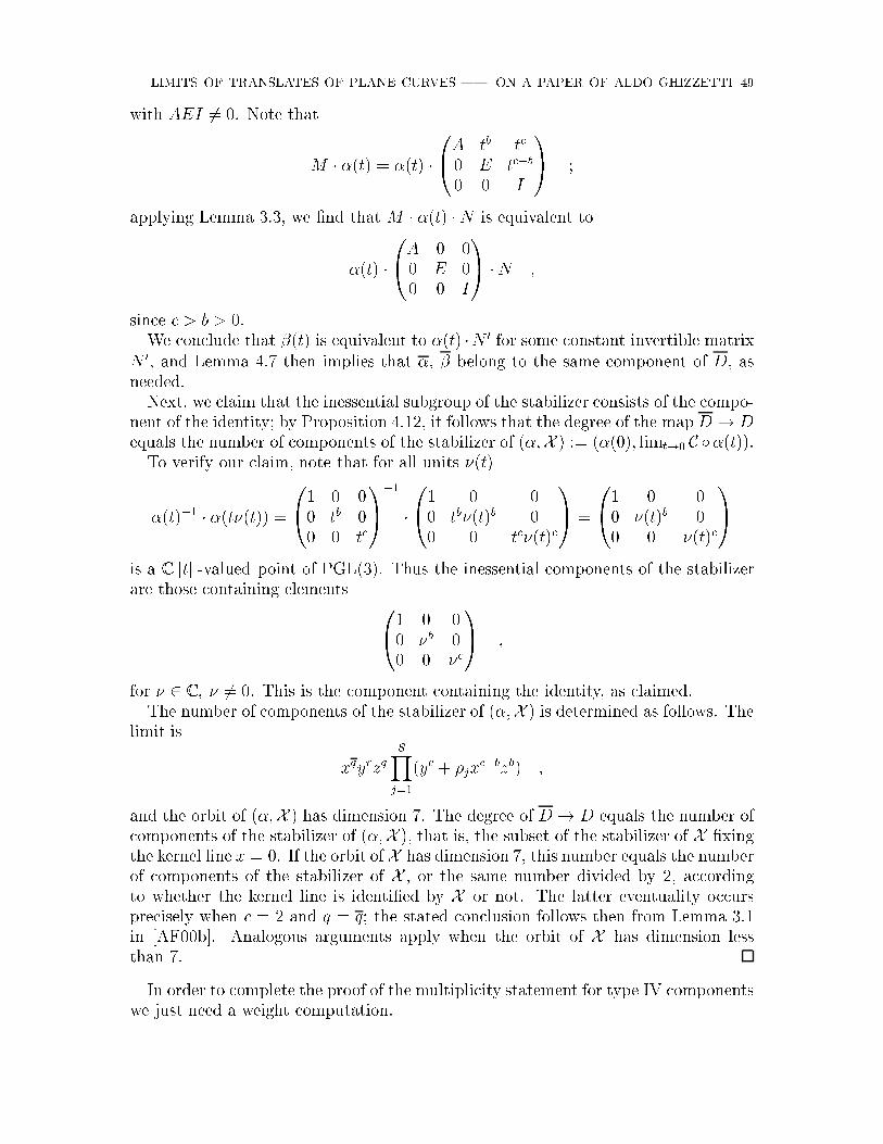
LIMITS OF TRANSLATES OF PLANE CURVES | ON A PAPER OF ALDO GHIZZETTI 49
with AEI 6= 0. Note that
M � �(t) = �(t) �
0@A tb tc
0 E tc�b
0 0 I
1A ;
applying Lemma 3.3, we �nd that M � �(t) �N is equivalent to
�(t) �
0@A 0 00 E 00 0 I
1A �N ;
since c > b > 0.We conclude that �(t) is equivalent to �(t) �N 0 for some constant invertible matrix
N 0, and Lemma 4.7 then implies that �, � belong to the same component of D, as
needed.Next, we claim that the inessential subgroup of the stabilizer consists of the compo-
nent of the identity; by Proposition 4.12, it follows that the degree of the map D! Dequals the number of components of the stabilizer of (�;X ) := (�(0); limt!0 C �(t)).
To verify our claim, note that for all units �(t)
�(t)�1 � �(t�(t)) =
0@1 0 0
0 tb 0
0 0 tc
1A�1
�
0@1 0 0
0 tb�(t)b 0
0 0 tc�(t)c
1A =
0@1 0 0
0 �(t)b 0
0 0 �(t)c
1A
is a C [[t]]-valued point of PGL(3). Thus the inessential components of the stabilizerare those containing elements 0
@1 0 0
0 �b 00 0 �c
1A ;
for � 2 C , � 6= 0. This is the component containing the identity, as claimed.
The number of components of the stabilizer of (�;X ) is determined as follows. Thelimit is
xqyrzqSYj=1
(yc + �jxc�bzb) ;
and the orbit of (�;X ) has dimension 7. The degree of D! D equals the number ofcomponents of the stabilizer of (�;X ), that is, the subset of the stabilizer of X �xingthe kernel line x = 0. If the orbit of X has dimension 7, this number equals the numberof components of the stabilizer of X , or the same number divided by 2, according
to whether the kernel line is identi�ed by X or not. The latter eventuality occursprecisely when c = 2 and q = q; the stated conclusion follows then from Lemma 3.1in [AF00b]. Analogous arguments apply when the orbit of X has dimension lessthan 7.
In order to complete the proof of the multiplicity statement for type IV componentswe just need a weight computation.

50 PAOLO ALUFFI, CAREL FABER
Lemma 4.19. The minimum weight of a marker germ for the component correspond-ing to a side of the Newton polygon with vertices (j0; k0), (j1; k1), j0 < j1, is
j1k0 � j0k1
S:
Proof. With notations as above, we have seen that every marker germ leading to thecomponent is equivalent to �(t) �N , where
�(t) =
0@1 0 0
0 tb 00 0 tc
1A ;
thus the minimum weight is achieved by this germ.The limit
xqyrzqSYj=1
(yc + �jxc�bzb)
appears with weight br + cq + Sbc, so we just have to show that
Sbc+ br + cq =j1k0 � j0k1
S:
This is immediate, as (j0; k0) = (r; q + Sb), (j1; k1) = (r + Sc; q).
The prescription for type IV components now follows from Lemmas 4.18 and 4.19,
Proposition 4.3, and Lemma 4.14.We note that the same prescription yields the correct multiplicity for type II limits
as well: indeed, the side of the Newton polygon corresponding to type II limits (as inx3.15) has vertices (0; m) and (2m; 0), wherem is the multiplicity of the corresponding
nonlinear component of C; so S = m and (j1k0 � j0k1)=S = 2m2=m = 2m, inagreement with Proposition 4.16.Fact 4(ii) in [AF00a], x2, reproduces the result proved here; the reader should note
that the number denoted A here is denoted A=Æ in loc. cit.The weight computed in Lemma 4.19:
j1k0 � j0k1
S;
happens to equal 2=S times the area of the triangle with vertices (0; 0), (j0; k0), and(j1; k1).

LIMITS OF TRANSLATES OF PLANE CURVES | ON A PAPER OF ALDO GHIZZETTI 51
An example illustrating this for b=c = 1=3:
x yd−3m 3m
m.2 Area=3
xd−m
zm
We do not have a conceptual explanation for this observation.
4.12. We are left with components of type V, whose analysis is predictably subtler.
In x3 we have found that such components arise from suitable truncations of thePuiseux expansion of the branches of C at a singular point p of its support. Choosingcoordinates (x : y : z) so that p = (1 : 0 : 0) and the branch has tangent conesupported on the line z = 0, we have found a marker germ
�(t) =
0@ 1 0 0
ta tb 0
f(ta) f 0(ta)tb tc
1A
where
z = f(y) =Xi�0
�iy�i
is the Puiseux expansion of a corresponding formal branch, a < b < c are positiveintegers, C = c
ais `characteristic' in the sense explained in 3.2, underlining denotes
truncation to tc, and a is the smallest positive integer for which all entries in �(t) are
polynomials. The limit obtained along this germ is:
xd�2SSYi=1
�zx�
�0(�0 � 1)
2 �0y
2 ��0 + C
2 �0+C
2
yx� (i)C x
2
�;
where (i)C are the coeÆcients of yC for all formal branches sharing the truncation
f(C)(y) =P
�i<C �iy
�i.As the situation is more complex than for other components, we proceed through
the proof of the multiplicity statement given in x4.2 one step at the time.
4.13. Through the procedure recalled above, the choice of a characteristic C and ofa truncation f(C)(y) of a formal branch determines a germ, and hence (by lifting to
the normalization) a component of E over a �xed type V component D of E. In fact,
by Proposition 3.15 and Lemma 4.7, every component D over D is marked in thisfashion.
Clearly di�erent points or di�erent lines in the tangent cone yield di�erent com-ponents D over D. As stated in x4.2, for a �xed point and line there are di�erent

52 PAOLO ALUFFI, CAREL FABER
contributions for truncations that are not `siblings'. In other words, we must showthat there is a bijection between the set of components D over D corresponding to agiven point and line, and set of data (C; f(C)(y)) as above, modulo the sibling relation.We will now recall this notion, and prove this fact in Proposition 4.21 below.
We say that (C; f(C)(y)), (C0; g(C0)(y)) (or the truncations f(C), g(C0) for short) are
sibling data if the corresponding integers a < b < c, a0 < b0 < c0 are the same (so inparticular C = C 0) and further
g(C)(y) =X�i<C
�a�i �iy�i
(that is, f(C)(ta) = g(C)((�t)
a)) for an a-th root � of 1.Both Proposition 4.21 and the determination of the inessential subgroup rely on
the following technical lemma.
Lemma 4.20. Let
�(t) =
0@ 1 0 0
ta tb 0
f(ta) f 0(ta)tb tc
1A ; �(t) =
0@ 1 0 0
ta0
tb0
0
g(ta0
) g0(ta0
)tb0
tc0
1A
be two marker germs of the type considered above, and assume that �(t)�1�(�(t)) is a
C [[t]]-valued point of PGL(3), for a change of parameter �(t) = t�(t) with �(t) 2 C [[t]]a unit. Then a0 = a, b0 = b, c0 = c, and �(t) = �(1 + tb�a�(t)), where � is an a-throot of 1 and �(t) 2 C [[t]]; further, g((�t)a) = f(ta).
Proof. Write '(t) = f(ta) and (t)tb = f 0(ta)tb. The hypothesis is that
�(t)�1 � �(�) =
0B@
1 0 0�a
0
�ta
tb�b0
tb0
g(�a0
)�'(t)�(�a0
�ta) (t)
tc
g0(�a0
)�b0
� (t)�b0
tc�c
0
tc
1CA
has entries in C [[t]], and its determinant is a unit in C [[t]]. The latter conditionimplies b0 = b and c0 = c. As
�a0
� ta
tb2 C [[t]] ;
necessarily a0 = a and ta(�(t)a� 1) = (�a� ta) � 0 mod tb. Since b > a, this implies
�(t) = �(1 + tb�a�(t))
for � an a-th root of 1 and �(t) 2 C [[t]]. Also note that since the triples (a; b; c) and(a0; b0; c0) coincide, necessarily the dominant term in g(y) has the same exponent �0as in f(y), since a�0 = 2a� 2b + c.Now we claim that
g(�a)� (�a � ta) (t) � g((�t)a) mod tc :
Granting this for a moment, it follows that
g(�a0
)� '(t)� (�a0
� ta) (t) � g((�t)a)� f(ta) mod tc ;

LIMITS OF TRANSLATES OF PLANE CURVES | ON A PAPER OF ALDO GHIZZETTI 53
hence, the fact that the (3; 1) entry is in C [[t]] implies that
g((�t)a) � f(ta) mod tc ;
which is what we need to show in order to complete the proof.Since the (3; 2) entry is in C [[t]], necessarily
g0(�a) � (t) mod tc�b ;
so our claim is equivalent to the assertion that
g(�a)� (�a � ta)g0(�a) � g((�t)a) mod tc :
By linearity, in order to prove this it is enough to verify the stated congruence for
g(y) = y�, with � � �0. That is, we have to verify that if � � �0 then
�a� � (�a � ta)��a��a � (�t)a� mod tc :
For this, observe
�a� = (�t)a�(1 + tb�a�(t))a� � (�t)a�(1 + a�tb�a�(t)) mod ta�+2(b�a)
and similarly
�a��a = (�t)a��a(1 + tb�a�(t))a��a � t�a(�t)a� mod ta��a+(b�a) ;
(�a � ta) = (�t)a(1 + tb�a�(t))a � ta � atb�(t) mod ta+2(b�a) :
Thus
(�a � ta)��a��a � (�t)a�a�tb�a�(t) mod ta�+2(b�a)
and
�a� � (�a � ta)��a��a � (�t)a� mod ta�+2(b�a) :
Since
a�+ 2(b� a) � a�0 + 2b� 2a = c ;
our claim follows.
4.14. The �rst use of this observation is in the following result.
Proposition 4.21. Two truncations f(C)(y), g(C0)(y) determine the same component
D over D if and only if they are siblings.
Proof. Assume that f(C)(y), g(C0)(y) are siblings. Then C = C 0, and for an a-th root� of 1 the corresponding germs
�(t) =
0@ 1 0 0
ta tb 0
f(ta) f 0(ta)tb tc
1A ; �(t) =
0@ 1 0 0
ta tb 0
g(ta) g0(ta)tb tc
1A
satisfy
�(�t) =
0@ 1 0 0
(�t)a (�t)b 0
f((�t)a) f 0((�t)a)(�t)b (�t)c
1A =
0@ 1 0 0
ta tb�b 0
g(ta) g0(ta)tb�b tc�c
1A
= �(t) �
0@1 0 0
0 �b 0
0 0 �c
1A :

54 PAOLO ALUFFI, CAREL FABER
By Lemma 4.7, the lifts of �(�t) and �(t) belong to the same component of E. As
�(�t) only di�ers from �(t) by a reparametrization, this shows that � and � belong
to the same component of E, as needed.
For the converse, assume
�(t) =
0@ 1 0 0
ta tb 0
f(ta) f 0(ta)tb tc
1A ; �(t) =
0@ 1 0 0
ta0
tb0
0
g(ta0
) g0(ta0
)tb0
tc0
1A
mark the same component D. Since the limit of C along �(t) has 7-dimensional orbit,
the action of PGL(3) on D is transitive on a dense open set. Therefore, we have that�(t) � N and �(t) are equivalent for some N 2 PGL(3). By Lemma 4.10, there is aC [h][[t]]-valued point N(h; t) of PGL(3) such that �(t�(t)) = �(t) �N(1; t), for a unit
�(t). That is,
N(1; t) = �(t)�1 � �(�(t))
is a C [[t]]-valued point of PGL(3), for �(t) = t�(t). By Lemma 4.20, this impliesa0 = a, b0 = b, c0 = c, and g((�t)a) = f(ta), for an a-th root � of 1, showing that the
truncations are siblings.
4.15. By Proposition 4.3, the multiplicity of D is a sum over the distinct siblingclasses of truncations producing a given limit. Evaluating the degree of the map
D! D requires the determination of the inessential subgroup of the stabilizer, whichalso makes crucial use of Lemma 4.20.
Lemma 4.22. Let
�(t) =
0@ 1 0 0
ta tb 0
f(ta) f 0(ta)tb tc
1A
be the germ determined by C and the truncation f(C)(y) =P
�i<C �iy
�i as above.
Then the inessential subgroup corresponding to �(t) consists of the components of thestabilizer of (�(0); limt!0C Æ �(t)) containing matrices0
@1 0 0
0 �b 00 0 �c
1A
with � an h-th root of 1, where h is the greatest common divisor of a and all a�i(�i < C).
Proof. For every h-th root � of 1, any component of the stabilizer containing a diagonalmatrix of the given form is in the inessential subgroup: indeed, such a diagonal matrixcan be realized as �(t)�1 � �(�t).
To see that, conversely, every component of the inessential subgroup is as stated,apply Lemma 4.20 with �(t) = �(t). We �nd that if �(t)�1 ��(t�(t)) is a C [[t]]-valuedpoint of PGL(3), then �(t) = �(1 + tb�a�(t)), with � an a-th root of 1, and further
f(ta) = f((�t)a) ;

LIMITS OF TRANSLATES OF PLANE CURVES | ON A PAPER OF ALDO GHIZZETTI 55
that is, X�i<C
�iy�i =
X�i<C
�a�i �iy�i :
Therefore �a�i = 1 for all i such that �i < C, and � is an h-th root of 1.For �(t) = �(1 + tb�a�(t)), the matrix �(t)�1 � �(t�(t))jt=0 is lower triangular, of
the form 0@ 1 0 0
a�0 �b 0
�0��02
�(a�0)
2 + �0+C
2
�0+C2
(a�0) 2 �0��02
�(a�0)�
b �c
1A
where �0 = �(0). If a component of the stabilizer contains this matrix for some �(t),then it must contain all such matrices for all �0, and in particular that componentmust contain the diagonal matrix0
@1 0 0
0 �b 00 0 �c
1A ;
the statement follows.
Note that �c = (�b)2 since c�2b = a�0�2a is divisible by h; this is in fact a necessarycondition for the diagonal matrix above to belong to the stabilizer. Moreover, if �0+C
2
6= 0, then necessarily �b = 1; as the proof of the following proposition shows,
this implies h = 1.
Proposition 4.23. For the component D determined by the truncation f(C)(y) asabove, let A be the number of components of the stabilizer of the limit
xd�2SSYi=1
�zx �
�0(�0 � 1)
2 �0y
2 ��0 + C
2 �0+C
2
yx� (i)C x
2
�
(that is, by [AF00b], x4.1, twice the number of automorphisms ! u +v preserving
the S-tuple f (1)C ; : : : ;
(S)C g). Then the degree of the map D ! D equals A
h, where h
is the number determined in Lemma 4.22.
Proof. As the kernel line � must be supported on the distinguished tangent of thelimit X , the stabilizer of (�;X ) equals the stabilizer of X , and in particular it consists
of A components.Next, observe that for �1 6= �2 two h-th roots of 1, the two matrices0
@1 0 0
0 �b1 00 0 �c1
1A ;
0@1 0 0
0 �b2 00 0 �c2
1A
are distinct: indeed, if �b = �c = 1, then the order of � divides every exponent of everyentry of �(t), hence it equals 1 by the minimality of a. Further, the components of thestabilizer containing these two matrices must be distinct: indeed, the description ofthe identity component of the stabilizer of a curve consisting of quadritangent conics
given in [AF00c], x1, shows that the only diagonal matrix in the component of theidentity is in fact the identity itself.

56 PAOLO ALUFFI, CAREL FABER
Hence the index of the inessential subgroup equals A=h, and the statement followsthen from Proposition 4.12.
4.16. All that is left is the computation of the weight of the marker germ
�(t) =
0@ 1 0 0
ta tb 0
f(ta) f 0(ta)tb tc
1A :
For every formal branch � of C at p, de�ne an integer w� as follows:
� if the branch is not tangent to the line z = 0, then w� = 1;� if the branch is tangent to the line z = 0, but does not truncate to f(C), thenw� = the �rst exponent at which � and the truncation di�er;
� if the branch truncates to f(C), then w� = C.
Lemma 4.24. The weight of �(t) equals aW , with W =Pw�.
Proof. It is immediately checked that aw� equals the order of vanishing in t of the
composition of each formal branch with �(t), so aPw� equals the order of vanishing
of F Æ �(t), which is the claim.
We are �nally ready to conclude the veri�cation of the multiplicity statement forcomponents of type V given in x4.2.The upshot of the foregoing discussion is that the multiplicity equals the sum of
contributions from each sibling class of truncations f(C)(y).
Proposition 4.25. Let D be the component of type V determined by the choice ofC and of the truncation f(C)(y), and let ` be the minimum among the positive inte-gers � such that f(C)(y
�) has integer exponents. Then, with notations as above, thecontribution of the sibling class of f(C)(y) to the multiplicity of D is `WA.
Proof. By Proposition 4.23 and Lemma 4.24, the sibling class of f(C)(y) contributes
aW Ah. So all we have to prove is that ` = a
h, with ` as in the statement.
For this, let �i, i = 1; : : : ; r be the exponents appearing in f(C)(y). If h0 is anydivisor of a and all a�i, then as a
h0�i are integers, necessarily a
h0is a multiple of `.
That is, h0 divides a`. On the other hand, a
`is a divisor of a and all a�i. Hence a
`
equals the greatest common divisor of a and all a�i, which is the claim.
Proposition 4.25 completes the proof of the multiplicity statement for type V com-ponents; also cf. [AF00a], x2, Fact 5.This concludes the proof of the multiplicity statement given in x4.2.
5. Examples
5.1. In this �nal section we collect several explicit examples of limits of translates
of plane curves, obtained by applying the results presented in this paper. We willdescribe the limits corresponding to the di�erent components of the PNC for thecurves we will consider, and marker germs for these components. We will generallypass in silence degenerate limits such as multiple lines (obtained for example as limCÆ
�(t), for �(0) a rank 1 matrix with image not contained in C), or rank-2 limits. Limitswill often be described in terms of the geometry of the curve, and representative

LIMITS OF TRANSLATES OF PLANE CURVES | ON A PAPER OF ALDO GHIZZETTI 57
pictures will be superimposed on the curve to emphasize this relation; of course suchpictures should not be taken too literally.We will also compute the degrees of the orbit closures of the curves we will consider,
as an illustration of the formulas in [AF00a] that we obtained as main application
of the results presented here. Several other enumerative examples can be found in[AF00a]. Concerning these enumerative computations, we will freely use the termi-nology introduced in loc. cit., and in particular the notions of predegree and adjustedpredegree polynomial (a.p.p.) (cf. x1 of [AF00a]).
5.2. Let d1; d2; m1; m2 be positive integers. Consider a curve C consisting of theunion of two general curves C1, C2 of degrees d1 � d2, in general position and appearing
with multiplicity m1, m2 respectively.We distinguish three cases:
1. 1 = d1 = d2;
2. 1 = d1 < d2;3. 1 < d1 � d2.
In case (1) the curve is the union of two distinct lines with multiplicity m1, m2.
II
According to x3.2 and x4.2, the PNC consists of two components of type I, appearingwith multiplicity m1, m2 (also cf. x3.7 and x4.8); and the limits attained by C areeither translates of C, or multiple lines.Since the line C1 meets the rest of C at one point with multiplicity m2, the contri-
bution of C1 to the a.p.p. of C is the antiderivative w.r.t. H of
�m3
1
2exp(�(m1 +m2)H)H2
�1 +m2H +
m22H
2
2
�(Proposition 3.1 in [AF00a]); and similarly for C2. The contribution of both togetheris therefore
�(m3
1 +m32)H
3
6+
(m41 +m4
2)H4
8�
(m51 +m5
2)H5
20+
(m31 +m3
2)2H6
72� : : : ;
so the a.p.p. of C is (Proposition 1.1 in [AF00a])
exp((m1 +m2)H)
�1�
(m31 +m3
2)H3
6+
(m41 +m4
2)H4
8�
(m51 +m5
2)H5
20+ : : :
�
= 1 + (m1 +m2)H +(m1 +m2)
2
2H2 +
m1m2(m1 +m2)
2H3 +
m21m
22
4H4

58 PAOLO ALUFFI, CAREL FABER
=
�1 +m1H +
m21H
2
2
��1 +m2H +
m22H
2
2
�:
It follows (x1 in [AF00a]) that the orbit closure of C has dimension 4, and predegree
4!m21m22
4; that is, degree (
6m21m
22 if m1 6= m2
3m4 if m1 = m2 = m
This of course agrees with the naive dimension count, and multiplicity and combina-torial considerations.In case (2) the curve is the transversal union of a line, with multiplicity m1, and a
general nonsingular curve of degree d2, with multiplicity m2.
IIIV
IV
IV
IV
I
According to x3.2 and x4.2 the PNC has one component of type I, with multiplicitym1,one component of type II, with multiplicity 2m2, and several `local components' oftype IV: one for each of the 3d2(d2� 2) ordinary exes of C2, and one for each of thed2 points of intersection of C1 and C2.
Limits corresponding to the type I component are obtained as limC �(t) for �(0)a rank-2 matrix whose image is the line C1. Such limits are fans determined by theintersection of C1 with the rest of the curve:
The multiplicity of the non-concurrent line in the fan is m1, and the multiplicities ofthe star lines all equal m2.

LIMITS OF TRANSLATES OF PLANE CURVES | ON A PAPER OF ALDO GHIZZETTI 59
The type II component can be marked by a 1-PS with weights (1; 2):
�(t) =
0@1 0 00 t 0
0 0 t2
1A
if p = (1 : 0 : 0) is a general point of C2, and the highest weight line z = 0 is thetangent line to C2 at p (cf. x3.15). The corresponding limit consists of a conic, with
multiplicitym2, and tangent to the kernel line, union the kernel line with multiplicitym1 +m2(d2 � 2):
At each in ection point the relevant side of the Newton polygon is
2 Area=3m2
joining (0; m2) and (3m2; 0); according to x4.2 such type IV components appear withmultiplicity 3m2 (cf. x4.11). Marker germs for one of these components can be chosento be 1-PS �(t) with weights (1; 3), image of �(0) equal to the ex, and highest weight
line on the in ectional tangent (x3.14). The limits consist of a cuspidal cubic withmultiplicity m2 and cuspidal tangent on the kernel line, union the kernel line with

60 PAOLO ALUFFI, CAREL FABER
multiplicity m1 +m2(d2 � 3):
The d2 points of intersection are nodes, with multiple branches, and one of whosebranches is supported on a line. The Newton polygons corresponding to the twotangent directions are
212 Area=(m +2m )
and only one side (joining (m1; m2) and (m1+2m2; 0)) has slope strictly between �1and 0. So each of these points contributes one component of type IV, appearing withmultiplicity m1 + 2m2. This component is marked by a 1-PS �(t) with weights (1; 2)with im�(0) an intersection point, and highest weight line tangent to the non-linear
branch. Limits consist of a conic with multiplicity m2 and tangent to the kernel line,the kernel line with multiplicity m2(d2 � 2), and a transversal line through the point

LIMITS OF TRANSLATES OF PLANE CURVES | ON A PAPER OF ALDO GHIZZETTI 61
of intersection, with multiplicity m1:
No components of type III appear, since the tangent cone at each point of type Cis supported on � 2 lines. The curve C has no characteristics at its singularities, so
the PNC has no components of type V in this case, cf. again x3.2.Proposition 3.1 in [AF00a] gives the contribution due to the type I component as
the antiderivative of
�m3
1
2exp(�(m1 +m2d2)H)H2
�1 +m2H +
m22H
2
2
�d2:
indeed, the line meets C2 at d2 points, each with multiplicity m2. Explicitly:
�
m31H
3
6+
m41H
4
8�
m51H
5
20+
m31(m
31 +m3
2d2)H6
72
�
m31(m
41 + 4m1m
32d2 + 3m4
2d2)H7
336+
m31(m
51 + 10m2
1m32d2 + 15m1m
42d2 + 6m5
2d2)H8
1920
As for the type II component, its contribution is
� 2m52d2
�H5
20�
(5(m1 +m2d2) + 18m2)H6
360+
(9(m1 +m2d2) + 8m2)m2H7
420
�
(m1 +m2d2)m22H
8
60
�
according to Proposition 3.2 in [AF00a].
`Local contributions' from type IV components are evaluated using Proposition 3.4in [AF00a]. The data needed in order to apply this formula consists of the vertices ofthe corresponding side of the Newton polygon, and the multiplicities of the curvilinearcomponents in the limit. We obtain a contribution of
�m6
2H6
48+
3m72H
7
70�
197m82H
8
4480
from each of the 3d2(d2 � 2) in ection points, and of
m1m32(m1 + 2m2)
��
(m1 +m2)H6
72+
(20m21 + 45m1m2 + 36m2
2)H7
1680
�
(10m31 + 35m2
1m2 + 48m1m22 + 32m3
2)H8
1920
�

62 PAOLO ALUFFI, CAREL FABER
from each of the d2 nodes. Combining all these contributions and applying Proposi-tion 1.1 in [AF00a] yields the a.p.p. for C. The coeÆcient of H8 in this polynomial,multiplied by 8!, gives the predegree of C for d2 > 2:
(d2 � 2)d2m62
�28(d42 + 2d32 + 4d22 � 22d2 � 33)m2
1
+ 8(d52 + 2d42 + 4d32 + 8d22 � 411d2 + 744)m1m2
+(d62 + 2d52 + 4d42 + 8d32 � 1356d22 + 5280d2 � 5319)m22
�This expression vanishes for d2 = 2 because in that case the orbit closure has dimen-sion < 8; the predegree can then be computed from the coeÆcient of H7 in the a.p.p.,giving 84m2
1m52. Accounting for the stabilizer, this gives 21m
21m
52 for the degree of the
orbit closure in this case, again agreeing with naive combinatorial considerations.For d2 > 2 and m1 = m2 = 1 the expression given above counts the number of
con�gurations containing 8 points in general position. The individual sub-expressionsin this formula can also be given a concrete enumerative interpretation. For example,
(d2 � 2)d2�d42 + 2d32 + 4d22 � 22d2 � 33
�= d62 � 30d32 + 11d22 + 66d2
is (for d2 > 2) the number of embeddings of a given general plane curve of degree d2containing 6 general points, and satisfying the constraint of having a given generalsection of O(1) contained in a prescribed line.
In case (3), C is the union of two general curves of degrees � 2, in general position.The discussion is analogous to that given in case (2); in this case the PNC will haveno component of type I, but a second component of type II, with multiplicity 2m1;and there will be 3d1(d1 � 2) new components of type IV corresponding to the exeson C1, each with multiplicity 3m1. A new phenomenon concerns the components of
type IV due to the points of intersection of C1 and C2. At such points the relevantNewton polygons:
12 Area=(2m +m )
2122 Area=(m +2m )
have two sides with slope between �1 and 0 (these will join the points (m1; m2) and
(m1 + 2m2; 0), respectively (m2; m1) and (2m1 + m2; 0)). Thus, each of these d1d2points can potentially contribute two components to the PNC. The components are

LIMITS OF TRANSLATES OF PLANE CURVES | ON A PAPER OF ALDO GHIZZETTI 63
marked, as above, by 1-PS germs �(t) with weights (1; 2), im�(0) the intersectionpoint, and highest weight line tangent to one of the branches. The correspondinglimits are schematically represented by
1m
2m2m
1m
indicating multiplicities. The components are distinct if and only if m1 6= m2 (ac-cording to x3.2). If m1 = m2 = m, the single type IV component determined by sucha point has multiplicity 6m in the PNC.The a.p.p. for C can be determined by using the results in [AF00a], similarly to
case (2), using the Newton polygon data listed above. The predegree of C turns outto be
(m1d1+m2d2)8�28(m1d1+m2d2)
2(49d21m
61+24d1d2m
51m2+30d1d2m
41m
22+20d1d2m
31m
32
+ 30d1d2m21m
42 + 24d1d2m1m
52 + 49d22m
62) + 72(d1m1 + d2m2)(111d
21m
71 + 63d1d2m
61m2
+ 42d1d2m51m
22 + 35d1d2m
41m
32 + 35d1d2m
31m
42 + 42d1d2m
21m
52 + 63d1d2m1m
62 + 111d22m
72)
� (15879d21m81 + 11904d1d2m
71m2 + 2688d1d2m
61m
22 + 2688d1d2m
51m
32 + 2310d1d2m
41m
42
+2688d1d2m31m
52+2688d1d2m
21m
62+11904d1d2m1m
72+15879d22m
82)+10638(d1m
81+d2m
82):
In the reduced case, let d = d1 + d2 be the degree of the curve and n = d1d2 be thenumber of points of intersection; then this formula evaluates the predegree of C as
d8 � 1372d4 + 7992d3 � 15879d2 + 10638d� 24n(35d2 � 174d+ 213) :
In fact, this is the predegree of a general plane curve of degree d with n ordinary
nodes, cf. Example 4.1 in [AF00a].
5.3. Let C be a star consisting of d � 3 distinct reduced lines through a point:
I
III
I
III

64 PAOLO ALUFFI, CAREL FABER
and let A be the number of automorphisms of the tuple of lines. Thus A = 6 ford = 3, A = 4 for general stars with d = 4, and A = 1 for general stars with d > 4.According to x3.2 and x4.2, the PNC for this curve has one reduced component oftype I for each line, and one component of type III, appearing with multiplicity dA.
If coordinates are chosen so that one of the lines is z = 0, the germ0@1 0 00 1 0
0 0 t
1A
marks the corresponding type I component. In this case the limit consists of a pairof lines, with multiplicities 1 and d� 1 respectively (Proposition 3.6):
1
d−1
The component of type III is marked by 1-PS with image the multiple point, and
equal weights (Proposition 3.11): 0@1 0 00 t 00 0 t
1A
if the center of the star is at (1 : 0 : 0). This example is somewhat atypical, in thatthese limits are nothing but translates of the original curve.Proposition 3.1 in [AF00a] can again be invoked to evaluate the (additive) contri-
bution to the a.p.p. due to the d type I components, as the antiderivative of
�d
2exp(�dH)H2
�1 + (d� 1)H +
(d� 1)2H2
2
�:
Proposition 3.3 in loc.cit. evaluates the contribution due to the type III component:
�d2(d� 1)(d� 2)(d2 + 3d� 3)
30
�H6
24�dH7
28+d2H8
64
�:
Note that the factor of A appearing in the multiplicity of the type III componentis absorbed by other factors in computing this contribution, so that the result doesnot depend on A after all. Also note that both contributions from type I and III
have nonzero coeÆcients for H6, H7, and H8; however, the a.p.p. of C must havedegree 5, because the dimension of the orbit closure of C has dimension 5. This

LIMITS OF TRANSLATES OF PLANE CURVES | ON A PAPER OF ALDO GHIZZETTI 65
means that cancellations must occur in the computation of the a.p.p., and indeed,applying Proposition 1.1 from [AF00a] gives
1 + dH +d2H2
2+
(d� 1)d(d+ 1)H3
3!+
(d� 1)d(d2 + d� 3)H4
4!
+(d� 2)(d� 1)d(d2 + 3d� 3)H5
5!:
The conclusion is that the degree of the orbit closure of C is
(d� 2)(d� 1)d(d2 + 3d� 3)
A:
In fact, the a.p.p. for C is seen to equal the truncation to H5 of the power�1 +H +
H2
2
�d;
a phenomenon that can be explained by `multiplicativity' considerations such as thosepresented in x4.2 of [AF00a]. Theorem 2.5 (i) in [AF00c] shows how to modify thisstatement in order to account for possible multiplicities of the lines in the star.
5.4. As a �nal example, we consider the curve C of degree 7 from x2.2 with equation
x3z4 � 2x2y3z2 + xy6 � 4xy5z � y7 = 0:
Without diÆculty, one �nds that C has three singularities, at P = (1 : 0 : 0),Q = (0 : 0 : 1), and R = (1 : �4 : �8). One sees that P and Q are irreducible
singularities, while R is an ordinary node. It follows that C is irreducible. Thus thePNC has one global component of type II, with multiplicity 2. Clearly, there are nocomponents of type III.To describe the local components of the PNC, a closer analysis of the singularities
of C is required. We begin at P = (1 : 0 : 0). It turns out that C has a very simplePuiseux expansion there: (
z = t6 + t7;
y = t4:
(In particular, C is a rational curve.) The singularity has two Puiseux pairs, (2; 3)and (2; 7). In the notation of x5 of [AF00a]: m = 4, n = e1 = 6, d1 = 2, e2 = 7,d2 = 1, r = 2, and the singularity absorbs 55 exes.
The singularity Q = (0 : 0 : 1) has one Puiseux pair (3; 7). In the notation ofloc. cit., m = 3, n = e1 = 7, d1 = 1, r = 1, and the singularity absorbs 43 exes.The ordinary node R absorbs at least 6 exes, which leaves at most 1 ex from thetotal number of 3d(d � 2) = 105 exes. It turns out that R is not a ecnode and
that the point F = (77; 2873; 2123) is a simple ex. (In the given parametrization, Fcorresponds to t = �4=7 and R to t = �1� i.)At the simple ex F , the relevant side of the Newton polygon joins the points (0; 1)
and (3; 0). The corresponding type IV component appears with multiplicity 3. It is
marked by a 1-PS �(t) with weights (1; 3), im�(0) = F , and highest weight line thetangent line to C at F .

66 PAOLO ALUFFI, CAREL FABER
At the ordinary node R, the two lines in the tangent cone both yield a side ofthe Newton polygon joining the points (1; 1) and (3; 0). The corresponding type IVcomponent appears with multiplicity 3 + 3 = 6. It is marked by 1-PS �(t) withweights (1; 2), im�(0) = R, and highest weight line one of the two tangent lines.
At the singular point Q = (0 : 0 : 1), the relevant side of the Newton polygonjoins the points (0; 3) and (7; 0). The corresponding type IV component appears withmultiplicity 21 and is marked by the 1-PS
�(t) =
0@t7 0 00 t3 0
0 0 1
1A :
The limit curve has equation x3z4 = y7. The 3 branches of C at Q do not possess acharacteristic C, so there isn't a component of type V here.Finally, consider the singular point P = (1 : 0 : 0). The relevant side of the
Newton polygon joins the points (0; 4), (3; 2), and (6; 0). The corresponding type IVcomponent is marked by the 1-PS
�(t) =
0@1 0 00 t2 00 0 t3
1A :
The limit curve has equation x3z4 � 2x2y3z2 + xy6 = x(y3 � xz2)2 = 0 (a double
cuspidal cubic together with its unique in ectional tangent, which equals the kernelline). Thus the type IV component appears with multiplicity 12.In Example 3.27 we obtained the components of type V due to P . The two trun-
cations y3=2 and �y3=2 are siblings (cf. Example 4.2; take a primitive 8th root of 1
for �). Thus we get a single contribution. We have ` = 2, W = 2 � 32+ 2 � 7
4= 13
2, and
A = 4. Hence the multiplicity of this component equals 52.We conclude by computing the a.p.p. for C. The contribution of the type II com-
ponent is
�7
10H5 +
371
180H6 �
71
30H7 +
49
30H8;
the contribution of the type IV component due to the ex F is
�1
48H6 +
3
70H7 �
197
4480H8;
and the contribution of the type IV component due to the node R is
�1
6H6 +
101
280H7 �
25
64H8;
all three are special cases of formulas stated earlier in this section.The contributions of the irreducible singularities P and Q are evaluated using
Theorem 5.1 in [AF00a]. In the notation used there, the (additive) contribution of Pis
�
�(24P (4; 6) + 2P (2; 4)) �
�k2H6
6!+kH7
7!+H8
8!
��2
= �577
30H6+
5779
70H7�
6353
35H8;

LIMITS OF TRANSLATES OF PLANE CURVES | ON A PAPER OF ALDO GHIZZETTI 67
while the contribution of Q equals
�
�21P (3; 7) �
�k2H6
6!+kH7
7!+H8
8!
��2
= �3059
240H6 +
2199
40H7 �
15775
128H8
(note P (1; 2) = 0).
The a.p.p. for C equals therefore the truncation to H8 of
exp(7H) �
�1�
7
10H5 �
5419
180H6 +
56939
420H7 �
509977
1680H8
�;
that is,
1+ 7H +49
2H2+
343
6H3+
2401
24H4+
16723
120H5+
6163
48H6+
119417
1680H7+
145139
13440H8:
Since P , Q, R, and F form a frame, C has trivial stabilizer. Therefore the degree ofits orbit closure equals
8! �145139
13440= 435417:
References
[AF93] Paolo AluÆ and Carel Faber. Linear orbits of smooth plane curves. J. Algebraic Geom.,
2(1):155{184, 1993.
[AF00a] Paolo AluÆ and Carel Faber. Linear orbits of arbitrary plane curves. Michigan Math. J.,
48:1{37, 2000. Dedicated to William Fulton on the occasion of his 60th birthday.
[AF00b] Paolo AluÆ and Carel Faber. Plane curves with small linear orbits. I. Ann. Inst. Fourier
(Grenoble), 50(1):151{196, 2000.
[AF00c] Paolo AluÆ and Carel Faber. Plane curves with small linear orbits. II. Internat. J. Math.,
11(5):591{608, 2000.
[BK86] Egbert Brieskorn and Horst Kn�orrer. Plane algebraic curves. Birkh�auser Verlag, Basel,
1986. Translated from the German by John Stillwell.
[CH98] Lucia Caporaso and Joe Harris. Counting plane curves of any genus. Invent. Math.,
131(2):345{392, 1998.
[Cil77] Ciro Ciliberto. Sulle variet�a limiti delle trasformate omogra�che di una variet�a assegnata.
Ricerche Mat., 26(1):161{176, 1977.
[CS03] Lucia Caporaso and Edoardo Sernesi. Recovering plane curves from their bitangents. J.
Algebraic Geom., 12(2):225{244, 2003.
[DL01] Jan Denef and Fran�cois Loeser. Geometry on arc spaces of algebraic varieties. In European
Congress of Mathematics, Vol. I (Barcelona, 2000), volume 201 of Progr. Math., pages
327{348. Birkh�auser, Basel, 2001.
[Fic94] Gaetano Fichera. Remembrance of Aldo Ghizzetti. Rend. Mat. Appl. (7), 14(1):9{36, 1994.
[Fis01] Gerd Fischer. Plane algebraic curves. American Mathematical Society, Providence, RI,
2001. Translated from the 1994 German original by Leslie Kay.
[Ghi36a] Aldo Ghizzetti. Determinazione delle curve limiti di un sistema continuo11 di curve piane
omogra�che. Atti Accad. naz. Lincei, Rend., Cl. Sci. �s. mat. nat., 23(6):261{264, 1936.
[Ghi36b] Aldo Ghizzetti. Sulle curve limiti di un sistema continuo 11 di curve piane omogra�che.
Memorie R. Accad. Sci. Torino, 68(2):123{141, 1936.
[Hac03] Paul Hacking. Compact moduli of plane curves, 2003, arXiv:math.AG/0310354.
[Has99] Brendan Hassett. Stable log surfaces and limits of quartic plane curves.Manuscripta Math.,
100(4):469{487, 1999.
[HM98] Joe Harris and Ian Morrison. Moduli of curves. Springer-Verlag, New York, 1998.

68 PAOLO ALUFFI, CAREL FABER
[Kon95] Maxim Kontsevich. Enumeration of rational curves via torus actions. In The moduli space
of curves (Texel Island, 1994), volume 129 of Progr. Math., pages 335{368. Birkh�auser
Boston, Boston, MA, 1995.
[MF82] David Mumford and John Fogarty. Geometric invariant theory. Springer-Verlag, Berlin,
second edition, 1982.
Max-Planck-Institut f�ur Mathematik, Postfach 7280, D-53072 Bonn, Germany
Dept. of Mathematics, Florida State University, Tallahassee FL 32306, U.S.A.
E-mail address : [email protected]
Inst. f�or Matematik, Kungliga Tekniska H�ogskolan, S-100 44 Stockholm, Sweden
E-mail address : [email protected]
Related Documents