Limitations of Autoregressive Models and Their Alternatives

Limitations of Autoregressive Models and Their Alternatives

Chu-Cheng Lin♯∗ Aaron Jaech♭ Xin Li♯ Matthew R. Gormley♮ Jason Eisner♯♯Department of Computer Science, Johns Hopkins University

♭Facebook AI♮Machine Learning Department, Carnegie Mellon University

{kitsing,lixints,jason}@cs.jhu.edu [email protected] [email protected]

Abstract

Standard autoregressive language models per-form only polynomial-time computation tocompute the probability of the next symbol.While this is attractive, it means they cannotmodel distributions whose next-symbol prob-ability is hard to compute. Indeed, they can-not even model them well enough to solveassociated easy decision problems for whichan engineer might want to consult a languagemodel. These limitations apply no matter howmuch computation and data are used to trainthe model, unless the model is given access tooracle parameters that grow superpolynomiallyin sequence length.

Thus, simply training larger autoregressive lan-guage models is not a panacea for NLP. Al-ternatives include energy-basedmodels (whichgive up efficient sampling) and latent-variableautoregressive models (which give up efficientscoring of a given string). Both are powerfulenough to escape the above limitations.

1 Introduction

Sequence modeling is a core NLP problem. Manysequence models ? are efficient at scoring strings:given a string x, its score ?(x) can be computed in$ (poly( |x|)). For example, an RNN (Mikolov et al.,2011) scores x in time $ ( |x|) while a Transformer(Vaswani et al., 2017) does so in time $ ( |x|2). Thescore may be an unnormalized probability, and canbe used to rank candidate strings.Many sequence models also make it easy to

compute marginal properties of ?. They support ef-ficient sampling of strings x (which allows unbiasedapproximation of marginal expectations). And theysupport efficient computation of the normalizingconstant / =

∑x ?(x) (or simply guarantee / = 1)

for any value of the model parameters.How about training? Briefly: If a sequence model

can efficiently compute ?(x) (and its derivatives∗Part of this work was done at Facebook AI.

Figure 1: Valid answers to hard natural language inferenceproblems can be hard to find (Munroe, 2009), but in manycases can be checked efficiently (e.g. the Knapsack problemin the comic). Given a large enough parametric autoregressivemodel with correct parameters, we can efficiently solve allproblem instances with input length =, and efficiently verify thesolutions—but the required model size can grow superpolyno-mially in =. (This allows the model to store precomputed resultsthat we can look up in$ (=) at test time.) A main observation ofthis paper is that assuming NP * P/poly, then without such asuperpolynomial growth in model size, autoregressive modelscannot even be used to verify answers to some problems wherepolynomial-time verification algorithms do exist.

with respect to model parameters), then it is efficientto compute parameter updates for noise-contrastiveestimation (Gutmann and Hyvärinen, 2010; Gut-mann and Hyvärinen, 2012) or score-matching(Hyvärinen, 2005). If sampling x or computing/ (and its derivatives) is also efficient, then it isefficient to compute parameter updates for ordinaryMLE training.

Finally, popular sequence models are compact.Usually a fixed-size model is used to score strings xof all lengths. More generally, it might be reasonableto use an $ (poly(=))-sized parameter vector )=when x has length =, at least if parameter vectorscan be obtained (perhaps from an oracle) for allneeded lengths. In this paper, we investigate whatcan and cannot be achieved with models that arecompact in this sense. This setup allows us to discussthe asymptotic behavior of model families.

Standard autoregressive models have the form

Model family Compactparameters?

Efficientscoring?

Efficient samplingand normalization? Support can be . . .

ELN/ELNCP: Autoregressive models (§3.1) 3 3 3 some but not all ! ∈ PEC/ECCP: Energy-based models (§4.1) 3 3 7 all ! ∈ P but no ! ∈ NPCLightly marginalized ELNCP: Latent-variable autoregressive models(§4.2) 3 7 3 all ! ∈ NP

Lookup models (§4.3) 7 3 3 anything

Table 1: A feature matrix of parametric model families discussed in this paper. Also see Figure 2 in the appendices.

?(x) = ∏C ?(GC | x<C )1 where each factor is ef-

ficient to compute from a fixed parameter vector.These models satisfy all three of the desiderataabove. By using flexible neural network architec-tures, standard autoregressive models have achievedstellar empirical results in many applications (Oordet al., 2016; Child et al., 2019; Zellers et al., 2019;Brown et al., 2020). However there are still tasksthat they have not mastered: e.g., it is reported thatthey struggle at deep logical structure, even wheninitialized to huge pretrained models (Wang et al.,2019a).

We point out that, unfortunately, there are certainsequence distributions whose unnormalized stringprobabilities ?(x) are easy to compute individually,yet whose autoregressive factors ?(GC | x<C ) areNP-hard to compute or even approximate, or areeven uncomputable. Thus, standard autoregressivemodels are misspecified for these distributions (can-not fit them). It does not help much to focus onstrings of bounded length, or to enlarge the model:under the common complexity-theoretic assumptionNP * P/poly, the parameter size |)= | must growsuperpolynomially in = to efficiently approximatethe probabilities of all strings of length up to =.Indeed, one of our main findings is that there

exist unweighted languages ! ∈ P for which nostandard autoregressive model has ! as its support,i.e., assigns weight > 0 to just the strings x ∈ !.This is downright depressing, considering the costsinvested in training huge parametric autoregressivemodels (Bender et al., 2021). Since ! ∈ P, it istrivial to build an efficient scoring function ?(x)with fixed parameters that has ! as its support—just not an autoregressive one. The problem holdsfor all standard autoregressive models, regardless ofhow much computation and training data are usedto learn the model parameters.

That is, for an NP-hard problem, scoring a stringx under a standard autoregressive model ?(x) can-not be used to verify a witness. Nor can finding awitness be solved by prompting such a model with

1In this paper we use the shorthand x<C , G1 . . . GC−1.

a description of a problem instance and samplinga continuation x of that string. Such problems areabundant in NLP: for example, surface realizationunder Optimality Theory (Idsardi, 2006), decodingtext from an AMR parse (Cai and Knight, 2013),phrase alignment between two sentences (DeNeroand Klein, 2008), and in general inference for propo-sitional logic (Cook, 1971), which underlies theNP-hardness of general natural language inference,as in Figure 1. In other words, our results implythat standard autoregressive models do not have theright structure to capture important linguistic regu-larities: e.g., that observed sequences were in factconstructed to be phonologically optimal, expressiveof a semantic form, or logically coherent!

Our work is also relevant to autoregressive mod-els of fixed-dimensional vectors, such as NADE(Uria et al., 2016). These can be extended to arbi-trary =-dimensional vectors by providing separateparameters )= for each =. Our constructions implythat for some distributions, |)= | must grow super-polynomially in =, even though this would be notbe necessary if the models were not autoregressive.

In the remainder of this paper, we formalize ourthree desiderata for sequence models. We formalizecompact autoregressive models and describe somelimitations on their expressiveness. We then showthat it can help to choose an alternative model familythat relaxes any one of the three desiderata (Table 1).

2 Background

2.1 Weighted languages

An unweighted language ! ⊆ +∗ is a set of stringsx over a finite alphabet+ . Aweighted language ? isa function ? : +∗ → R≥0. Itmaybe regardedas spec-ifying an unweighted language ! = support( ?) ,{x : ?(x) ≠ 0} along with positive weights for thestrings in !. We say that a weighted language ? isnormalizable if its global normalizing constant/ ,

∑x∈+ ∗ ?(x) is finite and strictly positive. When

? is normalizable, ?(x) , ?(x)// is a probabilitydistribution over !. A distribution is any weightedlanguage whose global normalizing constant is 1.

Let x � x mean that x is a prefix of x ∈ +∗ (notnecessarily a strict prefix). If ? is normalizable,then / (x) , ∑

x∈+ ∗:x�x ?(x) is ≤ / for any x ∈ +∗,yielding a marginal prefix probability / (x)// . Ifthe prefix x has positive prefix probability, then itadmits a local conditional probability ?(G | x) ,/ (x G)// (x) for each symbol G ∈ + , where thedenominator is interpreted as a local normalizingconstant. This is the conditional probability thatif a random string starts with the prefix x, the nextsymbol is G. There is also a probability ?($ | x) ,1−∑

G∈+ ?(G | x) = ?(x)// (x) ≥ 0 that the stringends immediately after x; the special symbol $ ∉ +represents “end of string.”

2.2 Computation for weighted languages

We define a weighted language ? to be computableif it is defined by a Turing machine (also called ?)that maps any x ∈ +∗ to ?(x) ∈ Q≥0 in finite time.The Turing machine does not have to compute / .

While the computable weighted languages allowany computable function as ?, most architecturesfor defining weighted languages (e.g., RNNs orTransformers) do only a bounded or linear amountof work per input symbol. As a result, they com-pute ?(x) in time $ (poly( |x|)) (that is, ? ∈ FP).We refer to such weighted languages as efficientlycomputable (EC). This does not imply that the nor-malized version ? is efficiently computable, sincefinding the denominator / requires summing overall of +∗.If we tried to construct the same normalized

distribution ? as in the previous paragraph usinga standard autoregressive model, we would modelit as a product of local conditional probabilities,?(x) = (∏ |x |

C=1 ?(GC | x<C ))?($ | x). Most sucharchitectures again do only a bounded or linearamount of work per input symbol. Yet one suspectsthat this may not always be enough work to dothe job: the local conditional probabilities of theoriginal ? are expensive to compute (unless ? hassome special structure making / (x) tractable).Indeed, the observation of this paper is that for

some efficiently computable weighted languages?, the local conditional probabilities are expensiveto compute or even to approximate well. Moreprecisely, autoregressive models cannot fit the localconditional probabilities unless they are superpoly-nomial either in their runtime or in their numberof parameters (where the parameters may be pre-computed at training time). We now explain how to

formalize these notions.

2.3 Non-uniform computation

In the machine learning approach to sequence mod-eling, we usually do not manually design the Turingmachine behind ?. Rather, we design a model "with parameters ). " is a Turing machine thatreads ) and outputs a specialized Turing machine?) , " ()) that can score strings x and hencedefines a weighted language. Without loss of gen-erality, we will express ) as a string in B∗ (whereB , {0, 1}). For each ), we obtain a potentiallydifferent weighted language.

Strings vary in length, and accurate modeling oflonger strings may sometimes require more complexcomputations with more parameters. For example,when + is a natural language alphabet, a recurrentneural network may require more hidden unitsto model sentences of the language rather thanindividual words, and even more units to modelwhole documents. To accommodate this, we allowan infinite sequence of parameter vectors,� = {)= ∈B∗ | = ∈ N}, which yields an infinite sequence ofTuring machines { ?= | = ∈ N} via ?= , " ()=).We then define ?�(x) , ? |x | (x), so a string oflength = is scored by the ?= machine. This is knownas non-uniform computation. Of course, it is legal(and common) for all of the )= to be equal, or empty,but if desired, we can obtain more power by allowingthe number of parameters to grow with = if needed.

We can now consider how rapidly the parametricand runtime complexity may grow.• If |)= | is permitted to grow exponentially, thenone can fit any weighted language ? (even anuncomputable one).2 Simply use )= to encode atrie with $ ( |+ |=+1) nodes that maps x ↦→ ?(x)for any |x| of length =, and design " such that theTuring machine ?= = " ()=) has a (large) statetransition table that mirrors the structure of thistrie. The resulting collection of Turing machines{ ?= | = ∈ N} can then compute ?(x) exactly forany x, with only linear runtime $ ( |x|) (which isused to traverse the trie).

• Separately, if unbounded runtime is permittedfor ", then one can exactly fit any computableweighted language ?. Simply have " , when runon )=, compute and return the large trie-structured?= that was mentioned above. In this case, "need not even use the parameters )=, except todetermine =.

2See our remark on computability in Appendix A.

• Finally, if unbounded runtime is permitted for ?=,then again one can exactly fit any computableweighted language ?. In this case, " triviallyreturns ?= = ? for all =.

• However, if the parameters � are “compact” inthe sense that |)= | grows only as$ (poly(=)), andalso ?= = " ()=) is constructed by " in time$ (poly(=)), and ?= scores any x of length = intime $ (poly(=)), then we say that the resultingweighted language ? is efficiently computablewith compact parameters (ECCP).3 We referto " paired with a parameter space of possiblecompact values for � as an ECCP model.Neural models of weighted languages are typi-

cally ECCP models. The construction and executionof the neural network ?= may perform a polynomialamount of total computation to score the stringx. This computation may involve parameters thatwere precomputed using any amount of effort (e.g.,training on data) or even obtained from an oracle(they need not be computable). However, the ex-ponentially many strings of length = must share apolynomial-size parameter vector )=, which pre-vents the solution given in the first bullet pointabove.

In practice one takes )= = ) for all = and obtains) ∈ R3 by training. However, we do not considerwhether such parameters are easy to estimate oreven computable. We simply ask, for a given targetlanguage ?, whether there exists a polynomiallygrowing sequence � of “good” parameter vectorsfor any parametric model " . When not, there canbe no scheme for estimating arbitrarily long finiteprefixes of such a sequence. So for any polynomial5 , any training scheme that purports to return atrained model of size 5 (=) that works “well” forstrings of length ≤ = must fail for large enough =—even if unlimited data, computation, and oracles areallowed at training time.

2.4 P, P/poly, and NP/poly

The phrase “efficiently computable with compactparameters” means that without access to thoseparameters, the ECCP weighted language may nolonger be efficiently computable. Indeed, it neednot be computable at all, if the parameter vectorsstore the outputs of some uncomputable function.

Our definitions above of EC and ECCP weighted

3Since we require " to run in polytime, it can only lookat a polynomial-sized portion of )=. Hence it is not reallycrucial for the parameters )p

= to be compact, but we nonethelessinclude this intuitive condition, without loss of generality.

languages are weighted generalizations of complex-ity classes P and P/poly, respectively,4 and theirsupports are always unweighted languages in P andP/poly, respectively. An unweighted language !is in P iff there is a deterministic Turing machinethat decides in $ (poly( |x|)) time whether x ∈ !.And an unweighted language ! ′ is in P/poly iff5

there exist Turing machines {"= : = ∈ N} suchthat "= decides in $ (poly(=)) time whether x oflength = is in ! ′, where each "= can be constructedin $ (poly(=)) time as " ()=), for some Turingmachine " and some sequence of polynomially-sized advice strings � = {)= | = ∈ N} with|)= | ∈ $ (poly(=)). We define the language classNP/poly similarly to P/poly: the only difference isthe family {"= : = ∈ N} consists of nondeterminis-tic Turing machines.

Naturally, P ⊆ P/poly. But P/poly is larger thanP: it contains all sparse languages, regardless of theirhardness—even sparse undecidable languages—as well as many dense languages. The extra powerof P/poly comes from its access to compact advicestrings that do not have to be recursively enumer-able, let alone efficient to find. This corresponds tostatistical modeling, where the trained model has acomputationally efficient architecture plus access toparameters that might have taken a long time to find.

2.5 NP-completeness and SatNP-complete decision problems have solutionsthat are efficient to validate but inefficient to find(assuming P ≠ NP). One of the most well-knownNP-complete problems is the boolean satisfiabilityproblem (Sat) (Cook, 1971). Given a booleanformula q, Sat accepts q iff q can be satisfied bysome value assignment. For example, the formula(�1∨¬�2∨ �3) ∧ (�1∨¬�4) is in Sat, since thereis a satisfying assignment �1...4 = 1101. We denote

4Namely the nonnegative functions in FP and FP/poly.5Our presentation of P/poly is a variant of Arora and

Barak (2009, §6), in which inputs x of length = are evaluatedby a polytime function " that is given an advice string)= as an auxiliary argument. This corresponds to a neuralarchitecture " that can consult trained parameters )= atruntime. We have replaced the standard call " ()=, x) withthe “curried” expression " ()=) (x), which we still require toexecute in polynomial total time. Here the intermediate result"= = " ()=) corresponds to a trained runtimemodel for inputsof length =. Our Turing machines "= have size polynomialin = (because they are constructed by " in polynomial time).They correspond to the polynomial-sized boolean circuits"= that are used to evaluate inputs of length = under theclassical definition of P/poly (Ladner, 1975). We exposedthese intermediate results "= only to observe in §2.3 and§4.3 that if we had allowed the "= to grow exponentially, theywould have been able to encode the answers in tries.

the number of satisfying assignments to q as #(q).It is widely believed that no NP-complete lan-

guages are in P/poly. Otherwise we would haveall of NP ⊆ P/poly and the polynomial hierarchywould collapse at the second level (Karp and Lipton,1980).

A capacity limitation of EC/ECCP weightedlanguages naturally follows from this belief:6Lemma 1. For any ! ∈ P, there exists an ECweighted language with support !. For any ! ∈P/poly, there exists an ECCP language with support!. But for any ! ∈ NP-complete, there exists noECCP language with support ! (assuming NP *P/poly).In addition to not capturing the support of NP-

complete languages, ECCP weighted languagescannot help solve other NP-hard problems, either.For example, many structured prediction problemsin NLP can be formulated as argmaxx:x�x ?(x): weare given a prefix x as input and look for its optimalcontinuation under ?. But if this problem is NP-hardfor a particular ?, then it is not in P/poly (assumingNP * P/poly), so it cannot be accomplished by anypolytime algorithm that queries an ECCP model.

3 Autoregressive ECCP models (ELNCPmodels) have reduced capacity

In this section we formally define autoregressiveECCP models, and prove that they have strictly lesscapacity than general ECCP models or even just ECmodels. Our proofs rely on the construction of aEC model ? where computing the local conditionalprobabilities ?(G | x) is NP-hard, so they cannotbe computed with compact parameters, if NP *P/poly.

3.1 ELN and ELNCP modelsMany parameter estimation techniques and inferencemethods specifically work with local conditionalprobabilities ?(G | x). Thus, it is common to useparametric models where such quantities can becomputed in time $ (poly( |x|)) (given the parame-ters).7 These are the “standard autoregressive mod-

6All omitted proofs are in Appendix A.7An autoregressive model architecture generally defines

?(x) as an efficiently computable (§2.2) product of localconditional probabilities. However, the parametrization usuallyensures only that ∑G∈+ ?) (G | x) = 1 for all prefixes x. Someparameter settings may give rise to inconsistent distributionswhere / , ∑

x∈+ ∗ ?) (x) < 1 because the generative processterminates with probability < 1 (Chen et al., 2018). In thiscase, the factors ?) (G | x) defined by the autoregressive modelare not actually the conditional probabilities of the weighted

els” we discussed in §1. We say that the resultingdistributions are efficiently locally normalizable,or ELN.We may again generalize ELNs to allow the

use of compact parameters. For any weightedlanguage ?, the Turing machine "q efficientlylocally normalizes ? with compact parameters�q = {)q

= | = ∈ N} if• the parameter size |)q

= | grows only as$ (poly(=))• "q()q

=) returns a Turing machine @= (similar to?= in §2.3) in time $ (poly(=))

• ? is normalizable (so ? exists)• @= maps xG ↦→ ?(G | x) for all G ∈ + ∪ {$} andall prefixes x ∈ +∗ with |x| ≤ = and / (x) > 0

• @= runs on those inputs xG in time $ (poly(=))If there is "q that efficiently locally normalizesa weighted language ? with compact parameters�q, we say ? is efficiently locally normalizablewith compact parameters, or ELNCP. Note thatthis is a property of the weighted language itself.In this case, it is obvious that ? is ECCP:Lemma 2. An ELNCP model ? is also ECCP.Likewise, an ELN model is also EC.

If we define ELNCP models analogously toECCP models, Lemma 2 means that locallynormalized models do not provide any extra power.Their distributions can always be captured byglobally normalized models (of an appropriatearchitecture that we used in the proof). But we willsee in Theorem 1 that the converse is likely not true:provided that NP * P/poly, there are efficientlycomputable weighted languages that cannot beefficiently locally normalized, even with the helpof compact parameters. That is, they are EC (henceECCP), yet they are not ELNCP (hence not ELN).

3.2 ELNCP models cannot exactly capture allEC (or ECCP) distributions

We reduce Sat to computing certain local condi-tional probabilities of ? (as defined in §2.1). Eachdecision Sat(q) (where q ranges over formulas)corresponds to a particular local conditional proba-bility, implying that there is no polytime scheme

language (as defined by §2.1). It is true that training ) witha likelihood objective does encourage finding a weightedlanguage whose generative process always terminates (hence/ = 1), since this is the behavior observed in the trainingcorpus (Chi and Geman, 1998; Chen et al., 2018; Wellecket al., 2020). Our definitions of ELN(CP) models require theactual conditional probabilities to be efficiently computable.Autoregressive models that do not sum to 1, whose normalizedprobabilities can be uncomputable, are not ruled out by ourtheorems that concern ELN(CP).

for computing all of these probabilities, even withpolynomially sized advice strings (i.e., parameters).

Without loss of generality, we consider only for-mulae q such that the set of variables mentionedat least once in q is {�1, . . . , � 9} for some 9 ∈ N;we use |q | to denote the number of variables 9in q. We say that a satisfies q if a ∈ B |q | and(�1 = 01, . . . , � |q | = 0 |q |) is a satisfying assign-ment. Finally, let boldface 5 ∈ B∗ denote enc(q)where enc is a prefix-free encoding function. Wecan now define the unweighted language ! = {5a |q is a formula and a ∈ B |q | and a satisfies q} overalphabet B, which contains each possible Sat prob-lem concatenated to each of its solutions.8We now convert ! to a weighted language ?,

defined by ?(x) = ?(5, a) = ( 13 )|x |+1 for x ∈ ! (oth-

erwise ?(x) = 0). ? is normalizable since / is bothfinite (/ =

∑x∈B∗ ?(x) ≤

∑x∈B∗ ( 13 )

|x |+1 = 1) andpositive (/ > 0 because the example string in foot-note 8 has weight > 0). The conditional distribution?(a | 5) is uniform over the satisfying assignmentsa of 5, as they all have the same length |q|.? is efficiently computable, and so is ? = ?// .9

Yet deciding whether the local conditional prob-abilities of ? are greater than 0 is NP-hard. Inparticular, we show that Sat can be reduced to de-ciding whether certain local probabilities are greaterthan 0, namely the ones that condition on prefixesx that consist only of a formula: x = 5 for someq. This implies, assuming NP * P/poly, that no("q,�q) can efficiently locally normalize ? withcompact parameters. Granted, the restriction of ?to the finite set {x ∈ B∗ : |x| ≤ =} can be locallynormalized by some polytime Turing machine @=,using the same trie trick sketched in §2.3. But suchtries have sizes growing exponentially in =, andit is not possible to produce a sequence of suchmachines, {@= : = ∈ N}, via a single master Turingmachine "q that runs in $ (poly(=)) on )

q=. That

is:Theorem 1. Assuming NP * P/poly, there existsan efficiently computable normalizable weightedlanguage ? that is not ELNCP.

Proof sketch. Take ? to be the weighted languagewe defined earlier in this section. ? is clearly effi-ciently computable. Wewill show that if it is ELNCP

8For example, ! contains the string 5a where 5 =

enc((�1 ∨ ¬�2 ∨ �3) ∧ (�1 ∨ ¬�4)) and a = 1101.9Almost. This / could be irrational, but at least it is

computable to any desired precision. For any rational / ≈ / ,we can say ? = ?// ≈ ? is EC, via a Turing machine " ? thatstores / . Further remarks on irrationality appear in Appendix A.

via ("q,�q), then the NP-complete problem Satis in P/poly, contradicting the assumption. We mustgive a method for using ("q,�q) to decide Sat inpolytime and with compact parameters �. Given q,our method constructs a simple related formula q′such that

• q′ has at least one satisfying assignment (so/ (5′) > 0 and thus ?(1 | 5′) is defined)

• q′ has satisfying assignments with �1 = 1 (i.e.,?(1 | 5′) > 0) if and only if q is satisfiable

Our construction also provides a polynomial func-tion 5 such that |5′ | is guaranteed to be ≤ 5 ( |5 |).We now define � by )= = )

q5 (=) (∀=). When our

Sat algorithm with compact parameters � is given5 of length =, it can use the polynomial-size advicestring )= to ask ("q,�q) in polynomial time for?(1 | 5′). Sat(5) returns true iff that probability is> 0.10 �

3.3 ELNCP models cannot even capture allEC (or ECCP) supports or rankings

We can strengthen Theorem 1 as follows:

Theorem 2. Assuming NP * P/poly, there existsan efficiently computable normalizable weightedlanguage ? where there is no ELNCP @ such thatsupport( ?) = support(@).

Proof. Observe that for any two weighted languages? and @ with the same support, ∀x ∈ +∗, / ? (x) >0 ⇐⇒ /@ (x) > 0 (where / ? and /@ return the pre-fix probabilities of ? and @ respectively). Thus, forany x with / ? (x) > 0, ?(1 | x) , / ? (x1)// ? (x)and @(1 | x) , /@ (x1)//@ (x) are well-defined and?(1 | x) > 0 ⇐⇒ @(1 | x) > 0. If @ is ELNCP,then all such probabilities @(1 | x) can be computedin polytime with compact parameters, so it is like-wise efficient to determine whether ?(1 | x) > 0.But this cannot be the case when ? is the weightedlanguage used in the proof of Theorem 1, sincethat would suffice to establish that Sat ∈ P/poly,following the proof of that theorem. �

To put this anotherway, there exists an unweightedlanguage in P (namely support( ?)) that is not thesupport of any ELNCP distribution.If they have different support, normalizable lan-

guages also differ in their ranking of strings:

Lemma 3. Let ?, @ be normalizable weightedlanguages with support( ?) ≠ support(@). Then

10See also the remark on implications for seq2seq modelsfollowing the proof in Appendix A.

∃x1, x2 ∈ +∗ such that ?(x1) < ?(x2) but@(x1) ≥ @(x2).

Therefore, no ELNCP @ captures the string rank-ing of ? from Theorem 2. And for some ?, anyELNCP @ misranks even string pairs of “similar”lengths:Theorem 3. Assuming NP * P/poly, there existsan efficiently computable normalizable weighted lan-guage ? such that no ELNCP @ with support(@) ⊇support( ?) has ?(x1) < ?(x2) ⇒ @(x1) < @(x2)for all x1, x2 ∈ +∗. Indeed, any such @ has a coun-terexample where ?(x1) = 0. Moreover, there isa polynomial 5@ : N → N such that a counterex-ample exists for every x1 such that ?(x1) = 0 and@(x1) > 0, where the x2 in this counterexamplealways satisfies |x2 | ≤ 5@ ( |x1 |).Theorem 3 is relevant if one wishes to train

a model @ to rerank strings that are proposed byanother method (e.g., beam search on @, or exact:-best decoding from a more tractable distribution).If the desired rankings are given by Theorem 3’s?, any smoothed11 ELNCP model @ will misranksome sets of candidate strings, even sets all ofwhose strings are “close” in length, by failingto rank an impossible string (x1 with ?(x1) = 0)below a possible one (x2 with ?(x2) > 0).

3.4 ELNCP models cannot even approximateEC (or ECCP) distributions

Theorem 2 implies that there exists ? whose localprobabilities ?(G | x) are not approximated by anyELNCP @ to within any constant factor _, since thatwould perfectly distinguish zeroes from non-zeroesand the resulting support sets would be equal.12However, this demonstration hinges on the diffi-

culty of multiplicative approximation of zeroes—whereas real-world distributions may lack zeroes.Below we further show that it is hard even to approx-imate the non-zero local conditional probabilities(even with the additional help of randomness).Theorem 4. Assuming NP * P/poly, there existsan efficiently computable weighted language ? :+∗ → R≥0 such that there is no ("q,�q) where

11Smoothing is used to avoid ever incorrectly predicting 0 (a“false negative”) by ensuring support(@) ⊇ support( ?). E.g.,autoregressive language models often define @(G | x) using asoftmax over + ∪ {$}, ensuring that @(x) > 0 for all x ∈ +∗.

12Dropping the normalization requirement on the approxi-mated local probabilities (so that possibly ∑

G∈+ @(G | x) ≠ 1)does not help. Otherwise, again, Sat could be solved in poly-nomial time (with the help of polysize advice strings) by using@(1 | 5′) to determine in the proof of Theorem 1 whether?(1 | 5′) > 0.

�q = {)q= | = ∈ N} that satisfies all of the following

properties (similar to §3.1):• the parameter size |)q

= | grows only as$ (poly(=))• "q()q

=) returns a probabilistic Turing machine@= in time $ (poly(=))

• there exists _ ≥ 1 such that for each G ∈ + ∪ {$}and x ∈ +∗ with |x| ≤ = and ?(G | x) > 0, theprobabilistic computation @= (xG) has probability> 2/3 of approximating ?(G | x) to within a factorof _ (that is, @= (xG)/?(G | x) ∈ [1/_, _])

• @= runs on those inputs xG in time $ (poly(=))Moreover, the statement above remains true(a) when the approximation guarantee is

only required to hold for prefixes x where{x : x � x} is finite (so ?(G | x) is computableby brute force)

(b) or, when support( ?) = +∗

3.5 ELN models are unconditionally weakOur above results rely on the NP-hardness of com-puting or approximating an EC distribution’s au-toregressive factors ?(· | x<C ). In Appendix A,we show that these factors can even be uncom-putable. In such cases, the distribution cannot beELN (Theorem 5), though sometimes it is still EL-NCP (Theorem 6). This result does not assumeP ≠ NP or NP * P/poly.

3.6 ELN(CP) models cannot correctly modelpropositional logic

In §1 we have asserted that autoregressive models donot make correct verifiers for formulae under propo-sitional logic—one of the simplest logic formalismswhere polynomial-time sound and complete proofsystems exist. Below is a formal claim:Theorem 7. Let ! be a language of propositionsunder the natural deduction system. Let !C ⊂ !

be the set of all tautological propositions in !,and ! 5 ⊂ ! be the set of all contradictory propo-sitions in !. There is no ELN model ? where∀x1 ∈ !C ,∀x2 ∈ ! 5 , ?(x1) > ?(x2). Moreover, as-sumingNP * P/poly, the results hold for all ELNCP?’s.

Theorem 7 has several implications: first, entirelyautoregressive proof generators (Gontier et al., 2020)will assign higher probabilities to ‘proofs’ that arepatently wrong (i.e. proofs that those ‘proofs’ arewrong can be verified in polynomial-time) thanto some correct proofs. Theorem 7 also impliesthat correct reasoning cannot be guaranteed understandard autoregressive models, suggesting that

the performance gap of reasoning between ora-cles and huge parametric autoregressive models(Hendrycks et al., 2021) cannot be closed regardlessof model parametrization choice, unless we resortto a superpolynomial growth of parameters.

4 Alternative model families

We now discuss alternative families of sequencedistributions that trade away efficiency or compact-ness in exchange for greater capacity, as shown inTable 1.

4.1 Energy-based models (EBMs)Energy-based models (LeCun et al., 2006) of dis-crete sequences (Rosenfeld et al., 2001; Sandbank,2008; Huang et al., 2018) traditionally refer to theECmodels of §2.2. Only the unnormalized probabil-ities ?) (x) are required to be efficiently computable.Lemmas 1 and 2 showed that this model familycontains all ELN languages and can achieve anysupport in P. While EBMss are known for theirflexible model-specifying mechanisms, we formallyshow that a capacity gap exists between EBMs andautoregressive models (and therefore autoregressiveapproximations of EBMs (Khalifa et al., 2021) ingeneral will be imperfect.) Specifically, Theorem 1shows that it also contains languages that are notELN or even ELNCP: intuitively, the reason isthat the sums / (x) needed to compute the localnormalizing constants (see §2.1) can be intractable.If we generalize energy-based sequence models

to include all ECCP models— that is, we allow non-uniform computation with compact parameters—then Lemmas 1 and 2 guarantee that they can captureall ELNCP languages and furthermore all languagesin P/poly (though still not NP-complete languages).

Experiments on different parameterizations.Maximum-likelihood parameter estimation (MLE)can be expensive in an EBM because the likelihoodformula involves the expensive summation/ =

∑x∈+ ∗ ?) (x). This forces us in practice to use

alternative estimators that do not require computingnormalized probabilities, such as noise-contrastiveestimation (NCE) or score matching (§1), whichare less statistically efficient. In pilot experimentswe found that both RNN- and Transformer-basedEBMs trained with NCE achieved worse held-outperplexity than comparable locally normalizedmodels trained with MLE.13

13This might be due to a capacity limitation of the specificglobally normalized architectures (i.e., no parameters work

Fortunately, it is possible to infuse a globallynormalized architecture with the inductive biasof a locally normalized one, which empiricallyyields good results. Residual energy-based mod-els (REBMs) (Bakhtin et al., 2021) are a simplehybrid architecture:

?) (x) ∝ ?) (x) , ?0(x) · exp 6) (x)

This simply multiplies our previous weight by a newfactor ?0(x). The base model ?0 : ! → (0, 1] is alocally normalized neural sequence model (ELNmodel) that was pretrained on the same distribu-tion. 6) : +∗ → R is a learnable function (withparameters )) that is used to adjust ?0, yieldinga weighted language ?) with the same support !.We implemented REBMs, again with NCE training,and evaluated them on two different neural architec-tures (GRU- and Transformer-based) and 3 datasets(WikiText (Merity et al., 2017), Yelp (Yelp), andRealNews (Zellers et al., 2019)). In each setting wetried, the REBM slightly but significantly improvedthe perplexity of the base model ?0 (? < 0.05).14

4.2 Latent-variable modelsAutoregressive models have / = 1 for any setting ofthe parameters (or at least any setting that guaranteesconsistency: see footnote 7). Clearly / = 1 ensuresthat / is both finite and tractable. Can we find amodel family that retains this convenience (unlikeEBMs), while still being expressive enough to haveany non-empty language in P as support?

Autoregressive latent-variable models form sucha family. As in directed graphical models, the useof latent variables provides a natural way to modelpartial observations of an underlying stochasticsequence of events. We will model an observedsequence x of length = as a function of a latentstring z of length $ (poly(=)). As in EBMs, theprobability ?(x) can be computationally intractable,allowing these models to break the expressivity bot-tleneck of ordinary autoregressive models. However,well), or excess capacity (i.e., too many parameters workwell onthe finite sample), or statistical inefficiency of the estimator (theNCE objective on the finite sample, with the noise distributionwe chose, does not distinguish among parameters as well asMLE does), or an optimization difficulty caused by local optimain the NCE optimization landscape.

14We independently conceived of and implemented theREBM idea proposed in Bakhtin et al. (2021). Details ofneural architecture choice, model parameter sizes, trainingregimen, and evaluation (Appendices B–D) differ betweenour work and theirs, which also reported positive empiricalresults (on different datasets). We regard the two independentpositive findings as a strong indication that the REBM designis effective.

the intractability no longer comes from exponen-tially many summands in the denominator / , butrather from exponentially many summands in thenumerator—namely, the summation over all latentz that could have produced x. Notice that as a result,even unnormalized string weights are now hard tocompute, although once computed they are alreadynormalized.

Formally, we define marginalized weighted lan-guages. We say that ? is a marginalization ofthe weighted language A if it can be expressed as?(x) = ∑

z:` (z)=x A (z), where ` : ( → +∗ is somefunction (themarginalization operator). We say itis a light marginalization if |z| ∈ $ (poly( |`(z) |))and ` runs in time $ (poly( |z|)).15 Typically `(z)extracts a subsequence of z; it can be regarded askeeping the observed symbols while throwing awaya polynomially bounded number of latent symbols.

Light marginalizations of ELN distributions area reasonable formalization of latent-variable autore-gressive models. They are more powerful than ELNdistributions, and even include some distributionsthat (by Lemma 1) are not even ELNCP or ECCP:Theorem 8. There exists a light marginalization ?of an ELN distribution, such that support(?) is anNP-complete language.

Our proof of Theorem 8 relies on special structureof a certain NP-complete language (Sat) and doesnot evidently generalize to all languages in NP.

However, light marginalizations of ELNCP distri-butions are more powerful still,16 and can have anylanguage ∈ NP or even NP/poly (§2.4) as support:Theorem 9. The following statements are equiva-lent for any nonempty ! ⊆ +∗:(a) ! ∈ NP/poly.(b) ! is the support of a light marginalization of

an ELNCP distribution.(c) ! is the support of a light marginalization of

an ECCP weighted language.Theorems 8 and 9 make use of unrestricted latent-

variable autoregressive models. There exist morepractical restricted families of such models thatadmit tractable computation of ?(x) (Lafferty et al.,2001; Rastogi et al., 2016; Wu et al., 2018; Buys andBlunsom, 2018). Such models are EC (and indeed,

15WLOG, ` can be required to run in linear time $ ( |z|), asit does in our constructions below.

16The capacity established by Theorem 9 does not needthe full power of marginalization. We could similarly de-fine light maximizations of ELNCP distributions, ?(x) =

maxz:` (z)=x A (z). Replacing sum by max does not change thesupport.

typically ELN)—but this limits their expressivity,by Theorem 1. Both Lin et al. (2019) and Buys andBlunsom (2018) observed that such models yieldworse empirical results than models that do not havetractable exact inference methods. The tractabilityrequirement is dropped in “self-talk” (blixt, 2020;Gontier et al., 2020; Shwartz et al., 2020), wherea neural autoregressive language model generatesan analysis of the prefix x via latent intermediatesymbols before predicting the next output symbol.17

We remark that for autoregressive models, the po-sition of the latent variables is significant. Marginal-izing out latent variables at the end of the stringadds no power. More precisely, if an ELNCP dis-tribution is over strings z of the form x#y, then itsmarginalization via `(x#y) = x can be expressedmore simply as an ELNCP language. Thus, by Theo-rem 2, marginalizations of such distributions cannothave arbitrary NP languages as support. Our proofsof Theorems 8 and 9 instead use latent strings ofthe form y#x, where all latent variables precede allobserved ones (as in Kingma and Welling, 2014).(This simple design can always be used without lossof generality.) Trying to reorder those latent stringsas x#y while preserving their weights would haveyielded a non-ELNCP distribution ?(x#y) (becauseif it were ELNCP, then ?(x) would be ELNCP also,and we know from Lemma 1 that it cannot be forany distribution whose support is an NP-completelanguage).

How about lightlymarginalizing ECCP languagesinstead of ELNCP ones? This cannot model any ad-ditional unweighted languages, by Theorem 9. But itmay be able to model more probability distributions.One can easily construct a light marginalization ?of an ECCP distribution such that #(q) = 2= · ?(5),where #(q) is the number of satisfying assignmentsof q and the constant 2= depends only on = = |5|.We conjecture that this is not possible with lightlymarginalized ELNCP distributions.

4.3 Lookup models§2.3 noted that with exponential growth in stored pa-rameters, it is possible to fit any weighted languageup to length =, with local probabilities computed in

17Here the marginal distribution of the next observedsymbol can require superpolynomial time to compute (if#P ≠ FP, which follows from NP * P/poly). Theorem 1could likewise be evaded by other autoregressive approachesthat invest superpolynomial computation in predicting thenext symbol (Graves, 2016). Each autoregressive step mightexplicitly invoke lookahead or reasoning algorithms, just asfeed-forward network layers can invoke optimizers or solvers(Amos and Kolter, 2017; Wang et al., 2019b).

only $ (=) time by lookup. Of course this rapidlybecomes impractical as = increases, even if theamount of training data increases accordingly. How-ever, there has been some recent movement towardstorage-heavy models. Such models are typicallysemiparametric: they use a parametric neural model,such as an autoregressive model, together with anexternal knowledge base of text strings or factoidsthat are not memorized in the layer weights. The neu-ral model generates queries against the knowledgebase and combines their results. Examples include:NNLMs (Khandelwal et al., 2020) and semipara-metric LMs (Yogatama et al., 2021). The knowledgebase grows linearly with the training data ratherthan compressing the data into a smaller parametervector. It is in fact a copy of the training data, indexedto allow fast lookup (Indyk and Motwani, 1998).(Preparing the index is much cheaper than neuralnetwork training.) Access to the large knowledgebase may reduce the amount of computation neededto find the local conditional probabilities, much asin the trie construction of §2.3.

5 Related work

Chen et al. (2018) show that it is hard to map RNNparameters to properties of the resulting autore-gressive weighted language, such as consistency(/ = 1). We focus on cases where the RNN pa-rameters are already known to be consistent, sothe RNN efficiently maps a string x to its localconditional distribution ?(· | x). Our point is thatfor some weighted languages, this is not possible(even allowing polynomially larger RNNs for longerstrings), so consistent RNNs and their ilk cannot beused to describe such languages.In a Bayes network—which is really just an

autoregressive model of fixed-length strings—ap-proximate marginal inference is NP-hard (Roth,1996). Assuming NP * P/poly and the grid-minorhypothesis, Chandrasekaran et al. (2008, Theorem5.6) further showed that for any infinite sequence ofgraphs �1, �2, . . . where �= has treewidth =, thereis no sequence of algorithms "1, "2, . . . such that"= performs approximate marginal inference intime $ (poly(=)) on graphical models of structure�=. This remarkable negative result says that inany graph sequence of unbounded treewidth, ap-proximating the normalizing constant for �= givenarbitrary parameters is hard (not $ (poly(=))), evenwith advice strings. Our negative result (Theorem 4)focuses on one particular infiniteweighted language,

showing that approximating local conditional prob-abilities given an arbitrary length-= prefix is hard inthe same way. (So this language cannot be capturedby an RNN, even with advice strings.)

6 Conclusion and future work

Autoregressive models are suited to those proba-bility distributions whose prefix probabilities areefficiently computable. This efficiency is convenientfor training and sampling. But unless we sacrificeit and allow runtime or parameter size to growsuperpolynomially in input length, autoregressivemodels are less expressive than models whose prefixprobabilities expensively marginalize over suffixesor latent variables.

Allmodel families we have discussed in this papercan be seen as making compromises between differ-ent desiderata (Table 1). Natural follow-up questionsinclude ‘Are there model families that win on allfronts?’ ‘What are other modeling desiderata?’While some languages ∈ P cannot be supports

of ELNCPs, we do not know if the same can besaid for most languages ∈ P. This problem seems tobe closely related to the average complexity of NP-complete languages, where most questions remainopen (Levin, 1986; Bogdanov and Trevisan, 2006).

Acknowledgements

We thank the anonymous reviewers for their com-ments. We also thank our colleagues at Johns Hop-kins University, Facebook, and Carnegie MellonUniversity for their comments on earlier versions ofthe manuscript. This material is based upon work atJohns Hopkins University supported by the NationalScience Foundation under Grant No. 1718846. Itdoes not represent the views of Microsoft (where Dr.Eisner is also a paid employee, in an arrangementthat has been reviewed and approved by the JohnsHopkins University in accordance with its conflictof interest policies).

ReferencesBrandon Amos and J. Zico Kolter. 2017. OptNet: Dif-

ferentiable optimization as a layer in neural networks.In ICML.

Sanjeev Arora and Boaz Barak. 2009. ComputationalComplexity: a Modern Approach. Cambridge Uni-versity Press.

Anton Bakhtin, Yuntian Deng, Sam Gross, Myle Ott,Marc’Aurelio Ranzato, and Arthur Szlam. 2021.

Residual energy-based models for text generation.JMLR, 22(40):1–41.

Emily M. Bender, Timnit Gebru, Angelina McMillan-Major, and Shmargaret Shmitchell. 2021. On thedangers of stochastic parrots: Can language modelsbe too big? . In FAccT.

blixt. 2020. Re: Teaching gpt-3 to identify non-sense. https://news.ycombinator.com/item?id=23990902. Online (accessed Oct 23, 2020).

Andrej Bogdanov and Luca Trevisan. 2006. Average-case complexity. Foundations and Trends in Theo-retical Computer Science, 2(1):1–106.

Tom B. Brown, Benjamin Mann, Nick Ryder, MelanieSubbiah, Jared Kaplan, Prafulla Dhariwal, ArvindNeelakantan, Pranav Shyam, Girish Sastry, AmandaAskell, Sandhini Agarwal, Ariel Herbert-Voss,Gretchen Krueger, Tom Henighan, Rewon Child,Aditya Ramesh, Daniel M. Ziegler, Jeffrey Wu,Clemens Winter, Christopher Hesse, Mark Chen,Eric Sigler, Mateusz Litwin, Scott Gray, BenjaminChess, Jack Clark, Christopher Berner, Sam Mc-Candlish, Alec Radford, Ilya Sutskever, and DarioAmodei. 2020. Language models are few-shot learn-ers.

Jan Buys and Phil Blunsom. 2018. Neural syntacticgenerative models with exact marginalization. InNAACL.

ShuCai andKevinKnight. 2013. Smatch: an evaluationmetric for semantic feature structures. In ACL.

Venkat Chandrasekaran, Nathan Srebro, and PrahladhHarsha. 2008. Complexity of inference in graphicalmodels. In UAI.

Yining Chen, Sorcha Gilroy, Andreas Maletti, JonathanMay, and Kevin Knight. 2018. Recurrent neural net-works as weighted language recognizers. In NAACL.

Zhiyi Chi and Stuart Geman. 1998. Estimation of prob-abilistic context-free grammars. Computational Lin-guistics, 24(2):299–305.

Rewon Child, Scott Gray, Alec Radford, and IlyaSutskever. 2019. Generating long sequences withsparse transformers. ArXiv, abs/1904.10509.

Stephen A. Cook. 1971. The complexity of theorem-proving procedures. In STOC.

John DeNero and D. Klein. 2008. The complexity ofphrase alignment problems. In ACL.

Nicolas Gontier, Koustuv Sinha, Siva Reddy, and C. Pal.2020. Measuring systematic generalization in neuralproof generation with transformers. In NeurIPS.

A. Graves. 2016. Adaptive computation time for recur-rent neural networks. ArXiv, abs/1603.08983.

Michael U. Gutmann and Aapo Hyvärinen. 2010.Noise-contrastive estimation: A new estimation prin-ciple for unnormalized statistical models. In AIS-TATS.

Michael U. Gutmann and Aapo Hyvärinen. 2012.Noise-contrastive estimation of unnormalized statis-ticalmodels, with applications to natural image statis-tics. JMLR, 13(11):307–361.

DanHendrycks, CollinBurns, StevenBasart, AndyZou,Mantas Mazeika, Dawn Song, and Jacob Steinhardt.2021. Measuring massive multitask language under-standing. In ICLR.

Y. Huang, A. Sethy, K. Audhkhasi, and B. Ramabhad-ran. 2018. Whole sentence neural language models.In ICASSP.

Aapo Hyvärinen. 2005. Estimation of non-normalizedstatistical models by score matching. JMLR,6(24):695–709.

W. Idsardi. 2006. A simple proof that optimality theoryis computationally intractable. Linguistic Inquiry,37:271–275.

Piotr Indyk and Rajeev Motwani. 1998. Approximatenearest neighbors: Towards removing the curse ofdimensionality. In STOC.

Richard M. Karp and Richard J. Lipton. 1980. Someconnections between nonuniform and uniform com-plexity classes. In STOC.

Muhammad Khalifa, Hady Elsahar, and Marc Dymet-man. 2021. A distributional approach to controlledtext generation. In ICLR.

Urvashi Khandelwal, Omer Levy, Dan Jurafsky, LukeZettlemoyer, and Mike Lewis. 2020. Generalizationthrough memorization: Nearest neighbor languagemodels. In ICLR.

Diederik P. Kingma and Max Welling. 2014. Auto-encoding variational Bayes. In ICLR.

Richard E. Ladner. 1975. The circuit value problem islog space complete for P. SIGACT News, 7(1):18–20.

John D. Lafferty, Andrew McCallum, and FernandoC. N. Pereira. 2001. Conditional random fields:Probabilistic models for segmenting and labeling se-quence data. In ICML.

Yann LeCun, Sumit Chopra, Raia Hadsell,Marc’Aurelio Ranzato, and Fu-Jie Huang. 2006. Atutorial on energy-based learning. In PredictingStructured Data. MIT Press.

Leonid A. Levin. 1986. Average case complete prob-lems. SIAM Journal on Computing, 15:285–286.

Chu-Cheng Lin, Hao Zhu, Matthew R. Gormley, andJason Eisner. 2019. Neural finite-state transducers:Beyond rational relations. In NAACL.

Zhuang Ma and Michael Collins. 2018. Noise con-trastive estimation and negative sampling for condi-tional models: Consistency and statistical efficiency.In EMNLP.

Stephen Merity, Caiming Xiong, James Bradbury, andRichard Socher. 2017. Pointer sentinel mixture mod-els. ArXiv, abs/1609.07843.

Tomas Mikolov, Stefan Kombrink, Anoop Deoras,Lukas Burget, and Jan Honza Cernocky. 2011.RNNLM—Recurrent neural network language mod-eling toolkit. In IEEE Automatic Speech Recognitionand Understanding Workshop.

Randall Munroe. 2009. My Hobby: Embedding NP-Complete Problems in Restaurant Orders. Online(accessed May 29, 2020).

Alexei G. Myasnikov and Alexander N. Rybalov. 2008.Generic complexity of undecidable problems. TheJournal of Symbolic Logic, 73(2):656–673.

Aaron van den Oord, Sander Dieleman, Heiga Zen,Karen Simonyan, Oriol Vinyals, Alex Graves,Nal Kalchbrenner, Andrew Senior, and KorayKavukcuoglu. 2016. WaveNet: A generative modelfor raw audio. ArXiv, abs/1609.03499.

AlecRadford, JeffWu,RewonChild,DavidLuan,DarioAmodei, and Ilya Sutskever. 2019. Language modelsare unsupervised multitask learners.

Pushpendre Rastogi, Ryan Cotterell, and Jason Eisner.2016. Weighting finite-state transductions with neu-ral context. In NAACL.

RonaldRosenfeld, StanleyChen, andXiaojin Zhu. 2001.Whole-sentence exponential language models: A ve-hicle for linguistic-statistical integration. ComputerSpeech & Language, 15(1):55–73.

Dan Roth. 1996. On the hardness of approximate rea-soning. Artificial Intelligence, 82(1–2):273–302.

Ben Sandbank. 2008. Refining generative languagemodels using discriminative learning. In EMNLP.

Vered Shwartz, Peter West, Ronan Le Bras, ChandraBhagavatula, and Yejin Choi. 2020. Unsupervisedcommonsense question answering with self-talk. InEMNLP.

Hava T. Siegelmann and Eduardo D. Sontag. 1992. Onthe computational power of neural nets. In COLT.

Ilya Sutskever, Oriol Vinyals, and Quoc V. Le. 2014.Sequence to sequence learning with neural networks.In NeurIPS.

BenignoUria,Marc-AlexandreCôté,KarolGregor, IainMurray, and Hugo Larochelle. 2016. Neural autore-gressive distribution estimation. JMLR, 17(1):7184–7220.

Ashish Vaswani, Noam Shazeer, Niki Parmar, JakobUszkoreit, Llion Jones, Aidan N. Gomez, LukaszKaiser, and Illia Polosukhin. 2017. Attention is allyou need. In NeurIPS.

Alex Wang, Amanpreet Singh, Julian Michael, FelixHill, Omer Levy, and Samuel R. Bowman. 2019a.GLUE: A multi-task benchmark and analysis plat-form for natural language understanding. In ICLR.

Po-Wei Wang, P. Donti, B. Wilder, and J. Z. Kolter.2019b. SATNet: Bridging deep learning and logicalreasoning using a differentiable satisfiability solver.In ICML.

Sean Welleck, Ilia Kulikov, Jaedeok Kim,Richard Yuanzhe Pang, and Kyunghyun Cho.2020. Consistency of a recurrent language modelwith respect to incomplete decoding. In EMNLP.

Shijie Wu, Pamela Shapiro, and Ryan Cotterell. 2018.Hard non-monotonic attention for character-leveltransduction. In EMNLP.

Yelp. Yelp open dataset. https://www.yelp.com/dataset.

Dani Yogatama, Cyprien de Masson d’Autume, andLingpeng Kong. 2021. Adaptive semiparametric lan-guage models. ArXiv, abs/2102.02557.

Rowan Zellers, Ari Holtzman, Hannah Rashkin,Yonatan Bisk, Ali Farhadi, Franziska Roesner, andYejin Choi. 2019. Defending against neural fakenews. In NeurIPS.

Lookup Models

Lightly Marginalized ELNCP Models

ELN

EC

(all unweighted languages)<latexit sha1_base64="s1npvV5mqQng659RwU2YXDao540=">AAAB+XicdVDLSgMxFM34rPU16tJNsAjVxZAZa1t3BTcuK9gHtGPJpGkbmskMSaZQhv6JGxeKuPVP3Pk3ZtoKKnogcDjnXu7JCWLOlEbow1pZXVvf2Mxt5bd3dvf27YPDpooSSWiDRDyS7QArypmgDc00p+1YUhwGnLaC8XXmtyZUKhaJOz2NqR/ioWADRrA2Us+2uyHWI4J5Wp8Vm/fnZz27gBxULrmeC5FzidyqhxbkqnIBXQfNUQBL1Hv2e7cfkSSkQhOOleq4KNZ+iqVmhNNZvpsoGmMyxkPaMVTgkCo/nSefwVOj9OEgkuYJDefq940Uh0pNw8BMZjnVby8T//I6iR5U/ZSJONFUkMWhQcKhjmBWA+wzSYnmU0MwkcxkhWSEJSbalJU3JXz9FP5Pmp7jlh3vtlSo1ZZ15MAxOAFF4IIKqIEbUAcNQMAEPIAn8Gyl1qP1Yr0uRles5c4R+AHr7RPtKJM0</latexit>

P(V ⇤)

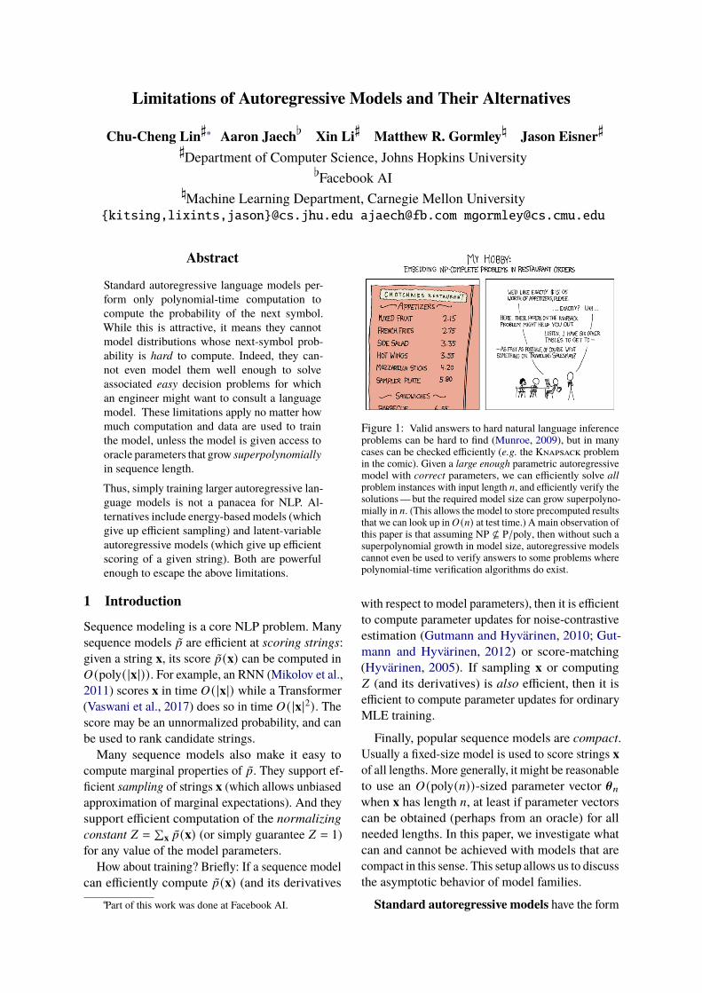
Figure 2: The space of unweighted languages. We assume in this diagram that NP * P/poly. Each rectangularoutline corresponds to a complexity class (named in its lower right corner) and encloses the languages whosedecision problems fall into that class. Each bold-italic label (colored to match its shape outline) names a modelfamily and encloses the languages that can be expressed as the support of some weighted language in that family.All induced partitions in the figure are non-empty sets: shape A properly encloses shape B if and only if languageclass A is a strict superset of language class B. As mentioned in Table 1, standard autoregressive models (ELNmodels) have support languages that form a strict subset of P (Lemmas 1 and 2, Theorem 5, and §2.4). ELNCPmodels (§3.1) extend ELN models by allowing the parameter size to grow polynomially in string length, allowingthem to capture both more languages inside P (Theorem 6) and languages outside P (including undecidable butsparse languages) that can be characterized autoregressively with the help of these compact parameters. All ofthose languages belong in the class P/poly. Theorem 2 establishes that energy-based (EC) and ECCP models gostrictly further than ELN and ELNCP models, respectively (Theorem 2): they correspond to the entire classes Pand P/poly (Lemma 1). However, even ECCP does not capture any NP-complete languages under our assumptionNP * P/poly. Allowing a polynomial number of latent symbols extends the power further still: lightly marginalizedELNCP or ECCP distributions cover exactly the languages ∈ NP/poly (Theorem 9). Finally, if we were to drop therequirement that the parameters � must be compact, we could store lookup tries to model any weighted language(§4.3).

A Proofs

Lemma 1. For any ! ∈ P, there exists an ECweighted language with support !. For any ! ∈P/poly, there exists an ECCP language with support!. But for any ! ∈ NP-complete, there exists noECCP language with support ! (assuming NP *P/poly).This simple lemma relates our classes EC and

ECCP of weighted languages to the complexityclasses P and P/poly of their supports, which areunweighted formal languages (§2). It holds becausecomputing a string’s weight can be made as easyas determining whether that weight is nonzero (ifwe set the weights in a simple way), but is certainlyno easier. We spell out the trivial proof to help thereader gain familiarity with the formalism.

Proof. Given !, define a weighted language ? withsupport ! by ?(x) = 1 if x ∈ ! and ?(x) = 0otherwise.If ! ∈ %, then clearly ? is EC since the return

value of 1 or 0 can be determined in polytime.If ! ∈ P/poly, ! can be described as a tuple(",�) following our characterization in §2.4. Itis easy to show that ? is ECCP, using the samepolynomially-sized advice strings �. We simplyconstruct " p such that " p()=) returns 1 or 0 oninput x according to whether " ()=) accepts orrejects x. Both " p()=) and " p()=) (x) are com-puted in time $ (poly(=)) if |x| = =. (The technicalconstruction is that " p simulates the operation of" on the input )= to obtain the description of theTuring machine "= = " ()=), and then outputs aslightly modified version of this description thatwill write 1 or 0 on an output tape.)

For the second half of the lemma, we use the re-verse construction. Suppose ? is an ECCP weightedlanguage with support !. ? can be characterized bya tuple (" p,�). It is easy to show that ! ∈ P/poly,using the same polynomially-sized advice strings�. We simply construct " such that " ()=) ac-cepts x iff " p()=) (x) > 0. Then by the assumption,! ∉ NP-complete. �

Lemma 2. An ELNCP model ? is also ECCP.Likewise, an ELN model is also EC.

Proof. Let ? be an ELNCP language. This impliesthat ? is normalizable, so let ?(x) , ?(x) / / asusual. Specifically, let "q efficiently locally nor-malize ? with compact parameters �q = {)q

= |= ∈ N}. It is simple to define a Turing machine

" r that maps each parameter string )q= to a Tur-

ing machine A=, where A= (x) simply computes(∏=C=1 @= (GC | x<C )

)· @= ($ | x). Then for all x

of length =, A= (x) =(∏=

C=1 ?(GC | x<C ))· ?($ | x),

by the definition of local normalization, and thusA= (x) = ?(x)." r can be constructed by incorporating the def-

inition of "q, so that A= = " r()q=) can include

@= = "q()q=) as a subroutine. This allows A= to

query @= for local conditional probabilities andmultiply them together.• Since "q runs in polytime, it is straightforwardfor this construction to ensure that " r runs inpolytime as well.

• Since @= (· | x) ∈ $ (poly(=)), this constructioncan ensure that A= runs in polytime as well.

• We were given that |)q= | ∈ $ (poly(=)) (compact

parameters).Since ? is the weighted language defined by(" r,�q), and " r and �q have the propertiesjust discussed, we see that ? is efficiently com-putablewith compact parameters (ECCP). Therefore?(x) = /?(x) is also ECCP.In the case where ? is more strongly known

to be ELN (the parameters �q are not needed),a simplification of this argument shows that it isEC. �

Theorem 1. Assuming NP * P/poly, there existsan efficiently computable normalizable weightedlanguage ? that is not ELNCP.

Proof. The proof was sketched in §3.2. Here we fillin the details.

The unweighted language ? defined in that sectionis efficiently computable via the following simplealgorithm that outputs ?(x) given x ∈ B∗. If x has aprefix that encodes a formula q, and the remainderof x is a satisfying assignment a to the variablesof q, then return ( 13 )

|x |+1. Otherwise return 0. Thisalgorithm can be made to run in polynomial timebecause whether an assignment satisfies a formulacan be determined in polynomial time (a fact that isstandardly used to establish that Sat ∈ NP).

Given a formula q with variables �1, . . . , � 9 , wedefine q′ = (¬�1 ∧ ¬�2 ∧ . . . ∧ ¬� 9 ∧ ¬� 9+1) ∨(�1 ∧ Shift(q)), where Shift(q) is a version ofq in which �8 has been renamed to �8+1 for all1 ≤ 8 ≤ 9 . It is obvious that q′ and ? have theproperties stated in the proof sketch. The strings in! that begin with 5′ are precisely the strings of theform 5′a′ where a′ is a satisfying assignment of

q′—which happen just when a′ = 0 9+1 or a′ = 1awhere a is a satisfying assignment of q. At leastone string in ! begins with 5′, namely 5′0 9+1,so / (5′) > 0. Moreover, / (5′1) > 0 iff q hasany satisfying assignments. Therefore the localprobability ?(1 | 5′) = / (5′1) / / (5′) is defined(see §2.1), and is > 0 iff Sat(q).

Notice that the formal problem used in the proofis a version of Sat whose inputs are encoded usingthe same prefix-free encoding function enc thatwas used by our definition of ! in §3.2. We mustchoose this encoding function to be concise in thesense that 5 , enc(q) can be converted to andfrom the conventional encoding of q in polynomialtime. This ensures that our version of Sat is ≤%<-interreducible with the conventional version andhence NP-complete. It also ensures that there isa polynomial function 5 such that |5′ | ≤ 5 ( |5|),as required by the proof sketch, since there is apolynomial-time function that maps 5 → q →q′ → 5′ and the output length of this function isbounded by its runtime. This is needed to show thatour version of Sat is in P/poly.Specifically, to show that the existence of("q,�q) implies Sat ∈ P/poly, we use it toconstruct an appropriate pair (",�) such that(" ()=)) (5) = Sat(q) if |5 | = =. As mentioned inthe proof sketch, we define � by )= = )

q5 (=) , and

observe that |)= | ∈ $ (poly(=)) (thanks to compact-ness of the parameters�q and the fact that 5 is poly-nomially bounded). Finally, define " ()=) to be aTuringmachine thatmaps its input5 of length = to 5′of length ≤ 5 (=), then calls "q()=) = "q()q

5 (=) )on 5′1 to obtain ?(1 | 5′), and returns true or falseaccording to whether ?(1 | 5′) > 0. Computing 5′

takes time polynomial in = (thanks to the propertiesof enc). Constructing "q() 5 (=) ) and calling it on5′ each take time polynomial in = (thanks to theproperties of 5 and "q). �

Remark on conditional models. While we fo-cus on modeling joint sequence probabilities inthis work, we note that in many applications it of-ten suffices to just model conditional probabilities(Sutskever et al., 2014). Unfortunately, our proof ofTheorem 1 above implies that ELNCPs do not makegood conditional models either: specifically, thereexists 5 such that deciding whether ?(1 | 5) > 0 isNP-hard, and thus beyond ELNCP’s capability.

Remark on irrationality. In our definitions ofECCP andELNCP languages,we implicitly assumed

that the Turing machines that return weights orprobabilities would write them in full on the outputtape, presumably as the ratio of two integers. Sucha Turing machine can only return rational numbers.

But then our formulation of Theorem 1 allows an-other proof. We could construct ? such that the localconditional probabilities ?(G | x) , / (xG)// (x)are sometimes irrational. In this case, they cannotbe output exactly by a Turing machine, implyingthat ? is not ELNCP. However, this proof exposesonly a trivial weakness of ELNCPs, namely the factthat they can only define distributions whose localmarginal probabilities are rational.We can correct this weakness by formulating

ELNCP languages slightly differently. A real numberis said to be computable if it can be output by aTuringmachine to any desired precision. That Turingmachine takes an extra input 1 which specifies thenumber of bits of precision of the output. Similarly,our definitions ofECCP andELNCP can bemodifiedso that their respective Turing machines ?= and @=take this form, are allowed to run in time$ (poly(=+1)), and have access to the respective parametervectors �p

=+1 and �q=+1. Since some of our results

concern the ability to distinguish zero from smallvalues (arbitrarily small in the case of Theorem 6),our modified definitions also require ?= and @= tooutput a bit indicating whether the output is exactlyzero. For simplicity, we suppressed these technicaldetails from our exposition.

Relatedly, in §4.3, we claimed that lookup modelscan fit any weighted language up to length =. Thisis not strictly true if the weights can be irrational.A more precise statement is that for any weightedlanguage ?, there is a lookup model that maps (x, 1)to the first 1 bits of ?(x). Indeed, this holds evenwhen ?(x) is uncomputable.

Remark on computability. In §2.1 we claimedthat any weighted language ? that has a finite andstrictly positive / can be normalized as ?(x) =? (x)// . However, / may be uncomputable: that is,there is no algorithm that takes number of bits ofprecision 1 as input, and outputs an approximationof / within 1 bits of precision. Therefore, evenif ? is computable, ? may have weights that arenot merely irrational but even uncomputable. Anexample appears in the proof of Theorem 6 below.Weighted language classes (e.g. ELNCP) that onlymodel normalized languages will not be able tomodel such languages, simply because the partitionfunction is uncomputable.

However, our proof of Theorem 1 does not relyon this issue, because the ? that it exhibits happensto have a computable / . For any 1, / may becomputed to 1 bits of precision as the explicit sum∑

x: |x | ≤# ?(x) for a certain large # that depends on1.

Remark on RNNs. Our proof of Theorem 1showed that our problematic language ? is efficientlycomputable (though not by any locally normalizedarchitecture with compact parameters). Becausethis paper is in part a response to popular neuralarchitectures, we now show that ? can in fact becomputed efficiently by a recurrent neural network(RNN) with compact parameters. Thus, this is anexample where a simple globally normalized RNNparameterization is fundamentally more efficient(in runtime or parameters) than any locally normal-ized parameterization of any architecture (RNN,Transformer, etc.).

Since we showed that ? is efficiently computable,the existence of an RNN implementation is es-tablished in some sense by the ability of finiterational-weighted RNNs to simulate Turing ma-chines (Siegelmann and Sontag, 1992), as well asan extension to Chen et al. (2018, Thm. 11) to afamily of RNNs, where each RNN instance alsotakes some formula encoding as input. However, it isstraightforward to give a concrete construction, foreach = ∈ N, for a simple RNN that maps each stringx ∈ B= to ?(x). Here ?(x) will be either ( 13 )

=+1 or0, according to whether x has the form 5a where5 encodes a 3-CNF-Sat formula q that is satisfiedby a.18 The basic idea is that 5 has 9 ≤ = variables,so there are only $ (=3) possible 3-CNF clauses.The RNN allocates one hidden unit to each of these.When reading 5a, each clause encountered in 5causes the corresponding hidden unit to turn on,and then each literal encountered in a turns off thehidden units for all clauses that would be satisfiedby that literal. If any hidden units remain on afterx has been fully read, then 5 was not satisfied bya, and the RNN’s final output unit should return 0.Otherwise it should return ( 13 )

=+1, which is constantfor this RNN. To obtain digital behaviors such asturning hidden units on and off, it is most conve-

18The restriction to 3-CNF-Sat formulas is convenient, butmakes this a slightly different definition of ! and ? than weused in the proofs above. Those proofs can be adjusted to showthat this ?, too, cannot be efficiently locally normalized withcompact parameters. The only change is that in the constructionof Theorem 1, q′ must be converted to 3-CNF. The proof thenobtains its contradiction by showing that 3-CNF-Sat ∈ P/poly(which suffices since 3-CNF-Sat is also NP-complete).

nient to use ramp activation functions for the hiddenunits and the final output unit, rather than sigmoidactivation functions. Note that our use of a separateRNN "RNN

= for each input length = is an exampleof using more hidden units for larger problems,a key idea that we introduced in §2.3 in order tolook at asymptotic behavior. The RNN’s parametersequence �RNN = {)RNN= | = ∈ N} is obviouslycompact, as )RNN= only has to store the input length=. With our alphabet B for ?, |)RNN= | ∈ $ (log =).Lemma 3. Let ?, @ be normalizable weightedlanguages with support( ?) ≠ support(@). Then∃x1, x2 ∈ +∗ such that ?(x1) < ?(x2) but@(x1) ≥ @(x2).

Proof. Suppose that the claim is false, i.e., ? and @have the same ranking of strings. Then theminimum-weight strings under ? must also be minimum-weight under @. WLOG, there exists x ∈ +∗ with?(x) = 0 and @(x) = 2 > 0. Then 2 > 0 isthe minimum weight of strings in @. But this isnot possible for a normalizable language @, since itmeans that /@ ,

∑x′∈+ ∗ @(x′) ≥

∑x′∈+ ∗ 2 diverges.

�

Theorem 3. Assuming NP * P/poly, there existsan efficiently computable normalizable weighted lan-guage ? such that no ELNCP @ with support(@) ⊇support( ?) has ?(x1) < ?(x2) ⇒ @(x1) < @(x2)for all x1, x2 ∈ +∗. Indeed, any such @ has a coun-terexample where ?(x1) = 0. Moreover, there isa polynomial 5@ : N → N such that a counterex-ample exists for every x1 such that ?(x1) = 0 and@(x1) > 0, where the x2 in this counterexamplealways satisfies |x2 | ≤ 5@ ( |x1 |).

Proof. Let ? be the weighted language from The-orem 2. Given an ELNCP @. By Theorem 2,support(@) ≠ support( ?), so there must exist astring x1 that is in one support language butnot the other. With the additional assumptionthat support(@) ⊇ support( ?), it must be thatx1 ∈ support(@), so ?(x1) = 0 but @(x1) > 0.

Given any such x1 with ?(x1) = 0 but @(x1) > 0,we must find a x2 of length $ (poly( |x1 |)) with?(x2) > 0 but @(x2) ≤ @(x1).To ensure that ?(x2) > 0, let us use the structure

of ?. For any 9 , we can construct a tautologicalformula q over variables �1, . . . � 9 , as q = (�1 ∨¬�1) ∧ · · · ∧ (� 9 ∨¬� 9). It follows that ?(5a) > 0for any a ∈ B 9 . We will take x2 = 5a for a particularchoice of 9 and a.

Specifically, we choose them to ensure that@(x2) ≤ @(x1). Since @ is ELNCP, it is normalizableand hence has a finite / . Thus, ∑a∈B 9 @(5a) ≤ / .So there must exist some a ∈ B 9 such that@(5a) ≤ //2 9 . We choose that a, after choosing9 large enough such that //2 9 ≤ @(x1). Then@(x2) = @(5a) ≤ //2 9 ≤ @(x1).

To achieve the last claim of the theorem, we mustalso ensure that |x2 | ∈ $ (poly( |x1 |)). Observe that@(x1) can be computed in polytime (with accessto compact parameters), by Lemma 2. But thismeans that the representation of @(x1) > 0 asa rational number must have ≤ 6( |x1 |) bits forsome polynomial 6. Then @(x1) ≥ 2−6 ( |x1 |)) , and itsuffices to choose 9 = d6( |x1 |) + log2 /e to ensurethat //2 9 ≤ 2−6 |x1 | ≤ @(x1) as required above.

But then 9 ∈ $ (poly( |x1 |)). Also, recall that theencoding function enc used in the construction of ?is guaranteed to have only polynomial blowup (seethe proof of Theorem 2). Thus, |x2 | = |5 | + |a| =|enc(q) | + 9 ∈ $ (poly( 9)) ⊆ $ (poly( |x1 |)) asrequired by the theorem. �

Lemma A.1. The first part of Theorem 4 (withoutthe modifications (a) and (b)).

We first prove the first part of Theorem 4 (whichis restated in full below). In this case we will use adistribution ? that does not have support +∗ (so itdoes not prove modification (b)).

Proof. We take ? to be the weighted language thatwas defined in §3.2, which was already shown tobe efficiently computable. Suppose ("q,�q, _) isa counterexample to Lemma A.1. Choose integer: ≥ 1 in a manner (dependent only on _) to bedescribed at the end of the proof.Suppose we would like to answer Sat where

q is a formula with variables �1, . . . , � 9 . Defineq′ = (¬�1∧¬�2∧ . . .∧¬� 9 ∧¬� 9+1∧¬� 9+:) ∨(�1 ∧ Shift(q)). Note that q′ augments q with: additional variables, namely �1 and � 9+2,..., 9+: .For : = 1, this is the same construction as in theproof of Theorem 1. Let = = |5′ | and note that = ispolynomial in the size of q (holding : constant).

The strings in ! = support( ?) that begin with 5′are precisely the strings of the form 5′a′ where a′is a satisfying assignment of q′. This is achievedprecisely when a′ = 0 9+: or a′ = 1a®1 where a is asatisfying assignment of q and ®1 ∈ B:−1.

By our definition of ?, all strings in ! that beginwith 5′ have equal weight under ?. Call this weight

F.19 Clearly / (5′0) = F, and / (5′1) = F · 2:−1 ·(number of satisfying assignments of q).Recall that ?(0 | 5′) = / (5′0)/(/ (5′0) +

/ (5′1)). Let us abbreviate this quantity by ?. Itfollows from the previous paragraph that if q isunsatisfiable, then ? = 1, but if q is satisfiable, then? ≤ 1/(1+2:−1). By hypothesis, ? is approximated(with error probability < 1/3) by the possibly randomquantity ("q()q

|5′ |)) (5′0), which we abbreviate by

@, to within a factor of _. That is, ? ∈ [@/_, _@].By choosing : large enough20 such that [@/_, _@]cannot contain both 1 and 1/(1+2:−1), we can use @to determine whether ? = 1 or ? ≤ 1/(1+2:−1). Thisallows us to determine Sat(q) in polynomial timewith error probability < 1/3, since by hypothesis @ iscomputable in polynomial time with compact param-eters. This shows that Sat ∈ BPP/poly = P/poly,implying NP ⊆ P/poly, contrary to our assumption.(BPP/poly is similar to P/poly but allows "q to bea bounded-error probabilistic Turing machine.) �

Theorem 4. Assuming NP * P/poly, there existsan efficiently computable weighted language ? :+∗ → R≥0 such that there is no ("q,�q) where�q = {)q

= | = ∈ N} that satisfies all of the followingproperties (similar to §3.1):• the parameter size |)q

= | grows only as$ (poly(=))• "q()q

=) returns a probabilistic Turing machine@= in time $ (poly(=))

• there exists _ ≥ 1 such that for each G ∈ + ∪ {$}and x ∈ +∗ with |x| ≤ = and ?(G | x) > 0, theprobabilistic computation @= (xG) has probability> 2/3 of approximating ?(G | x) to within a factorof _ (that is, @= (xG)/?(G | x) ∈ [1/_, _])

• @= runs on those inputs xG in time $ (poly(=))Moreover, the statement above remains true(a) when the approximation guarantee is

only required to hold for prefixes x where{x : x � x} is finite (so ?(G | x) is computableby brute force)

(b) or, when support( ?) = +∗

Proof. It remains to show that the statement remainstrue with modification (a) and with modification(b). For (a), the proof of Lemma A.1 suffices, sinceit reduces Sat to approximate local probabilityqueries of the stated form. That is, the true localprobabilities ?(G | x) that can be computed with

19Specifically, each such string has length = + 9 + : , so ?gives it a weight of F = ( 13 )

=+ 9+:+1.20It suffices to ensure that 1 + 2:−1 > _2, so take any

: > 1 + log2 (_2 − 1).

finite summations, thanks to the structure of ourexample language ?, which guarantees that theprefix x can only continue with suffixes of a fixedlength that is easily determined from x.For modification (b), again let + = B = {0, 1}.

Choose some n > 0 (any choice will do), and let

?1(x) =

( 13 )|x+1 | if x = 5a where 5 = enc(q)

and a satisfies q0 otherwise

?2(x) = ( 19 )|x+1 | > 0

?(x) = ?1(x) + n · ?2(x)

We use /1, /2, and / respectively to denote nor-malizing constants of these three weighted lan-guages. Note that ?1 is the weighted language thatwas previously used in the proofs of Theorem 1and Lemma A.1. Our new ? is intended to be verysimilar while satisfying the additional condition (b).It is easy to show that ? is efficiently computable,much as we showed for ?1 in Theorem 1. Also,? is normalizable, since / = /1 + n · /2, where/1 ≤ ( 13 )/(1 −

23 ) = 1 and /2 = ( 19 )/(1 −

29 ) =

17

are both finite.The proof proceeds as in Lemma A.1, with q′

constructed from q as before. Recall that q has 9variables, q′ has 9 + : variables, and |5′ | = =. Wemay assume WLOG that the encoding functionenc is such that an encoded formula always has atleast as many bits as the number of variables in theformula, so = ≥ 9 + : .Notice that /1(5′) sums over the satisfying as-

signments of q′, and there may be as few as oneof these (if q is unsatisfiable). By contrast, /2(5′)sums over an infinite number of continuations withpositive probability. The faster decay rate of 1

9 in ?2was chosen to keep /2(5′) small relative to /1(5′)despite this. Specifically,

/1(5′0) = ( 13 )=+ 9+:+1

/1(5′1) = ( 13 )=+ 9+:+1 · 2:−1

· (# of satisfying assignments of q)/2(5′0) = ( 19 )

= · 19 · (

19/(1 −

29 ))

= 17 · (

13 )

2(=+1)

< 17 · /1(5′0)

(because 2(= + 1) > = + 9 + : + 1)/2(5′1) = /2(5′0)

As in the proof of Lemma A.1, we will show that?(0 | 5′) is much larger when q is unsatisfiable.

Recall that / (x) = /1(x) + n · /2(x). When q haszero satisfying assignments,

?(0 | 5′) = / (5′0)/ (5′0) + / (5′1)

=/ (5′0)

/1(5′0) + n · /2(5′0) + n · /2(5′1)

>/ (5′0)

/1(5′0) + 2 · n7 · /1(5′0)

whereas if q has at least one satisfying assignment,then

?(0 | 5′) = / (5′0)/ (5′0) + / (5′1)

</ (5′0)

/1(5′0) + /1(5′1)

≤ / (5′0)/1(5′0) + 2:−1/1(5′0)

This rewrites both probabilities in terms of / · (5′0)quantities, which do not depend on the number ofsatisfying assignments. So now we can see that thefirst probability is at least (1 + 2:−1) / (1 + 2n

7 )times as large as the second probability. Choose :large enough21 such that [@/_, _@] cannot containboth probabilities, and complete the proof as inLemma A.1. �

Theorem 5. The set { ? : ? is normalizable, ? ∈EC, ? ∉ ELN} is not empty.

Theorem 5 states that some normalizable EC dis-tributions cannot be expressed as ELN distributions.The proof is based on the undecidability of the halt-ing problem, rather than the assumed inefficiencyof the Boolean satisfiability problem. Thus, unlikeTheorem 1, it does not rely on the assumption thatNP * P/poly, or even on the weaker assumptionthat P ≠ NP.

Proof. Given any unweighted language ! ⊆ B∗, wecan define a normalizable weighted language ? withsupport ! by ?(x) = 1/3 |x |+1 for x ∈ ! and ?(x) = 0otherwise. Moreover, if ! ∈ P, then ? ∈ EC.For our purposes, we take ! to consist of all

strings of the form x(1)x(2) , for which there ex-ists a deterministic Turing machine " such thatx(1) = enc(") (where enc is a prefix-free encodingfunction) and x(2) encodes an accepting executionpath of " on an empty input. (Such a path may berepresented as a sequence of transitions of " that

21It suffices to ensure that (1 + 2:−1)/(1 + 2n7 ) > _

2, sotake any : > 1 + log2 (_2 · (1 + 2n

7 ) − 1).

begins with an initial state and ends at an acceptingstate.) Note that any deterministic TM x(1) can bepaired with at most one accepting execution pathx(2) , and cannot be paired with any x(2) if it doesnot halt.Clearly ! ∈ P: given x ∈ B∗, we can decide

whether x ∈ ! by first checking if x can be expressedas a concatenation of strings x(1) and x(2) of therequired form. Then we build " from x(1) andsimulate it to check the transitions in x(2) on "step-by-step. This can be done in$ (poly( |x|)) totaltime. We conclude that the ? derived from ! is EC.Now, / (x(1) ) > 0 iff " halts on the empty

input. But this undecidable problem could be de-cided if there were an ELN weighted languagethat had support !, since then / (x(1) ) / / could befound as a product of local conditional probabilities,∏ |x(1) |C=1 ?(G (1)C | x

(1)<C ), that could each be computed

by a Turing machine. Therefore ? is not ELN. �

We have shown above that a certain unweightedlanguage ! is not the support of any ELN distribu-tion. We conjecture that it is also not the support ofany ELNCP distribution;22 a proof of this wouldstrengthen Theorem 5 to become an unconditionalversion of Theorem 1. However, ELNCP weightedlanguages do have more power than ELN weightedlanguages, as we now show.

Theorem 6. The set { ? : ? is normalizable, ? ∈EC, ? ∈ ELNCP, ? ∉ ELN} is not empty.

Theorem 6 justifies why this region is drawnas non-empty in Figure 2. Again, it does not relyon the assumption NP * P/poly or P ≠ NP. Notethat Theorem 5 can be regarded as a corollary ofTheorem 6.

Proof. The weighted language ? constructed inTheorem 5 is not necessarily ELNCP. To fix this,we modify the construction to obtain a weightedlanguage ?′ with sparse support ! ′. We will againbe able to show that ?′ is EC and not ELN. Toshow that ?′ is also ELNCP, we will rely on thesparsity of ! ′, meaning that prefixes(! ′) , {x′ :(∃x′ ∈ ! ′) x′ � x′} contains at most $ (poly(=))strings x′ of length ≤ = + 1. Thus, we can use�q= to store all of those strings x′ in polynomial

22We have not attempted to prove this. Our loose intuition isthat the compact parameters of an ELNCP language may helpit to memorize some small part of !, but the halting problemwould still be undecidable when restricted to the rest of !(Myasnikov and Rybalov, 2008).

space, along with their / (x′) values.23 Notice thatall strings x′ ∉ prefixes(! ′) have / (x′) = 0, so theyneed not be stored. Now for any x′ of length ≤ =,a Turing machine that consults )

q= can compute

@(G | x′) = / ?′ (x′G) / / ?′ (x′) in time $ (poly(=))as desired, establishing that ?′ is ELNCP.We may define ?′ as follows. Let sparsify(x)

be a version of x with many extra 0 symbols in-serted: specifically, it inserts 2C copies of 0 imme-diately before the Cth bit of x, for all 1 ≤ C ≤ |x|.We construct ?′ so that ?′(sparsify(x)) = ?(x).Specifically, let ! ′ , sparsify(!). The inverse func-tion sparsify−1(x′) is defined on exactly x′ ∈ ! ′,and is unique when defined. For all x′ ∈ B∗, let?′(x′) , ?(sparsify−1(x′)) if sparsify−1(x′) is de-fined, and ?′(x′) , 0 otherwise. This can be com-puted in polytime, so ?′ is EC. Also, its support ! ′is sparse as claimed, so ?′ is ELNCP.Finally, we claim ?′ is not ELN. A given deter-

ministic Turing machine " halts on the empty inputiff enc(") ∈ prefixes(!) iff sparsify(enc(")) ∈prefixes(! ′) iff / ′(sparsify(enc("))) > 0. Butas in the proof of Theorem 5, this would be de-cidable if ?′ were ELN as defined in §3.1, sincethen we would have a Turing machine to computethe local conditional probabilities ?′(GC | x<C ) forx = sparsify(enc(")). �

Theorem 8. There exists a light marginalization ?of an ELN distribution, such that support(?) is anNP-complete language.

Proof. We will construct ? such that support(?)is the NP-complete language Sat of all satisfiableboolean formulas. The idea is to construct an ELNdistribution A that can autoregressively generateany assignment a followed by any formula q that issatisfied by a. Thus, if we delete the a prefixes, thesupport consists of exactly the satisfiable formulasq (or more precisely, their encodings 5).To be more precise, we will have support(A)

be the language ! = {a#5 | a ∈B∗ and q is a formula satisfied by a}. This is de-fined similarly to the support language ! in §3.2, butwith the order of 5 and a crucially swapped: A willnow generate the “solution” a before the “problem”5. The alphabet + of this language contains at leastthe symbols {0, 1, #}, where # is a separator symbol,and any other symbols needed to encode q as 5.The marginalization operator ` maps a#5 to 5.

23More precisely, the first 1 bits of / (x′) ≤ 1 may be storedin �q

=+1 , when ELNCP is defined as explained in our “Remarkon irrationality” above.

Let 9 = |a|. As in §3.2, we will require q touse all of the variables �1, . . . , � 9 (and only thosevariables), implying that |5 | ≥ 9 . This ensuresthat marginalizing over the 9 + 1 latent symbolsis only light marginalization since 9 + 1 + |5 | ∈$ (poly( |5 |)). For convenience, we will also requireq to be a CNF formula. These requirements shrinksupport(?) but do not affect its NP-completeness.

The remaining challenge is to construct an autore-gressive distribution A whose support is !. We canthink of this distribution as describing an efficientprocedure for randomly generating a string from leftto right so that the procedure generates the Cth sym-bol in time $ (poly(C)), terminates with probability1,24 has positive probability of producing any stringin !, and has zero probability of producing anystring not in !. Below we give such a procedure.251. First, the procedure generates a# as a sequence

of random symbols from {0, 1, #}, making auniform draw at each step. It stops immediatelyafter generating # for the first time. The stringgenerated before # is called a andwe let 9 = |a|.For example, a = 010 and 9 = 3.

2. Second, the procedure must generate the en-coding 5 of a random CNF formula q thatis satisfied by a, such as (�2 ∨ ¬�3 ∨ ¬�2 ∨�2) ∧ (¬�1) in our example. This involvesgenerating a random sequence of 0 or moresatisfied clauses connected by ∧. At each step,the procedure decides whether to generate anew clause or end the formula. The probabilityof generating a new clause is ordinarily 1/2.However, this probability is 1 if the previousclauses do not yet mention all the variables�1, . . . , � 9 .How does it generate each satisfied clause?This involves generating a sequence of literalsconnected by ∨, at least one of which mustbe true. At each step of this subroutine, ituniformly chooses an integer 8 ∈ [1, 9], andthen flips a fair coin to decide whether to addthe literal �8 or ¬�8 to the current clause. Ifthe clause is now satisfied by a (i.e., at leastone of the literals is true), it then flips another

24Phase 1 almost surely terminates after a finite number ofbits. Phase 2 almost surely terminates after a finite number ofclauses, and each clause almost surely terminates after a finitenumber of literals. “Almost surely” means “with probability 1.”

25Our presentation here makes use of an infinite alphabetthat includes symbols such as �8 and ¬�8 for all 8 ∈ N>0, aswell as symbols such as 0, 1,∧,∨. We implicitly invoke someprefix-free encoding scheme to translate each symbol into afixed string over the finite alphabet + .

fair coin to decide whether to end the clause.A is ELN because there exists a Turing ma-

chine that computes from input xG—in time$ (poly( |x|))—the probability that the next symbolgenerated after the prefix x would be G, under theabove procedure. As discussed in footnote 7, thatprobability equals A (G | x)—which is what ourTuring machine is required to return—becausethe above procedure almost surely terminates (foot-note 24), ensuring that A is a consistent probabilitydistribution over +∗ (that is, ∑x∈+ ∗ A (x) = 1). �

Theorem 9. The following statements are equiva-lent for any nonempty ! ⊆ +∗:(a) ! ∈ NP/poly.(b) ! is the support of a light marginalization of

an ELNCP distribution.(c) ! is the support of a light marginalization of

an ECCP weighted language.

Proof. (b) implies (c) since any ELNCP distributionis an ECCP weighted language (Lemma 2). (c)implies (a) by LemmaA.2 below. Finally, (a) implies(b) by Lemma A.3 below. �

LemmaA.2. For any ECCPweighted language A , if? is a light marginalization of A , then support( ?) ∈NP/poly.Notice that this lemma concerns the class

NP/poly,notP/poly (see §2.4). The proof is straight-forward.

Proof. Suppose A is ECCP via (" r, ) r), and `is the marginalization operator such that ?(x) =∑

z:` (z)=x A (z). By the light marginalization as-sumption, there is a polynomial 5 such that |z| ≤5 ( |`(z) |).To prove support( ?) ∈ NP/poly, we must show

that there exists (",�) such that for all = ≥ 0,a nondeterministic Turing machine "= can beconstructed as " ()=) in time $ (poly(=)), whichcan in turn decide in time $ (poly(=)) whether?(x) > 0 for any x with |x| = =.Deciding ?(x) > 0 means deciding whether(∃z ∈ +∗) `(z) = x and A (z) > 0. But if|x| = =, the first condition `(z) = x implies|z| ≤ 5 ( |`(z) |) = 5 ( |x|) = 5 (=). Thus, we need"= to nondeterministically check only the z oflength up to 5 (=) to see whether `(z) = x andA (z) > 0.How can "= check a string z of length <? It

can decide the first condition `(z) = x in time$ (poly(<)), since the marginalization operator ` is

a polytime function. To decide the second conditionA (z) > 0, itmust construct the (deterministic) Turingmachine" r() r

<) and then apply it to z to obtain A (z):since A is ECCP, both steps take time$ (poly(<)) =$ (poly( 5 (=))) ⊆ $ (poly(=)) as required.

However, this means that"= = " ()=) must haveaccess to the parameter vectors ) r

< for all< ≤ 5 (=).We therefore make )= include this collection ofparameter vectors. Each |) r

< | ∈ $ (poly(<)) ⊆$ (poly(=)) since A is ECCP. So |)= | ∈ $ (poly(=))as required. �

Lemma A.3. For any ! ∈ NP/poly, there exists alight marginalization ? of an ELNCP distribution,such that support(?) = !.Lemma A.3 resembles Theorem 8, but it con-

structs distributions for all ! ∈ NP/poly, not justfor one particular ! ∈ NPC. The proof is similarbut more complicated. In both cases, the goal isto demonstrate how an ELNCP distribution A candefine a left-to-right stochastic string generationprocess such that the suffix of the generated stringmust be in ! and can be any element of !.Our string generation process in this case is

inspired by rejection sampling,awidely usedmethodfor sampling from an energy-based model withsupport !. The standard scheme is to first samplea string x from a tractable distribution @ suchthat support(@) ⊇ !, then accept the sample withan appropriate probability, which is 0 if x ∉ !.The process is repeated until a sample is finallyaccepted. There is no guarantee that this standardscheme will terminate in polynomial time, however.Fortunately, in our setting, we are not trying tomatch our sampling distribution ? to a given energy-based model, but simply match its support to agiven language !. We make use of the polysizeparameter vectors of ELNCP languages to storecertain ‘fallback strings’ that are guaranteed tobe in the desired language !. Wherever ordinaryrejection sampling would reject a string and trygenerating another, we switch to generating a storedfallback string of an appropriate length. This schemeplaces all of the rejected probability mass on thesmall set of fallback strings (in contrast to rejectionsampling, which in effect throws away this massand renormalizes). The advantage is that it does notiterate indefinitely. At a high level, A is a distributionover strings z that record traces of this generativestory we describe above.

Proof. WLOG we assume ! uses the alphabet

+ = {0, 1, #}. In the case where ! is finite, theresult is trivial. We simply define A (x) = 1/|! | forx ∈ ! and A (x) = 0 otherwise. We then take ? = A

(a trivial marginalization). It is easy to show thatA is ELN, and therefore ELNCP as desired, byconstructing an appropriate Turing machine thatmaps xG to A (G | x) in time $ ( |xG |), for any x thatis a prefix of some string in ! and any G ∈ + ∪ {$}.The finite state table of the Turing machine includesstates that correspond to all possible strings xG, withtransitions arranged in a trie. It reads the input stringxG from left to right to reach the state correspondingto xG. If it detects the end of the input while in thatstate, it writes A (G | x) on the output tape.Now we consider the case where ! is infinite.

For each 9 ∈ N≥0, let the ‘fallback string’ x( 9) besome string in ! of length ≥ 9 . For definiteness, letus take it to be the shortest such string, breakingties lexicographically. At least one such string doesexist because ! is infinite, so x( 9) is well-defined.Also, since ! ∈ NP/poly (§2.4), let (",�) be

an ordered pair and 5 be a polynomial such that" 9 = " (\ 9) nondeterministically accepts a within≤ 5 ( 9) steps iff a ∈ !.As in the proof of Theorem 8, we now describe

a procedure for randomly generating a string zfrom left to right. z will have the form a#b#2d,where d ∈ ! and the latent substring a#b#2 will beremoved by the marginalization operator `.1. First we generate a random string a ∈ B∗

followed by #, just as in the proof of Theorem 8.Again let 9 = |a|.

2. Next, we must consider whether a ∈ !. Wegenerate a random computation path b of " 9

on input a until it either accepts (in which casewe then generate #1 to record acceptance ofa) or has run for 5 ( 9) steps without accepting(in which case we then generate #0 to recordrejection).

3. In the former case (2 = 1) we finish by deter-ministically generating d , a ∈ !. In the lattercase (2 = 0), a ∉ !, so we fall back and finishby deterministically generating d , x( 9) ∈ !.

Let A (z) be the probability that the above pro-cedure generates z. support(A) is then the set ofstrings that can be generated by the above procedure.The marginalized language `(support(A)) keepsjust the d parts of those strings. It consists of allstrings a that are accepted by at least one path b of" |a | (which are exactly the strings in !) togetherwith the fallback strings (which form a subset of !).

Thus, `(support(A)) = ! as desired.

We wish to show that A is ELNCP. In otherwords, some Turing machine "q efficiently locallynormalizes A with compact parameters �q, as de-fined in §3.1. The parameters will be used to storeinformation about the infinite set of fallback strings.

In particular, for each =, )q= must have enough

information to construct a Turing machine @= =

"q()q=) such that @= (zI) returns A (I | z) for all

I ∈ + ∪ {$} and all z with |z| ≤ = and / (z) > 0.Here / (z) > 0 means that z is a prefix of a stringz = a#b#2d that could be generated by the aboveprocedure. The computation @= (zI) proceeds bysimulating the sequence of choices in the above pro-cedure that would be required to generate z, and thenreturning the probability that the procedure wouldgenerate symbol I next. That probability equalsA (I | z) as desired because the above procedurealmost surely terminates (as explained at the end ofthe proof of Theorem 8).

In general, the computation @= (zI) may have toconstruct " 9 = " (\ 9) and simulate it on a (for 9 =|a|) if I falls in the b#2 portion of z, and it may haveto look up a character of the fallback string x( 9)$ if Ifalls in the d portion of z or terminates that portionwith I = $. Fortunately 9 < =, and fortunately ifthe computation looks up the Cth character of x( 9)$then C < =. Thus, constructing and simulating " 9

can be done in time $ (poly( 9)) ⊆ $ (poly(=)),and looking up the Cth character of x( 9)$ can beachieved with access to the first = characters ofeach of x(1) , . . . , x(=) , which can be stored by )q

= inspace $ (=2). It follows that "q can construct andapply @= in polynomial time with access to compactparameters �q, so A is ELNCP.

�

B Implementation details of REBMs

B.1 Modeling finite subsets of infinitelanguages

The experiments of this paper are conducted ondatasets where we only observe strings that arefinitely long. Given a possibly infinite language !,we use the notation !≤) = {x | x ∈ !, |x| ≤ )}for the subset of strings that are most ) symbolslong. Specific values of ) for datasets used in ourexperiments are listed in Appendix D.1.

B.2 Design of base models ?0

?0 can be any distribution over !≤) 26 provided thatwe can sample from it, and evaluate ?0(x),∀x ∈!≤) , both in $ (poly( |x|)). In this work, we experi-mentwith two designs of ?0: GRU- andTransformer-based locally normalized language models. GRU-based models are used in WikiText and Yelp ex-periments. The GRU-based ?0’s are parametrizedwith 2-layer GRUs with 500 hidden units, and wordembeddings of dimension size 500.As for Transformer-based ?0’s, we make use

of Grover models (Zellers et al., 2019), which ef-fectively are GPT-2 models trained on the afore-mentioned RealNews dataset. In this work, weexperiment with the ‘base’ variant of public avail-able weights, which are 12-layered Transformers,with 12 heads, and 768 hidden units.

B.3 Design of discriminators 6)We formulate 6) (x) as a summation of scores atpositions 1 . . . |x|, passed through an activationfunction 5 :

6) (x) = 5

(|x |∑8=1

6C (x; ))). (1)

To verify whether lower-bounding 6) would helpwith learning, as we discuss in §4.1, we experimentwith two variants of 5 :

• tanh: 5 (G) = 2 · tanh(G)• softplus: 5 (G) = − log(1 + exp(G + B))

The former one is bounded between (−2, 2), whilethe second one has range (−∞, 0). The offset term B

in the softplus activation function determines initialvalues of /) . In this paper we set B = 20.

The design of 6C (x; )) follows their base modelcounterparts: we use Bi-GRU discriminators forGRU base models; and bi-directional Transformerdiscriminators for Transformer ones. For GRUs6C (x; )) = hC ·GC , For Transformers 6C (x; )) = ∑ hCwhere hC are the hidden states at time step C. In bothcases, the discriminators have access to informationof the whole sequence x at any timestep: the Bi-GRU discriminators achieve this through the bi-directional RNNs, and the Transformers through theattention mechanism without directional masking.

B.4 Training procedureAs we note in §4.1, MLE-based training methodsare generally not feasible for globally normalized

26Note that since ?0 does not have support over !, it has toassign ?($ | x1...) ) = 1, which is generally not an issue.

models. We therefore opt to train our model usingthe ranking variant of noise contrastive estimation(NCE) (Ma and Collins, 2018), which does notrequire samples from ?0 and has a simple formfor residual LMs. Using ?0 as a noise distribution,NCE training requires minimizing the followingsingle-sequence loss, in expectation over the truedistribution ?:

Lnce() , x, ?0, ) = − log?)?0(x)∑

:=0?)?0(x(:) )

, (2)

where x(0) , x, ?)?0(x) , ?) (x)

?0 (x) , and x(1) . . . x( ) ∼?0. Since ?) (x) = ?0(x) · exp 6) (x), we have?)?0(x) = exp 6) (x). The NCE minimization ob-

jective (2) now reduces to the simple form

Lnce() , x, ?0, )= −6) (x)

+ log(exp 6) (x) + ∑:=1

exp 6) (x(:) )). (3)

Notice that minimizing the expected loss withstochastic gradient descent methods Lnce definedin equation (3) requires only evaluating sequenceprobabilities under 6) , and tuning its parameters,but not the base model ?0. We only need to generatethe noise samples {x(:) ∼ @ | : ∈ [ ]} from ?0.This way we do not need to backpropagate throughparameters of the base model ?0, which can speedup training considerably when ?0 is backed bya huge network. In fact, the training of 6) can becompletely agnostic to the design of ?0, allowing forthe application of finetuning any locally normalized?0.Given the same discriminator 6) , the difference

of KL-divergence between the true model ? andresidual languagemodels ?′) (x) = ?

′0(x) ·exp 6) (x),

and the KL-divergence between the true modeland ?′′) (x) = ?

′′0 (x) · exp 6) (x), defined with base

models ?′0 and ?′′0 respectively, can be written as

KL[? | |?′)] − KL[? | |?′′) ]

= KL[? | |?′0] − KL[? | |?′′0 ] + log/ ′

/ ′′,

(4)

where / ′ = Ex∼?′0 [exp 6) (x)], and / ′′ is similarlydefined with ?′′0 . As a direct result of equation (4),we can see that finding ?′′0 where KL[? | |?′′0 ] <KL[? | |?′0] implies improvement inKL[? | |?′′) ] overKL[? | |?′)], under mild conditions:

Theorem B.1. If ∃: > 0 such thatEx∼?′0

[exp 6) (x) ]Ex∼?′′0

[exp 6) (x) ] > exp(−:) and KL[? | |?′0] −KL[? | |?′′0 ] > : then KL[? | |?′)] > KL[? | |?′′) ].

Proof.

KL[? | |?′)] − KL[? | |?′′) ]= E

x∼?[log ?′′) (x) − log ?′) (x)]

= Ex∼?[log

?′′0 (x) exp 6) (x)∑x′∈!≤) ?

′′0 (x) exp 6) (x)

− log?′0(x) exp 6) (x)∑

x′∈!≤) ?′0(x) exp 6) (x)

]

= Ex∼?[log

?′′0 (x) exp 6) (x)Ex′∼?′′0 [exp 6) (x)]

− log?′0(x) exp 6) (x)Ex′∼?′0 [exp 6) (x)]

]

= Ex∼?[log ?′′0 (x) − log ?′0(x)]

+ Ex∼?[log E

x′∼?′0[exp 6) (x)] − log E

x′∼?′′0[exp 6) (x)]]

= KL[? | |?′0] − KL[? | |?′′0 ]

+ logEx′∼?′0 [exp 6) (x)]Ex′∼?′′0 [exp 6) (x)]

. (5)

Plugging assumptionsEx∼?′0

[exp 6) (x) ]Ex∼?′′0

[exp 6) (x) ] > exp(−:)and KL[? | |?′0] −KL[? | |?′′0 ] > : into equation (5),KL[? | |?′)] − KL[? | |?′′) ] > 0. �

Theorem B.1 suggests a training strategy thatwe first train the base model ?0, then finetune 6) :under a roughly uniform 6) (e.g. when ) is newlyinitialized), Ex∼?′0

[exp 6) ]/Ex∼?′′0[exp 6) ] ≈ exp(0); so

improvements on the inclusive KL-divergence ofbase model KL[? | |?0] will mostly translate toimprovement in KL[? | | ?)]. Optimizing the basemodel (i.e. finding ?′′0 such that KL[? | |?′′0 ] <KL[? | |?′′0 ]) is much easier than directly minimizingKL[? | |?′)]: the former can be done by minimizingempirical cross entropy, which is computationallyefficient, while the latter involves an intractablepartition function ∑

x∈!≤) ?′) (x).

Pseudocode for fine-tuning 6) is listed in Algo-rithm 1.

B.5 Computing normalized probabilitiesThe unnormalized probability ?) (x) (in equa-tion (1)) can be evaluated easily, and should sufficefor (re)ranking purposes (e.g. for ASR and MTapplications). However, the normalized probability

Algorithm 1: Pseudocode for training 6)Input:

• Training/validation corpora D{train,dev}• base model ?0 : !≤) → [0, 1]• initial parameter vector )0 ∈ B3• noise sample size ∈ N

Output: unnormalized residual languagemodel @) : !≤) → [0, 1]

) ← )0 ;/* Lnce is defined inequation (3) */

while ∑x∈Ddev Lnce() , x, ?0, ) is still

decreasing doforeach x ∈ shuffle(Dtrain) do∇)Lnce = ∇)Lnce() , x, ?0, );) ← update-gradient() ,∇)Lnce);

endendreturn x ↦→ ?0(x) + exp 6) (x);

@) (x) , ?) (x)∑x ?) (x) does require computing the parti-

tion function /) . An unbiased importance samplingestimate of ∑x∈!≤) ?) (x) is

/) =∑

x∈!≤)?) (x)

=∑

x∈!≤)?0(x) exp 6) (x)

= Ex∼?0[exp 6) (x)]

≈"∑<=1

exp 6) (x(<) )"

= /)" , (6)

where x(1) . . . x(" ) ∼ @0.

C Comparison between REBMs andautoregressive models

We evaluate the effectiveness of REBMs on two dif-ferent neural architectures (GRU- and Transformer-based) and 3 datasets: WikiText (Merity et al., 2017),Yelp (Yelp), and RealNews (Zellers et al., 2019),on the task of modeling sequence probabilities. AnREBM ?) has two components, 6) and ?0, and wewould like to see how ?) competes against ?0 itself.We do not further tune ?0 while training ?) . Asa fair comparison, we also see how ?′0 comparesagainst ?0, where ?′0 is simply a version of ?0 thathas been trained as many additional epochs as wereused to train ?) .?0 models are pretrained on moderately large

corpora (in GRU cases) or a very large corpus

(in the Transformer case).27 We compare residualenergy-based models ?) to further-fine-tuned basemodels ?′0, on conservatively estimated (at the lowend of 95% confidence interval) token perplexityand bootstrap-sampled log likelihood improvements.The results are in Table 2. Residual energy-basedmodels show consistent perplexity improvementcompared to ?′0 that are trained on the same datausing the same maximum numbers of iterations. Al-though the improvement in log-likelihood of ?) over?0 is modest (especially for RealNews experiments,where ?0 is a very strong baseline), we verify thatthese improvements are all statistically significant(? < 0.05) using bootstrapped test datasets.

We experiment with different designs of thediscriminator 6) , evaluating the effectiveness ofbounding 6) and varying its number of parameters.We find that in Transformer-based experiments,bounding 6) considerably helps with performance;but the opposite happens for GRU-based models.We speculate that this is due to the base models’performance: the Transformer base models havehigh parameter count and were trained on a lot ofdata; and the true distribution ? likely is relativelysimilar to ?0, and benefits from a small hypothesisspace—even though we don’t know if the at-most-nerror assumption in §4.1 holds. On the other handour GRU-based ?0 has neither the capacity, northe huge amount of training data. As a result, theunbounded variant 6) (and @)) may end up learninga better approximation of ?.

D Experimental details

D.1 Datasets

Residual languagemodel experiments are conductedon these datasets:

• Segmented WikiText: we take the standardWikiText-2 corpus (Merity et al., 2017), andsegment it into sequences at new line breaks.We discard all empty lines, and any line thatstarts with the ‘=’ token. In effect, we obtainsequences that are mostly entire paragraphs.We also only keep lines that are shorter than800 tokens after BPE tokenization. Because ofour preprocessing, Segmented WikiText losesmuch interparagraph context information, anddoesn’t have the ‘simple’ header sequences

27In the Transformer case we simply take ?0 to be the Grover(Zellers et al., 2019) pretrained language model, which is basedon the GPT-2 (Radford et al., 2019) architecture and performscompetitively on news article generation.

Experiment (Architecture) Model Best configuration log likelihood improvement (95% CI) perplexity improvement

RealNews (Transformer) ?) 4-layer, tanh (−0.18, −0.13) , ` = −0.15 .03%RealNews (Transformer) ?′0 N/A N/A .00%

WikiText (GRU) ?) 1-layer/500, softplus (−1.85, −1.54) , ` = −1.69 1.44%WikiText (GRU) ?′0 N/A N/A .50%

Yelp (GRU) ?) 2-layer/500, softplus (−1.89, −1.67) , ` = −1.80 1.82%Yelp (GRU) ?′0 N/A N/A .49%

Table 2: Residual energy-based model ?) improvements over autoregressive base models ?0. The perplexity numbers areper-token, and log likelihood improvements are per sequence (in nats). We only report each dataset’s best model (according tovalidation data) in this table. See Appendix D for experimental details.

that were in the original WikiText corpus, andis much harder to language-model.

• Yelp: the Yelp dataset (Yelp) contains businessreviews. As in Segmented WikiText, We keepreviews shorter than 800 tokens.

• RealNews: we make use of the standardRealNews corpus comes from (Zellers et al.,2019), which contains news articles that areup to 1, 024 tokens long.

In all experiments we tokenize with BPE tokenizersderived from the GPT-2 language models: the GRUmodels use Huggingface’s implementation28 and theTransformers use Grover’s29. Number of sequencesin preprocessed datasets are listed in Table 3.

Train Dev Test

RealNews 3, 855 1, 533 6, 158WikiText 18, 519 878 2, 183Yelp 10, 951 9, 964 994

Table 3: Number of sequences in preprocessed datasets(for training and tuning the discriminators 6) , and eval-uation).

D.2 Pretraining base models ?0

We use a pretrained Grover model as the base modelin RealNews experiments. For GRU-based experi-ments, we train base models on WikiText and Yelpdatasets using separate training and validation splitsthan those of the discriminator 6) (Table 4). Thebase models are periodically (every 1, 000 itera-tions) evaluated on the validation split for earlystopping, where we stop if there is no improvementon validation perplexity for 10 consecutive eval-uations. The base models @) achieve 113.98 forSegmented WikiText, and 110.89 in test set per-plexity, respectively. Note that these base modelsare further fine-tuned on additional datasets in our

28https://github.com/huggingface/transformers

29https://github.com/rowanz/grover

comparison against residual language models.

Train Dev

WikiText 17, 556 1, 841Yelp 9, 954 1, 000

Table 4: Number of sequences in preprocessed datasets(for training and tuning the base model @). Note that wedo not train our own base models for RealNews, but useone of the pretrained models provided by (Zellers et al.,2019).

D.3 MetricsWe evaluate the relative performance of residuallanguage models against autoregressive models(i.e. fine-tuned base models) on two metrics, loglikelihood and perplexity improvement, which areapproximated as follows:

• Log likelihood improvement: since ?, ?) and@0 are all distributions over !≤) , we can quan-titatively evaluate their difference in log like-lihood. We measure the difference betweenKL[? | |?)] and KL[? | |?0]:30

KL[? | |?)] − KL[? | |?0]= E

x∼?[log ?) (x) − log ?0(x)]

= Ex∼?[log ?) (x) − log ?0(x)] − log /)

= Ex∼?[6) (x)] − log /)

≈∑

x∈Dtest 6) (x)|Dtest |

− log /)" , (7)

where /)" is estimated using equation (6).A negative value of log likelihood differenceindicates that @) approximates ? better than?0 in terms of KL-divergence.

30Note that ?0 here is the base model component of ?) .While comparing between residual language models andautoregressive models, we also finetune ?0 on additional datato get a new model @′0, which has different parameters than ?0.

• Perplexity improvement: perplexity is a com-mon language modeling metric. Following(Rosenfeld et al., 2001), we compute

perplexity improvement of ?)

=exp |D | log /)"

F (Dtest)

exp∑

x∈Dtest 6) (x)F (Dtest)

, (8)

where F(D) is the total token count of datasetD, and |D| is the number of sequences of D./)" is ecomputed Appendix B.5

Both evaluation metrics involve estimating the parti-tion function with /)" . For the perplexity improve-mentmetric,we obtain 32 estimates of /)" 31,whichare normally distributed, and compute equation (8)using /)" the conservative end of a 95% confidencelevel. To account for variance in our test datasets,we further make use of bootstrapping estimation forlog likelihood improvement: we bootstrap-sample1, 000 subsamples for each test dataset, and computeequation (7) for each datapoint in the Cartesianproduct (1, 000× 32 in total). We then report resultsat the 2.5% and 97.5% percentiles.

D.4 HyperparametersTransformer experiments. We train our modelson 64 GPUs across 8 nodes, with a total batchsize of 64 × 8 × 2 = 1, 024, and with 1 noisesequence ( = 1 in Appendix B.4) per batch. Weuse an initial learning rate of 54 − 5. The rest of thehyperparameters largely follow settings in (Zellerset al., 2019). Optimization is done with the Groverimplementation of AdaFactor.

GRU experiments. We train our models on 8GPUs on a single node, with a total batch size of8 × 2 = 16, and with 25 noise sequences ( = 25 inAppendix B.4) per batch. We have an initial learningrate of 14 − 4. Upon no improvement on validationdata, we half the learning rate, with patience =

1. The model parameters are ;2 regularized witha coefficient of 14 − 5. We also apply dropoutregularization with ? = 0.5. Optimization is donewith PyTorch-supplied Adam.

D.5 ConfigurationsWe study the effects of these configurations:

• Bounding 6) : we note in §4.1 that with thestrong hypothesis that the base model ?0 hasbounded error, 6) will have a bounded range,

31We set " = 512 in this paper.

and leads to a much smaller hypothesis space.In this work we experiment with both boundedand unbounded 6)’s, with ranges (−∞, 0) and(−2, 2) respectively. More details can be foundin Appendix B.3.

• Model capability of 6) : we hypothesize thatthe expressiveness of 6) does not need to beas rich as the parametrization of ?0, since6) essentially only has to tell whether the se-quence x comes from ? or ?0. For the GRU+ WikiText experiments, we experiment with{1, 2}-layer GRU models of 6) . For 1-layermodels, we additionally experiment with asetup that has only 250 hidden units. For theTransformers/RealNews dataset, we experi-ment with {12, 4}-layer Transformer models.

D.6 Log likelihood improvements underdifferent configurations

We also see in Table 5 that using tanh as the ac-tivation function 5 does better than softplus forTransformers; but performs very poorly for GRUs.We also observe degeneracy problems. We speculatethat our Transformer-based base models @) havealready learned a good approximation of the truedistribution; and limiting the model capacity of 6)in exchange of smaller variance results in a favor-able trade-off, and vice versa for GRUs. Regardingdiscriminator capability: we see that performance isnot sensitive to model size. Our best Transformersrun actually is from the smaller-model runs. Andthe 1-layer 500-unit GRU models achieve best per-formance. Overall, results in Table 5 suggests thatperformance is sensitive to the choice of modelconfiguration.

Model Size Activation log likelihood improvement

95% CI `

RealNews (Transformers)

12-layer softplus (−0.13, 0.08) −0.0912-layer tanh (−0.14,−0.10) −0.124-layer softplus (−0.15, 2.62) −0.024-layer tanh (−0.18,−0.13) −0.16

WikiText (GRUs)

2-layer / 500 tanh (−0.00, 0.00) −0.002-layer / 500 softplus (−1.32,−0.85) −1.181-layer / 500 tanh (−0.79,−0.64) −0.711-layer / 500 softplus (−1.85,−1.54) −1.691-layer / 250 tanh (−0.02, 0.02) −0.001-layer / 250 softplus (−1.85,−1.46) −1.67

Yelp (GRUs)

2-layer / 500 tanh (−0.03, 0.01) −0.022-layer / 500 softplus (−1.89,−1.67) −1.801-layer / 500 tanh (−0.65,−0.57) −0.611-layer / 500 softplus (−2.62,−2.03) −2.431-layer / 250 tanh (−0.00, 0.00) −0.001-layer / 250 softplus (−2.25,−1.99) −2.13

Table 5: Comparison of different configurations.