LightCycler ® 96 System For life science research only. Not for use in diagnostic procedures.

Welcome message from author
This document is posted to help you gain knowledge. Please leave a comment to let me know what you think about it! Share it to your friends and learn new things together.
Transcript
LightCycler® 96 System
For life science research only. Not for use in diagnostic procedures.
How to use the LightCycler® 96 System Guides0
Before reading, please review the section "Revision" for important information.
Quick GuideProvides a short set of instructions for use in the laboratory, describing the basic handling steps. Thisshorter form of information is for routine use after you are familiar with the details of theLightCycler® 96 System described in the User Training Guide.
User Training GuideProvides detailed step-by-step instructions for routine operation using the main applications of theLightCycler® 96 System, including instrument startup and shutdown.
Operator’s GuideProvides a detailed description of the LightCycler® 96 System, system components and all relevant soft-ware information not covered by the User Training Guide. For installation requirements, always refer to theOperator’s Guide.
RevisionsProvides updates to the LightCycler® 96 System Guides, including new supplementary information andcorrections to previous editions.

LightCycler® 96 Instrument
Addendum 1 to the LightCycler® 96 User Training Guide, Version 2.0 andthe LightCycler® 96 Operator’s Guide, Version 2.0 Software Version 1.1 June 2016
For life science research only. Not for use in diagnostic procedures.

Addendum to the LightCycler® 96 User Training Guide, Version 2.0 and the LightCycler® 96 Operator’s Guide, Version 2.0
Updated Information about the LightCycler® 96 Instrument
Dear Valued User of the LightCycler® 96 Instrument,
Please be informed that section III, Declaration of Conformity in the LightCycler® 96 User Training Guide, Version 2.0 and the LightCycler® 96 Operator’s Guide, Version 2.0 is replaced by the following section:
Approvals
The LightCycler® 96 Instrument meets the requirements laid down in:
c Directive 2014/30/EU of the European Parliament and Council of 26 February 2014 relating to electromagnetic compatibility (EMC).
c Directive 2014/35/EU of the European Parliament and Council of 26 February 2014 relating to electrical equipment designed for use within certain voltage limits.
c Directive 2011/65/EU of the European Parliament and of the Council of 8 June 2011 on the restriction of the use of certain hazardous substances in electrical and electronic equipment.
Compliance with the applicable directive(s) is provided by means of the Declaration of Conformity.
The following marks demonstrate compliance:
Complies with the provisions of the applicable EU directives.
Issued by Underwriters Laboratories, Inc. (UL) for Canada and the US.
Equipment de Laboratoire/ Laboratory Equipment
“Laboratory Equipment” is the product identifier as shown on the type plate.
If you have any questions regarding the LightCycler® 96 Instrument, please contact your Roche Diagnostics representative.
Updated Information about the LightCycler® 96 Instrument

Published byRoche Diagnostics GmbHSandhofer Strasse 11668305 MannheimGermany
© 2016 Roche Diagnostics. All rights reserved.
08041938001 0616
For life science research only. Not for use in diagnostic procedures.
LIGHTCYCLER is a trademark of Roche.
For life science research only. Not for use in diagnostic procedures.
LightCycler® 96 System Quick Guide: System installation
Unpack the instrument
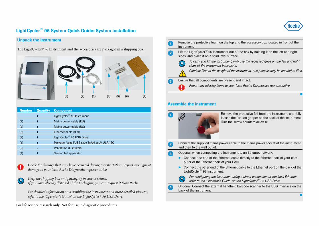
The LightCycler® 96 Instrument and the accessories are packaged in a shipping box.
Check for damage that may have occurred during transportation. Report any signs ofdamage to your local Roche Diagnostics representative.
Keep the shipping box and packaging in case of return.If you have already disposed of the packaging, you can request it from Roche.
For detailed information on assembling the instrument and more detailed pictures,refer to the ‘Operator’s Guide’ on the LightCycler® 96 USB Drive.
Assemble the instrumentNumber Quantity Component
1 LightCycler® 96 Instrument
(1) 1 Mains power cable (EU)
(2) 1 Mains power cable (US)
(3) 1 Ethernet cable (3 m)
(4) 1 LightCycler® 96 USB Drive
(5) 1 Package fuses FUSE 5x20 T8AH 250V ULR/IEC
(6) 2 Ventilation dust filters
(7) 1 Sealing foil applicator
(1) (2) (3) (4) (5) (6) (7)
Remove the protective foam on the top and the accessory box located in front of theinstrument.
Lift the LightCycler® 96 Instrument out of the box by holding it on the left and rightsides, and place it on a solid level surface.
To carry and lift the instrument, only use the recessed grips on the left and rightsides of the instrument base plate.
Caution: Due to the weight of the instrument, two persons may be needed to lift it.
Ensure that all components are present and intact.
Report any missing items to your local Roche Diagnostics representative.
Remove the protective foil from the instrument, and fullyloosen the fixation gripper on the back of the instrument.Turn the screw counterclockwise.
Connect the supplied mains power cable to the mains power socket of the instrument,and then to the wall outlet.
Optional, when connecting the instrument to an Ethernet network:
Connect one end of the Ethernet cable directly to the Ethernet port of your com-puter or the Ethernet port of your LAN.
Connect the other end of the Ethernet cable to the Ethernet port on the back of theLightCycler® 96 Instrument.
For configuring the instrument using a direct connection or the local Ethernet,refer to the ‘Operator’s Guide’ on the LightCycler® 96 USB Drive.
Optional: Connect the external handheld barcode scanner to the USB interface on theback of the instrument.
�
�
�
�
�
�
�
For life science research only. Not for use in diagnostic procedures.
LightCycler® 96 System Quick Guide: System installation
Remove the transport locking device
Install the LightCycler® 96 Application Software
For installing the LightCycler® 96 Application Software Version 1.1 as an upgrade,refer to the ‘Operator’s Guide’ on the LightCycler® 96 USB Drive.
New software releases and user guides for the LightCycler® 96 Instrument are avail-able in the download area of the Roche Applied Sciences website.
Disclaimer
Before setting up operation of the LightCycler® 96 System, it is important to read the userdocumentation completely. Non-observance of the instructions provided or performingany operations not stated in the user documentation could produce safety hazards.
Switch on the instrument using the mains power switch on the back of the instrument.The initialization process begins.
When the instrument has successfully initialized, choose the Eject button on the touch-screen to release the loading module. The loading module is ejected.
Manually pull the loading module completely out of the instrument.
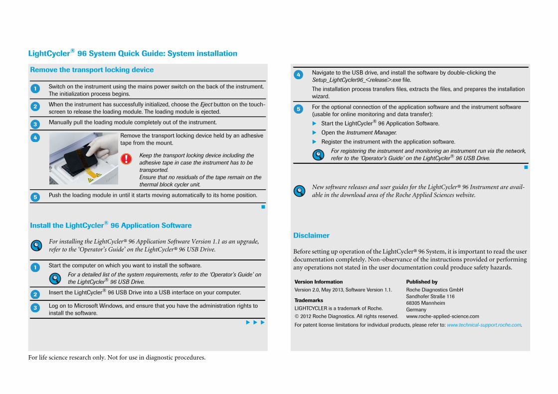
Remove the transport locking device held by an adhesivetape from the mount.
Keep the transport locking device including theadhesive tape in case the instrument has to betransported.Ensure that no residuals of the tape remain on thethermal block cycler unit.
Push the loading module in until it starts moving automatically to its home position.
Start the computer on which you want to install the software.
For a detailed list of the system requirements, refer to the ‘Operator’s Guide’ onthe LightCycler® 96 USB Drive.
Insert the LightCycler® 96 USB Drive into a USB interface on your computer.
Log on to Microsoft Windows, and ensure that you have the administration rights toinstall the software.
�
�
�
�
�
�
�
�
Navigate to the USB drive, and install the software by double-clicking theSetup_LightCycler96_<release>.exe file.
The installation process transfers files, extracts the files, and prepares the installationwizard.
For the optional connection of the application software and the instrument software(usable for online monitoring and data transfer):
Start the LightCycler® 96 Application Software.
Open the Instrument Manager.
Register the instrument with the application software.
For registering the instrument and monitoring an instrument run via the network,refer to the ‘Operator’s Guide’ on the LightCycler® 96 USB Drive.
Version InformationVersion 2.0, May 2013, Software Version 1.1.
TrademarksLIGHTCYCLER is a trademark of Roche.
© 2012 Roche Diagnostics. All rights reserved.
Published byRoche Diagnostics GmbHSandhofer Straße 11668305 MannheimGermanywww.roche-applied-science.com
For patent license limitations for individual products, please refer to: www.technical-support.roche.com.
�
�
For life science research only. Not for use in diagnostic procedures.
LightCycler® 96 System Quick Guide: Programming and running an experiment
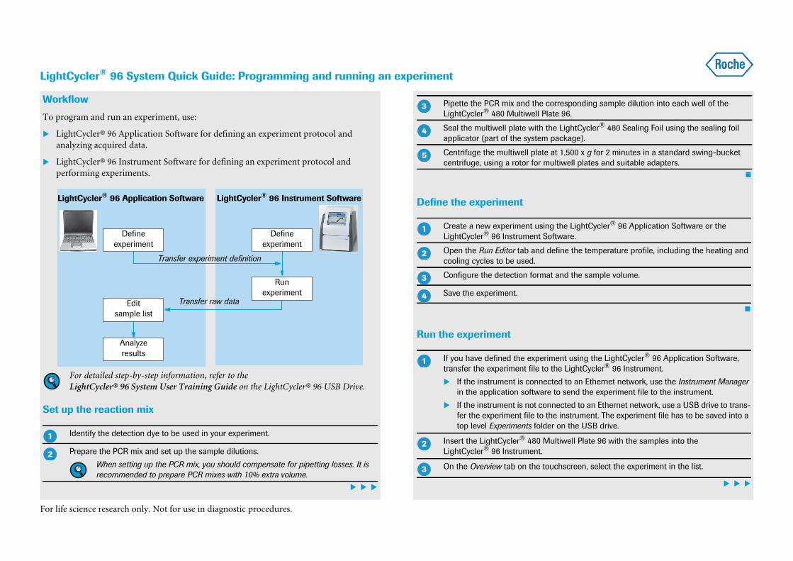
Workflow
To program and run an experiment, use:
LightCycler® 96 Application Software for defining an experiment protocol andanalyzing acquired data.
LightCycler® 96 Instrument Software for defining an experiment protocol andperforming experiments.
For detailed step-by-step information, refer to theLightCycler® 96 System User Training Guide on the LightCycler® 96 USB Drive.
Set up the reaction mix
Define the experiment
Run the experiment
Identify the detection dye to be used in your experiment.
Prepare the PCR mix and set up the sample dilutions.
When setting up the PCR mix, you should compensate for pipetting losses. It isrecommended to prepare PCR mixes with 10% extra volume.
Runexperiment
Defineexperiment
Editsample list
Analyzeresults
Transfer experiment definition
Transfer raw data
Defineexperiment
LightCycler® 96 Application Software LightCycler® 96 Instrument Software
�
�
Pipette the PCR mix and the corresponding sample dilution into each well of theLightCycler® 480 Multiwell Plate 96.
Seal the multiwell plate with the LightCycler® 480 Sealing Foil using the sealing foilapplicator (part of the system package).
Centrifuge the multiwell plate at 1,500 x g for 2 minutes in a standard swing-bucketcentrifuge, using a rotor for multiwell plates and suitable adapters.
Create a new experiment using the LightCycler® 96 Application Software or theLightCycler® 96 Instrument Software.
Open the Run Editor tab and define the temperature profile, including the heating andcooling cycles to be used.
Configure the detection format and the sample volume.
Save the experiment.
If you have defined the experiment using the LightCycler® 96 Application Software,transfer the experiment file to the LightCycler® 96 Instrument.
If the instrument is connected to an Ethernet network, use the Instrument Managerin the application software to send the experiment file to the instrument.
If the instrument is not connected to an Ethernet network, use a USB drive to trans-fer the experiment file to the instrument. The experiment file has to be saved into atop level Experiments folder on the USB drive.
Insert the LightCycler® 480 Multiwell Plate 96 with the samples into theLightCycler® 96 Instrument.
On the Overview tab on the touchscreen, select the experiment in the list.
�
�
�
�
�
�
�
�
�
�
For life science research only. Not for use in diagnostic procedures.
LightCycler® 96 System Quick Guide: Programming and running an experiment
Run finished
The end of a run is indicated as follows:
The status bar on the touchscreen displays the instrument status Ready.
The LightCycler® 96 Instrument unlocks the loading module.
The experiment progress window area shows the end time of the experiment run.
The Raw Data tab provides the final raw data.
Transfer the experiment to the application software
Edit the sample list
Analyze the data
Disclaimer
Before setting up operation of the LightCycler® 96 System, it is important to read the userdocumentation completely. Non-observance of the instructions provided or performingany operations not stated in the user documentation could produce safety hazards.
In the global action bar on the right, choose the Start button.
View the Raw Data tab to monitor the progress of the running experiment.
If the instrument is connected to an Ethernet network, use the Instrument Managerin the application software to retrieve the experiment file from the instrument.
If the instrument is not connected to an Ethernet network, use a USB drive to trans-fer the experiment file to your computer.
Edit the experiment according to your needs and save the file to your computer.
Open the Plate View tab of the Sample Editor.
Use the Clear Wells function to clear the empty wells. This eliminates the selected wellsfrom further analyses.
Select a well or a range of wells.
�
�
�
�
�
�
�
In the Reaction Properties window area to the right of the multiwell plate image, edit thesample-specific properties.
Ensure that the sample assignment on the ‘Sample Editor’ tab matches the pipet-ting scheme on the multiwell plate.
Save the experiment.
On the Analysis tab, add the appropriate analysis type.
Open the <analysis> Settings dialog box and set up the analysis-specific parameters.
Exclude samples if necessary.
Select the results to be displayed.
Optional: Export the result data.
Version InformationVersion 2.0, May 2013, Software Version 1.1.
TrademarksLIGHTCYCLER is a trademark of Roche.
© 2012 Roche Diagnostics. All rights reserved.
Published byRoche Diagnostics GmbHSandhofer Straße 11668305 MannheimGermanywww.roche-applied-science.com
For patent license limitations for individual products, please refer to: www.technical-support.roche.com.
�
�
�
�
�
�
�
For life science research only. Not for use in diagnostic procedures.
LightCycler® 96 SystemUser Training Guide, Version 2.0Software Version 1.1 May 2013

Table of contents
3
Prologue 7
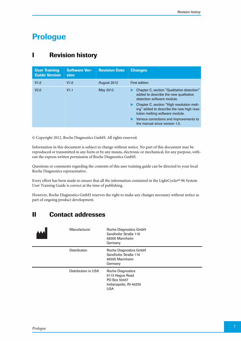
I Revision history ............................................................................................................................................... 7
II Contact addresses ......................................................................................................................................... 7
III Trademarks ........................................................................................................................................................ 8
IV Intended use ...................................................................................................................................................... 8
V Preamble ............................................................................................................................................................. 8
VI Disclaimer of licenses ................................................................................................................................. 8
VII Open Source licenses .................................................................................................................................. 8
VIII Conventions used in this guide .............................................................................................................. 9
IX Warnings and precautions ..................................................................................................................... 12
A Starting the system 15
1 Overview ........................................................................................................................................................... 15
2 Starting the LightCycler® 96 Application Software ................................................................. 17
3 Starting the LightCycler® 96 Instrument ....................................................................................... 17
B Programming and running an experiment 19
1 Programming the experiment with the LightCycler® 96 Application Software ....... 20
1.1 Creating the experiment ............................................................................................................................... 211.2 Creating the temperature profile ............................................................................................................... 231.3 Configuring the reaction volume and detection format ................................................................... 27
2 Transferring the experiment to the instrument .......................................................................... 30
3 Programming the experiment with the LightCycler® 96 Instrument Software ........ 32
3.1 Creating the experiment ............................................................................................................................... 323.2 Creating the temperature profile ............................................................................................................... 353.3 Configuring the detection format and reaction volume ................................................................... 40
4 Running the experiment .......................................................................................................................... 43
4.1 Starting the run ................................................................................................................................................ 434.2 Monitoring the run ......................................................................................................................................... 45
5 Transferring the experiment from the instrument to the application software ........ 47
6 Editing the sample list .............................................................................................................................. 50
C Main applications 57
1 Absolute quantification ............................................................................................................................ 58
1.1 Experiment overview ...................................................................................................................................... 581.2 Setting up the samples ................................................................................................................................. 581.3 Experiment run parameters ......................................................................................................................... 601.4 Editing the sample data ................................................................................................................................ 621.5 Analyzing the results ..................................................................................................................................... 68
1.5.1 Creating the analysis ..................................................................................................................................... 681.5.2 Analysis settings .............................................................................................................................................. 701.5.3 Amplification curves ...................................................................................................................................... 711.5.4 Standard curve ................................................................................................................................................. 721.5.5 Heat map ............................................................................................................................................................ 731.5.6 Result table ........................................................................................................................................................ 731.5.7 Cq bars ................................................................................................................................................................ 77
1.6 Exporting result data ...................................................................................................................................... 77
LightCycler® 96 System, User Training Guide V2.0
Table of contents
4
2 Endpoint SNP genotyping ....................................................................................................................... 78
2.1 Experiment overview ...................................................................................................................................... 782.2 Setting up the samples .................................................................................................................................. 782.3 Experiment run parameters ......................................................................................................................... 802.4 Editing the sample data ................................................................................................................................ 822.5 Analyzing the results ...................................................................................................................................... 86
2.5.1 Creating the analysis ...................................................................................................................................... 862.5.2 Analysis settings .............................................................................................................................................. 882.5.3 Amplification curves ....................................................................................................................................... 892.5.4 Scatter plot ......................................................................................................................................................... 912.5.5 Heat map ............................................................................................................................................................ 932.5.6 Result table ........................................................................................................................................................ 93
2.6 Exporting result data ...................................................................................................................................... 97
3 Relative quantification .............................................................................................................................. 98
3.1 Experiment overview ...................................................................................................................................... 983.2 Setting up the samples .................................................................................................................................. 993.3 Experiment run parameters ...................................................................................................................... 1023.4 Editing the sample data ............................................................................................................................. 1043.5 Analyzing the results ................................................................................................................................... 109
3.5.1 Creating the analysis ................................................................................................................................... 1093.5.2 Analysis settings ........................................................................................................................................... 1113.5.3 Amplification curves .................................................................................................................................... 1133.5.4 Ratio bars ......................................................................................................................................................... 1133.5.5 Heat map ......................................................................................................................................................... 1173.5.6 Result table ..................................................................................................................................................... 1183.5.7 Cq bars ............................................................................................................................................................. 118
3.6 Exporting result data ................................................................................................................................... 119
4 Qualitative detection ............................................................................................................................... 120
4.1 Experiment overview ................................................................................................................................... 1204.2 Setting up the samples ............................................................................................................................... 1204.3 Experiment run parameters ...................................................................................................................... 1224.4 Editing the sample data ............................................................................................................................. 1244.5 Analyzing the results ................................................................................................................................... 128
4.5.1 Creating the analysis ................................................................................................................................... 1284.5.2 Analysis settings ........................................................................................................................................... 1304.5.3 Amplification curves .................................................................................................................................... 1314.5.4 Heat map ......................................................................................................................................................... 1314.5.5 Combined call heat map ............................................................................................................................ 1324.5.6 Result table ..................................................................................................................................................... 133
4.6 Exporting result data ................................................................................................................................... 133
5 Tm calling ....................................................................................................................................................... 134
5.1 Experiment overview ................................................................................................................................... 1345.2 Setting up the samples ............................................................................................................................... 1345.3 Experiment run parameters ...................................................................................................................... 1365.4 Editing the sample data ............................................................................................................................. 1385.5 Analyzing the results ................................................................................................................................... 141
5.5.1 Creating the analysis ................................................................................................................................... 1415.5.2 Analysis settings ........................................................................................................................................... 1435.5.3 Amplification curves .................................................................................................................................... 1445.5.4 Melting curves ............................................................................................................................................... 1445.5.5 Melting peaks ................................................................................................................................................ 1455.5.6 Heat map ......................................................................................................................................................... 1465.5.7 Result table ..................................................................................................................................................... 146
5.6 Exporting result data ................................................................................................................................... 146
Table of contents
5
6 High resolution melting ......................................................................................................................... 147
6.1 Experiment overview .................................................................................................................................... 1476.2 Setting up the samples ............................................................................................................................... 1476.3 Experiment run parameters ....................................................................................................................... 1506.4 Editing the sample data .............................................................................................................................. 1526.5 Analyzing the results ................................................................................................................................... 155
6.5.1 Creating the analysis ................................................................................................................................... 1556.5.2 Analysis settings ............................................................................................................................................ 1586.5.3 Melting curves ................................................................................................................................................ 1596.5.4 Normalized melting curves ........................................................................................................................ 1616.5.5 Normalized melting peaks ......................................................................................................................... 1636.5.6 Result table ...................................................................................................................................................... 1646.5.7 Difference plot ................................................................................................................................................ 1656.5.8 Heat map .......................................................................................................................................................... 168
6.6 Exporting result data .................................................................................................................................... 168
D Shutting down the system 169
E Appendix 173
1 Index ................................................................................................................................................................. 173

LightCycler® 96 System, User Training Guide V2.06
Prologue
Revision history
7
Prologue
I Revision history
© Copyright 2012, Roche Diagnostics GmbH. All rights reserved.
Information in this document is subject to change without notice. No part of this document may bereproduced or transmitted in any form or by any means, electronic or mechanical, for any purpose, with-out the express written permission of Roche Diagnostics GmbH.
Questions or comments regarding the contents of this user training guide can be directed to your localRoche Diagnostics representative.
Every effort has been made to ensure that all the information contained in the LightCycler® 96 SystemUser Training Guide is correct at the time of publishing.
However, Roche Diagnostics GmbH reserves the right to make any changes necessary without notice aspart of ongoing product development.
II Contact addresses
User TrainingGuide Version
Software Ver-sion
Revision Date Changes
V1.0 V1.0 August 2012 First edition
V2.0 V1.1 May 2013 Chapter C, section "Qualitative detection"added to describe the new qualitativedetection software module.
Chapter C, section "High resolution melt-ing" added to describe the new high reso-lution melting software module.
Various corrections and improvements tothe manual since version 1.0.
Manufacturer Roche Diagnostics GmbHSandhofer Straße 11668305 MannheimGermany
Distribution Roche Diagnostics GmbHSandhofer Straße 11668305 MannheimGermany
Distribution in USA Roche Diagnostics9115 Hague RoadPO Box 50457Indianapolis, IN 46250USA
LightCycler® 96 System, User Training Guide V2.0
Trademarks
8
III Trademarks
FASTSTART, LC, LIGHTCYCLER, MAGNA PURE, RESOLIGHT and REALTIME READY are trade-marks of Roche.
SYBR is a registered trademark of Life Technologies Corporation.
All other product names and trademarks are the property of their respective owners.
IV Intended use
The LightCycler® 96 Instrument is intended for performing rapid, accurate polymerase chain reaction(PCR) in combination with real-time, online detection of DNA-binding fluorescent dyes or labeledprobes, enabling quantification or characterization of a target nucleic acid.
The LightCycler® 96 System is intended for life science research only. It must only be used by laboratoryprofessionals trained in laboratory techniques, who have studied the Instructions for Use of this instru-ment. The LightCycler® 96 Instrument is not for use in diagnostic procedures.
The LightCycler® 96 System is intended for indoor use only.
V Preamble
Before setting up operation of the LightCycler® 96 System, it is important to read the user documentationcompletely. Non-observance of the instructions provided or performing any operations not stated in theuser documentation could produce safety hazards.
VI Disclaimer of licenses
NOTICE: For patent license limitations for individual products please refer to:www.technical-support.roche.com.
VII Open Source licenses
Portions of the LightCycler® 96 Software might include one or more Open Source or commercial soft-ware programs. For copyright and other notices and licensing information regarding such software pro-grams included with LightCycler® 96 Software, please refer to the About information within theLightCycler® 96 Application Software and the USB drive provided with the product.
Prologue
Conventions used in this guide
9
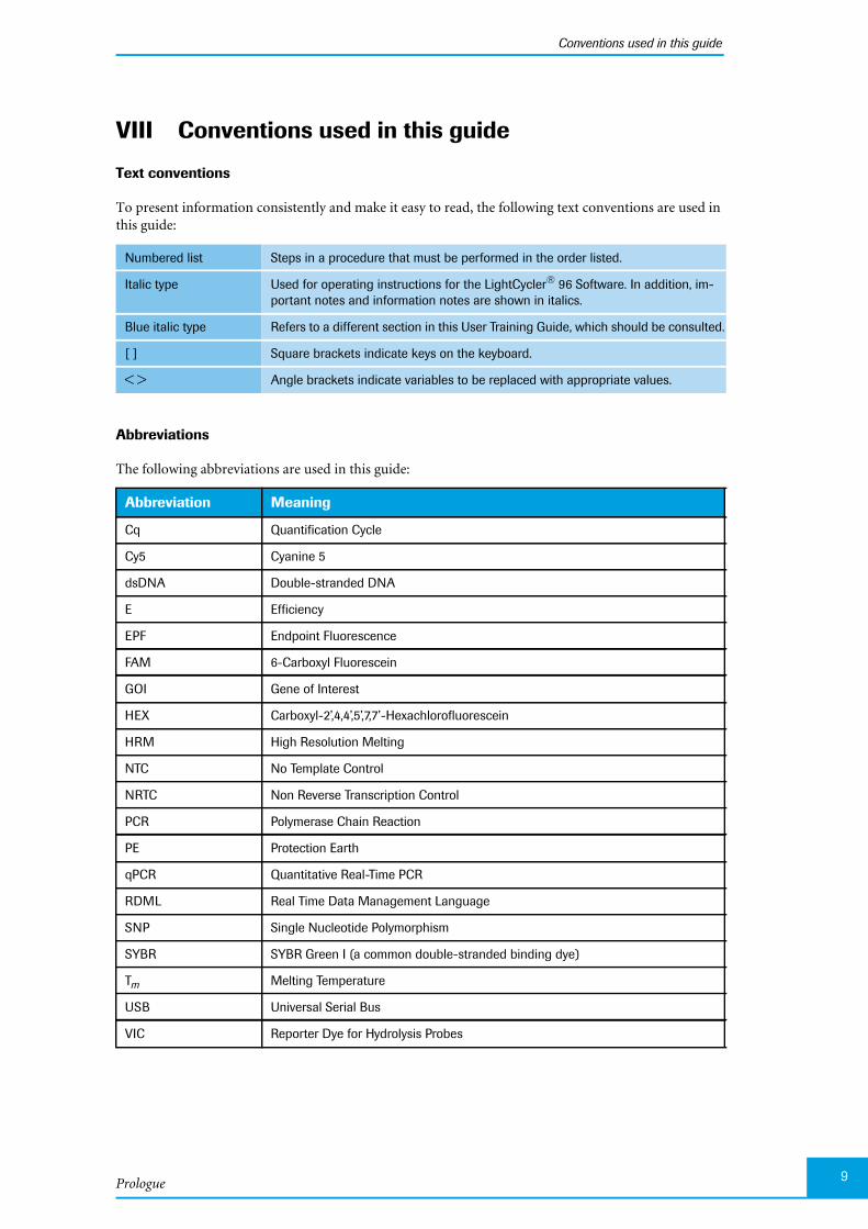
VIII Conventions used in this guide
Text conventions
To present information consistently and make it easy to read, the following text conventions are used inthis guide:
Abbreviations
The following abbreviations are used in this guide:
Numbered list Steps in a procedure that must be performed in the order listed.
Italic type Used for operating instructions for the LightCycler® 96 Software. In addition, im-portant notes and information notes are shown in italics.
Blue italic type Refers to a different section in this User Training Guide, which should be consulted.
[ ] Square brackets indicate keys on the keyboard.
< > Angle brackets indicate variables to be replaced with appropriate values.
Abbreviation Meaning
Cq Quantification Cycle
Cy5 Cyanine 5
dsDNA Double-stranded DNA
E Efficiency
EPF Endpoint Fluorescence
FAM 6-Carboxyl Fluorescein
GOI Gene of Interest
HEX Carboxyl-2’,4,4’,5’,7,7’-Hexachlorofluorescein
HRM High Resolution Melting
NTC No Template Control
NRTC Non Reverse Transcription Control
PCR Polymerase Chain Reaction
PE Protection Earth
qPCR Quantitative Real-Time PCR
RDML Real Time Data Management Language
SNP Single Nucleotide Polymorphism
SYBR SYBR Green I (a common double-stranded binding dye)
Tm Melting Temperature
USB Universal Serial Bus
VIC Reporter Dye for Hydrolysis Probes
LightCycler® 96 System, User Training Guide V2.0
Conventions used in this guide
10
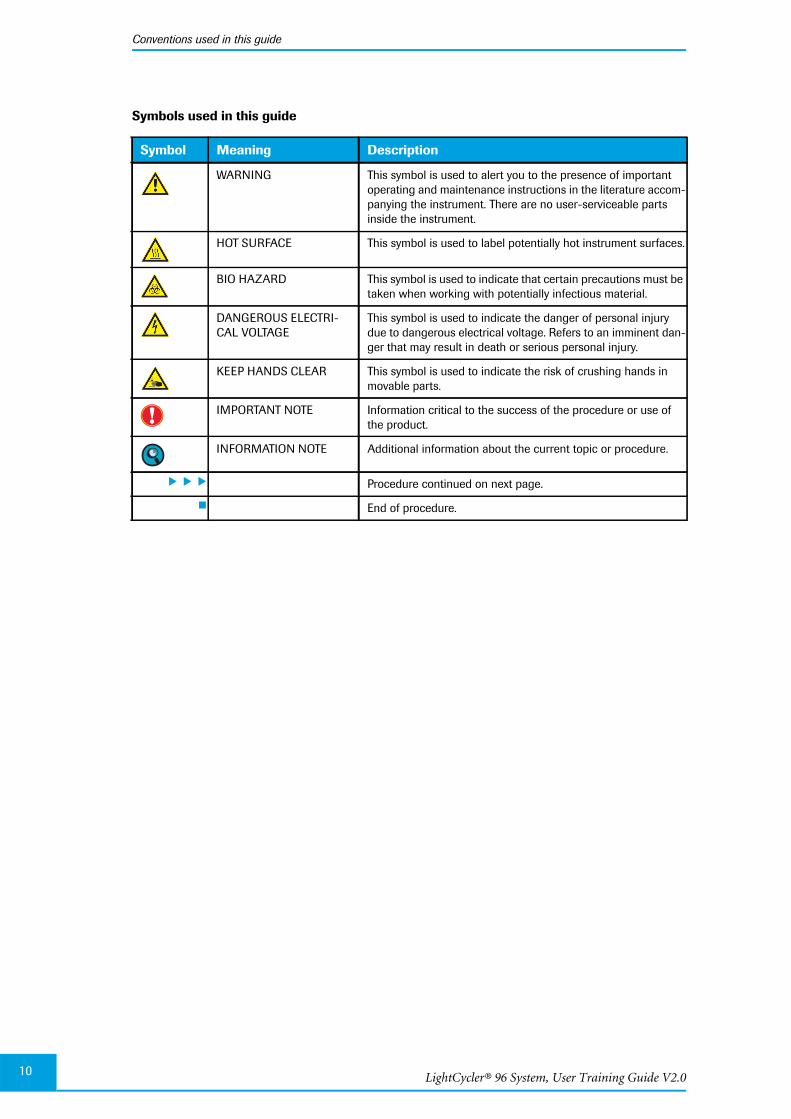
Symbols used in this guide
Symbol Meaning Description
WARNING This symbol is used to alert you to the presence of importantoperating and maintenance instructions in the literature accom-panying the instrument. There are no user-serviceable partsinside the instrument.
HOT SURFACE This symbol is used to label potentially hot instrument surfaces.
BIO HAZARD This symbol is used to indicate that certain precautions must betaken when working with potentially infectious material.
DANGEROUS ELECTRI-CAL VOLTAGE
This symbol is used to indicate the danger of personal injurydue to dangerous electrical voltage. Refers to an imminent dan-ger that may result in death or serious personal injury.
KEEP HANDS CLEAR This symbol is used to indicate the risk of crushing hands inmovable parts.
IMPORTANT NOTE Information critical to the success of the procedure or use ofthe product.
INFORMATION NOTE Additional information about the current topic or procedure.
Procedure continued on next page.
End of procedure.
Prologue
Conventions used in this guide
11
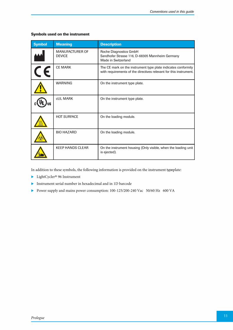
Symbols used on the instrument
In addition to these symbols, the following information is provided on the instrument typeplate:
LightCycler® 96 Instrument
Instrument serial number in hexadecimal and in 1D barcode
Power supply and mains power consumption: 100-125/200-240 Vac 50/60 Hz 600 VA
Symbol Meaning Description
MANUFACTURER OFDEVICE
Roche Diagnostics GmbHSandhofer Strasse 116, D-68305 Mannheim GermanyMade in Switzerland
CE MARK The CE mark on the instrument type plate indicates conformitywith requirements of the directives relevant for this instrument.
WARNING On the instrument type plate.
cUL MARK On the instrument type plate.
HOT SURFACE On the loading module.
BIO HAZARD On the loading module.
KEEP HANDS CLEAR On the instrument housing (Only visible, when the loading unitis ejected).

LightCycler® 96 System, User Training Guide V2.0
Warnings and precautions
12
IX Warnings and precautions
In an emergency, immediately unplug the instrument.
The LightCycler® 96 Instrument must only be used by trained and skilled personnel.
It is essential that the following safety information required for installation and operation of theLightCycler® 96 Instrument is carefully read and observed. Please ensure that this safety information isaccessible to all personnel working with the LightCycler® 96 Instrument.
Handling requirements
The LightCycler® 96 Instrument is an electromechanical instrument. There is a potential risk tothe user from electric shock or physical injury if the instrument is not used according to the in-structions given in this manual.
Follow all safety instructions printed on or attached to the analytical instrument.
Observe all general safety precautions which apply to electrical instruments.
Do not access any electrical parts while the LightCycler® 96 Instrument is connected tothe mains power supply.
Never touch the power cable with wet hands.
Never open the housing of the LightCycler® 96 Instrument .
Never clean the instrument without disconnecting the power cable.
Only authorized service personnel are allowed to perform service or repairs required forthis unit.
Do not use the network cable outdoors.
Always wear safety goggles and gloves when dealing with toxic, caustic, or infectiousmaterials.
Although working with highly purified nucleic acids, for your own safety, please regard allbiological material as potentially infectious. Handling and disposal of such material shouldbe performed according to local safety guidelines. Spills should be immediately disin-fected with an appropriate disinfectant solution to avoid contamination of laboratory per-sonnel or equipment.
For instructions on cleaning the LightCycler® 96 Instrument, refer to theLightCycler® 96 System Operator’s Guide, chapter Cleaning and care.
The multiwell plate mount may be hot after an experiment run.
Always keep your hands clear, when closing the loading unit.
Prologue
Warnings and precautions
13
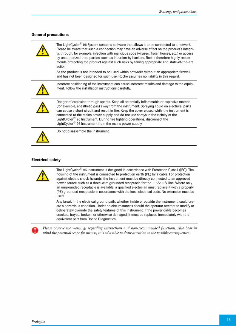
General precautions
Electrical safety
Please observe the warnings regarding interactions and non-recommended functions. Also bear inmind the potential scope for misuse; it is advisable to draw attention to the possible consequences.
The LightCycler® 96 System contains software that allows it to be connected to a network.Please be aware that such a connection may have an adverse effect on the product’s integri-ty, through, for example, infection with malicious code (viruses, Trojan horses, etc.) or accessby unauthorized third parties, such as intrusion by hackers. Roche therefore highly recom-mends protecting the product against such risks by taking appropriate and state-of-the-artaction.
As the product is not intended to be used within networks without an appropriate firewalland has not been designed for such use, Roche assumes no liability in this regard.
Incorrect positioning of the instrument can cause incorrect results and damage to the equip-ment. Follow the installation instructions carefully.
Danger of explosion through sparks. Keep all potentially inflammable or explosive material(for example, anesthetic gas) away from the instrument. Spraying liquid on electrical partscan cause a short circuit and result in fire. Keep the cover closed while the instrument isconnected to the mains power supply and do not use sprays in the vicinity of theLightCycler® 96 Instrument. During fire fighting operations, disconnect theLightCycler® 96 Instrument from the mains power supply.
Do not disassemble the instrument.
The LightCycler® 96 Instrument is designed in accordance with Protection Class I (IEC). Thehousing of the instrument is connected to protection earth (PE) by a cable. For protectionagainst electric shock hazards, the instrument must be directly connected to an approvedpower source such as a three-wire grounded receptacle for the 115/230 V line. Where onlyan ungrounded receptacle is available, a qualified electrician must replace it with a properly(PE) grounded receptacle in accordance with the local electrical code. No extension must beused.
Any break in the electrical ground path, whether inside or outside the instrument, could cre-ate a hazardous condition. Under no circumstances should the operator attempt to modify ordeliberately override the safety features of this instrument. If the power cable becomescracked, frayed, broken, or otherwise damaged, it must be replaced immediately with theequivalent part from Roche Diagnostics.

LightCycler® 96 System, User Training Guide V2.014
Starting the system
Overview
15
AAStarting the system 0
1 Overview
This section provides an overview of the following topics:
The main components of the LightCycler® 96 System and your workflow for using them, see below.
How to use this user training guide, see section How to use this user training guide, on page 16.
LightCycler® 96 System main components and workflow
The LightCycler® 96 System consists of two main components:
The LightCycler® 96 Application Software on your computer, which provides all functions for defin-ing an experiment protocol and for analyzing the data gathered during the experiment run.
The LightCycler® 96 Instrument, which is controlled by the LightCycler® 96 Instrument Software.The LightCycler® 96 Instrument Software provides all functions for configuring and controlling theLightCycler® 96 Instrument. These include functions for managing, creating, and executing experi-ments, and for monitoring an experiment run. The instrument software is operated using the touch-screen of the instrument.
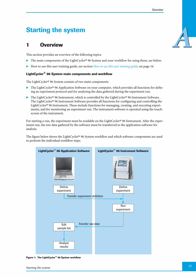
For starting a run, the experiment must be available on the LightCycler® 96 Instrument. After the exper-iment run, the raw data gathered by the software must be transferred to the application software foranalysis.
The figure below shows the LightCycler® 96 System workflow and which software components are usedto perform the individual workflow steps.
Figure 1: The LightCycler® 96 System workflow
Runexperiment
Defineexperiment
Defineexperiment
Editsample list
Analyzeresults
LightCycler® 96 Instrument SoftwareLightCycler® 96 Application Software
Transfer experiment definition
Transfer raw data
LightCycler® 96 System, User Training Guide V2.016
Overview
AAHow to use this user training guide
This user training guide is structured as follows:
Steps that are similar for all applications are described step-by-step in the chapter Programming andrunning an experiment. Read this chapter before starting an experiment.
Steps that are different for each application are described in the chapter Main applications, in a sepa-rate section for each application.
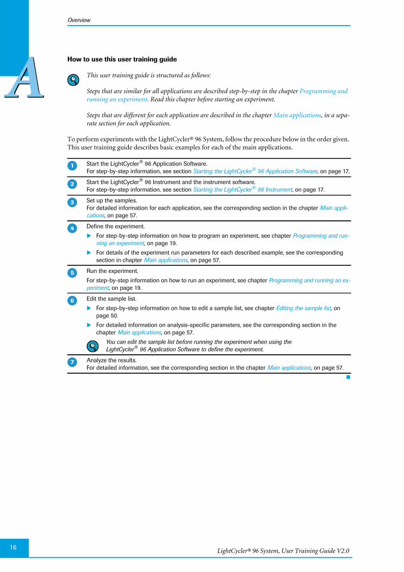
To perform experiments with the LightCycler® 96 System, follow the procedure below in the order given.This user training guide describes basic examples for each of the main applications.
Start the LightCycler® 96 Application Software.For step-by-step information, see section Starting the LightCycler® 96 Application Software, on page 17.
Start the LightCycler® 96 Instrument and the instrument software.For step-by-step information, see section Starting the LightCycler® 96 Instrument, on page 17.
Set up the samples.For detailed information for each application, see the corresponding section in the chapter Main appli-cations, on page 57.
Define the experiment.
For step-by-step information on how to program an experiment, see chapter Programming and run-ning an experiment, on page 19.
For details of the experiment run parameters for each described example, see the correspondingsection in chapter Main applications, on page 57.
Run the experiment.
For step-by-step information on how to run an experiment, see chapter Programming and running an ex-periment, on page 19.
Edit the sample list.
For step-by-step information on how to edit a sample list, see chapter Editing the sample list, onpage 50.
For detailed information on analysis-specific parameters, see the corresponding section in thechapter Main applications, on page 57.
You can edit the sample list before running the experiment when using theLightCycler® 96 Application Software to define the experiment.
Analyze the results.For detailed information, see the corresponding section in the chapter Main applications, on page 57.
�
�
�
�
�
�
�
Starting the system
Starting the LightCycler® 96 Application Software
17
AA2 Starting the LightCycler® 96 Application Software
Before starting the software, you must install it on your computer. For a detailed description of the install-tion, refer to the LightCycler® 96 System Operator’s Guide, chapter A, section Installation.
To start the LightCycler® 96 Application Software
3 Starting the LightCycler® 96 Instrument
Before starting, you must plug in the LightCycler® 96 Instrument. Refer to theLightCycler® 96 System Operator’s Guide, chapter A System Description for a detailed description of the in-strument parts, and chapter A, section Installation for a description of the installation.
The LightCycler® 96 Instrument Software is started together with the instrument.
To start the LightCycler® 96 Instrument
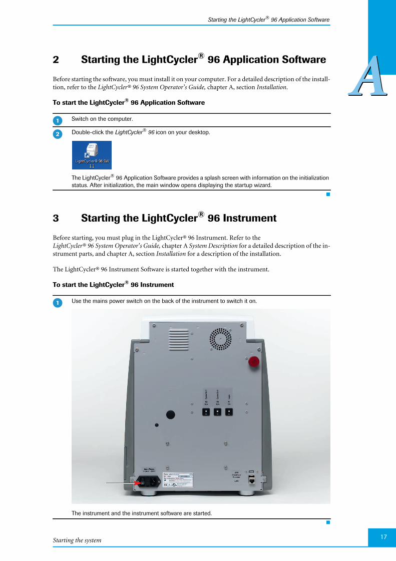
Switch on the computer.
Double-click the LightCycler® 96 icon on your desktop.
The LightCycler® 96 Application Software provides a splash screen with information on the initializationstatus. After initialization, the main window opens displaying the startup wizard.
Use the mains power switch on the back of the instrument to switch it on.
The instrument and the instrument software are started.
�
�
�

LightCycler® 96 System, User Training Guide V2.0
AA
18

Programming and running an experiment 19
BB
Programming and running an experiment 0For information on the order for performing the individual steps of a complete LightCycler® 96 Systemworkflow, see section Overview, on page 15.
You can create an experiment and define the temperature profile and the dye-specific parameters eitheron the instrument using the LightCycler® 96 Instrument Software or on a computer using theLightCycler® 96 Application Software. For starting an experiment run, the experiment must be availableon the instrument. Therefore, if you have programmed the experiment on a computer, it must be trans-ferred to the instrument for the run.
This chapter describes both ways of programming an experiment:
For detailed information on how to specify an experiment definition using the application software,see section Programming the experiment with the LightCycler® 96 Application Software, on page 20. Fordetailed information on how to transfer the experiment to the instrument, see section Transferring theexperiment to the instrument, on page 30.
For detailed information on how to specify an experiment definition using the instrument software,see section Programming the experiment with the LightCycler® 96 Instrument Software, on page 32.
After the experiment run, the raw data gathered by the software on the instrument must be transferredback to the application software for analysis. For detailed information on how to transfer the raw data tothe application software, see section Transferring the experiment from the instrument to the application soft-ware, on page 47.

LightCycler® 96 System, User Training Guide V2.020
Programming the experiment with the LightCycler® 96 Application Software
BB
1 Programming the experiment with theLightCycler® 96 Application Software
The information provided in the experiment definition controls the LightCycler® 96 Instrument duringan experiment run. The experiment definition specifies the target temperatures and hold times of thethermal block cycler, the number of cycles being executed, and other parameters.
For a comprehensive description of the LightCycler® 96 Application Software, refer to theLightCycler® 96 System Operator’s Guide, chapter LightCycler® 96 Application Software.
To program an experiment:
Create a new experiment, see section Creating the experiment, below.
Add one or more programs and define the temperature profile for each step of a program, see sectionCreating the temperature profile, on page 23.
Specify the reaction volume and the detection format for the experiment , see section Configuring thereaction volume and detection format, on page 27.
Programming and running an experiment
Programming the experiment with the LightCycler® 96 Application Software
21
BB
Creating the experiment
1.1 Creating the experiment
This user training guide describes how to generate a completely new experiment. For a detailed descrip-tion of all options for creating an experiment with the LightCycler® 96 Application Software, refer to theLightCycler® 96 System Operator’s Guide, chapter B, section Experiments.
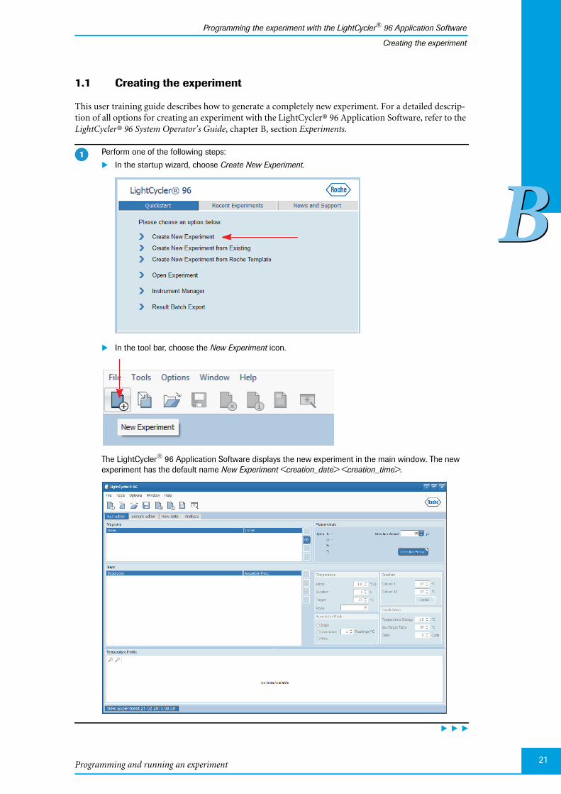
Perform one of the following steps:
In the startup wizard, choose Create New Experiment.
In the tool bar, choose the New Experiment icon.
The LightCycler® 96 Application Software displays the new experiment in the main window. The newexperiment has the default name New Experiment <creation_date> <creation_time>.
�

LightCycler® 96 System, User Training Guide V2.022
Programming the experiment with the LightCycler® 96 Application Software
BB
Creating the experiment
Optional: Enter a description for the experiment.
In the File menu, choose Properties.
In the Properties dialog box, open the Notes tab.
Enter a description.
Choose OK.
�

Programming and running an experiment
Programming the experiment with the LightCycler® 96 Application Software
23
BB
Creating the temperature profile
1.2 Creating the temperature profile
For detailed information on the applicable values for the experiment run parameters, see the corre-sponding section in the chapter Main applications, on page 57.
To create a temperature profile:
Add one or more new programs to the temperature profile and create the cycling sequence, see sectionTo add a new program and specify the number of cycles, below.
Define the temperature profile for each step of a program, see section To specify the temperature profilefor each step of a program, on page 25.
To add a new program and specify the number of cycles
Open the Run Editor tab.
In the Programs window area, choose the button to open the Predefined Programs dialog box.
Select one of the available programs for the first program and choose Add.
The program is added to the Programs list and displayed in the Temperature Profile window area.
�
�
�

LightCycler® 96 System, User Training Guide V2.024
Programming the experiment with the LightCycler® 96 Application Software
BB
Creating the temperature profile
Optional: To modify the name of the new program, proceed as follows:
In the Programs list, select the new program.
Specify the name.
Repeat steps 1 to 4 to add further programs to your profile.
If necessary (for example, for an amplification program) proceed as follows to specify the number of re-peats of a program (cycles):
In the Programs list, select the new program.
In the Cycles column, use the up and down arrows to specify how many times the cycle is to be re-peated in this experiment, or type in a value (possible values: 1 to 99).
For detailed information on the applicable values for the number of cycles, see the correspondingsection in the chapter Main applications, on page 57.
If necessary repeat step 6 to specify the corresponding number of cycles for further programs.
�
�
�
�

Programming and running an experiment
Programming the experiment with the LightCycler® 96 Application Software
25
BB
Creating the temperature profile
To specify the temperature profile for each step of a program
A step can only be edited as long as no run has been performed.
For a comprehensive description of all options of the LightCycler® 96 Application Software, refer to theLightCycler® 96 System Operator’s Guide, chapter LightCycler® 96 Application Software.
In the Steps window area, select the step you want to edit.
In the Temperature window area to the right of the Steps list, edit the default values of the following pa-rameters for the selected step:
Ramp (°C/s):Maximum value for heating: 4.4°C/sMaximum value for cooling: 2.2°C/s
Duration (s):Possible values: 1 to 7200 s (= 2 h)
Target (°C):Possible values: 37 to 98°C
Mode:Possible options:Standard: For detailed information on the corresponding options in the Aquisition Mode window ar-ea, see step 3.Gradient, Touch down: For detailed information on these modes and the corresponding parameters,refer to the LightCycler® 96 System Operator’s Guide, chapter LightCycler® 96 Application Software.
For detailed information on the applicable values for the experiment run parameters, see the corre-sponding section in the chapter Main applications, on page 57.
�
�
LightCycler® 96 System, User Training Guide V2.026
Programming the experiment with the LightCycler® 96 Application Software
BB
Creating the temperature profile
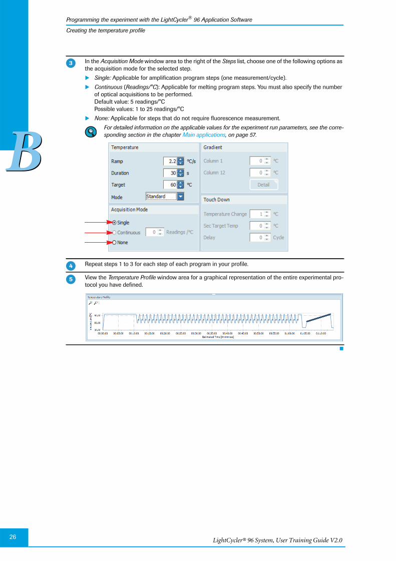
In the Acquisition Mode window area to the right of the Steps list, choose one of the following options asthe acquisition mode for the selected step.
Single: Applicable for amplification program steps (one measurement/cycle). Continuous (Readings/°C): Applicable for melting program steps. You must also specify the number
of optical acquisitions to be performed.Default value: 5 readings/°CPossible values: 1 to 25 readings/°C
None: Applicable for steps that do not require fluorescence measurement.
For detailed information on the applicable values for the experiment run parameters, see the corre-sponding section in the chapter Main applications, on page 57.
Repeat steps 1 to 3 for each step of each program in your profile.
View the Temperature Profile window area for a graphical representation of the entire experimental pro-tocol you have defined.
�
�
�
Programming and running an experiment
Programming the experiment with the LightCycler® 96 Application Software
27
BB
Configuring the reaction volume and detection format
1.3 Configuring the reaction volume and detection format
To complete the run definition:
Specify the reaction volume, see section To specify the reaction volume for the experiment, below.
Specify the dye-specific parameters for the detection format, see section To specify the detection formatfor the experiment, below.
Save the experiment, see section To save the experiment, on page 29.
To specify the reaction volume for the experiment
To specify the detection format for the experiment
The detection format specifies one or more excitation-emission filter combinations (detection channels)suitable for your experiment.
For detailed information on the applicable values for the dye-specific parameters for specifying the de-tection format, see the corresponding section in the chapter Main applications, on page 57.
For a comprehensive description of all options of the LightCycler® 96 Application Software, refer to theLightCycler® 96 System Operator’s Guide, chapter LightCycler® 96 Application Software.
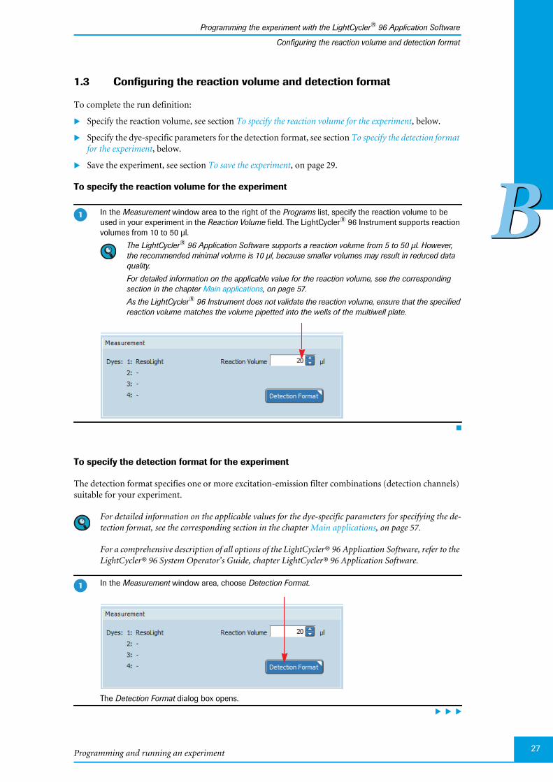
In the Measurement window area to the right of the Programs list, specify the reaction volume to beused in your experiment in the Reaction Volume field. The LightCycler® 96 Instrument supports reactionvolumes from 10 to 50 µl.
The LightCycler® 96 Application Software supports a reaction volume from 5 to 50 µl. However,the recommended minimal volume is 10 µl, because smaller volumes may result in reduced dataquality.
For detailed information on the applicable value for the reaction volume, see the correspondingsection in the chapter Main applications, on page 57.
As the LightCycler® 96 Instrument does not validate the reaction volume, ensure that the specifiedreaction volume matches the volume pipetted into the wells of the multiwell plate.
In the Measurement window area, choose Detection Format.
The Detection Format dialog box opens.
�
�
LightCycler® 96 System, User Training Guide V2.028
Programming the experiment with the LightCycler® 96 Application Software
BB
Configuring the reaction volume and detection format
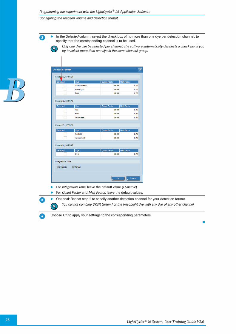
In the Selected column, select the check box of no more than one dye per detection channel, tospecify that the corresponding channel is to be used.
Only one dye can be selected per channel. The software automatically deselects a check box if youtry to select more than one dye in the same channel group.
For Integration Time, leave the default value (Dynamic).
For Quant Factor and Melt Factor, leave the default values.
Optional: Repeat step 2 to specify another detection channel for your detection format.
You cannot combine SYBR Green I or the ResoLight dye with any dye of any other channel.
Choose OK to apply your settings to the corresponding parameters.
�
�
�

Programming and running an experiment
Programming the experiment with the LightCycler® 96 Application Software
29
BB
Configuring the reaction volume and detection format
To save the experiment
Optional: Change the default directory for saving and loading experiment files.
In the Options menu, choose Preferences. The Preferences dialog box opens.
Choose the browse button next to the Default Directory field. The Browse For Folder dialog boxopens.
Specify a different default path, if applicable.
Choose OK.
In the tool bar, choose the Save Experiment icon to save the new experiment. The Save As dialog boxopens.
For a detailed description of all saving options, refer to the LightCycler® 96 System Operator’s Guide,chapter LightCycler® 96 Application Software.
Navigate to the directory where you want to store the experiment file.
Enter a file name for the experiment.
Choose Save. The dialog box closes.
The experiment is saved, depending on the processing status:
As a LightCycler® 96 file for an unprocessed experiment (*.lc96u).
As a LightCycler® 96 file for a processed experiment (*.lc96p).
�
�
�
�
�
LightCycler® 96 System, User Training Guide V2.030
Transferring the experiment to the instrument
BB
2 Transferring the experiment to the instrument
If you have specified the experiment definition on a computer using theLightCycler® 96 Application Software, the experiment must be transferred to the instrument for the run.
To transfer the experiment to the instrument using a USB drive
Insert a USB drive into one of the USB interfaces of your computer.
Open Windows Explorer and navigate to the experiment file.
Copy the experiment file (*.lc96u) and paste it into the Experiments folder on the USB drive.
Only experiment files that are located inside the top level ’Experiments’ folder will be recognized bythe instrument software. If you use a USB drive other than the one supplied with the instrument,first create the top level ’Experiments’ folder and then copy and paste in the experiment file.
Close Windows Explorer.
Remove the USB drive from your computer.
Switch on the LightCycler® 96 Instrument, see section Starting the LightCycler® 96 Instrument, onpage 17.
�
�
�
�
�
�
Programming and running an experiment
Transferring the experiment to the instrument
31
BB
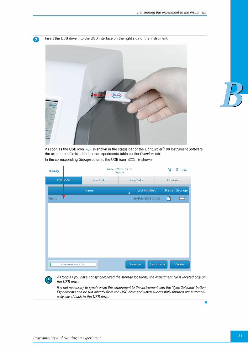
Insert the USB drive into the USB interface on the right side of the instrument.
As soon as the USB icon is shown in the status bar of the LightCycler® 96 Instrument Software,the experiment file is added to the experiments table on the Overview tab.
In the corresponding Storage column, the USB icon is shown.
As long as you have not synchronized the storage locations, the experiment file is located only onthe USB drive.
It is not necessary to synchronize the experiment to the instrument with the ‘Sync Selected’ button.Experiments can be run directly from the USB drive and when successfully finished are automati-cally saved back to the USB drive.
�
LightCycler® 96 System, User Training Guide V2.032
Programming the experiment with the LightCycler® 96 Instrument Software
BB
Creating the experiment
3 Programming the experiment with theLightCycler® 96 Instrument Software
The information provided in the experiment definition controls the LightCycler® 96 Instrument duringan experiment run. The experiment definition specifies the target temperatures and hold times of thethermal block cycler, the number of cycles being executed, and other parameters.
For programming the experiment with the instrument software, the LightCycler® 96 Instrument mustbe started.
For a comprehensive description of the LightCycler® 96 Instrument Software, refer to theLightCycler® 96 System Operator’s Guide, chapter LightCycler® 96 Instrument Software.
In addition, the help browser provides information on the currently open tab of theLightCycler® 96 Instrument Software.
To program an experiment:
Create a new experiment, see section Creating the experiment, below.
Add one or more programs and define the temperature profile for each step of a program, see sectionCreating the temperature profile, on page 35.
Specify the reaction volume and the detection format for the experiment, see section Configuring thedetection format and reaction volume, on page 40.
3.1 Creating the experiment
This user training guide describes how to generate a completely new experiment. For a detailed descrip-tion of all options for creating an experiment with the LightCycler® 96 Instrument Software, refer to theLightCycler® 96 System Operator’s Guide, chapter C, section Experiments.
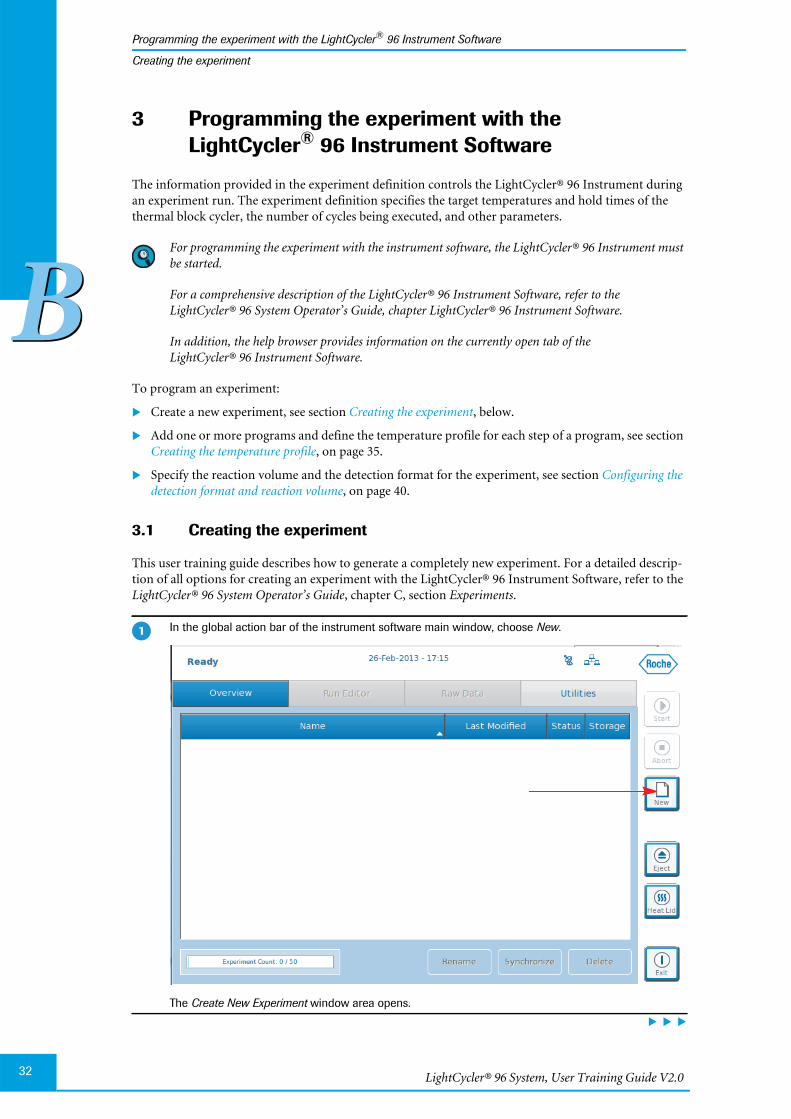
In the global action bar of the instrument software main window, choose New.
The Create New Experiment window area opens.
�
Programming and running an experiment
Programming the experiment with the LightCycler® 96 Instrument Software
33
BB
Creating the experiment
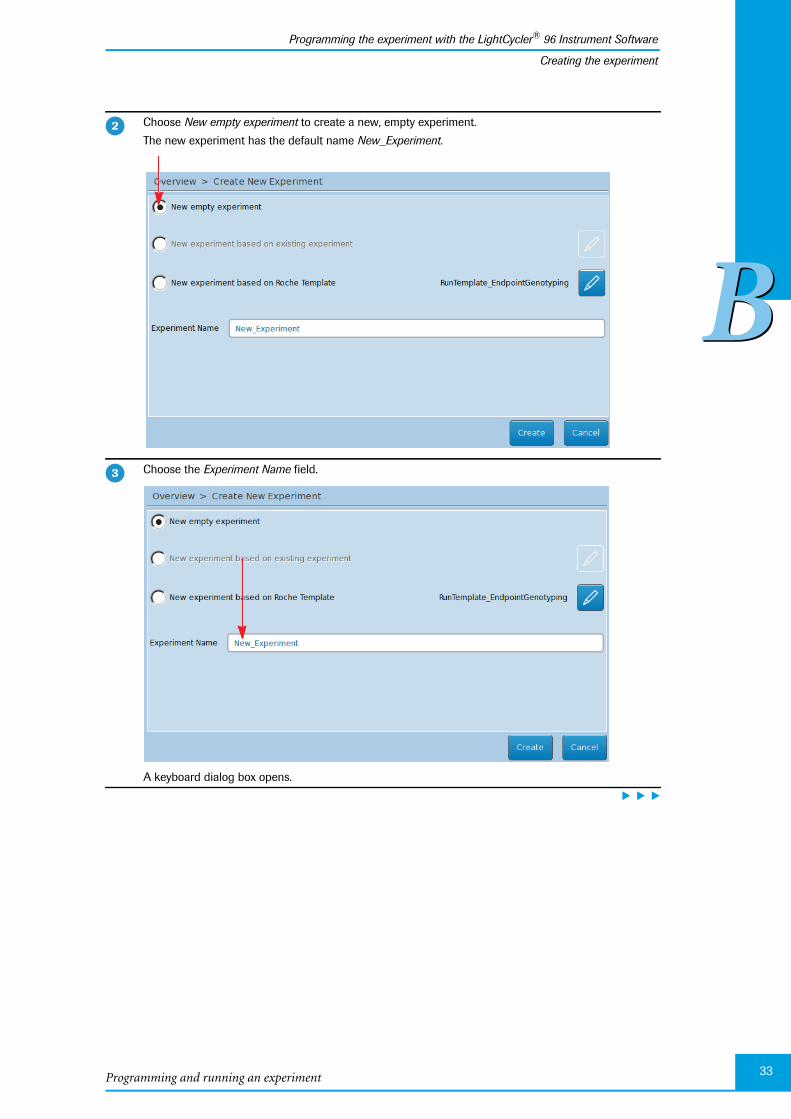
Choose New empty experiment to create a new, empty experiment.
The new experiment has the default name New_Experiment.
Choose the Experiment Name field.
A keyboard dialog box opens.
�
�

LightCycler® 96 System, User Training Guide V2.034
Programming the experiment with the LightCycler® 96 Instrument Software
BB
Creating the experiment
In the New Experiment Name field, specify the name for the new experiment using the keys, and closethe dialog box with OK.
In the Create New Experiment window area, choose Create.
The LightCycler® 96 Instrument Software performs the following steps:
It adds the new experiment to the list in the Overview tab.
It opens the Run Editor tab for the new experiment.
�
�
Programming and running an experiment
Programming the experiment with the LightCycler® 96 Instrument Software
35
BB
Creating the temperature profile
3.2 Creating the temperature profile
For detailed information on the applicable values for the experiment run parameters, see the correspond-ing section in the chapter Main applications, on page 57.
You can only edit a program, and thus also a profile, as long as no run has been performed.
To create a temperature profile:
Add one or more new programs to the temperature profile and specify the cycling sequence, see sec-tion To add a new program and specify the number of cycles, below.
Define the temperature profile for each step of a program, see section To specify the temperature profilefor each step of a program, on page 37.
To add a new program and specify the number of cycles
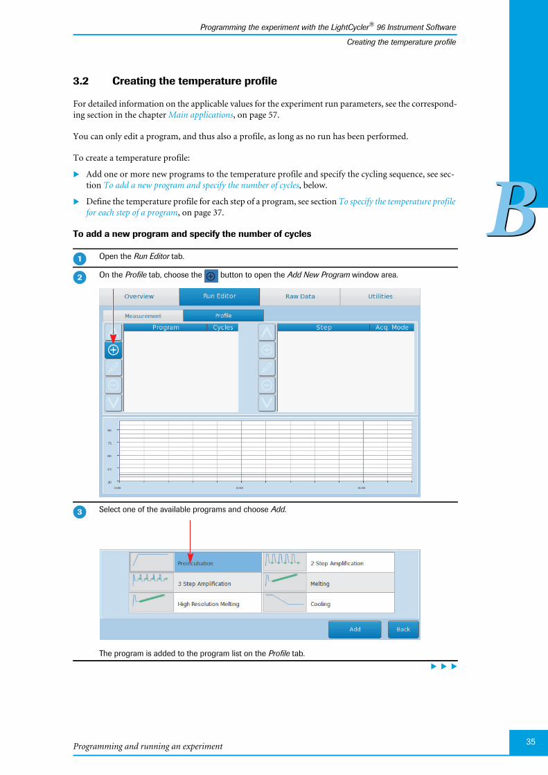
Open the Run Editor tab.
On the Profile tab, choose the button to open the Add New Program window area.
Select one of the available programs and choose Add.
The program is added to the program list on the Profile tab.
�
�
�

LightCycler® 96 System, User Training Guide V2.036
Programming the experiment with the LightCycler® 96 Instrument Software
BB
Creating the temperature profile
In the program list, choose the new program. Then choose the pencil button.
The Program Settings window area opens.
Optional: In the Name field, specify the name for the selected program.
If necessary (for example, for an amplification program) specify the number of repeats of the selectedprogram (cycles).Possible values: 1 to 99
For detailed information on the applicable values for the number of cycles, see the correspondingsection in the chapter Main applications, on page 57.
Choose Back to apply your settings to the selected program.
The Program Settings window area is closed. The program list is displayed with the changed settings.
Optional: Repeat steps 1 to 7 to add further programs to your profile and specify the correspondingnumber of cycles if necessary.
�
�
�
�
Programming and running an experiment
Programming the experiment with the LightCycler® 96 Instrument Software
37
BB
Creating the temperature profile
To specify the temperature profile for each step of a program
A step can only be edited as long as no run has been performed.
For a comprehensive description of all options of the LightCycler® 96 Instrument Software, refer to theLightCycler® 96 System Operator’s Guide, chapter LightCycler® 96 Instrument Software.
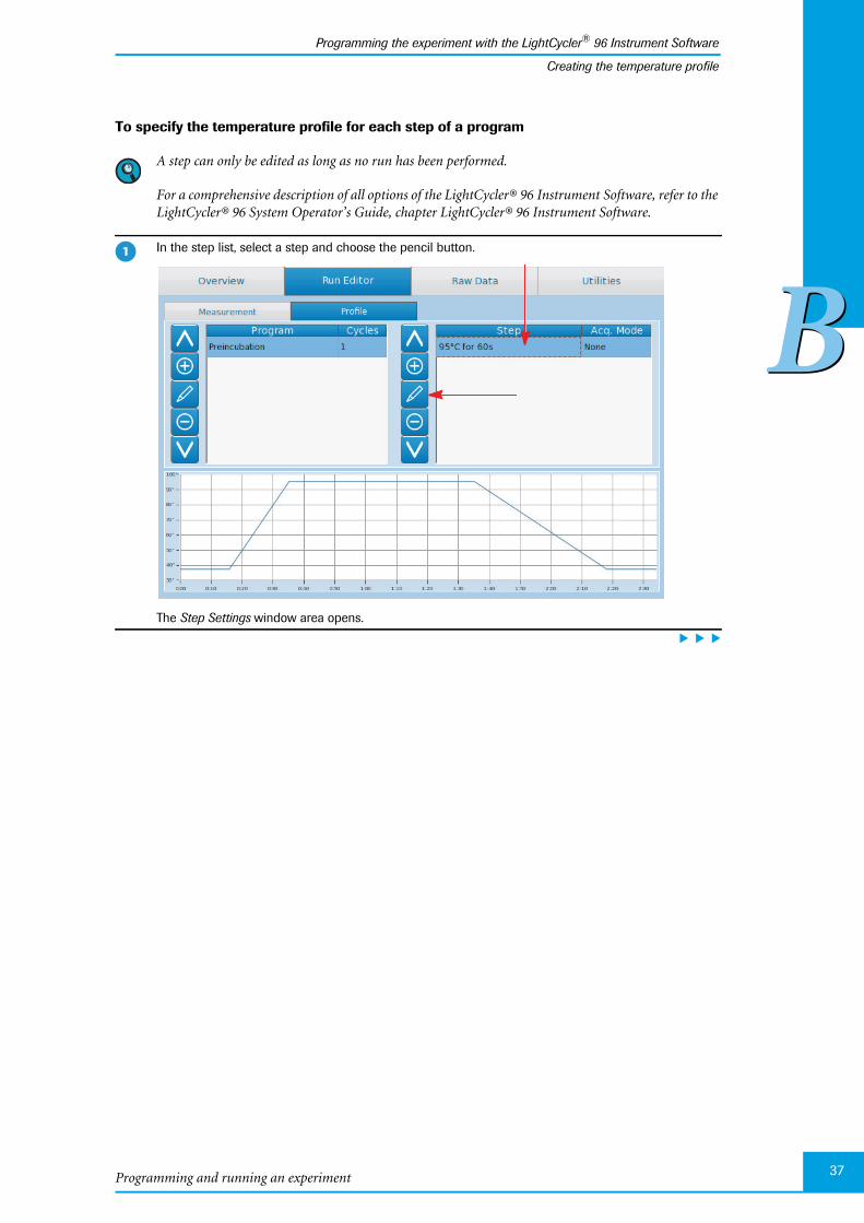
In the step list, select a step and choose the pencil button.
The Step Settings window area opens.
�
LightCycler® 96 System, User Training Guide V2.038
Programming the experiment with the LightCycler® 96 Instrument Software
BB
Creating the temperature profile
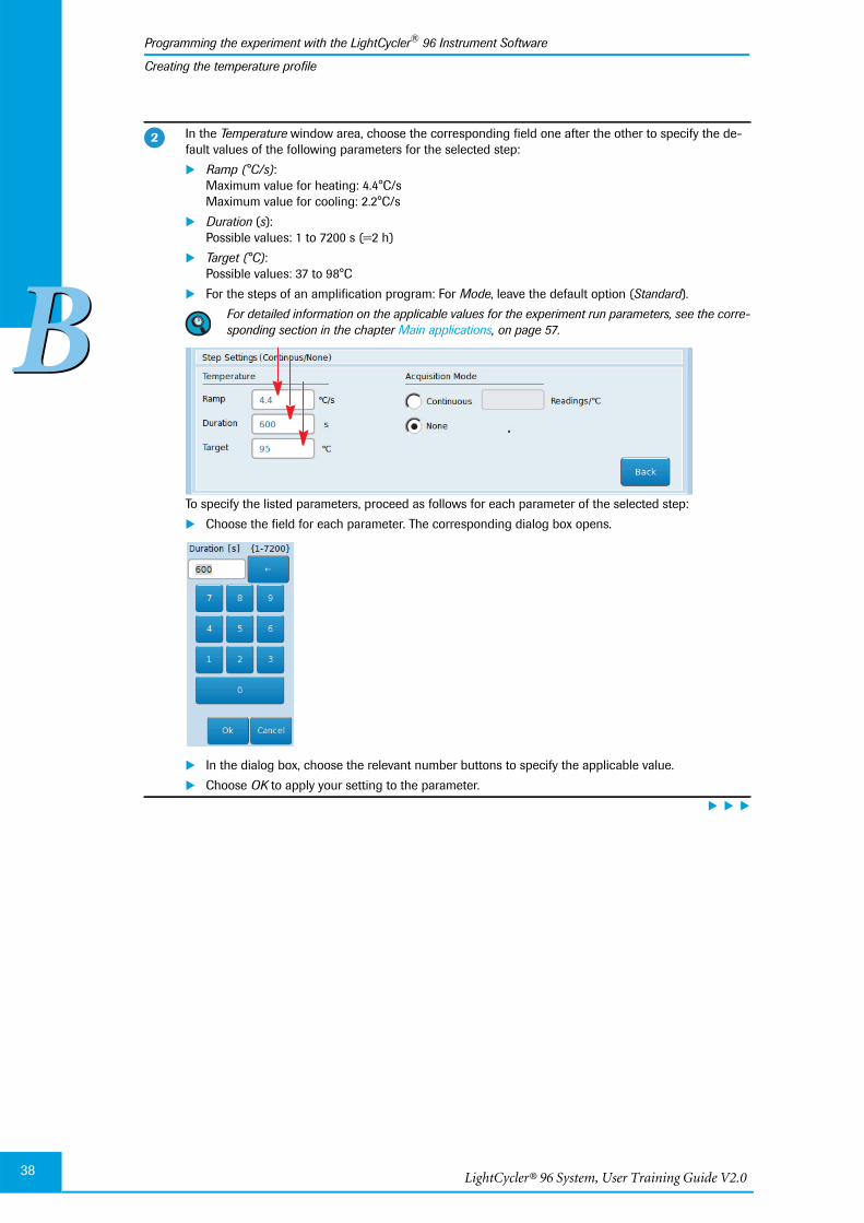
In the Temperature window area, choose the corresponding field one after the other to specify the de-fault values of the following parameters for the selected step:
Ramp (°C/s):Maximum value for heating: 4.4°C/sMaximum value for cooling: 2.2°C/s
Duration (s):Possible values: 1 to 7200 s (=2 h)
Target (°C):Possible values: 37 to 98°C
For the steps of an amplification program: For Mode, leave the default option (Standard).
For detailed information on the applicable values for the experiment run parameters, see the corre-sponding section in the chapter Main applications, on page 57.
To specify the listed parameters, proceed as follows for each parameter of the selected step:
Choose the field for each parameter. The corresponding dialog box opens.
In the dialog box, choose the relevant number buttons to specify the applicable value.
Choose OK to apply your setting to the parameter.
�
Programming and running an experiment
Programming the experiment with the LightCycler® 96 Instrument Software
39
BB
Creating the temperature profile
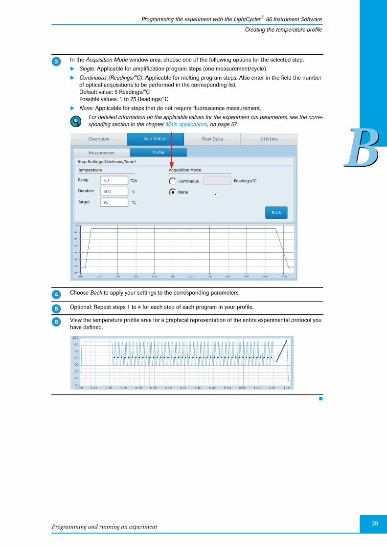
In the Acquisition Mode window area, choose one of the following options for the selected step.
Single: Applicable for amplification program steps (one measurement/cycle).
Continuous (Readings/°C): Applicable for melting program steps. Also enter in the field the numberof optical acquisitions to be performed in the corresponding list.Default value: 5 Readings/°CPossible values: 1 to 25 Readings/°C
None: Applicable for steps that do not require fluorescence measurement.
For detailed information on the applicable values for the experiment run parameters, see the corre-sponding section in the chapter Main applications, on page 57.
Choose Back to apply your settings to the corresponding parameters.
Optional: Repeat steps 1 to 4 for each step of each program in your profile.
View the temperature profile area for a graphical representation of the entire experimental protocol youhave defined.
�
�
�
�

LightCycler® 96 System, User Training Guide V2.040
Programming the experiment with the LightCycler® 96 Instrument Software
BB
Configuring the detection format and reaction volume
3.3 Configuring the detection format and reaction volume
You cannot change or customize the detection format definition after the run has started.
To complete the run definition:
Specify the dye-specific parameters for the detection format, see section To specify the detection formatfor the experiment, below.
Specify the reaction volume, see section To specify the reaction volume for the experiment, on page 42.
The LightCycler® 96 Instrument Software automatically saves all changes in the experiment file on theinstrument.
To specify the detection format for the experiment
The detection format specifies one or more excitation-emission filter combinations (detection channels)suitable for your experiment.
For detailed information on the applicable values for the detection format, see the corresponding sec-tion in the chapter Main applications, on page 57.
For a comprehensive description of all options of the LightCycler® 96 Instrument Software, refer to theLightCycler® 96 System Operator’s Guide, chapter LightCycler® 96 Instrument Software.
Open the Measurement tab.
Choose the pencil button next to the Detection Format list.
The Detection Format window area opens.
�
�

Programming and running an experiment
Programming the experiment with the LightCycler® 96 Instrument Software
41
BB
Configuring the detection format and reaction volume
Choose the tab of the detection channel you want to use.
In the Selected column, choose no more than one dye per detection channel, to specify that the cor-responding channel is to be used.
Only one dye can be selected per channel. The software automatically deselects a dye if you try toselect more than one dye in the same channel group.
For Quant Factor and Melt Factor, leave the default values.
For Integration Time [s], leave the default value (Dynamic).
Repeat steps 3 and 4 to specify another detection channel for your detection format.
You cannot combine SYBR Green I or the ResoLight dye with any dye of any other channel.
Choose Back to close the window area.
�
�
�
�
LightCycler® 96 System, User Training Guide V2.042
Programming the experiment with the LightCycler® 96 Instrument Software
BB
Configuring the detection format and reaction volume
To specify the reaction volume for the experiment
To save the experiment
The LightCycler® 96 Instrument Software automatically saves all changes in the experiment file on theinstrument.
The LightCycler® 96 Instrument Software supports the following experiment file types:
*.lc96p (LightCycler® 96 experiment files for processed experiments)
*.lc96u (LightCycler® 96 experiment files for unprocessed experiments)
For detailed information on saving in the instrument software, refer to theLightCycler® 96 System Operator’s Guide, chapter LightCycler® 96 Instrument Software.
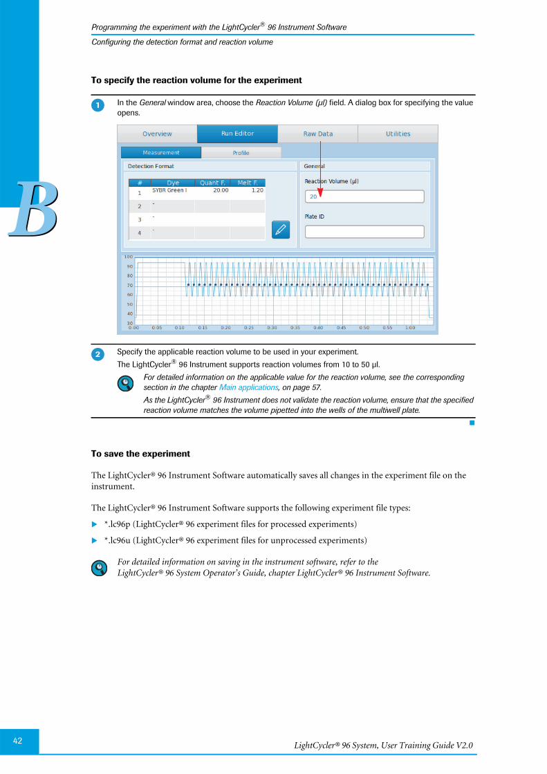
In the General window area, choose the Reaction Volume (µl) field. A dialog box for specifying the valueopens.
Specify the applicable reaction volume to be used in your experiment.
The LightCycler® 96 Instrument supports reaction volumes from 10 to 50 µl.
For detailed information on the applicable value for the reaction volume, see the correspondingsection in the chapter Main applications, on page 57.
As the LightCycler® 96 Instrument does not validate the reaction volume, ensure that the specifiedreaction volume matches the volume pipetted into the wells of the multiwell plate.
�
�
Programming and running an experiment
Running the experiment
43
BB
Starting the run
4 Running the experiment
After defining the setup parameters (temperature profile, reaction volume, and detection format), andsaving the definition, you are ready to run the LightCycler® 96 experiment.
For starting an experiment run, the experiment must be transferred to the LightCycler® 96 Instrument.An experiment run can only be started on the instrument using theLightCycler® 96 Instrument Software. For detailed information on how to transfer an experiment tothe instrument, see section Transferring the experiment to the instrument, on page 30.
During an experiment run, it is not recommended to use a USB drive, for example, for exporting orimporting data, or for synchronizing an experiment, as this may cause problems in the measurementprocess.
4.1 Starting the run
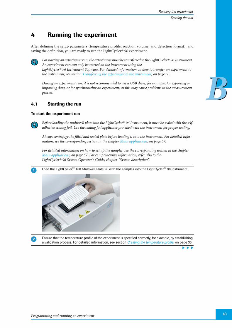
To start the experiment run
Before loading the multiwell plate into the LightCycler® 96 Instrument, it must be sealed with the self-adhesive sealing foil. Use the sealing foil applicator provided with the instrument for proper sealing.
Always centrifuge the filled and sealed plate before loading it into the instrument. For detailed infor-mation, see the corresponding section in the chapter Main applications, on page 57.
For detailed information on how to set up the samples, see the corresponding section in the chapterMain applications, on page 57. For comprehensive information, refer also to theLightCycler® 96 System Operator’s Guide, chapter "System description".
Load the LightCycler® 480 Multiwell Plate 96 with the samples into the LightCycler® 96 Instrument.
Ensure that the temperature profile of the experiment is specified correctly, for example, by establishinga validation process. For detailed information, see section Creating the temperature profile, on page 35.
�
�
LightCycler® 96 System, User Training Guide V2.044
Running the experiment
BB
Starting the run
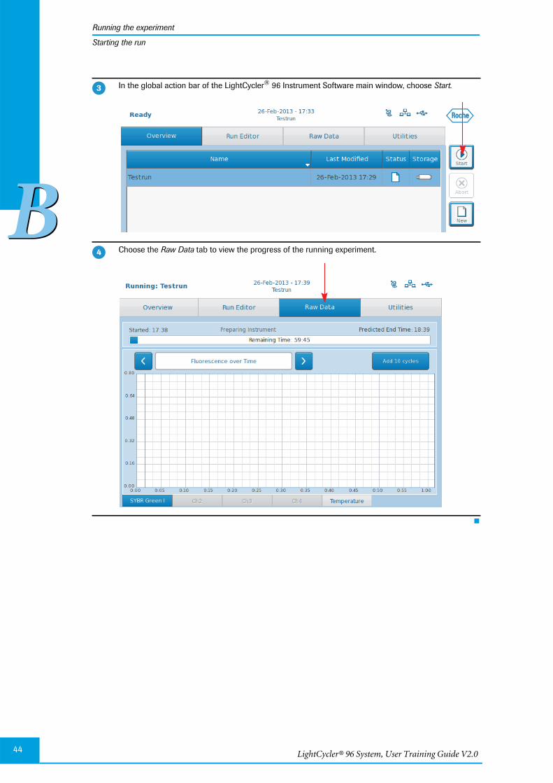
In the global action bar of the LightCycler® 96 Instrument Software main window, choose Start.
Choose the Raw Data tab to view the progress of the running experiment.
�
�

Programming and running an experiment
Running the experiment
45
BB
Monitoring the run
4.2 Monitoring the run
If the LightCycler® 96 Instrument and the computer running theLightCycler® 96 Application Software are not connected to a network, an experiment run can only bemonitored on the instrument using the LightCycler® 96 Instrument Software.
To monitor the experiment run
For a detailed description of the charts on the ‘Raw Data’ tab, refer to theLightCycler® 96 System Operator’s Guide, chapter LightCycler® 96 Instrument Software.
On the Raw Data tab, choose the Temperature tab to monitor the summary of the programs selected forthe experiment and their temperature and time settings in real time.
Choose one of the <dye> tabs, to monitor the relevant fluorescence curves, that is, the fluorescence in-tensity against the time in hours, minutes, and seconds for the entire run in real time. There is one curvefor each sample that has a gene labeled with the selected dye.
�
�
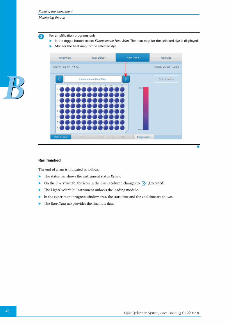
LightCycler® 96 System, User Training Guide V2.046
Running the experiment
BB
Monitoring the run
Run finished
The end of a run is indicated as follows:
The status bar shows the instrument status Ready.
On the Overview tab, the icon in the Status column changes to (Executed).
The LightCycler® 96 Instrument unlocks the loading module.
In the experiment progress window area, the start time and the end time are shown.
The Raw Data tab provides the final raw data.
For amplification programs only:
In the toggle button, select Fluorescence Heat Map. The heat map for the selected dye is displayed.
Monitor the heat map for the selected dye.
�
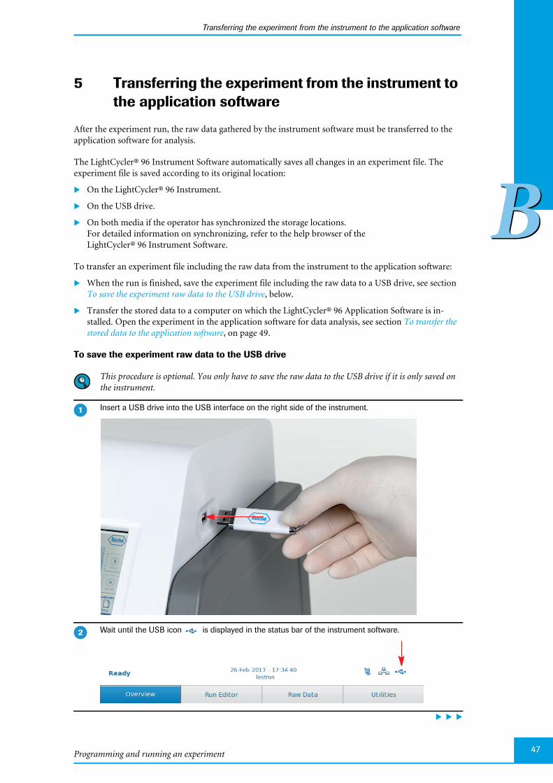
Programming and running an experiment
Transferring the experiment from the instrument to the application software
47
BB
5 Transferring the experiment from the instrument tothe application software
After the experiment run, the raw data gathered by the instrument software must be transferred to theapplication software for analysis.
The LightCycler® 96 Instrument Software automatically saves all changes in an experiment file. Theexperiment file is saved according to its original location:
On the LightCycler® 96 Instrument.
On the USB drive.
On both media if the operator has synchronized the storage locations.For detailed information on synchronizing, refer to the help browser of theLightCycler® 96 Instrument Software.
To transfer an experiment file including the raw data from the instrument to the application software:
When the run is finished, save the experiment file including the raw data to a USB drive, see sectionTo save the experiment raw data to the USB drive, below.
Transfer the stored data to a computer on which the LightCycler® 96 Application Software is in-stalled. Open the experiment in the application software for data analysis, see section To transfer thestored data to the application software, on page 49.
To save the experiment raw data to the USB drive
This procedure is optional. You only have to save the raw data to the USB drive if it is only saved onthe instrument.
Insert a USB drive into the USB interface on the right side of the instrument.
Wait until the USB icon is displayed in the status bar of the instrument software.
�
�
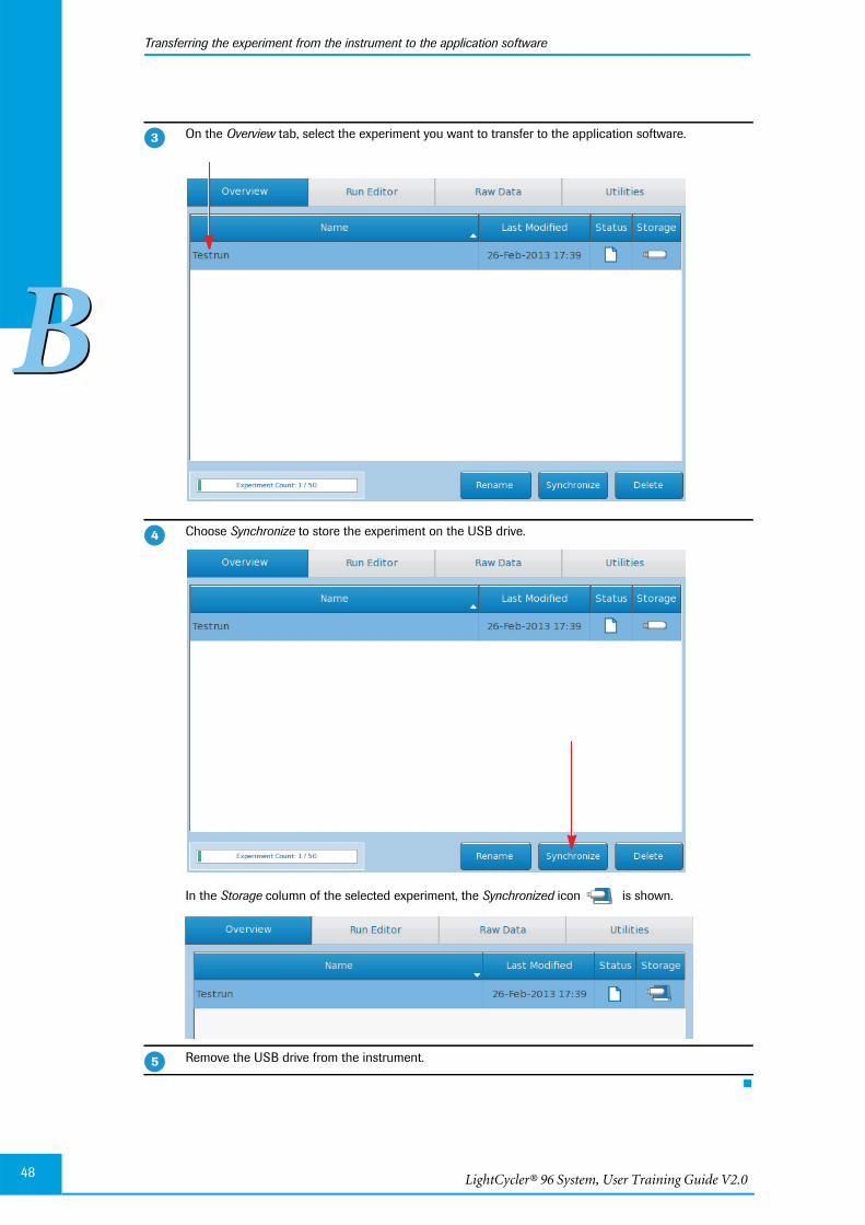
LightCycler® 96 System, User Training Guide V2.048
Transferring the experiment from the instrument to the application software
BB
On the Overview tab, select the experiment you want to transfer to the application software.
Choose Synchronize to store the experiment on the USB drive.
In the Storage column of the selected experiment, the Synchronized icon is shown.
Remove the USB drive from the instrument.
�
�
�
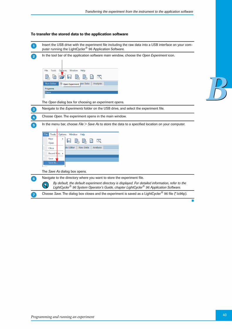
Programming and running an experiment
Transferring the experiment from the instrument to the application software
49
BB
To transfer the stored data to the application software
Insert the USB drive with the experiment file including the raw data into a USB interface on your com-puter running the LightCycler® 96 Application Software.
In the tool bar of the application software main window, choose the Open Experiment icon.
The Open dialog box for choosing an experiment opens.
Navigate to the Experiments folder on the USB drive, and select the experiment file.
Choose Open. The experiment opens in the main window.
In the menu bar, choose File > Save As to store the data to a specified location on your computer.
The Save As dialog box opens.
Navigate to the directory where you want to store the experiment file.
By default, the default experiment directory is displayed. For detailed information, refer to theLightCycler® 96 System Operator’s Guide, chapter LightCycler® 96 Application Software.
Choose Save. The dialog box closes and the experiment is saved as a LightCycler® 96 file (*.lc96p).
�
�
�
�
�
�
�

LightCycler® 96 System, User Training Guide V2.050
Editing the sample list
BB
6 Editing the sample list
For each experiment, you must edit the samples, that is, create, edit, delete, and rearrange samples andgenes present in the wells, as well as the dyes used to label each gene. This sample data is then used toperform the analysis.
For editing the sample list, the experiment must be opened in the LightCycler® 96Application Software.You can edit the sample list before or after the experiment run, depending on your preferred routine.
For editing the sample list, the ‘Sample Editor’ requires information about the selected dye(s). Whenyou edit the sample list before the experiment run (before transferring the experiment to the instrumentfor running), make sure that you have defined the run profile and selected the detection format in the‘Run Editor’.
The LightCycler® 96 Application Software offers two different views for editing the samples: the plateview and the table view. This user training guide describes how to edit the samples using the plate view,which shows the samples in 96 wells laid out to match the physical instrument. Changes in the plateview are immediately displayed in the table view and vice versa.
This section provides step-by-step information on how to edit the sample list in general. For detailed in-formation on further analysis-specific sample definitions for the different main applications, see the cor-responding section in the chapter Main applications, on page 57.
For a comprehensive description of all options of the LightCycler® 96 Application Software, refer to theLightCycler® 96 System Operator’s Guide, chapter LightCycler® 96 Application Software.
To edit the sample list:
Clear the empty wells to display only the applicable data, see section To clear empty wells, on page 51.
Specify the sample names and types, see section To edit the sample names and the sample types, onpage 53.
Assign a gene to the dye(s), see section To assign a gene to the dye(s), on page 55.

Programming and running an experiment
Editing the sample list
51
BB
To clear empty wells
Open the Sample Editor tab.
Open the Plate View.
In the multiwell plate image, choose the wells you want to clear, for example, columns 7 to 12:
Choose table header 7 to start the selection.
Press and hold down the [Shift] key on your keyboard.
Choose table header 12 to finish the selection.
All samples in the columns 7 to 12 are selected.
�
�
�

LightCycler® 96 System, User Training Guide V2.052
Editing the sample list
BB
Choose Clear Wells.
All property values are removed from the selected wells and the wells are deactivated. This means theycan no longer be edited and are not displayed in the table view or the analysis windows.
Repeat steps 3 and 4 for one or more rows of the multiwell plate image if necessary.
�
�
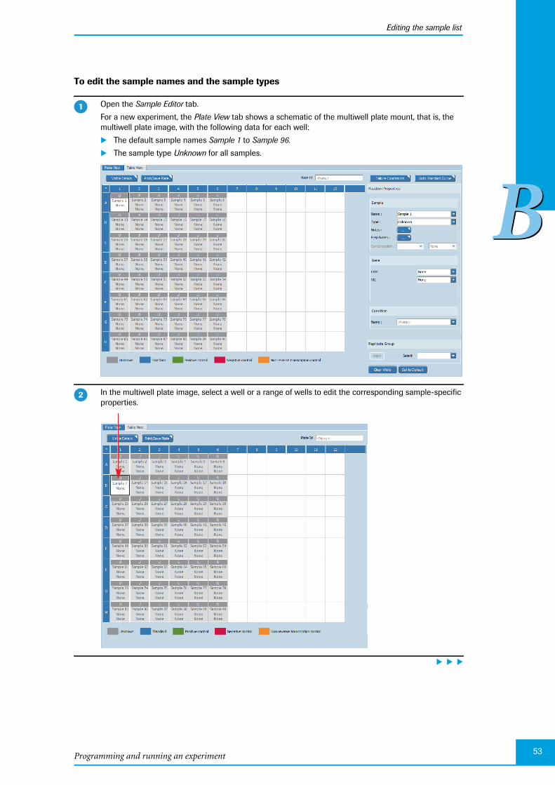
Programming and running an experiment
Editing the sample list
53
BB
To edit the sample names and the sample types
Open the Sample Editor tab.
For a new experiment, the Plate View tab shows a schematic of the multiwell plate mount, that is, themultiwell plate image, with the following data for each well:
The default sample names Sample 1 to Sample 96.
The sample type Unknown for all samples.
In the multiwell plate image, select a well or a range of wells to edit the corresponding sample-specificproperties.
�
�
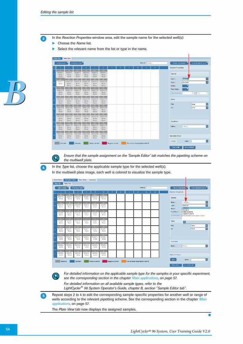
LightCycler® 96 System, User Training Guide V2.054
Editing the sample list
BB
In the Reaction Properties window area, edit the sample name for the selected well(s):
Choose the Name list.
Select the relevant name from the list or type in the name.
Ensure that the sample assignment on the ‘Sample Editor’ tab matches the pipetting scheme onthe multiwell plate.
In the Type list, choose the applicable sample type for the selected well(s).
In the multiwell plate image, each well is colored to visualize the sample type.
For detailed information on the applicable sample type for the samples in your specific experiment,see the corresponding section in the chapter Main applications, on page 57.
For detailed information on all available sample types, refer to theLightCycler® 96 System Operator’s Guide, chapter B, section "Sample Editor tab".
Repeat steps 2 to 4 to edit the corresponding sample-specific properties for another well or range ofwells according to the relevant pipetting scheme. See the corresponding section in the chapter Mainapplications, on page 57.
The Plate View tab now displays the assigned samples.
�
�
�
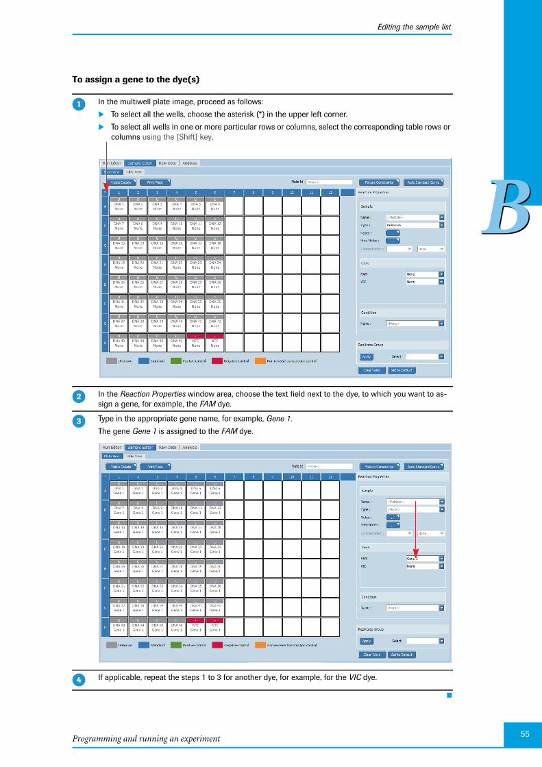
Programming and running an experiment
Editing the sample list
55
BB
To assign a gene to the dye(s)
In the multiwell plate image, proceed as follows:
To select all the wells, choose the asterisk (*) in the upper left corner.
To select all wells in one or more particular rows or columns, select the corresponding table rows orcolumns using the [Shift] key.
In the Reaction Properties window area, choose the text field next to the dye, to which you want to as-sign a gene, for example, the FAM dye.
Type in the appropriate gene name, for example, Gene 1.
The gene Gene 1 is assigned to the FAM dye.
If applicable, repeat the steps 1 to 3 for another dye, for example, for the VIC dye.
�
�
�
�
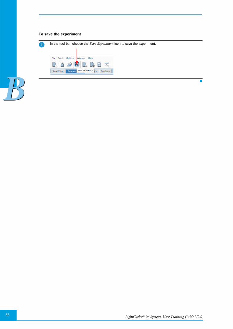
LightCycler® 96 System, User Training Guide V2.0
BB
56
To save the experiment
In the tool bar, choose the Save Experiment icon to save the experiment.
�
Main applications 57
CC
Main applications 0For information on the order in which you must perform the individual work steps of a complete ap-plication workflow, see section Overview, on page 15.
This chapter shows how to perform experiments with the LightCycler® 96 System using the following ex-amples:
Absolute quantification, on page 58.
Endpoint SNP genotyping, on page 78.
Relative quantification, on page 98.
Qualitative detection, on page 120.
Tm calling, on page 134.
High resolution melting, on page 147.
For all experiments a LightCycler® 480 Multiwell Plate 96, white, is used.
For each application, this chapter provides the following information:
How to set up the nucleic acid samples.
The applicable experiment run parameters relating to the temperature profile, detection format, andreaction volume.
The applicable basic sample data parameters relating to the empty wells, the sample names, the sampletypes, and the gene assignment.
How to edit the special sample data settings.
How to analyze the results.
Preconditions for all runs
A run can only be performed if:
The instrument is started; see section Starting the LightCycler® 96 Instrument, on page 17.
The experiment definition is transferred to the instrument if it was defined with the application soft-ware.
For a detailed description of the LightCycler® 96 Application Software and all elements of the graphi-cal user interface, refer to the LightCycler® 96 System Operator’s Guide, chapterLightCycler® 96 Application Software.
For a detailed description of the LightCycler® 96 Instrument Software and all elements of the graphicaluser interface, refer to the LightCycler® 96 System Operator’s Guide, chapterLightCycler® 96 Instrument Software.
LightCycler® 96 System, User Training Guide V2.058
Absolute quantification
CC
Experiment overview
1 Absolute quantification
Absolute quantification is used to quantify a gene and express the final result as an absolute value (forexample, copies/ml). Samples with an unknown quantity of gene are amplified alongside a dilution seriesof a gene-specific standard with known concentration. To obtain an absolute value for an unknown quan-tity of gene, the Cq of an unknown sample is compared to those of standards with known quantities.
In an absolute quantification analysis, the known concentration of each standard is automatically plottedagainst the measured Cq values. The resulting regression line is called the standard curve and shows thecorrelation between Cq and quantity. The concentration of an unknown sample is calculated by compar-ing its Cq with the standard curve.
For detailed information on absolute quantification analysis, refer to theLightCycler® 96 System Operator’s Guide, chapter A, section "Analysis principles".
1.1 Experiment overview
The following example describes how to set up, run, and analyze an assay for gene quantification using aFAM-labeled hydrolysis probe. Quantification of samples is based on a 5-point standard curve derivedfrom a plasmid standard dilution series covering a range of known quantities.
The assay is performed using a LightCycler® 480 Multiwell Plate 96, white. Each sample is set up in trip-licate.
1.2 Setting up the samples
Sample dilution
The standard sample is diluted to a 10-fold dilution series covering a range of 0.1 to 1000 ng/5 µl.
Continuously cool the samples during setup by keeping the reaction tubes on ice.
Controls
To ensure the absence of contaminating nucleic acids in PCR reagents, it is highly recommended that youinclude a no template control (NTC) in your experiment.
Samples Standard samples: Human Genomic DNA from human blood 0.1 ng to 1000 ng
5 DNA samples (unknown concentration)
Reagents FastStart Essential DNA Probes Master (2 x conc.)
RealTime ready Catalog AssaysAssay ID: 137341 (HSPA2)
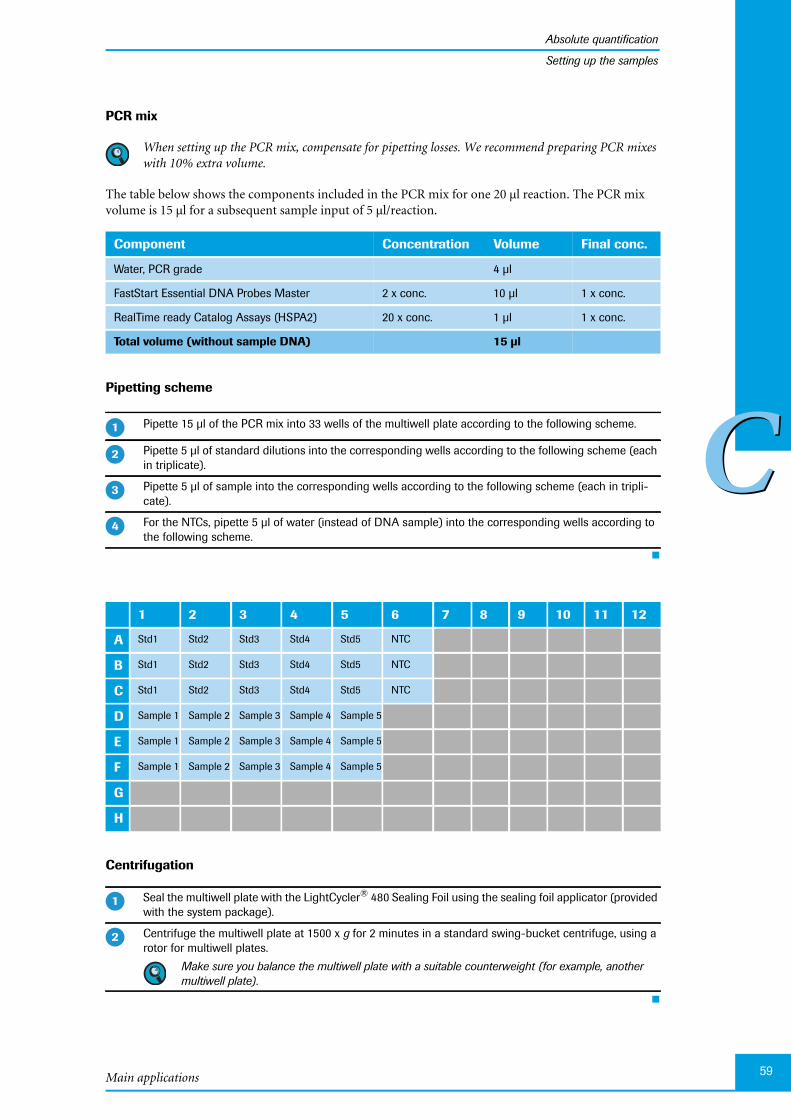
Main applications
Absolute quantification
59
CC
Setting up the samples
PCR mix
When setting up the PCR mix, compensate for pipetting losses. We recommend preparing PCR mixeswith 10% extra volume.
The table below shows the components included in the PCR mix for one 20 µl reaction. The PCR mixvolume is 15 µl for a subsequent sample input of 5 µl/reaction.
Pipetting scheme
Centrifugation
Component Concentration Volume Final conc.
Water, PCR grade 4 µl
FastStart Essential DNA Probes Master 2 x conc. 10 µl 1 x conc.
RealTime ready Catalog Assays (HSPA2) 20 x conc. 1 µl 1 x conc.
Total volume (without sample DNA) 15 µl
Pipette 15 µl of the PCR mix into 33 wells of the multiwell plate according to the following scheme.
Pipette 5 µl of standard dilutions into the corresponding wells according to the following scheme (eachin triplicate).
Pipette 5 µl of sample into the corresponding wells according to the following scheme (each in tripli-cate).
For the NTCs, pipette 5 µl of water (instead of DNA sample) into the corresponding wells according tothe following scheme.
1 2 3 4 5 6 7 8 9 10 11 12
A Std1 Std2 Std3 Std4 Std5 NTC
B Std1 Std2 Std3 Std4 Std5 NTC
C Std1 Std2 Std3 Std4 Std5 NTC
D Sample 1 Sample 2 Sample 3 Sample 4 Sample 5
E Sample 1 Sample 2 Sample 3 Sample 4 Sample 5
F Sample 1 Sample 2 Sample 3 Sample 4 Sample 5
G
H
Seal the multiwell plate with the LightCycler® 480 Sealing Foil using the sealing foil applicator (providedwith the system package).
Centrifuge the multiwell plate at 1500 x g for 2 minutes in a standard swing-bucket centrifuge, using arotor for multiwell plates.
Make sure you balance the multiwell plate with a suitable counterweight (for example, anothermultiwell plate).
�
�
�
�
�
�

LightCycler® 96 System, User Training Guide V2.060
Absolute quantification
CC
Experiment run parameters
1.3 Experiment run parameters
For detailed information on how to program an experiment, see one of the following sections:Programming the experiment with the LightCycler® 96 Application Software, on page 20.Programming the experiment with the LightCycler® 96 Instrument Software, on page 32.
Use a standard PCR profile for hydrolysis probes.
The experiment includes the run parameters listed in the following tables.
Temperature profile
For detailed information on how to program a temperature profile, see one of the following sections:For working with the LightCycler® 96 Application Software: Creating the temperature profile, onpage 23.For working with the LightCycler® 96 Instrument Software: Creating the temperature profile, onpage 35.
For this example, use the following heating and cooling cycles:
It is not necessary to add a separate cooling program at the end of the run. At the end of each run, thesamples are automatically cooled to +37°C.
For the ramp rate for heating and cooling (Ramp (°C/s)), the default values are used in this example.
For the steps of the amplification program, the following default settings are used in this example:
LightCycler® 96 Application Software: For Gradient and Touch down, the default settings are used.
For Mode, the default Standard option is used.
In the Temperature Profile window area, the following graphical summary of the programs selected for theexperiment and their temperature and time settings is displayed.
Programs Steps
Name Number ofcycles
Ramp (°C/s) Duration (s) Target (°C) AcquisitionMode
Preincubation 1 4.4 600 95 None
3-step amplifi-cation
45 4.4 10 95 None
2.2 30 60 None
4.4 1 72 Single
Cooling 1 2.2 30 37 None

Main applications
Absolute quantification
61
CC
Experiment run parameters
Detection format
Selecting the dye for this mono-color experiment determines the channel combination for the measure-ment during the run. For all other parameters, the default values are used in this example.
For detailed information on how to specify the detection format, see the following sections:For working with the LightCycler® 96 Application Software: To specify the detection format for the ex-periment, on page 27.For working with the LightCycler® 96 Instrument Software: To specify the detection format for the ex-periment, on page 40.
For this example, use the following channel:
Reaction volume
As the LightCycler® 96 Instrument does not validate the reaction volume, ensure that the specified re-action volume matches the volume pipetted into the wells of the multiwell plate.
For detailed information on how to specify the reaction volume, see one of the following sections:For working with the LightCycler® 96 Application Software: To specify the reaction volume for the ex-periment, on page 27.For working with the LightCycler® 96 Instrument Software: To specify the reaction volume for the ex-periment, on page 42.
For this example, use the following reaction volume:
Experiment run
Once you have set up the samples and defined the experiment run parameters, you can start the run. Fordetailed information on how to run the experiment, see section Running the experiment, on page 43.
Dye Channel
FAM 470/514
Reaction volume
20 µl
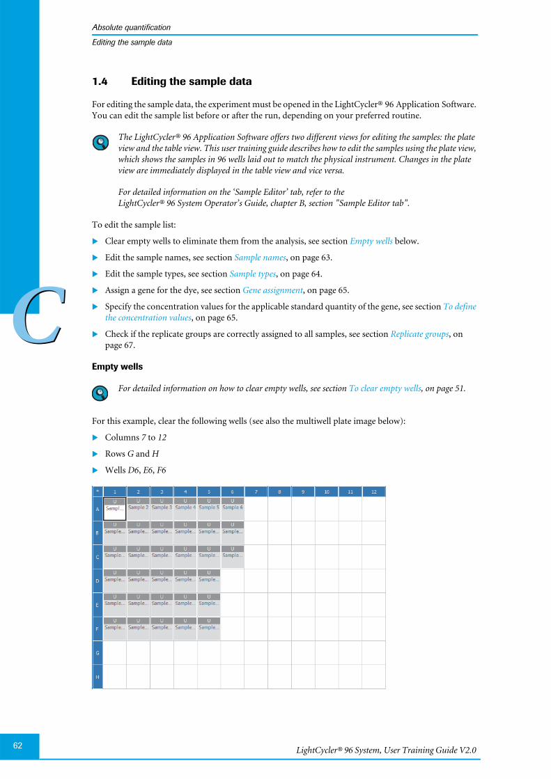
LightCycler® 96 System, User Training Guide V2.062
Absolute quantification
CC
Editing the sample data
1.4 Editing the sample data
For editing the sample data, the experiment must be opened in the LightCycler® 96 Application Software.You can edit the sample list before or after the run, depending on your preferred routine.
The LightCycler® 96 Application Software offers two different views for editing the samples: the plateview and the table view. This user training guide describes how to edit the samples using the plate view,which shows the samples in 96 wells laid out to match the physical instrument. Changes in the plateview are immediately displayed in the table view and vice versa.
For detailed information on the ‘Sample Editor’ tab, refer to theLightCycler® 96 System Operator’s Guide, chapter B, section "Sample Editor tab".
To edit the sample list:
Clear empty wells to eliminate them from the analysis, see section Empty wells below.
Edit the sample names, see section Sample names, on page 63.
Edit the sample types, see section Sample types, on page 64.
Assign a gene for the dye, see section Gene assignment, on page 65.
Specify the concentration values for the applicable standard quantity of the gene, see section To definethe concentration values, on page 65.
Check if the replicate groups are correctly assigned to all samples, see section Replicate groups, onpage 67.
Empty wells
For detailed information on how to clear empty wells, see section To clear empty wells, on page 51.
For this example, clear the following wells (see also the multiwell plate image below):
Columns 7 to 12
Rows G and H
Wells D6, E6, F6
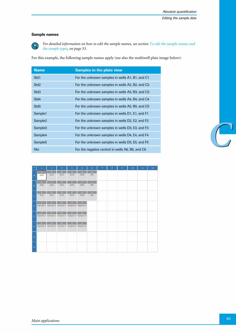
Main applications
Absolute quantification
63
CC
Editing the sample data
Sample names
For detailed information on how to edit the sample names, see section To edit the sample names andthe sample types, on page 53.
For this example, the following sample names apply (see also the multiwell plate image below):
Name Samples in the plate view
Std1 For the unknown samples in wells A1, B1, and C1
Std2 For the unknown samples in wells A2, B2, and C2
Std3 For the unknown samples in wells A3, B3, and C3
Std4 For the unknown samples in wells A4, B4, and C4
Std5 For the unknown samples in wells A5, B5, and C5
Sample1 For the unknown samples in wells D1, E1, and F1
Sample2 For the unknown samples in wells D2, E2, and F2
Sample3 For the unknown samples in wells D3, E3, and F3
Sample4 For the unknown samples in wells D4, E4, and F4
Sample5 For the unknown samples in wells D5, E5, and F5
Ntc For the negative control in wells A6, B6, and C6
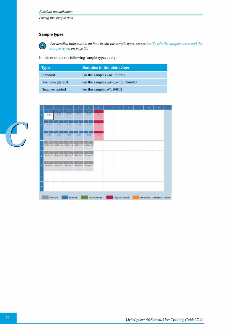
LightCycler® 96 System, User Training Guide V2.064
Absolute quantification
CC
Editing the sample data
Sample types
For detailed information on how to edit the sample types, see section To edit the sample names and thesample types, on page 53.
In this example the following sample types apply:
Type Samples in the plate view
Standard For the samples Std1 to Std5
Unknown (default) For the samples Sample1 to Sample5
Negative control For the samples Ntc (NTC)
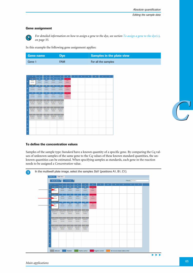
Main applications
Absolute quantification
65
CC
Editing the sample data
Gene assignment
For detailed information on how to assign a gene to the dye, see section To assign a gene to the dye(s),on page 55.
In this example the following gene assignment applies:
To define the concentration values
Samples of the sample type Standard have a known quantity of a specific gene. By comparing the Cq val-ues of unknown samples of the same gene to the Cq values of these known standard quantities, the un-known quantities can be estimated. When specifying samples as standards, each gene in the reactionneeds to be assigned a Concentration value.
Gene name Dye Samples in the plate view
Gene 1 FAM For all the samples
In the multiwell plate image, select the samples Std1 (positions A1, B1, C1).
�
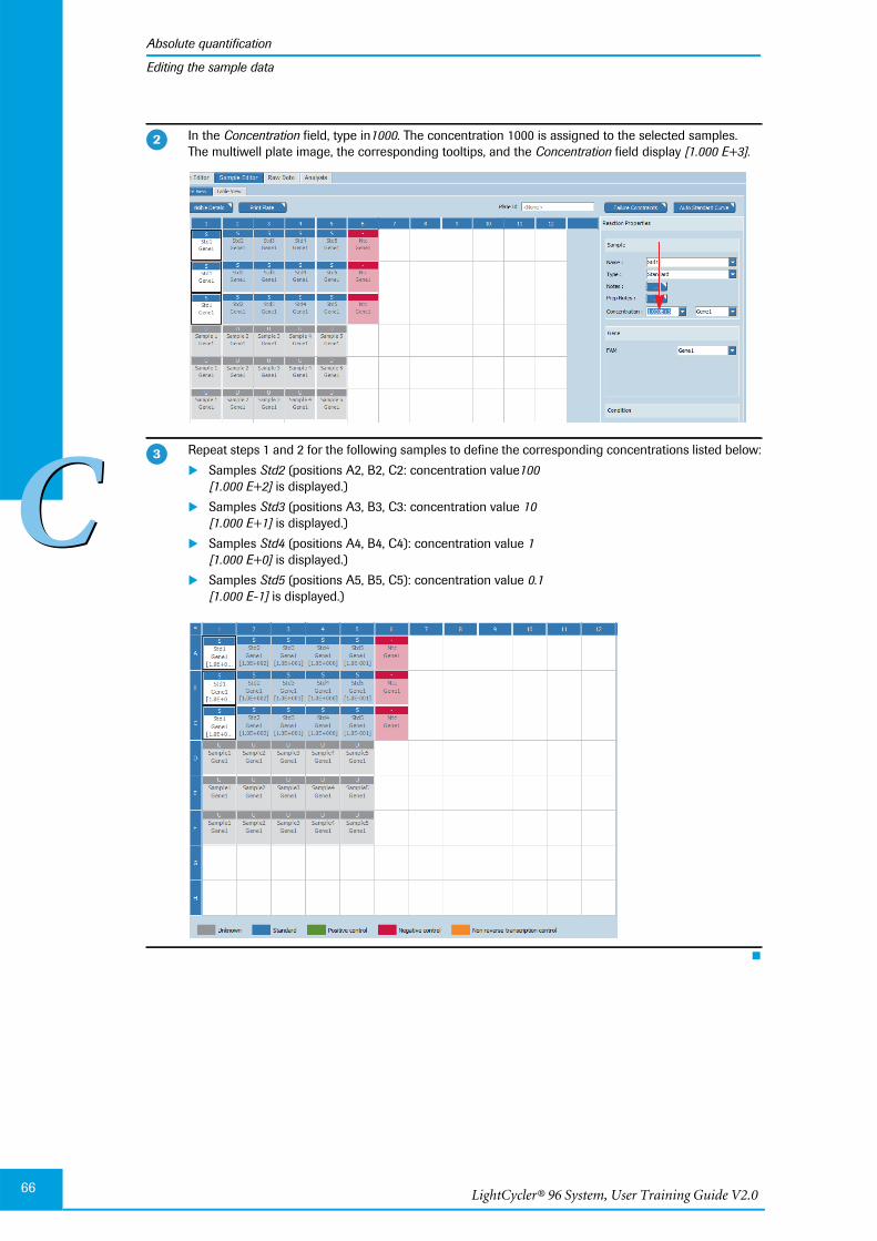
LightCycler® 96 System, User Training Guide V2.066
Absolute quantification
CC
Editing the sample data
In the Concentration field, type in1000. The concentration 1000 is assigned to the selected samples.The multiwell plate image, the corresponding tooltips, and the Concentration field display [1.000 E+3].
Repeat steps 1 and 2 for the following samples to define the corresponding concentrations listed below:
Samples Std2 (positions A2, B2, C2: concentration value100[1.000 E+2] is displayed.)
Samples Std3 (positions A3, B3, C3: concentration value 10[1.000 E+1] is displayed.)
Samples Std4 (positions A4, B4, C4): concentration value 1[1.000 E+0] is displayed.)
Samples Std5 (positions A5, B5, C5): concentration value 0.1[1.000 E-1] is displayed.)
�
�

Main applications
Absolute quantification
67
CC
Editing the sample data
Replicate groups
The LightCycler® 96 Application Software automatically groups samples into replicate groups, providedthey have identical values for the following properties:
Sample name
Sample type
Concentration
Gene name
Each replicate group is named according to the top leftmost of the grouped samples.
Changing one of these properties removes the corresponding sample from the replicate group.
Check if the multiwell plate image displays the same replicate groups for samples with identical values.
�

LightCycler® 96 System, User Training Guide V2.068
Absolute quantification
CC
Analyzing the results
1.5 Analyzing the results
For detailed information on the ‘Analysis’ tab, refer to the LightCycler® 96 System Operator’s Guide,chapter B, section "Absolute quantification".
For detailed information on working with tables and graphs, refer to theLightCycler® 96 System Operator’s Guide, chapter B, section "General software conventions".
To analyze the calculated results of the absolute quantification application:
Create the absolute quantification analysis, see section Creating the analysis below.
Optional: Specify the settings for the absolute quantification analysis, see section Analysis settings, onpage 70.
In the different views of the Abs Quant tab, check the analysis results and customize the result data ifnecessary:
For the Amplification Curves view, see section Amplification curves, on page 71.
For the Standard Curves view, see section Standard curve, on page 72.
For the Heat Map view, see section Heat map, on page 73.
For the Result Table view, see section Result table, on page 73.
For the Cq Bars view, see section Cq bars, on page 77.
1.5.1 Creating the analysis
To create the Abs Quant analysis
Open the Analysis tab.
In the tool bar, choose the Add Analysis icon to add a new analysis.
The Create New Analysis dialog box opens.
Choose Abs Quant.
�
�
�

Main applications
Absolute quantification
69
CC
Analyzing the results
Choose OK.
The Analysis tab displays four different views for the experiment using default values:
Amplification Curves
Standard Curves
Heat Map
Result Table
�

LightCycler® 96 System, User Training Guide V2.070
Absolute quantification
CC
Analyzing the results
1.5.2 Analysis settings
Optional: To specify the analysis settings
In the tool bar, choose the Analysis Settings icon.
The Abs Quant Settings dialog box opens.
In the Abs Quant Settings dialog box, specify the analysis-specific settings, for example:
On the Genes tab, remove a gene from the analysis.
On the Samples tab, remove samples from the analysis.
�
�

Main applications
Absolute quantification
71
CC
Analyzing the results
1.5.3 Amplification curves
On the Abs Quant tab, amplification curves display the fluorescence intensity against the number of cyclesin the amplification program. There is one curve for each sample that has a gene labeled with the selecteddye.
Optional: To modify the y axis scaling
Optional: For better distinction, perform the following steps:
Color all curves for the standard samples in one color and the curves for the unknown samples inanother. For detailed information on how to change the color of the samples, see section To changethe color of the samples, on page 74.
Modify the y axis scaling. For detailed information on how to modify the scaling of the y axis, seesection Optional: To modify the y axis scaling, below.
Check the Amplification Curves chart for correct amplification.
Choose the Y Axis Scaling icon.
The Axis Scaling Settings dialog box opens.
�
�
�
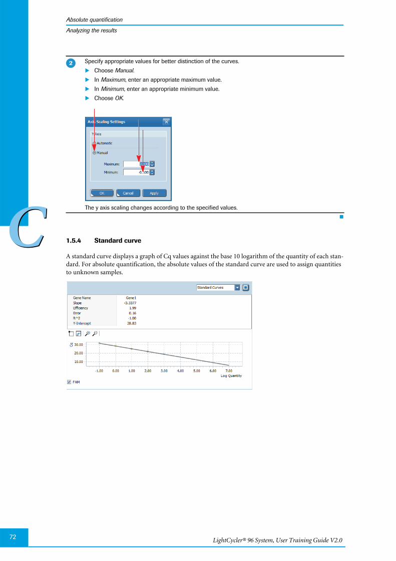
LightCycler® 96 System, User Training Guide V2.072
Absolute quantification
CC
Analyzing the results
1.5.4 Standard curve
A standard curve displays a graph of Cq values against the base 10 logarithm of the quantity of each stan-dard. For absolute quantification, the absolute values of the standard curve are used to assign quantitiesto unknown samples.
Specify appropriate values for better distinction of the curves.
Choose Manual.
In Maximum, enter an appropriate maximum value.
In Minimum, enter an appropriate minimum value.
Choose OK.
The y axis scaling changes according to the specified values.
�
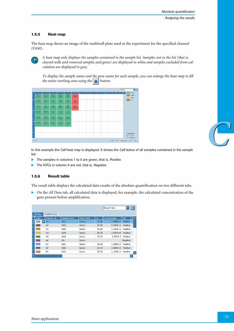
Main applications
Absolute quantification
73
CC
Analyzing the results
1.5.5 Heat map
The heat map shows an image of the multiwell plate used in the experiment for the specified channel(FAM).
A heat map only displays the samples contained in the sample list. Samples not in the list (that is,cleared wells and removed samples and genes) are displayed in white and samples excluded from cal-culation are displayed in gray.
To display the sample name and the gene name for each sample, you can enlarge the heat map to fillthe entire working area using the button.
In this example the Call heat map is displayed. It shows the Call status of all samples contained in the samplelist:
The samples in columns 1 to 5 are green, that is, Positive.
The NTCs in column 6 are red, that is, Negative.
1.5.6 Result table
The result table displays the calculated data results of the absolute quantification on two different tabs.
On the All Data tab, all calculated data is displayed, for example, the calculated concentration of thegene present before amplification.
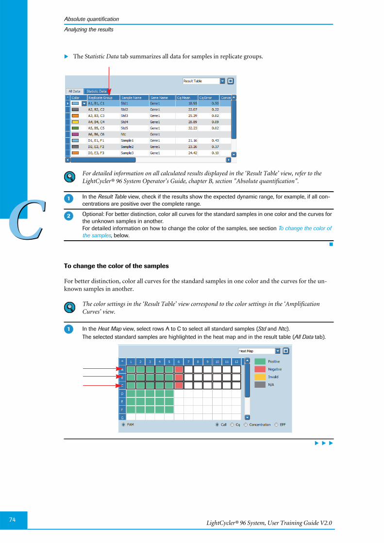
LightCycler® 96 System, User Training Guide V2.074
Absolute quantification
CC
Analyzing the results
The Statistic Data tab summarizes all data for samples in replicate groups.
For detailed information on all calculated results displayed in the ‘Result Table’ view, refer to theLightCycler® 96 System Operator’s Guide, chapter B, section "Absolute quantification".
To change the color of the samples
For better distinction, color all curves for the standard samples in one color and the curves for the un-known samples in another.
The color settings in the ‘Result Table’ view correspond to the color settings in the ‘AmplificationCurves’ view.
In the Result Table view, check if the results show the expected dynamic range, for example, if all con-centrations are positive over the complete range.
Optional: For better distinction, color all curves for the standard samples in one color and the curves forthe unknown samples in another.For detailed information on how to change the color of the samples, see section To change the color ofthe samples, below.
In the Heat Map view, select rows A to C to select all standard samples (Std and Ntc).The selected standard samples are highlighted in the heat map and in the result table (All Data tab).
�
�
�
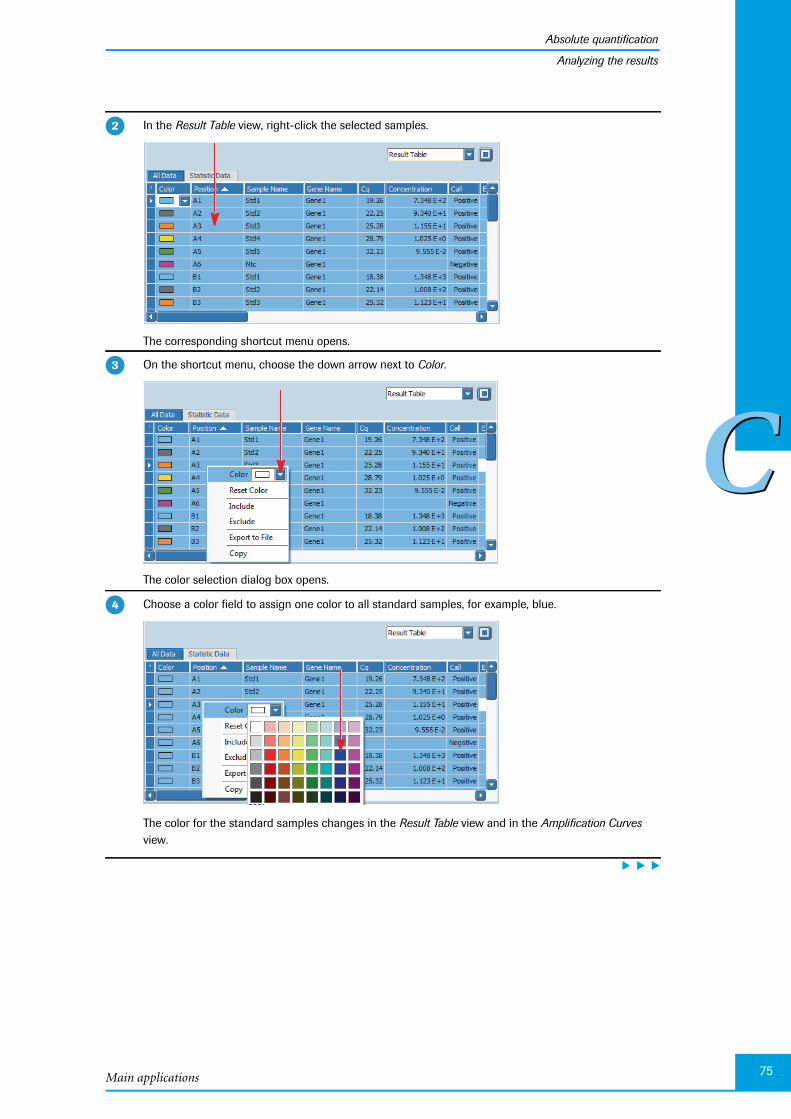
Main applications
Absolute quantification
75
CC
Analyzing the results
In the Result Table view, right-click the selected samples.
The corresponding shortcut menu opens.
On the shortcut menu, choose the down arrow next to Color.
The color selection dialog box opens.
Choose a color field to assign one color to all standard samples, for example, blue.
The color for the standard samples changes in the Result Table view and in the Amplification Curvesview.
�
�
�
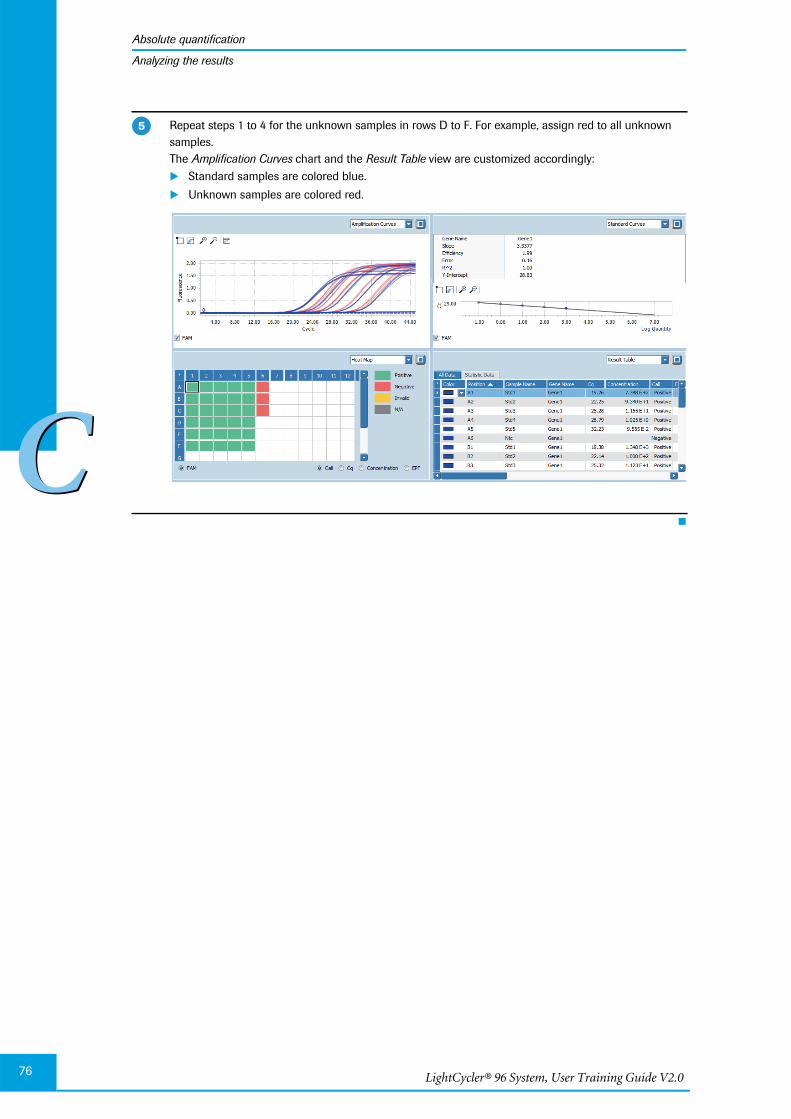
LightCycler® 96 System, User Training Guide V2.076
Absolute quantification
CC
Analyzing the results
Repeat steps 1 to 4 for the unknown samples in rows D to F. For example, assign red to all unknownsamples.The Amplification Curves chart and the Result Table view are customized accordingly: Standard samples are colored blue.
Unknown samples are colored red.
�

Main applications
Absolute quantification
77
CC
Exporting result data
1.5.7 Cq bars
The Cq Bars chart shows the same Cq data as the result table, but in a bar chart format. Each bar repre-sents a Cq value. The Cq Bars chart shows the corresponding Cq for each gene and each sample.
1.6 Exporting result data
You can export the following result data to Microsoft Word or Excel:
The result table as a text file.
The result graphs as a PNG file, GIF file, or text file.
For detailed information on how to export result data, refer to theLightCycler® 96 System Operator’s Guide, chapter B, section "Exporting analysis results".
Optional: For better distinction, customize the y axis scaling.For detailed information on how to modify the scaling of the y axis, see section Optional: To modify the yaxis scaling, on page 71
�
LightCycler® 96 System, User Training Guide V2.078
Endpoint SNP genotyping
CC
Experiment overview
2 Endpoint SNP genotyping
Endpoint SNP genotyping assays use hydrolysis probes for single-nucleotide polymorphism (SNP) geno-typing. Two sequence-specific probes detect the wild type and mutant alleles. Each is labeled with differ-ent reporter dyes, most frequently with a FAM dye and a VIC dye. Fluorescence data are collected usingPCR. To identify genotypes, only endpoint fluorescence intensities of the two reporter dyes are used. Rel-ative dye intensities discriminate between homozygous for allele x, homozygous for allele y, and hetero-zygous alleles.
For detailed information, refer to the LightCycler® 96 System Operator’s Guide, chapter A, sections"Detection formats" and "Endpoint genotyping analysis".
2.1 Experiment overview
The following example describes how to set up, run, and analyze a dual-color endpoint SNP genotypingassay.
The assay is performed using a LightCycler® 480 Multiwell Plate 96, white.
2.2 Setting up the samples
To set up the samples:
Set up the sample dilutions, see section Sample dilution below.
Include a no template control (NTC), see section Controls below.
Prepare the PCR mix, see section PCR mix, on page 79.
Pipette the sample dilution and the PCR mix, see section Pipetting scheme, on page 79.
Centrifuge the multiwell plate, see section Centrifugation, on page 79
Continuously cool the samples and PCR mix during setup by keeping the reaction tubes on ice.
Sample dilution
The human genomic DNA samples (concentration approximately 90 ng/µl) are diluted to a consistentconcentration of 5 ng/5 µl.
Controls
To ensure an accurate endpoint genotyping analysis, it is highly recommended that you include a no tem-plate control (NTC) in your experiment.
Samples 46 human genomic DNA samples, isolated with the MagNA Pure LC 2.0 Instrument(concentration approximately 90 ng/µl)
Reagents FastStart Essential DNA Probes Master (2 x conc.)
Genotyping mix (40 x conc.), containing forward primer, reverse primer, and twohydrolysis probes labeled with FAM and VIC respectively
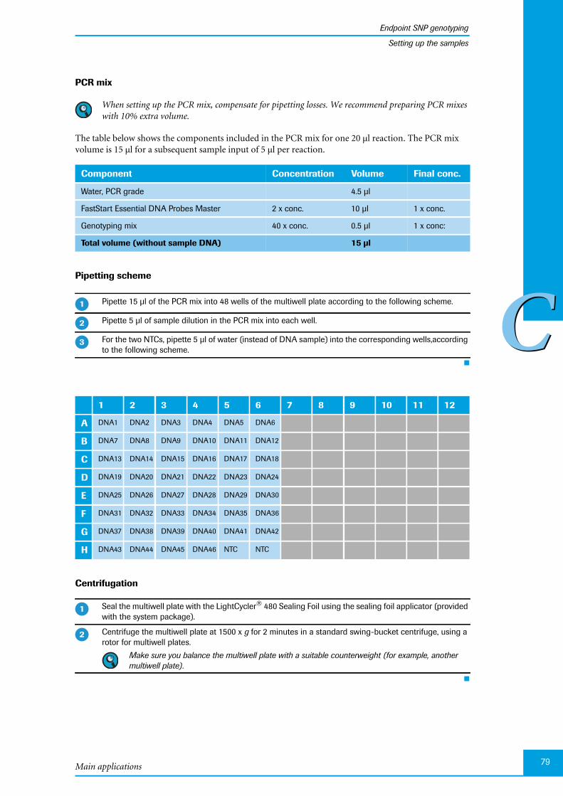
Main applications
Endpoint SNP genotyping
79
CC
Setting up the samples
PCR mix
When setting up the PCR mix, compensate for pipetting losses. We recommend preparing PCR mixeswith 10% extra volume.
The table below shows the components included in the PCR mix for one 20 µl reaction. The PCR mixvolume is 15 µl for a subsequent sample input of 5 µl per reaction.
Pipetting scheme
Centrifugation
Component Concentration Volume Final conc.
Water, PCR grade 4.5 µl
FastStart Essential DNA Probes Master 2 x conc. 10 µl 1 x conc.
Genotyping mix 40 x conc. 0.5 µl 1 x conc:
Total volume (without sample DNA) 15 µl
Pipette 15 µl of the PCR mix into 48 wells of the multiwell plate according to the following scheme.
Pipette 5 µl of sample dilution in the PCR mix into each well.
For the two NTCs, pipette 5 µl of water (instead of DNA sample) into the corresponding wells,accordingto the following scheme.
1 2 3 4 5 6 7 8 9 10 11 12
A DNA1 DNA2 DNA3 DNA4 DNA5 DNA6
B DNA7 DNA8 DNA9 DNA10 DNA11 DNA12
C DNA13 DNA14 DNA15 DNA16 DNA17 DNA18
D DNA19 DNA20 DNA21 DNA22 DNA23 DNA24
E DNA25 DNA26 DNA27 DNA28 DNA29 DNA30
F DNA31 DNA32 DNA33 DNA34 DNA35 DNA36
G DNA37 DNA38 DNA39 DNA40 DNA41 DNA42
H DNA43 DNA44 DNA45 DNA46 NTC NTC
Seal the multiwell plate with the LightCycler® 480 Sealing Foil using the sealing foil applicator (providedwith the system package).
Centrifuge the multiwell plate at 1500 x g for 2 minutes in a standard swing-bucket centrifuge, using arotor for multiwell plates.
Make sure you balance the multiwell plate with a suitable counterweight (for example, anothermultiwell plate).
�
�
�
�
�

LightCycler® 96 System, User Training Guide V2.080
Endpoint SNP genotyping
CC
Experiment run parameters
2.3 Experiment run parameters
For detailed information on how to program an experiment, see one of the following sections:Programming the experiment with the LightCycler® 96 Application Software, on page 20.Programming the experiment with the LightCycler® 96 Instrument Software, on page 32.
For this experiment, a standard PCR profile for hydrolysis probes is used. The experiment includes therun parameters for the temperature profile, the detection format, and the reaction volume. These param-eters are listed in the following tables.
Temperature profile
For detailed information on how to program a temperature profile, see one of the following sections:For working with the LightCycler® 96 Application Software: Creating the temperature profile, onpage 23.For working with the LightCycler® 96 Instrument Software: Creating the temperature profile, onpage 35.
For this example, use the following heating and cooling cycles:
It is not necessary to add a separate cooling program at the end of the run. At the end of each run, thesamples are automatically cooled to +37°C.
For the ramp rate for heating and cooling (Ramp (°C/s)), the default values are used in this example.
For the steps of the amplification program, the following default settings are used in this example:
LightCycler® 96 Application Software: For Gradient and Touch down, the default settings are used.
For Mode, the default Standard option is used.
In the Temperature Profile window area, the following graphical summary of the programs selected for theexperiment and their temperature and time settings is displayed.
Programs Steps
Name Number ofcycles
Ramp (°C/s) Duration (s) Target (°C) AcquisitionMode
Preincubation 1 4.4 600 95 None
2-step amplifi-cation
45 4.4 10 95 None
2.2 60 60 Single
Cooling 1 2.2 30 37 None
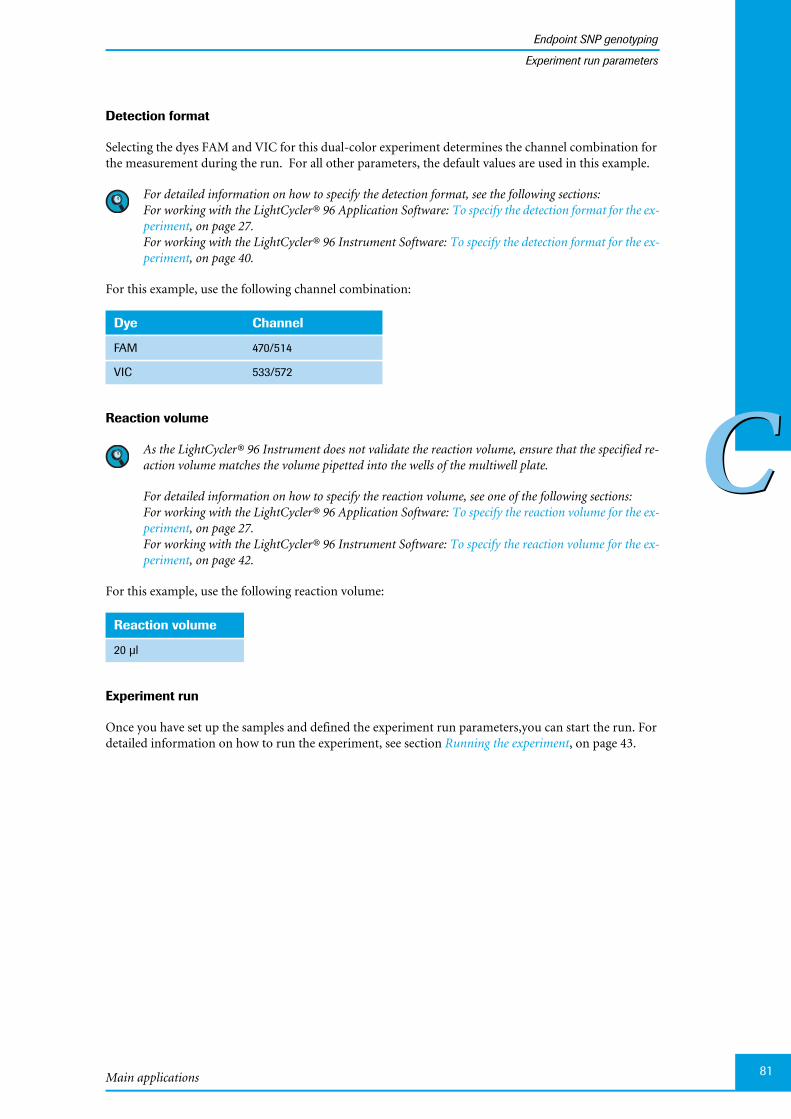
Main applications
Endpoint SNP genotyping
81
CC
Experiment run parameters
Detection format
Selecting the dyes FAM and VIC for this dual-color experiment determines the channel combination forthe measurement during the run. For all other parameters, the default values are used in this example.
For detailed information on how to specify the detection format, see the following sections:For working with the LightCycler® 96 Application Software: To specify the detection format for the ex-periment, on page 27.For working with the LightCycler® 96 Instrument Software: To specify the detection format for the ex-periment, on page 40.
For this example, use the following channel combination:
Reaction volume
As the LightCycler® 96 Instrument does not validate the reaction volume, ensure that the specified re-action volume matches the volume pipetted into the wells of the multiwell plate.
For detailed information on how to specify the reaction volume, see one of the following sections:For working with the LightCycler® 96 Application Software: To specify the reaction volume for the ex-periment, on page 27.For working with the LightCycler® 96 Instrument Software: To specify the reaction volume for the ex-periment, on page 42.
For this example, use the following reaction volume:
Experiment run
Once you have set up the samples and defined the experiment run parameters,you can start the run. Fordetailed information on how to run the experiment, see section Running the experiment, on page 43.
Dye Channel
FAM 470/514
VIC 533/572
Reaction volume
20 µl

LightCycler® 96 System, User Training Guide V2.082
Endpoint SNP genotyping
CC
Editing the sample data
2.4 Editing the sample data
For editing the sample data, the experiment must be opened in the LightCycler® 96 Application Software.You can edit the sample list before or after the run, depending on your preferred routine.
The LightCycler® 96 Application Software offers two different views for editing the samples: the plateview and the table view. This user training guide describes how to edit the samples using the plate view,which shows the samples in 96 wells laid out to match the physical instrument. Changes in the plateview are immediately displayed in the table view and vice versa.
For detailed information on the ‘Sample Editor’ tab, refer to theLightCycler® 96 System Operator’s Guide, chapter B, section "Sample Editor tab".
To edit the sample list:
Clear empty wells to eliminate them from the analysis, see section Empty wells below.
Edit the sample names, see section Sample names, on page 83.
Edit the sample types, see section Sample types, on page 84.
Assign a gene for each dye, see section Gene assignment, on page 85.
Empty wells
For detailed information on how to clear empty wells, see section To clear empty wells, on page 51.
For this example, clear the wells in columns 7 to 12 (see also the multiwell plate image below).

Main applications
Endpoint SNP genotyping
83
CC
Editing the sample data
Sample names
For detailed information on how to edit the sample names, see section To edit the sample names andthe sample types, on page 53.
For this example, the following sample names apply (see also the multiwell plate image below):
Name Samples in the plate view
DNA 1 to DNA 46 For the unknown samples in rows A to H
NTC For the negative control in wells H5 and H6
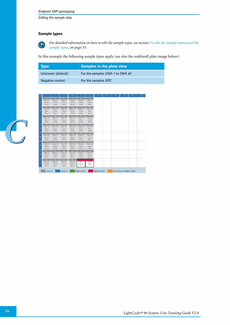
LightCycler® 96 System, User Training Guide V2.084
Endpoint SNP genotyping
CC
Editing the sample data
Sample types
For detailed information on how to edit the sample types, see section To edit the sample names and thesample types, on page 53.
In this example the following sample types apply (see also the multiwell plate image below):
Type Samples in the plate view
Unknown (default) For the samples DNA 1 to DNA 46
Negative control For the samples NTC
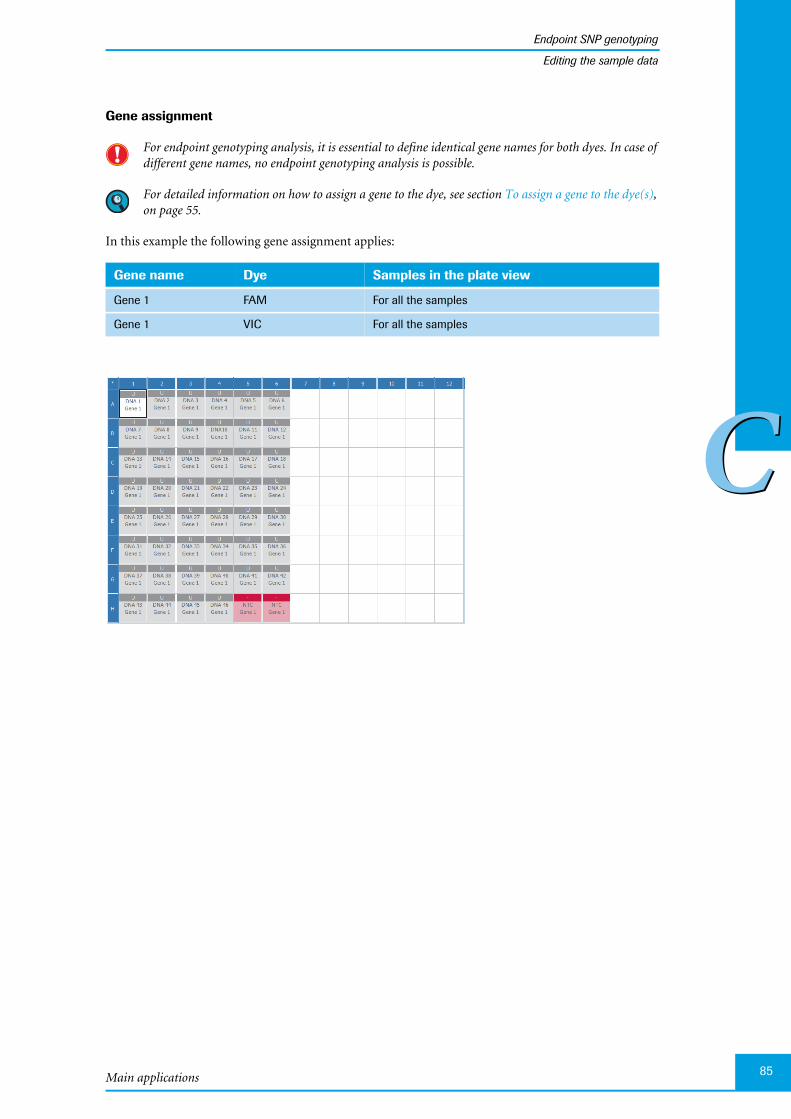
Main applications
Endpoint SNP genotyping
85
CC
Editing the sample data
Gene assignment
For endpoint genotyping analysis, it is essential to define identical gene names for both dyes. In case ofdifferent gene names, no endpoint genotyping analysis is possible.
For detailed information on how to assign a gene to the dye, see section To assign a gene to the dye(s),on page 55.
In this example the following gene assignment applies:
Gene name Dye Samples in the plate view
Gene 1 FAM For all the samples
Gene 1 VIC For all the samples
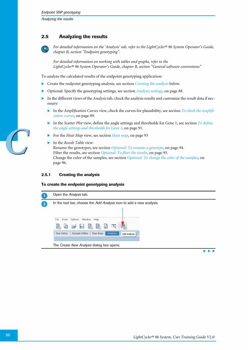
LightCycler® 96 System, User Training Guide V2.086
Endpoint SNP genotyping
CC
Analyzing the results
2.5 Analyzing the results
For detailed information on the ‘Analysis’ tab, refer to the LightCycler® 96 System Operator’s Guide,chapter B, section "Endpoint genotyping".
For detailed information on working with tables and graphs, refer to theLightCycler® 96 System Operator’s Guide, chapter B, section "General software conventions"
To analyze the calculated results of the endpoint genotyping application:
Create the endpoint genotyping analysis, see section Creating the analysis below.
Optional: Specify the genotyping settings, see section Analysis settings, on page 88.
In the different views of the Analysis tab, check the analysis results and customize the result data if nec-essary:
In the Amplification Curves view, check the curves for plausibility, see section To check the amplifi-cation curves, on page 89.
In the Scatter Plot view, define the angle settings and thresholds for Gene 1, see section To definethe angle settings and thresholds for Gene 1, on page 91.
For the Heat Map view, see section Heat map, on page 93
In the Result Table view:Rename the genotypes, see section Optional: To rename a genotype, on page 94.Filter the results, see section Optional: To filter the results, on page 95.Change the color of the samples, see section Optional: To change the color of the samples, onpage 96.
2.5.1 Creating the analysis
To create the endpoint genotyping analysis
Open the Analysis tab.
In the tool bar, choose the Add Analysis icon to add a new analysis.
The Create New Analysis dialog box opens.
�
�

Main applications
Endpoint SNP genotyping
87
CC
Analyzing the results
Choose Endpoint Genotyping.
Choose OK.
The Analysis tab displays four different views for the experiment using default values:
Amplification Curves
Scatter Plot
Heat Map
Result Table
�
�

LightCycler® 96 System, User Training Guide V2.088
Endpoint SNP genotyping
CC
Analyzing the results
2.5.2 Analysis settings
Optional: To specify the analysis settings
In the tool bar, choose the Analysis Settings icon.
The Endpoint Genotyping Settings dialog box opens.
In the Endpoint Genotyping Settings dialog box, specify the analysis-specific settings, for example:
On the Parameters tab, specify the threshold and angle settings for Gene 1.
The threshold and angle settings in the ‘Endpoint Genotyping Settings’ dialog box correspondto the slider settings in the scatter plot view. For detailed information, see section Scatter plot,on page 91.
On the Genes tab, exclude genes.
On the Samples tab, exclude samples.
�
�
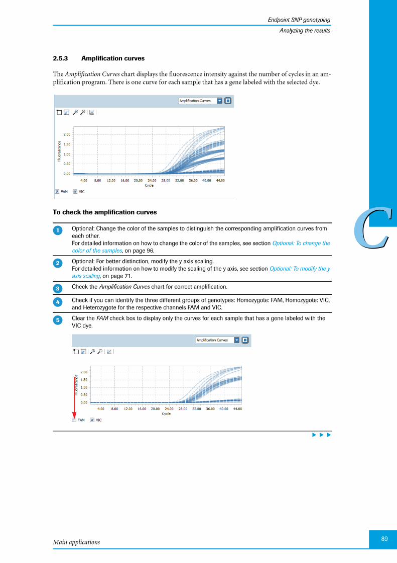
Main applications
Endpoint SNP genotyping
89
CC
Analyzing the results
2.5.3 Amplification curves
The Amplification Curves chart displays the fluorescence intensity against the number of cycles in an am-plification program. There is one curve for each sample that has a gene labeled with the selected dye.
To check the amplification curves
Optional: Change the color of the samples to distinguish the corresponding amplification curves fromeach other.For detailed information on how to change the color of the samples, see section Optional: To change thecolor of the samples, on page 96.
Optional: For better distinction, modify the y axis scaling.For detailed information on how to modify the scaling of the y axis, see section Optional: To modify the yaxis scaling, on page 71.
Check the Amplification Curves chart for correct amplification.
Check if you can identify the three different groups of genotypes: Homozygote: FAM, Homozygote: VIC,and Heterozygote for the respective channels FAM and VIC.
Clear the FAM check box to display only the curves for each sample that has a gene labeled with theVIC dye.
�
�
�
�
�

LightCycler® 96 System, User Training Guide V2.090
Endpoint SNP genotyping
CC
Analyzing the results
Select the FAM check box again and clear the VIC check box to display only the curves for each samplethat has a gene labeld with the FAM dye.
�
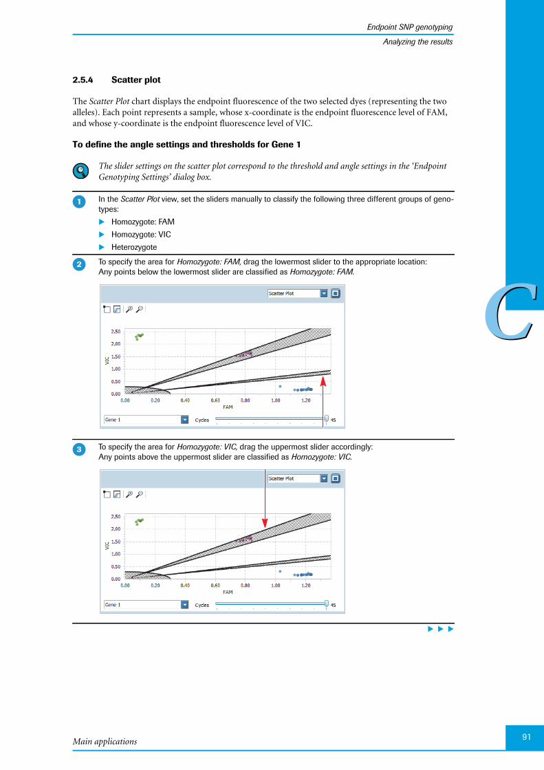
Main applications
Endpoint SNP genotyping
91
CC
Analyzing the results
2.5.4 Scatter plot
The Scatter Plot chart displays the endpoint fluorescence of the two selected dyes (representing the twoalleles). Each point represents a sample, whose x-coordinate is the endpoint fluorescence level of FAM,and whose y-coordinate is the endpoint fluorescence level of VIC.
To define the angle settings and thresholds for Gene 1
The slider settings on the scatter plot correspond to the threshold and angle settings in the ‘EndpointGenotyping Settings’ dialog box.
In the Scatter Plot view, set the sliders manually to classify the following three different groups of geno-types:
Homozygote: FAM
Homozygote: VIC
Heterozygote
To specify the area for Homozygote: FAM, drag the lowermost slider to the appropriate location:Any points below the lowermost slider are classified as Homozygote: FAM.
To specify the area for Homozygote: VIC, drag the uppermost slider accordingly:Any points above the uppermost slider are classified as Homozygote: VIC.
�
�
�

LightCycler® 96 System, User Training Guide V2.092
Endpoint SNP genotyping
CC
Analyzing the results
To specify the areas for unknown samples and to limit the area for heterozygote samples, drag the innersliders accordingly:
Any points in the shaded areas are classified as Unknown.
Any points between the shaded areas are classified as Heterozygote.
The Scatter Plot chart and the Heat Map are displayed according to the defined angles.
Check if the NTCs are in the Pos/Neg Threshold radius. In this example, keep the default value for thePos/Neg Threshold radius.
The Scatter Plot chart and the Heat Map are displayed according to the defined threshold and angles.
�
Homozygote: VIC Homozygote: FAMHeterozygoteUnknown
Unknown
�
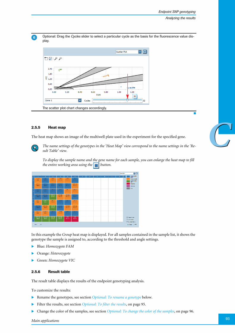
Main applications
Endpoint SNP genotyping
93
CC
Analyzing the results
2.5.5 Heat map
The heat map shows an image of the multiwell plate used in the experiment for the specified gene.
The name settings of the genotypes in the ‘Heat Map’ view correspond to the name settings in the ‘Re-sult Table’ view.
To display the sample name and the gene name for each sample, you can enlarge the heat map to fillthe entire working area using the button.
In this example the Group heat map is displayed. For all samples contained in the sample list, it shows thegenotype the sample is assigned to, according to the threshold and angle settings.
Blue: Homozygote FAM
Orange: Heterozygote
Green: Homozygote VIC
2.5.6 Result table
The result table displays the results of the endpoint genotyping analysis.
To customize the results:
Rename the genotypes, see section Optional: To rename a genotype below.
Filter the results, see section Optional: To filter the results, on page 95.
Change the color of the samples, see section Optional: To change the color of the samples, on page 96.
Optional: Drag the Cycles slider to select a particular cycle as the basis for the fluorescence value dis-play.
The scatter plot chart changes accordingly.
�

LightCycler® 96 System, User Training Guide V2.094
Endpoint SNP genotyping
CC
Analyzing the results
Optional: To rename a genotype
The name settings of the genotypes in the ‘Result Table’ view correspond to the name settings in the‘Heat Map’ view.
In the Result Table view, select the genotype that you want to rename, for example, Heterozygote.
The shortcut menu opens.
On the shortcut menu, choose Rename Genotype.
The Rename Genotype dialog box opens.
In the New Name: field, type in the new name for the selected genotype, for example, HeterozygoteGene 1, and choose OK.
All genotypes of this group are renamed in the Result Table view.
Repeat steps 1 to 3 for another group of genotypes.
�
�
�
�
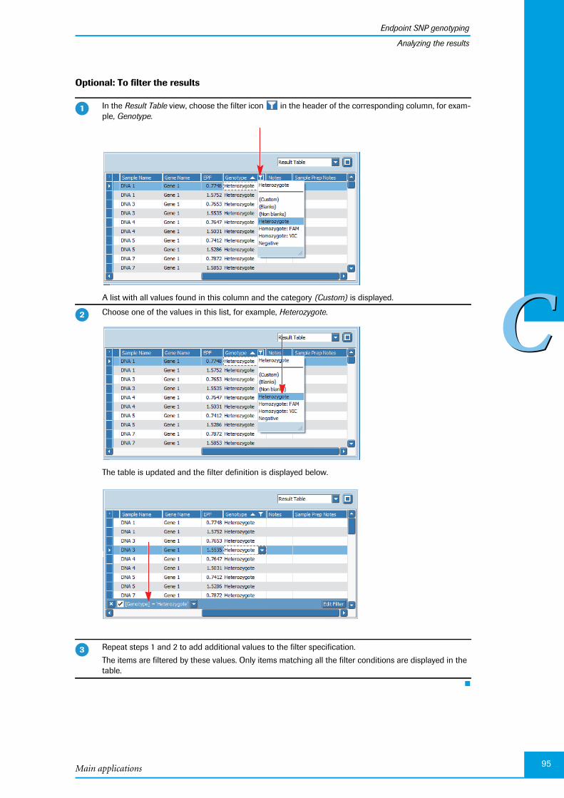
Main applications
Endpoint SNP genotyping
95
CC
Analyzing the results
Optional: To filter the results
In the Result Table view, choose the filter icon in the header of the corresponding column, for exam-ple, Genotype.
A list with all values found in this column and the category (Custom) is displayed.
Choose one of the values in this list, for example, Heterozygote.
The table is updated and the filter definition is displayed below.
Repeat steps 1 and 2 to add additional values to the filter specification.
The items are filtered by these values. Only items matching all the filter conditions are displayed in thetable.
�
�
�
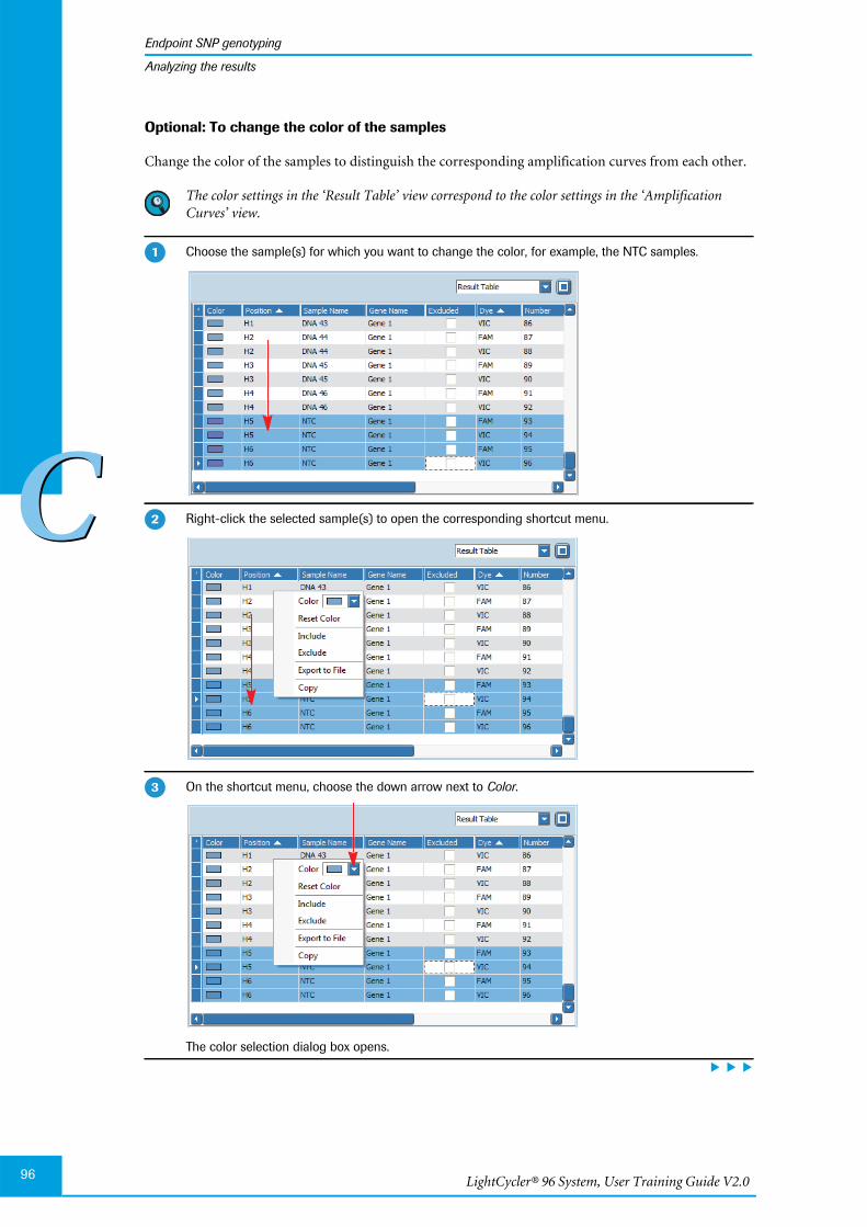
LightCycler® 96 System, User Training Guide V2.096
Endpoint SNP genotyping
CC
Analyzing the results
Optional: To change the color of the samples
Change the color of the samples to distinguish the corresponding amplification curves from each other.
The color settings in the ‘Result Table’ view correspond to the color settings in the ‘AmplificationCurves’ view.
Choose the sample(s) for which you want to change the color, for example, the NTC samples.
Right-click the selected sample(s) to open the corresponding shortcut menu.
On the shortcut menu, choose the down arrow next to Color.
The color selection dialog box opens.
�
�
�
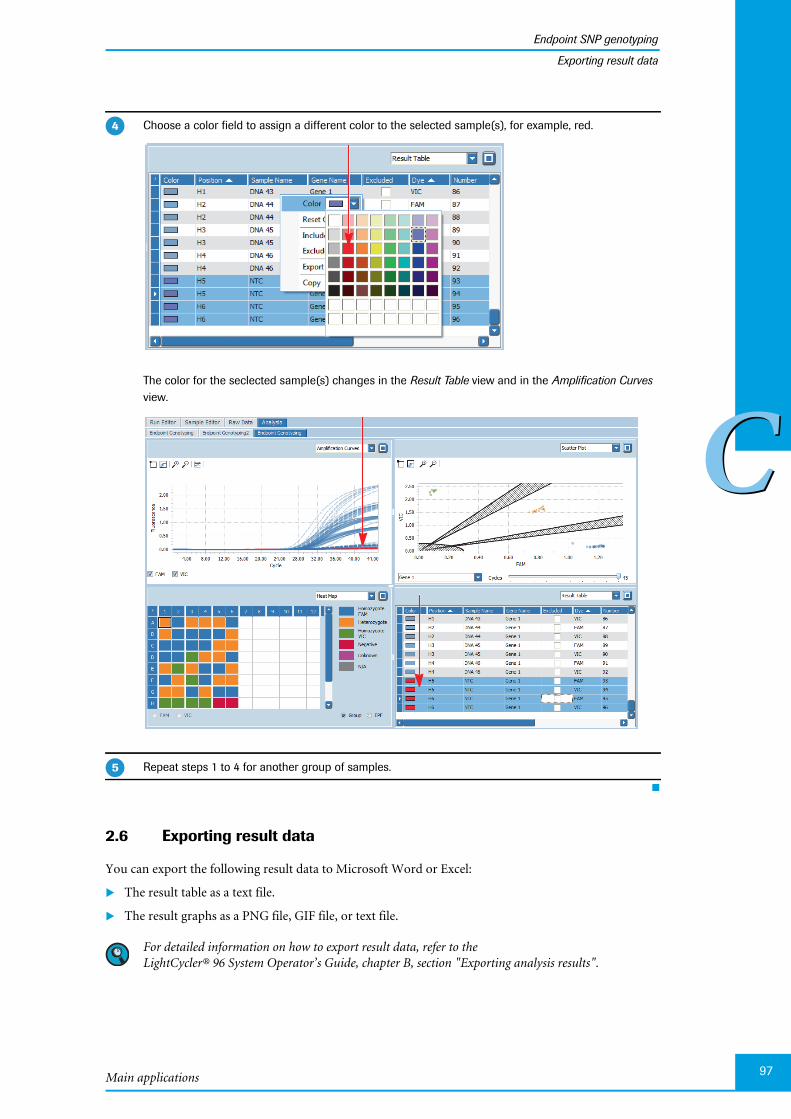
Main applications
Endpoint SNP genotyping
97
CC
Exporting result data
2.6 Exporting result data
You can export the following result data to Microsoft Word or Excel:
The result table as a text file.
The result graphs as a PNG file, GIF file, or text file.
For detailed information on how to export result data, refer to theLightCycler® 96 System Operator’s Guide, chapter B, section "Exporting analysis results".
Choose a color field to assign a different color to the selected sample(s), for example, red.
The color for the seclected sample(s) changes in the Result Table view and in the Amplification Curvesview.
Repeat steps 1 to 4 for another group of samples.
�
�
LightCycler® 96 System, User Training Guide V2.098
Relative quantification
CC
Experiment overview
3 Relative quantification
Relative quantification compares the levels of two different gene sequences in a single sample, for exam-ple, target gene of interest and a reference gene, and expresses the result as a ratio. For comparison pur-poses, the reference gene is known to be present in constant numbers under all test conditions. This ref-erence gene provides a basis for normalizing sample-to-sample differences.
The ratio of target gene to reference gene is a relative, dimensionless number, that is meaningful onlywhen compared between samples. In addition to calculating sample-specific ratios, a normalized ratio iscalculated by defining a "run calibrator" sample. The run calibrator is typically a positive sample with astable ratio of target to reference. Its value is used to normalize all samples within one run, and also toprovide a constant calibration point between several runs.
In addition to normalization, it is frequently required to measure the gene expression of each sample andeach gene at different times or under different conditions. To generate a meaningful result, the sample-specific measurements are normalized to a common basis, that is, a certain experimental condition, toprovide a scaled ratio. This condition is specified as the "study calibrator" condition.
For detailed information on relative quantification analysis, refer to theLightCycler® 96 System Operator’s Guide, chapter A, section "Analysis principles".
3.1 Experiment overview
The following example describes how to set up, run, and analyze a gene expression assay. It comprisesthree samples tested at three different times (that is, at the three conditions 0 hours, 1 hour, and 2 hours),one target gene and one reference gene.
The assay is performed using a LightCycler® 480 Multiwell Plate 96, white. Each sample is set up in dupli-cate.
Samples cDNA samples.
Three samples are tested at three different times.
Reagents FastStart Essential DNA Probes Master (2 x conc.)
Target primer mix, 5 µM (10 x conc.)
Target hydrolysis probe, 10 µM (50 x conc.)
Reference primer mix, 5 µM (10 x conc.)
Reference hydrolysis probe, 10 µM (50 x conc.)
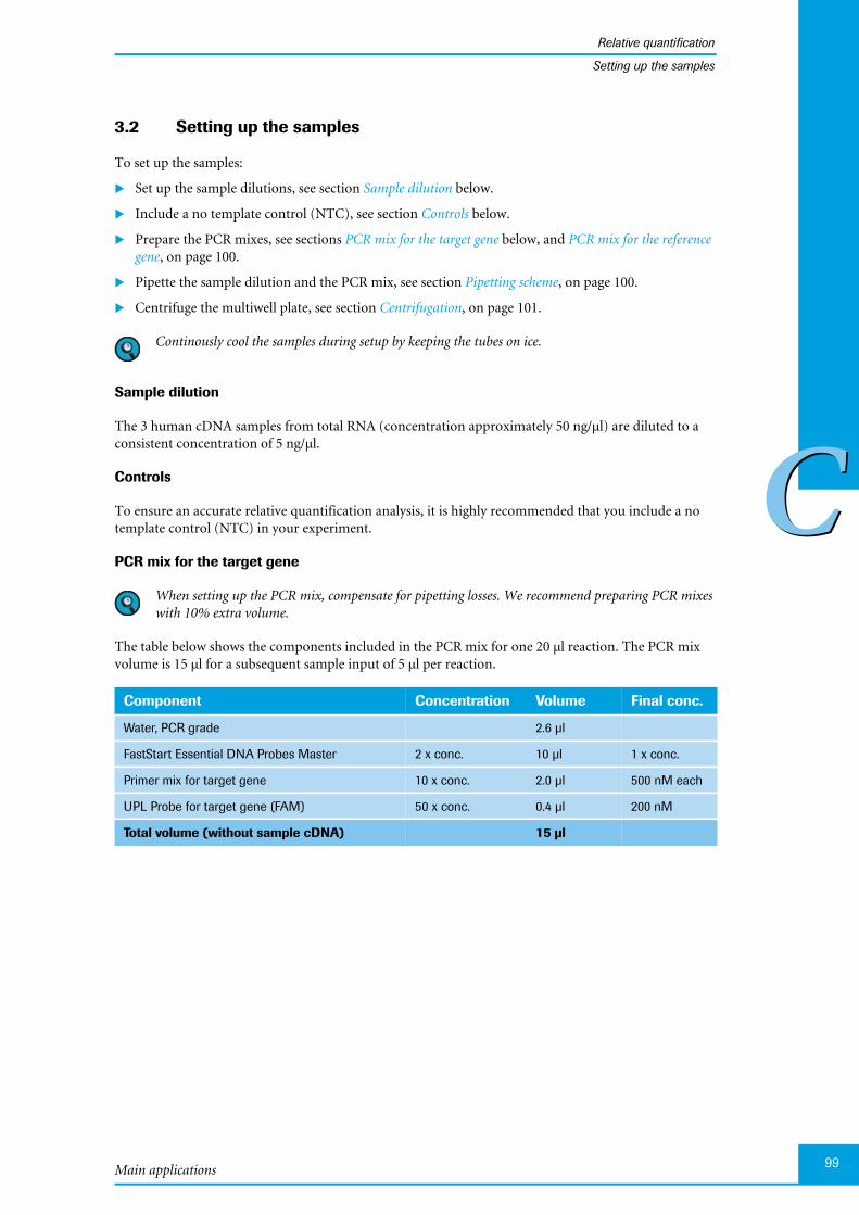
Main applications
Relative quantification
99
CC
Setting up the samples
3.2 Setting up the samples
To set up the samples:
Set up the sample dilutions, see section Sample dilution below.
Include a no template control (NTC), see section Controls below.
Prepare the PCR mixes, see sections PCR mix for the target gene below, and PCR mix for the referencegene, on page 100.
Pipette the sample dilution and the PCR mix, see section Pipetting scheme, on page 100.
Centrifuge the multiwell plate, see section Centrifugation, on page 101.
Continously cool the samples during setup by keeping the tubes on ice.
Sample dilution
The 3 human cDNA samples from total RNA (concentration approximately 50 ng/µl) are diluted to aconsistent concentration of 5 ng/µl.
Controls
To ensure an accurate relative quantification analysis, it is highly recommended that you include a notemplate control (NTC) in your experiment.
PCR mix for the target gene
When setting up the PCR mix, compensate for pipetting losses. We recommend preparing PCR mixeswith 10% extra volume.
The table below shows the components included in the PCR mix for one 20 µl reaction. The PCR mixvolume is 15 µl for a subsequent sample input of 5 µl per reaction.
Component Concentration Volume Final conc.
Water, PCR grade 2.6 µl
FastStart Essential DNA Probes Master 2 x conc. 10 µl 1 x conc.
Primer mix for target gene 10 x conc. 2.0 µl 500 nM each
UPL Probe for target gene (FAM) 50 x conc. 0.4 µl 200 nM
Total volume (without sample cDNA) 15 µl

LightCycler® 96 System, User Training Guide V2.0100
Relative quantification
CC
Setting up the samples
PCR mix for the reference gene
When setting up the PCR mix, compensate for pipetting losses. We recommend preparing PCR mixeswith 10% extra volume.
The table below shows the components included in the PCR mix for one 20 µl reaction. The PCR mixvolume is 15 µl for a subsequent sample input of 5 µl per reaction.
Pipetting scheme
Component Concentration Volume Final conc.
Water, PCR grade 2.6 µl
FastStart Essential DNA Probes Master 2 x conc. 10 µl 1 x conc.
Primer mix for reference gene 10 x conc. 2.0 µl 500 nM each
UPL Probe for reference gene (FAM) 50 x conc. 0.4 µl 200 nM
Total volume (without sample cDNA) 15 µl
Pipette 15 µl of the PCR mix for the target gene into 20 wells, rows A and B, columns 1 to 10 of the mul-tiwell plate according to the following scheme.
Pipette 15 µl of the PCR mix for the reference gene into 20 wells, rows C and D, columns 1 to 10 of themultiwell plate according to the following scheme.
Pipette 5 µl of cDNA sample into the corresponding wells according to the following scheme.
For the NTCs, pipette 5 µl of water (instead of cDNA sample) into the corresponding wells in column 10according to the following scheme.
1 2 3 4 5 6 7 8 9 10 11 12
A Sample10 h
Sample20 h
Sample30 h
Sample11 h
Sample21 h
Sample31 h
Sample12 h
Sample22 h
Sample32 h
NTC
B Sample10 h
Sample20 h
Sample30 h
Sample11 h
Sample21 h
Sample31 h
Sample12 h
Sample22 h
Sample32 h
NTC
C Sample10 h
Sample20 h
Sample30 h
Sample11 h
Sample21 h
Sample31 h
Sample12 h
Sample22 h
Sample32 h
NTC
D Sample10 h
Sample20 h
Sample30 h
Sample11 h
Sample21 h
Sample31 h
Sample12 h
Sample22 h
Sample32 h
NTC
E
F
G
H
�
�
�
�

Main applications
Relative quantification
101
CC
Setting up the samples
Centrifugation
Seal the multiwell plate with the LightCycler® 480 Sealing Foil using the sealing foil applicator (providedwith the system package).
Centrifuge the multiwell plate at 1500 x g for 2 minutes in a standard swing-bucket centrifuge, using arotor for multiwell plates.
Make sure you balance the multiwell plate with a suitable counterweight (for example, anothermultiwell plate).
�
�
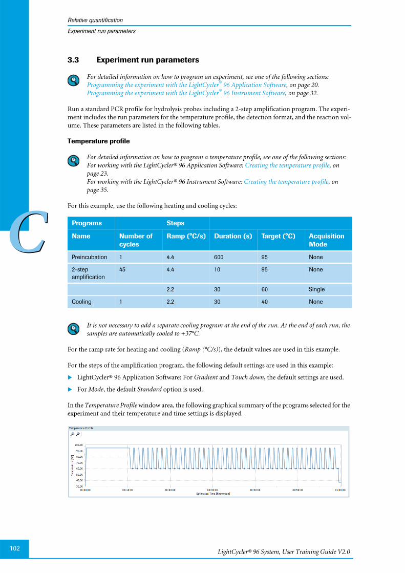
LightCycler® 96 System, User Training Guide V2.0102
Relative quantification
CC
Experiment run parameters
3.3 Experiment run parameters
For detailed information on how to program an experiment, see one of the following sections:Programming the experiment with the LightCycler® 96 Application Software, on page 20.Programming the experiment with the LightCycler® 96 Instrument Software, on page 32.
Run a standard PCR profile for hydrolysis probes including a 2-step amplification program. The experi-ment includes the run parameters for the temperature profile, the detection format, and the reaction vol-ume. These parameters are listed in the following tables.
Temperature profile
For detailed information on how to program a temperature profile, see one of the following sections:For working with the LightCycler® 96 Application Software: Creating the temperature profile, onpage 23.For working with the LightCycler® 96 Instrument Software: Creating the temperature profile, onpage 35.
For this example, use the following heating and cooling cycles:
It is not necessary to add a separate cooling program at the end of the run. At the end of each run, thesamples are automatically cooled to +37°C.
For the ramp rate for heating and cooling (Ramp (°C/s)), the default values are used in this example.
For the steps of the amplification program, the following default settings are used in this example:
LightCycler® 96 Application Software: For Gradient and Touch down, the default settings are used.
For Mode, the default Standard option is used.
In the Temperature Profile window area, the following graphical summary of the programs selected for theexperiment and their temperature and time settings is displayed.
Programs Steps
Name Number ofcycles
Ramp (°C/s) Duration (s) Target (°C) AcquisitionMode
Preincubation 1 4.4 600 95 None
2-stepamplification
45 4.4 10 95 None
2.2 30 60 Single
Cooling 1 2.2 30 40 None
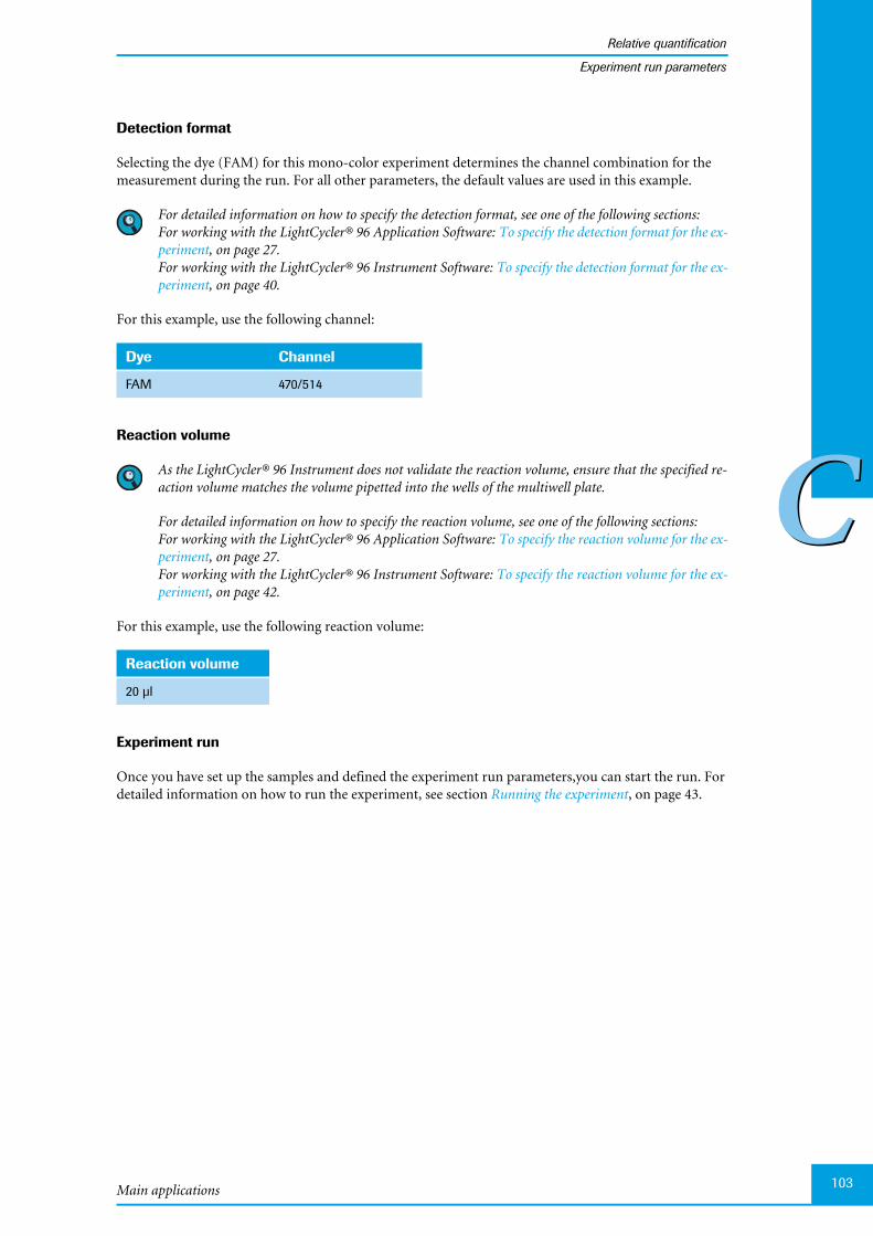
Main applications
Relative quantification
103
CC
Experiment run parameters
Detection format
Selecting the dye (FAM) for this mono-color experiment determines the channel combination for themeasurement during the run. For all other parameters, the default values are used in this example.
For detailed information on how to specify the detection format, see one of the following sections:For working with the LightCycler® 96 Application Software: To specify the detection format for the ex-periment, on page 27.For working with the LightCycler® 96 Instrument Software: To specify the detection format for the ex-periment, on page 40.
For this example, use the following channel:
Reaction volume
As the LightCycler® 96 Instrument does not validate the reaction volume, ensure that the specified re-action volume matches the volume pipetted into the wells of the multiwell plate.
For detailed information on how to specify the reaction volume, see one of the following sections:For working with the LightCycler® 96 Application Software: To specify the reaction volume for the ex-periment, on page 27.For working with the LightCycler® 96 Instrument Software: To specify the reaction volume for the ex-periment, on page 42.
For this example, use the following reaction volume:
Experiment run
Once you have set up the samples and defined the experiment run parameters,you can start the run. Fordetailed information on how to run the experiment, see section Running the experiment, on page 43.
Dye Channel
FAM 470/514
Reaction volume
20 µl

LightCycler® 96 System, User Training Guide V2.0104
Relative quantification
CC
Editing the sample data
3.4 Editing the sample data
For editing the sample data, the experiment must be opened in the LightCycler® 96 Application Software.You can edit the sample list before or after the run, depending on your preferred routine.
The LightCycler® 96 Application Software offers two different views for editing the samples: the plateview and the table view. This user training guide describes how to edit the samples using the plate view,which shows the samples in 96 wells laid out to match the physical instrument. Changes in the plateview are immediately displayed in the table view and vice versa.
For detailed information on the ‘Sample Editor’ tab, refer to theLightCycler® 96 System Operator’s Guide, chapter B, section "Sample Editor tab".
To edit the sample list:
Clear empty wells to eliminate them from the analysis, see section Empty wells below.
Edit the sample names, see section Sample names, on page 105.
Edit the sample types, see section Sample types, on page 106.
Assign a gene for the dye, see section Gene assignment, on page 107.
Specify the three conditions for each sample, see section To specify the conditions, on page 107.
Empty wells
For detailed information on how to clear empty wells, see section To clear empty wells, on page 51.
For this example, clear the following wells (see also the multiwell plate image below):
Columns 11 to 12
Rows E to H

Main applications
Relative quantification
105
CC
Editing the sample data
Sample names
For detailed information on how to edit the sample names, see section To edit the sample names andthe sample types, on page 53.
For this example, the following sample names apply (see also the multiwell plate image below):
Name Samples in the plate view
NTC For the negative control in column 10
Sample1 For the unknown samples in columns 1, 4, and 7
Sample2 For the unknown samples in columns 2, 5, and 8
Sample3 For the unknown samples in columns 3, 6, and 9
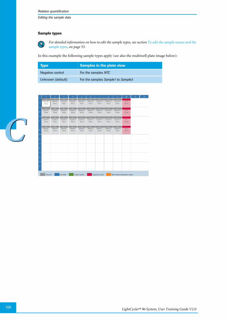
LightCycler® 96 System, User Training Guide V2.0106
Relative quantification
CC
Editing the sample data
Sample types
For detailed information on how to edit the sample types, see section To edit the sample names and thesample types, on page 53.
In this example the following sample types apply (see also the multiwell plate image below):
Type Samples in the plate view
Negative control For the samples NTC
Unknown (default) For the samples Sample1 to Sample3

Main applications
Relative quantification
107
CC
Editing the sample data
Gene assignment
For detailed information on how to assign a gene to the dye, see section To assign a gene to the dye(s),on page 55.
In this example the following gene assignment applies:
To specify the conditions
Gene name Dye Samples in the plate view
Gene 1 (target gene) FAM For the samples in the rows A and B
Ref 1 (reference gene) FAM For the samples in the rows C and D
In the multiwell plate image, select columns 1, 2, and 3.
�

LightCycler® 96 System, User Training Guide V2.0108
Relative quantification
CC
Editing the sample data
In the Reaction Properties window area, choose the Condition Name text field.
Type in 0 h.
The condition 0 h is assigned to all selected samples.
As described in steps 1 to 3, assign the condition 1 h to all wells in columns 4, 5, and 6.
As described in steps 1 to 3, assign the condition 2 h to all wells in columns 7, 8, and 9.
�
�
�
�

Main applications
Relative quantification
109
CC
Analyzing the results
3.5 Analyzing the results
For detailed information on the ‘Analysis’ tab, refer to theLightCycler® 96 System Operator’s Guide, chapter B, section "Relative quantification".
For detailed information on working with tables and graphs, refer to theLightCycler® 96 System Operator’s Guide, chapter B, section "General software conventions".
Relative quantification compares the levels of two different gene sequences, that is, the target gene of in-terest and a reference gene, in a single sample, and expresses the final result as a ratio of these genes.
To analyze the calculated results of the relative quantification application:
Create the relative quantification analysis, see section Creating the analysis below.
Specify the settings for the relative quantification analysis, see section Analysis settings, on page 111.
In the different views of the Rel Quant tab, check the analysis results and customize the result data ifnecessary:
For the Amplification Curves view, see section Amplification curves, on page 113.
For the Ratio Bars view, see section Ratio bars, on page 113.
For the Heat Map view, see section Heat map, on page 117.
For the Result Table view, see section Result table, on page 118.
For the Cq Bars view, see section Cq bars, on page 77.
3.5.1 Creating the analysis
To create the relative quantification analysis
Open the Analysis tab.
In the tool bar, choose the Add Analysis icon to add a new analysis.
The Create New Analysis dialog box opens.
Choose Rel Quant.
�
�
�
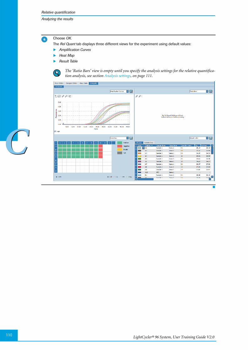
LightCycler® 96 System, User Training Guide V2.0110
Relative quantification
CC
Analyzing the results
Choose OK.
The Rel Quant tab displays three different views for the experiment using default values:
Amplification Curves
Heat Map
Result Table
The ‘Ratio Bars’ view is empty until you specify the analysis settings for the relative quantifica-tion analysis, see section Analysis settings, on page 111.
�
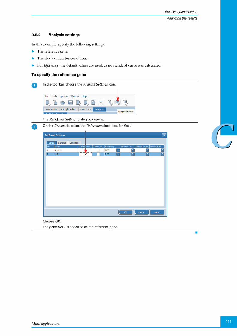
Main applications
Relative quantification
111
CC
Analyzing the results
3.5.2 Analysis settings
In this example, specify the following settings:
The reference gene.
The study calibrator condition.
For Efficiency, the default values are used, as no standard curve was calculated.
To specify the reference gene
In the tool bar, choose the Analysis Settings icon.
The Rel Quant Settings dialog box opens.
On the Genes tab, select the Reference check box for Ref 1.
Choose OK.
The gene Ref 1 is specified as the reference gene.
�
�
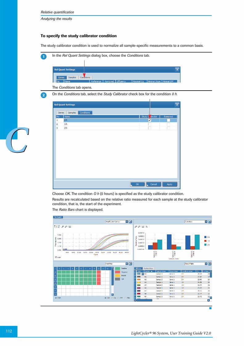
LightCycler® 96 System, User Training Guide V2.0112
Relative quantification
CC
Analyzing the results
To specify the study calibrator condition
The study calibrator condition is used to normalize all sample-specific measurements to a common basis.
In the Rel Quant Settings dialog box, choose the Conditions tab.
The Conditions tab opens.
On the Conditions tab, select the Study Calibrator check box for the condition 0 h.
Choose OK. The condition O h (0 hours) is specified as the study calibrator condition.
Results are recalculated based on the relative ratio measured for each sample at the study calibratorcondition, that is, the start of the experiment.
The Ratio Bars chart is displayed.
�
�
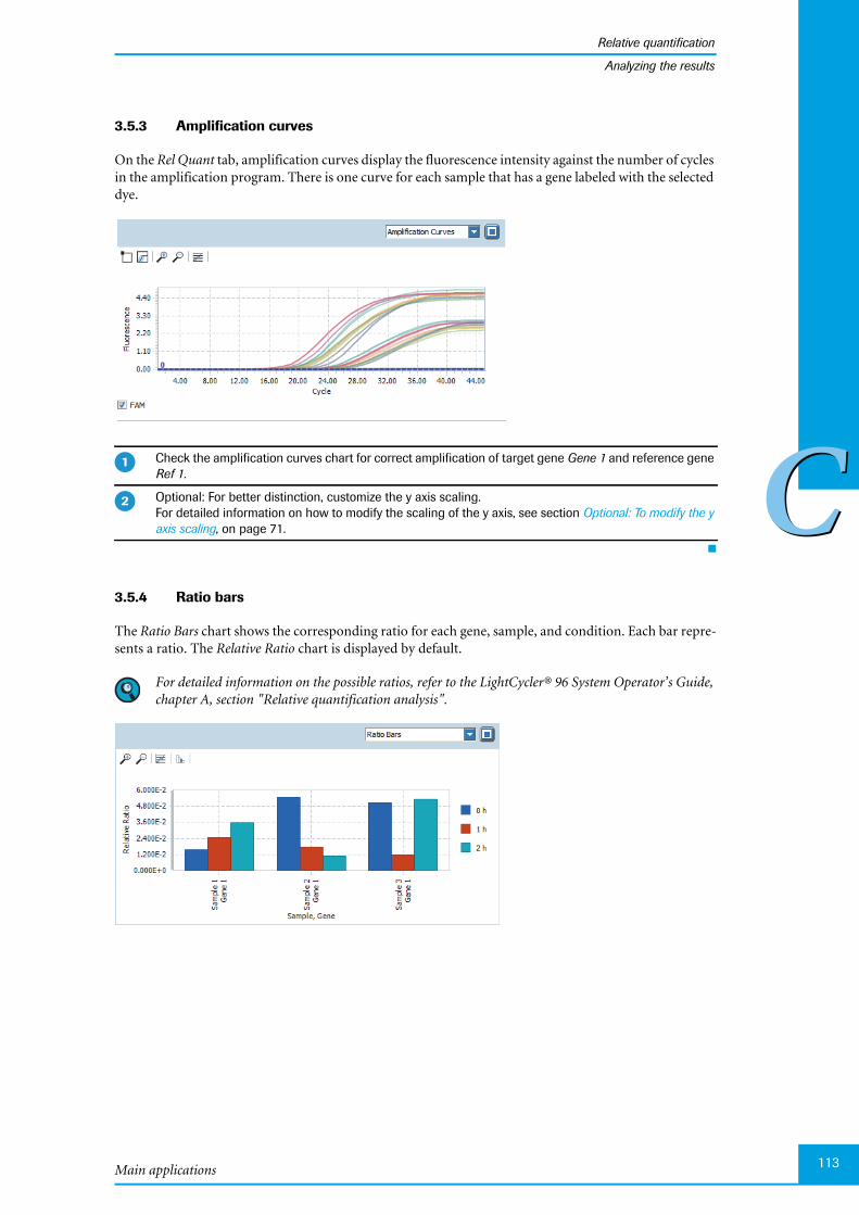
Main applications
Relative quantification
113
CC
Analyzing the results
3.5.3 Amplification curves
On the Rel Quant tab, amplification curves display the fluorescence intensity against the number of cyclesin the amplification program. There is one curve for each sample that has a gene labeled with the selecteddye.
3.5.4 Ratio bars
The Ratio Bars chart shows the corresponding ratio for each gene, sample, and condition. Each bar repre-sents a ratio. The Relative Ratio chart is displayed by default.
For detailed information on the possible ratios, refer to the LightCycler® 96 System Operator’s Guide,chapter A, section "Relative quantification analysis".
Check the amplification curves chart for correct amplification of target gene Gene 1 and reference geneRef 1.
Optional: For better distinction, customize the y axis scaling.For detailed information on how to modify the scaling of the y axis, see section Optional: To modify the yaxis scaling, on page 71.
�
�
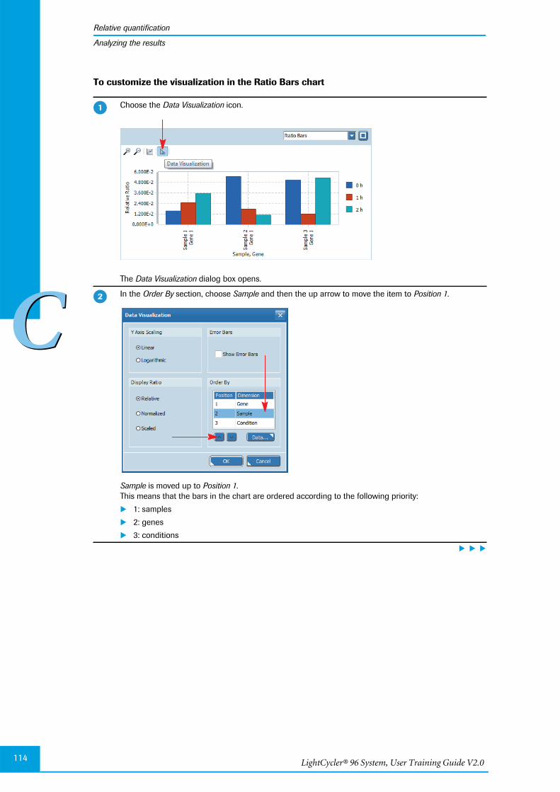
LightCycler® 96 System, User Training Guide V2.0114
Relative quantification
CC
Analyzing the results
To customize the visualization in the Ratio Bars chart
Choose the Data Visualization icon.
The Data Visualization dialog box opens.
In the Order By section, choose Sample and then the up arrow to move the item to Position 1.
Sample is moved up to Position 1.This means that the bars in the chart are ordered according to the following priority:
1: samples
2: genes
3: conditions
�
�
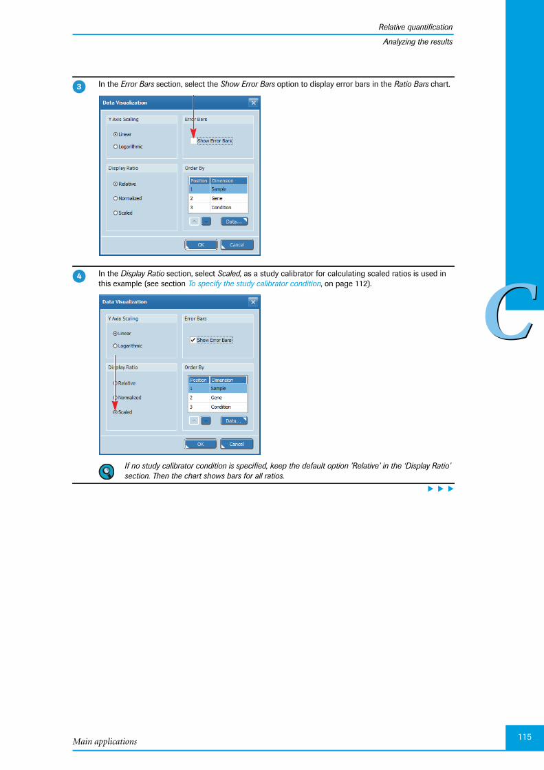
Main applications
Relative quantification
115
CC
Analyzing the results
In the Error Bars section, select the Show Error Bars option to display error bars in the Ratio Bars chart.
In the Display Ratio section, select Scaled, as a study calibrator for calculating scaled ratios is used inthis example (see section To specify the study calibrator condition, on page 112).
If no study calibrator condition is specified, keep the default option ’Relative’ in the ‘Display Ratio’section. Then the chart shows bars for all ratios.
�
�

LightCycler® 96 System, User Training Guide V2.0116
Relative quantification
CC
Analyzing the results
Choose OK.
Results are recalculated based on the relative ratio measured for each sample at the study calibratorcondition, that is, the start of the experiment.
The Scaled Ratio chart is displayed. This chart shows no bars for the study calibrator (condition 0 h).
Sample 1: The scaled ratio for gene 1 after two hours (condition 2 h) is higher than the scaled ratioafter one hour (condition 1 h).
Sample 2: The scaled ratio for gene 1 after two hours (condition 2 h) is lower than the scaled ratioafter one hour (condition 1 h).
Sample 3: The scaled ratio for gene 1 after two hours (condition 2 h) is higher than the scaled ratioafter one hour (condition 1 h).
Optional: For better distinction, modify the y axis scaling.For detailed information on how to modify the scaling of the y axis, see section Optional: To modify the yaxis scaling, on page 71.
�
�
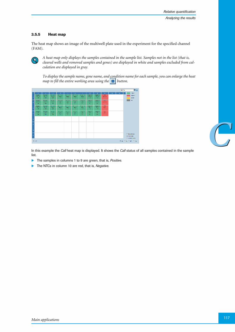
Main applications
Relative quantification
117
CC
Analyzing the results
3.5.5 Heat map
The heat map shows an image of the multiwell plate used in the experiment for the specified channel(FAM).
A heat map only displays the samples contained in the sample list. Samples not in the list (that is,cleared wells and removed samples and genes) are displayed in white and samples excluded from cal-culation are displayed in gray.
To display the sample name, gene name, and condition name for each sample, you can enlarge the heatmap to fill the entire working area using the button.
In this example the Call heat map is displayed. It shows the Call status of all samples contained in the samplelist.
The samples in columns 1 to 9 are green, that is, Positive.
The NTCs in column 10 are red, that is, Negative.
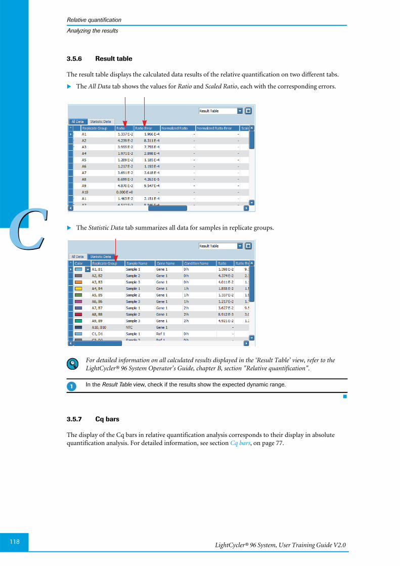
LightCycler® 96 System, User Training Guide V2.0118
Relative quantification
CC
Analyzing the results
3.5.6 Result table
The result table displays the calculated data results of the relative quantification on two different tabs.
The All Data tab shows the values for Ratio and Scaled Ratio, each with the corresponding errors.
The Statistic Data tab summarizes all data for samples in replicate groups.
For detailed information on all calculated results displayed in the ‘Result Table’ view, refer to theLightCycler® 96 System Operator’s Guide, chapter B, section "Relative quantification".
3.5.7 Cq bars
The display of the Cq bars in relative quantification analysis corresponds to their display in absolutequantification analysis. For detailed information, see section Cq bars, on page 77.
In the Result Table view, check if the results show the expected dynamic range.
�

Main applications
Relative quantification
119
CC
Exporting result data
3.6 Exporting result data
You can export the following result data to Microsoft Word or Excel:
The result table as a text file.
The Amplification Curves chart and the Standard Curves chart as a PNG file, GIF file, or text file.
The Ratio Bars chart as a PNG file or GIF file.
For detailed information on how to export result data, refer to theLightCycler® 96 System Operator’s Guide, chapter B, section "Exporting analysis results".
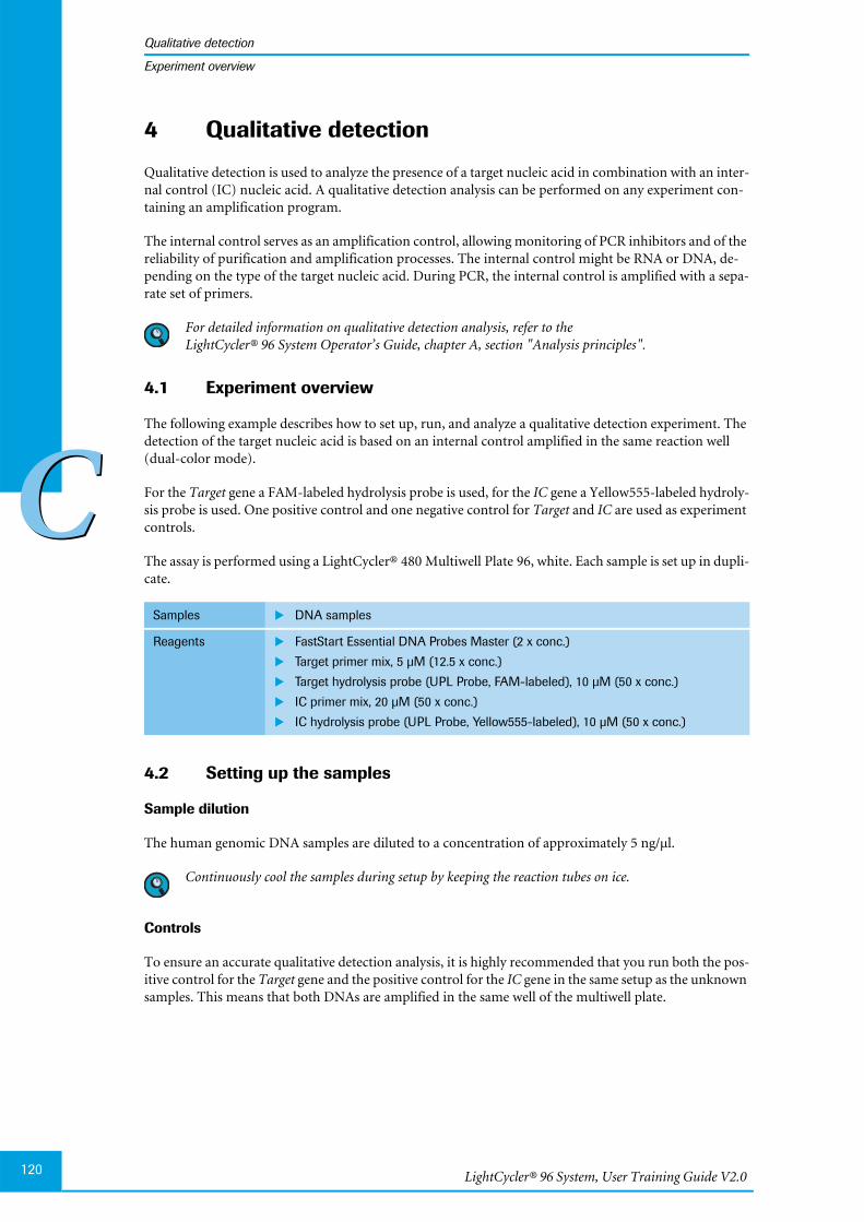
LightCycler® 96 System, User Training Guide V2.0120
Qualitative detection
CC
Experiment overview
4 Qualitative detection
Qualitative detection is used to analyze the presence of a target nucleic acid in combination with an inter-nal control (IC) nucleic acid. A qualitative detection analysis can be performed on any experiment con-taining an amplification program.
The internal control serves as an amplification control, allowing monitoring of PCR inhibitors and of thereliability of purification and amplification processes. The internal control might be RNA or DNA, de-pending on the type of the target nucleic acid. During PCR, the internal control is amplified with a sepa-rate set of primers.
For detailed information on qualitative detection analysis, refer to theLightCycler® 96 System Operator’s Guide, chapter A, section "Analysis principles".
4.1 Experiment overview
The following example describes how to set up, run, and analyze a qualitative detection experiment. Thedetection of the target nucleic acid is based on an internal control amplified in the same reaction well(dual-color mode).
For the Target gene a FAM-labeled hydrolysis probe is used, for the IC gene a Yellow555-labeled hydroly-sis probe is used. One positive control and one negative control for Target and IC are used as experimentcontrols.
The assay is performed using a LightCycler® 480 Multiwell Plate 96, white. Each sample is set up in dupli-cate.
4.2 Setting up the samples
Sample dilution
The human genomic DNA samples are diluted to a concentration of approximately 5 ng/µl.
Continuously cool the samples during setup by keeping the reaction tubes on ice.
Controls
To ensure an accurate qualitative detection analysis, it is highly recommended that you run both the pos-itive control for the Target gene and the positive control for the IC gene in the same setup as the unknownsamples. This means that both DNAs are amplified in the same well of the multiwell plate.
Samples DNA samples
Reagents FastStart Essential DNA Probes Master (2 x conc.)
Target primer mix, 5 µM (12.5 x conc.)
Target hydrolysis probe (UPL Probe, FAM-labeled), 10 µM (50 x conc.)
IC primer mix, 20 µM (50 x conc.)
IC hydrolysis probe (UPL Probe, Yellow555-labeled), 10 µM (50 x conc.)
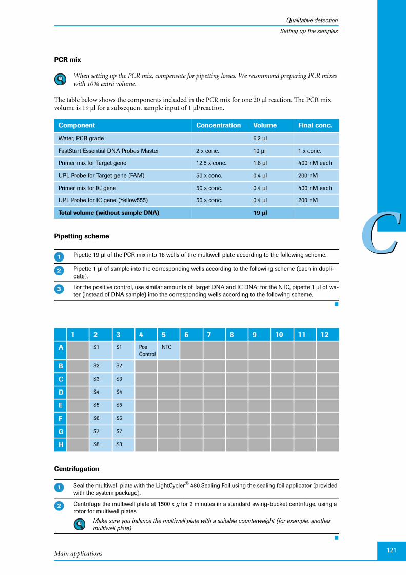
Main applications
Qualitative detection
121
CC
Setting up the samples
PCR mix
When setting up the PCR mix, compensate for pipetting losses. We recommend preparing PCR mixeswith 10% extra volume.
The table below shows the components included in the PCR mix for one 20 µl reaction. The PCR mixvolume is 19 µl for a subsequent sample input of 1 µl/reaction.
Pipetting scheme
Centrifugation
Component Concentration Volume Final conc.
Water, PCR grade 6.2 µl
FastStart Essential DNA Probes Master 2 x conc. 10 µl 1 x conc.
Primer mix for Target gene 12.5 x conc. 1.6 µl 400 nM each
UPL Probe for Target gene (FAM) 50 x conc. 0.4 µl 200 nM
Primer mix for IC gene 50 x conc. 0.4 µl 400 nM each
UPL Probe for IC gene (Yellow555) 50 x conc. 0.4 µl 200 nM
Total volume (without sample DNA) 19 µl
Pipette 19 µl of the PCR mix into 18 wells of the multiwell plate according to the following scheme.
Pipette 1 µl of sample into the corresponding wells according to the following scheme (each in dupli-cate).
For the positive control, use similar amounts of Target DNA and IC DNA; for the NTC, pipette 1 µl of wa-ter (instead of DNA sample) into the corresponding wells according to the following scheme.
1 2 3 4 5 6 7 8 9 10 11 12
A S1 S1 PosControl
NTC
B S2 S2
C S3 S3
D S4 S4
E S5 S5
F S6 S6
G S7 S7
H S8 S8
Seal the multiwell plate with the LightCycler® 480 Sealing Foil using the sealing foil applicator (providedwith the system package).
Centrifuge the multiwell plate at 1500 x g for 2 minutes in a standard swing-bucket centrifuge, using arotor for multiwell plates.
Make sure you balance the multiwell plate with a suitable counterweight (for example, anothermultiwell plate).
�
�
�
�
�
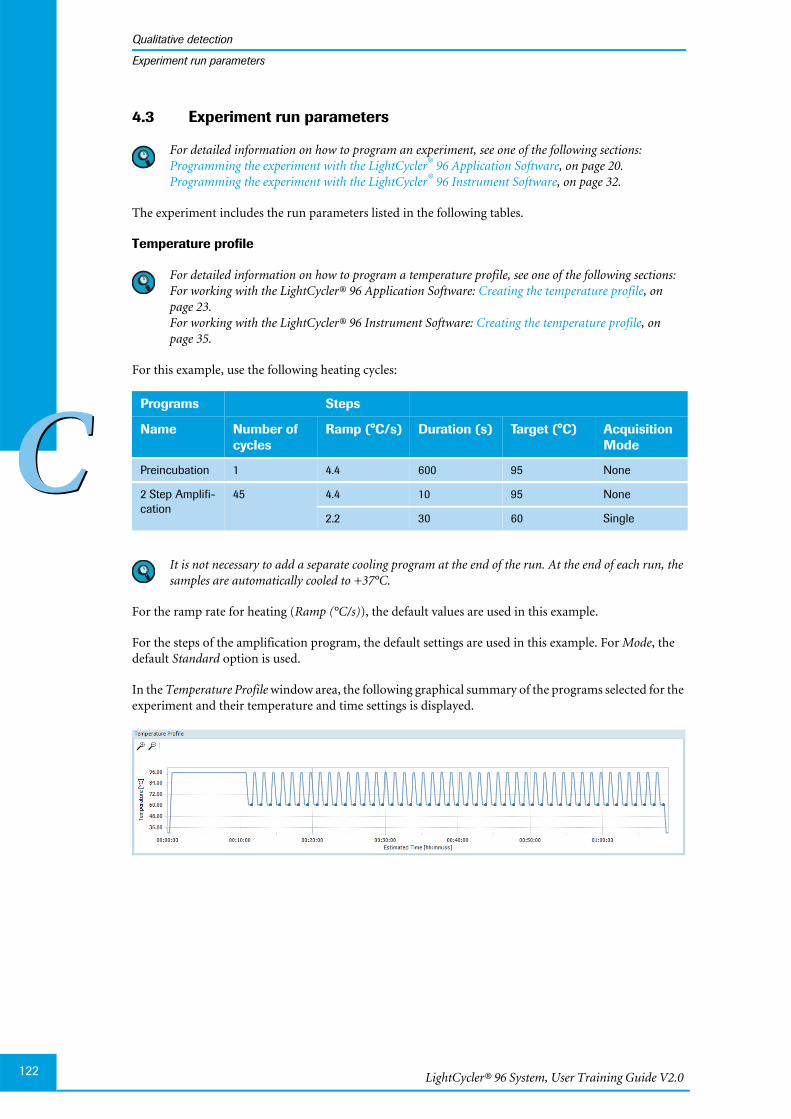
LightCycler® 96 System, User Training Guide V2.0122
Qualitative detection
CC
Experiment run parameters
4.3 Experiment run parameters
For detailed information on how to program an experiment, see one of the following sections:Programming the experiment with the LightCycler® 96 Application Software, on page 20.Programming the experiment with the LightCycler® 96 Instrument Software, on page 32.
The experiment includes the run parameters listed in the following tables.
Temperature profile
For detailed information on how to program a temperature profile, see one of the following sections:For working with the LightCycler® 96 Application Software: Creating the temperature profile, onpage 23.For working with the LightCycler® 96 Instrument Software: Creating the temperature profile, onpage 35.
For this example, use the following heating cycles:
It is not necessary to add a separate cooling program at the end of the run. At the end of each run, thesamples are automatically cooled to +37°C.
For the ramp rate for heating (Ramp (°C/s)), the default values are used in this example.
For the steps of the amplification program, the default settings are used in this example. For Mode, thedefault Standard option is used.
In the Temperature Profile window area, the following graphical summary of the programs selected for theexperiment and their temperature and time settings is displayed.
Programs Steps
Name Number ofcycles
Ramp (°C/s) Duration (s) Target (°C) AcquisitionMode
Preincubation 1 4.4 600 95 None
2 Step Amplifi-cation
45 4.4 10 95 None
2.2 30 60 Single
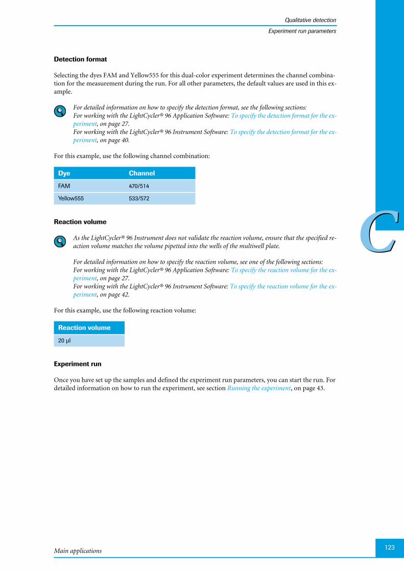
Main applications
Qualitative detection
123
CC
Experiment run parameters
Detection format
Selecting the dyes FAM and Yellow555 for this dual-color experiment determines the channel combina-tion for the measurement during the run. For all other parameters, the default values are used in this ex-ample.
For detailed information on how to specify the detection format, see the following sections:For working with the LightCycler® 96 Application Software: To specify the detection format for the ex-periment, on page 27.For working with the LightCycler® 96 Instrument Software: To specify the detection format for the ex-periment, on page 40.
For this example, use the following channel combination:
Reaction volume
As the LightCycler® 96 Instrument does not validate the reaction volume, ensure that the specified re-action volume matches the volume pipetted into the wells of the multiwell plate.
For detailed information on how to specify the reaction volume, see one of the following sections:For working with the LightCycler® 96 Application Software: To specify the reaction volume for the ex-periment, on page 27.For working with the LightCycler® 96 Instrument Software: To specify the reaction volume for the ex-periment, on page 42.
For this example, use the following reaction volume:
Experiment run
Once you have set up the samples and defined the experiment run parameters, you can start the run. Fordetailed information on how to run the experiment, see section Running the experiment, on page 43.
Dye Channel
FAM 470/514
Yellow555 533/572
Reaction volume
20 µl
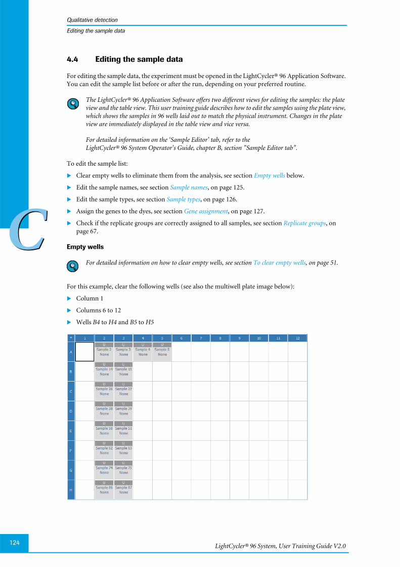
LightCycler® 96 System, User Training Guide V2.0124
Qualitative detection
CC
Editing the sample data
4.4 Editing the sample data
For editing the sample data, the experiment must be opened in the LightCycler® 96 Application Software.You can edit the sample list before or after the run, depending on your preferred routine.
The LightCycler® 96 Application Software offers two different views for editing the samples: the plateview and the table view. This user training guide describes how to edit the samples using the plate view,which shows the samples in 96 wells laid out to match the physical instrument. Changes in the plateview are immediately displayed in the table view and vice versa.
For detailed information on the ‘Sample Editor’ tab, refer to theLightCycler® 96 System Operator’s Guide, chapter B, section "Sample Editor tab".
To edit the sample list:
Clear empty wells to eliminate them from the analysis, see section Empty wells below.
Edit the sample names, see section Sample names, on page 125.
Edit the sample types, see section Sample types, on page 126.
Assign the genes to the dyes, see section Gene assignment, on page 127.
Check if the replicate groups are correctly assigned to all samples, see section Replicate groups, onpage 67.
Empty wells
For detailed information on how to clear empty wells, see section To clear empty wells, on page 51.
For this example, clear the following wells (see also the multiwell plate image below):
Column 1
Columns 6 to 12
Wells B4 to H4 and B5 to H5
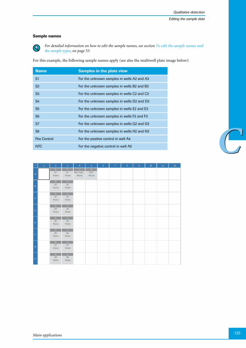
Main applications
Qualitative detection
125
CC
Editing the sample data
Sample names
For detailed information on how to edit the sample names, see section To edit the sample names andthe sample types, on page 53.
For this example, the following sample names apply (see also the multiwell plate image below):
Name Samples in the plate view
S1 For the unknown samples in wells A2 and A3
S2 For the unknown samples in wells B2 and B3
S3 For the unknown samples in wells C2 and C3
S4 For the unknown samples in wells D2 and D3
S5 For the unknown samples in wells E2 and E3
S6 For the unknown samples in wells F2 and F3
S7 For the unknown samples in wells G2 and G3
S8 For the unknown samples in wells H2 and H3
Pos Control For the positive control in well A4
NTC For the negative control in well A5

LightCycler® 96 System, User Training Guide V2.0126
Qualitative detection
CC
Editing the sample data
Sample types
For detailed information on how to edit the sample types, see section To edit the sample names and thesample types, on page 53.
In this example the following sample types apply:
Type Samples in the plate view
Unknown (default) For the samples S1 to S8
Positive control For the sample Pos Control
Negative control For the sample NTC
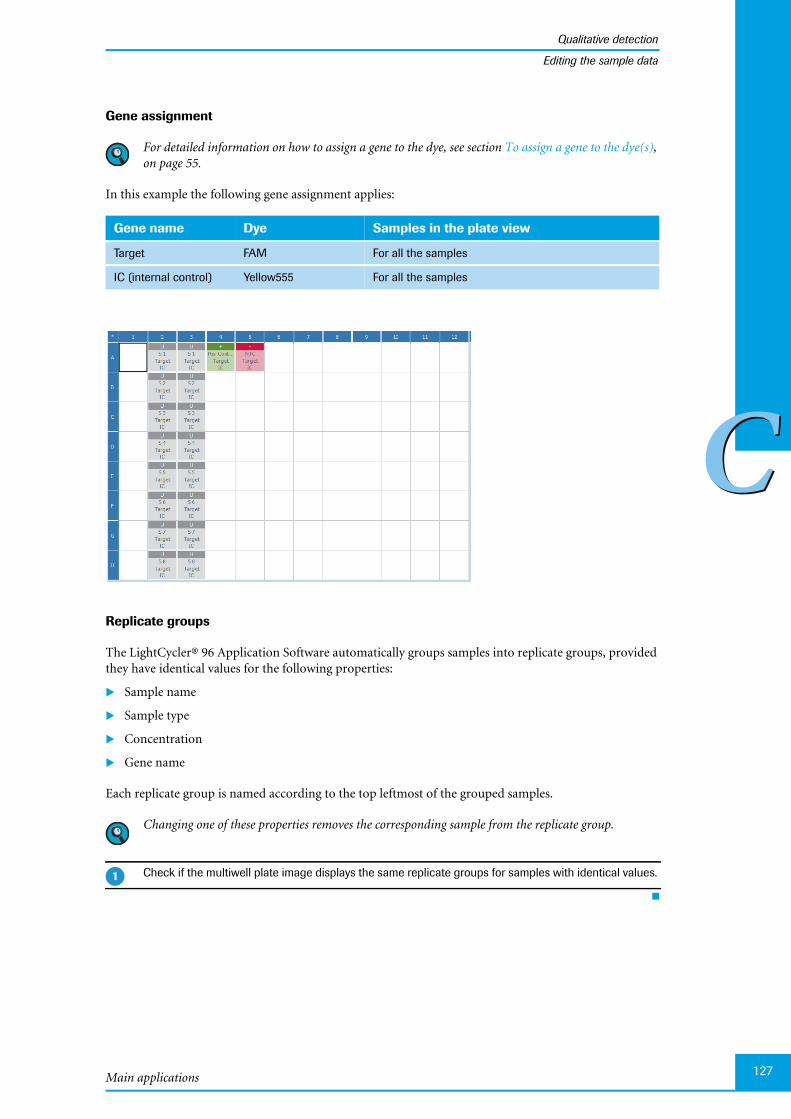
Main applications
Qualitative detection
127
CC
Editing the sample data
Gene assignment
For detailed information on how to assign a gene to the dye, see section To assign a gene to the dye(s),on page 55.
In this example the following gene assignment applies:
Replicate groups
The LightCycler® 96 Application Software automatically groups samples into replicate groups, providedthey have identical values for the following properties:
Sample name
Sample type
Concentration
Gene name
Each replicate group is named according to the top leftmost of the grouped samples.
Changing one of these properties removes the corresponding sample from the replicate group.
Gene name Dye Samples in the plate view
Target FAM For all the samples
IC (internal control) Yellow555 For all the samples
Check if the multiwell plate image displays the same replicate groups for samples with identical values.
�

LightCycler® 96 System, User Training Guide V2.0128
Qualitative detection
CC
Analyzing the results
4.5 Analyzing the results
For detailed information on the ‘Analysis’ tab, refer to the LightCycler® 96 System Operator’s Guide,chapter B, section "Qualitative detection".
For detailed information on working with tables and graphs, refer to theLightCycler® 96 System Operator’s Guide, chapter B, section "General software conventions".
To analyze the calculated results of the qualitative detection application:
Create the qualitative detection analysis, see section Creating the analysis below.
Optional: Specify the settings for the qualitative detection analysis, see section Analysis settings, onpage 130.
In the different views of the Qualitative Detection tab, check the analysis results and customize the re-sult data if necessary:
For the Amplification Curves view, see section Amplification curves, on page 131.
For the Heat Map view, see section Heat map, on page 131.
For the Combined Call Heat Map view, see section Combined call heat map, on page 132.
For the Result Table view, see section Result table, on page 133.
4.5.1 Creating the analysis
To create the Qualitative Detection analysis
Open the Analysis tab.
In the tool bar, choose the Add Analysis icon to add a new analysis.
The Create New Analysis dialog box opens.
Choose Qualitative Detection.
Choose OK.
The Qualitative Detection dialog box opens.
�
�
�
�
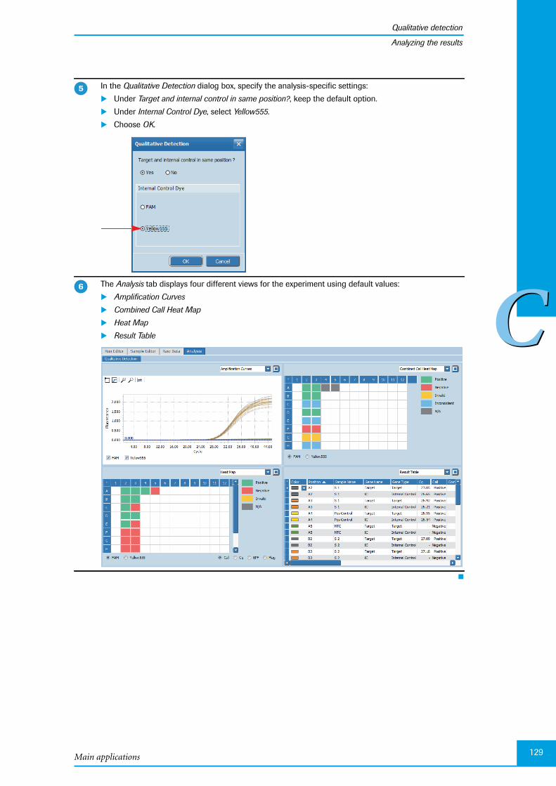
Main applications
Qualitative detection
129
CC
Analyzing the results
In the Qualitative Detection dialog box, specify the analysis-specific settings:
Under Target and internal control in same position?, keep the default option.
Under Internal Control Dye, select Yellow555.
Choose OK.
The Analysis tab displays four different views for the experiment using default values:
Amplification Curves
Combined Call Heat Map
Heat Map
Result Table
�
�

LightCycler® 96 System, User Training Guide V2.0130
Qualitative detection
CC
Analyzing the results
4.5.2 Analysis settings
Optional: To specify the analysis settings
In the tool bar, choose the Analysis Settings icon.
The Qualitative Detection Settings dialog box opens.
In the Qualitative Detection Settings dialog box, specify the analysis-specific settings, for example:
On the Genes tab, modify the value of the Minimal EPF, if applicable.
On the Samples tab, remove samples from the analysis, if applicable.
�
�
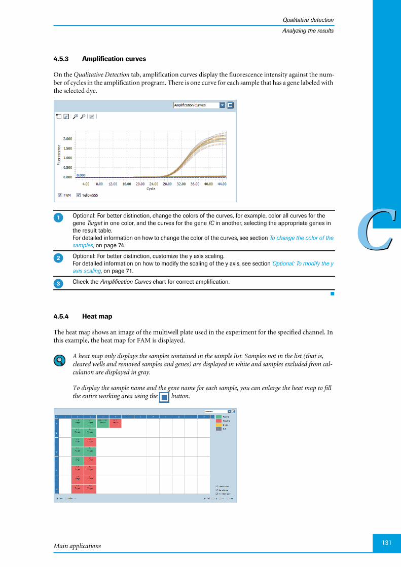
Main applications
Qualitative detection
131
CC
Analyzing the results
4.5.3 Amplification curves
On the Qualitative Detection tab, amplification curves display the fluorescence intensity against the num-ber of cycles in the amplification program. There is one curve for each sample that has a gene labeled withthe selected dye.
4.5.4 Heat map
The heat map shows an image of the multiwell plate used in the experiment for the specified channel. Inthis example, the heat map for FAM is displayed.
A heat map only displays the samples contained in the sample list. Samples not in the list (that is,cleared wells and removed samples and genes) are displayed in white and samples excluded from cal-culation are displayed in gray.
To display the sample name and the gene name for each sample, you can enlarge the heat map to fillthe entire working area using the button.
Optional: For better distinction, change the colors of the curves, for example, color all curves for thegene Target in one color, and the curves for the gene IC in another, selecting the appropriate genes inthe result table.For detailed information on how to change the color of the curves, see section To change the color of thesamples, on page 74.
Optional: For better distinction, customize the y axis scaling.For detailed information on how to modify the scaling of the y axis, see section Optional: To modify the yaxis scaling, on page 71.
Check the Amplification Curves chart for correct amplification.
�
�
�

LightCycler® 96 System, User Training Guide V2.0132
Qualitative detection
CC
Analyzing the results
In this example the Call heat map is displayed. It shows the Call status of all samples contained in the samplelist:
The samples A2, A3, A4, B2, B3, C2, D2, D3, and E2 are green, that is, Positive.
The samples A5, C3, E3, F2, F3, G2, G3, H2, H3, and the NTC A5 are red, that is, Negative.
4.5.5 Combined call heat map
The combined call heat map shows an image of the multiwell plate used in the experiment. It reports re-sults as a combined call by combining the individual calls of both genes, Target and IC.
The following basic result types are reported:
A combined call heat map only displays the samples contained in the sample list. Samples not in the list(that is, cleared wells and removed samples and genes) are displayed in white. Controls and Standards,if applicable, display combined call N/A.
To display the sample name and the gene name for each sample, you can enlarge the heat map to fillthe entire working area using the button.
This example shows the combined call result types of all samples contained in the sample list:
The samples A2, A3, B2, B3, D2, and D3 are green, that is, Positive.
The samples F2 and F3 are red, that is, Negative.
The samples G2 and G3 are yellow, that is, Invalid.
The samples C2, C3, E2, E3, H2, and H3 are blue, that is, Inconsistent.
The samples A4 and A5 are gray, that is, N/A (not available).
Combined call result type Meaning
Positive Target call positive, IC call positive or negative.
Negative Target call negative, IC call positive.
Invalid Target call negative, IC call negative.
Inconsistent One of the following result combinations applies:
Target replicate calls positive and negative, inde-pendent of IC replicate calls.
All Target replicate calls negative, IC replicate callspositive and negative.
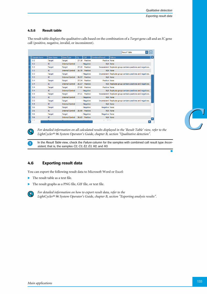
Main applications
Qualitative detection
133
CC
Exporting result data
4.5.6 Result table
The result table displays the qualitative calls based on the combination of a Target gene call and an IC genecall (positive, negative, invalid, or inconsistent).
For detailed information on all calculated results displayed in the ‘Result Table’ view, refer to theLightCycler® 96 System Operator’s Guide, chapter B, section "Qualitative detection".
4.6 Exporting result data
You can export the following result data to Microsoft Word or Excel:
The result table as a text file.
The result graphs as a PNG file, GIF file, or text file.
For detailed information on how to export result data, refer to theLightCycler® 96 System Operator’s Guide, chapter B, section "Exporting analysis results".
In the Result Table view, check the Failure column for the samples with combined call result type Incon-sistent, that is, the samples C2, C3, E2, E3, H2, and H3.
�
LightCycler® 96 System, User Training Guide V2.0134
Tm calling
CC
Experiment overview
5 Tm calling
When performing real-time PCR in the presence of an intercalating dye such as SYBR Green I, the in-crease in fluorescence is proportional to the amount of newly generated dsDNA. The SYBR Green I dye,however, binds all dsDNA, including specific and non-specific PCR products. This means that the pres-ence of primer-dimers and other non-specific products can affect the quality of real-time PCR data pro-duced using SYBR Green I. This also means that a melting curve analysis after the PCR is essential to verifyproduct identification.
A melting curve analysis in the presence of SYBR Green I identifies PCR products by GC content andlength. Both parameters determine the melting temperature (Tm) of a DNA fragment. Due to their smallsize, primer-dimers usually melt at a lower temperature than the specific PCR product.
For detailed information, refer to the LightCycler® 96 System Operator’s Guide, chapter A, sections"Detection formats" and "Analysis principles".
5.1 Experiment overview
The following example describes how to set up, run, and analyze a real-time PCR experiment using theSYBR Green I detection format. A Tm calling analysis for product identification enables the verification ofamplification results.
The assay is performed using a LightCycler® 480 Multiwell Plate 96, white. Each sample is set up in dupli-cate.
5.2 Setting up the samples
To set up the samples:
Include a no template control (NTC), see section Controls below.
Prepare the PCR mix, see section PCR mix, on page 135.
Pipette the sample dilution and the PCR mix, see section Pipetting scheme, on page 135.
Centrifuge the multiwell plate, see section Centrifugation, on page 135.
Continously cool the samples during setup by keeping the tubes on ice.
Controls
To ensure the absence of contaminating nucleic acids in PCR reagents, it is highly recommended that youinclude a no template control (NTC) in your experiment.
Samples 7 DNA samples (unknown concentration)
Reagents FastStart Essential DNA Green Master (2 x conc.)
Primer mix (20 x conc.), containing forward and reverse primer, 5 µM each
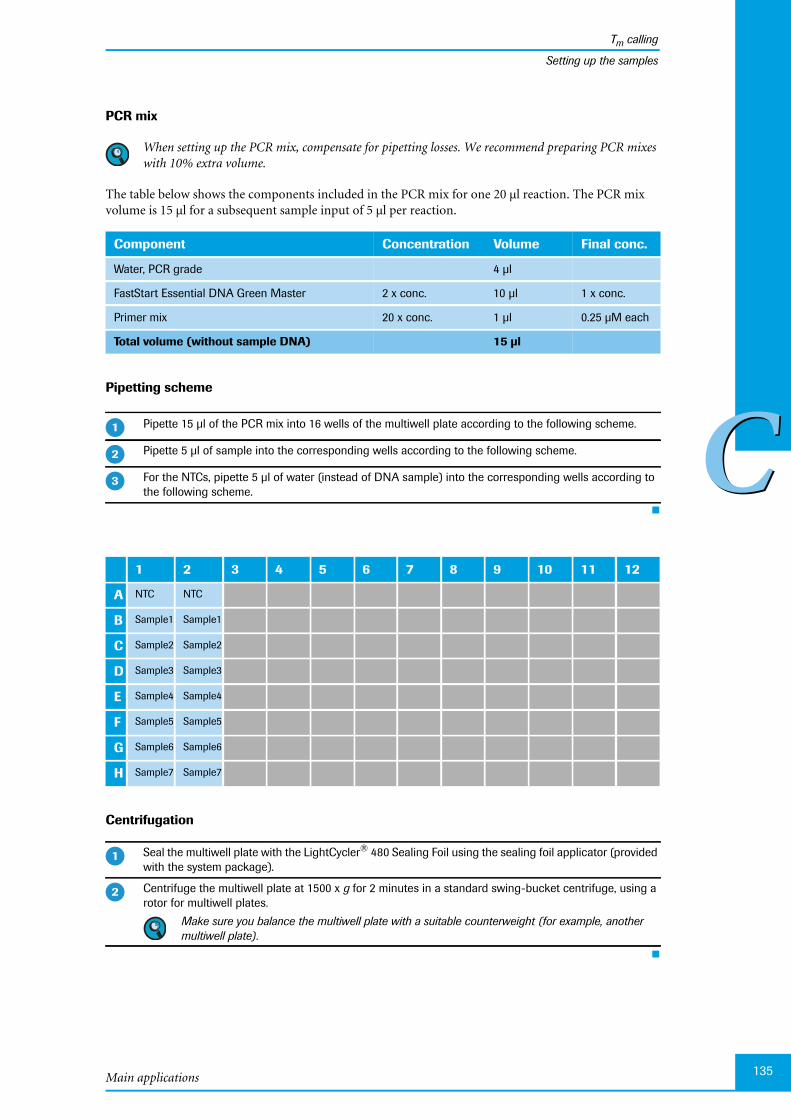
Main applications
Tm calling
135
CC
Setting up the samples
PCR mix
When setting up the PCR mix, compensate for pipetting losses. We recommend preparing PCR mixeswith 10% extra volume.
The table below shows the components included in the PCR mix for one 20 µl reaction. The PCR mixvolume is 15 µl for a subsequent sample input of 5 µl per reaction.
Pipetting scheme
Centrifugation
Component Concentration Volume Final conc.
Water, PCR grade 4 µl
FastStart Essential DNA Green Master 2 x conc. 10 µl 1 x conc.
Primer mix 20 x conc. 1 µl 0.25 µM each
Total volume (without sample DNA) 15 µl
Pipette 15 µl of the PCR mix into 16 wells of the multiwell plate according to the following scheme.
Pipette 5 µl of sample into the corresponding wells according to the following scheme.
For the NTCs, pipette 5 µl of water (instead of DNA sample) into the corresponding wells according tothe following scheme.
1 2 3 4 5 6 7 8 9 10 11 12
A NTC NTC
B Sample1 Sample1
C Sample2 Sample2
D Sample3 Sample3
E Sample4 Sample4
F Sample5 Sample5
G Sample6 Sample6
H Sample7 Sample7
Seal the multiwell plate with the LightCycler® 480 Sealing Foil using the sealing foil applicator (providedwith the system package).
Centrifuge the multiwell plate at 1500 x g for 2 minutes in a standard swing-bucket centrifuge, using arotor for multiwell plates.
Make sure you balance the multiwell plate with a suitable counterweight (for example, anothermultiwell plate).
�
�
�
�
�
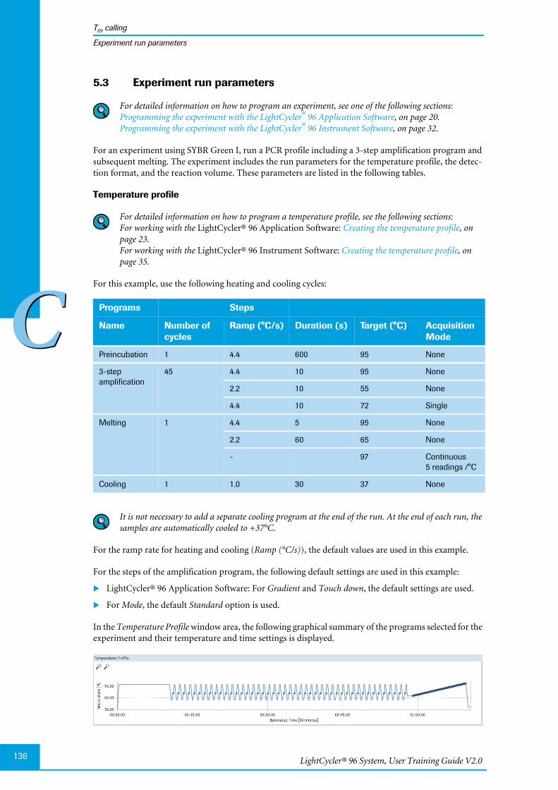
LightCycler® 96 System, User Training Guide V2.0136
Tm calling
CC
Experiment run parameters
5.3 Experiment run parameters
For detailed information on how to program an experiment, see one of the following sections:Programming the experiment with the LightCycler® 96 Application Software, on page 20.Programming the experiment with the LightCycler® 96 Instrument Software, on page 32.
For an experiment using SYBR Green I, run a PCR profile including a 3-step amplification program andsubsequent melting. The experiment includes the run parameters for the temperature profile, the detec-tion format, and the reaction volume. These parameters are listed in the following tables.
Temperature profile
For detailed information on how to program a temperature profile, see the following sections:For working with the LightCycler® 96 Application Software: Creating the temperature profile, onpage 23.For working with the LightCycler® 96 Instrument Software: Creating the temperature profile, onpage 35.
For this example, use the following heating and cooling cycles:
It is not necessary to add a separate cooling program at the end of the run. At the end of each run, thesamples are automatically cooled to +37°C.
For the ramp rate for heating and cooling (Ramp (°C/s)), the default values are used in this example.
For the steps of the amplification program, the following default settings are used in this example:
LightCycler® 96 Application Software: For Gradient and Touch down, the default settings are used.
For Mode, the default Standard option is used.
In the Temperature Profile window area, the following graphical summary of the programs selected for theexperiment and their temperature and time settings is displayed.
Programs Steps
Name Number ofcycles
Ramp (°C/s) Duration (s) Target (°C) AcquisitionMode
Preincubation 1 4.4 600 95 None
3-stepamplification
45 4.4 10 95 None
2.2 10 55 None
4.4 10 72 Single
Melting 1 4.4 5 95 None
2.2 60 65 None
- 97 Continuous5 readings /°C
Cooling 1 1.0 30 37 None

Main applications
Tm calling
137
CC
Experiment run parameters
Detection format
Selecting the dye (SYBR Green I) for this mono-color experiment determines the channel combinationfor the measurement during the run. For all other parameters, the default values are used in this example.
For detailed information on how to specify the detection format, see the following sections:For working with the LightCycler® 96 Application Software: To specify the detection format for the ex-periment, on page 27.For working with the LightCycler® 96 Instrument Software: To specify the detection format for the ex-periment, on page 40.
For this example, use the following channel:
Reaction volume
As the LightCycler® 96 Instrument does not validate the reaction volume, ensure that the specified re-action volume matches the volume pipetted into the wells of the multiwell plate.
For detailed information on how to specify the reaction volume, see the following sections:For working with the LightCycler® 96 Application Software: To specify the reaction volume for the ex-periment, on page 27.For working with the LightCycler® 96 Instrument Software: To specify the reaction volume for the ex-periment, on page 42.
For this example, use the following reaction volume:
Experiment run
Once you have set up the samples and defined the experiment run parameters,you can start the run. Fordetailed information on how to run the experiment, see section Running the experiment, on page 43.
Dye Channel
SYBR Green I 470/514
Reaction volume
20 µl

LightCycler® 96 System, User Training Guide V2.0138
Tm calling
CC
Editing the sample data
5.4 Editing the sample data
For editing the sample data, the experiment must be opened in the LightCycler® 96 Application Software.You can edit the sample list before or after the run, depending on your preferred routine.
The LightCycler® 96 Application Software offers two different views for editing the samples: the plateview and the table view. This user training guide describes how to edit the samples using the plate view,which shows the samples in 96 wells laid out to match the physical instrument. Changes in the plateview are immediately displayed in the table view and vice versa.
For detailed information on the ‘Sample Editor’ tab, refer to theLightCycler® 96 System Operator’s Guide, chapter B, section "Sample Editor tab".
To edit the sample list:
Clear empty wells to eliminate them from the analysis, see section Empty wells below.
Edit the sample names, see section Sample names, on page 139.
Edit the sample types, see section Sample types, on page 139.
Assign a gene for the dye, see section Gene assignment, on page 140.
Empty wells
For detailed information on how to clear empty wells, see section To clear empty wells, on page 51.
For this example, clear the wells in columns 3 to 12 (see also the multiwell plate image below).
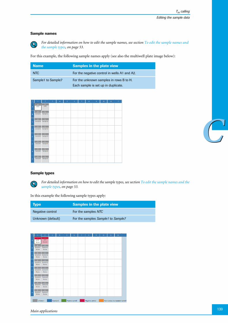
Main applications
Tm calling
139
CC
Editing the sample data
Sample names
For detailed information on how to edit the sample names, see section To edit the sample names andthe sample types, on page 53.
For this example, the following sample names apply (see also the multiwell plate image below):
Sample types
For detailed information on how to edit the sample types, see section To edit the sample names and thesample types, on page 53.
In this example the following sample types apply:
Name Samples in the plate view
NTC For the negative control in wells A1 and A2.
Sample1 to Sample7 For the unknown samples in rows B to H.
Each sample is set up in duplicate.
Type Samples in the plate view
Negative control For the samples NTC
Unknown (default) For the samples Sample1 to Sample7

LightCycler® 96 System, User Training Guide V2.0140
Tm calling
CC
Editing the sample data
Gene assignment
For detailed information on how to assign a gene to the dye, see section To assign a gene to the dye(s),on page 55.
In this example the following gene assignment applies:
Gene name Dye Samples in the plate view
Gene 1 SYBR Green I For all the samples

Main applications
Tm calling
141
CC
Analyzing the results
5.5 Analyzing the results
For detailed information on the ‘Analysis’ tab, refer to the LightCycler® 96 System Operator’s Guide,chapter B, section "Tm Calling".
For detailed information on working with tables and graphs, refer to theLightCycler® 96 System Operator’s Guide, chapter B, section "General software conventions".
To analyze the calculated results of the Tm Calling application:
Create the Abs Quant analysis and the Tm Calling analysis, see section Creating the analysis below.
Optional: Specify the melting analysis parameters, see section Analysis settings, on page 143.
In the different views of the Abs Quant and Tm Calling tabs, check the analysis results and customizethe result data if necessary:
On the Abs Quant tab, check the amplification curves for plausibility, see section Amplificationcurves, on page 144.
For the Melting Curves view, see section Melting curves, on page 144.
In the Melting Peaks view, specify a melting peak area, see section To specify the melting peak areaArea 1, on page 145.
For the Heat Map view, see section Heat map, on page 146.
In the Result Table view, check the melting temperature values, see section Result table, onpage 146.
5.5.1 Creating the analysis
To create the Abs Quant analysis
For detailed information on how to create the Abs Quant analysis, see section To create the Abs Quantanalysis, on page 68.
To create the Tm Calling analysis
Open the Analysis tab.
In the tool bar, choose the Add Analysis icon to add a new analysis.
The Create New Analysis dialog box opens.
�
�
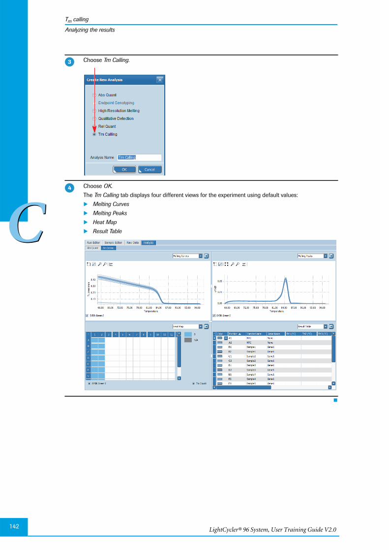
LightCycler® 96 System, User Training Guide V2.0142
Tm calling
CC
Analyzing the results
Choose Tm Calling.
Choose OK.
The Tm Calling tab displays four different views for the experiment using default values:
Melting Curves
Melting Peaks
Heat Map
Result Table
�
�

Main applications
Tm calling
143
CC
Analyzing the results
5.5.2 Analysis settings
Optional: To specify the analysis settings
In the tool bar, choose the Analysis Settings icon.
The Melting Analysis Parameters dialog box opens.
In the Melting Analysis Parameters dialog box, specify the analysis-specific settings, for example:
On the Areas tab, specify the areas where melting peaks are to be called. An area is displayed as arectangle which represents a temperature range and a fluorescence threshold.
The temperature and fluorescence settings in the Melting Analysis Parameters dialog box cor-respond to the area marking in the Melting Peaks graph. For detailed information, see sectionMelting peaks, on page 145.
On the Genes tab, remove a gene from the analysis.
On the Samples tab, remove samples from the analysis.
�
�
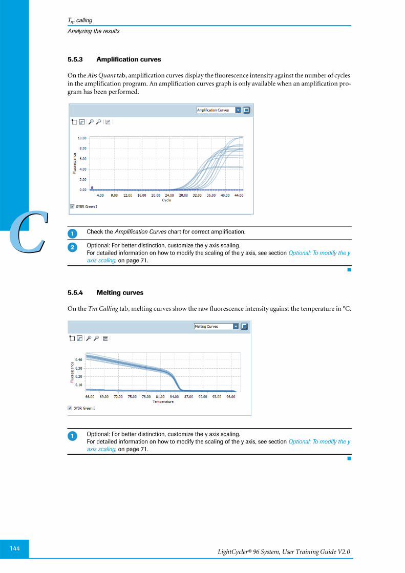
LightCycler® 96 System, User Training Guide V2.0144
Tm calling
CC
Analyzing the results
5.5.3 Amplification curves
On the Abs Quant tab, amplification curves display the fluorescence intensity against the number of cyclesin the amplification program. An amplification curves graph is only available when an amplification pro-gram has been performed.
5.5.4 Melting curves
On the Tm Calling tab, melting curves show the raw fluorescence intensity against the temperature in °C.
Check the Amplification Curves chart for correct amplification.
Optional: For better distinction, customize the y axis scaling.For detailed information on how to modify the scaling of the y axis, see section Optional: To modify the yaxis scaling, on page 71.
Optional: For better distinction, customize the y axis scaling.For detailed information on how to modify the scaling of the y axis, see section Optional: To modify the yaxis scaling, on page 71.
�
�
�

Main applications
Tm calling
145
CC
Analyzing the results
5.5.5 Melting peaks
The melting peaks graph displays the first negative derivative of the fluorescence with respect to the tem-perature in the melting program (-dF/dT). The graph shows a single melting peak, meaning that no addi-tional by-products are detected in the experiment.
To specify the melting peak area Area 1
The area marking in the melting peaks graph corresponds to the settings on the ‘Areas’ tab in the ‘Melt-ing Analysis Parameters’ dialog box, see section Analysis settings, on page 143.
Optional: For better distinction, customize the y axis scaling.For detailed information on how to modify the scaling of the y axis, see section Optional: To modify the yaxis scaling, on page 71.
In the Melting Peaks view, choose Area Marker to indicate that a marking action follows.
To specify the melting peak area Area 1:
Move the cursor to the point for the top left corner of the area.
Hold down the left mouse button and drag the cursor to the point for the bottom right corner of thearea.
Release the mouse button.
To change the size of the specified area, grab the relevant side or corner of the rectangle and drag itaccordingly.
The LightCycler® 96 Application Software allows five areas to be defined in one graph. To specifyan additional area, one of the existing areas must be deleted.
�
�
�

LightCycler® 96 System, User Training Guide V2.0146
Tm calling
CC
Exporting result data
5.5.6 Heat map
The heat map shows the melting temperatures for the melting peak area Area 1.
A heat map only displays the samples contained in the sample list. Samples not in the list (that is,cleared wells and removed samples and genes) are displayed in white and samples excluded from cal-culation are displayed in gray.
To display the sample name and the gene name for each sample, you can enlarge the heat map to fillthe entire working area using the button.
All samples for which the melting peak lies in the melting peak area Area 1 are assigned the correspondingarea number 1 and the color magenta, in this example the samples B1 to H2.
5.5.7 Result table
The result table displays the results of the Tm calling analysis. The TM1(°C) column shows the meltingtemperature (Tm) of any peak identified in Area 1 in the melting peaks graph. Where no peak is present,the table cells are blank.
5.6 Exporting result data
You can export the following result data to Microsoft Word or Excel:
The result table as a text file.
The result graphs as a PNG file, GIF file, or text file.
For detailed information on how to export result data, refer to theLightCycler® 96 System Operator’s Guide, chapter B, section "Exporting analysis results".
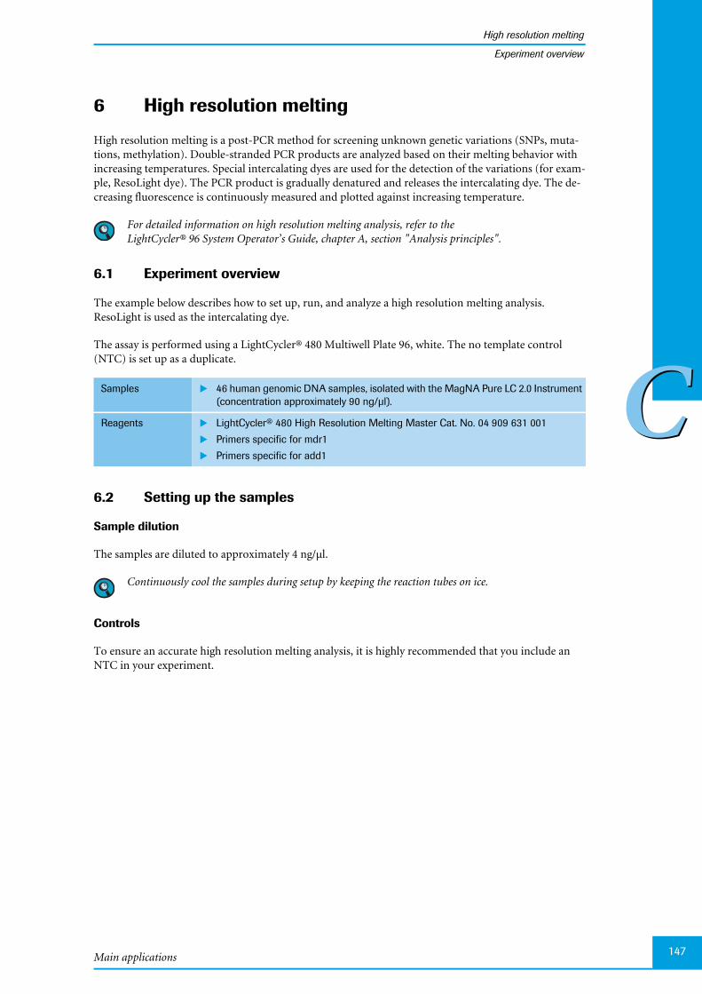
Main applications
High resolution melting
147
CC
Experiment overview
6 High resolution melting
High resolution melting is a post-PCR method for screening unknown genetic variations (SNPs, muta-tions, methylation). Double-stranded PCR products are analyzed based on their melting behavior withincreasing temperatures. Special intercalating dyes are used for the detection of the variations (for exam-ple, ResoLight dye). The PCR product is gradually denatured and releases the intercalating dye. The de-creasing fluorescence is continuously measured and plotted against increasing temperature.
For detailed information on high resolution melting analysis, refer to theLightCycler® 96 System Operator’s Guide, chapter A, section "Analysis principles".
6.1 Experiment overview
The example below describes how to set up, run, and analyze a high resolution melting analysis.ResoLight is used as the intercalating dye.
The assay is performed using a LightCycler® 480 Multiwell Plate 96, white. The no template control(NTC) is set up as a duplicate.
6.2 Setting up the samples
Sample dilution
The samples are diluted to approximately 4 ng/µl.
Continuously cool the samples during setup by keeping the reaction tubes on ice.
Controls
To ensure an accurate high resolution melting analysis, it is highly recommended that you include anNTC in your experiment.
Samples 46 human genomic DNA samples, isolated with the MagNA Pure LC 2.0 Instrument(concentration approximately 90 ng/µl).
Reagents LightCycler® 480 High Resolution Melting Master Cat. No. 04 909 631 001
Primers specific for mdr1
Primers specific for add1
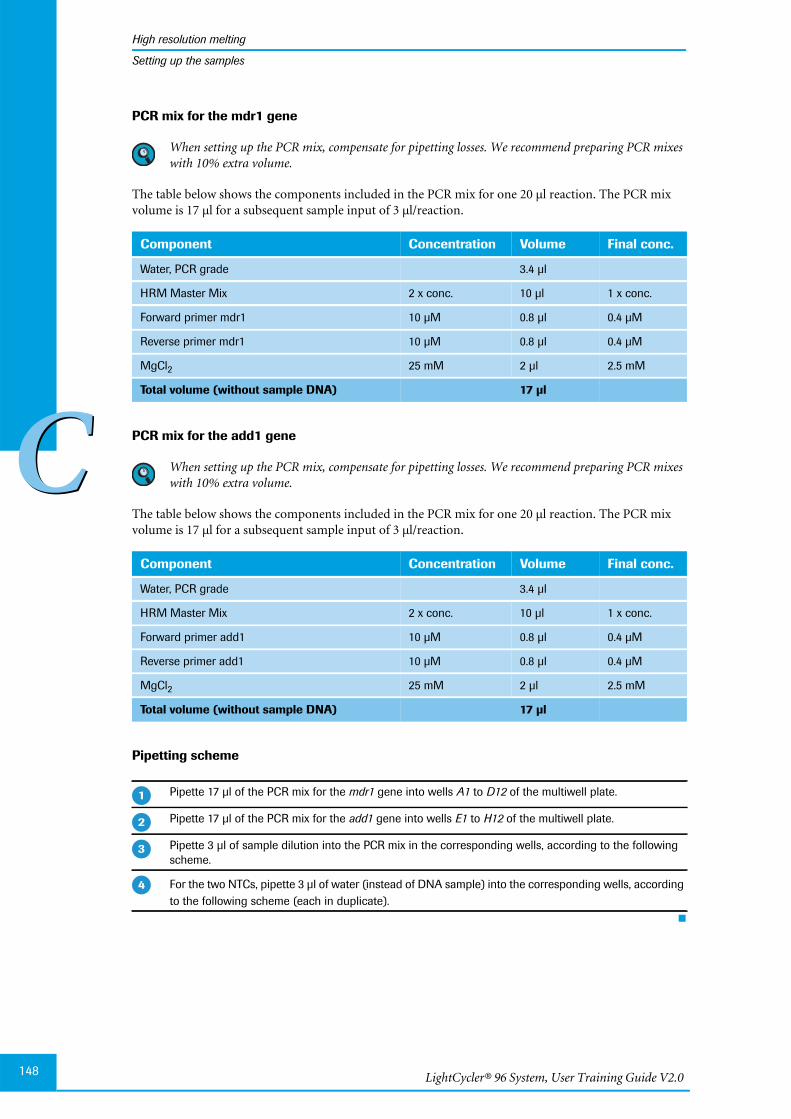
LightCycler® 96 System, User Training Guide V2.0148
High resolution melting
CC
Setting up the samples
PCR mix for the mdr1 gene
When setting up the PCR mix, compensate for pipetting losses. We recommend preparing PCR mixeswith 10% extra volume.
The table below shows the components included in the PCR mix for one 20 µl reaction. The PCR mixvolume is 17 µl for a subsequent sample input of 3 µl/reaction.
PCR mix for the add1 gene
When setting up the PCR mix, compensate for pipetting losses. We recommend preparing PCR mixeswith 10% extra volume.
The table below shows the components included in the PCR mix for one 20 µl reaction. The PCR mixvolume is 17 µl for a subsequent sample input of 3 µl/reaction.
Pipetting scheme
Component Concentration Volume Final conc.
Water, PCR grade 3.4 µl
HRM Master Mix 2 x conc. 10 µl 1 x conc.
Forward primer mdr1 10 µM 0.8 µl 0.4 µM
Reverse primer mdr1 10 µM 0.8 µl 0.4 µM
MgCl2 25 mM 2 µl 2.5 mM
Total volume (without sample DNA) 17 µl
Component Concentration Volume Final conc.
Water, PCR grade 3.4 µl
HRM Master Mix 2 x conc. 10 µl 1 x conc.
Forward primer add1 10 µM 0.8 µl 0.4 µM
Reverse primer add1 10 µM 0.8 µl 0.4 µM
MgCl2 25 mM 2 µl 2.5 mM
Total volume (without sample DNA) 17 µl
Pipette 17 µl of the PCR mix for the mdr1 gene into wells A1 to D12 of the multiwell plate.
Pipette 17 µl of the PCR mix for the add1 gene into wells E1 to H12 of the multiwell plate.
Pipette 3 µl of sample dilution into the PCR mix in the corresponding wells, according to the followingscheme.
For the two NTCs, pipette 3 µl of water (instead of DNA sample) into the corresponding wells, accordingto the following scheme (each in duplicate).
�
�
�
�
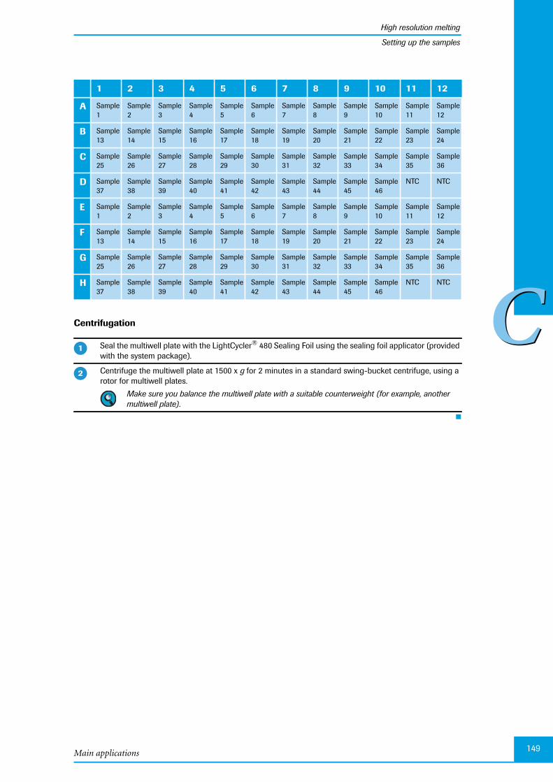
Main applications
High resolution melting
149
CC
Setting up the samples
Centrifugation
1 2 3 4 5 6 7 8 9 10 11 12
A Sample1
Sample2
Sample3
Sample4
Sample5
Sample6
Sample7
Sample8
Sample9
Sample10
Sample11
Sample12
B Sample13
Sample14
Sample15
Sample16
Sample17
Sample18
Sample19
Sample20
Sample21
Sample22
Sample23
Sample24
C Sample25
Sample26
Sample27
Sample28
Sample29
Sample30
Sample31
Sample32
Sample33
Sample34
Sample35
Sample36
D Sample37
Sample38
Sample39
Sample40
Sample41
Sample42
Sample43
Sample44
Sample45
Sample46
NTC NTC
E Sample1
Sample2
Sample3
Sample4
Sample5
Sample6
Sample7
Sample8
Sample9
Sample10
Sample11
Sample12
F Sample13
Sample14
Sample15
Sample16
Sample17
Sample18
Sample19
Sample20
Sample21
Sample22
Sample23
Sample24
G Sample25
Sample26
Sample27
Sample28
Sample29
Sample30
Sample31
Sample32
Sample33
Sample34
Sample35
Sample36
H Sample37
Sample38
Sample39
Sample40
Sample41
Sample42
Sample43
Sample44
Sample45
Sample46
NTC NTC
Seal the multiwell plate with the LightCycler® 480 Sealing Foil using the sealing foil applicator (providedwith the system package).
Centrifuge the multiwell plate at 1500 x g for 2 minutes in a standard swing-bucket centrifuge, using arotor for multiwell plates.
Make sure you balance the multiwell plate with a suitable counterweight (for example, anothermultiwell plate).
�
�
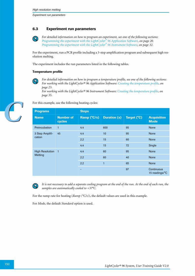
LightCycler® 96 System, User Training Guide V2.0150
High resolution melting
CC
Experiment run parameters
6.3 Experiment run parameters
For detailed information on how to program an experiment, see one of the following sections:Programming the experiment with the LightCycler® 96 Application Software, on page 20.Programming the experiment with the LightCycler® 96 Instrument Software, on page 32.
For the experiment, run a PCR profile including a 3-step amplification program and subsequent high res-olution melting.
The experiment includes the run parameters listed in the following tables.
Temperature profile
For detailed information on how to program a temperature profile, see one of the following sections:For working with the LightCycler® 96 Application Software: Creating the temperature profile, onpage 23.For working with the LightCycler® 96 Instrument Software: Creating the temperature profile, onpage 35.
For this example, use the following heating cycles:
It is not necessary to add a separate cooling program at the end of the run. At the end of each run, thesamples are automatically cooled to +37°C.
For the ramp rate for heating (Ramp (°C/s)), the default values are used in this example.
For Mode, the default Standard option is used.
Programs Steps
Name Number ofcycles
Ramp (°C/s) Duration (s) Target (°C) AcquisitionMode
Preincubation 1 4.4 600 95 None
3 Step Amplifi-cation
45 4.4 10 95 None
2.2 15 60 None
4.4 15 72 Single
High ResolutionMelting
1 4.4 60 95 None
2.2 60 40 None
2.2 1 65 None
- 97 Continuous15 readings/°C
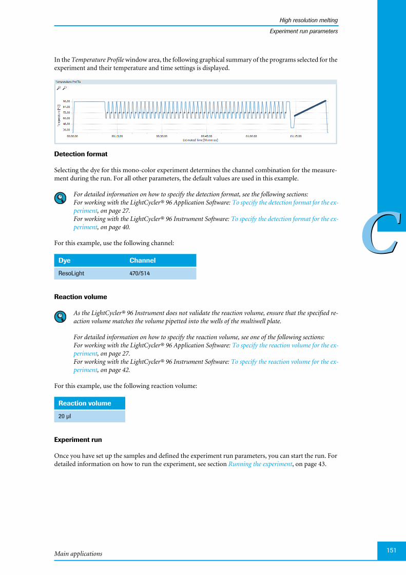
Main applications
High resolution melting
151
CC
Experiment run parameters
In the Temperature Profile window area, the following graphical summary of the programs selected for theexperiment and their temperature and time settings is displayed.
Detection format
Selecting the dye for this mono-color experiment determines the channel combination for the measure-ment during the run. For all other parameters, the default values are used in this example.
For detailed information on how to specify the detection format, see the following sections:For working with the LightCycler® 96 Application Software: To specify the detection format for the ex-periment, on page 27.For working with the LightCycler® 96 Instrument Software: To specify the detection format for the ex-periment, on page 40.
For this example, use the following channel:
Reaction volume
As the LightCycler® 96 Instrument does not validate the reaction volume, ensure that the specified re-action volume matches the volume pipetted into the wells of the multiwell plate.
For detailed information on how to specify the reaction volume, see one of the following sections:For working with the LightCycler® 96 Application Software: To specify the reaction volume for the ex-periment, on page 27.For working with the LightCycler® 96 Instrument Software: To specify the reaction volume for the ex-periment, on page 42.
For this example, use the following reaction volume:
Experiment run
Once you have set up the samples and defined the experiment run parameters, you can start the run. Fordetailed information on how to run the experiment, see section Running the experiment, on page 43.
Dye Channel
ResoLight 470/514
Reaction volume
20 µl
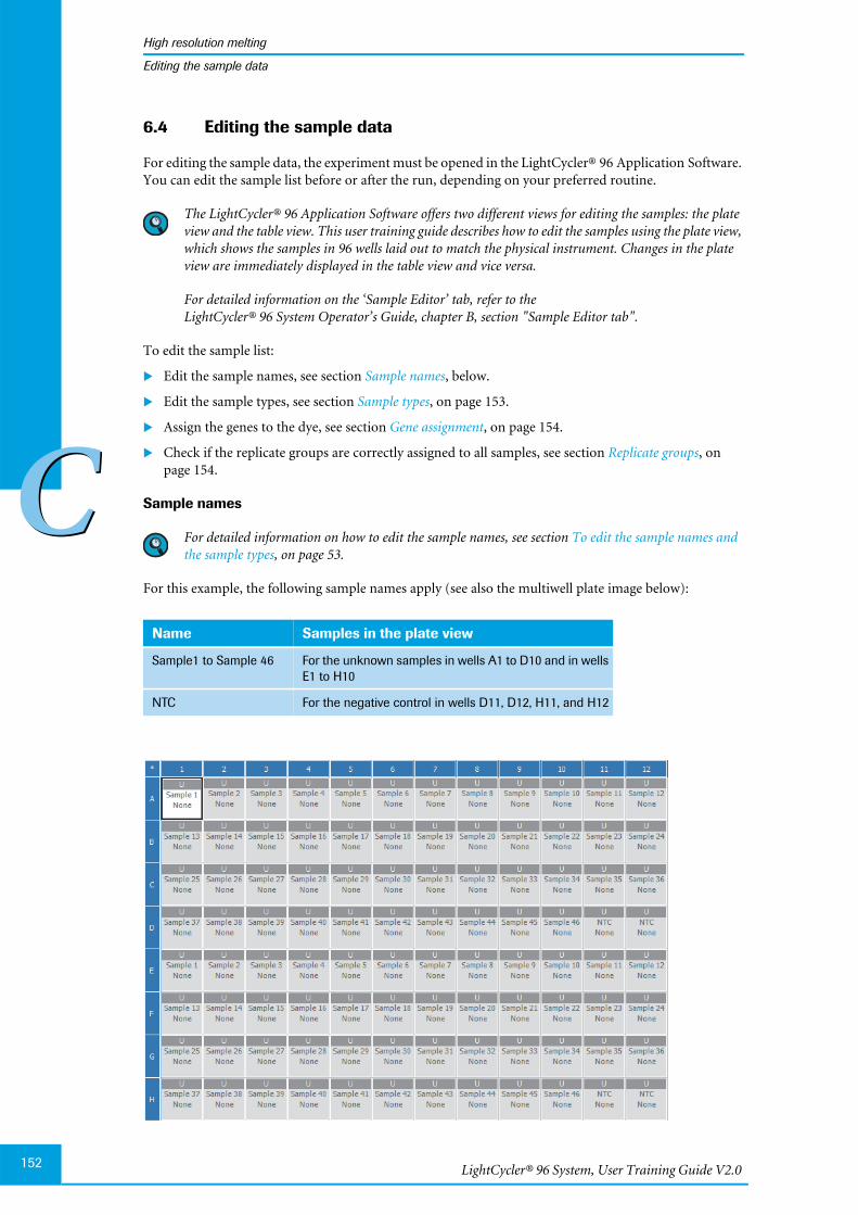
LightCycler® 96 System, User Training Guide V2.0152
High resolution melting
CC
Editing the sample data
6.4 Editing the sample data
For editing the sample data, the experiment must be opened in the LightCycler® 96 Application Software.You can edit the sample list before or after the run, depending on your preferred routine.
The LightCycler® 96 Application Software offers two different views for editing the samples: the plateview and the table view. This user training guide describes how to edit the samples using the plate view,which shows the samples in 96 wells laid out to match the physical instrument. Changes in the plateview are immediately displayed in the table view and vice versa.
For detailed information on the ‘Sample Editor’ tab, refer to theLightCycler® 96 System Operator’s Guide, chapter B, section "Sample Editor tab".
To edit the sample list:
Edit the sample names, see section Sample names, below.
Edit the sample types, see section Sample types, on page 153.
Assign the genes to the dye, see section Gene assignment, on page 154.
Check if the replicate groups are correctly assigned to all samples, see section Replicate groups, onpage 154.
Sample names
For detailed information on how to edit the sample names, see section To edit the sample names andthe sample types, on page 53.
For this example, the following sample names apply (see also the multiwell plate image below):
Name Samples in the plate view
Sample1 to Sample 46 For the unknown samples in wells A1 to D10 and in wellsE1 to H10
NTC For the negative control in wells D11, D12, H11, and H12

Main applications
High resolution melting
153
CC
Editing the sample data
Sample types
For detailed information on how to edit the sample types, see section To edit the sample names and thesample types, on page 53.
In this example the following sample types apply:
Type Samples in the plate view
Unknown (default) For the samples Sample1 to Sample46
Negative control For the samples NTC
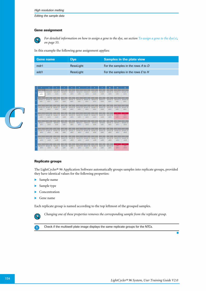
LightCycler® 96 System, User Training Guide V2.0154
High resolution melting
CC
Editing the sample data
Gene assignment
For detailed information on how to assign a gene to the dye, see section To assign a gene to the dye(s),on page 55.
In this example the following gene assignment applies:
Replicate groups
The LightCycler® 96 Application Software automatically groups samples into replicate groups, providedthey have identical values for the following properties:
Sample name
Sample type
Concentration
Gene name
Each replicate group is named according to the top leftmost of the grouped samples.
Changing one of these properties removes the corresponding sample from the replicate group.
Gene name Dye Samples in the plate view
mdr1 ResoLight For the samples in the rows A to D
add1 ResoLight For the samples in the rows E to H
Check if the multiwell plate image displays the same replicate groups for the NTCs.
�
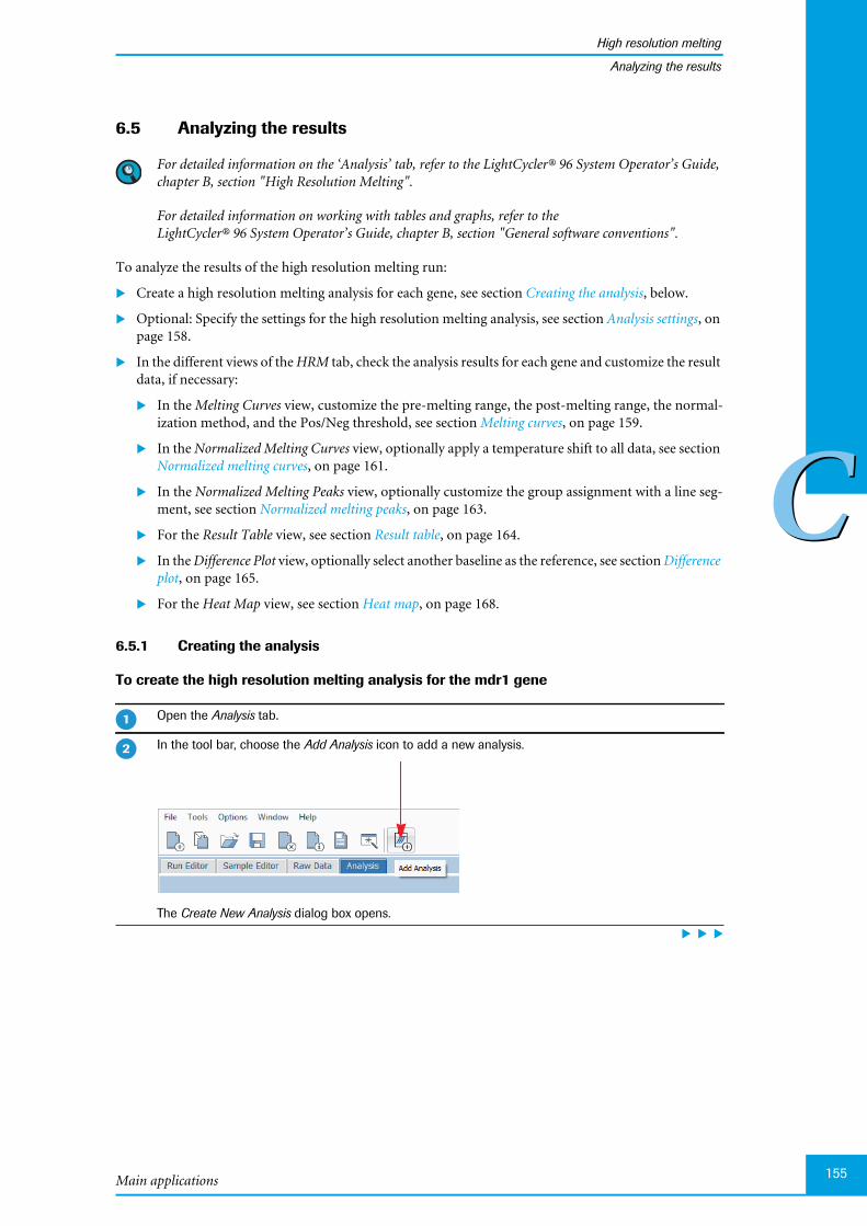
Main applications
High resolution melting
155
CC
Analyzing the results
6.5 Analyzing the results
For detailed information on the ‘Analysis’ tab, refer to the LightCycler® 96 System Operator’s Guide,chapter B, section "High Resolution Melting".
For detailed information on working with tables and graphs, refer to theLightCycler® 96 System Operator’s Guide, chapter B, section "General software conventions".
To analyze the results of the high resolution melting run:
Create a high resolution melting analysis for each gene, see section Creating the analysis, below.
Optional: Specify the settings for the high resolution melting analysis, see section Analysis settings, onpage 158.
In the different views of the HRM tab, check the analysis results for each gene and customize the resultdata, if necessary:
In the Melting Curves view, customize the pre-melting range, the post-melting range, the normal-ization method, and the Pos/Neg threshold, see section Melting curves, on page 159.
In the Normalized Melting Curves view, optionally apply a temperature shift to all data, see sectionNormalized melting curves, on page 161.
In the Normalized Melting Peaks view, optionally customize the group assignment with a line seg-ment, see section Normalized melting peaks, on page 163.
For the Result Table view, see section Result table, on page 164.
In the Difference Plot view, optionally select another baseline as the reference, see section Differenceplot, on page 165.
For the Heat Map view, see section Heat map, on page 168.
6.5.1 Creating the analysis
To create the high resolution melting analysis for the mdr1 gene
Open the Analysis tab.
In the tool bar, choose the Add Analysis icon to add a new analysis.
The Create New Analysis dialog box opens.
�
�

LightCycler® 96 System, User Training Guide V2.0156
High resolution melting
CC
Analyzing the results
Choose High Resolution Melting.
In Analysis Name, enter HRM mdr1.
Choose OK.
The Select HRM Gene dialog box opens.
From the Create HRM Analysis for Gene: drop-down list, choose mdr1.
Choose OK.
The HRM mdr1 tab opens.
�
�
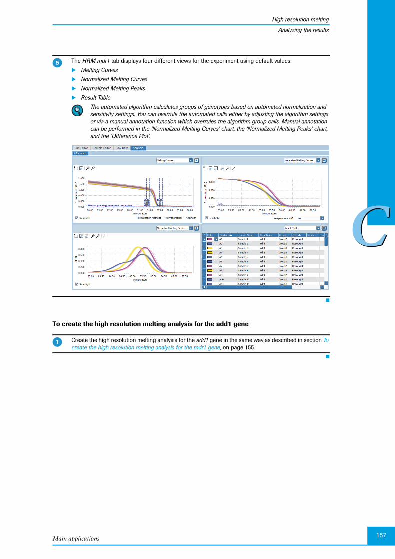
Main applications
High resolution melting
157
CC
Analyzing the results
To create the high resolution melting analysis for the add1 gene
The HRM mdr1 tab displays four different views for the experiment using default values:
Melting Curves
Normalized Melting Curves
Normalized Melting Peaks
Result Table
The automated algorithm calculates groups of genotypes based on automated normalization andsensitivity settings. You can overrule the automated calls either by adjusting the algorithm settingsor via a manual annotation function which overrules the algorithm group calls. Manual annotationcan be performed in the ‘Normalized Melting Curves’ chart, the ‘Normalized Melting Peaks’ chart,and the ‘Difference Plot’.
Create the high resolution melting analysis for the add1 gene in the same way as described in section Tocreate the high resolution melting analysis for the mdr1 gene, on page 155.
�
�
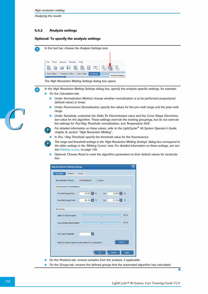
LightCycler® 96 System, User Training Guide V2.0158
High resolution melting
CC
Analyzing the results
6.5.2 Analysis settings
Optional: To specify the analysis settings
In the tool bar, choose the Analysis Settings icon.
The High Resolution Melting Settings dialog box opens.
In the High Resolution Melting Settings dialog box, specify the analysis-specific settings, for example:
On the Calculation tab:
Under Normalization Method, choose whether normalization is to be performed proportional(default value) or linear.
Under Fluorescence Normalization, specify the values for the pre-melt range and the post-meltrange.
Under Sensitivity, customize the Delta Tm Discrimination value and the Curve Shape Discrimina-tion value for the algorithm. These settings overrule the existing groupings, but do not overrulethe settings for Pos/Neg Threshold, normalization, and Temperature Shift.
For detailed information on these values, refer to the LightCycler® 96 System Operator’s Guide,chapter B, section "High Resolution Melting".
In Pos / Neg Threshold, specify the threshold value for the fluorescence.
The range and threshold settings in the ‘High Resolution Melting Settings’ dialog box correspond tothe slider settings in the ‘Melting Curves’ view. For detailed information on these settings, see sec-tion Melting curves, on page 159.
Optional: Choose Reset to reset the algorithm parameters to their default values for recalcula-tion.
On the Positions tab, remove samples from the analysis, if applicable.
On the Groups tab, rename the defined groups that the automated algorithm has calculated.
�
�
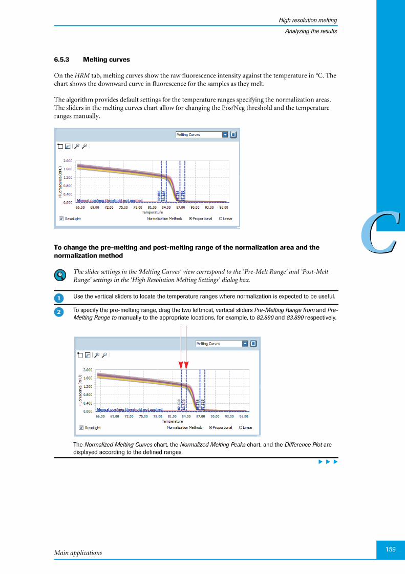
Main applications
High resolution melting
159
CC
Analyzing the results
6.5.3 Melting curves
On the HRM tab, melting curves show the raw fluorescence intensity against the temperature in °C. Thechart shows the downward curve in fluorescence for the samples as they melt.
The algorithm provides default settings for the temperature ranges specifying the normalization areas.The sliders in the melting curves chart allow for changing the Pos/Neg threshold and the temperatureranges manually.
To change the pre-melting and post-melting range of the normalization area and thenormalization method
The slider settings in the ‘Melting Curves’ view correspond to the ‘Pre-Melt Range’ and ‘Post-MeltRange’ settings in the ‘High Resolution Melting Settings’ dialog box.
Use the vertical sliders to locate the temperature ranges where normalization is expected to be useful.
To specify the pre-melting range, drag the two leftmost, vertical sliders Pre-Melting Range from and Pre-Melting Range to manually to the appropriate locations, for example, to 82.890 and 83.890 respectively.
The Normalized Melting Curves chart, the Normalized Melting Peaks chart, and the Difference Plot aredisplayed according to the defined ranges.
�
�

LightCycler® 96 System, User Training Guide V2.0160
High resolution melting
CC
Analyzing the results
To specify the post-melting range, drag the two rightmost, vertical sliders Post-Melting Range from andPost-Melting Range to manually to the appropriate locations, for example, to 86.770 and 87.770 respec-tively.
The Normalized Melting Curves chart, the Normalized Melting Peaks chart, and the Difference Plot aredisplayed according to the defined ranges.
Optional: To specify the Normalization Method, choose the corresponding option: Proportional or Linear.
The Normalized Melting Curves chart, the Normalized Melting Peaks chart, and the Difference Plot aredisplayed according to the specified method.
�
�
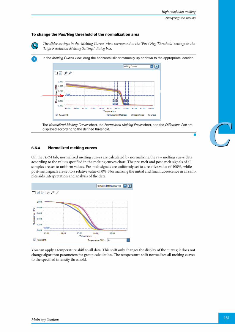
Main applications
High resolution melting
161
CC
Analyzing the results
To change the Pos/Neg threshold of the normalization area
The slider settings in the ‘Melting Curves’ view correspond to the ‘Pos / Neg Threshold’ settings in the‘High Resolution Melting Settings’ dialog box.
6.5.4 Normalized melting curves
On the HRM tab, normalized melting curves are calculated by normalizing the raw melting curve dataaccording to the values specified in the melting curves chart. The pre-melt and post-melt signals of allsamples are set to uniform values. Pre-melt signals are uniformly set to a relative value of 100%, whilepost-melt signals are set to a relative value of 0%. Normalizing the initial and final fluorescence in all sam-ples aids interpretation and analysis of the data.
You can apply a temperature shift to all data. This shift only changes the display of the curves; it does notchange algorithm parameters for group calculation. The temperature shift normalizes all melting curvesto the specified intensity threshold.
In the Melting Curves view, drag the horizontal slider manually up or down to the appropriate location.
The Normalized Melting Curves chart, the Normalized Melting Peaks chart, and the Difference Plot aredisplayed according to the defined threshold.
�
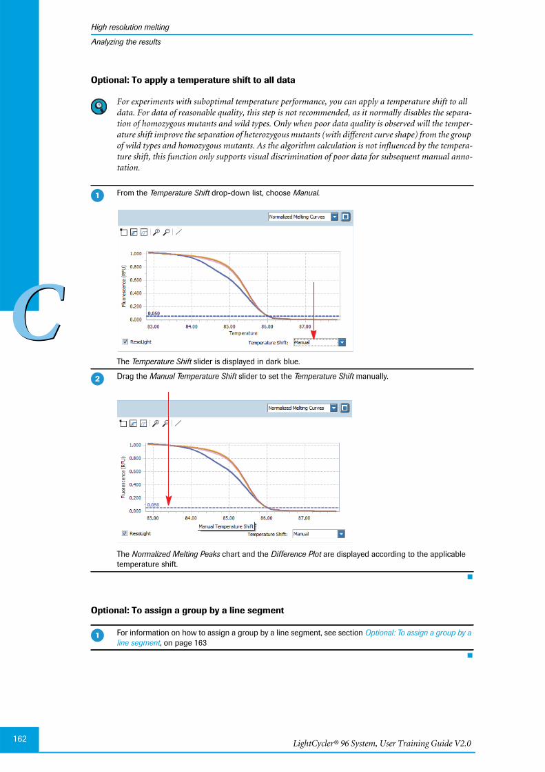
LightCycler® 96 System, User Training Guide V2.0162
High resolution melting
CC
Analyzing the results
Optional: To apply a temperature shift to all data
For experiments with suboptimal temperature performance, you can apply a temperature shift to alldata. For data of reasonable quality, this step is not recommended, as it normally disables the separa-tion of homozygous mutants and wild types. Only when poor data quality is observed will the temper-ature shift improve the separation of heterozygous mutants (with different curve shape) from the groupof wild types and homozygous mutants. As the algorithm calculation is not influenced by the tempera-ture shift, this function only supports visual discrimination of poor data for subsequent manual anno-tation.
Optional: To assign a group by a line segment
From the Temperature Shift drop-down list, choose Manual.
The Temperature Shift slider is displayed in dark blue.
Drag the Manual Temperature Shift slider to set the Temperature Shift manually.
The Normalized Melting Peaks chart and the Difference Plot are displayed according to the applicabletemperature shift.
For information on how to assign a group by a line segment, see section Optional: To assign a group by aline segment, on page 163
�
�
�
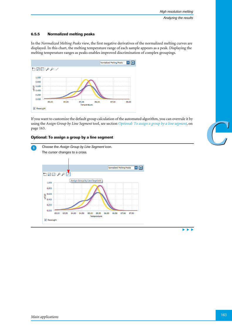
Main applications
High resolution melting
163
CC
Analyzing the results
6.5.5 Normalized melting peaks
In the Normalized Melting Peaks view, the first negative derivatives of the normalized melting curves aredisplayed. In this chart, the melting temperature range of each sample appears as a peak. Displaying themelting temperature ranges as peaks enables improved discrimination of complex groupings.
If you want to customize the default group calculation of the automated algorithm, you can overrule it byusing the Assign Group by Line Segment tool, see section Optional: To assign a group by a line segment, onpage 163.
Optional: To assign a group by a line segment
Choose the Assign Group by Line Segment icon.
The cursor changes to a cross.
�

LightCycler® 96 System, User Training Guide V2.0164
High resolution melting
CC
Analyzing the results
6.5.6 Result table
The result table displays the calculated results of the high resolution melting, for example, which groupeach sample belongs to. The sample colors in the result table are automatically assigned and updated ac-cording to the group calls.
For detailed information on all calculated results displayed in the ‘Result Table’ view, refer to theLightCycler® 96 System Operator’s Guide, chapter B, section "High resolution melting".
Select the samples that you want to assign to another group.
Click in the graph, for example the Normalized Melting Peaks graph.
Hold down the left mouse button and draw a line with the mouse to select one or more curves thatyou want to assign to another group.
When you release the mouse button, all curves which pass through the line will be selected and all oth-er curves deselected. The Group Assignment dialog box opens.
From the Assign to Group: drop-down list, choose the group the selected samples are to be assigned to.
Choose OK.
All charts on the HRM tab are displayed according to the new group assignment.
�
�
�
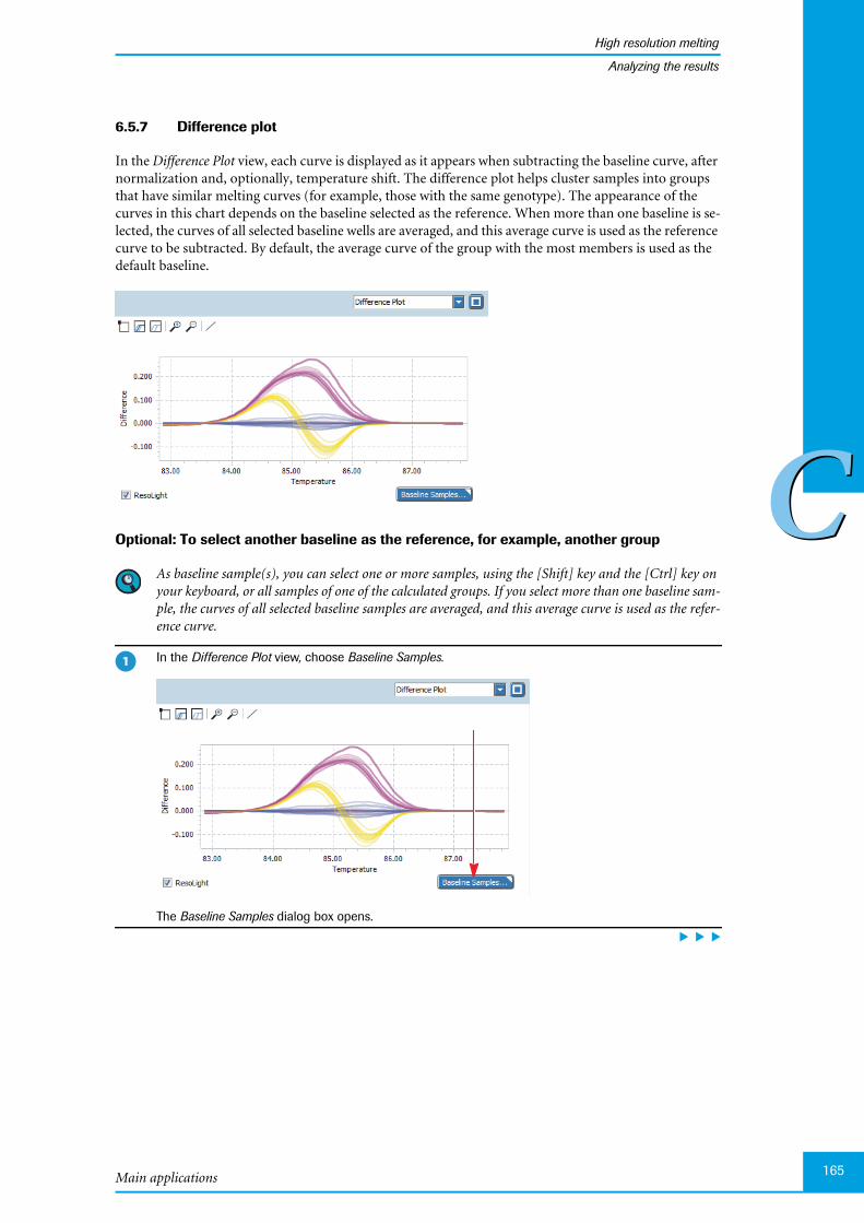
Main applications
High resolution melting
165
CC
Analyzing the results
6.5.7 Difference plot
In the Difference Plot view, each curve is displayed as it appears when subtracting the baseline curve, afternormalization and, optionally, temperature shift. The difference plot helps cluster samples into groupsthat have similar melting curves (for example, those with the same genotype). The appearance of thecurves in this chart depends on the baseline selected as the reference. When more than one baseline is se-lected, the curves of all selected baseline wells are averaged, and this average curve is used as the referencecurve to be subtracted. By default, the average curve of the group with the most members is used as thedefault baseline.
Optional: To select another baseline as the reference, for example, another group
As baseline sample(s), you can select one or more samples, using the [Shift] key and the [Ctrl] key onyour keyboard, or all samples of one of the calculated groups. If you select more than one baseline sam-ple, the curves of all selected baseline samples are averaged, and this average curve is used as the refer-ence curve.
In the Difference Plot view, choose Baseline Samples.
The Baseline Samples dialog box opens.
�
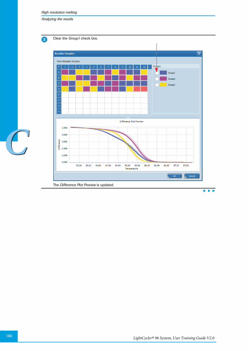
LightCycler® 96 System, User Training Guide V2.0166
High resolution melting
CC
Analyzing the results
Clear the Group1 check box.
The Difference Plot Preview is updated.
�
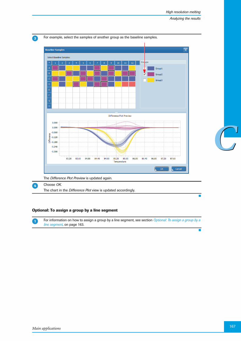
Main applications
High resolution melting
167
CC
Analyzing the results
Optional: To assign a group by a line segment
For example, select the samples of another group as the baseline samples.
The Difference Plot Preview is updated again.
Choose OK.
The chart in the Difference Plot view is updated accordingly.
For information on how to assign a group by a line segment, see section Optional: To assign a group by aline segment, on page 163.
�
�
�

LightCycler® 96 System, User Training Guide V2.0168
High resolution melting
CC
Exporting result data
6.5.8 Heat map
The heat map shows an image of the multiwell plate used in the experiment for the specified channel(ResoLight dye). For each well, the calculated group type is displayed. As the high resolution melting anal-ysis is gene-specific, only the samples the relevant gene is assigned to are displayed.
A heat map only displays the samples contained in the sample list. Samples not in the list (that is,cleared wells and removed samples) are displayed in white.
To display the sample name and the gene name for each sample, you can enlarge the heat map to fillthe entire working area using the button.
The image below shows the heat map for the samples the mdr1 gene is assigned to.
6.6 Exporting result data
You can export the following result data to Microsoft Word or Excel:
The result table as a text file.
The result graphs as a PNG file, GIF file, or text file.
For detailed information on how to export result data, refer to theLightCycler® 96 System Operator’s Guide, chapter B, section "Exporting analysis results".
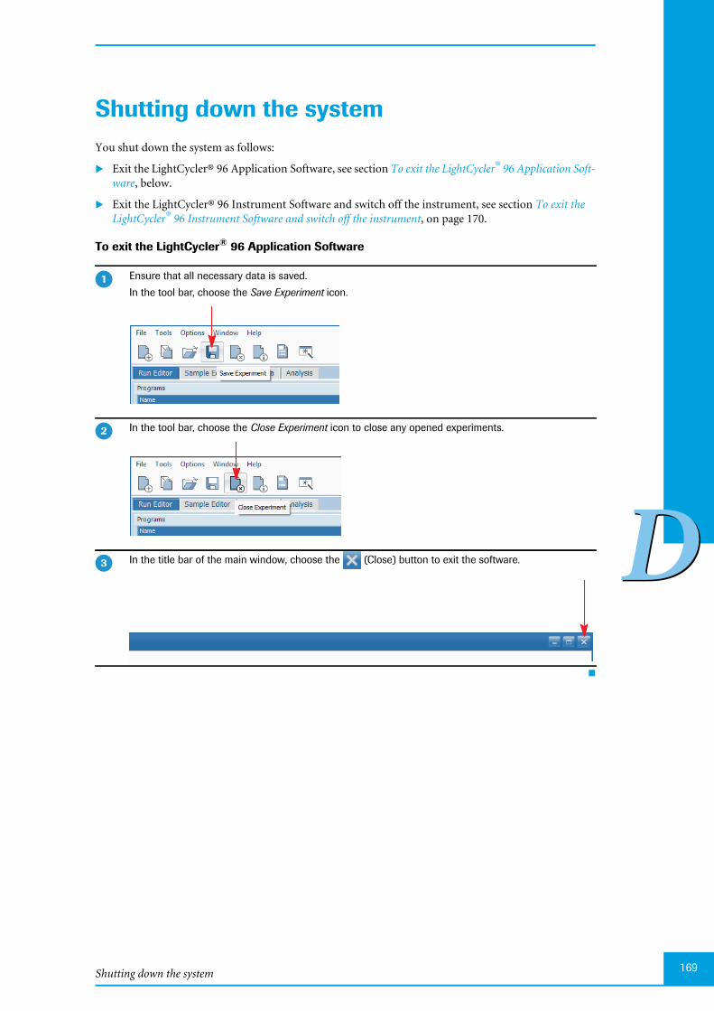
Shutting down the system 169
DD
Shutting down the system 0You shut down the system as follows:
Exit the LightCycler® 96 Application Software, see section To exit the LightCycler® 96 Application Soft-ware, below.
Exit the LightCycler® 96 Instrument Software and switch off the instrument, see section To exit theLightCycler® 96 Instrument Software and switch off the instrument, on page 170.
To exit the LightCycler® 96 Application Software
Ensure that all necessary data is saved.
In the tool bar, choose the Save Experiment icon.
In the tool bar, choose the Close Experiment icon to close any opened experiments.
In the title bar of the main window, choose the (Close) button to exit the software.
�
�
�
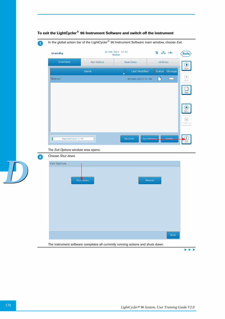
LightCycler® 96 System, User Training Guide V2.0170
DD
To exit the LightCycler® 96 Instrument Software and switch off the instrument
In the global action bar of the LightCycler® 96 Instrument Software main window, choose Exit.
The Exit Options window area opens.
Choose Shut down.
The instrument software completes all currently running actions and shuts down.
�
�
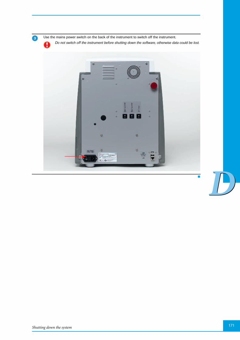
Shutting down the system 171
DD
Use the mains power switch on the back of the instrument to switch off the instrument.
Do not switch off the instrument before shutting down the software, otherwise data could be lost.
�

LightCycler® 96 System, User Training Guide V2.0
DD
172
Index
EE
Appendix 173
Appendix 0
1 Index
Symbols.lc96p................................................................. 42.lc96u................................................................. 42.rdml ................................................................. 42
AAbs Quant Settings dialog box .......................... 70Absolute quantification ..................................... 58
amplification curves ............................... 71analysis settings ...................................... 70concentration ......................................... 65controls .................................................. 58Cq bars ................................................... 77creating analysis ..................................... 68detection format .................................... 61editing sample data ................................ 62empty wells ............................................ 62gene assignment ..................................... 65heat map ................................................ 73PCR mix................................................. 59pipetting scheme .................................... 59reaction volume ..................................... 61replicate groups...................................... 67result table.............................................. 73sample color........................................... 74sample dilution ...................................... 58sample names......................................... 63sample types ........................................... 64standard curves ...................................... 72temperature profile ................................ 60
Add New Program dialog box ........................... 35All Data tab
relative quantification .......................... 118Amplification curves
absolute quantification........................... 71endpoint genotyping .............................. 89qualitative detection............................. 131relative quantification .......................... 113Tm calling ............................................ 144
Analysis settingsabsolute quantification........................... 70endpoint genotyping .............................. 88high resolution melting ........................ 158qualitative detection............................. 130relative quantification .......................... 111Tm calling ............................................ 143
Assign group by line segmenthigh resolution melting ........................ 163
Assigning gene to dye ........................................ 55
BBaseline samples
difference plot ...................................... 165
CCentrifugation.............. 59, 79, 101, 121, 135, 149Clearing wells .................................................... 51Combined call heat map
qualitative detection............................. 132Concentration
absolute quantification .......................... 65Conditions
relative quantification .......................... 107Controls
absolute quantification .......................... 58endpoint genotyping .............................. 78high resolution melting........................ 147qualitative detection............................. 120relative quantification ............................ 99Tm calling ............................................ 134
Cq ....................................................................... 9Cq bars
relative quantification .......................... 118Cq Bars chart..................................................... 77Creating
absolute quantification analysis ............. 68endpoint genotyping analysis................. 86experiment, application software ........... 21experiment, instrument software ........... 32high resolution melting analysis........... 155qualitative detection analysis................ 128relative quantification analysis ............. 109Tm calling analysis ............................... 141
Cy5 ...................................................................... 9
DData Visualization dialog box ......................... 114Detection format
absolute quantification .......................... 61application software ............................... 27endpoint genotyping .............................. 81high resolution melting........................ 151instrument software ............................... 40qualitative detection............................. 123relative quantification .......................... 103Tm calling ............................................ 137
Detection Format dialog boxapplication software ............................... 27
Detection Format window areainstrument software ............................... 40
Difference plothigh resolution melting........................ 165specifying baseline samples as reference165
dsDNA ................................................................ 9
LightCycler® 96 System, User Training Guide V2.0
EE
Index
174
EE .......................................................................... 9Editing sample names........................................ 53Editing sample types.......................................... 53Endpoint genotyping......................................... 78
amplification curves ............................... 89analysis settings ...................................... 88controls .................................................. 78creating analysis ..................................... 86detection format..................................... 81editing sample data ................................ 82empty wells............................................. 82filtering results ....................................... 95gene assignment ..................................... 85heat map ................................................ 93PCR mix ................................................. 79pipetting scheme .................................... 79reaction volume ..................................... 81renaming genotypes ............................... 94result table.............................................. 93sample dilution ...................................... 78sample names ......................................... 83sample types ........................................... 84scatter plot.............................................. 91temperature profile ................................ 80
EPF ...................................................................... 9Error bars ........................................................ 115Experiment
.rdml files ............................................... 42absolute quantification........................... 58assigning gene to dye .............................. 55clearing wells .......................................... 51creating, application software................. 21creating, instrument software................. 32detection format, application software... 27detection format, instrument software ... 40editing sample names ............................. 53editing sample types ............................... 53endpoint genotyping .............................. 78file types ................................................. 42LightCycler® 96 files............................... 42monitoring ............................................. 45reaction volume, application software.... 27reaction volume, instrument software.... 42run finished ............................................ 46sample list .............................................. 50sample names ......................................... 54sample types ........................................... 54saving, application software ............. 29, 56saving, instrument software ................... 42starting ................................................... 43synchronizing......................................... 48temperature profile, application software .................................................................. 23temperature profile, instrument software .................................................................. 35Tm calling ............................................ 134transferring to application software ....... 47transferring to the instrument................ 30
FFAM .................................................................... 9File suffix
.lc96p...................................................... 42
.lc96u...................................................... 42
.rdml ...................................................... 42
GGene assignment
absolute quantification........................... 65endpoint genotyping .............................. 85high resolution melting ........................ 154qualitative detection ............................. 127relative quantification .......................... 107Tm calling ............................................ 140
Genotypes.......................................................... 91renaming ................................................ 94
GOI ..................................................................... 9
HHeat map
absolute quantification........................... 73endpoint genotyping .............................. 93high resolution melting ........................ 168qualitative detection ............................. 131relative quantification .......................... 117Tm calling ............................................ 146
HEX .................................................................... 9High resolution melting .................................. 147
analysis settings .................................... 158assign group by line segment................ 163controls ................................................ 147creating analysis ................................... 155detection format................................... 151difference plot ...................................... 165editing sample data .............................. 152gene assignment ................................... 154heat map .............................................. 168melting curves ...................................... 159normalized melting curves ................... 161normalized melting peaks .................... 163PCR mix............................................... 148pipetting scheme .................................. 148reaction volume ................................... 151replicate groups.................................... 154result table............................................ 164sample dilution .................................... 147sample names ....................................... 152sample types ......................................... 153temperature profile .............................. 150
HRM ................................................................... 9

Index
EE
Appendix 175
LLightCycler® 96 Application Software
shutting down ...................................... 169starting ................................................... 17
LightCycler® 96 Instrumentshutting down ...................................... 170starting ................................................... 17symbols .................................................. 11
LightCycler® 96 Instrument Softwareshutting down ...................................... 170
MMelting Analysis Parameters dialog box.......... 143Melting curves
changing the Pos/Neg Threshold of thenormalization area ............................... 161changing the post-melting range.......... 159changing the pre-melting range ........... 159high resolution melting ........................ 159Tm calling ............................................ 144
Melting peak areasTm calling ............................................ 145
Melting peaksTm calling ............................................ 145
Monitoring experiment run .............................. 45
NNormalized melting curves
applying a temperature shift ................ 162high resolution melting ........................ 161
Normalized melting peakshigh resolution melting ........................ 163
NRC .................................................................... 9NTC .................................................................... 9
PPCR ..................................................................... 9PCR mix
absolute quantification........................... 59endpoint genotyping .............................. 79high resolution melting ........................ 148qualitative detection............................. 121relative quantification .................... 99, 100Tm calling ............................................ 135
PE........................................................................ 9Pipetting scheme
absolute quantification........................... 59endpoint genotyping .............................. 79high resolution melting ........................ 148qualitative detection............................. 121relative quantification .......................... 100Tm calling ............................................ 135
Plate View tab.................................................... 53Pos/Neg Threshold of the normalization area
melting curves ...................................... 161Post-melting range
melting curves ...................................... 159Preconditions .................................................... 57
Predefined Programs dialog box ....................... 23Pre-melting range
melting curves...................................... 159Program
adding, application software .................. 23adding, instrument software .................. 35
Program Settings window area .......................... 36
QqPCR ................................................................... 9Qualitative detection ....................................... 120
amplification curves............................. 131analysis settings .................................... 130combined call heat map ....................... 132controls ................................................ 120creating analysis ................................... 128detection format .................................. 123editing sample data .............................. 124empty wells .......................................... 124gene assignment ................................... 127heat map .............................................. 131PCR mix............................................... 121pipetting scheme .................................. 121reaction volume ................................... 123replicate groups.................................... 127result table............................................ 133sample dilution .................................... 120sample names....................................... 125sample types......................................... 126temperature profile .............................. 122
Qualitative Detection Settings dialog box ....... 130
RRatio bars ........................................................ 113
data visualization ................................. 114RDML ................................................................. 9Reaction volume
absolute quantification .......................... 61application software ............................... 27endpoint genotyping .............................. 81high resolution melting........................ 151instrument software ............................... 42qualitative detection............................. 123relative quantification .......................... 103Tm calling ............................................ 137
Reference generelative quantification .......................... 111
LightCycler® 96 System, User Training Guide V2.0
EE
Index
176
Relative quantificationAll Data tab .......................................... 118amplification curves ............................. 113analysis settings .................................... 111conditions ............................................ 107controls .................................................. 99Cq bars ................................................. 118creating analysis ................................... 109detection format................................... 103editing sample data .............................. 104empty wells........................................... 104error bars.............................................. 115gene assignment ................................... 107heat map .............................................. 117PCR mix, reference gene ...................... 100PCR mix, target gene.............................. 99pipetting scheme .................................. 100ratio bars .............................................. 113reaction volume ................................... 103reference gene ...................................... 111result table............................................ 118sample dilution ...................................... 99sample names ....................................... 105sample types ......................................... 106Statistic Data tab .................................. 118study calibrator .................................... 112temperature profile .............................. 102
Replicate groupsabsolute quantification........................... 67high resolution melting ........................ 154qualitative detection ............................. 127
Result tableabsolute quantification........................... 73endpoint genotyping .............................. 93filtering................................................... 95high resolution melting ........................ 164qualitative detection ............................. 133relative quantification .......................... 118Tm calling ............................................ 146
Runfinished .................................................. 46monitoring ............................................. 45preconditions ......................................... 57starting ................................................... 43
Run Editor tabapplication software ............................... 23instrument software ............................... 35
SSample color
absolute quantification........................... 74endpoint genotyping .............................. 96
Sample dataabsolute quantification........................... 62endpoint genotyping .............................. 82high resolution melting ........................ 152qualitative detection ............................. 124relative quantification .......................... 104Tm calling ............................................ 138
Sample dilutionabsolute quantification........................... 58endpoint genotyping .............................. 78high resolution melting ........................ 147qualitative detection ............................. 120relative quantification ............................ 99
Sample Editor tab .............................................. 53Sample list ......................................................... 50
clearing wells .......................................... 51Plate View tab ........................................ 53Sample Editor tab................................... 53
Sample names.................................................... 54absolute quantification........................... 63endpoint genotyping .............................. 83high resolution melting ........................ 152qualitative detection ............................. 125relative quantification .......................... 105Tm calling ............................................ 139
Sample types...................................................... 54absolute quantification........................... 64endpoint genotyping .............................. 84high resolution melting ........................ 153qualitative detection ............................. 126relative quantification .......................... 106Tm calling ............................................ 139
Savingexperiment to USB drive ........................ 47experiment, application software ..... 29, 56experiment, instrument software ........... 42
Scalingy axis ...................................................... 71
Scatter plot ........................................................ 91angles ..................................................... 91genotype groups ..................................... 91selecting cycle as basis for fluorescencevalue display........................................... 93slider settings.......................................... 91thresholds............................................... 91
Shutting downLightCycler® 96 Application Software.. 169LightCycler® 96 Instrument ................. 170LightCycler® 96 Instrument Software .. 170
SNP ..................................................................... 9Standard curve
absolute quantification........................... 72Starting
experiment run ...................................... 43LightCycler® 96 Application Software.... 17LightCycler® 96 Instrument ................... 17
Statistic Data tabrelative quantification .......................... 118
StepAcquisition Mode, application software. 26Acquisition Mode, instrument software. 39adding, application software .................. 25adding, instrument software .................. 37Temperature, application software......... 25Temperature, instrument software......... 38
Study calibrator ............................................... 112
Index
EE
Appendix 177
SYBR ................................................................... 9Sync Selected ..................................................... 48
TTemperature profile
absolute quantification........................... 60creating, application software ................ 23creating, instrument software ................ 35endpoint genotyping .............................. 80high resolution melting ........................ 150qualitative detection............................. 122relative quantification .......................... 102Tm calling ............................................ 136
Temperature shiftnormalized melting curves ................... 162
Tm....................................................................... 9Tm calling ....................................................... 134
amplification curves ............................. 144analysis settings .................................... 143controls ........................................ 134, 135creating analysis ................................... 141detection format .................................. 137editing sample data .............................. 138empty wells .......................................... 138gene assignment ................................... 140heat map .............................................. 146melting curves ...................................... 144melting peaks ....................................... 145PCR mix............................................... 135reaction volume ................................... 137result table............................................ 146sample names....................................... 139sample types ......................................... 139temperature profile .............................. 136
Transferringexperiment to application software ........ 47experiment to the instrument ................ 30
UUSB ..................................................................... 9USB drive
saving experiment .................................. 47synchronizing......................................... 48
VVIC...................................................................... 9
YY axis scaling ..................................................... 71
For life science research only. Not for use in diagnostic procedures.

Published by Roche Diagnostics GmbH Sandhofer Straße 11668305 Mannheim Germany
© 2012 Roche Diagnostics. All rights reserved.
www.roche-applied-science.com
b 0513
For life science research only. Not for use in diagnostic procedures.
LightCycler® 96 SystemOperator’s Guide, Version 2.0Software Version 1.1 May 2013

Table of contents
3
Prologue 9
I Revision history ............................................................................................................................................... 9
II Contact addresses ......................................................................................................................................... 9
III Declaration of conformity ....................................................................................................................... 10
IV Warranty ........................................................................................................................................................... 10
V Trademarks ..................................................................................................................................................... 10
VI Intended use ................................................................................................................................................... 10
VII License statements for the LightCycler® 96 Instrument ...................................................... 10
VIII Software License Agreement ............................................................................................................... 11
1 PROGRAM LICENSE AGREEMENT .......................................................................................................... 112 GRANT OF SOFTWARE LICENSE .............................................................................................................. 113 LIMITED WARRANTY .................................................................................................................................... 114 DISCLAIMER OF WARRANTIES ................................................................................................................ 125 LIMITATIONS OF REMEDIES ...................................................................................................................... 126 GENERAL INFORMATION ........................................................................................................................... 127 INTELLECTUAL PROPERTY RIGHTS ........................................................................................................ 138 DURATION AND TERMINATION .............................................................................................................. 139 IMPORT, EXPORT AND USE OF THE SOFTWARE .............................................................................. 1310 MISCELLANEOUS ........................................................................................................................................... 1311 GOVERNING LAW AND PLACE OF JURISDICTION .......................................................................... 13
IX Open Source licenses ............................................................................................................................... 14
X Preamble .......................................................................................................................................................... 14
XI Contents of this operator’s guide ....................................................................................................... 14
XII Conventions used in this guide ........................................................................................................... 15
XIII Warnings and precautions ..................................................................................................................... 18
XIV Disposal of the instrument ..................................................................................................................... 20
A System description 21
1 Introduction .................................................................................................................................................... 24
2 Specifications of the LightCycler® 96 Instrument .................................................................... 25
2.1 General specifications ................................................................................................................................... 252.1.1 Environmental parameters ........................................................................................................................... 252.1.2 Interfaces ............................................................................................................................................................ 26
2.2 Technical specifications ............................................................................................................................... 262.3 Specifications of the detection unit .......................................................................................................... 26
2.3.1 Excitation ............................................................................................................................................................ 262.3.2 Detection ............................................................................................................................................................ 26
2.4 Filter set .............................................................................................................................................................. 262.5 Specifications of the thermal block cycler ............................................................................................. 272.6 Specifications of the external handheld barcode scanner .............................................................. 27
3 The LightCycler® 96 System Package ............................................................................................. 28
4 System description ..................................................................................................................................... 29
4.1 The LightCycler® 96 Instrument ................................................................................................................ 294.1.1 Loading module ............................................................................................................................................... 304.1.2 Touchscreen ...................................................................................................................................................... 304.1.3 USB interfaces .................................................................................................................................................. 304.1.4 Instrument back ............................................................................................................................................... 314.1.5 Ventilation .......................................................................................................................................................... 32
LightCycler® 96 System, Operator’s Guide V2.0
Table of contents
4
4.2 Block cycler unit ............................................................................................................................................... 334.2.1 Thermal block cycler ...................................................................................................................................... 334.2.2 Multiwell plate mount .................................................................................................................................... 34
4.3 Detection unit ................................................................................................................................................... 354.3.1 Optic module ..................................................................................................................................................... 354.3.2 Filter module ...................................................................................................................................................... 364.3.3 CCD camera ...................................................................................................................................................... 37
4.4 Detection channels ......................................................................................................................................... 384.5 Disposables ........................................................................................................................................................ 394.6 Reagents ............................................................................................................................................................. 414.7 Additional equipment .................................................................................................................................... 41
5 Installation ....................................................................................................................................................... 42
5.1 Installing the LightCycler® 96 Instrument .............................................................................................. 425.1.1 Installation requirements .............................................................................................................................. 425.1.2 Space and power requirements ................................................................................................................. 435.1.3 Assembling the instrument .......................................................................................................................... 44
5.2 Installing and configuring the LightCycler® 96 Instrument Software ......................................... 505.2.1 Installing the LightCycler® 96 Instrument Software .......................................................................... 505.2.2 Configuring a one-to-one connection ..................................................................................................... 505.2.3 Configuring an Ethernet network connection ...................................................................................... 55
5.3 Installing the LightCycler® 96 Application Software ......................................................................... 575.3.1 System requirements ..................................................................................................................................... 575.3.2 Installing the LightCycler® 96 Application Software ......................................................................... 575.3.3 The LightCycler® 96 Application Software home directory ............................................................ 585.3.4 Uninstalling the LightCycler® 96 Application Software .................................................................... 59
5.4 Managing updates .......................................................................................................................................... 605.4.1 Installing a LightCycler® 96 Application Software update .............................................................. 605.4.2 Installing a LightCycler® 96 Instrument Software update ............................................................... 605.4.3 Upgrading the LightCycler® 96 Instrument Software Version 1.0 ................................................ 625.4.4 Installing a firmware update ........................................................................................................................ 63
6 Detection formats ........................................................................................................................................ 64
6.1 Monitoring PCR with an intercalating fluorescent dye ..................................................................... 656.2 Monitoring PCR with hydrolysis probes .................................................................................................. 66
7 Analysis principles ...................................................................................................................................... 68
7.1 Quantification analysis .................................................................................................................................. 687.1.1 Absolute quantification analysis ................................................................................................................ 717.1.2 Relative quantification analysis .................................................................................................................. 727.1.3 Qualitative detection analysis ..................................................................................................................... 77
7.2 Endpoint genotyping analysis ..................................................................................................................... 787.3 Tm calling analysis ........................................................................................................................................... 797.4 High resolution melting analysis ................................................................................................................ 81
Table of contents
5
B LightCycler® 96 Application Software 85
1 Overview ........................................................................................................................................................... 89
1.1 Starting the software ..................................................................................................................................... 901.2 Startup wizard .................................................................................................................................................. 901.3 The main window ............................................................................................................................................ 93
1.3.1 Menu bar ............................................................................................................................................................ 941.3.2 Tool bar ............................................................................................................................................................... 961.3.3 Working window area tabs .......................................................................................................................... 971.3.4 Experiment bar ................................................................................................................................................. 97
1.4 General software conventions .................................................................................................................... 981.4.1 Regional settings ............................................................................................................................................. 981.4.2 Buttons ................................................................................................................................................................ 981.4.3 Input fields ......................................................................................................................................................... 981.4.4 Working with tables ....................................................................................................................................... 991.4.5 Working with graphs ................................................................................................................................... 1061.4.6 Working with heat maps ............................................................................................................................ 1091.4.7 Working with plate views ........................................................................................................................... 1111.4.8 Working with sections ................................................................................................................................. 112
1.5 Experiments ..................................................................................................................................................... 1131.5.1 Experiment file types .................................................................................................................................... 1131.5.2 Creating an experiment .............................................................................................................................. 1131.5.3 Opening an experiment .............................................................................................................................. 1151.5.4 Saving an experiment .................................................................................................................................. 1161.5.5 Experiment properties ................................................................................................................................. 1171.5.6 Experiment report ......................................................................................................................................... 118
1.6 Import, export, and file transfer options ............................................................................................... 1211.6.1 Import data ...................................................................................................................................................... 1211.6.2 Export data ....................................................................................................................................................... 122
1.7 Disregarding positions from an analysis .............................................................................................. 1231.8 Exiting the software ...................................................................................................................................... 123
2 Tools .................................................................................................................................................................. 124
2.1 Instrument Manager .................................................................................................................................... 1242.1.1 Instruments window area ........................................................................................................................... 1252.1.2 Information tab ............................................................................................................................................... 1272.1.3 Send/Receive Experiments tab ................................................................................................................ 1282.1.4 Online Monitoring tab ................................................................................................................................. 130
2.2 Result Batch Export ...................................................................................................................................... 1312.2.1 Analysis type ................................................................................................................................................... 1322.2.2 File selection ................................................................................................................................................... 1322.2.3 Export ................................................................................................................................................................. 133
3 Preferences ................................................................................................................................................... 134
4 Run Editor tab .............................................................................................................................................. 135
4.1 Programs window area ............................................................................................................................... 1354.1.1 Programs list buttons ................................................................................................................................... 1364.1.2 Programs list shortcut menu ..................................................................................................................... 1364.1.3 Adding a new program ............................................................................................................................... 136
4.2 Steps window area ....................................................................................................................................... 1384.2.1 Steps list buttons ........................................................................................................................................... 1384.2.2 Steps list shortcut menu ............................................................................................................................. 1384.2.3 Step settings ................................................................................................................................................... 139
4.3 Measurement window area ...................................................................................................................... 1414.4 Temperature Profile window area ........................................................................................................... 142
LightCycler® 96 System, Operator’s Guide V2.0
Table of contents
6
5 Sample Editor tab ...................................................................................................................................... 143
5.1 Plate View tab ................................................................................................................................................ 1445.1.1 Multiwell plate image .................................................................................................................................. 1455.1.2 Reaction Properties window area ........................................................................................................... 1455.1.3 Replicate Group window area ................................................................................................................. 1475.1.4 Visible Details ................................................................................................................................................. 1485.1.5 Print/Save Plate ............................................................................................................................................. 1485.1.6 Plate ID ............................................................................................................................................................. 1495.1.7 Failure Constraints ....................................................................................................................................... 1505.1.8 Auto Standard Curve ................................................................................................................................... 1515.1.9 Clear Wells/Set to Default ......................................................................................................................... 153
5.2 Table View tab ............................................................................................................................................... 1545.2.1 Sample table ................................................................................................................................................... 1555.2.2 Exporting the sample list ........................................................................................................................... 1565.2.3 Importing sample data ................................................................................................................................ 157
6 Raw Data tab ............................................................................................................................................... 159
7 Analysis tab .................................................................................................................................................. 162
7.1 Absolute quantification .............................................................................................................................. 1667.1.1 Abs Quant Settings ...................................................................................................................................... 1677.1.2 Amplification Curves ................................................................................................................................... 1697.1.3 Heat Map ......................................................................................................................................................... 1707.1.4 Result Table .................................................................................................................................................... 1717.1.5 Standard Curves ............................................................................................................................................ 1747.1.6 Melting Peaks ................................................................................................................................................ 1747.1.7 Cq Bars ............................................................................................................................................................. 175
7.2 Relative quantification ................................................................................................................................ 1767.2.1 Rel Quant Settings ....................................................................................................................................... 1777.2.2 Amplification Curves ................................................................................................................................... 1797.2.3 Ratio Bars ........................................................................................................................................................ 1807.2.4 Result Table .................................................................................................................................................... 1817.2.5 Standard Curves ............................................................................................................................................ 1857.2.6 Melting Peaks ................................................................................................................................................ 1857.2.7 Heat Map ......................................................................................................................................................... 1857.2.8 Cq Bars ............................................................................................................................................................. 185
7.3 Qualitative Detection ................................................................................................................................... 1867.3.1 Qualitative Detection settings for a dual- or multi-color setup .................................................. 1877.3.2 Qualitative Detection Settings ................................................................................................................. 1877.3.3 Amplification Curves ................................................................................................................................... 1897.3.4 Heat Map ......................................................................................................................................................... 1897.3.5 Combined Call Heat Map .......................................................................................................................... 1907.3.6 Result Table .................................................................................................................................................... 191
7.4 Endpoint genotyping ................................................................................................................................... 1937.4.1 Endpoint Genotyping Settings ................................................................................................................. 1947.4.2 Amplification Curves ................................................................................................................................... 1957.4.3 Scatter Plot ...................................................................................................................................................... 1967.4.4 Heat Map ......................................................................................................................................................... 1987.4.5 Result Table .................................................................................................................................................... 199
7.5 Tm calling ......................................................................................................................................................... 2007.5.1 Melting Analysis Parameters ................................................................................................................... 2017.5.2 Melting Curves .............................................................................................................................................. 2037.5.3 Melting Peaks ................................................................................................................................................ 2037.5.4 Heat Map ......................................................................................................................................................... 2047.5.5 Result Table .................................................................................................................................................... 2057.5.6 Amplification Curves ................................................................................................................................... 206
Table of contents
7
7.6 High Resolution Melting ............................................................................................................................. 2077.6.1 Select HRM Gene .......................................................................................................................................... 2087.6.2 High Resolution Melting Settings ........................................................................................................... 2087.6.3 Melting Curves ............................................................................................................................................... 2127.6.4 Normalized Melting Curves ....................................................................................................................... 2137.6.5 Normalized Melting Peaks ......................................................................................................................... 2157.6.6 Difference Plot ................................................................................................................................................ 2157.6.7 Result Table ..................................................................................................................................................... 2167.6.8 Heat Map .......................................................................................................................................................... 2177.6.9 Amplification Curves .................................................................................................................................... 217
7.7 Exporting analysis results ........................................................................................................................... 2187.7.1 Exporting the result table ........................................................................................................................... 2187.7.2 Exporting multiple result data .................................................................................................................. 218
C LightCycler® 96 Instrument Software 219
1 Overview ......................................................................................................................................................... 221
1.1 The main window .......................................................................................................................................... 2221.1.1 Status bar ......................................................................................................................................................... 2231.1.2 Working window area tabs ........................................................................................................................ 2241.1.3 Global action bar ........................................................................................................................................... 2251.1.4 Alarms window area .................................................................................................................................... 226
1.2 General software conventions .................................................................................................................. 2271.2.1 Buttons .............................................................................................................................................................. 2271.2.2 Input fields ....................................................................................................................................................... 2271.2.3 Working with tables ..................................................................................................................................... 228
1.3 Experiments ..................................................................................................................................................... 2291.3.1 Experiment file types .................................................................................................................................... 2291.3.2 Creating an experiment .............................................................................................................................. 2291.3.3 Opening an experiment .............................................................................................................................. 2321.3.4 Saving an experiment .................................................................................................................................. 233
1.4 Import, export, and file transfer options ............................................................................................... 2341.4.1 Import data ...................................................................................................................................................... 2341.4.2 Export data ....................................................................................................................................................... 235
1.5 Exiting the software ...................................................................................................................................... 236
2 Overview tab ................................................................................................................................................ 237
2.1 Experiments table .......................................................................................................................................... 2372.2 Control bar ....................................................................................................................................................... 240
3 Run Editor tab .............................................................................................................................................. 242
3.1 Measurement tab .......................................................................................................................................... 2423.2 Profile tab ......................................................................................................................................................... 245
3.2.1 Programs window area ............................................................................................................................... 2453.2.2 Adding a new program ............................................................................................................................... 2463.2.3 Steps window area ....................................................................................................................................... 247
3.3 Temperature Profile window area ........................................................................................................... 249
4 Raw Data tab ................................................................................................................................................ 250
4.1 Experiment progress window area ......................................................................................................... 2504.2 Graphs window area .................................................................................................................................... 251
5 Utilities tab .................................................................................................................................................... 253
5.1 Instrument tab ................................................................................................................................................ 2535.1.1 Self Test Report .............................................................................................................................................. 2545.1.2 Current Date ................................................................................................................................................... 255
5.2 Configuration tab .......................................................................................................................................... 2565.2.1 Device Name / Hostname .......................................................................................................................... 2575.2.2 Network Information .................................................................................................................................... 2575.2.3 Email Information .......................................................................................................................................... 2595.2.4 Remote Monitoring ...................................................................................................................................... 2625.2.5 Automated Backup to Network Share .................................................................................................. 263
LightCycler® 96 System, Operator’s Guide V2.0
Table of contents
8
5.3 Service tab ....................................................................................................................................................... 2645.3.1 Axeda Service Client ................................................................................................................................... 2645.3.2 Export Service Log Files to USB Drive .................................................................................................. 2665.3.3 Backup/Restore/Reset ................................................................................................................................ 2675.3.4 Recalibrate Touch Screen ......................................................................................................................... 2695.3.5 Lock Instrument for Transportation ....................................................................................................... 271
6 Alarms and messages ............................................................................................................................ 272
6.1 Alarm history .................................................................................................................................................. 2736.2 Detailed information .................................................................................................................................... 275
7 Help browser ............................................................................................................................................... 276
D Cleaning and care 277
1 General maintenance ............................................................................................................................. 279
2 Cleaning instructions .............................................................................................................................. 279
3 Unlocking the loading module .......................................................................................................... 281
4 Exchanging the ventilation dust filters ......................................................................................... 283
5 Handling fuses ............................................................................................................................................ 285
6 Packing the instrument for shipping ............................................................................................. 287
6.1 Placing the transport locking device, if the instrument initializes .............................................. 2876.2 Placing the transport locking failure state foam, if the instrument does not initialize ....... 2896.3 Packing the instrument .............................................................................................................................. 290
E Troubleshooting 293
1 System messages and errors ............................................................................................................. 295
2 Remote service .......................................................................................................................................... 304
F Appendix 307
1 Ordering information .............................................................................................................................. 309
2 Index ................................................................................................................................................................. 310
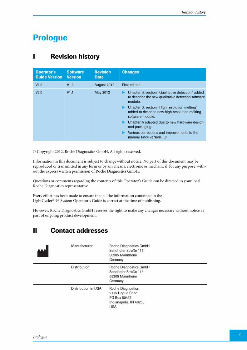
Prologue
Revision history
9
Prologue
I Revision history
© Copyright 2012, Roche Diagnostics GmbH. All rights reserved.
Information in this document is subject to change without notice. No part of this document may bereproduced or transmitted in any form or by any means, electronic or mechanical, for any purpose, with-out the express written permission of Roche Diagnostics GmbH.
Questions or comments regarding the contents of this Operator’s Guide can be directed to your localRoche Diagnostics representative.
Every effort has been made to ensure that all the information contained in theLightCycler® 96 System Operator’s Guide is correct at the time of publishing.
However, Roche Diagnostics GmbH reserves the right to make any changes necessary without notice aspart of ongoing product development.
II Contact addresses
Operator’sGuide Version
SoftwareVersion
RevisionDate
Changes
V1.0 V1.0 August 2012 First edition
V2.0 V1.1 May 2013 Chapter B, section "Qualitative detection" addedto describe the new qualitative detection softwaremodule.
Chapter B, section "High resolution melting"added to describe new high resolution meltingsoftware module.
Chapter A adapted due to new hardware designand packaging.
Various corrections and improvements to themanual since version 1.0.
Manufacturer Roche Diagnostics GmbHSandhofer Straße 11668305 MannheimGermany
Distribution Roche Diagnostics GmbHSandhofer Straße 11668305 MannheimGermany
Distribution in USA Roche Diagnostics9115 Hague RoadPO Box 50457Indianapolis, IN 46250USA

LightCycler® 96 System, Operator’s Guide V2.0
Declaration of conformity
10
III Declaration of conformity
IV Warranty
The warranty conditions are specified in the sales contract. Contact your local Roche Diagnostics repre-sentative for further information.
Any unauthorized modification of the LightCycler® 96 Instrument and/or the LightCycler® 96 Softwarewill result in the invalidation of the guarantee and service contract.
V Trademarks
LC, LIGHTCYCLER, MAGNA PURE, RESOLIGHT and REALTIME READY are trademarks of Roche.
Exiqon and ProbeLibrary are registered trademarks of Exiqon A/S, Vedbaek, Denmark.
SYBR is a registered trademark of Life Technologies Corporation.
All other product names and trademarks are the property of their respective owners.
VI Intended use
The LightCycler® 96 Instrument is intended for performing rapid, accurate polymerase chain reaction(PCR) in combination with real-time, online detection of DNA-binding fluorescent dyes or labeledprobes, enabling quantification or characterization of a target nucleic acid.
The LightCycler® 96 System is intended for life science research only. It must only be used by laboratoryprofessionals trained in laboratory techniques, who have studied the Instructions for Use of this instru-ment. The LightCycler® 96 Instrument is not for use in diagnostic procedures.
The LightCycler® 96 System is intended for indoor use only.
VII License statements for theLightCycler® 96 Instrument
NOTICE: For patent license limitations for individual products please refer to:www.technical-support.roche.com.
The instrument meets the requirements laid down in Council Directive 2004/108/EC relatingto "Electromagnetic Compatibility" and Council Directive 2006/95/EC relating to "Low Volt-age Equipment".
The following standards were applied: IEC/EN 61326-1 (EMC), IEC/EN 61010-1 (Safety),and IEC/EN 61010-2-081.
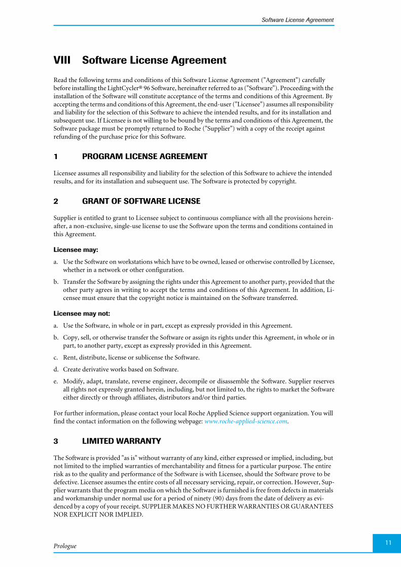
Prologue
Software License Agreement
11
VIII Software License Agreement
Read the following terms and conditions of this Software License Agreement ("Agreement") carefullybefore installing the LightCycler® 96 Software, hereinafter referred to as ("Software"). Proceeding with theinstallation of the Software will constitute acceptance of the terms and conditions of this Agreement. Byaccepting the terms and conditions of this Agreement, the end-user ("Licensee") assumes all responsibilityand liability for the selection of this Software to achieve the intended results, and for its installation andsubsequent use. If Licensee is not willing to be bound by the terms and conditions of this Agreement, theSoftware package must be promptly returned to Roche ("Supplier") with a copy of the receipt againstrefunding of the purchase price for this Software.
1 PROGRAM LICENSE AGREEMENT
Licensee assumes all responsibility and liability for the selection of this Software to achieve the intendedresults, and for its installation and subsequent use. The Software is protected by copyright.
2 GRANT OF SOFTWARE LICENSE
Supplier is entitled to grant to Licensee subject to continuous compliance with all the provisions herein-after, a non-exclusive, single-use license to use the Software upon the terms and conditions contained inthis Agreement.
Licensee may:
a. Use the Software on workstations which have to be owned, leased or otherwise controlled by Licensee,whether in a network or other configuration.
b. Transfer the Software by assigning the rights under this Agreement to another party, provided that theother party agrees in writing to accept the terms and conditions of this Agreement. In addition, Li-censee must ensure that the copyright notice is maintained on the Software transferred.
Licensee may not:
a. Use the Software, in whole or in part, except as expressly provided in this Agreement.
b. Copy, sell, or otherwise transfer the Software or assign its rights under this Agreement, in whole or inpart, to another party, except as expressly provided in this Agreement.
c. Rent, distribute, license or sublicense the Software.
d. Create derivative works based on Software.
e. Modify, adapt, translate, reverse engineer, decompile or disassemble the Software. Supplier reservesall rights not expressly granted herein, including, but not limited to, the rights to market the Softwareeither directly or through affiliates, distributors and/or third parties.
For further information, please contact your local Roche Applied Science support organization. You willfind the contact information on the following webpage: www.roche-applied-science.com.
3 LIMITED WARRANTY
The Software is provided "as is" without warranty of any kind, either expressed or implied, including, butnot limited to the implied warranties of merchantability and fitness for a particular purpose. The entirerisk as to the quality and performance of the Software is with Licensee, should the Software prove to bedefective. Licensee assumes the entire costs of all necessary servicing, repair, or correction. However, Sup-plier warrants that the program media on which the Software is furnished is free from defects in materialsand workmanship under normal use for a period of ninety (90) days from the date of delivery as evi-denced by a copy of your receipt. SUPPLIER MAKES NO FURTHER WARRANTIES OR GUARANTEESNOR EXPLICIT NOR IMPLIED.
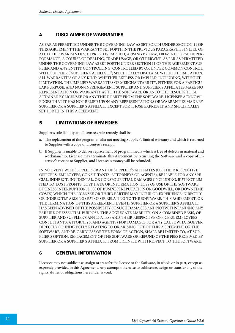
LightCycler® 96 System, Operator’s Guide V2.0
Software License Agreement
12
4 DISCLAIMER OF WARRANTIES
AS FAR AS PERMITTED UNDER THE GOVERNING LAW AS SET FORTH UNDER SECTION 11 OFTHIS AGREEMENT THE WARRANTY SET FORTH IN THE PREVIOUS PARAGRAPH, IS IN LIEU OFALL OTHER WARRANTIES, EXPRESS OR IMPLIED, ARISING BY LAW, FROM A COURSE OF PER-FORMANCE, A COURSE OF DEALING, TRADE USAGE, OR OTHERWISE. AS FAR AS PERMITTEDUNDER THE GOVERNING LAW AS SET FORTH UNDER SECTION 11 OF THIS AGREEMENT SUP-PLIER AND ANY ENTITY CONTROLLING, CONTROLLED BY OR UNDER COMMON CONTROLWITH SUPPLIER ("SUPPLIER'S AFFILIATE") SPECIFICALLY DISCLAIM, WITHOUT LIMITATION,ALL WARRANTIES OF ANY KIND, WHETHER EXPRESS OR IMPLIED, INCLUDING, WITHOUTLIMITATION, THE IMPLIED WARRANTIES OF MERCHANTABILITY, FITNESS FOR A PARTICU-LAR PURPOSE, AND NON-INFRINGEMENT. SUPPLIER AND SUPPLIER'S AFFILIATES MAKE NOREPRESENTATION OR WARRANTY AS TO THE SOFTWARE OR AS TO THE RESULTS TO BEATTAINED BY LICENSEE OR ANY THIRD PARTY FROM THE SOFTWARE. LICENSEE ACKNOWL-EDGES THAT IT HAS NOT RELIED UPON ANY REPRESENTATIONS OR WARRANTIES MADE BYSUPPLIER OR A SUPPLIER'S AFFILIATE EXCEPT FOR THOSE EXPRESSLY AND SPECIFICALLYSET FORTH IN THIS AGREEMENT.
5 LIMITATIONS OF REMEDIES
Supplier's sole liability and Licensee's sole remedy shall be:
a. The replacement of the program media not meeting Supplier's limited warranty and which is returnedto Supplier with a copy of Licensee's receipt;
b. If Supplier is unable to deliver replacement of program media which is free of defects in material andworkmanship, Licensee may terminate this Agreement by returning the Software and a copy of Li-censee's receipt to Supplier, and Licensee's money will be refunded.
IN NO EVENT WILL SUPPLIER OR ANY OF SUPPLIER'S AFFILIATES (OR THEIR RESPECTIVEOFFICERS, EMPLOYEES, CONSULTANTS, ATTORNEYS OR AGENTS), BE LIABLE FOR ANY SPE-CIAL, INDIRECT, INCIDENTAL, OR CONSEQUENTIAL DAMAGES (INCLUDING, BUT NOT LIM-ITED TO, LOST PROFITS, LOST DATA OR INFORMATION, LOSS OF USE OF THE SOFTWARE,BUSINESS INTERRUPTION, LOSS OF BUSINESS REPUTATION OR GOODWILL, OR DOWNTIMECOSTS) WHICH THE LICENSEE OR THIRD PARTIES MAY INCUR OR EXPERIENCE, DIRECTLYOR INDIRECTLY ARISING OUT OF OR RELATING TO THE SOFTWARE, THIS AGREEMENT, ORTHE TERMINATION OF THIS AGREEMENT, EVEN IF SUPPLIER OR A SUPPLIER'S AFFILIATEHAS BEEN ADVISED OF THE POSSIBILITY OF SUCH DAMAGES AND NOTWITHSTANDING ANYFAILURE OF ESSENTIAL PURPOSE. THE AGGREGATE LIABILITY, ON A COMBINED BASIS, OFSUPPLIER AND SUPPLIER'S AFFILI-ATES (AND THEIR RESPECTIVE OFFICERS, EMPLOYEESCONSULTANTS, ATTORNEYS, AND AGENTS) FOR DAMAGES FOR ANY CAUSE WHATSOEVERDIRECTLY OR INDIRECTLY RELATING TO OR ARISING OUT OF THIS AGREEMENT OR THESOFTWARE, AND RE-GARDLESS OF THE FORM OF ACTION, SHALL BE LIMITED TO, AT SUP-PLIER'S OPTION, REPLACEMENT OF THE SOFTWARE OR REFUND OF THE FEES RECEIVED BYSUPPLIER OR A SUPPLIER'S AFFILIATE FROM LICENSEE WITH RESPECT TO THE SOFTWARE.
6 GENERAL INFORMATION
Licensee may not sublicense, assign or transfer the license or the Software, in whole or in part, except asexpressly provided in this Agreement. Any attempt otherwise to sublicense, assign or transfer any of therights, duties or obligations hereunder is void.
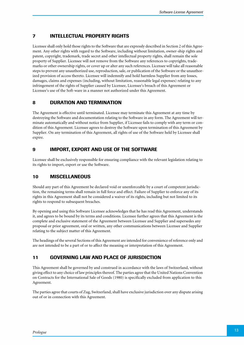
Prologue
Software License Agreement
13
7 INTELLECTUAL PROPERTY RIGHTS
Licensee shall only hold those rights to the Software that are expressly described in Section 2 of this Agree-ment. Any other rights with regard to the Software, including without limitation, owner-ship rights andpatent, copyright, trademark, trade secret and other intellectual property rights, shall remain the soleproperty of Supplier. Licensee will not remove from the Software any references to copyrights, trade-marks or other ownership rights, or cover up or alter any such references. Licensee will take all reasonablesteps to prevent any unauthorized use, reproduction, sale, or publication of the Software or the unauthor-ized provision of access thereto. Licensee will indemnify and hold harmless Supplier from any losses,damages, claims and expenses (including, without limitation, reasonable legal expenses) relating to anyinfringement of the rights of Supplier caused by Licensee, Licensee's breach of this Agreement orLicensee's use of the Soft-ware in a manner not authorized under this Agreement.
8 DURATION AND TERMINATION
The Agreement is effective until terminated. Licensee may terminate this Agreement at any time bydestroying the Software and documentation relating to the Software in any form. The Agreement will ter-minate automatically and without notice from Supplier, if Licensee fails to comply with any term or con-dition of this Agreement. Licensee agrees to destroy the Software upon termination of this Agreement bySupplier. On any termination of this Agreement, all rights of use of the Software held by Licensee shallexpire.
9 IMPORT, EXPORT AND USE OF THE SOFTWARE
Licensee shall be exclusively responsible for ensuring compliance with the relevant legislation relating toits rights to import, export or use the Software.
10 MISCELLANEOUS
Should any part of this Agreement be declared void or unenforceable by a court of competent jurisdic-tion, the remaining terms shall remain in full force and effect. Failure of Supplier to enforce any of itsrights in this Agreement shall not be considered a waiver of its rights, including but not limited to itsrights to respond to subsequent breaches.
By opening and using this Software Licensee acknowledges that he has read this Agreement, understandsit, and agrees to be bound by its terms and conditions. Licensee further agrees that this Agreement is thecomplete and exclusive statement of the Agreement between Licensee and Supplier and supersedes anyproposal or prior agreement, oral or written, any other communications between Licensee and Supplierrelating to the subject matter of this Agreement.
The headings of the several Sections of this Agreement are intended for convenience of reference only andare not intended to be a part of or to affect the meaning or interpretation of this Agreement.
11 GOVERNING LAW AND PLACE OF JURISDICTION
This Agreement shall be governed by and construed in accordance with the laws of Switzerland, withoutgiving effect to any choice of law principles thereof. The parties agree that the United Nations Conventionon Contracts for the International Sale of Goods (1980) is specifically excluded from application to thisAgreement.
The parties agree that courts of Zug, Switzerland, shall have exclusive jurisdiction over any dispute arisingout of or in connection with this Agreement.
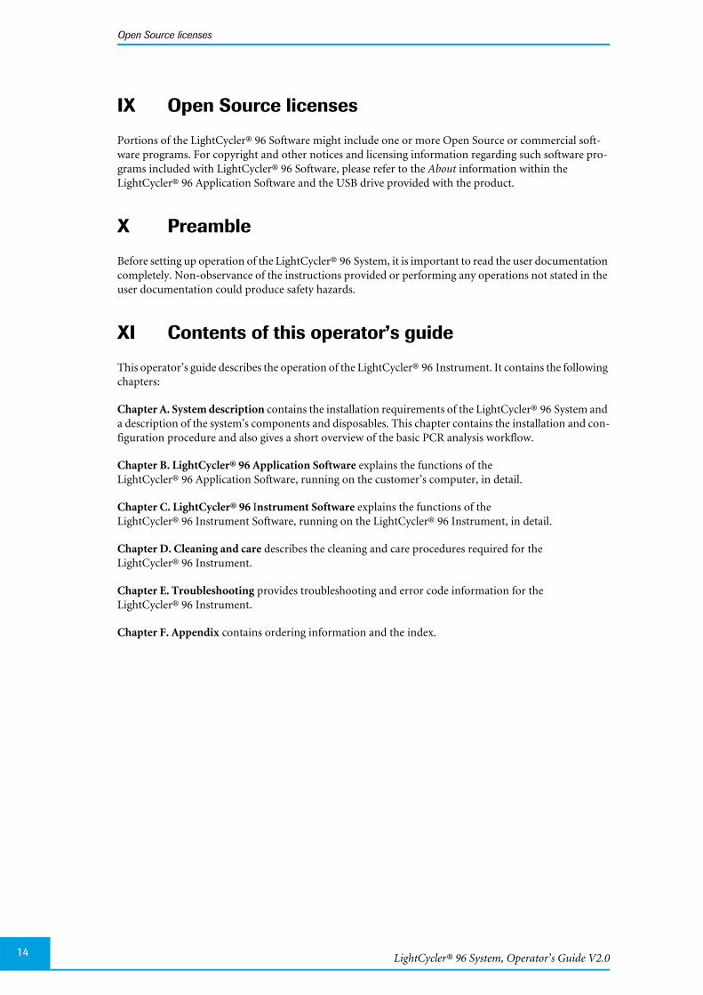
LightCycler® 96 System, Operator’s Guide V2.0
Open Source licenses
14
IX Open Source licenses
Portions of the LightCycler® 96 Software might include one or more Open Source or commercial soft-ware programs. For copyright and other notices and licensing information regarding such software pro-grams included with LightCycler® 96 Software, please refer to the About information within theLightCycler® 96 Application Software and the USB drive provided with the product.
X Preamble
Before setting up operation of the LightCycler® 96 System, it is important to read the user documentationcompletely. Non-observance of the instructions provided or performing any operations not stated in theuser documentation could produce safety hazards.
XI Contents of this operator’s guide
This operator’s guide describes the operation of the LightCycler® 96 Instrument. It contains the followingchapters:
Chapter A. System description contains the installation requirements of the LightCycler® 96 System anda description of the system's components and disposables. This chapter contains the installation and con-figuration procedure and also gives a short overview of the basic PCR analysis workflow.
Chapter B. LightCycler® 96 Application Software explains the functions of theLightCycler® 96 Application Software, running on the customer’s computer, in detail.
Chapter C. LightCycler® 96 Instrument Software explains the functions of theLightCycler® 96 Instrument Software, running on the LightCycler® 96 Instrument, in detail.
Chapter D. Cleaning and care describes the cleaning and care procedures required for theLightCycler® 96 Instrument.
Chapter E. Troubleshooting provides troubleshooting and error code information for theLightCycler® 96 Instrument.
Chapter F. Appendix contains ordering information and the index.
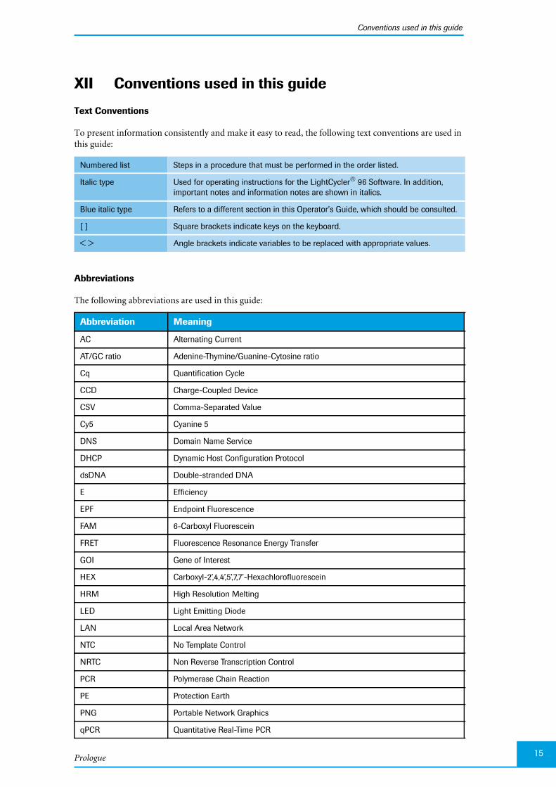
Prologue
Conventions used in this guide
15
XII Conventions used in this guide
Text Conventions
To present information consistently and make it easy to read, the following text conventions are used inthis guide:
Abbreviations
The following abbreviations are used in this guide:
Numbered list Steps in a procedure that must be performed in the order listed.
Italic type Used for operating instructions for the LightCycler® 96 Software. In addition,important notes and information notes are shown in italics.
Blue italic type Refers to a different section in this Operator’s Guide, which should be consulted.
[ ] Square brackets indicate keys on the keyboard.
< > Angle brackets indicate variables to be replaced with appropriate values.
Abbreviation Meaning
AC Alternating Current
AT/GC ratio Adenine-Thymine/Guanine-Cytosine ratio
Cq Quantification Cycle
CCD Charge-Coupled Device
CSV Comma-Separated Value
Cy5 Cyanine 5
DNS Domain Name Service
DHCP Dynamic Host Configuration Protocol
dsDNA Double-stranded DNA
E Efficiency
EPF Endpoint Fluorescence
FAM 6-Carboxyl Fluorescein
FRET Fluorescence Resonance Energy Transfer
GOI Gene of Interest
HEX Carboxyl-2’,4,4’,5’,7,7’-Hexachlorofluorescein
HRM High Resolution Melting
LED Light Emitting Diode
LAN Local Area Network
NTC No Template Control
NRTC Non Reverse Transcription Control
PCR Polymerase Chain Reaction
PE Protection Earth
PNG Portable Network Graphics
qPCR Quantitative Real-Time PCR
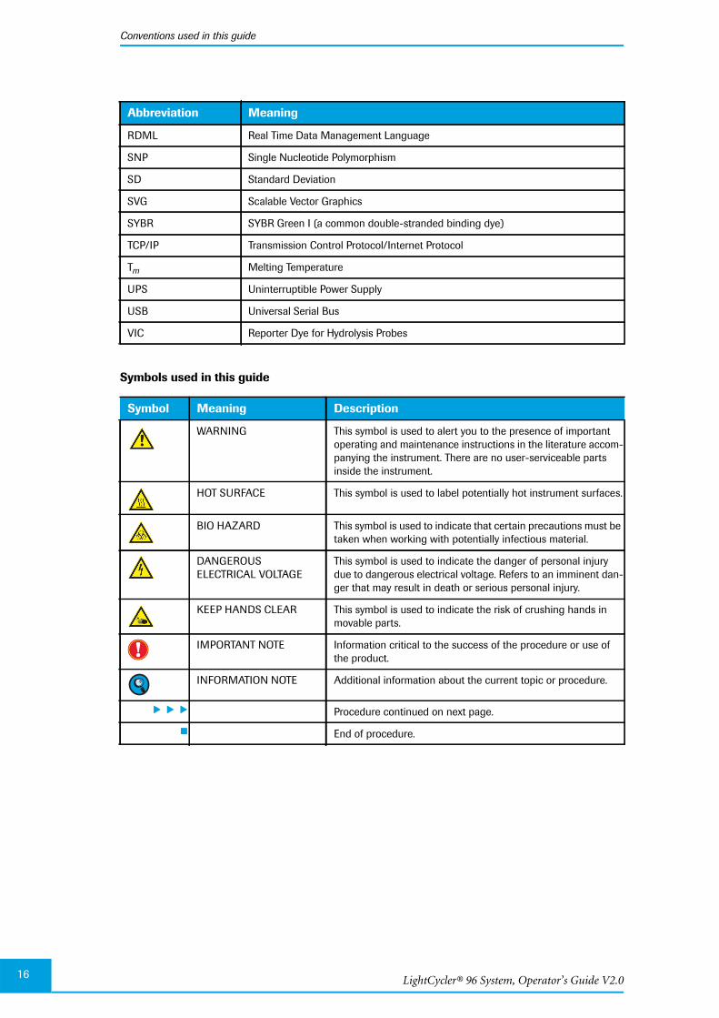
LightCycler® 96 System, Operator’s Guide V2.0
Conventions used in this guide
16
Symbols used in this guide
RDML Real Time Data Management Language
SNP Single Nucleotide Polymorphism
SD Standard Deviation
SVG Scalable Vector Graphics
SYBR SYBR Green I (a common double-stranded binding dye)
TCP/IP Transmission Control Protocol/Internet Protocol
Tm Melting Temperature
UPS Uninterruptible Power Supply
USB Universal Serial Bus
VIC Reporter Dye for Hydrolysis Probes
Symbol Meaning Description
WARNING This symbol is used to alert you to the presence of importantoperating and maintenance instructions in the literature accom-panying the instrument. There are no user-serviceable partsinside the instrument.
HOT SURFACE This symbol is used to label potentially hot instrument surfaces.
BIO HAZARD This symbol is used to indicate that certain precautions must betaken when working with potentially infectious material.
DANGEROUSELECTRICAL VOLTAGE
This symbol is used to indicate the danger of personal injurydue to dangerous electrical voltage. Refers to an imminent dan-ger that may result in death or serious personal injury.
KEEP HANDS CLEAR This symbol is used to indicate the risk of crushing hands inmovable parts.
IMPORTANT NOTE Information critical to the success of the procedure or use ofthe product.
INFORMATION NOTE Additional information about the current topic or procedure.
Procedure continued on next page.
End of procedure.
Abbreviation Meaning

Prologue
Conventions used in this guide
17
Symbols used on the instrument
In addition to these symbols, the following information is provided on the instrument type plate:
LightCycler® 96 Instrument
Instrument serial number in hexadecimal and in 1D barcode
Power supply and mains power consumption: 100-125/200-240 Vac 50/60 Hz 600 VA
Symbol Meaning Description
MANUFACTURER OFDEVICE
Roche Diagnostics GmbHSandhofer Strasse 116, D-68305 Mannheim GermanyMade in Switzerland
CE MARK The CE mark on the instrument type plate indicates conformitywith requirements of the directives relevant for this instrument.
WARNING On the instrument type plate.
cUL MARK On the instrument type plate.
HOT SURFACE On the loading module.
BIO HAZARD On the loading module.
KEEP HANDS CLEAR On the instrument housing (Only visible, when the loading unitis ejected).
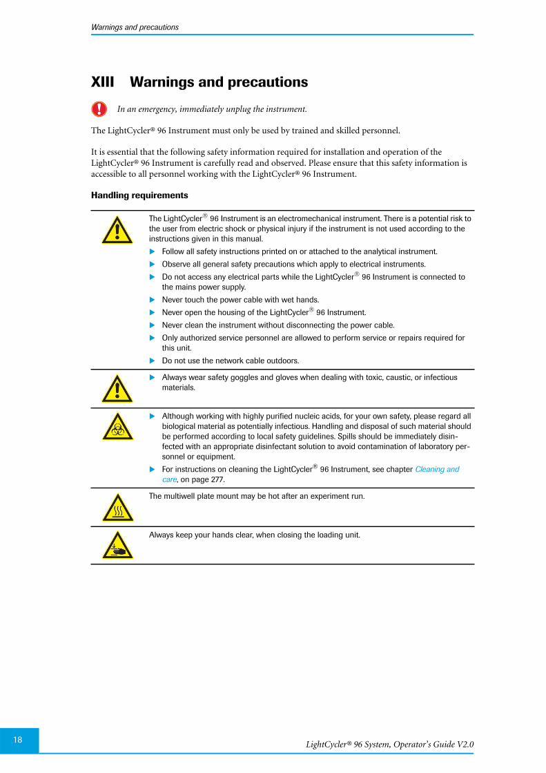
LightCycler® 96 System, Operator’s Guide V2.0
Warnings and precautions
18
XIII Warnings and precautions
In an emergency, immediately unplug the instrument.
The LightCycler® 96 Instrument must only be used by trained and skilled personnel.
It is essential that the following safety information required for installation and operation of theLightCycler® 96 Instrument is carefully read and observed. Please ensure that this safety information isaccessible to all personnel working with the LightCycler® 96 Instrument.
Handling requirements
The LightCycler® 96 Instrument is an electromechanical instrument. There is a potential risk tothe user from electric shock or physical injury if the instrument is not used according to theinstructions given in this manual.
Follow all safety instructions printed on or attached to the analytical instrument.
Observe all general safety precautions which apply to electrical instruments.
Do not access any electrical parts while the LightCycler® 96 Instrument is connected tothe mains power supply.
Never touch the power cable with wet hands.
Never open the housing of the LightCycler® 96 Instrument.
Never clean the instrument without disconnecting the power cable.
Only authorized service personnel are allowed to perform service or repairs required forthis unit.
Do not use the network cable outdoors.
Always wear safety goggles and gloves when dealing with toxic, caustic, or infectiousmaterials.
Although working with highly purified nucleic acids, for your own safety, please regard allbiological material as potentially infectious. Handling and disposal of such material shouldbe performed according to local safety guidelines. Spills should be immediately disin-fected with an appropriate disinfectant solution to avoid contamination of laboratory per-sonnel or equipment.
For instructions on cleaning the LightCycler® 96 Instrument, see chapter Cleaning andcare, on page 277.
The multiwell plate mount may be hot after an experiment run.
Always keep your hands clear, when closing the loading unit.

Prologue
Warnings and precautions
19
General Precautions
Electrical safety
Please observe the warnings regarding interactions and non-recommended functions. Also bear inmind the potential scope for misuse; it is advisable to draw attention to the possible consequences.
The LightCycler® 96 System contains software that allows it to be connected to a network.Please be aware that such a connection may have an adverse effect on the product’s integ-rity, through, for example, infection with malicious code (viruses, Trojan horses, etc.) oraccess by unauthorized third parties, such as intrusion by hackers. Roche therefore highlyrecommends protecting the product against such risks by taking appropriate and state-of-the-art action.
As the product is not intended to be used within networks without an appropriate firewalland has not been designed for such use, Roche assumes no liability in this regard.
Incorrect positioning of the instrument can cause incorrect results and damage to the equip-ment. Follow the installation instructions carefully.
Danger of explosion through sparks. Keep all potentially inflammable or explosive material(for example, anesthetic gas) away from the instrument. Spraying liquid on electrical partscan cause a short circuit and result in fire. Keep the cover closed while the instrument isconnected to the mains power supply and do not use sprays in the vicinity of theLightCycler® 96 Instrument. During fire fighting operations, disconnect theLightCycler® 96 Instrument from the mains power supply.
Do not disassemble the instrument.
The LightCycler® 96 Instrument is designed in accordance with Protection Class I (IEC). Thehousing of the instrument is connected to protection earth (PE) by a cable. For protectionagainst electric shock hazards, the instrument must be directly connected to an approvedpower source such as a three-wire grounded receptacle for the 115/230 V line. Where onlyan ungrounded receptacle is available, a qualified electrician must replace it with a properly(PE) grounded receptacle in accordance with the local electrical code. No extension must beused.
Any break in the electrical ground path, whether inside or outside the instrument, could cre-ate a hazardous condition. Under no circumstances should the operator attempt to modify ordeliberately override the safety features of this instrument. If the power cable becomescracked, frayed, broken, or otherwise damaged, it must be replaced immediately with theequivalent part from Roche Diagnostics.
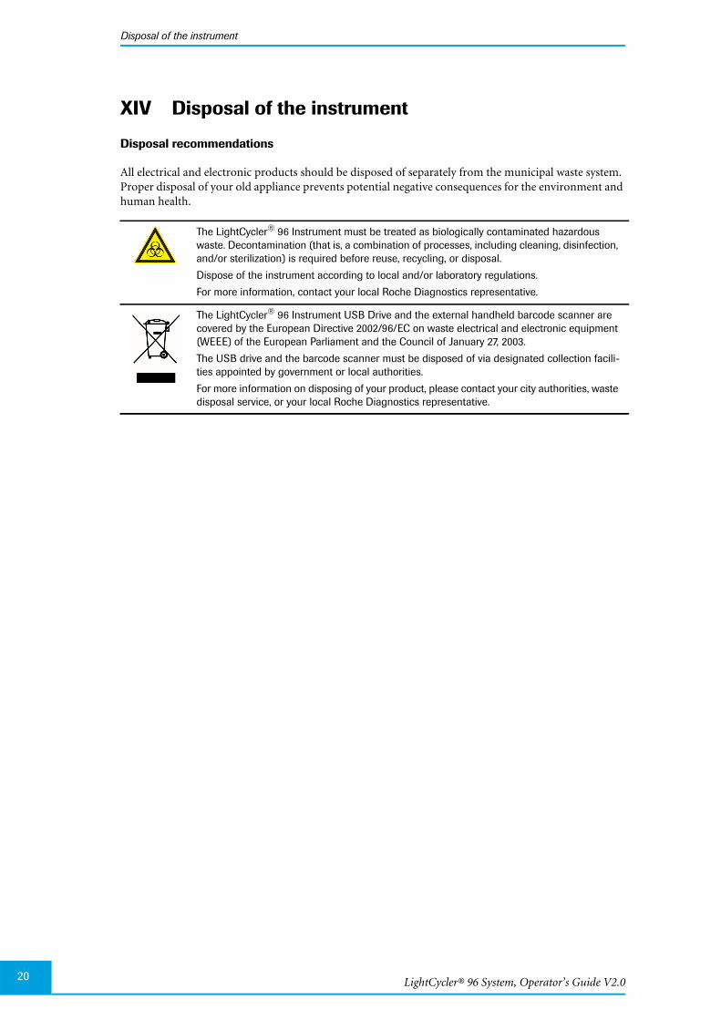
LightCycler® 96 System, Operator’s Guide V2.0
Disposal of the instrument
20
XIV Disposal of the instrument
Disposal recommendations
All electrical and electronic products should be disposed of separately from the municipal waste system.Proper disposal of your old appliance prevents potential negative consequences for the environment andhuman health.
The LightCycler® 96 Instrument must be treated as biologically contaminated hazardouswaste. Decontamination (that is, a combination of processes, including cleaning, disinfection,and/or sterilization) is required before reuse, recycling, or disposal.
Dispose of the instrument according to local and/or laboratory regulations.
For more information, contact your local Roche Diagnostics representative.
The LightCycler® 96 Instrument USB Drive and the external handheld barcode scanner arecovered by the European Directive 2002/96/EC on waste electrical and electronic equipment(WEEE) of the European Parliament and the Council of January 27, 2003.
The USB drive and the barcode scanner must be disposed of via designated collection facili-ties appointed by government or local authorities.
For more information on disposing of your product, please contact your city authorities, wastedisposal service, or your local Roche Diagnostics representative.

Chapter ASystem description
AAChapter A • System description
LightCycler® 96 System, Operator’s Guide V2.0
Table of Contents
AA
22
A System description 21
1 Introduction ..................................................................................................................................................... 24
2 Specifications of the LightCycler® 96 Instrument .................................................................... 25
2.1 General specifications ................................................................................................................................... 252.1.1 Environmental parameters ........................................................................................................................... 252.1.2 Interfaces ............................................................................................................................................................ 26
2.2 Technical specifications ................................................................................................................................ 262.3 Specifications of the detection unit .......................................................................................................... 26
2.3.1 Excitation ............................................................................................................................................................ 262.3.2 Detection ............................................................................................................................................................ 26
2.4 Filter set ............................................................................................................................................................... 262.5 Specifications of the thermal block cycler ............................................................................................. 272.6 Specifications of the external handheld barcode scanner .............................................................. 27
3 The LightCycler® 96 System Package ............................................................................................. 28
4 System description ..................................................................................................................................... 29
4.1 The LightCycler® 96 Instrument ................................................................................................................ 294.1.1 Loading module ............................................................................................................................................... 304.1.2 Touchscreen ...................................................................................................................................................... 304.1.3 USB interfaces .................................................................................................................................................. 304.1.4 Instrument back ............................................................................................................................................... 314.1.5 Ventilation .......................................................................................................................................................... 32
4.2 Block cycler unit ............................................................................................................................................... 334.2.1 Thermal block cycler ...................................................................................................................................... 334.2.2 Multiwell plate mount .................................................................................................................................... 34
4.3 Detection unit ................................................................................................................................................... 354.3.1 Optic module ..................................................................................................................................................... 354.3.2 Filter module ...................................................................................................................................................... 364.3.3 CCD camera ...................................................................................................................................................... 37
4.4 Detection channels ......................................................................................................................................... 384.5 Disposables ........................................................................................................................................................ 394.6 Reagents ............................................................................................................................................................. 414.7 Additional equipment .................................................................................................................................... 41
5 Installation ....................................................................................................................................................... 42
5.1 Installing the LightCycler® 96 Instrument .............................................................................................. 425.1.1 Installation requirements .............................................................................................................................. 425.1.2 Space and power requirements ................................................................................................................. 435.1.3 Assembling the instrument .......................................................................................................................... 44
5.2 Installing and configuring the LightCycler® 96 Instrument Software ......................................... 505.2.1 Installing the LightCycler® 96 Instrument Software .......................................................................... 505.2.2 Configuring a one-to-one connection ..................................................................................................... 505.2.3 Configuring an Ethernet network connection ...................................................................................... 55
5.3 Installing the LightCycler® 96 Application Software ......................................................................... 575.3.1 System requirements ..................................................................................................................................... 575.3.2 Installing the LightCycler® 96 Application Software ......................................................................... 575.3.3 The LightCycler® 96 Application Software home directory ............................................................ 585.3.4 Uninstalling the LightCycler® 96 Application Software .................................................................... 59
5.4 Managing updates .......................................................................................................................................... 605.4.1 Installing a LightCycler® 96 Application Software update .............................................................. 605.4.2 Installing a LightCycler® 96 Instrument Software update ............................................................... 605.4.3 Upgrading the LightCycler® 96 Instrument Software Version 1.0 ................................................ 625.4.4 Installing a firmware update ........................................................................................................................ 63
6 Detection formats ........................................................................................................................................ 64
6.1 Monitoring PCR with an intercalating fluorescent dye ..................................................................... 656.2 Monitoring PCR with hydrolysis probes .................................................................................................. 66

23
AA7 Analysis principles ...................................................................................................................................... 68
7.1 Quantification analysis .................................................................................................................................. 687.1.1 Absolute quantification analysis ................................................................................................................ 717.1.2 Relative quantification analysis .................................................................................................................. 727.1.3 Qualitative detection analysis ..................................................................................................................... 77
7.2 Endpoint genotyping analysis .................................................................................................................... 787.3 Tm calling analysis .......................................................................................................................................... 797.4 High resolution melting analysis ............................................................................................................... 81
LightCycler® 96 System, Operator’s Guide V2.024
Introduction
AA System description 0
1 Introduction
The LightCycler® 96 System enables you to perform real-time, online PCR combined with rapid cyclingof up to 96 samples.
After monitoring fluorescence during nucleic acid amplification, results can be analyzed, for example, byquantification. The outstanding thermal homogeneity and cycling speed of the LightCycler® 96 Systemprovide exact results in a short time.
The optical detection system offers the flexibility to detect a broad range of sequence-dependent probes(for example, hydrolysis probes) and sequence-independent dyes (for example, SYBR Green). It alsoallows a simultaneous measurement of all wells without sequential scanning, which is especially impor-tant for applications like high resolution melting.
The LightCycler® 96 Application Software runs on Microsoft Windows XP and Microsoft Windows 7platforms. The LightCycler® 96 Application Software and the LightCycler® 96 Instrument Software pro-vide excellent tools to generate high quality data. Advanced software tools facilitate fast, intuitive naviga-tion, allowing easy programming, data capture and analysis. The new software offers a broad range ofsupported applications combined with a versatile analysis workflow for each application.
Acquire relative quantification results in an easy setup of data you provide to the instrument. A corre-lation matrix will be provided in an attractive, publishable format that takes all relevant parametersinto account.
Easy import and export functions, email notifications after the run, online monitoring features andserver-based network capabilities enable you to communicate your data in whichever way serves yourneeds.
For detailed information on the broad range of software capabilities and their usage, see chaptersLightCycler® 96 Application Software, on page 85 and LightCycler® 96 Instrument Software, on page 219.
Based on the latest improvements, the LightCycler® 96 Instrument employs advanced state-of-the-artinstrument parts (for example, novel optical system and thermal block cycler).
For more detailed information on the LightCycler® 96 System, visit the LightCycler® 96 System SpecialInterest Site at www.lightcycler96.com.
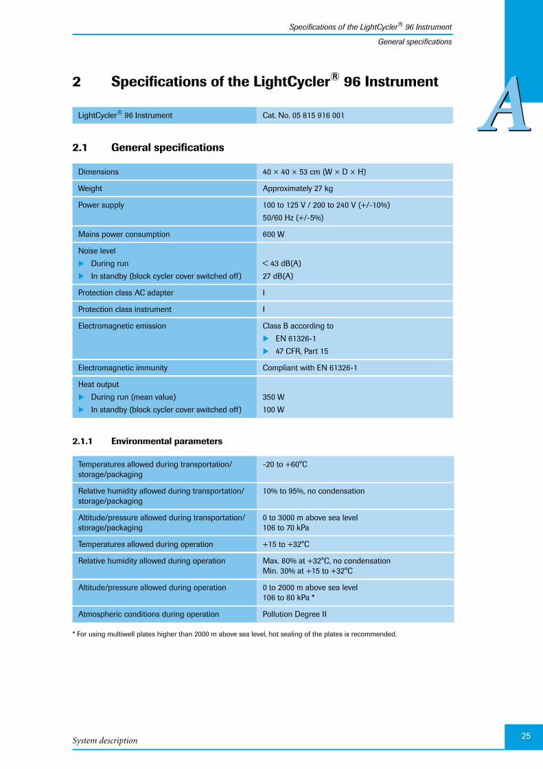
System description
Specifications of the LightCycler® 96 Instrument
25
AAGeneral specifications
2 Specifications of the LightCycler® 96 Instrument
2.1 General specifications
2.1.1 Environmental parameters
* For using multiwell plates higher than 2000 m above sea level, hot sealing of the plates is recommended.
LightCycler® 96 Instrument Cat. No. 05 815 916 001
Dimensions 40 × 40 × 53 cm (W × D × H)
Weight Approximately 27 kg
Power supply 100 to 125 V / 200 to 240 V (+/-10%)
50/60 Hz (+/-5%)
Mains power consumption 600 W
Noise level
During run
In standby (block cycler cover switched off)
< 43 dB(A)
27 dB(A)
Protection class AC adapter I
Protection class instrument I
Electromagnetic emission Class B according to
EN 61326-1
47 CFR, Part 15
Electromagnetic immunity Compliant with EN 61326-1
Heat output
During run (mean value)
In standby (block cycler cover switched off)
350 W
100 W
Temperatures allowed during transportation/storage/packaging
-20 to +60°C
Relative humidity allowed during transportation/storage/packaging
10% to 95%, no condensation
Altitude/pressure allowed during transportation/storage/packaging
0 to 3000 m above sea level106 to 70 kPa
Temperatures allowed during operation +15 to +32°C
Relative humidity allowed during operation Max. 80% at +32°C, no condensationMin. 30% at +15 to +32°C
Altitude/pressure allowed during operation 0 to 2000 m above sea level106 to 80 kPa *
Atmospheric conditions during operation Pollution Degree II
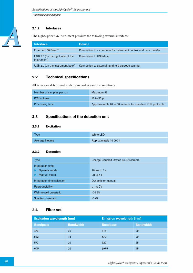
LightCycler® 96 System, Operator’s Guide V2.026
Specifications of the LightCycler® 96 Instrument
AATechnical specifications
2.1.2 Interfaces
The LightCycler® 96 Instrument provides the following external interfaces:
2.2 Technical specifications
All values are determined under standard laboratory conditions.
2.3 Specifications of the detection unit
2.3.1 Excitation
2.3.2 Detection
2.4 Filter set
Interface Device
Ethernet 100 Base T Connection to a computer for instrument control and data transfer
USB 2.0 (on the right side of theinstrument)
Connection to USB drive
USB 2.0 (on the instrument back) Connection to external handheld barcode scanner
Number of samples per run Maximum 96
PCR volume 10 to 50 µl
Processing time Approximately 40 to 50 minutes for standard PCR protocols
Type White LED
Average lifetime Approximately 10 000 h
Type Charge-Coupled Device (CCD) camera
Integration time
Dynamic mode
Manual mode
10 ms to 1 s
up to 4 s
Integration time selection Dynamic or manual
Reproducibility 1% CV
Well-to-well crosstalk < 0.5%
Spectral crosstalk < 4%
Excitation wavelength [nm] Emission wavelength [nm]
Bandpass Bandwidth Bandpass Bandwidth
470 30 514 20
533 15 572 20
577 20 620 25
645 20 697.5 45
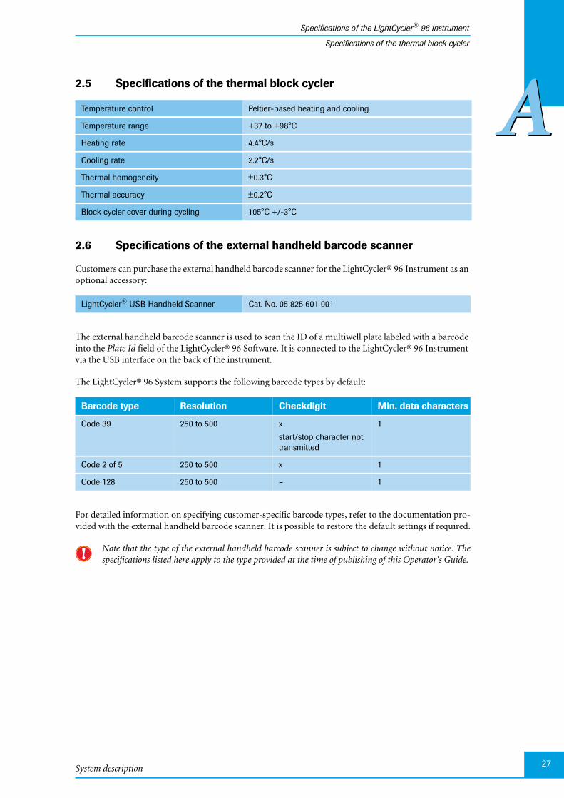
System description
Specifications of the LightCycler® 96 Instrument
27
AASpecifications of the thermal block cycler
2.5 Specifications of the thermal block cycler
2.6 Specifications of the external handheld barcode scanner
Customers can purchase the external handheld barcode scanner for the LightCycler® 96 Instrument as anoptional accessory:
The external handheld barcode scanner is used to scan the ID of a multiwell plate labeled with a barcodeinto the Plate Id field of the LightCycler® 96 Software. It is connected to the LightCycler® 96 Instrumentvia the USB interface on the back of the instrument.
The LightCycler® 96 System supports the following barcode types by default:
For detailed information on specifying customer-specific barcode types, refer to the documentation pro-vided with the external handheld barcode scanner. It is possible to restore the default settings if required.
Note that the type of the external handheld barcode scanner is subject to change without notice. Thespecifications listed here apply to the type provided at the time of publishing of this Operator’s Guide.
Temperature control Peltier-based heating and cooling
Temperature range +37 to +98°C
Heating rate 4.4°C/s
Cooling rate 2.2°C/s
Thermal homogeneity 0.3°C
Thermal accuracy 0.2°C
Block cycler cover during cycling 105°C +/-3°C
LightCycler® USB Handheld Scanner Cat. No. 05 825 601 001
Barcode type Resolution Checkdigit Min. data characters
Code 39 250 to 500 x
start/stop character nottransmitted
1
Code 2 of 5 250 to 500 x 1
Code 128 250 to 500 – 1
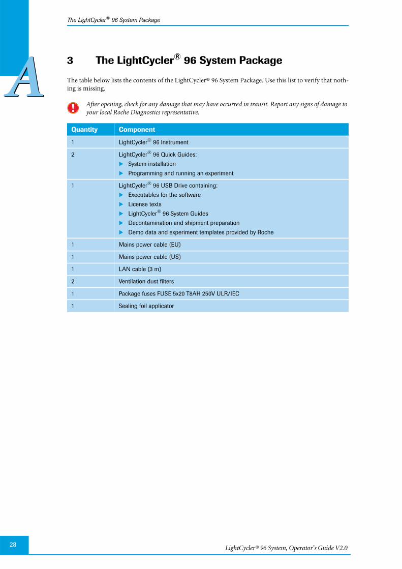
LightCycler® 96 System, Operator’s Guide V2.028
The LightCycler® 96 System Package
AA3 The LightCycler® 96 System Package
The table below lists the contents of the LightCycler® 96 System Package. Use this list to verify that noth-ing is missing.
After opening, check for any damage that may have occurred in transit. Report any signs of damage toyour local Roche Diagnostics representative.
Quantity Component
1 LightCycler® 96 Instrument
2 LightCycler® 96 Quick Guides:
System installation
Programming and running an experiment
1 LightCycler® 96 USB Drive containing:
Executables for the software
License texts
LightCycler® 96 System Guides
Decontamination and shipment preparation
Demo data and experiment templates provided by Roche
1 Mains power cable (EU)
1 Mains power cable (US)
1 LAN cable (3 m)
2 Ventilation dust filters
1 Package fuses FUSE 5x20 T8AH 250V ULR/IEC
1 Sealing foil applicator
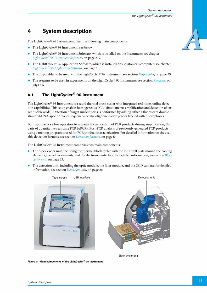
System description
System description
29
AAThe LightCycler® 96 Instrument
4 System description
The LightCycler® 96 System comprises the following main components:
The LightCycler® 96 Instrument; see below.
The LightCycler® 96 Instrument Software, which is installed on the instrument; see chapterLightCycler® 96 Instrument Software, on page 219.
The LightCycler® 96 Application Software, which is installed on a customer’s computer; see chapterLightCycler® 96 Application Software, on page 85.
The disposables to be used with the LightCycler® 96 Instrument; see section Disposables, on page 39.
The reagents to be used in experiments on the LightCycler® 96 Instrument; see section Reagents, onpage 41.
4.1 The LightCycler® 96 Instrument
The LightCycler® 96 Instrument is a rapid thermal block cycler with integrated real-time, online detec-tion capabilities. This setup enables homogeneous PCR (simultaneous amplification and detection of tar-get nucleic acids). Detection of target nucleic acids is performed by adding either a fluorescent double-stranded-DNA-specific dye or sequence-specific oligonucleotide probes labeled with fluorophores.
Both approaches allow operators to measure the generation of PCR products during amplification, thebasis of quantitative real-time PCR (qPCR). Post-PCR analysis of previously generated PCR productsusing a melting program is used for PCR product characterization. For detailed information on the avail-able detection formats, see section Detection formats, on page 64.
The LightCycler® 96 Instrument comprises two main components:
The block cycler unit, including the thermal block cycler with the multiwell plate mount, the coolingelements, the Peltier elements, and the electronics interface; for detailed information, see section Blockcycler unit, on page 33.
The detection unit, including the optic module, the filter module, and the CCD camera; for detailedinformation, see section Detection unit, on page 35.
Figure 1: Main components of the LightCycler® 96 Instrument
Block cycler unit
Touchscreen Detection unitUSB interface
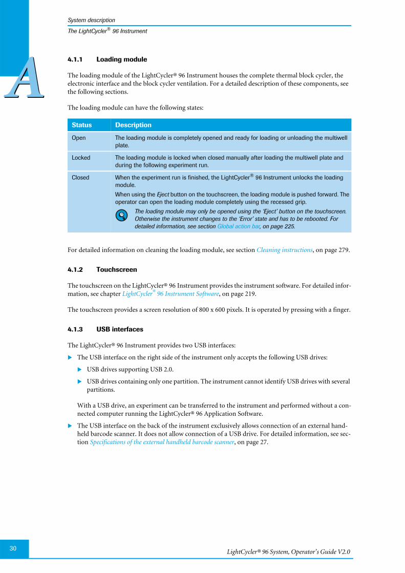
LightCycler® 96 System, Operator’s Guide V2.030
System description
AAThe LightCycler® 96 Instrument
4.1.1 Loading module
The loading module of the LightCycler® 96 Instrument houses the complete thermal block cycler, theelectronic interface and the block cycler ventilation. For a detailed description of these components, seethe following sections.
The loading module can have the following states:
For detailed information on cleaning the loading module, see section Cleaning instructions, on page 279.
4.1.2 Touchscreen
The touchscreen on the LightCycler® 96 Instrument provides the instrument software. For detailed infor-mation, see chapter LightCycler® 96 Instrument Software, on page 219.
The touchscreen provides a screen resolution of 800 x 600 pixels. It is operated by pressing with a finger.
4.1.3 USB interfaces
The LightCycler® 96 Instrument provides two USB interfaces:
The USB interface on the right side of the instrument only accepts the following USB drives:
USB drives supporting USB 2.0.
USB drives containing only one partition. The instrument cannot identify USB drives with severalpartitions.
With a USB drive, an experiment can be transferred to the instrument and performed without a con-nected computer running the LightCycler® 96 Application Software.
The USB interface on the back of the instrument exclusively allows connection of an external hand-held barcode scanner. It does not allow connection of a USB drive. For detailed information, see sec-tion Specifications of the external handheld barcode scanner, on page 27.
Status Description
Open The loading module is completely opened and ready for loading or unloading the multiwellplate.
Locked The loading module is locked when closed manually after loading the multiwell plate andduring the following experiment run.
Closed When the experiment run is finished, the LightCycler® 96 Instrument unlocks the loadingmodule.
When using the Eject button on the touchscreen, the loading module is pushed forward. Theoperator can open the loading module completely using the recessed grip.
The loading module may only be opened using the ‘Eject’ button on the touchscreen.Otherwise the instrument changes to the ‘Error’ state and has to be rebooted. Fordetailed information, see section Global action bar, on page 225.
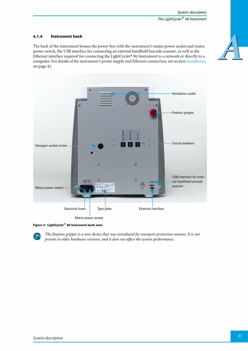
System description
System description
31
AAThe LightCycler® 96 Instrument
4.1.4 Instrument back
The back of the instrument houses the power box with the instrument’s mains power socket and mainspower switch, the USB interface for connecting an external handheld barcode scanner, as well as theEthernet interface required for connecting the LightCycler® 96 Instrument to a network or directly to acomputer. For details of the instrument’s power supply and Ethernet connection, see section Installation,on page 42.
Figure 2: LightCycler® 96 Instrument back view
The fixation gripper is a new device that was introduced for transport protection reasons. It is notpresent in older hardware versions, and it does not affect the system performance.
Hexagon socket screwCircuit breakers
Type plate
USB interface for exter-nal handheld barcodescanner
Ethernet interface
Mains power switch
Ventilation outlet
Electrical fuses
Mains power socket
Fixation gripper
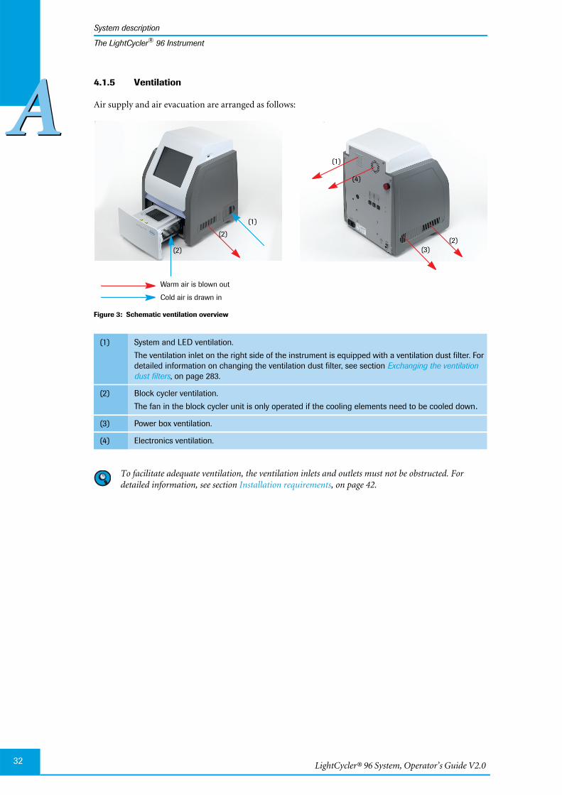
LightCycler® 96 System, Operator’s Guide V2.032
System description
AAThe LightCycler® 96 Instrument
4.1.5 Ventilation
Air supply and air evacuation are arranged as follows:
Figure 3: Schematic ventilation overview
.
To facilitate adequate ventilation, the ventilation inlets and outlets must not be obstructed. Fordetailed information, see section Installation requirements, on page 42.
(1) System and LED ventilation.
The ventilation inlet on the right side of the instrument is equipped with a ventilation dust filter. Fordetailed information on changing the ventilation dust filter, see section Exchanging the ventilationdust filters, on page 283.
(2) Block cycler ventilation.
The fan in the block cycler unit is only operated if the cooling elements need to be cooled down.
(3) Power box ventilation.
(4) Electronics ventilation.
Warm air is blown out
Cold air is drawn in
(2)(2)
(2)
(3)
(4)
(1)
(1)
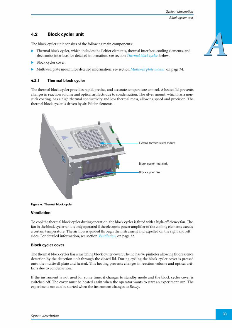
System description
System description
33
AABlock cycler unit
4.2 Block cycler unit
The block cycler unit consists of the following main components:
Thermal block cycler, which includes the Peltier elements, thermal interface, cooling elements, andelectronics interface; for detailed information, see section Thermal block cycler, below.
Block cycler cover.
Multiwell plate mount; for detailed information, see section Multiwell plate mount, on page 34.
4.2.1 Thermal block cycler
The thermal block cycler provides rapid, precise, and accurate temperature control. A heated lid preventschanges in reaction volume and optical artifacts due to condensation. The silver mount, which has a non-stick coating, has a high thermal conductivity and low thermal mass, allowing speed and precision. Thethermal block cycler is driven by six Peltier elements.
Figure 4: Thermal block cycler
Ventilation
To cool the thermal block cycler during operation, the block cycler is fitted with a high-efficiency fan. Thefan in the block cycler unit is only operated if the eletronic power amplifier of the cooling elements exeedsa certain temperature. The air flow is guided through the instrument and expelled on the right and leftsides. For detailed information, see section Ventilation, on page 32.
Block cycler cover
The thermal block cycler has a matching block cycler cover. The lid has 96 pinholes allowing fluorescencedetection by the detection unit through the closed lid. During cycling the block cycler cover is pressedonto the multiwell plate and heated. This heating prevents changes in reaction volume and optical arti-facts due to condensation.
If the instrument is not used for some time, it changes to standby mode and the block cycler cover isswitched off. The cover must be heated again when the operator wants to start an experiment run. Theexperiment run can be started when the instrument changes to Ready.
Block cycler heat sink
Block cycler fan
Electro-formed silver mount
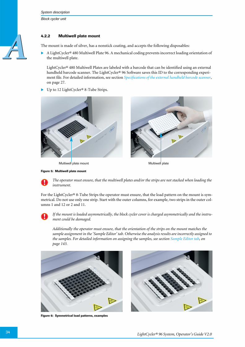
LightCycler® 96 System, Operator’s Guide V2.034
System description
AABlock cycler unit
4.2.2 Multiwell plate mount
The mount is made of silver, has a nonstick coating, and accepts the following disposables:
A LightCycler® 480 Multiwell Plate 96. A mechanical coding prevents incorrect loading orientation ofthe multiwell plate.
LightCycler® 480 Multiwell Plates are labeled with a barcode that can be identified using an externalhandheld barcode scanner. The LightCycler® 96 Software saves this ID to the corresponding experi-ment file. For detailed information, see section Specifications of the external handheld barcode scanner,on page 27.
Up to 12 LightCycler® 8-Tube Strips.
Figure 5: Multiwell plate mount
The operator must ensure, that the multiwell plates and/or the strips are not stacked when loading theinstrument.
For the LightCycler® 8-Tube Strips the operator must ensure, that the load pattern on the mount is sym-metrical. Do not use only one strip. Start with the outer columns, for example, two strips in the outer col-umns 1 and 12 or 2 and 11.
If the mount is loaded asymmetrically, the block cycler cover is charged asymmetrically and the instru-ment could be damaged.
Additionally the operator must ensure, that the orientation of the strips on the mount matches thesample assignment in the ‘Sample Editor’ tab. Otherwise the analysis results are incorrectly assigned tothe samples. For detailed information on assigning the samples, see section Sample Editor tab, onpage 143.
Figure 6: Symmetrical load patterns, examples
Multiwell plate mount Multiwell plate
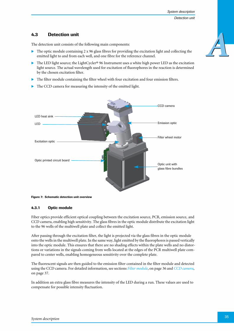
System description
System description
35
AADetection unit
4.3 Detection unit
The detection unit consists of the following main components:
The optic module containing 2 x 96 glass fibres for providing the excitation light and collecting theemitted light to and from each well, and one fibre for the reference channel.
The LED light source; the LightCycler® 96 Instrument uses a white high power LED as the excitationlight source. The actual wavelength used for excitation of fluorophores in the reaction is determinedby the chosen excitation filter.
The filter module containing the filter wheel with four excitation and four emission filters.
The CCD camera for measuring the intensity of the emitted light.
Figure 7: Schematic detection unit overview
4.3.1 Optic module
Fiber optics provide efficient optical coupling between the excitation source, PCR, emission source, andCCD camera, enabling high sensitivity. The glass fibres in the optic module distribute the excitation lightto the 96 wells of the multiwell plate and collect the emitted light.
After passing through the excitation filter, the light is projected via the glass fibres in the optic moduleonto the wells in the multiwell plate. In the same way, light emitted by the fluorophores is passed verticallyinto the optic module. This ensures that there are no shading effects within the plate wells and no distor-tions or variations in the signals coming from wells located at the edges of the PCR multiwell plate com-pared to center wells, enabling homogeneous sensitivity over the complete plate.
The fluorescent signals are then guided to the emission filter contained in the filter module and detectedusing the CCD camera. For detailed information, see sections Filter module, on page 36 and CCD camera,on page 37.
In addition an extra glass fibre measures the intensity of the LED during a run. These values are used tocompensate for possible intensity fluctuation.
LED heat sink
LED
Excitation optic
Optic printed circuit board
CCD camera
Emission optic
Filter wheel motor
Optic unit withglass fibre bundles
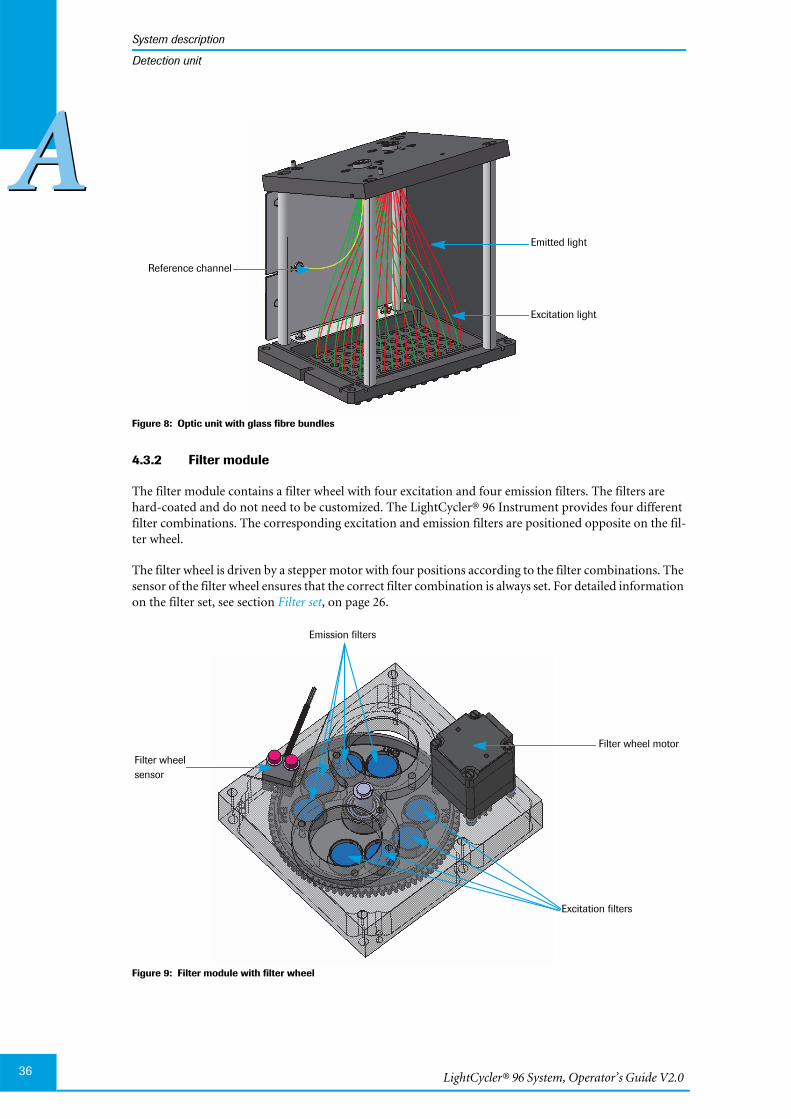
LightCycler® 96 System, Operator’s Guide V2.036
System description
AADetection unit
Figure 8: Optic unit with glass fibre bundles
4.3.2 Filter module
The filter module contains a filter wheel with four excitation and four emission filters. The filters arehard-coated and do not need to be customized. The LightCycler® 96 Instrument provides four differentfilter combinations. The corresponding excitation and emission filters are positioned opposite on the fil-ter wheel.
The filter wheel is driven by a stepper motor with four positions according to the filter combinations. Thesensor of the filter wheel ensures that the correct filter combination is always set. For detailed informationon the filter set, see section Filter set, on page 26.
Figure 9: Filter module with filter wheel
Emitted light
Excitation light
Reference channel
Excitation filters
Filter wheel motor
Emission filters
Filter wheelsensor

System description
System description
37
AADetection unit
4.3.3 CCD camera
The light-sensitive CCD camera contains a CCD chip. The acquisition time of the CCD camera isadjusted either manually or dynamically using the LightCycler® 96 Software. After measurements aretransferred to the software, it performs further corrections and noise reduction.
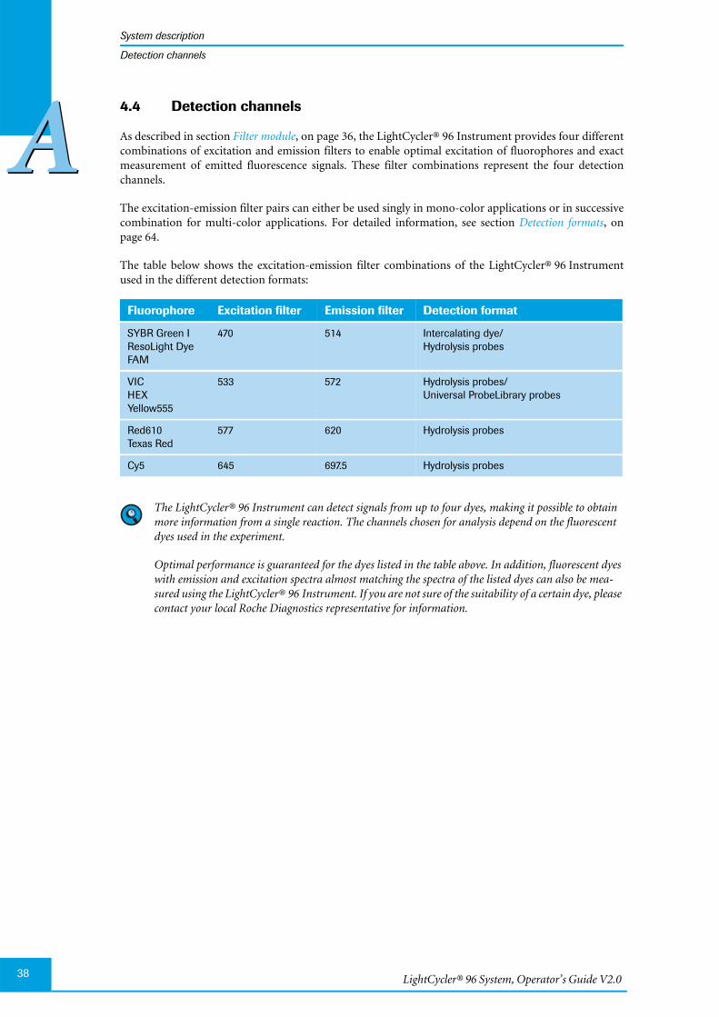
LightCycler® 96 System, Operator’s Guide V2.038
System description
AADetection channels
4.4 Detection channels
As described in section Filter module, on page 36, the LightCycler® 96 Instrument provides four differentcombinations of excitation and emission filters to enable optimal excitation of fluorophores and exactmeasurement of emitted fluorescence signals. These filter combinations represent the four detectionchannels.
The excitation-emission filter pairs can either be used singly in mono-color applications or in successivecombination for multi-color applications. For detailed information, see section Detection formats, onpage 64.
The table below shows the excitation-emission filter combinations of the LightCycler® 96 Instrumentused in the different detection formats:
The LightCycler® 96 Instrument can detect signals from up to four dyes, making it possible to obtainmore information from a single reaction. The channels chosen for analysis depend on the fluorescentdyes used in the experiment.
Optimal performance is guaranteed for the dyes listed in the table above. In addition, fluorescent dyeswith emission and excitation spectra almost matching the spectra of the listed dyes can also be mea-sured using the LightCycler® 96 Instrument. If you are not sure of the suitability of a certain dye, pleasecontact your local Roche Diagnostics representative for information.
Fluorophore Excitation filter Emission filter Detection format
SYBR Green IResoLight DyeFAM
470 514 Intercalating dye/Hydrolysis probes
VICHEXYellow555
533 572 Hydrolysis probes/Universal ProbeLibrary probes
Red610Texas Red
577 620 Hydrolysis probes
Cy5 645 697.5 Hydrolysis probes
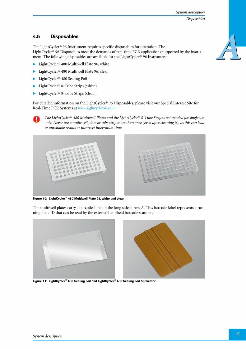
System description
System description
39
AADisposables
4.5 Disposables
The LightCycler® 96 Instrument requires specific disposables for operation. TheLightCycler® 96 Disposables meet the demands of real-time PCR applications supported by the instru-ment. The following disposables are available for the LightCycler® 96 Instrument:
LightCycler® 480 Multiwell Plate 96, white
LightCycler® 480 Multiwell Plate 96, clear
LightCycler® 480 Sealing Foil
LightCycler® 8-Tube Strips (white)
LightCycler® 8-Tube Strips (clear)
For detailed information on the LightCycler® 96 Disposables, please visit our Special Interest Site forReal-Time PCR Systems at www.lightcycler96.com.
The LightCycler® 480 Multiwell Plates and the LightCycler® 8-Tube Strips are intended for single useonly. Never use a multiwell plate or tube strip more than once (even after cleaning it), as this can leadto unreliable results or incorrect integration time.
Figure 10: LightCycler® 480 Multiwell Plate 96, white and clear
The multiwell plates carry a barcode label on the long side at row A. This barcode label represents a run-ning plate ID that can be read by the external handheld barcode scanner.
Figure 11: LightCycler® 480 Sealing Foil and LightCycler® 480 Sealing Foil Applicator

LightCycler® 96 System, Operator’s Guide V2.040
System description
AADisposables
Before the multiwell plate is loaded into the LightCycler® 96 Instrument, it must be sealed with theself-adhesive sealing foil. Use the sealing foil applicator provided with the instrument for proper seal-ing. You can order further sealing foil applicators directly from your local Roche Diagnostics represen-tative. Sealing the plate is crucial to eliminate evaporation at high temperatures. Use only the recom-mended foil.
For sealing a multiwell plate, apply the sealing foil applicator several times with sufficient pressureespecially for the wells at the outer edge of the plate.
Always centrifuge the filled and sealed plate before loading it into the instrument.
Always wear gloves and only handle the sealed plate by its edges. Fingerprints and other staining on theplate can affect the results.
Figure 12: LightCycler® 8-Tube Strips (white and clear)
Close the tubes by firmly pressing a strip of caps into place. Make sure the tubes are closed properly,otherwise the contents could evaporate during the run.
Place the strips symmetrically on the multiwell plate mount to ensure consistent temperature distribu-tion in the samples. For detailed information, see section Multiwell plate mount, on page 34.
Always centrifuge the filled and capped tube strips before loading them into the instrument.
Always wear gloves and take care not to contaminate the caps. Fingerprints and other staining on thecaps can affect the results.
System description
System description
41
AAReagents
4.6 Reagents
Optimal performance of the system is achieved using the LightCycler® 96 Instrument in combinationwith dedicated reagents. For detailed information on the LightCycler® 96 Reagents, please visit our Spe-cial Interest Site for Real-Time PCR Systems at www.lightcycler96.com.
4.7 Additional equipment
The following additional equipment is required to perform real-time PCR assays with theLightCycler® 96 System:
Standard swing-bucket centrifuge containing a rotor for multiwell plates with suitable adapters
Nuclease-free, aerosol-resistant pipette tips
Pipettes with disposable, positive-displacement tips
Sterile reaction tubes for preparing master mixes and dilutions
LightCycler® 96 System, Operator’s Guide V2.042
Installation
AAInstalling the LightCycler® 96 Instrument
5 Installation
5.1 Installing the LightCycler® 96 Instrument
The LightCycler® 96 Instrument is packed in a shipping box. The box includes theLightCycler® 96 Instrument and the accessories.
For the scope of delivery, see section The LightCycler® 96 System Package, on page 28.
For details of how to assemble the LightCycler® 96 Instrument, see section Assembling the instrument,on page 44.
The original shipping container must be transferred unopened to the installation site.On delivery, carefully inspect the shipping box for damage. Report any damage to your local RocheDiagnostics representative before accepting the unit.
Keep the shipping box and packaging in case of return.If you have already disposed of the packaging, you can request it from Roche.
Lift the LightCycler® 96 Instrument only by the sides using the recessed grips on the left and right sidesof the instrument base plate.
Caution!Due to the weight of the instrument, two persons may be needed to lift it.
5.1.1 Installation requirements
The LightCycler® 96 System is for indoor use only.
When installing a LightCycler® 96 Instrument that has been stored in a cold room or transported atlow temperatures, condensation may occur, which can cause malfunction of the instrument. The in-strument must be acclimated to room temperature for at least one hour prior to installation.
Place the LightCycler® 96 Instrument on a solid, level surface in the upright position.
Do not place the instrument in direct sunlight or close to radiators or heating devices.
Do not place the LightCycler® 96 Instrument next to instruments that cause vibration, electromagnet-ic interference, or have high inductance (for example, refrigerators, centrifuges, or mixers).
Peripheral instruments connected to the LightCycler® 96 Instrument must meet theIEC 60950 (UL 60950) standard.
Do not place anything on top of the instrument.
Use only the power cables and Ethernet cable supplied with the system package.
Do not use the Ethernet cable outdoors.
System description
Installation
43
AAInstalling the LightCycler® 96 Instrument
5.1.2 Space and power requirements
Place the LightCycler® 96 Instrument in a location that can support the following instrument require-ments:
Dimensions The LightCycler® 96 Instrument is 40 cm wide, 40 cm long, and 53 cm high.
Weight The LightCycler® 96 Instrument weighs approximately 27 kg.
Power The LightCycler® 96 Instrument operates at 100 to 125 V / 200 to 240 V(50/60 Hz).
The instrument can be connected to a single-phase or dual-phase supply only. Thecurrent consumption capacity of the mains power supply must not be exceeded.
There are no special provisions for protective grounding.
Caution!The instrument requires proper grounding. Any break in the electrical ground wire,whether inside or outside the instrument, or disconnection of the electrical groundconnection, could create a hazardous condition.
Caution!Do not under any circumstances attempt to modify or deliberately override the safetyfeatures of this system.
The LightCycler® 96 Instrument uses 600 VA.
Depending on the quality of electrical grounding, an uninterruptible power supply(UPS) with line conditioner and support for "Online/Direct Mode" may be required.A UPS is not provided with the LightCycler® 96 Instrument. Roche recommendscontacting a local supplier who can provide a UPS in accordance with the electricalrequirements.
Ventilation Do not place anything under the instrument, such as sheets of paper, since thesecould block the air inlet.
Do not cover the instrument – in particular do not block the ventilation holes.
Access A gap of 10 cm is recommended between the back of the instrument and the wall toallow access to the mains power switch and the Ethernet interface.
A gap of 20 cm is required on both sides to allow adequate air flow.
A gap of 5 cm is required above the instrument cover to access the USB interface.
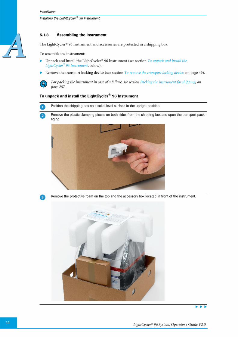
LightCycler® 96 System, Operator’s Guide V2.044
Installation
AAInstalling the LightCycler® 96 Instrument
5.1.3 Assembling the instrument
The LightCycler® 96 Instrument and accessories are protected in a shipping box.
To assemble the instrument:
Unpack and install the LightCycler® 96 Instrument (see section To unpack and install theLightCycler® 96 Instrument, below).
Remove the transport locking device (see section To remove the transport locking device, on page 49).
For packing the instrument in case of a failure, see section Packing the instrument for shipping, onpage 287.
To unpack and install the LightCycler® 96 Instrument
Position the shipping box on a solid, level surface in the upright position.
Remove the plastic clamping pieces on both sides from the shipping box and open the transport pack-aging.
Remove the protective foam on the top and the accessory box located in front of the instrument.
�
�
�

System description
Installation
45
AAInstalling the LightCycler® 96 Instrument
Lift the LightCycler® 96 Instrument out of the box by holding it on the left and right sides and place it ona solid level surface.
To carry and lift the instrument, only use the recessed grips on the left and right sides of the instru-ment base plate.
Caution:Due to the weight of the instrument, two persons may be needed to lift it.
Check for damage that may have occurred in transit. Report any signs of damage to your localRoche Diagnostics representative.
Position the instrument on the workbench in the upright position.
Remove the protective foil and the adhesive tape surrounding the instrument.
Ensure that no residuals of the tape are visible on the instrument.
�
�
�
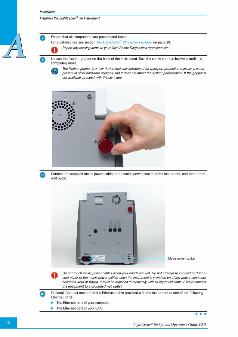
LightCycler® 96 System, Operator’s Guide V2.046
Installation
AAInstalling the LightCycler® 96 Instrument
Ensure that all components are present and intact.
For a detailed list, see section The LightCycler® 96 System Package, on page 28.
Report any missing items to your local Roche Diagnostics representative.
Loosen the fixation gripper on the back of the instrument. Turn the screw counterclockwise until it iscompletely loose.
The fixation gripper is a new device that was introduced for transport protection reasons. It is notpresent in older hardware versions, and it does not affect the system performance. If the gripper isnot available, proceed with the next step.
Connect the supplied mains power cable to the mains power socket of the instrument, and then to thewall outlet.
Do not touch mains power cables when your hands are wet. Do not attempt to connect or discon-nect either of the mains power cables when the instrument is switched on. If any power connectorbecomes worn or frayed, it must be replaced immediately with an approved cable. Always connectthe equipment to a grounded wall outlet.
Optional: Connect one end of the Ethernet cable provided with the instrument to one of the followingEthernet ports:
The Ethernet port of your computer.
The Ethernet port of your LAN.
�
Mains power socket
��
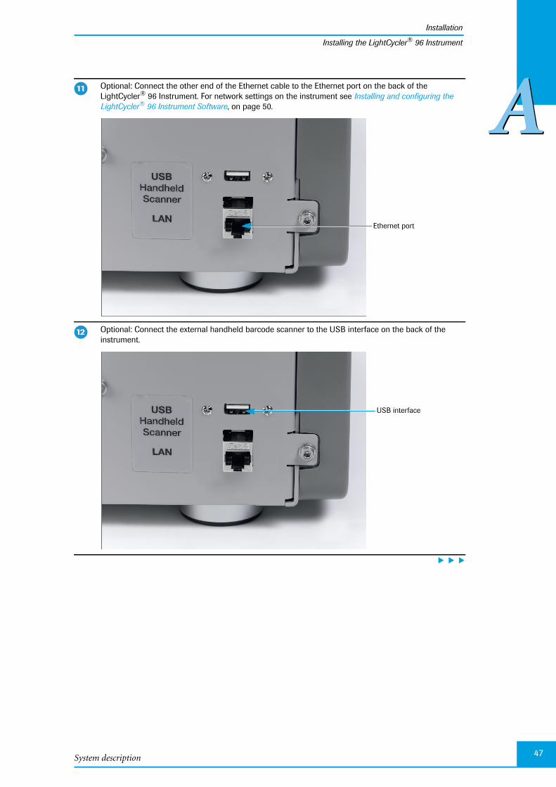
System description
Installation
47
AAInstalling the LightCycler® 96 Instrument
Optional: Connect the other end of the Ethernet cable to the Ethernet port on the back of theLightCycler® 96 Instrument. For network settings on the instrument see Installing and configuring theLightCycler® 96 Instrument Software, on page 50.
Optional: Connect the external handheld barcode scanner to the USB interface on the back of theinstrument.
��
Ethernet port
��
USB interface

LightCycler® 96 System, Operator’s Guide V2.048
Installation
AAInstalling the LightCycler® 96 Instrument
Ensure that the switches for all circuit breakers are in place, that is, all white buttons are depressed.
Switch on the instrument using the mains power switch on the back of the instrument.
��
Circuit breakers
��
Mains power switch
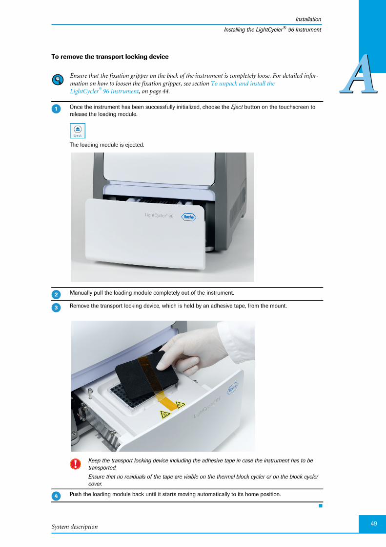
System description
Installation
49
AAInstalling the LightCycler® 96 Instrument
To remove the transport locking device
Ensure that the fixation gripper on the back of the instrument is completely loose. For detailed infor-mation on how to loosen the fixation gripper, see section To unpack and install theLightCycler® 96 Instrument, on page 44.
Once the instrument has been successfully initialized, choose the Eject button on the touchscreen torelease the loading module.
The loading module is ejected.
Manually pull the loading module completely out of the instrument.
Remove the transport locking device, which is held by an adhesive tape, from the mount.
Keep the transport locking device including the adhesive tape in case the instrument has to betransported.
Ensure that no residuals of the tape are visible on the thermal block cycler or on the block cyclercover.
Push the loading module back until it starts moving automatically to its home position.
�
�
�
�
LightCycler® 96 System, Operator’s Guide V2.050
Installation
AAInstalling and configuring the LightCycler® 96 Instrument Software
5.2 Installing and configuring the LightCycler® 96 Instrument Software
The LightCycler® 96 Instrument is controlled by the LightCycler® 96 Instrument Software. Each config-uration (instrument and instrument software) works as an independent system. TheLightCycler® 96 Instrument Software operates the LightCycler® 96 Instrument using the informationprovided by the user who defines the experiment run conditions.
For detailed information on monitoring the instrument and defining an experiment run, see chapterLightCycler® 96 Instrument Software, on page 219.
For detailed information on handling updates of the LightCycler® 96 Instrument Software, see sectionManaging updates, on page 60.
5.2.1 Installing the LightCycler® 96 Instrument Software
LightCycler® 96 Instrument Software is pre-installed on the instrument. For updating the software on theinstrument, see section Managing updates, on page 60.
For detailed information on upgrading the LightCycler® 96 Instrument Software Version 1.0 to theVersion 1.1, see section Upgrading the LightCycler® 96 Instrument Software Version 1.0, on page 62.
The LightCycler® 96 Instrument is compatible for use in a point-to-point connection over Ethernet.There are two ways of connecting the instrument:
A one-to-one connection between the instrument and the computer, using a single cable; see sectionsConfiguring a one-to-one connection, below.
An Ethernet network connection between the instrument and the local Ethernet network; see sectionConfiguring an Ethernet network connection, on page 55.
5.2.2 Configuring a one-to-one connection
For using a one-to-one connection between the LightCycler® 96 Instrument and the computer runningthe LightCycler® 96 Application Software, both devices must be configured.
Automatic one-to-one connection
When using a one-to-one connection and the Automated network configuration option is chosen, theinstrument assigns a default IP address itself. A computer running Microsoft Windows XP or MicrosoftWindows 7 as well assigns a default IP address to itself.
Connect the LightCycler® 96 Instrument to the computer, using the supplied network cable. For detailedinformation, see section Assembling the instrument, on page 44.
Switch on the instrument and the computer.
�
�

System description
Installation
51
AAInstalling and configuring the LightCycler® 96 Instrument Software
On the touchscreen, open the Network Information window area:Utilities > Configuration > Network Information.
Choose Automated.
The instrument assigns a default IP address to itself.
The process for assigning an instrument IP address might take up to one minute.
Automatically assigned IP addresses are in the range 169.254.0.1 to 169.254.0.254. When using de-fault Microsoft Windows XP or Microsoft Windows 7 settings, the computer automatically assignsan IP address from the same range to itself.
Check the connection using the Instrument Manager in the LightCycler® 96 Application Software. Fordetailed information, see section Instrument Manager, on page 124.
If the automatic one-to-one connection fails (for example, when the computer settings do not allow self-configuration of an IP address), configure the connection manually. For detailed information, see sectionManually configured one-to-one connection, assuming you have no administrator privileges on the com-puter, on page 54.
�
�
�
�
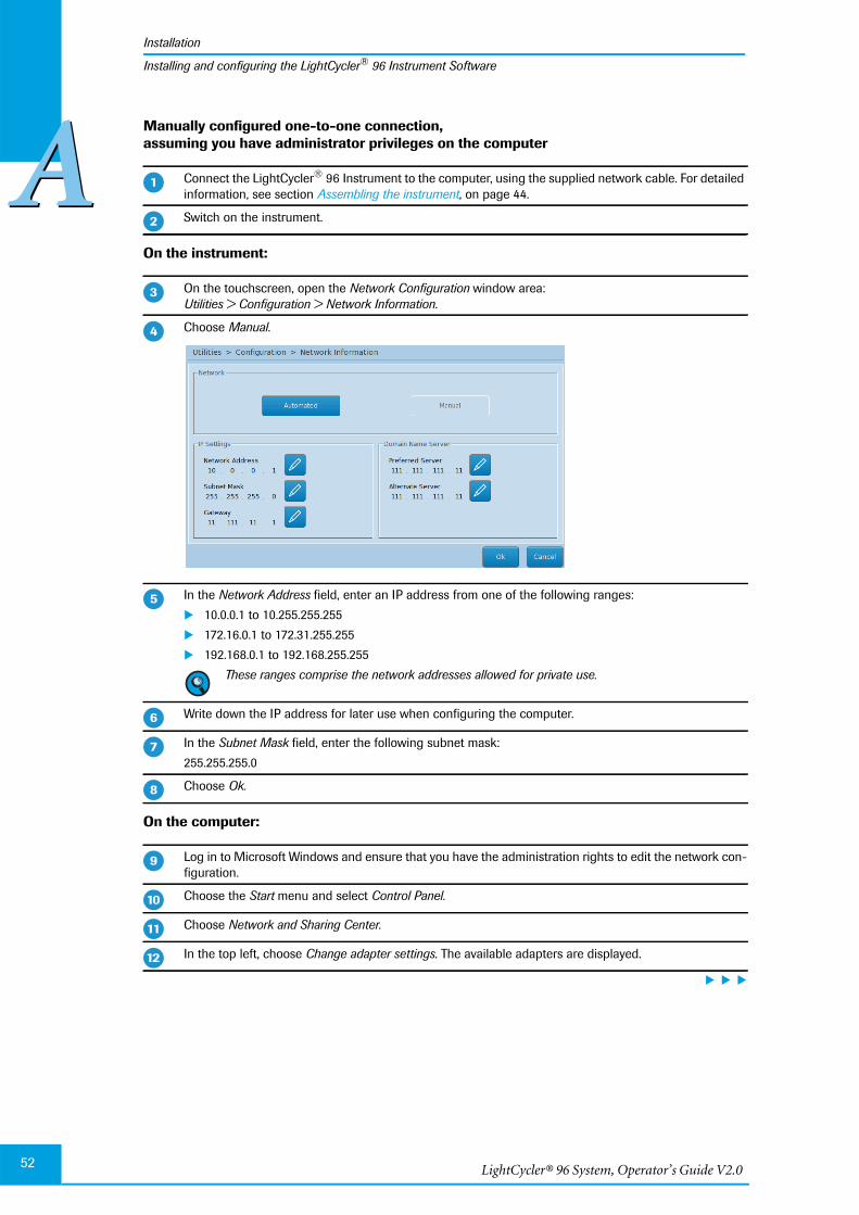
LightCycler® 96 System, Operator’s Guide V2.052
Installation
AAInstalling and configuring the LightCycler® 96 Instrument Software
Manually configured one-to-one connection,assuming you have administrator privileges on the computer
On the instrument:
On the computer:
Connect the LightCycler® 96 Instrument to the computer, using the supplied network cable. For detailedinformation, see section Assembling the instrument, on page 44.
Switch on the instrument.
On the touchscreen, open the Network Configuration window area:Utilities > Configuration > Network Information.
Choose Manual.
In the Network Address field, enter an IP address from one of the following ranges:
10.0.0.1 to 10.255.255.255
172.16.0.1 to 172.31.255.255
192.168.0.1 to 192.168.255.255
These ranges comprise the network addresses allowed for private use.
Write down the IP address for later use when configuring the computer.
In the Subnet Mask field, enter the following subnet mask:
255.255.255.0
Choose Ok.
Log in to Microsoft Windows and ensure that you have the administration rights to edit the network con-figuration.
Choose the Start menu and select Control Panel.
Choose Network and Sharing Center.
In the top left, choose Change adapter settings. The available adapters are displayed.
�
�
�
�
�
�
�
��
��
��
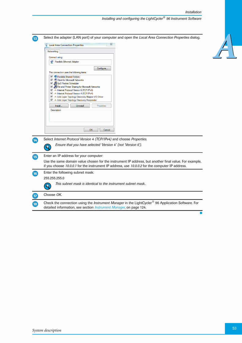
System description
Installation
53
AAInstalling and configuring the LightCycler® 96 Instrument Software
Select the adapter (LAN port) of your computer and open the Local Area Connection Properties dialog.
Select Internet Protocol Version 4 (TCP/IPv4) and choose Properties.
Ensure that you have selected ‘Version 4’ (not ‘Version 6’).
Enter an IP address for your computer:
Use the same domain value chosen for the instrument IP address, but another final value. For example,if you choose 10.0.0.1 for the instrument IP address, use 10.0.0.2 for the computer IP address.
Enter the following subnet mask:
255.255.255.0
This subnet mask is identical to the instrument subnet mask..
Choose OK.
Check the connection using the Instrument Manager in the LightCycler® 96 Application Software. Fordetailed information, see section Instrument Manager, on page 124.
��
��
��
��
��
�
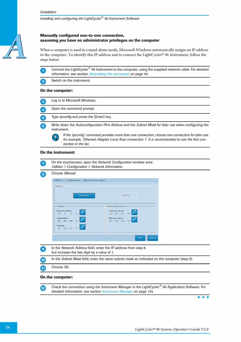
LightCycler® 96 System, Operator’s Guide V2.054
Installation
AAInstalling and configuring the LightCycler® 96 Instrument Software
Manually configured one-to-one connection,assuming you have no administrator privileges on the computer
When a computer is used in a stand-alone mode, Microsoft Windows automatically assigns an IP addressto the computer. To identify this IP address and to connect the LightCycler® 96 Instrument, follow thesteps below.
On the computer:
On the instrument:
On the computer:
Connect the LightCycler® 96 Instrument to the computer, using the supplied network cable. For detailedinformation, see section Assembling the instrument, on page 44.
Switch on the instrument.
Log in to Microsoft Windows.
Open the command prompt.
Type ipconfig and press the [Enter] key.
Write down the Autoconfiguration IPv4 Address and the Subnet Mask for later use when configuring theinstrument.
If the ‘ipconfig’ command provides more than one connection, choose one connection for later use,for example, ‘Ethernet-Adapter Local Area connection 1’. It is recommended to use the first con-nection in the list.
On the touchscreen, open the Network Configuration window area:Utilities > Configuration > Network Information.
Choose Manual.
In the Network Address field, enter the IP address from step 6,but increase the last digit by a value of 1.
In the Subnet Mask field, enter the same subnet mask as indicated on the computer (step 6).
Choose Ok.
Check the connection using the Instrument Manager in the LightCycler® 96 Application Software. Fordetailed information, see section Instrument Manager, on page 124.
�
�
�
�
�
�
�
��
��
��
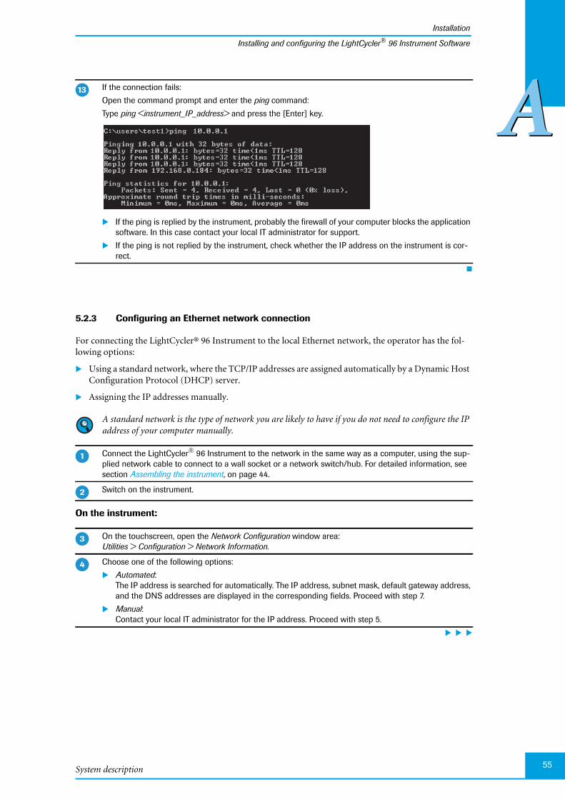
System description
Installation
55
AAInstalling and configuring the LightCycler® 96 Instrument Software
5.2.3 Configuring an Ethernet network connection
For connecting the LightCycler® 96 Instrument to the local Ethernet network, the operator has the fol-lowing options:
Using a standard network, where the TCP/IP addresses are assigned automatically by a Dynamic HostConfiguration Protocol (DHCP) server.
Assigning the IP addresses manually.
A standard network is the type of network you are likely to have if you do not need to configure the IPaddress of your computer manually.
On the instrument:
If the connection fails:
Open the command prompt and enter the ping command:
Type ping <instrument_IP_address> and press the [Enter] key.
If the ping is replied by the instrument, probably the firewall of your computer blocks the applicationsoftware. In this case contact your local IT administrator for support.
If the ping is not replied by the instrument, check whether the IP address on the instrument is cor-rect.
Connect the LightCycler® 96 Instrument to the network in the same way as a computer, using the sup-plied network cable to connect to a wall socket or a network switch/hub. For detailed information, seesection Assembling the instrument, on page 44.
Switch on the instrument.
On the touchscreen, open the Network Configuration window area:Utilities > Configuration > Network Information.
Choose one of the following options:
Automated:The IP address is searched for automatically. The IP address, subnet mask, default gateway address,and the DNS addresses are displayed in the corresponding fields. Proceed with step 7.
Manual:Contact your local IT administrator for the IP address. Proceed with step 5.
��
�
�
�
�

LightCycler® 96 System, Operator’s Guide V2.056
Installation
AAInstalling and configuring the LightCycler® 96 Instrument Software
On the computer:
If the connection to the instrument fails, even though you have connected all cables properly and con-figured the connection correctly, restart the instrument.
In the Network Address field, enter the IP address provided by your local IT administrator.
In the Subnet Mask field, enter the following subnet mask:
255.255.255.0
Write down the IP address.
Choose Ok.
Register the instrument with the LightCycler® 96 Application Software using the instrument IP addressor the host name. For detailed information, see section Instrument Manager, on page 124.
�
�
�
�
�

System description
Installation
57
AAInstalling the LightCycler® 96 Application Software
5.3 Installing the LightCycler® 96 Application Software
The LightCycler® 96 Application Software is installed on a computer which can be connected to theLightCycler® 96 Instrument either via a standard network or directly, as well as on a computer that is notconnected to a LightCycler® 96 Instrument.
For detailed information on connecting to a LightCycler® 96 Instrument, see section To register an in-strument, on page 126.
For detailed information on defining an experiment run and on analyzing the results, see chapterLightCycler® 96 Application Software, on page 85.
For detailed information on handling updates of the LightCycler® 96 Application Software, see sec-tion Managing updates, on page 60.
5.3.1 System requirements
To install and run the LightCycler® 96 Application Software, the computer must satisfy the followingminimum requirements:
Processor: Intel Core 2 duo 2.4 GHz
Memory: 2 GB
Hard disk: 250 GB
LAN: RJ45 Ethernet (100 MBit)
USB: USB 2.0
Display resolution: 1280 * 1024
Operating system: Microsoft Windows XP or Microsoft Windows 7, 32bit configuration
Microsoft .NET Framework 4.0 installed
Setting for regional and language options: English (USA)
5.3.2 Installing the LightCycler® 96 Application Software
The LightCycler® 96 Application Software is provided on the separate USB drive which is part of the sys-tem package. The software is installed via a standard installation program. Software updates are providedvia the download area of the Roche Applied Science website. For detailed information on handling updates,see section Managing updates, on page 60.
To install the LightCycler® 96 Application Software
Start the computer on which you want to install the software.
For installing the LightCycler® 96 Application Software Version 1.1 as an upgrade to theLightCycler® 96 Application Software Version 1.0, proceed as follows:
Download the new software release from the download area of the Roche Applied Sciencewebsite.
Unpack the *.zip archive.
Proceed with step 5.
Insert the USB drive.
Log in to Microsoft Windows, and ensure that you have the administration rights to install the software.
Open Windows Explorer and navigate to the USB drive.
�
�
�
�
LightCycler® 96 System, Operator’s Guide V2.058
Installation
AAInstalling the LightCycler® 96 Application Software
5.3.3 The LightCycler® 96 Application Software home directory
The LightCycler® 96 Application Software is installed in the home directory you specified during theinstallation process. By default, the home directory is created under:C:\Program Files\Roche Diagnostics\LightCycler® 96.
When the installation is complete, the home directory contains the following directories:
Double-click the Setup_LightCycler96_<release>.exe file.
The installation process transfers the files, extracts the files, and prepares the installation wizard. TheWelcome to the LightCycler® 96 Setup Wizard dialog box opens.
Choose Next.
You are prompted to agree to the license conditions:
Read the license agreement.
Check the I agree option.
Choose Next to proceed.
In the Select Installation Folder dialog box:
Select the location for the LightCycler® 96 Application Software:Either keep the default settings or browse to select a location for the installation.
By default, the software is installed in the‘C:\Program Files\Roche Diagnostics\LightCycler® 96’ directory.
Choose whether the software is to be accessed only by yourself or by anyone on the computer.
In the Confirm Installation dialog box, choose Next.
The selected components are installed. When the installation process has finished, theInstallation Complete dialog box opens.
Choose Close.
Directory Description
bin Program libraries, configuration files, and executable files for theLightCycler® 96 Software application.
DemoData Demo experiment files delivered with the software.
Manuals LightCycler® 96 System Guides.
Templates Non-executed experiments with run settings to be used as templates.
�
�
�

System description
Installation
59
AAInstalling the LightCycler® 96 Application Software
5.3.4 Uninstalling the LightCycler® 96 Application Software
Alternatively, you can use the Microsoft Windows Control Panel to uninstall theLightCycler® 96 Application Software.
Start the computer with the LightCycler® 96 Application Software.
Log in to Windows and ensure that you have the administration rights to uninstall the software.
In the Start menu, navigate to the LightCycler® 96 folder and choose the Uninstall LightCycler® 96 entry.
You are prompted to confirm that you want to uninstall the application.
Choose Yes.
During the installation, the directories bin, Manuals, and Templates are deleted.
When the process is finished, a message states that the software has been completely removed fromyour computer.
Choose OK.
�
�
�
�
�
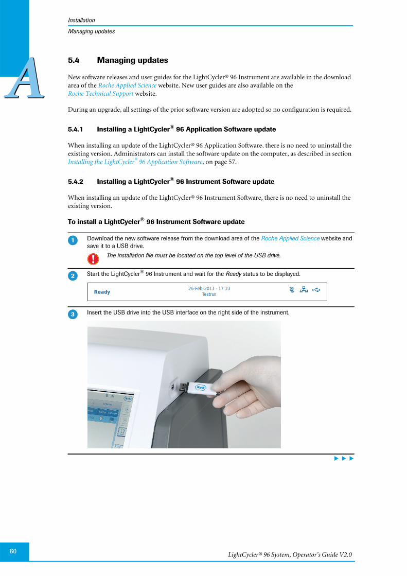
LightCycler® 96 System, Operator’s Guide V2.060
Installation
AAManaging updates
5.4 Managing updates
New software releases and user guides for the LightCycler® 96 Instrument are available in the downloadarea of the Roche Applied Science website. New user guides are also available on theRoche Technical Support website.
During an upgrade, all settings of the prior software version are adopted so no configuration is required.
5.4.1 Installing a LightCycler® 96 Application Software update
When installing an update of the LightCycler® 96 Application Software, there is no need to uninstall theexisting version. Administrators can install the software update on the computer, as described in sectionInstalling the LightCycler® 96 Application Software, on page 57.
5.4.2 Installing a LightCycler® 96 Instrument Software update
When installing an update of the LightCycler® 96 Instrument Software, there is no need to uninstall theexisting version.
To install a LightCycler® 96 Instrument Software update
Download the new software release from the download area of the Roche Applied Science website andsave it to a USB drive.
The installation file must be located on the top level of the USB drive.
Start the LightCycler® 96 Instrument and wait for the Ready status to be displayed.
Insert the USB drive into the USB interface on the right side of the instrument.
�
�
�
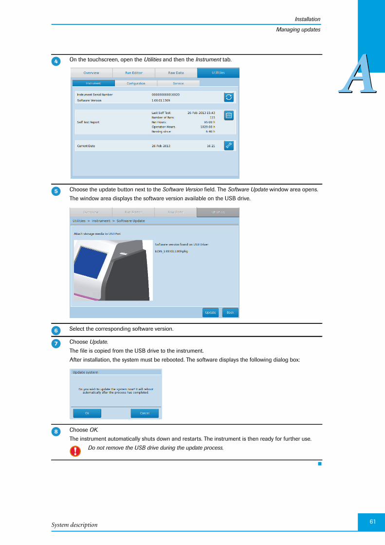
System description
Installation
61
AAManaging updates
On the touchscreen, open the Utilities and then the Instrument tab.
Choose the update button next to the Software Version field. The Software Update window area opens.
The window area displays the software version available on the USB drive.
Select the corresponding software version.
Choose Update.
The file is copied from the USB drive to the instrument.
After installation, the system must be rebooted. The software displays the following dialog box:
Choose OK.
The instrument automatically shuts down and restarts. The instrument is then ready for further use.
Do not remove the USB drive during the update process.
�
�
�
�
LightCycler® 96 System, Operator’s Guide V2.062
Installation
AAManaging updates
5.4.3 Upgrading the LightCycler® 96 Instrument Software Version 1.0
For installing the LightCycler® 96 Instrument Software Version 1.1 as an upgrade to theLightCycler® 96 Instrument Software Version 1.0, please note the following issues:
Compatibility with the application software
The LightCycler® 96 Instrument Software cannot cooperate with a different version of theLightCycler® 96 Application Software and vice versa. When different software versions are installed, it isnot possible to register an instrument with the application software, using the Instrument Manager tool.Operators must update both, the LightCycler® 96 Instrument Software and theLightCycler® 96 Application Software to the Version V1.1.
For detailed information on upgrading the software, see the following sections:
Installing the LightCycler® 96 Application Software, on page 57.
Installing a LightCycler® 96 Instrument Software update, on page 60.
.lc96 files
When installing the LightCycler® 96 Instrument Software Version 1.1, no experiment files generated withthe LightCycler® 96 Software Version 1.0 are allowed on the instrument. Operators must save and thenremove these files from the instrument before the installation. The following procedure is recommended:
For saving the experiments, perform one of the following steps:
On the instrument, synchronize the experiments with the connected USB drive using theSynchronize button. The experiments are transferred to the USB drive. For detailed information, seesection Overview tab, on page 237.
On your computer, retrieve the experiments from the instrument using the Instrument Manager toolin the application software. For detailed information, see section Send/Receive Experiments tab, onpage 128.
Remove the experiments from the instrument using the Delete button. For detailed information, see sec-tion Overview tab, on page 237.
Optional: Backup the instrument configuration to a connected USB drive. For detailed information, seesection Backup/Restore/Reset, on page 267.
Install the LightCycler® 96 Instrument Software Version 1.1. For detailed information, see sectionInstalling a LightCycler® 96 Instrument Software update, on page 60.
�
�
�
�
System description
Installation
63
AAManaging updates
Experiment file types
By default, all new experiment files, generated with the LightCycler® 96 Instrument Software orLightCycler® 96 Application Software Version 1.1 have the file types *.lc96p or *.lc96u:
*.lc96p for processed experiments.
*.lc96u for unprocessed experiments.
Experiments generated with the LightCycler® 96 Software Version 1.0 have the file type *.lc96. All threefile types can be opened in the LightCycler® 96 Application Software. In theLightCycler® 96 Instrument Software Version 1.1 however, only the file types *.lc96p or *.lc96u are sup-ported. For opening an *.lc96 file, operators must save it as a *.lc96p or *.lc96u file using the applicationsoftware. The following procedure is recommended:
5.4.4 Installing a firmware update
In some cases, the software will include improvements for the LightCycler® 96 Instrument, which willrequire the instrument to be updated. New software releases for the firmware will be delivered togetherwith the LightCycler® 96 Instrument Software and are automatically installed when the instrument soft-ware is updated. For detailed information, see section Installing a LightCycler® 96 Instrument Softwareupdate, on page 60.
Open the *.lc96 file in the LightCycler® 96 Application Software.
Save the file as *.lc96u or *.lc96p file depending on the processing status. For detailed information, seesection Saving an experiment, on page 116.
The data in the experiment file remain unchanged.The *.lc96 file is also retained.
Transfer the *.lc96u or *.lc96p file to the instrument.
�
�
�
LightCycler® 96 System, Operator’s Guide V2.064
Detection formats
AA6 Detection formats
The LightCycler® 96 Instrument makes use of fluorescent dyes for online, real-time monitoring of boththe generation of PCR products during cycling and the melting of PCR products. Fluorescence signalsmeasured during cycling are correlated with the amount of PCR product in the reaction, allowing calcu-lation of the input copy number of the target nucleic acid (possible both with sequence-specific and se-quence-independent detection formats). With sequence-independent detection formats, fluorescencemeasurements are also used for PCR product characterization by melting curve analysis. For maximumflexibility, the LightCycler® 96 Instrument supports several fluorescent detection formats and can be usedwith a broad range of probes and dyes:
Sequence-Specific Probe Binding Assays.
Rely on fluorophores coupled to sequence-specific oligonucleotide probes that hybridize to theircomplementary sequence in target PCR products, for example:
Hydrolysis probes (5´-nuclease assay).
Universal ProbeLibrary probes (5´-nuclease assay).
Sequence-Independent Detection Assays using double-stranded DNA-binding dyes.
Optimal performance of the system is achieved using the LightCycler® 96 Instrument in combinationwith dedicated reagents. For detailed information on the LightCycler® 96 Reagents, please visit ourSpecial Interest Site for Real-Time PCR Systems at www.lightcycler96.com.
Optimal performance is guaranteed for the dyes listed in the table listed in section Detection channels,on page 38. In addition, fluorescent dyes with emission and excitation spectra almost matching thespectra of the listed dyes can also be measured using the LightCycler® 96 Instrument. If you are not sureof the suitability of a certain dye, please contact your local Roche Diagnostics representative for infor-mation.

System description
Detection formats
65
AAMonitoring PCR with an intercalating fluorescent dye
6.1 Monitoring PCR with an intercalating fluorescent dye
Generation of PCR products is detected by measuring the increase in the dye fluorescence (measured at510 nm). In solution, unbound dye exhibits very little fluorescence. However, fluorescence is greatly en-hanced after dye intercalation into the helix of dsDNA. During PCR, the increase in fluorescence is pro-portional to the amount of newly generated dsDNA.
The following are the basic steps of DNA detection using intercalating dyes such as SYBR Green I duringreal-time PCR on the LightCycler® 96 System:
Since the dye binds all dsDNA, regardless of the DNA sequence, it cannot discriminate between specificPCR products, primer-dimers and other nonspecific products. Any double-stranded PCR artifact willcontribute to signal increase, which could result in overestimation of the concentration of the target se-quence.
To determine whether only the desired PCR product has been amplified, a melting curve analysis shouldbe performed directly after PCR. PCR product characterization by melting curve analysis is based on thefact that each particular dsDNA sequence has its characteristic melting point (the temperature at which50% of the DNA is double-stranded and 50% is melted, and becomes single-stranded). The most impor-tant factors that determine the thermal stability of dsDNA are length in base pairs and GC content of thesequence.
During a melting experiment, the reaction mixture is slowly heated up, for example, from +60°C to+95°C. When the temperature reaches the melting point of a PCR product present in the reaction, theDNA strands separate and the fluorescence of the released dye decreases sharply.
The LightCycler® 96 Instrument continuously monitors the fluorescence over the temperature transition.In the LightCycler® 96 Software, these data are displayed as a melting peaks chart (first negative derivativeof fluorescence [F] vs. temperature [T]), where the temperature of the melting peak maximum corre-sponds to the point of inflection in the melting curve that defines the melting point of the specific dsDNAfragment.
During annealing, PCR primers hybridize to the target DNAstrand and form small regions of dsDNA where the dyeintercalates: the amount of fluorescence signal increases.
In the elongation phase, more dsDNA is formed and moredye can intercalate: the fluorescence signal increases expo-nentially.
At the end of the elongation phase, each strand of dsDNAcontains the maximum amount of intercalated dye. For thisreason, the fluorescence is measured (510 nm) at the end ofeach elongation phase when using intercalating dyes inreal-time PCR.
�
�
�
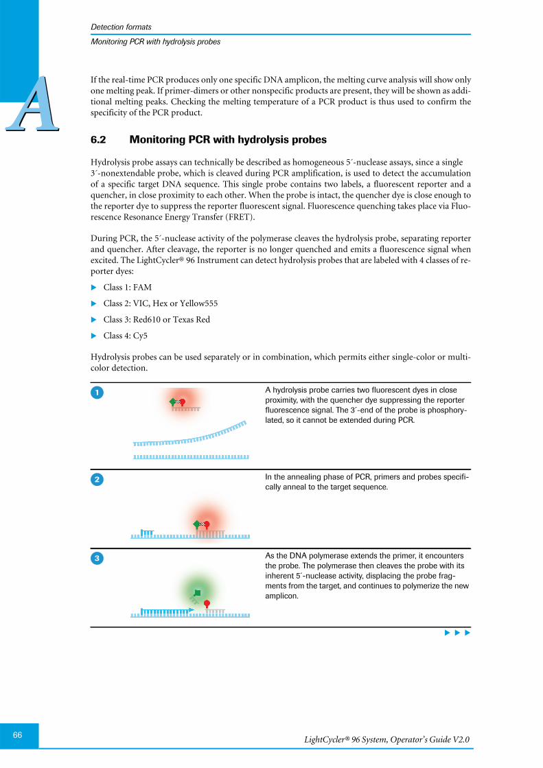
LightCycler® 96 System, Operator’s Guide V2.066
Detection formats
AAMonitoring PCR with hydrolysis probes
If the real-time PCR produces only one specific DNA amplicon, the melting curve analysis will show onlyone melting peak. If primer-dimers or other nonspecific products are present, they will be shown as addi-tional melting peaks. Checking the melting temperature of a PCR product is thus used to confirm thespecificity of the PCR product.
6.2 Monitoring PCR with hydrolysis probes
Hydrolysis probe assays can technically be described as homogeneous 5´-nuclease assays, since a single3´-nonextendable probe, which is cleaved during PCR amplification, is used to detect the accumulationof a specific target DNA sequence. This single probe contains two labels, a fluorescent reporter and aquencher, in close proximity to each other. When the probe is intact, the quencher dye is close enough tothe reporter dye to suppress the reporter fluorescent signal. Fluorescence quenching takes place via Fluo-rescence Resonance Energy Transfer (FRET).
During PCR, the 5´-nuclease activity of the polymerase cleaves the hydrolysis probe, separating reporterand quencher. After cleavage, the reporter is no longer quenched and emits a fluorescence signal whenexcited. The LightCycler® 96 Instrument can detect hydrolysis probes that are labeled with 4 classes of re-porter dyes:
Class 1: FAM
Class 2: VIC, Hex or Yellow555
Class 3: Red610 or Texas Red
Class 4: Cy5
Hydrolysis probes can be used separately or in combination, which permits either single-color or multi-color detection.
A hydrolysis probe carries two fluorescent dyes in closeproximity, with the quencher dye suppressing the reporterfluorescence signal. The 3´-end of the probe is phosphory-lated, so it cannot be extended during PCR.
In the annealing phase of PCR, primers and probes specifi-cally anneal to the target sequence.
As the DNA polymerase extends the primer, it encountersthe probe. The polymerase then cleaves the probe with itsinherent 5´-nuclease activity, displacing the probe frag-ments from the target, and continues to polymerize the newamplicon.
�
�
�
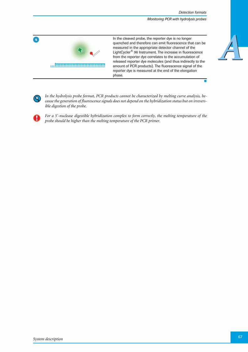
System description
Detection formats
67
AAMonitoring PCR with hydrolysis probes
In the hydrolysis probe format, PCR products cannot be characterized by melting curve analysis, be-cause the generation of fluorescence signals does not depend on the hybridization status but on irrevers-ible digestion of the probe.
For a 5'-nuclease digestible hybridization complex to form correctly, the melting temperature of theprobe should be higher than the melting temperature of the PCR primer.
In the cleaved probe, the reporter dye is no longerquenched and therefore can emit fluorescence that can bemeasured in the appropriate detector channel of theLightCycler® 96 Instrument. The increase in fluorescencefrom the reporter dye correlates to the accumulation ofreleased reporter dye molecules (and thus indirectly to theamount of PCR products). The fluorescence signal of thereporter dye is measured at the end of the elongationphase.
�
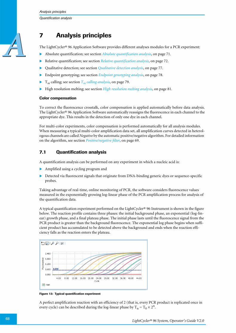
LightCycler® 96 System, Operator’s Guide V2.068
Analysis principles
AAQuantification analysis
7 Analysis principles
The LightCycler® 96 Application Software provides different analyses modules for a PCR experiment:
Absolute quantification; see section Absolute quantification analysis, on page 71.
Relative quantification; see section Relative quantification analysis, on page 72.
Qualitative detection; see section Qualitative detection analysis, on page 77.
Endpoint genotyping; see section Endpoint genotyping analysis, on page 78.
Tm calling; see section Tm calling analysis, on page 79.
High resolution melting; see section High resolution melting analysis, on page 81.
Color compensation
To correct the fluorescence crosstalk, color compensation is applied automatically before data analysis.The LightCycler® 96 Application Software automatically reassigns the fluorescence in each channel to theappropriate dye. This results in the detection of only one dye in each channel.
For multi-color experiments, color compensation is performed automatically for all analysis modules.When measuring a typical multi-color amplification data set, all amplification curves detected in heterol-ogous channels are called Negative by the automatic positive/negative algorithm. For detailed informationon the algorithm, see section Positive/negative filter, on page 69.
7.1 Quantification analysis
A quantification analysis can be performed on any experiment in which a nucleic acid is:
Amplified using a cycling program and
Detected via fluorescent signals that originate from DNA-binding generic dyes or sequence-specificprobes.
Taking advantage of real-time, online monitoring of PCR, the software considers fluorescence valuesmeasured in the exponentially growing log-linear phase of the PCR amplification process for analysis ofthe quantification data.
A typical quantification experiment performed on the LightCycler® 96 Instrument is shown in the figurebelow. The reaction profile contains three phases: the initial background phase, an exponential (log-lin-ear) growth phase, and a final plateau phase. The initial phase lasts until the fluorescence signal from thePCR product is greater than the background fluorescence. The exponential log phase begins when suffi-cient product has accumulated to be detected above the background and ends when the reaction effi-ciency falls as the reaction enters the plateau.
Figure 13: Typical quantification experiment
A perfect amplification reaction with an efficiency of 2 (that is, every PCR product is replicated once inevery cycle) can be described during the log-linear phase by Tn = T0 × 2n.
System description
Analysis principles
69
AAQuantification analysis
Real-time PCR experiments, however, are influenced by many factors, and therefore efficiency may notbe perfect. Thus PCR amplification is more accurately described as: Tn = T0 × En,where Tn is the amount of gene molecules at cycle n, T0 is the initial number of gene molecules, n is thenumber of amplification cycles, and E is the efficiency of amplification.
The figure above shows that the cycle where each reaction first rises above the background depends on theamount of the gene that is present at the beginning of the reaction. The cycle at which the fluorescence ofa sample rises above the background fluorescence is called the quantification cycle (Cq) of the sample,also known as "crossing point" (Cp) or "threshold cycle" (Ct).
The estimated quantity may be:
Absolute in terms of an actual copy number or quantity, or
Relative by comparing a target gene to a reference gene.
Absolute quantification and relative quantification share many common features, including calling of Cqvalues from amplification curves, use of standards, positive/negative calling, etc. However, since bothmethods are based on different calculation workflows, they are separated in different analysis modules.
Positive/negative filter
The LightCycler® 96 Application Software automatically applies a positive/negative filter to produce aqualitative call. The call is made based on criteria like endpoint fluorescence, relative growth, maximumrelative slope, and deviation from linearity. The positive/negative algorithm calls three different resulttypes:
Positive:The fluorescence curve fulfills the criteria for a positive call.
Negative:The fluorescence curve does not fulfill the criteria for a positive call.
Invalid:The fluorescence curve shows a very strong deviation from the expected curve shape (very rare cases).
The LightCycler® 96 Application Software provides a function to manually define gene-specific thresh-olds for the Cq (maximum value), slope (minimum value) and endpoint fluorescence (minimum value)to change the positive/negative call. For detailed information on these settings, see sections Abs QuantSettings, on page 167 and Rel Quant Settings, on page 177.
If results are displayed incorrectly as positive or negative, it is recommended to check the results andedit the corresponding thresholds manually.
Cycle of Quantification (Cq)
In an amplification reaction, the cycle at which the fluorescence of a sample rises above the backgroundfluorescence is called the cycle of quantification (Cq) of the sample. The Cq is thus a single value reflectingthe cycle number used for quantification.
The larger the quantity (or concentration) of the gene present before amplification, the fewer cycles ofamplification will be required to amplify that gene to a detectable level. As the gene reaches a detectablelevel, the exponential increase of the gene becomes visible as the fluorescence signal from the PCR prod-uct is greater than the background fluorescence.
This correlation between amount of template and value of Cq facilitates all types of real-time PCR-basedquantitative analysis. Because of this relationship between Cq and starting quantity, real-time PCR makesdata acquisition and analysis during the exponential phase easy and therefore allows sensitive quantifica-tion of a given target.

LightCycler® 96 System, Operator’s Guide V2.070
Analysis principles
AAQuantification analysis
The LightCycler® 96 Application Software uses predefined dye-specific fluorescence threshold values tocalculate the Cq value of a sample. The predefined fluorescence threshold value used in an experimentdepends on the specified detection format (dye). For detailed information on how to specify the detectionformat, see section Detection Format, on page 141.
The Cq value for a sample is only displayed in the results if the sample is determined ‘Positive’ by thepositive/negative filter algorithm or by the gene-specific threshold set manually by the operator.
The Cq threshold and the positive/negative threshold are two independent thresholds that are not cor-related. Cq values are calculated once for each sample and do not change when the positive/negativethreshold is changed manually by the operator. The Cq threshold cannot be changed by the operator.
Endpoint fluorescence
The endpoint fluorescence (EPF) of an amplification curve indicates the last fluorescence value of thebackground-corrected curve.
Background correction in all quantification analysis modules is performed by dividing each data point bythe background value of the relevant curve and subsequently subtracting a value of "1" (proportionalbackground correction).
Standard curves
In a quantification analysis, a standard curve is used to determine the quantity of unknown samples andthe amplification efficiency of a certain gene. In a standard curve, the quantities of standard samples areplotted against the Cqs of the samples. The x-axis represents the log of the initial target quantity, and they-axis represents Cq in cycles. The standard curve is a linear regression line through these plotted datapoints.
Figure 14: Standard curve in a quantification experiment
A standard curve is set up with at least three dilution steps. The quantities chosen for the standard curveshould fall between the expected quantity range of the gene of interest.
In the LightCycler® 96 Application Software, at least three standard concentrations are required to cal-culate the standard curve. Otherwise, no standard curve is calculated.
Dyes Predefined fluorescence threshold value
SYBR Green I, ResoLight 0.2
FAM, VIC, Hex, Yellow555, Red610, Texas Red, Cy5 0.05

System description
Analysis principles
71
AAQuantification analysis
The PCR Efficiency can be calculated using the formula: E = 10 -1/slope
(for example, slope = -3.3 E = 2).The software automatically calculates the efficiency and displays it in the standard curve chart.
For the valid use of the standard curve, PCR amplification must be highly reproducible and reactionconditions must be constant for all experiments. It is recommended to run tests to ensure stable PCRefficiency and to use replicate samples (especially for low quantities) to create the standard curve. Also,you should include a previously quantified sample in each analyzed run, to verify that the calculatedvalues are reproducible.
The Slope of the standard curve describes the kinetics of the PCR amplification. It indicates howquickly the amount of target nucleic acid (NA) can be expected to increase with the amplification cy-cles. The slope of the standard curve can be calculated from the Efficiency of the amplification reactionusing the formula s= -logE. A perfect amplification reaction would produce a standard curve with anefficiency of 2.00.
The display of a standard curve shows a Y-Intercept. The x-axis is adjusted to display the calculatedvalues properly.
The Standard Error of Estimate value (mean squared error of the single data points fitted to the regres-sion line) is a measure of the accuracy of the quantification result based on the standard curve (an ac-ceptable value should be < 0.2).
The Correlation Coefficient of a standard curve shows the r squared value of the correlation.
7.1.1 Absolute quantification analysis
Absolute quantification enables you to quantify a single or multiple genes and express the final result asan absolute value (for example, copies/ml). The absolute values for quantity or copy number are derivedfrom dilutions of gene-specific standards with known quantity/copy number.
The easiest way to obtain an absolute value for an unknown quantity of gene is to compare the Cq of anunknown sample against those of standards with known quantities. Standard material can be selectedfrom various sources (for example, linearized plasmid DNA carrying the cloned target sequence, purifiedPCR products). The gene quantity in the standard must be known. PCR is then performed with a seriesof dilutions of the standard, which represent different gene quantities in a reaction.
The known template amount of each standard dilution is automatically plotted against the measured Cqvalues. The resulting regression line is called the standard curve and shows the correlation between Cqand quantity. By comparing the Cq values from samples with unknown amounts of template to this stan-dard curve, one can determine the starting amount of template in each sample.

LightCycler® 96 System, Operator’s Guide V2.072
Analysis principles
AAQuantification analysis
7.1.2 Relative quantification analysis
Ratio
Relative quantification compares the levels of two different gene sequences in a single sample (for exam-ple, target gene of interest (GOI) and a reference gene), and expresses the final result as a ratio of thesegenes.
For comparison purposes, the reference gene is assumed to be present in constant numbers under all testconditions. This reference gene provides a basis for normalizing sample-to-sample differences. Toimprove this normalization step, multiple reference genes can be chosen. In this case, each relative ratiois calculated separately, and the geometric average is displayed. If no single reference gene is suitable forall samples, consider using more than one reference gene and averaging their assay levels to form a singlereference value.
Normalized ratio
In addition to calculating sample-specific ratios, a normalized ratio can be calculated by defining a specialrun-specific sample type, the "run calibrator" sample. This run calibrator is a positive sample with a stableratio of target-to-reference and is used to normalize all samples within one run. It also provides a constantcalibration point between several LightCycler® 96 System runs.
The result is expressed as a normalized ratio, that is, target/reference ratio (unknown sample) divided bytarget/reference ratio (calibrator):
While a calibrator corrects for differences in detection sensitivity between target and reference causedby differences in probe annealing, probe labeling, or dye extinction coefficients, it does not correct fordifferences in PCR efficiency between the target and reference gene.
Scaled ratio
In addition to normalization, it is frequently required to measure the gene expression of each sample andeach gene at different times or under different conditions. To generate a meaningful result, the sample-specific measurements are normalized to a common basis, that is, a certain experimental condition, toprovide a scaled ratio. This condition is specified as the "study calibrator" condition.
The scaled ratio for a specific sample is calculated by dividing all ratios by the ratio of the selected basevalue (that is, the value in the study calibrator condition):
target concentration
reference concentrationratio =
target/reference (unknown sample)
target/reference (run calibrator)
normalized ratio =
target/reference (unknown sample at condition x)
target/reference (unknown sample at study calibrator condition)
scaled ratio =
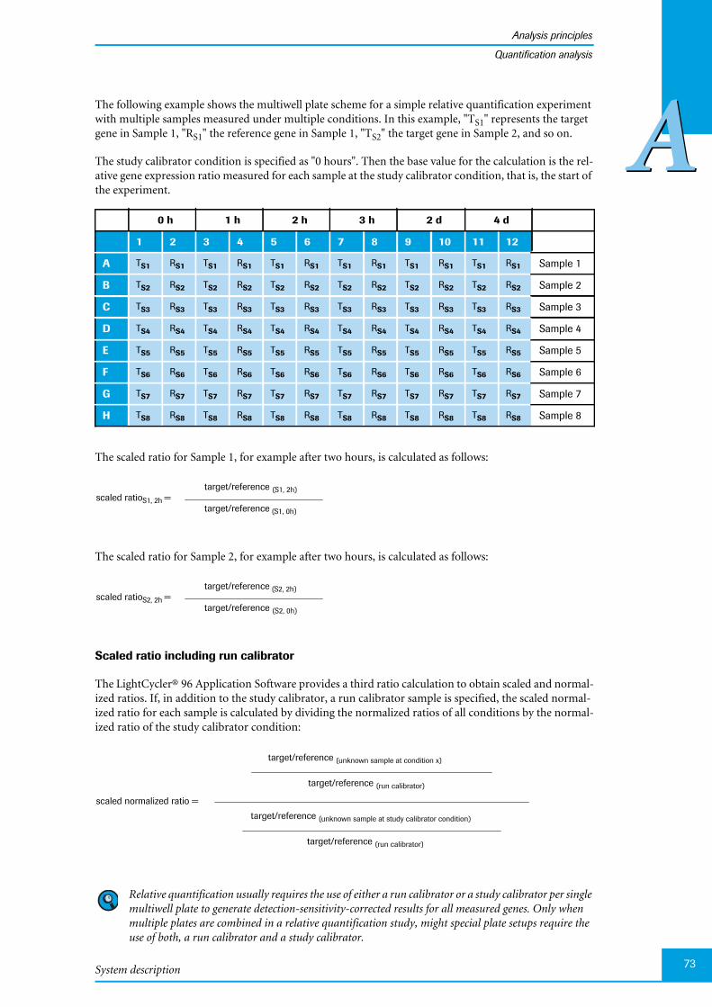
System description
Analysis principles
73
AAQuantification analysis
The following example shows the multiwell plate scheme for a simple relative quantification experimentwith multiple samples measured under multiple conditions. In this example, "TS1" represents the targetgene in Sample 1, "RS1" the reference gene in Sample 1, "TS2" the target gene in Sample 2, and so on.
The study calibrator condition is specified as "0 hours". Then the base value for the calculation is the rel-ative gene expression ratio measured for each sample at the study calibrator condition, that is, the start ofthe experiment.
The scaled ratio for Sample 1, for example after two hours, is calculated as follows:
The scaled ratio for Sample 2, for example after two hours, is calculated as follows:
Scaled ratio including run calibrator
The LightCycler® 96 Application Software provides a third ratio calculation to obtain scaled and normal-ized ratios. If, in addition to the study calibrator, a run calibrator sample is specified, the scaled normal-ized ratio for each sample is calculated by dividing the normalized ratios of all conditions by the normal-ized ratio of the study calibrator condition:
Relative quantification usually requires the use of either a run calibrator or a study calibrator per singlemultiwell plate to generate detection-sensitivity-corrected results for all measured genes. Only whenmultiple plates are combined in a relative quantification study, might special plate setups require theuse of both, a run calibrator and a study calibrator.
0 h 1 h 2 h 3 h 2 d 4 d
1 2 3 4 5 6 7 8 9 10 11 12
A TS1 RS1 TS1 RS1 TS1 RS1 TS1 RS1 TS1 RS1 TS1 RS1 Sample 1
B TS2 RS2 TS2 RS2 TS2 RS2 TS2 RS2 TS2 RS2 TS2 RS2 Sample 2
C TS3 RS3 TS3 RS3 TS3 RS3 TS3 RS3 TS3 RS3 TS3 RS3 Sample 3
D TS4 RS4 TS4 RS4 TS4 RS4 TS4 RS4 TS4 RS4 TS4 RS4 Sample 4
E TS5 RS5 TS5 RS5 TS5 RS5 TS5 RS5 TS5 RS5 TS5 RS5 Sample 5
F TS6 RS6 TS6 RS6 TS6 RS6 TS6 RS6 TS6 RS6 TS6 RS6 Sample 6
G TS7 RS7 TS7 RS7 TS7 RS7 TS7 RS7 TS7 RS7 TS7 RS7 Sample 7
H TS8 RS8 TS8 RS8 TS8 RS8 TS8 RS8 TS8 RS8 TS8 RS8 Sample 8
target/reference (S1, 2h)
target/reference (S1, 0h)
scaled ratioS1, 2h =
target/reference (S2, 2h)
target/reference (S2, 0h)
scaled ratioS2, 2h =
target/reference (unknown sample at study calibrator condition)
target/reference (run calibrator)
scaled normalized ratio =
target/reference (unknown sample at condition x)
target/reference (run calibrator)

LightCycler® 96 System, Operator’s Guide V2.074
Analysis principles
AAQuantification analysis
PCR efficiency correction
The reliability of all quantitative real-time PCR applications and, consequently, of all relative quantifica-tion calculations depends on the quality of the PCR. The final ratio resulting from the relative quantifica-tion is a function of PCR efficiency and of the quantification cycles. It does not require the knowledge ofabsolute copy numbers at the detection threshold. Thus, the analysis does not determine the actual quan-tity of DNA in the samples.
A target-specific efficiency can be either:
Derived from in-run target-specific standard curves, or
Set manually if no standards are defined or if standards are excluded from the calculation.
This efficiency-corrected ratio calculation is automatically performed by theLightCycler® 96 Application Software.
The basic prerequisites for accurate relative quantification are:
When standards are used, the efficiencies of the relative standards and the unknown samples areidentical.
The efficiencies of both target and reference PCR do not vary from sample to sample.
The reference gene is not regulated in the system being examined.
Ratio calculation for a single reference gene
If only one reference gene is used in experiments, the following basic calculations for ratio, normalizedratio and scaled ratio are performed:
ET Amplification efficiency of the target gene
ER Amplification efficiency of the reference gene
CqT Quantification cycle of the target gene
CqR Quantification cycle of the reference gene
cal Run or study calibrator
ratioER
CqR
ETCqT
--------------=
normalized or scaled ratioET
CqT cal CqT–
ERCqR cal CqR–
----------------------------------=
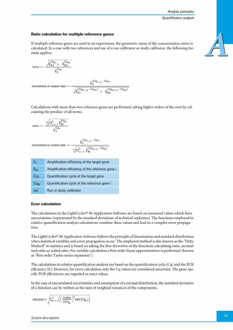
System description
Analysis principles
75
AAQuantification analysis
Ratio calculation for multiple reference genes
If multiple reference genes are used in an experiment, the geometric mean of the concentration ratios iscalculated. In a case with two references and use of a run calibrator or study calibrator, the following for-mula applies:
Calculations with more than two reference genes are performed, taking higher orders of the root by cal-culating the product of all terms.
Error calculation
The calculations in the LightCycler® 96 Application Software are based on measured values which haveuncertainties (represented by the standard deviations of technical replicates). The functions employed inrelative quantification analysis calculations combine these values and lead to a complex error propaga-tion.
The LightCycler® 96 Application Software follows the principle of linearization and standard distributionwhen statistical variables and error propagation occur. The employed method is also known as the "DeltaMethod" in statistics and is based on taking the first derivative of the functions calculating ratio, normal-ized ratio or scaled ratio. For variable calculation a first order linear approximation is performed (knownas "first order Taylor series expansion").
The calculations in relative quantification analysis are based on the quantification cycle (Cq) and the PCRefficiency (E). However, for error calculation only the Cq values are considered uncertain. The gene-spe-cific PCR efficiencies are regarded as exact values.
In the case of uncorrelated uncertainties and assumption of a normal distribution, the standard deviationof a function can be written as the sum of weighted variances of the components.
ET Amplification efficiency of the target gene
ERi Amplification efficiency of the reference gene i
CqT Quantification cycle of the target gene
CqRi Quantification cycle of the reference gene i
cal Run or study calibrator
ratioER1
CqR1 ER2CqR2
ETCqT
--------------------------------------=
normalized or scaled ratioET
CqT cal CqT–
ER1CqR1 cal CqR1–
ER2CqR2 cal CqR2–
-----------------------------------------------------------------------------------=
ratioi 1=
n ERiCqRin
ETCqT
----------------------------------=
normalized or scaled ratioET
CqT cal, CqT–
i 1=n ERi
CqRi cal, CqRi– n
------------------------------------------------------=
sd(ratio) k 1=n ratio
Cqk------------- 2
var Cqk
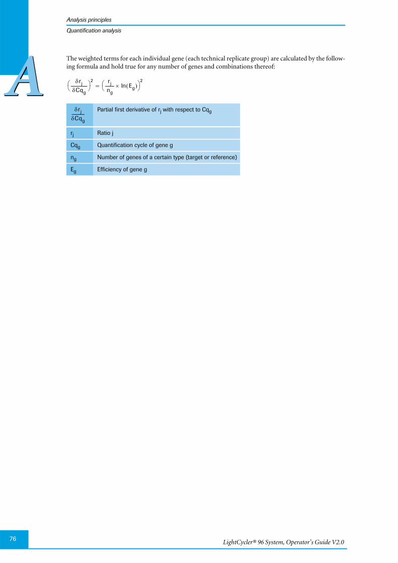
LightCycler® 96 System, Operator’s Guide V2.076
Analysis principles
AAQuantification analysis
The weighted terms for each individual gene (each technical replicate group) are calculated by the follow-ing formula and hold true for any number of genes and combinations thereof:
Partial first derivative of rj with respect to Cqg
rj Ratio j
Cqg Quantification cycle of gene g
ng Number of genes of a certain type (target or reference)
Eg Efficiency of gene g
rj
Cqg-------------- 2 rj
ng-------- Eg ln 2
=
rj
Cqg-----------

System description
Analysis principles
77
AAQuantification analysis
7.1.3 Qualitative detection analysis
Qualitative detection analyzes the presence of a target nucleic acid in combination with an internal con-trol nucleic acid. The internal control serves as an amplification control allowing:
Monitoring of PCR inhibitors.
Monitoring the reliability of purification and amplification processes.
The internal control might be RNA or DNA, depending on the type of the target nucleic acid. DuringPCR, the internal control is amplified with a separate set of primers. The analysis does not quantify theamount (copy number) of a target nucleic acid.
Operators can amplify the internal control either in a separate reaction well (mono-color mode) or in thesame reaction well (dual-color or multi-color mode):
The advantage of a mono-color setup is optimal sensitivity as there is no competition between targetand internal control.
The advantage of a dual-color or multi-color setup is the minimized material requirement (sampleamount and PCR components) and the direct inhibition control in the same well where the target isamplified. In a multi-color setup, different internal controls can be combined with different targetgenes.
The analysis provides the results as a "combined call" by combining individual positive or negative calls ofboth the target and the internal control.
Figure 15: Combined Call Heat Map for a dual-color qualitative detection experiment
Three basic result types are provided:
Positive combined call: Positive target call, positive or negative internal control call.
Negative combined call: Negative target call, positive internal control call.
Invalid combined call: Negative target call, negative internal control call.
When replicates are used, inconsistent combined calls might occur based on the following result combi-nations:
Inconsistent combined call: Target replicate calls positive and negative, independent of internal con-trol replicate calls.
Inconsistent combined call: All target replicate calls negative, internal control replicate calls positiveand negative.

LightCycler® 96 System, Operator’s Guide V2.078
Analysis principles
AAEndpoint genotyping analysis
7.2 Endpoint genotyping analysis
Endpoint genotyping analysis is used for SNP (single nucleotide polymorphism) genotyping (also knownas allelic discrimination). Endpoint genotyping assays use hydrolysis probes. For detailed information, seesection Monitoring PCR with hydrolysis probes, on page 66.
An endpoint genotyping assay includes two sequence-specific probes that are designed to detect allele xand allele y and are labeled with different reporter dyes.
In a standard setup
The FAM dye detects samples that are homozygous for allele x.
The VIC dye detects samples that are homozygous for allele y.
Figure 16: Dual-color principle of endpoint genotyping
Fluorescence data are collected throughout the PCR amplification. However, only the endpoint signalintensities of the two reporter dyes are used to identify the genotypes. The relative dye intensities can bevisualized on a scatter plot, simplifying discrimination into homozygous x, homozygous y, and heterozy-gous samples. After manually setting up the thresholds, the LightCycler® 96 Application Software groupsthe samples based on the intensity distribution of the two dyes.
LightCycler® 96 Application Software allows manual grouping of samples with similar fluorescence dis-tribution in the scatter plot. The following groups can be defined by the operator:
Negatives
Homozygous for allele x
Homozygous for allele y
Heterozygous
Unknowns
Figure 17: Scatterplot for an endpoint genotyping experiment
Each point represents a sample, whose x-coordinate is the endpoint level of allele x, and whose y-coordi-nate is the endpoint level of allele y.

System description
Analysis principles
79
AATm calling analysis
7.3 Tm calling analysis
The temperature at which DNA strands separate or melt when heated can vary over a wide range, depend-ing on the sequence, the length of the strand, DNA quantity, and buffer composition. For example, melt-ing temperatures can vary for products of the same length but different Adenine-Thymine/Guanine-Cytosine ratio (AT/GC ratio), or for products with the same length and GC content but with a differentGC distribution. Also, base pair mismatches between two DNA molecules lead to a decrease in meltingtemperature. This effect is more pronounced for short DNA amplicons.
The purpose of Tm calling is to determine the characteristic melting temperature of the target DNA.
To analyze sample melting temperature profiles, the fluorescence of the samples must be monitored whilethe temperature of the LightCycler® 96 Instrument thermal block cycler is steadily increased. As the tem-perature increases, sample fluorescence decreases. In the case of the double-stranded DNA-specific dyeSYBR Green I or the ResoLight dye, this is due to the separation of the DNA strands and consequently therelease of dye molecules.
A Tm calling analysis can be performed on any experiment that includes a melting program. A meltingprogram is usually performed after amplification of the target DNA. A typical melting program includesthree segments:
The samples are rapidly heated to a temperature high enough to denature all DNA molecules.
The samples are cooled below the annealing temperature of the target DNA.
The samples are slowly heated while measuring sample fluorescence as the target DNA melts.
You can use melting temperatures from +37 to +98°C.
Melting curves
The analysis displays a melting curves chart of sample fluorescence against temperature. The chart showsthe downward curve in fluorescence for the samples as they melt.
Figure 18: Melting Curves chart for a Tm calling experiment
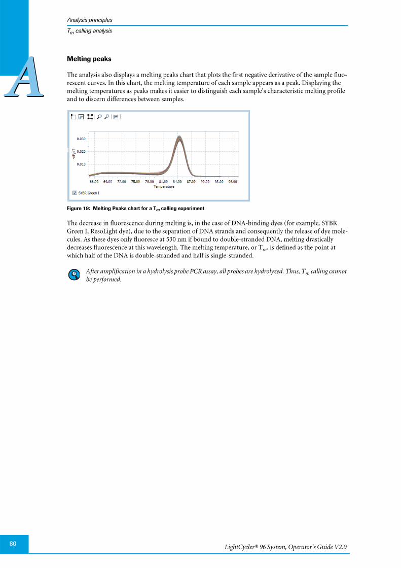
LightCycler® 96 System, Operator’s Guide V2.080
Analysis principles
AATm calling analysis
Melting peaks
The analysis also displays a melting peaks chart that plots the first negative derivative of the sample fluo-rescent curves. In this chart, the melting temperature of each sample appears as a peak. Displaying themelting temperatures as peaks makes it easier to distinguish each sample’s characteristic melting profileand to discern differences between samples.
Figure 19: Melting Peaks chart for a Tm calling experiment
The decrease in fluorescence during melting is, in the case of DNA-binding dyes (for example, SYBRGreen I, ResoLight dye), due to the separation of DNA strands and consequently the release of dye mole-cules. As these dyes only fluoresce at 530 nm if bound to double-stranded DNA, melting drasticallydecreases fluorescence at this wavelength. The melting temperature, or Tm, is defined as the point atwhich half of the DNA is double-stranded and half is single-stranded.
After amplification in a hydrolysis probe PCR assay, all probes are hydrolyzed. Thus, Tm calling cannotbe performed.

System description
Analysis principles
81
AAHigh resolution melting analysis
7.4 High resolution melting analysis
High resolution melting is a refinement of well-established DNA dissociation (or "melting") techniques(for example, to determine the Tm of a DNA hybrid). Like all melting analyses, the technique subjectsDNA samples to increasing temperatures and records the details of their dissociation from double-stranded (dsDNA) to single-stranded form (ssDNA).
Amplification and high resolution melting are performed in the presence of a fluorescent dye that bindsonly dsDNA (for example, ResoLight dye) and is present in excess of the binding capacity of DNA. Thedye does not interact with ssDNA, but fluoresces strongly after intercalating into dsDNA. This change influorescence can be used both to measure the increase in DNA quantity during PCR and then to directlymeasure thermally-induced DNA dissociation during high resolution melting.
While high resolution melting dyes bind the target DNA in saturation, dye dissociation during meltresults in a fluorescence decrease at any melting temperature, because released dye cannot bind back toremaining double-stranded sequences as all sequences are dye-saturated anyway. The use of dsDNA-binding dyes in saturation quantities prevents the measurement of artifacts which can result from dye-limited conditions.
For detection of sequence variations, differences in the melting curves of the amplicons are analyzed.Heterozygote DNA forms heteroduplexes that begin to separate into single strands at a lower temperatureand with a different curve shape than homozygote DNA. Homozygote mutants usually melt with a similarcurve shape but at different temperatures compared to the wild type. Melting temperature differences arevery small depending on the type of nucleotide exchange.
The table below shows the SNP classes and typical Tm shifts:
In a melting experiment, fluorescence is initially high, because the sample starts as dsDNA, but fluores-cence diminishes as the temperature is raised and DNA dissociates into single strands. The observed"melting" behavior is characteristic of a particular DNA sample. Mutations in PCR products are detect-able because they change the shape or location of the melting curve. When the mutant sample is com-pared to a reference "wild type" sample, these changes are visible.
An automated algorithm calculates groups of genotypes based on automated normalization and sensitiv-ity settings. Operators can overrule the automated calls either by adapting the algorithm settings or via amanual annotation function which overrules the algorithm group calls. Manual annotation can be per-formed in the normalized melting curves chart, the normalized melting peaks chart and the differenceplot.
SNP class Base change Typical Tm shift Occurrence inhuman genome
1 C/T & G/A approx. 1.0°C 64%
2 C/A & G/T approx. 1.0°C 20%
3 C/G 0.2 to 0.5°C 9%
4 A/T < 0.2°C 7%
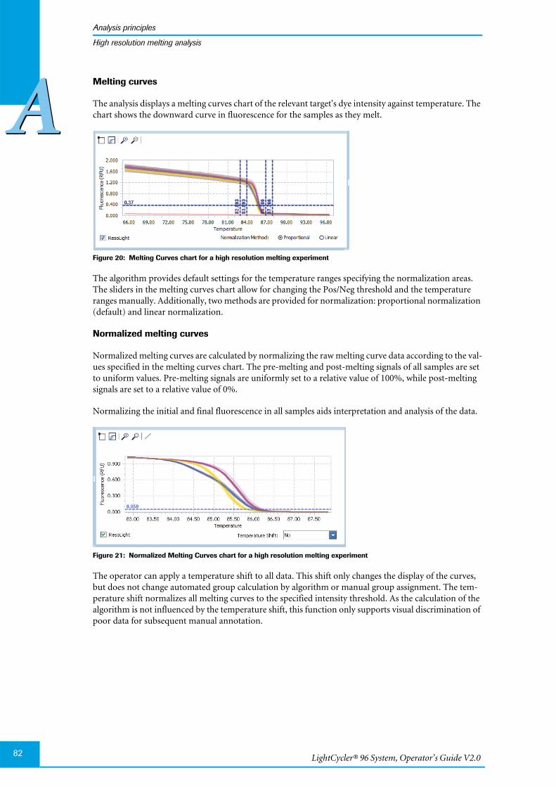
LightCycler® 96 System, Operator’s Guide V2.082
Analysis principles
AAHigh resolution melting analysis
Melting curves
The analysis displays a melting curves chart of the relevant target's dye intensity against temperature. Thechart shows the downward curve in fluorescence for the samples as they melt.
Figure 20: Melting Curves chart for a high resolution melting experiment
The algorithm provides default settings for the temperature ranges specifying the normalization areas.The sliders in the melting curves chart allow for changing the Pos/Neg threshold and the temperatureranges manually. Additionally, two methods are provided for normalization: proportional normalization(default) and linear normalization.
Normalized melting curves
Normalized melting curves are calculated by normalizing the raw melting curve data according to the val-ues specified in the melting curves chart. The pre-melting and post-melting signals of all samples are setto uniform values. Pre-melting signals are uniformly set to a relative value of 100%, while post-meltingsignals are set to a relative value of 0%.
Normalizing the initial and final fluorescence in all samples aids interpretation and analysis of the data.
Figure 21: Normalized Melting Curves chart for a high resolution melting experiment
The operator can apply a temperature shift to all data. This shift only changes the display of the curves,but does not change automated group calculation by algorithm or manual group assignment. The tem-perature shift normalizes all melting curves to the specified intensity threshold. As the calculation of thealgorithm is not influenced by the temperature shift, this function only supports visual discrimination ofpoor data for subsequent manual annotation.
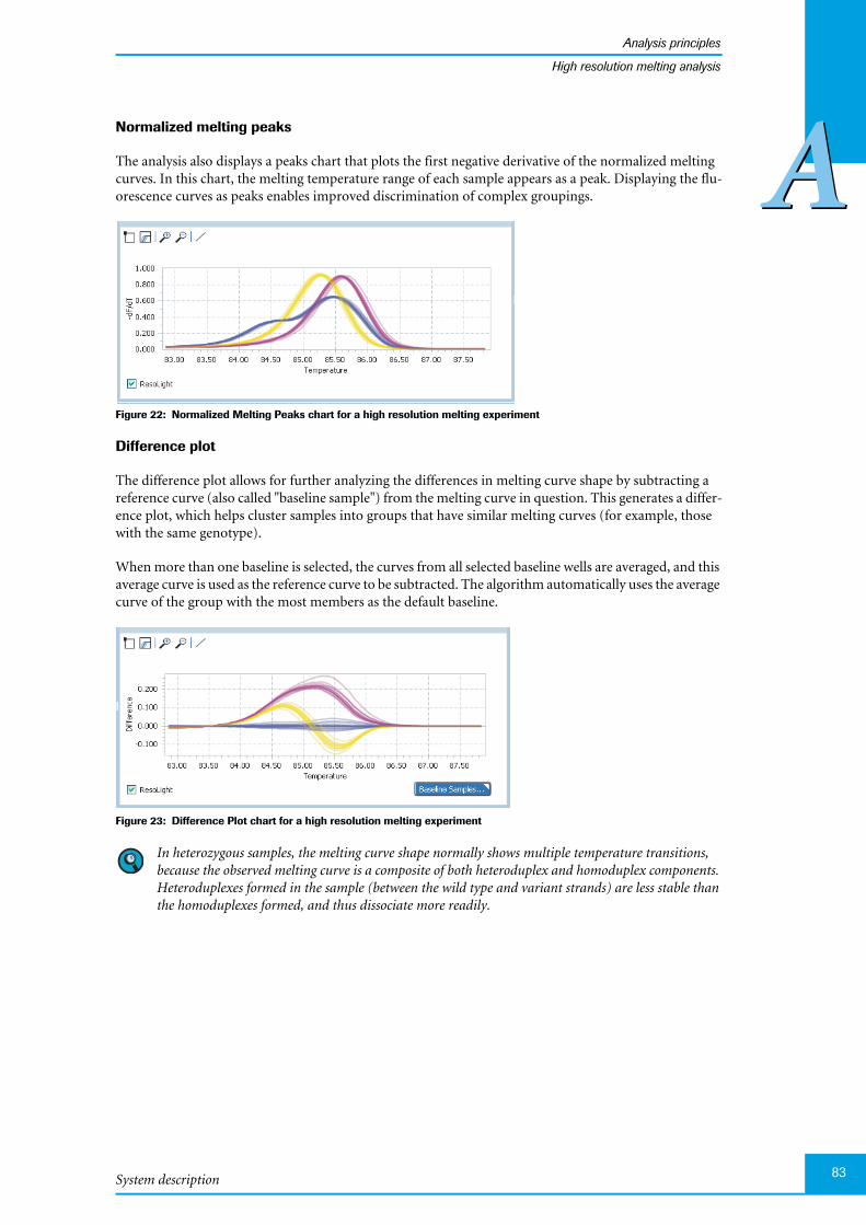
System description
Analysis principles
83
AAHigh resolution melting analysis
Normalized melting peaks
The analysis also displays a peaks chart that plots the first negative derivative of the normalized meltingcurves. In this chart, the melting temperature range of each sample appears as a peak. Displaying the flu-orescence curves as peaks enables improved discrimination of complex groupings.
Figure 22: Normalized Melting Peaks chart for a high resolution melting experiment
Difference plot
The difference plot allows for further analyzing the differences in melting curve shape by subtracting areference curve (also called "baseline sample") from the melting curve in question. This generates a differ-ence plot, which helps cluster samples into groups that have similar melting curves (for example, thosewith the same genotype).
When more than one baseline is selected, the curves from all selected baseline wells are averaged, and thisaverage curve is used as the reference curve to be subtracted. The algorithm automatically uses the averagecurve of the group with the most members as the default baseline.
Figure 23: Difference Plot chart for a high resolution melting experiment
In heterozygous samples, the melting curve shape normally shows multiple temperature transitions,because the observed melting curve is a composite of both heteroduplex and homoduplex components.Heteroduplexes formed in the sample (between the wild type and variant strands) are less stable thanthe homoduplexes formed, and thus dissociate more readily.

LightCycler® 96 System, Operator’s Guide V2.0
AA
84

Chapter BLightCycler® 96 Application Software
BBChapter B • LightCycler® 96 Application Software

LightCycler® 96 System, Operator’s Guide V2.0
Table of Contents
BB
86
B LightCycler® 96 Application Software 85
1 Overview ........................................................................................................................................................... 89
1.1 Starting the software ...................................................................................................................................... 901.2 Startup wizard ................................................................................................................................................... 901.3 The main window ............................................................................................................................................ 93
1.3.1 Menu bar ............................................................................................................................................................ 941.3.2 Tool bar ............................................................................................................................................................... 961.3.3 Working window area tabs .......................................................................................................................... 971.3.4 Experiment bar ................................................................................................................................................. 97
1.4 General software conventions .................................................................................................................... 981.4.1 Regional settings ............................................................................................................................................. 981.4.2 Buttons ................................................................................................................................................................ 981.4.3 Input fields ......................................................................................................................................................... 981.4.4 Working with tables ........................................................................................................................................ 991.4.5 Working with graphs ................................................................................................................................... 1061.4.6 Working with heat maps ............................................................................................................................ 1091.4.7 Working with plate views .......................................................................................................................... 1111.4.8 Working with sections ................................................................................................................................ 112
1.5 Experiments .................................................................................................................................................... 1131.5.1 Experiment file types ................................................................................................................................... 1131.5.2 Creating an experiment .............................................................................................................................. 1131.5.3 Opening an experiment .............................................................................................................................. 1151.5.4 Saving an experiment ................................................................................................................................. 1161.5.5 Experiment properties ................................................................................................................................. 1171.5.6 Experiment report ......................................................................................................................................... 118
1.6 Import, export, and file transfer options ............................................................................................... 1211.6.1 Import data ...................................................................................................................................................... 1211.6.2 Export data ...................................................................................................................................................... 122
1.7 Disregarding positions from an analysis ............................................................................................. 1231.8 Exiting the software ..................................................................................................................................... 123
2 Tools ................................................................................................................................................................. 124
2.1 Instrument Manager .................................................................................................................................... 1242.1.1 Instruments window area .......................................................................................................................... 1252.1.2 Information tab .............................................................................................................................................. 1272.1.3 Send/Receive Experiments tab ................................................................................................................ 1282.1.4 Online Monitoring tab ................................................................................................................................ 130
2.2 Result Batch Export ..................................................................................................................................... 1312.2.1 Analysis type .................................................................................................................................................. 1322.2.2 File selection ................................................................................................................................................... 1322.2.3 Export ................................................................................................................................................................ 133
3 Preferences .................................................................................................................................................. 134
4 Run Editor tab ............................................................................................................................................. 135
4.1 Programs window area ............................................................................................................................... 1354.1.1 Programs list buttons .................................................................................................................................. 1364.1.2 Programs list shortcut menu .................................................................................................................... 1364.1.3 Adding a new program .............................................................................................................................. 136
4.2 Steps window area ....................................................................................................................................... 1384.2.1 Steps list buttons .......................................................................................................................................... 1384.2.2 Steps list shortcut menu ............................................................................................................................ 1384.2.3 Step settings ................................................................................................................................................... 139
4.3 Measurement window area ...................................................................................................................... 1414.4 Temperature Profile window area .......................................................................................................... 142
87
BB
5 Sample Editor tab ...................................................................................................................................... 143
5.1 Plate View tab ................................................................................................................................................. 1445.1.1 Multiwell plate image .................................................................................................................................. 1455.1.2 Reaction Properties window area ........................................................................................................... 1455.1.3 Replicate Group window area .................................................................................................................. 1475.1.4 Visible Details ................................................................................................................................................. 1485.1.5 Print/Save Plate .............................................................................................................................................. 1485.1.6 Plate ID .............................................................................................................................................................. 1495.1.7 Failure Constraints ........................................................................................................................................ 1505.1.8 Auto Standard Curve ................................................................................................................................... 1515.1.9 Clear Wells/Set to Default .......................................................................................................................... 153
5.2 Table View tab ................................................................................................................................................ 1545.2.1 Sample table ................................................................................................................................................... 1555.2.2 Exporting the sample list ............................................................................................................................ 1565.2.3 Importing sample data ................................................................................................................................ 157
6 Raw Data tab ................................................................................................................................................ 159
7 Analysis tab .................................................................................................................................................. 162
7.1 Absolute quantification ............................................................................................................................... 1667.1.1 Abs Quant Settings ...................................................................................................................................... 1677.1.2 Amplification Curves .................................................................................................................................... 1697.1.3 Heat Map .......................................................................................................................................................... 1707.1.4 Result Table ..................................................................................................................................................... 1717.1.5 Standard Curves ............................................................................................................................................ 1747.1.6 Melting Peaks ................................................................................................................................................. 1747.1.7 Cq Bars .............................................................................................................................................................. 175
7.2 Relative quantification ................................................................................................................................. 1767.2.1 Rel Quant Settings ........................................................................................................................................ 1777.2.2 Amplification Curves .................................................................................................................................... 1797.2.3 Ratio Bars ......................................................................................................................................................... 1807.2.4 Result Table ..................................................................................................................................................... 1817.2.5 Standard Curves ............................................................................................................................................ 1857.2.6 Melting Peaks ................................................................................................................................................. 1857.2.7 Heat Map .......................................................................................................................................................... 1857.2.8 Cq Bars .............................................................................................................................................................. 185
7.3 Qualitative Detection ................................................................................................................................... 1867.3.1 Qualitative Detection settings for a dual- or multi-color setup ................................................... 1877.3.2 Qualitative Detection Settings .................................................................................................................. 1877.3.3 Amplification Curves .................................................................................................................................... 1897.3.4 Heat Map .......................................................................................................................................................... 1897.3.5 Combined Call Heat Map ........................................................................................................................... 1907.3.6 Result Table ..................................................................................................................................................... 191
7.4 Endpoint genotyping .................................................................................................................................... 1937.4.1 Endpoint Genotyping Settings .................................................................................................................. 1947.4.2 Amplification Curves .................................................................................................................................... 1957.4.3 Scatter Plot ...................................................................................................................................................... 1967.4.4 Heat Map .......................................................................................................................................................... 1987.4.5 Result Table ..................................................................................................................................................... 199
7.5 Tm calling ......................................................................................................................................................... 2007.5.1 Melting Analysis Parameters .................................................................................................................... 2017.5.2 Melting Curves ............................................................................................................................................... 2037.5.3 Melting Peaks ................................................................................................................................................. 2037.5.4 Heat Map .......................................................................................................................................................... 2047.5.5 Result Table ..................................................................................................................................................... 2057.5.6 Amplification Curves .................................................................................................................................... 206

LightCycler® 96 System, Operator’s Guide V2.088
BB
7.6 High Resolution Melting ............................................................................................................................ 2077.6.1 Select HRM Gene ......................................................................................................................................... 2087.6.2 High Resolution Melting Settings ........................................................................................................... 2087.6.3 Melting Curves .............................................................................................................................................. 2127.6.4 Normalized Melting Curves ...................................................................................................................... 2137.6.5 Normalized Melting Peaks ........................................................................................................................ 2157.6.6 Difference Plot ............................................................................................................................................... 2157.6.7 Result Table .................................................................................................................................................... 2167.6.8 Heat Map ......................................................................................................................................................... 2177.6.9 Amplification Curves ................................................................................................................................... 217
7.7 Exporting analysis results .......................................................................................................................... 2187.7.1 Exporting the result table .......................................................................................................................... 2187.7.2 Exporting multiple result data .................................................................................................................. 218
LightCycler® 96 Application Software
Overview
89
BB
LightCycler® 96 Application Software 0
1 Overview
The LightCycler® 96 Application Software provides all functions for defining an experiment protocol andanalyzing the data gathered during the experiment run.
Specifying the temperature profile and the dye-specific parameters for an experiment run; see sectionRun Editor tab, on page 135.
Creating, editing, deleting, and rearranging samples and genes present in the wells, as well as the dyesused to label each gene; see section Sample Editor tab, on page 143.
Creating analysis, defining analysis settings, and viewing the calculated results of an experiment run;see section Analysis tab, on page 162.
For starting a run, the experiment must be transferred to the LightCycler® 96 Instrument. For analysis,the raw data gathered by the LightCycler® 96 Instrument Software must be transferred back to the appli-cation software. For detailed information on the LightCycler® 96 Instrument Software, see chapterLightCycler® 96 Instrument Software, on page 219.
The computer running the LightCycler® 96 Application Software can be connected to theLightCycler® 96 Instrument either via a local Ethernet network or directly (one-to-one connection). Inboth cases, the operator can register the instrument with the software for monitoring the instrument andfor sending and retrieving experiments. For detailed information, see section Instrument Manager, onpage 124.
The LightCycler® 96 Application Software may be installed on a computer which is connected to a net-work. Please be aware that such connection may have an adverse effect on the product’s integrity, forexample, through infection with malicious code (viruses, Trojan horses, etc.) or access by unauthorizedthird parties (suc h as intrusion by hackers). Roche therefore highly recommends protecting the productagainst such risks by taking appropriate and state-of-the-art action.
As the product is not intended to be used within networks without an appropriate firewall, and has notbeen designed for such use, Roche assumes no liability in this regard.
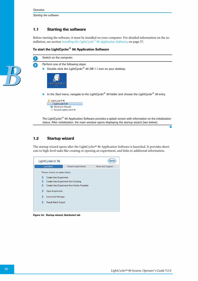
LightCycler® 96 System, Operator’s Guide V2.090
Overview
BB
Starting the software
1.1 Starting the software
Before starting the software, it must be installed on your computer. For detailed information on the in-stallation, see section Installing the LightCycler® 96 Application Software, on page 57.
To start the LightCycler® 96 Application Software
1.2 Startup wizard
The startup wizard opens after the LightCycler® 96 Application Software is launched. It provides short-cuts to high-level tasks like creating or opening an experiment, and links to additional information.
Figure 24: Startup wizard, Quickstart tab
Switch on the computer.
Perform one of the following steps:
Double-click the LightCycler® 96 SW 1.1 icon on your desktop.
In the Start menu, navigate to the LightCycler® 96 folder and choose the LightCycler® 96 entry.
The LightCycler® 96 Application Software provides a splash screen with information on the initializationstatus. After initialization, the main window opens displaying the startup wizard (see below).
�
�

LightCycler® 96 Application Software
Overview
91
BB
Startup wizard
Quickstart tab
The Quickstart tab (see Figure 24 above) provides the following shortcuts:
Recent Experiments tab
Figure 25: Startup wizard, Recent Experiments tab
The Recent Experiments tab lists the 10 last-opened experiments. If one of the recent experiments is nolonger available, the corresponding entry is deleted.
Choosing one of the list entries opens the corresponding experiment.
Shortcut Description
Create New Experiment Creates a new, empty experiment. For detailed information,see section To generate a new experiment, on page 113.
Create New Experiment from Existing Opens the Open dialog box for choosing an existing experi-ment to be used as a template. For detailed information, seesection To use an existing experiment as a template, onpage 114.
Create New Experiment from Roche Template Opens the Open dialog box for choosing an experimenttemplate provided by Roche. For detailed information, seesection To use a Roche template, on page 114.
Open Experiment Opens the Open dialog box for choosing an experiment. Fordetailed information, see section To open an experiment, onpage 115.
Instrument Manager Opens the Instrument Manager dialog box for managing theLightCycler® 96 Instruments registered with the applicationsoftware. For detailed information, see section InstrumentManager, on page 124.
Result Batch Export Opens the Result Batch Export wizard for creating a file withresult table data collected from different experiments of thesame type. For detailed information, see section ResultBatch Export, on page 131.
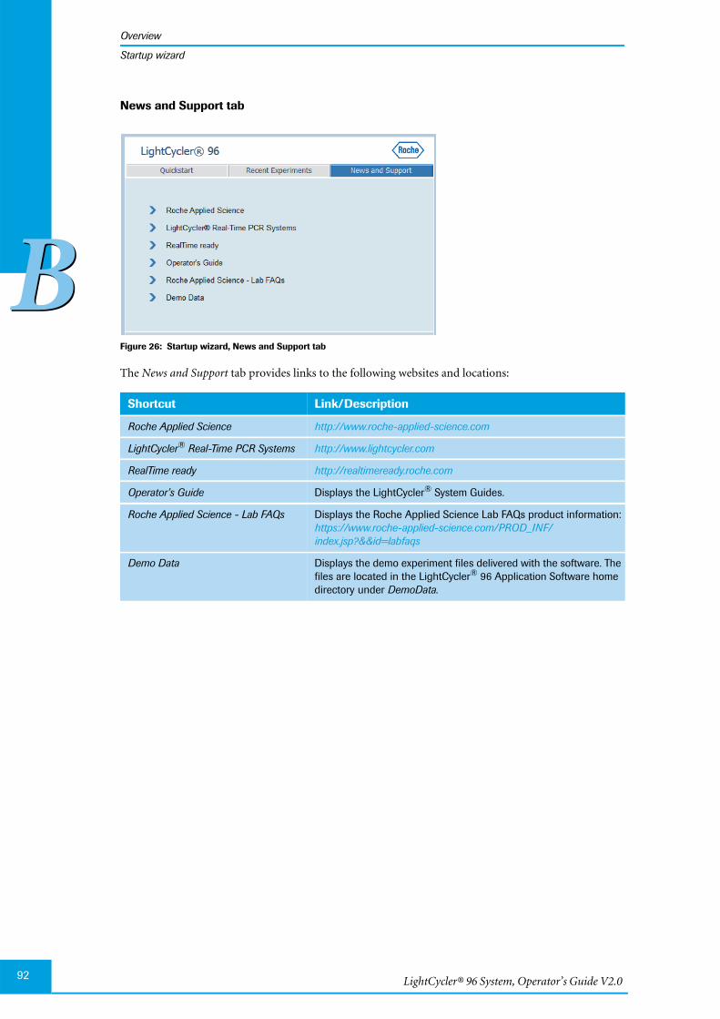
LightCycler® 96 System, Operator’s Guide V2.092
Overview
BB
Startup wizard
News and Support tab
Figure 26: Startup wizard, News and Support tab
The News and Support tab provides links to the following websites and locations:
Shortcut Link/Description
Roche Applied Science http://www.roche-applied-science.com
LightCycler® Real-Time PCR Systems http://www.lightcycler.com
RealTime ready http://realtimeready.roche.com
Operator’s Guide Displays the LightCycler® System Guides.
Roche Applied Science - Lab FAQs Displays the Roche Applied Science Lab FAQs product information:https://www.roche-applied-science.com/PROD_INF/index.jsp?&&id=labfaqs
Demo Data Displays the demo experiment files delivered with the software. Thefiles are located in the LightCycler® 96 Application Software homedirectory under DemoData.
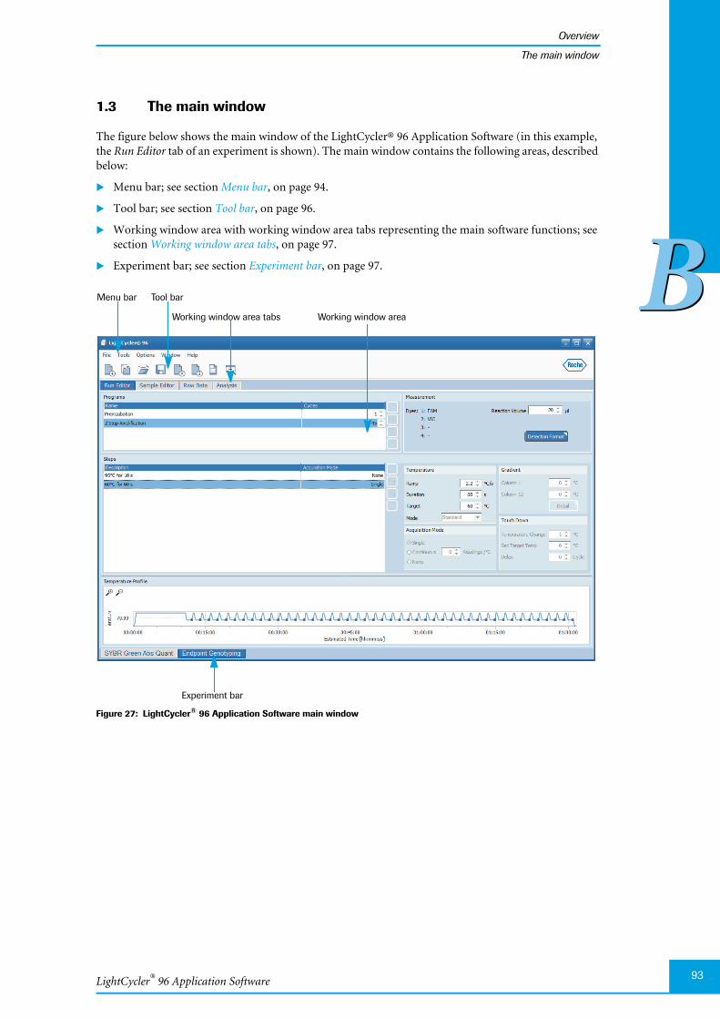
LightCycler® 96 Application Software
Overview
93
BB
The main window
1.3 The main window
The figure below shows the main window of the LightCycler® 96 Application Software (in this example,the Run Editor tab of an experiment is shown). The main window contains the following areas, describedbelow:
Menu bar; see section Menu bar, on page 94.
Tool bar; see section Tool bar, on page 96.
Working window area with working window area tabs representing the main software functions; seesection Working window area tabs, on page 97.
Experiment bar; see section Experiment bar, on page 97.
Figure 27: LightCycler® 96 Application Software main window
Working window area
Menu bar
Working window area tabs
Experiment bar
Tool bar
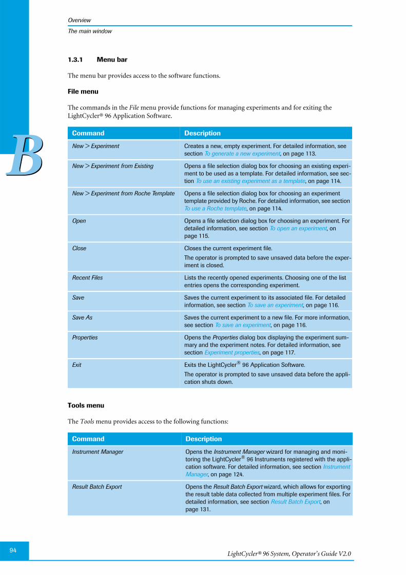
LightCycler® 96 System, Operator’s Guide V2.094
Overview
BB
The main window
1.3.1 Menu bar
The menu bar provides access to the software functions.
File menu
The commands in the File menu provide functions for managing experiments and for exiting theLightCycler® 96 Application Software.
Tools menu
The Tools menu provides access to the following functions:
Command Description
New > Experiment Creates a new, empty experiment. For detailed information, seesection To generate a new experiment, on page 113.
New > Experiment from Existing Opens a file selection dialog box for choosing an existing experi-ment to be used as a template. For detailed information, see sec-tion To use an existing experiment as a template, on page 114.
New > Experiment from Roche Template Opens a file selection dialog box for choosing an experimenttemplate provided by Roche. For detailed information, see sectionTo use a Roche template, on page 114.
Open Opens a file selection dialog box for choosing an experiment. Fordetailed information, see section To open an experiment, onpage 115.
Close Closes the current experiment file.
The operator is prompted to save unsaved data before the exper-iment is closed.
Recent Files Lists the recently opened experiments. Choosing one of the listentries opens the corresponding experiment.
Save Saves the current experiment to its associated file. For detailedinformation, see section To save an experiment, on page 116.
Save As Saves the current experiment to a new file. For more information,see section To save an experiment, on page 116.
Properties Opens the Properties dialog box displaying the experiment sum-mary and the experiment notes. For detailed information, seesection Experiment properties, on page 117.
Exit Exits the LightCycler® 96 Application Software.
The operator is prompted to save unsaved data before the appli-cation shuts down.
Command Description
Instrument Manager Opens the Instrument Manager wizard for managing and moni-toring the LightCycler® 96 Instruments registered with the appli-cation software. For detailed information, see section InstrumentManager, on page 124.
Result Batch Export Opens the Result Batch Export wizard, which allows for exportingthe result table data collected from multiple experiment files. Fordetailed information, see section Result Batch Export, onpage 131.
LightCycler® 96 Application Software
Overview
95
BB
The main window
Options menu
The Options menu provides general configuration functions. The Preferences command opens thePreferences dialog box, which provides access to the following functions. For detailed information, see sec-tion Preferences, on page 134.
Defining the default directory for searching for and saving experiment files.
Defining an email address to be linked to all experiments generated with the current software instance.
Window menu
The Show Startup Wizard command in the Window menu provides access to theLightCycler® 96 Application Software startup wizard. For detailed information, see sectionStartup wizard, on page 90.
Help menu
The Help menu provides access to the following information:
Command Description
Operator’s Guide Shortcut to the LightCycler® 96 System Guides in the installationfolder.
About Opens the About dialog box, which displays the software versionand copyright information about the software.
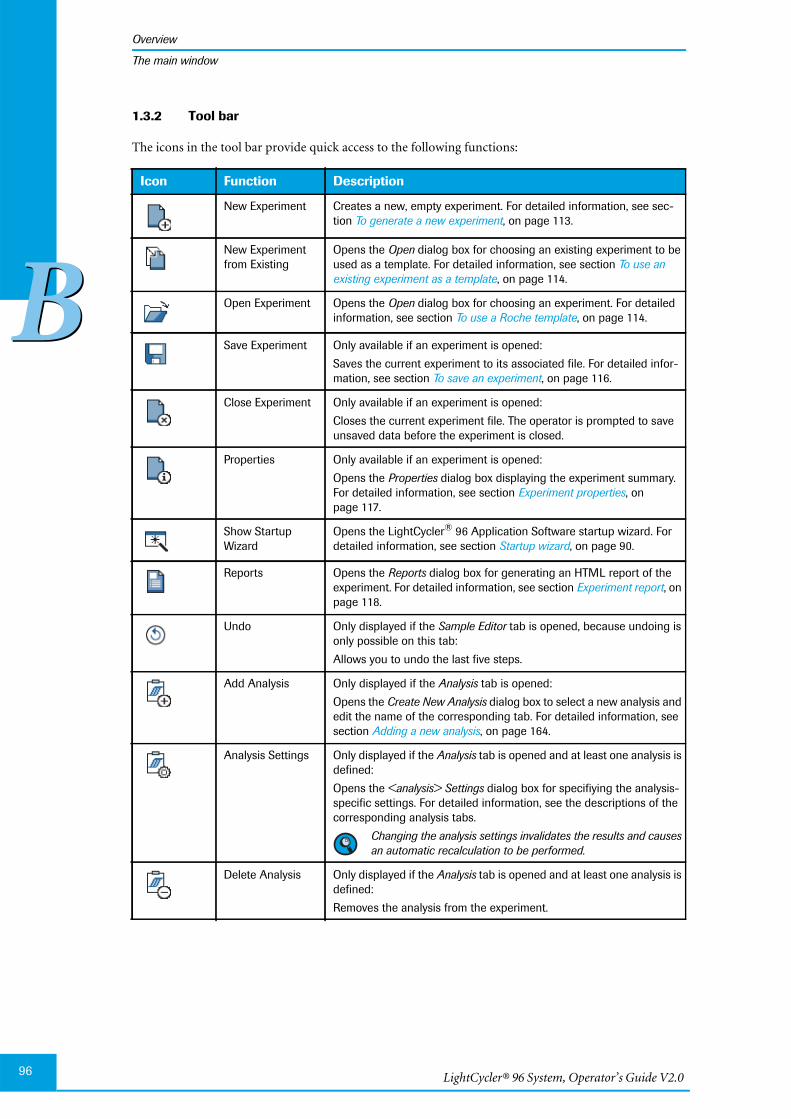
LightCycler® 96 System, Operator’s Guide V2.096
Overview
BB
The main window
1.3.2 Tool bar
The icons in the tool bar provide quick access to the following functions:
Icon Function Description
New Experiment Creates a new, empty experiment. For detailed information, see sec-tion To generate a new experiment, on page 113.
New Experimentfrom Existing
Opens the Open dialog box for choosing an existing experiment to beused as a template. For detailed information, see section To use anexisting experiment as a template, on page 114.
Open Experiment Opens the Open dialog box for choosing an experiment. For detailedinformation, see section To use a Roche template, on page 114.
Save Experiment Only available if an experiment is opened:
Saves the current experiment to its associated file. For detailed infor-mation, see section To save an experiment, on page 116.
Close Experiment Only available if an experiment is opened:
Closes the current experiment file. The operator is prompted to saveunsaved data before the experiment is closed.
Properties Only available if an experiment is opened:
Opens the Properties dialog box displaying the experiment summary.For detailed information, see section Experiment properties, onpage 117.
Show StartupWizard
Opens the LightCycler® 96 Application Software startup wizard. Fordetailed information, see section Startup wizard, on page 90.
Reports Opens the Reports dialog box for generating an HTML report of theexperiment. For detailed information, see section Experiment report, onpage 118.
Undo Only displayed if the Sample Editor tab is opened, because undoing isonly possible on this tab:
Allows you to undo the last five steps.
Add Analysis Only displayed if the Analysis tab is opened:
Opens the Create New Analysis dialog box to select a new analysis andedit the name of the corresponding tab. For detailed information, seesection Adding a new analysis, on page 164.
Analysis Settings Only displayed if the Analysis tab is opened and at least one analysis isdefined:
Opens the <analysis> Settings dialog box for specifiying the analysis-specific settings. For detailed information, see the descriptions of thecorresponding analysis tabs.
Changing the analysis settings invalidates the results and causesan automatic recalculation to be performed.
Delete Analysis Only displayed if the Analysis tab is opened and at least one analysis isdefined:
Removes the analysis from the experiment.

LightCycler® 96 Application Software
Overview
97
BB
The main window
1.3.3 Working window area tabs
The LightCycler® 96 Application Software provides the complete workflow via the tabs in the workingwindow area of the experiment:
1.3.4 Experiment bar
The experiment bar provides an entry for each open experiment. Choosing one of these entries displaysthe last opened tab for the corresponding experiment.
Each entry in the experiment bar provides a tooltip showing the location where the experiment file isstored. The tooltip for a new experiment shows the default name for new experiments.
Figure 28: Experiment bar
Tab Description
Run Editor Provides the following functions:
Defining the detection format and dye settings for the experiment.
Defining the temperature and cycling sequence for the experiment.
For detailed information, see section Run Editor tab, on page 135.
Sample Editor Provides the following functions:
Defining sample and gene names.
Defining the sample types.
For detailed information, see section Sample Editor tab, on page 143.
Raw Data Provides the raw data collected during an experiment run. For detailed information,see section Raw Data tab, on page 159.
Analysis Provides the functions and methods for analyzing the results of an experiment run.For detailed information, see section Analysis tab, on page 162.

LightCycler® 96 System, Operator’s Guide V2.098
Overview
BB
General software conventions
1.4 General software conventions
1.4.1 Regional settings
The LightCycler® 96 Application Software user interface displays date and floating-point numbers inEnglish (USA) specified by the Microsoft Windows Regional and Language Options.
1.4.2 Buttons
Button design
In the LightCycler® 96 Application Software user interface, general button design conventions illustratethe function of each button using specific button indicators:
Standard buttons
The LightCycler® 96 Application Software user interface uses the following standard buttons in dialogboxes:
1.4.3 Input fields
The LightCycler® 96 Application Software user interface provides several options for entering data intoinput fields:
Button Marking Description
White triangle in bottom left corner Completes the action and closes the dia-log.
White triangle in top right corner Opens a secondary dialog.
No triangle Performs a specified action in the currentdialog.
White border, label gray, button transpar-ent
Button is disabled.
Button Description
OK Closes the dialog box and applies the settings to the corresponding parameters.
Apply Applies the settings to the corresponding parameters without closing the dialog box.
Cancel Closes the dialog box and discards the settings.
... Browse button:
Opens a Browse For Folder dialog box, where the operator can navigate to a specificlocation.
Opens a text input dialog box, where the operator can enter text, for example, todescribe a sample.
Input Field Description
Text field Choose the field and type the text according to the rules specified for theparameter. You can enter up to 100 characters in an input field.
Text field with a list Choose the field and select a value from the pull-down list.
Numeric values field with upand down arrows
Choose the field and specify a value by choosing the up and down arrowsor enter the value directly.
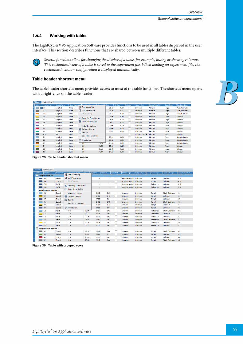
LightCycler® 96 Application Software
Overview
99
BB
General software conventions
1.4.4 Working with tables
The LightCycler® 96 Application Software provides functions to be used in all tables displayed in the userinterface. This section describes functions that are shared between multiple different tables.
Several functions allow for changing the display of a table, for example, hiding or showing columns.This customized view of a table is saved to the experiment file. When loading an experiment file, thecustomized window configuration is displayed automatically.
Table header shortcut menu
The table header shortcut menu provides access to most of the table functions. The shortcut menu openswith a right-click on the table header.
Figure 29: Table header shortcut menu
Figure 30: Table with grouped rows
LightCycler® 96 System, Operator’s Guide V2.0100
Overview
BB
General software conventions
The commands are disabled if the function is not allowed in the current context.
Command Description
Sort Ascending/Sort Descending
Sorts the corresponding column.
Clear Sorting Resets the row order to the default value.
Group By This Column Allows for grouping the values in a table by one or more selected columns;see Figure 30, above.
Show Group By Box Shows the header of the column(s) selected with Group By This Column in abox above the table header.
Using the shortcut menu in this <column> box, the rows in the grouped tablecan be rearranged as follows:
Full ExpandExpands all rows in the table to show the values in the other columns.
Full CollapseCollapses all rows in the table to hide the values.
UngroupUndoes the grouping of the columns.
Hide Group By BoxHide the <column> box.
Hide This Column/Show This Column
Hides/shows the selected column.
Column Selector Opens the Column Selector dialog box which lists the removed columns. Fordetailed information on the column selector, see section Hiding or showingcolumns, on page 103.
Best Fit Changes the column width to the best fit for the selected column.
Best Fit (all columns) Changes the column width to the best fit for all columns.
Clear Filter Resets the filter specified for the column to the default value.
Filter Editor Displays the Filter Builder dialog box. For detailed information on specifying fil-ters, see section Filtering table items, on page 104.
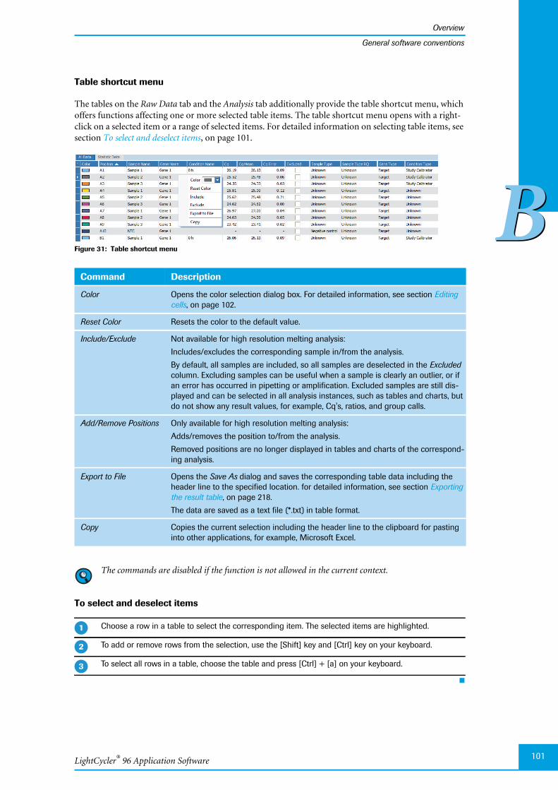
LightCycler® 96 Application Software
Overview
101
BB
General software conventions
Table shortcut menu
The tables on the Raw Data tab and the Analysis tab additionally provide the table shortcut menu, whichoffers functions affecting one or more selected table items. The table shortcut menu opens with a right-click on a selected item or a range of selected items. For detailed information on selecting table items, seesection To select and deselect items, on page 101.
Figure 31: Table shortcut menu
The commands are disabled if the function is not allowed in the current context.
To select and deselect items
Command Description
Color Opens the color selection dialog box. For detailed information, see section Editingcells, on page 102.
Reset Color Resets the color to the default value.
Include/Exclude Not available for high resolution melting analysis:
Includes/excludes the corresponding sample in/from the analysis.
By default, all samples are included, so all samples are deselected in the Excludedcolumn. Excluding samples can be useful when a sample is clearly an outlier, or ifan error has occurred in pipetting or amplification. Excluded samples are still dis-played and can be selected in all analysis instances, such as tables and charts, butdo not show any result values, for example, Cq's, ratios, and group calls.
Add/Remove Positions Only available for high resolution melting analysis:
Adds/removes the position to/from the analysis.
Removed positions are no longer displayed in tables and charts of the correspond-ing analysis.
Export to File Opens the Save As dialog and saves the corresponding table data including theheader line to the specified location. for detailed information, see section Exportingthe result table, on page 218.
The data are saved as a text file (*.txt) in table format.
Copy Copies the current selection including the header line to the clipboard for pastinginto other applications, for example, Microsoft Excel.
Choose a row in a table to select the corresponding item. The selected items are highlighted.
To add or remove rows from the selection, use the [Shift] key and [Ctrl] key on your keyboard.
To select all rows in a table, choose the table and press [Ctrl] + [a] on your keyboard.
�
�
�
LightCycler® 96 System, Operator’s Guide V2.0102
Overview
BB
General software conventions
Editing cells
Tables often allow direct editing of the contents of individual cells. Different types of cells respond slightlydifferently to editing:
To sort tables
To change the column width
Cell Type Editing
Text or numbers To enable editing:
Double-click in the cell. Edit the contents in the displayed input field.
Select the cell (by choosing the cell or using arrow keys) and start typing.To stop editing:
Press the [Enter] key to complete the change and start editing the next cellbelow.
Press the [Tab] key to complete the change and start editing the next cell tothe right.
Click outside the cell to complete the change and stop editing cells.
Boolean value Choose the cell to toggle the value.
If the cell is selected, press any key to toggle the value.
Color Select the cell. The color selection dialog box opens.
Choose a color in the color palette.
Choice Choose the cell and select an entry from the list displayed.
Choose the header of a column to sort the table by the column values.
Choosing the header several times toggles the sort order between descending and ascending.
In a ‘Position’ column, showing the position of a sample on the multiwell plate, choosing the headertoggles between sorting by row (A1, A2, A3, ...) or sorting by column (A1, B1, C1, ...).
Choosing the header of the ‘Number’ column allows for sorting a table upwards or downwards.
To sort the table by multiple columns, press the [Ctrl] key and choose the headers of the columns to beincluded in the sort. Start from the least significant column and proceed through to the most significantcolumn.
Move the cursor to the border of the table header you want to change.
When the cursor changes to a left and right arrow, hold down the left mouse button and drag the borderuntil the column has the appropriate width.
�
�
�
�
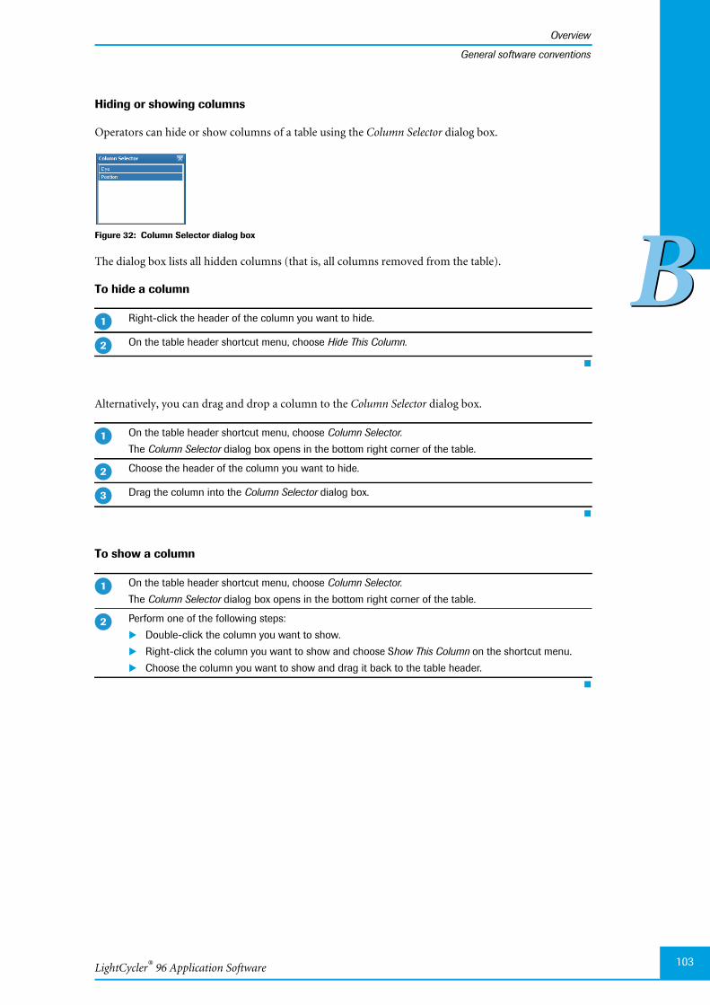
LightCycler® 96 Application Software
Overview
103
BB
General software conventions
Hiding or showing columns
Operators can hide or show columns of a table using the Column Selector dialog box.
Figure 32: Column Selector dialog box
The dialog box lists all hidden columns (that is, all columns removed from the table).
To hide a column
Alternatively, you can drag and drop a column to the Column Selector dialog box.
To show a column
Right-click the header of the column you want to hide.
On the table header shortcut menu, choose Hide This Column.
On the table header shortcut menu, choose Column Selector.
The Column Selector dialog box opens in the bottom right corner of the table.
Choose the header of the column you want to hide.
Drag the column into the Column Selector dialog box.
On the table header shortcut menu, choose Column Selector.
The Column Selector dialog box opens in the bottom right corner of the table.
Perform one of the following steps:
Double-click the column you want to show.
Right-click the column you want to show and choose Show This Column on the shortcut menu.
Choose the column you want to show and drag it back to the table header.
�
�
�
�
�
�
�
LightCycler® 96 System, Operator’s Guide V2.0104
Overview
BB
General software conventions
Filtering table items
Operators can filter items in a table to reduce the number of displayed rows by the values in specified col-umns.
When a filter is active, the filter control bar is displayed below the table. This bar allows for quick switch-ing between filter conditions and enabling/disabling filters.
Figure 33: Filter control bar
To filter table items with the filter icon
Filtering table items with the Filter Editor
Alternatively, you can filter the items using the appropriate expressions which you create with the FilterEditor function:
Figure 34: Filter Editor dialog box
Choose the filter icon in the header of the corresponding column.
The filter icon is only displayed if filtering is supported for the table.
A list with all values found in this column and the category (custom) is displayed.
Perform one of the following steps:
Choose one of the values in this list.
Choose the category (custom).The Custom Autofilter dialog box is displayed. The Custom Autofilter function allows you to combinetwo values for filtering.
The table is updated and the filter definition is displayed below.
Repeat these steps to add additional values to the filter definition.
The items are filtered by these values. Only items matching all the filter conditions are displayed and se-lected in the table.
�
�
�
Logical link between filter conditions
parameter
expression
value

LightCycler® 96 Application Software
Overview
105
BB
General software conventions
To filter table items with the Filter Editor
Perform one of the following steps:
Filter the items as described above and choose Edit Filter.
The ‘Edit Filter’ button is only displayed after you have specified a column filter setting.
Right-click the column header and choose Filter Editor on the shortcut menu.
The Filter Editor dialog box is displayed, see above.
Choose the <logical link> field and choose the appropriate expression from the pull-down list.
The ‘Add Group’ function in this list allows a different logical link between conditions within a groupand between groups of conditions.
Choose the + symbol to add a filter expression.
Choose the <parameter> field and choose the corresponding parameter from the pull-down list.
Choose <expression> and choose the appropriate expression from the pull-down list.
Choose the <value> field and type the necessary value.
Perform one of the following steps:
Choose Apply to filter the samples via the specified expression. The Filter Builder dialog box remainsopen.
Choose OK to filter the samples via the specified expression and close the Filter Builder dialog box.
The table is updated and the filter definition is displayed below.
�
�
�
�
�
�
�
LightCycler® 96 System, Operator’s Guide V2.0106
Overview
BB
General software conventions
1.4.5 Working with graphs
This section describes functions that are shared between multiple different graphs (in this example, anamplification curves graph is shown).
Figure 35: Graphs window area
As selection, zooming, and marking share the same mouse actions, the operator must indicate whichfunction will follow. Graphs in the software have several common tools to manage the display:
Icon Function Usage
Selection Choose the icon to select it.
Move the cursor over the graph window area, to the left of the curves youwish to select.
Hold down the left mouse button and drag the cursor to a point in themiddle of the curves. As you drag the cursor, a box will show the windowarea where curves will be selected.
Release the mouse button to make the selection. All curves which passthrough the box will be selected, and other curves will be deselected. Theselected curves are displayed bold.
ShowSelection
Choose this icon to show only the selected curves.
HideSelection
Only displayed in normalized melting curves, normalized melting peaks anddifference plot charts for high resolution melting analyses:
Choose this icon to hide the selected curves.
Area Marker Only displayed in melting peaks graphs:
Choose the icon to indicate that a marking action will follow.
Move the cursor over the graph window area to the point for the top leftcorner of the area.
Hold down the left mouse button and drag the cursor to the point for thebottom right corner of the area.
Release the mouse button.
To change the size of the specified area, select the corresponding side orcorner of the rectangle, and drag it accordingly.
The LightCycler® 96 Application Software allows five areas to be de-fined in one graph. To specify an additional area, one of the existing ar-eas must be deleted. For detailed information, see section Tm calling, onpage 200.
Zoom Choose the icon to zoom into the graph.
Move the cursor to the top left of the area you wish to zoom to.
Hold down the left mouse button and move the cursor to the bottom rightof the graph you wish to zoom into. As you drag the cursor, a box willshow the graph that will be zoomed into.
Release the mouse button to make the selection. The graph will now haveaxes set to display the selected window area.
LightCycler® 96 Application Software
Overview
107
BB
General software conventions
Dye selection
Each graph provides options to show only the curves according to the selected dye(s). An option is dis-played for each dye assigned in the corresponding detection format. For detailed information on how todefine a detection format, see section Detection Format, on page 141.
Figure 36: Dye selection in a graph
Tooltips
Many graphs will display tooltips that provide extra information associated with a curve, such as the posi-tion of the sample, etc.
Figure 37: Tooltips in a graph
Cancel Zoom Choose this icon to zoom out back to normal size.
Y AxisScaling
Only displayed in curve graphs and relative quantification bar charts:
Choose the icon to display the Axis Scaling Settings dialog box.
Choose Manual.
Choose the Maximum and Minimum values for the Y-axis in the corre-sponding lists.
Choose OK to confirm your settings.
DataVisualization
Only displayed in relative quantification bar charts:
Choose the icon to display the Data Visualization dialog box. For detailedinformation, see section Data Visualization, on page 180.
Assign Groupby LineSegment
Only displayed in normalized melting curves, normalized melting peaks, anddifference plot charts:
Choose the icon to initiate the Assign Group by Line Segment tool.
Hold down the left mouse button and draw a line with the mouse to selectone or more curves.
Release the mouse button.
All curves which pass through the line will be selected and all other curvesdeselected. The Group Assignment dialog box opens. For detailed informa-tion, see section High Resolution Melting, on page 207.
Icon Function Usage
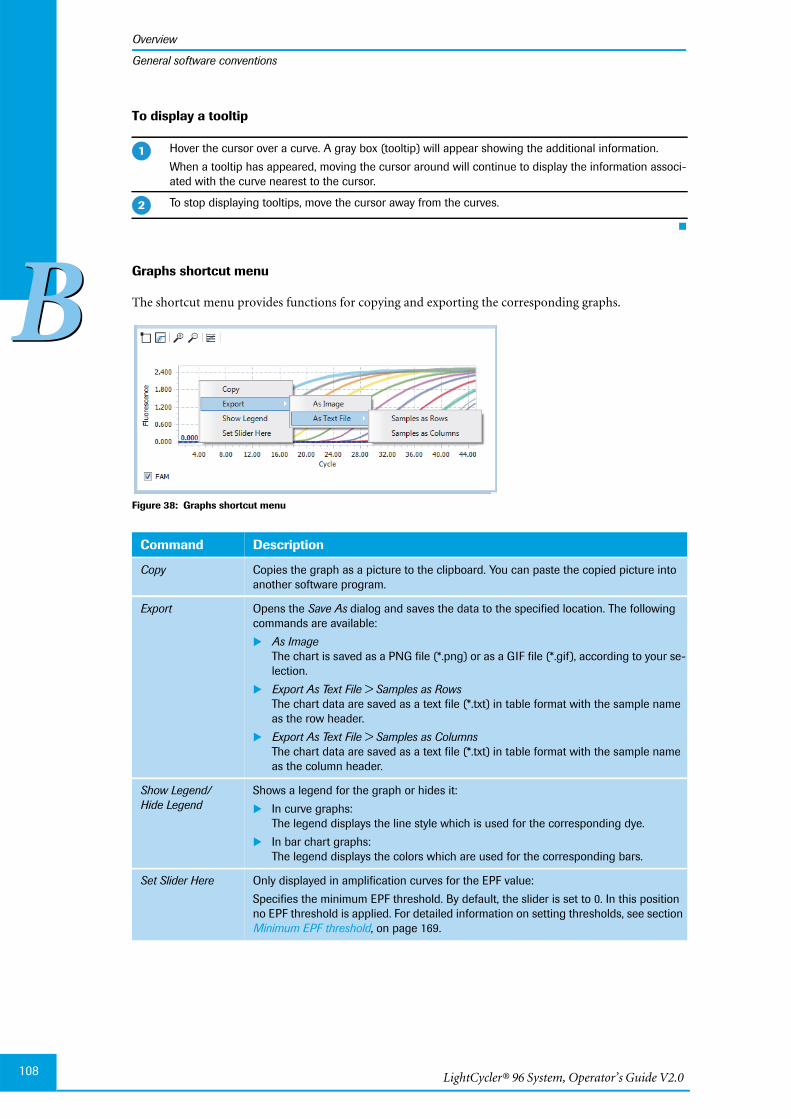
LightCycler® 96 System, Operator’s Guide V2.0108
Overview
BB
General software conventions
To display a tooltip
Graphs shortcut menu
The shortcut menu provides functions for copying and exporting the corresponding graphs.
Figure 38: Graphs shortcut menu
Hover the cursor over a curve. A gray box (tooltip) will appear showing the additional information.
When a tooltip has appeared, moving the cursor around will continue to display the information associ-ated with the curve nearest to the cursor.
To stop displaying tooltips, move the cursor away from the curves.
Command Description
Copy Copies the graph as a picture to the clipboard. You can paste the copied picture intoanother software program.
Export Opens the Save As dialog and saves the data to the specified location. The followingcommands are available:
As ImageThe chart is saved as a PNG file (*.png) or as a GIF file (*.gif), according to your se-lection.
Export As Text File > Samples as RowsThe chart data are saved as a text file (*.txt) in table format with the sample nameas the row header.
Export As Text File > Samples as ColumnsThe chart data are saved as a text file (*.txt) in table format with the sample nameas the column header.
Show Legend/Hide Legend
Shows a legend for the graph or hides it:
In curve graphs:The legend displays the line style which is used for the corresponding dye.
In bar chart graphs:The legend displays the colors which are used for the corresponding bars.
Set Slider Here Only displayed in amplification curves for the EPF value:
Specifies the minimum EPF threshold. By default, the slider is set to 0. In this positionno EPF threshold is applied. For detailed information on setting thresholds, see sectionMinimum EPF threshold, on page 169.
�
�
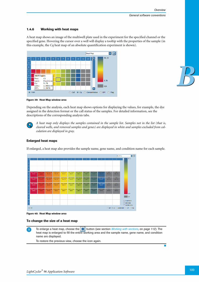
LightCycler® 96 Application Software
Overview
109
BB
General software conventions
1.4.6 Working with heat maps
A heat map shows an image of the multiwell plate used in the experiment for the specified channel or thespecified gene. Hovering the cursor over a well will display a tooltip with the properties of the sample (inthis example, the Cq heat map of an absolute quantification experiment is shown).
Figure 39: Heat Map window area
Depending on the analysis, each heat map shows options for displaying the values, for example, the dyeassigned in the detection format or the call status of the samples. For detailed information, see thedescriptions of the corresponding analysis tabs.
A heat map only displays the samples contained in the sample list. Samples not in the list (that is,cleared wells, and removed samples and genes) are displayed in white and samples excluded from cal-culation are displayed in gray.
Enlarged heat maps
If enlarged, a heat map also provides the sample name, gene name, and condition name for each sample.
Figure 40: Heat Map window area
To change the size of a heat map
To enlarge a heat map, choose the button (see section Working with sections, on page 112). Theheat map is enlarged to fill the entire working area and the sample name, gene name, and conditionname are displayed.
To restore the previous view, choose the icon again.
�
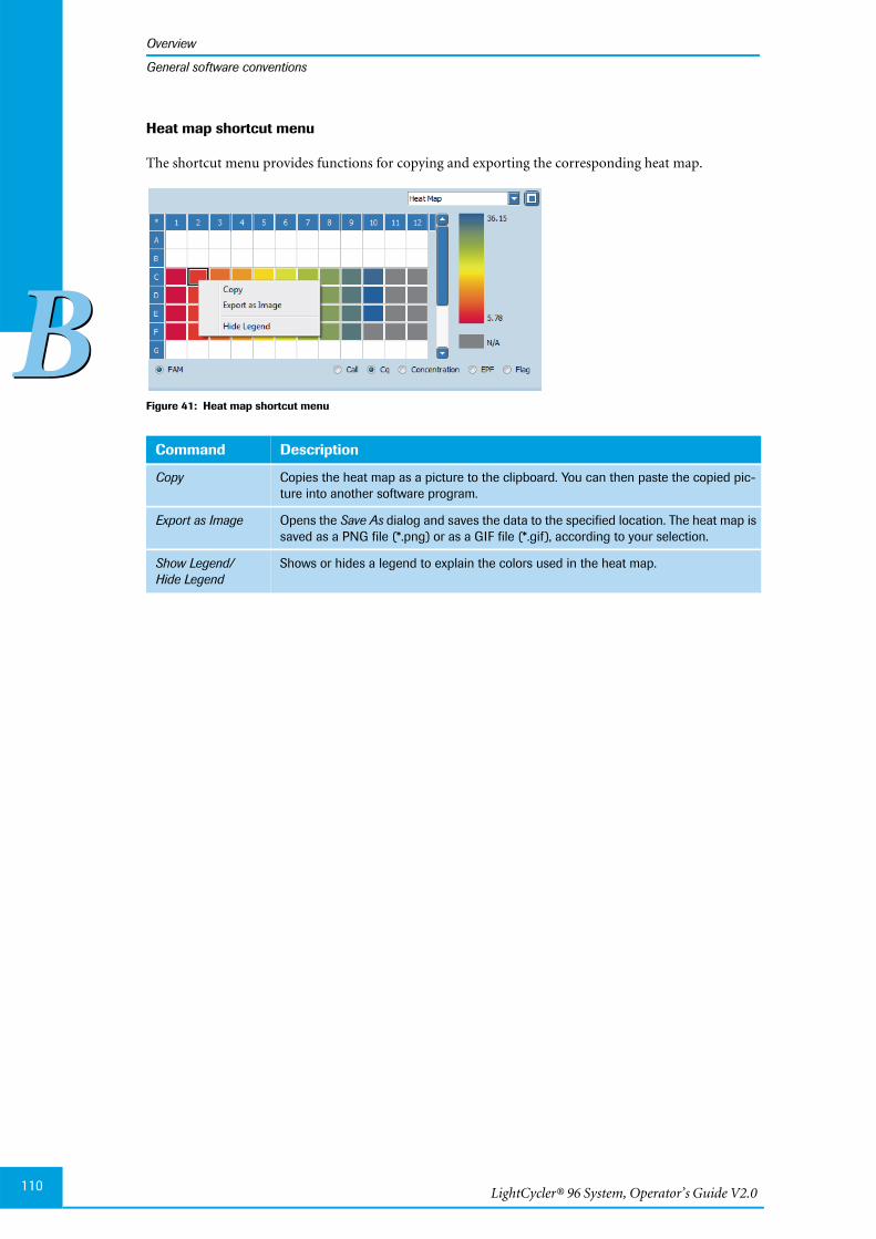
LightCycler® 96 System, Operator’s Guide V2.0110
Overview
BB
General software conventions
Heat map shortcut menu
The shortcut menu provides functions for copying and exporting the corresponding heat map.
Figure 41: Heat map shortcut menu
Command Description
Copy Copies the heat map as a picture to the clipboard. You can then paste the copied pic-ture into another software program.
Export as Image Opens the Save As dialog and saves the data to the specified location. The heat map issaved as a PNG file (*.png) or as a GIF file (*.gif), according to your selection.
Show Legend/Hide Legend
Shows or hides a legend to explain the colors used in the heat map.
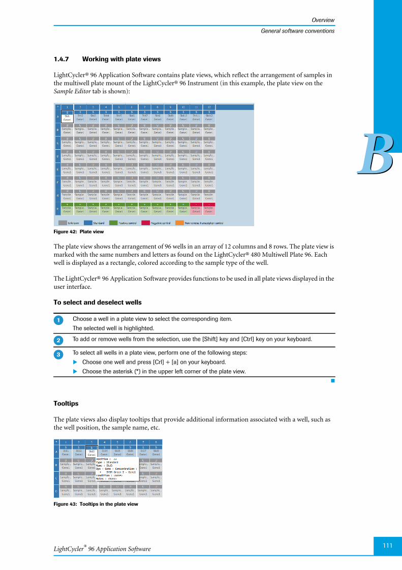
LightCycler® 96 Application Software
Overview
111
BB
General software conventions
1.4.7 Working with plate views
LightCycler® 96 Application Software contains plate views, which reflect the arrangement of samples inthe multiwell plate mount of the LightCycler® 96 Instrument (in this example, the plate view on theSample Editor tab is shown):
Figure 42: Plate view
The plate view shows the arrangement of 96 wells in an array of 12 columns and 8 rows. The plate view ismarked with the same numbers and letters as found on the LightCycler® 480 Multiwell Plate 96. Eachwell is displayed as a rectangle, colored according to the sample type of the well.
The LightCycler® 96 Application Software provides functions to be used in all plate views displayed in theuser interface.
To select and deselect wells
Tooltips
The plate views also display tooltips that provide additional information associated with a well, such asthe well position, the sample name, etc.
Figure 43: Tooltips in the plate view
Choose a well in a plate view to select the corresponding item.
The selected well is highlighted.
To add or remove wells from the selection, use the [Shift] key and [Ctrl] key on your keyboard.
To select all wells in a plate view, perform one of the following steps:
Choose one well and press [Crl] + [a] on your keyboard.
Choose the asterisk (*) in the upper left corner of the plate view.
�
�
�
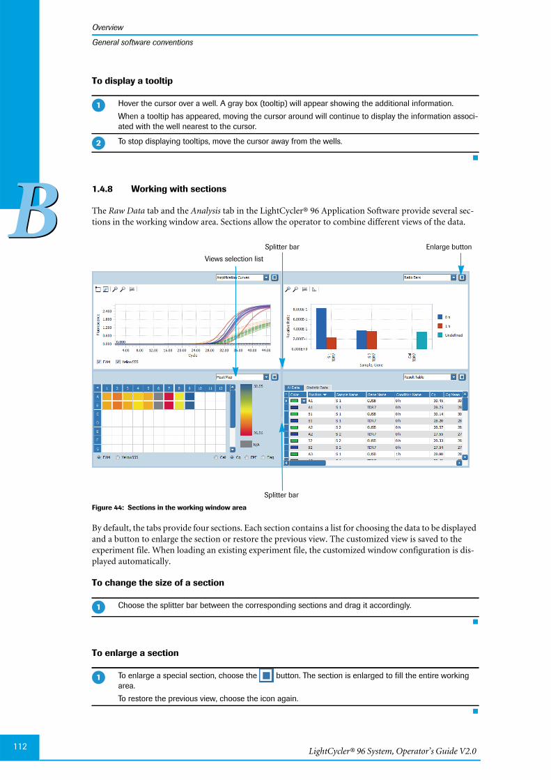
LightCycler® 96 System, Operator’s Guide V2.0112
Overview
BB
General software conventions
To display a tooltip
1.4.8 Working with sections
The Raw Data tab and the Analysis tab in the LightCycler® 96 Application Software provide several sec-tions in the working window area. Sections allow the operator to combine different views of the data.
Figure 44: Sections in the working window area
By default, the tabs provide four sections. Each section contains a list for choosing the data to be displayedand a button to enlarge the section or restore the previous view. The customized view is saved to theexperiment file. When loading an existing experiment file, the customized window configuration is dis-played automatically.
To change the size of a section
To enlarge a section
Hover the cursor over a well. A gray box (tooltip) will appear showing the additional information.
When a tooltip has appeared, moving the cursor around will continue to display the information associ-ated with the well nearest to the cursor.
To stop displaying tooltips, move the cursor away from the wells.
Choose the splitter bar between the corresponding sections and drag it accordingly.
To enlarge a special section, choose the button. The section is enlarged to fill the entire workingarea.
To restore the previous view, choose the icon again.
�
�
Views selection list
Enlarge buttonSplitter bar
Splitter bar
�
�

LightCycler® 96 Application Software
Overview
113
BB
Experiments
1.5 Experiments
The information provided in the experiment definition controls the LightCycler® 96 Instrument duringan experiment run. The experiment definition specifies the target temperatures and hold times of thethermal block cycler, the number of cycles being executed, and other parameters.
For starting an experiment run, the experiment must be transferred to the instrument. An experimentrun can only be started on the instrument using the LightCycler® 96 Instrument Software. For detailedinformation on how to send an experiment to the instrument, see section Instrument Manager, onpage 124.
1.5.1 Experiment file types
The LightCycler® 96 Application Software supports the following experiment file types:
*.lc96p (LightCycler® 96 experiment files for processed experiments).
*.lc96u (LightCycler® 96 experiment files for unprocessed experiments).
*.lc96 (LightCycler® 96 experiment files generated with LightCycler® 96 Software Version 1.0).
*.rdml (Real-time PCR Data Markup Language files).
By default, all newly generated experiment files have the file type *.lc96u. Operators can save experimentfiles as LightCycler® 96 files (*.lc96p or *.lc96u) or as RDML files without changing their content.
Aborted experiments are treated identically to processed experiments, that is, they are saved as *.lc96pfiles.
All file types can be opened in the LightCycler® 96 Application Software. To enable opening ofLightCycler® 96 experiment files with a third-party RDML-compatible software, the files must be savedas *.rdml.
1.5.2 Creating an experiment
Before a LightCycler® 96 Instrument run can be started, a new experiment has to be created. The operatorhas the following options for creating a new experiment:
Generating a completely new experiment.
Generating a new experiment by using an existing experiment as a template.
Generating a new experiment by using a predefined Roche template.
To generate a new experiment
Perform one of the following steps:
On the start screen, choose the Quickstart tab and then Create New Experiment.
In the File menu, choose New > Experiment.
In the tool bar, choose the New Experiment icon.
The LightCycler® 96 Application Software displays the new experiment in the main window. The newexperiment has the default name New Experiment <creation_date> <creation_time>.
Optional: Enter a description of the experiment.
In the File menu, choose Properties.
In the Properties dialog box, choose the Notes tab.
Enter a description.
Choose OK.
For detailed information on the Properties dialog box, see section Experiment properties, on page 117.
�
�

LightCycler® 96 System, Operator’s Guide V2.0114
Overview
BB
Experiments
To use an existing experiment as a template
To create a new experiment from an existing one (that is, to copy all settings of an experiment), the oper-ator must open the experiment file as a template. In this case, the raw data of the experiment is deleted.
Depending on the file type of the existing experiment, the following settings are provided for editing:
If the existing experiment is unprocessed (.lp96u), it only contains the run settings.
If the existing experiment is processed (.lp97p), it contains the run settings, the sample editor settingsand, possibly, the analysis settings.
To use a Roche template
Roche provides a number of predefined experiments as templates. A Roche template represents an exper-iment file for an unprocessed experiment (.lp96u). It therefore contains the run settings, that is, the tem-perature profile and the dye-specific parameters. The templates are located in theLightCycler® 96 Application Software home directory.
Perform one of the following steps:
On the start screen, choose the Quickstart tab and then Create New Experiment from Existing.
In the File menu, choose New > Experiment from Existing.
In the tool bar, choose the New Experiment from Existing icon.
The Open dialog box opens.
Navigate to the corresponding directory.
By default, the default experiment directory is displayed. This directory can be specified in the‘Default Directory’ dialog box. For detailed information, see section Preferences, on page 134.
In the list next to the File name field, select the file type to be displayed: *.lc96, *.lc96u, or *.lc96p
Select the experiment and choose Open. The experiment opens in the main window.
Change all settings according to your needs.
When detection format settings are changed (for example, the dye type in the same channel), allgene-specific settings (that is, gene name and concentration) are set to their default values.
Changing sample names or gene names might result in non-matching analysis-specific settings(for example, changing the gene name of a reference gene in relative quantification).
Perform one of the following steps:
On the start screen, choose the Quickstart tab and then Create New Experiment from Roche Tem-plate.
In the File menu, choose New > Experiment from Roche Template.
The Experiment from Roche Template dialog box opens.
�
�
�
�
�
�
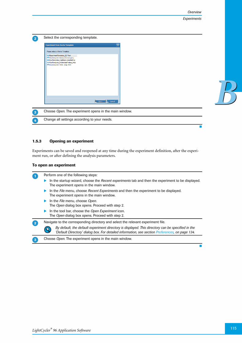
LightCycler® 96 Application Software
Overview
115
BB
Experiments
1.5.3 Opening an experiment
Experiments can be saved and reopened at any time during the experiment definition, after the experi-ment run, or after defining the analysis parameters.
To open an experiment
Select the corresponding template.
Choose Open. The experiment opens in the main window.
Change all settings according to your needs.
Perform one of the following steps:
In the startup wizard, choose the Recent experiments tab and then the experiment to be displayed.The experiment opens in the main window.
In the File menu, choose Recent Experiments and then the experiment to be displayed.The experiment opens in the main window.
In the File menu, choose Open.The Open dialog box opens. Proceed with step 2.
In the tool bar, choose the Open Experiment icon.The Open dialog box opens. Proceed with step 2.
Navigate to the corresponding directory and select the relevant experiment file.
By default, the default experiment directory is displayed. This directory can be specified in the‘Default Directory’ dialog box. For detailed information, see section Preferences, on page 134.
Choose Open. The experiment opens in the main window.
�
�
�
�
�
�

LightCycler® 96 System, Operator’s Guide V2.0116
Overview
BB
Experiments
1.5.4 Saving an experiment
Experiments can be saved at any time during the experiment definition, after the experiment run, or afterdefining the analysis parameters.
After the run is finished, you can no longer change any of the run parameters. For detailed informationon copying and reusing an existing experiment, see section To use an existing experiment as a template,on page 114.
To save an experiment
Perform one of the following steps:
In the File menu, choose Save to save the currently opened experiment. If no file exists, the Save Asdialog box opens.
In the File menu, choose Save As to save the experiment to a specified location. The Save as dialogbox opens.
In the tool bar, choose the Save Experiment icon to save the currently opened experiment. If no fileexists, the Save As dialog box opens.
Navigate to the directory where you want to store the experiment file.
By default, the default experiment directory is displayed. This directory can be specified in the‘Default Directory’ dialog box. For detailed information, see section Preferences, on page 134.
Enter a file name for the experiment.
Choose Save. The dialog box closes.
The experiment is saved according to the processing:
As a LightCycler® 96 file for an unprocessed experiment (*.lc96u).
As a LightCycler® 96 file for a processed experiment (*.lc96p).
By default, experiments are saved as LightCycler® 96 files (*.lc96u or *.lc96p).
The dialog additionally provides an option for saving experiments as RDML files (*.rdml). Both filetypes are compatible with the LightCycler® 96 Application Software. To enable openingLightCycler® 96 experiment files with a third-party RDML-compatible software, save the files as*.rdml.
�
�
�
�
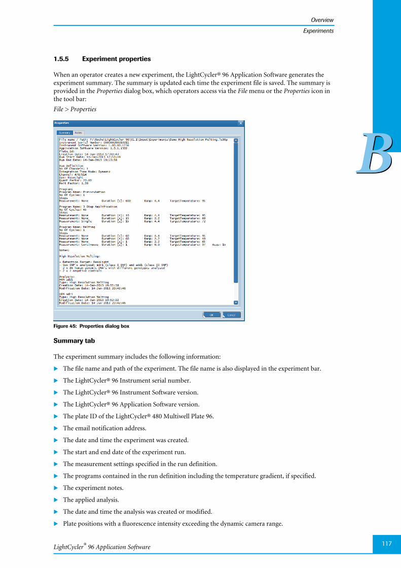
LightCycler® 96 Application Software
Overview
117
BB
Experiments
1.5.5 Experiment properties
When an operator creates a new experiment, the LightCycler® 96 Application Software generates theexperiment summary. The summary is updated each time the experiment file is saved. The summary isprovided in the Properties dialog box, which operators access via the File menu or the Properties icon inthe tool bar:
File > Properties
Figure 45: Properties dialog box
Summary tab
The experiment summary includes the following information:
The file name and path of the experiment. The file name is also displayed in the experiment bar.
The LightCycler® 96 Instrument serial number.
The LightCycler® 96 Instrument Software version.
The LightCycler® 96 Application Software version.
The plate ID of the LightCycler® 480 Multiwell Plate 96.
The email notification address.
The date and time the experiment was created.
The start and end date of the experiment run.
The measurement settings specified in the run definition.
The programs contained in the run definition including the temperature gradient, if specified.
The experiment notes.
The applied analysis.
The date and time the analysis was created or modified.
Plate positions with a fluorescence intensity exceeding the dynamic camera range.

LightCycler® 96 System, Operator’s Guide V2.0118
Overview
BB
Experiments
Notes tab
The Notes tab is a text input field for up to 10 000 characters in which you can add notes to the experimentif necessary. The notes are saved to the experiment file.
1.5.6 Experiment report
The LightCycler® 96 Application Software provides a function to generate an HTML report for eachexperiment. The report includes all data contained in the experiment file. The report can be displayed ina browser installed on your computer.
The HTML report is only validated for Microsoft Windows Internet Explorer 8 and 9. Other browsersor other Internet Explorer versions may fail to display the report information.
The report is generated in the Reports dialog box, which operators access via the Reports icon in the toolbar:
Figure 46: Reports dialog box
The dialog box allows for specifying the name and location of the corresponding report:
To generate an experiment-specific HTML report
Setting Description
Report Name Name of the report to be generated.
The LightCycler® 96 Application Software provides a default name which is identical to theexperiment name.
Location Location where you want to store the report. Each report is stored in a separate folder<report name>.
By default, the default experiment directory is displayed. This directory can be specifiedin the ‘Default Directory’ dialog box. For detailed information, see section Preferences,on page 134.
Open the relevant experiment.
In the toolbar, choose the Reports icon.
The Reports dialog box opens.
Specify the Report Name and the Location for the new report.
�
�
�
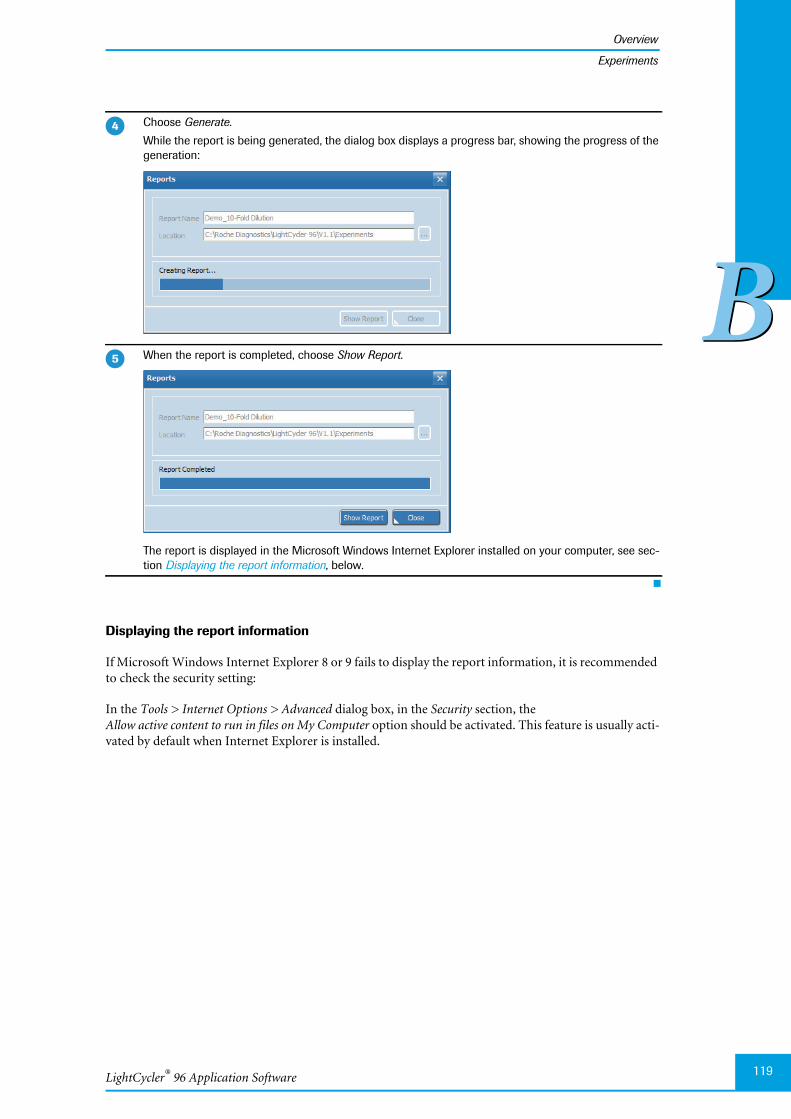
LightCycler® 96 Application Software
Overview
119
BB
Experiments
Displaying the report information
If Microsoft Windows Internet Explorer 8 or 9 fails to display the report information, it is recommendedto check the security setting:
In the Tools > Internet Options > Advanced dialog box, in the Security section, theAllow active content to run in files on My Computer option should be activated. This feature is usually acti-vated by default when Internet Explorer is installed.
Choose Generate.
While the report is being generated, the dialog box displays a progress bar, showing the progress of thegeneration:
When the report is completed, choose Show Report.
The report is displayed in the Microsoft Windows Internet Explorer installed on your computer, see sec-tion Displaying the report information, below.
�
�
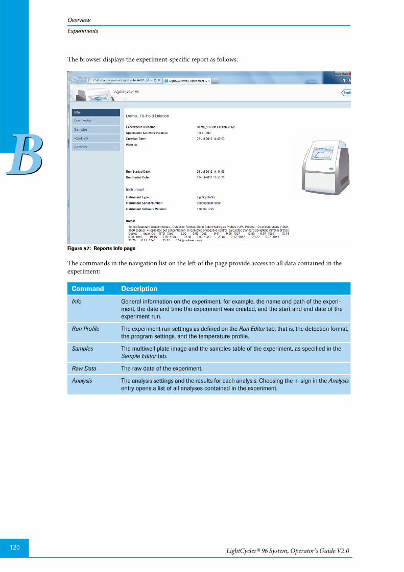
LightCycler® 96 System, Operator’s Guide V2.0120
Overview
BB
Experiments
The browser displays the experiment-specific report as follows:
Figure 47: Reports Info page
The commands in the navigation list on the left of the page provide access to all data contained in theexperiment:
Command Description
Info General information on the experiment, for example, the name and path of the experi-ment, the date and time the experiment was created, and the start and end date of theexperiment run.
Run Profile The experiment run settings as defined on the Run Editor tab, that is, the detection format,the program settings, and the temperature profile.
Samples The multiwell plate image and the samples table of the experiment, as specified in theSample Editor tab.
Raw Data The raw data of the experiment.
Analysis The analysis settings and the results for each analysis. Choosing the +-sign in the Analysisentry opens a list of all analyses contained in the experiment.

LightCycler® 96 Application Software
Overview
121
BB
Import, export, and file transfer options
1.6 Import, export, and file transfer options
The following figure shows the input and output data flows of the application software. The data to beimported and exported is described below.
Figure 48: LightCycler® 96 Application Software input and output data flow
Legacy experiments from LightCycler® 96 Application Software Version 1.0 (*.lc96 file types) can beopened with version 1.1. But after automatic conversion to version 1.1, the files are saved as *.lc96p or*.lc96u files.
1.6.1 Import data
To define a new experiment, the following data can be imported into theLightCycler® 96 Application Software:
Data File Format Description
Experiment template .lc96u, .lc96p Predefined operator settings to be specified in the experiment defini-tion.
For detailed information, see the following sections:
To use an existing experiment as a template, on page 114.
To use a Roche template, on page 114.
Sample data .txt.csv.xls
Sample information for an experiment, including sample names, genenames, and dye assignment. For detailed information, see section Toimport sample data into the sample list, on page 158.
Experiment files(.lc96u, .lc96p)
LightCycler® 96Application Software
Experiment templates(.lc96u, .lc96p)
MagNA Pure 96sample data (.txt)
Export options:
Open Save
Open
Import options:
Sample data (.txt, .csv)
Graphs (.png, .gif, .txt)
Result table data (.txt)
Result batch data (.txt)
Retrieve Send
Sample data(.txt, .csv, .xls)
RealTime ready Panelstarget information (.txt)
Sample data(.txt, .csv, .xls)
via USB drive or Ethernet
LightCycler® 96Application Software
Export options:
Open Save
Open
Graphs (.png, .gif, .txt)
Result table data (.txt)
Result batch data (.txt)
Retrieve Sendvia USB drive or Ethernet
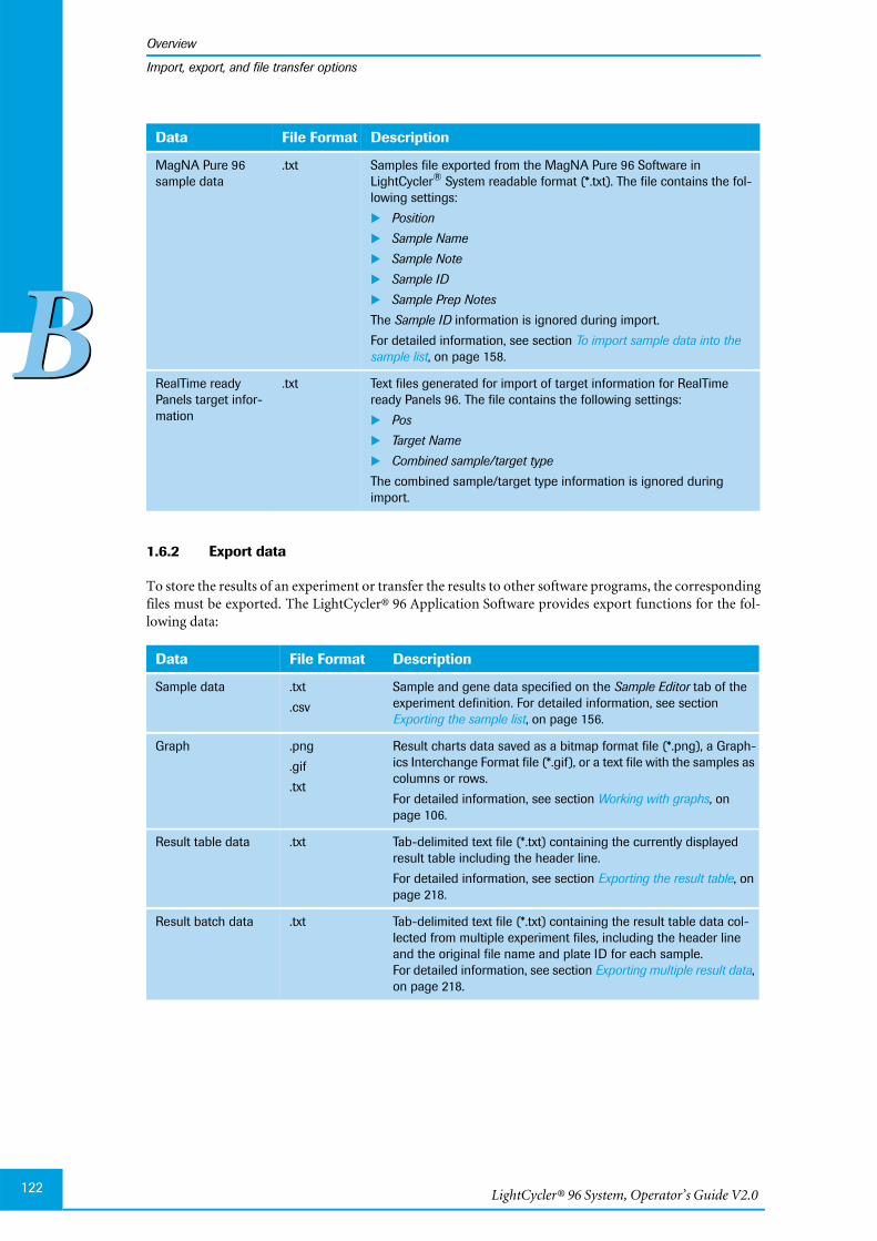
LightCycler® 96 System, Operator’s Guide V2.0122
Overview
BB
Import, export, and file transfer options
1.6.2 Export data
To store the results of an experiment or transfer the results to other software programs, the correspondingfiles must be exported. The LightCycler® 96 Application Software provides export functions for the fol-lowing data:
MagNA Pure 96sample data
.txt Samples file exported from the MagNA Pure 96 Software inLightCycler® System readable format (*.txt). The file contains the fol-lowing settings:
Position
Sample Name
Sample Note
Sample ID
Sample Prep Notes
The Sample ID information is ignored during import.
For detailed information, see section To import sample data into thesample list, on page 158.
RealTime readyPanels target infor-mation
.txt Text files generated for import of target information for RealTimeready Panels 96. The file contains the following settings:
Pos
Target Name
Combined sample/target type
The combined sample/target type information is ignored duringimport.
Data File Format Description
Sample data .txt
.csv
Sample and gene data specified on the Sample Editor tab of theexperiment definition. For detailed information, see sectionExporting the sample list, on page 156.
Graph .png
.gif
.txt
Result charts data saved as a bitmap format file (*.png), a Graph-ics Interchange Format file (*.gif), or a text file with the samples ascolumns or rows.
For detailed information, see section Working with graphs, onpage 106.
Result table data .txt Tab-delimited text file (*.txt) containing the currently displayedresult table including the header line.
For detailed information, see section Exporting the result table, onpage 218.
Result batch data .txt Tab-delimited text file (*.txt) containing the result table data col-lected from multiple experiment files, including the header lineand the original file name and plate ID for each sample.For detailed information, see section Exporting multiple result data,on page 218.
Data File Format Description
LightCycler® 96 Application Software
Overview
123
BB
Disregarding positions from an analysis
1.7 Disregarding positions from an analysis
The LightCycler® 96 Application Software provides the following options for eliminating positions fromthe analysis:
The Clear Wells function, provided on the Plate View tab of the Sample Editor. Clear Wells eliminatesthe selected wells from all analyses.
It is strongly recommended to use the ‘Clear Wells’ function for all empty wells ofLightCycler® 480 Multiwell Plates 96 and for positions not occupied by LightCycler® 8-Tube Strips.
The Remove function, provided in the <analysis> Settings dialog box of an analysis. Remove eliminatessamples, genes, and/or conditions (only for relative quantification) from the corresponding analysis.
The Exclude function, provided in the analysis result tables. Exclude eliminates the selected samplesfrom the result calculation of the corresponding analysis.
For detailed information, see section Eliminating positions from the analysis, on page 165.
1.8 Exiting the software
To exit the LightCycler® 96 Application Software
Perform one of the following steps:
In the File menu, choose Exit.
In the title bar of the main window, choose the button.You are prompted to save unsaved data before the application shuts down.
�
LightCycler® 96 System, Operator’s Guide V2.0124
Tools
BB
Instrument Manager
2 Tools
In the Tools menu, the LightCycler® 96 Application Software provides several tools for managing andmonitoring LightCycler® 96 Instruments and for exporting result data from multiple experiment files.
2.1 Instrument Manager
The Instrument Manager provides access to the following functions:
Registering a LightCycler® 96 Instrument with the application software, see section Instruments win-dow area, on page 125.
Transferring experiments to and from the selected instrument, see section Send/Receive Experimentstab, on page 128.
Opening an experiment in the application software or deleting an experiment from the instrument,see section Send/Receive Experiments tab, on page 128.
Monitoring an experiment run on an instrument, see section Online Monitoring tab, on page 130.
Preconditions
For using the functions of the Instrument Manager the following preconditions apply:
The LightCycler® 96 Instrument is switched on.
The instrument is configured for use in the network; see the following sections:
Configuring a one-to-one connection, on page 50.
Configuring an Ethernet network connection, on page 55.
The instrument is connected to the network; see section Assembling the instrument, on page 44.
The computer running the LightCycler® 96 Application Software is connected to the network.
The Remote Monitoring function is activated and configured accordingly in theLightCycler® 96 Instrument Software; see section Configuration tab, on page 256.
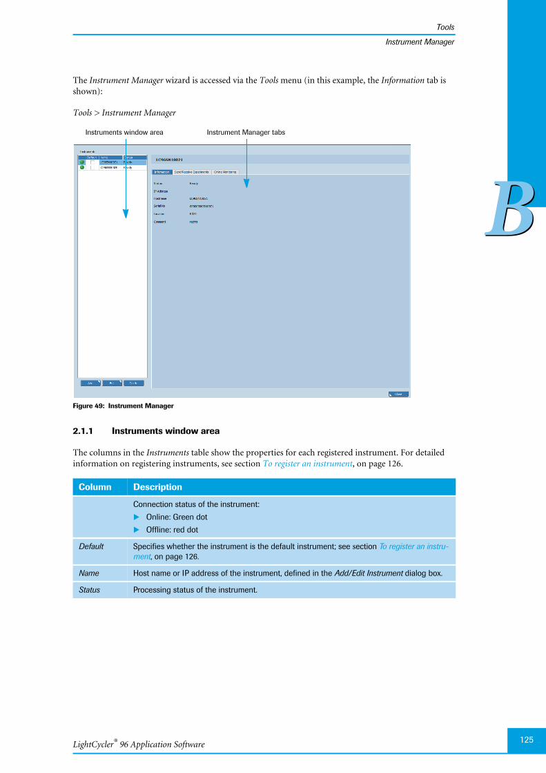
LightCycler® 96 Application Software
Tools
125
BB
Instrument Manager
The Instrument Manager wizard is accessed via the Tools menu (in this example, the Information tab isshown):
Tools > Instrument Manager
Figure 49: Instrument Manager
2.1.1 Instruments window area
The columns in the Instruments table show the properties for each registered instrument. For detailedinformation on registering instruments, see section To register an instrument, on page 126.
Column Description
Connection status of the instrument:
Online: Green dot
Offline: red dot
Default Specifies whether the instrument is the default instrument; see section To register an instru-ment, on page 126.
Name Host name or IP address of the instrument, defined in the Add/Edit Instrument dialog box.
Status Processing status of the instrument.
Instruments window area Instrument Manager tabs
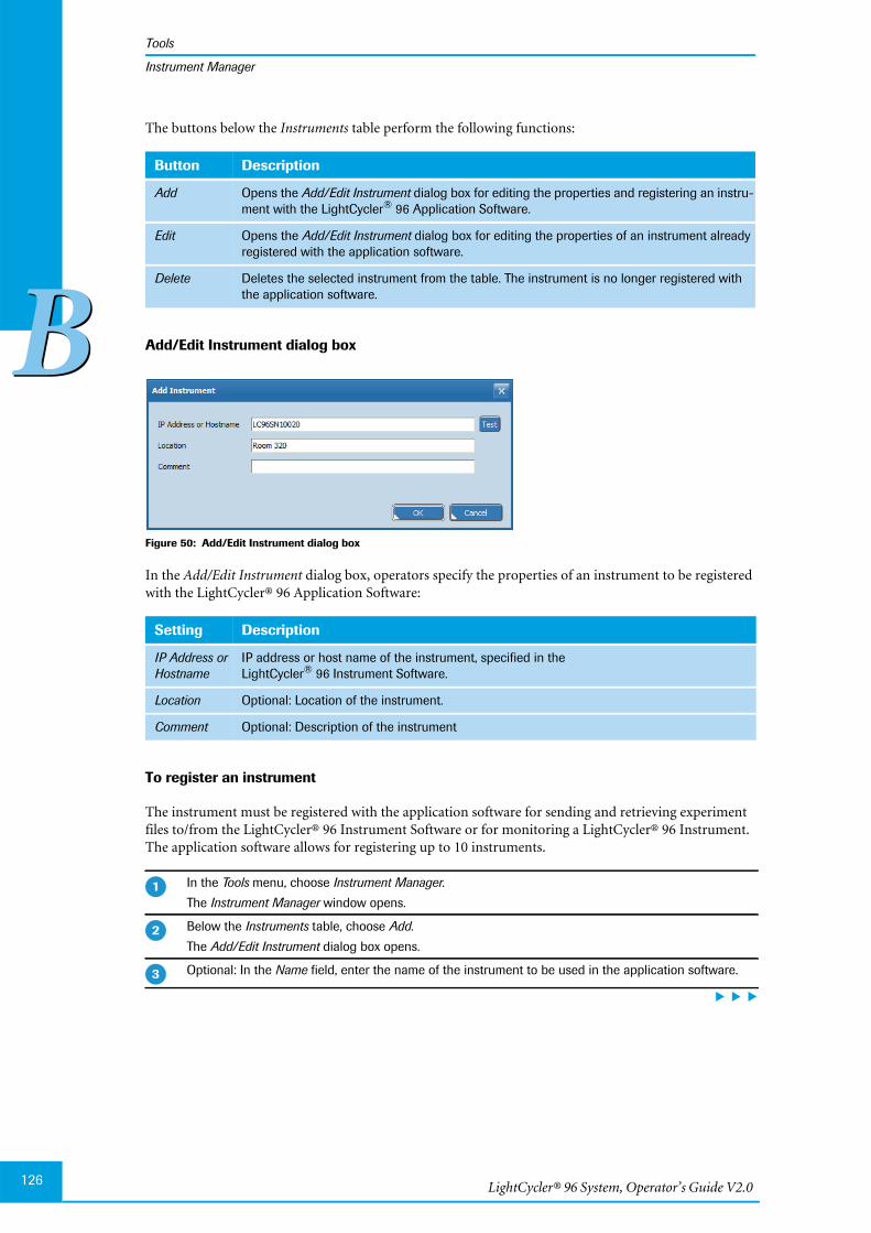
LightCycler® 96 System, Operator’s Guide V2.0126
Tools
BB
Instrument Manager
The buttons below the Instruments table perform the following functions:
Add/Edit Instrument dialog box
Figure 50: Add/Edit Instrument dialog box
In the Add/Edit Instrument dialog box, operators specify the properties of an instrument to be registeredwith the LightCycler® 96 Application Software:
To register an instrument
The instrument must be registered with the application software for sending and retrieving experimentfiles to/from the LightCycler® 96 Instrument Software or for monitoring a LightCycler® 96 Instrument.The application software allows for registering up to 10 instruments.
Button Description
Add Opens the Add/Edit Instrument dialog box for editing the properties and registering an instru-ment with the LightCycler® 96 Application Software.
Edit Opens the Add/Edit Instrument dialog box for editing the properties of an instrument alreadyregistered with the application software.
Delete Deletes the selected instrument from the table. The instrument is no longer registered withthe application software.
Setting Description
IP Address orHostname
IP address or host name of the instrument, specified in theLightCycler® 96 Instrument Software.
Location Optional: Location of the instrument.
Comment Optional: Description of the instrument
In the Tools menu, choose Instrument Manager.
The Instrument Manager window opens.
Below the Instruments table, choose Add.
The Add/Edit Instrument dialog box opens.
Optional: In the Name field, enter the name of the instrument to be used in the application software.
�
�
�
LightCycler® 96 Application Software
Tools
127
BB
Instrument Manager
2.1.2 Information tab
The Information tab displays the properties of a LightCycler® 96 Instrument selected in the Instrumentstable.
In the IP Address or Hostname field, enter the IP address or host name of the instrument in the network.
You specify the host name on the ‘Configuration’ tab of the LightCycler® 96 Instrument Software.For detailed information, see section Device Name / Hostname, on page 257.
Local networks are usually run by a DHCP (dynamic host configuration protocol) server. The serverprovides dynamic IP addresses to all hosts in the network. As the frequency for changing IPaddresses varies from network to network (IP addresses might change daily), it is recommended toregister an instrument in the ‘Instrument Manager’ via its host name instead of its IP address.
The host name does not change when the IP address changes. Thus, a stable connection is main-tained regardless of changing IP addresses.
Optional: Choose the Test button to test the connection to the IP address.
If the IP address is not available, the software displays an error message:
Warning: Test ConnectionCommunication failed: Could not get instrument data.
Error: Test ConnectionCommunication failed: Could not reach instrument.
Optional: In the Location field, enter the location of the instrument.
Optional: In the Comment field, enter a description of the instrument.
Choose OK. The dialog box closes.
The instrument is registered with the application software and displayed in the Instruments list.
The Information tab shows the properties of the instrument; see section Information tab, below.
Optional: To specify the instrument as the default, select the check box in the Default column.
Property Description
Status Processing status of the instrument.
IP Address IP address of the instrument, specified in the LightCycler® 96 Instrument Software.
Hostname Host name of the instrument, specified in the LightCycler® 96 Instrument Software.
Serial No Serial number of the instrument.
Location Optional: Location of the instrument.
Comment Optional: Description of the instrument.
�
�
�
�

LightCycler® 96 System, Operator’s Guide V2.0128
Tools
BB
Instrument Manager
2.1.3 Send/Receive Experiments tab
The Send/Receive Experiments tab provides a transfer function for experiments to and from a registeredLightCycler® 96 Instrument. If more than one experiment exists in the network, the operator must selectthe corresponding instrument.
Figure 51: Instrument Manager, Send/Receive Experiments tab
Your PC window area
The Your PC window area provides a file explorer for navigating to the location of the experiment file.
<instrument> window area
The <instrument> window area provides the following data:
The Disc Space bar showing the number of experiments saved on the instrument in relation to the pos-sible maximum number of experiments.
The experiments table displaying all experiments available on the instrument.
The buttons in the Send/Receive Experiments tab perform the following functions:
Column Description
Name Experiment name.
Date Date and time of the last modification.
Status Status of the experiment: Running, Processed, Unprocessed, or Aborted.
Storage Location of the experiment file: On the instrument, on the connected USB drive, or on bothlocations.
Button Description
Open Opens the selected experiment in the application software.
Delete Deletes the selected experiment from the instrument.

LightCycler® 96 Application Software
Tools
129
BB
Instrument Manager
To send an experiment to an instrument
To retrieve an experiment from an instrument
In the Tools menu, choose Instrument Manager.
The Instrument Manager window opens.
Open the Send/Receive Experiments tab.
In the Instruments table, select the instrument the experiment is to be sent to.
In the Your PC window area, navigate to the directory containing the experiment. All experiments in thisdirectory are displayed.
Select the experiment to be sent to the instrument.
Choose the button.
The experiment is sent to the selected instrument.
You are notified if the instrument does not have enough space for the experiment.
If an experiment with the same name already exists on the instrument, you are prompted for a newname.
In the Tools menu, choose Instrument Manager.
The Instrument Manager window opens.
Open the Send/Receive Experiments tab.
In the Instruments table, select the instrument the experiment is to be retrieved from.
In the Your PC window area, navigate to the directory the experiment is to be transferred to.
In the <instrument> area, select the experiment to be retrieved.
Choose the button.
The selected experiment is retrieved from the instrument and saved to the specified directory on yourcomputer.
If an experiment with the same name already exists in the selected directory, you are prompted fora new name.
�
�
�
�
�
�
�
�
�
�
�
�
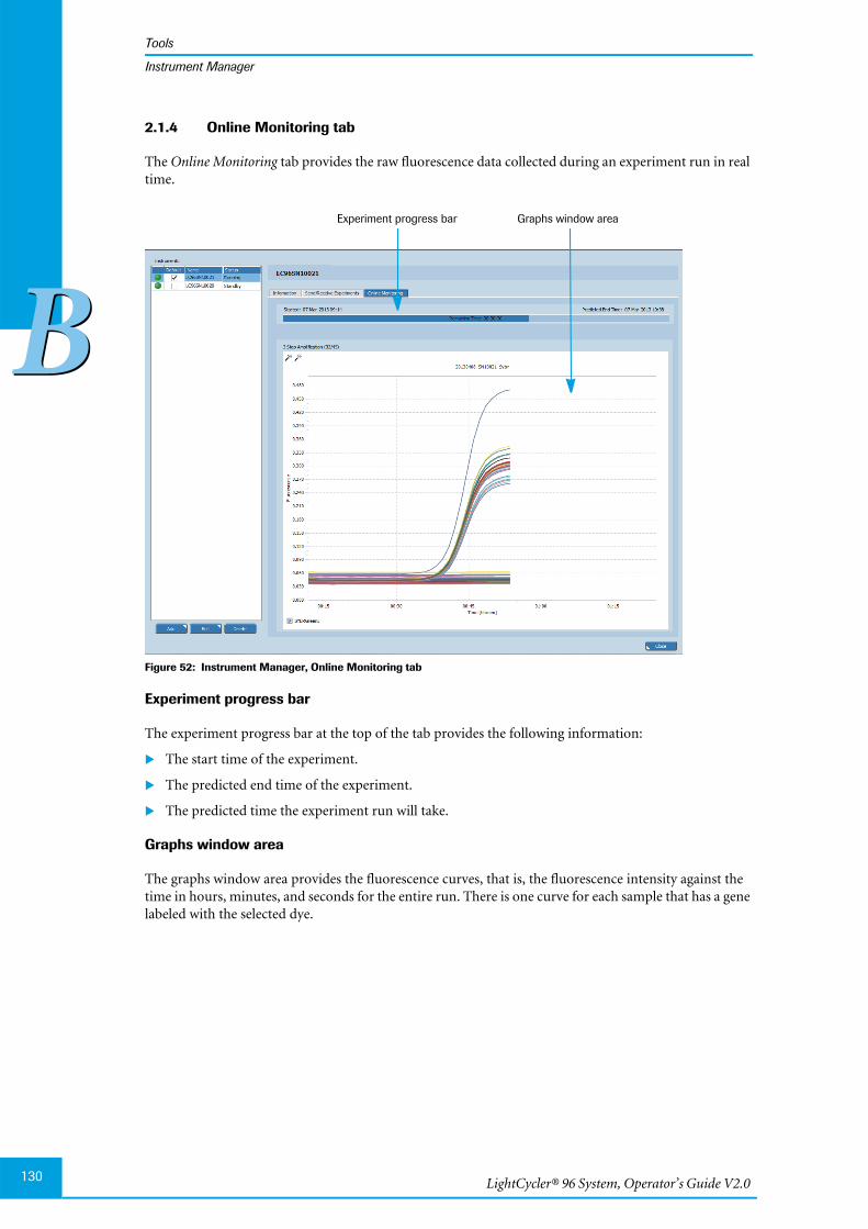
LightCycler® 96 System, Operator’s Guide V2.0130
Tools
BB
Instrument Manager
2.1.4 Online Monitoring tab
The Online Monitoring tab provides the raw fluorescence data collected during an experiment run in realtime.
Figure 52: Instrument Manager, Online Monitoring tab
Experiment progress bar
The experiment progress bar at the top of the tab provides the following information:
The start time of the experiment.
The predicted end time of the experiment.
The predicted time the experiment run will take.
Graphs window area
The graphs window area provides the fluorescence curves, that is, the fluorescence intensity against thetime in hours, minutes, and seconds for the entire run. There is one curve for each sample that has a genelabeled with the selected dye.
Experiment progress bar Graphs window area
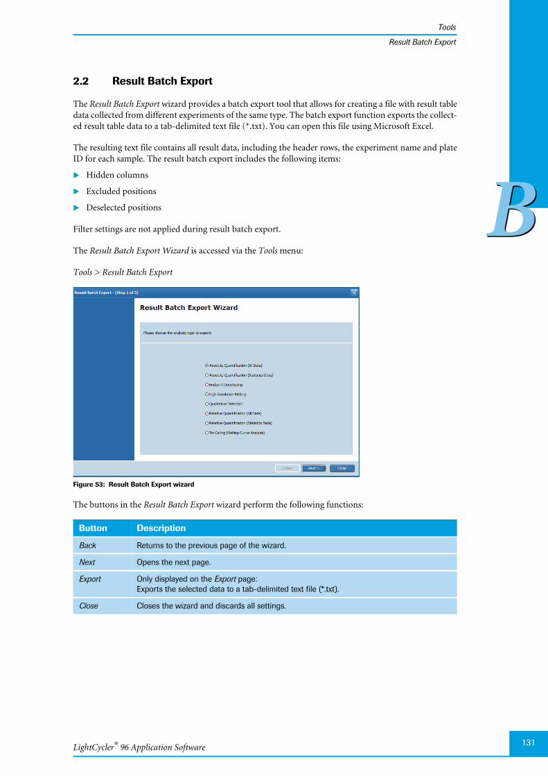
LightCycler® 96 Application Software
Tools
131
BB
Result Batch Export
2.2 Result Batch Export
The Result Batch Export wizard provides a batch export tool that allows for creating a file with result tabledata collected from different experiments of the same type. The batch export function exports the collect-ed result table data to a tab-delimited text file (*.txt). You can open this file using Microsoft Excel.
The resulting text file contains all result data, including the header rows, the experiment name and plateID for each sample. The result batch export includes the following items:
Hidden columns
Excluded positions
Deselected positions
Filter settings are not applied during result batch export.
The Result Batch Export Wizard is accessed via the Tools menu:
Tools > Result Batch Export
Figure 53: Result Batch Export wizard
The buttons in the Result Batch Export wizard perform the following functions:
Button Description
Back Returns to the previous page of the wizard.
Next Opens the next page.
Export Only displayed on the Export page:Exports the selected data to a tab-delimited text file (*.txt).
Close Closes the wizard and discards all settings.
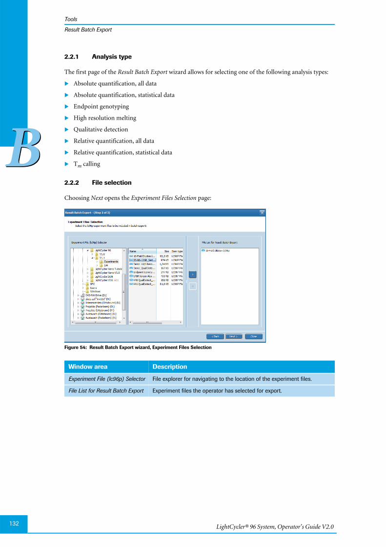
LightCycler® 96 System, Operator’s Guide V2.0132
Tools
BB
Result Batch Export
2.2.1 Analysis type
The first page of the Result Batch Export wizard allows for selecting one of the following analysis types:
Absolute quantification, all data
Absolute quantification, statistical data
Endpoint genotyping
High resolution melting
Qualitative detection
Relative quantification, all data
Relative quantification, statistical data
Tm calling
2.2.2 File selection
Choosing Next opens the Experiment Files Selection page:
Figure 54: Result Batch Export wizard, Experiment Files Selection
Window area Description
Experiment File (lc96p) Selector File explorer for navigating to the location of the experiment files.
File List for Result Batch Export Experiment files the operator has selected for export.
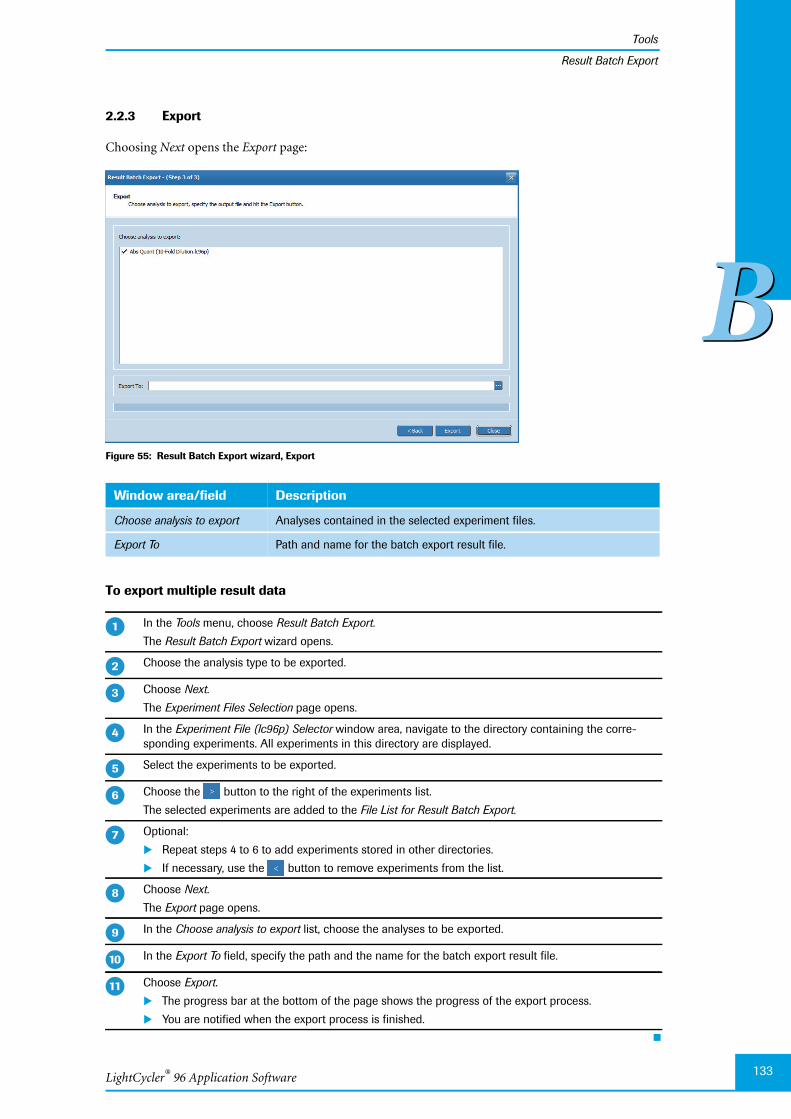
LightCycler® 96 Application Software
Tools
133
BB
Result Batch Export
2.2.3 Export
Choosing Next opens the Export page:
Figure 55: Result Batch Export wizard, Export
To export multiple result data
Window area/field Description
Choose analysis to export Analyses contained in the selected experiment files.
Export To Path and name for the batch export result file.
In the Tools menu, choose Result Batch Export.
The Result Batch Export wizard opens.
Choose the analysis type to be exported.
Choose Next.
The Experiment Files Selection page opens.
In the Experiment File (lc96p) Selector window area, navigate to the directory containing the corre-sponding experiments. All experiments in this directory are displayed.
Select the experiments to be exported.
Choose the button to the right of the experiments list.
The selected experiments are added to the File List for Result Batch Export.
Optional:
Repeat steps 4 to 6 to add experiments stored in other directories.
If necessary, use the button to remove experiments from the list.
Choose Next.
The Export page opens.
In the Choose analysis to export list, choose the analyses to be exported.
In the Export To field, specify the path and the name for the batch export result file.
Choose Export.
The progress bar at the bottom of the page shows the progress of the export process.
You are notified when the export process is finished.
�
�
�
�
�
�
�
��
��

LightCycler® 96 System, Operator’s Guide V2.0134
Preferences
BB
3 Preferences
The LightCycler® 96 Application Software provides the Preferences dialog box, where general settings arespecified, for example, the default directories to be used. The dialog box is accessed via the Options menu:
Options > Preferences
Figure 56: Preferences dialog box
Setting Description
Default Directory Default path for saving and loading experiment files
Remember Last Directory The last opened directory is to be remembered as long as the application isrunning.
After a restart, the software opens the specified default directory.
Email Address Email address to be linked to all experiments generated with the current soft-ware instance; when these experiments are executed, the instrument softwareautomatically sends an email notification to the defined email address after therun. The notification also contains the corresponding experiment file.
This email address is saved to the experiment file and is therefore avail-able in the properties of the experiment.
To stop automatic emailing of executed experiments, the operator mustdelete the email address from the ‘Email Address’ field.
It is not necessary to activate this email in the instrument’s email addressbook (see section Email Information, on page 259).
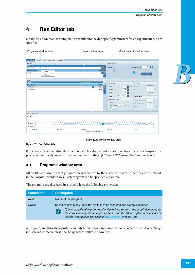
LightCycler® 96 Application Software
Run Editor tab
135
BB
Programs window area
4 Run Editor tab
On the Run Editor tab, the temperature profile and the dye-specific parameters for an experiment run arespecified.
Figure 57: Run Editor tab
For a new experiment, this tab shows no data. For detailed information on how to create a temperatureprofile and set the dye-specific parameters, refer to the LightCycler® 96 System User Training Guide.
4.1 Programs window area
All profiles are comprised of programs, which are run by the instrument in the order they are displayedin the Programs window area. Each program can be specified separately.
The programs are displayed in a list and have the following properties:
A program, and thus also a profile, can only be edited as long as no run has been performed. Every changeis displayed immediately in the Temperature Profile window area.
Parameter Description
Name Name of the program.
Cycles Specifies how many times the cycle is to be repeated, for example 45 times.
If, in an amplification program, the ‘Cycles’ are set to ‘1’, the acquisition mode forthe corresponding step changes to ‘None’ and the ‘Mode’ option is disabled. Fordetailed information, see section Step settings, on page 139.
Temperature Profile window area
Programs window area Steps window area Measurement window area
Temperature Profile window area
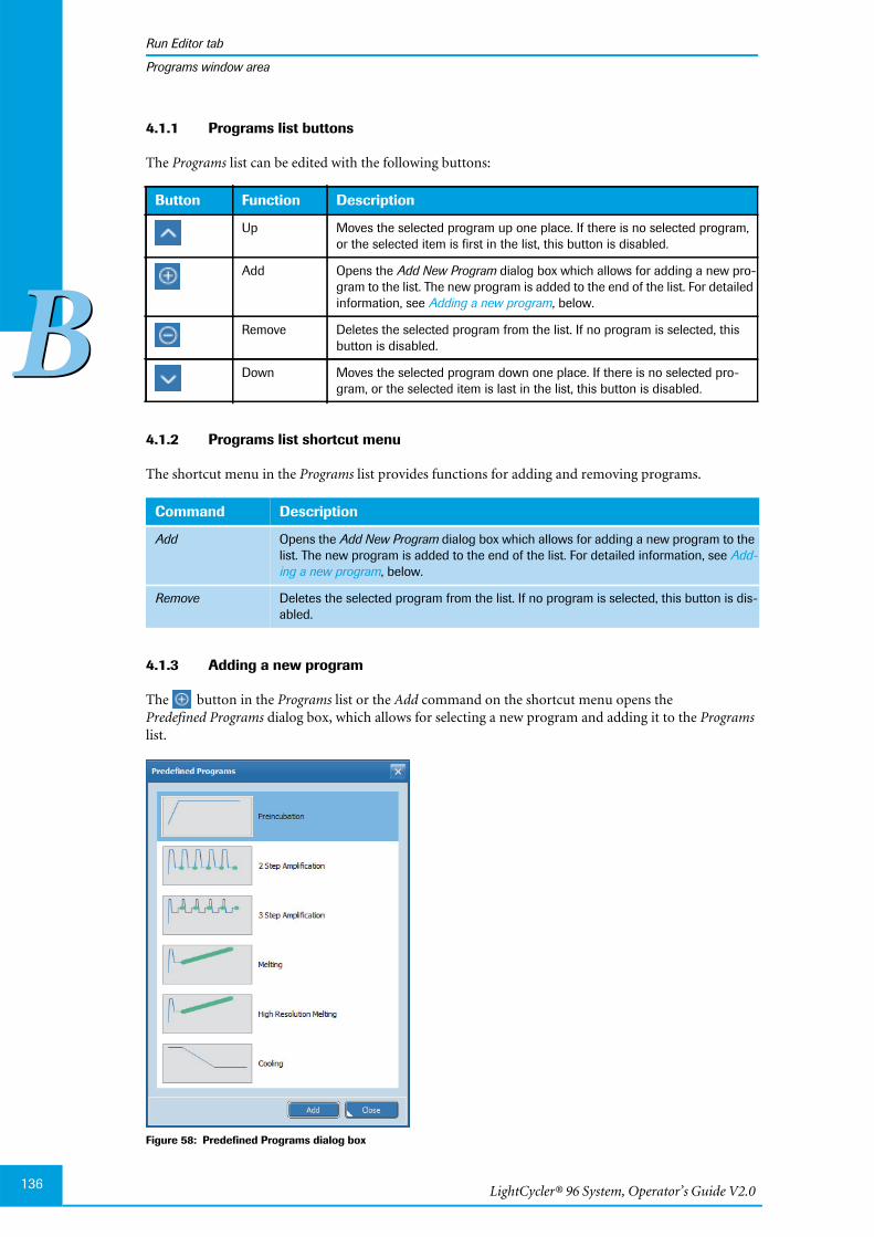
LightCycler® 96 System, Operator’s Guide V2.0136
Run Editor tab
BB
Programs window area
4.1.1 Programs list buttons
The Programs list can be edited with the following buttons:
4.1.2 Programs list shortcut menu
The shortcut menu in the Programs list provides functions for adding and removing programs.
4.1.3 Adding a new program
The button in the Programs list or the Add command on the shortcut menu opens thePredefined Programs dialog box, which allows for selecting a new program and adding it to the Programslist.
Figure 58: Predefined Programs dialog box
Button Function Description
Up Moves the selected program up one place. If there is no selected program,or the selected item is first in the list, this button is disabled.
Add Opens the Add New Program dialog box which allows for adding a new pro-gram to the list. The new program is added to the end of the list. For detailedinformation, see Adding a new program, below.
Remove Deletes the selected program from the list. If no program is selected, thisbutton is disabled.
Down Moves the selected program down one place. If there is no selected pro-gram, or the selected item is last in the list, this button is disabled.
Command Description
Add Opens the Add New Program dialog box which allows for adding a new program to thelist. The new program is added to the end of the list. For detailed information, see Add-ing a new program, below.
Remove Deletes the selected program from the list. If no program is selected, this button is dis-abled.
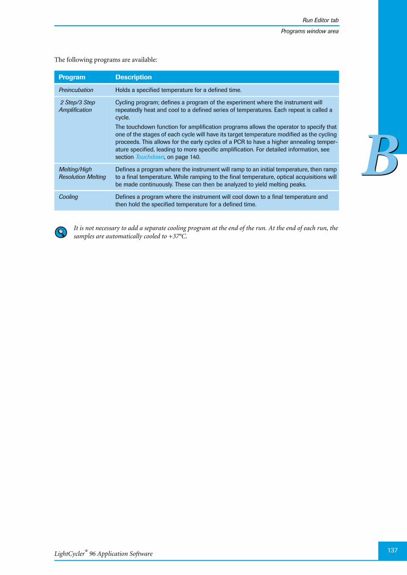
LightCycler® 96 Application Software
Run Editor tab
137
BB
Programs window area
The following programs are available:
It is not necessary to add a separate cooling program at the end of the run. At the end of each run, thesamples are automatically cooled to +37°C.
Program Description
Preincubation Holds a specified temperature for a defined time.
2 Step/3 StepAmplification
Cycling program; defines a program of the experiment where the instrument willrepeatedly heat and cool to a defined series of temperatures. Each repeat is called acycle.
The touchdown function for amplification programs allows the operator to specify thatone of the stages of each cycle will have its target temperature modified as the cyclingproceeds. This allows for the early cycles of a PCR to have a higher annealing temper-ature specified, leading to more specific amplification. For detailed information, seesection Touchdown, on page 140.
Melting/HighResolution Melting
Defines a program where the instrument will ramp to an initial temperature, then rampto a final temperature. While ramping to the final temperature, optical acquisitions willbe made continuously. These can then be analyzed to yield melting peaks.
Cooling Defines a program where the instrument will cool down to a final temperature andthen hold the specified temperature for a defined time.
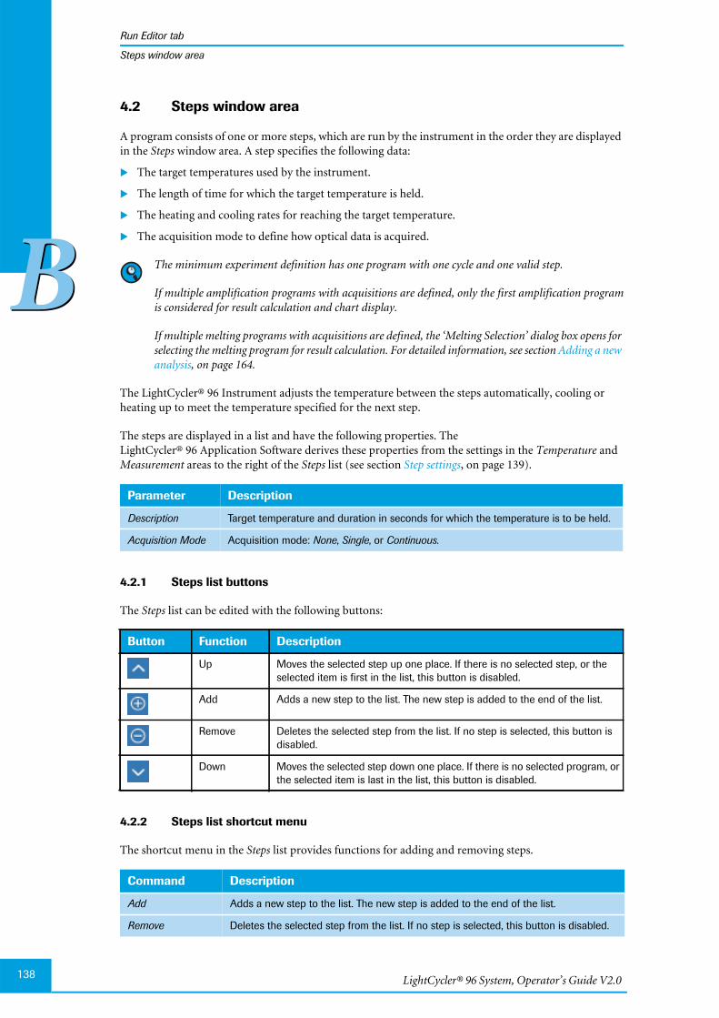
LightCycler® 96 System, Operator’s Guide V2.0138
Run Editor tab
BB
Steps window area
4.2 Steps window area
A program consists of one or more steps, which are run by the instrument in the order they are displayedin the Steps window area. A step specifies the following data:
The target temperatures used by the instrument.
The length of time for which the target temperature is held.
The heating and cooling rates for reaching the target temperature.
The acquisition mode to define how optical data is acquired.
The minimum experiment definition has one program with one cycle and one valid step.
If multiple amplification programs with acquisitions are defined, only the first amplification programis considered for result calculation and chart display.
If multiple melting programs with acquisitions are defined, the ‘Melting Selection’ dialog box opens forselecting the melting program for result calculation. For detailed information, see section Adding a newanalysis, on page 164.
The LightCycler® 96 Instrument adjusts the temperature between the steps automatically, cooling orheating up to meet the temperature specified for the next step.
The steps are displayed in a list and have the following properties. TheLightCycler® 96 Application Software derives these properties from the settings in the Temperature andMeasurement areas to the right of the Steps list (see section Step settings, on page 139).
4.2.1 Steps list buttons
The Steps list can be edited with the following buttons:
4.2.2 Steps list shortcut menu
The shortcut menu in the Steps list provides functions for adding and removing steps.
Parameter Description
Description Target temperature and duration in seconds for which the temperature is to be held.
Acquisition Mode Acquisition mode: None, Single, or Continuous.
Button Function Description
Up Moves the selected step up one place. If there is no selected step, or theselected item is first in the list, this button is disabled.
Add Adds a new step to the list. The new step is added to the end of the list.
Remove Deletes the selected step from the list. If no step is selected, this button isdisabled.
Down Moves the selected step down one place. If there is no selected program, orthe selected item is last in the list, this button is disabled.
Command Description
Add Adds a new step to the list. The new step is added to the end of the list.
Remove Deletes the selected step from the list. If no step is selected, this button is disabled.
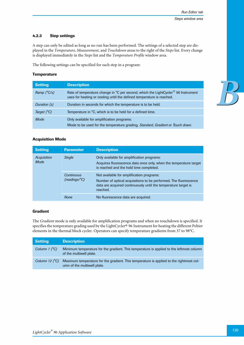
LightCycler® 96 Application Software
Run Editor tab
139
BB
Steps window area
4.2.3 Step settings
A step can only be edited as long as no run has been performed. The settings of a selected step are dis-played in the Temperature, Measurement, and Touchdown areas to the right of the Steps list. Every changeis displayed immediately in the Steps list and the Temperature Profile window area.
The following settings can be specified for each step in a program:
Temperature
Acquisition Mode
Gradient
The Gradient mode is only available for amplification programs and when no touchdown is specified. Itspecifies the temperature grading used by the LightCycler® 96 Instrument for heating the different Peltierelements in the thermal block cycler. Operators can specify temperature gradients from 37 to 98°C.
Setting Description
Ramp (°C/s) Rate of temperature change in °C per second, which the LightCycler® 96 Instrumentuses for heating or cooling until the defined temperature is reached.
Duration (s) Duration in seconds for which the temperature is to be held.
Target (°C) Temperature in °C, which is to be held for a defined time.
Mode Only available for amplification programs:
Mode to be used for the temperature grading, Standard, Gradient or Touch down.
Setting Parameter Description
AcquisitionMode
Single Only available for amplification programs:
Acquires fluorescence data once only, when the temperature targetis reached and the hold time completed.
Continuous(readings/°C)
Not available for amplification programs:
Number of optical acquisitions to be performed. The fluorescencedata are acquired continuously until the temperature target isreached.
None No fluorescence data are acquired.
Setting Description
Column 1 (°C) Minimum temperature for the gradient. This temperature is applied to the leftmost columnof the multiwell plate.
Column 12 (°C) Maximum temperature for the gradient. This temperature is applied to the rightmost col-umn of the multiwell plate.

LightCycler® 96 System, Operator’s Guide V2.0140
Run Editor tab
BB
Steps window area
The Detail button opens the Gradient dialog box, which displays a detailed view of the specified temper-ature gradient.
Figure 59: Gradient dialog box
The curve in the dialog box shows the applied temperature gradient according to the columns on the mul-tiwell plate.
Touchdown
The Touch Down mode is only available for amplification programs and when no gradient is specified.
Setting Description
TemperatureChange [°C]
Rate of temperature change in °C per cycle, at which the touchdown phase proceeds tothe final phase temperature.
Sec TargetTemp [°C]
Second target temperature to be reached by the last cycle of the program. This temper-ature is used to change the target temperature of a segment during the amplification re-action.
Delay [Cycles] Number of cycles after which the temperature change is first applied.
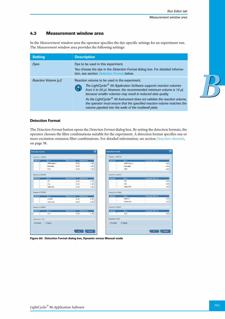
LightCycler® 96 Application Software
Run Editor tab
141
BB
Measurement window area
4.3 Measurement window area
In the Measurement window area the operator specifies the dye-specific settings for an experiment run.The Measurement window area provides the following settings:
Detection Format
The Detection Format button opens the Detection Format dialog box. By setting the detection formats, theoperator chooses the filter combinations suitable for the experiment. A detection format specifies one ormore excitation-emission filter combinations. For detailed information, see section Detection channels,on page 38.
Figure 60: Detection Format dialog box, Dynamic versus Manual mode
Setting Description
Dyes Dye to be used in this experiment.
You choose the dye in the Detection Format dialog box. For detailed informa-tion, see section Detection Format, below.
Reaction Volume [l] Reaction volume to be used in the experiment.
The LightCycler® 96 Application Software supports reaction volumesfrom 5 to 50 µl. However, the recommended minimum volume is 10 µl,because smaller volumes may result in reduced data quality.
As the LightCycler® 96 Instrument does not validate the reaction volume,the operator must ensure that the specified reaction volume matches thevolume pipetted into the wells of the multiwell plate.
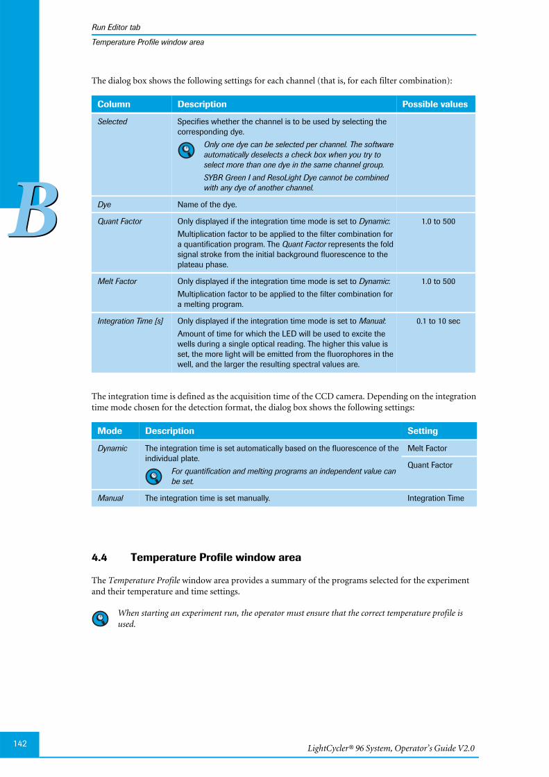
LightCycler® 96 System, Operator’s Guide V2.0142
Run Editor tab
BB
Temperature Profile window area
The dialog box shows the following settings for each channel (that is, for each filter combination):
The integration time is defined as the acquisition time of the CCD camera. Depending on the integrationtime mode chosen for the detection format, the dialog box shows the following settings:
4.4 Temperature Profile window area
The Temperature Profile window area provides a summary of the programs selected for the experimentand their temperature and time settings.
When starting an experiment run, the operator must ensure that the correct temperature profile isused.
Column Description Possible values
Selected Specifies whether the channel is to be used by selecting thecorresponding dye.
Only one dye can be selected per channel. The softwareautomatically deselects a check box when you try toselect more than one dye in the same channel group.
SYBR Green I and ResoLight Dye cannot be combinedwith any dye of another channel.
Dye Name of the dye.
Quant Factor Only displayed if the integration time mode is set to Dynamic:
Multiplication factor to be applied to the filter combination fora quantification program. The Quant Factor represents the foldsignal stroke from the initial background fluorescence to theplateau phase.
1.0 to 500
Melt Factor Only displayed if the integration time mode is set to Dynamic:
Multiplication factor to be applied to the filter combination fora melting program.
1.0 to 500
Integration Time [s] Only displayed if the integration time mode is set to Manual:
Amount of time for which the LED will be used to excite thewells during a single optical reading. The higher this value isset, the more light will be emitted from the fluorophores in thewell, and the larger the resulting spectral values are.
0.1 to 10 sec
Mode Description Setting
Dynamic The integration time is set automatically based on the fluorescence of theindividual plate.
For quantification and melting programs an independent value canbe set.
Melt Factor
Quant Factor
Manual The integration time is set manually. Integration Time
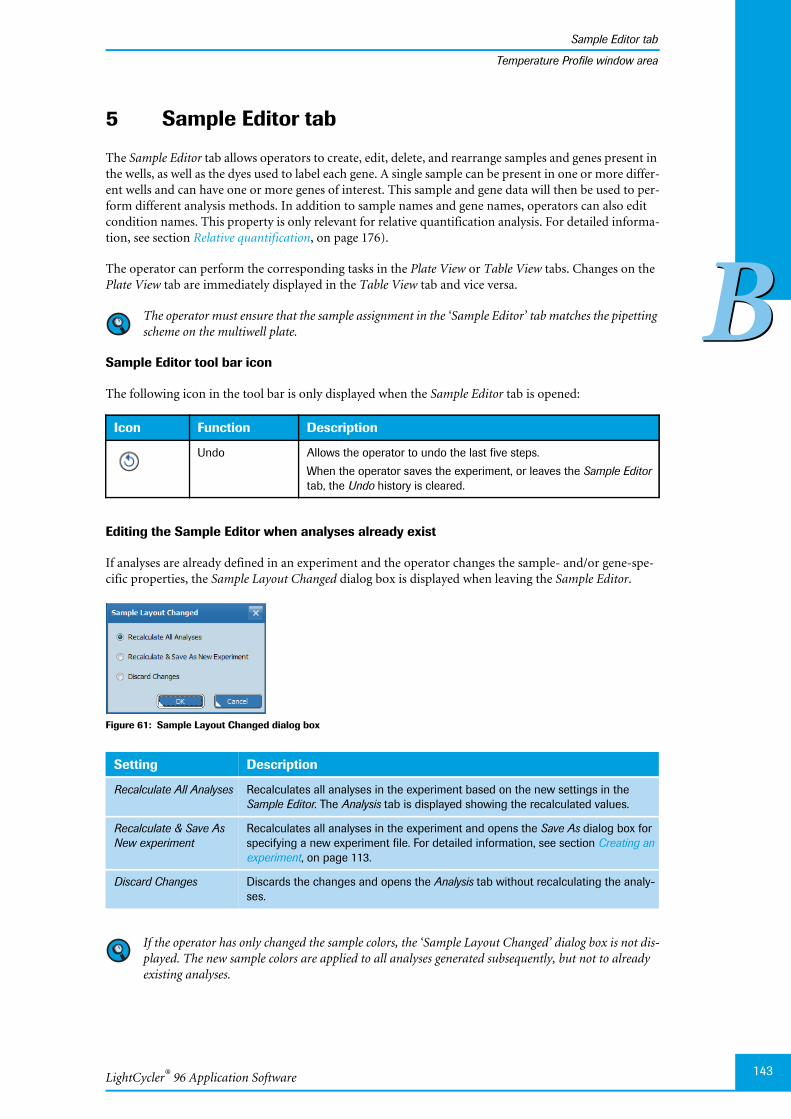
LightCycler® 96 Application Software
Sample Editor tab
143
BB
Temperature Profile window area
5 Sample Editor tab
The Sample Editor tab allows operators to create, edit, delete, and rearrange samples and genes present inthe wells, as well as the dyes used to label each gene. A single sample can be present in one or more differ-ent wells and can have one or more genes of interest. This sample and gene data will then be used to per-form different analysis methods. In addition to sample names and gene names, operators can also editcondition names. This property is only relevant for relative quantification analysis. For detailed informa-tion, see section Relative quantification, on page 176).
The operator can perform the corresponding tasks in the Plate View or Table View tabs. Changes on thePlate View tab are immediately displayed in the Table View tab and vice versa.
The operator must ensure that the sample assignment in the ‘Sample Editor’ tab matches the pipettingscheme on the multiwell plate.
Sample Editor tool bar icon
The following icon in the tool bar is only displayed when the Sample Editor tab is opened:
Editing the Sample Editor when analyses already exist
If analyses are already defined in an experiment and the operator changes the sample- and/or gene-spe-cific properties, the Sample Layout Changed dialog box is displayed when leaving the Sample Editor.
Figure 61: Sample Layout Changed dialog box
If the operator has only changed the sample colors, the ‘Sample Layout Changed’ dialog box is not dis-played. The new sample colors are applied to all analyses generated subsequently, but not to alreadyexisting analyses.
Icon Function Description
Undo Allows the operator to undo the last five steps.
When the operator saves the experiment, or leaves the Sample Editortab, the Undo history is cleared.
Setting Description
Recalculate All Analyses Recalculates all analyses in the experiment based on the new settings in theSample Editor. The Analysis tab is displayed showing the recalculated values.
Recalculate & Save AsNew experiment
Recalculates all analyses in the experiment and opens the Save As dialog box forspecifying a new experiment file. For detailed information, see section Creating anexperiment, on page 113.
Discard Changes Discards the changes and opens the Analysis tab without recalculating the analy-ses.
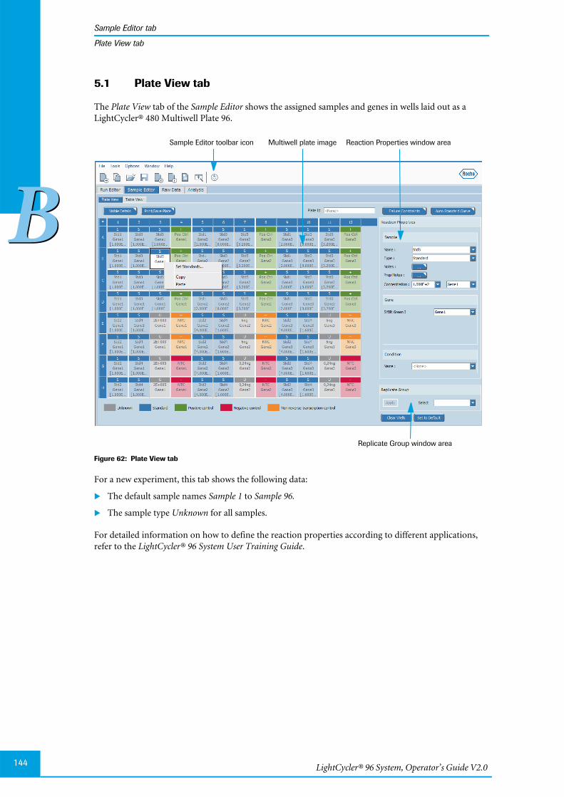
LightCycler® 96 System, Operator’s Guide V2.0144
Sample Editor tab
BB
Plate View tab
5.1 Plate View tab
The Plate View tab of the Sample Editor shows the assigned samples and genes in wells laid out as aLightCycler® 480 Multiwell Plate 96.
Figure 62: Plate View tab
For a new experiment, this tab shows the following data:
The default sample names Sample 1 to Sample 96.
The sample type Unknown for all samples.
For detailed information on how to define the reaction properties according to different applications,refer to the LightCycler® 96 System User Training Guide.
Replicate Group window area
Multiwell plate image Reaction Properties window areaSample Editor toolbar icon

LightCycler® 96 Application Software
Sample Editor tab
145
BB
Plate View tab
5.1.1 Multiwell plate image
The multiwell plate image provides a schematic of the multiwell plate mount for editing the range of sam-ples. Each row is allocated a letter from A to H. The wells of a row are displayed as columns and numberedfrom left to right.
Each well displays the sample properties according to the operator’s selection. For detailed informa-tion on how to customize the plate view, see section Visible Details, on page 148.
Each well is colored to match the sample type in the corresponding well.
Hovering the cursor over a well displays a tooltip with the properties of the sample.
Selecting a well or a range of wells allow editing of the corresponding properties using the fields in thewindow areas displayed to the right of the multiwell plate image.
Plate image shortcut menu
The multiwell plate image provides a shortcut menu containing the following command:
5.1.2 Reaction Properties window area
The Reaction Properties window area allows operators to create or edit the following properties of samplesand genes in a selected well or a range of wells. Property changes are immediately displayed in the multi-well plate image.
The Sample Editor allows operators to edit the sample- and/or gene-specific properties, and the condi-tion names (only relevant for relative quantification). Settings affecting the analysis of the data are tobe specified in the corresponding ‘Analysis’ tab. For detailed information, see section Analysis tab, onpage 162.
Command Description
Set Standards Opens the Auto Standard Curve dialog box. For detailed information, see section Auto Stan-dard Curve, on page 151.
Copy Copies the properties of the selected wells to the clipboard.
Paste Pastes the properties from the clipboard into the selected wells.
If the operator does not select enough wells for pasting, the paste function automati-cally completes the selection.
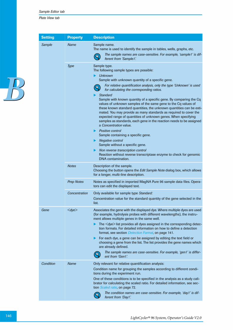
LightCycler® 96 System, Operator’s Guide V2.0146
Sample Editor tab
BB
Plate View tab
Setting Property Description
Sample Name Sample name.The name is used to identify the sample in tables, wells, graphs, etc.
The sample names are case-sensitive. For example, ‘sample1’ is dif-ferent from ‘Sample1’.
Type Sample type.The following sample types are possible:
UnknownSample with unknown quantity of a specific gene.
For relative quantification analysis, only the type ‘Unknown’ is usedfor calculating the corresponding ratios.
StandardSample with known quantity of a specific gene. By comparing the Cqvalues of unknown samples of the same gene to the Cq values ofthese known standard quantities, the unknown quantities can be esti-mated. You may provide as many standards as required to cover theexpected range of quantities of unknown genes. When specifyingsamples as standards, each gene in the reaction needs to be assigneda Concentration value.
Positive controlSample containing a specific gene.
Negative controlSample without a specific gene.
Non reverse transcription controlReaction without reverse transcriptase enzyme to check for genomicDNA contamination.
Notes Description of the sample.Choosing the button opens the Edit Sample Note dialog box, which allowsfor a longer, multi-line description.
Prep Notes Notes as specified in imported MagNA Pure 96 sample data files. Opera-tors can edit the displayed text.
Concentration Only available for sample type Standard:
Concentration value for the standard quantity of the gene selected in thelist.
Gene <dye> Associates the gene with the displayed dye. Where multiple dyes are used(for example, hydrolysis probes with different wavelengths), the instru-ment allows multiple genes in the same well.
The <dye> list provides all dyes assigned in the corresponding detec-tion formats. For detailed information on how to define a detectionformat, see section Detection Format, on page 141.
For each dye, a gene can be assigned by editing the text field orchoosing a gene from the list. The list provides the gene names whichare already defined.
The sample names are case-sensitive. For example, ‘gen1’ is differ-ent from ‘Gen1’.
Condition Name Only relevant for relative quantification analysis:
Condition name for grouping the samples according to different condi-tions during the experiment run.
One of these conditions is to be specified in the analysis as a study cali-brator for calculating the scaled ratio. For detailed information, see sec-tion Scaled ratio, on page 72.
The condition names are case-sensitive. For example, ‘day1’ is dif-ferent from ‘Day1’.
LightCycler® 96 Application Software
Sample Editor tab
147
BB
Plate View tab
5.1.3 Replicate Group window area
The Replicate Group window area allows operators to create new replicate groups and arrange samples inthem. The replicate group is always named according to the top leftmost of the corresponding wells. If this"master replicate" is removed, the next top leftmost position takes on the role.
If properties of one of the replicate group members are changed, the corresponding sample is removedfrom the replicate group.
The LightCycler® 96 Application Software automatically groups samples in replicate groups, providedthey have identical values for the following properties:
Sample name (case-sensitive)
Sample type
Concentration
Gene name (case-sensitive)
Condition (case-sensitive)
All members of a replicate group automatically display the identical color, corresponding to the color ofthe master replicate. Automatically assigned replicate group colors are not adopted to already existinganalyses, but only to subsequently generated analyses.
To create a replicate group
To select wells by replicate group
To add samples to a replicate group
Property Description
Select Name of the replicate group.
The list provides the already defined replicate groups.
In the multiwell plate image, select the corresponding wells.
In the Replicate Group window area, choose Apply.
The replicate group is created and named according to the top leftmost of the selected wells. The repli-cate group is now displayed in the Select list.
In the Replicate Group window area, choose a replicate group from the Select list.
In the Replicate Group window area, choose a replicate group from the Select list.
In the multiwell plate image, select the additional wells.
In the Replicate Group window area, choose Apply.
The properties of the samples in the replicate group are assigned to the additional samples.
�
�
�
�
�
�

LightCycler® 96 System, Operator’s Guide V2.0148
Sample Editor tab
BB
Plate View tab
5.1.4 Visible Details
The Visible Details button opens the Visible Details dialog box, which allows for customizing the sampleeditor display.
Figure 63: Visible Details dialog box
5.1.5 Print/Save Plate
The Print/Save Plate button opens the Print Plate Preview. Operators can print and save the plate view ofan experiment as pipetting information. The printout matches the view on the screen, meaning the visi-bility of the properties are identical. The printout also shows the following data:
The experiment name
The plate ID
The LightCycler® 96 Application Software version
The print date
Setting Description
Visible Details Properties to be displayed for the wells in the plate window area. Selectedproperties are displayed, unselected properties are hidden.
Visibility Specific to Dyes Dye-specific properties to be displayed for the wells in the plate windowarea. The table shows a row for each dye assigned to the sample.
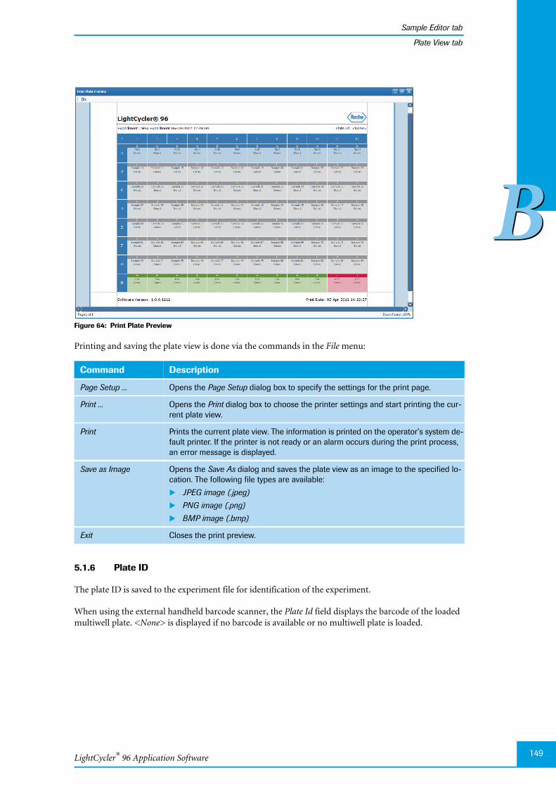
LightCycler® 96 Application Software
Sample Editor tab
149
BB
Plate View tab
Figure 64: Print Plate Preview
Printing and saving the plate view is done via the commands in the File menu:
5.1.6 Plate ID
The plate ID is saved to the experiment file for identification of the experiment.
When using the external handheld barcode scanner, the Plate Id field displays the barcode of the loadedmultiwell plate. <None> is displayed if no barcode is available or no multiwell plate is loaded.
Command Description
Page Setup ... Opens the Page Setup dialog box to specify the settings for the print page.
Print ... Opens the Print dialog box to choose the printer settings and start printing the cur-rent plate view.
Print Prints the current plate view. The information is printed on the operator’s system de-fault printer. If the printer is not ready or an alarm occurs during the print process,an error message is displayed.
Save as Image Opens the Save As dialog and saves the plate view as an image to the specified lo-cation. The following file types are available:
JPEG image (.jpeg)
PNG image (.png)
BMP image (.bmp)
Exit Closes the print preview.
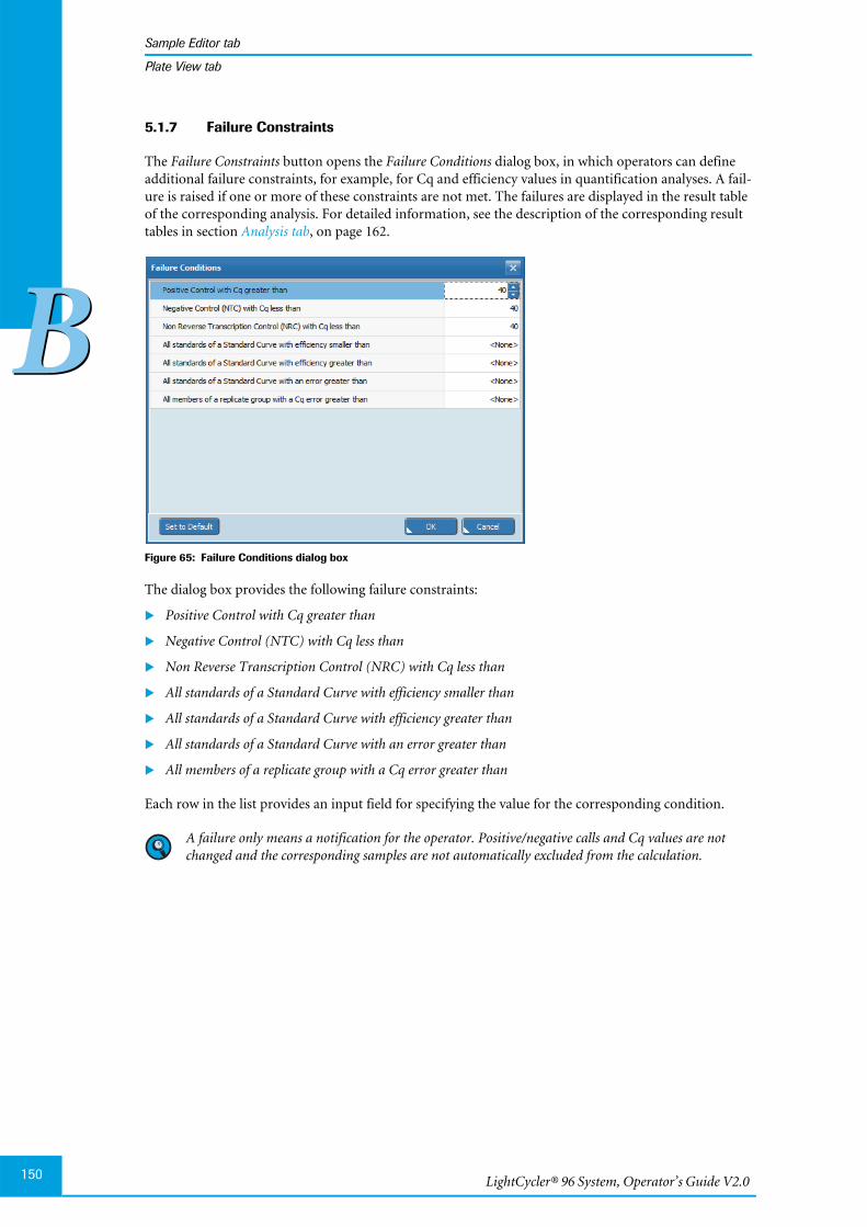
LightCycler® 96 System, Operator’s Guide V2.0150
Sample Editor tab
BB
Plate View tab
5.1.7 Failure Constraints
The Failure Constraints button opens the Failure Conditions dialog box, in which operators can defineadditional failure constraints, for example, for Cq and efficiency values in quantification analyses. A fail-ure is raised if one or more of these constraints are not met. The failures are displayed in the result tableof the corresponding analysis. For detailed information, see the description of the corresponding resulttables in section Analysis tab, on page 162.
Figure 65: Failure Conditions dialog box
The dialog box provides the following failure constraints:
Positive Control with Cq greater than
Negative Control (NTC) with Cq less than
Non Reverse Transcription Control (NRC) with Cq less than
All standards of a Standard Curve with efficiency smaller than
All standards of a Standard Curve with efficiency greater than
All standards of a Standard Curve with an error greater than
All members of a replicate group with a Cq error greater than
Each row in the list provides an input field for specifying the value for the corresponding condition.
A failure only means a notification for the operator. Positive/negative calls and Cq values are notchanged and the corresponding samples are not automatically excluded from the calculation.
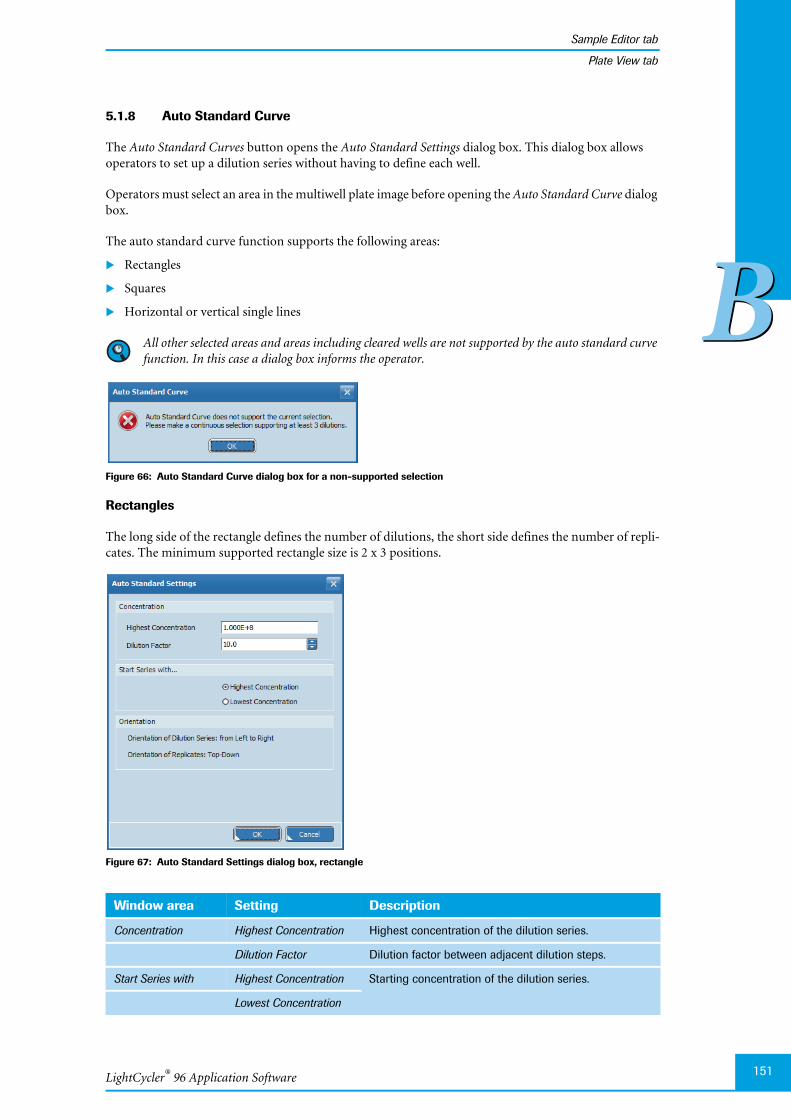
LightCycler® 96 Application Software
Sample Editor tab
151
BB
Plate View tab
5.1.8 Auto Standard Curve
The Auto Standard Curves button opens the Auto Standard Settings dialog box. This dialog box allowsoperators to set up a dilution series without having to define each well.
Operators must select an area in the multiwell plate image before opening the Auto Standard Curve dialogbox.
The auto standard curve function supports the following areas:
Rectangles
Squares
Horizontal or vertical single lines
All other selected areas and areas including cleared wells are not supported by the auto standard curvefunction. In this case a dialog box informs the operator.
Figure 66: Auto Standard Curve dialog box for a non-supported selection
Rectangles
The long side of the rectangle defines the number of dilutions, the short side defines the number of repli-cates. The minimum supported rectangle size is 2 x 3 positions.
Figure 67: Auto Standard Settings dialog box, rectangle
Window area Setting Description
Concentration Highest Concentration Highest concentration of the dilution series.
Dilution Factor Dilution factor between adjacent dilution steps.
Start Series with Highest Concentration Starting concentration of the dilution series.
Lowest Concentration
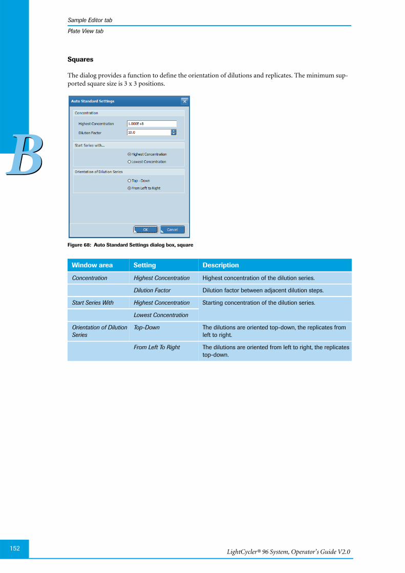
LightCycler® 96 System, Operator’s Guide V2.0152
Sample Editor tab
BB
Plate View tab
Squares
The dialog provides a function to define the orientation of dilutions and replicates. The minimum sup-ported square size is 3 x 3 positions.
Figure 68: Auto Standard Settings dialog box, square
Window area Setting Description
Concentration Highest Concentration Highest concentration of the dilution series.
Dilution Factor Dilution factor between adjacent dilution steps.
Start Series With Highest Concentration Starting concentration of the dilution series.
Lowest Concentration
Orientation of DilutionSeries
Top-Down The dilutions are oriented top-down, the replicates fromleft to right.
From Left To Right The dilutions are oriented from left to right, the replicatestop-down.
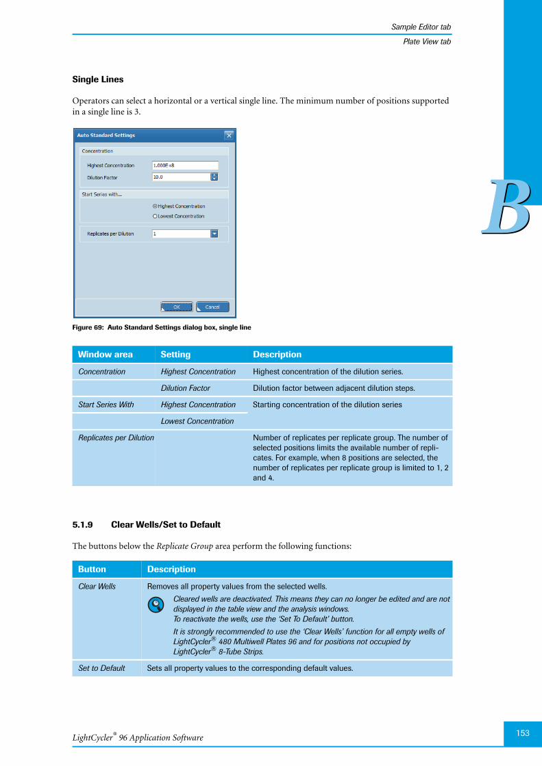
LightCycler® 96 Application Software
Sample Editor tab
153
BB
Plate View tab
Single Lines
Operators can select a horizontal or a vertical single line. The minimum number of positions supportedin a single line is 3.
Figure 69: Auto Standard Settings dialog box, single line
5.1.9 Clear Wells/Set to Default
The buttons below the Replicate Group area perform the following functions:
Window area Setting Description
Concentration Highest Concentration Highest concentration of the dilution series.
Dilution Factor Dilution factor between adjacent dilution steps.
Start Series With Highest Concentration Starting concentration of the dilution series
Lowest Concentration
Replicates per Dilution Number of replicates per replicate group. The number ofselected positions limits the available number of repli-cates. For example, when 8 positions are selected, thenumber of replicates per replicate group is limited to 1, 2and 4.
Button Description
Clear Wells Removes all property values from the selected wells.
Cleared wells are deactivated. This means they can no longer be edited and are notdisplayed in the table view and the analysis windows.To reactivate the wells, use the ‘Set To Default’ button.
It is strongly recommended to use the ‘Clear Wells’ function for all empty wells ofLightCycler® 480 Multiwell Plates 96 and for positions not occupied byLightCycler® 8-Tube Strips.
Set to Default Sets all property values to the corresponding default values.
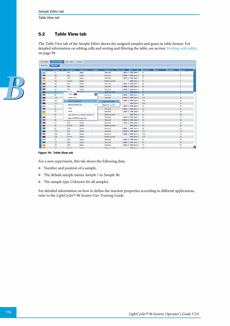
LightCycler® 96 System, Operator’s Guide V2.0154
Sample Editor tab
BB
Table View tab
5.2 Table View tab
The Table View tab of the Sample Editor shows the assigned samples and genes in table format. Fordetailed information on editing cells and sorting and filtering the table, see section Working with tables,on page 99.
Figure 70: Table View tab
For a new experiment, this tab shows the following data:
Number and position of a sample.
The default sample names Sample 1 to Sample 96.
The sample type Unknown for all samples.
For detailed information on how to define the reaction properties according to different applications,refer to the LightCycler® 96 System User Training Guide.
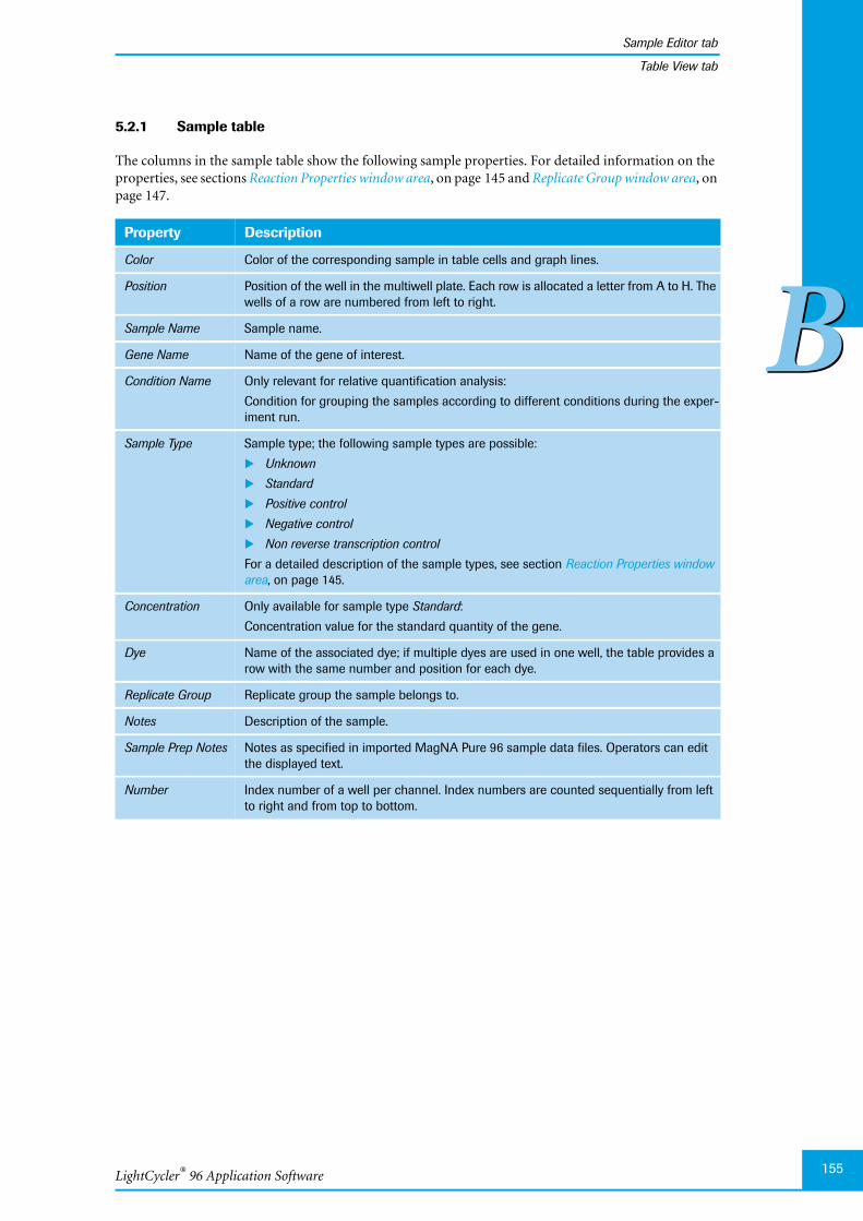
LightCycler® 96 Application Software
Sample Editor tab
155
BB
Table View tab
5.2.1 Sample table
The columns in the sample table show the following sample properties. For detailed information on theproperties, see sections Reaction Properties window area, on page 145 and Replicate Group window area, onpage 147.
Property Description
Color Color of the corresponding sample in table cells and graph lines.
Position Position of the well in the multiwell plate. Each row is allocated a letter from A to H. Thewells of a row are numbered from left to right.
Sample Name Sample name.
Gene Name Name of the gene of interest.
Condition Name Only relevant for relative quantification analysis:
Condition for grouping the samples according to different conditions during the exper-iment run.
Sample Type Sample type; the following sample types are possible:
Unknown
Standard
Positive control
Negative control
Non reverse transcription control
For a detailed description of the sample types, see section Reaction Properties windowarea, on page 145.
Concentration Only available for sample type Standard:
Concentration value for the standard quantity of the gene.
Dye Name of the associated dye; if multiple dyes are used in one well, the table provides arow with the same number and position for each dye.
Replicate Group Replicate group the sample belongs to.
Notes Description of the sample.
Sample Prep Notes Notes as specified in imported MagNA Pure 96 sample data files. Operators can editthe displayed text.
Number Index number of a well per channel. Index numbers are counted sequentially from leftto right and from top to bottom.
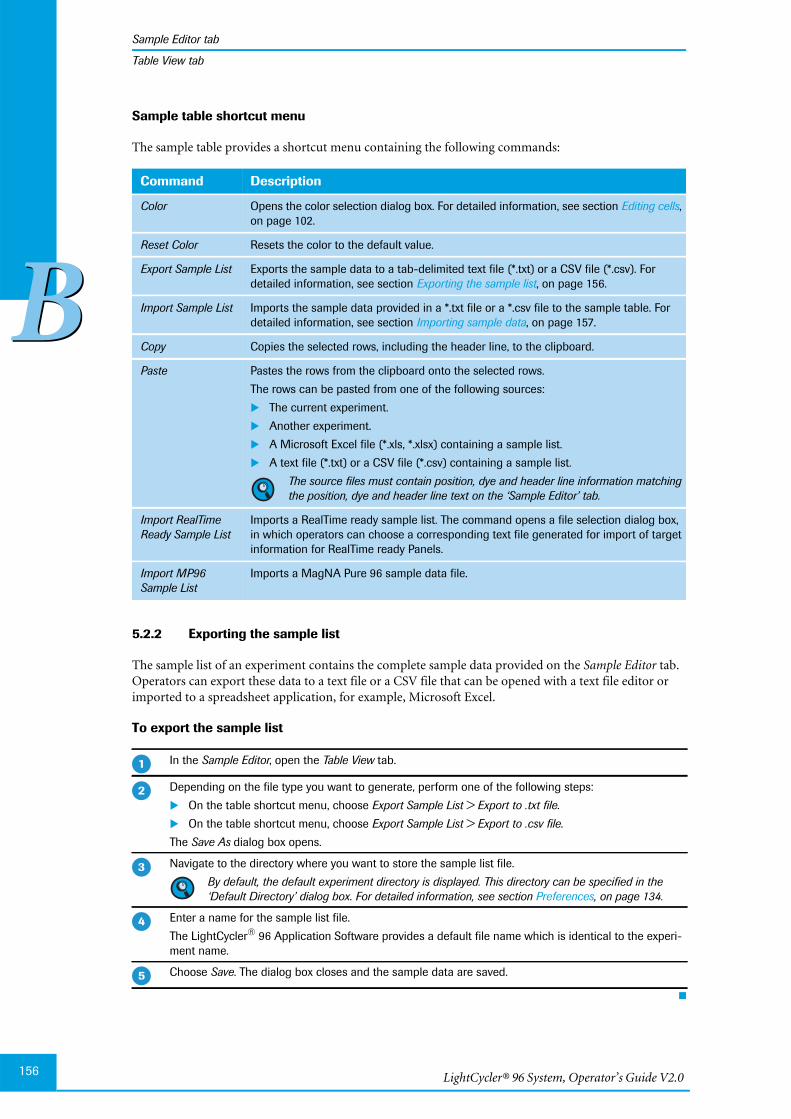
LightCycler® 96 System, Operator’s Guide V2.0156
Sample Editor tab
BB
Table View tab
Sample table shortcut menu
The sample table provides a shortcut menu containing the following commands:
5.2.2 Exporting the sample list
The sample list of an experiment contains the complete sample data provided on the Sample Editor tab.Operators can export these data to a text file or a CSV file that can be opened with a text file editor orimported to a spreadsheet application, for example, Microsoft Excel.
To export the sample list
Command Description
Color Opens the color selection dialog box. For detailed information, see section Editing cells,on page 102.
Reset Color Resets the color to the default value.
Export Sample List Exports the sample data to a tab-delimited text file (*.txt) or a CSV file (*.csv). Fordetailed information, see section Exporting the sample list, on page 156.
Import Sample List Imports the sample data provided in a *.txt file or a *.csv file to the sample table. Fordetailed information, see section Importing sample data, on page 157.
Copy Copies the selected rows, including the header line, to the clipboard.
Paste Pastes the rows from the clipboard onto the selected rows.
The rows can be pasted from one of the following sources:
The current experiment.
Another experiment.
A Microsoft Excel file (*.xls, *.xlsx) containing a sample list.
A text file (*.txt) or a CSV file (*.csv) containing a sample list.
The source files must contain position, dye and header line information matchingthe position, dye and header line text on the ‘Sample Editor’ tab.
Import RealTimeReady Sample List
Imports a RealTime ready sample list. The command opens a file selection dialog box,in which operators can choose a corresponding text file generated for import of targetinformation for RealTime ready Panels.
Import MP96Sample List
Imports a MagNA Pure 96 sample data file.
In the Sample Editor, open the Table View tab.
Depending on the file type you want to generate, perform one of the following steps:
On the table shortcut menu, choose Export Sample List > Export to .txt file.
On the table shortcut menu, choose Export Sample List > Export to .csv file.
The Save As dialog box opens.
Navigate to the directory where you want to store the sample list file.
By default, the default experiment directory is displayed. This directory can be specified in the‘Default Directory’ dialog box. For detailed information, see section Preferences, on page 134.
Enter a name for the sample list file.
The LightCycler® 96 Application Software provides a default file name which is identical to the experi-ment name.
Choose Save. The dialog box closes and the sample data are saved.
�
�
�
�
�

LightCycler® 96 Application Software
Sample Editor tab
157
BB
Table View tab
5.2.3 Importing sample data
The import function allows the operator to import sample data into the samples table.
Importable files must contain position, dye and header line information matching the position, dyeand header line text on the ‘Sample Editor’ tab.
The data can be imported from one of the following sources:
Any text or CSV file containing the information described above (position, dye, header line).
A sample list exported from another experiment as a text file (*.txt) or a CSV file (*.csv); for detailedinformation on exporting the sample list, see section To export the sample list, on page 156.
A results file exported from the MagNA Pure 96 Software in LightCycler® 96 System readable format(*.txt or *.xml).
A text file generated for RealTime ready Panels and Custom Panels.
The Import Sample List commands on the sample table shortcut menu open theImport Sample List - Preview window:
Figure 71: Import Sample List - Preview
The preview shows the sample table with the import status and the expected result. Overwritten cells arehighlighted.
The buttons below the table perform the following functions:
Button Description
Accept Closes the preview and applies the changes to the corresponding rows.
Reject Closes the preview and discards the changes.

LightCycler® 96 System, Operator’s Guide V2.0158
Sample Editor tab
BB
Table View tab
To import sample data into the sample list
In the Sample Editor, open the Table View tab.
Depending on the file type you want to import, perform one of the following steps:
On the table shortcut menu, choose Import Sample List > Import from .txt file.
On the table shortcut menu, choose Import Sample List > Import from .csv file.
The Open dialog box opens.
Navigate to the directory where the sample list file is stored.
By default, the default experiment directory is displayed. This directory can be specified in the‘Default Directory’ dialog box. For detailed information, see section Preferences, on page 134.
Select the sample list file and choose Open.
The Import Sample List - Preview window opens, showing the sample table with the expected results.
Choose Accept.
The Import Sample List - Preview window closes and the data are imported into the sample list.
�
�
�
�
�

LightCycler® 96 Application Software
Raw Data tab
159
BB
6 Raw Data tab
The Raw Data tab shows the temperature and optical data collected during an experiment run. The rawdata of an experiment contains all instrument corrections, but no color compensation, drift or back-ground correction.
Figure 72: Raw Data tab
By default, the Raw Data tab shows four sections. For detailed information on changing the number ofdisplayed sections and on resizing the sections, see section Working with sections, on page 112.
All sections on the Raw Data tab use the same selection: When the operator selects a curve in one of thegraphs or a well in the Plate View or Sample Table, the same wells are selected in each section.
The view selection list in the sections of the Raw Data tab provides the following data:
Plate View; see section Plate View, on page 160.
Fluorescence Curves; see section Fluorescence Curves, on page 160.
Melting Curves; see section Melting Curves, on page 160.This option is only available for melting programs.
Amplification Curves; see section Amplification Curves, on page 161.
Sample Table; see section Sample Table, on page 161.
Integration Time; see section Integration Time, on page 161.
View selection list
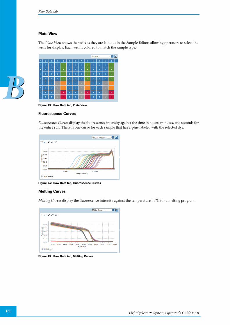
LightCycler® 96 System, Operator’s Guide V2.0160
Raw Data tab
BB
Plate View
The Plate View shows the wells as they are laid out in the Sample Editor, allowing operators to select thewells for display. Each well is colored to match the sample type.
Figure 73: Raw Data tab, Plate View
Fluorescence Curves
Fluorescence Curves display the fluorescence intensity against the time in hours, minutes, and seconds forthe entire run. There is one curve for each sample that has a gene labeled with the selected dye.
Figure 74: Raw Data tab, Fluorescence Curves
Melting Curves
Melting Curves display the fluorescence intensity against the temperature in °C for a melting program.
Figure 75: Raw Data tab, Melting Curves
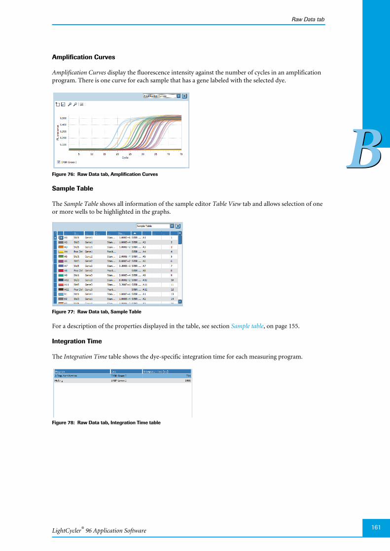
LightCycler® 96 Application Software
Raw Data tab
161
BB
Amplification Curves
Amplification Curves display the fluorescence intensity against the number of cycles in an amplificationprogram. There is one curve for each sample that has a gene labeled with the selected dye.
Figure 76: Raw Data tab, Amplification Curves
Sample Table
The Sample Table shows all information of the sample editor Table View tab and allows selection of oneor more wells to be highlighted in the graphs.
Figure 77: Raw Data tab, Sample Table
For a description of the properties displayed in the table, see section Sample table, on page 155.
Integration Time
The Integration Time table shows the dye-specific integration time for each measuring program.
Figure 78: Raw Data tab, Integration Time table
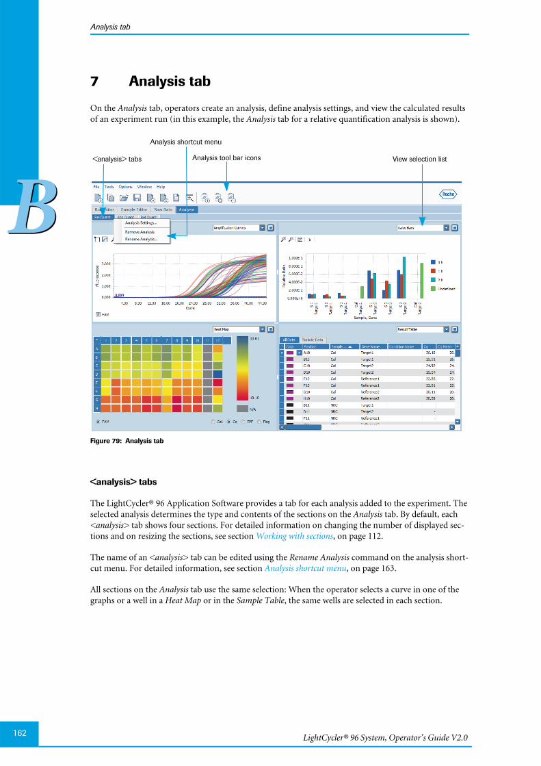
LightCycler® 96 System, Operator’s Guide V2.0162
Analysis tab
BB
7 Analysis tab
On the Analysis tab, operators create an analysis, define analysis settings, and view the calculated resultsof an experiment run (in this example, the Analysis tab for a relative quantification analysis is shown).
Figure 79: Analysis tab
<analysis> tabs
The LightCycler® 96 Application Software provides a tab for each analysis added to the experiment. Theselected analysis determines the type and contents of the sections on the Analysis tab. By default, each<analysis> tab shows four sections. For detailed information on changing the number of displayed sec-tions and on resizing the sections, see section Working with sections, on page 112.
The name of an <analysis> tab can be edited using the Rename Analysis command on the analysis short-cut menu. For detailed information, see section Analysis shortcut menu, on page 163.
All sections on the Analysis tab use the same selection: When the operator selects a curve in one of thegraphs or a well in a Heat Map or in the Sample Table, the same wells are selected in each section.
View selection list
Analysis shortcut menu
<analysis> tabs Analysis tool bar icons
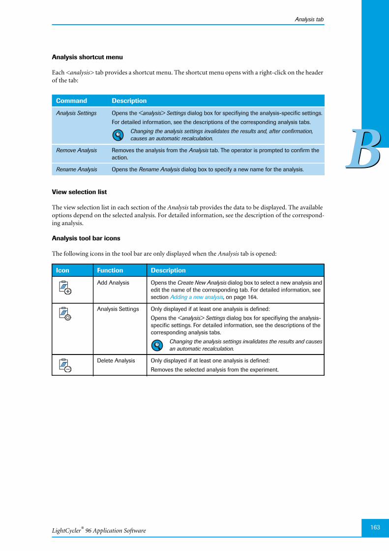
LightCycler® 96 Application Software
Analysis tab
163
BB
Analysis shortcut menu
Each <analysis> tab provides a shortcut menu. The shortcut menu opens with a right-click on the headerof the tab:
View selection list
The view selection list in each section of the Analysis tab provides the data to be displayed. The availableoptions depend on the selected analysis. For detailed information, see the description of the correspond-ing analysis.
Analysis tool bar icons
The following icons in the tool bar are only displayed when the Analysis tab is opened:
Command Description
Analysis Settings Opens the <analysis> Settings dialog box for specifiying the analysis-specific settings.
For detailed information, see the descriptions of the corresponding analysis tabs.
Changing the analysis settings invalidates the results and, after confirmation,causes an automatic recalculation.
Remove Analysis Removes the analysis from the Analysis tab. The operator is prompted to confirm theaction.
Rename Analysis Opens the Rename Analysis dialog box to specify a new name for the analysis.
Icon Function Description
Add Analysis Opens the Create New Analysis dialog box to select a new analysis andedit the name of the corresponding tab. For detailed information, seesection Adding a new analysis, on page 164.
Analysis Settings Only displayed if at least one analysis is defined:
Opens the <analysis> Settings dialog box for specifiying the analysis-specific settings. For detailed information, see the descriptions of thecorresponding analysis tabs.
Changing the analysis settings invalidates the results and causesan automatic recalculation.
Delete Analysis Only displayed if at least one analysis is defined:
Removes the selected analysis from the experiment.
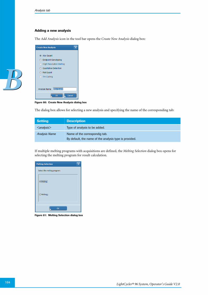
LightCycler® 96 System, Operator’s Guide V2.0164
Analysis tab
BB
Adding a new analysis
The Add Analysis icon in the tool bar opens the Create New Analysis dialog box:
Figure 80: Create New Analysis dialog box
The dialog box allows for selecting a new analysis and specifying the name of the corresponding tab:
If multiple melting programs with acquisitions are defined, the Melting Selection dialog box opens forselecting the melting program for result calculation.
Figure 81: Melting Selection dialog box
Setting Description
<analysis> Type of analysis to be added.
Analysis Name Name of the correspondig tab.
By default, the name of the analysis type is provided.
LightCycler® 96 Application Software
Analysis tab
165
BB
Eliminating positions from the analysis
The LightCycler® 96 Application Software provides functions in three levels for excluding positions fromthe analysis:
Clearing wells:The Clear Wells function is provided on the Plate View tab of the Sample Editor. Clear Wells eliminatesthe selected wells from all analyses. Cleared wells are deactivated. This means they can no longer beedited and are not displayed in the table view or the analysis windows.For detailed information, see section Clear Wells/Set to Default, on page 153.
It is strongly recommended to use the ‘Clear Wells’ function for all empty wells ofLightCycler® 480 Multiwell Plates and for positions not occupied by LightCycler® 8-Tube Strips.
Removing samples, genes, and/or conditions (for relative quantification only):The Remove function is provided in the <analysis> Settings dialog box of the corresponding analyses.Removed samples, genes, or conditions are no longer displayed in tables and charts of the analysis.For detailed information, see the descriptions of the corresponding analyses.
Excluding selected samples from the analysis:The Exclude function for specified samples is provided in the result tables of the corresponding anal-yses. Excluding samples can be useful when a sample is clearly an outlier, or if an error has occurredin pipetting or amplification. Excluded samples are displayed in tables and charts, but do not showany result values (for example, Cq values, Tm values, or ratios).For detailed information, see the descriptions of the corresponding analysis result tables.
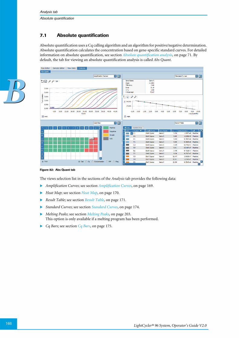
LightCycler® 96 System, Operator’s Guide V2.0166
Analysis tab
BB
Absolute quantification
7.1 Absolute quantification
Absolute quantification uses a Cq calling algorithm and an algorithm for positive/negative determination.Absolute quantification calculates the concentration based on gene-specific standard curves. For detailedinformation on absolute quantification, see section Absolute quantification analysis, on page 71. Bydefault, the tab for viewing an absolute quantification analysis is called Abs Quant.
Figure 82: Abs Quant tab
The views selection list in the sections of the Analysis tab provides the following data:
Amplification Curves; see section Amplification Curves, on page 169.
Heat Map; see section Heat Map, on page 170.
Result Table; see section Result Table, on page 171.
Standard Curves; see section Standard Curves, on page 174.
Melting Peaks; see section Melting Peaks, on page 203.This option is only available if a melting program has been performed.
Cq Bars; see section Cq Bars, on page 175.

LightCycler® 96 Application Software
Analysis tab
167
BB
Absolute quantification
7.1.1 Abs Quant Settings
The Abs Quant Settings dialog box allows operators to specify the analysis-specific settings. The dialog boxis accessed via the Analysis Settings command on the analysis shortcut menu or by choosing the AnalysisSettings icon in the tool bar.
Figure 83: Abs Quant Settings dialog box, Genes tab
Each tab shows a table for editing the gene- or sample-specific settings.
Genes tab
Column Setting
No Numbering of the defined genes.
Name Gene name; the genes are listed in the same order as specified in the Sample Editor tab.
Removed Removes the gene from the analysis. Removed genes are no longer displayed in tablesand charts of the corresponding analysis.
It is possible to add or remove multiple genes simultaneously by multi-selecting andusing either the ‘Add Selected’ or ‘Remove Selected’ command on the shortcutmenu of the table.
Efficiency Efficiency used for calculating efficiency-corrected concentrations.
Choosing the browse button in this column opens the Efficiency Editor dialog box forspecifiying the efficiency to be used:
E=Only available if no in-run standard curve for the relevant gene is present and if a sin-gle standard concentration is defined: The efficiency can be specified manually in thedisplayed field.Default value: 2.0
E from standard curveThe efficiency has been derived from the standard curve.
Maximal Cq Specifies the maximum Cq value, that is, the threshold for a positive call.
For all samples with a Cq value greater than the specified maximum Cq, the Cq valuesare removed from the result table.
The corresponding call status is set to Negative.
The Edited Call column in the result table is checked.
Minimal Slope Specifies the minimum slope of the amplification curve, that is, the threshold for a posi-tive call.
For all samples with a slope value less than the specified minimum, the correspondingcall status is set to Negative.
The resulting Cq value is removed from the result table.
The Edited Call column in the result table is checked.

LightCycler® 96 System, Operator’s Guide V2.0168
Analysis tab
BB
Absolute quantification
Samples tab
The Samples tab allows for removing samples from the analysis. Removed samples are no longer displayedin tables and charts of the corresponding analysis.
Figure 84: Abs Quant Settings dialog box, Samples tab
It is possible to add or remove multiple samples simultaneously by multi-selecting and using either the‘Add Selected’ or ‘Remove Selected’ command on the shortcut menu of the table.
Minimal EPF Specifies the minimum EPF value, that is, the threshold for a positive call.
The minimum value to apply as an EPF threshold corresponds to the predefined fluores-cence thresholds, see section Cycle of Quantification (Cq), on page 69.
For all samples with an EPF value less than the specified minimum EPF value, the cor-responding call status is set to Negative.
The resulting Cq value is removed from the result table.
The Edited Call column in the result table is checked.
It is also possible to specify the minimum EPF threshold using the slider in the‘Amplification Curves’ chart. For detailed information, see section To specify the EPFthreshold using the slider, on page 169.
The ‘Minimal EPF’ cannot be lower the threshold value which is used by the Cqalgorithm. For detailed information, see section Cycle of Quantification (Cq), onpage 69.
Column Setting
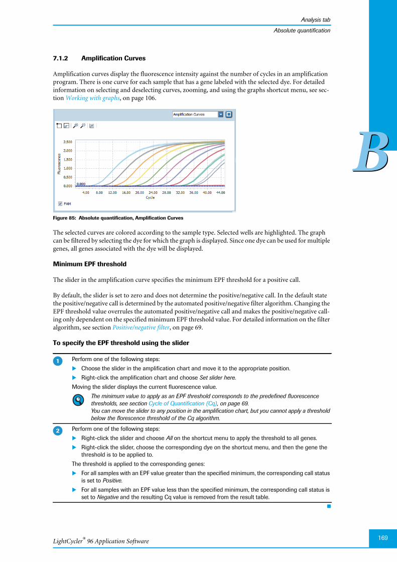
LightCycler® 96 Application Software
Analysis tab
169
BB
Absolute quantification
7.1.2 Amplification Curves
Amplification curves display the fluorescence intensity against the number of cycles in an amplificationprogram. There is one curve for each sample that has a gene labeled with the selected dye. For detailedinformation on selecting and deselecting curves, zooming, and using the graphs shortcut menu, see sec-tion Working with graphs, on page 106.
Figure 85: Absolute quantification, Amplification Curves
The selected curves are colored according to the sample type. Selected wells are highlighted. The graphcan be filtered by selecting the dye for which the graph is displayed. Since one dye can be used for multiplegenes, all genes associated with the dye will be displayed.
Minimum EPF threshold
The slider in the amplification curve specifies the minimum EPF threshold for a positive call.
By default, the slider is set to zero and does not determine the positive/negative call. In the default statethe positive/negative call is determined by the automated positive/negative filter algorithm. Changing theEPF threshold value overrules the automated positive/negative call and makes the positive/negative call-ing only dependent on the specified minimum EPF threshold value. For detailed information on the filteralgorithm, see section Positive/negative filter, on page 69.
To specify the EPF threshold using the slider
Perform one of the following steps:
Choose the slider in the amplification chart and move it to the appropriate position.
Right-click the amplification chart and choose Set slider here.
Moving the slider displays the current fluorescence value.
The minimum value to apply as an EPF threshold corresponds to the predefined fluorescencethresholds, see section Cycle of Quantification (Cq), on page 69.You can move the slider to any position in the amplification chart, but you cannot apply a thresholdbelow the florescence threshold of the Cq algorithm.
Perform one of the following steps:
Right-click the slider and choose All on the shortcut menu to apply the threshold to all genes.
Right-click the slider, choose the corresponding dye on the shortcut menu, and then the gene thethreshold is to be applied to.
The threshold is applied to the corresponding genes:
For all samples with an EPF value greater than the specified minimum, the corresponding call statusis set to Positive.
For all samples with an EPF value less than the specified minimum, the corresponding call status isset to Negative and the resulting Cq value is removed from the result table.
�
�
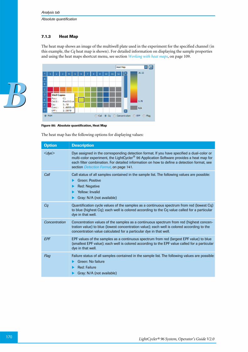
LightCycler® 96 System, Operator’s Guide V2.0170
Analysis tab
BB
Absolute quantification
7.1.3 Heat Map
The heat map shows an image of the multiwell plate used in the experiment for the specified channel (inthis example, the Cq heat map is shown). For detailed information on displaying the sample propertiesand using the heat maps shortcut menu, see section Working with heat maps, on page 109.
Figure 86: Absolute quantification, Heat Map
The heat map has the following options for displaying values:
Option Description
<dye> Dye assigned in the corresponding detection format. If you have specified a dual-color ormulti-color experiment, the LightCycler® 96 Application Software provides a heat map foreach filter combination. For detailed information on how to define a detection format, seesection Detection Format, on page 141.
Call Call status of all samples contained in the sample list. The following values are possible:
Green: Positive
Red: Negative
Yellow: Invalid
Gray: N/A (not available)
Cq Quantification cycle values of the samples as a continuous spectrum from red (lowest Cq)to blue (highest Cq); each well is colored according to the Cq value called for a particulardye in that well.
Concentration Concentration values of the samples as a continuous spectrum from red (highest concen-tration value) to blue (lowest concentration value); each well is colored according to theconcentration value calculated for a particular dye in that well.
EPF EPF values of the samples as a continuous spectrum from red (largest EPF value) to blue(smallest EPF value); each well is colored according to the EPF value called for a particulardye in that well.
Flag Failure status of all samples contained in the sample list. The following values are possible:
Green: No failure
Red: Failure
Gray: N/A (not available)
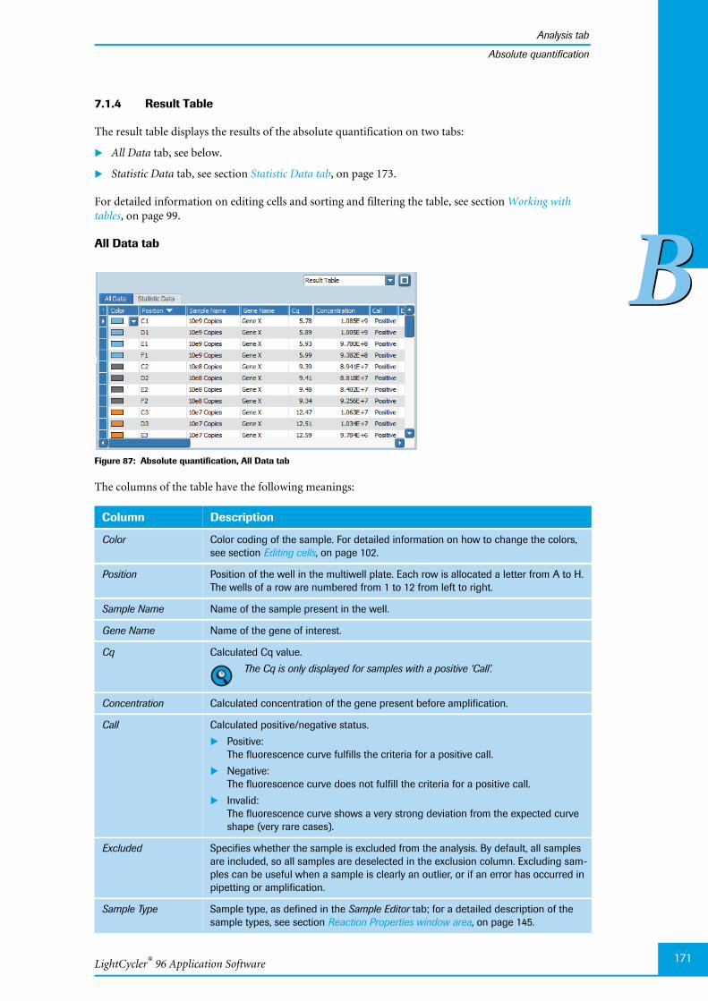
LightCycler® 96 Application Software
Analysis tab
171
BB
Absolute quantification
7.1.4 Result Table
The result table displays the results of the absolute quantification on two tabs:
All Data tab, see below.
Statistic Data tab, see section Statistic Data tab, on page 173.
For detailed information on editing cells and sorting and filtering the table, see section Working withtables, on page 99.
All Data tab
Figure 87: Absolute quantification, All Data tab
The columns of the table have the following meanings:
Column Description
Color Color coding of the sample. For detailed information on how to change the colors,see section Editing cells, on page 102.
Position Position of the well in the multiwell plate. Each row is allocated a letter from A to H.The wells of a row are numbered from 1 to 12 from left to right.
Sample Name Name of the sample present in the well.
Gene Name Name of the gene of interest.
Cq Calculated Cq value.
The Cq is only displayed for samples with a positive ‘Call’.
Concentration Calculated concentration of the gene present before amplification.
Call Calculated positive/negative status.
Positive:The fluorescence curve fulfills the criteria for a positive call.
Negative:The fluorescence curve does not fulfill the criteria for a positive call.
Invalid:The fluorescence curve shows a very strong deviation from the expected curveshape (very rare cases).
Excluded Specifies whether the sample is excluded from the analysis. By default, all samplesare included, so all samples are deselected in the exclusion column. Excluding sam-ples can be useful when a sample is clearly an outlier, or if an error has occurred inpipetting or amplification.
Sample Type Sample type, as defined in the Sample Editor tab; for a detailed description of thesample types, see section Reaction Properties window area, on page 145.
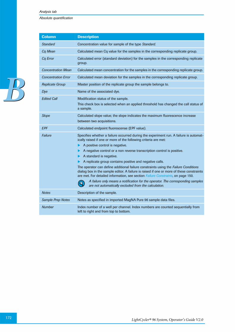
LightCycler® 96 System, Operator’s Guide V2.0172
Analysis tab
BB
Absolute quantification
Standard Concentration value for sample of the type Standard.
Cq Mean Calculated mean Cq value for the samples in the corresponding replicate group.
Cq Error Calculated error (standard deviation) for the samples in the corresponding replicategroup.
Concentration Mean Calculated mean concentration for the samples in the corresponding replicate group.
Concentration Error Calculated mean deviation for the samples in the corresponding replicate group.
Replicate Group Master position of the replicate group the sample belongs to.
Dye Name of the associated dye.
Edited Call Modification status of the sample.
This check box is selected when an applied threshold has changed the call status ofa sample.
Slope Calculated slope value; the slope indicates the maximum fluorescence increase
between two acquisitions.
EPF Calculated endpoint fluorescense (EPF value).
Failure Specifies whether a failure occurred during the experiment run. A failure is automat-ically raised if one or more of the following criteria are met:
A positive control is negative.
A negative control or a non reverse transcription control is positive.
A standard is negative.
A replicate group contains positive and negative calls.
The operator can define additional failure constraints using the Failure Conditionsdialog box in the sample editor. A failure is raised if one or more of these constraintsare met. For detailed information, see section Failure Constraints, on page 150.
A failure only means a notification for the operator. The corresponding samplesare not automatically excluded from the calculation.
Notes Description of the sample.
Sample Prep Notes Notes as specified in imported MagNA Pure 96 sample data files.
Number Index number of a well per channel. Index numbers are counted sequentially fromleft to right and from top to bottom.
Column Description
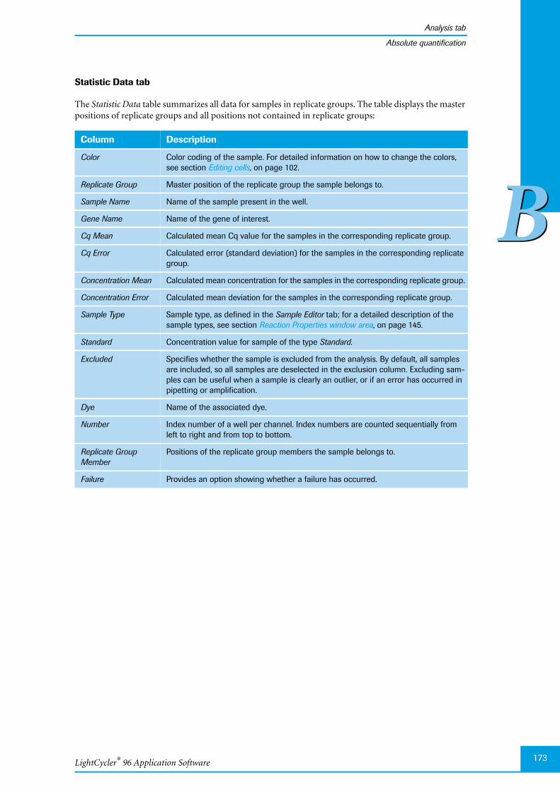
LightCycler® 96 Application Software
Analysis tab
173
BB
Absolute quantification
Statistic Data tab
The Statistic Data table summarizes all data for samples in replicate groups. The table displays the masterpositions of replicate groups and all positions not contained in replicate groups:
Column Description
Color Color coding of the sample. For detailed information on how to change the colors,see section Editing cells, on page 102.
Replicate Group Master position of the replicate group the sample belongs to.
Sample Name Name of the sample present in the well.
Gene Name Name of the gene of interest.
Cq Mean Calculated mean Cq value for the samples in the corresponding replicate group.
Cq Error Calculated error (standard deviation) for the samples in the corresponding replicategroup.
Concentration Mean Calculated mean concentration for the samples in the corresponding replicate group.
Concentration Error Calculated mean deviation for the samples in the corresponding replicate group.
Sample Type Sample type, as defined in the Sample Editor tab; for a detailed description of thesample types, see section Reaction Properties window area, on page 145.
Standard Concentration value for sample of the type Standard.
Excluded Specifies whether the sample is excluded from the analysis. By default, all samplesare included, so all samples are deselected in the exclusion column. Excluding sam-ples can be useful when a sample is clearly an outlier, or if an error has occurred inpipetting or amplification.
Dye Name of the associated dye.
Number Index number of a well per channel. Index numbers are counted sequentially fromleft to right and from top to bottom.
Replicate GroupMember
Positions of the replicate group members the sample belongs to.
Failure Provides an option showing whether a failure has occurred.
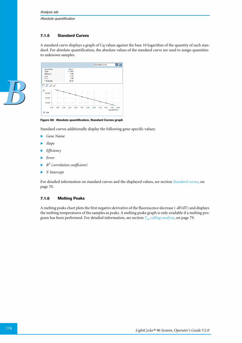
LightCycler® 96 System, Operator’s Guide V2.0174
Analysis tab
BB
Absolute quantification
7.1.5 Standard Curves
A standard curve displays a graph of Cq values against the base 10 logarithm of the quantity of each stan-dard. For absolute quantification, the absolute values of the standard curve are used to assign quantitiesto unknown samples.
Figure 88: Absolute quantification, Standard Curves graph
Standard curves additionally display the following gene-specific values:
Gene Name
Slope
Efficiency
Error
R2 (correlation coefficient)
Y-Intercept
For detailed information on standard curves and the displayed values, see section Standard curves, onpage 70.
7.1.6 Melting Peaks
A melting peaks chart plots the first negative derivative of the fluorescence decrease (-dF/dT) and displaysthe melting temperatures of the samples as peaks. A melting peaks graph is only available if a melting pro-gram has been performed. For detailed information, see section Tm calling analysis, on page 79.
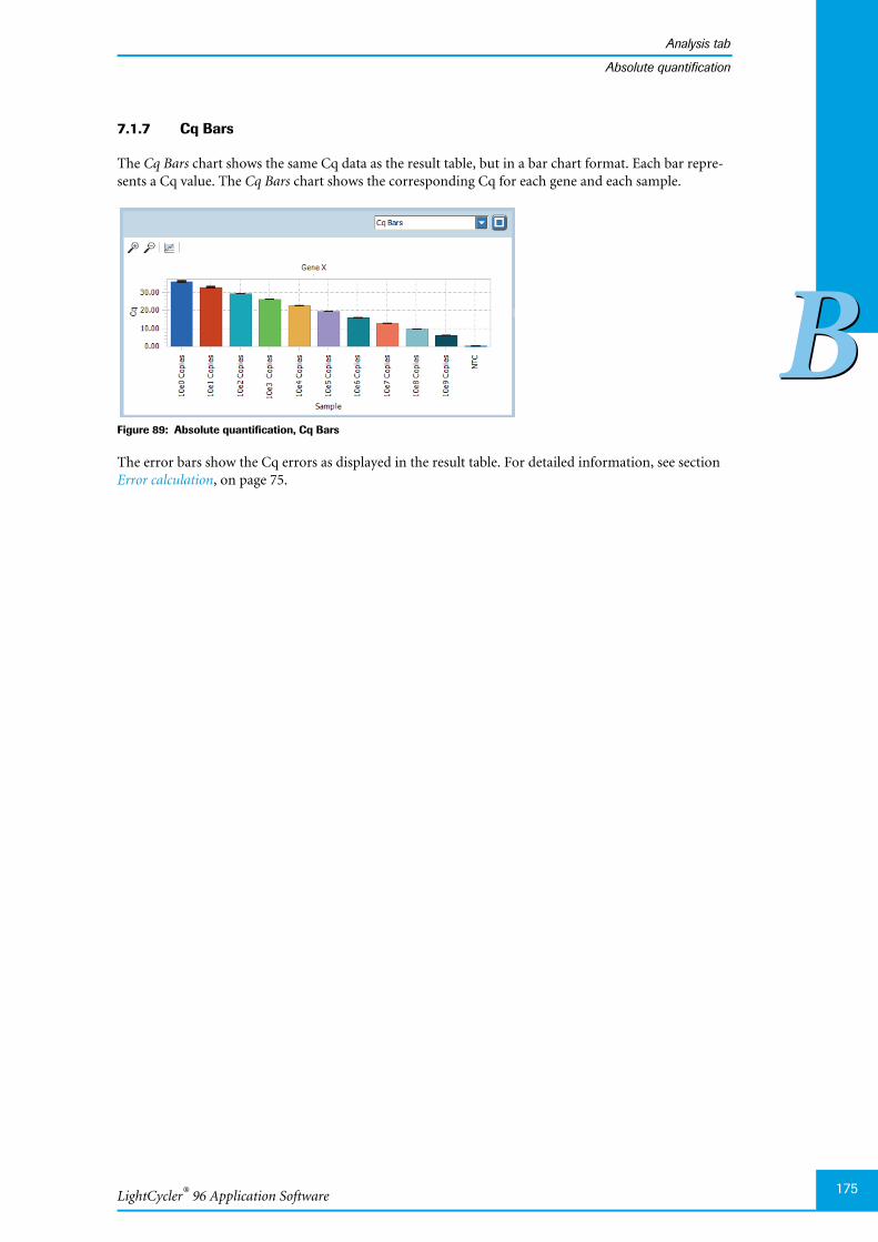
LightCycler® 96 Application Software
Analysis tab
175
BB
Absolute quantification
7.1.7 Cq Bars
The Cq Bars chart shows the same Cq data as the result table, but in a bar chart format. Each bar repre-sents a Cq value. The Cq Bars chart shows the corresponding Cq for each gene and each sample.
Figure 89: Absolute quantification, Cq Bars
The error bars show the Cq errors as displayed in the result table. For detailed information, see sectionError calculation, on page 75.

LightCycler® 96 System, Operator’s Guide V2.0176
Analysis tab
BB
Relative quantification
7.2 Relative quantification
Relative quantification compares the levels of two different gene sequences in a single sample (for exam-ple, target gene of interest and a reference gene), and expresses the final result as a ratio of these genes. Fordetailed information on relative quantification, see section Relative quantification analysis, on page 72. Bydefault, the tab for viewing a relative quantification analysis is called Rel Quant.
Figure 90: Rel Quant tab
The views selection list in the sections of the Analysis tab provides the following data:
Amplification Curves; see section Amplification Curves, on page 169.
Ratio Bars; see section Ratio Bars, on page 180.
Result Table; see section Result Table, on page 181.
Standard Curves; see section Standard Curves, on page 174.
Melting Peaks; see section Melting Peaks, on page 203.This option is only available if a melting program has been performed.
Heat Map; see section Heat Map, on page 170.
Cq Bars; see section Cq Bars, on page 175.
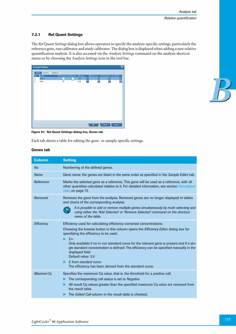
LightCycler® 96 Application Software
Analysis tab
177
BB
Relative quantification
7.2.1 Rel Quant Settings
The Rel Quant Settings dialog box allows operators to specify the analysis-specific settings, particularly thereference gene, run calibrator and study calibrator. The dialog box is displayed when adding a new relativequantification analysis. It is also accessed via the Analysis Settings command on the analysis shortcutmenu or by choosing the Analysis Settings icon in the tool bar.
Figure 91: Rel Quant Settings dialog box, Genes tab
Each tab shows a table for editing the gene- or sample-specific settings.
Genes tab
Column Setting
No Numbering of the defined genes.
Name Gene name; the genes are listed in the same order as specified in the Sample Editor tab.
Reference Marks the selected gene as a reference. This gene will be used as a reference, with allother quantities calculated relative to it. For detailed information, see section Normalizedratio, on page 72.
Removed Removes the gene from the analysis. Removed genes are no longer displayed in tablesand charts of the corresponding analysis.
It is possible to add or remove multiple genes simultaneously by multi-selecting andusing either the ‘Add Selected’ or ‘Remove Selected’ command on the shortcutmenu of the table.
Efficiency Efficiency used for calculating efficiency-corrected concentrations.
Choosing the browse button in this column opens the Efficiency Editor dialog box forspecifiying the efficiency to be used:
E=Only available if no in-run standard curve for the relevant gene is present and if a sin-gle standard concentration is defined: The efficiency can be specified manually in thedisplayed field.Default value: 2.0
E from standard curveThe efficiency has been derived from the standard curve.
Maximal Cq Specifies the maximum Cq value, that is, the threshold for a positive call.
The corresponding call status is set to Negative.
All result Cq values greater than the specified maximum Cq value are removed fromthe result table.
The Edited Call column in the result table is checked.
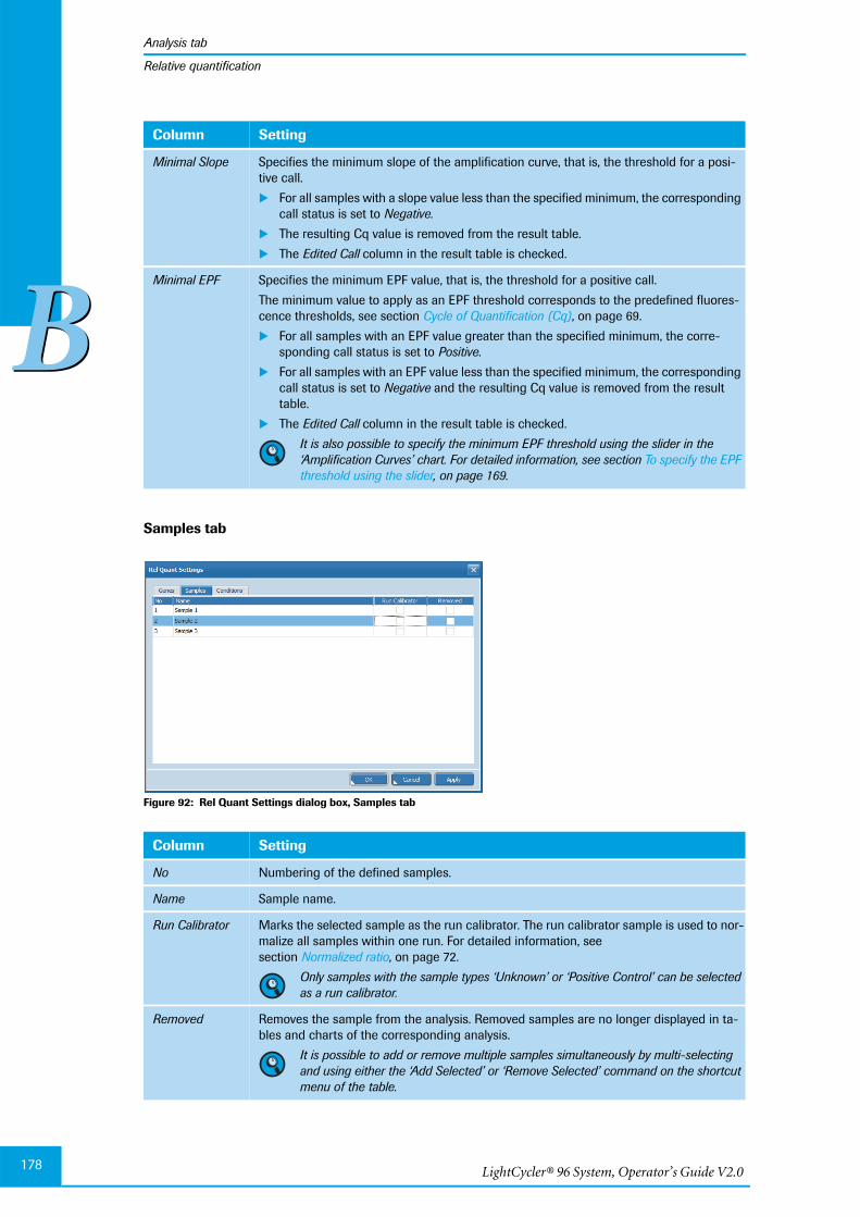
LightCycler® 96 System, Operator’s Guide V2.0178
Analysis tab
BB
Relative quantification
Samples tab
Figure 92: Rel Quant Settings dialog box, Samples tab
Minimal Slope Specifies the minimum slope of the amplification curve, that is, the threshold for a posi-tive call.
For all samples with a slope value less than the specified minimum, the correspondingcall status is set to Negative.
The resulting Cq value is removed from the result table.
The Edited Call column in the result table is checked.
Minimal EPF Specifies the minimum EPF value, that is, the threshold for a positive call.
The minimum value to apply as an EPF threshold corresponds to the predefined fluores-cence thresholds, see section Cycle of Quantification (Cq), on page 69.
For all samples with an EPF value greater than the specified minimum, the corre-sponding call status is set to Positive.
For all samples with an EPF value less than the specified minimum, the correspondingcall status is set to Negative and the resulting Cq value is removed from the resulttable.
The Edited Call column in the result table is checked.
It is also possible to specify the minimum EPF threshold using the slider in the‘Amplification Curves’ chart. For detailed information, see section To specify the EPFthreshold using the slider, on page 169.
Column Setting
No Numbering of the defined samples.
Name Sample name.
Run Calibrator Marks the selected sample as the run calibrator. The run calibrator sample is used to nor-malize all samples within one run. For detailed information, seesection Normalized ratio, on page 72.
Only samples with the sample types ‘Unknown’ or ‘Positive Control’ can be selectedas a run calibrator.
Removed Removes the sample from the analysis. Removed samples are no longer displayed in ta-bles and charts of the corresponding analysis.
It is possible to add or remove multiple samples simultaneously by multi-selectingand using either the ‘Add Selected’ or ‘Remove Selected’ command on the shortcutmenu of the table.
Column Setting
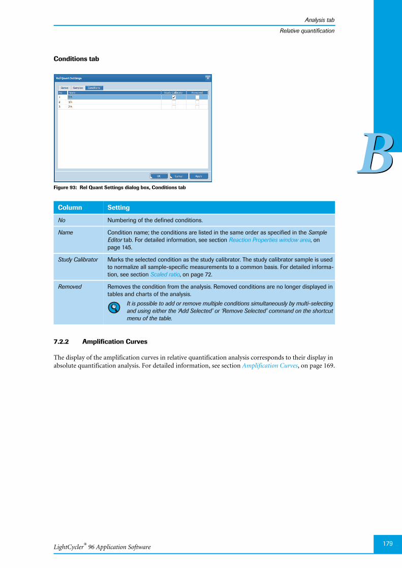
LightCycler® 96 Application Software
Analysis tab
179
BB
Relative quantification
Conditions tab
Figure 93: Rel Quant Settings dialog box, Conditions tab
7.2.2 Amplification Curves
The display of the amplification curves in relative quantification analysis corresponds to their display inabsolute quantification analysis. For detailed information, see section Amplification Curves, on page 169.
Column Setting
No Numbering of the defined conditions.
Name Condition name; the conditions are listed in the same order as specified in the SampleEditor tab. For detailed information, see section Reaction Properties window area, onpage 145.
Study Calibrator Marks the selected condition as the study calibrator. The study calibrator sample is usedto normalize all sample-specific measurements to a common basis. For detailed informa-tion, see section Scaled ratio, on page 72.
Removed Removes the condition from the analysis. Removed conditions are no longer displayed intables and charts of the analysis.
It is possible to add or remove multiple conditions simultaneously by multi-selectingand using either the ‘Add Selected’ or ‘Remove Selected’ command on the shortcutmenu of the table.

LightCycler® 96 System, Operator’s Guide V2.0180
Analysis tab
BB
Relative quantification
7.2.3 Ratio Bars
The Ratio Bars chart shows the same ratio data as the result table, but in a bar chart format. Each bar rep-resents a ratio, a normalized ratio, or a scaled ratio.
Figure 94: Ratio Bars chart
The Ratio Bars chart shows the corresponding ratio, normalized ratio, or scaled ratio for each gene, sam-ple, and condition.
Data Visualization
The ratios displayed in the Ratio Bars chart, as well as how they are scaled and ordered, depend on thesettings the operator specifies in the Data Visualization dialog box. The dialog box is accessed via the DataVisualization command on the chart’s shortcut menu or by choosing the Data Visualization icon.
Figure 95: Data Visualization dialog box
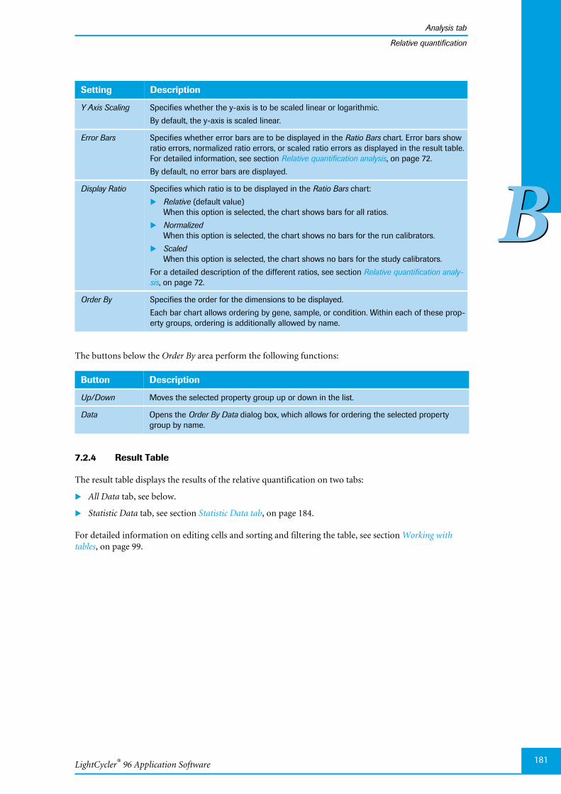
LightCycler® 96 Application Software
Analysis tab
181
BB
Relative quantification
The buttons below the Order By area perform the following functions:
7.2.4 Result Table
The result table displays the results of the relative quantification on two tabs:
All Data tab, see below.
Statistic Data tab, see section Statistic Data tab, on page 184.
For detailed information on editing cells and sorting and filtering the table, see section Working withtables, on page 99.
Setting Description
Y Axis Scaling Specifies whether the y-axis is to be scaled linear or logarithmic.
By default, the y-axis is scaled linear.
Error Bars Specifies whether error bars are to be displayed in the Ratio Bars chart. Error bars showratio errors, normalized ratio errors, or scaled ratio errors as displayed in the result table.For detailed information, see section Relative quantification analysis, on page 72.
By default, no error bars are displayed.
Display Ratio Specifies which ratio is to be displayed in the Ratio Bars chart:
Relative (default value)When this option is selected, the chart shows bars for all ratios.
NormalizedWhen this option is selected, the chart shows no bars for the run calibrators.
ScaledWhen this option is selected, the chart shows no bars for the study calibrators.
For a detailed description of the different ratios, see section Relative quantification analy-sis, on page 72.
Order By Specifies the order for the dimensions to be displayed.
Each bar chart allows ordering by gene, sample, or condition. Within each of these prop-erty groups, ordering is additionally allowed by name.
Button Description
Up/Down Moves the selected property group up or down in the list.
Data Opens the Order By Data dialog box, which allows for ordering the selected propertygroup by name.
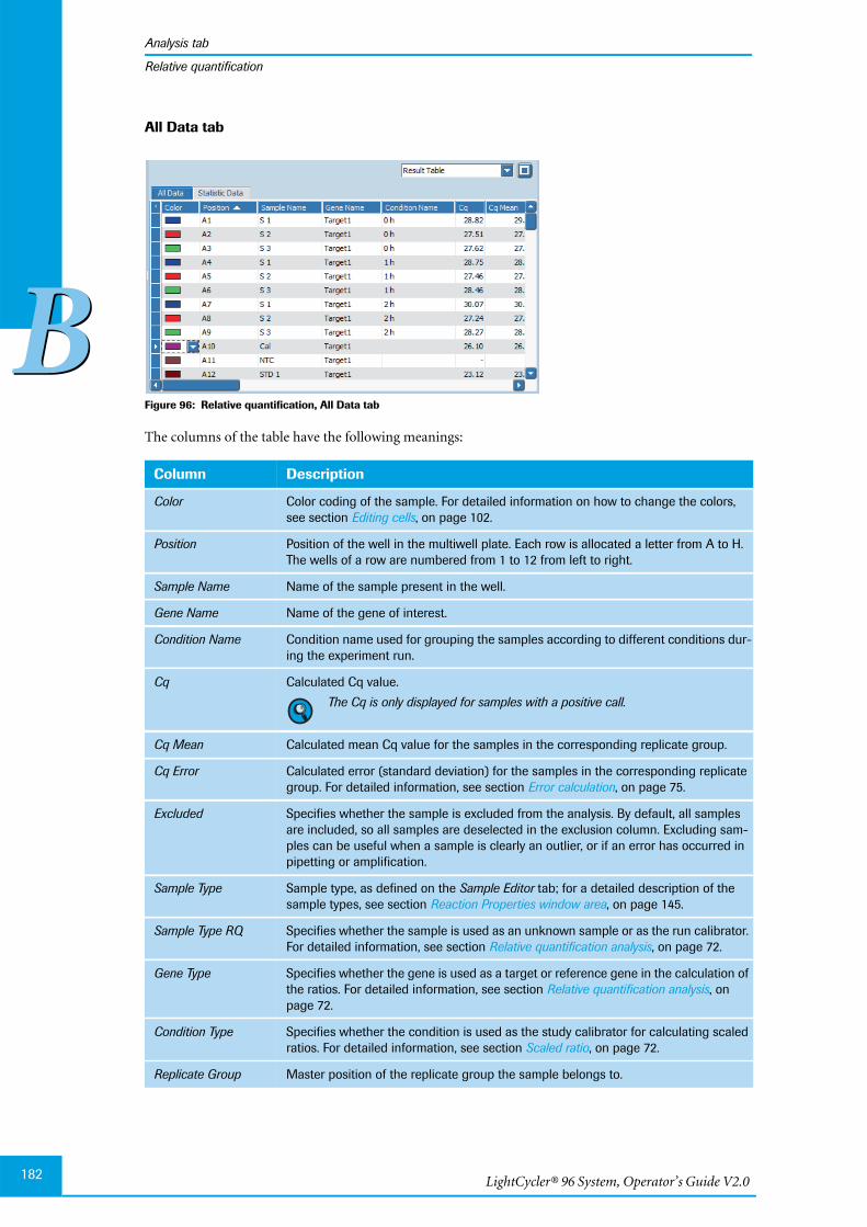
LightCycler® 96 System, Operator’s Guide V2.0182
Analysis tab
BB
Relative quantification
All Data tab
Figure 96: Relative quantification, All Data tab
The columns of the table have the following meanings:
Column Description
Color Color coding of the sample. For detailed information on how to change the colors,see section Editing cells, on page 102.
Position Position of the well in the multiwell plate. Each row is allocated a letter from A to H.The wells of a row are numbered from 1 to 12 from left to right.
Sample Name Name of the sample present in the well.
Gene Name Name of the gene of interest.
Condition Name Condition name used for grouping the samples according to different conditions dur-ing the experiment run.
Cq Calculated Cq value.
The Cq is only displayed for samples with a positive call.
Cq Mean Calculated mean Cq value for the samples in the corresponding replicate group.
Cq Error Calculated error (standard deviation) for the samples in the corresponding replicategroup. For detailed information, see section Error calculation, on page 75.
Excluded Specifies whether the sample is excluded from the analysis. By default, all samplesare included, so all samples are deselected in the exclusion column. Excluding sam-ples can be useful when a sample is clearly an outlier, or if an error has occurred inpipetting or amplification.
Sample Type Sample type, as defined on the Sample Editor tab; for a detailed description of thesample types, see section Reaction Properties window area, on page 145.
Sample Type RQ Specifies whether the sample is used as an unknown sample or as the run calibrator.For detailed information, see section Relative quantification analysis, on page 72.
Gene Type Specifies whether the gene is used as a target or reference gene in the calculation ofthe ratios. For detailed information, see section Relative quantification analysis, onpage 72.
Condition Type Specifies whether the condition is used as the study calibrator for calculating scaledratios. For detailed information, see section Scaled ratio, on page 72.
Replicate Group Master position of the replicate group the sample belongs to.
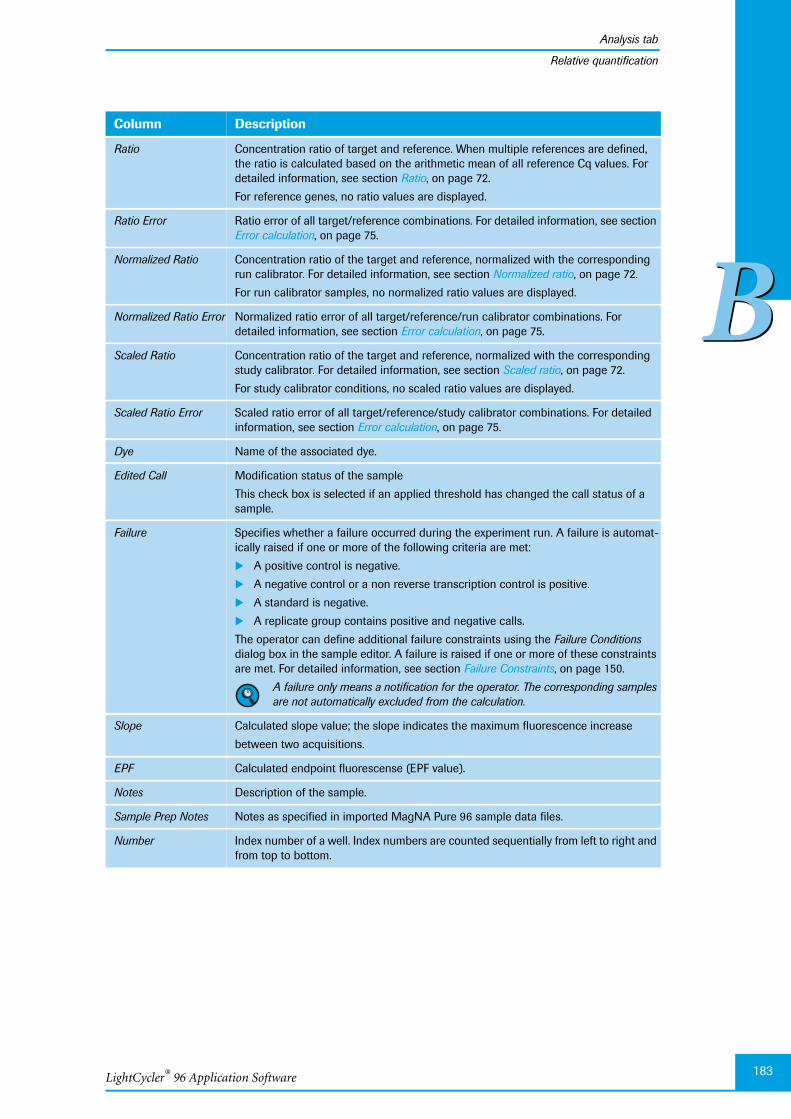
LightCycler® 96 Application Software
Analysis tab
183
BB
Relative quantification
Ratio Concentration ratio of target and reference. When multiple references are defined,the ratio is calculated based on the arithmetic mean of all reference Cq values. Fordetailed information, see section Ratio, on page 72.
For reference genes, no ratio values are displayed.
Ratio Error Ratio error of all target/reference combinations. For detailed information, see sectionError calculation, on page 75.
Normalized Ratio Concentration ratio of the target and reference, normalized with the correspondingrun calibrator. For detailed information, see section Normalized ratio, on page 72.
For run calibrator samples, no normalized ratio values are displayed.
Normalized Ratio Error Normalized ratio error of all target/reference/run calibrator combinations. Fordetailed information, see section Error calculation, on page 75.
Scaled Ratio Concentration ratio of the target and reference, normalized with the correspondingstudy calibrator. For detailed information, see section Scaled ratio, on page 72.
For study calibrator conditions, no scaled ratio values are displayed.
Scaled Ratio Error Scaled ratio error of all target/reference/study calibrator combinations. For detailedinformation, see section Error calculation, on page 75.
Dye Name of the associated dye.
Edited Call Modification status of the sample
This check box is selected if an applied threshold has changed the call status of asample.
Failure Specifies whether a failure occurred during the experiment run. A failure is automat-ically raised if one or more of the following criteria are met:
A positive control is negative.
A negative control or a non reverse transcription control is positive.
A standard is negative.
A replicate group contains positive and negative calls.
The operator can define additional failure constraints using the Failure Conditionsdialog box in the sample editor. A failure is raised if one or more of these constraintsare met. For detailed information, see section Failure Constraints, on page 150.
A failure only means a notification for the operator. The corresponding samplesare not automatically excluded from the calculation.
Slope Calculated slope value; the slope indicates the maximum fluorescence increase
between two acquisitions.
EPF Calculated endpoint fluorescense (EPF value).
Notes Description of the sample.
Sample Prep Notes Notes as specified in imported MagNA Pure 96 sample data files.
Number Index number of a well. Index numbers are counted sequentially from left to right andfrom top to bottom.
Column Description
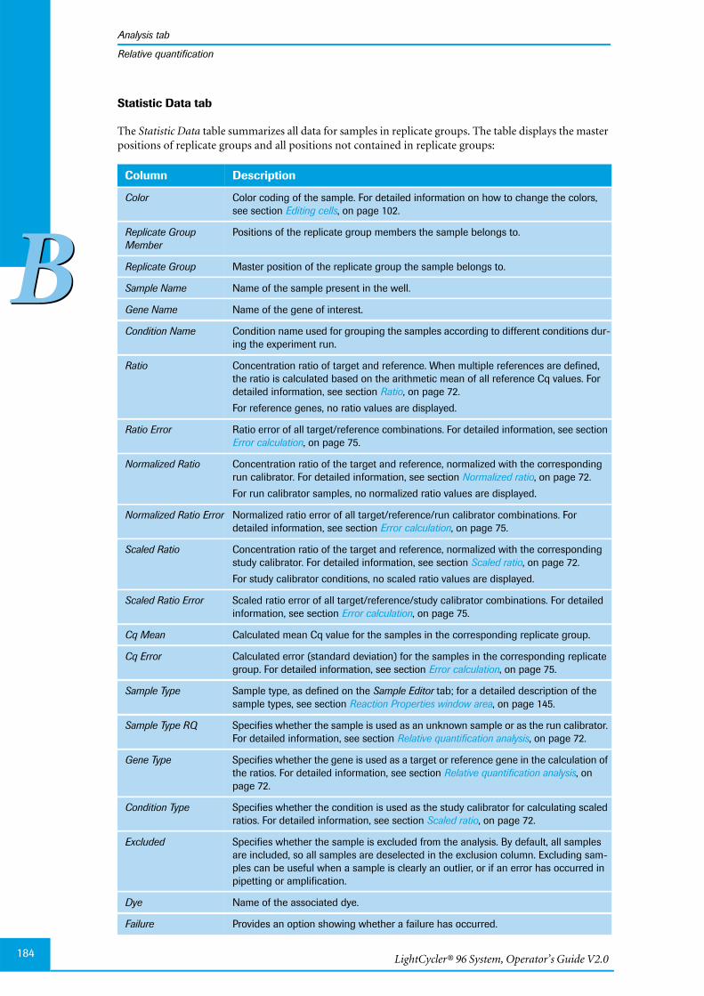
LightCycler® 96 System, Operator’s Guide V2.0184
Analysis tab
BB
Relative quantification
Statistic Data tab
The Statistic Data table summarizes all data for samples in replicate groups. The table displays the masterpositions of replicate groups and all positions not contained in replicate groups:
Column Description
Color Color coding of the sample. For detailed information on how to change the colors,see section Editing cells, on page 102.
Replicate GroupMember
Positions of the replicate group members the sample belongs to.
Replicate Group Master position of the replicate group the sample belongs to.
Sample Name Name of the sample present in the well.
Gene Name Name of the gene of interest.
Condition Name Condition name used for grouping the samples according to different conditions dur-ing the experiment run.
Ratio Concentration ratio of target and reference. When multiple references are defined,the ratio is calculated based on the arithmetic mean of all reference Cq values. Fordetailed information, see section Ratio, on page 72.
For reference genes, no ratio values are displayed.
Ratio Error Ratio error of all target/reference combinations. For detailed information, see sectionError calculation, on page 75.
Normalized Ratio Concentration ratio of the target and reference, normalized with the correspondingrun calibrator. For detailed information, see section Normalized ratio, on page 72.
For run calibrator samples, no normalized ratio values are displayed.
Normalized Ratio Error Normalized ratio error of all target/reference/run calibrator combinations. Fordetailed information, see section Error calculation, on page 75.
Scaled Ratio Concentration ratio of the target and reference, normalized with the correspondingstudy calibrator. For detailed information, see section Scaled ratio, on page 72.
For study calibrator conditions, no scaled ratio values are displayed.
Scaled Ratio Error Scaled ratio error of all target/reference/study calibrator combinations. For detailedinformation, see section Error calculation, on page 75.
Cq Mean Calculated mean Cq value for the samples in the corresponding replicate group.
Cq Error Calculated error (standard deviation) for the samples in the corresponding replicategroup. For detailed information, see section Error calculation, on page 75.
Sample Type Sample type, as defined on the Sample Editor tab; for a detailed description of thesample types, see section Reaction Properties window area, on page 145.
Sample Type RQ Specifies whether the sample is used as an unknown sample or as the run calibrator.For detailed information, see section Relative quantification analysis, on page 72.
Gene Type Specifies whether the gene is used as a target or reference gene in the calculation ofthe ratios. For detailed information, see section Relative quantification analysis, onpage 72.
Condition Type Specifies whether the condition is used as the study calibrator for calculating scaledratios. For detailed information, see section Scaled ratio, on page 72.
Excluded Specifies whether the sample is excluded from the analysis. By default, all samplesare included, so all samples are deselected in the exclusion column. Excluding sam-ples can be useful when a sample is clearly an outlier, or if an error has occurred inpipetting or amplification.
Dye Name of the associated dye.
Failure Provides an option showing whether a failure has occurred.
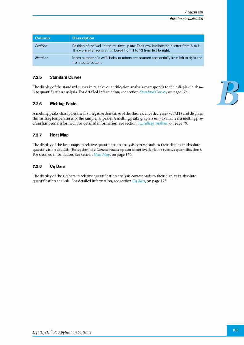
LightCycler® 96 Application Software
Analysis tab
185
BB
Relative quantification
7.2.5 Standard Curves
The display of the standard curves in relative quantification analysis corresponds to their display in abso-lute quantification analysis. For detailed information, see section Standard Curves, on page 174.
7.2.6 Melting Peaks
A melting peaks chart plots the first negative derivative of the fluorescence decrease (-dF/dT) and displaysthe melting temperatures of the samples as peaks. A melting peaks graph is only available if a melting pro-gram has been performed. For detailed information, see section Tm calling analysis, on page 79.
7.2.7 Heat Map
The display of the heat maps in relative quantification analysis corresponds to their display in absolutequantification analysis (Exception: the Concentration option is not available for relative quantification).For detailed information, see section Heat Map, on page 170.
7.2.8 Cq Bars
The display of the Cq bars in relative quantification analysis corresponds to their display in absolutequantification analysis. For detailed information, see section Cq Bars, on page 175.
Position Position of the well in the multiwell plate. Each row is allocated a letter from A to H.The wells of a row are numbered from 1 to 12 from left to right.
Number Index number of a well. Index numbers are counted sequentially from left to right andfrom top to bottom.
Column Description
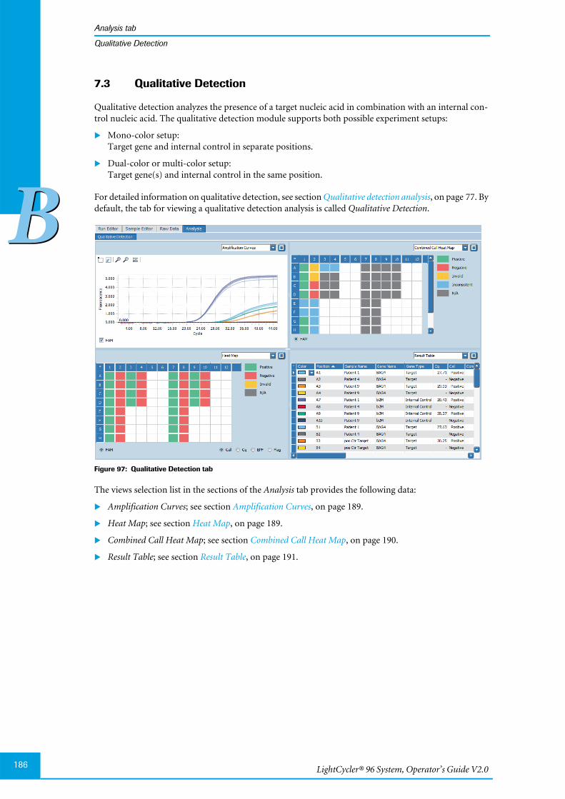
LightCycler® 96 System, Operator’s Guide V2.0186
Analysis tab
BB
Qualitative Detection
7.3 Qualitative Detection
Qualitative detection analyzes the presence of a target nucleic acid in combination with an internal con-trol nucleic acid. The qualitative detection module supports both possible experiment setups:
Mono-color setup:Target gene and internal control in separate positions.
Dual-color or multi-color setup:Target gene(s) and internal control in the same position.
For detailed information on qualitative detection, see section Qualitative detection analysis, on page 77. Bydefault, the tab for viewing a qualitative detection analysis is called Qualitative Detection.
Figure 97: Qualitative Detection tab
The views selection list in the sections of the Analysis tab provides the following data:
Amplification Curves; see section Amplification Curves, on page 189.
Heat Map; see section Heat Map, on page 189.
Combined Call Heat Map; see section Combined Call Heat Map, on page 190.
Result Table; see section Result Table, on page 191.

LightCycler® 96 Application Software
Analysis tab
187
BB
Qualitative Detection
7.3.1 Qualitative Detection settings for a dual- or multi-color setup
When target gene(s) and internal control are in the same position, the operator must specify the internalcontrol dye for automated result generation. The Qualitative Detection dialog box is displayed when add-ing a new analysis for a dual- or multi-color experiment.
Figure 98: Qualitative Detection dialog box
7.3.2 Qualitative Detection Settings
The Qualitiative Detection Settings dialog box allows operators to specify the analysis-specific settings. Thedialog box is accessed via the Analysis Settings command on the analysis shortcut menu or by choosing theAnalysis Settings icon in the tool bar.
For a mono-color experiment, it is mandatory to pair target genes and internal controls manually.
Figure 99: Qualitative Detection Settings dialog box, Genes tab
Setting Description
Target and internal control insame position?
Possible values:
Yes:Dual- or multi-color setup; the internal control dye is to be specified in theInternal Control Dye window area.
No:Mono-color setup; the options in the Internal Control Dye window area aredisabled.
Internal Control Dye List of the dyes as specified in the detection format; the selected dye is used asthe internal control dye.

LightCycler® 96 System, Operator’s Guide V2.0188
Analysis tab
BB
Qualitative Detection
Genes tab
Column Setting
No Numbering of the defined genes.
Name Target gene name; the genes are listed in the same order as specified on theSample Editor tab.
Removed Removes the gene from the analysis. Removed genes are no longer displayed in tablesand charts of the corresponding analysis.
It is possible to add or remove multiple genes simultaneously by multi-selecting andusing either the ‘Add Selected’ or ‘Remove Selected’ command on the shortcutmenu of the table.
Internal Control Internal control paired with the target gene specified in the Name column. Each internalcontrol gene (from multiple internal controls) can be assigned to one or more selectedtarget genes.
To avoid using a gene simultaneously as target and internal control, the following rulesapply:
If a gene is selected as internal control, it is not possible to assign another gene asinternal control to this gene.
If an internal control is assigned to a target gene, it is not possible to select this targetgene as internal control.
Maximal Cq Specifies the maximum Cq value, that is, the threshold for a positive call.
For all samples with a Cq value greater than the specified maximum Cq, the Cq valuesare removed from the result table.
The corresponding call status is set to Negative.
The Edited Call column in the result table is checked.
Minimal Slope Specifies the minimum slope of the amplification curve, that is, the threshold for a posi-tive call.
For all samples with a slope value less than the specified minimum, the correspondingcall status is set to Negative.
The resulting Cq value is removed from the result table.
The Edited Call column in the result table is checked.
Minimal EPF Specifies the minimum EPF value, that is, the threshold for a positive call.
The minimum value to apply as an EPF threshold corresponds to the predefined fluores-cence thresholds, see section Cycle of Quantification (Cq), on page 69.
For all samples with an EPF value less than the specified value, the corresponding callstatus is set to Negative.
The resulting Cq value is removed from the result table.
The Edited Call column in the result table is checked.
It is also possible to specify the minimum EPF threshold using the slider in the‘Amplification Curves’ chart. For detailed information, see section To specify the EPFthreshold using the slider, on page 169.
The ‘Minimal EPF’ cannot be lower than the threshold value used by the Cq algo-rithm. For detailed information, see section Cycle of Quantification (Cq), on page 69.
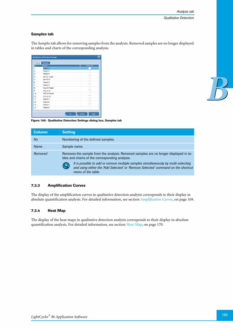
LightCycler® 96 Application Software
Analysis tab
189
BB
Qualitative Detection
Samples tab
The Samples tab allows for removing samples from the analysis. Removed samples are no longer displayedin tables and charts of the corresponding analysis.
Figure 100: Qualitative Detection Settings dialog box, Samples tab
7.3.3 Amplification Curves
The display of the amplification curves in qualitative detection analysis corresponds to their display inabsolute quantification analysis. For detailed information, see section Amplification Curves, on page 169.
7.3.4 Heat Map
The display of the heat maps in qualitative detection analysis corresponds to their display in absolutequantification analysis. For detailed information, see section Heat Map, on page 170.
Column Setting
No Numbering of the defined samples.
Name Sample name.
Removed Removes the sample from the analysis. Removed samples are no longer displayed in ta-bles and charts of the corresponding analysis.
It is possible to add or remove multiple samples simultaneously by multi-selectingand using either the ‘Add Selected’ or ‘Remove Selected’ command on the shortcutmenu of the table.
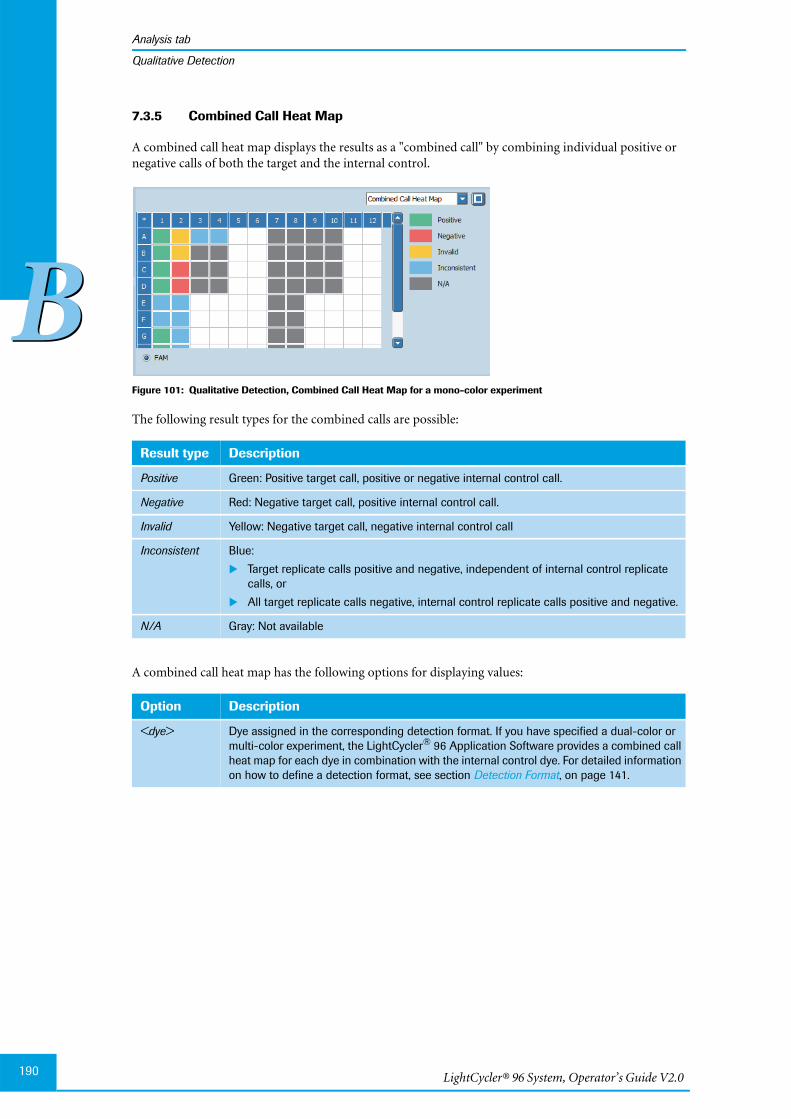
LightCycler® 96 System, Operator’s Guide V2.0190
Analysis tab
BB
Qualitative Detection
7.3.5 Combined Call Heat Map
A combined call heat map displays the results as a "combined call" by combining individual positive ornegative calls of both the target and the internal control.
Figure 101: Qualitative Detection, Combined Call Heat Map for a mono-color experiment
The following result types for the combined calls are possible:
A combined call heat map has the following options for displaying values:
Result type Description
Positive Green: Positive target call, positive or negative internal control call.
Negative Red: Negative target call, positive internal control call.
Invalid Yellow: Negative target call, negative internal control call
Inconsistent Blue:
Target replicate calls positive and negative, independent of internal control replicatecalls, or
All target replicate calls negative, internal control replicate calls positive and negative.
N/A Gray: Not available
Option Description
<dye> Dye assigned in the corresponding detection format. If you have specified a dual-color ormulti-color experiment, the LightCycler® 96 Application Software provides a combined callheat map for each dye in combination with the internal control dye. For detailed informationon how to define a detection format, see section Detection Format, on page 141.
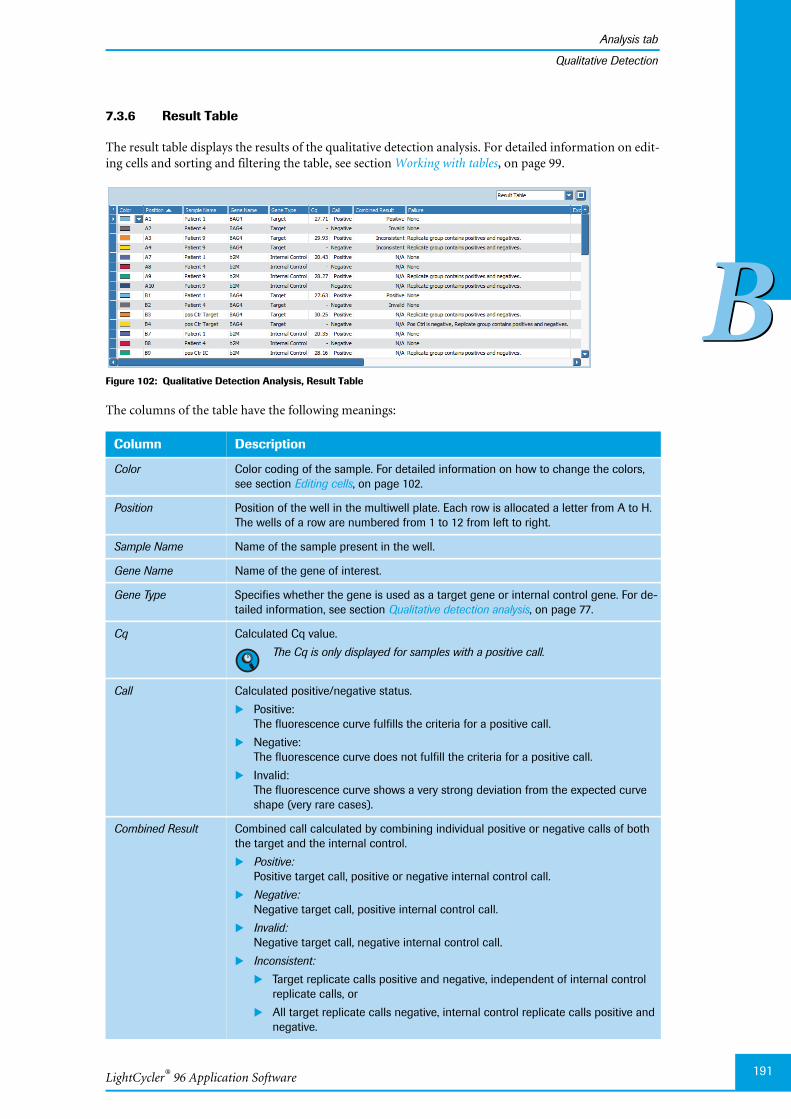
LightCycler® 96 Application Software
Analysis tab
191
BB
Qualitative Detection
7.3.6 Result Table
The result table displays the results of the qualitative detection analysis. For detailed information on edit-ing cells and sorting and filtering the table, see section Working with tables, on page 99.
Figure 102: Qualitative Detection Analysis, Result Table
The columns of the table have the following meanings:
Column Description
Color Color coding of the sample. For detailed information on how to change the colors,see section Editing cells, on page 102.
Position Position of the well in the multiwell plate. Each row is allocated a letter from A to H.The wells of a row are numbered from 1 to 12 from left to right.
Sample Name Name of the sample present in the well.
Gene Name Name of the gene of interest.
Gene Type Specifies whether the gene is used as a target gene or internal control gene. For de-tailed information, see section Qualitative detection analysis, on page 77.
Cq Calculated Cq value.
The Cq is only displayed for samples with a positive call.
Call Calculated positive/negative status.
Positive:The fluorescence curve fulfills the criteria for a positive call.
Negative:The fluorescence curve does not fulfill the criteria for a positive call.
Invalid:The fluorescence curve shows a very strong deviation from the expected curveshape (very rare cases).
Combined Result Combined call calculated by combining individual positive or negative calls of boththe target and the internal control.
Positive:Positive target call, positive or negative internal control call.
Negative:Negative target call, positive internal control call.
Invalid:Negative target call, negative internal control call.
Inconsistent:
Target replicate calls positive and negative, independent of internal controlreplicate calls, or
All target replicate calls negative, internal control replicate calls positive andnegative.
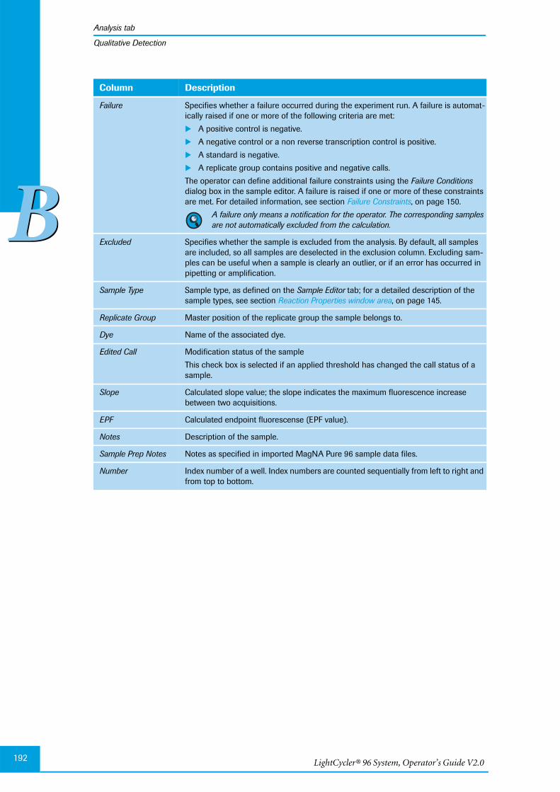
LightCycler® 96 System, Operator’s Guide V2.0192
Analysis tab
BB
Qualitative Detection
Failure Specifies whether a failure occurred during the experiment run. A failure is automat-ically raised if one or more of the following criteria are met:
A positive control is negative.
A negative control or a non reverse transcription control is positive.
A standard is negative.
A replicate group contains positive and negative calls.
The operator can define additional failure constraints using the Failure Conditionsdialog box in the sample editor. A failure is raised if one or more of these constraintsare met. For detailed information, see section Failure Constraints, on page 150.
A failure only means a notification for the operator. The corresponding samplesare not automatically excluded from the calculation.
Excluded Specifies whether the sample is excluded from the analysis. By default, all samplesare included, so all samples are deselected in the exclusion column. Excluding sam-ples can be useful when a sample is clearly an outlier, or if an error has occurred inpipetting or amplification.
Sample Type Sample type, as defined on the Sample Editor tab; for a detailed description of thesample types, see section Reaction Properties window area, on page 145.
Replicate Group Master position of the replicate group the sample belongs to.
Dye Name of the associated dye.
Edited Call Modification status of the sample
This check box is selected if an applied threshold has changed the call status of asample.
Slope Calculated slope value; the slope indicates the maximum fluorescence increasebetween two acquisitions.
EPF Calculated endpoint fluorescense (EPF value).
Notes Description of the sample.
Sample Prep Notes Notes as specified in imported MagNA Pure 96 sample data files.
Number Index number of a well. Index numbers are counted sequentially from left to right andfrom top to bottom.
Column Description
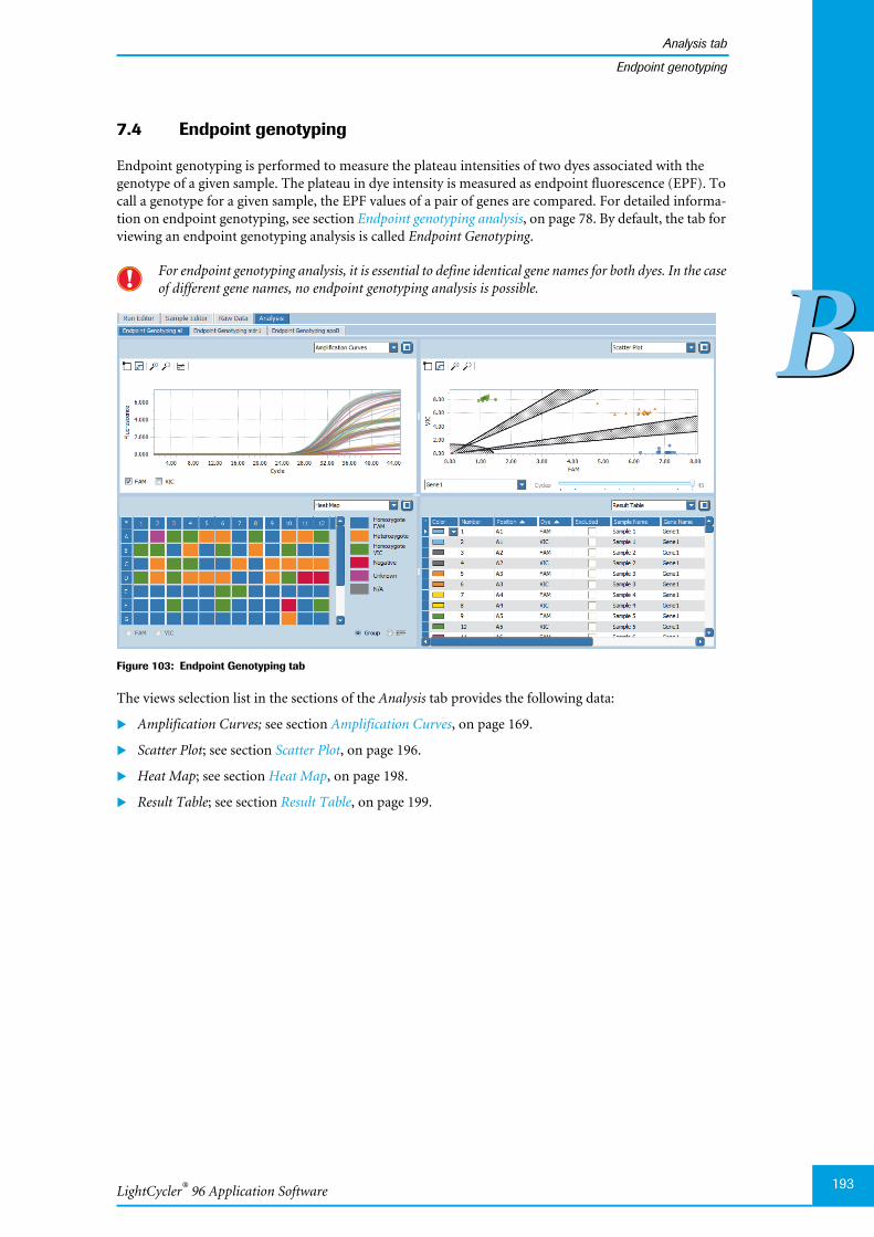
LightCycler® 96 Application Software
Analysis tab
193
BB
Endpoint genotyping
7.4 Endpoint genotyping
Endpoint genotyping is performed to measure the plateau intensities of two dyes associated with thegenotype of a given sample. The plateau in dye intensity is measured as endpoint fluorescence (EPF). Tocall a genotype for a given sample, the EPF values of a pair of genes are compared. For detailed informa-tion on endpoint genotyping, see section Endpoint genotyping analysis, on page 78. By default, the tab forviewing an endpoint genotyping analysis is called Endpoint Genotyping.
For endpoint genotyping analysis, it is essential to define identical gene names for both dyes. In the caseof different gene names, no endpoint genotyping analysis is possible.
Figure 103: Endpoint Genotyping tab
The views selection list in the sections of the Analysis tab provides the following data:
Amplification Curves; see section Amplification Curves, on page 169.
Scatter Plot; see section Scatter Plot, on page 196.
Heat Map; see section Heat Map, on page 198.
Result Table; see section Result Table, on page 199.
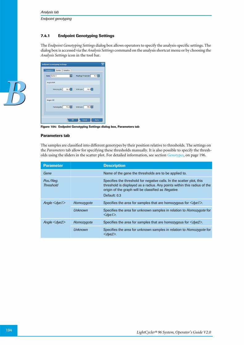
LightCycler® 96 System, Operator’s Guide V2.0194
Analysis tab
BB
Endpoint genotyping
7.4.1 Endpoint Genotyping Settings
The Endpoint Genotyping Settings dialog box allows operators to specify the analysis-specific settings. Thedialog box is accessed via the Analysis Settings command on the analysis shortcut menu or by choosing theAnalysis Settings icon in the tool bar.
Figure 104: Endpoint Genotyping Settings dialog box, Parameters tab
Parameters tab
The samples are classified into different genotypes by their position relative to thresholds. The settings onthe Parameters tab allow for specifying these thresholds manually. It is also possible to specify the thresh-olds using the sliders in the scatter plot. For detailed information, see section Genotypes, on page 196.
Parameter Description
Gene Name of the gene the thresholds are to be applied to.
Pos./Neg.Threshold
Specifies the threshold for negative calls. In the scatter plot, thisthreshold is displayed as a radius. Any points within this radius of theorigin of the graph will be classified as Negative.
Default: 0.3
Angle <dye1> Homozygote Specifies the area for samples that are homozygous for <dye1>.
Unknown Specifies the area for unknown samples in relation to Homozygote for<dye1>.
Angle <dye2> Homozygote Specifies the area for samples that are homozygous for <dye2>.
Unknown Specifies the area for unknown samples in relation to Homozygote for<dye2>.
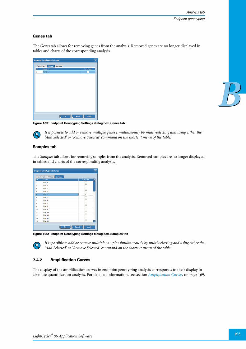
LightCycler® 96 Application Software
Analysis tab
195
BB
Endpoint genotyping
Genes tab
The Genes tab allows for removing genes from the analysis. Removed genes are no longer displayed intables and charts of the corresponding analysis.
Figure 105: Endpoint Genotyping Settings dialog box, Genes tab
It is possible to add or remove multiple genes simultaneously by multi-selecting and using either the‘Add Selected’ or ‘Remove Selected’ command on the shortcut menu of the table.
Samples tab
The Samples tab allows for removing samples from the analysis. Removed samples are no longer displayedin tables and charts of the corresponding analysis.
Figure 106: Endpoint Genotyping Settings dialog box, Samples tab
It is possible to add or remove multiple samples simultaneously by multi-selecting and using either the‘Add Selected’ or ‘Remove Selected’ command on the shortcut menu of the table.
7.4.2 Amplification Curves
The display of the amplification curves in endpoint genotyping analysis corresponds to their display inabsolute quantification analysis. For detailed information, see section Amplification Curves, on page 169.
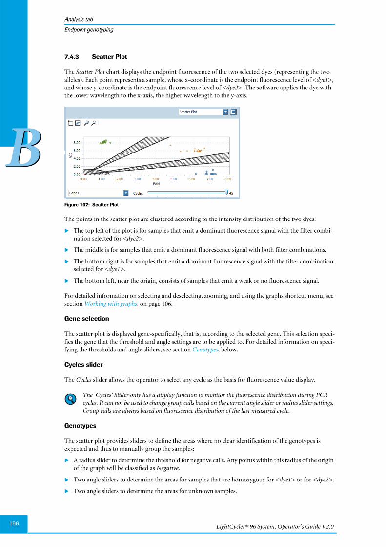
LightCycler® 96 System, Operator’s Guide V2.0196
Analysis tab
BB
Endpoint genotyping
7.4.3 Scatter Plot
The Scatter Plot chart displays the endpoint fluorescence of the two selected dyes (representing the twoalleles). Each point represents a sample, whose x-coordinate is the endpoint fluorescence level of <dye1>,and whose y-coordinate is the endpoint fluorescence level of <dye2>. The software applies the dye withthe lower wavelength to the x-axis, the higher wavelength to the y-axis.
Figure 107: Scatter Plot
The points in the scatter plot are clustered according to the intensity distribution of the two dyes:
The top left of the plot is for samples that emit a dominant fluorescence signal with the filter combi-nation selected for <dye2>.
The middle is for samples that emit a dominant fluorescence signal with both filter combinations.
The bottom right is for samples that emit a dominant fluorescence signal with the filter combinationselected for <dye1>.
The bottom left, near the origin, consists of samples that emit a weak or no fluorescence signal.
For detailed information on selecting and deselecting, zooming, and using the graphs shortcut menu, seesection Working with graphs, on page 106.
Gene selection
The scatter plot is displayed gene-specifically, that is, according to the selected gene. This selection speci-fies the gene that the threshold and angle settings are to be applied to. For detailed information on speci-fying the thresholds and angle sliders, see section Genotypes, below.
Cycles slider
The Cycles slider allows the operator to select any cycle as the basis for fluorescence value display.
The ‘Cycles’ Slider only has a display function to monitor the fluorescence distribution during PCRcycles. It can not be used to change group calls based on the current angle slider or radius slider settings.Group calls are always based on fluorescence distribution of the last measured cycle.
Genotypes
The scatter plot provides sliders to define the areas where no clear identification of the genotypes isexpected and thus to manually group the samples:
A radius slider to determine the threshold for negative calls. Any points within this radius of the originof the graph will be classified as Negative.
Two angle sliders to determine the areas for samples that are homozygous for <dye1> or for <dye2>.
Two angle sliders to determine the areas for unknown samples.
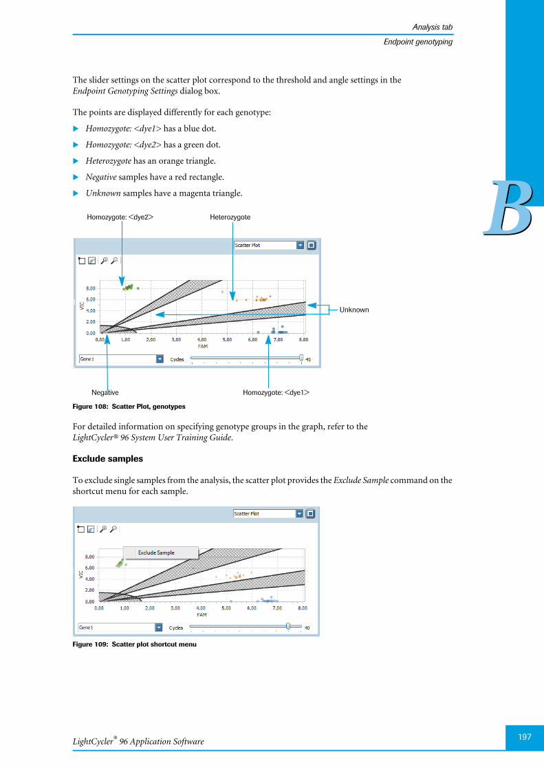
LightCycler® 96 Application Software
Analysis tab
197
BB
Endpoint genotyping
The slider settings on the scatter plot correspond to the threshold and angle settings in theEndpoint Genotyping Settings dialog box.
The points are displayed differently for each genotype:
Homozygote: <dye1> has a blue dot.
Homozygote: <dye2> has a green dot.
Heterozygote has an orange triangle.
Negative samples have a red rectangle.
Unknown samples have a magenta triangle.
Figure 108: Scatter Plot, genotypes
For detailed information on specifying genotype groups in the graph, refer to theLightCycler® 96 System User Training Guide.
Exclude samples
To exclude single samples from the analysis, the scatter plot provides the Exclude Sample command on theshortcut menu for each sample.
Figure 109: Scatter plot shortcut menu
Homozygote: <dye2> Heterozygote
Homozygote: <dye1>Negative
Unknown
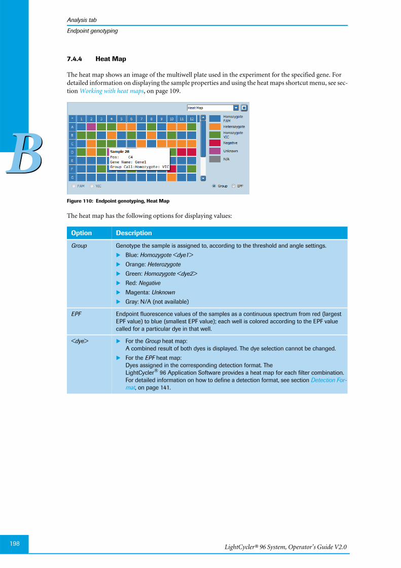
LightCycler® 96 System, Operator’s Guide V2.0198
Analysis tab
BB
Endpoint genotyping
7.4.4 Heat Map
The heat map shows an image of the multiwell plate used in the experiment for the specified gene. Fordetailed information on displaying the sample properties and using the heat maps shortcut menu, see sec-tion Working with heat maps, on page 109.
Figure 110: Endpoint genotyping, Heat Map
The heat map has the following options for displaying values:
Option Description
Group Genotype the sample is assigned to, according to the threshold and angle settings.
Blue: Homozygote <dye1>
Orange: Heterozygote
Green: Homozygote <dye2>
Red: Negative
Magenta: Unknown
Gray: N/A (not available)
EPF Endpoint fluorescence values of the samples as a continuous spectrum from red (largestEPF value) to blue (smallest EPF value); each well is colored according to the EPF valuecalled for a particular dye in that well.
<dye> For the Group heat map:A combined result of both dyes is displayed. The dye selection cannot be changed.
For the EPF heat map:Dyes assigned in the corresponding detection format. TheLightCycler® 96 Application Software provides a heat map for each filter combination.For detailed information on how to define a detection format, see section Detection For-mat, on page 141.

LightCycler® 96 Application Software
Analysis tab
199
BB
Endpoint genotyping
7.4.5 Result Table
The result table displays the results of the endpoint genotyping analysis. For detailed information on edit-ing cells and sorting and filtering the table, see section Working with tables, on page 99.
Figure 111: Endpoint genotyping, Result Table
The columns of the table have the following meanings:
Column Description
Color Color coding of the sample. For detailed information on how to change the colors,see section Editing cells, on page 102.
Number Index number of a well per dye. Index numbers are counted sequentially from left toright and from top to bottom.
Position Position of the well in the multiwell plate. Each row is allocated a letter from A to H.The wells of a row are numbered from 1 to 12 from left to right.
Dye Name of the associated dye.
Excluded Specifies whether the sample is excluded from the analysis. By default, all samplesare included, so all samples are deselected in the exclusion column. Excluding sam-ples can be useful when a sample is clearly an outlier, or if an error has occurred inpipetting or amplification.
Sample Name Name of the sample present in the well.
Gene Name Name of the gene of interest.
EPF Endpoint fluorescense value of the corresponding dye.
Genotype Genotype the sample is assigned to, according to the threshold and angle settings.
Notes Description of the sample.
Sample Prep Notes Notes as specified in imported MagNA Pure 96 sample data files. Operators can editthe displayed text.
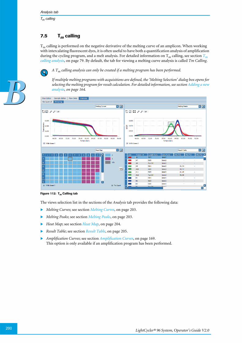
LightCycler® 96 System, Operator’s Guide V2.0200
Analysis tab
BB
Tm calling
7.5 Tm calling
Tm calling is performed on the negative derivative of the melting curve of an amplicon. When workingwith intercalating fluorescent dyes, it is often useful to have both a quantification analysis of amplificationduring the cycling program, and a melt analysis. For detailed information on Tm calling, see section Tmcalling analysis, on page 79. By default, the tab for viewing a melting curve analysis is called Tm Calling.
A Tm calling analysis can only be created if a melting program has been performed.
If multiple melting programs with acquisitions are defined, the ‘Melting Selection’ dialog box opens forselecting the melting program for result calculation. For detailed information, see section Adding a newanalysis, on page 164.
Figure 112: Tm Calling tab
The views selection list in the sections of the Analysis tab provides the following data:
Melting Curves; see section Melting Curves, on page 203.
Melting Peaks; see section Melting Peaks, on page 203.
Heat Map; see section Heat Map, on page 204.
Result Table; see section Result Table, on page 205.
Amplification Curves; see section Amplification Curves, on page 169.This option is only available if an amplification program has been performed.
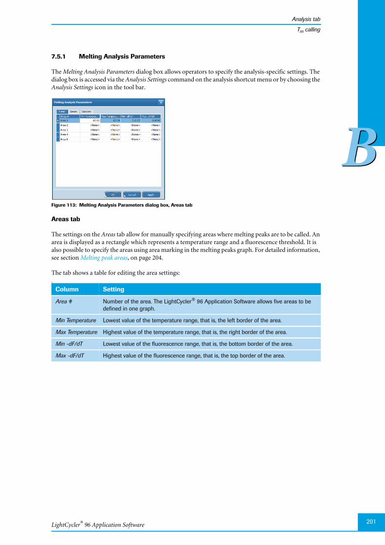
LightCycler® 96 Application Software
Analysis tab
201
BB
Tm calling
7.5.1 Melting Analysis Parameters
The Melting Analysis Parameters dialog box allows operators to specify the analysis-specific settings. Thedialog box is accessed via the Analysis Settings command on the analysis shortcut menu or by choosing theAnalysis Settings icon in the tool bar.
Figure 113: Melting Analysis Parameters dialog box, Areas tab
Areas tab
The settings on the Areas tab allow for manually specifying areas where melting peaks are to be called. Anarea is displayed as a rectangle which represents a temperature range and a fluorescence threshold. It isalso possible to specify the areas using area marking in the melting peaks graph. For detailed information,see section Melting peak areas, on page 204.
The tab shows a table for editing the area settings:68
Column Setting
Area # Number of the area. The LightCycler® 96 Application Software allows five areas to bedefined in one graph.
Min Temperature Lowest value of the temperature range, that is, the left border of the area.
Max Temperature Highest value of the temperature range, that is, the right border of the area.
Min -dF/dT Lowest value of the fluorescence range, that is, the bottom border of the area.
Max -dF/dT Highest value of the fluorescence range, that is, the top border of the area.
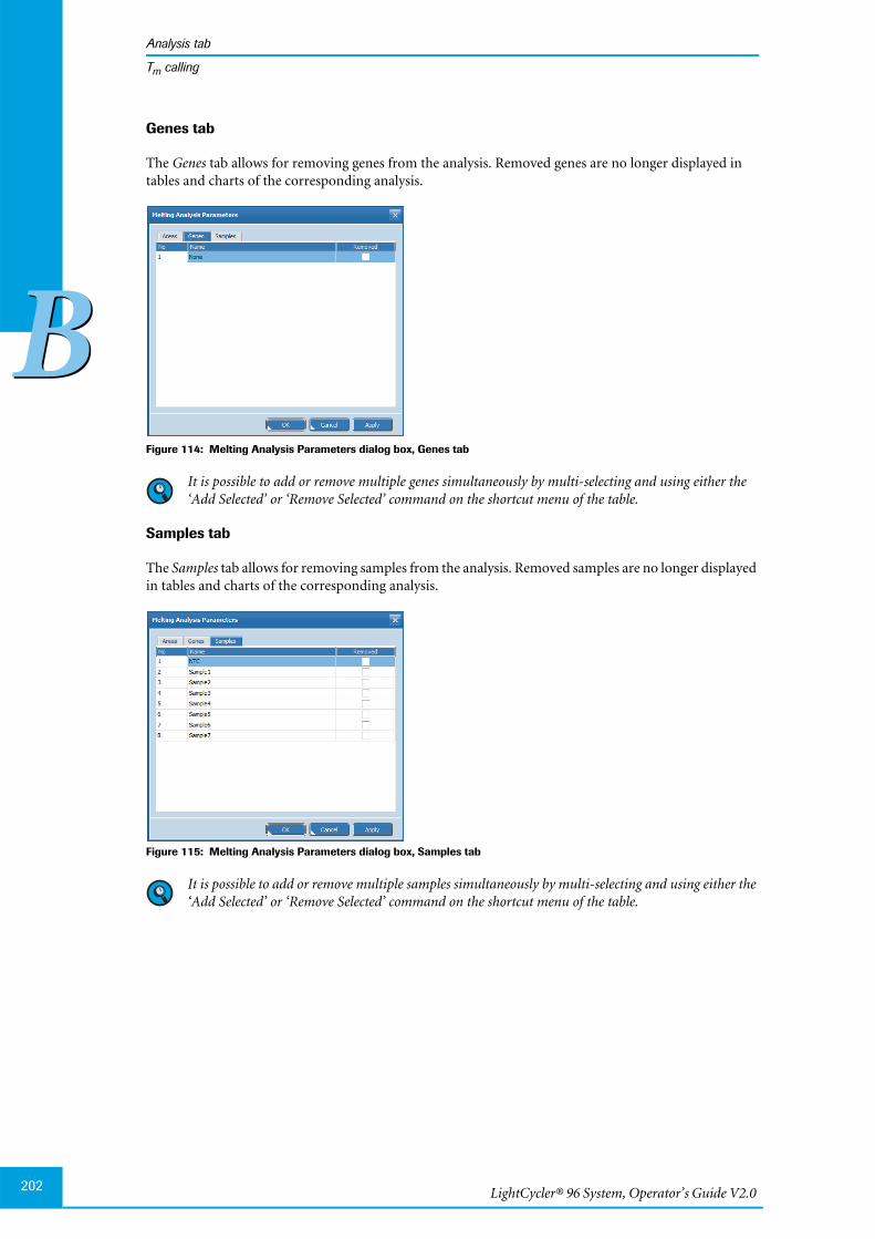
LightCycler® 96 System, Operator’s Guide V2.0202
Analysis tab
BB
Tm calling
Genes tab
The Genes tab allows for removing genes from the analysis. Removed genes are no longer displayed intables and charts of the corresponding analysis.
Figure 114: Melting Analysis Parameters dialog box, Genes tab
It is possible to add or remove multiple genes simultaneously by multi-selecting and using either the‘Add Selected’ or ‘Remove Selected’ command on the shortcut menu of the table.
Samples tab
The Samples tab allows for removing samples from the analysis. Removed samples are no longer displayedin tables and charts of the corresponding analysis.
Figure 115: Melting Analysis Parameters dialog box, Samples tab
It is possible to add or remove multiple samples simultaneously by multi-selecting and using either the‘Add Selected’ or ‘Remove Selected’ command on the shortcut menu of the table.
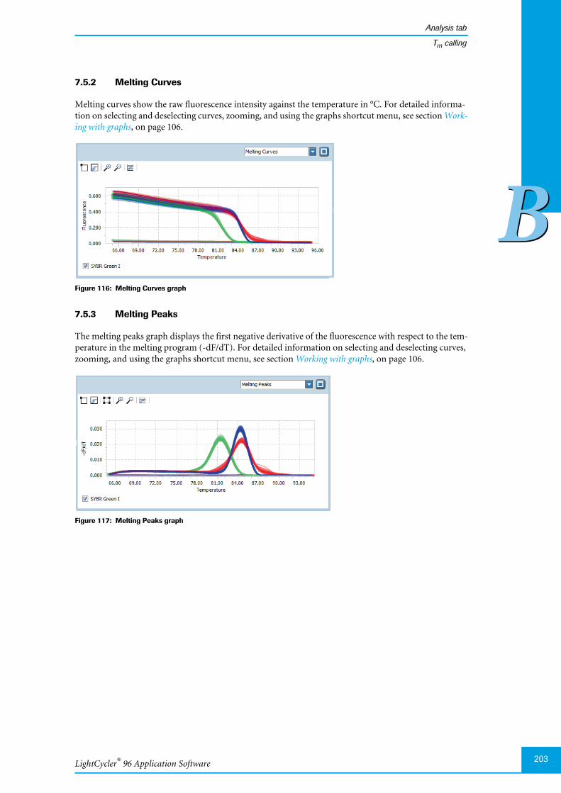
LightCycler® 96 Application Software
Analysis tab
203
BB
Tm calling
7.5.2 Melting Curves
Melting curves show the raw fluorescence intensity against the temperature in °C. For detailed informa-tion on selecting and deselecting curves, zooming, and using the graphs shortcut menu, see section Work-ing with graphs, on page 106.
Figure 116: Melting Curves graph
7.5.3 Melting Peaks
The melting peaks graph displays the first negative derivative of the fluorescence with respect to the tem-perature in the melting program (-dF/dT). For detailed information on selecting and deselecting curves,zooming, and using the graphs shortcut menu, see section Working with graphs, on page 106.
Figure 117: Melting Peaks graph
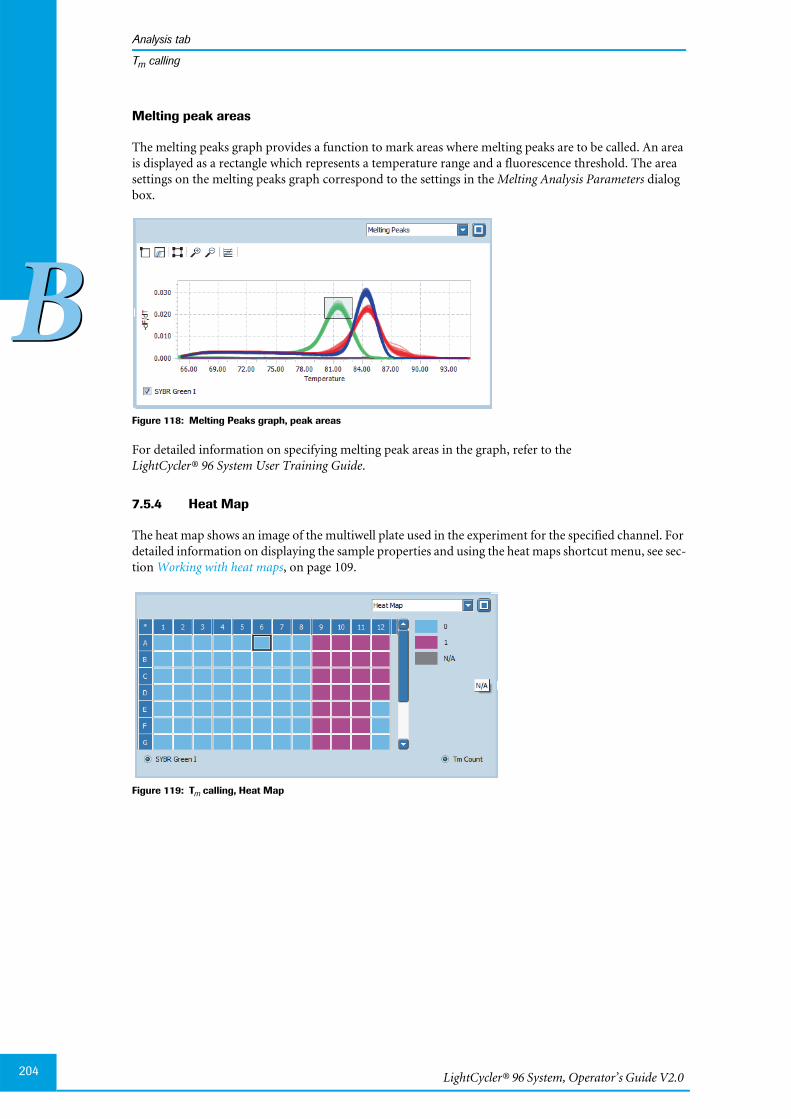
LightCycler® 96 System, Operator’s Guide V2.0204
Analysis tab
BB
Tm calling
Melting peak areas
The melting peaks graph provides a function to mark areas where melting peaks are to be called. An areais displayed as a rectangle which represents a temperature range and a fluorescence threshold. The areasettings on the melting peaks graph correspond to the settings in the Melting Analysis Parameters dialogbox.
Figure 118: Melting Peaks graph, peak areas
For detailed information on specifying melting peak areas in the graph, refer to theLightCycler® 96 System User Training Guide.
7.5.4 Heat Map
The heat map shows an image of the multiwell plate used in the experiment for the specified channel. Fordetailed information on displaying the sample properties and using the heat maps shortcut menu, see sec-tion Working with heat maps, on page 109.
Figure 119: Tm calling, Heat Map
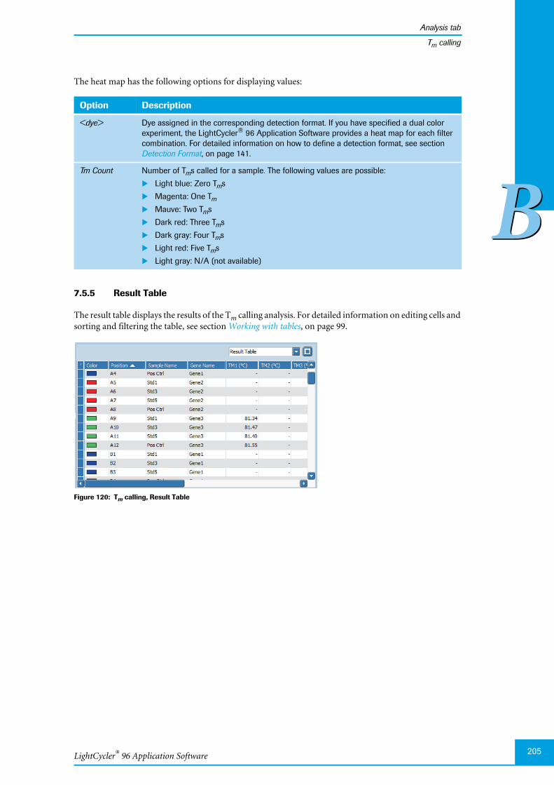
LightCycler® 96 Application Software
Analysis tab
205
BB
Tm calling
The heat map has the following options for displaying values:
7.5.5 Result Table
The result table displays the results of the Tm calling analysis. For detailed information on editing cells andsorting and filtering the table, see section Working with tables, on page 99.
Figure 120: Tm calling, Result Table
Option Description
<dye> Dye assigned in the corresponding detection format. If you have specified a dual colorexperiment, the LightCycler® 96 Application Software provides a heat map for each filtercombination. For detailed information on how to define a detection format, see sectionDetection Format, on page 141.
Tm Count Number of Tms called for a sample. The following values are possible:
Light blue: Zero Tms
Magenta: One Tm
Mauve: Two Tms
Dark red: Three Tms
Dark gray: Four Tms
Light red: Five Tms
Light gray: N/A (not available)
LightCycler® 96 System, Operator’s Guide V2.0206
Analysis tab
BB
Tm calling
The columns of the table have the following meanings:
7.5.6 Amplification Curves
The display of the amplification curves in a Tm calling analysis corresponds to their display in absolutequantification analysis. An amplification curves graph is only available if an amplification program hasbeen performed. For detailed information, see section Amplification Curves, on page 169.
Column Description
Color Color coding of the sample. For detailed information on how to change the colors,see section Editing cells, on page 102.
Position Position of the well in the multiwell plate. Each row is allocated a letter from A to H.The wells of a row are numbered from 1 to 12 from left to right.
Dye Name of the associated dye.
Excluded Specifies whether the sample is excluded from the analysis. By default, all samplesare included, so all samples are deselected in the exclusion column. Excluding sam-ples can be useful when a sample is clearly an outlier, or if an error has occurred inpipetting or amplification.
Sample Name Name of the sample present in the well.
The result table displays no rows for cleared wells, that is, deactivated wells. Fordetailed information on clearing wells, see section Clear Wells/Set to Default,on page 153.
Gene Name Name of the gene of interest.
TM1 (°C) to TM5 (°C) Temperature of the corresponding melting peak maximum according to the area set-tings in the melting peaks graph. The value is calculated from the maximum call of allcorresponding acquisitions.
Where no peak is present, the cells are blank.
Notes Description of the sample.
Sample Prep Notes Notes as specified in imported MagNA Pure 96 sample data files.
Number Index number of a well per dye. Index numbers are counted sequentially from left toright and from top to bottom.
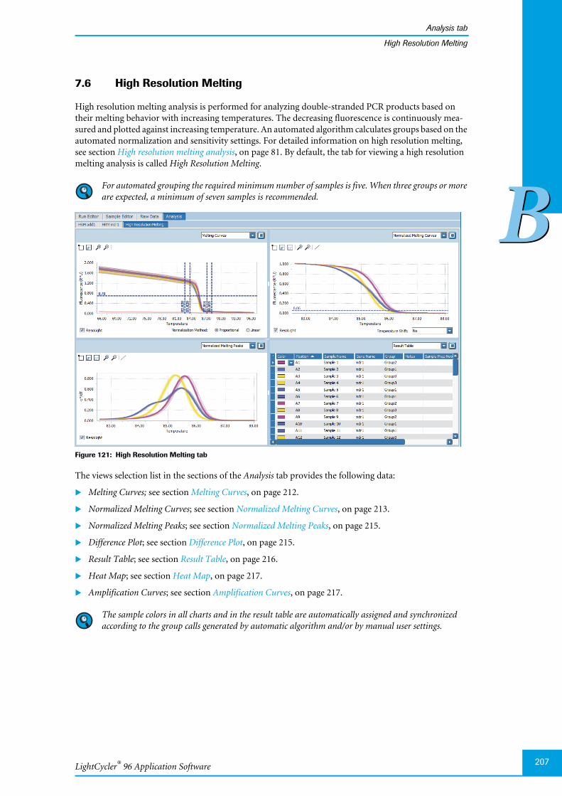
LightCycler® 96 Application Software
Analysis tab
207
BB
High Resolution Melting
7.6 High Resolution Melting
High resolution melting analysis is performed for analyzing double-stranded PCR products based ontheir melting behavior with increasing temperatures. The decreasing fluorescence is continuously mea-sured and plotted against increasing temperature. An automated algorithm calculates groups based on theautomated normalization and sensitivity settings. For detailed information on high resolution melting,see section High resolution melting analysis, on page 81. By default, the tab for viewing a high resolutionmelting analysis is called High Resolution Melting.
For automated grouping the required minimum number of samples is five. When three groups or moreare expected, a minimum of seven samples is recommended.
Figure 121: High Resolution Melting tab
The views selection list in the sections of the Analysis tab provides the following data:
Melting Curves; see section Melting Curves, on page 212.
Normalized Melting Curves; see section Normalized Melting Curves, on page 213.
Normalized Melting Peaks; see section Normalized Melting Peaks, on page 215.
Difference Plot; see section Difference Plot, on page 215.
Result Table; see section Result Table, on page 216.
Heat Map; see section Heat Map, on page 217.
Amplification Curves; see section Amplification Curves, on page 217.
The sample colors in all charts and in the result table are automatically assigned and synchronizedaccording to the group calls generated by automatic algorithm and/or by manual user settings.
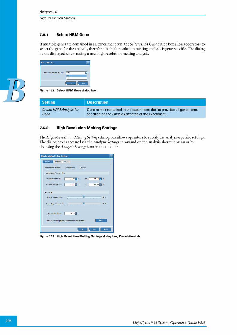
LightCycler® 96 System, Operator’s Guide V2.0208
Analysis tab
BB
High Resolution Melting
7.6.1 Select HRM Gene
If multiple genes are contained in an experiment run, the Select HRM Gene dialog box allows operators toselect the gene for the analysis, therefore the high resolution melting analysis is gene-specific. The dialogbox is displayed when adding a new high resolution melting analysis.
Figure 122: Select HRM Gene dialog box
7.6.2 High Resolution Melting Settings
The High Resolutiuon Melting Settings dialog box allows operators to specify the analysis-specific settings.The dialog box is accessed via the Analysis Settings command on the analysis shortcut menu or bychoosing the Analysis Settings icon in the tool bar.
Figure 123: High Resolution Melting Settings dialog box, Calculation tab
Setting Description
Create HRM Analysis forGene
Gene names contained in the experiment; the list provides all gene namesspecified on the Sample Editor tab of the experiment.

LightCycler® 96 Application Software
Analysis tab
209
BB
High Resolution Melting
Calculation tab
The settings on the Calculation tab allow for manually specifying the positive/negative threshold, the tem-perature ranges specifying the normalization areas, and the sensitivity settings for the automatic algo-rithm. When the settings for the positive/negative threshold, normalization and sensitivity are changedmanually, the algorithm automatically recalculates the group calls.
The Reset button on the Calculation tab resets all settings to the default values.
Setting Description
NormalizationMethod
Settings for the normalization method. Two normalization methods are provided:
Proportional Proportional normalization (default value)
Linear Linear normalization
FluorescenceNormalization
Temperature ranges where normalization is expected to be useful.
The automated algorithm provides default values for the ranges where normalization isassumed to be useful.
It is also possible to specify the temperature ranges using the vertical sliders in the‘Melting Curves’ chart. For detailed information, see section Melting Curves, onpage 212.
Pre-Melt Range from/to Pre-melting temperature range.
Post-melt Range from/to Post-melting temperature range.
Sensitivity Sensitivity settings for the automated algorithm.
Delta Tm Discrimination An increase of sensitivity subdivides the analyzedcurves into more groups. Small Tm differences are valu-ated higher to separate curves into different groups.
Curve Shape Discrimination An increase of sensitivity subdivides the analyzedcurves into more groups. Small differences in curvemorphology (for example, small shoulders) are valuatedhigher to separate curves into different groups.
Pos/Neg Threshold Minimum fluorescence value for a positive call.
It is also possible to specify the positive/negative threshold using the horizontalslider in the ‘Melting Curves’ chart. For detailed information, see section MeltingCurves, on page 212.
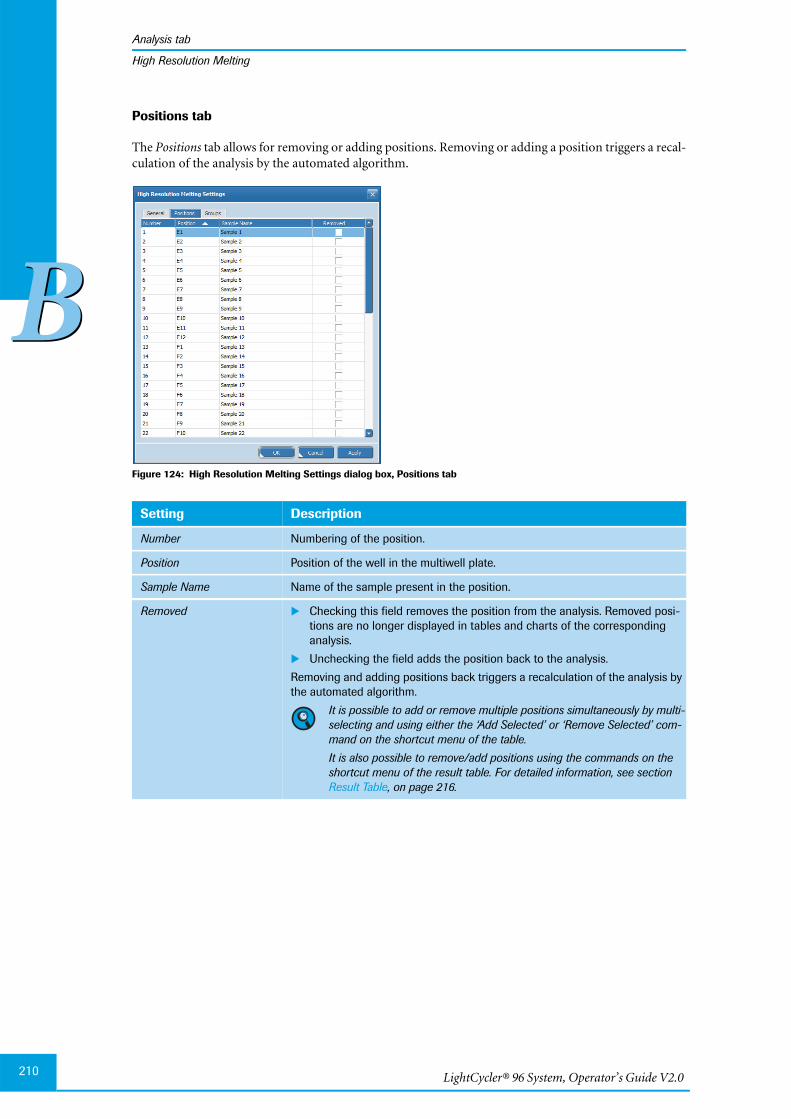
LightCycler® 96 System, Operator’s Guide V2.0210
Analysis tab
BB
High Resolution Melting
Positions tab
The Positions tab allows for removing or adding positions. Removing or adding a position triggers a recal-culation of the analysis by the automated algorithm.
Figure 124: High Resolution Melting Settings dialog box, Positions tab
Setting Description
Number Numbering of the position.
Position Position of the well in the multiwell plate.
Sample Name Name of the sample present in the position.
Removed Checking this field removes the position from the analysis. Removed posi-tions are no longer displayed in tables and charts of the correspondinganalysis.
Unchecking the field adds the position back to the analysis.
Removing and adding positions back triggers a recalculation of the analysis bythe automated algorithm.
It is possible to add or remove multiple positions simultaneously by multi-selecting and using either the ‘Add Selected’ or ‘Remove Selected’ com-mand on the shortcut menu of the table.
It is also possible to remove/add positions using the commands on theshortcut menu of the result table. For detailed information, see sectionResult Table, on page 216.
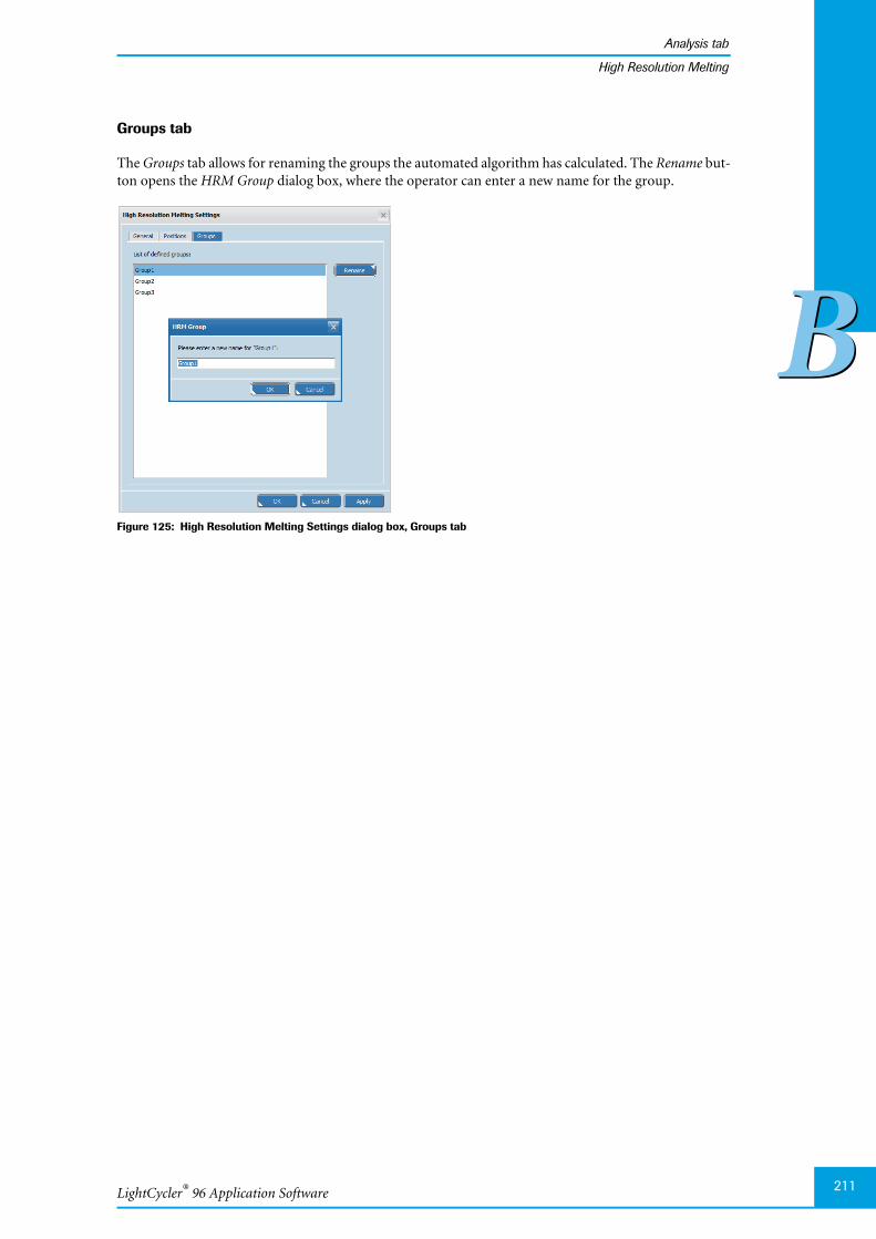
LightCycler® 96 Application Software
Analysis tab
211
BB
High Resolution Melting
Groups tab
The Groups tab allows for renaming the groups the automated algorithm has calculated. The Rename but-ton opens the HRM Group dialog box, where the operator can enter a new name for the group.
Figure 125: High Resolution Melting Settings dialog box, Groups tab
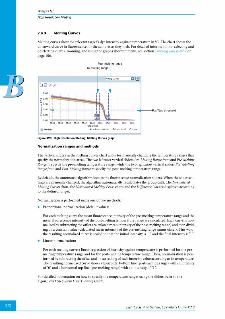
LightCycler® 96 System, Operator’s Guide V2.0212
Analysis tab
BB
High Resolution Melting
7.6.3 Melting Curves
Melting curves show the relevant target's dye intensity against temperature in °C. The chart shows thedownward curve in fluorescence for the samples as they melt. For detailed information on selecting anddeselecting curves, zooming, and using the graphs shortcut menu, see section Working with graphs, onpage 106.
Figure 126: High Resolution Melting, Melting Curves graph
Normalization ranges and methods
The vertical sliders in the melting curves chart allow for manually changing the temperature ranges thatspecify the normalization areas. The two leftmost vertical sliders Pre-Melting Range from and Pre-MeltingRange to specify the pre-melting temperature range, while the two rightmost vertical sliders Post-MeltingRange from and Post-Melting Range to specify the post-melting temperature range.
By default, the automated algorithm locates the fluorescence normalization sliders. When the slider set-tings are manually changed, the algorithm automatically recalculates the group calls. The NormalizedMelting Curves chart, the Normalized Melting Peaks chart, and the Difference Plot are displayed accordingto the defined ranges.
Normalization is performed using one of two methods:
Proportional normalization (default value):
For each melting curve the mean fluorescence intensity of the pre-melting temperature range and themean fluorescence intensity of the post-melting temperature range are calculated. Each curve is nor-malized by subtracting the offset (calculated mean intensity of the post-melting range) and then divid-ing by a constant value (calculated mean intensity of the pre-melting range minus offset). This way,the resulting normalized curve is scaled so that the initial intensity is "1" and the final intensity is "0".
Linear normalization:
For each melting curve a linear regression of intensity against temperature is performed for the pre-melting temperature range and for the post-melting temperature range. Then, normalization is per-formed by subtracting the offset and linear scaling of each intensity value according to its temperature.The resulting normalized curve shows a horizontal bottom line (post-melting range) with an intensityof "0" and a horizontal top line (pre-melting range) with an intensity of "1".
For detailed information on how to specify the temperature ranges using the sliders, refer to theLightCycler® 96 System User Training Guide.
Post-melting range
Pos/Neg threshold
Pre-melting range
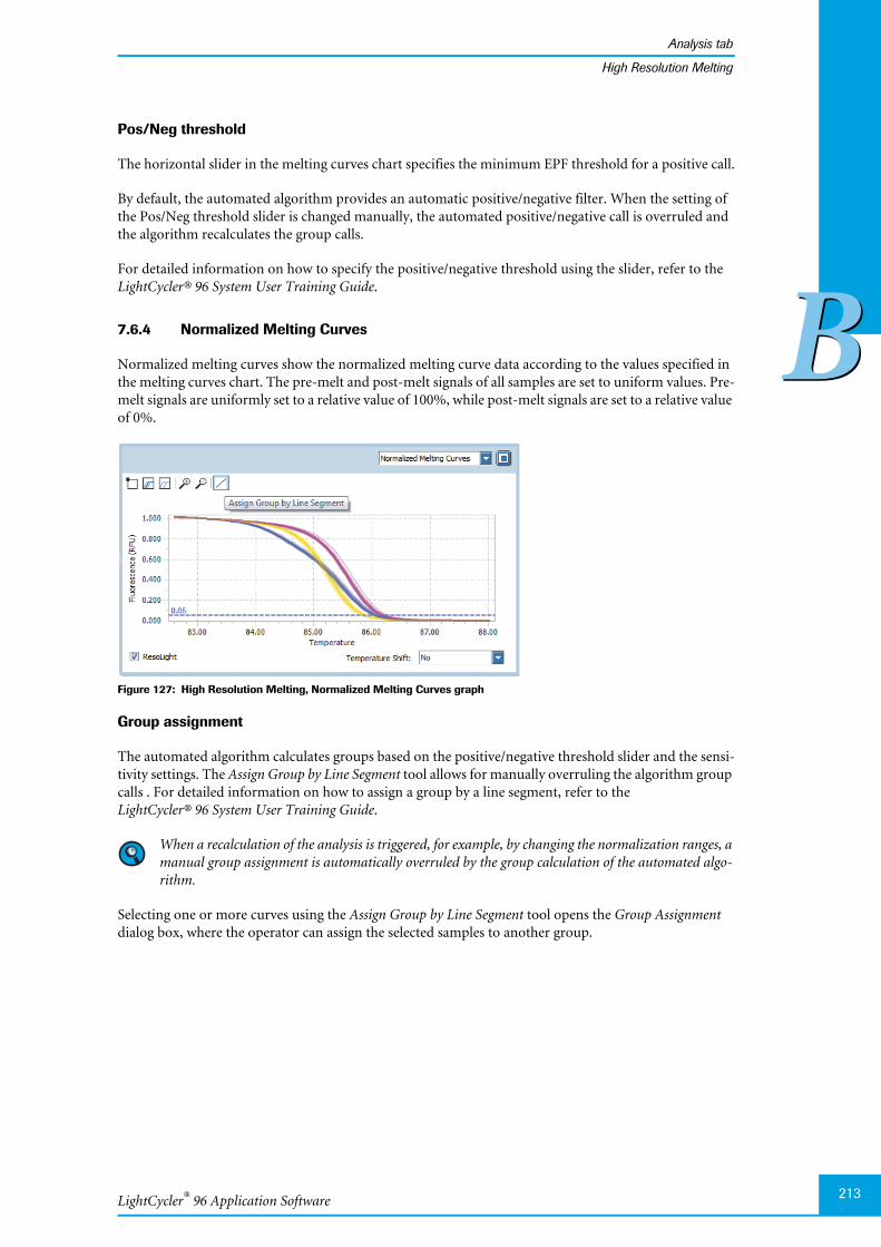
LightCycler® 96 Application Software
Analysis tab
213
BB
High Resolution Melting
Pos/Neg threshold
The horizontal slider in the melting curves chart specifies the minimum EPF threshold for a positive call.
By default, the automated algorithm provides an automatic positive/negative filter. When the setting ofthe Pos/Neg threshold slider is changed manually, the automated positive/negative call is overruled andthe algorithm recalculates the group calls.
For detailed information on how to specify the positive/negative threshold using the slider, refer to theLightCycler® 96 System User Training Guide.
7.6.4 Normalized Melting Curves
Normalized melting curves show the normalized melting curve data according to the values specified inthe melting curves chart. The pre-melt and post-melt signals of all samples are set to uniform values. Pre-melt signals are uniformly set to a relative value of 100%, while post-melt signals are set to a relative valueof 0%.
Figure 127: High Resolution Melting, Normalized Melting Curves graph
Group assignment
The automated algorithm calculates groups based on the positive/negative threshold slider and the sensi-tivity settings. The Assign Group by Line Segment tool allows for manually overruling the algorithm groupcalls . For detailed information on how to assign a group by a line segment, refer to theLightCycler® 96 System User Training Guide.
When a recalculation of the analysis is triggered, for example, by changing the normalization ranges, amanual group assignment is automatically overruled by the group calculation of the automated algo-rithm.
Selecting one or more curves using the Assign Group by Line Segment tool opens the Group Assignmentdialog box, where the operator can assign the selected samples to another group.
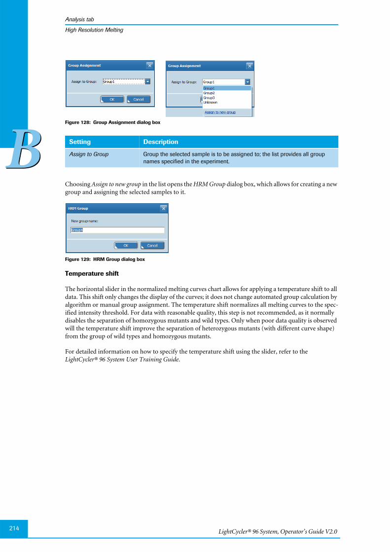
LightCycler® 96 System, Operator’s Guide V2.0214
Analysis tab
BB
High Resolution Melting
Figure 128: Group Assignment dialog box
Choosing Assign to new group in the list opens the HRM Group dialog box, which allows for creating a newgroup and assigning the selected samples to it.
Figure 129: HRM Group dialog box
Temperature shift
The horizontal slider in the normalized melting curves chart allows for applying a temperature shift to alldata. This shift only changes the display of the curves; it does not change automated group calculation byalgorithm or manual group assignment. The temperature shift normalizes all melting curves to the spec-ified intensity threshold. For data with reasonable quality, this step is not recommended, as it normallydisables the separation of homozygous mutants and wild types. Only when poor data quality is observedwill the temperature shift improve the separation of heterozygous mutants (with different curve shape)from the group of wild types and homozygous mutants.
For detailed information on how to specify the temperature shift using the slider, refer to theLightCycler® 96 System User Training Guide.
Setting Description
Assign to Group Group the selected sample is to be assigned to; the list provides all groupnames specified in the experiment.
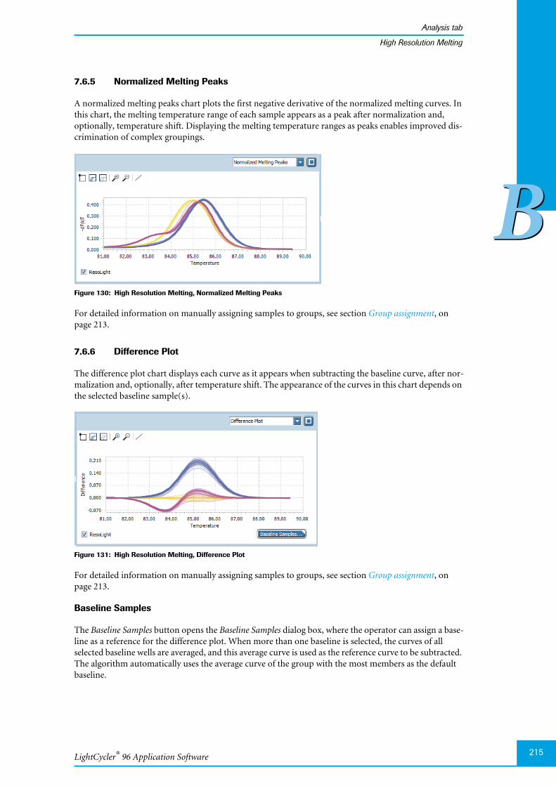
LightCycler® 96 Application Software
Analysis tab
215
BB
High Resolution Melting
7.6.5 Normalized Melting Peaks
A normalized melting peaks chart plots the first negative derivative of the normalized melting curves. Inthis chart, the melting temperature range of each sample appears as a peak after normalization and,optionally, temperature shift. Displaying the melting temperature ranges as peaks enables improved dis-crimination of complex groupings.
Figure 130: High Resolution Melting, Normalized Melting Peaks
For detailed information on manually assigning samples to groups, see section Group assignment, onpage 213.
7.6.6 Difference Plot
The difference plot chart displays each curve as it appears when subtracting the baseline curve, after nor-malization and, optionally, after temperature shift. The appearance of the curves in this chart depends onthe selected baseline sample(s).
Figure 131: High Resolution Melting, Difference Plot
For detailed information on manually assigning samples to groups, see section Group assignment, onpage 213.
Baseline Samples
The Baseline Samples button opens the Baseline Samples dialog box, where the operator can assign a base-line as a reference for the difference plot. When more than one baseline is selected, the curves of allselected baseline wells are averaged, and this average curve is used as the reference curve to be subtracted.The algorithm automatically uses the average curve of the group with the most members as the defaultbaseline.
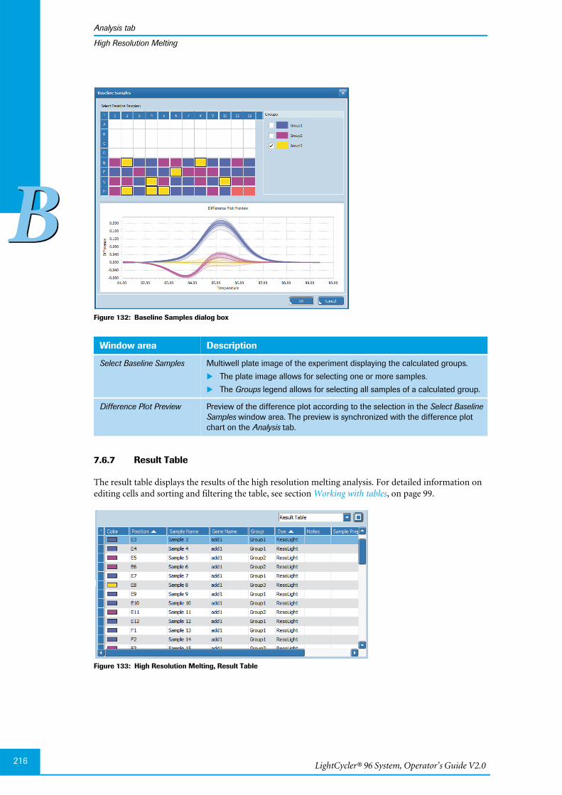
LightCycler® 96 System, Operator’s Guide V2.0216
Analysis tab
BB
High Resolution Melting
Figure 132: Baseline Samples dialog box
7.6.7 Result Table
The result table displays the results of the high resolution melting analysis. For detailed information onediting cells and sorting and filtering the table, see section Working with tables, on page 99.
Figure 133: High Resolution Melting, Result Table
Window area Description
Select Baseline Samples Multiwell plate image of the experiment displaying the calculated groups.
The plate image allows for selecting one or more samples.
The Groups legend allows for selecting all samples of a calculated group.
Difference Plot Preview Preview of the difference plot according to the selection in the Select BaselineSamples window area. The preview is synchronized with the difference plotchart on the Analysis tab.

LightCycler® 96 Application Software
Analysis tab
217
BB
High Resolution Melting
The columns of the table have the following meanings:
7.6.8 Heat Map
The heat map shows an image of the multiwell plate displaying the calculated groups and the assignmentof the samples to the groups. For detailed information on displaying the sample properties and using theheat maps shortcut menu, see section Working with heat maps, on page 109.
Figure 134: High Resolution Melting, Heat Map
7.6.9 Amplification Curves
The display of the amplification curves in high resolution melting analysis corresponds to their display inabsolute quantification analysis. For detailed information, see section Amplification Curves, on page 169.
Column Description
Color Color coding of the group the sample is assigned to. For detailed information on howto change the colors, see section Editing cells, on page 102.
Position Position of the well in the multiwell plate. Each row is allocated a letter from A to H.The wells of a row are numbered from 1 to 12 from left to right.
Sample Name Name of the sample present in the well.
Gene Name Name of the gene of interest.
Group Name of the group the sample is assigned to.
Dye Name of the associated dye.
Notes Description of the sample.
Sample Prep Notes Notes as specified in imported MagNA Pure 96 sample data files.
Number Index number of a well. Index numbers are counted sequentially from left to right andfrom top to bottom.
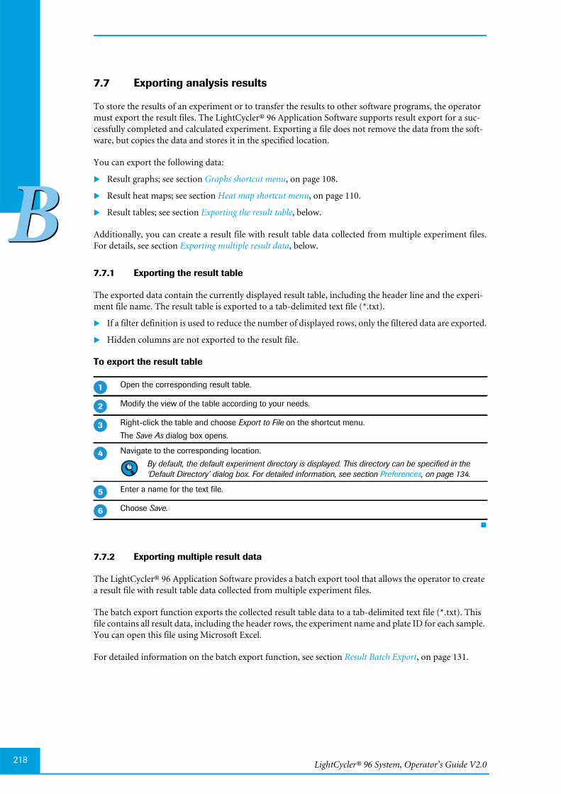
LightCycler® 96 System, Operator’s Guide V2.0
BB
218
7.7 Exporting analysis results
To store the results of an experiment or to transfer the results to other software programs, the operatormust export the result files. The LightCycler® 96 Application Software supports result export for a suc-cessfully completed and calculated experiment. Exporting a file does not remove the data from the soft-ware, but copies the data and stores it in the specified location.
You can export the following data:
Result graphs; see section Graphs shortcut menu, on page 108.
Result heat maps; see section Heat map shortcut menu, on page 110.
Result tables; see section Exporting the result table, below.
Additionally, you can create a result file with result table data collected from multiple experiment files.For details, see section Exporting multiple result data, below.
7.7.1 Exporting the result table
The exported data contain the currently displayed result table, including the header line and the experi-ment file name. The result table is exported to a tab-delimited text file (*.txt).
If a filter definition is used to reduce the number of displayed rows, only the filtered data are exported.
Hidden columns are not exported to the result file.
To export the result table
7.7.2 Exporting multiple result data
The LightCycler® 96 Application Software provides a batch export tool that allows the operator to createa result file with result table data collected from multiple experiment files.
The batch export function exports the collected result table data to a tab-delimited text file (*.txt). Thisfile contains all result data, including the header rows, the experiment name and plate ID for each sample.You can open this file using Microsoft Excel.
For detailed information on the batch export function, see section Result Batch Export, on page 131.
Open the corresponding result table.
Modify the view of the table according to your needs.
Right-click the table and choose Export to File on the shortcut menu.
The Save As dialog box opens.
Navigate to the corresponding location.
By default, the default experiment directory is displayed. This directory can be specified in the‘Default Directory’ dialog box. For detailed information, see section Preferences, on page 134.
Enter a name for the text file.
Choose Save.
�
�
�
�
�
�

Chapter CLightCycler® 96 Instrument Software
CCChapter C • LightCycler® 96 Instrument Software
LightCycler® 96 System, Operator’s Guide V2.0
Table of Contents
CC
220
C LightCycler® 96 Instrument Software 219
1 Overview ........................................................................................................................................................ 221
1.1 The main window ......................................................................................................................................... 2221.1.1 Status bar ........................................................................................................................................................ 2231.1.2 Working window area tabs ....................................................................................................................... 2241.1.3 Global action bar .......................................................................................................................................... 2241.1.4 Alarms window area .................................................................................................................................... 225
1.2 General software conventions ................................................................................................................. 2271.2.1 Buttons ............................................................................................................................................................. 2271.2.2 Input fields ...................................................................................................................................................... 2281.2.3 Working with tables ..................................................................................................................................... 228
1.3 Experiments .................................................................................................................................................... 2291.3.1 Experiment file types ................................................................................................................................... 2291.3.2 Creating an experiment .............................................................................................................................. 2291.3.3 Opening an experiment .............................................................................................................................. 2321.3.4 Saving an experiment ................................................................................................................................. 233
1.4 Import, export, and file transfer options ............................................................................................... 2341.4.1 Import data ...................................................................................................................................................... 2341.4.2 Export data ...................................................................................................................................................... 235
1.5 Exiting the software ..................................................................................................................................... 236
2 Overview tab ................................................................................................................................................ 237
2.1 Experiments table ......................................................................................................................................... 2372.2 Control bar ...................................................................................................................................................... 240
3 Run Editor tab ............................................................................................................................................. 242
3.1 Measurement tab ......................................................................................................................................... 2423.2 Profile tab ........................................................................................................................................................ 245
3.2.1 Programs window area ............................................................................................................................... 2453.2.2 Adding a new program .............................................................................................................................. 2463.2.3 Steps window area ....................................................................................................................................... 247
3.3 Temperature Profile window area .......................................................................................................... 249
4 Raw Data tab ............................................................................................................................................... 250
4.1 Experiment progress bar ............................................................................................................................ 2504.2 Graphs window area ................................................................................................................................... 251
5 Utilities tab .................................................................................................................................................... 253
5.1 Instrument tab ............................................................................................................................................... 2535.1.1 Self test report ............................................................................................................................................... 2545.1.2 Current Date ................................................................................................................................................... 255
5.2 Configuration tab .......................................................................................................................................... 2565.2.1 Device Name / Hostname ......................................................................................................................... 2575.2.2 Network Information ................................................................................................................................... 2575.2.3 Email Information ......................................................................................................................................... 2595.2.4 Remote Monitoring ...................................................................................................................................... 2625.2.5 Automated Backup ...................................................................................................................................... 263
5.3 Service tab ....................................................................................................................................................... 2645.3.1 Axeda client .................................................................................................................................................... 2645.3.2 Export Log Files ............................................................................................................................................. 2665.3.3 Backup and restore ..................................................................................................................................... 2675.3.4 Recalibrate Touch Screen ......................................................................................................................... 2695.3.5 Lock Instrument for Transportation ....................................................................................................... 271
6 Alarms and messages ............................................................................................................................ 272
6.1 Alarm history .................................................................................................................................................. 2736.2 Detailed information .................................................................................................................................... 275
7 Help browser ............................................................................................................................................... 276
LightCycler® 96 Instrument Software
Overview
221
CC
LightCycler® 96 Instrument Software 0
1 Overview
The LightCycler® 96 Instrument Software provides all functions for using, configuring and controllingthe LightCycler® 96 Instrument:
Managing experiments; see section Overview tab, on page 237.
Specifying the temperature profile and the dye-specific parameters for an experiment run; see sectionRun Editor tab, on page 242.
Monitoring an experiment run; see section Raw Data tab, on page 250.
Configuring the instrument; see section Utilities tab, on page 253.
After the experiment run, the raw data gathered by the software must be transferred to the applicationsoftware for analysis. For a detailed description of the LightCycler® 96 Application Software, see chapterLightCycler® 96 Application Software, on page 85.
The LightCycler® 96 Instrument Software is installed on the LightCycler® 96 Instrument which maybe connected to a network. Please be aware that such a connection poses a potential risk to the integrityof the product, for example, through infection with malicious code (viruses, Trojan horses, etc.) oraccess by unauthorized third parties (such as intrusion by hackers). Roche therefore highly recom-mends protecting the product against such risks with appropriate security measures.
For upgrading from LightCycler® 96 Instrument Software Version 1.0 to version 1.1, see sectionUpgrading the LightCycler® 96 Instrument Software Version 1.0, on page 62. It is important to saveand remove all version 1.0 experiment files from the instrument before upgrading to version 1.1.LightCycler® 96 Instrument Software Version 1.0 experiment files cannot be handled by version 1.1.
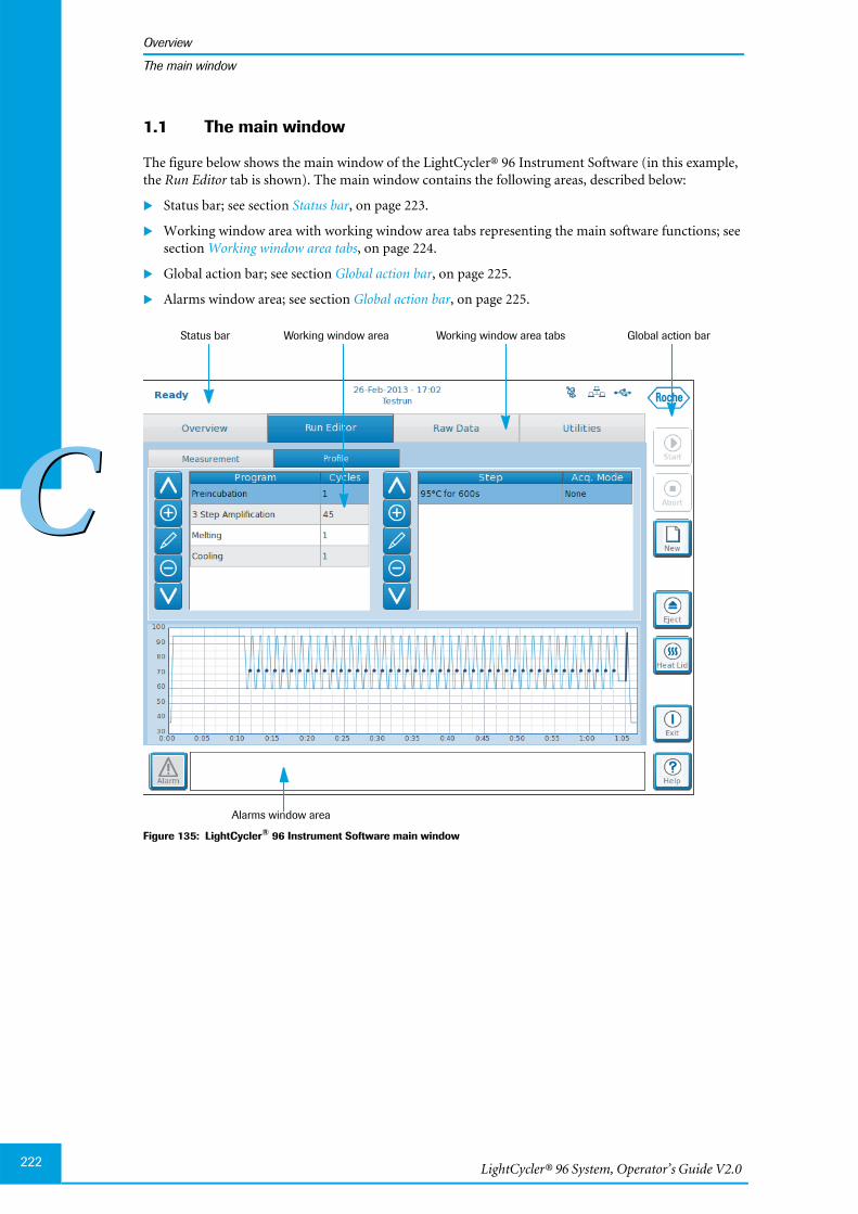
LightCycler® 96 System, Operator’s Guide V2.0222
Overview
CC
The main window
1.1 The main window
The figure below shows the main window of the LightCycler® 96 Instrument Software (in this example,the Run Editor tab is shown). The main window contains the following areas, described below:
Status bar; see section Status bar, on page 223.
Working window area with working window area tabs representing the main software functions; seesection Working window area tabs, on page 224.
Global action bar; see section Global action bar, on page 225.
Alarms window area; see section Global action bar, on page 225.
Figure 135: LightCycler® 96 Instrument Software main window
Working window areaStatus bar Working window area tabs
Alarms window area
Global action bar

LightCycler® 96 Instrument Software
Overview
223
CC
The main window
1.1.1 Status bar
The status bar displays the following information:
Field/Icon Description
<status> Current instrument status:
InitializingInitialization of the instrument hardware.
ReadyThe block cycler cover has reached the target temperature and the instrumentis ready to start a run.
Running: <experiment name>The specified experiment is running.
StandbyThe heater of the block cycler cover is switched off.
Lid ReheatingThe block cycler cover is heating up after a standby.
Aborting: <experiment name>The specified experiment run is being aborted.
ErrorA hardware or software error has occurred and has left the instrument unableto function.
Activating Transportation LockThe instrument is preparing the transportation lock.
Transportation LockThe instrument is ready for transport.
Experiment scheduled.
When a run is started in the Initializing or the Standby status, lid reheating isstarted automatically and the experiment is in Scheduled status. The Initializing orLid Reheating statuses are then displayed with a clock symbol.
<date - time>
<experiment name>
Current date and time.
Name of the currently selected experiment.
An experiment is currently being saved, removed, synchronized, or otherwise re-motely processed.
As long as this icon flashes, the instrument should not be switched off.
The instrument is connected to an Ethernet network.
The Ethernet network connection failed.
The Ethernet network connection has limited connectivity, that is, the instrumentrecognizes the network, but is unable to establish the connection.
A USB drive is connected to the instrument.
Remote monitoring is activated.
For detailed information, see section Remote Monitoring, on page 262.
Automated backup of experiments to a network share is activated.
For detailed information, see section Automated Backup to Network Share, onpage 263.
The Axeda client is activated.
For detailed information, see section Axeda Service Client, on page 264.
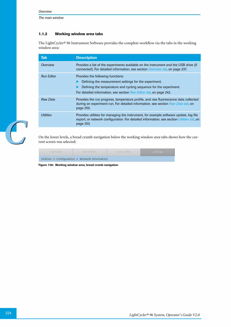
LightCycler® 96 System, Operator’s Guide V2.0224
Overview
CC
The main window
1.1.2 Working window area tabs
The LightCycler® 96 Instrument Software provides the complete workflow via the tabs in the workingwindow area:
On the lower levels, a bread crumb navigation below the working window area tabs shows how the cur-rent screen was selected:
Figure 136: Working window area, bread crumb navigation
Tab Description
Overview Provides a list of the experiments available on the instrument and the USB drive (ifconnected). For detailed information, see section Overview tab, on page 237.
Run Editor Provides the following functions:
Defining the measurement settings for the experiment.
Defining the temperature and cycling sequence for the experiment.
For detailed information, see section Run Editor tab, on page 242.
Raw Data Provides the run progress, temperature profile, and raw fluorescence data collectedduring an experiment run. For detailed information, see section Raw Data tab, onpage 250.
Utilities Provides utilities for managing the instrument, for example software update, log fileexport, or network configuration. For detailed information, see section Utilities tab, onpage 253.

LightCycler® 96 Instrument Software
Overview
225
CC
The main window
1.1.3 Global action bar
The buttons in the global action bar provide access to general software functions. Their availabilitydepends on the current status of the instrument. The buttons provide the following actions:
Button Function Description
Start Only enabled in Initializing, Ready, and Standby status:
Starts the experiment selected on the Overview tab. Scheduled experi-ments are started when the instrument status Ready is achieved.
For detailed information, see section Overview tab, on page 237.
Abort Only enabled while a run is being processed:
Aborts the currently executed or scheduled run.
You are prompted to confirm the abort.
When a scheduled run is aborted, the new experiment status isnot ’Aborted’, but is still ’Unprocessed’.
New Only enabled if less than 50 experiments are available on the instru-ment and a connected USB drive:
Opens the Create New Experiment window area.
For detailed information, see section Experiments, on page 229.
Eject Pushes the loading module forward. The operator can open the load-ing module completely using the recessed grip. For detailed informa-tion, see section Loading module, on page 30.
The loading module may only be opened using the ‘Eject’ buttonand when the button is enabled. Otherwise the instrumentchanges to the ‘Error’ state and has to be rebooted.
Heat Lid Only enabled in Standby status:
Starts heating of the block cycler cover. After heating, the instrumentchanges to the Ready status.
Exit Not available while a run is being processed:
Opens the Exit Options window area for shutting down or rebootingthe LightCycler® 96 Instrument Software.
For detailed information, see section Exiting the software, on page 236.
Help Opens the help browser of the LightCycler® 96 Instrument.
For detailed information, see section Help browser, on page 276.
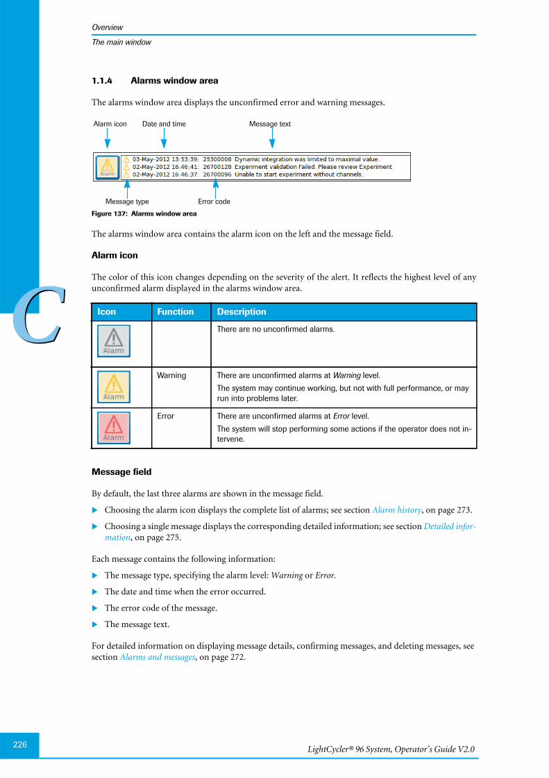
LightCycler® 96 System, Operator’s Guide V2.0226
Overview
CC
The main window
1.1.4 Alarms window area
The alarms window area displays the unconfirmed error and warning messages.
Figure 137: Alarms window area
The alarms window area contains the alarm icon on the left and the message field.
Alarm icon
The color of this icon changes depending on the severity of the alert. It reflects the highest level of anyunconfirmed alarm displayed in the alarms window area.
Message field
By default, the last three alarms are shown in the message field.
Choosing the alarm icon displays the complete list of alarms; see section Alarm history, on page 273.
Choosing a single message displays the corresponding detailed information; see section Detailed infor-mation, on page 275.
Each message contains the following information:
The message type, specifying the alarm level: Warning or Error.
The date and time when the error occurred.
The error code of the message.
The message text.
For detailed information on displaying message details, confirming messages, and deleting messages, seesection Alarms and messages, on page 272.
Icon Function Description
There are no unconfirmed alarms.
Warning There are unconfirmed alarms at Warning level.
The system may continue working, but not with full performance, or mayrun into problems later.
Error There are unconfirmed alarms at Error level.
The system will stop performing some actions if the operator does not in-tervene.
Alarm icon
Message type
Date and time
Error code
Message text
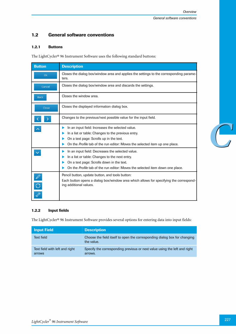
LightCycler® 96 Instrument Software
Overview
227
CC
General software conventions
1.2 General software conventions
1.2.1 Buttons
The LightCycler® 96 Instrument Software uses the following standard buttons:
1.2.2 Input fields
The LightCycler® 96 Instrument Software provides several options for entering data into input fields:
Button Description
Closes the dialog box/window area and applies the settings to the corresponding parame-ters.
Closes the dialog box/window area and discards the settings.
Closes the window area.
Closes the displayed information dialog box.
Changes to the previous/next possible value for the input field.
In an input field: Increases the selected value.
In a list or table: Changes to the previous entry.
On a text page: Scrolls up in the text.
On the Profile tab of the run editor: Moves the selected item up one place.
In an input field: Decreases the selected value.
In a list or table: Changes to the next entry.
On a text page: Scrolls down in the text.
On the Profile tab of the run editor: Moves the selected item down one place.
Pencil button, update button, and tools button:
Each button opens a dialog box/window area which allows for specifying the correspond-ing additional values.
Input Field Description
Text field Choose the field itself to open the corresponding dialog box for changingthe value.
Text field with left and rightarrows
Specify the corresponding previous or next value using the left and rightarrows.

LightCycler® 96 System, Operator’s Guide V2.0228
Overview
CC
General software conventions
1.2.3 Working with tables
The LightCycler® 96 Instrument Software provides functions to be used in all tables displayed in the userinterface. This section describes functions that are shared between the different tables.
To select and deselect items
To sort tables
Choose a row in a table to select the corresponding item. The selected item is highlighted.
Choosing another row deselects the previous row.
Choose the header of a column to sort the table by the column values.
Choosing the header several times toggles the sort order between descending and ascending.
�
�
LightCycler® 96 Instrument Software
Overview
229
CC
Experiments
1.3 Experiments
The information provided in the experiment definition controls the LightCycler® 96 Instrument duringan experiment run. The experiment definition specifies the target temperatures and hold times of thethermal block cycler, the number of cycles being executed, and other parameters. As the experiment pro-gresses, the software gathers fluorescence data from the instrument and displays it on the Raw Data tab.
For starting an experiment run, the experiment must be available on the instrument or on the connectedUSB drive in a sub folder experiments. Operators can specify an experiment definition as follows:
On the instrument using the LightCycler® 96 Instrument Software.
On a computer using the LightCycler® 96 Application Software. In this case, the experiment must betransferred to the instrument for the run. For detailed information on the application software, seechapter LightCycler® 96 Application Software, on page 85.
After the experiment run, the raw data gathered by the software on the instrument must be transferredback to the application software for analysis. For detailed information on how to send an experiment tothe instrument or retrieve it to the computer, see section Instrument Manager, on page 124.
During an experiment run, it is not recommended to use a USB drive, for example, for exporting orimporting data, or for synchronizing an experiment, as this may cause problems in the measurementprocess.
1.3.1 Experiment file types
The LightCycler® 96 Instrument Software supports the following experiment file types:
*.lc96p (LightCycler® 96 experiment files for processed experiments).
*.lc96u (LightCycler® 96 experiment files for unprocessed experiments).
Experiment files generated with LightCycler® 96 Software Version 1.0 (*.lc96) cannot be opened withversion 1.1. Operators must open these files in the LightCycler® 96 Application Software on the com-puter, save them as ‘*.lc96p’ or ‘*.lc96u’ files, and transfer the new files back to the instrument.
By default, all newly generated experiment files have the file type *.lc96u. Aborted experiments are treatedidentically to processed experiments, that is, they are saved as *.lc96p files.
It is not possible to generate analyses on aborted experiments in theLightCycler® 96 Application Software.
1.3.2 Creating an experiment
Before a LightCycler® 96 Instrument run can be started, a new experiment has to be created. The operatorhas the following options for creating a new experiment:
Generating a completely new experiment.
Generating a new experiment by using an existing experiment as a template.
Generating a new experiment by using a predefined Roche template.
Experiments are created in the Create New Experiment window area. You access the window area usingthe New button in the global action bar.

LightCycler® 96 System, Operator’s Guide V2.0230
Overview
CC
Experiments
Figure 138: Create New Experiment window area
Figure 139: Keyboard dialog box
Option Description
New empty experiment Creates a new, empty experiment.
New experiment based on existing experiment Opens the specified experiment as a template.
New experiment based on Roche template Opens the specified Roche template.
Experiment Name Experiment file name. Choosing the text field opens thekeyboard dialog box for specifying the name; see below.
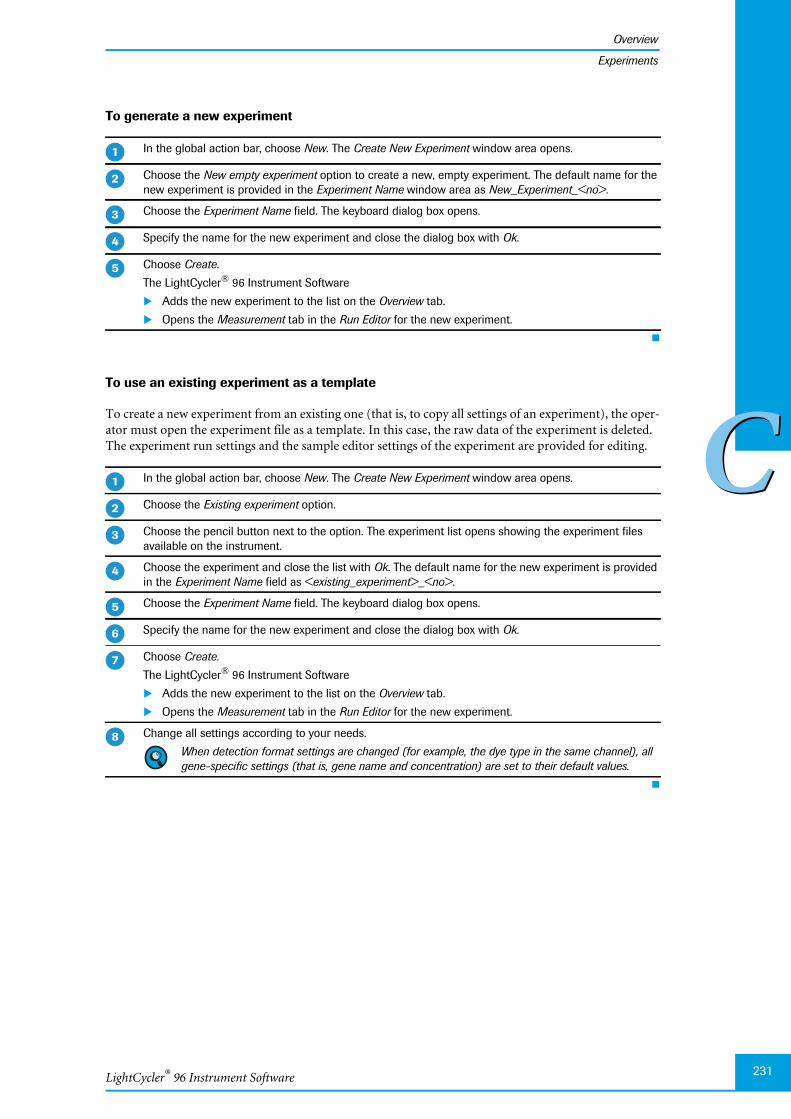
LightCycler® 96 Instrument Software
Overview
231
CC
Experiments
To generate a new experiment
To use an existing experiment as a template
To create a new experiment from an existing one (that is, to copy all settings of an experiment), the oper-ator must open the experiment file as a template. In this case, the raw data of the experiment is deleted.The experiment run settings and the sample editor settings of the experiment are provided for editing.
In the global action bar, choose New. The Create New Experiment window area opens.
Choose the New empty experiment option to create a new, empty experiment. The default name for thenew experiment is provided in the Experiment Name window area as New_Experiment_<no>.
Choose the Experiment Name field. The keyboard dialog box opens.
Specify the name for the new experiment and close the dialog box with Ok.
Choose Create.
The LightCycler® 96 Instrument Software
Adds the new experiment to the list on the Overview tab.
Opens the Measurement tab in the Run Editor for the new experiment.
In the global action bar, choose New. The Create New Experiment window area opens.
Choose the Existing experiment option.
Choose the pencil button next to the option. The experiment list opens showing the experiment filesavailable on the instrument.
Choose the experiment and close the list with Ok. The default name for the new experiment is providedin the Experiment Name field as <existing_experiment>_<no>.
Choose the Experiment Name field. The keyboard dialog box opens.
Specify the name for the new experiment and close the dialog box with Ok.
Choose Create.
The LightCycler® 96 Instrument Software
Adds the new experiment to the list on the Overview tab.
Opens the Measurement tab in the Run Editor for the new experiment.
Change all settings according to your needs.
When detection format settings are changed (for example, the dye type in the same channel), allgene-specific settings (that is, gene name and concentration) are set to their default values.
�
�
�
�
�
�
�
�
�
�
�
�

LightCycler® 96 System, Operator’s Guide V2.0232
Overview
CC
Experiments
To use a Roche template
Roche provides a number of predefined experiments as templates. An experiment template contains thetemperature profile and the dye-specific parameters for an experiment.
1.3.3 Opening an experiment
Experiments can be opened at any time before, during, or after the experiment run and during executionof another experiment.
The LightCycler® 96 Instrument Software allows for opening and editing an experiment while anotherexperiment is running.
To open an experiment
In the global action bar, choose New. The Create New Experiment window area opens.
Choose the Roche template option.
Choose the pencil button next to the option. The template list opens showing the Roche templates avail-able on the instrument.
Choose the template and close the list with Ok. The default name for the new experiment is provided inthe Experiment Name field as <template>_<no>.
Choose the Experiment Name field. The keyboard dialog box opens.
Specify the name for the new experiment and close the dialog box with Ok.
Choose Create.
The LightCycler® 96 Instrument Software
Adds the new experiment to the list on the Overview tab.
Opens the Measurement tab in the Run Editor for the new experiment.
Change all settings according to your needs.
On the Overview tab, select the experiment to be opened.
This experiment is then available on the Run Editor tab.
The experiment is executed when you choose the Start button in the global action bar.
If the experiment is running or completed, the temperature profile and the collected raw data aredisplayed on the Experiment tab.
�
�
�
�
�
�
�
�

LightCycler® 96 Instrument Software
Overview
233
CC
Experiments
1.3.4 Saving an experiment
The LightCycler® 96 Instrument Software automatically saves all changes in an experiment file. Theexperiment file is saved according to its original location:
On the LightCycler® 96 Instrument.
On the USB drive.
On both media, if the operator has synchronized the storage locations.For detailed information on synchronizing, see section Control bar, on page 240.
The experiment file is saved according to the processing status:
As a LightCycler® 96 file for an unprocessed experiment (*.lc96u).
As a LightCycler® 96 file for a processed, aborted or failed experiment (*.lc96p).
For safety reasons, operators should regularly download the experiment data from the instrumentusing one of the following functions.
On the LightCycler® 96 Instrument: Synchronizing the storage locations; see section Control bar,on page 240.
In the LightCycler® 96 Application Software: Retrieving the experiment from the instrument; seesection Instrument Manager, on page 124.
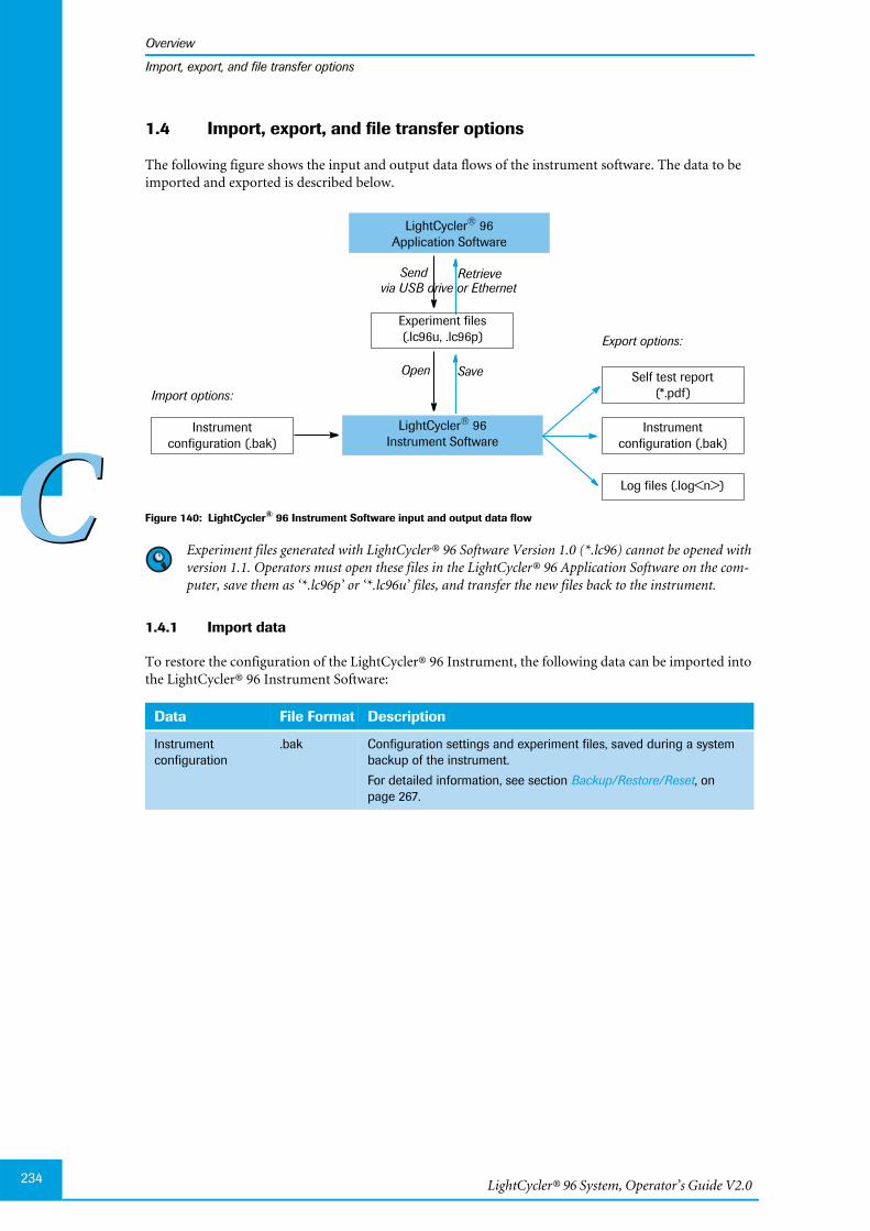
LightCycler® 96 System, Operator’s Guide V2.0234
Overview
CC
Import, export, and file transfer options
1.4 Import, export, and file transfer options
The following figure shows the input and output data flows of the instrument software. The data to beimported and exported is described below.
Figure 140: LightCycler® 96 Instrument Software input and output data flow
Experiment files generated with LightCycler® 96 Software Version 1.0 (*.lc96) cannot be opened withversion 1.1. Operators must open these files in the LightCycler® 96 Application Software on the com-puter, save them as ‘*.lc96p’ or ‘*.lc96u’ files, and transfer the new files back to the instrument.
1.4.1 Import data
To restore the configuration of the LightCycler® 96 Instrument, the following data can be imported intothe LightCycler® 96 Instrument Software:
Data File Format Description
Instrumentconfiguration
.bak Configuration settings and experiment files, saved during a systembackup of the instrument.
For detailed information, see section Backup/Restore/Reset, onpage 267.
LightCycler® 96Instrument Software
Export options:
Open Save
Send Retrieve
LightCycler® 96Application Software
Log files (.log<n>)
Import options:
Instrumentconfiguration (.bak)
via USB drive or Ethernet
Experiment files(.lc96u, .lc96p)
Self test report(*.pdf)
Instrumentconfiguration (.bak)
LightCycler® 96 Instrument Software
Overview
235
CC
Import, export, and file transfer options
1.4.2 Export data
To store the self test report, the configuration or the log files of the instrument, or to transfer the data forfurther analysis, the corresponding files must be exported. The LightCycler® 96 Instrument Software pro-vides export functions for the following data:
Data File Format Description
Self test report .pdf Results of the last self test of the instrument saved to a con-nected USB drive.
For detailed information, see section Self Test Report, onpage 254.
Instrument configuration .bak Configuration settings and experiment files, packed and savedas a backup file (*.bak) on a connected USB drive.
For detailed information, see section Backup/Restore/Reset, onpage 267.
Log files .log Log files containing the instrument log files.
For detailed information, see section Export Service Log Files toUSB Drive, on page 266.
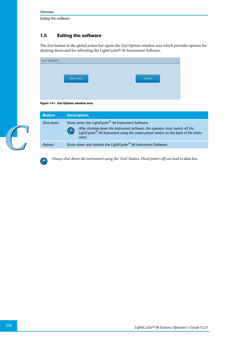
LightCycler® 96 System, Operator’s Guide V2.0236
Overview
CC
Exiting the software
1.5 Exiting the software
The Exit button in the global action bar opens the Exit Options window area which provides options forshutting down and for rebooting the LightCycler® 96 Instrument Software.
Figure 141: Exit Options window area
Always shut down the instrument using the ‘Exit’ button. Hard power-off can lead to data loss.
Button Description
Shut down Shuts down the LightCycler® 96 Instrument Software.
After shutting down the instrument software, the operator must switch off theLightCycler® 96 Instrument using the mains power switch on the back of the instru-ment.
Reboot Shuts down and reboots the LightCycler® 96 Instrument Software.

LightCycler® 96 Instrument Software
Overview tab
237
CC
Experiments table
2 Overview tab
The Overview tab provides a list of the experiments available on the instrument and the USB drive (if con-nected), the status of each experiment, and the memory usage on the instrument.
Figure 142: Overview tab
2.1 Experiments table
The experiments table shows all experiments available on the instrument and on a connected USB drive:
If an experiment is currently running, it is displayed with a bold font and a light green background. Arunning experiment cannot be renamed or deleted. Synchronization is possible, but not recommend-ed. For detailed information, see section Control bar, on page 240.
The currently selected experiment is displayed with a blue background. The selected experiment doesnot need to be the currently running experiment. For detailed information, see section Selecting anexperiment, on page 239.
Each experiment has the following properties:
Column Description
Name Name of the experiment file.
Last Modified Date and time of the last modification.
Status Status of the experiment. For detailed information on the various states, see sectionStatus, on page 238.
Storage Location of the experiment file. For detailed information on the location icons, see sec-tion Storage, on page 238.
Control bar
Experiments table
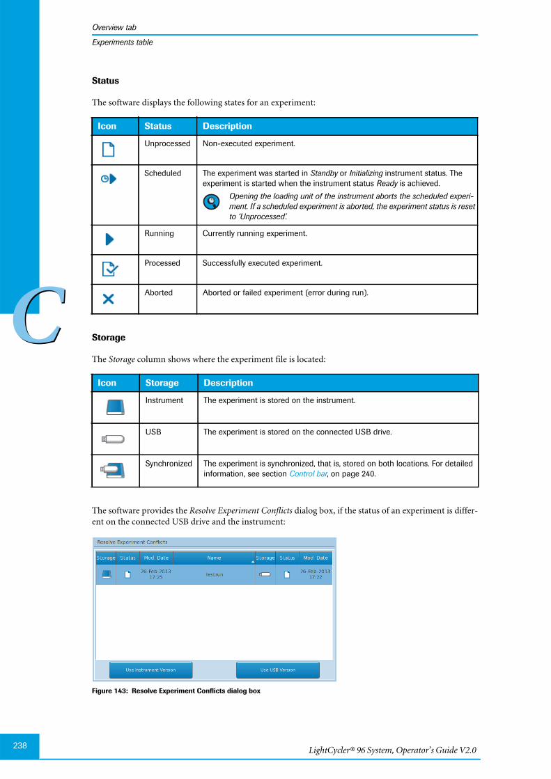
LightCycler® 96 System, Operator’s Guide V2.0238
Overview tab
CC
Experiments table
Status
The software displays the following states for an experiment:
Storage
The Storage column shows where the experiment file is located:
The software provides the Resolve Experiment Conflicts dialog box, if the status of an experiment is differ-ent on the connected USB drive and the instrument:
Figure 143: Resolve Experiment Conflicts dialog box
Icon Status Description
Unprocessed Non-executed experiment.
Scheduled The experiment was started in Standby or Initializing instrument status. Theexperiment is started when the instrument status Ready is achieved.
Opening the loading unit of the instrument aborts the scheduled experi-ment. If a scheduled experiment is aborted, the experiment status is resetto ‘Unprocessed’.
Running Currently running experiment.
Processed Successfully executed experiment.
Aborted Aborted or failed experiment (error during run).
Icon Storage Description
Instrument The experiment is stored on the instrument.
USB The experiment is stored on the connected USB drive.
Synchronized The experiment is synchronized, that is, stored on both locations. For detailedinformation, see section Control bar, on page 240.
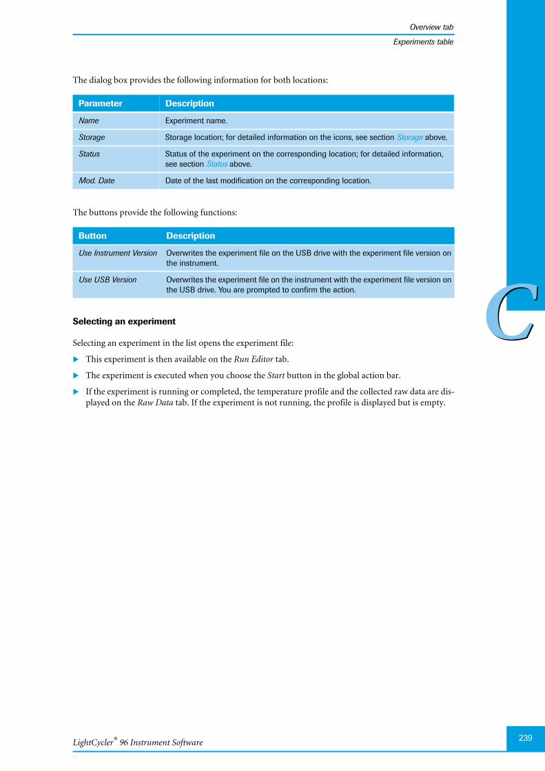
LightCycler® 96 Instrument Software
Overview tab
239
CC
Experiments table
The dialog box provides the following information for both locations:
The buttons provide the following functions:
Selecting an experiment
Selecting an experiment in the list opens the experiment file:
This experiment is then available on the Run Editor tab.
The experiment is executed when you choose the Start button in the global action bar.
If the experiment is running or completed, the temperature profile and the collected raw data are dis-played on the Raw Data tab. If the experiment is not running, the profile is displayed but is empty.
Parameter Description
Name Experiment name.
Storage Storage location; for detailed information on the icons, see section Storage above.
Status Status of the experiment on the corresponding location; for detailed information,see section Status above.
Mod. Date Date of the last modification on the corresponding location.
Button Description
Use Instrument Version Overwrites the experiment file on the USB drive with the experiment file version onthe instrument.
Use USB Version Overwrites the experiment file on the instrument with the experiment file version onthe USB drive. You are prompted to confirm the action.

LightCycler® 96 System, Operator’s Guide V2.0240
Overview tab
CC
Control bar
2.2 Control bar
The control bar on the Overview tab provides the following functions:
Experiment Count bar
The Experiment Count bar shows the total sum of experiments saved on the instrument and on a currentlyconnected USB drive.
The LightCycler® 96 Instrument memory provides space for a maximum of 50 experiments. If whileconnecting a USB drive, the total number of 50 experiments is exceeded, a warning is displayed.
Figure 144: Overview tab, Experiment Count bar
Buttons
The buttons on the Overview tab perform the following functions:
Rename Experiment window area
The Rename button in the control bar opens the Rename Experiment window area for specifying a namefor the selected experiment:
Figure 145: Rename Experiment window area
Button Description
Rename Opens the Rename Experiment window area to specifiy a new name for the selected exper-iment. For detailed information, see section Rename Experiment window area, below.
Synchronize Synchronizes the storage locations:If the selected experiment is located on the instrument, it is transferred to the USB driveand vice versa.
Delete Deletes the selected experiment. The operator is prompted to select the location of theexperiment to be deleted.

LightCycler® 96 Instrument Software
Overview tab
241
CC
Control bar
The window area provides the following options:
Parameter Description
Table Properties of the experiment as displayed on the Overview tab. For detailed informa-tion, see section Experiments table, on page 237.
New Name Input field for the new experiment name. Choosing the text field opens the keyboarddialog box for specifying the name.
Length: 1 to 100 characters
Allowed characters: a-z, A-Z, 0-9, _ (underscore), - (hyphen), . (dot), ( )
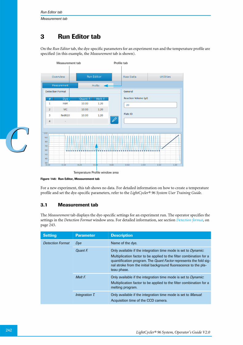
LightCycler® 96 System, Operator’s Guide V2.0242
Run Editor tab
CC
Measurement tab
3 Run Editor tab
On the Run Editor tab, the dye-specific parameters for an experiment run and the temperature profile arespecified (in this example, the Measurement tab is shown).
Figure 146: Run Editor, Measurement tab
For a new experiment, this tab shows no data. For detailed information on how to create a temperatureprofile and set the dye-specific parameters, refer to the LightCycler® 96 System User Training Guide.
3.1 Measurement tab
The Measurement tab displays the dye-specific settings for an experiment run. The operator specifies thesettings in the Detection Format window area. For detailed information, see section Detection format, onpage 243.
Setting Parameter Description
Detection Format Dye Name of the dye.
Quant F. Only available if the integration time mode is set to Dynamic:
Multiplication factor to be applied to the filter combination for aquantification program. The Quant Factor represents the fold sig-nal stroke from the initial background fluorescence to the pla-teau phase.
Melt F. Only available if the integration time mode is set to Dynamic:
Multiplication factor to be applied to the filter combination for amelting program.
Integration T. Only available if the integration time mode is set to Manual:
Acquisition time of the CCD camera.
Measurement tab
Temperature Profile window area
Profile tab
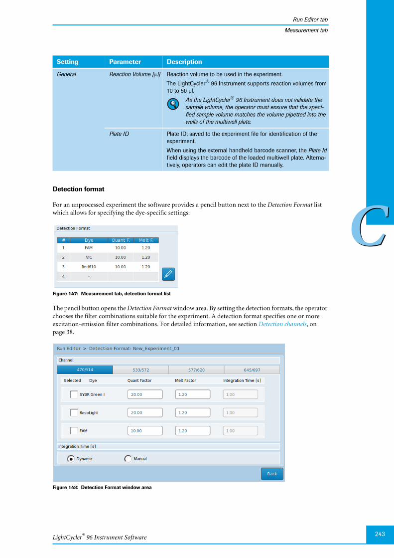
LightCycler® 96 Instrument Software
Run Editor tab
243
CC
Measurement tab
Detection format
For an unprocessed experiment the software provides a pencil button next to the Detection Format listwhich allows for specifying the dye-specific settings:
Figure 147: Measurement tab, detection format list
The pencil button opens the Detection Format window area. By setting the detection formats, the operatorchooses the filter combinations suitable for the experiment. A detection format specifies one or moreexcitation-emission filter combinations. For detailed information, see section Detection channels, onpage 38.
Figure 148: Detection Format window area
General Reaction Volume [l] Reaction volume to be used in the experiment.
The LightCycler® 96 Instrument supports reaction volumes from10 to 50 µl.
As the LightCycler® 96 Instrument does not validate thesample volume, the operator must ensure that the speci-fied sample volume matches the volume pipetted into thewells of the multiwell plate.
Plate ID Plate ID; saved to the experiment file for identification of theexperiment.
When using the external handheld barcode scanner, the Plate Idfield displays the barcode of the loaded multiwell plate. Alterna-tively, operators can edit the plate ID manually.
Setting Parameter Description
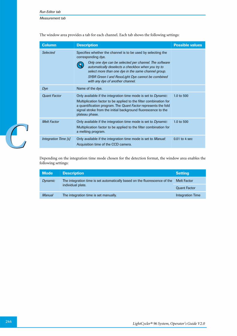
LightCycler® 96 System, Operator’s Guide V2.0244
Run Editor tab
CC
Measurement tab
The window area provides a tab for each channel. Each tab shows the following settings:
Depending on the integration time mode chosen for the detection format, the window area enables thefollowing settings:
Column Description Possible values
Selected Specifies whether the channel is to be used by selecting thecorresponding dye.
Only one dye can be selected per channel. The softwareautomatically deselects a checkbox when you try toselect more than one dye in the same channel group.
SYBR Green I and ResoLight Dye cannot be combinedwith any dye of another channel.
Dye Name of the dye.
Quant Factor Only available if the integration time mode is set to Dynamic:
Multiplication factor to be applied to the filter combination fora quantification program. The Quant Factor represents the foldsignal stroke from the initial background fluorescence to theplateau phase.
1.0 to 500
Melt Factor Only available if the integration time mode is set to Dynamic:
Multiplication factor to be applied to the filter combination fora melting program.
1.0 to 500
Integration Time [s] Only available if the integration time mode is set to Manual:
Acquisition time of the CCD camera.
0.01 to 4 sec
Mode Description Setting
Dynamic The integration time is set automatically based on the fluorescence of theindividual plate.
Melt Factor
Quant Factor
Manual The integration time is set manually. Integration Time
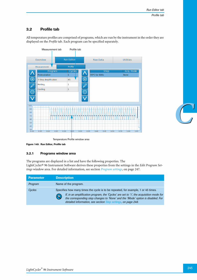
LightCycler® 96 Instrument Software
Run Editor tab
245
CC
Profile tab
3.2 Profile tab
All temperature profiles are comprised of programs, which are run by the instrument in the order they aredisplayed on the Profile tab. Each program can be specified separately.
Figure 149: Run Editor, Profile tab
3.2.1 Programs window area
The programs are displayed in a list and have the following properties. TheLightCycler® 96 Instrument Software derives these properties from the settings in the Edit Program Set-tings window area. For detailed information, see section Program settings, on page 247.
Parameter Description
Program Name of the program.
Cycles Specifies how many times the cycle is to be repeated, for example, 1 or 45 times.
If, in an amplification program, the ‘Cycles’ are set to ‘1’, the acquisition mode forthe corresponding step changes to ‘None’ and the ‘Mode’ option is disabled. Fordetailed information, see section Step settings, on page 248.
Measurement tab
Temperature Profile window area
Profile tab
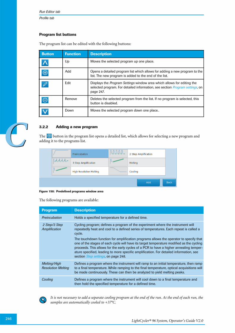
LightCycler® 96 System, Operator’s Guide V2.0246
Run Editor tab
CC
Profile tab
Program list buttons
The program list can be edited with the following buttons:
3.2.2 Adding a new program
The button in the program list opens a detailed list, which allows for selecting a new program andadding it to the programs list.
Figure 150: Predefined programs window area
The following programs are available:
It is not necessary to add a separate cooling program at the end of the run. At the end of each run, thesamples are automatically cooled to +37°C.
Button Function Description
Up Moves the selected program up one place.
Add Opens a detailed program list which allows for adding a new program to thelist. The new program is added to the end of the list.
Edit Displays the Program Settings window area which allows for editing theselected program. For detailed information, see section Program settings, onpage 247.
Remove Deletes the selected program from the list. If no program is selected, thisbutton is disabled.
Down Moves the selected program down one place..
Program Description
Preincubation Holds a specified temperature for a defined time.
2 Step/3 StepAmplification
Cycling program; defines a program of the experiment where the instrument willrepeatedly heat and cool to a defined series of temperatures. Each repeat is called acycle.
The touchdown function for amplification programs allows the operator to specify thatone of the stages of each cycle will have its target temperature modified as the cyclingproceeds. This allows for the early cycles of a PCR to have a higher annealing temper-ature specified, leading to more specific amplification. For detailed information, seesection Step settings, on page 248.
Melting/HighResolution Melting
Defines a program where the instrument will ramp to an initial temperature, then rampto a final temperature. While ramping to the final temperature, optical acquisitions willbe made continuously. These can then be analyzed to yield melting peaks.
Cooling Defines a program where the instrument will cool down to a final temperature andthen hold the specified temperature for a defined time.
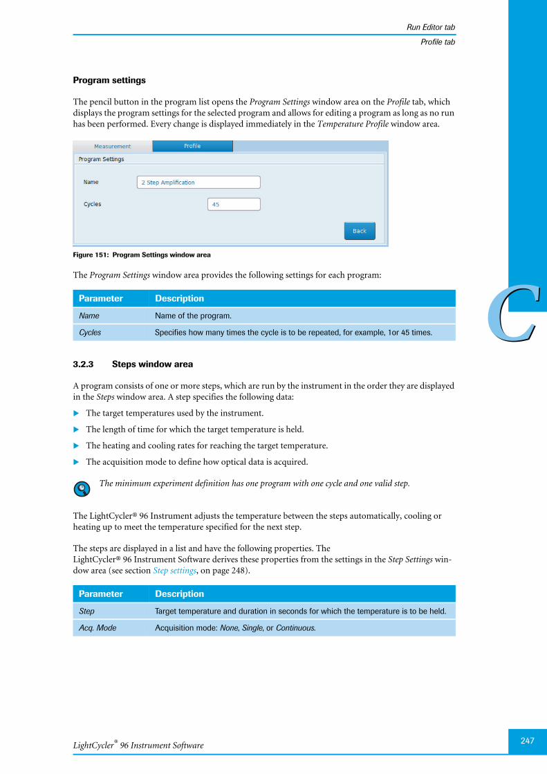
LightCycler® 96 Instrument Software
Run Editor tab
247
CC
Profile tab
Program settings
The pencil button in the program list opens the Program Settings window area on the Profile tab, whichdisplays the program settings for the selected program and allows for editing a program as long as no runhas been performed. Every change is displayed immediately in the Temperature Profile window area.
Figure 151: Program Settings window area
The Program Settings window area provides the following settings for each program:
3.2.3 Steps window area
A program consists of one or more steps, which are run by the instrument in the order they are displayedin the Steps window area. A step specifies the following data:
The target temperatures used by the instrument.
The length of time for which the target temperature is held.
The heating and cooling rates for reaching the target temperature.
The acquisition mode to define how optical data is acquired.
The minimum experiment definition has one program with one cycle and one valid step.
The LightCycler® 96 Instrument adjusts the temperature between the steps automatically, cooling orheating up to meet the temperature specified for the next step.
The steps are displayed in a list and have the following properties. TheLightCycler® 96 Instrument Software derives these properties from the settings in the Step Settings win-dow area (see section Step settings, on page 248).
Parameter Description
Name Name of the program.
Cycles Specifies how many times the cycle is to be repeated, for example, 1or 45 times.
Parameter Description
Step Target temperature and duration in seconds for which the temperature is to be held.
Acq. Mode Acquisition mode: None, Single, or Continuous.
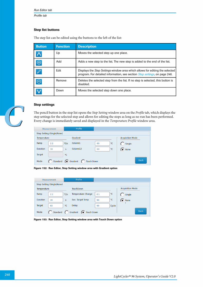
LightCycler® 96 System, Operator’s Guide V2.0248
Run Editor tab
CC
Profile tab
Step list buttons
The step list can be edited using the buttons to the left of the list:
Step settings
The pencil button in the step list opens the Step Setting window area on the Profile tab, which displays thestep settings for the selected step and allows for editing the steps as long as no run has been performed.Every change is immediately saved and displayed in the Temperature Profile window area.
Figure 152: Run Editor, Step Setting window area with Gradient option
Figure 153: Run Editor, Step Setting window area with Touch Down option
Button Function Description
Up Moves the selected step up one place.
Add Adds a new step to the list. The new step is added to the end of the list.
Edit Displays the Step Settings window area which allows for editing the selectedprogram. For detailed information, see section Step settings, on page 248.
Remove Deletes the selected step from the list. If no step is selected, this button isdisabled.
Down Moves the selected step down one place.
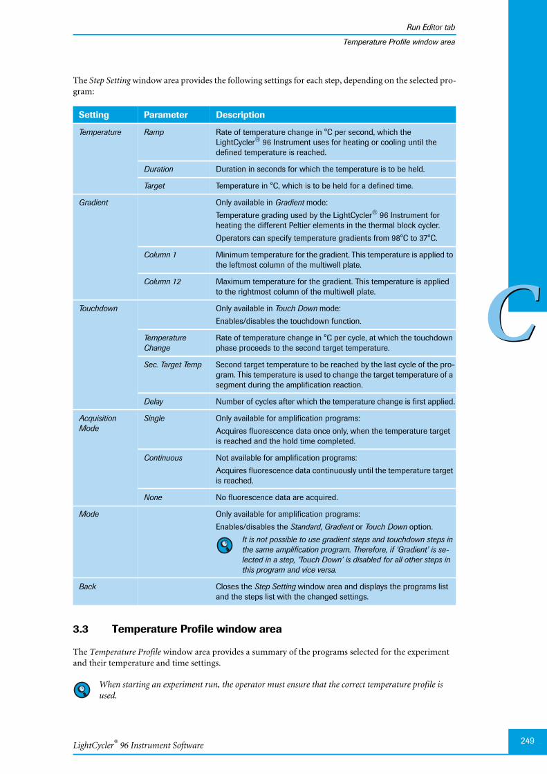
LightCycler® 96 Instrument Software
Run Editor tab
249
CC
Temperature Profile window area
The Step Setting window area provides the following settings for each step, depending on the selected pro-gram:
3.3 Temperature Profile window area
The Temperature Profile window area provides a summary of the programs selected for the experimentand their temperature and time settings.
When starting an experiment run, the operator must ensure that the correct temperature profile isused.
Setting Parameter Description
Temperature Ramp Rate of temperature change in °C per second, which theLightCycler® 96 Instrument uses for heating or cooling until thedefined temperature is reached.
Duration Duration in seconds for which the temperature is to be held.
Target Temperature in °C, which is to be held for a defined time.
Gradient Only available in Gradient mode:
Temperature grading used by the LightCycler® 96 Instrument forheating the different Peltier elements in the thermal block cycler.
Operators can specify temperature gradients from 98°C to 37°C.
Column 1 Minimum temperature for the gradient. This temperature is applied tothe leftmost column of the multiwell plate.
Column 12 Maximum temperature for the gradient. This temperature is appliedto the rightmost column of the multiwell plate.
Touchdown Only available in Touch Down mode:
Enables/disables the touchdown function.
TemperatureChange
Rate of temperature change in °C per cycle, at which the touchdownphase proceeds to the second target temperature.
Sec. Target Temp Second target temperature to be reached by the last cycle of the pro-gram. This temperature is used to change the target temperature of asegment during the amplification reaction.
Delay Number of cycles after which the temperature change is first applied.
AcquisitionMode
Single Only available for amplification programs:
Acquires fluorescence data once only, when the temperature targetis reached and the hold time completed.
Continuous Not available for amplification programs:
Acquires fluorescence data continuously until the temperature targetis reached.
None No fluorescence data are acquired.
Mode Only available for amplification programs:
Enables/disables the Standard, Gradient or Touch Down option.
It is not possible to use gradient steps and touchdown steps inthe same amplification program. Therefore, if ‘Gradient’ is se-lected in a step, ‘Touch Down’ is disabled for all other steps inthis program and vice versa.
Back Closes the Step Setting window area and displays the programs listand the steps list with the changed settings.
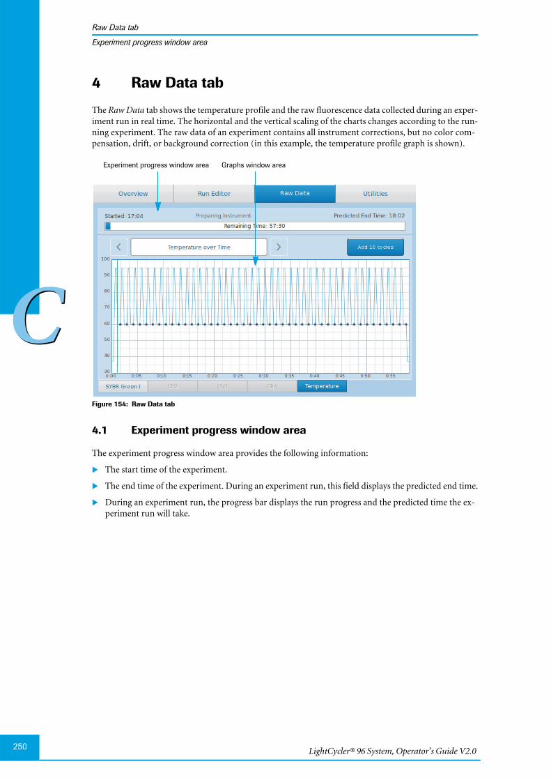
LightCycler® 96 System, Operator’s Guide V2.0250
Raw Data tab
CC
Experiment progress window area
4 Raw Data tab
The Raw Data tab shows the temperature profile and the raw fluorescence data collected during an exper-iment run in real time. The horizontal and the vertical scaling of the charts changes according to the run-ning experiment. The raw data of an experiment contains all instrument corrections, but no color com-pensation, drift, or background correction (in this example, the temperature profile graph is shown).
Figure 154: Raw Data tab
4.1 Experiment progress window area
The experiment progress window area provides the following information:
The start time of the experiment.
The end time of the experiment. During an experiment run, this field displays the predicted end time.
During an experiment run, the progress bar displays the run progress and the predicted time the ex-periment run will take.
Graphs window areaExperiment progress window area
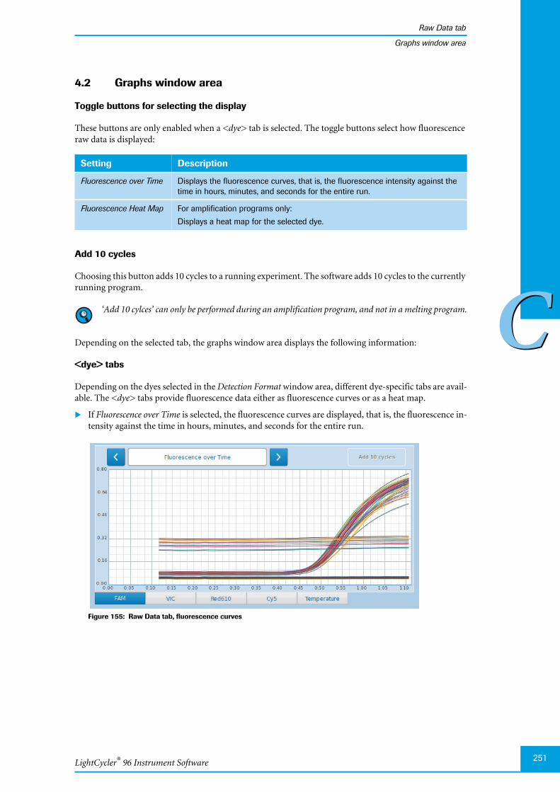
LightCycler® 96 Instrument Software
Raw Data tab
251
CC
Graphs window area
4.2 Graphs window area
Toggle buttons for selecting the display
These buttons are only enabled when a <dye> tab is selected. The toggle buttons select how fluorescenceraw data is displayed:
Add 10 cycles
Choosing this button adds 10 cycles to a running experiment. The software adds 10 cycles to the currentlyrunning program.
‘Add 10 cylces’ can only be performed during an amplification program, and not in a melting program.
Depending on the selected tab, the graphs window area displays the following information:
<dye> tabs
Depending on the dyes selected in the Detection Format window area, different dye-specific tabs are avail-able. The <dye> tabs provide fluorescence data either as fluorescence curves or as a heat map.
If Fluorescence over Time is selected, the fluorescence curves are displayed, that is, the fluorescence in-tensity against the time in hours, minutes, and seconds for the entire run.
Figure 155: Raw Data tab, fluorescence curves
Setting Description
Fluorescence over Time Displays the fluorescence curves, that is, the fluorescence intensity against thetime in hours, minutes, and seconds for the entire run.
Fluorescence Heat Map For amplification programs only:
Displays a heat map for the selected dye.
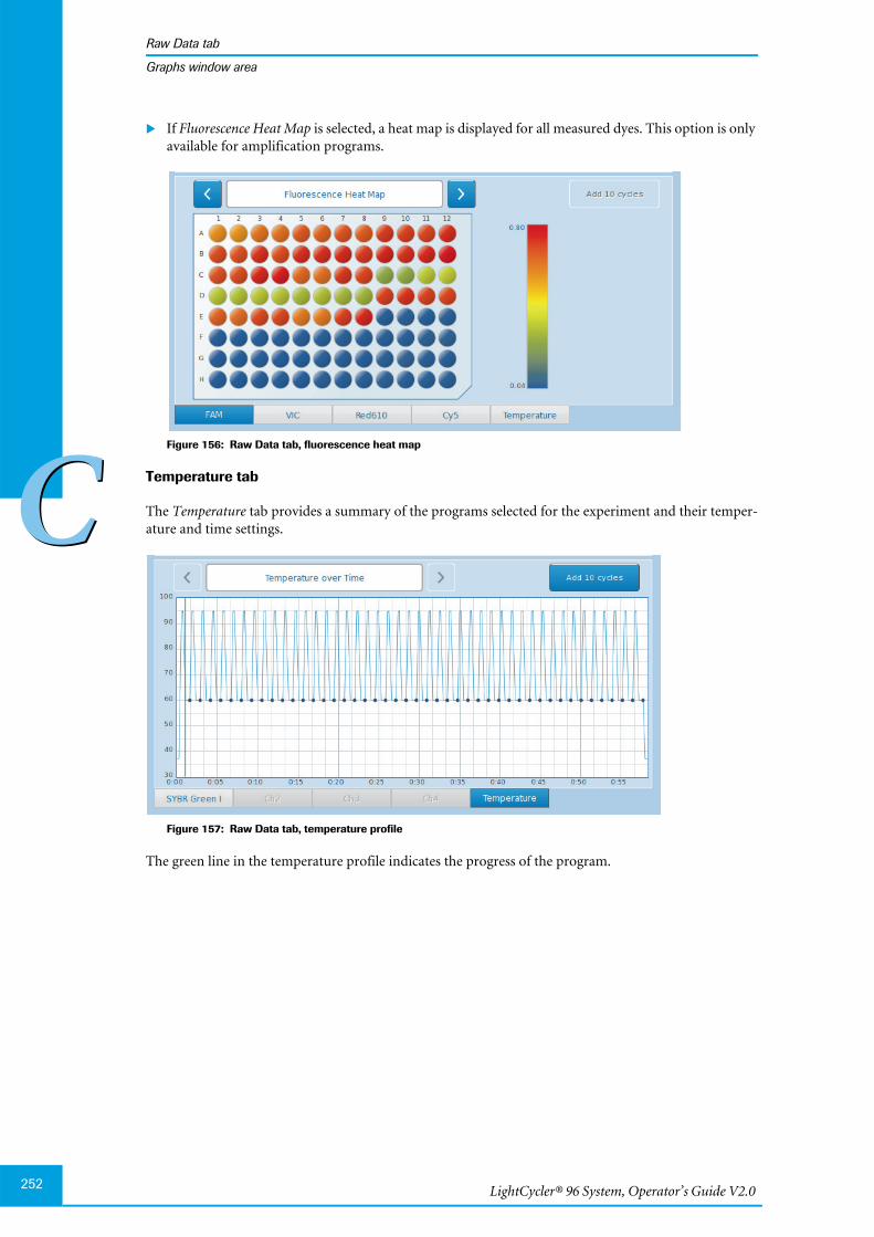
LightCycler® 96 System, Operator’s Guide V2.0252
Raw Data tab
CC
Graphs window area
If Fluorescence Heat Map is selected, a heat map is displayed for all measured dyes. This option is onlyavailable for amplification programs.
Figure 156: Raw Data tab, fluorescence heat map
Temperature tab
The Temperature tab provides a summary of the programs selected for the experiment and their temper-ature and time settings.
Figure 157: Raw Data tab, temperature profile
The green line in the temperature profile indicates the progress of the program.
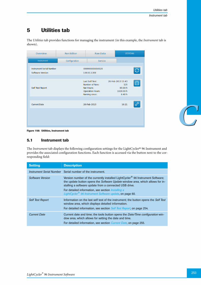
LightCycler® 96 Instrument Software
Utilities tab
253
CC
Instrument tab
5 Utilities tab
The Utilities tab provides functions for managing the instrument (in this example, the Instrument tab isshown).
Figure 158: Utilities, Instrument tab
5.1 Instrument tab
The Instrument tab displays the following configuration settings for the LightCycler® 96 Instrument andprovides the associated configuration functions. Each function is accessed via the button next to the cor-responding field:
Setting Description
Instrument Serial Number Serial number of the instrument.
Software Version Version number of the currently installed LightCycler® 96 Instrument Software;the update button opens the Software Update window area, which allows for in-stalling a software update from a connected USB drive.
For detailed information, see section Installing aLightCycler® 96 Instrument Software update, on page 60.
Self Test Report Information on the last self test of the instrument; the button opens the Self Testwindow area, which displays detailed information.
For detailed information, see section Self Test Report, on page 254.
Current Date Current date and time; the tools button opens the Date/Time configuration win-dow area, which allows for setting the date and time.
For detailed information, see section Current Date, on page 255.

LightCycler® 96 System, Operator’s Guide V2.0254
Utilities tab
CC
Instrument tab
5.1.1 Self Test Report
The button next to the Self Test Report field opens the Self Test window area, which displays detailed infor-mation on the last self test of the instrument. The self test is performed during initialization of the instru-ment.
Figure 159: Self Test window area
Export to USB
The Export to USB button allows for saving the last self test results to a connected USB drive. Results aresaved to a PDF file with the default name Selftest_Result_<series_no>_<date>.pdf.
Figure 160: Self Test Report PDF file

LightCycler® 96 Instrument Software
Utilities tab
255
CC
Instrument tab
5.1.2 Current Date
The tools button next to the Current Date field opens the Date/Time Configuration window area, whichallows for setting the current date and time.
Figure 161: Date/time configuration window area
The Ok and Reboot button changes the date and time settings and reboots the instrument.
Choosing the input fields opens the Set Date or Set Time dialog box, allowing the operator to specify thecurrent time and date.
Figure 162: Set Date and Set Time dialog boxes
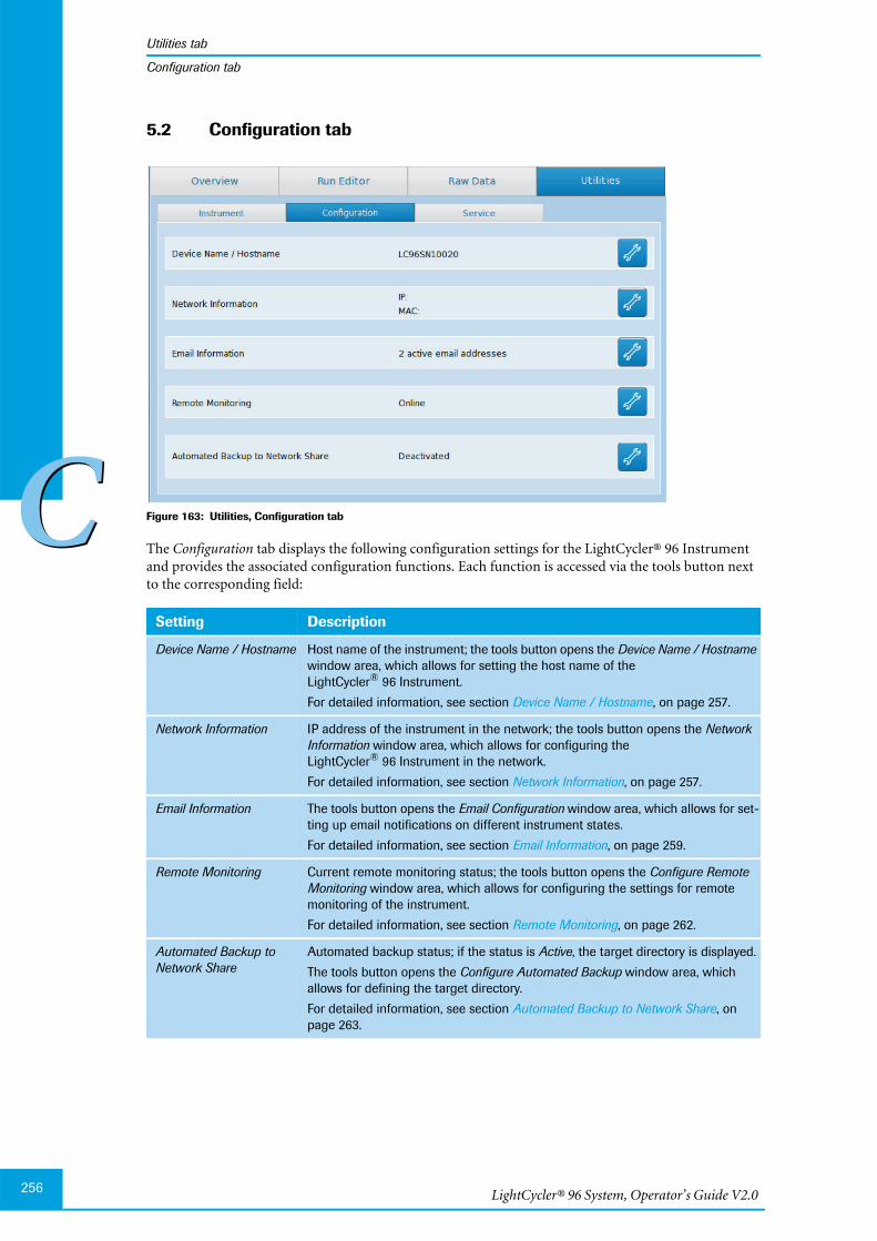
LightCycler® 96 System, Operator’s Guide V2.0256
Utilities tab
CC
Configuration tab
5.2 Configuration tab
Figure 163: Utilities, Configuration tab
The Configuration tab displays the following configuration settings for the LightCycler® 96 Instrumentand provides the associated configuration functions. Each function is accessed via the tools button nextto the corresponding field:
Setting Description
Device Name / Hostname Host name of the instrument; the tools button opens the Device Name / Hostnamewindow area, which allows for setting the host name of theLightCycler® 96 Instrument.
For detailed information, see section Device Name / Hostname, on page 257.
Network Information IP address of the instrument in the network; the tools button opens the NetworkInformation window area, which allows for configuring theLightCycler® 96 Instrument in the network.
For detailed information, see section Network Information, on page 257.
Email Information The tools button opens the Email Configuration window area, which allows for set-ting up email notifications on different instrument states.
For detailed information, see section Email Information, on page 259.
Remote Monitoring Current remote monitoring status; the tools button opens the Configure RemoteMonitoring window area, which allows for configuring the settings for remotemonitoring of the instrument.
For detailed information, see section Remote Monitoring, on page 262.
Automated Backup toNetwork Share
Automated backup status; if the status is Active, the target directory is displayed.
The tools button opens the Configure Automated Backup window area, whichallows for defining the target directory.
For detailed information, see section Automated Backup to Network Share, onpage 263.
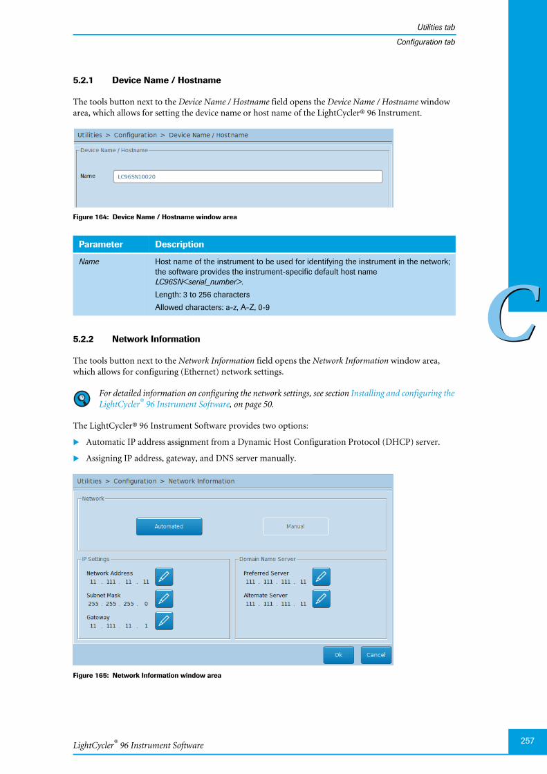
LightCycler® 96 Instrument Software
Utilities tab
257
CC
Configuration tab
5.2.1 Device Name / Hostname
The tools button next to the Device Name / Hostname field opens the Device Name / Hostname windowarea, which allows for setting the device name or host name of the LightCycler® 96 Instrument.
Figure 164: Device Name / Hostname window area
5.2.2 Network Information
The tools button next to the Network Information field opens the Network Information window area,which allows for configuring (Ethernet) network settings.
For detailed information on configuring the network settings, see section Installing and configuring theLightCycler® 96 Instrument Software, on page 50.
The LightCycler® 96 Instrument Software provides two options:
Automatic IP address assignment from a Dynamic Host Configuration Protocol (DHCP) server.
Assigning IP address, gateway, and DNS server manually.
Figure 165: Network Information window area
Parameter Description
Name Host name of the instrument to be used for identifying the instrument in the network;the software provides the instrument-specific default host nameLC96SN<serial_number>.
Length: 3 to 256 characters
Allowed characters: a-z, A-Z, 0-9
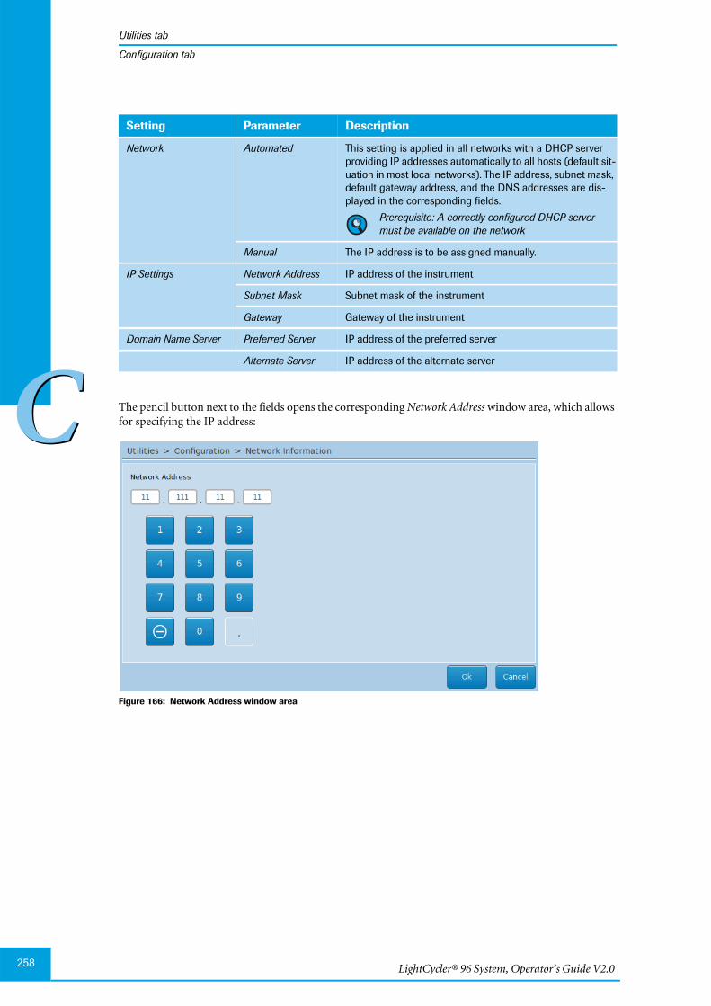
LightCycler® 96 System, Operator’s Guide V2.0258
Utilities tab
CC
Configuration tab
The pencil button next to the fields opens the corresponding Network Address window area, which allowsfor specifying the IP address:
Figure 166: Network Address window area
Setting Parameter Description
Network Automated This setting is applied in all networks with a DHCP serverproviding IP addresses automatically to all hosts (default sit-uation in most local networks). The IP address, subnet mask,default gateway address, and the DNS addresses are dis-played in the corresponding fields.
Prerequisite: A correctly configured DHCP servermust be available on the network
Manual The IP address is to be assigned manually.
IP Settings Network Address IP address of the instrument
Subnet Mask Subnet mask of the instrument
Gateway Gateway of the instrument
Domain Name Server Preferred Server IP address of the preferred server
Alternate Server IP address of the alternate server
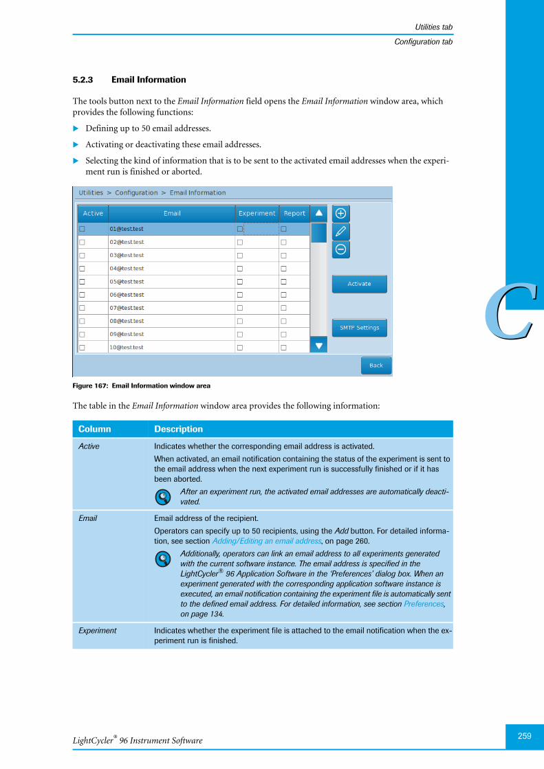
LightCycler® 96 Instrument Software
Utilities tab
259
CC
Configuration tab
5.2.3 Email Information
The tools button next to the Email Information field opens the Email Information window area, whichprovides the following functions:
Defining up to 50 email addresses.
Activating or deactivating these email addresses.
Selecting the kind of information that is to be sent to the activated email addresses when the experi-ment run is finished or aborted.
Figure 167: Email Information window area
The table in the Email Information window area provides the following information:
Column Description
Active Indicates whether the corresponding email address is activated.
When activated, an email notification containing the status of the experiment is sent tothe email address when the next experiment run is successfully finished or if it hasbeen aborted.
After an experiment run, the activated email addresses are automatically deacti-vated.
Email Email address of the recipient.
Operators can specify up to 50 recipients, using the Add button. For detailed informa-tion, see section Adding/Editing an email address, on page 260.
Additionally, operators can link an email address to all experiments generatedwith the current software instance. The email address is specified in theLightCycler® 96 Application Software in the ‘Preferences’ dialog box. When anexperiment generated with the corresponding application software instance isexecuted, an email notification containing the experiment file is automatically sentto the defined email address. For detailed information, see section Preferences,on page 134.
Experiment Indicates whether the experiment file is attached to the email notification when the ex-periment run is finished.

LightCycler® 96 System, Operator’s Guide V2.0260
Utilities tab
CC
Configuration tab
The emails list can be edited with the following buttons:
The additional buttons in the Email Information window area provide the following functions:
Adding/Editing an email address
The plus and the pencil button in the Email Information window area open a table for specifying the set-tings for a new email address.
Figure 168: Email Configuration window area, Add/Edit
Report Indicates whether a PDF email report is attached to the email notification when the ex-periment run is finished. The PDF report contains the following information:
Raw data amplification curves and fluorescence plate map (for amplification pro-gram only) of all measured dyes
Run temperature profile
Experiment name
Plate ID
Creation date
Run start and end time
Button Function Description
Add Adds a new email address to the list. For detailed information, see sectionAdding/Editing an email address, below.
Edit Opens a window area for editing the settings of the selected email address.For detailed information, see section Adding/Editing an email address, below.
Remove Removes the selected email address from the list.
Button Description
Activate/Deactivate Activates/Deactivates the selected email address.
SMTP Settings Opens a window area for editing the SMTP settings of the selected email address.For detailed information, see section SMTP Settings, on page 261.
Column Description
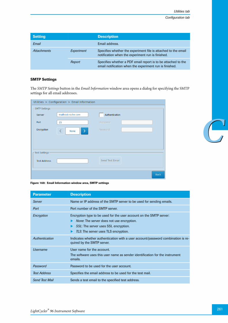
LightCycler® 96 Instrument Software
Utilities tab
261
CC
Configuration tab
SMTP Settings
The SMTP Settings button in the Email Information window area opens a dialog for specifying the SMTPsettings for all email addresses.
Figure 169: Email Information window area, SMTP settings
Setting Description
Email Email address.
Attachments Experiment Specifies whether the experiment file is attached to the emailnotification when the experiment run is finished.
Report Specifies whether a PDF email report is to be attached to theemail notification when the experiment run is finished.
Parameter Description
Server Name or IP address of the SMTP server to be used for sending emails.
Port Port number of the SMTP server.
Encryption Encryption type to be used for the user account on the SMTP server:
None: The server does not use encryption.
SSL: The server uses SSL encryption.
TLS: The server uses TLS encryption.
Authentication Indicates whether authentication with a user account/password combination is re-quired by the SMTP server.
Username User name for the account.
The software uses this user name as sender identification for the instrumentemails.
Password Password to be used for the user account.
Test Address Specifies the email address to be used for the test mail.
Send Test Mail Sends a test email to the specified test address.
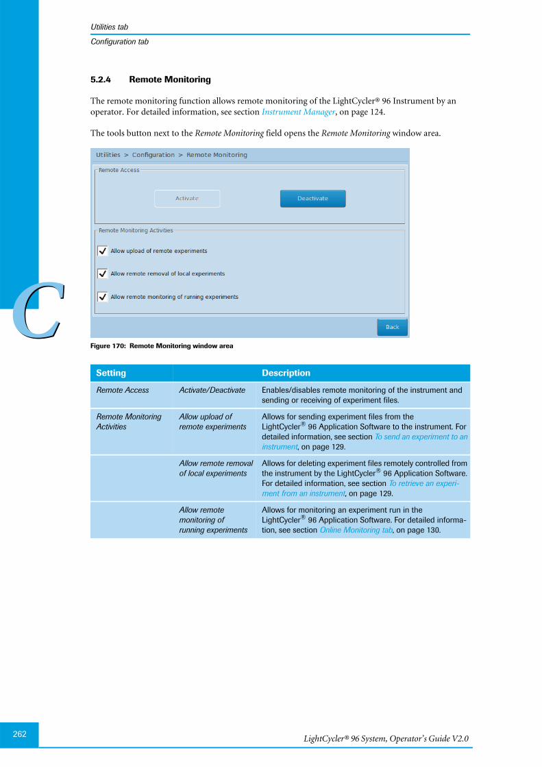
LightCycler® 96 System, Operator’s Guide V2.0262
Utilities tab
CC
Configuration tab
5.2.4 Remote Monitoring
The remote monitoring function allows remote monitoring of the LightCycler® 96 Instrument by anoperator. For detailed information, see section Instrument Manager, on page 124.
The tools button next to the Remote Monitoring field opens the Remote Monitoring window area.
Figure 170: Remote Monitoring window area
Setting Description
Remote Access Activate/Deactivate Enables/disables remote monitoring of the instrument andsending or receiving of experiment files.
Remote MonitoringActivities
Allow upload ofremote experiments
Allows for sending experiment files from theLightCycler® 96 Application Software to the instrument. Fordetailed information, see section To send an experiment to aninstrument, on page 129.
Allow remote removalof local experiments
Allows for deleting experiment files remotely controlled fromthe instrument by the LightCycler® 96 Application Software.For detailed information, see section To retrieve an experi-ment from an instrument, on page 129.
Allow remotemonitoring ofrunning experiments
Allows for monitoring an experiment run in theLightCycler® 96 Application Software. For detailed informa-tion, see section Online Monitoring tab, on page 130.
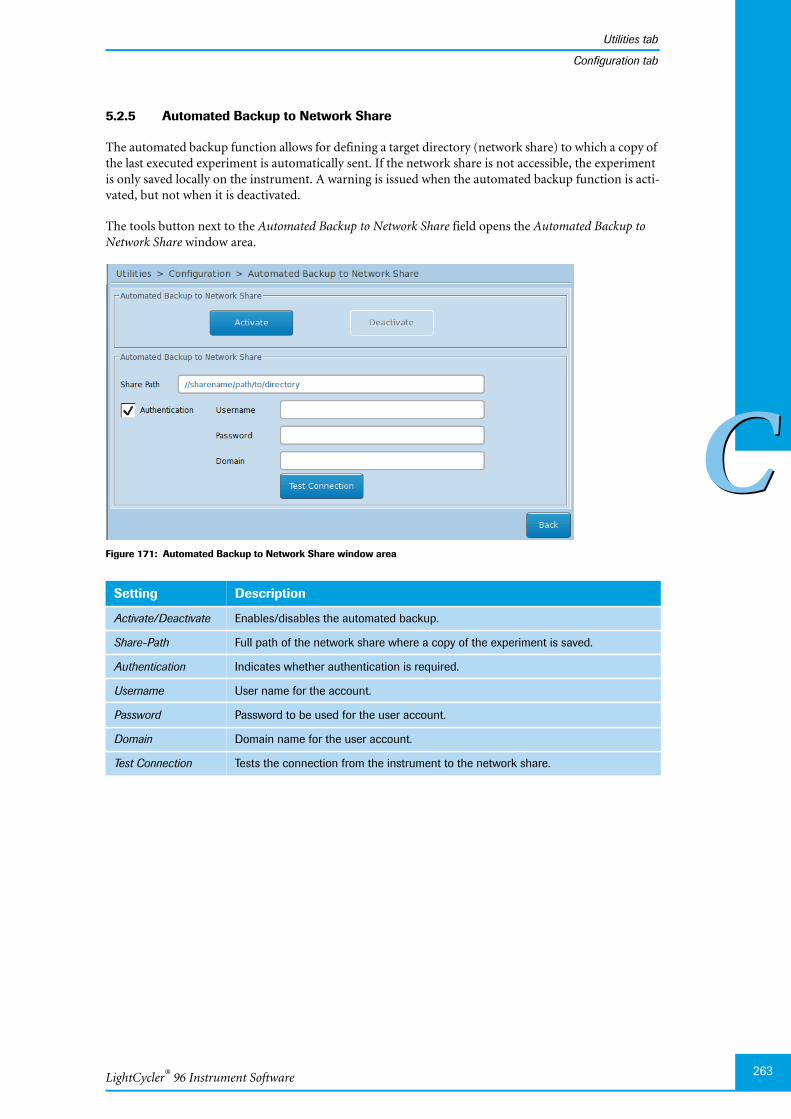
LightCycler® 96 Instrument Software
Utilities tab
263
CC
Configuration tab
5.2.5 Automated Backup to Network Share
The automated backup function allows for defining a target directory (network share) to which a copy ofthe last executed experiment is automatically sent. If the network share is not accessible, the experimentis only saved locally on the instrument. A warning is issued when the automated backup function is acti-vated, but not when it is deactivated.
The tools button next to the Automated Backup to Network Share field opens the Automated Backup toNetwork Share window area.
Figure 171: Automated Backup to Network Share window area
Setting Description
Activate/Deactivate Enables/disables the automated backup.
Share-Path Full path of the network share where a copy of the experiment is saved.
Authentication Indicates whether authentication is required.
Username User name for the account.
Password Password to be used for the user account.
Domain Domain name for the user account.
Test Connection Tests the connection from the instrument to the network share.
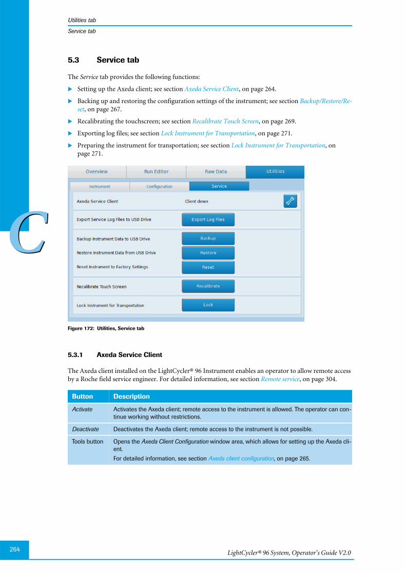
LightCycler® 96 System, Operator’s Guide V2.0264
Utilities tab
CC
Service tab
5.3 Service tab
The Service tab provides the following functions:
Setting up the Axeda client; see section Axeda Service Client, on page 264.
Backing up and restoring the configuration settings of the instrument; see section Backup/Restore/Re-set, on page 267.
Recalibrating the touchscreen; see section Recalibrate Touch Screen, on page 269.
Exporting log files; see section Lock Instrument for Transportation, on page 271.
Preparing the instrument for transportation; see section Lock Instrument for Transportation, onpage 271.
Figure 172: Utilities, Service tab
5.3.1 Axeda Service Client
The Axeda client installed on the LightCycler® 96 Instrument enables an operator to allow remote accessby a Roche field service engineer. For detailed information, see section Remote service, on page 304.
Button Description
Activate Activates the Axeda client; remote access to the instrument is allowed. The operator can con-tinue working without restrictions.
Deactivate Deactivates the Axeda client; remote access to the instrument is not possible.
Tools button Opens the Axeda Client Configuration window area, which allows for setting up the Axeda cli-ent.
For detailed information, see section Axeda client configuration, on page 265.

LightCycler® 96 Instrument Software
Utilities tab
265
CC
Service tab
Axeda client configuration
The tools button next to the Axeda Service Client up/down field opens the Axeda Client Configuration win-dow area, which allows for setting up the Axeda client.
Figure 173: Axeda Client Configuration window area
Setting Description
Axeda Client Activation Activate Activates the Axeda client; remote access to the instru-ment is allowed. The operator can continue workingwithout restrictions.
Deactivate Deactivates the Axeda client; remote access to the in-strument is not possible.
Axeda Client Status Current Status Current status of the Axeda client: Online or Offline.
Automated Deactivation Date and time of the last automated Axeda client deacti-vation.
The Axeda client is automatically deactivated after24 hours.
Data Transfer Date and time of the last data transfer.
Export User Data toAxeda
Experiments/Log Files/Configuration Files
Specifies which data are to be exported for access bythe Roche field service engineer.
Export Exports the specified data.
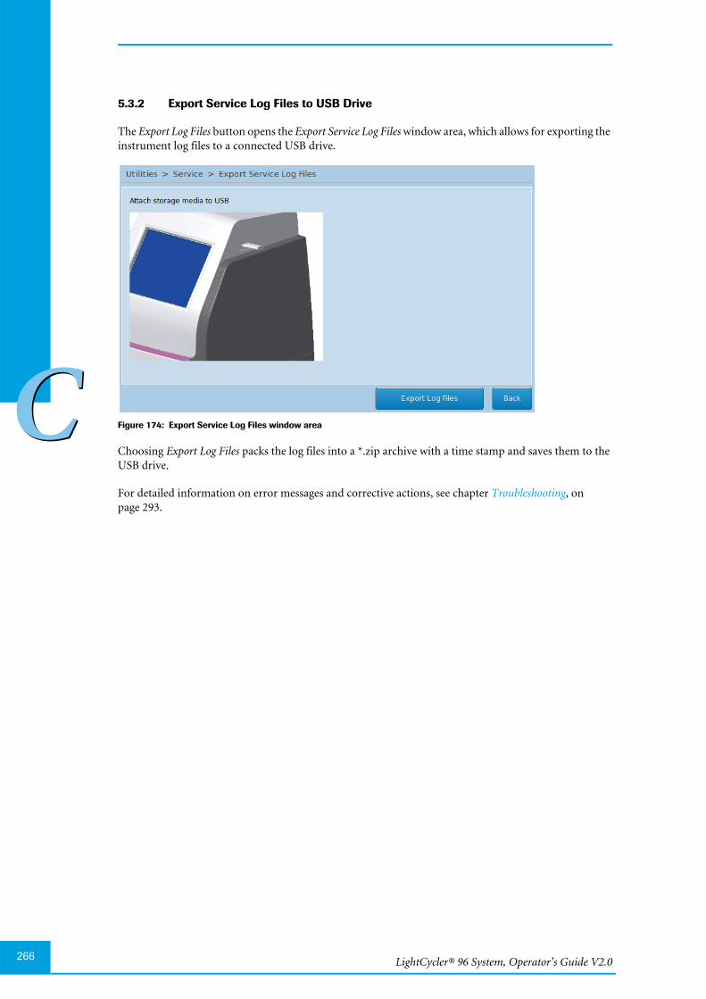
LightCycler® 96 System, Operator’s Guide V2.0
CC
266
5.3.2 Export Service Log Files to USB Drive
The Export Log Files button opens the Export Service Log Files window area, which allows for exporting theinstrument log files to a connected USB drive.
Figure 174: Export Service Log Files window area
Choosing Export Log Files packs the log files into a *.zip archive with a time stamp and saves them to theUSB drive.
For detailed information on error messages and corrective actions, see chapter Troubleshooting, onpage 293.
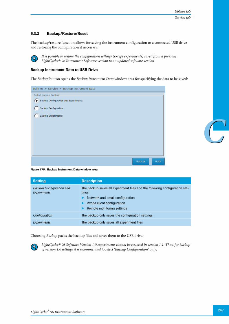
LightCycler® 96 Instrument Software
Utilities tab
267
CC
Service tab
5.3.3 Backup/Restore/Reset
The backup/restore function allows for saving the instrument configuration to a connected USB driveand restoring the configuration if necessary.
It is possible to restore the configuration settings (except experiments) saved from a previousLightCycler® 96 Instrument Software version to an updated software version.
Backup Instrument Data to USB Drive
The Backup button opens the Backup Instrument Data window area for specifying the data to be saved:
Figure 175: Backup Instrument Data window area
Choosing Backup packs the backup files and saves them to the USB drive.
LightCycler® 96 Software Version 1.0 experiments cannot be restored in version 1.1. Thus, for backupof version 1.0 settings it is recommended to select ‘Backup Configuration’ only.
Setting Description
Backup Configuration andExperiments
The backup saves all experiment files and the following configuration set-tings:
Network and email configuration
Axeda client configuration
Remote monitoring settings
Configuration The backup only saves the configuration settings.
Experiments The backup only saves all experiment files.
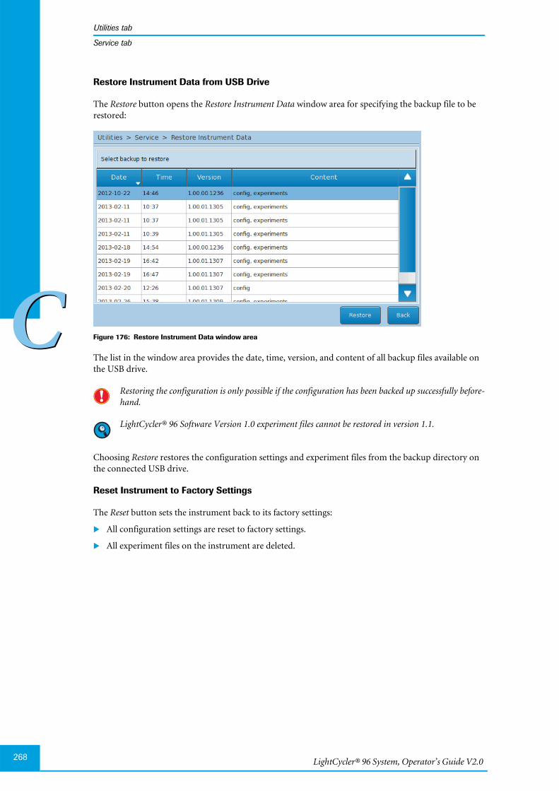
LightCycler® 96 System, Operator’s Guide V2.0268
Utilities tab
CC
Service tab
Restore Instrument Data from USB Drive
The Restore button opens the Restore Instrument Data window area for specifying the backup file to berestored:
Figure 176: Restore Instrument Data window area
The list in the window area provides the date, time, version, and content of all backup files available onthe USB drive.
Restoring the configuration is only possible if the configuration has been backed up successfully before-hand.
LightCycler® 96 Software Version 1.0 experiment files cannot be restored in version 1.1.
Choosing Restore restores the configuration settings and experiment files from the backup directory onthe connected USB drive.
Reset Instrument to Factory Settings
The Reset button sets the instrument back to its factory settings:
All configuration settings are reset to factory settings.
All experiment files on the instrument are deleted.
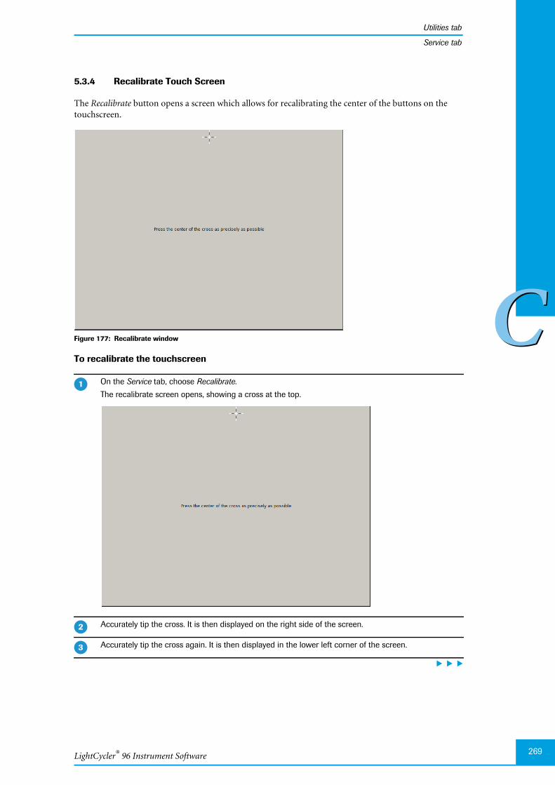
LightCycler® 96 Instrument Software
Utilities tab
269
CC
Service tab
5.3.4 Recalibrate Touch Screen
The Recalibrate button opens a screen which allows for recalibrating the center of the buttons on thetouchscreen.
Figure 177: Recalibrate window
To recalibrate the touchscreen
On the Service tab, choose Recalibrate.
The recalibrate screen opens, showing a cross at the top.
Accurately tip the cross. It is then displayed on the right side of the screen.
Accurately tip the cross again. It is then displayed in the lower left corner of the screen.
�
�
�

LightCycler® 96 System, Operator’s Guide V2.0270
Utilities tab
CC
Service tab
Accurately tip the cross again. A screen containing an OK button is displayed.
Choose OK.
The calibration screen closes and the Service tab is displayed using the updated touchscreen calibra-tion.
If you do not choose ‘OK’ during 30 seconds, the touchscreen reverts to the provious calibrationsettings.
�
�

LightCycler® 96 Instrument Software
Utilities tab
271
CC
Service tab
5.3.5 Lock Instrument for Transportation
The Lock button locks the loading module for transport. The operator is prompted to confirm that thetransport locking device is inserted. For detailed information on the transport locking device, see sectionAssembling the instrument, on page 44.
Figure 178: Activate Transport Lock dialog box
It is also necessary for transport to tighten the fixation gripper on the back of the instrument. Fordetailed information on the fixation gripper, see section To unpack and install theLightCycler® 96 Instrument, on page 44.
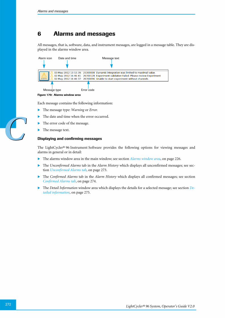
LightCycler® 96 System, Operator’s Guide V2.0272
Alarms and messages
CC
6 Alarms and messages
All messages, that is, software, data, and instrument messages, are logged in a message table. They are dis-played in the alarms window area.
Figure 179: Alarms window area
Each message contains the following information:
The message type: Warning or Error.
The date and time when the error occurred.
The error code of the message.
The message text.
Displaying and confirming messages
The LightCycler® 96 Instrument Software provides the following options for viewing messages andalarms in general or in detail:
The alarms window area in the main window; see section Alarms window area, on page 226.
The Unconfirmed Alarms tab in the Alarm History which displays all unconfirmed messages; see sec-tion Unconfirmed Alarms tab, on page 273.
The Confirmed Alarms tab in the Alarm History which displays all confirmed messages; see sectionConfirmed Alarms tab, on page 274.
The Detail Information window area which displays the details for a selected message; see section De-tailed information, on page 275.
Alarm icon
Message type
Date and time
Error code
Message text

LightCycler® 96 Instrument Software
Alarms and messages
273
CC
Alarm history
6.1 Alarm history
Choosing the alarm icon in the alarms window area opens the Alarm History.
Unconfirmed Alarms tab
The Unconfirmed Alarms tab displays a summary of all unconfirmed messages.
Figure 180: Alarm History, Unconfirmed Alarms tab
The table provides the following information:
For detailed information on how to work with tables, see section Working with tables, on page 228.
For detailed information on error messages and corrective actions, see chapter Troubleshooting, onpage 293.
To confirm all unconfirmed messages
Column Description
Alarm icon Severity of the alarm; operators can sort the log report by the severity of the alarms.
Code Error code of the message.
Date Date and time the message occurred.
Message Message text.
Choose the alarm icon in the message area. The Alarm History opens.
Open the unconfirmed Alarms tab.
Choose Confirm All.
The messages are removed from the list.
The Alarm History closes.
The alarm icon in the message area changes color to the highest level of any unconfirmed alarm.
�
�
�

LightCycler® 96 System, Operator’s Guide V2.0274
Alarms and messages
CC
Alarm history
Confirmed Alarms tab
The Confirmed Alarms tab displays a summary of all confirmed messages.
Figure 181: Alarm History, Confirmed Alarms tab
The table provides the following information:
For detailed information on how to work with tables, see section Working with tables, on page 228.
For detailed information on error messages and corrective actions, see chapter Troubleshooting, onpage 293.
Column Description
Alarm icon Severity of the alarm; operators can sort the log report by the severity of the alarms.
Code Error code of the message.
Date Date and time the message occurred.
Message Message text.

LightCycler® 96 Instrument Software
Alarms and messages
275
CC
Detailed information
6.2 Detailed information
Choosing a message in the alarms window area or in the Alarm History opens the Detail Information win-dow area, which displays the details for a selected message:
Figure 182: Detail Information window area
To confirm a single message
Choose the corresponding message in the alarms window area or in the Alarm History. The Detail Infor-mation window area opens, displaying detailed information for the selected message.
Choose Confirm.
The Detail Information closes.
The message is removed from the alarms window area.
The alarm icon in the message area changes color to the highest level of any unconfirmed alarm.
�
�
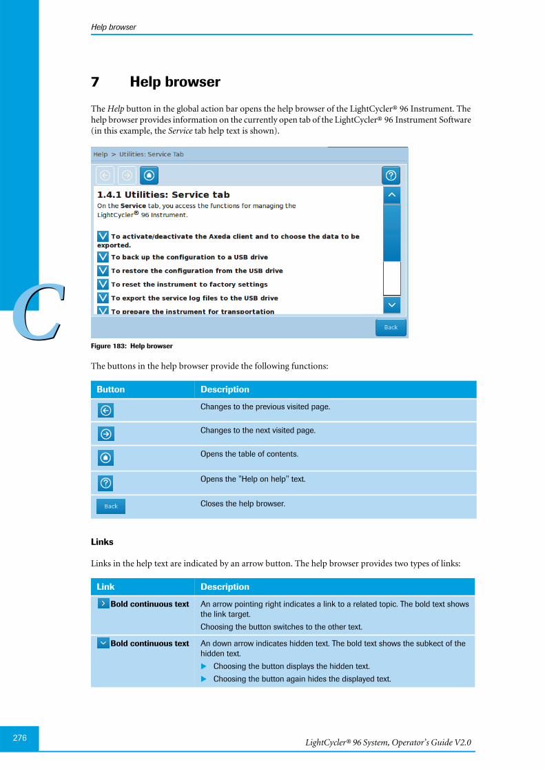
LightCycler® 96 System, Operator’s Guide V2.0276
Help browser
CC
7 Help browser
The Help button in the global action bar opens the help browser of the LightCycler® 96 Instrument. Thehelp browser provides information on the currently open tab of the LightCycler® 96 Instrument Software(in this example, the Service tab help text is shown).
Figure 183: Help browser
The buttons in the help browser provide the following functions:
Links
Links in the help text are indicated by an arrow button. The help browser provides two types of links:
Button Description
Changes to the previous visited page.
Changes to the next visited page.
Opens the table of contents.
Opens the "Help on help" text.
Closes the help browser.
Link Description
Bold continuous text An arrow pointing right indicates a link to a related topic. The bold text showsthe link target.
Choosing the button switches to the other text.
Bold continuous text An down arrow indicates hidden text. The bold text shows the subkect of thehidden text.
Choosing the button displays the hidden text.
Choosing the button again hides the displayed text.

Chapter DCleaning and care
DDChapter D • Cleaning and care

LightCycler® 96 System, Operator’s Guide V2.0
Table of Contents
DD
278
D Cleaning and care 277
1 General maintenance ............................................................................................................................. 279
2 Cleaning instructions .............................................................................................................................. 279
3 Unlocking the loading module .......................................................................................................... 281
4 Exchanging the ventilation dust filters ......................................................................................... 283
5 Handling fuses ............................................................................................................................................ 285
6 Packing the instrument for shipping ............................................................................................. 287
6.1 Placing the transport locking device, if the instrument initializes .............................................. 2876.2 Placing the transport locking failure state foam, if the instrument does not initialize ....... 289
6.3 Packing the instrument .............................................................................................................................. 290

Cleaning and care
General maintenance
279
DD
Cleaning and care 0This chapter provides basic cleaning instructions and describes how to exchange fuses and dust filters ofthe LightCycler® 96 Instrument.
1 General maintenance
The LightCycler® 96 Instrument is maintenance-free.
Precautions
The area around the LightCycler® 96 Instrument should be checked regularly to ensure that the air flowis unrestricted and that books, papers, or other items are not interfering with the air flow. For detailedrequirements, see section Installation requirements, on page 42.
2 Cleaning instructions
Caution!Do not clean the LightCycler® 96 Instrument when it is plugged in.
Caution!Do not pour fluids into the loading module, thermal block cycler, or the interior of the instrument.
Caution!As with all potentially biohazardous specimens, universal safety precautions should be taken whenhandling and processing samples. Spills should be immediately disinfected with an appropriate disin-fectant solution to avoid contamination of laboratory personnel or equipment. Handling and disposalof infectious material should be performed according to local safety guidelines.
General cleaning
Regular cleaning of the LightCycler® 96 Instrument and accessories is not required.
Use only the detergents recommended below for cleaning.
To clean the housing
Switch off the instrument.
Clean the housing of the instrument with a mild commercial detergent.
If necessary, use 70% ethanol to disinfect the instrument housing.
Do not aim sprays directly at the instrument, as malfunctions of the electronics may occur.
�
�
�
LightCycler® 96 System, Operator’s Guide V2.0280
Cleaning instructions
DD
To clean the touchscreen
To clean the thermal block cycler
To clean the multiwell plate mount
Switch off the instrument.
If the display is contaminated, gently wipe it with a dry, soft, lint-free or microfiber cloth.
If the display is still not completely clean, moisten the cloth with one of the following solvents:
Isopropyl alcohol
Ethyl alcohol
Other solvents could damage the polarizer. Especially, do not use water, ketone, or aromatic sol-vents.
Wipe the screen in a gentle motion to remove dust, oil, or fingerprint smudges.
Do not spray cleaners directly onto the touchscreen.
Switch off the instrument.
Clean the thermal block cycler with a mild commercial detergent.
If necessary, use 70% ethanol to disinfect the thermal block cycler.
Do not aim sprays directly at the instrument, as malfunctions of the electronics may occur.
Eject the loading module and switch off the instrument.
Pipette 125 µl of 70% ethanol or isopropanol into each well.
Do not aim sprays directly at the instrument, as malfunctions of the electronics may occur.
Make sure that no liquid passes between mount and cover, as malfunctions of the electronics mayoccur.
Take care not to destroy the block coating, for example, by scrubbing with sharp edged or pointedobjects.
After waiting 15 minutes pipette up and down several times.
Remove the liquid.
Let the multiwell plate mount dry before using it again.
Close the loading module and switch on the instrument.
�
�
�
�
�
�
�
�
�
�
�
�
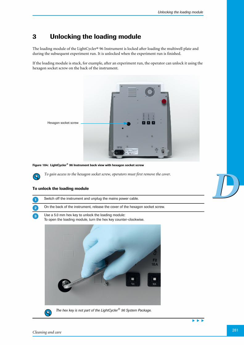
Cleaning and care
Unlocking the loading module
281
DD
3 Unlocking the loading module
The loading module of the LightCycler® 96 Instrument is locked after loading the multiwell plate andduring the subsequent experiment run. It is unlocked when the experiment run is finished.
If the loading module is stuck, for example, after an experiment run, the operator can unlock it using thehexagon socket screw on the back of the instrument.
Figure 184: LightCycler® 96 Instrument back view with hexagon socket screw
To gain access to the hexagon socket screw, operators must first remove the cover.
To unlock the loading module
Switch off the instrument and unplug the mains power cable.
On the back of the instrument, release the cover of the hexagon socket screw.
Use a 5.0 mm hex key to unlock the loading module:To open the loading module, turn the hex key counter-clockwise.
The hex key is not part of the LightCycler® 96 System Package.
Hexagon socket screw
�
�
�

LightCycler® 96 System, Operator’s Guide V2.0282
Unlocking the loading module
DD
Turn the hex key clockwise, to close the loading module again.
Restart the instrument to verify that the loading module is in the correct position.
�
�
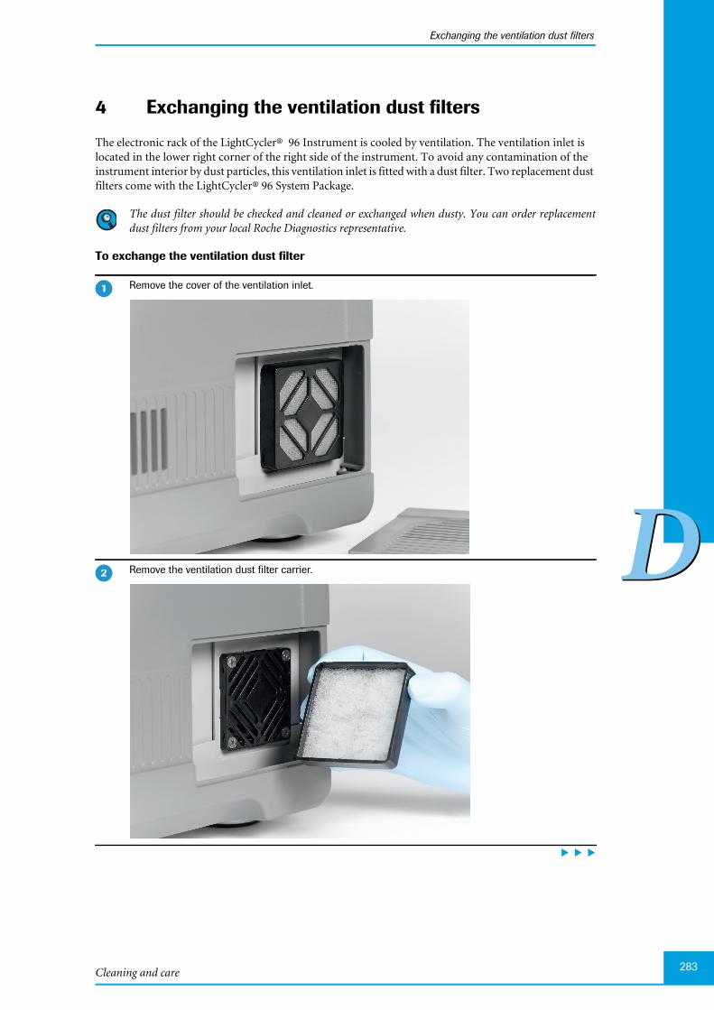
Cleaning and care
Exchanging the ventilation dust filters
283
DD
4 Exchanging the ventilation dust filters
The electronic rack of the LightCycler® 96 Instrument is cooled by ventilation. The ventilation inlet islocated in the lower right corner of the right side of the instrument. To avoid any contamination of theinstrument interior by dust particles, this ventilation inlet is fitted with a dust filter. Two replacement dustfilters come with the LightCycler® 96 System Package.
The dust filter should be checked and cleaned or exchanged when dusty. You can order replacementdust filters from your local Roche Diagnostics representative.
To exchange the ventilation dust filter
Remove the cover of the ventilation inlet.
Remove the ventilation dust filter carrier.
�
�

LightCycler® 96 System, Operator’s Guide V2.0284
Exchanging the ventilation dust filters
DD
Remove the used dust filter from the carrier and insert a new filter.
Replace the dust filter carrier on the ventilation inlet.
Close the cover of the ventilation inlet.
�
�
�
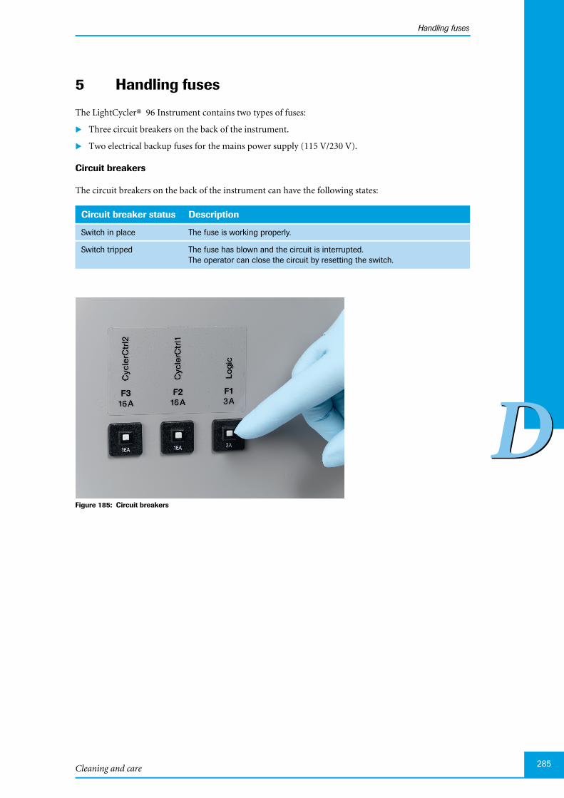
Cleaning and care
Handling fuses
285
DD
5 Handling fuses
The LightCycler® 96 Instrument contains two types of fuses:
Three circuit breakers on the back of the instrument.
Two electrical backup fuses for the mains power supply (115 V/230 V).
Circuit breakers
The circuit breakers on the back of the instrument can have the following states:
Figure 185: Circuit breakers
Circuit breaker status Description
Switch in place The fuse is working properly.
Switch tripped The fuse has blown and the circuit is interrupted.The operator can close the circuit by resetting the switch.

LightCycler® 96 System, Operator’s Guide V2.0
DD
286
Electrical fuses
These fuses must be exchanged by the operator when they are blown. TheLightCycler® 96 System Package includes a pack of replacement fuses.
Disconnect the instrument.
Remove the fuse holder from its fuse chamber.
Exchange the blown fuse with a replacement fuse.
Place the fuse holder back in the chamber.
�
�
�
�
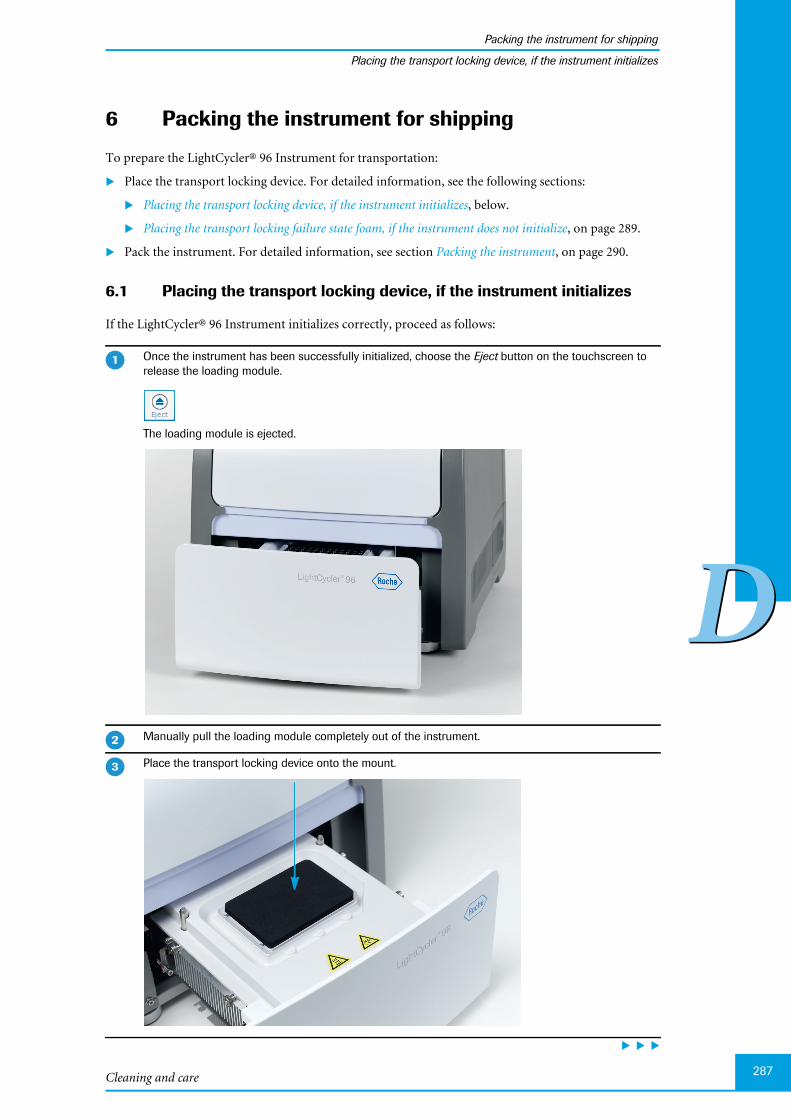
Cleaning and care
Packing the instrument for shipping
287
DD
Placing the transport locking device, if the instrument initializes
6 Packing the instrument for shipping
To prepare the LightCycler® 96 Instrument for transportation:
Place the transport locking device. For detailed information, see the following sections:
Placing the transport locking device, if the instrument initializes, below.
Placing the transport locking failure state foam, if the instrument does not initialize, on page 289.
Pack the instrument. For detailed information, see section Packing the instrument, on page 290.
6.1 Placing the transport locking device, if the instrument initializes
If the LightCycler® 96 Instrument initializes correctly, proceed as follows:
Once the instrument has been successfully initialized, choose the Eject button on the touchscreen torelease the loading module.
The loading module is ejected.
Manually pull the loading module completely out of the instrument.
Place the transport locking device onto the mount.
�
�
�
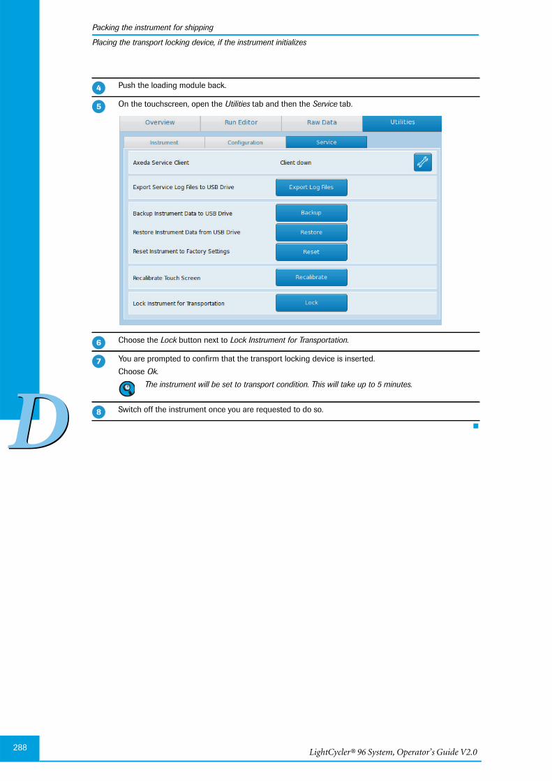
LightCycler® 96 System, Operator’s Guide V2.0288
Packing the instrument for shipping
DD
Placing the transport locking device, if the instrument initializes
Push the loading module back.
On the touchscreen, open the Utilities tab and then the Service tab.
Choose the Lock button next to Lock Instrument for Transportation.
You are prompted to confirm that the transport locking device is inserted.
Choose Ok.
The instrument will be set to transport condition. This will take up to 5 minutes.
Switch off the instrument once you are requested to do so.
�
�
�
�
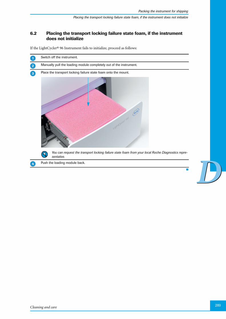
Cleaning and care
Packing the instrument for shipping
289
DD
Placing the transport locking failure state foam, if the instrument does not initialize
6.2 Placing the transport locking failure state foam, if the instrumentdoes not initialize
If the LightCycler® 96 Instrument fails to initialize, proceed as follows:
Switch off the instrument.
Manually pull the loading module completely out of the instrument.
Place the transport locking failure state foam onto the mount.
You can request the transport locking failure state foam from your local Roche Diagnostics repre-sentative.
Push the loading module back.
�
�
�
�
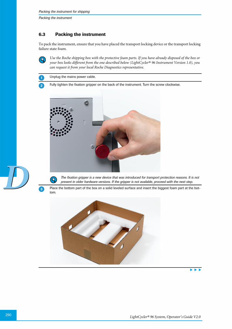
LightCycler® 96 System, Operator’s Guide V2.0290
Packing the instrument for shipping
DD
Packing the instrument
6.3 Packing the instrument
To pack the instrument, ensure that you have placed the transport locking device or the transport lockingfailure state foam.
Use the Roche shipping box with the protective foam parts. If you have already disposed of the box oryour box looks different from the one described below (LightCycler® 96 Instrument Version 1.0), youcan request it from your local Roche Diagnostics representative.
Unplug the mains power cable.
Fully tighten the fixation gripper on the back of the instrument. Turn the screw clockwise.
The fixation gripper is a new device that was introduced for transport protection reasons. It is notpresent in older hardware versions. If the gripper is not available, proceed with the next step.
Place the bottom part of the box on a solid leveled surface and insert the biggest foam part at the bot-tom.
�
�
�
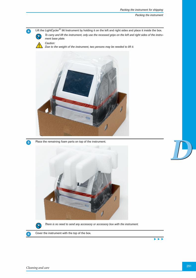
Cleaning and care
Packing the instrument for shipping
291
DD
Packing the instrument
Lift the LightCycler® 96 Instrument by holding it on the left and right sides and place it inside the box.
To carry and lift the instrument, only use the recessed grips on the left and right sides of the instru-ment base plate.
Caution:Due to the weight of the instrument, two persons may be needed to lift it.
Place the remaining foam parts on top of the instrument.
There is no need to send any accessory or accessory box with the instrument.
Cover the instrument with the top of the box.
�
�
�

LightCycler® 96 System, Operator’s Guide V2.0292
Packing the instrument for shipping
DD
Packing the instrument
Use the plastic clamping pieces to fasten the box top onto the box bottom.
�

Chapter ETroubleshooting
EEChapter E • Troubleshooting

LightCycler® 96 System, Operator’s Guide V2.0
Table of Contents
EE
294
E Troubleshooting 293
1 System messages and errors ............................................................................................................. 295
2 Remote service .......................................................................................................................................... 304
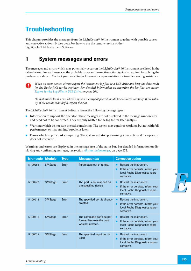
Troubleshooting
System messages and errors
295
EE
Troubleshooting 0This chapter provides the messages from the LightCycler® 96 Instrument together with possible causesand corrective actions. It also describes how to use the remote service of theLightCycler® 96 Instrument Software.
1 System messages and errors
The messages and errors which may potentially occur on the LightCycler® 96 Instrument are listed in thetables below. For each message, the probable cause and corrective action typically required for solving theproblem are shown. Contact your local Roche Diagnostics representative for troubleshooting assistance.
When an error occurs, always export the instrument log files to a USB drive and keep the data readyfor the Roche field service engineer. For detailed information on exporting the log files, see sectionExport Service Log Files to USB Drive, on page 266.
Data obtained from a run where a system message appeared should be evaluated carefully. If the valid-ity of the results is doubtful, repeat the run.
The LightCycler® 96 Instrument Software issues the following message types:
Information to support the operator. These messages are not displayed in the message window areaand need not to be confirmed. They are only written to the log file for later analysis.
Warnings which do not stop the task completing. The system may continue working, but not with fullperformance, or may run into problems later.
Errors which stop the task completing. The system will stop performing some actions if the operatordoes not intervene.
Warnings and errors are displayed in the message area of the status bar. For detailed information on dis-playing and confirming messages, see section Alarms and messages, on page 272.
Error code Module Type Message text Corrective action
17100256 SMStage Error Parameters out of range. Restart the instrument.
If the error persists, inform yourlocal Roche Diagnostics repre-sentative.
17100272 SMStage Error The port is not mapped onthe specified device.
Restart the instrument.
If the error persists, inform yourlocal Roche Diagnostics repre-sentative.
17100512 SMStage Error The specified port is alreadycreated.
Restart the instrument.
If the error persists, inform yourlocal Roche Diagnostics repre-sentative.
17100513 SMStage Error The command can't be per-formed because the portwas not created.
Restart the instrument.
If the error persists, inform yourlocal Roche Diagnostics repre-sentative.
17100514 SMStage Error The specified input port isused.
Restart the instrument.
If the error persists, inform yourlocal Roche Diagnostics repre-sentative.
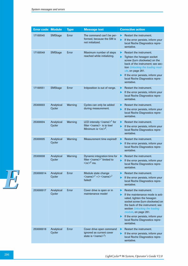
LightCycler® 96 System, Operator’s Guide V2.0296
System messages and errors
EE
17100545 SMStage Error The command can't be per-formed, because the SM isnot initialized.
Restart the instrument.
If the error persists, inform yourlocal Roche Diagnostics repre-sentative.
17100549 SMStage Error Maximum number of stepsreached while initializing.
Restart the instrument.
Tighten the hexagon socketscrew (turn clockwise) on theback of the instrument; see sec-tion Unlocking the loading mod-ule, on page 281.
If the error persists, inform yourlocal Roche Diagnostics repre-sentative.
17100551 SMStage Error Initposition is out of range. Restart the instrument.
If the error persists, inform yourlocal Roche Diagnostics repre-sentative.
25300003 AnalyticalCycler
Warning Cycles can only be addedduring measurement.
Restart the instrument.
If the error persists, inform yourlocal Roche Diagnostics repre-sentative.
25300004 AnalyticalCycler
Warning LED intensity <name>1 forfilter <name> is to low!Minimum is <nr>2.
Restart the instrument.
If the error persists, inform yourlocal Roche Diagnostics repre-sentative.
25300005 AnalyticalCycler
Warning Measurement time expired! Restart the instrument.
If the error persists, inform yourlocal Roche Diagnostics repre-sentative.
25300008 AnalyticalCycler
Warning Dynamic integration time forfilter <name>1 limited to<nr>2 ms.
Restart the instrument.
If the error persists, inform yourlocal Roche Diagnostics repre-sentative.
253000014 AnalyticalCycler
Error Module state change<name>1 => <name>1
failed!
Restart the instrument.
If the error persists, inform yourlocal Roche Diagnostics repre-sentative.
253000017 AnalyticalCycler
Error Cover drive is open or inmaintenance mode!
Restart the instrument.
If the maintenance mode is acti-vated, tighten the hexagonsocket screw (turn clockwise) onthe back of the instrument; seesection Unlocking the loadingmodule, on page 281.
If the error persists, inform yourlocal Roche Diagnostics repre-sentative.
253000018 AnalyticalCycler
Error Cover drive open commandignored as current coverstate is <name>1!
Restart the instrument.
If the error persists, inform yourlocal Roche Diagnostics repre-sentative.
Error code Module Type Message text Corrective action
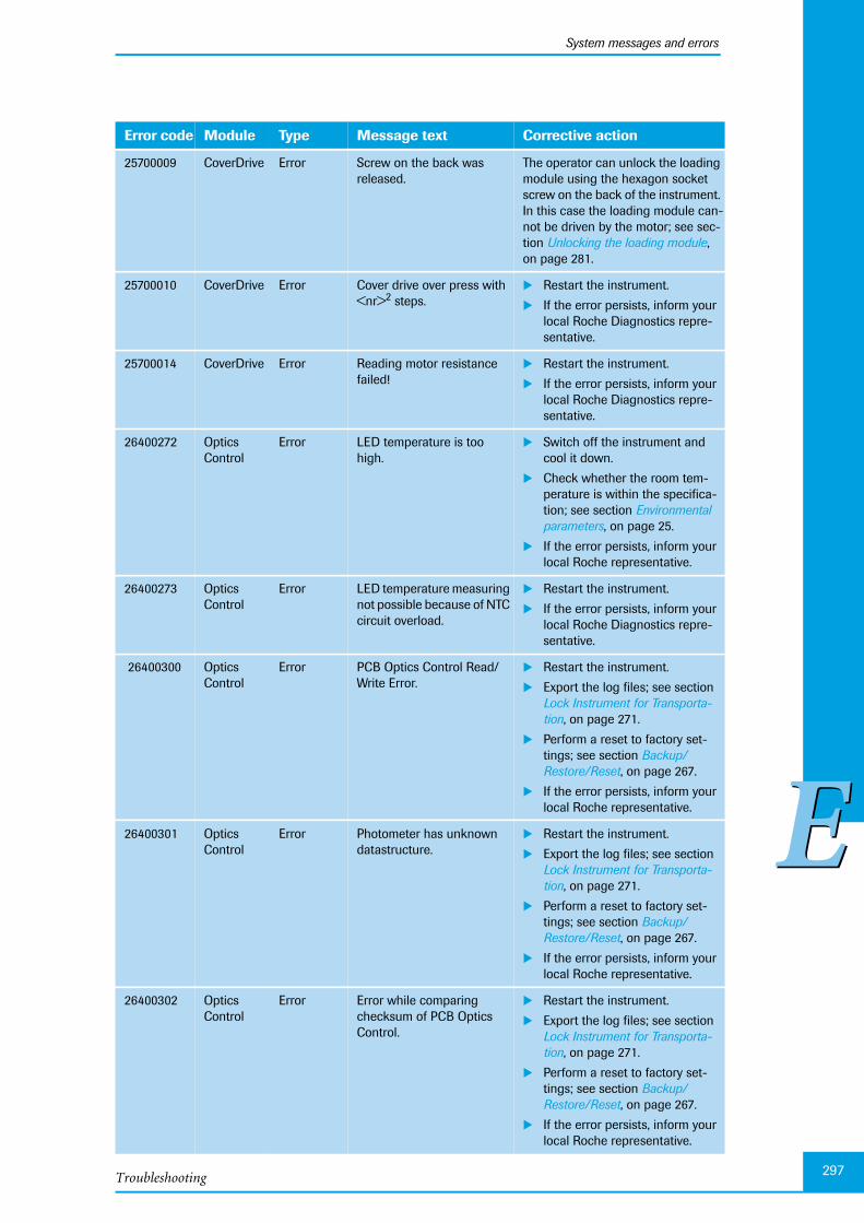
Troubleshooting
System messages and errors
297
EE
25700009 CoverDrive Error Screw on the back wasreleased.
The operator can unlock the loadingmodule using the hexagon socketscrew on the back of the instrument.In this case the loading module can-not be driven by the motor; see sec-tion Unlocking the loading module,on page 281.
25700010 CoverDrive Error Cover drive over press with<nr>2 steps.
Restart the instrument.
If the error persists, inform yourlocal Roche Diagnostics repre-sentative.
25700014 CoverDrive Error Reading motor resistancefailed!
Restart the instrument.
If the error persists, inform yourlocal Roche Diagnostics repre-sentative.
26400272 OpticsControl
Error LED temperature is toohigh.
Switch off the instrument andcool it down.
Check whether the room tem-perature is within the specifica-tion; see section Environmentalparameters, on page 25.
If the error persists, inform yourlocal Roche representative.
26400273 OpticsControl
Error LED temperature measuringnot possible because of NTCcircuit overload.
Restart the instrument.
If the error persists, inform yourlocal Roche Diagnostics repre-sentative.
26400300 OpticsControl
Error PCB Optics Control Read/Write Error.
Restart the instrument.
Export the log files; see sectionLock Instrument for Transporta-tion, on page 271.
Perform a reset to factory set-tings; see section Backup/Restore/Reset, on page 267.
If the error persists, inform yourlocal Roche representative.
26400301 OpticsControl
Error Photometer has unknowndatastructure.
Restart the instrument.
Export the log files; see sectionLock Instrument for Transporta-tion, on page 271.
Perform a reset to factory set-tings; see section Backup/Restore/Reset, on page 267.
If the error persists, inform yourlocal Roche representative.
26400302 OpticsControl
Error Error while comparingchecksum of PCB OpticsControl.
Restart the instrument.
Export the log files; see sectionLock Instrument for Transporta-tion, on page 271.
Perform a reset to factory set-tings; see section Backup/Restore/Reset, on page 267.
If the error persists, inform yourlocal Roche representative.
Error code Module Type Message text Corrective action

LightCycler® 96 System, Operator’s Guide V2.0298
System messages and errors
EE
26400310 OpticsControl
Error Timeout while controllingThermocycler.
Restart the instrument.
If the error persists, inform yourlocal Roche Diagnostics repre-sentative.
26400311 OpticsControl
Error Error during communica-tion with Thermocycler(CSM).
Restart the instrument.
If the error persists, inform yourlocal Roche Diagnostics repre-sentative.
26400312 OpticsControl
Error Error during communica-tion with Thermocycler(FWR).
Restart the instrument.
If the error persists, inform yourlocal Roche Diagnostics repre-sentative.
26500001 MessageBroker
Error Hardware error receivedfrom firmware.
Restart the instrument.
If the error persists, inform yourlocal Roche Diagnostics repre-sentative.
26500002 MessageBroker
Error Transit error information toparent module.
Restart the instrument.
If the error persists, inform yourlocal Roche Diagnostics repre-sentative.
26500004 MessageBroker
Error Procedure could not be exe-cuted - csm is in wrongstate.
Restart the instrument.
If the error persists, inform yourlocal Roche Diagnostics repre-sentative.
26500005 MessageBroker
Error Unhandled error. Restart the instrument.
If the error persists, inform yourlocal Roche Diagnostics repre-sentative.
26500006 MessageBroker
Error Generic error sent by a csm. Restart the instrument.
If the error persists, inform yourlocal Roche Diagnostics repre-sentative.
29200769 Blockcycler
Error Cover heater temperatureout of range
Reload theLightCycler® 96 InstrumentSoftware.
If the error persists, inform yourlocal Roche Diagnostics repre-sentative.
29200770 Blockcycler
Error Cover control sensordefective/out of range
Reload theLightCycler® 96 InstrumentSoftware.
If the error persists, inform yourlocal Roche Diagnostics repre-sentative.
40400007 Instrumentsoftware
Error Error saving lc96 file to<name>1.
Inform your local Roche Diagnosticsrepresentative.
40400011 Instrumentsoftware
Error File could not be removed:<name>1.
Inform your local Roche Diagnosticsrepresentative.
Error code Module Type Message text Corrective action
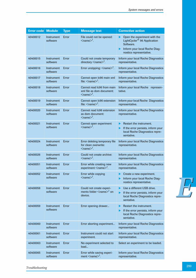
Troubleshooting
System messages and errors
299
EE
40400012 Instrumentsoftware
Error File could not be opened:<name>1.
Open the experiment with theLightCycler® 96 ApplicationSoftware.
Inform your local Roche Diag-nostics representative.
40400015 Instrumentsoftware
Error Could not create temporarydirectory <name>1.
Inform your local Roche Diagnosticsrepresentative.
40400016 Instrumentsoftware
Error Error unzipping: <name>1. Inform your local Roche Diagnosticsrepresentative.
40400017 Instrumentsoftware
Error Cannot open lc96 main xmlfile: <name>1.
Inform your local Roche Diagnosticsrepresentative.
40400018 Instrumentsoftware
Error Cannot read lc96 from mainxml file as dom document:<name>1.
Inform your local Roche represen-tative.
40400019 Instrumentsoftware
Error Cannot open lc96 extensionfile: <name>1.
Inform your local Roche Diagnosticsrepresentative.
40400020 Instrumentsoftware
Error Cannot read lc96 extensionas dom document:<name>1.
Inform your local Roche Diagnosticsrepresentative.
40400021 Instrumentsoftware
Error Cannot open experiment<name>1.
Restart the instrument.
If the error persists, inform yourlocal Roche Diagnostics repre-sentative.
40400024 Instrumentsoftware
Error Error deleting temporary filefor clean overwrite:<name>1.
Inform your local Roche Diagnosticsrepresentative.
40400026 Instrumentsoftware
Error Could not create archive:<name>1.
Inform your local Roche Diagnosticsrepresentative.
40400051 Instrumentsoftware
Error Error while creating newexperiment <name>1.
Inform your local Roche Diagnosticsrepresentative.
40400052 Instrumentsoftware
Error Error while copying<name>1.
Create a new experiment.
Inform your local Roche Diag-nostics representative.
40400058 Instrumentsoftware
Error Could not create experi-ments folder <name>1 ondevice.
Use a different USB drive.
If the error persists, inform yourlocal Roche Diagnostics repre-sentative.
40400059 Instrumentsoftware
Error Error opening drawer... Restart the instrument.
If the error persists, inform yourlocal Roche Diagnostics repre-sentative.
40400060 Instrumentsoftware
Error Error aborting experiment... Inform your local Roche Diagnosticsrepresentative.
40400061 Instrumentsoftware
Error Instrument could not startexperiment.
Inform your local Roche Diagnosticsrepresentative.
40400063 Instrumentsoftware
Error No experiment selected toload...
Select an experiment to be loaded.
40400065 Instrumentsoftware
Error Error while saving experi-ment <name>1.
Inform your local Roche Diagnosticsrepresentative.
Error code Module Type Message text Corrective action

LightCycler® 96 System, Operator’s Guide V2.0300
System messages and errors
EE
40400066 Instrumentsoftware
Error Error while adding 10 cyclesto current loaded experi-ment...
Inform your local Roche Diagnosticsrepresentative.
40400067 Instrumentsoftware
Error Error while adding 10 cyclesto current loaded experi-ment...
Inform your local Roche Diagnosticsrepresentative.
40400070 Instrumentsoftware
Error Instrument could not exe-cute experiment: <name>1.
Inform your local Roche Diagnosticsrepresentative.
40400071 Instrumentsoftware
Error Could not save experimentto xml: <name>1.
Inform your local Roche Diagnosticsrepresentative.
40400072 Instrumentsoftware
Error Instrument could not abortcurrent experiment.
Inform your local Roche Diagnosticsrepresentative.
40400073 Instrumentsoftware
Error Instrument could not opendrawer.
Check that the loading unit isnot locked; see section Unlock-ing the loading module, onpage 281.
Restart the instrument.
If the error persists, inform yourlocal Roche Diagnostics repre-sentative.
40400074 Instrumentsoftware
Error Error while adding 10 cyclesto current loaded experi-ment.
Inform your local Roche Diagnosticsrepresentative.
40400078 Instrumentsoftware
Error Predefined programs filedoesn't exists: <name>1.
Inform your local Roche Diagnosticsrepresentative.
40400079 Instrumentsoftware
Error Cannot open Predefinedprograms file: <name>1.
Inform your local Roche Diagnosticsrepresentative.
40400080 Instrumentsoftware
Error Cannot read Predefinedprograms as dom docu-ment: <name>1.
Inform your local Roche Diagnosticsrepresentative.
40400086 Instrumentsoftware
Warning Failed to start remote moni-toring server:
Check the network connection.
Call your local Roche represen-tative.
40400093 Instrumentsoftware
Warning Unable to start processedexperiment. Experiment hasto be unprocessed:<name>1.
Use a non-executed experiment.
40400094 Instrumentsoftware
Warning Experiment <name>1 hasno planned measurements.
Check the experiment settings.
40400095 Instrumentsoftware
Warning Unable to start experimentwithout programs:<name>1.
Check the experiment settings.
40400096 Instrumentsoftware
Warning Unable to start experimentwithout channels: <name>1.
Check the experiment settings.
40400097 Instrumentsoftware
Warning Unable to start experiment<name>1 with empty pro-grams.
Check the experiment settings.
Error code Module Type Message text Corrective action

Troubleshooting
System messages and errors
301
EE
40400100 Instrumentsoftware
Error Error while sending mail:<name>1.
Try again.
Check the network connections;see section Network Information,on page 257.
Check the email configuration;see section Email Information, onpage 259.
Inform your local Roche repre-sentative.
40400106 Instrumentsoftware
Error Cannot create new experi-ment '%1' since it alreadyexists.
Use different experiment name.
40400107 Instrumentsoftware
Error Error while creating newexperiment.
Restart the instrument.
If the error persists, inform yourlocal Roche Diagnostics repre-sentative.
40400110 Instrumentsoftware
Error Error while adding 10 addi-tional cycles to experiment<name>1.
Inform your local Roche Diagnosticsrepresentative.
40400111 Instrumentsoftware
Warning Error while saving experi-ment <name>1 to USBdevice.
Try again.
Use another USB drive.
40400114 Instrumentsoftware
Error Saving experiment<name>1 to USB devicefailed and could not berecovered.
Try again.
Use another USB drive.
40400120 Instrumentsoftware
Error Hardware error occured.Operation Aborted.
Restart the instrument.
If the error persists, inform yourlocal Roche Diagnostics repre-sentative.
40400122 Instrumentsoftware
Error Illegal ramp rate detected inprogram <nr>2 at step<nr>2. Ramp rate was set to<nr>2.
Check the experiment definition.
If the error persists, inform yourlocal Roche Diagnostics repre-sentative.
40400128 Instrumentsoftware
Warning Experiment validation forexperiment <name>1 failed.Please check experimentbefore starting again
Check the experiment definition.
If the error persists, inform yourlocal Roche Diagnostics repre-sentative.
40400131 Instrumentsoftware
Error Error exporting logfiles.Maybe usb device is full orhas wrong permissions.
Try again.
Check the USB drive status forpermissions and free disc space.
Use another USB drive.
40400133 Instrumentsoftware
Error Error exporting systembackup. Maybe usb deviceis full or has wrong permis-sion.
Try again.
Check the USB drive status forpermissions and free disc space.
Use another USB drive.
Error code Module Type Message text Corrective action
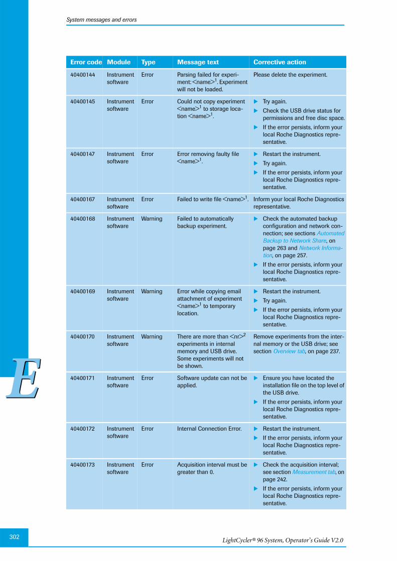
LightCycler® 96 System, Operator’s Guide V2.0302
System messages and errors
EE
40400144 Instrumentsoftware
Error Parsing failed for experi-ment: <name>1. Experimentwill not be loaded.
Please delete the experiment.
40400145 Instrumentsoftware
Error Could not copy experiment<name>1 to storage loca-tion <name>1.
Try again.
Check the USB drive status forpermissions and free disc space.
If the error persists, inform yourlocal Roche Diagnostics repre-sentative.
40400147 Instrumentsoftware
Error Error removing faulty file<name>1.
Restart the instrument.
Try again.
If the error persists, inform yourlocal Roche Diagnostics repre-sentative.
40400167 Instrumentsoftware
Error Failed to write file <name>1. Inform your local Roche Diagnosticsrepresentative.
40400168 Instrumentsoftware
Warning Failed to automaticallybackup experiment.
Check the automated backupconfiguration and network con-nection; see sections AutomatedBackup to Network Share, onpage 263 and Network Informa-tion, on page 257.
If the error persists, inform yourlocal Roche Diagnostics repre-sentative.
40400169 Instrumentsoftware
Warning Error while copying emailattachment of experiment<name>1 to temporarylocation.
Restart the instrument.
Try again.
If the error persists, inform yourlocal Roche Diagnostics repre-sentative.
40400170 Instrumentsoftware
Warning There are more than <nr>2
experiments in internalmemory and USB drive.Some experiments will notbe shown.
Remove experiments from the inter-nal memory or the USB drive; seesection Overview tab, on page 237.
40400171 Instrumentsoftware
Error Software update can not beapplied.
Ensure you have located theinstallation file on the top level ofthe USB drive.
If the error persists, inform yourlocal Roche Diagnostics repre-sentative.
40400172 Instrumentsoftware
Error Internal Connection Error. Restart the instrument.
If the error persists, inform yourlocal Roche Diagnostics repre-sentative.
40400173 Instrumentsoftware
Error Acquisition interval must begreater than 0.
Check the acquisition interval;see section Measurement tab, onpage 242.
If the error persists, inform yourlocal Roche Diagnostics repre-sentative.
Error code Module Type Message text Corrective action

Troubleshooting
System messages and errors
303
EE
40400174 Instrumentsoftware
Error Cannot handle pause orlidOpen.
Restart the instrument.
If the error persists, inform yourlocal Roche Diagnostics repre-sentative.
1. <name> here represents a placeholder for the name provided in the message on the LightCycler® 96 Instrumenttouchscreen.
2. <nr> here represents a placeholder for the number provided in the message on the LightCycler® 96 Instrumenttouchscreen.
Error code Module Type Message text Corrective action
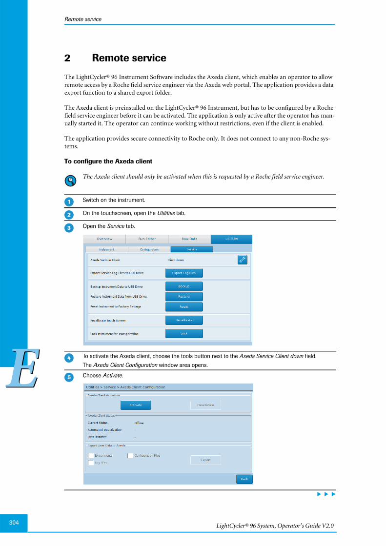
LightCycler® 96 System, Operator’s Guide V2.0304
Remote service
EE
2 Remote service
The LightCycler® 96 Instrument Software includes the Axeda client, which enables an operator to allowremote access by a Roche field service engineer via the Axeda web portal. The application provides a dataexport function to a shared export folder.
The Axeda client is preinstalled on the LightCycler® 96 Instrument, but has to be configured by a Rochefield service engineer before it can be activated. The application is only active after the operator has man-ually started it. The operator can continue working without restrictions, even if the client is enabled.
The application provides secure connectivity to Roche only. It does not connect to any non-Roche sys-tems.
To configure the Axeda client
The Axeda client should only be activated when this is requested by a Roche field service engineer.
Switch on the instrument.
On the touchscreen, open the Utilities tab.
Open the Service tab.
To activate the Axeda client, choose the tools button next to the Axeda Service Client down field.
The Axeda Client Configuration window area opens.
Choose Activate.
�
�
�
�
�

Troubleshooting
Remote service
305
EE
Choose the data to be exported to the shared export folder.
For detailed information on the configuration parameters, see section Axeda Service Client, on page 264.
To export the files to the shared export folder, choose Export.
Choose Back to close the window area.
�
�

LightCycler® 96 System, Operator’s Guide V2.0306
EE

Chapter FAppendix
FFChapter F • Appendix

LightCycler® 96 System, Operator’s Guide V2.0
Table of Contents
FF308
F Appendix 307
1 Ordering information .............................................................................................................................. 309
2 Index ................................................................................................................................................................. 310

Appendix
Ordering information
309
FF
Appendix 0
1 Ordering information
Roche Applied Science provides a large selection of isolation reagents and systems for life science research.For a complete overview of related products and guides, please visit our Special Interest Site for Real-TimePCR Systems at www.lightcycler96.com.

LightCycler® 96 System, Operator’s Guide V2.0
FF
Index
310
2 Index
Symbols.lc96 ................................................................. 113.lc96p ....................................................... 113, 229.lc96u ....................................................... 113, 229.rdml................................................................ 113
Numerics2 step amplification program .................. 137, 2463 step amplification program .................. 137, 246
AAbort button ................................................... 225Abs Quant Settings dialog box......................... 167Absolute quantification ............................. 71, 166
All Data tab .......................................... 171amplification curves ............................. 169analysis settings .................................... 167Cq bars ................................................. 175Efficiency.............................................. 167heat map .............................................. 170Maximal Cq ................................. 167, 188Minimal EPF ................................ 168, 188Minimal Slope .............................. 167, 188minimum EPF threshold...................... 169result table............................................ 171standard curves .................................... 174Statistic Data tab .................................. 173
AC ..................................................................... 15Access to the instrument ................................... 43Acquisition Mode
application software ............................. 139instrument software ............................. 249
Activate Transportation Lock dialog box ........ 271Add 10 cycles ................................................... 251Add Analysis icon .............................................. 96Add Instrument dialog box ............................. 126Adding
email address........................................ 260instrument ........................................... 126positions............................................... 101program, application software ............. 136program, instrument software.............. 246
Alarm History ................................................. 273Alarms ............................................................. 272
alarm history ........................................ 273Confirmed Alarms tab.......................... 274confirming ................................... 273, 275detailed information ............................ 275displaying ............................................. 272icons ..................................................... 226Unconfirmed Alarms tab ..................... 273
All Data tababsolute quantification......................... 171relative quantification .......................... 182
Amplification curvesabsolute quantification......................... 169endpoint fluorescence ............................ 70endpoint genotyping ............................ 195qualitative detection ..................... 189, 217Raw Data tab ........................................ 161relative quantification .......................... 179Tm calling ............................................ 206
Analysis principles............................................. 68absolute quantification........................... 71color compensation................................ 68endpoint genotyping .............................. 78high resolution melting .......................... 81qualitative detection ............................... 77quantification......................................... 68relative quantification ............................ 72Tm calling .............................................. 79
Analysis Settings icon ........................................ 96Analysis tab ..................................................... 162
absolute quantification......................... 166creating analysis ................................... 164endpoint genotyping ............................ 193exporting results................................... 218high resolution melting ........................ 207qualitative detection ............................. 186relative quantification .......................... 176sections ................................................ 163shortcut menu...................................... 163Tm calling ............................................ 200tool bar icons ....................................... 163
Area Marker icon ............................................ 106Assembling the instrument ............................... 44Assign Group by Line Segment icon................ 107AT/GC............................................................... 15Auto Standard Curve dialog box ..................... 151Automated backup icon .................................. 223Automated Backup to Network Share window area........................................................................ 263Axeda client............................................. 265, 304Axeda Client Configuration window area ............................................................................. 265, 304Axeda client icon ............................................. 223
BBackup Instrument Data window area ............ 267Block cycler cover.............................................. 33Block cycler unit................................................ 33Bread crumb navigation .................................. 224Buttons
application software ............................... 98instrument software ............................. 227

Index
FFAppendix 311
CCall
negative .................................................. 69positive................................................... 69
Cancel Zoom icon ........................................... 107CCD .................................................................. 15CCD camera...................................................... 37Circuit breakers............................................... 285Cleaning .......................................................... 279
accessories ............................................ 279instrument ........................................... 279instrument housing.............................. 279multiwell plate mount.......................... 280thermal block cycler ............................. 280touchscreen .......................................... 280
Clear Wells .............................................. 153, 165Close Experiment icon ...................................... 96Color compensation.......................................... 68Column Selector dialog box ............................ 103Combined call heat map ........................... 77, 190Compatibility .................................................... 62Concentration ................................................. 146Condition........................................................ 146Configuration tab............................................ 256
Automated Backup .............................. 263Device Name/Hostname ...................... 257Email Information ............................... 259Network Information................... 257, 258Remote Monitoring ............................. 262
Confirmed Alarms tab..................................... 274Confirming alarms .................................. 273, 275Cooling program..................................... 137, 246Copying
experiment, application software ......... 114experiment, instrument software ......... 231graphs .................................................. 108heat maps ............................................. 110sample data .......................................... 156tables .................................................... 101
Correlation Coefficient ..................................... 71Cq................................................................ 15, 69
calculation.............................................. 69predefined fluorescence values............... 70
Cq Barsabsolute quantification......................... 175relative quantification .......................... 185
Create New Analysis dialog box ...................... 164Creating
analysis................................................. 164experiment, application software ......... 113experiment, instrument software ......... 229replicate group ..................................... 147standard curves .................................... 151
Crossing point (Cp) see CqCSV ................................................................... 15Cy5 .................................................................... 15
Dd sDNA ............................................................. 81Data Visualization dialog box ......................... 180Data Visualization icon ................................... 107Date/Time configuration window area ........... 255Default directory ............................................. 134Delete Analysis icons ......................................... 96Deselecting
table items, application software .......... 101table items, instrument software .......... 228wells ..................................................... 111
Detail Information window area ..................... 275Detection channels ............................................ 38Detection format ............................................... 64
Integration Time, application software 142Integration Time, instrument software ............................................................242, 244Melt Factor, application software......... 142Melt Factor, instrument software..242, 244Quant Factor, application software ...... 142Quant Factor, instrument software ..... 242,244setting, application software................. 141setting, instrument software................. 243
Detection Format dialog boxapplication software ............................. 141
Detection Format window areainstrument software ............................. 243
Detection unit ................................................... 35CCD camera .......................................... 37filter module .......................................... 36filter set .................................................. 26filter wheel ............................................. 36optic module.......................................... 35specifications.......................................... 26
Device Name/Hostname window area ............ 257DHCP ..................................................15, 55, 257Difference plot ...........................................83, 215Dimensions of the instrument .......................... 43Displaying alarms............................................ 272Disposables ....................................................... 39
LightCycler® 480 Multiwell Plate 96 ...... 39LightCycler® 480 Sealing Foil................. 39LightCycler® 8-Tube Strips .................... 39
DNS .................................................................. 15Drawer see Loading moduledsDNA .............................................................. 15Duration
application software ............................. 139instrument software ............................. 249
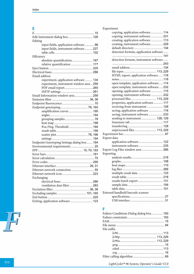
LightCycler® 96 System, Operator’s Guide V2.0
FF
Index
312
EE ........................................................................ 15Edit Instrument dialog box ............................. 126Editing
input fields, application software ........... 98input fields, instrument software ......... 227table cells .............................................. 102
Efficiencyabsolute quantification......................... 167relative quantification .......................... 177
Eject button ..................................................... 225Electrical fuses ................................................. 286Email address
experiment, application software ......... 134experiment, instrument window area .. 259PDF email report.................................. 260SMTP settings ...................................... 261
Email Information window area...................... 259Emission filter ............................................. 36, 38Endpoint fluorescence ....................................... 70Endpoint genotyping................................. 78, 193
amplification curves ............................. 195angles ................................................... 194grouping samples ................................... 78heat map .............................................. 198Pos./Neg. Threshold ............................. 194result table............................................ 199scatter plot...................................... 78, 196settings ................................................. 194
Endpoint Genotyping Settings dialog box ....... 194Environmental requirements ............................ 25EPF ...................................................... 15, 70, 193Error bars ........................................................ 181Error calculation................................................ 75Error codes ...................................................... 295Ethernet interface ........................................ 26, 31Ethernet network connection ............................ 55Ethernet network icon ..................................... 223Exchanging
electrical fuses ...................................... 286ventilation dust filter ............................ 283
Excitation filter............................................ 36, 38Excluding samples ................................... 101, 165Exit button ...................................................... 225Exiting, application software ........................... 123
Experimentcopying, application software............... 114copying, instrument software............... 231creating, application software .............. 113creating, instrument software............... 229default directory ................................... 134detection formats, application software .................................................................. 141detection formats, instrument software .................................................................. 243email address........................................ 134file types ....................................... 113, 229HTML report, application software ..... 118notes..................................................... 118open template, application software..... 114open template, instrument software..... 232opening, application software .............. 115opening, instrument software .............. 232processed files .............................. 113, 229properties, application software ........... 117receiving from instrument ................... 128saving, application software ................. 116saving, instrument software ................. 233sending to instrument .................. 128, 129Summary tab........................................ 117transferring .......................................... 128unprocessed files .......................... 113, 229
Experiment bar.................................................. 97Export data
application software ............................. 122instrument software ............................. 235
Export Log Files window area ......................... 266Exporting
analysis results...................................... 218graphs................................................... 108heat maps ............................................. 110log files ................................................. 266multiple result data .............................. 133result table............................................ 218results batch export .............................. 131sample data .......................................... 156table data.............................................. 101
External handheld barcode scannerspecifications.......................................... 27USB interface ......................................... 31
FFailure Conditions Dialog dialog box.............. 150Failure constraints ........................................... 150FAM .................................................................. 15File menu .......................................................... 94File suffix
.lc96...................................................... 113
.lc96p............................................ 113, 229
.lc96u............................................ 113, 229
.png ........................................................ 15
.rdml .................................................... 113
.svg ......................................................... 16Filter calling algorithm ...................................... 69
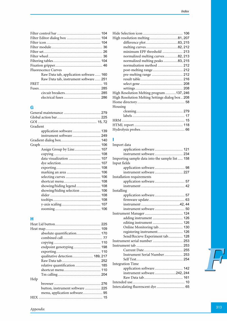
Index
FFAppendix 313
Filter control bar ............................................. 104Filter Editor dialog box ................................... 104Filter icon ........................................................ 104Filter module..................................................... 36Filter set............................................................. 26Filter wheel........................................................ 36Filtering tables ................................................. 104Fixation gripper................................................. 46Fluorescence Curves
Raw Data tab, application software ...... 160Raw Data tab, instrument software ...... 251
FRET ................................................................. 15Fuses................................................................ 285
circuit breakers..................................... 285electrical fuses ...................................... 286
GGeneral maintenance ...................................... 279Global action bar............................................. 225GOI ............................................................. 15, 72Gradient
application software ............................. 139instrument software ............................. 249
Gradient dialog box......................................... 140Graph .............................................................. 106
Assign Group by Line........................... 107copying ................................................ 108data visualization ................................. 107dye selection......................................... 107exporting.............................................. 108marking an area ................................... 106selecting curves .................................... 106shortcut menu...................................... 108showing/hiding legend ......................... 108showing/hiding selection ..................... 106slider .................................................... 108tooltips ................................................. 108y-axis scaling ........................................ 107zooming ............................................... 106
HHeat Lid button............................................... 225Heat map......................................................... 109
absolute quantification......................... 170combined call......................................... 77copying ................................................ 110endpoint genotyping ............................ 198exporting.............................................. 110qualitative detection..................... 189, 217Raw Data tab........................................ 252relative quantification .......................... 185shortcut menu...................................... 110Tm calling ............................................ 204
Helpbrowser ................................................ 276button, instrument software ................ 225menu, application software .................... 95
HEX .................................................................. 15
Hide Selection icon ......................................... 106High resolution melting .............................81, 207
difference plot .................................83, 215melting curves.................................82, 212minimum EPF threshold ..................... 213normalized melting curves ..............82, 213normalized melting peaks ...............83, 215normalzation method .......................... 212post-melting range ............................... 212pre-melting range ................................ 212result table............................................ 216select gene ............................................ 208settings ................................................. 208
High Resolution Melting program ...........137, 246High Resolution Melting Settings dialog box .. 208Home directory ................................................. 58Housing
cleaning................................................ 279labels ...................................................... 17
HRM ................................................................. 15HTML report .................................................. 118Hydrolysis probes.............................................. 66
IImport data
application software ............................. 121instrument software ............................. 234
Importing sample data into the sample list ..... 158Input fields
application software ............................... 98instrument software ............................. 227
Installation requirementsapplication software ............................... 57instrument ............................................. 42
Installingapplication software ............................... 57firmware update..................................... 63instrument ........................................42, 44instrument software ............................... 50
Instrument Manager ....................................... 124adding instrument ............................... 126editing instrument ............................... 126Online Monitoring tab......................... 130registering instrument.......................... 126Send/Recieve Experiment tab............... 128
Instrument serial number ............................... 253Instrument tab ................................................ 253
Current Date ........................................ 255Instrument Serial Number ................... 253Self Test................................................ 254
Integration Timeapplication software ............................. 142instrument software ......................242, 244Raw Data tab........................................ 161
Intended use...................................................... 10Intercalating fluorescent dye ............................. 65
LightCycler® 96 System, Operator’s Guide V2.0
FF
Index
314
InterfaceEthernet ........................................... 26, 31USB .................................................. 26, 30
Internal control ............................................... 188
LLAN................................................................... 15LED ................................................................... 15LightCycler® 480 Multiwell Plate 96.................. 39LightCycler® 480 Sealing Foil ............................ 39LightCycler® 8-Tube Strips ............................... 39LightCycler® 96 Application Software
buttons ................................................... 98exiting .................................................. 123experiment bar ....................................... 97experiments.......................................... 113export data ........................................... 122graphs................................................... 106heat maps ............................................. 109home directory ....................................... 58import data .......................................... 121input fields ............................................. 98input/output data................................. 121installation requirements ....................... 57installing................................................. 57Instrument Manager ............................ 124main window ......................................... 93menu bar ................................................ 94online monitoring ................................ 130plate view ............................................. 111preferences ........................................... 134regional settings ..................................... 98registering an instrument ..................... 126results batch export .............................. 131sections................................................. 112starting ................................................... 90startup wizard ........................................ 90tables ...................................................... 99tool bar icons.......................................... 96tools ..................................................... 124uninstalling ............................................ 59update .................................................... 60USB drive ............................................... 57working window area tabs...................... 97
LightCycler® 96 Disposables.............................. 39LightCycler® 96 Firmware update ..................... 63
LightCycler® 96 Instrument ............................ 304access requirements................................ 43additional equipment ............................. 41assembling.............................................. 44automated backup................................ 263Axeda client.......................................... 265back........................................................ 31block cycler cover ................................... 33block cycler unit ..................................... 33CCD camera........................................... 37cleaning ................................................ 279date/time configuration ....................... 255detection channels.................................. 38detection formats ................................... 38detection unit ......................................... 35device name/hostname configuration .. 257dimensions ............................................. 43disposables ............................................. 39email configuration .............................. 259exporting log files ................................. 266filter module .......................................... 36fixation gripper ...................................... 46installation requirements ....................... 42installing................................................. 42loading module ...................................... 30locking for transportation .................... 271messages............................................... 295multiwell plate mount............................ 34Network Address.................................. 258network configuration ......................... 257optic module .......................................... 35packing................................................. 290power requirements ............................... 43reagents .................................................. 41recalibrate touchscreen ........................ 269registering ............................................ 126remote monitoring............................... 262remote service ...................................... 304reset...................................................... 268self test ................................................. 254serial number ....................................... 253space and power requirements ............... 43specifications.......................................... 25symbols .................................................. 17system backup ...................................... 267system restore....................................... 268technical specifications........................... 26thermal block cycler ............................... 33touchscreen ............................................ 30transport locking device ......................... 49transportation ...................................... 287unpacking .............................................. 44ventilation .............................................. 32ventilation requirements ........................ 43warnings and precautions ...................... 18weight..................................................... 43
Index
FFAppendix 315
LightCycler® 96 Instrument Softwareautomatic one-to-one connection.......... 50buttons................................................. 227Ethernet network connection................. 55export data ........................................... 235global action bar................................... 225help browser......................................... 276import data .......................................... 234input fields ........................................... 227input/output data................................. 234installing ................................................ 50main window ....................................... 222manual one-to-one connection........ 52, 54message window area ........................... 226network configuration ........................... 54status bar.............................................. 223tables .................................................... 228update .................................................... 60working window area tabs.................... 224
LightCycler® 96 Reagents .................................. 41LightCycler® 96 System Package ....................... 28LightCycler® USB Handheld Scanner ............... 27Loading module ................................................ 30
unlocking ............................................. 281
MMagNA Pure 96 sample data ........................... 122Main window
application software ............................... 93experiment bar ....................................... 97instrument software ............................. 222menu bar................................................ 94tool bar................................................... 96touchscreen .......................................... 222
Maintenancegeneral.................................................. 279precautions .......................................... 279
Maximal Cqabsolute quantification................. 167, 188relative quantification .......................... 177
Measurement tab ............................................ 242Measurement window area ............................. 141Melt Factor
application software ............................. 142instrument software ..................... 242, 244
Melting Analysis Parameters dialog box.......... 201Melting Curve analysis see Tm callingMelting curves
high resolution melting .................. 82, 212Raw Data tab........................................ 160Tm calling ...................................... 79, 203
Melting peak area ............................................ 106creating ................................................ 201
Melting peaks .................................................... 80Melting program ..................................... 137, 246Melting Selection dialog box ........................... 164
Menu bar........................................................... 94File menu ............................................... 94Help menu ............................................. 95Options menu ........................................ 95Tools menu ............................................ 94Window menu ....................................... 95
Message window area ...................................... 226Messages...................................................272, 295
displaying............................................. 272Minimal EPF
absolute quantification .................168, 188relative quantification .......................... 178
Minimal Slopeabsolute quantification .................167, 188relative quantification .......................... 178
Minimum EPF thresholdabsolute quantification ........................ 169high resolution melting........................ 213slider .................................................... 169
Monitoring PCRhydrolysis probes ................................... 66intercalating fluorescent dye .................. 65
Mount ............................................................... 34Multicolor detection ......................................... 66Multiwell plate image ...................................... 145
shortcut menu...................................... 145Multiwell plate mount....................................... 34
cleaning................................................ 280
NNegative call ...................................................... 69Network Address window area........................ 258Network configuration
automatic one-to-one connection ......... 50Ethernet network connection................. 55instrument ............................................. 54instrument software ............................... 54manual one-to-one connection ........52, 54
Network Information window area................. 257New button ..................................................... 225New Experiment from Existing icon ................. 96New Experiment icon........................................ 96News and Support tab ....................................... 92Normalization method.................................... 212Normalized melting curves ........................82, 213Normalized melting peaks..........................83, 215Normalized ratio ............................................... 72Notes tab ......................................................... 118NRC .................................................................. 15NTC .................................................................. 15

LightCycler® 96 System, Operator’s Guide V2.0
FF
Index
316
OOne-to-one connection
automatic ............................................... 50manual ............................................. 52, 54
Online Monitoring tab .................................... 130Open Experiment icon ...................................... 96Opening
experiments, application software ........ 115experiments, instrument software ........ 232
Optic module .................................................... 35Options menu ................................................... 95Ordering information...................................... 309
PPacking the instrument ................................... 290Pasting sample data ......................................... 156PCR ................................................................... 15PCR efficiency ................................................... 71
correction............................................... 78PDF email report ............................................. 260PE ...................................................................... 15Peltier elements ................................................. 33Placing transport locking device.............. 287, 289Plate ID ........................................................... 149Plate view ........................................................ 111
Raw Data tab ........................................ 160Sample Editor tab................................. 144selecting/deselecting ............................. 111tooltips ................................................. 111
Plate View tab.................................................. 144Clear Wells ........................................... 153multiwell plate image ........................... 145Plate ID ................................................ 149Print Plate ............................................ 148Reaction Properties .............................. 145Set to Defaults ...................................... 153Visible Details ...................................... 148
PNG .................................................................. 15Positive call........................................................ 69Post-melting range .......................................... 212Power box ......................................................... 31Power requirements .......................................... 43Precautions................................................ 18, 279Predefined Programs dialog box
application software ............................. 136Predefined programs window area
instrument software ............................. 246Preferences dialog box..................................... 134Preincubation program ........................... 137, 246Pre-melting range............................................ 212Print Plate Preview dialog box......................... 148Printing, plate view.......................................... 148Profile tab ........................................................ 245Program settings
application software ............................. 135Program Settings window area ........................ 247
instrument software ............................. 247
Programs2 step amplification ...................... 137, 2463 step amplification ...................... 137, 246adding, application software ................ 136adding, instrument software ................ 246cooling ......................................... 137, 246high resolution melting ................ 137, 246melting ......................................... 137, 246preincubation............................... 137, 246touchdown function .................... 137, 246
Programs listapplication software ............................. 135buttons, application software ............... 136buttons, instrument software ............... 246instrument software ............................. 245shortcut menu, application software .... 136
Programs window area .................................... 245application software ............................. 135instrument software ............................. 245
Propertiesexperiments.......................................... 117
Properties icon .................................................. 96
QqPCR ................................................................. 15Qualitative Detection
analysis settings .................................... 187internal control settings ....................... 187
Qualitative detection ................................. 77, 186amplification curves ..................... 189, 217combined call heat map ................. 77, 190heat map ...................................... 189, 217internal control .................................... 188result table............................................ 191
Qualitative Detection dialog box ..................... 187Qualitative Detection Settings dialog box........ 187Quant Factor
application software ............................. 142instrument software ..................... 242, 244
Quantification analysis ...................................... 68absolute quantifiation ............................ 71Cq .......................................................... 69endpoint fluorescence ............................ 70positive/negative filter ............................ 69qualitative detection ............................... 77quantification cycle ................................ 69relative quantification ............................ 72standard curve........................................ 70
Quantification cycle .......................................... 69Quickstart tab.................................................... 91
Index
FFAppendix 317
RRamp
application software ............................. 139instrument software ............................. 249
Ratio.................................................................. 72multiple reference genes......................... 75single reference gene .............................. 74
Ratio Bars chart ............................................... 180Data Visualization........................ 107, 180Display Ratio........................................ 181Error Bars............................................. 181Order By .............................................. 181Y Axis Scaling....................................... 181
Raw Data tabAdd 10 cycles........................................ 251application software ............................. 159choosing the display ............................. 251instrument software ............................. 250sections ................................................ 159Temperature ........................................ 252
RDML ............................................................... 16Reaction properties ......................................... 145
concentration ....................................... 146condition.............................................. 146sample name ........................................ 146
Reaction Properties window area .................... 145Reagents ............................................................ 41RealTime ready Panels target information ...... 122Recalibrate touchscreen................................... 269Recent Experiments tab..................................... 91Reference gene .......................................... 72, 177Regional settings ............................................... 98Registering an instrument ............................... 126Rel Quant Settings dialog box ......................... 177Relative quantification .............................. 72, 176
All Data tab .......................................... 182amplification curves ............................. 179analysis settings .................................... 177Cq bars ................................................. 185Efficiency ............................................. 177error calculation..................................... 75heat map .............................................. 185Maximal Cq ......................................... 177Minimal EPF ........................................ 178Minimal Slope...................................... 178normalized ratio..................................... 72PCR efficiency correction....................... 74ratio ....................................................... 72Ratio Bars............................................. 180Reference ............................................. 177reference gene ........................................ 72result table............................................ 181Run Calibrator ..................................... 178run calibrator sample ............................. 72scaled ratio ............................................. 72standard curves .................................... 185Statistic Data tab .......................... 184, 216Study Calibrator................................... 179study calibrator condition...................... 72
Remote monitoring icon ................................. 223Remote Monitoring window area ................... 262Remote service ................................................ 304Removing
conditions ............................................ 165genes .................................................... 165positions .............................................. 101positions from analysis......................... 123samples ................................................ 165wells ..............................................153, 165
Rename Experiment window area................... 240Replicate group ............................................... 147Replicate Group window area ......................... 147Report
experiments, application software........ 118self test, instrument software ............... 254
Reports icon ...................................................... 96Requirements
application software ............................... 57environment .......................................... 25installation ............................................. 42power ..................................................... 43space ...................................................... 43
Restore Instrument Data window area ............ 268Result Batch Export
analyses ................................................ 133analysis type ......................................... 132experiment files.................................... 132
Result Batch Export wizard ............................. 131Result table
absolute quantification ........................ 171endpoint genotyping ............................ 199high resolution melting........................ 216qualitative detection analysis................ 191relative quantification .......................... 181Tm calling ............................................ 205
Run calibrator ................................................... 72setting .................................................. 178
Run Editoradding programs, application software ................................................................... 136adding programs, instrument software ................................................................... 246
LightCycler® 96 System, Operator’s Guide V2.0
FF
Index
318
Run Editor tabapplication software ............................. 135Detection Format, application software .................................................................. 141Detection Format, instrument software .................................................................. 243instrument software ............................. 242Measurement, application software ..... 141Measurement, instrument software...... 242Programs window area, applicationsoftware................................................ 135Programs window area, instrumentsoftware................................................ 245Steps window area, application software.................................................................. 138Steps window area, instrument software ................................................................. 247Temperature Profile, application software............................................................... 142Temperature Profile, instrument software..249
SSample
concentration ....................................... 146condition.............................................. 146excluding from analysis ........................ 165name .................................................... 146removing from analysis ........................ 165replicate group ..................................... 147type ...................................................... 146
Sample datacopying................................................. 156exporting .............................................. 156importing ............................................. 158pasting.................................................. 156
Sample Editor tab ............................................ 143Plate View ............................................ 144tool bar icon ......................................... 143
Sample name ................................................... 146Sample table .................................................... 155
exporting .............................................. 156importing ............................................. 158pasting.................................................. 156Raw Data tab ........................................ 161Sample Editor tab................................. 155shortcut menu ...................................... 156
Sample type ..................................................... 146Samples table
copying................................................. 156Save Experiment icon ........................................ 96Saved icon ....................................................... 223Saving
experiments, application software ........ 116experiments, instrument software ........ 233
Scaled ratio ........................................................ 72
Scatter plot ................................................ 78, 196cycles selection ..................................... 196excluding samples ................................ 197gene selection ....................................... 196sliders ................................................... 196
Scheduled icon ................................................ 223SD...................................................................... 16Sections ........................................................... 112
Analysis tab .......................................... 163Raw Data tab ........................................ 159
Select HRM Gene dialog box........................... 208Selecting
curves in a graph .................................. 106hiding/showing .................................... 106table items, application software .......... 101table items, instrument software .......... 228wells ..................................................... 111
Selection icon .................................................. 106Self Test Report window area .......................... 254Send/Receive Experiment tab .......................... 128Sequence-Independent Detection Assays .......... 64Sequence-Specific Probe Binding Assays ........... 64Service tab ....................................................... 264
Axeda client.......................................... 265Backup ................................................. 267Export Log Files ................................... 266Lock Instrument for Transportation .... 271Recalibrate ........................................... 269Reset..................................................... 268Restore ................................................. 268
Settingsabsolute quantification......................... 167endpoint genotyping ............................ 194high resolution melting ........................ 208qualitative detection ............................. 187relative quantification .......................... 177Tm calling ............................................ 201
Shortcut menugraphs................................................... 108heat maps ............................................. 110table header ............................................ 99tables .................................................... 101
Show Selection icon......................................... 106Show Startup Wizard icon................................. 96Show/Hide Legend .......................................... 108Slider ............................................................... 108Slope.................................................................. 71SMTP Settings ................................................. 261SNP ................................................................... 16Software Update window area ........................... 61Software version .............................................. 253Sorting
tables, application software .................. 102tables, instrument software .................. 228
Space requirements ........................................... 43
Index
FFAppendix 319
Specificationsdetection unit......................................... 26external handheld barcode scanner........ 27instrument ............................................. 25technical................................................. 26thermal block cycler ............................... 27
ssDNA ............................................................... 81Standard curve .................................................. 70
absolute quantification......................... 174Correlation Coefficient .......................... 71creating ................................................ 151PCR efficiency ........................................ 71relative quantification .......................... 185slope....................................................... 71Standard Error of Estimate .................... 71Y-Intercept............................................. 71
Standard Error of Estimate................................ 71Start button ..................................................... 225Starting
application software ............................... 90instrument ............................................. 48
Startup wizard ................................................... 90News and Support tab............................ 92Quickstart tab ........................................ 91Recent Experiments tab ......................... 91
Statistic Data tababsolute quantification......................... 173relative quantification .................. 184, 216
Status bar ........................................................ 223Step Settings window area ............................... 248Steps
Acquisition Mode, application software.................................................................. 139Acquisition Mode, instrument software.................................................................. 249Duration, application software ............ 139Duration, instrument software............. 249Gradient, instrument software ............. 249Ramp, application software.................. 139Ramp, instrument software.................. 249settings, application software ............... 139settings, instrument software ............... 248Target, application software ................. 139Target, instrument software ................. 249Touchdown, instrument software ........ 249
Steps listapplication software ............................. 138buttons, application software ............... 138buttons, instrument software ............... 248instrument software ............................. 247shortcut menu, application software.... 138
Steps window areaapplication software ............................. 138instrument software ............................. 247
Study calibrator ................................................. 72setting .................................................. 179
Summary tab ................................................... 117SVG ................................................................... 16SYBR ................................................................. 16
System Package ................................................. 28
TTable
Add Position ........................................ 101application software ............................... 99Best Fit ................................................. 100Clear Sorting ........................................ 100Color.................................................... 101Column Selector ...........................100, 103column width....................................... 102Copy .................................................... 101editing cells .......................................... 102Exclude ................................................ 101Export to File ....................................... 101filter control bar................................... 104Filter Editor...................................100, 104filter icon.............................................. 104filtering ................................................ 104Group By This Column ....................... 100Hide/Show This Column ..................... 100hiding columns .................................... 103Include ................................................. 101instrument software ............................. 228Remove Position .................................. 101Reset Color .......................................... 101selecting/deselecting, application software .............................................................. 101selecting/deselecting, instrument software .............................................................. 228Show Group By Box............................. 100showing columns ................................. 103Sort Ascending/Descending ................. 100sorting, application software ................ 102sorting, instrument software ................ 228table header shortcut menu ................... 99table shortcut menu ............................. 101
Table View tab ................................................ 154sample table ......................................... 155
Target temperatureapplication software ............................. 139instrument software ............................. 249
TCP/IP .........................................................16, 55Temperature Profile
application software ............................. 142instrument software ............................. 249
Temperature tab.............................................. 252Template
existing experiment, application software ............................................................... 114existing experiment, instrument software ............................................................... 231Roche template, application software .. 114Roche template, instrument software .. 232
Thermal block cycler ......................................... 33cleaning................................................ 280cover ...................................................... 33specifications.......................................... 27
Thresholds, slider ............................................ 108
LightCycler® 96 System, Operator’s Guide V2.0
FF
Index
320
Tm..................................................................... 16Tm calling ................................................. 79, 200
amplification curves ............................. 206heat map .............................................. 204melting curves ................................ 79, 203melting peak areas ................................ 201melting peaks ......................................... 80result table............................................ 205selecting melting program.................... 164settings ................................................. 201
Tool bar............................................................. 96Analysis tab .......................................... 163Sample Editor tab................................. 143
Tools ............................................................... 124Tools menu ....................................................... 94Tooltips
experiment bar ....................................... 97graphs................................................... 108heat maps ............................................. 109plate view ............................................. 111
Touchdown program .............................. 137, 246Touchscreen ...................................................... 30
cleaning ................................................ 280Transferring experiments ................................ 128Transport locking device ................................... 49
failure state ........................................... 289normal state ......................................... 287
UUnconfirmed Alarms tab................................. 273Undo icon ......................................................... 96Uninstalling
application software ............................... 59instrument software ............................... 60
Unlockinginstrument ............................................. 46loading module .................................... 281
Unpacking the instrument ................................ 44Update
application software ............................... 60compatibility .......................................... 62experiment files ................................ 62, 63firmware................................................. 63instrument software ............................... 60
UPS ................................................................... 16USB ................................................................... 16USB drive .......................................................... 57USB drive icon ................................................ 223USB interfaces ............................................. 26, 30Utilities tab ...................................................... 253
Configuration....................................... 256Instrument ........................................... 253Service .................................................. 264
VVentilation ........................................................ 32
requirements .......................................... 43Ventilation dust filter, exchanging .................. 283VIC.................................................................... 16View selection list
Analysis tab .......................................... 163Raw Data tab ........................................ 159
Visible Details dialog box ................................ 148
WWeight of the instrument .................................. 43Wells
cleaning ................................................ 280selecting/deselecting ............................. 111tooltips ................................................. 111
Window menu .................................................. 95Working window area tabs
application software ............................... 97instrument software ............................. 224
YY Axis Scaling icon .......................................... 107Y-Intercept ........................................................ 71
ZZoom icon....................................................... 106Zooming graphs .............................................. 106
For life science research only. Not for use in diagnostic procedures.


Published by Roche Diagnostics GmbH Sandhofer Straße 11668305 Mannheim Germany
© 2012 Roche Diagnostics. All rights reserved.
www.roche-applied-science.com
b 0513
Related Documents


