Lifetime Expected Income Breakeven Comparison between SPIAs and Managed Portfolios. Lifetime Expected Income Breakeven Comparison Between SPIAs and Managed Portfolios Presented at the Academy of Financial Services October 18, 2013 Session G3 Larry R Frank Sr., Registered Investment Adviser (California) Better Financial Education 300 Harding Blvd Suite 103D, Roseville, CA 95678 Corresponding author: [email protected] (916) 303-7777 John B. Mitchell, Department of Finance and Law 328 Sloan Hall, Central Michigan University, Mt. Pleasant, MI 48859 [email protected] (989) 330-2929 Wade Pfau, Professor of Retirement Income The American College, 270 S Bryn Mawr Ave., Bryn Mawr, PA 19010 [email protected] 610-526-1569 Larry R. Frank, Sr., MBA, CFP ® , a Registered Investment Advisor and author, lives in Rocklin, California. He has an MBA from the University of South Dakota, and a BS cum laude Physics from the University of Minnesota. ([email protected]) John B. Mitchell, D.B.A., is professor of finance at Central Michigan University. His research focuses include simulation-based retirement planning models, the statistical properties of financial time series, assessment of learning, and derivatives strategies. ([email protected]) Wade D. Pfau, Ph.D., CFA, is a professor of retirement income at The American College, and winner of the Journal’s 2011 Montgomery-Warschauer Award. He holds a doctorate in economics from Princeton University. ([email protected]) 1

Welcome message from author
This document is posted to help you gain knowledge. Please leave a comment to let me know what you think about it! Share it to your friends and learn new things together.
Transcript

Lifetime Expected Income Breakeven Comparison between SPIAs and Managed Portfolios.
Lifetime Expected Income Breakeven Comparison Between
SPIAs and Managed Portfolios
Presented at the Academy of Financial Services October 18, 2013 Session G3
Larry R Frank Sr., Registered Investment Adviser (California) Better Financial Education
300 Harding Blvd Suite 103D, Roseville, CA 95678 Corresponding author: [email protected]
(916) 303-7777
John B. Mitchell, Department of Finance and Law 328 Sloan Hall, Central Michigan University, Mt. Pleasant, MI 48859
[email protected] (989) 330-2929
Wade Pfau, Professor of Retirement Income
The American College, 270 S Bryn Mawr Ave., Bryn Mawr, PA 19010 [email protected]
610-526-1569
Larry R. Frank, Sr., MBA, CFP®, a Registered Investment Advisor and author, lives in Rocklin, California. He has an MBA from the University of South Dakota, and a BS cum laude Physics from the University of Minnesota. ([email protected])
John B. Mitchell, D.B.A., is professor of finance at Central Michigan University. His research focuses include simulation-based retirement planning models, the statistical properties of financial time series, assessment of learning, and derivatives strategies. ([email protected])
Wade D. Pfau, Ph.D., CFA, is a professor of retirement income at The American College, and winner of the Journal’s 2011 Montgomery-Warschauer Award. He holds a doctorate in economics from Princeton University. ([email protected])
1

Lifetime Expected Income Breakeven Comparison between SPIAs and Managed Portfolios.
Executive Summary This paper provides insight and guidance for the retiree decision making between whether to annuitize or manage their retirement savings. Tables and graphs demonstrate the breakeven age between annuitizing with a single premium immediate annuity (SPIA) versus managing a portfolio and the likelihood of outliving the breakeven cash flow sums for various annuitization ages (65 to 85), longevity percentiles of Period Life Tables, and portfolio allocations. Phase I calculations are based on 2013 SPIA rates, return data from 1926 to 2012, 2007 SSA Life Tables, and 2000 Annuity Tables. Monte Carlo simulation is employed to estimate managed portfolio cash flows while also incorporating longevity percentiles to establish the length of the Distribution Period (DP). Phase II calculations are imputed Annual Payout Rates based on matching SPIA cash flows to two target managed portfolio allocation cash flows, one at 50% equity allocation, the second at 20% equity allocation; both with 1% portfolio fees applied to the cash flows. Common points between both Phases:
• SPIA cash flows compared to managed portfolio distributions for expected longevity time frames (at both 50%, and 30%, of retirees outlive their cohorts) suggest that purchasing a SPIA at any age is unadvisable since the remaining portfolio values push lifetime cash flows ahead of SPIA cash flows.
• SPIA breakeven points for the 50% expected longevity timeframes do suggest that delaying purchase of a SPIA at age 85, or age 80 for 30% expected longevity percentiles, may be considered if the managed portfolio’s remaining balances are ignored (when retiree has viewpoint that those balances would surrendered anyway with purchase of a SPIA).
• The remaining balances of the managed portfolios may be viewed as the equivalent of the present value, at that age, of the potential mortality credits that surviving SPIA owners receive from retirees who do not outlive the longevity percentile time frames (e.g., 50% LP, 30% LP or age 105 determinations below).
• The remaining balance of unconsumed funds of a managed portfolio is the price the retiree pays to manage their exposure to probability of failure and retain ownership of their funds. At death, these funds are lost for consumption purposes just as the purchase price of the SPIA is lost. During life, these funds are retained for future consumption purposes just as the continued income from a SPIA would continue to provide income.
• For those retirees who may live to age 105, a SPIA may be considered for purchase at age 80 for a conservative retiree, or age 85 for other retirees.
Brief Overview Retirees have a choice to manage their retirement assets, or to annuitize some or all of those assets. Annuities (SPIA) provide protection against market fluctuations, though generally no protection against inflation and no end-of-life bequest. Managed portfolios provide less certainty of return but opportunity for growth and the potential for leaving some bequest at the end of life.
2

Lifetime Expected Income Breakeven Comparison between SPIAs and Managed Portfolios.
At what age(s) does it make sense to start with a managed portfolio, and switch to SPIA (a retiree cannot start with a SPIA and switch back to a managed portfolio)? This research looks at the decision from a comparison of the sum of total annual retirement income payments received. Implicit in this comparison are two assumptions; 1) that retirees value consumption equally in all years of retirement, and 2) that retirees do not value bequests equally: a) some retirees may be concerned about either having sufficient funds to fund further income beyond longevity percentile periods if they live that long, or leaving a bequest of uncertain value; b) while other retirees have no bequest desire and wish to consume their assets as their own income. These two assumptions lead to the conclusion that it is equally important to have adequate retirement income in each individual year of one’s life, however uncertain in length that life may be, but maybe not important to retain an ending portfolio value for whatever reason. These assumptions define a special case which serves as a base upon which retirees can value their own preferences. The Monte Carlo model used tracks cash flow and portfolio balances by age and allocation and determines the effect of prior cash flows on future balances. By comparing the total sum of payments received from a SPIA against the payments expected from a managed portfolio, retirees may determine which approach might maximize their lifetime consumption. Retirees can also evaluate when the cumulative cash flows from a managed portfolio will exceed those from a SPIA and the likelihood of outliving this breakeven age based on current withdrawal rate management technology and currently available data. It is equally interesting to look back in time, as well as have a useful methodology for future use, to examine if or when retirees should switch to a SPIA or continue to manage their assets until some future decision date. Phase II of this paper develops a method that compares the breakeven points between historical portfolio data series to past, present or future Annual Payout Rates (APR) of SPIAs. Comparing threshold APRs to the current APR for example, provides useful insight to help retirees decide if now is the time to purchase a SPIA, or if they should wait until they are older. The future, by definition, is unknown. This study helps retirees determine if the simplification of life and, presumed reduction in market risk from purchasing a SPIA is worth the price in reduced lifetime consumption. Literature Review (In Process) Blanchett (2013) states “Therefore Cash Flows are the most important determinant of retirement success.” Yet, past distribution research has not focused on cash flows but on maximizing the withdrawal rate which Blanchett in this same paper explains is more a function of the returns data used in the papers. This paper’s focus will be on cash flows as developed by the methodology in Frank, Mitchell and Blanchett (herein FMB) 2011, 2012a and 2012b that emanate throughout a simulated retirees’ potential lifetime. The FMB methodology is Age-Based where annual cash flows may be determined and summed over various expected longevity percentiles of Period Life Tables. Therefore, this paper is a practical application of the FMB
3

Lifetime Expected Income Breakeven Comparison between SPIAs and Managed Portfolios.
methodology comparing total expected lifetime cash flow sums between SPIAs and managed portfolios. Milevsky (1998) states “Consequently, given the low interest rate environment and the long-run propensity for equities to outperform fixed income investments, we apply our model (the mathematical model Milevsky discussed in his paper) to estimate that a sixty-five year old female (male) has a ninety-percent (eighty-five percent) chance of being able to beat the rate of return from a life annuity until age 80.” That was his conclusion with interest rates in Canada in 1998. Do those observations hold with lower, or higher, interest rates? Do they hold for other retiree ages older than age 65 (i.e., if a retiree waits, at what age should they reconsider a SPIA)? What is the effect of asset allocation on the choice? What is the effect of fees? Economists refer to the “annuity puzzle” as research since Yaari (1965) question why annuitization is such an uncommon solution for protecting from longevity risk. Numerous explanations have been offered throughout the years, and Benartzi, Previtero, and Thaler (2011) effectively summarize this literature. More recently, Reichling and Smetters (2013) indicate that because health shocks require increased liquidity while simultaneously reducing the present value of the remaining annuity payments as a result of heightened mortality, retirees act rationally in their decision to reduce annuity holdings. Kitces and Pfau (2013) also demonstrate that part of the explanation for the beneficial impacts of annuitization on a retirement portfolio can be explained through the implied rising equity glidepath of the strategy. With regard to research which compares the cash flow provided by different retirement income strategies, Pfau (2011) and Pfau (2013) both analyze the income stream supported by income guarantees on variable annuities to see how likely could be a systematic withdrawal strategy to replicate these payments. This literature review is meant to cover the main highlights on the topic explored by this paper and is not all inclusive. Overall Discussion Fundamentally, a retiree has two basic choices about how to fund their retirement income; 1) to annuitize their retirement assets, or 2) to manage those assets, either by themselves, or through assistance of an adviser. Plenty of research has looked at comparing these two choices. This paper breaks this comparison down to what this choice means to each retiree as they face this choice. At the end of the day, what is the total sum of money a retiree today may expect, under either choice, over their remaining expected lifetime? How does safety based (SPIA) total payouts compare to probability based (Monte Carlo) total payouts over the same time period established by the period life tables? There are two schools of thought on retirement income, the Safety First School and the Probability Based School. This paper compares these two schools of thought. The Safety First School basically says that making sure you have money to cover your expenses is paramount. Thus, purchasing a SPIA, or establishing a bond ladder made up of safe bonds, are suggested solutions by these proponents. Pensions and Social Security are often also used to ensure income as long as you live, however many times there is a gap between the income from
4

Lifetime Expected Income Breakeven Comparison between SPIAs and Managed Portfolios.
these sources and your total monthly expenses. Paying off the mortgage, for example is one common method in this school, to close that gap by lowering expenses by the amount of the mortgage payment (principal and interest). The Probability Based School is based on probabilities of the markets, often called Monte Carlo simulations or stochastic, establishes a “safe withdrawal rate” based on research that began in the mid 1990′s. This school of thought recognizes that markets go up and down and the early research suggested that 4% was reasonable as a “Safe Withdrawal Rate (SWR).” In today’s low interest rate environment, some have been challenging this “safe” rate of 4% as too high while ironically they suggested this rate as too low during the 1990’s. There tends to be two camps of thought in the Probability Based School. The older camp, based on the early research tends to be static. This approach sets an initial withdrawal rate to establish a beginning retirement income dollar amount, and adds an inflation adjustment to the dollar value each subsequent year - thus there is little further reference back to the existing portfolio value with Guyton and Klinger (2006) providing some decision rules to revise the fixed dollar withdrawal depending on how markets have done since a withdrawal regime was established. The newer camp is more dynamic with annually recalculated, serially connected, simulations to arrive at a Prudent Withdrawal Rate (PWR) that is sustainable given current conditions. Client annual reviews include annual updates to the simulation data to reflect 1) period life table changes and changes in personal health, 2) current portfolio value, 3) latest market data series, and 4) current year feasible spending needs. The dynamic school provides an ongoing method to address how often and by what method “revisiting” the PWR and making corrections to it recognizing that markets affect the safety of withdrawals and that time allows the PWR to increase. At any moment the future is unknown. However, Monte Carlo simulations are used by some advisers as a tool for insight into that unknown future. Insurance companies establish today’s SPIA payouts for today’s retiree based on what is known today as well – yet the future is equally unknown to all participants as of today, the moment any retiree tries to make this decision. The objective of this paper is to look at the past construction of this very same choice faced by those retirees of yesteryear. Using today’s simulation tools and past data, truncating out the data we know today, but unknown to them in the past. How do the two choices compare in the past? Are there insights to be gained about how we use these very same tools today to peer into the uncertain and unknown future? Probability based Three Dimensional (3D) Model Described The Monte Carlo simulations for this project are run using a three dimensional model developed by FMB) described in FMB 2011, 2012a and 2012b to reflect the dynamic PWR camp described above. This paper is basically a practical application of the FMB model to compare total cash flow sums between SPIA and managed portfolios by allocation exposure to equity and bonds, and by expected longevity percentile from period life tables. In the FMB 3D model, for the retiree’s current age, period life tables are used to set the length of the distribution period each year for retiree ages from age 65 and up; thus the length of the distribution period (DP) changes each year throughout the retiree’s lifetime based on their current cohort age and the respective expected longevity age. By being more specific as to the
5

Lifetime Expected Income Breakeven Comparison between SPIAs and Managed Portfolios.
length of the DP through the use of Period Life Table Longevity Percentiles (LP), combined with an annual update, it is possible to get more visibility on how cash flows change during retirement. A constant probability of failure (POF), which is the percentage of simulations that fail, is also set to determine the specific WR based on the DP described in the earlier paragraph. As described in FMB 2011, it is the interaction between the length of the DP and the POF that sets a specific WR for each cohort retiree’s current age which is also determined by asset allocations between 0% equity (100% bonds) through 100% equity (0% bonds) which adds the third dimension. Thus, the WR, given a target POF, is annually recalculated based on each annual DP. This paper sets the target POF for all values at 10%. An important difference between first generation approach and the second generation 3D model is that the length of the DP, combined with a target POF, determines a given withdrawal rate (WR) that holds for that single particular year, regardless of portfolio value. The DP is specifically determined by reference to a Period Life Table each year and the DP itself may be changed through strategic use of Longevity Percentiles within Period Life Tables. In other words, the WR is determined in the 3D model by the length of the DP at a given POF and a given LP. Possible subsequent annual withdrawal dollars (annual cash flows) and resulting annual portfolio values result from the WR calculation in this 3D model, not the reverse, and it is this annually recalculated, rolling DP/POF-determined-WR that is subsequently applied to the portfolio balance. Investor adviser fees and investor taxes would be applied to the cash flow that results from the WR applied to the portfolio balance. In other words, the annual cash flow is gross of fees and taxes. Since taxes may vary greatly, the values computed here are pre-tax, but post a range of adviser fees. A result of the difference in model design is that there is always a portfolio balance to which a WR may be applied because WR never reaches 100% (or unless simulation portfolio values go negative) through a limiting function to WR described in FMB 2012b (WR*(1 – 1/n) where n = annually recalculated DP). As in real life, the WR is recalculated each year and cash flow results are serially connected by portfolio value calculations post cash flow reduction. Past actions such as withdrawing more, or less in any given year, affect portfolio values the retiree has today; and the present portfolio value of the retiree affects what sustainable withdrawal dollar amounts are possible for the coming year(s). The effect of future market sequences on portfolio values are not directly under the retiree’s control beyond asset allocation, and allocation is a component of the 3D model to determine its impact (FMB 2011). The WR increases slightly each year because the DP shortens due to a slightly shorter expected longevity from the period life tables. This simulates the retiree aging and the dynamics of changing life expectancy as they age. The DP continually shortens as the retiree ages according to the updated expected longevity age for the retiree’s current age (DP = Age Expected Longevity minus Age Current).
6

Lifetime Expected Income Breakeven Comparison between SPIAs and Managed Portfolios.
With an established WR based on age, as described above, the actual dollar amount for a retiree at each age depends on how the markets have affected the retiree’s portfolio value the prior year. Annual Portfolio Value multiplied by the WR equals the Annual Dollar Distribution.The annual portfolio value, and thus annual dollar distribution is based on “good” or “bad” simulated markets. The 5th (best one in twenty) and 25th (best one in four) percentiles represent the “good” market sequence cash flows and the 75th (worst one of four) and 95th (worst one of twenty) percentiles represent the “bad” market sequence cash flows. The 50th percentile represents the median sequences. Finally, since managed portfolios usually have some sort of management fee, results will compare sensitivity at no fee, one-half percent fee, and one percent fees. The fees are subtracted from the annual cash flow, i.e., they are not subtracted separately from the portfolio value, and thus the cash flow reflects what the retiree nets after fees. Fees are considered in the managed portfolio for an apples-to-apples comparison, since the SPIA dollar amounts are net of fees to the retiree. Since retiree tax situations may differ widely, the taxes are not included in these calculations. Thus, retiree cash flow is pre-tax, but post fee. It will be the sum of these annual cash flows, based on simulation percentile, which this project will compare to the sum of the SPIA payments, over the identical expected longevity from the period life tables. These sums will also be similarly determined across the third dimension of asset allocation. The appendices below illustrate the dynamics described above. It should be noted that the market data and figures are as of year-end 2012 and SPIA data is from 2013 reflecting how a real life retiree would compare a SPIA with a managed portfolio. These will in all likelihood change over time when market returns and longevity data (when updated Life Tables become available in the future) are updated each year. Client age and portfolio values would also be a part of the annual update process in a dynamic model reflecting actual data and events in life. Period Life Tables are used in this paper as a continuation of such table usage in past papers in order to be consistent with past research by the authors as a practical application of the methodology. The description here is how the research values are determined. In practice, the retiree’s current WR is their current annual withdrawal dollar amount divided by their current portfolio value. The current WR also has a current POF determined by running current values through a Monte Carlo simulation. FMB 2011 discusses this significance and spending decisions based on an increasing POF. In sum, what is unique to this paper is the methodology to track cash flows annually through a portfolio distribution’s lifetime, by simulation percentile and asset allocation, and compare that cash flow to that of a SPIA. Methodology – Data Phase I Returns are based on four main asset classes from Ibbotson® SBBI® through December 2012: 30 day T-bill, US Intermediate-term Government Bonds, S&P 500 Stock, and US Small Stock. All returns are converted into “real returns” (i.e., adjusted for inflation) using SBBI US Inflation.
7

Lifetime Expected Income Breakeven Comparison between SPIAs and Managed Portfolios.
Methodology – Period Life Tables Social Security (2007) Period Life Table (available at http://www.ssa.gov/OACT/STATS/table4c6.html). 2000 Annuity Life Table (available at http://www.soa.org/ (search term 2000 Annuity Table). Methodology – Annuity (SPIA) Payout Rates Present SPIA payouts are used from http://www.immediateannuities.com/. Methodology – Comparison between Annuitization and Monte Carlo Simulation What is unique is using past study methodology with the development of annually recalculated at the 95th, 75th, 50th, 25th and 5th percentile of simulation results, rolling portfolio values and withdrawn dollar amounts each year, based on asset allocation; which are each serially connected to each other as they would be in real life. New to this study are example fees at the 0%, 0.5% and 1.0% levels calculated to determine a range of fee sensitivity if any. See FMB 2011, 2012a and 2012b for a description of this model. Therefore, the sum of withdrawal dollars and portfolio balances over any period of time may be calculated at each of the simulation percentile levels. These sums are used in this study to compare to sums of dollars a retiree may receive from a SPIA over the same given time period. The depicted sum of distribution dollars are between the 25th and 75th simulation percentiles to illustrate most likely boundaries that a retiree may experience throughout the remainder of their lifetime (i.e., portfolio values would most likely fluctuate within this range of values). Methodology compares an expected total sum of money received between a SPIA and managed assets, over a given time period, in real terms, across various asset allocations (from 0% equity to 100% equity). As described in the overview above, a retiree today faces a choice between annuitization and management of retirement income. Everything about the future, known today under either choice, is equally as blurry. How do the choices compare to a consumer in terms that matter to them? First, what is the present monthly SPIA payment available for a 65 year old female? Subsequent values to be annuitized at later ages will come from the 50th percentile portfolio balance at each future age at the 40% equity value (any %equity allocation may be used – the point is to use the same allocation consistently). This is because, at age 70 for example, our 65 year old female may not have annuitized, but managed her monthly income, through the model described earlier until reaching a later age. All portfolios are managed with withdrawal adjustments based on age as described in FMF 2012b in order to extend portfolio values into any superannuated age that a retiree may reach. The starting value is $1,000,000. From immediateannuities.com a 65 year-old female in Texas (a State with no SPIA premium tax; thus values here are pre-premium tax) today would receive a Single Life with No Payments to Beneficiaries monthly payment of $5,170 (see Appendix A3).
8

Lifetime Expected Income Breakeven Comparison between SPIAs and Managed Portfolios.
Second, what is the monthly payment from the 3D model? Appendix A1 shows that at age 65 the monthly income at the 50th percentile is $4,258 per month. What is her expected sum total of real (inflation-adjusted) payouts under either method? For the SPIA = ∑1
N(monthly SPIA*12)/((1+0.030401)^N), where N=number of years of total expected lifetime payments received. In this example N=21, the number of years of expected longevity (50% longevity percentile) from the Social Security Period Life Table and 3.0401 is the average inflation rate over the relative data period. The returns in the managed portfolio are real returns adjusted by the same inflation factor described in Methodology – Data above.
For the managed portfolio, Figure 1 summarizes the expected total income sums at various allocations, simulation percentiles (25th good sequences, 50th median, and 75th poor sequences), fees, by various ages that are time slices through the three dimensional model. In reality, market return sequences would tend to fluctuate around the median values. Monte Carlo simulations do not predict the future (what does?), but they do provide a range of possible outcomes upon which decisions may be made should a possible outcome indeed become the one real one. Rather than an assumed zero portfolio value at the end of any given distribution period, this paper looks at the range of possible portfolio values at the simulation's end age, which represent future income potential either through a managed portfolio approach, or through purchase of a SPIA at that end age, for income to continue beyond that age because the retiree is still alive. Therefore, this is a timeline approach where the decision to get a SPIA is delayed and comparison made going forward from those later ages so that market return sequence risk may be better evaluated from those changing ages going forward. The methodology provides a deeper insight into how much a retiree needs to outlive cohorts by comparing expected longevity (by definition the 50th percentile in longevity tables) to the 30th percentile where a retiree outlives 70% of their cohorts. Further research in needed to provide more insight regarding the sensitivity of the breakeven between SPIA lifetime total cash flow compared to that of a managed portfolio as a function of longevity percentile. For all Breakeven Comparison figures below, those graphed values that lie above the “Annuity” line are above that breakeven value, while those graphed values that lie below the “Annuity” line are below that breakeven value. The breakeven value is the total lifetime sum of annuity payments (discounted for inflation at the same rate that the nominal market returns values are discounted to real market returns values). For example, if none of the managed portfolio total income sums fall below the annuity breakeven line, with or without ending expected ending portfolio values, a SPIA, in those situations, would be a less than efficient manner to get better than breakeven total lifetimes sums of income. For all breakeven figures, the increased returns of higher equity allocations are best visualized by looking at the 50th Median simulation curves; while the increased volatility also associated with increased equity exposure is visualized by the wider dispersion of simulation percentile results between 25th and 75th Percentile results.
9

Lifetime Expected Income Breakeven Comparison between SPIAs and Managed Portfolios.
Note the second figure labeled “Zoom.” This figure focuses on the allocations at and below 50% equity since this is more likely the allocations a retiree would be comfortable with. Yes, higher equity allocations have more cash flow because of the nature of higher returns associated with those allocations. However, higher volatility is also associated with those allocations. Observation: If an individual lives to the expected longevity, or more, then the portfolio growth provides a sum total of expected payments that exceeds the sum total of SPIA payments at any annuitization age (65 – 85). The longer the time frame for the portfolio to distribute a cash flow, the greater the likelihood the total lifetime sum of money, distributed from the portfolio, will exceed that from a SPIA. What a SPIA does is provide protection against living through extensively long poor markets, i.e., longevity during bad times. The reason that SPIA begin to make sense for older retirees is that it is easier both to have a significantly long bad market compared to expected lifespan at greater ages AND at greater ages the variability of remaining life increases relative to expected longevity. So both parts of the risk avoided by SPIA are increasing. However, what cannot be observed in the figures is the risk of SPIA failure due to low returns during those same long poor markets. Figure 1 –Breakeven Comparison: Expected Longevity (50th Longevity Percentile) w/ Ending Balances
10

Lifetime Expected Income Breakeven Comparison between SPIAs and Managed Portfolios.
Data for Figure 1 is in Appendix A3. Figure 1 illustrates the dynamics of time and portfolio growth as well as the effect a higher withdrawal rate has on the remaining portfolio balance. You may think of Figure 1 as seeking an age where crossover from a managed portfolio to a SPIA may occur. When ending portfolio balances (Appendix A5) are added back to the total cash flow at expected longevity age (assumes the retiree died as expected), in all cases the sum total of cash flow from the portfolio exceeds the breakeven line representing the cash flow from the SPIA. In most cases, the longer the time a portfolio has for growth, the greater the difference between the total sum from a SPIA and a portfolio, in other words, a 65 year old has longer to reach their early 90’s as compared to an 80 year old. Note that the 75th and 25th simulation percentiles provide perspective on upper and lower markets over the retiree’s entire remaining lifetime. Portfolio values would most likely fluctuate much closer to the median value, especially if spending adjustments as described in FMB 2011 are used. Barberis (2013) describes the emotions of changing spending “The intuition is that, upon receiving a negative income shock, the individual prefers to lower future consumption rather than current consumption. After all, news that future consumption will be lower than expected is less painful than news that current consumption is lower than expected. Moreover, when, at some future time, the individual actually lowers consumption, the pain will be limited because, by that point, expectations will have adjusted downwards.”
11

Lifetime Expected Income Breakeven Comparison between SPIAs and Managed Portfolios.
Thus, if a retiree is pre-prepared for an eventuality, either positive or negative, in spending patterns, when the time comes the pain is more muted. Clinically, Frank experienced retirees who voluntarily reduced spending when their portfolio values declined in 2008 without being asked to do so; to some it seemed natural to cut back on spending in such circumstances. Figure 2 –Breakeven Comparison: Expected Longevity (50th Longevity Percentile) w/o Ending Balances
12

Lifetime Expected Income Breakeven Comparison between SPIAs and Managed Portfolios.
Data for Figure 2 is in Appendix A4. Ending Values data is in Appendix A5 (not graphed). The value difference between Figures 1 and 2 is the Ending Portfolio Balances. The total expected SPIA sum are the same by age in both figures. Ignoring ending portfolio balances At age 75, an allocation to equity over 30% would most likely provide more inflation adjusted income as compared to a SPIA. At age 80, an allocation of 50% equity or greater would most likely provide more inflation adjusted income. At age 85 an allocation of 100% equity would most likely be required. Clearly, risk tolerance and the risk capacity of the retiree come into consideration at these ages older ages. Additionally, health (Reichling and Smetters, 2013) considerations should be considered to evaluate whether to retain the portfolio values for income and not risk sudden loss of the portfolio value due to death prior to the living through the entire required longevity period to break even (Table 1). Note that ending portfolio values are not affected by fees and taxes. The methodology used in this paper is to take fees (0.5% or 1.0%) from the annual cash flows (fee comparisons are depicted in the figures). In other words, fees are considered part of the sustainable annual withdrawal cash amount. Taxes would be treated in the same manner, by coming from the annual cash flows, and are not included in this paper since taxes are situation dependent, i.e., distributions are pre-tax in this paper. The effect then is that the net after-tax cash flow would be different for different retirees. However, the gross cash flow is not affected by taxes using this method, and is thus comparable. Observations for retirees who may outlive 50% of their cohorts. The “Annuity” line in the Figures 1 and 2 represents the breakeven point between the SPIA cash flows and the managed portfolio cash flows for expected longevity (50th percentile). The expected longevity age compared to the current retiree’s age determines the DP over which the cash flows are compared and are summarized in Table 1. The age shown in each figure is the retiree’s current age. The results shown in each figure represent the values after the expected numbers of years from the life table have passed. Managed portfolio cash flows that plot above the Annuity line represent total cash flows that exceed the SPIA cash flows for the expected period in Table 1, and managed portfolio cash flows that plot below the Annuity line represent total cash flows that do not exceed the SPIA cash flows for the same time period.
13

Lifetime Expected Income Breakeven Comparison between SPIAs and Managed Portfolios.
• SPIA cash flows compared to managed portfolio distributions for expected longevity time frames (50% of retirees outlive their cohorts) suggest that purchasing a SPIA at any age is unadvisable since the remaining portfolio values push lifetime cash flows ahead of SPIA cash flows.
• SPIA breakeven points for the 50% expected longevity timeframes do suggest that delaying purchase of a SPIA to age 85 may be considered if the managed portfolio’s remaining balances are ignored (when retiree has viewpoint that those balances would surrendered anyway with purchase of a SPIA).
• The remaining balances of the managed portfolios may be viewed as the present value, at that age, of the potential mortality credits that surviving SPIA owners receive from retirees who do not outlive the longevity percentile time frames (e.g., 50% LP, 30% LP or age 105 determinations below).
Table 1. Distribution Period Lengths where X% of cohorts outlive expected age. Retiree’s Current Age
Expected Years (50% Outlive)
Expected Age at Death (50% Outlive)
Expected Years (30% Outlive)
Expected Age at Death (30% Outlive)
65 21 86 26 91 70 17 87 21 91 75 13 88 17 92 80 10 90 13 93 85 7 92 9 94
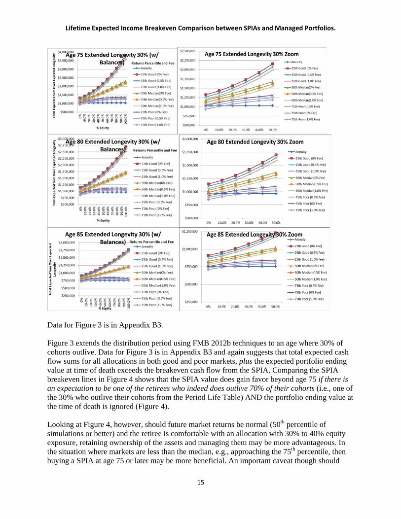
Figure 3. Breakeven Comparison: Extended Longevity to an age that 30% of cohorts outlive (w/ Ending Balances)
14
Lifetime Expected Income Breakeven Comparison between SPIAs and Managed Portfolios.
Data for Figure 3 is in Appendix B3. Figure 3 extends the distribution period using FMB 2012b techniques to an age where 30% of cohorts outlive. Data for Figure 3 is in Appendix B3 and again suggests that total expected cash flow sums for all allocations in both good and poor markets, plus the expected portfolio ending value at time of death exceeds the breakeven cash flow from the SPIA. Comparing the SPIA breakeven lines in Figure 4 shows that the SPIA value does gain favor beyond age 75 if there is an expectation to be one of the retirees who indeed does outlive 70% of their cohorts (i.e., one of the 30% who outlive their cohorts from the Period Life Table) AND the portfolio ending value at the time of death is ignored (Figure 4). Looking at Figure 4, however, should future market returns be normal (50th percentile of simulations or better) and the retiree is comfortable with an allocation with 30% to 40% equity exposure, retaining ownership of the assets and managing them may be more advantageous. In the situation where markets are less than the median, e.g., approaching the 75th percentile, then buying a SPIA at age 75 or later may be more beneficial. An important caveat though should
15

Lifetime Expected Income Breakeven Comparison between SPIAs and Managed Portfolios.
future markets be poor, the insurance companies would also experience those poor returns and the risk of their ability to sustain higher relative payments to annuitized retirees in such markets would increase. In other words, the insurance company may also be exposed to the risk of going out of business trying to sustain high payments in a poor market environment that those higher relative payments were not priced on. What the figures show that hasn’t been shown in previous research, is the degree of risk a retiree with a managed portfolio may be willing to take, based on their age as part of their decision to SPIA or not. If they are comfortable with an equity allocation higher than that indicated in a figure, then they should continue managing assets. If not comfortable, then they should SPIA. Notice too – very important – that the SPIA only begins to come into play for those who have a tendency to outlive their cohorts. And this is the real purpose of SPIAs … more so than speculating on markets as much as getting a better handle on how to identify long lifers.
The insight here is that a retiree does need to have both a sense of likely being in the group of long lived cohorts and a comfort level with the equity allocation required to do better than SPIA. Figure 4. Breakeven Comparison: Extended Longevity to an age that 30% of cohorts outlive (w/o Ending Balances)
16

Lifetime Expected Income Breakeven Comparison between SPIAs and Managed Portfolios.
Data for Figure 4 is in Appendix B4. Ending Values data is in Appendix B5 (not graphed). Observations for retirees who may outlive 70% of their cohorts (30% Longevity Percentile). The Annuity line in the figures 3 and 4 represents the breakeven point between the SPIA cash flows and the managed portfolio cash flows for extended longevity (where DP has been extended to represent 30th longevity percentile). The extended period for this longevity age compared to the current retiree’s age determines the DP over which the cash flows are compared and are summarized in Table 1. Managed portfolio cash flows that plot above the Annuity line represent total cash flows that exceed the SPIA cash flows for the extended period in Table 1, and managed portfolio cash flows that plot below the Annuity line represent total cash flows that do not exceed the SPIA cash flows for the same time period.
17

Lifetime Expected Income Breakeven Comparison between SPIAs and Managed Portfolios.
• SPIA cash flows compared to managed portfolio distributions for expected longevity time frames (30% of retirees outlive their cohorts) suggest that purchasing a SPIA at any age is unadvisable since the remaining portfolio values push lifetime cash flows ahead of SPIA cash flows (Figure 3).
• SPIA breakeven points for the 30% expected longevity time frames do suggest that delaying purchase of a SPIA to age 80 may be considered if the managed portfolio’s remaining balances are ignored (when retiree has viewpoint that those balances would surrendered anyway with purchase of a SPIA) (Figure 4).
• For those retirees who may outlive 70% of their cohorts, and where the portfolio ending balance is immaterial to the retiree, as compared to expected longevity at 50%, a SPIA may be considered for purchase earlier at age 75 for a conservative retiree, or later for other retirees.
• The remaining balances of the managed portfolios may be viewed as the present value, at that age, of the potential mortality credits that surviving SPIA owners receive from retirees who do not outlive the longevity percentile time frames (e.g., 50% LP, 30% LP or age 105 determinations below).
By their nature, a SPIA requires a retiree to purchase at some particular age while remaining lifetime is uncertain because this is the mechanism where mortality credits originate. Mortality credits happen when those who die before the expected age fund those who continue to live longer than expected. Clearly someone in poor health should not use a SPIA since they most likely would not live long enough to recoup their money or mortality credits. The purpose of this paper is to parse out an age where this calculus may begin to make sense from a retiree’s perspective. The percent outlive is adjusted since a real life retiree would make a series of expected longevity adjustments as they age based on their current age and health prospects. Retirees are faced with the dilemma that withdrawal rates can only be increased in two ways; 1) shorter distribution periods, or 2) a higher exposure to equities in an attempt to get growth (though at the expense of volatility which may result is the opposite effect). The FMB 2012b “burn the candle brightly” finding is that maximizing WR is perhaps a misguided approach to retirement funding. That finding appears to show up in this paper too, that balancing consumption with portfolio value preservation leads to higher portfolio values later, which when combined with higher possible withdrawal rates of older ages, due to the shorter life expectancy, leads to higher lifetime income. Note: California does have an annuitized annuity premium tax of 2.35%/0.5% non-qualified/qualified. Five other states have annuitized premium taxes between 1.0% and 3.5% (Virgin Islands 5.0%). This tax effect lowers the total sum of the SPIA value by that amount. This tax effect does not have a significant impact on results. For example, a Texas (no premium tax) 60-year old female with $1,000,000 is quoted $4,586/month vs. California $4,479. For an expected longevity of 26 years the Texas total sum equals $1,430,832 vs. $1,397,388 in California. The difference of $33,384 is the amount of the tax. Open Questions at this point.
18

Lifetime Expected Income Breakeven Comparison between SPIAs and Managed Portfolios.
Fundamental question for the retiree who wants to ignore ending value: they still have an ending value in their portfolio by design ... so how might they consume that potential ending value over their earlier lifetime? They have a higher ending value at 30% LP relative to 50% LP (compare Appendices A5 to B5). This is because the 30% LP reduces early consumption (lower WR relative to 50% LP WR) in order to conserve portfolio values for later years.
To have desired consumption earlier for the “little-ending-value” retiree would equate to raising their WR, thus a return to 50% LP WR consumption. And even then, they have a residual ending value either way in order to retain a portfolio value for possible older ages; less ending balances for 50% relative to 30%. So the question really gets down to life expectancy uncertainty. Yes market uncertainty also matters, but breakeven between the two comparisons above has helped put that market uncertainty into perspective.
Appendix Series C runs a "mixed case" LP scenario using strategy suggested in FMB 2012b where higher LP are initially used and then LP is reduced with age. The use of variable LP transitions cash flow from higher cash flows at younger retiree ages, to lower cash flows at superannuated ages. The concept is to pull consumption into early years with an additional goal to level cash flow consumption up to expected longevity. Withdrawals are restrained at that age to extend portfolio balances a bit allowing consumption of portfolio balances while older to provide income up to age 105 in this case. This strategy is measured at the 50th simulation percentile (median simulation returns) and would be adjusted based on how actual portfolio returns materialize as the retiree ages based on either good or poor market sequences (see Figure 7).
Summary: Competing concerns: 1) concern about living a long time; 2) concern about spending too much. The retiree who is "not concerned" about their ending value would logically then tend to spend it. The conundrum then is that by spending it early (50% LP figures 1 and 2) they won't have it later (30% LP figures 3 and 4) for that potential long life; and if they conserve it (30% LP), then a SPIA becomes more attractive because if self-managed they need to spend less earlier and it takes a long time to catch up with cash flow differences to break even.
How would managed portfolio cash flows compare to SPIA cash flows over a very long life, for example to age 105? The fundamental question for the retiree who wants to ignore ending value: they still have an ending value in their portfolio by design ... is how would they consume that ending value over their earlier lifetime?
The next section, Variable LP to Age 105, addresses these questions through use of variable longevity percentiles to manage the cash flow at higher rates during early and mid-retirement years, and then reduces the cash flow during later retirement years, with a secondary goal (and effect of spending decisions during all the prior retirement years) of reducing the ending values to a minimum by age 105 (chosen as a very old age few may outlive). Note that the WR is
19

Lifetime Expected Income Breakeven Comparison between SPIAs and Managed Portfolios.
adjusted as described in FMB 2012b (WR*(1 – 1/n) where n equals the period life table determined DP).
Variable LP to Age 105 – Initially 65% Outlive - 40% Equity
Figure 5. Breakeven Comparison: Variable Longevity Changing as Retiree Ages to Age 105 (w/ Ending Balances) (see Appendices C)
20

Lifetime Expected Income Breakeven Comparison between SPIAs and Managed Portfolios.
Data for Figure 5 is in Appendix C3. Age 105 is used in this segment to demonstrate that the differences between lifetime cash flows, with or without a portfolio value, converges because the ending portfolio values are essentially very small. Figure 6. Breakeven Comparison: Variable Longevity Changing as Retiree Ages to Age 105 (w/o Ending Balances) (see appendices C)
21

Lifetime Expected Income Breakeven Comparison between SPIAs and Managed Portfolios.
Data for Figure 6 is in Appendix C4. Ending Values data is in Appendix C5 (not graphed). From the figures above, SPIA’s should not be recommended except for those who may begin to outlive 70% of their cohorts (30% Longevity and Variable longevity to age 105). And even for those retirees, it doesn’t appear to breakeven until age 85 (possibly age 80 with low equity % or
22

Lifetime Expected Income Breakeven Comparison between SPIAs and Managed Portfolios.
poor market returns). The conundrum still is “knowing” who those “long-life” people are. However, the breakeven data appears to suggest that the decision to annuitize doesn’t really need to be made until late 70’s or early 80’s. The starting portfolio values are dynamic were the retiree starts at $1m at age 65, but then the median value is tracked for use at the retiree’s later subsequent ages. The retiree may have more or less than a median simulation value, hence the inclusion of the 75th and 25th simulation percentiles in the figures. The sum of cash flows would most likely lie between these values. See the appendices, or Figure 7 series, to visualize potential data streams based on simulation percentiles, and starting simulation portfolio values based on age taken from simulation data. Observations for retirees who may live to age 105. The Annuity line in the figures 5 and 6 represents the breakeven point between the SPIA cash flows and the managed portfolio cash flows for extended longevity (where DP has been extended to reach age 105 for all ages). Managed portfolio cash flows that plot above the Annuity line represent total cash flows that exceed the SPIA cash flows for the extended period where the retiree lives to age 105, and managed portfolio cash flows that plot below the Annuity line represent total cash flows that do not exceed the SPIA cash flows for the same time period.
• SPIA breakeven points for the longevity reaching age 105 suggest that delaying purchase of a SPIA to age 80, or age 75 for more conservative retirees, may be considered if the managed portfolio’s remaining balances are ignored. The remaining balances at this age are very low and therefore remaining balances may be essentially ignored in the breakeven decision at this age (by design).
Figure 7. By Age: Cash Flow & Portfolio Balances Comparisons between 50%Outlive, 30%Outlive, and Variable Longevity Figure 7.1. Variable Longevity Cash Flow and Portfolio Balances by Age (Start Age 65)
23

Lifetime Expected Income Breakeven Comparison between SPIAs and Managed Portfolios.
Figure 7.2. Variable Longevity Cash Flow and Portfolio Balances by Age (Start Age 70)
Figure 7.3. Variable Longevity Cash Flow and Portfolio Balances by Age (Start Age 75)
Figure 7.4. Variable Longevity Cash Flow and Portfolio Balances by Age (Start Age 80)
24

Lifetime Expected Income Breakeven Comparison between SPIAs and Managed Portfolios.
Figure 7.5. Variable Longevity Cash Flow and Portfolio Balances by Age (Start Age 85)
Longevity: Less than 1% of 65, 70, 75, 80 and 85 year olds outlive age 105. Thus, the cash flows between SPIA and managed are more comparable. Figure 7 series and Appendices C demonstrate that an income cash flow may be sustained if properly managed from young retirement years, through early centenarian ages. The model, using serially connected and annually recalculated cash flows, demonstrates that early spending decisions do have an impact on later portfolio balances and as a result, subsequent future cash flows, given the same relative returns. A higher desired balance at any time in the future requires less spending in the present and past. Figure 7 series graphs for Expected and Extended cash flow by age and portfolio balances may be seen in the lower right corner of Appendices A and B where the data generator is depicted. Figure 7 cash flow remains relatively constant, relative to market sequence returns, through early 90’s and then consumption is accelerated through age 105. What about using other Longevity Tables? Figure 8. DP Differences between Longevity Tables at select Longevity Percentiles.
0
2
4
6
61 64 67 70 73 76 79 82 85 88 91 94 97 100
103
106
109
DP D
iffer
ence
s bet
wee
n Ta
bles
Age
Distribution Period (DP) Differences by Longevity
Percentile (LP)
20% LP
50% LP
80% LP
25

Lifetime Expected Income Breakeven Comparison between SPIAs and Managed Portfolios.
Table 2.
Table 2 compares the healthy population table (2000 Annuity) expected longevity periods with the percent of the general population (Social Security) table that outlive those longer annuity periods. Some differences are due primarily to rounding algorithm that determines table percentiles. Basically, approximately 60% of the “general” (Social Security) population die by the time period that corresponds to “healthy” (2000 Annuity) population expected longevity (50% outlive by definition in both cases). A retiree really doesn’t know which group they are in except by continuing to live. Some readers may ponder the question of using longevity tables that result in older expected longevity ages as compared to the Social Security table. Let us compare the data between the Social Security table and the Annuity 2000 table at this point in the paper as an example of the methodology. Figure 8 addresses the use of other longevity tables and compares DP at various LP between the Social Security Table to the 2000 Annuity Table. Basically the effect of a shorter (longer) DP is a higher (lower) WR and thus slight higher (lower) annual cash flow. More on the impact between tables may be found in FMB 2011 SSRN. Since the breakeven point began to favor SPIAs when the longevity percentile was where 30% of the cohorts outlived their peers, the comparison in this paper is demonstrated using that longevity percentile. Appendices series D adjusts the data by using the 2000 Annuity Table. By comparing the inputs between Appendices D and B the reader may see that the distribution period for the Annuity Table is 3 years longer at age 65 for our Female (Appendix D 29 years left vs. 26 years left in Appendix B – Social Security tables). The adjusted withdrawal rate using Annuity Tables with a slightly longer distribution period is 4.19% compared to the Social Security Table withdrawal rate of 4.47%.
Annuity Period @ 50% Outlive Social Security Corresponding
Age # Years % Outlive* Annuity Period60 29 38%65 24 39%70 20 38%75 15 42%80 11 39%85 8 37%90 6 39%95 4 43%
100 3 46%*50% Expected Longevity
Female Example (Longer Longevity) Comparison between Annuity 2000 (Healthy Population)
Table and Social Security (General Population) Table
26

Lifetime Expected Income Breakeven Comparison between SPIAs and Managed Portfolios.
What is the long term effect of using a more conservative period life table? Figures 9 and 10 illustrate the breakeven cash flows. The first observable effect from lower relative withdrawal rates is on the portfolio balances where lower rate balances are higher relative to higher withdrawal rate balances at any given comparison age. How does this affect the total lifetime cash flow sum comparisons and breakeven point? A comparison of Appendices D3 through D5 using the Annuity table (longer distribution periods due to “healthier” cohorts) with their cousins Appendices B3 through B5 using the Social Security table reveals the following observations:
• Lower overall withdrawal percentage rates leads to higher relative portfolio values at any given age.
• Because portfolio values are preserved due to lower withdrawal percentage rates using longer distribution periods from the Annuity table, the result is a higher lifetime total cash flow for the slightly longer distribution period.
• Also, because of the greater preservation of portfolio values, the retiree has a greater asset value with which to purchase a SPIA at a later age. The higher portfolio value results in a higher SPIA monthly payment at older purchase ages. Example at age 85 using the Social Security table, a median simulated portfolio value of $739,000 may purchase a monthly SPIA income of $8,100. Using the Annuity 2000 table, the median simulated portfolio value of $830,000 may purchase a monthly SPIA income of $9,291.
• The higher monthly SPIA income raises the total remaining cash flow sum breakeven point. The managed portfolio has less time remaining for market returns to overcome the higher breakeven value. Thus, using period life tables that result in longer distribution periods yields lower withdrawal percentage rates that tend to preserve portfolio value for later SPIA purchase.
• It should be pointed out that the retiree does need to evaluate their likelihood that they are in the group which may outlive 70% of their cohorts in this example.
• These results are consistent with the bequest motive findings in FMB 2012b where lower percentage withdrawal rates that result from using longevity percentiles that fewer retiree cohorts may outlive, due to portfolio values preserved for bequest instead of using higher relative percentage withdrawal rates that would result in a consumption motive.
• Therefore, a retiree having a bequest motive would find it more beneficial to switch to a SPIA because the result of their motive would be higher relative portfolio values. Of course, they could change their motive from bequest to concern about outliving their assets at any time. However, the breakeven ages in Figures 9 and 10 suggest evaluation of this post-age 75 as the optimal time frame.
Figure 9 illustrates the breakeven sums for a retiree wishing to leave a bequest; therefore ending portfolio values are included in the total lifetime sums. Figure 10 is for a retiree without a bequest motive and thus the ending portfolio values are not included in the total lifetime sums of the managed portfolios. A retiree with a bequest motive would be psychologically harder to switch to a consumption goal by purchasing a SPIA. The retiree should evaluate their comfort level with how much exposure to equity and well as their continued likelihood of their being in the group outliving 70% or more of their cohorts.
27

Lifetime Expected Income Breakeven Comparison between SPIAs and Managed Portfolios.
Figure 9. Breakeven Comparison: Extended Longevity to an age that 30% of cohorts outlive (w/ Ending Balances) Annuity Tables. Compare to Figure 3 that uses Social Security Tables.
28

Lifetime Expected Income Breakeven Comparison between SPIAs and Managed Portfolios.
Figure 10. Breakeven Comparison: Extended Longevity to an age that 30% of cohorts outlive (w/o Ending Balances) Annuity Tables. Compare to Figure 4 that uses Social Security Tables.
General Observation Phase I. The current low interest rate environment, where SPIA cash flows are low as a result, suggest that policy decisions about encouraging the purchase of SPIAs prior to age 80 may be misplaced. However, a SPIA may be appropriate if the retiree may demonstrate a tendency as a spend thrift and a managed portfolio approach may not be appropriate to ensure a prudent income for life. If a retiree is concerned about outliving the ages in Table 1, and not comfortable with an allocation above the SPIA breakeven line in Figure 2, then they should consider purchasing a SPIA based on their current age. On the other hand, if they do not believe they’ll outlive the ages in Table 1, then the benefits of a SPIA that go hand in hand with insuring income for long life
29

Lifetime Expected Income Breakeven Comparison between SPIAs and Managed Portfolios.
would not be realized and thus the retiree should not buy a SPIA, especially if they are comfortable with an allocation above the SPIA breakeven line in Figure 4. If they retain ownership of their portfolio by not buying a SPIA, then the relevant figures are Figure 1 and 3 since the ending balances are still retained by not buying a SPIA. How do higher interest rates affect the breakeven decision? Phase II will look at historical SPIA cash flows from a higher interest rate era similarly compared to managed portfolio cash flows with returns data truncated to end at the same year the SPIA rate comes from. Methodology As defined by ImmediateAnnuities.com, the Annual Payout Rate (APR) is the percentage of the purchase price (i.e., the premium) which is paid back to you each year and includes both interest and return of principal. The Payout Rate is NOT an interest rate. It is significantly higher than the actual interest rate credited to the premium.
The APR is the result of a search function that solves for an equal value of total cash flow sum for the SPIA with the total cash flow sum for the targeted Monte Carlo simulation value (by allocation and fee level). Thus, a practitioner can compare past, present or future threshold APR values as demonstrated in Table 3.
Table 3 and figures 11 through 14 are compiled using the same managed portfolio data as that above. The difference is that the APR is calculated that targets setting the breakeven point for the annuity line specifically at 50% equity allocation, 1% fee. This is specifically done to see what APR is required as a breakeven comparison. In this manner, past, present and future APRs may be calculated and compared in such a manner to determine what APR may suggest a SPIA or retaining the managed assets.
Table 3. Annual Payout Rate (APR) Comparison Results
APR Expected Longevity Extended Longevity Expected Longevity Extended LongevityAge 2013 50% Outlive 30% Outlive 50% Outlive 30% Outlive65 6.20% 11.61% 11.28% 7.77% 7.94%70 6.93% 12.21% 11.59% 8.05% 7.81%75 8.29% 13.64% 12.19% 8.60% 8.09%80 10.33% 15.64% 13.61% 9.81% 8.63%85 13.15% 19.84% 16.84% 11.89% 9.77%
APR Expected Longevity Extended Longevity Expected Longevity Extended LongevityAge 2013 50% Outlive 30% Outlive 50% Outlive 30% Outlive65 6.20% 8.89% 8.16% 6.40% 6.19%70 6.93% 9.82% 8.87% 6.94% 6.44%75 8.29% 11.51% 9.87% 7.76% 7.01%80 10.33% 13.71% 11.50% 9.14% 7.80%85 13.15% 18.02% 14.89% 11.42% 9.21%
With Ending Portfolio Balances Without Ending Portfolio Balances
Target APR is LESS than 2013 APR
Degr
ee o
f Sen
sitity
to A
nnua
l Pay
out R
ate
With Ending Portfolio Balances Without Ending Portfolio BalancesTarget APR @ 50% Equity and 1% Portfolio Fee
Target APR is LESS than 2013 APR
SPIA Annual Payout Rate (APR) Table Comparing 50% Equity to 20% Equity
Target APR @ 20% Equity and 1% Portfolio Fee
30

Lifetime Expected Income Breakeven Comparison between SPIAs and Managed Portfolios.
Data for Table 3 and Figures 11 through 14 is in Appendices E1 through E8.
The basic question a retiree may ask themselves about a managed portfolio is with what allocation are they comfortable with? If they are comfortable with an allocation above the SPIA breakeven line, while also considering the range of possible future market outcomes (between continuous poor markets depicted at 75th percentile, and continuous good markets depicted at 25th percentile, or somewhere in-between) then the retiree should opt to continue to manage their assets outside of a SPIA. In this case, they would also evaluate their situation using the insight provided with data that retains the ending portfolio values. If the retiree is uncomfortable with any allocations above the SPIA breakeven line, then they should consider buying a SPIA with their assets. In which case, the evaluation should use data that does not retain the portfolio balances since those would be given up to buy the SPIA.
With this in mind, how does a retiree determine their sensitivity to asset allocation and the SPIA breakeven line. Figures 11 through 14 show the gap between the 50% equity and the 20% equity allocation breakeven points when the Annual Payout Rate (APR) of SPIAs are targeted to match those two cash flows.
Those targeted APRs are derived values in order for a retiree, or their adviser, to compare SPIA APRs at any given time to a targeted APR derived from setting a target cash flow breakeven. The yellow highlighted APRs in Table 3 suggest that if a retiree firmly believes they may outlive 70% of their cohorts, then buying a SPIA at any age 65 and older should be considered. Notice though, that if their belief is that they may outlive only 50% of their cohorts, then age 75 or 80 is when they should consider buying a SPIA with their assets. The discussion above about their comfort level with equity exposure is also a consideration.
Using the Annuity period life table results in longer distribution periods, due to the "healthier" population represented by the tables’ longer longevity. The effect of longer DPs is to lower the withdrawal rate relative to the withdrawal rate of the Social Security (general population) tables. The result is to preserve the portfolio value, at all ages relative to the Social Security table, which extends the distribution ability of the managed portfolio by conserving the portfolio value for later spending. APR - A retiree can compare the current APR to the threshold APR to determine whether they should opt for the SPIA or retain the managed portfolio until such time as the current APR exceeds the threshold APR.
31

Lifetime Expected Income Breakeven Comparison between SPIAs and Managed Portfolios.
Figure 11. Cash flow comparison below 50% equity allocations (w/ Ending Balances) (50% Expected Longevity Percentile)
Figure 12. Cash flow comparison below 50% equity allocations (w/ Ending Balances) (30% Extended Longevity Percentile)
32

Lifetime Expected Income Breakeven Comparison between SPIAs and Managed Portfolios.
Figure 13. Cash flow comparison below 50% equity allocations (w/o Ending Balances) (50% Expected Longevity Percentile)
33

Lifetime Expected Income Breakeven Comparison between SPIAs and Managed Portfolios.
Figure 14. Cash flow comparison below 50% equity allocations (w/o Ending Balances) (30% Extended Longevity Percentile)
Overall General Observations What we’ve found is that the higher SPIA payout, that occurs from the start relative to the lower managed portfolio payout at the start, is overcome over time by the greater REAL returns that raise the total payout sum for the managed portfolio and thus the total REAL sum of money the retiree receives is greater for the managed account (to what extent depends on the asset
34

Lifetime Expected Income Breakeven Comparison between SPIAs and Managed Portfolios.
allocation). For older starting ages, where the SPIA payout is, again, higher initially relative to managed, there is not enough time for the combination of inflation (that lowers the real payout of the SPIA) and the effect of real returns (that raises the managed payout – degree depends on allocation again) to overcome the SPIA initial payout advantage. Our Monte Carlo approach shows us the spread between continual poor markets and continual good markets which shows us the comparison of the SPIA between both of those kinds of markets. That spread provides valuable insight into the impact market sequences may have on the decision. A retiree’s Transient Stage (JFP Nov 2011 paper describes this) would migrate over time between those percentile depictions rather than stay precisely on the median markets values because of what the market and economic cycles do in the future. What our findings provide is more information about what factors to consider … some retirees may be comfortable with higher equity allocations which would mean they would remain managed longer; while others may be uncomfortable with equity and be inclined to tilt towards a SPIA decision. This decision then needs to consider where their health suggests they may be relative to their cohorts since the healthier, older, retiree who may outlive 70% of their cohorts, should consider a SPIA as a stronger option versus the “normal expected longevity” retiree. Another important variable is how well funded a client is with regard to their retirement plans. Someone who is very well funded can afford to take greater equity risk and doesn't need to worry about an annuity. Someone who is more constrained cannot afford the equity risk and needs to work more toward building the floor with fixed income. With a higher bond allocation, the expected return will be less and it will be easier for the annuity to provide a material benefit. Social Security (and a pension if the retiree has one) should also be considered as fixed income sources. The breakeven point between just how much equity/bond a retiree may need as evaluated with their comfort level and capacity with that required portfolio risk may be compared with the expected SPIA outcome. How can they make that decision today? The authors’ graphs and findings provide insight into what age, at what allocation, and in Phase II, at what Annual Payout Rate (APR) they should favor the SPIA over managed, or vice versa. So, if they need more equity than they may be comfortable with, then the annuity may be more beneficial. However, this is only if the SPIA breakeven point is ABOVE the allocation point at which the retiree would be uncomfortable.
Practical application The methodology and software used in this, and referenced, studies simulate a series of annual reviews that practitioners typically have each year with their retirees. The software used in this series of research papers is not required. The conclusions and observations from this and supporting papers in the series are what are important! When, and what kind of, decisions should be made as the retiree ages through retirement are important so that portfolio values and cash flows may "metabolize" as needed as the retiree continues to live into ever older ages. Not all risks are the same. If there is a risk of the retiree being a spendthrift for example, then a SPIA would provide income for life and avoid such risk. If there is little risk of long life, transferring assets to a SPIA to insure against that risk is not efficient. At what point does transferring assets to a SPIA make sense? The results above suggest that only when the
35

Lifetime Expected Income Breakeven Comparison between SPIAs and Managed Portfolios.
possibility of outliving 70% or more of your cohorts exists, and then only at elderly ages when this possibility begins to become clearer. In other words, for those in their 80’s, it is clear that they may be the ones likely to outlive their past cohorts, and depending on their health in their 80’s, it may become clear that they may outlive 70% or more of their cohorts at those older ages beyond the 80’s as well. For ages younger than the 80’s, the assets are best kept within the family and future heirs since both inflation and possible future market returns have time to do better than SPIA lifetime sums do. The methodology used in this paper for a SPIA may also be used to evaluate a decision between choosing a pension lump sum offer, which would then be managed in a portfolio, vs. accepting the pension payments for life (no COLA), which would be comparable to a SPIA. A factor, not considered in this paper, is that a retiree should consider the business risk of the insurance company; will they remain in business as long, or longer, than the retiree is alive? SPIA payments should not be considered completely risk free. Since the insurance company issuing a SPIA invests in the same markets as do the managed portfolios, if the retiree concern is continued poor markets (e.g., the 75th percentile managed values), then the risk increases that the insurance company cannot continue to afford a SPIA established during better times. Overall insights and practical application Inflation risk goes down with shorter time frames because the retiree is exposed to the effect of inflation for less time. The challenge is to balance equity allocations to overcome the inflation effect for the given time period against the fluctuation in portfolio values that equity allocation exposes the retiree to. The SPIA payout amount in dollar terms is always higher relative to the portfolio payout rate at any given age. Thus, it takes more time for the portfolio growth rate to overcome this payout advantage; with longer time periods, and higher equity exposure the rule in general. If retaining value for bequest motives is a goal, clearly using all of the portfolio value for SPIA purchases would not work well. Comparing the sum of the present values of the annual SPIA payments over the same time period as the sum of the expected annual payments from a portfolio, with sensitivity analysis as to both asset allocation differences in these payments, and consideration of the range between poor market sequence sums and good market sequence sums, a retiree gets deeper insight into factors they should consider when deciding between keeping some or all of their portfolio or purchasing a SPIA. Abbreviated Terms DP Distribution Period FMB Frank, Mitchell, and Blanchett LP Longevity Percentiles inherent within Period Life Tables POF Probability of Failure (Percentage of simulations that fail the current DP) WR Withdrawal Rate APR Annual Payout Rate References:
36

Lifetime Expected Income Breakeven Comparison between SPIAs and Managed Portfolios.
Barberis, Nicholas C. 2013. “Thirty Years of Prospect Theory in Economics: A Review and Assessment.” Journal of Economic Perspectives 27 (Winter): 173–196. Benartzi, Schlomo, A. Previtero, and R.H. Thaler. 2011. “Annuitization Puzzles.” Journal of Economic Perspectives 25 (4): 143-164. Blanchett, David M. 2013. “The ABCDs of Retirement Success.” Journal of Financial Planning 26 (5): 38-45. Frank, Larry R. Mitchell, J.B. and Blanchett, D.M. 2011. “Probability-of-Failure-Based Decision Rules to Manage Sequence Risk in Retirement.” Journal of Financial Planning 24 (November): 44–53. A working paper, which includes appendices, data, and figures, is available at: http://papers.ssrn.com/sol3/papers.cfm?abstract_id=1849868 (FMB 2010 SSRN). Frank, Larry R. Mitchell, J.B. and Blanchett, D.M.. 2012. “An Age-Based, Three-Dimensional Distribution Model Incorporating Sequence and Longevity Risks.” Journal of Financial Planning 25 (March): 52–60. A working paper, which includes appendices, data, and figures, is available at: http://papers.ssrn.com/sol3/papers.cfm?abstract_id=1849983 (FMB 2011 SSRN). Frank, Larry R. Mitchell, J.B. and Blanchett, D.M. 2012. “Transition Through Old Age in a Dynamic Retirement Distribution Model.” Journal of Financial Planning, 25 (December): 42-50. A working paper, which includes appendices, data, and figures, is available at: http://papers.ssrn.com/sol3/papers.cfm?abstract_id=2050003 (FMB 2012 SSRN). Guyton, J. T. and Klinger, W. J. (2006). “Decision rules and maximum initial withdrawal rates.” Journal of Financial Planning, 19, 49-57. Kitces, Michael E., and Wade D. Pfau. 2013. “The True Impact of Annuities on Retirement Sustainability: A Total Wealth Perspective.” Retirement Management Journal, forthcoming. Milevsky, Moshe A. 1998. “Optimal Asset Allocation Towards the End of Life Cycle: To Annuitize or Not to Annuitize?” The Journal of Risk and Insurance 65 (September): 401-426. Pfau, Wade D. 2013. “Analyzing an Income Guarantee Rider in a Retirement Portfolio.” Journal of Retirement 1, 1 (Summer): 100-109. Pfau, Wade D. 2011. “GLWBs: Retiree Protection or Money Illusion?”Advisor Perspectives (December 13). Pye, Gordon B. 2001. “Adjusting Withdrawal Rates for Taxes and Expenses.” Journal of Financial Planning, 14 (April). Reichling, Felix, and Kent Smetters. 2013. “Optimal Annuitization with Stochastic Mortality Probabilities.” Congressional Budget Office Working Paper 2013-05 (June).
37

Lifetime Expected Income Breakeven Comparison between SPIAs and Managed Portfolios.
Yaari, Menachim. 1965. “Uncertain Lifetime, Life Insurance, and the Theory of the Consumer.” Review of Economic Studies 32 (2): 137–50. Appendices General Index Appendix A Series – Expected Longevity – 50% of Cohorts Outlive – Social Security Tables Appendix B Series – Extended Longevity – 30% of Cohorts Outlive– Social Security Tables Appendix C Series – Extended Longevity – Variable Cohorts Outlive– Social Security Tables Appendix D Series – Extended Longevity – 30% of Cohorts Outlive – Annuity 2000 Tables Appendix E Series – Targeted Annual Payout Rates (APRs) for 50% Equity and 20% Equity Allocations @ 1% Portfolio Fee
38

Lifetime Expected Income Comparison between Immediate Annuities and an Age-Based, Three-Dimensional, Universal Distribution Model.
Appendix A Series – Expected Longevity (50% Outlive) – Social Security Tables Appendix A1 - Age 65 Example 40% Equity
Type Female 4,258$ Female65-65-0.5 Cash Flow Distribution Portfolio Value Distribution End of Year$2,280,751 w/ Yr# Outlive% Years Left Yr# POF Withdraw% Yr# Factor Include% Multiple Yr# After Reduce CF Yr Age 95th 75th 50th 25th 5th Age 95th 75th 50th 25th 5th
Male Age 65 $1,809,637 w/ 1 50% 21 1 10.00% 5.36% 1 4.76% 100.00% 95.24% 1 5.11% 1 66 $51,090 $51,090 $51,090 $51,090 $51,090 66 $846,762 $936,731 $1,000,633 $1,064,132 $1,159,841Female Age 65 $1,437,779 w/ 2 50% 20 2 10.00% 5.55% 2 5.00% 100.00% 95.00% 2 5.28% 2 67 $44,678 $49,425 $52,796 $56,147 $61,197 67 $777,450 $905,982 $993,595 $1,085,546 $1,228,455
86 86 $1,592,925 w/o 3 50% 19 3 10.00% 5.77% 3 5.26% 100.00% 94.74% 3 5.46% 3 68 $42,475 $49,498 $54,284 $59,308 $67,116 68 $733,172 $876,148 $987,610 $1,101,320 $1,275,764LifeTable SocialSecurity $1,302,161 w/o 4 50% 19 4 10.00% 5.77% 4 5.26% 100.00% 94.74% 4 5.46% 4 69 $40,056 $47,868 $53,957 $60,170 $69,700 69 $697,652 $851,954 $975,639 $1,108,640 $1,329,516Maximum W% 50% $1,063,794 w/o 5 50% 18 5 10.00% 6.02% 5 5.56% 100.00% 94.44% 5 5.69% 5 70 $39,689 $48,467 $55,503 $63,070 $75,635 70 $657,041 $833,543 $964,641 $1,119,269 $1,371,166
$687,826 E.V. 6 50% 17 6 10.00% 6.30% 6 5.88% 100.00% 94.12% 6 5.93% 6 71 $38,979 $49,450 $57,227 $66,400 $81,344 71 $625,962 $804,632 $951,806 $1,113,137 $1,395,214Equity% 40% $507,476 E.V. 7 50% 16 7 10.00% 6.63% 7 6.25% 100.00% 93.75% 7 6.22% 7 72 $38,918 $50,026 $59,176 $69,207 $86,744 72 $598,865 $780,154 $933,727 $1,111,271 $1,412,106
$373,985 E.V. 8 50% 15 8 10.00% 7.01% 8 6.67% 100.00% 93.33% 8 6.54% 8 73 $39,173 $51,032 $61,077 $72,691 $92,369 73 $570,404 $755,369 $914,329 $1,101,999 $1,429,757Real Ret Std Dev 9 50% 15 9 10.00% 7.01% 9 6.67% 100.00% 93.33% 9 6.54% 9 74 $37,311 $49,410 $59,808 $72,084 $93,524 74 $546,227 $735,369 $897,695 $1,094,187 $1,458,974
Values 5.04% 9.55% 10 50% 14 10 10.00% 7.42% 10 7.14% 100.00% 92.86% 10 6.89% 10 75 $37,645 $50,680 $61,868 $75,409 $100,550 75 $522,599 $710,771 $873,815 $1,073,325 $1,446,349Test 5.04% 9.55% 11 50% 13 11 10.00% 7.90% 11 7.69% 100.00% 92.31% 11 7.29% 11 76 $38,104 $51,824 $63,711 $78,258 $105,456 76 $494,415 $681,312 $848,529 $1,050,006 $1,451,425
Fee 12 50% 12 12 10.00% 8.46% 12 8.33% 100.00% 91.67% 12 7.76% 12 77 $38,355 $52,854 $65,826 $81,456 $112,597 77 $463,273 $658,869 $826,061 $1,029,346 $1,441,516Start Value $1,000,000 0.00% 13 50% 12 13 10.00% 8.46% 13 8.33% 100.00% 91.67% 13 7.76% 13 78 $35,939 $51,113 $64,083 $79,853 $111,828 78 $439,383 $633,962 $800,302 $1,008,063 $1,425,196
14 50% 11 14 10.00% 9.11% 14 9.09% 100.00% 90.91% 14 8.28% 14 79 $36,388 $52,503 $66,278 $83,484 $118,030 79 $407,380 $598,341 $775,654 $988,052 $1,405,10315 50% 10 15 10.00% 9.91% 15 10.00% 100.00% 90.00% 15 8.92% 15 80 $36,324 $53,352 $69,162 $88,100 $125,287 80 $381,565 $561,135 $740,985 $953,896 $1,374,195
Min Max Outlive% 16 50% 10 16 10.00% 9.91% 16 10.00% 100.00% 90.00% 16 8.92% 16 81 $34,023 $50,034 $66,070 $85,055 $122,531 81 $355,558 $534,392 $707,397 $918,255 $1,340,2480 4 50% 17 50% 9 17 10.00% 10.89% 17 11.11% 100.00% 88.89% 17 9.68% 17 82 $34,429 $51,745 $68,497 $88,915 $129,777 82 $338,448 $505,176 $666,817 $875,718 $1,306,2115 9 50% 18 50% 8 18 10.00% 12.15% 18 12.50% 100.00% 87.50% 18 10.63% 18 83 $35,974 $53,696 $70,877 $93,082 $138,839 83 $312,318 $471,354 $624,102 $835,721 $1,252,103
10 14 50% 19 50% 8 19 10.00% 12.15% 19 12.50% 100.00% 87.50% 19 10.63% 19 84 $33,197 $50,101 $66,337 $88,830 $133,088 84 $287,325 $438,850 $589,093 $787,892 $1,181,72315 19 50% 20 50% 7 20 10.00% 13.78% 20 14.29% 100.00% 85.71% 20 11.81% 20 85 $33,932 $51,827 $69,570 $93,048 $139,558 85 $264,729 $404,739 $550,089 $738,947 $1,117,28720 24 50% 21 50% 7 21 10.00% 13.78% 21 14.29% 100.00% 85.71% 21 11.81% 21 86 $31,264 $47,799 $64,964 $87,268 $131,948 86 $242,089 $373,985 $507,476 $687,826 $1,051,21825 29 50% 22 50% 6 22 10.00% 15.98% 22 16.67% 100.00% 83.33% 22 13.31% 22 87 $32,228 $49,787 $67,558 $91,567 $139,944 87 $213,822 $339,241 $460,094 $630,696 $986,51530 34 50% 23 50% 6 23 10.00% 15.98% 23 16.67% 100.00% 83.33% 23 13.31% 23 88 $28,465 $45,162 $61,250 $83,962 $131,331 88 $191,075 $304,407 $418,987 $581,347 $936,58435 39 50% 24 50% 5 24 10.00% 19.07% 24 20.00% 100.00% 80.00% 24 15.26% 24 89 $29,151 $46,442 $63,923 $88,693 $142,890 89 $167,231 $270,967 $375,306 $526,995 $852,29040 44 50% 25 50% 5 25 10.00% 19.07% 25 20.00% 100.00% 80.00% 25 15.26% 25 90 $25,514 $41,340 $57,258 $80,401 $130,029 90 $146,980 $240,272 $337,516 $473,527 $773,82545 49 50% 26 50% 4 26 10.00% 23.78% 26 25.00% 100.00% 75.00% 26 17.84% 26 91 $26,217 $42,858 $60,203 $84,464 $138,029 91 $125,532 $205,534 $291,163 $414,131 $676,26450 100 50% 27 50% 4 27 10.00% 23.78% 27 25.00% 100.00% 75.00% 27 17.84% 27 92 $22,391 $36,661 $51,935 $73,869 $120,627 92 $105,876 $177,092 $253,345 $362,981 $595,138
28 50% 4 28 10.00% 23.78% 28 25.00% 100.00% 75.00% 28 17.84% 28 93 $18,885 $31,588 $45,190 $64,746 $106,156 93 $90,193 $151,624 $220,917 $316,302 $535,48629 50% 4 29 10.00% 23.78% 29 25.00% 100.00% 75.00% 29 17.84% 29 94 $16,088 $27,045 $39,405 $56,419 $95,516 94 $77,077 $131,483 $192,111 $277,767 $467,241
Min Max POF% 30 50% 3 30 10.00% 31.84% 30 33.33% 100.00% 66.67% 30 21.23% 30 95 $16,363 $27,913 $40,785 $58,969 $99,194 95 $62,366 $108,194 $159,103 $232,805 $398,6330 4 10% 31 50% 3 31 10.00% 31.84% 31 33.33% 100.00% 66.67% 31 21.23% 31 96 $13,240 $22,969 $33,777 $49,424 $84,629 96 $50,595 $89,605 $131,950 $195,257 $336,8405 9 10% 32 50% 3 32 10.00% 31.84% 32 33.33% 100.00% 66.67% 32 21.23% 32 97 $10,741 $19,023 $28,013 $41,453 $71,510 97 $41,205 $73,957 $110,658 $163,811 $285,385
10 14 10% 33 50% 3 33 10.00% 31.84% 33 33.33% 100.00% 66.67% 33 21.23% 33 98 $8,748 $15,701 $23,492 $34,777 $60,587 98 $34,095 $61,226 $91,454 $137,408 $241,97415 19 10% 34 50% 3 34 10.00% 31.84% 34 33.33% 100.00% 66.67% 34 21.23% 34 99 $7,238 $12,998 $19,416 $29,171 $51,371 99 $27,797 $50,560 $75,980 $114,555 $205,96920 24 10% 35 50% 2 35 10.00% 48.22% 35 50.00% 100.00% 50.00% 35 24.11% 35 100 $6,701 $12,189 $18,318 $27,617 $49,656 100 $21,760 $40,328 $61,096 $92,555 $167,92325 29 10% 36 50% 2 36 10.00% 48.22% 36 50.00% 100.00% 50.00% 36 24.11% 36 101 $5,246 $9,722 $14,729 $22,313 $40,484 101 $17,158 $32,120 $49,266 $75,218 $137,02430 34 10% 37 50% 2 37 10.00% 48.22% 37 50.00% 100.00% 50.00% 37 24.11% 37 102 $4,137 $7,743 $11,877 $18,134 $33,034 102 $13,569 $25,627 $39,331 $60,484 $110,89735 39 10% 38 50% 2 38 10.00% 48.22% 38 50.00% 100.00% 50.00% 38 24.11% 38 103 $3,271 $6,178 $9,482 $14,582 $26,735 103 $10,881 $20,109 $31,586 $49,051 $91,43040 44 10% 39 50% 2 39 10.00% 48.22% 39 50.00% 100.00% 50.00% 39 24.11% 39 104 $2,623 $4,848 $7,615 $11,825 $22,042 104 $8,529 $16,155 $25,489 $39,596 $74,64945 49 10% 40 50% 2 40 10.00% 48.22% 40 50.00% 100.00% 50.00% 40 24.11% 40 105 $2,056 $3,895 $6,145 $9,546 $17,997 105 $6,775 $12,712 $20,404 $32,142 $61,17050 100 10% 41 50% 2 41 10.00% 48.22% 41 50.00% 100.00% 50.00% 41 24.11% 41 106 $1,633 $3,065 $4,919 $7,749 $14,747 106 $5,332 $10,203 $16,296 $25,869 $50,323
42 50% 2 42 10.00% 48.22% 42 50.00% 100.00% 50.00% 42 24.11% 42 107 $1,285 $2,460 $3,929 $6,237 $12,132 107 $4,140 $8,137 $13,075 $20,948 $39,92143 50% 2 43 10.00% 48.22% 43 50.00% 100.00% 50.00% 43 24.11% 43 108 $998 $1,962 $3,152 $5,050 $9,624 108 $3,314 $6,495 $10,517 $16,930 $32,396
Min Max Include% 44 50% 2 44 10.00% 48.22% 44 50.00% 100.00% 50.00% 44 24.11% 44 109 $799 $1,566 $2,536 $4,081 $7,810 109 $2,609 $5,187 $8,392 $13,681 $26,7590 4 100% 45 50% 1 45 10.00% 100.00% 45 100.00% 100.00% 0.00% 45 0.00% 45 110 $0 $0 $0 $0 $0 110 $2,732 $5,417 $8,814 $14,283 $28,8255 9 100% 46 50% 1 46 10.00% 100.00% 46 100.00% 100.00% 0.00% 46 0.00% 46 111 $0 $0 $0 $0 $0 111 $2,867 $5,662 $9,252 $15,025 $30,177
10 14 100% 47 50% 1 47 10.00% 100.00% 47 100.00% 100.00% 0.00% 47 0.00% 47 112 $0 $0 $0 $0 $0 112 $2,931 $5,965 $9,697 $15,858 $31,63915 19 100% 48 50% 2 48 10.00% 48.22% 48 50.00% 100.00% 50.00% 48 24.11% 48 113 $707 $1,438 $2,338 $3,823 $7,628 113 $2,274 $4,806 $7,759 $12,903 $26,13020 24 100% 49 50% 1 49 10.00% 100.00% 49 100.00% 100.00% 0.00% 49 0.00% 49 114 $0 $0 $0 $0 $0 114 $2,386 $4,981 $8,098 $13,377 $27,69725 29 100% 50 50% 1 50 10.00% 100.00% 50 100.00% 100.00% 0.00% 50 0.00% 50 115 $0 $0 $0 $0 $0 115 $2,457 $5,169 $8,472 $14,151 $29,06530 34 100%35 39 100% $1,437,779 $1,809,637 $2,280,751 $373,985 $507,476 $687,82640 44 100% $1,063,794 $1,302,161 $1,592,92545 49 100% $373,985 $507,476 $687,82650 100 100%
Percentage of Simulations Fail
Outlive % for # of Years in Retirement
Longevity Reduction Multiple
$0
$20,000
$40,000
$60,000
$80,000
$100,000
$120,000
$140,000
$160,000
66 69 72 75 78 81 84 87 90 93 96 99 102 105
Cash
Flo
w
Age
95th 75th 50th 25th 5th
$0
$200,000
$400,000
$600,000
$800,000
$1,000,000
$1,200,000
$1,400,000
$1,600,000
66 69 72 75 78 81 84 87 90 93 96 99 102 105
Acco
unt B
alan
ce
Age
95th 75th 50th 25th 5th
39

Lifetime Expected Income Comparison between Immediate Annuities and an Age-Based, Three-Dimensional, Universal Distribution Model.
Appendix A2 - Age 70 Example 40% Equity
Type Female 4,771$ Female70-70-0.5 Cash Flow Distribution Portfolio Value Distribution End of Year$1,937,208 w/ Yr# Outlive% Years Left Yr# POF Withdraw% Yr# Factor Include% Multiple Yr# After Reduce CF Yr Age 95th 75th 50th 25th 5th Age 95th 75th 50th 25th 5th
Male Age 70 $1,573,283 w/ 1 50% 17 1 10.00% 6.30% 1 5.88% 100.00% 94.12% 1 5.93% 1 71 $57,248 $57,248 $57,248 $57,248 $57,248 71 $809,179 $895,998 $957,664 $1,018,940 $1,111,300Female Age 70 $1,276,469 w/ 2 50% 16 2 10.00% 6.63% 2 6.25% 100.00% 93.75% 2 6.22% 2 72 $50,309 $55,707 $59,540 $63,350 $69,092 72 $735,238 $858,127 $941,882 $1,029,873 $1,166,679
87 87 $1,324,498 w/o 3 50% 15 3 10.00% 7.01% 3 6.67% 100.00% 93.33% 3 6.54% 3 73 $48,094 $56,132 $61,611 $67,366 $76,315 73 $684,986 $820,488 $925,987 $1,033,693 $1,199,202LifeTable SocialSecurity $1,109,090 w/o 4 50% 15 4 10.00% 7.01% 4 6.67% 100.00% 93.33% 4 6.54% 4 74 $44,807 $53,670 $60,571 $67,616 $78,443 74 $644,867 $788,932 $904,896 $1,029,342 $1,236,854Maximum W% 50% $926,277 w/o 5 50% 14 5 10.00% 7.42% 5 7.14% 100.00% 92.86% 5 6.89% 5 75 $44,443 $54,372 $62,364 $70,941 $85,242 75 $599,270 $762,321 $883,796 $1,026,948 $1,259,887
$612,710 E.V. 6 50% 13 6 10.00% 7.90% 6 7.69% 100.00% 92.31% 6 7.29% 6 76 $43,694 $55,582 $64,439 $74,877 $91,860 76 $563,081 $725,516 $859,661 $1,007,064 $1,265,174Equity% 40% $464,193 E.V. 7 50% 12 7 10.00% 8.46% 7 8.33% 100.00% 91.67% 7 7.76% 7 77 $43,682 $56,283 $66,690 $78,125 $98,148 77 $529,640 $692,380 $830,544 $990,114 $1,261,864
$350,192 E.V. 8 50% 12 8 10.00% 8.46% 8 8.33% 100.00% 91.67% 8 7.76% 8 78 $41,088 $53,713 $64,431 $76,810 $97,891 78 $497,846 $661,672 $802,874 $970,017 $1,262,378Real Ret Std Dev 9 50% 11 9 10.00% 9.11% 9 9.09% 100.00% 90.91% 9 8.28% 9 79 $41,230 $54,797 $66,491 $80,334 $104,546 79 $467,941 $632,723 $773,991 $945,420 $1,266,718
Values 5.04% 9.55% 10 50% 10 10 10.00% 9.91% 10 10.00% 100.00% 90.00% 10 8.92% 10 80 $41,724 $56,417 $69,013 $84,299 $112,948 80 $438,732 $598,280 $737,940 $908,322 $1,229,361Test 5.04% 9.55% 11 50% 10 11 10.00% 9.91% 11 10.00% 100.00% 90.00% 11 8.92% 11 81 $39,120 $53,346 $65,799 $80,991 $109,617 81 $407,303 $563,683 $704,870 $874,044 $1,213,871
Fee 12 50% 9 12 10.00% 10.89% 12 11.11% 100.00% 88.89% 12 9.68% 12 82 $39,439 $54,582 $68,253 $84,634 $117,539 82 $373,698 $534,490 $672,057 $840,112 $1,182,135Start Value $965,000 0.00% 13 50% 8 13 10.00% 12.15% 13 12.50% 100.00% 87.50% 13 10.63% 13 83 $39,721 $56,812 $71,434 $89,297 $125,651 83 $344,132 $498,477 $632,355 $799,200 $1,135,539
14 50% 8 14 10.00% 12.15% 14 12.50% 100.00% 87.50% 14 10.63% 14 84 $36,578 $52,984 $67,214 $84,948 $120,698 84 $310,655 $458,776 $597,228 $763,584 $1,091,75115 50% 7 15 10.00% 13.78% 15 14.29% 100.00% 85.71% 15 11.81% 15 85 $36,687 $54,180 $70,531 $90,177 $128,933 85 $281,915 $416,616 $553,018 $715,734 $1,039,604
Min Max Outlive% 16 50% 7 16 10.00% 13.78% 16 14.29% 100.00% 85.71% 16 11.81% 16 86 $33,293 $49,201 $65,310 $84,526 $122,774 86 $253,992 $384,983 $511,928 $668,232 $978,7650 4 50% 17 50% 6 17 10.00% 15.98% 17 16.67% 100.00% 83.33% 17 13.31% 17 87 $33,813 $51,251 $68,151 $88,959 $130,299 87 $232,128 $350,192 $464,193 $612,710 $919,7675 9 50% 18 50% 6 18 10.00% 15.98% 18 16.67% 100.00% 83.33% 18 13.31% 18 88 $30,902 $46,620 $61,796 $81,568 $122,445 88 $208,135 $316,712 $421,727 $568,525 $859,048
10 14 50% 19 50% 5 19 10.00% 19.07% 19 20.00% 100.00% 80.00% 19 15.26% 19 89 $31,754 $48,319 $64,341 $86,737 $131,060 89 $182,209 $280,194 $378,820 $509,614 $770,36815 19 50% 20 50% 5 20 10.00% 19.07% 20 20.00% 100.00% 80.00% 20 15.26% 20 90 $27,799 $42,748 $57,795 $77,749 $117,531 90 $160,778 $248,739 $340,246 $459,644 $702,25920 24 50% 21 50% 4 21 10.00% 23.78% 21 25.00% 100.00% 75.00% 21 17.84% 21 91 $28,678 $44,368 $60,690 $81,988 $125,263 91 $137,539 $214,757 $293,358 $400,813 $618,94525 29 50% 22 50% 4 22 10.00% 23.78% 22 25.00% 100.00% 75.00% 22 17.84% 22 92 $24,533 $38,307 $52,327 $71,494 $110,402 92 $115,176 $184,957 $252,824 $348,519 $553,14730 34 50% 23 50% 4 23 10.00% 23.78% 23 25.00% 100.00% 75.00% 23 17.84% 23 93 $20,544 $32,991 $45,097 $62,166 $98,666 93 $98,170 $157,146 $218,505 $306,672 $498,92935 39 50% 24 50% 4 24 10.00% 23.78% 24 25.00% 100.00% 75.00% 24 17.84% 24 94 $17,511 $28,030 $38,975 $54,702 $88,995 94 $82,663 $136,339 $190,312 $269,476 $440,03740 44 50% 25 50% 3 25 10.00% 31.84% 25 33.33% 100.00% 66.67% 25 21.23% 25 95 $17,549 $28,944 $40,403 $57,209 $93,419 95 $67,866 $112,255 $159,255 $225,941 $374,45645 49 50% 26 50% 3 26 10.00% 31.84% 26 33.33% 100.00% 66.67% 26 21.23% 26 96 $14,408 $23,832 $33,809 $47,967 $79,496 96 $55,688 $92,403 $132,202 $190,636 $316,54850 100 50% 27 50% 3 27 10.00% 31.84% 27 33.33% 100.00% 66.67% 27 21.23% 27 97 $11,822 $19,617 $28,066 $40,472 $67,203 97 $45,030 $76,555 $110,787 $159,875 $266,556
28 50% 3 28 10.00% 31.84% 28 33.33% 100.00% 66.67% 28 21.23% 28 98 $9,560 $16,252 $23,520 $33,941 $56,589 98 $36,740 $62,970 $92,651 $134,308 $230,57429 50% 3 29 10.00% 31.84% 29 33.33% 100.00% 66.67% 29 21.23% 29 99 $7,800 $13,368 $19,670 $28,513 $48,950 99 $29,898 $52,400 $77,317 $113,269 $194,705
Min Max POF% 30 50% 2 30 10.00% 48.22% 30 50.00% 100.00% 50.00% 30 24.11% 30 100 $7,208 $12,633 $18,640 $27,307 $46,940 100 $23,385 $41,511 $61,736 $91,564 $159,4650 4 10% 31 50% 2 31 10.00% 48.22% 31 50.00% 100.00% 50.00% 31 24.11% 31 101 $5,638 $10,008 $14,884 $22,075 $38,444 101 $18,314 $33,197 $49,458 $74,250 $129,7565 9 10% 32 50% 2 32 10.00% 48.22% 32 50.00% 100.00% 50.00% 32 24.11% 32 102 $4,415 $8,003 $11,924 $17,901 $31,282 102 $14,388 $26,436 $40,035 $59,852 $106,778
10 14 10% 33 50% 2 33 10.00% 48.22% 33 50.00% 100.00% 50.00% 33 24.11% 33 103 $3,469 $6,373 $9,652 $14,429 $25,742 103 $11,485 $21,098 $31,973 $48,363 $87,66515 19 10% 34 50% 2 34 10.00% 48.22% 34 50.00% 100.00% 50.00% 34 24.11% 34 104 $2,769 $5,086 $7,708 $11,660 $21,135 104 $9,046 $16,847 $25,632 $39,198 $71,67920 24 10% 35 50% 2 35 10.00% 48.22% 35 50.00% 100.00% 50.00% 35 24.11% 35 105 $2,181 $4,061 $6,180 $9,450 $17,281 105 $7,124 $13,396 $20,653 $31,576 $58,43525 29 10% 36 50% 2 36 10.00% 48.22% 36 50.00% 100.00% 50.00% 36 24.11% 36 106 $1,717 $3,230 $4,979 $7,613 $14,088 106 $5,593 $10,729 $16,617 $25,641 $47,50330 34 10% 37 50% 2 37 10.00% 48.22% 37 50.00% 100.00% 50.00% 37 24.11% 37 107 $1,348 $2,587 $4,006 $6,182 $11,452 107 $4,418 $8,503 $13,256 $20,622 $38,47635 39 10% 38 50% 2 38 10.00% 48.22% 38 50.00% 100.00% 50.00% 38 24.11% 38 108 $1,065 $2,050 $3,196 $4,972 $9,276 108 $3,552 $6,686 $10,687 $16,677 $31,65640 44 10% 39 50% 2 39 10.00% 48.22% 39 50.00% 100.00% 50.00% 39 24.11% 39 109 $856 $1,612 $2,577 $4,020 $7,632 109 $2,790 $5,369 $8,606 $13,552 $25,99145 49 10% 40 50% 1 40 10.00% 100.00% 40 100.00% 100.00% 0.00% 40 0.00% 40 110 $0 $0 $0 $0 $0 110 $2,898 $5,560 $9,019 $14,249 $27,35750 100 10% 41 50% 1 41 10.00% 100.00% 41 100.00% 100.00% 0.00% 41 0.00% 41 111 $0 $0 $0 $0 $0 111 $3,005 $5,782 $9,339 $14,981 $29,070
42 50% 1 42 10.00% 100.00% 42 100.00% 100.00% 0.00% 42 0.00% 42 112 $0 $0 $0 $0 $0 112 $3,076 $6,060 $9,763 $15,669 $29,97843 50% 2 43 10.00% 48.22% 43 50.00% 100.00% 50.00% 43 24.11% 43 113 $742 $1,461 $2,354 $3,778 $7,227 113 $2,427 $4,789 $7,843 $12,647 $24,379
Min Max Include% 44 50% 1 44 10.00% 100.00% 44 100.00% 100.00% 0.00% 44 0.00% 44 114 $0 $0 $0 $0 $0 114 $2,515 $5,021 $8,203 $13,182 $26,0280 4 100% 45 50% 1 45 10.00% 100.00% 45 100.00% 100.00% 0.00% 45 0.00% 45 115 $0 $0 $0 $0 $0 115 $2,648 $5,283 $8,542 $13,972 $27,6795 9 100% 46 50% 1 46 10.00% 100.00% 46 100.00% 100.00% 0.00% 46 0.00% 46 116 $0 $0 $0 $0 $0 116 $2,790 $5,508 $8,992 $14,691 $29,039
10 14 100% 47 50% 1 47 10.00% 100.00% 47 100.00% 100.00% 0.00% 47 0.00% 47 117 $0 $0 $0 $0 $0 117 $2,831 $5,773 $9,417 $15,270 $30,35115 19 100% 48 50% 1 48 10.00% 100.00% 48 100.00% 100.00% 0.00% 48 0.00% 48 118 $0 $0 $0 $0 $0 118 $2,882 $6,083 $9,767 $16,192 $32,81320 24 100% 49 50% 1 49 10.00% 100.00% 49 100.00% 100.00% 0.00% 49 0.00% 49 119 $0 $0 $0 $0 $0 119 $2,998 $6,328 $10,209 $16,925 $34,34025 29 100% 50 50% 1 50 10.00% 100.00% 50 100.00% 100.00% 0.00% 50 0.00% 50 120 $0 $0 $0 $0 $0 120 $3,110 $6,571 $10,645 $17,722 $36,05530 34 100%35 39 100% $1,276,469 $1,573,283 $1,937,208 $350,192 $464,193 $612,71040 44 100% $926,277 $1,109,090 $1,324,49845 49 100% $350,192 $464,193 $612,71050 100 100%
Percentage of Simulations Fail
Outlive % for # of Years in Retirement
Longevity Reduction Multiple
$0
$20,000
$40,000
$60,000
$80,000
$100,000
$120,000
$140,000
71 74 77 80 83 86 89 92 95 98 101 104
Cash
Flo
w
Age
95th 75th 50th 25th 5th
$0
$200,000
$400,000
$600,000
$800,000
$1,000,000
$1,200,000
$1,400,000
71 74 77 80 83 86 89 92 95 98 101 104
Acco
unt B
alan
ce
Age
95th 75th 50th 25th 5th
40

Lifetime Expected Income Comparison between Immediate Annuities and an Age-Based, Three-Dimensional, Universal Distribution Model.
Appendix A3 – Expected Longevity (50% Cohorts Outlive) Data Table (w/ Ending Balances)
http://www.immediateannuities.com/ Female TX Single Life Income with No Payments to Beneficiaries ("SL")Note: 1/n adjustment is used to mute the exponential effect of decreasing DP lengths
Monthly Expected Lifetime Sum This Tab uses Social Security Table Expected Longevity set whereAge SPIA SPIA Expected years Expected Age 50% of cohorts outlive expected years65 5,170$ 4,258$ 952,664$ 21 86 <<40% Equity in all runs for all ages.
WITH Ending Portfolio Values $1,000,000 Expected Lifetime Sum (All Ages w/ 50% Longevity Percentile) (Income PLUS Expected ending Value by Percentile)Simulation % Equity > 0% 10.0% 20.0% 30.0% 40.0% 50.0% 60.0% 70.0% 80.0% 90.0% 100.0%Percentiles Annuity 952,664$ 952,664$ 952,664$ 952,664$ 952,664$ 952,664$ 952,664$ 952,664$ 952,664$ 952,664$ 952,664$
25th Good (0% Fee) $1,458,361 1,597,629$ 1,778,184$ 2,005,642$ 2,280,751$ $2,605,426 2,985,425$ 3,425,315$ 3,933,486$ 4,511,176$ 5,174,449$ 50th Median(0% Fee) $1,271,896 1,392,879$ 1,521,820$ 1,659,982$ 1,809,637$ $1,970,857 2,142,886$ 2,326,250$ 2,518,702$ 2,721,262$ 2,924,924$
75th Poor (0% Fee) $1,110,670 1,215,937$ 1,303,035$ 1,375,591$ 1,437,779$ $1,491,907 1,537,120$ 1,573,999$ 1,601,535$ 1,621,194$ 1,627,825$ 25th Good (0.5% Fee) $1,377,869 1,514,057$ 1,689,273$ 1,909,247$ 2,174,957$ $2,488,405 2,855,372$ 3,280,203$ 3,771,073$ 4,329,180$ 4,970,075$
50th Median(0.5% Fee) $1,199,530 1,317,826$ 1,443,192$ 1,576,966$ 1,721,524$ $1,877,025 2,042,838$ 2,219,417$ 2,404,525$ 2,599,293$ 2,794,564$ 75th Poor (0.5% Fee) $1,045,615 1,148,540$ 1,233,519$ 1,304,090$ 1,364,385$ $1,416,661 1,460,177$ 1,495,398$ 1,521,465$ 1,539,728$ 1,545,177$
25th Good (1.0% Fee) $1,297,376 1,430,486$ 1,600,362$ 1,812,851$ 2,069,164$ $2,371,384 2,725,319$ 3,135,090$ 3,608,660$ 4,147,185$ 4,765,702$ 50th Median(1.0% Fee) $1,127,164 1,242,773$ 1,364,565$ 1,493,949$ 1,633,412$ $1,783,194 1,942,791$ 2,112,584$ 2,290,347$ 2,477,325$ 2,664,204$
75th Poor (1.0% Fee) $980,560 1,081,143$ 1,164,004$ 1,232,588$ 1,290,991$ $1,341,416 1,383,233$ 1,416,796$ 1,441,395$ 1,458,261$ 1,462,529$
Monthly Expected Lifetime SumAge SPIA SPIA Expected years Expected Age70 5,575$ 4,771$ 877,976$ 17 87 <<40% Equity
WITH Ending Portfolio Values $965,000 Expected Lifetime Sum (All Ages w/ 50% Longevity Percentile) (Income PLUS Expected ending Value by Percentile)Simulation % Equity > 0% 10.0% 20.0% 30.0% 40.0% 50.0% 60.0% 70.0% 80.0% 90.0% 100.0%Percentiles Annuity 877,976$ 877,976$ 877,976$ 877,976$ 877,976$ 877,976$ 877,976$ 877,976$ 877,976$ 877,976$ 877,976$
25th Good (0% Fee) $1,330,425 $1,434,987 $1,570,695 $1,738,300 $1,937,208 $2,168,186 $2,429,761 $2,725,250 $3,058,601 $3,432,033 $3,847,41150th Median(0% Fee) $1,175,997 $1,268,102 $1,364,364 $1,465,617 $1,573,283 $1,685,942 $1,803,523 $1,925,193 $2,052,796 $2,183,255 $2,314,699
75th Poor (0% Fee) $1,038,930 $1,119,993 $1,184,529 $1,235,187 $1,276,469 $1,309,731 $1,335,785 $1,355,834 $1,366,545 $1,370,124 $1,368,28625th Good (0.5% Fee) $1,268,535 $1,371,155 $1,503,435 $1,666,283 $1,859,280 $2,083,313 $2,336,983 $2,623,544 $2,946,883 $3,309,173 $3,712,039
50th Median(0.5% Fee) $1,119,723 $1,210,109 $1,304,085 $1,402,548 $1,507,005 $1,616,121 $1,729,898 $1,847,477 $1,970,748 $2,096,657 $2,223,29375th Poor (0.5% Fee) $987,800 $1,067,345 $1,130,549 $1,180,004 $1,220,177 $1,252,395 $1,277,506 $1,296,681 $1,306,633 $1,309,523 $1,307,137
25th Good (1.0% Fee) $1,206,645 $1,307,323 $1,436,176 $1,594,266 $1,781,352 $1,998,439 $2,244,205 $2,521,838 $2,835,164 $3,186,312 $3,576,66850th Median(1.0% Fee) $1,063,449 $1,152,116 $1,243,806 $1,339,480 $1,440,726 $1,546,300 $1,656,273 $1,769,761 $1,888,699 $2,010,058 $2,131,887
75th Poor (1.0% Fee) $936,671 $1,014,697 $1,076,570 $1,124,820 $1,163,884 $1,195,059 $1,219,228 $1,237,527 $1,246,722 $1,248,922 $1,245,988
Monthly Expected Lifetime SumAge SPIA SPIA Expected years Expected Age75 6,108$ 5,371$ 777,504$ 13 88 <<40% Equity
WITH Ending Portfolio Values $884,000 Expected Lifetime Sum (All Ages w/ 50% Longevity Percentile) (Income PLUS Expected ending Value by Percentile)Simulation % Equity > 0% 10.0% 20.0% 30.0% 40.0% 50.0% 60.0% 70.0% 80.0% 90.0% 100.0%Percentiles Annuity 777,504$ 777,504$ 777,504$ 777,504$ 777,504$ 777,504$ 777,504$ 777,504$ 777,504$ 777,504$ 777,504$
25th Good (0% Fee) $1,153,358 $1,224,845 $1,317,528 $1,430,297 $1,561,763 $1,710,328 $1,874,905 $2,055,959 $2,252,427 $2,472,183 $2,710,40650th Median(0% Fee) $1,034,002 $1,097,934 $1,163,435 $1,231,505 $1,301,299 $1,373,809 $1,447,858 $1,523,038 $1,600,894 $1,675,021 $1,752,629
75th Poor (0% Fee) $927,672 $984,880 $1,028,253 $1,060,823 $1,085,118 $1,103,874 $1,116,047 $1,123,072 $1,125,994 $1,122,360 $1,114,15525th Good (0.5% Fee) $1,110,050 $1,180,469 $1,271,223 $1,381,342 $1,509,556 $1,654,371 $1,814,756 $1,991,182 $2,182,568 $2,396,746 $2,628,832
50th Median(0.5% Fee) $994,146 $1,057,118 $1,121,342 $1,187,872 $1,255,922 $1,326,524 $1,398,558 $1,471,622 $1,547,263 $1,619,084 $1,694,29675th Poor (0.5% Fee) $891,010 $947,356 $990,003 $1,021,951 $1,045,691 $1,063,945 $1,075,686 $1,082,356 $1,084,986 $1,081,107 $1,072,702
25th Good (1.0% Fee) $1,066,742 $1,136,094 $1,224,918 $1,332,387 $1,457,350 $1,598,415 $1,754,607 $1,926,406 $2,112,709 $2,321,310 $2,547,25750th Median(1.0% Fee) $954,291 $1,016,302 $1,079,250 $1,144,240 $1,210,545 $1,279,239 $1,349,258 $1,420,206 $1,493,632 $1,563,148 $1,635,962
75th Poor (1.0% Fee) $854,347 $909,831 $951,754 $983,078 $1,006,263 $1,024,016 $1,035,324 $1,041,640 $1,043,978 $1,039,853 $1,031,249
Monthly Expected Lifetime SumAge SPIA SPIA Expected years Expected Age80 6,421$ 5,543$ 655,926$ 10 90 <<40% Equity
WITH Ending Portfolio Values $746,000 Expected Lifetime Sum (All Ages w/ 50% Longevity Percentile) (Income PLUS Expected ending Value by Percentile)Simulation % Equity > 0% 10.0% 20.0% 30.0% 40.0% 50.0% 60.0% 70.0% 80.0% 90.0% 100.0%Percentiles Annuity 655,926$ 655,926$ 655,926$ 655,926$ 655,926$ 655,926$ 655,926$ 655,926$ 655,926$ 655,926$ 655,926$
25th Good (0% Fee) $928,810 $973,871 $1,032,871 $1,104,394 $1,186,707 $1,278,541 $1,379,025 $1,487,421 $1,605,701 $1,734,416 $1,870,82250th Median(0% Fee) $842,881 $883,646 $924,851 $966,610 $1,009,068 $1,052,523 $1,095,556 $1,139,188 $1,182,507 $1,226,212 $1,267,764
75th Poor (0% Fee) $765,053 $801,954 $828,422 $846,309 $858,212 $865,973 $870,243 $870,645 $866,729 $860,891 $850,02625th Good (0.5% Fee) $900,994 $945,515 $1,003,511 $1,073,648 $1,154,286 $1,244,209 $1,342,589 $1,448,690 $1,564,477 $1,690,480 $1,824,005
50th Median(0.5% Fee) $817,010 $857,283 $897,825 $938,786 $980,352 $1,022,840 $1,064,862 $1,107,439 $1,149,664 $1,192,227 $1,232,63675th Poor (0.5% Fee) $741,006 $777,460 $803,568 $821,158 $832,811 $840,357 $844,456 $844,717 $840,706 $834,784 $823,894
25th Good (1.0% Fee) $873,178 $917,159 $974,150 $1,042,903 $1,121,864 $1,209,878 $1,306,152 $1,409,960 $1,523,253 $1,646,545 $1,777,18850th Median(1.0% Fee) $791,139 $830,920 $870,799 $910,962 $951,637 $993,156 $1,034,168 $1,075,690 $1,116,820 $1,158,241 $1,197,508
75th Poor (1.0% Fee) $716,959 $752,965 $778,713 $796,008 $807,411 $814,741 $818,669 $818,789 $814,683 $808,677 $797,763
Monthly Expected Lifetime SumAge SPIA SPIA Expected years Expected Age85 6,105$ 5,482$ 455,742$ 7 92 <<40% Equity
WITH Ending Portfolio Values $557,000 Expected Lifetime Sum (All Ages w/ 50% Longevity Percentile) (Income PLUS Expected ending Value by Percentile)Simulation % Equity > 0% 10.0% 20.0% 30.0% 40.0% 50.0% 60.0% 70.0% 80.0% 90.0% 100.0%Percentiles Annuity 455,742$ 455,742$ 455,742$ 455,742$ 455,742$ 455,742$ 455,742$ 455,742$ 455,742$ 455,742$ 455,742$
25th Good (0% Fee) $663,096 $686,655 $718,098 $756,498 $800,285 $848,640 $900,656 $956,324 $1,015,870 $1,079,714 $1,146,81150th Median(0% Fee) $610,026 $631,678 $653,250 $675,093 $696,823 $718,482 $739,691 $760,678 $780,892 $801,232 $821,300
75th Poor (0% Fee) $560,206 $580,050 $593,077 $600,867 $604,645 $605,954 $605,246 $602,706 $598,288 $591,783 $583,61625th Good (0.5% Fee) $648,284 $671,633 $702,678 $740,527 $783,653 $831,268 $882,480 $937,279 $995,897 $1,058,760 $1,124,832
50th Median(0.5% Fee) $596,066 $617,524 $638,836 $660,364 $681,741 $703,031 $723,851 $744,437 $764,235 $784,148 $803,78475th Poor (0.5% Fee) $547,068 $566,732 $579,623 $587,315 $591,013 $592,261 $591,509 $588,937 $584,495 $577,990 $569,836
25th Good (1.0% Fee) $633,472 $656,612 $687,258 $724,556 $767,021 $813,897 $864,305 $918,234 $975,924 $1,037,806 $1,102,85350th Median(1.0% Fee) $582,106 $603,370 $624,422 $645,635 $666,658 $687,580 $708,012 $728,196 $747,578 $767,064 $786,269
75th Poor (1.0% Fee) $533,929 $553,414 $566,170 $573,762 $577,380 $578,568 $577,771 $575,168 $570,702 $564,198 $556,056
Managed Portfolio
Managed Portfolio
Managed Portfolio
Managed Portfolio
Managed Portfolio
41

Lifetime Expected Income Comparison between Immediate Annuities and an Age-Based, Three-Dimensional, Universal Distribution Model.
Appendix A4 – Expected Longevity (50% Cohorts Outlive) Data Table (w/o Ending Balances)
http://www.immediateannuities.com/ Female TX Single Life Income with No Payments to Beneficiaries ("SL")Note: 1/n adjustment is used to mute the exponential effect of decreasing DP lengths
Monthly Expected Lifetime Sum This Tab uses Social Security Table Expected Longevity set whereAge Annuity Annuity Expected years Expected Age 50% of cohorts outlive expected years65 5,170$ 4,258$ 952,664$ 21 86 <<40% Equity in all runs for all ages.
WITHOUT Ending Portfolio Values 1,000,000$ Expected Lifetime Sum (All Ages w/ 50% Longevity Percentile) (Income by Percentile w/o Expected Ending Value)Simulation % Equity > 0% 10.0% 20.0% 30.0% 40.0% 50.0% 60.0% 70.0% 80.0% 90.0% 100.0%Percentiles Annuity 952,664$ 952,664$ 952,664$ 952,664$ 952,664$ 952,664$ 952,664$ 952,664$ 952,664$ 952,664$ 952,664$
25th Good (0% Fee) $1,088,594 1,190,255$ 1,307,412$ 1,441,955$ 1,592,925$ $1,759,824 1,942,316$ 2,140,012$ 2,353,276$ 2,576,165$ 2,811,974$ 50th Median(0% Fee) $965,792 1,055,573$ 1,140,562$ 1,222,238$ 1,302,161$ $1,380,652 1,456,865$ 1,530,570$ 1,600,960$ 1,664,111$ 1,721,448$
75th Poor (0% Fee) $856,619 935,885$ 994,458$ 1,035,730$ 1,063,794$ $1,082,103 1,090,855$ 1,091,702$ 1,083,082$ 1,066,890$ 1,041,242$ 25th Good (0.5% Fee) $1,008,102 1,106,683$ 1,218,501$ 1,345,560$ 1,487,131$ $1,642,803 1,812,263$ 1,994,900$ 2,190,863$ 2,394,169$ 2,607,600$
50th Median(0.5% Fee) $893,426 980,520$ 1,061,934$ 1,139,222$ 1,214,048$ $1,286,820 1,356,817$ 1,423,737$ 1,486,783$ 1,542,142$ 1,591,088$ 75th Poor (0.5% Fee) $791,564 868,488$ 924,942$ 964,229$ 990,400$ $1,006,857 1,013,912$ 1,013,101$ 1,003,012$ 985,424$ 958,594$
25th Good (1.0% Fee) $927,609 1,023,112$ 1,129,590$ 1,249,164$ 1,381,338$ $1,525,782 1,682,210$ 1,849,787$ 2,028,450$ 2,212,174$ 2,403,227$ 50th Median(1.0% Fee) $821,060 905,467$ 983,307$ 1,056,205$ 1,125,936$ $1,192,989 1,256,770$ 1,316,904$ 1,372,605$ 1,420,174$ 1,460,728$
75th Poor (1.0% Fee) $726,509 801,091$ 855,427$ 892,727$ 917,006$ $931,612 936,968$ 934,499$ 922,942$ 903,957$ 875,946$
Monthly Expected Lifetime SumAge Annuity Annuity Expected years Expected Age70 5,575$ 4,771$ 877,976$ 17 87 <<40% Equity
WITHOUT Ending Portfolio Values $965,000 Expected Lifetime Sum (All Ages w/ 50% Longevity Percentile) (Income by Percentile w/o Expected Ending Value)Simulation % Equity > 0% 10.0% 20.0% 30.0% 40.0% 50.0% 60.0% 70.0% 80.0% 90.0% 100.0%Percentiles Annuity 877,976$ 877,976$ 877,976$ 877,976$ 877,976$ 877,976$ 877,976$ 877,976$ 877,976$ 877,976$ 877,976$
25th Good (0% Fee) $970,356 $1,044,507 $1,128,195 $1,221,803 $1,324,498 $1,435,545 $1,553,632 $1,678,219 $1,807,816 $1,940,076 $2,077,57750th Median(0% Fee) $872,754 $939,162 $999,712 $1,055,951 $1,109,090 $1,159,510 $1,206,961 $1,251,698 $1,291,787 $1,326,045 $1,355,385
75th Poor (0% Fee) $783,972 $843,363 $884,623 $911,084 $926,277 $933,293 $933,257 $926,998 $914,056 $895,381 $870,46225th Good (0.5% Fee) $908,466 $980,675 $1,060,935 $1,149,786 $1,246,570 $1,350,672 $1,460,854 $1,576,513 $1,696,098 $1,817,216 $1,942,205
50th Median(0.5% Fee) $816,480 $881,169 $939,433 $992,882 $1,042,812 $1,089,689 $1,133,336 $1,173,982 $1,209,739 $1,239,447 $1,263,97975th Poor (0.5% Fee) $732,842 $790,715 $830,643 $855,901 $869,985 $875,957 $874,978 $867,845 $854,144 $834,780 $809,313
25th Good (1.0% Fee) $846,576 $916,843 $993,676 $1,077,769 $1,168,642 $1,265,798 $1,368,076 $1,474,807 $1,584,379 $1,694,355 $1,806,83450th Median(1.0% Fee) $760,206 $823,176 $879,154 $929,814 $976,533 $1,019,868 $1,059,711 $1,096,266 $1,127,690 $1,152,848 $1,172,573
75th Poor (1.0% Fee) $681,713 $738,067 $776,664 $800,717 $813,692 $818,621 $816,700 $808,691 $794,233 $774,179 $748,164
Monthly Expected Lifetime SumAge Annuity Annuity Expected years Expected Age75 6,108$ 5,371$ 777,504$ 13 88 <<40% Equity
WITHOUT Ending Portfolio Values $884,000 Expected Lifetime Sum (All Ages w/ 50% Longevity Percentile) (Income by Percentile w/o Expected Ending Value)Simulation % Equity > 0% 10.0% 20.0% 30.0% 40.0% 50.0% 60.0% 70.0% 80.0% 90.0% 100.0%Percentiles Annuity 777,504$ 777,504$ 777,504$ 777,504$ 777,504$ 777,504$ 777,504$ 777,504$ 777,504$ 777,504$ 777,504$
25th Good (0% Fee) $800,242 $848,197 $900,711 $957,382 $1,017,631 $1,080,850 $1,146,286 $1,213,505 $1,280,688 $1,347,723 $1,415,35950th Median(0% Fee) $730,461 $774,062 $811,745 $844,757 $874,014 $900,591 $924,296 $945,369 $962,646 $975,979 $985,560
75th Poor (0% Fee) $666,387 $705,998 $731,208 $744,917 $750,178 $749,516 $743,898 $733,867 $719,357 $701,300 $679,81625th Good (0.5% Fee) $756,934 $803,821 $854,406 $908,427 $965,424 $1,024,893 $1,086,137 $1,148,728 $1,210,829 $1,272,286 $1,333,785
50th Median(0.5% Fee) $690,605 $733,246 $769,652 $801,124 $828,637 $853,306 $874,996 $893,953 $909,015 $920,042 $927,22775th Poor (0.5% Fee) $629,725 $668,474 $692,958 $706,045 $710,751 $709,587 $703,537 $693,151 $678,349 $660,047 $638,363
25th Good (1.0% Fee) $713,626 $759,446 $808,101 $859,472 $913,218 $968,937 $1,025,988 $1,083,952 $1,140,970 $1,196,850 $1,252,21050th Median(1.0% Fee) $650,750 $692,430 $727,560 $757,492 $783,260 $806,021 $825,696 $842,537 $855,384 $864,106 $868,893
75th Poor (1.0% Fee) $593,062 $630,949 $654,709 $667,172 $671,323 $669,658 $663,175 $652,435 $637,341 $618,793 $596,910
Monthly Expected Lifetime SumAge Annuity Annuity Expected years Expected Age80 6,421$ 5,543$ 655,926$ 10 90 <<40% Equity
WITHOUT Ending Portfolio Values $746,000 Expected Lifetime Sum (All Ages w/ 50% Longevity Percentile) (Income by Percentile w/o Expected Ending Value)Simulation % Equity > 0% 10.0% 20.0% 30.0% 40.0% 50.0% 60.0% 70.0% 80.0% 90.0% 100.0%Percentiles Annuity 655,926$ 655,926$ 655,926$ 655,926$ 655,926$ 655,926$ 655,926$ 655,926$ 655,926$ 655,926$ 655,926$
25th Good (0% Fee) $633,824 $662,839 $694,228 $727,742 $762,512 $798,520 $834,799 $871,718 $907,917 $943,672 $978,89750th Median(0% Fee) $585,519 $612,221 $634,425 $653,017 $668,575 $682,178 $693,515 $703,315 $710,467 $715,298 $717,937
75th Poor (0% Fee) $540,487 $565,034 $579,142 $585,121 $585,204 $581,350 $574,089 $564,551 $551,786 $537,162 $520,46825th Good (0.5% Fee) $606,008 $634,483 $664,868 $696,996 $730,091 $764,188 $798,363 $832,987 $866,693 $899,736 $932,080
50th Median(0.5% Fee) $559,648 $585,858 $607,399 $625,193 $639,859 $652,495 $662,821 $671,566 $677,624 $681,313 $682,80975th Poor (0.5% Fee) $516,440 $540,540 $554,288 $559,970 $559,803 $555,734 $548,302 $538,623 $525,763 $511,055 $494,336
25th Good (1.0% Fee) $578,192 $606,127 $635,507 $666,251 $697,669 $729,857 $761,926 $794,257 $825,469 $855,801 $885,26350th Median(1.0% Fee) $533,777 $559,495 $580,373 $597,369 $611,144 $622,811 $632,127 $639,817 $644,780 $647,327 $647,681
75th Poor (1.0% Fee) $492,393 $516,045 $529,433 $534,820 $534,403 $530,118 $522,515 $512,695 $499,740 $484,948 $468,205
Monthly Expected Lifetime SumAge Annuity Annuity Expected years Expected Age85 6,105$ 5,482$ 455,742$ 7 92 <<40% Equity
WITHOUT Ending Portfolio Values $557,000 Expected Lifetime Sum (All Ages w/ 50% Longevity Percentile) (Income by Percentile w/o Expected Ending Value)Simulation % Equity > 0% 10.0% 20.0% 30.0% 40.0% 50.0% 60.0% 70.0% 80.0% 90.0% 100.0%Percentiles Annuity 455,742$ 455,742$ 455,742$ 455,742$ 455,742$ 455,742$ 455,742$ 455,742$ 455,742$ 455,742$ 455,742$
25th Good (0% Fee) $428,119 $441,974 $456,552 $471,698 $486,979 $502,578 $517,815 $533,029 $547,427 $561,046 $573,92150th Median(0% Fee) $401,481 $414,440 $424,485 $432,291 $438,302 $443,026 $446,584 $449,114 $450,328 $450,377 $449,560
75th Poor (0% Fee) $375,898 $387,999 $393,999 $395,104 $392,970 $388,856 $382,939 $375,772 $367,271 $357,325 $346,69825th Good (0.5% Fee) $413,307 $426,952 $441,132 $455,727 $470,347 $485,206 $499,639 $513,984 $527,454 $540,092 $551,942
50th Median(0.5% Fee) $387,521 $400,286 $410,071 $417,562 $423,220 $427,575 $430,744 $432,873 $433,671 $433,293 $432,04475th Poor (0.5% Fee) $362,760 $374,681 $380,545 $381,552 $379,338 $375,163 $369,202 $362,003 $353,478 $343,532 $332,918
25th Good (1.0% Fee) $398,495 $411,931 $425,712 $439,756 $453,715 $467,835 $481,464 $494,939 $507,481 $519,138 $529,96350th Median(1.0% Fee) $373,561 $386,132 $395,657 $402,833 $408,137 $412,124 $414,905 $416,632 $417,014 $416,209 $414,529
75th Poor (1.0% Fee) $349,621 $361,363 $367,092 $367,999 $365,705 $361,470 $355,464 $348,234 $339,685 $329,740 $319,138
Managed Portfolio
Managed Portfolio
Managed Portfolio
Managed Portfolio
Managed Portfolio
42

Lifetime Expected Income Comparison between Immediate Annuities and an Age-Based, Three-Dimensional, Universal Distribution Model.
Appendix A5 – Expected Longevity (50% Cohorts Outlive) Data Table (Ending Balance Values)
http://www.immediateannuities.com/ Female TX Single Life Income with No Payments to Beneficiaries ("SL")Note: 1/n adjustment is used to mute the exponential effect of decreasing DP lengths
Monthly Expected Lifetime Sum This Tab uses Social Security Table Expected Longevity set whereAge SPIA SPIA Expected years Expected Age 50% of cohorts outlive expected years65 5,170$ 4,258$ 952,664$ 21 86 <<40% Equity in all runs for all ages.
Ending Portfolio Values 1,000,000$ (All Ages w/ 50% Longevity Percentile) (Expected ending Value by Percentile)Simulation % Equity > 0% 10.0% 20.0% 30.0% 40.0% 50.0% 60.0% 70.0% 80.0% 90.0% 100.0%Percentiles Annuity 952,664$ 952,664$ 952,664$ 952,664$ 952,664$ 952,664$ 952,664$ 952,664$ 952,664$ 952,664$ 952,664$
25th Good (0% Fee) $369,767 407,374$ 470,772$ 563,687$ 687,826$ $845,602 1,043,109$ 1,285,303$ 1,580,210$ 1,935,011$ 2,362,475$ 50th Median(0% Fee) $306,104 337,306$ 381,258$ 437,744$ 507,476$ $590,205 686,021$ 795,680$ 917,742$ 1,057,151$ 1,203,476$
75th Poor (0% Fee) $254,051 280,052$ 308,577$ 339,861$ 373,985$ $409,804 446,265$ 482,297$ 518,453$ 554,304$ 586,583$ 25th Good (0.5% Fee) $369,767 407,374$ 470,772$ 563,687$ 687,826$ $845,602 1,043,109$ 1,285,303$ 1,580,210$ 1,935,011$ 2,362,475$
50th Median(0.5% Fee) $306,104 337,306$ 381,258$ 437,744$ 507,476$ $590,205 686,021$ 795,680$ 917,742$ 1,057,151$ 1,203,476$ 75th Poor (0.5% Fee) $254,051 280,052$ 308,577$ 339,861$ 373,985$ $409,804 446,265$ 482,297$ 518,453$ 554,304$ 586,583$
25th Good (1.0% Fee) $369,767 407,374$ 470,772$ 563,687$ 687,826$ $845,602 1,043,109$ 1,285,303$ 1,580,210$ 1,935,011$ 2,362,475$ 50th Median(1.0% Fee) $306,104 337,306$ 381,258$ 437,744$ 507,476$ $590,205 686,021$ 795,680$ 917,742$ 1,057,151$ 1,203,476$
75th Poor (1.0% Fee) $254,051 280,052$ 308,577$ 339,861$ 373,985$ $409,804 446,265$ 482,297$ 518,453$ 554,304$ 586,583$
Monthly Expected Lifetime SumAge SPIA SPIA Expected years Expected Age70 5,575$ 4,771$ 877,976$ 17 87 <<40% Equity
Ending Portfolio Values $965,000 (All Ages w/ 50% Longevity Percentile) (Expected ending Value by Percentile)Simulation % Equity > 0% 10.0% 20.0% 30.0% 40.0% 50.0% 60.0% 70.0% 80.0% 90.0% 100.0%Percentiles Annuity 877,976$ 877,976$ 877,976$ 877,976$ 877,976$ 877,976$ 877,976$ 877,976$ 877,976$ 877,976$ 877,976$
25th Good (0% Fee) $360,069 $390,480 $442,500 $516,497 $612,710 $732,641 $876,129 $1,047,031 $1,250,785 $1,491,957 $1,769,83450th Median(0% Fee) $303,243 $328,940 $364,652 $409,666 $464,193 $526,432 $596,562 $673,495 $761,009 $857,210 $959,314
75th Poor (0% Fee) $254,958 $276,630 $299,906 $324,103 $350,192 $376,438 $402,528 $428,836 $452,489 $474,743 $497,82425th Good (0.5% Fee) $360,069 $390,480 $442,500 $516,497 $612,710 $732,641 $876,129 $1,047,031 $1,250,785 $1,491,957 $1,769,834
50th Median(0.5% Fee) $303,243 $328,940 $364,652 $409,666 $464,193 $526,432 $596,562 $673,495 $761,009 $857,210 $959,31475th Poor (0.5% Fee) $254,958 $276,630 $299,906 $324,103 $350,192 $376,438 $402,528 $428,836 $452,489 $474,743 $497,824
25th Good (1.0% Fee) $360,069 $390,480 $442,500 $516,497 $612,710 $732,641 $876,129 $1,047,031 $1,250,785 $1,491,957 $1,769,83450th Median(1.0% Fee) $303,243 $328,940 $364,652 $409,666 $464,193 $526,432 $596,562 $673,495 $761,009 $857,210 $959,314
75th Poor (1.0% Fee) $254,958 $276,630 $299,906 $324,103 $350,192 $376,438 $402,528 $428,836 $452,489 $474,743 $497,824
Monthly Expected Lifetime SumAge SPIA SPIA Expected years Expected Age75 6,108$ 5,371$ 777,504$ 13 88 <<40% Equity
Ending Portfolio Values $884,000 (All Ages w/ 50% Longevity Percentile) (Expected ending Value by Percentile)Simulation % Equity > 0% 10.0% 20.0% 30.0% 40.0% 50.0% 60.0% 70.0% 80.0% 90.0% 100.0%Percentiles Annuity 777,504$ 777,504$ 777,504$ 777,504$ 777,504$ 777,504$ 777,504$ 777,504$ 777,504$ 777,504$ 777,504$
25th Good (0% Fee) $353,116 $376,648 $416,817 $472,915 $544,132 $629,478 $728,619 $842,454 $971,739 $1,124,460 $1,295,04750th Median(0% Fee) $303,541 $323,872 $351,690 $386,748 $427,285 $473,218 $523,562 $577,669 $638,248 $699,042 $767,069
75th Poor (0% Fee) $261,285 $278,882 $297,045 $315,906 $334,940 $354,358 $372,149 $389,205 $406,637 $421,060 $434,33925th Good (0.5% Fee) $353,116 $376,648 $416,817 $472,915 $544,132 $629,478 $728,619 $842,454 $971,739 $1,124,460 $1,295,047
50th Median(0.5% Fee) $303,541 $323,872 $351,690 $386,748 $427,285 $473,218 $523,562 $577,669 $638,248 $699,042 $767,06975th Poor (0.5% Fee) $261,285 $278,882 $297,045 $315,906 $334,940 $354,358 $372,149 $389,205 $406,637 $421,060 $434,339
25th Good (1.0% Fee) $353,116 $376,648 $416,817 $472,915 $544,132 $629,478 $728,619 $842,454 $971,739 $1,124,460 $1,295,04750th Median(1.0% Fee) $303,541 $323,872 $351,690 $386,748 $427,285 $473,218 $523,562 $577,669 $638,248 $699,042 $767,069
75th Poor (1.0% Fee) $261,285 $278,882 $297,045 $315,906 $334,940 $354,358 $372,149 $389,205 $406,637 $421,060 $434,339
Monthly Expected Lifetime SumAge SPIA SPIA Expected years Expected Age80 6,421$ 5,543$ 655,926$ 10 90 <<40% Equity
Ending Portfolio Values $746,000 (All Ages w/ 50% Longevity Percentile) (Expected ending Value by Percentile)Simulation % Equity > 0% 10.0% 20.0% 30.0% 40.0% 50.0% 60.0% 70.0% 80.0% 90.0% 100.0%Percentiles Annuity 655,926$ 655,926$ 655,926$ 655,926$ 655,926$ 655,926$ 655,926$ 655,926$ 655,926$ 655,926$ 655,926$
25th Good (0% Fee) $294,986 $311,032 $338,643 $376,652 $424,195 $480,021 $544,226 $615,703 $697,784 $790,744 $891,92550th Median(0% Fee) $257,362 $271,425 $290,426 $313,593 $340,493 $370,345 $402,041 $435,873 $472,040 $510,914 $549,827
75th Poor (0% Fee) $224,566 $236,920 $249,280 $261,188 $273,008 $284,623 $296,154 $306,094 $314,943 $323,729 $329,55825th Good (0.5% Fee) $294,986 $311,032 $338,643 $376,652 $424,195 $480,021 $544,226 $615,703 $697,784 $790,744 $891,925
50th Median(0.5% Fee) $257,362 $271,425 $290,426 $313,593 $340,493 $370,345 $402,041 $435,873 $472,040 $510,914 $549,82775th Poor (0.5% Fee) $224,566 $236,920 $249,280 $261,188 $273,008 $284,623 $296,154 $306,094 $314,943 $323,729 $329,558
25th Good (1.0% Fee) $294,986 $311,032 $338,643 $376,652 $424,195 $480,021 $544,226 $615,703 $697,784 $790,744 $891,92550th Median(1.0% Fee) $257,362 $271,425 $290,426 $313,593 $340,493 $370,345 $402,041 $435,873 $472,040 $510,914 $549,827
75th Poor (1.0% Fee) $224,566 $236,920 $249,280 $261,188 $273,008 $284,623 $296,154 $306,094 $314,943 $323,729 $329,558
Monthly Expected Lifetime SumAge SPIA SPIA Expected years Expected Age85 6,105$ 5,482$ 455,742$ 7 92 <<40% Equity
Ending Portfolio Values $557,000 (All Ages w/ 50% Longevity Percentile) (Expected ending Value by Percentile)Simulation % Equity > 0% 10.0% 20.0% 30.0% 40.0% 50.0% 60.0% 70.0% 80.0% 90.0% 100.0%Percentiles Annuity 455,742$ 455,742$ 455,742$ 455,742$ 455,742$ 455,742$ 455,742$ 455,742$ 455,742$ 455,742$ 455,742$
25th Good (0% Fee) $234,977 $244,681 $261,546 $284,800 $313,306 $346,062 $382,841 $423,295 $468,443 $518,668 $572,89050th Median(0% Fee) $208,545 $217,238 $228,765 $242,802 $258,521 $275,456 $293,107 $311,564 $330,564 $350,855 $371,740
75th Poor (0% Fee) $184,308 $192,051 $199,078 $205,763 $211,675 $217,098 $222,307 $226,934 $231,017 $234,458 $236,91825th Good (0.5% Fee) $234,977 $244,681 $261,546 $284,800 $313,306 $346,062 $382,841 $423,295 $468,443 $518,668 $572,890
50th Median(0.5% Fee) $208,545 $217,238 $228,765 $242,802 $258,521 $275,456 $293,107 $311,564 $330,564 $350,855 $371,74075th Poor (0.5% Fee) $184,308 $192,051 $199,078 $205,763 $211,675 $217,098 $222,307 $226,934 $231,017 $234,458 $236,918
25th Good (1.0% Fee) $234,977 $244,681 $261,546 $284,800 $313,306 $346,062 $382,841 $423,295 $468,443 $518,668 $572,89050th Median(1.0% Fee) $208,545 $217,238 $228,765 $242,802 $258,521 $275,456 $293,107 $311,564 $330,564 $350,855 $371,740
75th Poor (1.0% Fee) $184,308 $192,051 $199,078 $205,763 $211,675 $217,098 $222,307 $226,934 $231,017 $234,458 $236,918
Managed Portfolio
Managed Portfolio
Managed Portfolio
Managed Portfolio
Managed Portfolio
43

Lifetime Expected Income Comparison between Immediate Annuities and an Age-Based, Three-Dimensional, Universal Distribution Model.
Appendix B Series –Extended Longevity – 30% of Cohorts Outlive Appendix B1 - Age 65 Example 40% Equity
Type Female 3,722$ Female65-65-0.3 Cash Flow Distribution Portfolio Value Distribution End of Year$2,628,229 w/ Yr# Outlive% Years Left Yr# POF Withdraw% Yr# Factor Include% Multiple Yr# After Reduce CF Yr Age 95th 75th 50th 25th 5th Age 95th 75th 50th 25th 5th
Male Age 65 $2,027,998 w/ 1 30% 26 1 10.00% 4.64% 1 3.85% 100.00% 96.15% 1 4.47% 1 66 $44,659 $44,659 $44,659 $44,659 $44,659 66 $853,193 $943,161 $1,007,064 $1,070,562 $1,166,271Female Age 65 $1,576,033 w/ 2 30% 25 2 10.00% 4.76% 2 4.00% 100.00% 96.00% 2 4.57% 2 67 $38,964 $43,073 $45,991 $48,891 $53,262 67 $789,429 $918,920 $1,007,169 $1,099,696 $1,243,483
91 91 $1,928,629 w/o 3 30% 24 3 10.00% 4.89% 3 4.17% 100.00% 95.83% 3 4.69% 3 68 $37,019 $43,091 $47,230 $51,569 $58,311 68 $750,620 $895,834 $1,009,015 $1,124,126 $1,301,100LifeTable SocialSecurity $1,533,936 w/o 4 30% 23 4 10.00% 5.03% 4 4.35% 100.00% 95.65% 4 4.81% 4 69 $36,079 $43,059 $48,500 $54,033 $62,539 69 $719,175 $877,082 $1,003,381 $1,139,164 $1,364,496Maximum W% 50% $1,223,698 w/o 5 30% 22 5 10.00% 5.19% 5 4.55% 100.00% 95.45% 5 4.95% 5 70 $35,612 $43,432 $49,686 $56,410 $67,568 70 $682,697 $864,414 $999,560 $1,158,344 $1,417,321
$699,600 E.V. 6 30% 21 6 10.00% 5.36% 6 4.76% 100.00% 95.24% 6 5.11% 6 71 $34,879 $44,163 $51,067 $59,179 $72,410 71 $656,226 $841,631 $994,364 $1,162,143 $1,453,636Equity% 40% $494,062 E.V. 7 30% 20 7 10.00% 5.55% 7 5.00% 100.00% 95.00% 7 5.28% 7 72 $34,624 $44,407 $52,465 $61,318 $76,698 72 $633,828 $823,945 $984,668 $1,170,721 $1,484,847
$352,335 E.V. 8 30% 19 8 10.00% 5.77% 8 5.26% 100.00% 94.74% 8 5.46% 8 73 $34,629 $45,016 $53,796 $63,961 $81,123 73 $610,839 $806,730 $975,554 $1,173,379 $1,518,986Real Ret Std Dev 9 30% 19 9 10.00% 5.77% 9 5.26% 100.00% 94.74% 9 5.46% 9 74 $33,373 $44,075 $53,299 $64,107 $82,989 74 $591,339 $794,285 $967,708 $1,177,993 $1,566,156
Values 5.04% 9.55% 10 30% 18 10 10.00% 6.02% 10 5.56% 100.00% 94.44% 10 5.69% 10 75 $33,641 $45,186 $55,052 $67,015 $89,097 75 $573,491 $777,049 $954,126 $1,169,825 $1,573,334Test 5.04% 9.55% 11 30% 17 11 10.00% 6.30% 11 5.88% 100.00% 94.12% 11 5.93% 11 76 $34,022 $46,098 $56,603 $69,399 $93,337 76 $549,927 $755,538 $939,619 $1,160,000 $1,598,674
Fee 12 30% 16 12 10.00% 6.63% 12 6.25% 100.00% 93.75% 12 6.22% 12 77 $34,190 $46,974 $58,419 $72,120 $99,394 77 $523,720 $742,670 $929,318 $1,154,810 $1,612,207Start Value $1,000,000 0.00% 13 30% 15 13 10.00% 7.01% 13 6.67% 100.00% 93.33% 13 6.54% 13 78 $34,258 $48,580 $60,789 $75,539 $105,458 78 $503,466 $724,069 $911,425 $1,145,882 $1,614,660
14 30% 14 14 10.00% 7.42% 14 7.14% 100.00% 92.86% 14 6.89% 14 79 $34,698 $49,902 $62,814 $78,972 $111,280 79 $473,320 $693,202 $896,051 $1,138,599 $1,611,70015 30% 14 15 10.00% 7.42% 15 7.14% 100.00% 92.86% 15 6.89% 15 80 $32,620 $47,774 $61,754 $78,470 $111,076 80 $453,499 $664,119 $873,657 $1,122,149 $1,610,968
Min Max Outlive% 16 30% 13 16 10.00% 7.90% 16 7.69% 100.00% 92.31% 16 7.29% 16 81 $33,065 $48,422 $63,700 $81,818 $117,458 81 $431,363 $643,531 $848,795 $1,099,522 $1,596,8670 4 30% 17 30% 12 17 10.00% 8.46% 17 8.33% 100.00% 91.67% 17 7.76% 17 82 $33,464 $49,923 $65,847 $85,297 $123,880 82 $418,368 $620,585 $815,667 $1,068,835 $1,588,6115 9 30% 18 30% 11 18 10.00% 9.11% 18 9.09% 100.00% 90.91% 18 8.28% 18 83 $34,648 $51,395 $67,551 $88,517 $131,563 83 $394,695 $593,730 $783,251 $1,044,783 $1,559,611
10 14 30% 19 30% 11 19 10.00% 9.11% 19 9.09% 100.00% 90.91% 19 8.28% 19 84 $32,687 $49,171 $64,866 $86,525 $129,162 84 $372,117 $566,975 $758,220 $1,008,761 $1,508,49015 19 30% 20 30% 10 20 10.00% 9.91% 20 10.00% 100.00% 90.00% 20 8.92% 20 85 $33,180 $50,555 $67,607 $89,947 $134,506 85 $354,917 $539,975 $728,769 $975,628 $1,467,53420 24 30% 21 30% 9 21 10.00% 10.89% 21 11.11% 100.00% 88.89% 21 9.68% 21 86 $34,367 $52,286 $70,567 $94,470 $142,102 86 $332,192 $509,499 $689,568 $929,204 $1,412,00025 29 30% 22 30% 9 22 10.00% 10.89% 22 11.11% 100.00% 88.89% 22 9.68% 22 87 $32,166 $49,335 $66,771 $89,975 $136,724 87 $305,521 $481,497 $650,181 $885,504 $1,374,03930 34 30% 23 30% 8 23 10.00% 12.15% 23 12.50% 100.00% 87.50% 23 10.63% 23 88 $32,474 $51,179 $69,109 $94,122 $146,049 88 $282,073 $445,347 $608,425 $841,411 $1,341,39435 39 30% 24 30% 8 24 10.00% 12.15% 24 12.50% 100.00% 87.50% 24 10.63% 24 89 $29,982 $47,337 $64,670 $89,435 $142,579 89 $259,515 $416,587 $573,968 $800,744 $1,281,26140 44 30% 25 30% 7 25 10.00% 13.78% 25 14.29% 100.00% 85.71% 25 11.81% 25 90 $30,648 $49,198 $67,784 $94,566 $151,313 90 $237,874 $384,494 $536,338 $747,819 $1,209,23645 49 30% 26 30% 7 26 10.00% 13.78% 26 14.29% 100.00% 85.71% 26 11.81% 26 91 $28,092 $45,408 $63,340 $88,315 $142,807 91 $217,787 $352,335 $494,062 $699,600 $1,124,85650 100 30% 27 30% 6 27 10.00% 15.98% 27 16.67% 100.00% 83.33% 27 13.31% 27 92 $28,993 $46,905 $65,772 $93,135 $149,747 92 $194,173 $318,848 $453,700 $643,923 $1,044,646
28 30% 6 28 10.00% 15.98% 28 16.67% 100.00% 83.33% 28 13.31% 28 93 $25,850 $42,447 $60,399 $85,723 $139,069 93 $173,213 $287,907 $415,149 $591,216 $989,90629 30% 5 29 10.00% 19.07% 29 20.00% 100.00% 80.00% 29 15.26% 29 94 $26,426 $43,924 $63,337 $90,199 $151,025 94 $152,346 $256,880 $373,167 $533,264 $885,638
Min Max POF% 30 30% 5 30 10.00% 19.07% 30 20.00% 100.00% 80.00% 30 15.26% 30 95 $23,243 $39,191 $56,932 $81,357 $135,117 95 $133,198 $227,692 $331,047 $478,853 $814,1590 4 10% 31 30% 5 31 10.00% 19.07% 31 20.00% 100.00% 80.00% 31 15.26% 31 96 $20,321 $34,738 $50,506 $73,056 $124,212 96 $115,964 $202,371 $293,788 $430,211 $732,7065 9 10% 32 30% 4 32 10.00% 23.78% 32 25.00% 100.00% 75.00% 32 17.84% 32 97 $20,685 $36,097 $52,404 $76,738 $130,694 97 $98,554 $173,804 $256,824 $375,665 $646,161
10 14 10% 33 30% 4 33 10.00% 23.78% 33 25.00% 100.00% 75.00% 33 17.84% 33 98 $17,579 $31,002 $45,810 $67,008 $115,257 98 $84,750 $149,320 $220,723 $326,527 $569,22915 19 10% 34 30% 4 34 10.00% 23.78% 34 25.00% 100.00% 75.00% 34 17.84% 34 99 $15,117 $26,634 $39,371 $58,243 $101,534 99 $71,920 $128,906 $190,739 $285,072 $503,60820 24 10% 35 30% 4 35 10.00% 23.78% 35 25.00% 100.00% 75.00% 35 17.84% 35 100 $12,829 $22,993 $34,022 $50,849 $89,830 100 $60,854 $110,711 $166,162 $248,147 $442,56025 29 10% 36 30% 3 36 10.00% 31.84% 36 33.33% 100.00% 66.67% 36 21.23% 36 101 $12,919 $23,504 $35,276 $52,681 $93,955 101 $49,590 $91,692 $138,564 $208,441 $374,58130 34 10% 37 30% 3 37 10.00% 31.84% 37 33.33% 100.00% 66.67% 37 21.23% 37 102 $10,528 $19,466 $29,417 $44,252 $79,523 102 $40,857 $75,464 $114,292 $173,738 $312,75635 39 10% 38 30% 3 38 10.00% 31.84% 38 33.33% 100.00% 66.67% 38 21.23% 38 103 $8,674 $16,021 $24,264 $36,884 $66,397 103 $33,848 $61,674 $95,450 $145,731 $268,49240 44 10% 39 30% 3 39 10.00% 31.84% 39 33.33% 100.00% 66.67% 39 21.23% 39 104 $7,186 $13,093 $20,264 $30,938 $57,000 104 $27,545 $51,060 $79,540 $122,424 $225,98945 49 10% 40 30% 3 40 10.00% 31.84% 40 33.33% 100.00% 66.67% 40 21.23% 40 105 $5,848 $10,840 $16,886 $25,990 $47,977 105 $22,744 $41,887 $66,172 $102,800 $191,36650 100 10% 41 30% 3 41 10.00% 31.84% 41 33.33% 100.00% 66.67% 41 21.23% 41 106 $4,828 $8,893 $14,048 $21,824 $40,627 106 $18,531 $34,847 $54,718 $85,959 $163,490
42 30% 3 42 10.00% 31.84% 42 33.33% 100.00% 66.67% 42 21.23% 42 107 $3,934 $7,398 $11,617 $18,249 $34,709 107 $14,938 $28,879 $45,435 $71,786 $134,76943 30% 2 43 10.00% 48.22% 43 50.00% 100.00% 50.00% 43 24.11% 43 108 $3,601 $6,962 $10,954 $17,307 $32,491 108 $11,987 $22,939 $36,606 $58,114 $108,423
Min Max Include% 44 30% 2 44 10.00% 48.22% 44 50.00% 100.00% 50.00% 44 24.11% 44 109 $2,890 $5,530 $8,825 $14,010 $26,139 109 $9,411 $18,304 $29,266 $46,843 $90,3670 4 100% 45 30% 2 45 10.00% 48.22% 45 50.00% 100.00% 50.00% 45 24.11% 45 110 $2,269 $4,413 $7,056 $11,293 $21,786 110 $7,460 $14,684 $23,541 $37,796 $74,4015 9 100% 46 30% 2 46 10.00% 48.22% 46 50.00% 100.00% 50.00% 46 24.11% 46 111 $1,799 $3,540 $5,675 $9,112 $17,937 111 $5,955 $11,783 $19,071 $30,652 $60,639
10 14 100% 47 30% 2 47 10.00% 48.22% 47 50.00% 100.00% 50.00% 47 24.11% 47 112 $1,436 $2,841 $4,598 $7,390 $14,619 112 $4,673 $9,481 $15,302 $24,759 $48,59215 19 100% 48 30% 2 48 10.00% 48.22% 48 50.00% 100.00% 50.00% 48 24.11% 48 113 $1,127 $2,286 $3,689 $5,969 $11,715 113 $3,648 $7,595 $12,282 $20,205 $40,81120 24 100% 49 30% 1 49 10.00% 100.00% 49 100.00% 100.00% 0.00% 49 0.00% 49 114 $0 $0 $0 $0 $0 114 $3,823 $7,889 $12,749 $21,061 $43,50425 29 100% 50 30% 1 50 10.00% 100.00% 50 100.00% 100.00% 0.00% 50 0.00% 50 115 $0 $0 $0 $0 $0 115 $3,950 $8,180 $13,355 $22,269 $45,19930 34 100%35 39 100% $1,576,033 $2,027,998 $2,628,229 $352,335 $494,062 $699,60040 44 100% $1,223,698 $1,533,936 $1,928,62945 49 100% $352,335 $494,062 $699,60050 100 100%
Percentage of Simulations Fail
Outlive % for # of Years in Retirement
Longevity Reduction Multiple
$0
$20,000
$40,000
$60,000
$80,000
$100,000
$120,000
$140,000
$160,000
66 69 72 75 78 81 84 87 90 93 96 99
Cash
Flo
w
Age
95th 75th 50th 25th 5th
$0
$200,000
$400,000
$600,000
$800,000
$1,000,000
$1,200,000
$1,400,000
$1,600,000
$1,800,000
66 69 72 75 78 81 84 87 90 93 96 99
Acco
unt B
alan
ce
Age
95th 75th 50th 25th 5th
44

Lifetime Expected Income Comparison between Immediate Annuities and an Age-Based, Three-Dimensional, Universal Distribution Model.
Appendix B2 - Age 70 Example 40% Equity
Type Female 4,258$ Female70-70-0.3 Cash Flow Distribution Portfolio Value Distribution End of Year$2,274,410 w/ Yr# Outlive% Years Left Yr# POF Withdraw% Yr# Factor Include% Multiple Yr# After Reduce CF Yr Age 95th 75th 50th 25th 5th Age 95th 75th 50th 25th 5th
Male Age 70 $1,805,986 w/ 1 30% 21 1 10.00% 5.36% 1 4.76% 100.00% 95.24% 1 5.11% 1 71 $51,090 $51,090 $51,090 $51,090 $51,090 71 $846,762 $936,731 $1,000,633 $1,064,132 $1,159,841Female Age 70 $1,435,027 w/ 2 30% 20 2 10.00% 5.55% 2 5.00% 100.00% 95.00% 2 5.28% 2 72 $44,678 $49,425 $52,796 $56,147 $61,197 72 $777,450 $905,982 $993,595 $1,085,546 $1,228,455
91 91 $1,598,489 w/o 3 30% 19 3 10.00% 5.77% 3 5.26% 100.00% 94.74% 3 5.46% 3 73 $42,475 $49,498 $54,284 $59,308 $67,116 73 $733,172 $876,148 $987,610 $1,101,320 $1,275,764LifeTable SocialSecurity $1,306,806 w/o 4 30% 19 4 10.00% 5.77% 4 5.26% 100.00% 94.74% 4 5.46% 4 74 $40,056 $47,868 $53,957 $60,170 $69,700 74 $697,652 $851,954 $975,639 $1,108,640 $1,329,516Maximum W% 50% $1,067,549 w/o 5 30% 18 5 10.00% 6.02% 5 5.56% 100.00% 94.44% 5 5.69% 5 75 $39,689 $48,467 $55,503 $63,070 $75,635 75 $657,041 $833,543 $964,641 $1,119,269 $1,371,166
$675,921 E.V. 6 30% 17 6 10.00% 6.30% 6 5.88% 100.00% 94.12% 6 5.93% 6 76 $38,979 $49,450 $57,227 $66,400 $81,344 76 $625,962 $804,632 $951,806 $1,113,137 $1,395,214Equity% 40% $499,180 E.V. 7 30% 16 7 10.00% 6.63% 7 6.25% 100.00% 93.75% 7 6.22% 7 77 $38,918 $50,026 $59,176 $69,207 $86,744 77 $598,865 $780,154 $933,727 $1,111,271 $1,412,106
$367,478 E.V. 8 30% 15 8 10.00% 7.01% 8 6.67% 100.00% 93.33% 8 6.54% 8 78 $39,173 $51,032 $61,077 $72,691 $92,369 78 $570,404 $755,369 $914,329 $1,101,999 $1,429,757Real Ret Std Dev 9 30% 14 9 10.00% 7.42% 9 7.14% 100.00% 92.86% 9 6.89% 9 79 $39,311 $52,059 $63,014 $75,948 $98,536 79 $544,175 $732,633 $894,381 $1,090,032 $1,454,181
Values 5.04% 9.55% 10 30% 14 10 10.00% 7.42% 10 7.14% 100.00% 92.86% 10 6.89% 10 80 $37,504 $50,492 $61,639 $75,123 $100,220 80 $520,699 $707,991 $870,737 $1,069,574 $1,441,290Test 5.04% 9.55% 11 30% 13 11 10.00% 7.90% 11 7.69% 100.00% 92.31% 11 7.29% 11 81 $37,965 $51,621 $63,487 $77,984 $105,087 81 $492,464 $678,956 $845,712 $1,046,284 $1,445,696
Fee 12 30% 12 12 10.00% 8.46% 12 8.33% 100.00% 91.67% 12 7.76% 12 82 $38,204 $52,671 $65,608 $81,167 $112,152 82 $461,546 $656,507 $823,008 $1,025,906 $1,436,693Start Value $1,000,000 0.00% 13 30% 11 13 10.00% 9.11% 13 9.09% 100.00% 90.91% 13 8.28% 13 83 $38,224 $54,370 $68,159 $84,962 $118,982 83 $435,404 $628,252 $793,198 $999,267 $1,413,578
14 30% 11 14 10.00% 9.11% 14 9.09% 100.00% 90.91% 14 8.28% 14 84 $36,059 $52,030 $65,690 $82,756 $117,068 84 $403,627 $592,904 $768,251 $979,177 $1,392,19615 30% 10 15 10.00% 9.91% 15 10.00% 100.00% 90.00% 15 8.92% 15 85 $35,990 $52,867 $68,502 $87,309 $124,136 85 $378,046 $555,980 $734,341 $945,510 $1,363,514
Min Max Outlive% 16 30% 9 16 10.00% 10.89% 16 11.11% 100.00% 88.89% 16 9.68% 16 86 $36,606 $53,836 $71,106 $91,554 $132,029 86 $349,802 $525,307 $695,570 $902,804 $1,318,0890 4 30% 17 30% 9 17 10.00% 10.89% 17 11.11% 100.00% 88.89% 17 9.68% 17 87 $33,871 $50,866 $67,352 $87,419 $127,631 87 $332,217 $496,578 $655,206 $860,875 $1,284,0995 9 30% 18 30% 8 18 10.00% 12.15% 18 12.50% 100.00% 87.50% 18 10.63% 18 88 $35,312 $52,782 $69,643 $91,504 $136,489 88 $306,683 $463,249 $613,427 $821,784 $1,232,037
10 14 30% 19 30% 8 19 10.00% 12.15% 19 12.50% 100.00% 87.50% 19 10.63% 19 89 $32,598 $49,240 $65,202 $87,349 $130,955 89 $282,021 $430,949 $579,412 $774,853 $1,161,94715 19 30% 20 30% 7 20 10.00% 13.78% 20 14.29% 100.00% 85.71% 20 11.81% 20 90 $33,306 $50,894 $68,427 $91,508 $137,223 90 $259,986 $397,677 $540,804 $726,711 $1,099,65520 24 30% 21 30% 7 21 10.00% 13.78% 21 14.29% 100.00% 85.71% 21 11.81% 21 91 $30,704 $46,965 $63,867 $85,823 $129,866 91 $237,782 $367,478 $499,180 $675,921 $1,033,60725 29 30% 22 30% 6 22 10.00% 15.98% 22 16.67% 100.00% 83.33% 22 13.31% 22 92 $31,655 $48,921 $66,454 $89,983 $137,600 92 $209,893 $333,410 $452,390 $620,272 $969,75130 34 30% 23 30% 6 23 10.00% 15.98% 23 16.67% 100.00% 83.33% 23 13.31% 23 93 $27,942 $44,385 $60,225 $82,574 $129,099 93 $187,720 $299,049 $411,601 $571,600 $921,67135 39 30% 24 30% 5 24 10.00% 19.07% 24 20.00% 100.00% 80.00% 24 15.26% 24 94 $28,639 $45,624 $62,796 $87,206 $140,614 94 $164,196 $266,297 $369,088 $518,133 $838,01840 44 30% 25 30% 5 25 10.00% 19.07% 25 20.00% 100.00% 80.00% 25 15.26% 25 95 $25,050 $40,627 $56,310 $79,049 $127,852 95 $144,336 $235,993 $331,589 $465,588 $760,68945 49 30% 26 30% 5 26 10.00% 19.07% 26 20.00% 100.00% 80.00% 26 15.26% 26 96 $22,021 $36,004 $50,589 $71,032 $116,054 96 $127,291 $208,213 $294,515 $419,512 $683,23050 100 30% 27 30% 4 27 10.00% 23.78% 27 25.00% 100.00% 75.00% 27 17.84% 27 97 $22,705 $37,139 $52,533 $74,829 $121,869 97 $107,480 $179,192 $256,609 $367,485 $603,040
28 30% 4 28 10.00% 23.78% 28 25.00% 100.00% 75.00% 28 17.84% 28 98 $19,171 $31,963 $45,772 $65,549 $107,565 98 $91,376 $153,626 $223,853 $320,614 $541,74929 30% 4 29 10.00% 23.78% 29 25.00% 100.00% 75.00% 29 17.84% 29 99 $16,299 $27,403 $39,929 $57,189 $96,633 99 $77,930 $133,295 $194,666 $281,074 $472,800
Min Max POF% 30 30% 4 30 10.00% 23.78% 30 25.00% 100.00% 75.00% 30 17.84% 30 100 $13,900 $23,776 $34,723 $50,136 $84,334 100 $66,294 $114,151 $167,853 $245,250 $420,8960 4 10% 31 30% 3 31 10.00% 31.84% 31 33.33% 100.00% 66.67% 31 21.23% 31 101 $14,074 $24,234 $35,635 $52,066 $89,355 101 $53,465 $94,565 $138,976 $205,374 $354,8835 9 10% 32 30% 3 32 10.00% 31.84% 32 33.33% 100.00% 66.67% 32 21.23% 32 102 $11,351 $20,076 $29,504 $43,600 $75,341 102 $43,467 $77,942 $116,446 $172,343 $300,408
10 14 10% 33 30% 3 33 10.00% 31.84% 33 33.33% 100.00% 66.67% 33 21.23% 33 103 $9,228 $16,547 $24,721 $36,588 $63,776 103 $35,987 $64,361 $96,365 $144,416 $254,89615 19 10% 34 30% 3 34 10.00% 31.84% 34 33.33% 100.00% 66.67% 34 21.23% 34 104 $7,640 $13,664 $20,458 $30,659 $54,114 104 $29,363 $53,402 $79,939 $120,870 $216,96920 24 10% 35 30% 3 35 10.00% 31.84% 35 33.33% 100.00% 66.67% 35 21.23% 35 105 $6,234 $11,337 $16,971 $25,661 $46,062 105 $23,834 $44,090 $66,917 $101,062 $182,60325 29 10% 36 30% 3 36 10.00% 31.84% 36 33.33% 100.00% 66.67% 36 21.23% 36 106 $5,060 $9,360 $14,206 $21,455 $38,766 106 $19,422 $36,486 $55,773 $84,871 $154,46330 34 10% 37 30% 3 37 10.00% 31.84% 37 33.33% 100.00% 66.67% 37 21.23% 37 107 $4,123 $7,746 $11,841 $18,018 $32,792 107 $16,004 $30,094 $46,260 $70,652 $128,80235 39 10% 38 30% 2 38 10.00% 48.22% 38 50.00% 100.00% 50.00% 38 24.11% 38 108 $3,858 $7,255 $11,153 $17,033 $31,052 108 $12,777 $23,635 $37,143 $57,312 $106,31640 44 10% 39 30% 2 39 10.00% 48.22% 39 50.00% 100.00% 50.00% 39 24.11% 39 109 $3,080 $5,698 $8,955 $13,817 $25,631 109 $10,044 $18,934 $29,854 $46,461 $87,33845 49 10% 40 30% 2 40 10.00% 48.22% 40 50.00% 100.00% 50.00% 40 24.11% 40 110 $2,421 $4,565 $7,197 $11,201 $21,056 110 $7,974 $14,989 $23,958 $37,586 $71,24550 100 10% 41 30% 2 41 10.00% 48.22% 41 50.00% 100.00% 50.00% 41 24.11% 41 111 $1,923 $3,614 $5,776 $9,061 $17,176 111 $6,271 $11,987 $19,110 $30,314 $58,529
42 30% 2 42 10.00% 48.22% 42 50.00% 100.00% 50.00% 42 24.11% 42 112 $1,512 $2,890 $4,607 $7,308 $14,110 112 $4,866 $9,574 $15,324 $24,546 $46,66943 30% 2 43 10.00% 48.22% 43 50.00% 100.00% 50.00% 43 24.11% 43 113 $1,173 $2,308 $3,694 $5,918 $11,251 113 $3,896 $7,645 $12,314 $19,812 $37,612
Min Max Include% 44 30% 1 44 10.00% 100.00% 44 100.00% 100.00% 0.00% 44 0.00% 44 114 $0 $0 $0 $0 $0 114 $3,988 $7,958 $12,787 $20,735 $40,2430 4 100% 45 30% 1 45 10.00% 100.00% 45 100.00% 100.00% 0.00% 45 0.00% 45 115 $0 $0 $0 $0 $0 115 $4,218 $8,319 $13,374 $21,852 $43,1295 9 100% 46 30% 1 46 10.00% 100.00% 46 100.00% 100.00% 0.00% 46 0.00% 46 116 $0 $0 $0 $0 $0 116 $4,425 $8,636 $14,076 $22,743 $45,380
10 14 100% 47 30% 1 47 10.00% 100.00% 47 100.00% 100.00% 0.00% 47 0.00% 47 117 $0 $0 $0 $0 $0 117 $4,549 $9,134 $14,786 $24,038 $47,37115 19 100% 48 30% 1 48 10.00% 100.00% 48 100.00% 100.00% 0.00% 48 0.00% 48 118 $0 $0 $0 $0 $0 118 $4,610 $9,574 $15,438 $25,310 $50,94620 24 100% 49 30% 1 49 10.00% 100.00% 49 100.00% 100.00% 0.00% 49 0.00% 49 119 $0 $0 $0 $0 $0 119 $4,851 $9,941 $16,113 $26,298 $54,01725 29 100% 50 30% 1 50 10.00% 100.00% 50 100.00% 100.00% 0.00% 50 0.00% 50 120 $0 $0 $0 $0 $0 120 $4,976 $10,336 $16,826 $27,969 $56,91830 34 100%35 39 100% $1,435,027 $1,805,986 $2,274,410 $367,478 $499,180 $675,92140 44 100% $1,067,549 $1,306,806 $1,598,48945 49 100% $367,478 $499,180 $675,92150 100 100%
Percentage of Simulations Fail
Outlive % for # of Years in Retirement
Longevity Reduction Multiple
$0
$20,000
$40,000
$60,000
$80,000
$100,000
$120,000
$140,000
$160,000
71 74 77 80 83 86 89 92 95 98 101 104
Cash
Flo
w
Age
95th 75th 50th 25th 5th
$0
$200,000
$400,000
$600,000
$800,000
$1,000,000
$1,200,000
$1,400,000
$1,600,000
71 74 77 80 83 86 89 92 95 98 101 104
Acco
unt B
alan
ce
Age
95th 75th 50th 25th 5th
45

Lifetime Expected Income Comparison between Immediate Annuities and an Age-Based, Three-Dimensional, Universal Distribution Model.
Appendix B3 – Extended Longevity – 30% of Cohorts Outlive Data Table – WITH Ending Portfolio Value
http://www.immediateannuities.com/ Female TX Single Life Income with No Payments to Beneficiaries ("SL")Note: 1/n adjustment is used to mute the exponential effect of decreasing DP lengths This Tab uses Social Security Table
Monthly Expected Lifetime Sum Extended Longevity set whereAge SPIA SPIA Expected years Expected Age 30% of cohorts outlive expected years65 5,170$ 3,722$ 1,103,978$ 26 91 <<40% Equity in all runs for all ages.
WITH Ending Portfolio Values $1,000,000 Extended Lifetime Sum (All Ages w/ 30% Longevity Percentile) (Income PLUS Expected ending Value by Percentile)Simulation % Equity > 0% 10.0% 20.0% 30.0% 40.0% 50.0% 60.0% 70.0% 80.0% 90.0% 100.0%Percentiles Annuity 1,103,978$ 1,103,978$ 1,103,978$ 1,103,978$ 1,103,978$ 1,103,978$ 1,103,978$ 1,103,978$ 1,103,978$ 1,103,978$ 1,103,978$
25th Good (0% Fee) $1,550,677 1,728,153$ 1,960,707$ 2,258,335$ 2,628,229$ $3,077,103 3,614,866$ 4,260,243$ 5,025,295$ 5,935,937$ 6,984,039$ 50th Median(0% Fee) $1,332,604 1,484,411$ 1,648,483$ 1,828,764$ 2,027,998$ $2,248,963 2,488,258$ 2,751,364$ 3,034,871$ 3,338,866$ 3,663,775$
75th Poor (0% Fee) $1,148,557 1,278,830$ 1,391,001$ 1,488,735$ 1,576,033$ $1,655,827 1,727,467$ 1,791,298$ 1,846,175$ 1,890,689$ 1,917,308$ 25th Good (0.5% Fee) $1,450,880 1,623,726$ 1,848,364$ 2,134,789$ 2,490,381$ $2,921,763 3,438,681$ 4,059,441$ 4,795,600$ 5,672,681$ 6,681,519$
50th Median(0.5% Fee) $1,243,944 1,391,772$ 1,550,565$ 1,724,269$ 1,915,769$ $2,127,918 2,357,362$ 2,609,569$ 2,881,026$ 3,171,987$ 3,482,857$ 75th Poor (0.5% Fee) $1,069,704 1,196,557$ 1,305,538$ 1,400,173$ 1,484,409$ $1,561,130 1,629,795$ 1,690,740$ 1,742,854$ 1,784,756$ 1,809,000$
25th Good (1.0% Fee) $1,351,083 1,519,299$ 1,736,020$ 2,011,244$ 2,352,533$ $2,766,422 3,262,497$ 3,858,640$ 4,565,906$ 5,409,425$ 6,378,998$ 50th Median(1.0% Fee) $1,155,283 1,299,134$ 1,452,647$ 1,619,773$ 1,803,539$ $2,006,874 2,226,467$ 2,467,774$ 2,727,181$ 3,005,107$ 3,301,939$
75th Poor (1.0% Fee) $990,852 1,114,284$ 1,220,076$ 1,311,611$ 1,392,784$ $1,466,434 1,532,123$ 1,590,181$ 1,639,534$ 1,678,822$ 1,700,693$
Monthly Expected Lifetime SumAge SPIA SPIA Expected years Expected Age70 5,778$ 4,258$ 1,064,699$ 21 91 <<40% Equity
WITH Ending Portfolio Values $1,000,000 Extended Lifetime Sum (All Ages w/ 30% Longevity Percentile) (Income PLUS Expected ending Value by Percentile)Simulation % Equity > 0% 10.0% 20.0% 30.0% 40.0% 50.0% 60.0% 70.0% 80.0% 90.0% 100.0%Percentiles Annuity 1,064,699$ 1,064,699$ 1,064,699$ 1,064,699$ 1,064,699$ 1,064,699$ 1,064,699$ 1,064,699$ 1,064,699$ 1,064,699$ 1,064,699$
25th Good (0% Fee) $1,456,523 $1,595,068 $1,775,034 $2,001,054 $2,274,410 $2,597,347 $2,975,295 $3,412,879 $3,916,944 $4,493,595 $5,150,36750th Median(0% Fee) $1,270,665 $1,391,104 $1,519,243 $1,656,833 $1,805,986 $1,965,993 $2,137,541 $2,319,197 $2,510,760 $2,712,942 $2,913,555
75th Poor (0% Fee) $1,109,755 $1,214,536 $1,301,226 $1,373,295 $1,435,027 $1,488,900 $1,533,712 $1,570,155 $1,597,383 $1,616,273 $1,623,21925th Good (0.5% Fee) $1,376,415 $1,511,901 $1,686,561 $1,905,149 $2,169,170 $2,480,955 $2,845,950 $3,268,543 $3,755,443 $4,312,677 $4,947,269
50th Median(0.5% Fee) $1,198,634 $1,316,402 $1,440,991 $1,574,220 $1,718,306 $1,872,640 $2,038,006 $2,212,895 $2,397,164 $2,591,612 $2,783,93775th Poor (0.5% Fee) $1,044,985 $1,147,439 $1,232,025 $1,302,124 $1,361,970 $1,414,003 $1,457,125 $1,491,911 $1,517,672 $1,535,196 $1,540,982
25th Good (1.0% Fee) $1,296,308 $1,428,734 $1,598,089 $1,809,244 $2,063,929 $2,364,563 $2,716,604 $3,124,206 $3,593,943 $4,131,759 $4,744,17150th Median(1.0% Fee) $1,126,602 $1,241,700 $1,362,739 $1,491,607 $1,630,626 $1,779,286 $1,938,471 $2,106,594 $2,283,567 $2,470,281 $2,654,320
75th Poor (1.0% Fee) $980,216 $1,080,341 $1,162,824 $1,230,953 $1,288,912 $1,339,105 $1,380,538 $1,413,668 $1,437,962 $1,454,119 $1,458,745
Monthly Expected Lifetime SumAge SPIA SPIA Expected years Expected Age75 6,660$ 4,766$ 1,035,931$ 17 92 <<40% Equity
WITH Ending Portfolio Values $964,000 Extended Lifetime Sum (All Ages w/ 30% Longevity Percentile) (Income PLUS Expected ending Value by Percentile)Simulation % Equity > 0% 10.0% 20.0% 30.0% 40.0% 50.0% 60.0% 70.0% 80.0% 90.0% 100.0%Percentiles Annuity 1,035,931$ 1,035,931$ 1,035,931$ 1,035,931$ 1,035,931$ 1,035,931$ 1,035,931$ 1,035,931$ 1,035,931$ 1,035,931$ 1,035,931$
25th Good (0% Fee) $1,326,955 $1,430,628 $1,565,332 $1,731,624 $1,928,472 $2,157,986 $2,417,188 $2,709,818 $3,040,690 $3,410,923 $3,821,02850th Median(0% Fee) $1,173,202 $1,264,538 $1,360,027 $1,460,526 $1,567,291 $1,678,744 $1,796,102 $1,916,423 $2,043,258 $2,171,399 $2,300,916
75th Poor (0% Fee) $1,036,991 $1,117,426 $1,181,306 $1,231,620 $1,272,458 $1,305,239 $1,331,341 $1,350,995 $1,361,418 $1,365,253 $1,362,17925th Good (0.5% Fee) $1,265,583 $1,367,330 $1,498,637 $1,660,216 $1,851,208 $2,073,842 $2,325,208 $2,608,968 $2,929,914 $3,289,114 $3,686,886
50th Median(0.5% Fee) $1,117,391 $1,207,022 $1,300,243 $1,397,974 $1,501,565 $1,609,505 $1,723,081 $1,839,340 $1,961,870 $2,085,524 $2,210,30875th Poor (0.5% Fee) $986,274 $1,065,203 $1,127,759 $1,176,876 $1,216,611 $1,248,356 $1,273,510 $1,292,293 $1,301,970 $1,305,122 $1,301,520
25th Good (1.0% Fee) $1,204,211 $1,304,032 $1,431,942 $1,588,808 $1,773,944 $1,989,698 $2,233,227 $2,508,119 $2,819,139 $3,167,305 $3,552,74550th Median(1.0% Fee) $1,061,580 $1,149,506 $1,240,460 $1,335,422 $1,435,839 $1,540,266 $1,650,060 $1,762,257 $1,880,483 $1,999,648 $2,119,700
75th Poor (1.0% Fee) $935,557 $1,012,980 $1,074,212 $1,122,131 $1,160,765 $1,191,472 $1,215,679 $1,233,591 $1,242,521 $1,244,992 $1,240,861
Monthly Expected Lifetime SumAge SPIA SPIA Expected years Expected Age80 7,574$ 5,347$ 964,116$ 13 93 <<40% Equity
WITH Ending Portfolio Values $880,000 Extended Lifetime Sum (All Ages w/ 30% Longevity Percentile) (Income PLUS Expected ending Value by Percentile)Simulation % Equity > 0% 10.0% 20.0% 30.0% 40.0% 50.0% 60.0% 70.0% 80.0% 90.0% 100.0%Percentiles Annuity 964,116$ 964,116$ 964,116$ 964,116$ 964,116$ 964,116$ 964,116$ 964,116$ 964,116$ 964,116$ 964,116$
25th Good (0% Fee) $1,146,304 $1,216,924 $1,308,432 $1,420,071 $1,550,200 $1,697,127 $1,859,910 $2,038,769 $2,233,611 $2,450,714 $2,686,88950th Median(0% Fee) $1,028,199 $1,091,335 $1,156,255 $1,223,210 $1,292,435 $1,364,031 $1,436,783 $1,511,663 $1,587,196 $1,661,802 $1,739,097
75th Poor (0% Fee) $922,713 $979,232 $1,022,039 $1,054,295 $1,078,412 $1,096,762 $1,108,535 $1,115,995 $1,118,361 $1,115,325 $1,106,44525th Good (0.5% Fee) $1,103,530 $1,173,096 $1,262,698 $1,371,713 $1,498,630 $1,641,851 $1,800,476 $1,974,762 $2,164,575 $2,376,142 $2,606,289
50th Median(0.5% Fee) $988,830 $1,051,018 $1,114,672 $1,180,108 $1,247,605 $1,317,310 $1,388,070 $1,460,853 $1,534,193 $1,606,514 $1,681,45575th Poor (0.5% Fee) $886,497 $942,165 $984,253 $1,015,886 $1,039,453 $1,057,307 $1,068,645 $1,075,739 $1,077,818 $1,074,534 $1,065,472
25th Good (1.0% Fee) $1,060,756 $1,129,269 $1,216,964 $1,323,355 $1,447,059 $1,586,576 $1,741,042 $1,910,755 $2,095,539 $2,301,569 $2,525,68950th Median(1.0% Fee) $949,460 $1,010,701 $1,073,088 $1,137,005 $1,202,775 $1,270,588 $1,339,358 $1,410,042 $1,481,190 $1,551,227 $1,623,814
75th Poor (1.0% Fee) $850,280 $905,098 $946,466 $977,477 $1,000,494 $1,017,852 $1,028,754 $1,035,484 $1,037,275 $1,033,743 $1,024,499
Monthly Expected Lifetime SumAge SPIA SPIA Expected years Expected Age85 8,100$ 5,963$ 755,397$ 9 94 <<40% Equity
WITH Ending Portfolio Values $739,000 Extended Lifetime Sum (All Ages w/ 30% Longevity Percentile) (Income PLUS Expected ending Value by Percentile)Simulation % Equity > 0% 10.0% 20.0% 30.0% 40.0% 50.0% 60.0% 70.0% 80.0% 90.0% 100.0%Percentiles Annuity 755,397$ 755,397$ 755,397$ 755,397$ 755,397$ 755,397$ 755,397$ 755,397$ 755,397$ 755,397$ 755,397$
25th Good (0% Fee) $911,595 $952,962 $1,007,423 $1,073,512 $1,148,837 $1,232,445 $1,323,665 $1,422,289 $1,528,198 $1,643,307 $1,764,92650th Median(0% Fee) $829,298 $866,895 $904,870 $943,332 $982,358 $1,021,441 $1,060,272 $1,100,664 $1,140,543 $1,178,978 $1,215,064
75th Poor (0% Fee) $754,414 $788,534 $812,594 $828,677 $838,772 $844,746 $846,136 $845,061 $839,405 $832,567 $821,46525th Good (0.5% Fee) $885,911 $926,825 $980,433 $1,045,348 $1,119,257 $1,201,253 $1,290,711 $1,387,422 $1,491,265 $1,604,141 $1,723,401
50th Median(0.5% Fee) $805,321 $842,503 $879,920 $917,713 $955,990 $994,265 $1,032,248 $1,071,769 $1,110,737 $1,148,231 $1,183,37575th Poor (0.5% Fee) $732,055 $765,795 $789,559 $805,406 $815,309 $821,120 $822,380 $821,210 $815,488 $808,602 $797,497
25th Good (1.0% Fee) $860,226 $900,687 $953,443 $1,017,183 $1,089,676 $1,170,062 $1,257,756 $1,352,555 $1,454,332 $1,564,974 $1,681,87650th Median(1.0% Fee) $781,344 $818,112 $854,970 $892,094 $929,623 $967,090 $1,004,225 $1,042,875 $1,080,931 $1,117,483 $1,151,687
75th Poor (1.0% Fee) $709,695 $743,057 $766,523 $782,134 $791,846 $797,493 $798,625 $797,359 $791,570 $784,638 $773,529
Managed Portfolio
Managed Portfolio
Managed Portfolio
Managed Portfolio
Managed Portfolio
46

Lifetime Expected Income Comparison between Immediate Annuities and an Age-Based, Three-Dimensional, Universal Distribution Model.
Appendix B4 – Expected Longevity (30% Cohorts Outlive) Data Table (w/o Ending Balances)
http://www.immediateannuities.com/ Female TX Single Life Income with No Payments to Beneficiaries ("SL")Note: 1/n adjustment is used to mute the exponential effect of decreasing DP lengths
This Tab uses Social Security Table Monthly Expected Lifetime Sum Extended Longevity set whereAge SPIA SPIA Expected years Expected Age 30% of cohorts outlive expected years65 5,170$ 3,722$ 1,103,978$ 26 91 <<40% Equity in all runs for all ages.
WITHOUT Ending Portfolio Values 1,000,000$ Extended Lifetime Sum (All Ages w/ 30% Longevity Percentile) (Income by Percentile w/o Expected Ending Value)Simulation % Equity > 0% 10.0% 20.0% 30.0% 40.0% 50.0% 60.0% 70.0% 80.0% 90.0% 100.0%Percentiles Annuity 1,103,978$ 1,103,978$ 1,103,978$ 1,103,978$ 1,103,978$ 1,103,978$ 1,103,978$ 1,103,978$ 1,103,978$ 1,103,978$ 1,103,978$
25th Good (0% Fee) $1,217,271 1,353,122$ 1,514,766$ 1,706,476$ 1,928,629$ $2,183,369 2,471,544$ 2,794,187$ 3,152,382$ 3,542,382$ 3,970,099$ 50th Median(0% Fee) $1,063,310 1,181,400$ 1,297,713$ 1,414,798$ 1,533,936$ $1,655,463 1,779,123$ 1,903,550$ 2,028,275$ 2,147,107$ 2,258,723$
75th Poor (0% Fee) $930,241 1,033,084$ 1,113,807$ 1,175,922$ 1,223,698$ $1,260,339 1,286,092$ 1,301,055$ 1,305,500$ 1,298,730$ 1,279,941$ 25th Good (0.5% Fee) $1,117,474 1,248,695$ 1,402,423$ 1,582,930$ 1,790,781$ $2,028,029 2,295,359$ 2,593,385$ 2,922,687$ 3,279,126$ 3,667,579$
50th Median(0.5% Fee) $974,650 1,088,761$ 1,199,795$ 1,310,303$ 1,421,707$ $1,534,418 1,648,227$ 1,761,755$ 1,874,430$ 1,980,228$ 2,077,805$ 75th Poor (0.5% Fee) $851,388 950,811$ 1,028,344$ 1,087,360$ 1,132,074$ $1,165,642 1,188,420$ 1,200,497$ 1,202,179$ 1,192,797$ 1,171,633$
25th Good (1.0% Fee) $1,017,677 1,144,268$ 1,290,079$ 1,459,385$ 1,652,933$ $1,872,688 2,119,175$ 2,392,584$ 2,692,993$ 3,015,870$ 3,365,058$ 50th Median(1.0% Fee) $885,989 996,123$ 1,101,877$ 1,205,807$ 1,309,477$ $1,413,374 1,517,332$ 1,619,960$ 1,720,585$ 1,813,348$ 1,896,887$
75th Poor (1.0% Fee) $772,536 868,538$ 942,882$ 998,798$ 1,040,449$ $1,070,946 1,090,748$ 1,099,938$ 1,098,859$ 1,086,863$ 1,063,326$
Monthly Expected Lifetime SumAge SPIA SPIA Expected years Expected Age70 5,778$ 4,258$ 1,064,699$ 21 91 <<40% Equity
WITHOUT Ending Portfolio Values $1,000,000 Extended Lifetime Sum (All Ages w/ 30% Longevity Percentile) (Income by Percentile w/o Expected Ending Value)Simulation % Equity > 0% 10.0% 20.0% 30.0% 40.0% 50.0% 60.0% 70.0% 80.0% 90.0% 100.0%Percentiles Annuity 1,064,699$ 1,064,699$ 1,064,699$ 1,064,699$ 1,064,699$ 1,064,699$ 1,064,699$ 1,064,699$ 1,064,699$ 1,064,699$ 1,064,699$
25th Good (0% Fee) $1,093,671 $1,195,211 $1,312,457 $1,447,189 $1,598,489 $1,765,936 $1,948,826 $2,147,749 $2,361,269 $2,584,738 $2,822,62050th Median(0% Fee) $970,230 $1,059,929 $1,144,876 $1,226,665 $1,306,806 $1,385,427 $1,461,747 $1,536,173 $1,606,727 $1,670,368 $1,728,411
75th Poor (0% Fee) $860,537 $939,732 $998,208 $1,039,389 $1,067,549 $1,085,949 $1,094,597 $1,095,633 $1,087,081 $1,070,760 $1,045,61825th Good (0.5% Fee) $1,013,563 $1,112,044 $1,223,984 $1,351,284 $1,493,249 $1,649,544 $1,819,481 $2,003,413 $2,199,768 $2,403,820 $2,619,522
50th Median(0.5% Fee) $898,199 $985,227 $1,066,624 $1,144,052 $1,219,126 $1,292,074 $1,362,212 $1,429,871 $1,493,131 $1,549,038 $1,598,79375th Poor (0.5% Fee) $795,767 $872,635 $929,007 $968,218 $994,492 $1,011,052 $1,018,010 $1,017,389 $1,007,370 $989,683 $963,381
25th Good (1.0% Fee) $933,456 $1,028,877 $1,135,512 $1,255,379 $1,388,008 $1,533,152 $1,690,135 $1,859,076 $2,038,268 $2,222,902 $2,416,42450th Median(1.0% Fee) $826,167 $910,525 $988,372 $1,061,439 $1,131,446 $1,198,720 $1,262,677 $1,323,570 $1,379,534 $1,427,707 $1,469,176
75th Poor (1.0% Fee) $730,998 $805,537 $859,806 $897,047 $921,434 $936,154 $941,423 $939,146 $927,660 $908,606 $881,144
Monthly Expected Lifetime SumAge SPIA SPIA Expected years Expected Age75 6,660$ 4,766$ 1,035,931$ 17 92 <<40% Equity
WITHOUT Ending Portfolio Values $964,000 Extended Lifetime Sum (All Ages w/ 30% Longevity Percentile) (Income by Percentile w/o Expected Ending Value)Simulation % Equity > 0% 10.0% 20.0% 30.0% 40.0% 50.0% 60.0% 70.0% 80.0% 90.0% 100.0%Percentiles Annuity 1,035,931$ 1,035,931$ 1,035,931$ 1,035,931$ 1,035,931$ 1,035,931$ 1,035,931$ 1,035,931$ 1,035,931$ 1,035,931$ 1,035,931$
25th Good (0% Fee) $973,847 $1,047,602 $1,130,998 $1,224,361 $1,326,882 $1,437,860 $1,555,632 $1,680,555 $1,809,993 $1,942,405 $2,080,27650th Median(0% Fee) $875,988 $942,046 $1,002,344 $1,058,437 $1,111,305 $1,161,713 $1,209,090 $1,253,815 $1,293,965 $1,328,062 $1,357,768
75th Poor (0% Fee) $787,003 $846,084 $887,145 $913,458 $928,536 $935,534 $935,454 $929,148 $916,040 $897,501 $872,89225th Good (0.5% Fee) $912,475 $984,304 $1,064,303 $1,152,953 $1,249,618 $1,353,716 $1,463,652 $1,579,705 $1,699,217 $1,820,596 $1,946,134
50th Median(0.5% Fee) $820,177 $884,530 $942,560 $995,885 $1,045,579 $1,092,474 $1,136,069 $1,176,732 $1,212,577 $1,242,187 $1,267,16075th Poor (0.5% Fee) $736,286 $793,861 $833,598 $858,714 $872,689 $878,651 $877,623 $870,446 $856,592 $837,370 $812,233
25th Good (1.0% Fee) $851,103 $921,006 $997,608 $1,081,545 $1,172,354 $1,269,572 $1,371,671 $1,478,856 $1,588,442 $1,698,787 $1,811,99350th Median(1.0% Fee) $764,366 $827,014 $882,777 $933,333 $979,853 $1,023,235 $1,063,048 $1,099,649 $1,131,190 $1,156,311 $1,176,552
75th Poor (1.0% Fee) $685,569 $741,638 $780,051 $803,969 $816,843 $821,767 $819,792 $811,744 $797,143 $777,240 $751,574
Monthly Expected Lifetime SumAge SPIA SPIA Expected years Expected Age80 7,574$ 5,347$ 964,116$ 13 93 <<40% Equity
WITHOUT Ending Portfolio Values $880,000 Extended Lifetime Sum (All Ages w/ 30% Longevity Percentile) (Income by Percentile w/o Expected Ending Value)Simulation % Equity > 0% 10.0% 20.0% 30.0% 40.0% 50.0% 60.0% 70.0% 80.0% 90.0% 100.0%Percentiles Annuity 964,116$ 964,116$ 964,116$ 964,116$ 964,116$ 964,116$ 964,116$ 964,116$ 964,116$ 964,116$ 964,116$
25th Good (0% Fee) $800,016 $847,473 $899,497 $955,830 $1,015,630 $1,078,458 $1,143,682 $1,210,405 $1,277,111 $1,344,138 $1,411,41450th Median(0% Fee) $730,453 $773,603 $810,977 $843,572 $872,649 $899,136 $922,513 $943,490 $960,536 $973,816 $983,617
75th Poor (0% Fee) $666,524 $705,722 $730,641 $744,233 $749,319 $748,573 $742,930 $733,116 $718,454 $700,499 $679,20625th Good (0.5% Fee) $757,242 $803,645 $853,763 $907,472 $964,060 $1,023,182 $1,084,248 $1,146,398 $1,208,075 $1,269,566 $1,330,814
50th Median(0.5% Fee) $691,084 $733,286 $769,394 $800,470 $827,819 $852,415 $873,800 $892,680 $907,533 $918,528 $925,97575th Poor (0.5% Fee) $630,308 $668,655 $692,855 $705,824 $710,360 $709,118 $703,040 $692,860 $677,911 $659,708 $638,233
25th Good (1.0% Fee) $714,468 $759,818 $808,029 $859,114 $912,489 $967,907 $1,024,814 $1,082,391 $1,139,039 $1,194,993 $1,250,21450th Median(1.0% Fee) $651,714 $692,969 $727,810 $757,367 $782,989 $805,693 $825,088 $841,869 $854,530 $863,241 $868,334
75th Poor (1.0% Fee) $594,091 $631,588 $655,068 $667,415 $671,401 $669,663 $663,149 $652,605 $637,368 $618,917 $597,260
Monthly Expected Lifetime SumAge SPIA SPIA Expected years Expected Age85 8,100$ 5,963$ 755,397$ 9 94 <<40% Equity
WITHOUT Ending Portfolio Values $739,000 Extended Lifetime Sum (All Ages w/ 30% Longevity Percentile) (Income by Percentile w/o Expected Ending Value)Simulation % Equity > 0% 10.0% 20.0% 30.0% 40.0% 50.0% 60.0% 70.0% 80.0% 90.0% 100.0%Percentiles Annuity 755,397$ 755,397$ 755,397$ 755,397$ 755,397$ 755,397$ 755,397$ 755,397$ 755,397$ 755,397$ 755,397$
25th Good (0% Fee) $578,181 $603,450 $629,801 $657,168 $684,977 $713,274 $741,194 $769,304 $796,007 $821,854 $847,04750th Median(0% Fee) $536,945 $560,321 $578,961 $593,847 $605,800 $615,625 $623,412 $629,509 $633,246 $634,729 $634,668
75th Poor (0% Fee) $498,063 $519,668 $531,482 $535,801 $534,696 $530,037 $522,447 $512,738 $500,326 $486,075 $470,55225th Good (0.5% Fee) $552,497 $577,313 $602,811 $629,004 $655,397 $682,082 $708,240 $734,437 $759,074 $782,688 $805,522
50th Median(0.5% Fee) $512,968 $535,929 $554,011 $568,228 $579,432 $588,449 $595,388 $600,614 $603,440 $603,982 $602,97975th Poor (0.5% Fee) $475,704 $496,929 $508,447 $512,530 $511,233 $506,411 $498,691 $488,887 $476,409 $462,110 $446,584
25th Good (1.0% Fee) $526,812 $551,175 $575,821 $600,839 $625,816 $650,891 $675,285 $699,570 $722,141 $743,521 $763,99750th Median(1.0% Fee) $488,991 $511,538 $529,061 $542,609 $553,065 $561,274 $567,365 $571,720 $573,634 $573,234 $571,291
75th Poor (1.0% Fee) $453,344 $474,191 $485,411 $489,258 $487,770 $482,784 $474,936 $465,036 $452,491 $438,146 $422,616
Managed Portfolio
Managed Portfolio
Managed Portfolio
Managed Portfolio
Managed Portfolio
47

Lifetime Expected Income Comparison between Immediate Annuities and an Age-Based, Three-Dimensional, Universal Distribution Model.
Appendix B5 – Expected Longevity (30% Cohorts Outlive) Data Table (Ending Balance Values)
http://www.immediateannuities.com/ Female TX Single Life Income with No Payments to Beneficiaries ("SL")Note: 1/n adjustment is used to mute the exponential effect of decreasing DP lengths
Monthly Expected Lifetime Sum Social Security Table Extended Longevity set whereAge SPIA SPIA Expected years Expected Age 30% of cohorts outlive expected years65 5,170$ 3,722$ 1,103,978$ 26 91 <<40% Equity in all runs for all ages.
Ending Portfolio Values 1,000,000$ (All Ages w/ 30% Longevity Percentile) (Expected ending Value by Percentile)Simulation % Equity > 0% 10.0% 20.0% 30.0% 40.0% 50.0% 60.0% 70.0% 80.0% 90.0% 100.0%Percentiles Annuity 1,103,978$ 1,103,978$ 1,103,978$ 1,103,978$ 1,103,978$ 1,103,978$ 1,103,978$ 1,103,978$ 1,103,978$ 1,103,978$ 1,103,978$
25th Good (0% Fee) $333,406 375,031$ 445,941$ 551,859$ 699,600$ $893,734 1,143,322$ 1,466,056$ 1,872,913$ 2,393,555$ 3,013,940$ 50th Median(0% Fee) $269,294 303,011$ 350,770$ 413,966$ 494,062$ $593,500 709,135$ 847,814$ 1,006,596$ 1,191,759$ 1,405,052$
75th Poor (0% Fee) $218,316 245,746$ 277,194$ 312,813$ 352,335$ $395,488 441,375$ 490,243$ 540,675$ 591,959$ 637,367$ 25th Good (0.5% Fee) $333,406 375,031$ 445,941$ 551,859$ 699,600$ $893,734 1,143,322$ 1,466,056$ 1,872,913$ 2,393,555$ 3,013,940$
50th Median(0.5% Fee) $269,294 303,011$ 350,770$ 413,966$ 494,062$ $593,500 709,135$ 847,814$ 1,006,596$ 1,191,759$ 1,405,052$ 75th Poor (0.5% Fee) $218,316 245,746$ 277,194$ 312,813$ 352,335$ $395,488 441,375$ 490,243$ 540,675$ 591,959$ 637,367$
25th Good (1.0% Fee) $333,406 375,031$ 445,941$ 551,859$ 699,600$ $893,734 1,143,322$ 1,466,056$ 1,872,913$ 2,393,555$ 3,013,940$ 50th Median(1.0% Fee) $269,294 303,011$ 350,770$ 413,966$ 494,062$ $593,500 709,135$ 847,814$ 1,006,596$ 1,191,759$ 1,405,052$
75th Poor (1.0% Fee) $218,316 245,746$ 277,194$ 312,813$ 352,335$ $395,488 441,375$ 490,243$ 540,675$ 591,959$ 637,367$
Monthly Expected Lifetime SumAge SPIA SPIA Expected years Expected Age70 5,778$ 4,258$ 1,064,699$ 21 91 <<40% Equity
Ending Portfolio Values $1,000,000 (All Ages w/ 30% Longevity Percentile) (Expected ending Value by Percentile)Simulation % Equity > 0% 10.0% 20.0% 30.0% 40.0% 50.0% 60.0% 70.0% 80.0% 90.0% 100.0%Percentiles Annuity 1,064,699$ 1,064,699$ 1,064,699$ 1,064,699$ 1,064,699$ 1,064,699$ 1,064,699$ 1,064,699$ 1,064,699$ 1,064,699$ 1,064,699$
25th Good (0% Fee) $362,852 $399,857 $462,577 $553,865 $675,921 $831,411 $1,026,469 $1,265,130 $1,555,675 $1,908,857 $2,327,74750th Median(0% Fee) $300,435 $331,175 $374,367 $430,168 $499,180 $580,566 $675,794 $783,024 $904,033 $1,042,574 $1,185,144
75th Poor (0% Fee) $249,218 $274,804 $303,018 $333,906 $367,478 $402,951 $439,115 $474,522 $510,302 $545,513 $577,60125th Good (0.5% Fee) $362,852 $399,857 $462,577 $553,865 $675,921 $831,411 $1,026,469 $1,265,130 $1,555,675 $1,908,857 $2,327,747
50th Median(0.5% Fee) $300,435 $331,175 $374,367 $430,168 $499,180 $580,566 $675,794 $783,024 $904,033 $1,042,574 $1,185,14475th Poor (0.5% Fee) $249,218 $274,804 $303,018 $333,906 $367,478 $402,951 $439,115 $474,522 $510,302 $545,513 $577,601
25th Good (1.0% Fee) $362,852 $399,857 $462,577 $553,865 $675,921 $831,411 $1,026,469 $1,265,130 $1,555,675 $1,908,857 $2,327,74750th Median(1.0% Fee) $300,435 $331,175 $374,367 $430,168 $499,180 $580,566 $675,794 $783,024 $904,033 $1,042,574 $1,185,144
75th Poor (1.0% Fee) $249,218 $274,804 $303,018 $333,906 $367,478 $402,951 $439,115 $474,522 $510,302 $545,513 $577,601
Monthly Expected Lifetime SumAge SPIA SPIA Expected years Expected Age75 6,660$ 4,766$ 1,035,931$ 17 92 <<40% Equity
Ending Portfolio Values $964,000 (All Ages w/ 30% Longevity Percentile) (Expected ending Value by Percentile)Simulation % Equity > 0% 10.0% 20.0% 30.0% 40.0% 50.0% 60.0% 70.0% 80.0% 90.0% 100.0%Percentiles Annuity 1,035,931$ 1,035,931$ 1,035,931$ 1,035,931$ 1,035,931$ 1,035,931$ 1,035,931$ 1,035,931$ 1,035,931$ 1,035,931$ 1,035,931$
25th Good (0% Fee) $353,108 $383,026 $434,334 $507,263 $601,590 $720,126 $861,556 $1,029,263 $1,230,697 $1,468,518 $1,740,75250th Median(0% Fee) $297,214 $322,492 $357,683 $402,089 $455,986 $517,031 $587,012 $662,608 $749,293 $843,337 $943,148
75th Poor (0% Fee) $249,988 $271,342 $294,161 $318,162 $343,922 $369,705 $395,887 $421,847 $445,378 $467,752 $489,28725th Good (0.5% Fee) $353,108 $383,026 $434,334 $507,263 $601,590 $720,126 $861,556 $1,029,263 $1,230,697 $1,468,518 $1,740,752
50th Median(0.5% Fee) $297,214 $322,492 $357,683 $402,089 $455,986 $517,031 $587,012 $662,608 $749,293 $843,337 $943,14875th Poor (0.5% Fee) $249,988 $271,342 $294,161 $318,162 $343,922 $369,705 $395,887 $421,847 $445,378 $467,752 $489,287
25th Good (1.0% Fee) $353,108 $383,026 $434,334 $507,263 $601,590 $720,126 $861,556 $1,029,263 $1,230,697 $1,468,518 $1,740,75250th Median(1.0% Fee) $297,214 $322,492 $357,683 $402,089 $455,986 $517,031 $587,012 $662,608 $749,293 $843,337 $943,148
75th Poor (1.0% Fee) $249,988 $271,342 $294,161 $318,162 $343,922 $369,705 $395,887 $421,847 $445,378 $467,752 $489,287
Monthly Expected Lifetime SumAge SPIA SPIA Expected years Expected Age80 7,574$ 5,347$ 964,116$ 13 93 <<40% Equity
Ending Portfolio Values $880,000 (All Ages w/ 30% Longevity Percentile) (Expected ending Value by Percentile)Simulation % Equity > 0% 10.0% 20.0% 30.0% 40.0% 50.0% 60.0% 70.0% 80.0% 90.0% 100.0%Percentiles Annuity 964,116$ 964,116$ 964,116$ 964,116$ 964,116$ 964,116$ 964,116$ 964,116$ 964,116$ 964,116$ 964,116$
25th Good (0% Fee) $346,288 $369,451 $408,935 $464,241 $534,570 $618,669 $716,228 $828,364 $956,500 $1,106,576 $1,275,47550th Median(0% Fee) $297,746 $317,732 $345,278 $379,638 $419,786 $464,895 $514,270 $568,173 $626,660 $687,986 $755,480
75th Poor (0% Fee) $256,189 $273,510 $291,398 $310,062 $329,093 $348,189 $365,605 $382,879 $399,907 $414,826 $427,23925th Good (0.5% Fee) $346,288 $369,451 $408,935 $464,241 $534,570 $618,669 $716,228 $828,364 $956,500 $1,106,576 $1,275,475
50th Median(0.5% Fee) $297,746 $317,732 $345,278 $379,638 $419,786 $464,895 $514,270 $568,173 $626,660 $687,986 $755,48075th Poor (0.5% Fee) $256,189 $273,510 $291,398 $310,062 $329,093 $348,189 $365,605 $382,879 $399,907 $414,826 $427,239
25th Good (1.0% Fee) $346,288 $369,451 $408,935 $464,241 $534,570 $618,669 $716,228 $828,364 $956,500 $1,106,576 $1,275,47550th Median(1.0% Fee) $297,746 $317,732 $345,278 $379,638 $419,786 $464,895 $514,270 $568,173 $626,660 $687,986 $755,480
75th Poor (1.0% Fee) $256,189 $273,510 $291,398 $310,062 $329,093 $348,189 $365,605 $382,879 $399,907 $414,826 $427,239
Monthly Expected Lifetime SumAge SPIA SPIA Expected years Expected Age85 8,100$ 5,963$ 755,397$ 9 94 <<40% Equity
Ending Portfolio Values $739,000 (All Ages w/ 30% Longevity Percentile) (Expected ending Value by Percentile)Simulation % Equity > 0% 10.0% 20.0% 30.0% 40.0% 50.0% 60.0% 70.0% 80.0% 90.0% 100.0%Percentiles Annuity 755,397$ 755,397$ 755,397$ 755,397$ 755,397$ 755,397$ 755,397$ 755,397$ 755,397$ 755,397$ 755,397$
25th Good (0% Fee) $333,414 $349,512 $377,622 $416,344 $463,860 $519,171 $582,471 $652,985 $732,191 $821,453 $917,87950th Median(0% Fee) $292,353 $306,574 $325,909 $349,485 $376,558 $405,816 $436,860 $471,155 $507,297 $544,249 $580,396
75th Poor (0% Fee) $256,351 $268,866 $281,112 $292,876 $304,076 $314,709 $323,689 $332,323 $339,079 $346,492 $350,91325th Good (0.5% Fee) $333,414 $349,512 $377,622 $416,344 $463,860 $519,171 $582,471 $652,985 $732,191 $821,453 $917,879
50th Median(0.5% Fee) $292,353 $306,574 $325,909 $349,485 $376,558 $405,816 $436,860 $471,155 $507,297 $544,249 $580,39675th Poor (0.5% Fee) $256,351 $268,866 $281,112 $292,876 $304,076 $314,709 $323,689 $332,323 $339,079 $346,492 $350,913
25th Good (1.0% Fee) $333,414 $349,512 $377,622 $416,344 $463,860 $519,171 $582,471 $652,985 $732,191 $821,453 $917,87950th Median(1.0% Fee) $292,353 $306,574 $325,909 $349,485 $376,558 $405,816 $436,860 $471,155 $507,297 $544,249 $580,396
75th Poor (1.0% Fee) $256,351 $268,866 $281,112 $292,876 $304,076 $314,709 $323,689 $332,323 $339,079 $346,492 $350,913
Managed Portfolio
Managed Portfolio
Managed Portfolio
Managed Portfolio
Managed Portfolio
48

Lifetime Expected Income Comparison between Immediate Annuities and an Age-Based, Three-Dimensional, Universal Distribution Model.
Appendix C Series –Extended Longevity to Age 105 – Variable Cohorts Outlive– Social Security Tables Appendix A2 - Age 65 Example – Variable % Longevity – Initially 65% Outlive - 40% Equity
Type Female 4,944$ Female65-65-0.65 Cash Flow Distribution Portfolio Value Distribution End of Year$2,562,635 w/ Yr# Outlive% Years Left Yr# POF Withdraw% Yr# Factor Include% Multiple Yr# After Reduce CF Yr Age 95th 75th 50th 25th 5th Age 95th 75th 50th 25th 5th
Male Age 65 $1,979,309 w/ 1 65% 17 1 10.00% 6.30% 1 5.88% 100.00% 94.12% 1 5.93% 1 66 $59,325 $59,325 $59,325 $59,325 $59,325 66 $838,527 $928,496 $992,398 $1,055,897 $1,151,606Female Age 65 $1,538,614 w/ 2 65% 16 2 10.00% 6.63% 2 6.25% 100.00% 93.75% 2 6.22% 2 67 $52,133 $57,727 $61,700 $65,648 $71,598 67 $761,905 $889,251 $976,044 $1,067,226 $1,208,994
82 82 $2,526,079 w/o 3 60% 17 3 10.00% 6.30% 3 5.88% 100.00% 94.12% 3 5.93% 3 68 $45,200 $52,754 $57,903 $63,313 $71,723 68 $715,015 $855,576 $965,653 $1,077,459 $1,249,726LifeTable SocialSecurity $1,956,002 w/o 4 60% 16 4 10.00% 6.63% 4 6.25% 100.00% 93.75% 4 6.22% 4 69 $44,454 $53,193 $60,037 $66,988 $77,699 69 $675,127 $825,686 $946,717 $1,076,614 $1,292,888Maximum W% 50% $1,524,107 w/o 5 60% 15 5 10.00% 7.01% 5 6.67% 100.00% 93.33% 5 6.54% 5 70 $44,162 $54,010 $61,927 $70,424 $84,571 70 $630,000 $800,590 $927,876 $1,077,655 $1,322,354
$36,556 E.V. 6 55% 16 6 10.00% 6.63% 6 6.25% 100.00% 93.75% 6 6.22% 6 71 $39,169 $49,775 $57,688 $67,001 $82,214 71 $598,123 $770,504 $912,718 $1,069,013 $1,341,427Equity% 40% $23,307 E.V. 7 55% 15 7 10.00% 7.01% 7 6.67% 100.00% 93.33% 7 6.54% 7 72 $39,125 $50,400 $59,703 $69,927 $87,746 72 $570,784 $744,921 $892,358 $1,063,509 $1,353,025
$14,507 E.V. 8 55% 14 8 10.00% 7.42% 8 7.14% 100.00% 92.86% 8 6.89% 8 73 $39,337 $51,339 $61,500 $73,295 $93,248 73 $541,696 $718,390 $870,754 $1,050,465 $1,364,741Real Ret Std Dev 9 50% 15 9 10.00% 7.01% 9 6.67% 100.00% 93.33% 9 6.54% 9 74 $35,434 $46,992 $56,958 $68,713 $89,271 74 $518,284 $699,529 $854,867 $1,043,450 $1,392,136
Values 5.04% 9.55% 10 50% 14 10 10.00% 7.42% 10 7.14% 100.00% 92.86% 10 6.89% 10 75 $35,719 $48,210 $58,916 $71,913 $95,944 75 $496,640 $675,893 $832,476 $1,023,512 $1,381,845Test 5.04% 9.55% 11 50% 13 11 10.00% 7.90% 11 7.69% 100.00% 92.31% 11 7.29% 11 76 $36,211 $49,281 $60,697 $74,626 $100,753 76 $469,451 $647,675 $808,088 $1,000,487 $1,385,307
Fee 12 45% 13 12 10.00% 7.90% 12 7.69% 100.00% 92.31% 12 7.29% 12 77 $34,229 $47,223 $58,919 $72,947 $101,005 77 $442,005 $630,456 $790,903 $985,073 $1,381,847Start Value $1,000,000 0.00% 13 45% 12 13 10.00% 8.46% 13 8.33% 100.00% 91.67% 13 7.76% 13 78 $34,289 $48,909 $61,356 $76,419 $107,199 78 $419,718 $606,529 $766,022 $965,803 $1,367,995
14 45% 12 14 10.00% 8.46% 14 8.33% 100.00% 91.67% 14 7.76% 14 79 $32,560 $47,053 $59,426 $74,924 $106,125 79 $390,610 $575,259 $745,977 $951,872 $1,352,36915 43% 11 15 10.00% 9.11% 15 9.09% 100.00% 90.91% 15 8.28% 15 80 $32,349 $47,641 $61,779 $78,831 $111,999 80 $369,291 $543,260 $717,231 $924,139 $1,335,154
Min Max Outlive% 16 43% 11 16 10.00% 9.11% 16 9.09% 100.00% 90.91% 16 8.28% 16 81 $30,583 $44,991 $59,399 $76,534 $110,573 81 $347,425 $520,835 $690,055 $895,903 $1,308,6320 2 65% 17 43% 10 17 10.00% 9.91% 17 10.00% 100.00% 90.00% 17 8.92% 17 82 $30,978 $46,441 $61,529 $79,884 $116,685 82 $332,580 $496,492 $654,804 $860,817 $1,285,7793 5 60% 18 40% 10 18 10.00% 9.91% 18 10.00% 100.00% 90.00% 18 8.92% 18 83 $29,655 $44,270 $58,386 $76,755 $114,647 83 $312,304 $471,413 $624,314 $835,719 $1,254,5296 8 55% 19 40% 9 19 10.00% 10.89% 19 11.11% 100.00% 88.89% 19 9.68% 19 84 $30,240 $45,647 $60,452 $80,923 $121,476 84 $289,580 $444,063 $595,590 $794,993 $1,194,5839 11 50% 20 40% 9 20 10.00% 10.89% 20 11.11% 100.00% 88.89% 20 9.68% 20 85 $28,040 $42,999 $57,671 $76,979 $115,672 85 $274,183 $419,157 $568,550 $762,787 $1,152,800
12 14 45% 21 43% 8 21 10.00% 12.15% 21 12.50% 100.00% 87.50% 21 10.63% 21 86 $29,143 $44,553 $60,432 $81,078 $122,533 86 $253,957 $391,556 $532,053 $719,410 $1,099,31715 17 43% 22 43% 7 22 10.00% 13.78% 22 14.29% 100.00% 85.71% 22 11.81% 22 87 $29,992 $46,242 $62,834 $84,960 $129,826 87 $227,804 $361,514 $490,184 $671,290 $1,046,76018 20 40% 23 43% 7 23 10.00% 13.78% 23 14.29% 100.00% 85.71% 23 11.81% 23 88 $26,903 $42,694 $57,889 $79,277 $123,619 88 $207,817 $330,214 $453,061 $629,147 $1,010,42921 23 43% 24 45% 6 24 10.00% 15.98% 24 16.67% 100.00% 83.33% 24 13.31% 24 89 $27,666 $43,960 $60,314 $83,756 $134,514 89 $185,853 $299,667 $415,422 $581,276 $937,82124 26 45% 25 45% 5 25 10.00% 19.07% 25 20.00% 100.00% 80.00% 25 15.26% 25 90 $28,355 $45,719 $63,379 $88,682 $143,078 90 $163,288 $265,890 $373,267 $523,104 $853,45927 29 50% 26 45% 5 26 10.00% 19.07% 26 20.00% 100.00% 80.00% 26 15.26% 26 91 $24,912 $40,565 $56,947 $79,807 $130,208 91 $143,747 $234,848 $331,334 $470,926 $765,86330 100 50% 27 50% 4 27 10.00% 23.78% 27 25.00% 100.00% 75.00% 27 17.84% 27 92 $25,640 $41,890 $59,101 $84,000 $136,609 92 $121,672 $201,909 $288,977 $413,118 $674,060
28 50% 4 28 10.00% 23.78% 28 25.00% 100.00% 75.00% 28 17.84% 28 93 $21,703 $36,015 $51,545 $73,689 $120,233 93 $103,011 $172,878 $251,436 $359,852 $607,08229 50% 4 29 10.00% 23.78% 29 25.00% 100.00% 75.00% 29 17.84% 29 94 $18,374 $30,837 $44,849 $64,188 $108,286 94 $88,219 $150,053 $219,157 $315,579 $529,904
Min Max POF% 30 50% 3 30 10.00% 31.84% 30 33.33% 100.00% 66.67% 30 21.23% 30 95 $18,729 $31,856 $46,527 $66,997 $112,498 95 $71,470 $123,943 $181,330 $264,355 $452,9990 4 10% 31 50% 3 31 10.00% 31.84% 31 33.33% 100.00% 66.67% 31 21.23% 31 96 $15,173 $26,313 $38,496 $56,122 $96,171 96 $57,902 $102,253 $150,375 $221,758 $382,5185 9 10% 32 50% 3 32 10.00% 31.84% 32 33.33% 100.00% 66.67% 32 21.23% 32 97 $12,292 $21,708 $31,924 $47,079 $81,208 97 $47,212 $84,373 $126,069 $186,466 $323,905
10 14 10% 33 50% 3 33 10.00% 31.84% 33 33.33% 100.00% 66.67% 33 21.23% 33 98 $10,023 $17,912 $26,764 $39,586 $68,764 98 $38,920 $69,605 $104,199 $156,105 $274,54115 19 10% 34 50% 3 34 10.00% 31.84% 34 33.33% 100.00% 66.67% 34 21.23% 34 99 $8,263 $14,777 $22,121 $33,141 $58,285 99 $31,812 $57,700 $86,460 $130,249 $233,88820 24 10% 35 50% 2 35 10.00% 48.22% 35 50.00% 100.00% 50.00% 35 24.11% 35 100 $7,669 $13,911 $20,844 $31,401 $56,387 100 $24,858 $46,065 $69,598 $105,340 $190,58425 29 10% 36 50% 2 36 10.00% 48.22% 36 50.00% 100.00% 50.00% 36 24.11% 36 101 $5,993 $11,106 $16,779 $25,396 $45,947 101 $19,527 $36,676 $56,103 $85,599 $155,04230 34 10% 37 50% 2 37 10.00% 48.22% 37 50.00% 100.00% 50.00% 37 24.11% 37 102 $4,708 $8,842 $13,525 $20,636 $37,378 102 $15,468 $29,252 $44,768 $68,809 $125,94335 39 10% 38 50% 2 38 10.00% 48.22% 38 50.00% 100.00% 50.00% 38 24.11% 38 103 $3,729 $7,052 $10,793 $16,589 $30,363 103 $12,425 $22,963 $35,925 $55,804 $103,81340 44 10% 39 50% 2 39 10.00% 48.22% 39 50.00% 100.00% 50.00% 39 24.11% 39 104 $2,996 $5,536 $8,661 $13,453 $25,028 104 $9,748 $18,412 $29,063 $45,102 $84,34345 49 10% 40 50% 2 40 10.00% 48.22% 40 50.00% 100.00% 50.00% 40 24.11% 40 105 $2,350 $4,439 $7,007 $10,873 $20,334 105 $7,769 $14,507 $23,307 $36,556 $69,32050 100 10% 41 50% 2 41 10.00% 48.22% 41 50.00% 100.00% 50.00% 41 24.11% 41 106 $1,873 $3,497 $5,619 $8,813 $16,712 106 $6,106 $11,633 $18,543 $29,519 $57,154
42 50% 2 42 10.00% 48.22% 42 50.00% 100.00% 50.00% 42 24.11% 42 107 $1,472 $2,805 $4,470 $7,116 $13,779 107 $4,761 $9,286 $14,893 $23,828 $45,19843 50% 2 43 10.00% 48.22% 43 50.00% 100.00% 50.00% 43 24.11% 43 108 $1,148 $2,239 $3,591 $5,744 $10,896 108 $3,789 $7,416 $11,951 $19,225 $36,802
Min Max Include% 44 50% 2 44 10.00% 48.22% 44 50.00% 100.00% 50.00% 44 24.11% 44 109 $913 $1,788 $2,881 $4,635 $8,872 109 $2,974 $5,908 $9,584 $15,543 $30,4890 4 100% 45 50% 1 45 10.00% 100.00% 45 100.00% 100.00% 0.00% 45 0.00% 45 110 $0 $0 $0 $0 $0 110 $3,117 $6,168 $10,049 $16,275 $32,7575 9 100% 46 50% 1 46 10.00% 100.00% 46 100.00% 100.00% 0.00% 46 0.00% 46 111 $0 $0 $0 $0 $0 111 $3,284 $6,455 $10,529 $17,102 $34,256
10 14 100% 47 50% 1 47 10.00% 100.00% 47 100.00% 100.00% 0.00% 47 0.00% 47 112 $0 $0 $0 $0 $0 112 $3,357 $6,787 $11,047 $18,017 $35,83615 19 100% 48 50% 2 48 10.00% 48.22% 48 50.00% 100.00% 50.00% 48 24.11% 48 113 $809 $1,636 $2,663 $4,344 $8,639 113 $2,596 $5,484 $8,829 $14,673 $29,59420 24 100% 49 50% 1 49 10.00% 100.00% 49 100.00% 100.00% 0.00% 49 0.00% 49 114 $0 $0 $0 $0 $0 114 $2,730 $5,687 $9,211 $15,254 $31,62825 29 100% 50 50% 1 50 10.00% 100.00% 50 100.00% 100.00% 0.00% 50 0.00% 50 115 $0 $0 $0 $0 $0 115 $2,806 $5,885 $9,669 $16,108 $33,03030 34 100%35 39 100% $1,538,614 $1,979,309 $2,562,635 $14,507 $23,307 $36,55640 44 100% $1,524,107 $1,956,002 $2,526,07945 49 100% $14,507 $23,307 $36,55650 100 100%
Percentage of Simulations Fail
Outlive % for # of Years in Retirement
Longevity Reduction Multiple
$0
$20,000
$40,000
$60,000
$80,000
$100,000
$120,000
$140,000
$160,000
66 69 72 75 78 81 84 87 90 93 96 99 102 105
Cash
Flo
w
Age
95th 75th 50th 25th 5th
$0
$200,000
$400,000
$600,000
$800,000
$1,000,000
$1,200,000
$1,400,000
$1,600,000
66 69 72 75 78 81 84 87 90 93 96 99 102 105
Acco
unt B
alan
ce
Age
95th 75th 50th 25th 5th
49

Lifetime Expected Income Comparison between Immediate Annuities and an Age-Based, Three-Dimensional, Universal Distribution Model.
Appendix C3 – Variable Longevity – Variable% of Cohorts Outlive Data Table (w/ Ending Balances)
http://www.immediateannuities.com/ Female TX Single Life Income with No Payments to Beneficiaries ("SL")Note: 1/n adjustment is used to mute the exponential effect of decreasing DP lengths This Tab uses Social Security Table
Monthly Managed Longevity (Variable%) Lifetime Sum Variable Longevity set whereAge SPIA SPIA Expected years Expected Age 17 Year DP Variable% of cohorts outlive expected years65 5,170$ 4,944$ 1,424,790$ 40 105 <<40% Equity 65% Outlive for a short number of years.
WITH Ending Portfolio Values $1,000,000 Variable Lifetime Sum (%Outlive Blue box) (Income PLUS Expected ending Value by Percentile)Simulation % Equity > 0% 10.0% 20.0% 30.0% 40.0% 50.0% 60.0% 70.0% 80.0% 90.0% 100.0%Percentiles Annuity 1,424,790$ 1,424,790$ 1,424,790$ 1,424,790$ 1,424,790$ 1,424,790$ 1,424,790$ 1,424,790$ 1,424,790$ 1,424,790$ 1,424,790$
25th Good (0% Fee) $1,508,808 1,675,337$ 1,898,757$ 2,190,879$ 2,562,635$ $3,028,468 3,605,971$ 4,318,118$ 5,196,138$ 6,274,820$ 7,583,113$ 50th Median(0% Fee) $1,304,901 1,446,323$ 1,602,634$ 1,778,888$ 1,979,309$ $2,205,795 2,460,961$ 2,747,062$ 3,067,757$ 3,420,368$ 3,803,236$
75th Poor (0% Fee) $1,131,789 1,252,265$ 1,357,684$ 1,451,683$ 1,538,614$ $1,620,989 1,697,701$ 1,768,154$ 1,831,498$ 1,885,201$ 1,923,358$ 25th Good (0.5% Fee) $1,417,035 1,578,739$ 1,793,776$ 2,073,823$ 2,429,707$ $2,875,540 3,428,348$ 4,110,222$ 4,951,245$ 5,984,760$ 7,238,565$
50th Median(0.5% Fee) $1,223,668 1,361,000$ 1,511,678$ 1,680,743$ 1,872,448$ $2,088,748 2,332,222$ 2,604,979$ 2,910,513$ 3,246,119$ 3,610,145$ 75th Poor (0.5% Fee) $1,059,758 1,176,761$ 1,278,689$ 1,369,104$ 1,452,295$ $1,530,779 1,603,567$ 1,670,047$ 1,729,438$ 1,779,208$ 1,813,761$
25th Good (1.0% Fee) $1,325,262 1,482,142$ 1,688,794$ 1,956,766$ 2,296,778$ $2,722,611 3,250,724$ 3,902,326$ 4,706,352$ 5,694,699$ 6,894,017$ 50th Median(1.0% Fee) $1,142,435 1,275,676$ 1,420,723$ 1,582,598$ 1,765,587$ $1,971,702 2,203,483$ 2,462,897$ 2,753,268$ 3,071,869$ 3,417,053$
75th Poor (1.0% Fee) $987,728 1,101,257$ 1,199,695$ 1,286,525$ 1,365,977$ $1,440,569 1,509,433$ 1,571,939$ 1,627,378$ 1,673,215$ 1,704,164$
Monthly Managed Longevity (Variable%) Lifetime SumAge SPIA SPIA Expected years Expected Age 16 Year DP70 6,412$ 4,808$ 1,325,297$ 35 105 <<40% Equity 55% Outlive
WITH Ending Portfolio Values $928,000 Variable Lifetime Sum (%Outlive Blue box) (Income PLUS Expected ending Value by Percentile)Simulation % Equity > 0% 10.0% 20.0% 30.0% 40.0% 50.0% 60.0% 70.0% 80.0% 90.0% 100.0%Percentiles Annuity 1,325,297$ 1,325,297$ 1,325,297$ 1,325,297$ 1,325,297$ 1,325,297$ 1,325,297$ 1,325,297$ 1,325,297$ 1,325,297$ 1,325,297$
25th Good (0% Fee) $1,342,277 $1,471,548 $1,643,379 $1,864,597 $2,140,022 $2,476,221 $2,883,010 $3,372,835 $3,958,324 $4,660,056 $5,492,79050th Median(0% Fee) $1,172,153 $1,283,228 $1,403,963 $1,537,074 $1,685,205 $1,849,369 $2,029,602 $2,227,052 $2,442,312 $2,674,962 $2,922,879
75th Poor (0% Fee) $1,025,457 $1,121,130 $1,202,188 $1,271,719 $1,333,573 $1,389,514 $1,439,127 $1,482,404 $1,518,254 $1,547,048 $1,562,86225th Good (0.5% Fee) $1,269,438 $1,395,386 $1,561,425 $1,774,377 $2,039,100 $2,362,099 $2,752,935 $3,223,608 $3,786,222 $4,460,659 $5,261,025
50th Median(0.5% Fee) $1,107,062 $1,215,287 $1,332,119 $1,460,314 $1,602,562 $1,759,951 $1,932,561 $2,121,481 $2,327,223 $2,549,358 $2,785,74175th Poor (0.5% Fee) $967,233 $1,060,459 $1,139,120 $1,206,253 $1,265,661 $1,319,123 $1,366,296 $1,407,157 $1,440,661 $1,467,145 $1,480,899
25th Good (1.0% Fee) $1,196,599 $1,319,225 $1,479,471 $1,684,156 $1,938,178 $2,247,976 $2,622,860 $3,074,381 $3,614,121 $4,261,263 $5,029,26050th Median(1.0% Fee) $1,041,970 $1,147,347 $1,260,275 $1,383,553 $1,519,920 $1,670,533 $1,835,520 $2,015,909 $2,212,133 $2,423,755 $2,648,603
75th Poor (1.0% Fee) $909,008 $999,789 $1,076,052 $1,140,787 $1,197,749 $1,248,732 $1,293,464 $1,331,909 $1,363,067 $1,387,242 $1,398,936
Monthly Managed Longevity (Variable%) Lifetime SumAge SPIA SPIA Expected years Expected Age 13 Year DP75 5,838$ 5,234$ 1,209,732$ 30 105 <<40% Equity 50% Outlive
WITH Ending Portfolio Values $845,000 Variable Lifetime Sum (%Outlive Blue box) (Income PLUS Expected ending Value by Percentile)Simulation % Equity > 0% 10.0% 20.0% 30.0% 40.0% 50.0% 60.0% 70.0% 80.0% 90.0% 100.0%Percentiles Annuity 1,209,732$ 1,209,732$ 1,209,732$ 1,209,732$ 1,209,732$ 1,209,732$ 1,209,732$ 1,209,732$ 1,209,732$ 1,209,732$ 1,209,732$
25th Good (0% Fee) $1,165,857 $1,261,196 $1,387,488 $1,547,736 $1,744,616 $1,980,629 $2,259,074 $2,586,830 $2,971,385 $3,420,784 $3,940,26750th Median(0% Fee) $1,029,838 $1,112,563 $1,201,166 $1,297,459 $1,402,576 $1,517,012 $1,640,661 $1,773,027 $1,914,533 $2,063,835 $2,219,128
75th Poor (0% Fee) $910,625 $982,532 $1,041,446 $1,090,079 $1,131,394 $1,167,364 $1,197,288 $1,221,867 $1,239,862 $1,251,857 $1,254,54725th Good (0.5% Fee) $1,111,196 $1,204,340 $1,326,784 $1,481,607 $1,671,528 $1,899,084 $2,167,517 $2,483,493 $2,854,242 $3,287,486 $3,788,241
50th Median(0.5% Fee) $980,566 $1,061,390 $1,147,394 $1,240,441 $1,341,723 $1,451,791 $1,570,588 $1,697,634 $1,833,294 $1,976,252 $2,124,70475th Poor (0.5% Fee) $866,184 $936,444 $993,768 $1,040,842 $1,080,599 $1,115,009 $1,143,440 $1,166,578 $1,183,226 $1,193,926 $1,195,497
25th Good (1.0% Fee) $1,056,536 $1,147,485 $1,266,080 $1,415,478 $1,598,440 $1,817,539 $2,075,959 $2,380,157 $2,737,098 $3,154,188 $3,636,21550th Median(1.0% Fee) $931,295 $1,010,218 $1,093,621 $1,183,423 $1,280,871 $1,386,570 $1,500,515 $1,622,240 $1,752,054 $1,888,669 $2,030,280
75th Poor (1.0% Fee) $821,743 $890,356 $946,091 $991,606 $1,029,805 $1,062,655 $1,089,592 $1,111,289 $1,126,590 $1,135,996 $1,136,447
Monthly Managed Longevity (Variable%) Lifetime SumAge SPIA SPIA Expected years Expected Age 11 Year DP80 6,197$ 4,969$ 1,075,501$ 25 105 <<40% Equity 43% Outlive
WITH Ending Portfolio Values $720,000 Variable Lifetime Sum (%Outlive Blue box) (Income PLUS Expected ending Value by Percentile)Simulation % Equity > 0% 10.0% 20.0% 30.0% 40.0% 50.0% 60.0% 70.0% 80.0% 90.0% 100.0%Percentiles Annuity 1,075,501$ 1,075,501$ 1,075,501$ 1,075,501$ 1,075,501$ 1,075,501$ 1,075,501$ 1,075,501$ 1,075,501$ 1,075,501$ 1,075,501$
25th Good (0% Fee) $949,569 $1,013,814 $1,098,672 $1,205,320 $1,333,743 $1,484,133 $1,657,405 $1,857,106 $2,085,338 $2,345,526 $2,638,08350th Median(0% Fee) $848,291 $904,725 $964,092 $1,027,508 $1,095,212 $1,167,534 $1,244,016 $1,323,613 $1,407,439 $1,493,839 $1,581,591
75th Poor (0% Fee) $758,199 $807,783 $846,751 $877,178 $901,392 $920,929 $936,094 $946,703 $952,615 $953,768 $949,54625th Good (0.5% Fee) $911,976 $974,940 $1,057,535 $1,161,007 $1,285,421 $1,431,036 $1,598,758 $1,792,058 $2,012,934 $2,264,666 $2,547,705
50th Median(0.5% Fee) $814,069 $869,381 $927,219 $988,739 $1,054,233 $1,124,076 $1,197,851 $1,274,533 $1,355,186 $1,438,208 $1,522,38775th Poor (0.5% Fee) $727,038 $775,640 $813,683 $843,224 $866,577 $885,280 $899,656 $909,538 $914,768 $915,306 $910,567
25th Good (1.0% Fee) $874,384 $936,066 $1,016,398 $1,116,695 $1,237,099 $1,377,939 $1,540,110 $1,727,009 $1,940,530 $2,183,805 $2,457,32750th Median(1.0% Fee) $779,848 $834,037 $890,346 $949,970 $1,013,254 $1,080,618 $1,151,685 $1,225,452 $1,302,933 $1,382,576 $1,463,183
75th Poor (1.0% Fee) $695,878 $743,497 $780,614 $809,271 $831,762 $849,630 $863,218 $872,372 $876,920 $876,844 $871,589
Monthly Managed Longevity (Variable%) Lifetime SumAge SPIA SPIA Expected years Expected Age 8 Year DP85 6,302$ 5,093$ 919,586$ 20 105 <<40% Equity 40% Outlive
WITH Ending Portfolio Values $575,000 Variable Lifetime Sum (%Outlive Blue box) (Income PLUS Expected ending Value by Percentile)Simulation % Equity > 0% 10.0% 20.0% 30.0% 40.0% 50.0% 60.0% 70.0% 80.0% 90.0% 100.0%Percentiles Annuity 919,586$ 919,586$ 919,586$ 919,586$ 919,586$ 919,586$ 919,586$ 919,586$ 919,586$ 919,586$ 919,586$
25th Good (0% Fee) $724,751 $764,053 $816,139 $881,100 $958,156 $1,046,600 $1,146,722 $1,259,384 $1,386,648 $1,527,839 $1,683,64250th Median(0% Fee) $655,548 $690,422 $726,630 $764,731 $804,806 $846,524 $889,864 $934,586 $980,529 $1,026,858 $1,073,332
75th Poor (0% Fee) $592,994 $623,944 $647,026 $663,952 $676,486 $685,547 $691,438 $694,169 $694,410 $691,031 $683,49925th Good (0.5% Fee) $701,399 $740,013 $790,886 $854,159 $929,112 $1,015,103 $1,112,406 $1,221,883 $1,345,522 $1,482,676 $1,633,990
50th Median(0.5% Fee) $634,100 $668,365 $703,752 $740,843 $779,753 $820,196 $862,155 $905,408 $949,777 $994,449 $1,039,20775th Poor (0.5% Fee) $573,296 $603,707 $626,298 $642,767 $654,863 $663,516 $669,033 $671,431 $671,355 $667,713 $659,987
25th Good (1.0% Fee) $678,047 $715,974 $765,634 $827,218 $900,068 $983,606 $1,078,090 $1,184,382 $1,304,395 $1,437,512 $1,584,33950th Median(1.0% Fee) $612,653 $646,309 $680,874 $716,956 $754,700 $793,867 $834,447 $876,229 $919,025 $962,040 $1,005,082
75th Poor (1.0% Fee) $553,597 $583,470 $605,571 $621,581 $633,239 $641,486 $646,628 $648,694 $648,301 $644,396 $636,475
Managed Portfolio
Managed Portfolio
Managed Portfolio
Managed Portfolio
Managed Portfolio
50

Lifetime Expected Income Comparison between Immediate Annuities and an Age-Based, Three-Dimensional, Universal Distribution Model.
Appendix C4 – Variable Longevity – Variable% of Cohorts Outlive Data Table (w/o Ending Balances)
http://www.immediateannuities.com/ Female TX Single Life Income with No Payments to Beneficiaries ("SL")Note: 1/n adjustment is used to mute the exponential effect of decreasing DP lengths
This Tab uses Social Security Table Monthly Managed Longevity (Variable%) Lifetime Sum Variable Longevity set whereAge SPIA SPIA Expected years Expected Age Variable% of cohorts outlive expected years65 5,170$ 4,944$ 1,424,790$ 40 105 <<40% Equity 65% Outlive for a short number of years.
WITHOUT Ending Portfolio Values 1,000,000$ Variable Lifetime Sum (%Outlive Blue box) (Income w/o Expected ending Value by Percentile)Simulation % Equity > 0% 10.0% 20.0% 30.0% 40.0% 50.0% 60.0% 70.0% 80.0% 90.0% 100.0%Percentiles Annuity 1,424,790$ 1,424,790$ 1,424,790$ 1,424,790$ 1,424,790$ 1,424,790$ 1,424,790$ 1,424,790$ 1,424,790$ 1,424,790$ 1,424,790$
25th Good (0% Fee) $1,498,908 1,662,907$ 1,881,768$ 2,166,337$ 2,526,079$ $2,973,624 3,524,026$ 4,195,906$ 5,015,380$ 6,011,957$ 7,203,544$ 50th Median(0% Fee) $1,297,425 1,436,928$ 1,590,228$ 1,761,998$ 1,956,002$ $2,173,716 2,417,160$ 2,687,819$ 2,988,013$ 3,315,263$ 3,666,489$
75th Poor (0% Fee) $1,126,179 1,245,207$ 1,348,710$ 1,440,248$ 1,524,107$ $1,602,719 1,674,946$ 1,740,302$ 1,797,890$ 1,845,501$ 1,877,312$ 25th Good (0.5% Fee) $1,407,135 1,566,309$ 1,776,787$ 2,049,281$ 2,393,151$ $2,820,696 3,346,403$ 3,988,010$ 4,770,487$ 5,721,897$ 6,858,996$
50th Median(0.5% Fee) $1,216,192 1,351,605$ 1,499,272$ 1,663,853$ 1,849,141$ $2,056,669 2,288,421$ 2,545,736$ 2,830,769$ 3,141,014$ 3,473,398$ 75th Poor (0.5% Fee) $1,054,148 1,169,703$ 1,269,715$ 1,357,669$ 1,437,788$ $1,512,509 1,580,812$ 1,642,195$ 1,695,830$ 1,739,508$ 1,767,715$
25th Good (1.0% Fee) $1,315,362 1,469,712$ 1,671,805$ 1,932,224$ 2,260,222$ $2,667,767 3,168,779$ 3,780,114$ 4,525,594$ 5,431,836$ 6,514,448$ 50th Median(1.0% Fee) $1,134,959 1,266,281$ 1,408,317$ 1,565,708$ 1,742,280$ $1,939,623 2,159,682$ 2,403,654$ 2,673,524$ 2,966,764$ 3,280,306$
75th Poor (1.0% Fee) $982,118 1,094,199$ 1,190,721$ 1,275,090$ 1,351,470$ $1,422,299 1,486,678$ 1,544,087$ 1,593,770$ 1,633,515$ 1,658,118$
Monthly Managed Longevity (Variable%) Lifetime SumAge SPIA SPIA Expected years Expected Age70 6,412$ 4,808$ 1,325,297$ 35 105 <<40% Equity 55% Outlive
WITHOUT Ending Portfolio Values $928,000 Variable Lifetime Sum (%Outlive Blue box) (Income w/o Expected ending Value by Percentile)Simulation % Equity > 0% 10.0% 20.0% 30.0% 40.0% 50.0% 60.0% 70.0% 80.0% 90.0% 100.0%Percentiles Annuity 1,325,297$ 1,325,297$ 1,325,297$ 1,325,297$ 1,325,297$ 1,325,297$ 1,325,297$ 1,325,297$ 1,325,297$ 1,325,297$ 1,325,297$
25th Good (0% Fee) $1,331,850 $1,458,727 $1,626,338 $1,840,729 $2,105,850 $2,426,833 $2,811,518 $3,270,308 $3,812,571 $4,455,416 $5,206,34550th Median(0% Fee) $1,164,131 $1,273,357 $1,391,267 $1,520,297 $1,662,779 $1,819,367 $1,989,689 $2,174,427 $2,373,603 $2,586,387 $2,809,960
75th Poor (0% Fee) $1,019,324 $1,113,572 $1,192,787 $1,260,009 $1,318,999 $1,371,586 $1,417,326 $1,456,275 $1,487,334 $1,511,154 $1,522,10325th Good (0.5% Fee) $1,259,011 $1,382,565 $1,544,384 $1,750,509 $2,004,928 $2,312,711 $2,681,443 $3,121,081 $3,640,469 $4,256,019 $4,974,580
50th Median(0.5% Fee) $1,099,040 $1,205,416 $1,319,423 $1,443,537 $1,580,136 $1,729,949 $1,892,648 $2,068,856 $2,258,514 $2,460,783 $2,672,82275th Poor (0.5% Fee) $961,100 $1,052,901 $1,129,719 $1,194,543 $1,251,087 $1,301,195 $1,344,495 $1,381,028 $1,409,741 $1,431,251 $1,440,140
25th Good (1.0% Fee) $1,186,172 $1,306,404 $1,462,430 $1,660,288 $1,904,006 $2,198,588 $2,551,368 $2,971,854 $3,468,368 $4,056,623 $4,742,81550th Median(1.0% Fee) $1,033,948 $1,137,476 $1,247,579 $1,366,776 $1,497,494 $1,640,531 $1,795,607 $1,963,284 $2,143,424 $2,335,180 $2,535,684
75th Poor (1.0% Fee) $902,875 $992,231 $1,066,651 $1,129,077 $1,183,175 $1,230,804 $1,271,663 $1,305,780 $1,332,147 $1,351,348 $1,358,177
Monthly Managed Longevity (Variable%) Lifetime SumAge SPIA SPIA Expected years Expected Age75 5,838$ 5,234$ 1,209,732$ 30 105 <<40% Equity 50% Outlive
WITHOUT Ending Portfolio Values $845,000 Variable Lifetime Sum (%Outlive Blue box) (Income w/o Expected ending Value by Percentile)Simulation % Equity > 0% 10.0% 20.0% 30.0% 40.0% 50.0% 60.0% 70.0% 80.0% 90.0% 100.0%Percentiles Annuity 1,209,732$ 1,209,732$ 1,209,732$ 1,209,732$ 1,209,732$ 1,209,732$ 1,209,732$ 1,209,732$ 1,209,732$ 1,209,732$ 1,209,732$
25th Good (0% Fee) $1,153,324 $1,246,130 $1,368,039 $1,521,469 $1,708,279 $1,929,909 $2,188,572 $2,489,697 $2,838,108 $3,239,980 $3,697,75150th Median(0% Fee) $1,020,089 $1,100,844 $1,186,525 $1,278,741 $1,378,341 $1,485,678 $1,600,272 $1,721,474 $1,849,445 $1,982,450 $2,119,426
75th Poor (0% Fee) $903,087 $973,463 $1,030,462 $1,076,782 $1,115,355 $1,148,121 $1,174,568 $1,195,438 $1,209,249 $1,217,110 $1,216,06325th Good (0.5% Fee) $1,098,663 $1,189,274 $1,307,335 $1,455,340 $1,635,191 $1,848,364 $2,097,015 $2,386,360 $2,720,965 $3,106,682 $3,545,725
50th Median(0.5% Fee) $970,817 $1,049,671 $1,132,753 $1,221,723 $1,317,488 $1,420,457 $1,530,199 $1,646,081 $1,768,206 $1,894,867 $2,025,00275th Poor (0.5% Fee) $858,646 $927,375 $982,784 $1,027,545 $1,064,560 $1,095,766 $1,120,720 $1,140,149 $1,152,613 $1,159,179 $1,157,013
25th Good (1.0% Fee) $1,044,003 $1,132,419 $1,246,631 $1,389,211 $1,562,103 $1,766,819 $2,005,457 $2,283,024 $2,603,821 $2,973,384 $3,393,69950th Median(1.0% Fee) $921,546 $998,499 $1,078,980 $1,164,705 $1,256,636 $1,355,236 $1,460,126 $1,570,687 $1,686,966 $1,807,284 $1,930,578
75th Poor (1.0% Fee) $814,205 $881,287 $935,107 $978,309 $1,013,766 $1,043,412 $1,066,872 $1,084,860 $1,095,977 $1,101,249 $1,097,963
Monthly Managed Longevity (Variable%) Lifetime SumAge SPIA SPIA Expected years Expected Age80 6,197$ 4,969$ 1,075,501$ 25 105 <<40% Equity 43% Outlive
WITHOUT Ending Portfolio Values $720,000 Variable Lifetime Sum (%Outlive Blue box) (Income w/o Expected ending Value by Percentile)Simulation % Equity > 0% 10.0% 20.0% 30.0% 40.0% 50.0% 60.0% 70.0% 80.0% 90.0% 100.0%Percentiles Annuity 1,075,501$ 1,075,501$ 1,075,501$ 1,075,501$ 1,075,501$ 1,075,501$ 1,075,501$ 1,075,501$ 1,075,501$ 1,075,501$ 1,075,501$
25th Good (0% Fee) $936,023 $997,899 $1,078,781 $1,179,402 $1,299,371 $1,438,119 $1,596,206 $1,775,588 $1,977,695 $2,205,518 $2,456,22450th Median(0% Fee) $837,560 $892,111 $948,767 $1,008,528 $1,071,520 $1,137,978 $1,207,271 $1,278,520 $1,352,515 $1,426,886 $1,501,994
75th Poor (0% Fee) $749,683 $797,765 $834,936 $863,269 $885,079 $902,039 $914,423 $922,172 $925,283 $923,454 $916,38125th Good (0.5% Fee) $898,430 $959,025 $1,037,644 $1,135,089 $1,251,049 $1,385,022 $1,537,559 $1,710,540 $1,905,291 $2,124,658 $2,365,846
50th Median(0.5% Fee) $803,338 $856,767 $911,894 $969,759 $1,030,541 $1,094,520 $1,161,106 $1,229,440 $1,300,262 $1,371,255 $1,442,79075th Poor (0.5% Fee) $718,522 $765,622 $801,868 $829,315 $850,264 $866,390 $877,985 $885,007 $887,436 $884,992 $877,402
25th Good (1.0% Fee) $860,838 $920,151 $996,507 $1,090,777 $1,202,727 $1,331,925 $1,478,911 $1,645,491 $1,832,887 $2,043,797 $2,275,46850th Median(1.0% Fee) $769,117 $821,423 $875,021 $930,990 $989,562 $1,051,062 $1,114,940 $1,180,359 $1,248,009 $1,315,623 $1,383,586
75th Poor (1.0% Fee) $687,362 $733,479 $768,799 $795,362 $815,449 $830,740 $841,547 $847,841 $849,588 $846,530 $838,424
Monthly Managed Longevity (Variable%) Lifetime SumAge SPIA SPIA Expected years Expected Age85 6,302$ 5,093$ 919,586$ 20 105 <<40% Equity 40% Outlive
WITHOUT Ending Portfolio Values $575,000 Variable Lifetime Sum (%Outlive Blue box) (Income w/o Expected ending Value by Percentile)Simulation % Equity > 0% 10.0% 20.0% 30.0% 40.0% 50.0% 60.0% 70.0% 80.0% 90.0% 100.0%Percentiles Annuity 919,586$ 919,586$ 919,586$ 919,586$ 919,586$ 919,586$ 919,586$ 919,586$ 919,586$ 919,586$ 919,586$
25th Good (0% Fee) $708,706 $745,671 $793,942 $853,353 $922,898 $1,001,466 $1,089,339 $1,186,695 $1,294,652 $1,412,072 $1,539,39350th Median(0% Fee) $642,559 $675,531 $709,099 $743,750 $779,596 $816,270 $853,653 $891,621 $929,755 $967,598 $1,004,395
75th Poor (0% Fee) $582,540 $611,949 $633,289 $648,291 $658,734 $665,573 $669,183 $669,692 $667,650 $662,257 $653,23925th Good (0.5% Fee) $685,354 $721,631 $768,689 $826,412 $893,854 $969,969 $1,055,023 $1,149,194 $1,253,526 $1,366,909 $1,489,741
50th Median(0.5% Fee) $621,111 $653,474 $686,221 $719,862 $754,543 $789,942 $825,944 $862,443 $899,003 $935,189 $970,27075th Poor (0.5% Fee) $562,842 $591,712 $612,561 $627,106 $637,111 $643,542 $646,778 $646,954 $644,595 $638,939 $629,727
25th Good (1.0% Fee) $662,002 $697,592 $743,437 $799,471 $864,810 $938,472 $1,020,707 $1,111,693 $1,212,399 $1,321,745 $1,440,09050th Median(1.0% Fee) $599,664 $631,418 $663,343 $695,975 $729,490 $763,613 $798,236 $833,264 $868,251 $902,780 $936,145
75th Poor (1.0% Fee) $543,143 $571,475 $591,834 $605,920 $615,487 $621,512 $624,373 $624,217 $621,541 $615,622 $606,215
Managed Portfolio
Managed Portfolio
Managed Portfolio
Managed Portfolio
Managed Portfolio
51

Lifetime Expected Income Comparison between Immediate Annuities and an Age-Based, Three-Dimensional, Universal Distribution Model.
Appendix C5 – Variable Longevity – Variable% of Cohorts Outlive Data Table (Ending Balance Values)
http://www.immediateannuities.com/ Female TX Single Life Income with No Payments to Beneficiaries ("SL")Note: 1/n adjustment is used to mute the exponential effect of decreasing DP lengths
Monthly Managed Longevity (Variable%) Lifetime SumSocial Security Table Variable Longevity set whereAge SPIA SPIA Expected years Expected Age Variable% of cohorts outlive expected years65 5,170$ 4,944$ 1,424,790$ 40 105 <<40% Equity 65% Outlive for a short number of years.
Ending Portfolio Values 1,000,000$ (%Outlive Blue box) (Expected ending Value by Market Simulation Percentile)Simulation % Equity > 0% 10.0% 20.0% 30.0% 40.0% 50.0% 60.0% 70.0% 80.0% 90.0% 100.0%Percentiles Annuity 1,424,790$ 1,424,790$ 1,424,790$ 1,424,790$ 1,424,790$ 1,424,790$ 1,424,790$ 1,424,790$ 1,424,790$ 1,424,790$ 1,424,790$
25th Good (0% Fee) $9,900 12,430$ 16,989$ 24,542$ 36,556$ $54,844 81,945$ 122,212$ 180,758$ 262,863$ 379,569$ 50th Median(0% Fee) $7,476 9,395$ 12,406$ 16,890$ 23,307$ $32,079 43,801$ 59,243$ 79,744$ 105,105$ 136,747$
75th Poor (0% Fee) $5,610 7,058$ 8,974$ 11,435$ 14,507$ $18,270 22,755$ 27,852$ 33,608$ 39,700$ 46,046$ 25th Good (0.5% Fee) $9,900 12,430$ 16,989$ 24,542$ 36,556$ $54,844 81,945$ 122,212$ 180,758$ 262,863$ 379,569$
50th Median(0.5% Fee) $7,476 9,395$ 12,406$ 16,890$ 23,307$ $32,079 43,801$ 59,243$ 79,744$ 105,105$ 136,747$ 75th Poor (0.5% Fee) $5,610 7,058$ 8,974$ 11,435$ 14,507$ $18,270 22,755$ 27,852$ 33,608$ 39,700$ 46,046$
25th Good (1.0% Fee) $9,900 12,430$ 16,989$ 24,542$ 36,556$ $54,844 81,945$ 122,212$ 180,758$ 262,863$ 379,569$ 50th Median(1.0% Fee) $7,476 9,395$ 12,406$ 16,890$ 23,307$ $32,079 43,801$ 59,243$ 79,744$ 105,105$ 136,747$
75th Poor (1.0% Fee) $5,610 7,058$ 8,974$ 11,435$ 14,507$ $18,270 22,755$ 27,852$ 33,608$ 39,700$ 46,046$
Monthly Managed Longevity (Variable%) Lifetime SumAge SPIA SPIA Expected years Expected Age70 6,412$ 4,808$ 1,325,297$ 35 105 <<40% Equity 55% Outlive
Ending Portfolio Values $928,000 (%Outlive Blue box) (Expected ending Value by Market Simulation Percentile)Simulation % Equity > 0% 10.0% 20.0% 30.0% 40.0% 50.0% 60.0% 70.0% 80.0% 90.0% 100.0%Percentiles Annuity 1,325,297$ 1,325,297$ 1,325,297$ 1,325,297$ 1,325,297$ 1,325,297$ 1,325,297$ 1,325,297$ 1,325,297$ 1,325,297$ 1,325,297$
25th Good (0% Fee) $10,427 $12,821 $17,041 $23,868 $34,172 $49,388 $71,492 $102,527 $145,753 $204,640 $286,44550th Median(0% Fee) $8,022 $9,871 $12,696 $16,777 $22,426 $30,002 $39,913 $52,625 $68,709 $88,575 $112,919
75th Poor (0% Fee) $6,133 $7,558 $9,401 $11,710 $14,574 $17,928 $21,801 $26,129 $30,920 $35,894 $40,75925th Good (0.5% Fee) $10,427 $12,821 $17,041 $23,868 $34,172 $49,388 $71,492 $102,527 $145,753 $204,640 $286,445
50th Median(0.5% Fee) $8,022 $9,871 $12,696 $16,777 $22,426 $30,002 $39,913 $52,625 $68,709 $88,575 $112,91975th Poor (0.5% Fee) $6,133 $7,558 $9,401 $11,710 $14,574 $17,928 $21,801 $26,129 $30,920 $35,894 $40,759
25th Good (1.0% Fee) $10,427 $12,821 $17,041 $23,868 $34,172 $49,388 $71,492 $102,527 $145,753 $204,640 $286,44550th Median(1.0% Fee) $8,022 $9,871 $12,696 $16,777 $22,426 $30,002 $39,913 $52,625 $68,709 $88,575 $112,919
75th Poor (1.0% Fee) $6,133 $7,558 $9,401 $11,710 $14,574 $17,928 $21,801 $26,129 $30,920 $35,894 $40,759
Monthly Managed Longevity (Variable%) Lifetime SumAge SPIA SPIA Expected years Expected Age75 5,838$ 5,234$ 1,209,732$ 30 105 <<40% Equity 50% Outlive
Ending Portfolio Values $845,000 (%Outlive Blue box) (Expected ending Value by Market Simulation Percentile)Simulation % Equity > 0% 10.0% 20.0% 30.0% 40.0% 50.0% 60.0% 70.0% 80.0% 90.0% 100.0%Percentiles Annuity 1,209,732$ 1,209,732$ 1,209,732$ 1,209,732$ 1,209,732$ 1,209,732$ 1,209,732$ 1,209,732$ 1,209,732$ 1,209,732$ 1,209,732$
25th Good (0% Fee) $12,533 $15,066 $19,449 $26,267 $36,337 $50,720 $70,502 $97,133 $133,277 $180,804 $242,51650th Median(0% Fee) $9,749 $11,719 $14,641 $18,718 $24,235 $31,334 $40,389 $51,553 $65,088 $81,385 $99,702
75th Poor (0% Fee) $7,538 $9,069 $10,984 $13,297 $16,039 $19,243 $22,720 $26,429 $30,613 $34,747 $38,48425th Good (0.5% Fee) $12,533 $15,066 $19,449 $26,267 $36,337 $50,720 $70,502 $97,133 $133,277 $180,804 $242,516
50th Median(0.5% Fee) $9,749 $11,719 $14,641 $18,718 $24,235 $31,334 $40,389 $51,553 $65,088 $81,385 $99,70275th Poor (0.5% Fee) $7,538 $9,069 $10,984 $13,297 $16,039 $19,243 $22,720 $26,429 $30,613 $34,747 $38,484
25th Good (1.0% Fee) $12,533 $15,066 $19,449 $26,267 $36,337 $50,720 $70,502 $97,133 $133,277 $180,804 $242,51650th Median(1.0% Fee) $9,749 $11,719 $14,641 $18,718 $24,235 $31,334 $40,389 $51,553 $65,088 $81,385 $99,702
75th Poor (1.0% Fee) $7,538 $9,069 $10,984 $13,297 $16,039 $19,243 $22,720 $26,429 $30,613 $34,747 $38,484
Monthly Managed Longevity (Variable%) Lifetime SumAge SPIA SPIA Expected years Expected Age80 6,197$ 4,969$ 1,075,501$ 25 105 <<40% Equity 43% Outlive
Ending Portfolio Values $720,000 (%Outlive Blue box) (Expected ending Value by Market Simulation Percentile)Simulation % Equity > 0% 10.0% 20.0% 30.0% 40.0% 50.0% 60.0% 70.0% 80.0% 90.0% 100.0%Percentiles Annuity 1,075,501$ 1,075,501$ 1,075,501$ 1,075,501$ 1,075,501$ 1,075,501$ 1,075,501$ 1,075,501$ 1,075,501$ 1,075,501$ 1,075,501$
25th Good (0% Fee) $13,546 $15,915 $19,891 $25,918 $34,372 $46,014 $61,199 $81,518 $107,643 $140,008 $181,85950th Median(0% Fee) $10,731 $12,614 $15,325 $18,980 $23,692 $29,556 $36,745 $45,093 $54,924 $66,953 $79,597
75th Poor (0% Fee) $8,516 $10,018 $11,815 $13,909 $16,313 $18,890 $21,671 $24,531 $27,332 $30,314 $33,16525th Good (0.5% Fee) $13,546 $15,915 $19,891 $25,918 $34,372 $46,014 $61,199 $81,518 $107,643 $140,008 $181,859
50th Median(0.5% Fee) $10,731 $12,614 $15,325 $18,980 $23,692 $29,556 $36,745 $45,093 $54,924 $66,953 $79,59775th Poor (0.5% Fee) $8,516 $10,018 $11,815 $13,909 $16,313 $18,890 $21,671 $24,531 $27,332 $30,314 $33,165
25th Good (1.0% Fee) $13,546 $15,915 $19,891 $25,918 $34,372 $46,014 $61,199 $81,518 $107,643 $140,008 $181,85950th Median(1.0% Fee) $10,731 $12,614 $15,325 $18,980 $23,692 $29,556 $36,745 $45,093 $54,924 $66,953 $79,597
75th Poor (1.0% Fee) $8,516 $10,018 $11,815 $13,909 $16,313 $18,890 $21,671 $24,531 $27,332 $30,314 $33,165
Monthly Managed Longevity (Variable%) Lifetime SumAge SPIA SPIA Expected years Expected Age85 6,302$ 5,093$ 919,586$ 20 105 <<40% Equity 40% Outlive
Ending Portfolio Values $575,000 (%Outlive Blue box) (Expected ending Value by Market Simulation Percentile)Simulation % Equity > 0% 10.0% 20.0% 30.0% 40.0% 50.0% 60.0% 70.0% 80.0% 90.0% 100.0%Percentiles Annuity 919,586$ 919,586$ 919,586$ 919,586$ 919,586$ 919,586$ 919,586$ 919,586$ 919,586$ 919,586$ 919,586$
25th Good (0% Fee) $16,045 $18,382 $22,197 $27,747 $35,258 $45,134 $57,383 $72,689 $91,996 $115,767 $144,24950th Median(0% Fee) $12,989 $14,891 $17,531 $20,981 $25,210 $30,254 $36,211 $42,965 $50,774 $59,260 $68,937
75th Poor (0% Fee) $10,454 $11,995 $13,737 $15,661 $17,752 $19,974 $22,255 $24,477 $26,760 $28,774 $30,26025th Good (0.5% Fee) $16,045 $18,382 $22,197 $27,747 $35,258 $45,134 $57,383 $72,689 $91,996 $115,767 $144,249
50th Median(0.5% Fee) $12,989 $14,891 $17,531 $20,981 $25,210 $30,254 $36,211 $42,965 $50,774 $59,260 $68,93775th Poor (0.5% Fee) $10,454 $11,995 $13,737 $15,661 $17,752 $19,974 $22,255 $24,477 $26,760 $28,774 $30,260
25th Good (1.0% Fee) $16,045 $18,382 $22,197 $27,747 $35,258 $45,134 $57,383 $72,689 $91,996 $115,767 $144,24950th Median(1.0% Fee) $12,989 $14,891 $17,531 $20,981 $25,210 $30,254 $36,211 $42,965 $50,774 $59,260 $68,937
75th Poor (1.0% Fee) $10,454 $11,995 $13,737 $15,661 $17,752 $19,974 $22,255 $24,477 $26,760 $28,774 $30,260
Managed Portfolio
Managed Portfolio
Managed Portfolio
Managed Portfolio
Managed Portfolio
52

Lifetime Expected Income Comparison between Immediate Annuities and an Age-Based, Three-Dimensional, Universal Distribution Model.
Appendix D Series Annuity 2000 Table (Longer Distribution Periods) – Extended Longevity – 30% of Cohorts Outlive Appendix D1 - Age 65 Example 40% Equity
Type Female 3,489$ Female65-65-0.3 Cash Flow Distribution Portfolio Value Distribution End of Year$2,865,381 w/ Yr# Outlive% Years Left Yr# POF Withdraw% Yr# Factor Include% Multiple Yr# After Reduce CF Yr Age 95th 75th 50th 25th 5th Age 95th 75th 50th 25th 5th
Male Age 65 $2,186,386 w/ 1 30% 29 1 10.00% 4.34% 1 3.45% 100.00% 96.55% 1 4.19% 1 66 $41,867 $41,867 $41,867 $41,867 $41,867 66 $855,985 $945,953 $1,009,856 $1,073,354 $1,169,063Female Age 65 $1,669,570 w/ 2 30% 28 2 10.00% 4.42% 2 3.57% 100.00% 96.43% 2 4.27% 2 67 $36,511 $40,349 $43,075 $45,783 $49,865 67 $794,605 $924,501 $1,013,009 $1,105,801 $1,249,963
94 94 $2,130,228 w/o 3 30% 27 3 10.00% 4.52% 3 3.70% 100.00% 96.30% 3 4.35% 3 68 $34,572 $40,223 $44,074 $48,111 $54,383 68 $758,219 $904,437 $1,018,324 $1,134,080 $1,312,101LifeTable Annuity2000 $1,668,938 w/o 4 30% 26 4 10.00% 4.64% 4 3.85% 100.00% 96.15% 4 4.47% 4 69 $33,861 $40,391 $45,477 $50,647 $58,597 69 $729,052 $888,635 $1,016,107 $1,153,213 $1,380,471Maximum W% 50% $1,312,679 w/o 5 30% 25 5 10.00% 4.76% 5 4.00% 100.00% 96.00% 5 4.57% 5 70 $33,295 $40,582 $46,404 $52,665 $63,044 70 $694,876 $879,144 $1,016,192 $1,177,031 $1,439,324
$735,153 E.V. 6 30% 24 6 10.00% 4.89% 6 4.17% 100.00% 95.83% 6 4.69% 6 71 $32,585 $41,226 $47,653 $55,195 $67,495 71 $671,000 $859,754 $1,015,279 $1,185,897 $1,482,084Equity% 40% $517,448 E.V. 7 30% 23 7 10.00% 5.03% 7 4.35% 100.00% 95.65% 7 4.81% 7 72 $32,252 $41,325 $48,801 $57,002 $71,238 72 $651,212 $845,838 $1,010,015 $1,200,279 $1,520,818
$356,891 E.V. 8 30% 22 8 10.00% 5.19% 8 4.55% 100.00% 95.45% 8 4.95% 8 73 $32,247 $41,885 $50,014 $59,436 $75,309 73 $631,028 $832,329 $1,005,947 $1,208,726 $1,563,341Real Ret Std Dev 9 30% 21 9 10.00% 5.36% 9 4.76% 100.00% 95.24% 9 5.11% 9 74 $32,239 $42,523 $51,393 $61,753 $79,871 74 $613,168 $822,585 $1,001,227 $1,218,065 $1,617,483
Values 5.04% 9.55% 10 30% 20 10 10.00% 5.55% 10 5.00% 100.00% 95.00% 10 5.28% 10 75 $32,353 $43,402 $52,828 $64,269 $85,343 75 $597,426 $808,197 $991,418 $1,214,696 $1,632,182Test 5.04% 9.55% 11 30% 19 11 10.00% 5.77% 11 5.26% 100.00% 94.74% 11 5.46% 11 76 $32,640 $44,155 $54,165 $66,364 $89,173 76 $575,252 $789,393 $980,977 $1,210,236 $1,665,815
Fee 12 30% 19 12 10.00% 5.77% 12 5.26% 100.00% 94.74% 12 5.46% 12 77 $31,428 $43,128 $53,595 $66,120 $91,010 77 $552,174 $782,235 $978,034 $1,213,360 $1,692,185Start Value $1,000,000 0.00% 13 30% 18 13 10.00% 6.02% 13 5.56% 100.00% 94.44% 13 5.69% 13 78 $31,413 $44,501 $55,640 $69,027 $96,267 78 $535,936 $769,260 $967,344 $1,215,172 $1,709,435
14 30% 17 14 10.00% 6.30% 14 5.88% 100.00% 94.12% 14 5.93% 14 79 $31,794 $45,636 $57,387 $72,090 $101,412 79 $508,974 $743,788 $960,270 $1,219,801 $1,722,49115 30% 16 15 10.00% 6.63% 15 6.25% 100.00% 93.75% 15 6.22% 15 80 $31,644 $46,243 $59,702 $75,838 $107,092 80 $491,354 $717,705 $942,865 $1,209,451 $1,734,917
Min Max Outlive% 16 30% 15 16 10.00% 7.01% 16 6.67% 100.00% 93.33% 16 6.54% 16 81 $32,141 $46,947 $61,675 $79,113 $113,485 81 $470,882 $700,665 $923,153 $1,193,557 $1,731,5110 4 30% 17 30% 14 17 10.00% 7.42% 17 7.14% 100.00% 92.86% 17 6.89% 17 82 $32,452 $48,289 $63,622 $82,258 $119,333 82 $461,552 $682,287 $894,751 $1,171,047 $1,737,7295 9 30% 18 30% 14 18 10.00% 7.42% 18 7.14% 100.00% 92.86% 18 6.89% 18 83 $31,809 $47,022 $61,665 $80,707 $119,761 83 $441,730 $662,277 $871,803 $1,160,350 $1,729,630
10 14 30% 19 30% 13 19 10.00% 7.90% 19 7.69% 100.00% 92.31% 19 7.29% 19 84 $32,207 $48,288 $63,565 $84,603 $126,110 84 $420,587 $639,317 $852,157 $1,132,325 $1,687,16415 19 30% 20 30% 12 20 10.00% 8.46% 20 8.33% 100.00% 91.67% 20 7.76% 20 85 $32,628 $49,596 $66,108 $87,842 $130,885 85 $406,105 $615,871 $829,959 $1,108,902 $1,662,60920 24 30% 21 30% 11 21 10.00% 9.11% 21 9.09% 100.00% 90.91% 21 8.28% 21 86 $33,632 $51,004 $68,734 $91,836 $137,692 86 $386,029 $589,793 $796,702 $1,070,764 $1,622,13225 29 30% 22 30% 11 22 10.00% 9.11% 22 9.09% 100.00% 90.91% 22 8.28% 22 87 $31,970 $48,845 $65,980 $88,677 $134,340 87 $360,003 $566,341 $762,144 $1,036,795 $1,600,62430 34 30% 23 30% 10 23 10.00% 9.91% 23 10.00% 100.00% 90.00% 23 8.92% 23 88 $32,100 $50,498 $67,957 $92,447 $142,721 88 $338,684 $532,962 $727,227 $1,003,346 $1,591,50335 39 30% 24 30% 10 24 10.00% 9.91% 24 10.00% 100.00% 90.00% 24 8.92% 24 89 $30,199 $47,522 $64,844 $89,464 $141,908 89 $318,423 $507,524 $697,596 $971,041 $1,546,79740 44 30% 25 30% 9 25 10.00% 10.89% 25 11.11% 100.00% 88.89% 25 9.68% 25 90 $30,833 $49,144 $67,548 $94,026 $149,777 90 $298,457 $480,000 $667,784 $926,454 $1,492,78545 49 30% 26 30% 8 26 10.00% 12.15% 26 12.50% 100.00% 87.50% 26 10.63% 26 91 $31,724 $51,020 $70,980 $98,474 $158,671 91 $276,569 $445,137 $622,398 $877,638 $1,407,56650 100 30% 27 30% 8 27 10.00% 12.15% 27 12.50% 100.00% 87.50% 27 10.63% 27 92 $29,397 $47,314 $66,156 $93,286 $149,612 92 $253,724 $415,759 $588,589 $832,430 $1,346,545
28 30% 8 28 10.00% 12.15% 28 12.50% 100.00% 87.50% 28 10.63% 28 93 $26,969 $44,192 $62,562 $88,480 $143,126 93 $233,465 $385,800 $554,347 $786,198 $1,303,20029 30% 7 29 10.00% 13.78% 29 14.29% 100.00% 85.71% 29 11.81% 29 94 $27,572 $45,562 $65,467 $92,848 $153,904 94 $213,573 $356,891 $517,448 $735,153 $1,216,088
Min Max POF% 30 30% 7 30 10.00% 13.78% 30 14.29% 100.00% 85.71% 30 11.81% 30 95 $25,222 $42,148 $61,109 $86,819 $143,616 95 $194,353 $329,531 $477,210 $686,041 $1,157,7730 4 10% 31 30% 6 31 10.00% 15.98% 31 16.67% 100.00% 83.33% 31 13.31% 31 96 $25,873 $43,869 $63,529 $91,330 $154,130 96 $172,906 $299,421 $432,665 $630,881 $1,065,2825 9 10% 32 30% 6 32 10.00% 15.98% 32 16.67% 100.00% 83.33% 32 13.31% 32 97 $23,018 $39,861 $57,599 $83,986 $141,817 97 $154,781 $271,207 $396,829 $579,457 $986,952
10 14 10% 33 30% 6 33 10.00% 15.98% 33 16.67% 100.00% 83.33% 33 13.31% 33 98 $20,605 $36,105 $52,828 $77,141 $131,389 98 $139,243 $244,752 $359,877 $528,813 $911,30315 19 10% 34 30% 5 34 10.00% 19.07% 34 20.00% 100.00% 80.00% 34 15.26% 34 99 $21,244 $37,340 $54,905 $80,678 $139,033 99 $122,231 $217,969 $319,979 $476,521 $833,55220 24 10% 35 30% 5 35 10.00% 19.07% 35 20.00% 100.00% 80.00% 35 15.26% 35 100 $18,648 $33,254 $48,818 $72,700 $127,171 100 $106,362 $193,182 $287,335 $426,666 $752,90925 29 10% 36 30% 5 36 10.00% 19.07% 36 20.00% 100.00% 80.00% 36 15.26% 36 101 $16,227 $29,473 $43,837 $65,094 $114,867 101 $93,931 $171,310 $257,165 $383,187 $678,09430 34 10% 37 30% 4 37 10.00% 23.78% 37 25.00% 100.00% 75.00% 37 17.84% 37 102 $16,755 $30,557 $45,871 $68,350 $120,953 102 $80,920 $147,231 $220,996 $334,105 $594,57235 39 10% 38 30% 4 38 10.00% 23.78% 38 25.00% 100.00% 75.00% 38 17.84% 38 103 $14,434 $26,262 $39,420 $59,595 $106,055 103 $69,557 $125,215 $191,619 $290,844 $529,19840 44 10% 39 30% 4 39 10.00% 23.78% 39 25.00% 100.00% 75.00% 39 17.84% 39 104 $12,407 $22,335 $34,179 $51,878 $94,394 104 $58,975 $107,812 $166,506 $253,775 $461,97945 49 10% 40 30% 4 40 10.00% 23.78% 40 25.00% 100.00% 75.00% 40 17.84% 40 105 $10,519 $19,231 $29,700 $45,266 $82,404 105 $50,635 $92,198 $144,379 $221,822 $407,22550 100 10% 41 30% 3 41 10.00% 31.84% 41 33.33% 100.00% 66.67% 41 21.23% 41 106 $10,750 $19,573 $30,651 $47,092 $86,453 106 $41,280 $76,657 $119,282 $185,537 $347,592
42 30% 3 42 10.00% 31.84% 42 33.33% 100.00% 66.67% 42 21.23% 42 107 $8,764 $16,274 $25,323 $39,389 $73,793 107 $33,073 $63,608 $98,902 $155,189 $288,03843 30% 3 43 10.00% 31.84% 43 33.33% 100.00% 66.67% 43 21.23% 43 108 $7,021 $13,504 $20,997 $32,946 $61,150 108 $27,705 $52,220 $82,490 $130,294 $240,510
Min Max Include% 44 30% 2 44 10.00% 48.22% 44 50.00% 100.00% 50.00% 44 24.11% 44 109 $6,679 $12,589 $19,887 $31,412 $57,983 109 $21,595 $41,916 $66,020 $104,508 $199,1300 4 100% 45 30% 2 45 10.00% 48.22% 45 50.00% 100.00% 50.00% 45 24.11% 45 110 $5,206 $10,105 $15,916 $25,195 $48,007 110 $17,179 $33,498 $53,065 $84,584 $164,6115 9 100% 46 30% 2 46 10.00% 48.22% 46 50.00% 100.00% 50.00% 46 24.11% 46 111 $4,142 $8,076 $12,793 $20,392 $39,685 111 $13,798 $26,859 $43,047 $68,611 $134,532
10 14 100% 47 30% 2 47 10.00% 48.22% 47 50.00% 100.00% 50.00% 47 24.11% 47 112 $3,326 $6,475 $10,378 $16,541 $32,434 112 $10,756 $21,675 $34,410 $55,418 $108,00315 19 100% 48 30% 1 48 10.00% 100.00% 48 100.00% 100.00% 0.00% 48 0.00% 48 113 $0 $0 $0 $0 $0 113 $11,066 $22,598 $36,074 $58,426 $116,55620 24 100% 49 30% 1 49 10.00% 100.00% 49 100.00% 100.00% 0.00% 49 0.00% 49 114 $0 $0 $0 $0 $0 114 $11,564 $23,520 $37,466 $61,207 $124,24225 29 100% 50 30% 1 50 10.00% 100.00% 50 100.00% 100.00% 0.00% 50 0.00% 50 115 $0 $0 $0 $0 $0 115 $11,917 $24,283 $39,226 $64,861 $129,17730 34 100%35 39 100% $1,669,570 $2,186,386 $2,865,381 $356,891 $517,448 $735,15340 44 100% $1,312,679 $1,668,938 $2,130,22845 49 100% $356,891 $517,448 $735,15350 100 100%
Percentage of Simulations Fail
Outlive % for # of Years in Retirement
Longevity Reduction Multiple
$0
$20,000
$40,000
$60,000
$80,000
$100,000
$120,000
$140,000
$160,000
$180,000
66 69 72 75 78 81 84 87 90 93 96 99 102 105
Cash
Flo
w
Age
95th 75th 50th 25th 5th
$0
$200,000
$400,000
$600,000
$800,000
$1,000,000
$1,200,000
$1,400,000
$1,600,000
$1,800,000
$2,000,000
66 69 72 75 78 81 84 87 90 93 96 99 102 105
Acco
unt B
alan
ce
Age
95th 75th 50th 25th 5th
53

Lifetime Expected Income Comparison between Immediate Annuities and an Age-Based, Three-Dimensional, Universal Distribution Model.
Appendix D2 - Age 75 Example 40% Equity
Type Female 4,512$ Female75-75-0.3 Cash Flow Distribution Portfolio Value Distribution End of Year$2,130,922 w/ Yr# Outlive% Years Left Yr# POF Withdraw% Yr# Factor Include% Multiple Yr# After Reduce CF Yr Age 95th 75th 50th 25th 5th Age 95th 75th 50th 25th 5th
Male Age 75 $1,707,891 w/ 1 30% 19 1 10.00% 5.77% 1 5.26% 100.00% 94.74% 1 5.46% 1 76 $54,142 $54,142 $54,142 $54,142 $54,142 76 $835,629 $924,788 $988,115 $1,051,042 $1,145,890Female Age 75 $1,368,841 w/ 2 30% 19 2 10.00% 5.77% 2 5.26% 100.00% 94.74% 2 5.46% 2 77 $45,654 $50,525 $53,985 $57,423 $62,605 77 $765,537 $892,755 $979,305 $1,070,167 $1,211,425
94 94 $1,447,500 w/o 3 30% 18 3 10.00% 6.02% 3 5.56% 100.00% 94.44% 3 5.69% 3 78 $43,551 $50,788 $55,712 $60,881 $68,917 78 $720,374 $861,370 $971,186 $1,083,208 $1,255,456LifeTable Annuity2000 $1,197,473 w/o 4 30% 17 4 10.00% 6.30% 4 5.88% 100.00% 94.12% 4 5.93% 4 79 $42,736 $51,100 $57,615 $64,261 $74,479 79 $682,127 $833,401 $954,941 $1,085,429 $1,302,543Maximum W% 50% $989,642 w/o 5 30% 16 5 10.00% 6.63% 5 6.25% 100.00% 93.75% 5 6.22% 5 80 $42,410 $51,815 $59,371 $67,484 $80,982 80 $638,697 $810,877 $939,199 $1,090,225 $1,336,177
$979,791 E.V. 6 30% 15 6 10.00% 7.01% 6 6.67% 100.00% 93.33% 6 6.54% 6 81 $41,779 $53,041 $61,435 $71,314 $87,403 81 $604,990 $777,772 $920,746 $1,077,049 $1,351,156Equity% 40% $790,759 E.V. 7 30% 14 7 10.00% 7.42% 7 7.14% 100.00% 92.86% 7 6.89% 7 82 $41,695 $53,603 $63,456 $74,228 $93,119 82 $574,107 $748,983 $897,214 $1,068,503 $1,358,634
$379,199 E.V. 8 30% 14 8 10.00% 7.42% 8 7.14% 100.00% 92.86% 8 6.89% 8 83 $39,566 $51,619 $61,834 $73,639 $93,635 83 $544,676 $722,201 $875,436 $1,055,941 $1,371,677Real Ret Std Dev 9 30% 13 9 10.00% 7.90% 9 7.69% 100.00% 92.31% 9 7.29% 9 84 $39,713 $52,657 $63,829 $76,990 $100,011 84 $517,629 $697,905 $852,592 $1,039,831 $1,389,864
Values 5.04% 9.55% 10 30% 12 10 10.00% 8.46% 10 8.33% 100.00% 91.67% 10 7.76% 10 85 $40,156 $54,141 $66,141 $80,667 $107,821 85 $491,028 $668,159 $822,652 $1,011,416 $1,364,967Test 5.04% 9.55% 11 30% 11 11 10.00% 9.11% 11 9.09% 100.00% 90.91% 11 8.28% 11 86 $40,665 $55,335 $68,129 $83,762 $113,042 86 $459,289 $633,877 $790,759 $979,791 $1,356,662
Fee 12 30% 11 12 10.00% 9.11% 12 9.09% 100.00% 90.91% 12 8.28% 12 87 $38,037 $52,496 $65,488 $81,143 $112,354 87 $427,766 $609,973 $765,566 $955,359 $1,339,599Start Value $991,000 0.00% 13 30% 10 13 10.00% 9.91% 13 10.00% 100.00% 90.00% 13 8.92% 13 88 $38,142 $54,389 $68,262 $85,185 $119,446 88 $401,202 $579,317 $733,010 $924,524 $1,310,028
4,511.83 14 30% 10 14 10.00% 9.91% 14 10.00% 100.00% 90.00% 14 8.92% 14 89 $35,773 $51,655 $65,359 $82,436 $116,810 89 $369,239 $543,555 $705,373 $899,796 $1,282,45215 30% 9 15 10.00% 10.89% 15 11.11% 100.00% 88.89% 15 9.68% 15 90 $35,753 $52,633 $68,301 $87,127 $124,180 90 $342,947 $505,204 $668,364 $862,076 $1,246,392
Min Max Outlive% 16 30% 8 16 10.00% 12.15% 16 12.50% 100.00% 87.50% 16 10.63% 16 91 $36,452 $53,699 $71,041 $91,631 $132,481 91 $314,003 $472,636 $627,115 $814,977 $1,192,5540 4 30% 17 30% 8 17 10.00% 12.15% 17 12.50% 100.00% 87.50% 17 10.63% 17 92 $33,376 $50,237 $66,657 $86,625 $126,758 92 $295,038 $442,768 $584,894 $769,347 $1,149,6065 9 30% 18 30% 8 18 10.00% 12.15% 18 12.50% 100.00% 87.50% 18 10.63% 18 93 $31,360 $47,063 $62,169 $81,775 $122,193 93 $272,919 $412,403 $546,561 $734,880 $1,104,389
10 14 30% 19 30% 7 19 10.00% 13.78% 19 14.29% 100.00% 85.71% 19 11.81% 19 94 $32,231 $48,704 $64,547 $86,787 $130,425 94 $247,854 $379,199 $510,418 $683,422 $1,027,35615 19 30% 20 30% 7 20 10.00% 13.78% 20 14.29% 100.00% 85.71% 20 11.81% 20 95 $29,271 $44,782 $60,279 $80,710 $121,328 95 $227,684 $349,787 $476,149 $641,052 $972,42520 24 30% 21 30% 6 21 10.00% 15.98% 21 16.67% 100.00% 83.33% 21 13.31% 21 96 $30,311 $46,566 $63,388 $85,341 $129,455 96 $205,177 $317,607 $432,456 $586,994 $899,67025 29 30% 22 30% 6 22 10.00% 15.98% 22 16.67% 100.00% 83.33% 22 13.31% 22 97 $27,314 $42,282 $57,571 $78,144 $119,769 97 $181,092 $288,398 $392,107 $538,808 $844,32930 34 30% 23 30% 6 23 10.00% 15.98% 23 16.67% 100.00% 83.33% 23 13.31% 23 98 $24,108 $38,393 $52,200 $71,729 $112,402 98 $162,167 $258,845 $356,673 $496,364 $800,55135 39 30% 24 30% 5 24 10.00% 19.07% 24 20.00% 100.00% 80.00% 24 15.26% 24 99 $24,741 $39,491 $54,416 $75,728 $122,136 99 $141,907 $230,136 $319,787 $449,479 $727,75640 44 30% 25 30% 5 25 10.00% 19.07% 25 20.00% 100.00% 80.00% 25 15.26% 25 100 $21,650 $35,111 $48,788 $68,575 $111,030 100 $124,423 $204,058 $287,254 $404,280 $661,65745 49 30% 26 30% 5 26 10.00% 19.07% 26 20.00% 100.00% 80.00% 26 15.26% 26 101 $18,983 $31,132 $43,825 $61,679 $100,945 101 $109,871 $180,096 $255,385 $363,828 $594,40150 100 30% 27 30% 4 27 10.00% 23.78% 27 25.00% 100.00% 75.00% 27 17.84% 27 102 $19,598 $32,124 $45,553 $64,897 $106,024 102 $92,838 $155,015 $222,681 $318,977 $524,557
28 30% 4 28 10.00% 23.78% 28 25.00% 100.00% 75.00% 28 17.84% 28 103 $16,560 $27,650 $39,720 $56,897 $93,566 103 $78,936 $132,910 $193,977 $278,120 $471,28829 30% 4 29 10.00% 23.78% 29 25.00% 100.00% 75.00% 29 17.84% 29 104 $14,080 $23,707 $34,600 $49,609 $84,065 104 $67,155 $115,144 $168,762 $244,129 $410,934
Min Max POF% 30 30% 4 30 10.00% 23.78% 30 25.00% 100.00% 75.00% 30 17.84% 30 105 $11,979 $20,538 $30,102 $43,546 $73,299 105 $57,210 $98,831 $145,386 $212,664 $365,4770 4 10% 31 30% 3 31 10.00% 31.84% 31 33.33% 100.00% 66.67% 31 21.23% 31 106 $12,146 $20,982 $30,865 $45,148 $77,590 106 $46,099 $81,886 $120,411 $178,063 $308,3635 9 10% 32 30% 3 32 10.00% 31.84% 32 33.33% 100.00% 66.67% 32 21.23% 32 107 $9,787 $17,384 $25,563 $37,802 $65,465 107 $37,476 $67,569 $100,944 $149,865 $260,964
10 14 10% 33 30% 3 33 10.00% 31.84% 33 33.33% 100.00% 66.67% 33 21.23% 33 108 $7,956 $14,345 $21,430 $31,816 $55,402 108 $31,098 $55,696 $83,457 $125,333 $221,33115 19 10% 34 30% 2 34 10.00% 48.22% 34 50.00% 100.00% 50.00% 34 24.11% 34 109 $7,497 $13,427 $20,120 $30,216 $53,359 109 $24,368 $44,565 $66,883 $101,210 $182,31120 24 10% 35 30% 2 35 10.00% 48.22% 35 50.00% 100.00% 50.00% 35 24.11% 35 110 $5,875 $10,744 $16,124 $24,400 $43,952 110 $19,123 $35,512 $53,962 $81,763 $148,50825 29 10% 36 30% 2 36 10.00% 48.22% 36 50.00% 100.00% 50.00% 36 24.11% 36 111 $4,610 $8,561 $13,009 $19,712 $35,803 111 $15,002 $28,345 $43,473 $66,305 $121,29830 34 10% 37 30% 2 37 10.00% 48.22% 37 50.00% 100.00% 50.00% 37 24.11% 37 112 $3,617 $6,833 $10,481 $15,985 $29,243 112 $11,892 $22,542 $34,688 $53,375 $97,59035 39 10% 38 30% 1 38 10.00% 100.00% 38 100.00% 100.00% 0.00% 38 0.00% 38 113 $0 $0 $0 $0 $0 113 $12,556 $23,336 $36,341 $55,884 $104,58140 44 10% 39 30% 1 39 10.00% 100.00% 39 100.00% 100.00% 0.00% 39 0.00% 39 114 $0 $0 $0 $0 $0 114 $13,062 $24,222 $38,165 $58,848 $110,18445 49 10% 40 30% 1 40 10.00% 100.00% 40 100.00% 100.00% 0.00% 40 0.00% 40 115 $0 $0 $0 $0 $0 115 $13,545 $25,054 $39,767 $62,077 $116,17750 100 10% 41 30% 1 41 10.00% 100.00% 41 100.00% 100.00% 0.00% 41 0.00% 41 116 $0 $0 $0 $0 $0 116 $13,810 $26,151 $41,324 $65,380 $123,216
42 30% 1 42 10.00% 100.00% 42 100.00% 100.00% 0.00% 42 0.00% 42 117 $0 $0 $0 $0 $0 117 $14,154 $27,454 $43,430 $68,420 $127,56443 30% 1 43 10.00% 100.00% 43 100.00% 100.00% 0.00% 43 0.00% 43 118 $0 $0 $0 $0 $0 118 $14,829 $28,461 $45,293 $71,702 $133,552
Min Max Include% 44 30% 1 44 10.00% 100.00% 44 100.00% 100.00% 0.00% 44 0.00% 44 119 $0 $0 $0 $0 $0 119 $15,351 $29,693 $47,146 $74,672 $143,5740 4 100% 45 30% 1 45 10.00% 100.00% 45 100.00% 100.00% 0.00% 45 0.00% 45 120 $0 $0 $0 $0 $0 120 $15,878 $30,910 $49,276 $78,700 $151,6785 9 100% 46 30% 1 46 10.00% 100.00% 46 100.00% 100.00% 0.00% 46 0.00% 46 121 $0 $0 $0 $0 $0 121 $16,672 $32,483 $51,825 $82,820 $158,499
10 14 100% 47 30% 1 47 10.00% 100.00% 47 100.00% 100.00% 0.00% 47 0.00% 47 122 $0 $0 $0 $0 $0 122 $16,811 $34,032 $54,232 $86,650 $168,04615 19 100% 48 30% 1 48 10.00% 100.00% 48 100.00% 100.00% 0.00% 48 0.00% 48 123 $0 $0 $0 $0 $0 123 $17,534 $35,456 $56,079 $91,494 $179,72720 24 100% 49 30% 1 49 10.00% 100.00% 49 100.00% 100.00% 0.00% 49 0.00% 49 124 $0 $0 $0 $0 $0 124 $18,188 $37,068 $58,681 $95,794 $191,49025 29 100% 50 30% 1 50 10.00% 100.00% 50 100.00% 100.00% 0.00% 50 0.00% 50 125 $0 $0 $0 $0 $0 125 $18,848 $38,543 $61,146 $100,767 $200,09030 34 100%35 39 100% $1,368,841 $1,707,891 $2,130,922 $379,199 $790,759 $979,79140 44 100% $989,642 $1,197,473 $1,447,50045 49 100% $379,199 $510,418 $683,42250 100 100%
Percentage of Simulations Fail
Outlive % for # of Years in Retirement
Longevity Reduction Multiple
$0
$20,000
$40,000
$60,000
$80,000
$100,000
$120,000
$140,000
76 79 82 85 88 91 94 97 100 103 106 109 112
Cash
Flo
w
Age
95th 75th 50th 25th 5th
$0
$200,000
$400,000
$600,000
$800,000
$1,000,000
$1,200,000
$1,400,000
$1,600,000
76 79 82 85 88 91 94 97 100 103 106 109 112
Acc
ount
Bal
ance
Age
95th 75th 50th 25th 5th
54

Lifetime Expected Income Comparison between Immediate Annuities and an Age-Based, Three-Dimensional, Universal Distribution Model.
Appendix D3 – Annuity Table – Extended Longevity – 30% of Cohorts Outlive Data Table – WITH Ending Portfolio Value
http://www.immediateannuities.com/ Female TX Single Life Income with No Payments to Beneficiaries ("SL")Note: 1/n adjustment is used to mute the exponential effect of decreasing DP lengths This Tab uses Annuity 2000 Table
Monthly Extended Longevity (30%) Lifetime Sum Extended Longevity set whereAge SPIA SPIA Expected years Expected Age 30% of cohorts outlive expected years75 7,065$ 4,512$ 1,210,072$ 19 94 <<40% Equity in all runs for all ages.
WITH Ending Portfolio Values $991,000 Extended Lifetime Sum (All Ages w/ 30% Longevity Percentile) (Income PLUS Expected ending Value by Percentile)Simulation % Equity > 0% 10.0% 20.0% 30.0% 40.0% 50.0% 60.0% 70.0% 80.0% 90.0% 100.0%Percentiles Annuity 1,210,072$ 1,210,072$ 1,210,072$ 1,210,072$ 1,210,072$ 1,210,072$ 1,210,072$ 1,210,072$ 1,210,072$ 1,210,072$ 1,210,072$
25th Good (0% Fee) $1,409,134 $1,532,572 $1,692,741 $1,892,230 $2,130,922 $2,410,094 $2,732,452 $3,101,421 $3,534,711 $4,014,728 $4,555,58150th Median(0% Fee) $1,235,701 $1,343,571 $1,457,275 $1,578,283 $1,707,891 $1,845,436 $1,988,828 $2,140,147 $2,300,428 $2,462,625 $2,633,946
75th Poor (0% Fee) $1,083,969 $1,178,311 $1,254,933 $1,317,505 $1,368,841 $1,413,193 $1,448,100 $1,476,242 $1,495,677 $1,506,573 $1,506,56425th Good (0.5% Fee) $1,337,014 $1,457,932 $1,613,704 $1,807,063 $2,038,099 $2,308,198 $2,620,139 $2,977,176 $3,396,982 $3,861,848 $4,385,535
50th Median(0.5% Fee) $1,170,523 $1,276,179 $1,386,943 $1,504,361 $1,629,821 $1,762,763 $1,901,165 $2,047,075 $2,201,585 $2,357,646 $2,522,50375th Poor (0.5% Fee) $1,025,074 $1,117,474 $1,192,367 $1,253,355 $1,303,196 $1,346,118 $1,379,716 $1,406,601 $1,424,972 $1,434,852 $1,434,004
25th Good (1.0% Fee) $1,264,894 $1,383,291 $1,534,666 $1,721,896 $1,945,276 $2,206,303 $2,507,827 $2,852,930 $3,259,253 $3,708,968 $4,215,48950th Median(1.0% Fee) $1,105,345 $1,208,787 $1,316,612 $1,430,440 $1,551,751 $1,680,089 $1,813,503 $1,954,003 $2,102,743 $2,252,667 $2,411,061
75th Poor (1.0% Fee) $966,179 $1,056,636 $1,129,802 $1,189,205 $1,237,552 $1,279,043 $1,311,333 $1,336,960 $1,354,267 $1,363,132 $1,361,444
Monthly Extended Longevity (30%) Lifetime SumAge SPIA SPIA Expected years Expected Age80 8,261$ 5,124$ 1,180,006$ 15 95 <<40% Equity
WITH Ending Portfolio Values $940,000 Extended Lifetime Sum (All Ages w/ 30% Longevity Percentile) (Income PLUS Expected ending Value by Percentile)Simulation % Equity > 0% 10.0% 20.0% 30.0% 40.0% 50.0% 60.0% 70.0% 80.0% 90.0% 100.0%Percentiles Annuity 1,180,006$ 1,180,006$ 1,180,006$ 1,180,006$ 1,180,006$ 1,180,006$ 1,180,006$ 1,180,006$ 1,180,006$ 1,180,006$ 1,180,006$
25th Good (0% Fee) $1,264,137 $1,353,533 $1,469,619 $1,611,971 $1,780,225 $1,973,604 $2,189,489 $2,434,237 $2,705,542 $3,000,395 $3,335,32950th Median(0% Fee) $1,124,459 $1,203,716 $1,285,931 $1,372,208 $1,462,824 $1,556,979 $1,655,223 $1,756,383 $1,857,774 $1,960,247 $2,069,364
75th Poor (0% Fee) $997,335 $1,067,409 $1,121,852 $1,163,067 $1,194,719 $1,219,283 $1,236,935 $1,250,458 $1,256,108 $1,255,228 $1,247,58125th Good (0.5% Fee) $1,210,718 $1,298,610 $1,412,020 $1,550,675 $1,714,368 $1,902,446 $2,112,352 $2,350,415 $2,614,288 $2,900,945 $3,226,806
50th Median(0.5% Fee) $1,075,609 $1,153,524 $1,233,958 $1,318,078 $1,406,233 $1,497,692 $1,593,039 $1,691,132 $1,789,297 $1,888,431 $1,994,04475th Poor (0.5% Fee) $952,690 $1,021,569 $1,074,982 $1,115,287 $1,146,113 $1,169,914 $1,186,889 $1,199,811 $1,204,959 $1,203,642 $1,195,665
25th Good (1.0% Fee) $1,157,299 $1,243,687 $1,354,422 $1,489,378 $1,648,510 $1,831,288 $2,035,216 $2,266,593 $2,523,035 $2,801,495 $3,118,28450th Median(1.0% Fee) $1,026,758 $1,103,332 $1,181,985 $1,263,948 $1,349,642 $1,438,405 $1,530,855 $1,625,880 $1,720,820 $1,816,615 $1,918,723
75th Poor (1.0% Fee) $908,044 $975,728 $1,028,112 $1,067,506 $1,097,507 $1,120,544 $1,136,842 $1,149,164 $1,153,810 $1,152,055 $1,143,748
Monthly Extended Longevity (30%) Lifetime SumAge SPIA SPIA Expected years Expected Age85 9,291$ 5,728$ 1,029,306$ 11 96 <<40% Equity
WITH Ending Portfolio Values $830,000 Extended Lifetime Sum (All Ages w/ 30% Longevity Percentile) (Income PLUS Expected ending Value by Percentile)Simulation % Equity > 0% 10.0% 20.0% 30.0% 40.0% 50.0% 60.0% 70.0% 80.0% 90.0% 100.0%Percentiles Annuity 1,029,306$ 1,029,306$ 1,029,306$ 1,029,306$ 1,029,306$ 1,029,306$ 1,029,306$ 1,029,306$ 1,029,306$ 1,029,306$ 1,029,306$
25th Good (0% Fee) $1,054,082 $1,111,387 $1,185,708 $1,275,522 $1,378,943 $1,495,401 $1,624,625 $1,764,637 $1,916,861 $2,081,001 $2,258,11250th Median(0% Fee) $951,561 $1,003,197 $1,055,484 $1,108,907 $1,163,499 $1,219,359 $1,275,617 $1,332,571 $1,390,495 $1,445,383 $1,502,720
75th Poor (0% Fee) $858,732 $905,242 $939,350 $963,261 $980,008 $991,882 $998,357 $1,001,613 $999,145 $992,909 $982,79525th Good (0.5% Fee) $1,018,885 $1,075,444 $1,148,392 $1,236,311 $1,337,428 $1,451,257 $1,577,570 $1,714,387 $1,863,152 $2,023,488 $2,196,518
50th Median(0.5% Fee) $918,968 $969,928 $1,021,309 $1,073,642 $1,127,006 $1,181,545 $1,236,411 $1,291,907 $1,348,321 $1,401,632 $1,457,36775th Poor (0.5% Fee) $828,565 $874,463 $908,071 $931,565 $947,959 $959,529 $965,744 $968,788 $966,176 $959,811 $949,640
25th Good (1.0% Fee) $983,688 $1,039,501 $1,111,075 $1,197,099 $1,295,914 $1,407,112 $1,530,514 $1,664,137 $1,809,443 $1,965,975 $2,134,92550th Median(1.0% Fee) $886,375 $936,659 $987,133 $1,038,378 $1,090,513 $1,143,732 $1,197,205 $1,251,244 $1,306,148 $1,357,881 $1,412,013
75th Poor (1.0% Fee) $798,399 $843,685 $876,792 $899,870 $915,910 $927,177 $933,131 $935,962 $933,208 $926,712 $916,486
Managed Portfolio
Managed Portfolio
Managed Portfolio
55

Lifetime Expected Income Comparison between Immediate Annuities and an Age-Based, Three-Dimensional, Universal Distribution Model.
Appendix D4 – Annuity Table – Expected Longevity (30% Cohorts Outlive) Data Table (w/o Ending Balances)
http://www.immediateannuities.com/ Female TX Single Life Income with No Payments to Beneficiaries ("SL")Note: 1/n adjustment is used to mute the exponential effect of decreasing DP lengths This Tab uses Annuity 2000 Table
Monthly Extended Longevity (30%) Lifetime Sum Extended Longevity set whereAge SPIA SPIA Expected years Expected Age 30% of cohorts outlive expected years75 7,065$ 3,708$ 1,210,072$ 19 94 <<40% Equity in all runs for all ages.
WITHOUT Ending Portfolio Values $991,000 Extended Lifetime Sum (All Ages w/ 30% Longevity Percentile) (Income by Percentile w/o Expected Ending Value)Simulation % Equity > 0% 10.0% 20.0% 30.0% 40.0% 50.0% 60.0% 70.0% 80.0% 90.0% 100.0%Percentiles Annuity 1,210,072$ 1,210,072$ 1,210,072$ 1,210,072$ 1,210,072$ 1,210,072$ 1,210,072$ 1,210,072$ 1,210,072$ 1,210,072$ 1,210,072$
25th Good (0% Fee) $1,023,503 $1,111,289 $1,210,809 $1,323,241 $1,447,500 $1,583,182 $1,728,615 $1,884,473 $2,047,974 $2,216,801 $2,393,20950th Median(0% Fee) $914,178 $992,251 $1,064,488 $1,132,477 $1,197,473 $1,259,871 $1,319,333 $1,376,015 $1,427,922 $1,474,008 $1,512,896
75th Poor (0% Fee) $816,236 $885,632 $935,284 $968,642 $989,642 $1,001,545 $1,005,045 $1,001,612 $989,391 $971,088 $945,02025th Good (0.5% Fee) $951,383 $1,036,649 $1,131,772 $1,238,074 $1,354,677 $1,481,286 $1,616,302 $1,760,228 $1,910,245 $2,063,921 $2,223,163
50th Median(0.5% Fee) $849,000 $924,859 $994,156 $1,058,555 $1,119,403 $1,177,198 $1,231,670 $1,282,943 $1,329,079 $1,369,029 $1,401,45375th Poor (0.5% Fee) $757,341 $824,795 $872,718 $904,492 $923,997 $934,470 $936,661 $931,971 $918,686 $899,367 $872,460
25th Good (1.0% Fee) $879,263 $962,008 $1,052,734 $1,152,907 $1,261,854 $1,379,391 $1,503,990 $1,635,982 $1,772,516 $1,911,041 $2,053,11750th Median(1.0% Fee) $783,822 $857,467 $923,825 $984,634 $1,041,333 $1,094,524 $1,144,008 $1,189,871 $1,230,237 $1,264,050 $1,290,011
75th Poor (1.0% Fee) $698,446 $763,957 $810,153 $840,342 $858,353 $867,395 $868,278 $862,330 $847,981 $827,647 $799,900
Monthly Extended Longevity (30%) Lifetime SumAge SPIA SPIA Expected years Expected Age80 8,261$ 5,124$ 1,180,006$ 15 95 <<40% Equity
WITHOUT Ending Portfolio Values $940,000 Extended Lifetime Sum (All Ages w/ 30% Longevity Percentile) (Income by Percentile w/o Expected Ending Value)Simulation % Equity > 0% 10.0% 20.0% 30.0% 40.0% 50.0% 60.0% 70.0% 80.0% 90.0% 100.0%Percentiles Annuity 1,180,006$ 1,180,006$ 1,180,006$ 1,180,006$ 1,180,006$ 1,180,006$ 1,180,006$ 1,180,006$ 1,180,006$ 1,180,006$ 1,180,006$
25th Good (0% Fee) $879,837 $940,472 $1,007,256 $1,080,288 $1,158,656 $1,241,503 $1,327,731 $1,417,539 $1,509,198 $1,601,052 $1,694,26450th Median(0% Fee) $797,790 $852,532 $900,891 $944,216 $983,622 $1,019,795 $1,052,975 $1,083,084 $1,108,841 $1,129,050 $1,145,055
75th Poor (0% Fee) $722,818 $772,185 $805,112 $824,694 $834,244 $836,625 $832,719 $823,665 $808,923 $789,678 $765,48625th Good (0.5% Fee) $826,418 $885,549 $949,657 $1,018,992 $1,092,799 $1,170,345 $1,250,594 $1,333,717 $1,417,944 $1,501,602 $1,585,741
50th Median(0.5% Fee) $748,940 $802,340 $848,918 $890,086 $927,031 $960,508 $990,791 $1,017,833 $1,040,364 $1,057,234 $1,069,73575th Poor (0.5% Fee) $678,173 $726,345 $758,242 $776,914 $785,638 $787,256 $782,673 $773,018 $757,774 $738,092 $713,570
25th Good (1.0% Fee) $772,999 $830,626 $892,059 $957,695 $1,026,941 $1,099,187 $1,173,458 $1,249,895 $1,326,691 $1,402,152 $1,477,21950th Median(1.0% Fee) $700,089 $752,148 $796,945 $835,956 $870,440 $901,221 $928,607 $952,581 $971,887 $985,418 $994,414
75th Poor (1.0% Fee) $633,527 $680,504 $711,372 $729,133 $737,032 $737,886 $732,626 $722,371 $706,625 $686,505 $661,653
Monthly Extended Longevity (30%) Lifetime SumAge SPIA SPIA Expected years Expected Age85 9,291$ 5,728$ 1,029,306$ 11 96 <<40% Equity
WITHOUT Ending Portfolio Values $830,000 Extended Lifetime Sum (All Ages w/ 30% Longevity Percentile) (Income by Percentile w/o Expected Ending Value)Simulation % Equity > 0% 10.0% 20.0% 30.0% 40.0% 50.0% 60.0% 70.0% 80.0% 90.0% 100.0%Percentiles Annuity 1,029,306$ 1,029,306$ 1,029,306$ 1,029,306$ 1,029,306$ 1,029,306$ 1,029,306$ 1,029,306$ 1,029,306$ 1,029,306$ 1,029,306$
25th Good (0% Fee) $681,540 $717,802 $756,036 $796,239 $837,753 $880,295 $923,152 $966,757 $1,008,746 $1,050,278 $1,090,73250th Median(0% Fee) $627,449 $660,684 $688,147 $710,940 $730,136 $746,438 $760,142 $771,819 $780,100 $785,316 $787,738
75th Poor (0% Fee) $577,378 $607,829 $625,972 $634,392 $635,668 $632,091 $624,748 $614,359 $599,973 $583,220 $563,78525th Good (0.5% Fee) $646,343 $681,859 $718,720 $757,028 $796,238 $836,151 $876,097 $916,507 $955,037 $992,765 $1,029,138
50th Median(0.5% Fee) $594,856 $627,415 $653,972 $675,675 $693,643 $708,624 $720,936 $731,155 $737,926 $741,565 $742,38575th Poor (0.5% Fee) $547,211 $577,050 $594,693 $602,696 $603,619 $599,738 $592,135 $581,534 $567,004 $550,122 $530,630
25th Good (1.0% Fee) $611,146 $645,916 $681,403 $717,816 $754,724 $792,006 $829,041 $866,257 $901,328 $935,252 $967,54550th Median(1.0% Fee) $562,263 $594,146 $619,796 $640,411 $657,150 $670,811 $681,730 $690,492 $695,753 $697,814 $697,031
75th Poor (1.0% Fee) $517,045 $546,272 $563,414 $571,001 $571,570 $567,386 $559,522 $548,708 $534,036 $517,023 $497,476
Managed Portfolio
Managed Portfolio
Managed Portfolio
56

Lifetime Expected Income Comparison between Immediate Annuities and an Age-Based, Three-Dimensional, Universal Distribution Model.
Appendix D5 – Expected Longevity (30% Cohorts Outlive) Data Table (Ending Balance Values)
http://www.immediateannuities.com/ Female TX Single Life Income with No Payments to Beneficiaries ("SL")Note: 1/n adjustment is used to mute the exponential effect of decreasing DP lengths This Tab uses Annuity 2000 Table
Monthly Extended Longevity (30%) Lifetime Sum Extended Longevity set whereAge SPIA SPIA Expected years Expected Age 30% of cohorts outlive expected years75 7,065$ 3,708$ 1,210,072$ 19 94 <<40% Equity in all runs for all ages.
Ending Portfolio Values $991,000 (All Ages w/ 30% Longevity Percentile) (Expected ending Value by Percentile)Simulation % Equity > 0% 10.0% 20.0% 30.0% 40.0% 50.0% 60.0% 70.0% 80.0% 90.0% 100.0%Percentiles Annuity 1,210,072$ 1,210,072$ 1,210,072$ 1,210,072$ 1,210,072$ 1,210,072$ 1,210,072$ 1,210,072$ 1,210,072$ 1,210,072$ 1,210,072$
25th Good (0% Fee) $702,520 $737,664 $797,011 $878,126 $979,791 $1,098,261 $1,235,856 $1,392,529 $1,566,166 $1,761,494 $1,974,65850th Median(0% Fee) $614,541 $645,382 $686,135 $735,121 $790,759 $852,320 $918,047 $990,214 $1,067,151 $1,146,796 $1,232,785
75th Poor (0% Fee) $267,733 $292,679 $319,649 $348,863 $379,199 $411,648 $443,055 $474,630 $506,286 $535,485 $561,54425th Good (0.5% Fee) $702,520 $737,664 $797,011 $878,126 $979,791 $1,098,261 $1,235,856 $1,392,529 $1,566,166 $1,761,494 $1,974,658
50th Median(0.5% Fee) $614,541 $645,382 $686,135 $735,121 $790,759 $852,320 $918,047 $990,214 $1,067,151 $1,146,796 $1,232,78575th Poor (0.5% Fee) $267,733 $292,679 $319,649 $348,863 $379,199 $411,648 $443,055 $474,630 $506,286 $535,485 $561,544
25th Good (1.0% Fee) $702,520 $737,664 $797,011 $878,126 $979,791 $1,098,261 $1,235,856 $1,392,529 $1,566,166 $1,761,494 $1,974,65850th Median(1.0% Fee) $614,541 $645,382 $686,135 $735,121 $790,759 $852,320 $918,047 $990,214 $1,067,151 $1,146,796 $1,232,785
75th Poor (1.0% Fee) $267,733 $292,679 $319,649 $348,863 $379,199 $411,648 $443,055 $474,630 $506,286 $535,485 $561,544
Monthly Extended Longevity (30%) Lifetime SumAge SPIA SPIA Expected years Expected Age80 8,261$ 5,124$ 1,180,006$ 15 95 <<40% Equity
Ending Portfolio Values $940,000 (All Ages w/ 30% Longevity Percentile) (Expected ending Value by Percentile)Simulation % Equity > 0% 10.0% 20.0% 30.0% 40.0% 50.0% 60.0% 70.0% 80.0% 90.0% 100.0%Percentiles Annuity 1,180,006$ 1,180,006$ 1,180,006$ 1,180,006$ 1,180,006$ 1,180,006$ 1,180,006$ 1,180,006$ 1,180,006$ 1,180,006$ 1,180,006$
25th Good (0% Fee) $384,300 $413,061 $462,363 $531,683 $621,569 $732,101 $861,758 $1,016,698 $1,196,344 $1,399,343 $1,641,06550th Median(0% Fee) $326,669 $351,184 $385,040 $427,992 $479,202 $537,184 $602,248 $673,299 $748,933 $831,197 $924,309
75th Poor (0% Fee) $274,517 $295,224 $316,740 $338,373 $360,475 $382,658 $404,216 $426,793 $447,185 $465,550 $482,09525th Good (0.5% Fee) $384,300 $413,061 $462,363 $531,683 $621,569 $732,101 $861,758 $1,016,698 $1,196,344 $1,399,343 $1,641,065
50th Median(0.5% Fee) $326,669 $351,184 $385,040 $427,992 $479,202 $537,184 $602,248 $673,299 $748,933 $831,197 $924,30975th Poor (0.5% Fee) $274,517 $295,224 $316,740 $338,373 $360,475 $382,658 $404,216 $426,793 $447,185 $465,550 $482,095
25th Good (1.0% Fee) $384,300 $413,061 $462,363 $531,683 $621,569 $732,101 $861,758 $1,016,698 $1,196,344 $1,399,343 $1,641,06550th Median(1.0% Fee) $326,669 $351,184 $385,040 $427,992 $479,202 $537,184 $602,248 $673,299 $748,933 $831,197 $924,309
75th Poor (1.0% Fee) $274,517 $295,224 $316,740 $338,373 $360,475 $382,658 $404,216 $426,793 $447,185 $465,550 $482,095
Monthly Extended Longevity (30%) Lifetime SumAge SPIA SPIA Expected years Expected Age85 9,291$ 5,728$ 1,029,306$ 11 96 <<40% Equity
Ending Portfolio Values $830,000 (All Ages w/ 30% Longevity Percentile) (Expected ending Value by Percentile)Simulation % Equity > 0% 10.0% 20.0% 30.0% 40.0% 50.0% 60.0% 70.0% 80.0% 90.0% 100.0%Percentiles Annuity 1,029,306$ 1,029,306$ 1,029,306$ 1,029,306$ 1,029,306$ 1,029,306$ 1,029,306$ 1,029,306$ 1,029,306$ 1,029,306$ 1,029,306$
25th Good (0% Fee) $372,542 $393,585 $429,672 $479,283 $541,190 $615,106 $701,473 $797,880 $908,115 $1,030,723 $1,167,38050th Median(0% Fee) $324,112 $342,513 $367,337 $397,967 $433,363 $472,921 $515,475 $560,752 $610,395 $660,067 $714,982
75th Poor (0% Fee) $281,354 $297,413 $313,378 $328,869 $344,340 $359,791 $373,609 $387,254 $399,172 $409,689 $419,01025th Good (0.5% Fee) $372,542 $393,585 $429,672 $479,283 $541,190 $615,106 $701,473 $797,880 $908,115 $1,030,723 $1,167,380
50th Median(0.5% Fee) $324,112 $342,513 $367,337 $397,967 $433,363 $472,921 $515,475 $560,752 $610,395 $660,067 $714,98275th Poor (0.5% Fee) $281,354 $297,413 $313,378 $328,869 $344,340 $359,791 $373,609 $387,254 $399,172 $409,689 $419,010
25th Good (1.0% Fee) $372,542 $393,585 $429,672 $479,283 $541,190 $615,106 $701,473 $797,880 $908,115 $1,030,723 $1,167,38050th Median(1.0% Fee) $324,112 $342,513 $367,337 $397,967 $433,363 $472,921 $515,475 $560,752 $610,395 $660,067 $714,982
75th Poor (1.0% Fee) $281,354 $297,413 $313,378 $328,869 $344,340 $359,791 $373,609 $387,254 $399,172 $409,689 $419,010
Managed Portfolio
Managed Portfolio
Managed Portfolio
57

Lifetime Expected Income Comparison between Immediate Annuities and an Age-Based, Three-Dimensional, Universal Distribution Model.
Appendix E – Targeted Annual Payout Rates for 50% Equity and 20% Equity Allocations @ 1% Portfolio Fee Appendix E-1 Expected 50%LP w/Balances @ 50% Equity
http://www.immediateannuities.com/ Female TX Single Life Income with No Payments to Beneficiaries ("SL")Annual Note: 1/n adjustment is used to mute the exponential effect of decreasing DP lengths This Tab uses Social Security TablePayout Rate Monthly Expected (50%) Lifetime Sum SPIA with adjusted Annual Payout Rate Expected Longevity set where
11.61% Age SPIA SPIA Expected years Expected Age 50% of cohorts outlive expected years65 9,677$ 4,258$ 1,783,158$ 21 86 <<40% Equity in all runs for all ages.
WITH Ending Portfolio Values $1,000,000 Expected Lifetime Sum (All Ages w/ 50% Longevity Percentile) (Income PLUS Expected ending Value by Percentile)Simulation % Equity > 0% 10.0% 20.0% 30.0% 40.0% 50.0% 60.0% 70.0% 80.0% 90.0% 100.0%Percentiles Annuity 50 1,783,158$ 1,783,158$ 1,783,158$ 1,783,158$ 1,783,158$ 1,783,158$ 1,783,158$ 1,783,158$ 1,783,158$ 1,783,158$ 1,783,158$
25th Good (0% Fee) $1,458,361 1,597,629$ 1,778,184$ 2,005,642$ 2,280,751$ $2,605,426 2,985,425$ 3,425,315$ 3,933,486$ 4,511,176$ 5,174,449$ 50th Median(0% Fee) $1,271,896 1,392,879$ 1,521,820$ 1,659,982$ 1,809,637$ $1,970,857 2,142,886$ 2,326,250$ 2,518,702$ 2,721,262$ 2,924,924$
75th Poor (0% Fee) $1,110,670 1,215,937$ 1,303,035$ 1,375,591$ 1,437,779$ $1,491,907 1,537,120$ 1,573,999$ 1,601,535$ 1,621,194$ 1,627,825$ 25th Good (0.5% Fee) $1,377,869 1,514,057$ 1,689,273$ 1,909,247$ 2,174,957$ $2,488,405 2,855,372$ 3,280,203$ 3,771,073$ 4,329,180$ 4,970,075$
50th Median(0.5% Fee) $1,199,530 1,317,826$ 1,443,192$ 1,576,966$ 1,721,524$ $1,877,025 2,042,838$ 2,219,417$ 2,404,525$ 2,599,293$ 2,794,564$ 75th Poor (0.5% Fee) $1,045,615 1,148,540$ 1,233,519$ 1,304,090$ 1,364,385$ $1,416,661 1,460,177$ 1,495,398$ 1,521,465$ 1,539,728$ 1,545,177$
25th Good (1.0% Fee) $1,297,376 1,430,486$ 1,600,362$ 1,812,851$ 2,069,164$ $2,371,384 2,725,319$ 3,135,090$ 3,608,660$ 4,147,185$ 4,765,702$ 50th Median(1.0% Fee) $1,127,164 1,242,773$ 1,364,565$ 1,493,949$ 1,633,412$ $1,783,194 1,942,791$ 2,112,584$ 2,290,347$ 2,477,325$ 2,664,204$
75th Poor (1.0% Fee) $980,560 1,081,143$ 1,164,004$ 1,232,588$ 1,290,991$ $1,341,416 1,383,233$ 1,416,796$ 1,441,395$ 1,458,261$ 1,462,529$ $36
AnnualPayout Rate Monthly Expected (50%) Lifetime Sum
12.21% Age SPIA SPIA Expected years Expected Age70 9,819$ 4,771$ 1,546,340$ 17 87 <<40% Equity
WITH Ending Portfolio Values $965,000 Expected Lifetime Sum (All Ages w/ 50% Longevity Percentile) (Income PLUS Expected ending Value by Percentile)Simulation % Equity > 0% 10.0% 20.0% 30.0% 40.0% 50.0% 60.0% 70.0% 80.0% 90.0% 100.0%Percentiles Annuity 50 1,546,340$ 1,546,340$ 1,546,340$ 1,546,340$ 1,546,340$ 1,546,340$ 1,546,340$ 1,546,340$ 1,546,340$ 1,546,340$ 1,546,340$
25th Good (0% Fee) $1,330,425 $1,434,987 $1,570,695 $1,738,300 $1,937,208 $2,168,186 $2,429,761 $2,725,250 $3,058,601 $3,432,033 $3,847,41150th Median(0% Fee) $1,175,997 $1,268,102 $1,364,364 $1,465,617 $1,573,283 $1,685,942 $1,803,523 $1,925,193 $2,052,796 $2,183,255 $2,314,699
75th Poor (0% Fee) $1,038,930 $1,119,993 $1,184,529 $1,235,187 $1,276,469 $1,309,731 $1,335,785 $1,355,834 $1,366,545 $1,370,124 $1,368,28625th Good (0.5% Fee) $1,268,535 $1,371,155 $1,503,435 $1,666,283 $1,859,280 $2,083,313 $2,336,983 $2,623,544 $2,946,883 $3,309,173 $3,712,039
50th Median(0.5% Fee) $1,119,723 $1,210,109 $1,304,085 $1,402,548 $1,507,005 $1,616,121 $1,729,898 $1,847,477 $1,970,748 $2,096,657 $2,223,29375th Poor (0.5% Fee) $987,800 $1,067,345 $1,130,549 $1,180,004 $1,220,177 $1,252,395 $1,277,506 $1,296,681 $1,306,633 $1,309,523 $1,307,137
25th Good (1.0% Fee) $1,206,645 $1,307,323 $1,436,176 $1,594,266 $1,781,352 $1,998,439 $2,244,205 $2,521,838 $2,835,164 $3,186,312 $3,576,66850th Median(1.0% Fee) $1,063,449 $1,152,116 $1,243,806 $1,339,480 $1,440,726 $1,546,300 $1,656,273 $1,769,761 $1,888,699 $2,010,058 $2,131,887
75th Poor (1.0% Fee) $936,671 $1,014,697 $1,076,570 $1,124,820 $1,163,884 $1,195,059 $1,219,228 $1,237,527 $1,246,722 $1,248,922 $1,245,988-$40
Annual
Payout Rate Monthly Expected (50%) Lifetime Sum13.64% Age SPIA SPIA Expected years Expected Age
75 10,050$ 5,371$ 1,279,293$ 13 88 <<40% EquityWITH Ending Portfolio Values $884,000 Expected Lifetime Sum (All Ages w/ 50% Longevity Percentile) (Income PLUS Expected ending Value by Percentile)
Simulation % Equity > 0% 10.0% 20.0% 30.0% 40.0% 50.0% 60.0% 70.0% 80.0% 90.0% 100.0%Percentiles Annuity 50 1,279,293$ 1,279,293$ 1,279,293$ 1,279,293$ 1,279,293$ 1,279,293$ 1,279,293$ 1,279,293$ 1,279,293$ 1,279,293$ 1,279,293$
25th Good (0% Fee) $1,153,358 $1,224,845 $1,317,528 $1,430,297 $1,561,763 $1,710,328 $1,874,905 $2,055,959 $2,252,427 $2,472,183 $2,710,40650th Median(0% Fee) $1,034,002 $1,097,934 $1,163,435 $1,231,505 $1,301,299 $1,373,809 $1,447,858 $1,523,038 $1,600,894 $1,675,021 $1,752,629
75th Poor (0% Fee) $927,672 $984,880 $1,028,253 $1,060,823 $1,085,118 $1,103,874 $1,116,047 $1,123,072 $1,125,994 $1,122,360 $1,114,15525th Good (0.5% Fee) $1,110,050 $1,180,469 $1,271,223 $1,381,342 $1,509,556 $1,654,371 $1,814,756 $1,991,182 $2,182,568 $2,396,746 $2,628,832
50th Median(0.5% Fee) $994,146 $1,057,118 $1,121,342 $1,187,872 $1,255,922 $1,326,524 $1,398,558 $1,471,622 $1,547,263 $1,619,084 $1,694,29675th Poor (0.5% Fee) $891,010 $947,356 $990,003 $1,021,951 $1,045,691 $1,063,945 $1,075,686 $1,082,356 $1,084,986 $1,081,107 $1,072,702
25th Good (1.0% Fee) $1,066,742 $1,136,094 $1,224,918 $1,332,387 $1,457,350 $1,598,415 $1,754,607 $1,926,406 $2,112,709 $2,321,310 $2,547,25750th Median(1.0% Fee) $954,291 $1,016,302 $1,079,250 $1,144,240 $1,210,545 $1,279,239 $1,349,258 $1,420,206 $1,493,632 $1,563,148 $1,635,962
75th Poor (1.0% Fee) $854,347 $909,831 $951,754 $983,078 $1,006,263 $1,024,016 $1,035,324 $1,041,640 $1,043,978 $1,039,853 $1,031,249-$53
AnnualPayout Rate Monthly Expected (50%) Lifetime Sum
15.64% Age SPIA SPIA Expected years Expected Age80 9,722$ 5,543$ 993,134$ 10 90 <<40% Equity
WITH Ending Portfolio Values $746,000 Expected Lifetime Sum (All Ages w/ 50% Longevity Percentile) (Income PLUS Expected ending Value by Percentile)Simulation % Equity > 0% 10.0% 20.0% 30.0% 40.0% 50.0% 60.0% 70.0% 80.0% 90.0% 100.0%Percentiles Annuity 50 993,134$ 993,134$ 993,134$ 993,134$ 993,134$ 993,134$ 993,134$ 993,134$ 993,134$ 993,134$ 993,134$
25th Good (0% Fee) $928,810 $973,871 $1,032,871 $1,104,394 $1,186,707 $1,278,541 $1,379,025 $1,487,421 $1,605,701 $1,734,416 $1,870,82250th Median(0% Fee) $842,881 $883,646 $924,851 $966,610 $1,009,068 $1,052,523 $1,095,556 $1,139,188 $1,182,507 $1,226,212 $1,267,764
75th Poor (0% Fee) $765,053 $801,954 $828,422 $846,309 $858,212 $865,973 $870,243 $870,645 $866,729 $860,891 $850,02625th Good (0.5% Fee) $900,994 $945,515 $1,003,511 $1,073,648 $1,154,286 $1,244,209 $1,342,589 $1,448,690 $1,564,477 $1,690,480 $1,824,005
50th Median(0.5% Fee) $817,010 $857,283 $897,825 $938,786 $980,352 $1,022,840 $1,064,862 $1,107,439 $1,149,664 $1,192,227 $1,232,63675th Poor (0.5% Fee) $741,006 $777,460 $803,568 $821,158 $832,811 $840,357 $844,456 $844,717 $840,706 $834,784 $823,894
25th Good (1.0% Fee) $873,178 $917,159 $974,150 $1,042,903 $1,121,864 $1,209,878 $1,306,152 $1,409,960 $1,523,253 $1,646,545 $1,777,18850th Median(1.0% Fee) $791,139 $830,920 $870,799 $910,962 $951,637 $993,156 $1,034,168 $1,075,690 $1,116,820 $1,158,241 $1,197,508
75th Poor (1.0% Fee) $716,959 $752,965 $778,713 $796,008 $807,411 $814,741 $818,669 $818,789 $814,683 $808,677 $797,763$22
AnnualPayout Rate Monthly Expected (50%) Lifetime Sum
19.84% Age SPIA SPIA Expected years Expected Age85 9,211$ 5,482$ 687,606$ 7 92 <<40% Equity
WITH Ending Portfolio Values $557,000 Expected Lifetime Sum (All Ages w/ 50% Longevity Percentile) (Income PLUS Expected ending Value by Percentile)Simulation % Equity > 0% 10.0% 20.0% 30.0% 40.0% 50.0% 60.0% 70.0% 80.0% 90.0% 100.0%Percentiles Annuity 50 687,606$ 687,606$ 687,606$ 687,606$ 687,606$ 687,606$ 687,606$ 687,606$ 687,606$ 687,606$ 687,606$
25th Good (0% Fee) $663,096 $686,655 $718,098 $756,498 $800,285 $848,640 $900,656 $956,324 $1,015,870 $1,079,714 $1,146,81150th Median(0% Fee) $610,026 $631,678 $653,250 $675,093 $696,823 $718,482 $739,691 $760,678 $780,892 $801,232 $821,300
75th Poor (0% Fee) $560,206 $580,050 $593,077 $600,867 $604,645 $605,954 $605,246 $602,706 $598,288 $591,783 $583,61625th Good (0.5% Fee) $648,284 $671,633 $702,678 $740,527 $783,653 $831,268 $882,480 $937,279 $995,897 $1,058,760 $1,124,832
50th Median(0.5% Fee) $596,066 $617,524 $638,836 $660,364 $681,741 $703,031 $723,851 $744,437 $764,235 $784,148 $803,78475th Poor (0.5% Fee) $547,068 $566,732 $579,623 $587,315 $591,013 $592,261 $591,509 $588,937 $584,495 $577,990 $569,836
25th Good (1.0% Fee) $633,472 $656,612 $687,258 $724,556 $767,021 $813,897 $864,305 $918,234 $975,924 $1,037,806 $1,102,85350th Median(1.0% Fee) $582,106 $603,370 $624,422 $645,635 $666,658 $687,580 $708,012 $728,196 $747,578 $767,064 $786,269
75th Poor (1.0% Fee) $533,929 $553,414 $566,170 $573,762 $577,380 $578,568 $577,771 $575,168 $570,702 $564,198 $556,056-$26
Managed Portfolio
Managed Portfolio
Managed Portfolio
Managed Portfolio
Managed Portfolio
58

Lifetime Expected Income Comparison between Immediate Annuities and an Age-Based, Three-Dimensional, Universal Distribution Model.
Appendix E-2 Expected 50%LP w/Balances @ 20% Equity
http://www.immediateannuities.com/ Female TX Single Life Income with No Payments to Beneficiaries ("SL")Annual Note: 1/n adjustment is used to mute the exponential effect of decreasing DP lengths This Tab uses Social Security TablePayout Rate Monthly Expected (50%) Lifetime Sum SPIA with adjusted Annual Payout Rate Expected Longevity set where
8.89% Age SPIA SPIA Expected years Expected Age 50% of cohorts outlive expected years65 7,405$ 4,258$ 1,364,502$ 21 86 <<40% Equity in all runs for all ages.
WITH Ending Portfolio Values $1,000,000 Expected Lifetime Sum (All Ages w/ 50% Longevity Percentile) (Income PLUS Expected ending Value by Percentile)Simulation % Equity > 0% 10.0% 20.0% 30.0% 40.0% 50.0% 60.0% 70.0% 80.0% 90.0% 100.0%Percentiles Annuity 20 1,364,502$ 1,364,502$ 1,364,502$ 1,364,502$ 1,364,502$ 1,364,502$ 1,364,502$ 1,364,502$ 1,364,502$ 1,364,502$ 1,364,502$
25th Good (0% Fee) $1,458,361 1,597,629$ 1,778,184$ 2,005,642$ 2,280,751$ $2,605,426 2,985,425$ 3,425,315$ 3,933,486$ 4,511,176$ 5,174,449$ 50th Median(0% Fee) $1,271,896 1,392,879$ 1,521,820$ 1,659,982$ 1,809,637$ $1,970,857 2,142,886$ 2,326,250$ 2,518,702$ 2,721,262$ 2,924,924$
75th Poor (0% Fee) $1,110,670 1,215,937$ 1,303,035$ 1,375,591$ 1,437,779$ $1,491,907 1,537,120$ 1,573,999$ 1,601,535$ 1,621,194$ 1,627,825$ 25th Good (0.5% Fee) $1,377,869 1,514,057$ 1,689,273$ 1,909,247$ 2,174,957$ $2,488,405 2,855,372$ 3,280,203$ 3,771,073$ 4,329,180$ 4,970,075$
50th Median(0.5% Fee) $1,199,530 1,317,826$ 1,443,192$ 1,576,966$ 1,721,524$ $1,877,025 2,042,838$ 2,219,417$ 2,404,525$ 2,599,293$ 2,794,564$ 75th Poor (0.5% Fee) $1,045,615 1,148,540$ 1,233,519$ 1,304,090$ 1,364,385$ $1,416,661 1,460,177$ 1,495,398$ 1,521,465$ 1,539,728$ 1,545,177$
25th Good (1.0% Fee) $1,297,376 1,430,486$ 1,600,362$ 1,812,851$ 2,069,164$ $2,371,384 2,725,319$ 3,135,090$ 3,608,660$ 4,147,185$ 4,765,702$ 50th Median(1.0% Fee) $1,127,164 1,242,773$ 1,364,565$ 1,493,949$ 1,633,412$ $1,783,194 1,942,791$ 2,112,584$ 2,290,347$ 2,477,325$ 2,664,204$
75th Poor (1.0% Fee) $980,560 1,081,143$ 1,164,004$ 1,232,588$ 1,290,991$ $1,341,416 1,383,233$ 1,416,796$ 1,441,395$ 1,458,261$ 1,462,529$ $62
AnnualPayout Rate Monthly Expected (50%) Lifetime Sum
9.82% Age SPIA SPIA Expected years Expected Age70 7,898$ 4,771$ 1,243,812$ 17 87 <<40% Equity
WITH Ending Portfolio Values $965,000 Expected Lifetime Sum (All Ages w/ 50% Longevity Percentile) (Income PLUS Expected ending Value by Percentile)Simulation % Equity > 0% 10.0% 20.0% 30.0% 40.0% 50.0% 60.0% 70.0% 80.0% 90.0% 100.0%Percentiles Annuity 20 1,243,812$ 1,243,812$ 1,243,812$ 1,243,812$ 1,243,812$ 1,243,812$ 1,243,812$ 1,243,812$ 1,243,812$ 1,243,812$ 1,243,812$
25th Good (0% Fee) $1,330,425 $1,434,987 $1,570,695 $1,738,300 $1,937,208 $2,168,186 $2,429,761 $2,725,250 $3,058,601 $3,432,033 $3,847,41150th Median(0% Fee) $1,175,997 $1,268,102 $1,364,364 $1,465,617 $1,573,283 $1,685,942 $1,803,523 $1,925,193 $2,052,796 $2,183,255 $2,314,699
75th Poor (0% Fee) $1,038,930 $1,119,993 $1,184,529 $1,235,187 $1,276,469 $1,309,731 $1,335,785 $1,355,834 $1,366,545 $1,370,124 $1,368,28625th Good (0.5% Fee) $1,268,535 $1,371,155 $1,503,435 $1,666,283 $1,859,280 $2,083,313 $2,336,983 $2,623,544 $2,946,883 $3,309,173 $3,712,039
50th Median(0.5% Fee) $1,119,723 $1,210,109 $1,304,085 $1,402,548 $1,507,005 $1,616,121 $1,729,898 $1,847,477 $1,970,748 $2,096,657 $2,223,29375th Poor (0.5% Fee) $987,800 $1,067,345 $1,130,549 $1,180,004 $1,220,177 $1,252,395 $1,277,506 $1,296,681 $1,306,633 $1,309,523 $1,307,137
25th Good (1.0% Fee) $1,206,645 $1,307,323 $1,436,176 $1,594,266 $1,781,352 $1,998,439 $2,244,205 $2,521,838 $2,835,164 $3,186,312 $3,576,66850th Median(1.0% Fee) $1,063,449 $1,152,116 $1,243,806 $1,339,480 $1,440,726 $1,546,300 $1,656,273 $1,769,761 $1,888,699 $2,010,058 $2,131,887
75th Poor (1.0% Fee) $936,671 $1,014,697 $1,076,570 $1,124,820 $1,163,884 $1,195,059 $1,219,228 $1,237,527 $1,246,722 $1,248,922 $1,245,988-$7
Annual
Payout Rate Monthly Expected (50%) Lifetime Sum11.51% Age SPIA SPIA Expected years Expected Age
75 8,478$ 5,371$ 1,079,188$ 13 88 <<40% EquityWITH Ending Portfolio Values $884,000 Expected Lifetime Sum (All Ages w/ 50% Longevity Percentile) (Income PLUS Expected ending Value by Percentile)
Simulation % Equity > 0% 10.0% 20.0% 30.0% 40.0% 50.0% 60.0% 70.0% 80.0% 90.0% 100.0%Percentiles Annuity 20 1,079,188$ 1,079,188$ 1,079,188$ 1,079,188$ 1,079,188$ 1,079,188$ 1,079,188$ 1,079,188$ 1,079,188$ 1,079,188$ 1,079,188$
25th Good (0% Fee) $1,153,358 $1,224,845 $1,317,528 $1,430,297 $1,561,763 $1,710,328 $1,874,905 $2,055,959 $2,252,427 $2,472,183 $2,710,40650th Median(0% Fee) $1,034,002 $1,097,934 $1,163,435 $1,231,505 $1,301,299 $1,373,809 $1,447,858 $1,523,038 $1,600,894 $1,675,021 $1,752,629
75th Poor (0% Fee) $927,672 $984,880 $1,028,253 $1,060,823 $1,085,118 $1,103,874 $1,116,047 $1,123,072 $1,125,994 $1,122,360 $1,114,15525th Good (0.5% Fee) $1,110,050 $1,180,469 $1,271,223 $1,381,342 $1,509,556 $1,654,371 $1,814,756 $1,991,182 $2,182,568 $2,396,746 $2,628,832
50th Median(0.5% Fee) $994,146 $1,057,118 $1,121,342 $1,187,872 $1,255,922 $1,326,524 $1,398,558 $1,471,622 $1,547,263 $1,619,084 $1,694,29675th Poor (0.5% Fee) $891,010 $947,356 $990,003 $1,021,951 $1,045,691 $1,063,945 $1,075,686 $1,082,356 $1,084,986 $1,081,107 $1,072,702
25th Good (1.0% Fee) $1,066,742 $1,136,094 $1,224,918 $1,332,387 $1,457,350 $1,598,415 $1,754,607 $1,926,406 $2,112,709 $2,321,310 $2,547,25750th Median(1.0% Fee) $954,291 $1,016,302 $1,079,250 $1,144,240 $1,210,545 $1,279,239 $1,349,258 $1,420,206 $1,493,632 $1,563,148 $1,635,962
75th Poor (1.0% Fee) $854,347 $909,831 $951,754 $983,078 $1,006,263 $1,024,016 $1,035,324 $1,041,640 $1,043,978 $1,039,853 $1,031,249$62
AnnualPayout Rate Monthly Expected (50%) Lifetime Sum
13.71% Age SPIA SPIA Expected years Expected Age80 8,524$ 5,543$ 870,754$ 10 90 <<40% Equity
WITH Ending Portfolio Values $746,000 Expected Lifetime Sum (All Ages w/ 50% Longevity Percentile) (Income PLUS Expected ending Value by Percentile)Simulation % Equity > 0% 10.0% 20.0% 30.0% 40.0% 50.0% 60.0% 70.0% 80.0% 90.0% 100.0%Percentiles Annuity 20 870,754$ 870,754$ 870,754$ 870,754$ 870,754$ 870,754$ 870,754$ 870,754$ 870,754$ 870,754$ 870,754$
25th Good (0% Fee) $928,810 $973,871 $1,032,871 $1,104,394 $1,186,707 $1,278,541 $1,379,025 $1,487,421 $1,605,701 $1,734,416 $1,870,82250th Median(0% Fee) $842,881 $883,646 $924,851 $966,610 $1,009,068 $1,052,523 $1,095,556 $1,139,188 $1,182,507 $1,226,212 $1,267,764
75th Poor (0% Fee) $765,053 $801,954 $828,422 $846,309 $858,212 $865,973 $870,243 $870,645 $866,729 $860,891 $850,02625th Good (0.5% Fee) $900,994 $945,515 $1,003,511 $1,073,648 $1,154,286 $1,244,209 $1,342,589 $1,448,690 $1,564,477 $1,690,480 $1,824,005
50th Median(0.5% Fee) $817,010 $857,283 $897,825 $938,786 $980,352 $1,022,840 $1,064,862 $1,107,439 $1,149,664 $1,192,227 $1,232,63675th Poor (0.5% Fee) $741,006 $777,460 $803,568 $821,158 $832,811 $840,357 $844,456 $844,717 $840,706 $834,784 $823,894
25th Good (1.0% Fee) $873,178 $917,159 $974,150 $1,042,903 $1,121,864 $1,209,878 $1,306,152 $1,409,960 $1,523,253 $1,646,545 $1,777,18850th Median(1.0% Fee) $791,139 $830,920 $870,799 $910,962 $951,637 $993,156 $1,034,168 $1,075,690 $1,116,820 $1,158,241 $1,197,508
75th Poor (1.0% Fee) $716,959 $752,965 $778,713 $796,008 $807,411 $814,741 $818,669 $818,789 $814,683 $808,677 $797,763$45
AnnualPayout Rate Monthly Expected (50%) Lifetime Sum
18.02% Age SPIA SPIA Expected years Expected Age85 8,365$ 5,482$ 624,452$ 7 92 <<40% Equity
WITH Ending Portfolio Values $557,000 Expected Lifetime Sum (All Ages w/ 50% Longevity Percentile) (Income PLUS Expected ending Value by Percentile)Simulation % Equity > 0% 10.0% 20.0% 30.0% 40.0% 50.0% 60.0% 70.0% 80.0% 90.0% 100.0%Percentiles Annuity 20 624,452$ 624,452$ 624,452$ 624,452$ 624,452$ 624,452$ 624,452$ 624,452$ 624,452$ 624,452$ 624,452$
25th Good (0% Fee) $663,096 $686,655 $718,098 $756,498 $800,285 $848,640 $900,656 $956,324 $1,015,870 $1,079,714 $1,146,81150th Median(0% Fee) $610,026 $631,678 $653,250 $675,093 $696,823 $718,482 $739,691 $760,678 $780,892 $801,232 $821,300
75th Poor (0% Fee) $560,206 $580,050 $593,077 $600,867 $604,645 $605,954 $605,246 $602,706 $598,288 $591,783 $583,61625th Good (0.5% Fee) $648,284 $671,633 $702,678 $740,527 $783,653 $831,268 $882,480 $937,279 $995,897 $1,058,760 $1,124,832
50th Median(0.5% Fee) $596,066 $617,524 $638,836 $660,364 $681,741 $703,031 $723,851 $744,437 $764,235 $784,148 $803,78475th Poor (0.5% Fee) $547,068 $566,732 $579,623 $587,315 $591,013 $592,261 $591,509 $588,937 $584,495 $577,990 $569,836
25th Good (1.0% Fee) $633,472 $656,612 $687,258 $724,556 $767,021 $813,897 $864,305 $918,234 $975,924 $1,037,806 $1,102,85350th Median(1.0% Fee) $582,106 $603,370 $624,422 $645,635 $666,658 $687,580 $708,012 $728,196 $747,578 $767,064 $786,269
75th Poor (1.0% Fee) $533,929 $553,414 $566,170 $573,762 $577,380 $578,568 $577,771 $575,168 $570,702 $564,198 $556,056-$30
Managed Portfolio
Managed Portfolio
Managed Portfolio
Managed Portfolio
Managed Portfolio
59

Lifetime Expected Income Comparison between Immediate Annuities and an Age-Based, Three-Dimensional, Universal Distribution Model.
Appendix E-3 Extended 30%LP w/Balances @ 50% Equity
http://www.immediateannuities.com/ Female TX Single Life Income with No Payments to Beneficiaries ("SL")Annual Note: 1/n adjustment is used to mute the exponential effect of decreasing DP lengths This Tab uses Social Security TablePayout Rate Monthly Extended (30%) Lifetime SumSPIA with adjusted Annual Payout Rate Extended Longevity set where
11.28% Age SPIA SPIA Expected years Expected Age 30% of cohorts outlive expected years65 9,398$ 3,722$ 2,006,807$ 26 91 <<40% Equity in all runs for all ages.
WITH Ending Portfolio Values $1,000,000 Extended Lifetime Sum (All Ages w/ 30% Longevity Percentile) (Income PLUS Expected ending Value by Percentile)Simulation % Equity > 0% 10.0% 20.0% 30.0% 40.0% 50.0% 60.0% 70.0% 80.0% 90.0% 100.0%Percentiles Annuity 50 2,006,807$ 2,006,807$ 2,006,807$ 2,006,807$ 2,006,807$ 2,006,807$ 2,006,807$ 2,006,807$ 2,006,807$ 2,006,807$ 2,006,807$
25th Good (0% Fee) $1,550,677 1,728,153$ 1,960,707$ 2,258,335$ 2,628,229$ $3,077,103 3,614,866$ 4,260,243$ 5,025,295$ 5,935,937$ 6,984,039$ 50th Median(0% Fee) $1,332,604 1,484,411$ 1,648,483$ 1,828,764$ 2,027,998$ $2,248,963 2,488,258$ 2,751,364$ 3,034,871$ 3,338,866$ 3,663,775$
75th Poor (0% Fee) $1,148,557 1,278,830$ 1,391,001$ 1,488,735$ 1,576,033$ $1,655,827 1,727,467$ 1,791,298$ 1,846,175$ 1,890,689$ 1,917,308$ 25th Good (0.5% Fee) $1,450,880 1,623,726$ 1,848,364$ 2,134,789$ 2,490,381$ $2,921,763 3,438,681$ 4,059,441$ 4,795,600$ 5,672,681$ 6,681,519$
50th Median(0.5% Fee) $1,243,944 1,391,772$ 1,550,565$ 1,724,269$ 1,915,769$ $2,127,918 2,357,362$ 2,609,569$ 2,881,026$ 3,171,987$ 3,482,857$ 75th Poor (0.5% Fee) $1,069,704 1,196,557$ 1,305,538$ 1,400,173$ 1,484,409$ $1,561,130 1,629,795$ 1,690,740$ 1,742,854$ 1,784,756$ 1,809,000$
25th Good (1.0% Fee) $1,351,083 1,519,299$ 1,736,020$ 2,011,244$ 2,352,533$ $2,766,422 3,262,497$ 3,858,640$ 4,565,906$ 5,409,425$ 6,378,998$ 50th Median(1.0% Fee) $1,155,283 1,299,134$ 1,452,647$ 1,619,773$ 1,803,539$ $2,006,874 2,226,467$ 2,467,774$ 2,727,181$ 3,005,107$ 3,301,939$
75th Poor (1.0% Fee) $990,852 1,114,284$ 1,220,076$ 1,311,611$ 1,392,784$ $1,466,434 1,532,123$ 1,590,181$ 1,639,534$ 1,678,822$ 1,700,693$ $67
AnnualPayout Rate Monthly Extended (30%) Lifetime Sum
11.59% Age SPIA SPIA Expected years Expected Age70 9,656$ 4,258$ 1,779,289$ 21 91 <<40% Equity
WITH Ending Portfolio Values $1,000,000 Extended Lifetime Sum (All Ages w/ 30% Longevity Percentile) (Income PLUS Expected ending Value by Percentile)Simulation % Equity > 0% 10.0% 20.0% 30.0% 40.0% 50.0% 60.0% 70.0% 80.0% 90.0% 100.0%Percentiles Annuity 50 1,779,289$ 1,779,289$ 1,779,289$ 1,779,289$ 1,779,289$ 1,779,289$ 1,779,289$ 1,779,289$ 1,779,289$ 1,779,289$ 1,779,289$
25th Good (0% Fee) $1,456,523 $1,595,068 $1,775,034 $2,001,054 $2,274,410 $2,597,347 $2,975,295 $3,412,879 $3,916,944 $4,493,595 $5,150,36750th Median(0% Fee) $1,270,665 $1,391,104 $1,519,243 $1,656,833 $1,805,986 $1,965,993 $2,137,541 $2,319,197 $2,510,760 $2,712,942 $2,913,555
75th Poor (0% Fee) $1,109,755 $1,214,536 $1,301,226 $1,373,295 $1,435,027 $1,488,900 $1,533,712 $1,570,155 $1,597,383 $1,616,273 $1,623,21925th Good (0.5% Fee) $1,376,415 $1,511,901 $1,686,561 $1,905,149 $2,169,170 $2,480,955 $2,845,950 $3,268,543 $3,755,443 $4,312,677 $4,947,269
50th Median(0.5% Fee) $1,198,634 $1,316,402 $1,440,991 $1,574,220 $1,718,306 $1,872,640 $2,038,006 $2,212,895 $2,397,164 $2,591,612 $2,783,93775th Poor (0.5% Fee) $1,044,985 $1,147,439 $1,232,025 $1,302,124 $1,361,970 $1,414,003 $1,457,125 $1,491,911 $1,517,672 $1,535,196 $1,540,982
25th Good (1.0% Fee) $1,296,308 $1,428,734 $1,598,089 $1,809,244 $2,063,929 $2,364,563 $2,716,604 $3,124,206 $3,593,943 $4,131,759 $4,744,17150th Median(1.0% Fee) $1,126,602 $1,241,700 $1,362,739 $1,491,607 $1,630,626 $1,779,286 $1,938,471 $2,106,594 $2,283,567 $2,470,281 $2,654,320
75th Poor (1.0% Fee) $980,216 $1,080,341 $1,162,824 $1,230,953 $1,288,912 $1,339,105 $1,380,538 $1,413,668 $1,437,962 $1,454,119 $1,458,745-$3
Annual
Payout Rate Monthly Extended (30%) Lifetime Sum12.19% Age SPIA SPIA Expected years Expected Age
75 9,793$ 4,766$ 1,540,239$ 17 92 <<40% EquityWITH Ending Portfolio Values $964,000 Extended Lifetime Sum (All Ages w/ 30% Longevity Percentile) (Income PLUS Expected ending Value by Percentile)
Simulation % Equity > 0% 10.0% 20.0% 30.0% 40.0% 50.0% 60.0% 70.0% 80.0% 90.0% 100.0%Percentiles Annuity 50 1,540,239$ 1,540,239$ 1,540,239$ 1,540,239$ 1,540,239$ 1,540,239$ 1,540,239$ 1,540,239$ 1,540,239$ 1,540,239$ 1,540,239$
25th Good (0% Fee) $1,326,955 $1,430,628 $1,565,332 $1,731,624 $1,928,472 $2,157,986 $2,417,188 $2,709,818 $3,040,690 $3,410,923 $3,821,02850th Median(0% Fee) $1,173,202 $1,264,538 $1,360,027 $1,460,526 $1,567,291 $1,678,744 $1,796,102 $1,916,423 $2,043,258 $2,171,399 $2,300,916
75th Poor (0% Fee) $1,036,991 $1,117,426 $1,181,306 $1,231,620 $1,272,458 $1,305,239 $1,331,341 $1,350,995 $1,361,418 $1,365,253 $1,362,17925th Good (0.5% Fee) $1,265,583 $1,367,330 $1,498,637 $1,660,216 $1,851,208 $2,073,842 $2,325,208 $2,608,968 $2,929,914 $3,289,114 $3,686,886
50th Median(0.5% Fee) $1,117,391 $1,207,022 $1,300,243 $1,397,974 $1,501,565 $1,609,505 $1,723,081 $1,839,340 $1,961,870 $2,085,524 $2,210,30875th Poor (0.5% Fee) $986,274 $1,065,203 $1,127,759 $1,176,876 $1,216,611 $1,248,356 $1,273,510 $1,292,293 $1,301,970 $1,305,122 $1,301,520
25th Good (1.0% Fee) $1,204,211 $1,304,032 $1,431,942 $1,588,808 $1,773,944 $1,989,698 $2,233,227 $2,508,119 $2,819,139 $3,167,305 $3,552,74550th Median(1.0% Fee) $1,061,580 $1,149,506 $1,240,460 $1,335,422 $1,435,839 $1,540,266 $1,650,060 $1,762,257 $1,880,483 $1,999,648 $2,119,700
75th Poor (1.0% Fee) $935,557 $1,012,980 $1,074,212 $1,122,131 $1,160,765 $1,191,472 $1,215,679 $1,233,591 $1,242,521 $1,244,992 $1,240,861$27
AnnualPayout Rate Monthly Extended (30%) Lifetime Sum
13.61% Age SPIA SPIA Expected years Expected Age80 9,982$ 5,347$ 1,270,637$ 13 93 <<40% Equity
WITH Ending Portfolio Values $880,000 Extended Lifetime Sum (All Ages w/ 30% Longevity Percentile) (Income PLUS Expected ending Value by Percentile)Simulation % Equity > 0% 10.0% 20.0% 30.0% 40.0% 50.0% 60.0% 70.0% 80.0% 90.0% 100.0%Percentiles Annuity 50 1,270,637$ 1,270,637$ 1,270,637$ 1,270,637$ 1,270,637$ 1,270,637$ 1,270,637$ 1,270,637$ 1,270,637$ 1,270,637$ 1,270,637$
25th Good (0% Fee) $1,146,304 $1,216,924 $1,308,432 $1,420,071 $1,550,200 $1,697,127 $1,859,910 $2,038,769 $2,233,611 $2,450,714 $2,686,88950th Median(0% Fee) $1,028,199 $1,091,335 $1,156,255 $1,223,210 $1,292,435 $1,364,031 $1,436,783 $1,511,663 $1,587,196 $1,661,802 $1,739,097
75th Poor (0% Fee) $922,713 $979,232 $1,022,039 $1,054,295 $1,078,412 $1,096,762 $1,108,535 $1,115,995 $1,118,361 $1,115,325 $1,106,44525th Good (0.5% Fee) $1,103,530 $1,173,096 $1,262,698 $1,371,713 $1,498,630 $1,641,851 $1,800,476 $1,974,762 $2,164,575 $2,376,142 $2,606,289
50th Median(0.5% Fee) $988,830 $1,051,018 $1,114,672 $1,180,108 $1,247,605 $1,317,310 $1,388,070 $1,460,853 $1,534,193 $1,606,514 $1,681,45575th Poor (0.5% Fee) $886,497 $942,165 $984,253 $1,015,886 $1,039,453 $1,057,307 $1,068,645 $1,075,739 $1,077,818 $1,074,534 $1,065,472
25th Good (1.0% Fee) $1,060,756 $1,129,269 $1,216,964 $1,323,355 $1,447,059 $1,586,576 $1,741,042 $1,910,755 $2,095,539 $2,301,569 $2,525,68950th Median(1.0% Fee) $949,460 $1,010,701 $1,073,088 $1,137,005 $1,202,775 $1,270,588 $1,339,358 $1,410,042 $1,481,190 $1,551,227 $1,623,814
75th Poor (1.0% Fee) $850,280 $905,098 $946,466 $977,477 $1,000,494 $1,017,852 $1,028,754 $1,035,484 $1,037,275 $1,033,743 $1,024,499-$49
AnnualPayout Rate Monthly Extended (30%) Lifetime Sum
16.84% Age SPIA SPIA Expected years Expected Age85 10,370$ 5,963$ 967,094$ 9 94 <<40% Equity
WITH Ending Portfolio Values $739,000 Extended Lifetime Sum (All Ages w/ 30% Longevity Percentile) (Income PLUS Expected ending Value by Percentile)Simulation % Equity > 0% 10.0% 20.0% 30.0% 40.0% 50.0% 60.0% 70.0% 80.0% 90.0% 100.0%Percentiles Annuity 50 967,094$ 967,094$ 967,094$ 967,094$ 967,094$ 967,094$ 967,094$ 967,094$ 967,094$ 967,094$ 967,094$
25th Good (0% Fee) $911,595 $952,962 $1,007,423 $1,073,512 $1,148,837 $1,232,445 $1,323,665 $1,422,289 $1,528,198 $1,643,307 $1,764,92650th Median(0% Fee) $829,298 $866,895 $904,870 $943,332 $982,358 $1,021,441 $1,060,272 $1,100,664 $1,140,543 $1,178,978 $1,215,064
75th Poor (0% Fee) $754,414 $788,534 $812,594 $828,677 $838,772 $844,746 $846,136 $845,061 $839,405 $832,567 $821,46525th Good (0.5% Fee) $885,911 $926,825 $980,433 $1,045,348 $1,119,257 $1,201,253 $1,290,711 $1,387,422 $1,491,265 $1,604,141 $1,723,401
50th Median(0.5% Fee) $805,321 $842,503 $879,920 $917,713 $955,990 $994,265 $1,032,248 $1,071,769 $1,110,737 $1,148,231 $1,183,37575th Poor (0.5% Fee) $732,055 $765,795 $789,559 $805,406 $815,309 $821,120 $822,380 $821,210 $815,488 $808,602 $797,497
25th Good (1.0% Fee) $860,226 $900,687 $953,443 $1,017,183 $1,089,676 $1,170,062 $1,257,756 $1,352,555 $1,454,332 $1,564,974 $1,681,87650th Median(1.0% Fee) $781,344 $818,112 $854,970 $892,094 $929,623 $967,090 $1,004,225 $1,042,875 $1,080,931 $1,117,483 $1,151,687
75th Poor (1.0% Fee) $709,695 $743,057 $766,523 $782,134 $791,846 $797,493 $798,625 $797,359 $791,570 $784,638 $773,529-$4
Managed Portfolio
Managed Portfolio
Managed Portfolio
Managed Portfolio
Managed Portfolio
60

Lifetime Expected Income Comparison between Immediate Annuities and an Age-Based, Three-Dimensional, Universal Distribution Model.
Appendix E-4 Extended 30%LP w/Balances @ 20% Equity
http://www.immediateannuities.com/ Female TX Single Life Income with No Payments to Beneficiaries ("SL")Annual Note: 1/n adjustment is used to mute the exponential effect of decreasing DP lengths This Tab uses Social Security TablePayout Rate Monthly Extended (30%) Lifetime SumSPIA with adjusted Annual Payout Rate Extended Longevity set where
8.16% Age SPIA SPIA Expected years Expected Age 30% of cohorts outlive expected years65 6,803$ 3,722$ 1,452,682$ 26 91 <<40% Equity in all runs for all ages.
WITH Ending Portfolio Values $1,000,000 Extended Lifetime Sum (All Ages w/ 30% Longevity Percentile) (Income PLUS Expected ending Value by Percentile)Simulation % Equity > 0% 10.0% 20.0% 30.0% 40.0% 50.0% 60.0% 70.0% 80.0% 90.0% 100.0%Percentiles Annuity 20 1,452,682$ 1,452,682$ 1,452,682$ 1,452,682$ 1,452,682$ 1,452,682$ 1,452,682$ 1,452,682$ 1,452,682$ 1,452,682$ 1,452,682$
25th Good (0% Fee) $1,550,677 1,728,153$ 1,960,707$ 2,258,335$ 2,628,229$ $3,077,103 3,614,866$ 4,260,243$ 5,025,295$ 5,935,937$ 6,984,039$ 50th Median(0% Fee) $1,332,604 1,484,411$ 1,648,483$ 1,828,764$ 2,027,998$ $2,248,963 2,488,258$ 2,751,364$ 3,034,871$ 3,338,866$ 3,663,775$
75th Poor (0% Fee) $1,148,557 1,278,830$ 1,391,001$ 1,488,735$ 1,576,033$ $1,655,827 1,727,467$ 1,791,298$ 1,846,175$ 1,890,689$ 1,917,308$ 25th Good (0.5% Fee) $1,450,880 1,623,726$ 1,848,364$ 2,134,789$ 2,490,381$ $2,921,763 3,438,681$ 4,059,441$ 4,795,600$ 5,672,681$ 6,681,519$
50th Median(0.5% Fee) $1,243,944 1,391,772$ 1,550,565$ 1,724,269$ 1,915,769$ $2,127,918 2,357,362$ 2,609,569$ 2,881,026$ 3,171,987$ 3,482,857$ 75th Poor (0.5% Fee) $1,069,704 1,196,557$ 1,305,538$ 1,400,173$ 1,484,409$ $1,561,130 1,629,795$ 1,690,740$ 1,742,854$ 1,784,756$ 1,809,000$
25th Good (1.0% Fee) $1,351,083 1,519,299$ 1,736,020$ 2,011,244$ 2,352,533$ $2,766,422 3,262,497$ 3,858,640$ 4,565,906$ 5,409,425$ 6,378,998$ 50th Median(1.0% Fee) $1,155,283 1,299,134$ 1,452,647$ 1,619,773$ 1,803,539$ $2,006,874 2,226,467$ 2,467,774$ 2,727,181$ 3,005,107$ 3,301,939$
75th Poor (1.0% Fee) $990,852 1,114,284$ 1,220,076$ 1,311,611$ 1,392,784$ $1,466,434 1,532,123$ 1,590,181$ 1,639,534$ 1,678,822$ 1,700,693$ -$35
AnnualPayout Rate Monthly Extended (30%) Lifetime Sum
8.87% Age SPIA SPIA Expected years Expected Age70 7,395$ 4,258$ 1,362,660$ 21 91 <<40% Equity
WITH Ending Portfolio Values $1,000,000 Extended Lifetime Sum (All Ages w/ 30% Longevity Percentile) (Income PLUS Expected ending Value by Percentile)Simulation % Equity > 0% 10.0% 20.0% 30.0% 40.0% 50.0% 60.0% 70.0% 80.0% 90.0% 100.0%Percentiles Annuity 20 1,362,660$ 1,362,660$ 1,362,660$ 1,362,660$ 1,362,660$ 1,362,660$ 1,362,660$ 1,362,660$ 1,362,660$ 1,362,660$ 1,362,660$
25th Good (0% Fee) $1,456,523 $1,595,068 $1,775,034 $2,001,054 $2,274,410 $2,597,347 $2,975,295 $3,412,879 $3,916,944 $4,493,595 $5,150,36750th Median(0% Fee) $1,270,665 $1,391,104 $1,519,243 $1,656,833 $1,805,986 $1,965,993 $2,137,541 $2,319,197 $2,510,760 $2,712,942 $2,913,555
75th Poor (0% Fee) $1,109,755 $1,214,536 $1,301,226 $1,373,295 $1,435,027 $1,488,900 $1,533,712 $1,570,155 $1,597,383 $1,616,273 $1,623,21925th Good (0.5% Fee) $1,376,415 $1,511,901 $1,686,561 $1,905,149 $2,169,170 $2,480,955 $2,845,950 $3,268,543 $3,755,443 $4,312,677 $4,947,269
50th Median(0.5% Fee) $1,198,634 $1,316,402 $1,440,991 $1,574,220 $1,718,306 $1,872,640 $2,038,006 $2,212,895 $2,397,164 $2,591,612 $2,783,93775th Poor (0.5% Fee) $1,044,985 $1,147,439 $1,232,025 $1,302,124 $1,361,970 $1,414,003 $1,457,125 $1,491,911 $1,517,672 $1,535,196 $1,540,982
25th Good (1.0% Fee) $1,296,308 $1,428,734 $1,598,089 $1,809,244 $2,063,929 $2,364,563 $2,716,604 $3,124,206 $3,593,943 $4,131,759 $4,744,17150th Median(1.0% Fee) $1,126,602 $1,241,700 $1,362,739 $1,491,607 $1,630,626 $1,779,286 $1,938,471 $2,106,594 $2,283,567 $2,470,281 $2,654,320
75th Poor (1.0% Fee) $980,216 $1,080,341 $1,162,824 $1,230,953 $1,288,912 $1,339,105 $1,380,538 $1,413,668 $1,437,962 $1,454,119 $1,458,745$79
Annual
Payout Rate Monthly Extended (30%) Lifetime Sum9.87% Age SPIA SPIA Expected years Expected Age
75 7,926$ 4,766$ 1,240,446$ 17 92 <<40% EquityWITH Ending Portfolio Values $964,000 Extended Lifetime Sum (All Ages w/ 30% Longevity Percentile) (Income PLUS Expected ending Value by Percentile)
Simulation % Equity > 0% 10.0% 20.0% 30.0% 40.0% 50.0% 60.0% 70.0% 80.0% 90.0% 100.0%Percentiles Annuity 20 1,240,446$ 1,240,446$ 1,240,446$ 1,240,446$ 1,240,446$ 1,240,446$ 1,240,446$ 1,240,446$ 1,240,446$ 1,240,446$ 1,240,446$
25th Good (0% Fee) $1,326,955 $1,430,628 $1,565,332 $1,731,624 $1,928,472 $2,157,986 $2,417,188 $2,709,818 $3,040,690 $3,410,923 $3,821,02850th Median(0% Fee) $1,173,202 $1,264,538 $1,360,027 $1,460,526 $1,567,291 $1,678,744 $1,796,102 $1,916,423 $2,043,258 $2,171,399 $2,300,916
75th Poor (0% Fee) $1,036,991 $1,117,426 $1,181,306 $1,231,620 $1,272,458 $1,305,239 $1,331,341 $1,350,995 $1,361,418 $1,365,253 $1,362,17925th Good (0.5% Fee) $1,265,583 $1,367,330 $1,498,637 $1,660,216 $1,851,208 $2,073,842 $2,325,208 $2,608,968 $2,929,914 $3,289,114 $3,686,886
50th Median(0.5% Fee) $1,117,391 $1,207,022 $1,300,243 $1,397,974 $1,501,565 $1,609,505 $1,723,081 $1,839,340 $1,961,870 $2,085,524 $2,210,30875th Poor (0.5% Fee) $986,274 $1,065,203 $1,127,759 $1,176,876 $1,216,611 $1,248,356 $1,273,510 $1,292,293 $1,301,970 $1,305,122 $1,301,520
25th Good (1.0% Fee) $1,204,211 $1,304,032 $1,431,942 $1,588,808 $1,773,944 $1,989,698 $2,233,227 $2,508,119 $2,819,139 $3,167,305 $3,552,74550th Median(1.0% Fee) $1,061,580 $1,149,506 $1,240,460 $1,335,422 $1,435,839 $1,540,266 $1,650,060 $1,762,257 $1,880,483 $1,999,648 $2,119,700
75th Poor (1.0% Fee) $935,557 $1,012,980 $1,074,212 $1,122,131 $1,160,765 $1,191,472 $1,215,679 $1,233,591 $1,242,521 $1,244,992 $1,240,861$13
AnnualPayout Rate Monthly Extended (30%) Lifetime Sum
11.50% Age SPIA SPIA Expected years Expected Age80 8,430$ 5,347$ 1,073,078$ 13 93 <<40% Equity
WITH Ending Portfolio Values $880,000 Extended Lifetime Sum (All Ages w/ 30% Longevity Percentile) (Income PLUS Expected ending Value by Percentile)Simulation % Equity > 0% 10.0% 20.0% 30.0% 40.0% 50.0% 60.0% 70.0% 80.0% 90.0% 100.0%Percentiles Annuity 20 1,073,078$ 1,073,078$ 1,073,078$ 1,073,078$ 1,073,078$ 1,073,078$ 1,073,078$ 1,073,078$ 1,073,078$ 1,073,078$ 1,073,078$
25th Good (0% Fee) $1,146,304 $1,216,924 $1,308,432 $1,420,071 $1,550,200 $1,697,127 $1,859,910 $2,038,769 $2,233,611 $2,450,714 $2,686,88950th Median(0% Fee) $1,028,199 $1,091,335 $1,156,255 $1,223,210 $1,292,435 $1,364,031 $1,436,783 $1,511,663 $1,587,196 $1,661,802 $1,739,097
75th Poor (0% Fee) $922,713 $979,232 $1,022,039 $1,054,295 $1,078,412 $1,096,762 $1,108,535 $1,115,995 $1,118,361 $1,115,325 $1,106,44525th Good (0.5% Fee) $1,103,530 $1,173,096 $1,262,698 $1,371,713 $1,498,630 $1,641,851 $1,800,476 $1,974,762 $2,164,575 $2,376,142 $2,606,289
50th Median(0.5% Fee) $988,830 $1,051,018 $1,114,672 $1,180,108 $1,247,605 $1,317,310 $1,388,070 $1,460,853 $1,534,193 $1,606,514 $1,681,45575th Poor (0.5% Fee) $886,497 $942,165 $984,253 $1,015,886 $1,039,453 $1,057,307 $1,068,645 $1,075,739 $1,077,818 $1,074,534 $1,065,472
25th Good (1.0% Fee) $1,060,756 $1,129,269 $1,216,964 $1,323,355 $1,447,059 $1,586,576 $1,741,042 $1,910,755 $2,095,539 $2,301,569 $2,525,68950th Median(1.0% Fee) $949,460 $1,010,701 $1,073,088 $1,137,005 $1,202,775 $1,270,588 $1,339,358 $1,410,042 $1,481,190 $1,551,227 $1,623,814
75th Poor (1.0% Fee) $850,280 $905,098 $946,466 $977,477 $1,000,494 $1,017,852 $1,028,754 $1,035,484 $1,037,275 $1,033,743 $1,024,499$10
AnnualPayout Rate Monthly Extended (30%) Lifetime Sum
14.89% Age SPIA SPIA Expected years Expected Age85 9,168$ 5,963$ 854,997$ 9 94 <<40% Equity
WITH Ending Portfolio Values $739,000 Extended Lifetime Sum (All Ages w/ 30% Longevity Percentile) (Income PLUS Expected ending Value by Percentile)Simulation % Equity > 0% 10.0% 20.0% 30.0% 40.0% 50.0% 60.0% 70.0% 80.0% 90.0% 100.0%Percentiles Annuity 20 854,997$ 854,997$ 854,997$ 854,997$ 854,997$ 854,997$ 854,997$ 854,997$ 854,997$ 854,997$ 854,997$
25th Good (0% Fee) $911,595 $952,962 $1,007,423 $1,073,512 $1,148,837 $1,232,445 $1,323,665 $1,422,289 $1,528,198 $1,643,307 $1,764,92650th Median(0% Fee) $829,298 $866,895 $904,870 $943,332 $982,358 $1,021,441 $1,060,272 $1,100,664 $1,140,543 $1,178,978 $1,215,064
75th Poor (0% Fee) $754,414 $788,534 $812,594 $828,677 $838,772 $844,746 $846,136 $845,061 $839,405 $832,567 $821,46525th Good (0.5% Fee) $885,911 $926,825 $980,433 $1,045,348 $1,119,257 $1,201,253 $1,290,711 $1,387,422 $1,491,265 $1,604,141 $1,723,401
50th Median(0.5% Fee) $805,321 $842,503 $879,920 $917,713 $955,990 $994,265 $1,032,248 $1,071,769 $1,110,737 $1,148,231 $1,183,37575th Poor (0.5% Fee) $732,055 $765,795 $789,559 $805,406 $815,309 $821,120 $822,380 $821,210 $815,488 $808,602 $797,497
25th Good (1.0% Fee) $860,226 $900,687 $953,443 $1,017,183 $1,089,676 $1,170,062 $1,257,756 $1,352,555 $1,454,332 $1,564,974 $1,681,87650th Median(1.0% Fee) $781,344 $818,112 $854,970 $892,094 $929,623 $967,090 $1,004,225 $1,042,875 $1,080,931 $1,117,483 $1,151,687
75th Poor (1.0% Fee) $709,695 $743,057 $766,523 $782,134 $791,846 $797,493 $798,625 $797,359 $791,570 $784,638 $773,529-$27
Managed Portfolio
Managed Portfolio
Managed Portfolio
Managed Portfolio
Managed Portfolio
61

Lifetime Expected Income Comparison between Immediate Annuities and an Age-Based, Three-Dimensional, Universal Distribution Model.
Appendix E-5 Extended 50%LP w/o Balances @ 50% Equity
http://www.immediateannuities.com/ Female TX Single Life Income with No Payments to Beneficiaries ("SL")Annual Note: 1/n adjustment is used to mute the exponential effect of decreasing DP lengthsPayout Rate Monthly Expected (50%) Lifetime Sum This Tab uses Social Security Table Expected Longevity set where
7.77% Age Annuity Annuity Expected years Expected Age 50% of cohorts outlive expected years65 6,475$ 4,258$ 1,193,133$ 21 86 <<40% Equity in all runs for all ages.
WITHOUT Ending Portfolio Values 1,000,000$ Expected Lifetime Sum (All Ages w/ 50% Longevity Percentile) (Income by Percentile w/o Expected Ending Value)Simulation % Equity > 0% 10.0% 20.0% 30.0% 40.0% 50.0% 60.0% 70.0% 80.0% 90.0% 100.0%Percentiles Annuity 50% 1,193,133$ 1,193,133$ 1,193,133$ 1,193,133$ 1,193,133$ 1,193,133$ 1,193,133$ 1,193,133$ 1,193,133$ 1,193,133$ 1,193,133$
25th Good (0% Fee) $1,088,594 1,190,255$ 1,307,412$ 1,441,955$ 1,592,925$ $1,759,824 1,942,316$ 2,140,012$ 2,353,276$ 2,576,165$ 2,811,974$ 50th Median(0% Fee) $965,792 1,055,573$ 1,140,562$ 1,222,238$ 1,302,161$ $1,380,652 1,456,865$ 1,530,570$ 1,600,960$ 1,664,111$ 1,721,448$
75th Poor (0% Fee) $856,619 935,885$ 994,458$ 1,035,730$ 1,063,794$ $1,082,103 1,090,855$ 1,091,702$ 1,083,082$ 1,066,890$ 1,041,242$ 25th Good (0.5% Fee) $1,008,102 1,106,683$ 1,218,501$ 1,345,560$ 1,487,131$ $1,642,803 1,812,263$ 1,994,900$ 2,190,863$ 2,394,169$ 2,607,600$
50th Median(0.5% Fee) $893,426 980,520$ 1,061,934$ 1,139,222$ 1,214,048$ $1,286,820 1,356,817$ 1,423,737$ 1,486,783$ 1,542,142$ 1,591,088$ 75th Poor (0.5% Fee) $791,564 868,488$ 924,942$ 964,229$ 990,400$ $1,006,857 1,013,912$ 1,013,101$ 1,003,012$ 985,424$ 958,594$
25th Good (1.0% Fee) $927,609 1,023,112$ 1,129,590$ 1,249,164$ 1,381,338$ $1,525,782 1,682,210$ 1,849,787$ 2,028,450$ 2,212,174$ 2,403,227$ 50th Median(1.0% Fee) $821,060 905,467$ 983,307$ 1,056,205$ 1,125,936$ $1,192,989 1,256,770$ 1,316,904$ 1,372,605$ 1,420,174$ 1,460,728$
75th Poor (1.0% Fee) $726,509 801,091$ 855,427$ 892,727$ 917,006$ $931,612 936,968$ 934,499$ 922,942$ 903,957$ 875,946$ -$144
AnnualPayout Rate Monthly Expected (50%) Lifetime Sum
8.05% Age Annuity Annuity Expected years Expected Age70 6,476$ 4,771$ 1,019,870$ 17 87 <<40% Equity
WITHOUT Ending Portfolio Values $965,000 Expected Lifetime Sum (All Ages w/ 50% Longevity Percentile) (Income by Percentile w/o Expected Ending Value)Simulation % Equity > 0% 10.0% 20.0% 30.0% 40.0% 50.0% 60.0% 70.0% 80.0% 90.0% 100.0%Percentiles Annuity 50% 1,019,870$ 1,019,870$ 1,019,870$ 1,019,870$ 1,019,870$ 1,019,870$ 1,019,870$ 1,019,870$ 1,019,870$ 1,019,870$ 1,019,870$
25th Good (0% Fee) $970,356 $1,044,507 $1,128,195 $1,221,803 $1,324,498 $1,435,545 $1,553,632 $1,678,219 $1,807,816 $1,940,076 $2,077,57750th Median(0% Fee) $872,754 $939,162 $999,712 $1,055,951 $1,109,090 $1,159,510 $1,206,961 $1,251,698 $1,291,787 $1,326,045 $1,355,385
75th Poor (0% Fee) $783,972 $843,363 $884,623 $911,084 $926,277 $933,293 $933,257 $926,998 $914,056 $895,381 $870,46225th Good (0.5% Fee) $908,466 $980,675 $1,060,935 $1,149,786 $1,246,570 $1,350,672 $1,460,854 $1,576,513 $1,696,098 $1,817,216 $1,942,205
50th Median(0.5% Fee) $816,480 $881,169 $939,433 $992,882 $1,042,812 $1,089,689 $1,133,336 $1,173,982 $1,209,739 $1,239,447 $1,263,97975th Poor (0.5% Fee) $732,842 $790,715 $830,643 $855,901 $869,985 $875,957 $874,978 $867,845 $854,144 $834,780 $809,313
25th Good (1.0% Fee) $846,576 $916,843 $993,676 $1,077,769 $1,168,642 $1,265,798 $1,368,076 $1,474,807 $1,584,379 $1,694,355 $1,806,83450th Median(1.0% Fee) $760,206 $823,176 $879,154 $929,814 $976,533 $1,019,868 $1,059,711 $1,096,266 $1,127,690 $1,152,848 $1,172,573
75th Poor (1.0% Fee) $681,713 $738,067 $776,664 $800,717 $813,692 $818,621 $816,700 $808,691 $794,233 $774,179 $748,164-$2
Annual
Payout Rate Monthly Expected (50%) Lifetime Sum8.60% Age Annuity Annuity Expected years Expected Age
75 6,332$ 5,371$ 806,018$ 13 88 <<40% EquityWITHOUT Ending Portfolio Values $884,000 Expected Lifetime Sum (All Ages w/ 50% Longevity Percentile) (Income by Percentile w/o Expected Ending Value)
Simulation % Equity > 0% 10.0% 20.0% 30.0% 40.0% 50.0% 60.0% 70.0% 80.0% 90.0% 100.0%Percentiles Annuity 50% 806,018$ 806,018$ 806,018$ 806,018$ 806,018$ 806,018$ 806,018$ 806,018$ 806,018$ 806,018$ 806,018$
25th Good (0% Fee) $800,242 $848,197 $900,711 $957,382 $1,017,631 $1,080,850 $1,146,286 $1,213,505 $1,280,688 $1,347,723 $1,415,35950th Median(0% Fee) $730,461 $774,062 $811,745 $844,757 $874,014 $900,591 $924,296 $945,369 $962,646 $975,979 $985,560
75th Poor (0% Fee) $666,387 $705,998 $731,208 $744,917 $750,178 $749,516 $743,898 $733,867 $719,357 $701,300 $679,81625th Good (0.5% Fee) $756,934 $803,821 $854,406 $908,427 $965,424 $1,024,893 $1,086,137 $1,148,728 $1,210,829 $1,272,286 $1,333,785
50th Median(0.5% Fee) $690,605 $733,246 $769,652 $801,124 $828,637 $853,306 $874,996 $893,953 $909,015 $920,042 $927,22775th Poor (0.5% Fee) $629,725 $668,474 $692,958 $706,045 $710,751 $709,587 $703,537 $693,151 $678,349 $660,047 $638,363
25th Good (1.0% Fee) $713,626 $759,446 $808,101 $859,472 $913,218 $968,937 $1,025,988 $1,083,952 $1,140,970 $1,196,850 $1,252,21050th Median(1.0% Fee) $650,750 $692,430 $727,560 $757,492 $783,260 $806,021 $825,696 $842,537 $855,384 $864,106 $868,893
75th Poor (1.0% Fee) $593,062 $630,949 $654,709 $667,172 $671,323 $669,658 $663,175 $652,435 $637,341 $618,793 $596,910$3
AnnualPayout Rate Monthly Expected (50%) Lifetime Sum
9.81% Age Annuity Annuity Expected years Expected Age80 6,097$ 5,543$ 622,828$ 10 90 <<40% Equity
WITHOUT Ending Portfolio Values $746,000 Expected Lifetime Sum (All Ages w/ 50% Longevity Percentile) (Income by Percentile w/o Expected Ending Value)Simulation % Equity > 0% 10.0% 20.0% 30.0% 40.0% 50.0% 60.0% 70.0% 80.0% 90.0% 100.0%Percentiles Annuity 50% 622,828$ 622,828$ 622,828$ 622,828$ 622,828$ 622,828$ 622,828$ 622,828$ 622,828$ 622,828$ 622,828$
25th Good (0% Fee) $633,824 $662,839 $694,228 $727,742 $762,512 $798,520 $834,799 $871,718 $907,917 $943,672 $978,89750th Median(0% Fee) $585,519 $612,221 $634,425 $653,017 $668,575 $682,178 $693,515 $703,315 $710,467 $715,298 $717,937
75th Poor (0% Fee) $540,487 $565,034 $579,142 $585,121 $585,204 $581,350 $574,089 $564,551 $551,786 $537,162 $520,46825th Good (0.5% Fee) $606,008 $634,483 $664,868 $696,996 $730,091 $764,188 $798,363 $832,987 $866,693 $899,736 $932,080
50th Median(0.5% Fee) $559,648 $585,858 $607,399 $625,193 $639,859 $652,495 $662,821 $671,566 $677,624 $681,313 $682,80975th Poor (0.5% Fee) $516,440 $540,540 $554,288 $559,970 $559,803 $555,734 $548,302 $538,623 $525,763 $511,055 $494,336
25th Good (1.0% Fee) $578,192 $606,127 $635,507 $666,251 $697,669 $729,857 $761,926 $794,257 $825,469 $855,801 $885,26350th Median(1.0% Fee) $533,777 $559,495 $580,373 $597,369 $611,144 $622,811 $632,127 $639,817 $644,780 $647,327 $647,681
75th Poor (1.0% Fee) $492,393 $516,045 $529,433 $534,820 $534,403 $530,118 $522,515 $512,695 $499,740 $484,948 $468,205-$17
AnnualPayout Rate Monthly Expected (50%) Lifetime Sum
11.89% Age Annuity Annuity Expected years Expected Age85 5,521$ 5,482$ 412,146$ 7 92 <<40% Equity
WITHOUT Ending Portfolio Values $557,000 Expected Lifetime Sum (All Ages w/ 50% Longevity Percentile) (Income by Percentile w/o Expected Ending Value)Simulation % Equity > 0% 10.0% 20.0% 30.0% 40.0% 50.0% 60.0% 70.0% 80.0% 90.0% 100.0%Percentiles Annuity 50% 412,146$ 412,146$ 412,146$ 412,146$ 412,146$ 412,146$ 412,146$ 412,146$ 412,146$ 412,146$ 412,146$
25th Good (0% Fee) $428,119 $441,974 $456,552 $471,698 $486,979 $502,578 $517,815 $533,029 $547,427 $561,046 $573,92150th Median(0% Fee) $401,481 $414,440 $424,485 $432,291 $438,302 $443,026 $446,584 $449,114 $450,328 $450,377 $449,560
75th Poor (0% Fee) $375,898 $387,999 $393,999 $395,104 $392,970 $388,856 $382,939 $375,772 $367,271 $357,325 $346,69825th Good (0.5% Fee) $413,307 $426,952 $441,132 $455,727 $470,347 $485,206 $499,639 $513,984 $527,454 $540,092 $551,942
50th Median(0.5% Fee) $387,521 $400,286 $410,071 $417,562 $423,220 $427,575 $430,744 $432,873 $433,671 $433,293 $432,04475th Poor (0.5% Fee) $362,760 $374,681 $380,545 $381,552 $379,338 $375,163 $369,202 $362,003 $353,478 $343,532 $332,918
25th Good (1.0% Fee) $398,495 $411,931 $425,712 $439,756 $453,715 $467,835 $481,464 $494,939 $507,481 $519,138 $529,96350th Median(1.0% Fee) $373,561 $386,132 $395,657 $402,833 $408,137 $412,124 $414,905 $416,632 $417,014 $416,209 $414,529
75th Poor (1.0% Fee) $349,621 $361,363 $367,092 $367,999 $365,705 $361,470 $355,464 $348,234 $339,685 $329,740 $319,138-$21
Managed Portfolio
Managed Portfolio
Managed Portfolio
Managed Portfolio
Managed Portfolio
62

Lifetime Expected Income Comparison between Immediate Annuities and an Age-Based, Three-Dimensional, Universal Distribution Model.
Appendix E-6 Extended 50%LP w/o Balances @ 20% Equity
http://www.immediateannuities.com/ Female TX Single Life Income with No Payments to Beneficiaries ("SL")Annual Note: 1/n adjustment is used to mute the exponential effect of decreasing DP lengthsPayout Rate Monthly Expected (50%) Lifetime Sum This Tab uses Social Security Table Expected Longevity set where
6.40% Age Annuity Annuity Expected years Expected Age 50% of cohorts outlive expected years65 5,336$ 4,258$ 983,252$ 21 86 <<40% Equity in all runs for all ages.
WITHOUT Ending Portfolio Values 1,000,000$ Expected Lifetime Sum (All Ages w/ 50% Longevity Percentile) (Income by Percentile w/o Expected Ending Value)Simulation % Equity > 0% 10.0% 20.0% 30.0% 40.0% 50.0% 60.0% 70.0% 80.0% 90.0% 100.0%Percentiles Annuity 20% 983,252$ 983,252$ 983,252$ 983,252$ 983,252$ 983,252$ 983,252$ 983,252$ 983,252$ 983,252$ 983,252$
25th Good (0% Fee) $1,088,594 1,190,255$ 1,307,412$ 1,441,955$ 1,592,925$ $1,759,824 1,942,316$ 2,140,012$ 2,353,276$ 2,576,165$ 2,811,974$ 50th Median(0% Fee) $965,792 1,055,573$ 1,140,562$ 1,222,238$ 1,302,161$ $1,380,652 1,456,865$ 1,530,570$ 1,600,960$ 1,664,111$ 1,721,448$
75th Poor (0% Fee) $856,619 935,885$ 994,458$ 1,035,730$ 1,063,794$ $1,082,103 1,090,855$ 1,091,702$ 1,083,082$ 1,066,890$ 1,041,242$ 25th Good (0.5% Fee) $1,008,102 1,106,683$ 1,218,501$ 1,345,560$ 1,487,131$ $1,642,803 1,812,263$ 1,994,900$ 2,190,863$ 2,394,169$ 2,607,600$
50th Median(0.5% Fee) $893,426 980,520$ 1,061,934$ 1,139,222$ 1,214,048$ $1,286,820 1,356,817$ 1,423,737$ 1,486,783$ 1,542,142$ 1,591,088$ 75th Poor (0.5% Fee) $791,564 868,488$ 924,942$ 964,229$ 990,400$ $1,006,857 1,013,912$ 1,013,101$ 1,003,012$ 985,424$ 958,594$
25th Good (1.0% Fee) $927,609 1,023,112$ 1,129,590$ 1,249,164$ 1,381,338$ $1,525,782 1,682,210$ 1,849,787$ 2,028,450$ 2,212,174$ 2,403,227$ 50th Median(1.0% Fee) $821,060 905,467$ 983,307$ 1,056,205$ 1,125,936$ $1,192,989 1,256,770$ 1,316,904$ 1,372,605$ 1,420,174$ 1,460,728$
75th Poor (1.0% Fee) $726,509 801,091$ 855,427$ 892,727$ 917,006$ $931,612 936,968$ 934,499$ 922,942$ 903,957$ 875,946$ $54
AnnualPayout Rate Monthly Expected (50%) Lifetime Sum
6.94% Age Annuity Annuity Expected years Expected Age70 5,582$ 4,771$ 879,078$ 17 87 <<40% Equity
WITHOUT Ending Portfolio Values $965,000 Expected Lifetime Sum (All Ages w/ 50% Longevity Percentile) (Income by Percentile w/o Expected Ending Value)Simulation % Equity > 0% 10.0% 20.0% 30.0% 40.0% 50.0% 60.0% 70.0% 80.0% 90.0% 100.0%Percentiles Annuity 20% 879,078$ 879,078$ 879,078$ 879,078$ 879,078$ 879,078$ 879,078$ 879,078$ 879,078$ 879,078$ 879,078$
25th Good (0% Fee) $970,356 $1,044,507 $1,128,195 $1,221,803 $1,324,498 $1,435,545 $1,553,632 $1,678,219 $1,807,816 $1,940,076 $2,077,57750th Median(0% Fee) $872,754 $939,162 $999,712 $1,055,951 $1,109,090 $1,159,510 $1,206,961 $1,251,698 $1,291,787 $1,326,045 $1,355,385
75th Poor (0% Fee) $783,972 $843,363 $884,623 $911,084 $926,277 $933,293 $933,257 $926,998 $914,056 $895,381 $870,46225th Good (0.5% Fee) $908,466 $980,675 $1,060,935 $1,149,786 $1,246,570 $1,350,672 $1,460,854 $1,576,513 $1,696,098 $1,817,216 $1,942,205
50th Median(0.5% Fee) $816,480 $881,169 $939,433 $992,882 $1,042,812 $1,089,689 $1,133,336 $1,173,982 $1,209,739 $1,239,447 $1,263,97975th Poor (0.5% Fee) $732,842 $790,715 $830,643 $855,901 $869,985 $875,957 $874,978 $867,845 $854,144 $834,780 $809,313
25th Good (1.0% Fee) $846,576 $916,843 $993,676 $1,077,769 $1,168,642 $1,265,798 $1,368,076 $1,474,807 $1,584,379 $1,694,355 $1,806,83450th Median(1.0% Fee) $760,206 $823,176 $879,154 $929,814 $976,533 $1,019,868 $1,059,711 $1,096,266 $1,127,690 $1,152,848 $1,172,573
75th Poor (1.0% Fee) $681,713 $738,067 $776,664 $800,717 $813,692 $818,621 $816,700 $808,691 $794,233 $774,179 $748,164$75
Annual
Payout Rate Monthly Expected (50%) Lifetime Sum7.76% Age Annuity Annuity Expected years Expected Age
75 5,716$ 5,371$ 727,606$ 13 88 <<40% EquityWITHOUT Ending Portfolio Values $884,000 Expected Lifetime Sum (All Ages w/ 50% Longevity Percentile) (Income by Percentile w/o Expected Ending Value)
Simulation % Equity > 0% 10.0% 20.0% 30.0% 40.0% 50.0% 60.0% 70.0% 80.0% 90.0% 100.0%Percentiles Annuity 20% 727,606$ 727,606$ 727,606$ 727,606$ 727,606$ 727,606$ 727,606$ 727,606$ 727,606$ 727,606$ 727,606$
25th Good (0% Fee) $800,242 $848,197 $900,711 $957,382 $1,017,631 $1,080,850 $1,146,286 $1,213,505 $1,280,688 $1,347,723 $1,415,35950th Median(0% Fee) $730,461 $774,062 $811,745 $844,757 $874,014 $900,591 $924,296 $945,369 $962,646 $975,979 $985,560
75th Poor (0% Fee) $666,387 $705,998 $731,208 $744,917 $750,178 $749,516 $743,898 $733,867 $719,357 $701,300 $679,81625th Good (0.5% Fee) $756,934 $803,821 $854,406 $908,427 $965,424 $1,024,893 $1,086,137 $1,148,728 $1,210,829 $1,272,286 $1,333,785
50th Median(0.5% Fee) $690,605 $733,246 $769,652 $801,124 $828,637 $853,306 $874,996 $893,953 $909,015 $920,042 $927,22775th Poor (0.5% Fee) $629,725 $668,474 $692,958 $706,045 $710,751 $709,587 $703,537 $693,151 $678,349 $660,047 $638,363
25th Good (1.0% Fee) $713,626 $759,446 $808,101 $859,472 $913,218 $968,937 $1,025,988 $1,083,952 $1,140,970 $1,196,850 $1,252,21050th Median(1.0% Fee) $650,750 $692,430 $727,560 $757,492 $783,260 $806,021 $825,696 $842,537 $855,384 $864,106 $868,893
75th Poor (1.0% Fee) $593,062 $630,949 $654,709 $667,172 $671,323 $669,658 $663,175 $652,435 $637,341 $618,793 $596,910-$46
AnnualPayout Rate Monthly Expected (50%) Lifetime Sum
9.14% Age Annuity Annuity Expected years Expected Age80 5,681$ 5,543$ 580,333$ 10 90 <<40% Equity
WITHOUT Ending Portfolio Values $746,000 Expected Lifetime Sum (All Ages w/ 50% Longevity Percentile) (Income by Percentile w/o Expected Ending Value)Simulation % Equity > 0% 10.0% 20.0% 30.0% 40.0% 50.0% 60.0% 70.0% 80.0% 90.0% 100.0%Percentiles Annuity 20% 580,333$ 580,333$ 580,333$ 580,333$ 580,333$ 580,333$ 580,333$ 580,333$ 580,333$ 580,333$ 580,333$
25th Good (0% Fee) $633,824 $662,839 $694,228 $727,742 $762,512 $798,520 $834,799 $871,718 $907,917 $943,672 $978,89750th Median(0% Fee) $585,519 $612,221 $634,425 $653,017 $668,575 $682,178 $693,515 $703,315 $710,467 $715,298 $717,937
75th Poor (0% Fee) $540,487 $565,034 $579,142 $585,121 $585,204 $581,350 $574,089 $564,551 $551,786 $537,162 $520,46825th Good (0.5% Fee) $606,008 $634,483 $664,868 $696,996 $730,091 $764,188 $798,363 $832,987 $866,693 $899,736 $932,080
50th Median(0.5% Fee) $559,648 $585,858 $607,399 $625,193 $639,859 $652,495 $662,821 $671,566 $677,624 $681,313 $682,80975th Poor (0.5% Fee) $516,440 $540,540 $554,288 $559,970 $559,803 $555,734 $548,302 $538,623 $525,763 $511,055 $494,336
25th Good (1.0% Fee) $578,192 $606,127 $635,507 $666,251 $697,669 $729,857 $761,926 $794,257 $825,469 $855,801 $885,26350th Median(1.0% Fee) $533,777 $559,495 $580,373 $597,369 $611,144 $622,811 $632,127 $639,817 $644,780 $647,327 $647,681
75th Poor (1.0% Fee) $492,393 $516,045 $529,433 $534,820 $534,403 $530,118 $522,515 $512,695 $499,740 $484,948 $468,205$40
AnnualPayout Rate Monthly Expected (50%) Lifetime Sum
11.42% Age Annuity Annuity Expected years Expected Age85 5,300$ 5,482$ 395,648$ 7 92 <<40% Equity
WITHOUT Ending Portfolio Values $557,000 Expected Lifetime Sum (All Ages w/ 50% Longevity Percentile) (Income by Percentile w/o Expected Ending Value)Simulation % Equity > 0% 10.0% 20.0% 30.0% 40.0% 50.0% 60.0% 70.0% 80.0% 90.0% 100.0%Percentiles Annuity 20% 395,648$ 395,648$ 395,648$ 395,648$ 395,648$ 395,648$ 395,648$ 395,648$ 395,648$ 395,648$ 395,648$
25th Good (0% Fee) $428,119 $441,974 $456,552 $471,698 $486,979 $502,578 $517,815 $533,029 $547,427 $561,046 $573,92150th Median(0% Fee) $401,481 $414,440 $424,485 $432,291 $438,302 $443,026 $446,584 $449,114 $450,328 $450,377 $449,560
75th Poor (0% Fee) $375,898 $387,999 $393,999 $395,104 $392,970 $388,856 $382,939 $375,772 $367,271 $357,325 $346,69825th Good (0.5% Fee) $413,307 $426,952 $441,132 $455,727 $470,347 $485,206 $499,639 $513,984 $527,454 $540,092 $551,942
50th Median(0.5% Fee) $387,521 $400,286 $410,071 $417,562 $423,220 $427,575 $430,744 $432,873 $433,671 $433,293 $432,04475th Poor (0.5% Fee) $362,760 $374,681 $380,545 $381,552 $379,338 $375,163 $369,202 $362,003 $353,478 $343,532 $332,918
25th Good (1.0% Fee) $398,495 $411,931 $425,712 $439,756 $453,715 $467,835 $481,464 $494,939 $507,481 $519,138 $529,96350th Median(1.0% Fee) $373,561 $386,132 $395,657 $402,833 $408,137 $412,124 $414,905 $416,632 $417,014 $416,209 $414,529
75th Poor (1.0% Fee) $349,621 $361,363 $367,092 $367,999 $365,705 $361,470 $355,464 $348,234 $339,685 $329,740 $319,138$9
Managed Portfolio
Managed Portfolio
Managed Portfolio
Managed Portfolio
Managed Portfolio
63

Lifetime Expected Income Comparison between Immediate Annuities and an Age-Based, Three-Dimensional, Universal Distribution Model.
Appendix E-7 Extended 30%LP w/o Balances @ 50% Equity
http://www.immediateannuities.com/ Female TX Single Life Income with No Payments to Beneficiaries ("SL")Annual Note: 1/n adjustment is used to mute the exponential effect of decreasing DP lengthsPayout Rate Monthly Extended (30%) Lifetime SumThis Tab uses Social Security Table Extended Longevity set where
7.94% Age SPIA SPIA Expected years Expected Age 30% of cohorts outlive expected years65 6,619$ 3,722$ 1,413,391$ 26 91 <<40% Equity in all runs for all ages.
WITHOUT Ending Portfolio Values 1,000,000$ Extended Lifetime Sum (All Ages w/ 30% Longevity Percentile) (Income by Percentile w/o Expected Ending Value)Simulation % Equity > 0% 10.0% 20.0% 30.0% 40.0% 50.0% 60.0% 70.0% 80.0% 90.0% 100.0%Percentiles Annuity 50% 1,413,391$ 1,413,391$ 1,413,391$ 1,413,391$ 1,413,391$ 1,413,391$ 1,413,391$ 1,413,391$ 1,413,391$ 1,413,391$ 1,413,391$
25th Good (0% Fee) $1,217,271 1,353,122$ 1,514,766$ 1,706,476$ 1,928,629$ $2,183,369 2,471,544$ 2,794,187$ 3,152,382$ 3,542,382$ 3,970,099$ 50th Median(0% Fee) $1,063,310 1,181,400$ 1,297,713$ 1,414,798$ 1,533,936$ $1,655,463 1,779,123$ 1,903,550$ 2,028,275$ 2,147,107$ 2,258,723$
75th Poor (0% Fee) $930,241 1,033,084$ 1,113,807$ 1,175,922$ 1,223,698$ $1,260,339 1,286,092$ 1,301,055$ 1,305,500$ 1,298,730$ 1,279,941$ 25th Good (0.5% Fee) $1,117,474 1,248,695$ 1,402,423$ 1,582,930$ 1,790,781$ $2,028,029 2,295,359$ 2,593,385$ 2,922,687$ 3,279,126$ 3,667,579$
50th Median(0.5% Fee) $974,650 1,088,761$ 1,199,795$ 1,310,303$ 1,421,707$ $1,534,418 1,648,227$ 1,761,755$ 1,874,430$ 1,980,228$ 2,077,805$ 75th Poor (0.5% Fee) $851,388 950,811$ 1,028,344$ 1,087,360$ 1,132,074$ $1,165,642 1,188,420$ 1,200,497$ 1,202,179$ 1,192,797$ 1,171,633$
25th Good (1.0% Fee) $1,017,677 1,144,268$ 1,290,079$ 1,459,385$ 1,652,933$ $1,872,688 2,119,175$ 2,392,584$ 2,692,993$ 3,015,870$ 3,365,058$ 50th Median(1.0% Fee) $885,989 996,123$ 1,101,877$ 1,205,807$ 1,309,477$ $1,413,374 1,517,332$ 1,619,960$ 1,720,585$ 1,813,348$ 1,896,887$
75th Poor (1.0% Fee) $772,536 868,538$ 942,882$ 998,798$ 1,040,449$ $1,070,946 1,090,748$ 1,099,938$ 1,098,859$ 1,086,863$ 1,063,326$ -$17
AnnualPayout Rate Monthly Extended (30%) Lifetime Sum
7.81% Age SPIA SPIA Expected years Expected Age70 6,505$ 4,258$ 1,198,661$ 21 91 <<40% Equity
WITHOUT Ending Portfolio Values $1,000,000 Extended Lifetime Sum (All Ages w/ 30% Longevity Percentile) (Income by Percentile w/o Expected Ending Value)Simulation % Equity > 0% 10.0% 20.0% 30.0% 40.0% 50.0% 60.0% 70.0% 80.0% 90.0% 100.0%Percentiles Annuity 50% 1,198,661$ 1,198,661$ 1,198,661$ 1,198,661$ 1,198,661$ 1,198,661$ 1,198,661$ 1,198,661$ 1,198,661$ 1,198,661$ 1,198,661$
25th Good (0% Fee) $1,093,671 $1,195,211 $1,312,457 $1,447,189 $1,598,489 $1,765,936 $1,948,826 $2,147,749 $2,361,269 $2,584,738 $2,822,62050th Median(0% Fee) $970,230 $1,059,929 $1,144,876 $1,226,665 $1,306,806 $1,385,427 $1,461,747 $1,536,173 $1,606,727 $1,670,368 $1,728,411
75th Poor (0% Fee) $860,537 $939,732 $998,208 $1,039,389 $1,067,549 $1,085,949 $1,094,597 $1,095,633 $1,087,081 $1,070,760 $1,045,61825th Good (0.5% Fee) $1,013,563 $1,112,044 $1,223,984 $1,351,284 $1,493,249 $1,649,544 $1,819,481 $2,003,413 $2,199,768 $2,403,820 $2,619,522
50th Median(0.5% Fee) $898,199 $985,227 $1,066,624 $1,144,052 $1,219,126 $1,292,074 $1,362,212 $1,429,871 $1,493,131 $1,549,038 $1,598,79375th Poor (0.5% Fee) $795,767 $872,635 $929,007 $968,218 $994,492 $1,011,052 $1,018,010 $1,017,389 $1,007,370 $989,683 $963,381
25th Good (1.0% Fee) $933,456 $1,028,877 $1,135,512 $1,255,379 $1,388,008 $1,533,152 $1,690,135 $1,859,076 $2,038,268 $2,222,902 $2,416,42450th Median(1.0% Fee) $826,167 $910,525 $988,372 $1,061,439 $1,131,446 $1,198,720 $1,262,677 $1,323,570 $1,379,534 $1,427,707 $1,469,176
75th Poor (1.0% Fee) $730,998 $805,537 $859,806 $897,047 $921,434 $936,154 $941,423 $939,146 $927,660 $908,606 $881,144$59
Annual
Payout Rate Monthly Extended (30%) Lifetime Sum8.09% Age SPIA SPIA Expected years Expected Age
75 6,497$ 4,766$ 1,023,294$ 17 92 <<40% EquityWITHOUT Ending Portfolio Values $964,000 Extended Lifetime Sum (All Ages w/ 30% Longevity Percentile) (Income by Percentile w/o Expected Ending Value)
Simulation % Equity > 0% 10.0% 20.0% 30.0% 40.0% 50.0% 60.0% 70.0% 80.0% 90.0% 100.0%Percentiles Annuity 50% 1,023,294$ 1,023,294$ 1,023,294$ 1,023,294$ 1,023,294$ 1,023,294$ 1,023,294$ 1,023,294$ 1,023,294$ 1,023,294$ 1,023,294$
25th Good (0% Fee) $973,847 $1,047,602 $1,130,998 $1,224,361 $1,326,882 $1,437,860 $1,555,632 $1,680,555 $1,809,993 $1,942,405 $2,080,27650th Median(0% Fee) $875,988 $942,046 $1,002,344 $1,058,437 $1,111,305 $1,161,713 $1,209,090 $1,253,815 $1,293,965 $1,328,062 $1,357,768
75th Poor (0% Fee) $787,003 $846,084 $887,145 $913,458 $928,536 $935,534 $935,454 $929,148 $916,040 $897,501 $872,89225th Good (0.5% Fee) $912,475 $984,304 $1,064,303 $1,152,953 $1,249,618 $1,353,716 $1,463,652 $1,579,705 $1,699,217 $1,820,596 $1,946,134
50th Median(0.5% Fee) $820,177 $884,530 $942,560 $995,885 $1,045,579 $1,092,474 $1,136,069 $1,176,732 $1,212,577 $1,242,187 $1,267,16075th Poor (0.5% Fee) $736,286 $793,861 $833,598 $858,714 $872,689 $878,651 $877,623 $870,446 $856,592 $837,370 $812,233
25th Good (1.0% Fee) $851,103 $921,006 $997,608 $1,081,545 $1,172,354 $1,269,572 $1,371,671 $1,478,856 $1,588,442 $1,698,787 $1,811,99350th Median(1.0% Fee) $764,366 $827,014 $882,777 $933,333 $979,853 $1,023,235 $1,063,048 $1,099,649 $1,131,190 $1,156,311 $1,176,552
75th Poor (1.0% Fee) $685,569 $741,638 $780,051 $803,969 $816,843 $821,767 $819,792 $811,744 $797,143 $777,240 $751,574-$58
AnnualPayout Rate Monthly Extended (30%) Lifetime Sum
8.63% Age SPIA SPIA Expected years Expected Age80 6,329$ 5,347$ 805,636$ 13 93 <<40% Equity
WITHOUT Ending Portfolio Values $880,000 Extended Lifetime Sum (All Ages w/ 30% Longevity Percentile) (Income by Percentile w/o Expected Ending Value)Simulation % Equity > 0% 10.0% 20.0% 30.0% 40.0% 50.0% 60.0% 70.0% 80.0% 90.0% 100.0%Percentiles Annuity 50% 805,636$ 805,636$ 805,636$ 805,636$ 805,636$ 805,636$ 805,636$ 805,636$ 805,636$ 805,636$ 805,636$
25th Good (0% Fee) $800,016 $847,473 $899,497 $955,830 $1,015,630 $1,078,458 $1,143,682 $1,210,405 $1,277,111 $1,344,138 $1,411,41450th Median(0% Fee) $730,453 $773,603 $810,977 $843,572 $872,649 $899,136 $922,513 $943,490 $960,536 $973,816 $983,617
75th Poor (0% Fee) $666,524 $705,722 $730,641 $744,233 $749,319 $748,573 $742,930 $733,116 $718,454 $700,499 $679,20625th Good (0.5% Fee) $757,242 $803,645 $853,763 $907,472 $964,060 $1,023,182 $1,084,248 $1,146,398 $1,208,075 $1,269,566 $1,330,814
50th Median(0.5% Fee) $691,084 $733,286 $769,394 $800,470 $827,819 $852,415 $873,800 $892,680 $907,533 $918,528 $925,97575th Poor (0.5% Fee) $630,308 $668,655 $692,855 $705,824 $710,360 $709,118 $703,040 $692,860 $677,911 $659,708 $638,233
25th Good (1.0% Fee) $714,468 $759,818 $808,029 $859,114 $912,489 $967,907 $1,024,814 $1,082,391 $1,139,039 $1,194,993 $1,250,21450th Median(1.0% Fee) $651,714 $692,969 $727,810 $757,367 $782,989 $805,693 $825,088 $841,869 $854,530 $863,241 $868,334
75th Poor (1.0% Fee) $594,091 $631,588 $655,068 $667,415 $671,401 $669,663 $663,149 $652,605 $637,368 $618,917 $597,260$57
AnnualPayout Rate Monthly Extended (30%) Lifetime Sum
9.77% Age SPIA SPIA Expected years Expected Age85 6,019$ 5,963$ 561,325$ 9 94 <<40% Equity
WITHOUT Ending Portfolio Values $739,000 Extended Lifetime Sum (All Ages w/ 30% Longevity Percentile) (Income by Percentile w/o Expected Ending Value)Simulation % Equity > 0% 10.0% 20.0% 30.0% 40.0% 50.0% 60.0% 70.0% 80.0% 90.0% 100.0%Percentiles Annuity 50% 561,325$ 561,325$ 561,325$ 561,325$ 561,325$ 561,325$ 561,325$ 561,325$ 561,325$ 561,325$ 561,325$
25th Good (0% Fee) $578,181 $603,450 $629,801 $657,168 $684,977 $713,274 $741,194 $769,304 $796,007 $821,854 $847,04750th Median(0% Fee) $536,945 $560,321 $578,961 $593,847 $605,800 $615,625 $623,412 $629,509 $633,246 $634,729 $634,668
75th Poor (0% Fee) $498,063 $519,668 $531,482 $535,801 $534,696 $530,037 $522,447 $512,738 $500,326 $486,075 $470,55225th Good (0.5% Fee) $552,497 $577,313 $602,811 $629,004 $655,397 $682,082 $708,240 $734,437 $759,074 $782,688 $805,522
50th Median(0.5% Fee) $512,968 $535,929 $554,011 $568,228 $579,432 $588,449 $595,388 $600,614 $603,440 $603,982 $602,97975th Poor (0.5% Fee) $475,704 $496,929 $508,447 $512,530 $511,233 $506,411 $498,691 $488,887 $476,409 $462,110 $446,584
25th Good (1.0% Fee) $526,812 $551,175 $575,821 $600,839 $625,816 $650,891 $675,285 $699,570 $722,141 $743,521 $763,99750th Median(1.0% Fee) $488,991 $511,538 $529,061 $542,609 $553,065 $561,274 $567,365 $571,720 $573,634 $573,234 $571,291
75th Poor (1.0% Fee) $453,344 $474,191 $485,411 $489,258 $487,770 $482,784 $474,936 $465,036 $452,491 $438,146 $422,616-$51
Managed Portfolio
Managed Portfolio
Managed Portfolio
Managed Portfolio
Managed Portfolio
64

Lifetime Expected Income Comparison between Immediate Annuities and an Age-Based, Three-Dimensional, Universal Distribution Model.
Appendix E-8 Extended 30%LP w/o Balances @ 20% Equity
http://www.immediateannuities.com/ Female TX Single Life Income with No Payments to Beneficiaries ("SL")Annual Note: 1/n adjustment is used to mute the exponential effect of decreasing DP lengthsPayout Rate Monthly Extended (30%) Lifetime SumThis Tab uses Social Security Table Extended Longevity set where
6.19% Age SPIA SPIA Expected years Expected Age 30% of cohorts outlive expected years65 5,160$ 3,722$ 1,101,843$ 26 91 <<40% Equity in all runs for all ages.
WITHOUT Ending Portfolio Values 1,000,000$ Extended Lifetime Sum (All Ages w/ 30% Longevity Percentile) (Income by Percentile w/o Expected Ending Value)Simulation % Equity > 0% 10.0% 20.0% 30.0% 40.0% 50.0% 60.0% 70.0% 80.0% 90.0% 100.0%Percentiles Annuity 20% 1,101,843$ 1,101,843$ 1,101,843$ 1,101,843$ 1,101,843$ 1,101,843$ 1,101,843$ 1,101,843$ 1,101,843$ 1,101,843$ 1,101,843$
25th Good (0% Fee) $1,217,271 1,353,122$ 1,514,766$ 1,706,476$ 1,928,629$ $2,183,369 2,471,544$ 2,794,187$ 3,152,382$ 3,542,382$ 3,970,099$ 50th Median(0% Fee) $1,063,310 1,181,400$ 1,297,713$ 1,414,798$ 1,533,936$ $1,655,463 1,779,123$ 1,903,550$ 2,028,275$ 2,147,107$ 2,258,723$
75th Poor (0% Fee) $930,241 1,033,084$ 1,113,807$ 1,175,922$ 1,223,698$ $1,260,339 1,286,092$ 1,301,055$ 1,305,500$ 1,298,730$ 1,279,941$ 25th Good (0.5% Fee) $1,117,474 1,248,695$ 1,402,423$ 1,582,930$ 1,790,781$ $2,028,029 2,295,359$ 2,593,385$ 2,922,687$ 3,279,126$ 3,667,579$
50th Median(0.5% Fee) $974,650 1,088,761$ 1,199,795$ 1,310,303$ 1,421,707$ $1,534,418 1,648,227$ 1,761,755$ 1,874,430$ 1,980,228$ 2,077,805$ 75th Poor (0.5% Fee) $851,388 950,811$ 1,028,344$ 1,087,360$ 1,132,074$ $1,165,642 1,188,420$ 1,200,497$ 1,202,179$ 1,192,797$ 1,171,633$
25th Good (1.0% Fee) $1,017,677 1,144,268$ 1,290,079$ 1,459,385$ 1,652,933$ $1,872,688 2,119,175$ 2,392,584$ 2,692,993$ 3,015,870$ 3,365,058$ 50th Median(1.0% Fee) $885,989 996,123$ 1,101,877$ 1,205,807$ 1,309,477$ $1,413,374 1,517,332$ 1,619,960$ 1,720,585$ 1,813,348$ 1,896,887$
75th Poor (1.0% Fee) $772,536 868,538$ 942,882$ 998,798$ 1,040,449$ $1,070,946 1,090,748$ 1,099,938$ 1,098,859$ 1,086,863$ 1,063,326$ $34
AnnualPayout Rate Monthly Extended (30%) Lifetime Sum
6.44% Age SPIA SPIA Expected years Expected Age70 5,364$ 4,258$ 988,412$ 21 91 <<40% Equity
WITHOUT Ending Portfolio Values $1,000,000 Extended Lifetime Sum (All Ages w/ 30% Longevity Percentile) (Income by Percentile w/o Expected Ending Value)Simulation % Equity > 0% 10.0% 20.0% 30.0% 40.0% 50.0% 60.0% 70.0% 80.0% 90.0% 100.0%Percentiles Annuity 20% 988,412$ 988,412$ 988,412$ 988,412$ 988,412$ 988,412$ 988,412$ 988,412$ 988,412$ 988,412$ 988,412$
25th Good (0% Fee) $1,093,671 $1,195,211 $1,312,457 $1,447,189 $1,598,489 $1,765,936 $1,948,826 $2,147,749 $2,361,269 $2,584,738 $2,822,62050th Median(0% Fee) $970,230 $1,059,929 $1,144,876 $1,226,665 $1,306,806 $1,385,427 $1,461,747 $1,536,173 $1,606,727 $1,670,368 $1,728,411
75th Poor (0% Fee) $860,537 $939,732 $998,208 $1,039,389 $1,067,549 $1,085,949 $1,094,597 $1,095,633 $1,087,081 $1,070,760 $1,045,61825th Good (0.5% Fee) $1,013,563 $1,112,044 $1,223,984 $1,351,284 $1,493,249 $1,649,544 $1,819,481 $2,003,413 $2,199,768 $2,403,820 $2,619,522
50th Median(0.5% Fee) $898,199 $985,227 $1,066,624 $1,144,052 $1,219,126 $1,292,074 $1,362,212 $1,429,871 $1,493,131 $1,549,038 $1,598,79375th Poor (0.5% Fee) $795,767 $872,635 $929,007 $968,218 $994,492 $1,011,052 $1,018,010 $1,017,389 $1,007,370 $989,683 $963,381
25th Good (1.0% Fee) $933,456 $1,028,877 $1,135,512 $1,255,379 $1,388,008 $1,533,152 $1,690,135 $1,859,076 $2,038,268 $2,222,902 $2,416,42450th Median(1.0% Fee) $826,167 $910,525 $988,372 $1,061,439 $1,131,446 $1,198,720 $1,262,677 $1,323,570 $1,379,534 $1,427,707 $1,469,176
75th Poor (1.0% Fee) $730,998 $805,537 $859,806 $897,047 $921,434 $936,154 $941,423 $939,146 $927,660 $908,606 $881,144-$40
Annual
Payout Rate Monthly Extended (30%) Lifetime Sum7.01% Age SPIA SPIA Expected years Expected Age
75 5,630$ 4,766$ 882,742$ 17 92 <<40% EquityWITHOUT Ending Portfolio Values $964,000 Extended Lifetime Sum (All Ages w/ 30% Longevity Percentile) (Income by Percentile w/o Expected Ending Value)
Simulation % Equity > 0% 10.0% 20.0% 30.0% 40.0% 50.0% 60.0% 70.0% 80.0% 90.0% 100.0%Percentiles Annuity 20% 882,742$ 882,742$ 882,742$ 882,742$ 882,742$ 882,742$ 882,742$ 882,742$ 882,742$ 882,742$ 882,742$
25th Good (0% Fee) $973,847 $1,047,602 $1,130,998 $1,224,361 $1,326,882 $1,437,860 $1,555,632 $1,680,555 $1,809,993 $1,942,405 $2,080,27650th Median(0% Fee) $875,988 $942,046 $1,002,344 $1,058,437 $1,111,305 $1,161,713 $1,209,090 $1,253,815 $1,293,965 $1,328,062 $1,357,768
75th Poor (0% Fee) $787,003 $846,084 $887,145 $913,458 $928,536 $935,534 $935,454 $929,148 $916,040 $897,501 $872,89225th Good (0.5% Fee) $912,475 $984,304 $1,064,303 $1,152,953 $1,249,618 $1,353,716 $1,463,652 $1,579,705 $1,699,217 $1,820,596 $1,946,134
50th Median(0.5% Fee) $820,177 $884,530 $942,560 $995,885 $1,045,579 $1,092,474 $1,136,069 $1,176,732 $1,212,577 $1,242,187 $1,267,16075th Poor (0.5% Fee) $736,286 $793,861 $833,598 $858,714 $872,689 $878,651 $877,623 $870,446 $856,592 $837,370 $812,233
25th Good (1.0% Fee) $851,103 $921,006 $997,608 $1,081,545 $1,172,354 $1,269,572 $1,371,671 $1,478,856 $1,588,442 $1,698,787 $1,811,99350th Median(1.0% Fee) $764,366 $827,014 $882,777 $933,333 $979,853 $1,023,235 $1,063,048 $1,099,649 $1,131,190 $1,156,311 $1,176,552
75th Poor (1.0% Fee) $685,569 $741,638 $780,051 $803,969 $816,843 $821,767 $819,792 $811,744 $797,143 $777,240 $751,574$34
AnnualPayout Rate Monthly Extended (30%) Lifetime Sum
7.80% Age SPIA SPIA Expected years Expected Age80 5,718$ 5,347$ 727,860$ 13 93 <<40% Equity
WITHOUT Ending Portfolio Values $880,000 Extended Lifetime Sum (All Ages w/ 30% Longevity Percentile) (Income by Percentile w/o Expected Ending Value)Simulation % Equity > 0% 10.0% 20.0% 30.0% 40.0% 50.0% 60.0% 70.0% 80.0% 90.0% 100.0%Percentiles Annuity 20% 727,860$ 727,860$ 727,860$ 727,860$ 727,860$ 727,860$ 727,860$ 727,860$ 727,860$ 727,860$ 727,860$
25th Good (0% Fee) $800,016 $847,473 $899,497 $955,830 $1,015,630 $1,078,458 $1,143,682 $1,210,405 $1,277,111 $1,344,138 $1,411,41450th Median(0% Fee) $730,453 $773,603 $810,977 $843,572 $872,649 $899,136 $922,513 $943,490 $960,536 $973,816 $983,617
75th Poor (0% Fee) $666,524 $705,722 $730,641 $744,233 $749,319 $748,573 $742,930 $733,116 $718,454 $700,499 $679,20625th Good (0.5% Fee) $757,242 $803,645 $853,763 $907,472 $964,060 $1,023,182 $1,084,248 $1,146,398 $1,208,075 $1,269,566 $1,330,814
50th Median(0.5% Fee) $691,084 $733,286 $769,394 $800,470 $827,819 $852,415 $873,800 $892,680 $907,533 $918,528 $925,97575th Poor (0.5% Fee) $630,308 $668,655 $692,855 $705,824 $710,360 $709,118 $703,040 $692,860 $677,911 $659,708 $638,233
25th Good (1.0% Fee) $714,468 $759,818 $808,029 $859,114 $912,489 $967,907 $1,024,814 $1,082,391 $1,139,039 $1,194,993 $1,250,21450th Median(1.0% Fee) $651,714 $692,969 $727,810 $757,367 $782,989 $805,693 $825,088 $841,869 $854,530 $863,241 $868,334
75th Poor (1.0% Fee) $594,091 $631,588 $655,068 $667,415 $671,401 $669,663 $663,149 $652,605 $637,368 $618,917 $597,260-$50
AnnualPayout Rate Monthly Extended (30%) Lifetime Sum
9.21% Age SPIA SPIA Expected years Expected Age85 5,673$ 5,963$ 529,057$ 9 94 <<40% Equity
WITHOUT Ending Portfolio Values $739,000 Extended Lifetime Sum (All Ages w/ 30% Longevity Percentile) (Income by Percentile w/o Expected Ending Value)Simulation % Equity > 0% 10.0% 20.0% 30.0% 40.0% 50.0% 60.0% 70.0% 80.0% 90.0% 100.0%Percentiles Annuity 20% 529,057$ 529,057$ 529,057$ 529,057$ 529,057$ 529,057$ 529,057$ 529,057$ 529,057$ 529,057$ 529,057$
25th Good (0% Fee) $578,181 $603,450 $629,801 $657,168 $684,977 $713,274 $741,194 $769,304 $796,007 $821,854 $847,04750th Median(0% Fee) $536,945 $560,321 $578,961 $593,847 $605,800 $615,625 $623,412 $629,509 $633,246 $634,729 $634,668
75th Poor (0% Fee) $498,063 $519,668 $531,482 $535,801 $534,696 $530,037 $522,447 $512,738 $500,326 $486,075 $470,55225th Good (0.5% Fee) $552,497 $577,313 $602,811 $629,004 $655,397 $682,082 $708,240 $734,437 $759,074 $782,688 $805,522
50th Median(0.5% Fee) $512,968 $535,929 $554,011 $568,228 $579,432 $588,449 $595,388 $600,614 $603,440 $603,982 $602,97975th Poor (0.5% Fee) $475,704 $496,929 $508,447 $512,530 $511,233 $506,411 $498,691 $488,887 $476,409 $462,110 $446,584
25th Good (1.0% Fee) $526,812 $551,175 $575,821 $600,839 $625,816 $650,891 $675,285 $699,570 $722,141 $743,521 $763,99750th Median(1.0% Fee) $488,991 $511,538 $529,061 $542,609 $553,065 $561,274 $567,365 $571,720 $573,634 $573,234 $571,291
75th Poor (1.0% Fee) $453,344 $474,191 $485,411 $489,258 $487,770 $482,784 $474,936 $465,036 $452,491 $438,146 $422,616$3
Managed Portfolio
Managed Portfolio
Managed Portfolio
Managed Portfolio
Managed Portfolio
65
Related Documents