Life Cycle Assessment of Cotton Fiber & Fabric Full Report Prepared for VISION 21 A Project of The Cotton Foundation

Welcome message from author
This document is posted to help you gain knowledge. Please leave a comment to let me know what you think about it! Share it to your friends and learn new things together.
Transcript
Life Cycle Assessment of Cotton Fiber & FabricFull Report
Prepared for VISION 21 A Project of The Cotton Foundation
Life Cycle Assessment of Cotton Fiber and Fabric was prepared for VISION 21, a project of The Cotton Foundation and managed by Cotton Incorporated, Cotton Council International and The National Cotton Council. The research was conducted by Cotton Incorporated and PE International. See Appendix D for contributors.
©2012 Cotton Incorporated
All rights reserved; America’s Cotton Producers and Importers
Contents
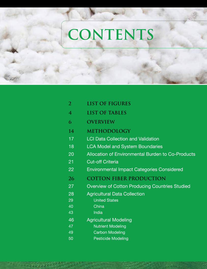
2 List of Figures
4 List of Tables
6 Overview
14 Methodology
17 LCI Data Collection and Validation
18 LCA Model and System Boundaries
20 Allocation of Environmental Burden to Co-Products
21 Cut-off Criteria
22 Environmental Impact Categories Considered
26 Cotton Fiber Production
27 Overview of Cotton Producing Countries Studied
28 Agricultural Data Collection29 United States
40 China
43 India
46 Agricultural Modeling47 Nutrient Modeling
49 Carbon Modeling
50 Pesticide Modeling
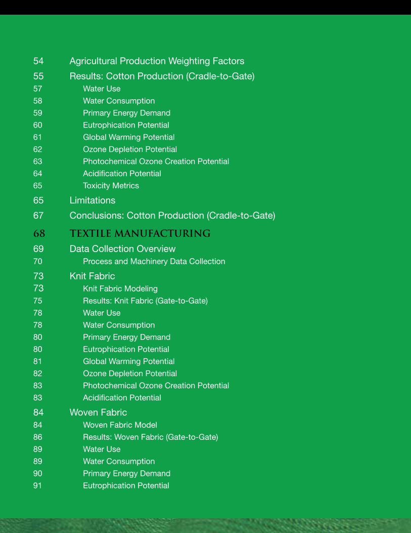
54 Agricultural Production Weighting Factors
55 Results: Cotton Production (Cradle-to-Gate)57 Water Use
58 Water Consumption
59 Primary Energy Demand
60 Eutrophication Potential
61 Global Warming Potential
62 Ozone Depletion Potential
63 Photochemical Ozone Creation Potential
64 Acidification Potential
65 Toxicity Metrics
65 Limitations
67 Conclusions: Cotton Production (Cradle-to-Gate)
68 Textile Manufacturing
69 Data Collection Overview70 Process and Machinery Data Collection
73 Knit Fabric73 Knit Fabric Modeling
75 Results: Knit Fabric (Gate-to-Gate)
78 Water Use
78 Water Consumption
80 Primary Energy Demand
80 Eutrophication Potential
81 Global Warming Potential
82 Ozone Depletion Potential
83 Photochemical Ozone Creation Potential
83 Acidification Potential
84 Woven Fabric84 Woven Fabric Model
86 Results: Woven Fabric (Gate-to-Gate)
89 Water Use
89 Water Consumption
90 Primary Energy Demand
91 Eutrophication Potential
92 Global Warming Potential
93 Ozone Depletion Potential
94 Photochemical Ozone Creation Potential
95 Acidification Potential
96 Results in Context96 Spinning Sensitivity Analysis
97 Limitations
101 Conclusions: Textile Manufacturing of Knit and Woven Fabrics (Gate-to-Gate)
102 Use Phase
103 Cut-and-Sew Methodology
104 Consumer Use Methodology
108 End of Life Methodology
108 Results: Consumer Use Scenarios109 Water Use and Water Consumption
111 Primary Energy Demand
112 Eutrophication Potential
112 Global Warming Potential
113 Ozone Depletion Potential
114 Photochemical Ozone Creation Potential
114 Acidification Potential
116 Results in Context116 Consumer Use Sensitivity Analysis
117 Conclusions: Use Phase
118 Cotton Life Cycle (Cradle-to-Grave) Results
122 Summary: Cotton Life Cycle (Cradle-to-Grave)
124 Continued Research
126 References
136 Appendix A—Life Cycle Inventory Datasets
139 Appendix B—Agricultural Data Questionnaire
145 Appendix C—Product CARBON Footprint verification Letter
148 Appendix D—Contributors
148 Cotton Incorporated148 Cotton Production
148 Textile Production
148 Consumer End-Use
148 National Cotton Council
148 PE International
1
Figure 1: LCA System Boundaries and Functional Units 8Figure 2: Relative Contribution to Impact Category for Batch-Dyed Knit Fabric Life Cycle 12Figure 3: LCA System Boundaries and Functional Units 19Figure 4: Cotton Production per County in the US in 2008 29Figure 5: 30-year Average Rainfall in the Cotton-producing States 31Figure 6: Dominant Soil Orders in the United States 32Figure 7: Soil Cropland Erosion Rates for the United States 33Figure 8: Determination of Ground Water Levels in California SJV, Spring 2009 36Figure 9: Westlands Water District Water Supply 1988–2005 37Figure 10: China's Cotton Regions and Production by Province (2010-11 crop year). 42Figure 11: Regions of Cotton Production in India (2009-2010 crop year). 45Figure 12: Nitrogen System Flows (PE INTERNATIONAL AG, 2011) 47Figure 13: Main Dispersion Routes for Pesticide Applied to a Crop Field 51Figure 14: Emissions of Pesticides to Air, Plant, Soil and Water at the Time of Pesticide Application. 52Figure 15: Relative Contribution to Each Impact Category for Cotton Fiber Production 57Figure 16: Water Usage in Cotton Production [m3/1,000 kg Cotton Fiber] by Water Source 58Figure 17: Water Consumption in Cotton Production [m3/1,000 kg Cotton Fiber] 58Figure 18: Primary Energy Demand from Fossil Sources by Contributors 59Figure 19: Eutrophication Potential [kg PO43- eq./1,000 kg of Cotton Fiber] by Contributors 60Figure 20: Global Warming Potential [kg CO2 eq./1,000 kg of Cotton Fiber] by Contributors 61Figure 21: Ozone Depletion Potential [kg R11 eq./1,000 kg of Cotton Fiber] by Contributors 62Figure 22: Photochemical Ozone Creation Potential [kgC2H4 eq./1,000 kg of Cotton Fiber] by Contributors 63Figure 23: Acidification Potential [kg SO2 eq./ 1,000 kg of Cotton Fiber] by Contributors 64Figure 24: Knit Fabric Unit Process Chain (Bale to Knitting) 74Figure 25: Knit Fabric Unit Process Chain (Knitting to Finished Knit Fabric) 75Figure 26: Relative Contribution to Each Life Cycle Impact Category for Batch-Dyed Knit Fabric 76Figure 27 Relative Impact Contribution by Textile Process Step for Batch-Dyed Knit Fabric 77Figure 28: Relative Impact Contribution by Textile Process Step for Yarn-Dyed Knit Fabric 78Figure 29: Water Usage for Knit Fabric Manufacturing by Textile Process Step 79Figure 30: Water Consumption for Knit Fabric by Textile Process Step 79Figure 31: Primary Energy Demand for Knit Fabric Manufacturing by Textile Process Step 80Figure 32: Eutrophication Potential for Knit Fabric Manufacturing by Textile Process Step 81Figure 33: Global Warming Potential for Knit Fabric Manufacturing by Textile Process Step 81Figure 34: Ozone Depletion Potential for Knit Fabric by Textile Process Step 82Figure 35: Photochemical Ozone Creation Potential for Knit Fabric by Textile Process Step 83
List Of Figures
LCA FULL REport / List of Figures2
Figure 36: Acidification Potential for Knit Fabric Manufacturing by Textile Process Step 84Figure 37: Woven Fabric Unit Process Chain (Bale to Weaving) 85Figure 38: Woven Fabric Unit Process Chain (Weaving to Finished Woven Fabric) 86Figure 39: Relative Contribution to Each Impact Category for Woven Fabric Life cycle 87Figure 40 Percent Impact Contribution by Textile Process Step for Woven Fabric 87Figure 41: Water Usage for Woven Fabric Manufacturing by Textile Process Step 89Figure 42: Water Consumption for Woven Fabric by Textile Process Step 89Figure 43: Primary Energy Demand from Fossil Sources for Woven
Fabric Manufacturing by Textile Process Step 90Figure 44: Eutrophication Potential for Woven Fabric Manufacturing by Textile Process Step 91Figure 45: Global Warming Potential for Woven Fabric Manufacturing by Textile Process Step 92Figure 46: Ozone Depletion Potential for Woven Fabric Manufacturing by Textile Process Step 93Figure 47: Photochemical Ozone Creation Potential for Woven Fabric Manufacturing by Textile Process Step 94Figure 48: Acidification Potential for Woven Fabric Manufacturing by Textile Process Step 95Figure 49: Spinning Sensitivity for Acidification Potential 98Figure 50: Spinning Sensitivity for Photochemical Ozone Creation Potential 98Figure 51: Water Usage by Fabric and Consumer Use Scenario 110Figure 52: Water Consumption by Fabric and Consumer Use Scenario 110Figure 53: Energy Demand by Fabric and Consumer Use Scenario 111Figure 54: Eutrophication Potential by Fabric and Consumer Use Scenario 112Figure 55: Global Warming Potential by Fabric and Consumer Use Scenario 113Figure 56: Ozone Depletion by Fabric and Consumer Use Scenario 114Figure 57: Photochemical Ozone Creation Potential by Fabric and Consumer Use Scenario 115Figure 58: Acidification Potential by Fabric and Consumer Use Scenario 115Figure 59: Sensitivity of Consumer Behavior Choices (Relative to the Average Use Case) 116Figure 60: Relative Contribution to Each Impact Category for Batch-Dyed Knit Fabric 121Figure 61: Relative Contribution to Each Impact Category for Yarn-Dyed Knit Fabric 121Figure 62: Relative Contribution to Each Impact Category for Woven Fabric 122
LCA FULL REport / List of Figures 3
Table 1: Environmental Impact Categories 9Table 2: Global Average LCIA Results for Cotton Fiber, Knit Fabric and Woven Fabric 11Table 3: Summary of Inclusions and Exclusions 20Table 4: Environmental Impact Categories 25Table 5: Example of Calculation of Production Weighting Function for the Southeastern United States 30Table 6: Example Fuel Use Requirements 38Table 7: Characteristics of Cotton Growing Regions in the U.S for 2005 to 2009. 39Table 8: Selected Characteristics of Cotton Production in China by Region. 41Table 9: Selected Characteristics of Cotton Production in India by Region. 44Table 10: Default Pesticide emission factors to partition mass not emitted to air. 53Table 11: Data Used to Create Global Weighting Factor. 54Table 12: Relative Contribution to Each Impact Category for Cotton Fiber Production 56Table 13: Mean and Standard Deviation for Impact Measures in the Agricultural Phase. 66Table 14: Textile Unit Processes 70Table 15: Process Machinery Energy from Equipment Manufacturers 71Table 16: Calculated Mill-Reported Energy Data for Bale Opening – Spinning 72Table 17: Mean and Standard Deviation for Impact Metrics in the Textile Phase. 100Table 18: Garment Components 103Table 19: Use Scenarios 104Table 20: Washing Machine Data 105Table 21: Dryer Data 105Table 22: Summary of Cotton Incorporated Lifestyle Monitor™ Data 107Table 23: Additional References for Garment Life 107Table 24: Relative Contribution to Impact Category By Use Phase Process for Knits 108Table 25: Global Average LCIA Results for Cotton Fiber, Knit Fabric, and Woven Fabric 119Table 26: Relative Contribution to Each Impact Category by Fabric 120
List Of Tables
LCA FULL REport / List of Tables4
5
Overview
Life Cycle Assessment (LCA) is a systematic evaluation of the potential environmental impact and resource utiliza-tion of a product, starting at the raw material stage and ending with disposal at the end of the product’s life.
A fundamental component of LCA is the Life Cycle Inventory or LCI. An LCI is a quantification of the relevant energy and material inputs and environmental re-lease or emissions data associated with product creation and use. The primary purpose of this project was to compile a robust and current LCI dataset for global cotton fiber production and textile manufacturing. A secondary objective was to use the LCI data to conduct a complete Life Cycle Impact Assessment (LCIA) of a hypothetical knit shirt and a woven pant to better understand the environmental impact of cotton textiles so the cotton industry can effectively direct research and resources towards reducing future impacts.
The Cotton Foundation commissioned PE International to perform these studies according to the principles of the International Organization for Standardization (ISO) 14040 series of standards for Life Cycle Assessment (ISO, 2006). Because the LCI will be published in proprietary and open source LCA databases, the entire study was reviewed by a third-party Critical Review Team comprised of agricultural, LCA, and textile experts. The LCI data were also submitted to The Carbon Trust, a not-for-profit company in the United Kingdom, for certification and to bring additional third-party review and credibility to the data. The project was managed by The National Cotton Council of America, Cotton Incorporated, and Cotton Council International.
Figure 1 shows the three key cotton life cycle phases that were examined in this study: 1) cotton fiber production (agricultural field practices and ginning); 2) textile manufacturing (knits and wovens); and 3) garment use (consumer washing and wearing), including the cut-and-sew and garment end-of-life phases. Transporta-tion was also considered.
LCA FULL REport / OVERVIEW 7
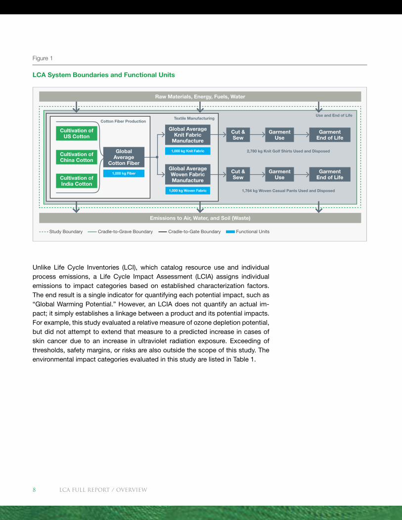
Unlike Life Cycle Inventories (LCI), which catalog resource use and individual process emissions, a Life Cycle Impact Assessment (LCIA) assigns individual emissions to impact categories based on established characterization factors. The end result is a single indicator for quantifying each potential impact, such as “Global Warming Potential.” However, an LCIA does not quantify an actual im-pact; it simply establishes a linkage between a product and its potential impacts. For example, this study evaluated a relative measure of ozone depletion potential, but did not attempt to extend that measure to a predicted increase in cases of skin cancer due to an increase in ultraviolet radiation exposure. Exceeding of thresholds, safety margins, or risks are also outside the scope of this study. The environmental impact categories evaluated in this study are listed in Table 1.
Figure 1
LCA System Boundaries and Functional Units
Study Boundary Cradle-to-Grave Boundary Cradle-to-Gate Boundary Functional Units
Emissions to Air, Water, and Soil (Waste)
Cotton Fiber Production
Cut & Sew
Cut & Sew
Garment Use
Garment Use
Garment End of Life
Garment End of Life
1,000 kg Knit Fabric 2,780 kg Knit Golf Shirts Used and Disposed
1,764 kg Woven Casual Pants Used and Disposed 1,000 kg Woven Fabric
Textile ManufacturingUse and End of Life
Raw Materials, Energy, Fuels, Water
Cultivation of US Cotton
Cultivation of China Cotton
Cultivation of India Cotton
1,000 kg Fiber
Global Average
Cotton Fiber
Global Average Knit Fabric
Manufacture
Global Average Woven Fabric Manufacture
LCA FULL REport / OVERVIEW8
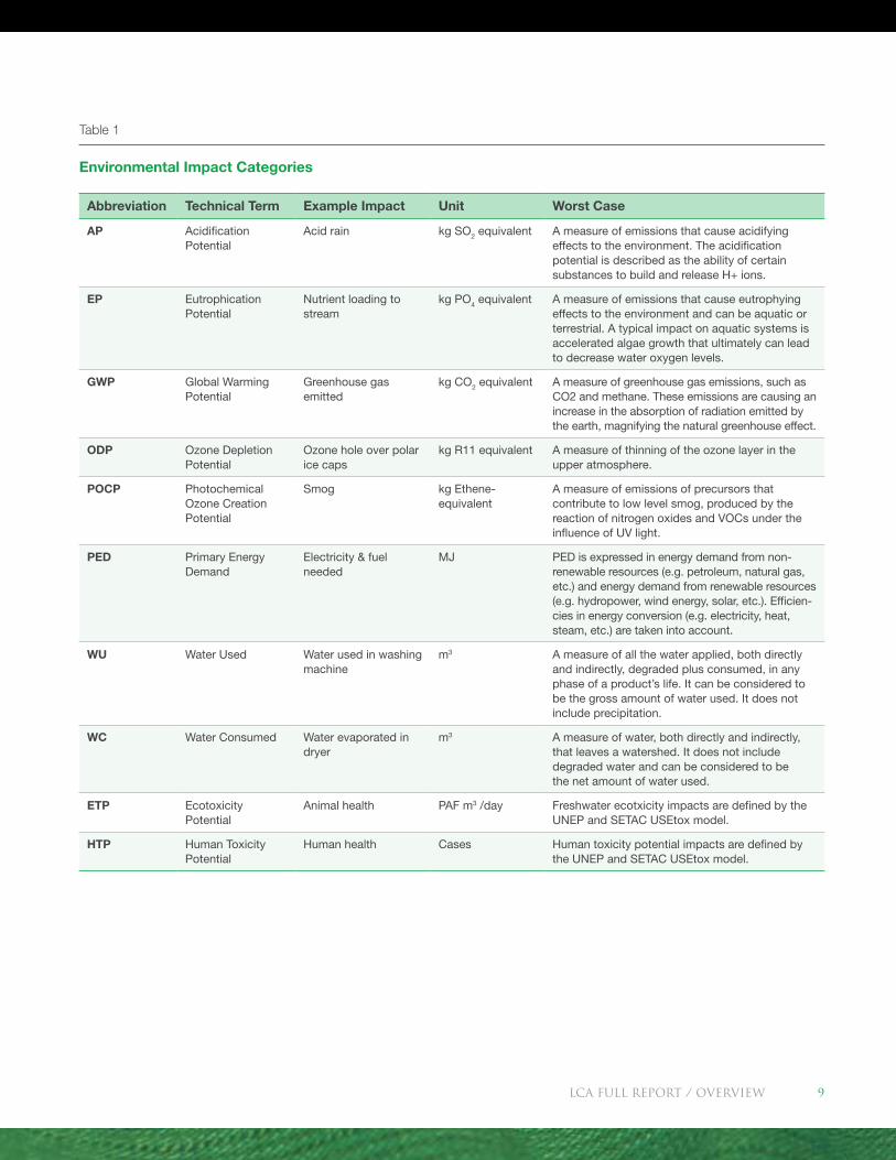
Table 1
Environmental Impact Categories
Abbreviation Technical Term Example Impact Unit Worst Case
AP Acidification Potential
Acid rain kg SO2 equivalent A measure of emissions that cause acidifying effects to the environment. The acidification potential is described as the ability of certain substances to build and release H+ ions.
EP Eutrophication Potential
Nutrient loading to stream
kg PO4 equivalent A measure of emissions that cause eutrophying effects to the environment and can be aquatic or terrestrial. A typical impact on aquatic systems is accelerated algae growth that ultimately can lead to decrease water oxygen levels.
GWP Global Warming Potential
Greenhouse gas emitted
kg CO2 equivalent A measure of greenhouse gas emissions, such as CO2 and methane. These emissions are causing an increase in the absorption of radiation emitted by the earth, magnifying the natural greenhouse effect.
ODP Ozone Depletion Potential
Ozone hole over polar ice caps
kg R11 equivalent A measure of thinning of the ozone layer in the upper atmosphere.
POCP Photochemical Ozone Creation Potential
Smog kg Ethene- equivalent
A measure of emissions of precursors that contribute to low level smog, produced by the reaction of nitrogen oxides and VOCs under the influence of UV light.
PED Primary Energy Demand
Electricity & fuel needed
MJ PED is expressed in energy demand from non-renewable resources (e.g. petroleum, natural gas, etc.) and energy demand from renewable resources (e.g. hydropower, wind energy, solar, etc.). Efficien-cies in energy conversion (e.g. electricity, heat, steam, etc.) are taken into account.
WU Water Used Water used in washing machine
m3 A measure of all the water applied, both directly and indirectly, degraded plus consumed, in any phase of a product’s life. It can be considered to be the gross amount of water used. It does not include precipitation.
WC Water Consumed Water evaporated in dryer
m3 A measure of water, both directly and indirectly, that leaves a watershed. It does not include degraded water and can be considered to be the net amount of water used.
ETP Ecotoxicity Potential
Animal health PAF m3 /day Freshwater ecotxicity impacts are defined by the UNEP and SETAC USEtox model.
HTP Human Toxicity Potential
Human health Cases Human toxicity potential impacts are defined by the UNEP and SETAC USEtox model.
LCA FULL REport / OVERVIEW 9
Cotton fiber production data were collected by production regions within the U.S. (4 regions), China (3 regions), and India (3 regions) and represented the years 2005 to 2009 (averaged to reduce variation due to weather and other environ-mental conditions). The U.S., China, and India represented 67% of the world’s cotton fiber production in 2010 (USDA, 2011). The fiber production phase cov-ers raw material production from field through ginning (cradle-to-gate) and data collection included soil types, climate, seed and chemical inputs, water and fuel use, and dates of key operations (for example, planting, fertilizer application, and harvest). These data were then input to an agricultural cultivation model developed by PE International to estimate the nitrogen and carbon cycles in each of the regions. Impacts were calculated for a functional unit of 1,000 kilograms (kg) of cotton fiber.
Data on fabric production for both knit and woven fabrics were collected from representative mills in four regions: Turkey, India, China, and Latin America. These areas represented 66% of knit and 51% of woven world fabric manu-facturing in 2009 (ITMF, 2009). Candidate textile mills were identified through interviews conducted during site visits to more than 40 cotton textile compa-nies representing over 75% of global textile processing in regions of China, India, Turkey, Southeast Asia, and the Americas during a previous study by Cotton Incorporated. The information from the interviews was combined with Cotton Incorporated staff technical service experiences to identify “typical” mills that would accurately reflect textile production practices in the countries of interest. Data collection included raw material inputs and outputs; energy inputs by source; dye/chemical inputs, outputs, and emissions; water use and solid waste stream (recycled, sold, and landfill).
Results of the LCIA for 1,000 kg of cotton fiber, 1,000 kg of knit fabric, and 1,000 kg of woven fabric are shown in Table 2. Cotton fiber production covered plant-ing through ginning (cradle-to-gate), and included carbon sequestration in the fiber (lowering GWP in the agricultural phase) and then assumed released at end of life. Knit and woven fabric manufacturing included yarn spinning through preparation, dyeing and finishing (gate-to-gate). Water usage for fiber produc-tion included irrigation water use only (rainfall not included). The study also included an evaluation of two additional categories, Ecotoxicity Potential (ETP) and Human Toxicity Potential (HTP) but the results are not reported here as the precision of the toxicity model, USEtox™, is limited and we are still evaluat-ing parameters and methods the model uses to better assess its accuracy for agricultural and textile processes.
LCA FULL REport / OVERVIEW10
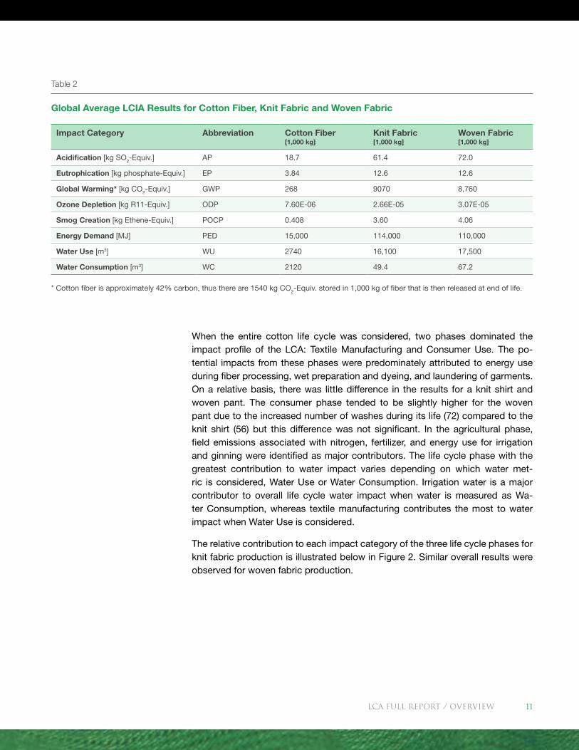
When the entire cotton life cycle was considered, two phases dominated the impact profile of the LCA: Textile Manufacturing and Consumer Use. The po-tential impacts from these phases were predominately attributed to energy use during fiber processing, wet preparation and dyeing, and laundering of garments. On a relative basis, there was little difference in the results for a knit shirt and woven pant. The consumer phase tended to be slightly higher for the woven pant due to the increased number of washes during its life (72) compared to the knit shirt (56) but this difference was not significant. In the agricultural phase, field emissions associated with nitrogen, fertilizer, and energy use for irrigation and ginning were identified as major contributors. The life cycle phase with the greatest contribution to water impact varies depending on which water met-ric is considered, Water Use or Water Consumption. Irrigation water is a major contributor to overall life cycle water impact when water is measured as Wa-ter Consumption, whereas textile manufacturing contributes the most to water impact when Water Use is considered.
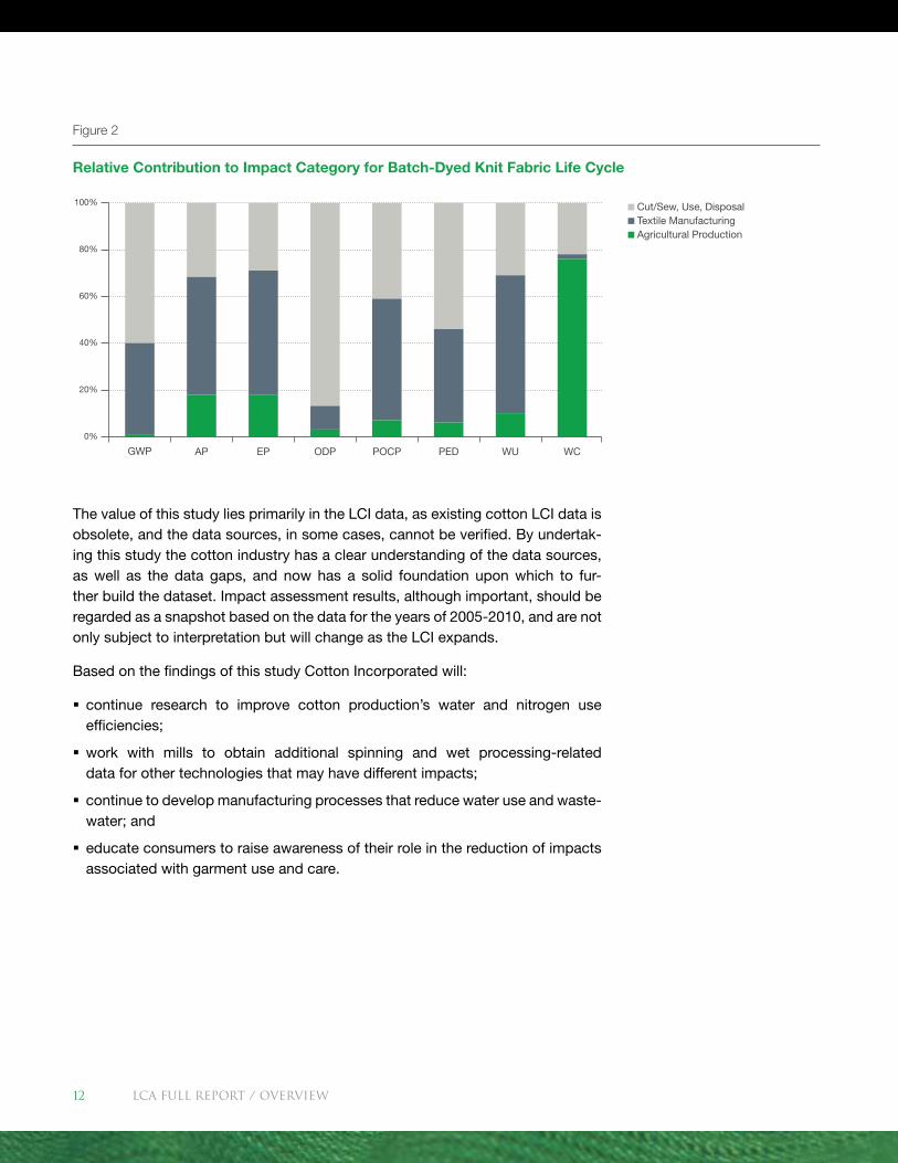
The relative contribution to each impact category of the three life cycle phases for knit fabric production is illustrated below in Figure 2. Similar overall results were observed for woven fabric production.
Table 2
Global Average LCIA Results for Cotton Fiber, Knit Fabric and Woven Fabric
Impact Category Abbreviation Cotton Fiber [1,000 kg]
Knit Fabric [1,000 kg]
Woven Fabric [1,000 kg]
Acidification [kg SO2-Equiv.] AP 18.7 61.4 72.0
Eutrophication [kg phosphate-Equiv.] EP 3.84 12.6 12.6
Global Warming* [kg CO2-Equiv.] GWP 268 9070 8,760
Ozone Depletion [kg R11-Equiv.] ODP 7.60E-06 2.66E-05 3.07E-05
Smog Creation [kg Ethene-Equiv.] POCP 0.408 3.60 4.06
Energy Demand [MJ] PED 15,000 114,000 110,000
Water Use [m3] WU 2740 16,100 17,500
Water Consumption [m3] WC 2120 49.4 67.2
* Cotton fiber is approximately 42% carbon, thus there are 1540 kg CO2-Equiv. stored in 1,000 kg of fiber that is then released at end of life.
LCA FULL REport / OVERVIEW 11
The value of this study lies primarily in the LCI data, as existing cotton LCI data is obsolete, and the data sources, in some cases, cannot be verified. By undertak-ing this study the cotton industry has a clear understanding of the data sources, as well as the data gaps, and now has a solid foundation upon which to fur-ther build the dataset. Impact assessment results, although important, should be regarded as a snapshot based on the data for the years of 2005-2010, and are not only subject to interpretation but will change as the LCI expands.
Based on the findings of this study Cotton Incorporated will:
� continue research to improve cotton production’s water and nitrogen use efficiencies;
� work with mills to obtain additional spinning and wet processing-related data for other technologies that may have different impacts;
� continue to develop manufacturing processes that reduce water use and waste-water; and
� educate consumers to raise awareness of their role in the reduction of impacts associated with garment use and care.
Figure 2
Relative Contribution to Impact Category for Batch-Dyed Knit Fabric Life Cycle
Cut/Sew, Use, Disposal Textile Manufacturing Agricultural Production
100%
80%
60%
40%
20%
0%
GWP AP EP ODP POCP PED WU WC
LCA FULL REport / OVERVIEW12
With the growing interest in the measurement of environmental impact, compa-nies are turning to LCA’s to fully understand the risks and liabilities across their supply chains. Major textile brands have performed product-level LCA’s and are changing business practices as a result of those assessments. Broader efforts, such as The Sustainability Consortium and the Sustainable Apparel Coalition are developing LCA-based metrics to define product environmental performance. Increasingly, LCI data are being considered prior to product design to aid in the selection of materials that will minimally impact the environment. The value of this study extends beyond simply an environmental benchmarking exercise for global cotton; this LCA provides the means for users of cotton to evaluate the environmental impact of products specific to their own businesses and to determine where improvements can be made.
LCA FULL REport / OVERVIEW 13

Methodology
This section contains general methodological information common to the phases of the cotton life cycle comprising this study. Detailed information on data collection, includ-ing modeling and results, specific to each life cycle phase are reported in the Cotton Fiber Production, Textile Manu-facturing, and Consumer Use sections of this report.
LCA is a demonstrated method to scientifically evaluate the environmental impact and resource utilization of a product, from the raw materials used in its creation to the disposal of the product at the end of its useful life. LCA consists of four basic stages: goal and scope definition; inventory analysis; impact assessment; and in-terpretation. In the goal and scope phase the system boundaries and the processes included in the LCA are defined. During inventory analysis the relevant energy, ma-terial inputs, and environmental release data associated with the identified process-es are quantified. This dataset underlying an LCA is called a Life Cycle Inventory or LCI. The quality and integrity of the LCI are critical since the Life Cycle Impact Assessment (LCIA) and subsequent interpretation are derived from this data.
The Cotton Foundation commissioned PE International to perform these studies according to the principles of the International Organization for Standardization’s (ISO) 14040 series of standards for Life Cycle Assessment (ISO, 2006). The project was managed by The National Cotton Council of America, Cotton Incorporated, and Cotton Council International. Cotton Incorporated’s Agricultural and Environ-mental Research, Product Development and Implementation (with the assistance of Global Supply Chain Marketing), and Corporate Strategy and Program Met-rics divisions were responsible for data collection and analysis of cotton produc-tion, textile production, and consumer data, respectively. Because the LCI will be published in proprietary and open source LCA databases, the entire study was reviewed by agricultural, LCA, and textile experts, who were a third-party Criti-cal Review Team according to the ISO 14040 series of standards for LCA. The critical review team members were:
� Agricultural expert: Dr. Alan Fanzluebbers, USDA, ARS;
� Textile experts: Dr. Fred Cook, Georgia Tech and Dr. Martin Bide, University of Rhode Island; and
� LCA expert: Dr. Scott Kaufman, Carbon Trust, Brooklyn, NY.
LCA FULL REport / Methodology 15
The results of this study and LCI data used to calculate the results were also verified by Carbon Trust Certification (CTC) against PAS 2050:2008. CTC provides inde-pendent verification of the carbon footprints of products (goods and services) and is accredited by the United Kingdom Accreditation Service to ISO 14065:2007 to provide greenhouse gas verification against PAS 2050.
CTC’s mission is to deliver robust verification and certification of product and or-ganization carbon footprints. For products, this is done by providing an impartial and accurate assessment of carbon footprints against internationally recognized footprinting standards including PAS 2050. This helps organizations to accurately measure, manage, communicate and reduce their carbon footprints across their whole supply chain.
CTC found the results and LCI data to be broadly in conformity with PAS 2050, with the exception of clauses 4.3. (product differentiation), 5.5 (land use change) and 7.8 (Non-CO2 emissions data for livestock & soils).
Excluded Clauses
Demonstrating conformity with clause 4.3 of PAS 2050 was considered to be out-side of the scope of this project. This is because PAS 2050 is intended to be applied by organizations to uniquely identifiable products directly under their control. The results of the study are based on regionally and globally gathered data footprints for a range of cotton products produced and supplied by multiple organizations. The Cotton Foundation does not own or control these products and for these reasons it was not possible or appropriate to demonstrate conformity with clause 4.3 of PAS 2050.
Clause 5.5 of PAS 2050 requires organizations to account for land use change (de-forestation and other removals of biomass). There is insufficient evidence to de-termine whether any change occurred in relation to the cotton products that have been footprinted. Land use change has been excluded from the calculation of the carbon footprint results of this study. Where these results are used and land use change may be a factor, it is strongly recommended that the impacts are properly considered and the footprint results adjusted accordingly in conformity with PAS 2050 clause 5.5.
Clause 7.8 of PAS 2050 requires organizations to calculate Non-CO2 emissions (such as N2O) in a methodology determined by the latest IPCC (Intergovernmental Panel on Climate change) National Greenhouse Gas Inventories. The data used and methodology chosen to represent agricultural emissions were derived from PE In-ternational’s agricultural model, which was considered by PE International and the Cotton Foundation to be a more accurate representation of N2O emissions, rather than being based on IPCC data and methodology.
LCA FULL REport / Methodology16
The average figure quoted is deemed to be accurate within the scope of this proj-ect. However, as a consequence of not demonstrating conformity with the excluded clauses, the verified results may not necessarily be comparable with other certified or verified product carbon footprints, nor should the results be used as a compara-tor against which the product carbon footprints of other cotton products outside of this study are formally benchmarked.
Further details on the results of this verification process are presented in Appen-dix D.
The specific objectives of this study were to:
1. Build up-to-date, representative, and well-documented LCI’s for cotton fiber production and fabric manufacturing and integrate them into both propri-etary and open source LCI databases (e.g., Ecoinvent and the USDA Digital Commons).
2. Conduct an LCIA of textile products (golf shirt for knits, casual pants for wovens) constructed from cotton.
Although the objectives of this LCA do not include comparative fiber assertions, the cotton LCI dataset will be integrated into open source LCI databases and will be accessible to those who want to conduct such comparisons. Additionally, The LCI datasets will be housed in an interactive software tool called i-Report that gives Cotton Incorporated the ability to evaluate the environmental attributes of specific cotton products.
LCI Data Collection and Validation
Primary data collection was conducted globally, based on regions in the US, China, India, Turkey, and Latin America representative of specific growing and manufacturing conditions. Primary data collection was accomplished in the form of spreadsheets and questionnaires, and supplemented by conversations with cotton growers, textile mills, and consumers. In cases where primary data were not available or were inconsistent, secondary data that were readily avail-able from literature, machinery manufacturers, previous Life Cycle Inventory (LCI) studies, and life cycle databases were used for the analysis. The sources for any secondary data used are documented throughout the agricultural, textile, and use phase sections of this study report.
Average cotton cultivation in the US, China, and India for the years 2005–2009 was incorporated into PE INTERNATIONAL’s cultivation model based on region-al production-weighted averages. Collecting data over a range of years averages out seasonal and annual variations such as droughts and floods. The US, China, and India represented 67% of the world’s cotton fiber production in 2010 (USDA 2011).
LCA FULL REport / Methodology 17
Data on fabric production for both knits and wovens were collected from representative mills in each of the four regions (Turkey, India, China, and Latin America) with geographic differences for background energy systems. China, In-dia, Turkey and Latin America represent approximately 66% of knit and 51% of woven world fabric manufacturing in 2009 (ITMF 2009).
The mill data for textile production as well as and for cut-and-sew processes were supplemented with process energy calculations from machinery manufac-turers and data available from Cotton Incorporated experts. Background data on ancillary materials, energy and fuels, transportation, and end-of-life were tak-en from the PE International’s GaBi databases. Background data on use phase energy and materials were taken from existing PE International GaBi data combined with consumer behavior data from the Cotton Incorporated Lifestyle Monitor™ survey. Background data on landfilling at end-of-life were taken from PE International GaBi databases.
Internal quality assurance (QA) was applied at different stages of the project. The objective of the QA process was to ensure that the data collection, the development of the LCI model, and the final results were consistent with the scope of the study and that the study delivered the required information. The QA included a check of the LCI datasets, general model structure, results applicability, and report docu-mentation. Quality was acceptable at all levels of the project.
LCA Model and System Boundaries
The LCA model was originally created using the GaBi 4 software system developed by PE International, and the analysis was updated when the GaBi software was upgraded to version 5 in 2011. (GaBi 4, 2006; GaBi 5, 2011). The databases within the GaBi software were the source of the secondary LCI data upon which energy production, raw and process materials, transport, and wastewater treatment were modeled. These data were used to account for regional differences for similar pro-cesses. For example, China, India, Turkey and Latin America (the locations chosen for textile production) produce larger Acidification Potential (AP), Eutrophication Po-tential (EP), Global Warming Potential (GWP), and Photochemical Ozone Creation Potential (POCP) per kilowatt-hour when compared to the emissions profile of the U.S. electrical grid. However, Ozone Depletion Potential (ODP) is much higher in the U.S. emissions profile, which is the location for all of the assumed consumer use in this study. These factors will be important when comparing the overall contributions for each phase to each potential impact.
LCA FULL REport / Methodology18
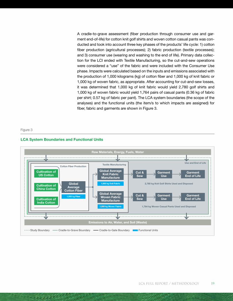
A cradle-to-grave assessment (fiber production through consumer use and gar-ment end-of-life) for cotton knit golf shirts and woven cotton casual pants was con-ducted and took into account three key phases of the products’ life cycle: 1) cotton fiber production (agricultural processes); 2) fabric production (textile processes); and 3) consumer use (wearing and washing to the end of life). Primary data collec-tion for the LCI ended with Textile Manufacturing, so the cut-and-sew operations were considered a “use” of the fabric and were included with the Consumer Use phase. Impacts were calculated based on the inputs and emissions associated with the production of 1,000 kilograms (kg) of cotton fiber and 1,000 kg of knit fabric or 1,000 kg of woven fabric, as appropriate. After accounting for cut-and-sew losses, it was determined that 1,000 kg of knit fabric would yield 2,780 golf shirts and 1,000 kg of woven fabric would yield 1,764 pairs of casual pants (0.36 kg of fabric per shirt; 0.57 kg of fabric per pant). The LCA system boundaries (the scope of the analyses) and the functional units (the item/s to which impacts are assigned) for fiber, fabric and garments are shown in Figure 3.
Figure 3
LCA System Boundaries and Functional Units
Study Boundary Cradle-to-Grave Boundary Cradle-to-Gate Boundary Functional Units
Emissions to Air, Water, and Soil (Waste)
Cotton Fiber Production
Cut & Sew
Cut & Sew
Garment Use
Garment Use
Garment End of Life
Garment End of Life
1,000 kg Knit Fabric 2,780 kg Knit Golf Shirts Used and Disposed
1,764 kg Woven Casual Pants Used and Disposed 1,000 kg Woven Fabric
Textile ManufacturingUse and End of Life
Raw Materials, Energy, Fuels, Water
Cultivation of US Cotton
Cultivation of China Cotton
Cultivation of India Cotton
1,000 kg Fiber
Global Average
Cotton Fiber
Global Average Knit Fabric
Manufacture
Global Average Woven Fabric Manufacture
LCA FULL REport / Methodology 19
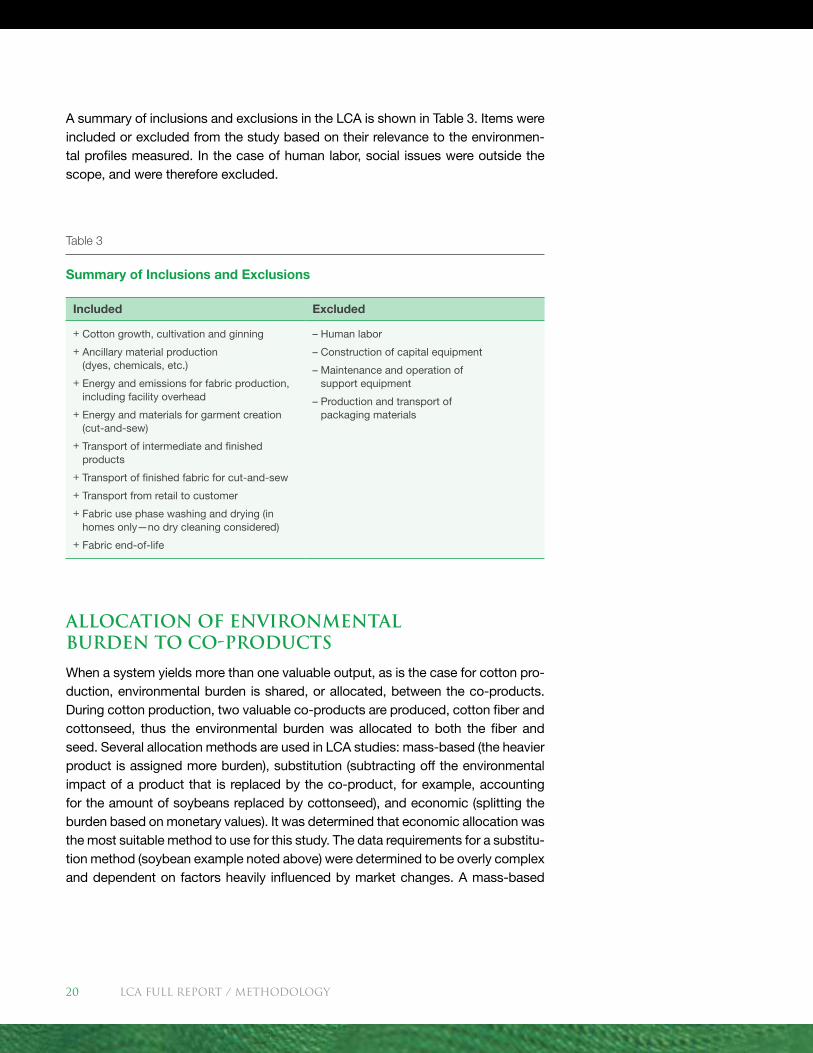
A summary of inclusions and exclusions in the LCA is shown in Table 3. Items were included or excluded from the study based on their relevance to the environmen-tal profiles measured. In the case of human labor, social issues were outside the scope, and were therefore excluded.
Allocation of Environmental Burden to Co-Products
When a system yields more than one valuable output, as is the case for cotton pro-duction, environmental burden is shared, or allocated, between the co-products. During cotton production, two valuable co-products are produced, cotton fiber and cottonseed, thus the environmental burden was allocated to both the fiber and seed. Several allocation methods are used in LCA studies: mass-based (the heavier product is assigned more burden), substitution (subtracting off the environmental impact of a product that is replaced by the co-product, for example, accounting for the amount of soybeans replaced by cottonseed), and economic (splitting the burden based on monetary values). It was determined that economic allocation was the most suitable method to use for this study. The data requirements for a substitu-tion method (soybean example noted above) were determined to be overly complex and dependent on factors heavily influenced by market changes. A mass-based
Table 3
Summary of Inclusions and Exclusions
Included Excluded
+ Cotton growth, cultivation and ginning
+ Ancillary material production (dyes, chemicals, etc.)
+ Energy and emissions for fabric production, including facility overhead
+ Energy and materials for garment creation (cut-and-sew)
+ Transport of intermediate and finished products
+ Transport of finished fabric for cut-and-sew
+ Transport from retail to customer
+ Fabric use phase washing and drying (in homes only—no dry cleaning considered)
+ Fabric end-of-life
– Human labor
– Construction of capital equipment
– Maintenance and operation of support equipment
– Production and transport of packaging materials
LCA FULL REport / Methodology20
allocation would have placed most of the burden on the cottonseed, and, as cotton is perceived as a fiber crop, this approach seemed implausible. Thus, for economic allocation, data on the value of cotton fiber and cottonseed from the United States from 2005 to 2009, as reported by the USDA, were used. The allocation took into account that 1.4 units of cottonseed are produced per unit of cotton fiber. The eco-nomic allocation resulted in 84% of the agricultural burden assigned to the fiber and 16% to the seed. No burden was assigned to the stalks or gin waste.
Noils, a co-product from fabric manufacturing, are too valuable to be considered waste (approximately $0.75 per kg compared to $1.50 per kg for fiber) and are subjected to the same production and textile manufacturing systems as primary fabric. For this reason an economic allocation of impact was deemed reasonable in this case. In contrast, lower value waste material generated throughout the textile manufacturing processes, such as start-up fabric from knitting or weaving, for ex-ample, are usually recycled internally or sold offsite for a low price. These types of wastes were considered to be byproducts and no allocation of burden was deemed necessary in these cases.
Cut-off Criteria
To ensure that all relevant environmental impacts were represented in the study the following cut-off criteria were used.
Æ Mass—If the flow was less than 1% of the cumulative mass of all the inputs and outputs of the LCI model, it was excluded, provided its environmental relevance was not a concern.
Æ Energy—If the flow was less than 1% of the cumulative energy of all the inputs and outputs of the LCI model, it was excluded, provided its environmental rel-evance was not a concern.
Æ Environmental relevance—If the flow met the above criteria for exclusion yet was thought to have a potentially significant environmental impact, it was evaluated with proxies identified by chemical and material experts within PE International. If the proxy for an excluded material had a significant contribution to the overall LCIA, more information was collected and evaluated in the system.
Æ The sum of the neglected material flows did not exceed 2% of mass or energy
LCA FULL REport / Methodology 21
Environmental Impact Categories Considered
Unlike LCI’s which only report individual emissions, LCIA assigns individual emis-sions to impact categories based on established characterization of the emissions factors. The end result is a single indicator for quantifying each potential impact, such as “Global Warming Potential.” The environmental impact categories evalu-ated in this study are listed in in Table 4. Because the raw data for a particular cat-egory was collected in units that differed from the impact category units, the raw data was converted to common units in order to calculate a total for the impact cat-egory. For example, in the case of Global Warming Potential (GWP), GWP data on the mass of individual greenhouse gases were collected (e.g., nitrous oxide, meth-ane) then converted to the equivalent mass of carbon dioxide needed to produce the same impact on GWP. The impact assessment results for Acidification Potential (AP), Eutrophication Potential (EP), Global Warming Potential (GWP), Ozone Deple-tion Potential (ODP), and Photochemical Ozone Creation Potential (POCP) were calculated using characterization factors published by the University of Leiden, In-stitute of Environmental Sciences (CML). The factors were updated in November 2009. It should be noted that the impact categories represent potential impact; in other words, they are approximations of environmental impacts that could occur if the emitted molecules would (a) actually follow the underlying impact pathway and (b) meet certain conditions in the receiving environment while doing so. LCIA results are therefore relative expressions only and do not predict actual impacts, the exceeding of thresholds, safety margins, or risks. In addition, energy demand, water used and water consumed are reported as Environmental Indicators only and no further impact methodology was applied.
It is important to note that an LCA considers both direct and indirect water use. Direct water use refers to water used directly in the production of cotton products such as irrigation water, water to dye and finish textile products, and water used in the washing machine. Indirect water use can come from several sources, but a major source is the water associated with power generation. For example, a pro-cess that usually involves no direct water use, such as spinning a fiber into a yarn, can have a significant amount of indirect water use due to power generation. Rain-fall is not typically included in LCA.
LCA FULL REport / Methodology22
Several new metrics to describe water use from an LCA perspective are in develop-ment; however, presently there are two primary methods for modeling and reporting water and both were used for this study:
Water Used (WU) refers to all of the water involved, both directly and indirectly, in any phase of a product’s life. WU includes the groundwater, river and surface water used for irrigation during cotton cultivation and the water used for wet processing during the textile manufacturing phase. WU also includes the cooling water diverted during electricity (energy) production. It can be considered the gross amount of water used.
Water Consumed (WC) also consists of both direct and indirect water and is de-fined as the water that leaves the watershed from which it was drawn. In cases where water is returned to the same watershed, such as for treated wastewater from textile processes and consumer laundering, a credit is applied. In the case of irrigation water, it is considered to be 100% consumed since the water taken up by the cotton plant evaporates and falls later as rainfall into a different watershed or into the ocean and therefore no credit is applied. WC can be thought of as the net amount of water used.
To further illustrate both definitions, consider the direct water used and consumed during the laundering of a shirt. WU can be thought of as all the water that flows through the washing machine during the wash cycle. WC can be thought of as the amount of water that was retained in the shirt and then evaporated during drying. The indirect water associated with the production of the electricity needed to run the washing machine would be added to both WU and WC. In power generation a portion of the indirect water is returned to the same watershed so a credit would be given for this water in the WC calculation.
Two additional impact categories, Ecotoxicity Potential (ETP) and Human Toxicity Potential (HTP) were included in the LCA to evaluate the potential toxic impacts of chemical compounds used during the life cycle of a cotton product. The UNEP-SETAC USEtox® characterization model was used for both ETP and HTP modeling (Rosenbaum, 2008). Results showed that over the entire cradle-to-grave life cycle of cotton, nearly all of ETP is associated with pesticide application during the Agri-cultural Production phase. It should be noted that the precision of the current USE-tox® characterization factors is less robust than for all other impact categories. For
LCA FULL REport / Methodology 23
example, toxicity impacts can be caused by numerous embedded substances and emissions. The number of “elementary flows” (substances) related to toxicity can range from 1,000 to 10,000, and the variation in toxic impact of those substances can vary by orders of magnitude. In addition, emission profiles for some of the sub-stances are incomplete. In contrast, non-toxicity related impact categories such as energy or GWP are comprised of fewer embedded substances (10-500). Therefore, the uncertainties for toxicity assessment are greater than for other impact catego-ries since there are many more substances to study and model. For this reason, the USEtox® characterization factors in this study were used only as a means to iden-tify the key contributors within a product life cycle that significantly influence the product’s toxicity potential. Materials were noted as ‘substances of high concern’ but comparative assertions across products or across impact categories were not made. Additional studies are underway to more precisely understand the charac-terization, use amounts and emission factors for specific substances used in cotton production and textile processing and how they influence the underlying model.
LCA FULL REport / Methodology24
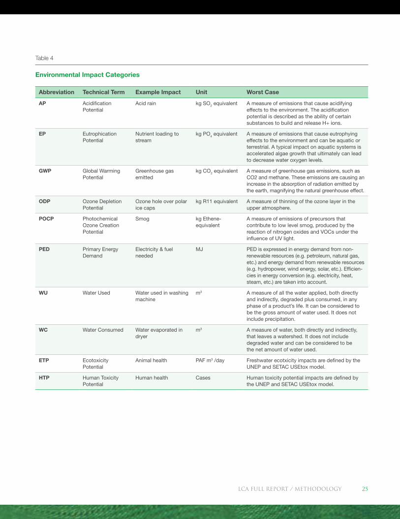
Table 4
Environmental Impact Categories
Abbreviation Technical Term Example Impact Unit Worst Case
AP Acidification Potential
Acid rain kg SO2 equivalent A measure of emissions that cause acidifying effects to the environment. The acidification potential is described as the ability of certain substances to build and release H+ ions.
EP Eutrophication Potential
Nutrient loading to stream
kg PO4 equivalent A measure of emissions that cause eutrophying effects to the environment and can be aquatic or terrestrial. A typical impact on aquatic systems is accelerated algae growth that ultimately can lead to decrease water oxygen levels.
GWP Global Warming Potential
Greenhouse gas emitted
kg CO2 equivalent A measure of greenhouse gas emissions, such as CO2 and methane. These emissions are causing an increase in the absorption of radiation emitted by the earth, magnifying the natural greenhouse effect.
ODP Ozone Depletion Potential
Ozone hole over polar ice caps
kg R11 equivalent A measure of thinning of the ozone layer in the upper atmosphere.
POCP Photochemical Ozone Creation Potential
Smog kg Ethene- equivalent
A measure of emissions of precursors that contribute to low level smog, produced by the reaction of nitrogen oxides and VOCs under the influence of UV light.
PED Primary Energy Demand
Electricity & fuel needed
MJ PED is expressed in energy demand from non-renewable resources (e.g. petroleum, natural gas, etc.) and energy demand from renewable resources (e.g. hydropower, wind energy, solar, etc.). Efficien-cies in energy conversion (e.g. electricity, heat, steam, etc.) are taken into account.
WU Water Used Water used in washing machine
m3 A measure of all the water applied, both directly and indirectly, degraded plus consumed, in any phase of a product’s life. It can be considered to be the gross amount of water used. It does not include precipitation.
WC Water Consumed Water evaporated in dryer
m3 A measure of water, both directly and indirectly, that leaves a watershed. It does not include degraded water and can be considered to be the net amount of water used.
ETP Ecotoxicity Potential
Animal health PAF m3 /day Freshwater ecotxicity impacts are defined by the UNEP and SETAC USEtox model.
HTP Human Toxicity Potential
Human health Cases Human toxicity potential impacts are defined by the UNEP and SETAC USEtox model.
LCA FULL REport / Methodology 25
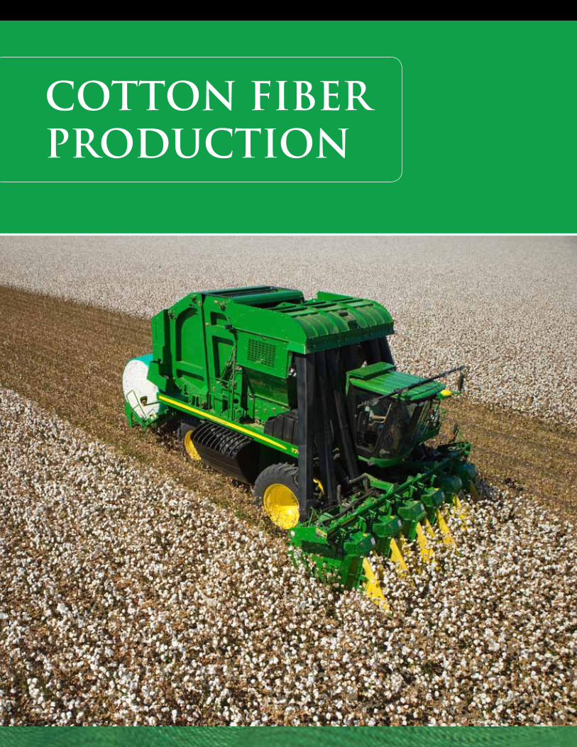
Cotton Fiber Production
This section addresses cotton fiber production and includes inputs and emissions from all field operations from planting of the crop until a bale of fiber exited the cotton gin.
Overview of Cotton Producing Countries Studied
Data collection and modeling of the agricultural system focused on the top three cotton-producing countries as of 2010: the U.S., China, and India. For modeling purposes each country was sub-divided into regions of similar climates and pro-duction practices. Agricultural production in China and India is conducted on small farm holdings using labor-intensive practices in contrast to the U.S. where cotton production is highly mechanized and is conducted on farm holdings of 500 hect-ares (ha) or larger (USDA 2009). In China, the majority of farms are less than 1 ha in size and in India the average farm size ranges from 0.5 to 2 ha. The exceptions for both China and India are in the northern growing regions of both countries where farms tend to be larger and there is a higher level of mechanization. The land in the southern provinces of China and India is intensively farmed and intercropping production practices are common. Bullocks (or other animals) are frequently used for land preparation and plowing in India and to a lesser extent in China. Farmers in both countries have access to hand (walk-behind) tractors, and many use powered backpack sprayers to apply farm chemicals.
The level of irrigation is similar for all three countries, with irrigation available to 25 to 40% of the cotton area. In most regions, irrigation supplements rainfall. The excep-tions are the Northern Zone in India and the Far West in the US where 100% of the cotton area is irrigated (Choudhary and Gaur, 2010; USDA 2009) and in Northwest China where the China Statistical Yearbook reports that about 60% of the total farmland is irrigated. However, considering that relatively high yields are reported for Northwest China and there is less than 200 mm of rainfall each year, it is reason-able to assume that the irrigated cotton area approaches 100%.
Transgenic technology has been adopted in all three countries. The U.S. planted 96% of the cotton area to transgenic varieties in 2010, including both herbicide tolerant and Bt technologies. China and India have adopted only Bt technology. In 2010, 86% of the cotton area in India was planted to Bt cotton hybrids while 69% of the cotton area in China was planted to Bt cotton varieties (James 2010).
India has the largest area planted to cotton in the world (10.3 million ha) and is sec-ond in cotton production (23.0 million bales). However, yields of 486 kg per ha are lower than in the U.S. or China. China, number one in cotton production, harvested 32.0 million bales from 5.3 million ha. China leads the U.S. and India with average yields of 1,315 kg per ha, primarily due to the fact that irrigation is available to more than 50% of the area in China versus approximately 40% in India and 36% in the U.S. While China and India both have small holder farms, farmers in China typically
LCA FULL REport / Cotton Fiber Production 27
have greater access to new technologies than those in India. The U.S. is third in production with 12.2 million bales harvested from 4.3 million ha. Cotton yields in the U.S. averaged 871 kg per ha in 2010. Together the three countries produced 67.2 million bales in 2010—66% of the world’s production (101.4 million bales) (USDA 2011). Note that for determining country level weighting factors and region cotton yield in the U.S., Meyer et al. (2009) were used to obtain averages from 2005-2009. However, in evaluating regional yields in China and India, country specific informa-tion was used as described in the following sections. A list of the types of agricul-tural data collected is provided in Appendix B–Agricultural Data.
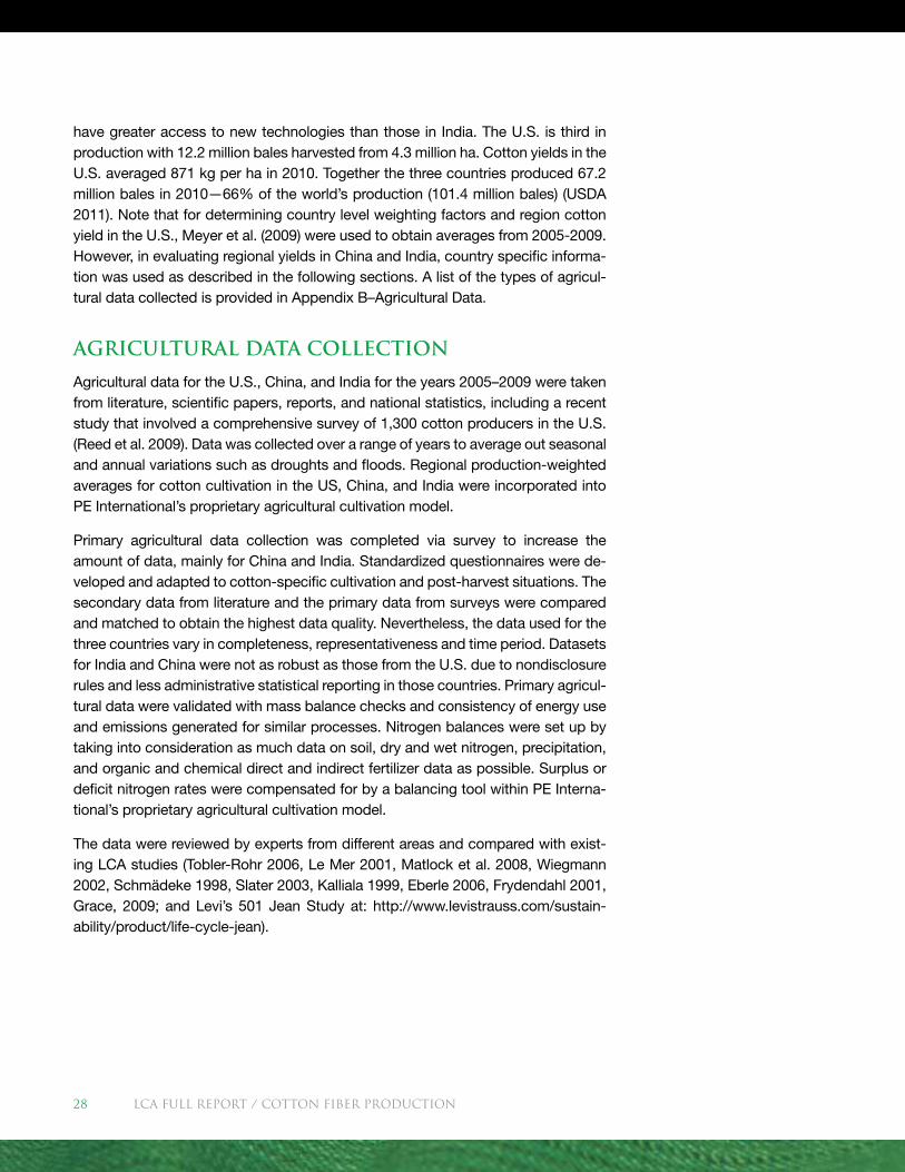
Agricultural Data Collection
Agricultural data for the U.S., China, and India for the years 2005–2009 were taken from literature, scientific papers, reports, and national statistics, including a recent study that involved a comprehensive survey of 1,300 cotton producers in the U.S. (Reed et al. 2009). Data was collected over a range of years to average out seasonal and annual variations such as droughts and floods. Regional production-weighted averages for cotton cultivation in the US, China, and India were incorporated into PE International’s proprietary agricultural cultivation model.
Primary agricultural data collection was completed via survey to increase the amount of data, mainly for China and India. Standardized questionnaires were de-veloped and adapted to cotton-specific cultivation and post-harvest situations. The secondary data from literature and the primary data from surveys were compared and matched to obtain the highest data quality. Nevertheless, the data used for the three countries vary in completeness, representativeness and time period. Datasets for India and China were not as robust as those from the U.S. due to nondisclosure rules and less administrative statistical reporting in those countries. Primary agricul-tural data were validated with mass balance checks and consistency of energy use and emissions generated for similar processes. Nitrogen balances were set up by taking into consideration as much data on soil, dry and wet nitrogen, precipitation, and organic and chemical direct and indirect fertilizer data as possible. Surplus or deficit nitrogen rates were compensated for by a balancing tool within PE Interna-tional’s proprietary agricultural cultivation model.
The data were reviewed by experts from different areas and compared with exist-ing LCA studies (Tobler-Rohr 2006, Le Mer 2001, Matlock et al. 2008, Wiegmann 2002, Schmädeke 1998, Slater 2003, Kalliala 1999, Eberle 2006, Frydendahl 2001, Grace, 2009; and Levi’s 501 Jean Study at: http://www.levistrauss.com/sustain-ability/product/life-cycle-jean).
LCA FULL REport / Cotton Fiber Production28
United States
The most robust agricultural data set in this study was from the U.S. due in part to the vast amount of publicly available government datasets. In this section an effort has been made to provide examples of both the temporal and spatial rich-ness of the U.S. data. In many cases, the data reside in public and government maintained databases and were supplemented with grower and expert scientific interviews. In order to characterize cotton production practices in the U.S., the 17 cotton-growing states in the country were assigned to four regions:
1. Southeast: Virginia, North Carolina, South Carolina, Georgia, Alabama, and Florida
2. Mid-south: Mississippi, Louisiana, Tennessee, Missouri, and Arkansas
3. Southwest: Texas, Oklahoma, and Kansas
4. Far West: California, Arizona, and New Mexico
Where possible, all regional data were calculated as production-weighted averages (i.e., more weight to data from states that produced more bales). The goal was to represent the average conditions from 2005 to 2009, and when possible, an-nual data were averaged for these years before calculating production-weighted regional averages. Data for both upland and pima cotton varieties are included in the U.S. data. Pima production was primarily limited to California during the study period, but is grown in far west Texas, New Mexico and Arizona.
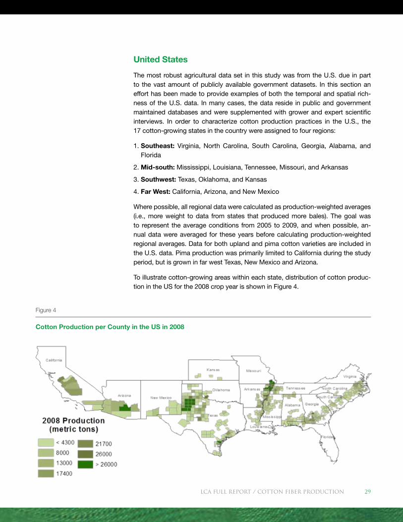
To illustrate cotton-growing areas within each state, distribution of cotton produc-tion in the US for the 2008 crop year is shown in Figure 4.
Figure 4
Cotton Production per County in the US in 2008
LCA FULL REport / Cotton Fiber Production 29
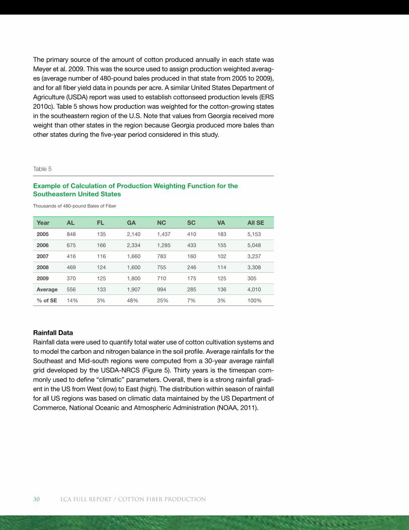
The primary source of the amount of cotton produced annually in each state was Meyer et al. 2009. This was the source used to assign production weighted averag-es (average number of 480-pound bales produced in that state from 2005 to 2009), and for all fiber yield data in pounds per acre. A similar United States Department of Agriculture (USDA) report was used to establish cottonseed production levels (ERS 2010c). Table 5 shows how production was weighted for the cotton-growing states in the southeastern region of the U.S. Note that values from Georgia received more weight than other states in the region because Georgia produced more bales than other states during the five-year period considered in this study.
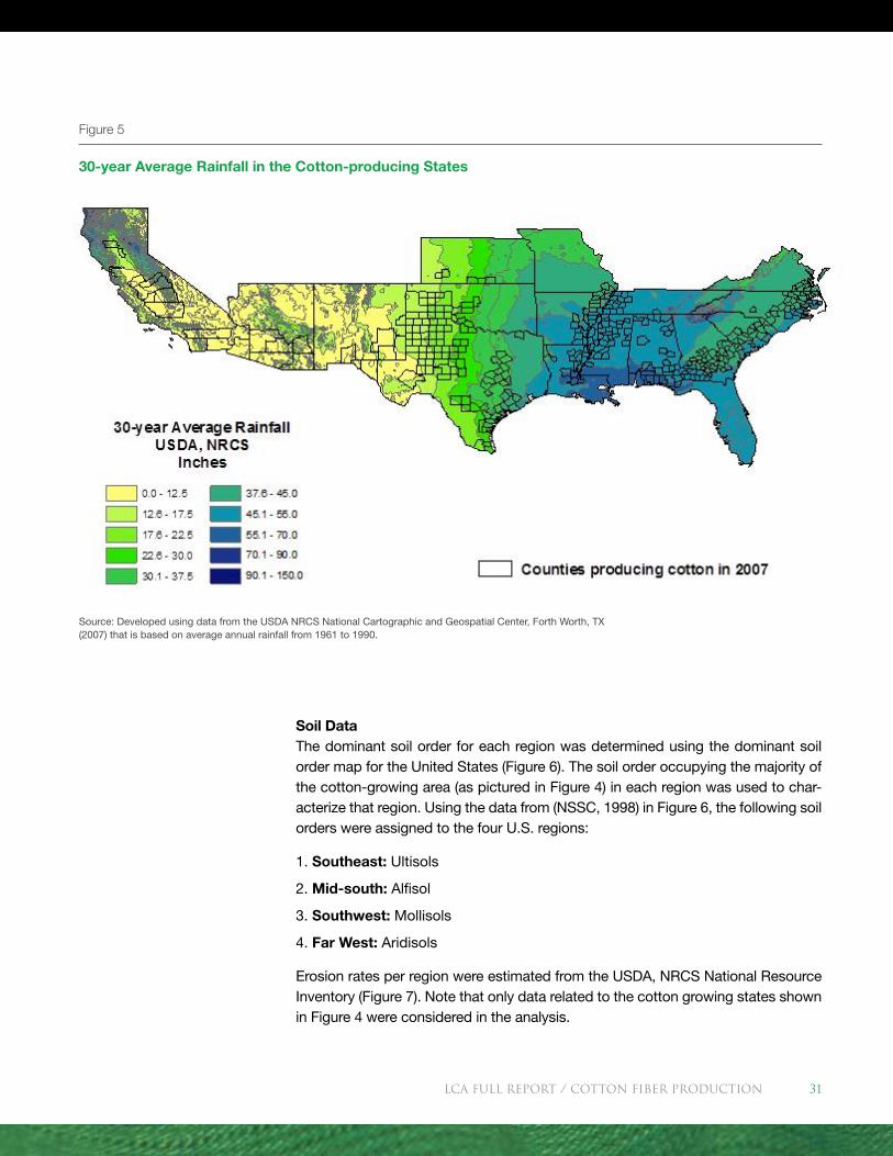
Rainfall DataRainfall data were used to quantify total water use of cotton cultivation systems and to model the carbon and nitrogen balance in the soil profile. Average rainfalls for the Southeast and Mid-south regions were computed from a 30-year average rainfall grid developed by the USDA-NRCS (Figure 5). Thirty years is the timespan com-monly used to define “climatic” parameters. Overall, there is a strong rainfall gradi-ent in the US from West (low) to East (high). The distribution within season of rainfall for all US regions was based on climatic data maintained by the US Department of Commerce, National Oceanic and Atmospheric Administration (NOAA, 2011).
Table 5
Example of Calculation of Production Weighting Function for the Southeastern United States
Thousands of 480-pound Bales of Fiber
Year AL FL GA NC SC VA All SE
2005 848 135 2,140 1,437 410 183 5,153
2006 675 166 2,334 1,285 433 155 5,048
2007 416 116 1,660 783 160 102 3,237
2008 469 124 1,600 755 246 114 3,308
2009 370 125 1,800 710 175 125 305
Average 556 133 1,907 994 285 136 4,010
% of SE 14% 3% 48% 25% 7% 3% 100%
LCA FULL REport / Cotton Fiber Production30
Soil DataThe dominant soil order for each region was determined using the dominant soil order map for the United States (Figure 6). The soil order occupying the majority of the cotton-growing area (as pictured in Figure 4) in each region was used to char-acterize that region. Using the data from (NSSC, 1998) in Figure 6, the following soil orders were assigned to the four U.S. regions:
1. Southeast: Ultisols
2. Mid-south: Alfisol
3. Southwest: Mollisols
4. Far West: Aridisols
Erosion rates per region were estimated from the USDA, NRCS National Resource Inventory (Figure 7). Note that only data related to the cotton growing states shown in Figure 4 were considered in the analysis.
Figure 5
30-year Average Rainfall in the Cotton-producing States
Source: Developed using data from the USDA NRCS National Cartographic and Geospatial Center, Forth Worth, TX (2007) that is based on average annual rainfall from 1961 to 1990.
LCA FULL REport / Cotton Fiber Production 31
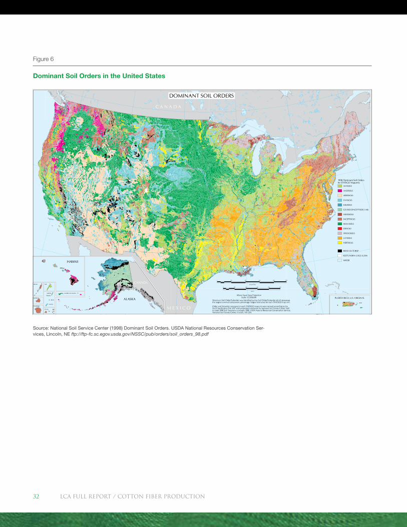
Figure 6
Dominant Soil Orders in the United States
Source: National Soil Service Center (1998) Dominant Soil Orders. USDA National Resources Conservation Ser-vices, Lincoln, NE ftp://ftp-fc.sc.egov.usda.gov/NSSC/pub/orders/soil_orders_98.pdf
LCA FULL REport / Cotton Fiber Production32
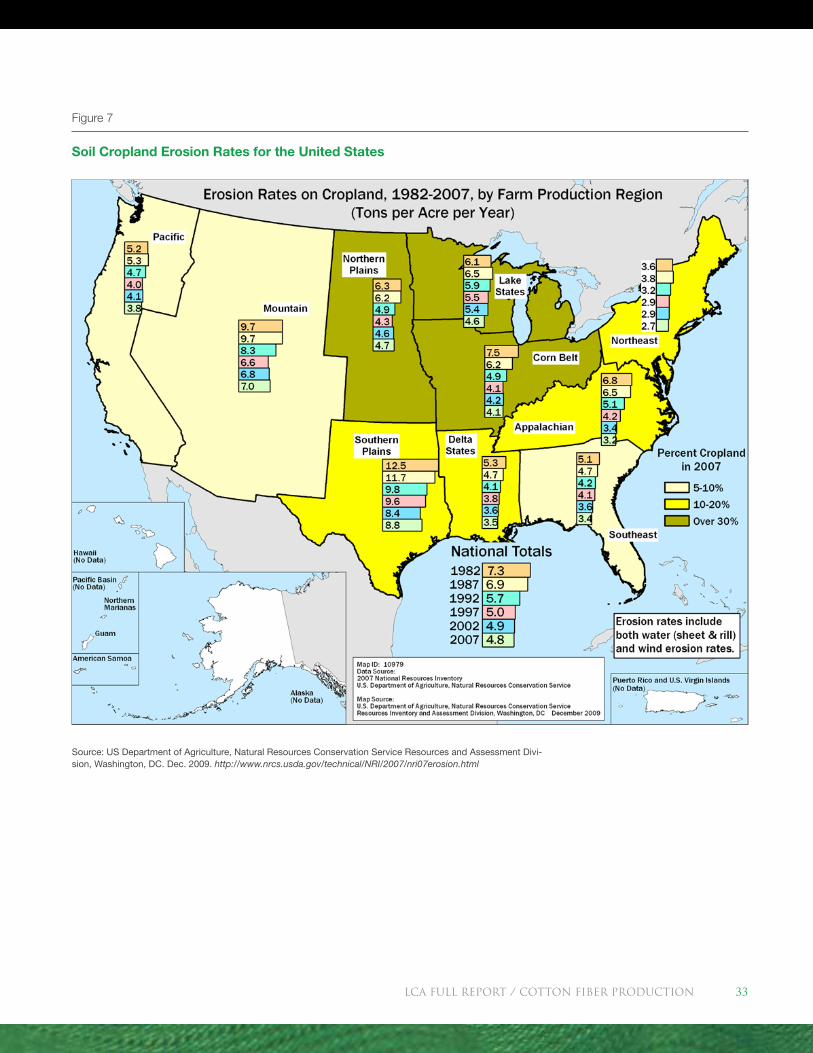
Figure 7
Soil Cropland Erosion Rates for the United States
Source: US Department of Agriculture, Natural Resources Conservation Service Resources and Assessment Divi-sion, Washington, DC. Dec. 2009. http://www.nrcs.usda.gov/technical/NRI/2007/nri07erosion.html
LCA FULL REport / Cotton Fiber Production 33
Grower PracticesThe primary source of information for U.S. producer practices was from Cotton In-corporated’s 2007/2008 Natural Resource Survey, a comprehensive grower survey of 1,300 U.S. cotton producers that represented 16% of cotton acres grown in the U.S. in 2008 (Reed et al. 2009). Data from these sources were used to character-ize producers’ tillage systems, number of chemical applications, rotational crops, double-cropping practices, cover crops, timings of operations and to supplement information on irrigation practices. Data on the amount of planting seed used and the timing of planting and harvest were largely based on data from the USDA Agricultural Resource Management Survey (ARMS) (ERS 2010).
The following are the typical dates when planting and harvest of 50% of the cotton acreage in a particular region has been completed (ERS 2010):
1. Southeast – Plant May 5; Harvest October 22
2. Mid-south – Plant May 7; Harvest October 17
3. Southwest – Plant May 20; Harvest November 14
4. Far West – Plant April 20; Harvest October 23
Thus, much of the U.S. crop has been planted by late May and harvest concluded by mid-November.
In cases of missing data or questions on production practices in a given region, cotton specialists and other agricultural experts in that region were consulted. At least one in-person grower interview per region was conducted at the conclusion of data collection to confirm that the combined data sets were realistic and to ad-dress any final questions on grower practices for that region. Missing data were minimal in the U.S. and were primarily related to the type of cover crop and the type of previous crop grown. A minor limitation was the fact that some state-level data were unavailable. In these cases, regional data were used instead.
Irrigation and Water Use Data Applied irrigation water and irrigated acreage was determined from the USDA’s Farm and Ranch Irrigation survey (USDA 2008b). This source was also consulted for pumping depth data; however, those data were not reported by commodity, and, in some states, particularly in the west, state-level data did not accurate-ly represent the cotton-growing region of the state. For example, the challenge in identifying pumping energy to assign for water applied in California is outlined below:
� Groundwater data (depth to water of 123 feet) from the Farm and Ranch Survey appears to represent only the cotton growing area of California despite the fact that it is reported as a statewide average.
� Groundwater data from the California department of water resources for spring 2009 were interpolated into a grid (Figure 8). Based on this interpolation, the aver-age depth to groundwater was 107 feet with a standard deviation in the data of
LCA FULL REport / Cotton Fiber Production34
80 feet. The range was from 0.8 to 608 feet, so there a great deal of variability exists in this measurement. For the LCA, a depth of 123 feet was ultimately used for California.
� Data from the Farm and Ranch Survey as well as the ERS farms data (ERS 2010) were in agreement that irrigation water is split between surface and ground sources in California at 52% ground; 46% surface.
� Figure 8 from a water district in the California San Joaquin Valley (SJV) illus-trates how the source of water in any given year can change dramatically. Fur-thermore, even if the data shown in the figure were available for all of the water districts with cotton production in the Far West, quantifying the energy footprint from the different water sources is still complex. For example, in many years the SJV district uses water from the “Central Valley Project (CVP)”:
� The Central Valley Project, operated by the US Bureau of Reclamation, is one of the world’s largest water storage and transport systems. Its 22 reservoirs have a combined storage of 11 million acre-feet, of which 7 million acre-feet is delivered in an average year (CA.gov 2011).
� The CVP relies on multiple sources of water. For example, approximate eleva-tion gain in the California Aqueduct from the Delta to the San Luis Reservoir is approximately 250 feet; however, other water sources that supply agriculture in the region are gravity-fed, and, in many cases, the canal systems transporting the water are used to generate electricity.
Bob Hutmacher, cotton specialist with the University of California, Davis, and Greg Palla, Executive Vice president of the SJV Quality Cotton Growers Asso-ciation in Bakersfield, California, provided important information regarding the various sources of agricultural water in California. They both confirmed that the variation in sources noted in the example of Figure 8 are typical of many California water management districts.
Figure 8 shows the 30-year average rainfall and well data points (USDA 2007) and NRCS’ estimate of cotton growing area. It is an interpolated map of well readings in feet from ground to water surface. The area in red was used for the statistics used in this LCA study.
The challenge of calculating irrigation pumping energy was true in Arizona as well as California. Arizona irrigation districts typically obtain water from either the Cen-tral Arizona Project (CAP) or from groundwater wells depending on the cost of the CAP water compared to the costs of the energy and labor to pump groundwater; it is not uncommon for Arizona irrigation districts to vary their use of both during any given season. Data from the Arizona Water Atlas showed that from 2001 to 2005 in the Pinal Active Management Area (largest cotton-growing region in the state) about 50% of the agricultural water came from groundwater and approxi-mately 50% came from CAP (ADWR 2011). A small amount of water came from other surface waters and effluent.
LCA FULL REport / Cotton Fiber Production 35
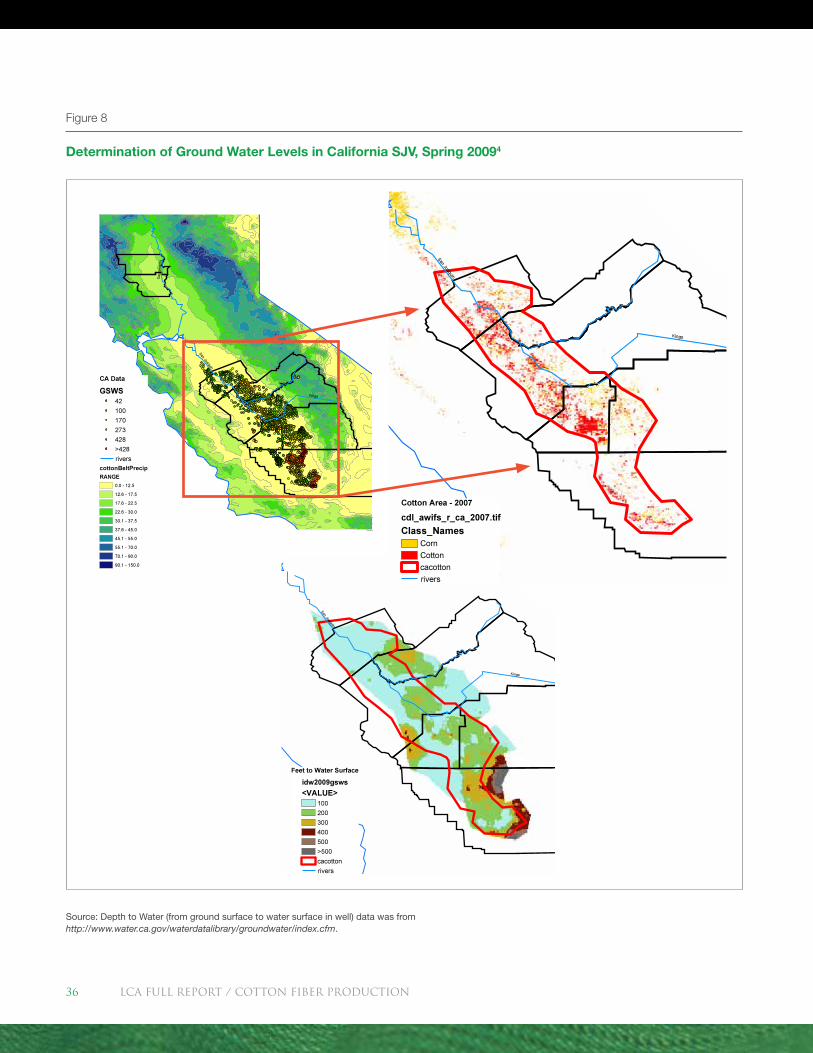
Figure 8
Determination of Ground Water Levels in California SJV, Spring 20094
Source: Depth to Water (from ground surface to water surface in well) data was from http://www.water.ca.gov/waterdatalibrary/groundwater/index.cfm.
LCA FULL REport / Cotton Fiber Production36
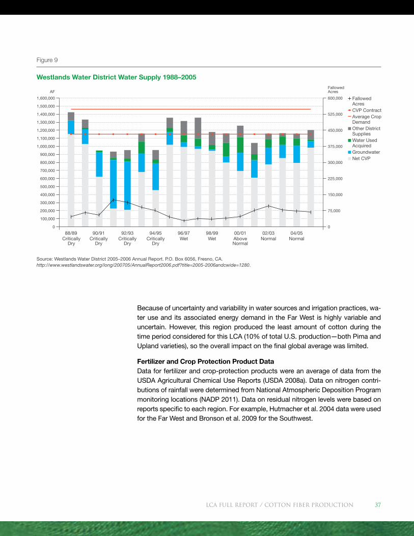
Source: Westlands Water District 2005–2006 Annual Report. P.O. Box 6056, Fresno, CA. http://www.westlandswater.org/long/200705/AnnualReport2006.pdf?title=2005-2006andcwide=1280.
Because of uncertainty and variability in water sources and irrigation practices, wa-ter use and its associated energy demand in the Far West is highly variable and uncertain. However, this region produced the least amount of cotton during the time period considered for this LCA (10% of total U.S. production—both Pima and Upland varieties), so the overall impact on the final global average was limited.
Fertilizer and Crop Protection Product DataData for fertilizer and crop-protection products were an average of data from the USDA Agricultural Chemical Use Reports (USDA 2008a). Data on nitrogen contri-butions of rainfall were determined from National Atmospheric Deposition Program monitoring locations (NADP 2011). Data on residual nitrogen levels were based on reports specific to each region. For example, Hutmacher et al. 2004 data were used for the Far West and Bronson et al. 2009 for the Southwest.
Figure 9
Westlands Water District Water Supply 1988–2005
88/89 90/91 92/93 94/95 00/01 02/03 04/05Critically
DryCritically
DryCritically
DryCritically
Dry
96/97 98/99Wet Wet Above
NormalNormal Normal
0
100,000
200,000
300,000
400,000
500,000
600,000
700,000
800,000
900,000
1,000,000
1,100,000
1,200,000
1,300,000
1,400,000
1,500,000
1,600,000
AF
600,000
Fallowed Acres
525,000
450,000
375,000
300,000
0
75,000
150,000
225,000
Fallowed Acres CVP Contract Average Crop Demand Other District Supplies Water Used Acquired Groundwater Net CVP
LCA FULL REport / Cotton Fiber Production 37
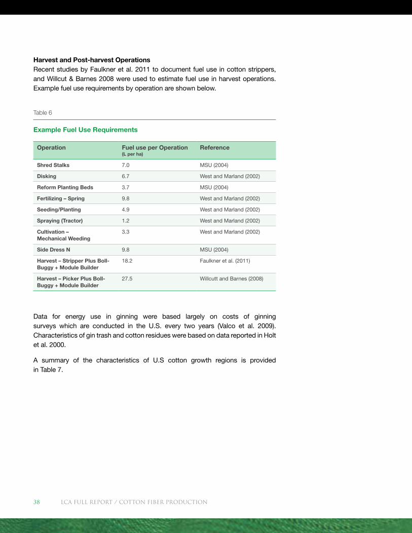
Harvest and Post-harvest OperationsRecent studies by Faulkner et al. 2011 to document fuel use in cotton strippers, and Willcut & Barnes 2008 were used to estimate fuel use in harvest operations. Example fuel use requirements by operation are shown below.
Data for energy use in ginning were based largely on costs of ginning surveys which are conducted in the U.S. every two years (Valco et al. 2009). Characteristics of gin trash and cotton residues were based on data reported in Holt et al. 2000.
A summary of the characteristics of U.S cotton growth regions is provided in Table 7.
Table 6
Example Fuel Use Requirements
Operation Fuel use per Operation (L per ha)
Reference
Shred Stalks 7.0 MSU (2004)
Disking 6.7 West and Marland (2002)
Reform Planting Beds 3.7 MSU (2004)
Fertilizing – Spring 9.8 West and Marland (2002)
Seeding/Planting 4.9 West and Marland (2002)
Spraying (Tractor) 1.2 West and Marland (2002)
Cultivation – Mechanical Weeding
3.3 West and Marland (2002)
Side Dress N 9.8 MSU (2004)
Harvest – Stripper Plus Boll-Buggy + Module Builder
18.2 Faulkner et al. (2011)
Harvest – Picker Plus Boll-Buggy + Module Builder
27.5 Willcutt and Barnes (2008)
LCA FULL REport / Cotton Fiber Production38
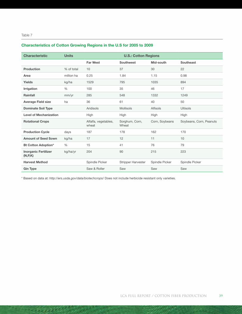
Table 7
Characteristics of Cotton Growing Regions in the U.S for 2005 to 2009
Characteristic Units U.S.: Cotton Regions
Far West Southwest Mid-south Southeast
Production % of total 10 37 30 22
Area million ha 0.25 1.84 1.15 0.98
Yields kg/ha 1529 795 1035 894
Irrigation % 100 35 46 17
Rainfall mm/yr 285 548 1332 1249
Average Field size ha 36 61 40 50
Dominate Soil Type Aridisols Mollisols Alfisols Ultisols
Level of Mechanization High High High High
Rotational Crops Alfalfa, vegetables, wheat
Sorghum, Corn, Wheat
Corn, Soybeans Soybeans, Corn, Peanuts
Production Cycle days 187 178 162 170
Amount of Seed Sown kg/ha 17 12 11 10
Bt Cotton Adoption* % 15 41 76 79
Inorganic Fertilizer (N,P,K)
kg/ha/yr 204 90 215 223
Harvest Method Spindle Picker Stripper Harvester Spindle Picker Spindle Picker
Gin Type Saw & Roller Saw Saw Saw
* Based on data at: http://ers.usda.gov/data/biotechcrops/ Does not include herbicide resistant only varieties.
LCA FULL REport / Cotton Fiber Production 39
China
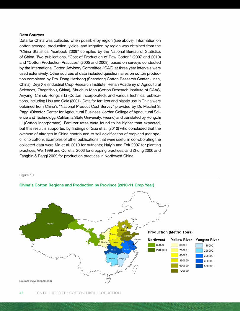
China ranks number one in the world in cotton production. In 2010-2011 at 6.3 mil-lion metric tons, China produced 27% of the world’s cotton (www.cottonlook.com). The primary growing regions are the Northwest, Yellow River Basin and Yangtze River Basin (Figure 10). Provinces making up these regions are:
1. Northeast: Gansu and Xinjiang
2. Yellow River Basin: Hebei, Henan, Shaanxi, Shandong, Shanxi, Tianjin, and Beijing
3. Yangtze River Basin: Hubei, Hunan, Jiangsu, Jiangxi, Zhejiang, and Anhui
Grower PracticesAbout 9 million Chinese farmers grow cotton. Unlike India which grows four spe-cies of cotton, farmers in China grow upland cotton, Gossypium hirsutum, and long staple cotton, G. barbadense. Hybrid cotton is grown on about 25% of the area with the majority in the Yangtze River Basin.
Daily air temperatures during the cotton season in China range from 18-25C. The Northwest is characterized by arid conditions requiring irrigation to grow the crop. Dry conditions in this region keep pest and diseases to a minimum. Frequent flood-ing can be a problem in the Yangtze River Basin while the Yellow River Basin experi-ences frequent drought and water shortages.
Chinese cotton farmers employ practices that shorten the cotton growing season. In the Yellow River and Yangtze River Basins cotton is double cropped. Practices in these regions include the transplanting of seedlings and the use of plastic film as mulch. In the Northwest the growing season is short therefore there is only one crop per year. The plastic mulch protects the seedlings from the broad swings in temperatures during the day and minimizes the loss of soil moisture.
An estimated five million hectares were planted to cotton in 2010-2011. Of that 69% was planted to Bt cotton. The adoption rate for Bt cotton is greater than 90% in the Yellow and Yangtze River Basins. It is estimated at about 10 to 15% of the cotton area in Xinjiang where insect pressure is relatively low. Xinjiang grows about 47% of China’s cotton. From 1997 when Bt cotton was first introduced in China to 2010 insecticide use has decreased 60% (James 2010). Other characteristics of the three regions are given in Table 8.
LCA FULL REport / Cotton Fiber Production40
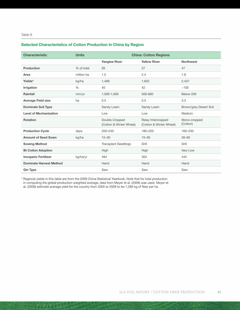
Table 8
Selected Characteristics of Cotton Production in China by Region
Characteristic Units China: Cotton Regions
Yangtze River Yellow River Northwest
Production % of total 26 27 47
Area million ha 1.5 2.4 1.8
Yields* kg/ha 1,499 1,652 2,437
Irrigation % 40 42 ~100
Rainfall mm/yr 1,000-1,600 500-800 Below 200
Average Field size ha 0.5 0.5 3.3
Dominate Soil Type Sandy Loam Sandy Loam Brown/grey Desert Soil
Level of Mechanization Low Low Medium
Rotation Double Cropped
(Cotton & Winter Wheat)
Relay Intercropped
(Cotton & Winter Wheat)
Mono-cropped (Cotton)
Production Cycle days 200–240 180–220 160–230
Amount of Seed Sown kg/ha 15–30 15–30 30–60
Sowing Method Transplant Seedlings Drill Drill
Bt Cotton Adoption High High Very Low
Inorganic Fertilizer kg/ha/yr 494 304 445
Dominate Harvest Method Hand Hand Hand
Gin Type Saw Saw Saw
* Regional yields in this table are from the 2009 China Statistical Yearbook. Note that for total production in computing the global production weighted average, data from Meyer et al. (2009) was used. Meyer et al. (2009) estimate average yield for the country from 2005 to 2009 to be 1,280 kg of fiber per ha.
LCA FULL REport / Cotton Fiber Production 41
Data SourcesData for China was collected when possible by region (see above). Information on cotton acreage, production, yields, and irrigation by region was obtained from the “China Statistical Yearbook 2009” compiled by the National Bureau of Statistics of China. Two publications, “Cost of Production of Raw Cotton” (2007 and 2010) and “Cotton Production Practices” (2005 and 2008), based on surveys conducted by the International Cotton Advisory Committee (ICAC) at three year intervals were used extensively. Other sources of data included questionnaires on cotton produc-tion completed by Drs. Dong Hezhong (Shandong Cotton Research Center, Jinan, China), Deyi Xie (Industrial Crop Research Institute, Henan Academy of Agricultural Sciences, Zhegnzhou, China), Shuchun Mao (Cotton Research Institute of CAAS, Anyang, China), Hongzhi Li (Cotton Incorporated), and various technical publica-tions, including Hsu and Gale (2001). Data for fertilizer and plastic use in China were obtained from China’s “National Product Cost Survey” provided by Dr. Mechel S. Paggi (Director, Center for Agricultural Business, Jordan College of Agricultural Sci-ence and Technology, California State University, Fresno) and translated by Hongzhi Li (Cotton Incorporated). Fertilizer rates were found to be higher than expected, but this result is supported by findings of Guo et al. (2010) who concluded that the overuse of nitrogen in China contributed to soil acidification of cropland (not spe-cific to cotton). Examples of other publications that were useful in corroborating the collected data were Ma et al. 2010 for nutrients; Naiyin and Fok 2007 for planting practices; Wei 1999 and Qui et al 2003 for cropping practices; and Zhong 2006 and Fangbin & Paggi 2009 for production practices in Northwest China.
Figure 10
China's Cotton Regions and Production by Province (2010-11 Crop Year)
Source: www.cotlook.com
Xinjiang
Gansu Hebei
Hubei
Hunan
Shaanxi Henan
Anhui
Shanxi
Jiangxi
Shandong
Jiangsu
Tianjin
Production (Metric Tons)
Yangtze River110000
290000
300000
320000
500000
Yellow River60000
70000
80000
350000
600000
720000
Northwest80000
2700000
LCA FULL REport / Cotton Fiber Production42
India
India is highly dependent on agriculture. In 2010-2011, about 6.9 million Indian farmers produced 5.5 million metric tons of cotton. This was 22% of the world’s cotton, making India second only to China in production. At 10.3 million ha India ranks number one in hectares planted to cotton but has lower yields than China and the United States, the average cotton holdings per farm being about 1.5 ha. The majority of the cotton is grown in ten provinces which are grouped into three different regions: North, Central, and South (Figure 11). Provinces making up these regions are:
1. North: Punjab, Haryana, and Rajasthan
2. Central: Gujarat, Maharshtra, Madhya Pradesh, and Orissa
3. South: Andhra Pradesh, Karnataka, and Tamil Nadu
Grower PracticesIndia is the only country to grow all four species of cultivated cotton. These are the Asian cottons G. arboreum (Desi cotton) and G. herbaceum as well as G. bar-badense and G. hirsutum. Hybrid cottons are planted on 90% of the cotton area. Production practices varied somewhat according to the type of cotton planted. In 2010, 86% of the cotton area was planted to Bt cotton. The introduction of this technology into the Indian production system has led to a 39% decrease in the number of insecticide sprays since its introduction in 2002 (James 2010).
The North Region is characterized by cotton grown entirely as an irrigated crop. The climate is adverse at planting with high temperatures and the growing period is limited to May to October. The Central Region is characterized by a hot, semi-arid climate. Planting in this region is dependent upon the onset of monsoon (middle of June to July). The South Region is also characterized by a hot semi-arid climate. However, the agro-climate is more suitable for cotton, especially with the bimodal distribution of rainfall in some areas of the South Region. The planting season is primarily August to September but there is also a small summer crop planted in January – February in Tamil Nadu.
Approximately 65% of India’s cotton is produced on dry land and 35% on irrigated land. The North Region is almost 100% irrigated while the Central and South regions are primarily rainfed. Other characteristics of the regions are given in Table 9.
LCA FULL REport / Cotton Fiber Production 43
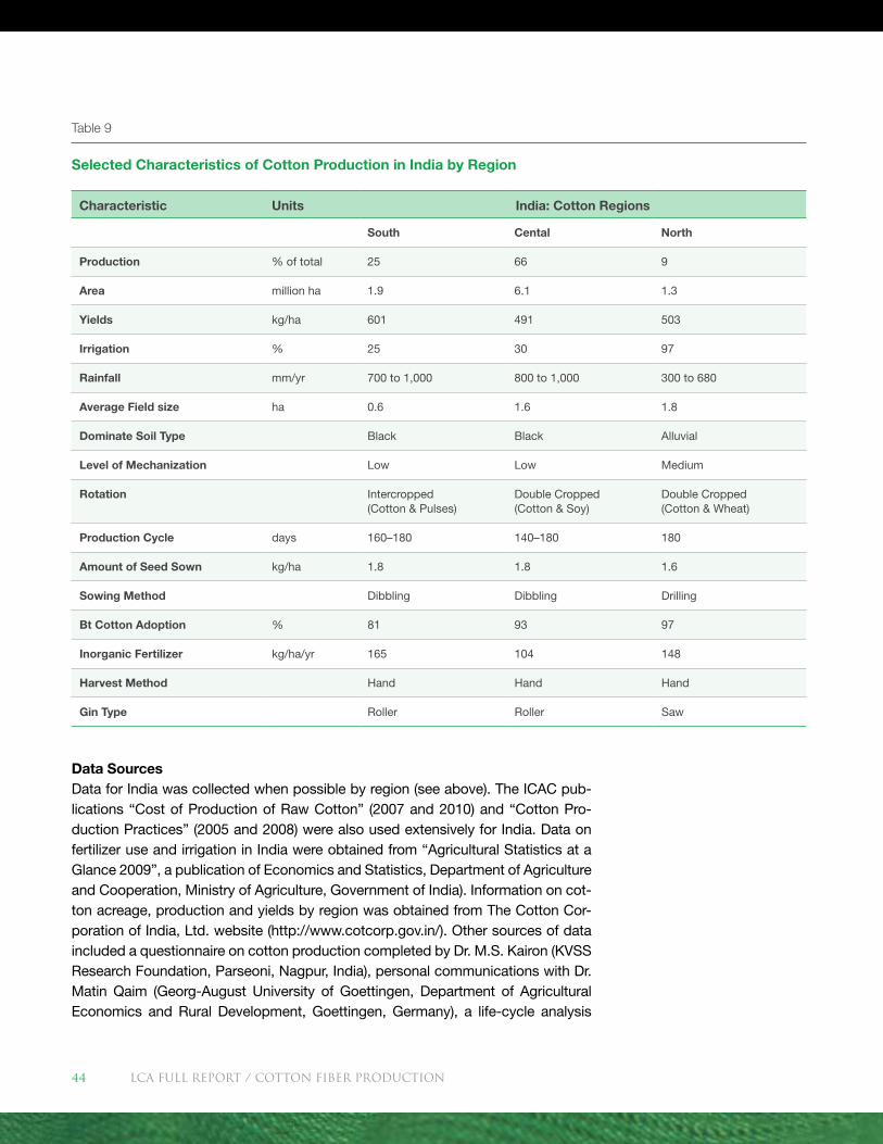
Table 9
Selected Characteristics of Cotton Production in India by Region
Characteristic Units India: Cotton Regions
South Cental North
Production % of total 25 66 9
Area million ha 1.9 6.1 1.3
Yields kg/ha 601 491 503
Irrigation % 25 30 97
Rainfall mm/yr 700 to 1,000 800 to 1,000 300 to 680
Average Field size ha 0.6 1.6 1.8
Dominate Soil Type Black Black Alluvial
Level of Mechanization Low Low Medium
Rotation Intercropped (Cotton & Pulses)
Double Cropped (Cotton & Soy)
Double Cropped (Cotton & Wheat)
Production Cycle days 160–180 140–180 180
Amount of Seed Sown kg/ha 1.8 1.8 1.6
Sowing Method Dibbling Dibbling Drilling
Bt Cotton Adoption % 81 93 97
Inorganic Fertilizer kg/ha/yr 165 104 148
Harvest Method Hand Hand Hand
Gin Type Roller Roller Saw
Data SourcesData for India was collected when possible by region (see above). The ICAC pub-lications “Cost of Production of Raw Cotton” (2007 and 2010) and “Cotton Pro-duction Practices” (2005 and 2008) were also used extensively for India. Data on fertilizer use and irrigation in India were obtained from “Agricultural Statistics at a Glance 2009”, a publication of Economics and Statistics, Department of Agriculture and Cooperation, Ministry of Agriculture, Government of India). Information on cot-ton acreage, production and yields by region was obtained from The Cotton Cor-poration of India, Ltd. website (http://www.cotcorp.gov.in/). Other sources of data included a questionnaire on cotton production completed by Dr. M.S. Kairon (KVSS Research Foundation, Parseoni, Nagpur, India), personal communications with Dr. Matin Qaim (Georg-August University of Goettingen, Department of Agricultural Economics and Rural Development, Goettingen, Germany), a life-cycle analysis
LCA FULL REport / Cotton Fiber Production44
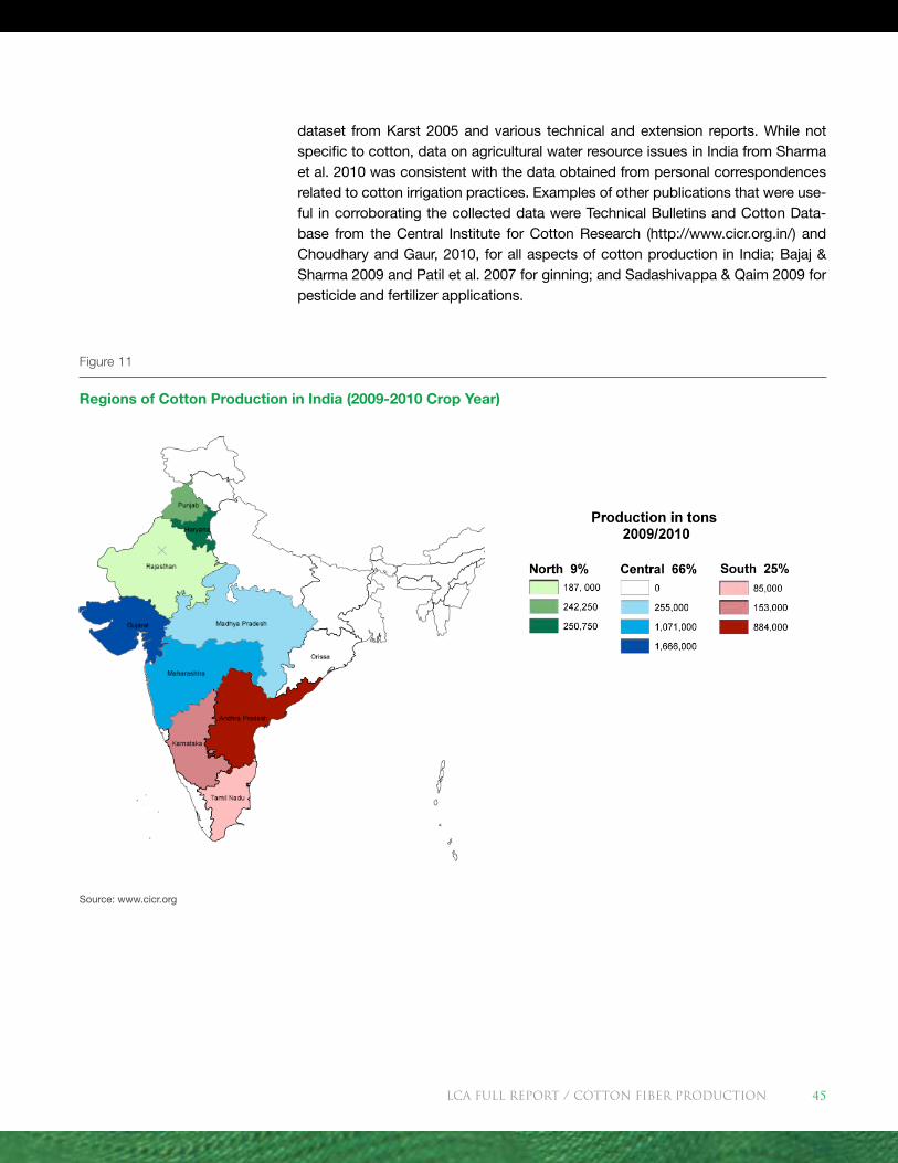
dataset from Karst 2005 and various technical and extension reports. While not specific to cotton, data on agricultural water resource issues in India from Sharma et al. 2010 was consistent with the data obtained from personal correspondences related to cotton irrigation practices. Examples of other publications that were use-ful in corroborating the collected data were Technical Bulletins and Cotton Data-base from the Central Institute for Cotton Research (http://www.cicr.org.in/) and Choudhary and Gaur, 2010, for all aspects of cotton production in India; Bajaj & Sharma 2009 and Patil et al. 2007 for ginning; and Sadashivappa & Qaim 2009 for pesticide and fertilizer applications.
Figure 11
Regions of Cotton Production in India (2009-2010 Crop Year)
Source: www.cicr.org
LCA FULL REport / Cotton Fiber Production 45
Agricultural Modeling
Agrarian systems belong to the most complex production systems within LCA due to their dependence on variable environmental conditions in both time (e.g., within a year, from year to year) and space (e.g., varies by country, region, site conditions). The following factors contribute to the complexity of agricultural modeling:
� The variety of different locations
� Small scale soil variability within locations
� The large number of farms
� The variety of agricultural management practices employed,
� Technically, no determined border to the environment
� Complex and indirect dependence of the output (harvest, emissions) on the input (fertilizers, location conditions, etc.)
� Variable weather conditions within and between different years
� Variable pest populations (insects, weeds, disease pathogens, etc.)
� Different crop rotations
Due to these inherent complexities, a process-based agrarian simulation model developed by PE and the University of Stuttgart, Germany, was used for plant pro-duction and cultivation; this model covers a multitude of input data, emission fac-tors, and parameters. The model was used for the cradle-to-gate (seed-to-bale) environmental impact assessment of cotton production and accounted for planting, growing, harvesting, processing, handling and distributing cotton. For the purposes of this LCA, a cultivation period was defined as starting immediately after harvest of the preceding crop and ending after harvest of the respective crop.
The entire production process of cotton (and its by-products), including harvest processes up to the field edge, is accounted for by the agrarian cultivation mod-el. The model included cradle-to-gate burdens of all relevant input materials for the cultivation process itself (inorganic fertilizer including lime, organic fertilizer, pesticides, and seeds including their production and transport), cradle-to-gate accounting for fuel consumed in the field by farm equipment, including direct emissions to air from combustion of the fuel, and irrigation. Agricultural infra-structure, equipment production, and farm buildings were excluded. All relevant processes taking place on the area under cultivation including emissions into air and groundwater (lower limit of rooted soil zone) were integrated. Heavy metals remaining in soil were considered to be emissions to soil. Integration of erosive loss of Norg (organic nitrogen) and Corg (organic carbon) as well as nutrients in water (e.g., phosphorus) were considered.
LCA FULL REport / Cotton Fiber Production46
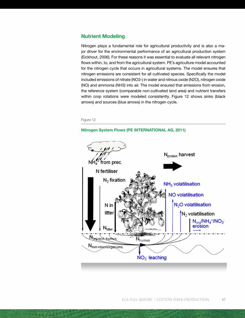
Nutrient Modeling
Nitrogen plays a fundamental role for agricultural productivity and is also a ma-jor driver for the environmental performance of an agricultural production system (Eickhout, 2006). For these reasons it was essential to evaluate all relevant nitrogen flows within, to, and from the agricultural system. PE’s agriculture model accounted for the nitrogen cycle that occurs in agricultural systems. The model ensures that nitrogen emissions are consistent for all cultivated species. Specifically the model included emissions of nitrate (NO3-) in water and nitrous oxide (N2O), nitrogen oxide (NO) and ammonia (NH3) into air. The model ensured that emissions from erosion, the reference system (comparable non-cultivated land area) and nutrient transfers within crop rotations were modeled consistently. Figure 12 shows sinks (black arrows) and sources (blue arrows) in the nitrogen cycle.
Figure 12
Nitrogen System Flows (PE INTERNATIONAL AG, 2011)
LCA FULL REport / Cotton Fiber Production 47
The different N-based emissions were calculated as follows:
� NH3 emissions to air from organic fertilizers were adapted from the model of Brentrup et al. 2000 and modelled specifically for the cropping system depen-dent on the fertilizer-NH4 content, the soil-pH, rainfall and temperature. NH3 emissions to air from mineral fertilizers were also adapted from Brentrup et al. 2000 and modelled specifically for the cropping system dependent on the kind of fertilizer and the soil pH.
� N2 emissions to air were derived from complete denitrification. N2 emissions were assumed to be 9% of the N-fertilizer input based on a literature review by Van Cleemput (Van Cleemput O 1998). N2 emissons were also taken into con-sideration to determine the nitrate leaching potential.
� NO emissions to air were derived from partial denitrification. NO emissions were calculated from the reference system after N-input from air plus 0.43% of the N-fertilizer input specific for the cultivation system as NO.
� N2O emissions to air were derived from partial denitrification. According to various sources and the IPCC, N2O emissions were calculated from the refer-ence system after N-input from air plus 1% of the N being used as fertilizer specifically to the cultivation system (minus NH3 losses) as N2O-N.
� Norg, NO3- and NH4 emissions to water occurred due to erosive surface run-off. Specifically for the cultivation system, they were calculated from the emis-sion of eroded soil multiplied by the respective Norg-, NO3- and NH4+ contents of the eroded fraction and also multiplied by a fraction of the eroded materials being transferred into the drainage and not being deposited beforehand.
� NO3-emission to groundwater was calculated from the rest of the incoming N not occurring as gaseous losses or in harvests, litter, unused extractions from the site, storage in soil, etc. Depending on the quantity of water leakage during the time period evaluated, an increasing part of this remaining N was calcu-lated as leached nitrate. When remaining N was calculated to be negative (for instance due to a higher extraction than fertilizer input) a minimum N-loss factor was applied on the applied fertilizer and Nmin quantity.
Compared to a pure N-balance model, this approach allows for the illustration of N-losses in cases of very low N-fertilization (e.g., N-deficiency in rubber-tree plan-tations). In the case of high N-fertilization (e.g., intensive farming applications), the models correspond with the total N-balance approach.
In addition to nitrogen-based emissions to water and air, phosphorus emissions were taken into consideration by the model. However, although phosphorus is a stable compound which does not leach significantly to groundwater it can enter surface water from soil erosion and can cause eutrophication of water bodies. In this study it was assumed that 10% of the eroded soil accessed water while the rest accumulated to colluviums on other surfaces and was assumed to be irrelevant in the life cycle assessment.
LCA FULL REport / Cotton Fiber Production48
The nitrogen balance in the model was closed: Ninput = Noutput for the examined cultivation crop. That is, if any cultivation processes were to yield a net nitrogen reduction or accumulation in the soil, this difference would be balanced by addition-al or reduced external fertilizer demand. The nitrogen balance was calculated as net nitrogen surplus or deficit after accounting for leaching and mineralization. There-fore, the amount of N being fixed in humus in the long run was assumed constant. This adjustment addressed the long-term effects of cultivation systems without fertilizer application, which tend to reduce the nutrient pool in soil, thereby reducing the growth potential of the site.
In the case of cultivation systems without fertilizer, the net nutrient removal must be balanced by integrating it as an external fertilizer requirement. A credit was applied to cotton in situations where a nutrient surplus remained in the soil since nitrogen was available to follow-up crops.
Carbon Modeling
Carbon-based emissions such as CH4, CO, CO2 were also taken into consideration by the agrarian cultivation model. Emissions resulting from production of fertilizer, pesticides, electricity, and diesel were taken into account as were CO2 emissions from the combustion of fossil fuels by the tractors or irrigation engines, and from the application and decomposition of urea fertilizer in the soil.
Soil carbon is a potential source or sink of carbon dioxide. Soil carbon balances are used to describe any increase or decrease in soil organic carbon (SOC) content caused by a change in land management, with the implication that increased/de-creased soil carbon storage mitigates or increases climate change. The net effect of cotton cultivation is highly variable and depends on various factors such as fertil-ization or soil cultivation practices. In particular, conservation tillage techniques are viewed as a promising approach to increase SOC. It is estimated that by applying no tillage in the Southeastern U.S., that SOC increases on average by 0.48±0.56 t C ha-1 yr-1 compared to conventional tillage (Causarano et al. 2006). Assuming that all of the carbon can be stored in the soil on a long term basis, a CO2 reduction in the amount of 0.59 kg CO2eq per kg of seed cotton can be realized (assuming a yield of 3,000 kg fw/ha, 2,676 lb fw/ac and an average carbon storage rate of 0.48 t C ha-1 yr-). This would imply a significant potential reduction of the GHG footprint of cotton fibers. However, there are limitations to modeling carbon sequestration for climate change mitigation. Some of these are: (i) the quantity of carbon stored in soil is finite, (ii) the process is reversible and (iii) even if SOC is increased there may be changes in the fluxes of other greenhouse gases, especially nitrous oxide (N2O) and methane. Due to these variations and related uncertainties (see also Powlson et al. 2011) soil carbon sequestration could have been significant, but it was not considered to be within the scope of this study.
LCA FULL REport / Cotton Fiber Production 49
Beside emissions, positive effects (sinks) due to natural conversion of gases in the soil were considered. Gaseous sinks are related predominantly to the methane de-pression function of natural soils due to their oxidizing and microbial transformation of methane. A default value of 0.7 kg is given for fields, though there is information that it can reach clearly higher values in woods and fallow land. Data for methane oxidation in cultivation systems were taken from various sources (e.g., Schmädeke 1998, Powlson et al. 2011).
The biogenic CO2 sequestered in the cotton plant and its fiber was directly ac-counted for in the inventory as an input or uptake of carbon dioxide, which was treated as a negative emission of carbon dioxide to air. For cradle-to-gate cotton fiber production, note that the positive value for GWP denotes a net CO2 release during agricultural production, which means that the atmospheric carbon uptake of the fiber is less than the burden associated with cultivation. The carbon seques-tered in cotton will eventually return to the air upon final disposal, so for this LCA, the CO2 sequestered during growth of the cotton plants was modeled as a direct release to the atmosphere during the end-of-life phase.
Pesticide Modeling
LCI data on pesticide production were modeled in PE INTERNATIONAL GaBi 5 software based on generic pesticide production data taken from multiple sourc-es (Birkved et al. 2006, Green 1987, Hauschild 2000, Williams 2006, and Williams 2009). For each pesticide group (herbicides, fungicides, insecticides, and plant growth regulators) a manufacturing model was built that represented the average production of all pesticides in that category. Lacking comprehensive data on the manufacture of all pesticides (many of which have proprietary chemical formula-tions), five pesticide models are used as proxies to estimate the embedded en-ergy and other environmental burdens of the manufacturing processes for all of the pesticides. Data from two studies (Van Cleemput O 1998, and West & Marland 2002) indicate there are not large differences in energy requirements and carbon emissions between herbicides, insecticides and fungicides, so representative com-pounds were used.
The amount of pesticides applied to cotton fields was taken from USDA sources (USDA 2006 and USDA 2007) for the U.S., one study (Brookes & Barfoot, 2010) for China and two studies (Hsu & Gale 2001 and ICAC 2009) for India. Pesticides studied were limited to those applied on more than 10% of the (relevant) agricul-tural area in the U.S. and India. In the U.S., the data were available by region, so the 10% threshold was applied at the regional level and resulted in the inclusion of some compounds that represent less than 10% of the area when considered on a country basis. The pesticide data for China were based on a limited set of farmer in-terviews, while the data in the U.S. were based on a government-sponsored survey of all cotton producers in the country. Although the national inventory data for China were not as extensive as that from the U.S. it did provide accurate representation
LCA FULL REport / Cotton Fiber Production50
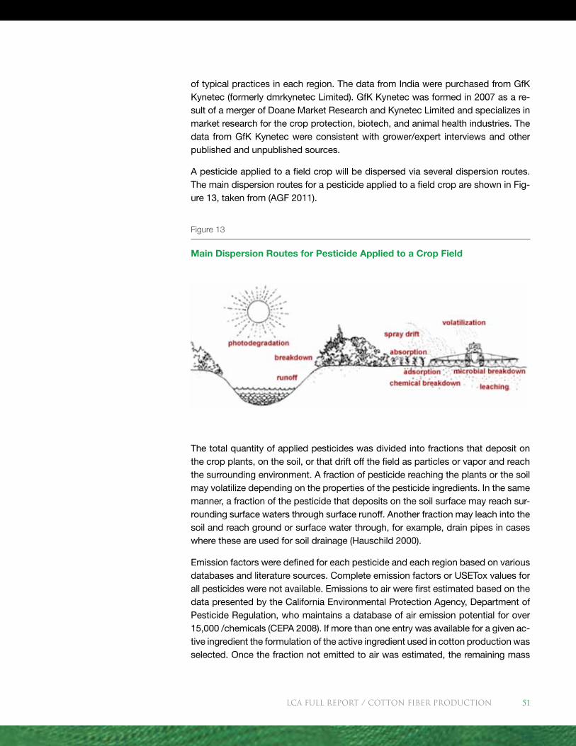
of typical practices in each region. The data from India were purchased from GfK Kynetec (formerly dmrkynetec Limited). GfK Kynetec was formed in 2007 as a re-sult of a merger of Doane Market Research and Kynetec Limited and specializes in market research for the crop protection, biotech, and animal health industries. The data from GfK Kynetec were consistent with grower/expert interviews and other published and unpublished sources.
A pesticide applied to a field crop will be dispersed via several dispersion routes. The main dispersion routes for a pesticide applied to a field crop are shown in Fig-ure 13, taken from (AGF 2011).
The total quantity of applied pesticides was divided into fractions that deposit on the crop plants, on the soil, or that drift off the field as particles or vapor and reach the surrounding environment. A fraction of pesticide reaching the plants or the soil may volatilize depending on the properties of the pesticide ingredients. In the same manner, a fraction of the pesticide that deposits on the soil surface may reach sur-rounding surface waters through surface runoff. Another fraction may leach into the soil and reach ground or surface water through, for example, drain pipes in cases where these are used for soil drainage (Hauschild 2000).
Emission factors were defined for each pesticide and each region based on various databases and literature sources. Complete emission factors or USETox values for all pesticides were not available. Emissions to air were first estimated based on the data presented by the California Environmental Protection Agency, Department of Pesticide Regulation, who maintains a database of air emission potential for over 15,000 /chemicals (CEPA 2008). If more than one entry was available for a given ac-tive ingredient the formulation of the active ingredient used in cotton production was selected. Once the fraction not emitted to air was estimated, the remaining mass
Figure 13
Main Dispersion Routes for Pesticide Applied to a Crop Field
LCA FULL REport / Cotton Fiber Production 51
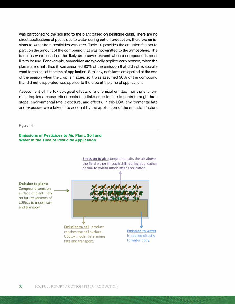
was partitioned to the soil and to the plant based on pesticide class. There are no direct applications of pesticides to water during cotton production, therefore emis-sions to water from pesticides was zero. Table 10 provides the emission factors to partition the amount of the compound that was not emitted to the atmosphere. The fractions were based on the likely crop cover present when a compound is most like to be use. For example, acaracides are typically applied early season, when the plants are small, thus it was assumed 90% of the emission that did not evaporate went to the soil at the time of application. Similarly, defoliants are applied at the end of the season when the crop is mature, so it was assumed 90% of the compound that did not evaporated was applied to the crop at the time of application.
Assessment of the toxicological effects of a chemical emitted into the environ-ment implies a cause–effect chain that links emissions to impacts through three steps: environmental fate, exposure, and effects. In this LCA, environmental fate and exposure were taken into account by the application of the emission factors
Figure 14
Emissions of Pesticides to Air, Plant, Soil and Water at the Time of Pesticide Application
LCA FULL REport / Cotton Fiber Production52
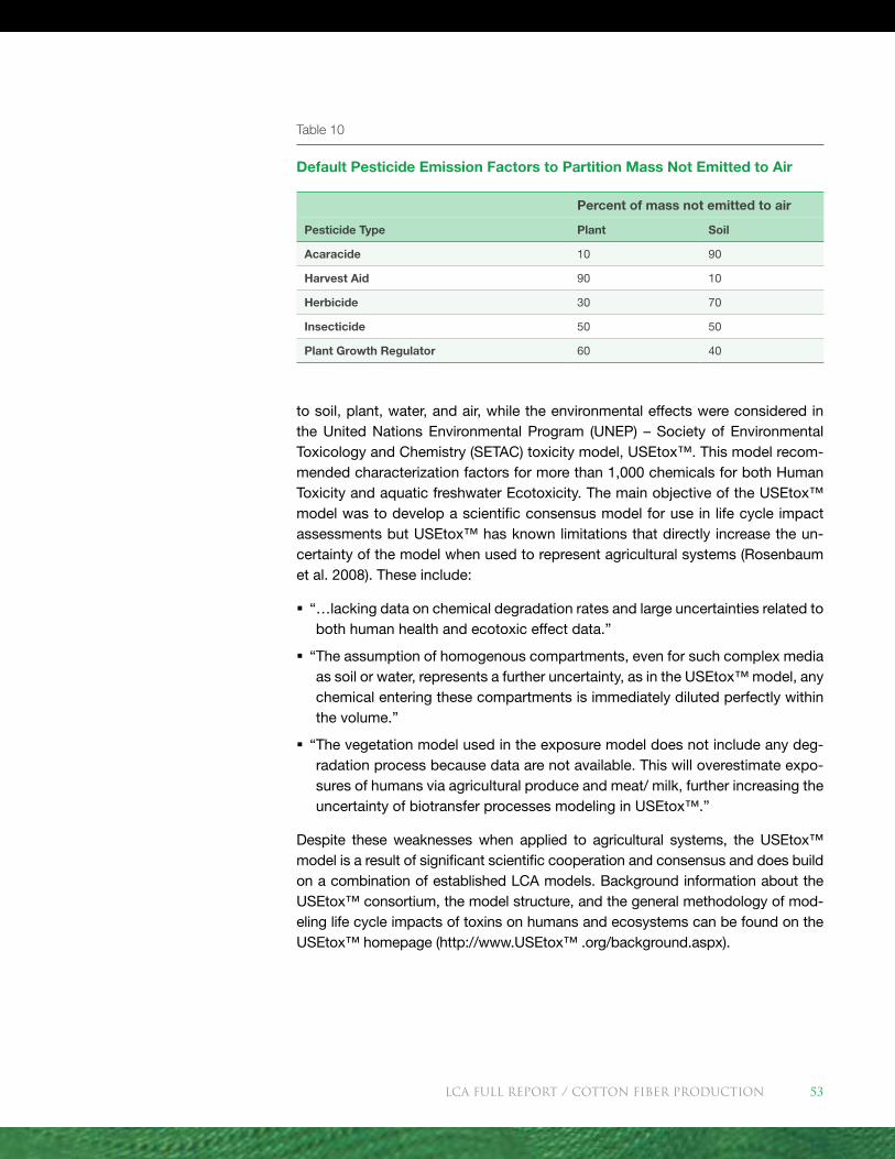
to soil, plant, water, and air, while the environmental effects were considered in the United Nations Environmental Program (UNEP) – Society of Environmental Toxicology and Chemistry (SETAC) toxicity model, USEtox™. This model recom-mended characterization factors for more than 1,000 chemicals for both Human Toxicity and aquatic freshwater Ecotoxicity. The main objective of the USEtox™ model was to develop a scientific consensus model for use in life cycle impact assessments but USEtox™ has known limitations that directly increase the un-certainty of the model when used to represent agricultural systems (Rosenbaum et al. 2008). These include:
� “ …lacking data on chemical degradation rates and large uncertainties related to both human health and ecotoxic effect data.”
� “ The assumption of homogenous compartments, even for such complex media as soil or water, represents a further uncertainty, as in the USEtox™ model, any chemical entering these compartments is immediately diluted perfectly within the volume.”
� “ The vegetation model used in the exposure model does not include any deg-radation process because data are not available. This will overestimate expo-sures of humans via agricultural produce and meat/ milk, further increasing the uncertainty of biotransfer processes modeling in USEtox™.”
Despite these weaknesses when applied to agricultural systems, the USEtox™ model is a result of significant scientific cooperation and consensus and does build on a combination of established LCA models. Background information about the USEtox™ consortium, the model structure, and the general methodology of mod-eling life cycle impacts of toxins on humans and ecosystems can be found on the USEtox™ homepage (http://www.USEtox™ .org/background.aspx).
Table 10
Default Pesticide Emission Factors to Partition Mass Not Emitted to Air
Percent of mass not emitted to air
Pesticide Type Plant Soil
Acaracide 10 90
Harvest Aid 90 10
Herbicide 30 70
Insecticide 50 50
Plant Growth Regulator 60 40
LCA FULL REport / Cotton Fiber Production 53
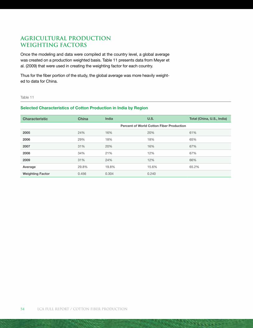
Agricultural Production Weighting Factors
Once the modeling and data were compiled at the country level, a global average was created on a production weighted basis. Table 11 presents data from Meyer et al. (2009) that were used in creating the weighting factor for each country.
Thus for the fiber portion of the study, the global average was more heavily weight-ed to data for China.
Table 11
Selected Characteristics of Cotton Production in India by Region
Characteristic China India U.S. Total (China, U.S., India)
Percent of World Cotton Fiber Production
2005 24% 16% 20% 61%
2006 29% 18% 18% 65%
2007 31% 20% 16% 67%
2008 34% 21% 12% 67%
2009 31% 24% 12% 66%
Average 29.8% 19.8% 15.6% 65.2%
Weighting Factor 0.456 0.304 0.240
LCA FULL REport / Cotton Fiber Production54
Results: Cotton Production (Cradle-to-Gate)
All agricultural in-field processes were evaluated for contribution to impact using the PE INTERNATIONAL cultivation model and are presented per 1,000 kg of cot-ton fiber at gin gate (after ginning). Tractor operations (e.g., seeding, fertilizer and pesticide application), biological transformation processes in the soil, harvest and post-harvest processes including ginning and transportation were considered. The results are based on the latest version of the cultivation model developed by PE INTERNATIONAL within the GaBi 5 software. The global average fiber results are presented for a production-weighted percentage of cotton fiber in the three respec-tive countries. Graphs are split into main contributor as follows:
� Crop Rotation: Credits or impacts due to nutrient surplus or deficit. The magnitude of the value was dependent on crop-specific nutrient efficiency, soil parameters, previous and following crop, and management practices.
� Fertilizer: All the energy and emissions associated with the manufacture of fertilizers, including potential impacts associated with the raw materials used in its production.
� Field Emissions: Impacts associated with the estimated loss of fertilizer and pesticides to the air, water or soil outside the crop’s root zone.
� Irrigation: Water used for irrigation as well as energy associated with its ap-plication and conveyance.
� Pesticides Manufacture: All the inputs (energy and chemicals) needed to man-ufacture the pesticides used.
� Post Harvest: Transport to cotton gin, processing through the cotton gin, and all packaging materials used (module covers, bale bags and ties).
� Reference System: The reference system is used to model the system’s behavior without human use. In particular, losses of nitrate to groundwater and gaseous nitrogen compounds captured in precipitation are mapped. This discharge and conversion to different emissions are relevant for both the main cropping system as well as on unused land. Therefore, not all of these emissions can be assigned to the crop since they also occur in the case of non-cultivation, e.g., for a fallow or nature reserve. For the reference system it is assumed that the nitrogen cycle is balanced, as any entry of nitrogen with rainfall is re-emitted from the systems in various forms into groundwater and air.
� Seeds production: Seed production and transport from planting seed distribu-tor to farm and field.
� Field Fuel Use: Field operations (e.g., sowing, fertilizing, harvesting).
� Transport: Transports from production facility to farm (e.g., fertilizer, lime, pes-ticides, diesel).
LCA FULL REport / Cotton Fiber Production 55
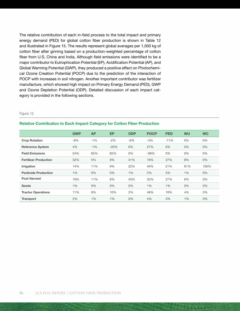
Figure 12
Relative Contribution to Each Impact Category for Cotton Fiber Production
The relative contribution of each in-field process to the total impact and primary energy demand (PED) for global cotton fiber production is shown in Table 12 and illustrated in Figure 15. The results represent global averages per 1,000 kg of cotton fiber after ginning based on a production-weighted percentage of cotton fiber from U.S, China and India. Although field emissions were identified to be a major contributor to Eutrophication Potential (EP), Acidification Potential (AP), and Global Warming Potential (GWP), they produced a positive effect on Photochemi-cal Ozone Creation Potential (POCP) due to the prediction of the interaction of POCP with increases in soil nitrogen. Another important contributor was fertilizer manufacture, which showed high impact on Primary Energy Demand (PED), GWP and Ozone Depletion Potential (ODP). Detailed discussion of each impact cat-egory is provided in the following sections.
GWP AP EP ODP POCP PED WU WC
Crop Rotation -8% -1% -2% -9% -4% -11% 0% 0%
Reference System 4% -1% -20% 0% 27% 0% 0% 0%
Field Emissions 24% 65% 85% 0% -68% 0% 0% 0%
Fertilizer Production 32% 5% 9% 41% 18% 37% 8% 0%
Irrigation 14% 11% 9% 22% 40% 21% 81% 100%
Pesticide Production 1% 0% 0% 1% 2% 3% 1% 0%
Post Harvest 19% 11% 8% 43% 32% 27% 6% 0%
Seeds 1% 0% 0% 0% 1% 1% 0% 0%
Tractor Operations 11% 8% 10% 2% 48% 19% 4% 0%
Transport 2% 1% 1% 0% 4% 3% 1% 0%
LCA FULL REport / Cotton Fiber Production56
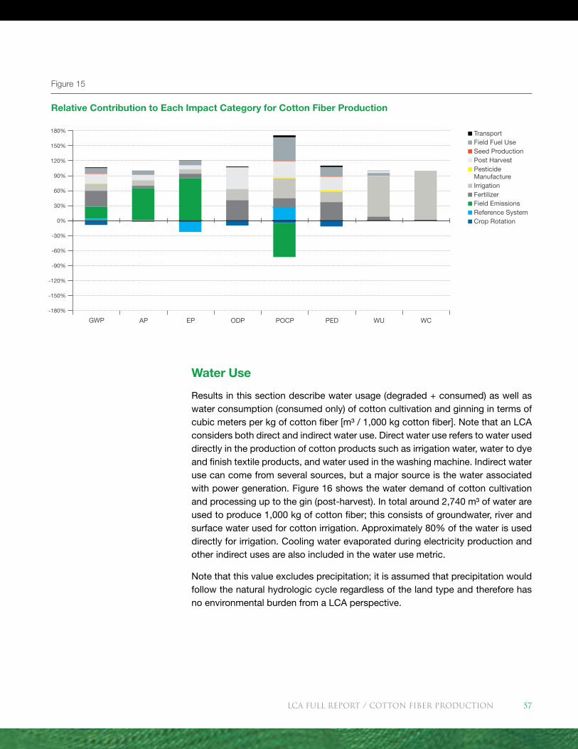
Water Use
Results in this section describe water usage (degraded + consumed) as well as water consumption (consumed only) of cotton cultivation and ginning in terms of cubic meters per kg of cotton fiber [m³ / 1,000 kg cotton fiber]. Note that an LCA considers both direct and indirect water use. Direct water use refers to water used directly in the production of cotton products such as irrigation water, water to dye and finish textile products, and water used in the washing machine. Indirect water use can come from several sources, but a major source is the water associated with power generation. Figure 16 shows the water demand of cotton cultivation and processing up to the gin (post-harvest). In total around 2,740 m³ of water are used to produce 1,000 kg of cotton fiber; this consists of groundwater, river and surface water used for cotton irrigation. Approximately 80% of the water is used directly for irrigation. Cooling water evaporated during electricity production and other indirect uses are also included in the water use metric.
Note that this value excludes precipitation; it is assumed that precipitation would follow the natural hydrologic cycle regardless of the land type and therefore has no environmental burden from a LCA perspective.
Figure 15
Relative Contribution to Each Impact Category for Cotton Fiber Production
Transport Field Fuel Use Seed Production Post Harvest Pesticide Manufacture
Irrigation Fertilizer Field Emissions Reference System Crop Rotation
GWP AP EP ODP POCP PED WU WC
180%
-180%
150%
-150%
120%
-120%
90%
-90%
30%
-30%
60%
-60%
0%
LCA FULL REport / Cotton Fiber Production 57
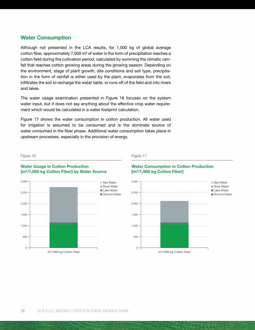
Water Consumption
Although not presented in the LCA results, for 1,000 kg of global average cotton fiber, approximately 7,000 m³ of water in the form of precipitation reaches a cotton field during the cultivation period, calculated by summing the climatic rain-fall that reaches cotton growing areas during the growing season. Depending on the environment, stage of plant growth, site conditions and soil type, precipita-tion in the form of rainfall is either used by the plant, evaporates from the soil, infiltrates the soil to recharge the water table, or runs off of the field and into rivers and lakes.
The water usage examination presented in Figure 16 focuses on the system water input, but it does not say anything about the effective crop water require-ment which would be calculated in a water footprint calculation.
Figure 17 shows the water consumption in cotton production. All water used for irrigation is assumed to be consumed and is the dominate source of water consumed in the fiber phase. Additional water consumption takes place in upstream processes, especially in the provision of energy.
Figure 17
Water Consumption in Cotton Production [m3/1,000 kg Cotton Fiber]
Figure 16
Water Usage in Cotton Production [m3/1,000 kg Cotton Fiber] by Water Source
Sea Water River Water Lake Water Ground Water
3,000
2,500
2,000
1,500
500
1,000
0
m3/1000 kg Cotton Fiber
Sea Water River Water Lake Water Ground Water
3,000
2,500
2,000
1,500
500
1,000
0
m3/1000 kg Cotton Fiber
LCA FULL REport / Cotton Fiber Production58
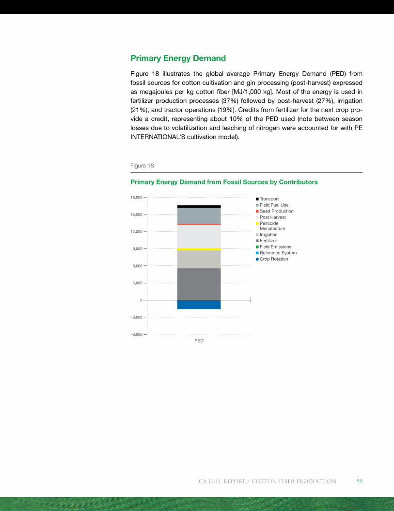
Primary Energy Demand
Figure 18 illustrates the global average Primary Energy Demand (PED) from fossil sources for cotton cultivation and gin processing (post-harvest) expressed as megajoules per kg cotton fiber [MJ/1,000 kg]. Most of the energy is used in fertilizer production processes (37%) followed by post-harvest (27%), irrigation (21%), and tractor operations (19%). Credits from fertilizer for the next crop pro-vide a credit, representing about 10% of the PED used (note between season losses due to volatilization and leaching of nitrogen were accounted for with PE INTERNATIONAL’S cultivation model).
Figure 18
Primary Energy Demand from Fossil Sources by Contributors
Transport Field Fuel Use Seed Production Post Harvest Pesticide Manufacture
Irrigation Fertilizer Field Emissions Reference System Crop Rotation
18,000
15,000
12,000
9,000
3,000
-3,000
6,000
-6,000
0
PED
LCA FULL REport / Cotton Fiber Production 59
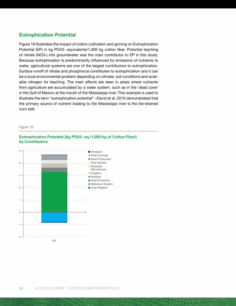
Eutrophication Potential
Figure 19 illustrates the impact of cotton cultivation and ginning on Eutrophication Potential (EP) in kg PO43- equivalents/1,000 kg cotton fiber. Potential leaching of nitrate (NO3-) into groundwater was the main contributor to EP in this study. Because eutrophication is predominantly influenced by emissions of nutrients to water, agricultural systems are one of the largest contributors to eutrophication. Surface runoff of nitrate and phosphorus contributes to eutrophication and it can be a local environmental problem depending on climate, soil conditions and avail-able nitrogen for leaching. The main effects are seen in areas where nutrients from agriculture are accumulated by a water system, such as in the ‘dead zone’ in the Gulf of Mexico at the mouth of the Mississippi river. This example is used to illustrate the term “eutrophication potential” –David et al. 2010 demonstrated that the primary source of nutrient loading to the Mississippi river is the tile-drained corn belt.
Figure 19
Eutrophication Potential [kg PO43- eq./1,000 kg of Cotton Fiber] by Contributors
Transport Field Fuel Use Seed Production Post Harvest Pesticide Manufacture
Irrigation Fertilizer Field Emissions Reference System Crop Rotation
5
4
3
1
2
2
1
0
EP
LCA FULL REport / Cotton Fiber Production60
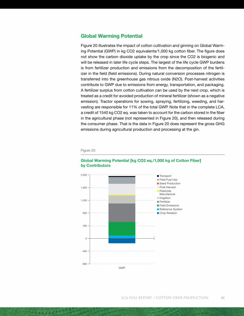
Global Warming Potential
Figure 20 illustrates the impact of cotton cultivation and ginning on Global Warm-ing Potential (GWP) in kg CO2 equivalents/1,000 kg cotton fiber. The figure does not show the carbon dioxide uptake by the crop since the CO2 is biogenic and will be released in later life cycle steps. The largest of the life cycle GWP burdens is from fertilizer production and emissions from the decomposition of the fertil-izer in the field (field emissions). During natural conversion processes nitrogen is transferred into the greenhouse gas nitrous oxide (N2O). Post-harvest activities contribute to GWP due to emissions from energy, transportation, and packaging. A fertilizer surplus from cotton cultivation can be used by the next crop, which is treated as a credit for avoided production of mineral fertilizer (shown as a negative emission). Tractor operations for sowing, spraying, fertilizing, weeding, and har-vesting are responsible for 11% of the total GWP. Note that in the complete LCA, a credit of 1540 kg CO2 eq. was taken to account for the carbon stored in the fiber in the agricultural phase (not represented in Figure 20), and then released during the consumer phase. That is the data in Figure 20 does represent the gross GHG emissions during agricultural production and processing at the gin.
Figure 20
Global Warming Potential [kg CO2 eq./1,000 kg of Cotton Fiber] by Contributors
Transport Field Fuel Use Seed Production Post Harvest Pesticide Manufacture
Irrigation Fertilizer Field Emissions Reference System Crop Rotation
2,000
1,600
1,200
400
-800
800
-400
0
GWP
LCA FULL REport / Cotton Fiber Production 61
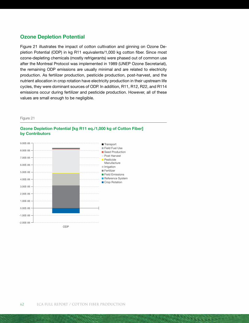
Ozone Depletion Potential
Figure 21 illustrates the impact of cotton cultivation and ginning on Ozone De-pletion Potential (ODP) in kg R11 equivalents/1,000 kg cotton fiber. Since most ozone-depleting chemicals (mostly refrigerants) were phased out of common use after the Montreal Protocol was implemented in 1989 (UNEP Ozone Secretariat), the remaining ODP emissions are usually minimal and are related to electricity production. As fertilizer production, pesticide production, post-harvest, and the nutrient allocation in crop rotation have electricity production in their upstream life cycles, they were dominant sources of ODP. In addition, R11, R12, R22, and R114 emissions occur during fertilizer and pesticide production. However, all of these values are small enough to be negligible.
Figure 21
Ozone Depletion Potential [kg R11 eq./1,000 kg of Cotton Fiber] by Contributors
Transport Field Fuel Use Seed Production Post Harvest Pesticide Manufacture
Irrigation Fertilizer Field Emissions Reference System Crop Rotation
9.00E-06
8.00E-06
7.00E-06
6.00E-06
3.00E-06
4.00E-06
2.00E-06
1.00E-06
-1.00E-06
5.00E-06
-2.00E-06
0.00E-06
ODP
LCA FULL REport / Cotton Fiber Production62
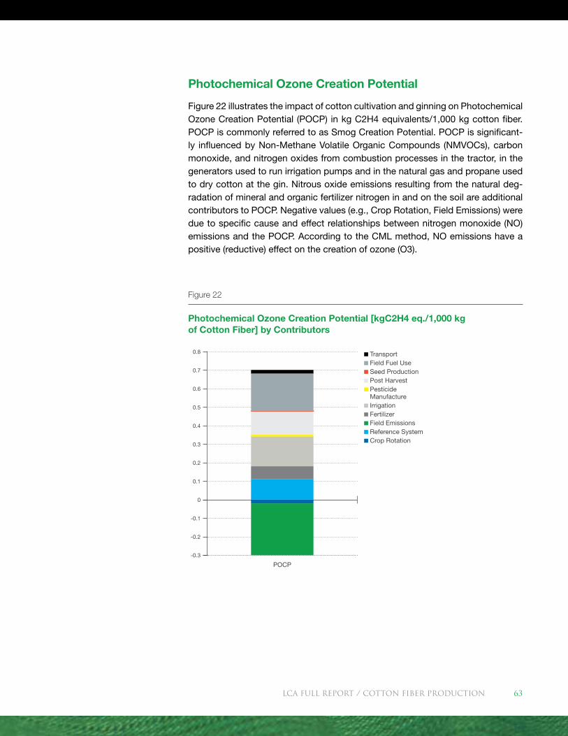
Photochemical Ozone Creation Potential
Figure 22 illustrates the impact of cotton cultivation and ginning on Photochemical Ozone Creation Potential (POCP) in kg C2H4 equivalents/1,000 kg cotton fiber. POCP is commonly referred to as Smog Creation Potential. POCP is significant-ly influenced by Non-Methane Volatile Organic Compounds (NMVOCs), carbon monoxide, and nitrogen oxides from combustion processes in the tractor, in the generators used to run irrigation pumps and in the natural gas and propane used to dry cotton at the gin. Nitrous oxide emissions resulting from the natural deg-radation of mineral and organic fertilizer nitrogen in and on the soil are additional contributors to POCP. Negative values (e.g., Crop Rotation, Field Emissions) were due to specific cause and effect relationships between nitrogen monoxide (NO) emissions and the POCP. According to the CML method, NO emissions have a positive (reductive) effect on the creation of ozone (O3).
Figure 22
Photochemical Ozone Creation Potential [kgC2H4 eq./1,000 kg of Cotton Fiber] by Contributors
Transport Field Fuel Use Seed Production Post Harvest Pesticide Manufacture
Irrigation Fertilizer Field Emissions Reference System Crop Rotation
0.8
0.7
0.5
0.3
0.1
0.6
0.2
-0.2
-0.3
0.4
-0.1
0
POCP
LCA FULL REport / Cotton Fiber Production 63
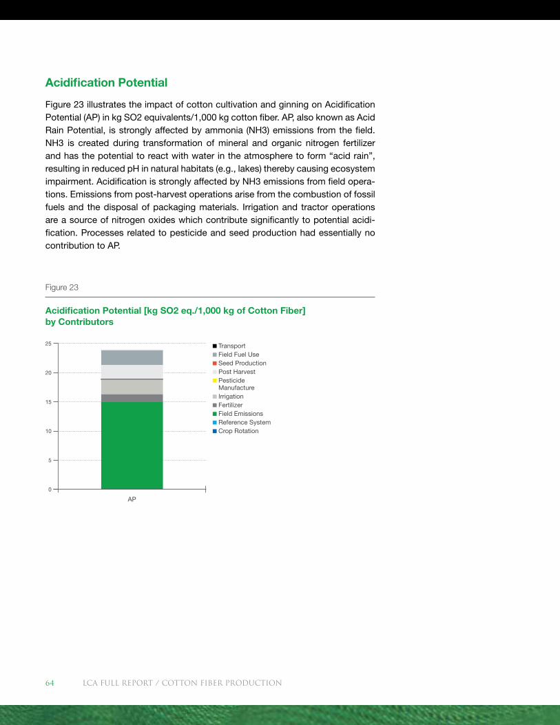
Acidification Potential
Figure 23 illustrates the impact of cotton cultivation and ginning on Acidification Potential (AP) in kg SO2 equivalents/1,000 kg cotton fiber. AP, also known as Acid Rain Potential, is strongly affected by ammonia (NH3) emissions from the field. NH3 is created during transformation of mineral and organic nitrogen fertilizer and has the potential to react with water in the atmosphere to form “acid rain”, resulting in reduced pH in natural habitats (e.g., lakes) thereby causing ecosystem impairment. Acidification is strongly affected by NH3 emissions from field opera-tions. Emissions from post-harvest operations arise from the combustion of fossil fuels and the disposal of packaging materials. Irrigation and tractor operations are a source of nitrogen oxides which contribute significantly to potential acidi-fication. Processes related to pesticide and seed production had essentially no contribution to AP.
Figure 23
Acidification Potential [kg SO2 eq./1,000 kg of Cotton Fiber] by Contributors
Transport Field Fuel Use Seed Production Post Harvest Pesticide Manufacture
Irrigation Fertilizer Field Emissions Reference System Crop Rotation
25
20
15
5
10
0
AP
LCA FULL REport / Cotton Fiber Production64
Toxicity Metrics
One area where there was a high degree of uncertainty in the agricultural model was the emission factors to estimate the fate of a chemical, particularly pesti-cides, at the time of application. While the best possible estimates were made, the values do not account for the numerous factors that impact a compound’s fi-nal resting place at the time of application, such as humidity, wind speed, percent plant and weed cover, and type of application equipment used. There is further uncertainty in the factors used to predict the fate and transport of the compound once it does come to rest.
The precision of the characterization model as used in this study was within a factor of 100–1,000 for HTP and 10–100 for ETP. Although this is a substantial improve-ment over previously available toxicity characterization models, the uncertainty of this metric is substantially higher than for the other impact categories in this study. Uncertainties around the USEtox™ model notwithstanding, the impact results of the present study showed that certain pesticides outweighed all other life cycle toxicity impacts by a large margin. However, there were implausible inconsistencies between characterizations of certain pesticides and the measured effects shown by this study. For example, acephate, a non-restricted use pesticide in the U.S. was re-sponsible for much of cotton’s HTP whereas certain other restricted use chemicals had little impact. Acephate is the primary active ingredient in Orthene®, a readily available, over–the-counter insecticide commonly used for pest control in home gardens in the U.S. Additional work is underway to further understand the param-eters used to characterized many of the compounds in this study.
Limitations
While extensive data were collected to quantify agricultural impacts, agricultural systems are inherently difficult to generalize. Differences in yearly weather condi-tions, spatial variations in soil type, topography, and individual grower manage-ment practices all introduce considerable variability for agricultural data. Where possible, this was partially addressed by using five year averages. In each country where a large percentage of the acres are irrigated, there is significant uncertainty surrounding irrigation pumping depths, and the estimates of energy use are highly influenced by this measurement.
A measure of the variability in the agricultural phase is provided in Table 13 which shows the standard deviation of country averages compared to the global mean value. For many of the impact categories, the standard deviation is about 60% of the mean, with the clear exception of EP. This variability in EP may be partially due to an artifact of the agricultural model used, but may also represent a true response to different fertility programs in many different environments. The vari-ability of GWP is also high. One reason is because the mean has been adjusted
LCA FULL REport / Cotton Fiber Production 65
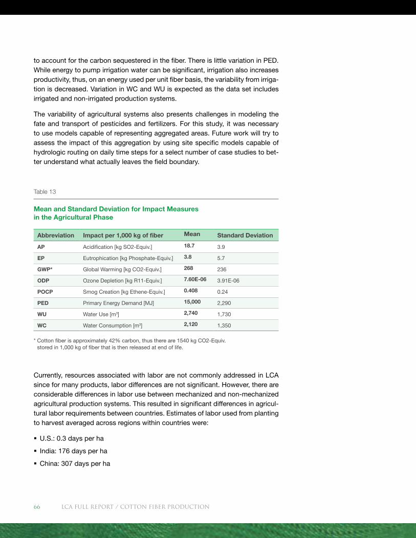
to account for the carbon sequestered in the fiber. There is little variation in PED. While energy to pump irrigation water can be significant, irrigation also increases productivity, thus, on an energy used per unit fiber basis, the variability from irriga-tion is decreased. Variation in WC and WU is expected as the data set includes irrigated and non-irrigated production systems.
The variability of agricultural systems also presents challenges in modeling the fate and transport of pesticides and fertilizers. For this study, it was necessary to use models capable of representing aggregated areas. Future work will try to assess the impact of this aggregation by using site specific models capable of hydrologic routing on daily time steps for a select number of case studies to bet-ter understand what actually leaves the field boundary.
Currently, resources associated with labor are not commonly addressed in LCA since for many products, labor differences are not significant. However, there are considerable differences in labor use between mechanized and non-mechanized agricultural production systems. This resulted in significant differences in agricul-tural labor requirements between countries. Estimates of labor used from planting to harvest averaged across regions within countries were:
� U.S.: 0.3 days per ha
� India: 176 days per ha
� China: 307 days per ha
Table 13
Mean and Standard Deviation for Impact Measures in the Agricultural Phase
Abbreviation Impact per 1,000 kg of fiber Mean Standard Deviation
AP Acidification [kg SO2-Equiv.] 18.7 3.9
EP Eutrophication [kg Phosphate-Equiv.] 3.8 5.7
GWP* Global Warming [kg CO2-Equiv.] 268 236
ODP Ozone Depletion [kg R11-Equiv.] 7.60E-06 3.91E-06
POCP Smog Creation [kg Ethene-Equiv.] 0.408 0.24
PED Primary Energy Demand [MJ] 15,000 2,290
WU Water Use [m3] 2,740 1,730
WC Water Consumption [m3] 2,120 1,350
* Cotton fiber is approximately 42% carbon, thus there are 1540 kg CO2-Equiv. stored in 1,000 kg of fiber that is then released at end of life.
LCA FULL REport / Cotton Fiber Production66
The implications of these differences are difficult to quantify from an LCA per-spective and were not addressed in this study but the findings do highlight an interesting aspect of global agricultural systems.
A final comment is that the data density for agricultural production was greatest for the U.S., where a majority of the data were available at a regional or smaller level from official government estimates. Data for India was not as extensive, but were robust enough to adequately represent growing regions within the country. Data for China was the most limited and had the highest level of uncertainty. Despite the limitations, it was clear that for most of the inputs to the LCA model, the differences between regions within a country exceeded the differences between the mean val-ues of a country owing primarily to differences in the environment.
Conclusions: Cotton Production (Cradle-to-Gate)
� Field emissions were a major contributor to several environmental impact cat-egories: Eutrophication Potential was strongly influenced by nitrate, Acidifica-tion Potential was influenced by ammonia and Global Warming Potential was influenced by nitrous oxide. The Photochemical Ozone Creation Potential was reduced by nitrogen monoxide emissions which are known to have a reductive effect on the creation of ozone. All these substances originate from the trans-formation process of biogenic and chemical nitrogen. Precision management of nitrogen fertilizer will continue to be a high priority for the cotton producers around the world.
� Fertilizer production is another important contributor with a high impact on Pri-mary Energy Demand, Global Warming Potential and Photochemical Ozone Creation Potential. Nitrogen fertilizer represents a majority of that contribution, reinforcing the need for careful nitrogen management.
� Despite a high uncertainty of toxicity effects in the impact categories Ecotoxic-ity Potential and Human Toxicity Potential, it is evident that field application of pesticides was the main contributor to impact based on the parameters in the current USEtox™model. Further studies will be conducted to determine how well USEtox™represents the fate and transport of pesticides.
� GHG emissions during the agricultural phase of the LCA were relatively low and close to the same magnitude of the carbon dioxide equivalents represented by the carbon contained in the fiber.
LCA FULL REport / Cotton Fiber Production 67
Textile Manufacturing
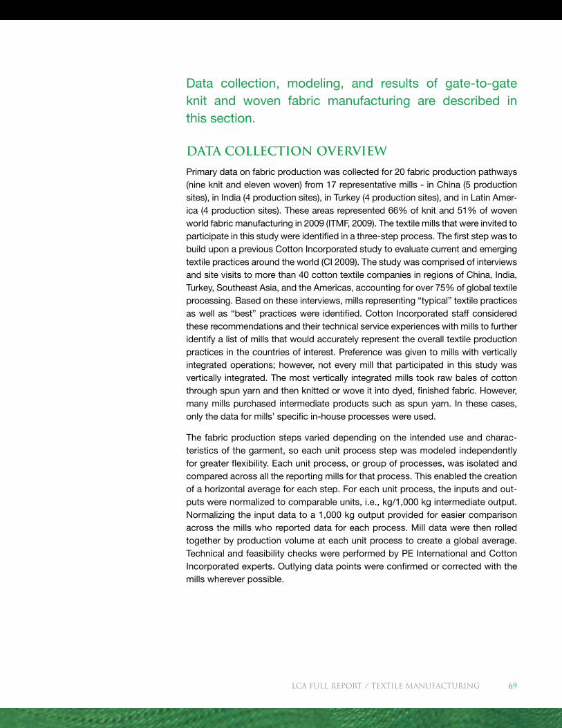
Data collection, modeling, and results of gate-to-gate knit and woven fabric manufacturing are described in this section.
Data Collection Overview
Primary data on fabric production was collected for 20 fabric production pathways (nine knit and eleven woven) from 17 representative mills - in China (5 production sites), in India (4 production sites), in Turkey (4 production sites), and in Latin Amer-ica (4 production sites). These areas represented 66% of knit and 51% of woven world fabric manufacturing in 2009 (ITMF, 2009). The textile mills that were invited to participate in this study were identified in a three-step process. The first step was to build upon a previous Cotton Incorporated study to evaluate current and emerging textile practices around the world (CI 2009). The study was comprised of interviews and site visits to more than 40 cotton textile companies in regions of China, India, Turkey, Southeast Asia, and the Americas, accounting for over 75% of global textile processing. Based on these interviews, mills representing “typical” textile practices as well as “best” practices were identified. Cotton Incorporated staff considered these recommendations and their technical service experiences with mills to further identify a list of mills that would accurately represent the overall textile production practices in the countries of interest. Preference was given to mills with vertically integrated operations; however, not every mill that participated in this study was vertically integrated. The most vertically integrated mills took raw bales of cotton through spun yarn and then knitted or wove it into dyed, finished fabric. However, many mills purchased intermediate products such as spun yarn. In these cases, only the data for mills’ specific in-house processes were used.
The fabric production steps varied depending on the intended use and charac-teristics of the garment, so each unit process step was modeled independently for greater flexibility. Each unit process, or group of processes, was isolated and compared across all the reporting mills for that process. This enabled the creation of a horizontal average for each step. For each unit process, the inputs and out-puts were normalized to comparable units, i.e., kg/1,000 kg intermediate output. Normalizing the input data to a 1,000 kg output provided for easier comparison across the mills who reported data for each process. Mill data were then rolled together by production volume at each unit process to create a global average. Technical and feasibility checks were performed by PE International and Cotton Incorporated experts. Outlying data points were confirmed or corrected with the mills wherever possible.
LCA FULL REport / Textile manufacturing 69
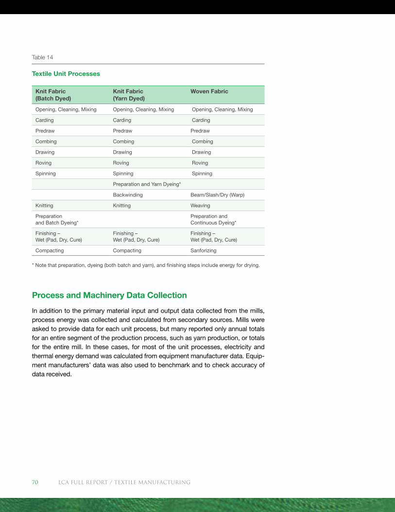
Table 14
Textile Unit Processes
Knit Fabric (Batch Dyed)
Knit Fabric (Yarn Dyed)
Woven Fabric
Opening, Cleaning, Mixing Opening, Cleaning, Mixing Opening, Cleaning, Mixing
Carding Carding Carding
Predraw Predraw Predraw
Combing Combing Combing
Drawing Drawing Drawing
Roving Roving Roving
Spinning Spinning Spinning
Preparation and Yarn Dyeing*
Backwinding Beam/Slash/Dry (Warp)
Knitting Knitting Weaving
Preparation and Batch Dyeing*
Preparation and Continuous Dyeing*
Finishing – Wet (Pad, Dry, Cure)
Finishing – Wet (Pad, Dry, Cure)
Finishing – Wet (Pad, Dry, Cure)
Compacting Compacting Sanforizing
* Note that preparation, dyeing (both batch and yarn), and finishing steps include energy for drying.
Process and Machinery Data Collection
In addition to the primary material input and output data collected from the mills, process energy was collected and calculated from secondary sources. Mills were asked to provide data for each unit process, but many reported only annual totals for an entire segment of the production process, such as yarn production, or totals for the entire mill. In these cases, for most of the unit processes, electricity and thermal energy demand was calculated from equipment manufacturer data. Equip-ment manufacturers’ data was also used to benchmark and to check accuracy of data received.
LCA FULL REport / Textile manufacturing70
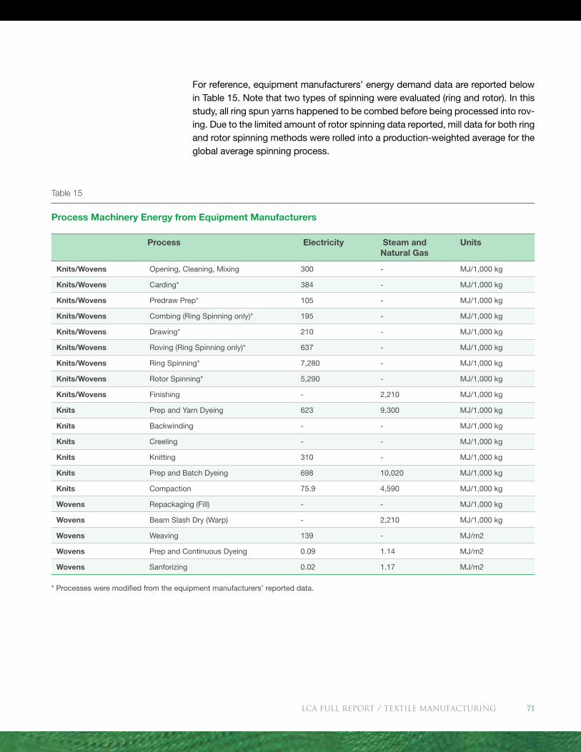
For reference, equipment manufacturers’ energy demand data are reported below in Table 15. Note that two types of spinning were evaluated (ring and rotor). In this study, all ring spun yarns happened to be combed before being processed into rov-ing. Due to the limited amount of rotor spinning data reported, mill data for both ring and rotor spinning methods were rolled into a production-weighted average for the global average spinning process.
* Processes were modified from the equipment manufacturers’ reported data.
Table 15
Process Machinery Energy from Equipment Manufacturers
Process Electricity Steam and Natural Gas
Units
Knits/Wovens Opening, Cleaning, Mixing 300 - MJ/1,000 kg
Knits/Wovens Carding* 384 - MJ/1,000 kg
Knits/Wovens Predraw Prep* 105 - MJ/1,000 kg
Knits/Wovens Combing (Ring Spinning only)* 195 - MJ/1,000 kg
Knits/Wovens Drawing* 210 - MJ/1,000 kg
Knits/Wovens Roving (Ring Spinning only)* 637 - MJ/1,000 kg
Knits/Wovens Ring Spinning* 7,280 - MJ/1,000 kg
Knits/Wovens Rotor Spinning* 5,290 - MJ/1,000 kg
Knits/Wovens Finishing - 2,210 MJ/1,000 kg
Knits Prep and Yarn Dyeing 623 9,300 MJ/1,000 kg
Knits Backwinding - - MJ/1,000 kg
Knits Creeling - - MJ/1,000 kg
Knits Knitting 310 - MJ/1,000 kg
Knits Prep and Batch Dyeing 698 10,020 MJ/1,000 kg
Knits Compaction 75.9 4,590 MJ/1,000 kg
Wovens Repackaging (Fill) - - MJ/1,000 kg
Wovens Beam Slash Dry (Warp) - 2,210 MJ/1,000 kg
Wovens Weaving 139 - MJ/m2
Wovens Prep and Continuous Dyeing 0.09 1.14 MJ/m2
Wovens Sanforizing 0.02 1.17 MJ/m2
LCA FULL REport / Textile manufacturing 71
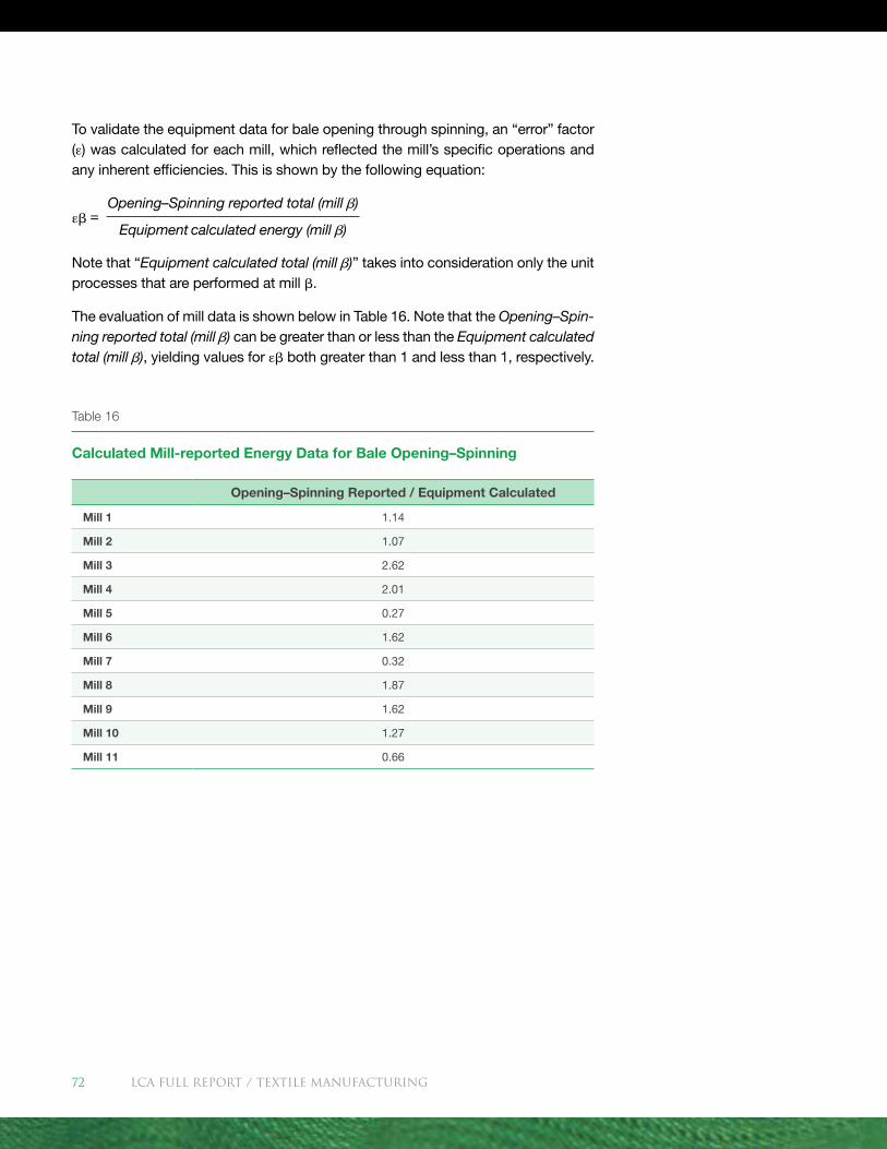
To validate the equipment data for bale opening through spinning, an “error” factor () was calculated for each mill, which reflected the mill’s specific operations and any inherent efficiencies. This is shown by the following equation:
=
Note that “Equipment calculated total (mill )” takes into consideration only the unit processes that are performed at mill .
The evaluation of mill data is shown below in Table 16. Note that the Opening–Spin-ning reported total (mill ) can be greater than or less than the Equipment calculated total (mill ), yielding values for both greater than 1 and less than 1, respectively.
Table 16
Calculated Mill-reported Energy Data for Bale Opening–Spinning
Opening–Spinning Reported / Equipment Calculated
Mill 1 1.14
Mill 2 1.07
Mill 3 2.62
Mill 4 2.01
Mill 5 0.27
Mill 6 1.62
Mill 7 0.32
Mill 8 1.87
Mill 9 1.62
Mill 10 1.27
Mill 11 0.66
Opening–Spinning reported total (mill )
Equipment calculated energy (mill )
LCA FULL REport / Textile manufacturing72
Three mills provided an Opening–Spinning reported total for electricity but did not report process specifics. For these three mills, unit process energy was calculated by scaling the equipment energy demand with an adjustment factor specific to the mill :
Unit Process calculated energy = Equipment calculated energy
In one case, a mill reported only an entire facility energy demand, so no opening through spinning adjustment was possible. Rather than assuming energy demand based on the machinery totals, a production-weighted average of other mills was created for each unit process, and these values were assumed for that spe-cific mill.
Most mills’ reported energy demand for unit processes after spinning was incom-plete, so equipment manufacturers’ data were used directly for all mills.
In some cases, mills reported a single line item to represent multiple chemicals. For example, in the dyeing process, these mills provided a consolidated input for “Scouring Agents”, “Alkali”, “Acids” or “Other Chemicals”. Since the mills were unable to clarify this data any further, a chemical split was calculated based on the technologies and chemistries used in that process. Each dye process reported an-nual usage of reactive, vat, and sulfur dyes. Depending on which dyes were used, a chemical split was interpolated from common dyeing formulas with the help of Cotton Incorporated experts to model the “Other Chemicals” used in this process.
Knit Fabric
As previously noted, data was collected from nine knit production pathways from nine textile mills in China, India, Turkey, and the Americas. This section describes knit fabric modeling as well as results of knit fabric production.
Knit Fabric Modeling
The data collection model for knit fabric manufacturing is illustrated in Figure 24 and Figure 25. The model includes ring spinning as well as yarn and batch-dyeing processes. The fabric production steps varied depending on the intended use and characteristics of the garment, so each unit process step was modeled indepen-dently for greater flexibility.
LCA FULL REport / Textile manufacturing 73
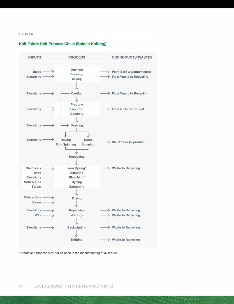
Figure 24
Knit Fabric Unit Process Chain (Bale to Knitting)
* Inputs and process may not be used in the manufacturing of all fabrics.
COPRODUCTS/WASTESPROCESS
Fiber Waste to Recycling
Fiber Waste to Recycling
Fiber Noils Coproduct
Short Fiber Coproduct
Waste to Recycling
Waste to Recycling
Waste to Recycling
Waste to Recycling
Carding
Drawing
Repacking
Roving
Ring Spinning
Rotor
Spinning
Drying
Repacking
Waxing•
Backwinding
Knitting
Yarn Dyeing*
Scouring
Bleaching*
Dyeing
Extracting
Waste to Recycling
Predraw
Lap Prep
Combing
Opening
Cleaning
Mixing
INPUTS
Bales
Electricity
Natural Gas
Electricity
Wax
Steam
Chemicals
Dyes
Electricity
Natural Gas
Steam
Electricity
Electricity
Electricity
Electricity
Electricity
Plant Bark & Contaminants
LCA FULL REport / Textile manufacturing74
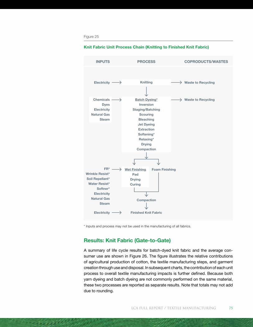
Figure 25
Knit Fabric Unit Process Chain (Knitting to Finished Knit Fabric)
* Inputs and process may not be used in the manufacturing of all fabrics.
COPRODUCTS/WASTESPROCESS
Waste to Recycling
Compaction
Foam Finishing
Finished Knit Fabric
Waste to Recycling
Knitting
INPUTS
Electricity
Chemicals
Dyes
Electricity
Natural Gas
Steam
Electricity
FR*
Wrinkle Resist*
Soil Repellant*
Water Resist*
Softner*
Electricity
Natural Gas
Steam
Batch Dyeing*
Inversion
Staging/Batching
Scouring
Bleaching
Jet Dyeing
Extraction
Softening*
Relaxing*
Drying
Compaction
Wet Finishing
Pad
Drying
Curing
Results: Knit Fabric (Gate-to-Gate)
A summary of life cycle results for batch-dyed knit fabric and the average con-sumer use are shown in Figure 26. The figure illustrates the relative contributions of agricultural production of cotton, the textile manufacturing steps, and garment creation through use and disposal. In subsequent charts, the contribution of each unit process to overall textile manufacturing impacts is further defined. Because both yarn dyeing and batch dyeing are not commonly performed on the same material, these two processes are reported as separate results. Note that totals may not add due to rounding.
LCA FULL REport / Textile manufacturing 75
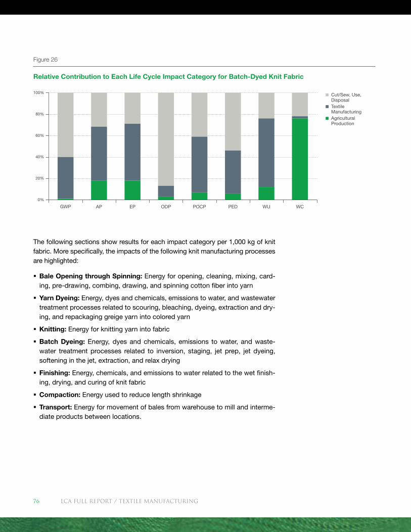
The following sections show results for each impact category per 1,000 kg of knit fabric. More specifically, the impacts of the following knit manufacturing processes are highlighted:
� Bale Opening through Spinning: Energy for opening, cleaning, mixing, card-ing, pre-drawing, combing, drawing, and spinning cotton fiber into yarn
� Yarn Dyeing: Energy, dyes and chemicals, emissions to water, and wastewater treatment processes related to scouring, bleaching, dyeing, extraction and dry-ing, and repackaging greige yarn into colored yarn
� Knitting: Energy for knitting yarn into fabric
� Batch Dyeing: Energy, dyes and chemicals, emissions to water, and waste-water treatment processes related to inversion, staging, jet prep, jet dyeing, softening in the jet, extraction, and relax drying
� Finishing: Energy, chemicals, and emissions to water related to the wet finish-ing, drying, and curing of knit fabric
� Compaction: Energy used to reduce length shrinkage
� Transport: Energy for movement of bales from warehouse to mill and interme-diate products between locations.
Figure 26
Relative Contribution to Each Life Cycle Impact Category for Batch-Dyed Knit Fabric
Cut/Sew, Use, Disposal
Textile Manufacturing
Agricultural Production
100%
80%
60%
40%
20%
0%
GWP AP EP ODP POCP PED WU WC
LCA FULL REport / Textile manufacturing76
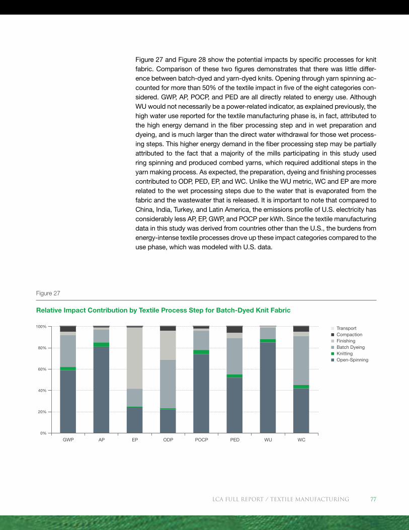
Figure 27 and Figure 28 show the potential impacts by specific processes for knit fabric. Comparison of these two figures demonstrates that there was little differ-ence between batch-dyed and yarn-dyed knits. Opening through yarn spinning ac-counted for more than 50% of the textile impact in five of the eight categories con-sidered. GWP, AP, POCP, and PED are all directly related to energy use. Although WU would not necessarily be a power-related indicator, as explained previously, the high water use reported for the textile manufacturing phase is, in fact, attributed to the high energy demand in the fiber processing step and in wet preparation and dyeing, and is much larger than the direct water withdrawal for those wet process-ing steps. This higher energy demand in the fiber processing step may be partially attributed to the fact that a majority of the mills participating in this study used ring spinning and produced combed yarns, which required additional steps in the yarn making process. As expected, the preparation, dyeing and finishing processes contributed to ODP, PED, EP, and WC. Unlike the WU metric, WC and EP are more related to the wet processing steps due to the water that is evaporated from the fabric and the wastewater that is released. It is important to note that compared to China, India, Turkey, and Latin America, the emissions profile of U.S. electricity has considerably less AP, EP, GWP, and POCP per kWh. Since the textile manufacturing data in this study was derived from countries other than the U.S., the burdens from energy-intense textile processes drove up these impact categories compared to the use phase, which was modeled with U.S. data.
Figure 27
Relative Impact Contribution by Textile Process Step for Batch-Dyed Knit Fabric
Transport Compaction Finishing Batch Dyeing Knitting Open-Spinning
100%
80%
60%
40%
20%
0%
GWP AP EP ODP POCP PED WU WC
LCA FULL REport / Textile manufacturing 77
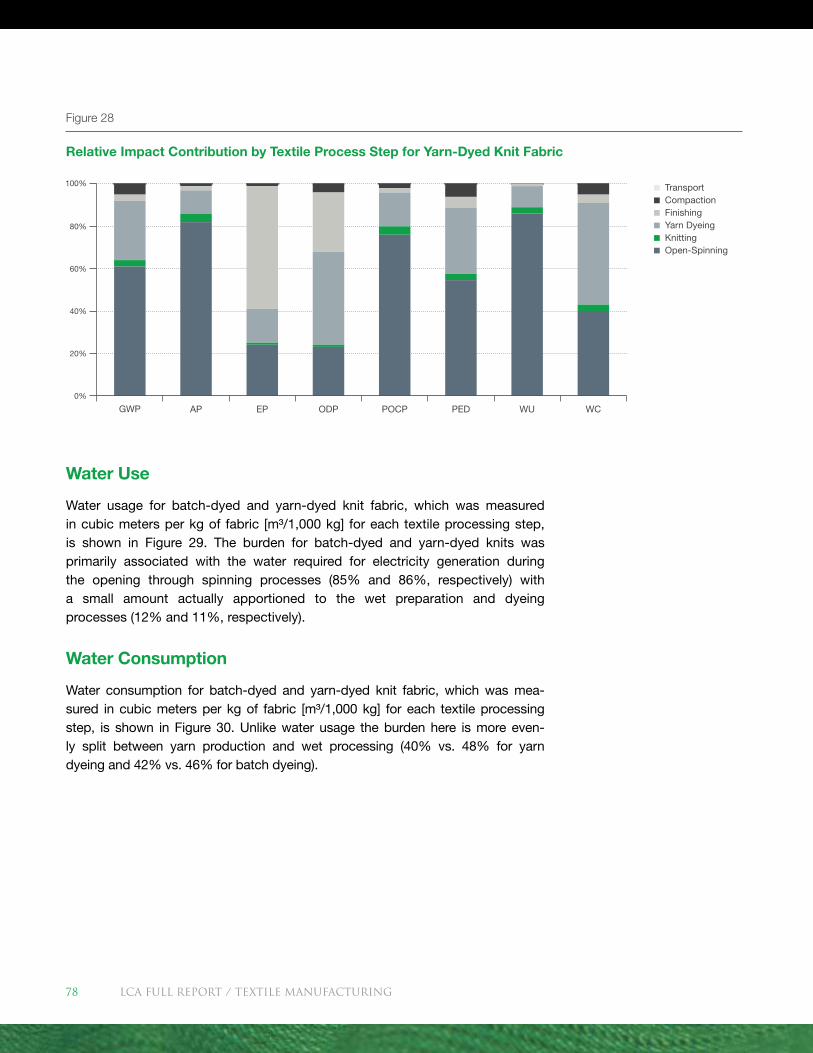
Water Use
Water usage for batch-dyed and yarn-dyed knit fabric, which was measured in cubic meters per kg of fabric [m³/1,000 kg] for each textile processing step, is shown in Figure 29. The burden for batch-dyed and yarn-dyed knits was primarily associated with the water required for electricity generation during the opening through spinning processes (85% and 86%, respectively) with a small amount actually apportioned to the wet preparation and dyeing processes (12% and 11%, respectively).
Water Consumption
Water consumption for batch-dyed and yarn-dyed knit fabric, which was mea-sured in cubic meters per kg of fabric [m³/1,000 kg] for each textile processing step, is shown in Figure 30. Unlike water usage the burden here is more even-ly split between yarn production and wet processing (40% vs. 48% for yarn dyeing and 42% vs. 46% for batch dyeing).
Figure 28
Relative Impact Contribution by Textile Process Step for Yarn-Dyed Knit Fabric
Transport Compaction Finishing Yarn Dyeing Knitting Open-Spinning
80%
60%
40%
20%
0%
GWP AP EP ODP POCP PED WU WC
100%
LCA FULL REport / Textile manufacturing78
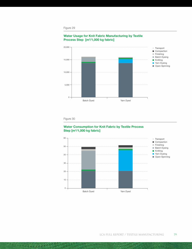
Figure 30
Water Consumption for Knit Fabric by Textile Process Step [m3/1,000 kg fabric]
Figure 29
Water Usage for Knit Fabric Manufacturing by Textile Process Step [m3/1,000 kg fabric]
Transport Compaction Finishing Batch Dyeing Knitting Yarn Dyeing Open-Spinning
20,000
15,000
10,000
5,000
0
Batch Dyed Yarn Dyed
Transport Compaction Finishing Batch Dyeing Knitting Yarn Dyeing Open-Spinning
60
50
20
20
30
10
0
Batch Dyed Yarn Dyed
LCA FULL REport / Textile manufacturing 79
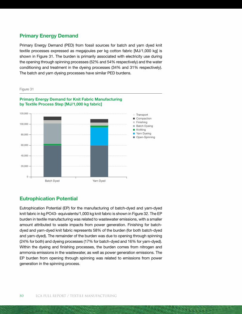
Primary Energy Demand
Primary Energy Demand (PED) from fossil sources for batch and yarn dyed knit textile processes expressed as megajoules per kg cotton fabric [MJ/1,000 kg] is shown in Figure 31. The burden is primarily associated with electricity use during the opening through spinning processes (52% and 54% respectively) and the water conditioning and treatment in the dyeing processes (34% and 31% respectively). The batch and yarn dyeing processes have similar PED burdens.
Eutrophication Potential
Eutrophication Potential (EP) for the manufacturing of batch-dyed and yarn-dyed knit fabric in kg PO43- equivalents/1,000 kg knit fabric is shown in Figure 32. The EP burden in textile manufacturing was related to wastewater emissions, with a smaller amount attributed to waste impacts from power generation. Finishing for batch-dyed and yarn-dyed knit fabric represents 58% of the burden (for both batch-dyed and yarn-dyed). The remainder of the burden was due to opening through spinning (24% for both) and dyeing processes (17% for batch-dyed and 16% for yarn-dyed). Within the dyeing and finishing processes, the burden comes from nitrogen and ammonia emissions in the wastewater, as well as power generation emissions. The EP burden from opening through spinning was related to emissions from power generation in the spinning process.
Figure 31
Primary Energy Demand for Knit Fabric Manufacturing by Textile Process Step [MJ/1,000 kg fabric]
Transport Compaction Finishing Batch Dyeing Knitting Yarn Dyeing Open-Spinning
120,000
80,000
40,000
20,000
100,000
60,000
0
Batch Dyed Yarn Dyed
LCA FULL REport / Textile manufacturing80
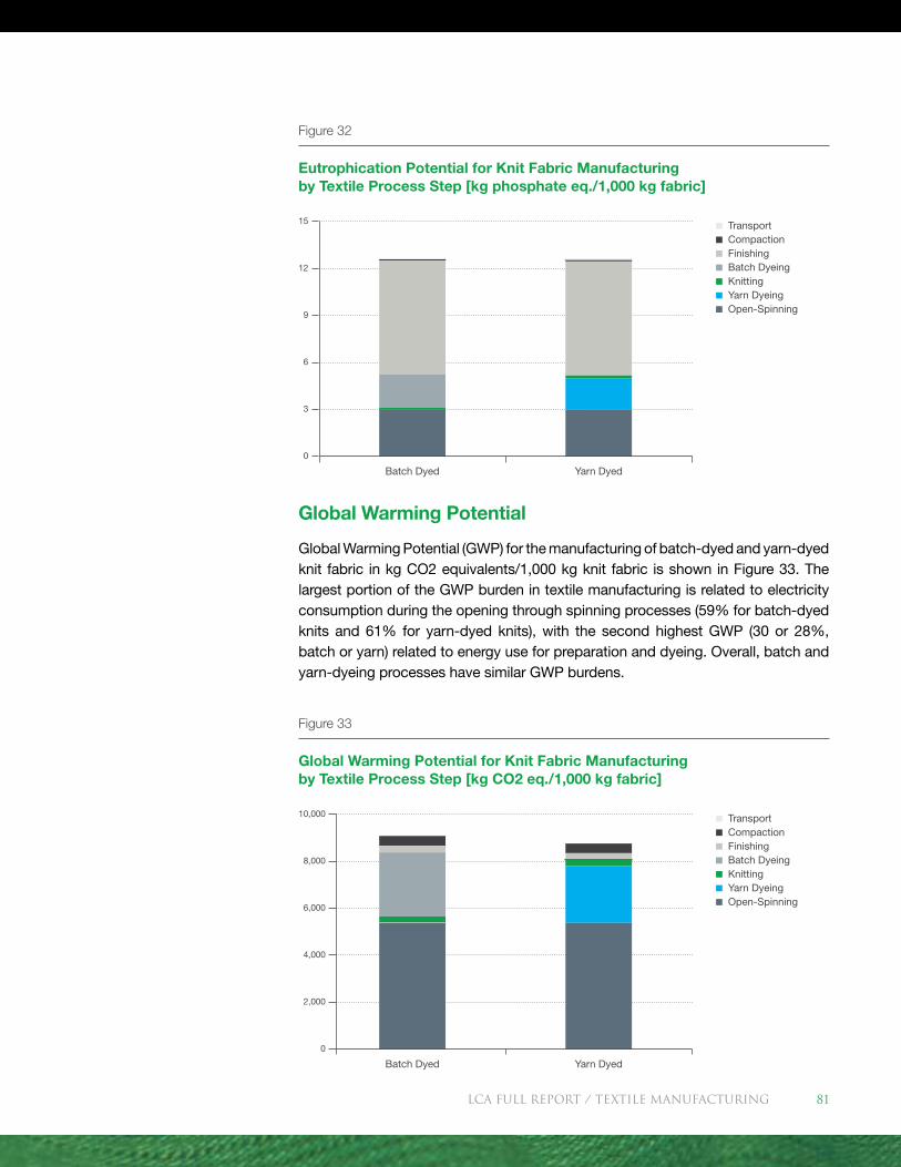
Global Warming Potential
Global Warming Potential (GWP) for the manufacturing of batch-dyed and yarn-dyed knit fabric in kg CO2 equivalents/1,000 kg knit fabric is shown in Figure 33. The largest portion of the GWP burden in textile manufacturing is related to electricity consumption during the opening through spinning processes (59% for batch-dyed knits and 61% for yarn-dyed knits), with the second highest GWP (30 or 28%, batch or yarn) related to energy use for preparation and dyeing. Overall, batch and yarn-dyeing processes have similar GWP burdens.
Figure 32
Eutrophication Potential for Knit Fabric Manufacturing by Textile Process Step [kg phosphate eq./1,000 kg fabric]
Figure 33
Global Warming Potential for Knit Fabric Manufacturing by Textile Process Step [kg CO2 eq./1,000 kg fabric]
Transport Compaction Finishing Batch Dyeing Knitting Yarn Dyeing Open-Spinning
Transport Compaction Finishing Batch Dyeing Knitting Yarn Dyeing Open-Spinning
10,000
8,000
6,000
4,000
2,000
0
15
12
9
6
3
0
Batch Dyed Yarn Dyed
Batch Dyed Yarn Dyed
LCA FULL REport / Textile manufacturing 81
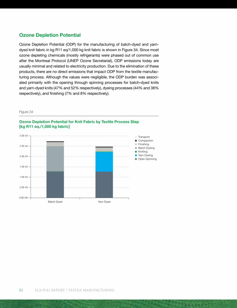
Ozone Depletion Potential
Ozone Depletion Potential (ODP) for the manufacturing of batch-dyed and yarn-dyed knit fabric in kg R11 eq/1,000 kg knit fabric is shown in Figure 34. Since most ozone depleting chemicals (mostly refrigerants) were phased out of common use after the Montreal Protocol (UNEP Ozone Secretariat), ODP emissions today are usually minimal and related to electricity production. Due to the elimination of these products, there are no direct emissions that impact ODP from the textile manufac-turing process. Although the values were negligible, the ODP burden was associ-ated primarily with the opening through spinning processes for batch-dyed knits and yarn-dyed knits (47% and 52% respectively), dyeing processes (44% and 38% respectively), and finishing (7% and 8% respectively).
Figure 34
Ozone Depletion Potential for Knit Fabric by Textile Process Step [kg R11 eq./1,000 kg fabric]
Transport Compaction Finishing Batch Dyeing Knitting Yarn Dyeing Open-Spinning
3.0E-04
2.0E-04
1.5E-04
2.5E-04
1.0E-04
5.0E-04
0.0E+00
Batch Dyed Yarn Dyed
LCA FULL REport / Textile manufacturing82
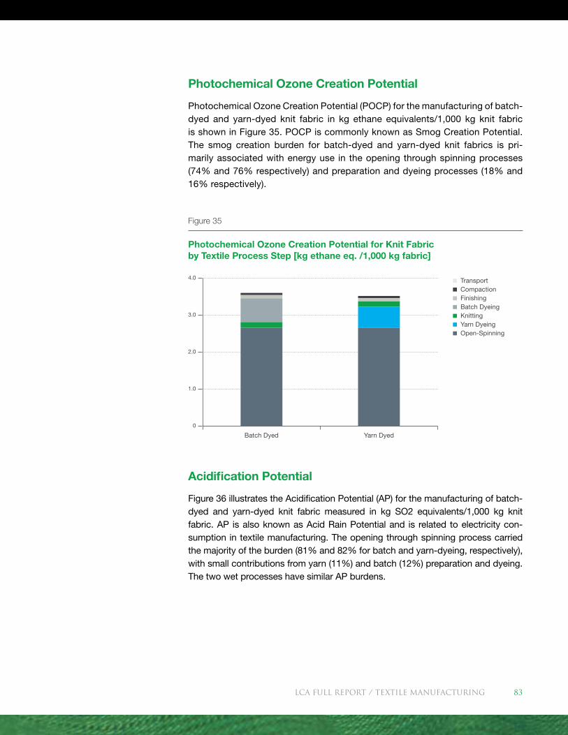
Photochemical Ozone Creation Potential
Photochemical Ozone Creation Potential (POCP) for the manufacturing of batch-dyed and yarn-dyed knit fabric in kg ethane equivalents/1,000 kg knit fabric is shown in Figure 35. POCP is commonly known as Smog Creation Potential. The smog creation burden for batch-dyed and yarn-dyed knit fabrics is pri-marily associated with energy use in the opening through spinning processes (74% and 76% respectively) and preparation and dyeing processes (18% and 16% respectively).
Acidification Potential
Figure 36 illustrates the Acidification Potential (AP) for the manufacturing of batch-dyed and yarn-dyed knit fabric measured in kg SO2 equivalents/1,000 kg knit fabric. AP is also known as Acid Rain Potential and is related to electricity con-sumption in textile manufacturing. The opening through spinning process carried the majority of the burden (81% and 82% for batch and yarn-dyeing, respectively), with small contributions from yarn (11%) and batch (12%) preparation and dyeing. The two wet processes have similar AP burdens.
Figure 35
Photochemical Ozone Creation Potential for Knit Fabric by Textile Process Step [kg ethane eq. /1,000 kg fabric]
Transport Compaction Finishing Batch Dyeing Knitting Yarn Dyeing Open-Spinning
4.0
3.0
2.0
1.0
0
Batch Dyed Yarn Dyed
LCA FULL REport / Textile manufacturing 83
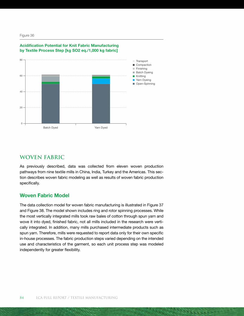
Figure 36
Acidification Potential for Knit Fabric Manufacturing by Textile Process Step [kg SO2 eq./1,000 kg fabric]
Transport Compaction Finishing Batch Dyeing Knitting Yarn Dyeing Open-Spinning
80
60
40
20
0
Batch Dyed Yarn Dyed
Woven Fabric
As previously described, data was collected from eleven woven production pathways from nine textile mills in China, India, Turkey and the Americas. This sec-tion describes woven fabric modeling as well as results of woven fabric production specifically.
Woven Fabric Model
The data collection model for woven fabric manufacturing is illustrated in Figure 37 and Figure 38. The model shown includes ring and rotor spinning processes. While the most vertically integrated mills took raw bales of cotton through spun yarn and wove it into dyed, finished fabric, not all mills included in the research were verti-cally integrated. In addition, many mills purchased intermediate products such as spun yarn. Therefore, mills were requested to report data only for their own specific in-house processes. The fabric production steps varied depending on the intended use and characteristics of the garment, so each unit process step was modeled independently for greater flexibility.
LCA FULL REport / Textile manufacturing84
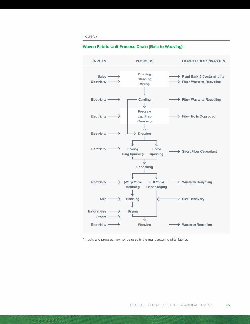
Figure 37
Woven Fabric Unit Process Chain (Bale to Weaving)
* Inputs and process may not be used in the manufacturing of all fabrics.
COPRODUCTS/WASTESPROCESS
Fiber Waste to Recycling
Fiber Waste to Recycling
Fiber Noils Coproduct
Short Fiber Coproduct
Size Recovery
Waste to Recycling
Carding
Drawing
Repacking
Roving
Ring Spinning
(Warp Yarn)
Beaming
Slashing
Drying
Rotor
Spinning
(Fill Yarn)
Repackaging
Weaving
Waste to Recycling
Predraw
Lap Prep
Combing
Opening
Cleaning
Mixing
INPUTS
Bales
Natural Gas
Size
Electricity
Steam
Electricity
Electricity
Electricity
Electricity
Electricity
Electricity
Plant Bark & Contaminants
LCA FULL REport / Textile manufacturing 85
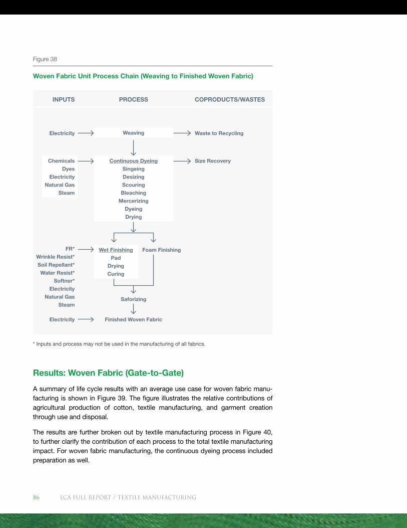
Results: Woven Fabric (Gate-to-Gate)
A summary of life cycle results with an average use case for woven fabric manu-facturing is shown in Figure 39. The figure illustrates the relative contributions of agricultural production of cotton, textile manufacturing, and garment creation through use and disposal.
The results are further broken out by textile manufacturing process in Figure 40, to further clarify the contribution of each process to the total textile manufacturing impact. For woven fabric manufacturing, the continuous dyeing process included preparation as well.
Figure 38
Woven Fabric Unit Process Chain (Weaving to Finished Woven Fabric)
* Inputs and process may not be used in the manufacturing of all fabrics.
COPRODUCTS/WASTESPROCESS
Waste to Recycling
Saforizing
Foam Finishing
Finished Woven Fabric
Size Recovery
Weaving
INPUTS
Electricity
Chemicals
Dyes
Electricity
Natural Gas
Steam
Electricity
FR*
Wrinkle Resist*
Soil Repellant*
Water Resist*
Softner*
Electricity
Natural Gas
Steam
Continuous Dyeing
Singeing
Desizing
Scouring
Bleaching
Mercerizing
Dyeing
Drying
Wet Finishing
Pad
Drying
Curing
LCA FULL REport / Textile manufacturing86
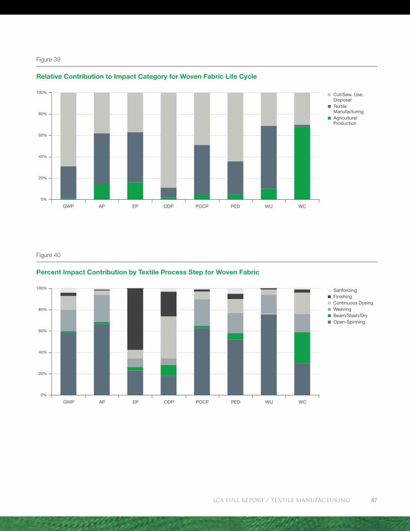
0%
GWP AP EP ODP POCP PED WU WC
Figure 40
Percent Impact Contribution by Textile Process Step for Woven Fabric
Sanforizing Finishing Continuous Dyeing Weaving Beam/Slash/Dry Open-Spinning
100%
80%
60%
40%
20%
Figure 39
Relative Contribution to Impact Category for Woven Fabric Life Cycle
Cut/Sew, Use, Disposal
Textile Manufacturing
Agricultural Production
100%
80%
60%
40%
20%
0%
GWP AP EP ODP POCP PED WU WC
LCA FULL REport / Textile manufacturing 87

The following sections show results for 1,000 kg of woven fabric. Although kg is not a unit typically used to represent woven production (usually square meters is used), the results were normalized in this way in order to compare with the knit outcomes.
More specifically, the impacts of the following woven manufacturing processes are highlighted:
� Bale Opening through Spinning: Energy for opening, cleaning, mixing, card-ing, pre-drawing, combing, drawing, and spinning cotton fiber into yarn
� Beam/Slash/Drying: Energy and chemicals for beaming, slashing, and drying warp yarn
� Weaving: Energy for weaving warp and fill yarn into fabric
� Continuous Dyeing: Energy, dyes, chemicals, emissions to water, and waste-water treatment processes related to singeing, desizing, scouring, bleaching, mercerizing, drying, dyeing, and redrying of greige yarn into colored yarn
� Finishing: Energy, chemicals, and emissions to water related to the wet finish-ing, drying, and curing of woven fabric
� Sanforizing: Energy and water used for shrinkage control of the finished fabric
� Transport: Energy for movement of bales from warehouse to mill and interme-diate products between locations
It is important to note that compared to China, India, Turkey, and Latin America, the emissions profile of US electricity has considerably less AP, EP, GWP, and POCP per kWh. Since the textile manufacturing data in this study was derived from countries other than the U.S., the burdens from energy-intense textile pro-cesses drove up these impact categories compared to the use phase, which was modeled with U.S. data.
LCA FULL REport / Textile manufacturing88
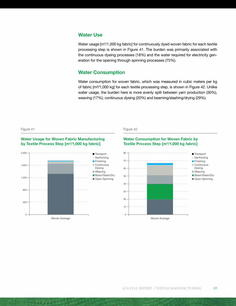
Water Use
Water usage [m3/1,000 kg fabric] for continuously dyed woven fabric for each textile processing step is shown in Figure 41. The burden was primarily associated with the continuous dyeing processes (18%) and the water required for electricity gen-eration for the opening through spinning processes (75%).
Water Consumption
Water consumption for woven fabric, which was measured in cubic meters per kg of fabric [m³/1,000 kg] for each textile processing step, is shown in Figure 42. Unlike water usage, the burden here is more evenly split between yarn production (30%), weaving (17%), continuous dyeing (20%) and beaming/slashing/drying (29%).
Figure 42
Water Consumption for Woven Fabric by Textile Process Step [m3/1,000 kg fabric]
Figure 41
Water Usage for Woven Fabric Manufacturing by Textile Process Step [m3/1,000 kg fabric]
Transport Sanforizing Finishing Continuous Dyeing Weaving Beam/Slash/Dry Open-Spinning
2,000
1,600
1,200
800
400
0
Woven Average
Transport Sanforizing Finishing Continuous Dyeing
Weaving Beam/Slash/Dry Open-Spinning
80
70
60
50
30
10
20
40
0
Woven Average
LCA FULL REport / Textile manufacturing 89
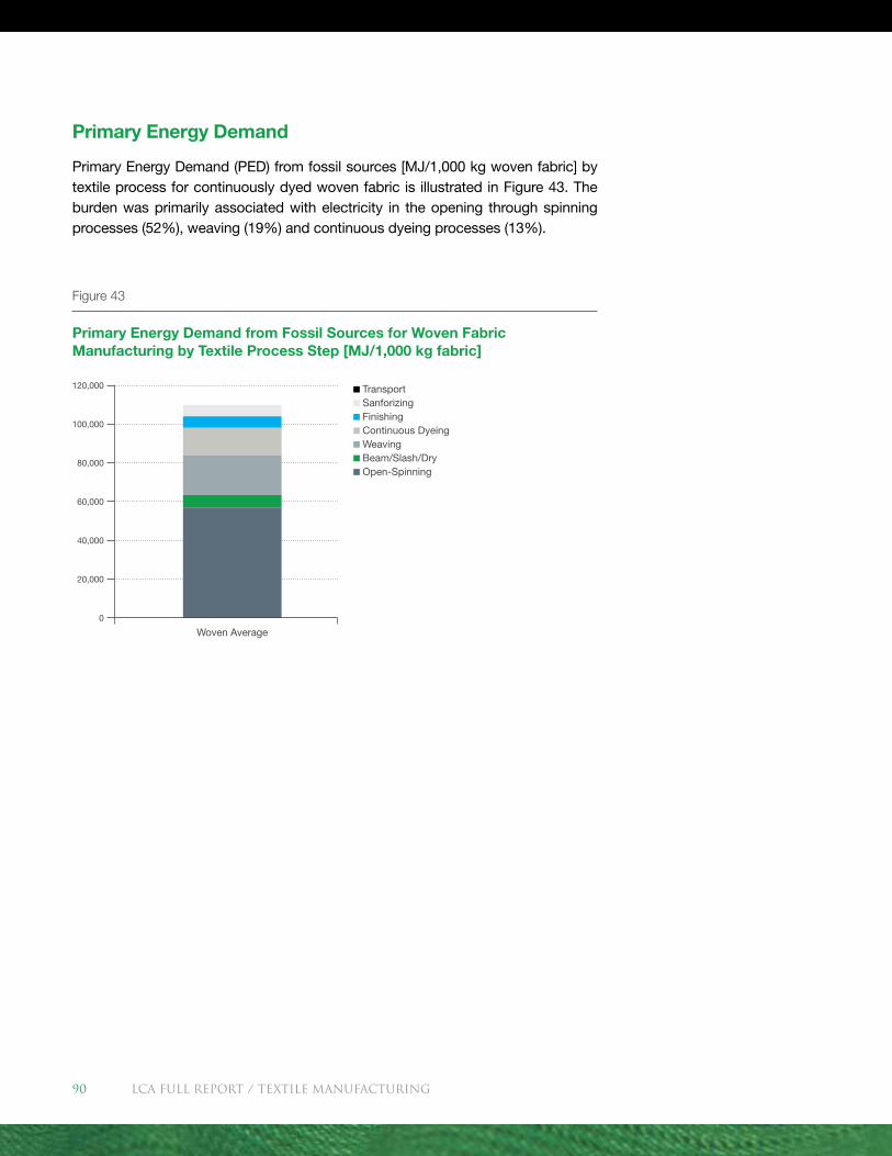
Primary Energy Demand
Primary Energy Demand (PED) from fossil sources [MJ/1,000 kg woven fabric] by textile process for continuously dyed woven fabric is illustrated in Figure 43. The burden was primarily associated with electricity in the opening through spinning processes (52%), weaving (19%) and continuous dyeing processes (13%).
Figure 43
Primary Energy Demand from Fossil Sources for Woven Fabric Manufacturing by Textile Process Step [MJ/1,000 kg fabric]
Transport Sanforizing Finishing Continuous Dyeing Weaving Beam/Slash/Dry Open-Spinning
120,000
100,000
80,000
60,000
20,000
40,000
0
Woven Average
LCA FULL REport / Textile manufacturing90
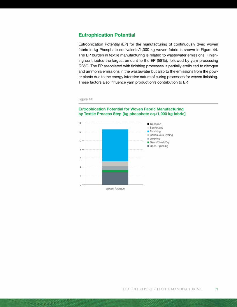
Eutrophication Potential
Eutrophication Potential (EP) for the manufacturing of continuously dyed woven fabric in kg Phosphate equivalents/1,000 kg woven fabric is shown in Figure 44. The EP burden in textile manufacturing is related to wastewater emissions. Finish-ing contributes the largest amount to the EP (58%), followed by yarn processing (23%). The EP associated with finishing processes is partially attributed to nitrogen and ammonia emissions in the wastewater but also to the emissions from the pow-er plants due to the energy intensive nature of curing processes for woven finishing. These factors also influence yarn production’s contribution to EP.
Figure 44
Eutrophication Potential for Woven Fabric Manufacturing by Textile Process Step [kg phosphate eq./1,000 kg fabric]
Transport Sanforizing Finishing Continuous Dyeing Weaving Beam/Slash/Dry Open-Spinning
14
10
12
8
6
2
4
0
Woven Average
LCA FULL REport / Textile manufacturing 91
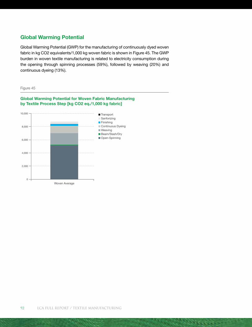
Global Warming Potential
Global Warming Potential (GWP) for the manufacturing of continuously dyed woven fabric in kg CO2 equivalents/1,000 kg woven fabric is shown in Figure 45. The GWP burden in woven textile manufacturing is related to electricity consumption during the opening through spinning processes (59%), followed by weaving (20%) and continuous dyeing (13%).
Figure 45
Global Warming Potential for Woven Fabric Manufacturing by Textile Process Step [kg CO2 eq./1,000 kg fabric]
Transport Sanforizing Finishing Continuous Dyeing Weaving Beam/Slash/Dry Open-Spinning
10,000
8,000
6,000
4,000
2,000
0
Woven Average
LCA FULL REport / Textile manufacturing92
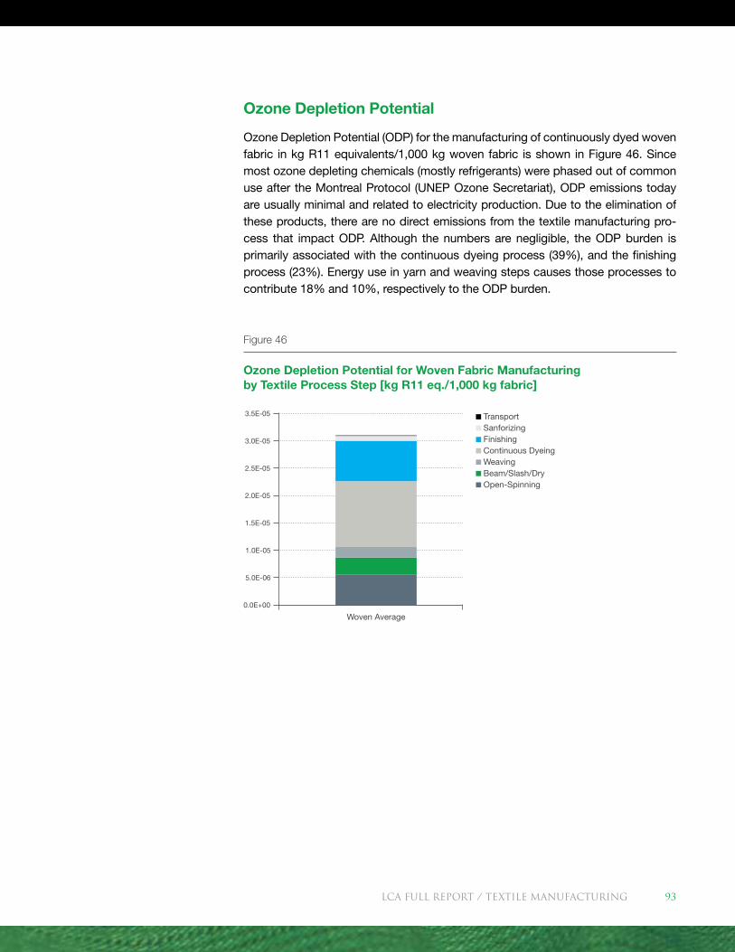
Ozone Depletion Potential
Ozone Depletion Potential (ODP) for the manufacturing of continuously dyed woven fabric in kg R11 equivalents/1,000 kg woven fabric is shown in Figure 46. Since most ozone depleting chemicals (mostly refrigerants) were phased out of common use after the Montreal Protocol (UNEP Ozone Secretariat), ODP emissions today are usually minimal and related to electricity production. Due to the elimination of these products, there are no direct emissions from the textile manufacturing pro-cess that impact ODP. Although the numbers are negligible, the ODP burden is primarily associated with the continuous dyeing process (39%), and the finishing process (23%). Energy use in yarn and weaving steps causes those processes to contribute 18% and 10%, respectively to the ODP burden.
Figure 46
Ozone Depletion Potential for Woven Fabric Manufacturing by Textile Process Step [kg R11 eq./1,000 kg fabric]
1.0E-05
5.0E-06
Transport Sanforizing Finishing Continuous Dyeing Weaving Beam/Slash/Dry Open-Spinning
3.5E-05
3.0E-05
2.5E-05
2.0E-05
1.5E-05
0.0E+00
Woven Average
LCA FULL REport / Textile manufacturing 93
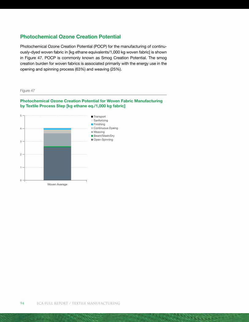
Photochemical Ozone Creation Potential
Photochemical Ozone Creation Potential (POCP) for the manufacturing of continu-ously-dyed woven fabric in [kg ethane equivalents/1,000 kg woven fabric] is shown in Figure 47. POCP is commonly known as Smog Creation Potential. The smog creation burden for woven fabrics is associated primarily with the energy use in the opening and spinning process (63%) and weaving (25%).
Figure 47
Photochemical Ozone Creation Potential for Woven Fabric Manufacturing by Textile Process Step [kg ethane eq./1,000 kg fabric]
Transport Sanforizing Finishing Continuous Dyeing Weaving Beam/Slash/Dry Open-Spinning
5
4
3
1
2
0
Woven Average
LCA FULL REport / Textile manufacturing94
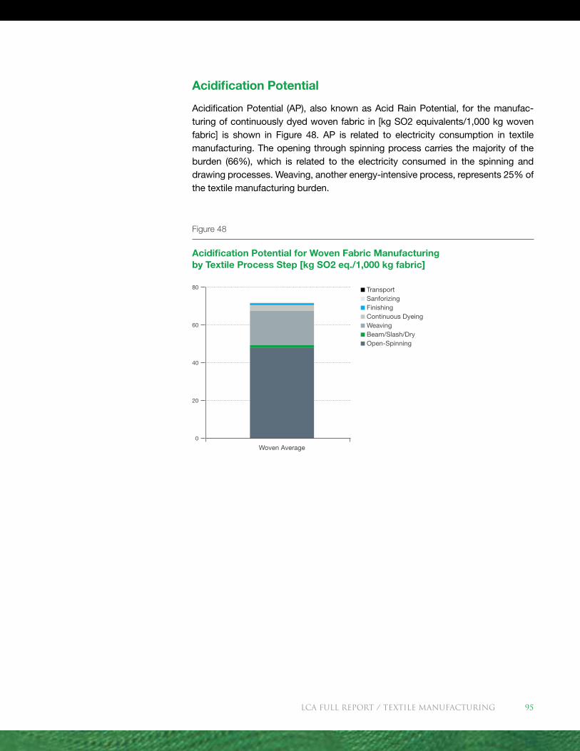
Acidification Potential
Acidification Potential (AP), also known as Acid Rain Potential, for the manufac-turing of continuously dyed woven fabric in [kg SO2 equivalents/1,000 kg woven fabric] is shown in Figure 48. AP is related to electricity consumption in textile manufacturing. The opening through spinning process carries the majority of the burden (66%), which is related to the electricity consumed in the spinning and drawing processes. Weaving, another energy-intensive process, represents 25% of the textile manufacturing burden.
Figure 48
Acidification Potential for Woven Fabric Manufacturing by Textile Process Step [kg SO2 eq./1,000 kg fabric]
Transport Sanforizing Finishing Continuous Dyeing Weaving Beam/Slash/Dry Open-Spinning
80
60
20
40
0
Woven Average
LCA FULL REport / Textile manufacturing 95
Results in Context
Spinning Sensitivity Analysis
The LCIA results of this study are influenced by only a few aspects of the cotton life cycle. Within textile manufacturing, the opening through spinning process energy for both knit and woven fabrics was the main contributor to Primary Energy Demand and its associated impacts—Global Warming Potential, Ozone Depletion Potential, Photochemical Ozone Creation Potential, and Acidification Potential. The main driver for energy demand and its associated impacts is the electricity associ-ated with yarn spinning. The range of reported spinning electricity in this study was wide, ranging from 1,910 to 16,095 MJ/ton yarn, and the standard deviation for the values was 4,349, which is 45% of the mean value. This variation could be attribut-ed to the following variables associated with fiber processing and could, therefore, impact electricity demand:
� Raw Material Choice—Trash content, fiber length, and micronaire (fineness) can greatly impact the efficiency of the spinning operation. Choosing fiber prop-erties that are most appropriate for the process, the yarn count, and the end product will mean higher efficiencies.
� Level of Processing and Technical Knowledge—This aspect is defined as the level to which a mill is capable of making the best technical choices to maintain and manage their equipment and processes. These choices impact greatly the efficiency of the operation.
� Capital Investment—This variable relates to a mill’s level of capital invest-ment, specifically toward process machinery and hardware technology. Newer and more advanced hardware have the potential to produce higher efficiencies and reduce energy consumption. However, poor management and technical knowledge can effectively negate the potential savings from a new technology or hardware.
� Spinning System—Ring, rotor, and air jet are the main spinning system choic-es available in the world today. Each system has advantages and disadvan-tages. Yarn count, end product, performance, and cost are important factors to consider when deciding which spinning system to use. Depending on the factors specific to a particular operation, choices may be limited and in some cases, there may only be one choice. Ring spinning is most likely the least efficient method, but it produces a yarn with characteristics and performance that cannot be duplicated by the other systems. Rotor spinning is perhaps the most efficient spinning system, but it has limitations as to yarn count range, tensile properties, and fabric hand. Air jet most likely falls somewhere between the two, but it has significant limitations as to yarn count range and tensile properties. Although air jet spinning is more closely related to rotor spinning than to ring spinning in its efficiency in producing yarn, it is not widely used in the produc-tion of 100% cotton yarns.
LCA FULL REport / Textile manufacturing96
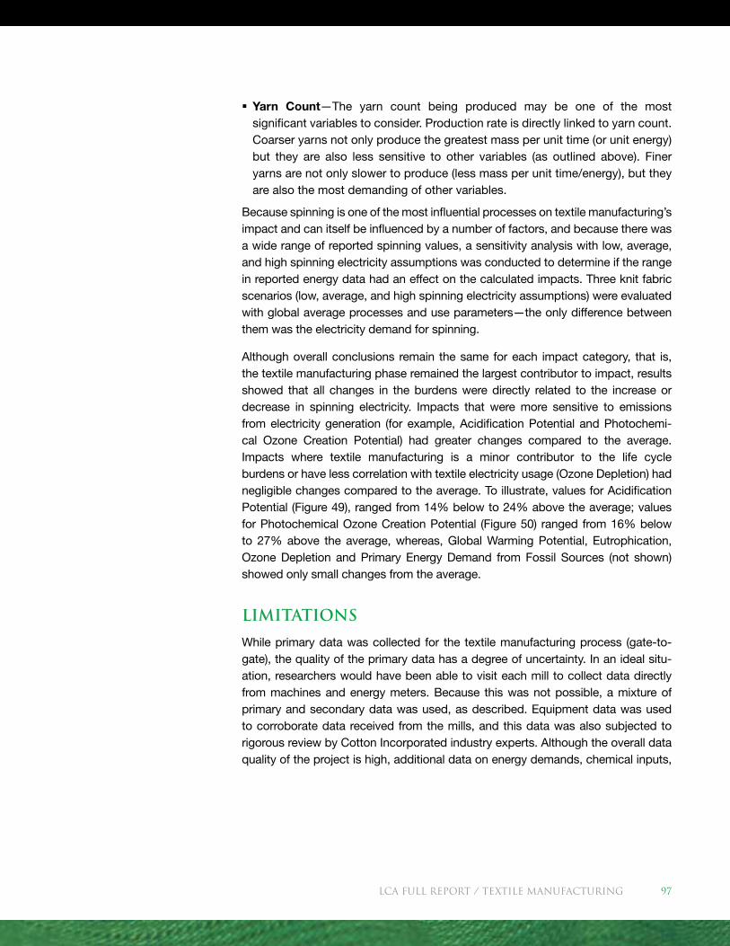
� Yarn Count—The yarn count being produced may be one of the most significant variables to consider. Production rate is directly linked to yarn count. Coarser yarns not only produce the greatest mass per unit time (or unit energy) but they are also less sensitive to other variables (as outlined above). Finer yarns are not only slower to produce (less mass per unit time/energy), but they are also the most demanding of other variables.
Because spinning is one of the most influential processes on textile manufacturing’s impact and can itself be influenced by a number of factors, and because there was a wide range of reported spinning values, a sensitivity analysis with low, average, and high spinning electricity assumptions was conducted to determine if the range in reported energy data had an effect on the calculated impacts. Three knit fabric scenarios (low, average, and high spinning electricity assumptions) were evaluated with global average processes and use parameters—the only difference between them was the electricity demand for spinning.
Although overall conclusions remain the same for each impact category, that is, the textile manufacturing phase remained the largest contributor to impact, results showed that all changes in the burdens were directly related to the increase or decrease in spinning electricity. Impacts that were more sensitive to emissions from electricity generation (for example, Acidification Potential and Photochemi-cal Ozone Creation Potential) had greater changes compared to the average. Impacts where textile manufacturing is a minor contributor to the life cycle burdens or have less correlation with textile electricity usage (Ozone Depletion) had negligible changes compared to the average. To illustrate, values for Acidification Potential (Figure 49), ranged from 14% below to 24% above the average; values for Photochemical Ozone Creation Potential (Figure 50) ranged from 16% below to 27% above the average, whereas, Global Warming Potential, Eutrophication, Ozone Depletion and Primary Energy Demand from Fossil Sources (not shown) showed only small changes from the average.
Limitations
While primary data was collected for the textile manufacturing process (gate-to-gate), the quality of the primary data has a degree of uncertainty. In an ideal situ-ation, researchers would have been able to visit each mill to collect data directly from machines and energy meters. Because this was not possible, a mixture of primary and secondary data was used, as described. Equipment data was used to corroborate data received from the mills, and this data was also subjected to rigorous review by Cotton Incorporated industry experts. Although the overall data quality of the project is high, additional data on energy demands, chemical inputs,
LCA FULL REport / Textile manufacturing 97
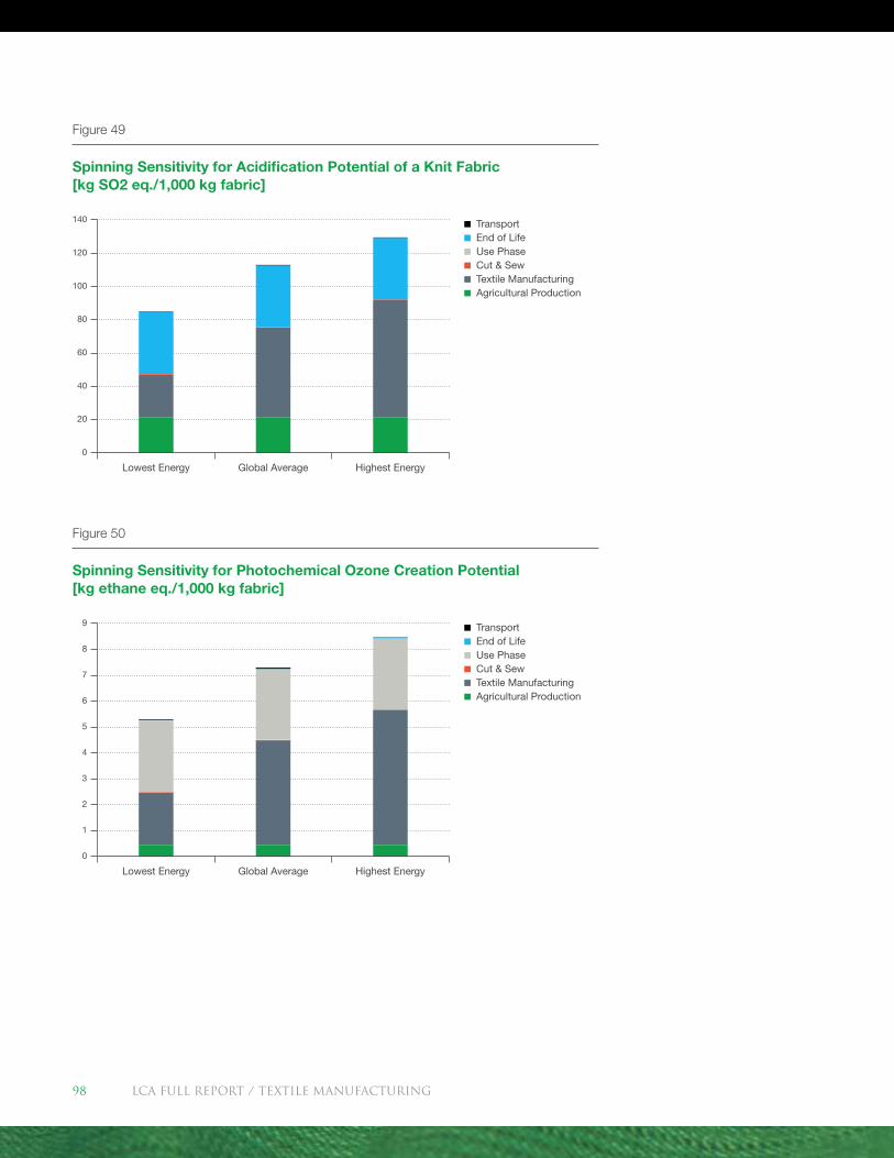
Figure 49
Spinning Sensitivity for Acidification Potential of a Knit Fabric [kg SO2 eq./1,000 kg fabric]
Figure 50
Spinning Sensitivity for Photochemical Ozone Creation Potential [kg ethane eq./1,000 kg fabric]
Transport End of Life Use Phase Cut & Sew Textile Manufacturing Agricultural Production
140
120
80
60
100
40
20
0
Lowest Energy Global Average Highest Energy
Transport End of Life Use Phase Cut & Sew Textile Manufacturing Agricultural Production
9
7
6
8
4
3
5
2
1
0
Lowest Energy Global Average Highest Energy
LCA FULL REport / Textile manufacturing98
and wastewater outputs will enhance future studies. In addition, a larger mill sample size would provide greater detail for certain processes and help to smooth out vari-ability in reported values. However, as seen from the spinning sensitivity analysis, the variability in energy data, even for such an important process, did not have a large effect on the calculated LCIA values.
Table 17 illustrates of the variability in the other measures by looking at the vari-ability of individual mill data compared to the global average. For a majority of the parameters, the standard deviation is within 50% of the mean with some clear ex-ceptions. Note that one source of variability applicable to all of the parameters is related to the difference in power grids between countries evaluated. Much of the variability seen in EP can be traced back to the finishing process where there were considerable differences between individual mills. Variability in ODP is partially due to the fact that the mean value is small (as previously noted, many ozone depleting chemistries have been eliminated from manufacturing). Similarly, the mean WC was relatively small, and in some cases measurement procedures resulted in negative values at some mills.
The emissions figures provided in this report have been calculated in accordance with the requirements of the PAS 2050 method, using the primary and secondary sources of data specified above. Based on the PAS 2050 method of assessment we believe that our assessment has identified 95% of the likely GHG emissions associ-ated with the full life cycle of the product(s) covered in this report. However, readers should be aware that even primary sources of data are estimates and are subject to variation over time, and the figures given in this report should be considered as our best estimates, based on reasonable cost of evaluation.
LCA FULL REport / Textile manufacturing 99
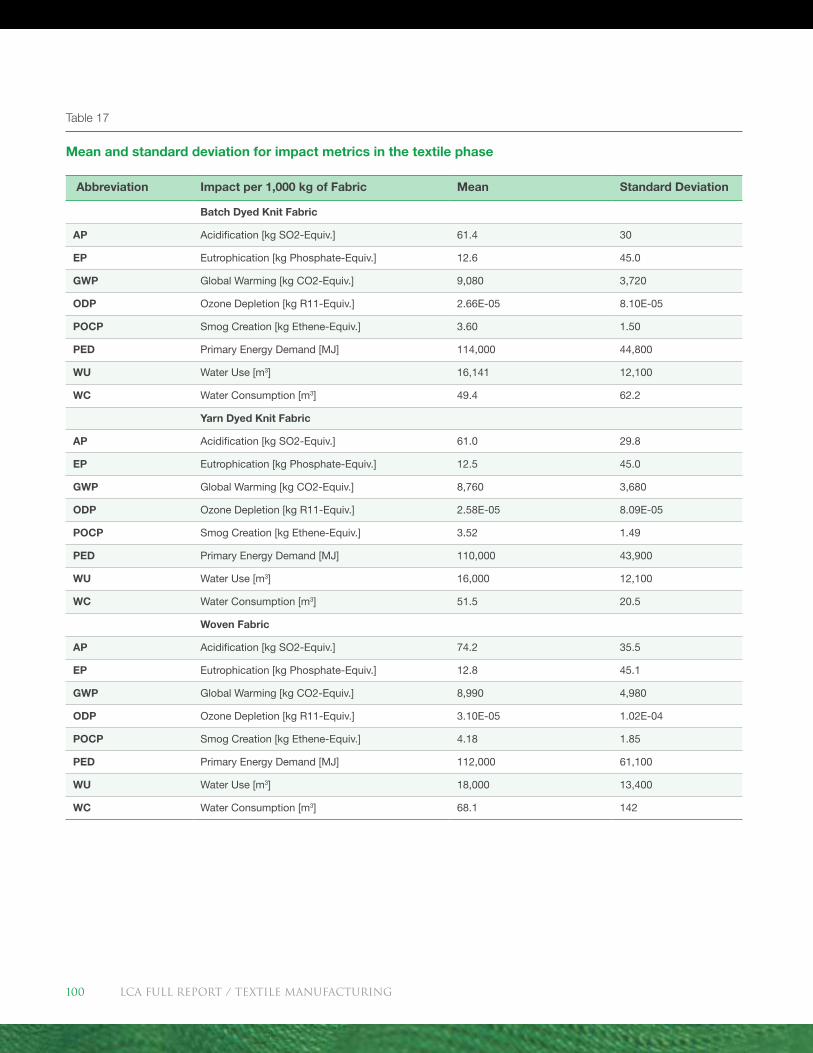
Table 17
Mean and standard deviation for impact metrics in the textile phase
Abbreviation Impact per 1,000 kg of Fabric Mean Standard Deviation
Batch Dyed Knit Fabric
AP Acidification [kg SO2-Equiv.] 61.4 30
EP Eutrophication [kg Phosphate-Equiv.] 12.6 45.0
GWP Global Warming [kg CO2-Equiv.] 9,080 3,720
ODP Ozone Depletion [kg R11-Equiv.] 2.66E-05 8.10E-05
POCP Smog Creation [kg Ethene-Equiv.] 3.60 1.50
PED Primary Energy Demand [MJ] 114,000 44,800
WU Water Use [m3] 16,141 12,100
WC Water Consumption [m3] 49.4 62.2
Yarn Dyed Knit Fabric
AP Acidification [kg SO2-Equiv.] 61.0 29.8
EP Eutrophication [kg Phosphate-Equiv.] 12.5 45.0
GWP Global Warming [kg CO2-Equiv.] 8,760 3,680
ODP Ozone Depletion [kg R11-Equiv.] 2.58E-05 8.09E-05
POCP Smog Creation [kg Ethene-Equiv.] 3.52 1.49
PED Primary Energy Demand [MJ] 110,000 43,900
WU Water Use [m3] 16,000 12,100
WC Water Consumption [m3] 51.5 20.5
Woven Fabric
AP Acidification [kg SO2-Equiv.] 74.2 35.5
EP Eutrophication [kg Phosphate-Equiv.] 12.8 45.1
GWP Global Warming [kg CO2-Equiv.] 8,990 4,980
ODP Ozone Depletion [kg R11-Equiv.] 3.10E-05 1.02E-04
POCP Smog Creation [kg Ethene-Equiv.] 4.18 1.85
PED Primary Energy Demand [MJ] 112,000 61,100
WU Water Use [m3] 18,000 13,400
WC Water Consumption [m3] 68.1 142
LCA FULL REport / Textile manufacturing100
Conclusions: Textile Manufacturing of Knit and Woven Fabrics (Gate-to-Gate)
� Yarn production (spinning) is the main contributor for Global Warming Potential, Acidification Potential, Photochemical Ozone Creation Potential, and Primary Energy Demand due to its high electricity demand. Energy for weaving is also a relevant contributor for these impacts.
� Energy for conditioning, processing, and heating, and eventual drying of the water in the preparation and dye processes is also a significant contributor within the textile manufacturing life cycle stage.
� The relevant contributors to Eutrophication Potential in the Textile Manufacturing Phase are more complex than the other impacts. For wovens, wastewater emis-sions from continuous preparation and dyeing are primary influencers to EP. For the knit fabric manufacturing processes, upstream impacts from manufacturing of chemicals for batch preparation and dyeing and for finishing, as well as emis-sions from power generation processes can have as much impact on the EP as the actual wet processes.
� Though considerable amounts of water are used in preparation, dyeing, and finishing, much of that water is returned to the watershed, so is not considered in the Water Consumption metric. The water consumed in manufacturing is spread between wet processes and the upstream production of energy. These manufacturing water flows are far outweighed by water consumed during irriga-tion and consumer washing.
LCA FULL REport / Textile manufacturing 101

USE PHASE
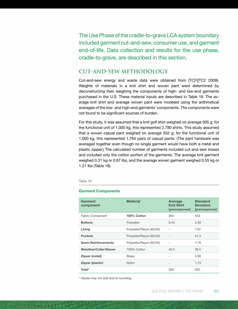
The Use Phase of the cradle-to-grave LCA system boundary included garment cut-and-sew, consumer use, and garment end-of-life. Data collection and results for the use phase, cradle-to-grave, are described in this section.
Cut-and-Sew Methodology
Cut-and-sew energy and waste data were obtained from [TC]2([TC2 2009). Weights of materials in a knit shirt and woven pant were determined by deconstructing then weighing the components of high- and low-end garments purchased in the U.S. These material inputs are described in Table 18. The av-erage knit shirt and average woven pant were modeled using the arithmetical averages of the low- and high-end garments’ components. The components were not found to be significant sources of burden.
For this study, it was assumed that a knit golf shirt weighed on average 305 g; for the functional unit of 1,000 kg, this represented 2,780 shirts. This study assumed that a woven casual pant weighed on average 552 g; for the functional unit of 1,000 kg, this represented 1,764 pairs of casual pants. (The pant hardware was averaged together even though no single garment would have both a metal and plastic zipper.) The calculated number of garments included cut-and-sew losses and included only the cotton portion of the garments. The average knit garment weighed 0.31 kg or 0.67 lbs, and the average woven garment weighed 0.55 kg or 1.21 lbs (Table 18).
Table 18
Garment Components
Garment component
Material Average Knit Shirt [grams/garment]
Standard Deviation [grams/garment]
Fabric Component 100% Cotton 264 453
Buttons Polyester 0.45 2.39
Lining Polyester/Rayon (65/35) - 7.07
Pockets Polyester/Rayon (65/35) - 41.3
Seam Reinforcements Polyester/Rayon (65/35) - 1.78
Waistline/Collar/Sleeve 100% Cotton 40.3 39.5
Zipper (metal) Brass - 4.90
Zipper (plastic) Nylon - 1.73
Total* 305 552
* Values may not add due to rounding.
LCA FULL REport / Use Phase 103
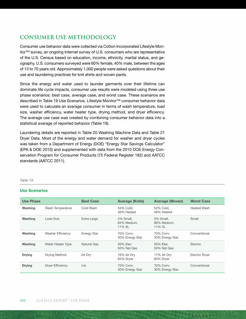
Consumer Use Methodology
Consumer use behavior data were collected via Cotton Incorporated Lifestyle Mon-itor™ survey, an ongoing Internet survey of U.S. consumers who are representative of the U.S. Census based on education, income, ethnicity, marital status, and ge-ography. U.S. consumers surveyed were 60% female, 40% male, between the ages of 13 to 70 years old. Approximately 1,000 people were asked questions about their use and laundering practices for knit shirts and woven pants.
Since the energy and water used to launder garments over their lifetime can dominate life cycle impacts, consumer use results were modeled using three use phase scenarios: best case, average case, and worst case. These scenarios are described in Table 19 Use Scenarios. Lifestyle Monitor™ consumer behavior data were used to calculate an average consumer in terms of wash temperature, load size, washer efficiency, water heater type, drying method, and dryer efficiency. The average use case was created by combining consumer behavior data into a statistical average of reported behavior (Table 19).
Laundering details are reported in Table 20 Washing Machine Data and Table 21 Dryer Data. Most of the energy and water demand for washer and dryer cycles was taken from a Department of Energy (DOE) “Energy Star Savings Calculator” (EPA & DOE 2010) and supplemented with data from the 2010 DOE Energy Con-servation Program for Consumer Products (75 Federal Register 182) and AATCC standards (AATCC 2011).
Table 19
Use Scenarios
Use Phase Best Case Average (Knits) Average (Woven) Worst Case
Washing Wash Temperature Cold Wash 54% Cold, 46% Heated
52% Cold, 48% Heated
Heated Wash
Washing Load Size Extra Large 5% Small, 84% Medium, 11% XL
3% Small, 86% Medium, 11% XL
Small
Washing Washer Efficiency Energy Star 70% Conv. 30% Energy Star
70% Conv. 30% Energy Star
Conventional
Washing Water Heater Type Natural Gas 50% Elec 50% Nat Gas
50% Elec 50% Nat Gas
Electric
Drying Drying Method Air Dry 16% Air Dry 84% Dryer
17% Air Dry 83% Dryer
Electric Dryer
Drying Dryer Efficiency n/a 70% Conv. 30% Energy Star
70% Conv. 30% Energy Star
Conventional
LCA FULL REport / Use Phase104
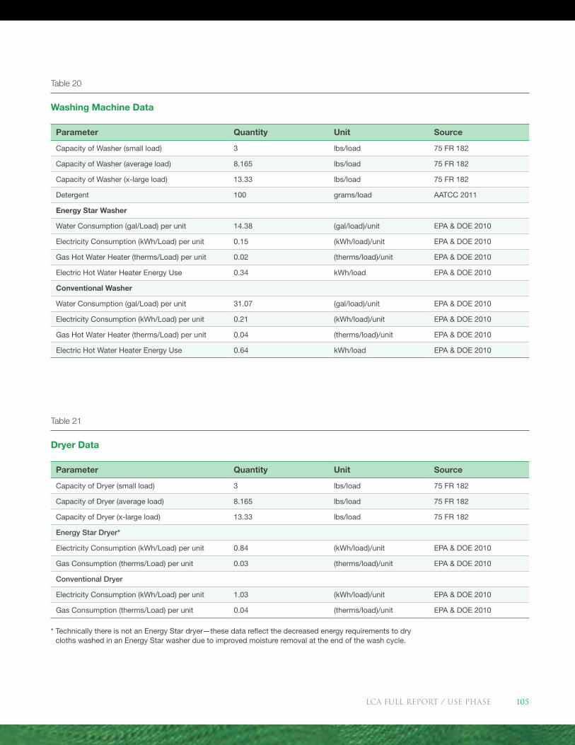
Table 20
Washing Machine Data
Parameter Quantity Unit Source
Capacity of Washer (small load) 3 lbs/load 75 FR 182
Capacity of Washer (average load) 8.165 lbs/load 75 FR 182
Capacity of Washer (x-large load) 13.33 lbs/load 75 FR 182
Detergent 100 grams/load AATCC 2011
Energy Star Washer
Water Consumption (gal/Load) per unit 14.38 (gal/load)/unit EPA & DOE 2010
Electricity Consumption (kWh/Load) per unit 0.15 (kWh/load)/unit EPA & DOE 2010
Gas Hot Water Heater (therms/Load) per unit 0.02 (therms/load)/unit EPA & DOE 2010
Electric Hot Water Heater Energy Use 0.34 kWh/load EPA & DOE 2010
Conventional Washer
Water Consumption (gal/Load) per unit 31.07 (gal/load)/unit EPA & DOE 2010
Electricity Consumption (kWh/Load) per unit 0.21 (kWh/load)/unit EPA & DOE 2010
Gas Hot Water Heater (therms/Load) per unit 0.04 (therms/load)/unit EPA & DOE 2010
Electric Hot Water Heater Energy Use 0.64 kWh/load EPA & DOE 2010
Table 21
Dryer Data
Parameter Quantity Unit Source
Capacity of Dryer (small load) 3 lbs/load 75 FR 182
Capacity of Dryer (average load) 8.165 lbs/load 75 FR 182
Capacity of Dryer (x-large load) 13.33 lbs/load 75 FR 182
Energy Star Dryer*
Electricity Consumption (kWh/Load) per unit 0.84 (kWh/load)/unit EPA & DOE 2010
Gas Consumption (therms/Load) per unit 0.03 (therms/load)/unit EPA & DOE 2010
Conventional Dryer
Electricity Consumption (kWh/Load) per unit 1.03 (kWh/load)/unit EPA & DOE 2010
Gas Consumption (therms/Load) per unit 0.04 (therms/load)/unit EPA & DOE 2010
* Technically there is not an Energy Star dryer—these data reflect the decreased energy requirements to dry cloths washed in an Energy Star washer due to improved moisture removal at the end of the wash cycle.
LCA FULL REport / Use Phase 105
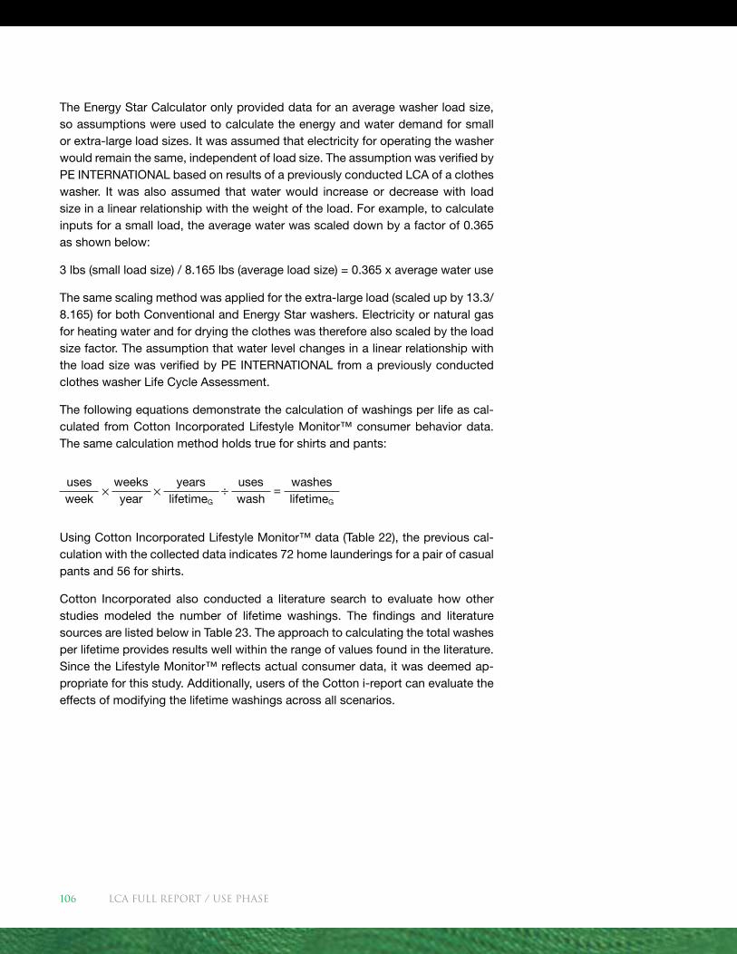
The Energy Star Calculator only provided data for an average washer load size, so assumptions were used to calculate the energy and water demand for small or extra-large load sizes. It was assumed that electricity for operating the washer would remain the same, independent of load size. The assumption was verified by PE INTERNATIONAL based on results of a previously conducted LCA of a clothes washer. It was also assumed that water would increase or decrease with load size in a linear relationship with the weight of the load. For example, to calculate inputs for a small load, the average water was scaled down by a factor of 0.365 as shown below:
3 lbs (small load size) / 8.165 lbs (average load size) = 0.365 x average water use
The same scaling method was applied for the extra-large load (scaled up by 13.3/ 8.165) for both Conventional and Energy Star washers. Electricity or natural gas for heating water and for drying the clothes was therefore also scaled by the load size factor. The assumption that water level changes in a linear relationship with the load size was verified by PE INTERNATIONAL from a previously conducted clothes washer Life Cycle Assessment.
The following equations demonstrate the calculation of washings per life as cal-culated from Cotton Incorporated Lifestyle Monitor™ consumer behavior data. The same calculation method holds true for shirts and pants:
usesweek
weeksyear
yearslifetimeG
useswash
washeslifetimeG
=
Using Cotton Incorporated Lifestyle Monitor™ data (Table 22), the previous cal-culation with the collected data indicates 72 home launderings for a pair of casual pants and 56 for shirts.
Cotton Incorporated also conducted a literature search to evaluate how other studies modeled the number of lifetime washings. The findings and literature sources are listed below in Table 23. The approach to calculating the total washes per lifetime provides results well within the range of values found in the literature. Since the Lifestyle Monitor™ reflects actual consumer data, it was deemed ap-propriate for this study. Additionally, users of the Cotton i-report can evaluate the effects of modifying the lifetime washings across all scenarios.
LCA FULL REport / Use Phase106
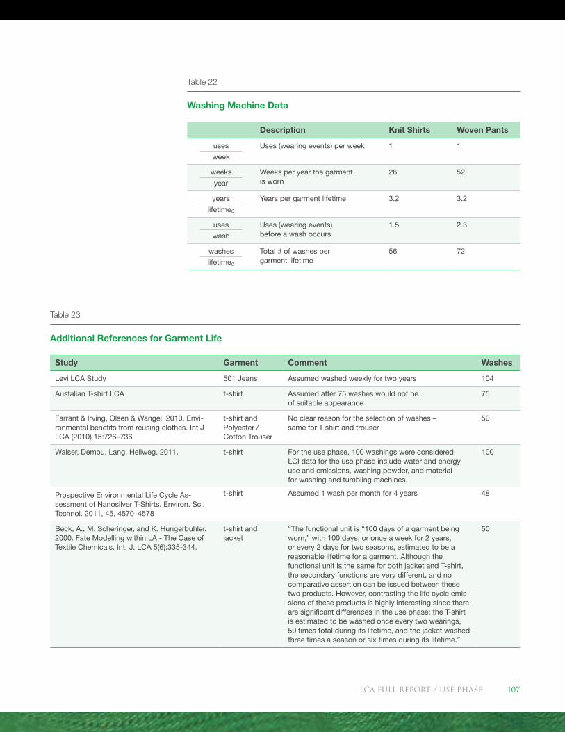
Table 22
Washing Machine Data
Table 23
Additional References for Garment Life
Description Knit Shirts Woven Pants
uses
week
Uses (wearing events) per week 1 1
weeks
year
Weeks per year the garment is worn
26 52
years
lifetimeG
Years per garment lifetime 3.2 3.2
uses
wash
Uses (wearing events) before a wash occurs
1.5 2.3
washes
lifetimeG
Total # of washes per garment lifetime
56 72
Study Garment Comment Washes
Levi LCA Study 501 Jeans Assumed washed weekly for two years 104
Austalian T-shirt LCA t-shirt Assumed after 75 washes would not be of suitable appearance
75
Farrant & Irving, Olsen & Wangel. 2010. Envi-ronmental benefits from reusing clothes. Int J LCA (2010) 15:726–736
t-shirt and Polyester / Cotton Trouser
No clear reason for the selection of washes – same for T-shirt and trouser
50
Walser, Demou, Lang, Hellweg. 2011. t-shirt For the use phase, 100 washings were considered. LCI data for the use phase include water and energy use and emissions, washing powder, and material for washing and tumbling machines.
100
Prospective Environmental Life Cycle As-sessment of Nanosilver T-Shirts. Environ. Sci. Technol. 2011, 45, 4570–4578
t-shirt Assumed 1 wash per month for 4 years 48
Beck, A., M. Scheringer, and K. Hungerbuhler. 2000. Fate Modelling within LA - The Case of Textile Chemicals. Int. J. LCA 5(6):335-344.
t-shirt and jacket
“The functional unit is “100 days of a garment being worn,” with 100 days, or once a week for 2 years, or every 2 days for two seasons, estimated to be a reasonable lifetime for a garment. Although the functional unit is the same for both jacket and T-shirt, the secondary functions are very different, and no comparative assertion can be issued between these two products. However, contrasting the life cycle emis-sions of these products is highly interesting since there are significant differences in the use phase: the T-shirt is estimated to be washed once every two wearings, 50 times total during its lifetime, and the jacket washed three times a season or six times during its lifetime.”
50
LCA FULL REport / Use Phase 107
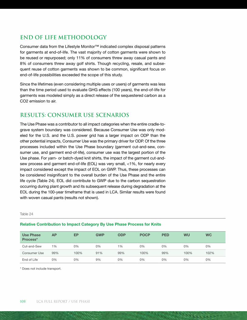
End of Life Methodology
Consumer data from the Lifestyle Monitor™ indicated complex disposal patterns for garments at end-of-life. The vast majority of cotton garments were shown to be reused or repurposed; only 11% of consumers threw away casual pants and 8% of consumers threw away golf shirts. Though recycling, resale, and subse-quent reuse of cotton garments was shown to be common, significant focus on end-of-life possibilities exceeded the scope of this study.
Since the lifetimes (even considering multiple uses or users) of garments was less than the time period used to evaluate GHG effects (100 years), the end-of-life for garments was modeled simply as a direct release of the sequestered carbon as a CO2 emission to air.
Results: Consumer Use Scenarios
The Use Phase was a contributor to all impact categories when the entire cradle-to-grave system boundary was considered. Because Consumer Use was only mod-eled for the U.S. and the U.S. power grid has a larger impact on ODP than the other potential impacts, Consumer Use was the primary driver for ODP. Of the three processes included within the Use Phase boundary (garment cut-and-sew, con-sumer use, and garment end-of-life), consumer use was the largest portion of the Use phase. For yarn- or batch-dyed knit shirts, the impact of the garment cut-and-sew process and garment end-of-life (EOL) was very small, <1%, for nearly every impact considered except the impact of EOL on GWP. Thus, these processes can be considered insignificant to the overall burden of the Use Phase and the entire life cycle (Table 24). EOL did contribute to GWP due to the carbon sequestration occurring during plant growth and its subsequent release during degradation at the EOL during the 100-year timeframe that is used in LCA. Similar results were found with woven casual pants (results not shown).
Table 24
Relative Contribution to Impact Category By Use Phase Process for Knits
Use Phase Process*
AP EP GWP ODP POCP PED WU WC
Cut-and-Sew 1% 0% 0% 1% 0% 0% 0% 0%
Consumer Use 99% 100% 91% 99% 100% 99% 100% 102%
End of Life 0% 0% 9% 0% 0% 0% 0% 0%
* Does not include transport.
LCA FULL REport / Use Phase108
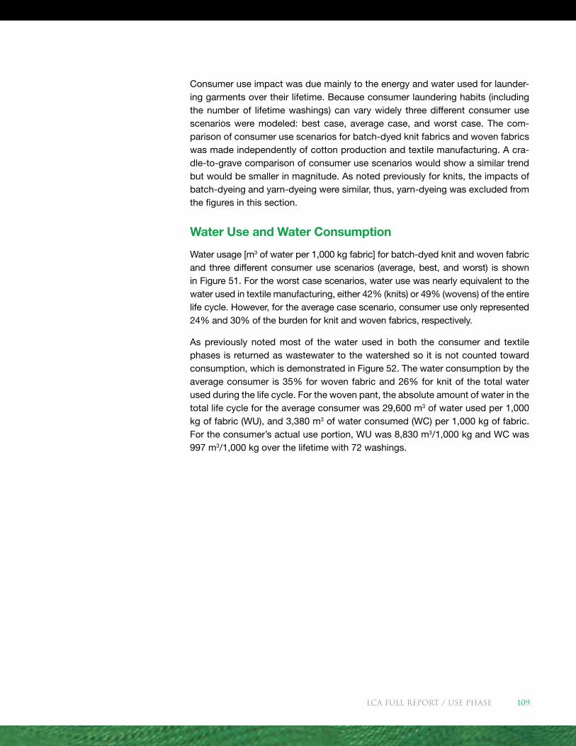
Consumer use impact was due mainly to the energy and water used for launder-ing garments over their lifetime. Because consumer laundering habits (including the number of lifetime washings) can vary widely three different consumer use scenarios were modeled: best case, average case, and worst case. The com-parison of consumer use scenarios for batch-dyed knit fabrics and woven fabrics was made independently of cotton production and textile manufacturing. A cra-dle-to-grave comparison of consumer use scenarios would show a similar trend but would be smaller in magnitude. As noted previously for knits, the impacts of batch-dyeing and yarn-dyeing were similar, thus, yarn-dyeing was excluded from the figures in this section.
Water Use and Water Consumption
Water usage [m3 of water per 1,000 kg fabric] for batch-dyed knit and woven fabric and three different consumer use scenarios (average, best, and worst) is shown in Figure 51. For the worst case scenarios, water use was nearly equivalent to the water used in textile manufacturing, either 42% (knits) or 49% (wovens) of the entire life cycle. However, for the average case scenario, consumer use only represented 24% and 30% of the burden for knit and woven fabrics, respectively.
As previously noted most of the water used in both the consumer and textile phases is returned as wastewater to the watershed so it is not counted toward consumption, which is demonstrated in Figure 52. The water consumption by the average consumer is 35% for woven fabric and 26% for knit of the total water used during the life cycle. For the woven pant, the absolute amount of water in the total life cycle for the average consumer was 29,600 m3 of water used per 1,000 kg of fabric (WU), and 3,380 m3 of water consumed (WC) per 1,000 kg of fabric. For the consumer’s actual use portion, WU was 8,830 m3/1,000 kg and WC was 997 m3/1,000 kg over the lifetime with 72 washings.
LCA FULL REport / Use Phase 109
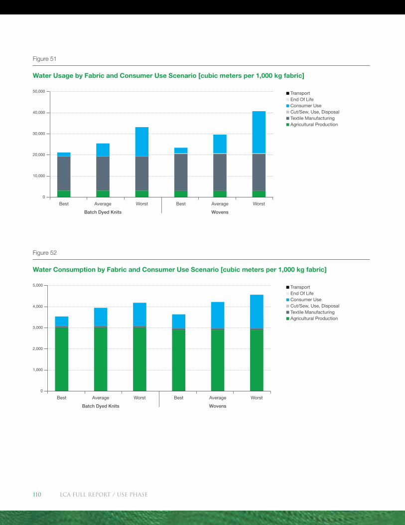
Figure 51
Water Usage by Fabric and Consumer Use Scenario [cubic meters per 1,000 kg fabric]
Transport End Of Life Consumer Use Cut/Sew, Use, Disposal Textile Manufacturing Agricultural Production
50,000
40,000
30,000
20,000
10,000
0
Best BestAverage
Batch Dyed Knits Wovens
AverageWorst Worst
Figure 52
Water Consumption by Fabric and Consumer Use Scenario [cubic meters per 1,000 kg fabric]
Transport End Of Life Consumer Use Cut/Sew, Use, Disposal Textile Manufacturing Agricultural Production
5,000
4,000
3,000
2,000
1,000
0
Best BestAverage
Batch Dyed Knits Wovens
AverageWorst Worst
LCA FULL REport / Use Phase110
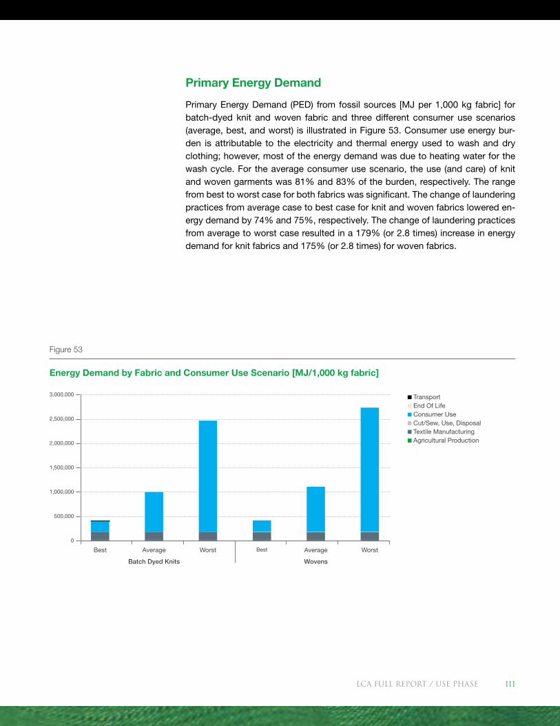
Primary Energy Demand
Primary Energy Demand (PED) from fossil sources [MJ per 1,000 kg fabric] for batch-dyed knit and woven fabric and three different consumer use scenarios (average, best, and worst) is illustrated in Figure 53. Consumer use energy bur-den is attributable to the electricity and thermal energy used to wash and dry clothing; however, most of the energy demand was due to heating water for the wash cycle. For the average consumer use scenario, the use (and care) of knit and woven garments was 81% and 83% of the burden, respectively. The range from best to worst case for both fabrics was significant. The change of laundering practices from average case to best case for knit and woven fabrics lowered en-ergy demand by 74% and 75%, respectively. The change of laundering practices from average to worst case resulted in a 179% (or 2.8 times) increase in energy demand for knit fabrics and 175% (or 2.8 times) for woven fabrics.
Figure 53
Energy Demand by Fabric and Consumer Use Scenario [MJ/1,000 kg fabric]
Transport End Of Life Consumer Use Cut/Sew, Use, Disposal Textile Manufacturing Agricultural Production
3,000,000
2,500,000
2,000,000
1,500,000
1,000,000
500,000
0
Best BestAverage
Batch Dyed Knits Wovens
AverageWorst Worst
LCA FULL REport / Use Phase 111
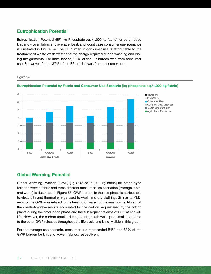
Eutrophication Potential
Eutrophication Potential (EP) [kg Phosphate eq. /1,000 kg fabric] for batch-dyed knit and woven fabric and average, best, and worst case consumer use scenarios is illustrated in Figure 54. The EP burden in consumer use is attributable to the treatment of waste wash water and the energy required during washing and dry-ing the garments. For knits fabrics, 29% of the EP burden was from consumer use. For woven fabric, 37% of the EP burden was from consumer use.
Global Warming Potential
Global Warming Potential (GWP) [kg CO2 eq. /1,000 kg fabric] for batch-dyed knit and woven fabric and three different consumer use scenarios (average, best, and worst) is illustrated in Figure 55. GWP burden in the use phase is attributable to electricity and thermal energy used to wash and dry clothing. Similar to PED, most of the GWP was related to the heating of water for the wash cycle. Note that the cradle-to-grave results accounted for the carbon sequestered by the cotton plants during the production phase and the subsequent release of CO2 at end-of-life. However, the carbon uptake during plant growth was quite small compared to the other GWP releases throughout the life cycle and is not visible in this graph.
For the average use scenario, consumer use represented 54% and 63% of the GWP burden for knit and woven fabrics, respectively.
Figure 54
Eutrophication Potential by Fabric and Consumer Use Scenario [kg phosphate eq./1,000 kg fabric]
Transport End Of Life Consumer Use Cut/Sew, Use, Disposal Textile Manufacturing Agricultural Production
35
25
30
20
15
10
5
0
Best BestAverage
Batch Dyed Knits Wovens
AverageWorst Worst
LCA FULL REport / Use Phase112
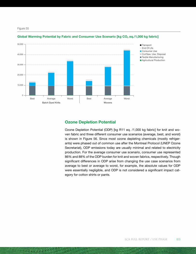
Ozone Depletion Potential
Ozone Depletion Potential (ODP) [kg R11 eq. /1,000 kg fabric] for knit and wo-ven fabric and three different consumer use scenarios (average, best, and worst) is shown in Figure 56. Since most ozone depleting chemicals (mostly refriger-ants) were phased out of common use after the Montreal Protocol (UNEP Ozone Secretariat), ODP emissions today are usually minimal and related to electricity production. For the average consumer use scenario, consumer use represented 86% and 88% of the ODP burden for knit and woven fabrics, respectively. Though significant differences in ODP arise from changing the use case scenarios from average to best or average to worst, for example, the absolute values for ODP were essentially negligible, and ODP is not considered a significant impact cat-egory for cotton shirts or pants.
Figure 55
Global Warming Potential by Fabric and Consumer Use Scenario [kg CO2 eq./1,000 kg fabric]
Transport End Of Life Consumer Use Cut/Sew, Use, Disposal Textile Manufacturing Agricultural Production
50,000
40,000
30,000
20,000
10,000
0
Best BestAverage
Batch Dyed Knits Wovens
AverageWorst Worst
LCA FULL REport / Use Phase 113
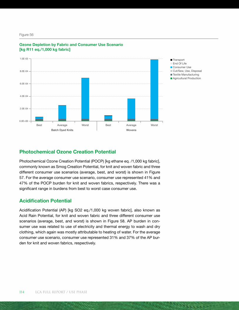
Photochemical Ozone Creation Potential
Photochemical Ozone Creation Potential (POCP) [kg ethane eq. /1,000 kg fabric], commonly known as Smog Creation Potential, for knit and woven fabric and three different consumer use scenarios (average, best, and worst) is shown in Figure 57. For the average consumer use scenario, consumer use represented 41% and 47% of the POCP burden for knit and woven fabrics, respectively. There was a significant range in burdens from best to worst case consumer use.
Acidification Potential
Acidification Potential (AP) [kg SO2 eq./1,000 kg woven fabric], also known as Acid Rain Potential, for knit and woven fabric and three different consumer use scenarios (average, best, and worst) is shown in Figure 58. AP burden in con-sumer use was related to use of electricity and thermal energy to wash and dry clothing, which again was mostly attributable to heating of water. For the average consumer use scenario, consumer use represented 31% and 37% of the AP bur-den for knit and woven fabrics, respectively.
Figure 56
Ozone Depletion by Fabric and Consumer Use Scenario [kg R11 eq./1,000 kg fabric]
Transport End Of Life Consumer Use Cut/Sew, Use, Disposal Textile Manufacturing Agricultural Production
1.0E-03
4.0E-04
6.0E-04
8.0E-04
2.0E-04
0.0E+00
Best BestAverage
Batch Dyed Knits Wovens
AverageWorst Worst
LCA FULL REport / Use Phase114
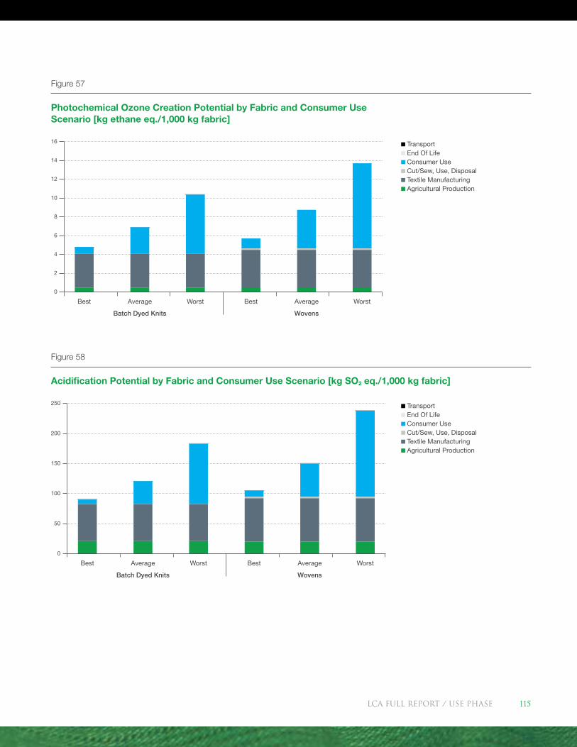
Figure 57
Photochemical Ozone Creation Potential by Fabric and Consumer Use Scenario [kg ethane eq./1,000 kg fabric]
Transport End Of Life Consumer Use Cut/Sew, Use, Disposal Textile Manufacturing Agricultural Production
16
10
12
14
8
6
4
2
0
Best BestAverage
Batch Dyed Knits Wovens
AverageWorst Worst
Figure 58
Acidification Potential by Fabric and Consumer Use Scenario [kg SO2 eq./1,000 kg fabric]
Transport End Of Life Consumer Use Cut/Sew, Use, Disposal Textile Manufacturing Agricultural Production
250
150
200
100
50
0
Best BestAverage
Batch Dyed Knits Wovens
AverageWorst Worst
LCA FULL REport / Use Phase 115
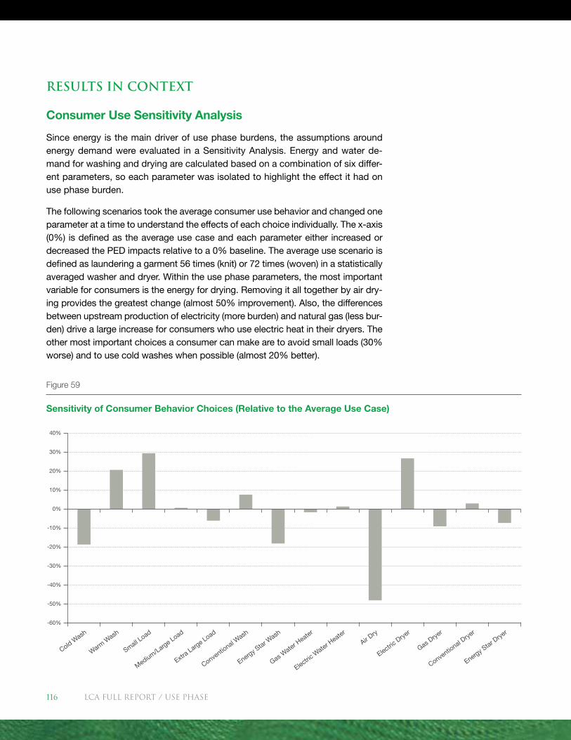
Results in Context
Consumer Use Sensitivity Analysis
Since energy is the main driver of use phase burdens, the assumptions around energy demand were evaluated in a Sensitivity Analysis. Energy and water de-mand for washing and drying are calculated based on a combination of six differ-ent parameters, so each parameter was isolated to highlight the effect it had on use phase burden.
The following scenarios took the average consumer use behavior and changed one parameter at a time to understand the effects of each choice individually. The x-axis (0%) is defined as the average use case and each parameter either increased or decreased the PED impacts relative to a 0% baseline. The average use scenario is defined as laundering a garment 56 times (knit) or 72 times (woven) in a statistically averaged washer and dryer. Within the use phase parameters, the most important variable for consumers is the energy for drying. Removing it all together by air dry-ing provides the greatest change (almost 50% improvement). Also, the differences between upstream production of electricity (more burden) and natural gas (less bur-den) drive a large increase for consumers who use electric heat in their dryers. The other most important choices a consumer can make are to avoid small loads (30% worse) and to use cold washes when possible (almost 20% better).
Figure 59
Sensitivity of Consumer Behavior Choices (Relative to the Average Use Case)
-60%
-50%
-40%
-30%
-20%
-10%
Cold Wash
Warm W
ash
Small Load
Medium/Large Load
Extra Large Load
Conventio
nal Wash
Energy Star W
ash
Gas Water H
eater
Electric W
ater Heater
Air Dry
Electric D
ryer
Gas Drye
r
Conventio
nal Drye
r
Energy Star D
ryer
40%
30%
20%
10%
0%
LCA FULL REport / Use Phase116
Conclusions: Use Phase
Use phase laundering is the largest contributor to GWP, ODP, and PED. Within the use phase parameters, the most important variable for consumers is the energy used during machine drying. Removing this variable through air drying of gar-ments instead of machine drying provided the greatest change. Other important choices a consumer can make are to avoid small loads and to use cold washes when possible.
LCA FULL REport / Use Phase 117
COTTON LIFE CYCLE(CRADLE-TO-GRAVE) RESULTS
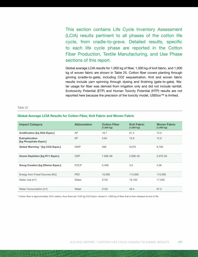
This section contains Life Cycle Inventory Assessment (LCIA) results pertinent to all phases of the cotton life cycle, from cradle-to-grave. Detailed results, specific to each life cycle phase are reported in the Cotton Fiber Production, Textile Manufacturing, and Use Phase sections of this report.
Global average LCIA results for 1,000 kg of fiber, 1,000 kg of knit fabric, and 1,000 kg of woven fabric are shown in Table 25. Cotton fiber covers planting through ginning (cradle-to-gate), including CO2 sequestration. Knit and woven fabric results include yarn spinning through dyeing and finishing (gate-to-gate). Wa-ter usage for fiber was derived from irrigation only and did not include rainfall. Ecotoxicity Potential (ETP) and Human Toxicity Potential (HTP) results are not reported here because the precision of the toxicity model, USEtox™ is limited.
Table 25
Global Average LCIA Results for Cotton Fiber, Knit Fabric and Woven Fabric
Impact Category Abbreviation Cotton Fiber [1,000 kg]
Knit Fabric [1,000 kg]
Woven Fabric [1,000 kg]
Acidification [kg SO2-Equiv.] AP 18.7 61.4 72.0
Eutrophication [kg Phosphate-Equiv.]
EP 3.84 12.6 12.6
Global Warming * [kg CO2-Equiv.] GWP 268 9,070 8,760
Ozone Depletion [kg R11-Equiv.] ODP 7.60E-06 2.66E-05 3.07E-05
Smog Creation [kg Ethene-Equiv.] POCP 0.408 3.6 4.06
Energy from Fossil Sources [MJ] PED 15,000 114,000 110,000
Water Use [m3] Water 2740 16,100 17,500
Water Consumption [m3] Water 2120 49.4 67.2
* Cotton fiber is approximately 42% carbon, thus there are 1540 kg CO2-Equiv. stored in 1,000 kg of fiber that is then released at end of life.
LCA FULL REport / COTTON LIFE CYCLE (CRADLE-TO-GRAVE) RESULTS 119
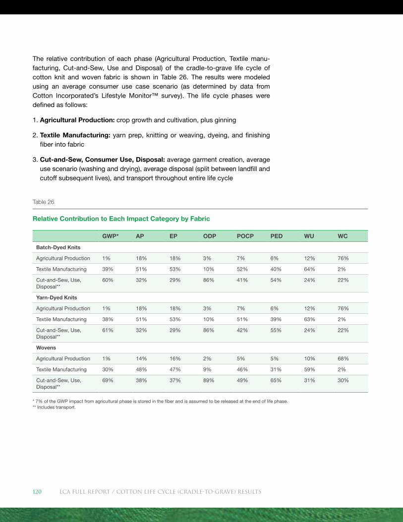
The relative contribution of each phase (Agricultural Production, Textile manu-facturing, Cut-and-Sew, Use and Disposal) of the cradle-to-grave life cycle of cotton knit and woven fabric is shown in Table 26. The results were modeled using an average consumer use case scenario (as determined by data from Cotton Incorporated’s Lifestyle Monitor™ survey). The life cycle phases were defined as follows:
1. Agricultural Production: crop growth and cultivation, plus ginning
2. Textile Manufacturing: yarn prep, knitting or weaving, dyeing, and finishing fiber into fabric
3. Cut-and-Sew, Consumer Use, Disposal: average garment creation, average use scenario (washing and drying), average disposal (split between landfill and cutoff subsequent lives), and transport throughout entire life cycle
Table 26
Relative Contribution to Each Impact Category by Fabric
GWP* AP EP ODP POCP PED WU WC
Batch-Dyed Knits
Agricultural Production 1% 18% 18% 3% 7% 6% 12% 76%
Textile Manufacturing 39% 51% 53% 10% 52% 40% 64% 2%
Cut-and-Sew, Use, Disposal**
60% 32% 29% 86% 41% 54% 24% 22%
Yarn-Dyed Knits
Agricultural Production 1% 18% 18% 3% 7% 6% 12% 76%
Textile Manufacturing 38% 51% 53% 10% 51% 39% 63% 2%
Cut-and-Sew, Use, Disposal**
61% 32% 29% 86% 42% 55% 24% 22%
Wovens
Agricultural Production 1% 14% 16% 2% 5% 5% 10% 68%
Textile Manufacturing 30% 48% 47% 9% 46% 31% 59% 2%
Cut-and-Sew, Use, Disposal**
69% 38% 37% 89% 49% 65% 31% 30%
* 7% of the GWP impact from agricultural phase is stored in the fiber and is assumed to be released at the end of life phase.** Includes transport.
LCA FULL REport / COTTON LIFE CYCLE (CRADLE-TO-GRAVE) RESULTS120
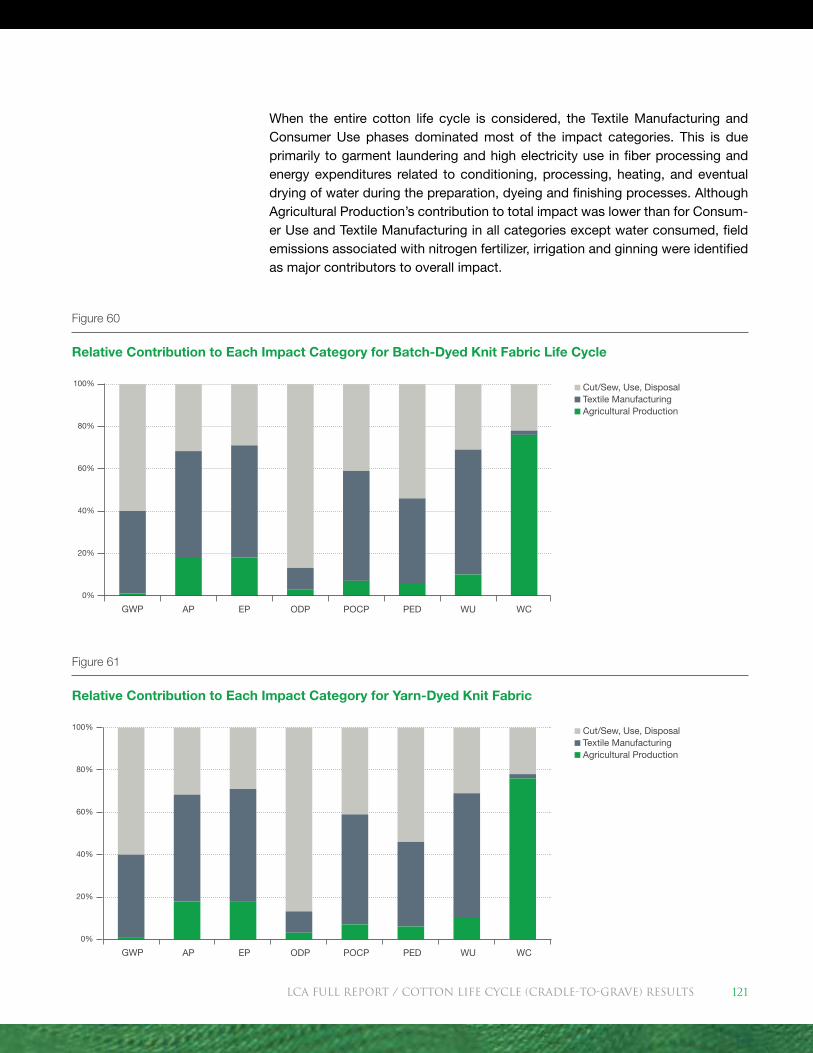
When the entire cotton life cycle is considered, the Textile Manufacturing and Consumer Use phases dominated most of the impact categories. This is due primarily to garment laundering and high electricity use in fiber processing and energy expenditures related to conditioning, processing, heating, and eventual drying of water during the preparation, dyeing and finishing processes. Although Agricultural Production’s contribution to total impact was lower than for Consum-er Use and Textile Manufacturing in all categories except water consumed, field emissions associated with nitrogen fertilizer, irrigation and ginning were identified as major contributors to overall impact.
Figure 61
Relative Contribution to Each Impact Category for Yarn-Dyed Knit Fabric
Cut/Sew, Use, Disposal Textile Manufacturing Agricultural Production
100%
80%
60%
40%
20%
0%
GWP AP EP ODP POCP PED WU WC
Figure 60
Relative Contribution to Each Impact Category for Batch-Dyed Knit Fabric Life Cycle
Cut/Sew, Use, Disposal Textile Manufacturing Agricultural Production
100%
80%
60%
40%
20%
0%
GWP AP EP ODP POCP PED WU WC
GWP AP EP ODP POCP PED WU WC
LCA FULL REport / COTTON LIFE CYCLE (CRADLE-TO-GRAVE) RESULTS 121
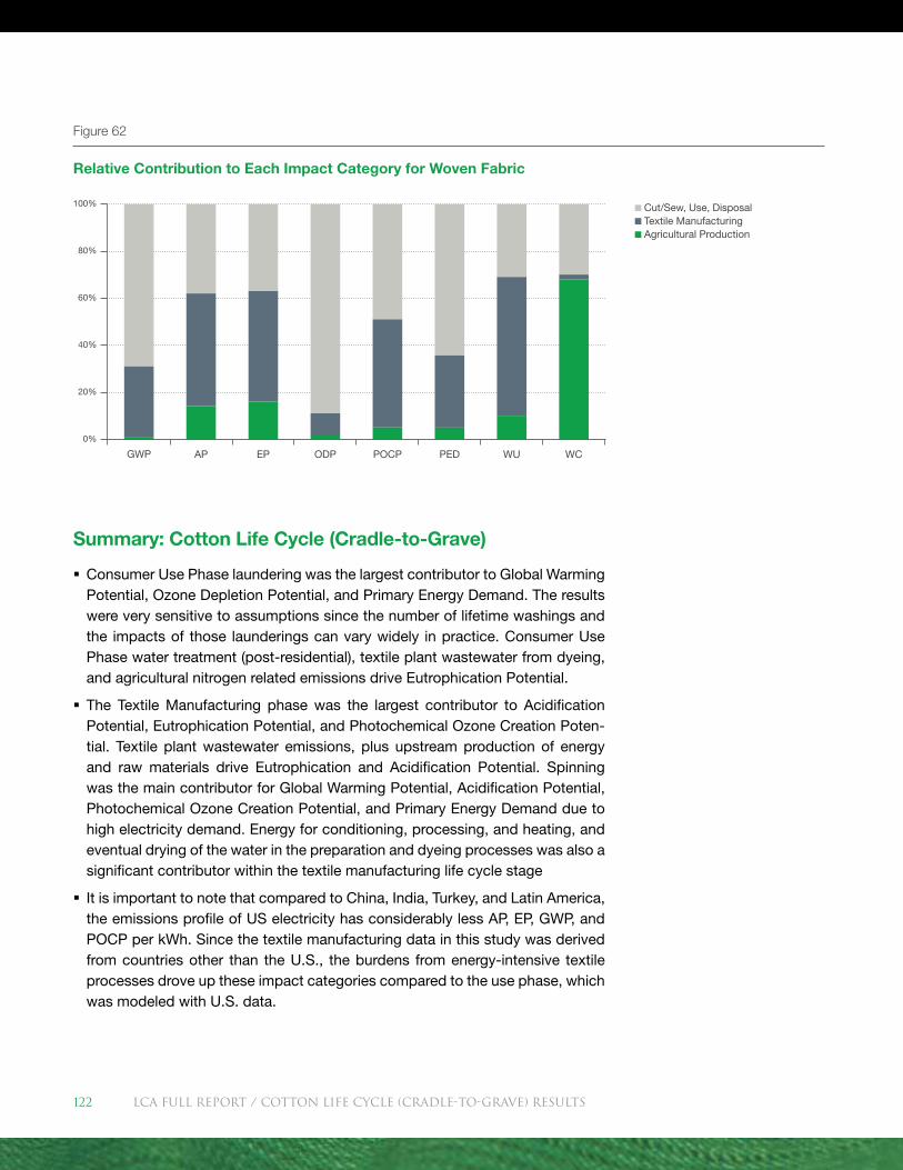
Figure 62
Relative Contribution to Each Impact Category for Woven Fabric
Cut/Sew, Use, Disposal Textile Manufacturing Agricultural Production
100%
80%
60%
40%
20%
0%
GWP AP EP ODP POCP PED WU WC
Summary: Cotton Life Cycle (Cradle-to-Grave)
� Consumer Use Phase laundering was the largest contributor to Global Warming Potential, Ozone Depletion Potential, and Primary Energy Demand. The results were very sensitive to assumptions since the number of lifetime washings and the impacts of those launderings can vary widely in practice. Consumer Use Phase water treatment (post-residential), textile plant wastewater from dyeing, and agricultural nitrogen related emissions drive Eutrophication Potential.
� The Textile Manufacturing phase was the largest contributor to Acidification Potential, Eutrophication Potential, and Photochemical Ozone Creation Poten-tial. Textile plant wastewater emissions, plus upstream production of energy and raw materials drive Eutrophication and Acidification Potential. Spinning was the main contributor for Global Warming Potential, Acidification Potential, Photochemical Ozone Creation Potential, and Primary Energy Demand due to high electricity demand. Energy for conditioning, processing, and heating, and eventual drying of the water in the preparation and dyeing processes was also a significant contributor within the textile manufacturing life cycle stage
� It is important to note that compared to China, India, Turkey, and Latin America, the emissions profile of US electricity has considerably less AP, EP, GWP, and POCP per kWh. Since the textile manufacturing data in this study was derived from countries other than the U.S., the burdens from energy-intensive textile processes drove up these impact categories compared to the use phase, which was modeled with U.S. data.
LCA FULL REport / COTTON LIFE CYCLE (CRADLE-TO-GRAVE) RESULTS122
� With the exception of water consumed, Agricultural Production’s contribution to total impact was lower than for Consumer Use and Textile Manufacturing in all of the categories evaluated. However, field emissions and fertilizer pro-duction were major contributors to several environmental impact categories: Eutrophication Potential was strongly influenced by nitrate, Acidification Poten-tial was influenced by ammonia and Global Warming Potential was influenced by nitrous oxide—all related to nitrogen fertilizers. The ginning process and energy required for irrigation played a role in Primary Energy Demand.
� Although the USEtox™ model is currently the most precise LCA model for eval-uating toxicity, there are still wide ranges in uncertainty around the actual effects of pesticides and other chemicals.
� Carbon sequestered during the growth of cotton is modeled as a CO2 emission at End-of-Life, even though garments won’t necessarily be thrown away after their first useful life.
LCA FULL REport / COTTON LIFE CYCLE (CRADLE-TO-GRAVE) RESULTS 123
Continued Research
The Life Cycle Assessment of Cotton Fiber and Fabric should be regarded as a snapshot based on data for the years of 2005-2010.
The results will change as the LCI expands and additional best manage-ment practices are identified and integrated into standard practice. Research to address areas needing improvement is already underway and strategies for continual improvement are in development. The following next steps have been identified as most critical:
� Continue research to improve cotton’s water and nitrogen use efficiencies during fiber production.
� Work with the LCA community to better model agricultural processes with respect to toxicity impact estimates.
� Work with mills to measure additional spinning and wet processing energy demands and water use. Once high quality primary data exists for these pro-cesses, effective strategies to reduce the burdens associated with textile manu-facturing can be identified.
� Continue to support wastewater reduction research.
� Educate and engage with consumers to reduce the impacts at the use phase level. Focus messaging on choice of load size and washer type and conduct research to understand the cleanliness and performance of clothing while laundering using these choices.
LCA FULL REport / COntinued research 125
REFERENCES
AATCC 2011 | American Association of Textile Chemists and Colorists. (2011). Technical Manual, TM150-2010, pg 255. Standardization of Home Laundry Test Conditions, p.402. Reference Liquid Laundry Detergent, “2003 detergent”, p. 396.
Acephate 2011 | Acephate Technical Fact Sheet, National Pesticide Information Center, Oregon State University and the US Environmental Protection Agency. http://npic.orst.edu/factsheets/acephatech.pdf
ADWR 2011 | Arizona Department of Water Resources (ADWR). (2011). Arizona Water Atlas, Volume 8: Active Management Area Planning Area. Table 8.0-10, p. 63 Retrieved from: http://www.adwr.state.az.us/azdwr/StatewidePlanning/Water-Atlas/ActiveManagementAreas/documents/Volume_8_overview_final.pdf
AGF 2011 | AGF 2011. Environmental Protection. Environmental Fate. Ministry of Agriculture. British Columbia. Retrieved February 25, 2011 from: http://www.agf.gov.bc.ca/pesticides/c_2.htm
ANL 1997 | Argonne National Lab report (ANL). (1997). ANL/ESD/08-02, pp. 14-17. Data were retrieved from USDA, 2007b, Data Sets: Commodity Costs and Re-turns, available at http://www.ers.usda.gov/Data/CostsAndReturns/Fuelbystate.xls, accessed Nov. 2007. Current data was pulled from Ag resource and manage-ment survey (ARMS), Economic Research Service, USDA, for year 1997.
Antunes 2008 | Antunes ,J.M. (2008). Brasilé referência mundial emplantio di-reto d Embrapa. EMBRAPA – Empresa Brasilieirade Pesquisa Agropecuária Retrieved May 1, 2011 from: http://www.embrapa.br/embrapa/imprensa/ noticias/2008/fevereiro/2a-semana/brasil-e-referencia-mundial-em-plantio- direto. Cited in Da Silva et al. 2010
AREI 2006 | Agricultural Resources & Economic Indicators (AREI). (2006). Edition/EIB-16/Economic Research Services/USDA, p. 97. Based on 2002 survey by the Economic Research Services of the USDA, approximately 80% of the soybean acres in the 10 major producing states use corn-soybean rotation. The average lime application rate was allocated to soybeans based on the ratio of soybean and corn usage.
Bajaj & Sharma 2009 | Bajaj R., Sharma, M.K. (2009). Value addition to cot-ton chain in India—Significant contribution by Bajaj Steel Industries Limited. International Workshop on “Utilization of Cotton Plant By-Produce for Value Added Products”. November 9-11, 2009, Nagpur India.
LCA FULL REport / References126
BCMA 2011 | British Columbia Ministry of Agriculture (BCMA). (2011). Retrieved from: http://www.agf.gov.bc.ca/pesticides/c_2.htm
Birkved et al. 2006 | Birkved, M., Hauschild, M. (2006). PestLCI—A model for estimating field emissions of pesticides in agricultural LCA. 198, ( 3-4), 433-451
Bouwman 1996 | Bouwmann, A.F. (1996). Direct emission of nitrous oxide from agricultural soils. Nutrient Cycling in Agroecosystems. 1, 53-70.
Brentrup et al. 2000 | Brentrup, F. et al. (2000). Methods to estimate on-field nitrogen emissions from crop production as an input to LCA studies in the Agri-cultural Sector. The International Journal of Life Cycle Assessment. 5(6), 349-357.
Bronson et al. 2009 | Bronson, K.F., A. Malapati, J.D. Booker, B.R. Scanlon, W. H. Hudnall, and A.M. Schubert. 2009. Residual soil nitrate in irrigated Southern High Plains cotton fields and Ogallala groundwater nitrate. Journal of Soil and Water Conservation 64(2): 98-104.
Brookes & Barfoot, 2010 | Brookes, Graham & Peter Barfoot. 2010. GM crops: global socio-economic and environmental impacts 1996–2008. PG Economics Ltd, Dorchester, UK.
BSI 2008 | British Standards Institution (BSI). (2008). PAS 2050: How to Assess the carbon footprint of goods and services. Specification for the assessment of the life cycle greenhouse gas emissions of goods and services.
Caires 2006 | Caires, E.F., Barth, G. & Garbuio, F.J. (2006). Lime application in the establishment of a no-till system for grain crop production in Southern Brazil. Soil Till. 89, 3–12.
CA.gov 2011 | State of California (Ca.gov). (2011). Department of Water Resources California State Water Project and the Cetnral Valley Project. Retrieved from: http://www.water.ca.gov/swp/cvp.cfm
Causarano et al. 2006 | Causarano, H.J., Franzluebbers, A.J., Reeves, D.W., Shaw, J.N. (2006): Soil organic carbon sequestration in cotton production systems of the southeastern United States: A review Journal of Environmental Quality, 35 (4), pp. 1374-1383.
Cavalett and Ortega 2010 | Cavalett, O. & Ortega, E. (2010). Integrated environmental assessment of biodiesel production from soybean in Brazil. Journal of Cleaner Production. 18, 55–70.
Cederberg 2004 | Cederberg, C. & Flysjo, A. (2004). Environmental assessment of future pig farming systems. Swedish institute for food and biotechnology, cited in Cavalett & Ortega 2010.
LCA FULL REport / References 127
CEPA 2008 | CEPA. 2008. Emission Potentials Data Dictionary. California Environmental Protection Agency, Department of Pesticide Regulation Rev 05/2008. 2008 EP data file used—see: http://www.cdpr.ca.gov/docs/ emon/vocs/vocproj/voc_ep.htm
CEPEA 2010 | (CEPEA) Advanced Studies on Applied Economics. Average value from: Agromensal—ESALQ/BM&F Retrieved from http://www.cepea.esalq.usp.br/ cited in Cavalett & Ortega 2010.
Choudhary & Gaur 2010 | Choudhary B., Gaur, K. (2010). Bt cotton in India: A country profile. ISAAA. Series of Biotech Crop Profiles: Ithaca, N.Y.
CI 2009 | Cotton Incorporated (CI). (2009). A World of Ideas: Technologies for Sustainable Cotton Textile Manufacturing. 1-2.
CIMIS 2009 | California Irrigation management Information System (CIMIS). (2009). Stations 002 (Fivepoints); 005 (Shafter); 015 (Stratford); and 148 (Merced). Retrieved from: http://wwwcimis.water.ca.gov/
Da Silva et al. 2010 | Da Silva et al. (2010): Variability in environmental impacts of Brazilian soybean according to crop production and transport scenarios. Journal of Environmental Management. 91, 1831-1839
David et al. 2010 | M.B. David, L.E. Drinkwater, and G.F. McIsaac. 2010. Sources of nitrate yields in the Mississippi river basin. J. Environ. Qual. 39:1657–1667.
Eberle 2006 | Eberle, U., Möller, M. 2006. Life Cycle Analysis of hand-drying sys-tems. A comparison of cotton towels and paper towels. Freiburg, 13 June 2006. Technical report. Öko-Institut e.V. Geschäftsstelle Freiburg
Embrapa 2004 | EMBRAPA (Brasil’s Minsitry of Agriculture). (2004): Sistemas de produção 5: tecnologia de produção de soja e Paraná 2005.Embrapa Soja, first ed. EMBRAPA, Londrina, Brazil, cited in Da Silva et al. 2010
EPA & DOE 2010 | US Environmental Protection Agency (EPA) and Department of Energy (DOE). (2010). Life Cycle Cost Estimate for 1 Energy Star Qualified Residential Clothes Washer(s). Retrieved from: http://www.energystar.gov/index.cfm?fuseaction=find_a_product.showProductGroupandpgw_code=CW
ERM 2002 | Environmental Resources Management (ERM). (2002). Streamlined Life Cycle Assessment of Two Marks & Spencer plc Apparel Products for Marks & Spencer. Retrieved from: http://circa.europa.eu/Public/irc/env/waste_strat/library?l=/test/eurocommerce_spencerpdf_2/_EN_1.0_&a=d
ERS 2010a | Economic Research Service (ERS). (2010). United States Department of Agriculture (USDA) Agricultural Management Survey. Retrieved from: http://www.ers.usda.gov/data/arms/
LCA FULL REport / References128
ERS 2010b | Economic Research Service (ERS). (2010). United States Department of Agriculture (USDA) Agricultural Management Survey. Retrieved from: http://maps.ers.usda.gov/mapimages/fpr_color.gif
ERS 2010c | Economic Research Service (ERS). (2010). Oil Crops Situation and Outlook Yearbook, March 2010. Market and Trade Economics Division, Eco-nomic Research Service, USDA. Table 16.
FAO 2004 | Food and Agriculture Organization of the United Nations (FAO). (2004). Fertilizer use by crop in Brazil Land and Plant Nutrition Management Service, Land and Water Development Division, Rome, 2004
FAO 2010 | Food and Agriculture Organization of the United Nations (FAO). (2010). Retrieved from: http://faostat.fao.org/site/
Faulkner et al. 2011 | Faulkner, W.B., J.D. Wanjura, R.K. Boman, B.W. Shaw, and C.B. Parnell. 2011. Comparison of Modern Cotton Harvest Systems on Irrigated Cotton: Economic Returns. Trans. ASABE In Press.
75 Federal Register 182 | Energy Conservation Program for Consumer Products: Test Procedure for Residential Clothes Washers, Department of Energy, Notice of Proposed Rulemaking, 75 Federal Register 182 (21 September 2010), pp. 57556-57595.
Ferraro 2002 | Ferraro, D. O. 2002. Energy Cost/Use in Pesticide Production. Ency-clopedia of Pest Management (Print) Chapter 96. CRC Press 2002. DOI:10.1201/NOE0824706326.ch96
Fok 2007 | Fok, M. & Xu, N. (2007). GM cotton in China: Innovation integra-tion and seed market disintegration. AIEA2 International Conference “Knowl-edge, Sustainability, and Bio-Resources in the further Development of Agri-food Systems”. July 22-27, 2007. Londrina (Parana, Brazil).
Frydendahl 2001 | Frydendal, J. (2001). Life Cycle Assessment of Berend-sen Care Bed ads. Part of Master Thesis at Department of Manufacturing Engineering, Technical University of Denmark.
GaBi 4 2006 | GaBi 4. (2006). Software and Databases for Life-Cycle- Assessment and Life-Cycle-Engineering, LBP University of Stuttgart and PE INTERNATIONAL GmbH, Leinfelden-Echterdingen.
Grace 2009 | Grace, P. 2009. Life cycle assessment of a 100% Australian- cotton t-shirt. Institute for Sustainable Resources, Queensland University of Tech-nology, BRISBANE QLD. 107 pp.
Green 1987 | Green, M.B., 1987: Energy in pesticide manufacture, distribu-tion and use. In: HelseL, Z.R., (Ed.): Energy in Plant Nutrition and Pest Control. Amsterdam, Elsevier, pp. 165-177.
LCA FULL REport / References 129
Guinée 2006 | Guinée, J., Oers, V. L., Koning, D. A., & Tamis, W. (2006). Life cycle approaches for Conservation Agriculture, 171. Department of Industrial Ecology & Department of Environmental Biology, 156.
Guinée et al. 2001 | Guinée et al. (2006). An operational guide to the ISO-stan-dards. Centre for Milieukunde (CML), Leiden 2001.
Guo et al. 2010 | Guo, J. H., X. J. Liu, Y. Zhang, J. L. Shen, W. X. Han, W. F. Zhang, P. Christie, K. W. T. Goulding, P. M. Vitousek, and F. S. Zhang. 2010. Significant acidification in major Chinese Croplands. Science 327:1008-1010.
Hauschild 2000 | Hauschild, M.Z. (2000). Estimating pesticide emissions for LCA of agricultural products. Conference paper. University of Denmark.
Holt et al. 2000 | Holt, G. A., G. L. Barker, R. V. Baker, A. Brashears. 2000. Characterization of cotton gin byproducts produced by various machin-ery groups used in the ginning operation. Transactions of the ASAE. VOL. 43(6): 1393-1400
Hsu & Gale 2001 | Hsu, H., and F. Gale. 2001. Regional shifts in China’s cotton production and use. Cotton and Wool Situation and Outlook/CWS-2001/Novem-ber 2001. USDA, Economic Research Service. p. 19-25.
Hutmacher et al. 2004 | Hutmacher, R.B., R. L. Travis, D. W. Rains, R. N. Vargas, B. A. Roberts, B. L. Weir, S. D. Wright, D. S. Munk, B. H. Marsh, M. P. Keeley, F. B. Fritschi, D. J. Munier, R. L. Nichols, and R. Delgado. 2004. Response of Recent Acala Cotton Varieties to Variable Nitrogen Rates in the San Joaquin Valley of California. Agron. J. 96:48–62.
ICAC 2009 | International Cotton Advisory Committee (ICAC). (2009). Provided pesticide data purchased from GfK Kynetec, Nuremberg, Germany.
Inmet 2010 | Instituto Nacional de Meteorologia (INMET, National Institute of Me-teorology) . (2010). Retrieved from: http://www.inmet.gov.br/ cited in Cavalett and Ortega 2010.
IPCC 2003 | Intergovernmental Panel on Climate Change (IPCC). (2003). Good Practice Guidance for Land Use, Land-Use Change and Forestry. Institute for Global Environmental strategies (IGES) for the Intergovernmental Panel on Climate Change, Kanagawa, Japan.
IPCC 2006 | Intergovernmental Panel on Climate Change (IPCC). (2006). Guidelines for National Greenhouse Gas Inventories, Volume 4 Agriculture, Forestry and Other Land Use, Retrieved December 22, 2009 from: http://www.ipccnggip.iges.or.jp/public/2006gl/vol4.html
ISO 2006 | International Organization for Standardization (ISO). (2006). Environ-mental Management—Life Cycle Assessment—Principles and Framework. Series 14040 and 14044.
LCA FULL REport / References130
ITMF 2009 | International Textile Manufacturers Federation (ITMF). (2009). International Textile Machinery Shipment Statistics. Vol 32.
James 2010 | James, C. (2010). Global status of commercialized biotech/GM crops: 2010. ISAAA Brief No. 42. ISAAA: Ithaca, NY. http://www.isaaa.org/ resources/publications/briefs/42/.
Kalliala 1999 | Kalliala, E.M., Nousiainen, P. 1999. Life Cycle Assessment ENVIRONMENTAL PROFILE OF COTTON AND POLYESTER-COTTON FABRICS. AUTEX Research Journal Vol 1, No.1, 1999, http://www.autex.org/v1n1/2264_99.pdf
Karst 2005 | Kooistra, Karst. (2005). Masters Thesis. Wageningen University, Bio-logical Farming Systems Group.
Le Mer 2001 | Le Mer, J., Roger, P. (2001): Production, oxidation, emission and consumption of methane by soils: A review Eur. J. Soil Biol. 37 (2001) 25−50
Ma 2010 | Ma, L. et al. (2010) Modeling nutrient flows in the food chain of China. Journal of Environmental Quality. 39, 1279-1289.
Margni 2002 | Margni, M. et al. (2002) Life cycle impact assessment of pesticides on human health and ecosystems. Agriculture, Ecosystems and Environment 93, 379–392
Marques 2000 | ELEMENTOS PARA UMA ABORDAGEM AMBIENTAL INTEGRADAJoão Fernando MarquesEmbrapa - Meio AmbienteJaguariúna, Campinas, S.P., Brasil. Retrieved from: http://www.fea.unicamp.br/docentes/ortega/livro/C17-EAnaliseAl-JM.pdf, cited in Cavalett & Ortega 2010.
Marques 2006 | Marques, B.D.A. (2006): Consideraçoes ambientaise exergéticas na fase depós – colheita de graos: estudo de caso do Estadodo Paraná. Disserta-tion. Universida de Federal do Paraná, Curitiba, Brazil. Retrieved from: http://hdl.handle.net/1884/3930 (05.01.2011) cited in Da Silva et al. 2010
Matlock et al. 2008 | Matlock, M. et al. (2008). Energy Use Life Cycle Assess-ment for Global Cotton Production Practices. Center for Agricultural and Rural Sustainability. University of Arkansas Division of Agriculture. Final report. UA Divi-sion of Agriculture LCA for Cotton.http://asc.uark.edu/Cotton_Incorporated_En-ergy_LCA_Final.doc
Meyer et al. 2009 | Meyer, L., MacDonald, S. & Kiawu, J., (2009). Cotton and Wool Situation and Outlook Yearbook. Washington, D.C.: Economic Research Service, US Department of Agriculture (USDA), Retrieved from: http://usda.mannlib.cor-nell.edu/MannUsda/viewDocumentInfo.do?documentID=1228
Monsanto 2008 | Monsanto China & Plant Protection Institute of the Chinese Academy of Agricultural Sciences
LCA FULL REport / References 131
MSU 2004 | Mississippi State University. 2004. Cotton 2005 planning budgets. Department of Agricultural Economics Budget Report 2004-003.
NADP 2011 | National Atmospheric Deposition Program (NADP). (2011). Retrieved from: https://nadp.isws.illinois.edu/sites/ntnmap.asp
NCSU 2009 | North Carolina State University (NCSU). (2009). 2009 Cotton Infor-mation. North Carolina Cooperative Extension Service, College of Agriculture and Life Sciences, p. 209.
Nemecek et al. 2004 | Nemecek T., Heil A., Huguenin O., Meier S., Erzinger S., Blaser S., Dux. D. and Zimmermann A. (2004). Life Cycle Inventories of Agricul-tural Production Systems. Ecoinvent 2000 No. 15. Agroscope FAL Reckenholz and FAT Taenikon, Swiss Centre for Life Cycle Inventories, Dübendorf, CH
NOAA, 2011 | US Department of Commerce, National Oceanic and Atmospheric Administration (NOAA). Earth System Research Laboratory. Create a monthly or seasonal time series of climate variables. Retrieved from: http://www.esrl.noaa.gov/psd/data/timeseries/
NSSC, 1998 | National Soil Service Center (NSSC). 1998. Dominant Soil Orders. USDA National Resources Conservation Services, Lincoln, NE.
OmniTech 2010 | Omnitech International (OmniTech). 2010. Life Cycle Impact of Soybean production and Soy Industrial products. United Soybean Board Life Cycle Profile. US: Soy Delivers Environmental & Energy Benefits
Ostermayer 2002 | Ostermayer, A. (2002): Ökobilanz für DL-Methionin in der Ge-flügelmast. Endbericht im Auftrag der Degussa AG. Institut für Energie- und Um-weltforschung Heidelberg, Heidelberg 2002
Panichelli 2008 | Panichelli 2008: Life cycle assessment of soybean-based bio-diesel in Argentina for export. International Journal of Life Cycle Assessment. 1–16
Patil et al. 2007 | Patil, et al. (2007). Improving ling quality using modified dou-ble roller gins in India. Proceedings World Cotton Research Conference—4. September 10-14, 2007 Lubbock, Texas USA.
PEI 2010 | PE INTERNATIONAL (PEI). (2010): Expert Judgment PE INTERNATIONAL
Phyllis 2010 | Phyllis. (2010). Phyllis, database for biomass and waste: ECN Bio-mass, Coal and Environmental Research. Energy research Centre of the Nether-lands. Retrieved from: http://www.ecn.nl/phyllis/
Powlson et al. 2011 | Powlson, D.S., Whitmore, K.W., Goulding, W.T. (2011): Soil carbon sequestration to mitigate climate change: a critical re-examination to identify the true and the false. European Journal of Soil Science, February 2011, 62, 42–55
LCA FULL REport / References132
Qaim 2006 | Qaim, M. et al. (2006). Adoption of Bt cotton and impact variability: Insights from India. Review of Agricultural Economics. 28 (1) 48-58.
Qiao 2009 | Qiao, F. & Paggi, M.S. (2009). Cotton transportation cost in China. Proceedings 2009 Beltwide Cotton Conference. January 5-8, 2009. San Antonio, Texas USA. 343-353.
Qui et al 2003 | Qui, J. et al. (2003). Mapping single-, double-, and triple-crop agriculture in China at 0.5° X 0.5° by combining county-scale census data with a remote sensing-derived land cover map. Geocarto International. 18 (2), 3-13.
Raper & Bergtold 2007 | Raper and Bergtold. (2007). In-row subsoiling: A review and suggestions for reducing cost of this conservation tillage operation. Applied Engineering in Agriculture. 23(4), 463-471.
Reed et al. 2009 | Reed, J.N., E.M. Barnes and K.D. Hake. (2009). Technical Information Section. US Cotton Growers Respond to Natural Resource Survey. International Cotton Advisory Committee, The ICAC Recorder. XXVII(2), June.
Rosenbaum et al. 2008 | Rosenbaum et al. (2008). USEtox™—the UNEP-SE-TAC toxicity model: recommended characterization factors for Human Toxicity and freshwater Ecotoxicity in life cycle impact assessment, International Journal of Life Cycle Assessment, Retrieved October 6, 2010 at: http://potency.berkeley.edu/pdfs/Setac.pdf
Roy 2006 | Roy, R.N., Finck A., Blair G.J. & Tandon H.L.S. (2006). Plant nutrition for food security. A guide for integrated nutrient management. FAO Fertilizer and Plant Nutrition Bulletin No.16. Food and Agriculture Organization of the United Nations (FAO), Rome, Italy.
Sadashivappa & Qaim 2009 | Sadashivappa, P. & Qaim, M. (2009). Bt cotton in India: Development of benefits and the role of government seed price interven-tions. AgBioForum. 12 (2) 172-183.
Salvagotti 2008 | Salvagiotti, F. et al. (2008). Nitrogen uptake, fixation and response to fertilizer N in soybeans: A review. Journal of Field Crops Research. 108, 1-13.
Schmädeke 1998 | Schmädeke, P. (1998): Lachgas- und Methanflüsse eines Gley-Auenbodens unter dem Einfluß einer Rapsfruchtfolge und in Abhängigkeit von der N-Düngung. Dissertation der Fakultät für Agrarwissenschaften der Georg-August-Universität Göttingen. http://webdoc.sub.gwdg.de/diss/1999/schmaede/inhalt.htm#inhalt. (25.09.09).
Sharma et al. 2010 | Sharma, B.R., K.V. Rao, K.P.R. Vittal, Y.S. Ramakrishna, and U. Amarasinghe. 2010. Estimating the potential of rainfed agriculture in India: Prospects for water productivity improvements. Agricultural Water Management 97:23–30.
LCA FULL REport / References 133
Slater 2003 | Slater, K. (2003). Environmental impact of textiles, production, processes and protection, Woodhead Publishing Limited in association with The Textile Institute.
TC2 2009 | TC2. (2009). Textile/Clothing Technology Corporation for the cut-and-sew data utilizing the comparison of power consumption from Juki Corporation bulletin December 2009 DDL-9000B.
Tobler-Rohr 2006 | Tobler-Rohr, M.I., Schaerer , S. (2006). Yield, cost and LCA of different cotton growing systems in the Texas high plains. Institute for Production Automation. Sustainable Textiles. ETH Zurich, Switzerland. Retrieved May 20, 2010 from: www.emsc.ch/.../Yield,%20cost%20and%20LCA%20of%20cotton%20growing%20BCC2003.pdf
University of Arizona 2010 | University of Arizona. (2010). Maricopa, ETo: Reference EvapoTranspiration (inches, 1987-2002). College of Agriculture and Life Sciences. Retrieved from: http://ag.arizona.edu/azmet/data/06etrain.htm
USDA 2004 | United States Department of Agriculture (USDA). Farm & Ranch Irrigation Survey reports for 1994, 1998, and 2003, Retrieved from: www.agcensus.usda.gov.
USDA 2006 | United States Department of Agriculture (USDA). (20065). Agricultural Chemical Usage 2005 Field Crops Summary.
USDA 2007 | United States Department of Agriculture (USDA). NASS Agricultural Chemical Usage Field Crops Summary Reports for 2006, 2005, 2004, 2002 and 2001, Retrieved from: www.nass.usda.gov.
USDA 2008a | United States Department of Agriculture (USDA). (2008). Agricultural Chemical Usage 2007 Field Crops Summary. May 2008. United States Department of Agriculture, National Agricultural Statistics Service. Ag Ch 1 (08).
USDA 2008b | United States Department of Agriculture (USDA). (2008). Farm and Ranch Irrigation survey (2003). Vol. 3, Special Studies, Part 1. Issued November 2004. United States Department of Agriculture, National Agricultural Statistics Service.
USDA 2008c | United States Department of Agriculture (USDA). (2008). Agricultural Chemical Usage 2007 Field Crops Summary.
USDA 2009 | United States Department of Agriculture (USDA). (2009) 2007 Cen-sus of Agriculture. http://www.agcensus.usda.gov/Publications/2007/index.asp.
USDA 2011 | United States Department of Agriculture (USDA). (2011). Official USDA estimates, Retrieved from http://www.fas.usda.gov/psdonline/ psdQuery.aspx.
LCA FULL REport / References134
Valco et al. 2009 | Valco, T.D., J.K. Green, R.A. Isom, D.S. Findley, T.L. Price, and H. Ashley. (2009). The Cost of Ginning Cotton – 2007 survey results. 2009 Belt-wide Cotton Conferences, NCC
Van Cleemput O 1998 | Van Cleemput O (1998): Subsoils: chemo- and biological denitrification, N2O and N2 emissions. Nutrient Cycling Agroecosystems 52, 187-194
Wei 1999 | Wei, S.J. (1999) The new direction of China’s cotton policy. Agricultural Outlook Forum 1999. February 23, 1999. http://purl.umn.edu/32938.
West & Marland 2002 | West, T,O., and Marland, G. (2002). A Synthesis of Carbon Sequestration, Carbon Emissions, and Net carbon Flux in Agriculture: Comparing Tillage Practices in the United States. Agriculture, Ecosystems and Environment. 91, 217–232.
Wiegmann 2002 | Wiegmann. K. 2002. Anbau und Verarbeitung von Baum-wolle. Dokumentation der GEMIS Daten. Institut für angewandte Ökologie e.V. (Öko-Institut e.V.
Willcut & Barnes 2008 | Willcut, M.H., and E.M. Barnes. (2008). Fuel consumption in spindle picker cotton harvesting systems. Beltwide Cotton Conferences, Nashville, Tennessee, January 8-11, 2008.
Williams 2006 | Williams. (2006). Determining the environmental burdens and re-source use in the production of agricultural and horticultural commodities.
Williams 2009 | Williams et al 2009: Estimation of the greenhouse gas emissions from agricultural pesticide manufacture and use
Williams et al. 2009 | Williams et al. (2009). Estimation of the greenhouse gas emissions from agricultural pesticide manufacture and use.
Zhong 2006 | Zhong, F. et al. (2006). Crop Insurance and agrochemical use in the Manasi watershed, Xinjiang, China. Economy and Environmental Program for Southeast Asia. http://econpapers.repec.org/paper/eepreport/rr2007071.htm.
LCA FULL REport / References 135
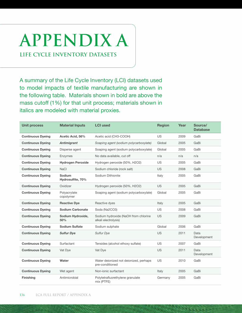
LIFE CYCLE INVENTORY DATASETS
A summary of the Life Cycle Inventory (LCI) datasets used to model impacts of textile manufacturing are shown in the following table. Materials shown in bold are above the mass cutoff (1%) for that unit process; materials shown in italics are modeled with material proxies.
Unit process Material Inputs LCI used Region Year Source/ Database
Continuous Dyeing Acetic Acid, 56% Acetic acid (CH3-COOH) US 2009 GaBi
Continuous Dyeing Antimigrant Soaping agent (sodium polycarboxylate) Global 2005 GaBi
Continuous Dyeing Disperse agent Soaping agent (sodium polycarboxylate) Global 2005 GaBi
Continuous Dyeing Enzymes No data available, cut off n/a n/a n/a
Continuous Dyeing Hydrogen Peroxide Hydrogen peroxide (50%, H2O2) US 2005 GaBi
Continuous Dyeing NaCl Sodium chloride (rock salt) US 2008 GaBi
Continuous Dyeing Sodium Hydrosulfite, 70%
Sodium Dithionite Italy 2005 GaBi
Continuous Dyeing Oxidizer Hydrogen peroxide (50%, H2O2) US 2005 GaBi
Continuous Dyeing Polyacrylate copolymer
Soaping agent (sodium polycarboxylate) Global 2005 GaBi
Continuous Dyeing Reactive Dye Reactive dyes Italy 2005 GaBi
Continuous Dyeing Sodium Carbonate Soda (Na2CO3) US 2008 GaBi
Continuous Dyeing Sodium Hydroxide, 50%
Sodium hydroxide (NaOH from chlorine alkali electrolysis)
US 2009 GaBi
Continuous Dyeing Sodium Sulfate Sodium sulphate Global 2006 GaBi
Continuous Dyeing Sulfur Dye Sulfur Dye US 2011 Data Development
Continuous Dyeing Surfactant Tensides (alcohol ethoxy sulfate) US 2007 GaBi
Continuous Dyeing Vat Dye Vat Dye US 2011 Data Development
Continuous Dyeing Water Water deionized not deionized, perhaps pre-conditioned
US 2010 GaBi
Continuous Dyeing Wet agent Non-ionic surfactant Italy 2005 GaBi
Finishing Antimicrobial Polytetrafluorethylene granulate mix (PTFE)
Germany 2005 GaBi
APPENDIX A
LCA FULL REport / Appendix A136
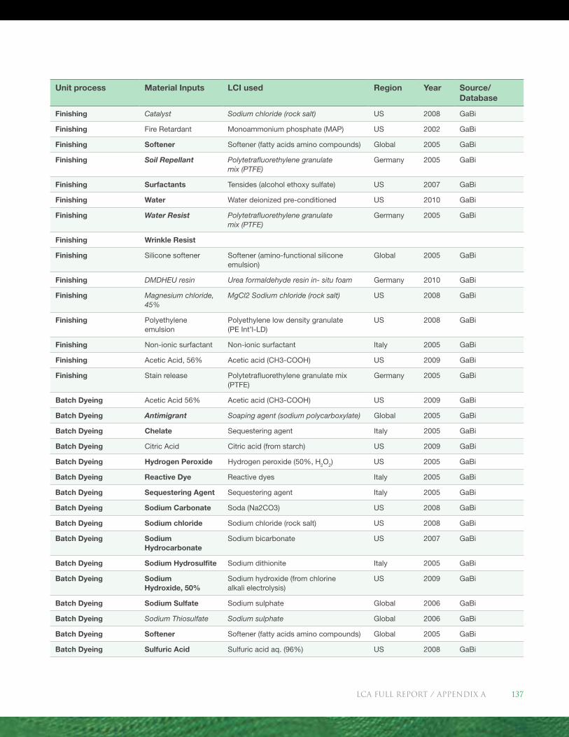
Unit process Material Inputs LCI used Region Year Source/ Database
Finishing Catalyst Sodium chloride (rock salt) US 2008 GaBi
Finishing Fire Retardant Monoammonium phosphate (MAP) US 2002 GaBi
Finishing Softener Softener (fatty acids amino compounds) Global 2005 GaBi
Finishing Soil Repellant Polytetrafluorethylene granulate mix (PTFE)
Germany 2005 GaBi
Finishing Surfactants Tensides (alcohol ethoxy sulfate) US 2007 GaBi
Finishing Water Water deionized pre-conditioned US 2010 GaBi
Finishing Water Resist Polytetrafluorethylene granulate mix (PTFE)
Germany 2005 GaBi
Finishing Wrinkle Resist
Finishing Silicone softener Softener (amino-functional silicone emulsion)
Global 2005 GaBi
Finishing DMDHEU resin Urea formaldehyde resin in- situ foam Germany 2010 GaBi
Finishing Magnesium chloride, 45%
MgCl2 Sodium chloride (rock salt) US 2008 GaBi
Finishing Polyethylene emulsion
Polyethylene low density granulate (PE Int’l-LD)
US 2008 GaBi
Finishing Non-ionic surfactant Non-ionic surfactant Italy 2005 GaBi
Finishing Acetic Acid, 56% Acetic acid (CH3-COOH) US 2009 GaBi
Finishing Stain release Polytetrafluorethylene granulate mix (PTFE)
Germany 2005 GaBi
Batch Dyeing Acetic Acid 56% Acetic acid (CH3-COOH) US 2009 GaBi
Batch Dyeing Antimigrant Soaping agent (sodium polycarboxylate) Global 2005 GaBi
Batch Dyeing Chelate Sequestering agent Italy 2005 GaBi
Batch Dyeing Citric Acid Citric acid (from starch) US 2009 GaBi
Batch Dyeing Hydrogen Peroxide Hydrogen peroxide (50%, H2O2) US 2005 GaBi
Batch Dyeing Reactive Dye Reactive dyes Italy 2005 GaBi
Batch Dyeing Sequestering Agent Sequestering agent Italy 2005 GaBi
Batch Dyeing Sodium Carbonate Soda (Na2CO3) US 2008 GaBi
Batch Dyeing Sodium chloride Sodium chloride (rock salt) US 2008 GaBi
Batch Dyeing Sodium Hydrocarbonate
Sodium bicarbonate US 2007 GaBi
Batch Dyeing Sodium Hydrosulfite Sodium dithionite Italy 2005 GaBi
Batch Dyeing Sodium Hydroxide, 50%
Sodium hydroxide (from chlorine alkali electrolysis)
US 2009 GaBi
Batch Dyeing Sodium Sulfate Sodium sulphate Global 2006 GaBi
Batch Dyeing Sodium Thiosulfate Sodium sulphate Global 2006 GaBi
Batch Dyeing Softener Softener (fatty acids amino compounds) Global 2005 GaBi
Batch Dyeing Sulfuric Acid Sulfuric acid aq. (96%) US 2008 GaBi
LCA FULL REport / Appendix A 137

Unit process Material Inputs LCI used Region Year Source/ Database
Batch Dyeing Surfactant Tensides (alcohol ethoxy sulfate) US 2007 GaBi
Batch Dyeing Water Water US 2010 GaBi
Batch Dyeing Wetting agent Non-ionic surfactant Italy 2005 GaBi
Yarn Dyeing Acetic Acid 56% Acetic acid (CH3-COOH) US 2009 GaBi
Yarn Dyeing Antimigrant Soaping agent (sodium polycarboxylate) Global 2005 GaBi
Yarn Dyeing Catalyst Sodium chloride (rock salt)no catalyst used in yarn dyeing
US 2008 GaBi
Yarn Dyeing Caustic Soda Sodium hydroxide (from chlorine alkali electrolysis)
US 2009 GaBi
Yarn Dyeing Detergent Tensides (alcohol ethoxy sulfate) US 2007 GaBi
Yarn Dyeing Disperse agent Dispersing agent (ethoxylate fatty alcohols)
Italy 2005 GaBi
Yarn Dyeing Hydrogen Peroxide Hydrogen peroxide (50%, H2O2) US 2005 GaBi
Yarn Dyeing NaCl Sodium chloride (rock salt) US 2008 GaBi
Yarn Dyeing Polyacrylate copolymer
Soaping agent (sodium polycarboxylate) Global 2005 GaBi
Yarn Dyeing Reactive dye Reactive dyes Italy 2005 GaBi
Yarn Dyeing Sodium carbonate Soda (Na2CO3) US 2008 GaBi
Yarn Dyeing Sodium hydrosulfite Sodium dithionite Italy 2005 GaBi
Yarn Dyeing Sodium sulfate Sodium sulphate Global 2006 GaBi
Yarn Dyeing Sulfuric Acid Sulfuric acid aq. (96%) US 2008 GaBi
Yarn Dyeing Surfactant (Fatty alcohol)
Non-ionic surfactant Italy 2005 GaBi
Yarn Dyeing
Vat Dye Vat Dye US 2011 Data Devel-opment
Yarn Dyeing Water Water US 2010 GaBi
Yarn Dyeing Water resist Polytetrafluorethylene granulate mix (PTFE)
Germany 2005 GaBi
Yarn Dyeing Wetting agent Non-ionic surfactant Italy 2005 GaBi
Yarn Dyeing Wetting agent Non-ionic surfactant Italy 2005 GaBi
LCA FULL REport / Appendix A138
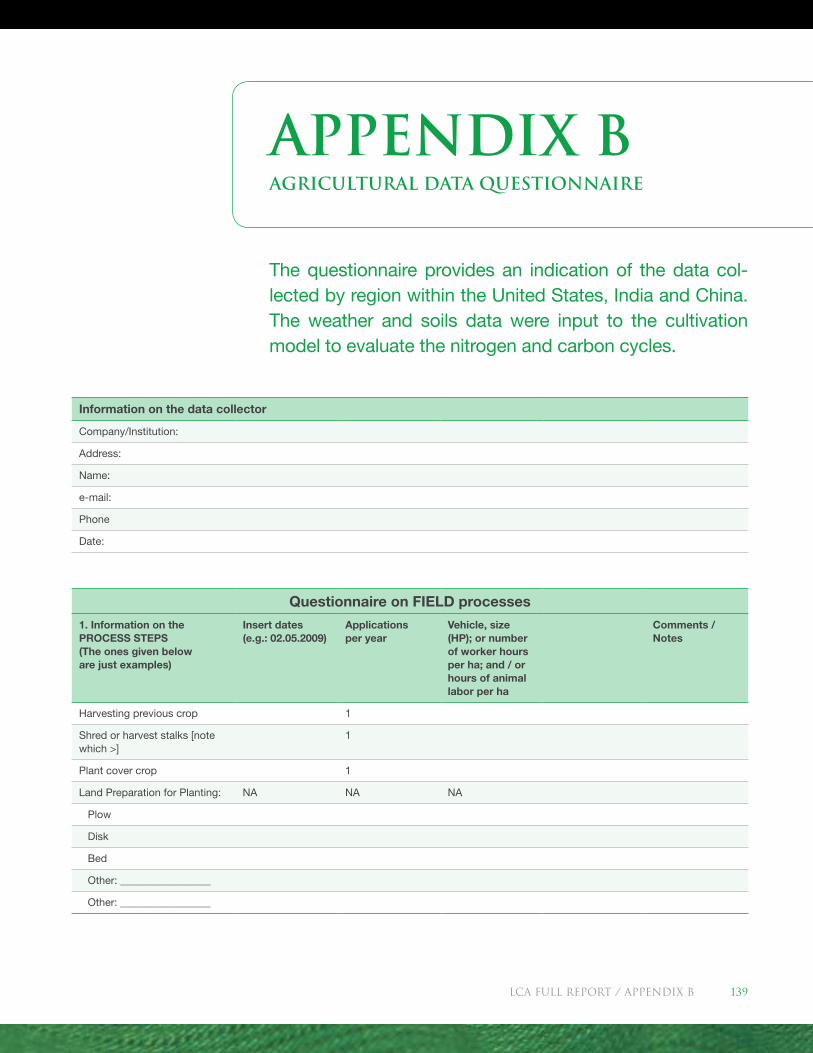
AGRICULTURAL DATA QUESTIONNAIRE
The questionnaire provides an indication of the data col-lected by region within the United States, India and China. The weather and soils data were input to the cultivation model to evaluate the nitrogen and carbon cycles.
APPENDIX B
Questionnaire on FIELD processes
1. Information on the PROCESS STEPS (The ones given below are just examples)
Insert dates (e.g.: 02.05.2009)
Applications per year
Vehicle, size (HP); or number of worker hours per ha; and / or hours of animal labor per ha
Comments / Notes
Harvesting previous crop 1
Shred or harvest stalks [note which >]
1
Plant cover crop 1
Land Preparation for Planting: NA NA NA
Plow
Disk
Bed
Other: _________________
Other: _________________
Information on the data collector
Company/Institution:
Address:
Name:
e-mail:
Phone
Date:
LCA FULL REport / Appendix B 139
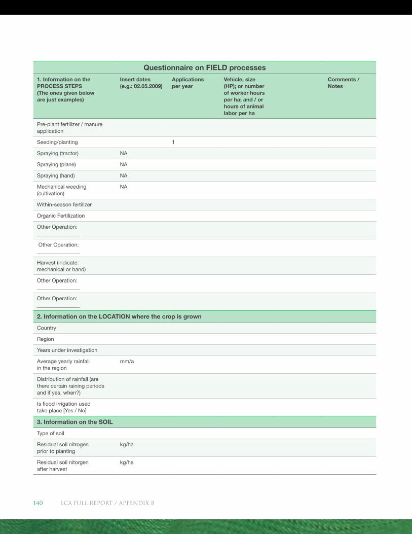
Questionnaire on FIELD processes
1. Information on the PROCESS STEPS (The ones given below are just examples)
Insert dates (e.g.: 02.05.2009)
Applications per year
Vehicle, size (HP); or number of worker hours per ha; and / or hours of animal labor per ha
Comments / Notes
Pre-plant fertilizer / manure application
Seeding/planting 1
Spraying (tractor) NA
Spraying (plane) NA
Spraying (hand) NA
Mechanical weeding (cultivation)
NA
Within-season fertilizer
Organic Fertilization
Other Operation: ________________
Other Operation: ________________
Harvest (indicate: mechanical or hand)
Other Operation: ________________
Other Operation: ________________
2. Information on the LOCATION where the crop is grown
Country
Region
Years under investigation
Average yearly rainfall in the region
mm/a
Distribution of rainfall (are there certain raining periods and if yes, when?)
Is flood irrigation used take place [Yes / No]
3. Information on the SOIL
Type of soil
Residual soil nitrogen prior to planting
kg/ha
Residual soil nitorgen after harvest
kg/ha
LCA FULL REport / Appendix B140
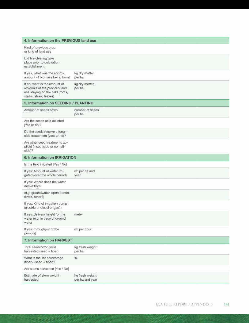
4. Information on the PREVIOUS land use
Kind of previous crop or kind of land use
Did fire clearing take place prior to cultivation establishment
If yes, what was the approx. amount of biomass being burnt
kg dry matter per ha
If no, what is the amount of residuals of the previous land use staying on the field (roots, stalks, straw, leaves)
kg dry matter per ha
5. Information on SEEDING / PLANTING
Amount of seeds sown number of seeds per ha
Are the seeds acid delinted [Yes or no]?
Do the seeds receive a fungi-cide treatement (yest or no)?
Are other seed treatments ap-plield (insecticide or nemati-cide)?
6. Information on IRRIGATION
Is the field irrigated [Yes / No]
If yes: Amount of water irri-gated (over the whole period)
m3 per ha and year
If yes: Where does the water derive from
(e.g. groundwater, open ponds, rivers, other?)
If yes: Kind of irrigation pump (electric or diesel or gas?)
If yes: delivery height for the water (e.g. in case of ground water
meter
If yes: throughput of the pump(s)
m3 per hour
7. Information on HARVEST
Total seedcotton yield harvested (seed + fiber)
kg fresh weight per ha
What is the lint percentage (fiber / (seed + fiber)?
%
Are stems harvested [Yes / No]
Estimate of stem weight harvested:
kg fresh weight per ha and year
LCA FULL REport / Appendix B 141
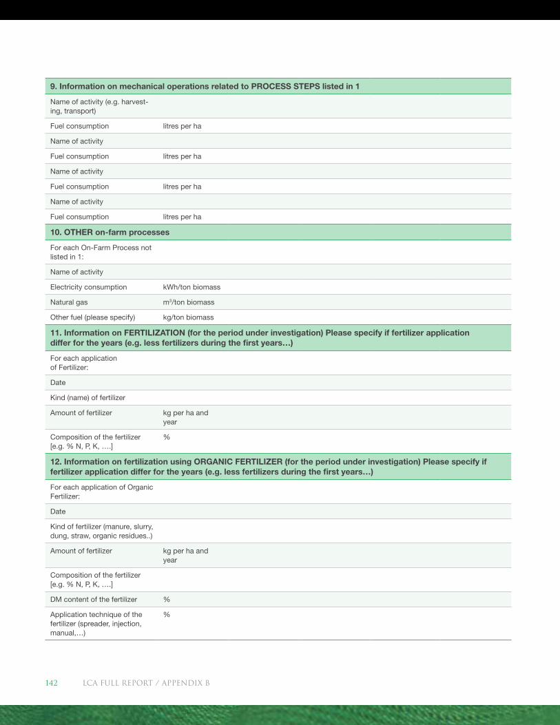
9. Information on mechanical operations related to PROCESS STEPS listed in 1
Name of activity (e.g. harvest-ing, transport)
Fuel consumption litres per ha
Name of activity
Fuel consumption litres per ha
Name of activity
Fuel consumption litres per ha
Name of activity
Fuel consumption litres per ha
10. OTHER on-farm processes
For each On-Farm Process not listed in 1:
Name of activity
Electricity consumption kWh/ton biomass
Natural gas m3/ton biomass
Other fuel (please specify) kg/ton biomass
11. Information on FERTILIZATION (for the period under investigation) Please specify if fertilizer application differ for the years (e.g. less fertilizers during the first years…)
For each application of Fertilizer:
Date
Kind (name) of fertilizer
Amount of fertilizer kg per ha and year
Composition of the fertilizer [e.g. % N, P, K, ….]
%
12. Information on fertilization using ORGANIC FERTILIZER (for the period under investigation) Please specify if fertilizer application differ for the years (e.g. less fertilizers during the first years…)
For each application of Organic Fertilizer:
Date
Kind of fertilizer (manure, slurry, dung, straw, organic residues..)
Amount of fertilizer kg per ha and year
Composition of the fertilizer [e.g. % N, P, K, ….]
DM content of the fertilizer %
Application technique of the fertilizer (spreader, injection, manual,…)
%
LCA FULL REport / Appendix B142
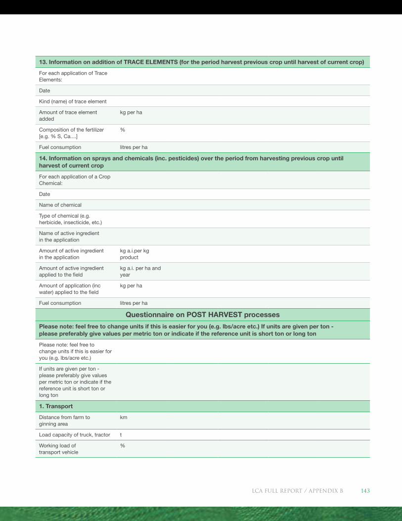
13. Information on addition of TRACE ELEMENTS (for the period harvest previous crop until harvest of current crop)
For each application of Trace Elements:
Date
Kind (name) of trace element
Amount of trace element added
kg per ha
Composition of the fertilizer [e.g. % S, Ca....]
%
Fuel consumption litres per ha
14. Information on sprays and chemicals (inc. pesticides) over the period from harvesting previous crop until harvest of current crop
For each application of a Crop Chemical:
Date
Name of chemical
Type of chemical (e.g. herbicide, insecticide, etc.)
Name of active ingredient in the application
Amount of active ingredient in the application
kg a.i.per kg product
Amount of active ingredient applied to the field
kg a.i. per ha and year
Amount of application (inc water) applied to the field
kg per ha
Fuel consumption litres per ha
Questionnaire on POST HARVEST processes
Please note: feel free to change units if this is easier for you (e.g. lbs/acre etc.) If units are given per ton - please preferably give values per metric ton or indicate if the reference unit is short ton or long ton
Please note: feel free to change units if this is easier for you (e.g. lbs/acre etc.)
If units are given per ton - please preferably give values per metric ton or indicate if the reference unit is short ton or long ton
1. Transport
Distance from farm to ginning area
km
Load capacity of truck, tractor t
Working load of transport vehicle
%
LCA FULL REport / Appendix B 143
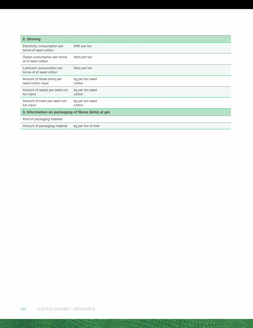
2. Ginning
Electricity consumption per tonne of seed cotton
kWh per ton
Diesel consumption per tonne of of seed cotton
liters per ton
Lubricant consumption per tonne of of seed cotton
liters per ton
Amount of fibres (lints) per seed cotton input
kg per ton seed cotton
Amount of seeds per seed cot-ton input
kg per ton seed cotton
Amount of trash per seed cot-ton input
kg per ton seed cotton
3. Information on packaging of fibres (lints) at gin
Kind of packaging material
Amount of packaging material kg per ton of lints
LCA FULL REport / Appendix B144
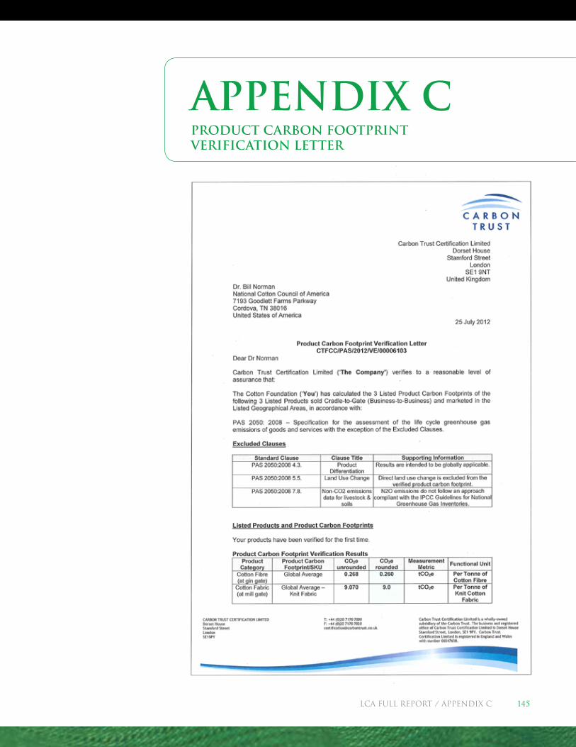
Product Carbon Footprint Verification Letter
APPENDIX C
LCA FULL REport / Appendix C 145
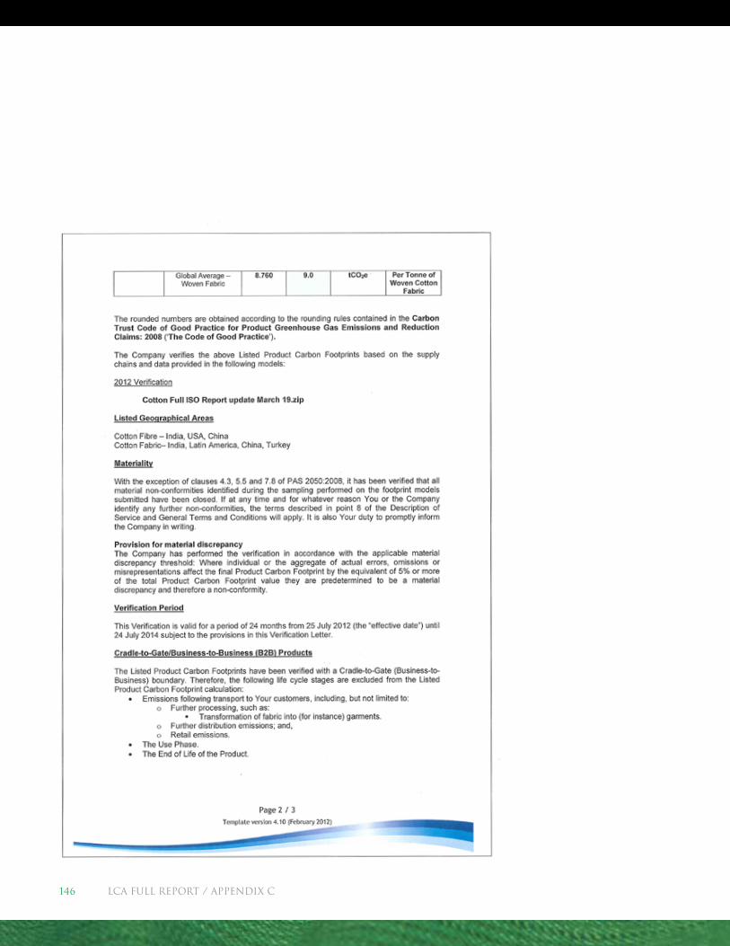
LCA FULL REport / Appendix C146
LCA FULL REport / Appendix C 147
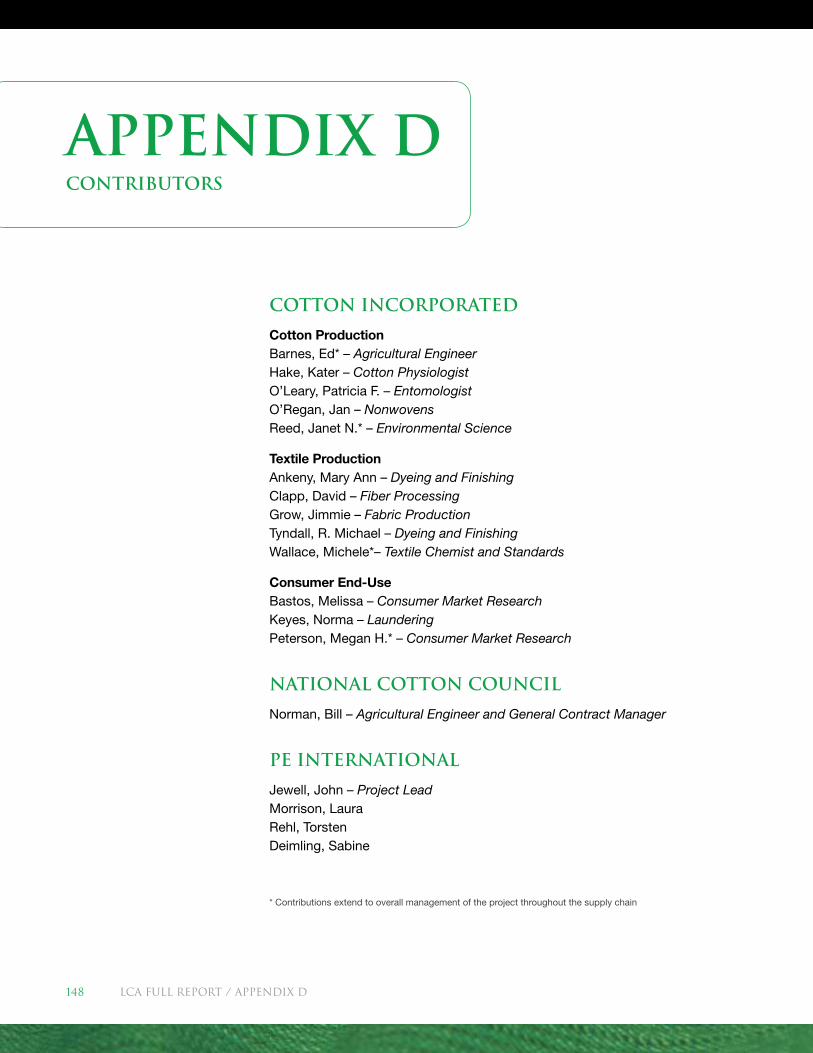
Cotton Incorporated
Cotton ProductionBarnes, Ed* – Agricultural Engineer Hake, Kater – Cotton Physiologist O’Leary, Patricia F. – Entomologist O’Regan, Jan – Nonwovens Reed, Janet N.* – Environmental Science
Textile ProductionAnkeny, Mary Ann – Dyeing and Finishing Clapp, David – Fiber Processing Grow, Jimmie – Fabric Production Tyndall, R. Michael – Dyeing and Finishing Wallace, Michele*– Textile Chemist and Standards
Consumer End-UseBastos, Melissa – Consumer Market Research Keyes, Norma – Laundering Peterson, Megan H.* – Consumer Market Research
National Cotton Council
Norman, Bill – Agricultural Engineer and General Contract Manager
PE International
Jewell, John – Project Lead Morrison, Laura Rehl, Torsten Deimling, Sabine
* Contributions extend to overall management of the project throughout the supply chain
APPENDIX DCONTRIBUTORS
LCA FULL REport / Appendix D148


The Cotton Foundation | National Cotton Council of America
Cotton Incorporated | Cotton Council International
Additional information on The Life Cycle Inventory & Life Cycle Assessment o f Cotton Fiber & Fabric can be found in an Executive Summary, available at http://cottontoday.cottoninc.com.
The Life Cycle Inventory & Life Cycle Assessment of Cotton Fiber & Fabric is a facet of the VISION 21 Project of The Cotton Foundation, and managed by the Cotton Board, Cotton Incorporated and Cotton Council International.
For more information, contact James Pruden at [email protected].
Related Documents


![mocha - iThinkSew...SKYLAR CUFFED PANTS mocha | m o d e r n + c o m f o r t MATERIAL LIST Waist Hip [FABRIC] Fabric Weight: Medium weight Fabric: Cotton, Cotton Blends, Washed Cotton,](https://static.cupdf.com/doc/110x72/6039e1743f7334329f21be0f/mocha-ithinksew-skylar-cuffed-pants-mocha-m-o-d-e-r-n-c-o-m-f-o-r-t-material.jpg)