HAL Id: tel-01485786 https://tel.archives-ouvertes.fr/tel-01485786 Submitted on 9 Mar 2017 HAL is a multi-disciplinary open access archive for the deposit and dissemination of sci- entific research documents, whether they are pub- lished or not. The documents may come from teaching and research institutions in France or abroad, or from public or private research centers. L’archive ouverte pluridisciplinaire HAL, est destinée au dépôt et à la diffusion de documents scientifiques de niveau recherche, publiés ou non, émanant des établissements d’enseignement et de recherche français ou étrangers, des laboratoires publics ou privés. Life-cycle assessment of 3rd-generation organic photovoltaic systems: developing a framework for studying the benefits and risks of emerging technologies Michael Tsang To cite this version: Michael Tsang. Life-cycle assessment of 3rd-generation organic photovoltaic systems : developing a framework for studying the benefits and risks of emerging technologies. Analytical chemistry. Uni- versité de Bordeaux, 2016. English. NNT : 2016BORD0331. tel-01485786

Welcome message from author
This document is posted to help you gain knowledge. Please leave a comment to let me know what you think about it! Share it to your friends and learn new things together.
Transcript
HAL Id: tel-01485786https://tel.archives-ouvertes.fr/tel-01485786
Submitted on 9 Mar 2017
HAL is a multi-disciplinary open accessarchive for the deposit and dissemination of sci-entific research documents, whether they are pub-lished or not. The documents may come fromteaching and research institutions in France orabroad, or from public or private research centers.
L’archive ouverte pluridisciplinaire HAL, estdestinée au dépôt et à la diffusion de documentsscientifiques de niveau recherche, publiés ou non,émanant des établissements d’enseignement et derecherche français ou étrangers, des laboratoirespublics ou privés.
Life-cycle assessment of 3rd-generation organicphotovoltaic systems : developing a framework for
studying the benefits and risks of emerging technologiesMichael Tsang
To cite this version:Michael Tsang. Life-cycle assessment of 3rd-generation organic photovoltaic systems : developing aframework for studying the benefits and risks of emerging technologies. Analytical chemistry. Uni-versité de Bordeaux, 2016. English. �NNT : 2016BORD0331�. �tel-01485786�
i
THÈSE PRÉSENTÉE
POUR OBTENIR LE GRADE DE
DOCTEUR DE
L’UNIVERSITÉ DE BORDEAUX
ÉCOLE DOCTORALE
SPÉCIALITÉ : CHIMIE ANALYTIQUE ET ENVIRONNEMENTALE
Par Michael TSANG
Cycle de vie de systèmes photovoltaïques organiques 3ème génération :
Élaboration d'un cadre pour étudier les avantages et les risques des technologies émergentes
Life-cycle Assessment of 3rd-Generation Organic Photovoltaic Systems:
Developing a Framework for Studying the Benefits and Risks of Emerging Technologies
Sous la direction de : Guido SONNEMANN (co-directeur : Dario BASSANI)
Soutenue le 07 Décembre 2016 Membres du jury : M. Ralph Rosenbaum, Chaire industrielle ELSA-PACT Irstea Montpellier Rapporteur Mme Lisolette Schebek, Professeur Université Darmstadt Rapporteur M. Nicola Armaroli, Directeur de Recherche, CNR Examinateur M. Philippe Garrigues, Directeur de Recherche, CNRS Président M. Dario M. Bassani, Directeur de Recherche, CNRS Co-directeur de thèse M. Guido W. Sonnemann, Professeur Université Bordeaux Directeur de thèse
Titre : Analyse du cycle de vie de systèmes photovoltaïques organiques de 3ème génération : Élaboration d'un cadre pour étudier les avantages et les risques des technologies émergentes
Résumé : Les systèmes photovoltaïques organiques sont des technologies
émergentes présentant de forts potentiels d’économie de ressources et de réduction des impacts sur l'environnement et la santé humaine par rapport aux dispositifs photovoltaïques conventionnels. La méthode de l’analyse du cycle de vie est appliquée afin d'évaluer la façon dont les différents procédés de fabrication, les caractéristiques des dispositifs, la phase d’utilisation et les scénarios de fin de vie des cellules photovoltaïques organiques influent sur ces avantages potentiels. Les impacts de cette technologie émergente sont comparés aux technologies conventionnelles à base de silicium pour établir un référentiel de performance des technologies photovoltaïques. En outre, les effets potentiels sur la santé humaine de l'utilisation de nanomatériaux dans les cellules photovoltaïques organiques ont été spécifiquement étudiés ; et la pertinence de l’analyse du cycle de vie pour évaluer cette catégorie d’impact a été examinée. Ainsi, un nouveau modèle d'évaluation de l'impact sur le cycle de vie est présenté afin de quantifier les dangers potentiels posés par les nanomatériaux. Enfin, ces impacts potentiels sont comparés aux avantages des cellules photovoltaïques organiques sur les cellules à base de silicium.
Mots clés : l’analyse du cycle de vie, photovoltaïques organiques, nanomatériaux
fabriqués, l'evaluation des risques, l'exposition, énergie renouvelable
Title : Life-cycle Assessment of 3rd-Generation Organic Photovoltaic Systems: Developing a Framework for Studying the Benefits and Risks of Emerging Technologies
Abstract : Organic photovoltaics present an emerging technology with significant
potential for increasing the resource efficiencies and reducing the environmental and human health hazards of photovoltaic devices. The discipline of life-cycle assessment is applied to assess how various prospective manufacturing routes, device characteristics, uses and disposal options of organic photovoltaics influences these potential advantages. The results of this assessment are further compared to silicon based photovoltaics as a benchmark for performance. A deeper look is given to the potential human health impacts of the use of engineered nanomaterials in organic photovoltaics and the appropriateness of life-cycle assessment to evaluate this impact criteria. A newly developed life-cycle impact assessment model is presented to demonstrate whether the use of and potential hazards posed by engineered nanomaterials outweighs any of the resource efficiencies and advantages organic photovoltaics possess over silicon photovoltaics.

Keywords : Life-Cycle Assessment, Organic Photovoltaics, Engineered
Nanomaterials, Risk Assessment, Characterization Factor, Indoor Occupational Exposure, Monte Carlo Analysis, Sustainable Production, Eco-Design, Renewable Energy, Life-Cycle Impact Assessment, production durable, éco-conception,
Institut des Sciences Moléculaires
[CYVI Group, 351 Cours de la Libération 33405 Talence]

ii
Dedication
This work is dedicated to my wife and daughter who are my foundation and to my parents who have
continuously encouraged my educational and professional pursuits.

iii
Acknowledgements
A tremendous amount of gratitude is owed to the many people who were involved in and around my
Ph.D. I, first, would like to thank my co-advisors Professors Guido W. Sonnemann and Dario M. Bassani
for providing me with the opportunity to broaden and strengthen my research and professional pursuits.
It cannot be emphasized enough that a successful Ph.D. depends on the relationship a student has with
their advisor(s), and I was fortunate to have advisors that were engaged, supportive and productively-
challenging throughout my three years of research.
The work presented in this dissertation also involved the partnership and collaboration with several other
Universities and research groups. I would like to thank Professor Antonio Marcomini and Danail Hristozov
from Ca’ Foscari University in Venice, Italy for inviting and hosting me in their research group for 3-months.
Additionally, I would like to thank Professor Sangwon Suh from the University of California, Santa Barbara
for, similarly, funding and hosting me in his research group for 3-months. These were both indispensable
(and memorable) opportunities which were the basis for two critical chapters of this thesis.
I would like to extend my appreciation to Philippe Garrigues, Ralph Rosenbaum, Liselotte Schebek, and
Nicola Armaroli for participating in my defense and being a part of this vital aspect of the Ph.D. process.
Many, many thanks are due to Karine Ndiaye for always being so incredibly gracious and generous with
her time, particularly during my first months in Bordeaux. Without her assistance, it is doubtful my stay in
France would have been a success.
My wife for her support and understanding of the time commitments these last three-years have required.
My daughter for defining the word precious.
And to the countless other individuals who have helped and contributed to my Ph.D. along the way: Alex
Zabeo (Ca’ Foscari), Sara Alba (Ca’ Foscari), Stella Stoycheva (Ca’ Foscari), Chengfang Pang (Ca’ Foscari);
Professor Lang Tran and the MODENA (E.U.) COST initiative for funding my research in Venice, Italy; Keld
Alstrup Jensen (Technical University of Denmark), Joonas Koivisto (Technical University of Denmark);
Arturo Keller (UCSB), Dingsheng Li (UCSB), Kendra Garner (UCSB); Masahiko Hirao (University of Tokyo),
Emi Kikuchi (University of Tokyo); Cyril Aymonier (University of Bordeaux), Gilles Philippot (University of
Bordeaux), Eskinder Gemechu (University of Bordeaux), Amandine Foulet (University of Bordeaux)

iv
Philippe Loubet (University of Bordeaux), Dieuwetje Schrijvers (University of Bordeaux), Baptiste Pillain
(University of Bordeaux), Edis Glogic (University of Bordeaux), Raphaël Brière (University of Bordeaux),
Thibaut Maury (University of Bordeaux), Amélie Thevenot (University of Bordeaux), Annie Corrêa Da Costa
(University of Bordeaux), Fabrice Forlini (University of Bordeaux) and Pascal Pajot (University of
Bordeaux).
v
Table of Contents
DEDICATION .......................................................................................................................................................... II
ACKNOWLEDGEMENTS ......................................................................................................................................... III
LIST OF TABLES ..................................................................................................................................................... IX
LIST OF FIGURES .................................................................................................................................................... XI
LIST OF EQUATIONS ............................................................................................................................................ XVI
EXECUTIVE SUMMARY .......................................................................................................................................XVII
LIST OF ABBREVIATIONS ...................................................................................................................................... XX
CHAPTER 1 ORGANIC PHOTOVOLTAICS AS A SUSTAINABLE TECHNOLOGY .......................................................... 22
PHOTOVOLTAIC TECHNOLOGY: BACKGROUND .................................................................................................................... 22 ORGANIC PHOTOVOLTAICS: THE THIRD-GENERATION OF PHOTOVOLTAICS .............................................................................. 26 OVERALL OBJECTIVES OF THE THESIS ................................................................................................................................ 27 LIFE-CYCLE ASSESSMENT: A PRIMER ................................................................................................................................ 28
Photovoltaic Life-Cycle Assessments: A Brief Background .................................................................................. 30 REVIEW OF ORGANIC PHOTOVOLTAIC LIFE-CYCLE ASSESSMENTS ........................................................................................... 31
Material Choices and Device Structures .............................................................................................................. 31 Scope and Boundaries ......................................................................................................................................... 36 Environmental and Human Health Impact Assessment Criteria ......................................................................... 38 Environmental and Human Health Impact Assessment Results ......................................................................... 39 Summary of the Review ...................................................................................................................................... 42
OVERVIEW OF PROBLEM CONTEXT FOR THE THESIS ............................................................................................................. 44 Hypotheses .......................................................................................................................................................... 44 Questions Addressed in this Thesis: .................................................................................................................... 45
STRUCTURE OF THE THESIS ............................................................................................................................................. 45
CHAPTER 2 LIFE-CYCLE ASSESSMENT AND ITS APPLICATION TO ORGANIC PHOTOVOLTAICS ............................... 48
LIFE-CYCLE ASSESSMENT: A BRIEF HISTORY....................................................................................................................... 48 Goal and Scope Definition ................................................................................................................................... 49
Attributional and Consequential Life-Cycle Assessment .................................................................................................. 50 Life-Cycle Inventory ............................................................................................................................................. 51 Life-Cycle Impact Assessment ............................................................................................................................. 54
Climate Change Potential (Global Warming Potential) .................................................................................................... 60 Ozone Layer Depletion ..................................................................................................................................................... 60 Photochemical Oxidation Formation (Smog) Potential .................................................................................................... 61 Resource (Minerals) Depletion ......................................................................................................................................... 61 Land Use, Land Occupation and Land Transformation ..................................................................................................... 61 Energy Use (Cumulative Energy Demand) ........................................................................................................................ 62 Water Depletion ............................................................................................................................................................... 62 Acidification ...................................................................................................................................................................... 62 Eutrophication .................................................................................................................................................................. 63 Ionizing Radiation ............................................................................................................................................................. 63 Particulate Matter Formation .......................................................................................................................................... 64 Ecotoxicity ........................................................................................................................................................................ 64 Human Toxicity ................................................................................................................................................................. 64
Interpretation ...................................................................................................................................................... 65
vi
CHAPTER 3 CRADLE-TO-GATE LIFE-CYCLE ASSESSMENT OF ORGANIC PHOTOVOLTAICS ....................................... 67
ORGANIC PHOTOVOLTAIC DEVICE STRUCTURE AND MATERIAL CHOICES IN THIS THESIS .............................................................. 67 LIFE-CYCLE ASSESSMENT METHODS ................................................................................................................................. 70
Goal and Scope Definition ................................................................................................................................... 70 Life Cycle Inventory ............................................................................................................................................. 72
Substrate .......................................................................................................................................................................... 72 Transparent (Front) Anode ............................................................................................................................................... 72 Hole Transporter .............................................................................................................................................................. 72 Active Layer ...................................................................................................................................................................... 73 Cathode ............................................................................................................................................................................ 73 Encapsulation and Lamination ......................................................................................................................................... 73
Sensitivity Analysis .............................................................................................................................................. 73 Comparison to Conventional Silicon-Based Photovoltaics .................................................................................. 74 Energy Payback Time .......................................................................................................................................... 75 Carbon Payback Time .......................................................................................................................................... 76 Minimum Required Lifetime ................................................................................................................................ 76
RESULTS AND DISCUSSION ............................................................................................................................................. 76 Sensitivity Analysis .............................................................................................................................................. 78 Comparison to Conventional Silicon-Based Photovoltaics .................................................................................. 79 Energy and Carbon Payback Times ..................................................................................................................... 80 Minimum Required Lifetime ................................................................................................................................ 82
CONCLUSION ............................................................................................................................................................... 83
CHAPTER 4 CRADLE-TO-GRAVE LIFE-CYCLE ASSESSMENT OF ORGANIC PHOTOVOLTAICS .................................... 84
METHODS ................................................................................................................................................................... 84 Goal and Scope ................................................................................................................................................... 84 Life-Cycle Inventory: System 1 (Rooftop Solar Array) .......................................................................................... 86
Organic Photovoltaic Technology Description ................................................................................................................. 86 Silicon-Based Photovoltaic Technology Description ......................................................................................................... 88 Balance of System ............................................................................................................................................................ 88 End-of-Life Considerations ............................................................................................................................................... 89
Life-Cycle Inventory: System 2 (Portable Solar Charger) ..................................................................................... 90 OPV Technology Description ............................................................................................................................................ 90 Silicon-Based Photovoltaic Technology Description ......................................................................................................... 90 End-of-Life Considerations ............................................................................................................................................... 91
Energy Payback Time .......................................................................................................................................... 91 Carbon Payback Time .......................................................................................................................................... 91 Minimum Required Lifetime of Organic Photovoltaics ....................................................................................... 92 Sensitivity Analysis .............................................................................................................................................. 92
RESULTS AND DISCUSSION ............................................................................................................................................. 93 Results for the Default Organic Photovoltaic Technologies in Scenario 1 and Scenario 2 .................................. 93 Energy and Carbon Payback Times ..................................................................................................................... 96 Minimum Required Lifetime of Organic Photovoltaics ....................................................................................... 98 Influence of Lifetimes and Efficiencies on LCA Results ...................................................................................... 100 Impacts by Life-Cycle Stage ............................................................................................................................... 103
CONCLUSION ............................................................................................................................................................. 105
CHAPTER 5 OPTIONS FOR ASSESSING THE TOXICOLOGICAL IMPACTS FROM ENGINEERED NANOMATERIALS USE
IN ORGANIC PHOTOVOLTAICS ........................................................................................................................... 107
TOXICOLOGICAL HAZARDS OF ORGANIC PHOTOVOLTAICS ................................................................................................... 107
vii
Engineered Nanomaterials: Resource Efficiencies and Hazards ....................................................................... 108 LIFE-CYCLE IMPACT ASSESSMENT: HAZARDS AND IMPACTS................................................................................................. 109
Review of Previously Published Characterization Factors for Engineered Nanomaterials ................................ 112 RISK ASSESSMENT: HAZARDS AND RISKS ......................................................................................................................... 114 COMPLEMENTARY AND INTEGRATED APPROACHES FOR LIFE-CYCLE ASSESSMENT AND RISK ASSESSMENT .................................... 117
Separate Use of LCA and RA for Nanotechnologies .......................................................................................... 118 Complementary Use of LCA and RA for Nanotechnologies ............................................................................... 118 Integration of LCA and RA for Nanotechnologies ............................................................................................. 120
CONCLUSION ............................................................................................................................................................. 124
CHAPTER 6 HUMAN HEALTH RISK ASSESSMENTS: QUANTITATIVE ASSESSMENT OF TITANIUM DIOXIDE AND
QUALITATIVE ASSESSMENT OF C60 FULLERENE NANOPARTICLES ....................................................................... 126
QUALITATIVE (SCREENING LEVEL) HUMAN HEALTH RISK ASSESSMENT.................................................................................. 126 Qualitative Exposure Assessment ..................................................................................................................... 126 Hazard Identification of C60-fullerenes and PCBM ............................................................................................ 129 Hazard Identification of Titanium Dioxide Nanoparticles ................................................................................. 129 Relevance of the Qualitative Exposure Assessment and Hazard Data Availability ........................................... 131
QUANTITATIVE RISK ASSESSMENT.................................................................................................................................. 131 Methods ............................................................................................................................................................ 131
Dose-Response Assessment ........................................................................................................................................... 132 Exposure Assessment ..................................................................................................................................................... 134 Risk Characterization ...................................................................................................................................................... 137
Results ............................................................................................................................................................... 137 Dose-Response Analysis ................................................................................................................................................. 137 Exposure assessment ..................................................................................................................................................... 139 Risk Characterization and Uncertainty ........................................................................................................................... 141
Discussion .......................................................................................................................................................... 142 Risk Relevance to Engineered Nanomaterials Use in Production of Organic Photovoltaics........................................... 142 Uncertainties within the Risk Assessment Procedure .................................................................................................... 143
Conclusions ....................................................................................................................................................... 144
CHAPTER 7 LIFE-CYCLE IMPACT ASSESSMENT NANOMATERIAL CHARACTERIZATION FACTORS: TITANIUM
DIOXIDE CASE STUDY ......................................................................................................................................... 146
METHODS ................................................................................................................................................................. 147 Emissions of and Exposure Scenarios for Nano-TiO2 in the Occupational Indoor Setting ................................. 147 Fate and Transport Model for Airborne Emissions of Nano-TiO2 in Occupational Indoor Air ........................... 149 Exposure to Nano-TiO2 in Occupational Indoor Air ........................................................................................... 152 Retained-Intake Fraction of Nano-TiO2 Emissions to Occupational Indoor Air ................................................. 153 Effect Factors for Nano-TiO2 in Occupational Indoor Air .................................................................................. 154 Classes of Occupational Indoor Air Human Health Characterization Factors for Nano-TiO2 ............................ 156
RESULTS ................................................................................................................................................................... 157 Emissions of Nano-TiO2 in the Occupational Indoor Setting ............................................................................. 157 Fate and Transport of Airborne Emissions of Nano-TiO2 in Occupational Indoor Air ....................................... 158 Exposure to Nano-TiO2 in Occupational Indoor Air ........................................................................................... 162 Effect Factors for Nano-TiO2 in Occupational Indoor Air .................................................................................. 172 Classes of Occupational Indoor Air Human Health Characterization Factors for Nano-TiO2 ............................ 174
DISCUSSION .............................................................................................................................................................. 177 LIFE-CYCLE ASSESSMENT OF ORGANIC PHOTOVOLTAICS WITH ENM-SPECIFIC CHARACTERIZATION FACTORS ............................... 181
Preliminary Results............................................................................................................................................ 183
viii
CHAPTER 8 CONCLUSIONS AND PERSPECTIVES .................................................................................................. 186
THE METHODOLOGICAL OPTIONS PRESENTED IN THIS THESIS .............................................................................................. 186 OVERVIEW OF THE RESULTS OF EACH METHODOLOGICAL OPTION ....................................................................................... 187
Life-Cycle Assessment of Organic Photovoltaic Systems ................................................................................... 187 Emissions of and Human Health Impacts from Engineered Nanomaterials using Risk Assessment ................. 189 Integrating Life-Cycle Assessment and Risk Assessment for the Evaluation of Organic Photovoltaics ............. 189
PERSPECTIVES ON THE ENVIRONMENTAL PREFERENCE OF OPV ........................................................................................... 190 PERSPECTIVES ON ENVIRONMENTAL AND HUMAN HEALTH MODELING OPTIONS, DEVELOPMENT AND DATA REQUIREMENTS ......... 191
Consequential Life-Cycle Assessment of Organic Photovoltaics ....................................................................... 192 Data Requirements ........................................................................................................................................... 192
Data Requirements for Emissions of Engineered Nanomaterials from Organic Photovoltaics ...................................... 193 CONCLUDING STATEMENTS .......................................................................................................................................... 194
BIBLIOGRAPHY ................................................................................................................................................... 195
APPENDICES............................................................................................................................................................ I
APPENDIX: CHAPTER 3 ..................................................................................................................................................... I APPENDIX: CHAPTER 4 ................................................................................................................................................. XV APPENDIX: CHAPTER 6 ............................................................................................................................................... XXX APPENDIX: CHAPTER 7 ................................................................................................................................................. XLI
LIST OF PUBLICATIONS ...................................................................................................................................... XLIX
RÉSUMÉ DETAILLE.................................................................................................................................................. L
ix
List of Tables TABLE 1-1 MATERIAL CHOICES OF THE LIFE-CYCLE ASSESSMENT STUDIES ON ORGANIC PHOTOVOLTAIC SYSTEMS EXISTING IN THE PEER-
REVIEWED LITERATURE UP TO DECEMBER 2013. ............................................................................................................ 32 TABLE 1-2 SCOPE, BOUNDARIES AND SELECT NUMBER OF ASSUMPTIONS THAT WERE MADE IN THE LIFE-CYCLE ASSESSMENT STUDIES ON
ORGANIC PHOTOVOLTAIC SYSTEMS EXISTING IN THE PEER-REVIEWED LITERATURE UP TO DECEMBER 2013. ................................ 37 TABLE 1-3 LIFE-CYCLE ASSESSMENT STUDIES ON ORGANIC PHOTOVOLTAIC SYSTEMS EXISTING IN THE PEER-REVIEWED LITERATURE UP TO THE
END OF 2013. (ADAPTED FROM CHATZISIDERIS ET AL.67) ................................................................................................ 44 TABLE 1-4 FLOW DIAGRAM OF THE STRUCTURE, OBJECTIVES, HYPOTHESES AND RESEARCH QUESTIONS PUT FORTH IN THIS THESIS ........... 47 TABLE 2-1 COMMONLY APPLIED LIFE-CYCLE IMPACT ASSESSMENT METHODOLOGIES AND THEIR COMMONLY DEFINED MIDPOINT IMPACT
CATEGORIES. (ADAPTED FROM ACERO ET AL.82) ............................................................................................................. 56 TABLE 2-2 LIFE-CYCLE IMPACT ASSESSMENT CATEGORIES CONSIDERED IN THIS STUDY. RECIPE 2008 MIDPOINT (H) IMPACT CATEGORIES
WERE USED, WITH TOXICITY ESTIMATED USING THE MIDPOINT USETOX 2.0 INDICATORS AND CUMULATIVE ENERGY DEMAND
ESTIMATED BASED ON HISCHIER ET AL.92 ....................................................................................................................... 59 TABLE 3-1 ESTIMATED PARAMETERS USED TO CALCULATE THE ENERGY-PAYBACK TIMES FOR EACH SOLAR CELL CONSIDERED. INSOLATION IS
BASED ON AN AVERAGE EUROPEAN INSOLATION OF 1300 KWH PER M2.............................................................................. 75 TABLE 3-2 POWER GENERATION, EMBODIED ENERGY, ENERGY PAYBACK TIME, EMBODIED CARBON, AND CARBON PAYBACK TIME FOR EACH
SOLAR CELL CONSIDERED IN THIS CHAPTER, ASSUMING AN AVERAGE EUROPEAN INSOLATION VALUE OF 1300 KWH PER M2. ......... 81 TABLE 3-3 MINIMUM LIFETIMES REQUIRED OF ORGANIC PHOTOVOLTAIC TO ACHIEVE ENVIRONMENTAL AND HUMAN HEALTH PARITY WITH
AMORPHOUS SILICON CELLS HAVING 25-YEAR LIFETIMES. CATEGORIES ARE DISPLAYED IN DESCENDING ORDER OF RESULTS FOR THE
DEFAULT OPV. ....................................................................................................................................................... 82 TABLE 4-1 GENERALIZED ACCOUNT OF MATERIAL COMPONENTS AND ENERGY REQUIREMENTS FOR PRODUCING ONE M2 OF AN OPV-D
PANEL BASED ON THE DESCRIPTION IN CHAPTER 3 FOR THE FTOINKJET OPV. INDIRECT, UPSTREAM OR AUXILIARY MATERIAL AND
ENERGY REQUIREMENTS AS WELL AS EMISSIONS ARE NOT REPORTED HERE. .......................................................................... 87 TABLE 4-2 INVENTORY FOR AN AVERAGE KWH OF INSTALLED OPV SOLAR ROOFING ARRAY, MOUNTED WITH SUPPORT (S1) .................. 88 TABLE 4-3 INVENTORY FOR AN AVERAGE TEN WATT-HOURS OF AN ORGANIC PHOTOVOLTAIC PORTABLE SOLAR CHARGER (S2) ............... 90 TABLE 4-4 ESTIMATED PARAMETERS USED TO CALCULATE THE ENERGY AND CARBON PAYBACK TIMES ................................................ 91 TABLE 4-5 POWER GENERATION, CUMULATIVE ENERGY DEMAND AND ENERGY PAYBACK TIME FOR SYSTEM 1 (ROOFTOP ARRAY) AND
SYSTEM 2 (PORTABLE CHARGER) ................................................................................................................................. 96 TABLE 4-6 MINIMUM REQUIRED LIFETIMES (IN YEARS) OF THE DEFAULT ORGANIC PHOTOVOLTAIC SCENARIO FOR SYSTEM 1 (ROOFTOP
ARRAY) AND SYSTEM 2 (PORTABLE CHARGER) COMPARED TO THEIR RESPECTIVE SILICON-BASED PHOTOVOLTAIC COUNTERPARTS .... 98 TABLE 5-1 CONSIDERATION OF NANOMATERIAL-SPECIFIC EMISSIONS AND IMPACTS ACROSS THE PREVIOUSLY PUBLISHED LIFE-CYCLE
ASSESSMENTS ON ORGANIC PHOTOVOLTAICS ............................................................................................................... 107 TABLE 6-1 SUMMARY OF THE STUDY283 AND SELECT DOSE-RESPONSE DATA USED TO CHARACTERIZE THE INFLAMMATORY RESPONSE UPON
INHALATION EXPOSURE TO NANO-TIO2 ...................................................................................................................... 133 TABLE 6-2 DESCRIPTION OF THE EXPOSURE SCENARIOS USED FOR THE HUMAN HEALTH RISK ASSESSMENT OF INHALATION EXPOSURE TO
NANOPARTICLES OF TITANIUM DIOXIDE IN THE OCCUPATIONAL WORKPLACE. HI: HANDLING ENERGY FACTOR. ........................... 134 TABLE 6-3 PARAMETERS USED IN THE NANOSAFER V1.1 EXPOSURE ASSESSMENT MODEL WHERE HI = HANDLING ENERGY FACTOR, TWC IS
WORK CYCLE TIME, PWC IS PAUSE BETWEEN WORK CYCLES, NWC IS NUMBER OF WORK CYCLES, ATRANSFER IS AMOUNT OF MATERIAL
TRANSFERRED PER TRANSFER EVENT WITHIN EACH WORK CYCLE, VTOT IS THE TOTAL VOLUME OF THE WORK ROOM, AND AER IS THE
GENERAL AIR EXCHANGE RATIO IN THE WORK-ROOM. .................................................................................................... 135 TABLE 6-4 DAILY AVERAGED, INHALATION BENCHMARK CONCENTRATIONS (MG/M3) FOR IN VIVO ANIMAL STUDIES AND CORRESPONDING
MODELS FIT FOR A 20% INCREASE IN NEUTROPHIL COUNT IN MICE. .................................................................................. 138 TABLE 6-5 CALCULATED NEAR-FIELD AND FAR-FIELD AIRBORNE CONCENTRATIONS OF NANO-TIO2 FOR THE THREE SEPARATE EXPOSURE
SCENARIOS CONSIDERED IN THE HUMAN HEALTH RISK ASSESSMENT .................................................................................. 140 TABLE 6-6 SUMMARY OF THE RISK CHARACTERIZATION (REPORTED AS RISK CHARACTERIZATION RATIOS) DISTRIBUTIONS FOR EACH NEAR-
AND FAR-FIELD EXPOSURE SCENARIOS. RESULTS REPRESENT 10,000 MONTE-CARLO SIMULATIONS. ...................................... 141 TABLE 7-1 PARAMETERS USED IN THE FATE-TRANSPORT MODEL DESCRIBING THE EXPOSURE SCENARIOS INVOLVED WITH “DUMPING LARGE
AMOUNTS OF POWDER IN A VESSEL” PER THE DESCRIPTION IN CHAPTER 6, TABLE 6-2. THE EXPOSURE SCENARIOS DIFFER BASED ON

x
THE MAGNITUDE OF THE EMISSION, E, PER MINUTE AND THE FREQUENCY OF THE WORK-CYCLE ACTIVITY, F. HI = HANDLING ENERGY
FACTOR, TWC IS WORK CYCLE TIME, PWC IS PAUSE BETWEEN WORK CYCLES, NWC IS NUMBER OF WORK CYCLES, AHANDLED IS AMOUNT OF
MATERIAL TRANSFERRED PER TRANSFER EVENT WITHIN EACH WORK CYCLE, VTOT IS THE TOTAL VOLUME OF THE WORK ROOM, AND
AER IS THE GENERAL AIR EXCHANGE RATIO IN THE WORK-ROOM ..................................................................................... 148 TABLE 7-2 PARAMETERS AND THEIR VALUES USED IN THE FATE AND TRANSPORT MODEL ............................................................... 151 TABLE 7-3 RESULTS FOR EMISSIONS AND FINAL NEAR-FIELD AND FAR-FIELD CONCENTRATIONS. ...................................................... 157 TABLE 7-4 RESULTS FOR THE INTERNAL WET LUNG BURDEN AND THE RETAINED-INTAKE FRACTION, REPORTED AS EITHER A LIFETIME OR 1-
YEAR VALUE .......................................................................................................................................................... 162 TABLE 7-5 EFFECT FACTORS (EF), INTAKE FRACTIONS (RIF) AND ENM-SPECIFIC CHARACTERIZATION FACTORS (CFNS) FOR SIX DIFFERENT
EMISSION AND EXPOSURE SCENARIOS THAT INVOLVED DIFFERENCES IN EMISSION RATES (E) AND EMISSION INTERVAL FREQUENCIES (F)
.......................................................................................................................................................................... 175 TABLE 7-6 HUMAN HEALTH IMPACTS PER WATT-PEAK OF OPV CELL PRODUCTION WITHOUT A ENM-SPECIFIC CHARACTERIZATION FACTOR
FOR NANO-TIO2 (LEFT COLUMNS) AND WITH A ENM-SPECIFIC CHARACTERIZATION FACTOR (RIGHT COLUMNS) ........................ 183
xi
List of Figures FIGURE 1-1 ILLUSTRATIONS OF (A) THE SETUP DESCRIBED BY BECQUEREL IN 1939 TO ACHIEVE THE FIRST KNOWN, INTENTIONALLY
PRODUCED PHOTOVOLTAIC EFFECT AND (B) THE OLDEST CONTEMPORARY INTERPRETATION OF THE P-N SILICON SEMICONDUCTING
CELL AS IT IS KNOWN TODAY. (SOURCE: GREET 2002)12 .................................................................................................. 23 FIGURE 1-2 LABORATORY-BASED SOLAR CELL EFFICIENCY RECORDS (SOURCE: U.S. NATIONAL RENEWABLE ENERGY LABORATORY)22 ...... 25 FIGURE 1-3 GEOMETRY AND LAYOUT OF A GENERIC PHOTOVOLTAIC CELL. .................................................................................... 26 FIGURE 1-4 GEOMETRY AND LAYOUT OF A GENERIC ORGANIC PHOTOVOLTAIC CELL. ....................................................................... 27 FIGURE 1-5 EXAMPLE OF PRINTED ORGANIC PHOTOVOLTAIC PANEL ............................................................................................ 27 FIGURE 1-6 THE (A) FOUR PRINCIPLE STEPS OF A LIFE-CYCLE ASSESSMENT BEGINNING WITH THE GOAL AND SCOPE DEFINITION WHICH
IDENTIFIES THE PROBLEM AND THE BOUNDARIES OF THE STUDY. THE SECOND STEP IS THE INVENTORY ANALYSIS AND CORRESPONDS
WITH ALL RELEVANT DATA COLLECTION REQUIREMENTS. NEXT THE IMPACT ASSESSMENT STAGE CONVERTS THE INVENTORY ENTRIES
INTO POTENTIAL IMPACTS USING CHARACTERIZATION FACTORS. LASTLY, THE STEP OF INTERPRETATION IS CONDUCTED THROUGHOUT
THE ENTIRE STUDY TO REFINE ANY NECESSARY STEPS AND DISCUSS THE SIGNIFICANCE OF THE INVENTORY AND IMPACT RESULTS IN
CONTEXT OF THE ORIGINAL SCOPE OF THE STUDY. THE (B) GENERAL LIFE-CYCLE STAGES THAT CAN BE CONSIDERED IN A LIFE-CYCLE
ASSESSMENT. (SOURCE: FIGURE (A) ADAPTED FROM ISO 1404028) .................................................................................. 29 FIGURE 1-7 TWO-DIMENSIONAL STRUCTURES OF (A) AN UNMODIFIED FULLERENE WITH 60 CARBON ATOMS AND (B) A FUNCTIONALIZED
60-CARBON RING FULLERENE (PCBM). (SOURCE: PUBCHEM OPEN CHEMISTRY ONLINE DATABASE) ....................................... 34 FIGURE 1-8 SELECTION OF P-TYPE POLYMERS THAT COULD BE USED WITH PCBM AS A BASIS FOR THE ACTIVE LAYER OF AN ORGANIC
PHOTOVOLTAIC SOLAR CELL. (SOURCE: YAN AND SAUNDERS 201455) ................................................................................ 35 FIGURE 1-9 CUMULATIVE ENERGY DEMAND FOR ORGANIC PHOTOVOLTAIC CELLS AS REPORTED IN THE LITERATURE UP THROUGH DECEMBER
2013 PER WATT-PEAK OF POWER PRODUCTION ............................................................................................................. 39 FIGURE 2-1 GROWTH IN THE NUMBER OF PEER REVIEWED SCIENTIFIC JOURNAL ARTICLES IN THE SUBJECT AREA OF “LIFE-CYCLE
ASSESSMENT.” RESULTS GENERATED USING SCOPUS (WWW.SCOPUS.COM)....................................................................... 49 FIGURE 2-2 THE (A) ATTRIBUTIONAL MODELING APPROACH IN LIFE-CYCLE ASSESSMENT DEPICTED AS A SHARE OF TOTAL, CURRENT GLOBAL
ENVIRONMENTAL BURDENS OF A PRODUCT OR PROCESS AS OPPOSED TO THE (B) CONSEQUENTIAL MODELING APPROACH THAT IS
CONCERNED WITH THE CHANGES IN TOTAL, GLOBAL ENVIRONMENTAL BURDENS DUE TO DECISIONS MADE REGARDING THE PRODUCT
OR PROCESS. (SOURCE: WEIDEMA 200377) .................................................................................................................. 50 FIGURE 2-3 GENERAL FLOW DIAGRAM CREATED DURING THE LIFE-CYCLE INVENTORY PHASE. THE FLOW DIAGRAM HELPS TO OUTLINE THE
DATA REQUIREMENTS FOR EACH PROCESS AND ALONG EACH STEP OF A LIFE-CYCLE ASSESSMENT. (SOURCE: U.S. EPA78) .............. 52 FIGURE 2-4 ILLUSTRATION OF FOREGROUND AND BACKGROUND PROCESSES WITHIN A LIFE-CYCLE INVENTORY. FOREGROUND PROCESSES
ARE DEFINED AS THE PRIMARY PROCESSES OF CONCERN AND/OR WHICH THE DEVELOPMENT OF NEW AND NOVEL DATA IS USED TO
DEFINE THOSE PROCESSES. THUS, FOREGROUND PROCESSES CAN REPRESENT ANY STAGE OF THE LIFE-CYCLE ASSESSMENT SUCH AS
DURING (A) RAW MATERIAL EXTRACTION, (B) PRODUCT MANUFACTURING, (C) USE AND/OR (D) END-OF-LIFE SCENARIOS. ............ 53 FIGURE 2-5 A GENERAL CAUSE AND EFFECT CHAIN CONSIDERED IN LIFE-CYCLE IMPACT ASSESSMENT METHODOLOGIES, FOLLOWING THE
CLASSIFICATION OF INVENTORY ITEMS INTO THEIR RESPECTIVE MIDPOINT AND/OR ENDPOINT LEVELS OF IMPACT AND CONVERTED TO
IMPACT VALUES USING EACH CATEGORIES’ SUBSTANCE-SPECIFIC CHARACTERIZATION FACTOR. (SOURCE: EUROPEAN COMMISSION
JOINT RESEARCH CENTRE) ......................................................................................................................................... 58 FIGURE 3-1 GENERAL DEPICTION OF THE BULK HETEROJUNCTION ORGANIC PHOTOVOLTAIC CELL CONSIDERED IN THIS CHAPTER,
INCORPORATING (THE SKELETAL FORMULAS OF) (A) PHENYL-C61-BUTYRIC ACID METHYL ESTER (PCBM) WHICH ACTS AS THE
ELECTRON ACCEPTOR AND (B) POLY(3-HEXYLTHIPHENE) (P3HT) WHICH ACTS AS THE ELECTRON DONOR IN THE ACTIVE LAYER. ...... 68 FIGURE 3-2 GENERIC SCHEMATIC OF THE FIELD STRENGTH OF LIGHT AT THE ACTIVE LAYER FOR AN OPV DEVICE WITHOUT AN OPTICAL
SPACER (LEFT) AND WITH AN OPTICAL SPACER (RIGHT). (SOURCE: KIM ET AL.121) .................................................................. 69 FIGURE 3-3 SYSTEM BOUNDARIES OF THE CRADLE-TO-GATE LIFE-CYCLE ASSESSMENT ILLUSTRATING THE MAIN COMPONENTS FOR THE
PRODUCTION OF A PROSPECTIVE ORGANIC PHOTOVOLTAIC PANEL. ALL RELEVANT PROCESSES, MATERIALS, AND WASTE-STREAMS UP
TO THE PRODUCTION OF THE SOLAR CELL ARE CONSIDERED, THUS EXCLUDING ANY CONSIDERATION OF THE USE-PHASE OR END-OF-
LIFE CONSIDERATIONS. .............................................................................................................................................. 71 FIGURE 3-4 THE CONTRIBUTIONS OF LIFE-CYCLE STAGES AND PRODUCTION PROCESSES TO THE OVERALL IMPACTS OF THE DEFAULT ORGANIC
PHOTOVOLTAIC CELL CONSIDERED IN THIS STUDY. ........................................................................................................... 77
xii
FIGURE 3-5 LIFE-CYCLE IMPACT RESULTS FOR THE THREE ALTERNATIVE AND ONE DEFAULT ORGANIC PHOTOVOLTAIC CELLS CONSIDERED IN
THIS LIFE-CYCLE ASSESSMENT. THE IMPACT RESULTS ARE INTERNALLY NORMALIZED USING DIVISION BY THE MAXIMUM IMPACT VALUE
PER IMPACT CATEGORY. ............................................................................................................................................. 78 FIGURE 3-6 COMPARISON OF LIFE-CYCLE IMPACTS FOR THE ORGANIC PHOTOVOLTAIC CELLS AND TWO CONVENTIONAL SILICON CELLS. THE
IMPACT RESULTS ARE INTERNALLY NORMALIZED USING DIVISION BY THE MAXIMUM IMPACT VALUE PER IMPACT CATEGORY............ 80 FIGURE 3-7 COMPARISON OF CUMULATIVE ENERGY DEMAND PER WATT-PEAK FOR ORGANIC PHOTOVOLTAIC CELLS REPORTED IN THE
LITERATURE AS WELL AS FROM THIS THESIS. ................................................................................................................... 81 FIGURE 4-1 SYSTEM BOUNDARIES FOR (A) SYSTEM 1 (ROOFTOP ARRAY) AND (B) SYSTEM 2 (PORTABLE CHARGER). INCINERATION WAS JUST
ONE OF THE END-OF-LIFE SCENARIOS MODELED IN THE LIFE-CYCLE ASSESSMENT AND IS SHOWN FOR CLARIFICATION OF HOW THE
ENERGY RECOVERY WAS CONSIDERED IN THE LIFE-CYCLE INVENTORY. .................................................................................. 85 FIGURE 4-2 EXAMPLES OF THE TWO DIFFERENT SYSTEMS (I.E. FUNCTIONAL UNITS) STUDIED IN THIS CHAPTER ..................................... 86 FIGURE 4-3 RELATIVE DEFAULT IMPACTS OF (A) SYSTEM 1 (ROOFTOP ARRAY) COMPARING THE DEFAULT OPV-D SCENARIO WITH M-SI
PANELS AND (B) SYSTEM 2 (PORTABLE CHARGER) COMPARING THE DEFAULT OPV-D WITH A-SI PANELS. TWO SEPARATE DISPOSAL
PROCESSES ARE ADDITIONALLY SHOWN FOR EACH SYSTEM. THE IMPACT RESULTS ARE INTERNALLY NORMALIZED USING DIVISION BY
THE MAXIMUM IMPACT VALUE PER IMPACT CATEGORY. ................................................................................................... 93 FIGURE 4-4 CHANGES IN LIFE-CYCLE IMPACTS FOR S1 (ROOFTOP, INCINERATION) ACCORDING TO FORECASTS IN (A) LIFETIME OF ORGANIC
PHOTOVOLTAIC PANELS (WITH A 1% EFFICIENCY) AND (B) EFFICIENCIES OF ORGANIC PHOTOVOLTAIC PANELS (WITH A 1-YEAR
LIFETIME). THE IMPACT RESULTS ARE INTERNALLY NORMALIZED TO THE IMPACT VALUES OF M-SI (I.E. M-SI’S IMPACTS ARE SET AT
100%). SEE APPENDIX: CHAPTER 4 FOR THE SENSITIVITY ANALYSIS FOR S1 WITH LANDFILLING AS THE END-OF-LIFE OPTION. ...... 100 FIGURE 4-5 CHANGES IN LIFE-CYCLE IMPACTS FOR SYSTEM 2 (PORTABLE CHARGER, INCINERATION) ACCORDING TO FORECASTS IN (A)
LIFETIME OF ORGANIC PHOTOVOLTAIC PANELS (WITH A 1% EFFICIENCY) AND (B) EFFICIENCIES OF ORGANIC PHOTOVOLTAIC PANELS
(WITH A 1-YEAR LIFETIME). THE IMPACT RESULTS ARE INTERNALLY NORMALIZED TO THE IMPACT VALUES OF A-SI (I.E. A-SI’S IMPACTS
ARE SET AT 100%). SEE APPENDIX: CHAPTER 4 FOR THE SENSITIVITY ANALYSIS FOR SYSTEM 2 WITH LANDFILLING AS THE END-OF-LIFE
OPTION. ............................................................................................................................................................... 102 FIGURE 4-6 COMPARISON OF ORGANIC PHOTOVOLTAIC ALTERNATIVES FOR (A) SYSTEM 1 THAT INVOLVED REMOVING THE MOUNTING
STRUCTURE (NO MOUNT) AND (B) SYSTEM 2 BASED ON PORTABLE CHARGERS WITHOUT CASING (NC). THE IMPACT RESULTS IN
SYSTEM 1 ARE ALL INTERNALLY NORMALIZED TO OPV-D AS THE MAXIMUM VALUE (I.E. 100%). THE IMPACT RESULTS IN SYSTEM 2
ARE INTERNALLY NORMALIZED BY TECHNOLOGY-TYPE (I.E. OPV-NC IS NORMALIZED BY OPV-D AND A-SI-NC IS NORMALIZED BY A-
SI). SEE APPENDIX: CHAPTER 4 FOR THE RESULTS OF THE LANDFILLING OPTIONS. ................................................................ 104 FIGURE 5-1 NUMBER OF PUBLICATIONS BETWEEN 1980-2013 THAT MATCH THE SEARCH CRITERIA OF “NANOTOXICOLOGY” (ADAPTED
FROM H. F. KRUG 2014.182). .................................................................................................................................. 109 FIGURE 5-2 CONSIDERATION OF LIFE-CYCLE RESOURCE CONSUMPTION AND WASTE EMISSIONS USING A GENERIC NANOTECHNOLOGY
EXAMPLE. THE LEFT SIDE OF THE FIGURE (A) PROVIDES A GENERALIZATION ABOUT THE CONSIDERATIONS DURING LIFE-CYCLE
ASSESSMENTS OF ENM-ENABLED PRODUCTS. RESOURCE EXTRACTION AND MATERIAL PROCESSING WOULD INVOLVE ALL RELEVANT
MATERIALS TO THE INTENDED PRODUCT BUT ALSO THOSE THAT ARE ENM-SPECIFIC (I.E. EXTRACTION OF THE ENM PRECURSOR AND
PROCESSING IT INTO THE NANOMETER SIZE RANGE). PRODUCT MANUFACTURING WILL OUTLINE THE PRODUCTION OF A SINGLE TYPE
OF PRODUCT (E.G. SPORTING EQUIPMENT WITH CARBON NANOTUBES) LEADING TO ITS RELATED USE AND POTENTIAL END-OF-LIFE
OPTIONS (E.G. INCINERATION). THE RIGHT SIDE OF THE FIGURE (B) REPRESENTS A HYPOTHETICAL EXAMPLE OF A ENM-ENABLED
VERSUS NON-ENM (BULK) PRODUCT APPLIED IN THE FUNCTION OF WALL-PROTECTION (I.E. A PAINT WITH A CONVENTIONAL
PIGMENT VERSUS A PAINT USING ENM-BASED PIGMENTS). IN THIS EXAMPLE, IT IS ASSUMED THAT THE TWO PIGMENTS (I) ARE OF
THE SAME CHEMICAL COMPOSITION BUT DIFFERENT SIZES, (II) ENM- VERSUS BULK-MANUFACTURING DIFFER BY THE ENERGY AND
MATERIALS (E.G. SOLVENTS) REQUIRED TO MECHANICALLY GRIND BULK MATERIAL TO ENM-SIZES, (III) DUE TO ITS HIGHER
EFFICIENCY, LESS ENM-ENABLED MATERIAL IS REQUIRED DURING THE USE-PHASE AND THUS LESS UPSTREAM RAW MATERIAL
EXTRACTION IS REQUIRED AND (IV) ALTHOUGH LESS ACTIVE INGREDIENT IS EMITTED DURING THE USE PHASE, IT IS DISTINCT THAT IT IS
BEING EMITTED IN THE ENM FORM AS OPPOSED TO BULK EMISSIONS. THE DIFFERENCE IN ENERGY CONSUMPTION, MATERIAL USE,
WASTE GENERATION AND EMISSIONS DEPICTED BY UP/DOWN ARROWS REPRESENT THE RELATIVE LIFE-CYCLE INVENTORY OF THE
ENM-ENABLED PRODUCT (WITH UP DESIGNATING THE ENM-ENABLED AMOUNTS ARE HIGHER AND VICE VERSA BUT WITHOUT ANY
INDICATION OF THE MAGNITUDE OF CHANGE). AGGREGATION OF ALL INVENTORY VALUES WOULD THEN RELATE TO THEIR POTENTIAL
ENVIRONMENTAL IMPACTS VIA ITS MATERIAL SPECIFIC CHARACTERIZATION FACTOR. ............................................................ 110
xiii
FIGURE 5-3 ILLUSTRATION FOR CARRYING OUT A HUMAN HEALTH RISK ASSESSMENT TO DETERMINE ISSUES OF CHEMICAL AND SUBSTANCE-
SPECIFIC TOXICITY. HUMAN HEALTH RISK ASSESSMENT INVOLVES IDENTIFYING RELEVANT HEALTH HAZARDS, QUANTIFYING THE
CRITICAL DOSE OF CONCERN BY EVALUATING THE RELATIONSHIP BETWEEN DOSE TO THE SUBSTANCE AND TOXICOLOGICAL RESPONSE,
ESTIMATING THE MEASURE OF EXPOSURE OF THE RECEPTOR (I.E. THE INDIVIDUAL HUMAN) TO THE SUBSTANCE AND CALCULATING THE
RISK INVOLVED BY COMPARING THE EXPOSURE VALUE TO THE CRITICAL DOSE. ..................................................................... 115 FIGURE 5-4 BROAD OVERVIEW OF THE SCOPE OF LIFE-CYCLE ASSESSMENT (LEFT) AND OF HUMAN HEALTH RISK ASSESSMENT (RIGHT). THE
FORMER CONSISTING OF EMISSIONS, ALONG WITH THEIR FATE AND EXPOSURE, AS WELL AS ELEMENTARY AND TECHNO-SPHERE
FLOWS, ALL OF WHICH ARE CONNECTED TO VARIOUS ENVIRONMENTAL AND SUSTAINABILITY METRICS USED TO MEASURE LEVELS OF
RESOURCE EFFICIENCY BETWEEN PRODUCTS AND PROCESSES. HUMAN HEALTH RISK ASSESSMENT IS DEPICTED BY ITS DISCREET SCOPE
THAT FOCUSES ON THE TOXICOLOGICAL RISKS. WHILE BOTH CAN EVALUATE ISSUES OF CHEMICAL TOXICITY, THEY DO SO WITH
DIFFERENT METHODS, AND IN THE CASE OF LIFE-CYCLE ASSESSMENT, APPLICATION OF METHODS TO DETERMINE ENM-TOXICITY ARE
NOT CURRENTLY EMPLOYED IN PRACTICE, THEY ARE FOR HUMAN HEALTH RISK ASSESSMENT. ................................................. 116 FIGURE 5-5 ONE SEPARATE, ONE COMPLEMENTARY AND THREE INTEGRATED OPTIONS FOR USING OF LIFE-CYCLE ASSESSMENT AND RISK
ASSESSMENT TO EVALUATE PRODUCTS CONTAINING ENGINEERED NANOMATERIALS. CHOICES ARE PRESENTED FROM THE PERSPECTIVE
OF DIFFERENT PARTICULAR STAKEHOLDERS AND THEIR OBJECTIVES. DECISION MAKERS, FOR EXAMPLE, MAY BE CONCERNED BY BOTH
RESOURCE EFFICIENCY (E.G. CHANGES IN ENERGY CONSUMPTION FOR A ENM-ENABLED PRODUCT) AND TOXICOLOGICAL IMPACTS
AND RISKS OF A NANOTECHNOLOGY OR ONLY A SINGLE DIMENSION OF THESE IMPACTS. ........................................................ 119 FIGURE 5-6 ILLUSTRATION DEMONSTRATING THAT THE RESULTS OF A HUMAN HEALTH RISK ASSESSMENT (LEFT SIDE OF FIGURE) MAY NOT
ALWAYS BE CONGRUENT WITH LIFE-CYCLE ASSESSMENT HUMAN HEALTH RESULTS, SINCE THEY ARE CALCULATED USING DIFFERENT
METHODS, MOST IMPORTANT OF WHICH IS THE SCOPE BY WHICH THESE TWO TOOLS ARE DEFINED. ........................................ 120 FIGURE 5-7 KEY ASPECTS OF LIFE-CYCLE AND RISK ASSESSMENT INTEGRATION AT THE METHODOLOGICAL LEVEL. INTEGRATION IS REPLACED
ON ITS LEVEL OF SPATIAL AND TEMPORAL SPECIFICITY AS WELL AS MODEL AND DATA COMPLEXITY. FOR EXAMPLE, LOW TEMPORAL
RESOLUTION (I.E. NO CHANGES IN EMISSIONS OVER TIME) WITH A GLOBAL SPATIAL SCOPE WILL RESULT IN A STEADY-STATE MODEL
THAT USES CONSTANT (I.E. NON-VARIABLE) AND HIGHLY AGGREGATED DATA, RESPECTIVELY, SIMILAR TO WHAT IS USED IN CURRENT
LIFE-CYCLE ASSESSMENT METHODS SUCH AS USETOX. THIS IS THE CASE LABELED AS “GI” OR GLOBAL INTEGRATION, AND
REPRESENTS ONE OF THE THREE LEVELS OF INTEGRATION SET FORTH IN THIS THESIS, HOWEVER THE DEGREE OF INTEGRATION IS
DYNAMIC FOR EACH AXIS, INDEPENDENT OF ONE ANOTHER. FOR INSTANCE, LOW TEMPORAL RESOLUTION WITH A LOCAL SPATIAL
SCOPE (I.E. HIGH SPATIAL RESOLUTION) WILL SIMILARLY RESULT IN A STEADY-STATE MODEL USING CONSTANT, BUT, NON-
AGGREGATED (I.E. SITE-SPECIFIC) DATA. TO ILLUSTRATE THESE POINTS FURTHER, ENM EMISSIONS MODELING IS SHOWN IN THE
FIGURE AS A PRACTICAL REPRESENTATION. GLOBAL INTEGRATION, THUS, RESULTS IN THE USE OF NON-CHANGING, AGGREGATED
EMISSIONS DATA THAT IS AVERAGED FOR A LARGE CONTINENTAL REGION IN A STEADY-STATE MODEL. IN TERMS OF ITS RELEVANCY TO
ENM, THIS APPROACH HAS LESS PREDICTIVE POWER THAN THE OTHER TWO OPTIONS SHOWN IN THE FIGURE. FOR EXAMPLE, SITE-
SPECIFIC INTEGRATION (SSI), USES THE EMPIRICALLY DETERMINED CHANGES IN SINGLE-SOURCE EMISSIONS DATA MEASURED OVER
AN UNCONDITIONAL TIMEFRAME IN A FULLY-DYNAMIC MODEL. CONTEXT-DEPENDENT INTEGRATION (CDI) MODELS EMISSIONS
USING A GENERALIZED TIME-DEPENDENT ASSUMPTION (E.G. POSITIVE, LINEAR CORRELATION) FOR CLASSES OF SOURCES AVERAGED
AT THE COUNTRY LEVEL IN A PARTIALLY-DYNAMIC MODEL. .............................................................................................. 121 FIGURE 6-1 POTENTIAL EXPOSURE TO ENGINEERED NANOMATERIALS ACROSS THE LIFE-CYCLE FOR A GENERIC ENM-CONTAINING PRODUCT.
EXPOSURE ALONG THE LIFE-CYCLE OF A ENM-ENABLED PRODUCT CAN RESULT FROM EMISSIONS OF ENGINEERED NANOMATERIALS AT
ANY STAGE, INTRODUCING POTENTIAL FOR OCCUPATIONAL, CONSUMER AND ECOLOGICAL EXPOSURES AND CORRESPONDING
TOXICOLOGICAL IMPACTS OR RISKS. ........................................................................................................................... 127 FIGURE 6-2 QUALITATIVE EXPOSURE ASSESSMENT OF PCBM AND NANO-TIO2 ACROSS THE LIFE-CYCLE OF THE OPV PANELS .............. 128 FIGURE 6-3 TWO-DIMENSIONAL STRUCTURE OF TITANIUM DIOXIDE IN ITS TWO MOST COMMONLY FOUND FORMS: RUTILE AND ANATASE.
(SOURCE: U.S. NATIONAL INSTITUTE OF OCCUPATIONAL SAFETY AND HEALTH) ................................................................. 130 FIGURE 6-4 LOG-NORMAL DISTRIBUTIONS OF (A) THE INTERSPECIES TOXICO-DYNAMIC EXTRAPOLATION FACTOR WITH A GEOMETRIC MEAN
OF 1 AND GEOMETRIC STANDARD DEVIATION OF 3.27 AND (B) THE INTRASPECIES EXTRAPOLATION FACTOR WITH A GEOMETRIC MEAN
OF 1 AND GEOMETRIC STANDARD DEVIATION OF 2.7. THE X-AXIS IS WITHOUT UNITS. .......................................................... 133 FIGURE 6-5 INTERPRETATIONS OF THE RESIDUAL VALUES OF THE LOG-TRANSFORMED STANDARD DEVIATIONS FOR 59 PARTICULATE
POWDER TESTS (NOTE: THREE TESTS INCLUDED MISSING VALUES). THE UPPER AND LOWER LEFT GRAPHS INDICATE THAT THE
ASSUMPTION OF NORMALITY FOR THE ERROR TERMS IS VALID, AS THERE IS NO SIGNIFICANT DEVIATION FROM THE CENTRAL TREND
xiv
LINE AND THE HIGHEST FREQUENCY IS FOR VALUES EQUAL TO ZERO. THE UPPER RIGHT GRAPH PLOTS THE ERROR TERMS AGAINST
THEIR FITTED VALUES, INDICATING WHETHER THAT THE MEAN VALUE OF ZERO HOLDS TRUE. .................................................. 136 FIGURE 6-6 FITTED LOG-LOGISTIC MODELS USING PROAST SOFTWARE WITH REPORTED CONFIDENCE INTERVALS TO THE MICE AND RAT
NEUTROPHIL PERCENT CHANGES UPON INHALATION OF NANO-TIO2. THE DOSE-RESPONSE RESULTS DEMONSTRATE DIFFERENCES IN
THE SLOPE OF THE LINES PER SPECIES, WITH A MUCH MORE SENSITIVE RESPONSE FOR RATS. THE DOES-RESPONSE CURVE SHOWN IN
THIS EXAMPLE WAS FITTED WITH A LOG-LIKELIHOOD OF -1374. THE BENCHMARK DOSE FOR RATS IS SHOWN BY THE LOWER CURVE
CORRESPONDING TO DATA WITH LARGE CIRCLES, WHILE THE BENCHMARK DOSE FOR MICE IS SHOWN FOR THE UPPER CURVE USING
CORRESPONDING TRIANGULAR DATA POINTS. (SEE APPENDIX: CHAPTER 6 FOR FULL SET OF MODELS FIT TO THE DOSE-RESPONSE
DATA) .................................................................................................................................................................. 138 FIGURE 6-7 RESULTS OF (A) THE 10,000 MONTE-CARLO SIMULATIONS USED TO ESTIMATE THE BENCHMARK CONCENTRATION FOR
HUMANS (BMCH) AND (B) THE CONTRIBUTION OF EACH PARAMETER USED TO ESTIMATE THE BENCHMARK CONCENTRATIONS FOR
HUMANS. ............................................................................................................................................................. 139 FIGURE 6-8 POTENTIAL EXPOSURE TIME-SERIES IN THE (A) NEAR FIELD AND (B) FAR FIELD. NOTE: THIS FIGURE SHOWS THE RESULTS FOR A
LARGER RANGE OF EXPOSURE SCENARIOS THAN PRESENTED IN THIS CHAPTER. THESE ADDITIONAL SCENARIOS WERE COMPLETED AS A
PART OF A LARGER PUBLICATION OUT OF DIRECT CONTEXT OF THIS CHAPTER. ADDITIONAL INFORMATION FOR THE OTHER SCENARIOS
CAN BE FOUND IN APPENDIX: CHAPTER 6. ................................................................................................................... 140 FIGURE 6-9 RESULTS OF 10,000 MONTE-CARLO RISK CHARACTERIZATION RATIO SIMULATIONS FOR EXPOSURE SCENARIO 2 IN THE (A)
NEAR-FIELD AND (B) FAR-FIELD. NOTE THAT RIGHT-END TAILS OF THE DISTRIBUTION ARE ARTIFICIALLY TRUNCATED FOR
PRESENTATION. CONTRIBUTIONS TO THE UNCERTAINTY AND VARIATION ARE DISPLAYED IN (C) FOR THE NEAR-FIELD AND IN (D) FOR
THE FAR-FIELD. ...................................................................................................................................................... 142 FIGURE 7-1 COMPARISON OF YEARLY EMISSIONS AND EMISSION RATE. ...................................................................................... 158 FIGURE 7-2 RESULTS OF THE FATE AND TRANSPORT MODEL FOR EXPOSURE SCENARIO 1 SHOWING NEAR-FIELD (BLUE) AND FAR-FIELD
(ORANGE) NANO-TIO2 AIRBORNE CONCENTRATIONS DURING 1 WORKING DAY OF 8 HOURS. ES1-ES6 ARE PRESENTED IN ORDER
SEQUENTIAL ORDER (A)-(F). THE X-AXIS REPORTS TIME IN UNITS OF MINUTES AND THE Y-AXIS REPORTS NANO-TIO2 CONCENTRATION
IN UNITS OF ΜG/M3................................................................................................................................................ 159 FIGURE 7-3 COMPARISON OF AVERAGE AND MAXIMUM DAILY AIRBORNE NANO-TIO2 CONCENTRATION. ......................................... 160 FIGURE 7-4 PROPORTIONAL FATE AND TRANSPORT OF NANO-TIO2 PER “COMPARTMENT” DURING (A) THE FIRST 10-MINUTES OF THE FIRST
EMISSION CYCLE OF ES1 AND (B) THE FINAL 10-MINUTE EMISSION CYCLE OF ES1 AT THE END OF THE WORK DAY ...................... 161 FIGURE 7-5 RETENTION OF NANO-TIO2 IN THE LUNG ESTIMATED OVER 1 FULL WORK YEAR FOR ES1. THE X-AXIS REPRESENTS TIME IN
MINUTES OVER 1-YEAR AND THE Y-AXIS REPRESENTS THE MASS (ΜG) OF NANO-TIO2 IN THE WET LUNG. THE GREEN TREND LINE
REPRESENTS THE CHANGE IN MASS IN THE AIR-EXCHANGE (PULMONARY) REGIONS OF THE LUNG, THE BLUE TREND LINE REPRESENTS
THE CHANGE IN MASS IN THE INTERSTITIAL REGIONS OF THE LUNG, THE PINK TREND LINE REPRESENTS THE CHANGE IN MASS IN THE
TRACHEA-BRONCHIAL REGIONS OF THE LUNG, THE RED TREND LINE REPRESENTS THE TOTAL RETENTION IN THE WET LUNG INCLUDING
THE AIR-EXCHANGE (PULMONARY) REGIONS, INTERSTITIAL REGIONS, TRACHEA-BRONCHIAL REGIONS AND THEIR MACROPHAGES. . 163 FIGURE 7-6 TIME-WEIGHTED RETENTION IN THE WET LUNG OVER LIFETIME AS A FUNCTION OF THE (A) EMISSION RATE AND (B) YEARLY
EMISSIONS.AS WELL AS THE RESULTING RETAINED INTAKE FRACTION AS A FUNCTION OF (C) THE EMISSION RATE AND (D) THE YEARLY
EMISSIONS. ........................................................................................................................................................... 164 FIGURE 7-7 RETENTION OF NANO-TIO2 IN THE (A) WET LUNG AND (B) TOTAL AIRWAY SYSTEM BASED ON AIRWAY REGIONS FOR ALL SIX
EXPOSURE SCENARIOS. ............................................................................................................................................ 165 FIGURE 7-8 RETENTION OF NANO-TIO2 IN THE LUNG ESTIMATED OVER 1 FULL WORK YEAR FOR ES4. THE X-AXIS REPRESENTS TIME IN
MINUTES OVER 1-YEAR AND THE Y-AXIS REPRESENTS THE MASS (ΜG) OF NANO-TIO2 IN THE WET LUNG. THE GREEN TREND LINE
REPRESENTS THE CHANGE IN MASS IN THE AIR-EXCHANGE (PULMONARY) REGIONS OF THE LUNG, THE BLUE TREND LINE REPRESENTS
THE CHANGE IN MASS IN THE INTERSTITIAL REGIONS OF THE LUNG, THE PINK TREND LINE REPRESENTS THE CHANGE IN MASS IN THE
TRACHEA-BRONCHIAL REGIONS OF THE LUNG, THE GREY TREND LINE REPRESENTS THE CHANGE IN MASS IN THE LUNG MACROPHAGES,
THE DARK-BLUE LINE REPRESENTS THE CHANGE IN MASS IN THE PULMONARY MACROPHAGES, THE RED TREND LINE REPRESENTS THE
TOTAL RETENTION IN THE WET LUNG INCLUDING THE AIR-EXCHANGE (PULMONARY) REGIONS, INTERSTITIAL REGIONS, TRACHEA-
BRONCHIAL REGIONS AND THEIR MACROPHAGES. ......................................................................................................... 168 FIGURE 7-9 RETENTION OF NANO-TIO2 IN THE LUNG ESTIMATED OVER 1 FULL WORK YEAR FOR ES4. THE X-AXIS REPRESENTS TIME IN
MINUTES OVER 1-YEAR AND THE Y-AXIS REPRESENTS THE MASS (ΜG) OF NANO-TIO2 IN THE WET LUNG. THE PINK TREND LINE
xv
REPRESENTS THE CHANGE IN MASS IN THE TRACHEA-BRONCHIAL REGIONS OF THE LUNG, THE YELLOW TREND LINE REPRESENTS THE
CHANGE IN MASS IN THE UPPER AIRWAY, THE DARK-BLUE LINE REPRESENTS THE CHANGE IN MASS IN THE PULMONARY
MACROPHAGES, THE RED TREND LINE REPRESENTS THE TOTAL RETENTION IN THE WET LUNG INCLUDING THE AIR-EXCHANGE
(PULMONARY) REGIONS, INTERSTITIAL REGIONS, TRACHEA-BRONCHIAL REGIONS AND THEIR MACROPHAGES. ........................... 171 FIGURE 7-10 COMPARISON OF THE INTAKE FRACTION (SHOWN IN LOG-SCALE) AND NUMBER OF EXPOSED WORKERS .......................... 172 FIGURE 7-11 BENCHMARK DOSE RESULTS FOR CANCEROUS IMPACTS TO BOTH MICE (BLACK CIRCLES) AND RATS (RED TRIANGLES). THE X-
AXIS REPRESENTS THE INTERNAL LUNG DOSE REPORTED AS SURFACE AREA OF NANO-TIO2 PER G-DRY LUNG. THE Y-AXIS IS REPORTED
AS THE FRACTION OF THE ANIMALS THAT RESULT IN CASES OF CANCER. THE LOG-LIKELIHOOD OF THE FITTED HILL MODEL WAS -
208.82. THE REPORTED BENCHMARK DOSE WAS 1.43 M2/G-DRY LUNG BASED ON THE EXCESS RISK OF 50% OVER BACKGROUND
CANCER RATES. ...................................................................................................................................................... 173 FIGURE 7-12 BENCHMARK DOSE RESULTS FOR NON-CANCEROUS IMPACTS TO BOTH MICE (BLACK CIRCLES) AND RATS (RED TRIANGLES). THE
X-AXIS REPRESENTS THE INTERNAL LUNG DOSE REPORTED AS ΜG OF NANO-TIO2 PER G-DRY LUNG. THE Y-AXIS IS REPORTED AS THE
FRACTION OF THE ANIMALS THAT RESULT IN INFLAMMATION (I.E. THE 20% INCREASE IN NEUTROPHIL COUNT OVER BACKGROUND
RATES). THE LOG-LIKELIHOOD OF THE FITTED HILL MODEL WAS -1386.37. THE REPORTED BENCHMARK DOSES WERE 27352 ΜG/G-
DRY LUNG FOR MICE AND 7807 ΜG/G-DRY LUNG FOR RATS BASED ON THE EXCESS RISK OF 50% OVER BACKGROUND INFLAMMATION
RATES. ................................................................................................................................................................. 174 FIGURE 7-13 NON-CARCINOGENIC CHARACTERIZATION FACTORS (LIFETIME) AS A FUNCTION OF THE (A) TOTAL EMISSIONS PER YEAR, (B)
EMISSION RATE IN LOG-SCALE, (C) EXPOSED POPULATION OF WORKERS (NOTE: RESULTS ONLY DISPLAYED FOR ES1.00 (E-HIGH, F-
SHORT) SCENARIO), AND (D) ACUTE, 1-YEAR VERSUS CHRONIC, LIFETIME CHARACTERIZATION FACTORS. .................................. 176 FIGURE 7-14 CONTRIBUTION TO HUMAN HEALTH IMPACTS BY LIFE-CYCLE STAGE ......................................................................... 184

xvi
List of Equations (2-1) (2-2) (3-1) (3-2) (3-3) (3-4) (4-1) (5-1) (6-1) (6-2) (6-3) (6-4) (7-1) (7-2) (7-3) (7-4) (7-5) (7-6) (7-7) (7-8) (7-9) (7-10) (7-11)
…………………………………………………………………………………………………………………………………………... …………………………………………………………………………………………………………………………………………... …………………………………………………………………………………………………………………………………………... …………………………………………………………………………………………………………………………………………... …………………………………………………………………………………………………………………………………………... …………………………………………………………………………………………………………………………………………... …………………………………………………………………………………………………………………………………………... …………………………………………………………………………………………………………………………………………... …………………………………………………………………………………………………………………………………………... …………………………………………………………………………………………………………………………………………... …………………………………………………………………………………………………………………………………………... …………………………………………………………………………………………………………………………………………... …………………………………………………………………………………………………………………………………………... …………………………………………………………………………………………………………………………………………... …………………………………………………………………………………………………………………………………………... …………………………………………………………………………………………………………………………………………... …………………………………………………………………………………………………………………………………………... …………………………………………………………………………………………………………………………………………... …………………………………………………………………………………………………………………………………………... …………………………………………………………………………………………………………………………………………... …………………………………………………………………………………………………………………………………………...
35 46 56 56 57 73 96 113 116 116 118 130 130 131 131 132 132 133 135 135 136
Executive Summary
xvii
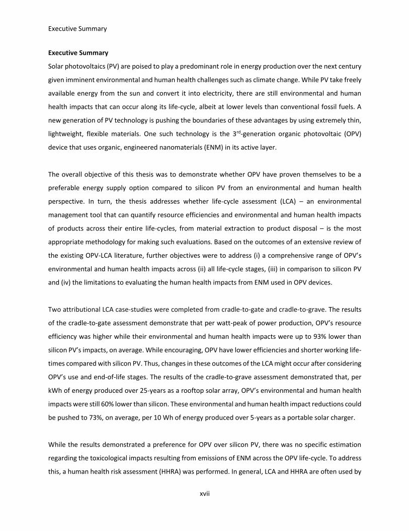
Executive Summary
Solar photovoltaics (PV) are poised to play a predominant role in energy production over the next century
given imminent environmental and human health challenges such as climate change. While PV take freely
available energy from the sun and convert it into electricity, there are still environmental and human
health impacts that can occur along its life-cycle, albeit at lower levels than conventional fossil fuels. A
new generation of PV technology is pushing the boundaries of these advantages by using extremely thin,
lightweight, flexible materials. One such technology is the 3rd-generation organic photovoltaic (OPV)
device that uses organic, engineered nanomaterials (ENM) in its active layer.
The overall objective of this thesis was to demonstrate whether OPV have proven themselves to be a
preferable energy supply option compared to silicon PV from an environmental and human health
perspective. In turn, the thesis addresses whether life-cycle assessment (LCA) – an environmental
management tool that can quantify resource efficiencies and environmental and human health impacts
of products across their entire life-cycles, from material extraction to product disposal – is the most
appropriate methodology for making such evaluations. Based on the outcomes of an extensive review of
the existing OPV-LCA literature, further objectives were to address (i) a comprehensive range of OPV’s
environmental and human health impacts across (ii) all life-cycle stages, (iii) in comparison to silicon PV
and (iv) the limitations to evaluating the human health impacts from ENM used in OPV devices.
Two attributional LCA case-studies were completed from cradle-to-gate and cradle-to-grave. The results
of the cradle-to-gate assessment demonstrate that per watt-peak of power production, OPV’s resource
efficiency was higher while their environmental and human health impacts were up to 93% lower than
silicon PV’s impacts, on average. While encouraging, OPV have lower efficiencies and shorter working life-
times compared with silicon PV. Thus, changes in these outcomes of the LCA might occur after considering
OPV’s use and end-of-life stages. The results of the cradle-to-grave assessment demonstrated that, per
kWh of energy produced over 25-years as a rooftop solar array, OPV’s environmental and human health
impacts were still 60% lower than silicon. These environmental and human health impact reductions could
be pushed to 73%, on average, per 10 Wh of energy produced over 5-years as a portable solar charger.
While the results demonstrated a preference for OPV over silicon PV, there was no specific estimation
regarding the toxicological impacts resulting from emissions of ENM across the OPV life-cycle. To address
this, a human health risk assessment (HHRA) was performed. In general, LCA and HHRA are often used by
Executive Summary
xviii
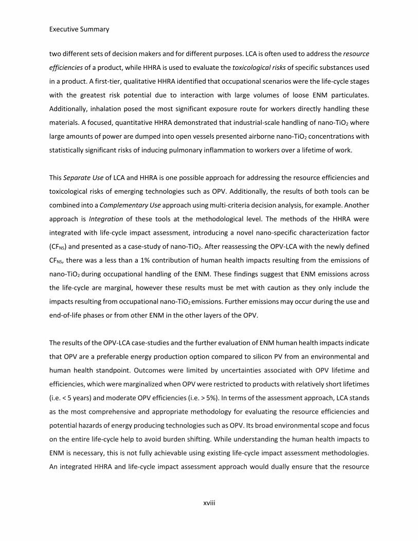
two different sets of decision makers and for different purposes. LCA is often used to address the resource
efficiencies of a product, while HHRA is used to evaluate the toxicological risks of specific substances used
in a product. A first-tier, qualitative HHRA identified that occupational scenarios were the life-cycle stages
with the greatest risk potential due to interaction with large volumes of loose ENM particulates.
Additionally, inhalation posed the most significant exposure route for workers directly handling these
materials. A focused, quantitative HHRA demonstrated that industrial-scale handling of nano-TiO2 where
large amounts of power are dumped into open vessels presented airborne nano-TiO2 concentrations with
statistically significant risks of inducing pulmonary inflammation to workers over a lifetime of work.
This Separate Use of LCA and HHRA is one possible approach for addressing the resource efficiencies and
toxicological risks of emerging technologies such as OPV. Additionally, the results of both tools can be
combined into a Complementary Use approach using multi-criteria decision analysis, for example. Another
approach is Integration of these tools at the methodological level. The methods of the HHRA were
integrated with life-cycle impact assessment, introducing a novel nano-specific characterization factor
(CFNS) and presented as a case-study of nano-TiO2. After reassessing the OPV-LCA with the newly defined
CFNS, there was a less than a 1% contribution of human health impacts resulting from the emissions of
nano-TiO2 during occupational handling of the ENM. These findings suggest that ENM emissions across
the life-cycle are marginal, however these results must be met with caution as they only include the
impacts resulting from occupational nano-TiO2 emissions. Further emissions may occur during the use and
end-of-life phases or from other ENM in the other layers of the OPV.
The results of the OPV-LCA case-studies and the further evaluation of ENM human health impacts indicate
that OPV are a preferable energy production option compared to silicon PV from an environmental and
human health standpoint. Outcomes were limited by uncertainties associated with OPV lifetime and
efficiencies, which were marginalized when OPV were restricted to products with relatively short lifetimes
(i.e. < 5 years) and moderate OPV efficiencies (i.e. > 5%). In terms of the assessment approach, LCA stands
as the most comprehensive and appropriate methodology for evaluating the resource efficiencies and
potential hazards of energy producing technologies such as OPV. Its broad environmental scope and focus
on the entire life-cycle help to avoid burden shifting. While understanding the human health impacts to
ENM is necessary, this is not fully achievable using existing life-cycle impact assessment methodologies.
An integrated HHRA and life-cycle impact assessment approach would dually ensure that the resource

Executive Summary
xix
efficiencies of OPV do not come at the expense of shifting burdens to the occupational human health
impacts.
Keywords: Life-Cycle Assessment, Organic Photovoltaics, Engineered Nanomaterials, Risk Assessment,
Characterization Factor, Indoor Occupational Exposure, Monte Carlo Analysis, Sustainable Production,
Eco-Design, Renewable Energy, Life-Cycle Impact Assessment
xx
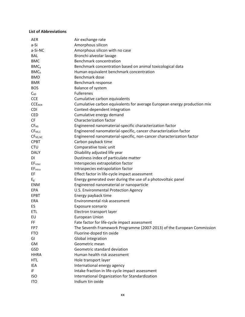
List of Abbreviations
AER Air exchange rate a-Si Amorphous silicon a-Si-NC Amorphous silicon with no case BAL Bronchi-alveolar lavage BMC Benchmark concentration BMCa Benchmark concentration based on animal toxicological data BMCh Human equivalent benchmark concentration BMD Benchmark dose BMR Benchmark response BOS Balance of system C60 Fullerenes CCE Cumulative carbon equivalents CCERER Cumulative carbon equivalents for average European energy production mix CDI Context-dependent integration CED Cumulative energy demand CF Characterization factor CFNS Engineered nanomaterial-specific characterization factor CFNS,C Engineered nanomaterial-specific, cancer characterization factor CFNS,NC Engineered nanomaterial-specific, non-cancer characterization factor CPBT Carbon payback time CTU Comparative toxic unit DALY Disability adjusted life year DI Dustiness index of particulate matter EFinter Interspecies extrapolation factor EFintra Intraspecies extrapolation factor EF Effect factor in life-cycle impact assessment Eg Energy generated over during the use of a photovoltaic panel ENM Engineered nanomaterial or nanoparticle EPA U.S. Environmental Protection Agency EPBT Energy payback time ERA Environmental risk assessment ES Exposure scenario ETL Electron transport layer EU European Union FF Fate factor for life-cycle impact assessment FP7 The Seventh Framework Programme (2007-2013) of the European Commission FTO Fluorine-doped tin oxide GI Global integration GM Geometric mean GSD Geometric standard deviation HHRA Human health risk assessment HTL Hole transport layer IEA International energy agency iF Intake fraction in life-cycle impact assessment ISO International Organization for Standardization ITO Indium tin oxide
xxi
LCA Life-cycle assessment LOAEL Low observed adverse effect level MC Monte-Carlo Analysis MRL Minimum required lifetime m-Si Multi-crystalline silicon NF Near-field workroom volume NIOSH U.S. National Institute of Occupational Safety and Health NMVOC Non-methane volatile organic compounds NOAEL No observed adverse effect level OPV Organic photovoltaics OPV-NC Organic photovoltaics with no case P3HT Poly(3-hexyl)thiophene PBPK Physiologically-based pharmacokinetic PCBM [6,6]-phenyl C61 butyric acid methyl ester PCS Phagocytizing cells PEDOT:PSS Poly(3,4-ethylenedioxythiophene) polystyrene sulfonate PET Polyethylene terephthalate POP Workplace population PV Photovoltaic RA Risk assessment REL Recommended exposure limit RiF Retained-intake fraction for use in life-cycle impact assessment RIVM Netherland’s National Institute for Public Health and the Environment SSI Site-specific integration Wp Watt-peak XF Exposure Factor in life-cycle impact assessment
Chapter 1 Organic Photovoltaics as a Sustainable Technology
22
Chapter 1 Organic Photovoltaics as a Sustainable Technology
Energy is arguably the most important issue confronting society in the 21st century. That is because energy
seems to be at the heart of what is considered to be sustainability. Although sustainability means many
things to many people, it is often reduced to three core pillars of sustainability development: economics,
society and environment.1 In this way, it is hard to imagine another factor over the previous two and a
half centuries that has been so influential on society. The development and use of fossil fuels has spurred
tremendous growth in industry and the overall global population as well as technological achievements
on a scale never seen before the industrial revolution. Along the way, however, this has come at the
expense of certain environmental and public health costs. The world is now, arguably, entering an era of
peak-oil,2 coincidentally while changes to the earth’s atmosphere due to anthropogenic sources of
greenhouse gases and pollution3 are producing environmental conditions, such as global climate change,
that will test the limit of society’s capacity for adaptation and resiliency.4
Thus, sustainability is not simply an energy issue but also an environmental and public health issue. The
true cost of an energy source cannot be quantified solely as a function of its procurement, refinement and
distribution transactions, for example, but it must also account for the “externalities” or indirect costs
related to its environmental and human health damage. Taking this comprehensive vantage point is
necessary to avoid burden shifting, for instance, as can be the case with biofuels and its issues of adverse
land and freshwater use impacts5–7 and increases in greenhouse gas emissions8 or in regards to the use of
solar photovoltaics (PV) and increases in the use and consumption of metals.9
Therefore, research and development into new, sustainable sources of meeting the world’s current and
future energy demands will, consequently, continue to be an important topic throughout the 21st century.
Coupled with the urgent need to address greenhouse gas emissions and climate change, among a host of
other environmental and public health challenges, renewable energy sources such as PV are poised to
take on a more pronounced role in the world’s energy procurement strategy.
Photovoltaic Technology: Background
The photovoltaic effect is the production of electric current under the application of light. Its discovery is
attributed to the French physicist Edmond Becquerel who, in 1939, used silver bromide coated platinum
electrodes to produce a current when illuminated in solution (Figure 1-1).10,11
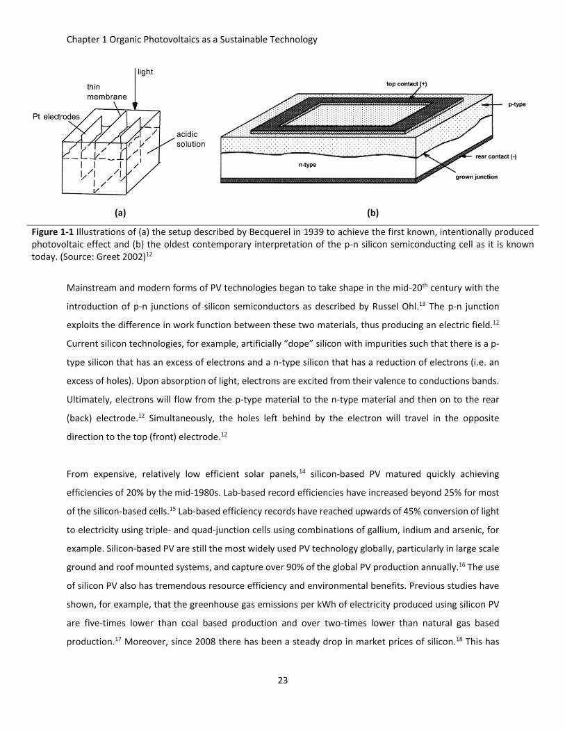
Chapter 1 Organic Photovoltaics as a Sustainable Technology
23
(a) (b)
Figure 1-1 Illustrations of (a) the setup described by Becquerel in 1939 to achieve the first known, intentionally produced photovoltaic effect and (b) the oldest contemporary interpretation of the p-n silicon semiconducting cell as it is known today. (Source: Greet 2002)12
Mainstream and modern forms of PV technologies began to take shape in the mid-20th century with the
introduction of p-n junctions of silicon semiconductors as described by Russel Ohl.13 The p-n junction
exploits the difference in work function between these two materials, thus producing an electric field.12
Current silicon technologies, for example, artificially “dope” silicon with impurities such that there is a p-
type silicon that has an excess of electrons and a n-type silicon that has a reduction of electrons (i.e. an
excess of holes). Upon absorption of light, electrons are excited from their valence to conductions bands.
Ultimately, electrons will flow from the p-type material to the n-type material and then on to the rear
(back) electrode.12 Simultaneously, the holes left behind by the electron will travel in the opposite
direction to the top (front) electrode.12
From expensive, relatively low efficient solar panels,14 silicon-based PV matured quickly achieving
efficiencies of 20% by the mid-1980s. Lab-based record efficiencies have increased beyond 25% for most
of the silicon-based cells.15 Lab-based efficiency records have reached upwards of 45% conversion of light
to electricity using triple- and quad-junction cells using combinations of gallium, indium and arsenic, for
example. Silicon-based PV are still the most widely used PV technology globally, particularly in large scale
ground and roof mounted systems, and capture over 90% of the global PV production annually.16 The use
of silicon PV also has tremendous resource efficiency and environmental benefits. Previous studies have
shown, for example, that the greenhouse gas emissions per kWh of electricity produced using silicon PV
are five-times lower than coal based production and over two-times lower than natural gas based
production.17 Moreover, since 2008 there has been a steady drop in market prices of silicon.18 This has
Chapter 1 Organic Photovoltaics as a Sustainable Technology
24
put PV technology at close price parity with conventional energy sources as such as coal.19 Although this
is great news for the renewable energy market in general, this trend may stabilize and even reverse in the
near-term.20
The competitive price of silicon PV may have the unintended consequences of reducing incentives to
invest in and develop alternative PV technologies that may not yet be as cost competitive.21 Nonetheless,
the last four decades of PV development are marked by research and development of a wide range of
viable technologies, spanning from conventional single-crystal silicon and multi-crystalline silicon (m-Si)
PV to second generation technologies such as amorphous silicon (a-Si), cadmium-telluride and cadmium-
indium-gallium-selenium cells. Since the mid- to late- 1990s, increasing amounts of research and
development have gone into the so-called third generation (3rd-generation) PV technologies. This
generation of PV are much more diverse from previous generations and include dye-sensitized,
perovskite, quantum dot and organic photovoltaic (OPV) cells, among others (Figure 1-2).
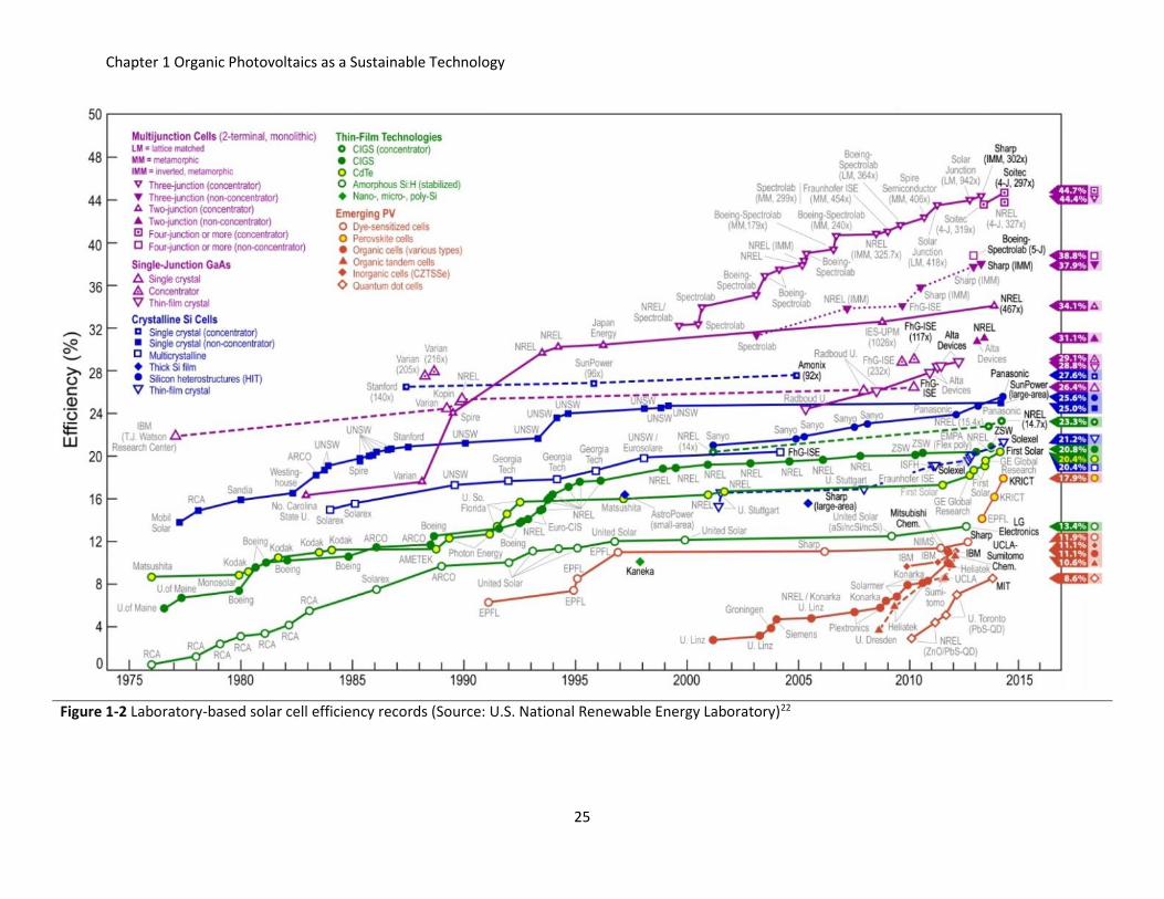
Chapter 1 Organic Photovoltaics as a Sustainable Technology
25
Figure 1-2 Laboratory-based solar cell efficiency records (Source: U.S. National Renewable Energy Laboratory)22
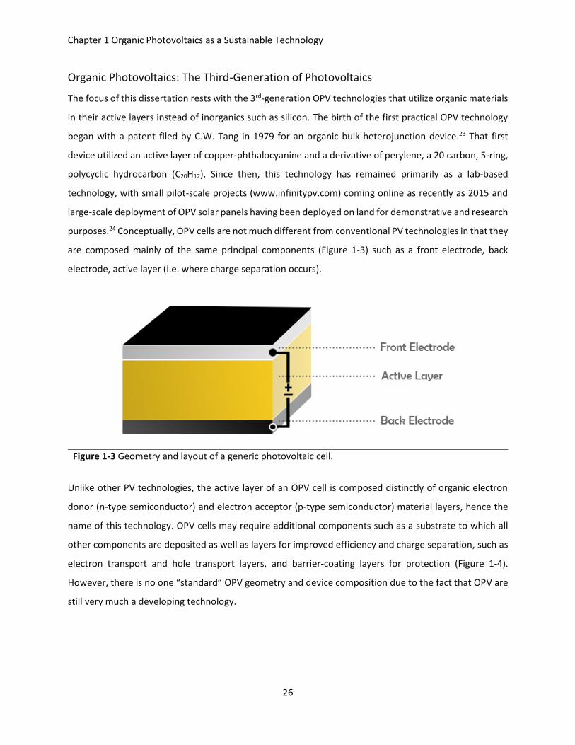
Chapter 1 Organic Photovoltaics as a Sustainable Technology
26
Organic Photovoltaics: The Third-Generation of Photovoltaics
The focus of this dissertation rests with the 3rd-generation OPV technologies that utilize organic materials
in their active layers instead of inorganics such as silicon. The birth of the first practical OPV technology
began with a patent filed by C.W. Tang in 1979 for an organic bulk-heterojunction device.23 That first
device utilized an active layer of copper-phthalocyanine and a derivative of perylene, a 20 carbon, 5-ring,
polycyclic hydrocarbon (C20H12). Since then, this technology has remained primarily as a lab-based
technology, with small pilot-scale projects (www.infinitypv.com) coming online as recently as 2015 and
large-scale deployment of OPV solar panels having been deployed on land for demonstrative and research
purposes.24 Conceptually, OPV cells are not much different from conventional PV technologies in that they
are composed mainly of the same principal components (Figure 1-3) such as a front electrode, back
electrode, active layer (i.e. where charge separation occurs).
Figure 1-3 Geometry and layout of a generic photovoltaic cell.
Unlike other PV technologies, the active layer of an OPV cell is composed distinctly of organic electron
donor (n-type semiconductor) and electron acceptor (p-type semiconductor) material layers, hence the
name of this technology. OPV cells may require additional components such as a substrate to which all
other components are deposited as well as layers for improved efficiency and charge separation, such as
electron transport and hole transport layers, and barrier-coating layers for protection (Figure 1-4).
However, there is no one “standard” OPV geometry and device composition due to the fact that OPV are
still very much a developing technology.
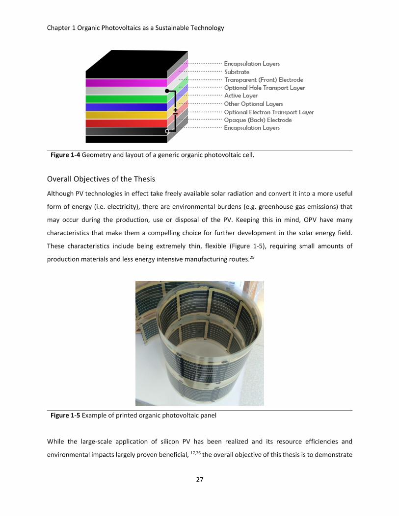
Chapter 1 Organic Photovoltaics as a Sustainable Technology
27
Figure 1-4 Geometry and layout of a generic organic photovoltaic cell.
Overall Objectives of the Thesis
Although PV technologies in effect take freely available solar radiation and convert it into a more useful
form of energy (i.e. electricity), there are environmental burdens (e.g. greenhouse gas emissions) that
may occur during the production, use or disposal of the PV. Keeping this in mind, OPV have many
characteristics that make them a compelling choice for further development in the solar energy field.
These characteristics include being extremely thin, flexible (Figure 1-5), requiring small amounts of
production materials and less energy intensive manufacturing routes.25
Figure 1-5 Example of printed organic photovoltaic panel
While the large-scale application of silicon PV has been realized and its resource efficiencies and
environmental impacts largely proven beneficial, 17,26 the overall objective of this thesis is to demonstrate
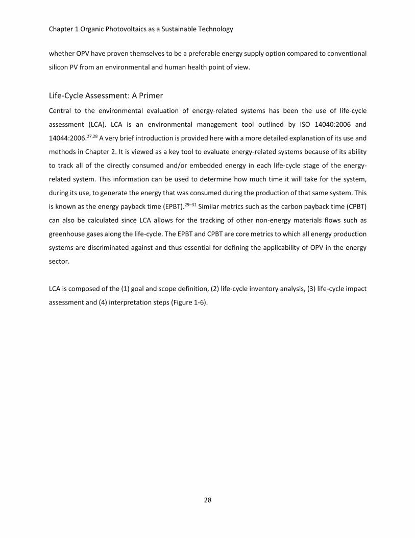
Chapter 1 Organic Photovoltaics as a Sustainable Technology
28
whether OPV have proven themselves to be a preferable energy supply option compared to conventional
silicon PV from an environmental and human health point of view.
Life-Cycle Assessment: A Primer
Central to the environmental evaluation of energy-related systems has been the use of life-cycle
assessment (LCA). LCA is an environmental management tool outlined by ISO 14040:2006 and
14044:2006.27,28 A very brief introduction is provided here with a more detailed explanation of its use and
methods in Chapter 2. It is viewed as a key tool to evaluate energy-related systems because of its ability
to track all of the directly consumed and/or embedded energy in each life-cycle stage of the energy-
related system. This information can be used to determine how much time it will take for the system,
during its use, to generate the energy that was consumed during the production of that same system. This
is known as the energy payback time (EPBT).29–31 Similar metrics such as the carbon payback time (CPBT)
can also be calculated since LCA allows for the tracking of other non-energy materials flows such as
greenhouse gases along the life-cycle. The EPBT and CPBT are core metrics to which all energy production
systems are discriminated against and thus essential for defining the applicability of OPV in the energy
sector.
LCA is composed of the (1) goal and scope definition, (2) life-cycle inventory analysis, (3) life-cycle impact
assessment and (4) interpretation steps (Figure 1-6).
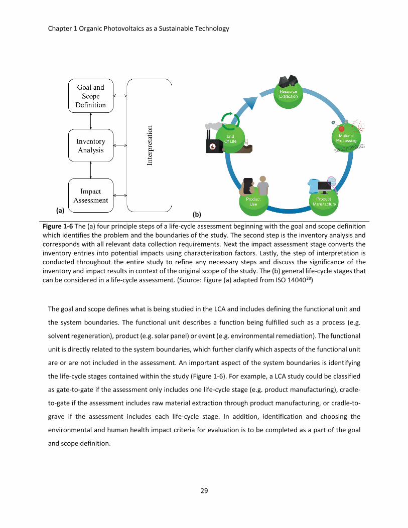
Chapter 1 Organic Photovoltaics as a Sustainable Technology
29
(a) (b)
Figure 1-6 The (a) four principle steps of a life-cycle assessment beginning with the goal and scope definition which identifies the problem and the boundaries of the study. The second step is the inventory analysis and corresponds with all relevant data collection requirements. Next the impact assessment stage converts the inventory entries into potential impacts using characterization factors. Lastly, the step of interpretation is conducted throughout the entire study to refine any necessary steps and discuss the significance of the inventory and impact results in context of the original scope of the study. The (b) general life-cycle stages that can be considered in a life-cycle assessment. (Source: Figure (a) adapted from ISO 1404028)
The goal and scope defines what is being studied in the LCA and includes defining the functional unit and
the system boundaries. The functional unit describes a function being fulfilled such as a process (e.g.
solvent regeneration), product (e.g. solar panel) or event (e.g. environmental remediation). The functional
unit is directly related to the system boundaries, which further clarify which aspects of the functional unit
are or are not included in the assessment. An important aspect of the system boundaries is identifying
the life-cycle stages contained within the study (Figure 1-6). For example, a LCA study could be classified
as gate-to-gate if the assessment only includes one life-cycle stage (e.g. product manufacturing), cradle-
to-gate if the assessment includes raw material extraction through product manufacturing, or cradle-to-
grave if the assessment includes each life-cycle stage. In addition, identification and choosing the
environmental and human health impact criteria for evaluation is to be completed as a part of the goal
and scope definition.
Chapter 1 Organic Photovoltaics as a Sustainable Technology
30
The second step of a LCA, the life-cycle inventory, involves the identification, quantification and
aggregation of all the material, energy and waste streams contained within the boundaries of the
functional unit. Many times, the inventory data can be obtained from pre-existing life-cycle inventory
databases such as Ecoinvent (The Ecoinvent Association, Zurich) which is the most widely used database
for LCA studies. The life-cycle impact assessment involves the conversion of life-cycle inventory data into
environmental and human health impacts, sometimes referred to as life-cycle impacts. These impacts may
include, but are not limited to, acidification of land and water, climate change potential, resource
depletion potential, ecotoxicity, eutrophication of waterways, human toxicity, ionizing radiation potential,
land use changes, ozone layer depletion potential, particulate matter formation, and photochemical
oxidant (smog) formation potential. The final step in an LCA, interpretation, is used to (a) understand and
make the logical connections between the life-cycle impact assessment results, life-cycle inventory and
the goal/scope definition, but also to (b) identify anomalies and errors that may present themselves in
each of these LCA steps. Lastly, LCA does not quantify absolute environmental or human health impacts.
Instead, LCA uses generalized models that provide a potential, relative impact. This is in contrast to certain
other impact analyses such as human health risk assessment (HHRA)32 and environmental risk assessment
(ERA).33 In those approaches, individual substances contained within a product are identified and assessed
for their probability of exposure in a population in distinct and specifically defined environmental
conditions. Chapter 5 and Chapter 6 will introduce HHRA and ERA in greater detail.
Photovoltaic Life-Cycle Assessments: A Brief Background
PV-related LCA studies date back to 1995 with a first such study published by Huber and Kolb.34 That study
demonstrated the first known life-cycle inventory for a silicon-based PV system as well as the first life-
cycle impact assessment using 15 different environmental and human health criteria. By the time of the
International Energy Agency’s (IEA) 2011 report on Life Cycle Inventories and Life Cycle Assessments of
Photovoltaic Systems,35 there had been many dozens of PV-LCA studies published in the literature.
However, acknowledging the steep life-cycle inventory demands and technical nature of this technology,
the IEA report aimed to provide further guidance on conducting PV-LCA to assure “consistency, balance,
transparency and quality” as well as the “credibility and reliability of [LCA] results.” While their report
gathered the best-known life-cycle inventory data for crystalline silicon, cadmium telluride, and high-
concentration PV, there was no consideration of OPV systems or other 3rd-generation technologies in that
report. This exclusion was understandable given the lack of maturity and consistency in the developments
of OPV at that time. Consequently, the OPV-LCA literature itself is heterogeneous, representing material
Chapter 1 Organic Photovoltaics as a Sustainable Technology
31
choices, processing routes and device structures as well as varying methods and environmental and
human health impact results. The following sections outline the findings from a review of the OPV-LCA
literature that was conducted at the start of this thesis and thus considers the published literature up to
the end of 2013.
Review of Organic Photovoltaic Life-Cycle Assessments
The first OPV-LCA appeared in 2009 by Roes et al.29 and between then and the end of 2013 there were a
total of ten such studies (Table 1-1).29–31,36–42 However, an additional eight peer-reviewed case studies,
including the two from this thesis, have been published through October 2016.
Material Choices and Device Structures
Between 2009 and 2013, the types of OPV devices represented in the LCA literature have some overall
consistency, owing to the fact that eight out of ten of these studies were either (a) from the same group
of related authors30,31,36–38,41 or (b) were based on devices described in a prior LCA study that came before
it.39,40 Nearly all of the studies considered a flexible OPV device that had a plastic substrate, however the
very first two published OPV-LCA considered OPV devices on rigid, glass substrates.29,30 Glass substrates
are typical for lab-based experiments and production, but since the time of the first OPV-LCA, it has been
shown that the physics and performance of OPV are fully compatible with plastic, flexible substrates such
as polyethylene terephthalate (PET).43
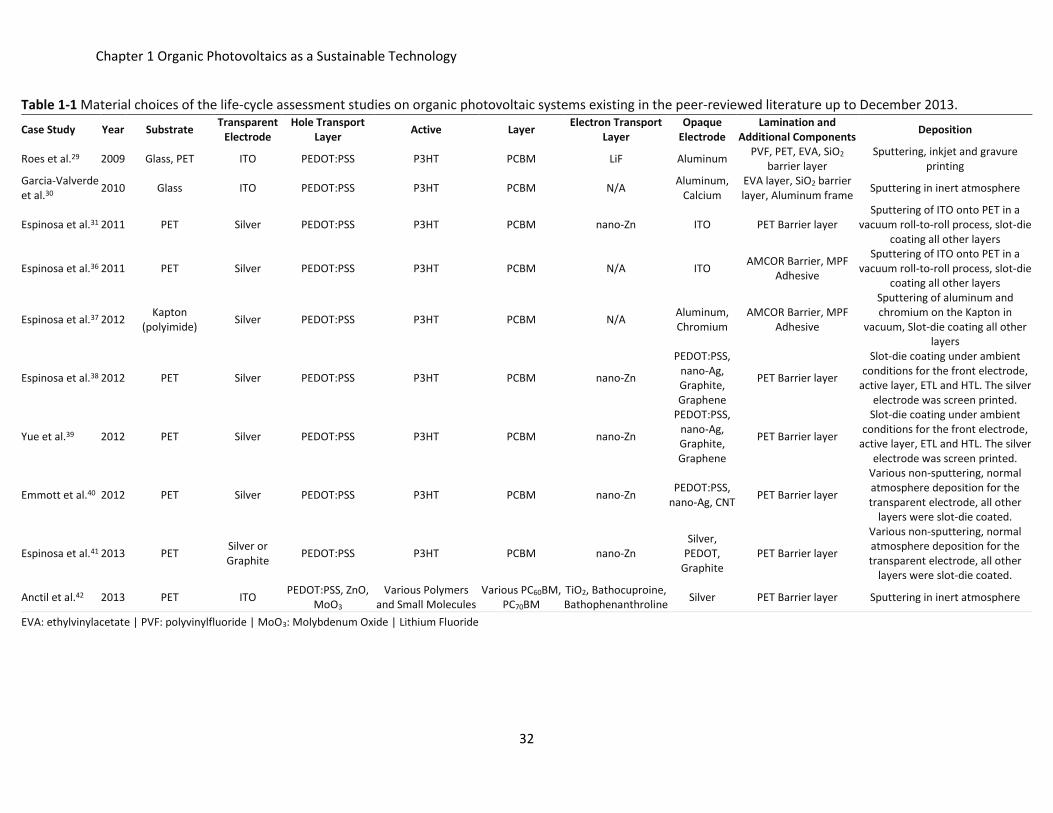
Chapter 1 Organic Photovoltaics as a Sustainable Technology
32
Table 1-1 Material choices of the life-cycle assessment studies on organic photovoltaic systems existing in the peer-reviewed literature up to December 2013.
Case Study Year Substrate Transparent
Electrode Hole Transport
Layer Active Layer
Electron Transport Layer
Opaque Electrode
Lamination and Additional Components
Deposition
Roes et al.29 2009 Glass, PET ITO PEDOT:PSS P3HT PCBM LiF Aluminum PVF, PET, EVA, SiO2 barrier layer
Sputtering, inkjet and gravure printing
Garcia-Valverde et al.30
2010 Glass ITO PEDOT:PSS P3HT PCBM N/A Aluminum, Calcium
EVA layer, SiO2 barrier layer, Aluminum frame Sputtering in inert atmosphere
Espinosa et al.31 2011 PET Silver PEDOT:PSS P3HT PCBM nano-Zn ITO PET Barrier layer Sputtering of ITO onto PET in a
vacuum roll-to-roll process, slot-die coating all other layers
Espinosa et al.36 2011 PET Silver PEDOT:PSS P3HT PCBM N/A ITO AMCOR Barrier, MPF Adhesive
Sputtering of ITO onto PET in a vacuum roll-to-roll process, slot-die
coating all other layers
Espinosa et al.37 2012 Kapton
(polyimide) Silver PEDOT:PSS P3HT PCBM N/A Aluminum, Chromium
AMCOR Barrier, MPF Adhesive
Sputtering of aluminum and chromium on the Kapton in
vacuum, Slot-die coating all other layers
Espinosa et al.38 2012 PET Silver PEDOT:PSS P3HT PCBM nano-Zn
PEDOT:PSS, nano-Ag, Graphite, Graphene
PET Barrier layer
Slot-die coating under ambient conditions for the front electrode,
active layer, ETL and HTL. The silver electrode was screen printed.
Yue et al.39 2012 PET Silver PEDOT:PSS P3HT PCBM nano-Zn
PEDOT:PSS, nano-Ag, Graphite, Graphene
PET Barrier layer
Slot-die coating under ambient conditions for the front electrode,
active layer, ETL and HTL. The silver electrode was screen printed.
Emmott et al.40 2012 PET Silver PEDOT:PSS P3HT PCBM nano-Zn PEDOT:PSS, nano-Ag, CNT PET Barrier layer
Various non-sputtering, normal atmosphere deposition for the transparent electrode, all other
layers were slot-die coated.
Espinosa et al.41 2013 PET Silver or Graphite PEDOT:PSS P3HT PCBM nano-Zn
Silver, PEDOT,
Graphite PET Barrier layer
Various non-sputtering, normal atmosphere deposition for the transparent electrode, all other
layers were slot-die coated.
Anctil et al.42 2013 PET ITO PEDOT:PSS, ZnO, MoO3
Various Polymers and Small Molecules
Various PC60BM, PC70BM
TiO2, Bathocuproine, Bathophenanthroline Silver PET Barrier layer Sputtering in inert atmosphere
EVA: ethylvinylacetate | PVF: polyvinylfluoride | MoO3: Molybdenum Oxide | Lithium Fluoride
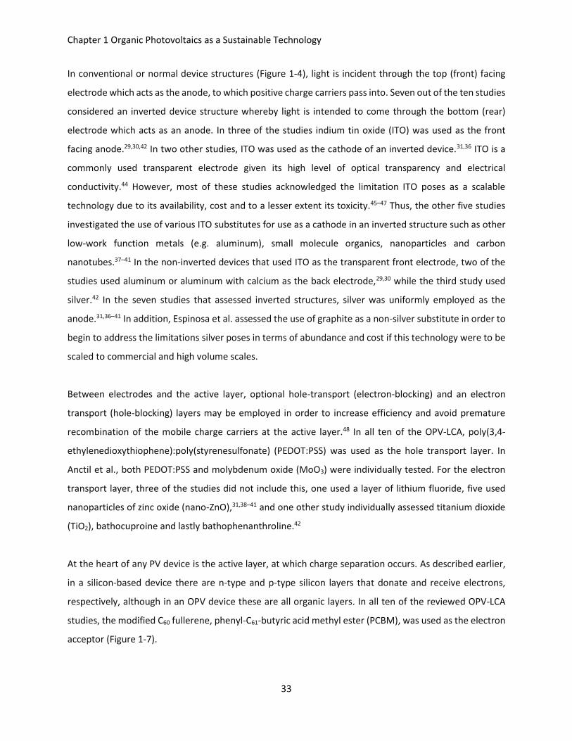
Chapter 1 Organic Photovoltaics as a Sustainable Technology
33
In conventional or normal device structures (Figure 1-4), light is incident through the top (front) facing
electrode which acts as the anode, to which positive charge carriers pass into. Seven out of the ten studies
considered an inverted device structure whereby light is intended to come through the bottom (rear)
electrode which acts as an anode. In three of the studies indium tin oxide (ITO) was used as the front
facing anode.29,30,42 In two other studies, ITO was used as the cathode of an inverted device.31,36 ITO is a
commonly used transparent electrode given its high level of optical transparency and electrical
conductivity.44 However, most of these studies acknowledged the limitation ITO poses as a scalable
technology due to its availability, cost and to a lesser extent its toxicity.45–47 Thus, the other five studies
investigated the use of various ITO substitutes for use as a cathode in an inverted structure such as other
low-work function metals (e.g. aluminum), small molecule organics, nanoparticles and carbon
nanotubes.37–41 In the non-inverted devices that used ITO as the transparent front electrode, two of the
studies used aluminum or aluminum with calcium as the back electrode,29,30 while the third study used
silver.42 In the seven studies that assessed inverted structures, silver was uniformly employed as the
anode.31,36–41 In addition, Espinosa et al. assessed the use of graphite as a non-silver substitute in order to
begin to address the limitations silver poses in terms of abundance and cost if this technology were to be
scaled to commercial and high volume scales.
Between electrodes and the active layer, optional hole-transport (electron-blocking) and an electron
transport (hole-blocking) layers may be employed in order to increase efficiency and avoid premature
recombination of the mobile charge carriers at the active layer.48 In all ten of the OPV-LCA, poly(3,4-
ethylenedioxythiophene):poly(styrenesulfonate) (PEDOT:PSS) was used as the hole transport layer. In
Anctil et al., both PEDOT:PSS and molybdenum oxide (MoO3) were individually tested. For the electron
transport layer, three of the studies did not include this, one used a layer of lithium fluoride, five used
nanoparticles of zinc oxide (nano-ZnO),31,38–41 and one other study individually assessed titanium dioxide
(TiO2), bathocuproine and lastly bathophenanthroline.42
At the heart of any PV device is the active layer, at which charge separation occurs. As described earlier,
in a silicon-based device there are n-type and p-type silicon layers that donate and receive electrons,
respectively, although in an OPV device these are all organic layers. In all ten of the reviewed OPV-LCA
studies, the modified C60 fullerene, phenyl-C61-butyric acid methyl ester (PCBM), was used as the electron
acceptor (Figure 1-7).
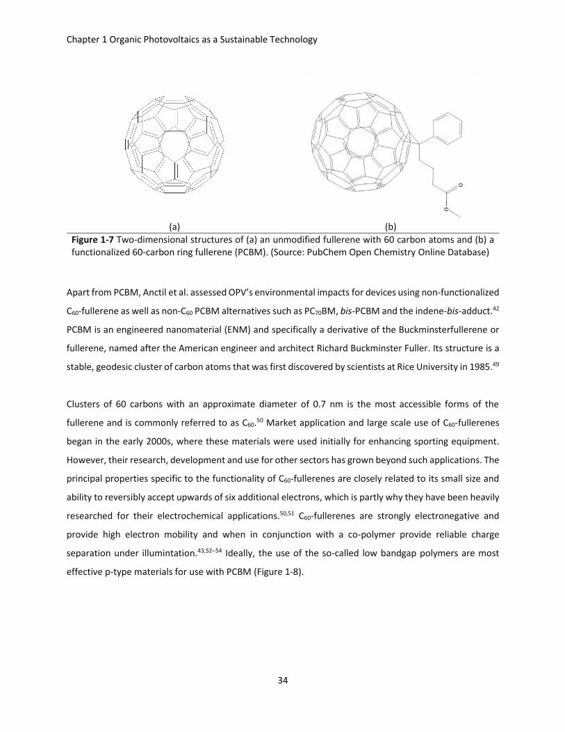
Chapter 1 Organic Photovoltaics as a Sustainable Technology
34
(a) (b)
Figure 1-7 Two-dimensional structures of (a) an unmodified fullerene with 60 carbon atoms and (b) a functionalized 60-carbon ring fullerene (PCBM). (Source: PubChem Open Chemistry Online Database)
Apart from PCBM, Anctil et al. assessed OPV’s environmental impacts for devices using non-functionalized
C60-fullerene as well as non-C60 PCBM alternatives such as PC70BM, bis-PCBM and the indene-bis-adduct.42
PCBM is an engineered nanomaterial (ENM) and specifically a derivative of the Buckminsterfullerene or
fullerene, named after the American engineer and architect Richard Buckminster Fuller. Its structure is a
stable, geodesic cluster of carbon atoms that was first discovered by scientists at Rice University in 1985.49
Clusters of 60 carbons with an approximate diameter of 0.7 nm is the most accessible forms of the
fullerene and is commonly referred to as C60.50 Market application and large scale use of C60-fullerenes
began in the early 2000s, where these materials were used initially for enhancing sporting equipment.
However, their research, development and use for other sectors has grown beyond such applications. The
principal properties specific to the functionality of C60-fullerenes are closely related to its small size and
ability to reversibly accept upwards of six additional electrons, which is partly why they have been heavily
researched for their electrochemical applications.50,51 C60-fullerenes are strongly electronegative and
provide high electron mobility and when in conjunction with a co-polymer provide reliable charge
separation under illumintation.43,52–54 Ideally, the use of the so-called low bandgap polymers are most
effective p-type materials for use with PCBM (Figure 1-8).
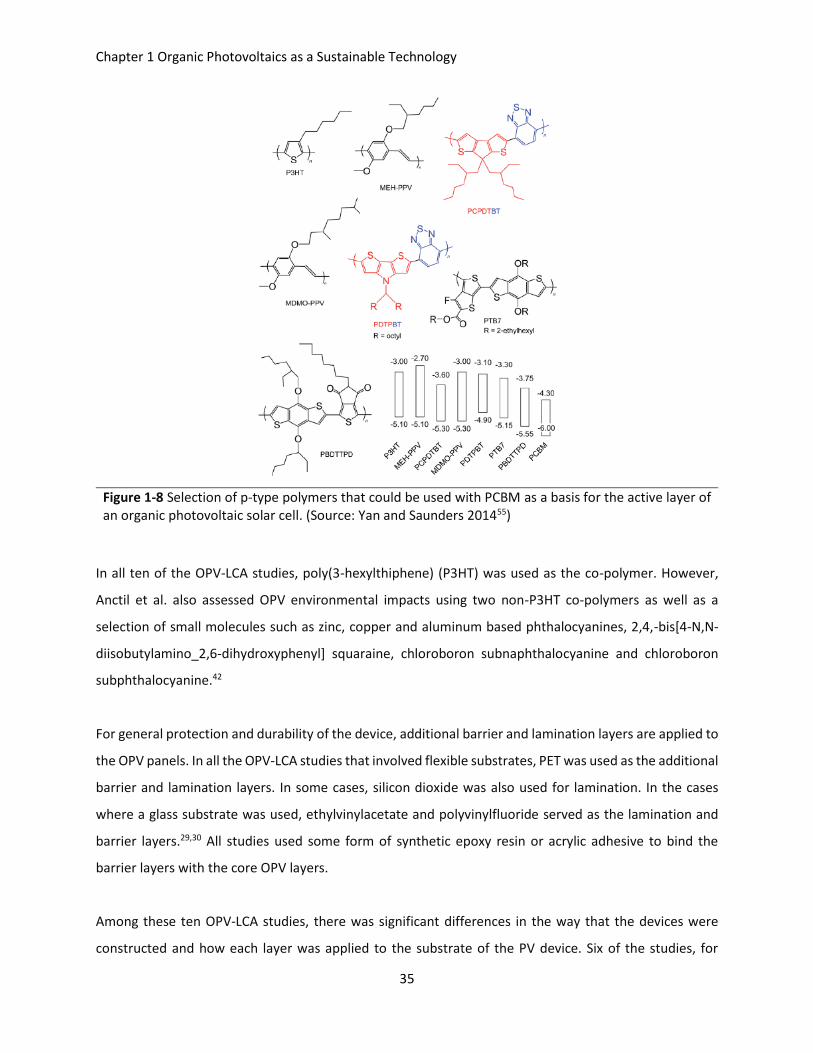
Chapter 1 Organic Photovoltaics as a Sustainable Technology
35
Figure 1-8 Selection of p-type polymers that could be used with PCBM as a basis for the active layer of an organic photovoltaic solar cell. (Source: Yan and Saunders 201455)
In all ten of the OPV-LCA studies, poly(3-hexylthiphene) (P3HT) was used as the co-polymer. However,
Anctil et al. also assessed OPV environmental impacts using two non-P3HT co-polymers as well as a
selection of small molecules such as zinc, copper and aluminum based phthalocyanines, 2,4,-bis[4-N,N-
diisobutylamino_2,6-dihydroxyphenyl] squaraine, chloroboron subnaphthalocyanine and chloroboron
subphthalocyanine.42
For general protection and durability of the device, additional barrier and lamination layers are applied to
the OPV panels. In all the OPV-LCA studies that involved flexible substrates, PET was used as the additional
barrier and lamination layers. In some cases, silicon dioxide was also used for lamination. In the cases
where a glass substrate was used, ethylvinylacetate and polyvinylfluoride served as the lamination and
barrier layers.29,30 All studies used some form of synthetic epoxy resin or acrylic adhesive to bind the
barrier layers with the core OPV layers.
Among these ten OPV-LCA studies, there was significant differences in the way that the devices were
constructed and how each layer was applied to the substrate of the PV device. Six of the studies, for
Chapter 1 Organic Photovoltaics as a Sustainable Technology
36
example, utilized sputtering of ITO onto the PET using vacuum and/or intern atmospheric conditions.29–
31,36,37,42 In the other four studies, these conditions were avoided altogether and substituted with other
solution based deposition processes such as slot-die coating.38–41 For other layers, various techniques
were used such as screen printing, gravure printing and inkjet printing. Besides Garcia-Valverde et al.,30
all of the studies assumed non-batch processing using continuous roll-to-roll production.
The diversity in the materials, production routes and device structures used in these ten studies resulted
in a range of OPV defined by differences in (i) the (photo)-active area of the panel, (ii) conversion efficiency
and (iii) lifetime of the device. The active area of the OPV ranged from a low of 45% to a high of 90%.
These differences were sometimes actual measurements and in other times forecasted estimations of
near-term feasible limits.29,39,42 The efficiencies of the OPV ranged between 1% to 10%. Again, some of
these values were based on actual measurements, while many of the studies engaged in sensitivity
analyses to test various near-term changes in device efficiency.30,37–39,42 These projections are not unheard
of, given that lab-scale OPV has reached upwards of 12% as of 2016.15 Lastly, only seven of the OPV-LCA
made any mention of device lifetime, with assumptions ranging from 2-15 year30,36–41 and in one case as
high as 25 years.29 Up to 2016, maximum reported OPV lifetimes have reached seven years.56 Thus, the
projected lifetimes of some of the reviewed OPV-LCA studies are overestimations and thus underestimate
their reported environmental impacts.
Scope and Boundaries
The majority of the OPV-LCA studies were limited to a cradle-to-gate assessment from raw material
extraction through the manufacture of the OPV panel (Table 1-2). 29–31,37–42
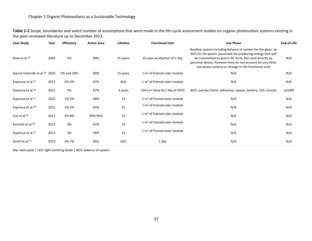
Chapter 1 Organic Photovoltaics as a Sustainable Technology
37
Table 1-2 Scope, boundaries and select number of assumptions that were made in the life-cycle assessment studies on organic photovoltaic systems existing in the peer-reviewed literature up to December 2013.
Case Study Year Efficiency Active Area Lifetime Functional Unit Use Phase End-of-Life
Roes et al.29 2009 5% 90% 25 years 25-year production of 1 Wp
Rooftop system including balance of system for the glass, no BOS for the plastic (assumed not producing energy that will
be transmitted to grid in AC form, but used directly by personal device, however they do not account for any other
use phase systems or change in the functional unit)
N/A
Garcia-Valverde et al.30 2010 5% and 10% 90% 15 years 1 m2 of framed solar module N/A N/A
Espinosa et al.31 2011 2%-3% 67% N/A 1 m2 of framed solar module N/A N/A
Espinosa et al.36 2011 5% 67% 2 years 104 cm2 lamp (0.1 Wp of OPV) BOS: overlay frame, adhesives, spacer, battery, LED, circuits Landfill
Espinosa et al.37 2012 1%-5% 68% 15 1 m2 of framed solar module N/A N/A
Espinosa et al.38 2012 1%-5% 45% 15 1 m2 of framed solar module N/A N/A
Yue et al.39 2012 3%-8% 45%-85% 15 1 m2 of framed solar module N/A N/A
Emmott et al.40 2012 3% 67% 15 1 m2 of framed solar module N/A N/A
Espinosa et al.41 2013 3% 46% 15 1 m2 of framed solar module N/A N/A
Anctil et al.42 2013 3%-7% 85% N/A 1 Wp N/A N/A
Wp: watt-peak | LED: light emitting diode | BOS: balance of system
Chapter 1 Organic Photovoltaics as a Sustainable Technology
38
Accordingly, the functional units were defined for 1 m2 of OPV panel. Anctil et al. defined their functional
unit as a watt-peak (Wp) of power production. A Wp is defined as the nominal power of a solar cell, where
the ability of a device to produce one Wp is tested under standardized conditions. Roes et al. stated that
the scope of their study included the use-phase in the form of a rooftop mounted system using a
functional unit defined as an average Wp of power produced over 25 years. As mentioned above, these
results of their LCA study might be underestimating the environmental impacts given that the assumed
lifetime of the OPV in that study was 25 years. Espinosa et al. was the only study that considered a use
phase as well as an end-of-life phase.36 Their use phase included the production of light using an OPV-
integrated lamp and the end-of-life phase considered landfilling of the lamp. The functional unit for their
study was the production of 0.31 Wp for light production over two years.
Environmental and Human Health Impact Assessment Criteria
All of the ten OPV-LCA studies published between 2009-2013 estimated the impact criteria of cumulative
energy demand (CED), EPBT or a combination of both. This makes sense since OPV are an energy
producing technology and one of the most obvious questions one can ask is how much energy is consumed
in order to produce energy and how much time does it take for that technology to reproduce the energy it
consumed (i.e. EPBT). These are useful calculations that also allow for comparisons between different
types of energy producing systems (i.e. PV versus wind versus nuclear). In addition, six of the studies
calculated the greenhouse gas emissions29–31,36,37,41 and two of the studies assessed a more comprehensive
set of environmental impacts beyond energy or greenhouse gas accounting as were presented in the
previous “primer” on LCA.29,41
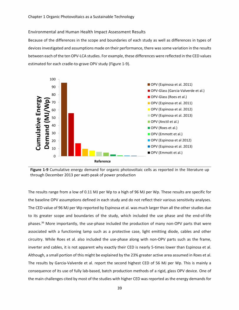
Chapter 1 Organic Photovoltaics as a Sustainable Technology
39
Environmental and Human Health Impact Assessment Results
Because of the differences in the scope and boundaries of each study as well as differences in types of
devices investigated and assumptions made on their performance, there was some variation in the results
between each of the ten OPV-LCA studies. For example, these differences were reflected in the CED values
estimated for each cradle-to-grave OPV study (Figure 1-9).
Figure 1-9 Cumulative energy demand for organic photovoltaic cells as reported in the literature up through December 2013 per watt-peak of power production
The results range from a low of 0.11 MJ per Wp to a high of 96 MJ per Wp. These results are specific for
the baseline OPV assumptions defined in each study and do not reflect their various sensitivity analyses.
The CED value of 96 MJ per Wp reported by Espinosa et al. was much larger than all the other studies due
to its greater scope and boundaries of the study, which included the use phase and the end-of-life
phases.36 More importantly, the use-phase included the production of many non-OPV parts that were
associated with a functioning lamp such as a protective case, light emitting diode, cables and other
circuitry. While Roes et al. also included the use-phase along with non-OPV parts such as the frame,
inverter and cables, it is not apparent why exactly their CED is nearly 5-times lower than Espinosa et al.
Although, a small portion of this might be explained by the 23% greater active area assumed in Roes et al.
The results by Garcia-Valverde et al. report the second highest CED of 56 MJ per Wp. This is mainly a
consequence of its use of fully lab-based, batch production methods of a rigid, glass OPV device. One of
the main challenges cited by most of the studies with higher CED was reported as the energy demands for
0
10
20
30
40
50
60
70
80
90
100
Reference
Cu
mu
lati
ve E
ne
rgy
De
man
d (
MJ/
Wp
)
OPV (Espinosa et al. 2011)
OPV-Glass (Garcia-Valverde et al.)
OPV-Glass (Roes et al.)
OPV (Espinosa et al. 2011)
OPV (Espinosa et al. 2012)
OPV (Espinosa et al. 2013)
OPV (Anctil et al.)
OPV (Roes et al.)
OPV (Emmott et al.)
OPV (Espinosa et al 2012)
OPV (Espinosa et al. 2013)
OPV (Emmott et al.)
Chapter 1 Organic Photovoltaics as a Sustainable Technology
40
producing and sputtering ITO on the substrate under vacuum or inert atmospheric conditions.29–31,36,37 In
some cases ITO production and deposition account for upwards of 87% of the embodied energy of the
entire OPV.30,31 ITO itself is an energy intensive material to extract, produce and refine, however even if
substituted with another material, it was found that the inert atmosphere needed for deposition could
still account for nearly 17% of the energy demand.37 In the cradle-to-grave study by Espinosa et al., the
ITO substrate only constituted 35% of the overall CED, while the protective plastic layers, blocking diode,
and light emitting diode represented 22%, 16% and 16% of the total demand. Those results again
demonstrate the importance of and difference between cradle-to-gate and cradle-to-grave studies. When
produced in normal atmosphere conditions, the reported CED values dropped significantly by over one-
order of magnitude.38–41 Under these conditions, the main energy consuming aspects of the OPV shifted
to the substrate, hole transport layer and electrodes.
It is curious to note that, since most of the studies were either from the same group of related
authors30,31,36–38,41 or were based on devices described in a prior LCA study that came before it,39,40 a lot of
the life-cycle inventory data originate from a single source. If the data come from a primary, industrial
source this could be reliable, however in many cases these data were being reported from lab-based
processes, older techniques, expert judgement or stoichiometric calculations. One clear example of this
influence on the results was brought to light in a LCA study by Anctil et al.42 In a previous study, those
authors completed an assessment of the CED for the processing and manufacturing of C60-fullerenes and
PCBM.57 They found their results were much higher than previously reported energy demands per kg of
fullerene production and reasoned this to be on prior studies’ use of older and/or incomplete data of the
production route, particularly the purification steps.57 When they integrated this information back into
their OPV-LCA, they found that nearly 20% of the CED was due to the production of PCBM.42 This is in
contrast to the much lower percentages ranging between 0.21%-10% reported in the other OPV-LCA
studies reviewed. Thus, whereas most of the other studies pointed to the non-active layer components
as the main bottle-necks or targets for environmental improvement, Anctil et al. was the first study to
identify the active layer as such.
Correspondingly, the EPBT reported in the OPV-LCA studies range from a low of 0.35 years to a high of 9.9
years. Because the EPBT is determined using the CED, the differences in the EPBT results can be attributed
to the same factors driving the CED results. Once again, the highest EPBT of 9.9 years was reported by the
cradle-to-grave study by Espinosa et al. that included the non-OPV components utilized during the use
Chapter 1 Organic Photovoltaics as a Sustainable Technology
41
phase and impacts from the end-of-life landfilling process.36 The glass-substrate OPV devices reported by
Garcia-Valverde et al. and Roes et al. had EPBT of 4.0 and 1.3 years, respectively.29,30 Those two studies
also happened to report the highest active areas of 90%. Using Monte-Carlo uncertainty analysis,58 Yue et
al. demonstrated that the active area and efficiency of the OPV devices were the most significant sources
of uncertainty in the calculation of the EPBT. Those authors also took into consideration the degradation
rate of the OPV, as opposed to the other OPV-LCA studies, and found that it contributes upwards of 9%
of the total uncertainty in the results.39 When OPV manufacturing switched from inert to normal
atmosphere conditions, the EPBT decreased by over one-order of magnitude similar to the CED values.38–
41
The results from the two studies that reported a more comprehensive set of environmental impacts
differed quite significantly. Some of the impacts reported by Espinosa et al.41 were upwards of 3-orders
of magnitude lower than Roes et al., for instance, in ozone depletion potential. These differences were
most likely a consequence of the manufacturing differences taken by Espinosa et al. which used normal
atmosphere conditions compared to Roes et al. who used an inert atmosphere for ITO sputtering onto
the substrate.
In regards to conventional silicon PV, only half of the OPV-LCA studies made a comparison between OPV
and conventional panels.29,30,36,39,42 Garcia-Valverde et al. reported that the CED of a 5% efficient OPV
panel was 56 MJ/Wp, nearly two-times and over three-times greater than the referenced values of 28.3-
29.9 MJ/Wp and 15.9 MJ/Wp for m-Si and a-Si, respectively.30 This resulted in a 4.0-year EPBT that was 1-
2 times longer than the EPBT values of 2.7-4.1 referenced for m-Si as well as 4-times longer than the values
referenced for a-Si. Anctil et al. reported CED values ranging between 3-10 MJ/Wp for the 26 different
OPV tested in their study. All such values were below the referenced CED of 16-24 MJ/Wp and 29 MJ/Wp
for a-Si and m-Si, respectively. Yue et al. reported EPBT < 0.25 years for OPV which were one order of
magnitude smaller than the nearly 2.4 years estimated for m-Si. Using two different functional units, Roes
et al. compared a glass-substrate OPV and plastic-substrate OPV to both m-Si and a-Si. The EPBT for the
glass-substrate OPV was 1.3 years compared with 2.33 years and 1.93 years for m-Si and a-Si PV,
respectively. The EPBT for the plastic-substrate OPV was 0.2 years compared with 2.0 and 1.3 years for
m-Si and a-Si, respectively. The reason why the EPBT for the silicon-based PV became shorter in the second
comparison was due to the change in the functional unit which eliminated certain use-phase components
(i.e. fewer physical materials used and thus a lower embodied energy of the entire system). Furthermore,
Chapter 1 Organic Photovoltaics as a Sustainable Technology
42
Roes et al. compared OPV and silicon cells across 6 other impact categories: climate change potential,
(abiotic) resource depletion, ozone layer depletion, photochemical oxidant formation, acidification and
eutrophication. For the glass-substrate, all impacts were lower for OPV, however the extent of which was
not uniform for all impact categories. For instance, whereas ozone layer depletion for OPV was over 1-
order of magnitude smaller than m-Si, acidification for OPV was only 13% lower. The reductions over m-
Si were more pronounced for the plastic-substrate OPV. For instance, the acidification potential was now
81% lower for OPV compared to silicon. However, the plastic-substrate scenario resulted in a
photochemical oxidant formation potential that was 25% greater than m-Si due to the toluene emissions
estimated for gravure printing. In comparison, the results presented by Espinosa et al. were unique in the
fact that the LCA was cradle-to-grave, as opposed to the cradle-to-gate or cradle-to-use scopes that were
applied in the other four studies that made comparisons to silicon-based PV. Espinosa et al. demonstrated
that switching from an a-Si PV lamp to an OPV powered lamp can save 0.52 kg of greenhouse gas emissions
per Wh of electricity produced and nearly 64 MJ of energy per lamp over a two-year period of use.36
However, it should be noted that there were differences in the type of battery and other non-OPV
components that contribute to this difference. The relative difference between OPV and the silicon PV
reported by these five studies were of course influenced by the distinct types of OPV and methods of each
study. However, different versions of pre-existing, background life-cycle inventory source data were used
as a basis of the silicon-based analysis.26,59–61
Summary of the Review
The OPV systems represented in the ten OPV-LCA studies reviewed up to the end of 2013 represented a
mix of different material choices and device structures for the OPV as well as a mix of scopes, boundaries,
functional units, inventory data and impact assessment categories. Some of these studies were unique in
that they happen to be produced at fairly high production volumes akin to pilot-scale setups,31,36–38 while
their technical capacities, since 2013, have also been tested in large-scale outdoor demonstrations.24,62
Even so, OPV still lack proper industrial scale technology or a market for use and consumption. Therefore,
OPV may have the potential to reduce cradle-to-gate carbon emissions and energy consumption by over
an order of magnitude compared to silicon (Figure 1-9), but such resource efficiencies may not necessarily
remain after considering the use and end-of-life phases.36 This is because OPV are also known to be less
efficient22,63 and have shorter lifetimes45 compared to conventional PV. Consequently, environmental
benefits seen during OPV manufacturing might be offset by the cumulative use and replacement of
exhausted OPV panels over an entire lifetime of its service. In addition, important questions remain
Chapter 1 Organic Photovoltaics as a Sustainable Technology
43
regarding how PV panels can and will be disposed of at their end-of-life.64 This infrastructure is lacking for
conventional PV, with landfilling being a default solution.65 It is similarly uncertain how OPV panels might
be disposed of once they are used at large scales or commercially. Thus, it is important to anticipate the
influence a disposal route will have on the environmental impacts of these technologies.
In addition to considering the entire life-cycle, standard OPV-LCA should include impact categories beyond
CED or greenhouse gas accounting as was limited to in a majority of the reviewed studies. While those
two metrics are important for outlining baseline progress and advantages in this field, energy
consumption and greenhouse gas emissions are only a limited selection of other environmental and
human health indicators and impacts. A life-cycle approach should accommodate a broad range of
environmental criteria in order to expose and reduce any potential environmental burden-shifting.66 This
recommendation is important because although CED may on occasion be a proxy for other potential
impacts,29 this may not always be the case. For example, what would be the correlation between CED and
human toxicity? Even when there may be some correlation with CED and other potential impacts, that
relationship is not necessarily linearly correlated.45 Thus, comparing products based on one or two
indicators may result in an unintended increase in other environmental impacts that were, as a
consequence, not explicitly estimated. To date, only half of the currently published OPV-LCA completed
such an assessment.
Furthermore, to demonstrate OPV advantages as an alternative, new source of sustainable energy, LCA
studies should ideally compare them with conventional silicon-based PV, which currently dominate the
market.16 However, and as was discussed above, only five of the previously published OPV-LCA literature
have done so, and of those, only one study has compared OPV and silicon PV across the entire cradle-to-
grave.62 Thus, a review of OPV-LCA studies that are cradle-to-grave, multi-criterion based, and
comparatively assessed with conventional silicon shows there were no such existing studies in the
literature through at the start of the research put forth in this dissertation (i.e. the end of 2013) (Table
1-3).
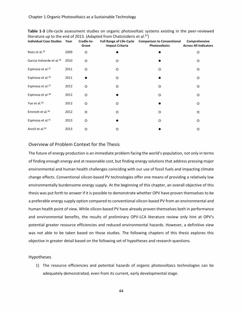
Chapter 1 Organic Photovoltaics as a Sustainable Technology
44
Table 1-3 Life-cycle assessment studies on organic photovoltaic systems existing in the peer-reviewed literature up to the end of 2013. (Adapted from Chatzisideris et al.67)
Individual Case Studies Year Cradle-to-Grave
Full Range of Life-Cycle Impact Criteria
Comparison to Conventional Photovoltaics
Comprehensive Across All Indicators
Roes et al.29 2009 ○ ● ● ○
Garcia-Valverde et al.30 2010 ○ ○ ● ○
Espinosa et al.31 2011 ○ ○ ○ ○
Espinosa et al.36 2011 ● ○ ● ○
Espinosa et al.37 2012 ○ ○ ○ ○
Espinosa et al.38 2012 ○ ● ○ ○
Yue et al.39 2012 ○ ○ ● ○
Emmott et al.40 2012 ○ ○ ○ ○
Espinosa et al.41 2013 ○ ● ○ ○
Anctil et al.42 2013 ○ ○ ● ○
Overview of Problem Context for the Thesis
The future of energy production is an immediate problem facing the world’s population, not only in terms
of finding enough energy and at reasonable cost, but finding energy solutions that address pressing major
environmental and human health challenges coinciding with our use of fossil fuels and impacting climate
change effects. Conventional silicon-based PV technologies offer one means of providing a relatively low
environmentally burdensome energy supply. At the beginning of this chapter, an overall objective of this
thesis was put forth to answer if it is possible to demonstrate whether OPV have proven themselves to be
a preferable energy supply option compared to conventional silicon-based PV from an environmental and
human health point of view. While silicon-based PV have already proven themselves both in performance
and environmental benefits, the results of preliminary OPV-LCA literature review only hint at OPV’s
potential greater resource efficiencies and reduced environmental hazards. However, a definitive view
was not able to be taken based on those studies. The following chapters of this thesis explores this
objective in greater detail based on the following set of hypotheses and research questions.
Hypotheses
1) The resource efficiencies and potential hazards of organic photovoltaics technologies can be
adequately demonstrated, even from its current, early developmental stage.
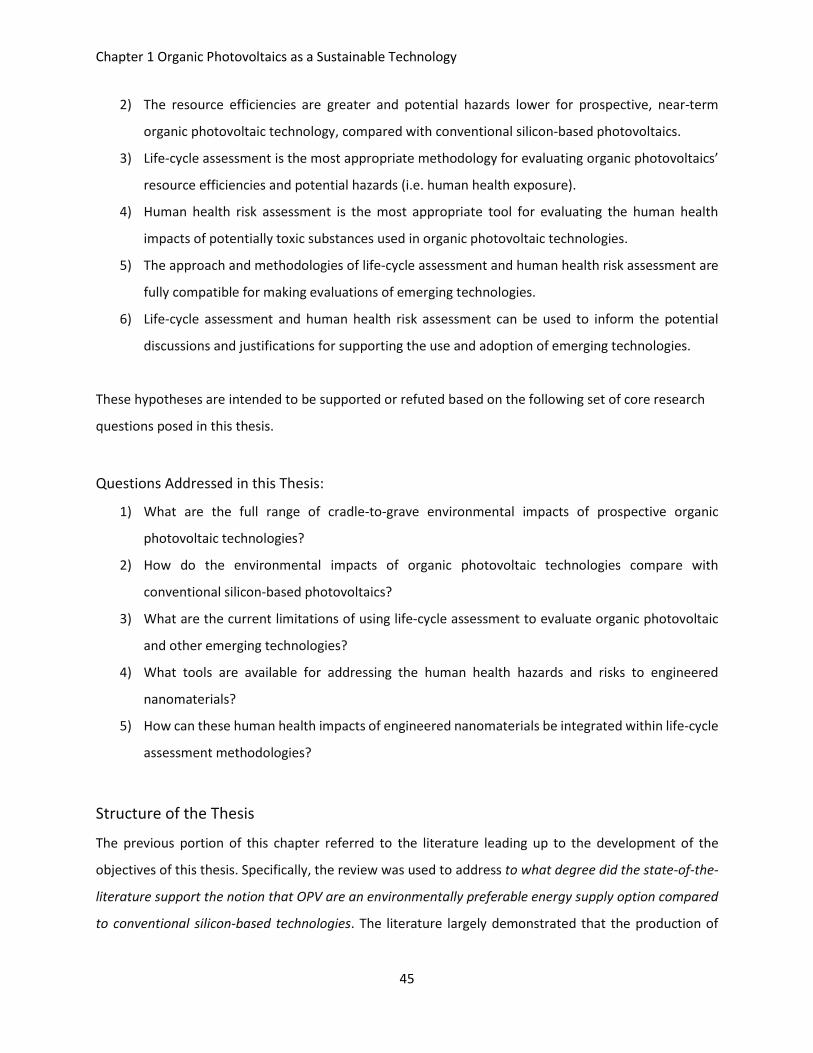
Chapter 1 Organic Photovoltaics as a Sustainable Technology
45
2) The resource efficiencies are greater and potential hazards lower for prospective, near-term
organic photovoltaic technology, compared with conventional silicon-based photovoltaics.
3) Life-cycle assessment is the most appropriate methodology for evaluating organic photovoltaics’
resource efficiencies and potential hazards (i.e. human health exposure).
4) Human health risk assessment is the most appropriate tool for evaluating the human health
impacts of potentially toxic substances used in organic photovoltaic technologies.
5) The approach and methodologies of life-cycle assessment and human health risk assessment are
fully compatible for making evaluations of emerging technologies.
6) Life-cycle assessment and human health risk assessment can be used to inform the potential
discussions and justifications for supporting the use and adoption of emerging technologies.
These hypotheses are intended to be supported or refuted based on the following set of core research
questions posed in this thesis.
Questions Addressed in this Thesis:
1) What are the full range of cradle-to-grave environmental impacts of prospective organic
photovoltaic technologies?
2) How do the environmental impacts of organic photovoltaic technologies compare with
conventional silicon-based photovoltaics?
3) What are the current limitations of using life-cycle assessment to evaluate organic photovoltaic
and other emerging technologies?
4) What tools are available for addressing the human health hazards and risks to engineered
nanomaterials?
5) How can these human health impacts of engineered nanomaterials be integrated within life-cycle
assessment methodologies?
Structure of the Thesis
The previous portion of this chapter referred to the literature leading up to the development of the
objectives of this thesis. Specifically, the review was used to address to what degree did the state-of-the-
literature support the notion that OPV are an environmentally preferable energy supply option compared
to conventional silicon-based technologies. The literature largely demonstrated that the production of
Chapter 1 Organic Photovoltaics as a Sustainable Technology
46
OPV on a watt-for-watt basis have shorter EPBT and lower greenhouse gas emissions compared to silicon.
There were also some indications that environmental and human health impacts may remain lower even
after considering the use and disposal of OPV products. However, there is further support that needs to
be demonstrated to support the claim that OPV are truly an environmentally preferable energy
production option compared to conventional silicon.
In Chapter 2, a more detailed account of LCA is presented in order to better understand the environmental
criteria and assessment methods that have been largely used to evaluate OPV. Chapter 3 introduces a
cradle-to-gate LCA up to the point of the production of a prospective OPV cell. These results are further
compared to the life-cycle results for conventional PV cells, discussing the implied advantages and
drawbacks of each technology. Chapter 4 is a direct extension on the work of Chapter 3 and expands the
LCA to explore the potential uses and end-of-life scenarios for OPV. Chapter 5 takes a further look at the
possible issues of burden shifting, specifically examining LCA’s limitations in estimating the human health
impacts from the production, use and release of ENM across the OPV life-cycle. Chapter 6 then presents
a more formal HHRA study to address these potential ENM impacts, and Chapter 7 reintegrates this
information into the LCA methodology to reassess the overall environmental performance of the OPV.
Chapter 8 takes stock of the results provided by the updated LCA with human health impacts to address
whether there is a case to be made regarding the environmental preference of OPV over silicon-based PV.
Lastly, ongoing work and future opportunities for developing OPV are presented. Following the main text,
in order, are the Bibliography, Appendices and List of Publications.
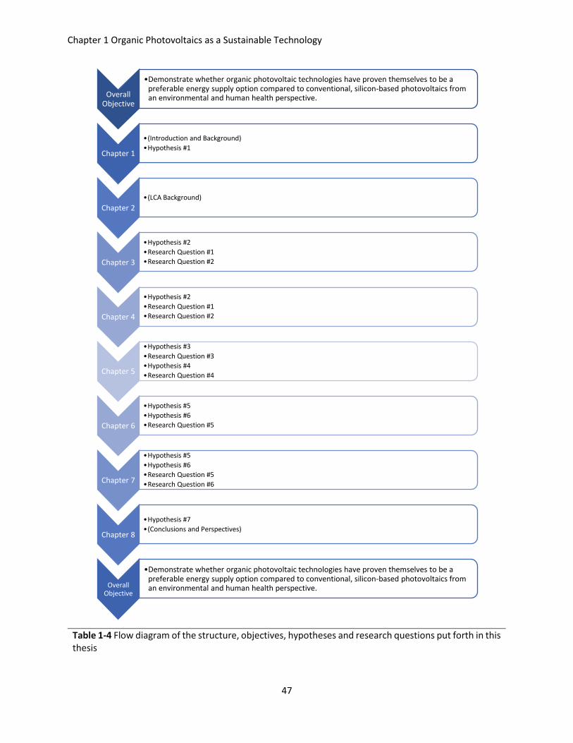
Chapter 1 Organic Photovoltaics as a Sustainable Technology
47
Table 1-4 Flow diagram of the structure, objectives, hypotheses and research questions put forth in this thesis
Overall Objective
•Demonstrate whether organic photovoltaic technologies have proven themselves to be a preferable energy supply option compared to conventional, silicon-based photovoltaics from an environmental and human health perspective.
Chapter 1
•(Introduction and Background)
•Hypothesis #1
Chapter 2
•(LCA Background)
Chapter 3
•Hypothesis #2
•Research Question #1
•Research Question #2
Chapter 4
•Hypothesis #2
•Research Question #1
•Research Question #2
Chapter 5
•Hypothesis #3
•Research Question #3
•Hypothesis #4
•Research Question #4
Chapter 6
•Hypothesis #5
•Hypothesis #6
•Research Question #5
Chapter 7
•Hypothesis #5
•Hypothesis #6
•Research Question #5
•Research Question #6
Chapter 8
•Hypothesis #7
•(Conclusions and Perspectives)
Overall Objective
•Demonstrate whether organic photovoltaic technologies have proven themselves to be a preferable energy supply option compared to conventional, silicon-based photovoltaics from an environmental and human health perspective.
Chapter 2 Life-Cycle Assessment and Its Application to Organic Photovoltaics
48
Chapter 2 Life-Cycle Assessment and Its Application to Organic
Photovoltaics
In Chapter 1 the topic of LCA was briefly introduced as a primer and segue before discussing the OPV-
relevant literature on the subject. It is worthwhile to discuss this tool and its methodology in greater
detail, not only for providing the appropriate background for non-LCA experts, but also to describe the
life-cycle inventory and life-cycle impact assessment methods that were applied in the case studies
presented in Chapter 3 and Chapter 4. The latter point will also serve to orient the reader later in Chapter
5 and Chapter 7 during further review and analysis, respectively, of the impact assessment models created
in this thesis.
Life-Cycle Assessment: A Brief History
Coinciding with the trends in industrial development and concerns over environmental protection and
public health, the ideas of defining a product’s resource efficiency date back to the early-mid 20th century.
Early in the development of such assessments, energy was the main criteria of focus but soon after started
to assess emissions, pollutants and waste generation. This was exemplified in one of the first types of
these studies commissioned by the Coca-Cola Company in 1969, studying the effects of using different
types of containers for their soda-products.68 After a period of relative inactivity in this field of science, a
formal report published in the mid-1980’s by the Swiss Federal Laboratories for Materials Testing and
Research (EMPA) outlined the data requirements for producing a life-cycle inventory.68 Yet, it was not
until the beginning of the 1990s until LCA, in its current form, began to take shape. This period of time
saw a number of workshops, frameworks, journal articles, codes of practice and standards being officially
published and promulgated on an internationally recognized basis.27,28,69–73 Today, LCA has grown into a
core scientific discipline finding its application in a myriad of other subjects which is reflected by the
growth of published “life-cycle assessments” over the past two decades (Figure 2-1).
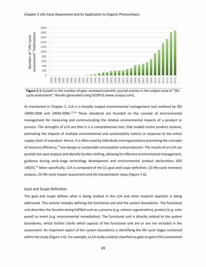
Chapter 2 Life-Cycle Assessment and Its Application to Organic Photovoltaics
49
Figure 2-1 Growth in the number of peer reviewed scientific journal articles in the subject area of “life-cycle assessment.” Results generated using SCOPUS (www.scopus.com).
As mentioned in Chapter 1, LCA is a broadly scoped environmental management tool outlined by ISO
14040:2006 and 14044:2006.27,28 These standards are founded on the concept of environmental
management for measuring and communicating the relative environmental impacts of a product or
process. The strengths of LCA are that it is a comprehensive tool, that models entire product systems,
estimating the impacts of multiple environmental and sustainability metrics in response to the entire
supply-chain of a product. Hence, it is often used by individuals and organizations promoting the concepts
of resource efficiency,74 eco-design or sustainable consumption and production. The results of an LCA can
provide hot-spot analysis and identify burden-shifting, allowing for effective environmental management,
guidance during early-stage technology development and environmental product declarations (ISO
14025).75 More specifically, LCA is composed of the (1) goal and scope definition, (2) life-cycle inventory
analysis, (3) life-cycle impact assessment and (4) interpretation steps (Figure 1-6).
Goal and Scope Definition
The goal and scope defines what is being studied in the LCA and what research question is being
addressed. This activity includes defining the functional unit and the system boundaries. The functional
unit describes the function being fulfilled such as a process (e.g. solvent regeneration), product (e.g. solar
panel) or event (e.g. environmental remediation). The functional unit is directly related to the system
boundaries, which further clarify which aspects of the functional unit are or are not included in the
assessment. An important aspect of the system boundaries is identifying the life-cycle stages contained
within the study (Figure 1-6). For example, a LCA study could be classified as gate-to-gate if the assessment
0
200
400
600
800
1000
1200
1400
1600
1800
2000
19
90
19
89
19
88
19
87
19
86
19
85
19
91
19
84
19
92
19
93
19
94
19
95
19
96
19
97
19
99
20
02
20
00
19
98
20
01
20
03
20
04
20
06
20
05
20
07
20
08
20
09
20
10
20
11
20
12
20
13
20
14
20
15
Nu
mb
er o
f "L
ife
-Cyc
le
Ass
essm
en
t" P
ub
licat
ion
s
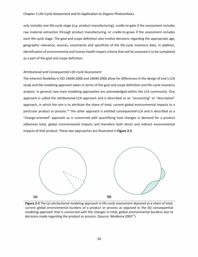
Chapter 2 Life-Cycle Assessment and Its Application to Organic Photovoltaics
50
only includes one life-cycle stage (e.g. product manufacturing), cradle-to-gate if the assessment includes
raw material extraction through product manufacturing, or cradle-to-grave if the assessment includes
each life-cycle stage. The goal and scope definition also involve decisions regarding the appropriate age,
geographic relevance, sources, uncertainty and specificity of the life-cycle inventory data. In addition,
identification of environmental and human health impact criteria that will be assessed is to be completed
as a part of the goal and scope definition.
Attributional and Consequential Life-Cycle Assessment
The inherent flexibility in ISO 14040:2006 and 14044:2006 allow for differences in the design of one’s LCA
study and the modeling approach taken in terms of the goal and scope definition and life-cycle inventory
analysis. In general, two main modeling approaches are acknowledged within the LCA community. One
approach is called the attributional-LCA approach and is described as an “accounting” or “descriptive”
approach, in which the aim is to attribute the share of total, current global environmental impacts to a
particular product or process.76 The other approach is entitled consequential-LCA and is described as a
“change-oriented” approach as is concerned with quantifying how changes in demand for a product
influences total, global environmental impacts and therefore both direct and indirect environmental
impacts of that product. These two approaches are illustrated in Figure 2-2.
(a) (b)
Figure 2-2 The (a) attributional modeling approach in life-cycle assessment depicted as a share of total, current global environmental burdens of a product or process as opposed to the (b) consequential modeling approach that is concerned with the changes in total, global environmental burdens due to decisions made regarding the product or process. (Source: Weidema 200377)
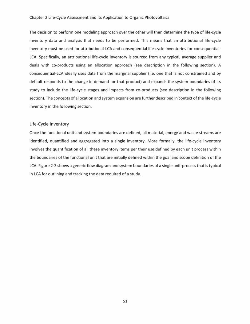
Chapter 2 Life-Cycle Assessment and Its Application to Organic Photovoltaics
51
The decision to perform one modeling approach over the other will then determine the type of life-cycle
inventory data and analysis that needs to be performed. This means that an attributional life-cycle
inventory must be used for attributional-LCA and consequential life-cycle inventories for consequential-
LCA. Specifically, an attributional life-cycle inventory is sourced from any typical, average supplier and
deals with co-products using an allocation approach (see description in the following section). A
consequential-LCA ideally uses data from the marginal supplier (i.e. one that is not constrained and by
default responds to the change in demand for that product) and expands the system boundaries of its
study to include the life-cycle stages and impacts from co-products (see description in the following
section). The concepts of allocation and system expansion are further described in context of the life-cycle
inventory in the following section.
Life-Cycle Inventory
Once the functional unit and system boundaries are defined, all material, energy and waste streams are
identified, quantified and aggregated into a single inventory. More formally, the life-cycle inventory
involves the quantification of all these inventory items per their use defined by each unit process within
the boundaries of the functional unit that are initially defined within the goal and scope definition of the
LCA. Figure 2-3 shows a generic flow diagram and system boundaries of a single unit-process that is typical
in LCA for outlining and tracking the data required of a study.
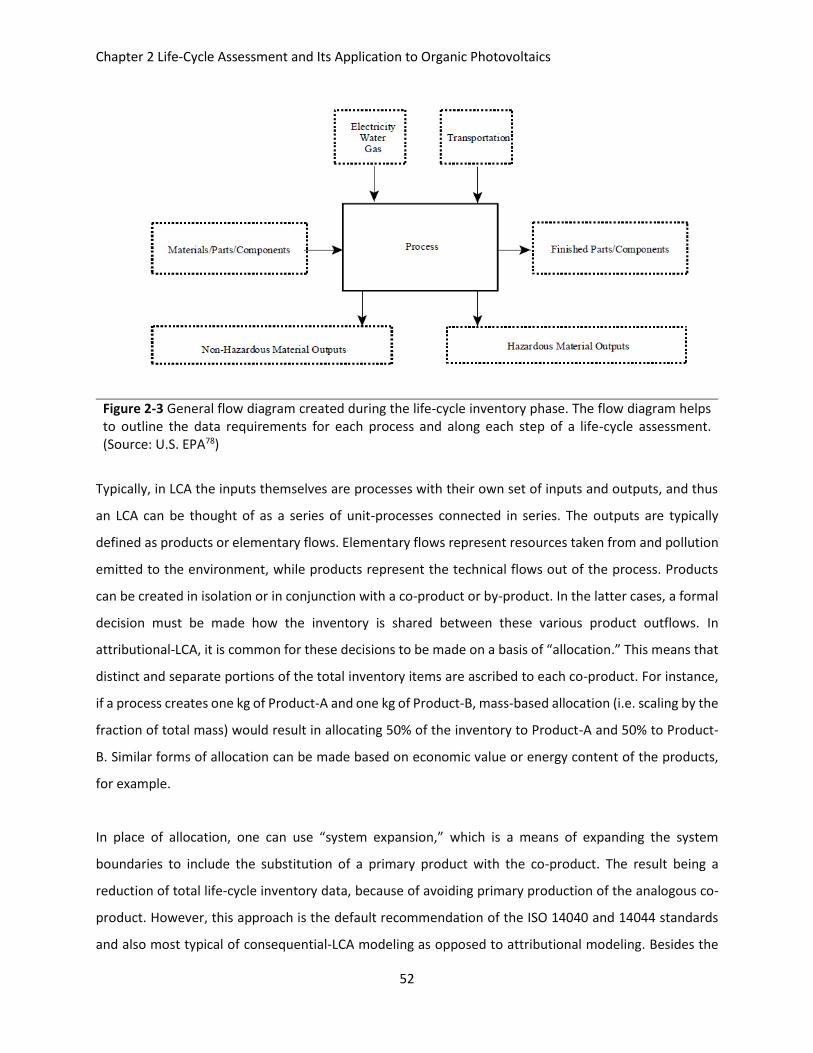
Chapter 2 Life-Cycle Assessment and Its Application to Organic Photovoltaics
52
Figure 2-3 General flow diagram created during the life-cycle inventory phase. The flow diagram helps to outline the data requirements for each process and along each step of a life-cycle assessment. (Source: U.S. EPA78)
Typically, in LCA the inputs themselves are processes with their own set of inputs and outputs, and thus
an LCA can be thought of as a series of unit-processes connected in series. The outputs are typically
defined as products or elementary flows. Elementary flows represent resources taken from and pollution
emitted to the environment, while products represent the technical flows out of the process. Products
can be created in isolation or in conjunction with a co-product or by-product. In the latter cases, a formal
decision must be made how the inventory is shared between these various product outflows. In
attributional-LCA, it is common for these decisions to be made on a basis of “allocation.” This means that
distinct and separate portions of the total inventory items are ascribed to each co-product. For instance,
if a process creates one kg of Product-A and one kg of Product-B, mass-based allocation (i.e. scaling by the
fraction of total mass) would result in allocating 50% of the inventory to Product-A and 50% to Product-
B. Similar forms of allocation can be made based on economic value or energy content of the products,
for example.
In place of allocation, one can use “system expansion,” which is a means of expanding the system
boundaries to include the substitution of a primary product with the co-product. The result being a
reduction of total life-cycle inventory data, because of avoiding primary production of the analogous co-
product. However, this approach is the default recommendation of the ISO 14040 and 14044 standards
and also most typical of consequential-LCA modeling as opposed to attributional modeling. Besides the
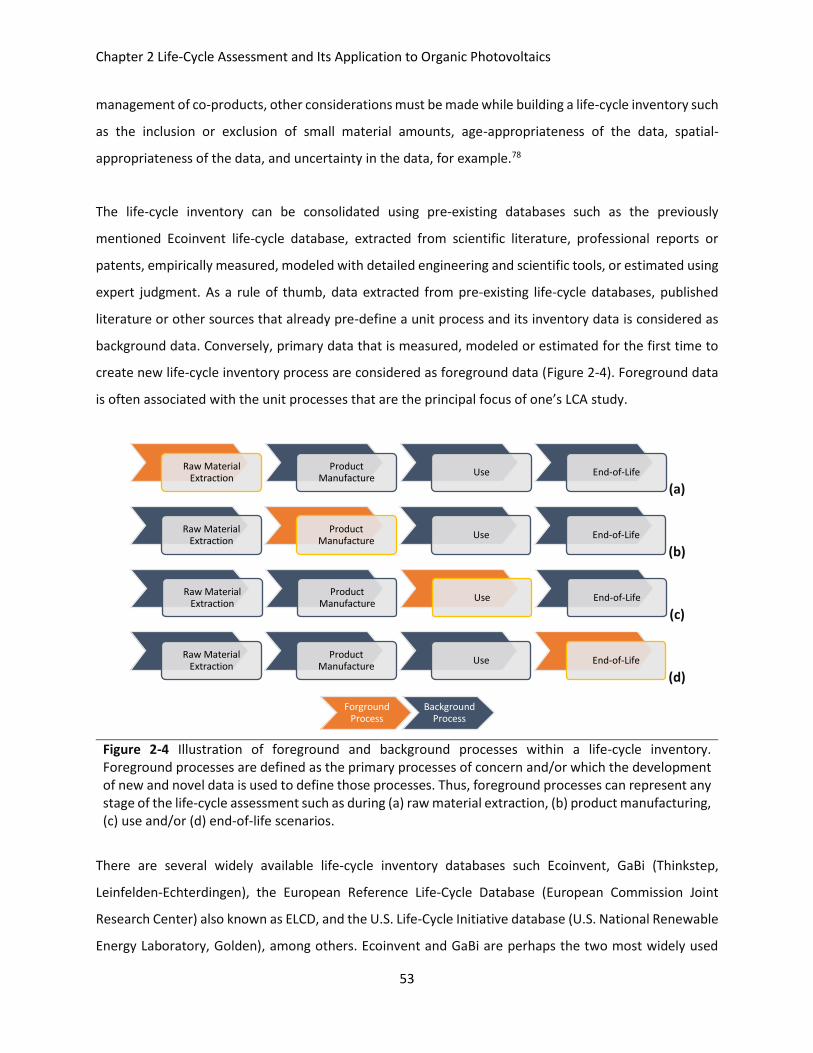
Chapter 2 Life-Cycle Assessment and Its Application to Organic Photovoltaics
53
management of co-products, other considerations must be made while building a life-cycle inventory such
as the inclusion or exclusion of small material amounts, age-appropriateness of the data, spatial-
appropriateness of the data, and uncertainty in the data, for example.78
The life-cycle inventory can be consolidated using pre-existing databases such as the previously
mentioned Ecoinvent life-cycle database, extracted from scientific literature, professional reports or
patents, empirically measured, modeled with detailed engineering and scientific tools, or estimated using
expert judgment. As a rule of thumb, data extracted from pre-existing life-cycle databases, published
literature or other sources that already pre-define a unit process and its inventory data is considered as
background data. Conversely, primary data that is measured, modeled or estimated for the first time to
create new life-cycle inventory process are considered as foreground data (Figure 2-4). Foreground data
is often associated with the unit processes that are the principal focus of one’s LCA study.
(a)
(b)
(c)
(d)
Figure 2-4 Illustration of foreground and background processes within a life-cycle inventory. Foreground processes are defined as the primary processes of concern and/or which the development of new and novel data is used to define those processes. Thus, foreground processes can represent any stage of the life-cycle assessment such as during (a) raw material extraction, (b) product manufacturing, (c) use and/or (d) end-of-life scenarios.
There are several widely available life-cycle inventory databases such Ecoinvent, GaBi (Thinkstep,
Leinfelden-Echterdingen), the European Reference Life-Cycle Database (European Commission Joint
Research Center) also known as ELCD, and the U.S. Life-Cycle Initiative database (U.S. National Renewable
Energy Laboratory, Golden), among others. Ecoinvent and GaBi are perhaps the two most widely used
Raw Material Extraction
Product Manufacture
Use End-of-Life
Raw Material Extraction
Product Manufacture
Use End-of-Life
Raw Material Extraction
Product Manufacture
Use End-of-Life
Raw Material Extraction
Product Manufacture
Use End-of-Life
Forground Process
Background Process
Chapter 2 Life-Cycle Assessment and Its Application to Organic Photovoltaics
54
life-cycle inventory databases globally. While both are quite comprehensive in their amount and types of
inventory data collected across a wide range of industrial sectors, business activities and technospheres,
GaBi is distinct in that it utilizes inventory data collected from industrial sources. Although such data
provides tremendous value and validation to the LCA process, much of this data is “rolled up” into
aggregated system processes (i.e. a collection of so-called smaller unit processes) to protect sensitive
industrial data and provide insulation to any one company from targeted scrutiny. Ecoinvent on the other
hand contains a greater number of unit processes and thus greater resolution at the impact assessment
stage, although much of its data come from non-industrially supplied sources. However, many of the
Ecoinvent inventories relevant to PV systems such as semiconductor-grade level silicon, production of PV
cells, did include non-aggregated, industry-specific data.79 Since a majority of environmental impacts are
heavily influenced by background processes, it is beneficial to have non-aggregated data for
understanding the sources of potential hazards related to PV systems.35
Life-Cycle Impact Assessment
During the impact assessment step – the environmental and human health impact categories and
methodologies are initially chosen in the goal and scope definition but then applied separately – inventory
data are converted into potential impacts using their corresponding characterization (i.e. conversion)
factors (CF) (equation (2-1)).
𝐼𝑚𝑝𝑎𝑐𝑡 𝐴𝑠𝑠𝑒𝑠𝑠𝑚𝑒𝑛𝑡 𝑆𝑐𝑜𝑟𝑒 =𝐼x ∙ 𝐶𝐹x,i ∙ 𝑊i
𝑁i (2-1)
Ix: Inventory value for flow, x
CFi: Characterization factor for inventory flow, x, and impact category, i
Wi: Weighting factor for impact category, i (optional) Ni: Normalization value for impact category, i (optional)
The optional steps of normalization and weighting can be employed during the life-cycle impact
assessment step. Weighting provides an approach expressing one’s preference of concern for some
impact categories over other. After weighting, normalization can be applied to harmonize impact category
units so that each can be directly and relatively compared. External normalization involves dividing impact
results by reference values, such as total global emissions. Internal normalization can be used when there
are multiple alternatives fulfilling the same functional unit and division by the alternative with the greatest
impact per impact category is used, for example.

Chapter 2 Life-Cycle Assessment and Its Application to Organic Photovoltaics
55
There are a wide set of both environmental and human health impacts one can consider in an LCA. Often,
these can be chosen from pre-defined impact assessment methodologies such as ReCiPe80 (www.lcia-
recipe.net), ILCD81 (European Commission), TRACI (U.S. EPA), LC-Impact (www.lc-impact.eu), CML
(University of Leiden), Cumulative Energy Demand (CED), or USEtox (www.usetox.org), among others
(Table 2-1).
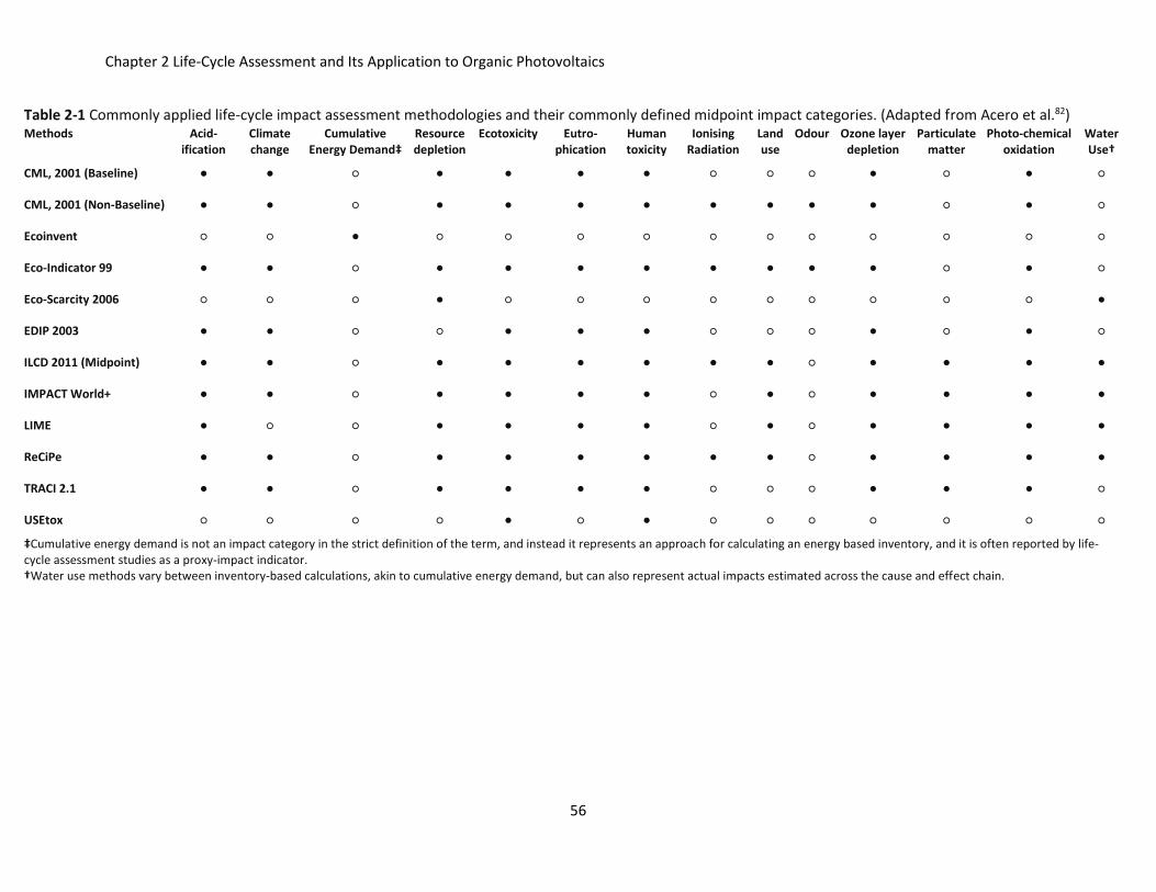
Chapter 2 Life-Cycle Assessment and Its Application to Organic Photovoltaics
56
Table 2-1 Commonly applied life-cycle impact assessment methodologies and their commonly defined midpoint impact categories. (Adapted from Acero et al.82) Methods Acid-
ification Climate change
Cumulative Energy Demand‡
Resource depletion
Ecotoxicity Eutro-phication
Human toxicity
Ionising Radiation
Land use
Odour Ozone layer depletion
Particulate matter
Photo-chemical oxidation
Water Use†
CML, 2001 (Baseline) ● ● ○ ● ● ● ● ○ ○ ○ ● ○ ● ○
CML, 2001 (Non-Baseline) ● ● ○ ● ● ● ● ● ● ● ● ○ ● ○
Ecoinvent ○ ○ ● ○ ○ ○ ○ ○ ○ ○ ○ ○ ○ ○
Eco-Indicator 99 ● ● ○ ● ● ● ● ● ● ● ● ○ ● ○
Eco-Scarcity 2006 ○ ○ ○ ● ○ ○ ○ ○ ○ ○ ○ ○ ○ ●
EDIP 2003 ● ● ○ ○ ● ● ● ○ ○ ○ ● ○ ● ○
ILCD 2011 (Midpoint) ● ● ○ ● ● ● ● ● ● ○ ● ● ● ●
IMPACT World+ ● ● ○ ● ● ● ● ○ ● ○ ● ● ● ●
LIME ● ○ ○ ● ● ● ● ○ ● ○ ● ● ● ●
ReCiPe ● ● ○ ● ● ● ● ● ● ○ ● ● ● ●
TRACI 2.1 ● ● ○ ● ● ● ● ○ ○ ○ ● ● ● ○
USEtox ○ ○ ○ ○ ● ○ ● ○ ○ ○ ○ ○ ○ ○
‡Cumulative energy demand is not an impact category in the strict definition of the term, and instead it represents an approach for calculating an energy based inventory, and it is often reported by life-cycle assessment studies as a proxy-impact indicator. †Water use methods vary between inventory-based calculations, akin to cumulative energy demand, but can also represent actual impacts estimated across the cause and effect chain.
Chapter 2 Life-Cycle Assessment and Its Application to Organic Photovoltaics
57
These life-cycle impact assessment methods differ on the types of impact categories included, the spatial
representativeness of the methods, and their modeling choices, among other things. Although Table 2-1
is not a comprehensive account of all possible impact categories, it is representative of 14 very common
environmental and human health criteria. Some of these impacts, for instance, represent multiple impact
categories such as ecotoxicity which can be sub-divided into freshwater or marine water ecotoxicity. Other
impact categories which are nevertheless important, such as impacts from noise pollution, are not
commonly included in these methods, lack formal reporting within life-cycle inventory databases and are,
thus, not included in the Table 2-1.83 The majority of the life-cycle impact assessment methodologies are
specific for European conditions and impacts. These include CML, Eco-indicator99, EDIP, ILCD and ReCiPe.
TRACI was developed specifically for estimating the impacts within North America, while LIME was
originally developed for the Japan but has since expanded its focus. Other impact methodologies such as
Eco-Scarcity, Ecoinvent and USEtox focus on resource depletion, CED and toxicity, respectively. USEtox, in
particular, is a consensus model focused on estimating freshwater ecotoxicity as well as non-cancerous
and cancerous human health toxicity.84 It was developed from authors of formerly and widely used
environmental impact models such as CalTOX,85 IMPACT 2002,86 BETR,87 EDIP,88 WATSON,89 USES-LCA90
and EcoSense.91
Inventory flows must be classified into specific impact categories. Inventory flows might contribute to
more than one impact category (i.e. one compound might influence two separate types of environmental
impacts). Thus, formal decisions must be made regarding how to partition the inventory flows, which will
in turn affect how the final environmental and human health impacts. Impact assessment modeling can
be divided into midpoint- or endpoint-modeling (Figure 2-5).
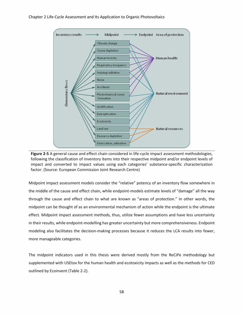
Chapter 2 Life-Cycle Assessment and Its Application to Organic Photovoltaics
58
Figure 2-5 A general cause and effect chain considered in life-cycle impact assessment methodologies, following the classification of inventory items into their respective midpoint and/or endpoint levels of impact and converted to impact values using each categories’ substance-specific characterization factor. (Source: European Commission Joint Research Centre)
Midpoint impact assessment models consider the “relative” potency of an inventory flow somewhere in
the middle of the cause and effect chain, while endpoint-models estimate levels of “damage” all the way
through the cause and effect chain to what are known as “areas of protection.” In other words, the
midpoint can be thought of as an environmental mechanism of action while the endpoint is the ultimate
effect. Midpoint impact assessment methods, thus, utilize fewer assumptions and have less uncertainty
in their results, while endpoint-modelling has greater uncertainty but more comprehensiveness. Endpoint
modeling also facilitates the decision-making processes because it reduces the LCA results into fewer,
more manageable categories.
The midpoint indicators used in this thesis were derived mostly from the ReCiPe methodology but
supplemented with USEtox for the human health and ecotoxicity impacts as well as the methods for CED
outlined by Ecoinvent (Table 2-2).
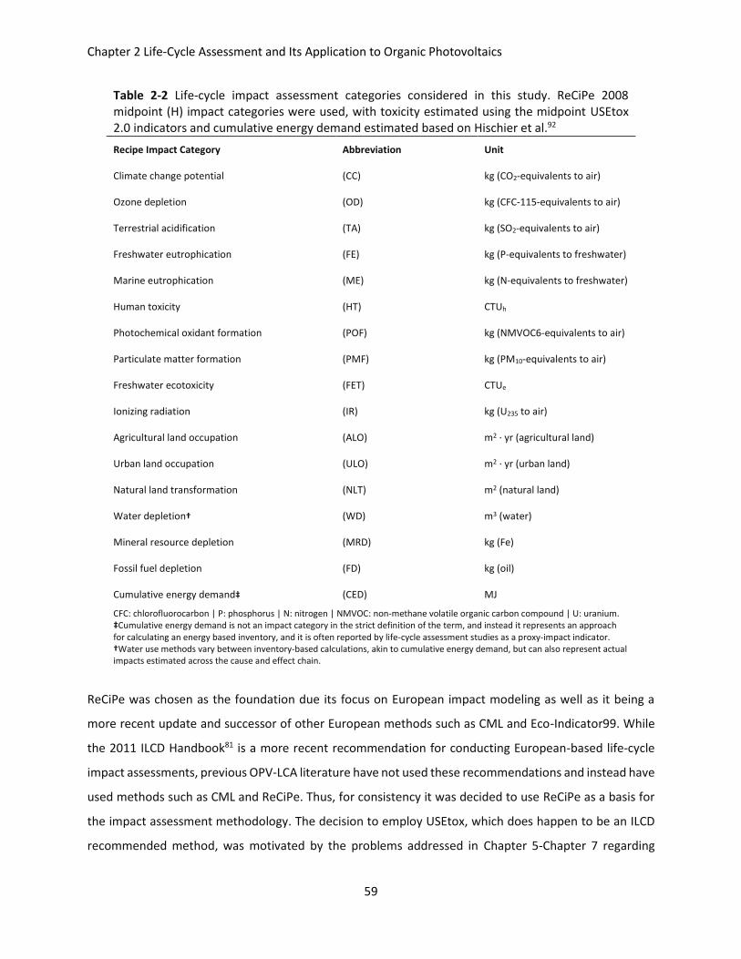
Chapter 2 Life-Cycle Assessment and Its Application to Organic Photovoltaics
59
Table 2-2 Life-cycle impact assessment categories considered in this study. ReCiPe 2008 midpoint (H) impact categories were used, with toxicity estimated using the midpoint USEtox 2.0 indicators and cumulative energy demand estimated based on Hischier et al.92
Recipe Impact Category Abbreviation Unit
Climate change potential (CC) kg (CO2-equivalents to air)
Ozone depletion (OD) kg (CFC-115-equivalents to air)
Terrestrial acidification (TA) kg (SO2-equivalents to air)
Freshwater eutrophication (FE) kg (P-equivalents to freshwater)
Marine eutrophication (ME) kg (N-equivalents to freshwater)
Human toxicity (HT) CTUh
Photochemical oxidant formation (POF) kg (NMVOC6-equivalents to air)
Particulate matter formation (PMF) kg (PM10-equivalents to air)
Freshwater ecotoxicity (FET) CTUe
Ionizing radiation (IR) kg (U235 to air)
Agricultural land occupation (ALO) m2 · yr (agricultural land)
Urban land occupation (ULO) m2 · yr (urban land)
Natural land transformation (NLT) m2 (natural land)
Water depletion† (WD) m3 (water)
Mineral resource depletion (MRD) kg (Fe)
Fossil fuel depletion (FD) kg (oil)
Cumulative energy demand‡ (CED) MJ
CFC: chlorofluorocarbon | P: phosphorus | N: nitrogen | NMVOC: non-methane volatile organic carbon compound | U: uranium. ‡Cumulative energy demand is not an impact category in the strict definition of the term, and instead it represents an approach for calculating an energy based inventory, and it is often reported by life-cycle assessment studies as a proxy-impact indicator. †Water use methods vary between inventory-based calculations, akin to cumulative energy demand, but can also represent actual impacts estimated across the cause and effect chain.
ReCiPe was chosen as the foundation due its focus on European impact modeling as well as it being a
more recent update and successor of other European methods such as CML and Eco-Indicator99. While
the 2011 ILCD Handbook81 is a more recent recommendation for conducting European-based life-cycle
impact assessments, previous OPV-LCA literature have not used these recommendations and instead have
used methods such as CML and ReCiPe. Thus, for consistency it was decided to use ReCiPe as a basis for
the impact assessment methodology. The decision to employ USEtox, which does happen to be an ILCD
recommended method, was motivated by the problems addressed in Chapter 5-Chapter 7 regarding
Chapter 2 Life-Cycle Assessment and Its Application to Organic Photovoltaics
60
compatibility of impact assessment methodologies with emerging technologies and to create consistency
with the previous work in this area that had already considered USEtox in their methodological
approaches.93–97
A brief description of the midpoint impact indicators used in this thesis are included in the following sub-
sections. Their descriptions are by no means exhaustive and serve only to provide sufficient information
for understanding the fundamental implications of the results reported in this thesis. Additionally, it
should be noted that ReCiPe adapts three different impact assessment “perspectives” that represent
three different modeling choices and decision makers’ perspectives: individualist (I), hierarchist (H) and
egalitarian (E).98 These perspectives only influence a portion of the total impact categories and differ
mainly by their time-frames over which environmental and human health impacts to occur. Perspective I
can be thought of as an optimistic model, Perspective E a precautionary model and Perspective H as the
average model.
Climate Change Potential (Global Warming Potential)
The effects of climate change are in large part driven by the amounts of greenhouse gases contained in
the Earth’s atmosphere, such as carbon dioxide, methane, nitrous oxide and fluorinated gases. These
gases, whose concentrations are growing due to human induced activities, have the capacity to trap and
retain heat, raising near-surface temperatures of the planet.99 Each gas has a different radiative forcing
value and lifetime in the lower atmosphere (e.g. troposphere), meaning each has a distinct and relative
“strength” for influencing climate change.100 CO2 is considered the standard reference greenhouse gas to
which all other substances are given CO2-equivalent values. These CO2-equivalent values represent the
midpoint CF, while endpoint CF consider the relative temperature increase as well as the specific effect
on the areas of protection due to that increase (e.g. extinction of species).101
Ozone Layer Depletion
The ozone layer is defined as a portion of the stratosphere that contains an essential layer of ozone
molecules (i.e. O3) that is effective at absorbing and thus blocking incoming radiation from the sun. Some
of this radiation, such as ultra-violet B or UVB, is known to have both negative human health and
environmental consequences such as contributing to skin cancer. By the 1970s it was identified that many
man-made substances such as chlorofluorocarbons can react and deplete the ozone layer.102 Similar to
the effects of climate change with greenhouse gases, ozone depleting substances have different, relevant
Chapter 2 Life-Cycle Assessment and Its Application to Organic Photovoltaics
61
strengths and lifetimes in the atmosphere. One of these substances CFC11, a refrigerant, is used as the
standard reference ozone depleting substance to which all others are defined by their CFC11-equivalent
values. These values represent the midpoint CF, while endpoint CF are concerned with estimating the
amount of increased radiation that results from the release of these substances and the corresponding
influence on certain types of skin cancers as a result.101
Photochemical Oxidation Formation (Smog) Potential
Like climate change potential, photochemical oxidation potential concerns itself with releases of
pollutants in the lower troposphere that form photo-oxidants. Photo-oxidants form when nitrogen oxides
(NOx) react with hydrocarbons in the presence of sunlight.103 This reaction leads to the creation of
“ground-level” ozone, as opposed to stratospheric ozone that comprises the protective ozone layer.
Ground level ozone can be dangerous to humans, causing various adverse pulmonary effects.104 It can also
have adverse impacts on terrestrial species, resulting in the loss of vegetation and plant life.105 Midpoint
CF are expressed as equivalents of non-methane volatile organic compounds (NMVOC-equivalents),
expressing the marginal change in ground-level ozone per emission of a substance, x.101 Endpoint CF are
further defined by their level of exposure either by humans or terrestrial systems (e.g. plants) and their
corresponding adverse effects per kg of ozone uptake.101
Resource (Minerals) Depletion
This impact category represents multiple types of resources, often categorized by minerals and fossil fuels.
At the midpoint level, resource depletion represents the quantity of resources used in comparison to their
known quantity of obtainable reserves existing in nature. These midpoints are reported in terms of kg of
iron-equivalents (kg Fe-eq.) and kg of oil-equivalents (kg Oil-eq.) for mineral and fossil fuel depletion,
respectively.101 At the endpoint level, resource depletion includes the consideration of decreasing ore
grades as a function of depletion and is reported in terms of monetary costs (e.g. USD) per mass of
extracted resource.101
Land Use, Land Occupation and Land Transformation
Specific types of activities (e.g. mining) and structures (e.g. warehouses) require land either through which
they directly use as a raw material or as a place to physically occupy. At the midpoint level, the impacts of
land use are defined by the area (e.g. m2) of physical land occupied or transformed as well as the
timeframe (e.g. years) for these activities.101 The endpoint impact may be defined by species-land
Chapter 2 Life-Cycle Assessment and Its Application to Organic Photovoltaics
62
relationships whereby an increase in the area of available natural land, or a decrease in time of
occupied/transformed land, implies an increase in the number of vegetative-species present in that same
space.101 Furthermore, the time of restoration is assumed to be linearly linked to the overall impact. Of
course, this approach implies that the impacts of land use will be heavily dependent on the geographical
location, considering that default species abundances and resiliency of the land to restore itself will be
closely linked to the type of “natural” landscape present in a region.
Energy Use (Cumulative Energy Demand)
Although energy use is not a true impact category,106 the concept of CED is important to energy related
systems because it facilitates the calculation of how much time it will take for a device, during its use, to
generate the energy that was consumed during the production of that same device (i.e. EPBT). The CED
quantifies all the directly consumed energy across the entire life-cycle of a system as well as the indirect,
embodied energy of materials consumed, created and discarded along the way. So far, there is no
standardized approach for quantifying the CED in life-cycle impact assessment methodologies. The
approach most commonly used in life-cycle impact assessment methods is the Ecoinvent approach that
applies the upper heating value (e.g. MJ-energy per kg-material) for estimating the indirect energy
consumed in a system. Other sources of non-combustible energy such as nuclear, hydro, wind and solar
power are also included in the calculation and can be reported with or without the non-renewable sources
of energy.
Water Depletion
The reporting of a water-based impact category has not been fully harmonized in impact assessment
methodologies either. Some methods may report water use impacts similar to resource depletion impacts
in terms of an overall summation of water use, potentially comparing it with known obtainable amounts
for that resource. However, this is largely an inventory based statistic, similar to CED, and does not
estimate any particular impact from water use specifically. Such values are typical of midpoint water use
impact categories and are reported as m3 of water used.101
Acidification
There are a number of pollutants that have the capacity to increase the number of hydrogen (H+) ions in
the environment, including sulfur dioxide, nitrous oxides, hydrogen chloride and ammonia, for example.107
The release or formation of H+ can decrease the pH in both soil and water systems. Such changes can
Chapter 2 Life-Cycle Assessment and Its Application to Organic Photovoltaics
63
cause imbalances in local ecosystems and ultimately result in the loss of species.107 The fate and transport
of these pollutants are defined by their behavior in the atmosphere as well as their behavior in the soil
using steady-state and dynamic models, respectively. The midpoint CF are defined in equivalents of sulfur
dioxide (SO2-equivalents) and represent the ratio of the fate for substance, x, with the fate of SO2.101
Endpoint CF are defined by for a potentially disappeared fraction of plant species impacted by the change
in pH of the media.101
Eutrophication
Eutrophication is a phenomenon that occurs in fresh and marine water systems whereby an excess of
nutrients, namely phosphorous and nitrogen, can cause unfavorable ecological conditions for living
organisms. Specifically, excess phosphorous and nitrogen can promote the exponential growth of algae
and other organisms.108 In the long run, if growth is excessive, it can result in low oxygen conditions in the
water, due to interference with photosynthesis-cycles of sub-surface plant life and the aerobic breakdown
of the algae by bacteria. The lack of oxygen can ultimately cause stress and death in certain organisms
within the hypoxic zones.108 The midpoints for eutrophication are defined in terms of phosphorous- (P-
equivalents) and nitrogen-equivalent (N-equivalents) mass emissions for freshwater and marine water
environments, respectively.101 Eutrophication endpoints are defined by a linear effect factor describing
the number of disappeared species based on the change in phosphorous- or nitrogen-equivalent
emissions in the environment.101
Ionizing Radiation
The effects of radioactive isotopes may occur if humans encounter these substances either by directly
working with them or after they are released into the environment. Although naturally occurring
radioactive isotopes are the most abundant form of these substances, anthropogenic sources contribute
to these levels through combustion of coal, production of nuclear fuel and use of military weapons, for
example.109 When these substances decay they release high amounts of ionizing radiation that can induce
alterations in one’s DNA and other organ systems.110 The midpoint CF is defined by the internally absorbed
dose, expressed using the mass of U235-equivalents and interpreted from the commonly applied unit
Sievert (Sv), while the endpoint takes into consideration the incidence and severity of corresponding
diseases (e.g. cancer) for this amount of internal dose.101
Chapter 2 Life-Cycle Assessment and Its Application to Organic Photovoltaics
64
Particulate Matter Formation
In ReCiPe, particulate matter is defined as substances with diameters less than 10 μm (PM10). This type of
particulate matter can form from emissions of sulfur dioxide, ammonia and nitrogen oxides, for
example.111 Particulate matter is specifically important for human health impacts, where they are
associated with pulmonary diseases such as inflammation and/or cancer.111 The fate of and exposure to
particulate matter is calculated using steady-state models, while the resulting intake fraction is estimated
directly from the number of persons exposed and their respective breathing rates.101 The midpoint CF is
then expressed in equivalents of the intake for PM10 (PM10-equivalents).101 Endpoint CF are then defined
based on the corresponding effect at that particular exposure dose, estimated from a corresponding dose-
response relationship.101
Ecotoxicity
The life-cycle impact assessment methodology embodied by USEtox considers the potential eco-
toxicological impacts that result from the exposure to organic chemicals and certain non-organic metals
in freshwater. USEtox is a consensus model that came out of the Life-Cycle Initiative jointly partnered by
the United National Environment Programme (UNEP) and the Society for Environmental Toxicology and
Chemistry (SETAC). The goal of the initiative was to produce recommended ecotoxicity (and human
health) CF for LCA. Multi-compartmental models are used to trace the fate and transport of a chemical
from the source of its emission in one medium to the final concentration of another medium. Steady-
state, equilibrium models are employed, largely dependent on partition (equilibrium) coefficients for
characterizing these behaviors.84 Exposure is estimated using steady-state bioaccumulation models using
the same types of partition coefficients mentioned above.84 This estimated level of exposure (e.g.
bioavailable mass) is then combined with an estimation of the concentration at which 50% of the
population has the observed impact, referred to as the effective concentration at 50% (EC50).84 The EC50
value is calculated from in vivo toxicological studies for at least three different species/trophic levels.84
The midpoint impact is defined here as a non-reference unit expressed as the comparative toxic unit for
ecosystems (CTUe).84 The endpoint may be combined with a damage factor that estimates the number of
potentially disappeared fraction of species.
Human Toxicity
The life-cycle impact assessment methodology embodied by USEtox considers the potential human health
impacts that result from the exposure to organic chemicals and certain non-organic metals. Multi-
Chapter 2 Life-Cycle Assessment and Its Application to Organic Photovoltaics
65
compartmental models are used to trace the fate and transport of a chemical from the source of its
emission in one medium to the final concentration of another medium. Steady-state, equilibrium models
are employed, largely dependent on partition (equilibrium) coefficients for characterizing these behaviors
(equation (2-2)).84
𝐶𝐹i,j = 𝐹𝐹i ∙ 𝑋𝐹i ∙ 𝐸𝐹i,j = (𝑖𝐹i) ∙ 𝐸𝐹i,j (2-2)
FFi: fate factor (days) for substance i
XFi: exposure factor (days-1) for substance i
iFi: intake fraction for substance i
EFi: effect factor (cases/kg) for substance i and pathology j
The FF represents the various transformation and removal mechanisms from one compartment to
another and is reported in days. Exposure is limited to inhalation and ingestion, without consideration of
dermal exposure and is expressed as the XF in units of 1/days. It is assessed on a population-based level
as opposed to an individual level, the latter being more conventional for HHRA methods. The results of
the fate and exposure calculations provide a lifetime intake fraction (iF), which is defined as the ingested
or inhaled amount per mass of emitted substance. This intake fraction is then combined with an
estimation of the human-equivalent dose at which 50% of the population has the observed impact. This
is referred to as the effective dose at 50% (ED50) and represented as the EF with units of cases of
cancerous or non-cancerous disease per kg of emitted substance.84 This dose is generally quantified using
in vivo, animal dose-response toxicological data at which 50% of the test subjects gave a response. Both
carcinogenic and non-carcinogenic doses may be defined depending. Midpoint impacts are expressed in
non-equivalent unit defined as the comparative toxic unit for humans (CTUh).84 Endpoints may be
presented in terms of the disability-adjusted life years (DALY), where one DALY is defined as one year of
lost life (YLL) due to mortality and/or due to disease and disabilities (YLD).112
Interpretation
The interpretation stage is a process that is involved along each of the three other steps of the LCA (i.e.
the goal/scope definition, the life-cycle inventory analysis and the life-cycle impact assessment). LCA is
commonly described as an iterative process, one in which the development of the objective, methods and
result calculations are repeated and refined based on the previous set of outcomes. Interpretation should
be used to (a) understand and make the logical connections between the life-cycle impact assessment
Chapter 2 Life-Cycle Assessment and Its Application to Organic Photovoltaics
66
results, life-cycle inventory and the goal/scope definition, but also to (b) identify anomalies and errors
that may present themselves in each of these LCA steps. Because LCA is involved with copious amounts
of data, it is often best to use systematic approaches to the interpretation phase such as (i) contribution
analysis (i.e. analyzing each impact category per life-cycle stage, unit-process and/or elemental flow), (ii)
uncertainty analysis (e.g. defining the inventory data with distributions based on their inherent
uncertainty and variability as opposed to deterministic values), and (iii) sensitivity analysis (e.g. modifying
the life-cycle inventory to reflect specific technology decisions at the early development and design
stages).78
It should be noted that inventory items and their resulting impacts are aggregated over time and broad
environmental landscapes/compartments. Consequently, LCA results do not communicate absolute
values, as briefly mentioned in Chapter 1. Thus, the environmental impact results of an LCA derived for
one product are best utilized when they are compared to the impacts of another product instead of being
used to measure its definitive, absolute impact on human health or the environment, as is done in HHRA
or ERA. Both HHRA and ERA will be presented in greater detail in Chapter 5 and Chapter 6.
Chapter 3 Cradle-to-Gate Life-Cycle Assessment of Organic Photovoltaics
67
Chapter 3 Cradle-to-Gate Life-Cycle Assessment of Organic
Photovoltaics
From a material and device structure perspective, there are a variety of OPV that have been studied using
LCA (Chapter 1). While there are some general consistencies across the devices such as the use of a
PCBM:P3HT active layer, there are some noticeable differences in such choices as the electrodes, for
example. The results of those studies identified hot-spots that could be addressed for improving the
environmental performance of OPV devices. Additionally, there were points raised about technical and
functional aspects of material choices that should be addressed such as the assumptions regarding their
lifetimes as well as their efficiencies. Furthermore, only three of the ten previous OPV-LCA studies looked
beyond CED or greenhouse gas accounting. Of those that did, only one study compared those impact
categories to conventional silicon PV. Illustrating the differences between OPV and silicon PV across a
greater range of LCA impact categories, can help provide meaningful motivation for the development of
this technology. Therefore, the objective of this chapter is to define a near-term, prospective OPV life-
cycle inventory based on the recommendations and lessons from the review in Chapter 1 and complete a
life-cycle impact assessment comparing OPV and silicon-based PV across a comprehensive set of LCA
impact categories.
Organic Photovoltaic Device Structure and Material Choices in this Thesis
As was discussed in Chapter 1, all the previously reviewed LCA literature was completed on devices that
exploit the functionality of ENM such as C60-fullerenes and their derivatives. C60-fullerenes have garnered
the most interest in OPV research as an organic “n-type” (i.e. electron acceptor) semiconductor because
of its strong electronegativity and high electron mobility. Specifically, the fullerene derivative PCBM is
widely employed, often in conjunction with the common “p-type” (i.e. electron donor) polymer P3HT.43,52–
54 During charge separation in the active layer, there is the creation of both a negative and positive charge
carrier, the latter referred to as a “hole” or absence of an electron in an atom. Current is created when
the negative charge is allowed to move through the PCBM and through to the (back) cathode while the
holes simultaneously propagate through the P3HT and on to the transparent anode.48
Substrates of early OPV devices were originally rigid structures such as glass, however it has become
common and technologically feasible to print the components of an OPV cell directly onto a flexible
substrate.25,43 The substrate used in this work was polyethylene terephthalate (PET), which has proved to
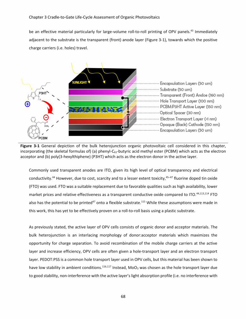
Chapter 3 Cradle-to-Gate Life-Cycle Assessment of Organic Photovoltaics
68
be an effective material particularly for large-volume roll-to-roll printing of OPV panels.43 Immediately
adjacent to the substrate is the transparent (front) anode layer (Figure 3-1), towards which the positive
charge carriers (i.e. holes) travel.
Figure 3-1 General depiction of the bulk heterojunction organic photovoltaic cell considered in this chapter, incorporating (the skeletal formulas of) (a) phenyl-C61-butyric acid methyl ester (PCBM) which acts as the electron acceptor and (b) poly(3-hexylthiphene) (P3HT) which acts as the electron donor in the active layer.
Commonly used transparent anodes are ITO, given its high level of optical transparency and electrical
conductivity.44 However, due to cost, scarcity and to a lesser extent toxicity,45–47 fluorine doped tin oxide
(FTO) was used. FTO was a suitable replacement due to favorable qualities such as high availability, lower
market prices and relative effectiveness as a transparent conductive oxide compared to ITO.44,113,114 FTO
also has the potential to be printed47 onto a flexible substrate.115 While these assumptions were made in
this work, this has yet to be effectively proven on a roll-to-roll basis using a plastic substrate.
As previously stated, the active layer of OPV cells consists of organic donor and acceptor materials. The
bulk heterojunction is an interlacing morphology of donor:acceptor materials which maximizes the
opportunity for charge separation. To avoid recombination of the mobile charge carriers at the active
layer and increase efficiency, OPV cells are often given a hole-transport layer and an electron transport
layer. PEDOT:PSS is a common hole transport layer used in OPV cells, but this material has been shown to
have low stability in ambient conditions.116,117 Instead, MoO3 was chosen as the hole transport layer due
to good stability, non-interference with the active layer’s light absorption profile (i.e. no interference with
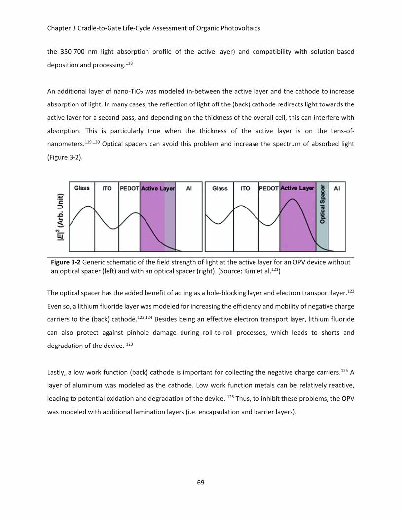
Chapter 3 Cradle-to-Gate Life-Cycle Assessment of Organic Photovoltaics
69
the 350-700 nm light absorption profile of the active layer) and compatibility with solution-based
deposition and processing.118
An additional layer of nano-TiO2 was modeled in-between the active layer and the cathode to increase
absorption of light. In many cases, the reflection of light off the (back) cathode redirects light towards the
active layer for a second pass, and depending on the thickness of the overall cell, this can interfere with
absorption. This is particularly true when the thickness of the active layer is on the tens-of-
nanometers.119,120 Optical spacers can avoid this problem and increase the spectrum of absorbed light
(Figure 3-2).
Figure 3-2 Generic schematic of the field strength of light at the active layer for an OPV device without an optical spacer (left) and with an optical spacer (right). (Source: Kim et al.121)
The optical spacer has the added benefit of acting as a hole-blocking layer and electron transport layer.122
Even so, a lithium fluoride layer was modeled for increasing the efficiency and mobility of negative charge
carriers to the (back) cathode.123,124 Besides being an effective electron transport layer, lithium fluoride
can also protect against pinhole damage during roll-to-roll processes, which leads to shorts and
degradation of the device. 123
Lastly, a low work function (back) cathode is important for collecting the negative charge carriers.125 A
layer of aluminum was modeled as the cathode. Low work function metals can be relatively reactive,
leading to potential oxidation and degradation of the device. 125 Thus, to inhibit these problems, the OPV
was modeled with additional lamination layers (i.e. encapsulation and barrier layers).
Chapter 3 Cradle-to-Gate Life-Cycle Assessment of Organic Photovoltaics
70
Life-Cycle Assessment Methods
Goal and Scope Definition
The work in this chapter followed ISO 14040:2006 and 14044:2006 guidelines for conducting a LCA study
and the recommendations of the IEA’s 2011 guidelines and best practices for implementing an LCA for
PV.27,28,35 A cradle-to-gate LCA on the production of OPV cells in comparison to conventional technologies
such as silicon is presented in this chapter. This work aims to define a baseline understanding of the life-
cycle inventory and corresponding environmental and human health impacts for a prospective device with
the most potential for real-world applications but also reduced environmental impacts.45
The life-cycle inventory is built for the production of a default OPV cell produced as a bulk heterojunction
cell of PCBM:P3HT as the active layer. The functional unit considered was one Wp. The OPV cell was
assumed to require 200 cm² of surface area per Wp power produced at a module efficiency of 5%.29
Efficiencies in the range of 2-3% were historically reported for lab-based PCBM-based cells without much
improvement.30,38,63 However, a large-scale deployment of OPV cells on land have already reported
efficiencies near 2%.24 Moreover, lab-scale efficiencies as high as 15% (Figure 1-2) have been reported in
the literature for PCBM-based devices similar to what will be considered in this thesis.126 Generally, as PV
technologies mature, their lab-to-industrial scale efficiencies might decrease from 20%-50%.127 Thus, the
efficiency assumption in this work represents an optimistic yet realistic near-term objective.
The OPV cells were subsequently compared with conventional m-Si and a-Si PV. For each technology
option, environmental flows were tracked across raw material extraction, material processing,
manufacture, and transportation requirements for each solar cell design. Figure 3-3 depicts these life-
cycle stages for the OPV cell.
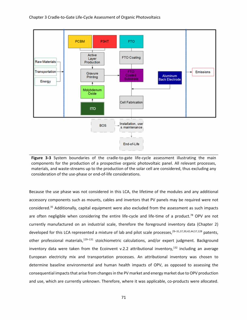
Chapter 3 Cradle-to-Gate Life-Cycle Assessment of Organic Photovoltaics
71
Figure 3-3 System boundaries of the cradle-to-gate life-cycle assessment illustrating the main components for the production of a prospective organic photovoltaic panel. All relevant processes, materials, and waste-streams up to the production of the solar cell are considered, thus excluding any consideration of the use-phase or end-of-life considerations.
Because the use phase was not considered in this LCA, the lifetime of the modules and any additional
accessory components such as mounts, cables and invertors that PV panels may be required were not
considered.35 Additionally, capital equipment were also excluded from the assessment as such impacts
are often negligible when considering the entire life-cycle and life-time of a product.78 OPV are not
currently manufactured on an industrial scale, therefore the foreground inventory data (Chapter 2)
developed for this LCA represented a mixture of lab and pilot scale processes,29–31,37,39,42,44,57,128 patents,
other professional materials,129–131 stoichiometric calculations, and/or expert judgment. Background
inventory data were taken from the Ecoinvent v.2.2 attributional inventory,132 including an average
European electricity mix and transportation processes. An attributional inventory was chosen to
determine baseline environmental and human health impacts of OPV, as opposed to assessing the
consequential impacts that arise from changes in the PV market and energy market due to OPV production
and use, which are currently unknown. Therefore, where it was applicable, co-products were allocated.
Chapter 3 Cradle-to-Gate Life-Cycle Assessment of Organic Photovoltaics
72
Mass allocation, as opposed to economic allocation, was generally applied given that the industrial-scale,
price information on specialty chemicals and substances was not available. All transportation
requirements for incoming foreground chemicals and materials were taken into account using 100 km
truck and 600 km rail transport, while outbound waste materials were estimated using ten km truck
transport.132 The LCA was conducted in OpenLCA v1.4 (GreenDelta, Berlin). The life-cycle impact
categories (Table 2-2) were chosen as ReCiPe80 v1.0.5 midpoint (H) impact categories with the substitution
of USEtox 2.0 for the human health and freshwater ecotoxicity indicators as well as the addition of the
CED.92 A detailed account of the foreground inventory data collected and calculated in this chapter are
explained in greater detail in Appendix: Chapter 3.
Life Cycle Inventory
Substrate
To produce one m² OPV panel, 0.074 kg of PET was used.29 PET substrate production was modeled using
the Ecoinvent process for “extrusion, plastic film” using the input “polyethylene terephthalate, granulate,
amorphous, at plant” as the substrate source material.
Transparent (Front) Anode
The FTO anode was modeled as a solution produced from tin tetrachloride pentahydrate, ammonium
fluoride, ethanol and water and heated to 60°C.47,133 It was assumed that the only energy consuming step
was for raising the temperature of water and ethanol from room temperature. The materials and energy
to produce tin tetrachloride pentahydrate were based on stoichiometric calculations.131 Wastes generated
from these processes were not estimated. The amount of FTO solution applied was 0.042 liters per m²
and was calculated as an average of the values reported for ITO in Garcia-Valverde et al.30 and Roes et
al.29 FTO deposition in the default OPV cell was modeled via sputtering in a roll-to-roll process.
Hole Transporter
MoO3 was modeled as the hole transport layer.116,117 Oxides of molybdenum do not occur in large amounts
in nature, but rather as sulfides (e.g. molybdenite). Production of MoO3 was modeled by roasting
molybdenite at high temperatures in the presence of oxygen.134 The amount of MoO3 was estimated as
0.24g per m2 of OPV.30,31,128 Deposition of MoO3 was modeled via gravure printing in a roll-to-roll process
as has been demonstrated for PEDOT:PSS.43,135,136
Chapter 3 Cradle-to-Gate Life-Cycle Assessment of Organic Photovoltaics
73
Active Layer
The active layer consisted of a bulk heterojunction of PCBM and P3HT. PCBM can be produced in different
ways including plasma and pyrolysis techniques.57 Although plasma techniques can produce a more
discrete distribution of C60-fullerenes, this technique also produces smaller quantities of C60-fullerenes,
while pyrolysis can produce large quantities of various sized C60-fullerenes.128 PCBM production was
modeled via the pyrolysis technique using toluene as a feedstock.57 P3HT is a region-regular polymer
derived from 3-bromothiophene and bromohexane.30 Data for bromothiophene production was taken
from the inventory presented in Garcia-Valverde et al., 30 while thiophene production was calculated
based on stoichiometric calculations.130 The energy input for annealing the active layer was estimated
from Espinosa et al.38 as 5.07 MJ per m2 and includes the energy for drying the electron transport and hole
transport layers. Per m2 of OPV, 0.21 g of PCBM and 0.235 g of P3HT were required.30,31,128 Additionally, a
30 nm (0.13 g per m2 of panel) optical spacer composed of nano-TiO2 particles was modeled on the back-
side of the active layer.120,121,137,138 Deposition of P3HT:PCBM plus the optical spacer was modeled via
gravure printing in a roll-to-roll process135,136 using chlorobenzene as the solvent.30
Cathode
Per m2 of OPV, 0.3 g of aluminum was modeled for the (back) cathode.29,42 A layer of lithium fluoride was
deposited along with aluminum to act as an electron transport layer.29 Deposition of both layers was
modeled via gravure printing.11
Encapsulation and Lamination
Framing of the polymer solar cell is not considered in this inventory. Instead, several additional barrier
layers were modeled. Per m2 of OPV, 133 g PET, 0.44 g silica (SiO2), 0.99 g of an epoxy-silica ENM-
composite, and 9.25 g of an epoxy resin was used per the description in Roes et al.29 Deposition of all
layers was modeled as gravure printing.11
Sensitivity Analysis
Alternative production and manufacturing options were assessed and compared with the default OPV
production route as described above. The first alternative, labeled FTOinkjet, involved a change in the
deposition method of the transparent electrode (i.e. FTO), using inkjet printing in place of sputtering.44
Samad et al.47 demonstrate the application of FTO solutions onto glass substrates using inkjet printing. As
a prospective analysis, the approach presented by Samad et al. was assumed to be compatible with
Chapter 3 Cradle-to-Gate Life-Cycle Assessment of Organic Photovoltaics
74
printing onto a flexible PET substrate and roll-to-roll compatible.139 Electricity usage for inkjet printing was
estimated as 21.3 kJ per m² substrate.29 The second alternative, labeled PCBMdcb, was based on changes
to the solvent used during PCBM manufacturing. Anctil et al. previously identified PCBM as a notable
contributor to the total CED of OPV panel production.57 PCBM requires large amounts of solvent,
particularly toluene, during production.57 Instead, another common industrial solvent, dichlorobenzene,
was substituted for toluene as the solvent in PCBM production.
Additionally, a second OPV technology (OPV-PP) was considered as an all-polymer (i.e. polymer accepter-
polymer donor) panel.140 C60-fullerenes can represent nearly a quarter of an OPV’s total material and
production cost. They also require relatively large amounts of energy input for production, processing
steps and purification to achieve electronic grade materials. Thus, some developments of alternative OPV
devices such as those that utilize non-fullerene acceptors in the active layer are currently being researched
and developed. The company Polyera reported a laboratory-based record of 6.4% with such an all polymer
cell. Although, their materials are proprietary, these records have been verified by the National
Renewable Energy Laboratory (NREL).141 Others have demonstrated advancements upwards of 7% and
10% efficiency by using small molecule acceptors and non-bulk-heterojunction active layers.142–144
However, average efficiencies for these devices are still low (i.e. circa 2%) and particularly lower than
fullerene-based cells.140 That being said, the effectiveness of this technology seems probable and the
adaptation of existing PCBM:P3HT production routes to accommodate an all polymer active layer is
extremely feasible. Thus, an additional consideration in this work was to evaluate the environmental
impacts to produce an all polymer active layer. The alternative tested in this study exchanged PCBM with
a n-type polymer. The inventory for the n-type polymer was based on the P3HT polymer as a proxy. For
the sake of demonstration, an OPV-PP panel was modeled with the same 5% efficiency as the OPV-D panel
outlined above and an identical geometry apart from the polymer substitution in place of PCBM.
Comparison to Conventional Silicon-Based Photovoltaics
The OPV devices described above were further compared to two conventional silicon-based PV: m-Si and
a-Si. m-Si technology has the largest share of global PV production at 70% of the market.16 a-Si is 2nd-
generation thin film technology that once has nearly 10% market share in early 2000 but has since receded
due to the influence of other 2nd-generation technologies such as cadmium-telluride and copper-indium-
gallium-selenium PV.16 The inventories for the silicon modules were taken from Ecoinvent 2.2.132 To
appropriately compare the silicon-based PV to OPV, the silicon inventories excluded glass encapsulation.
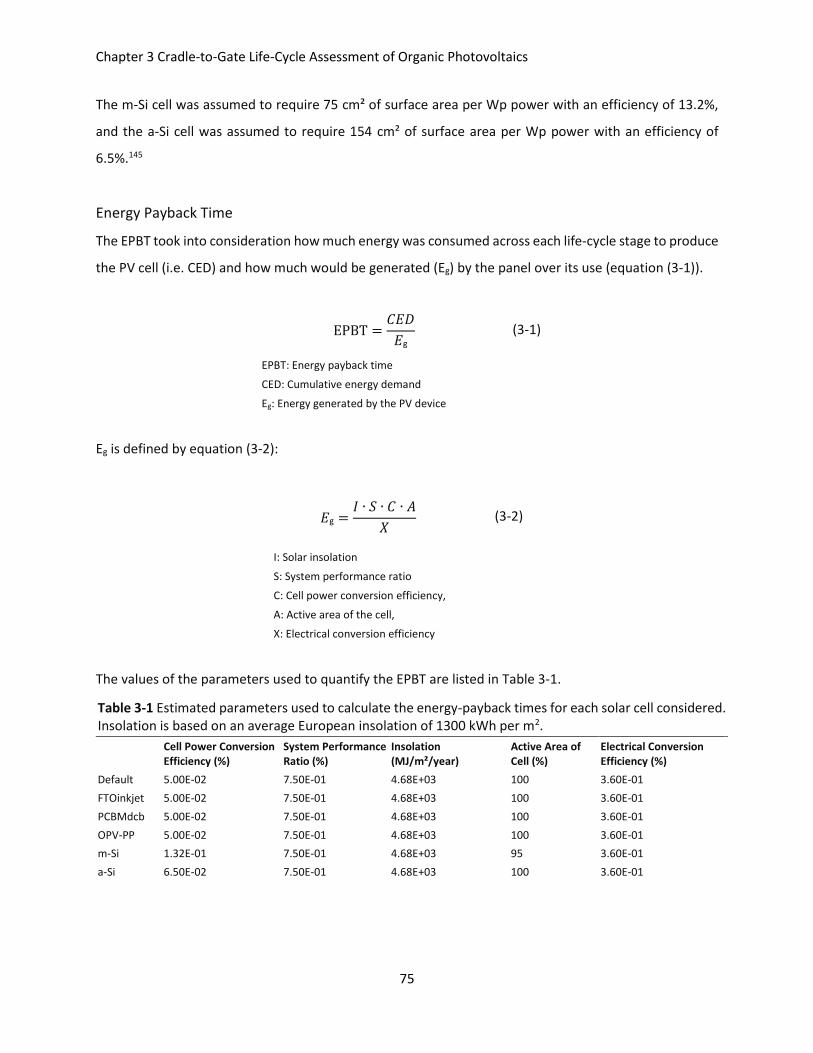
Chapter 3 Cradle-to-Gate Life-Cycle Assessment of Organic Photovoltaics
75
The m-Si cell was assumed to require 75 cm² of surface area per Wp power with an efficiency of 13.2%,
and the a-Si cell was assumed to require 154 cm² of surface area per Wp power with an efficiency of
6.5%.145
Energy Payback Time
The EPBT took into consideration how much energy was consumed across each life-cycle stage to produce
the PV cell (i.e. CED) and how much would be generated (Eg) by the panel over its use (equation (3-1)).
EPBT =𝐶𝐸𝐷
𝐸g (3-1)
EPBT: Energy payback time CED: Cumulative energy demand
Eg: Energy generated by the PV device
Eg is defined by equation (3-2):
𝐸g =𝐼 ∙ 𝑆 ∙ 𝐶 ∙ 𝐴
𝑋 (3-2)
I: Solar insolation
S: System performance ratio
C: Cell power conversion efficiency, A: Active area of the cell, X: Electrical conversion efficiency
The values of the parameters used to quantify the EPBT are listed in Table 3-1.
Table 3-1 Estimated parameters used to calculate the energy-payback times for each solar cell considered. Insolation is based on an average European insolation of 1300 kWh per m2.
Cell Power Conversion Efficiency (%)
System Performance Ratio (%)
Insolation (MJ/m²/year)
Active Area of Cell (%)
Electrical Conversion Efficiency (%)
Default 5.00E-02 7.50E-01 4.68E+03 100 3.60E-01
FTOinkjet 5.00E-02 7.50E-01 4.68E+03 100 3.60E-01
PCBMdcb 5.00E-02 7.50E-01 4.68E+03 100 3.60E-01
OPV-PP 5.00E-02 7.50E-01 4.68E+03 100 3.60E-01
m-Si 1.32E-01 7.50E-01 4.68E+03 95 3.60E-01
a-Si 6.50E-02 7.50E-01 4.68E+03 100 3.60E-01
Chapter 3 Cradle-to-Gate Life-Cycle Assessment of Organic Photovoltaics
76
Carbon Payback Time
To calculate the carbon payback time (CPBT), the cumulative, cradle-to-gate CO2-equivalent emissions
(CCE) of each PV panel was compared to the CCE avoided from a European average electricity production
mix (CCERER) for the same Wp produced by the PV panel per year of operation (equation (3-3)).
𝐶𝑃𝐵𝑇 =𝐶𝐶𝐸
(Eg ∙ CCERER) (3-3)
CPBT: Carbon payback time CCE: Cradle-to-gate CO2-eq. emissions generated for the PV device CCERER: CO2-eq. emissions avoided from an average European electricity mix per kWh of energy produced Eg: The amount of energy (kWh) produced by the PV device over one year
CCERER was estimated as 4.9E-04 kg per Wp of the Ecoinvent process “electricity, medium voltage,
production RER, at grid.”
Minimum Required Lifetime
The concept of a minimum required lifetime was used to communicate how long the OPV should be
operational such that its environmental impacts are no greater than conventional PV (equation (3-4)):
𝑀𝑅𝐿 = To,n
Ti,n ∙ 𝐿i (3-4)
MRL: Minimum required lifetime
To,n: Environmental and human health impact criteria (n) for OPV (o)
Ti,n: Environmental and human health impact criteria (n) for the silicon PV (i)
Li: Lifetime of the ith technology
The minimum required lifetime was estimated using a-Si as the ith technology.
Results and Discussion
The greatest contribution to the overall environmental and human health impacts of the default OPV
arose from the production and deposition (i.e. sputtering) of the FTO anode onto the substrate. FTO
substrate production had an average contribution of 62% across all impact categories, with a high of 95%
for metal depletion and low of 57% for fossil fuel depletion (Figure 3-4).
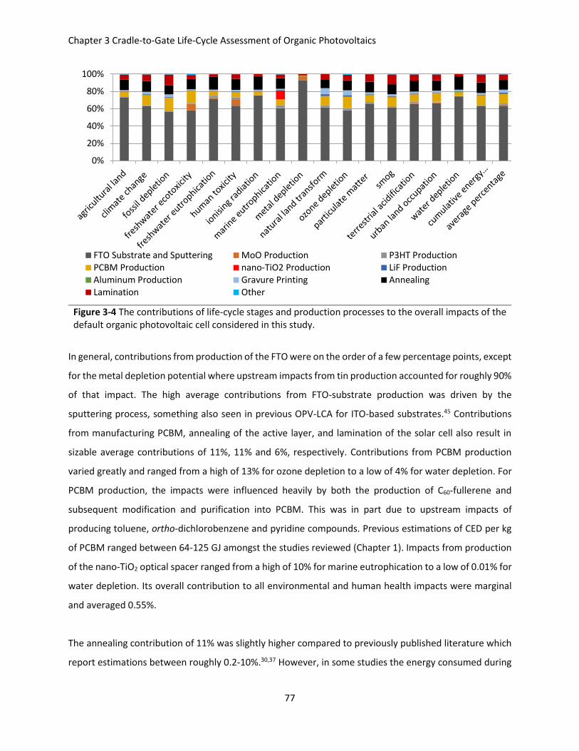
Chapter 3 Cradle-to-Gate Life-Cycle Assessment of Organic Photovoltaics
77
Figure 3-4 The contributions of life-cycle stages and production processes to the overall impacts of the default organic photovoltaic cell considered in this study.
In general, contributions from production of the FTO were on the order of a few percentage points, except
for the metal depletion potential where upstream impacts from tin production accounted for roughly 90%
of that impact. The high average contributions from FTO-substrate production was driven by the
sputtering process, something also seen in previous OPV-LCA for ITO-based substrates.45 Contributions
from manufacturing PCBM, annealing of the active layer, and lamination of the solar cell also result in
sizable average contributions of 11%, 11% and 6%, respectively. Contributions from PCBM production
varied greatly and ranged from a high of 13% for ozone depletion to a low of 4% for water depletion. For
PCBM production, the impacts were influenced heavily by both the production of C60-fullerene and
subsequent modification and purification into PCBM. This was in part due to upstream impacts of
producing toluene, ortho-dichlorobenzene and pyridine compounds. Previous estimations of CED per kg
of PCBM ranged between 64-125 GJ amongst the studies reviewed (Chapter 1). Impacts from production
of the nano-TiO2 optical spacer ranged from a high of 10% for marine eutrophication to a low of 0.01% for
water depletion. Its overall contribution to all environmental and human health impacts were marginal
and averaged 0.55%.
The annealing contribution of 11% was slightly higher compared to previously published literature which
report estimations between roughly 0.2-10%.30,37 However, in some studies the energy consumed during
0%
20%
40%
60%
80%
100%
FTO Substrate and Sputtering MoO Production P3HT ProductionPCBM Production nano-TiO2 Production LiF ProductionAluminum Production Gravure Printing AnnealingLamination Other
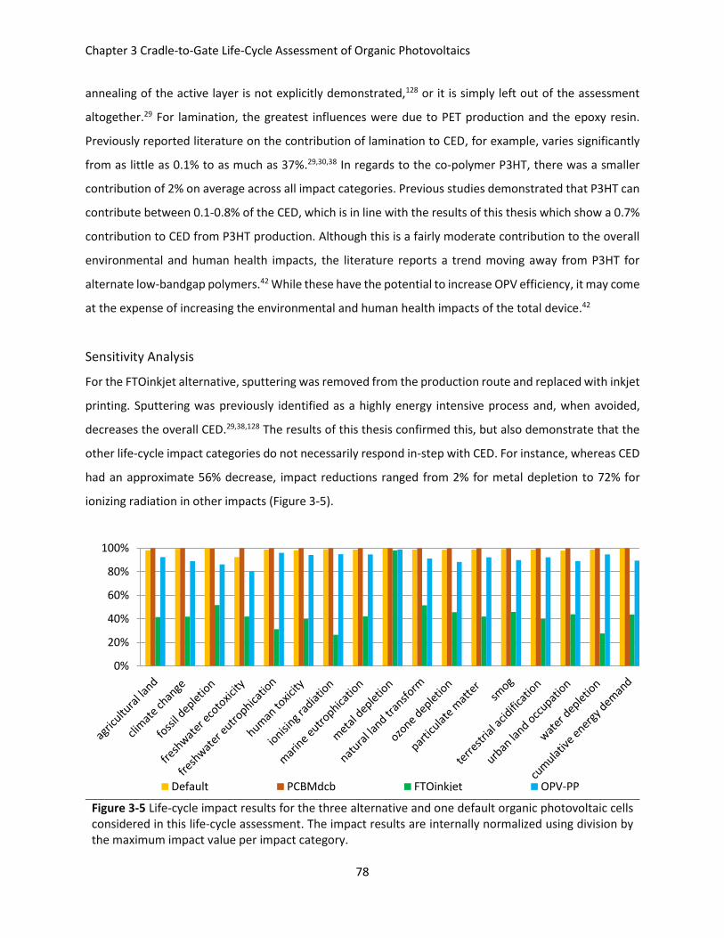
Chapter 3 Cradle-to-Gate Life-Cycle Assessment of Organic Photovoltaics
78
annealing of the active layer is not explicitly demonstrated,128 or it is simply left out of the assessment
altogether.29 For lamination, the greatest influences were due to PET production and the epoxy resin.
Previously reported literature on the contribution of lamination to CED, for example, varies significantly
from as little as 0.1% to as much as 37%.29,30,38 In regards to the co-polymer P3HT, there was a smaller
contribution of 2% on average across all impact categories. Previous studies demonstrated that P3HT can
contribute between 0.1-0.8% of the CED, which is in line with the results of this thesis which show a 0.7%
contribution to CED from P3HT production. Although this is a fairly moderate contribution to the overall
environmental and human health impacts, the literature reports a trend moving away from P3HT for
alternate low-bandgap polymers.42 While these have the potential to increase OPV efficiency, it may come
at the expense of increasing the environmental and human health impacts of the total device.42
Sensitivity Analysis
For the FTOinkjet alternative, sputtering was removed from the production route and replaced with inkjet
printing. Sputtering was previously identified as a highly energy intensive process and, when avoided,
decreases the overall CED.29,38,128 The results of this thesis confirmed this, but also demonstrate that the
other life-cycle impact categories do not necessarily respond in-step with CED. For instance, whereas CED
had an approximate 56% decrease, impact reductions ranged from 2% for metal depletion to 72% for
ionizing radiation in other impacts (Figure 3-5).
Figure 3-5 Life-cycle impact results for the three alternative and one default organic photovoltaic cells considered in this life-cycle assessment. The impact results are internally normalized using division by the maximum impact value per impact category.
0%
20%
40%
60%
80%
100%
Default PCBMdcb FTOinkjet OPV-PP
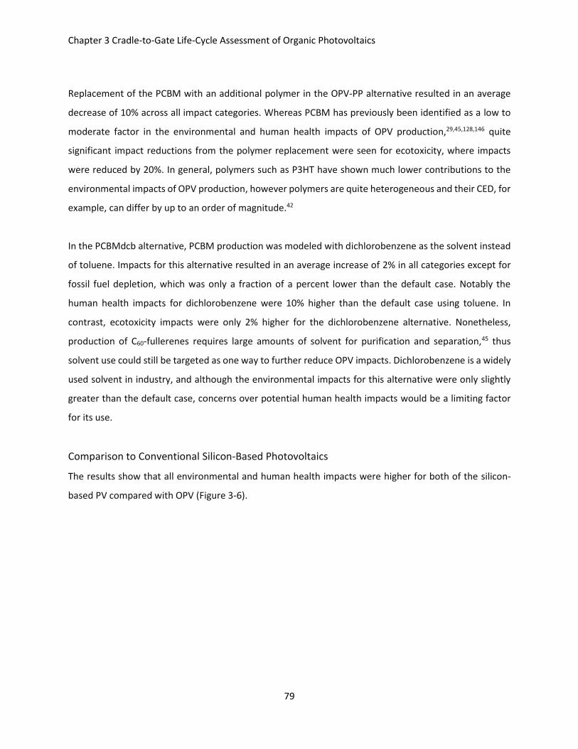
Chapter 3 Cradle-to-Gate Life-Cycle Assessment of Organic Photovoltaics
79
Replacement of the PCBM with an additional polymer in the OPV-PP alternative resulted in an average
decrease of 10% across all impact categories. Whereas PCBM has previously been identified as a low to
moderate factor in the environmental and human health impacts of OPV production,29,45,128,146 quite
significant impact reductions from the polymer replacement were seen for ecotoxicity, where impacts
were reduced by 20%. In general, polymers such as P3HT have shown much lower contributions to the
environmental impacts of OPV production, however polymers are quite heterogeneous and their CED, for
example, can differ by up to an order of magnitude.42
In the PCBMdcb alternative, PCBM production was modeled with dichlorobenzene as the solvent instead
of toluene. Impacts for this alternative resulted in an average increase of 2% in all categories except for
fossil fuel depletion, which was only a fraction of a percent lower than the default case. Notably the
human health impacts for dichlorobenzene were 10% higher than the default case using toluene. In
contrast, ecotoxicity impacts were only 2% higher for the dichlorobenzene alternative. Nonetheless,
production of C60-fullerenes requires large amounts of solvent for purification and separation,45 thus
solvent use could still be targeted as one way to further reduce OPV impacts. Dichlorobenzene is a widely
used solvent in industry, and although the environmental impacts for this alternative were only slightly
greater than the default case, concerns over potential human health impacts would be a limiting factor
for its use.
Comparison to Conventional Silicon-Based Photovoltaics
The results show that all environmental and human health impacts were higher for both of the silicon-
based PV compared with OPV (Figure 3-6).
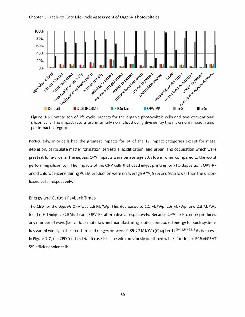
Chapter 3 Cradle-to-Gate Life-Cycle Assessment of Organic Photovoltaics
80
Figure 3-6 Comparison of life-cycle impacts for the organic photovoltaic cells and two conventional silicon cells. The impact results are internally normalized using division by the maximum impact value per impact category.
Particularly, m-Si cells had the greatest impacts for 14 of the 17 impact categories except for metal
depletion, particulate matter formation, terrestrial acidification, and urban land occupation which were
greatest for a-Si cells. The default OPV impacts were on average 93% lower when compared to the worst
performing silicon cell. The impacts of the OPV cells that used inkjet printing for FTO deposition, OPV-PP
and dichlorobenzene during PCBM production were on average 97%, 93% and 92% lower than the silicon-
based cells, respectively.
Energy and Carbon Payback Times
The CED for the default OPV was 2.6 MJ/Wp. This decreased to 1.1 MJ/Wp, 2.6 MJ/Wp, and 2.3 MJ/Wp
for the FTOinkjet, PCBMdcb and OPV-PP alternatives, respectively. Because OPV cells can be produced
any number of ways (i.e. various materials and manufacturing routes), embodied energy for such systems
has varied widely in the literature and ranges between 0.89-27 MJ/Wp (Chapter 1).29–31,38,42,128 As is shown
in Figure 3-7, the CED for the default case is in line with previously published values for similar PCBM:P3HT
5% efficient solar cells.
0%
20%
40%
60%
80%
100%
Default DCB (PCBM) FTOinkjet OPV-PP m-Si a-Si
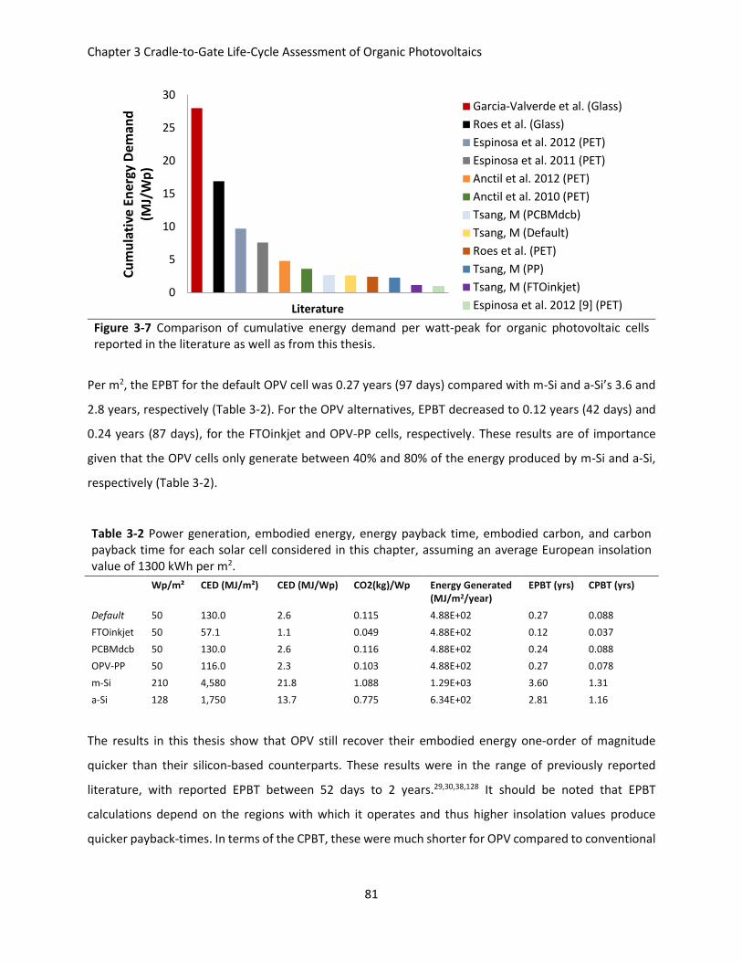
Chapter 3 Cradle-to-Gate Life-Cycle Assessment of Organic Photovoltaics
81
Per m2, the EPBT for the default OPV cell was 0.27 years (97 days) compared with m-Si and a-Si’s 3.6 and
2.8 years, respectively (Table 3-2). For the OPV alternatives, EPBT decreased to 0.12 years (42 days) and
0.24 years (87 days), for the FTOinkjet and OPV-PP cells, respectively. These results are of importance
given that the OPV cells only generate between 40% and 80% of the energy produced by m-Si and a-Si,
respectively (Table 3-2).
Table 3-2 Power generation, embodied energy, energy payback time, embodied carbon, and carbon payback time for each solar cell considered in this chapter, assuming an average European insolation value of 1300 kWh per m2.
Wp/m² CED (MJ/m²) CED (MJ/Wp) CO2(kg)/Wp Energy Generated (MJ/m2/year)
EPBT (yrs) CPBT (yrs)
Default 50 130.0 2.6 0.115 4.88E+02 0.27 0.088
FTOinkjet 50 57.1 1.1 0.049 4.88E+02 0.12 0.037
PCBMdcb 50 130.0 2.6 0.116 4.88E+02 0.24 0.088
OPV-PP 50 116.0 2.3 0.103 4.88E+02 0.27 0.078
m-Si 210 4,580 21.8 1.088 1.29E+03 3.60 1.31
a-Si 128 1,750 13.7 0.775 6.34E+02 2.81 1.16
The results in this thesis show that OPV still recover their embodied energy one-order of magnitude
quicker than their silicon-based counterparts. These results were in the range of previously reported
literature, with reported EPBT between 52 days to 2 years.29,30,38,128 It should be noted that EPBT
calculations depend on the regions with which it operates and thus higher insolation values produce
quicker payback-times. In terms of the CPBT, these were much shorter for OPV compared to conventional
Figure 3-7 Comparison of cumulative energy demand per watt-peak for organic photovoltaic cells reported in the literature as well as from this thesis.
0
5
10
15
20
25
30
Literature
Cu
mu
lati
ve E
ner
gy D
eman
d
(MJ/
Wp
)
Garcia-Valverde et al. (Glass)
Roes et al. (Glass)
Espinosa et al. 2012 (PET)
Espinosa et al. 2011 (PET)
Anctil et al. 2012 (PET)
Anctil et al. 2010 (PET)
Tsang, M (PCBMdcb)
Tsang, M (Default)
Roes et al. (PET)
Tsang, M (PP)
Tsang, M (FTOinkjet)
Espinosa et al. 2012 [9] (PET)
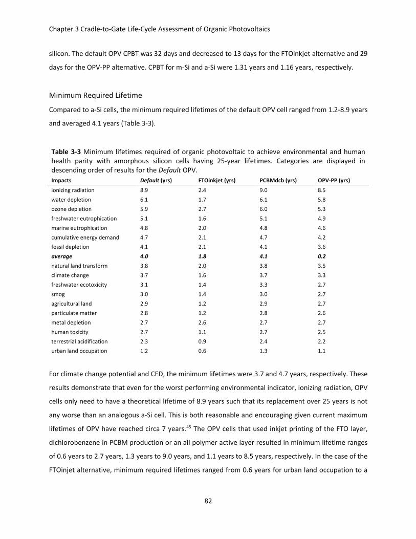
Chapter 3 Cradle-to-Gate Life-Cycle Assessment of Organic Photovoltaics
82
silicon. The default OPV CPBT was 32 days and decreased to 13 days for the FTOinkjet alternative and 29
days for the OPV-PP alternative. CPBT for m-Si and a-Si were 1.31 years and 1.16 years, respectively.
Minimum Required Lifetime
Compared to a-Si cells, the minimum required lifetimes of the default OPV cell ranged from 1.2-8.9 years
and averaged 4.1 years (Table 3-3).
Table 3-3 Minimum lifetimes required of organic photovoltaic to achieve environmental and human health parity with amorphous silicon cells having 25-year lifetimes. Categories are displayed in descending order of results for the Default OPV.
Impacts Default (yrs) FTOinkjet (yrs) PCBMdcb (yrs) OPV-PP (yrs)
ionizing radiation 8.9 2.4 9.0 8.5
water depletion 6.1 1.7 6.1 5.8
ozone depletion 5.9 2.7 6.0 5.3
freshwater eutrophication 5.1 1.6 5.1 4.9
marine eutrophication 4.8 2.0 4.8 4.6
cumulative energy demand 4.7 2.1 4.7 4.2
fossil depletion 4.1 2.1 4.1 3.6
average 4.0 1.8 4.1 0.2
natural land transform 3.8 2.0 3.8 3.5
climate change 3.7 1.6 3.7 3.3
freshwater ecotoxicity 3.1 1.4 3.3 2.7
smog 3.0 1.4 3.0 2.7
agricultural land 2.9 1.2 2.9 2.7
particulate matter 2.8 1.2 2.8 2.6
metal depletion 2.7 2.6 2.7 2.7
human toxicity 2.7 1.1 2.7 2.5
terrestrial acidification 2.3 0.9 2.4 2.2
urban land occupation 1.2 0.6 1.3 1.1
For climate change potential and CED, the minimum lifetimes were 3.7 and 4.7 years, respectively. These
results demonstrate that even for the worst performing environmental indicator, ionizing radiation, OPV
cells only need to have a theoretical lifetime of 8.9 years such that its replacement over 25 years is not
any worse than an analogous a-Si cell. This is both reasonable and encouraging given current maximum
lifetimes of OPV have reached circa 7 years.45 The OPV cells that used inkjet printing of the FTO layer,
dichlorobenzene in PCBM production or an all polymer active layer resulted in minimum lifetime ranges
of 0.6 years to 2.7 years, 1.3 years to 9.0 years, and 1.1 years to 8.5 years, respectively. In the case of the
FTOinjet alternative, minimum required lifetimes ranged from 0.6 years for urban land occupation to a
Chapter 3 Cradle-to-Gate Life-Cycle Assessment of Organic Photovoltaics
83
high of 2.7 years for ozone depletion. The average values for this alternative was only 1.8 years which is
an even more promising result for the future of this technology.
Conclusion
The results from this LCA forecast a rather optimistic place for OPV as an energy producing technology,
where all environmental and human health impact results indicate a much more favorable option for OPV
on a watt-per-watt basis compared with conventional silicon cells. Although, the results of this LCA are
applicable to the OPV described in this chapter, the materials used and modeling assumptions which were
all chosen based on reasonable expectations that such a device could enter the market in the near-term.
As was demonstrated in this LCA, researchers in this field should be encouraged to consider a broader
range of environmental and human health impacts for assessing the benefits of OPV over conventional
technologies. As was presented, estimations of OPV minimum lifetimes to reach parity with a 25-year
lifetime a-Si solar cell ranged from 1.2-8.9 years in the default case and as short as 0.6-2.7 in the FTOinkjet
case. These represent moving targets for stakeholders, researchers and regulators in the field. More
specifically and from an LCA perspective, the higher reported minimum required lifetimes reported for
the default OPV demonstrate that OPV may be most advantageous in niche and short-term use scenarios
compared to traditional long-term solar arrays. Although, the results for the FTOinkjet OPV point to
potential justifications for using them in such traditional settings. However, these results were simplified
theoretical calculations based on power production for just the PV cell (i.e. just the cradle-to-gate
consideration up to the point of PV cell production were considered). The results implicitly imply that the
PV would need no other components to be fully operational and would also have no impacts from the
use-phase and/or end-of-life phases. Thus, this is an over simplified set of assumptions and no definitive
determination can be given as to whether OPV are a preferred technology option over silicon-based PV
from an environmental and human health perspective. Further research in this area should focus on how
the use phase and end-of-life considerations will influence potential OPV deployment. For instance,
recycling of precious metals has the potential to reduce the EPBT by 13% for OPV cells.147 However,
collection and the ultimate recovery rate of both the solar cells and materials with value will depend on
where and how the OPV cells are employed.148,149 The focus of Chapter 4 begins to address these questions
by extending the system boundaries to include potential uses and end-of-life scenarios for OPV panels.
Chapter 4 Cradle-to-Grave Life-Cycle Assessment of Organic Photovoltaics
84
Chapter 4 Cradle-to-Grave Life-Cycle Assessment of Organic
Photovoltaics
In Chapter 1, a review of the OPV-LCA literature through the end of 2013 demonstrated that only two of
the ten studies had considered the use phase, with one of those two studies also considering an end-of-
life phase of the OPV. Of the two use phases considered, one was a rooftop glass-substrate system29 while
the other was a flexible-substrate OPV-powered street lamp.36 The latter study also included the impacts
from landfilling the OPV device, however as far as can be told, there does not seem to be any reporting
of those end-of-life impacts in the results or mention of how this life-cycle stage influenced the overall
LCA profile of the OPV. It should be noted that between the end of 2013 and the time this chapter was
being prepared for submission, there were three other OPV-LCA studies published that contained use
and/or end-of-life phases. In 2014, Espinosa et al. completed a cradle-to-use LCA for ground-installed solar
arrays as well as three non-conventional onshore, offshore and balloon arrays.24 In 2015, Espinosa et al.
completed a cradle-to-grave LCA for a ground-installed solar array with the additional consideration of
either recycling or incinerating the entire solar-array.62 Lastly, in 2014 Sondergaard et al. completed a LCA
that considered the cradle-to-gate production of the OPV plus the additional consideration of recycling
the silver content at its end-of-life (i.e. without the consideration of the use-phase).147 The results of those
studies are presented later in the results and discussion of and in context with the results of this chapter.
Methods
Goal and Scope
This LCA was conducted according to ISO 14040:200628 and 14044:200627 guidelines and the IEA’s
recommendations for implementing LCA for PV technology.35 All life-cycle stages and impacts from raw
materials extraction, materials processing, PV manufacturing, use, end-of-life considerations were
included (Figure 4-1).
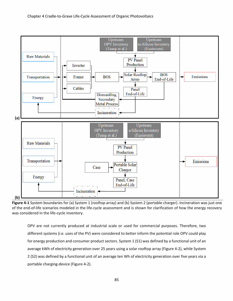
Chapter 4 Cradle-to-Grave Life-Cycle Assessment of Organic Photovoltaics
85
(a)
(b)
Figure 4-1 System boundaries for (a) System 1 (rooftop array) and (b) System 2 (portable charger). Incineration was just one of the end-of-life scenarios modeled in the life-cycle assessment and is shown for clarification of how the energy recovery was considered in the life-cycle inventory.
OPV are not currently produced at industrial scale or used for commercial purposes. Therefore, two
different systems (i.e. uses of the PV) were considered to better inform the potential role OPV could play
for energy production and consumer product sectors. System 1 (S1) was defined by a functional unit of an
average kWh of electricity generation over 25 years using a solar rooftop array (Figure 4-2), while System
2 (S2) was defined by a functional unit of an average ten Wh of electricity generation over five years via a
portable charging-device (Figure 4-2).
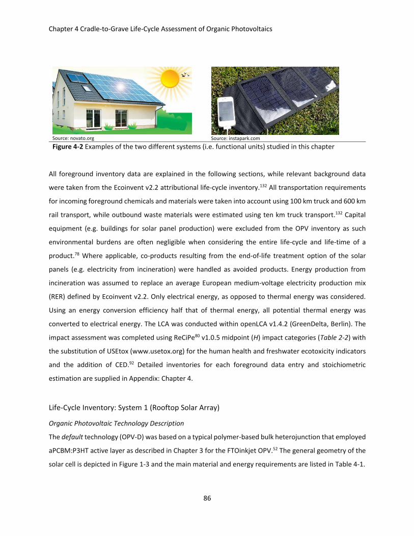
Chapter 4 Cradle-to-Grave Life-Cycle Assessment of Organic Photovoltaics
86
All foreground inventory data are explained in the following sections, while relevant background data
were taken from the Ecoinvent v2.2 attributional life-cycle inventory.132 All transportation requirements
for incoming foreground chemicals and materials were taken into account using 100 km truck and 600 km
rail transport, while outbound waste materials were estimated using ten km truck transport.132 Capital
equipment (e.g. buildings for solar panel production) were excluded from the OPV inventory as such
environmental burdens are often negligible when considering the entire life-cycle and life-time of a
product.78 Where applicable, co-products resulting from the end-of-life treatment option of the solar
panels (e.g. electricity from incineration) were handled as avoided products. Energy production from
incineration was assumed to replace an average European medium-voltage electricity production mix
(RER) defined by Ecoinvent v2.2. Only electrical energy, as opposed to thermal energy was considered.
Using an energy conversion efficiency half that of thermal energy, all potential thermal energy was
converted to electrical energy. The LCA was conducted within openLCA v1.4.2 (GreenDelta, Berlin). The
impact assessment was completed using ReCiPe80 v1.0.5 midpoint (H) impact categories (Table 2-2) with
the substitution of USEtox (www.usetox.org) for the human health and freshwater ecotoxicity indicators
and the addition of CED.92 Detailed inventories for each foreground data entry and stoichiometric
estimation are supplied in Appendix: Chapter 4.
Life-Cycle Inventory: System 1 (Rooftop Solar Array)
Organic Photovoltaic Technology Description
The default technology (OPV-D) was based on a typical polymer-based bulk heterojunction that employed
aPCBM:P3HT active layer as described in Chapter 3 for the FTOinkjet OPV.52 The general geometry of the
solar cell is depicted in Figure 1-3 and the main material and energy requirements are listed in Table 4-1.
Source: novato.org
Source: instapark.com
Figure 4-2 Examples of the two different systems (i.e. functional units) studied in this chapter
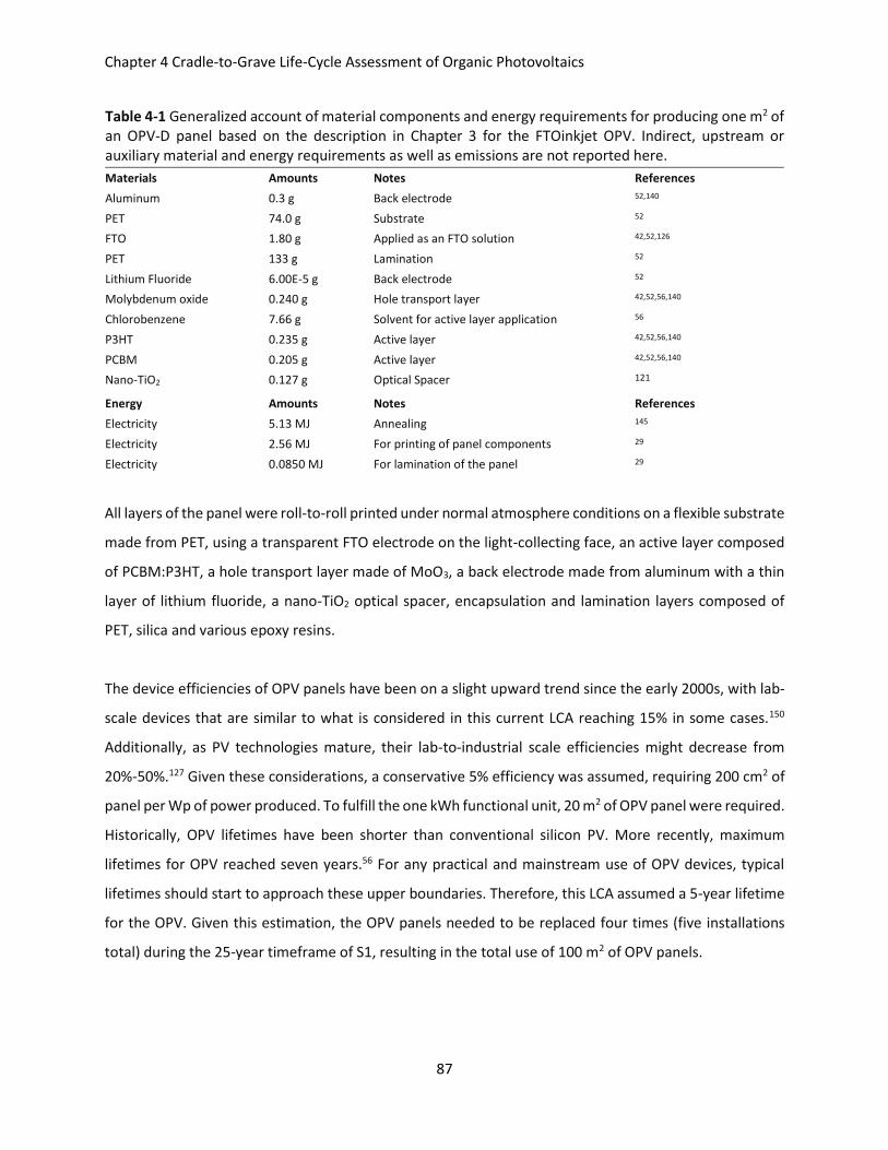
Chapter 4 Cradle-to-Grave Life-Cycle Assessment of Organic Photovoltaics
87
Table 4-1 Generalized account of material components and energy requirements for producing one m2 of an OPV-D panel based on the description in Chapter 3 for the FTOinkjet OPV. Indirect, upstream or auxiliary material and energy requirements as well as emissions are not reported here.
Materials Amounts Notes References
Aluminum 0.3 g Back electrode 52,140
PET 74.0 g Substrate 52
FTO 1.80 g Applied as an FTO solution 42,52,126
PET 133 g Lamination 52
Lithium Fluoride 6.00E-5 g Back electrode 52
Molybdenum oxide 0.240 g Hole transport layer 42,52,56,140
Chlorobenzene 7.66 g Solvent for active layer application 56
P3HT 0.235 g Active layer 42,52,56,140
PCBM 0.205 g Active layer 42,52,56,140
Nano-TiO2 0.127 g Optical Spacer 121
Energy Amounts Notes References
Electricity 5.13 MJ Annealing 145
Electricity 2.56 MJ For printing of panel components 29
Electricity 0.0850 MJ For lamination of the panel 29
All layers of the panel were roll-to-roll printed under normal atmosphere conditions on a flexible substrate
made from PET, using a transparent FTO electrode on the light-collecting face, an active layer composed
of PCBM:P3HT, a hole transport layer made of MoO3, a back electrode made from aluminum with a thin
layer of lithium fluoride, a nano-TiO2 optical spacer, encapsulation and lamination layers composed of
PET, silica and various epoxy resins.
The device efficiencies of OPV panels have been on a slight upward trend since the early 2000s, with lab-
scale devices that are similar to what is considered in this current LCA reaching 15% in some cases.150
Additionally, as PV technologies mature, their lab-to-industrial scale efficiencies might decrease from
20%-50%.127 Given these considerations, a conservative 5% efficiency was assumed, requiring 200 cm2 of
panel per Wp of power produced. To fulfill the one kWh functional unit, 20 m2 of OPV panel were required.
Historically, OPV lifetimes have been shorter than conventional silicon PV. More recently, maximum
lifetimes for OPV reached seven years.56 For any practical and mainstream use of OPV devices, typical
lifetimes should start to approach these upper boundaries. Therefore, this LCA assumed a 5-year lifetime
for the OPV. Given this estimation, the OPV panels needed to be replaced four times (five installations
total) during the 25-year timeframe of S1, resulting in the total use of 100 m2 of OPV panels.
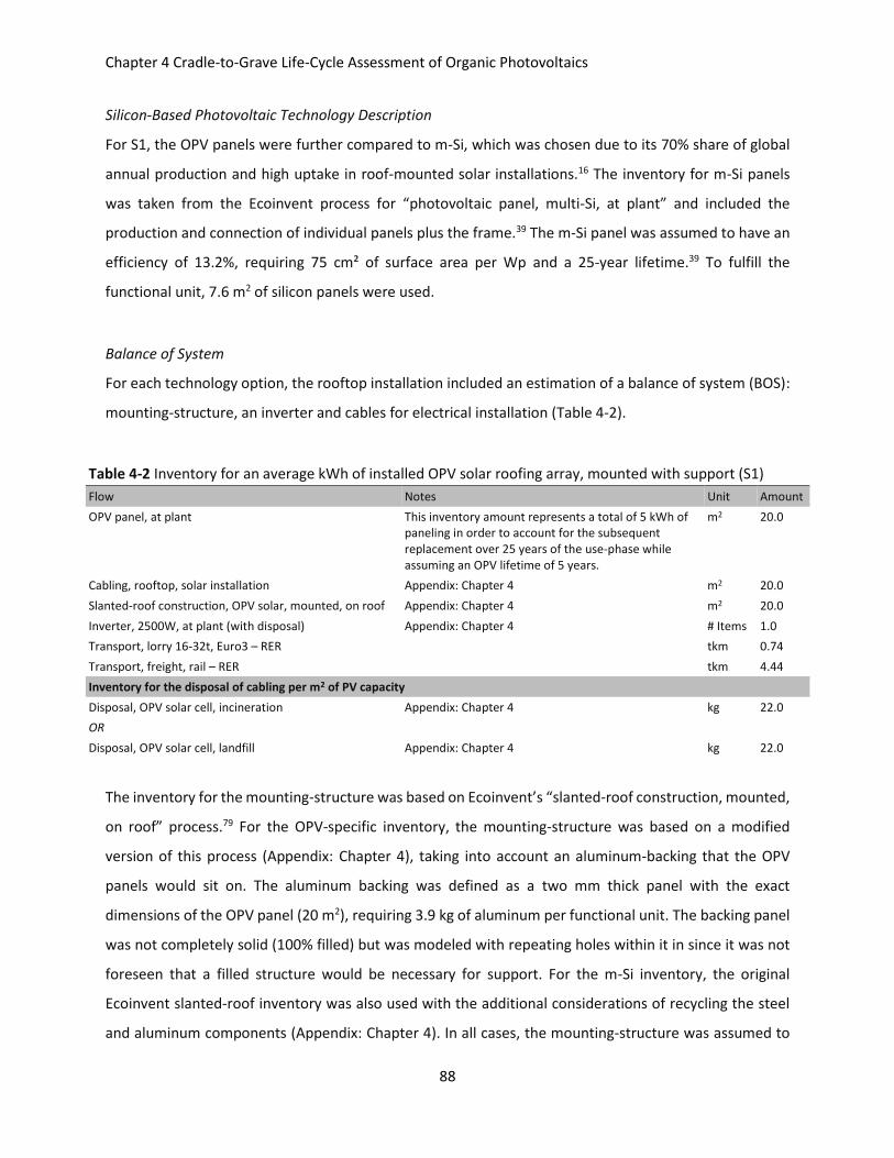
Chapter 4 Cradle-to-Grave Life-Cycle Assessment of Organic Photovoltaics
88
Silicon-Based Photovoltaic Technology Description
For S1, the OPV panels were further compared to m-Si, which was chosen due to its 70% share of global
annual production and high uptake in roof-mounted solar installations.16 The inventory for m-Si panels
was taken from the Ecoinvent process for “photovoltaic panel, multi-Si, at plant” and included the
production and connection of individual panels plus the frame.39 The m-Si panel was assumed to have an
efficiency of 13.2%, requiring 75 cm² of surface area per Wp and a 25-year lifetime.39 To fulfill the
functional unit, 7.6 m2 of silicon panels were used.
Balance of System
For each technology option, the rooftop installation included an estimation of a balance of system (BOS):
mounting-structure, an inverter and cables for electrical installation (Table 4-2).
Table 4-2 Inventory for an average kWh of installed OPV solar roofing array, mounted with support (S1)
Flow Notes Unit Amount
OPV panel, at plant This inventory amount represents a total of 5 kWh of paneling in order to account for the subsequent replacement over 25 years of the use-phase while assuming an OPV lifetime of 5 years.
m2 20.0
Cabling, rooftop, solar installation Appendix: Chapter 4 m2 20.0
Slanted-roof construction, OPV solar, mounted, on roof Appendix: Chapter 4 m2 20.0
Inverter, 2500W, at plant (with disposal) Appendix: Chapter 4 # Items 1.0
Transport, lorry 16-32t, Euro3 – RER tkm 0.74
Transport, freight, rail – RER tkm 4.44
Inventory for the disposal of cabling per m2 of PV capacity
Disposal, OPV solar cell, incineration Appendix: Chapter 4 kg 22.0
OR
Disposal, OPV solar cell, landfill Appendix: Chapter 4 kg 22.0
The inventory for the mounting-structure was based on Ecoinvent’s “slanted-roof construction, mounted,
on roof” process.79 For the OPV-specific inventory, the mounting-structure was based on a modified
version of this process (Appendix: Chapter 4), taking into account an aluminum-backing that the OPV
panels would sit on. The aluminum backing was defined as a two mm thick panel with the exact
dimensions of the OPV panel (20 m2), requiring 3.9 kg of aluminum per functional unit. The backing panel
was not completely solid (100% filled) but was modeled with repeating holes within it in since it was not
foreseen that a filled structure would be necessary for support. For the m-Si inventory, the original
Ecoinvent slanted-roof inventory was also used with the additional considerations of recycling the steel
and aluminum components (Appendix: Chapter 4). In all cases, the mounting-structure was assumed to
Chapter 4 Cradle-to-Grave Life-Cycle Assessment of Organic Photovoltaics
89
last 25 years and was recycled after use. Recycling estimations were made assuming 100% collection of
the mounting components and entrance into the recycling waste stream, whereby aluminum and steel
were used as scrap to produce secondary aluminum at conversion rates of 97% and 90%, respectively. As
described above and at any single time during the use-phase, 20 m2 of OPV panels were needed to fulfill
the one kWh functional unit, requiring the installation of a 20 m2-equivalent OPV-specific mounting
structure. Similarly, 7.6 m2-equivalent of the m-Si-specific mounting structure were installed for the m-Si
panels.
The inventory for the inverter was based on a modified version the Ecoinvent “inverter, 2500W, at plant”
process whereby recycling of the inverter was estimated using a mix of manual and mechanical
dismantling processes and material transfer coefficients to recover aluminum, copper and steel
(Appendix: Chapter 4). All three metals were assumed to be used as scrap in the secondary metals market
with conversion rates of 97%, 76% and 90%, respectively, while the remaining waste was incinerated to
generate electricity at 2.97 MJ/kg of waste. It was assumed that a single inverter was used throughout
the duration of the functional unit.
Cabling requirements151 included the recovery of copper used in secondary metal production at a 76%
conversion rate. The remainder of the plastics was assumed incinerated, ultimately producing four MJ of
electricity per kg of plastics waste. Twenty m2-equivalent of cabling and 7.6 m2-equivalent of cabling were
required for both OPV panels and the m-Si panels, respectively.
End-of-Life Considerations
Assumptions were made that 100% of all PV devices were collected and directed to the appropriate waste
stream, with 100% of the m-Si aluminum frame (19.99 kg) being dismantled and recycled along with the
aluminum BOS mounting-structure components. No further energy or material inputs were considered
for dismantling these components. Two end-of-life scenarios were considered: (a) incineration and (b)
landfilling. Currently, the core infrastructure, economics, regulatory frameworks and the size of the waste
stream indicate that most PV panels fall into these conventional disposal options as opposed to
recycling.64,65,152 Both disposal-process inventories were calculated using Ecoinvent’s waste disposal
modeling tools.150 The tool was used to create a waste-inventory (Appendix: Chapter 4) based partially on
the elemental composition of the waste as well as an assumed set of non-waste-specific technosphere
and disposal related processes. The composition of the waste for each panel was based on the panel
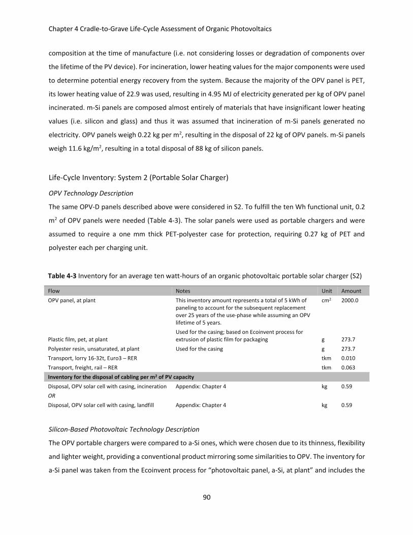
Chapter 4 Cradle-to-Grave Life-Cycle Assessment of Organic Photovoltaics
90
composition at the time of manufacture (i.e. not considering losses or degradation of components over
the lifetime of the PV device). For incineration, lower heating values for the major components were used
to determine potential energy recovery from the system. Because the majority of the OPV panel is PET,
its lower heating value of 22.9 was used, resulting in 4.95 MJ of electricity generated per kg of OPV panel
incinerated. m-Si panels are composed almost entirely of materials that have insignificant lower heating
values (i.e. silicon and glass) and thus it was assumed that incineration of m-Si panels generated no
electricity. OPV panels weigh 0.22 kg per m2, resulting in the disposal of 22 kg of OPV panels. m-Si panels
weigh 11.6 kg/m2, resulting in a total disposal of 88 kg of silicon panels.
Life-Cycle Inventory: System 2 (Portable Solar Charger)
OPV Technology Description
The same OPV-D panels described above were considered in S2. To fulfill the ten Wh functional unit, 0.2
m2 of OPV panels were needed (Table 4-3). The solar panels were used as portable chargers and were
assumed to require a one mm thick PET-polyester case for protection, requiring 0.27 kg of PET and
polyester each per charging unit.
Table 4-3 Inventory for an average ten watt-hours of an organic photovoltaic portable solar charger (S2)
Flow Notes Unit Amount
OPV panel, at plant This inventory amount represents a total of 5 kWh of paneling to account for the subsequent replacement over 25 years of the use-phase while assuming an OPV lifetime of 5 years.
cm2 2000.0
Plastic film, pet, at plant Used for the casing; based on Ecoinvent process for extrusion of plastic film for packaging g 273.7
Polyester resin, unsaturated, at plant Used for the casing g 273.7
Transport, lorry 16-32t, Euro3 – RER tkm 0.010
Transport, freight, rail – RER tkm 0.063
Inventory for the disposal of cabling per m2 of PV capacity
Disposal, OPV solar cell with casing, incineration Appendix: Chapter 4 kg 0.59
OR
Disposal, OPV solar cell with casing, landfill Appendix: Chapter 4 kg 0.59
Silicon-Based Photovoltaic Technology Description
The OPV portable chargers were compared to a-Si ones, which were chosen due to its thinness, flexibility
and lighter weight, providing a conventional product mirroring some similarities to OPV. The inventory for
a-Si panel was taken from the Ecoinvent process for “photovoltaic panel, a-Si, at plant” and includes the
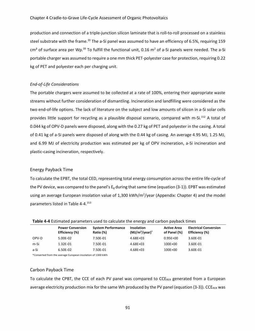
Chapter 4 Cradle-to-Grave Life-Cycle Assessment of Organic Photovoltaics
91
production and connection of a triple-junction silicon laminate that is roll-to-roll processed on a stainless
steel substrate with the frame.39 The a-Si panel was assumed to have an efficiency of 6.5%, requiring 159
cm² of surface area per Wp.39 To fulfill the functional unit, 0.16 m2 of a-Si panels were needed. The a-Si
portable charger was assumed to require a one mm thick PET-polyester case for protection, requiring 0.22
kg of PET and polyester each per charging unit.
End-of-Life Considerations
The portable chargers were assumed to be collected at a rate of 100%, entering their appropriate waste
streams without further consideration of dismantling. Incineration and landfilling were considered as the
two end-of-life options. The lack of literature on the subject and low amounts of silicon in a-Si solar cells
provides little support for recycling as a plausible disposal scenario, compared with m-Si.152 A total of
0.044 kg of OPV-D panels were disposed, along with the 0.27 kg of PET and polyester in the casing. A total
of 0.41 kg of a-Si panels were disposed of along with the 0.44 kg of casing. An average 4.95 MJ, 1.25 MJ,
and 6.99 MJ of electricity production was estimated per kg of OPV incineration, a-Si incineration and
plastic-casing incineration, respectively.
Energy Payback Time
To calculate the EPBT, the total CED, representing total energy consumption across the entire life-cycle of
the PV device, was compared to the panel’s Eg during that same time (equation (3-1)). EPBT was estimated
using an average European insolation value of 1,300 kWh/m2/year (Appendix: Chapter 4) and the model
parameters listed in Table 4-4.153
Table 4-4 Estimated parameters used to calculate the energy and carbon payback times
Power Conversion Efficiency (%)
System Performance Ratio (%)
Insolation (MJ/m²/year)*
Active Area of Panel (%)
Electrical Conversion Efficiency (%)
OPV-D 5.00E-02 7.50E-01 4.68E+03 0.95E+00 3.60E-01
m-Si 1.32E-01 7.50E-01 4.68E+03 100E+00 3.60E-01
a-Si 6.50E-02 7.50E-01 4.68E+03 100E+00 3.60E-01
*Converted from the average European insolation of 1300 kWh
Carbon Payback Time
To calculate the CPBT, the CCE of each PV panel was compared to CCERER generated from a European
average electricity production mix for the same Wh produced by the PV panel (equation (3-3)). CCERER was
Chapter 4 Cradle-to-Grave Life-Cycle Assessment of Organic Photovoltaics
92
estimated as 0.49 kg per kWh of the Ecoinvent process “electricity, medium voltage, production RER, at
grid.”
Minimum Required Lifetime of Organic Photovoltaics
The minimum lifetime afforded by or required of OPV determined the lifetime of the panel which
theoretically would result in the same environmental impacts compared to silico-based PV. It was
calculated using equation (4-1):
𝑀𝑅𝐿 =(𝐴 ∙ 𝑍)
(𝐶 − 𝐵) (4-1)
MRL: Minimum required lifetime A: OPVi panel-specific1 impacts (i) B: all other (OPV) impacts C: total silicon impact Z: default OPV lifetime
Sensitivity Analysis
Although the default analysis rests on interpreting and estimating realistic efficiencies and lifetimes from
their experimental maximums,56 there is still considerable uncertainty in whether industrial production of
such cells could achieve these estimates in the near-term. For instance, when transitioning from the lab
to large-scale development, device efficiencies decline roughly by a factor of two, which could lead to
situations where the default assumptions are potentially overly optimistic, particularly given the range of
probable OPV devices in development and their corresponding range of lifetimes and efficiencies. The
assumptions were tested assuming (a) lifetimes of one, three, five, seven and nine years with a constant
efficiency of one percent and (b) assuming efficiencies of one, three, five, seven and nine percent with a
constant lifetime of one year. The constants of one percent and one year were chosen in order to reflect
more actual immediate-term scenarios which in effect act as a baseline set of characteristics from which
industrial-level characteristics could be targeted.
1
Referring to the impacts that result from the production and disposal of the panel as opposed to the BOS components
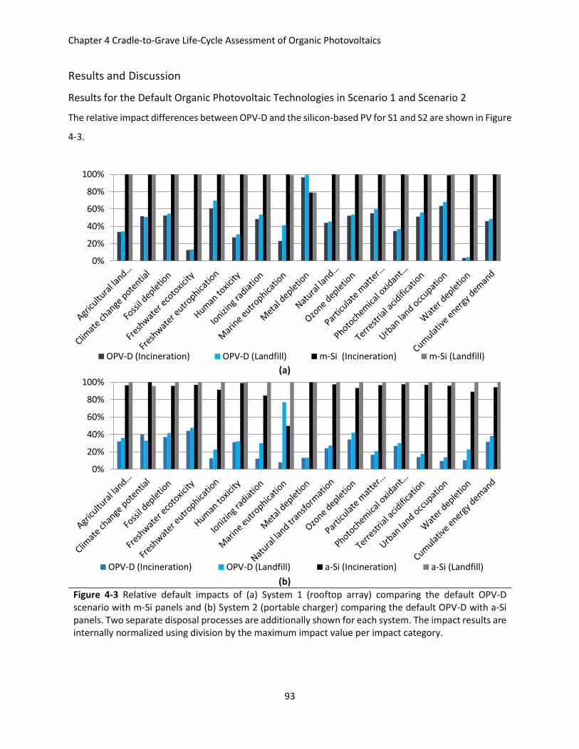
Chapter 4 Cradle-to-Grave Life-Cycle Assessment of Organic Photovoltaics
93
Results and Discussion
Results for the Default Organic Photovoltaic Technologies in Scenario 1 and Scenario 2
The relative impact differences between OPV-D and the silicon-based PV for S1 and S2 are shown in Figure
4-3.
(a)
(b)
Figure 4-3 Relative default impacts of (a) System 1 (rooftop array) comparing the default OPV-D scenario with m-Si panels and (b) System 2 (portable charger) comparing the default OPV-D with a-Si panels. Two separate disposal processes are additionally shown for each system. The impact results are internally normalized using division by the maximum impact value per impact category.
0%
20%
40%
60%
80%
100%
OPV-D (Incineration) OPV-D (Landfill) m-Si (Incineration) m-Si (Landfill)
0%
20%
40%
60%
80%
100%
OPV-D (Incineration) OPV-D (Landfill) a-Si (Incineration) a-Si (Landfill)
Chapter 4 Cradle-to-Grave Life-Cycle Assessment of Organic Photovoltaics
94
In both S1 and S2, the OPV panels have lower environmental and human health impacts compared to
their silicon counterparts. In S1, OPV-D (with incineration) impacts ranged from 96% lower for water
depletion to 40% lower for freshwater eutrophication, with the exception that metal depletion was
approximately 21% greater for OPV-D mainly due to upstream demands of producing tin for the FTO
electrode (Appendix: Chapter 4).
The OPV-D impact in S2 ranged from 92% lower for marine eutrophication to 56% lower for freshwater
ecotoxicity compared with a-Si. In S2, the relative decrease between OPV and the silicon-based PV was
more pronounced than in S1. The reason for the differences in OPV’s relative impacts between S1 and S2
are in part explained by the different use phases. The use phase of S1 is 5-times longer than S2 (i.e. 25
years versus 5 years). Therefore, given the assumed 5-year OPV lifetime, there was a need to replace
“exhausted” OPV panels many times over during the 25-year use-phase of S1. This contrasts with S2 which
did not require replacements over the 5-year use-phase and thus the environmental and human health
impacts were comparatively much lower for the portable charger compared with the rooftop setting. This
is similar to the findings of Espinosa et al. where, on average, the majority of the cradle-to-grave impacts
from their “solar-park” (duration 35 years) were due to the production and disposal of the panels
themselves.62 In that study, OPV-specific contributions were, for example, more than 90% for resource
depletion, non-cancerous human toxicity and freshwater toxicity. However, in some cases the OPV-
specific contributions were less than 50%, as was seen with particulate matter formation and ionizing
radiation. Those authors ultimately attribute many of these high OPV-specific impacts to the production
of silver electrode and its associated upstream processing and production. On the contrary, a 2014 study
by Espinosa et al. reported that various on-land and offshore solar-array configurations contained support
structures that were roughly 50% of the total CED. In the case of a balloon system, over 75% of the CED
was due to components other than the OPV panel. Thus, use phase contributions to overall environmental
and human health impacts over the OPV life-cycle should not be underestimated.
The results of this current chapter were mostly uniform regardless of the disposal route (i.e. incineration
versus landfill). This was particularly true for S1 but not for S2, which had more noticeable impact
reductions for incineration due to the added value of incinerating the plastic casing along with the OPV
panel. It should be noted that climate change impacts for OPV-D were 3% (S1) and 16% (S2) greater when
they are incinerated compared with when they are landfilled. This is a necessary consequence of
combustion of the plastic components which were converted wholly into CO2 during the process.
Chapter 4 Cradle-to-Grave Life-Cycle Assessment of Organic Photovoltaics
95
Specifically looking at CED results, OPV-D saw reductions of 53% (S1, incineration) and 51% (S2,
incineration) over their silicon-based counterparts. Previous studies have demonstrated that cradle-to-
gate energy consumption savings for OPV panels can be nearly one-sixth and one-fourth the demand of
m-Si and a-Si panels.140 Roes et al. completed a cradle-to-gate LCA of a flexible OPV cell compared to a m-
Si cell and estimated an average decrease of 73% in environmental impacts.29 Similarly, the findings in
Chapter 3 demonstrated average reductions in cradle-to-gate OPV impacts up to 97% and 92% over m-Si
and a-Si cells, respectively. The results of the current cradle-to-grave LCA highlight that cradle-to-gate
impacts were only part of the picture and that some amount of resource efficiency will be reduced when
including the use and end-of-life phases for OPV.
Although the end-of-life options tested in this LCA were only marginally influential on the environmental
and human health impacts, this analysis did not include potential effects from recycling of the PV panels.
Silicon-based PV may stand to gain the most from recycling since silicon-wafer and panel production were
dominant influences on the overall impacts for both m-Si and a-Si (Appendix: Chapter 4). Müller et al.,
previously reported a nearly 57% reduction in energy consumption for m-Si modules made with recycled
silicon wafers.154 In the context of S1, the reduced cradle-to-gate energy demands reported by Müller et
al. could lead to potential CED reductions of 49% for m-Si panels (Appendix: Chapter 4), resulting in a CED
of 12,520 MJ. This estimate is just slightly higher than the CED estimate of 11,634 MJ for OPV-D, thus
highlighting the potential importance of this end-of-life option. Although CED is not linearly related to the
other impact categories,146 a reasonable assumption would be that many of the other impact categories
will also decrease, although at an unknown magnitude. This brings about some uncertainty surrounding
the environmental benefits of OPV over conventional panels. Unlike m-Si, no relevant information on
potential recycling options for a-Si is found in the literature, and due to its much lower silicon content the
feasibility of recycling a-Si is not certain.152
Recycling of OPV panels may also provide some environmental and human health benefits, albeit with
lower yields compared to silicon PV. Sondergaard et al. demonstrated that use and subsequent recycling
of silver for both front and back OPV electrodes may provide a decrease in cradle-to-grave CED for OPV
panels by 12%.147 They estimated a theoretical yield of 95% recycling rate of the original silver content
used in the OPV panel. In almost all cases and as should be expected, recycling resulted in lower impacts
across all impact categories they reported. This was not the case for climate change potential, however,
which was higher than the non-recycling case. This increase in CO2-equivalent emissions was due to the
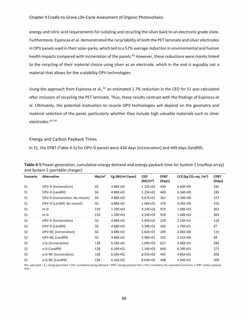
Chapter 4 Cradle-to-Grave Life-Cycle Assessment of Organic Photovoltaics
96
energy and nitric acid requirements for isolating and recycling the silver back to an electronic grade state.
Furthermore, Espinosa et al. demonstrated the recyclability of both the PET laminate and silver electrodes
in OPV panels used in their solar-parks, which led to a 57% average reduction in environmental and human
health impacts compared with incineration of the panels.62 However, these reductions were mainly linked
to the recycling of their material choice using silver as an electrode, which in the end is arguably not a
material that allows for the scalability OPV technologies.
Using the approach from Espinosa et al.,62 an estimated 1.7% reduction in the CED for S1 was calculated
after inclusion of recycling the PET laminate. Thus, these results contrast with the findings of Espinosa et
al. Ultimately, the potential motivation to recycle OPV technologies will depend on the geometry and
material selection of the panel, particularly whether they include high valuable materials such as silver
electrodes.62,147
Energy and Carbon Payback Times
In S1, the EPBT (Table 4-5) for OPV-D panels were 436 days (incineration) and 449 days (landfill).
Table 4-5 Power generation, cumulative energy demand and energy payback time for System 1 (rooftop array) and System 2 (portable charger)
Scenario Alternative Wp/m² Eg (MJ/m2/year) CED (MJ/m²)
EPBT (Days)
CCE (kg CO2-eq. /m²) CPBT (Days)
S1 OPV-D (Incineration) 50 4.88E+02 1.22E+02 436 6.60E+00 192
S1 OPV-D (Landfill) 50 4.88E+02 1.25E+02 449 6.34E+00 185
S1 OPV-D (Incineration, No mount) 50 4.88E+02 9.67E+01 362 5.30E+00 157
S1 OPV-D (Landfill, No mount) 50 4.88E+02 1.00E+02 376 5.05E+00 150
S1 m-Si 210 1.29E+03 3.24E+03 919 1.68E+02 362
S1 m-Si 210 1.29E+03 3.24E+03 918 1.68E+02 363
S2 OPV-D (Incineration) 50 4.88E+02 2.93E+02 220 2.14E+01 118
S2 OPV-D (Landfill) 50 4.88E+02 3.54E+02 265 1.76E+01 97
S2 OPV-NC (Incineration) 50 4.88E+02 5.62E+01 209 2.86E+00 115
S2 OPV-NC (Landfill) 50 4.88E+02 5.98E+01 255 2.61E+00 94
S2 a-Si (Incineration) 128 6.34E+02 1.09E+03 627 6.68E+01 284
S2 a-Si (Landfill) 128 6.34E+02 1.16E+03 666 6.39E+01 271
S2 a-Si-NC (Incineration) 128 6.34E+02 8.55E+02 492 4.85E+01 206
S2 a-Si-NC (Landfill) 128 6.34E+02 8.64E+02 498 4.90E+01 209
Wp: watt-peak | Eg: energy generated | CED: cumulative energy demand | EPBT: energy payback time | CCE: cumulative CO2-equivalent emissions | CPBT: carbon payback time
Chapter 4 Cradle-to-Grave Life-Cycle Assessment of Organic Photovoltaics
97
These EPBT were approximately 53% and 51% shorter than the m-Si panels. In S2, the EPBT for OPV-D
panels were noticeably much shorter at 220 days (incineration) and 265 days (landfill). These EPBT were
approximately 65% (incineration) and 60% (landfill) shorter than the a-Si panels. As previously explained
for other impacts in this chapter, it is likely that the EPBT for S1 were much higher due to the influence of
having to replace the OPV-D panels every five years over 25 years. Additionally, a negative consequence
of the energy production from incineration of the (mostly) plastic OPV-D panels could be seen by the
shortened EPBT compared with landfilling. This effect was also slightly more influential in S2 due to the
added amount of incinerated plastic from the casing materials, since those were assumed to follow the
same end-of-life options as the panels. Although the results demonstrate that default OPV-D panels
resulted in a 50%-65% reduction in EPBT compared to silicon panels, they were much higher than the
payback-times previously seen for cradle-to-gate production of the panel alone which are on the order of
days to weeks (Chapter 3).29,38,128,146,149 This is in part due to the greater scope of this current chapter which
evaluates the use and end-of-life phases, but also that previous studies calculated the EPBT and CPBT for
regions with higher insolation values (e.g. Southern European conditions).
In S1, the CPBT for OPV-D panels were 192 days (incineration) and 185 days (landfill), approximately 47%
and 50% shorter than the m-Si panels, respectively (Table 4-5). Similar to the EPBT, the CPBTs for S2 were
also shorter at 118 days (incineration) and 98 days (landfill). These CPBT were approximately 59% and
64% shorter than the a-Si panels. It should be noted that the CPBT rose slightly for incineration of OPV
panels due to direct releases of CO2 from combustion of the plastic components of the panel as discussed
previously for the results of the climate change potential.
It should be noted that payback times calculated for S2 were purely theoretical measurements assuming
chargers were consistently exposed to the sun under typical 24-hour patterns of light/dark 365 days per
year. However, products like solar chargers are not intended to be an alternative energy supply but
instead are a commodity. In reality, these chargers will be much less utilized by a consumer (i.e. compared
with solar rooftop arrays) and in actuality EPBT will depend on the individual pattern of use by the
consumer. To demonstrate this trade-off, a hypothetical example is presented whereby each PV was used
to charge a typical 1.2 amps, 5-volt cell phone battery. It was assumed that the consumer used the
portable charger five times (full-charging cycle) per week and that the charging cycle had a duration of
two hours. Given these technical specifications and usage patterns, OPV-D consumer-adjusted EPBT of
5.3 years (incineration) and 6.3 years (landfill) would be expected, an increase of nearly 850% over the
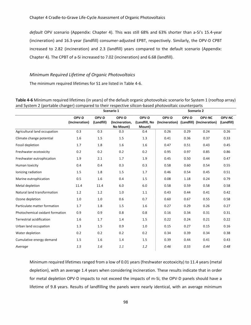
Chapter 4 Cradle-to-Grave Life-Cycle Assessment of Organic Photovoltaics
98
default OPV scenario (Appendix: Chapter 4). This was still 68% and 63% shorter than a-Si’s 15.4-year
(incineration) and 16.3-year (landfill) consumer-adjusted EPBT, respectively. Similarly, the OPV-D CPBT
increased to 2.82 (incineration) and 2.3 (landfill) years compared to the default scenario (Appendix:
Chapter 4). The CPBT of a-Si increased to 7.02 (incineration) and 6.68 (landfill).
Minimum Required Lifetime of Organic Photovoltaics
The minimum required lifetimes for S1 are listed in Table 4-6.
Table 4-6 Minimum required lifetimes (in years) of the default organic photovoltaic scenario for System 1 (rooftop array) and System 2 (portable charger) compared to their respective silicon-based photovoltaic counterparts
Scenario 1 Scenario 2
OPV-D (Incineration)
OPV-D (Landfill)
OPV-D (Incineration,
No Mount)
OPV-D (Landfill, No
Mount)
OPV-D (Incineration)
OPV-D (Landfill)
OPV-NC (Incineration)
OPV-NC (Landfill)
Agricultural land occupation 0.3 0.3 0.3 0.4 0.26 0.29 0.24 0.26
Climate change potential 1.6 1.5 1.5 1.3 0.41 0.36 0.37 0.33
Fossil depletion 1.7 1.8 1.6 1.6 0.47 0.51 0.43 0.45
Freshwater ecotoxicity 0.2 0.2 0.2 0.2 0.95 0.97 0.85 0.86
Freshwater eutrophication 1.9 2.1 1.7 1.9 0.45 0.50 0.44 0.47
Human toxicity 0.4 0.4 0.3 0.3 0.58 0.60 0.54 0.55
Ionizing radiation 1.5 1.8 1.5 1.7 0.46 0.54 0.45 0.51
Marine eutrophication 0.5 1.6 0.4 1.5 0.08 1.18 0.24 0.79
Metal depletion 11.4 11.4 6.0 6.0 0.58 0.59 0.58 0.58
Natural land transformation 1.2 1.2 1.0 1.1 0.43 0.44 0.41 0.42
Ozone depletion 1.0 1.0 0.6 0.7 0.60 0.67 0.55 0.58
Particulate matter formation 1.7 1.8 1.5 1.6 0.27 0.29 0.26 0.27
Photochemical oxidant formation 0.9 0.9 0.8 0.8 0.16 0.34 0.31 0.31
Terrestrial acidification 1.6 1.7 1.4 1.5 0.22 0.24 0.21 0.22
Urban land occupation 1.3 1.5 0.9 1.0 0.15 0.27 0.15 0.16
Water depletion 0.2 0.2 0.2 0.2 0.34 0.39 0.34 0.38
Cumulative energy demand 1.5 1.6 1.4 1.5 0.39 0.44 0.41 0.43
Average 1.5 1.6 1.1 1.2 0.46 0.55 0.44 0.48
Minimum required lifetimes ranged from a low of 0.01 years (freshwater ecotoxicity) to 11.4 years (metal
depletion), with an average 1.4 years when considering incineration. These results indicate that in order
for metal depletion OPV-D impacts to not exceed the impacts of m-Si, the OPV-D panels should have a
lifetime of 9.8 years. Results of landfilling the panels were nearly identical, with an average minimum

Chapter 4 Cradle-to-Grave Life-Cycle Assessment of Organic Photovoltaics
99
required lifetime of 1.6 years. The lifetime values for S2 averaged 0.46 years (incineration) and 0.55 years
(landfill), while specifically for incineration they were as low as 0.08 years (marine eutrophication) and as
high as of 0.9 years (freshwater ecotoxicity). For landfilling, the minimum required lifetime was lowest for
terrestrial acidification at 0.24 years, however it was highest at 1.18 years for marine eutrophication due
to associated landfilling activities and processes leading to nitrate releases in the environment. The
impacts of marine eutrophication were landfill-specific impacts that would have occurred irrespective of
the type of material discarded.
These overall minimum require lifetimes are encouraging for OPV development given that experimental
maximum lifetimes for this technology have surpassed all the results reported for S2 and have started to
approach the upper bound minimum required lifetime values for S1.56 However, it should be noted that
these results are based on the assumed OPV efficiency of 5%. In the next section, this assumption is
challenged against a range of different efficiencies as well as different lifetimes to better understand the
influences these assumptions have on the overall environmental and human health impacts of OPV
systems.
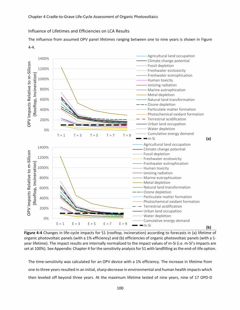
Chapter 4 Cradle-to-Grave Life-Cycle Assessment of Organic Photovoltaics
100
Influence of Lifetimes and Efficiencies on LCA Results
The influence from assumed OPV panel lifetimes ranging between one to nine years is shown in Figure
4-4.
(a)
(b)
Figure 4-4 Changes in life-cycle impacts for S1 (rooftop, incineration) according to forecasts in (a) lifetime of organic photovoltaic panels (with a 1% efficiency) and (b) efficiencies of organic photovoltaic panels (with a 1-year lifetime). The impact results are internally normalized to the impact values of m-Si (i.e. m-Si’s impacts are set at 100%). See Appendix: Chapter 4 for the sensitivity analysis for S1 with landfilling as the end-of-life option.
The time-sensitivity was calculated for an OPV device with a 1% efficiency. The increase in lifetime from
one to three years resulted in an initial, sharp decrease in environmental and human health impacts which
then leveled off beyond three years. At the maximum lifetime tested of nine years, nine of 17 OPD-D
0%
200%
400%
600%
800%
1000%
1200%
1400%
T = 1 T = 3 T = 5 T = 7 T = 9
OP
V Im
pac
ts R
elat
ive
to m
-Sili
con
(R
oo
fto
p, I
nci
ner
atio
n)
Agricultural land occupationClimate change potentialFossil depletionFreshwater ecotoxicityFreshwater eutrophicationHuman toxicityIonizing radiationMarine eutrophicationMetal depletionNatural land transformationOzone depletionParticulate matter formationPhotochemical oxidant formationTerrestrial acidificationUrban land occupationWater depletionCumulative energy demandm-Si
0%
200%
400%
600%
800%
1000%
1200%
1400%
E = 1 E = 3 E = 5 E = 7 E = 9
OP
V Im
pac
ts R
elat
ive
to m
-Sili
con
(R
oo
fto
p, I
nci
ner
atio
n)
Agricultural land occupationClimate change potentialFossil depletionFreshwater ecotoxicityFreshwater eutrophicationHuman toxicityIonizing radiationMarine eutrophicationMetal depletionNatural land transformationOzone depletionParticulate matter formationPhotochemical oxidant formationTerrestrial acidificationUrban land occupationWater depletionCumulative energy demandm-Si
Chapter 4 Cradle-to-Grave Life-Cycle Assessment of Organic Photovoltaics
101
impacts, including climate change potential and CED remained proportionally higher than m-Si.
Accordingly, the EPBT and CPBT never fell below that of m-Si. The EPBT ranged from a high of 16 years for
panel lifetimes of one year to a low of 3.5 years for lifetimes of nine years, while the CPBT ranged from a
high of 6.4 years to a low of 1.6 years, respectively. The results of increasing the efficiencies against a
constant lifetime of one year were additionally tested. A similar trend was observed where increases in
the efficiency from 1-3% was correlated with an initial sharp decrease in environmental and human health
impacts (Figure 4-4). Beyond 3%, the impact reductions began to level off but not as sharply as in the case
of the lifetime sensitivity. Thus, at efficiencies of 9% only metal depletion remained proportionally higher
than m-Si. In particular, the CED and climate change potential were 18% and 16% lower than m-Si, with
an EPBT and CPBT of 2.1 years and 305 days, respectively.
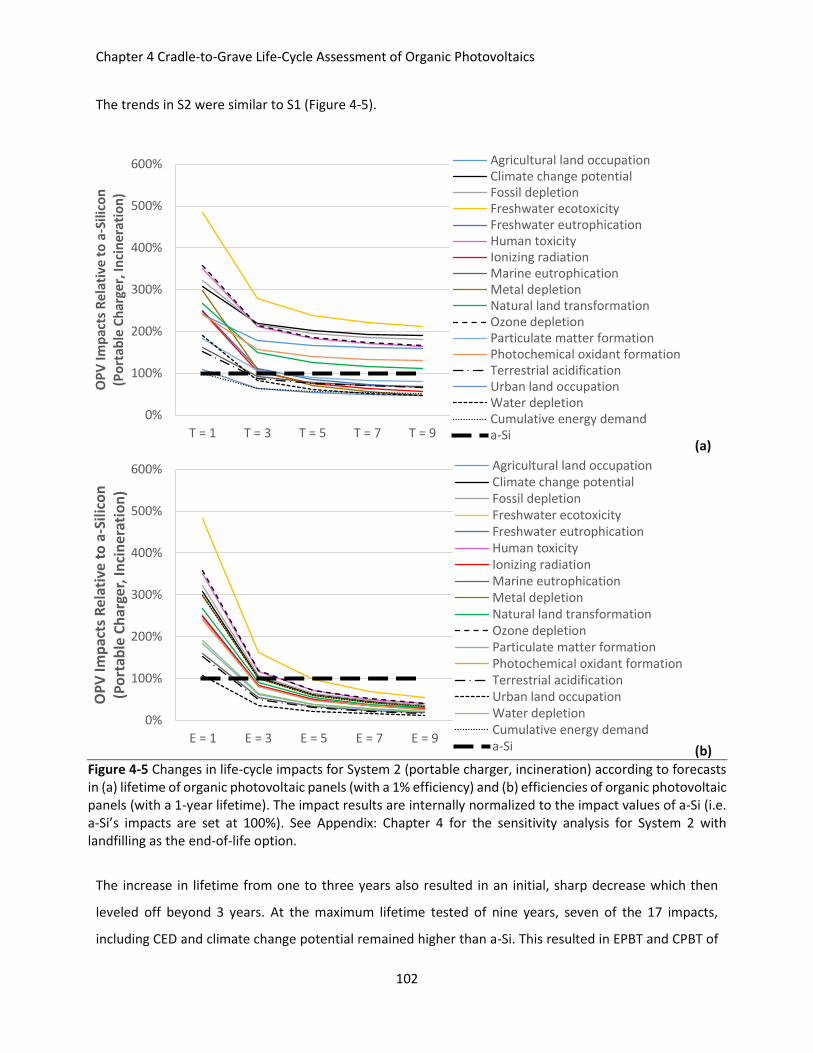
Chapter 4 Cradle-to-Grave Life-Cycle Assessment of Organic Photovoltaics
102
The trends in S2 were similar to S1 (Figure 4-5).
(a)
(b) Figure 4-5 Changes in life-cycle impacts for System 2 (portable charger, incineration) according to forecasts in (a) lifetime of organic photovoltaic panels (with a 1% efficiency) and (b) efficiencies of organic photovoltaic panels (with a 1-year lifetime). The impact results are internally normalized to the impact values of a-Si (i.e. a-Si’s impacts are set at 100%). See Appendix: Chapter 4 for the sensitivity analysis for System 2 with landfilling as the end-of-life option.
The increase in lifetime from one to three years also resulted in an initial, sharp decrease which then
leveled off beyond 3 years. At the maximum lifetime tested of nine years, seven of the 17 impacts,
including CED and climate change potential remained higher than a-Si. This resulted in EPBT and CPBT of
0%
100%
200%
300%
400%
500%
600%
T = 1 T = 3 T = 5 T = 7 T = 9
OP
V Im
pac
ts R
ela
tive
to
a-S
ilico
n
(Po
rtab
le C
har
ger,
Inci
ner
atio
n)
Agricultural land occupationClimate change potentialFossil depletionFreshwater ecotoxicityFreshwater eutrophicationHuman toxicityIonizing radiationMarine eutrophicationMetal depletionNatural land transformationOzone depletionParticulate matter formationPhotochemical oxidant formationTerrestrial acidificationUrban land occupationWater depletionCumulative energy demanda-Si
0%
100%
200%
300%
400%
500%
600%
E = 1 E = 3 E = 5 E = 7 E = 9
OP
V Im
pac
ts R
elat
ive
to a
-Sili
con
(P
ort
able
Ch
arge
r, In
cin
erat
ion
)
Agricultural land occupationClimate change potentialFossil depletionFreshwater ecotoxicityFreshwater eutrophicationHuman toxicityIonizing radiationMarine eutrophicationMetal depletionNatural land transformationOzone depletionParticulate matter formationPhotochemical oxidant formationTerrestrial acidificationUrban land occupationWater depletionCumulative energy demanda-Si
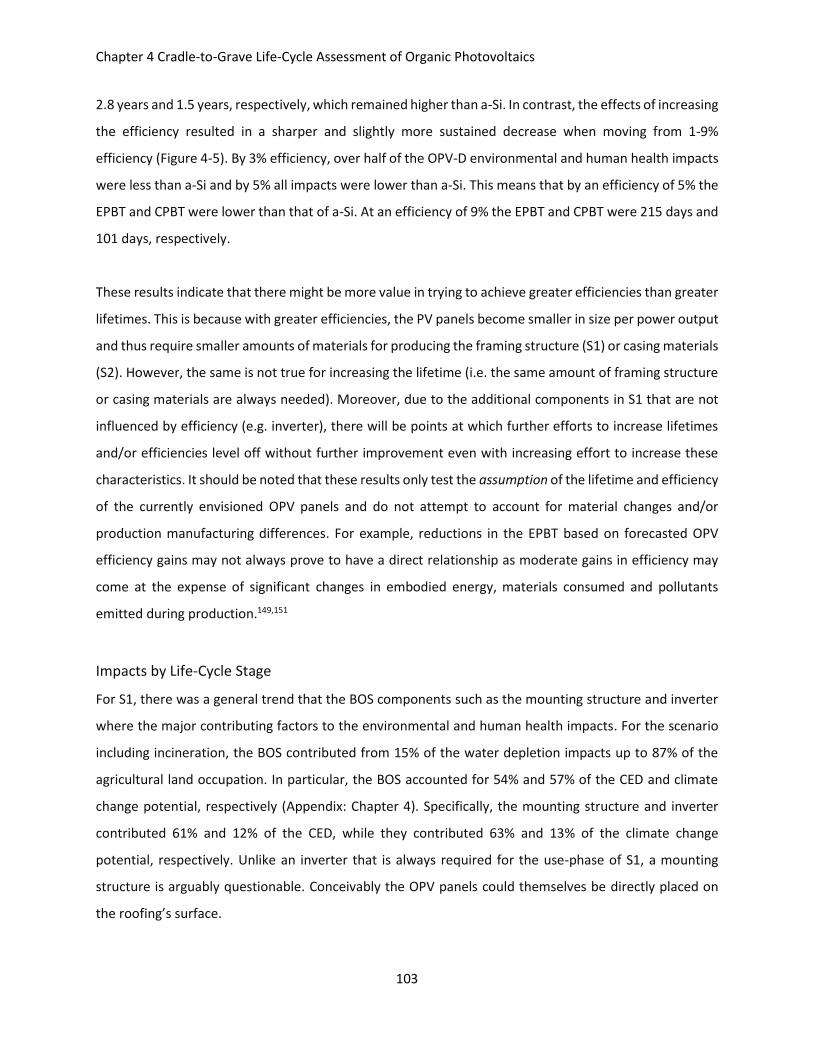
Chapter 4 Cradle-to-Grave Life-Cycle Assessment of Organic Photovoltaics
103
2.8 years and 1.5 years, respectively, which remained higher than a-Si. In contrast, the effects of increasing
the efficiency resulted in a sharper and slightly more sustained decrease when moving from 1-9%
efficiency (Figure 4-5). By 3% efficiency, over half of the OPV-D environmental and human health impacts
were less than a-Si and by 5% all impacts were lower than a-Si. This means that by an efficiency of 5% the
EPBT and CPBT were lower than that of a-Si. At an efficiency of 9% the EPBT and CPBT were 215 days and
101 days, respectively.
These results indicate that there might be more value in trying to achieve greater efficiencies than greater
lifetimes. This is because with greater efficiencies, the PV panels become smaller in size per power output
and thus require smaller amounts of materials for producing the framing structure (S1) or casing materials
(S2). However, the same is not true for increasing the lifetime (i.e. the same amount of framing structure
or casing materials are always needed). Moreover, due to the additional components in S1 that are not
influenced by efficiency (e.g. inverter), there will be points at which further efforts to increase lifetimes
and/or efficiencies level off without further improvement even with increasing effort to increase these
characteristics. It should be noted that these results only test the assumption of the lifetime and efficiency
of the currently envisioned OPV panels and do not attempt to account for material changes and/or
production manufacturing differences. For example, reductions in the EPBT based on forecasted OPV
efficiency gains may not always prove to have a direct relationship as moderate gains in efficiency may
come at the expense of significant changes in embodied energy, materials consumed and pollutants
emitted during production.149,151
Impacts by Life-Cycle Stage
For S1, there was a general trend that the BOS components such as the mounting structure and inverter
where the major contributing factors to the environmental and human health impacts. For the scenario
including incineration, the BOS contributed from 15% of the water depletion impacts up to 87% of the
agricultural land occupation. In particular, the BOS accounted for 54% and 57% of the CED and climate
change potential, respectively (Appendix: Chapter 4). Specifically, the mounting structure and inverter
contributed 61% and 12% of the CED, while they contributed 63% and 13% of the climate change
potential, respectively. Unlike an inverter that is always required for the use-phase of S1, a mounting
structure is arguably questionable. Conceivably the OPV panels could themselves be directly placed on
the roofing’s surface.
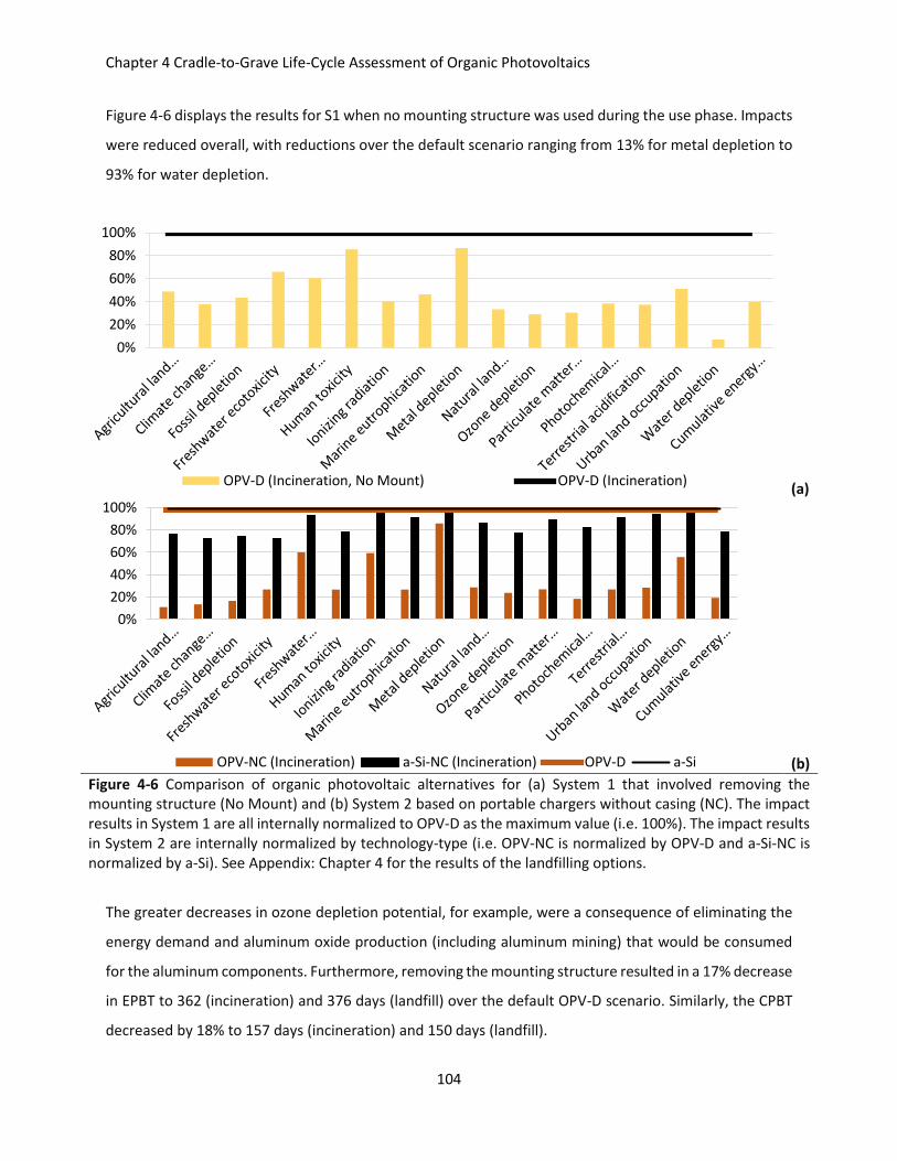
Chapter 4 Cradle-to-Grave Life-Cycle Assessment of Organic Photovoltaics
104
Figure 4-6 displays the results for S1 when no mounting structure was used during the use phase. Impacts
were reduced overall, with reductions over the default scenario ranging from 13% for metal depletion to
93% for water depletion.
(a)
(b)
Figure 4-6 Comparison of organic photovoltaic alternatives for (a) System 1 that involved removing the mounting structure (No Mount) and (b) System 2 based on portable chargers without casing (NC). The impact results in System 1 are all internally normalized to OPV-D as the maximum value (i.e. 100%). The impact results in System 2 are internally normalized by technology-type (i.e. OPV-NC is normalized by OPV-D and a-Si-NC is normalized by a-Si). See Appendix: Chapter 4 for the results of the landfilling options.
The greater decreases in ozone depletion potential, for example, were a consequence of eliminating the
energy demand and aluminum oxide production (including aluminum mining) that would be consumed
for the aluminum components. Furthermore, removing the mounting structure resulted in a 17% decrease
in EPBT to 362 (incineration) and 376 days (landfill) over the default OPV-D scenario. Similarly, the CPBT
decreased by 18% to 157 days (incineration) and 150 days (landfill).
0%
20%
40%
60%
80%
100%
OPV-D (Incineration, No Mount) OPV-D (Incineration)
0%
20%
40%
60%
80%
100%
OPV-NC (Incineration) a-Si-NC (Incineration) OPV-D a-Si
Chapter 4 Cradle-to-Grave Life-Cycle Assessment of Organic Photovoltaics
105
For S2, a similar trend was seen where the casing material heavily dominated the impacts for the OPV-D
panels. Overall, the casing contributed from 21% of the metal depletion up to 91% of the photochemical
oxidant formation potential in the incineration scenario. Alternatively, S2 could be envisioned without the
need for external casing to protect the portable charger, for both the OPV-D and a-Si panels. Direct
comparisons of the OPV (OPV-NC) and a-Si panels without casing (a-Si-NC) showed more pronounced
decreases for the OPV-NC panels compared to a-Si-NC in contrast to the relative decreases found when
both panels had casing. This is because a-Si impacts depend more on the contribution from the panel itself
as opposed to the casing. A highly noticeable finding was the EPBT for OPV-NC panels that were on the
order of 42 days (incineration) and 45 days (landfill) in total. Similarly, the CPBT for this technology
decreased to 16 days and 14 days, respectively.
The high impact contribution from the BOS for OPV-D panels contrasts with the m-Si panels, whose
environmental and human health impacts were most heavily influenced by production of the solar cell
itself (Appendix: Chapter 4). This was somewhat expected knowing that the production of OPV-D panels
is much less impactful on a watt-per-watt basis, compared with m-Si panels.146 However, these results
were also dependent on the expected lifetime of the OPV-D panels. For instance, Epsinosa et al. found
that the majority of the environmental and human health impacts from their OPV “solar-park” resulted
from the production of the panels themselves,62 whose lifetimes were estimated at one year compared
to the default scenario of five years in this chapter. In contrast, S2 saw a decrease in the contribution
arising from the production of the OPV-D panel itself. As discussed previously, S1 required that the OPV-
D panels be replaced every five years, leading to a greater contribution of the panels themselves to the
overall results. The shorter use-phase of S2 resulted in a situation where such replacements were not
necessary and thus the impacts from the panels had diminished.
Conclusion
As was demonstrated in Chapter 3, the production of OPV panels (i.e. cradle-to-gate analysis) have shown
greater resource efficiencies and lower environmental hazards compared to conventional silicon-based
PV. The findings of the current chapter demonstrate that these potential advantages remain after
including the use and end-of-life stages, albeit at a lower relative value. Obvious uncertainties remain
regarding the assumed lifetimes and efficiencies that will be achieved at the industrial scale. Increasing
both are necessary to reducing the environmental and human health impacts of this technology, however
there is a non-linear relationship between lifetimes or efficiencies and impacts changes across the life-
Chapter 4 Cradle-to-Grave Life-Cycle Assessment of Organic Photovoltaics
106
cycle. This is a consequence of the use-phase application setting which dictates what other contributing
factors (i.e. auxiliary components other than the panel itself) will exist in the production, use and end-of-
life phases.
The current results suggest that OPV are a preferred energy producing technology compared with silicon-
based PV from an environmental and human health perspective, particularly for uses where the product
lifetime is relatively short (i.e. < 5 years) or where product systems are extremely simplified. This latter
point was reflected in the LCA results for the solar rooftop array (S1) that had no mounting structure and
the portable charger (S2) that had no case. This was also noticeable based on the quicker EPBT and CPBT
for S2 compared with S1. Additionally, there may be important sources of uncertainty for the silicon panels
as well. Although m-Si and a-Si are much more mature technologies, advances in silicon-cell technology
at the lab-scale still continue.15 However, their influence on the average market silicon-module efficiency
is not yet apparent.22 Moreover, as more 1st-generation silicon panels come to their end of serviceable
life, the switch to full-scale silicon recycling could have a greater impact on the environmental profile of
that technology compared with incremental adjustments to the efficiencies and lifetimes.
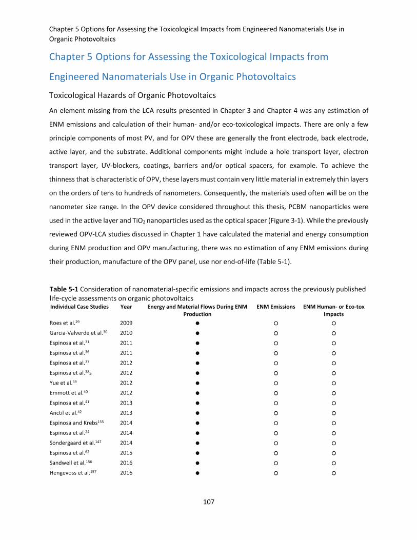
Chapter 5 Options for Assessing the Toxicological Impacts from Engineered Nanomaterials Use in
Organic Photovoltaics
107
Chapter 5 Options for Assessing the Toxicological Impacts from
Engineered Nanomaterials Use in Organic Photovoltaics
Toxicological Hazards of Organic Photovoltaics
An element missing from the LCA results presented in Chapter 3 and Chapter 4 was any estimation of
ENM emissions and calculation of their human- and/or eco-toxicological impacts. There are only a few
principle components of most PV, and for OPV these are generally the front electrode, back electrode,
active layer, and the substrate. Additional components might include a hole transport layer, electron
transport layer, UV-blockers, coatings, barriers and/or optical spacers, for example. To achieve the
thinness that is characteristic of OPV, these layers must contain very little material in extremely thin layers
on the orders of tens to hundreds of nanometers. Consequently, the materials used often will be on the
nanometer size range. In the OPV device considered throughout this thesis, PCBM nanoparticles were
used in the active layer and TiO2 nanoparticles used as the optical spacer (Figure 3-1). While the previously
reviewed OPV-LCA studies discussed in Chapter 1 have calculated the material and energy consumption
during ENM production and OPV manufacturing, there was no estimation of any ENM emissions during
their production, manufacture of the OPV panel, use nor end-of-life (Table 5-1).
Table 5-1 Consideration of nanomaterial-specific emissions and impacts across the previously published life-cycle assessments on organic photovoltaics
Individual Case Studies Year Energy and Material Flows During ENM Production
ENM Emissions ENM Human- or Eco-tox Impacts
Roes et al.29 2009 ● ○ ○ Garcia-Valverde et al.30 2010 ● ○ ○ Espinosa et al.31 2011 ● ○ ○ Espinosa et al.36 2011 ● ○ ○ Espinosa et al.37 2012 ● ○ ○ Espinosa et al.38s 2012 ● ○ ○ Yue et al.39 2012 ● ○ ○ Emmott et al.40 2012 ● ○ ○ Espinosa et al.41 2013 ● ○ ○ Anctil et al.42 2013 ● ○ ○ Espinosa and Krebs155 2014 ● ○ ○ Espinosa et al.24 2014 ● ○ ○ Sondergaard et al.147 2014 ● ○ ○ Espinosa et al.62 2015 ● ○ ○ Sandwell et al.156 2016 ● ○ ○ Hengevoss et al.157 2016 ● ○ ○
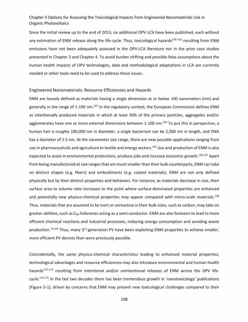
Chapter 5 Options for Assessing the Toxicological Impacts from Engineered Nanomaterials Use in
Organic Photovoltaics
108
Since the initial review up to the end of 2013, six additional OPV-LCA have been published, each without
any estimation of ENM release along the life-cycle. Thus, toxicological hazards158–162 resulting from ENM
emissions have not been adequately assessed in the OPV-LCA literature nor in the prior case studies
presented in Chapter 3 and Chapter 4. To avoid burden shifting and possible false assumptions about the
human health impacts of OPV technologies, data and methodological adaptations in LCA are currently
needed or other tools need to be used to address these issues.
Engineered Nanomaterials: Resource Efficiencies and Hazards
ENM are loosely defined as materials having a single dimension at or below 100 nanometers (nm) and
generally in the range of 1-100 nm.163 In the regulatory context, the European Commission defines ENM
as intentionally produced materials in which at least 50% of the primary particles, aggregates and/or
agglomerates have one or more external dimensions between 1-100 nm.164 To put this in perspective, a
human hair is roughly 100,000 nm in diameter, a single bacterium can be 2,500 nm in length, and DNA
has a diameter of 2.5 nm. At the nanometer size range, there are new possible applications ranging from
use in pharmaceuticals and agriculture to textile and energy sectors.165 Use and production of ENM is also
expected to assist in environmental protections, produce jobs and increase economic growth.166,167 Apart
from being manufactured at size ranges that are much smaller than their bulk counterparts, ENM can take
on distinct shapes (e.g. fibers) and embodiments (e.g. coated materials). ENM are not only defined
physically but by their distinct properties and behaviors. For instance, as materials decrease in size, their
surface area to volume ratio increases to the point where surface-dominated properties are enhanced
and potentially new physico-chemical properties may appear compared with micro-scale materials.168
Thus, materials that are assumed to be inert or unreactive in their bulk-sizes, such as carbon, may take on
greater abilities, such as C60-fullerenes acting as a semi-conductor. ENM are also foreseen to lead to more
efficient chemical reactions and industrial processes, reducing energy consumption and avoiding waste
production.74,169 Thus, many 3rd-generation PV have been exploiting ENM properties to achieve smaller,
more efficient PV devices than were previously possible.
Coincidentally, the same physico-chemical characteristics leading to enhanced material properties,
technological advantages and resource efficiencies may also introduce environmental and human health
hazards170–173 resulting from intentional and/or unintentional releases of ENM across the OPV life-
cycle.174,175 In the last two decades there has been tremendous growth in ‘nanotoxicology’ publications
(Figure 5-1), driven by concerns that ENM may present new toxicological challenges compared to their
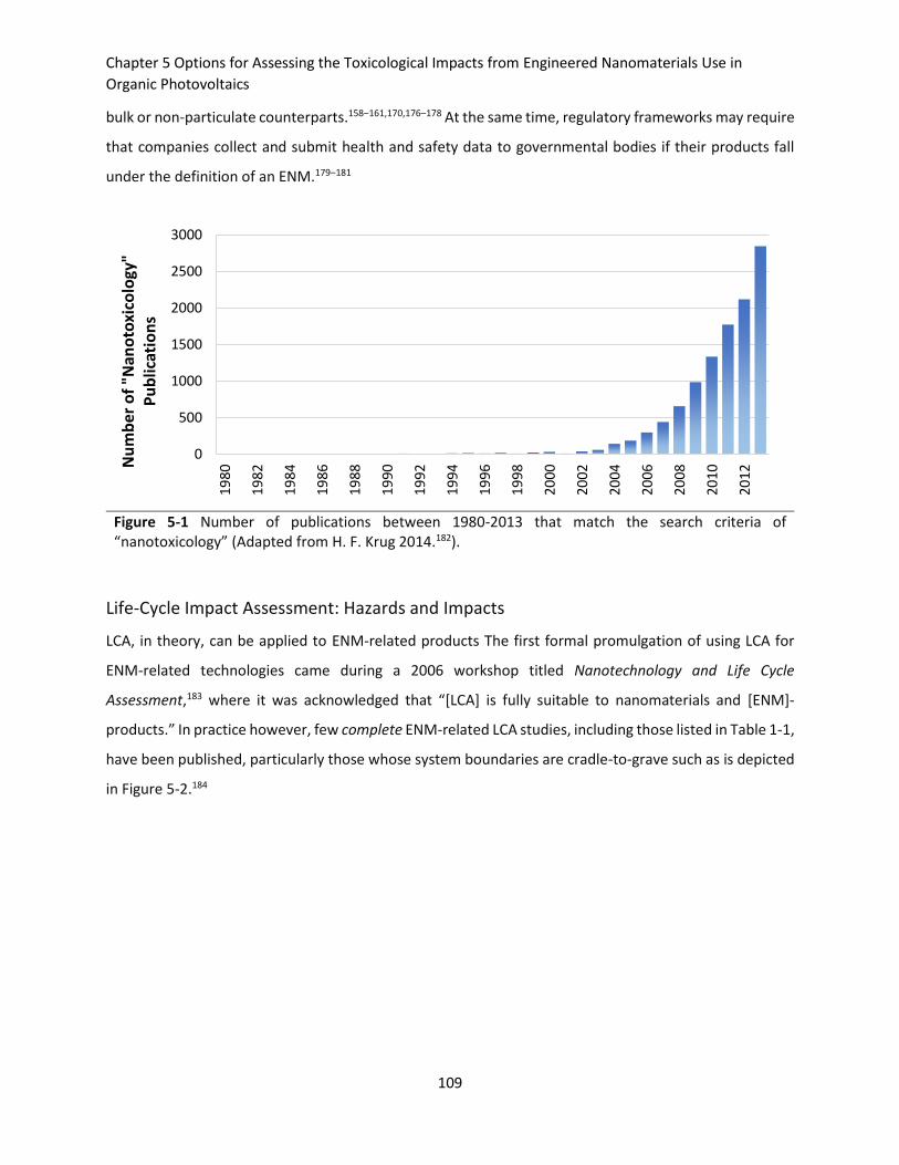
Chapter 5 Options for Assessing the Toxicological Impacts from Engineered Nanomaterials Use in
Organic Photovoltaics
109
bulk or non-particulate counterparts.158–161,170,176–178 At the same time, regulatory frameworks may require
that companies collect and submit health and safety data to governmental bodies if their products fall
under the definition of an ENM.179–181
Figure 5-1 Number of publications between 1980-2013 that match the search criteria of “nanotoxicology” (Adapted from H. F. Krug 2014.182).
Life-Cycle Impact Assessment: Hazards and Impacts
LCA, in theory, can be applied to ENM-related products The first formal promulgation of using LCA for
ENM-related technologies came during a 2006 workshop titled Nanotechnology and Life Cycle
Assessment,183 where it was acknowledged that “[LCA] is fully suitable to nanomaterials and [ENM]-
products.” In practice however, few complete ENM-related LCA studies, including those listed in Table 1-1,
have been published, particularly those whose system boundaries are cradle-to-grave such as is depicted
in Figure 5-2.184
0
500
1000
1500
2000
2500
300019
80
1982
1984
1986
1988
1990
1992
1994
1996
1998
2000
2002
2004
2006
2008
2010
2012
Nu
mb
er o
f "N
ano
toxi
colo
gy"
Pu
blic
atio
ns
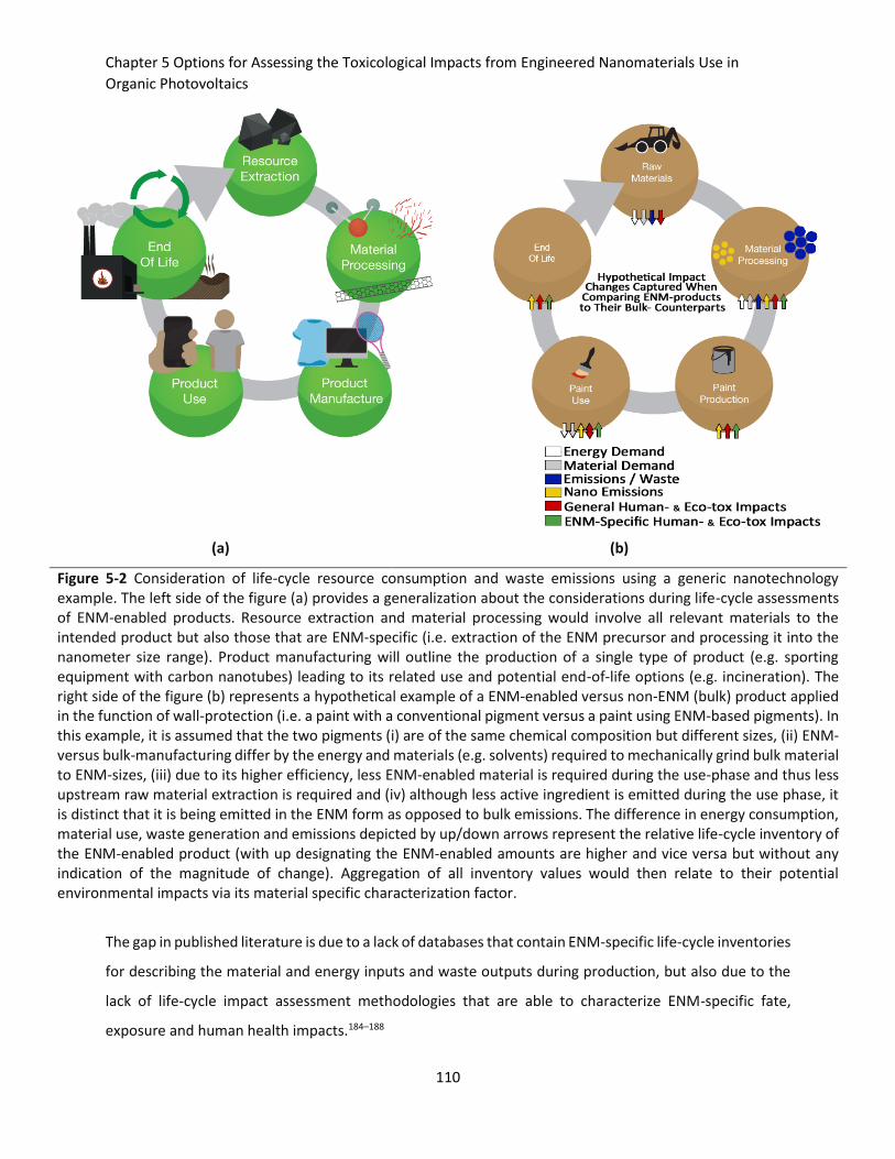
Chapter 5 Options for Assessing the Toxicological Impacts from Engineered Nanomaterials Use in
Organic Photovoltaics
110
(a) (b)
Figure 5-2 Consideration of life-cycle resource consumption and waste emissions using a generic nanotechnology example. The left side of the figure (a) provides a generalization about the considerations during life-cycle assessments of ENM-enabled products. Resource extraction and material processing would involve all relevant materials to the intended product but also those that are ENM-specific (i.e. extraction of the ENM precursor and processing it into the nanometer size range). Product manufacturing will outline the production of a single type of product (e.g. sporting equipment with carbon nanotubes) leading to its related use and potential end-of-life options (e.g. incineration). The right side of the figure (b) represents a hypothetical example of a ENM-enabled versus non-ENM (bulk) product applied in the function of wall-protection (i.e. a paint with a conventional pigment versus a paint using ENM-based pigments). In this example, it is assumed that the two pigments (i) are of the same chemical composition but different sizes, (ii) ENM- versus bulk-manufacturing differ by the energy and materials (e.g. solvents) required to mechanically grind bulk material to ENM-sizes, (iii) due to its higher efficiency, less ENM-enabled material is required during the use-phase and thus less upstream raw material extraction is required and (iv) although less active ingredient is emitted during the use phase, it is distinct that it is being emitted in the ENM form as opposed to bulk emissions. The difference in energy consumption, material use, waste generation and emissions depicted by up/down arrows represent the relative life-cycle inventory of the ENM-enabled product (with up designating the ENM-enabled amounts are higher and vice versa but without any indication of the magnitude of change). Aggregation of all inventory values would then relate to their potential environmental impacts via its material specific characterization factor.
The gap in published literature is due to a lack of databases that contain ENM-specific life-cycle inventories
for describing the material and energy inputs and waste outputs during production, but also due to the
lack of life-cycle impact assessment methodologies that are able to characterize ENM-specific fate,
exposure and human health impacts.184–188
Chapter 5 Options for Assessing the Toxicological Impacts from Engineered Nanomaterials Use in
Organic Photovoltaics
111
In regards to the emissions, there have been some attempts to model and calculate major environmental
ENM flows leading from the production189–191 but also the use192–194 and disposal of these materials.195
These approaches and models can be used to estimate average, global ENM emissions that might be used
to create foreground life-cycle inventory emissions data of ENM-related products and processes. To be
useful in LCA, each ENM emission must contain a corresponding characterization factor (CFNS) that
converts its emission into a potential environmental or human health impact.
There are a handful of published papers that have made first approximations to model ENM fate, exposure
and toxicity within LCA.93–96 Those first approximations include one for human health93 and threeii for
ecotoxicity CF for nanomaterials.94–96 In each case, the authors modified existing CF in USEtox to make
them ENM-specific. Currently existing life-cycle impact assessment methods, such as USEtox, take
advantage of a number of assumptions that conveniently describe the fate and transport of small organic
molecules and metals quite well, but these methods are not appropriate for ENM or similarly described
colloidal materials.196 The major assumptions utilized in life-cycle impact assessment methods are that
conditions are at steady-state and systems have reached thermodynamic equilibrium.101,197 Consequently,
these models assume that there are no changes in concentration of the pollutant over time and that the
fate of these pollutants can be estimated using (equilibrium) partition coefficients (e.g. octanol-water
partition coefficient, Kow). These coefficients are defined by the ratio of the resulting pollutant
concentration in one medium versus another (e.g. octanol versus water), once the system involving both
mediums has achieved equilibrium.
However, when released into a specific medium, ENM exist in their own phase and do not form uniform
phases with the surrounding medium unlike organics. Therefore, and by definition, ENM are not
thermodynamically stable, even if certain ENM may be kinetically stable for long periods of time.196 In
other words, an ENM concentration ratio between two mediums cannot be predicted from a previously
measured partition coefficient if conditions were not exactly the same between the two scenarios.196 This
is because the behavior of ENM in the environment are heavily concentration dependent (i.e. the initial
conditions of , the amount of ENM in, and the time at which the system is measured will produce different
results).95,196 Thus, in place of equilibrium partition coefficients, ENM should be described kinetically using
dynamic fate and exposure models. For example, such models might employ the use of first-order rate
iiWalser et al indirectly calculated the impacts from nanosilver by using experimentally derived bioavailable fraction values to estimate the amount of ionic silver
released during use and disposal. The applied characterization factor was thus, technically not specific for nanosilver but for ionic silver.

Chapter 5 Options for Assessing the Toxicological Impacts from Engineered Nanomaterials Use in
Organic Photovoltaics
112
constants to describe the dissolution of ENM into ions in the water column.198 Furthermore, steady-state
models are also not in agreement with the fact that ENM emissions rates are not typically constant events.
This is particularly true for indoor, occupational scenarios.199,200 Instead, ENM emissions are likely to be
episodic, further influencing the concentration in the environment and the concentration-dependent
transformations specific to that material. Lastly, the exposure to ENM, and specifically inhalation of ENM,
will present concentration-dependent mechanisms for deposition, clearance and retention in the lung.
That is, inhalation of ENM is not only dependent on the inhalation rate of the individual who is exposed201
but also the ENM characteristics, biological mechanisms and time at which exposure is measured.202 It has
been proposed to use a ENM-specific retention factor, R, for such purposes, calculated using human
airway lung deposition and clearance models such as the Multiple-Path Particle Dosimetry (MPPD) model
.97 The MPPD model is a tool typically used in HHRA for determining the internal lung dose from exposure
to airborne concentrations of chemicals and particulates. However, the current MPPD model does not
allow for estimating deposition or clearance while using exposure conditions that change over time.
Review of Previously Published Characterization Factors for Engineered Nanomaterials
In previously published CFNS, Eckelman et al.94 estimated the fate and exposure of carbon nanotubes in
the environment using empirically derived values for the partition coefficients already used in USEtox such
as the octanol-water partition coefficient, Henry’s law coefficient, and bioaccumulation factor in fish, for
example. In addition, they added a parameter for aggregation and sedimentation that was reported as a
deterministic fraction of the carbon nanotubes that are removed from the freshwater. Eckelman et al.
report a worst-case and realistic set of results, in which the worst-case fate calculation resulted in a
residence time of carbon nanotubes in water of 143 days. Under more “realistic” conditions in which
aggregation and sedimentation are considered, the residence time decreased to several days. Their
estimation of the exposure calculated as a percentage of the total concentration of carbon nanotubes in
water according to the USEtox procedure, resulted in 100% exposure in the worst-case scenario and 98%
in the realistic scenario. The resulting CFNS were 29,000 and 3,700 potentially affected fraction of species
per kg of emitted carbon nanotubes in the worst- and realistic-case scenarios, respectively.
Miseljik and Olsen96 presented a simplified USEtox fate calculation by artificially defining the residence
time of nanoparticles of silver (nano-Ag) and TiO2 as one day. This was conceived on a quasi-kinetic basis
representing the residence time given aggregation and sedimentation of these materials in freshwater
systems. However, this kinetic parameter was ultimately used inside of a steady-state model, as was done
Chapter 5 Options for Assessing the Toxicological Impacts from Engineered Nanomaterials Use in
Organic Photovoltaics
113
in Eckelman et al.96 These authors assumed an exposure factor of one in lieu of considering differences
between external concentrations and uptake by the species. The resulting CFNS for nano-Ag and TiO2 were
8,573 and 26.2 potentially affected fraction of species per kg of emitted nanomaterial, respectively. Given
the fate and exposure calculations were identical for both silver and TiO2, the differences in the CFNS
resulted from their respective eco-toxicity dose-response relationships, whereby nano-Ag were found to
be much more toxic than nano-TiO2.
Salieri et al.95 defined their fate factor for nano-TiO2 using properly defined kinetic descriptors of fate and
transport, unlike the two previous studies. Although, the fate factor was employed inside of a steady-
state model like the two previous studies. Specifically, Salieri et al. considered the ENM-specific
transformation processes of dissolution, homo-aggregation and hetero-aggregation, and sedimentation
velocity inside of a freshwater and sediment compartmental model. The results of their fate calculations
showed that the residence time for nano-TiO2 in freshwater was quite short, ranging from 0.1 days for 8
nm diameter particles to 0.001 days for 400 nm diameter particles. Such residence times are much shorter
than the previously reported values of Eckelman et al. and Miseljik and Olsen, showing the potential
importance of ENM-specific kinetic parameters in the calculation of fate and transport in life-cycle impact
assessment models. Their reported fate and transport calculations were combined with a worst-case
exposure factor of 1, citing no known knowledge about describing the bioaccumulation and bioavailability
of ENM by freshwater species.95 After creating a weighted-average residence time for nano-TiO2, the
resulting CFNS was reported as 0.28 potentially affected fraction of species per kg of emitted nano-TiO2.
This value is two-orders of magnitude smaller than what was reported by Miseljik and Olsen for nano-
TiO2. While this difference can be partially explained by the difference in residence times calculated
between the two studies, there were also differences in the reported eco-toxicity dose-response
relationships. Salieri et al. reported an effective concentration at which 50% of species were effected
between 0.013-0.018 kg/m3, while that of Mislejic and Olsen was reported as 0.019 kg/m3.
In regards to human health, Pini et al.93 published a human health CFNS based on the framework of Walser
et al.97 The latter framework introduces the potential use of ENM-specific transformations such as
aggregation, agglomeration and gravitational settling for calculating the fate of ENM in the indoor air
setting.97 In the end, the CFNS published by Pini et al. estimated the fate of nano-TiO2 as a function of
advective air flow between the indoor and outdoor air, without the consideration of ENM-specific
transformations that were outlined in Walser et al.93 Pini et al. estimated exposure using a retention factor
Chapter 5 Options for Assessing the Toxicological Impacts from Engineered Nanomaterials Use in
Organic Photovoltaics
114
in order to account for the fact that particle deposition should not assumed to be 100%. Deposition of
particles in the human airway may occur in the upper airway (i.e. nasal and mouth cavities),
tracheobronchial region, air-exchange regions and/or the interstitial space, for example. The deposition
and ultimate retention is a function of both bulk air movement through the airways but also a function of
biological and chemical mechanisms that are responsible for sequestering, relocating and eliminating
particles from the body. The retention factor calculated using the MPPD model in Pini et al. was specific
for deposition, clearance and final retention under constant, steady-state exposure conditions.97
However, the exposure to ENM, and specifically inhalation of ENM, will present concentration-dependent
mechanisms for deposition, clearance and retention in the lung. That is, inhalation of ENM is not only
dependent on the inhalation rate of the individual who is exposed201 but also the ENM characteristics,
biological mechanisms and time at which exposure is measured.202 Since the current version of the MPPD
model does not allow for estimating deposition or clearance while using variable exposure conditions, an
alternate approach would need to be used to adapt steady-state models for handling these estimations
of exposure.
To summarize, while it is possible – even if challenging – to build life-cycle inventories that estimate and
quantify ENM emissions along the OPV life-cycle,190,192,203,204 currently available life-cycle impact
assessment software and methodologies do not contain CFNS that are necessary for quantifying the fate
of, exposure to and impacts from those ENM.187
Risk Assessment: Hazards and Risks
Risk, in the context of environmental and public health disciplines, is defined as the probability that
adverse ecological or human health impact results from exposure to an environmental stressor, which
may be any physical, biological or chemical entity. To quantify substance-related risks, a HHRA or ERA
must be conducted. In contrast to LCA, the aim of these other tools is to quantify absolute values of risk.
The National Research Council outlined the basic tenants to a generalized account of risk assessment in
their 1983 publication on the subject and which was directly interpreted in this chapter to mean HHRA.205
The main framework of a HHRA contains four steps: (1) hazard identification, (2) dose-response
assessment, (3) exposure assessment, and (4) risk characterization (Figure 5-3).
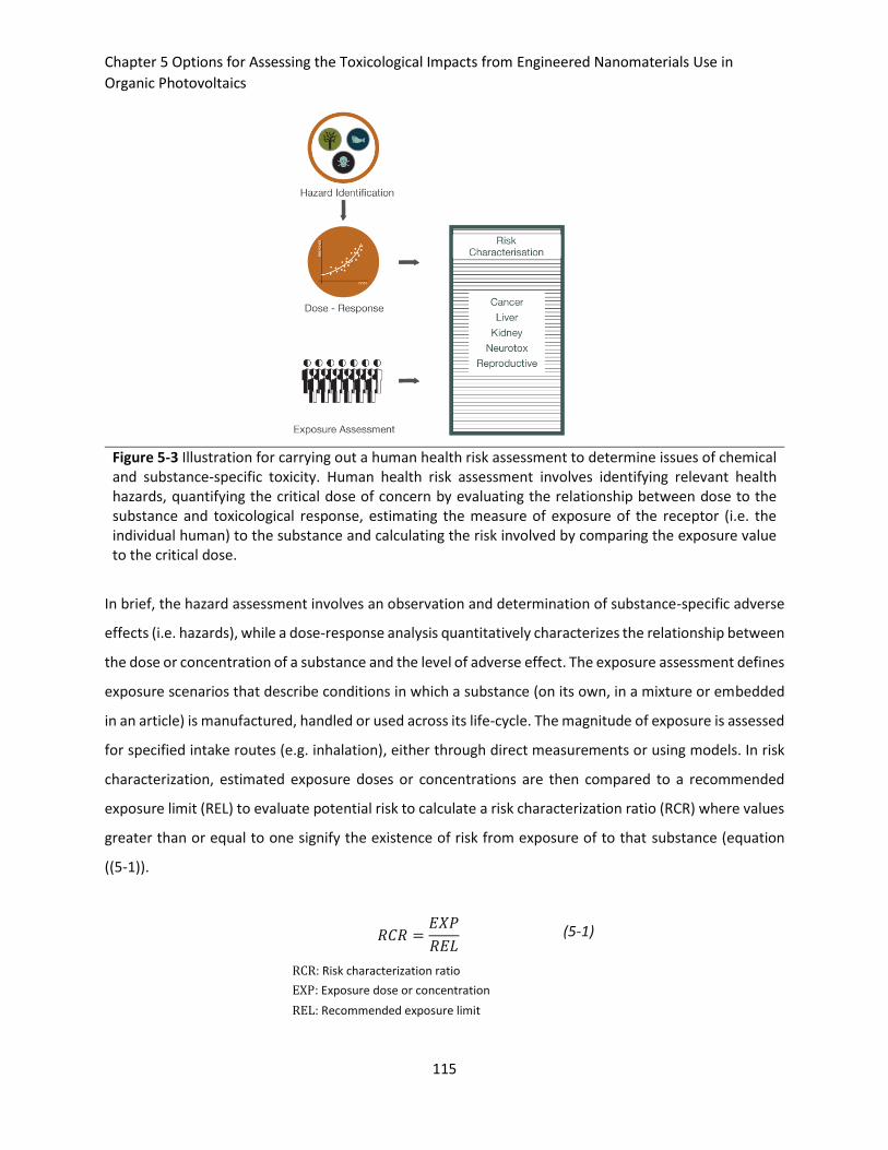
Chapter 5 Options for Assessing the Toxicological Impacts from Engineered Nanomaterials Use in
Organic Photovoltaics
115
Figure 5-3 Illustration for carrying out a human health risk assessment to determine issues of chemical and substance-specific toxicity. Human health risk assessment involves identifying relevant health hazards, quantifying the critical dose of concern by evaluating the relationship between dose to the substance and toxicological response, estimating the measure of exposure of the receptor (i.e. the individual human) to the substance and calculating the risk involved by comparing the exposure value to the critical dose.
In brief, the hazard assessment involves an observation and determination of substance-specific adverse
effects (i.e. hazards), while a dose-response analysis quantitatively characterizes the relationship between
the dose or concentration of a substance and the level of adverse effect. The exposure assessment defines
exposure scenarios that describe conditions in which a substance (on its own, in a mixture or embedded
in an article) is manufactured, handled or used across its life-cycle. The magnitude of exposure is assessed
for specified intake routes (e.g. inhalation), either through direct measurements or using models. In risk
characterization, estimated exposure doses or concentrations are then compared to a recommended
exposure limit (REL) to evaluate potential risk to calculate a risk characterization ratio (RCR) where values
greater than or equal to one signify the existence of risk from exposure of to that substance (equation
((5-1)).
𝑅𝐶𝑅 =𝐸𝑋𝑃
𝑅𝐸𝐿 (5-1)
RCR: Risk characterization ratio EXP: Exposure dose or concentration REL: Recommended exposure limit
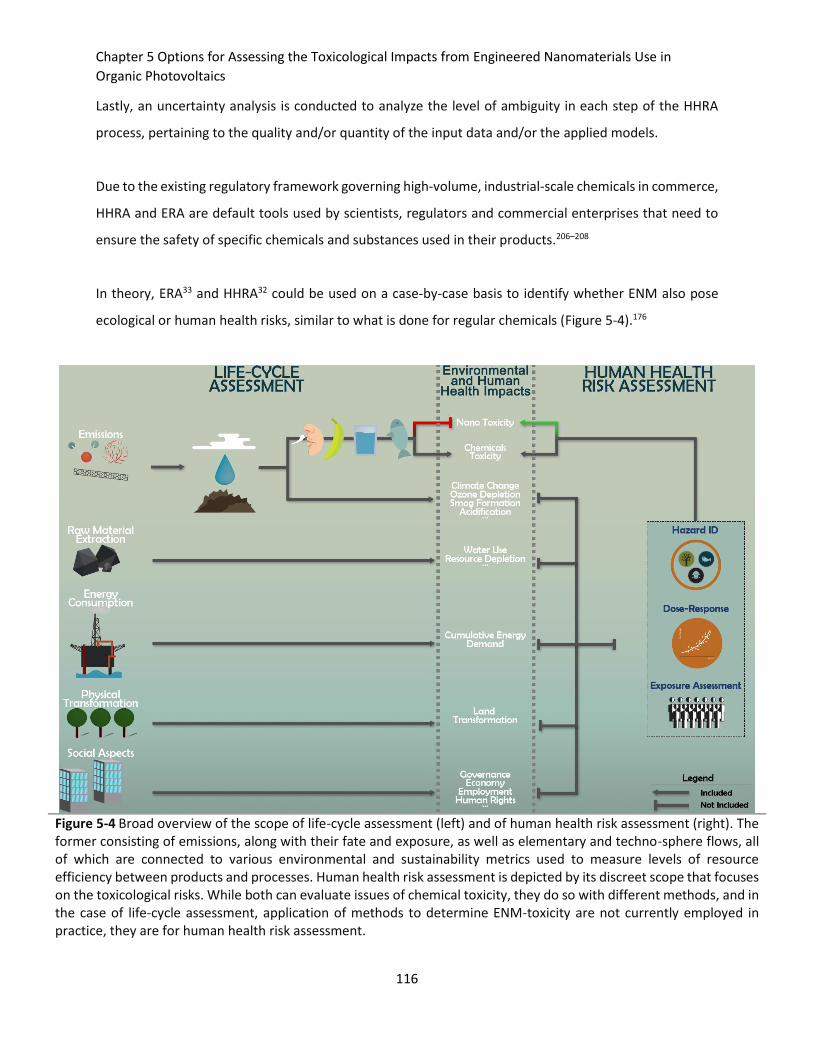
Chapter 5 Options for Assessing the Toxicological Impacts from Engineered Nanomaterials Use in
Organic Photovoltaics
116
Lastly, an uncertainty analysis is conducted to analyze the level of ambiguity in each step of the HHRA
process, pertaining to the quality and/or quantity of the input data and/or the applied models.
Due to the existing regulatory framework governing high-volume, industrial-scale chemicals in commerce,
HHRA and ERA are default tools used by scientists, regulators and commercial enterprises that need to
ensure the safety of specific chemicals and substances used in their products.206–208
In theory, ERA33 and HHRA32 could be used on a case-by-case basis to identify whether ENM also pose
ecological or human health risks, similar to what is done for regular chemicals (Figure 5-4).176
Figure 5-4 Broad overview of the scope of life-cycle assessment (left) and of human health risk assessment (right). The former consisting of emissions, along with their fate and exposure, as well as elementary and techno-sphere flows, all of which are connected to various environmental and sustainability metrics used to measure levels of resource efficiency between products and processes. Human health risk assessment is depicted by its discreet scope that focuses on the toxicological risks. While both can evaluate issues of chemical toxicity, they do so with different methods, and in the case of life-cycle assessment, application of methods to determine ENM-toxicity are not currently employed in practice, they are for human health risk assessment.
Chapter 5 Options for Assessing the Toxicological Impacts from Engineered Nanomaterials Use in
Organic Photovoltaics
117
However, HHRA is not immune to the same data and methodological gaps that have presented themselves
for LCA, and thus HHRA may not necessarily serve as a panacea to the question of human health impacts
for ENM-containing products such as OPV. For example, current HHRA efforts for ENM have not kept pace
with their production and use in industry. To date, the U.S. Environmental Protection Agency (U.S. EPA)
has released just one ENM-HHRA,209 while the U.S. National Institute of Occupational Safety and Health
(U.S. NIOSH) has released two ENM-specific occupational safety exposure levels.161,210 Data gaps in toxicity
and exposure assessments largely hinder the HHRA process from moving forward at sufficient
speed.174,211,212 While the U.S.213 and E.U.,181 for example, can demand and gather data to assist in the
HHRA procedure for ENM, an assessment of all registered ENM has not been completed. Although, some
data and modeling efforts can be bypassed in HHRA, for example, by directly measuring the exposure
doses or concentrations that one is subjected to. More commonly, however, qualitative HHRA214–217
approaches have been put forth for prioritizing research efforts, environmental management and
regulatory activities in the case of ENM. Nonetheless, many ENM-specific models, from those qualitative
control banding approaches218 to more sophisticated, dynamic approaches219,220 have been or are
currently being developed for ENM. Such tools are, thus, one option for addressing the human health
impacts of ENM used in OPV.
Complementary and Integrated Approaches for Life-Cycle Assessment and Risk
Assessment
Developing nanotechnologies in a responsible and sustainable way should require that the net value to
society is considered by considering their resource efficiencies as well as their potential human health and
environmental risks. The general tendency is for different stakeholders to focus on these issues as distinct
endpoints that must use distinct tools (e.g. LCA, HHRA, ERA), either out of familiarity or opinion, ultimately
excepting the exclusion of a more comprehensive viewpoint.74,221 Together, aspects from both LCA and
HHRA may provide an adequate understanding of this information.185,222–225 However, their use as
separate, distinct tools is only one potential option for doing so. In the remainder of this chapter, other
options for achieving this objective are presented and discussed in greater detail. These options will be
presented in a decision-depend context, exploring the application of ENM as an emerging technology and
the corresponding evaluation objectives that may present themselves at different stages of product
maturity. In total, five different options for using and combining LCA and HHRA for the environmental
evaluation of ENM-related technologies are discussed: one separate, one complementary, and three
integrative approaches.
Chapter 5 Options for Assessing the Toxicological Impacts from Engineered Nanomaterials Use in
Organic Photovoltaics
118
Separate Use of LCA and RA for Nanotechnologies
LCA and HHRA are two separate tools that have distinct methodologies and report different results. While
LCA allows the calculation of potential human health impacts from many competing sources of emissions
along the life-cycle, decision makers might find it useful to employ this tool at all stages of technology
development and eco-design purposes. However, for ENM-containing technologies, if evaluation of ENM
is not possible, decision makers may choose to simply use HHRA instead, particularly once product
development has increased to relatively large volumes, full-scale development or product adaption by
society requires that human health risks are avoided. This is because full scale development will require
registration with the appropriate regulatory agencies who may require HHRA knowledge as part of the
registration or compliance with agencies tasked with ensuring occupational and consumer protections.
While having the ability to provide definitive estimates of ENM human health risk, a critical drawback of
this option is the level of detail involved, which is not necessary in the case of early stage development of
products containing ENM. Consequently, these tools are often utilized separately by different types of
stakeholders who have distinctly different needs. Thus, the separate use of LCA or HHRA (i.e. without the
use of the other) for emerging technologies will be limited to one set of results but not the other as well
as limited by when along the development of the technology to use these tools.
Complementary Use of LCA and RA for Nanotechnologies
However, Complementary Use, defined by using both tools separately and then combining their results,
is an obvious approach when the evaluation of both the resource efficiencies and the human health
effects of ENM needs to be considered. This option thus necessarily involves a detailed assessment of the
exposure to and risk from ENM. Therefore, much like the Separate Use HHRA option discussed above,
Complementary Use will be most appropriate during full-scale technology development (Figure 5-5) or
when it is necessary to ensure human health safety.214,226,227
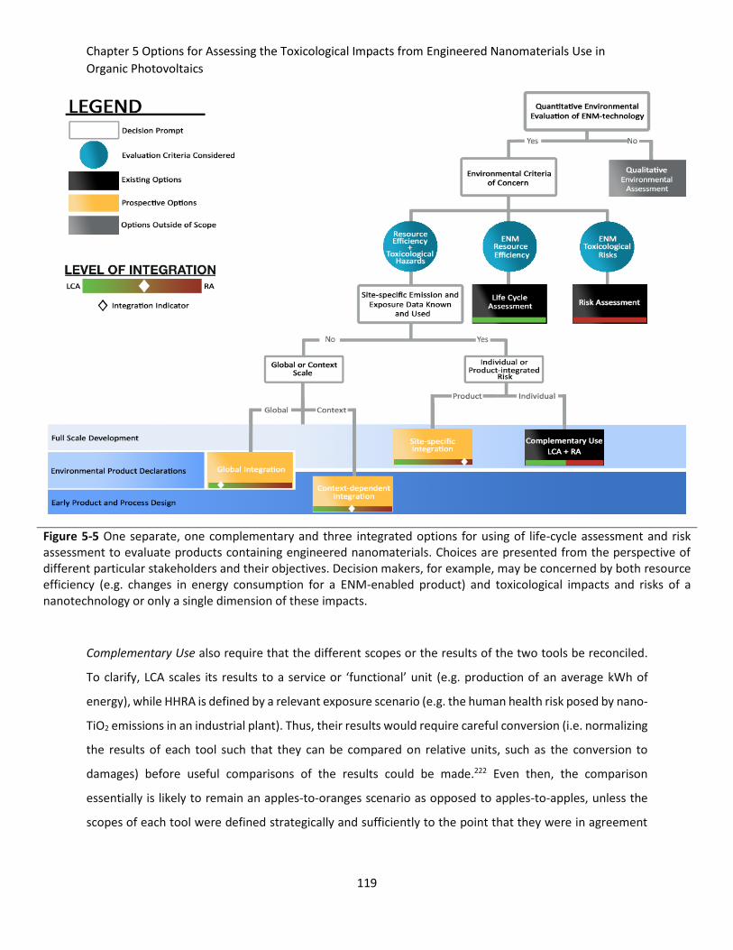
Chapter 5 Options for Assessing the Toxicological Impacts from Engineered Nanomaterials Use in
Organic Photovoltaics
119
Figure 5-5 One separate, one complementary and three integrated options for using of life-cycle assessment and risk assessment to evaluate products containing engineered nanomaterials. Choices are presented from the perspective of different particular stakeholders and their objectives. Decision makers, for example, may be concerned by both resource efficiency (e.g. changes in energy consumption for a ENM-enabled product) and toxicological impacts and risks of a nanotechnology or only a single dimension of these impacts.
Complementary Use also require that the different scopes or the results of the two tools be reconciled.
To clarify, LCA scales its results to a service or ‘functional’ unit (e.g. production of an average kWh of
energy), while HHRA is defined by a relevant exposure scenario (e.g. the human health risk posed by nano-
TiO2 emissions in an industrial plant). Thus, their results would require careful conversion (i.e. normalizing
the results of each tool such that they can be compared on relative units, such as the conversion to
damages) before useful comparisons of the results could be made.222 Even then, the comparison
essentially is likely to remain an apples-to-oranges scenario as opposed to apples-to-apples, unless the
scopes of each tool were defined strategically and sufficiently to the point that they were in agreement
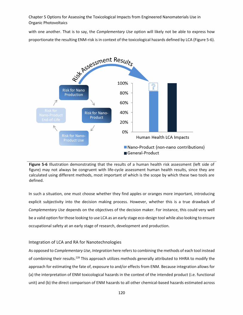
Chapter 5 Options for Assessing the Toxicological Impacts from Engineered Nanomaterials Use in
Organic Photovoltaics
120
with one another. That is to say, the Complementary Use option will likely not be able to express how
proportionate the resulting ENM-risk is in context of the toxicological hazards defined by LCA (Figure 5-6).
Figure 5-6 Illustration demonstrating that the results of a human health risk assessment (left side of figure) may not always be congruent with life-cycle assessment human health results, since they are calculated using different methods, most important of which is the scope by which these two tools are defined.
In such a situation, one must choose whether they find apples or oranges more important, introducing
explicit subjectivity into the decision making process. However, whether this is a true drawback of
Complementary Use depends on the objectives of the decision maker. For instance, this could very well
be a valid option for those looking to use LCA as an early stage eco-design tool while also looking to ensure
occupational safety at an early stage of research, development and production.
Integration of LCA and RA for Nanotechnologies
As opposed to Complementary Use, Integration here refers to combining the methods of each tool instead
of combining their results.228 This approach utilizes methods generally attributed to HHRA to modify the
approach for estimating the fate of, exposure to and/or effects from ENM. Because integration allows for
(a) the interpretation of ENM toxicological hazards in the context of the intended product (i.e. functional
unit) and (b) the direct comparison of ENM hazards to all other chemical-based hazards estimated across
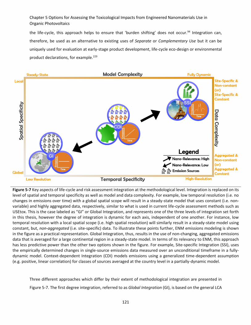
Chapter 5 Options for Assessing the Toxicological Impacts from Engineered Nanomaterials Use in
Organic Photovoltaics
121
the life-cycle, this approach helps to ensure that ‘burden shifting’ does not occur.94 Integration can,
therefore, be used as an alternative to existing uses of Separate or Complementary Use but it can be
uniquely used for evaluation at early-stage product development, life-cycle eco-design or environmental
product declarations, for example.229
Figure 5-7 Key aspects of life-cycle and risk assessment integration at the methodological level. Integration is replaced on its level of spatial and temporal specificity as well as model and data complexity. For example, low temporal resolution (i.e. no changes in emissions over time) with a global spatial scope will result in a steady-state model that uses constant (i.e. non-variable) and highly aggregated data, respectively, similar to what is used in current life-cycle assessment methods such as USEtox. This is the case labeled as “GI” or Global Integration, and represents one of the three levels of integration set forth in this thesis, however the degree of integration is dynamic for each axis, independent of one another. For instance, low temporal resolution with a local spatial scope (i.e. high spatial resolution) will similarly result in a steady-state model using constant, but, non-aggregated (i.e. site-specific) data. To illustrate these points further, ENM emissions modeling is shown in the figure as a practical representation. Global Integration, thus, results in the use of non-changing, aggregated emissions data that is averaged for a large continental region in a steady-state model. In terms of its relevancy to ENM, this approach has less predictive power than the other two options shown in the figure. For example, Site-specific Integration (SSI), uses the empirically determined changes in single-source emissions data measured over an unconditional timeframe in a fully-dynamic model. Context-dependent Integration (CDI) models emissions using a generalized time-dependent assumption (e.g. positive, linear correlation) for classes of sources averaged at the country level in a partially-dynamic model.
Three different approaches which differ by their extent of methodological integration are presented in
Figure 5-7. The first degree integration, referred to as Global Integration (GI), is based on the general LCA
Chapter 5 Options for Assessing the Toxicological Impacts from Engineered Nanomaterials Use in
Organic Photovoltaics
122
framework but supplemented with ENM-specific estimations of toxicity, for example, using the USEtox
life-cycle impact assessment approach.93–96,197 Global Integration, represents a feasible, first-tier tool that
covers the scope of both resource efficiency and toxicological hazards. It is particularly well-suited for
supporting eco-design or environmental product declarations which must be evaluated using current LCA
standards. However, this approach relies on the predominant tools available, which ignore spatial and
temporal acuity in both the life-cycle inventory and also the estimations of fate, exposure and hazard.
Models that do not possess sufficient spatial or temporal resolution cannot incorporate specific
environmental details and exposure conditions necessary for appropriately estimating the fate of, and
exposure to ENM, as discussed earlier in this chapter.97 ENM are also influenced by both physical and
molecular forces akin to colloidal materials, leading to an array of transformations (e.g. aggregation) that
are important in determining their fate and exposure.174,198,211,230 The context setting (e.g. indoor versus
outdoor emissions) and their local landscape parameters (e.g. ventilation rates) will also influence these
behaviors in important ways.
Thus, emission, fate and exposure models that incorporate more spatial and temporal detail would be
more appropriate for and increase the predictive power of ENM evaluation. Therefore, two further
degrees of integration are considered: Context-dependent Integration (CDI) and Site-specific Integration
(SSI) that represent models with greater levels of time and spatial resolution compared to Global
Integration (Figure 5-7). Context-dependent Integration relies on models whose underlying parameters
(e.g. emission magnitude, ENM size) are estimated per ‘group’ or ‘class’. Groupings can be applied, but
not limited, to emission sources (e.g. workplace activity), emission pattern (e.g. constant), emission time-
frame, ENM-type (e.g. size), and conditions of the receiving compartment (e.g. ventilation rates).231
Classes should be defined by statistically significant generalizations such that impact results differ from
class to class but not within each class.232 For example, statistically determined environmental conditions
(e.g. meteorological data), operating parameters (e.g. stack height of emissions source) and receptor
densities of the air pollution emissions were determined for waste treatment sites across Spain.232 In this
way, the spatial distribution around an emission point could be considered for estimating the
concentration increment per receptor in geographically distinguishable environments. Indoor air ENM
emissions and exposure scenarios could prove an extremely practical first case-study of the Context-
dependent Integration approach, given that indoor environmental conditions are more constrained than
ambient ones. Indoor, occupational scenarios may even present conditions whereby ENM fate and
transport are more dependent on workplace conditions rather than ENM characteristics.97,233 These
Chapter 5 Options for Assessing the Toxicological Impacts from Engineered Nanomaterials Use in
Organic Photovoltaics
123
conditions, together, could allow for the relatively simplified grouping of indoor, occupational model
parameters, similar to what has been done for regular chemicals in residential indoor air,234,235 industrial
processes232 and consumer products.236–238
Site-specific Integration is the third-degree of the most ideal form of integration, whereby complete
spatial and temporal resolution is known and incorporated into a fully-dynamic set of emission, fate and
exposure models (Figure 5-7). This approach also assumes that all ENM emissions are known and
quantifiable across the life-cycle of the ENM-containing product. Site-specific Integration would provide
the most accurate results (e.g. absolute impact values), however it can only be applied on a case-by-case
approach because of how inclusive the data and model requirements would be. The latter point most
fitting for full-scale development and/or the need to ensure human health or ecological safety. Mature
nanotechnology market products, such as certain paints and pigments, have well-established
manufacturing routes, production volumes and intended uses that pose potential exposures across the
life-cycle. In such real-world scenarios, absolute damage and evaluations of risk are necessary to ensure
human health safety, local ecosystem integrity and ensure regulatory compliance. While Complementary
Use would essentially allow an analogous evaluation of both the environmental resource efficiencies and
risks of products containing ENM, as was discussed in the section above, this assessment option lacks
harmony in the scopes of the two tools, leading to greater difficulty in interpreting the distinct LCA and
RA results. Furthermore, it should be noted that as the number of ENM-emitting processes along the life-
cycle become large (e.g. > 20), data collection may become untenable and the option of Site-specific
Integration impractical.232 As an alternative in such a situation, a special case of the Complementary Use
approach might involve using Global Integration or Context-dependent Integration to identify the ENM
emission hot-spots of greatest concern, which could then be followed by RA where it is warranted (e.g.
where ENM emissions contribute to a noticeably large fraction of the total human health impact across
the life-cycle).
On the contrary, the level of data and model detail that is required of Site-specific Integration or
Complementary Use would be unnecessary in cases of early product and process design of
nanotechnologies since localized (i.e. site-specific) environmental conditions and operating parameters
would not be known. To illustrate more clearly in context of this thesis, 3rd-generation PV devices are a
mostly lab-scale technology that exploit the photoelectric properties of ENM for their functionality. In
Chapter 3 and Chapter 4, use of LCA as a single tool demonstrated the resource efficiency of these devices
Chapter 5 Options for Assessing the Toxicological Impacts from Engineered Nanomaterials Use in
Organic Photovoltaics
124
such as potential to reduce embodied energy and carbon of PV. However, those results lack any
estimation of the direct toxicological hazards ENM pose to humans across the life-cycle. According to
Figure 5-5 a decision-maker at early-stage development (e.g. lab- or pilot-scale) concerned with
addressing both the resource efficiency and the toxicological hazards would find Global Integration and/or
Context-dependent Integration most suits their needs (i.e. effective hot-spot analysis to identify where in
the life-cycle toxicological impacts and eventually risks may occur). This is because at the current scale of
OPV development, there is too much uncertainty in production volumes or operating conditions, for
example, and thus spending resources to determine the absolute damages (i.e. using Site-specific
Integration) or risks (i.e. using Complementary Use) posed by ENM in such scenarios would have little to
no basis.
Conclusion
LCA and HHRA offer decision makers the ability to evaluate the resource efficiencies and human health
risks of their products and substances within their products, respectively, such as OPV. Specifically, LCA
was used in Chapter 3 and Chapter 4 to compare the environmental and human health impacts of OPV
with silicon-based PV. The results of those chapters demonstrate that OPV benefit from greater resource
efficiency and have lower relative impacts overall. However, the results did not include the potential
human health impacts from ENM.
The separate or complementary use of HHRA could potentially provide a solution to this assessment gap.
Making use of the HHRA makes most sense at the point of full-scale development or ensuring human
health safety is required. Conversely, the detailed data needs required to complete a HHRA at early-stage
product development would be highly uncertain and largely unwarranted. Instead, integrating HHRA
approaches into LCA could provide an alternative option that is more appropriate for early-stage
development and eco-design purposes, for example. Unfortunately, a lack of relevant data for most types
of ENM remains a barrier for conducting both HHRA as well as LCA, and without such data neither
approach will be feasible, let alone present opportunities for integration. For example, without known
ENM emissions a life-cycle inventory cannot be calculated nor can an exposure assessment in HHRA be
made. The same is true for ENM-specific data that is required for building fate and exposure models and
determining dose-response relationship for both life-cycle impact assessment as well as HHRA.
Chapter 5 Options for Assessing the Toxicological Impacts from Engineered Nanomaterials Use in
Organic Photovoltaics
125
While data is currently limited for ENM, materials such as certain metals, metal oxides and carbon based
ENM have relatively more reported data in the literature compared with others and can serve as starting
points for establishing HHRA or integrated, dynamic life-cycle impact assessment models similar to what
has been done for steady-state models.93–96 This is quite relevant for the case of OPV who use both carbon
and metal-oxide ENM in their material layers and thus could be used to make further evaluations of the
potential human health impacts resulting from the use of ENM in OPV. In terms of the three integrative
approaches presented in this chapter, the previous steady-state adaptations made for these materials are
what is referred to as Global Integration in this chapter. Given its use of existing steady-state models, this
could serve as an immediate and near-term (i.e. circa 5 years) objective for most ENM evaluations.
However, as described previously, this approach also has less relevance for certain fate and exposure
processes and, thus, less predictive power for estimating ENM human health impacts. Context-dependent
Integration, on the other hand, can introduce a more dynamic process to the modeling approach and,
hence, more relevant estimations of fate, exposure and impacts. This integration option will require
greater coordination among the scientific community to identify the relevant data and appropriate
emission, fate and exposure ‘classes’ that will be relevant to ENM development and uses.
In view of these potential options, Chapter 6 presents a more focused HHRA for the carbon and metal
oxide ENM used in OPV. Chapter 7 then uses the approach and lessons learned from the HHRA to
construct a Context-dependent Integration life-cycle impact assessment approach for estimating human
health impacts of ENM.
Chapter 6 Human Health Risk Assessments: Quantitative Assessment of Titanium Dioxide and Qualitative Assessment of C60 Fullerene Nanoparticles
126
Chapter 6 Human Health Risk Assessments: Quantitative Assessment of
Titanium Dioxide and Qualitative Assessment of C60 Fullerene
Nanoparticles
Chapter 3 and Chapter 4 explored the environmental and human health impacts of OPV technologies,
their uses and their end-of-life considerations. The results of those assessments demonstrate that OPV
have greater resource efficiencies and lower relative environmental and human health hazards compared
with their silicon-based counterparts. Chapter 5 highlighted the absence of ENM-specific life-cycle
inventory flows to the environment as well as the absence of their corresponding potential human health
impacts in those LCA studies. A further analysis was provided in Chapter 5 regarding life-cycle impact
assessment methodologies and HHRA, specifically what opportunities exist to use these tools in a
complementary or integrative way in order to provide a comprehensive evaluation of the environmental
and human health impacts of OPV technologies that use ENM. In this current chapter, HHRA is used as a
preliminary tool to evaluate the human health risks of those ENM, and then key methodological HHRA
aspects are identified that can be integrated within life-cycle impact assessment methods.
Qualitative (Screening Level) Human Health Risk Assessment
Qualitative Exposure Assessment
As was discussed in Chapter 5, data and methodological gaps for HHRA present challenges to fully
implementing this tool across the entire life-cycle of OPV devices. Thus, it was out of the scope of this
thesis to focus quantitatively on all exposure scenarios (Figure 6-1) nor the risk therein posed by both
PCBM and nano-TiO2.
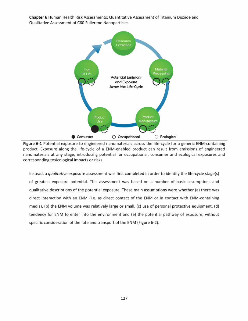
Chapter 6 Human Health Risk Assessments: Quantitative Assessment of Titanium Dioxide and Qualitative Assessment of C60 Fullerene Nanoparticles
127
Figure 6-1 Potential exposure to engineered nanomaterials across the life-cycle for a generic ENM-containing product. Exposure along the life-cycle of a ENM-enabled product can result from emissions of engineered nanomaterials at any stage, introducing potential for occupational, consumer and ecological exposures and corresponding toxicological impacts or risks.
Instead, a qualitative exposure assessment was first completed in order to identify the life-cycle stage(s)
of greatest exposure potential. This assessment was based on a number of basic assumptions and
qualitative descriptions of the potential exposure. These main assumptions were whether (a) there was
direct interaction with an ENM (i.e. as direct contact of the ENM or in contact with ENM-containing
media), (b) the ENM volume was relatively large or small, (c) use of personal protective equipment, (d)
tendency for ENM to enter into the environment and (e) the potential pathway of exposure, without
specific consideration of the fate and transport of the ENM (Figure 6-2).
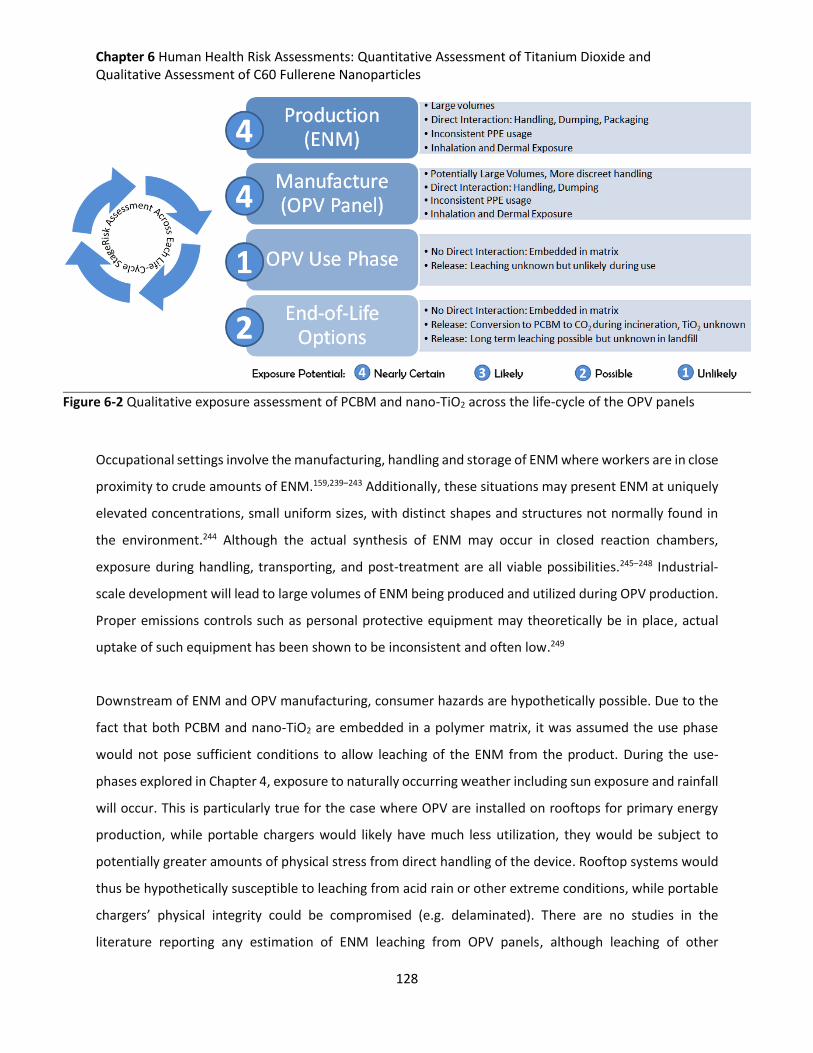
Chapter 6 Human Health Risk Assessments: Quantitative Assessment of Titanium Dioxide and Qualitative Assessment of C60 Fullerene Nanoparticles
128
Figure 6-2 Qualitative exposure assessment of PCBM and nano-TiO2 across the life-cycle of the OPV panels
Occupational settings involve the manufacturing, handling and storage of ENM where workers are in close
proximity to crude amounts of ENM.159,239–243 Additionally, these situations may present ENM at uniquely
elevated concentrations, small uniform sizes, with distinct shapes and structures not normally found in
the environment.244 Although the actual synthesis of ENM may occur in closed reaction chambers,
exposure during handling, transporting, and post-treatment are all viable possibilities.245–248 Industrial-
scale development will lead to large volumes of ENM being produced and utilized during OPV production.
Proper emissions controls such as personal protective equipment may theoretically be in place, actual
uptake of such equipment has been shown to be inconsistent and often low.249
Downstream of ENM and OPV manufacturing, consumer hazards are hypothetically possible. Due to the
fact that both PCBM and nano-TiO2 are embedded in a polymer matrix, it was assumed the use phase
would not pose sufficient conditions to allow leaching of the ENM from the product. During the use-
phases explored in Chapter 4, exposure to naturally occurring weather including sun exposure and rainfall
will occur. This is particularly true for the case where OPV are installed on rooftops for primary energy
production, while portable chargers would likely have much less utilization, they would be subject to
potentially greater amounts of physical stress from direct handling of the device. Rooftop systems would
thus be hypothetically susceptible to leaching from acid rain or other extreme conditions, while portable
chargers’ physical integrity could be compromised (e.g. delaminated). There are no studies in the
literature reporting any estimation of ENM leaching from OPV panels, although leaching of other
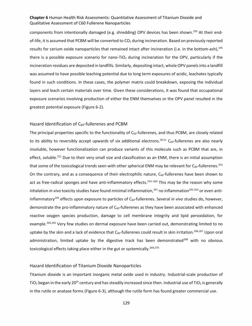
Chapter 6 Human Health Risk Assessments: Quantitative Assessment of Titanium Dioxide and Qualitative Assessment of C60 Fullerene Nanoparticles
129
components from intentionally damaged (e.g. shredding) OPV devices has been shown.250 At their end-
of-life, it is assumed that PCBM will be converted to CO2 during incineration. Based on previously reported
results for cerium oxide nanoparticles that remained intact after incineration (i.e. in the bottom-ash),195
there is a possible exposure scenario for nano-TiO2 during incineration for the OPV, particularly if the
incineration residues are deposited in landfills. Similarly, depositing intact, whole OPV panels into a landfill
was assumed to have possible leaching potential due to long term exposures of acidic, leachates typically
found in such conditions. In these cases, the polymer matrix could breakdown, exposing the individual
layers and leach certain materials over time. Given these considerations, it was found that occupational
exposure scenarios involving production of either the ENM themselves or the OPV panel resulted in the
greatest potential exposure (Figure 6-2).
Hazard Identification of C60-fullerenes and PCBM
The principal properties specific to the functionality of C60-fullerenes, and thus PCBM, are closely related
to its ability to reversibly accept upwards of six additional electrons.50,51 C60-fullerenes are also nearly
insoluble, however functionalization can produce variants of this molecule such as PCBM that are, in
effect, soluble.251 Due to their very small size and classification as an ENM, there is an initial assumption
that some of the toxicological trends seen with other spherical ENM may be relevant for C60-fullerenes.252
On the contrary, and as a consequence of their electrophilic nature, C60-fullerenes have been shown to
act as free-radical sponges and have anti-inflammatory effects.253–260 This may be the reason why some
inhalation in vivo toxicity studies have found minimal inflammation,261 no inflammation262,263 or even anti-
inflammatory259 effects upon exposure to particles of C60-fullerenes. Several in vivo studies do, however,
demonstrate the pro-inflammatory nature of C60-fullerenes as they have been associated with enhanced
reactive oxygen species production, damage to cell membrane integrity and lipid peroxidation, for
example.264,265 Very few studies on dermal exposure have been carried out, demonstrating limited to no
uptake by the skin and a lack of evidence that C60-fullerenes could result in skin irritation.266,267 Upon oral
administration, limited uptake by the digestive track has been demonstrated268 with no obvious
toxicological effects taking place either in the gut or systemically.269,270
Hazard Identification of Titanium Dioxide Nanoparticles
Titanium dioxide is an important inorganic metal oxide used in industry. Industrial-scale production of
TiO2 began in the early 20th century and has steadily increased since then. Industrial use of TiO2 is generally
in the rutile or anatase forms (Figure 6-3), although the rutile form has found greater commercial use.
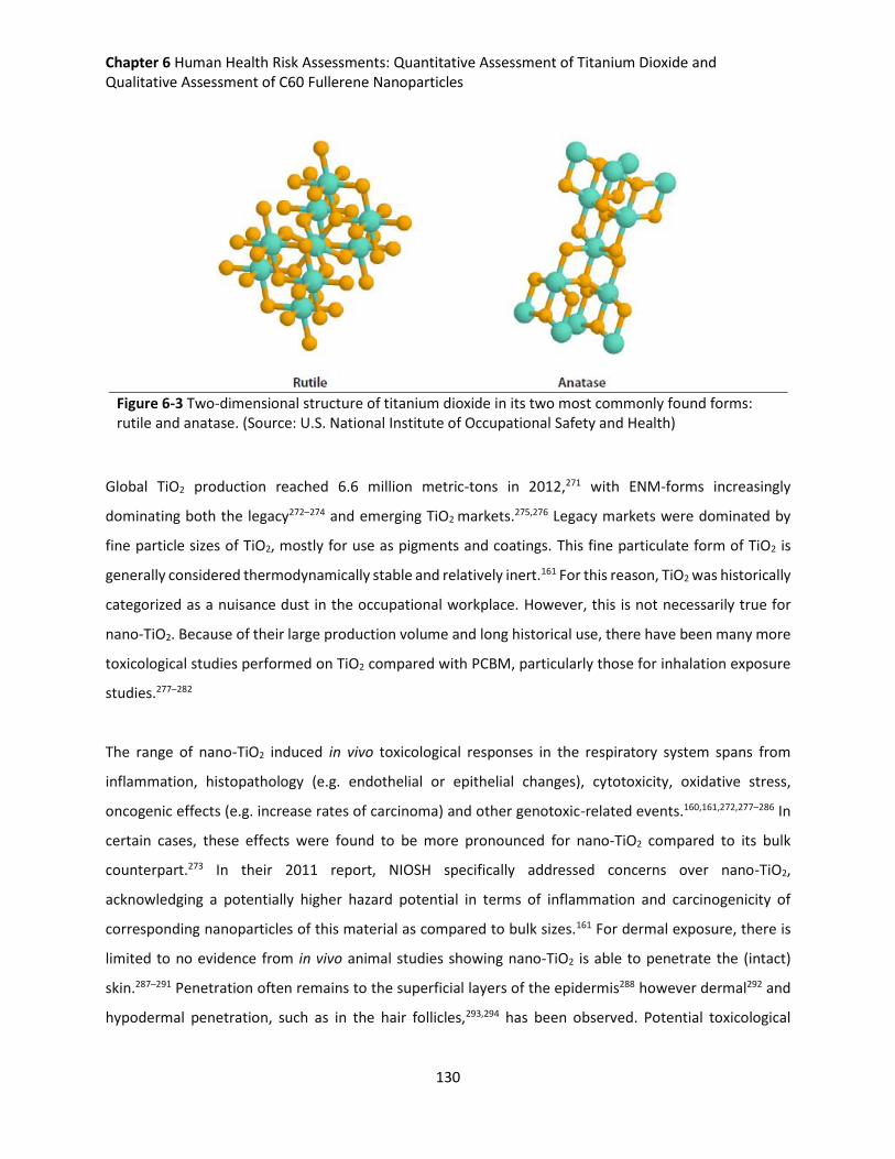
Chapter 6 Human Health Risk Assessments: Quantitative Assessment of Titanium Dioxide and Qualitative Assessment of C60 Fullerene Nanoparticles
130
Figure 6-3 Two-dimensional structure of titanium dioxide in its two most commonly found forms: rutile and anatase. (Source: U.S. National Institute of Occupational Safety and Health)
Global TiO2 production reached 6.6 million metric-tons in 2012,271 with ENM-forms increasingly
dominating both the legacy272–274 and emerging TiO2 markets.275,276 Legacy markets were dominated by
fine particle sizes of TiO2, mostly for use as pigments and coatings. This fine particulate form of TiO2 is
generally considered thermodynamically stable and relatively inert.161 For this reason, TiO2 was historically
categorized as a nuisance dust in the occupational workplace. However, this is not necessarily true for
nano-TiO2. Because of their large production volume and long historical use, there have been many more
toxicological studies performed on TiO2 compared with PCBM, particularly those for inhalation exposure
studies.277–282
The range of nano-TiO2 induced in vivo toxicological responses in the respiratory system spans from
inflammation, histopathology (e.g. endothelial or epithelial changes), cytotoxicity, oxidative stress,
oncogenic effects (e.g. increase rates of carcinoma) and other genotoxic-related events.160,161,272,277–286 In
certain cases, these effects were found to be more pronounced for nano-TiO2 compared to its bulk
counterpart.273 In their 2011 report, NIOSH specifically addressed concerns over nano-TiO2,
acknowledging a potentially higher hazard potential in terms of inflammation and carcinogenicity of
corresponding nanoparticles of this material as compared to bulk sizes.161 For dermal exposure, there is
limited to no evidence from in vivo animal studies showing nano-TiO2 is able to penetrate the (intact)
skin.287–291 Penetration often remains to the superficial layers of the epidermis288 however dermal292 and
hypodermal penetration, such as in the hair follicles,293,294 has been observed. Potential toxicological
Chapter 6 Human Health Risk Assessments: Quantitative Assessment of Titanium Dioxide and Qualitative Assessment of C60 Fullerene Nanoparticles
131
effects from dermal exposure range from limited to no skin irritation295 to oxidative stress296 and lesions
in certain organ systems.292 Oral administration to animals has demonstrated their uptake particularly to
the liver but also other organs such as the kidney, brain and testes.297 Potential toxicological effects from
oral exposure range from oxidative stress and neorinflammation298 to necropathy,297,299,300 for example.
Relevance of the Qualitative Exposure Assessment and Hazard Data Availability
The limitations to conducting a quantitative HHRA rest on the data availability and/or appropriate models
available. For example, toxicological data with multiple dosing groups is required to complete a dose-
response analysis. Such data should also involve relevant exposure routes (e.g. inhalation as opposed to
instillation) and preferably as long-term studies (e.g. chronic). Thus, the lack sufficient positively
correlated toxicological data on C60-fullerenes or PCBM, particularly for in vivo long-term, multi-dose
studies precludes its further analysis from the HHRA. This decision not to carry out a quantitative HHRA
on C60-fullerenes should not be seen as a formal determination that these materials pose no human health
risk across the life-cycle of OPV, since as the qualitative exposure assessment discussed, there is a high
likelihood that emissions will occur along the OPV life-cycle. On the other hand, current human health
relevant toxicological literature does not point to clear and consistent adverse responses nor is there
sufficient data to carry out a quantitative assessment. There is, however, sufficient evidence in the
literature points to both adverse non-cancerous and cancerous, chronic and sub-chronic human relevant
toxicity of nano-TiO2. Sufficient data also exist to carry out an appropriate dose-response analysis of this
material. The remainder of this chapter focuses on the quantitative HHRA of nano-TiO2 in occupational
exposure scenarios in the OPV life-cycle.
Quantitative Risk Assessment
Methods
As described in Chapter 5, the four principle steps of HHRA involve (1) hazard identification, (2) dose-
response assessment, (3) exposure assessment, and (4) risk characterization (Figure 5-3). Hazard
identification and the background on PCBM and nano-TiO2’s toxicological concerns were addressed in the
previous section of this chapter as a part of the qualitative HHRA. The methods sections below will
describe steps (2), (3) and (4) in greater detail.

Chapter 6 Human Health Risk Assessments: Quantitative Assessment of Titanium Dioxide and Qualitative Assessment of C60 Fullerene Nanoparticles
132
Dose-Response Assessment
The benchmark dose (BMD) method was used to quantify the exposure concentration at which the
adverse health effect occurs (i.e. dose-response relationship). This concentration was estimated from the
corresponding, pre-defined benchmark response (BMR). The BMD is an alternative to the no-observed-
adverse-effect-level (NOAEL) and lowest-observed-adverse-effect-level (LOAEL). In this chapter, the
terminology benchmark concentration (BMC) is used to clarify that the dose-response modeling used data
correlating to exposure concentrations from whole body animal studies. Calculation of the BMC was
completed using the Netherland’s National Institute for Public Health and the Environment’s (RIVM)
PROAST software (www.rivm.nl). PROAST was used to first calculate a BMCanimal (BMCa) based on the in
vivo animal data. This value was converted to a distribution using PROAST’s parametric bootstrap option
(i.e. sampling with replacement) over 10,000 simulations. The BMCa was extrapolated to a human effect
threshold referred to as the BMChuman (BMCh), by applying the appropriate extrapolation factors301 using
equation (6-1):
BMCh =BMCa
EFinter ∙ EFintra ∙ UFi (6-1)
BMCh: Human equivalent benchmark concentration
BMCa: Benchmark concentration based on animal toxicological data EFinter: Interspecies extrapolation factor
EFintra: Intraspecies extrapolation factor
UFi: sources of uncertainty (i)
Extrapolation factors represent differences between and among species according to anatomical
differences (e.g. body size) and physiological functions (e.g. metabolism). Values are scaled with the
extrapolation factors according the allocation scaling principle. The difference (i.e. increase) in breathing
rates for persons exposed in the occupational setting are assumed to be elevated compared to persons
at rest or not working and are captured within the EFintra. Log-normal distributions for these factors were
defined using similar approaches presented by Slob et al.302 A brief rationale follows. Biological
mechanisms in a population (e.g. survival times after disease onset) are generally asymmetrical as
opposed to being described by normal “bell-shape” curves.303 In deterministic HHRA procedures, it is
typical to use factors of ten to extrapolate to conservative yet acceptable human equivalent doses.
Although extrapolation factors of ten are supposed to be conservative protective values, it is understood
that this does not always provide protection. However, for transparency, demonstration of the approach,
and ease of interpretation the log-normal distributions were defined such that a value of ten was one-
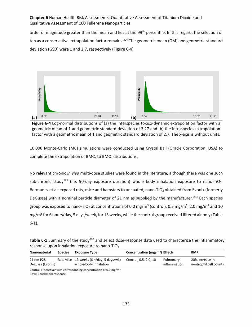
Chapter 6 Human Health Risk Assessments: Quantitative Assessment of Titanium Dioxide and Qualitative Assessment of C60 Fullerene Nanoparticles
133
order of magnitude greater than the mean and lies at the 99th-percentile. In this regard, the selection of
ten as a conservative extrapolation factor remains.304 The geometric mean (GM) and geometric standard
deviation (GSD) were 1 and 2.7, respectively (Figure 6-4).
(a) (b)
Figure 6-4 Log-normal distributions of (a) the interspecies toxico-dynamic extrapolation factor with a geometric mean of 1 and geometric standard deviation of 3.27 and (b) the intraspecies extrapolation factor with a geometric mean of 1 and geometric standard deviation of 2.7. The x-axis is without units.
10,000 Monte-Carlo (MC) simulations were conducted using Crystal Ball (Oracle Corporation, USA) to
complete the extrapolation of BMCa to BMCh distributions.
No relevant chronic in vivo multi-dose studies were found in the literature, although there was one such
sub-chronic study283 (i.e. 90-day exposure duration) whole body inhalation exposure to nano-TiO2.
Bermudez et al. exposed rats, mice and hamsters to uncoated, nano-TiO2 obtained from Evonik (formerly
DeGussa) with a nominal particle diameter of 21 nm as supplied by the manufacturer.283 Each species
group was exposed to nano-TiO2 at concentrations of 0.0 mg/m3 (control), 0.5 mg/m3, 2.0 mg/m3 and 10
mg/m3 for 6 hours/day, 5 days/week, for 13 weeks, while the control group received filtered air only (Table
6-1).
Table 6-1 Summary of the study283 and select dose-response data used to characterize the inflammatory response upon inhalation exposure to nano-TiO2
Nanomaterial Species Exposure Type Concentration (mg/m3) Effects BMR
21 nm P25 Degussa (Evonik)
Rat, Mice 13 weeks (6 h/day; 5 days/wk) whole-body inhalation
Control, 0.5, 2.0, 10 Pulmonary inflammation
20% increase in neutrophil cell counts
Control: Filtered air with corresponding concentration of 0.0 mg/m3 BMR: Benchmark response
0.02 29.48 38.91
Pro
bab
ility
0.04 16.32 21.53
Pro
bab
ility
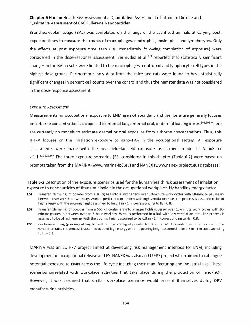
Chapter 6 Human Health Risk Assessments: Quantitative Assessment of Titanium Dioxide and Qualitative Assessment of C60 Fullerene Nanoparticles
134
Bronchoalveolar lavage (BAL) was completed on the lungs of the sacrificed animals at varying post-
exposure times to measure the counts of macrophages, neutrophils, eosinophils and lymphocytes. Only
the effects at post exposure time zero (i.e. immediately following completion of exposure) were
considered in the dose-response assessment. Bermudez et al.283 reported that statistically significant
changes in the BAL results were limited to the macrophages, neutrophil and lymphocyte cell types in the
highest dose-groups. Furthermore, only data from the mice and rats were found to have statistically
significant changes in percent cell counts over the control and thus the hamster data was not considered
in the dose-response assessment.
Exposure Assessment
Measurements for occupational exposure to ENM are not abundant and the literature generally focuses
on airborne concentrations as opposed to internal lung, internal oral, or dermal loading doses.305,306 There
are currently no models to estimate dermal or oral exposure from airborne concentrations. Thus, this
HHRA focuses on the inhalation exposure to nano-TiO2 in the occupational setting. All exposure
assessments were made with the near-field–far-field exposure assessment model in NanoSafer
v.1.1.219,220,307 The three exposure scenarios (ES) considered in this chapter (Table 6-2) were based on
prompts taken from the MARINA (www.marina-fp7.eu) and NANEX (www.nanex-project.eu) databases.
Table 6-2 Description of the exposure scenarios used for the human health risk assessment of inhalation exposure to nanoparticles of titanium dioxide in the occupational workplace. Hi: handling energy factor.
ES1 Transfer (dumping) of powder from a 10 kg bag into a mixing tank over 10-minute work cycles with 10-minute pauses in-between over an 8-hour workday. Work is performed in a room with high ventilation rate. The process is assumed to be of high energy with the pouring height assumed to be 0.3 m - 1 m corresponding to Hi = 0.8.
ES2 Transfer (dumping) of powder from a 560 kg containers into a larger holding vessel over 10-minute work cycles with 20-minute pauses in-between over an 8-hour workday. Work is performed in a hall with low ventilation rate. The process is assumed to be of high energy with the pouring height assumed to be 0.3 m - 1 m corresponding to Hi = 0.8.
ES3 Continuous filling (pouring) of bag bin with a total 250 kg of powder for 8 hours. Work is performed in a room with low ventilation rate. The process is assumed to be of high energy with the pouring height assumed to be 0.3 m - 1 m corresponding to Hi = 0.8.
MARINA was an EU FP7 project aimed at developing risk management methods for ENM, including
development of occupational release and ES. NANEX was also an EU FP7 project which aimed to catalogue
potential exposure to EMN across the life-cycle including their manufacturing and industrial use. These
scenarios correlated with workplace activities that take place during the production of nano-TiO2.
However, it was assumed that similar workplace scenarios would present themselves during OPV
manufacturing activities.
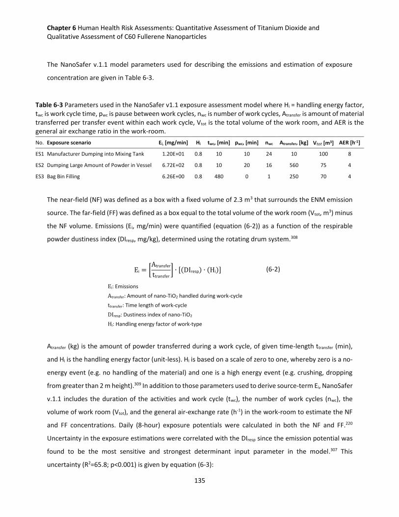
Chapter 6 Human Health Risk Assessments: Quantitative Assessment of Titanium Dioxide and Qualitative Assessment of C60 Fullerene Nanoparticles
135
The NanoSafer v.1.1 model parameters used for describing the emissions and estimation of exposure
concentration are given in Table 6-3.
Table 6-3 Parameters used in the NanoSafer v1.1 exposure assessment model where Hi = handling energy factor, twc is work cycle time, pwc is pause between work cycles, nwc is number of work cycles, Atransfer is amount of material transferred per transfer event within each work cycle, Vtot is the total volume of the work room, and AER is the general air exchange ratio in the work-room.
No. Exposure scenario Ei, [mg/min] Hi twc, [min] pwc, [min] nwc Atransfer, [kg] Vtot [m3] AER [h-1]
ES1 Manufacturer Dumping into Mixing Tank 1.20E+01 0.8 10 10 24 10 100 8
ES2 Dumping Large Amount of Powder in Vessel 6.72E+02 0.8 10 20 16 560 75 4
ES3 Bag Bin Filling 6.26E+00 0.8 480 0 1 250 70 4
The near-field (NF) was defined as a box with a fixed volume of 2.3 m3 that surrounds the ENM emission
source. The far-field (FF) was defined as a box equal to the total volume of the work room (Vtot, m3) minus
the NF volume. Emissions (Ei, mg/min) were quantified (equation (6-2)) as a function of the respirable
powder dustiness index (DIresp, mg/kg), determined using the rotating drum system.308
Ei = [Atransfer
ttransfer] ∙ [(DIresp) ∙ (Hi)] (6-2)
Ei: Emissions
Atransfer: Amount of nano-TiO2 handled during work-cycle
ttransfer: Time length of work-cycle
DIresp: Dustiness index of nano-TiO2
Hi: Handling energy factor of work-type
Atransfer (kg) is the amount of powder transferred during a work cycle, of given time-length ttransfer (min),
and Hi is the handling energy factor (unit-less). Hi is based on a scale of zero to one, whereby zero is a no-
energy event (e.g. no handling of the material) and one is a high energy event (e.g. crushing, dropping
from greater than 2 m height).309 In addition to those parameters used to derive source-term Ei, NanoSafer
v.1.1 includes the duration of the activities and work cycle (twc), the number of work cycles (nwc), the
volume of work room (Vtot), and the general air-exchange rate (h-1) in the work-room to estimate the NF
and FF concentrations. Daily (8-hour) exposure potentials were calculated in both the NF and FF.220
Uncertainty in the exposure estimations were correlated with the DIresp since the emission potential was
found to be the most sensitive and strongest determinant input parameter in the model.307 This
uncertainty (R2=65.8; p<0.001) is given by equation (6-3):
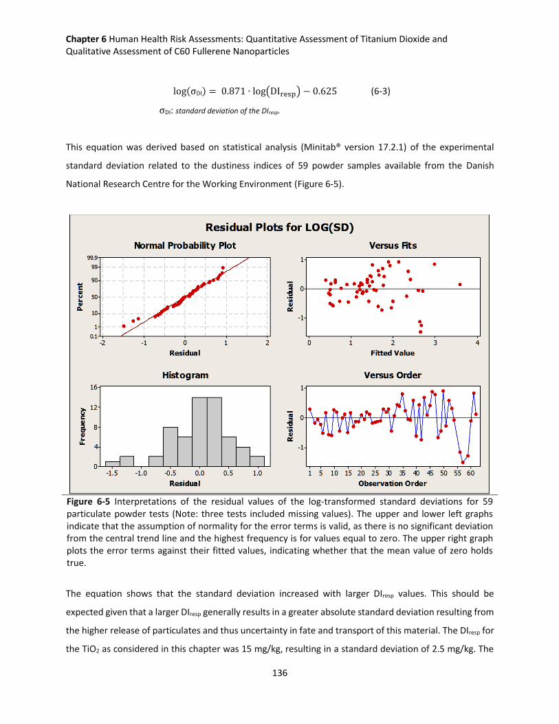
Chapter 6 Human Health Risk Assessments: Quantitative Assessment of Titanium Dioxide and Qualitative Assessment of C60 Fullerene Nanoparticles
136
log(σDI) = 0.871 ∙ log(DIresp) − 0.625 (6-3)
σDI: standard deviation of the DIresp.
This equation was derived based on statistical analysis (Minitab® version 17.2.1) of the experimental
standard deviation related to the dustiness indices of 59 powder samples available from the Danish
National Research Centre for the Working Environment (Figure 6-5).
Figure 6-5 Interpretations of the residual values of the log-transformed standard deviations for 59 particulate powder tests (Note: three tests included missing values). The upper and lower left graphs indicate that the assumption of normality for the error terms is valid, as there is no significant deviation from the central trend line and the highest frequency is for values equal to zero. The upper right graph plots the error terms against their fitted values, indicating whether that the mean value of zero holds true.
The equation shows that the standard deviation increased with larger DIresp values. This should be
expected given that a larger DIresp generally results in a greater absolute standard deviation resulting from
the higher release of particulates and thus uncertainty in fate and transport of this material. The DIresp for
the TiO2 as considered in this chapter was 15 mg/kg, resulting in a standard deviation of 2.5 mg/kg. The
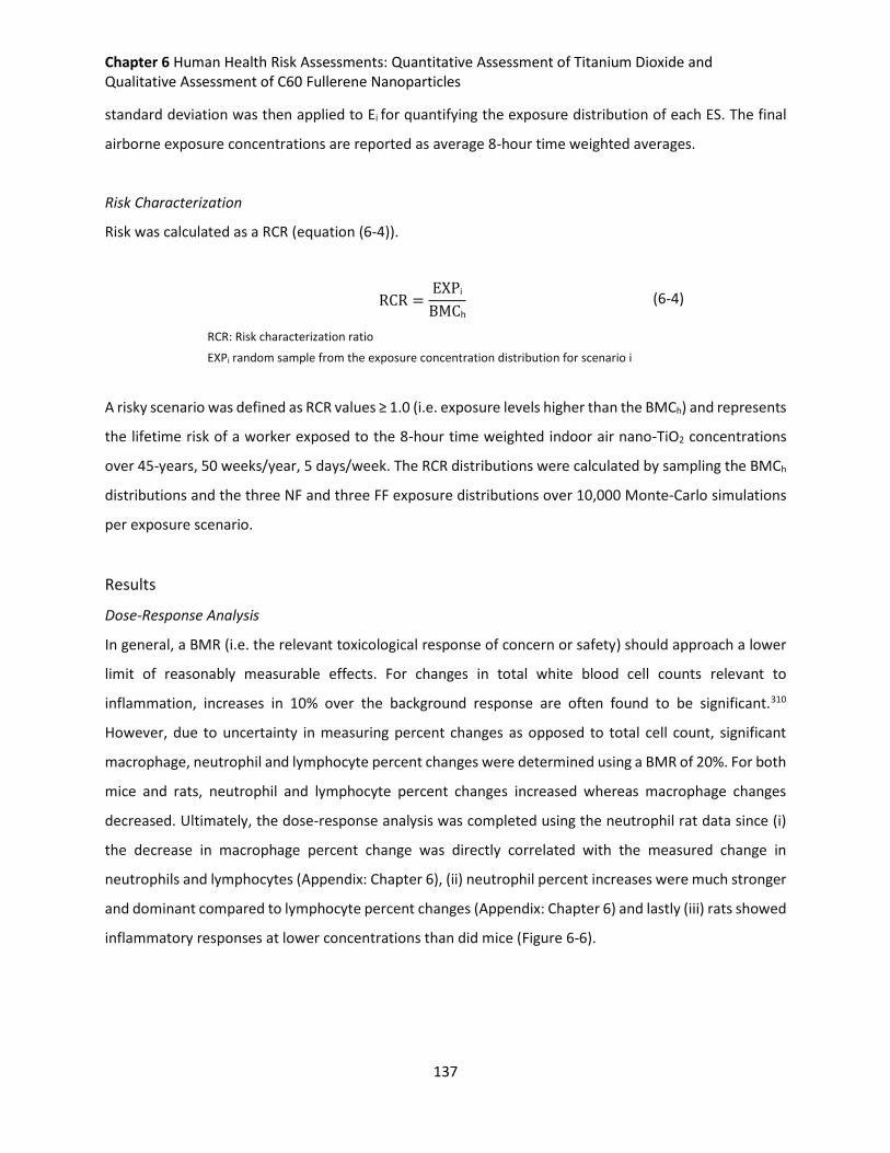
Chapter 6 Human Health Risk Assessments: Quantitative Assessment of Titanium Dioxide and Qualitative Assessment of C60 Fullerene Nanoparticles
137
standard deviation was then applied to Ei for quantifying the exposure distribution of each ES. The final
airborne exposure concentrations are reported as average 8-hour time weighted averages.
Risk Characterization
Risk was calculated as a RCR (equation (6-4)).
RCR =EXPi
BMCh (6-4)
RCR: Risk characterization ratio
EXPi random sample from the exposure concentration distribution for scenario i
A risky scenario was defined as RCR values ≥ 1.0 (i.e. exposure levels higher than the BMCh) and represents
the lifetime risk of a worker exposed to the 8-hour time weighted indoor air nano-TiO2 concentrations
over 45-years, 50 weeks/year, 5 days/week. The RCR distributions were calculated by sampling the BMCh
distributions and the three NF and three FF exposure distributions over 10,000 Monte-Carlo simulations
per exposure scenario.
Results
Dose-Response Analysis
In general, a BMR (i.e. the relevant toxicological response of concern or safety) should approach a lower
limit of reasonably measurable effects. For changes in total white blood cell counts relevant to
inflammation, increases in 10% over the background response are often found to be significant.310
However, due to uncertainty in measuring percent changes as opposed to total cell count, significant
macrophage, neutrophil and lymphocyte percent changes were determined using a BMR of 20%. For both
mice and rats, neutrophil and lymphocyte percent changes increased whereas macrophage changes
decreased. Ultimately, the dose-response analysis was completed using the neutrophil rat data since (i)
the decrease in macrophage percent change was directly correlated with the measured change in
neutrophils and lymphocytes (Appendix: Chapter 6), (ii) neutrophil percent increases were much stronger
and dominant compared to lymphocyte percent changes (Appendix: Chapter 6) and lastly (iii) rats showed
inflammatory responses at lower concentrations than did mice (Figure 6-6).
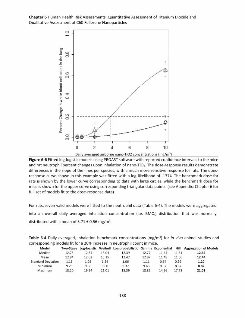
Chapter 6 Human Health Risk Assessments: Quantitative Assessment of Titanium Dioxide and Qualitative Assessment of C60 Fullerene Nanoparticles
138
Per
cen
t C
han
ge in
wh
ite
blo
od
cel
l co
un
t in
th
e lu
ng
Daily averaged airborne nano-TiO2 concentrations (mg/m3)
Figure 6-6 Fitted log-logistic models using PROAST software with reported confidence intervals to the mice and rat neutrophil percent changes upon inhalation of nano-TiO2. The dose-response results demonstrate differences in the slope of the lines per species, with a much more sensitive response for rats. The does-response curve shown in this example was fitted with a log-likelihood of -1374. The benchmark dose for rats is shown by the lower curve corresponding to data with large circles, while the benchmark dose for mice is shown for the upper curve using corresponding triangular data points. (see Appendix: Chapter 6 for full set of models fit to the dose-response data)
For rats, seven valid models were fitted to the neutrophil data (Table 6-4). The models were aggregated
into an overall daily averaged inhalation concentration (i.e. BMCa) distribution that was normally
distributed with a mean of 3.71 ± 0.56 mg/m3.
Table 6-4 Daily averaged, inhalation benchmark concentrations (mg/m3) for in vivo animal studies and corresponding models fit for a 20% increase in neutrophil count in mice.
Model Two-Stage Log-logistic Weibull Log-probabilistic Gamma Exponential Hill Aggregation of Models Median 12.76 12.54 13.04 12.39 12.77 11.44 11.61 12.32 Mean 12.84 12.62 13.15 12.47 12.87 11.48 11.66 12.44
Standard Deviation 1.15 1.05 1.24 1.06 1.11 0.64 0.99 1.20 Minimum 9.25 9.58 9.60 9.37 9.66 9.57 8.82 8.82 Maximum 18.20 19.54 21.01 18.39 18.85 14.66 17.78 21.01
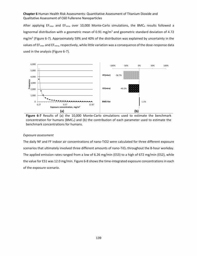
Chapter 6 Human Health Risk Assessments: Quantitative Assessment of Titanium Dioxide and Qualitative Assessment of C60 Fullerene Nanoparticles
139
After applying EFinter and EFintra over 10,000 Monte-Carlo simulations, the BMCh results followed a
lognormal distribution with a geometric mean of 0.91 mg/m3 and geometric standard deviation of 4.72
mg/m3 (Figure 6-7). Approximately 59% and 40% of the distribution was explained by uncertainty in the
values of EFinter and EFintra, respectively, while little variation was a consequence of the dose-response data
used in the analysis (Figure 6-7).
(a)
(b)
Figure 6-7 Results of (a) the 10,000 Monte-Carlo simulations used to estimate the benchmark concentration for humans (BMCh) and (b) the contribution of each parameter used to estimate the benchmark concentrations for humans.
Exposure assessment
The daily NF and FF indoor air concentrations of nano-TiO2 were calculated for three different exposure
scenarios that ultimately involved three different amounts of nano-TiO2 throughout the 8-hour workday.
The applied emission rates ranged from a low of 6.26 mg/min (ES3) to a high of 672 mg/min (ES2), while
the value for ES1 was 12.0 mg/min. Figure 6-8 shows the time-integrated exposure concentrations in each
of the exposure scenario.
0
1,000
2,000
3,000
4,000
5,000
6,000
0.27 6.57 12.87
Freq
uen
cy
Exposure concentration, mg/m3
-58.7%
-40.2%
1.1%
-100% -50% 0% 50% 100%
EF(inter)
EF(intra)
BMD Rat
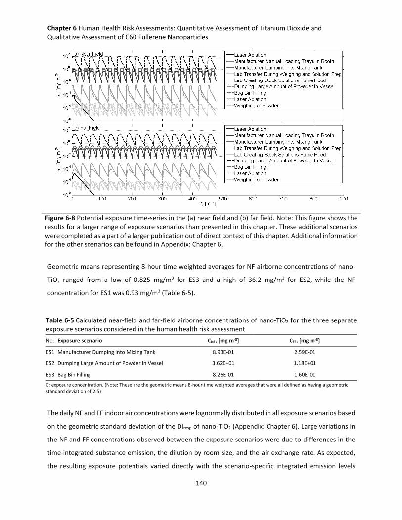
Chapter 6 Human Health Risk Assessments: Quantitative Assessment of Titanium Dioxide and Qualitative Assessment of C60 Fullerene Nanoparticles
140
Figure 6-8 Potential exposure time-series in the (a) near field and (b) far field. Note: This figure shows the results for a larger range of exposure scenarios than presented in this chapter. These additional scenarios were completed as a part of a larger publication out of direct context of this chapter. Additional information for the other scenarios can be found in Appendix: Chapter 6.
Geometric means representing 8-hour time weighted averages for NF airborne concentrations of nano-
TiO2 ranged from a low of 0.825 mg/m3 for ES3 and a high of 36.2 mg/m3 for ES2, while the NF
concentration for ES1 was 0.93 mg/m3 (Table 6-5).
Table 6-5 Calculated near-field and far-field airborne concentrations of nano-TiO2 for the three separate exposure scenarios considered in the human health risk assessment
No. Exposure scenario CNF, [mg m-3] CFF, [mg m-3]
ES1 Manufacturer Dumping into Mixing Tank 8.93E-01 2.59E-01
ES2 Dumping Large Amount of Powder in Vessel 3.62E+01 1.18E+01
ES3 Bag Bin Filling 8.25E-01 1.60E-01
C: exposure concentration. (Note: These are the geometric means 8-hour time weighted averages that were all defined as having a geometric standard deviation of 2.5)
The daily NF and FF indoor air concentrations were lognormally distributed in all exposure scenarios based
on the geometric standard deviation of the DIresp of nano-TiO2 (Appendix: Chapter 6). Large variations in
the NF and FF concentrations observed between the exposure scenarios were due to differences in the
time-integrated substance emission, the dilution by room size, and the air exchange rate. As expected,
the resulting exposure potentials varied directly with the scenario-specific integrated emission levels
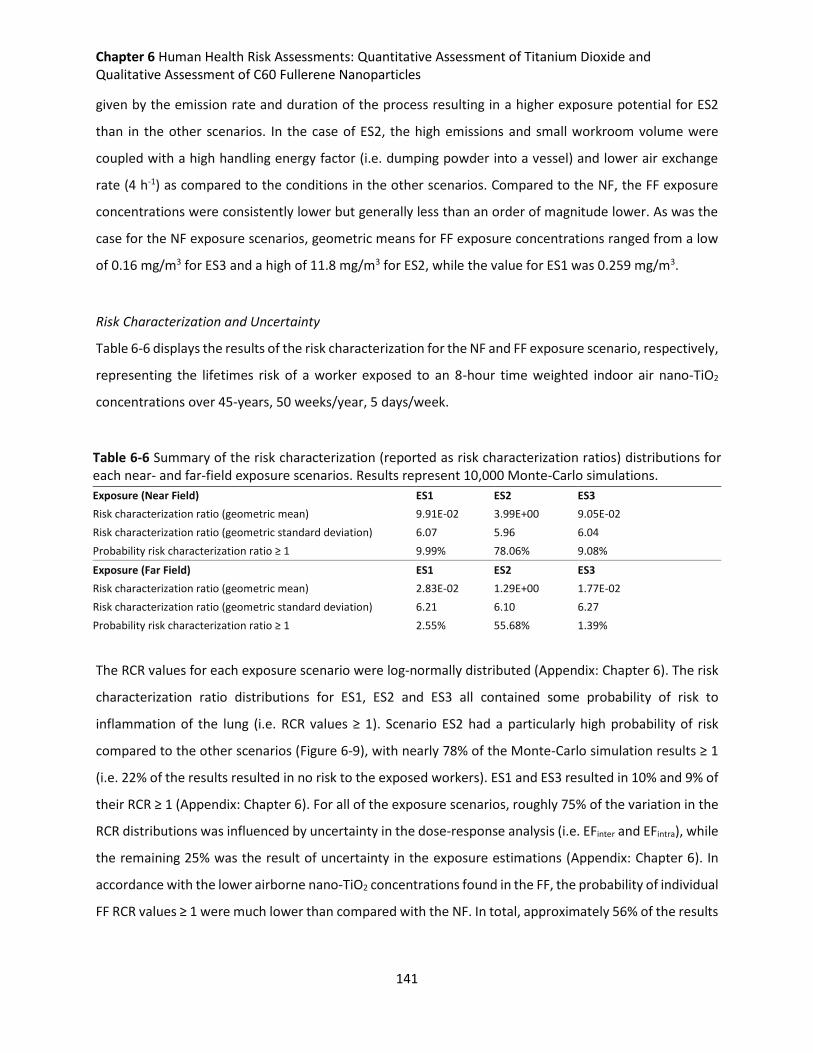
Chapter 6 Human Health Risk Assessments: Quantitative Assessment of Titanium Dioxide and Qualitative Assessment of C60 Fullerene Nanoparticles
141
given by the emission rate and duration of the process resulting in a higher exposure potential for ES2
than in the other scenarios. In the case of ES2, the high emissions and small workroom volume were
coupled with a high handling energy factor (i.e. dumping powder into a vessel) and lower air exchange
rate (4 h-1) as compared to the conditions in the other scenarios. Compared to the NF, the FF exposure
concentrations were consistently lower but generally less than an order of magnitude lower. As was the
case for the NF exposure scenarios, geometric means for FF exposure concentrations ranged from a low
of 0.16 mg/m3 for ES3 and a high of 11.8 mg/m3 for ES2, while the value for ES1 was 0.259 mg/m3.
Risk Characterization and Uncertainty
Table 6-6 displays the results of the risk characterization for the NF and FF exposure scenario, respectively,
representing the lifetimes risk of a worker exposed to an 8-hour time weighted indoor air nano-TiO2
concentrations over 45-years, 50 weeks/year, 5 days/week.
Table 6-6 Summary of the risk characterization (reported as risk characterization ratios) distributions for each near- and far-field exposure scenarios. Results represent 10,000 Monte-Carlo simulations.
Exposure (Near Field) ES1 ES2 ES3
Risk characterization ratio (geometric mean) 9.91E-02 3.99E+00 9.05E-02
Risk characterization ratio (geometric standard deviation) 6.07 5.96 6.04
Probability risk characterization ratio ≥ 1 9.99% 78.06% 9.08%
Exposure (Far Field) ES1 ES2 ES3
Risk characterization ratio (geometric mean) 2.83E-02 1.29E+00 1.77E-02
Risk characterization ratio (geometric standard deviation) 6.21 6.10 6.27
Probability risk characterization ratio ≥ 1 2.55% 55.68% 1.39%
The RCR values for each exposure scenario were log-normally distributed (Appendix: Chapter 6). The risk
characterization ratio distributions for ES1, ES2 and ES3 all contained some probability of risk to
inflammation of the lung (i.e. RCR values ≥ 1). Scenario ES2 had a particularly high probability of risk
compared to the other scenarios (Figure 6-9), with nearly 78% of the Monte-Carlo simulation results ≥ 1
(i.e. 22% of the results resulted in no risk to the exposed workers). ES1 and ES3 resulted in 10% and 9% of
their RCR ≥ 1 (Appendix: Chapter 6). For all of the exposure scenarios, roughly 75% of the variation in the
RCR distributions was influenced by uncertainty in the dose-response analysis (i.e. EFinter and EFintra), while
the remaining 25% was the result of uncertainty in the exposure estimations (Appendix: Chapter 6). In
accordance with the lower airborne nano-TiO2 concentrations found in the FF, the probability of individual
FF RCR values ≥ 1 were much lower than compared with the NF. In total, approximately 56% of the results
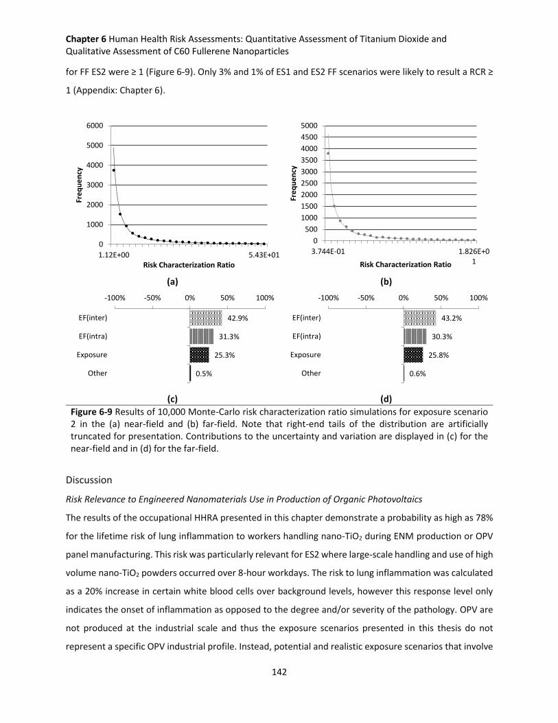
Chapter 6 Human Health Risk Assessments: Quantitative Assessment of Titanium Dioxide and Qualitative Assessment of C60 Fullerene Nanoparticles
142
for FF ES2 were ≥ 1 (Figure 6-9). Only 3% and 1% of ES1 and ES2 FF scenarios were likely to result a RCR ≥
1 (Appendix: Chapter 6).
(a) (b)
(c) (d)
Figure 6-9 Results of 10,000 Monte-Carlo risk characterization ratio simulations for exposure scenario 2 in the (a) near-field and (b) far-field. Note that right-end tails of the distribution are artificially truncated for presentation. Contributions to the uncertainty and variation are displayed in (c) for the near-field and in (d) for the far-field.
Discussion
Risk Relevance to Engineered Nanomaterials Use in Production of Organic Photovoltaics
The results of the occupational HHRA presented in this chapter demonstrate a probability as high as 78%
for the lifetime risk of lung inflammation to workers handling nano-TiO2 during ENM production or OPV
panel manufacturing. This risk was particularly relevant for ES2 where large-scale handling and use of high
volume nano-TiO2 powders occurred over 8-hour workdays. The risk to lung inflammation was calculated
as a 20% increase in certain white blood cells over background levels, however this response level only
indicates the onset of inflammation as opposed to the degree and/or severity of the pathology. OPV are
not produced at the industrial scale and thus the exposure scenarios presented in this thesis do not
represent a specific OPV industrial profile. Instead, potential and realistic exposure scenarios that involve
0
1000
2000
3000
4000
5000
6000
1.12E+00 5.43E+01
Fre
qu
en
cy
Risk Characterization Ratio
0
500
1000
1500
2000
2500
3000
3500
4000
4500
5000
3.744E-01 1.826E+01
Fre
qu
en
cy
Risk Characterization Ratio
42.9%
31.3%
25.3%
0.5%
-100% -50% 0% 50% 100%
EF(inter)
EF(intra)
Exposure
Other
43.2%
30.3%
25.8%
0.6%
-100% -50% 0% 50% 100%
EF(inter)
EF(intra)
Exposure
Other
Chapter 6 Human Health Risk Assessments: Quantitative Assessment of Titanium Dioxide and Qualitative Assessment of C60 Fullerene Nanoparticles
143
the production and handling of nano-TiO2 were presented and therefore provide a first-tier assessment
for OPV. For example, if OPV devices utilizing PCBM and/or TiO2 come to full industrial scale and uptake
to the marketplace, large volumes of these substances will be handled, loaded and dispensed either into
other containers, holding tanks or vessels for mixing and/or application to the OPV panel. ES1 and ES3
involved exposure scenarios handling over an order of magnitude less nano-TiO2 powder compared with
ES2. Thus, these represent production volumes that are much more moderate than ES2. Nevertheless,
there remained a 10% lifetime probability of lung inflammation to workers handling these lower amounts
of powders over an 8-hour workday.
Uncertainties within the Risk Assessment Procedure
The dose-response assessment was completed specifically from nano-TiO2 in vivo toxicological data, in
accordance with the scientific literature that demonstrates the toxicological responses upon exposure to
ENM and bulk substances can differ. Additionally, the emissions calculation was defined by a distribution
that was defined by the standard deviation of nano-TiO2’s dustiness index. While the dustiness index was
material specific, its mass-based measurement does not provide detailed information about the size-
distributions in the dustiness tests. Overestimations for emissions and exposures from powder handling
may be a result, whereas calculations for spray or fugitive-type releases might be closer to reality.
Airborne concentrations were further calculated using a two-zone near- and far-field model, which is
particularly relevant for single source, non-fugitive emissions311 that are very relevant for ENM. For
instance, the persistence of uniformly small airborne ENM may quickly decline due to aggregation and
agglomeration,199,312,313 meaning that exposure to primary or small “nano” aggregates might be most
relevant close to the emission source.314–316
It should be noted that the fate and exposure model, NanoSafer, used in this work largely relied on
advection and bulk air flow to estimate the concentration of nano-TiO2 in the workplace. The exposure
also is based on external airborne concentrations as opposed to internal doses. Particle sizes are an
important characteristic influencing the effectiveness of ventilation control, personal protective
equipment and ultimately where ENM retention will occur in the lung. For example, ENM might lodge
deeper and more uniformly in the lung (i.e. alveoli) as compared to larger-size materials.314 Modifying
factors (e.g. use of personal protective equipment) were not considered and should be considered for
future assessments. For example, Fransman et al.317 provides protection factors for common localized
controls and personal protective equipment, although these can deviate significantly from applied
Chapter 6 Human Health Risk Assessments: Quantitative Assessment of Titanium Dioxide and Qualitative Assessment of C60 Fullerene Nanoparticles
144
protection factors for ENM.318 Additionally, a few occupational exposure studies have shown that particle
size distributions in some cases may be similar for both ENM and conventional powders.199,312 Such
considerations could be included in models that utilize size-resolved concentration data (e.g. mass median
aerodynamic diameters) in their models.283,284,319 Given these relative uncertainties, the exposure
assessments and corresponding risk calculations in this HHRA can be considered as worst-case scenarios.
The uncertainty arising from the use of a mass-based dose-metric was not addressed in this chapter.
Ideally, HHRA of ENM should use a dose-metric that is the best indication of toxicity as well as exposure.246
For example, this might be indicated by mass concentration, particle number, or lung-deposited surface
area. Although mass may not necessarily be the most suitable dose-metric to describe ENM dose-
response relationships,320–323 it is the metric most easily and reliably determined for measuring and
managing occupational exposures as management of particle numbers or surface area is not yet
achievable.161 The extrapolation of one dose-metric to another may be possible using specific uncertainty
factors. For instance, the surface area can be estimated from a particle concentration size distribution of
spherical ENM. However, there are considerable challenges in reliable measurements and, therefore, data
conversion between these metrics for ENM with non-spherical morphologies45 and their agglomerates
and aggregates.324,325
Conclusions
These findings presented in this chapter suggest that the potential human health impacts from ENM used
in OPV cannot, by default, be assumed to be negligible and may in fact be highly probable. This issue may
not necessarily be relevant to the current technology and production level of OPV but should be
considered for future scale-ups of these devices. It is important to note that the HHRA results are not
scaled to the functional units defined by the LCA in Chapter 3 and Chapter 4. The difference in scopes
means that the risk pertains to the handling a mass of the ENM that is independent of exact amounts of
nano-TiO2 required to fulfill the functional unit (e.g. production of 1 Wp of OPV). Therefore, the risk cannot
be directly interpreted in terms of its overall relevance to the OPV life-cycle, particularly any prospective
analysis of future, large scale production of this technology. Of course, the exact exposure to these ENM
used at current lab- and small-scale production per functional unit could, in some cases, be determined
for the HHRA. While these results might be beneficial from a health and safety perspective for laboratory
managers, for example, it may ultimately provide little relevance from an eco-design perspective where
material choices and occupational workplace conditions at the industrial scale are being extrapolated

Chapter 6 Human Health Risk Assessments: Quantitative Assessment of Titanium Dioxide and Qualitative Assessment of C60 Fullerene Nanoparticles
145
from lab- or research-based scenarios and where uncertainty is thus high. Instead, potential human health
impacts calculated within LCA, as opposed to absolute values of risk, might prove more useful for early
design and development of emerging technologies. The next chapter presents the methods and results of
calculating the potential human health impacts for ENM within the context of life-cycle impact assessment
and the OPV-LCA case studies presented in earlier chapters.
Chapter 7 Life-Cycle Impact Assessment Nanomaterial Characterization Factors: Titanium Dioxide Case Study
146
Chapter 7 Life-Cycle Impact Assessment Nanomaterial Characterization
Factors: Titanium Dioxide Case Study
In the previous chapter, a HHRA was conducted to calculate the human health risk associated with
handling and working with moderate to large amounts of nano-TiO2. The results demonstrate that there
are high probabilities of lifetime risk to lung inflammation for workers handling these materials based on
the 8-hour time weighted average exposures calculated with the NanoSafer fate and exposure model. The
HHRA results will be particularly important and relevant for industries where workplace conditions
particularly match the descriptions of the exposure scenarios tested in Chapter 6 (i.e. that represent large
or industrial-scale production). It would be of benefit to be able to integrate these methods with life-cycle
impact assessment methods. The advantages would allow the simultaneous analysis for other similarly
related metal oxide ENM, with the potential to modify the approach for non-metal oxide ENM that are
both found in OPV. Additionally, integration facilitates the comparison of ENM-specific human health
impacts with non-ENM sources of human health impacts by directly converting all such impacts to the
functional units used in Chapter 3 and Chapter 4. Such results could be used to identify if ENM is a driving
influence in human health impacts over the OPV life-cycle and, thus, more appropriately prioritize eco-
design and product development efforts.
A handful of studies have made first approximations to incorporate the ecotoxicity or human health
impacts from ENM into their LCA studies,93–96 but otherwise these impacts have been conspicuously
missing from the majority of published ENM-related LCA studies.96,184 In those studies that addressed
these issues, mainly ambient emissions of and ecotoxicity relevant CFNS have been published. Other
studies show that pollutant emissions, including ENM, in occupational and indoor settings can be very
important contributors to overall LCA results.227,326,327,235,328 Occupational settings present unique
scenarios where production329 of pristine particles with small size distributions and thus exposure may
occur. Neglecting such occupational, indoor ENM emissions in a LCA may result in burden shifting from
the environment to workers. Currently, there is only one such CFNS relevant to indoor emissions of these
ENM.
These previously reported CFNS have made use of existing life-cycle impact assessment methods such as
USEtox. This approach takes advantage of a number of assumptions that conveniently describe the fate
and transport of small organic molecules and metals quite well, but these methods are not appropriate
Chapter 7 Life-Cycle Impact Assessment Nanomaterial Characterization Factors: Titanium Dioxide Case Study
147
for ENM.196 The major assumptions utilized in human health life-cycle impact assessment methods are
that conditions are at steady-state and systems have reached thermodynamic equilibrium.101,197 However,
ENM behave, in effect, like colloidal substances that, when released into a specific medium, exist in their
own phase and will not form uniform phases with the surrounding medium unlike organics. Therefore and
by definition, ENM are not thermodynamically stable, even if certain ENM may be kinetically stable for
long periods of time.196 Previous adaptations to current life-cycle impact assessment methodologies such
as USEtox have been made to estimate the ecological94–96 and human health impacts93 of ENM. In all
previous cases, steady-state conditions were kept in the model, and as was previously discussed in
Chapter 5. Thus, the aim of this chapter is to present a dynamic life-cycle impact assessment fate and
exposure model for estimating the human health impacts from indoor, occupational ENM air emissions.
The approach presented in this chapter integrates part of the HHRA methodology proposes in Chapter 6
with life-cycle impact assessment. The results of the integration are applied for nano-TiO2.
Methods
The calculation of a CFNS for use in LCA is further presented in this chapter, where CF is defined in an
analogous fashion to equation (2-2).234,330 However, unlike the that equation, the iF is not estimated using
(equilibrium) partition coefficients inside of steady-state models. Instead, a dynamic fate and exposure
model using kinetically defined fate and exposure parameters is used to define a newly introduced
Retained-intake Fraction (RiF).
Emissions of and Exposure Scenarios for Nano-TiO2 in the Occupational Indoor Setting
ENM emissions can be directly measured, estimated from published literature or calculated using models.
In many cases, means for measuring emissions or the primary data needed may not exist. Therefore, it
can be useful and often necessary to model such emissions. A total of six exposure scenarios (ES1-ES6)
(Table 7-1) were modeled and identified from the previous HHRA in Chapter 6.
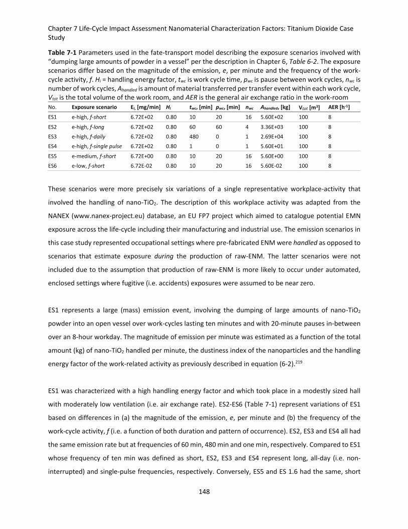
Chapter 7 Life-Cycle Impact Assessment Nanomaterial Characterization Factors: Titanium Dioxide Case Study
148
Table 7-1 Parameters used in the fate-transport model describing the exposure scenarios involved with “dumping large amounts of powder in a vessel” per the description in Chapter 6, Table 6-2. The exposure scenarios differ based on the magnitude of the emission, e, per minute and the frequency of the work-cycle activity, f. Hi = handling energy factor, twc is work cycle time, pwc is pause between work cycles, nwc is number of work cycles, Ahandled is amount of material transferred per transfer event within each work cycle, Vtot is the total volume of the work room, and AER is the general air exchange ratio in the work-room
No. Exposure scenario Ei, [mg/min] Hi twc, [min] pwc, [min] nwc Ahandled, [kg] Vtot [m3] AER [h-1]
ES1 e-high, f-short 6.72E+02 0.80 10 20 16 5.60E+02 100 8
ES2 e-high, f-long 6.72E+02 0.80 60 60 4 3.36E+03 100 8
ES3 e-high, f-daily 6.72E+02 0.80 480 0 1 2.69E+04 100 8
ES4 e-high, f-single pulse 6.72E+02 0.80 1 0 1 5.60E+01 100 8
ES5 e-medium, f-short 6.72E+00 0.80 10 20 16 5.60E+00 100 8
ES6 e-low, f-short 6.72E-02 0.80 10 20 16 5.60E-02 100 8
These scenarios were more precisely six variations of a single representative workplace-activity that
involved the handling of nano-TiO2. The description of this workplace activity was adapted from the
NANEX (www.nanex-project.eu) database, an EU FP7 project which aimed to catalogue potential EMN
exposure across the life-cycle including their manufacturing and industrial use. The emission scenarios in
this case study represented occupational settings where pre-fabricated ENM were handled as opposed to
scenarios that estimate exposure during the production of raw-ENM. The latter scenarios were not
included due to the assumption that production of raw-ENM is more likely to occur under automated,
enclosed settings where fugitive (i.e. accidents) exposures were assumed to be near zero.
ES1 represents a large (mass) emission event, involving the dumping of large amounts of nano-TiO2
powder into an open vessel over work-cycles lasting ten minutes and with 20-minute pauses in-between
over an 8-hour workday. The magnitude of emission per minute was estimated as a function of the total
amount (kg) of nano-TiO2 handled per minute, the dustiness index of the nanoparticles and the handling
energy factor of the work-related activity as previously described in equation (6-2).219
ES1 was characterized with a high handling energy factor and which took place in a modestly sized hall
with moderately low ventilation (i.e. air exchange rate). ES2-ES6 (Table 7-1) represent variations of ES1
based on differences in (a) the magnitude of the emission, e, per minute and (b) the frequency of the
work-cycle activity, f (i.e. a function of both duration and pattern of occurrence). ES2, ES3 and ES4 all had
the same emission rate but at frequencies of 60 min, 480 min and one min, respectively. Compared to ES1
whose frequency of ten min was defined as short, ES2, ES3 and ES4 represent long, all-day (i.e. non-
interrupted) and single-pulse frequencies, respectively. Conversely, ES5 and ES 1.6 had the same, short
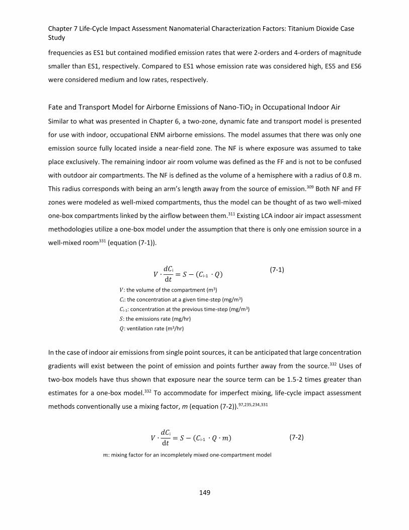
Chapter 7 Life-Cycle Impact Assessment Nanomaterial Characterization Factors: Titanium Dioxide Case Study
149
frequencies as ES1 but contained modified emission rates that were 2-orders and 4-orders of magnitude
smaller than ES1, respectively. Compared to ES1 whose emission rate was considered high, ES5 and ES6
were considered medium and low rates, respectively.
Fate and Transport Model for Airborne Emissions of Nano-TiO2 in Occupational Indoor Air
Similar to what was presented in Chapter 6, a two-zone, dynamic fate and transport model is presented
for use with indoor, occupational ENM airborne emissions. The model assumes that there was only one
emission source fully located inside a near-field zone. The NF is where exposure was assumed to take
place exclusively. The remaining indoor air room volume was defined as the FF and is not to be confused
with outdoor air compartments. The NF is defined as the volume of a hemisphere with a radius of 0.8 m.
This radius corresponds with being an arm’s length away from the source of emission.309 Both NF and FF
zones were modeled as well-mixed compartments, thus the model can be thought of as two well-mixed
one-box compartments linked by the airflow between them.311 Existing LCA indoor air impact assessment
methodologies utilize a one-box model under the assumption that there is only one emission source in a
well-mixed room331 (equation (7-1)).
𝑉 ∙𝑑𝐶i
d𝑡= 𝑆 − (𝐶i-1 ∙ 𝑄)
(7-1)
𝑉: the volume of the compartment (m3) 𝐶i: the concentration at a given time-step (mg/m3) 𝐶i-1: concentration at the previous time-step (mg/m3) 𝑆: the emissions rate (mg/hr) 𝑄: ventilation rate (m3/hr)
In the case of indoor air emissions from single point sources, it can be anticipated that large concentration
gradients will exist between the point of emission and points further away from the source.332 Uses of
two-box models have thus shown that exposure near the source term can be 1.5-2 times greater than
estimates for a one-box model.332 To accommodate for imperfect mixing, life-cycle impact assessment
methods conventionally use a mixing factor, m (equation (7-2)).97,235,234,331
𝑉 ∙𝑑𝐶i
d𝑡= 𝑆 − (𝐶i-1 ∙ 𝑄 ∙ 𝑚) (7-2)
𝑚: mixing factor for an incompletely mixed one-compartment model
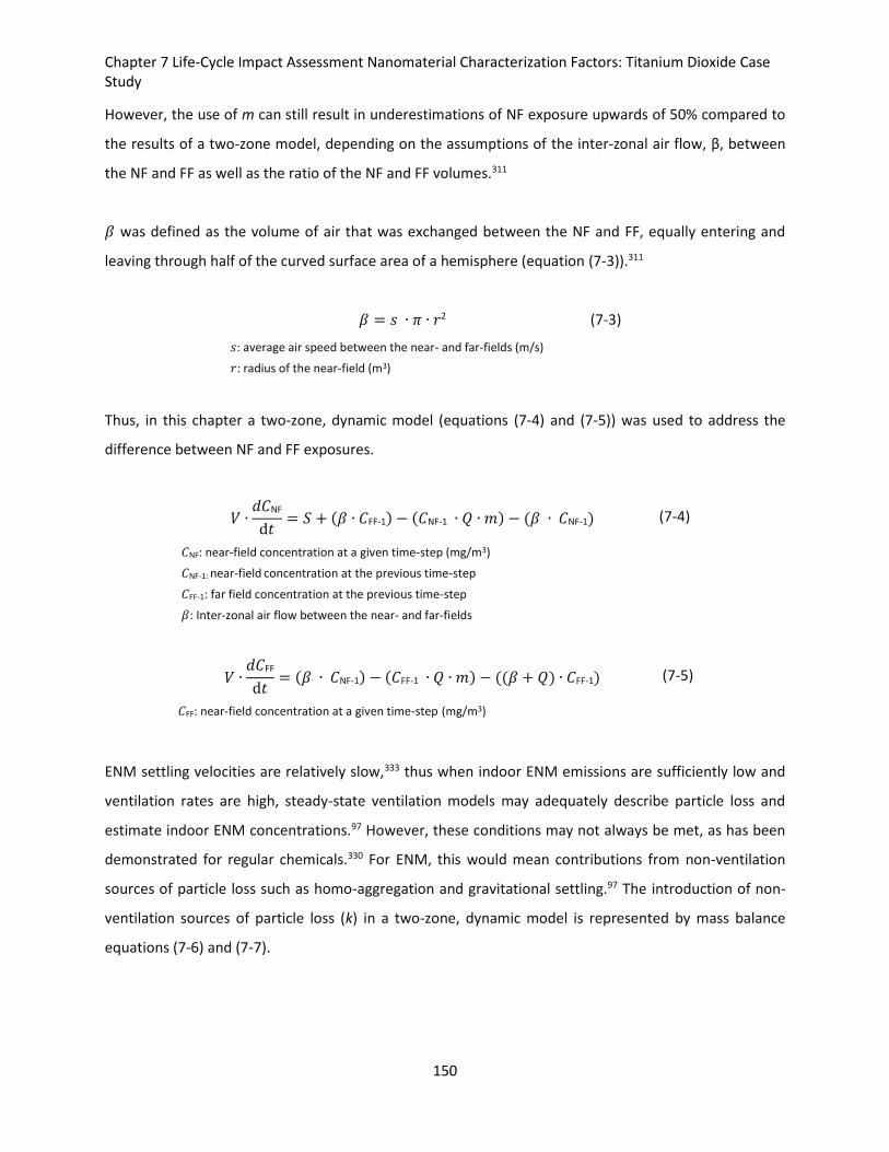
Chapter 7 Life-Cycle Impact Assessment Nanomaterial Characterization Factors: Titanium Dioxide Case Study
150
However, the use of m can still result in underestimations of NF exposure upwards of 50% compared to
the results of a two-zone model, depending on the assumptions of the inter-zonal air flow, β, between
the NF and FF as well as the ratio of the NF and FF volumes.311
𝛽 was defined as the volume of air that was exchanged between the NF and FF, equally entering and
leaving through half of the curved surface area of a hemisphere (equation (7-3)).311
𝛽 = 𝑠 ∙ 𝜋 ∙ 𝑟2 (7-3)
𝑠: average air speed between the near- and far-fields (m/s) 𝑟: radius of the near-field (m3)
Thus, in this chapter a two-zone, dynamic model (equations (7-4) and (7-5)) was used to address the
difference between NF and FF exposures.
𝑉 ∙𝑑𝐶NF
d𝑡= 𝑆 + (𝛽 ∙ 𝐶FF-1) − (𝐶NF-1 ∙ 𝑄 ∙ 𝑚) − (𝛽 ∙ 𝐶NF-1) (7-4)
𝐶NF: near-field concentration at a given time-step (mg/m3) 𝐶NF-1: near-field concentration at the previous time-step 𝐶FF-1: far field concentration at the previous time-step 𝛽: Inter-zonal air flow between the near- and far-fields
𝑉 ∙𝑑𝐶FF
d𝑡= (𝛽 ∙ 𝐶NF-1) − (𝐶FF-1 ∙ 𝑄 ∙ 𝑚) − ((𝛽 + 𝑄) ∙ 𝐶FF-1) (7-5)
𝐶FF: near-field concentration at a given time-step (mg/m3)
ENM settling velocities are relatively slow,333 thus when indoor ENM emissions are sufficiently low and
ventilation rates are high, steady-state ventilation models may adequately describe particle loss and
estimate indoor ENM concentrations.97 However, these conditions may not always be met, as has been
demonstrated for regular chemicals.330 For ENM, this would mean contributions from non-ventilation
sources of particle loss such as homo-aggregation and gravitational settling.97 The introduction of non-
ventilation sources of particle loss (k) in a two-zone, dynamic model is represented by mass balance
equations (7-6) and (7-7).
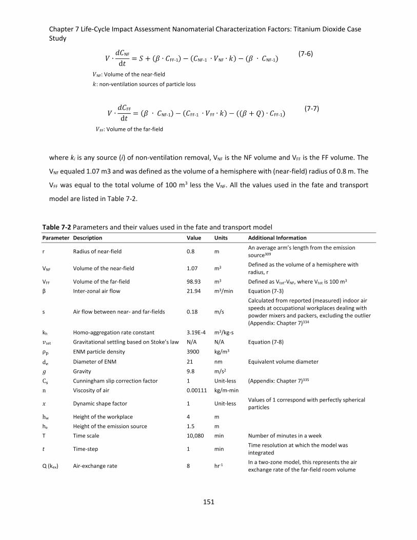
Chapter 7 Life-Cycle Impact Assessment Nanomaterial Characterization Factors: Titanium Dioxide Case Study
151
𝑉 ∙𝑑𝐶NF
d𝑡= 𝑆 + (𝛽 ∙ 𝐶FF-1) − (𝐶NF-1 ∙ 𝑉NF ∙ 𝑘) − (𝛽 ∙ 𝐶NF-1)
(7-6)
𝑉NF: Volume of the near-field 𝑘: non-ventilation sources of particle loss
𝑉 ∙𝑑𝐶FF
d𝑡= (𝛽 ∙ 𝐶NF-1) − (𝐶FF-1 ∙ 𝑉FF ∙ 𝑘) − ((𝛽 + 𝑄) ∙ 𝐶FF-1)
(7-7)
𝑉FF: Volume of the far-field
where ki is any source (i) of non-ventilation removal, VNF is the NF volume and VFF is the FF volume. The
VNF equaled 1.07 m3 and was defined as the volume of a hemisphere with (near-field) radius of 0.8 m. The
VFF was equal to the total volume of 100 m3 less the VNF. All the values used in the fate and transport
model are listed in Table 7-2.
Table 7-2 Parameters and their values used in the fate and transport model
Parameter Description Value Units Additional Information
r Radius of near-field 0.8 m An average arm’s length from the emission source309
VNF Volume of the near-field 1.07 m3 Defined as the volume of a hemisphere with radius, r
VFF Volume of the far-field 98.93 m3 Defined as Vtot-VNF, where Vtot is 100 m3
β Inter-zonal air flow 21.94 m3/min Equation (7-3)
s Air flow between near- and far-fields 0.18 m/s
Calculated from reported (measured) indoor air speeds at occupational workplaces dealing with powder mixers and packers, excluding the outlier (Appendix: Chapter 7)334
kh Homo-aggregation rate constant 3.19E-4 m3/kg-s
𝑣set Gravitational settling based on Stoke’s law N/A N/A Equation (7-8)
ρp ENM particle density 3900 kg/m3
de Diameter of ENM 21 nm Equivalent volume diameter
𝑔 Gravity 9.8 m/s2
Cs Cunningham slip correction factor 1 Unit-less (Appendix: Chapter 7)335
n Viscosity of air 0.00111 kg/m-min
𝑥 Dynamic shape factor 1 Unit-less Values of 1 correspond with perfectly spherical particles
hw Height of the workplace 4 m
he Height of the emission source 1.5 m
T Time scale 10,080 min Number of minutes in a week
t Time-step 1 min Time resolution at which the model was integrated
Q (kex) Air-exchange rate 8 hr-1 In a two-zone model, this represents the air exchange rate of the far-field room volume
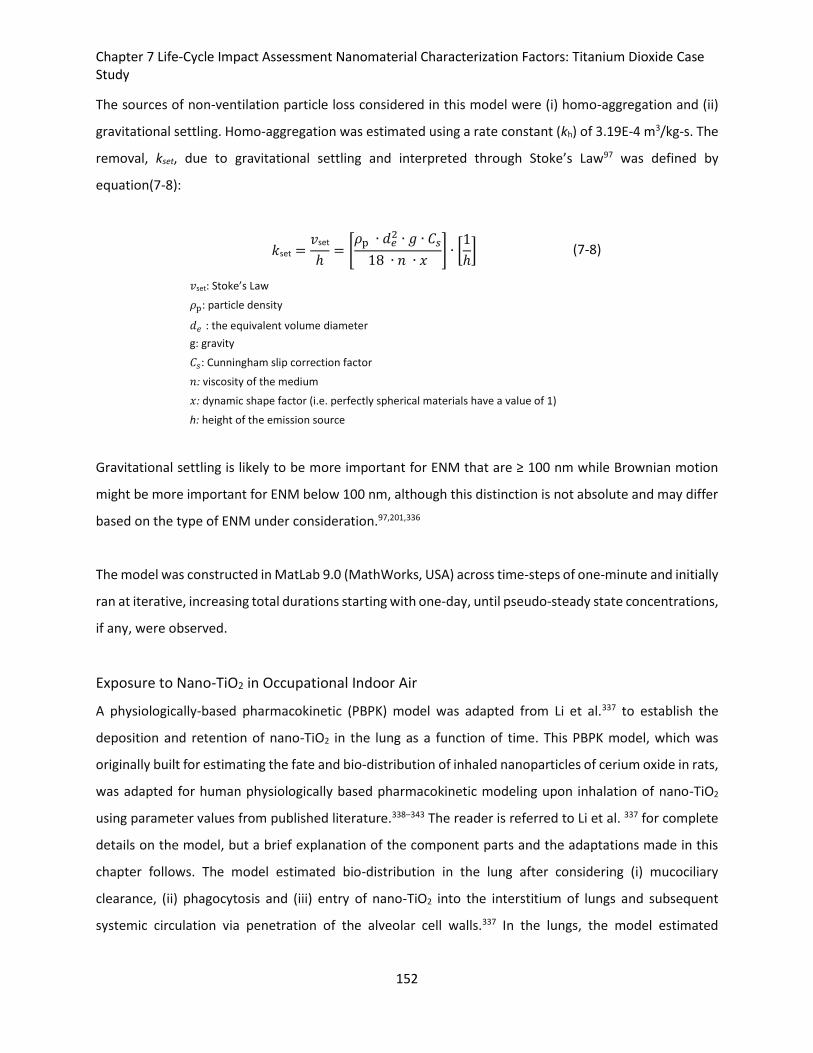
Chapter 7 Life-Cycle Impact Assessment Nanomaterial Characterization Factors: Titanium Dioxide Case Study
152
The sources of non-ventilation particle loss considered in this model were (i) homo-aggregation and (ii)
gravitational settling. Homo-aggregation was estimated using a rate constant (kh) of 3.19E-4 m3/kg-s. The
removal, kset, due to gravitational settling and interpreted through Stoke’s Law97 was defined by
equation(7-8):
𝑘set =𝑣set
ℎ= [
𝜌p ∙ 𝑑𝑒2 ∙ 𝑔 ∙ 𝐶𝑠
18 ∙ 𝑛 ∙ 𝑥] ∙ [
1
ℎ] (7-8)
𝑣set: Stoke’s Law 𝜌p: particle density 𝑑𝑒 : the equivalent volume diameter g: gravity 𝐶𝑠: Cunningham slip correction factor 𝑛: viscosity of the medium 𝑥: dynamic shape factor (i.e. perfectly spherical materials have a value of 1) h: height of the emission source
Gravitational settling is likely to be more important for ENM that are ≥ 100 nm while Brownian motion
might be more important for ENM below 100 nm, although this distinction is not absolute and may differ
based on the type of ENM under consideration.97,201,336
The model was constructed in MatLab 9.0 (MathWorks, USA) across time-steps of one-minute and initially
ran at iterative, increasing total durations starting with one-day, until pseudo-steady state concentrations,
if any, were observed.
Exposure to Nano-TiO2 in Occupational Indoor Air
A physiologically-based pharmacokinetic (PBPK) model was adapted from Li et al.337 to establish the
deposition and retention of nano-TiO2 in the lung as a function of time. This PBPK model, which was
originally built for estimating the fate and bio-distribution of inhaled nanoparticles of cerium oxide in rats,
was adapted for human physiologically based pharmacokinetic modeling upon inhalation of nano-TiO2
using parameter values from published literature.338–343 The reader is referred to Li et al. 337 for complete
details on the model, but a brief explanation of the component parts and the adaptations made in this
chapter follows. The model estimated bio-distribution in the lung after considering (i) mucociliary
clearance, (ii) phagocytosis and (iii) entry of nano-TiO2 into the interstitium of lungs and subsequent
systemic circulation via penetration of the alveolar cell walls.337 In the lungs, the model estimated
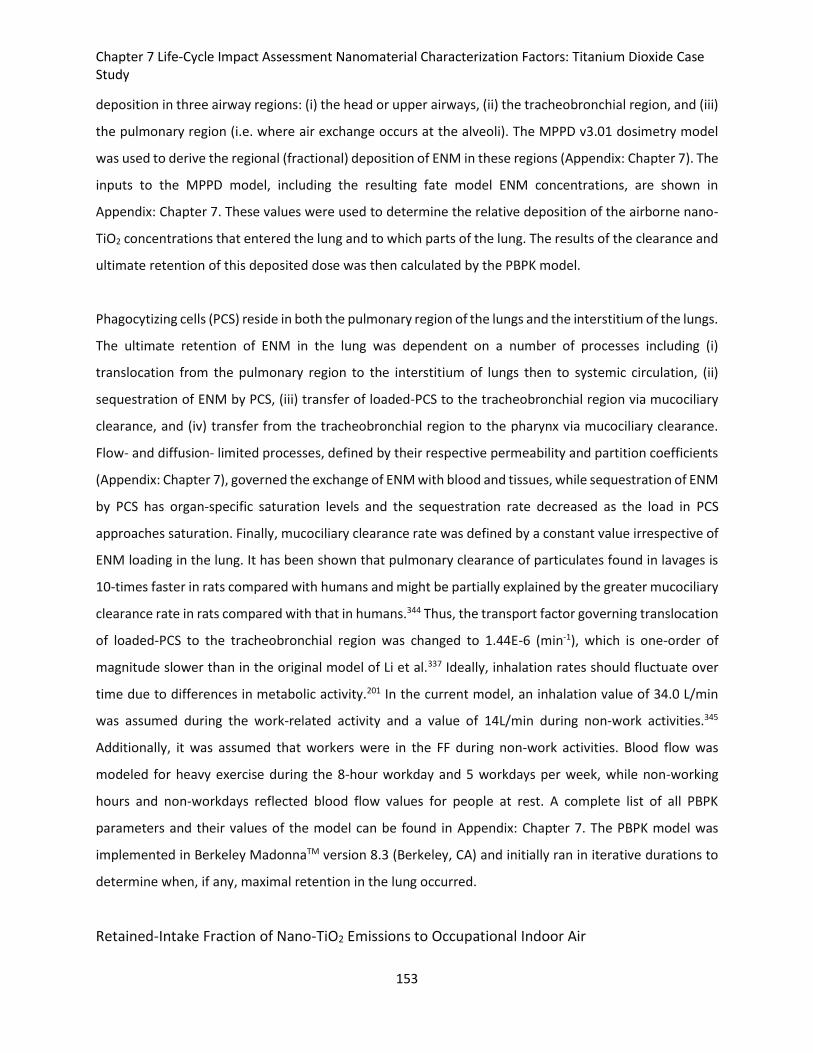
Chapter 7 Life-Cycle Impact Assessment Nanomaterial Characterization Factors: Titanium Dioxide Case Study
153
deposition in three airway regions: (i) the head or upper airways, (ii) the tracheobronchial region, and (iii)
the pulmonary region (i.e. where air exchange occurs at the alveoli). The MPPD v3.01 dosimetry model
was used to derive the regional (fractional) deposition of ENM in these regions (Appendix: Chapter 7). The
inputs to the MPPD model, including the resulting fate model ENM concentrations, are shown in
Appendix: Chapter 7. These values were used to determine the relative deposition of the airborne nano-
TiO2 concentrations that entered the lung and to which parts of the lung. The results of the clearance and
ultimate retention of this deposited dose was then calculated by the PBPK model.
Phagocytizing cells (PCS) reside in both the pulmonary region of the lungs and the interstitium of the lungs.
The ultimate retention of ENM in the lung was dependent on a number of processes including (i)
translocation from the pulmonary region to the interstitium of lungs then to systemic circulation, (ii)
sequestration of ENM by PCS, (iii) transfer of loaded-PCS to the tracheobronchial region via mucociliary
clearance, and (iv) transfer from the tracheobronchial region to the pharynx via mucociliary clearance.
Flow- and diffusion- limited processes, defined by their respective permeability and partition coefficients
(Appendix: Chapter 7), governed the exchange of ENM with blood and tissues, while sequestration of ENM
by PCS has organ-specific saturation levels and the sequestration rate decreased as the load in PCS
approaches saturation. Finally, mucociliary clearance rate was defined by a constant value irrespective of
ENM loading in the lung. It has been shown that pulmonary clearance of particulates found in lavages is
10-times faster in rats compared with humans and might be partially explained by the greater mucociliary
clearance rate in rats compared with that in humans.344 Thus, the transport factor governing translocation
of loaded-PCS to the tracheobronchial region was changed to 1.44E-6 (min-1), which is one-order of
magnitude slower than in the original model of Li et al.337 Ideally, inhalation rates should fluctuate over
time due to differences in metabolic activity.201 In the current model, an inhalation value of 34.0 L/min
was assumed during the work-related activity and a value of 14L/min during non-work activities.345
Additionally, it was assumed that workers were in the FF during non-work activities. Blood flow was
modeled for heavy exercise during the 8-hour workday and 5 workdays per week, while non-working
hours and non-workdays reflected blood flow values for people at rest. A complete list of all PBPK
parameters and their values of the model can be found in Appendix: Chapter 7. The PBPK model was
implemented in Berkeley MadonnaTM version 8.3 (Berkeley, CA) and initially ran in iterative durations to
determine when, if any, maximal retention in the lung occurred.
Retained-Intake Fraction of Nano-TiO2 Emissions to Occupational Indoor Air
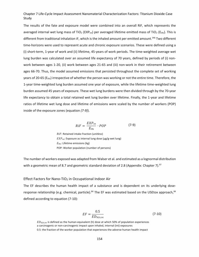
Chapter 7 Life-Cycle Impact Assessment Nanomaterial Characterization Factors: Titanium Dioxide Case Study
154
The results of the fate and exposure model were combined into an overall RiF, which represents the
averaged internal wet lung mass of TiO2 (EXPint) per averaged lifetime emitted mass of TiO2 (Elife). This is
different from traditional inhalation iF, which is the inhaled amount per emitted amount.346 Two different
time-horizons were used to represent acute and chronic exposure scenarios. These were defined using a
(i) short-term, 1-year of work and (ii) lifetime, 45-years of work periods. The time-weighted average wet
lung burden was calculated over an assumed life expectancy of 70 years, defined by periods of (i) non-
work between ages 1-20, (ii) work between ages 21-65 and (iii) non-work in their retirement between
ages 66-70. Thus, the model assumed emissions that persisted throughout the complete set of working
years of 20-65 (Elife) irrespective of whether the person was working or not the entire time. Therefore, the
1-year time-weighted lung burden assumed one year of exposure, while the lifetime time-weighted lung
burden assumed 45 years of exposure. These wet lung burdens were then divided through by the 70-year
life expectancy to obtain a total retained wet lung burden over lifetime. Finally, the 1-year and lifetime
ratios of lifetime wet lung dose and lifetime of emissions were scaled by the number of workers (POP)
inside of the exposure zones (equation (7-9)).
𝑅𝑖𝐹 = 𝐸𝑋𝑃int
𝐸life ∙ 𝑃𝑂𝑃 (7-9)
𝑅𝑖𝐹: Retained intake fraction (unitless)
𝐸𝑋𝑃int: Exposure as internal lung dose (μg/g-wet lung) 𝐸life: Lifetime emissions (kg) POP: Worker population (number of persons)
The number of workers exposed was adapted from Walser et al. and estimated as a lognormal distribution
with a geometric mean of 8.7 and geometric standard deviation of 2.8 (Appendix: Chapter 7).97
Effect Factors for Nano-TiO2 in Occupational Indoor Air
The EF describes the human health impact of a substance and is dependent on its underlying dose-
response relationship (e.g. chemical, particle).84 The EF was estimated based on the USEtox approach,84
defined according to equation (7-10):
𝐸𝐹 =0.5
𝐸𝐷50,h,int (7-10)
𝐸𝐷50,h,int is defined as the human-equivalent (h) dose at which 50% of population experiences a carcinogenic or non-carcinogenic impact upon inhaled, internal (int) exposures
0.5: the fraction of the worker population that experiences the adverse human health impact
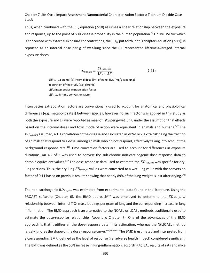
Chapter 7 Life-Cycle Impact Assessment Nanomaterial Characterization Factors: Titanium Dioxide Case Study
155
Thus, when combined with the RiF, equation (7-10) assumes a linear relationship between the exposure
and response, up to the point of 50% disease probability in the human population.84 Unlike USEtox which
is concerned with external exposure concentrations, the ED50 put forth in this chapter (equation (7-11)) is
reported as an internal dose per g of wet-lung since the RiF represented lifetime-averaged internal
exposure doses.
𝐸𝐷50,h,int =𝐸𝐷50a,t,int
𝐴𝐹a ∙ 𝐴𝐹t (7-11)
𝐸𝐷50a,t,int: animal (a) internal dose (int) of nano-TiO2 (mg/g-wet lung)
t: duration of the study (e.g. chronic)
𝐴𝐹a: interspecies extrapolation factor 𝐴𝐹t: study-time conversion factor
Interspecies extrapolation factors are conventionally used to account for anatomical and physiological
differences (e.g. metabolic rates) between species, however no such factor was applied in this study as
both the exposure and EF were reported as mass of TiO2 per g-wet lung, under the assumption that effects
based on the internal doses and toxic mode of action were equivalent in animals and humans.347 The
𝐸𝐷50a,t,int assumed, a 1:1 correlation of the disease and calculated as extra risk. Extra risk being the fraction
of animals that respond to a dose, among animals who do not respond, effectively taking into account the
background response rate.310 Time conversion factors are used to account for differences in exposure
durations. An AFt of 2 was used to convert the sub-chronic non-carcinogenic dose-response data to
chronic-equivalent values.347 The dose-response data used to estimate the 𝐸𝐷50a,t,int was specific for dry-
lung sections. Thus, the dry-lung 𝐸𝐷50a,t,int values were converted to a wet-lung value with the conversion
factor of 0.11 based on previous results showing that nearly 89% of the lung-weight is lost after drying.348
The non-carcinogenic 𝐸𝐷50a,t,int was estimated from experimental data found in the literature. Using the
PROAST software (Chapter 6), the BMD approach349 was employed to determine the 𝐸𝐷50a,t,inh,NC
relationship between internal TiO2 mass loadings per gram of lung and the corresponding increase in lung
inflammation. The BMD approach is an alternative to the NOAEL or LOAEL methods traditionally used to
estimate the dose-response relationship (Appendix: Chapter 7). One of the advantages of the BMD
approach is that it utilizes all the dose-response data in its estimation, whereas the N(L)OAEL method
largely ignores the shape of the dose-response curve.310,349–353 The BMD is estimated and interpreted from
a corresponding BMR, defined as the level of response (i.e. adverse health impact) considered significant.
The BMR was defined as the 50% increase in lung-inflammation, according to BAL results of rats and mice
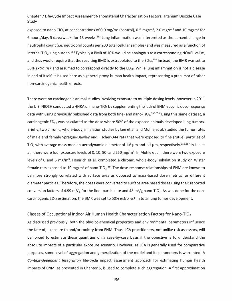
Chapter 7 Life-Cycle Impact Assessment Nanomaterial Characterization Factors: Titanium Dioxide Case Study
156
exposed to nano-TiO2 at concentrations of 0.0 mg/m3 (control), 0.5 mg/m3, 2.0 mg/m3 and 10 mg/m3 for
6 hours/day, 5 days/week, for 13 weeks.283 Lung inflammation was interpreted as the percent change in
neutrophil count (i.e. neutrophil counts per 200 total cellular samples) and was measured as a function of
internal TiO2 lung burden.283 Typically a BMR of 10% would be analogous to a corresponding NOAEL value,
and thus would require that the resulting BMD is extrapolated to the ED50.354 Instead, the BMR was set to
50% extra risk and assumed to correspond directly to the ED50. While lung inflammation is not a disease
in and of itself, it is used here as a general proxy-human health impact, representing a precursor of other
non-carcinogenic health effects.
There were no carcinogenic animal studies involving exposure to multiple dosing levels, however in 2011
the U.S. NIOSH conducted a HHRA on nano-TiO2 by supplementing the lack of ENM-specific dose-response
data with using previously published data from both fine- and nano-TiO2.355,356 Using this same dataset, a
carcinogenic ED50 was calculated as the dose where 50% of the exposed animals developed lung tumors.
Briefly, two chronic, whole-body, inhalation studies by Lee et al. and Muhle et al. studied the tumor rates
of male and female Sprague-Dawley and Fischer-344 rats that were exposed to fine (rutile) particles of
TiO2 with average mass-median-aerodynamic-diameter of 1.6 μm and 1.1 μm, respectively.355,357 In Lee et
al., there were four exposure levels of 0, 10, 50, and 250 mg/m3. In Muhle et al., there were two exposure
levels of 0 and 5 mg/m3. Heinrich et al. completed a chronic, whole-body, inhalation study on Wistar
female rats exposed to 10 mg/m3 of nano-TiO2.284 The dose-response relationships of ENM are known to
be more strongly correlated with surface area as opposed to mass-based dose metrics for different
diameter particles. Therefore, the doses were converted to surface area based doses using their reported
conversion factors of 4.99 m2/g for the fine- particulate and 48 m2/g nano-TiO2. As was done for the non-
carcinogenic ED50 estimation, the BMR was set to 50% extra risk in total lung tumor development.
Classes of Occupational Indoor Air Human Health Characterization Factors for Nano-TiO2
As discussed previously, both the physico-chemical properties and environmental parameters influence
the fate of, exposure to and/or toxicity from ENM. Thus, LCA practitioners, not unlike risk assessors, will
be forced to estimate these quantities on a case-by-case basis if the objective is to understand the
absolute impacts of a particular exposure scenario. However, as LCA is generally used for comparative
purposes, some level of aggregation and generalization of the model and its parameters is warranted. A
Context-dependent Integration life-cycle impact assessment approach for estimating human health
impacts of ENM, as presented in Chapter 5, is used to complete such aggregation. A first approximation
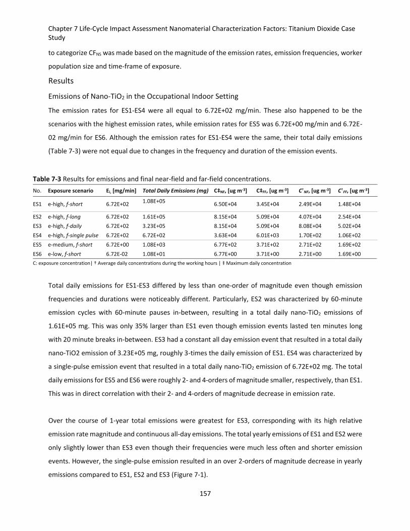
Chapter 7 Life-Cycle Impact Assessment Nanomaterial Characterization Factors: Titanium Dioxide Case Study
157
to categorize CFNS was made based on the magnitude of the emission rates, emission frequencies, worker
population size and time-frame of exposure.
Results
Emissions of Nano-TiO2 in the Occupational Indoor Setting
The emission rates for ES1-ES4 were all equal to 6.72E+02 mg/min. These also happened to be the
scenarios with the highest emission rates, while emission rates for ES5 was 6.72E+00 mg/min and 6.72E-
02 mg/min for ES6. Although the emission rates for ES1-ES4 were the same, their total daily emissions
(Table 7-3) were not equal due to changes in the frequency and duration of the emission events.
Table 7-3 Results for emissions and final near-field and far-field concentrations.
No. Exposure scenario Ei, [mg/min] Total Daily Emissions (mg) C‡NF, [ug m-3] C‡FF, [ug m-3] C†NF, [ug m-3] C†
FF, [ug m-3]
ES1 e-high, f-short 6.72E+02 1.08E+05 6.50E+04 3.45E+04 2.49E+04 1.48E+04
ES2 e-high, f-long 6.72E+02 1.61E+05 8.15E+04 5.09E+04 4.07E+04 2.54E+04
ES3 e-high, f-daily 6.72E+02 3.23E+05 8.15E+04 5.09E+04 8.08E+04 5.02E+04
ES4 e-high, f-single pulse 6.72E+02 6.72E+02 3.63E+04 6.01E+03 1.70E+02 1.06E+02
ES5 e-medium, f-short 6.72E+00 1.08E+03 6.77E+02 3.71E+02 2.71E+02 1.69E+02
ES6 e-low, f-short 6.72E-02 1.08E+01 6.77E+00 3.71E+00 2.71E+00 1.69E+00
C: exposure concentration| † Average daily concentrations during the working hours | ‡ Maximum daily concentration
Total daily emissions for ES1-ES3 differed by less than one-order of magnitude even though emission
frequencies and durations were noticeably different. Particularly, ES2 was characterized by 60-minute
emission cycles with 60-minute pauses in-between, resulting in a total daily nano-TiO2 emissions of
1.61E+05 mg. This was only 35% larger than ES1 even though emission events lasted ten minutes long
with 20 minute breaks in-between. ES3 had a constant all day emission event that resulted in a total daily
nano-TiO2 emission of 3.23E+05 mg, roughly 3-times the daily emission of ES1. ES4 was characterized by
a single-pulse emission event that resulted in a total daily nano-TiO2 emission of 6.72E+02 mg. The total
daily emissions for ES5 and ES6 were roughly 2- and 4-orders of magnitude smaller, respectively, than ES1.
This was in direct correlation with their 2- and 4-orders of magnitude decrease in emission rate.
Over the course of 1-year total emissions were greatest for ES3, corresponding with its high relative
emission rate magnitude and continuous all-day emissions. The total yearly emissions of ES1 and ES2 were
only slightly lower than ES3 even though their frequencies were much less often and shorter emission
events. However, the single-pulse emission resulted in an over 2-orders of magnitude decrease in yearly
emissions compared to ES1, ES2 and ES3 (Figure 7-1).
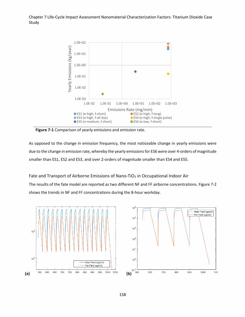
Chapter 7 Life-Cycle Impact Assessment Nanomaterial Characterization Factors: Titanium Dioxide Case Study
158
Figure 7-1 Comparison of yearly emissions and emission rate.
As opposed to the change in emission frequency, the most noticeable change in yearly emissions were
due to the change in emission rate, whereby the yearly emissions for ES6 were over 4-orders of magnitude
smaller than ES1, ES2 and ES3, and over 2-orders of magnitude smaller than ES4 and ES5.
Fate and Transport of Airborne Emissions of Nano-TiO2 in Occupational Indoor Air
The results of the fate model are reported as two different NF and FF airborne concentrations. Figure 7-2
shows the trends in NF and FF concentrations during the 8-hour workday.
(a) (b)
1.0E-03
1.0E-02
1.0E-01
1.0E+00
1.0E+01
1.0E+02
1.0E-02 1.0E-01 1.0E+00 1.0E+01 1.0E+02 1.0E+03
Year
ly E
mis
sio
ns
(kg/
year
)
Emissions Rate (mg/min)ES1 (e-high, f-short) ES2 (e-high, f-long)ES3 (e-high, f-all day) ES4 (e-high, f-single pulse)ES5 (e-medium, f-short) ES6 (e-low, f-short)
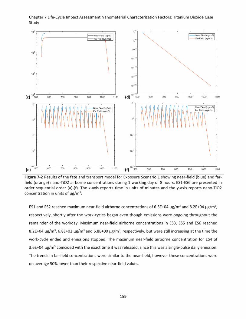
Chapter 7 Life-Cycle Impact Assessment Nanomaterial Characterization Factors: Titanium Dioxide Case Study
159
(c) (d)
(e) (f)
Figure 7-2 Results of the fate and transport model for Exposure Scenario 1 showing near-field (blue) and far-field (orange) nano-TiO2 airborne concentrations during 1 working day of 8 hours. ES1-ES6 are presented in order sequential order (a)-(f). The x-axis reports time in units of minutes and the y-axis reports nano-TiO2 concentration in units of μg/m3.
ES1 and ES2 reached maximum near-field airborne concentrations of 6.5E+04 μg/m3 and 8.2E+04 μg/m3,
respectively, shortly after the work-cycles began even though emissions were ongoing throughout the
remainder of the workday. Maximum near-field airborne concentrations in ES3, ES5 and ES6 reached
8.2E+04 μg/m3, 6.8E+02 μg/m3 and 6.8E+00 μg/m3, respectively, but were still increasing at the time the
work-cycle ended and emissions stopped. The maximum near-field airborne concentration for ES4 of
3.6E+04 μg/m3 coincided with the exact time it was released, since this was a single-pulse daily emission.
The trends in far-field concentrations were similar to the near-field, however these concentrations were
on average 50% lower than their respective near-field values.
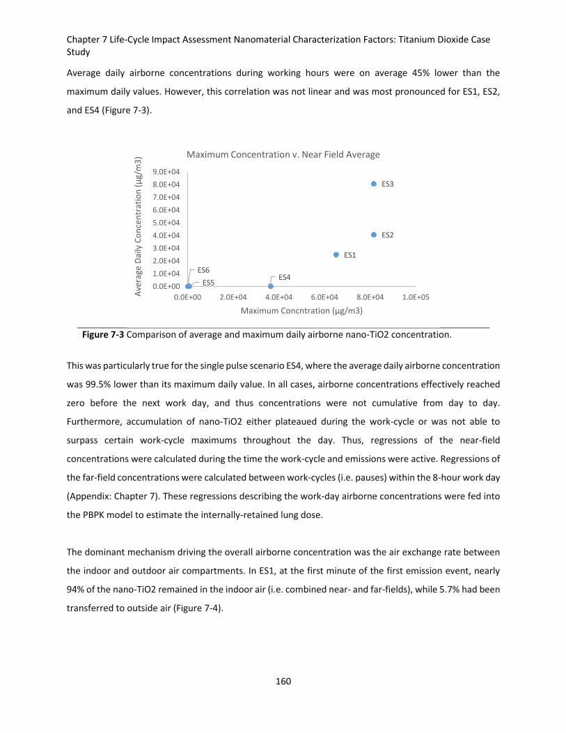
Chapter 7 Life-Cycle Impact Assessment Nanomaterial Characterization Factors: Titanium Dioxide Case Study
160
Average daily airborne concentrations during working hours were on average 45% lower than the
maximum daily values. However, this correlation was not linear and was most pronounced for ES1, ES2,
and ES4 (Figure 7-3).
Figure 7-3 Comparison of average and maximum daily airborne nano-TiO2 concentration.
This was particularly true for the single pulse scenario ES4, where the average daily airborne concentration
was 99.5% lower than its maximum daily value. In all cases, airborne concentrations effectively reached
zero before the next work day, and thus concentrations were not cumulative from day to day.
Furthermore, accumulation of nano-TiO2 either plateaued during the work-cycle or was not able to
surpass certain work-cycle maximums throughout the day. Thus, regressions of the near-field
concentrations were calculated during the time the work-cycle and emissions were active. Regressions of
the far-field concentrations were calculated between work-cycles (i.e. pauses) within the 8-hour work day
(Appendix: Chapter 7). These regressions describing the work-day airborne concentrations were fed into
the PBPK model to estimate the internally-retained lung dose.
The dominant mechanism driving the overall airborne concentration was the air exchange rate between
the indoor and outdoor air compartments. In ES1, at the first minute of the first emission event, nearly
94% of the nano-TiO2 remained in the indoor air (i.e. combined near- and far-fields), while 5.7% had been
transferred to outside air (Figure 7-4).
ES1
ES2
ES3
ES4ES5
ES6
0.0E+00
1.0E+04
2.0E+04
3.0E+04
4.0E+04
5.0E+04
6.0E+04
7.0E+04
8.0E+04
9.0E+04
0.0E+00 2.0E+04 4.0E+04 6.0E+04 8.0E+04 1.0E+05Ave
rage
Dai
ly C
on
cen
trat
ion
(μ
g/m
3)
Maximum Concntration (μg/m3)
Maximum Concentration v. Near Field Average
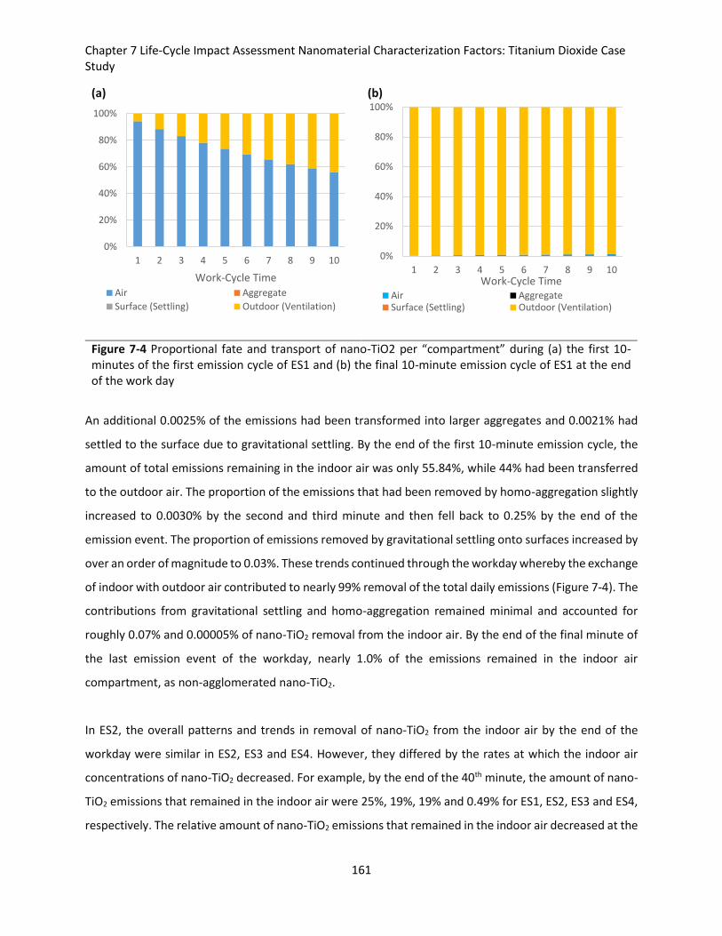
Chapter 7 Life-Cycle Impact Assessment Nanomaterial Characterization Factors: Titanium Dioxide Case Study
161
(a)
(b)
Figure 7-4 Proportional fate and transport of nano-TiO2 per “compartment” during (a) the first 10-minutes of the first emission cycle of ES1 and (b) the final 10-minute emission cycle of ES1 at the end of the work day
An additional 0.0025% of the emissions had been transformed into larger aggregates and 0.0021% had
settled to the surface due to gravitational settling. By the end of the first 10-minute emission cycle, the
amount of total emissions remaining in the indoor air was only 55.84%, while 44% had been transferred
to the outdoor air. The proportion of the emissions that had been removed by homo-aggregation slightly
increased to 0.0030% by the second and third minute and then fell back to 0.25% by the end of the
emission event. The proportion of emissions removed by gravitational settling onto surfaces increased by
over an order of magnitude to 0.03%. These trends continued through the workday whereby the exchange
of indoor with outdoor air contributed to nearly 99% removal of the total daily emissions (Figure 7-4). The
contributions from gravitational settling and homo-aggregation remained minimal and accounted for
roughly 0.07% and 0.00005% of nano-TiO2 removal from the indoor air. By the end of the final minute of
the last emission event of the workday, nearly 1.0% of the emissions remained in the indoor air
compartment, as non-agglomerated nano-TiO2.
In ES2, the overall patterns and trends in removal of nano-TiO2 from the indoor air by the end of the
workday were similar in ES2, ES3 and ES4. However, they differed by the rates at which the indoor air
concentrations of nano-TiO2 decreased. For example, by the end of the 40th minute, the amount of nano-
TiO2 emissions that remained in the indoor air were 25%, 19%, 19% and 0.49% for ES1, ES2, ES3 and ES4,
respectively. The relative amount of nano-TiO2 emissions that remained in the indoor air decreased at the
0%
20%
40%
60%
80%
100%
1 2 3 4 5 6 7 8 9 10
Work-Cycle TimeAir Aggregate
Surface (Settling) Outdoor (Ventilation)
0%
20%
40%
60%
80%
100%
1 2 3 4 5 6 7 8 9 10Work-Cycle Time
Air AggregateSurface (Settling) Outdoor (Ventilation)
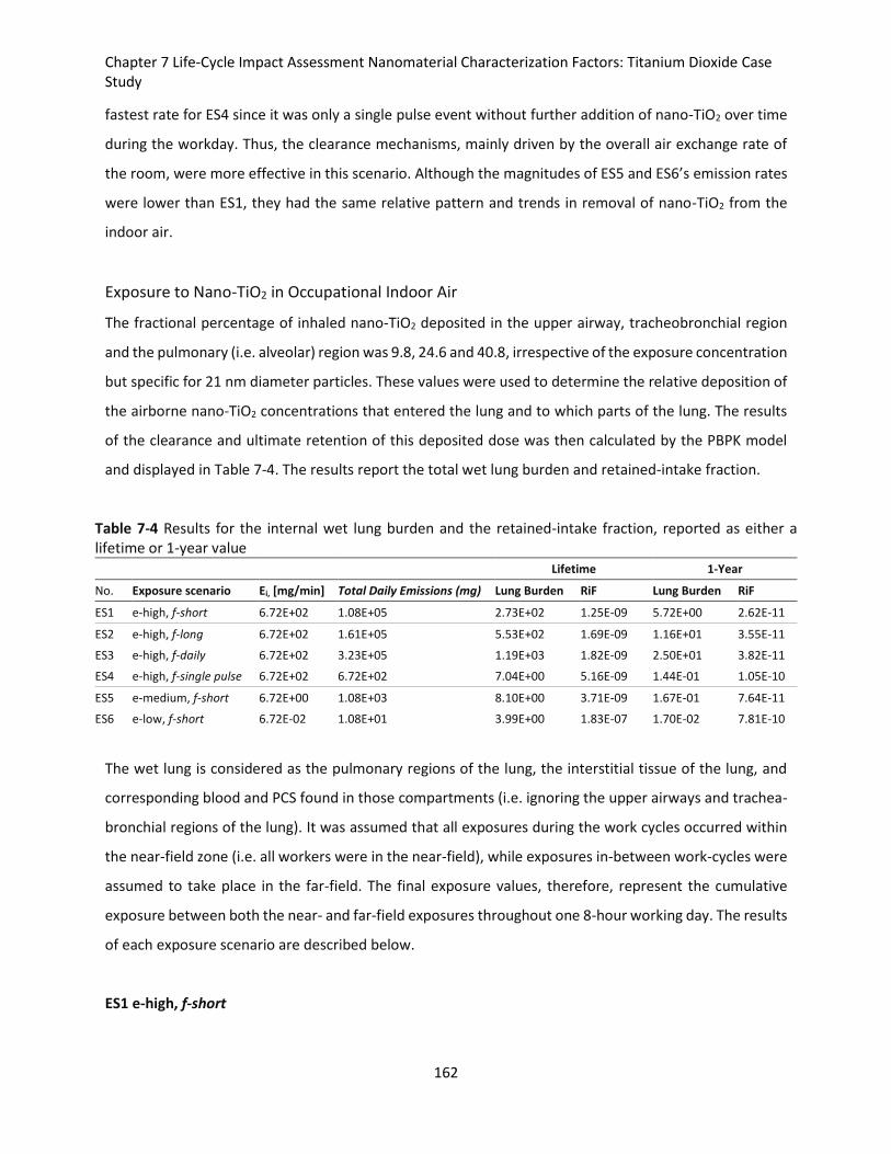
Chapter 7 Life-Cycle Impact Assessment Nanomaterial Characterization Factors: Titanium Dioxide Case Study
162
fastest rate for ES4 since it was only a single pulse event without further addition of nano-TiO2 over time
during the workday. Thus, the clearance mechanisms, mainly driven by the overall air exchange rate of
the room, were more effective in this scenario. Although the magnitudes of ES5 and ES6’s emission rates
were lower than ES1, they had the same relative pattern and trends in removal of nano-TiO2 from the
indoor air.
Exposure to Nano-TiO2 in Occupational Indoor Air
The fractional percentage of inhaled nano-TiO2 deposited in the upper airway, tracheobronchial region
and the pulmonary (i.e. alveolar) region was 9.8, 24.6 and 40.8, irrespective of the exposure concentration
but specific for 21 nm diameter particles. These values were used to determine the relative deposition of
the airborne nano-TiO2 concentrations that entered the lung and to which parts of the lung. The results
of the clearance and ultimate retention of this deposited dose was then calculated by the PBPK model
and displayed in Table 7-4. The results report the total wet lung burden and retained-intake fraction.
Table 7-4 Results for the internal wet lung burden and the retained-intake fraction, reported as either a lifetime or 1-year value
Lifetime 1-Year
No. Exposure scenario Ei, [mg/min] Total Daily Emissions (mg) Lung Burden RiF Lung Burden RiF
ES1 e-high, f-short 6.72E+02 1.08E+05 2.73E+02 1.25E-09 5.72E+00 2.62E-11
ES2 e-high, f-long 6.72E+02 1.61E+05 5.53E+02 1.69E-09 1.16E+01 3.55E-11
ES3 e-high, f-daily 6.72E+02 3.23E+05 1.19E+03 1.82E-09 2.50E+01 3.82E-11
ES4 e-high, f-single pulse 6.72E+02 6.72E+02 7.04E+00 5.16E-09 1.44E-01 1.05E-10
ES5 e-medium, f-short 6.72E+00 1.08E+03 8.10E+00 3.71E-09 1.67E-01 7.64E-11
ES6 e-low, f-short 6.72E-02 1.08E+01 3.99E+00 1.83E-07 1.70E-02 7.81E-10
The wet lung is considered as the pulmonary regions of the lung, the interstitial tissue of the lung, and
corresponding blood and PCS found in those compartments (i.e. ignoring the upper airways and trachea-
bronchial regions of the lung). It was assumed that all exposures during the work cycles occurred within
the near-field zone (i.e. all workers were in the near-field), while exposures in-between work-cycles were
assumed to take place in the far-field. The final exposure values, therefore, represent the cumulative
exposure between both the near- and far-field exposures throughout one 8-hour working day. The results
of each exposure scenario are described below.
ES1 e-high, f-short
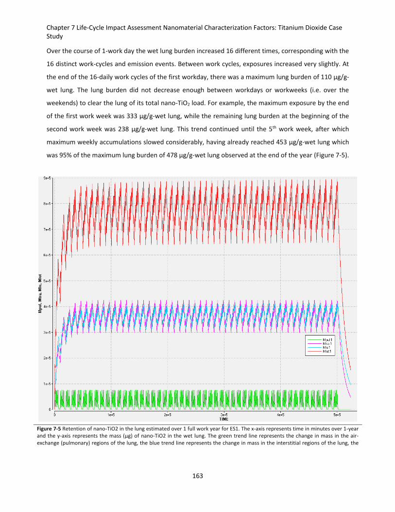
Chapter 7 Life-Cycle Impact Assessment Nanomaterial Characterization Factors: Titanium Dioxide Case Study
163
Over the course of 1-work day the wet lung burden increased 16 different times, corresponding with the
16 distinct work-cycles and emission events. Between work cycles, exposures increased very slightly. At
the end of the 16-daily work cycles of the first workday, there was a maximum lung burden of 110 μg/g-
wet lung. The lung burden did not decrease enough between workdays or workweeks (i.e. over the
weekends) to clear the lung of its total nano-TiO2 load. For example, the maximum exposure by the end
of the first work week was 333 μg/g-wet lung, while the remaining lung burden at the beginning of the
second work week was 238 μg/g-wet lung. This trend continued until the 5th work week, after which
maximum weekly accumulations slowed considerably, having already reached 453 μg/g-wet lung which
was 95% of the maximum lung burden of 478 μg/g-wet lung observed at the end of the year (Figure 7-5).
Figure 7-5 Retention of nano-TiO2 in the lung estimated over 1 full work year for ES1. The x-axis represents time in minutes over 1-year and the y-axis represents the mass (μg) of nano-TiO2 in the wet lung. The green trend line represents the change in mass in the air-exchange (pulmonary) regions of the lung, the blue trend line represents the change in mass in the interstitial regions of the lung, the
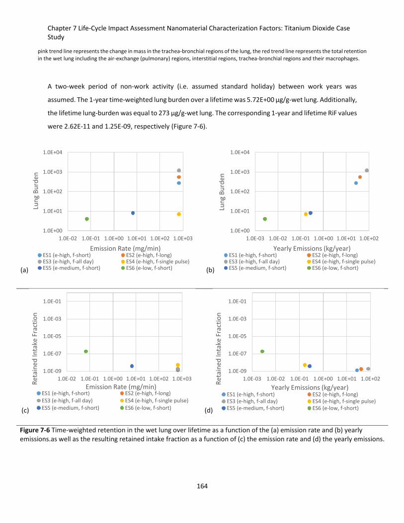
Chapter 7 Life-Cycle Impact Assessment Nanomaterial Characterization Factors: Titanium Dioxide Case Study
164
pink trend line represents the change in mass in the trachea-bronchial regions of the lung, the red trend line represents the total retention in the wet lung including the air-exchange (pulmonary) regions, interstitial regions, trachea-bronchial regions and their macrophages.
A two-week period of non-work activity (i.e. assumed standard holiday) between work years was
assumed. The 1-year time-weighted lung burden over a lifetime was 5.72E+00 μg/g-wet lung. Additionally,
the lifetime lung-burden was equal to 273 μg/g-wet lung. The corresponding 1-year and lifetime RiF values
were 2.62E-11 and 1.25E-09, respectively (Figure 7-6).
(a) (b)
(c) (d)
Figure 7-6 Time-weighted retention in the wet lung over lifetime as a function of the (a) emission rate and (b) yearly emissions.as well as the resulting retained intake fraction as a function of (c) the emission rate and (d) the yearly emissions.
1.0E+00
1.0E+01
1.0E+02
1.0E+03
1.0E+04
1.0E-02 1.0E-01 1.0E+00 1.0E+01 1.0E+02 1.0E+03
Lun
g B
urd
en
Emission Rate (mg/min)ES1 (e-high, f-short) ES2 (e-high, f-long)ES3 (e-high, f-all day) ES4 (e-high, f-single pulse)ES5 (e-medium, f-short) ES6 (e-low, f-short)
1.0E+00
1.0E+01
1.0E+02
1.0E+03
1.0E+04
1.0E-03 1.0E-02 1.0E-01 1.0E+00 1.0E+01 1.0E+02
Lun
g B
urd
en
Yearly Emissions (kg/year)ES1 (e-high, f-short) ES2 (e-high, f-long)ES3 (e-high, f-all day) ES4 (e-high, f-single pulse)ES5 (e-medium, f-short) ES6 (e-low, f-short)
1.0E-09
1.0E-07
1.0E-05
1.0E-03
1.0E-01
1.0E-02 1.0E-01 1.0E+00 1.0E+01 1.0E+02 1.0E+03
Ret
ain
ed In
take
Fra
ctio
n
Emission Rate (mg/min)ES1 (e-high, f-short) ES2 (e-high, f-long)ES3 (e-high, f-all day) ES4 (e-high, f-single pulse)ES5 (e-medium, f-short) ES6 (e-low, f-short)
1.0E-09
1.0E-07
1.0E-05
1.0E-03
1.0E-01
1.0E-03 1.0E-02 1.0E-01 1.0E+00 1.0E+01 1.0E+02
Ret
ain
ed In
take
Fra
ctio
n
Yearly Emissions (kg/year)ES1 (e-high, f-short) ES2 (e-high, f-long)ES3 (e-high, f-all day) ES4 (e-high, f-single pulse)ES5 (e-medium, f-short) ES6 (e-low, f-short)
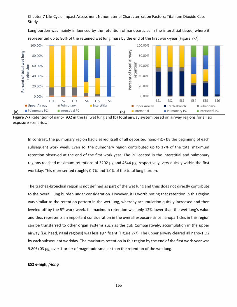
Chapter 7 Life-Cycle Impact Assessment Nanomaterial Characterization Factors: Titanium Dioxide Case Study
165
Lung burden was mainly influenced by the retention of nanoparticles in the interstitial tissue, where it
represented up to 80% of the retained wet lung mass by the end of the first work-year (Figure 7-7).
(a) (b) Figure 7-7 Retention of nano-TiO2 in the (a) wet lung and (b) total airway system based on airway regions for all six exposure scenarios.
In contrast, the pulmonary region had cleared itself of all deposited nano-TiO2 by the beginning of each
subsequent work week. Even so, the pulmonary region contributed up to 17% of the total maximum
retention observed at the end of the first work-year. The PC located in the interstitial and pulmonary
regions reached maximum retentions of 3202 μg and 4644 μg, respectively, very quickly within the first
workday. This represented roughly 0.7% and 1.0% of the total lung burden.
The trachea-bronchial region is not defined as part of the wet lung and thus does not directly contribute
to the overall lung burden under consideration. However, it is worth noting that retention in this region
was similar to the retention pattern in the wet lung, whereby accumulation quickly increased and then
leveled off by the 5th work week. Its maximum retention was only 12% lower than the wet lung’s value
and thus represents an important consideration in the overall exposure since nanoparticles in this region
can be transferred to other organ systems such as the gut. Comparatively, accumulation in the upper
airway (i.e. head, nasal regions) was less significant (Figure 7-7). The upper airway cleared all nano-TiO2
by each subsequent workday. The maximum retention in this region by the end of the first work-year was
9.80E+03 μg, over 1-order of magnitude smaller than the retention of the wet lung.
ES2 e-high, f-long
0.00%
20.00%
40.00%
60.00%
80.00%
100.00%
ES1 ES2 ES3 ES4 ES5 ES6
Pe
rce
nt
of
tota
l we
t lu
ng
rete
nti
on
Upper Airway Pulmonary Interstitial
Pulmonary PC Interstitial PC
0.00%
20.00%
40.00%
60.00%
80.00%
100.00%
ES1 ES2 ES3 ES4 ES5 ES6
Pe
rcen
t o
f to
tal a
irw
ay
rete
nti
on
Upper Airway Trach-Bronch Pulmonary
Interstitial Pulmonary PC Interstitial PC
Chapter 7 Life-Cycle Impact Assessment Nanomaterial Characterization Factors: Titanium Dioxide Case Study
166
Over the course of 1-work day the wet lung burden increased 6 different times, corresponding with each
of the 6 work-cycles and emission events. Between work cycles, exposures increased very slightly. At the
end of the first workday, there was a maximum wet lung burden of 223 μg/g-wet lung. The lung burden
did not decrease enough between workdays or workweeks (i.e. over the weekends) to clear the lung of
its total nano-TiO2 load. For example, the maximum exposure by the end of the first work week was 656
μg/g-wet lung, while at the start of the second work week it was 475 μg/g-wet lung. This trend continued
until the 6th work week, after which maximum weekly accumulations slowed considerably, having already
reached 917 μg/g-wet lung which is 94% of the maximum lung burden of 980 μg/g-wet lung at the end of
the year (Appendix: Chapter 7). A two-week period of non-work activity (i.e. assumed standard holiday)
between work years was assumed. The 1-year time-weighted lung burden over a lifetime was 1.16E+01
μg/g-wet lung. Additionally, the lifetime lung-burden was equal to 553 μg/g-wet lung. The corresponding
1-year and lifetime RiF values were 3.55E-11 and 1.69E-09, respectively (Figure 7-6).
Lung burden was mainly influenced by the retention of nanoparticles in the interstitial region, where it
represented up to 81% of the retained wet lung mass by the end of the first work-year (Figure 7-7). In
contrast, the pulmonary region cleared itself of all deposited nano-TiO2 by the beginning of each
subsequent work week. Even so, the pulmonary region contributed up to 17% of the total maximum
retention observed at the end of the first work-year. The PCS located in the interstitial and pulmonary
regions reached maximum retentions of 3202 μg and 4644 μg, respectively, very quickly within the first
workday. This represented roughly 0.3% and 0.5% of the total lung burden.
Retention in the trachea-bronchial region was similar to the retention pattern in the wet lung, whereby
accumulation quickly increased and then leveled off by the 6th work week. Its maximum retention was
10% lower than the wet lung’s maximum retention value and thus represents an important consideration
in the overall exposure as explained previously for ES1. Comparatively, accumulation in the upper airway
was less significant. The upper airway cleared all nano-TiO2 by each subsequent workday. The maximum
retention in this region by the end of the first work-year was 2.2E+04 μg, over 1-order of magnitude
smaller than retention in the wet lung.
ES3 e-high, f-daily
Over the course of 1-work day the wet lung burden increased steadily without pause and correlated with
the all-day, constant exposure emissions of this model. At the end of the first workday, the maximum lung
Chapter 7 Life-Cycle Impact Assessment Nanomaterial Characterization Factors: Titanium Dioxide Case Study
167
burden was 486 μg/g-wet lung. The lung burden did not decrease enough between workdays or
workweeks (i.e. over the weekends) to clear the lung of its total nano-TiO2 load. For example, the
maximum exposure by the end of the first work week was 1.45E+03 μg/g-wet lung, while at the beginning
of the second work week it was 1.02E+03 μg/g-wet lung. This trend continued until the 6th work week,
after which maximum weekly accumulations slowed considerably, having already reached 1.99E+03 μg/g-
wet lung which is 96% of the maximum lung burden of 2.08E+03 μg/g-wet lung at the end of the year
(Appendix: Chapter 7). A two-week period of non-work activity (i.e. assumed standard holiday) between
work years was assumed. The 1-year time-weighted lung burden over a lifetime was 2.50E+01 μg/g-wet
lung. Additionally, the lifetime lung-burden was equal to 1.19E+03 μg/g-wet lung. The corresponding 1-
year and lifetime RiF values were 3.82E-11 and 1.82E-09, respectively (Figure 7-6).
Lung burden was mainly influenced by the retention of nanoparticles in the interstitial region, where it
represented up to 90% of the retained wet lung mass by the end of the first work-year (Figure 7-7). In
contrast, the pulmonary region cleared itself of all deposited nano-TiO2 by the beginning of each
subsequent work week. Even so, the pulmonary region contributed up to 16% of the total maximum
retention observed at the end of the first work-year. The PCS located in the interstitial and pulmonary
regions reached maximum retentions of 3202 μg and 4644 μg, respectively, very quickly within the first
workday. This represented roughly 0.20% and 0.23% of the total lung burden.
Retention in the trachea-bronchial region was similar to the retention pattern in the wet lung, whereby
accumulation quickly increased and then leveled off by the 6th work week. Its maximum retention was
only 8% lower than the wet lung’s maximum retention value and thus represents an important
consideration in the overall exposure as explained previously for ES1. Comparatively, accumulation in the
upper airway was less significant. The upper airway cleared all nano-TiO2 by each subsequent workday.
The maximum retention in this region by the end of the first work-year was 4.1E+04 μg, over 1-order of
magnitude smaller than retention in the wet lung.
ES4 e-high, f-single pulse
Over the course of 1-work day there was an initial maximum daily lung burden seen within the first hour
of exposure, which then slightly decreased by the end of the workday to 0.72 μg/g-wet lung. There were
no decreases between workdays nor was there significant decreases between workweeks. This trend
continued until the 18th work week when there was a sudden spike in total wet lung retention. The peak
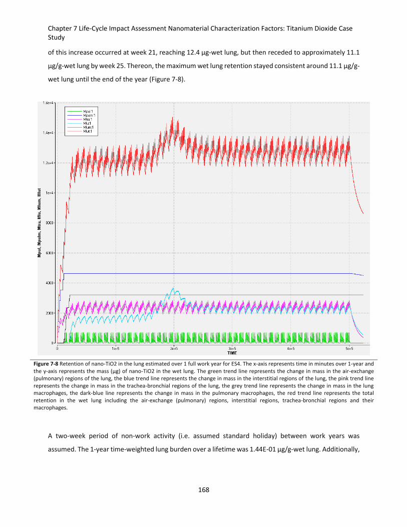
Chapter 7 Life-Cycle Impact Assessment Nanomaterial Characterization Factors: Titanium Dioxide Case Study
168
of this increase occurred at week 21, reaching 12.4 μg-wet lung, but then receded to approximately 11.1
μg/g-wet lung by week 25. Thereon, the maximum wet lung retention stayed consistent around 11.1 μg/g-
wet lung until the end of the year (Figure 7-8).
Figure 7-8 Retention of nano-TiO2 in the lung estimated over 1 full work year for ES4. The x-axis represents time in minutes over 1-year and the y-axis represents the mass (μg) of nano-TiO2 in the wet lung. The green trend line represents the change in mass in the air-exchange (pulmonary) regions of the lung, the blue trend line represents the change in mass in the interstitial regions of the lung, the pink trend line represents the change in mass in the trachea-bronchial regions of the lung, the grey trend line represents the change in mass in the lung macrophages, the dark-blue line represents the change in mass in the pulmonary macrophages, the red trend line represents the total retention in the wet lung including the air-exchange (pulmonary) regions, interstitial regions, trachea-bronchial regions and their macrophages.
A two-week period of non-work activity (i.e. assumed standard holiday) between work years was
assumed. The 1-year time-weighted lung burden over a lifetime was 1.44E-01 μg/g-wet lung. Additionally,
Chapter 7 Life-Cycle Impact Assessment Nanomaterial Characterization Factors: Titanium Dioxide Case Study
169
the lifetime lung-burden was equal to 7.04E+00 μg/g-wet lung. The corresponding 1-year and lifetime RiF
values were 1.05E-10 and 5.16E-09, respectively (Figure 7-6).
Lung burden was mainly influenced by the retention of nanoparticles in the interstitial and pulmonary
PCS, where they represented 29% and 42%, respectively, of the maximum retained dose seen at the end
of the year (Figure 7-7). The interstitium had a maximum retention of 3.20E+03 μg by the end of the work
year. This was 22% of the total wet lung retention and is in contrast to ES1-ES3 where the interstitium was
the most significant contributor to the total wet lung burden. The pulmonary region cleared itself of all
deposited nano-TiO2 by the beginning of each subsequent work week. This region only contributed up to
6% of the maximum wet lung retention observed at the end of the first work-year.
Retention in the trachea-bronchial region was similar to the retention pattern in the wet lung, however
there was no secondary spike in this region’s retention, which had leveled off by the 5th work week. Its
maximum retention was 74% lower than the wet lung’s maximum retention value. Comparatively,
accumulation in the upper airway was negligible and only represented 1% of the total wet lung retention
by the end of the work-year.
ES5 e-medium, f-short
Over the course of 1-work day there were 16 distinct increases in wet lung retention that corresponded
with the 16 emission events throughout the day. By the end of the first workday the maximum wet lung
retention was 1.15 μg/g-wet lung. There was little decrease between workdays and between work-days.
This trend continued until the 11th work week when there was a sudden spike in total wet lung retention.
The peak of this increase occurred at week 14, reaching 14 μg-wet lung, but then receding to
approximately 12.6 μg/g-wet lung by week 17. Thereon, the maximum wet lung retention stayed
consistent around 12.6 μg/g-wet lung until the end of the work-year (Appendix: Chapter 7). The 1-year
time-weighted lung burden over a lifetime was 1.67E-01 μg/g-wet lung. Additionally, the lifetime lung-
burden was equal to 8.10E+00 μg/g-wet lung. The corresponding 1-year and lifetime RiF values were
7.64E-11 and 3.17E-09, respectively (Figure 7-6).
Lung burden was mainly influenced by the retention of nanoparticles in the pulmonary PCS, where they
accounted for 38% of the maximum total retention by the end of the work-year (Figure 7-7). The
interstitium accounted for 32% of the maximum total wet lung retention and was also correlated with the
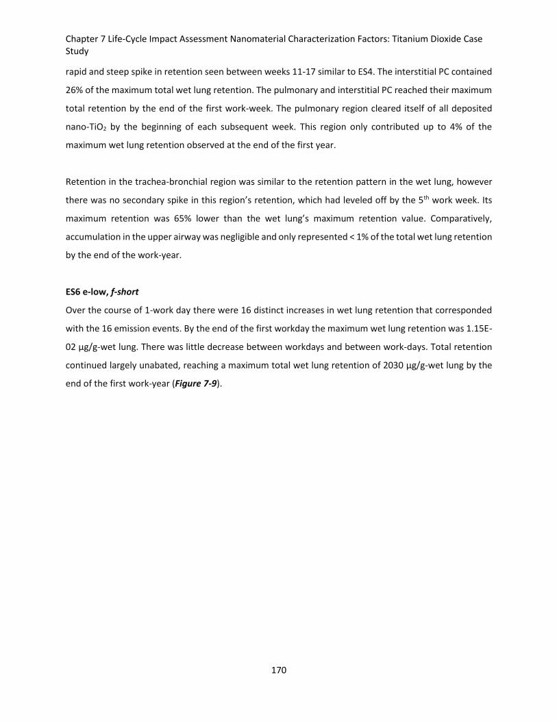
Chapter 7 Life-Cycle Impact Assessment Nanomaterial Characterization Factors: Titanium Dioxide Case Study
170
rapid and steep spike in retention seen between weeks 11-17 similar to ES4. The interstitial PC contained
26% of the maximum total wet lung retention. The pulmonary and interstitial PC reached their maximum
total retention by the end of the first work-week. The pulmonary region cleared itself of all deposited
nano-TiO2 by the beginning of each subsequent week. This region only contributed up to 4% of the
maximum wet lung retention observed at the end of the first year.
Retention in the trachea-bronchial region was similar to the retention pattern in the wet lung, however
there was no secondary spike in this region’s retention, which had leveled off by the 5th work week. Its
maximum retention was 65% lower than the wet lung’s maximum retention value. Comparatively,
accumulation in the upper airway was negligible and only represented < 1% of the total wet lung retention
by the end of the work-year.
ES6 e-low, f-short
Over the course of 1-work day there were 16 distinct increases in wet lung retention that corresponded
with the 16 emission events. By the end of the first workday the maximum wet lung retention was 1.15E-
02 μg/g-wet lung. There was little decrease between workdays and between work-days. Total retention
continued largely unabated, reaching a maximum total wet lung retention of 2030 μg/g-wet lung by the
end of the first work-year (Figure 7-9).
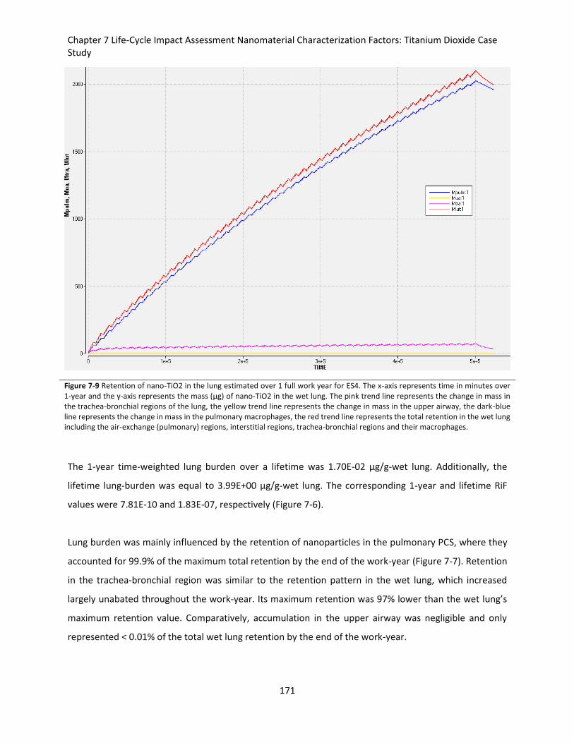
Chapter 7 Life-Cycle Impact Assessment Nanomaterial Characterization Factors: Titanium Dioxide Case Study
171
Figure 7-9 Retention of nano-TiO2 in the lung estimated over 1 full work year for ES4. The x-axis represents time in minutes over 1-year and the y-axis represents the mass (μg) of nano-TiO2 in the wet lung. The pink trend line represents the change in mass in the trachea-bronchial regions of the lung, the yellow trend line represents the change in mass in the upper airway, the dark-blue line represents the change in mass in the pulmonary macrophages, the red trend line represents the total retention in the wet lung including the air-exchange (pulmonary) regions, interstitial regions, trachea-bronchial regions and their macrophages.
The 1-year time-weighted lung burden over a lifetime was 1.70E-02 μg/g-wet lung. Additionally, the
lifetime lung-burden was equal to 3.99E+00 μg/g-wet lung. The corresponding 1-year and lifetime RiF
values were 7.81E-10 and 1.83E-07, respectively (Figure 7-6).
Lung burden was mainly influenced by the retention of nanoparticles in the pulmonary PCS, where they
accounted for 99.9% of the maximum total retention by the end of the work-year (Figure 7-7). Retention
in the trachea-bronchial region was similar to the retention pattern in the wet lung, which increased
largely unabated throughout the work-year. Its maximum retention was 97% lower than the wet lung’s
maximum retention value. Comparatively, accumulation in the upper airway was negligible and only
represented < 0.01% of the total wet lung retention by the end of the work-year.
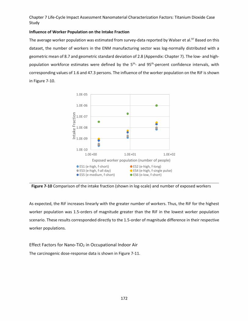
Chapter 7 Life-Cycle Impact Assessment Nanomaterial Characterization Factors: Titanium Dioxide Case Study
172
Influence of Worker Population on the Intake Fraction
The average worker population was estimated from survey-data reported by Walser et al.97 Based on this
dataset, the number of workers in the ENM manufacturing sector was log-normally distributed with a
geometric mean of 8.7 and geometric standard deviation of 2.8 (Appendix: Chapter 7). The low- and high-
population workforce estimates were defined by the 5th- and 95th-percent confidence intervals, with
corresponding values of 1.6 and 47.3 persons. The influence of the worker population on the RiF is shown
in Figure 7-10.
Figure 7-10 Comparison of the intake fraction (shown in log-scale) and number of exposed workers
As expected, the RiF increases linearly with the greater number of workers. Thus, the RiF for the highest
worker population was 1.5-orders of magnitude greater than the RiF in the lowest worker population
scenario. These results corresponded directly to the 1.5-order of magnitude difference in their respective
worker populations.
Effect Factors for Nano-TiO2 in Occupational Indoor Air
The carcinogenic dose-response data is shown in Figure 7-11.
1.0E-10
1.0E-09
1.0E-08
1.0E-07
1.0E-06
1.0E-05
1.0E+00 1.0E+01 1.0E+02
Inta
ke F
ract
ion
Exposed worker population (number of people)
ES1 (e-high, f-short) ES2 (e-high, f-long)ES3 (e-high, f-all day) ES4 (e-high, f-single pulse)ES5 (e-medium, f-short) ES6 (e-low, f-short)
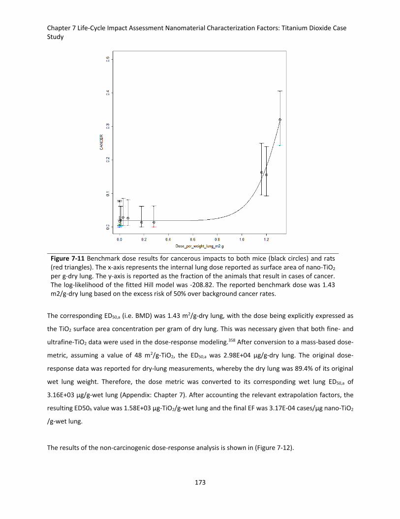
Chapter 7 Life-Cycle Impact Assessment Nanomaterial Characterization Factors: Titanium Dioxide Case Study
173
Figure 7-11 Benchmark dose results for cancerous impacts to both mice (black circles) and rats (red triangles). The x-axis represents the internal lung dose reported as surface area of nano-TiO2 per g-dry lung. The y-axis is reported as the fraction of the animals that result in cases of cancer. The log-likelihood of the fitted Hill model was -208.82. The reported benchmark dose was 1.43 m2/g-dry lung based on the excess risk of 50% over background cancer rates.
The corresponding ED50,a (i.e. BMD) was 1.43 m2/g-dry lung, with the dose being explicitly expressed as
the TiO2 surface area concentration per gram of dry lung. This was necessary given that both fine- and
ultrafine-TiO2 data were used in the dose-response modeling.358 After conversion to a mass-based dose-
metric, assuming a value of 48 m2/g-TiO2, the ED50,a was 2.98E+04 μg/g-dry lung. The original dose-
response data was reported for dry-lung measurements, whereby the dry lung was 89.4% of its original
wet lung weight. Therefore, the dose metric was converted to its corresponding wet lung ED50,a of
3.16E+03 μg/g-wet lung (Appendix: Chapter 7). After accounting the relevant extrapolation factors, the
resulting ED50h value was 1.58E+03 μg-TiO2/g-wet lung and the final EF was 3.17E-04 cases/μg nano-TiO2
/g-wet lung.
The results of the non-carcinogenic dose-response analysis is shown in (Figure 7-12).
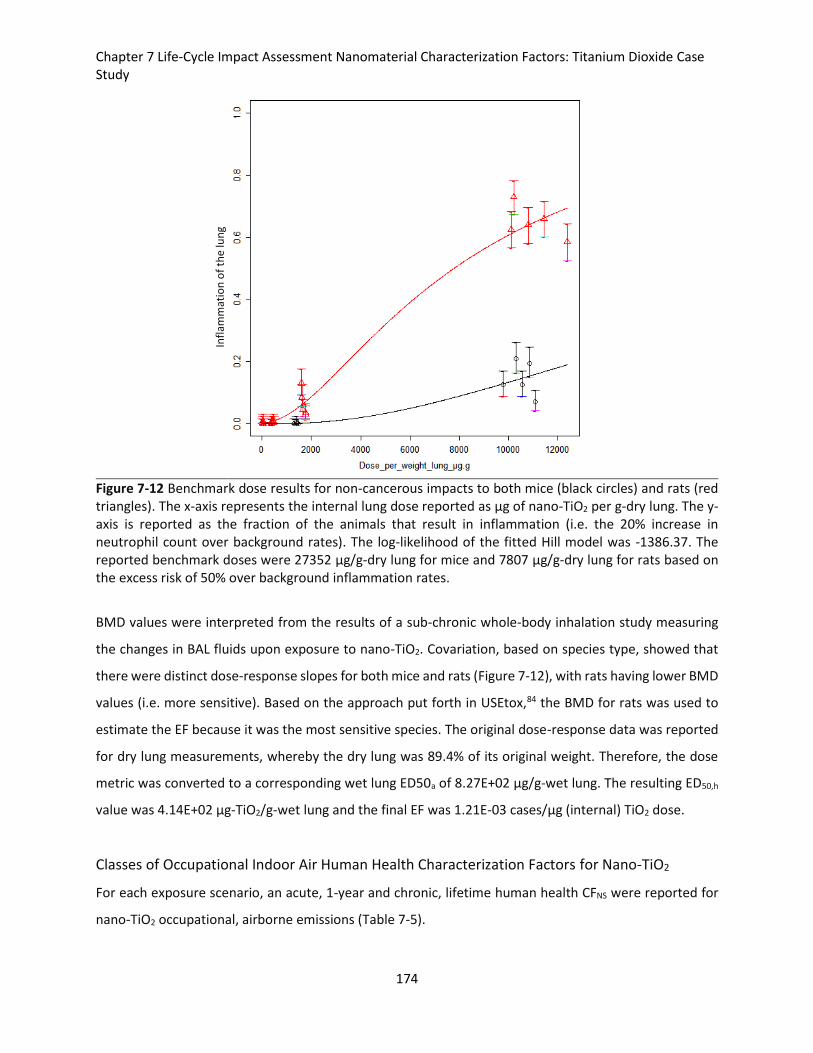
Chapter 7 Life-Cycle Impact Assessment Nanomaterial Characterization Factors: Titanium Dioxide Case Study
174
Infl
amm
atio
n o
f th
e lu
ng
Figure 7-12 Benchmark dose results for non-cancerous impacts to both mice (black circles) and rats (red triangles). The x-axis represents the internal lung dose reported as μg of nano-TiO2 per g-dry lung. The y-axis is reported as the fraction of the animals that result in inflammation (i.e. the 20% increase in neutrophil count over background rates). The log-likelihood of the fitted Hill model was -1386.37. The reported benchmark doses were 27352 μg/g-dry lung for mice and 7807 μg/g-dry lung for rats based on the excess risk of 50% over background inflammation rates.
BMD values were interpreted from the results of a sub-chronic whole-body inhalation study measuring
the changes in BAL fluids upon exposure to nano-TiO2. Covariation, based on species type, showed that
there were distinct dose-response slopes for both mice and rats (Figure 7-12), with rats having lower BMD
values (i.e. more sensitive). Based on the approach put forth in USEtox,84 the BMD for rats was used to
estimate the EF because it was the most sensitive species. The original dose-response data was reported
for dry lung measurements, whereby the dry lung was 89.4% of its original weight. Therefore, the dose
metric was converted to a corresponding wet lung ED50a of 8.27E+02 μg/g-wet lung. The resulting ED50,h
value was 4.14E+02 μg-TiO2/g-wet lung and the final EF was 1.21E-03 cases/μg (internal) TiO2 dose.
Classes of Occupational Indoor Air Human Health Characterization Factors for Nano-TiO2
For each exposure scenario, an acute, 1-year and chronic, lifetime human health CFNS were reported for
nano-TiO2 occupational, airborne emissions (Table 7-5).
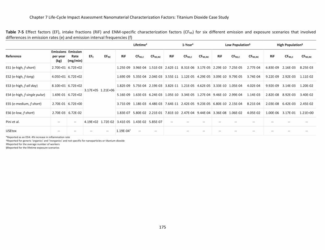
Chapter 7 Life-Cycle Impact Assessment Nanomaterial Characterization Factors: Titanium Dioxide Case Study
175
Table 7-5 Effect factors (EF), intake fractions (RiF) and ENM-specific characterization factors (CFNS) for six different emission and exposure scenarios that involved differences in emission rates (e) and emission interval frequencies (f)
Lifetime‡ 1-Year‡ Low Population§ High Population§
Reference Emissions per year
(kg)
Emission Rate
(mg/min) EFC EFNC RiF CFNS,C CFNS,NC RiF CFNS,C CFNS,NC RiF CFNS,C CFNS,NC RiF CFNS,C CFNS,NC
ES1 (e-high, f-short) 2.70E+01 6.72E+02
3.17E+05 1.21E+06
1.25E-09 3.96E-04 1.51E-03 2.62E-11 8.31E-06 3.17E-05 2.29E-10 7.25E-05 2.77E-04 6.83E-09 2.16E-03 8.25E-03
ES2 (e-high, f-long) 4.05E+01 6.72E+02 1.69E-09 5.35E-04 2.04E-03 3.55E-11 1.12E-05 4.29E-05 3.09E-10 9.79E-05 3.74E-04 9.22E-09 2.92E-03 1.11E-02
ES3 (e-high, f-all day) 8.10E+01 6.72E+02 1.82E-09 5.75E-04 2.19E-03 3.82E-11 1.21E-05 4.62E-05 3.33E-10 1.05E-04 4.02E-04 9.92E-09 3.14E-03 1.20E-02
ES4 (e-high, f-single pulse) 1.69E-01 6.72E+02 5.16E-09 1.63E-03 6.24E-03 1.05E-10 3.34E-05 1.27E-04 9.46E-10 2.99E-04 1.14E-03 2.82E-08 8.92E-03 3.40E-02
ES5 (e-medium, f-short) 2.70E-01 6.72E+00 3.71E-09 1.18E-03 4.48E-03 7.64E-11 2.42E-05 9.23E-05 6.80E-10 2.15E-04 8.21E-04 2.03E-08 6.42E-03 2.45E-02
ES6 (e-low, f-short) 2.70E-03 6.72E-02 1.83E-07 5.80E-02 2.21E-01 7.81E-10 2.47E-04 9.44E-04 3.36E-08 1.06E-02 4.05E-02 1.00E-06 3.17E-01 1.21E+00
Pini et al. -- -- 4.19E+02 1.72E-02 3.41E-05 1.43E-02 5.85E-07 -- -- -- -- -- -- -- -- --
USEtox -- -- -- -- 1.19E-04† -- -- -- -- -- -- -- -- -- --
*Reported as an ED4: 4% increase in inflammation rate †Reported for generic ‘organics’ and ‘inorganics’ and not specific for nanoparticles or titanium dioxide ‡Reported for the average number of workers §Reported for the lifetime exposure scenarios
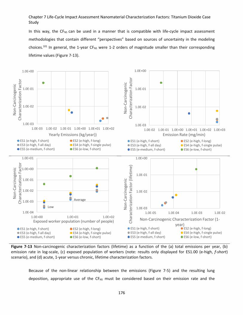
Chapter 7 Life-Cycle Impact Assessment Nanomaterial Characterization Factors: Titanium Dioxide Case Study
176
In this way, the CFNS can be used in a manner that is compatible with life-cycle impact assessment
methodologies that contain different “perspectives” based on sources of uncertainty in the modeling
choices.101 In general, the 1-year CFNS were 1-2 orders of magnitude smaller than their corresponding
lifetime values (Figure 7-13).
Figure 7-13 Non-carcinogenic characterization factors (lifetime) as a function of the (a) total emissions per year, (b) emission rate in log-scale, (c) exposed population of workers (note: results only displayed for ES1.00 (e-high, f-short) scenario), and (d) acute, 1-year versus chronic, lifetime characterization factors.
Because of the non-linear relationship between the emissions (Figure 7-5) and the resulting lung
deposition, appropriate use of the CFNS must be considered based on their emission rate and the
1.0E-03
1.0E-02
1.0E-01
1.0E+00
1.0E-03 1.0E-02 1.0E-01 1.0E+00 1.0E+01 1.0E+02
No
n-C
arci
no
gen
ic
Ch
arac
teri
zati
on
Fac
tor
Yearly Emissions (kg/year))
ES1 (e-high, f-short) ES2 (e-high, f-long)ES3 (e-high, f-all day) ES4 (e-high, f-single pulse)ES5 (e-medium, f-short) ES6 (e-low, f-short)
1.0E-03
1.0E-02
1.0E-01
1.0E+00
1.0E-02 1.0E-01 1.0E+00 1.0E+01 1.0E+02 1.0E+03N
on
-Car
cin
oge
nic
C
har
acte
riza
tio
n F
acto
rEmission Rate (mg/min)
ES1 (e-high, f-short) ES2 (e-high, f-long)ES3 (e-high, f-all day) ES4 (e-high, f-single pulse)ES5 (e-medium, f-short) ES6 (e-low, f-short)
Average
Low
1.0E-04
1.0E-03
1.0E-02
1.0E-01
1.0E+00
1.0E+01
1.0E+00 1.0E+01 1.0E+02
No
n-C
arci
no
gen
ic
Ch
arac
teri
zati
on
Fac
tor
Exposed worker population (number of people)
ES1 (e-high, f-short) ES2 (e-high, f-long)ES3 (e-high, f-all day) ES4 (e-high, f-single pulse)ES5 (e-medium, f-short) ES6 (e-low, f-short)
1.0E-03
1.0E-02
1.0E-01
1.0E+00
1.0E-05 1.0E-04 1.0E-03 1.0E-02
No
n-C
arci
no
gen
ic
Ch
arac
teri
zati
on
Fac
tor
(lif
etim
e)
Non-Carcinogenic Characterization Factor (1-year)
ES1 (e-high, f-short) ES2 (e-high, f-long)ES3 (e-high, f-all day) ES4 (e-high, f-single pulse)ES5 (e-medium, f-short) ES6 (e-low, f-short)
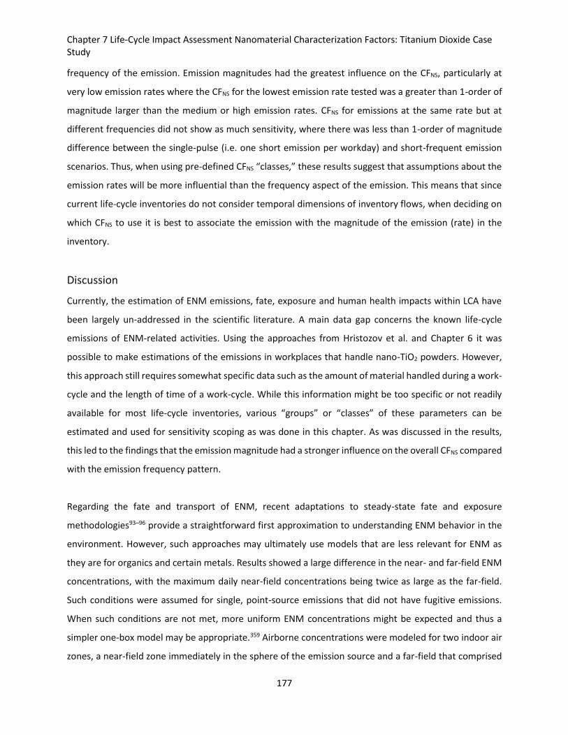
Chapter 7 Life-Cycle Impact Assessment Nanomaterial Characterization Factors: Titanium Dioxide Case Study
177
frequency of the emission. Emission magnitudes had the greatest influence on the CFNS, particularly at
very low emission rates where the CFNS for the lowest emission rate tested was a greater than 1-order of
magnitude larger than the medium or high emission rates. CFNS for emissions at the same rate but at
different frequencies did not show as much sensitivity, where there was less than 1-order of magnitude
difference between the single-pulse (i.e. one short emission per workday) and short-frequent emission
scenarios. Thus, when using pre-defined CFNS “classes,” these results suggest that assumptions about the
emission rates will be more influential than the frequency aspect of the emission. This means that since
current life-cycle inventories do not consider temporal dimensions of inventory flows, when deciding on
which CFNS to use it is best to associate the emission with the magnitude of the emission (rate) in the
inventory.
Discussion
Currently, the estimation of ENM emissions, fate, exposure and human health impacts within LCA have
been largely un-addressed in the scientific literature. A main data gap concerns the known life-cycle
emissions of ENM-related activities. Using the approaches from Hristozov et al. and Chapter 6 it was
possible to make estimations of the emissions in workplaces that handle nano-TiO2 powders. However,
this approach still requires somewhat specific data such as the amount of material handled during a work-
cycle and the length of time of a work-cycle. While this information might be too specific or not readily
available for most life-cycle inventories, various “groups” or “classes” of these parameters can be
estimated and used for sensitivity scoping as was done in this chapter. As was discussed in the results,
this led to the findings that the emission magnitude had a stronger influence on the overall CFNS compared
with the emission frequency pattern.
Regarding the fate and transport of ENM, recent adaptations to steady-state fate and exposure
methodologies93–96 provide a straightforward first approximation to understanding ENM behavior in the
environment. However, such approaches may ultimately use models that are less relevant for ENM as
they are for organics and certain metals. Results showed a large difference in the near- and far-field ENM
concentrations, with the maximum daily near-field concentrations being twice as large as the far-field.
Such conditions were assumed for single, point-source emissions that did not have fugitive emissions.
When such conditions are not met, more uniform ENM concentrations might be expected and thus a
simpler one-box model may be appropriate.359 Airborne concentrations were modeled for two indoor air
zones, a near-field zone immediately in the sphere of the emission source and a far-field that comprised
Chapter 7 Life-Cycle Impact Assessment Nanomaterial Characterization Factors: Titanium Dioxide Case Study
178
the remaining indoor room volume. For example, a steady-state approximation is applied (Appendix:
Chapter 7)311 to ES1, the resulting near-field airborne concentration would be 3.52 mg/m3. The result is
approximately 95% smaller than the maximum near-field concentration predicted by the dynamic model.
Indoor occupational emissions are likely to be episodic, leading to non-constant airborne concentrations.
This was borne out by the results of the fate model that demonstrated only 2 of the 6 emission scenarios
resulted in any pseudo-steady state conditions where airborne concentrations remained constant for at
least some portion of the emission event. This only occurred in the two longest emission scenario of 60
minute and all-day emission. Such findings are particularly important since the fate and transport of ENM
can be concentration dependent. As has been eluded to by Walser et al., the results of the fate and
transport model showed that the overall air exchange rate between the indoor and outdoor air was most
influential parameter on airborne nano-TiO2 concentrations in the workplace.97 The air exchange rates
were high at 8 hr-1 but typical for occupational working conditions. This resulted in only minor amounts
of removal from homo-aggregation and gravitational settling mechanisms, which might be expected given
that the settling velocity of even 1 μm sized particles is circa 12.5 cm/hr.333 Still, the overall removal from
gravitational settling was < 1% in most of the exposure scenarios. These removal mechanisms will likely
become much more important when air exchange rates are kept low or particle number concentrations
become very high. While it is assumed that conditions in the workplace are likely to be kept high for safety
issues, some studies have reported much lower air exchange rates for ENM manufacturing conditions,359
not to mention other non-industrial workplaces.360
In the exposure model applied in this case study, there was a significant departure from currently applied
life-cycle impact assessment methods that generally assume inhalation exposures are linearly related to
an individual’s respiration rate and the concentration of the chemical in air. Walser et al.97 recently
proposed, and Pini et al.93 implemented, a retention factor based on the outputs from the MPPD model,
however this value was actually interpreted from the assumed deposition calculation made by that model
and did not consider clearance and ultimate retention of the nano-TiO2. This could be one reason that
the lifetime RiF was over 2-orders of magnitude less than what was reported in Pini et al. The results in
this chapter show that the retention of nano-TiO2 in the lung was similar to those from previously reported
in vivo studies which were on the order of hundreds of days.202,344,361 This has been shown to be
particularly true for deposition in the air-exchange and interstitial regions of the lung, which the results
were in agreement with. Of the three main pathways in the model that governed ENM retention in the
lung, translocation of loaded-PCS from the pulmonary (i.e. alveolar) to the tracheobronchial region is the
Chapter 7 Life-Cycle Impact Assessment Nanomaterial Characterization Factors: Titanium Dioxide Case Study
179
most sensitive parameter and subsequently the limiting factor determining clearance of ENM from the
lung. This value was modified to reflect the slower clearance rate of particulates in the human lung
compared with the rat lung.344 In reality, it may be that the difference in retention times is influenced by
the rate of phagocytosis by PC and also the penetration of ENM into the alveolar interstitium. However,
at the cellular level, it is not clear that such dramatic differences would occur between rat and human
rates of phagocytosis nor for the penetration into the interstitium, thus not being to fully explain the
retention differences between the species. In the highest exposure scenario, PC were easily saturated and
overburdened, leading to accumulation in many of the lung regions. The overall unlimited accumulation
found in the air-exchange and interstitial regions for some of the exposure scenarios may be occurring
due to mucociliary clearance becoming overburdened, which cannot remove particles at a fast enough
rate to reach zero lung burden even at times of low- or no-exposure. However, these results may also be
limited by the model’s capability to adjust for the increase or decrease of mucociliary clearance activity
depending on the mass loading of nanoparticles in the airway. The current version of the model uses a
constant transfer factor to describe this mechanism. Additionally, the high concentration of nano-TiO2
found in the tracheobronchial region was expected given the primary particle sizes upon exposure were
assumed to be 21 nm. Particles ≤ 100 nm will have a significant amount of deposition in the alveolar
region, however particles ≤ 30 nm, particularly those below 10 nm,344 will show greater deposition and
retention in the tracheobronchial region.202 Additionally, although the density of the particles do not
affect deposition of ENM ≤ 100 nm, above this size, lower densities will result in greater deposition in the
upper airways such as the tracheobronchial region.202
The newly introduced RiF in this study shows an inverse relationship with the emission rate, which is
counter-intuitive given that iF values in traditional LCIA are independent of the emission rate. This can be
explained by the saturation of PC in the lungs and the relative contribution of PC-sequestered ENM to the
overall wet lung burden. Neither of these scales linearly with emission rate, thus bearing the inverse
relationship discovered in this study. Further examination on the details of the dynamics of the wet lung
burden are shown below. As shown in the results for the exposure, after saturation, the relative
contribution of PCS sequestered ENM to the overall wet lung burden decreases as emission rates
increases. The amounts in the pulmonary region and interstitium of the lungs scales proportionally with
the emission rate after the PCS are saturated. The lifetime wet lung burden increases 3.4 times while
emission rate increases 100-fold from low to medium. This is because PCS still play a major role at medium
emission rate. But at high emission, which is a 100-fold increase from medium emission, lifetime wet lung
Chapter 7 Life-Cycle Impact Assessment Nanomaterial Characterization Factors: Titanium Dioxide Case Study
180
burden increases 31 times, closer to the magnitude of increase in emission rate. This is because the PCS
are less important as emission rate goes even higher. This highlights the importance of the emission rate
on the “iF” when considering the target organ’s physiology.
It should be noted that the RiF and exposure results should be interpreted with caution. Although
adaptations were made to the original rat-based model developed by Li et al.337 to estimate bio-
distribution in humans, the results of this model have not been validated by experimental evidence. Li et
al. validated their model with empirical data and found good agreement in the measured and estimated
amounts of cerium oxide bio-distribution337. Also, and in general, reviews of previously used first-order
clearance PBPK models tend to under-predict the retention of particulates in the lung when exposure
concentrations are either very high or very low344. In addition, the model was built based on exposure
concentrations that were 2-orders of magnitude lower than the highest exposure scenario presented in
this study, which is in effect the worst-case scenario. The results of applying the PBPK-rat model to human
exposure scenarios should be considered as potential impacts as opposed to absolute values. The
resulting RiF calculated in this chapter did not include the effects and use of personal-protection-
equipment in the work environment. At the time of this study, it was not evident which occupational
scenarios would require PPE, at what rate PPE would be used and the effectiveness of the PPE to filtering
ENM. However, if patterns of PPE usage are known, this could be included in the exposure model.
Additionally, the CFNS presented in this study were calculated for inhalation exposures in the occupational
setting, since inhalation is the primary intake route in the workplace scenario.97 However, the fate and
transport model estimates the settling of particles out of the air that could be used for approximating
dermal exposures. If there is potential inhalation exposure, there is likely to be potential dermal exposure
in the same scenario either from direct settling of ENM onto the skin or settling of ENM onto indoor
surfaces that later contact the skin of occupational persons. Dermal exposure and toxicity studies in the
literature are much fewer than inhalation studies, potentially being the limiting factor to this approach.
As was discussed for fullerenes and titanium dioxide nano-powders in Chapter 6, penetration of such
particles into the body through dermal uptake is not anticipated to be as efficient as through inhalation.
Furthermore, apart from direct impacts to the lungs and lung-related injuries, ENM that are deposited in
the lung may translocate to other regions of the body after inhalation (Oberdorster 2005).362–364 Although
the exposure model presented in this approach allows for the estimation of ENM in 10 other organs of
the body, these values were not yet used to address systemic-human health impacts upon inhalation to
Chapter 7 Life-Cycle Impact Assessment Nanomaterial Characterization Factors: Titanium Dioxide Case Study
181
nano-TiO2. Future work in this area will address the compounded effects from multi-system organ
toxicity.
The EFC reported in this study was almost 1-order of magnitude smaller than the EFNC. It should be noted
that the non-carcinogenic endpoint was pulmonary inflammation, a precursor to the carcinogenic
endpoint of pulmonary tumors. Thus, these results intuitively make sense. It would be expected that many
more cases of a non-cancerous diseases occur compared with more advanced pathologies such as cancer.
This is in contrast to the only other study in the literature that has reported a human health EF for nano-
TiO2.93 Pini et al. report a EFC that is 4-orders of magnitude greater than their reported EFNC, thus implying
that there are many more expected cases of cancer compared with inflammation.93 However, a likely
explanation regarding this discrepancy is the fact that Pini et al. used an inflammation study283 as a proxy
for the carcinogenic endpoint.93 Therefore, a comparison of their EFC to the EFNC presented in this chapter
is more appropriate. This comparison shows that this work’s EFNC was still over 3-orders of magnitude
greater than Pini et al.’s EFC value. Their EFC value was calculated for as an ED4 (i.e. a 4% increase over
background response) and thus it seems appropriate that they report a lower value compared to ours
which was calculated for a 50% increase over the background rate. Thus, while the overall difference in
both the non-carcinogenic and carcinogenic CFNS reported in this thesis and what has been previously
reported using steady-state models is partially explained by the difference in the fate, exposure and
(retained) intake-fractions, a significant difference arises from the selection of toxicological data used to
calculate the effect factor (i.e. something that has nothing to do with steady-state versus dynamic models)
Life-Cycle Assessment of Organic Photovoltaics with ENM-Specific Characterization
Factors
Life-cycle inventories do not allow for time integrated emission-flows nor are they categorized by time-
scale (e.g. kg emissions per hour). If there is exact information regarding the rate of production for the
reference-flow (i.e. product), then the reported emissions for that reference-flow could be defined as an
emission rate for use in the fate and transport model. Often, this level of life-cycle inventory detail might
not be attainable. In such as case, assumptions regarding the emission rate would have to be made. As
explained above, the results of the CFNS calculations were most sensitive to the magnitude of the emission
rate as opposed to emission frequency. Thus, static inventory flows should be interpreted as the
magnitude of an emission rate for best correlation. Based on the previous set of results, it was assumed
that the emissions reported in the OPV inventory (Appendix: Chapter 3 and Appendix: Chapter 4)
Chapter 7 Life-Cycle Impact Assessment Nanomaterial Characterization Factors: Titanium Dioxide Case Study
182
correspond with the highest emission rate. This is because the highest emission rate was characteristic of
an industrial scale scenario, and since the purpose of this thesis is to forecast the potential environmental
and human health risks for a prospective, large-scale OPV device, this assumption is warranted.
Furthermore, the highest emission rate was correlated with the highest level of risk based on the HHRA
in Chapter 6, it was useful to explore whether the LCA results would echo this human health hazard.
Therefore, the highest emission rate was used as an initial proof of concept to estimate the human health
hazards of nano-TiO2 use in OPV. Within this category of emission rates, there was a range of half an order
of magnitude based on differences in emission frequencies. Since the original frequency was originally
described for an actual occupational exposure scenario at the industrial scale, this value was chosen as a
proof of concept due to its relevance in forecasting human health impacts at the industrial scale. Both the
long-term (lifetime) and the short-term (1-year) CFNS were tested for their influence on the LCA results.
Thus, lifetime CFNS for ES1 was used as a worst-case scenario proof-of-concept for a first approximation
of the human health impacts from nano-TiO2 handled and used at the industrial scale. Emissions across
the life-cycle of the OPV panel were considered only during production of the nano-TiO2 power itself, and
during production of the OPV panel. Emissions during nano-TiO2 production were estimated for the
production route outlined by sulfate production route. Hischier et al. assumed there were no emissions
to air during production, however this neglects the issues of handling, transferring, and packing the
powder once it is created.193 Thus, emissions were estimated using an average of lower-estimate and
higher-estimate emission scenarios as described by the material flow analysis of various ENM reported by
Gottschalk and Nowack.191 This resulted in an estimated 0.25% of the total production rate being emitted
to air, and, thus, per kg of nano-TiO2 produced and handled there were 0.32 mg of this material that ended
up as occupational, indoor air emissions. Additionally, there were no known nano-TiO2 emissions during
the production of the OPV panel, and the same modeling assumptions stated above applied for OPV
production. It was further assumed that this emission was to indoor occupational air, as opposed to
outdoor environmental emissions. The reported emission (e.g. 0.32 mg) was then combined with the both
the non-carcinogenic and carcinogenic lifetime CFNS for ES1 to calculate the potential human health
impacts. This implicit assumption is that the CFNS for ES1 represents an industrial-scale scenario and the
inventory, including the emissions, built for the nano-TiO2 production and OPV manufacturing represent
emissions of a similar magnitude over time at the industrial-scale. This is a significant caveat because there
is no relatable time-scale on the inventory.
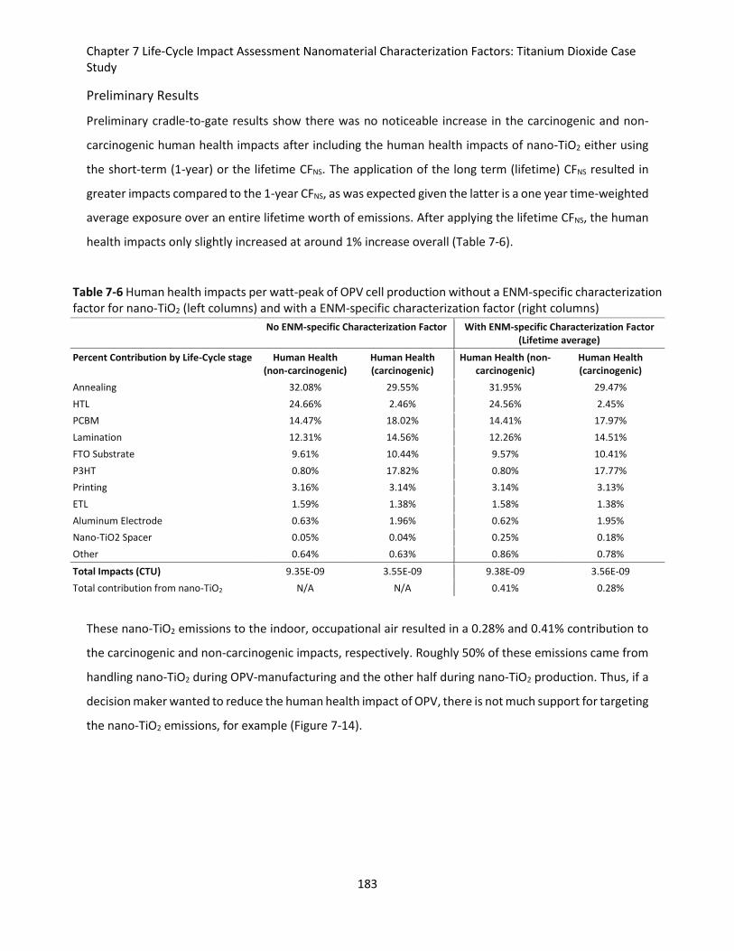
Chapter 7 Life-Cycle Impact Assessment Nanomaterial Characterization Factors: Titanium Dioxide Case Study
183
Preliminary Results
Preliminary cradle-to-gate results show there was no noticeable increase in the carcinogenic and non-
carcinogenic human health impacts after including the human health impacts of nano-TiO2 either using
the short-term (1-year) or the lifetime CFNS. The application of the long term (lifetime) CFNS resulted in
greater impacts compared to the 1-year CFNS, as was expected given the latter is a one year time-weighted
average exposure over an entire lifetime worth of emissions. After applying the lifetime CFNS, the human
health impacts only slightly increased at around 1% increase overall (Table 7-6).
Table 7-6 Human health impacts per watt-peak of OPV cell production without a ENM-specific characterization factor for nano-TiO2 (left columns) and with a ENM-specific characterization factor (right columns)
No ENM-specific Characterization Factor With ENM-specific Characterization Factor
(Lifetime average)
Percent Contribution by Life-Cycle stage Human Health (non-carcinogenic)
Human Health (carcinogenic)
Human Health (non-carcinogenic)
Human Health (carcinogenic)
Annealing 32.08% 29.55% 31.95% 29.47%
HTL 24.66% 2.46% 24.56% 2.45%
PCBM 14.47% 18.02% 14.41% 17.97%
Lamination 12.31% 14.56% 12.26% 14.51%
FTO Substrate 9.61% 10.44% 9.57% 10.41%
P3HT 0.80% 17.82% 0.80% 17.77%
Printing 3.16% 3.14% 3.14% 3.13%
ETL 1.59% 1.38% 1.58% 1.38%
Aluminum Electrode 0.63% 1.96% 0.62% 1.95%
Nano-TiO2 Spacer 0.05% 0.04% 0.25% 0.18%
Other 0.64% 0.63% 0.86% 0.78%
Total Impacts (CTU) 9.35E-09 3.55E-09 9.38E-09 3.56E-09
Total contribution from nano-TiO2 N/A N/A 0.41% 0.28%
These nano-TiO2 emissions to the indoor, occupational air resulted in a 0.28% and 0.41% contribution to
the carcinogenic and non-carcinogenic impacts, respectively. Roughly 50% of these emissions came from
handling nano-TiO2 during OPV-manufacturing and the other half during nano-TiO2 production. Thus, if a
decision maker wanted to reduce the human health impact of OPV, there is not much support for targeting
the nano-TiO2 emissions, for example (Figure 7-14).
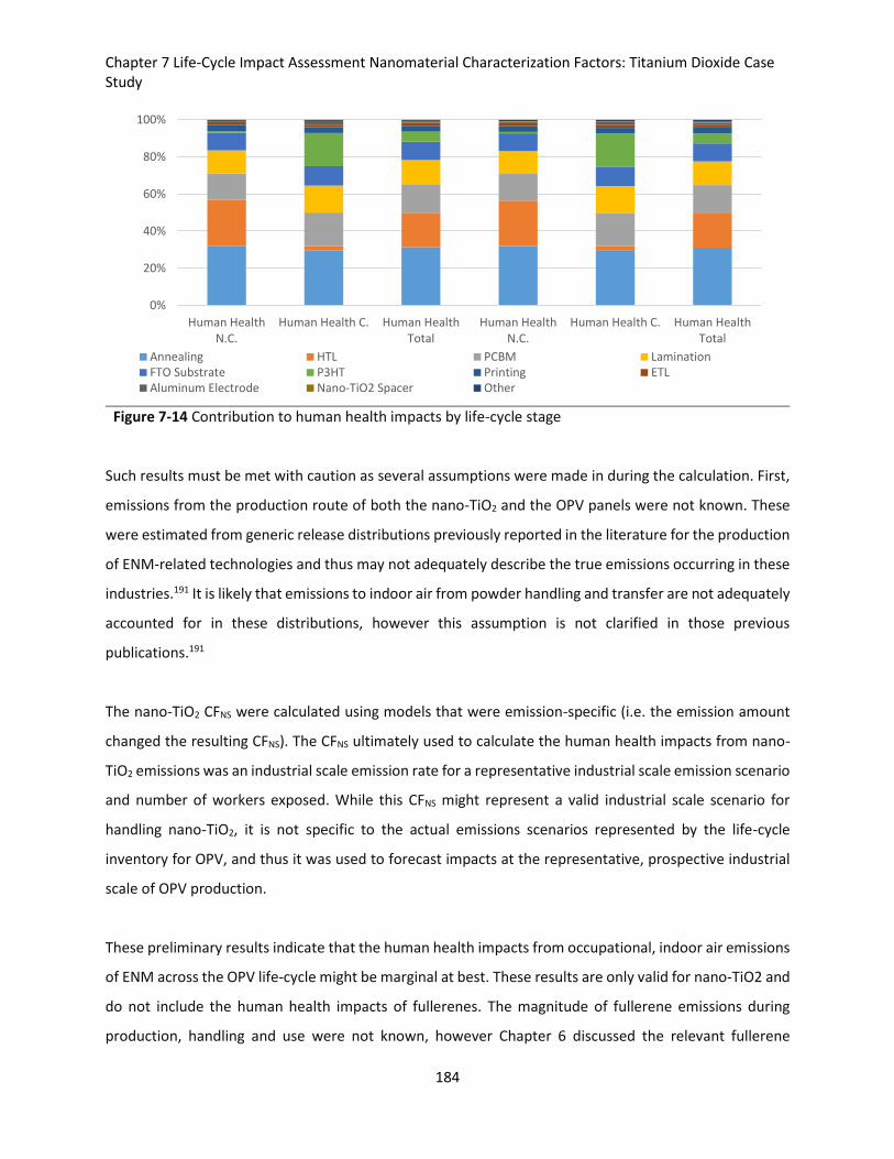
Chapter 7 Life-Cycle Impact Assessment Nanomaterial Characterization Factors: Titanium Dioxide Case Study
184
Figure 7-14 Contribution to human health impacts by life-cycle stage
Such results must be met with caution as several assumptions were made in during the calculation. First,
emissions from the production route of both the nano-TiO2 and the OPV panels were not known. These
were estimated from generic release distributions previously reported in the literature for the production
of ENM-related technologies and thus may not adequately describe the true emissions occurring in these
industries.191 It is likely that emissions to indoor air from powder handling and transfer are not adequately
accounted for in these distributions, however this assumption is not clarified in those previous
publications.191
The nano-TiO2 CFNS were calculated using models that were emission-specific (i.e. the emission amount
changed the resulting CFNS). The CFNS ultimately used to calculate the human health impacts from nano-
TiO2 emissions was an industrial scale emission rate for a representative industrial scale emission scenario
and number of workers exposed. While this CFNS might represent a valid industrial scale scenario for
handling nano-TiO2, it is not specific to the actual emissions scenarios represented by the life-cycle
inventory for OPV, and thus it was used to forecast impacts at the representative, prospective industrial
scale of OPV production.
These preliminary results indicate that the human health impacts from occupational, indoor air emissions
of ENM across the OPV life-cycle might be marginal at best. These results are only valid for nano-TiO2 and
do not include the human health impacts of fullerenes. The magnitude of fullerene emissions during
production, handling and use were not known, however Chapter 6 discussed the relevant fullerene
0%
20%
40%
60%
80%
100%
Human HealthN.C.
Human Health C. Human HealthTotal
Human HealthN.C.
Human Health C. Human HealthTotal
Annealing HTL PCBM LaminationFTO Substrate P3HT Printing ETLAluminum Electrode Nano-TiO2 Spacer Other
Chapter 7 Life-Cycle Impact Assessment Nanomaterial Characterization Factors: Titanium Dioxide Case Study
185
toxicity data. While some indication of inflammation, for instance, have been demonstrated, fullerenes
have also been shown to have anti-inflammatory effects. Thus, its potential to significantly contribute to
the human health impacts of OPV due to emissions in occupational indoor air is not anticipated.
Furthermore, these are just two material types used in OPV that have been explicitly called-out as ENM.
Since OPV are constructed on the order of hundreds of nanometers in thickness, this implies that the all
the layers would necessarily have to be composed of materials in the nanometer size range. While this is
not usually explicitly stated, this technically implies that the use of ENM comprises the entire panel (less
the plastic-substrate). Consequently, the cumulative contribution of ENM emissions along the life-cycle of
OPV could potentially be more influential than this preliminary assessment suggests. Lastly, while human
health impacts from occupational indoor air emissions seemed to be the most relevant potential impact
pathway, emissions during the use phase and end-of-life phase cannot be ruled out. Such emissions will
also be important for the determination of potential environmental and ecological impacts.
Chapter 8 Conclusions and Perspectives
186
Chapter 8 Conclusions and Perspectives
The future of energy production and development of sustainable technology options are primed to be,
arguably, the most important issues in the 21st-century. In the face of mounting climate change and public
health impacts, energy must be evaluated as a sustainability issue addressing not only economic impacts
but also impacts on society and the environment. For instance, past experiences with biofuels have
demonstrated that when objectives are limited to simply finding alternative or renewable energies,
environmental burden shifting can occur.5–8 The introduction of modern, conventional forms of PV
systems in the mid-20th century offered one option of producing electricity from limitless amounts of
energy from the sun. Moreover, PV are basically an emission free and environmentally benign technology
while it is being used, however there are environmental burdens (e.g. greenhouse gas emissions) that may
occur during the production, use or disposal of the PV. Particularly for conventional silicon-based PV, the
processing of silicon into semi-conducting wafers and entire panels is a fairly energy intensive process.
Consequently, the research and development into alternative PV technologies that are less energy
intensive and environmentally preferable is an ongoing endeavor. In this regard, OPV have captured the
imaginations of many researchers since it’s a very thin, flexible technology requiring much fewer amounts
of materials per Wp of power production. However, OPV are also known to have much lower conversion
efficiencies and lower lifetimes compared with silicon-based PV. Therefore, the overall objective of this
thesis was to demonstrate whether OPV have proven themselves to be an environmentally preferable
energy supply option compared with conventional silicon PV.
The Methodological Options Presented in this Thesis
Implicit to the overall objective of the thesis was the question whether existing methodologies commonly
used to evaluate the environmental performance of energy supply systems are fully compatible for
carrying out such evaluations. In Chapter 1, a review of the literature up to the end of 2013 was made on
the environmental performance of OPV. Central to the environmental evaluation of energy-related
systems has been the use of LCA because of it facilitates the calculation of the EPBT (i.e. the time it takes
to produce the same amount of energy that was consumed in creating the technology). However, LCA
also facilitates the calculation of additional environmental and human health impacts of products.
Therefore, Chapter 3 and Chapter 4 employed the use of LCA to evaluate prospective OPV devices, their
uses and their end-of-life options.
Chapter 8 Conclusions and Perspectives
187
Chapter 5 highlighted the gaps in life-cycle impact assessment methodologies in regards to the human
health and ecotoxicity impacts resulting from ENM emissions along the OPV life-cycle. HHRA and ERA are
two tools traditionally used for making assessments about the potential human health and environmental
risks from regular chemicals. In principal, these tools can also be used to understand the impacts from
ENM, although they too can suffer from data and methodological gaps similar to LCA. Chapter 5 expands
on these issues and the potential approaches to use LCA and HHRA3 in separate, complementary or
integrated uses for evaluating the environmental and human health benefits of emerging technologies
These methodology options were the separate use of LCA, the separate use of HHRA, the combined use
of LCA and HHRA (i.e. combining their results together), and three additional approaches to integration
of HHRA and LCA at the methodological level. These latter three options were Global, Context-dependent
and Site-specific integration. Global integration makes use of steady-state models that are less relevant
for ENM, Context-dependent integration makes use of partially-dynamic models with aggregated
environmental and ENM-specific parameters and Site-specific integration uses fully-dynamic models with
perfect local and material-specific information. Chapter 6 presented the HHRA of the potential ENM-
emissions along the OPV life-cycle. Chapter 7 presented the methodology of Global Integration,
culminating in the production of an occupational, indoor air, human health CFNS for nano-TiO2.
Overview of the Results of Each Methodological Option
Life-Cycle Assessment of Organic Photovoltaic Systems
The review of existing literature through the end of 2013 demonstrated a general finding that the resource
efficiencies and environmental hazards of OPV were lower than that of conventional silicon PV. However,
the majority of these studies were limited in their scope, focusing mainly on cradle-to-gate assessments
up to the manufacture of the OPV panel as well as limiting their environmental criteria to CED, EPBT and
greenhouse gas emissions. For example, CED for the reviewed literature showed values as low as 0.76
MJ/Wp of power production, compared with conventional m-Si which could be as high as 30 MJ/Wp.
Chapter 3 introduced a new, prospective OPV device based on the reviewed literature in terms of their
reported material choices, structure and performance of the solar cells as well as other foreseen
developments in this area of research. For instance, material choices eliminated the use of resource scarce
3 This thesis took particular focus on the human health assessment modeling, however the use of ecological risk assessment, its data and methodological gaps, and its synergisms with life-cycle assessment also apply in the environmental (non-human health context)
Chapter 8 Conclusions and Perspectives
188
or cost prohibitive materials such as indium and silver. The results of the CED, for example, ranged from
1.13-2.32 MJ/Wp and were largely in agreement with the prior studies. Looking beyond embodied energy,
the environmental and human health impacts decreased across the board compared with conventional
silicon-based PV. However, these differences were not uniform across all impact categories. For instance,
whereas marine eutrophication impacts for OPV were between 94-97% lower than m-Si, decreases in
ionizing radiation were between 77-94% lower. Further results, showed that at a 5% efficiency, OPV would
need between 1-9 years of working lifetime such that they achieve environmental parity with silicon-
based PV. However, these lifetimes are based on purely hypothetical estimations if there were no other
impacts resulting from further use or end-of-life phases.
Chapter 4 expanded the scope of the LCA presented in Chapter 3 to include possible use and end-of-life
phases for OPV systems. Two different use phases were considered: a rooftop, solar array and a portable
solar charger. Two different end-of-life options were also considered: landfilling and incineration.
Whereas cradle-to-gate impacts were, on average, over 90% lower for OPV compared to silicon-based PV,
cradle-to-grave impacts of using OPV panels on rooftops were only 60% lower. In one case, metal
depletion potential, OPV impacts were in fact greater than m-Si PV. The increases in impacts were due to
the need to continually replace the OPV panels every five years over the course of the 25-year rooftop
lifetime. The difference between the cradle-to-gate and cradle-to-grave environmental impacts are thus
not trivial and demonstrate how significant the use phase can be, even though technically there are no
direct emissions during its use. This concept was reinforced by the results of using OPV as a portable
charger, which were on average 74% lower than a-Si PV. In contrast to the rooftop scenario, metal
depletion remained 87% lower than a-Si for the portable charger scenario.
Consideration of the end-of-life showed only minimal influence on the total cradle-to-grave impacts,
however recycling of the panels was not considered. Currently recycling is not applied to solar panels,
whereby the majority end up going to landfills. If recycling comes online as a major end-of-life route for
silicon cells, there could be a significant reduction in their total impacts. OPV on the other hand do not
stand a lot to gain from recycling as their total energy content is minimal given their thinness and low
material mass. Thus, eco-design concepts for emerging technologies may stand to benefit by further
developing and including prospective use and end-of-life phases to make targeted evaluations of how
they can extract the most resource efficiencies and avoid the most environmental hazards.
Chapter 8 Conclusions and Perspectives
189
Emissions of and Human Health Impacts from Engineered Nanomaterials using Risk Assessment
Those aforementioned environmental and human health impacts calculated using LCA did not include the
impacts from the ENM used in the OPV technology. ENM-specific emissions had not been estimated either
in the prior studies reviewed literature in 0. Main obstacles to including these potential impacts go beyond
the reporting of emissions and are limited by current life-cycle impact assessment methodologies that
were originally built for understanding the behavior of organic and some metals in the environment, but
not ENM. To address this, a more focused HHRA was presented in which potential occupational exposure
scenarios during production and use of nano-TiO2 was presented. The HHRA was conducted for the
industrial-scale handling of nano-TiO2 in order to forecast potential human health risks in the OPV life-
cycle if this were to reach the industrial level The results showed there was upwards of a 78% lifetime risk
of lung inflammation to workers handling nano-TiO2 during ENM production or OPV panel manufacturing.
This estimation of risk was a worst-case scenario, for instance, under the assumption that no personal
protective equipment was used and exposure to the individual was 100% of the concentration in the air.
The highest probability of risk was particularly relevant when handling and transfer of high volumes of dry
nano-TiO2 powders occurred over 8-hour workdays. The results suggest that risk may exist along the OPV
life-cycle if industrial-scale production of this technology is achieved. While these results might be
beneficial from a health and safety perspective for laboratory managers, for example, it may ultimately
provide little relevance from an eco-design perspective where material choices and occupational
workplace conditions at the industrial scale, if reached, may not have the same exposure conditions that
were presented in the HHRA. Instead, potential human health impacts calculated within LCA, as opposed
to absolute values of risk, might prove more useful for early design and development of emerging
technologies such as OPV.
Integrating Life-Cycle Assessment and Risk Assessment for the Evaluation of Organic
Photovoltaics
Instead, it would suit decision makers well if there were a tool harmonized at the methodological level to
evaluated the human health impacts of occupational, indoor air emissions of ENM. There is one such study
in the literature by Pini et al. who published an occupational, indoor air CFNS for nano-TiO2. Their model
can be categorized as a Global integrative approach as defined in Chapter 5. In contrast, Chapter 7
introduced a dynamic, mechanistic fate and exposure model based on the approaches and experiences of
applying HHRA to the case study of nano-TiO2. Since the approach to HHRA necessitates very specific
exposure conditions, and would mean that strict integration of HHRA into LCA would have to be on a case-
Chapter 8 Conclusions and Perspectives
190
by-case basis (see Site-Specific Integration in Chapter 5). As an alternative, Context-Dependent integration
was used to derive different CFNS “classes” based on certain parameters of the model. These classes were
based on magnitude of the emission rates, emission frequency patterns (i.e. frequency as well as duration
of the emission), workforce population (i.e. number of people exposed), and time-horizon (i.e. short-term
versus long-term exposure). The lifetime nor the 1-year CFNS demonstrated any appreciable concern for
nano-TiO2 human health impacts over the cradle-to-gate environmental impacts for producing the OPV
panel. Unlike the results of the HHRA, these are results from a tool harmonized at the methodological
level, therefore they can be directly interpreted and assessed in the context of all the other human health
and life-cycle impact categories presented in the LCA. For example, it was possible to identify how
significant the human health impact contributions were for nano-TiO2 compared to the rest of the human
health impacts. Ultimately, nano-TiO2 emissions to air resulted in a marginal 0.41% and 0.28%
contribution to the carcinogenic and non-carcinogenic impacts, respectively. Roughly 50% of these
emissions came from OPV panel production and the other half from nano-TiO2 production. These results
provide a clearer indication that efforts to reduce impacts from nano-TiO2 may not be well justified, in
context of other relative human health impact contributors within the OPV life-cycle. All such analyses are
either impossible or very difficult when using the Complementary Use approach of combing the individual
results from LCA and HHRA.
Perspectives on the Environmental Preference of OPV
Presented in this work was a comprehensive set of environmental and human health impacts for a
prospective OPV product including its use and end-of-life phases. Compared with conventional silicon,
OPV resource efficiencies are greater and their environmental and human health hazards lower, on
average. These results are limited by how the PV devices are used and for how long. Uncertainties, mainly
associated with the lifetime and efficiencies of OPV, prevent definitive answers in all cases as to whether
OPV prove themselves to be an environmentally preferable energy supply option. However, these
uncertainties can be marginalized when OPV are limited to products with relatively short lifetimes (e.g.
products where the use is typically < 5 years), and the preference for OPV becomes evident for such
technology choices and applications. Even so, and based on the results of this thesis, there is still some
basis to support the notion that OPV should be employed for such uses as solar rooftop arrays where
conventional silicon-based PV has dominated for decades. The human health hazards resulting from the
use of ENM in OPV seems marginal at best per the results presented in Chapter 7. It must be noted that
these results were specific only to nano-TiO2 emissions in the occupational indoor air compartment and
Chapter 8 Conclusions and Perspectives
191
their resulting human health impacts. Emissions at other parts of the life-cycle may lead to additional
impacts, particularly environmental and ecological toxicity due to emissions at the end-of-life.
Moreover, the resource efficiencies of OPV could be further exploited in other non-conventional and
evolving applications and products. One example would be the integration of PV with automobiles and
other modes of transportation. This is because the added benefit of producing additional solar power
must not come at a price of adding too much additional weight to these application settings. Added weight
would have the negative side effect of weighing down the transport device and requiring more energy to
overcome inertia. Since OPV are much thinner and lighter than silicon cells or even other 2nd-generation
thin-films, the reductions in weight could see the biggest benefits for all-solar powered modes of transport
(e.g. www.planetsolar.ch). The obvious assumption here is that OPV would have to have the same
efficiency as conventional PV. This is currently not the reality and would require much larger surface areas
of the transport system to be covered with the OPV, surface area that might not be feasibly attainable
with current efficiencies.
Perspectives on Environmental and Human Health Modeling Options, Development and
Data Requirements
LCA stands as the most comprehensive and appropriate methodology for evaluating the resource
efficiencies and potential hazards of energy producing technologies such as OPV. Its broad environmental
scope and focus on the full extent of a product life-cycle help to ensure that the development or
dissemination of a product does not simply just result in the shifting of burdens from one impact category
to another. Although, understanding the human health and ecological hazards to ENM is necessary for
the evaluation of this technology, which is not achievable using currently existing life-cycle impact
assessment methodologies. While ecological risk is also important, the focus of this thesis was on human
health modeling of ENM. Even so, the lessons learned in this thesis are applicable to environmental
modeling as well. Ultimately, choosing the most appropriate methodological tool for human health
evaluation depends on the context of the problem. HHRA is a valid tool for addressing human health risks
to ENM and is most appropriate for industrial-scale production of emerging technologies or where human
health safety must be ensured. Life-cycle impact assessment can also be adapted to include the human
health impacts to ENM, albeit not with the same specificity and determination of risk like in HHRA. This
type of approach that integrates the human health impacts of ENM into LCA is an effective tool for early
product design and development, or so called eco-design purposes. This is evident by the fact that since
Chapter 8 Conclusions and Perspectives
192
OPV are very much in the early stages of development, other approaches such as Complementary Use
which involves HHRA, evaluations of absolute risk might be too ambitious since as the technology scales
up, the exposure conditions that were specific to the risk assessment are likely to change. Thus, the
Context-Dependent integrative approach provides a method of evaluating the relative human health
impacts of ENM that would be more effective at OPV’s current scale of development.
Consequential Life-Cycle Assessment of Organic Photovoltaics
A further distinction can be made within LCA between attributional and consequential modeling as was
briefly presented in Chapter 2. The LCA work in this thesis employed attributional models, whereby the
question being posed was “what is the share of current, total global environmental burden that is
attributed to OPV technologies?” While this approach is relevant for hot-spot analysis and a baseline
understanding of the environmental burdens associated with OPV, consequential-LCA could be used to
better understand what the future and/or long-term effects would be for the large-scale production of
and the energy introduced into the market by OPV. This approach would be appropriate for better
understanding what, if any, influence energy produced by OPV would replace other technologies, for
example.
Data Requirements
Furthermore, models and tools can be extremely useful but only if there is data to accompany it. The
latter point represents an unfortunate problem when evaluating emerging technologies such as ENM and
OPV. Lab-scale or recently introduced products and processes often mean that good representative data
is hard to come by or that it simply doesn’t exist. LCA and HHRA require quite comprehensive data and
information. Fate and exposure models describing scenarios in which ENM emissions occur and how ENM
behave in the environment will require somewhat specific contextual information. The occupational,
indoor air environment presented in this thesis represents a much simpler context compared with
outdoor fate and transport models that will use several nested and connected media compartments each
controlled by their own relative model parameters and ENM-specific parameters. Similar to what was
proposed in this thesis, different classes of archetypes or “classes” of environmental conditions should be
focused on models with enough detail such that they are both manageable to build and operate yet
meaningful in their results. Lastly, as was confronted in this thesis with C60-fullerenes, the existence of
relevant toxicological information remains a major barrier to development of relevant LCA and HHRA
models. Chronic, multi-dose, in vivo toxicological studies are time intensive and expensive to conduct. As
Chapter 8 Conclusions and Perspectives
193
a consequence, there is relatively little published data in vivo that can be used to calculate both cancerous
and non-cancerous dose-response relationships that are relevant for humans.97 The resulting set of
relatively small amounts of data thus will carry with it greater amounts of uncertainty.
Data Requirements for Emissions of Engineered Nanomaterials from Organic Photovoltaics
In the past few years, models attempting to calculate the emissions from high volume production ENM
have been published, however their uncertainty remains high and estimations are limited to certain
industries, production routes or use phases, if the latter is included at all.189–191,199,329,365,366 This thesis was
not able to address the question surrounding the ENM emissions during the use and end-of-life phases of
the panels, however this remains an ongoing part of the work initiated by this thesis and will subsequently
continue. A handful of previous studies have considered the leaching potential of OPV panels but none
report the amounts of ENM in the leachates. For instance, Zimmerman et al.367 found 2.4 ± 0.77 μg Al, 1.3
± 0.3 μg Ag and 4.4 ± 0.1 μg Zn per gram of PV leached with freshwater, 0.7 ± 0.1 μg Cu2+ and 3.9 ± 0.7 μg
Zn per gram of PV leached with acidic rainwater, and 0.9 ± 0.2 μg Al and 14.6 ± 1.8 μg Ag per gram of PV
leached with seawater367. Brun et al.368 made similar tests finding 63 ± 7 μg Zn2+ per liter of mesotrophic
water, 14 ± 2 μg Cu2+ and 87 ± 7 μg Zn2+ per liter of acidic water, and 78 ± 7 μg AgCl2- and 17 ± 1 μg Zn2+
per liter of seawater368.
Espinosa et al.250 assessed the leaching potential over the course of 1-year of both intact rolls of pristine
and damaged OPV panels in situ while used in a standard solar array (1 kW grid) and in a simulated
unintended disposal scenario where shredded and intact OPV panels were buried in soil columns. They
found that up to 30% of the Ag (14.3 mg per m2 OPV) and 100% of the Zn (79.0 mg per m2 OPV) leached
in the case of deliberately damaged panels. Interestingly, there were two sets of pristine panels tested,
one in which stayed intact the entire testing period and another that started to de-laminate between days
90 and the end of the testing period (day 182). The intact panel leached no considerable amounts of Ag
or Zn while the delaminated panel leached 30% of its total Ag and 54% of its total zinc content250. In their
soil column experiments, no appreciable Zn leached however up to 15.7% (771.7 mg) and 0.5% (25.6 mg)
of the total Ag content leached from the shredded and intact panels, respectively.250
These results demonstrate that OPV can in fact leach substances from their individual layers over time,
particularly when damaged or they have been physically compromised. However, there is no data showing
whether ENM emissions are occurring as well. For reasons discussed in this thesis regarding the current
Chapter 8 Conclusions and Perspectives
194
regulatory environment over ENM, for example, understanding the potential leaching of these materials
will likely surface as notable concern. In addition, this information will be of interest in comparison to
other 3rd-generation PV such as perovskite solar cells. For example, there are some concerns over the use
of heavy metals such as lead used in the perovskite cells, whose related eco- and human-toxicity impacts
could potentially be a limiting factor for this technology.
Concluding Statements
The future is bright for OPV technologies. In terms of their resource efficiencies and potential hazards,
OPV have proven themselves to be a preferential option compared to conventional silicon-based PV and
a sustainable energy supply option for certain applications. The limits of these conclusions rest on the
uncertainties OPV possess in terms of their lifetimes and efficiencies. The results presented in this thesis
recommend the use and application of OPV for products with short lifetimes as the greater resource
efficiencies and lower environmental hazards compared with silicon-based PV were very compelling.
Further caveats to these findings involve the assumption that OPV material choices and device structures
will continue along the trends pointed to in this thesis. Additionally, LCA, in many ways, was the most
appropriate methodology for making these claims, particularly at its current, early-stage development as
an emerging technology. HHRA, on the other hand, may be the most powerful methodology for evaluating
the human health impacts from the ENM components used in the OPV, although this will be most
appropriate at industrial-scales of production. In practice, the general tendency is for different
stakeholders to hold on to their tool of choice (e.g. LCA, HHRA, ERA), either out of familiarity or opinion,
ultimately excepting the exclusion of a more comprehensive viewpoint.74,221 An integrated approach,
however, that combines the methodologies of LCA and HHRA (as well as ERA) can offer the most flexibility
and applicability for OPV given their current level of development while also addressing both the resource
efficiencies and hazards of this technology.
Bibliography
195
Bibliography 1. Robert, K. W., Parris, T. M. & Leiserowitz, A. A. What is Sustainable Development? Goals, Indicators, Values, and Practice. Environ. Sci.
Policy Sustain. Dev. 47, 8–21 (2005). 2. Bardi, U. Peak oil: The four stages of a new idea. Energy 34, 323–326 (2009). 3. Carbon accounting. Nat. Clim. Chang. (2016). doi:10.1038/nclimate3137 4. Moss, R. H. et al. The next generation of scenarios for climate change research and assessment. Nature 463, 747–756 (2010). 5. Fraiture, C. de, Giordano, M. & Liao, Y. Biofuels and implications for agricultural water use: blue impacts of green energy. Water Policy
10, 67 (2008). 6. Escobar, J. C. et al. Biofuels: Environment, technology and food security. Renew. Sustain. Energy Rev. 13, 1275–1287 (2009). 7. Howarth, R. W. & Bringezu, S. Biofuels: Environmental Consequences and Interactions with Changing Land Use - Proceedings of the
Scientific Committee on Problems of the Environment (SCOPE) International Biofuels Project Rapid Assessment. (2008). at <http://cip.cornell.edu/DPubS?service=UI&version=1.0&verb=Display&page=current&handle=scope>
8. Searchinger, T. et al. Use of U.S. Croplands for Biofuels Increases Greenhouse Gases Through Emissions from Land-Use Change. Science (80-. ). 319, 1238–1240 (2008).
9. Hertwich, E. G. et al. Integrated life-cycle assessment of electricity-supply scenarios confirms global environmental benefit of low-carbon technologies. Proc. Natl. Acad. Sci. 112, 6277–6282 (2015).
10. Spanggaard, H. & Krebs, F. C. A brief history of the development of organic and polymeric photovoltaics. Sol. Energy Mater. Sol. Cells 83, 125–146 (2004).
11. Becquerel, A. Recherches sur les effets de la radiation chimique de la lumière solaire, au moyen des courants électriques. Comptes Rendus L´Academie des Sci. 9, 145–149 (1939).
12. Green, M. A. Photovoltaic principles. Phys. E Low-dimensional Syst. Nanostructures 14, 11–17 (2002). 13. Ohl, R. S. Light-sensitive electric device. (1946). 14. Green, M. A. Photovoltaics: coming of age. in IEEE Conference on Photovoltaic Specialists 1–8 (IEEE). doi:10.1109/PVSC.1990.111582 15. Green, M. A., Emery, K., Hishikawa, Y., Warta, W. & Dunlop, E. D. Solar cell efficiency tables (version 47). Prog. Photovoltaics Res.
Appl. 24, 3–11 (2016). 16. Fraunhofer Institute for Solar Energy Systems ISE. Photovoltaics Report (2016). (2016). 17. Fthenakis, V. & Alsema, E. Photovoltaics energy payback times, greenhouse gas emissions and external costs: 2004–early 2005 status.
Prog. Photovoltaics Res. Appl. 14, 275–280 (2006). 18. Barbose, G. et al. Tracking US photovoltaic system prices 1998-2012: a rapidly changing market. Prog. Photovoltaics Res. Appl. 23,
692–704 (2015). 19. U.S. Energy Information Agency. Levelized Cost and Levelized Avoided Cost of New Generation Resources in the Annual Energy Outlook
2016. (2016). at <http://www.eia.gov/forecasts/aeo/pdf/electricity_generation.pdf> 20. Roselund, C. Demand begins to exceed supply for multicrystalline silicon PV. PV Magazine (2015). 21. Kalowekamo, J. & Baker, E. Estimating the manufacturing cost of purely organic solar cells. Sol. Energy 83, 1224–1231 (2009). 22. Laboratory, U. S. N. R. E. Photovoltaic Efficiency Chart. (2016). at <http://www.nrel.gov/ncpv/images/efficiency_chart.jpg> 23. Tang, C. W. Multilayer organic photovoltaic elements. (1979). 24. Espinosa, N., Hösel, M., Jørgensen, M. & Krebs, F. C. Large scale deployment of polymer solar cells on land, on sea and in the air.
Energy Environ. Sci. 7, 855 (2014). 25. Krebs, F. C., Tromholt, T. & Jørgensen, M. Upscaling of polymer solar cell fabrication using full roll-to-roll processing. Nanoscale 2, 873
(2010). 26. Jungbluth, N. Life cycle assessment of crystalline photovoltaics in the Swiss ecoinvent database. Prog. Photovoltaics Res. Appl. 13,
429–446 (2005). 27. International Organization for Standardization. ISO 14044 - Environmental management - Life cycle assessment - Requirements and
guidelines. (2006). 28. International Organization for Standardization. ISO 14040 - Environmental Management - Life cycle assessment - Principles and
framework. (2006). 29. Roes, A. L., Alsema, E. A., Blok, K. & Patel, M. K. Ex-ante environmental and economic evaluation of polymer photovoltaics. Prog.
Photovoltaics Res. Appl. 17, 372–393 (2009). 30. García-Valverde, R., Cherni, J. A. & Urbina, A. Life cycle analysis of organic photovoltaic technologies. Prog. Photovoltaics Res. Appl.
18, 535–558 (2010). 31. Espinosa, N., García-Valverde, R., Urbina, A. & Krebs, F. C. A life cycle analysis of polymer solar cell modules prepared using roll-to-roll
methods under ambient conditions. Sol. Energy Mater. Sol. Cells 95, 1293–1302 (2011). 32. US EPA, O. Human Health Risk Assessment. 33. European Union European Environment Agency. Environmental Risk Assessment - Approaches, Experiences and Information Sources
— European Environment Agency. (1998). at <http://www.eea.europa.eu/publications/GH-07-97-595-EN-C2> 34. Huber, W. & Kolb, G. Life cycle analysis of silicon-based photovoltaic systems. Sol. Energy 54, 153–163 (1995). 35. Fthenakis, V. et al. Life Cycle Inventories and Life Cycle Assessments of Photovoltaic Systems. (2011). 36. Espinosa, N., García-Valverde, R. & Krebs, F. C. Life-cycle analysis of product integrated polymer solar cells. Energy Environ. Sci. 4,
1547 (2011). 37. Espinosa, N. et al. Life cycle assessment of ITO-free flexible polymer solar cells prepared by roll-to-roll coating and printing. Sol.
Energy Mater. Sol. Cells 97, 3–13 (2012). 38. Espinosa, N., Hösel, M., Angmo, D. & Krebs, F. C. Solar cells with one-day energy payback for the factories of the future. Energy
Environ. Sci. 5, 5117–5132 (2012). 39. Yue, D., Khatav, P., You, F. & Darling, S. B. Deciphering the uncertainties in life cycle energy and environmental analysis of organic
Bibliography
196
photovoltaics. Energy Environ. Sci. 5, 9163 (2012). 40. Emmott, C. J. M., Urbina, A. & Nelson, J. Environmental and economic assessment of ITO-free electrodes for organic solar cells. Sol.
Energy Mater. Sol. Cells 97, 14–21 (2012). 41. Espinosa, N. et al. OPV for mobile applications: an evaluation of roll-to-roll processed indium and silver free polymer solar cells
through analysis of life cycle, cost and layer quality using inline optical and functional inspection tools. J. Mater. Chem. A 1, 7037 (2013).
42. Anctil, A., Babbitt, C. W., Raffaelle, R. P. & Landi, B. J. Cumulative energy demand for small molecule and polymer photovoltaics. Prog. Photovoltaics Res. Appl. 21, 1541–1554 (2013).
43. Krebs, F. C. Fabrication and processing of polymer solar cells: A review of printing and coating techniques. Sol. Energy Mater. Sol. Cells 93, 394–412 (2009).
44. Krebs, F. C. Roll-to-roll fabrication of monolithic large-area polymer solar cells free from indium-tin-oxide. Sol. Energy Mater. Sol. Cells 93, 1636–1641 (2009).
45. Lizin, S. et al. Life cycle analyses of organic photovoltaics: a review. Energy Environ. Sci. 6, 3136 (2013). 46. Kumar, A. & Zhou, C. The Race To Replace Tin-Doped Indium Oxide: Which Material Will Win? ACS Nano 4, 11–14 (2010). 47. Samad, W. Z., Yarmo, M. A., Salleh, M. M. & Shafiee, A. Structural, Optical and Electrical Properties of Fluorine Doped Tin Oxide Thin
Films Deposited Using Ink jet Printing Technique. Sains Malaysiana 40, 251–257 (2011). 48. Koster, L. J. A. The optimal band gap for plastic photovoltaics. SPIE Newsroom (2007). doi:10.1117/2.1200701.0528 49. Krätschmer, W., Lamb, L. D., Fostiropoulos, K. & Huffman, D. R. Solid C60: a new form of carbon. Nature 347, 354–358 (1990). 50. Taylor, R. & Walton, D. R. M. The chemistry of fullerenes. Nature 363, 685–693 (1993). 51. Wudl, F. The chemical properties of buckminsterfullerene (C60) and the birth and infancy of fulleroids. Acc. Chem. Res. 25, 157–161
(1992). 52. Thompson, B. C. & Fréchet, J. M. J. Polymer–Fullerene Composite Solar Cells. Angew. Chemie Int. Ed. 47, 58–77 (2008). 53. Kroon, R., Lenes, M., Hummelen, J. C., Blom, P. W. M. & de Boer, B. Small Bandgap Polymers for Organic Solar Cells (Polymer Material
Development in the Last 5 Years). Polym. Rev. 48, 531–582 (2008). 54. Li, C.-Z., Yip, H.-L. & Jen, A. K.-Y. Functional fullerenes for organic photovoltaics. J. Mater. Chem. 22, 4161 (2012). 55. Yan, J. & Saunders, B. R. Third-generation solar cells: a review and comparison of polymer:fullerene, hybrid polymer and perovskite
solar cells. RSC Adv. 4, 43286–43314 (2014). 56. Peters, C. H. et al. High Efficiency Polymer Solar Cells with Long Operating Lifetimes. Adv. Energy Mater. 1, 491–494 (2011). 57. Anctil, A., Babbitt, C. W., Raffaelle, R. P. & Landi, B. J. Material and Energy Intensity of Fullerene Production. Environ. Sci. Technol. 45,
2353–2359 (2011). 58. Greenland, S. Sensitivity Analysis, Monte Carlo Risk Analysis, and Bayesian Uncertainty Assessment. Risk Anal. 21, 579–584 (2001). 59. Pacca, S., Sivaraman, D. & Keoleian, G. A. Parameters affecting the life cycle performance of PV technologies and systems. Energy
Policy 35, 3316–3326 (2007). 60. E, A. & M., W.-S. Environmental impacts of crystalline silicon photovoltaic module production. in Proceedings 13th CIRP International
Conference on Life Cycle Engineering (2006). 61. DeWild-Scholten, M. & Alsema, E. Environmental Life Cycle Inventory of Crystalline Silicon Photovoltaic Module Production. in
Materials Research Society Conference (2006). 62. Espinosa, N., Laurent, A. & Krebs, F. C. Ecodesign of organic photovoltaic modules from Danish and Chinese perspectives. Energy
Environ. Sci. 8, 2537–2550 (2015). 63. Service, R. F. Outlook Brightens for Plastic Solar Cells. Science (80-. ). 332, 293–293 (2011). 64. Larsen, K. End-of-life PV: then what? Renew. Energy Focus 10, 48–53 (2009). 65. Choi, J.-K. & Fthenakis, V. Crystalline silicon photovoltaic recycling planning: macro and micro perspectives. J. Clean. Prod. 66, 443–
449 (2014). 66. Manfredi, S., Allacker, K., Chomkhamsri, Kirana Pelletier, N. & Maia de Souza, D. Product Environmental Footprint (PEF) Guide. (2012). 67. Chatzisideris, M. D., Espinosa, N., Laurent, A. & Krebs, F. C. Ecodesign perspectives of thin-film photovoltaic technologies: A review of
life cycle assessment studies. Sol. Energy Mater. Sol. Cells 156, 2–10 (2016). 68. Guinee, J. B. et al. Life Cycle Assessment: Past, Present, and Future †. Environ. Sci. Technol. 45, 90–96 (2011). 69. Battelle and Franklin Associates. Product Life Cycle Assessment - Guidelines and Principles (Final Report). (1992). 70. Fava, J. et al. A technical framework for life cycle assessment: workshop report. (1991). 71. R.G. Hunt, Sellers, J. D. & Franklin, W. E. Resource and Environmental Profile Analysis: A Life Cycle Environmental Assessment for
Products and Procedures. Environ. Impact Assess. Rev. 12, (1992). 72. (SETAC), S. of E. T. and C. Guidelines for Life-Cycle Assessment: A Code of Practice. (1993). 73. Curran, Ma. A. Environmental life-cycle assessment. Int. J. Life Cycle Assess. 1, 179–179 (1996). 74. Steinfeldt, M. & Petschow, U. Nanotechnologies, Hazards and Resource Efficiency. (Springer-Verlag, 2007). 75. International Organization for Standardization. ISO 14025:2006 - Environmental labels and declarations -- Type III environmental
declarations -- Principles and procedures. (2006). 76. Programme, U. N. E. Global Guidance Principles for Life Cycle Assessment Databases - A Basis for Greener Processes and Products.
(2011). 77. Weidema, B. Market information in life-cycle assessment. (2003). 78. US Environmental Protection Agency. Life Cycle Assessment: Principles and Practice. (2006). 79. Jungbluth, N., Stucki, M., Frischknecht, R. & Busser, R. Ecoinvent report No.6 Part XII: Photovoltaics. (2009). 80. Goedkoop, M. J. et al. A life cycle impact assessment method which comprises harmonised category indicators at the midpoint and the
endpoint level. (2009). 81. Sustainability, E. C. J. R. C. I. for E. and. Recommendations for the life cycle impact assessment in the European context. (2011).
doi:10.278/33030 82. Acero, A. P., Rodriguez, C. & Ciroth, A. LCIA Methods - Impact assessment methods in Life Cycle Assessment and their impact
Bibliography
197
categories. (2014). 83. Cucurachi, S., Heijungs, R. & Ohlau, K. Towards a general framework for including noise impacts in LCA. Int. J. Life Cycle Assess. 17,
471–487 (2012). 84. Rosenbaum, R. K. et al. USEtox—the UNEP-SETAC toxicity model: recommended characterisation factors for human toxicity and
freshwater ecotoxicity in life cycle impact assessment. Int. J. Life Cycle Assess. 13, 532–546 (2008). 85. McKone, T., Bennett, D. & Maddalena, R. CalTOX 4.0 Technical Support Document. (2001). 86. Jolliet, O. et al. IMPACT 2002+: A new life cycle impact assessment methodology. Int. J. Life Cycle Assess. 8, 324–330 (2003). 87. MacLeod, M. et al. BETR North America: A regionally segmented multimedia contaminant fate model for North America. Environ. Sci.
Pollut. Res. 8, 156 (2001). 88. Wenzel, H., Hauschild, M. Z. & Alting, L. Environmental Assessment of Products. (Springer U.S., 1997). 89. Bachmann, T. M. Hazardous substances and human health: exposure, impact and external cost assessment at the European scale.
Trace metals and other contaminants in the environment. (Elsevier, 2006). 90. Huijbregts, M. A. J. et al. Priority assessment of toxic substances in life cycle assessment. Part I: Calculation of toxicity potentials for
181 substances with the nested multi-media fate, exposure and effects model USES–LCA. Chemosphere 41, 541–573 (2000). 91. European Commission. ExternE Externalities of Energy ExternE Externalities of Energy. (2005). at <http://www.externe.info/> 92. Hischier, R. et al. Implementation of Life Cycle Impact Assessment Methods. (2010). 93. Pini, M., Salieri, B., Ferrari, A. M., Nowack, B. & Hischier, R. Human health characterization factors of nano-TiO2 for indoor and
outdoor environments. Int. J. Life Cycle Assess. (2016). doi:10.1007/s11367-016-1115-8 94. Eckelman, M. J., Mauter, M. S., Isaacs, J. a & Elimelech, M. New perspectives on nanomaterial aquatic ecotoxicity: production impacts
exceed direct exposure impacts for carbon nanotoubes. Environ. Sci. Technol. 46, 2902–2910 (2012). 95. Salieri, B., Righi, S., Pasteris, A. & Olsen, S. I. Freshwater ecotoxicity characterisation factor for metal oxide nanoparticles: a case study
on titanium dioxide nanoparticle. Sci. Total Environ. 505, 494–502 (2015). 96. Miseljic, M. & Olsen, S. I. Life-cycle assessment of engineered nanomaterials: a literature review of assessment status. J. Nanoparticle
Res. 16, 1–33 (2014). 97. Walser, T. et al. Life-cycle assessment framework for indoor emissions of synthetic nanoparticles. J. Nanoparticle Res. 17, 1–18 (2015). 98. Hofstetter, P., Baumgartner, T. & Scholz, R. W. Modelling the valuesphere and the ecosphere: Integrating the decision makers’
perspectives into LCA. Int. J. Life Cycle Assess. 5, 161–175 (2000). 99. Oreskes, N. BEYOND THE IVORY TOWER: The Scientific Consensus on Climate Change. Science (80-. ). 306, 1686–1686 (2004). 100. American Chemical Society. Radiative Forcing. (2016). at
<https://www.acs.org/content/acs/en/climatescience/atmosphericwarming/radiativeforcing.html> 101. Goedkoop, M. et al. ReCiPe 2008. (2008). at <http://www.pre-sustainability.com/download/misc/ReCiPe_main_report_final_27-02-
2009_web.pdf> 102. National Geographic. Ozone Depletion Information, Ozone Depletion Facts, Ozone Layer, Ozone Hole. (2016). at
<http://environment.nationalgeographic.com/environment/global-warming/ozone-depletion-overview/> 103. Air Pollution by Photochemical Oxidants. 52, (Springer Berlin Heidelberg, 1985). 104. Lippmann, M. HEALTH EFFECTS OF OZONE A Critical Review. JAPCA 39, 672–695 (1989). 105. Rich, S. Ozone Damage to Plants. Annu. Rev. Phytopathol. 2, 253–266 (1964). 106. Frischknecht, R., Heijungs, R. & Hofstetter, P. Einstein’ssons for energy accounting in LCA. Int. J. Life Cycle Assess. 3, 266–272 (1998). 107. Pawłowski, L. Acidification: its impact on the environment and mitigation strategies. Ecol. Eng. 8, 271–288 (1997). 108. US Department of Commerce, N. O. and A. A. NOAA’s National Ocean Service Education: Estuaries. 109. WHO. Environmental radiation. WHO (2013). 110. Canadian Nuclear Safety Commission. Types and sources of radiation. (2015). at
<http://nuclearsafety.gc.ca/eng/resources/radiation/introduction-to-radiation/types-and-sources-of-radiation.cfm> 111. Humbert, S., Fantke, P. & Jolliet, O. in 97–113 (2015). doi:10.1007/978-94-017-9744-3_6 112. WHO | Metrics: Disability-Adjusted Life Year (DALY). WHO (2014). 113. Kim, H., Kushto, G. P., Auyeung, R. C. Y. & Piqué, A. Optimization of F-doped SnO2 electrodes for organic photovoltaic devices. Appl.
Phys. A 93, (2008). 114. Yu, S., Li, L., Lyu, X. & Zhang, W. Preparation and investigation of nano-thick FTO/Ag/FTO multilayer transparent electrodes with high
figure of merit. Sci. Rep. 6, 20399 (2016). 115. Su, H. et al. Highly Conductive and Low Cost Ni-PET Flexible Substrate for Efficient Dye-Sensitized Solar Cells. ACS Appl. Mater.
Interfaces 6, 5577–5584 (2014). 116. Jiang, C. Y., Sun, X. W., Zhao, D. W., Kyaw, A. K. K. & Li, Y. N. Low work function metal modified ITO as cathode for inverted polymer
solar cells. Sol. Energy Mater. Sol. Cells 94, 1618–1621 (2010). 117. Voroshazi, E., Verreet, B., Aernouts, T. & Heremans, P. Long-term operational lifetime and degradation analysis of P3HT:PCBM
photovoltaic cells. Sol. Energy Mater. Sol. Cells 95, 1303–1307 (2011). 118. Girotto, C., Voroshazi, E., Cheyns, D., Heremans, P. & Rand, B. P. Solution-Processed MoO 3 Thin Films As a Hole-Injection Layer for
Organic Solar Cells. ACS Appl. Mater. Interfaces 3, 3244–3247 (2011). 119. Steim, R., Kogler, F. R. & Brabec, C. J. Interface materials for organic solar cells. J. Mater. Chem. 20, 2499 (2010). 120. Roy, A. et al. Titanium suboxide as an optical spacer in polymer solar cells. Appl. Phys. Lett. 95, 13302 (2009). 121. Kim, J. Y. et al. New Architecture for High-Efficiency Polymer Photovoltaic Cells Using Solution-Based Titanium Oxide as an Optical
Spacer. Adv. Mater. 18, 572–576 (2006). 122. Hayakawa, A., Yoshikawa, O., Fujieda, T., Uehara, K. & Yoshikawa, S. High performance polythiophene/fullerene bulk-heterojunction
solar cell with a TiO[sub x] hole blocking layer. Appl. Phys. Lett. 90, 163517 (2007). 123. Apilo, P. et al. Roll-to-roll gravure printing of organic photovoltaic modules-insulation of processing defects by an interfacial layer.
Prog. Photovoltaics Res. Appl. 23, 918–928 (2015). 124. Brabec, C. J., Shaheen, S. E., Winder, C., Sariciftci, N. S. & Denk, P. Effect of LiF/metal electrodes on the performance of plastic solar
Bibliography
198
cells. Appl. Phys. Lett. 80, 1288 (2002). 125. Zhou, Y. et al. A Universal Method to Produce Low-Work Function Electrodes for Organic Electronics. Science (80-. ). 336, 327–332
(2012). 126. Scharber, M. C. & Sariciftci, N. S. Efficiency of bulk-heterojunction organic solar cells. Prog. Polym. Sci. 38, 1929–1940 (2013). 127. Darling, S. B. & You, F. The case for organic photovoltaics. RSC Adv. 3, 17633 (2013). 128. Anctil, A. & Fthenakis, V. in Third Generation Photovoltaics (InTech, 2012). doi:10.5772/38977 129. Jung, S. et al. All-Inkjet-Printed, All-Air-Processed Solar Cells. Adv. Energy Mater. 4, 1400432 (2014). 130. Swantson, J. in Ulmann’s Encyclopedia of Industrial Chemistry (2007). 131. Graf, G. in Ulmann’s Encyclopedia of Industrial Chemistry (2007). 132. Frischknecht, R. et al. Overview and Methodology; Final Report Ecoinvent Data 2.0. (2007). 133. Aukkaravittayapun, S. et al. Large scale F-doped SnO2 coating on glass by spray pyrolysis. Thin Solid Films 496, 117–120 (2006). 134. Kim, B.-S., Lee, H.-I., Choi, Y.-Y. & Kim, S. Kinetics of the Oxidative Roasting of Low Grade Mongolian Molybdenite Concentrate. Mater.
Trans. 50, 2669–2674 (2009). 135. Yang, J. et al. Organic photovoltaic modules fabricated by an industrial gravure printing proofer. Sol. Energy Mater. Sol. Cells 109, 47–
55 (2013). 136. Kopola, P. et al. Gravure printed flexible organic photovoltaic modules. Sol. Energy Mater. Sol. Cells 95, 1344–1347 (2011). 137. Zimmermann, Y.-S. et al. Organic photovoltaics: Potential fate and effects in the environment. Environ. Int. 49, 128–140 (2012). 138. Andersson, B. V., Huang, D. M., Moule, A. J. & Inganas, O. An optical spacer is no panacea for light collection in organic solar cells.
Appl. Phys. Lett. 94, 43302 (2009). 139. Huang, X. et al. Preparation of fluorine-doped tin oxide (SnO2:F) film on polyethylene terephthalate (PET) substrate. Mater. Lett. 64,
1701–1703 (2010). 140. Facchetti, A. Polymer donor–polymer acceptor (all-polymer) solar cells. Mater. Today 16, 123–132 (2013). 141. OSA DIRECT. Polyera achieves 6.4% efficiency for all-polymer organic photovoltaic. at
<http://www.osadirect.com/news/article/951/polyera-achieves-64-efficiency-for-all-polymer-organic-photovoltaic/> 142. Badgujar, S. et al. Highly Efficient and Thermally Stable Fullerene-Free Organic Solar Cells based on Small Molecule Donor and
Acceptor. J. Mater. Chem. A (2016). doi:10.1039/C6TA06367E 143. Liu, T. et al. Ternary Organic Solar Cells Based on Two Compatible Nonfullerene Acceptors with Power Conversion Efficiency >10%.
Adv. Mater. (2016). doi:10.1002/adma.201602570 144. Holliday, S. et al. High-efficiency and air-stable P3HT-based polymer solar cells with a new non-fullerene acceptor. Nat. Commun. 7,
11585 (2016). 145. Jungbluth, N., Tuchschmid, M. & de Wild-Scholten, M. Life Cycle Assessment of Photovoltaics: update of ecoinvent data V2.0. (2008).
doi:ECN-O--08-025 146. Tsang, M. P., Sonnemann, G. W. & Bassani, D. M. A comparative human health, ecotoxicity, and product environmental assessment
on the production of organic and silicon solar cells. Prog. Photovoltaics Res. Appl. 24, 645–655 (2016). 147. Søndergaard, R. R., Espinosa, N., Jørgensen, M. & Krebs, F. C. Efficient decommissioning and recycling of polymer solar cells:
justification for use of silver. Energy Environ. Sci. 7, 1006 (2014). 148. Fthenakis, V. M. End-of-life management and recycling of PV modules. Energy Policy 28, 1051–1058 (2000). 149. Goe, M. & Gaustad, G. Strengthening the case for recycling photovoltaics: An energy payback analysis. Appl. Energy 120, 41–48
(2014). 150. Doka, G. Ecoinvent report No. 13, parts I-V: Life cycle invntories of waste treatment services. (2009). 151. Fthenakis, V. M. & Kim, H. C. Photovoltaics: Life-cycle analyses. Sol. Energy 85, 1609–1628 (2011). 152. McDonald, N. C. & Pearce, J. M. Producer responsibility and recycling solar photovoltaic modules. Energy Policy 38, 7041–7047
(2010). 153. Šúri, M., Huld, T. A., Dunlop, E. D. & Ossenbrink, H. A. Potential of solar electricity generation in the European Union member states
and candidate countries. Sol. Energy 81, 1295–1305 (2007). 154. Müller, A., Wambach, K. & Alsema, E. Life Cycle Analysis of Solar Module Recycling Process. MRS Proc. 895, 895-G03-7 (2005). 155. Espinosa, N. & Krebs, F. C. Life cycle analysis of organic tandem solar cells: When are they warranted? Sol. Energy Mater. Sol. Cells
120, 692–700 (2014). 156. Sandwell, P. et al. Off-grid solar photovoltaic systems for rural electrification and emissions mitigation in India. Sol. Energy Mater. Sol.
Cells 156, 147–156 (2016). 157. Hengevoss, D., Baumgartner, C., Nisato, G. & Hugi, C. Life Cycle Assessment and eco-efficiency of prospective, flexible, tandem
organic photovoltaic module. Sol. Energy 137, 317–327 (2016). 158. Stone, V. Engineered Nanoparticles : Review of Health and Environmental Safety. (2009). 159. Aschberger, K. et al. Review of carbon nanotubes toxicity and exposure--appraisal of human health risk assessment based on open
literature. Crit. Rev. Toxicol. 40, 759–790 (2010). 160. Johnston, H. J. et al. A review of the in vivo and in vitro toxicity of silver and gold particulates: Particle attributes and biological
mechanisms responsible for the observed toxicity. Crit. Rev. Toxicol. 40, 328–346 (2010). 161. National Institute for Occupational Safety and Health. Current Intelligence Bulletin 63: Occupational Exposure to Titanium Dioxide.
(2011). 162. Hristozov, D., Ertel, J. & TechnoValuation, M. Nanotechnology and Sustainability: Benefits and Risks of Nanotechnology for
Environmental Sustainability. Forum Forsch 22, 161–168 (2009). 163. Som, C. et al. The importance of life cycle concepts for the development of safe nanoproducts. Toxicology 269, 160–169 (2010). 164. European Commission. Commission recommendation on the definition of nanomaterial. Off. J. Eur. Union L, 38–40 (2011). 165. The Project on Emerging Nanotechnologies. The Nanotechnology Consumer Products Inventory. (2015). at
<http://www.nanotechproject.org/cpi/> 166. Roco, M. C. Nanotechnology’s Future. Sci. Am. 295, 39–39 (2006).
Bibliography
199
167. European Commission. Communication from the Commission to the European Parliament, The Council and the European Economic and Social Committee (Second Regulatory Review on Nanomaterials. (2012).
168. Vance, M. E. et al. Nanotechnology in the real world: Redeveloping the nanomaterial consumer products inventory. Beilstein J. Nanotechnol. 6, 1769–1780 (2015).
169. Greßler, S; Nentwich, M. Nano and the environment–Part I: Potential environmental benefits and sustainability effects. Nano Trust Dossiers 26, 1–4 (2012).
170. Royal Society and Royal Academy of Engineering. Nanoscience and nanotechnologies: opportunities and uncertainties. Nanoscience and Nanotechnologies Opportunities and Uncertainties (Royal Society, 2004).
171. Yokel, R. A. & MacPhail, R. C. Engineered nanomaterials: exposures, hazards, and risk prevention. J. Occup. Med. Toxicol. 6, 7 (2011). 172. European Commission. Second regulatory review on nanomaterials. Communication from the Commission to the European
Parliament, the Council and the European Economic and Social Committee. (2012). 173. Pietroiusti, A. Health implications of engineered nanomaterials. Nanoscale 4, 1231 (2012). 174. Klaine, S. J. et al. Nanomaterials in the environment: behavior, fate, bioavailability, and effects. Environ. Toxicol. Chem. 27, 1825–1851
(2008). 175. Greßler, S; Nentwich, M. Nano and Environment–Part II : Hazard potentials and risks. Nano Trust Dossiers 27, 1–6 (2012). 176. MacPhail, R. C., Grulke, E. A. & Yokel, R. A. Assessing nanoparticle risk poses prodigious challenges. Wiley Interdiscip. Rev.
Nanomedicine Nanobiotechnology 5, 374–387 (2013). 177. Chang, X., Zhang, Y., Tang, M. & Wang, B. Health effects of exposure to nano-TiO2: a meta-analysis of experimental studies.
Nanoscale Res. Lett. 8, 51 (2013). 178. Griffitt, R. J., Luo, J., Gao, J., Bonzongo, J.-C. & Barber, D. S. Effects of particle composition and species on toxicity of metallic
nanomaterials in aquatic organisms. Environ. Toxicol. Chem. 27, 1972–1978 (2008). 179. U.S. Food and Drug Administration. FDA’s Approach to Regulation of Nanotechnology Products. (2015). 180. U.S. Environmental Protection Agency. Control of Nanoscale Materials under the Toxic Substances Control Act. (2016). 181. European Chemicals Agency. Nanomaterials. at <http://echa.europa.eu/regulations/nanomaterials> 182. Krug, H. F. Nanosafety Research-Are We on the Right Track? Angew. Chemie Int. Ed. n/a-n/a (2014). doi:10.1002/anie.201403367 183. Curran, M. A., Frankl, P., Jeijungs, R., Kohler, A. & Olsen, S. I. Nanotechnology and life cycle assessment: A systems approach to
Nanotechnology and the environment: Synthesis of results obtained at a workshop. (2007). 184. Hischier, R. & Walser, T. Life cycle assessment of engineered nanomaterials: State of the art and strategies to overcome existing gaps.
Sci. Total Environ. 425, 271–282 (2012). 185. Grieger, K. D. et al. Analysis of current research addressing complementary use of life-cycle assessment and risk assessment for
engineered nanomaterials: have lessons been learned from previous experience with chemicals? J. Nanoparticle Res. 14, 1–23 (2012). 186. Wender, B. A. et al. Illustrating anticipatory life cycle assessment for emerging photovoltaic technologies. Environ. Sci. Technol. 48,
10531–10538 (2014). 187. Gavankar, S., Suh, S. & Keller, A. F. Life cycle assessment at nanoscale: review and recommendations. Int. J. Life Cycle Assess. 17, 295–
303 (2012). 188. Jolliet, O., Rosenbaum, R. K. & Laurent, A. in Nanotechnology and Human Health (eds. Malsch, I. & Emond, C.) 214–265 (CRC Press,
2014). 189. Keller, A. a., McFerran, S., Lazareva, A. & Suh, S. Global life cycle releases of engineered nanomaterials. J. Nanoparticle Res. 15, 1–17
(2013). 190. Sun, T. Y., Gottschalk, F., Hungerbühler, K. & Nowack, B. Comprehensive probabilistic modelling of environmental emissions of
engineered nanomaterials. Environ. Pollut. 185, 69–76 (2014). 191. Gottschalk, F. & Nowack, B. The release of engineered nanomaterials to the environment. J. Environ. Monit. 13, 1145 (2011). 192. Keller, A. A., Vosti, W., Wang, H. & Lazareva, A. Release of engineered nanomaterials from personal care products throughout their
life cycle. J. Nanoparticle Res. 16, 2489 (2014). 193. Hischier, R. et al. Life cycle assessment of façade coating systems containing manufactured nanomaterials. J. Nanoparticle Res. 17, 68
(2015). 194. Walser, T., Demou, E., Lang, D. J. & Hellweg, S. Prospective environmental life cycle assessment of nanosilver T-shirts. Environ. Sci.
Technol. 45, 4570–8 (2011). 195. Walser, T. et al. Persistence of engineered nanoparticles in a municipal solid-waste incineration plant. Nat. Nanotechnol. 7, 520–524
(2012). 196. Praetorius, A. et al. The road to nowhere: equilibrium partition coefficients for nanoparticles. Environ. Sci. Nano 1, 317 (2014). 197. Rosenbaum, R. K. et al. USEtox—the UNEP-SETAC toxicity model: recommended characterisation factors for human toxicity and
freshwater ecotoxicity in life cycle impact assessment. Int. J. Life Cycle Assess. 13, 532–546 (2008). 198. Meesters, J. A. J., Koelmans, A. A., Quik, J. T. K., Hendriks, A. J. & van de Meent, D. Multimedia Modeling of Engineered Nanoparticles
with SimpleBox4nano: Model Definition and Evaluation. Environ. Sci. Technol. 48, 5726–5736 (2014). 199. Koivisto, A. J. et al. Industrial worker exposure to airborne particles during the packing of pigment and nanoscale titanium dioxide.
Inhal. Toxicol. 24, 839–49 (2012). 200. Nazaroff, W. W. Indoor particle dynamics. Indoor Air, Suppl. 14, 175–183 (2004). 201. Hodas, N. et al. Indoor inhalation intake fractions of fine particulate matter: Review of influencing factors. Indoor Air n/a-n/a (2015).
doi:10.1111/ina.12268 202. Braakhuis, H. M., Park, M. V., Gosens, I., De Jong, W. H. & Cassee, F. R. Physicochemical characteristics of nanomaterials that affect
pulmonary inflammation. Part. Fibre Toxicol. 11, 18 (2014). 203. Gottschalk, F., Sun, T. & Nowack, B. Environmental concentrations of engineered nanomaterials: Review of modeling and analytical
studies. Environ. Pollut. 181, 287–300 (2013). 204. Gottschalk, F., Sonderer, T., Scholz, R. W. & Nowack, B. Modeled Environmental Concentrations of Engineered Nanomaterials (TiO 2 ,
ZnO, Ag, CNT, Fullerenes) for Different Regions. Environ. Sci. Technol. 43, 9216–9222 (2009).
Bibliography
200
205. National Research Council. Risk Assessment in the Federal Government. (National Academies Press, 1983). doi:10.17226/366 206. Organization for Economic Cooperation and Development. Co-operation on risk assessment: Prioritization of important issues on risk
assessment of manufactured nanomaterials (Final Report). Development 33, (2009). 207. European Food Safety Authority. The Potential Risks Arising from Nanoscience and Nanotechnologies on Food and Feed Safety. The
EFSA Journal 958, (European Food Safety Authority, 2009). 208. Stone, V. et al. ITS-NANO - Prioritising nanosafety research to develop a stakeholder driven intelligent testing strategy. Part. Fibre
Toxicol. 11, 9 (2014). 209. US EPA. Decision document: Conditional registration of HeiQ AGS-20 as a materials preservative in textiles. (2011). 210. National Institute for Occupational Safety and Health. Current Intelligence Bulletin 65: Occupational Exposure to Carbon Nanotubes
and Nanofibers. (2013). 211. Lin, D., Tian, X., Wu, F. & Xing, B. Fate and transport of engineered nanomaterials in the environment. J. Environ. Qual. 39, 1896–1908
(2010). 212. Hristozov, D. R., Gottardo, S., Critto, A. & Marcomini, A. Risk assessment of engineered nanomaterials: a review of available data and
approaches from a regulatory perspective. Nanotoxicology 6, 1–19 (2012). 213. US EPA. EPA Actions to Reduce Risk for New Chemicals under TSCA (SNUR). (2015). at <http://www.epa.gov/reviewing-new-
chemicals-under-toxic-substances-control-act-tsca/epa-actions-reduce-risk-new> 214. Barberio, G., Scalbi, S., Buttol, P., Masoni, P. & Righi, S. Combining life cycle assessment and qualitative risk assessment: the case
study of alumina nanofluid production. Sci. Total Environ. 496, 122–31 (2014). 215. Schulte, P. a., Murashov, V., Zumwalde, R., Kuempel, E. D. & Geraci, C. L. Occupational exposure limits for nanomaterials: State of the
art. J. Nanoparticle Res. 12, 1971–1987 (2010). 216. Ling, M.-P. et al. Risk management strategy to increase the safety of workers in the nanomaterials industry. J. Hazard. Mater. 229–
230, 83–93 (2012). 217. Liao, C. M., Chiang, Y. H. & Chio, C. P. Model-based assessment for human inhalation exposure risk to airborne nano/fine titanium
dioxide particles. Sci. Total Environ. 407, 165–177 (2008). 218. Brouwer, D. H. Control banding approaches for nanomaterials. Ann. Occup. Hyg. 56, 506–514 (2012). 219. Hristozov, D. et al. Demonstration of a modelling-based multi-criteria decision analysis procedure for prioritisation of occupational
risks from manufactured nanomaterials. Nanotoxicology 1–14 (2016). doi:10.3109/17435390.2016.1144827 220. Jensen, K. A. et al. NanoSafer version 1.1: A web-based precautionary risk assessment and management tool for manufactured
nanomaterials using first order modeling. unpublished work (2016). 221. Shatkin, J. A. Informing Environmental Decision Making by Combining Life Cycle Assessment and Risk Analysis. J. Ind. Ecol. 12, 278–
281 (2008). 222. Linkov, I. & Seager, T. P. Coupling multi-criteria decision analysis, life-cycle assessment, and risk assessment for emerging threats.
Environ. Sci. Technol. 45, 5068–74 (2011). 223. Breedveld, L. Combining LCA and RA for the integrated risk management of emerging technologies. J. Risk Res. 16, 459–468 (2013). 224. Meyer, D. E. & Upadhyayula, V. K. K. The use of life cycle tools to support decision making for sustainable nanotechnologies. Clean
Technol. Environ. Policy 16, 757–772 (2014). 225. Beaudrie, C. E. H., Kandlikar, M. & Satterfield, T. From cradle-to-grave at the nanoscale: Gaps in U.S. regulatory oversight along the
nanomaterial life cycle. Environ. Sci. Technol. 47, 5524–5534 (2013). 226. Kikuchi, Y. & Hirao, M. Practical Method of Assessing Local and Global Impacts for Risk-Based Decision Making: A Case Study of Metal
Degreasing Processes. Environ. Sci. Technol. 42, 4527–4533 (2008). 227. Walser, T., Juraske, R., Demou, E. & Hellweg, S. Indoor exposure to toluene from printed matter matters: complementary views from
life cycle assessment and risk assessment. Environ. Sci. Technol. 48, 689–97 (2014). 228. Harder, R., Holmquist, H., Molander, S., Svanström, M. & Peters, G. M. Review of Environmental Assessment Case Studies Blending
Elements of Risk Assessment and Life Cycle Assessment. Environ. Sci. Technol. 49, 13083–13093 (2015). 229. Ingwersen, W. W. & Subramanian, V. Guidance for product category rule development: process, outcome, and next steps. Int. J. Life
Cycle Assess. 19, 532–537 (2013). 230. Darlington, T. K., Neigh, A. M., Spencer, M. T., Nguyen, O. T. & Oldenburg, S. J. Nanoparticle characteristics affecting environmental
fate and transport through soil. Environ. Toxicol. Chem. 28, 1191–1199 (2009). 231. Potting, Jose; Hauschild, M. Spatial Differentiation in Life Cycle Impact Assessment: A decade of method development to increase the
environmental realism of LCIA. Int. J. Life Cycle Assess. 11, 11–13 (2006). 232. Sonnemann, G. & Schuhmacher, M. Integrated Life-Cycle and Risk Assessment for Industrial Processes. (CRC, 2004). 233. Hinds, W. C. Aerosol Technology: Properties, Behavior, and Measurement of Airborne Particles. (Wiley-Interscience, 1999). 234. Rosenbaum, R. K. et al. Indoor air pollutant exposure for life cycle assessment: regional health impact factors for households. Environ.
Sci. Technol. 49, 12823–12831 (2015). 235. Hellweg, S. et al. Integrating Human Indoor Air Pollutant Exposure within Life Cycle Impact Assessment. Environ. Sci. Technol. 43,
1670–1679 (2009). 236. Nigge, K.-M. Life Cycle Assessment of Natural Gas Vehicles - Development and Application of Site-Dependent Impact Indicators.
(Springer Berlin Heidelberg, 2000). doi:10.1007/978-3-642-59775-6 237. Jolliet, O., Ernstoff, A. S., Csiszar, S. A. & Fantke, P. Defining Product Intake Fraction to Quantify and Compare Exposure to Consumer
Products. Environ. Sci. Technol. 49, 8924–8931 (2015). 238. Fantke, P. & Jolliet, O. Life cycle human health impacts of 875 pesticides. Int. J. Life Cycle Assess. 21, 722–733 (2016). 239. Kuempel, E. D., Geraci, C. L. & Schulte, P. A. Risk assessment and risk management of nanomaterials in the workplace: translating
research to practice. Ann. Occup. Hyg. 56, 491–505 (2012). 240. Schneider, T. & Jensen, K. Relevance of aerosol dynamics and dustiness for personal exposure to manufactured nanoparticles. J.
Nanoparticle Res. 11, 1637–1650 (2009). 241. Stebounova, L. V., Morgan, H., Grassian, V. H. & Brenner, S. Health and safety implications of occupational exposure to engineered
Bibliography
201
nanomaterials. Wiley Interdiscip. Rev. Nanomedicine Nanobiotechnology 4, 310–321 (2012). 242. Schneider, T. & Jensen, K. A. Relevance of aerosol dynamics and dustiness for personal exposure to manufactured nanoparticles. J.
Nanoparticle Res. 11, 1637–1650 (2009). 243. Bouillard, J. X. & Vignes, A. Nano-Evaluris: an inhalation and explosion risk evaluation method for nanoparticle use. Part I: description
of the methodology. J. Nanoparticle Res. 16, 2149 (2014). 244. Buzea, C., Pacheco, I. I. & Robbie, K. Nanomaterials and nanoparticles: sources and toxicity. Biointerphases 2, 17–71 (2007). 245. Nowack, B. et al. Analysis of the occupational, consumer and environmental exposure to engineered nanomaterials used in 10
technology sectors. Nanotoxicology 7, 1–5 (2012). 246. Brouwer, D. H. et al. Workplace air measurements and likelihood of exposure to manufactured nano-objects, agglomerates, and
aggregates. J. Nanoparticle Res. 15, 2090 (2013). 247. Biswas, P. & Wu, C.-Y. Nanoparticles and the Environment. J. Air Waste Manage. Assoc. 55, 708–746 (2005). 248. Brouwer, D. H. et al. Workplace air measurements and likelihood of exposure to manufactured nano-objects, agglomerates, and
aggregates. J. Nanoparticle Res. 15, 2090 (2013). 249. Kimberyly-Clark. Alarming Number of Workers Fail to Wear Required Protective Equipment (NYSE:KMB). (2012). at
<http://investor.kimberly-clark.com/releasedetail.cfm?ReleaseID=712258> 250. Espinosa, N., Zimmermann, Y.-S., dos Reis Benatto, G. A., Lenz, M. & Krebs, F. C. Outdoor fate and environmental impact of polymer
solar cells through leaching and emission to rainwater and soil. Energy Environ. Sci. 9, 1–5 (2016). 251. Hummelen, J. C. et al. Preparation and Characterization of Fulleroid and Methanofullerene Derivatives. J. Org. Chem. 60, 532–538
(1995). 252. Johnston, H. J., Hutchison, G. R., Christensen, F. M., Aschberger, K. & Stone, V. The Biological Mechanisms and Physicochemical
Characteristics Responsible for Driving Fullerene Toxicity. Toxicol. Sci. 114, 162–182 (2010). 253. Tykhomyrov, A. A., Nedzvetsky, V. S., Klochkov, V. K. & Andrievsky, G. V. Nanostructures of hydrated C60 fullerene (C60HyFn) protect
rat brain against alcohol impact and attenuate behavioral impairments of alcoholized animals. Toxicology 246, 158–165 (2008). 254. Lin, A. M.-Y. et al. Local carboxyfullerene protects cortical infarction in rat brain. Neurosci. Res. 43, 317–321 (2002). 255. Injac, R. et al. Protective effects of fullerenol C60(OH)24 against doxorubicin-induced cardiotoxicity and hepatotoxicity in rats with
colorectal cancer. Biomaterials 30, 1184–1196 (2009). 256. Gharbi, N. et al. [60]Fullerene is a Powerful Antioxidant in Vivo with No Acute or Subacute Toxicity. Nano Lett. 5, 2578–2585 (2005). 257. BOGDANOVIĆ, V. et al. Fullerenol C60(OH)24 Effects on Antioxidative Enzymes Activity in Irradiated Human Erythroleukemia Cell Line.
J. Radiat. Res. 49, 321–327 (2008). 258. Huang, S.-T., Liao, J.-S., Fang, H.-W. & Lin, C.-M. Synthesis and anti-inflammation evaluation of new C60 fulleropyrrolidines bearing
biologically active xanthine. Bioorg. Med. Chem. Lett. 18, 99–103 (2008). 259. Roursgaard, M. et al. Polyhydroxylated C 60 Fullerene (Fullerenol) Attenuates Neutrophilic Lung Inflammation in Mice. Basic Clin.
Pharmacol. Toxicol. 103, 386–388 (2008). 260. Liu, Y. et al. Immunostimulatory properties and enhanced TNF- α mediated cellular immunity for tumor therapy by C 60 (OH) 20
nanoparticles. Nanotechnology 20, 415102 (2009). 261. Fujita, K. et al. Gene expression profiles in rat lung after inhalation exposure to C60 fullerene particles. Toxicology 258, 47–55 (2009). 262. Baker, G. L. et al. Inhalation Toxicity and Lung Toxicokinetics of C60 Fullerene Nanoparticles and Microparticles. Toxicol. Sci. 101, 122–
131 (2007). 263. Morimoto, Y. et al. Inflammogenic effect of well-characterized fullerenes in inhalation and intratracheal instillation studies. Part. Fibre
Toxicol. 7, 4 (2010). 264. Sayes, C. M. et al. Nano-C60 cytotoxicity is due to lipid peroxidation. Biomaterials 26, 7587–7595 (2005). 265. Kamat, J. Reactive oxygen species mediated membrane damage induced by fullerene derivatives and its possible biological
implications. Toxicology 155, 55–61 (2000). 266. Huczko, A., Lange, H. & Calko, E. Short Communication: Fullerenes: Experimental Evidence for a Null Risk of Skin Irritation and Allergy.
Fuller. Sci. Technol. 7, 935–939 (1999). 267. Aoshima, H., Saitoh, Y., Ito, S., Yamana, S. & Miwa, N. Safety evaluation of highly purified fullerenes (HPFs): based on screening of eye
and skin damage. J. Toxicol. Sci. 34, 555–562 (2009). 268. Yamago, S. et al. In vivo biological behavior of a water-miscible fullerene: 14C labeling, absorption, distribution, excretion and acute
toxicity. Chem. Biol. 2, 385–389 (1995). 269. Mori, T. et al. Preclinical studies on safety of fullerene upon acute oral administration and evaluation for no mutagenesis. Toxicology
225, 48–54 (2006). 270. Chen, H. H. C. et al. Acute and Subacute Toxicity Study of Water-Soluble Polyalkylsulfonated C60 in Rats. Toxicol. Pathol. 26, 143–151
(1998). 271. Global and China Titanium Dioxide Industry Report, 2014-2017. (2015). at <http://www.prnewswire.com/news-releases/global-and-
china-titanium-dioxide-industry-report-2014-2017-300077141.html> 272. Hext, P. M., Tomenson, J. A. & Thompson, P. Titanium dioxide: inhalation toxicology and epidemiology. Ann. Occup. Hyg. 49, 461–72
(2005). 273. Varner, K. E., Rindfusz, K., Gaglione, A. & Viveiros, E. Nano Titanium Dioxide Environmental Matters: State of the Science Literature
Review. (2010). at <http://cfpub.epa.gov/si/si_public_file_download.cfm?p_download_id=498019> 274. U.S. Geological Survey. 2012 Minerals Yearbook - Titanium. (2012). at
<http://minerals.usgs.gov/minerals/pubs/commodity/titanium/myb1-2012-titan.pdf> 275. Agrios, A. G. & Pichat, P. State of the art and perspectives on materials and applications of photocatalysis over TiO2. J. Appl.
Electrochem. 35, 655–663 (2005). 276. Chen, X. & Mao, S. S. Titanium dioxide nanomaterials: Synthesis, properties, modifications and applications. Chem. Rev. 107, 2891–
2959 (2007). 277. Shakeel, M. et al. Toxicity of Nano-Titanium Dioxide (TiO2-NP) Through Various Routes of Exposure: a Review. Biol. Trace Elem. Res.
Bibliography
202
172, 1–36 (2016). 278. Noël, A. & Truchon, G. Inhaled Titanium Dioxide Nanoparticles: A Review of Their Pulmonary Responses with Particular Focus on the
Agglomeration State. Nano Life 5, 1450008 (2015). 279. Czajka, M. et al. Toxicity of titanium dioxide nanoparticles in central nervous system. Toxicol. Vitr. 29, 1042–1052 (2015). 280. Zhang, X., Li, W. & Yang, Z. Toxicology of nanosized titanium dioxide: an update. Arch. Toxicol. 89, 2207–2217 (2015). 281. Shi, H., Magaye, R., Castranova, V. & Zhao, J. Titanium dioxide nanoparticles: a review of current toxicological data. Part. Fibre Toxicol.
10, 15 (2013). 282. Iavicoli, I., Leso, V. & Bergamaschi, A. Toxicological Effects of Titanium Dioxide Nanoparticles: A Review of In Vivo Studies. J.
Nanomater. 2012, 1–36 (2012). 283. Bermudez, E. et al. Pulmonary responses of mice, rats, and hamsters to subchronic inhalation of ultrafine titanium dioxide particles.
Toxicol. Sci. 77, 347–357 (2004). 284. Heinrich, U. et al. Chronic Inhalation Exposure of Wistar Rats and two Different Strains of Mice to Diesel Engine Exhaust, Carbon Black,
and Titanium Dioxide. Inhal. Toxicol. 7, 533 (1995). 285. Warheit, D. Subchronic inhalation of high concentrations of low toxicity, low solubility participates produces sustained pulmonary
inflammation and cellular proliferation. Toxicol. Lett. 88, 249–253 (1996). 286. Chang, X., Zhang, Y., Tang, M. & Wang, B. Health effects of exposure to nano-TiO2: a meta-analysis of experimental studies.
Nanoscale Res. Lett. 8, 51 (2013). 287. Newman, M. D., Stotland, M. & Ellis, J. I. The safety of nanosized particles in titanium dioxide– and zinc oxide–based sunscreens. J.
Am. Acad. Dermatol. 61, 685–692 (2009). 288. Sadrieh, N. et al. Lack of Significant Dermal Penetration of Titanium Dioxide from Sunscreen Formulations Containing Nano- and
Submicron-Size TiO2 Particles. Toxicol. Sci. 115, 156–166 (2010). 289. Filipe, P. et al. Stratum Corneum Is an Effective Barrier to TiO2 and ZnO Nanoparticle Percutaneous Absorption. Skin Pharmacol.
Physiol. 22, 266–275 (2009). 290. Monteiro-Riviere, N. A. et al. Safety Evaluation of Sunscreen Formulations Containing Titanium Dioxide and Zinc Oxide Nanoparticles
in UVB Sunburned Skin: An In Vitro and In Vivo Study. Toxicol. Sci. 123, 264–280 (2011). 291. Furukawa, F. et al. Lack of skin carcinogenicity of topically applied titanium dioxide nanoparticles in the mouse. Food Chem. Toxicol.
49, 744–749 (2011). 292. Wu, J. et al. Toxicity and penetration of TiO2 nanoparticles in hairless mice and porcine skin after subchronic dermal exposure.
Toxicol. Lett. 191, 1–8 (2009). 293. Senzui, M. et al. Study on penetration of titanium dioxide (TiO2) nanoparticles into intact and damaged skin in vitro. J. Toxicol. Sci. 35,
107–113 (2010). 294. Bennat & Müller-Goymann. Skin penetration and stabilization of formulations containing microfine titanium dioxide as physical UV
filter. Int. J. Cosmet. Sci. 22, 271–283 (2000). 295. WARHEIT, D. et al. Development of a base set of toxicity tests using ultrafine TiO2 particles as a component of nanoparticle risk
management. Toxicol. Lett. 171, 99–110 (2007). 296. Unnithan, J., Rehman, M. U., Ahmad, F. J. & Samim, M. Aqueous Synthesis and Concentration-Dependent Dermal Toxicity of TiO2
Nanoparticles in Wistar Rats. Biol. Trace Elem. Res. 143, 1682–1694 (2011). 297. WANG, J. et al. Acute toxicity and biodistribution of different sized titanium dioxide particles in mice after oral administration. Toxicol.
Lett. 168, 176–185 (2007). 298. Ze, Y. et al. TiO2 Nanoparticles Induced Hippocampal Neuroinflammation in Mice. PLoS One 9, e92230 (2014). 299. Shrivastava, R., Raza, S., Yadav, A., Kushwaha, P. & Flora, S. J. S. Effects of sub-acute exposure to TiO 2 , ZnO and Al 2 O 3
nanoparticles on oxidative stress and histological changes in mouse liver and brain. Drug Chem. Toxicol. 37, 336–347 (2014). 300. A. Yakubu, M. Determination of lindane and its metabolites by HPLC-UV-Vis and MALDI-TOF. J. Clin. Toxicol. 1, (2012). 301. European Chemicals Agency. Chapter R.8: Characterisation of dose[concentration]-response for human health. Guidance on
information requirements and chemical safety assessment (2012). 302. Slob, W., Bakker, M. I., Biesebeek, J. D. Te & Bokkers, B. G. H. Exploring the uncertainties in cancer risk assessment using the
integrated probabilistic risk assessment (IPRA) approach. Risk Anal. 34, 1401–22 (2014). 303. Limpert, E., Stahel, W. a. & Abbt, M. Log-normal Distributions across the Sciences: Keys and Clues. Bioscience 51, 341 (2001). 304. Slob, W. & Pieters, M. N. A probabilistic approach for deriving acceptable human intake limits and human health risks from
toxicological studies: general framework. Risk Anal. 18, 787–98 (1998). 305. Pietroiusti, A. & Magrini, A. Engineered nanoparticles at the workplace: current knowledge about workers’ risk. Occup. Med. (Chic. Ill).
64, 319–330 (2014). 306. Brouwer, D. H. et al. Occupational dermal exposure to nanoparticles and nano-enabled products: Part 2, exploration of exposure
processes and methods of assessment. Int. J. Hyg. Environ. Health 219, 503–512 (2016). 307. Liguori, B., Jensen, A. C. Ø., Hansen, S. F., Baun, A. & Jensen, K. A. Sensitivity Analysis of the exposure assessment module in
NanoSafer version 1.1: Ranking of Determining Parameters and Uncertainty. unpublished work (2016). 308. European Committee for Standardization (CEN). EN 15051 Workplace exposure. Measurement of the dustiness of bulk materials.
Requirements and choice of test methods. (2013). 309. Ramachandran, G. Occupational Exposure Assessment for Air Contaminants. (CRC Press, 2005). 310. Crump, K. S. A New Method for Determining Allowable Daily Intakes. Fondam. Appl. Toxicol. 871, 854–871 (1984). 311. Nicas, M. Estimating Exposure Intensity in an Imperfectly Mixed Room. Am. Ind. Hyg. Assoc. J. 57, 542–550 (1996). 312. Koivisto, A. J. et al. Range-finding risk assessment of inhalation exposure to nanodiamonds in a laboratory environment. Int. J.
Environ. Res. Public Health 11, 5382–5402 (2014). 313. Schneider, T. et al. Conceptual model for assessment of inhalation exposure to manufactured nanoparticles. J. Expo. Sci. Environ.
Epidemiol. 21, 450–63 (2011). 314. Organization for Economic Cooperation and Development. Inhalation toxicity testing: expert meeting on potential revisions to OECD
Bibliography
203
test guidelines and guidance document. (2012). 315. Levin, M. et al. Influence of relative humidity and physical load during storage on dustiness of inorganic nanomaterials: implications
for testing and risk assessment. J. Nanoparticle Res. 17, 1–13 (2015). 316. Hinds, W. C. Aerosol technology: Properties, behavior, and measurement of airborne particles. (Wiley-Interscience, 1999). 317. Fransman, W. et al. Advanced reach tool (ART): Development of the mechanistic model. Ann. Occup. Hyg. 55, 957–979 (2011). 318. Koivisto, A. J. et al. Workplace performance of a loose-fitting powered air purifying respirator during nanoparticle synthesis. J.
Nanoparticle Res. 17, 177 (2015). 319. Oberdorster, G., Ferin, J. & Lehnert, B. E. Correlation between particle size, in vivo particle persistence, and lung injury. in
Environmental Health Perspectives 102, 173–179 (1994). 320. Auffan, M. et al. Towards a definition of inorganic nanoparticles from an environmental, health and safety perspective. Nat.
Nanotechnol. 4, 634–41 (2009). 321. Donaldson, K. & Poland, C. A. Nanotoxicity: challenging the myth of nano-specific toxicity. Curr. Opin. Biotechnol. 24, 724–734 (2013). 322. Simko, M., Nosske, D. & Kreyling, W. G. Metrics, dose, and dose concept: The need for a proper dose concept in the risk assessment
of nanoparticles. Int. J. Environ. Res. Public Health 11, 4026–4048 (2014). 323. Koivisto, A. J. et al. Concept To Estimate Regional Inhalation Dose of Industrially Synthesized Nanoparticles. ACS Nano 6, 1195–1203
(2012). 324. Levin, M. et al. Limitations in the Use of Unipolar Charging for Electrical Mobility Sizing Instruments: A Study of the Fast Mobility
Particle Sizer. Aerosol Sci. Technol. 49, 556–565 (2015). 325. Levin, M. et al. Can We Trust Real Time Measurements of Lung Deposited Surface Area Concentrations in Dust from Powder
Nanomaterials? Aerosol Air Qual. Res. 16, 1105–1117 (2016). 326. Hellweg, S., Demou, E., Scheringer, M., McKone, T. E. & Hungerbühler, K. Confronting Workplace Exposure to Chemicals with LCA:
Examples of Trichloroethylene and Perchloroethylene in Metal Degreasing and Dry Cleaning. Environ. Sci. Technol. 39, 7741–7748 (2005).
327. Meijer, A., Huijbregts, M. & Reijnders, L. Human Health Damages due to Indoor Sources of Organic Compounds and Radioactivity in Life Cycle Impact Assessment of Dwellings - Part 1: Characterisation Factors (8 pp). Int. J. Life Cycle Assess. 10, 309–316 (2005).
328. Kikuchi, E., Kikuchi, Y. & Hirao, M. Monitoring and Analysis of Solvent Emissions from Metal Cleaning Processes for Practical Process Improvement. Ann. Occup. Hyg. 56, 829–842 (2012).
329. Piccinno, F., Gottschalk, F., Seeger, S. & Nowack, B. Industrial production quantities and uses of ten engineered nanomaterials in Europe and the world. J. Nanoparticle Res. 14, 1–11 (2012).
330. Wenger, Y., Li, D. & Jolliet, O. Indoor intake fraction considering surface sorption of air organic compounds for life cycle assessment. Int. J. Life Cycle Assess. 17, 919–931 (2012).
331. Demou, E., Hellweg, S., Wilson, M. P., Hammond, S. K. & McKone, T. E. Evaluating Indoor Exposure Modeling Alternatives for LCA: A Case Study in the Vehicle Repair Industry. Environ. Sci. Technol. 43, 5804–5810 (2009).
332. Jr., E. J. F., Pandian, M. D., Nelson, D. R. & Behar, J. V. Modeling Indoor Air Concentrations Near Emission Sources in Imperfectly Mixed Rooms. J. Air Waste Manage. Assoc. 46, 861–868 (1996).
333. Phalen, R. F. & Phalen, R. N. Introduction to Air Pollution Science. (Jones and Bartlett Learning, 2011). 334. BALDWIN, P. E. J. & MAYNARD, A. D. A Survey of Wind Speeds in Indoor Workplaces. Ann. Occup. Hyg. 42, 303–313 (1998). 335. Clift, R., Grace, J. R. & Weber, M. E. Bubbles, Drops, and Particles. (Academic Press, 1978). 336. Kleinstreuer, C., Zhang, Z. & Li, Z. Modeling airflow and particle transport/deposition in pulmonary airways. Respir. Physiol. Neurobiol.
163, 128–138 (2008). 337. Li, D. et al. In vivo biodistribution and physiologically based pharmacokinetic modeling of inhaled fresh and aged cerium oxide
nanoparticles in rats. Part. Fibre Toxicol. 13, 45 (2015). 338. Carlander, U., Li, D., Jolliet, O., Emond, C. & Johanson, G. Toward a general physiologically-based pharmacokinetic model for
intravenously injected nanoparticles. Int. J. Nanomedicine 625 (2016). doi:10.2147/IJN.S94370 339. Molina, D. K. & DiMaio, V. J. M. Normal Organ Weights in Men. Am. J. Forensic Med. Pathol. 33, 368–372 (2012). 340. Molina, D. K. & DiMaio, V. J. M. Normal Organ Weights in Men. Am. J. Forensic Med. Pathol. 33, 362–367 (2012). 341. Fox, S. Human Physiology. (McGraw-Hill, 2010). 342. Salmasi, A.-M. & Iskandrian, A. S. Cardiac Output and Regional Flow in Health and Disease. 138, (Springer Netherlands, 1993). 343. Brown, R. P., Delp, M. D., Lindstedt, S. L., Rhomberg, L. R. & Beliles, R. P. Physiological Parameter Values for Physiologically Based
Pharmacokinetic Models. Toxicol. Ind. Health 13, 407–484 (1997). 344. Kuempel, E. D., Sweeney, L. M., Morris, J. B. & Jarabek, A. M. Advances in Inhalation Dosimetry Models and Methods for Occupational
Risk Assessment and Exposure Limit Derivation. J. Occup. Environ. Hyg. 12, S18–S40 (2015). 345. EPA., U. S. Exposure Factors Handbook. (2011). 346. Bennett, D. H. et al. Peer Reviewed: Defining Intake Fraction. Environ. Sci. Technol. 36, 206A–211A (2002). 347. Huijbregts, M. A. J., Rombouts, L. J. A., Ragas, A. M. J. & van de Meent, D. Human-Toxicological Effect and Damage Factors of
Carcinogenic and Noncarcinogenic Chemicals for Life Cycle Impact Assessment. Integr. Environ. Assess. Manag. 1, 181 (2005). 348. Levine, K. E., Fernando, R. A., Lang, M., Essader, A. & Wong, B. A. Development and Validation of a High- Throughput Method for the
Determination of Titanium Dioxide in Rodent Lung and Lung-Associated Lymph Node Tissues. Anal. Lett. 36, 563–576 (2003). 349. Crump, K. S. Calculation of Benchmark Doses from Continuous Data. Risk Anal. 15, 79–89 (1995). 350. Jager, T., Vermeire, T. G., Rikken, M. G. J. & Van der Poel, P. Opportunities for a probabilistic risk assessment of chemicals in the
European Union. Chemosphere 43, 257–264 (2001). 351. Davis, J. A., Gift, J. S. & Zhao, Q. J. Introduction to benchmark dose methods and U.S. EPA’s benchmark dose software (BMDS) version
2.1.1. Toxicol. Appl. Pharmacol. 254, 181–191 (2011). 352. Barlow, S. et al. Guidance of the scientific committee on a request from EFSA on the use of the benchmark dose approach in risk
assessment. EFSA J. 1150, 1–72 (2009). 353. Allen, B. C., Kavlock, R. J., Kimmel, C. a. & Faustman, E. M. Dose-response assessment for developmental toxicity: II. Comparison of
Bibliography
204
generic benchmark dose estimates with no observed adverse effect levels. Fundam. Appl. Toxicol. 23, 487–495 (1994). 354. Risk Assessment of Chemicals: An Introduction. (Springer Netherlands, 2007). doi:10.1007/978-1-4020-6102-8 355. Muhle, H. et al. Pulmonary response to toner upon chronic inhalation exposure in rats. Fundam. Appl. Toxicol. 17, 280–299 (1991). 356. Lee, K. P., Trochimowicz, H. J. & Reinhardt, C. F. Pulmonary Response of Rats Exposed to Titanium by Inhalation for Two Years Dioxide
( Ti02 ). Toxicol. Appl. Pharmacol. 79, 179–192 (1985). 357. LEE, K. P., TROCHIMOWICZ, H. J. & REINHARDT, C. F. PULMONARY RESPONSE OF RATS EXPOSED TO TITANIUM-DIOXIDE (TIO2) BY
INHALATION FOR 2 YEARS. Toxicol. Appl. Pharmacol. 79, 179–192 (1985). 358. Kuempel, E. D., Tran, C. L., Castranova, V. & Bailer, a J. Lung dosimetry and risk assessment of nanoparticles: evaluating and
extending current models in rats and humans. Inhal. Toxicol. 18, 717–24 (2006). 359. Demou, E., Peter, P. & Hellweg, S. Exposure to Manufactured Nanostructured Particles in an Industrial Pilot Plant. Ann. Occup. Hyg.
52, 695–706 (2008). 360. Sundell, J., Levin, H. & Novosel, D. Ventilation rates and health: report of an interdisciplinary review of the scientific literature. (2006). 361. Oberdorster, G., Ferin, J. & Lehnert, B. E. Correlation between particle size, in vivo particle persistence, and lung injury. Environ.
Health Perspect. 102, 173–179 (1994). 362. Borm, P. J. A. et al. The potential risks of nanomaterials: a review carried out for ECETOC. Particle and fibre toxicology 3, (2006). 363. Geiser, M. et al. Ultrafine Particles Cross Cellular Membranes by Nonphagocytic Mechanisms in Lungs and in Cultured Cells. Environ.
Health Perspect. 113, 1555–1560 (2005). 364. Fertsch-Gapp, S., Semmler-Behnke, M., Wenk, A. & Kreyling, W. G. Binding of polystyrene and carbon black nanoparticles to blood
serum proteins. Inhal. Toxicol. 23, 468–475 (2011). 365. Keller, A. A. & Lazareva, A. Predicted releases of engineered nanomaterials: From global to regional to local. Environ. Sci. Technol.
Lett. 1, 65–70 (2013). 366. Fonseca, A. S. et al. Characterization of exposure to carbon nanotubes in an industrial setting. Ann. Occup. Hyg. 59, 586–599 (2015). 367. Zimmermann, Y.-S., Schäffer, A., Corvini, P. F.-X. & Lenz, M. Thin-Film Photovoltaic Cells: Long-Term Metal(loid) Leaching at Their End-
of-Life. Environ. Sci. Technol. 47, 13151–13159 (2013). 368. Brun, N. R., Wehrli, B. & Fent, K. Ecotoxicological assessment of solar cell leachates: Copper indium gallium selenide (CIGS) cells show
higher activity than organic photovoltaic (OPV) cells. Sci. Total Environ. 543, 703–714 (2016). 369. Hudson, K. L., Misra, C., Perrotta, J., Wefers, K. & Williams, F. in Ulmann’s Encyclopedia of Industrial Chemistry (Wiley-VCH, 2007). 370. Zapp, K. H. et al. in Ullmann’s Encyclopedia of Industrial Chemistry (Wiley-VCH, 2007). 371. Geisler, G., Hofstetter, T. B. & Hungerbühler, K. Production of fine and speciality chemicals: procedure for the estimation of LCIs. Int. J.
Life Cycle Assess. 9, 101–113 372. Koponen, I. K., Jensen, K. A. & Schneider, T. Comparison of dust released from sanding conventional and nanoparticle-doped wall and
wood coatings. J. Expo. Sci. Environ. Epidemiol. 21, 408–418 (2011). 373. Vorbau, M., Hillemann, L. & Stintz, M. Method for the characterization of the abrasion induced nanoparticle release into air from
surface coatings. J. Aerosol. Sci. 40, 209–217 (2009). 374. Aitken, R. A. et al. Specific Advice on Exposure Assessment and Hazard/Risk Characterisation for Nanomaterials under REACH (RIP-oN
3). (2011). at <http://ec.europa.eu/environment/chemicals/nanotech/pdf/report_ripon3.pdf> 375. Cherrie, J. W. The Effect of Room Size and General Ventilation on the Relationship Between Near and Far-Field Concentrations. Appl.
Occup. Environ. Hyg. 14, 539–546 (1999).
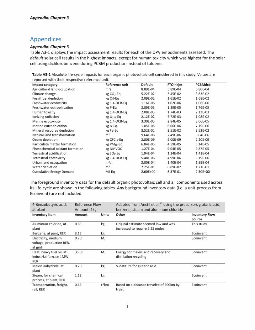
Appendix: Chapter 3
I
Appendices Appendix: Chapter 3 Table A3-1 displays the impact assessment results for each of the OPV embodiments assessed. The default solar cell results in the highest impacts, except for human toxicity which was highest for the solar cell using dichlorobenzene during PCBM production instead of toluene.
Table A3-1 Absolute life-cycle impacts for each organic photovoltaic cell considered in this study. Values are reported with their respective reference unit. Impact category Reference unit Default FTOinkjet PCBMdcb Agricultural land occupation m2a 8.89E-04 5.89E-04 6.80E-04 Climate change kg CO2-Eq 5.22E-02 3.45E-02 3.83E-02 Fossil fuel depletion kg Oil-Eq 2.09E-02 1.61E-02 1.68E-02 Freshwater ecotoxicity kg 1,4-DCB-Eq 1.16E-06 1.02E-06 1.06E-06 Freshwater eutrophication kg P-Eq 2.89E-05 1.39E-05 1.76E-05 Human toxicity kg 1,4-DCB-Eq 2.08E-03 1.74E-03 2.13E-03 Ionizing radiation kg U235-Eq 2.12E-02 7.72E-03 1.08E-02 Marine ecotoxicity kg 1,4-DCB-Eq 3.30E-05 2.84E-05 3.06E-05 Marine eutrophication kg N-Eq 1.05E-05 6.06E-06 7.19E-06 Mineral resource depletion kg Fe-Eq 3.52E-02 3.51E-02 3.52E-02 Natural land transformation m2 9.64E-06 7.49E-06 8.04E-06 Ozone depletion kg CFC11-Eq 2.80E-09 2.00E-09 2.20E-09 Particulate matter formation kg PM10-Eq 6.84E-05 4.59E-05 5.14E-05 Photochemical oxidant formation kg NMVOC 1.27E-04 9.04E-05 9.87E-05 Terrestrial acidification kg SO2-Eq 1.94E-04 1.24E-04 1.41E-04 Terrestrial ecotoxicity kg 1,4-DCB-Eq 5.48E-06 4.99E-06 5.19E-06 Urban land occupation m2a 2.00E-04 1.40E-04 1.59E-04 Water depletion m3 2.25E-01 8.89E-02 1.21E-01 Cumulative Energy Demand MJ-Eq 2.60E+00 8.37E-01 2.30E+00
The foreground inventory data for the default organic photovoltaic cell and all components used across its life-cycle are shown in the following tables. Any background inventory data (i.e. a unit-process from Ecoinvent) are not included.
4-Benzobutyric acid, at plant
Reference Flow Amount: 1kg
Adapted from Anctil et al.57 using the precursors glutaric acid, benzene, steam and aluminum chloride
Inventory Item Amount Units Other Inventory Flow Source
Aluminum chloride, at plant
0.83 kg Original estimate seemed low and was increased to require 6.25 moles
This study
Benzene, at pant, RER 3.15 kg Ecoinvent
Electricity, medium voltage, production RER, at grid
0.70 MJ Ecoinvent
Heat, heavy fuel oil, at industrial furnace 1MW, RER
35.03 MJ Energy for maleic acid recovery and distillation recycling
Ecoinvent
Maleic anhydride, at plant
0.70 kg Substitute for glutaric acid Ecoinvent
Steam, for chemical process, at plant, RER
1.18 kg Ecoinvent
Transportation, freight, rail, RER
0.69 t*km Based on a distance traveled of 600km by train.
Ecoinvent
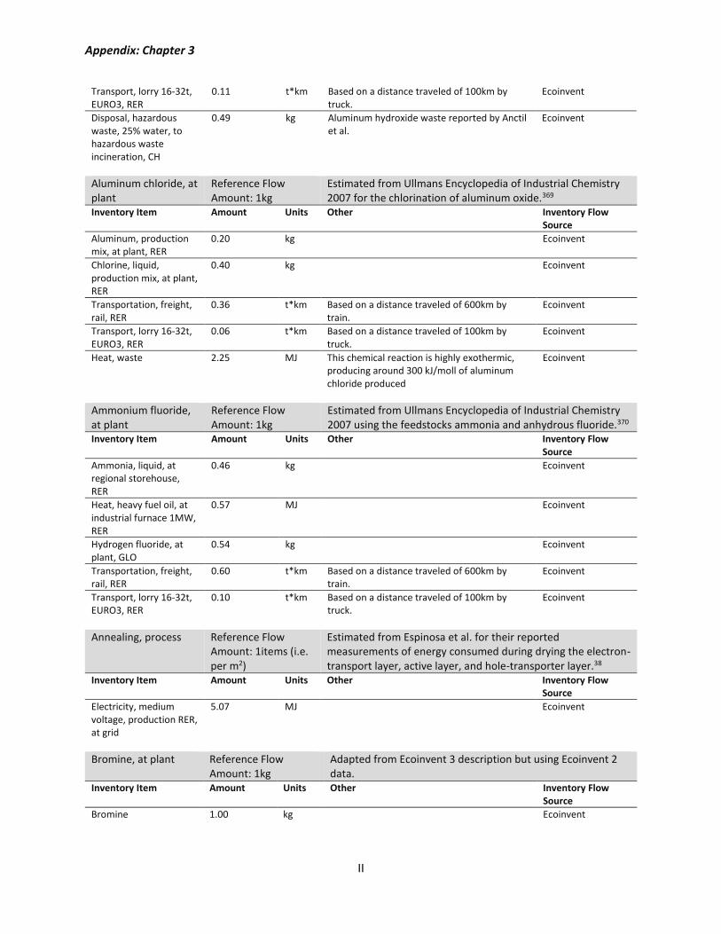
Appendix: Chapter 3
II
Transport, lorry 16-32t, EURO3, RER
0.11 t*km Based on a distance traveled of 100km by truck.
Ecoinvent
Disposal, hazardous waste, 25% water, to hazardous waste incineration, CH
0.49 kg Aluminum hydroxide waste reported by Anctil et al.
Ecoinvent
Aluminum chloride, at plant
Reference Flow Amount: 1kg
Estimated from Ullmans Encyclopedia of Industrial Chemistry 2007 for the chlorination of aluminum oxide.369
Inventory Item Amount Units Other Inventory Flow Source
Aluminum, production mix, at plant, RER
0.20 kg Ecoinvent
Chlorine, liquid, production mix, at plant, RER
0.40 kg Ecoinvent
Transportation, freight, rail, RER
0.36 t*km Based on a distance traveled of 600km by train.
Ecoinvent
Transport, lorry 16-32t, EURO3, RER
0.06 t*km Based on a distance traveled of 100km by truck.
Ecoinvent
Heat, waste 2.25 MJ This chemical reaction is highly exothermic, producing around 300 kJ/moll of aluminum chloride produced
Ecoinvent
Ammonium fluoride, at plant
Reference Flow Amount: 1kg
Estimated from Ullmans Encyclopedia of Industrial Chemistry 2007 using the feedstocks ammonia and anhydrous fluoride.370
Inventory Item Amount Units Other Inventory Flow Source
Ammonia, liquid, at regional storehouse, RER
0.46 kg Ecoinvent
Heat, heavy fuel oil, at industrial furnace 1MW, RER
0.57 MJ Ecoinvent
Hydrogen fluoride, at plant, GLO
0.54 kg Ecoinvent
Transportation, freight, rail, RER
0.60 t*km Based on a distance traveled of 600km by train.
Ecoinvent
Transport, lorry 16-32t, EURO3, RER
0.10 t*km Based on a distance traveled of 100km by truck.
Ecoinvent
Annealing, process Reference Flow Amount: 1items (i.e. per m2)
Estimated from Espinosa et al. for their reported measurements of energy consumed during drying the electron-transport layer, active layer, and hole-transporter layer.38
Inventory Item Amount Units Other Inventory Flow Source
Electricity, medium voltage, production RER, at grid
5.07 MJ Ecoinvent
Bromine, at plant Reference Flow Amount: 1kg
Adapted from Ecoinvent 3 description but using Ecoinvent 2 data.
Inventory Item Amount Units Other Inventory Flow Source
Bromine 1.00 kg Ecoinvent
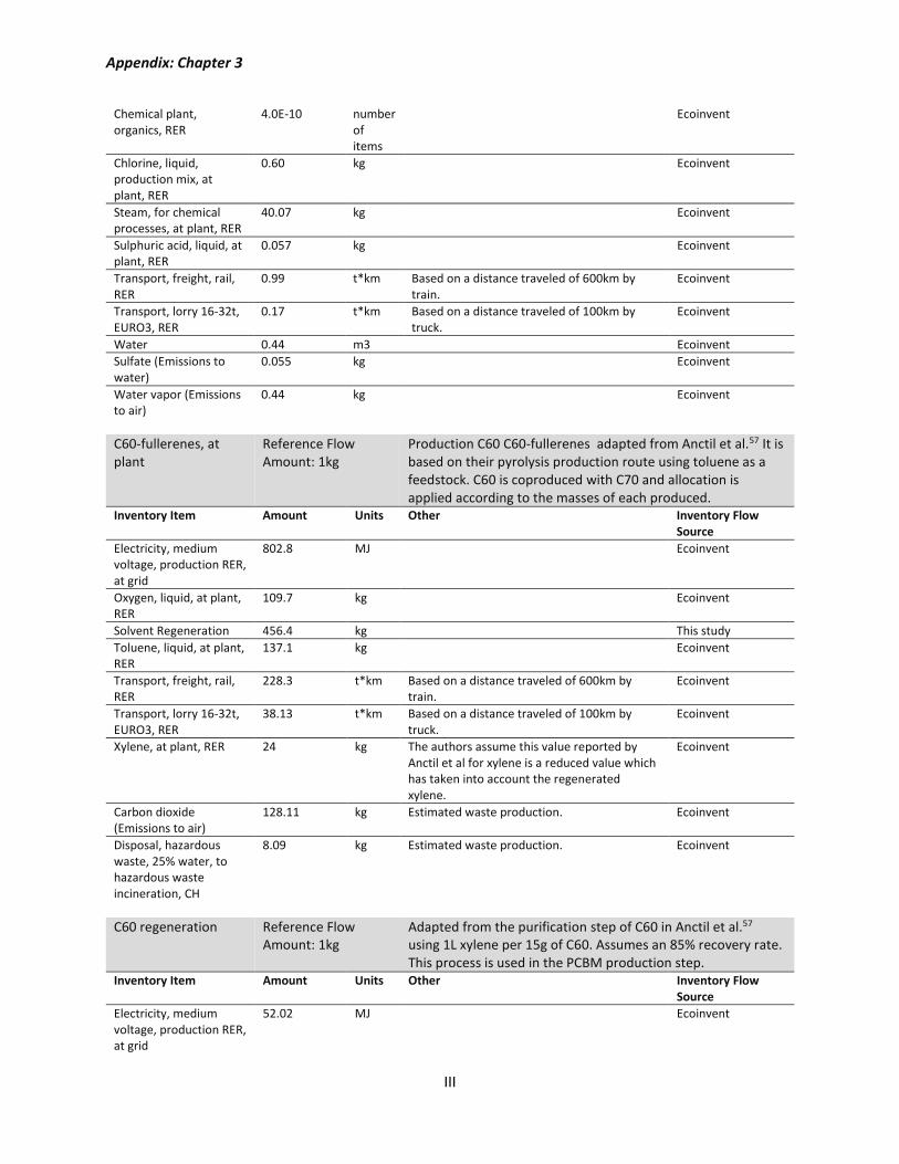
Appendix: Chapter 3
III
Chemical plant, organics, RER
4.0E-10 number of items
Ecoinvent
Chlorine, liquid, production mix, at plant, RER
0.60 kg Ecoinvent
Steam, for chemical processes, at plant, RER
40.07 kg Ecoinvent
Sulphuric acid, liquid, at plant, RER
0.057 kg Ecoinvent
Transport, freight, rail, RER
0.99 t*km Based on a distance traveled of 600km by train.
Ecoinvent
Transport, lorry 16-32t, EURO3, RER
0.17 t*km Based on a distance traveled of 100km by truck.
Ecoinvent
Water 0.44 m3 Ecoinvent
Sulfate (Emissions to water)
0.055 kg Ecoinvent
Water vapor (Emissions to air)
0.44 kg Ecoinvent
C60-fullerenes, at plant
Reference Flow Amount: 1kg
Production C60 C60-fullerenes adapted from Anctil et al.57 It is based on their pyrolysis production route using toluene as a feedstock. C60 is coproduced with C70 and allocation is applied according to the masses of each produced.
Inventory Item Amount Units Other Inventory Flow Source
Electricity, medium voltage, production RER, at grid
802.8 MJ Ecoinvent
Oxygen, liquid, at plant, RER
109.7 kg Ecoinvent
Solvent Regeneration 456.4 kg This study
Toluene, liquid, at plant, RER
137.1 kg Ecoinvent
Transport, freight, rail, RER
228.3 t*km Based on a distance traveled of 600km by train.
Ecoinvent
Transport, lorry 16-32t, EURO3, RER
38.13 t*km Based on a distance traveled of 100km by truck.
Ecoinvent
Xylene, at plant, RER 24 kg The authors assume this value reported by Anctil et al for xylene is a reduced value which has taken into account the regenerated xylene.
Ecoinvent
Carbon dioxide (Emissions to air)
128.11 kg Estimated waste production. Ecoinvent
Disposal, hazardous waste, 25% water, to hazardous waste incineration, CH
8.09 kg Estimated waste production. Ecoinvent
C60 regeneration Reference Flow Amount: 1kg
Adapted from the purification step of C60 in Anctil et al.57 using 1L xylene per 15g of C60. Assumes an 85% recovery rate. This process is used in the PCBM production step.
Inventory Item Amount Units Other Inventory Flow Source
Electricity, medium voltage, production RER, at grid
52.02 MJ Ecoinvent
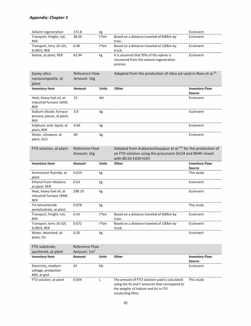
Appendix: Chapter 3
IV
Solvent regeneration 172.8 kg Ecoinvent
Transport, freight, rail, RER
38.36 t*km Based on a distance traveled of 600km by train.
Ecoinvent
Transport, lorry 16-32t, EURO3, RER
6.40 t*km Based on a distance traveled of 100km by truck.
Ecoinvent
Xylene, at plant, RER 63.94 kg It is assumed that 95% of the xylene is recovered from the solvent regeneration process.
Ecoinvent
Epoxy silica nanocomposite, at plant
Reference Flow Amount: 1kg
Adapted from the production of silica sol used in Roes et al.29
Inventory Item Amount Units Other Inventory Flow Source
Heat, heavy fuel oil, at industrial furnace 1MW, RER
23 MJ Ecoinvent
Sodium silicate, furnace process, pieces, at plant, RER
3.9 kg Ecoinvent
Sulphuric acid, liquid, at plant, RER
0.66 kg Ecoinvent
Water, ultrapure, at plant, GLO
40 kg Ecoinvent
FTO solution, at plant Reference Flow Amount: 1kg
Adapted from Aukkaravittayapun et al.133 for the production of an FTO solution using the precursors SnCl4 and NH4F mixed with 80:20 EtOH:H2O
Inventory Item Amount Units Other Inventory Flow Source
Ammonium fluoride, at plant
0.014 kg This study
Ethanol from ethylene, at plant, RER
0.63 kg Ecoinvent
Heat, heavy fuel oil, at industrial furnace 1MW, RER
298.19 kg Ecoinvent
Tin tetrachloride pentahydrate, at plant
0.078 kg This study
Transport, freight, rail, RER
0.43 t*km Based on a distance traveled of 600km by train.
Ecoinvent
Transport, lorry 16-32t, EURO3, RER
0.072 t*km Based on a distance traveled of 100km by truck.
Ecoinvent
Water, deionized, at plant, CH
0.20 kg Ecoinvent
FTO substrate, sputtered, at plant
Reference Flow Amount: 1m2
Inventory Item Amount Units Other Inventory Flow Source
Electricity, medium voltage, production RER, at grid
24 MJ Ecoinvent
FTO solution, at plant 0.034 L The amount of FTO solution used is calculated using the Sn and F amounts that correspond to the weights of indium and tin in ITO conducting films.
This study
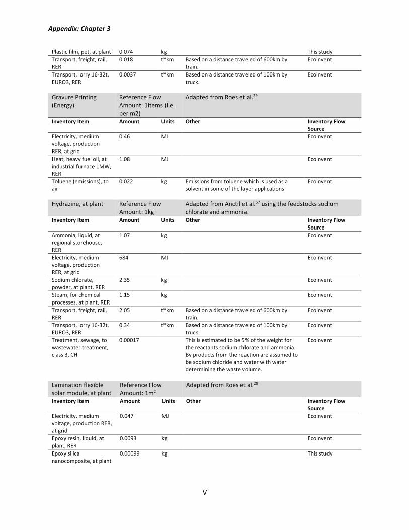
Appendix: Chapter 3
V
Plastic film, pet, at plant 0.074 kg This study
Transport, freight, rail, RER
0.018 t*km Based on a distance traveled of 600km by train.
Ecoinvent
Transport, lorry 16-32t, EURO3, RER
0.0037 t*km Based on a distance traveled of 100km by truck.
Ecoinvent
Gravure Printing (Energy)
Reference Flow Amount: 1items (i.e. per m2)
Adapted from Roes et al.29
Inventory Item Amount Units Other Inventory Flow Source
Electricity, medium voltage, production RER, at grid
0.46 MJ Ecoinvent
Heat, heavy fuel oil, at industrial furnace 1MW, RER
1.08 MJ Ecoinvent
Toluene (emissions), to air
0.022 kg Emissions from toluene which is used as a solvent in some of the layer applications
Ecoinvent
Hydrazine, at plant Reference Flow Amount: 1kg
Adapted from Anctil et al.57 using the feedstocks sodium chlorate and ammonia.
Inventory Item Amount Units Other Inventory Flow Source
Ammonia, liquid, at regional storehouse, RER
1.07 kg Ecoinvent
Electricity, medium voltage, production RER, at grid
684 MJ Ecoinvent
Sodium chlorate, powder, at plant, RER
2.35 kg Ecoinvent
Steam, for chemical processes, at plant, RER
1.15 kg Ecoinvent
Transport, freight, rail, RER
2.05 t*km Based on a distance traveled of 600km by train.
Ecoinvent
Transport, lorry 16-32t, EURO3, RER
0.34 t*km Based on a distance traveled of 100km by truck.
Ecoinvent
Treatment, sewage, to wastewater treatment, class 3, CH
0.00017 This is estimated to be 5% of the weight for the reactants sodium chlorate and ammonia. By products from the reaction are assumed to be sodium chloride and water with water determining the waste volume.
Ecoinvent
Lamination flexible solar module, at plant
Reference Flow Amount: 1m2
Adapted from Roes et al.29
Inventory Item Amount Units Other Inventory Flow Source
Electricity, medium voltage, production RER, at grid
0.047 MJ Ecoinvent
Epoxy resin, liquid, at plant, RER
0.0093 kg Ecoinvent
Epoxy silica nanocomposite, at plant
0.00099 kg This study
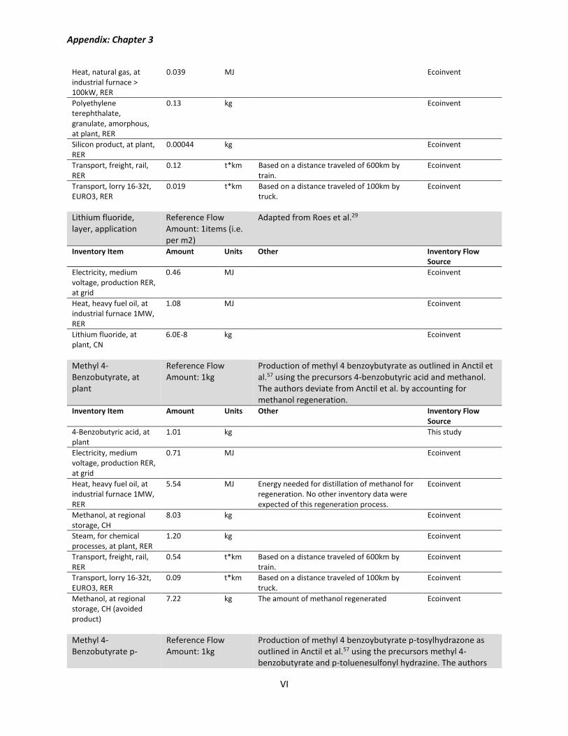
Appendix: Chapter 3
VI
Heat, natural gas, at industrial furnace > 100kW, RER
0.039 MJ Ecoinvent
Polyethylene terephthalate, granulate, amorphous, at plant, RER
0.13 kg Ecoinvent
Silicon product, at plant, RER
0.00044 kg Ecoinvent
Transport, freight, rail, RER
0.12 t*km Based on a distance traveled of 600km by train.
Ecoinvent
Transport, lorry 16-32t, EURO3, RER
0.019 t*km Based on a distance traveled of 100km by truck.
Ecoinvent
Lithium fluoride, layer, application
Reference Flow Amount: 1items (i.e. per m2)
Adapted from Roes et al.29
Inventory Item Amount Units Other Inventory Flow Source
Electricity, medium voltage, production RER, at grid
0.46 MJ Ecoinvent
Heat, heavy fuel oil, at industrial furnace 1MW, RER
1.08 MJ Ecoinvent
Lithium fluoride, at plant, CN
6.0E-8 kg Ecoinvent
Methyl 4-Benzobutyrate, at plant
Reference Flow Amount: 1kg
Production of methyl 4 benzoybutyrate as outlined in Anctil et al.57 using the precursors 4-benzobutyric acid and methanol. The authors deviate from Anctil et al. by accounting for methanol regeneration.
Inventory Item Amount Units Other Inventory Flow Source
4-Benzobutyric acid, at plant
1.01 kg This study
Electricity, medium voltage, production RER, at grid
0.71 MJ Ecoinvent
Heat, heavy fuel oil, at industrial furnace 1MW, RER
5.54 MJ Energy needed for distillation of methanol for regeneration. No other inventory data were expected of this regeneration process.
Ecoinvent
Methanol, at regional storage, CH
8.03 kg Ecoinvent
Steam, for chemical processes, at plant, RER
1.20 kg Ecoinvent
Transport, freight, rail, RER
0.54 t*km Based on a distance traveled of 600km by train.
Ecoinvent
Transport, lorry 16-32t, EURO3, RER
0.09 t*km Based on a distance traveled of 100km by truck.
Ecoinvent
Methanol, at regional storage, CH (avoided product)
7.22 kg The amount of methanol regenerated Ecoinvent
Methyl 4-Benzobutyrate p-
Reference Flow Amount: 1kg
Production of methyl 4 benzoybutyrate p-tosylhydrazone as outlined in Anctil et al.57 using the precursors methyl 4-benzobutyrate and p-toluenesulfonyl hydrazine. The authors
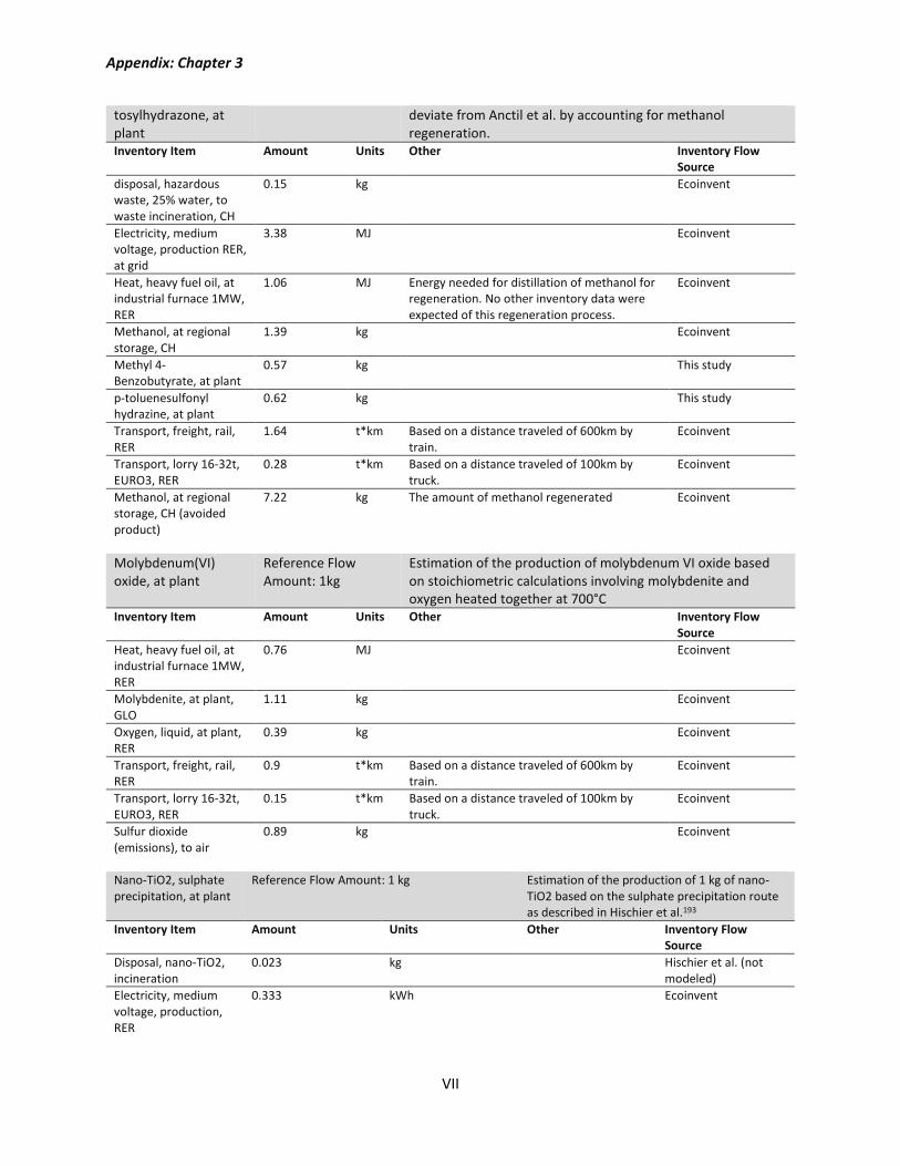
Appendix: Chapter 3
VII
tosylhydrazone, at plant
deviate from Anctil et al. by accounting for methanol regeneration.
Inventory Item Amount Units Other Inventory Flow Source
disposal, hazardous waste, 25% water, to waste incineration, CH
0.15 kg Ecoinvent
Electricity, medium voltage, production RER, at grid
3.38 MJ Ecoinvent
Heat, heavy fuel oil, at industrial furnace 1MW, RER
1.06 MJ Energy needed for distillation of methanol for regeneration. No other inventory data were expected of this regeneration process.
Ecoinvent
Methanol, at regional storage, CH
1.39 kg Ecoinvent
Methyl 4-Benzobutyrate, at plant
0.57 kg This study
p-toluenesulfonyl hydrazine, at plant
0.62 kg This study
Transport, freight, rail, RER
1.64 t*km Based on a distance traveled of 600km by train.
Ecoinvent
Transport, lorry 16-32t, EURO3, RER
0.28 t*km Based on a distance traveled of 100km by truck.
Ecoinvent
Methanol, at regional storage, CH (avoided product)
7.22 kg The amount of methanol regenerated Ecoinvent
Molybdenum(VI) oxide, at plant
Reference Flow Amount: 1kg
Estimation of the production of molybdenum VI oxide based on stoichiometric calculations involving molybdenite and oxygen heated together at 700°C
Inventory Item Amount Units Other Inventory Flow Source
Heat, heavy fuel oil, at industrial furnace 1MW, RER
0.76 MJ Ecoinvent
Molybdenite, at plant, GLO
1.11 kg Ecoinvent
Oxygen, liquid, at plant, RER
0.39 kg Ecoinvent
Transport, freight, rail, RER
0.9 t*km Based on a distance traveled of 600km by train.
Ecoinvent
Transport, lorry 16-32t, EURO3, RER
0.15 t*km Based on a distance traveled of 100km by truck.
Ecoinvent
Sulfur dioxide (emissions), to air
0.89 kg Ecoinvent
Nano-TiO2, sulphate precipitation, at plant
Reference Flow Amount: 1 kg Estimation of the production of 1 kg of nano-TiO2 based on the sulphate precipitation route as described in Hischier et al.193
Inventory Item Amount Units Other Inventory Flow Source
Disposal, nano-TiO2, incineration
0.023 kg Hischier et al. (not modeled)
Electricity, medium voltage, production, RER
0.333 kWh Ecoinvent
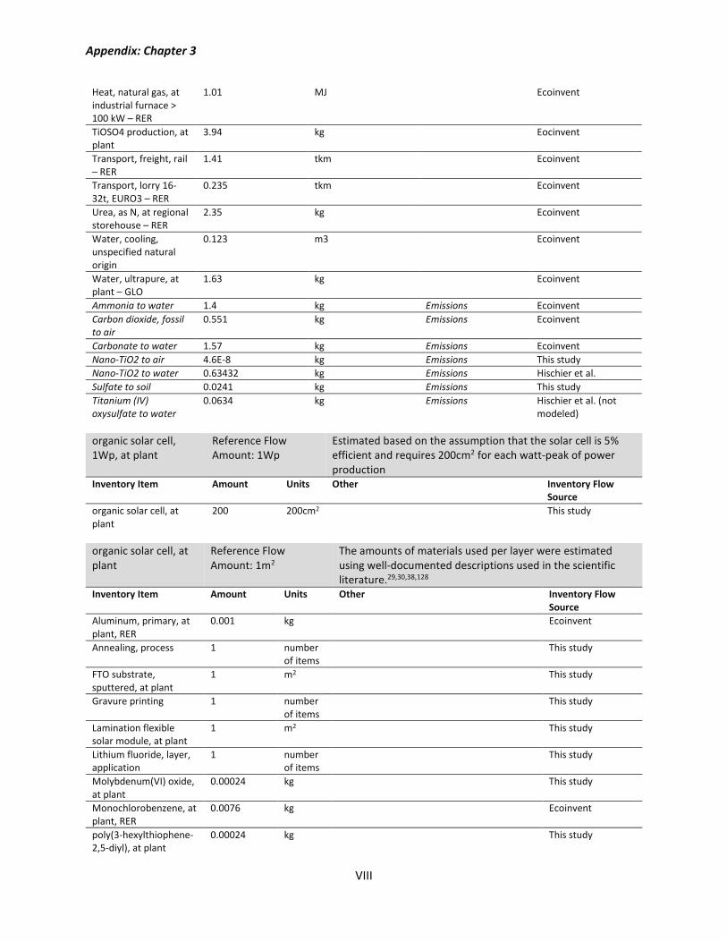
Appendix: Chapter 3
VIII
Heat, natural gas, at industrial furnace > 100 kW – RER
1.01 MJ Ecoinvent
TiOSO4 production, at plant
3.94 kg Eocinvent
Transport, freight, rail – RER
1.41 tkm Ecoinvent
Transport, lorry 16-32t, EURO3 – RER
0.235 tkm Ecoinvent
Urea, as N, at regional storehouse – RER
2.35 kg Ecoinvent
Water, cooling, unspecified natural origin
0.123 m3 Ecoinvent
Water, ultrapure, at plant – GLO
1.63 kg Ecoinvent
Ammonia to water 1.4 kg Emissions Ecoinvent
Carbon dioxide, fossil to air
0.551 kg Emissions Ecoinvent
Carbonate to water 1.57 kg Emissions Ecoinvent
Nano-TiO2 to air 4.6E-8 kg Emissions This study
Nano-TiO2 to water 0.63432 kg Emissions Hischier et al.
Sulfate to soil 0.0241 kg Emissions This study
Titanium (IV) oxysulfate to water
0.0634 kg Emissions Hischier et al. (not modeled)
organic solar cell, 1Wp, at plant
Reference Flow Amount: 1Wp
Estimated based on the assumption that the solar cell is 5% efficient and requires 200cm2 for each watt-peak of power production
Inventory Item Amount Units Other Inventory Flow Source
organic solar cell, at plant
200 200cm2 This study
organic solar cell, at plant
Reference Flow Amount: 1m2
The amounts of materials used per layer were estimated using well-documented descriptions used in the scientific literature.29,30,38,128
Inventory Item Amount Units Other Inventory Flow Source
Aluminum, primary, at plant, RER
0.001 kg Ecoinvent
Annealing, process 1 number of items
This study
FTO substrate, sputtered, at plant
1 m2 This study
Gravure printing 1 number of items
This study
Lamination flexible solar module, at plant
1 m2 This study
Lithium fluoride, layer, application
1 number of items
This study
Molybdenum(VI) oxide, at plant
0.00024 kg This study
Monochlorobenzene, at plant, RER
0.0076 kg Ecoinvent
poly(3-hexylthiophene-2,5-diyl), at plant
0.00024 kg This study
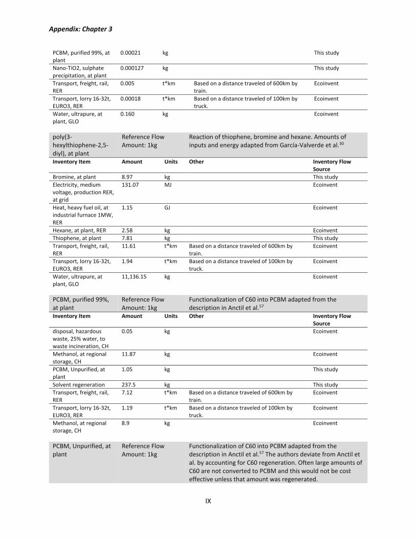
Appendix: Chapter 3
IX
PCBM, purified 99%, at plant
0.00021 kg This study
Nano-TiO2, sulphate precipitation, at plant
0.000127 kg This study
Transport, freight, rail, RER
0.005 t*km Based on a distance traveled of 600km by train.
Ecoinvent
Transport, lorry 16-32t, EURO3, RER
0.00018 t*km Based on a distance traveled of 100km by truck.
Ecoinvent
Water, ultrapure, at plant, GLO
0.160 kg Ecoinvent
poly(3-hexylthiophene-2,5-diyl), at plant
Reference Flow Amount: 1kg
Reaction of thiophene, bromine and hexane. Amounts of inputs and energy adapted from García-Valverde et al.30
Inventory Item Amount Units Other Inventory Flow Source
Bromine, at plant 8.97 kg This study
Electricity, medium voltage, production RER, at grid
131.07 MJ Ecoinvent
Heat, heavy fuel oil, at industrial furnace 1MW, RER
1.15 GJ Ecoinvent
Hexane, at plant, RER 2.58 kg Ecoinvent
Thiophene, at plant 7.81 kg This study
Transport, freight, rail, RER
11.61 t*km Based on a distance traveled of 600km by train.
Ecoinvent
Transport, lorry 16-32t, EURO3, RER
1.94 t*km Based on a distance traveled of 100km by truck.
Ecoinvent
Water, ultrapure, at plant, GLO
11,136.15 kg Ecoinvent
PCBM, purified 99%, at plant
Reference Flow Amount: 1kg
Functionalization of C60 into PCBM adapted from the description in Anctil et al.57
Inventory Item Amount Units Other Inventory Flow Source
disposal, hazardous waste, 25% water, to waste incineration, CH
0.05 kg Ecoinvent
Methanol, at regional storage, CH
11.87 kg Ecoinvent
PCBM, Unpurified, at plant
1.05 kg This study
Solvent regeneration 237.5 kg This study
Transport, freight, rail, RER
7.12 t*km Based on a distance traveled of 600km by train.
Ecoinvent
Transport, lorry 16-32t, EURO3, RER
1.19 t*km Based on a distance traveled of 100km by truck.
Ecoinvent
Methanol, at regional storage, CH
8.9 kg Ecoinvent
PCBM, Unpurified, at plant
Reference Flow Amount: 1kg
Functionalization of C60 into PCBM adapted from the description in Anctil et al.57 The authors deviate from Anctil et al. by accounting for C60 regeneration. Often large amounts of C60 are not converted to PCBM and this would not be cost effective unless that amount was regenerated.
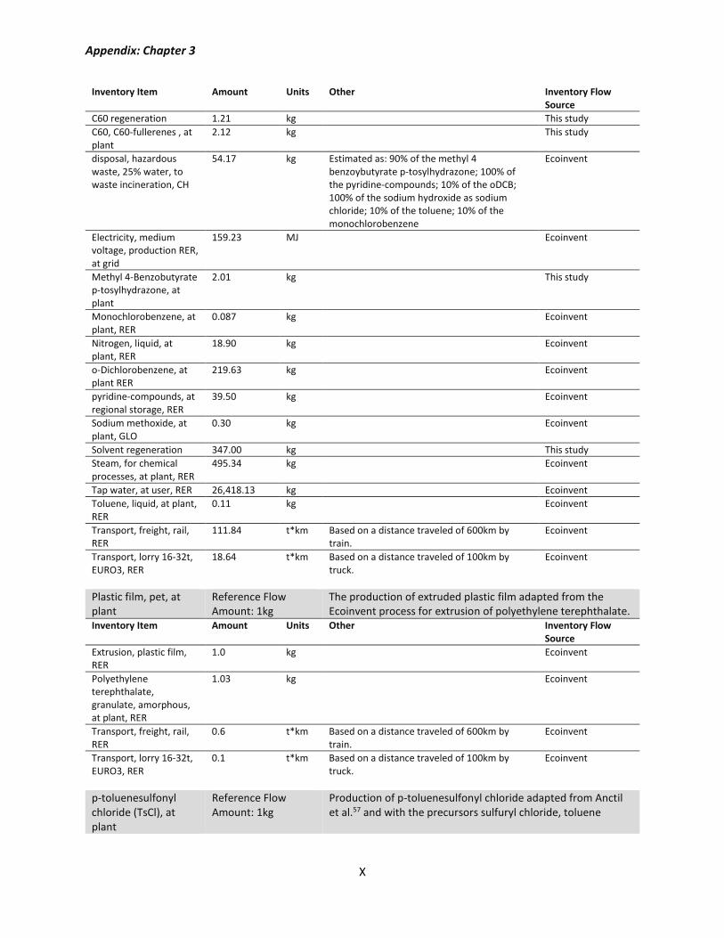
Appendix: Chapter 3
X
Inventory Item Amount Units Other Inventory Flow Source
C60 regeneration 1.21 kg This study
C60, C60-fullerenes , at plant
2.12 kg This study
disposal, hazardous waste, 25% water, to waste incineration, CH
54.17 kg Estimated as: 90% of the methyl 4 benzoybutyrate p-tosylhydrazone; 100% of the pyridine-compounds; 10% of the oDCB; 100% of the sodium hydroxide as sodium chloride; 10% of the toluene; 10% of the monochlorobenzene
Ecoinvent
Electricity, medium voltage, production RER, at grid
159.23 MJ Ecoinvent
Methyl 4-Benzobutyrate p-tosylhydrazone, at plant
2.01 kg This study
Monochlorobenzene, at plant, RER
0.087 kg Ecoinvent
Nitrogen, liquid, at plant, RER
18.90 kg Ecoinvent
o-Dichlorobenzene, at plant RER
219.63 kg Ecoinvent
pyridine-compounds, at regional storage, RER
39.50 kg Ecoinvent
Sodium methoxide, at plant, GLO
0.30 kg Ecoinvent
Solvent regeneration 347.00 kg This study
Steam, for chemical processes, at plant, RER
495.34 kg Ecoinvent
Tap water, at user, RER 26,418.13 kg Ecoinvent
Toluene, liquid, at plant, RER
0.11 kg Ecoinvent
Transport, freight, rail, RER
111.84 t*km Based on a distance traveled of 600km by train.
Ecoinvent
Transport, lorry 16-32t, EURO3, RER
18.64 t*km Based on a distance traveled of 100km by truck.
Ecoinvent
Plastic film, pet, at plant
Reference Flow Amount: 1kg
The production of extruded plastic film adapted from the Ecoinvent process for extrusion of polyethylene terephthalate.
Inventory Item Amount Units Other Inventory Flow Source
Extrusion, plastic film, RER
1.0 kg Ecoinvent
Polyethylene terephthalate, granulate, amorphous, at plant, RER
1.03 kg Ecoinvent
Transport, freight, rail, RER
0.6 t*km Based on a distance traveled of 600km by train.
Ecoinvent
Transport, lorry 16-32t, EURO3, RER
0.1 t*km Based on a distance traveled of 100km by truck.
Ecoinvent
p-toluenesulfonyl chloride (TsCl), at plant
Reference Flow Amount: 1kg
Production of p-toluenesulfonyl chloride adapted from Anctil et al.57 and with the precursors sulfuryl chloride, toluene
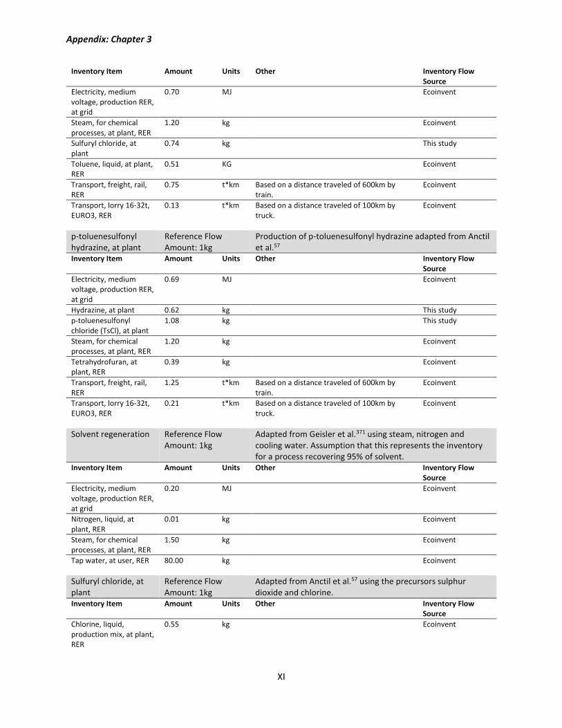
Appendix: Chapter 3
XI
Inventory Item Amount Units Other Inventory Flow Source
Electricity, medium voltage, production RER, at grid
0.70 MJ Ecoinvent
Steam, for chemical processes, at plant, RER
1.20 kg Ecoinvent
Sulfuryl chloride, at plant
0.74 kg This study
Toluene, liquid, at plant, RER
0.51 KG Ecoinvent
Transport, freight, rail, RER
0.75 t*km Based on a distance traveled of 600km by train.
Ecoinvent
Transport, lorry 16-32t, EURO3, RER
0.13 t*km Based on a distance traveled of 100km by truck.
Ecoinvent
p-toluenesulfonyl hydrazine, at plant
Reference Flow Amount: 1kg
Production of p-toluenesulfonyl hydrazine adapted from Anctil et al.57
Inventory Item Amount Units Other Inventory Flow Source
Electricity, medium voltage, production RER, at grid
0.69 MJ Ecoinvent
Hydrazine, at plant 0.62 kg This study
p-toluenesulfonyl chloride (TsCl), at plant
1.08 kg This study
Steam, for chemical processes, at plant, RER
1.20 kg Ecoinvent
Tetrahydrofuran, at plant, RER
0.39 kg Ecoinvent
Transport, freight, rail, RER
1.25 t*km Based on a distance traveled of 600km by train.
Ecoinvent
Transport, lorry 16-32t, EURO3, RER
0.21 t*km Based on a distance traveled of 100km by truck.
Ecoinvent
Solvent regeneration Reference Flow Amount: 1kg
Adapted from Geisler et al.371 using steam, nitrogen and cooling water. Assumption that this represents the inventory for a process recovering 95% of solvent.
Inventory Item Amount Units Other Inventory Flow Source
Electricity, medium voltage, production RER, at grid
0.20 MJ Ecoinvent
Nitrogen, liquid, at plant, RER
0.01 kg Ecoinvent
Steam, for chemical processes, at plant, RER
1.50 kg Ecoinvent
Tap water, at user, RER 80.00 kg Ecoinvent
Sulfuryl chloride, at plant
Reference Flow Amount: 1kg
Adapted from Anctil et al.57 using the precursors sulphur dioxide and chlorine.
Inventory Item Amount Units Other Inventory Flow Source
Chlorine, liquid, production mix, at plant, RER
0.55 kg Ecoinvent
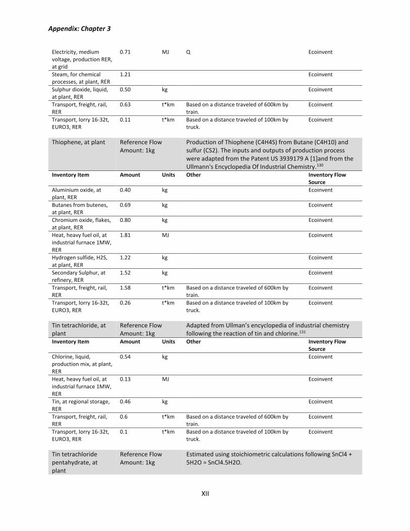
Appendix: Chapter 3
XII
Electricity, medium voltage, production RER, at grid
0.71 MJ Q Ecoinvent
Steam, for chemical processes, at plant, RER
1.21 Ecoinvent
Sulphur dioxide, liquid, at plant, RER
0.50 kg Ecoinvent
Transport, freight, rail, RER
0.63 t*km Based on a distance traveled of 600km by train.
Ecoinvent
Transport, lorry 16-32t, EURO3, RER
0.11 t*km Based on a distance traveled of 100km by truck.
Ecoinvent
Thiophene, at plant Reference Flow Amount: 1kg
Production of Thiophene (C4H4S) from Butane (C4H10) and sulfur (CS2). The inputs and outputs of production process were adapted from the Patent US 3939179 A [1]and from the Ullmann's Encyclopedia Of Industrial Chemistry.130
Inventory Item Amount Units Other Inventory Flow Source
Aluminium oxide, at plant, RER
0.40 kg Ecoinvent
Butanes from butenes, at plant, RER
0.69 kg Ecoinvent
Chromium oxide, flakes, at plant, RER
0.80 kg Ecoinvent
Heat, heavy fuel oil, at industrial furnace 1MW, RER
1.81 MJ Ecoinvent
Hydrogen sulfide, H2S, at plant, RER
1.22 kg Ecoinvent
Secondary Sulphur, at refinery, RER
1.52 kg Ecoinvent
Transport, freight, rail, RER
1.58 t*km Based on a distance traveled of 600km by train.
Ecoinvent
Transport, lorry 16-32t, EURO3, RER
0.26 t*km Based on a distance traveled of 100km by truck.
Ecoinvent
Tin tetrachloride, at plant
Reference Flow Amount: 1kg
Adapted from Ullman’s encyclopedia of industrial chemistry following the reaction of tin and chlorine.131
Inventory Item Amount Units Other Inventory Flow Source
Chlorine, liquid, production mix, at plant, RER
0.54 kg Ecoinvent
Heat, heavy fuel oil, at industrial furnace 1MW, RER
0.13 MJ Ecoinvent
Tin, at regional storage, RER
0.46 kg Ecoinvent
Transport, freight, rail, RER
0.6 t*km Based on a distance traveled of 600km by train.
Ecoinvent
Transport, lorry 16-32t, EURO3, RER
0.1 t*km Based on a distance traveled of 100km by truck.
Ecoinvent
Tin tetrachloride pentahydrate, at plant
Reference Flow Amount: 1kg
Estimated using stoichiometric calculations following SnCl4 + 5H2O = SnCl4.5H2O.
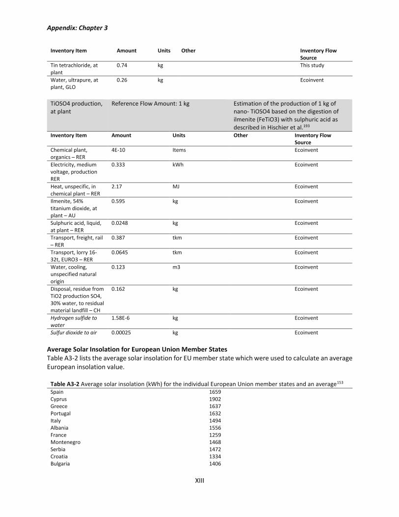
Appendix: Chapter 3
XIII
Inventory Item Amount Units Other Inventory Flow Source
Tin tetrachloride, at plant
0.74 kg This study
Water, ultrapure, at plant, GLO
0.26 kg Ecoinvent
TiOSO4 production, at plant
Reference Flow Amount: 1 kg Estimation of the production of 1 kg of nano- TiOSO4 based on the digestion of ilmenite (FeTiO3) with sulphuric acid as described in Hischier et al.193
Inventory Item Amount Units Other Inventory Flow Source
Chemical plant, organics – RER
4E-10 Items Ecoinvent
Electricity, medium voltage, production RER
0.333 kWh Ecoinvent
Heat, unspecific, in chemical plant – RER
2.17 MJ Ecoinvent
Ilmenite, 54% titanium dioxide, at plant – AU
0.595 kg Ecoinvent
Sulphuric acid, liquid, at plant – RER
0.0248 kg Ecoinvent
Transport, freight, rail – RER
0.387 tkm Ecoinvent
Transport, lorry 16-32t, EURO3 – RER
0.0645 tkm Ecoinvent
Water, cooling, unspecified natural origin
0.123 m3 Ecoinvent
Disposal, residue from TiO2 production SO4, 30% water, to residual material landfill – CH
0.162 kg Ecoinvent
Hydrogen sulfide to water
1.58E-6 kg Ecoinvent
Sulfur dioxide to air 0.00025 kg Ecoinvent
Average Solar Insolation for European Union Member States Table A3-2 lists the average solar insolation for EU member state which were used to calculate an average European insolation value.
Table A3-2 Average solar insolation (kWh) for the individual European Union member states and an average153 Spain 1659 Cyprus 1902 Greece 1637 Portugal 1632 Italy 1494 Albania 1556 France 1259 Montenegro 1468 Serbia 1472 Croatia 1334 Bulgaria 1406

Appendix: Chapter 3
XIV
Bosnia and Herz 1315 Switzerland 1233 Romania 1301 Slovenia 1270 Moldova 1276 Hungary 1266 Austria 1194 Slovakia 1182 Germany 1066 Czech Rep 1109 UK 972 Poland 1071 Netherlands 1025 Belgium 1052 Denmark 987 Ireland 926 Turkey* 1661 Average 1298.67
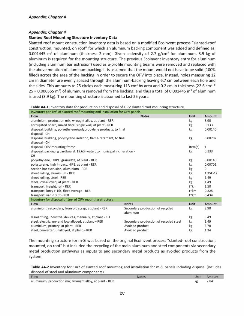
Appendix: Chapter 4
XV
Appendix: Chapter 4 Slanted Roof Mounting Structure Inventory Data Slanted roof mount construction inventory data is based on a modified Ecoinvent process “slanted-roof construction, mounted, on roof” for which an aluminum backing component was added and defined as: 0.001445 m3 of aluminum (thickness 2 mm). Given a density of 2.7 g/cm3 for aluminum, 3.9 kg of aluminum is required for the mounting structure. The previous Ecoinvent inventory entry for aluminum (including aluminum bar extrusion) used as u-profile mounting beams were removed and replaced with the above mention of aluminum backing. It is assumed that the mount would not have to be solid (100% filled) across the area of the backing in order to secure the OPV into place. Instead, holes measuring 12 cm in diameter are evenly spaced through the aluminum-backing leaving 6.7 cm between each hole and the sides. This amounts to 25 circles each measuring 113 cm2 by area and 0.2 cm in thickness (22.6 cm3 * 25 = 0.000555 m3) of aluminum removed from the backing, and thus a total of 0.001445 m3 of aluminum is used (3.9 kg). The mounting structure is assumed to last 25 years.
Table A4-1 Inventory data for production and disposal of OPV slanted roof mounting structure. Inventory per 1m2 of slanted roof mounting and installation for OPV panels Flow Notes Unit Amount aluminium, production mix, wrought alloy, at plant - RER kg 3.90 corrugated board, mixed fibre, single wall, at plant - RER kg 0.133 disposal, building, polyethylene/polypropylene products, to final disposal - CH
kg 0.00140
disposal, building, polystyrene isolation, flame-retardant, to final disposal - CH
kg 0.00702
disposal, OPV mounting frame Item(s) 1 disposal, packaging cardboard, 19.6% water, to municipal incineration - CH
kg 0.133
polyethylene, HDPE, granulate, at plant - RER kg 0.00140 polystyrene, high impact, HIPS, at plant - RER kg 0.00702 section bar extrusion, aluminium - RER kg 0 sheet rolling, aluminium - RER kg 1.35E-12 sheet rolling, steel - RER kg 1.49 steel, low-alloyed, at plant - RER kg 1.49 transport, freight, rail - RER t*km 1.50 transport, lorry > 16t, fleet average - RER t*km 0.225 transport, van < 3.5t - RER t*km 0.434 Inventory for disposal of 1m2 of OPV mounting structure Flow Notes Unit Amount aluminium, secondary, from old scrap, at plant - RER Secondary production of recycled
aluminum kg 3.90
dismantling, industrial devices, manually, at plant - CH kg 5.49 steel, electric, un- and low-alloyed, at plant – RER Secondary production of recycled steel kg 1.49 aluminium, primary, at plant - RER Avoided product kg 3.78 steel, converter, unalloyed, at plant – RER Avoided product kg 1.34
The mounting structure for m-Si was based on the original Ecoinvent process “slanted-roof construction, mounted, on roof” but included the recycling of the main aluminum and steel components via secondary metal production pathways as inputs to and secondary metal products as avoided products from the system.
Table A4-2 Inventory for 1m2 of slanted roof mounting and installation for m-Si panels including disposal (includes disposal of steel and aluminum components) Flow Notes Unit Amount aluminium, production mix, wrought alloy, at plant - RER
kg 2.84
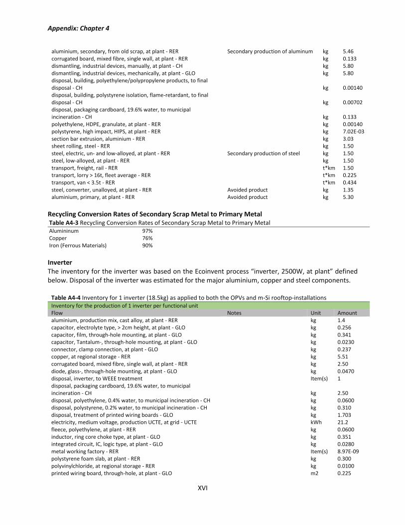
Appendix: Chapter 4
XVI
aluminium, secondary, from old scrap, at plant - RER Secondary production of aluminum kg 5.46 corrugated board, mixed fibre, single wall, at plant - RER kg 0.133 dismantling, industrial devices, manually, at plant - CH kg 5.80 dismantling, industrial devices, mechanically, at plant - GLO kg 5.80 disposal, building, polyethylene/polypropylene products, to final disposal - CH kg 0.00140 disposal, building, polystyrene isolation, flame-retardant, to final disposal - CH kg 0.00702 disposal, packaging cardboard, 19.6% water, to municipal incineration - CH kg 0.133 polyethylene, HDPE, granulate, at plant - RER kg 0.00140 polystyrene, high impact, HIPS, at plant - RER kg 7.02E-03 section bar extrusion, aluminium - RER kg 3.03 sheet rolling, steel - RER kg 1.50 steel, electric, un- and low-alloyed, at plant - RER Secondary production of steel kg 1.50 steel, low-alloyed, at plant - RER kg 1.50 transport, freight, rail - RER t*km 1.50 transport, lorry > 16t, fleet average - RER t*km 0.225 transport, van < 3.5t - RER t*km 0.434 steel, converter, unalloyed, at plant - RER Avoided product kg 1.35 aluminium, primary, at plant - RER Avoided product kg 5.30
Recycling Conversion Rates of Secondary Scrap Metal to Primary Metal Table A4-3 Recycling Conversion Rates of Secondary Scrap Metal to Primary Metal Alumininum 97% Copper 76% Iron (Ferrous Materials) 90% Inverter The inventory for the inverter was based on the Ecoinvent process “inverter, 2500W, at plant” defined below. Disposal of the inverter was estimated for the major aluminium, copper and steel components.
Table A4-4 Inventory for 1 inverter (18.5kg) as applied to both the OPVs and m-Si rooftop-installations Inventory for the production of 1 inverter per functional unit Flow Notes Unit Amount aluminium, production mix, cast alloy, at plant - RER kg 1.4 capacitor, electrolyte type, > 2cm height, at plant - GLO kg 0.256 capacitor, film, through-hole mounting, at plant - GLO kg 0.341 capacitor, Tantalum-, through-hole mounting, at plant - GLO kg 0.0230 connector, clamp connection, at plant - GLO kg 0.237 copper, at regional storage - RER kg 5.51 corrugated board, mixed fibre, single wall, at plant - RER kg 2.50 diode, glass-, through-hole mounting, at plant - GLO kg 0.0470 disposal, inverter, to WEEE treatment Item(s) 1 disposal, packaging cardboard, 19.6% water, to municipal incineration - CH kg 2.50 disposal, polyethylene, 0.4% water, to municipal incineration - CH kg 0.0600 disposal, polystyrene, 0.2% water, to municipal incineration - CH kg 0.310 disposal, treatment of printed wiring boards - GLO kg 1.703 electricity, medium voltage, production UCTE, at grid - UCTE kWh 21.2 fleece, polyethylene, at plant - RER kg 0.0600 inductor, ring core choke type, at plant - GLO kg 0.351 integrated circuit, IC, logic type, at plant - GLO kg 0.0280 metal working factory - RER Item(s) 8.97E-09 polystyrene foam slab, at plant - RER kg 0.300 polyvinylchloride, at regional storage - RER kg 0.0100 printed wiring board, through-hole, at plant - GLO m2 0.225
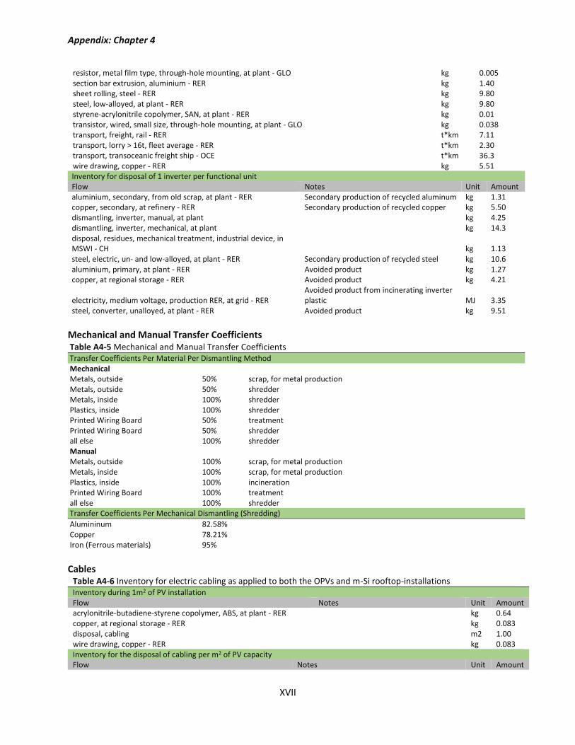
Appendix: Chapter 4
XVII
resistor, metal film type, through-hole mounting, at plant - GLO kg 0.005 section bar extrusion, aluminium - RER kg 1.40 sheet rolling, steel - RER kg 9.80 steel, low-alloyed, at plant - RER kg 9.80 styrene-acrylonitrile copolymer, SAN, at plant - RER kg 0.01 transistor, wired, small size, through-hole mounting, at plant - GLO kg 0.038 transport, freight, rail - RER t*km 7.11 transport, lorry > 16t, fleet average - RER t*km 2.30 transport, transoceanic freight ship - OCE t*km 36.3 wire drawing, copper - RER kg 5.51 Inventory for disposal of 1 inverter per functional unit Flow Notes Unit Amount aluminium, secondary, from old scrap, at plant - RER Secondary production of recycled aluminum kg 1.31 copper, secondary, at refinery - RER Secondary production of recycled copper kg 5.50 dismantling, inverter, manual, at plant kg 4.25 dismantling, inverter, mechanical, at plant kg 14.3 disposal, residues, mechanical treatment, industrial device, in MSWI - CH kg 1.13 steel, electric, un- and low-alloyed, at plant - RER Secondary production of recycled steel kg 10.6 aluminium, primary, at plant - RER Avoided product kg 1.27 copper, at regional storage - RER Avoided product kg 4.21
electricity, medium voltage, production RER, at grid - RER Avoided product from incinerating inverter plastic MJ 3.35
steel, converter, unalloyed, at plant - RER Avoided product kg 9.51
Mechanical and Manual Transfer Coefficients Table A4-5 Mechanical and Manual Transfer Coefficients Transfer Coefficients Per Material Per Dismantling Method Mechanical Metals, outside 50% scrap, for metal production Metals, outside 50% shredder Metals, inside 100% shredder Plastics, inside 100% shredder Printed Wiring Board 50% treatment Printed Wiring Board 50% shredder all else 100% shredder Manual Metals, outside 100% scrap, for metal production Metals, inside 100% scrap, for metal production Plastics, inside 100% incineration Printed Wiring Board 100% treatment all else 100% shredder Transfer Coefficients Per Mechanical Dismantling (Shredding)
Alumininum 82.58% Copper 78.21% Iron (Ferrous materials) 95% Cables
Table A4-6 Inventory for electric cabling as applied to both the OPVs and m-Si rooftop-installations Inventory during 1m2 of PV installation Flow Notes Unit Amount acrylonitrile-butadiene-styrene copolymer, ABS, at plant - RER kg 0.64 copper, at regional storage - RER kg 0.083 disposal, cabling m2 1.00 wire drawing, copper - RER kg 0.083 Inventory for the disposal of cabling per m2 of PV capacity Flow Notes Unit Amount
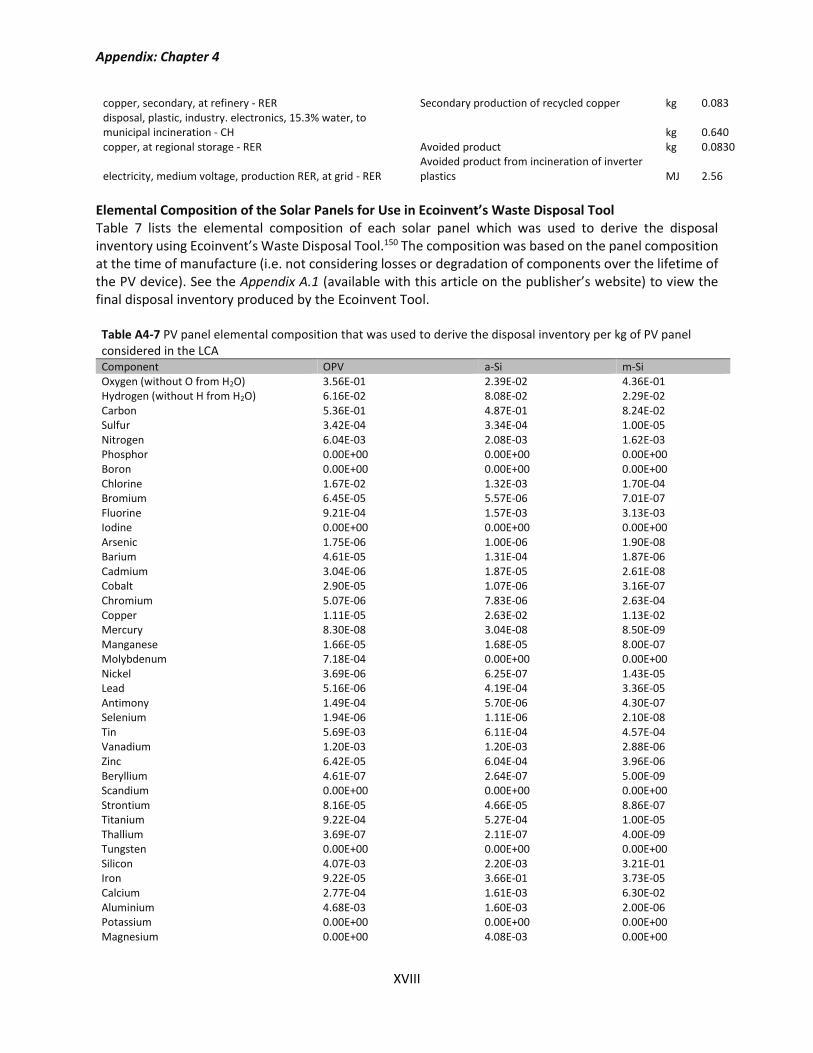
Appendix: Chapter 4
XVIII
copper, secondary, at refinery - RER Secondary production of recycled copper kg 0.083 disposal, plastic, industry. electronics, 15.3% water, to municipal incineration - CH kg 0.640 copper, at regional storage - RER Avoided product kg 0.0830
electricity, medium voltage, production RER, at grid - RER Avoided product from incineration of inverter plastics MJ 2.56
Elemental Composition of the Solar Panels for Use in Ecoinvent’s Waste Disposal Tool Table 7 lists the elemental composition of each solar panel which was used to derive the disposal inventory using Ecoinvent’s Waste Disposal Tool.150 The composition was based on the panel composition at the time of manufacture (i.e. not considering losses or degradation of components over the lifetime of the PV device). See the Appendix A.1 (available with this article on the publisher’s website) to view the final disposal inventory produced by the Ecoinvent Tool. Table A4-7 PV panel elemental composition that was used to derive the disposal inventory per kg of PV panel considered in the LCA Component OPV a-Si m-Si Oxygen (without O from H2O) 3.56E-01 2.39E-02 4.36E-01 Hydrogen (without H from H2O) 6.16E-02 8.08E-02 2.29E-02 Carbon 5.36E-01 4.87E-01 8.24E-02 Sulfur 3.42E-04 3.34E-04 1.00E-05 Nitrogen 6.04E-03 2.08E-03 1.62E-03 Phosphor 0.00E+00 0.00E+00 0.00E+00 Boron 0.00E+00 0.00E+00 0.00E+00 Chlorine 1.67E-02 1.32E-03 1.70E-04 Bromium 6.45E-05 5.57E-06 7.01E-07 Fluorine 9.21E-04 1.57E-03 3.13E-03 Iodine 0.00E+00 0.00E+00 0.00E+00 Arsenic 1.75E-06 1.00E-06 1.90E-08 Barium 4.61E-05 1.31E-04 1.87E-06 Cadmium 3.04E-06 1.87E-05 2.61E-08 Cobalt 2.90E-05 1.07E-06 3.16E-07 Chromium 5.07E-06 7.83E-06 2.63E-04 Copper 1.11E-05 2.63E-02 1.13E-02 Mercury 8.30E-08 3.04E-08 8.50E-09 Manganese 1.66E-05 1.68E-05 8.00E-07 Molybdenum 7.18E-04 0.00E+00 0.00E+00 Nickel 3.69E-06 6.25E-07 1.43E-05 Lead 5.16E-06 4.19E-04 3.36E-05 Antimony 1.49E-04 5.70E-06 4.30E-07 Selenium 1.94E-06 1.11E-06 2.10E-08 Tin 5.69E-03 6.11E-04 4.57E-04 Vanadium 1.20E-03 1.20E-03 2.88E-06 Zinc 6.42E-05 6.04E-04 3.96E-06 Beryllium 4.61E-07 2.64E-07 5.00E-09 Scandium 0.00E+00 0.00E+00 0.00E+00 Strontium 8.16E-05 4.66E-05 8.86E-07 Titanium 9.22E-04 5.27E-04 1.00E-05 Thallium 3.69E-07 2.11E-07 4.00E-09 Tungsten 0.00E+00 0.00E+00 0.00E+00 Silicon 4.07E-03 2.20E-03 3.21E-01 Iron 9.22E-05 3.66E-01 3.73E-05 Calcium 2.77E-04 1.61E-03 6.30E-02 Aluminium 4.68E-03 1.60E-03 2.00E-06 Potassium 0.00E+00 0.00E+00 0.00E+00 Magnesium 0.00E+00 4.08E-03 0.00E+00
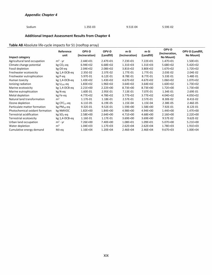
Appendix: Chapter 4
XIX
Sodium 1.35E-03 9.51E-04 5.59E-02
Additional Impact Assessment Results from Chapter 4
Table A8 Absolute life-cycle impacts for S1 (rooftop array)
Impact category
Reference unit
OPV-D (Incineration)
OPV-D (Landfill)
m-Si (Incineration)
m-Si (Landfill)
OPV-D (Incineration,
No Mount)
OPV-D (Landfill, No Mount)
Agricultural land occupation m2 · yr 2.44E+01 2.47E+01 7.23E+01 7.22E+01 1.47E+01 1.50E+01 Climate change potential kg CO2-eq 6.94E+02 6.68E+02 1.31E+03 1.31E+03 5.68E+02 5.42E+02 Fossil depletion kg Oil-eq 2.04E+02 2.08E+02 3.81E+02 3.80E+02 1.67E+02 1.72E+02 Freshwater ecotoxicity kg 1,4-DCB-eq 2.35E-02 2.37E-02 1.77E-01 1.77E-01 2.03E-02 2.04E-02 Freshwater eutrophication kg P-eq 5.97E-01 6.12E-01 8.78E-01 8.77E-01 5.33E-01 5.48E-01 Human toxicity kg 1,4-DCB-eq 1.43E+02 1.43E+02 4.67E+02 4.67E+02 1.06E+02 1.07E+02 Ionizing radiation kg U235-eq 1.83E+02 1.96E+02 3.64E+02 3.64E+02 1.60E+02 1.73E+02 Marine ecotoxicity kg 1,4-DCB-eq 2.21E+00 2.22E+00 8.73E+00 8.73E+00 1.72E+00 1.73E+00 Marine eutrophication kg N-eq 1.60E-01 2.95E-01 7.13E-01 7.07E-01 1.34E-01 2.69E-01 Metal depletion kg Fe-eq 4.77E+02 4.78E+02 3.77E+02 3.77E+02 4.04E+02 4.05E+02 Natural land transformation m2 1.17E-01 1.18E-01 2.57E-01 2.57E-01 8.30E-02 8.41E-02 Ozone depletion kg CFC11-eq 6.11E-05 6.19E-05 1.15E-04 1.15E-04 2.38E-05 2.46E-05 Particulate matter formation kg PM10-eq 9.32E-01 9.52E-01 1.59E+00 1.58E+00 7.92E-01 8.12E-01 Photochemical oxidant formation kg NMVOC 1.82E+00 1.84E+00 4.98E+00 4.94E+00 1.44E+00 1.47E+00 Terrestrial acidification kg SO2-eq 2.58E+00 2.64E+00 4.71E+00 4.68E+00 2.16E+00 2.22E+00 Terrestrial ecotoxicity kg 1,4-DCB-eq 1.16E-01 1.17E-01 3.69E+00 3.69E+00 9.57E-02 9.62E-02 Urban land occupation m2 · yr 7.26E+00 7.40E+00 1.08E+01 1.09E+01 5.07E+00 5.21E+00 Water depletion m3 1.04E+03 1.17E+03 2.62E+04 2.62E+04 1.78E+03 1.91E+03 Cumulative energy demand MJ-eq 1.16E+04 1.20E+04 2.46E+04 2.46E+04 9.67E+03 1.00E+04
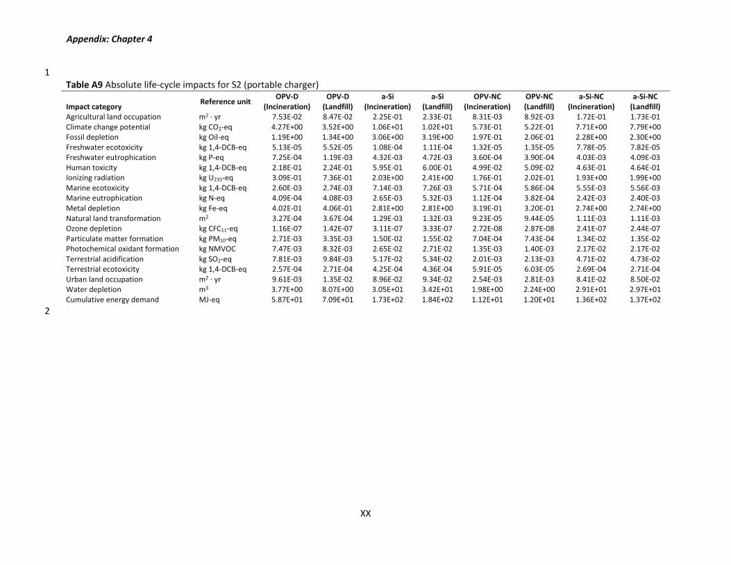
Appendix: Chapter 4
XX
1 Table A9 Absolute life-cycle impacts for S2 (portable charger)
Impact category Reference unit
OPV-D (Incineration)
OPV-D (Landfill)
a-Si (Incineration)
a-Si (Landfill)
OPV-NC (Incineration)
OPV-NC (Landfill)
a-Si-NC (Incineration)
a-Si-NC (Landfill)
Agricultural land occupation m2 · yr 7.53E-02 8.47E-02 2.25E-01 2.33E-01 8.31E-03 8.92E-03 1.72E-01 1.73E-01 Climate change potential kg CO2-eq 4.27E+00 3.52E+00 1.06E+01 1.02E+01 5.73E-01 5.22E-01 7.71E+00 7.79E+00 Fossil depletion kg Oil-eq 1.19E+00 1.34E+00 3.06E+00 3.19E+00 1.97E-01 2.06E-01 2.28E+00 2.30E+00 Freshwater ecotoxicity kg 1,4-DCB-eq 5.13E-05 5.52E-05 1.08E-04 1.11E-04 1.32E-05 1.35E-05 7.78E-05 7.82E-05 Freshwater eutrophication kg P-eq 7.25E-04 1.19E-03 4.32E-03 4.72E-03 3.60E-04 3.90E-04 4.03E-03 4.09E-03 Human toxicity kg 1,4-DCB-eq 2.18E-01 2.24E-01 5.95E-01 6.00E-01 4.99E-02 5.09E-02 4.63E-01 4.64E-01 Ionizing radiation kg U235-eq 3.09E-01 7.36E-01 2.03E+00 2.41E+00 1.76E-01 2.02E-01 1.93E+00 1.99E+00 Marine ecotoxicity kg 1,4-DCB-eq 2.60E-03 2.74E-03 7.14E-03 7.26E-03 5.71E-04 5.86E-04 5.55E-03 5.56E-03 Marine eutrophication kg N-eq 4.09E-04 4.08E-03 2.65E-03 5.32E-03 1.12E-04 3.82E-04 2.42E-03 2.40E-03 Metal depletion kg Fe-eq 4.02E-01 4.06E-01 2.81E+00 2.81E+00 3.19E-01 3.20E-01 2.74E+00 2.74E+00 Natural land transformation m2 3.27E-04 3.67E-04 1.29E-03 1.32E-03 9.23E-05 9.44E-05 1.11E-03 1.11E-03 Ozone depletion kg CFC11-eq 1.16E-07 1.42E-07 3.11E-07 3.33E-07 2.72E-08 2.87E-08 2.41E-07 2.44E-07 Particulate matter formation kg PM10-eq 2.71E-03 3.35E-03 1.50E-02 1.55E-02 7.04E-04 7.43E-04 1.34E-02 1.35E-02 Photochemical oxidant formation kg NMVOC 7.47E-03 8.32E-03 2.65E-02 2.71E-02 1.35E-03 1.40E-03 2.17E-02 2.17E-02 Terrestrial acidification kg SO2-eq 7.81E-03 9.84E-03 5.17E-02 5.34E-02 2.01E-03 2.13E-03 4.71E-02 4.73E-02 Terrestrial ecotoxicity kg 1,4-DCB-eq 2.57E-04 2.71E-04 4.25E-04 4.36E-04 5.91E-05 6.03E-05 2.69E-04 2.71E-04 Urban land occupation m2 · yr 9.61E-03 1.35E-02 8.96E-02 9.34E-02 2.54E-03 2.81E-03 8.41E-02 8.50E-02 Water depletion m3 3.77E+00 8.07E+00 3.05E+01 3.42E+01 1.98E+00 2.24E+00 2.91E+01 2.97E+01 Cumulative energy demand MJ-eq 5.87E+01 7.09E+01 1.73E+02 1.84E+02 1.12E+01 1.20E+01 1.36E+02 1.37E+02
2
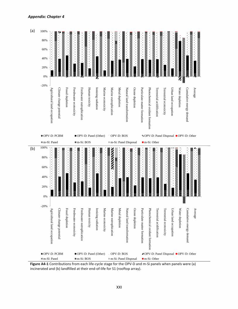
Appendix: Chapter 4
XXI
(a)
(b)
Figure A4-1 Contributions from each life-cycle stage for the OPV-D and m-Si panels when panels were (a) incinerated and (b) landfilled at their end-of-life for S1 (rooftop array).
-20%
0%
20%
40%
60%
80%
100%
Agricu
ltural lan
d o
ccupatio
n
Clim
ate chan
ge p
oten
tial
Fossil d
epletio
n
Fresh
water eco
tox
icity
Fresh
water eu
troph
ication
Hum
an to
xicity
Ionizin
g rad
iation
Marin
e ecoto
xicity
Marin
e eutro
phicatio
n
Metal d
epletio
n
Natu
ral land tran
sform
ation
Ozo
ne d
epletio
n
Particu
late matter fo
rmatio
n
Pho
toch
emical o
xid
ant fo
rmatio
n
Terrestrial acid
ification
Terrestrial eco
toxicity
Urb
an lan
d o
ccupatio
n
Water d
epletio
n
Cu
mulativ
e energ
y d
eman
d
Averag
e
OPV-D: PCBM OPV-D: Panel (Other) OPV-D: BOS OPV-D: Panel Disposal OPV-D: Other
m-Sl: Panel m-Si: BOS m-Si: Panel Disposal m-Si: Other
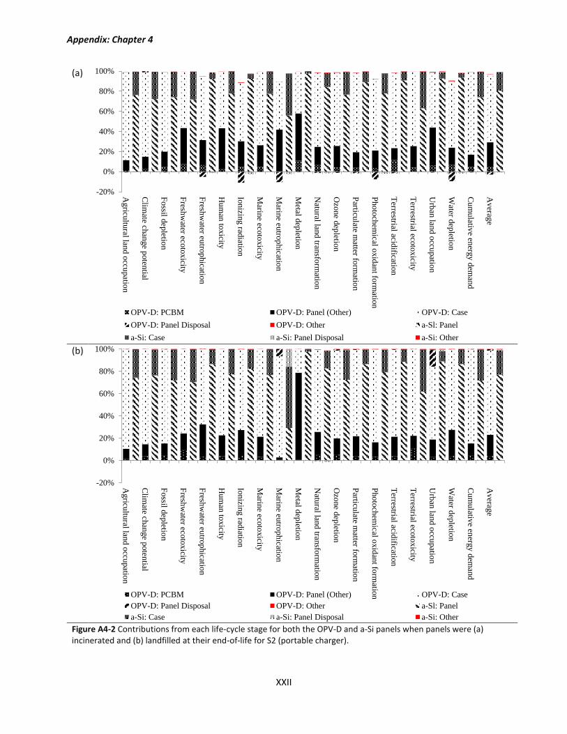
Appendix: Chapter 4
XXII
(a)
(b)
Figure A4-2 Contributions from each life-cycle stage for both the OPV-D and a-Si panels when panels were (a) incinerated and (b) landfilled at their end-of-life for S2 (portable charger).
-20%
0%
20%
40%
60%
80%
100%
Ag
ricultu
ral land o
ccupatio
n
Clim
ate chan
ge p
oten
tial
Fossil d
epletio
n
Fresh
water eco
tox
icity
Fresh
water eu
trop
hicatio
n
Hu
man
toxicity
Ion
izing
radiatio
n
Marin
e ecoto
xicity
Marin
e eutro
phicatio
n
Metal d
epletio
n
Natu
ral land
transfo
rmatio
n
Ozo
ne d
epletio
n
Particu
late matter fo
rmatio
n
Pho
toch
emical o
xid
ant fo
rmatio
n
Terrestrial acid
ification
Terrestrial eco
tox
icity
Urb
an lan
d o
ccupatio
n
Water d
epletio
n
Cu
mulativ
e energ
y d
eman
d
Av
erage
OPV-D: PCBM OPV-D: Panel (Other) OPV-D: Case
OPV-D: Panel Disposal OPV-D: Other a-Sl: Panel
a-Si: Case a-Si: Panel Disposal a-Si: Other
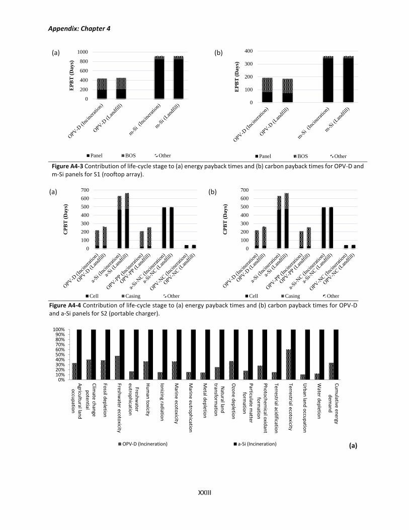
Appendix: Chapter 4
XXIII
(a)
(b)
Figure A4-3 Contribution of life-cycle stage to (a) energy payback times and (b) carbon payback times for OPV-D and m-Si panels for S1 (rooftop array).
(a)
(b)
Figure A4-4 Contribution of life-cycle stage to (a) energy payback times and (b) carbon payback times for OPV-D and a-Si panels for S2 (portable charger).
(a)
0
200
400
600
800
1000
EP
BT
(D
ay
s)
Panel BOS Other
0
100
200
300
400
EP
BT
(D
ay
s)
Panel BOS Other
0
100
200
300
400
500
600
700
CP
BT
(D
ay
s)
Cell Casing Other
0
100
200
300
400
500
600
700
CP
BT
(D
ay
s)
Cell Casing Other
0%10%20%30%40%50%60%70%80%90%
100%A
gricultu
ral land
occu
patio
n
Clim
ate chan
gep
oten
tial
Fossil d
epletio
n
Freshw
ater ecoto
xicity
Freshw
atereu
trop
hicatio
n
Hu
man
toxicity
Ion
izing rad
iation
Marin
e ecoto
xicity
Marin
e eutro
ph
ication
Metal d
eple
tion
Natu
ral land
transfo
rmatio
n
Ozo
ne d
eple
tion
Particu
late matter
form
ation
Ph
oto
che
mical o
xidan
tfo
rmatio
n
Terrestrial acidificatio
n
Terrestrial ecoto
xicity
Urb
an lan
d o
ccup
ation
Water d
epletio
n
Cu
mu
lative energy
dem
and
OPV-D (Incineration) a-Si (Incineration)
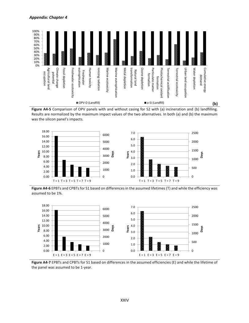
Appendix: Chapter 4
XXIV
(b) Figure A4-5 Comparison of OPV panels with and without casing for S2 with (a) incineration and (b) landfilling. Results are normalized by the maximum impact values of the two alternatives. In both (a) and (b) the maximum was the silicon panel’s impacts.
Figure A4-6 EPBTs and CPBTs for S1 based on differences in the assumed lifetimes (T) and while the efficiency was assumed to be 1%.
Figure A4-7 EPBTs and CPBTs for S1 based on differences in the assumed efficiencies (E) and while the lifetime of the panel was assumed to be 1-year.
0%10%20%30%40%50%60%70%80%90%
100%
Agricu
ltural lan
do
ccup
ation
Clim
ate chan
gep
oten
tial
Fossil d
epletio
n
Freshw
ater ecoto
xicity
Freshw
atereu
trop
hicatio
n
Hu
man
toxicity
Ion
izing rad
iation
Marin
e ecoto
xicity
Marin
e eutro
ph
ication
Metal d
eple
tion
Natu
ral land
transfo
rmatio
n
Ozo
ne d
eple
tion
Particu
late matter
form
ation
Ph
oto
che
mical o
xidan
tfo
rmatio
n
Terrestrial acidificatio
n
Terrestrial ecoto
xicity
Urb
an lan
d o
ccup
ation
Water d
epletio
n
Cu
mu
lative energy
dem
and
OPV-D (Landfill) a-Si (Landfill)
0
1000
2000
3000
4000
5000
6000
0.00
2.00
4.00
6.00
8.00
10.00
12.00
14.00
16.00
18.00
T = 1 T = 3 T = 5 T = 7 T = 9
Day
s
Ye
ars
0
500
1000
1500
2000
2500
0.0
1.0
2.0
3.0
4.0
5.0
6.0
7.0
T = 1 T = 3 T = 5 T = 7 T = 9
Day
s
Ye
ars
0
1000
2000
3000
4000
5000
6000
0.00
2.00
4.00
6.00
8.00
10.00
12.00
14.00
16.00
18.00
E = 1 E = 3 E = 5 E = 7 E = 9
Day
s
Ye
ars
0
500
1000
1500
2000
2500
0.0
1.0
2.0
3.0
4.0
5.0
6.0
7.0
E = 1 E = 3 E = 5 E = 7 E = 9
Day
s
Ye
ars
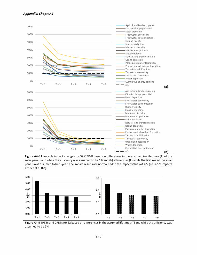
Appendix: Chapter 4
XXV
(a)
(b) Figure A4-8 Life-cycle impact changes for S2 OPV-D based on differences in the assumed (a) lifetimes (T) of the solar panels and while the efficiency was assumed to be 1% and (b) efficiencies (E) while the lifetime of the solar panels was assumed to be 1-year. The impact results are normalized to the impact values of a-Si (i.e. a-Si’s impacts are set at 100%).
Figure A4-9 EPBTs and CPBTs for S2 based on differences in the assumed lifetimes (T) and while the efficiency was assumed to be 1%.
0%
100%
200%
300%
400%
500%
600%
700%
T = 1 T = 3 T = 5 T = 7 T = 9
Agricultural land occupationClimate change potentialFossil depletionFreshwater ecotoxicityFreshwater eutrophicationHuman toxicityIonizing radiationMarine ecotoxicityMarine eutrophicationMetal depletionNatural land transformationOzone depletionParticulate matter formationPhotochemical oxidant formationTerrestrial acidificationTerrestrial ecotoxicityUrban land occupationWater depletionCumulative energy demanda-Si
0%
100%
200%
300%
400%
500%
600%
700%
E = 1 E = 3 E = 5 E = 7 E = 9
Agricultural land occupationClimate change potentialFossil depletionFreshwater ecotoxicityFreshwater eutrophicationHuman toxicityIonizing radiationMarine ecotoxicityMarine eutrophicationMetal depletionNatural land transformationOzone depletionParticulate matter formationPhotochemical oxidant formationTerrestrial acidificationTerrestrial ecotoxicityUrban land occupationWater depletionCumulative energy demanda-Si
0.00
1.00
2.00
3.00
4.00
5.00
6.00
T = 1 T = 3 T = 5 T = 7 T = 9
Ye
ars
0.0
1.0
2.0
3.0
T = 1 T = 3 T = 5 T = 7 T = 9
Ye
ars
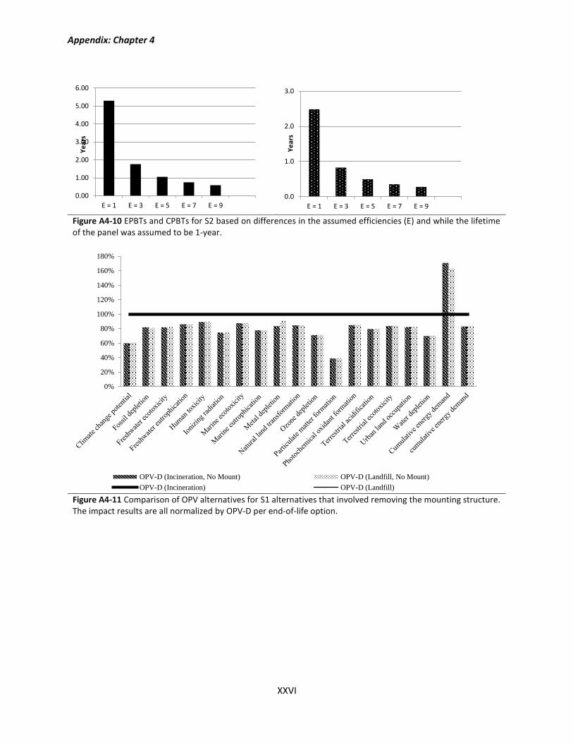
Appendix: Chapter 4
XXVI
Figure A4-10 EPBTs and CPBTs for S2 based on differences in the assumed efficiencies (E) and while the lifetime of the panel was assumed to be 1-year.
Figure A4-11 Comparison of OPV alternatives for S1 alternatives that involved removing the mounting structure. The impact results are all normalized by OPV-D per end-of-life option.
0.00
1.00
2.00
3.00
4.00
5.00
6.00
E = 1 E = 3 E = 5 E = 7 E = 9
Ye
ars
0.0
1.0
2.0
3.0
E = 1 E = 3 E = 5 E = 7 E = 9
Ye
ars
0%
20%
40%
60%
80%
100%
120%
140%
160%
180%
OPV-D (Incineration, No Mount) OPV-D (Landfill, No Mount)
OPV-D (Incineration) OPV-D (Landfill)
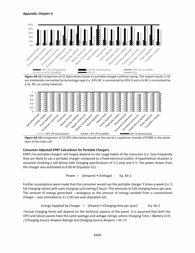
Appendix: Chapter 4
XXVII
Figure A4-12 Comparison of S2 alternatives based on portable chargers without casing. The impact results in S2 are individually normalized by technology-type (i.e. OPV-NC is normalized by OPV-D and a-Si-NC is normalized by a-SI). NS: no casing materials.
Figure A4-13 Comparison of S2 OPV alternatives based on the use of a copolymer instead of PCBM in the active layer of the solar cell.
Consumer-Adjusted EPBT Calculation for Portable Chargers EPBTs for portable chargers will largely depend on the usage habits of the consumer (i.e. how frequently they are likely to use a portable charger compared to a fixed electrical outlet). A hypothetical situation is assumed involving a cell phone with charging specifications of 1.2 amp and 5 V. The power drawn from the charger was estimated as 6.00 W (Equation S1):
Power = (Ampere) • (Voltage) Eq. A4-1 Further assumptions were made that the consumer would use the portable charger 5 times a week (i.e. 5 full charging cycles) with each charging cycle lasting 2 hours. This amounts to 520 charging hours per year. The amount of energy generated – analogous to the amount of energy avoided from a conventional charger – was estimated as 11.2 MJ per year (Equation S2):
Energy Supplied by Charger = (Power) • (Charging time per year)† Eq. A4-2
†Actual charging times will depend on the technical aspects of the panel. It is assumed that both the OPV and silicon panels have the same wattage and voltage ratings, where Charging Time = (Battery A-h) / (Charging Source Ampere Rating) and Charging Source Ampere = W / V.
0%
20%
40%
60%
80%
100%
OPV-NC (Incineration) a-Si-NC (Incineration) OPV-NC (Landfill)a-Si-NC (Landfill) OPV-D a-Si
0
0.2
0.4
0.6
0.8
1
OPV-PP (Incineration) OPV-PP (Landfill) OPV-D (Incineration)
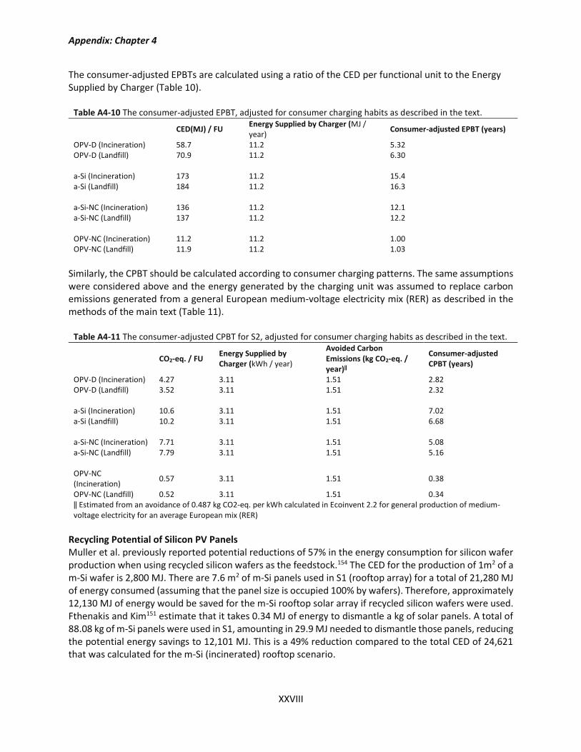
Appendix: Chapter 4
XXVIII
The consumer-adjusted EPBTs are calculated using a ratio of the CED per functional unit to the Energy Supplied by Charger (Table 10).
Table A4-10 The consumer-adjusted EPBT, adjusted for consumer charging habits as described in the text.
CED(MJ) / FU Energy Supplied by Charger (MJ / year)
Consumer-adjusted EPBT (years)
OPV-D (Incineration) 58.7 11.2 5.32 OPV-D (Landfill) 70.9 11.2 6.30
a-Si (Incineration) 173 11.2 15.4 a-Si (Landfill) 184 11.2 16.3
a-Si-NC (Incineration) 136 11.2 12.1 a-Si-NC (Landfill) 137 11.2 12.2
OPV-NC (Incineration) 11.2 11.2 1.00 OPV-NC (Landfill) 11.9 11.2 1.03
Similarly, the CPBT should be calculated according to consumer charging patterns. The same assumptions were considered above and the energy generated by the charging unit was assumed to replace carbon emissions generated from a general European medium-voltage electricity mix (RER) as described in the methods of the main text (Table 11).
Table A4-11 The consumer-adjusted CPBT for S2, adjusted for consumer charging habits as described in the text.
CO2-eq. / FU Energy Supplied by Charger (kWh / year)
Avoided Carbon Emissions (kg CO2-eq. / year)‖
Consumer-adjusted CPBT (years)
OPV-D (Incineration) 4.27 3.11 1.51 2.82 OPV-D (Landfill) 3.52 3.11 1.51 2.32 a-Si (Incineration) 10.6 3.11 1.51 7.02 a-Si (Landfill) 10.2 3.11 1.51 6.68 a-Si-NC (Incineration) 7.71 3.11 1.51 5.08 a-Si-NC (Landfill) 7.79 3.11 1.51 5.16 OPV-NC (Incineration)
0.57 3.11 1.51 0.38
OPV-NC (Landfill) 0.52 3.11 1.51 0.34 ‖ Estimated from an avoidance of 0.487 kg CO2-eq. per kWh calculated in Ecoinvent 2.2 for general production of medium-voltage electricity for an average European mix (RER)
Recycling Potential of Silicon PV Panels Muller et al. previously reported potential reductions of 57% in the energy consumption for silicon wafer production when using recycled silicon wafers as the feedstock.154 The CED for the production of 1m2 of a m-Si wafer is 2,800 MJ. There are 7.6 m2 of m-Si panels used in S1 (rooftop array) for a total of 21,280 MJ of energy consumed (assuming that the panel size is occupied 100% by wafers). Therefore, approximately 12,130 MJ of energy would be saved for the m-Si rooftop solar array if recycled silicon wafers were used. Fthenakis and Kim151 estimate that it takes 0.34 MJ of energy to dismantle a kg of solar panels. A total of 88.08 kg of m-Si panels were used in S1, amounting in 29.9 MJ needed to dismantle those panels, reducing the potential energy savings to 12,101 MJ. This is a 49% reduction compared to the total CED of 24,621 that was calculated for the m-Si (incinerated) rooftop scenario.

Appendix: Chapter 4
XXIX
Recycling Potential of OPV Panels Espinosa et al. estimate that OPV panels could be delaminated using 14.76 MJ of electricity (mechanical delamination) per kg of panel processed.62 This would amount to nearly 325 MJ consumed for the recovery of the PET. The assumption can be made that this is directly consumed in a secondary PET production process and that this process consumes only half of the energy (1066 MJ) of primary production for the 13 kg of PET consumed in the functional unit, just for illustration, then a total 858 MJ (208 MJ savings) of energy would be consumed in order to recycle the PET.

Appendix: Chapter 6
XXX
Appendix: Chapter 6 Table A6-1 Toxicological data used to calculate the non-carcinogenic dose-response data
Dose mg/m3
Diameter (nm)
Species BAL Cell Sample Size
Macrophages (%)
Macrophages (Count)
Neutrophil (%)
Neutrophil (Count)
0 21 M 200 0.99 198 0 0
0 21 M 200 1 200 0 0
0 21 M 200 0.99 198 0 0
0 21 M 200 1 200 0 0
0 21 M 200 1 200 0 0
0.5 21 M 200 0.995 199 0 0
0.5 21 M 200 1 200 0 0
0.5 21 M 200 0.995 199 0 0
0.5 21 M 200 0.99 198 0 0
0.5 21 M 200 1 200 0 0
2 21 M 200 0.995 199 0.005 1
2 21 M 200 1 200 0 0
2 21 M 200 1 200 0 0
2 21 M 200 0.995 199 0.005 1
2 21 M 200 1 200 0 0
10 21 M 200 0.8 160 0.195 39
10 21 M 200 0.865 173 0.125 25
10 21 M 200 0.915 183 0.07 14
10 21 M 200 0.775 155 0.21 42
10 21 M 200 0.875 175 0.125 25
0 21 R 200 1 200 0 0
0 21 R 200 0.995 199 0.005 1
0 21 R 200 1 200 0 0
0 21 R 200 0.99 198 0.01 2
0 21 R 200 0.99 198 0.005 1
0.5 21 R 200 0.995 199 0.005 1
0.5 21 R 200 0.985 197 0.01 2
0.5 21 R 200 0.99 198 0.005 1
0.5 21 R 200 0.99 198 0.005 1
0.5 21 R 200 1 200 0 0
2 21 R 200 0.91 182 0.085 17
2 21 R 200 0.97 194 0.03 6
2 21 R 200 0.96 192 0.035 7
2 21 R 200 0.87 174 0.13 26
2 21 R 200 0.95 190 0.045 9
10 21 R 200 0.235 47 0.73 146
10 21 R 200 0.4 80 0.585 117
10 21 R 200 0.365 73 0.625 125
10 21 R 200 0.315 63 0.66 132
10 21 R 200 0.35 70 0.64 128
0 21 H 200 0.965 193 0.02 4
0 21 H 200 0.955 191 0.025 5
0 21 H 200 0.995 199 0.005 1
0 21 H 200 0.965 193 0.03 6
0 21 H 200 0.93 186 0.035 7
0.5 21 H 200 0.945 189 0.015 3
0.5 21 H 200 0.975 195 0.015 3
0.5 21 H 200 0.955 191 0.005 1
0.5 21 H 200 0.99 198 0.005 1
0.5 21 H 200 0.905 181 0.025 5
2 21 H 200 0.985 197 0.005 1
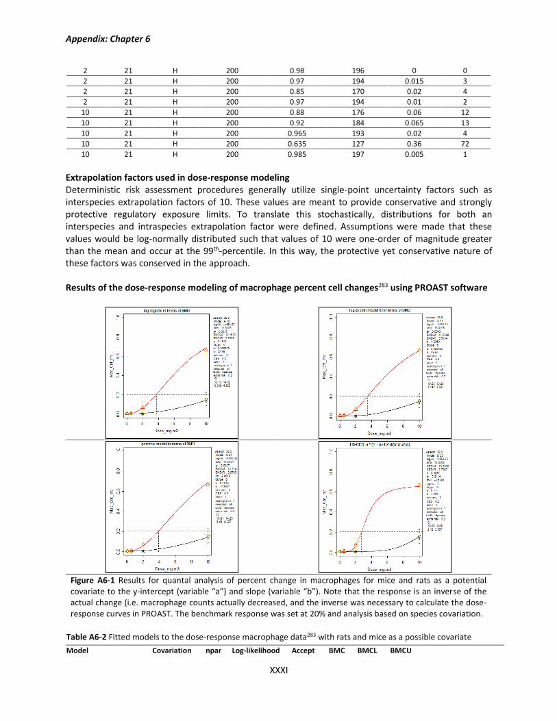
Appendix: Chapter 6
XXXI
2 21 H 200 0.98 196 0 0
2 21 H 200 0.97 194 0.015 3
2 21 H 200 0.85 170 0.02 4
2 21 H 200 0.97 194 0.01 2
10 21 H 200 0.88 176 0.06 12
10 21 H 200 0.92 184 0.065 13
10 21 H 200 0.965 193 0.02 4
10 21 H 200 0.635 127 0.36 72
10 21 H 200 0.985 197 0.005 1
Extrapolation factors used in dose-response modeling Deterministic risk assessment procedures generally utilize single-point uncertainty factors such as interspecies extrapolation factors of 10. These values are meant to provide conservative and strongly protective regulatory exposure limits. To translate this stochastically, distributions for both an interspecies and intraspecies extrapolation factor were defined. Assumptions were made that these values would be log-normally distributed such that values of 10 were one-order of magnitude greater than the mean and occur at the 99th-percentile. In this way, the protective yet conservative nature of these factors was conserved in the approach. Results of the dose-response modeling of macrophage percent cell changes283 using PROAST software
Figure A6-1 Results for quantal analysis of percent change in macrophages for mice and rats as a potential covariate to the y-intercept (variable “a”) and slope (variable “b”). Note that the response is an inverse of the actual change (i.e. macrophage counts actually decreased, and the inverse was necessary to calculate the dose-response curves in PROAST. The benchmark response was set at 20% and analysis based on species covariation.
Table A6-2 Fitted models to the dose-response macrophage data283 with rats and mice as a possible covariate
Model Covariation npar Log-likelihood Accept BMC BMCL BMCU
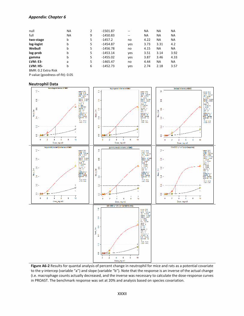
Appendix: Chapter 6
XXXII
null NA 2 -1501.87 -- NA NA NA full NA 9 -1450.83 -- NA NA NA two-stage b 5 -1457.2 no 4.22 NA NA log-logist b 5 -1454.87 yes 3.73 3.31 4.2 Weibull b 5 -1456.78 no 4.15 NA NA log-prob b 5 -1453.14 yes 3.51 3.14 3.92 gamma b 5 -1455.02 yes 3.87 3.46 4.33 LVM: E3- a 5 -1465.47 no 4.44 NA NA LVM: H5- b 6 -1452.73 yes 2.74 2.18 3.57 BMR: 0.2 Extra Risk P-value (goodness-of-fit): 0.05
Neutrophil Data
Figure A6-2 Results for quantal analysis of percent change in neutrophil for mice and rats as a potential covariate to the y-intercep (variable “a”) and slope (variable “b”). Note that the response is an inverse of the actual change (i.e. macrophage counts actually decreased, and the inverse was necessary to calculate the dose-response curves in PROAST. The benchmark response was set at 20% and analysis based on species covariation.
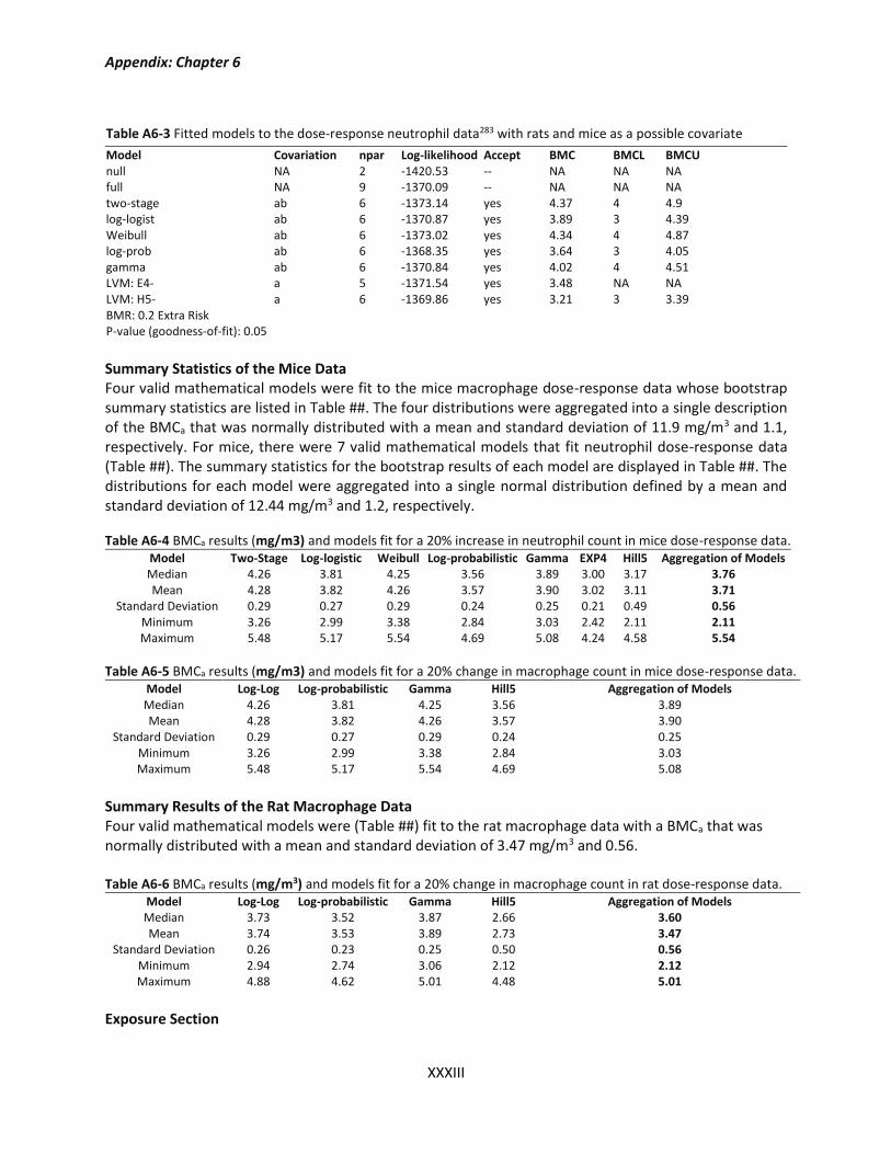
Appendix: Chapter 6
XXXIII
Table A6-3 Fitted models to the dose-response neutrophil data283 with rats and mice as a possible covariate
Model Covariation npar Log-likelihood Accept BMC BMCL BMCU null NA 2 -1420.53 -- NA NA NA full NA 9 -1370.09 -- NA NA NA two-stage ab 6 -1373.14 yes 4.37 4 4.9 log-logist ab 6 -1370.87 yes 3.89 3 4.39 Weibull ab 6 -1373.02 yes 4.34 4 4.87 log-prob ab 6 -1368.35 yes 3.64 3 4.05 gamma ab 6 -1370.84 yes 4.02 4 4.51 LVM: E4- a 5 -1371.54 yes 3.48 NA NA LVM: H5- a 6 -1369.86 yes 3.21 3 3.39 BMR: 0.2 Extra Risk P-value (goodness-of-fit): 0.05
Summary Statistics of the Mice Data Four valid mathematical models were fit to the mice macrophage dose-response data whose bootstrap summary statistics are listed in Table ##. The four distributions were aggregated into a single description of the BMCa that was normally distributed with a mean and standard deviation of 11.9 mg/m3 and 1.1, respectively. For mice, there were 7 valid mathematical models that fit neutrophil dose-response data (Table ##). The summary statistics for the bootstrap results of each model are displayed in Table ##. The distributions for each model were aggregated into a single normal distribution defined by a mean and standard deviation of 12.44 mg/m3 and 1.2, respectively.
Summary Results of the Rat Macrophage Data Four valid mathematical models were (Table ##) fit to the rat macrophage data with a BMCa that was normally distributed with a mean and standard deviation of 3.47 mg/m3 and 0.56.
Exposure Section
Table A6-4 BMCa results (mg/m3) and models fit for a 20% increase in neutrophil count in mice dose-response data. Model Two-Stage Log-logistic Weibull Log-probabilistic Gamma EXP4 Hill5 Aggregation of Models Median 4.26 3.81 4.25 3.56 3.89 3.00 3.17 3.76 Mean 4.28 3.82 4.26 3.57 3.90 3.02 3.11 3.71
Standard Deviation 0.29 0.27 0.29 0.24 0.25 0.21 0.49 0.56 Minimum 3.26 2.99 3.38 2.84 3.03 2.42 2.11 2.11 Maximum 5.48 5.17 5.54 4.69 5.08 4.24 4.58 5.54
Table A6-5 BMCa results (mg/m3) and models fit for a 20% change in macrophage count in mice dose-response data. Model Log-Log Log-probabilistic Gamma Hill5 Aggregation of Models Median 4.26 3.81 4.25 3.56 3.89 Mean 4.28 3.82 4.26 3.57 3.90
Standard Deviation 0.29 0.27 0.29 0.24 0.25 Minimum 3.26 2.99 3.38 2.84 3.03 Maximum 5.48 5.17 5.54 4.69 5.08
Table A6-6 BMCa results (mg/m3) and models fit for a 20% change in macrophage count in rat dose-response data. Model Log-Log Log-probabilistic Gamma Hill5 Aggregation of Models Median 3.73 3.52 3.87 2.66 3.60 Mean 3.74 3.53 3.89 2.73 3.47
Standard Deviation 0.26 0.23 0.25 0.50 0.56 Minimum 2.94 2.74 3.06 2.12 2.12 Maximum 4.88 4.62 5.01 4.48 5.01
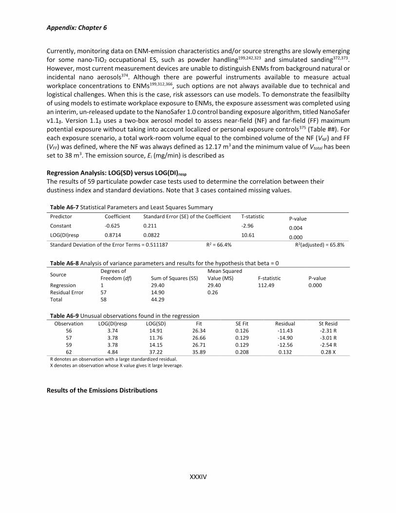
Appendix: Chapter 6
XXXIV
Currently, monitoring data on ENM-emission characteristics and/or source strengths are slowly emerging for some nano-TiO2 occupational ES, such as powder handling199,242,323 and simulated sanding372,373. However, most current measurement devices are unable to distinguish ENMs from background natural or incidental nano aerosols374. Although there are powerful instruments available to measure actual workplace concentrations to ENMs199,312,366, such options are not always available due to technical and logistical challenges. When this is the case, risk assessors can use models. To demonstrate the feasilbilty of using models to estimate workplace exposure to ENMs, the exposure assessment was completed using an interim, un-released update to the NanoSafer 1.0 control banding exposure algorithm, titled NanoSafer v1.1β. Version 1.1β uses a two-box aerosol model to assess near-field (NF) and far-field (FF) maximum potential exposure without taking into account localized or personal exposure controls375 (Table ##). For each exposure scenario, a total work-room volume equal to the combined volume of the NF (VNF) and FF (VFF) was defined, where the NF was always defined as 12.17 m3 and the minimum value of Vtotal has been set to 38 m3. The emission source, Ei (mg/min) is described as Regression Analysis: LOG(SD) versus LOG(DI)resp The results of 59 particulate powder case tests used to determine the correlation between their dustiness index and standard deviations. Note that 3 cases contained missing values.
Table A6-7 Statistical Parameters and Least Squares Summary
Predictor Coefficient Standard Error (SE) of the Coefficient T-statistic P-value Constant -0.625 0.211 -2.96 0.004 LOG(DI)resp 0.8714 0.0822 10.61 0.000
Standard Deviation of the Error Terms = 0.511187 R2 = 66.4% R2(adjusted) = 65.8%
Table A6-8 Analysis of variance parameters and results for the hypothesis that beta = 0
Source Degrees of Freedom (df) Sum of Squares (SS)
Mean Squared Value (MS) F-statistic P-value
Regression 1 29.40 29.40 112.49 0.000 Residual Error 57 14.90 0.26 Total 58 44.29
Table A6-9 Unusual observations found in the regression
Observation LOG(DI)resp LOG(SD) Fit SE Fit Residual St Resid 56 3.74 14.91 26.34 0.126 -11.43 -2.31 R 57 3.78 11.76 26.66 0.129 -14.90 -3.01 R 59 3.78 14.15 26.71 0.129 -12.56 -2.54 R 62 4.84 37.22 35.89 0.208 0.132 0.28 X
R denotes an observation with a large standardized residual. X denotes an observation whose X value gives it large leverage.
Results of the Emissions Distributions
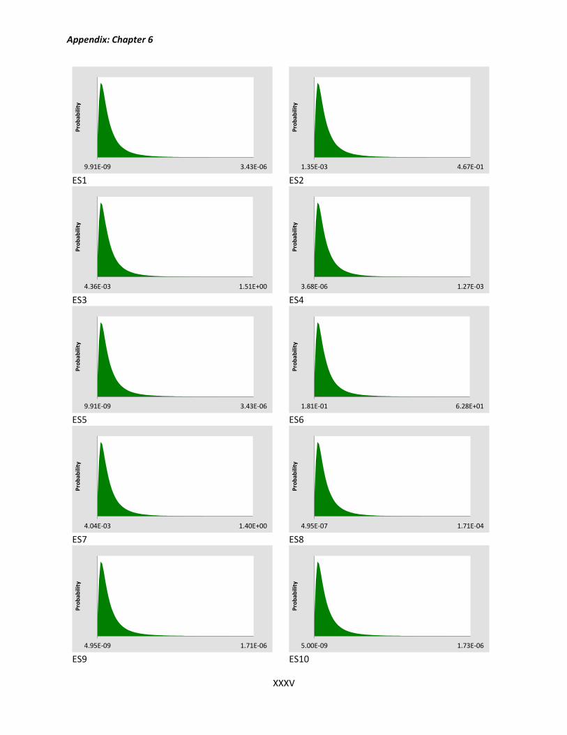
Appendix: Chapter 6
XXXV
ES1 ES2
ES3 ES4
ES5 ES6
ES7 ES8
ES9 ES10
9.91E-09 3.43E-06
Pro
bab
ility
1.35E-03 4.67E-01
Pro
bab
ility
4.36E-03 1.51E+00
Pro
bab
ility
3.68E-06 1.27E-03P
rob
abili
ty
9.91E-09 3.43E-06
Pro
bab
ility
1.81E-01 6.28E+01
Pro
bab
ility
4.04E-03 1.40E+00
Pro
bab
ility
4.95E-07 1.71E-04
Pro
bab
ility
4.95E-09 1.71E-06
Pro
bab
ility
5.00E-09 1.73E-06
Pro
bab
ility
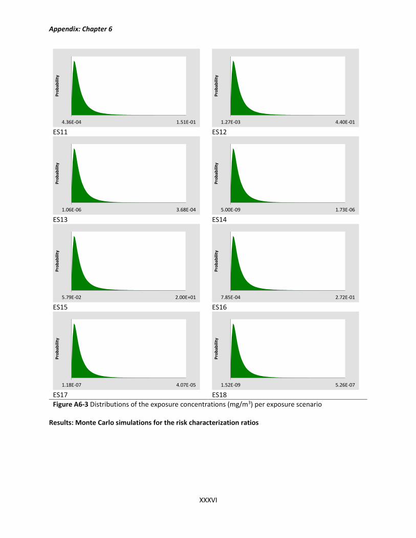
Appendix: Chapter 6
XXXVI
ES11 ES12
ES13 ES14
ES15 ES16
ES17 ES18
Figure A6-3 Distributions of the exposure concentrations (mg/m3) per exposure scenario Results: Monte Carlo simulations for the risk characterization ratios
4.36E-04 1.51E-01
Pro
bab
ility
1.27E-03 4.40E-01
Pro
bab
ility
1.06E-06 3.68E-04
Pro
bab
ility
5.00E-09 1.73E-06P
rob
abili
ty
5.79E-02 2.00E+01
Pro
bab
ility
7.85E-04 2.72E-01
Pro
bab
ility
1.18E-07 4.07E-05
Pro
bab
ility
1.52E-09 5.26E-07
Pro
bab
ility
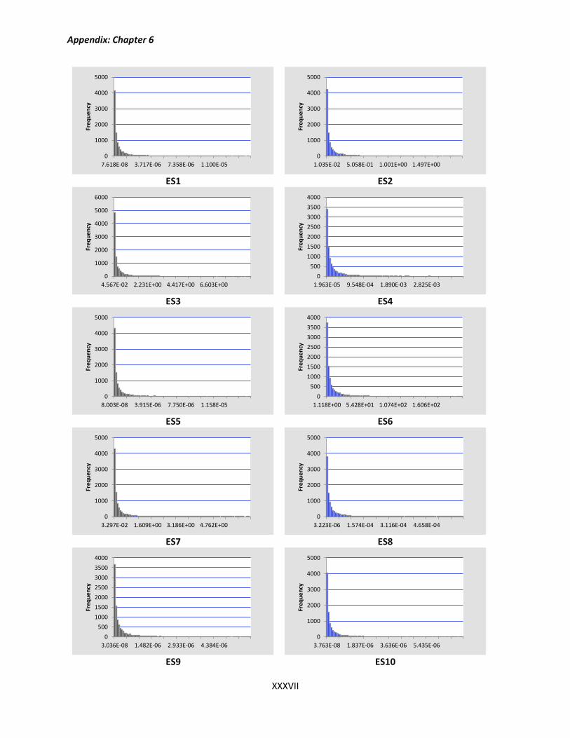
Appendix: Chapter 6
XXXVII
ES1 ES2
ES3 ES4
ES5 ES6
ES7 ES8
ES9 ES10
0
1000
2000
3000
4000
5000
7.618E-08 3.717E-06 7.358E-06 1.100E-05
Freq
uen
cy
0
1000
2000
3000
4000
5000
1.035E-02 5.058E-01 1.001E+00 1.497E+00
Freq
uen
cy
0
1000
2000
3000
4000
5000
6000
4.567E-02 2.231E+00 4.417E+00 6.603E+00
Freq
uen
cy
0
500
1000
1500
2000
2500
3000
3500
4000
1.963E-05 9.548E-04 1.890E-03 2.825E-03
Freq
uen
cy
0
1000
2000
3000
4000
5000
8.003E-08 3.915E-06 7.750E-06 1.158E-05
Freq
uen
cy
0
500
1000
1500
2000
2500
3000
3500
4000
1.118E+00 5.428E+01 1.074E+02 1.606E+02
Freq
uen
cy
0
1000
2000
3000
4000
5000
3.297E-02 1.609E+00 3.186E+00 4.762E+00
Freq
uen
cy
0
1000
2000
3000
4000
5000
3.223E-06 1.574E-04 3.116E-04 4.658E-04
Freq
uen
cy
0
500
1000
1500
2000
2500
3000
3500
4000
3.036E-08 1.482E-06 2.933E-06 4.384E-06
Freq
uen
cy
0
1000
2000
3000
4000
5000
3.763E-08 1.837E-06 3.636E-06 5.435E-06
Freq
uen
cy
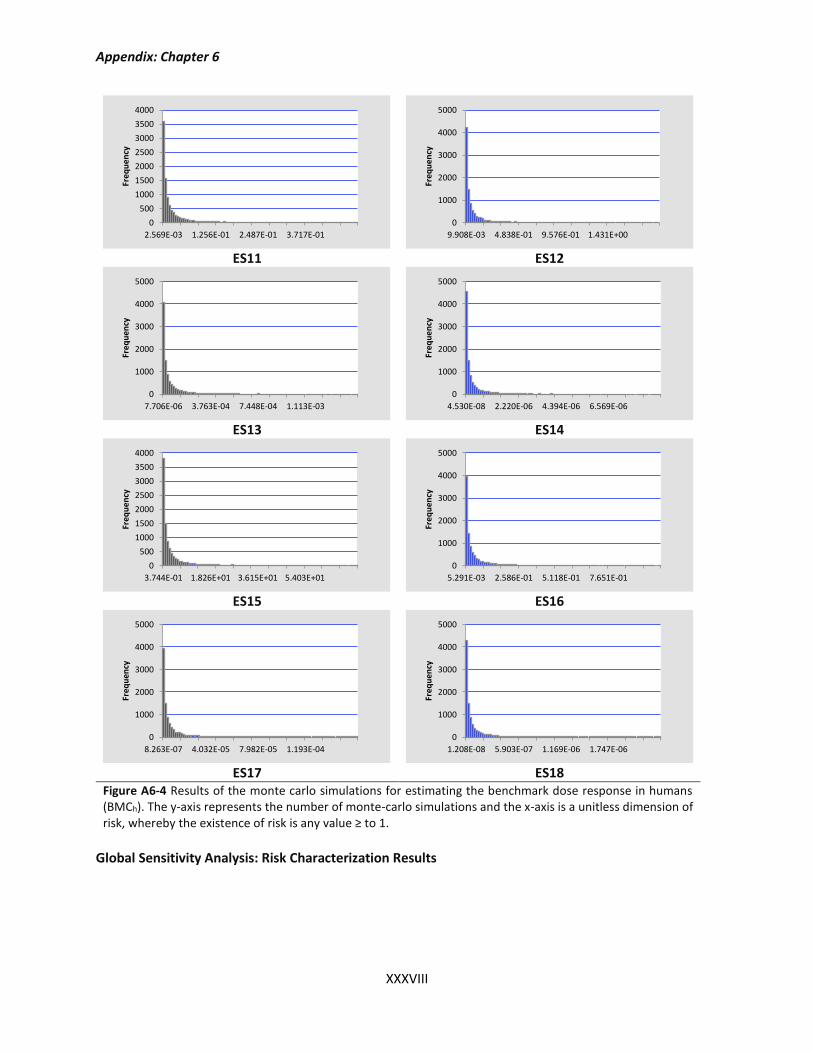
Appendix: Chapter 6
XXXVIII
ES11 ES12
ES13 ES14
ES15 ES16
ES17 ES18
Figure A6-4 Results of the monte carlo simulations for estimating the benchmark dose response in humans (BMCh). The y-axis represents the number of monte-carlo simulations and the x-axis is a unitless dimension of risk, whereby the existence of risk is any value ≥ to 1.
Global Sensitivity Analysis: Risk Characterization Results
0
500
1000
1500
2000
2500
3000
3500
4000
2.569E-03 1.256E-01 2.487E-01 3.717E-01
Freq
uen
cy
0
1000
2000
3000
4000
5000
9.908E-03 4.838E-01 9.576E-01 1.431E+00
Freq
uen
cy
0
1000
2000
3000
4000
5000
7.706E-06 3.763E-04 7.448E-04 1.113E-03
Freq
uen
cy
0
1000
2000
3000
4000
5000
4.530E-08 2.220E-06 4.394E-06 6.569E-06
Freq
uen
cy
0
500
1000
1500
2000
2500
3000
3500
4000
3.744E-01 1.826E+01 3.615E+01 5.403E+01
Freq
uen
cy
0
1000
2000
3000
4000
5000
5.291E-03 2.586E-01 5.118E-01 7.651E-01
Freq
uen
cy
0
1000
2000
3000
4000
5000
8.263E-07 4.032E-05 7.982E-05 1.193E-04
Freq
uen
cy
0
1000
2000
3000
4000
5000
1.208E-08 5.903E-07 1.169E-06 1.747E-06
Freq
uen
cy
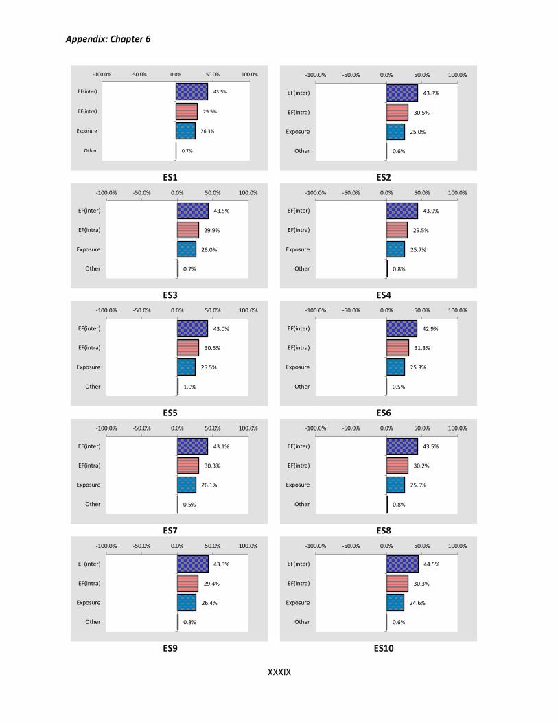
Appendix: Chapter 6
XXXIX
ES1 ES2
ES3 ES4
ES5 ES6
ES7 ES8
ES9 ES10
43.5%
29.5%
26.3%
0.7%
-100.0% -50.0% 0.0% 50.0% 100.0%
EF(inter)
EF(intra)
Exposure
Other
43.8%
30.5%
25.0%
0.6%
-100.0% -50.0% 0.0% 50.0% 100.0%
EF(inter)
EF(intra)
Exposure
Other
43.5%
29.9%
26.0%
0.7%
-100.0% -50.0% 0.0% 50.0% 100.0%
EF(inter)
EF(intra)
Exposure
Other
43.9%
29.5%
25.7%
0.8%
-100.0% -50.0% 0.0% 50.0% 100.0%
EF(inter)
EF(intra)
Exposure
Other
43.0%
30.5%
25.5%
1.0%
-100.0% -50.0% 0.0% 50.0% 100.0%
EF(inter)
EF(intra)
Exposure
Other
42.9%
31.3%
25.3%
0.5%
-100.0% -50.0% 0.0% 50.0% 100.0%
EF(inter)
EF(intra)
Exposure
Other
43.1%
30.3%
26.1%
0.5%
-100.0% -50.0% 0.0% 50.0% 100.0%
EF(inter)
EF(intra)
Exposure
Other
43.5%
30.2%
25.5%
0.8%
-100.0% -50.0% 0.0% 50.0% 100.0%
EF(inter)
EF(intra)
Exposure
Other
43.3%
29.4%
26.4%
0.8%
-100.0% -50.0% 0.0% 50.0% 100.0%
EF(inter)
EF(intra)
Exposure
Other
44.5%
30.3%
24.6%
0.6%
-100.0% -50.0% 0.0% 50.0% 100.0%
EF(inter)
EF(intra)
Exposure
Other
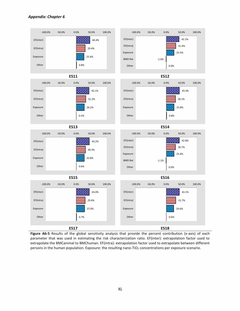
Appendix: Chapter 6
XL
ES11 ES12
ES13 ES14
ES15 ES16
ES17 ES18
Figure A6-5 Results of the global sensitivity analysis that provide the percent contribution (x-axis) of each parameter that was used in estimating the risk characterization ratio. EF(inter): extrapolation factor used to extrapolate the BMCanimal to BMChuman. EF(intra): extrapolation factor used to extrapolate between different persons in the human population. Exposure: the resulting nano-TiO2 concentrations per exposure scenario.
44.4%
29.4%
25.4%
0.8%
-100.0% -50.0% 0.0% 50.0% 100.0%
EF(inter)
EF(intra)
Exposure
Other
42.1%
31.4%
25.5%
-1.0%
0.0%
-100.0% -50.0% 0.0% 50.0% 100.0%
EF(inter)
EF(intra)
Exposure
BMD Rat
Other
42.1%
31.2%
26.2%
0.5%
-100.0% -50.0% 0.0% 50.0% 100.0%
EF(inter)
EF(intra)
Exposure
Other
43.3%
30.1%
25.8%
0.8%
-100.0% -50.0% 0.0% 50.0% 100.0%
EF(inter)
EF(intra)
Exposure
Other
43.2%
30.3%
25.8%
0.6%
-100.0% -50.0% 0.0% 50.0% 100.0%
EF(inter)
EF(intra)
Exposure
Other
42.8%
30.7%
25.4%
-1.1%
0.0%
-100.0% -50.0% 0.0% 50.0% 100.0%
EF(inter)
EF(intra)
Exposure
BMD Rat
Other
43.0%
29.4%
27.0%
0.7%
-100.0% -50.0% 0.0% 50.0% 100.0%
EF(inter)
EF(intra)
Exposure
Other
43.1%
31.7%
24.6%
0.6%
-100.0% -50.0% 0.0% 50.0% 100.0%
EF(inter)
EF(intra)
Exposure
Other
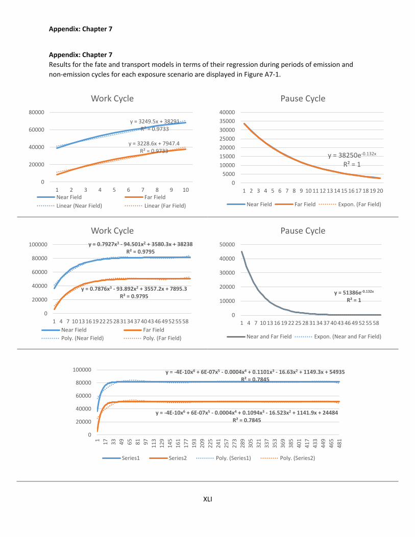
Appendix: Chapter 7
XLI
Appendix: Chapter 7
Results for the fate and transport models in terms of their regression during periods of emission and
non-emission cycles for each exposure scenario are displayed in Figure A7-1.
y = 3249.5x + 38291R² = 0.9733
y = 3228.6x + 7947.4R² = 0.9733
0
20000
40000
60000
80000
1 2 3 4 5 6 7 8 9 10
Work Cycle
Near Field Far Field
Linear (Near Field) Linear (Far Field)
y = 38250e-0.132x
R² = 1
0
5000
10000
15000
20000
25000
30000
35000
40000
1 2 3 4 5 6 7 8 9 10 11 12 13 14 15 16 17 18 19 20
Pause Cycle
Near Field Far Field Expon. (Far Field)
y = 0.7927x3 - 94.501x2 + 3580.3x + 38238R² = 0.9795
y = 0.7876x3 - 93.892x2 + 3557.2x + 7895.3R² = 0.9795
0
20000
40000
60000
80000
100000
1 4 7 10 13 16 19 22 25 28 31 34 37 40 43 46 49 52 55 58
Work Cycle
Near Field Far Field
Poly. (Near Field) Poly. (Far Field)
y = 51386e-0.132x
R² = 1
0
10000
20000
30000
40000
50000
1 4 7 10 13 16 19 22 25 28 31 34 37 40 43 46 49 52 55 58
Pause Cycle
Near and Far Field Expon. (Near and Far Field)
y = -4E-10x6 + 6E-07x5 - 0.0004x4 + 0.1101x3 - 16.63x2 + 1149.3x + 54935R² = 0.7845
y = -4E-10x6 + 6E-07x5 - 0.0004x4 + 0.1094x3 - 16.523x2 + 1141.9x + 24484R² = 0.7845
0
20000
40000
60000
80000
100000
1
17
33
49
65
81
97
11
3
12
9
14
5
16
1
17
7
19
3
20
9
22
5
24
1
25
7
27
3
28
9
30
5
32
1
33
7
35
3
36
9
38
5
40
1
41
7
43
3
44
9
46
5
48
1
Series1 Series2 Poly. (Series1) Poly. (Series2)
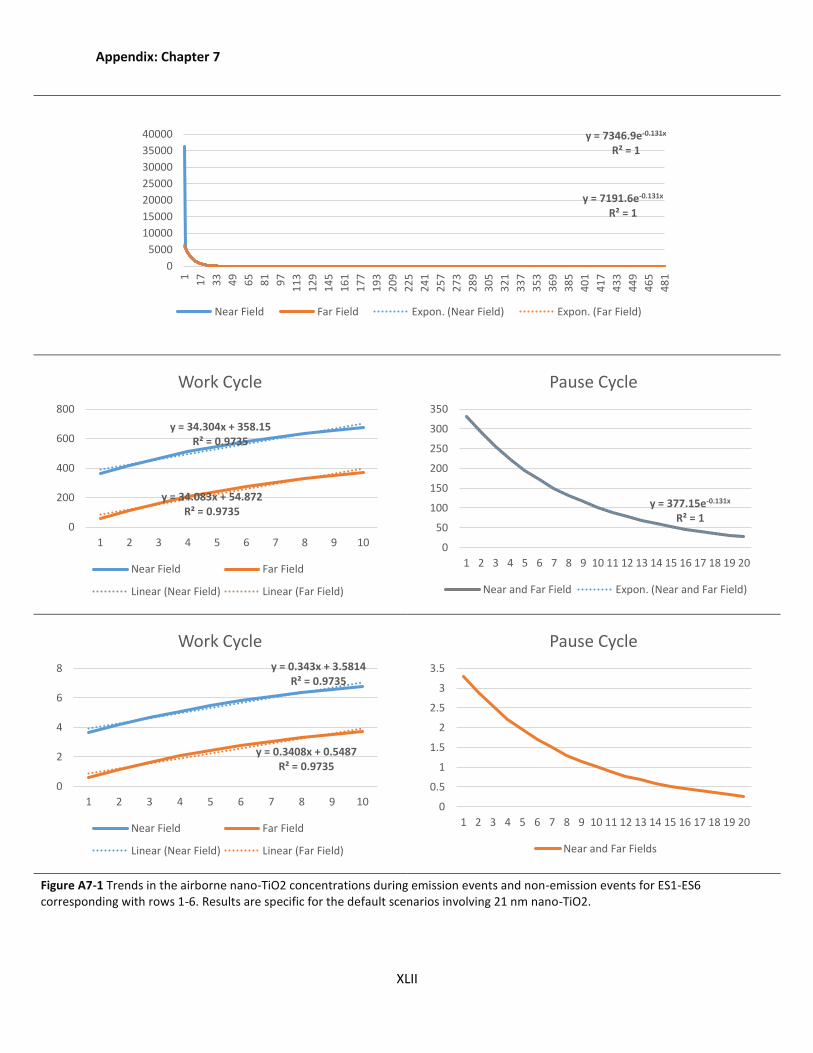
Appendix: Chapter 7
XLII
Figure A7-1 Trends in the airborne nano-TiO2 concentrations during emission events and non-emission events for ES1-ES6 corresponding with rows 1-6. Results are specific for the default scenarios involving 21 nm nano-TiO2.
y = 7346.9e-0.131x
R² = 1
y = 7191.6e-0.131x
R² = 1
0
5000
10000
15000
20000
25000
30000
35000
40000
1
17
33
49
65
81
97
11
3
12
9
14
5
16
1
17
7
19
3
20
9
22
5
24
1
25
7
27
3
28
9
30
5
32
1
33
7
35
3
36
9
38
5
40
1
41
7
43
3
44
9
46
5
48
1
Near Field Far Field Expon. (Near Field) Expon. (Far Field)
y = 34.304x + 358.15R² = 0.9735
y = 34.083x + 54.872R² = 0.9735
0
200
400
600
800
1 2 3 4 5 6 7 8 9 10
Work Cycle
Near Field Far Field
Linear (Near Field) Linear (Far Field)
y = 377.15e-0.131x
R² = 1
0
50
100
150
200
250
300
350
1 2 3 4 5 6 7 8 9 10 11 12 13 14 15 16 17 18 19 20
Pause Cycle
Near and Far Field Expon. (Near and Far Field)
y = 0.343x + 3.5814R² = 0.9735
y = 0.3408x + 0.5487R² = 0.9735
0
2
4
6
8
1 2 3 4 5 6 7 8 9 10
Work Cycle
Near Field Far Field
Linear (Near Field) Linear (Far Field)
0
0.5
1
1.5
2
2.5
3
3.5
1 2 3 4 5 6 7 8 9 10 11 12 13 14 15 16 17 18 19 20
Pause Cycle
Near and Far Fields
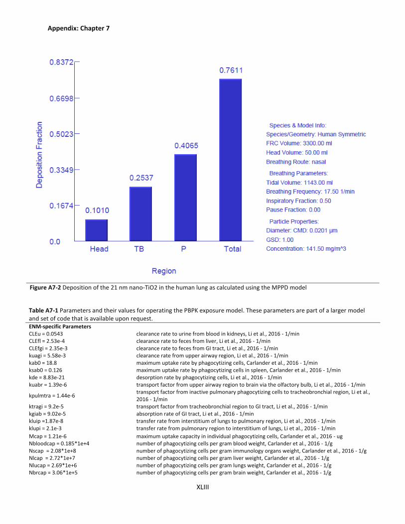
Appendix: Chapter 7
XLIII
Figure A7-2 Deposition of the 21 nm nano-TiO2 in the human lung as calculated using the MPPD model
Table A7-1 Parameters and their values for operating the PBPK exposure model. These parameters are part of a larger model and set of code that is available upon request. ENM-specific Parameters
CLEu = 0.0543 clearance rate to urine from blood in kidneys, Li et al., 2016 - 1/min CLEfl = 2.53e-4 clearance rate to feces from liver, Li et al., 2016 - 1/min CLEfgi = 2.35e-3 clearance rate to feces from GI tract, Li et al., 2016 - 1/min kuagi = 5.58e-3 clearance rate from upper airway region, Li et al., 2016 - 1/min kab0 = 18.8 maximum uptake rate by phagocytizing cells, Carlander et al., 2016 - 1/min ksab0 = 0.126 maximum uptake rate by phagocytizing cells in spleen, Carlander et al., 2016 - 1/min kde = 8.83e-21 desorption rate by phagocytizing cells, Li et al., 2016 - 1/min kuabr = 1.39e-6 transport factor from upper airway region to brain via the olfactory bulb, Li et al., 2016 - 1/min
kpulmtra = 1.44e-6 transport factor from inactive pulmonary phagocytizing cells to tracheobronchial region, Li et al., 2016 - 1/min
ktragi = 9.2e-5 transport factor from tracheobronchial region to GI tract, Li et al., 2016 - 1/min kgiab = 9.02e-5 absorption rate of GI tract, Li et al., 2016 - 1/min kluip =1.87e-8 transfer rate from interstitium of lungs to pulmonary region, Li et al., 2016 - 1/min klupi = 2.1e-3 transfer rate from pulmonary region to interstitium of lungs, Li et al., 2016 - 1/min Mcap = 1.21e-6 maximum uptake capacity in individual phagocytizing cells, Carlander et al., 2016 - ug Nbloodcap = 0.185*1e+4 number of phagocytizing cells per gram blood weight, Carlander et al., 2016 - 1/g Nscap = 2.08*1e+8 number of phagocytizing cells per gram immunology organs weight, Carlander et al., 2016 - 1/g Nlcap = 2.72*1e+7 number of phagocytizing cells per gram liver weight, Carlander et al., 2016 - 1/g Nlucap = 2.69*1e+6 number of phagocytizing cells per gram lungs weight, Carlander et al., 2016 - 1/g Nbrcap = 3.06*1e+5 number of phagocytizing cells per gram brain weight, Carlander et al., 2016 - 1/g
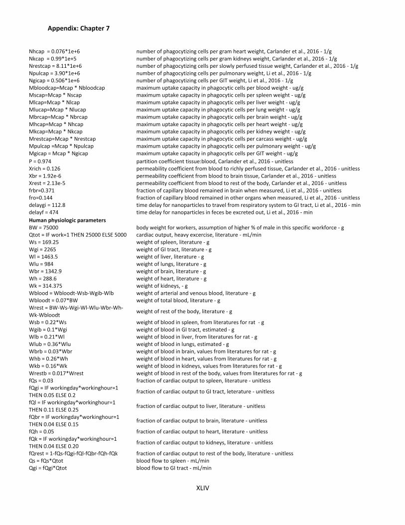
Appendix: Chapter 7
XLIV
Nhcap = 0.076*1e+6 number of phagocytizing cells per gram heart weight, Carlander et al., 2016 - 1/g Nkcap = 0.99*1e+5 number of phagocytizing cells per gram kidneys weight, Carlander et al., 2016 - 1/g Nrestcap = 8.11*1e+6 number of phagocytizing cells per slowly perfused tissue weight, Carlander et al., 2016 - 1/g Npulcap = 3.90*1e+6 number of phagocytizing cells per pulmonary weight, Li et al., 2016 - 1/g Ngicap = 0.506*1e+6 number of phagocytizing cells per GIT weight, Li et al., 2016 - 1/g Mbloodcap=Mcap * Nbloodcap maximum uptake capacity in phagocytic cells per blood weight - ug/g Mscap=Mcap * Nscap maximum uptake capacity in phagocytic cells per spleen weight - ug/g Mlcap=Mcap * Nlcap maximum uptake capacity in phagocytic cells per liver weight - ug/g Mlucap=Mcap * Nlucap maximum uptake capacity in phagocytic cells per lung weight - ug/g Mbrcap=Mcap * Nbrcap maximum uptake capacity in phagocytic cells per brain weight - ug/g Mhcap=Mcap * Nhcap maximum uptake capacity in phagocytic cells per heart weight - ug/g Mkcap=Mcap * Nkcap maximum uptake capacity in phagocytic cells per kidney weight - ug/g Mrestcap=Mcap * Nrestcap maximum uptake capacity in phagocytic cells per carcass weight - ug/g Mpulcap =Mcap * Npulcap maximum uptake capacity in phagocytic cells per pulmonary weight - ug/g Mgicap = Mcap * Ngicap maximum uptake capacity in phagocytic cells per GIT weight - ug/g P = 0.974 partition coefficient tissue:blood, Carlander et al., 2016 - unitless Xrich = 0.126 permeability coefficient from blood to richly perfused tissue, Carlander et al., 2016 - unitless Xbr = 1.92e-6 permeability coefficient from blood to brain tissue, Carlander et al., 2016 - unitless Xrest = 2.13e-5 permeability coefficient from blood to rest of the body, Carlander et al., 2016 - unitless frbr=0.371 fraction of capillary blood remained in brain when measured, Li et al., 2016 - unitless fro=0.144 fraction of capillary blood remained in other organs when measured, Li et al., 2016 - unitless delaygi = 112.8 time delay for nanoparticles to travel from respiratory system to GI tract, Li et al., 2016 - min delayf = 474 time delay for nanoparticles in feces be excreted out, Li et al., 2016 - min Human physiologic parameters BW = 75000 body weight for workers, assumption of higher % of male in this specific workforce - g Qtot = IF work=1 THEN 25000 ELSE 5000 cardiac output, heavy excercise, literature - mL/min Ws = 169.25 weight of spleen, literature - g Wgi = 2265 weight of GI tract, literature - g Wl = 1463.5 weight of liver, literature - g Wlu = 984 weight of lungs, literature - g Wbr = 1342.9 weight of brain, literature - g Wh = 288.6 weight of heart, literature - g Wk = 314.375 weight of kidneys, - g Wblood = Wbloodt-Wsb-Wgib-Wlb weight of arterial and venous blood, literature - g Wbloodt = 0.07*BW weight of total blood, literature - g Wrest = BW-Ws-Wgi-Wl-Wlu-Wbr-Wh-Wk-Wbloodt
weight of rest of the body, literature - g
Wsb = 0.22*Ws weight of blood in spleen, from literatures for rat - g Wgib = 0.1*Wgi weight of blood in GI tract, estimated - g Wlb = 0.21*Wl weight of blood in liver, from literatures for rat - g Wlub = 0.36*Wlu weight of blood in lungs, estimated - g Wbrb = 0.03*Wbr weight of blood in brain, values from literatures for rat - g Whb = 0.26*Wh weight of blood in heart, values from literatures for rat - g Wkb = 0.16*Wk weight of blood in kidneys, values from literatures for rat - g Wrestb = 0.017*Wrest weight of blood in rest of the body, values from literatures for rat - g fQs = 0.03 fraction of cardiac output to spleen, literature - unitless fQgi = IF workingday*workinghour=1 THEN 0.05 ELSE 0.2
fraction of cardiac output to GI tract, leterature - unitless
fQl = IF workingday*workinghour=1 THEN 0.11 ELSE 0.25
fraction of cardiac output to liver, literature - unitless
fQbr = IF workingday*workinghour=1 THEN 0.04 ELSE 0.15
fraction of cardiac output to brain, literature - unitless
fQh = 0.05 fraction of cardiac output to heart, literature - unitless fQk = IF workingday*workinghour=1 THEN 0.04 ELSE 0.20
fraction of cardiac output to kidneys, literature - unitless
fQrest = 1-fQs-fQgi-fQl-fQbr-fQh-fQk fraction of cardiac output to rest of the body, literature - unitless Qs = fQs*Qtot blood flow to spleen - mL/min Qgi = fQgi*Qtot blood flow to GI tract - mL/min
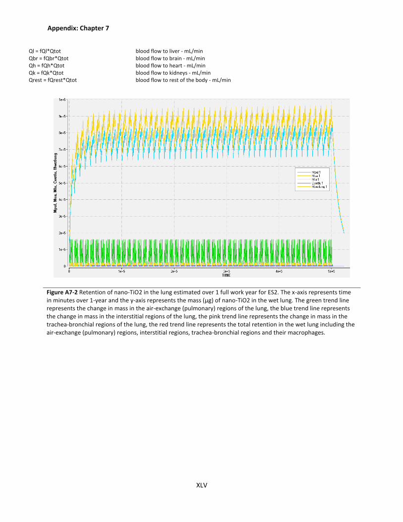
Appendix: Chapter 7
XLV
Ql = fQl*Qtot blood flow to liver - mL/min Qbr = fQbr*Qtot blood flow to brain - mL/min Qh = fQh*Qtot blood flow to heart - mL/min Qk = fQk*Qtot blood flow to kidneys - mL/min Qrest = fQrest*Qtot blood flow to rest of the body - mL/min
Figure A7-2 Retention of nano-TiO2 in the lung estimated over 1 full work year for ES2. The x-axis represents time in minutes over 1-year and the y-axis represents the mass (μg) of nano-TiO2 in the wet lung. The green trend line represents the change in mass in the air-exchange (pulmonary) regions of the lung, the blue trend line represents the change in mass in the interstitial regions of the lung, the pink trend line represents the change in mass in the trachea-bronchial regions of the lung, the red trend line represents the total retention in the wet lung including the air-exchange (pulmonary) regions, interstitial regions, trachea-bronchial regions and their macrophages.
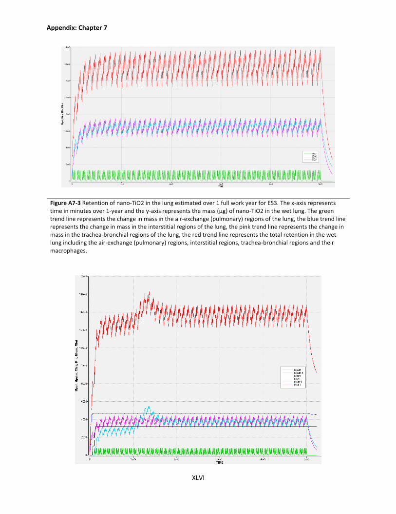
Appendix: Chapter 7
XLVI
Figure A7-3 Retention of nano-TiO2 in the lung estimated over 1 full work year for ES3. The x-axis represents time in minutes over 1-year and the y-axis represents the mass (μg) of nano-TiO2 in the wet lung. The green trend line represents the change in mass in the air-exchange (pulmonary) regions of the lung, the blue trend line represents the change in mass in the interstitial regions of the lung, the pink trend line represents the change in mass in the trachea-bronchial regions of the lung, the red trend line represents the total retention in the wet lung including the air-exchange (pulmonary) regions, interstitial regions, trachea-bronchial regions and their macrophages.
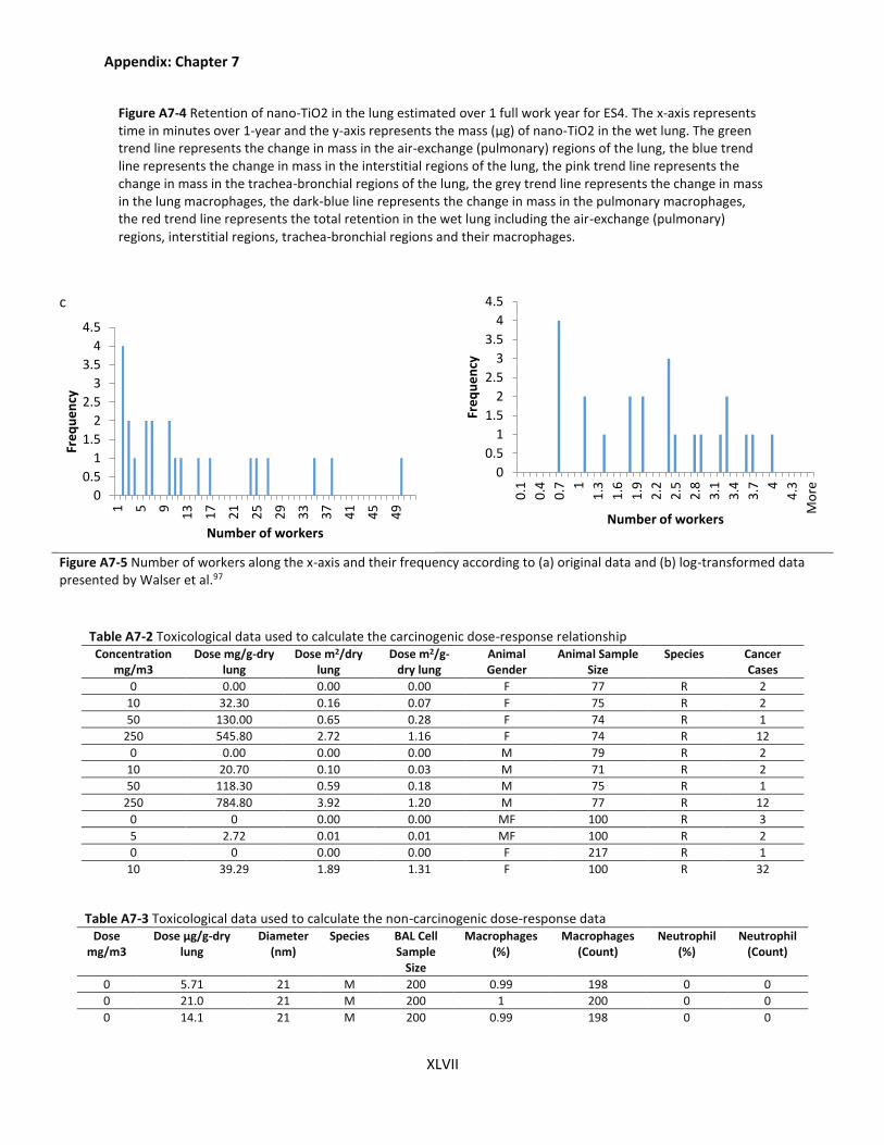
Appendix: Chapter 7
XLVII
Figure A7-4 Retention of nano-TiO2 in the lung estimated over 1 full work year for ES4. The x-axis represents time in minutes over 1-year and the y-axis represents the mass (μg) of nano-TiO2 in the wet lung. The green trend line represents the change in mass in the air-exchange (pulmonary) regions of the lung, the blue trend line represents the change in mass in the interstitial regions of the lung, the pink trend line represents the change in mass in the trachea-bronchial regions of the lung, the grey trend line represents the change in mass in the lung macrophages, the dark-blue line represents the change in mass in the pulmonary macrophages, the red trend line represents the total retention in the wet lung including the air-exchange (pulmonary) regions, interstitial regions, trachea-bronchial regions and their macrophages.
c
Figure A7-5 Number of workers along the x-axis and their frequency according to (a) original data and (b) log-transformed data presented by Walser et al.97
Table A7-2 Toxicological data used to calculate the carcinogenic dose-response relationship Concentration
mg/m3 Dose mg/g-dry
lung Dose m2/dry
lung Dose m2/g-
dry lung Animal Gender
Animal Sample Size
Species Cancer Cases
0 0.00 0.00 0.00 F 77 R 2
10 32.30 0.16 0.07 F 75 R 2
50 130.00 0.65 0.28 F 74 R 1
250 545.80 2.72 1.16 F 74 R 12
0 0.00 0.00 0.00 M 79 R 2
10 20.70 0.10 0.03 M 71 R 2
50 118.30 0.59 0.18 M 75 R 1
250 784.80 3.92 1.20 M 77 R 12
0 0 0.00 0.00 MF 100 R 3
5 2.72 0.01 0.01 MF 100 R 2
0 0 0.00 0.00 F 217 R 1
10 39.29 1.89 1.31 F 100 R 32
Table A7-3 Toxicological data used to calculate the non-carcinogenic dose-response data Dose
mg/m3 Dose µg/g-dry
lung Diameter
(nm) Species BAL Cell
Sample Size
Macrophages (%)
Macrophages (Count)
Neutrophil (%)
Neutrophil (Count)
0 5.71 21 M 200 0.99 198 0 0
0 21.0 21 M 200 1 200 0 0
0 14.1 21 M 200 0.99 198 0 0
0
0.5
1
1.5
2
2.5
3
3.5
4
4.5
1 5 9
13
17
21
25
29
33
37
41
45
49
Fre
qu
en
cy
Number of workers
0
0.5
1
1.5
2
2.5
3
3.5
4
4.5
0.1
0.4
0.7 1
1.3
1.6
1.9
2.2
2.5
2.8
3.1
3.4
3.7 4
4.3
Mo
re
Fre
qu
en
cy
Number of workers

Appendix: Chapter 7
XLVIII
0 32.7 21 M 200 1 200 0 0
0 15.5 21 M 200 1 200 0 0
0.5 381 21 M 200 0.995 199 0 0
0.5 335 21 M 200 1 200 0 0
0.5 349 21 M 200 0.995 199 0 0
0.5 361 21 M 200 0.99 198 0 0
0.5 365 21 M 200 1 200 0 0
2 1411 21 M 200 0.995 199 0.005 1
2 1458 21 M 200 1 200 0 0
2 1411 21 M 200 1 200 0 0
2 1400 21 M 200 0.995 199 0.005 1
2 1299 21 M 200 1 200 0 0
10 10860 21 M 200 0.8 160 0.195 39
10 9776 21 M 200 0.865 173 0.125 25
10 11080 21 M 200 0.915 183 0.07 14
10 10306 21 M 200 0.775 155 0.21 42
10 10540 21 M 200 0.875 175 0.125 25
0 42.4 21 R 200 1 200 0 0
0 35.3 21 R 200 0.995 199 0.005 1
0 35.5 21 R 200 1 200 0 0
0 38.6 21 R 200 0.99 198 0.01 2
0 31.4 21 R 200 0.99 198 0.005 1
0.5 423 21 R 200 0.995 199 0.005 1
0.5 454 21 R 200 0.985 197 0.01 2
0.5 483 21 R 200 0.99 198 0.005 1
0.5 382 21 R 200 0.99 198 0.005 1
0.5 380 21 R 200 1 200 0 0
2 1620 21 R 200 0.91 182 0.085 17
2 1769 21 R 200 0.97 194 0.03 6
2 1772 21 R 200 0.96 192 0.035 7
2 1605 21 R 200 0.87 174 0.13 26
2 1660 21 R 200 0.95 190 0.045 9
10 10211 21 R 200 0.235 47 0.73 146
10 12383 21 R 200 0.4 80 0.585 117
10 10110 21 R 200 0.365 73 0.625 125
10 11440 21 R 200 0.315 63 0.66 132
10 10793 21 R 200 0.35 70 0.64 128
List of Publications
XLIX
List of Publications
Much of the methods, results and other content contained in Chapter 3 was previously published in
Progress in Photovoltaics: Research and Applications and can be found online at. The full citation of this
publication is: Tsang, M. P., Sonnemann, G. W. & Bassani, D. M. A comparative human health, ecotoxicity,
and product environmental assessment on the production of organic and silicon solar cells. Prog.
Photovoltaics Res. Appl. 24, 645–655 (2016). [http://onlinelibrary.wiley.com/doi/10.1002/pip.2704/full].
Most of the methods, results and other content contained in Chapter 4 was published in Solar Energy
Materials and Solar Cells. The full citation of this publication is: Tsang, M. P., Sonnemann, G. W. & Bassani,
D. M. Life-cycle assessment of cradle-to-grave opportunities and environmental impacts of organic
photovoltaic solar panels compared to conventional technologies. Sol. Energy Mater. Sol. Cells 156, 37–
48 (2016). [http://dx.doi.org/10.1016/j.solmat.2016.04.024].
Portions of Chapter 5 were submitted as a single manuscript in 2015 and is currently still under peer-
review.
Chapter 6 was submitted in 2016 and is currently under peer-review.
Chapter 7 is currently being prepared for submission in late 2016.
Résumé Détaillé
L
Résumé Détaillé
Introduction
L’énergie est une problématique fondamentale de la société au 21ème siècle, et au centre des enjeux de
durabilité. Au cours des deux derniers siècles, l’énergie a été le facteur le plus influent sur la modification
de la société. Le développement et l'utilisation des combustibles fossiles ont stimulé une importante
croissance de l'industrie et de la population mondiale ainsi que des réalisations technologiques à une
échelle jamais vue avant la révolution industrielle. Cependant, cela s'est fait au détriment d’importants
coûts environnementaux et de santé publique. Le monde est à présent entré dans une ère de pic pétrolier
et les émissions de gaz à effet de serre d’origines anthropiques produisent des modifications
environnementales majeures et problématiques telles que le changement climatique. 4
Dans ce contexte, la durabilité n'est pas simplement une question d'énergie, mais aussi une question
d'environnement et de santé publique. Le coût réel d'une source d'énergie ne peut pas être quantifié
uniquement en fonction de ses coûts d’extraction, de raffinage et de distribution, mais il doit également
tenir compte des « externalités » ou des coûts indirects liés à ses dommages environnementaux. Ce point
de vue global est nécessaire pour éviter un transfert d’impacts, comme cela peut être le cas
avec les biocarburants (qui génèrent une utilisation des terres et une consommation d'eau douce
accrues)5-7 ou pour l'utilisation de l'énergie solaire avec des panneaux photovoltaïques (PV) qui génèrent
une augmentation de l’utilisation de métaux. 9
Par conséquent, la recherche et le développement de nouvelles sources durables pour
répondre aux demandes énergétiques actuelles et futures est un enjeu majeur du 21eme siècle. Face à la
nécessité urgente de diminuer les émissions de gaz à effet de serre, les sources d'énergie renouvelable
comme le PV ont un rôle important dans la stratégie mondiale d'approvisionnement en énergie.
D’abord coûteuses et de faible efficacité, les cellules PV à base de silicium 10 ont rapidement mûri pour
atteindre des rendements de 20% au milieu des années 1980. A l’échelle du laboratoire, le rendement a
été augmenté au - delà de 25% pour la plupart des cellules à base de silicium. 11 Des records de
rendement en laboratoire ont été atteint avec plus de 45 % de conversion de la lumière
en électricité en utilisant par exemple des cellules de gallium, d'indium et d'arsenic. Les cellules
à base de silicium sont encore la technologie photovoltaïque la plus largement utilisée dans
le monde, en particulier à grande échelle et pour les systèmes placés sur les toits. Elle
Résumé Détaillé
LI
représente plus de 90% de la production mondiale de PV par an. 12 L'utilisation du PV à base de silicium
engendre des bénéfices environnementaux important et une meilleure gestion des ressources par rapport
aux systèmes de production électriques classiques. Des études antérieures ont montré, par exemple, que
les émissions de gaz à effet de serre par kWh d'électricité produit à l'aide de PV à base de silicium sont
cinq fois plus faibles que la production à base de charbon et plus de deux fois plus faibles
que la production à base de gaz naturel 13. En outre, les quatre dernières décennies de développement du
PV sont marquées par la recherche et le développement d'une large gamme de technologies viables,
allant du PV classique à base de silicium monocristallin et multi-cristallin (m-Si)
aux technologies de deuxième génération, telles que le silicium amorphe (a-Si), le cadmium-tellurure et
le cadmium-indium-gallium-sélénium. Depuis la fin des années 1990, les financements de R&D ont permis
de développer les technologies dites de troisième génération. Cette génération de PV est beaucoup plus
diversifiée par rapport aux générations précédentes et comprend notamment des cellules
photovoltaïques sensibilisées par colorant, avec de la perovskite, des points quantiques ou bien des
cellules photovoltaïques organiques (PVO).
L'objectif de cette thèse repose sur les technologies de 3ème génération qui utilisent des matériaux
organiques dans leurs couches actives au lieu de composés inorganiques tels que le silicium. La première
technologie PVO a été développée par CW Tang en 1979 avec un dispositif organique d’hétérojonction
14. Ce premier dispositif utilisait une couche active de phtalocyanine de cuivre et d'un dérivé de pérylène,
un carbone polycyclique. Cette technologie est restée principalement une technologie de laboratoire,
avec de petits projets pilotes (www.infinitypv.com) en ligne seulement depuis 2015 et le déploiement à
grande échelle de panneaux solaires PVO déployés sur le terrain à des fins de recherche et de
démonstration15. Conceptuellement, les cellules PVO ne sont pas très différentes des technologies
photovoltaïques classiques dans le sens où elles sont composées des mêmes composants principaux
comme deux électrodes et une couche active (i.e. où la séparation de charge se produit). Contrairement
à d'autres technologies photovoltaïques, la couche active d'une cellule PVO est composée de couches de
matériaux organiques donneurs d'électrons (semi-conducteur n) et accepteur d'électrons (semi-
conducteur p), d'où le nom de cette technologie. De plus, pour atteindre leur extrême finesse, les
dispositifs PVO utilisent généralement des nanomatériaux fabriqués (NMF) comme composants
principaux des couches actives et additionnelles. Les cellules PVO peuvent nécessiter des composants
supplémentaires tels qu'un substrat sur lequel tous les autres composants sont déposés ainsi que des
couches pour améliorer l'efficacité et la séparation des charges, telles que le transport d'électrons et les
Résumé Détaillé
LII
couches de transport de trous, et des couches de revêtement barrière pour la protection. Cependant, il
n'y a pas de géométrie PVO ni de composition "standard" les PVO étant encore une technologie en plein
développement.
Objectif de cette thèse
Bien que les technologies photovoltaïques captent le rayonnement solaire disponible et le transforment
en une forme d'énergie plus utile (c.-à-d. l'électricité), des charges environnementales (des émissions de
gaz à effet de serre par exemple) peuvent survenir pendant la production, l'utilisation ou l'élimination du
panneau PV. Ceci étant dit, le PVO a de nombreuses caractéristiques qui en font un choix convaincant
pour un développement ultérieur dans le domaine de l'énergie solaire. Ainsi, les cellules photovoltaïques
sont extrêmement minces, flexibles, nécessitent de faibles quantités de matériaux et des processus de
production à faible consommation énergétique 16. L'objectif général de cette thèse est de vérifier si le
PVO est préférable pour l'approvisionnement en énergie par rapport au PV classique à base de silicium
d'un point de vue environnemental et de santé humaine. Un objectif sous-jacent de la thèse est de vérifier
que les méthodologies existantes, couramment utilisées pour évaluer la performance environnementale
des systèmes d'approvisionnement en énergie, comme l’analyse du cycle de vie (ACV), sont
appropriées. Cette thèse aborde également les questions concernant les limites actuelles de l'utilisation
de l’ACV pour évaluer les impacts associés au PVO, tels que les impacts potentiels sur la santé humaine
associés à l'utilisation de nanomatériaux, et de quelle façon et avec quels outils cette question peut-elle
être traitée pour informer de manière constructive le développement de cette technologie.
Questions abordées dans cette thèse:
1) Quelle est la gamme complète des impacts environnementaux du berceau à la tombe des
technologies photovoltaïques organiques potentielles ?
2) Comment les impacts environnementaux des technologies photovoltaïques organiques se
comparent-ils aux photovoltaïques traditionnels à base de silicium ?
3) Quelles sont les limites actuelles de l'utilisation de l'évaluation du cycle de vie pour évaluer les
technologies photovoltaïques organiques et autres technologies émergentes ?
4) Quels sont les outils disponibles pour traiter les risques pour la santé humaine et les risques pour
les nanomatériaux fabriqués ?
5) Comment ces impacts sur la santé humaine des nanomatériaux artificiels peuvent-ils être intégrés
dans les méthodologies d'évaluation du cycle de vie ?
Résumé Détaillé
LIII
Analyse du cycle de vie
L'utilisation de l'ACV est l'élément central de l'évaluation environnementale des systèmes liés à
l'énergie. L’ACV est un outil de gestion de l'environnement décrit par la norme ISO 14040:2006 et
14044:2006. 18,19 Une très brève introduction est fournie ici, une explication plus détaillée de son
utilisation et des méthodes se trouvant dans le chapitre 2. L’ACV est considérée comme un outil essentiel
d’évaluation en raison de sa capacité à suivre l'ensemble de l'énergie utilisée à chaque étape du cycle de
vie du système. Cette information peut être utilisée pour déterminer combien de temps il faudra au
système, pendant son utilisation, pour générer l'énergie qui a été consommée pendant la production de
ce même système. Ceci est connu comme le temps de retour énergétique (TRE) 20-22. Des mesures
similaires telles que le temps de retour carbone (TRC) peuvent également être calculées puisque l’ACV
permet le suivi de flux de matières non énergétiques tels que l'émission de gaz à effet de serre tout au
long du cycle de vie. Le TRE et le TRC sont des paramètres essentiels auxquels tous les systèmes de
production d'énergie sont discriminés. L'ACV se compose de (1) l'objectif et la définition du champ
d'application, (2) l'inventaire du cycle de vie, (3) l’évaluation d'impact du cycle de vie et (4) les étapes
d'interprétation.
Le but et le champ d’étude définissent ce qui est étudié dans l'ACV et incluent la définition de l'unité
fonctionnelle et des limites du système. L'unité fonctionnelle décrit une fonction remplie, telle qu'un
processus (une régénération de solvant), un produit (un panneau solaire) ou un événement (une
restauration environnementale). L'unité fonctionnelle est directement liée aux limites du système, ce qui
clarifie davantage les aspects de l'unité fonctionnelle qui sont ou non inclus dans l'évaluation. Un aspect
important des limites du système est l'identification des phases du cycle de vie contenues dans
l'étude. Par exemple, une étude peut être définie de porte à porte (gate-to-gate) si l'évaluation ne
comprend qu'une étape du cycle de vie (par exemple, la fabrication d'un produit), du berceau à la porte
de l’usine si l'évaluation inclut l'extraction de la matière première jusqu’à la fabrication du produit, et du
berceau à la tombe si l'évaluation comprend chaque étape du cycle de vie. De plus, l'identification et le
choix des critères d'évaluation de l'impact sur l'environnement et la santé humaine doivent être réalisés
dans le cadre de la définition de l'objectif et du cadre de l’étude.
La deuxième étape d'une ACV, l'inventaire du cycle de vie, consiste à identifier, quantifier et regrouper
tous les flux de matières, d'énergie et de déchets contenus dans l’unité fonctionnelle dans les limites des
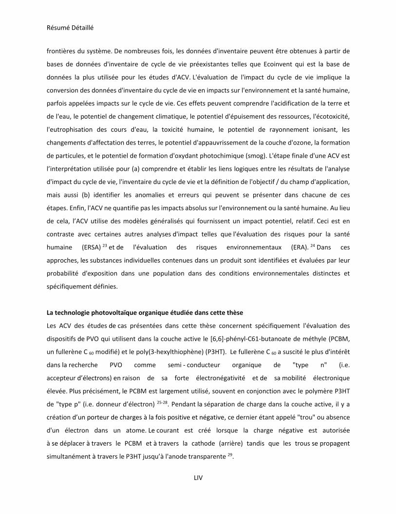
Résumé Détaillé
LIV
frontières du système. De nombreuses fois, les données d'inventaire peuvent être obtenues à partir de
bases de données d'inventaire de cycle de vie préexistantes telles que Ecoinvent qui est la base de
données la plus utilisée pour les études d'ACV. L'évaluation de l'impact du cycle de vie implique la
conversion des données d'inventaire du cycle de vie en impacts sur l'environnement et la santé humaine,
parfois appelées impacts sur le cycle de vie. Ces effets peuvent comprendre l'acidification de la terre et
de l'eau, le potentiel de changement climatique, le potentiel d'épuisement des ressources, l'écotoxicité,
l'eutrophisation des cours d'eau, la toxicité humaine, le potentiel de rayonnement ionisant, les
changements d'affectation des terres, le potentiel d'appauvrissement de la couche d'ozone, la formation
de particules, et le potentiel de formation d'oxydant photochimique (smog). L'étape finale d'une ACV est
l’interprétation utilisée pour (a) comprendre et établir les liens logiques entre les résultats de l'analyse
d'impact du cycle de vie, l'inventaire du cycle de vie et la définition de l'objectif / du champ d'application,
mais aussi (b) identifier les anomalies et erreurs qui peuvent se présenter dans chacune de ces
étapes. Enfin, l'ACV ne quantifie pas les impacts absolus sur l'environnement ou la santé humaine. Au lieu
de cela, l’ACV utilise des modèles généralisés qui fournissent un impact potentiel, relatif. Ceci est en
contraste avec certaines autres analyses d'impact telles que l'évaluation des risques pour la santé
humaine (ERSA) 23 et de l'évaluation des risques environnementaux (ERA). 24 Dans ces
approches, les substances individuelles contenues dans un produit sont identifiées et évaluées par leur
probabilité d'exposition dans une population dans des conditions environnementales distinctes et
spécifiquement définies.
La technologie photovoltaïque organique étudiée dans cette thèse
Les ACV des études de cas présentées dans cette thèse concernent spécifiquement l'évaluation des
dispositifs de PVO qui utilisent dans la couche active le [6,6]-phényl-C61-butanoate de méthyle (PCBM,
un fullerène C 60 modifié) et le poly(3-hexylthiophène) (P3HT). Le fullerène C 60 a suscité le plus d'intérêt
dans la recherche PVO comme semi - conducteur organique de "type n" (i.e.
accepteur d’électrons) en raison de sa forte électronégativité et de sa mobilité électronique
élevée. Plus précisément, le PCBM est largement utilisé, souvent en conjonction avec le polymère P3HT
de "type p" (i.e. donneur d’électron) 25-28. Pendant la séparation de charge dans la couche active, il y a
création d’un porteur de charges à la fois positive et négative, ce dernier étant appelé "trou" ou absence
d'un électron dans un atome. Le courant est créé lorsque la charge négative est autorisée
à se déplacer à travers le PCBM et à travers la cathode (arrière) tandis que les trous se propagent
simultanément à travers le P3HT jusqu’à l'anode transparente 29.
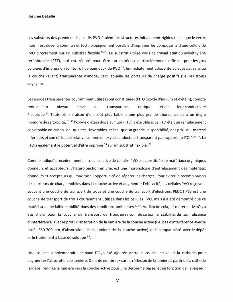
Résumé Détaillé
LV
Les substrats des premiers dispositifs PVO étaient des structures initialement rigides telles que le verre,
mais il est devenu commun et technologiquement possible d'imprimer les composants d'une cellule de
PVO directement sur un substrat flexible 16,26. Le substrat utilisé dans ce travail était du polyéthylène
téréphtalate (PET), qui est réputé pour être un matériau particulièrement efficace pour les gros
volumes d’impression roll-to-roll de panneaux de PVO 26. Immédiatement adjacente au substrat se situe
la couche (avant) transparente d'anode, vers laquelle les porteurs de charge positifs (i.e. les trous)
voyagent.
Les anodes transparentes couramment utilisés sont constituées d’ITO (oxyde d'indium et d'étain), compte
tenu de leur niveau élevé de transparence optique et de leur conductivité
électrique 30. Toutefois, en raison d’un coût plus faible, d’une plus grande abondance et à un degré
moindre de sa toxicité, 31-33 l’oxyde d'étain dopé au fluor (FTO) a été utilisé. Le FTO était un remplacement
convenable en raison de qualités favorables telles que sa grande disponibilité, des prix du marché
inférieurs et son efficacité relative comme un oxyde conducteur transparent par rapport au ITO 30,34,35. Le
FTO a également le potentiel d'être imprimé 33 sur un substrat flexible. 36
Comme indiqué précédemment, la couche active de cellules PVO est constituée de matériaux organiques
donneurs et accepteurs. L'hétérojonction en vrac est une morphologie d'entrelacement des matériaux
donneurs et accepteurs qui maximise l'opportunité de séparer les charges. Pour éviter la recombinaison
des porteurs de charge mobiles dans la couche active et augmenter l'efficacité, les cellules PVO reçoivent
souvent une couche de transport de trous et une couche de transport d'électrons. PEDOT:PSS est une
couche de transport de trous couramment utilisée dans les cellules PVO, mais il a été démontré que ce
matériau a une faible stabilité dans des conditions ambiantes 37,38. Au lieu de cela, le matériau MoO 3 a
été choisi pour la couche de transport de trous en raison de sa bonne stabilité, de son absence
d’interférence avec le profil d'absorption de la lumière de la couche active (i.e. pas d'interférence avec le
profil 350-700 nm d'absorption de la lumière de la couche active) et la compatibilité avec le dépôt
et le traitement à base de solution 39.
Une couche supplémentaire de nano-TiO2 a été ajoutée entre la couche active et la cathode, pour
augmenter l’absorption de lumière. Dans de nombreux cas, la réflexion de la lumière à partir de la cathode
(arrière) redirige la lumière vers la couche active pour une deuxième passe, et en fonction de l'épaisseur
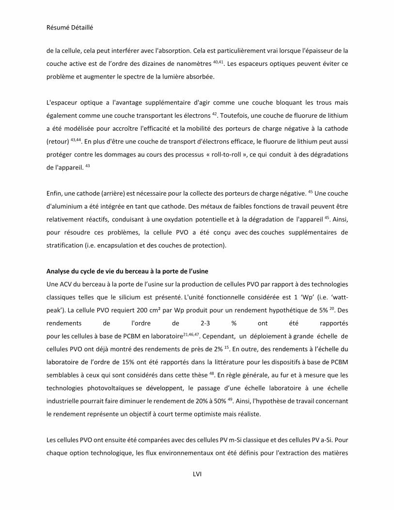
Résumé Détaillé
LVI
de la cellule, cela peut interférer avec l'absorption. Cela est particulièrement vrai lorsque l'épaisseur de la
couche active est de l’ordre des dizaines de nanomètres 40,41. Les espaceurs optiques peuvent éviter ce
problème et augmenter le spectre de la lumière absorbée.
L'espaceur optique a l'avantage supplémentaire d'agir comme une couche bloquant les trous mais
également comme une couche transportant les électrons 42. Toutefois, une couche de fluorure de lithium
a été modélisée pour accroître l'efficacité et la mobilité des porteurs de charge négative à la cathode
(retour) 43,44. En plus d'être une couche de transport d'électrons efficace, le fluorure de lithium peut aussi
protéger contre les dommages au cours des processus « roll-to-roll », ce qui conduit à des dégradations
de l'appareil. 43
Enfin, une cathode (arrière) est nécessaire pour la collecte des porteurs de charge négative. 45 Une couche
d'aluminium a été intégrée en tant que cathode. Des métaux de faibles fonctions de travail peuvent être
relativement réactifs, conduisant à une oxydation potentielle et à la dégradation de l'appareil 45. Ainsi,
pour résoudre ces problèmes, la cellule PVO a été conçu avec des couches supplémentaires de
stratification (i.e. encapsulation et des couches de protection).
Analyse du cycle de vie du berceau à la porte de l’usine
Une ACV du berceau à la porte de l’usine sur la production de cellules PVO par rapport à des technologies
classiques telles que le silicium est présenté. L'unité fonctionnelle considérée est 1 ‘Wp’ (i.e. ‘watt-
peak’). La cellule PVO requiert 200 cm² par Wp produit pour un rendement hypothétique de 5% 20. Des
rendements de l'ordre de 2-3 % ont été rapportés
pour les cellules à base de PCBM en laboratoire21,46,47. Cependant, un déploiement à grande échelle de
cellules PVO ont déjà montré des rendements de près de 2% 15. En outre, des rendements à l’échelle du
laboratoire de l’ordre de 15% ont été rapportés dans la littérature pour les dispositifs à base de PCBM
semblables à ceux qui sont considérés dans cette thèse 48. En règle générale, au fur et à mesure que les
technologies photovoltaïques se développent, le passage d’une échelle laboratoire à une échelle
industrielle pourrait faire diminuer le rendement de 20% à 50% 49. Ainsi, l'hypothèse de travail concernant
le rendement représente un objectif à court terme optimiste mais réaliste.
Les cellules PVO ont ensuite été comparées avec des cellules PV m-Si classique et des cellules PV a-Si. Pour
chaque option technologique, les flux environnementaux ont été définis pour l'extraction des matières
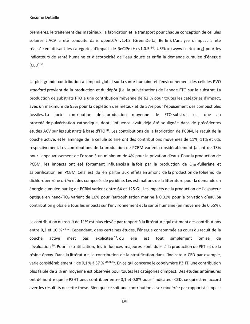
Résumé Détaillé
LVII
premières, le traitement des matériaux, la fabrication et le transport pour chaque conception de cellules
solaires. L’ACV a été conduite dans openLCA v1.4.2 (GreenDelta, Berlin). L'analyse d'impact a été
réalisée en utilisant les catégories d’impact de ReCiPe (H) v1.0.5 50, USEtox (www.usetox.org) pour les
indicateurs de santé humaine et d’écotoxicité de l’eau douce et enfin la demande cumulée d’énergie
(CED) 51.
La plus grande contribution à l'impact global sur la santé humaine et l'environnement des cellules PVO
standard provient de la production et du dépôt (i.e. la pulvérisation) de l'anode FTO sur le substrat. La
production de substrats FTO a une contribution moyenne de 62 % pour toutes les catégories d'impact,
avec un maximum de 95% pour la déplétion des métaux et de 57% pour l'épuisement des combustibles
fossiles. La forte contribution de la production moyenne de FTO-substrat est due au
procédé de pulvérisation cathodique, dont l’influence avait déjà été soulignée dans de précédentes
études ACV sur les substrats à base d'ITO 31. Les contributions de la fabrication de PCBM, le recuit de la
couche active, et le laminage de la cellule solaire ont des contributions moyennes de 11%, 11% et 6%,
respectivement. Les contributions de la production de PCBM varient considérablement (allant de 13%
pour l'appauvrissement de l'ozone à un minimum de 4% pour la privation d'eau). Pour la production de
PCBM, les impacts ont été fortement influencés à la fois par la production de C 60 -fullerène et
sa purification en PCBM. Cela est dû en partie aux effets en amont de la production de toluène, de
dichlorobenzène ortho et des composés de pyridine. Les estimations de la littérature pour la demande en
énergie cumulée par kg de PCBM varient entre 64 et 125 GJ. Les impacts de la production de l’espaceur
optique en nano-TiO2 varient de 10% pour l'eutrophisation marine à 0,01% pour la privation d’eau. Sa
contribution globale à tous les impacts sur l'environnement et la santé humaine (en moyenne de 0,55%).
La contribution du recuit de 11% est plus élevée par rapport à la littérature qui estiment des contributions
entre 0,2 et 10 % 21,52. Cependant, dans certaines études, l'énergie consommée au cours du recuit de la
couche active n’est pas explicitée 53, ou elle est tout simplement omise de
l'évaluation 20. Pour la stratification, les influences majeures sont dues à la production de PET et de la
résine époxy. Dans la littérature, la contribution de la stratification dans l’indicateur CED par exemple,
varie considérablement : de 0,1 % à 37 % 20,21,46. En ce qui concerne le copolymère P3HT, une contribution
plus faible de 2 % en moyenne est observée pour toutes les catégories d'impact. Des études antérieures
ont démontré que le P3HT peut contribuer entre 0,1 et 0,8% pour l’indicateur CED, ce qui est en accord
avec les résultats de cette thèse. Bien que ce soit une contribution assez modérée par rapport à l'impact
Résumé Détaillé
LVIII
global, la littérature fait état d'une tendance à remplacer le P3HT par de nouveaux polymères. 54 Bien que
ceux - ci ont le potentiel d'accroître l'efficacité des cellules PVO, ils pourraient générer une augmentation
des impacts 54.
Une autre modélisation a été réalisée pour substituer la pulvérisation de l'électrode FTO par l'impression
par jet d'encre de l'électrode. La pulvérisation a déjà été identifiée comme étant un processus énergivore
et, lorsqu’il est évité, diminue l'ensemble de l’indicateur CED 20,46,53. Les résultats de cette
thèse ont confirmé cela, mais aussi démontré que les autres catégories d'impact ne répondent pas
nécessairement à la même tendance que la CED. Par exemple, alors que la CED présente une diminution
d'impact d'environ 56 %, les réductions d'impact variaient de 2 % pour l'épuisement des métaux à 72 %
pour les rayonnements ionisants. En outre, une évaluation pour un dispositif remplaçant le PCBM avec un
copolymère dans la couche active a été effectuée. Il en résulte une diminution moyenne de 10 % pour
toutes les catégories d'impact. Considérant que le PCBM a déjà été identifié comme un facteur ayant une
influence de faible à modérée dans les impacts de la production de la cellule PVO sur la santé humaine
et l'environnement 20,31,53,55, des réductions relativement importantes du au remplacement du polymère
ont été observées pour l'écotoxicité, où les impacts ont été réduits de 20 %. En général, les polymères tels
que le P3HT ont montré des contributions beaucoup plus faibles aux impacts environnementaux
de la production de PVO, mais les polymères sont très hétérogènes et leur CED, par exemple, peut varier
d’un ordre de grandeur54.
Par rapport à des cellules m-Si et a-Si, les impacts du PVO par défaut étaient en moyenne 93% plus
faibles. Le TRE (c’est-à-dire le temps qu’il faudra au système pour générer l'énergie consommée pendant
la production de ce même système) a été évalué à 0,27 ans (97 jours) pour la cellule PVO par défaut. Les
cellules m-Si et a-Si ont un TRE de respectivement 3,6 et 2,8 ans. Pour les variantes du PVO, le TRE est de
0,12 ans (42 jours) et de 0,24 ans (87 jours) respectivement pour le dispositif à jet d'encre et pour toutes
les cellules en polymère.
Analyse du cycle de vie du berceau à la tombe
Les résultats de cette ACV sont largement en faveur des cellules PVO, puisque tous les résultats d’impact
sont plus faibles que pour les cellules de silicium classiques à unité fonctionnelle identique. Cependant,
les résultats de cette ACV initiale du berceau à la porte de l’usine ne tiennent pas compte des phases
d’utilisation et de fin de vie du dispositif PVO et étant donné les faibles rendements et la durée de vie du
Résumé Détaillé
LIX
PVO, cela pourrait avoir une influence importante sur la comparaison des deux types de système. Ainsi,
l’ACV est étendue du berceau à la tombe en incluant les phases d'utilisation et de fin de vie. Les cellules
photovoltaïques organiques ne sont actuellement pas produites à l'échelle industrielle ou utilisées à des
fins commerciales. Par conséquent, deux systèmes différents (deux utilisations du PV) ont été pris en
compte afin de mieux éclairer le rôle que le PVO pourrait jouer pour les secteurs de la production
d'énergie et des produits de consommation. Le système 1 (S1) est défini par une unité fonctionnelle d'une
production d’un kWh moyen d'électricité durant 25 ans sur un toit (Figure 4 -2), tandis que le système 2
(S2) est défini par une unité fonctionnelle d'une production moyenne de 10 Wh d'électricité sur cinq ans
via un dispositif de chargeur de portable. Pour S1, en plus de l'installation sur le toit des panneaux PVO et
silicium, la structure de montage, un onduleur et des câbles pour l'installation électrique ont été
également pris en compte. Pour S2, on a supposé que les chargeurs portatifs nécessitent un étui de
protection en PET-polyester d'un mm d'épaisseur.
Deux scénarios de fin de vie ont été envisagés : (a) incinération et (b) mise en décharge. À l'heure actuelle,
les infrastructures, l’économie, la législation et la taille du flux de déchets montrent
que la plupart des panneaux PV finissent dans ces filières d'élimination classiques, par opposition au
recyclage 56-58. Ces deux processus de gestion de fin de vie ont été calculés en utilisant les outils de
modélisation de la fin de vie dans Ecoinvent 59. L'outil a été utilisé pour créer un inventaire basé en partie
sur la composition élémentaire des déchets. La composition des déchets pour chaque panneau est basée
sur la composition du panneau au moment de la fabrication (c'est-à-dire sans tenir compte des pertes ou
de la dégradation des composants pendant la durée de vie du dispositif photovoltaïque). Pour
l'incinération, le pouvoir calorifique inférieur (PCI) des principaux composants ont été utilisées pour
déterminer la récupération d'énergie potentielle du système. Comme la plupart des panneaux PVO sont
en PET, leur PCI de 22,9 MJ/kg a été utilisée. Ainsi, 4,95 MJ d’énergie sont produits par kg de panneau
PVO incinéré. Les cellules m-Si sont composées presque entièrement de matériaux qui ont des PCI très
faibles et on a donc supposé que l'incinération des panneaux m-Si ne produisait pas d'énergie. Les
panneaux PVO pèsent 0,22 kg par m 2, ce qui entraîne l'élimination de 22 kg de panneaux de PVO. Les
panneaux m-Si pèsent 12 kg / m 2, ce qui entraîne une élimination totale de 88 kg de panneaux en silicium.
Les systèmes PVO S1 et S2 ont moins d'impact que leurs homologues à base de silicium. Pour S1, les
impacts du panneau PVO-D (avec incinération) sont plus faibles de 96% pour l'épuisement de l'eau à 40%
pour l'eutrophisation d'eau douce. Par contre l'appauvrissement des métaux était d'environ 21% plus
Résumé Détaillé
LX
élevé pour le système PVO-D que pour le système à base de silicium à cause de la production de l'électrode
FTO.
L'impact du système PVO-D S2 est plus faible que pour le système a-Si : on remarque une diminution de
92% pour l'eutrophisation marine à 56% pour l'écotoxicité en eau douce. Pour les systèmes S2, la
diminution relative entre le PVO et le PV à base de silicium est plus prononcée que pour les systèmes
S1. La raison des différences entre les impacts relatifs entre le S1 et le S2 s'explique en partie par les
différentes phases d'utilisation. La phase d'utilisation de S1 est 5 fois plus longue que pour S2
(respectivement 25 ans et 5 ans). Par conséquent, compte tenu de la durée de vie du PVO supposée de 5
ans, il a été nécessaire de remplacer les panneaux PVO " plusieurs fois au cours de la phase d'utilisation
du système S1. Pour le système S2 il n’y a pas besoin de remplacements car la phase d'utilisation est de 5
ans. Ce résultat est similaire à ceux d'Espinosa et al. où, en moyenne, la majorité des impacts générés sur
l’ensemble du cycle de vie de leur parc solaire (d’une durée de 35 ans) est due à la production et à
l' élimination des panneaux eux - mêmes. 60
Pour le système S1, le TRE (tableau 4 -5) des panneaux PVO-D est de 436 jours (incinération) et 449 jours
(décharge). Ces TRE sont d'environ 53% et 51% plus courts que pour les panneaux à base de silicium. Pour
le système S2, le TRE pour les panneaux PVO-D était plus court : 220 jours (incinération) et 265 jours (mise
en décharge). Comme il a été expliqué précédemment, il est probable que le TRE pour S1 soit beaucoup
plus élevé en raison de l'obligation de remplacer les panneaux PVO-D tous les cinq ans. De plus, le TRE
plus faible pour le scénario « incinération » par rapport au scénario « mise en décharge » est une
conséquence de la production d'énergie lors de l’incinération. Cet effet est légèrement plus influent pour
S2 en raison de la quantité ajoutée de plastique incinéré. Bien que les résultats démontrent que les
panneaux PVO-D par défaut ont abouti à une réduction de 50% à 65% de TRE par rapport aux panneaux
de silicium, les TRE sont plus élevés que ceux précédemment observés de l'ordre de quelques jours ou
semaines (chapitre 3). 20,46,53,55,61
Les résultats de ce chapitre sont uniformes quel que soit le mode de gestion de fin de vie (c'est-à-dire
l'incinération par rapport à la décharge). Cela est particulièrement vrai pour S1 mais pas pour S2, qui avait
des réductions d'impact plus marquées pour l'incinération en raison de la valeur ajoutée apporté par
l'incinération du boîtier en plastique avec le panneau PVO. Il convient de noter que les impacts du
changement climatique pour le VPO-D sont supérieurs de 3 % (S1) et de 16 % (S2) lorsqu'ils sont incinérés
Résumé Détaillé
LXI
plutôt qu’enfouis. Ceci est une conséquence nécessaire de la combustion des composants en plastique
qui ont été convertis entièrement en CO2 au cours du processus. Bien que les options de fin de vie testées
dans cette ACV n'aient eu qu'une influence marginale sur les impacts sur l'environnement et la santé
humaine, cette analyse n'a pas inclus les effets potentiels du recyclage des panneaux photovoltaïques. Le
PV à base de silicium peut tirer le meilleur parti du recyclage puisque la production de plaquettes de
silicium et de panneaux a une contribution majeure sur les impacts globaux pour le m-Si et l'a-Si. Müller
et al., ont fait état d'une réduction de près de 57 % de la consommation d'énergie pour les modules m-Si
fabriqués avec des plaques de silicium recyclé 62. Dans le cadre du S1, dans l’approche du berceau à la
porte de l’usine, la diminution du besoin énergétique rapportée par Müller et al. pourrait conduire à des
réductions potentielles de la CED de 49 % pour les panneaux m-Si, ce qui donne une CED de 12 520
MJ. Cette estimation est légèrement supérieure à l'estimation de la CED de 11 634 MJ pour le VPO-D,
soulignant ainsi l'importance de cette option en fin de vie. Bien que la CED n‘ait pas une relation linéaire
avec les autres catégories d'impact, 55 une hypothèse raisonnable serait que la plupart des autres
catégories d'impact diminueront également, mais avec une amplitude différente. Cela entraîne
une certaine incertitude entourant les avantages environnementaux du PVO sur les panneaux
conventionnels. Contrairement aux m-Si, aucune information pertinente sur les options de recyclage
possibles pour les a-Si ne se trouve dans la littérature, et en raison de sa teneur en silicium beaucoup plus
faible, la faisabilité du recyclage des a-Si est incertaine. 58
Ces résultats reposent sur les hypothèses que les PVO ont une durée de vie de 5 ans et une efficacité
de conversion de 5%. Afin de tester l'influence de ces hypothèses sur les résultats globaux, différentes
analyses de sensibilité ont été réalisées : dans un premier temps des panneaux ayant un rendement de 1
% et une durée de vie allant de 1 à 9 ans ont été testés puis dans un second temps, leur durée de vie a été
fixée à 1 an et les rendements ont varié de 1 à 9 %. Pour S1, l'augmentation de la durée de vie d'un à trois
ans a entraîné une forte baisse initiale des impacts sur la santé humaine et l'environnement, qui ensuite
se stabilise après ces trois ans. Lorsqu’une durée de vie maximale de neuf ans est considérée, 9 des 17
impacts pour l’OPD-D, y compris le potentiel de changement climatique et la CED sont restés
proportionnellement plus élevés que les panneaux m-Si. En conséquence, le TRE et le TRC ne sont jamais
inférieurs aux m-Si. Le TRE varie d'un maximum de 16 ans pour une durée de vie d’1 an pour un minimum
de 3,5 ans pour une durée de vie de 9 ans, alors que le TRC va d'un maximum de 6,4 ans à un minimum
de 1,6 ans, respectivement. Une tendance similaire a été observée pour l’analyse de sensibilité sur le
rendement du panneau : une augmentation de 1-3 % du rendement induit également une forte baisse
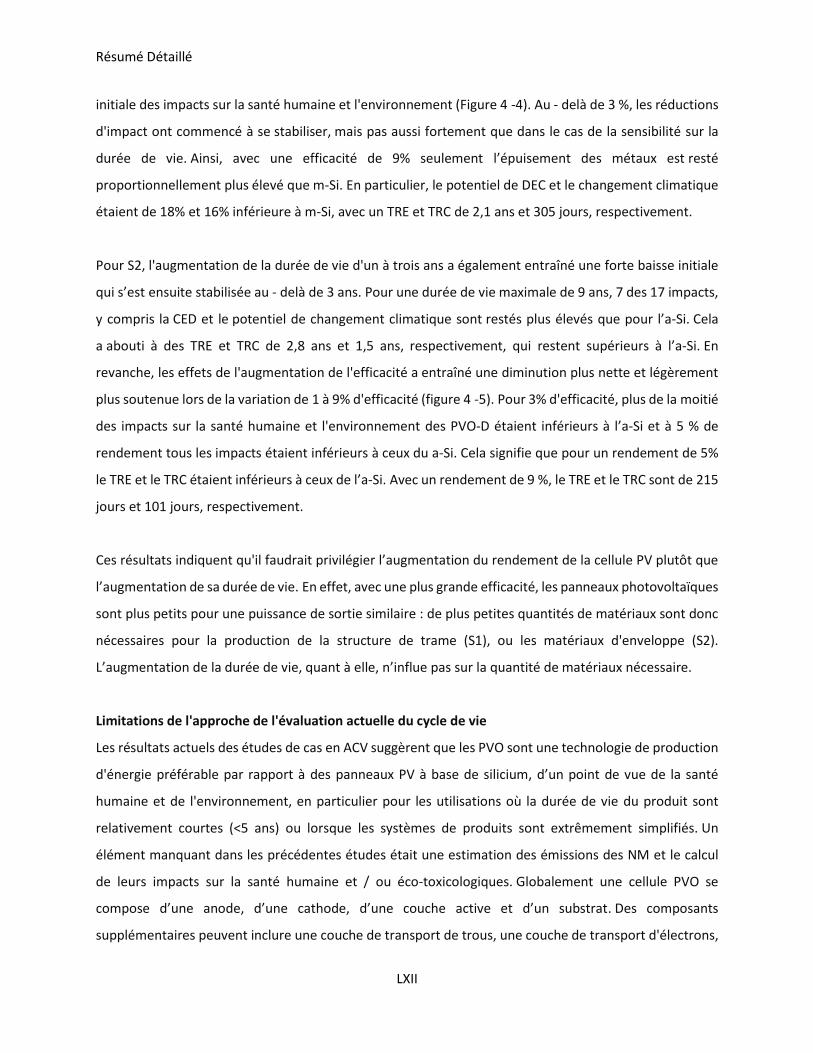
Résumé Détaillé
LXII
initiale des impacts sur la santé humaine et l'environnement (Figure 4 -4). Au - delà de 3 %, les réductions
d'impact ont commencé à se stabiliser, mais pas aussi fortement que dans le cas de la sensibilité sur la
durée de vie. Ainsi, avec une efficacité de 9% seulement l’épuisement des métaux est resté
proportionnellement plus élevé que m-Si. En particulier, le potentiel de DEC et le changement climatique
étaient de 18% et 16% inférieure à m-Si, avec un TRE et TRC de 2,1 ans et 305 jours, respectivement.
Pour S2, l'augmentation de la durée de vie d'un à trois ans a également entraîné une forte baisse initiale
qui s’est ensuite stabilisée au - delà de 3 ans. Pour une durée de vie maximale de 9 ans, 7 des 17 impacts,
y compris la CED et le potentiel de changement climatique sont restés plus élevés que pour l’a-Si. Cela
a abouti à des TRE et TRC de 2,8 ans et 1,5 ans, respectivement, qui restent supérieurs à l’a-Si. En
revanche, les effets de l'augmentation de l'efficacité a entraîné une diminution plus nette et légèrement
plus soutenue lors de la variation de 1 à 9% d'efficacité (figure 4 -5). Pour 3% d'efficacité, plus de la moitié
des impacts sur la santé humaine et l'environnement des PVO-D étaient inférieurs à l’a-Si et à 5 % de
rendement tous les impacts étaient inférieurs à ceux du a-Si. Cela signifie que pour un rendement de 5%
le TRE et le TRC étaient inférieurs à ceux de l’a-Si. Avec un rendement de 9 %, le TRE et le TRC sont de 215
jours et 101 jours, respectivement.
Ces résultats indiquent qu'il faudrait privilégier l’augmentation du rendement de la cellule PV plutôt que
l’augmentation de sa durée de vie. En effet, avec une plus grande efficacité, les panneaux photovoltaïques
sont plus petits pour une puissance de sortie similaire : de plus petites quantités de matériaux sont donc
nécessaires pour la production de la structure de trame (S1), ou les matériaux d'enveloppe (S2).
L’augmentation de la durée de vie, quant à elle, n’influe pas sur la quantité de matériaux nécessaire.
Limitations de l'approche de l'évaluation actuelle du cycle de vie
Les résultats actuels des études de cas en ACV suggèrent que les PVO sont une technologie de production
d'énergie préférable par rapport à des panneaux PV à base de silicium, d’un point de vue de la santé
humaine et de l'environnement, en particulier pour les utilisations où la durée de vie du produit sont
relativement courtes (<5 ans) ou lorsque les systèmes de produits sont extrêmement simplifiés. Un
élément manquant dans les précédentes études était une estimation des émissions des NM et le calcul
de leurs impacts sur la santé humaine et / ou éco-toxicologiques. Globalement une cellule PVO se
compose d’une anode, d’une cathode, d’une couche active et d’un substrat. Des composants
supplémentaires peuvent inclure une couche de transport de trous, une couche de transport d'électrons,
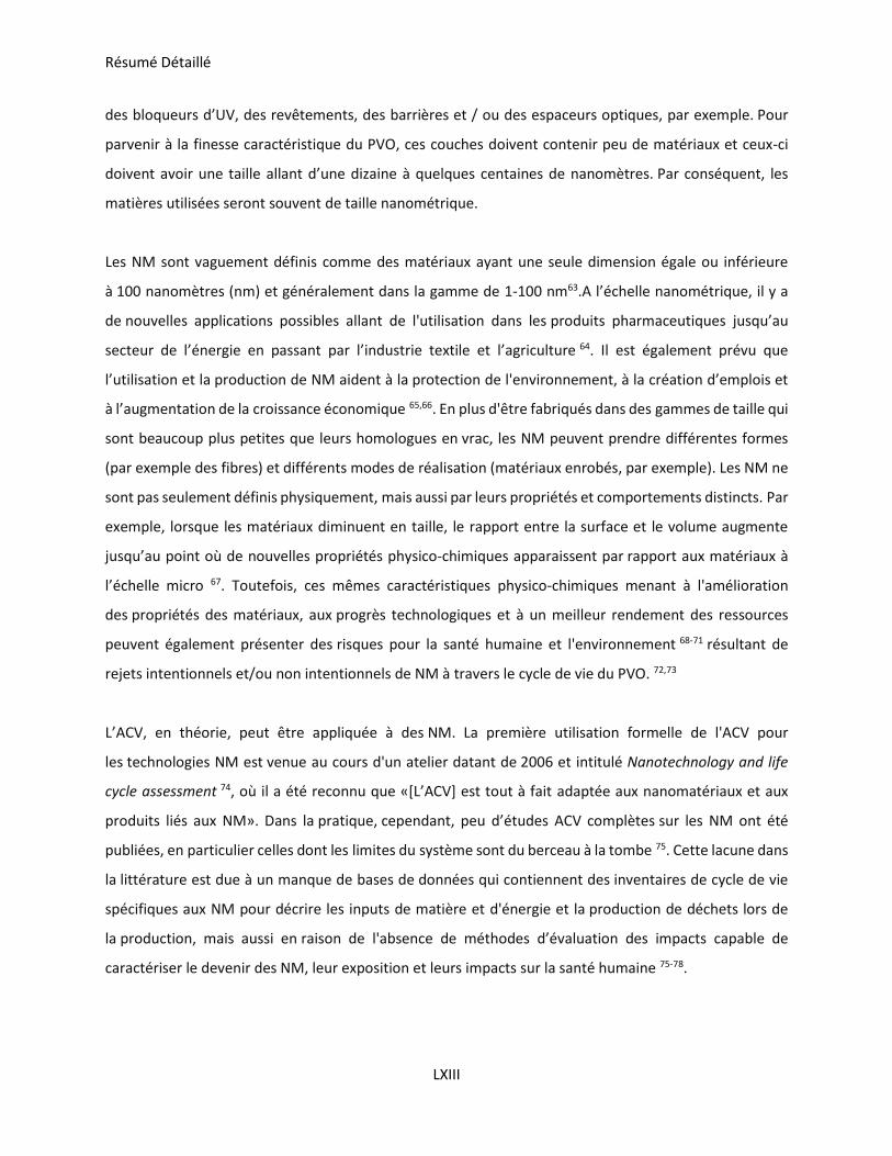
Résumé Détaillé
LXIII
des bloqueurs d’UV, des revêtements, des barrières et / ou des espaceurs optiques, par exemple. Pour
parvenir à la finesse caractéristique du PVO, ces couches doivent contenir peu de matériaux et ceux-ci
doivent avoir une taille allant d’une dizaine à quelques centaines de nanomètres. Par conséquent, les
matières utilisées seront souvent de taille nanométrique.
Les NM sont vaguement définis comme des matériaux ayant une seule dimension égale ou inférieure
à 100 nanomètres (nm) et généralement dans la gamme de 1-100 nm63.A l’échelle nanométrique, il y a
de nouvelles applications possibles allant de l'utilisation dans les produits pharmaceutiques jusqu’au
secteur de l’énergie en passant par l’industrie textile et l’agriculture 64. Il est également prévu que
l’utilisation et la production de NM aident à la protection de l'environnement, à la création d’emplois et
à l’augmentation de la croissance économique 65,66. En plus d'être fabriqués dans des gammes de taille qui
sont beaucoup plus petites que leurs homologues en vrac, les NM peuvent prendre différentes formes
(par exemple des fibres) et différents modes de réalisation (matériaux enrobés, par exemple). Les NM ne
sont pas seulement définis physiquement, mais aussi par leurs propriétés et comportements distincts. Par
exemple, lorsque les matériaux diminuent en taille, le rapport entre la surface et le volume augmente
jusqu’au point où de nouvelles propriétés physico-chimiques apparaissent par rapport aux matériaux à
l’échelle micro 67. Toutefois, ces mêmes caractéristiques physico-chimiques menant à l'amélioration
des propriétés des matériaux, aux progrès technologiques et à un meilleur rendement des ressources
peuvent également présenter des risques pour la santé humaine et l'environnement 68-71 résultant de
rejets intentionnels et/ou non intentionnels de NM à travers le cycle de vie du PVO. 72,73
L’ACV, en théorie, peut être appliquée à des NM. La première utilisation formelle de l'ACV pour
les technologies NM est venue au cours d'un atelier datant de 2006 et intitulé Nanotechnology and life
cycle assessment 74, où il a été reconnu que «[L’ACV] est tout à fait adaptée aux nanomatériaux et aux
produits liés aux NM». Dans la pratique, cependant, peu d’études ACV complètes sur les NM ont été
publiées, en particulier celles dont les limites du système sont du berceau à la tombe 75. Cette lacune dans
la littérature est due à un manque de bases de données qui contiennent des inventaires de cycle de vie
spécifiques aux NM pour décrire les inputs de matière et d'énergie et la production de déchets lors de
la production, mais aussi en raison de l'absence de méthodes d’évaluation des impacts capable de
caractériser le devenir des NM, leur exposition et leurs impacts sur la santé humaine 75-78.
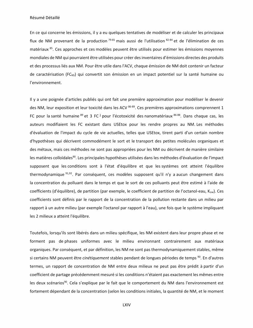
Résumé Détaillé
LXIV
En ce qui concerne les émissions, il y a eu quelques tentatives de modéliser et de calculer les principaux
flux de NM provenant de la production 79-81 mais aussi de l'utilisation 82-84 et de l'élimination de ces
matériaux 85. Ces approches et ces modèles peuvent être utilisés pour estimer les émissions moyennes
mondiales de NM qui pourraient être utilisées pour créer des inventaires d’émissions directes des produits
et des processus liés aux NM. Pour être utile dans l'ACV, chaque émission de NM doit contenir un facteur
de caractérisation (FCNS) qui convertit son émission en un impact potentiel sur la santé humaine ou
l’environnement.
Il y a une poignée d'articles publiés qui ont fait une première approximation pour modéliser le devenir
des NM, leur exposition et leur toxicité dans les ACV 86-89. Ces premières approximations comprennent 1
FC pour la santé humaine 89 et 3 FC 1 pour l’écotoxicité des nanomatériaux 86-88. Dans chaque cas, les
auteurs modifiaient les FC existant dans USEtox pour les rendre propres au NM. Les méthodes
d'évaluation de l'impact du cycle de vie actuelles, telles que USEtox, tirent parti d'un certain nombre
d'hypothèses qui décrivent commodément le sort et le transport des petites molécules organiques et
des métaux, mais ces méthodes ne sont pas appropriées pour les NM ou décrivent de manière similaire
les matières colloïdales90. Les principales hypothèses utilisées dans les méthodes d'évaluation de l'impact
supposent que les conditions sont à l'état d'équilibre et que les systèmes ont atteint l'équilibre
thermodynamique 91,92. Par conséquent, ces modèles supposent qu'il n'y a aucun changement dans
la concentration du polluant dans le temps et que le sort de ces polluants peut être estimé à l'aide de
coefficients (d’équilibre), de partition (par exemple, le coefficient de partition de l’octanol-eau, Kow). Ces
coefficients sont définis par le rapport de la concentration de la pollution restante dans un milieu par
rapport à un autre milieu (par exemple l'octanol par rapport à l'eau), une fois que le système impliquant
les 2 milieux a atteint l'équilibre.
Toutefois, lorsqu'ils sont libérés dans un milieu spécifique, les NM existent dans leur propre phase et ne
forment pas de phases uniformes avec le milieu environnant contrairement aux matériaux
organiques. Par conséquent, et par définition, les NM ne sont pas thermodynamiquement stables, même
si certains NM peuvent être cinétiquement stables pendant de longues périodes de temps 90. En d'autres
termes, un rapport de concentration de NM entre deux milieux ne peut pas être prédit à partir d'un
coefficient de partage précédemment mesuré si les conditions n’étaient pas exactement les mêmes entre
les deux scénarios90. Cela s’explique par le fait que le comportement du NM dans l'environnement est
fortement dépendant de la concentration (selon les conditions initiales, la quantité de NM, et le moment
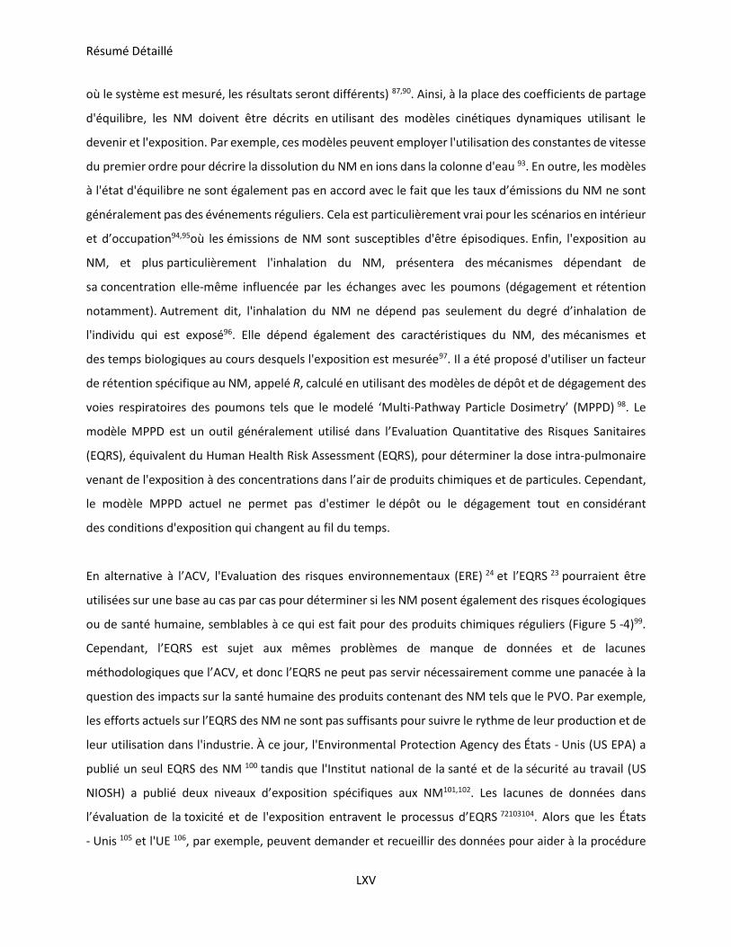
Résumé Détaillé
LXV
où le système est mesuré, les résultats seront différents) 87,90. Ainsi, à la place des coefficients de partage
d'équilibre, les NM doivent être décrits en utilisant des modèles cinétiques dynamiques utilisant le
devenir et l'exposition. Par exemple, ces modèles peuvent employer l'utilisation des constantes de vitesse
du premier ordre pour décrire la dissolution du NM en ions dans la colonne d'eau 93. En outre, les modèles
à l'état d'équilibre ne sont également pas en accord avec le fait que les taux d’émissions du NM ne sont
généralement pas des événements réguliers. Cela est particulièrement vrai pour les scénarios en intérieur
et d’occupation94,95où les émissions de NM sont susceptibles d'être épisodiques. Enfin, l'exposition au
NM, et plus particulièrement l'inhalation du NM, présentera des mécanismes dépendant de
sa concentration elle-même influencée par les échanges avec les poumons (dégagement et rétention
notamment). Autrement dit, l'inhalation du NM ne dépend pas seulement du degré d’inhalation de
l'individu qui est exposé96. Elle dépend également des caractéristiques du NM, des mécanismes et
des temps biologiques au cours desquels l'exposition est mesurée97. Il a été proposé d'utiliser un facteur
de rétention spécifique au NM, appelé R, calculé en utilisant des modèles de dépôt et de dégagement des
voies respiratoires des poumons tels que le modelé ‘Multi-Pathway Particle Dosimetry’ (MPPD) 98. Le
modèle MPPD est un outil généralement utilisé dans l’Evaluation Quantitative des Risques Sanitaires
(EQRS), équivalent du Human Health Risk Assessment (EQRS), pour déterminer la dose intra-pulmonaire
venant de l'exposition à des concentrations dans l’air de produits chimiques et de particules. Cependant,
le modèle MPPD actuel ne permet pas d'estimer le dépôt ou le dégagement tout en considérant
des conditions d'exposition qui changent au fil du temps.
En alternative à l’ACV, l'Evaluation des risques environnementaux (ERE) 24 et l’EQRS 23 pourraient être
utilisées sur une base au cas par cas pour déterminer si les NM posent également des risques écologiques
ou de santé humaine, semblables à ce qui est fait pour des produits chimiques réguliers (Figure 5 -4)99.
Cependant, l’EQRS est sujet aux mêmes problèmes de manque de données et de lacunes
méthodologiques que l’ACV, et donc l’EQRS ne peut pas servir nécessairement comme une panacée à la
question des impacts sur la santé humaine des produits contenant des NM tels que le PVO. Par exemple,
les efforts actuels sur l’EQRS des NM ne sont pas suffisants pour suivre le rythme de leur production et de
leur utilisation dans l'industrie. À ce jour, l'Environmental Protection Agency des États - Unis (US EPA) a
publié un seul EQRS des NM 100 tandis que l'Institut national de la santé et de la sécurité au travail (US
NIOSH) a publié deux niveaux d’exposition spécifiques aux NM101,102. Les lacunes de données dans
l’évaluation de la toxicité et de l'exposition entravent le processus d’EQRS 72103104. Alors que les États
- Unis 105 et l'UE 106, par exemple, peuvent demander et recueillir des données pour aider à la procédure
Résumé Détaillé
LXVI
d’EQRS pour les NM, une évaluation de tous les NM enregistrés n'a pas été réalisée. Bien que certaines
données et certains efforts de modélisation puissent être contournés avec une EQRS, par exemple, en
mesurant directement les doses d'exposition ou les concentrations auxquelles on est soumis. Plus
communément, cependant, des approches qualitatives d’EQRS107-110 ont été mises en avant
pour prioriser les efforts de recherche, la gestion de l'environnement et les activités de réglementation
dans le cas des NM. Néanmoins, de nombreux modèles spécifiques aux NM, des approches qualitatives
par niveaux de contrôle jusqu’à des approches dynamiques plus sophistiquées112.113ont été élaborées ou
sont en cours d'élaboration pour les NM. Ces outils sont donc une option pour lutter contre les effets sur
la santé humaine des NM utilisés dans le PVO.
Par conséquent, l'ACV permettant le calcul des impacts potentiels sur la santé humaine de nombreuses
sources d’émissions tout au long du cycle de vie, les décideurs pourraient trouver utile d'employer cet
outil à tous les stades de développement de la technologie et à des fins d'écoconception. Toutefois, pour
les technologies contenant des NM, si l'évaluation des NM n'est pas possible, les décideurs peuvent choisir
d'utiliser simplement une EQRS, en particulier une fois la fabrication d’un produit atteint des volumes
relativement importants. Le développement à grande échelle ou l’adoption d'un produit par la société
exige que les risques sur la santé humaine soient évités. Le développement à grande échelle implique un
enregistrement auprès des organismes de réglementation appropriés qui peuvent avoir besoin d’une
EQRS dans le cadre de l'enregistrement ou de la conformité d’un produit. Tout en ayant la capacité de
fournir des estimations définitives des risques des NM pour la santé humaine, un inconvénient critique
de cette option est le niveau de détail induit, qui n’est pas nécessaire dans le cas du développement à un
stade précoce. Par conséquent, ces outils sont souvent utilisés séparément par différents types de parties
prenantes qui ont différents besoins.
Cependant, une utilisation complémentaire, en utilisant les deux outils séparément, puis en combinant
leurs résultats, est une approche évidente lorsque l'évaluation à la fois de l'efficacité des ressources et
des effets sur la santé du NM doit être envisagée. Cette option implique donc nécessairement une
évaluation détaillée de l'exposition au risque et du NM. Par conséquent, une utilisation
complémentaire sera la plus appropriée au cours du développement de la technologie à grande échelle
ou quand il sera nécessaire d'assurer la protection de la santé humaine107114115. Cette
utilisation complémentaire exige également que les différents champs d'application ou les résultats des
deux outils soient conciliés. Pour clarifier, l’ACV échelonne ses résultats à un service ou à une unité «
Résumé Détaillé
LXVII
fonctionnelle » (par exemple, la production d'un kWh d'énergie moyenne), tandis que l’ERE est définie
par un scénario d'exposition pertinent (par exemple, le risque pour la santé humaine posé par des
émissions de TiO2 à l’échelle nano dans une installation industrielle). Ainsi, leurs résultats demandent une
conversion à réaliser avec prudence (i.e. normaliser les résultats de chaque outil de telle sorte qu'ils
puissent être comparés sur des unités relatives, telles que la conversion en dommages) avant que les
comparaisons des résultats puissent être faites 116. Même dans ce cas-là, ces 2 méthodes peuvent ne pas
être comparables, à moins que les champs d'application de chaque outil aient été définis de
façon stratégique. Autrement dit, l'utilisation complémentaire ne sera probablement pas en mesure
d'exprimer la façon proportionnelle l'ENM-risque qui en résulte dans le contexte des risques
toxicologiques définies par LCA.
Par opposition à l’utilisation complémentaire, l'intégration se réfère ici à la combinaison des méthodes de
chaque outil au lieu de combiner leurs résultats. 117 Cette approche utilise des méthodes généralement
attribuées à l’ERSA pour estimer le sort et les effets dus à l’exposition aux NM. Parce que l'intégration
permet (a) l'interprétation des risques toxicologiques des NM dans un produit (unité fonctionnelle) et (b)
la comparaison directe des risques des NM à tous les autres risques chimiques estimés pendant le cycle
de vie, cette approche permet de veiller à ce que le transfert d’impacts ne se produise pas. 86 L'intégration
peut donc être utilisé comme une alternative à des utilisations existantes d’utilisation complémentaire ou
séparée, mais il peut être aussi utilisé uniquement pour l'évaluation du développement d’un produit dans
sa phase de conception, pour de l’écoconception, ou pour des déclarations environnementales de produit
par exemple. 118
Santé humaine et évaluation des risques : Étude de cas du dioxyde de titane
L’ERE est utilisée comme un outil préliminaire pour évaluer les risques pour la santé humaine des NM
utilisés dans les dispositifs de PVO, puis les principaux aspects méthodologiques des EQRS sont identifiés
afin d’être intégrés dans les méthodes d'évaluation de l'impact du cycle de vie. Alors que les émissions de
NM peuvent conduire à des impacts sur l’environnement et la santé humaine, cette thèse a choisi de se
concentrer sur les aspects de la santé humaine. Pour commencer à déterminer ces impacts potentiels,
l’EQRS a été appliquée aux études de cas sur le PVO utilisées dans cette thèse. L’EQRS est un moyen
d'identifier les dangers d'une substance, de quantifier la relation « dose-effet » de la substance avec les
dommages toxicologiques, d’estimer l'exposition à la substance et de quantifier la probabilité du risque
basée sur la comparaison du niveau d'exposition avec la relation « dose-effet ». Dans le cadre de thèse,
Résumé Détaillé
LXVIII
seul l’aspect qualitatif des risques posés par les émissions de NM durant les étapes du cycle de vie du
PVO sera abordé. Ainsi, une EQRS qualitative a été utilisée pour identifier les étapes du cycle de vie et
les scénarios d'exposition qui justifieraient une analyse plus approfondie par une EQRS
quantitative. En utilisant un ensemble de critères qualitatifs, il a été évalué (i) l'existence d'une interaction
directe avec le NM, (ii) le volume de NM impliqués, (iii) l’utilisation d'équipements de protection
individuelle, (iv) la probabilité que les émissions de NM se produisent, et (v) la voie d'exposition
potentielle. Sur la base de ces critères, il a été constaté que les émissions et l'exposition finale au NM
étaient plus susceptibles de se produire lors de la production du NM, ainsi que lors la fabrication des
panneaux PVO. Alors que les émissions et l'exposition lors de l'utilisation et des phases de fin de vie ne
pouvaient pas être exclues, il était attendu que les émissions seraient beaucoup plus faibles au cours
de ces étapes du cycle de vie puisque les NM sont encapsulés dans une matrice polymère, au lieu d'être
traités comme des poudres sèches et volatiles pendant les étapes de production et de fabrication. Dans
ces scénarios de travail, les émissions seraient limitées à l’air intérieur environnant, conduisant
potentiellement à deux voies d'exposition : par inhalation et par voie cutanée.
Cette thèse se concentre sur un NM représentatif de ce qui est utilisé en quantités industrielles et dont
les données toxicologiques et physico-chimiques seraient suffisamment fournies pour établir le devenir,
l'exposition et la modélisation de l'effet pour l'EQRS quantitative. Par conséquent, le TiO2 (dioxyde de
titane) nanométrique utilisé comme espaceur optique du PVO est utilisé comme étude de cas dans cette
thèse pour étudier et déterminer les impacts potentiels sur la santé humaine induits par l'utilisation des
technologies NM dans le PVO. En ce qui concerne les études in vivo d’inhalation des animaux, le nano-
TiO2 a été relié à plusieurs impacts négatifs tels que l’inflammation, l'histopathologie, la cytotoxicité,
le stress oxydant, les effets oncogènes et les impacts géno-toxiques. Par rapport à son homologue
dispersé, ces effets se sont révélés être plus prononcés. En ce qui concerne les effets néfastes de
l’exposition cutanée, les études in vivo sur animaux démontrent un certain niveau de pénétration,
principalement dans les couches épidermiques superficielles de la peau. Dans certains cas, du stress
oxydant ou des lésions sur les organes peuvent se produire alors que peu ou pas d’irritation de la peau
est observée. L'EQRS a modélisé les émissions pour plusieurs volumes (de faible à élevé) d‘utilisation de
nano-TiO2 qui ont inclus la manipulation de ces matériaux en opposition aux émissions lors de la
production des matériaux. Le devenir et le transport des nano-TiO2 ont été modélisés dans un modèle
d’atmosphère intérieur à deux zones où l'émission est supposée venir d’une seule source située dans une
zone de champ proche qui a ensuite été reliée à une zone de champ lointain au sein de cette même
Résumé Détaillé
LXIX
pièce. L'exposition a été supposée se produire complètement à l'intérieur de la zone de champ proche et
a été estimée comme étant la concentration dans l'air sans prendre en compte du dépôt et / ou de
la rétention des particules dans les poumons. Cette corrélation avec les données in vivo de toxicité a été
prise à partir d'un modèle d’exposition par inhalation chronique pour mesurer les effets de l'inflammation
pulmonaire chez la souris et le rat. Les résultats de l'EQRS ont démontré que le risque d'inflammation due
à l'inhalation de nano-TiO2 était très probable dans les cas où de grands volumes de nano-poudre sont
manipulés et jetés dans de grands conteneurs ouverts. Plus précisément, ce fut le cas pour lequel des sacs
de 10 kg de nano-TiO2 ont été transférés sur une période de 10 minutes dans de grands réservoirs de
mélange tout au long d'une journée de travail de 8 heures. De tels scénarios peuvent se présenter à la fois
lors de la production de nano-TiO2 ainsi que lors de la fabrication du panneau PVO, dans l’hypothèse où
cette technologie atteint des volumes de production industrielle à grande échelle.
Les résultats de l'EQRS démontrent que l'inquiétude suscitée par les risques toxicologiques potentiels
pour la santé humaine lors de l'utilisation de NM dans le PVO peut être justifiée, même dans les cas où de
grands volumes de NM sont utilisés dans des configurations à l'échelle industrielle. Ces résultats sont
importants et signalent que les technologies PV émergentes telles que le PVO peuvent engendrer des
risques éventuels sur la santé humaine et l'environnement. Bien que cette information soit
particulièrement importante pour les gestionnaires de risques professionnels qui veulent identifier et
diminuer l’importance des impacts sur la santé humaine sur un lieu de travail, les résultats de tels cas
EQRS ne permettent de savoir si le PVO sont un choix de production d'énergie préférable par rapport au
silicium photovoltaïque. Pour ce faire, l'estimation du devenir, de l'exposition et de l'effet devrait être en
corrélation avec l'unité fonctionnelle dans une ACV pour permettre des comparaisons directes avec les
impacts sur la santé humaine du silicium PV.
Intégration des impacts ‘nano-spécifiques’ sur la santé humaine via la méthodologie ACV : Application
au photovoltaïque organique
L’EQRS a été intégrée à l'évaluation de l'impact du cycle de vie. De cette façon, les résultats de l'ACV ont
été mis à jour pour inclure les contributions des nano-TiO2 comme une première indication de la façon
dont les impacts sur la santé humaine pourraient évoluer suite à la prise en compte des émissions liées
au NM au long du cycle de vie du PVO. Ce travail a abouti à la création d'un facteur de caractérisation
spécifique aux nano particules (CFNS) pour une utilisation dans l'ACV. Plus précisément, la plupart des
éléments de la modélisation EQRS utilisés pour estimer les quantités émises, le devenir et les effets
Résumé Détaillé
LXX
associés à ces substances ont été adaptés pour une utilisation dans l’étape d’évaluation des
impacts. L’objectif de cette thèse étant une analyse prospective, le scénario d'émission à l'échelle
industrielle a été utilisé pour suivre les conditions et les rejets de nano-TiO2 du fait des volumes élevés
sur le lieu de travail. En raison de la nature non-équilibrée du comportement des NM dans
l'environnement, le devenir et l’exposition des résultats sont directement dépendant de l'intensité de
la source d'émission et des concentrations dans l'air en nano-TiO2. Ainsi, diverses sources d'émission et
ainsi que les fréquences d’émission associées ont été évaluées afin de déterminer leur influence sur le
devenir et l'exposition des particules nano-TiO2. Le modèle présente deux compartiments, champ proche
et champ lointain, ce dernier ayant été modifié pour tenir compte des autres sources (hors ventilation)
de l'élimination des particules du compartiment de l'air intérieur. Ces mécanismes d'élimination incluent
l’homo-agrégation et la sédimentation gravitationnelle des particules sur des surfaces
intérieures. L'exposition au nano-TiO2 a été évaluée à l'aide d'un modèle pharmacocinétique basé sur la
physiologie (PBPK) pour déterminer le dépôt, le dégagement et la rétention de ces particules dans les
poumons au cours du temps. Le modèle PBPK a calculé la dose pulmonaire interne de nano-
TiO2 conduisant à une série de réactions impliquant la translocation due aux particules dans la région
pulmonaire et l'interstitium des poumons, mais également à la circulation systémique, la séquestration
de particules par les cellules phagocytaires, et le transfert de particules et / ou de cellules vers la zone
trachéo-bronchique via la clairance muco-ciliaire. Le facteur de caractérisation final CFNS a été défini pour
deux catégories d'impact sur la santé humaine : les impacts cancérigènes et non cancérigènes sur la base
de données in vivo pertinentes reposant sur des mécanismes toxicologiques de dose-effet conduisant à
la croissance de tumeurs pulmonaires et à l’inflammation du poumon chez les animaux.
Les résultats de la modélisation du CF NS pour les particules nano-TiO2 démontrent qu'il existe
une sensibilité significative en fonction de la puissance de la source d'émission ainsi que des durées
pendant lesquelles la population des travailleurs est exposée sur le site industriel. Cependant, pour le cas
où des travailleurs étaient exposés régulièrement dans une production à l’échelle industrielle, il y avait
très peu de changements dans les impacts sur la santé humaine de l'étude ACV-PVO après réévaluation
du cycle de vie selon l’approche « Berceau à la porte de l’usine » avec la prise en compte du CFNS
nouvellement défini. La contribution totale s’élève à moins de 1% des impacts sur la santé humaine
provoqués par les émissions de nano-TiO2 au cours de la production de NM ou la fabrication de PVO. Ces
résultats suggèrent que les émissions de NM à travers le cycle de vie peuvent être considérées comme
marginales dans la majorité des cas. Cependant, ces résultats doivent être considérés avec prudence car
Résumé Détaillé
LXXI
ils ne tiennent en compte que des impacts liés aux émissions de nano-TiO2 pendant seulement une partie
du cycle de vie complet du PVO. D'autres émissions peuvent se produire pendant la phase
d'utilisation, mais plus probablement pendant les phases de fin de vie, surtout lors d’une mise en
décharge avec des émissions au fil du temps. En outre, les panneaux PVO sont fabriqués avec des couches
de matériaux qui sont toutes déposées à des niveaux d’épaisseur de l’ordre du nanomètre. Par
conséquent, le PVO peut présenter beaucoup plus d'émissions de NM le long du cycle de vie que
seulement les particules nano-TiO2. Néanmoins, tous ces matériaux ne peuvent être préparés et
manipulés de la même manière, ils auront donc probablement des niveaux différents de toxicité. Ainsi,
leur contribution ultime pour les impacts sur la santé humaine à travers le cycle de vie du PVO variera.
Conclusions et perspectives
Les résultats de l’étude de cas ACV-PVO et l'évaluation ultérieure des impacts sur la santé humaine due à
l'utilisation de certains NM dans le PVO conduisent à penser que la technologie PVO est une option de
production d'énergie préférable par rapport au PV silicium pour les critères de santé humaine et d’impacts
sur l'environnement. Ces résultats sont fortement dépendants de la manière dont les dispositifs
photovoltaïques sont utilisés et de leurs durées de vie. Les incertitudes, principalement liées à la durée
de vie et l'efficacité du PVO, empêchent de se prononcer définitivement afin de savoir si le PVO se révèle
être une option d'approvisionnement en énergie écologiquement préférable. Cependant, ces incertitudes
peuvent être marginalisées lorsque les technologies PVO sont limitées à des produits ayant des durées
de vie relativement courtes (par exemple les produits où l'utilisation est typiquement <5 ans), pour
lesquelles la préférence pour le PVO devient manifeste. Les résultats de cette thèse ont cependant montré
que le PVO avait vocation à être utilisé pour des panneaux solaires sur les toits, là où le PV à base de
silicium a dominé pendant des décennies.
En terme d’approche la plus appropriée pour évaluer les technologies émergentes, l’ACV se présente
comme la méthode la plus complète pour évaluer l'efficacité des ressources et les dangers potentiels des
technologies de production d'énergie telles que le PVO. Sa large prise en compte des différentes variables
environnementales sur toute l'étendue du cycle de vie d’un produit contribue à assurer que le
développement ou la diffusion d'un produit ne se traduisent pas par un transfert de pollution d'une
catégorie d'impact à l'autre. La compréhension de la santé humaine et des risques écologiques des NM
est nécessaire pour l'évaluation de cette technologie, mais n’est pas totalement possible par les
méthodologies d'évaluation d'impact actuelles. Alors que l'EQRS a permis une évaluation plus détaillée
Résumé Détaillé
LXXII
des risques absolus de l'utilisation de NM à une étape du cycle de vie spécifique, les évaluations de risque
absolu sont peut-être trop ambitieuses depuis que la technologie PVO se développe. Au lieu de cela, une
approche intégrée dans l'évaluation des impacts du cycle de vie permet d'évaluer à des stades de
développement antérieures du PVO de telle façon que les résultats des impacts des NM sur la santé
humaine puissent être directement interprétés et évalués dans le cadre de toutes les autres catégories
d'impact sur la santé humaine présentes dans l’ACV. Cette approche permet des analyses sur les points
sensibles, l'identification et l'évitement de transferts de pollution et le soutien pour les concepts d'éco-
conception, nécessaires pour le développement durable d'une source d'énergie renouvelable émergente.
Les travaux de cette thèse visent à combler les lacunes de données et les choix de modélisation. En
particulier, la probabilité et la quantification des émissions de NM à travers le cycle de vie demeurent
largement inconnues. Bien que certains travaux ont démontré que le PVO peut émettre des lixiviats
provenant des différentes couches au fil du temps, 119-121 en particulier lorsqu’elles sont endommagées, il
n'y a pas de données montrant quelle fraction de ces substances sont dans leur nano-forme (i.e. par
opposition à ionique). En ce qui concerne la modélisation, une autre distinction peut être faite dans l’ACV
entre attributionnel et conséquentiel. Ce travail de thèse a utilisé des ACV attributionnelles pour répondre
à la question « Quelle est la part de charge environnementale globale, qui peut être attribuée aux
technologies PVO ?» Bien que cette approche soit pertinente pour l'analyse des points sensibles et une
compréhension basique des charges environnementales associées au PVO, une ACV conséquentielle
pourrait être utilisée pour mieux comprendre ce que les effets futurs et / ou à long terme seraient dans
le secteur de l’énergie avec l’émergence des panneaux PVO. Cette approche serait appropriée pour
une meilleure compréhension, le cas échéant, des conséquences liées à une substitution partielle d’une
technologie classique par du PVO.
Mots clés : l’analyse du cycle de vie, photovoltaïques organiques, nanomatériaux fabriqués, l'evaluation
des risques, l'exposition, énergie renouvelable
Bibliographie du Résumé Détaillé
1. Robert, K. W., Parris, T. M. & Leiserowitz, A. A. What is Sustainable Development? Goals, Indicators, Values, and Practice. Environ. Sci.
Policy Sustain. Dev. 47, 8–21 (2005).
2. Bardi, U. Peak oil: The four stages of a new idea. Energy 34, 323–326 (2009).
3. Carbon accounting. Nat. Clim. Chang. (2016). doi:10.1038/nclimate3137
4. Moss, R. H. et al. The next generation of scenarios for climate change research and assessment. Nature 463, 747–756 (2010).
5. Fraiture, C. de, Giordano, M. & Liao, Y. Biofuels and implications for agricultural water use: blue impacts of green energy. Water Policy
Résumé Détaillé
LXXIII
10, 67 (2008).
6. Escobar, J. C. et al. Biofuels: Environment, technology and food security. Renew. Sustain. Energy Rev. 13, 1275–1287 (2009).
7. Howarth, R. W. & Bringezu, S. Biofuels: Environmental Consequences and Interactions with Changing Land Use - Proceedings of the
Scientific Committee on Problems of the Environment (SCOPE) International Biofuels Project Rapid Assessment. (2008). at
<http://cip.cornell.edu/DPubS?service=UI&version=1.0&verb=Display&page=current&handle=scope>
8. Searchinger, T. et al. Use of U.S. Croplands for Biofuels Increases Greenhouse Gases Through Emissions from Land-Use Change.
Science (80-. ). 319, 1238–1240 (2008).
9. Hertwich, E. G. et al. Integrated life-cycle assessment of electricity-supply scenarios confirms global environmental benefit of low-
carbon technologies. Proc. Natl. Acad. Sci. 112, 6277–6282 (2015).
10. Green, M. A. Photovoltaics: coming of age. in IEEE Conference on Photovoltaic Specialists 1–8 (IEEE). doi:10.1109/PVSC.1990.111582
11. Green, M. A., Emery, K., Hishikawa, Y., Warta, W. & Dunlop, E. D. Solar cell efficiency tables (version 47). Prog. Photovoltaics Res.
Appl. 24, 3–11 (2016).
12. Fraunhofer Institute for Solar Energy Systems ISE. Photovoltaics Report (2016). (2016).
13. Fthenakis, V. & Alsema, E. Photovoltaics energy payback times, greenhouse gas emissions and external costs: 2004–early 2005 status.
Prog. Photovoltaics Res. Appl. 14, 275–280 (2006).
14. Tang, C. W. Multilayer organic photovoltaic elements. (1979).
15. Espinosa, N., Hösel, M., Jørgensen, M. & Krebs, F. C. Large scale deployment of polymer solar cells on land, on sea and in the air.
Energy Environ. Sci. 7, 855 (2014).
16. Krebs, F. C., Tromholt, T. & Jørgensen, M. Upscaling of polymer solar cell fabrication using full roll-to-roll processing. Nanoscale 2, 873
(2010).
17. Jungbluth, N. Life cycle assessment of crystalline photovoltaics in the Swiss ecoinvent database. Prog. Photovoltaics Res. Appl. 13,
429–446 (2005).
18. International Organization for Standardization. ISO 14044 - Environmental management - Life cycle assessment - Requirements and
guidelines. (2006).
19. International Organization for Standardization. ISO 14040 - Environmental Management - Life cycle assessment - Principles and
framework. (2006).
20. Roes, A. L., Alsema, E. A., Blok, K. & Patel, M. K. Ex-ante environmental and economic evaluation of polymer photovoltaics. Prog.
Photovoltaics Res. Appl. 17, 372–393 (2009).
21. García-Valverde, R., Cherni, J. A. & Urbina, A. Life cycle analysis of organic photovoltaic technologies. Prog. Photovoltaics Res. Appl.
18, 535–558 (2010).
22. Espinosa, N., García-Valverde, R., Urbina, A. & Krebs, F. C. A life cycle analysis of polymer solar cell modules prepared using roll-to-roll
methods under ambient conditions. Sol. Energy Mater. Sol. Cells 95, 1293–1302 (2011).
23. US EPA, O. Human Health Risk Assessment.
24. European Union European Environment Agency. Environmental Risk Assessment - Approaches, Experiences and Information Sources
— European Environment Agency. (1998). at <http://www.eea.europa.eu/publications/GH-07-97-595-EN-C2>
25. Thompson, B. C. & Fréchet, J. M. J. Polymer–Fullerene Composite Solar Cells. Angew. Chemie Int. Ed. 47, 58–77 (2008).
26. Krebs, F. C. Fabrication and processing of polymer solar cells: A review of printing and coating techniques. Sol. Energy Mater. Sol. Cells
93, 394–412 (2009).
27. Kroon, R., Lenes, M., Hummelen, J. C., Blom, P. W. M. & de Boer, B. Small Bandgap Polymers for Organic Solar Cells (Polymer Material
Development in the Last 5 Years). Polym. Rev. 48, 531–582 (2008).
28. Li, C.-Z., Yip, H.-L. & Jen, A. K.-Y. Functional fullerenes for organic photovoltaics. J. Mater. Chem. 22, 4161 (2012).
29. Koster, L. J. A. The optimal band gap for plastic photovoltaics. SPIE Newsroom (2007). doi:10.1117/2.1200701.0528
30. Krebs, F. C. Roll-to-roll fabrication of monolithic large-area polymer solar cells free from indium-tin-oxide. Sol. Energy Mater. Sol. Cells
93, 1636–1641 (2009).
Résumé Détaillé
LXXIV
31. Lizin, S. et al. Life cycle analyses of organic photovoltaics: a review. Energy Environ. Sci. 6, 3136 (2013).
32. Kumar, A. & Zhou, C. The Race To Replace Tin-Doped Indium Oxide: Which Material Will Win? ACS Nano 4, 11–14 (2010).
33. Samad, W. Z., Yarmo, M. A., Salleh, M. M. & Shafiee, A. Structural, Optical and Electrical Properties of Fluorine Doped Tin Oxide Thin
Films Deposited Using Ink jet Printing Technique. Sains Malaysiana 40, 251–257 (2011).
34. Kim, H., Kushto, G. P., Auyeung, R. C. Y. & Piqué, A. Optimization of F-doped SnO2 electrodes for organic photovoltaic devices. Appl.
Phys. A 93, (2008).
35. Yu, S., Li, L., Lyu, X. & Zhang, W. Preparation and investigation of nano-thick FTO/Ag/FTO multilayer transparent electrodes with high
figure of merit. Sci. Rep. 6, 20399 (2016).
36. Su, H. et al. Highly Conductive and Low Cost Ni-PET Flexible Substrate for Efficient Dye-Sensitized Solar Cells. ACS Appl. Mater.
Interfaces 6, 5577–5584 (2014).
37. Jiang, C. Y., Sun, X. W., Zhao, D. W., Kyaw, A. K. K. & Li, Y. N. Low work function metal modified ITO as cathode for inverted polymer
solar cells. Sol. Energy Mater. Sol. Cells 94, 1618–1621 (2010).
38. Voroshazi, E., Verreet, B., Aernouts, T. & Heremans, P. Long-term operational lifetime and degradation analysis of P3HT:PCBM
photovoltaic cells. Sol. Energy Mater. Sol. Cells 95, 1303–1307 (2011).
39. Girotto, C., Voroshazi, E., Cheyns, D., Heremans, P. & Rand, B. P. Solution-Processed MoO 3 Thin Films As a Hole-Injection Layer for
Organic Solar Cells. ACS Appl. Mater. Interfaces 3, 3244–3247 (2011).
40. Steim, R., Kogler, F. R. & Brabec, C. J. Interface materials for organic solar cells. J. Mater. Chem. 20, 2499 (2010).
41. Roy, A. et al. Titanium suboxide as an optical spacer in polymer solar cells. Appl. Phys. Lett. 95, 13302 (2009).
42. Hayakawa, A., Yoshikawa, O., Fujieda, T., Uehara, K. & Yoshikawa, S. High performance polythiophene/fullerene bulk-heterojunction
solar cell with a TiO[sub x] hole blocking layer. Appl. Phys. Lett. 90, 163517 (2007).
43. Apilo, P. et al. Roll-to-roll gravure printing of organic photovoltaic modules-insulation of processing defects by an interfacial layer.
Prog. Photovoltaics Res. Appl. 23, 918–928 (2015).
44. Brabec, C. J., Shaheen, S. E., Winder, C., Sariciftci, N. S. & Denk, P. Effect of LiF/metal electrodes on the performance of plastic solar
cells. Appl. Phys. Lett. 80, 1288 (2002).
45. Zhou, Y. et al. A Universal Method to Produce Low-Work Function Electrodes for Organic Electronics. Science (80-. ). 336, 327–332
(2012).
46. Espinosa, N., Hösel, M., Angmo, D. & Krebs, F. C. Solar cells with one-day energy payback for the factories of the future. Energy
Environ. Sci. 5, 5117–5132 (2012).
47. Service, R. F. Outlook Brightens for Plastic Solar Cells. Science (80-. ). 332, 293–293 (2011).
48. Scharber, M. C. & Sariciftci, N. S. Efficiency of bulk-heterojunction organic solar cells. Prog. Polym. Sci. 38, 1929–1940 (2013).
49. Darling, S. B. & You, F. The case for organic photovoltaics. RSC Adv. 3, 17633 (2013).
50. Goedkoop, M. J. et al. A life cycle impact assessment method which comprises harmonised category indicators at the midpoint and the
endpoint level. (2009).
51. Hischier, R. et al. Implementation of Life Cycle Impact Assessment Methods. (2010).
52. Espinosa, N. et al. Life cycle assessment of ITO-free flexible polymer solar cells prepared by roll-to-roll coating and printing. Sol.
Energy Mater. Sol. Cells 97, 3–13 (2012).
53. Anctil, A. & Fthenakis, V. in Third Generation Photovoltaics (InTech, 2012). doi:10.5772/38977
54. Anctil, A., Babbitt, C. W., Raffaelle, R. P. & Landi, B. J. Cumulative energy demand for small molecule and polymer photovoltaics. Prog.
Photovoltaics Res. Appl. 21, 1541–1554 (2013).
55. Tsang, M. P., Sonnemann, G. W. & Bassani, D. M. A comparative human health, ecotoxicity, and product environmental assessment
on the production of organic and silicon solar cells. Prog. Photovoltaics Res. Appl. 24, 645–655 (2016).
56. Choi, J.-K. & Fthenakis, V. Crystalline silicon photovoltaic recycling planning: macro and micro perspectives. J. Clean. Prod. 66, 443–
449 (2014).
57. Larsen, K. End-of-life PV: then what? Renew. Energy Focus 10, 48–53 (2009).
Résumé Détaillé
LXXV
58. McDonald, N. C. & Pearce, J. M. Producer responsibility and recycling solar photovoltaic modules. Energy Policy 38, 7041–7047
(2010).
59. Doka, G. Ecoinvent report No. 13, parts I-V: Life cycle invntories of waste treatment services. (2009).
60. Espinosa, N., Laurent, A. & Krebs, F. C. Ecodesign of organic photovoltaic modules from Danish and Chinese perspectives. Energy
Environ. Sci. 8, 2537–2550 (2015).
61. Goe, M. & Gaustad, G. Strengthening the case for recycling photovoltaics: An energy payback analysis. Appl. Energy 120, 41–48
(2014).
62. Müller, A., Wambach, K. & Alsema, E. Life Cycle Analysis of Solar Module Recycling Process. MRS Proc. 895, 895-G03-7 (2005).
63. Som, C. et al. The importance of life cycle concepts for the development of safe nanoproducts. Toxicology 269, 160–169 (2010).
64. The Project on Emerging Nanotechnologies. The Nanotechnology Consumer Products Inventory. (2015). at
<http://www.nanotechproject.org/cpi/>
65. Roco, M. C. Nanotechnology’s Future. Sci. Am. 295, 39–39 (2006).
66. European Commission. Communication from the Commission to the European Parliament, The Council and the European Economic
and Social Committee (Second Regulatory Review on Nanomaterials. (2012).
67. Vance, M. E. et al. Nanotechnology in the real world: Redeveloping the nanomaterial consumer products inventory. Beilstein J.
Nanotechnol. 6, 1769–1780 (2015).
68. Royal Society and Royal Academy of Engineering. Nanoscience and nanotechnologies: opportunities and uncertainties. Nanoscience
and Nanotechnologies Opportunities and Uncertainties (Royal Society, 2004).
69. Yokel, R. A. & MacPhail, R. C. Engineered nanomaterials: exposures, hazards, and risk prevention. J. Occup. Med. Toxicol. 6, 7 (2011).
70. European Commission. Second regulatory review on nanomaterials. Communication from the Commission to the European
Parliament, the Council and the European Economic and Social Committee. (2012).
71. Pietroiusti, A. Health implications of engineered nanomaterials. Nanoscale 4, 1231 (2012).
72. Klaine, S. J. et al. Nanomaterials in the environment: behavior, fate, bioavailability, and effects. Environ. Toxicol. Chem. 27, 1825–1851
(2008).
73. Greßler, S; Nentwich, M. Nano and Environment–Part II : Hazard potentials and risks. Nano Trust Dossiers 27, 1–6 (2012).
74. Curran, M. A., Frankl, P., Jeijungs, R., Kohler, A. & Olsen, S. I. Nanotechnology and life cycle assessment: A systems approach to
Nanotechnology and the environment: Synthesis of results obtained at a workshop. (2007).
75. Hischier, R. & Walser, T. Life cycle assessment of engineered nanomaterials: State of the art and strategies to overcome existing gaps.
Sci. Total Environ. 425, 271–282 (2012).
76. Grieger, K. D. et al. Analysis of current research addressing complementary use of life-cycle assessment and risk assessment for
engineered nanomaterials: have lessons been learned from previous experience with chemicals? J. Nanoparticle Res. 14, 1–23 (2012).
77. Wender, B. A. et al. Illustrating anticipatory life cycle assessment for emerging photovoltaic technologies. Environ. Sci. Technol. 48,
10531–10538 (2014).
78. Gavankar, S., Suh, S. & Keller, A. F. Life cycle assessment at nanoscale: review and recommendations. Int. J. Life Cycle Assess. 17, 295–
303 (2012).
79. Keller, A. a., McFerran, S., Lazareva, A. & Suh, S. Global life cycle releases of engineered nanomaterials. J. Nanoparticle Res. 15, 1–17
(2013).
80. Sun, T. Y., Gottschalk, F., Hungerbühler, K. & Nowack, B. Comprehensive probabilistic modelling of environmental emissions of
engineered nanomaterials. Environ. Pollut. 185, 69–76 (2014).
81. Gottschalk, F. & Nowack, B. The release of engineered nanomaterials to the environment. J. Environ. Monit. 13, 1145 (2011).
82. Keller, A. A., Vosti, W., Wang, H. & Lazareva, A. Release of engineered nanomaterials from personal care products throughout their
life cycle. J. Nanoparticle Res. 16, 2489 (2014).
83. Hischier, R. et al. Life cycle assessment of façade coating systems containing manufactured nanomaterials. J. Nanoparticle Res. 17, 68
(2015).
Résumé Détaillé
LXXVI
84. Walser, T., Demou, E., Lang, D. J. & Hellweg, S. Prospective environmental life cycle assessment of nanosilver T-shirts. Environ. Sci.
Technol. 45, 4570–8 (2011).
85. Walser, T. et al. Persistence of engineered nanoparticles in a municipal solid-waste incineration plant. Nat. Nanotechnol. 7, 520–524
(2012).
86. Eckelman, M. J., Mauter, M. S., Isaacs, J. a & Elimelech, M. New perspectives on nanomaterial aquatic ecotoxicity: production impacts
exceed direct exposure impacts for carbon nanotoubes. Environ. Sci. Technol. 46, 2902–2910 (2012).
87. Salieri, B., Righi, S., Pasteris, A. & Olsen, S. I. Freshwater ecotoxicity characterisation factor for metal oxide nanoparticles: a case study
on titanium dioxide nanoparticle. Sci. Total Environ. 505, 494–502 (2015).
88. Miseljic, M. & Olsen, S. I. Life-cycle assessment of engineered nanomaterials: a literature review of assessment status. J. Nanoparticle
Res. 16, 1–33 (2014).
89. Pini, M., Salieri, B., Ferrari, A. M., Nowack, B. & Hischier, R. Human health characterization factors of nano-TiO2 for indoor and
outdoor environments. Int. J. Life Cycle Assess. (2016). doi:10.1007/s11367-016-1115-8
90. Praetorius, A. et al. The road to nowhere: equilibrium partition coefficients for nanoparticles. Environ. Sci. Nano 1, 317 (2014).
91. Rosenbaum, R. K. et al. USEtox—the UNEP-SETAC toxicity model: recommended characterisation factors for human toxicity and
freshwater ecotoxicity in life cycle impact assessment. Int. J. Life Cycle Assess. 13, 532–546 (2008).
92. Goedkoop, M. et al. ReCiPe 2008. (2008). at <http://www.pre-sustainability.com/download/misc/ReCiPe_main_report_final_27-02-
2009_web.pdf>
93. Meesters, J. A. J., Koelmans, A. A., Quik, J. T. K., Hendriks, A. J. & van de Meent, D. Multimedia Modeling of Engineered Nanoparticles
with SimpleBox4nano: Model Definition and Evaluation. Environ. Sci. Technol. 48, 5726–5736 (2014).
94. Koivisto, A. J. et al. Industrial worker exposure to airborne particles during the packing of pigment and nanoscale titanium dioxide.
Inhal. Toxicol. 24, 839–49 (2012).
95. Nazaroff, W. W. Indoor particle dynamics. Indoor Air, Suppl. 14, 175–183 (2004).
96. Hodas, N. et al. Indoor inhalation intake fractions of fine particulate matter: Review of influencing factors. Indoor Air n/a-n/a (2015).
doi:10.1111/ina.12268
97. Braakhuis, H. M., Park, M. V., Gosens, I., De Jong, W. H. & Cassee, F. R. Physicochemical characteristics of nanomaterials that affect
pulmonary inflammation. Part. Fibre Toxicol. 11, 18 (2014).
98. Walser, T. et al. Life-cycle assessment framework for indoor emissions of synthetic nanoparticles. J. Nanoparticle Res. 17, 1–18 (2015).
99. MacPhail, R. C., Grulke, E. A. & Yokel, R. A. Assessing nanoparticle risk poses prodigious challenges. Wiley Interdiscip. Rev.
Nanomedicine Nanobiotechnology 5, 374–387 (2013).
100. US EPA. Decision document: Conditional registration of HeiQ AGS-20 as a materials preservative in textiles. (2011).
101. National Institute for Occupational Safety and Health. Current Intelligence Bulletin 63: Occupational Exposure to Titanium Dioxide.
(2011).
102. National Institute for Occupational Safety and Health. Current Intelligence Bulletin 65: Occupational Exposure to Carbon Nanotubes
and Nanofibers. (2013).
103. Lin, D., Tian, X., Wu, F. & Xing, B. Fate and transport of engineered nanomaterials in the environment. J. Environ. Qual. 39, 1896–1908
(2010).
104. Hristozov, D. R., Gottardo, S., Critto, A. & Marcomini, A. Risk assessment of engineered nanomaterials: a review of available data and
approaches from a regulatory perspective. Nanotoxicology 6, 1–19 (2012).
105. US EPA. EPA Actions to Reduce Risk for New Chemicals under TSCA (SNUR). (2015). at <http://www.epa.gov/reviewing-new-
chemicals-under-toxic-substances-control-act-tsca/epa-actions-reduce-risk-new>
106. European Chemicals Agency. Nanomaterials. at <http://echa.europa.eu/regulations/nanomaterials>
107. Barberio, G., Scalbi, S., Buttol, P., Masoni, P. & Righi, S. Combining life cycle assessment and qualitative risk assessment: the case
study of alumina nanofluid production. Sci. Total Environ. 496, 122–31 (2014).
108. Schulte, P. a., Murashov, V., Zumwalde, R., Kuempel, E. D. & Geraci, C. L. Occupational exposure limits for nanomaterials: State of the
Résumé Détaillé
LXXVII
art. J. Nanoparticle Res. 12, 1971–1987 (2010).
109. Ling, M.-P. et al. Risk management strategy to increase the safety of workers in the nanomaterials industry. J. Hazard. Mater. 229–
230, 83–93 (2012).
110. Liao, C. M., Chiang, Y. H. & Chio, C. P. Model-based assessment for human inhalation exposure risk to airborne nano/fine titanium
dioxide particles. Sci. Total Environ. 407, 165–177 (2008).
111. Brouwer, D. H. Control banding approaches for nanomaterials. Ann. Occup. Hyg. 56, 506–514 (2012).
112. Hristozov, D. et al. Demonstration of a modelling-based multi-criteria decision analysis procedure for prioritisation of occupational
risks from manufactured nanomaterials. Nanotoxicology 1–14 (2016). doi:10.3109/17435390.2016.1144827
113. Jensen, K. A. et al. NanoSafer version 1.1: A web-based precautionary risk assessment and management tool for manufactured
nanomaterials using first order modeling. unpublished work (2016).
114. Kikuchi, Y. & Hirao, M. Practical Method of Assessing Local and Global Impacts for Risk-Based Decision Making: A Case Study of Metal
Degreasing Processes. Environ. Sci. Technol. 42, 4527–4533 (2008).
115. Walser, T., Juraske, R., Demou, E. & Hellweg, S. Indoor exposure to toluene from printed matter matters: complementary views from
life cycle assessment and risk assessment. Environ. Sci. Technol. 48, 689–97 (2014).
116. Linkov, I. & Seager, T. P. Coupling multi-criteria decision analysis, life-cycle assessment, and risk assessment for emerging threats.
Environ. Sci. Technol. 45, 5068–74 (2011).
117. Harder, R., Holmquist, H., Molander, S., Svanström, M. & Peters, G. M. Review of Environmental Assessment Case Studies Blending
Elements of Risk Assessment and Life Cycle Assessment. Environ. Sci. Technol. 49, 13083–13093 (2015).
118. Ingwersen, W. W. & Subramanian, V. Guidance for product category rule development: process, outcome, and next steps. Int. J. Life
Cycle Assess. 19, 532–537 (2013).
119. Brun, N. R., Wehrli, B. & Fent, K. Ecotoxicological assessment of solar cell leachates: Copper indium gallium selenide (CIGS) cells show
higher activity than organic photovoltaic (OPV) cells. Sci. Total Environ. 543, 703–714 (2016).
120. Zimmermann, Y.-S., Schäffer, A., Corvini, P. F.-X. & Lenz, M. Thin-Film Photovoltaic Cells: Long-Term Metal(loid) Leaching at Their End-
of-Life. Environ. Sci. Technol. 47, 13151–13159 (2013).
121. Espinosa, N., Zimmermann, Y.-S., dos Reis Benatto, G. A., Lenz, M. & Krebs, F. C. Outdoor fate and environmental impact of polymer
solar cells through leaching and emission to rainwater and soil. Energy Environ. Sci. 9, 1–5 (2016).

(Intentionally Blank Page)
Related Documents