Life Cycle Assessment and Cost: Analysis of Distributed ...

EPA/600/R-18/280 | June 2019 | www.epa.gov/research

Office of Research and Development Washington, D.C.

Life Cycle Assessment and Cost Analysis of Distributed Mixed Wastewater & Graywater Treatment for Water Recycling in the Context of an Urban Case Study

United States Environmental Protection Agency

Life Cycle Assessment and CostAnalysis of Distributed Mixed

Wastewater and Graywater Treatment for Water Recycling in the Context of an

Urban Case Study

Ben Morelli and Sarah Cashman

Eastern Research Group, Inc. 110 Hartwell Ave

Lexington, MA 02421

Prepared for:

Cissy Ma, Jay Garland, Diana Bless, Michael Jahne

U.S. Environmental Protection Agency National Exposure Research Laboratory

National Risk Management Research Laboratory Office of Research and Development

26 W. Martin Luther King Drive Cincinnati, OH 45268

Date: June 7, 2019

Draft Report: EPA Contract No. EP-C-16-015, Task Order 0003 Report Revisions: EPA Contract No. EP-C-15-010, Work Assignment 3-32

Although the information in this document has been funded by the United States Environmental Protection Agency under Contract EP-C-16-015 to Eastern Research Group, Inc. (Draft Report) and EPA Contract No. EP-C-15-010 to Pegasus Technical Services, Inc. (Report Revisions), it

does not necessarily reflect the views of the Agency and no official endorsement should be inferred.

Abstract

ABSTRACT

Communities such as San Francisco, California are promoting decentralized wastewater treatment coupled with on-site, non-potable reuse (NPR) as a strategy for alleviating water scarcity. This research uses life cycle assessment (LCA) and life cycle cost assessment (LCCA) to evaluate several urban building and district scale treatment technologies based on a suite of environmental and cost indicators. The project evaluates aerobic membrane bioreactors (AeMBRs), anaerobic membrane bioreactors (AnMBRs), and recirculating vertical flow wetlands (RVFWs) treating both mixed wastewater and source separated graywater. Life cycle inventory (LCI) data were compiled from published, peer reviewed literature and generated using GPS-X™ wastewater modeling software. Several sensitivity analyses were conducted to quantify the effects of system scale, reuse quantity, AnMBR sparging rate, and the addition of thermal recovery on environmental and cost results. Results indicate that the volume of treated graywater is sufficient to provide for on-site urban NPR applications, and that net impact is lowest when the quantity of treated wastewater provides but does not considerably exceed NPR demand. Of the treatment options analyzed, the AeMBR and RVFW both demonstrated similarly low global warming potential (GWP) impact results, while the AeMBR had the lowest estimated system net present value (NPV) over a 30-year operational period. The addition of thermal recovery considerably reduced GWP impact for the AeMBR treatment process it was applied to, and similar benefits should be available if thermal recovery were applied to other treatment processes. The AnMBR treatment system demonstrated substantially higher GWP and cumulative energy demand (CED) results compared to the other treatment systems, due primarily to the need for several post-treatment processes required to prepare the effluent for disinfection. When the quantity of treated wastewater closely matches NPR demand, the environmental benefit of avoiding potable water production and distribution (for non-potable applications) leads to net environmental benefits for the AeMBR and RVFW treatment systems. The same benefit is possible for the AnMBR if intermittent membrane sparging can successfully prevent membrane fouling.

i

List of Acronyms

LIST OF ACRONYMS

AeMBR Aerobic membrane bioreactor ALH Administrative labor hours AnMBR Anaerobic membrane bioreactor BOD Biological oxygen demand BV Bed volume CAS Conventional activated sludge CED Cumulative energy demand CHP Combined heat and power CPI Consumer price index COD Chemical oxygen demand COP Coefficient of performance CSTR Continually stirred tank reactor CT Contact time CV Coefficient of variation DHS Downflow hanging sponge EOL End-of-life EPA Environmental Protection Agency (U.S.) ERG Eastern Research Group, Inc. GE General Electric GHG Greenhouse gas gpm Gallons per minute gpd Gallons per day GW Graywater GWP Global warming potential HDPE High-density polyethylene HHV Higher heating value HRT Hydraulic retention time IPCC Intergovernmental Panel on Climate Change ISO International Standardization Organization LCA Life cycle assessment LCCA Life cycle cost assessment LCI Life cycle inventory LCIA Life cycle impact assessment LMH Liters per m2 per hour LRT Log reduction target LRV Log reduction value MBR Membrane bioreactor MCF Methane correction factor MGD Million gallons per day MLSS Mixed liquor suspended solids NPR Non-potable reuse NPV Net present value

ii

List of Acronyms

O&M Operation and maintenance P Phosphorus psi Pounds per square inch PVDF Polyvinylidene fluoride RVFW Recirculating vertical flow wetland SCFM Standard cubic feet per minute SOTE Standard oxygen transfer efficiencies SRT Solids retention time TKN Total kjeldahl nitrogen TSS Total suspended solids TRACI Tool for the Reduction and Assessment of Chemical and Environmental Impacts U.S. LCI United States Life Cycle Inventory Database UV Ultraviolet VSS Volatile suspended solids WW Wastewater WRRF Water resource recovery facility

iii

Table of Contents

TABLE OF CONTENTS

Page

1. STUDY GOAL AND SCOPE ................................................................................................ 1-1 1.1 Background and Study Goal ................................................................................ 1-1 1.2 Functional Unit .................................................................................................... 1-2 1.3 Case Study Building and District Scenarios ........................................................ 1-2 1.4 Case Study Water Reuse Scenarios ..................................................................... 1-4 1.5 Water Quality Characteristics .............................................................................. 1-6 1.6 System Definition and Boundaries ...................................................................... 1-7

1.6.1 Aerobic Membrane Bioreactor ............................................................... 1-7 1.6.2 Aerobic Membrane Bioreactor with Thermal Energy

Recovery ................................................................................................. 1-8 1.6.3 Anaerobic Membrane Bioreactor ........................................................... 1-9 1.6.4 Recirculating Vertical Flow Wetland ................................................... 1-10

1.7 Background Life Cycle Inventory Databases .................................................... 1-11 1.8 Metrics and Life Cycle Impact Assessment Scope ............................................ 1-12

2. LIFE CYCLE INVENTORY METHODS ............................................................................... 2-1 2.1 Pre-Treatment ...................................................................................................... 2-1 2.2 Aerobic Membrane Bioreactor ............................................................................ 2-2

2.2.1 Thermal Energy Recovery for the AeMBR ............................................ 2-5 2.3 Anaerobic Membrane Bioreactor ......................................................................... 2-8

2.3.1 Membrane Fouling and Sludge Output ................................................. 2-12 2.3.2 Biogas Utilization ................................................................................. 2-13 2.3.3 Post-Treatment ...................................................................................... 2-13

2.4 Recirculating Vertical Flow Wetland ................................................................ 2-17 2.5 Disinfection ........................................................................................................ 2-20

2.5.1 Ozone .................................................................................................... 2-23 2.5.2 Ultraviolet ............................................................................................. 2-25 2.5.3 Chlorination .......................................................................................... 2-26

2.6 Water Reuse Scenarios ...................................................................................... 2-26 2.6.1 Wastewater Generation and On-site Reuse Potential ........................... 2-27 2.6.2 Recycled Water Distribution Piping ..................................................... 2-28 2.6.3 Recycled Water Distribution Pumping Energy .................................... 2-30 2.6.4 Displaced Potable Water ....................................................................... 2-34 2.6.5 Centralized Collection and WRRF Treatment ...................................... 2-35

2.7 District-Unsewered Scenario ............................................................................. 2-35 2.7.1 Dewatering – Screw Press .................................................................... 2-35 2.7.2 Composting ........................................................................................... 2-36 2.7.3 Compost Land Application ................................................................... 2-36

2.8 LCI Limitations, Data Quality & Appropriate Use ........................................... 2-38

3. LIFE CYCLE COST ANALYSIS METHODS ........................................................................ 3-1 3.1 LCCA Data Sources ............................................................................................. 3-1

iv

Table of Contents

TABLE OF CONTENTS (Continued)

Page

3.2 LCCA Methods .................................................................................................... 3-1 3.2.1 Total Capital Costs ................................................................................. 3-1 3.2.2 Unit Process Costs .................................................................................. 3-2 3.2.3 Direct Costs ............................................................................................ 3-2 3.2.4 Indirect Costs .......................................................................................... 3-2 3.2.5 Total Annual Costs ................................................................................. 3-4 3.2.6 Net Present Value ................................................................................... 3-4

3.3 Unit Process Costs ............................................................................................... 3-5 3.3.1 Full System Costs ................................................................................... 3-5 3.3.2 Fine Screening ........................................................................................ 3-6 3.3.3 Equalization ............................................................................................ 3-7 3.3.4 Primary Clarification .............................................................................. 3-8 3.3.5 Sludge Pumping ...................................................................................... 3-8 3.3.6 AeMBR ................................................................................................... 3-9 3.3.7 AnMBR................................................................................................. 3-11 3.3.8 RVFW ................................................................................................... 3-16 3.3.9 Building & District Reuse .................................................................... 3-17 3.3.10 Ozone Disinfection ............................................................................... 3-18 3.3.11 UV Disinfection .................................................................................... 3-18 3.3.12 Chlorine Disinfection ............................................................................ 3-18 3.3.13 Thermal Recovery System .................................................................... 3-20 3.3.14 District Unsewered ............................................................................... 3-20

4. BUILDING SCALE MIXED WASTEWATER RESULTS ........................................................ 4-1 4.1 Mixed Wastewater Summary Findings ................................................................ 4-1 4.2 Detailed Results by Impact Category .................................................................. 4-3

4.2.1 Global Warming Potential ...................................................................... 4-3 4.2.2 Cumulative Energy Demand ................................................................... 4-5 4.2.3 Life Cycle Costs ..................................................................................... 4-6

5. BUILDING SCALE GRAYWATER RESULTS ....................................................................... 5-1 5.1 Graywater Summary Findings ............................................................................. 5-1 5.2 Detailed Results by Impact Category .................................................................. 5-3


6. SENSITIVITY ANALYSES AND ANNUAL RESULTS ............................................................ 6-1 6.1 AnMBR Biogas Sparging .................................................................................... 6-1 6.2 Full Utilization of Treated Water ......................................................................... 6-3 6.3 Thermal Recovery Hot Water Heater .................................................................. 6-6 6.4 Annual Results ..................................................................................................... 6-8 6.5 Life Cycle Cost Results Considering Avoided Utility Costs ............................. 6-11

v

TABLE OF CONTENTS (Continued)

Table of Contents

Page

7. DISTRICT SCALE MIXED WASTEWATER AND GRAYWATER RESULTS .......................... 7-1 7.1 Mixed Wastewater Summary Findings ................................................................ 7-1 7.2 Detailed Results by Impact Category .................................................................. 7-2


7.3 Graywater Summary Findings ............................................................................. 7-5 7.4 Detailed Results by Impact Category .................................................................. 7-6

7.4.1 Global Warming Potential and Cumulative Energy Demand ................. 7-6 7.4.2 Life Cycle Costs ..................................................................................... 7-7

8. CONCLUSIONS .................................................................................................................. 8-1

9. REFERENCES .................................................................................................................... 9-1

Appendix A: Life Cycle Inventory and Life Cycle Cost Analysis Calculations

Appendix B: Life Cycle Cost Analysis Detailed Results

Appendix C: Life Cycle Inventory

vi

List of Tables

LIST OF TABLES

Page Table 1-1. Baseline Scenarios for Decentralized Wastewater Treatment.................................... 1-3

Table 1-2. Distribution of Indoor Water Use in Residential Buildings

Table 1-3. Fraction of Treated Wastewater and Graywater Reused On-site (Indoor and

....................................... 1-5

Outdoor) – Replacing Municipal Potable Water Use ............................................... 1-5

Table 1-4. Mixed Wastewater and Graywater Influent Characteristics....................................... 1-6

Table 1-5. California Electrical Grid Mix.................................................................................. 1-12

Table 1-6. Environmental Impact and Cost Metrics.................................................................. 1-12

Table 1-7. Description of LCA Impact Categories .................................................................... 1-13

Table 2-1. AeMBR Design Parameters ....................................................................................... 2-3

Table 2-2. Thermal Recovery System Design and Performance Parameters .............................. 2-8

Table 2-3. AnMBR Design and Operational Parameters............................................................. 2-9

Table 2-4. Operational Parameters of AnMBRs Treating Domestic Wastewater ..................... 2-11

Table 2-5. Downflow Hanging Sponge Design and Operational Parameters ........................... 2-15

Table 2-6. Zeolite Ammonium Adsorption Sytem Design and Performance Parameters ......... 2-16

Table 2-7. Wetland Treatment Performance.............................................................................. 2-19

Table 2-8. Mixed Wastewater and Graywater Wetland Design Parameters ............................. 2-20

Table 2-9. Wetland Greenhouse Gas Emissions........................................................................ 2-20

Table 2-10. Log Reduction Targets for 10-4 Infection Risk Target, Non-Potable Reuse: Wastewater and Graywatera.................................................................................... 2-20

Table 2-11. Log Reduction Values by Unit Process and Disinfection Technology for Viruses, Protozoa and Bacteria............................................................................... 2-21

Table 2-12. Disinfection System Specification for Aerobic and Anaerobic MBRs: Mixed Wastewater ............................................................................................................. 2-22

Table 2-13. Disinfection System Specification for Aerobic and Anaerobic MBRs: Graywater ............................................................................................................... 2-22

Table 2-14. Disinfection System Specification for Recirculating Vertical Flow Wetland: Mixed Wastewater .................................................................................................. 2-22

Table 2-15. Disinfection System Specification for Recirculating Vertical Flow Wetland: Graywater ............................................................................................................... 2-23

Table 2-16. Rapid Ozone Demand of Wastewater Constituents ............................................... 2-23

vii

List of Tables

LIST OF TABLES (Continued)

Page

Table 2-17. Calculated Breakpoint and Chlorine Dose Requirements ...................................... 2-26

Table 2-18. On-site Wastewater Generation and Reuse Potential ............................................. 2-27

Table 2-19. Building Pipe Network Characteristics .................................................................. 2-30

Table 2-20. Pipe Unit Weights................................................................................................... 2-30

Table 2-21. Reuse Water Pumping Calculations, Large Mixed-Use Building.......................... 2-32

Table 2-22. Reuse Water Pumping Calculations, Six-Story District Building.......................... 2-32

Table 2-23. Reuse Water Pumping Calculations, Four-Story District Building........................ 2-32

Table 2-24. Potable Water Pumping Calculations, Large Mixed-Use Building........................ 2-33

Table 2-25. Potable Water Pumping Calculations, Six-Story District Building........................ 2-33

Table 2-26. Potable Water Pumping Calculations, Four-Story District Buildinga .................... 2-34

Table 2-27. Finished Compost Specifications ........................................................................... 2-37

Table 2-28. Agricultural Emissions per Cubic Meter of Wastewater Treated. ......................... 2-38

Table 3-1. Direct Cost Factors ..................................................................................................... 3-2

Table 3-2. Indirect Cost Factors................................................................................................... 3-3

Table 3-3. Administration and Laboratory Costs ........................................................................ 3-6

Table 4-1. Summary Integrated LCA, LCCA and LRV Results for Building Scale Configurations Treating Mixed Wastewater (Per Cubic Meter Mixed Wastewater Treated) ................................................................................................. 4-2

Table 4-2. Process Contributions to Global Warming Potential for Building Scale Mixed Wastewater Treatment Technologies ....................................................................... 4-5

Table 4-3. Process Contributions to Cumulative Energy Demand for Building Scale Mixed Wastewater Treatment Technologies ............................................................ 4-6

Table 5-1. Summary Integrated LCA, LCCA and LRT Results for Building scale Configurations Treating Graywater (Per Cubic Meter Graywater Treated)............. 5-2

Table 6-1. Annual Global Warming Potential Results for Low Reuse Scenario by Treatment Stage for Mixed Wastewater (WW) and Graywater (GW) Systems (kg CO2 eq./Year) ..................................................................................................... 6-9

Table 6-2. Annual Cumulative Energy Demand Results by Treatment Stage for Low Reuse Scenario for Mixed Wastewater (WW) and Graywater (GW) Systems (MJ/Year)................................................................................................................ 6-10

viii

List of Tables

LIST OF TABLES (Continued)

Page

Table 7-1. Summary Integrated LCA, LCCA and LRT Results for District scale AeMBR Configurations Treating Mixed Wastewater (Per Cubic Meter Mixed Wastewater Treated) ................................................................................................. 7-1

Table 7-2. Summary Integrated LCA, LCCA and LRT Results for District scale AeMBR Configuration Treating Graywater (Per Cubic Meter Graywater Treated) .............. 7-6

ix

List of Figures

LIST OF FIGURES

Page Figure 1-1. System boundaries for aerobic membrane bioreactor. .............................................. 1-8

Figure 1-2. System boundaries for aerobic membrane bioreactor with thermal energy recovery. ................................................................................................................... 1-9

Figure 1-3. System boundaries for anaerobic membrane bioreactor analysis. .......................... 1-10

Figure 1-4. System boundaries for recirculating vertical flow wetland analysis. ...................... 1-11

Figure 2-1. Daily fluctuation in the use of potable water. ........................................................... 2-1

Figure 2-2. AeMBR simplified process flow diagram. ................................................................ 2-2

Figure 2-3. AeMBR subprocess configuration. ........................................................................... 2-2

Figure 2-4. System diagram for the water-to-water heat pump thermal recovery system. .......... 2-6

Figure 2-5. AnMBR simplified process flow diagram. ............................................................... 2-9

Figure 2-6. Diagram depicting the process flow of the recirculating vertical flow wetland. .... 2-17

Figure 2-7. Diagram depicting the cross-section of the recirculating vertical flow wetland. .... 2-18

Figure 2-8. Side view of the modeled building piping networks. .............................................. 2-28

Figure 2-9. Top view of the modeled building piping networks. .............................................. 2-29

Figure 4-1. Comparative LCA and LCCA results for building scale configurations treating mixed wastewater, presented relative to maximum results in each impact category. ........................................................................................................ 4-3

Figure 4-2. Global warming potential for building scale mixed wastewater treatment technologies. ............................................................................................................. 4-4

Figure 4-3. Cumulative energy demand for building scale mixed wastewater treatment technologies. ............................................................................................................. 4-6

Figure 4-4. Net present value for building scale mixed wastewater treatment technologies in the low reuse scenario. Results shown by treatment process designation. ........... 4-7

Figure 4-5. Net present value for building scale mixed wastewater treatment technologies in the low reuse scenario. Results shown by cost category. ..................................... 4-8

Figure 5-1. Comparative LCA and LCCA results for building scale configurations treating graywater, presented relative to maximum results in each impact category. .................................................................................................................... 5-3

Figure 5-2. Global warming potential for building scale graywater treatment technologies. ............................................................................................................. 5-4

Figure 5-3. Cumulative energy demand for building scale graywater treatment technologies. ............................................................................................................. 5-5

x

LIST OF FIGURES (Continued)

List of Figures

Page

Figure 5-4. Net present value for building scale graywater treatment technologies in the low reuse scenario. Results shown by treatment process designation...................... 5-6

Figure 5-5. Net present value for building scale graywater treatment technologies in the low reuse scenario. Results shown by cost category. ............................................... 5-7

Figure 6-1. AnMBR biogas sparging global warming potential sensitivity analysis for the treatment of mixed wastewater and graywater at the building scale. ....................... 6-1

Figure 6-2. AnMBR biogas sparging cumulative energy demand sensitivity analysis for the treatment of mixed wastewater and graywater at the building scale. ................. 6-2

Figure 6-3. AnMBR biogas sparging net present value sensitivity analysis for the treatment of mixed wastewater and graywater at the building scale. ....................... 6-2

Figure 6-4. Global warming potential sensitivity analysis of full utilization of treated water. Results are compared according to treatment process designation across building scale mixed wastewater (WW) and graywater systems (GW). ....... 6-4

Figure 6-5. Cumulative energy demand sensitivity analysis of full utilization of treated water. Results are compared according to treatment process designation across building scale mixed wastewater (WW) and graywater (GW) systems. ....... 6-5

Figure 6-6. AeMBR – thermal recovery global warming potential sensitivity analysis for the treatment of mixed wastewater and graywater at the building scale. ................. 6-7

Figure 6-7. AeMBR – thermal recovery cumulative energy demand sensitivity analysis for the treatment of mixed wastewater and graywater at the building scale ............ 6-8

Figure 6-8. Net present value for building scale mixed wastewater treatment technologies in the low reuse scenario compared to avoided utility fees. Results shown by treatment process designation................................................................................. 6-11

Figure 6-9. Net present value for building scale graywater treatment technologies in the low reuse scenario compared to avoided utility fees. Results shown by treatment process designation................................................................................. 6-12

Figure 7-1. Global warming potential for district scale mixed wastewater treatment technologies. ............................................................................................................. 7-2

Figure 7-2. Cumulative energy demand for district scale mixed wastewater treatment technologies. ............................................................................................................. 7-3

Figure 7-3. Net present value for district scale mixed wastewater treatment technologies. Results are shown by treatment process designation................................................ 7-4

Figure 7-4. Net present value for district scale mixed wastewater treatment technologies. Results are shown by cost category. ......................................................................... 7-5

xi

List of Figures

LIST OF FIGURES (Continued)

Page

Figure 7-5. LCA results for district scale graywater treatment technologies. Results shown by life cycle stage (a) global warming potential and (b) cumulative energy demand.......................................................................................................... 7-7

Figure 7-6. Net present value for district scale graywater treatment technologies. Results shown by (a) life cycle stage and (b) cost category.................................................. 7-8

xii

1—Study Goal and Scope

1. STUDY GOAL AND SCOPE

The occurrence of increased instances of severe drought in some regions across the U.S.coupled with increased pressure on aging centralized water treatment infrastructure has created a need to find novel wastewater treatment and reuse solutions. Some urban communities such as San Francisco have adopted ordinances requiring all new commercial, mixed-use or multi-family building projects treat on-site wastewater or graywater for non-potable reuse (NPR) (SFPUC 2018). This study examines the environmental and cost effects of implementing various mixed wastewater or graywater treatment configurations for new mixed-use building scale or district scale NPR projects. While such projects are inevitably moving forward to ensure community resiliency, the findings of this study can be used to help optimize the environmental and cost performance of on-site treatment and reuse.

1.1 Background and Study Goal As one of the largest federal water research and development laboratories in the United

States, the Environmental Protection Agency (EPA) generates innovative solutions that protect human health and the environment. The Office of Research and Development’s (ORD) Safe and Sustainable Water Resources (SSWR) Program is the principle research lead seeking metrics and tools to compare the tradeoffs between economic, human health and environmental aspects of current and future municipal water and wastewater services. Changes in drinking water and wastewater management have historically focused on developing and implementing additions to the current treatment and delivery schemes. However, these additions are generally undertaken in the absence of a system’s holistic view and result in transferring issues from one problem area to another (Ma et al. 2015). Future alternatives need to address the whole water services physical system to shift towards more sustainable water services such that water scarcity is alleviated. Furthermore, these sustainable systems should be based on water resource recovery facility (WRRF) concepts such as decentralized water treatment and recovery, energy recovery, and nutrient recovery. Therefore, a range of integrated metrics and tools need to be used to evaluate the multifaceted solutions and identify “next-generation” sustainable water systems.

The purpose of this study is to develop environmental life cycle assessments (LCAs) and life cycle cost analyses (LCCA) associated with decentralized (also referred to as distributed) water treatment and reuse systems. LCA and LCCA are tools used to quantify sustainability-related metrics from a systems perspective. EPA previously developed a report entitled “Life Cycle Assessment and Cost Analysis of Water and Wastewater Treatment Options for Sustainability: Influence of Scale on Membrane Bioreactor Systems” (Cashman et al. 2016). In this study, EPA conducted a theoretical evaluation of aerobic and anaerobic membrane bioreactors (MBR) as a sewer mining transitional strategy and investigated the impacts of different scales (0.05-10 million gallons per day), population density (2,000-10,000 people per square mile) and climate and operational factors (e.g., temperature and methane recovery). MBRs represent a promising technology for decentralized wastewater treatment and can produce recycled water to displace potable water or non-potable water. In the current report, EPA builds upon the previously developed MBR models to develop LCAs and LCCAs of MBRs and other decentralized wastewater technology options in the context of an urban case study, using San Francisco California as the case study city. The study focuses on one key commercial treatment technology, aerobic MBRs (AeMBR). The AeMBR results are compared to alternative

1-1


technologies including anaerobic membrane bioreactors (AnMBR), AeMBRs with thermal energy recovery, and recirculating vertical flow wetlands (RVFW). While Cashman et al. (2016) only investigated treatment of mixed wastewater, this current study considers treatment of both mixed wastewater as well as source separated graywater.

This study assumes NPR projects are inevitably moving forward in certain water-stressed regions due to drivers aimed at increasing community-level resiliency and reliability. Therefore, we focus on comparative findings of different NPR configurations rather than comparing NPR to conventional centralized collection and treatment systems. Previous studies have examined the life cycle implications of urban NPR systems versus conventional collection and treatment (Kavvada et al. 2016).

This study design follows the guidelines for LCA provided by ISO 14044 (ISO 2006). The following subsections describe the scope of the study based on the treatment system configurations selected and the functional unit used for comparison, as well as the system boundaries, life cycle impact assessment (LCIA) methods, and datasets used in this study.

1.2 Functional Unit A functional unit provides the basis for comparing results in an LCA. The key

consideration in selecting a functional unit is to ensure the treatment system configurations are compared on a fair and transparent basis and provide an equivalent end service to the community. The functional unit for this study is the treatment of one cubic meter of either municipal wastewater or graywater with the influent wastewater characteristics shown in Section 1.5. Treatment configurations for graywater are only compared to other treatment systems for graywater and are not directly compared to treatment systems for mixed wastewater in the baseline results. In the baseline results, the centralized treatment of the separated blackwater for the graywater systems is outside the study scope. The sensitivity analysis presented in Section 6.2 does directly compare mixed wastewater and graywater systems by displaying results on the basis of treatment of a cubic meter of wastewater produced at the building and incorporating the separated blackwater centralized treatment into the scope. All treatment configurations were developed to ensure that guidelines for indoor NPR were met (Sharvelle et al. 2017).

1.3 Case Study Building and District Scenarios Table 1-1 shows the total flow rate of wastewater produced by each source area, the

quantity of water treated, and the source water type. We developed configurations to be representative of building or block size, building density, and water use in San Francisco’s South of Market district based on comparisons with existing building statistics and satellite imagery of the area. All scenarios are modeled as transitional solutions that are connected to the sewer for centralized solids handling. For district scale mixed wastewater treatment, an unsewered scenario is incorporated for local solids handling via off-site windrow composting.

1-2


Table 1-1. Baseline Scenarios for Decentralized Wastewater Treatment

Mixed Wastewater Separated Graywater

Lar

ge M

ixed

Use

(O

ffic

e/R

esid

entia

l)

Dis

tric

t

Lar

ge M

ixed

Use

(O

ffic

e/R

esid

entia

l)

Dis

tric

t

Total Wastewater Flow Rate 0.025 MGD

0.05 MGD

Flow Rate of Treated Wastewater or Graywater

0.016 MGD 0.025 MGD 0.031 MGD

0.05 MGD

Sewer Connection Sewered

Unsewered Total Building Occupantsa 1,100 2,300 1,100 2,300

Residential Occupants 520 990 520 990 Office Workers 590 1,300 590 1,300

Building Footprint (Roof Area) 20,000 160,000 20,000 160,000 Total Building Area (sq. ft.) 380,000 760,000 380,000 760,000

Residential Building Area 270,000 510,000 270,000 510,000 Commercial Building Area 110,000 250,000 110,000 250,000

a Sum of residential occupants and office workers. Acronyms: MGD = million gallons per day

Details of the building and district configurations related to the split between residential and office space were determined based on total wastewater flowrates, listed in Table 1-1, using the per capita floor area requirements and indoor water use estimates discussed below.

We assumed that an average of 195 ft2 of floor area was required per office worker (Heschmeyer 2013). Residential floor requirements were based on an average household size of 2.42 persons (BOC 2016) and an apartment area of 1,000 ft2. Residential per capita indoor water use was assumed to be 35.8 gallons per day (gpd). This value is approximately 69 percent of the national average, 52 gpd per capita (DeOreo et al. 2016), and was selected to match the target flowrate of 0.025 million gallons per day (MGD) while reflecting the focus on water conservation in the San Francisco region. This can be compared to high-efficiency water use household survey results from DeOreo et al. (2016) that indicate an indoor water use rate of 112 gpd per household, or 40.5 gpd per capita based on an average household size of 2.76 persons across the survey region. Commercial indoor water use was set at 11.3 gpd per worker, which is a value adapted by Schoen et al. (2018) to reflect the implementation of water conservation efforts based on original values from DeOreo et al. (2016).

1-3


The resulting mixed-use building is 19 stories tall with a floor area of 20,000 ft2, corresponding to a total building area of 380,000 ft2. Seventy percent of building floor space was allocated to private residences, with the remaining 30 percent of floor area designated as office space. The hypothetical district configuration occupies a typical San Francisco block area of approximately 230,000 ft2 (5 acres). Sixty-nine percent of block area was assumed to be covered by mixed use buildings, with the remainder of the space being reserved for sidewalks, parking, and recreational or municipal open space. Forty and 29 percent of block area was assumed to be developed as four and six story mixed-use commercial and residential building spaces. Floor space in the four-story building was split equally between commercial and residential uses. The bottom floor was reserved for commercial use in the six-story building.

Blackwater was assumed to comprise 28 percent of residential indoor wastewater generation, while the remaining 72 percent consists of graywater (DeOreo et al. 2016). Office workers use less water overall (gpd), but a greater fraction of this water contributes to blackwater flows. For office wastewater generation, blackwater was assumed to comprise 63 percent of indoor water generation, while the remaining 37 consists of graywater generation based on survey results from four commercial office buildings (Dziegielewski et al. 2000). Faucets and miscellaneous indoor uses are the two primary graywater sources in office buildings. Residential and commercial indoor wastewater generation estimates do not include water for irrigation or operation of centralized cooling systems, neither of which will contribute directly to wastewater flows, either infiltrating to groundwater or evaporating. Further detail on wastewater generation and on-site reuse potential is provided in Section 2.6.

1.4 Case Study Water Reuse Scenarios This study assumed that recycled water from mixed wastewater and graywater treatment

is used for toilet flushing, laundry, and on-site irrigation displacing drinking water treatment and delivery. Low reuse and high reuse scenarios were analyzed to assess the sensitivity of LCA results to reuse quantity and to reflect uncertainty regarding the quantity of wastewater that will ultimately be reused. A sensitivity scenario that looks at LCA results when 100% of treated wastewater is reused is presented in Section 6.2.

The end use fractions in Table 1-2 were used to estimate the share of treated residential wastewater and graywater that can be reused on-site. The selected study values represent a wider range of on-site reuse potential than do the corresponding values from DeOreo et al. (2016), which are provided for comparison. The reuse potential of commercial buildings was estimated based on toilets’ 63% share of indoor water use (Schoen et al. 2018).

1-4


Table 1-2. Distribution of Indoor Water Use in Residential Buildings

Water Use Category

Water Type

Average Efficiency Users High Efficiency Users Study

Valuesa (DeOreo et al.

2016) Study

Valuesb (DeOreo et al.

2016) Toilet Blackwater 28% 24% 15% 19% Dishwashing 1.4% 1.2% 1.7% 2.0% Bath

Graywater

1.8% 2.6% 6.5% 5.9% Laundry 23% 16% 11% 19% Faucet 16% 19% 17% 19% Shower 18% 19% 31% 23% Leakage 10% 13% 18% 10% Other 2.2% 4.3% 0.8% 1.3%

Estimated Reuse Fraction 51% 41% 26% 38% a (Tchobanoglous et al. 2014) b (Sharvelle et al. 2013) Note: DeOreo et al. (2016) values are only provided for reference and are not used in this analysis.

Table 1-3 shows the fraction of treated wastewater that was estimated for onsite reuse, displacing treated drinking water. The low reuse scenario recognizes that reduced flow-toilets, washing machines, and water efficient landscapes reduce on-site reuse potential. Values in Table 1-3 include indoor and irrigation water use. Further details on the assumptions that contribute to calculation of reuse fractions are provided in Section 2.6. As an example of how to read Table 1-3, in the mixed wastewater-high reuse scenario, on-site NPR requires 72% of treated wastewater, and only 35% in the low reuse scenario.

Table 1-3. Fraction of Treated Wastewater and Graywater Reused On-site (Indoor and Outdoor) – Replacing Municipal Potable Water Use

Wastewater Scenario Building

Configuration High reusea Low reuseb

Mixed Wastewater Mixed Use Building 72% 35% District 72% 35%

Separated Graywater Mixed Use Building 100% 55% District 100% 57%

a Representative of buildings with average efficiency appliances. b Representative of buildings with high efficiency appliances.

For the water reuse scenarios in this analysis, only the separated graywater systems for buildings with average efficiency appliances could achieve recycling of 100 percent of the treated water. In most scenarios, and especially for the mixed wastewater treatment systems, more water is treated on-site than is demanded by the building or district. A sensitivity analysis is presented in Section 6.2 modeling a theoretical scenario with 100 percent recycling of all treated water. This may be achievable through sharing recycled water with adjacent buildings or storing water for future uses (e.g., fire suppression). Alternatively, the building could opt to not treat the full amount of wastewater or graywater produced. We did not investigate this scenario

1-5


in the current study, but it could be a consideration when faced with surplus volumes of recycled water.

1.5 Water Quality Characteristics Table 1-4 presents water quality characteristics for mixed wastewater and separated

graywater entering the treatment facility. Separated graywater can consist of wastewater from showers, baths, faucets in the kitchen and bath, laundry machines, and dishwashing machines. In the U.S., graywater is usually defined as from bathroom faucets, showers, baths, and laundry machines, and excludes water from kitchen sink and dishwasher (Sharvelle et al. 2013). Graywater characteristics in Table 1-4 follow this definition.

Mixed wastewater characteristics were primarily based on values for medium strength domestic wastewater from Tchobanoglous et al. (2014), highlighted in bold in Table 1-4. The primary graywater characteristics, also in bold in Table 1-4, were calculated as the median of values reported in literature reviews of graywater treatment and reuse studies (Eriksson et al. 2002; Li et al. 2009; Boyjoo et al. 2013; Ghaitidak and Yadav 2013). The GPS-X™ influent characterization mass-balance feature was used to determine the other reported wastewater characteristic values based on the primary input values in bold. The calculated values in Table 1-4 can be compared to corresponding values from Tchobanoglous et al. (2014) and the graywater literature review in Appendix Table A-1.

Differences in mixed wastewater strength between residential and commercial sources were not accounted for in the study. Mixed wastewater influent values are expected to be more representative of residential generation, which accounts for 71% and 74% of water use in the large building and district scenarios, respectively. Adjustment to reflect higher wastewater strength for the commercial fraction is likely to increase the environmental impact of wastewater treatment, but will have less of an effect on comparative results across systems.

Graywater and wastewater temperatures were assumed to be the same in winter and summer as the wastewater travels a short distance between the source and treatment location. We modeled the treatment system as housed in a climate-controlled building.

Table 1-4. Mixed Wastewater and Graywater Influent Characteristics

Water Quality Characteristics Influent Values Target Effluent Quality

Mixed WW Separated GW Both

Characteristic Unit

Medium Strength (Building

& District)a

Low Pollutant Load with Laundrya

Effluent Quality for Unrestricted Urban

Use

Suspended Solids mg/L 220 94 <5 Volatile Solids % 80 47 -cBOD5 mg/L 200 170 -BOD5 mg/L 240 190 <10 Soluble BOD5 mg/L 140 120 -

1-6


Table 1-4. Mixed Wastewater and Graywater Influent Characteristics

Water Quality Characteristics Influent Values Target Effluent Quality

Mixed WW Separated GW Both

Characteristic Unit

Medium Strength (Building

& District)a

Low Pollutant Load with Laundrya

Effluent Quality for Unrestricted Urban

Use

Soluble cBOD5 mg/L 120 100 -COD mg/L 510 330 -Soluble COD mg/L 200 150 -TKN mg N/L 35 8.5 -Soluble TKN mg N/L 21 6.9 -Ammonia mg N/L 20 1.9 -Total Phosphorus mg P/L 5.6 1.1 -Nitrite mg N/L 0 0 -Nitrate mg N/L 0 0.64 -Average Summer deg C 23 30 -Average Winter deg C 23 30 -Chlorine Residual mg/L n/a n/a 0.5-2.5

a Values in bold were used as inputs to the GPS-X™ influent advisor. Acronyms: BOD – biological oxygen demand, C – Celsius, COD – chemical oxygen demand, GW – graywater, N – nitrogen, n/a – not applicable, P – phosphorus, TKN – total kjeldahl nitrogen, WW – wastewater

1.6 System Definition and Boundaries

1.6.1 Aerobic Membrane Bioreactor

Figure 1-1 presents the system boundaries for the AeMBR analysis. The system boundary starts at the collection of wastewater from sources such as toilet flushing, laundry, sinks, dishwashers, showers, and baths. Additional infrastructure needs to be installed for the collection of graywater from showers, baths, laundry, and bathroom sinks. The MBR was assumed to be in the building basement. The collected mixed wastewater or graywater is first stored in an equalization chamber, such that a consistent flow can be treated. After the equalization chamber, the mixed wastewater or graywater goes through pre-treatment via fine screening and grit removal prior to MBR operation. Ultraviolet (UV) treatment was modeled as the primary disinfection step, with chlorine subsequently added to establish a residual. For all building scale results, it was assumed that the solids from biological processes are sent to centralized treatment. Under a district scale sensitivity analysis, the solids are dewatered and then undergo windrow composting followed by land application to replace the need for commercial fertilizers. The recycled water is pumped to the applicable NPR points. Section 2.2 provides more detail on the AeMBR process.

1-7


Key

End Use

Influent Mixed

Wastewater

Influent Graywater

Fine Screening and Grit Removal

Aerobic Membrane Bioreactor

Screening and Grit to Landfill Sludge to Municipal

Wastewater Treatment

Chlorination UV

Disinfection

Recycled Water

Pumping

Irrigation

Showers and Baths

Dishwasher and Kitchen

Sink

Graywater Collection Gravity System

Wastewater Collection Gravity System

StorageToilet Flushing

Bathroom Sinks

Laundry

Displaced Potable Water Treatment and Delivery

Or gate (multiple inputs)

Or gate (multiple outputs)

Unit process within system

boundary

Unit process outside system

boundary

Displaced unit process

Demanded Drinking Water Treatment and

Delivery

Dewateringa

Sludge Transporta

Windrow Compostinga

Notes a Unsewered scenario only considered for district-level analysis treating mixed wastewater.

Flow within system boundaries

Flow outside system boundaries

Displaced product flow

Displaced Fertilizer

Productiona

Land Application of Composta

Water from dewatering stepa

Equalization

Figure 1-1. System boundaries for aerobic membrane bioreactor.

1.6.2 Aerobic Membrane Bioreactor with Thermal Energy Recovery

Figure 1-2 presents the system boundaries for the analysis of AeMBR with thermal energy recovery. The boundary is the same as discussed in Section 1.6.1, except for the thermal recovery step. A heat pump is installed prior to MBR treatment to recover thermal energy from either the graywater or mixed wastewater. Thermal energy recovery was modeled as occurring prior to MBR treatment to avoid potential heat loss from the mixed wastewater or graywater. The recovered thermal energy is used for hot water heating, replacing the need for natural gas or electricity. Section 2.2.1 provides more detail on heat pump energy recovery.

1-8


Key

End Use

Influent Mixed

Wastewater

Influent Graywater


Aerobic Membrane Bioreactor

Screening and Grit to Landfill

Sludge to Municipal Wastewater Treatment

Chlorination UV

Disinfection

Recycled Water

Pumping

Irrigation

Showers and Baths


Sink




Bathroom Sinks

Laundry





boundary


boundary



Delivery



Heat Pump

Displaced Natural Gas for Water

Heating

Building Hot Water Heating

Equalization

Figure 1-2. System boundaries for aerobic membrane bioreactor with thermal energy recovery.

1.6.3 Anaerobic Membrane Bioreactor

Figure 1-3 presents the system boundaries for the AnMBR analysis. Most of the system boundaries are similar to those presented for the AeMBR with some key differences. Methane in the headspace of the reactor is recovered for building water heating purposes, and it was assumed that the recovered methane reduces the buildings’ overall natural gas demand. Methane in the permeate is also recovered via a downflow hanging sponge (DHS), which simultaneously recovers methane, thus avoiding greenhouse gas (GHG) emissions, performs chemical and

1-9


biological oxygen demand (COD/BOD) removal, and provides partial nitrification. However, additional post-treatment, using zeolite adsorption, is still required to remove ammonium in order to establish a free chlorine residual. The resulting brine from the adsorption step is transported off-site for underground injection. Section 2.3 provides more detail on the AnMBR process.

Key

End Use

Influent Mixed

Wastewater

Influent Graywater


Anaerobic Membrane Bioreactor



Chlorination

UV Disinfection

Recycled Water

Pumping

Irrigation

Showers and Baths


Sink




Bathroom Sinks

Laundry





boundary


boundary



Delivery




Methane from Headspace

Methane Recovery for

Heat

Building Hot Water Heating

Methane from Permeate

Equalization

Zeolite Adsorption

Downflow Hanging Sponge

Transport and Underground Injection of

Brine

Displaced Natural Gas for Water Heating

Figure 1-3. System boundaries for anaerobic membrane bioreactor analysis.

1.6.4 Recirculating Vertical Flow Wetland

Figure 1-4 presents the system boundaries for the RVFW analysis. For the RVFW, pre-treatment steps include fine screening and grit removal, followed by slant plant clarification and equalization. These pre-treatment steps ensure consistent inflow and reduce suspended solid concentration, minimizing the potential for clogging of the media bed. After RVFW treatment,

1-10


disinfection is required, which varies between the mixed wastewater and graywater systems. For the mixed wastewater, ozone treatment is followed by UV disinfection and chlorination to establish a residual. Ozone treatment is not required for the graywater systems. Section 2.4 provides more detail on the RVFW processes.

Key

End Use

Influent Mixed

Wastewater

Influent Graywater


Recirculating Vertical Flow

Wetland



Chlorination

UV Disinfection

Recycled Water

Pumping

Irrigation

Showers and Baths


Sink




Bathroom Sinks

Laundry





boundary


boundary



Delivery




Ozone Treatmenta

Equalization

Slant Plate Clarifier

Notes a Applicable only to systems treating mixed wastewater.

Figure 1-4. System boundaries for recirculating vertical flow wetland analysis.

1.7 Background Life Cycle Inventory Databases Several background life cycle inventory (LCI) databases were used to provide

information on upstream processes such as electricity inputs, transportation, and manufacturing of chemical and material inputs. Ecoinvent 2.2 serves as the basis for most of the upstream infrastructure inputs and chemical and avoided fertilizer manufacturing (Frischknecht et al.

1-11


2005). The U.S. Life Cycle Inventory (U.S. LCI) database was used to represent the manufacture of some chemical and energy inputs in cases where applicable U.S. specific processes were available in the database (NREL 2012).

All foreground (i.e., on-site) unit processes were modeled using the 2016 California electrical grid mix (Table 1-5).

Table 1-5. California Electrical Grid Mix Percent

Energy Source Contribution Natural gas 42.7% Hydropower 13.8% Nuclear 10.7% Wind 10.6% Solar 9.5% Geothermal 5.1% Coal 4.8% Biomass 2.6% Cogeneration 0.2% Oil 0.01% Reference: (CEC 2017)

1.8 Metrics and Life Cycle Impact Assessment Scope Table 1-6 summarizes the metrics calculated for each treatment system option, together

with the method and units used to characterize results. Most of the LCIA metrics are generated using U.S. EPA’s LCIA method the Tool for the Reduction and Assessment of Chemical and Environmental Impacts (TRACI), version 2.1 (Bare et al. 2002; Bare 2011). TRACI incorporates a compilation of methods representing current best practice for estimating ecosystem and human health impacts based on U.S. conditions and emissions information provided by LCI models. Global warming potential (GWP) is estimated using the 100-year characterization factors provided by the Intergovernmental Panel on Climate Change (IPCC) 4th Assessment Report, which are the GWPs currently used by the U.S. EPA for international reporting (Myhre et al. 2013). In addition to TRACI, the ReCiPe LCIA method is used to characterize water use and fossil fuel depletion potential (Goedkoop et al. 2009). To provide another perspective on energy, cumulative energy demand (CED), which includes the energy content of all non-renewable and renewable energy resources extracted throughout the supply chains associated with each treatment configuration, is estimated using a cumulative inventory method adapted from one provided by Althaus et al. (2010). Table 1-7 provides a description of each impact category. The LCCA is calculated using a net present value (NPV) method, discussed in Section 3.

Table 1-6. Environmental Impact and Cost Metrics Metric Method Unit Acidification Potential TRACI 2.1 kg SO2 eq. Cost (Net Present Value) LCCA USD (2016) Cumulative Energy Demand Ecoinvent MJ

1-12


Table 1-6. Environmental Impact and Cost Metrics Metric Method Unit Eutrophication Potential TRACI 2.1 kg N eq. Fossil Depletion Potential ReCiPe kg oil eq. Global Warming Potential TRACI 2.1 kg CO2 eq.

Particulate Matter Formation Potential TRACI 2.1 kg PM2.5 eq.

Smog Formation Potential TRACI 2.1 kg O3 eq.

Water Use ReCiPe m3

Acronyms: LCCA – life cycle cost assessment, USD – United States Dollars

Table 1-7. Description of LCA Impact Categories

Impact/Inventory Category Description Unit

Acidification Potential

Acidification potential quantifies the acidifying effect of substances on their environment. Acidification can damage sensitive plant and animal populations and lead to harmful effects on human infrastructure (i.e. acid rain) (Norris 2002). Important emissions leading to acidification include SO2, NOx, and NH3. Results are characterized as kg SO2 eq. according to the TRACI 2.1 impact assessment method.

kg SO2 eq.

Cumulative Energy Demand

The cumulative energy demand indicator accounts for the total usage of non-renewable fuels (natural gas, petroleum, coal, and nuclear) and renewable fuels (such as biomass and hydro). Energy is tracked based on the heating value of the fuel utilized from point of extraction, with all energy values reported on a MJ basis.

MJ

Eutrophication Potential

Eutrophication potential assesses the impact from excessive loading of macro-nutrients to the environment and eventual deposition in waterbodies. Excessive macrophyte growth resulting from increased nutrient availability can directly affect species composition or lead to reductions in oxygen availability that harm aquatic ecosystems. Pollutants covered in this category are phosphorus and nitrogen based chemicals. The method used is from TRACI 2.1, which is a general eutrophication method that characterizes limiting nutrients in both freshwater and marine environments, phosphorus and nitrogen respectively, and reports a combined impact result.

kg N eq.

Fossil Fuel Depletion

Fossil fuel depletion captures the consumption of fossil fuels, primarily coal, natural gas, and crude oil. All fuels are normalized to kg oil eq. based on the heating value of the fossil fuel and according to the ReCiPe impact assessment method.

kg oil eq.

1-13


Table 1-7. Description of LCA Impact Categories

Impact/Inventory Category Description Unit

Global Warming Potential

The global warming potential impact category represents the heat trapping capacity of GHGs over a 100-year time horizon. All GHGs are characterized as kg CO2 eq. using the TRACI 2.1 method. TRACI GHG characterization factors align with the IPCC 4th Assessment Report for a 100-year time horizon.

kg CO2 eq.

Particulate Matter Formation Potential

Particulate matter formation potential results in health impacts such as effects on breathing and respiratory systems, damage to lung tissue, cancer, and premature death. Primary pollutants (including PM2.5) and secondary pollutants (e.g., SOx and NOx) leading to particulate matter formation are characterized as kg PM2.5 eq. based on the TRACI 2.1 impact assessment method.

kg PM2.5

eq.

Smog Formation Potential

Smog formation potential results determine the formation of reactive substances that cause harm to human respiratory health and can lead to reduced photosynthesis and vegetative growth (Norris 2002). Results are characterized as kg of ozone (O3) eq. according to the TRACI 2.1 impact assessment method. Some key emissions leading to smog formation potential include CO, CH4, NOx, NMVOCs, and SOx.

kg O3 eq.

Water Use

Water use results are based on the volume of freshwater inputs to the life cycle of products within the treatment configuration supply-chain. Water use results include displaced potable water. Water use is an inventory category, and does not characterize the relative water stress related to water withdrawals. This category has been adapted from the water depletion category in the ReCiPe impact assessment method.

m3

Acronyms: GHG – greenhouse gas, IPCC – Intergovernmental Panel on Climate Change, TRACI - Tool for the Reduction and Assessment of Chemical and Environmental Impacts

1-14

2—Life Cycle Inventory Methods

2. LIFE CYCLE INVENTORY METHODS

This chapter describes the data sources, assumptions, and parameters used to establish the LCI values in this study. Appendix Table C-1 provides a summary table of the baseline LCI developed for each wastewater treatment system.

2.1 Pre-Treatment Pre-treatment includes an equalization chamber and fine screening. The equalization

chamber was sized such that the treatment systems receive a consistent hourly flow of wastewater despite the daily fluctuations in household water use depicted in Figure 2-1. Water use peaks between the hours of seven and eight AM during which time a household typically consumes 15 percent of daily, indoor water use (Omaghomi et al. 2016). We estimated infrastructure requirements for the equalization tank using tank dimensions assuming reinforced concrete construction. Floating aerators provide simultaneous mixing and aeration. We sized floating aerators using the CAPDETWorks™ approach, which is based on an oxygen transfer efficiency per unit of mixing power. We specified a minimum dissolved oxygen content of 2 mg/L in the model.

16% 14% 12% 10% 8% 6% 4% 2% 0%

Hour (1 = midnight)

Perc

ent o

f Dai

ly F

low

1 2 3 4 5 6 7 8 9 10 11 12 13 14 15 16 17 18 19 20 21 22 23 24

Figure 2-1. Daily fluctuation in the use of potable water.

A 2mm fine screen was specified to remove solids from influent wastewater that could cause fouling issues for the MBR. Typical BOD and total suspended solids (TSS) removal for a fine screen is in the range of 5 to 20 and 5 to 30 percent, respectively (Tchobanoglous et al. 2014). A seven percent removal efficiency was used in the GPS-X™ model. Screening disposal was estimated based on the average screenings generation rate, 0.9 ft3/million gallons, of eight WRRFs (U.S. EPA 2003). Fine screen electricity consumption was estimated using Equation 1 (Harris et al. 1982).

𝐴𝐴𝐴𝐴𝐴𝐴𝐴𝐴𝐴𝐴𝐴𝐴 𝐸𝐸𝐴𝐴𝐸𝐸𝐸𝐸𝐸𝐸𝐸𝐸𝐸𝐸𝐸𝐸𝐸𝐸𝐸𝐸𝐸𝐸 𝑈𝑈𝑈𝑈𝐸𝐸 = 16,000 × (𝑄𝑄𝐴𝐴𝑄𝑄𝑄𝑄)0.4631

Equation 1

2-1


Where: Annual Electricity Use = Expressed in kWh/year Qavg = Average daily flowrate, in MGD

2.2 Aerobic Membrane Bioreactor The AeMBR LCI model was primarily based on modeling simulations in

CAPDETWorks™ design and costing software and GPS-X™. Figure 2-2 depicts a simplified process flow diagram for the AeMBR treatment system. Figure 2-3 identifies subprocesses associated with AeMBR operation.

Figure 2-2. AeMBR simplified process flow diagram.

Figure 2-3. AeMBR subprocess configuration.

The AeMBR system combines a continually stirred tank reactor (CSTR) with a submerged membrane filter. No internal recycle was required. Energy from the diffused aeration system was assumed to be sufficient to keep mixed liquor suspended solids (MLSS) in suspension. Wasted sludge is disposed of via the sanitary sewer. Aeration blowers provide both biological and membrane scour air. The AeMBR treatment unit is organized as three parallel trains, as shown in Figure 2-2, each designed to treat 50 percent of the average daily flowrate. Two of the three units will typically be in operation, with the third unit reserved as a standby unit for use during routine maintenance or in the case of system failure.

2-2


Table 2-1 presents design and operational parameters of the AeMBR process. A solids retention time (SRT) of 15 days was specified in the GPS-X™ model. Design SRT of MBR unit processes can vary between 10 and 50 in practice. An SRT of 20 days is typical for municipal MBR systems (Yoon 2016). A representative hydraulic retention time (HRT) of 5 hours was selected for the combined biological and filtration process. HRT typically ranges between 2 and 6 hours for combined aeration and filtration MBR processes (Yoon 2016). We calculated tank dimensions based on HRT and GPS-X™ default depth-to-volume and length-to-width ratios. We specified a permeate flux of 20 liters per m2 per hour (LMH) in the GPS-X™ model.

Table 2-1. AeMBR Design Parameters

Parameter Mixed WW, Building

Mixed WW, District

Graywater, Building

Graywater District Units

SRTa 15 days HRTa 5.0 hours

Biological SOTEb 0.07 per m submergence

Scour SOTEc 0.02 per m submergence

Biological SOTEb 0.16 0.20 0.15 0.18 total Cross-flow SOTEc 0.06 0.08 0.06 0.07 total Dissolved Oxygen Setpoint 2.0 mg O2/L

Membrane flux 20 LMH Backflush fluxd 40 LMH Membrane area, operation 200 390 130 240 m2

Membrane area, total 300 590 190 370 m2

Biological airflow 66 85 17 30 m3/hr Scour airflow 44 89 28 55 m3/hr Tank depth, operational 2.7 3.4 2.7 3.0 m

Tank length 3.3 4.0 2.1 3.4 m Tank widthe 1.1 1.5 1.1 1.2 m Tank volume, operational 20 39 13 24 m3

Scour air demand 0.23 Nm3/m2/hr MLSS 12,000 12,000 11,000 11,000 mg/L Physical cleaning intervalf 10 minutes

2-3


Table 2-1. AeMBR Design Parameters

Parameter Mixed WW, Building

Mixed WW, District

Graywater, Building

Graywater District Units

Physical cleaning durationf 45 seconds

Chemical cleaning intervalf 84 hours

a (Yoon 2016) b SOTE – Standard Oxygen Transfer Efficiency (Tarallo et al. 2015) c SOTE – Standard Oxygen Transfer Efficiency (Sanitaire 2014) d Backflush flowrate is twice the permeate flux (Yoon 2016). e Refers to individual process train. Three trains per system. f (Best 2015) Acronyms: HRT – hydraulic retention time, LMH - liters per m2 per hour, MLSS – mixed liquor suspended solids, SOTE - standard oxygen transfer efficiency, SRT – solids retention time, WW - wastewater

We estimated operational and total membrane area based on system flowrate and membrane flux. The hollow fiber membrane is made of polyvinylidene fluoride (PVDF) (Cote et al. 2012). The quantity of PVDF used in the membrane was calculated based on CAPDETWorks™ results for the total surface area of membrane required for each size system and manufacturer specifications for the inner and outer diameter of a hollow fiber (Suez 2017b). An ecoinvent dataset for polyvinyl fluoride was used to model PVDF (Frischknecht et al. 2005). Manufacture of MBR cassettes was not included in the model as data were not available, and infrastructure typically is a small impact contributor in LCAs when amortized over the equipment lifetime and compared to daily operational requirements. Membrane lifetime was estimated to be 10 years (Cote et al. 2012).

Aeration requirements were estimated based on standard oxygen transfer efficiencies (SOTE) for fine and course bubble aeration per unit depth. Fine bubble aeration systems have a SOTE of 0.07 per meter (0.02 per foot) of submergence (Tarallo et al. 2015). Coarse bubble aeration was specified for cross membrane airflow, and has an SOTE of 0.02 per meter (0.0075 per foot) of submergence (Sanitaire 2014). Diffusers are located 0.3 meters (1 foot) above the floor of the treatment unit. Because of the process configuration, airflow intended for membrane cleaning serves to reduce total biological air requirements within the unit process, but is subject to a lower transfer efficiency. Table 2-1 lists the total SOTE of biological and cross-flow (scour) air input into GPS-X™. The GPS-X™ model was used to estimate aeration electricity requirements using the approach described in Section A.1.4.

Cross-flow aeration was determined based on a scour air demand of 0.225 m3/m2/hour. This value is the average of the default CAPDETWorks™ scour air demand estimate, of 0.3 m3/m2/hour and the General Electric (GE) eco-aeration scour rate of 0.15 m3/m2/hour. The GPS-X™ model was used to estimate MLSS concentration as a function of the specified SRT. The GPS-X™ model was set to operate simulating a 45 second backflush at 10 minute intervals. We determined the backflush flowrate assuming a flux twice the normal permeate flux, or 40 LMH (Yoon 2016).

2-4


We estimated permeate pumping energy requirements using Appendix Equation A-1 and Equation A-2 assuming a differential head of 14 meters (45 ft) (Suez 2017a). An additional electricity consumption factor of 25 percent was applied to the sum of aeration, permeate pumping, and sludge pumping energy use to represent additional miscellaneous energy requirements providing better alignment with energy consumption estimates specified in literature summary that follows. Using this factor, total electricity consumption for the AeMBR process, treating mixed wastewater, is 0.62 kWh/m3 of treated wastewater, which aligns closely with the average energy consumption range reported in other studies (Krzeminski et al. 2012). Other studies often report specific energy consumption for the full treatment system (i.e. including pre- and post-treatment), with values for AeMBR based systems ranging from 0.4 to 4 kwh/m3 (Cornel and Krause 2004; Martin et al. 2011; Krzeminski et al. 2012). Typical values are in the range of 0.8 to 1.75 kWh/m3. Total electricity consumption for the mixed wastewater, AeMBR treatment system is 0.87 kWh/m3 in this analysis.

We assumed that sodium hypochlorite (NaOCl) is used for periodic membrane cleaning every 84 hours. The LCI quantity was estimated assuming that 950 L of 12.5 percent NaOCl is required per year per 1,650 m2 (17,760 ft2) of membrane surface area (Suez 2017a).

Process emissions of methane (CH4) and nitrous oxide (N2O) are estimated for the AeMBR treatment systems using Appendix Equation A-7 and Equation A-8, as presented in the IPCC Guidelines for National Inventories (Doorn et al. 2006). We used GPS-X™ to estimate BOD and total kjeldahl nitrogen (TKN) loads entering the AeMBR as inputs to these equations.

2.2.1 Thermal Energy Recovery for the AeMBR

We modeled a scenario where low-grade heat from the mixed wastewater and graywater is recovered using a water-to-water heat pump prior to AeMBR treatment. Figure 2-4 presents a system diagram of the heat pump used for thermal recovery.

Thermal recovery was assumed to directly follow wastewater screening to eliminate heat loss that would occur during the wastewater treatment process. Additionally, the lag in thermal recovery that would occur due to system HRT would challenge the system’s ability to supply heat at times of peak demand.

Filtered graywater and wastewater is pumped into a heat exchanger called the evaporator. The evaporator contains a refrigerant, R-134a, which absorbs heat from the effluent causing the refrigerant to evaporate. Gaseous refrigerant is compressed in the heat pump causing its temperature to rise. Compressed refrigerant then enters a second heat exchanger called the condenser where heat is transferred from the refrigerant to the hot water supply. An expansion valve is used following the condenser to reduce the pressure and temperature of the refrigerant before the cycle begins again.

2-5


Figure 2-4. System diagram for the water-to-water heat pump thermal recovery system.

Table 2-2 lists the design and operational parameters used to model thermal recovery for the wastewater and graywater AeMBR treatment systems. Wastewater and graywater temperatures entering the evaporator are 23 and 30°C (WWin,h), respectively. Temperature differences realized on the evaporator and condenser sides of the heat pump were based on Kahraman and Çelebi (2009). The Kahraman and Çelebi study reports the temperature difference between the inlet and outlet of the condenser side heat exchanger (ΔTc) for three refrigerant recirculation flowrates and influent wastewater temperatures of 10, 20 and 30°C. The lowest refrigerant recirculation rate demonstrated the best performance, and the 20 and 30°C experimental runs were used for the mixed wastewater and graywater, respectively.

The average coefficient of performance (COP) for the appropriate influent wastewater temperature and the lowest refrigerant recirculation rate were used to estimate condenser and pump energy requirements, using Equation 2 (Kahraman and Çelebi 2009). Electricity consumption was estimated assuming an electrical efficiency of 78% which is representative of screw and reciprocating type compressors commonly used in heat pumps. A separate COP specific to the compressor alone was used to estimate compressor power (Wcomp) (Studer 2007). Compressor COP was scaled to reflect the effect of influent wastewater temperature (Kahraman and Çelebi 2009).

𝑄𝑄𝑤𝑤𝑤𝑤 𝐶𝐶𝐶𝐶𝐶𝐶 = �𝑊𝑊𝑐𝑐𝑐𝑐𝑐𝑐𝑐𝑐 + 𝑊𝑊𝑐𝑐𝑝𝑝𝑐𝑐𝑐𝑐�

Equation 2

2-6


Where:

Qww = Obtainable thermal power in wastewater or graywater COP = Combined coefficient of performance, unitless Wcomp = Compressor power Wpump = Pump power

Total thermal energy transferred to the building hot water system is the sum of Qww and compressor power (Wcomp) imparted to the working fluid minus internal losses (Cipolla and Maglionico 2014). Obtainable wastewater thermal energy was calculated based on the temperature difference between water entering and exiting the evaporator side heat exchanger (ΔTe) by working backwards from ΔTc (Kahraman and Çelebi 2009) using the reported COPs (Equation 3). The reported ΔTc values include system losses, so there is no need to consider them explicitly.

𝑄𝑄𝑤𝑤𝑤𝑤 = 𝑚𝑚𝑤𝑤𝑤𝑤𝐸𝐸𝑐𝑐∆𝑇𝑇𝑒𝑒

Equation 3

Where: Qww = Obtainable thermal power in wastewater or graywater, watts mww = Mass flowrate of wastewater or graywater, kg/sec cp = Specific heat of water, 4180 J/kg-°C ΔTe = Inlet and outlet wastewater or graywater temperature difference, evaporator side, °C

Environmental benefits of the thermal recovery system were estimated by avoiding either natural gas combustion or electricity use for water heating. Unlike the biogas recovery system for the AnMBR where biogas combustion leads to a similar emission profile to that of natural gas (see Section 2.3.2), the thermal recovery system avoids all natural gas combustion emissions.

Storage water heater (i.e. not on demand) options were compared based on delivered energy (ED) (Equation 4) exclusive of pipe network losses, which are expected to be equivalent between the three systems. Energy factors of 0.69 and 0.925 were used to model the natural gas and electric hot water heaters (Hoeschele et al. 2012). Energy factors provide an estimate of the energy efficiency of a water heating system that includes thermal efficiency and standby losses. Standby losses are greater in natural gas storage tanks due to the presence of a central flue. Standby losses for the heat pump system were assumed to be equivalent to those of the electric hot water heater, which were calculated to be six percent assuming a 98 percent thermal efficiency. Avoided energy (fuel) consumption was calculated by dividing ED by the appropriate energy factor. Natural gas quantity was calculated assuming a higher heating value (HHV) of 40.6 MJ/m3 (U.S. DOE 2017).

2-7


𝐷𝐷𝐸𝐸𝐴𝐴𝐸𝐸𝑄𝑄𝐸𝐸𝐸𝐸𝐸𝐸𝐷𝐷 𝐸𝐸𝐴𝐴𝐸𝐸𝐸𝐸𝑄𝑄𝐸𝐸 (𝐸𝐸𝐷𝐷 ) = �𝑄𝑄𝑤𝑤𝑤𝑤 + 𝑊𝑊𝑐𝑐𝑐𝑐𝑐𝑐𝑐𝑐� × (1 − 𝑆𝑆𝐿𝐿 )

Equation 4

Where: ED = Energy delivered by the thermal recovery system, kWh Qww = Obtainable thermal power in wastewater or graywater Wcomp = Compressor power SL = Standby losses, fraction

Heat pump infrastructure estimates and GHG emissions were based on the inventory for water-to-water heat pumps presented in Greening and Azapagic (2012). Fugitive emission of R-134a were assumed to be three and six percent during manufacture and annual operation, respectively.

Table 2-2. Thermal Recovery System Design and Performance Parameters

Parameter Mixed

Wastewater Graywater Units Mass Flowrate (mww) 1.1 0.70 kg/sec Temperature, in evaporator (WWin,h) 23 30 °C Temperature, out evaporator (WWout,c) 19 26 °C ΔT, evaporator (ΔTe) 4.2 4.3 °C Water specific heat (cp) 4180 J/kg-°C Obtainable thermal power (Qww) 19 13 kW Compressor coefficient of performance 3.0 3.1 Combined coefficient of performancea 2.5 2.6 Compressor power 10 6 kW Compressor efficiency 0.78 Heat pump electricity consumption 150,000 91,000 kWh/year ΔT, condenser (ΔTc) 6.2 6.3 °C Total thermal energy to hot water system 250,000 160,000 kWh/year Natural gas, HHV 40.6 MJ/m3

Water heater thermal efficiency 0.9 Avoided natural gasb 31,000 20,000 m3/year

Avoided electricityc 260,000 170,000 kWh/year a Includes compressor and fluid recirculation pump. b Corresponds to scenario for the natural gas fired water heater. c Corresponds to scenario for the electric water heater. Acronyms: HHV – higher heating value

2.3 Anaerobic Membrane Bioreactor The AnMBR unit process was analyzed as an alternative treatment system for the

building scale water reuse scenario. A simplified process flow diagram for the modeled AnMBR configuration is shown in Figure 2-5, with the required post-treatment processes described in Section 2.3.3. The AnMBR is a psychrophilic process intended to operate at ambient temperatures (approximately 23°C). Operating at ambient temperature has the benefit of

2-8


eliminating influent heating energy demand required for mesophilic or thermophilic operation. Psychrophilic reactors are possible with MBR reactors due to their ability to decouple HRT and SRT, facilitating accumulation of slower growing psychrophilic organisms (Smith et al. 2013). The anaerobic reactor was modeled as a CSTR, the most frequently used AnMBR configuration (Song et al. 2018), based on the design of a continuously-stirred anaerobic digester. The unit consists of a cylindrical concrete tank and floating cover with mechanical mixing. The system utilizes a series of three external, submerged membrane tanks each of which are designed to handle 50 percent of the average daily flowrate, making it a two-stage AnMBR. Two stage designs are the most commonly studied pilot-scale AnMBR systems (Song et al. 2018). Only two of the three tanks are intended to be in continuous operation. Membrane tank dimensions are based on the Z-MOD L Package Plants (Suez 2017a). Table 2-3 provides a comparison of basic design and operational parameters for the mixed wastewater and graywater AnMBR treatment systems.

Figure 2-5. AnMBR simplified process flow diagram.

Table 2-3. AnMBR Design and Operational Parameters System Component Parameter Mixed

Wastewater Graywater Units

SRT 60 days HRT 8.0 hours MLSS concentration 12 g/L

COD/BOD removal 90% of influent concentration

Anaerobic Reactor Tank diameter 4.0 3.5 m Tank height 4.8 4.0 m Mixing power 0.84 0.53 HP Biogas production 14 6.3 m3/day

Biogas recirculationa 120 76 m3/hour

2-9


Table 2-3. AnMBR Design and Operational Parameters System Component Parameter Mixed

Wastewater Graywater Units

Sludge production 0.69 0.44 m3/day

Electricity consumptionb 0.81 0.82 kWh/m3

Membrane Tank

Flux 7.5 LMH Membrane area, operational 530 340 m2

Membrane area, total 790 500 m2

Tank depth, per train 3.7 m

Tank length, per trainc 0.73 0.47 m

Tank width, per trainc 2.7 m NaOCl, membrane cleaning 440 280 kg 15% solution

Effluent

COD 47 31 mg/L BOD 14 9.3 mg/L TSS 2.0 2.0 mg/L Ammonia 35 8.5 mg/L

a For membrane cleaning. b Includes energy use for tank mixing, permeate pumping, membrane cleaning and sludge pumping. c The system has three parallel membrane tanks. Acronyms: BOD – biological oxygen demand, COD – chemical oxygen demand, HRT – hydraulic retention time, MLSS – mixed liquor suspended solids, SRT – solids retention time, TSS – total suspended solids

Anaerobic digestion of wastewater leads to the formation of biogas. Typical biogas has a methane content of 60 to 70 percent (Wiser P.E. et al. 2010). The higher end of this range, 70 percent (by volume), was assumed in this analysis as several studies cite high methane content for biogas from psychrophilic reactors (Hu and Stuckey 2006; David Martinez-Sosa et al. 2011). Biogas and associated methane production were estimated as a function of COD loading and removal within the anaerobic reactor using the following assumptions. Methane production rates of 0.25 and 0.26 kg CH4/kg COD removed were estimated for the 23°C and 30°C reactors, by linearly scaling based on values reported in David Martinez-Sosa et al. (2011). This value is further supported by literature documenting operational parameters of AnMBRs treating domestic wastewater as reported in Table 2-4. A COD removal rate of 90 percent was used to estimate methane production (Ho and Sung 2009; Ho and Sung 2010; Chang 2014). Effluent BOD5 concentration was calculated assuming a BOD/COD ratio of 0.3, based on the higher end of the reported range of 0.1 to 0.3 (Tchobanoglous et al. 2014). Nitrogen and phosphorus have negligible removal rates in anaerobic reactors (Mai et al. 2018). All influent TKN was assumed to be released in the form of ammonia. The AnMBR was assumed to achieve an effluent TSS concentration of less than 2 mg/L (Christian et al. 2010).

2-10


Table 2-4. Operational Parameters of AnMBRs Treating Domestic Wastewater

Source

Influent CODb

Strength (mg/L)

CODb

Removal (%)

Reactor Temperature

(ºC)

HRTb

(day)

Reactor Volume

(m3)

Biogas production (m3 CH4/kg

COD) (Baek et al. 2010) - 64 - 0.5-2 0.01 -(Bérubé et al. 2006) - 70-90 11-32 - - -

(Chang 2014) 342-600 90 20-30 1-25 0.06-0.35 0.25-0.35 (Chu et al. 2005) 383-849 - - 6.0 - -(Gao et al. 2010) 500 - - 2.1 - -(Giménez et al. 2011) 445 ± 95 87 ± 3.4 33±0.2 0.25-

0.88 1.3 0.29 ± 0.04

(Ho and Sung 2009) 500 >90 25 0.25-

0.50 0.004 0.21-0.22

(Ho and Sung 2010) 500 85-95 15-25 3.8-15 0.004 -

(Hu and Stuckey 2006) 460±20 >90 35 2.0 0.003 0.22-0.33

(Huang et al. 2011) 550 >97 25-30 0.33-0.5 0.006 0.14-0.25 (Kim et al. 2011) 513 99 35 0.18-

0.25 0.003 -

(Lew et al. 2009) 540 88 25 0.25 0.18 -(Lin et al. 2011) 425 90 30±3 0.42 0.08 0.24 (Martin et al. 2011) 400-500 - 35 0.33-.58 - 0.29-0.33

(D. Martinez-Sosa et al. 2011) 750±90 90 35±1 0.80-2.0 0.35-0.80 0.20-0.36

(David Martinez-Sosa et al. 2011) 603±82 80-90 20-35 0.8 0.35 0.23-0.27

(Saddoud et al. 2007) 685 88 37 0.63-2.5 - -

(Salazar-Peláez et al. 2011) 350 80 - 0.16-

0.50 - -

(Smith et al. 2011) 440 92 15 0.67 -(Smith et al. 2014) 430 85-90 15-25 0.33 - 0.35 (Wen et al. 1999) 100-2600 97 12-25 0.16-

0.25 - -

Acronyms: COD - chemical oxygen demand, HRT - hydraulic retention time; SRT - solids retention time Note: table reproduced from Cashman et al. (2016).

An 8 hour (0.33 day) HRT at the average daily flowrate was used to size the anaerobic reactor. Song et al. (2018) cites several studies that consider similar HRTs for AnMBR treatment systems. SRT for AnMBRs is typically between 40-80 days, with a MLSS concentration between 10 and 14 g/liter. This study assumes an SRT of 60 days and a MLSS concentration of 12 g/L.

2-11


Membrane surface area was determined by dividing the average daily flow by the average net flux of 7.5 LMH reported in a literature review by Chang (2014) for AnMBR systems and confirmed through personal communication with a GE AnMBR product manager (Nelson Fonseca, GE Power and Water Lead Product Manager for Anaerobic MBR, August 18, 2015). Other authors have noted that increases in membrane flux are a possibility, and may provide benefits associated with reduced energy consumption for membrane fouling systems and lower membrane capital cost (Smith et al. 2014).

Mechanical mixing is required to ensure adequate digestion. Mixing horsepower requirements were estimated assuming 0.5 HP per 28.3 m3 (1000 ft3) of reactor volume. A motor efficiency of 88 percent was modeled (Harris et al. 1982).

2.3.1 Membrane Fouling and Sludge Output

Requirements for preventing membrane fouling, as indicated by previous work, were assumed to be independent of wastewater strength (Smith et al. 2014). Biogas sparging and periodic backflushing were modeled for membrane fouling control. A biogas recirculation rate of 0.23 Nm3/m2/hr was specified (Smith et al. 2014). Continuous biogas sparging was used to generate baseline results, as it is expected to yield better system performance. Intermittent sparging is examined as a sensitivity analysis, assuming 15 minutes of sparging every 2 hours (Feickert et al. 2012). Backflushing is carried out for 45 seconds every ten minutes. The backflush flowrate was estimated assuming a flux twice that of the AeMBR permeate flux, 40 LMH (Yoon 2016). NaOCl is used for periodic membrane cleaning and was estimated assuming 950 L of 12.5 percent NaOCl per year per 1650 m2 (17,760 ft2) of membrane surface area (Suez 2017a). Table 2-3 lists membrane surface area and annual NaOCl requirement for each AnMBR system.

The amount of sludge returned to the municipal sewer system to be treated downstream at the centralized WRRF was calculated using Equation 5 from Tchobanoglous et al. (2014). Solving for Qw obtains the volume of sludge wasted per day.

𝑋𝑋𝐴𝐴𝑉𝑉𝐴𝐴 + 𝑋𝑋𝑀𝑀𝑉𝑉𝑀𝑀 𝑆𝑆𝑆𝑆𝑇𝑇 = �𝑄𝑄𝑊𝑊𝑋𝑋𝑀𝑀

�

Equation 5

Where:

VA = volume of anaerobic reactor (m3) VM = volume of membrane separation tank (m3) XA = solids concentration in the anaerobic reactor (mg/L) XM = solids concentration in the membrane separation tank (mg/L) QW = waste sludge flow rate (m3/day)

2-12


2.3.2 Biogas Utilization

The recovered methane from the headspace was assumed to be converted to thermal energy to supplement natural gas demand for building hot water use. Biogas cleaning and compression was not included in this model due to lack of available data. A methane destruction efficiency of 99% was modeled for biogas combusted in an energy/thermal device (e.g., dual fuel biogas/natural gas boiler or flare) (IPCC 2006), with five percent of produced biogas escaping as fugitive emission (UNFCCC 2012). Avoided natural gas production and fossil carbon dioxide emissions are calculated based on fuel heat content using Equation 6. Other emissions resulting from biogas combustion are assumed to be equivalent to those of the replaced natural gas given equivalent combustion technology and appropriate biogas cleaning (Darrow et al. 2017).

𝐸𝐸𝐶𝐶𝐶𝐶𝐶𝐶4 = (𝐶𝐶𝑆𝑆𝐶𝐶𝐶𝐶4 × 𝐻𝐻𝐻𝐻𝑉𝑉𝐶𝐶𝐶𝐶4) × 𝐵𝐵ŋ

Equation 6

Where:

EPCH4 = Thermal energy from recovered headspace methane in kW PRCH4 = Methane production rate (grams CH4/second) HHVCH4 = Higher heating value methane (modeled as 55.5 kJ/g) Bŋ = Boiler thermal efficiency, 80 percent (using HHV) (Harris et al. 1982)

2.3.3 Post-Treatment

2.3.3.1 Permeate Methane

A portion of produced methane is dissolved in solution and leaves the system in the permeate (Smith et al. 2012). While supersaturation of dissolved methane occurs in some types of anaerobic reactors, this has not been found in AnMBR systems (Cookney et al. 2016). Thus, the amount of methane per liter of permeate was calculated based on Henry’s Law and the van’t Hoff-Arrhenius relationship along with coefficients for methane used to calculate Henry’s constant for methane.

Van’t Hoff Arrhenius Relationship, solved for Henry’s Constant (Tchobanoglous et al. 2014) is shown in Equation 7 and Equation 8:

−𝐴𝐴 𝑇𝑇 +𝐵𝐵� 𝐻𝐻𝐶𝐶𝐶𝐶4 = 10�

Equation 7

Where:

HCH4 = Henry’s constant for methane at a given reactor temperature A = 675.75 B = 6.880 T = reactor temperature in Kelvin

2-13


Henry’s Law (adapted from Smith et al. (2014)):

𝐶𝐶𝐶𝐶𝐶𝐶4𝐶𝐶𝐻𝐻4,𝑑𝑑𝑑𝑑𝑑𝑑𝑑𝑑𝑐𝑐𝑑𝑑𝑑𝑑𝑒𝑒𝑑𝑑 = � � (𝑀𝑀)�𝑀𝑀𝑊𝑊𝐶𝐶𝐶𝐶4�𝐻𝐻𝐶𝐶𝐶𝐶4

Equation 8

Where:

CH4, dissolved =concentration of dissolved methane in solution (g/liter) PCH4 = 0.65 atm, the partial pressure of methane in biogas HCH4 = Henry’s constant, as calculated for a given reactor temperature M = 55.5 mol/liter, the molarity of water MWCH4 = 16.04 g/mol, the molecular weight of methane

The concentration of methane dissolved in permeate varies depending on the temperature of the reactor. Based on these calculations, approximately 21 and 27 percent of produced methane is dissolved in permeate for the mixed wastewater and graywater systems, respectively. Other authors have reported that between 24 and 58 percent of produced methane is dissolved in permeate (Song et al. 2018).

Recent publications have noted that permeate methane recovery is a relatively young technology that is not yet proven to be commercially or energetically viable (Smith et al. 2014). However, several technologies haven proven effective at the lab or pilot scale (Hatamoto et al. 2011; Cookney et al. 2012; Matsuura et al. 2015). A downflow hanging sponge system was modeled for permeate methane recovery in this analysis as described in Section 2.3.3.2.

2.3.3.2 Downflow-Hanging Sponge

A two-stage DHS was selected as the methane recovery method to simultaneously recover or oxidize permeate methane, perform further COD/BOD removal and provide partial nitrification. Basic design and operational parameters for the modeled DHS system are included in Table 2-5, and are based on the work of Matsuura et al. (2015). The interior of the DHS reactor is lined with triangular blocks of polyurethane sponge that house the biofilm. The sponge itself occupies 44 percent of reactor volume (includes void space), having a void space of approximately 98 percent (Onodera et al. 2016). Each of the two DHS stages has an HRT of 2 hours, calculated based on total sponge volume. A standard tank height of 2 meters was specified. Tank diameter was adjusted to achieve the target volume. The DHS configuration of Matsuura et al. (2015) is a closed/flooded reactor, relying on active aeration for methane stripping and oxidation.

The first-stage reactor is a counter flow unit where AnMBR permeate enters at the top of the reactor with airflow entering at the bottom. The flows move opposite of one another, with recovered biogas being collected at the top of the reactor. Seventy-three percent of permeate methane is recovered in the first-stage DHS (Matsuura et al. 2015). Stage one has a relatively low air flowrate of 313 liters/m3 reactor volume/day to avoid reducing the methane concentration in the recovered biogas below the 30 percent threshold required for successful combustion.

2-14


Biogas recovered from the first-stage reactor is combined with biogas from the main anaerobic reactor and used to provide thermal energy for building hot water systems.

Wastewater effluent and air both enter at the top of the second-stage DHS reactor. The second-stage reactor is not intended for methane recovery, and instead oxidizes the permeate methane to reduce methane off-gassing within the building’s plumbing system. A methane destruction rate of 99 percent was assumed (Matsuura et al. 2015). Calculation of dissolved permeate methane entering the DHS reactor is described in Section 2.3.3.1. Airflow entering the second-stage reactor is 2,500 liters/m3 reactor volume/day. The pumping energy requirement was estimated using Appendix Equation A-1, assuming a head loss of 6 meters (1.5 times reactor height). Blower power requirement was estimated using Appendix Equation A-3, assuming diffuser submergence of 2 meters.

Overall the DHS process achieves a 55 and 73 percent reduction in influent COD and BOD concentration, respectively. A 22 percent reduction in influent ammonia concentration results from partial nitrification.

Table 2-5. Downflow Hanging Sponge Design and Operational Parameters

Parameter Mixed Wastewater Graywater Units Reactor HRTa 2.0 hours Reactor volume 18 11 m3

Sponge volume 7.9 5 m3

Reactor height 2.0 m Reactor diameter 3.4 2.7 m Methane recovery, first-stage 73% of dissolved CH4

Airflow rate, first-stage 313 L/m3/day Methane destruction, second-stage 99% of dissolved CH4

Airflow rate, second-stage 2500 L/m3/day Total airflow 2.1 1.3 m3/hr COD removal 55% of influent concentration BOD removal 73% of influent concentration Ammonia removal 22% of influent concentration Effluent COD 21 14 mg/L Effluent BOD 3.8 2.5 mg/L Effluent ammonia 27 6.6 mg/L Fugitive methane emissions 5.0 2.9 kg/yr Avoided natural gas 500 280 m3/yr

a DHS HRT was calculated using sponge volume, and not total reactor volume. Acronyms: BOD – biological oxygen demand, COD – chemical oxygen demand, HRT – hydraulic retention time

2.3.3.3 Ammonium Adsorption – Zeolite

A zeolite ammonium adsorption (ion-exchange) system is used following the DHS reactors to remove the majority of effluent ammonium, thereby reducing the quantity of NaOCl required to establish a free chlorine residual. The ammonium adsorption system consists of an upflow, packed bed zeolite reactor. A sodium chloride (NaCl) solution is circulated through the packed bed to regenerate the zeolite once effluent ammonium concentrations exceed five percent

2-15


of the influent concentration. The point at which the effluent ammonium concentration exceeds the designated threshold, five percent, is termed “breakthrough.” Design and operational parameters of the ammonium adsorption system, listed in Table 2-6, are based on the work of Deng et al. (2014).

Table 2-6. Zeolite Ammonium Adsorption Sytem Design and Performance Parameters

Parameter Mixed Wastewater Graywater Units

Ammonium removal rate 95% of influent Zeolite adsorption capacity 3.1 mg NH4/g zeolite/cycle Influent ammonium concentration 27 6.6 mg NH4/liter Effluent ammonium concentration 1.4 0.33 mg NH4/liter Ammonium load 2.6 0.40 kg NH4/day Zeolite requirementa 800 125 kg per reactor Design flowrate 6 Bed volumes Additional zeolite to meet design flowrateb 340 600 kg per reactor

Total reactor zeolite 1100 730 kg Zeolite bed volume 0.66 0.42 m3

Number of regeneration cycles 9 count Daily zeolite replacement 34 6.8 kg Annual zeolite requirement 12400 2500 kg NaCl solution strength 10 g/liter NaCl consumption 7800 1200 kg/year NaOH consumption 6900 4400 kg/year

a Minimum zeolite required to adsorb 95 percent of influent ammonium load. b The zeolite requirement based on adsorption capacity was not sufficient to attain a flowrate of 6 BV per hour. Additional zeolite was specified to increase the volume of the zeolite bed.

As wastewater flows over the packed bed, the positively charged ammonium ions are adsorbed to the surface of the zeolite. The adsorption capacity of the zeolite bed depends on several factors including the type of zeolite, ammonium ion concentration, the presence of competing ions, and use history (age) of the zeolite medium. As the reactor functions, potential adsorption-sites become occupied and the removal efficiency of the system will decrease. The continuous column, pilot scale reactor was able to achieve 95 percent removal efficiency over the course of nine regeneration cycles when operating at a flowrate of between four and eight bed volumes (BV) per hour. This analysis assumed a flowrate of six BV per hour.

The initial adsorption (exchange) capacity of the natural zeolite medium was 3.1 mg NH4-N/g of zeolite. At the end of nine regeneration cycles, the exchange capacity had dropped by 39 percent to 1.9 mg NH4-N/g zeolite. The elapsed time to reach breakthrough decreased from 42 hours initially, to 12 hours at the conclusion of nine regeneration cycles. The average adsorption capacity of 2.4 mg NH4-N/g (3.1 mg NH4/g) zeolite, over the nine regeneration cycles, was used to estimate the required zeolite quantity. An additional quantity of zeolite was specified to reach the target flowrate of six BVs. One tenth of the required zeolite quantity is replaced at the conclusion of each regeneration cycle (the oldest medium) such that the average

2-16


adsorption capacity is maintained over time. The average breakthrough time over nine cycles is 21 hours.

It was assumed that regeneration occurs once daily for a two hour period. Installation of two zeolite columns was specified and the units are expected to be used in alternating fashion. A 10 g/l NaCl solution with a pH of 12 is used as the regenerating fluid. The high concentration of sodium ions displaces the ammonium, thereby regenerating the zeolite for continued use. The brine solution was assumed to be disposed of by deepwater injection. We assumed a transport distance of 100 km to the injection well. Brine injection requires 1.8 kWh of electricity consumption per m3 of fluid injected. Sodium hydroxide (NaOH) is used to raise the pH of the NaCl solution, which was shown to considerably decrease the required NaCl concentration. The NaCl requirement is 3.5 g of Na+ per gram of adsorbed NH4. The NaOH dose used in the analysis was 0.2 kg per m3 of treated wastewater (Deng et al. 2014). An effluent ammonium concentration of less than 1.5 mg/L is expected for the mixed wastewater and graywater systems.

2.4 Recirculating Vertical Flow Wetland The RVFW system is analyzed for the building scale scenario and was modeled

according to Figure 2-6. The wetland basins are preceded by a fine screen, slant plate clarifier and equalization basin to ensure consistent inflow and reduce suspended solid concentration, minimizing the potential for clogging of the media bed. Suspended solids removal exceeds 95 percent in slant plate clarifiers, and requires minimal floor area. The mixed wastewater and graywater RVFW systems require two and three 40 gallon per minute (gpm) clarifiers to ensure adequate flow capacity during peak water use hours. Clarifier infrastructure requirement was approximated based on a unit mass of 1,600 kg assuming all steel construction. Sludge is pumped from the slate plate clarifier and disposed of in the sanitary sewer. Sludge flowrate was estimated based on influent TSS concentration, design removal rate, and an assumed sludge solids content of 1.2 percent. We calculated the sludge wastage rate to be 0.37 and 1.6 m3/day for the graywater and wastewater systems, respectively. Appendix Equation A-1 was used to estimate pump power requirements and associated electricity consumption.

Figure 2-6. Diagram depicting the process flow of the recirculating vertical flow wetland.

The equalization tank has an 18 hour retention time to allow the RVFWs to be operated in batch mode (safety factor of 1.5). Clarified wastewater fills the equalization tank during the 12 hour wetland treatment cycle. Section 2.1 describes the approach used to estimate infrastructure and energy consumption associated with the equalization basin and fine screens.

The RVFW was designed as a modular adaptation of a pilot-scale wetland with bed dimensions of 30 m by 2 m. RVFW wetlands utilize a pumped re-circulation of treated graywater

2-17


or wastewater to meet treatment goals, while minimizing space requirements. Basic design parameters are from the work of Sklarz et al. (2010).

Figure 2-7 depicts a cross-section of the modeled wetland configuration, excluding the cement structure. The wetland consists of an upper bed that is filled with limestone, gravel and a top layer of soil that is planted with emergent, wetland vegetation. We estimated primary infrastructure material requirements for the wetland treatment system based on unit dimensions assuming reinforced concrete construction, and a wall thickness of 0.23 m (9 in). Unit weights were used to estimate the steel requirement for rebar, steel grating, and pumps. Piping was assumed to be made of high-density polyethylene (HDPE).

Clarified wastewater and recirculation flow is distributed evenly over the surface of the gravel layer via a manifold and distribution pipes. Water travels vertically, downwards through the media layers for treatment. It is assumed that the units are planted, but plant material is not reflected in the LCI as the plants do not notably contribute to treatment and are expected to be present in landscaping regardless of the decision to use constructed wetlands for wastewater treatment. Depth of the planted media basin is 0.6 meters.

The upper bed is supported by stainless steel grating and is suspended above a 1 meter deep collection and pumping basin. A minimum distance of 0.5 meters is maintained between the lower edge of the planted bed and the water surface below. Water falls freely from the planted bed into the lower basin, facilitating aeration. Determination of the flow rate per unit area was based on Gross et al. (2007a), which suggests that 8-12 hours of recirculation is sufficient to reach steady-state TSS and BOD removal when recirculating 300 L of water over 1 m2 of wetland area. This corresponds to a treatment rate of 0.6 m3 of wastewater per m2 of wetland area per day, which was used to calculate required wetland area.

Figure 2-7. Diagram depicting the cross-section of the recirculating vertical flow wetland.

2-18


We used a recirculation rate equal to 1.5 meters (depth) per hour, which corresponds to the optimal recirculation rate identified by Sklarz et al. (2010). The recirculation rate is equal to 60 times the influent flowrate. Following treatment in the wetland, water is pumped back into the building into a series of storage tanks prior to disinfection.

Large variability in influent graywater quality was shown not to have a significant effect on resulting effluent quality from RVFW systems Alfiya et al. (2013), when expressed as percent removal. The average removal rate from the studies reported in Table 2-7 were taken as the modeled removal rate.

Table 2-7. Wetland Treatment Performance

Study Flow Rate Recycle Rate TSS (mg/l) BOD (mg/l) (m3/d) (m3/h) In Out Rem (%) In Out Rem (%)

(Alfiya et al. 2013) 0.16 0.30 n/a

166 1.6 99% (Alfiya et al. 2013) 0.11 0.30 136 4.6 97% (Alfiya et al. 2013) 0.16 0.30 229 2.7 99% (Gross et al. 2007a) 0.45 0.39 158 3.0 98% 466 0.7 100%

(Gross et al. 2007b) 0.01 0.06 46 3.0 93% n/a

(Gross et al. 2008) 0.30 2.50 97 9.5 90% 122 5.0 96% (Gross et al. 2008) 0.40 2.50 158 3.0 98% 105 1.0 99% (Sklarz et al. 2009) 0.30 4.50 90 10 89% 120 5.0 96% (Sklarz et al. 2010) 0.30 2.50 103 6.8 93% 178 6.2 97% (Sklarz et al. 2010) 0.30 2.50 103 3.3 97% 178 5.2 97%

Average Removal 94% 98% Acronyms: BOD – biological oxygen demand, Rem – removal, TSS – total suspended solids

Pump power and electricity requirements are calculated using Appendix Equation A-1 and Equation A-2, respectively. A high-flow, low head pump is required for this application. The pumps run continuously. A combined pump and motor efficiency of 60 percent was assumed (Tarallo et al. 2015). Pipe head loss was estimated using the Hazen-Williams equation (Equation A-6). Piping was sized based on fluid flowrate and target pipe velocity. The smallest available diameter of HDPE pipe was selected for the vertical pipe and manifold such that the associated fluid velocity is less than 1.5 m/sec (5 ft/sec). We assumed a maximum flow velocity of 0.61 m/sec (2 ft/sec) for horizontal distribution piping to limit energy demands associated with friction head loss. HDPE pipe with a 5.8 inch inner diameter was modeled for all wetland piping based on these requirements. Table 2-8 presents basic design parameters of the mixed wastewater and graywater wetland systems.

2-19


Table 2-8. Mixed Wastewater and Graywater Wetland Design Parameters

Parameter Mixed Wastewater Graywater Units System flowrate, English 0.025 0.016 MGD System flowrate, metric 95 61 m3/day Wetland area, minimum required 160 100 m2

Minimum beds required 3 2 Count Wetland area, modeled 180 120 m2

Pump size, per bed 0.43 HP Recirculation flowrate, per bed 90 m3/hour

Acronyms: HP – horsepower, MGD – million gallons per day

Process GHG emissions of N2O and biogenic carbon dioxide (CO2-biogenic) were estimated for the RVFW system (Teiter and Mander 2005). We used Appendix Equation A-7 to estimate CH4 emissions using the IPCC method (Ebie et al. 2013). The average methane correction factor for vertical subsurface flow constructed wetlands of 0.01 was applied. Table 2-9 presents emission factors used in the analysis.

Table 2-9. Wetland Greenhouse Gas Emissions Parameter Valuea Units Methane 0.006 kg CH4/kg BODb

CO2-biogenic 3.4 kg CO2/m2/yr Nitrous oxide 6.0E-3 kg N2O/m2/yr a Calculated as average of values presented in Teiter and Mander (2005) b Refers to kg of BOD entering the treatment wetland Acronyms: BOD – biological oxygen demand

2.5 Disinfection We selected disinfection processes for each treatment system to meet or exceed log

reduction targets (LRTs) identified for indoor NPR (Sharvelle et al. 2017). Table 2-10 presents LRTs for domestic wastewater and graywater to achieve risk level of 1 in 10,000 infections per person per year. Separate LRTs are specified for each of three general pathogen types: viruses, protozoa, and bacteria.

Table 2-10. Log Reduction Targets for 10-4 Infection Risk Target, Non-Potable Reuse: Wastewater and Graywatera

Enteric Viruses

Parasitic Protozoa

Enteric Bacteria

Indoor Use Domestic Wastewater 8.5 7.0 6.0 Graywater 6.0 4.5 3.5

Unrestricted Irrigation

Domestic Wastewater 8.0 7.0 6.0 Graywater 5.5 4.5 3.5

a Table reproduced from Table 3-3 in Sharvelle et al. (2017).

2-20


Log reduction values (LRVs) listed in Table 2-11 were used to select disinfection technologies and dosage rates required to meet LRTs in Table 2-10. Effective dosage rates are a function of disinfection method and physical and chemical characteristics of the treated wastewater as described in Sections 2.5.1 through 2.5.3. General wastewater characteristics such as temperature and pH were not treated explicitly in the calculation of dosage rates, and were assumed to be within the range required for effective disinfection. In all cases, we developed process configurations that meet the LRTs and provide multiple disinfection barriers.

Table 2-11. Log Reduction Values by Unit Process and Disinfection Technology for Viruses, Protozoa and Bacteria

Enteric Viruses

Parasitic Protozoa

Enteric Bacteria Units

Membrane Bioreactora Log Reduction 5 5 5 log

Wetland 0.5 1.0 0.8 log

Free Chlorine

1 Log10 n/a 2000-2600 0.4-0.6 mg-min/L 2 Log10 1.5-1.8 n/a 0.8-1.2 mg-min/L 3 Log10 2.2-2.6 n/a 1.2-1.8 mg-min/L 4 Log10 3-3.5 n/a 1.6-2.4 mg-min/L

Ozone

1 Log10 n/a 4-4.5 0.005-0.01 mg-min/L 2 Log10 0.25-0.3 8-8.5 0.01-0.02 mg-min/L 3 Log10 0.35-0.45 12-13 0.02-0.03 mg-min/L 4 Log10 0.5-0.6 n/a 0.03-0.04 mg-min/L

UV Radiation

1 Log10 50-60 2-3 10-15 mJ/cm2

2 Log10 90-110 5-6 20-30 mJ/cm2

3 Log10 140-150 11-12 30-45 mJ/cm2

4 Log10 180-200 20-25 40-60 mJ/cm2

a An LRV of five was used as a conservative estimate. Sharvelle et al. (2017) lists MBR LRV as >6. Acronyms: UV – ultraviolet Note: table compiled from Tables 4-3, 4-4, and 4-5 in Sharvelle et al. (2017).

Table 2-12 through Table 2-15 present the disinfection scenarios developed for each treatment system and wastewater type, listing disinfection technologies, dosage rates, and associated LRVs. LRVs are independent of treatment process scale and are applicable to both building and district scenarios. Disinfection processes and design dosages are identical for AeMBR and AnMBR treatment processes. The RVFW requires additional disinfection processes and higher dosage rates to meet LRTs for indoor and outdoor NPR. Pathogen log reductions within the wetland are considerably lower than those associated with the MBR process technologies. A minimum UV dose of 30 mJ/cm2 was used (BGLUMR 2014). A free chloride residual of 1 mg/L was specified for all systems, based on California residual chlorine requirements for NPR (Sharvelle et al. 2017). A standard chlorine contact time of 30 minutes was used for dose calculations (BGLUMR 2014).

2-21


Table 2-12. Disinfection System Specification for Aerobic and Anaerobic MBRs: Mixed Wastewater

Organism Virus Protozoa Bacteria LRT 8.5 7.0 6.0 Technology LRV LRV LRV Dose Dose Units Membrane bioreactor 5.0 5.0 5.0 n/a n/a Ozone - - - - -UV - 4.0 2.0 30 mJ/cm2

Chlorination 4.0 - 4.0 32 mg-min/L Total LRV 9.0 9.0 11

Acronyms: LRV – log reduction value, UV - ultraviolet

Table 2-13. Disinfection System Specification for Aerobic and Anaerobic MBRs: Graywater

Organism Virus Protozoa Bacteria LRT 6.0 4.5 3.5 Technology LRV LRV LRV Dose Dose Units Membrane bioreactor 5.0 5.0 5.0 n/a n/a Ozone - - - - -UV - 4.0 2.0 30 mJ/cm2


Acronyms: LRV – log reduction value, UV – ultraviolet

Table 2-14. Disinfection System Specification for Recirculating Vertical Flow Wetland: Mixed Wastewater

Organism Virus Protozoa Bacteria LRT 8.5 7.0 6.0 Technology LRV LRV LRV Dose Dose Units RVFW 0.50 1.0 0.80 n/a n/a Ozone 4.0 2.0 4.0 8.3 mg-min/L UV 1.0 4.0 4.0 55 mJ/cm2



2-22


Table 2-15. Disinfection System Specification for Recirculating Vertical Flow Wetland: Graywater

Organism Virus Protozoa Bacteria LRT 6.0 4.5 3.5 Technology LRV LRV LRV Dose Dose Units RVFW 0.50 1.0 0.80 n/a n/a Ozone - - - - mg-min/L UV 2.0 4.0 4.0 95 mJ/cm2

Chlorination 4.0 - 4.0 32 mg-min/L Total LRV 6.5 5.0 8.8


2.5.1 Ozone

Ozone disinfection was only required for the RVFW system treating mixed wastewater. A three zone contact basin was modeled for disinfection, providing a total contact time of eight minutes (Tchobanoglous et al. 2014). Total reactor volume is 530 liters, based on the 0.025 MGD flowrate. The first basin has a contact time of two minutes, which is used to satisfy instantaneous ozone demand associated with COD. Table 2-16 presents ozone demand estimates for select wastewater constituents (Eagleton 1999). The primary constituents expected to contribute to ozone demand for the RVFW are COD or total organic carbon (TOC). Due to the overlap between the two constituents and availability of data on wastewater COD, only ozone demand of COD was estimated. Nitrogen is expected to be primarily in the form of nitrate, which has no associated ozone demand.

Table 2-16. Rapid Ozone Demand of Wastewater Constituents

Constituent O3 Demand (mg O3/L per constituent unit) Constituent Units

TOC 4.0 mg C/L CODa 2.0 mg/L Iron 0.43 mg Fe/L Manganese 0.88 mg Mn/L Sulfide 6.0 mg S/L Nitrite 2.0 mg NO2/L

a (Absolute Ozone 2018) Acronyms: COD – chemical oxygen demand, TOC – total organic carbon

The second and third contact zones each have a contact time of three minutes. Equation 9 estimates ozone decay. Lambda was calculated based on an ozone half-life of 20 minutes at 20°C (Lenntech 2018).

2-23

= [𝐶𝐶]0𝐸𝐸−𝜆𝜆𝑡𝑡 [𝐶𝐶]𝑡𝑡


Equation 9

Where:

[O]0 = Ozone concentration at time zero, mg O3/L [O]t = Ozone concentration at time t, mg O3/L 𝜆𝜆 = Ozone decay constant, 0.035, unitless t = Elapsed time, minutes

The ozone dose that affects disinfection in the wastewater was calculated as the product of average ozone concentration in the second and third contact zones times the duration of contact (Equation 10). No disinfection was assumed to occur in zone one due to instantaneous demand. The required ozone dose was divided by an 85 percent transfer efficiency to calculate the quantity of ozone that must be generated on-site (Summerfelt 2003).

𝑚𝑚𝑄𝑄 ∗ 𝑚𝑚𝐸𝐸𝐴𝐴 𝑆𝑆𝐸𝐸𝑅𝑅𝐴𝐴𝐸𝐸𝐸𝐸𝐸𝐸𝐷𝐷 𝐶𝐶𝑂𝑂𝑂𝑂𝐴𝐴𝐸𝐸 𝐷𝐷𝑂𝑂𝑈𝑈𝐸𝐸 � � =

𝐿𝐿

([𝐶𝐶𝑑𝑑𝑖𝑖] + [𝐶𝐶𝑐𝑐𝑝𝑝𝑡𝑡 ]) 2

× 𝐸𝐸

Equation 10

Where:

[Oin] = Ozone concentration entering second contact zone, mg O3/L [Oout] = Ozone concentration exiting the contact basin, mg O3/L t = Duration of contact in second and third contact zones, minutes

We modeled on-site ozone generation requirements for electricity consumption and liquid oxygen based on manufacturer specifications for the Primozone® GM-series of ozone generators (Primozone® 2014). The outcome of the calculations described above indicates a facility ozone demand of approximately two kg/day or 83 grams/hour. Two Primozone® GM1 units were specified, each having a maximum ozone generation rate of 60 grams/hour. Energy consumption at 100 percent capacity is 0.6 kW per unit. Product literature shows that energy use is roughly proportional to capacity utilization (Primozone® 2013). The average ozone requirement constitutes 69 percent of generation capacity, corresponding to 0.8 kW of power consumption, and 7,200 kWh of annual electricity consumption. Approximately 0.4 normalized m3/hr of oxygen are required to produce 83 grams/hour of ozone, corresponding to an annual oxygen requirement of 4,600 kg.

We assumed 75 percent steel and 25 percent aluminum construction for each 40 kg unit and an expected lifespan of 20 years. The ozone contact basin was modeled assuming reinforced concrete construction and a 0.1 m (4 in) wall thickness.

2-24


2.5.2 Ultraviolet

UV disinfection was specified for all treatment scenarios. A minimum UV dose of 30 mJ/cm2 was used (BGLUMR 2014). UV dose is a function of delivered UV intensity and contact time. Nominal UV intensity (IN) is a measure of bulb output, and is typically reported as a function of wastewater transmittance. Delivered intensity (ID) is augmented according to intensity reduction factors as applied in Equation 11. Only a fraction of bulb output is in the UV spectrum, and can range for 30 to 100 percent of bulb output (Tchobanoglous et al. 2014). A lamp UV output factor (UVout) of 0.85 was used in the analysis. A quartz sleeve transmittance (Ts) of 0.85 was used (Pirnie et al. 2006). Lamp UV output decreases over time with bulb age. A lamp aging factor (A) of 0.7 was selected, and represents UV output after 7000 hours of use (Hiltunen et al. 2002). The UV dose, in mJ/cm2, received by the wastewater was calculated using Equation 12, as a function of delivered UV intensity (ID) and contact time (CT). Contact time is measured in seconds.

𝐼𝐼𝐷𝐷 = 𝐼𝐼𝑁𝑁 × 𝑇𝑇𝑆𝑆 × 𝑈𝑈𝑉𝑉𝑐𝑐𝑝𝑝𝑡𝑡 × 𝐴𝐴

Equation 11

𝐷𝐷𝑂𝑂𝑈𝑈𝐸𝐸 = 𝐼𝐼𝐷𝐷 × 𝐶𝐶𝑇𝑇 Equation 12

Where:

ID = Intensity delivered, mW/cm2

IN = Nominal intensity, mW/cm2

TS = Quartz sleeve transmittance, 0.85 (unitless) UVout = Lamp UV output, 0.85 (unitless) A = Lamp aging factor, 0.7 (unitless) CT = Contact time, seconds

Electricity consumption estimates for UV system operation were based on power use figures for the commercially available Sanitron® UV purifiers produced by Atlantic Ultraviolet Corporation. Two Sanitron® S50C units were modeled for building scale MBR systems, delivering the prescribed 30 mJ/cm2 dose at their rated flowrate of 20 gpm. Only one unit is required to be online under typical operational conditions. Each unit has a rated power consumption of 54 watts, which corresponds to 470 kWh of annual electricity consumption. The RVFW systems treating mixed wastewater and graywater require higher design dosages of 55 and 95 mJ/cm2, respectively. The RVFW treating mixed wastewater requires two 40 gpm Sanitron® UV systems, of which one is expected to be in continuous operation. Power consumption for the 40 gpm unit is 0.14 kW, or approximately 1200 kWh of annual electricity consumption. Two of the 83 gpm Sanitron® S5,000C UV units were required for the RVFW system treating graywater. Power consumption for the 83 gpm unit is 0.28 kW, or approximately 2400 kWh of electricity consumption per year. Infrastructure requirements for each UV system were based on manufacturer reported unit mass, assuming all steel construction and a 30 year unit lifespan.

2-25


2.5.3 Chlorination

Chlorination was modeled for all treatment systems to provide a one mg/L free chlorine residual. A standard chlorine contact time of 30 minutes (BGLUMR 2014) and system flowrate was used to size the chlorine contact vessel. A liquid NaOCl solution, containing 15 percent available chlorine, was used as the disinfectant. Instantaneous chlorine demand needs to be satisfied before a free residual can be established. The instantaneous demand of wastewater TOC content was estimated using an approach outline in the GPS-X™ technical reference (Hydromantis 2017). Instantaneous demand of ammonia, required to reach the breakpoint, was estimated using the influent ammonia concentration and a chlorine demand factor of 7.6 mg Cl2/mg NH4-N (Tchobanoglous et al. 2014). We used a first-order rate equation to estimate chlorine decay, assuming a decay constant of 0.42. Total chlorine dose is the sum of instantaneous demand, decay, and the specified one mg/L Cl2 residual. The calculated free chlorine requirement was converted into the corresponding quantity of NaOCl. Table 2-17 lists the calculated breakpoint and chlorine dose requirements for each treatment system. The building scale AnMBR treating mixed wastewater has considerably greater influent ammonia concentrations than other treatment systems, leading to elevated breakpoint demand.

Table 2-17. Calculated Breakpoint and Chlorine Dose Requirements

System Breakpoint Chlorine Requirement (mg Cl2/L)

Chlorine Dose (mg Cl2/L)

AeMBR, Building, Graywater 1.90 3.05 AeMBR, Building, Mixed Wastewater 2.28 3.43 AnMBR, Building, Graywater 2.87 4.21 AnMBR, Building Mixed Wastewater 10.70 11.85 RVFW, Building, Graywater 0.30 1.45 RVFW, Building, Mixed Wastewater 0.35 1.50 AeMBR, District, Graywater 1.93 3.08 AeMBR, District, Mixed Wastewater 2.33 3.48

We estimated electricity consumption required for NaOCl injection assuming continuous operation of a 0.2 kW peristaltic pump, which corresponds to 1,800 kWh of annual electricity use. Infrastructure was estimated assuming reinforced concrete construction of the chlorine contact basin based on a wall thickness of 0.1 m (4 in).

2.6 Water Reuse Scenarios The analysis investigated reuse of treated mixed wastewater and graywater for on-site

landscape irrigation and indoor NPR. In all scenarios, reuse water was assumed to replace potable drinking water, reducing water use at the point of extraction for the local water utility, and avoiding environmental burdens of potable water treatment. We analyzed two reuse scenarios that vary assumptions related to the fraction of treated wastewater that can be reused on-site, termed the high reuse and low reuse scenarios.

2-26


2.6.1 Wastewater Generation and On-site Reuse Potential

The high and low wastewater reuse scenarios assess the sensitivity of LCA impacts to reuse quantity, and reflect uncertainty regarding the quantity of wastewater that can ultimately be reused. The high reuse scenario represents NPR associated with current, average water demand. The low reuse scenario represents NPR in a region or development employing high efficiency fixtures. Table 2-18 indicates the quantity of wastewater generated and treated on-site and on-site reuse potential. On-site reuse potential is expressed as a percentage of available, treated wastewater or graywater. On-site wastewater generation considers a mixture of residential and commercial building occupants and associated wastewater generation rates for the mixed-use building and district configurations described in Section 1.3.

The fraction of treated wastewater that can be reused was modeled as the sum of toilet flushing, laundry water, and irrigation water associated with the building or district. We assumed that for the high reuse scenario toilet and laundry water constitute 28 and 23 percent of total indoor water use, respectively (Tchobanoglous et al. 2014). For the low reuse scenario, toilet and laundry water constitute 15 and 11 percent of total indoor water use (Sharvelle et al. 2013). We estimated annual irrigation water use for the high reuse scenario assuming 3.4 gallons/ft2 of residential floor area and 6.0 gallons/ft2 of commercial floor area (Refocus 2015). Building floor areas devoted to these two use categories are listed in Table 1-1, and were calculated based on reported estimates of indoor water use per occupant. The low reuse estimate for district irrigation water was developed based on landscape water demand calculations assuming that 26 percent of the district block area is landscaped using version 1.01 of California’s Water Budget Workbook (CDWR 2010). Section A.1.2 provides additional parameter values input into the irrigation water budget workbook. Building scale irrigation water use for the low reuse scenario was estimated by scaling the high reuse irrigation water estimate by the ratio between district irrigation water use in the low and high reuse scenarios.

Table 2-18. On-site Wastewater Generation and Reuse Potential

Wastewater Scenario Building Configuration High Reuse Low Reuse

On-site Wastewater Generation (million gallons per year)

Mixed WW Mixed Use Building

9.1 Graywater 5.7 Mixed WW

District 18

Graywater 11

On-site Reuse Potential (million gallons per year)

Indoor Non-potable Mixed Use Building 4.9 2.5 Irrigation 1.6 0.6 Indoor Non-potable District 9.9 5.1 Irrigation 3.2 1.3

Fraction of Mixed WW Reused On-site Mixed Use Building 72% 35% District 72% 35%

Fraction of Graywater Reused On-site Mixed Use Building 100% 55% District 100% 57%

Acronyms: WW - wastewater

2-27


2.6.2 Recycled Water Distribution Piping

A typical commercial or residential building will contain separate plumbing networks for hot and cold potable water distribution as well as wastewater disposal. Distribution of recycled wastewater requires its own pipe system. Graywater reuse systems require a second additional plumbing network for graywater collection. A simple pipe network was modeled for the large mixed-use building, and the four and six-story district buildings to approximate the additional on-site infrastructure requirement.

Hot and cold potable water, wastewater, and irrigation plumbing networks are present regardless of whether water reuse is practiced, and were therefore excluded from the analysis. While it may be possible to reduce pipe size in these networks with the adoption of wastewater recycling, this potential was not considered. We assumed that all domestic hot water was provided using the potable water supply, regardless of scenario. Given these considerations, the material requirement of the two additional plumbing networks were quantified based on the pipe network depicted in Figure 2-8 (side view) and Figure 2-9 (top view).

Figure 2-8. Side view of the modeled building piping networks.

2-28


Figure 2-9. Top view of the modeled building piping networks.

The large mixed-use building was divided into three pressure zones to satisfy the maximum and minimum zone pressures listed in Table 2-19. Maximum zone pressure defines the highest pressure that will be seen by a plumbing fixture, and should be kept at or below 70 pounds per square inch (psi) to maintain reasonable flow velocities and to avoid damaging fixtures (Steele 2003). A minimum amount of pressure is required for proper fixture functioning. Static differential pressure describes the pressure required to move water from the building basement up to the highest floors. Section 2.6.3 describes pressure calculations used to determine required pumping energy.

The pipe networks include a main vertical riser, zone risers, floor mainlines, unit mainlines, and in-unit distribution pipes. The main vertical riser connects the treatment systems to zone risers, which distribute recycled water to each floor. Floor mainlines distribute water between commercial and residential units. In-unit mainlines run along two walls of each unit, and are connected to distribution pipe that connects directly to necessary fixtures. Specific fixture requirements were not considered in the analysis.

2-29


Table 2-19. Building Pipe Network Characteristics

Parameter Large Mixed-Use Building

Six-story Building

Four-story Building Units

Building Heighta 290 110 82 ft Potable Water Pressureb 85 85 85 psi Pressure Lossc 17 13 12 psi Static Differential Pressured 120 47 36 psi Distribution Zones 3 1 1 Maximum Distribution Pressure 70 70 70 psi

Minimum Distribution Pressure 30 30 30 psi a Assumes average height per floor of 13.7 ft and a basement depth of 27 ft. b Pressure of distribution network at street. c Includes losses due to pipe friction, water meter, valves and backflow prevention. d Measure of the pressure required to pump to the top of the building. Excluding losses.

We modeled two inch polyvinyl chloride (PVC) pipe for both the main vertical and zone risers. One inch PVC pipe was modeled for floor mains. One inch and 0.5 inch crosslinked polyethylene (PEX) pipe was specified for in-unit main and distribution piping, respectively. Mainline pipe was sized based on the expected peak flowrate and a maximum flow velocity of 1.5 m/sec (5 ft/sec). Greater flow velocities increase friction losses and can lead to undesirable pipe noise (Steele 2003). Peak flowrate for all water and wastewater categories, in gpm, was estimated assuming that 15 percent of building water use occurs during a one hour period when people are waking up and getting ready for the day (Omaghomi et al. 2016). In-unit pipe size was based on standard pipe dimensions used in domestic high-rise buildings (Beveridge 2007). Table 2-20 presents unit weights used to estimate material requirements for the LCI.

Table 2-20. Pipe Unit Weights

Pipe Type Unit Weight (kg/m)

PVC, 2 inch 1.1 PVC, 1 inch 0.50 PEX, 1 inch 0.25 PEX, 0.5 inch 0.08

Acronyms: PEX – crosslinked polyethylene, PVC – polyvinyl chloride

2.6.3 Recycled Water Distribution Pumping Energy

Distribution of reuse water requires additional on-site pumping energy beyond what would be necessary if potable water were used to make up for the distribution pressure of the potable water supply. This analysis assumes a potable water distribution pressure, at the street, of 85 psi (Beveridge 2007). Following on-site treatment, water is placed in temporary storage to await reuse at ambient pressure. Pumping scenarios assess the differential pumping energy that is required to distribute the two potential water sources.

2-30


Four water use categories were considered to meet the buildings’ total water demand including: potable water, domestic hot water, indoor NPR water, and irrigation water. Building and district scale reuse scenarios calculate potable water requirements by subtracting reuse quantities presented in Table 2-18 from total indoor water use. Domestic hot water use constitutes 33 percent of total potable water demand. We derived this estimate by dividing a residential hot water demand of 17 gpd (Parker et al. 2015) by average residential indoor water use (51 gpd). Required pumping energy was calculated for each source category using Equation 13 (Beveridge 2007). The supply pressure factors, Psupply and Fstreet, do not apply to recycled water.

𝐶𝐶𝑐𝑐𝑝𝑝𝑐𝑐𝑐𝑐 = (𝐶𝐶𝑑𝑑𝑡𝑡𝑠𝑠𝑡𝑡𝑑𝑑𝑐𝑐 + 𝐹𝐹𝑑𝑑𝑑𝑑𝑑𝑑𝑡𝑡 + 𝐶𝐶𝑐𝑐𝑑𝑑𝑖𝑖) − (𝐶𝐶𝑑𝑑𝑝𝑝𝑐𝑐𝑐𝑐𝑑𝑑𝑠𝑠 ∗ −𝐹𝐹𝑑𝑑𝑡𝑡𝑠𝑠𝑒𝑒𝑒𝑒𝑡𝑡 )

Equation 13

Where:

Ppump = Required pumping pressure, in psi Pstatic = Static differential pressure, based on building height, in psi Fdist = Friction loss, in psi Pmin = Minimum distribution pressure at the end of each zone, in psi Psupply = Supply pressure of the potable water system, in psi Fstreet = Friction loss from the water main to the building, in psi

Pump energy was estimated assuming continual pump operation at the daily average flowrate. A pump efficiency of 60 percent was assumed (Tarallo et al. 2015). Table 2-21 through Table 2-26 list pumping energy requirements per cubic meter of water use and supporting parameter values for each reuse scenario according to water use category. The highest energy requirement is 0.51 kWh/m3 for indoor reuse water in the large mixed-use building. For the large mixed-use building, potable water pumping requires 0.27 kWh/m3 due to the supply pressure of the water distribution system. The four-story building does not require any pumping energy to distribute potable water.

The net difference in pumping energy between the status-quo scenario (i.e. 100 percent reliance on potable water use) and the building and district reuse scenarios was calculated using the weighted average pump energy demand per cubic meter of water use. Weighting was based on the fraction of water use in each category. The net increase in pumping energy required for recycled water distribution is included in the LCI. The avoided centralized treatment and distribution processes were used to assess the avoided pumping energy from the centralized treatment facility to the building or district.

2-31


Table 2-21. Reuse Water Pumping Calculations, Large Mixed-Use Building

Indoor -Recycled Water

Indoor - Potable Water

Domestic Hot Water

Irrigation Water -

Recycled

Scenario Parameter Low Reuse

High Reuse

Low Reuse

High Reuse

Low Reuse

High Reuse

Low Reuse

High Reuse

Peak Flowrate (gpm) 17 34 30 19 15 10 64 160 Daily average flowrate (gpm) 4.8 9.4 8.4 5.3 4.2 2.7 1.2 3.0 Required pumping pressure (psi) 160 160 86 86 86 86 42 42

Minimum pipe diameter, inner (in) 1.2 1.7 1.6 1.2 1.1 0.9 2.3 3.6

Pumping energy requirement (kW) 0.56 1.1 0.52 0.33 0.26 0.17 1.9 4.8

Pumping duration (hr/yr) 8,760 8,760 8,760 8,760 8,760 8,760 170 170 Electricity use (kWh/yr) 4,900 9,600 4,600 2,900 2,300 1,400 330 800 Electricity use (kWh/m3) 0.51 0.51 0.27 0.27 0.27 0.27 0.13 0.13 Fraction of building water use 26% 46% 45% 26% 22% 13% 7% 15%

Table 2-22. Reuse Water Pumping Calculations, Six-Story District Building Indoor –

Recycled Water Indoor -

Potable Water Domestic Hot

Water Irrigation Water –

Recycleda


High Reuse

Low Reuse

High Reuse

Low Reuse

High Reuse

Low Reuse

High Reuse

Peak Flowrate (gpm) 5.7 11 9.8 6.2 4.9 1.6 130 320 Daily average flowrate (gpm) 1.6 3.1 2.7 1.7 1.4 0.86 42 42 Required pumping pressure (psi) 80 80 4.8 4.8 4.8 4.8 3.3 5.1

Minimum pipe diameter, inner (in) 0.68 0.95 0.89 0.71 0.63 0.36 3.3 5.1

Pumping energy requirement (kW) 0.09 0.18 9.6E-

3 6.0E-3 4.8E-3

3.0E-3 3.9 9.6

Pumping duration (hr/yr) 8,760 8,760 8,760 8,760 8,760 8,760 170 170 Electricity use (kWh/yr) 800 1,600 84 53 42 26 660 1,600 Electricity use (kWh/m3) 0.25 0.25 0.02 0.02 0.02 0.02 0.13 0.13 Fraction of building water use 28% 54% 48% 30% 24% 15% n/aa n/aa

a Irrigation water use applies to the whole district

Table 2-23. Reuse Water Pumping Calculations, Four-Story District Building Indoor - Recycled

Water Indoor - Potable

Water Domestic Hot

Water


High Reuse

Low Reuse

High Reuse

Low Reuse

High Reuse

Peak flowrate (gpm) 3.6 7.0 6.2 3.9 3.1 0.98 Daily average flowrate (gpm) 0.99 1.9 1.7 1.1 0.86 0.54 Required pumping pressure (psi) 67 67 - - - -Minimum pipe diameter, inner (in) 0.54 0.76 0.71 0.56 0.50 0.28 Pumping energy requirement (kW) 0.05 0.09 - - - -

2-32


Table 2-23. Reuse Water Pumping Calculations, Four-Story District Building Indoor - Recycled

Water Indoor - Potable

Water Domestic Hot

Water


High Reuse

Low Reuse

High Reuse

Low Reuse

High Reuse

Pumping duration (hr/yr) 8,760 8,760 8,760 8,760 8,760 8,760 Electricity use (kWh/yr) 430 830 - - - -Electricity use (kWh/m3) 0.22 0.22 - - - -Fraction of building water use 28% 54% 48% 30% 24% 15%

Table 2-24. Potable Water Pumping Calculations, Large Mixed-Use Building Indoor -Recycled

Water

Indoor -Potable Water

Domestic Hot Water

Irrigation Water -

Recycled Scenario Parameter Low and High Reuse Peak flowrate (gpm)

None

42 21 64 Daily average flowrate (gpm) 12 5.8 1.2 Required pumping pressure (psi) 86 86 -33 Minimum pipe diameter, inner (in) 1.8 1.3 2.3 Pumping energy requirement (kW) 0.65 0.22 -0.93 Pumping duration (hr/yr) 8,760 8,760 170 Electricity use (kWh/yr) 9,500 3,200 -Electricity use (kWh/m3) 0.27 0.27 -Fraction of building water use - Low Reuse 62% 31% 7% Fraction of building water use - High Reuse 57% 28% 15%

Table 2-25. Potable Water Pumping Calculations, Six-Story District Building Indoor -Recycled

Water


Domestic Hot Water

Irrigation Water -

Recycled Scenario Parameter Low and High Reuse Peak flowrate (gpm)

None

45 22 n/aa

Daily average flowrate (gpm) 12 6.2 n/aa

Required pumping pressure (psi) 4.8 4.8 -Minimum pipe diameter, inner (in) 1.9 1.3 n/aa

Pumping energy requirement (kW) 0.03 0.01 -Pumping duration (hr/yr) 8,760 8,760 170 Electricity use (kWh/yr) 380 190 -Electricity use (kWh/m3) 0.02 0.02 -Fraction of district water use - Low Reuseb 33% 17% 7% Fraction of district water use - High Reuseb 30% 15% 15%

a Quantity of irrigation water varies for the low and high reuse scenarios, but no pumping energy is required due to sufficient supply pressure from the water delivery system. b Values total 100% when added to four-story water use fractions in Table 2-26.

2-33


Table 2-26. Potable Water Pumping Calculations, Four-Story District Buildinga

Indoor -Recycled

Water


Domestic Hot Water

Scenario Parameter Low and High Reuse Peak flowrate (gpm)

None

19 3.0 Daily average flowrate (gpm) 5.4 5.8 Required pumping pressure (psi) - -Minimum pipe diameter, inner (in) 1.3 0.49 Pumping energy requirements (kW) - -Pumping duration (hr/yr) 8,760 8,760 Electricity use (kWh/yr) - -Electricity use (kWh/m3) - -Fraction of water use - Low Reuseb 29% 14% Fraction of water use - High Reuseb 26% 13% a Irrigation water is accounted for in Table 2-25. b Values total 100% when added to six-story water use fractions in Table 2-25.

2.6.4 Displaced Potable Water

The impacts of drinking water production, which are displaced in this study for non-potable uses, were derived from LCI data provided in Cashman et al. (2014a) since there was not an existing LCI specific to the San Francisco drinking water treatment and delivery system available for use in the model. The displaced potable water LCI model was adapted to operations and conditions in San Francisco to the extent possible. The water treatment system is originally based on the Greater Cincinnati Water Works (GCWW) Richard Miller Treatment Plant. The data in the GCWW model was adjusted to reflect the potable water treatment system in San Francisco (Presidio Trust 2016). The Hetch Hetchy Reservoir provides high quality source water to the city of San Francisco that is delivered to the treatment facility through a gravity system. The model includes source water acquisition, flocculation, sedimentation, conditioning, conventional UV primary disinfection, fluoridation, and addition of sodium hypochlorite to establish a residual. The system boundaries for drinking water include water losses during distribution to the consumer and the distribution pipe network infrastructure. There is an estimated 18.7 percent loss of potable water to the consumer during delivery and an additional 0.3 percent loss of fresh water during the treatment process (Cashman et al. 2014a). No water loss was modeled for distribution of the recycled water at the building scale. Electricity requirements for distribution of the displaced potable water are based on the median value of literature sources (EPRI 1996; IAMU 2002; Lundie et al. 2004; Hutson et al. 2005; Carlson and Walburger 2007; Lassaux et al. 2007; DeMonsabert et al. 2008; Maas 2009; Amores et al. 2013). Water treatment and finished water distribution electricity demands were modeled using the 2016 California electrical grid mix (Table 1-5).

2-34


2.6.5 Centralized Collection and WRRF Treatment

In all scenarios connected to the sewer, the solids/sludge from fine screening and biological processes are sent to centralized WRRF treatment via a gravity collection system. Blackwater treatment, via the centralized sewer, was considered to be outside of the system boundary in the baseline graywater treatment scenarios. The impact of blackwater treatment is incorporated in the system boundary in the Section 6.2 “Full Utilization of Treated Water” sensitivity analysis and in the Section 6.4 “Annual Results” to allow direct comparison between graywater and mixed wastewater treatment systems. The collection system infrastructure is based on Cashman et al. (2014b). Centralized WWRF operations were modeled using the conventional plug-flow activated sludge treatment process LCI from U.S. EPA (2018). This is similar to the wastewater treatment process operations at San Francisco’s two main WRRFs (SFWPS 2017a; SFWPS 2018). Biogas produced from anaerobic digestion of wastewater solids is combusted in a combined heat and power (CHP) system for energy recovery. The CHP system provides on-site energy and heat to the WRRFs. The resulting sludge may be sent to landfill or used for beneficial purposes such as composting or land application. Our model used the simplifying assumption that all produced sludge is sent to landfill after dewatering. Treated effluent is discharged directly into the Pacific Ocean. Because the effluent is released into a marine environment and not an at-risk freshwater system, advanced nutrient removal technologies, which may increase WRRF energy and chemical inputs, are not required. WRRF electricity demands were modeled using the 2016 California electrical grid mix (Table 1-5).

2.7 District-Unsewered Scenario Sensitivity results are generated for a scenario in which the district scale AeMBR

discharges no waste to the municipal WRRF. The main treatment processes and performance are the same as those described elsewhere in Section 2. Solids removed from the AeMBR are dewatered in a screw press, stored on-site and trucked to a windrow composting facility approximately 130 km northeast of San Francisco. Finished compost was assumed to be transported 100 km, and land applied to agricultural fields as a soil amendment, replacing chemical fertilizer.

2.7.1 Dewatering – Screw Press

A screw press was selected as a low energy and low maintenance technology for producing a dewatered cake ready for transport to composting. The unit processes 2.6 m3 of waste activated sludge per day, with an influent solids’ concentration of 13,200 mg/L. The screw press produces a dewatered cake with 18 percent (w/w) solid concentration (Huber Technology 2018). The unit reduces sludge transport volume by approximately 94 percent. Liquid removed from the sludge stream is returned to the AeMBR for reprocessing. Infrastructure estimates for the screw press are based on a unit mass of 1,080 kg assuming all steel construction. Electricity consumption for screw press operation is 20 kWh per dry short ton of solids processed (Huber Technology 2018). Influent and effluent nitrogen and phosphorus concentrations in the sludge stream are estimated using GPS-X™, and are linked to the composting unit process to estimate emissions and avoided fertilizer quantities. A solids capture rate of 90 percent was assumed.

2-35


2.7.2 Composting

Dewatered biosolids are trucked 130 km to a windrow composting facility in a neighboring community. The composting process is intended to achieve an initial pile moisture content of 55 percent and a C:N ratio of approximately 30:1. Nitrogen and phosphorus content of the dried cake was estimated using GPS-X™. We assumed that carbon comprises 73 percent of cake dry solids based on values reported for raw sludge (Maulini-Duran et al. 2013). Woodchips and dry leaves are used as a supplemental organic material to increase the C:N ratio and decrease moisture content. No shredding of dewatered biosolids cake is required prior to composting.

Windrows are turned regularly using a self-propelled compost turner. To be classified as Class A biosolids it is necessary to maintain compost pile temperatures at 55ºC for a minimum period of 15 days with 5 turnings during this time (U.S. EPA 2002). It was assumed that compost is left on-site for a total period of 14 to 16 weeks for curing with an additional two turnings during this time. Finished compost is screened to ensure a uniform product. The inventory assumes that 1.4 liters of diesel fuel are consumed for screening and compost turning per ton of dry material composted. Miscellaneous electricity use was assessed assuming 0.13 kWh per dry ton (ROU 2007).

Measured and estimated emissions of CH4 and N2O during the composting process range widely within the published literature. Some authors indicate that no methane is released (U.S. EPA 2006; ROU 2007), while others indicate that up to 2.5 percent of incoming carbon content in the composting feedstock can be lost as methane during the composting process (SYLVIS 2011). The 2006 IPCC Guidelines for National GHG Inventories suggest that less than one percent to over four percent of incoming carbon content can be released as methane. The potential emission range for N2O indicates that between 0.5 and 5 percent of initial nitrogen content will be released as N2O-N (IPCC 2006).

Other LCA work by the authors of this report has demonstrated that climate change impact potential of WRRFs employing composting as a biosolids stabilization strategy is sensitive to selection of compost emission factors (Morelli and Cashman 2017). This study uses the average value reported across several studies, assuming that 0.78 and 2.1 percent of C and N entering the compost facility are lost as CH4 and N2O, respectively (Hellmann et al. 1997; Hellebrand 1998; Fukumoto et al. 2003; SYLVIS 2011; Maulini-Duran et al. 2013). The range of results reported in the cited studies is similar to that suggested in IPCC guidelines. Ammonia (NH3), non-methane volatile organic compounds (NMVOC), CO2 and carbon monoxide (CO) emissions are also included in the inventory. Emission of CO2 does not contribute to climate change potential as the carbon is biogenic in origin.

2.7.3 Compost Land Application

The LCI includes 100 km of transportation from the compost facility to farm fields where it applied as a fertilizer and soil amendment. Table 2-27 lists specifications of the finished compost. Nitrogen and phosphorus content of the compost was calculated by subtracting emissions during composting from GPS-X™ output values for biosolid nutrient content. The model estimates that approximately nine percent of initial cake nitrogen is lost as N2O and NH3 during composting.

2-36


Table 2-27. Finished Compost Specifications Parameter Value Unit

Total N 2.7 % of dry matter Total P 0.69 % of dry matter Total Ka 0.20 % of dry matter

a Potassium values is from (ROU 2007)

We assumed that 1.06 liters of diesel fuel are required to spread one ton of finished compost (ROU 2007). Field emissions were based on a compost application that provides 110 kg N/ha (98 lb N/acre) and 44 kg P2O5/ha (40 lb P2O5/acre) of plant available nutrient assuming a fertilizer replacement value of 55 percent (Smith and Durham 2002; Rigby et al. 2016). The fertilizer replacement value is based on the total quantity of mineralized nitrogen available over a three-year period. Negligible additional mineralization typically occurs after three years when biosolids are applied at typical agronomic rates (Rigby et al. 2016). The same fertilizer replacement value was used for P2O5 as a proxy. Compost was assumed to replace urea, rock phosphate, and potassium chloride avoiding the production of these fertilizers.

Field emissions of N2O, NH3, NO3, and P were estimated assuming that increased quantities of N and P are applied to agricultural fields to achieve equivalent plant available nutrients. The fertilizer replacement value was used to calculate the additional N and P requirement if compost is used to replace chemical fertilizers. The methods used to estimate field emissions are based on total nutrient application rates, and therefore lead to higher estimated agricultural emissions as nutrient applications increase.

Table 2-28 lists the agricultural LCI emission factors calculated. N2O, NH3, and NO3 emissions were calculated using approaches adapted from the IPCC method (De Klein et al. 2006). Emissions of N2O include direct emissions due to fertilizer application and indirect emissions from volatized and leached nitrogen. Indirect emissions associated with land occupation for agricultural activities are equivalent regardless of fertilizer type and application quantity, and are excluded from the analysis. Phosphorus and NOx emissions were based on approaches outlined in an ecoinvent agricultural LCI report (Nemecek and Kägi 2007). Carbon sequestration was estimated based on the BEAM model (The Biosolids Emissions Assessment Model (BEAM) 2011), which indicates that 0.25 metric tons of CO2 are sequestered per dry metric ton of compost land applied. The carbon sequestration credit was applied to the full quantity of compost produced, as chemical fertilizers do not contain carbon.

2-37


Table 2-28. Agricultural Emissions per Cubic Meter of Wastewater Treated.

Emissions Species Value Units Nitrous oxide 1.0E-4 kg N2O/m3

Nitrogen oxides 4.5E-5 kg NOx/m3

Ammonia 1.1E-3 kg NH3/m3

Nitrate 6.1E-3 kg NO3/m3

Phosphorus, surface water 1.0E-4 kg P/m3

Phosphate, groundwater 3.4E-6 kg P/m3

Carbon, sequestration -0.05 kg CO2 eq/m3

2.8 LCI Limitations, Data Quality & Appropriate Use LCI information that falls outside of the system boundary was introduced and discussed

in Section 1.6. More general LCI limitations that readers should understand when interpreting the data and findings are as follows:

• Transferability of Results. While this study is intended to inform decision-making for treatment configurations of similar size and design, the data presented here relates to the specific scenarios described, and should be considered carefully when applying results and conclusions to work in other contexts that include:

o System scale: System scale can considerably affect impact and cost per unit volume of wastewater treated. Results will not accurately reflect impact at different scales.

o Building and district configuration: Several aspects of building and district configuration impact LCI quantities and resulting LCA impacts. The split between residential and office workers directly affects the split between blackwater and graywater generation, subsequent treatment requirements, and corresponding LCA impacts. Building and district configuration also directly influences distribution and collection material and energy requirements reflected in the developed LCI.

o Wastewater composition: Wastewater composition included in this study reflects average municipal wastewater and a graywater source that includes laundry water. In practice, residential and commercial/institutional sources produce wastewaters of considerably varying strength depending on the breakdown of indoor water uses and fixture selection (Dziegielewski et al. 2000; DeOreo et al. 2016).

o Centralized drinking water and wastewater treatment: Models for displaced centralized drinking water treatment as well as centralized blackwater treatment were adapted to be specific to San Francisco as described in Section 0 and 2.6.5. Impacts for centralized treatment will vary depending on the local treatment configurations. Displaced distribution of potable water is modeled according to U.S. average kWh requirements and using the California electrical grid mix (Table 1-5). Electrical grid impacts are dependent on the regional electricity supply and will vary for different regions across the U.S. Impacts for distributing

2-38


potable water will vary based on local topography and distance from the drinking water treatment plant.

• Data Accuracy and Uncertainty. In a complex study with thousands of numeric entries, the accuracy of the data and how it affects conclusions is truly a difficult subject, and one that does not lend itself to standard error analysis techniques. The reader should keep in mind the uncertainty associated with LCI data when interpreting the results. Comparative conclusions should not be drawn based on small differences in impact results.

• Process Management. WRRFs are complex facilities requiring skilled management to achieve the level of effluent quality identified in this report as being required for indoor NPR applications. In addition to achieving treatment goals, facility and process management practices have the potential to dramatically alter the LCI and associated environmental performance data detailed throughout this report. The treatment process LCIs described in this work were developed with the intention of selecting values that are both representative and conservative in the sense that they do not drastically underestimate or overestimate the treatment potential of individual technologies.

• Process Maturity and Optimization. All the treatment processes, particularly AnMBRs and RVFWs, are yet to be widely deployed for the delivery of recycled water for decentralized NPR applications. As such it is believed that opportunities for optimization of process equipment performance and operational practice are inevitable. Opportunities for cost reduction are also expected as scale appropriate technologies and equipment standardization develop. This work is intended to guide such developments by identifying opportunities to reduce system cost and environmental impact, while improving or maintaining treatment performance. Notable opportunities for optimization in equipment performance and process operation include: AeMBR and AnMBR scour rate, RVFW recirculation rate, DHS biogas recovery and ammonia removal, zeolite replacement rate and regeneration efficiency, heat pump COP, and pump efficiency.

• Representativeness of Background LCI Data. Background processes are representative of either U.S. average data (in the case of data from U.S. EPA LCI or U.S. LCI) or European average (in the case of ecoinvent) data. In some cases, European ecoinvent processes were used to represent U.S. inputs to the model (e.g., for chemical inputs) due to lack of available representative U.S. processes for these inputs. The background data, however, met the criteria listed in the project quality assurance project plan for completeness, representativeness, accuracy, and reliability.

2-39

3—Life Cycle Cost Analysis Methods

3. LIFE CYCLE COST ANALYSIS METHODS

This section presents the methodology used to develop life cycle costs. Cost data was collected and adjusted from several sources as described in Section 3.1. Basic LCCA methods are described in Section 3.2. Section 3.3 describes unit process specific cost calculations.

3.1 LCCA Data Sources Cost data were obtained from the following sources:

• CAPDETWorks™ Design & Costing Software; • RS Means (2016); • Manufacturer Cost Quotes (2017/18); • Online vendor data (2017/18).

3.2 LCCA Methods The LCCA uses NPV to consider capital costs and annual or otherwise periodic costs

associated with construction, operation, maintenance, and material replacement over a 30-year time horizon. The goal of the LCCA is to compare the present value of several alternative treatment options at the building scale. NPV results are also compared to the district scale for unsewered versus sewered AeMBR treatment configurations for mixed wastewater. All costs are expressed in 2016 dollars.

3.2.1 Total Capital Costs

Total capital costs include unit process costs, direct, and indirect costs. Unit process costs were developed for each step in the treatment process and include purchased equipment and installation. Direct costs pertain to the integration of individual unit processes within the larger WRRF. Indirect costs include all other expenditures not typically considered a direct construction expense, including professional services, profit, and contingency. Direct and indirect costs were determined using cost factors applied to installed equipment cost. Equation 14 was used to calculated total capital cost.

𝑇𝑇𝑂𝑂𝐸𝐸𝐴𝐴𝐴𝐴 𝐶𝐶𝐴𝐴𝐶𝐶𝐸𝐸𝐸𝐸𝐴𝐴𝐴𝐴 𝐶𝐶𝑂𝑂𝑈𝑈𝐸𝐸 = 𝑈𝑈𝐴𝐴𝐸𝐸𝐸𝐸 𝐶𝐶𝐸𝐸𝑂𝑂𝐸𝐸𝐸𝐸𝑈𝑈𝑈𝑈 𝐶𝐶𝑂𝑂𝑈𝑈𝐸𝐸𝑈𝑈 + 𝐷𝐷𝐸𝐸𝐸𝐸𝐸𝐸𝐸𝐸𝐸𝐸 𝐶𝐶𝑂𝑂𝑈𝑈𝐸𝐸𝑈𝑈 + 𝐼𝐼𝐴𝐴𝐷𝐷𝐸𝐸𝐸𝐸𝐸𝐸𝐸𝐸𝐸𝐸 𝐶𝐶𝑂𝑂𝑈𝑈𝐸𝐸𝑈𝑈

Equation 14

Where:

Total Capital Cost (2016 $) = Total capital costs Unit Process Costs (2016 $) = Unit process equipment and installation cost Direct Costs (2016 $) = Costs incurred as a direct result of WRRF integration Indirect Costs (2016 $) = Costs incurred for professional services and miscellaneous expenses

3-1


3.2.2 Unit Process Costs

The cost of purchased equipment was developed using sources listed in Section 3.1. Section 3.3 describes specific data sources and estimation methods used for each unit process. Unit process cost includes the cost associated with installation of purchased equipment. Detailed cost data is provided in Appendix B.

3.2.3 Direct Costs

Direct costs include mobilization, site preparation, site electrical, yard piping, instrumentation and control, and lab and administration building construction. Lab and administration building costs were excluded from this analysis as all facilities were assumed to be in the building basement or on existing grounds.

Table 3-1 lists the direct cost factors used for this project. The full list of direct costs applies to newly constructed treatment processes. Equation 15 was used to calculate unit process direct cost by applying direct cost factors to installed equipment cost. Direct costs account for system integration and costs not directly associated with an individual unit process.

𝐷𝐷𝐸𝐸𝐸𝐸𝐸𝐸𝐸𝐸𝐸𝐸 𝐶𝐶𝑂𝑂𝑈𝑈𝐸𝐸 = 𝐷𝐷𝐸𝐸𝐸𝐸𝐸𝐸𝐸𝐸𝐸𝐸 𝐶𝐶𝑂𝑂𝑈𝑈𝐸𝐸 𝐹𝐹𝐴𝐴𝐸𝐸𝐸𝐸𝑂𝑂𝐸𝐸 × 𝑈𝑈𝐴𝐴𝐸𝐸𝐸𝐸 𝐶𝐶𝐸𝐸𝑂𝑂𝐸𝐸𝐸𝐸𝑈𝑈𝑈𝑈 𝐶𝐶𝑂𝑂𝑈𝑈𝐸𝐸

Equation 15

Where:

Direct Cost (2016 $) = Direct cost in excess of purchased equipment price Direct Cost Factor (%) = Direct cost factor for each direct cost element, see Table 3-1 Unit Process Costs (2016 $) = Total unit process equipment and installation cost

Table 3-1. Direct Cost Factors

Direct Cost Elements Direct Cost Factor (% of Purchased Equipment Cost)

Mobilization 5% Site Preparation 7% Site Electrical 15% Yard Piping 10% Instrumentation and Control 8% Lab and Administration Building n/a

Note: Adapted from Hydromantis (2014)

3.2.4 Indirect Costs

Indirect costs typically include land costs, legal costs, engineering design fee, inspection, contingency, technical costs, interest during construction, and profit. Table 3-2 lists indirect cost factors as reported by CAPDETWorks™ engineering cost estimation software. Additional land cost was not assumed to be required beyond that associated with the initial building or district

3-2


development, and was excluded from the analysis. Total indirect costs are the sum of all individual indirect costs as calculated in Equation 16.

𝑇𝑇𝑂𝑂𝐸𝐸𝐴𝐴𝐴𝐴 𝐼𝐼𝐴𝐴𝐷𝐷𝐸𝐸𝐸𝐸𝐸𝐸𝐸𝐸𝐸𝐸 𝐶𝐶𝑂𝑂𝑈𝑈𝐸𝐸 = 𝐼𝐼𝐴𝐴𝐷𝐷𝐸𝐸𝐸𝐸𝐸𝐸𝐸𝐸𝐸𝐸 𝐶𝐶𝑂𝑂𝑈𝑈𝐸𝐸 𝐹𝐹𝐴𝐴𝐸𝐸𝐸𝐸𝑂𝑂𝐸𝐸 × (𝑈𝑈𝐴𝐴𝐸𝐸𝐸𝐸 𝐶𝐶𝐸𝐸𝑂𝑂𝐸𝐸𝐸𝐸𝑈𝑈𝑈𝑈 𝐶𝐶𝑂𝑂𝑈𝑈𝐸𝐸𝑈𝑈 + 𝐷𝐷𝐸𝐸𝐸𝐸𝐸𝐸𝐸𝐸𝐸𝐸 𝐶𝐶𝑂𝑂𝑈𝑈𝐸𝐸) + 𝐼𝐼𝐴𝐴𝐸𝐸𝐸𝐸𝐸𝐸𝐸𝐸𝑈𝑈𝐸𝐸 𝐷𝐷𝐴𝐴𝐸𝐸𝐸𝐸𝐴𝐴𝑄𝑄 𝐶𝐶𝑂𝑂𝐴𝐴𝑈𝑈𝐸𝐸𝐸𝐸𝐴𝐴𝐸𝐸𝐸𝐸𝐸𝐸𝑂𝑂𝐴𝐴

Equation 16

Where:

Total Indirect Cost (2016 $) = Sum of indirect costs Indirect Cost Factor (%) = Indirect cost factor for each indirect cost element, see Table 3-2 Unit Process Costs (2016 $) = Total unit process equipment and installation cost Direct Cost (2016 $) = Total direct costs Interest During Construction (2016 $) = Calculated in Equation 17

Table 3-2. Indirect Cost Factors Indirect Cost Elements Indirect Cost Factor Miscellaneous Costs 5% Legal Costs 2% Engineering Design Fee 15% Inspection Costs 2% Contingency 10% Technical 2% Profit 15%

Note: Adapted from Hydromantis (2014) and AACEI (2016)

Equation 17 was used to assess interest during construction. A 1.7 percent interest rate was used in the cost analysis, corresponding to the March 2017 interest rate offered by California’s Clean Water State Revolving Fund (CWB 2018).

𝐸𝐸𝑠𝑠 𝐼𝐼𝐶𝐶 = �(𝑈𝑈𝐴𝐴𝐸𝐸𝐸𝐸 𝐶𝐶𝐸𝐸𝑂𝑂𝐸𝐸𝐸𝐸𝑈𝑈𝑈𝑈 𝐶𝐶𝑂𝑂𝑈𝑈𝐸𝐸𝑈𝑈 + 𝐷𝐷𝐸𝐸𝐸𝐸𝐸𝐸𝐸𝐸𝐸𝐸 𝐶𝐶𝑂𝑂𝑈𝑈𝐸𝐸𝑈𝑈 + 𝑆𝑆𝐸𝐸𝑚𝑚𝐴𝐴𝐸𝐸𝐴𝐴𝐸𝐸𝐴𝐴𝑄𝑄 𝐼𝐼𝐴𝐴𝐷𝐷𝐸𝐸𝐸𝐸𝐸𝐸𝐸𝐸𝐸𝐸 𝐶𝐶𝑂𝑂𝑈𝑈𝐸𝐸𝑈𝑈) × 𝑇𝑇𝐶𝐶𝐶𝐶 × � �2

Equation 17

Where:

IC (2016 $) = Interest paid during construction Unit Process Costs (2016 $) = Total unit process equipment and installation cost Direct Costs (2016 $) = Total direct costs Remaining Indirect Costs (2014 $) = Indirect costs, including miscellaneous items, legal costs, engineering design fee, inspection costs, contingency, and technical TCP = Construction period, 3 years based on CAPDETWorks™ default construction period (Hydromantis 2014) ir = Interest rate during construction, %

3-3


3.2.5 Total Annual Costs

Total annual cost includes operation and maintenance labor, materials, chemicals, and energy purchases. These treatment systems were not assumed to produce any direct revenue. The value of avoided utility costs is considered in Section 6.5. Total annual cost was calculated using Equation 18. Material costs include material replacement, which was assessed using the expected lifespan of plant components and installed equipment cost. Equipment that has an expected lifespan of 30 years or greater was outside the temporal scope of the cost analysis.

𝑇𝑇𝑂𝑂𝐸𝐸𝐴𝐴𝐴𝐴 𝐴𝐴𝐴𝐴𝐴𝐴𝐴𝐴𝐴𝐴𝐴𝐴 𝐶𝐶𝑂𝑂𝑈𝑈𝐸𝐸 = 𝐶𝐶&𝑀𝑀 𝐿𝐿𝐴𝐴𝐿𝐿𝑂𝑂𝐸𝐸 + 𝑀𝑀𝐴𝐴𝐸𝐸𝐸𝐸𝐸𝐸𝐸𝐸𝐴𝐴𝐴𝐴 𝐶𝐶𝑂𝑂𝑈𝑈𝐸𝐸 + 𝐶𝐶ℎ𝐸𝐸𝑚𝑚𝐸𝐸𝐸𝐸𝐴𝐴𝐴𝐴 𝐶𝐶𝑂𝑂𝑈𝑈𝐸𝐸 + 𝐸𝐸𝐴𝐴𝐸𝐸𝐸𝐸𝑄𝑄𝐸𝐸 𝐶𝐶𝑂𝑂𝑈𝑈𝐸𝐸

Equation 18

Where:

O&M Labor (2016 $/year) = Operations and maintenance labor costs required to operate the WRRF, including administrative and laboratory labor Materials Costs (2016 $/year) = Material and physical service costs (e.g. sludge disposal fee) for operation and maintenance of the WRRF, including equipment replacement Chemical Costs (2016 $/year) = Cost of chemicals required for WRRF operation (e.g., NaOCl, polymer) Energy Costs (2016 $/year) = Cost of electricity required for WRRF operation

3.2.6 Net Present Value

NPV for each treatment system was calculated using Equation 19 (Fuller and Petersen 1996). A real discount rate of three percent was used in the cost analysis. The analysis does not include escalation rates beyond the standard inflation rate for any cost categories except for energy costs (Fuller and Petersen 1996). The LCCA was performed in constant (non-inflated) dollars and uses a real discount rate corresponding to the constant dollar method. Electricity was escalated according to 2017 annual energy escalation factors in the California region (Lavappa et al. 2017). Energy escalation factors are applied by multiplying base year energy cost by the escalation factor corresponding to the appropriate calendar year. Energy escalation factors are included in Appendix Table A-3.

𝐶𝐶𝑂𝑂𝑈𝑈𝐸𝐸𝑥𝑥 𝑁𝑁𝐸𝐸𝐸𝐸 𝐶𝐶𝐸𝐸𝐸𝐸𝑈𝑈𝐸𝐸𝐴𝐴𝐸𝐸 𝑉𝑉𝐴𝐴𝐴𝐴𝐴𝐴𝐸𝐸 = �� (1 + 𝐸𝐸)𝑥𝑥

Equation 19

Where:

NPV (2016 $) = Net present value of all costs and revenues necessary to construct and operate the WRRF Costx = Cost in future year x i (%) = Real discount rate x = number of years in the future

3-4


3.3 Unit Process Costs The following sections describe data sources and cost estimation assumptions for

individual unit processes. Detailed capital costs for each system are listed in Appendix B. All costs are presented in 2016 dollars unless otherwise noted.

Several of the process technologies evaluated are not yet widely deployed in commercial applications. Cost estimation methods specific to the 0.025 to 0.05 MGD process scale were not in all cases available, and there is uncertainty regarding how some of the unit costs will vary at the building and district scale. Subsections within Section 3.3 make explicit note of such instances, referring readers to discussion of specific concerns in Section A.2.3.

3.3.1 Full System Costs

Several costs were estimated based on the full treatment system, and are not assigned to individual unit processes.

The labor rate was determined using the average of seven 2016 labor rates for construction trades related to WRRF construction (U.S. DOL 2017). The seven labor categories we used and their labor rates in 2016 $ were:

• First-Line Supervisor of Construction Trades: $34.38/hr • Construction Laborers: $17.88/hr • Construction Equipment Operators: $23.12/hr • Electricians: $31.60/hr • Pipe layers, Plumbers, Pipefitters, and Steamfitters: $22.16/hr • Construction Trades Helpers: $15.91/hr • Other Construction and Related Workers: $21.91/hr

The average labor rate was $23.85/hr in 2016 $, exclusive of overhead and employee benefits. We used a multiplier of 2.1 to estimate the loaded labor rate, resulting in an average construction labor rate of approximately $50 per hour. This labor rate was applied to unit specific construction, operation, and maintenance labor requirements as described throughout this section.

Administrative labor cost was estimated on the basis of system flowrate using Equation 20 (Harris et al. 1982).

0.7829 𝐴𝐴𝐷𝐷𝑚𝑚𝐸𝐸𝐴𝐴𝐸𝐸𝑈𝑈𝐸𝐸𝐸𝐸𝐴𝐴𝐸𝐸𝐸𝐸𝑄𝑄𝐸𝐸 𝐿𝐿𝐴𝐴𝐿𝐿𝑂𝑂𝐸𝐸 𝐻𝐻𝑂𝑂𝐴𝐴𝐸𝐸𝑈𝑈 (𝐴𝐴𝐿𝐿𝐻𝐻) = 348.7 × �𝑄𝑄𝑠𝑠𝑑𝑑𝑎𝑎�

Equation 20

Where:

Administrative labor hours (ALH), in hours per year Qavg = Average daily flowrate, in MGD

3-5


The administrative labor rate was calculated as a function of estimated administrative labor hours and the labor rate using Equation 21 (Harris et al. 1982).

𝐴𝐴𝐷𝐷𝑚𝑚𝐸𝐸𝐴𝐴𝐸𝐸𝑈𝑈𝐸𝐸𝐸𝐸𝐴𝐴𝐸𝐸𝐸𝐸𝑄𝑄𝐸𝐸 𝐿𝐿𝐴𝐴𝐿𝐿𝑂𝑂𝐸𝐸 𝑆𝑆𝐴𝐴𝐸𝐸𝐸𝐸 = 20.92 × 𝐴𝐴𝐿𝐿𝐻𝐻−0.3210 × 𝐶𝐶𝐿𝐿𝑆𝑆

Equation 21

Where:

Administrative labor rate, in salary dollars per hour equivalents ALH = Administrative labor hours, in hours per year OLR = Operator Labor Rate, $50 per hour

The laboratory labor rate was estimated to be 110 percent of the operations labor rate, or $55 per hour. Laboratory labor hour requirements for each system was estimated using Equation 22. The relationship is expected to be valid for system flowrates of 0.01 to 20 MGD (Harris et al. 1982). Administrative and laboratory labor hours and associated annual cost for each treatment system are listed in Table 3-3.

0.1515 𝐿𝐿𝐴𝐴𝐿𝐿𝑂𝑂𝐸𝐸𝐴𝐴𝐸𝐸𝑂𝑂𝐸𝐸𝐸𝐸 𝐿𝐿𝐴𝐴𝐿𝐿𝑂𝑂𝐸𝐸 𝐻𝐻𝑂𝑂𝐴𝐴𝐸𝐸𝑈𝑈 = 2450 × �𝑄𝑄𝑠𝑠𝑑𝑑𝑎𝑎�

Equation 22

Where:

Laboratory labor hours, in hours per year Qavg = Average daily flowrate, in MGD

Table 3-3. Administration and Laboratory Costs

Scenario Administrative Labor Hours

Annual Administration Cost ($/yr)

Laboratory Labor Hours

Annual Laboratory Cost ($/yr)

Building Scale, Graywater 14 6,200 1,300 72,000 Building Scale, Wastewater 19 7,800 1,400 77,000 District Scale, Graywater 23 8,800 1,400 80,000 District Scale, Wastewater 33 11,000 1,600 86,000

3.3.2 Fine Screening

Bare construction cost, including installation, of the fine screen systems was estimated based on system flowrate using Equation 23 (Harris et al. 1982). Fine screening precedes equalization in the RVFW treatment system. Design flowrate for RVFW systems was specified assuming a peaking factor of 3.6, which corresponds to 15 percent of daily water use (i.e. wastewater generation) occurring in a one hour period (Omaghomi et al. 2016). Screening capital cost for other treatment systems was calculated using the average daily flowrate, as fine

3-6


screening takes place following flow equalization. Two identical units were specified, one unit is reserved for standby use.

𝐶𝐶𝐶𝐶𝐼𝐼2016 𝑆𝑆𝐸𝐸𝐸𝐸𝐸𝐸𝐸𝐸𝐴𝐴𝐸𝐸𝐴𝐴𝑄𝑄 𝐵𝐵𝐴𝐴𝐸𝐸𝐸𝐸 𝐶𝐶𝑂𝑂𝐴𝐴𝑈𝑈𝐸𝐸𝐸𝐸𝐴𝐴𝐸𝐸𝐸𝐸𝐸𝐸𝑂𝑂𝐴𝐴 𝐶𝐶𝑂𝑂𝑈𝑈𝐸𝐸 = 40,000 × 𝑄𝑄0.6233 × � �𝐶𝐶𝐶𝐶𝐼𝐼1977

Equation 23

Where:

Screening bare construction cost, in 2016 $s Q = design flowrate, in MGD Consumer Price Index (CPI) was used to adjust system cost into present dollars

Annual material costs for maintenance were estimated as 2.5 percent of bare construction cost. Maintenance labor cost was assumed to be equivalent to material cost. Operational labor hours were estimated based on system flowrate using Equation 24. The equation is intended to be valid for average system flowrates between 0 and 3 MGD (Harris et al. 1982).

0.3382 𝐶𝐶𝐶𝐶𝐸𝐸𝐸𝐸𝐴𝐴𝐸𝐸𝐸𝐸𝑂𝑂𝐴𝐴 𝐿𝐿𝐴𝐴𝐿𝐿𝑂𝑂𝐸𝐸 𝐻𝐻𝑂𝑂𝐴𝐴𝐸𝐸𝑈𝑈 = 600 × 𝑄𝑄𝑠𝑠𝑑𝑑𝑎𝑎

Equation 24

Electricity consumption was estimated using Equation 1 in Section 2.1.

3.3.3 Equalization

Capital costs for flow equalization include concrete, rebar, and forming for basin construction and aeration system costs. Concrete, rebar and forming requirements were based on unit dimensions. Material and installation cost data for concrete, rebar and forming requirements are from the RSMeans database (RSMeans 2016). Installed aeration system costs are based on the approach developed for the CAPDETWorks™ software using Equation 25 through Equation 27. The cost of the aeration system includes the aerator, associated electrical/mechanical equipment, and installation labor. Direct and indirect costs are applied to the sum of unit capital costs.

0.2686��20.7 × 𝐻𝐻𝐶𝐶𝑠𝑠 𝐹𝐹𝐴𝐴𝑂𝑂𝐴𝐴𝐸𝐸𝐸𝐸𝐴𝐴𝑄𝑄 𝐴𝐴𝐸𝐸𝐸𝐸𝐴𝐴𝐸𝐸𝑂𝑂𝐸𝐸 𝐶𝐶𝑂𝑂𝑈𝑈𝐸𝐸 (𝐹𝐹𝐸𝐸𝐶𝐶) = 𝐴𝐴𝐶𝐶50 × 100

Equation 25

Where:

Floating aerator cost, installed cost AC50 = Cost of 50 HP aerator, in 2016 $s HPa = Horsepower of installed aerator

The cost of additional electrical and mechanical equipment was calculated using Equation 26.

3-7


−0.1465�𝐴𝐴𝐴𝐴𝐸𝐸𝐸𝐸𝐴𝐴𝐴𝐴𝐴𝐴𝐸𝐸𝐸𝐸 𝐸𝐸𝑅𝑅𝐴𝐴𝐸𝐸𝐶𝐶𝑚𝑚𝐸𝐸𝐴𝐴𝐸𝐸 𝐶𝐶𝑂𝑂𝑈𝑈𝐸𝐸 = 𝐹𝐹𝐸𝐸𝐶𝐶 × �0.589 × 𝐻𝐻𝐶𝐶𝑠𝑠

Equation 26

Where:

FEC = Floating aerator cost (installed), 2016 $s HPa = Horsepower of installed aerator

Installation labor hours are calculated using Equation 27.

𝐼𝐼𝐴𝐴𝑈𝑈𝐸𝐸𝐴𝐴𝐴𝐴𝐴𝐴𝐴𝐴𝐸𝐸𝐸𝐸𝑂𝑂𝐴𝐴 𝐿𝐿𝐴𝐴𝐿𝐿𝑂𝑂𝐸𝐸 = (0.633 × 𝐻𝐻𝐶𝐶𝑠𝑠) + 40

Equation 27

Where:

Installation labor, in hours HPa = Horsepower of installed aerator

Maintenance material and labor costs for the aerator and tank were estimated as five and 1.5 percent of bare construction costs, respectively (City Of Alexandria 2015). Operational labor cost was assumed to be equivalent to maintenance cost, due to a lack of alternative information.

3.3.4 Primary Clarification

Primary clarification precedes equalization in the RVFW treatment system. Two and three 40 gpm slant plate clarifiers are required to handle the peak wastewater flowrate for the building scale graywater and mixed wastewater systems, respectively. The capital cost of purchased equipment was based on price estimates from the M.W. Watermark Company. The slant-plate clarifiers arrive fully assembled. Twenty-five hours of installation labor was estimated per clarifier. Maintenance material and labor cost for the clarifier tanks were estimated assuming a 1.5 percent cost factor applied to installed equipment cost (City Of Alexandria 2015). Operational labor cost was estimated assuming 350 hours per year for clarifiers with a surface area of less than 1000 ft2 (Harris et al. 1982).

3.3.5 Sludge Pumping

Sludge is pumped out of the membrane bioreactors or primary clarification vessel in the case of the RVFW system. Equation 28 was used to estimate pump cost. The equation is valid over a pump flowrate range from 0 to 5000 gpm (Harris et al. 1982). For AeMBR systems, sludge flowrate was estimated using GPS-X™. For the AnMBR systems, we used Equation 5 to estimate daily sludge wasting. The cost estimate includes specification of a backup pump. A cost factor of 2.5 was applied to pump equipment cost to estimate total pumping cost including installation.

A five percent cost factor was applied to installed equipment cost to estimate maintenance material and labor cost. No additional operational cost was estimated.

3-8


0.4404 2.93 × 𝐶𝐶𝐴𝐴𝑚𝑚𝐶𝐶𝑥𝑥 𝐼𝐼𝐴𝐴𝑈𝑈𝐸𝐸𝐴𝐴𝐴𝐴𝐴𝐴𝐸𝐸𝐷𝐷 𝐶𝐶𝐴𝐴𝑚𝑚𝐶𝐶𝑥𝑥 𝐶𝐶𝑂𝑂𝑈𝑈𝐸𝐸 = 2.5 × �� × 𝐶𝐶𝐶𝐶3000�100

Equation 28

Where:

Pumpx Cost, cost of pump with x flowrate, in gpm (2016 $s) Pumpx, pump flowrate in gpm PC3000, cost of a standard 3000 gpm pump, $21,000 (2016 $s) (Hydromantis 2014)

3.3.6 AeMBR

We calculated tank capital cost based on unit dimensions presented in Table 2-1 and a wall thickness of 0.30 m (1.0 foot) estimated using Equation 29. The design assumes two layers of #5 rebar, 1.6 cm (5/8 inch), with a unit weight of 1.6 kg/meter (1.0 lb/foot). Material and installation cost data for concrete, rebar and forming requirements are from the RSMeans database (RSMeans 2016).

𝐸𝐸𝑤𝑤 = 7.5 + (0.5 × 𝑆𝑆𝑊𝑊𝐷𝐷) Equation 29

Where:

tw = Tank wall thickness, inches SWD = Side-water depth, ft

The biological and scour air delivery system for each tank consists of two blowers, distribution piping, swing arm headers, and fine and coarse diffusers. Each blower was sized to provide 115 percent of aeration demand at the daily average flowrate, as estimated by GPS-X™. Only one unit is expected to be required under typical operating conditions. Blower cost was calculated using Equation 30 (Harris et al. 1982). The equation is valid over a blower capacity range of 0 to 30,000 standard cubic feet per minute (scfm). Table 2-1 lists airflow requirements for all wastewater treatment scenarios.

0.6169 0.7 ∗ 𝐵𝐵𝐶𝐶𝑥𝑥 𝐶𝐶𝐶𝐶𝐼𝐼2016 𝐵𝐵𝐴𝐴𝑂𝑂𝐵𝐵𝐸𝐸𝐸𝐸𝑥𝑥 𝐶𝐶𝑂𝑂𝑈𝑈𝐸𝐸 = 𝐵𝐵𝐶𝐶3000 × � � × � �100 𝐶𝐶𝐶𝐶𝐼𝐼2014

Equation 30

Where:

BC3000 = Standard cost of 3000 scfm blower, $ 58,000 (Hydromantis 2014) BCx = Blowerx capacity, in scfm

3-9


The cost of distribution piping was estimated based on the design capacity of the blowers using Equation 31. The equation is intended to be valid over a design blower capacity range of 100 to 1000 scfm (Harris et al. 1982). Several systems have an aeration demand that is lower than the minimum recommended airflow for this parametric cost estimation equation. Figure A-1 is included to justify the use of this estimation approach at lower airflow rates.

𝐶𝐶𝐶𝐶𝐼𝐼2016 𝐴𝐴𝐸𝐸𝐸𝐸 𝐶𝐶𝐸𝐸𝐶𝐶𝐸𝐸𝐴𝐴𝑄𝑄 𝐶𝐶𝑂𝑂𝑈𝑈𝐸𝐸 = 617.2 × (𝐵𝐵𝐶𝐶𝑥𝑥)0.2553 × � �𝐶𝐶𝐶𝐶𝐼𝐼1977

Equation 31

Where:

Air Piping Cost, in 2016 $s BCx = Design blowerx capacity, in scfm

Three swing arm headers are specified, one for each process train, to which fine and coarse bubble diffusers are mounted to provide biological and scour airflow. Each swing arm header is capable of handling a maximum airflow of 550 scfm, with an associated equipment cost of $16,200 (Hydromantis 2014). Each swing arm header was estimated to require 25 hours of installation labor, including diffuser installation. System cost for the swing arm headers is consistent across the system scale and wastewater scenarios due to their rated airflow capacities. We applied an additional 10 percent cost factor to swing arm and diffuser equipment price to estimate air distribution ancillary cost.

We determined the number of diffusers required based on the installed blower capacity. Biological air is delivered using two scfm fine bubble diffusers, at a cost of $59 per diffuser. Scour air is delivered using 12 scfm coarse air diffusers, at a cost of $36 per diffuser (Hydromantis 2014). We estimated membrane system cost using a cost factor of $80 per m2

($7.40 per ft2), based on membrane area requirements as summarized in Table 2-1. NaOCl for membrane cleaning is purchased as a 15 percent solution, with a unit cost of $0.30 per kg (Hydromantis 2014).

Permeate pump cost was estimated based on pump design flowrate, in gpm, using Equation 28. A cost factor of 2.5 was applied to pump equipment cost to estimate total pumping cost including installation. Two pumps were specified per process train, with one pump reserved for standby use.

The material costs of system maintenance for the air distribution and membrane systems were estimated using Equation 32. The equation estimates a cost factor that was then applied to total bare construction cost of AeMBR infrastructure. Equation 32 was originally intended for application to the air distribution system, swing-arm header, and diffuser infrastructure, but was also applied to the membrane system in this analysis. The O&M material cost factors range between eight and 10 percent of bare construction cost for the flowrates considered in this analysis.

3-10


−0,2626.𝐶𝐶&𝑀𝑀 𝑀𝑀𝐴𝐴𝐸𝐸𝐸𝐸𝐸𝐸𝐸𝐸𝐴𝐴𝐴𝐴 𝐶𝐶𝑂𝑂𝑈𝑈𝐸𝐸 = 3.57 × 𝑄𝑄𝑠𝑠𝑑𝑑𝑎𝑎

Equation 32

Where:

O&M material cost, percent of bare capital cost Qavg = Average daily flowrate, in MGD

We estimated maintenance material and labor cost for the pumps and process basins assuming five and 1.5 percent of installed equipment costs, respectively (City Of Alexandria 2015). Operational and maintenance labor hours requirements for the MBR treatment system are estimated as a function of design airflow using Equation 33 and Equation 34 (Harris et al. 1982). For the building scale system, treating mixed wastewater these equations estimate a total, average operational and maintenance labor requirement of approximately 1.4 hours per day. We apply a labor rate of $50 per hour to estimate cost.

0.3972 𝐶𝐶𝐶𝐶𝐸𝐸𝐸𝐸𝐴𝐴𝐸𝐸𝐸𝐸𝑂𝑂𝐴𝐴 𝐿𝐿𝐴𝐴𝐿𝐿𝑂𝑂𝐸𝐸 𝐻𝐻𝑂𝑂𝐴𝐴𝐸𝐸𝑈𝑈 = 62.36 × 𝐶𝐶𝐹𝐹𝑀𝑀𝐷𝐷

Equation 33 0.4379 𝑀𝑀𝐴𝐴𝐸𝐸𝐴𝐴𝐸𝐸𝐸𝐸𝐴𝐴𝐴𝐴𝐴𝐴𝐸𝐸𝐸𝐸 𝐿𝐿𝐴𝐴𝐿𝐿𝑂𝑂𝐸𝐸 𝐻𝐻𝑂𝑂𝐴𝐴𝐸𝐸𝑈𝑈 = 22.82 × 𝐶𝐶𝐹𝐹𝑀𝑀𝐷𝐷

Equation 34

Where:

Operation and maintenance labor hours, in hours per year CFMD = Airflow at average operating conditions, in scfm

3.3.7 AnMBR

We calculated anaerobic reactor tank capital cost based on unit dimensions presented in Table 2-3 and Equation 35 (Harris et al. 1982). Tank wall thickness (tw) was calculated using Equation 29.

𝑉𝑉𝑐𝑐𝑐𝑐𝑖𝑖 = (0.275 × (𝑆𝑆𝑊𝑊𝐷𝐷 + 4.5) × 𝐷𝐷𝑡𝑡𝑠𝑠𝑖𝑖𝑡𝑡 × 𝐸𝐸𝑤𝑤)/35.3

Equation 35

Where:

Vcon = Volume of tank concrete, m3

Dtank = Tank diameter, ft tw = Tank wall thickness, inches SWD = Side-water depth, ft

Effluent from the anaerobic tank flows into one of three external tanks for membrane filtration. Capital cost of the membrane tanks was estimated using the dimensions listed in Table

3-11


2-3 and an assumed wall and slab thickness of 0.23 m (9 in) and 0.3 m (1 ft), respectively. The design includes two layers of #5 rebar, 1.6 cm (5/8 inch), with a unit weight of 1.6 kg/meter (1.0 lb/foot). Material and installation cost data for concrete, rebar, and forming requirements are from the RSMeans database (RSMeans 2016). Piping requirements for the anaerobic reactor are estimated based on tank sidewater depth and diameter. Piping requirements for the membrane tank are based on tank dimensions and the pipe network configuration for G.E’s Z-MOD LeapMBR system (Suez 2017a). Pipe material and installation cost are from the RSMeans database (RSMeans 2016). Minor piping cost was estimated to be 25 percent of major piping cost (Harris et al. 1982).

Cost of the membrane system was estimated using a cost factor of $79.70 per m2 ($7.40 per ft2), based on membrane area requirements as summarized in Table 2-3. NaOCl for membrane cleaning is purchased as a 15 percent solution, with a unit cost of $0.30 per kg (Hydromantis 2014).

Mechanical mixers were sized as described in Section 2.3, rounding up estimated horsepower to the nearest whole number. One backup mixer was specified. Permeate pump cost was estimated based on pump design flowrate, in gpm, using Equation 28. A cost factor of 2.5 was used to estimate total mechanical equipment cost including installation. Two pumps were specified per process train, with one pump reserved for standby use. Blower size (for biogas scouring) and installed capital cost were calculated using Appendix Equation A-3 and Equation 30, respectively, applying a 100 percent cost factor to account for equipment installation.

The anaerobic reactor is equipped with a floating cover for gas storage. The CAPDETWorks™ floating cover cost estimation approach is presented in Equation 36. The equation is recommended for application to systems with a tank diameter of between 30 and 70 ft, and was used to estimate the capital cost of a 30 foot floating cover. A straightline approach to cost estimation was then applied to approximate floating cover cost for the mixed wastewater and graywater treatment systems, as it is expected to yield a better cost estimate for tanks between 10 and 30 feet in diameter, see Appendix A.1, Figure A-3 for further detail. A 23% ancillary material cost was applied to the cover cost estimated using Equation 36. Labor hours required for floating cover installation were estimated based on cover diameter (Harris et al. 1982).

𝐶𝐶𝑂𝑂𝑄𝑄𝐸𝐸𝐸𝐸 𝐶𝐶𝑂𝑂𝑈𝑈𝐸𝐸 = 𝐶𝐶𝑂𝑂𝑈𝑈𝐸𝐸70𝑓𝑓𝑡𝑡 × �0.14 × 10(0.0122×𝐷𝐷𝑡𝑡𝑡𝑡𝑡𝑡𝑡𝑡)�

Equation 36

Where:

Cost70ft = Cost of a 70 ft diameter floating cover, $280,000 (2016 $s) Dtank = Tank diameter, feet

The anaerobic reactor and permeate methane recovery system require gas safety equipment that includes pressure relief valves, flame traps, pressure and gas gauges, and a flare. Gas safety equipment cost was estimated using Equation 37. Installation cost was estimated to be 90 percent of equipment capital cost (Harris et al. 1982). CAPDETWorks™ Engineering Design

3-12


& Costing software recommends 2” gas safety piping for systems with tank diameter less than 30 feet.

𝑆𝑆𝐴𝐴𝑆𝑆𝐸𝐸𝐸𝐸𝐸𝐸 𝐸𝐸𝑅𝑅𝐴𝐴𝐸𝐸𝐶𝐶𝑚𝑚𝐸𝐸𝐴𝐴𝐸𝐸 𝐶𝐶𝑂𝑂𝑈𝑈𝐸𝐸 = 𝐶𝐶𝑂𝑂𝑈𝑈𝐸𝐸2𝑑𝑑𝑖𝑖 ÷ �0.675 + (0.1625 ∗ 𝐷𝐷𝑐𝑐�

Equation 37

Where:

Cost2in = Cost of a 2 inch gas safety system, $28,000 (2016 $s) Dp = Diameter of gas safety piping, 2 inches

Maintenance material cost factors for the anaerobic reactor, membrane tanks, and biogas recirculation and safety systems are calculated using Equation 32. Maintenance material costs for pumps and mixers are estimated using a 2.5 percent cost factor. Operation and maintenance hours are estimated as a function of the biogas recirculation rate using Equation 33 and Equation 34.

3.3.7.1 Downflow Hanging Sponge Reactor

The DHS treatment process consists of first and second stage reaction vessels. Capital cost for the tanks was based on unit dimensions presented in Table 2-5 and an assumed wall thickness of 0.24 m (9.5 in). The design assumes two layers of #5 rebar, 1.6 cm (5/8 inch), with a unit weight of 1.6 kg/meter (1.0 lb/foot). The tanks are closed on top with a concrete lid. Material and installation cost data for concrete, rebar, and forming requirements are from the RSMeans database (RSMeans 2016).

Forty-four percent of the internal volume of each tank is occupied by hanging sheets of polyurethane sponge with a unit cost of 325 $/cubic meter (Alibaba 2018b). A 200 percent installation labor and ancillary material cost factor was applied to the material cost of the bulk polyurethane sponge. Lifespan of the sponge is assumed to be 10 years, using the lifespan of filtration membrane as a proxy value.

The DHS reactor uses forced aeration to accurately control the methane stripping and oxidation rate. Blower size and installed capital cost were calculated using Appendix Equation A-3 and Equation 30, respectively. No standard cost estimating procedures were found to quantify the cost of air and water distribution piping networks. Identical pipe configurations, consisting of a manifold and three distribution pipes, were assumed for both the air and water distribution networks, based on unit dimensions listed in Table 2-5. Pipe diameter was determined based on wastewater flowrate and a maximum flow velocity of 1.5 m/s (5 ft/sec). Pipe, ancillary material, and installation labor cost was estimated using RSMeans (2016). A 32 percent cost factor was applied to the installed pipe cost to estimate minor additional material costs, based on the cost factor provided for trickling filter water distribution systems (Harris et al. 1982). Annual electricity cost was included for pumping and blower operation as described in Section 2.3.3.2.

Operation and maintenance labor hours were estimated using Equation 38 and Equation 39, which are intended for trickling filter systems with an average flowrate of less than one

3-13


MGD. A maintenance material cost factor of one percent is applied to installed equipment costs for non-mechanical DHS infrastructure. Maintenance material cost for blowers was estimated using a 2.5 percent cost factor.

0.301 𝐶𝐶𝐶𝐶𝐸𝐸𝐸𝐸𝐴𝐴𝐸𝐸𝐸𝐸𝑂𝑂𝐴𝐴 𝐿𝐿𝐴𝐴𝐿𝐿𝑂𝑂𝐸𝐸 = 128 × 𝑄𝑄𝑠𝑠𝑑𝑑𝑎𝑎

Equation 38 0.2430 𝑀𝑀𝐴𝐴𝐸𝐸𝐴𝐴𝐸𝐸𝐸𝐸𝐴𝐴𝐴𝐴𝐴𝐴𝐸𝐸𝐸𝐸 𝐿𝐿𝐴𝐴𝐿𝐿𝑂𝑂𝐸𝐸 = 112 × 𝑄𝑄𝑠𝑠𝑑𝑑𝑎𝑎

Equation 39

Where:

Qavg = System flowrate, MGD

3.3.7.2 Zeolite Adsorption System

Capital costs for the zeolite adsorption system are based on CAPDETWorks™ modeling approach for activated carbon adsorption. Vessel size based on the CAPDETWorks™ activated carbon design approach was compared to that of the zeolite adsorption system to determine applicability of the cost assessment approach. Vessel size estimated using the CAPDETWorks™ design approach is within one percent of the volume of the zeolite system. Cost estimation Equation 40 through Equation 45 are originally intended to be applicable for a system flowrate between 0.5 and 10 MGD. Justification of the applicability of the cost estimation approach to smaller system flowrates is included in Appendix Section A.2.2.

Two parallel zeolite adsorption vessels are required to provide back-up capacity and to maintain continuous operation during the two hour regeneration cycle. The cost of two stainless steel vessels was estimated using Equation 40.

𝐶𝐶𝐶𝐶𝐼𝐼2016 𝑉𝑉𝐸𝐸𝑈𝑈𝑈𝑈𝐸𝐸𝐴𝐴 𝐶𝐶𝑂𝑂𝑈𝑈𝐸𝐸 = (133,000 × 𝑄𝑄𝑠𝑠𝑑𝑑𝑎𝑎 0.587) × � �

𝐶𝐶𝐶𝐶𝐼𝐼1977

Equation 40

Where:

Vessel Cost = Installed vessel cost, 2016 $s Qavg = System flowrate CPI is used to adjust system cost into present dollars

Feed pump, piping, wet well, and dry well cost for the zeolite system was estimated using Equation 41.

3-14


𝐶𝐶𝐶𝐶𝐼𝐼2016 𝐹𝐹𝐸𝐸𝐸𝐸𝐷𝐷 𝑆𝑆𝐸𝐸𝑈𝑈𝐸𝐸𝐸𝐸𝑚𝑚 𝐶𝐶𝑂𝑂𝑈𝑈𝐸𝐸 = (35,500 × 𝑄𝑄𝑠𝑠𝑑𝑑𝑎𝑎 0.6) × � �

𝐶𝐶𝐶𝐶𝐼𝐼1977

Equation 41

Where:

Feed system cost = Installed feed system cost, 2016 $s Qavg = System flowrate CPI is used to adjust system cost into present dollars

The carbon adsorption system includes a cost estimation equation for a backwashing system. Backwashing system unit cost estimated in Equation 42 was used as a proxy for the equipment required to recirculate zeolite regeneration fluid. The carbon adsorption backwash flowrate per unit area of media bed is approximately three times greater than the flowrate of NaCl and NaOH regeneration fluid. The original equation showed that for every tripling of flowrate, system cost increases by approximately 52 percent. Therefore, a factor of 1.5 was included in Equation 42 to account for the difference in flowrate between the backwash and regeneration systems.

0.38��30,000 × 𝑄𝑄𝑠𝑠𝑑𝑑𝑎𝑎 𝐶𝐶𝐶𝐶𝐼𝐼2016 𝑆𝑆𝐸𝐸𝑄𝑄𝐸𝐸𝐴𝐴𝐸𝐸𝐸𝐸𝐴𝐴𝐸𝐸𝐸𝐸𝑂𝑂𝐴𝐴 𝑆𝑆𝐸𝐸𝑈𝑈𝐸𝐸𝐸𝐸𝑚𝑚 𝐶𝐶𝑂𝑂𝑈𝑈𝐸𝐸 = × � �1.5 𝐶𝐶𝐶𝐶𝐼𝐼1977

Equation 42

Where:

Regeneration system cost = Installed regeneration system cost, 2016 $s Qavg = System flowrate CPI is used to adjust system cost into present dollars

The carbon handling system used for activated carbon regeneration was used to estimate the cost of similar system requirements for zeolite removal and disposal following 10 regeneration cycles. System cost includes piping, valves, fittings, spent media storage, wet well, dry well, eductors, and eductor pumps. The eductor system is used for pneumatic conveyance of the spent media, being suitable for both granular zeolite and activated carbon conveyance. System cost was estimated using Equation 43.

𝐶𝐶𝐶𝐶𝐼𝐼2016 0.28� × �𝑍𝑍𝐸𝐸𝑂𝑂𝐴𝐴𝐸𝐸𝐸𝐸𝐸𝐸 𝐻𝐻𝐴𝐴𝐴𝐴𝐷𝐷𝐴𝐴𝐸𝐸𝐴𝐴𝑄𝑄 𝑆𝑆𝐸𝐸𝑈𝑈𝐸𝐸𝐸𝐸𝑚𝑚 𝐶𝐶𝑂𝑂𝑈𝑈𝐸𝐸 = �19,600 × 𝑄𝑄𝑠𝑠𝑑𝑑𝑎𝑎 �𝐶𝐶𝐶𝐶𝐼𝐼1977

Equation 43

Where:

Zeolite handling system cost = Installed handling system cost, 2016 $s Qavg = System flowrate CPI is used to adjust system cost into present dollars

3-15


Operation and maintenance labor hour requirement were estimated using Equation 44. The mixed wastewater and graywater DHS systems require an estimated 150 and 122 annual O&M labor hours.

0.473 𝐶𝐶&𝑀𝑀 𝐿𝐿𝐴𝐴𝐿𝐿𝑂𝑂𝐸𝐸 𝐻𝐻𝑂𝑂𝐴𝐴𝐸𝐸𝑈𝑈 = 860 × 𝑄𝑄𝑠𝑠𝑑𝑑𝑎𝑎

Equation 44

Where:

O&M Labor, in hours Qavg = Average system flowrate, in MGD

Maintenance material cost was estimated using Equation 45, which yields a maintenance cost factor of 1.7 and 1.6 percent of installed equipment cost for the graywater and mixed wastewater systems, respectively.

𝑀𝑀𝐴𝐴𝐸𝐸𝐸𝐸𝐸𝐸𝐸𝐸𝐴𝐴𝐴𝐴 𝐶𝐶𝑂𝑂𝑈𝑈𝐸𝐸 𝐹𝐹𝐴𝐴𝐸𝐸𝐸𝐸𝑂𝑂𝐸𝐸 = 0.55 − 0.664 log10 𝑄𝑄𝑠𝑠𝑑𝑑𝑎𝑎

Equation 45

Where:

Material cost factor, as a percent of installed capital cost Qavg = Average system flowrate, in MGD

3.3.8 RVFW

We estimated material requirements for the wetland beds based on dimensions and construction materials described in Section 2.4. Capital cost for the RVFW beds include concrete, rebar, form material, HDPE piping, and wetland media. All bed piping is 5.8 inches (inner diameter). Steel grating is used to support the wetland media, which includes a layer of crushed limestone, gravel and wood chips. RVFW bed and media costs for materials and installation were drawn from the RSMeans database (RSMeans 2016).

Recirculation pump cost was estimated based on pump design flowrate, in gpm, using Equation 28. A cost factor of 2.5 was applied to pump equipment cost to estimate total pumping cost including installation. Two pumps were specified per bed, with one pump reserved for standby use. The equation is valid over a pump flowrate range from 0 to 5000 gpm (Harris et al. 1982).

Operation and maintenance labor cost was estimated assuming $100 per square meter of wetland area (Gross et al. 2007a). We estimated maintenance material and labor cost for the recirculation pumps using a cost factor of five percent of installed equipment costs.

Effluent is processed in batches, and requires pumping back to the building basement and temporary storage following RVFW treatment and preceding the disinfection step. Multiple

3-16


5,000 gallon HDPE tanks are used for RVFW effluent storage. Three tanks, or 15,000 gallons, of storage capacity are required for the building scale, mixed wastewater scenario. Two tanks are required for the building scale, graywater scenario. The tanks come fully assembled. A 100 percent cost factor was applied to tank cost as an estimate of installation and ancillary equipment cost.

Electricity cost for recirculation and pumping to the storage tanks was included in the analysis. The cost of earthwork was not considered, and assumed to be incidental to construction of other building and landscaping requirements. Inter-unit piping and associated instrumentation and control costs were assessed using the direct and indirect cost factors, Sections 3.2.3 and 3.2.4.

3.3.9 Building & District Reuse

Building or district wastewater reuse requires additional constructions costs associated with installation of the recycled water pipe network, plus a separate graywater collection system for the graywater scenario. We estimated capital cost of these two additional plumbing networks based on the pipe network descriptions provided in Section 2.6.2. The RSMeans database (RSMeans 2016) provided pipe, fitting, and installation costs for PVC riser and mainline piping. PEX pipe material cost was also available in the (RSMeans 2016). We used a 400 percent cost factor applied to PEX pipe material cost (per meter) to estimate the cost of fittings and installation. Even considering the high cost factor, the unit price of PEX pipe is only one third that of PVC pipe of a similar diameter. PEX pipe is expected to have a lower unit cost due to a reduction in the number of required fittings and a relative reduction in installation labor.

Additional pumping capacity is required to distribute reuse water within buildings and for landscape irrigation. We estimated reuse and irrigation pump cost using Equation 28 and the peak flowrates listed in Table 2-21 through Table 2-23. The net reduction in potable water pump cost was subtracted from the cost of reuse and irrigation pumps to estimate the net increase in pump cost attributable to water reuse. Booster pump cost for potable water distribution was estimated based on pump power requirements listed in Table 2-21 through Table 2-26. We used the retail price of Berkeley® High-Pressure Booster pumps to estimate equipment cost. Installation and ancillary material cost for pump installation was estimated by applying a 150 percent cost factor to pump equipment cost.

We applied an additional 50 percent cost factor to installed pipe and pump costs to estimate the cost of ancillary material and installation associated with graywater and reuse piping networks. These costs are expected to include pump control systems, pressure reducing valves, system venting, and additional fittings.

A five and 1.5 percent cost factor was applied to installed pump and piping cost, respectively, to estimate annual maintenance material and labor cost. No additional operational cost was included.

Section 6.5 compares the estimated life cycle cost of on-site treatment systems to avoided utility fees. Avoided potable water service fees were estimated based on the 2017 residential and commercial rate schedules for San Francisco’s water service. Fees of $5.58 and $6.49 were

3-17


assessed per 1000 cubic foot (Ccf) of potable water provided to residential and commercial users, respectively. Avoided wastewater service fees were estimated based on the 2017 multi-family residential rate schedule for San Francisco’s wastewater service, and were assessed at a rate of $9.95 per 1000 cubic foot (Ccf) of wastewater discharged (SFWPS 2017b).

3.3.10 Ozone Disinfection

Capital costs for the ozone disinfection system include on-site construction of a concrete contact basin, ozone generator, injection system and ancillary equipment and installation costs. Installed equipment cost of an ozone generation system with a variable production capacity of up to 1.8 kg/day (4 lb) costs approximately $26,500. Two units are specified for the RVFW system treating mixed wastewater. An additional $19,000 is required for plumbing, electrical, and monitoring equipment (Eagleton 1999). Material and installation costs for concrete, rebar and forming for the ozone contact basin are from the RSMeans database (RSMeans 2016).

Estimation of ozone requirements are described in Section 2.5.1. Manufacturer specifications for the Primozone® GM-series of ozone generators are used to estimate electricity and liquid oxygen requirements associated with ozone generation for the appropriately sized unit. A unit cost of liquid oxygen of 0.13 $/kg ($117/ton) was used to estimate annual material cost (Carollo 2012). The outlet pressure of the Primozone® generators was assumed to be sufficient for injection, such that additional electricity is not required.

Annual maintenance costs for the ozone generator are assessed on the basis of unit capital cost, assuming three percent of installed equipment cost (City Of Alexandria 2015). The structural maintenance cost factor of 1.5 percent was applied to the contact basin. Operational labor cost was estimated assuming 550 labor hours per year (Hansen et al. 1979).

3.3.11 UV Disinfection

Capital costs of UV disinfection systems are based on pricing for commercially available Sanitron® systems, produced by the Atlantic UV Corporation. The cost of UV system installation and ancillary material requirements was estimated assuming 100 percent of purchased equipment costs. The standard direct and indirect cost method described in Section 3.2 was used to estimate total capital cost. The annual cost of electricity was calculated based on system specific electricity consumption and electricity unit costs per kWh of consumption (Atlantic UV Corp. 2007). Annual maintenance cost, excluding bulb and quartz sleeve replacement, was estimated as 1.5 percent of total capital cost (City Of Alexandria 2015). Bulb and sleeve pricing specific to each Sanitron® unit were included assuming bulb and sleeve lifespans of 10,000 hours and 5 years, respectively. The lifespan of UV bulbs is based on manufacturer recommendations (Atlantic UV Corp. 2007). The lifespan of quartz sleeves is specified in CAPDETWorks™. Lifespan of the UV housing is 30 years, as specified in CAPDETWorks™. The operational labor requirement for the average daily flowrates of 10-20 gpm were estimated to be 24 hours per year.

3.3.12 Chlorine Disinfection

Chlorine disinfection is required for all treatment systems to provide residual disinfection up to the point of use. Capital equipment costs for the metering pumps and injection system are

3-18


calculated using Equation 46 (Harris et al. 1982). Equipment includes the hypochlorite injection system, chemical storage, flow recorders, booster pumps, and residual analyzers. The cost of chlorination equipment is equivalent for systems with daily chlorine demand of between zero and 50 pounds per day, which encompasses all the systems studied.

𝐶𝐶ℎ𝐴𝐴𝑂𝑂𝐸𝐸𝐸𝐸𝐴𝐴𝐴𝐴𝐸𝐸𝐸𝐸𝑂𝑂𝐴𝐴 𝐸𝐸𝑅𝑅𝐴𝐴𝐸𝐸𝐶𝐶𝑚𝑚𝐸𝐸𝐴𝐴𝐸𝐸 = 4.33 × 2,700 × �𝐶𝐶𝐶𝐶𝐶𝐶2016�𝐶𝐶𝐶𝐶𝐶𝐶1977

Equation 46

Where:

Chlorination equipment = Installed equipment cost, 2016 $s

The chlorine contact basin is based on a pre-cast tank design, with a maximum capacity of 1200 gallons. Material and installation costs for concrete, rebar and forming are drawn from the RSMeans database (2016).

Operation and maintenance material cost was estimated using the average material and supply cost factor, 6.5 percent, calculated across all treatment systems (see Appendix Section A.2.4). The same cost factor was used because equipment cost is equivalent across systems. Maintenance labor cost was estimated based on daily chlorine requirement, using Equation 47 (Harris et al. 1982).

𝑀𝑀𝐴𝐴𝐸𝐸𝐴𝐴𝐸𝐸𝐸𝐸𝐴𝐴𝐴𝐴𝐴𝐴𝐸𝐸𝐸𝐸 𝐿𝐿𝐴𝐴𝐿𝐿𝑂𝑂𝐸𝐸 𝐻𝐻𝑂𝑂𝐴𝐴𝐸𝐸𝑈𝑈 = 15.82 × 𝐶𝐶𝑆𝑆0.3141

Equation 47

Where:

Maintenance labor hours, in hours per year CR = Chemical requirement, in lb Cl per day

Operation labor cost was estimated based on daily chlorine requirement, using Equation 48 (Harris et al. 1982).

𝐶𝐶𝐶𝐶𝐸𝐸𝐸𝐸𝐴𝐴𝐸𝐸𝐸𝐸𝑂𝑂𝐴𝐴 𝐿𝐿𝐴𝐴𝐿𝐿𝑂𝑂𝐸𝐸 𝐻𝐻𝑂𝑂𝐴𝐴𝐸𝐸𝑈𝑈 = 40.48 × 𝐶𝐶𝑆𝑆0.5316

Equation 48

Where:

Operation labor hours, in hours per year CR = Chemical requirement, in lb Cl per day

NaOCl is purchased as a 15 percent solution, with a unit cost of $0.30 per kg (Hydromantis 2014).

3-19


3.3.13 Thermal Recovery System

Heat pump cost and system integration was analyzed as part of a sensitivity analysis looking at thermal recovery for building scale AeMBR treatment systems. Systems were sized based on thermal recovery calculations presented in Section 2.2.1. Equipment costs for the building scale graywater and mixed wastewater treatment systems were based on manufacturer prices for 22 and 31 kW heat pumps (heating capacity), which are $13,800 and $17,500, respectively. A cost factor of 2.5 was applied to heat pump equipment cost to estimate total installed cost. Maintenance material and labor cost for the heat pump was estimated using a 5 percent cost factor applied to installed equipment cost.

3.3.14 District Unsewered

The district unsewered scenario includes the additional cost of on-site dewatering and fees for disposal of dewatered biosolids. We specified two screw presses for solids dewatering. Each unit is capable of processing between 3 and 5 kg of solids per hour. The uninstalled equipment cost for each unit is $14,500 (Alibaba 2018a). The cost of ancillary equipment and installation was estimated as 100 percent of screw press equipment cost. The 100 percent cost factor is based on the cost factor provided for centrifuge dewatering, and is noted to include conveyors, polymer feed system, pumps, and associated tankage (Harris et al. 1982). We estimated annual polymer cost assuming 19 lb polymer per dry short ton of solids processed (Macomber 2016). Approximately 14 short tons of solids are processed annually. Polymer unit price is $1.30 per lb (Hydromantis 2014).

The screw press manufacturer Huber Technology indicates a maintenance requirement for their Hub Q-Press® of less than 30 minutes per day (Macomber 2016). We estimate annual operation labor cost assuming 20 minutes of operator time daily, or 122 hours per year. Maintenance material and labor costs for the screw press were estimated using a 5 percent cost factor, for general mechanical and electrical equipment, applied to bare construction cost.

Recology provides compost, trash, and recyclable collection and processing in San Francisco. Recology charges a uniform price based on commercial bin size. The district scale AeMBR produces approximately 1.1 m3 (1.5 yd3) of dewater solids per week. Recology charges $446 for weekly pick-up of a 1.5 yd3 container. An additional surcharge of $0.091 per lb is applied to 1.5 yd3 containers in excess of 205 kg (450 lb) (Recology 2017). The mass of 1.5 yd3

of biosolids is approximately 1,220 kg (2,700 lb), corresponding to a density of 1,070 kg/m3. Total annual disposal cost was estimated to be $45,200. To incentivize composting and recycling, Recology applies a diversion discount based on the volumetric fraction of waste that avoids landfill disposal, however this was not applied in the cost analysis because of uncertainty about the magnitude of the discount.

To ensure a fair comparison, we included estimated utility costs associated with disposal of AeMBR waste activated sludge to the sanitary sewer for the district sewered scenario based on the 2017 non-residential rate schedule for San Francisco’s wastewater service (SFWPS 2017b). The non-residential rate schedule assesses cost based on the volume of wastewater discharged plus surcharges per pound of COD, TSS and oil and grease sent to the sanitary sewer. A fee of $6.45 was assessed per 1,000 cubic foot (Ccf) of wastewater discharged. Surcharges of

3-20


$0.46 and $0.87 per pound of COD and TSS were added based on output of the GPS-X™ model. The district mixed wastewater scenario discharges 25,000 pounds of TSS and 31,000 pounds of COD to the sanitary sewer annually. The district graywater scenario discharges 8,000 pounds of both TSS and COD annually.

3-21

4—Building Scale Mixed Wastewater Results

4. BUILDING SCALE MIXED WASTEWATER RESULTS

For the building scale, we investigated multiple mixed wastewater and graywater treatment technologies including the AeMBR, AeMBR with thermal recovery, AnMBR, and RVFW. As discussed in Section 1.4, two “reuse” scenarios are included, varying the building’s non-potable water demand. AnMBR results in Section 4.2 represent continuous biogas sparging (baseline). Results for the AnMBR with intermittent biogas sparging are included in the Section 4.1 summary findings. For the AeMBR with thermal recovery, results in this section represent use of a natural gas building hot water heater.

Section 4.1 presents summary LCA and LCCA results for the building scale mixed wastewater treatment systems. Section 4.2 describes detailed GWP, CED and NPV results. Due to a lack of available data, no uncertainty assessment was included in the analysis. Modest differences in potential environmental impact should not be taken to indicate significant differences in environmental impact when comparing treatment technologies.

4.1 Mixed Wastewater Summary Findings Table 4-1 presents summary LCA, LCCA and LRV results for building scale systems

treating mixed wastewater. Figure 4-1 presents comparative LCA and LCCA results, relative to the maximum impact result in each category. The AeMBR without thermal recovery demonstrates the lowest environmental impact in five of eight impact categories. The RVFW is the second best performing treatment system across the assessed LCA categories, but has the highest life cycle cost. The AeMBR with thermal energy recovery achieves the lowest GWP and fossil fuel depletion impacts, but shows increased environmental impacts in the other LCA impact categories compared to the AeMBR system without thermal energy recovery. This is attributable to the additional electricity required to recover the thermal energy. While natural gas is displaced in the thermal energy recovery system, the net increase in electricity consumption outweighs this benefit for specific impact categories such as acidification potential, particulate matter formation potential, eutrophication potential, and smog formation potential. For the AnMBR, results vary notably depending on whether biogas sparging is intermittent or continuous. The AnMBR with continuous sparging demonstrates the highest environmental impact results in six of eight impact categories. AnMBR systems with intermittent sparing have the lowest CED, and are much more environmentally competitive with other treatment options, but potentially result in poorer system performance as a result of increased membrane fouling. Since the AeMBR is a current commercial technology and the alternative systems are still emerging technologies, there are likely opportunities to optimize performance of the alternative systems as they become commercialized.

Significant water use savings are seen for all systems. This is a primary benefit of applying these NPR technologies. Since the overall water savings is driven almost exclusively by the supply of recycled water, which does not vary across the compared technologies, detailed results are not presented for the water use category. Water use savings include the direct quantity of drinking water displaced as well as any drinking water that may have been lost during distribution.

4-1


Table 4-1. Summary Integrated LCA, LCCA and LRV Results for Building Scale Configurations Treating Mixed Wastewater (Per Cubic Meter Mixed Wastewater Treated)

Indicator Unit

Mixed Wastewater Building-Scale, Low Reusea

AeMBR

AeMBR -Thermal

Recoveryb

AnMBR -Continuous

Sparging

AnMBR -Intermittent

Sparging RVFW

LC

A a

nd L

CC

A R

esul

ts Acidification Potential kg SO2 eq 2.9E-4 1.8E-3 3.3E-3 2.7E-3 6.0E-4

Cumulative Energy Demand MJ 4.9 12 8.7 2.5 7.5

Eutrophication Potential kg N eq 3.1E-4 5.9E-4 6.3E-4 5.8E-4 4.7E-4

Fossil Depletion Potential kg oil eq 0.06 -0.15 0.11 0.02 0.09 Global Warming Potential kg CO2 eq 0.36 0.04 0.64 0.38 0.31

Particulate Matter Formation Potential kg PM2.5 eq 1.7E-5 1.6E-4 1.8E-4 1.4E-4 6.9E-5 Smog Formation Potential kg O3 eq 8.8E-3 0.04 0.10 0.08 0.01 Water Use m3 H2O -0.43 -0.42 -0.42 -0.42 -0.42 Cost (NPV) USD $3,900,000 $4,100,000 $5,400,000 $5,300,000 $5,700,000

Tot

alL

RV

Virus (LRT = 8.5) 9.0 9.0 9.0 9.0 9.5

Protozoa (LRT = 7.0) 9.0 9.0 9.0 9.0 7.0

Bacteria (LRT = 6.0) 11 11 11 11 13 a The low reuse scenario represents a building with high-efficiency appliances. b Thermal recovery modeled as providing heat to a natural gas-based building hot water heater. Acronyms: LRT = Log Reduction Target, LRV = Log Reduction Value, NPV = Net Present Value.

4-2


Figure 4-1. Comparative LCA and LCCA results for building scale configurations treating mixed wastewater, presented relative to maximum results in each impact category.

4.2 Detailed Results by Impact Category

4.2.1 Global Warming Potential

Figure 4-2 displays GWP results for building scale treatment configurations treating mixed wastewater for NPR. Table 4-2 lists the percent contribution of several process categories to gross, positive GWP (i.e. calculated relative to non-negative impact).

The AnMBR demonstrates the highest net GWP impact among the presented technologies. Continuous biogas sparging, post-treatment, and brine disposal negate the AnMBR benefit of avoiding aeration energy. Biogas energy recovery, and associated avoided natural gas combustion, reduces GWP by approximately 20 percent. The cumulative effect of post-treatment processes indicate that the AnMBR system may be more practical for production of irrigation

4-3


water, where removing ammonia to achieve the chlorine residual required for indoor NPR would not be necessary. Table 4-2 shows that electricity and chemical consumption and transportation associated with post-treatment processes contribute strongly to GWP impact.

Thermal energy recovery considerably reduces GWP impact, exceeding the GWP reduction associated with AnMBR biogas recovery. Thermal recovery was modeled as occurring prior to wastewater treatment. Practical implementation of this sequence of unit processes needs to be studied further. Implementing thermal recovery prior to the main biological treatment step is likely less of an issue for graywater systems. Because thermal recovery occurs prior to treatment, the unit could also theoretically be combined with the RVFW. Thermal recovery is not likely to be a paired with the AnMBR, since the recovered thermal energy would reduce influent temperatures below those recommended for psychrophilic reactor operation. The RVFW system shows the lowest GWP results despite considerable pump energy use, infrastructure requirements, and the need for ozone disinfection. Electricity and infrastructure impacts contribute approximately 75 and 15 percent of positive GWP impact for the RVFW. GWP results are sensitive to the amount of treated wastewater that can be reused, as demonstrated by the magnitude of the water recycling credit. Avoidance of potable water production and distribution reduces GWP impact by between 30 and 45 percent depending upon the system considered. Net GWP benefits are seen for the AeMBR with thermal recovery under the high reuse scenario.

Figure 4-2. Global warming potential for building scale mixed wastewater treatment technologies.

4-4


Table 4-2. Process Contributions to Global Warming Potential for Building Scale Mixed Wastewater Treatment Technologies

Treatment Systema U

nit P

roce

ssE

mis

sion

s

Che

mic

als

Ele

ctri

city

Infr

astr

uctu

re

Ene

rgy

Rec

over

y

Was

te D

ispo

sal

Rec

ycle

d W

ater

Tra

nspo

rt

AeMBR 34% 2% 58% 5% 0% 1% -42% 0% AnMBR 10% 27% 54% 8% -22% 1% -29% 24% RVFW 6% 3% 74% 16% 0% 1% -45% 0%

a Refers to AeMBR without thermal recovery and AnMBR with continuous sparging.

4.2.2 Cumulative Energy Demand

Figure 4-3 displays CED results for building scale treatment configurations treating mixed wastewater for NPR. Table 4-3 lists the percent contribution of several process categories to gross, positive CED (i.e. calculated relative to non-negative impact).

CED results are driven by electricity consumption, primarily associated with biological processes, and the CED credit from potable water displacement. Potable water displacement reduces net CED by between 25 and 45 percent depending on the system under consideration. For the AnMBR treatment system, chemical use during post-treatment increases CED by 20 percent, while biogas recovery reduces CED by 20 percent. Figure 4-3 indicates that CED increases when thermal recovery replaces hot water provided by a natural gas heater. This result is counter-intuitive, but can be explained by the fact that the energy demand for heat pump compressor and pump operation is greater than the thermal energy recovered when a life cycle perspective is taken. Heat pump COPs are based on the electricity required to run a heat pump compressor, not considering energy losses during electricity generation and distribution. This same explanation accounts for the large reduction in CED that is realized when thermal recovery replaces an electric hot water heater as seen in the sensitivity analysis in Section 6.3. The RVFW CED results are higher than those seen for the AeMBR. The RVFW substitutes the space intensity of more traditional constructed wetlands for the energy intensity of active circulation. Ozone disinfection, only required for the RVFW treating mixed wastewater, also incrementally increases the CED of this system.

4-5


Figure 4-3. Cumulative energy demand for building scale mixed wastewater treatment technologies.

Table 4-3. Process Contributions to Cumulative Energy Demand for Building Scale Mixed Wastewater Treatment Technologies

Treatment Systema U

nit P

roce

ssE

mis

sion

s

Che

mic

als

Ele

ctri

city

Infr

astr

uctu

re

Ene

rgy

Rec

over

y

Was

te D

ispo

sal

Rec

ycle

d W

ater

Tra

nspo

rt

AeMBR 0% 1% 96% 3% 0% 0% -45% 0% AnMBR 0% 21% 75% 3% -21% 0% -26% 0% RVFW 0% 2% 88% 10% 0% 0% -35% 0%

a Refers to AeMBR without thermal recovery and AnMBR with continuous sparging.

4.2.3 Life Cycle Costs

Figure 4-4 displays the NPV of building scale systems treating mixed wastewater. Results in this figure are grouped according to treatment process designation. Figure 4-5 shows the same results grouped by cost category. Baseline cost results are presented only for the low reuse scenario, as system NPV does not vary considerably based on reuse potential. Section 6.5

4-6


presents additional results that compare estimates of system NPV against avoided utility costs associated with reduced potable water consumption and wastewater treatment services that do not figure directly into calculation of system NPV.

The AnMBR and RVFW systems have the highest life cycle costs. The AnMBR is more expensive due to the additional post-treatment processes and increased reactor infrastructure costs. The higher cost of the RVFW is due to additional pre-treatment infrastructure (e.g., slant plate clarifier) and the inclusion of ozone treatment. The ‘other’ cost category in Figure 4-4 includes administration labor and the cost of laboratory testing, which is consistent across treatment options.

The O&M labor cost category is the largest contributor to life cycle cost for all of the treatment systems, followed by capital cost. Labor costs are greatest for the RVFW system due to the addition of ozone disinfection and increased labor requirements of the larger capacity equalization basin and fine screen. The relatively higher AnMBR material costs are attributable to the greater membrane area of AnMBRs, relative to AeMBRs, due to their lower flux. Additional material costs associated with the added AnMBR post-treatment processes also contribute additional material costs.

Figure 4-4. Net present value for building scale mixed wastewater treatment technologies in the low reuse scenario. Results shown by treatment process designation.

4-7


Figure 4-5. Net present value for building scale mixed wastewater treatment technologies in the low reuse scenario. Results shown by cost category.

4-8

a AnMBR results modeled with continuous biogas sparging.

5—Building Scale Graywater Results

5. BUILDING SCALE GRAYWATER RESULTS

The building scale source separated graywater system assumes the same overallwastewater production as the building scale mixed wastewater systems, but the blackwater is sent to a centralized WRRF instead of being treated on-site. Results shown here are presented per cubic meter of graywater treated.

5.1 Graywater Summary Findings Integrated summary LCA, LCCA and LRV results are shown for building scale systems

treating graywater in Table 5-1. Figure 5-1 presents comparative LCA and LCCA results, relative to the maximum impact result in each category. Overall, net impacts are lower than those seen for mixed wastewater. Because a larger percentage of the graywater can be reused, as discussed in Section 2.6, a greater overall benefit is seen on a functional unit basis for displacement of potable water. This is evident in the water use saving results in Table 5-1.

Many of the impact trends across technologies are similar to those discussed in the mixed wastewater treatment findings with a number of exceptions. The increased benefits of avoided potable water consumption cause impact results for the AeMBR to yield net environmental benefits for acidification potential and particulate matter formation potential. The AeMBR with thermal recovery yields net environmental benefits in GWP. Impact results for other treatment technologies are reduced as well, but still lead to net impacts per cubic meter of treated graywater. Results for the AeMBR with thermal recovery demonstrate improved environmental performance relative to the other treatment options because of the higher graywater influent temperature and the corresponding increase in energy recovery. When treating graywater, the NPV of RVFW treatment is below that of the AnMBR treatment option due to a greater relative reduction in RVFW infrastructure costs.

5-1


Table 5-1. Summary Integrated LCA, LCCA and LRT Results for Building scale Configurations Treating Graywater (Per Cubic Meter Graywater Treated)

Indicator Unit

Graywater Building-Scale, Low Reusea

AeMBR

AeMBR -Thermal

Recoveryb

AnMBR -Continuous

Sparging

AnMBR -Intermittent

Sparging RVFW

LC

A a

nd L

CC

A R

esul

ts

Acidification Potential kg SO2 eq -2.2E-04 0.0011 0.0013 6.8E-04 1.1E-04

Cumulative Energy Demand MJ 1.49 7.24 7.17 0.84 4.27

Eutrophication Potential kg N eq 2.2E-04 4.9E-04 4.3E-04 3.8E-04 3.7E-04

Fossil Depletion Potential kg oil eq 0.015 -0.23 0.091 0.0032 0.045

Global Warming Potential kg CO2 eq 0.089 -0.29 0.34 0.083 0.11 Particulate Matter Formation Potential kg PM2.5 eq -2.2E-05 1.1E-04 7.6E-05 3.6E-05 3.2E-05

Smog Formation Potential kg O3 eq 0.0012 0.032 0.037 0.025 0.0073

Water Use m3 H2O -0.68 -0.68 -0.68 -0.68 -0.68Cost (NPV) USD $4,000,000 $4,100,000 $5,000,000 $5,000,000 $4,700,000

Tot

al L

RV Virus (LRT = 6.0) 9.0 9.0 9.0 9.0 6.5

Protozoa (LRT = 4.5) 9.0 9.0 9.0 9.0 5.0 Bacteria (LRT = 3.5) 11 11 11 11 9.0

a The low reuse scenario represents a building with high-efficiency appliances. b Thermal recovery modeled as providing heat to a natural gas-based building hot water heater. Acronyms: LRT = Log Reduction Target, LRV = Log Reduction Value, NPV = Net Present Value.

5-2


Figure 5-1. Comparative LCA and LCCA results for building scale configurations treating graywater, presented relative to maximum results in each impact category.



Figure 5-2 displays GWP results for building scale treatment configurations handling graywater for NPR. Water recycling benefits are consistent across treatment options, leading to considerable reductions in GWP and GWP benefits in the high reuse scenario for the AeMBR and RVFW treatment systems. These benefits indicate that the cumulative impact of the decentralized treatment systems is less than that of the potable water systems that they replace. The AnMBR with continuous membrane scouring generates net positive impact results for both reuse scenarios. For all graywater systems, new collection infrastructure is required. This impact is included in the “water recycling” stage in Figure 5-2. This increase in infrastructure has a negligible effect on GWP results when compared to other operational requirements.

5-3


The lower strength of graywater, relative to mixed wastewater, leads to reduced energy demand and process emissions for the AeMBR. For the AnMBR, lower wastewater strength means that the system recovers less energy in the graywater scenario. The impact of brine disposal is notably reduced for the AnMBR systems treating source separated graywater due to the lower nitrogen content of this waste stream. Ozone disinfection is not required for the RVFW treating source separated graywater, leading to a reduction in GWP. Greater thermal energy recovery is possible with graywater systems due to the higher temperature of graywater compared to mixed wastewater (30˚ C versus 23˚ C).

Figure 5-2. Global warming potential for building scale graywater treatment technologies.


Figure 5-3 displays building scale CED results for systems treating source separated graywater. The AeMBR has the lowest CED. The AeMBR with thermal energy recovery demonstrates reduced CED, relative to the mixed wastewater scenario, that is nearly identical to the net CED of the AnMBR treatment option. Because of the higher temperature of influent wastewater, the graywater heat pump has an improved COP that requires less electricity consumption for compressor operation per unit of thermal energy recovered. The CED increase associated with the thermal energy recovery was described in Section 4.2.2. Thermal recovery in the baseline results assumes the generated heat displaces a natural gas hot water heater. Section 6.3 presents results when recovered heat displaces operation of an electric-based hot water heater. As with GWP, AnMBR systems recover less energy within the graywater scenario

5-4


leading to an increase in energy demand. Other CED results are similar to those discussed for mixed wastewater.

Figure 5-3. Cumulative energy demand for building scale graywater treatment technologies.


NPV results for building scale graywater treatment systems are shown in Figure 5-4 by treatment process designation and in Figure 5-5 by cost category. Baseline cost results are presented only for the low reuse scenario, as system NPV does not vary considerably based on reuse potential. Section 6.5 presents additional results that compare estimates of system NPV against avoided utility costs associated with reduced potable water consumption and wastewater treatment services that don’t figure directly into calculation of system NPV.

Total costs for the AeMBR graywater system increase slightly compared to the mixed wastewater system. While the preliminary/primary and biological treatment costs are lower for the graywater system, the cost of the additional graywater collection and reuse piping systems increases the overall system cost. The capital cost of these pipe networks is equivalent and amounts to approximately $310,000 dollars for pipes, fittings, and installation plus an additional 50 percent cost factor for ancillary equipment, materials, and labor. The building reuse system also includes the cost of water distribution pumps and effluent storage tanks.

For the AnMBR and RVFW treatment systems the total system cost is lower for the graywater system, as the reductions in unit process costs outweigh the cost of installing a

5-5


graywater collection system. Disinfection and post-treatment costs decrease considerably for the RVFW and AnMBR treatment systems. The cost to build and operate the main biological treatment processes is lower in the graywater scenario relative to other system costs for all treatment options. Labor costs are slightly reduced in the graywater scenario both in magnitude, and relative to capital cost.

Figure 5-4. Net present value for building scale graywater treatment technologies in the low reuse scenario. Results shown by treatment process designation.

5-6

a AnMBR results modeled with continuous biogas sparging. b Other = Administrative costs.


Figure 5-5. Net present value for building scale graywater treatment technologies in the low reuse scenario. Results shown by cost category.

5-7

a AnMBR results modeled with continuous biogas sparging.

6—Sensitivity Analyses and Annual Results

6. SENSITIVITY ANALYSES AND ANNUAL RESULTS

Sensitivity analyses are presented at the building scale for modeling assumptions associated with AnMBR biogas sparging, water reuse potential, and AeMBR thermal recovery options. Results are shown for GWP, CED and NPV. Section 6.4 also includes results presented on an annual basis. Section 6.5 compares baseline system NPV against the avoided utility costs of investing in on-site NPR.

6.1 AnMBR Biogas Sparging Results of the biogas sparging sensitivity analysis are depicted in Figure 6-1 for GWP, in

Figure 6-2 for CED, and in Figure 6-3 for NPV. Summary results for all impact categories are presented for the low reuse scenario in Table 4-1 for mixed wastewater and in Table 5-1 for graywater. Intermittent membrane sparging assumes a sparging duration of 15 minutes every 2 hours based on Feickert et al. (2012), as was modeled in Cashman et al. (2016). Intermittent sparging reduces biological treatment GWP impact by 40 to 65 percent compared to continuous sparging. CED is even more strongly influenced by AnMBR sparging frequency, being reduced by more than 70 percent in all four scenarios. Under the mixed wastewater scenario, intermittent biogas sparging results in an 80 percent decrease in reactor electricity demand compared to continuous sparging. However, this decrease in electricity consumption could result in reduced system performance with a potential increase in membrane fouling. Cost results are insensitive to the sparging assumptions, since AnMBR NPV is not strongly influenced by electricity consumption.

Figure 6-1. AnMBR biogas sparging global warming potential sensitivity analysis for the treatment of mixed wastewater and graywater at the building scale.

6-1


Figure 6-2. AnMBR biogas sparging cumulative energy demand sensitivity analysis for the treatment of mixed wastewater and graywater at the building scale.

Figure 6-3. AnMBR biogas sparging net present value sensitivity analysis for the treatment of mixed wastewater and graywater at the building scale.

6-2


6.2 Full Utilization of Treated Water Full reuse of recycled water was only achieved in the high reuse graywater scenario.

Other scenarios, specifically for the mixed wastewater systems, are generally treating more water than is currently demanded for NPR at the building-level. This sensitivity analysis considers a theoretical scenario in which 100 percent of the treated water can be recycled (e.g., through exporting to other buildings). We have also included centralized WRRF treatment of the blackwater fraction for the graywater systems, to facilitate a more direct comparison of the mixed wastewater and graywater configurations. Results of this analysis are shown in Figure 6-4 for GWP and in Figure 6-5 for CED.

The net impact differences between the graywater and mixed wastewater systems are smaller in this sensitivity analysis than in previously presented results. While mixed wastewater systems have greater operational impacts, they also have greater savings associated with the increased volume of displaced potable water. When recycling all treated water, all systems result in approximately neutral GWP impact, with most systems achieving small GWP benefits.

The thermal recovery system shows notable GWP benefits, especially when coupled with an electric hot water heater. There is more thermal energy recovery possible with the mixed wastewater systems (treats a larger volume of water). However, thermal recovery occurs prior to biological treatment in our model and, therefore, may be more practical for graywater systems. Figure 6-5 clearly shows the effect of hot water heater type on thermal recovery CED results.

The main benefit associated with on-site treatment of the full amount of wastewater produced by a building is the potential water savings. Approximately 1.20 m3 of potable water use can be saved per m3 of wastewater produced in the mixed wastewater scenarios. This result is applicable to all technology configurations. More than one cubic meter of wastewater can be saved because NPR displaces not only the same volume of potable water, but also displaces all the potable water losses in the distribution system and any water losses at the centralized drinking water treatment plant. Comparatively, graywater systems can displace up to 0.79 m3 of potable water per m3 of wastewater produced. The system treating source separated graywater does not displace potable water for the blackwater fraction treated at the municipal WRRF. Inclusion of treatment of blackwater at the centralized WRRF within the study results for graywater does not have a notable effect on the results shown in Figure 6-4 and Figure 6-5. As discussed in Section 2.6.5, biogas produced from anaerobic digestion of wastewater solids at the WRRFs in San Francisco is combusted in a CHP system for energy recovery, making these centralized treatment configurations relatively low GWP and CED options.

6-3


Figure 6-4. Global warming potential sensitivity analysis of full utilization of treated water. Results are compared according to treatment process designation across building scale mixed wastewater (WW) and graywater systems (GW).

6-4


Figure 6-5. Cumulative energy demand sensitivity analysis of full utilization of treated water. Results are compared according to treatment process designation across building scale mixed wastewater (WW) and graywater (GW) systems.

6-5


6.3 Thermal Recovery Hot Water Heater We evaluated the effect of thermal recovery on impact per m3 of treated wastewater for

the building scale AeMBR treatment system as part of a sensitivity analysis. Thermal recovery is performed prior to wastewater treatment, and so it is expected that similar results can be applied to the RVFW treatment system. Figure 6-6 displays thermal recovery hot water heater GWP sensitivity analysis results. Thermal recovery benefits and burdens were evaluated for both natural gas and electric hot water heaters. Figure 6-7 presents CED results for the same scenarios.

Figure 6-6 shows that the inclusion of thermal recovery yields reductions in GWP for both types of treated wastewater and electric and natural gas hot water heaters. The amount of thermal energy recovered is not dependent on the quantity of wastewater that can be reused within the building, and therefore the magnitude of the process’s environment benefit is the same for both reuse scenarios. Results for both GWP and CED show that avoiding the use of electric hot water heaters yields a greater environmental benefit compared to a natural gas based water heater, due to the lower relative environmental performance of an electric hot water heater operated using electricity characteristic of the San Francisco electrical grid mix.

Figure 6-7 indicates that CED per m3 increases when thermal recovery replaces hot water provided by a natural gas heater. This result is counter-intuitive, but can be explained by the fact that the energy demand for heat pump compressor and pump operation is greater than the thermal energy recovered when a life cycle perspective is taken. Heat pump COPs are based on the electricity required to run a heat pump compressor, not considering energy losses during electricity generation and distribution. This same explanation accounts for the large reduction in CED that is realized when thermal recovery replaces an electric hot water heater.

These results are representative of the specific heat pump and hot water heater specifications described in Section 2.2.1. Changes in system performance parameters or the underlying electrical grid mix will affect the reported results.

6-6


Figure 6-6. AeMBR – thermal recovery global warming potential sensitivity analysis for the treatment of mixed wastewater and graywater at the building scale.

6-7


Figure 6-7. AeMBR – thermal recovery cumulative energy demand sensitivity analysis for the treatment of mixed wastewater and graywater at the building scale

6.4 Annual Results GWP results are shown for the low reuse scenario on an annual basis in Table 6-1 by unit

process (i.e., treatment stage). Centralized WRRF treatment of blackwater is included in the graywater results to allow for a fair comparison between the mixed wastewater and graywater systems. As discussed in Section 2.6.5, the centralized WRRF modeled for San Francisco is representative of a low-impact treatment system. The tables also include district level sewered and unsewered scenarios. The quantity of water treated on-site is not consistent between scenarios. Building scale systems reuse approximately 15,000 to 30,000 cubic meters of wastewater annually in the low and high reuse scenarios, respectively. This volume approximately doubles in the district scale scenario.

6-8


Table 6-1. Annual Global Warming Potential Results for Low Reuse Scenario by Treatment Stage for Mixed Wastewater (WW) and Graywater (GW) Systems (kg CO2 eq./Year)

AeMBR AnMBRc AeMBR - Thermal Energy Recovery RVFW

Sewered Unsewered Sewered Sewered Sewered Building District Building Building Building

Treatment Stage WW GW WW GW WW WW GW WW GW WW GW Fine Screening 1,400 1,100 2,100 1,500 2,100 1,400 1,100 1,400 1,100 1,400 1,000 Flow Equalization Primary Clarification

1,500 1,100 2,900

30,000

1,800 2,900 1,500

14,000

1,100

8,500

1,500 1,100 2,800 620

2,100 350

Membrane Bioreactor Operation 16,000 6,800 13,000 30,000 16,000 6,800 MBR Infrastructure 730 510 1,300 880 1,400 1,600 1,200 730 510 Recirculating Vertical Flow Wetland Operation

-200 -20.0

6,700 2,300

4,300 1,500 Wetland Media

Recovery of Methane (Headspace and Permeate) Ammonia Adsorption 7,600 4,100

Ammonia Brine Disposal 7,900 1,200

Biogas Energy Recovery -5,500 -2,200

Thermal Recovery -11,000 -8,400

Ozone Treatment 3,200 0 UV Disinfection 190 160 490 490 490 190 150 190 160 490 490 Chlorination 1,100 920 1,400 1,300 1,400 1,700 1,100 1,100 920 890 820 Recycled Water Pumping and Piping 410 410 780 790 840 410 410 410 410 1,100 850 Displaced Potable Water Treatment and Delivery Dewatering

-8,800 -9,000 -18,000 -18,000 -18,000 480

12,000

-8,800 -9,000 -8,800 -9,000 -8,800 -9,000

Windrow Composting Land Application of Compost -920 Centralized Blackwater Treatmentb 1,300 2,700 1,300 1,300 1,300

Totals 13,000 3,300 21,000 4,500 33,000 22,000 8,900 1,500 -5,100 11,000 3,700 a Values are rounded to two significant figures. b Included in graywater annual results only. Applies to blackwater portion such that the graywater and mixed wastewater scenarios treat the same overall volume of water. Centralized treatment of sewered system sludge is also incorporated and reported in the operation treatment stage. c AnMBR modeled with continuous sparging. Acronyms: MBR – membrane bioreactor, RVFW – recirculating vertical flow wetland, UV – ultraviolet

6-9


Table 6-2. Annual Cumulative Energy Demand Results by Treatment Stage for Low Reuse Scenario for Mixed Wastewater (WW) and Graywater (GW) Systems (MJ/Year)

Treatment Stage

Fine Screening Flow Equalization Primary Clarification Membrane Bioreactor Operation MBR Infrastructure Recirculating Vertical Flow Wetland Operation

Wetland Media Recovery of Methane (Headspace and Permeate) Ammonia Adsorption Ammonia Brine Disposal Biogas Energy Recovery Thermal Recovery Ozone Treatment UV Disinfection Chlorination

Recycled Water Pumping and Piping Displaced Potable Water Treatment and Delivery Dewatering Windrow Composting Land Application of Compost Centralized Blackwater Treatmentb

Totals

AeMBR Sewered

Building WW GW WW

28,000 23,000 39,000 33,000 23,000 65,000

210,000 90,000 380,000 4,400 3,000 8,200

4,500 3,700 12,000 20,000 19,000 24,000

11,000 11,000 21,000

-140,000 -140,000 -280,000

-5,500

170,000 27,000 270,000

District GW

31,000 40,000

180,000 5,400

12,000 21,000

21,000

-280,000

-12,000

18,000

Unsewered

WW

39,000 65,000

380,000 8,600

12,000 24,000

21,000

-280,000 6,300

14,000 600

290,000

AnMBRc

Sewered Building

WW GW

28,000 23,000 33,000 23,000

270,000 170,000 11,000 7,200

-5,900 -2,300 140,000 74,000

15,000 2,300 -90,000 -37,000

4,500 3,700 26,000 21,000

11,000 11,000

-140,000 -140,000

-5,500

300,000 150,000

AeMBR - Thermal Energy Recovery

Sewered Building

WW GW

28,000 23,000 33,000 23,000

210,000 90,000 4,400 3,000

250,000 130,000

4,500 3,700 20,000 19,000

11,000 11,000

-140,000 -140,000

-5,500

420,000 160,000

RVFW Sewered Building

WW GW

28,000 23,000 63,000 47,000 2,900 3,000

140,000 89,000

30,000 20,000

75,000 0 12,000 12,000 19,000 18,000

28,000 22,000

-140,000 -140,000

-5,500

260,000 89,000 a Values rounded to two significant figures.

b Included in graywater annual results only. Applies to blackwater portion such that the graywater and mixed wastewater scenarios treat the same overall volume of water. Centralized treatment of sewered system sludge is also incorporated and reported in the operation treatment stage. c AnMBR modeled with continuous sparging. Acronyms: MBR – membrane bioreactor, RVFW – recirculating vertical flow wetland, UV – ultraviolet

6-10


6.5 Life Cycle Cost Results Considering Avoided Utility Costs Figure 6-8 and Figure 6-9 compare baseline system NPV against utility costs avoided as a

result of on-site wastewater treatment for the mixed wastewater and graywater treatment systems. Avoided utility fees do not directly affect system NPV, but do provide a useful estimate of alternative fees for equivalent service. Avoided utility fees include wastewater and potable water cost estimated over the 30 year analysis period, expressed as NPV in 2016 dollars. Section 3.3.9 describes the utility rates used in the analysis. The magnitude of avoided utility costs is not sufficient to cover the cost of investment in on-site wastewater treatment, but do considerably reduce the relative increase in long-term expenditure for water and wastewater services for systems treating both mixed wastewater and graywater. Comparison of results for the low and high reuse scenarios show that while system NPV remains relatively consistent, the delivered value of water and wastewater services, as estimated by avoided utility costs, increases with NPR demand. Additional utility savings are possible if meter size is reduced as a result of installation of on-site treatment.

Figure 6-8. Net present value for building scale mixed wastewater treatment technologies in the low reuse scenario compared to avoided utility fees. Results shown by treatment process designation.

6-11


Figure 6-9. Net present value for building scale graywater treatment technologies in the low reuse scenario compared to avoided utility fees. Results shown by treatment process designation.

6-12

7—District Scale Mixed Wastewater and Graywater Results

7. DISTRICT SCALE MIXED WASTEWATER AND GRAYWATER RESULTS

District scale LCA and LCCA results were generated for the AeMBR treatment process. The district represents a hypothetical city block in San Francisco with mixed-use four and six-story buildings. For the district scale mixed wastewater scenario, we considered a sewered scenario where process solids are disposed of in the municipal sewer system and a scenario in which the district is not connected to a sewer (i.e., “unsewered”) and handles its solids with on-site dewatering and off-site windrow composting followed by land application.

7.1 Mixed Wastewater Summary Findings Table 7-1 displays the summary LCA and LCCA results for the sewered versus

unsewered scenario. Overall, impacts increase for the unsewered scenario. Eutrophication impacts increase substantially for the unsewered scenario due to the land application of compost, which leads to nutrient runoff, as described in Section 2.7.3. Acidification potential and particulate matter formation potential also increase considerably due to ammonia emissions resulting from compost and land application of the compost. Smog formation potential increases for the unsewered scenario due to emissions associated with the truck transport of solids to the composting location.

Results for the district scale sewered scenario are slightly lower than those in the building scale analysis per cubic meter of treated wastewater due to economies of scale for the treatment system and reduced pumping requirements for the recycled water. Solids processing at the centralized WRRF was excluded from the analysis, but is expected to be minor based on results presented in Section 6.2.

Detailed results by life cycle stage are provided for GWP, CED, and NPV in Section 7.2.

Table 7-1. Summary Integrated LCA, LCCA and LRT Results for District scale AeMBR Configurations Treating Mixed Wastewater (Per Cubic Meter Mixed Wastewater Treated)

Indicator Unit Sewered Unsewered % Change

LC

A a

nd L

CC

A R

esul

ts

Acidification Potential kg SO2 eq 1.8E-4 4.2E-3 2239% Cumulative Energy Demand MJ 3.9 4.2 8% Eutrophication Potential kg N eq 2.8E-4 1.2E-3 339% Fossil Depletion Potential kg oil eq 0.05 0.06 14%

Global Warming Potential kg CO2 eq 0.31 0.48 55% Particulate Matter Formation Potential kg PM2.5 eq 6.7E-6 1.5E-4 2123%

Smog Formation Potential kg O3 eq 6.6E-3 0.02 172%

Water Use m3 H2O -0.43 -0.43 0% Cost (NPV) USD $6,000,000 $6,500,000 8%

Tot

al L

RV Virus (LRT = 6.0) 9.0 9.0 0%

Protozoa (LRT = 4.5) 9.0 9.0 0% Bacteria (LRT = 3.5) 11 11 0%

Note: Applicable to low reuse scenarios representative of buildings with high efficiency appliances.

7-1




Figure 7-1 presents district scale AeMBR mixed wastewater treatment GWP results for the sewered and unsewered scenarios. While the unsewered scenario negates the needs for centralized treatment of the sludge, and the resulting compost avoids the need for commercial fertilizer, there is still a notable GWP increase when disconnecting from the sewer. This is represented in the red composting/land application bar in Figure 7-1. The increase in GWP impacts for the composting/land application life cycle stage are from nitrous oxide and methane emissions during the windrow composting process. As discussed in Section 2.7.2, this study assumes that 0.78 and 2.1 percent of C and N entering the compost facility are lost as CH4 and N2O, respectively. This value can vary markedly depending on the management of the compost system. Alternate composting methods, such as the aerated static pile, could be employed to minimize the GWP impact of composting.

Figure 7-1. Global warming potential for district scale mixed wastewater treatment technologies.


Figure 7-2 presents district scale AeMBR mixed wastewater treatment CED results for the sewered and unsewered scenarios. Unlike results for other impact categories assessed, CED impacts are not sensitive to the solids handling method, with results increasing only slightly in the unsewered scenario.

7-2


Figure 7-2. Cumulative energy demand for district scale mixed wastewater treatment technologies.


Figure 7-3 presents the NPV of the sewered versus unsewered scenarios according to treatment process designation. Figure 7-4 presents system NPV broken out by cost category. Sludge handling and disposal costs are included in both sewered and unsewered life cycle cost calculations. In the sewered scenario, sludge is discharged to the sanitary sewered with utility fees assessed based on the volume and strength of wastewater discharged. Sludge handling and disposal costs in the unsewered scenario include on-site dewater, transportation, and windrow composting of the waste activated sludge. Disconnecting the district wastewater treatment system from the sanitary sewer leads to an 8 percent increase in system NPV over a 30 year period. Approximately 70 percent of sludge handling and disposal costs in the unsewered scenario are associated with transportation and tipping feeds at the composting facility. The remaining 30 percent of cost is associated with dewatering equipment and operation labor. Costs associated with composting are classified as materials in Figure 7-4.

7-3


Figure 7-3. Net present value for district scale mixed wastewater treatment technologies. Results are shown by treatment process designation.

7-4


Figure 7-4. Net present value for district scale mixed wastewater treatment technologies. Results are shown by cost category.

7.3 Graywater Summary Findings Summary graywater LCA and LCCA results are shown in Table 7-2 for the AeMBR

district scale systems treating graywater. LCA results across impact categories are consistently lower per cubic meter of treated graywater in the district scenario as compared to the similar building scale AeMBR treating graywater. The fine screen, equalization basin, and chlorine disinfection process show reduced impacts per cubic meter at the larger district scale, and are largely responsible for reduced impacts relative to building scale results. Detailed results for GWP, CED, and cost are shown in Section 7.4.

7-5


Table 7-2. Summary Integrated LCA, LCCA and LRT Results for District scale AeMBR Configuration Treating Graywater (Per Cubic Meter Graywater Treated)

Indicator Unit AeMBR Sewered

LC

A a

nd L

CC

A R

esul

ts Acidification Potential kg SO2 eq -3.1E-4

Cumulative Energy Demand MJ 0.77 Eutrophication Potential kg N eq 2.0E-4 Fossil Depletion Potential kg oil eq 4.9E-3 Global Warming Potential kg CO2 eq 0.054 Particulate Matter Formation Potential kg PM2.5 eq -3.1E-5 Smog Formation Potential kg O3 eq -2.3E-4

Water Use m3 H2O -0.69 Cost (NPV) USD $6,000,000

Tot

alL

RV Virus (LRT = 6.0) 9.0

Protozoa (LRT = 4.5) 9.0 Bacteria (LRT = 3.5) 11

Note: Applicable to low reuse scenarios representative of buildings with high efficiency appliances.


7.4.1 Global Warming Potential and Cumulative Energy Demand

Figure 7-5 presents detailed GWP and CED results for the district scale graywater system. In the high reuse scenario, where the full volume of treated graywater displaces centrally treated potable drinking water, the district scale graywater system produces net environmental benefits in both GWP and CED. Operation of the biological treatment process is the primary source of impact for both categories.

7-6

0.6

0.4

0.2

(a) (b)

8.0

kg C

O2

eq./m

3 G

rayw

ater

Tre

ated

-

-0.2

-0.4

-0.6 MJ/

m3

Gra

ywat

er T

reat

ed 6.0

4.0

2.0

-

-2.0

-4.0

-6.0

-8.0

-10.0

-12.0 -0.8Low Reuse High Reuse Low Reuse High Reuse

Biological Process Preliminary/Primary Post-Treatment Chlorine Disinfection UV Disinfection Water Recycling Net Impact


Figure 7-5. LCA results for district scale graywater treatment technologies. Results shown by life cycle stage (a) global warming potential and (b) cumulative energy demand.


Figure 7-6 shows NPV results for the district graywater scenarios on both a life cycle stage and a cost category basis. Building reuse systems contribute significant life cycle costs to the district scale graywater treatment system as do administrative costs associated with water quality testing.

7-7

0.054

-0.22

0.77

-3.22

(a) (b)

Figure 7-6. Net present value for district scale graywater treatment technologies. Results shown by (a) life cycle stage and (b) cost category.


7-8

8—Conclusions

8. CONCLUSIONS

The findings of this study describe the environmental and cost benefits and trade-offs of several decentralized (or distributed) mixed wastewater and graywater treatment configurations intended for NPR applications in an urban setting.

The study was structured such that the full volume of mixed wastewater or graywater produced within the building or district is processed in the on-site treatment facility. As demonstrated in Table 1-3, in most scenarios the volume of treated wastewater or graywater considerably exceeds on-site demand for NPR. Only in the two high reuse graywater scenarios, do the building or district consume the full quantity of treated water. The results presented in Sections 4 and 5 demonstrate that, for a given treatment technology, the system treating source separated graywater produces lower impacts per unit of treated water. This is largely explained by the fact that for graywater systems, a larger fraction of the wastewater treated can be used for NPR, thereby generating an avoided burden credit for potable water treatment and distribution that would otherwise have been required. The results of the full utilization sensitivity analysis, Section 6.2, take these observations one step further by correcting for the discrepancy in reuse fraction and accounting for the environmental impact of centralized blackwater treatment. These adjustments reduce the gap in environmental performance between mixed wastewater and graywater systems. For most treatment systems, GWP and CED impact is still slightly lower for the graywater system, however the difference is not usually large enough to indicate a substantial difference in environmental performance. The impacts of centralized blackwater treatment are quite small per unit of treated wastewater due to San Francisco’s centralized WRRFs’ use of anaerobic digestion coupled with energy recovery. Recovered energy can substantially reduce the environmental impact of WRRFs when displacing fossil fuel consumption. Incorporation of centralized blackwater treatment within the graywater system boundaries may have a more notable impact in other regions in the country where WRRFs do not practice energy recovery. These findings indicate the benefits of decentralized wastewater treatment when the majority of treated water can be reused. For communities with low impact centralized treatment plants, such as San Francisco, excess water volume not required for NPR could be treated at the municipal treatment plant at a lower cost and environmental burden.

Baseline building scale summary results for mixed wastewater show that for most impact categories, the AeMBR treatment system has the lowest environmental impact and the lowest system NPV. The environmental performance of the AeMBR is closely followed by that of the RVFW. The AnMBR is associated with the highest environmental impacts, even when employing intermittent sparging. System NPV is comparable for the AnMBR and RVFW systems treating mixed wastewater. The life cycle cost of these two systems is approximately 40 percent greater than the comparable AeMBR treatment option for mixed wastewater. The difference in life cycle cost across systems is reduced when treating source separated graywater.

The RVFW is unlike passive wetland systems, utilizing active pumping to achieve a high recirculation rate of the treated wastewater, thereby limiting land area requirements. Active recirculation is used to boost treatment performance and consistency, but also increases energy demand. Electricity consumption accounts for approximately 75 percent of RVFW GWP impact. Despite being compact for a wetland, the RVFW still has greater infrastructure demands than the other treatment systems due in part to the batch-processing operational mode of the designed

8-1

8—Conclusions

system. Batch processing is not an issue for very small systems, but even for a 0.016 MGD graywater treatment system the storage requirements and increases in equipment size required to achieve treatment goals tend to increase material and cost requirements. Moving away from a batch processing format and focusing on optimization of recirculation rates are both likely to yield reductions in cost and environmental impact. Given the potential for optimization, and the marginally higher environmental impact of the RVFW system relative to the AeMBR, the results presented here reflect positively on the potential use of building scale RVFW systems.

The AnMBR treatment system performance demonstrated the highest impact among the building scale treatment systems. Biogas sparging sensitivity results presented in Section 6.1 demonstrate the influence of sparging rate (due to associated energy use) on both GWP and CED. If the intermittent sparging rates presented by Feickert et al. (2012) are proven effective, the results of this analysis indicate that impact results comparable to those of the AeMBR and RVFW are possible. The need to establish a chlorine residual for indoor NPR challenges the AnMBR due to the high ammonia content of AnMBR effluent. The resources cited in this paper indicate the ability of DHS and zeolite post-treatment units to overcome this issue, but at the expense of increased cost, energy, and chemical consumption. The lower nitrogen content of graywater reduces energy and chemical demands of the post-treatment processes, while the lower COD content of graywater reduces biogas production leading to a tradeoff that mutes both the benefits and burdens of AnMBR utilization. None of these processes are fully commercialized at the system scales that we have considered, and active research is ongoing to identify optimized, low-cost solutions to help bring AnMBRs to market. Creative solutions are required to deal with the ammonia in AnMBR effluent if indoor NPR is the goal. A simple alternative strategy would be to utilize AnMBR technologies to produce irrigation water for NPR, avoiding the need for extensive post-processing.

Results of the thermal recovery sensitivity presented in Section 6.3 demonstrate the promise of this simple, innovative energy recovery option. Using thermal recovery with mixed wastewater and even graywater does pose some practical challenges due to the consistency of the fluid, but the energy recovery potential is great even given the modest system performance parameters utilized in this analysis. Moreover, if thermal recovery can be successfully employed prior to the wastewater treatment process, it is feasible to maximize the obtainable energy and provide supplemental heat with minimal lag time at times of peak building energy demand.

The cost of these systems is not negligible, requiring ongoing operation, maintenance, and administrative and laboratory support to ensure continued, successful operation. The capital cost of the mixed wastewater AeMBR system is approximately $1.2 million while that of the AnMBR and RVFW is $2.1 million. The cost of regular laboratory testing accounts for a considerable portion of ongoing O&M labor cost. The analysis presented in Section 6.5 demonstrates that on-site treatment does have the potential to considerably reduce water and wastewater utility bills, but the total magnitude of this benefit is not sufficient to pay back the estimated cost of system construction and ongoing operation.

This research highlights the environmental benefit of displacing centralized potable water production and distribution with decentralized NPR. The full utilization sensitivity demonstrates that systems treating both mixed wastewater and graywater can be used to produce treated effluent suitable for NPR with comparable levels of impact. The choice of which source water

8-2

8—Conclusions

best suits the needs of the project can be determined based on expected demand for NPR water, local regulations, and preferences regarding treatment system type. The results presented highlight several challenges for RVFW and AnMBR treatment systems, indicating several potentially valuable opportunities for system refinement. The AeMBR treatment technology appears to be a suitable option for building and district scale wastewater and graywater treatment for NPR applications, demonstrating low relative cost and environmental impacts among the systems studied.

8-3

9—References

9. REFERENCES

AACEI (American Association of Cost Engineers International). 2016. Cost Estimate Classification System – As Applied in Engineering, Procurement, and Construction for the Process Industries. Recommended Practice No. 18R-97. TCM Framework: 7.3 - Cost Estimating and Budgeting. American Association of Cost Engineers International.

Absolute Ozone. 2018. Sizing of Ozone Equipment. http://www.absoluteozone.com/sizing-of-ozone-equipment.html. Accessed March 4, 2018.

Alfiya, Y., A. Gross, M. Sklarz, and E. Friedler. 2013. Reliability of on-site greywater treatment systems in Mediterranean and arid environments - A case study. Water Science and Technology 67: 1389–1395. doi:10.2166/wst.2013.687.

Alibaba. 2018a. DL-101 Screw Press. https://wholesaler.alibaba.com/product-detail/Stainless-steel-concentration-and-separation- sludge_60644413017.html?spm=a2700.778293 2.0.0.2ac61e7a25vDzh. Accessed June 6, 2019.

Alibaba. 2018b. Polyurethane Foam Filter Sponge. https://www.alibaba.com/product-detail/polyurethane-foam-filter-polyurethane-foam-filter_60469051703.html? spm=a2700.7724857.4.1.680b4a44SlHRyp&s=p. Accessed June 6, 2019.

Althaus, H.J. C. Bauer, G. Doka, R. Dones, R. Frischknecht, S. Hellweg, S. Humbert, N. Jungbluth, T. Köllner, Y. Loerincik, M. Margni, and T. Nemecek. 2010. Implementation of Life Cycle Impact Assessment Methods Data v2.2. EcoInvent Centre, St. Gallen, Switzerland.

Amores, M. J., M. Meneses, J. Pasqualino, A. Antón, and F. Castells. 2013. Environmental assessment of urban water cycle on Mediterranean conditions by LCA approach. Journal of Cleaner Production 43: 84–92. doi:10.1016/j.jclepro.2012.12.033.

Atlantic UV Corp. 2007. Sanitron® Ultraviolet Water Purifiers. Hauppauge, NY: Atlantic Ultraviolet Corporation. https://www.freshwatersystems.com/collections/atlantic-ultraviolet-corporation?page=3. Accessed June 6, 2019.

Baek, S. H., K. R. Pagilla, and H. J. Kim. 2010. Lab-scale study of an anaerobic membrane bioreactor (AnMBR) for dilute municipal wastewater treatment. Biotechnology and Bioprocess Engineering 15: 704–708. doi:10.1007/s12257-009-0194-9.

Bare, J. 2011. The Tool for the Reduction and Assessment of Chemical and other Environmental Impacts 2.0. Clean Technology and Environmental Policy 13: 687–696.

Bare, J., G. A. Norris, D. W. Pennington, and T. McKone. 2002. TRACI: The Tool for the Reduction and Assessment of Chemical and other Environmental Impacts. Journal of Industrial Ecology 6: 49–78. doi:10.1162/108819802766269539.

Bérubé, P. R., E. R. Hall, and P. M. Sutton. 2006. Parameters Governing Permeate Flux in an Anaerobic Membrane Bioreactor Treating Low-Strength Municipal Wastewaters: A

9-1

https://www.freshwatersystems.com/collections/atlantic

https://www.alibaba.com/product

https://wholesaler.alibaba.com/product-detail/Stainless

http://www.absoluteozone.com/sizing-of

9—References

Literature Review. Water Environment Research 78: 887–896. doi:10.2175/106143005X72858.

Best, G. 2015. Personal Communication Graham Best, GE Power, Water Regional Sales Manager.

Beveridge, J. 2007. Domestic Water System Design for High-rise Buildings. Plumbing Systems & Design: 40–45.

BGLUMR (Great Lakes-Upper Mississippi River Board of State and Provincial Public Health and Environmental Managers). 2014. Recommended Standards for Wastewater Facilities. Health Research, Inc. Albany, NY. https://www.health.state.mn.us /communities/environment/water/docs/tenstates/wstewtrstnds2014secured.pdf. Accessed June 6, 2019.

BOC (Bureau of the Census). 2016. 2015 American Community Survey 1-year estimates. https://factfinder.census.gov/faces/tableservices/jsf/pages/productview.xhtml?src=bkmk. Accessed June 6, 2019.

Boyjoo, Y., V. K. Pareek, and M. Ang. 2013. A review of greywater characteristics and treatment processes. Water Science and Technology 67: 1403–1424. doi:10.2166/wst.2013.675.

Carlson, S. W., and A. Walburger. 2007. Energy Index Development for Benchmarking Water and Wastewater Utilities. AWWA Research Foundation. https://www.nyserda.ny.gov/-/media/Files/EERP/Commercial/Sector/Municipal-Water-Wastewater-Facilities/bench marking-water-wastewater-utilities.pdf. Accessed June 6, 2019.

Carollo Engineers. 2012. Long Range Facilities Plan for the Regional Water Quality Control Plant. City of Palo Alto. https://www.cityofpaloalto.org/civicax/filebank/ documents/ 32042. Accessed June 6, 2019.

Cashman, S., A. Gaglione, J. Mosley, L. Weiss, N. Ashbolt, T. Hawkins, J. Cashdollar, X. Xue, et al. 2014a. Environmental and cost life cycle assessment of disinfection options for municipal drinking water treatment. EPA 600/R-14/376. U.S. Environmental Protection Agency, Washington, D.C.

Cashman, S., A. Gaglione, J. Mosley, L. Weiss, N. Ashbolt, T. Hawkins, J. Cashdollar, X. Xue, et al. 2014b. Environmental and cost life cycle assessment of disinfection options for municipal wastewater treatment. EPA/600/R-14/377. U.S. Environmental Protection Agency, Washington, D.C.

Cashman, S., J. Mosley, C. Ma, J. Garland, J. Cashdollar, and D. Bless. 2016. Life Cycle Assessment and Cost Analysis of Water and Wastewater Treatment Options for Sustainability: Influence of Scale on Membrane Bioreactor Systems. EPA/600/R-16/243. U.S. Environmental Protection Agency, Washington, D.C.

9-2

https://www.cityofpaloalto.org/civicax/filebank

https://www.nyserda.ny.gov

https://factfinder.census.gov/faces/tableservices/jsf/pages/productview.xhtml?src=bkmk

https://www.health.state.mn.us

9—References

CDWR, (California Department of Water Resources). 2010. Water Budget Workbook. http://water.ca.gov/wateruseefficiency/docs/WaterBudget101.xls. Accessed June 6, 2019.

CEC, (California Energy Commission). 2017. 2016 Total System Electric Generation: California. https://www.energy.ca.gov/almanac/electricity_data/system_power/2016 _total_system_power.html. Accessed June 6, 2019.

Chandran, K. 2012. Greenhouse Nitrogen Emissions from Wastewater Treatment Operation Phase I: Molecular level through whole reactor level characterization. Water Environment Research Foundation, Alexandria, Virginia.

Chang, S. 2014. Anaerobic Membrane Bioreactors (AnMBR) for Wastewater Treatment. Advances in Chemical Engineering and Science 04: 56–61. doi:10.4236/aces.2014.41008.

Christian, S., S. Grant, D. Wilson, P. McCarthy, D. Mills, and M. Kolakowski. 2010. The first two years of full-scale anaerobic membrane bioreactor operation treating high strength wastewater at Kens Foods Inc. WEF Conference Proceedings: 4019–4033.

Chu, L.B., Y. Feng-Lin, and X.-W. Zhang. 2005. Anaerobic treatment of domestic wastewater in a membrane-coupled expended granular sludge bed (EGSB) reactor under moderate to low temperature. Process Biochemistry 40: 1063–1070. doi:10.1016/j.procbio.2004.03.010.

Cipolla, S. S., and M. Maglionico. 2014. Heat recovery from urban wastewater: Analysis of the variability of flow rate and temperature in the sewer of Bologna, Italy. Energy Procedia 45: 288–297. doi:10.1016/j.egypro.2014.01.031.

City Of Alexandria. 2015. CSS Long Term Control Plan Update, Basis for Cost Opinions. City of Alexandria, VA. https://www.alexandriava.gov/uploadedFiles/tes/oeq/info/Basis%20 for%20Cost%20Opinions-FINAL.pdf. Accessed June 6, 2019.

Cookney, J., E. Cartmell, B. Jefferson, and E. J. McAdam. 2012. Recovery of methane from anaerobic process effluent using poly-di-methyl-siloxane membrane contactors. Water Science & Technology 65: 604–610. doi:10.2166/wst.2012.897.

Cookney, J., A. Mcleod, V. Mathioudakis, P. Ncube, A. Soares, B. Jefferson, and E. J. McAdam. 2016. Dissolved methane recovery from anaerobic effluents using hollow fibre membrane contactors. Journal of Membrane Science 502: 141–150. doi:10.1016/j.memsci.2015.12.037.

Cornel, P., and S. Krause. 2004. State of the Art of MBR in Europe. Technical Note of National Institute for Land and Infrastructure Management: 151–162.

Cote, P., Z. Alam, and J. Penny. 2012. Hollow fiber membrane life in membrane bioreactors (MBR). Desalination 288: 145–151. doi:10.1016/j.desal.2011.12.026.

9-3

https://www.alexandriava.gov/uploadedFiles/tes/oeq/info/Basis%20

https://www.energy.ca.gov/almanac/electricity_data/system_power/2016

http://water.ca.gov/wateruseefficiency/docs/WaterBudget101.xls

9—References

Crawford, M., J. Church and B. Akin. 2017. CPI Detailed Report Data for January 2017. United States Department of Labor, Burea of Labor Statistics. https://www.bls.gov/cpi/tables/ detailed-reports/home.htm. Accessed June 6, 2019.

CWB, (California Water Boards). 2018. Clean W ater State Revolving Fund Interest Rate History. https://www.waterboards.ca.gov/water_issues/programs/grants_loans/srf/docs /trueinterestcost.pdf. Accessed June 6, 2019.

Darrow, K., R. Tidball, J. Wang, and A. Hampson. 2017. Catalog of CHP Technologies. U.S. U.S. Environmental Protection Agency. https://www.epa.gov/sites/production/files/2015-07/documents/catalog_of_chp_technologies.pdf. Accessed June 6, 2019.

De Klein, C., R. S. A. Novoa, S. Ogle, K. A. Smith, P. Rochette, and T. C. Wirth. 2006. N2O Emissions from Managed Soils, and CO2 Emissions from Lime and Urea Application. Volume 4: Agriculture, Forestry and Other Land Use. 2006 IPCC Guidelines for National Greenhouse Gas Inventories. IPCC.

DeMonsabert, S. M., A. Bakhshi, and J. L. Headley. 2008. Embodied energy in municipal water and wastewater. In Proceedings of the Water Environment Federation - Sustainability, 202-222 (21). Water Environment Federation.

Deng, Q., B. R. Dhar, E. Elbeshbishy, and H. S. Lee. 2014. Ammonium nitrogen removal from the permeates of anaerobic membrane bioreactors: Economic regeneration of exhausted zeolite. Environmental Technology (United Kingdom) 35: 2008–2017. doi:10.1080/09593330.2014.889759.

DeOreo, W. B., P. W. Mayer, B. Dziegielewski, and J. Kiefer. 2016. Residential End Uses of Water, Version 2. Report Number: 4309b. Water Research Foundation, Denver, CO.

Doorn, M. R. J., S. Towprayoon, S. Maria Manso Vieira, W. Irving, C. Palmer, R. Pipatti, and C. Wang. 2006. IPCC Guidelines for National Greenhouse Gas Inventories: Wastewater Treatment and Discharge (Chapter 6).

Dziegielewski, B., J. C. Kiefer, E. M. Opitz, G. A. Porter, G. L. Lantz, W. B. DeOreo, P. W. Mayer, and J. O. Nelson. 2000. Commercial and Institutional End Uses of Water. AWWA Research Foundation, Denver, CO.

Eagleton, J. 1999. Ozone In Drinking Water Treatment A Brief Overview - 106 years & still going. https://www.delozone.com/files/ozone-overview-drinkingh2o-1999.pdf. Accessed June 6, 2019.

Ebie, Y., S. Towprayoon, C. Chiemchaisri, U. Mander, S. Furlan Nogueira, and B. Jamsranjav. 2013. 2013 Supplement to the 2006 IPCC Guidelines for National Greenhouse Gas Inventories: Wetlands (Chapter 6).

EPRI (Electric Power Research Institute). 1996. Water and wastewater industries: characteristics and energy management opportunities. CR-106941. Palo Alto, CA.

9-4

https://www.delozone.com/files/ozone-overview-drinkingh2o-1999.pdf

https://www.epa.gov/sites/production/files/2015

https://www.waterboards.ca.gov/water_issues/programs/grants_loans/srf/docs

https://www.bls.gov/cpi/tables

9—References

Eriksson, E., K. Auffarth, M. Henze, and A. Ledin. 2002. Characteristics of grey wastewater. Urban Water 4: 85–104. doi:10.1016/S1462-0758(01)00064-4.

Feickert, C. A., K. Guy, and M. Page. 2012. Energy Balance Calculations for an Anaerobic Membrane Bioreactor. U.S. Army Corps of Engineers, Engineer Research and Development Center, Champaign, Illinois.

Frischknecht, R., N. Jungbluth, H.-J. Althaus, G. Doka, R. Dones, T. Heck, S. Hellweg, R. Hischier, et al. 2005. The ecoinvent Database: Overview and Methodological Framework. The International Journal of Life Cycle Assessment 10: 3–9. doi:10.1065/lca2004.10.181.1.

Fukumoto, Y., T. Osada, D. Hanajima, and K. Haga. 2003. Patterns and quantities of NH3, N2O and CH4 emissions during swine manure composting without forced aeration––effect of compost pile scale. Bioresource Technology 89: 109–114. doi:10.1016/S0960-8524(03)00060-9.

Fuller, S. K., and S. R. Petersen. 1996. Life-Cycle Costing Manual for the Federal Energy Management Program. National Instititute of Standards and Technology, Washington, D.C.

Gao, D.W., T. Zhang, C.-. Y. Tang, W.M. Wu, C.Y. Wong, Y. H. Lee, D. H. Yeh, and C. S. Criddle. 2010. Membrane fouling in an anaerobic membrane bioreactor: Differences in relative abundance of bacterial species in the membrane foulant layer and in suspension. Journal of Membrane Science 364: 331–338. doi:10.1016/j.memsci.2010.08.031.

Ghaitidak, D. M., and K. D. Yadav. 2013. Characteristics and treatment of greywater - a review. Environmental Science and Pollution Research 20: 2795–2809. doi:10.1007/s11356-013-1533-0.

Giménez, J. B., R. A., L. Carretero, F. Durán, M. V. Ruano, M. N. Gatti, J. Ribes, J. Ferrer, et al. 2011. Experimental study of the anaerobic urban wastewater treatment in a submerged hollow-fibre membrane bioreactor at pilot scale. Bioresource Technology 102: 8799– 8806. doi:10.1016/j.biortech.2011.07.014.

Goedkoop, M., R. Heijungs, M. Huijbregts, A. De Schryver, J. Struijs, and R. van Zelm. 2009. ReCiPe 2008 A life cycle impact assessment method which comprises harmonised category indicators at the midpoint and the endpoint level: Report 1 Characterization. https://www.leidenuniv.nl/cml/ssp/publications/recipe_characterisation.pdf. Accessed June 6, 2019.

Greening, B., and A. Azapagic. 2012. Domestic heat pumps: Life cycle environmental impacts and potential implications for the UK. Energy 39 (1): 205–217. doi:10.1016/j.energy.2012.01.028.

Gross, A., O. Shmueli, Z. Ronen, and E. Raveh. 2007a. Recycled vertical flow constructed wetland ( RVFCW )— a novel method of recycling greywater for irrigation in small

9-5

https://www.leidenuniv.nl/cml/ssp/publications/recipe_characterisation.pdf

9—References

communities and households. Chemosphere 66: 916–923. doi: 10.1016/j.chemosphere.2006.06.006.

Gross, A., D. Kaplan, and K. Baker. 2007b. Removal of chemical and microbiological contaminants from domestic greywater using a recycled vertical flow bioreactor (RVFB). Ecological Engineering 32: 107–114. doi:10.1016/j.ecoleng.2007.06.006.

Gross, A., Y. Sklarz, A. Yakirevich, and M. I. M. Soares. 2008. Small scale recirculating vertical flow constructed wetland (RVFCW) for the treatment and reuse of wastewater. Water Science and Technology 58: 487–494. doi:10.2166/wst.2008.367.

Gross, A., O. Shmueli, Z. Ronen, and E. Raveh. Recycled vertical flow constructed wetland ( RVFCW )— a novel method of recycling greywater for irrigation in small communities and households. Chemosphere 66: 916–923.

Hansen, S. P., R. C. Gumerman, and R. L. Culp. 1979. Estimating water treatment costs: Cost curves applicable to 2500 gpd to 1 mgd Treatment Plants. EPA-600/2-79-1. U.S. Environmental Protection Agency, Cincinnati, OH.

Harris, R. W., M. J. Cullinane, and P. T. Sun. 1982. Process Design and Cost Estimating Algorithms for the Computer Assisted Procedure for Design and Evaluation of Wastewater Treatment Systems (CAPDET). PB 82-190455. U.S. Environmental Protection Agency, Washington D.C.

Hatamoto, M., T. Miyauchi, T. Kindaichi, N. Ozaki, and A. Ohashi. 2011. Dissolved methane oxidation and competition for oxygen in down-flow hanging sponge reactor for post-treatment of anaerobic wastewater treatment. Bioresource Technology 102: 10299– 10304. doi:10.1016/j.biortech.2011.08.099.

Hellebrand, H. J. 1998. Emission of Nitrous Oxide and other Trace Gases during Composting of Grass and Green Waste. Journal of Agricultural Engineering Research 69: 365–375. doi:10.1006/jaer.1997.0257.

Hellmann, B., L. Zelles, A. Palojarvi, and Q. Bai. 1997. Emission of Climate-Relevant Trace Gases and Succession of Microbial Communities during Open-Windrow Composting. Applied and Environmental Microbiology 63: 1011–1018.

Heschmeyer, M. 2013. Changing Office Trends Hold Major Implications for Future Office Demand. https://www.costar.com/webimages/watchlist/wl3-14.pdf. Accessed June 6, 2019.

Hiltunen, T., P. Summers, and R. B. Robinson. 2002. Small Public Water System Technology Guide Volume II: Ultraviolet Disinfection. http://www.unh.edu/wttac/WTTAC_Water_ Tech_Guide_Vol2/default.html. Accessed June 6, 2019.

Ho, J., and S. Sung. 2009. Anaerobic Membrane Bioreactor Treatment of Synthetic Municipal Wastewater at Ambient Temperature. Water Environment Research 81: 922–928. doi:10.2175/106143009X407339.

9-6

http://www.unh.edu/wttac/WTTAC_Water

https://www.costar.com/webimages/watchlist/wl3-14.pdf

9—References

Ho, J., and S. Sung. 2010. Methanogenic activities in anaerobic membrane bioreactors (AnMBR) treating synthetic municipal wastewater. Bioresource Technology 101: 2191–2196. doi:10.1016/j.biortech.2009.11.042.

Hoeschele, M., D. Springer, A. German, J. Staller, and Y. Zhang. 2015. Strategy Guideline: Proper Water Heater Selection. U.S. Department of Energy. https://www.nrel.gov/ docs/fy15osti/63880.pdf. Accessed June 6, 2019.

Hu, A. Y., and D. C. Stuckey. 2006. Treatment of Dilute Wastewaters Using a Novel Submerged Anaerobic Membrane Bioreactor. Journal of Environmental Engineering 132: 190–198. doi:10.1061/(ASCE)0733-9372(2006)132:2(190).

Huang, Z., S. L. Ong, and H. Y. Ng. 2011. Submerged anaerobic membrane bioreactor for low-strength wastewater treatment: Effect of HRT and SRT on treatment performance and membrane fouling. Water Research 45: 705–713. doi:10.1016/j.watres.2010.08.035.

Huber Technology. 2018. HUBER Screw Press Q-PRESS. https://www.huber-technology .com/fileadmin/huber-technology/documents/pdf/pro_qpress_usa.pdf. Accessed June 6, 2019.

Hutson, S.S. N.L. Barber, J.F. Kenny, K.S. Linsey, D.S. Lumia and M.A. Maupin. 2005. Estimated Use of Water in the United States in 2000. Circular 1268. U.S. Geological Survey, Reston, Virginia.

Hydromantis. 2014. CAPDETWorks Version 3.0 Software: Rapid Design and Costing Solution for Wastewater Treatment Plants. https://www.hydromantis.com/CapdetWorks.html. Accessed June 6, 2019.

Hydromantis. 2017. GPS-X 7.0 Technical Reference. Hamilton, Ontario.

IAMU (Iowa Association of Municipal Utilities). 2002. Energy consumption and costs to treat water and wastewater in Iowa, Part I: An overview of energy consumption and treatment costs in Iowa. Iowa Association of Municipal Utilities.

IPCC (Intergovernmental Panel on Climate Change). 2006. IPCC Guidelines for National Greenhouse Gas Inventories. Edited by Simon Eggleston, Leandro Buendia, Kyoko Miwa, Todd Ngara, and Kiyoto Tanabe. IGES, Japan: Intergovernmental Panel on Climate Change, National Greenhouse Gas Inventories Programme.

ISO (International Organization for Standardization). 2006. ISO 14044: 2006 Environmental management -- Life cycle assessment -- Requirements and guidelines. ISO 14044: 2006.

Kahraman, A., and A. Çelebi. 2009. Investigation of the performance of a heat pump using waste water as a heat source. Energies 2: 697–713. doi:10.3390/en20300697.

Kavvada, O., A. Horvath, J. R. Stokes-Draut, T. P. Hendrickson, W. A. Eisenstein, and K. L. Nelson. 2016. Assessing Location and Scale of Urban Nonpotable Water Reuse Systems

9-7

https://www.hydromantis.com/CapdetWorks.html

https://www.huber-technology

https://www.nrel.gov

9—References

for Life-Cycle Energy Consumption and Greenhouse Gas Emissions. Environmental Science & Technology 50: 13184–13194. doi:10.1021/acs.est.6b02386.

Kim, J., K. Kim, H. Ye, E. Lee, C. Shin, P. L. McCarty, and J. Bae. 2011. Anaerobic Fluidized Bed Membrane Bioreactor for Wastewater Treatment. Environmental Science & Technology 45: 576–581. doi:10.1021/es1027103.

Krzeminski, P., J. H. J. M. van der Graaf, and J. B. van Lier. 2012. Specific energy consumption of membrane bioreactor (MBR) for sewage treatment. Water Science & Technology 65(2): 380-392. doi:10.2166/wst.2012.861.

Lassaux, S., R. Renzoni, and A. Germain. 2007. A life cycle assessment of water from the pumping station to the wastewater treatment plant. The International Journal of Life Cycle Assessment 12: 118–126. doi:10.1065/lca2005.12.243.

Lavappa, P. D., J. D. Kneifel, and E. O’Rear. 2017. Energy Price Indices and Discount Factors for Life-Cycle Cost Analysis – 2017 Annual Supplement to NIST Handbook 135. NISTIR 85-3273-32. National Instititute of Standards and Technology.

Lenntech. 2018. Ozone decomposition. https://www.lenntech.com/library/ozone/decomp osition/ozone-decomposition.htm. Accessed June 6, 2019.

Lew, B., S. Tarre, M. Beliavski, C. Dosoretz, and M. Green. 2009. Anaerobic membrane bioreactor (AnMBR) for domestic wastewater treatment. Desalination 243: 251–257. doi:10.1016/j.desal.2008.04.027.

Li, F., K. Wichmann, and R. Otterpohl. 2009. Review of the technological approaches for grey water treatment and reuses. Science of the Total Environment 407(11): 3439–3449. doi:10.1016/j.scitotenv.2009.02.004.

Lin, H., J. Chen, F. Wang, L. Ding, and H. Hong. 2011. Feasibility evaluation of submerged anaerobic membrane bioreactor for municipal secondary wastewater treatment. Desalination 280: 120–126. doi:10.1016/j.desal.2011.06.058.

Lundie, S., G. M. Peters, and P. C. Beavis. 2004. Life cycle assessment of sustainable metropolitan water systems planning. Environmental Science and Technology 38: 3465– 3473. doi:10.1021/es034206m.

Ma, X., X. Xue, A. González-Mejía, J. Garland, J. Cashdollar and A. Mejia. 2015. Sustainable Water Systems for the City of Tomorrow—A Conceptual Framework. Sustainability 7(9): 12071-12105. doi: 10.3390/su70912071.

Maas, C. 2009. Greenhouse Gas and Energy Co-Benefits of Water Conservation. POLIS Report 09-01. POLIS Project on Ecological Governance.

Macomber, S. 2016. Seeing the big picture: Huber’s New Q-Press. Huber Technology. https://www.newea.org/wp-content/uploads/2016/09/Plant16_Huber.pdf. Accessed June 6, 2019.

9-8

https://www.newea.org/wp-content/uploads/2016/09/Plant16_Huber.pdf

https://www.lenntech.com/library/ozone/decomp

9—References

Mai, D. T., C. Kunacheva, and D. C. Stuckey. 2018. A review of posttreatment technologies for anaerobic effluents for discharge and recycling of wastewater. Critical Reviews in Environmental Science and Technology 48(2): 167–209. doi:10.1080/10643389.2018.1443667.

Martin, I., M. Pidou, A. Soares, S. Judd, and B. Jefferson. 2011. Modelling the energy demands of aerobic and anaerobic membrane bioreactors for wastewater treatment. Environmental Technology 32: 921–932. doi:10.1080/09593330.2011.565806.

Martinez-Sosa D., B. Helmreich, T. Netter, S. Paris, F. Bischof, and H. Horn. 2011. Anaerobic submerged membrane bioreactor (AnSMBR) for municipal wastewater treatment under mesophilic and psychrophilic temperature conditions. Bioresource Technology 102(22): 10377–10385. doi:10.1016/j.biortech.2011.09.012.

Martinez-Sosa, D., B. Helmreich, T. Netter, S. Paris, F. Bischof, and H. Horn. 2011. Pilot-scale anaerobic submerged membrane bioreactor (AnSMBR) treating municipal wastewater: the fouling phenomenon and long-term operation. Water Science & Technology 64(9): 1804–1811. doi: 10.2166/wst.2011.745.

Matsuura, N., M. Hatamoto, H. Sumino, K. Syutsubo, T. Yamaguchi, and A. Ohashi. 2015. Recovery and biological oxidation of dissolved methane in effluent from UASB treatment of municipal sewage using a two-stage closed downflow hanging sponge system. Journal of Environmental Management 151: 200–209. doi:10.1016/j.jenvman.2014.12.026.

Maulini-Duran, C., A. Artola, X. Font, and A. Sanchez. 2013. A Systematic Study of the Gaseous Emissions from Biosolids Composting: Raw Sludge versus Anaerobically Digested Sludge. Bioresource Technology 147: 43–51. doi:10.1016/j.biortech.2013.07.118.

Morelli, B., and S. Cashman. 2017. Environmental Life Cycle Assessment and Cost Analysis of Bath, NY Wastewater Treatment Plant: Potential Upgrade Implications. EPA/600/R-17/207. U.S. Environmental Protection Agency, Washington, D.C.

Myhre, G., D. Shindell, F.-M. Breon, W. Collins, J. Fuglestvedt, J. Huang, D. Koch, J.-F. Lamarque, et al. 2013. Anthropogenic and Natural Radiative Forcing. In: Climate Change 2013: The Physical Science Basis. Contribution of Working Group I to the Fifth Assessment Report of the Intergovernmental Panel on Climate Change. Edited by T F Stocker, D Qin, G K Plattner, M Tignor, S K Allen, J Boschung, A Nauels, V Bex, et al. Cambridge University Press, Cambridge, UK and New York, NY.

Nemecek, T., and T. Kägi. 2007. Life Cycle Inventories of Agricultural Production Systems. Ecoinvent No. 15. Zurich and Dubendorf: Agrosope Research Station (ART).

Norris, G. A. 2002. Impact Characterization in the Tool for the Reduction and Assessment of Chemical and Other Environmental Impacts: Methods for Acidification, Eutrophication, and Ozone Formation. Journal of Industrial Ecology 6: 79–101. doi:10.1162/108819802766269548.

9-9

9—References

NREL (National Renewable Energy Laboratory). 2012. United States Life Cycle Inventory Database. https://www.nrel.gov/lci/. Accessed June 6, 2019.

Omaghomi, T., S. Bucherberger, T. Wolfe, J. Hewitt, and D. Cole. 2016. Peak Water Demand Study : Development of Metrics and Method for Estimating Design Flows in Buildings. In ACEEE 2016 Hot Water Forum. Portland, Oregon.

Onodera, T., D. Takayama, A. Ohashi, T. Yamaguch, S. Uemura, and H. Harada. 2016. Evaluation of the resilience of a full-scale down-flow hanging sponge reactor to long-term outages at a sewage treatment plant in India. Journal of Environmental Management 181: 832–837. doi:10.1016/j.jenvman.2016.06.058.

Parker, D. S., P. W. Fairey, and J. D. Lutz. 2015. Estimating daily domestic hot-water use in North American homes. ASHRAE Transactions 121: 258–270.

Pirnie, M., K. G. Linden, and J. P. J. Malley. 2006. Ultraviolet disinfection guidance manual for the final long term 2 enhanced surface water treatment rule. EPA 815-R-06-007. U.S. Environmental Protection Agency, Washington, D.C.

Presidio Trust. 2016. 2016 Annual Water Quality Report. San Francisco, CA. https://www.presidio.gov/presidio-trust/planning-internal/Shared%20Documents /Annual%20Reports/EXD-700-WtrQRpt-2016.pdf. Accessed June 6, 2019.

Primozone®. 2013. Primozone® GM-Series - high concentration ozone generators, Product Data Sheet. https://www.tctechllc.com/pdf/Ozone%20Systems%20Product%20data%20 sheet%20GM-series_OWS_Primozon.pdf. Accessed June 6, 2019.

Primozone®. 2014. Primozone® GM1-GM2-GM3 - high concentration ozone generators with compact design. https://primozone.com/wp-content/uploads/2018/09/Primozone_ PRODUCT-SHEET-GM1-GM2-GM3.pdf. Accessed June 6, 2019.

Recology. 2017. Uniform Commercial Rates 2017. https://sfpublicworks.org/sites/default/files /Commercial%20Rates%20July%202017.pdf. Accessed June 6, 2019.

Refocus Partners. 2015. San Francisco City Report 2015. http://www.refocuspartners.com/wp-content/uploads/pdf/RE.invest_San-Francisco-City-Report.pdf. Accessed June 6, 2019.

Rigby, H., B. Clarke, D. L. Pritchard, B. Meehan, F. Beshah, S. R. Smith, and N. A. Porter. 2016. A critical review of nitrogen mineralization in biosolids-amended soil, the associated fertilizer value of crop production and potential for emissions to the environment. Science of The Total Environment 541: 1310–1338. doi: 10.1016/j.scitotenv.2015.08.089.

ROU (Recycled Organics Unit). 2007. Life Cycle Inventory and Life Cycle Assessment for Windrow Composting Systems. New South Wales Department of Environment and Conservation, Sydney, Australia.

9-10

http://www.refocuspartners.com/wp

https://sfpublicworks.org/sites/default/files

https://primozone.com/wp-content/uploads/2018/09/Primozone

https://www.tctechllc.com/pdf/Ozone%20Systems%20Product%20data%20

https://www.presidio.gov/presidio-trust/planning-internal/Shared%20Documents

https://www.nrel.gov/lci

9—References

RSMeans; 2016. Building Construction Cost Data. https://www.rsmeans.com/. Accessed June 6, 2019.

Saddoud, A., M. Ellouze, A. Dhouib, and S. Sayadi. 2007. Anaerobic membrane bioreactor treatment of domestic wastewater in Tunisia. Desalination 207: 205–215. doi:10.1016/j.desal.2006.08.005.

Salazar-Peláez, M., J. M. Morgan-Sagastume, and A. Noyola. 2011. Influence of hydraulic retention time on fouling in a UASB coupled with an external ultrafiltration membrane treating synthetic municipal wastewater. Desalination 277: 164–170. doi:10.1016/j.desal.2011.04.021.

Sanitaire. 2014. Aeration Systems and Efficient Oxygen Transfer. http://scv.cwea.org/wp-content/uploads/2014/09/CWEA-Sanitaire-Aeration-Systems-7.17.14-for-distr.pdf. Accessed June 6, 2019.

Schoen, M. E., M. A. Jahne, and J. Garland. 2018. Human health impact of non-potable reuse of distributed wastewater and greywater treated by membrane bioreactors. Microbial Risk Analysis 9: 72–81. doi:10.1016/j.mran.2018.01.003.

SFPUC (San Francisco Public Utilities Commission). 2018. Non-potable Water Program Guidebook: A Guide for Implementing On-site Non-potable Water Systems in San Francisco. San Francisco, CA.

SFWPS (San Francisco Water Power Sewer). 2017a. Oceanside Wastewater Treatment Plant Process. San Francisco, CA: San Francisco Public Utilities Commission. https://sfwater.org/modules/showdocument.aspx?documentid=11257. Accessed June 6, 2019.

SFWPS (San Francisco Water Power Sewer). 2017b. Rates Schedules & Fees for Water Power and Sewer Service (Fiscal Year 2017-2018). San Francisco, CA: San Francisco Public Utilities Commission.

SFWPS (San Francisco Water Power Sewer). 2018. Southeast Wastewater Treatment Plant Process. San Francisco, CA: San Francisco Public Utilities Commission. https://sfwater.org/modules/showdocument.aspx?documentid=12196. Accessed June 6, 2019.

Sharvelle, S., L. Roesner, and R. Glenn. 2013. Treatment, Public Health, and Regulatory Issues Associated with Graywater Reuse: Guidance Document. WateReuse Research Foundation, Alexandria, VA.

Sharvelle, S., N. Ashbolt, E. Clerico, R. Hultquist, H. Leverenz, and A. Olivieri. 2017. Risk-Based Framework for the Development of Public Health Guidance for Decentralized Non-Potable Water Systems. Water Environment & Reuse Foundation, Alexandria, Virginia.

9-11

https://sfwater.org/modules/showdocument.aspx?documentid=12196

https://sfwater.org/modules/showdocument.aspx?documentid=11257

http://scv.cwea.org/wp

https://www.rsmeans.com

9—References

Sklarz, M. Y., A. Gross, A. Yakirevich, and M.I.M. Soares. 2009. A recirculating vertical flow constructed wetland for the treatment of domestic wastewater. Desalination 246: 617– 624. doi:10.1016/j.desal.2008.09.002.

Sklarz, M. Y., A. Gross, M. I. M. Soares, and A. Yakirevich. 2010. Mathematical model for analysis of recirculating vertical flow constructed wetlands. Water Research 44(6): 2010– 2020. doi:10.1016/j.watres.2009.12.011.

Smith, A. L., H. Dorer, N. G. Love, S. J. Skerlos, and L. Raskin. 2011. Role of membrane biofilm in psychrophilic anaerobic membrane bioreactor for domestic wastewater treatment. In 84th Annual Water Environment Federation Technical Exhibition and Conference (WEFTEC). WEFTEC, Los Angeles, California.

Smith, A. L., L. B. Stadler, N. G. Love, S. J. Skerlos, and L. Raskin. 2012. Perspectives on anaerobic membrane bioreactor treatment of domestic wastewater: A critical review. Bioresource Technology 122: 149–159. doi:10.1016/j.biortech.2012.04.055.

Smith, A. L., S. J. Skerlos, and L. Raskin. 2013. Psychrophilic anaerobic membrane bioreactor treatment of domestic wastewater. Water Research 47(4): 1655–1665. doi: 10.1016/j.watres.2012.12.028.

Smith, A. L., L. B. Stadler, L. Cao, N. G. Love, L. Raskin, and J. Steven. 2014. Navigating Wastewater Energy Recovery Strategies: A Life Cycle Comparison of Wastewater Energy Recovery Strategies : Anaerobic Membrane Bioreactor and High Rate Activated Sludge with Anaerobic Digestion. Environmental Science & Technology 48(10): 5972– 5981. doi:10.1021/es5006169.

Smith, S. R., and E. Durham. 2002. Nitrogen Release and Fertiliser Value of Thermally-Dried Biosolids. Water and Environment Journal 16(2): 121-126. doi: 10.1111/j.1747-6593.2002.tb00382.x

Song, X., W. Luo, F. I. Hai, W. E. Price, W. Guo, and H. H. Ngo. 2018. Resource recovery from wastewater by anaerobic membrane bioreactors : Opportunities and challenges. Bioresource Technology 270: 669–677. doi:10.1016/j.biortech.2018.09.001.

Stanford University. 2005. Guidelines for Life Cycle Cost Analysis. https://sustainable. stanford.edu/sites/default/files/Guidelines_for_Life_Cycle_Cost_Analysis.pdf. Accessed June 6, 2019.

Steele, A. P. C. 2003. High-Rise Domestic Water Systems. Plumbing Systems & Design: 26–32.

Studer, U. 2007. Heat recovery from raw sewage - An alternative for thermal energy supply in cities. In Proceedings of Clima 2007 WellBeing Indoors, 7. Helsinki, Finland.

Suez. 2017a. Z-MOD L Packaged Plants: MBR Platform Systems featuring LEAPmbr Technology. https://www.suezwatertechnologies.com/kcpguest/documents/Fact%20 Sheets_Cust/Americas/English/FSmbrZMODL_EN.pdf. Accessed June 6, 2019.

9-12

https://www.suezwatertechnologies.com/kcpguest/documents/Fact%20

https://stanford.edu/sites/default/files/Guidelines_for_Life_Cycle_Cost_Analysis.pdf

https://sustainable

9—References

Suez. 2017b. ZeeWeed * 500D Module. Fact Sheet. Suez Water Technologies & Solutions. https://www.suezwatertechnologies.com/kcpguest/documents/Fact%20Sheets_Cust/Amer icas/English/FSpw500D-MOD_EN.pdf. Accessed June 6, 2019.

Summerfelt, S. T. 2003. Ozonation and UV irradiation—an introduction and examples of current applications. Aquacultural Engineering 28(1-2): 21–36. doi: 10.1016/S0144-8609(02)00069-9.

SYLVIS Environmental. 2011. The Biosolids Emissions Assessment Model (BEAM). Canadian Council of Ministers of the Environment. https://www.ccme.ca/en/resources/waste /biosolids.html. Accessed June 6, 2019.

Tarallo, S., A. Shaw, P. Kohl, and R. Eschborn. 2015. A Guide to Net-Zero Energy Solutions for Water Resource Recovery Facilities. IWA Publishing, London, UK.

Tchobanoglous, G., F. L. Burton, D. H. Stensel, R. Tsuchihashi, M. Abu-Orf, G. Bowden, and W. Pfrang. 2014. Wastewater Engineering: Treatment and Resource Recovery. 5th ed. McGraw-Hill Education, New York, NY.

Teiter, S., and U. Mander. 2005. Emission of N2O, N2, CH4, and CO2 from constructed wetlands for wastewater treatment and from riparian buffer zones. Ecological Engineering 25: 528–541. doi:10.1016/j.ecoleng.2005.07.011.

UNFCCC (United Nations Framework Convention on Climate Change). 2017. Clean Development Mechanism: Methodological Tool: Project and leakage emissions from anaerobic digestion v2.0. CDM Methodology. https://cdm.unfccc.int/methodologies/ PAmethodologies/tools/am-tool-14-v2.pdf. Accessed June 6, 2019.

U.S. DOE (U.S. Department of Energy). 2017. GREET® Model. U.S. Department of Energy. https://greet.es.anl.gov/. Accessed June 6, 2019.

U.S. DOL (U.S. Department of Labor). 2017. May 2016 National Industry-Specific Occupational Employment and Wage Estimates for NAICS 221300 – Water, Sewage and Other Systems. https://www.bls.gov/oes/2016/may/oessrci.htm. Accessed June 6, 2019.

U.S. EPA (U.S. Environmental Protection Agency). 2002. Biosolids technology fact sheet use of composting for biosolids management. EPA 832-F-02-024. U.S. Environmental Protection Agency, Washington, D.C

U.S. EPA (U.S. Environmental Protection Agency). 2003. Wastewater Technology Fact Sheet, Screening and Grit Removal. EPA 832-F-03-011. U.S. Environmental Protection Agency, Washington D.C.

U.S. EPA (U.S. Environmental Protection Agency). 2006. Solid waste management and greenhouse gases. A life-cycle assessment of emissions and sinks. Third Edition. U.S. Environmental Protection Agency, Washington, D.C.

9-13

https://www.bls.gov/oes/2016/may/oessrci.htm

https://greet.es.anl.gov

https://cdm.unfccc.int/methodologies

https://www.ccme.ca/en/resources/waste

https://www.suezwatertechnologies.com/kcpguest/documents/Fact%20Sheets_Cust/Amer

9—References

Wen, C., X. Huang, and Y. Qian. 1999. Domestic wastewater treatment using an anaerobic bioreactor coupled with membrane filtration. Process Biochemistry 35: 335–340. doi:10.1016/S0032-9592(99)00076-X.

Wiser, J. R. P.E., J. W. Schettler P.E., and J. L. Willis P.E. 2010. Evaluation of Combined Heat and Power Technologies for Wastewater Treatment Facilities. EPA 832-R-10-006. U.S. Environmental Protection Agency.

Yoon, S-H. 2016. Membrane Bioreactor Processes: Principles and Applications. http://onlinembr.info/. Accessed June 6, 2019.

9-14

http://onlinembr.info

Appendix A

Appendix A: Life Cycle Inventory and Life Cycle Cost Analysis Calculations

Appendix A

APPENDIX A: LIFE CYCLE INVENTORY AND LIFE CYCLE COST ANALYSIS CALCULATIONS

A.1 LCI Calculations

A.1.1. Influent Wastewater Characteristics

Table A-1 presents influent mixed wastewater and graywater characteristics as reported in (Tchobanoglous et al. 2014) and the graywater literature review (Eriksson et al. 2002; Li et al. 2009; Boyjoo et al. 2013; Ghaitidak and Yadav 2013). Values in Table A-1 can be compared to study values listed in Table 1-4, which have been adjusted based on the GPS-X™ mass balance feature. Values listed as “n/a” in Table A-1 are not presented in the sources listed above.

Table A-1. Mixed Wastewater and Graywater Influent Values Water Quality Characteristics Mixed WW Separated GW

Characteristic Unit

Medium Strength

(Residential & District)

Low Pollutant Load with Laundry

Suspended Solids mg/L 195 90 % Volatile Solids % 78 47 cBOD5 mg/L n/a n/a BOD5 mg/L 200 166 Soluble BOD5 mg/L n/a 100 Soluble cBOD5 mg/L n/a n/a COD mg/L 508 333 Soluble COD mg/L n/a 153 TKN mgN/L 35 8.5 Soluble TKN mgN/L n/a n/a Ammonia mgN/L 20 1.9 Total Phosphorus mgP/L 5.6 1.1 Nitrite mgN/L 0 0 Nitrate mgN/L 0 0.64 Average Summer deg C 23 29 Average Winter deg C 23 29 Chlorine Residual mg/L n/a n/a

Acronyms: GW – graywater, WW - wastewater

A.1.2. Irrigation Water Use

San Francisco’s annual average evapotranspiration rate of 35.1 inches/year was used as an input to version 1.01 of California’s Water Budget Workbook (CDWR 2010). We assumed that 50, 25, and 25 percent of landscaped area was occupied by plants with high, medium, and low water use requirements, respectively. A default irrigation water use efficiency of 0.71 was

A-1

Appendix A

used. We assumed a landscaped area of 58,900 ft2, which corresponds to 26% of district block area.

A.1.3. Pump Power Calculation

Pumping power requirement was calculated using Equation A-1. Electricity demand for pump operation was calculated using Equation A-2.

𝑄𝑄 × 𝜌𝜌 ×𝑎𝑎 ×ℎPump 𝐶𝐶𝑂𝑂𝐵𝐵𝐸𝐸𝐸𝐸 (𝐶𝐶) = (3.6𝐸𝐸6)

Equation A-1

Where:

Pump Power, in kilowatts, kW Q = Fluid flow, m3/hr 𝜌𝜌 = Fluid density, kg/m3

g = Acceleration due to gravity, 9.81 m/s2

h = Differential head, m

𝐶𝐶 𝐸𝐸𝐴𝐴𝐸𝐸𝐸𝐸𝐸𝐸𝐸𝐸𝐸𝐸𝐸𝐸𝐸𝐸𝐸𝐸𝐸𝐸 = × 𝐸𝐸

ŋ Equation A-2

Where:

Electricity, in kWh P = Pump Power, in kW ŋ = Combined motor and pump efficiency, fraction t = Annual pumping time, hours

A.1.4. Blower Power Calculation

Blower power requirement was calculated using Equation A-3 (Tchobanoglous et al. 2014). A specific heat ratio of 0.23 was used for biogas recirculation. Electricity demand for blower operation was calculated using Equation A-2.

𝐵𝐵𝑆𝑆𝑇𝑇 𝐶𝐶𝑐𝑐𝑖𝑖

𝐵𝐵𝐴𝐴𝑂𝑂𝐵𝐵𝐸𝐸𝐸𝐸 𝐶𝐶𝑂𝑂𝐵𝐵𝐸𝐸𝐸𝐸 = � − 1�28.97𝐴𝐴𝐸𝐸 𝐶𝐶𝑑𝑑

Equation A-3

Where:

w = Weight of air flowrate, kg/sec R = Universal gas constant, 8.314 J/mol-K T = Temperature, 296.15 K (23°C)

A-2

Appendix A

n = Specific heat ratio of dry air, 0.283 e = Combined blower/motor efficiency, 0.7 (Tarallo et al. 2015) pi = Inlet pressure, atm po = Outlet/discharge pressure, atm

Inlet pressure was calculated using Equation A-4 (Hydromantis 2017).

𝐼𝐼𝐴𝐴𝐴𝐴𝐸𝐸𝐸𝐸 𝐶𝐶𝐸𝐸𝐸𝐸𝑈𝑈𝑈𝑈𝐴𝐴𝐸𝐸𝐸𝐸 (𝐶𝐶𝑑𝑑) = 𝐶𝐶𝑑𝑑 − ∆𝐶𝐶𝑠𝑠

Equation A-4

Where:

pi = Inlet pressure, atm Ps = Barometric pressure, 1 atm (101.325 kPa) Δpa = Pressure drop in inlet filter and piping to blower, 0.02 atm (0.25 psi) (Tarallo et al. 2015)

Outlet pressure was calculated using Equation A-5 (Hydromantis 2017). Diffuser submergence is based on the configuration of specific process reactors.

𝐶𝐶𝐴𝐴𝐸𝐸𝐴𝐴𝐸𝐸𝐸𝐸 𝐶𝐶𝐸𝐸𝐸𝐸𝑈𝑈𝑈𝑈𝐴𝐴𝐸𝐸𝐸𝐸 (𝐶𝐶𝑐𝑐) = 𝐶𝐶𝑑𝑑 + 𝑄𝑄 × 𝐷𝐷 × 𝜌𝜌 × 9.86−6 + ∆𝐶𝐶𝑑𝑑

Equation A-5

Where:

po = Outlet/discharge pressure, atm Ps = Barometric pressure, 1 atm g = Gravitational constant, 9.81 m/s2

d = Diffuser submergence depth, m 𝜌𝜌 = Fluid density, kg/m3

Δpd = Pressure drop in air distribution piping and diffuser, 0.17 atm (2.5 psi) (Tarallo et al. 2015)

A.1.5. Head loss in Pipe Networks

Total pumping head is estimated as the sum of vertical head and head loss due to friction loss. Head loss in pipe elbows and fixtures is not included.

Head loss due to friction in piping networks is estimated using the Hazen-Williams, empirical head loss equation, Equation A-6.

100 𝑄𝑄1.852

)1.852 ℎ𝑓𝑓 = 0.2083 × ( × 4.8655 𝐸𝐸 𝐷𝐷ℎ

Equation A-6

A-3

Appendix A

Where:

hf = Head loss due to friction, ft H2O/100ft pipe c = Hazen-Williams roughness constant Q = Fluid flow, gallons per minute dh = Hydraulic diameter, inches

A.1.6. Aerobic Biological Treatment Process Greenhouse Gas Emissions

Methane (CH4) and nitrous oxide (N2O) emissions were estimated for the AeMBR treatment systems using Equation A-7 and Equation A-8, as presented in the IPCC Guidelines for national inventories (Doorn et al. 2006). The GPS-X™ model was used to estimate BOD and TKN loads entering the AeMBR. IPCC guidelines suggest that for a well-managed aerobic treatment plant the methane correct factor (MCF) will vary between 0 and 0.1. We used the midpoint of this range, 0.05, as the MCF in this analysis. We used an N2O emission factor of 3.8E-3, which is the average of four emissions factors for plug-flow aerobic treatment processes (Chandran 2012).

𝐶𝐶𝐻𝐻4 𝐸𝐸𝑚𝑚𝐸𝐸𝑈𝑈𝑈𝑈𝐸𝐸𝑂𝑂𝐴𝐴𝑈𝑈 = 𝐵𝐵𝐶𝐶𝐷𝐷 × 𝐵𝐵𝑐𝑐 × 𝑀𝑀𝐶𝐶𝐹𝐹

Equation A-7

Where:

CH4 Emissions from AeMBR unit process, kg CH4 /yr BOD = BOD entering biological treatment process, mg/L Bo = maximum CH4 producing capacity, 0.6 kg CH4/kg BOD (Doorn et al. 2006) MCF = methane correction factor, fraction

44𝑁𝑁2𝐶𝐶 𝐸𝐸𝑚𝑚𝐸𝐸𝑈𝑈𝑈𝑈𝐸𝐸𝑂𝑂𝐴𝐴𝑈𝑈 = 𝑇𝑇𝑇𝑇𝑁𝑁 × 𝐸𝐸𝐹𝐹 ×

28 Equation A-8

Where:

N2O Emissions from AeMBR unit process, kg N2O/yr TKN =Total kjeldahl nitrogen entering biological treatment process, mg N/L EF = Emission factor, fraction

A.2 LCCA Calculations

A.2.1. Dollar Year Adjustment

In cases where cost data was found for years other than the analysis year (2016), the cost information is scaled to the analysis year based on the national average, urban CPI. The most recent available CPI values from the Bureau of Labor Services are record in Table 7-1. No CPI value is yet available for 2017. For the purposes of this analysis 2016 and 2017 costs were assumed to be equivalent.

A-4

Appendix A

𝐶𝐶𝐶𝐶𝐼𝐼2016 2016 𝐶𝐶𝑂𝑂𝑈𝑈𝐸𝐸 = 𝐶𝐶𝑂𝑂𝑈𝑈𝐸𝐸𝑠𝑠 × 𝐶𝐶𝐶𝐶𝐼𝐼𝑠𝑠

Equation A-9

Where:

2016 Cost = Cost of item x, in 2016 $ Costy = Cost of item x in year y, $ CPI2016 = CPI score for 2016, relative to 1982-84 CPIy = CPI value for year y, relative to 1982-84

Table A-2. Consumer Price Index Values: 1980-2016 (Crawford and Church 2017)

Year CPI Year CPI 1980 82.4 1999 166.6 1981 90.9 2000 172.2 1982 96.5 2001 177.1 1983 99.6 2002 179.9 1984 103.9 2003 184.0 1985 107.6 2004 188.9 1986 109.6 2005 195.3 1987 113.6 2006 201.6 1988 118.3 2007 207.3 1989 124.0 2008 215.3 1990 130.7 2009 214.5 1991 136.2 2010 218.1 1992 140.3 2011 224.9 1993 144.5 2012 229.6 1994 148.2 2013 233.0 1995 152.4 2014 236.7 1996 156.9 2015 237.0 1997 160.5 2016 240.0 1998 163.0 2017 n/a

A.2.2. LCCA Energy Escalation Factors

Table A-3 presents electricity cost (real) escalation factors for the California region used to estimate future electricity prices in constant base dollars (Fuller and Petersen 1996; Lavappa et al. 2017).

A-5

Appendix A

Table A-3. Electricity Cost Escalation Factors

Year Electricity Escalation Factora

2016b 1.00 2017b 1.00 2018 0.98 2019 0.98 2020 0.98 2021 1.00 2022 1.02 2023 1.06 2024 1.07 2025 1.07 2026 1.09 2027 1.10 2028 1.10 2029 1.10 2030 1.11 2031 1.11 2032 1.12 2033 1.13 2034 1.13 2035 1.14 2036 1.15 2037 1.15 2038 1.16 2039 1.16 2040 1.17 2041 1.18 2042 1.19 2043 1.20 2044 1.21 2045 1.22

a Value for 2018-2045 from (Lavappa et al. 2017). b Values for 2016 and 2017 assumed to be 1.0.

A.2.3. Cost Estimation Support

Several of the treatment systems being analyzed such as the AnMBR, DHS, and zeolite adsorption system are not in wide current use, necessitating the use of proxy cost estimation approaches. Additionally, CAPDETWorks™ cost estimation equations are not universally applicable for system flowrates corresponding to building and district scale decentralized WRRFs. This section provides discussion and further information on specific cost estimation approaches that fall into these categories.

Several CAPDETWorks™ cost estimation equations are intended for cost estimation of larger treatment systems. In some cases these equations are deemed applicable at lower flowrates

A-6

Appendix A

when they continue to produce realistic decreases in system cost outside of their intended range of application. For example, Figure A-1 graphs the relationship been air piping system cost and design airflow described in Equation 31. The equation is intended for parametric estimation of air piping installed equipment costs for design airflow rates of 100 to 1000 scfm. The lower end of the intended application range is identified with the yellow diamond marker at 100 scfm. Several of the designed systems have a design airflow rate that is outside the recommended range (i.e. less than 100 scfm). The figure shows that as system airflow increases, costs rise rapidly before beginning to plateau. Costs per unit of air delivered are highest at lower airflow as would be expected. Over the entire depicted airflow range for every order of magnitude increase in system size, air piping cost increases by a factor of 1.8 (parametric cost factor).

The described parametric cost factors are an indication of the extent to which economies of scale affect specific elements of WRRF construction. Lower cost factors indicate greater economies of scale.

Figure A-1. Cost of AeMBR air piping system as a function of airflow.

A similar relationship is demonstrated in Figure A-2 for adsorption vessel cost estimated as a function of system flowrate. Over the entire depicted range of system flowrate for every order of magnitude increase in system size, adsorption vessel cost increases by a factor of 3.9. System component capital costs and parametric cost factors for the zeolite adsorption system are listed in Table A-4.

A-7

Appendix A

Figure A-2. Cost of AnMBR zeolite adsorption vessel as a function of system size.

Table A-4. Cost Summary for Zeolite Adsorption System.

System Component Cost Parameter AnMBR, Mixed WW

AnMBR, GW

Adsorption Vessel Capital Cost $60,420 $46,495 Parametric Cost Factor 3.9

Feed System Capital Cost $15,372 $11,761 Parametric Cost Factor 4.0

Regeneration System Capital Cost $19,265 $16,260 Parametric Cost Factor 2.4

Zeolite Handling System

Capital Cost $27,632 $24,386 Parametric Cost Factor 1.9

Acronyms: GW – graywater, WW - wastewater

A-8

Appendix A

Figure A-3. Comparison of two methods for floating cover cost estimation.

Figure A-3 graphs floating cover cost as a function of tank diameter using two estimation approaches. The standard CAPDETWorks™ approach, shown in red is intended for cover diameters between 30 (yellow diamond) and 70 feet. A straightline approach was used to estimate the cost of floating covers between 10 and 30 foot diameter, based on CAPDETWorks™ estimated floating cover cost of $91,400 for a 30 foot digester.

A.2.4. Chlorination

Equation A-10 was used to estimate annual material costs for chlorine maintenance and operation (excluding chemical cost). Table A-5 shows the daily chlorine requirement for each system. The estimated maintenance material cost factor is applied to installed equipment cost.

6.255 × 𝐶𝐶𝑆𝑆−0.0797

𝑀𝑀𝐴𝐴𝐸𝐸𝐴𝐴𝐸𝐸𝐸𝐸𝐴𝐴𝐴𝐴𝐴𝐴𝐸𝐸𝐸𝐸 𝑚𝑚𝐴𝐴𝐸𝐸𝐸𝐸𝐸𝐸𝐸𝐸𝐴𝐴𝐴𝐴 𝐸𝐸𝑂𝑂𝑈𝑈𝐸𝐸 𝑆𝑆𝐴𝐴𝐸𝐸𝐸𝐸𝑂𝑂𝐸𝐸 = 100

Equation A-10

Where:

CR = Daily chlorine requirement, in lb/day

A-9

Appendix A

Table A-5. Daily Chlorine Requirements by Treatment System (lb Cl/day)

System Chlorine Requirement (lb Cl/day)

AeMBR, Building, Graywater 0.41 AeMBR, Building, Mixed Wastewater 0.72 AnMBR, Building, Graywater 0.74 AnMBR, Building Mixed Wastewater 2.5 RVFW, Building, Graywater 0.19 RVFW, Building, Mixed Wastewater 0.31 AeMBR, District, Graywater 0.80 AeMBR, District, Mixed Wastewater 1.5

A-10

Appendix B

Appendix B: Life Cycle Cost Analysis Detailed Results

Appendix B

APPENDIX B: LIFE CYCLE COST ANALYSIS DETAILED RESULTS

Results in this Appendix are based on the following LCCA factors (Table B-1). Detailed NPV results by process for assessed building scale and district scale scenarios are shown in Table B-2 through Table B-10.

Table B-1. Life Cycle Cost Analysis Factors

Description Quantity Value Unit Source Assumed LCCA Time Period

Years 30 years For New Construction (Stanford University 2005)

Electricity 1 kWh 0.194 $/kWh Annual Average Small Commercial Electricity Rate in SF (SFWPS 2017b)

Discount rate Time value of money 0.050 % (as decimal) Scenario Value = 5%

Interest During construction period

0.017 % (as decimal) Scenario Value = 1.7% (CWB 2018)

Oxygen Cost Kg 0.13 $/kg $110/ton (in 2011 $s) (Carollo 2012)

Sodium Hypochlorite (NaOCl)

Kg 0.30 $/kg (as 15% solution)

9.76 $/ft3 (Hydromantis 2014)

Polymer Lb 1.3 $/lb CAPDETWorks™

Labor Rate Fully loaded 50 $/hour (U.S. DOL 2017), see report for calculations.

Laboratory Labor Rate Fully loaded 55 $/hour 110% of labor rate (Harris et al. 1982)

Annual Maintenance Costsa

Structural Units & AnMBR

1.5% of bare construction cost

storage tanks (City Of Alexandria 2015), material and labor cost


Electrical/Mechanical Units

5.0% of bare construction cost

material and labor, original factor is 2.5% (CAPDETWorks™) for materials only.

Annual Maintenance Costs

DHS reactor 1.0% of bare construction cost

CAPDETWorks™ Trickling filter as proxy, materials only


Building GW 10% of bare construction cost

(Harris et al. 1982) (varies with system size)


Building WW 9.3% of bare construction cost



District GW 8.8% of bare construction cost



District WW 7.8% of bare construction cost



Disinfection 3.0% of bare construction cost

storage tanks (City Of Alexandria 2015), material and labor cost

a Includes material and labor costs of maintenance. Acronyms: GW – graywater, WW - wastewater

B-1

Appendix B

Table B-2. NPV for Mixed Wastewater Building scale AeMBR Systems (2016 USD)

Process Interest During

Construction Capital O&M Labor Material Chemical Energy

Thermal Recoverya 2,444 95,824 17,660 39,765 - -

Equalization 2,822 110,679 48,373 34,014 - 11,252

Fine Screen 1,775 69,600 141,789 28,883 - 9,731

AeMBR 10,404 408,015 400,566 265,307 817 72,170

UV 283 11,088 19,982 2,757 - 1,588

Chlorination 2,773 108,732 65,198 40,722 4,085 6,002

Building Reuse 13,969 547,806 52,227 62,089 - -

Administration - - 1,370,314 - - -

Totalb 34,469 1,351,743 2,116,110 473,536 4,902 100,743 a Only applicable for AeMBR systems with thermal recovery. b Total includes cost of the thermal recovery system. Acronyms: O&M – operations and maintenance, UV – ultraviolet

Table B-3. NPV for Graywater Building scale AeMBR Systems (2016 USD)



Thermal Recovery 1,925 75,506 13,916 31,333 - -

Equalization 2,494 97,815 44,313 31,512 - 7,875

Fine Screen 1,344 52,699 129,300 21,869 - 7,875

AeMBR 8,355 327,645 279,469 237,744 522 31,728

UV 233 9,126 19,874 1,770 - 1,296

Chlorination 2,723 106,793 55,853 40,315 2,323 6,002

Building Reuse 25,733 1,009,150 89,683 99,545 - -


Totalb 42,808 1,678,733 1,894,684 464,088 2,845 54,776 a Only applicable for AeMBR systems with thermal recovery. b Total includes cost of the thermal recovery system. Acronyms: O&M – operations and maintenance, UV – ultraviolet

B-2

Appendix B

Table B-4. NPV for Mixed Wastewater Building scale AnMBR Systems (2016 USD)



Equalization 2,822 110,679 48,373 34,014 - 11,252 Fine Screen 1,775 69,600 141,789 28,883 - 9,731 AnMBRa 19,278 756,000 412,518 389,112 2,176 93,639 Zeolite 8,834 346,439 137,214 44,432 110,541 5,262 DHS 3,585 140,607 70,915 26,165 - -UV 283 11,088 19,982 2,757 - 1,588

Chlorination 2,773 108,732 96,143 40,722 14,092 6,002 Building Reuse 13,969 547,806 52,227 62,089 - -Administration - - 1,370,314 - - -

Total 53,319 2,090,950 2,349,475 628,173 126,808 127,473 a Applicable for AnMBR systems withy continuous biogas sparging. Acronyms: DHS – downflow hanging sponge, O&M – operations and maintenance, UV – ultraviolet

Table B-5. NPV for Graywater Building scale AnMBR Systems (2016 USD)



Equalization 2,494 97,815 44,313 31,512 - 7,875 Fine Screen 1,344 52,699 129,300 21,869 - 7,875 AnMBRa 13,639 534,879 343,615 338,242 1,393 60,671 Zeolite 6,140 240,769 98,163 51,992 33,264 2,498 DHS 2,158 84,625 62,846 17,509 - -UV 233 9,126 19,874 1,770 - 1,296

Chlorination 2,723 106,793 65,313 40,315 4,204 6,002 Building Reuse 25,733 1,009,150 89,683 99,545 - -Administration - - 1,262,277 - - -

Total 54,464 2,135,855 2,115,385 602,753 38,861 86,216 a Applicable for AnMBR systems withy continuous biogas sparging. Acronyms: DHS – downflow hanging sponge, O&M – operations and maintenance, UV – ultraviolet

Table B-6. NPV for Mixed Wastewater Building scale RVFW Systems (2016 USD)


Construction Capital O&M Labor Material Chemical Energy Equalization 3,338 130,901 55,976 39,081 - 21,930 Clarification 4,181 163,945 292,643 11,392 - -Fine Screen 3,944 154,651 242,978 64,177 - 9,731 Wetland 21,568 845,809 389,182 103,926 - 47,070 Ozone 4,080 159,990 461,445 92,501 9,741 24,320

UV 580 22,736 20,626 7,087 - 4,119

B-3

Appendix B

Table B-6. NPV for Mixed Wastewater Building scale RVFW Systems (2016 USD)



Chlorination 2,773 108,732 52,847 40,722 1,787 6,002 Building Reuse 13,969 547,806 52,227 62,089 - -Administration - - 1,370,314 - - -

Total 54,432 2,134,569 2,938,239 420,974 11,528 113,172 Acronyms: O&M – operations and maintenance, UV – ultraviolet

Table B-7. NPV for Graywater Building scale RVFW Systems (2016 USD)



Equalization 2,970 116,462 51,732 36,563 - 16,445

Clarification 2,765 108,422 289,090 7,310 - -

Fine Screen 2,986 117,097 206,010 48,593 - 7,912

Wetland 14,379 563,872 259,455 69,281 - 31,379

UV 580 22,736 - - - 4,119

Chlorination 2,723 106,793 20,626 7,087 1,088 6,002

Building Reuse 25,733 1,009,150 47,097 40,315 - -

Administration - - 89,683 99,545 - -

Total 52,136 2,044,531 1,262,277 - 1,088 65,856 Acronyms: O&M – operations and maintenance, UV – ultraviolet

Table B-8. NPV for Mixed Wastewater District scale AeMBR Systems - Sewered (2016 USD)



Equalization 3,739 146,633 58,586 39,950 - 22,504

Fine Screen 2,734 107,211 169,325 44,490 - 13,414

AeMBR 14,054 551,133 484,599 332,328 1,629 132,082

UV 580 22,736 20,626 8,141 - 4,119

Chlorination 2,773 108,732 80,115 40,315 8,279 6,002

Building Reuse 27,884 1,093,472 111,532 138,312 - -

Administration - - 1,564,398 - - -Sludge disposala - - - 624,283 - -

Total 51,763 2,029,918 2,489,180 1,227,819 9,908 178,120 a Sludge disposal via the sanitary sewer is included in the district sewered scenario for direct comparison with the unsewered scenario.

Acronyms: O&M – operations and maintenance, UV – ultraviolet

B-4

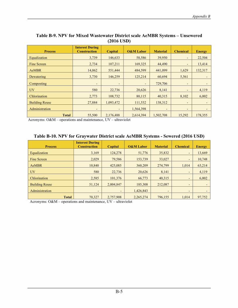
Appendix B

Table B-9. NPV for Mixed Wastewater District scale AeMBR Systems – Unsewered (2016 USD)



Equalization 3,739 146,633 58,586 39,950 - 22,504

Fine Screen 2,734 107,211 169,325 44,490 - 13,414

AeMBR 14,062 551,444 484,599 441,099 1,629 132,317

Dewatering 3,730 146,259 125,214 60,694 5,561 -

Composting - - - 729,706 - -

UV 580 22,736 20,626 8,141 - 4,119

Chlorination 2,773 108,732 80,115 40,315 8,102 6,002

Building Reuse 27,884 1,093,472 111,532 138,312 - -


Total 55,500 2,176,488 2,614,394 1,502,708 15,292 178,355 Acronyms: O&M – operations and maintenance, UV – ultraviolet

Table B-10. NPV for Graywater District scale AeMBR Systems - Sewered (2016 USD)



Equalization 3,169 124,278 51,776 35,832 - 13,669

Fine Screen 2,029 79,586 153,739 33,027 - 10,748

AeMBR 10,840 425,085 360,209 274,799 1,014 63,214

UV 580 22,736 20,626 8,141 - 4,119

Chlorination 2,585 101,376 66,773 40,315 - 6,002

Building Reuse 51,124 2,004,847 185,308 212,087 - -


Total 70,327 2,757,908 2,265,274 796,155 1,014 97,752 Acronyms: O&M – operations and maintenance, UV – ultraviolet

B-5

Appendix C

Appendix C: Life Cycle Inventory

Appendix C

APPENDIX C: LIFE CYCLE INVENTORY

Table C-1 presents a summary of the life cycle inventory associated with each wastewater treatment system.

Table C-1. Life Cycle Inventories

Unit Process Input/Output A

eMB

R, B

uild

ing,

Gra

ywat

er

AeM

BR

, Bui

ldin

g,M

ixed

Was

tew

ater

AnM

BR

, Bui

ldin

g,G

rayw

ater

AnM

BR

, Bui

ldin

gM

ixed

Was

tew

ater

RV

FW, B

uild

ing,

Gra

ywat

er

RV

FW, B

uild

ing,

Mix

ed W

aste

wat

er

AeM

BR

, Dis

tric

t,G

rayw

ater

AeM

BR

, Dis

tric

t,M

ixed

Was

tew

ater

Units (per m3)

Fine Screen Electricity 0.107 0.084 0.107 0.084 0.107 0.084 0.075 0.058 kWh Screening Disposal 4.07E-3 9.54E-3 4.07E-3 9.54E-3 4.08E-3 9.54E-3 4.07E-3 9.54E-3 kg Steel 1.34E-3 8.57E-4 1.34E-3 8.57E-4 1.34E-3 8.57E-4 6.91E-4 4.28E-4 kg

Equalization

Concrete 1.35E-5 1.13E-5 1.35E-5 1.13E-5 1.86E-5 1.56E-5 1.12E-5 9.21E-6 m3

Steel 8.04E-4 6.76E-4 8.04E-4 6.76E-4 5.34E-4 4.46E-4 6.68E-4 5.49E-4 kg Electricity 0.106 0.097 0.106 0.097 0.222 0.189 0.095 0.097 kWh HDPE n/a n/a n/a n/a 7.82E-5 7.15E-5 2.33E-5 1.69E-5 kg

Clarification Steel

n/a n/a n/a n/a 3.80E-3 3.64E-3

n/a n/a kg

Sludge Disposal 7.32E-3 0.017 m3

Electricity 6.41E-4 1.50E-3 kWh

Biological Process


Steel 1.54E-3 1.29E-3 2.66E-3 2.07E-3 0.011 0.010 1.18E-3 9.66E-4 kg HDPE - - 1.04E-4 1.20E-4 8.32E-4 7.99E-4 - - kg Polyvinyl Fluoride 5.92E-4 5.92E-4 1.58E-3 1.58E-3 n/a n/a 5.92E-4 5.92E-4 kg Lower Media, Crushed Limestone

n/a n/a n/a n/a

0.022 0.021

n/a n/a

kg

Middle Media, Gravel 0.076 0.073 kg

Organic Cover, Wood Chips 0.081 0.078 kg

Sodium Hypochlorite 7.19E-4 7.20E-4 1.92E-3 1.92E-3 n/a n/a 7.19E-4 7.19E-4 kg

Electricity 0.427 0.622 0.817 0.808 0.423 0.406 0.439 0.569 kWh Methane 4.86E-3 5.94E-3 2.42E-3 3.50E-3 7.45E-4 9.05E-4 4.80E-3 5.94E-3 kg CH4

C-1

Appendix C

Table C-1. Life Cycle Inventories

Unit Process Input/Output A

eMB

R, B

uild

ing,

Gra

ywat

er

AeM

BR

, Bui

ldin

g,M

ixed

Was

tew

ater

AnM

BR

, Bui

ldin

g,G

rayw

ater

AnM

BR

, Bui

ldin

gM

ixed

Was

tew

ater

RV

FW, B

uild

ing,

Gra

ywat

er

RV

FW, B

uild

ing,

Mix

ed W

aste

wat

er

AeM

BR

, Dis

tric

t,G

rayw

ater

AeM

BR

, Dis

tric

t,M

ixed

Was

tew

ater

Units (per m3) N2O 5.01E-5 2.03E-4 - - 3.26E-5 3.13E-5 5.01E-5 2.03E-4 kg N2O Sludge 8.32E-3 0.014 7.25E-3 7.26E-3 n/a n/a 8.32E-3 0.014 m3

Biogas Recovery

Natural Gas, Avoided n/a n/a 0.045 0.070 n/a n/a n/a n/a m3

Downflow Hanging Sponge

Electricity

n/a n/a

0.035 0.035

n/a n/a n/a n/a

kWh Methane 1.29E-4 1.46E-4 kg CH4

Natural Gas 0.013 0.014 m3

Concrete 2.53E-5 2.14E-5 m3

Steel 1.19E-3 1.04E-3 kg HDPE 2.33E-5 3.15E-5 kg

Zeolite

Zeolite 0.112 0.360 kg NaCl (99+%) 0.055 0.227 kg NaCl NaOH 0.200 0.200 kg NaOH Electricity 0.034 0.045 kWh Disposal, Brine Injection 5.51E-3 0.023 m3

UV Electricity 0.017 0.014 0.017 0.014 0.056 0.036 0.029 0.018 kWh Steel 3.42E-5 3.15E-5 3.42E-5 3.15E-5 4.92E-5 3.15E-5 2.54E-5 1.57E-5 kg

Chlorination


Steel 8.53E-5 7.42E-5 8.53E-5 7.42E-5 8.53E-5 7.42E-5 5.83E-6 3.71E-5 kg Electricity 0.081 0.052 0.081 0.052 0.081 0.052 0.042 0.026 kWh Sodium Hypochlorite 3.20E-3 3.60E-3 5.79E-3 0.012 1.50E-3 1.57E-3 3.23E-3 3.65E-3 kg NaOCl

Storage HDPE 9.01E-4 8.66E-4 9.01E-4 8.66E-4 1.80E-3 1.73E-3 9.30E-4 7.21E-4 kg Electricity n/a n/a n/a n/a 0.045 0.045 n/a n/a kWh

C-2

PRESORTED STANDARD POSTAGE & FEES PAID

EPA PERMIT NO. G-35

Office of Research and Development (8101R) Washington, DC 20460

Official Business Penalty for Private Use $300