AVERTISSEMENT Ce document est le fruit d'un long travail approuvé par le jury de soutenance et mis à disposition de l'ensemble de la communauté universitaire élargie. Il est soumis à la propriété intellectuelle de l'auteur. Ceci implique une obligation de citation et de référencement lors de l’utilisation de ce document. D'autre part, toute contrefaçon, plagiat, reproduction illicite encourt une poursuite pénale. Contact : [email protected] LIENS Code de la Propriété Intellectuelle. articles L 122. 4 Code de la Propriété Intellectuelle. articles L 335.2- L 335.10 http://www.cfcopies.com/V2/leg/leg_droi.php http://www.culture.gouv.fr/culture/infos-pratiques/droits/protection.htm

Welcome message from author
This document is posted to help you gain knowledge. Please leave a comment to let me know what you think about it! Share it to your friends and learn new things together.
Transcript

AVERTISSEMENT
Ce document est le fruit d'un long travail approuvé par le jury de soutenance et mis à disposition de l'ensemble de la communauté universitaire élargie. Il est soumis à la propriété intellectuelle de l'auteur. Ceci implique une obligation de citation et de référencement lors de l’utilisation de ce document. D'autre part, toute contrefaçon, plagiat, reproduction illicite encourt une poursuite pénale. Contact : [email protected]
LIENS Code de la Propriété Intellectuelle. articles L 122. 4 Code de la Propriété Intellectuelle. articles L 335.2- L 335.10 http://www.cfcopies.com/V2/leg/leg_droi.php http://www.culture.gouv.fr/culture/infos-pratiques/droits/protection.htm
Université de Lorraine
Collegium Sciences et Technologies
Ecole doctorale EMMA
Ioffe Physical‐Technical Institute
of the Russian Academy of Sciences
Division of Plasma Physics,
Atomic Physics and Astrophysics
High Temperature Plasma Physics Laboratory
Thèse
présentée pour lʹobtention du titre de
Docteur de l’Université de Lorraine
en Physique
par Natalia KOSOLAPOVA
Recontruction du spectre en nombre dʹondes radiaux
à partir des données de la réflectométrie de corrélation radiale
Soutenance publique le 16 Novembre 2012
Membres du Jury :
Rapporteurs : Dr. Victor BULANIN
Dr. Dominique GRESILLON
SPbSPU, Saint‐Petersburg, Russie
CNRS, Palaiseau, France
Examinateurs : Dr. Alexey POPOV
Dr. Michael IRZAK
Dr. Roland SABOT
Ioffe Institute, Saint‐Petersburg, Russie
Ioffe Institute, Saint‐Petersburg, Russie
CEA, Saint‐Paul‐lès‐Durance, France
Directeur de thèse : Pr. Stéphane HEURAUX Institute Jean Lamour, Nancy, France
Co‐directeur de thèse : Pr. Evgeniy GUSAKOV Ioffe Institute, Saint‐Petersburg, Russie
_____________________________________________________________________________________________________________________________________
Institute Jean Lamour UMR 7198 CNRS
Laboratoire de Physique des Milieux Ionisés et Applications
Faculté des Sciences & Techniques ‐ 54500 Vandœuvre‐lès‐Nancy

Université de Lorraine
Collegium Sciences et Technologies
Ecole doctorale EMMA
Ioffe Physical‐Technical Institute
of the Russian Academy of Sciences
Division of Plasma Physics,
Atomic Physics and Astrophysics
High Temperature Plasma Physics Laboratory
Thesis
presented for obtaining the title of
Doctor of the University of Lorraine
in Physics
by Natalia KOSOLAPOVA
Reconstruction of microturbulence wave number spectra
from radial correlation reflectometry data
Public defense on the 16th of November 2012
Members of the Jury :
Referees : Dr. Victor BULANIN
Dr. Dominique GRESILLON
SPbSPU, Saint‐Petersburg, Russia
CNRS, Palaiseau, France
Examinators : Dr. Aleksey POPOV
Dr. Mikhail IRZAK
Dr. Roland SABOT
Ioffe Institute, Saint‐Petersburg, Russia
Ioffe Institute, Saint‐Petersburg, Russia
CEA, Saint‐Paul‐lès‐Durance, France
Supervisor : Pr. Stéphane HEURAUX Institute Jean Lamour, Nancy, France
Co‐Supervisor : Pr. Evgeniy GUSAKOV Ioffe Institute, Saint‐Petersburg, Russia
_____________________________________________________________________________________________________________________________________
Institute Jean Lamour UMR 7198 CNRS
Laboratoire de Physique des Milieux Ionisés et Applications
Faculté des Sciences & Techniques ‐ 54500 Vandœuvre‐lès‐Nancy

____________________________________________________________________________Summary
Reconstruction of microturbulence wave number spectra from radial correlation
reflectometry data
Summary: Turbulence is supposed to be the main source of anomalous transport in tokamaks
which leads to loss of heat much faster than as it is predicted by neoclassical theory.
Development of plasma turbulence diagnostics is one of the key issues of nuclear fusion to
control turbulent particles and energy transport in a future fusion power station. Diagnostics
based on microwaves scattered from plasma attract attention of researchers as non‐disturbing
and requiring just a single access to plasma. The phase of the reflected wave contains
information on the position of the cut‐off layer and density fluctuations. Correlation
reflectometry is now a routinely used technique providing information on plasma
microturbulence. Although the diagnostics is widely spread data interpretation remains quite a
complicated task. Thus, it was supposed that the distance at which the correlation of two
signals received from plasma is suppressed is equal to the turbulence correlation length.
However this approach is incorrect and introduces huge errors to determined plasma
microturbulence parameters.
The aim of this thesis is to develop an analytical theory, to give a correct interpretation of
radial correlation reflectometry (RCR) data and to provide researchers with simple formulae for
extracting information on microturbulence parameters from RCR experiments. Numerical
simulations based on the theory prove applicability of this theoretical method and give an
insight for experimentalists on its capability and on optimized diagnostic parameters to use.
Furthermore the results obtained on three different machines are carefully analyzed and
compared with theoretical predictions and numerical simulations as well.
Keywords: Tokamaks – Plasmas – Turbulence – Reflectometry – Correlation

_____________________________________________________________________________Résumé
Recontruction des spectres microturbulence en nombre dʹondes à partir des données de la
réflectométrie de corrélation radiale
Résumé : La turbulence est supposée être la source principale du transport anormal dans les
tokamaks, qui conduit à la perte de chaleur beaucoup plus rapidement que celui prédit par la
théorie néoclassique. Développement de diagnostics dédiés à la caractérisation de la turbulence
du plasma est lʹun des principaux enjeux de la fusion nucléaire pour contrôler les flux de
particules et de transport dʹénergie de la centrale électrique de fusion avenir. Les diagnostics
basés sur la diffusion des micro‐ondes induite par le plasma ont focalisé lʹattention des
chercheurs comme outils non perturbants, et nécessitant seulement un accès unique de faible
encombrement au plasma. Le principe de base est lié à la phase de lʹonde réfléchie qui contient
des informations sur la position de la couche de coupure et les fluctuations de densité. La
réflectométrie corrélation considérée ici, maintenant couramment utilisée dans les expériences,
est la technique fournissant de lʹinformation sur le plasma microturbulence. Bien que le
diagnostic soit largement répandu lʹinterprétation des données reste une tâche assez
compliquée. Ainsi, il a été supposé que la distance à laquelle la corrélation des deux signaux
reçus à partir du plasma est supprimée est égale à la longueur de corrélation de turbulence.
Toutefois, cette approche est erronée et introduit des erreurs énormes sur lʹévaluation des
paramètres de la microturbulence du plasma.
Lʹobjectif de cette thèse fut dʹabord le développement dʹune théorie analytique, puis de
fournir une interprétation correcte des données de la réflectométrie de corrélation radiale (RCR)
et enfin dʹoffrir aux chercheurs des formules simples pour extraire des informations sur les
paramètres de turbulence à partir dʹexpériences utilisant la RCR. Des simulations numériques
basées sur la théorie ont été utilisées pour prouver lʹapplicabilité de la méthode théorique, pour
donner un aperçu aux expérimentateurs sur ses capacités et pour optimiser les paramètres du
diagnostic lors de son utilisation en fonction des conditions de plasma. De plus, les résultats
obtenus sur trois machines différentes sont soigneusement analysés et comparés avec les
prédictions théoriques et des simulations numériques.
Mots clés : Tokamaks – Plasmas – Turbulence – Spectroscopie de réflectance – Corrélation


__________________________________________________________________________Аннотация
Определение спектров микротурбулентности по данным радиальной
корреляционной рефлектометрии
Аннотация: Турбулентность считается основной причиной аномального переноса в
токамаках, что приводит к потере тепла намного быстрее, чем это предсказывает
неоклассическая теория. Развитие диагностики турбулентности плазмы с целью контроля
турбулентных частиц и переноса энергии в будущей термоядерной электростанции
является одной из основных задач термоядерного синтеза. Диагностики, основанные на
отражении микроволн, привлекают внимание исследователей как невозмущающие
плазму и требующие только одного доступа к плазме. Фаза отраженной волны содержит
информацию о позиции отсечки и флуктуациях плотности. Корреляционная
рефлектометрия в настоящее время – повсеместно используемая диагностика, дающая
информацию о микротурбулентности плазмы. Хотя диагностика широко
распространена, интерпретация ее данных остается довольно сложной задачей. Так,
предполагалось, что расстояние, на котором корреляция двух сигналов, принятых из
плазмы, падает в е раз, эквивалентно корреляционной длине турбулентности. Однако,
этот подход неверен и приводит к большим ошибкам в определении параметров плазмы.
Цель этой диссертации – разработать аналитическую теорию и метод, позволяющий
корректно интерпретировать данные радиальной корреляционной рефлектометрии
(РКР), вывести простую формулу для определения параметров микротурбулентности из
РКР экспериментов. Численное моделирование, основанное на теории, подтверждает
применимость данного теоретического метода и дает представление экспериментаторам
о его возможностях и оптимальных экспериментальных параматрах. Более того,
результаты, полученные на трех различных машинах, детально проанализированы и
были сопоставлены с теоретическими выкладками и численным моделированием.
Ключевые слова: Токамак – Плазма – Турбулентность – Рефлектометрия – Корреляция
______________________________________Contents
I. Introduction ........................................................................................................ 1
1.1. The world energy problem ...................................................................................................... 3
1.2. Nuclear fusion: energy source for the future ........................................................................ 4
1.3. The tokamak............................................................................................................................... 7
1.3.1. Tokamaks in this work ................................................................................................ 8
1.3.1.1. Tore Supra..................................................................................................... 8
1.3.1.2. FT‐2 .............................................................................................................. 10
1.3.1.3. JET ................................................................................................................ 11
1.3.1.4. ITER ............................................................................................................. 12
1.3.1.5. Main parameters of machines mentioned in this work........................ 13
1.4. Turbulence in fusion plasma ................................................................................................. 14
1.4.1. How fluctuations cause anomalous transport ....................................................... 15
1.4.2. Bohm or Gyro‐Bohm (drift wave) scaling for turbulence .................................... 17
1.4.3. Theoretical description of the turbulence wave number spectrum .................... 18
1.4.4. Examples of turbulence wave number spectra ...................................................... 20
1.4.5. Turbulence suppression ............................................................................................ 21
1.4.5.1. Radial electric field shear.......................................................................... 21
1.4.5.2. Zonal Flows ................................................................................................ 22
1.5. Turbulence diagnostics........................................................................................................... 22
1.6. Radial correlation reflectometry............................................................................................ 24
1.7. Scope of this work ................................................................................................................... 26
II. Theoretical background of radial correlation reflectometry ................. 27
2.1. Propagation of electromagnetic waves in plasmas ............................................................ 29
2.1.1. Approximations and restrictions used.................................................................... 29
2.1.1.1. Stationary plasma ...................................................................................... 29
2.1.1.2. Cold plasma approximation..................................................................... 30
2.1.1.3. High frequencies ........................................................................................ 30
2.1.1.4. Anisotropy .................................................................................................. 30
2.1.1.5. Propagationg waves .................................................................................. 30
_____________________________________________________________________________Contents
2.1.1.6. Linear approximation................................................................................ 31
2.1.2. Propagation in homogeneous plasma..................................................................... 31
2.1.2.1. Perpendicular propagation ...................................................................... 32
2.1.3. Propagation in inhomogeneous plasma ................................................................. 34
2.1.3.1. Wentzel – Kramers – Brillouin approximation...................................... 34
2.2. Plasma density fluctuations................................................................................................... 35
2.3. Mechanism of back and forward Bragg scattering............................................................. 36
2.4. Reflectometry principles ........................................................................................................ 37
2.4.1. Standard reflectometry for plasma density profile masurements ...................... 37
2.4.2. Fluctuation reflectometry.......................................................................................... 40
2.5. Basic assumptions and equations in 1D analysis ............................................................... 41
2.5.1. Reciprocity theorem................................................................................................... 41
2.6. Scattering signal in case of linear plasma density profile ................................................. 45
2.6.1. Asymptotic forms of the characteristic integral..................................................... 47
2.6.1.1. Contribution of the pole............................................................................ 47
2.6.1.2. Contribution of the branch point............................................................. 48
2.6.1.3. Contribution of the stationary phase points .......................................... 48
2.6.2. Asymptotic forms of scattering signal .................................................................... 49
2.6.3. Numerical computation example ............................................................................ 50
2.6.4. WKB representation of Airy function ..................................................................... 51
2.6.5. Long wavelength limit .............................................................................................. 51
2.7. Scattering signal in case of arbitrary plasma density profile ............................................ 52
2.7.1. Numerical computation example for parabolic plasma density profile ............ 54
2.7.2. Short summary on validity domain of Helmholtz equation solutions .............. 55
2.8. The RCR CCF........................................................................................................................... 56
2.8.1. RCR CCF for linear plasma density profile............................................................ 56
2.8.2. RCR CCF for arbitrary plasma density profile ...................................................... 58
2.9. Turbulence spectrum reconstruction from the RCR CCF ................................................. 60
2.10. Direct transform formulae for RCR...................................................................................... 62
2.10.1. Forward transformation kernel................................................................................ 62
2.10.2. Numerical simulation example of forward kernel usage..................................... 63
2.10.3. Inverse transformation kernel .................................................................................. 65
Contents_____________________________________________________________________________
2.11. Ideas for a combined diagnostic using reflectometry and other density fluctuation
diagnostic.................................................................................................................................................. 66
2.11.1. Forward and inverse transforms for ICF ................................................................ 67
2.12. Summary .................................................................................................................................. 69
III. Numerical modeling .................................................................................... 73
3.1. Numerical model..................................................................................................................... 75
3.1.1. Numerical solution of unperturbed Helmholtz equation. ................................... 75
3.1.2. Reflectometry signal partial amplitude integral computation ............................ 76
3.1.3. Signal CCF computation ........................................................................................... 77
3.1.4. Turbulence wave number spectrum and TCCF reconstruction .......................... 78
3.2. O‐mode probing in case of linear plasma density profile ................................................. 78
3.2.1. Reconstruction of turbulence spectrum and CCF for large machine.................. 78
3.2.1.2. CCF and spectrum reconstruction in conditions relevant to
experiment................................................................................................................... 83
3.2.2. Reconstruction of the turbulence spectrum and CCF for small machine .......... 87
3.2.2.1. Standard conditions of reconstruction at FT‐2 ...................................... 88
3.2.2.2. Optimized reconstruction in more realistic conditions ........................ 88
3.2.3. Amplitude CCF computation................................................................................... 89
3.2.4. Inhomogeneous turbulence ...................................................................................... 90
3.3. O‐mode probing in case of density profile close to experimental one ............................ 92
3.3.1. Tore Supra – like plasma density profile ................................................................ 92
3.3.2. Plasma density profile with a steep gradient ......................................................... 93
3.4. Synthetic X‐mode RCR experiment ...................................................................................... 95
3.5. Summary .................................................................................................................................. 97
IV. Applications to experiments....................................................................... 99
4.1. General remarks on data analysis....................................................................................... 101
4.1.1. Reflectometer generic scheme ................................................................................ 101
4.1.2. Quadrature phase detection ................................................................................... 102
4.1.3. Probing range and step............................................................................................ 103
4.1.4. Statistical analysis .................................................................................................... 103
4.2. Results of RCR experiment at Tore Supra ......................................................................... 104
4.2.1. Reflectometers at Tore Supra.................................................................................. 104
_____________________________________________________________________________Contents
4.2.2. Phase calibration ...................................................................................................... 105
4.2.3. Data analysis and interpretation............................................................................ 107
4.2.3.1. Probing with equidistant spatial step ................................................... 107
4.2.3.2. Probing with exponentially growing spatial step............................... 109
4.2.4. Summary ................................................................................................................... 114
4.3. Experimental results obtained at FT‐2 tokamak............................................................... 115
4.3.1. Radial correlation reflectometers at FT‐2.............................................................. 115
4.3.2. O‐mode probing from HFS..................................................................................... 116
4.3.3. X‐mode probing from HFS ..................................................................................... 118
4.3.4. Summary ................................................................................................................... 120
4.4. Results of experimental campaign at JET .......................................................................... 121
4.4.1. RCR diagnostic at JET.............................................................................................. 121
4.4.2. Experimental results ................................................................................................ 123
4.4.2.1. Shot #82671 data analysis ....................................................................... 124
4.4.2.2. Shot #82633 data analysis ....................................................................... 128
4.4.3. Summary ................................................................................................................... 128
Conclusion .......................................................................................................... 129
Future plans..................................................................................................................................... 131
Appendix ............................................................................................................. 133
Appendix A. Stationary phase method ....................................................................................... 133
Appendix B. 4th order Numerov scheme ..................................................................................... 134
References .............................................................................................................................................. 137
Acknowledgements.............................................................................................................................. 151

1
Chapter I
Introduction
_____________________________________________________________________________________
In this Chapter we give a short overview of world energy resources and estimate the future
energy needs of the world. The most reliable future energy source, nuclear fusion, is briefly
surveyed. One of the ways to produce energy from fusion – magnetic confinement – and the
tokamak, the most likely device for the future power station are reviewed. We also describe the
impact of anomalous transport caused by microturbulence on the fusion device performance
and discuss advantages and disadvantages of contemporary turbulence diagnostics. We
conclude the Chapter I by describing the scope of this work.

2
_________________________________________________________1.1. The world energy problem
1.1. The world energy problem
As the population of the world has passed the 7 billion mark and continues to grow more
than linearly in time [1], the demand for energy is becoming an ever more critical challenge. At
present day the world annual primary energy (before any conversion to secondary forms of
energy) consumption is about 15TWyr [2]. The World Energy Council [3] projects that by the
year 2050 the world wide energy demand will be double its present level. Therefore in the 21st
century the prevalent task is to satisfy the need for new long‐term sources of energy.
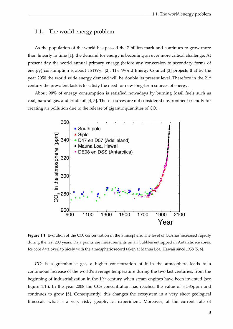
About 90% of energy consumption is satisfied nowadays by burning fossil fuels such as
coal, natural gas, and crude oil [4, 5]. These sources are not considered environment friendly for
creating air pollution due to the release of gigantic quantities of CO2.
Figure 1.1. Evolution of the CO2 concentration in the atmosphere. The level of CO2 has increased rapidly
during the last 200 years. Data points are measurements on air bubbles entrapped in Antarctic ice cores.
Ice core data overlap nicely with the atmospheric record taken at Manua Loa, Hawaii since 1958 [5, 6].
CO2 is a greenhouse gas, a higher concentration of it in the atmosphere leads to a
continuous increase of the world’s average temperature during the two last centuries, from the
beginning of industrialization in the 19th century when steam engines have been invented (see
figure 1.1.). In the year 2008 the CO2 concentration has reached the value of 385ppm and
continues to grow [5]. Consequently, this changes the ecosystem in a very short geological
timescale what is a very risky geophysics experiment. Moreover, at the current rate of
3
Chapter I. Introduction________________________________________________________________
4
consumption the world’s stock of oil will end in the nearest 40‐50 years, of natural gas in 60‐70
years. The estimated source of coal is enough for next 250 years however this won’t satisfy the
world’s future energy demand [2, 4, 5].
The first alternative to burning fossil fuels is renewable energy sources, among them are:
solar heating, ocean thermal, wind, waves, hydro electricity, tidal power, geothermal heat,
biofuel, wood, etc. Currently the contribution of this kind of sources to the world primary
energy production is only about 1.3% [4]. The most effective are considered to be solar heating,
wave power and hydroelectricity. Unfortunately the exploitation of renewables is limited by
natural conditions at the exact location. Renewable energy sources do not directly produce CO2;
the emission of greenhouse gases is released in life‐cycle and is indirect. Hence the use of land
and indirect emissions are the two negative aspects of renewables which should not be
forgotten. Although these non‐fossil energy sources are large and inexhaustible they have only
limited potential.
The second alternative is nuclear energy (fission and fusion). Nuclear power in the form of
fission produces large amounts of inexpensive fuel. Unfortunately it is not favorable as well due
to the highly radioactive waste created and not stored properly. In addition, known uranium
(U‐235) sources will be run out in 50‐80 years [7]. It could be stretched by extracting uranium
from seawater or by transformation of non‐fissile elements to fissile elements (breeder reactions
using U‐238 and Th) however the safety and environmental problems overbalance.
Nuclear fusion is the youngest and less developed energy source nevertheless it promises to
produce safe, environment friendly and inexhaustible energy. This should be the best solution
of the staggering task to develop new energy source for mankind.
1.2. Nuclear fusion: energy source for the future
The idea of controlled thermonuclear fusion appeared in the middle of 20th century. Basic
principles were borrowed from the most famous thermonuclear reactor – the Sun [8, 9]. In the
process that powers the Sun the four protons are combined to produce helium, releasing
globally energy in three steps:
(1) 32
3 3 42 2 2 2
ep p D e
D p He
He He He p
The idea to realize controlled nuclear fusion on Earth was evoked by analogy with solar
fusion production. However it is impossible to reproduce solar conditions on Earth. The
probability of the fusion reaction is too small due to extremely low value of the proton‐proton
cross section reaction [10] and is compensated by space scales of Sun and other stars. By looking
__________________________________________1.2. Nuclear fusion: energy source for the future
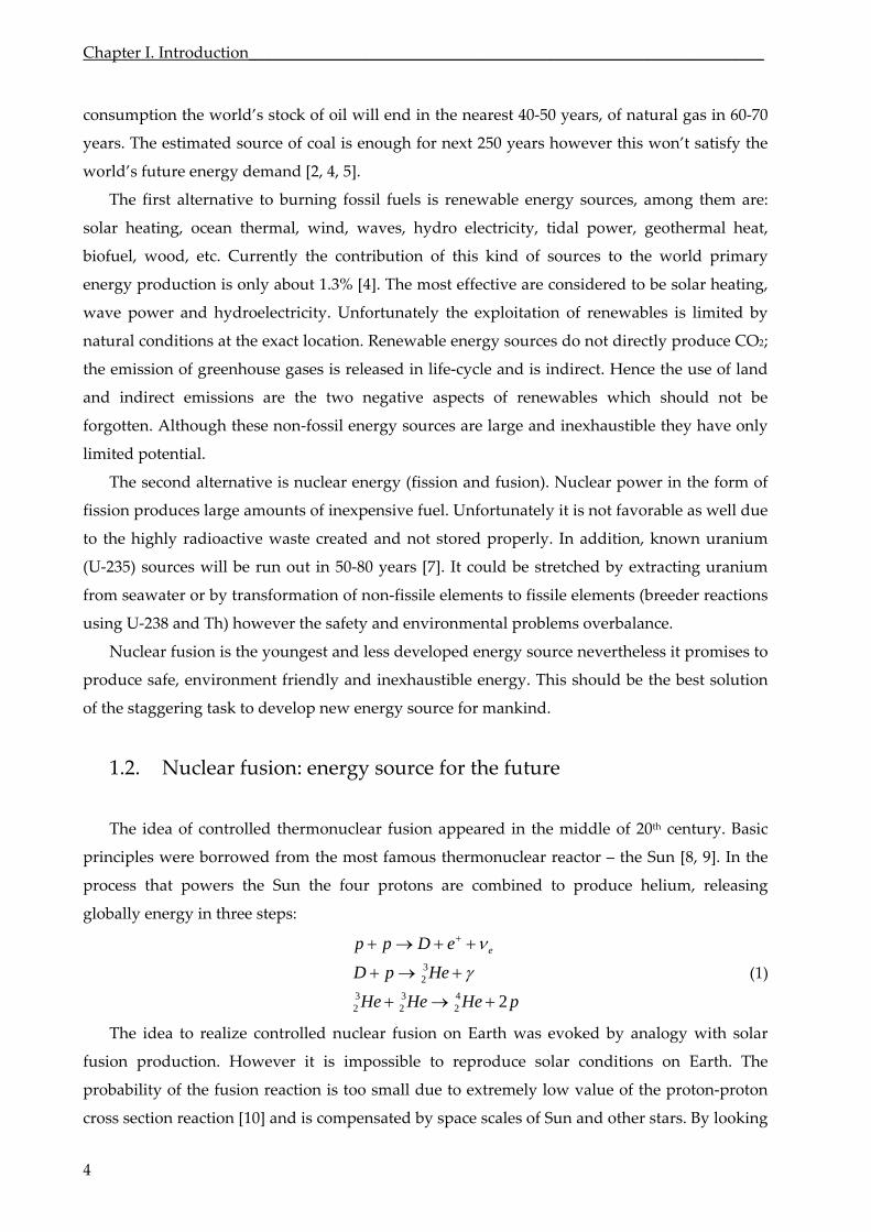
at the cross sections of fusion reaction (see figure 1.2.), on Earth the least difficult fusion reaction
is between the hydrogen isotopes deuterium D (the stable isotope of hydrogen with a nucleus
consisting of one proton and one neutron) and tritium T (the radioactive isotope of hydrogen
with a nucleus of one proton and two neutrons):
(2) 2 3 4 (3.5 ) (14.1 )D T He MeV n MeV
The products of the reaction are neutral helium which carries one third of the result energy and
high energy neutron. The energy of neutron can be converted into heat. Other possible
candidates for nuclear fusion are:
(3)
2 2 3
2 2 3 1
2 3 4 1
(0.82 ) (2.45 )
(1.01 ) (3.02 )
(3.6 ) (14.7 )
D D He MeV n MeV
D D T MeV H MeV
D He He MeV H MeV
The cross sections of these reactions are shown in figure 1.2. The D‐T reaction (2) has the highest
cross section at lowest temperature and is easier to be realized. Usually the D‐T reaction is
accompanied by side reactions, the most important of which are D‐D and T‐T reactions
however these reactions could be neglected due to small fusion cross section.
The energy production of reaction (2) using deuterium containing in 1l of water (33 mg) is
equal to that of 260l of gasoline. Deuterium can be cheaply extracted from ordinary water.
Tritium is a radioactive isotope of hydrogen and has a rather short half‐life about 12.3 years [7]
and does not exist in nature. It can be produced as a product of nuclear reaction between
neutrons produced in D‐T reaction (2) and lithium [7] which is like deuterium a widely
available element [11]. Thus, sources for nuclear fusion present on Earth seem to be
inexhaustible.
Figure 1.2. Cross sections versus center‐of‐mass energy for key fusion reactions [7, 12].
5
Chapter I. Introduction________________________________________________________________
6
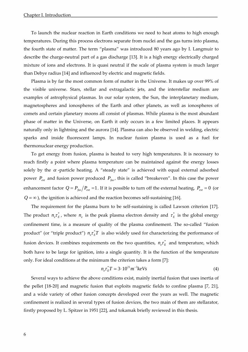
To launch the nuclear reaction in Earth conditions we need to heat atoms to high enough
temperatures. During this process electrons separate from nuclei and the gas turns into plasma,
the fourth state of matter. The term “plasma” was introduced 80 years ago by I. Langmuir to
describe the charge‐neutral part of a gas discharge [13]. It is a high energy electrically charged
mixture of ions and electrons. It is quasi neutral if the scale of plasma system is much larger
than Debye radius [14] and influenced by electric and magnetic fields.
Plasma is by far the most common form of matter in the Universe. It makes up over 99% of
the visible universe. Stars, stellar and extragalactic jets, and the interstellar medium are
examples of astrophysical plasmas. In our solar system, the Sun, the interplanetary medium,
magnetospheres and ionospheres of the Earth and other planets, as well as ionospheres of
comets and certain planetary moons all consist of plasmas. While plasma is the most abundant
phase of matter in the Universe, on Earth it only occurs in a few limited places. It appears
naturally only in lightning and the aurora [14]. Plasma can also be observed in welding, electric
sparks and inside fluorescent lamps. In nuclear fusion plasma is used as a fuel for
thermonuclear energy production.
To get energy from fusion, plasma is heated to very high temperatures. It is necessary to
reach firstly a point where plasma temperature can be maintained against the energy losses
solely by the ‐particle heating. A “steady state” is achieved with equal external adsorbed
power and fusion power produced extP fusP , this is called “breakeven”. In this case the power
enhancement factor 1fus extQ P P . If it is possible to turn off the external heating, (or
), the ignition is achieved and the reaction becomes self‐sustaining [16
0extP
Q ].
The requirement for the plasma burn to be self‐sustaining is called Lawson criterion [17].
The product *e En , where is the peak plasma electron density and en *
E is the global energy
confinement time, is a measure of quality of the plasma confinement. The so‐called “fusion
product” (or “triple product”) *e En T is also widely used for characterizing the performance of
fusion devices. It combines requirements on the two quantities, *e En and temperature, which
both have to be large for ignition, into a single quantity. It is the function of the temperature
only. For ideal conditions at the minimum the criterion takes a form [7]:
(4) * 21 33 10e En T m keVs
Several ways to achieve the above conditions exist, mainly inertial fusion that uses inertia of
the pellet [18‐20] and magnetic fusion that exploits magnetic fields to confine plasma [7, 21],
and a wide variety of other fusion concepts developed over the years as well. The magnetic
confinement is realized in several types of fusion devices, the two main of them are stellarator,
firstly proposed by L. Spitzer in 1951 [22], and tokamak briefly reviewed in this thesis.
_____________________________________________________________________1.3. The tokamak
1.3. The tokamak
Tokamak (from Russian “токамак”, “ТОроидальная Камера с Магнитными
Катушками”, – “toroidal camera with magnetic coils”) is the predominant device in
thermonuclear fusion. It is the earliest fusion device which was firstly proposed by I. Tamm and
his former postgraduate student A. Sakharov in 1950 [23‐26].
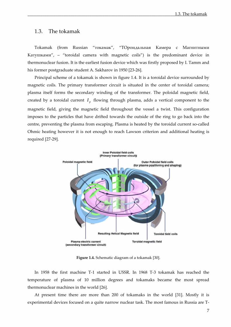
Principal scheme of a tokamak is shown in figure 1.4. It is a toroidal device surrounded by
magnetic coils. The primary transformer circuit is situated in the center of toroidal camera;
plasma itself forms the secondary winding of the transformer. The poloidal magnetic field,
created by a toroidal current pI flowing through plasma, adds a vertical component to the
magnetic field, giving the magnetic field throughout the vessel a twist. This configuration
imposes to the particles that have drifted towards the outside of the ring to go back into the
centre, preventing the plasma from escaping. Plasma is heated by the toroidal current so‐called
Ohmic heating however it is not enough to reach Lawson criterion and additional heating is
required [27‐29].
Figure 1.4. Schematic diagram of a tokamak [30].
In 1958 the first machine T‐1 started in USSR. In 1968 T‐3 tokamak has reached the
temperature of plasma of 10 million degrees and tokamaks became the most spread
thermonuclear machines in the world [26].
At present time there are more than 200 of tokamaks in the world [31]. Mostly it is
experimental devices focused on a quite narrow nuclear task. The most famous in Russia are T‐
7
Chapter I. Introduction________________________________________________________________
10
wing through the magnetic coils
gen
nt in a superconducting coil which has been cryogenically cooled to a temperature below
its
e the tokamaks mentioned in this thesis: Tore Supra, FT‐
2, JET and future nuclear fusion reactor ITER. The results of numerical modeling performed for
all
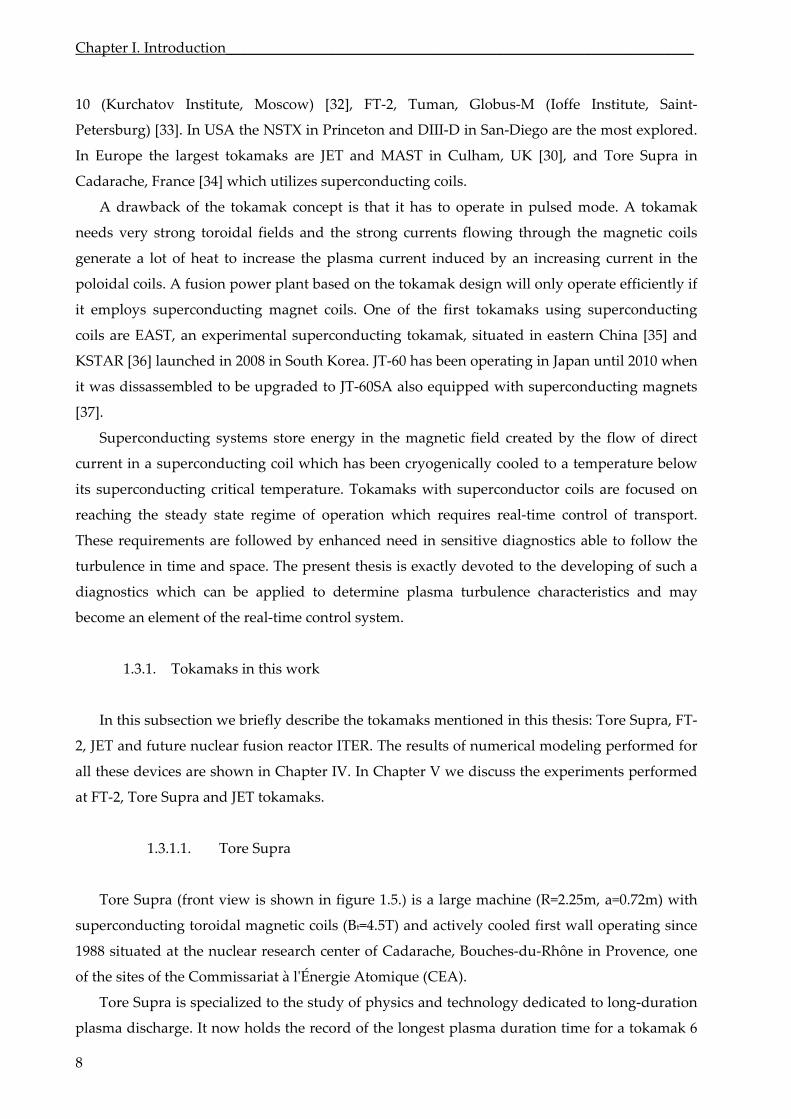
n in figure 1.5.) is a large machine (R=2.25m, a=0.72m) with
superconducting toroidal magnetic coils (Bt=4.5T) and actively cooled first wall operating since
198
ma duration time for a tokamak 6
(Kurchatov Institute, Moscow) [32], FT‐2, Tuman, Globus‐M (Ioffe Institute, Saint‐
Petersburg) [33]. In USA the NSTX in Princeton and DIII‐D in San‐Diego are the most explored.
In Europe the largest tokamaks are JET and MAST in Culham, UK [30], and Tore Supra in
Cadarache, France [34] which utilizes superconducting coils.
A drawback of the tokamak concept is that it has to operate in pulsed mode. A tokamak
needs very strong toroidal fields and the strong currents flo
erate a lot of heat to increase the plasma current induced by an increasing current in the
poloidal coils. A fusion power plant based on the tokamak design will only operate efficiently if
it employs superconducting magnet coils. One of the first tokamaks using superconducting
coils are EAST, an experimental superconducting tokamak, situated in eastern China [35] and
KSTAR [36] launched in 2008 in South Korea. JT‐60 has been operating in Japan until 2010 when
it was dissassembled to be upgraded to JT‐60SA also equipped with superconducting magnets
[37].
Superconducting systems store energy in the magnetic field created by the flow of direct
curre
superconducting critical temperature. Tokamaks with superconductor coils are focused on
reaching the steady state regime of operation which requires real‐time control of transport.
These requirements are followed by enhanced need in sensitive diagnostics able to follow the
turbulence in time and space. The present thesis is exactly devoted to the developing of such a
diagnostics which can be applied to determine plasma turbulence characteristics and may
become an element of the real‐time control system.
1.3.1. Tokamaks in this work
In this subsection we briefly describ
these devices are shown in Chapter IV. In Chapter V we discuss the experiments performed
at FT‐2, Tore Supra and JET tokamaks.
1.3.1.1. Tore Supra
Tore Supra (front view is show
8 situated at the nuclear research center of Cadarache, Bouches‐du‐Rhône in Provence, one
of the sites of the Commissariat à lʹÉnergie Atomique (CEA).
Tore Supra is specialized to the study of physics and technology dedicated to long‐duration
plasma discharge. It now holds the record of the longest plas
8
_____________________________________________________________________1.3. The tokamak
min
us heat and particles
rem
utes 30 seconds and over 1000 MJ of energy injected and extracted in 2003. It allows to test
critical parts of equipment such as plasma facing wall components or superconducting magnets
that will be used in its successor, ITER, demonstrating the capability of Tore Supra to run long
pulses on a regular basis. A new ITER relevant lower hybrid current drive (LHCD) launcher has
allowed coupling to the plasma a power level of 2.7MW for 78s, corresponding to a power
density close to the design value foreseen for an ITER LHCD system [38].
As soon as the purpose of Tore Supra is to obtain long stationary discharges, the two major
questions are addressed: non‐inductive current generation and continuo
oval. The physics program therefore has two principal research orientations, complemented
by studies on magnetohydrodynamic (MHD) stability, turbulence, and transport. The first
physics program concerns the interaction of electromagnetic (Lower Hybrid and Ion Cyclotron)
waves with the hot central plasma. All or part of the plasma current can be generated in this
manner, thus controlling the current density profile. The second physics program concerns the
edge plasma and its interaction with the first wall. The originality of Tore Supra is the ergodic
divertor, which perturbs the magnetic field at the plasma edge by creating a chaotic magnetic
field region, resulting in outfluxes of hot plasma collected on neutralizers. Highly radiative
layers have been obtained with this device, while preserving a good particle extraction capacity.
Figure 1.5. Front view of Tore Supra [34].
A detailed description of cial CEA website [34]. Tore
Supra has been stopped for upgrade since 2011.
the machine can be found on the offi
9
Chapter I. Introduction________________________________________________________________
1.3.1.2. FT‐2
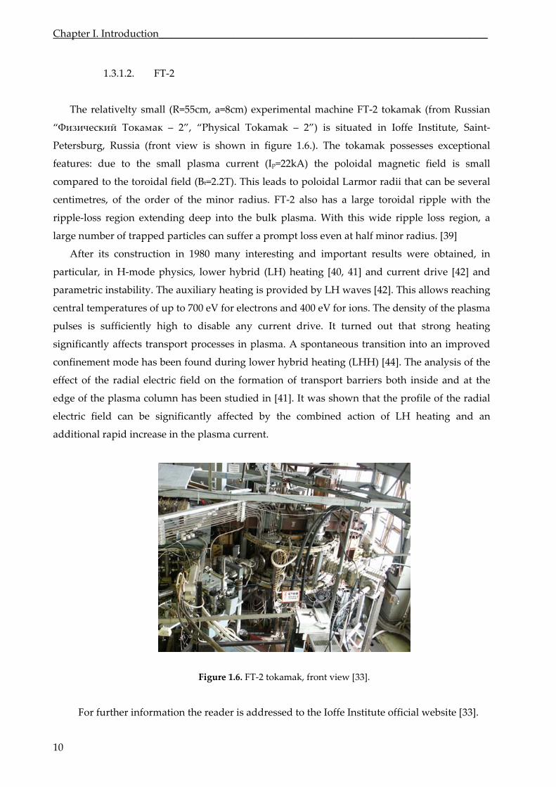
The relativelty small (R=55cm, a=8cm) experimental machine FT‐2 tokamak (from Russian
“Физический Токамак – 2”, “Physical Tokamak – 2”) is situated in Ioffe Institute, Saint‐
Pet
] and
par
ersburg, Russia (front view is shown in figure 1.6.). The tokamak possesses exceptional
features: due to the small plasma current (Ip=22kA) the poloidal magnetic field is small
compared to the toroidal field (Bt=2.2T). This leads to poloidal Larmor radii that can be several
centimetres, of the order of the minor radius. FT‐2 also has a large toroidal ripple with the
ripple‐loss region extending deep into the bulk plasma. With this wide ripple loss region, a
large number of trapped particles can suffer a prompt loss even at half minor radius. [39]
After its construction in 1980 many interesting and important results were obtained, in
particular, in H‐mode physics, lower hybrid (LH) heating [40, 41] and current drive [42
ametric instability. The auxiliary heating is provided by LH waves [42]. This allows reaching
central temperatures of up to 700 eV for electrons and 400 eV for ions. The density of the plasma
pulses is sufficiently high to disable any current drive. It turned out that strong heating
significantly affects transport processes in plasma. A spontaneous transition into an improved
confinement mode has been found during lower hybrid heating (LHH) [44]. The analysis of the
effect of the radial electric field on the formation of transport barriers both inside and at the
edge of the plasma column has been studied in [41]. It was shown that the profile of the radial
electric field can be significantly affected by the combined action of LH heating and an
additional rapid increase in the plasma current.
Figure 1.6. FT‐2 tokamak, front view [33].
For further information th te official website [33].
e reader is addressed to the Ioffe Institu
10
_____________________________________________________________________1.3. The tokamak
1.3.1.3. JET
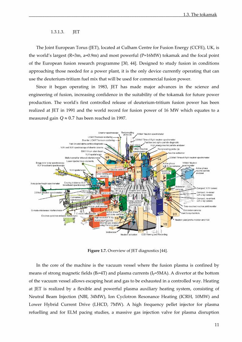
us (JET), located at Culham Centre for Fusion Energy (CCFE), UK, is
the world’ largest (R=3m, a=0.9m) and most powerful (P=16MW) tokamak and the focal point
of t
power
pro
The Joint European Tor
s
he European fusion research programme [30, 44]. Designed to study fusion in conditions
approaching those needed for a power plant, it is the only device currently operating that can
use the deuterium‐tritium fuel mix that will be used for commercial fusion power.
Since it began operating in 1983, JET has made major advances in the science and
engineering of fusion, increasing confidence in the suitability of the tokamak for future
duction. The worldʹs first controlled release of deuterium‐tritium fusion power has been
realized at JET in 1991 and the world record for fusion power of 16 MW which equates to a
measured gain 0.7Q has been reached in 1997.
Figure 1.7. Overview of JET diagnostics [44].
In the core of the machin n plasma is confined by
means of strong magnetic fields (Bt=4T) and plasma currents (Ip=5MA). A divertor at the bottom
of t
e is the vacuum vessel where the fusio
he vacuum vessel allows escaping heat and gas to be exhausted in a controlled way. Heating
at JET is realized by a flexible and powerful plasma auxiliary heating system, consisting of
Neutral Beam Injection (NBI, 34MW), Ion Cyclotron Resonance Heating (ICRH, 10MW) and
Lower Hybrid Current Drive (LHCD, 7MW). A high frequency pellet injector for plasma
refuelling and for ELM pacing studies, a massive gas injection valve for plasma disruption
11
Chapter I. Introduction________________________________________________________________
studies are among JET facilities as well. Remote handling facilities allows advanced engineering
work to be performed inside the vacuum vessel without the need for manned access.
An impressive range of diagnostics has been developed over the years for monitoring and
analysis of JET operations. JET is surrounded by more than 100 different diagnostic systems (see
figu
sion reactor ITER. In recent years, JET has carried out
mu
tinuously achieved on JET and other fusion experiments, it is clear
that a larger and more powerful device would be necessary to demonstrate the feasibility of
nuc
nally to the electricity
pro
ting tokamak facility with striking design similarities to JET, but twice the linear
dim
re 1.7) and 60 of them are in use during an average experiment capturing up to 18GB of raw
data per plasma pulse. The data could be analysed using remote access facilities of CCFE due to
the JET facilities are collectively used by all European fusion laboratories under the European
Fusion Development Agreement (EFDA).
JET possesses unique capabilities to operate with beryllium plasma‐facing components
mirroring the material choices of future fu
ch important work to assist the design and construction of ITER. After more than 25 years of
successful operation, JET is still at the forefront of fusion research and is closely involved in
testing plasma physics, systems and materials for ITER. Today, its primary task is to prepare for
the construction and operation of ITER, acting as a test bed for ITER technologies and plasma
operating scenarios.
For more information please see the EFDA website [44].
1.3.1.4. ITER
Despite the progress con
lear fusion energy on a reactor scale. This is the purpose of the research and development
project ITER (International Thermonuclear Experimental Reactor), an international nuclear
fusion research and engineering project [46]. It is the first attempt of the humanity to build the
worldʹs largest and most advanced experimental nuclear fusion reactor.
It is beibg built at CEA Cadarache facility in the south of France. The project is the first step
on the way from experimental reactors to first DEMO‐reactor and fi
ducing power plant. The project is funded and run by seven member entities — the
European Union (EU), India, Japan, China, Russia, South Korea and the United States. The
history of ITER began in 1985 when the Soviet Union, European Union, Japan and the USA
have built the collaboration to develop the hugest tokamak in the world. In 2006 the ITER
agreement was officially signed and in 2007 entered into force, the ITER Organization was
established.
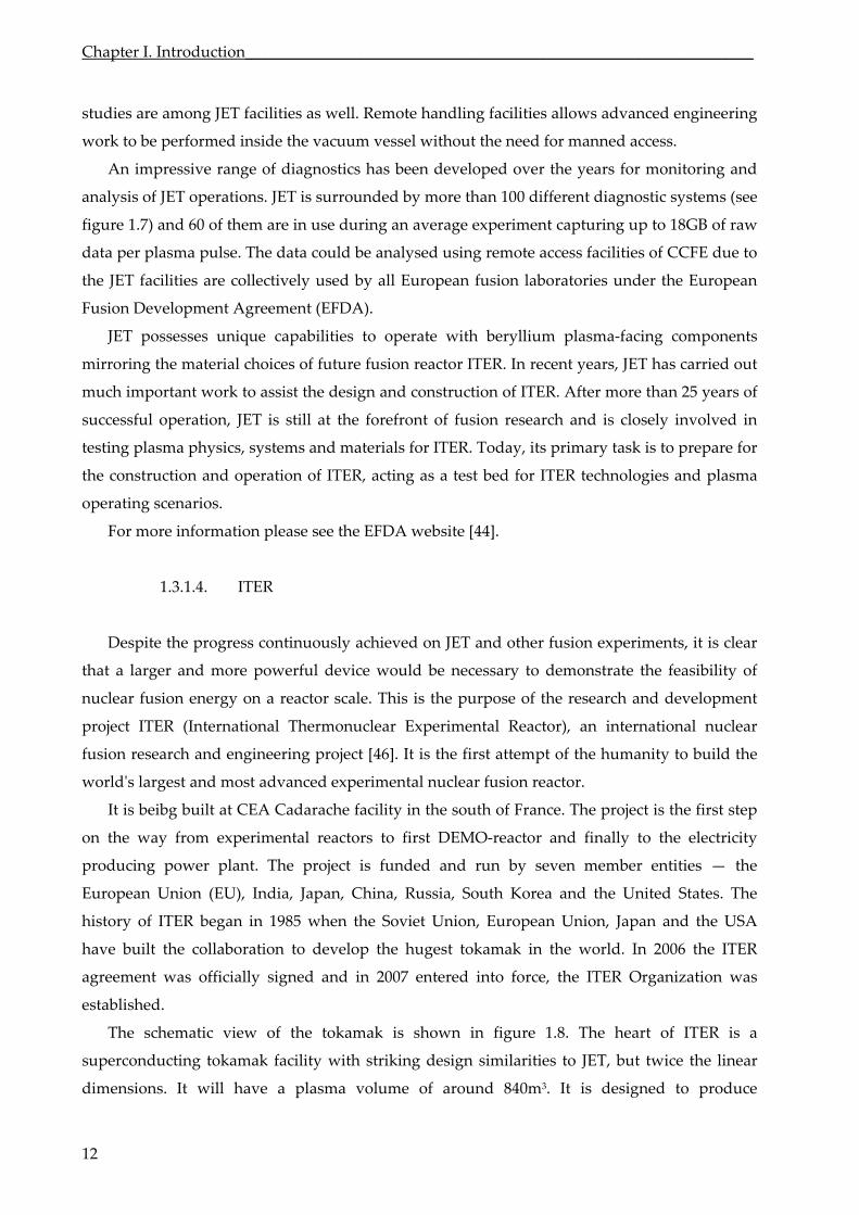
The schematic view of the tokamak is shown in figure 1.8. The heart of ITER is a
superconduc
ensions. It will have a plasma volume of around 840m3. It is designed to produce
12
_____________________________________________________________________1.3. The tokamak
approximately 500MW of fusion power sustained for more than 400s. ITER will be the first
fusion experiment with an output power higher than the input power.
Figure 1.8. ITER schematic view [46].
The ITER program is anticipated to last for years — 10 years for construction, and 20
yea
1.3.1.5. Main parameters of machines mentioned in this work
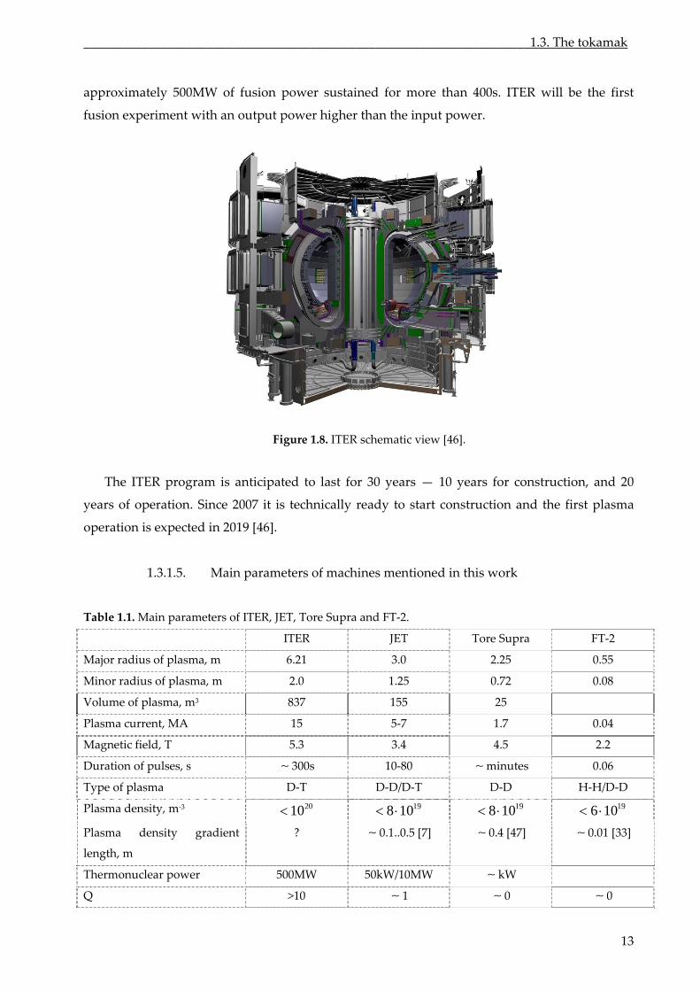
Table 1.1. Main parameters of ITER, JET, Tore Supra and FT‐2.
Tore Supra FT‐2
30
rs of operation. Since 2007 it is technically ready to start construction and the first plasma
operation is expected in 2019 [46].
ITER JET
Major radius o plasma, m f 6.21 3.0 2.25 0.55
Minor radius of plasma, m 2.0 1.25 0.72 0.08
Volume of plasma, m3 837 155 25
Plasma current, MA 15 5‐7 1.7 0. 4 0
Magnetic field, T 5.3 3.4 4.5 2.2
Duration of pulses, s s 1 minutes 300 0‐80 0.06
Type of plasma D D H‐ D ‐T ‐D/D‐T D‐D H/D‐
Plasma density, m‐3 2010 198 10
198 10 196 10
Plasma density gradient
? 0.1..0.5 [ 0.4 [47 0.01 [33
length, m
7] ] ]
Thermonuclear power 500MW 50kW/10MW kW Q >10 1 0 0
13
Chapter I. Introduction________________________________________________________________
14
1.4. Turbulence in fusio lasma
Magnetically confined fusion plasma is a more complex system than the neutral fluid. In
plasmas there are at least two fluids, electrons and ions, which cause great number of
instabilities. Microinstabilities cause fluctuations of electric and magnetic fields which in its turn
cause fluctuations in velocities and particle positions therefore microinstabilities have an
influence on transport. Turbulence is induced by incoherent motion appearing from
instabilities. It is rather frequent phenomenon in plasma experiments. Observations show that
plasma is a fluctuating medium in all its parameters such as density, magnetic field, potential
and temperature. Various instabilities that cause turbulence present in various regions of
plasma with different characteristics: SOL, edge and core.
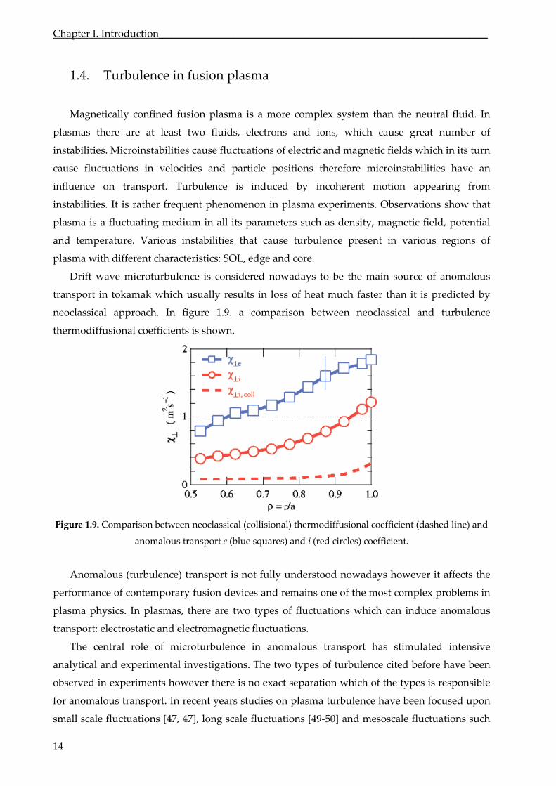
Drift wave microturbulence is considered nowadays to be the main source of anomalous
transport in tokamak which usually results in loss of heat much faster than it is predicted by
neoclassical approach. In figure 1.9. a comparison between neoclassical and turbulence
thermodiffusional coefficients is shown.
n p
Figure 1.9. Comparison between neoclassical (collisional) thermodiffusional coefficient (dashed line) and
anomalous transport e (blue squares) and i (red circles) coefficient.
Anomalous (turbulence) transport is not fully understood nowadays however it affects the
performance of contemporary fusion devices and remains one of the most complex problems in
plasma physics. In plasmas, there are two types of fluctuations which can induce anomalous
transport: electrostatic and electromagnetic fluctuations.
The central role of microturbulence in anomalous transport has stimulated intensive
analytical and experimental investigations. The two types of turbulence cited before have been
observed in experiments however there is no exact separation which of the types is responsible
for anomalous transport. In recent years studies on plasma turbulence have been focused upon
small scale fluctuations [47, 47], long scale fluctuations [49‐50] and mesoscale fluctuations such
________________________________________________________1.4. Turbulence in fusion plasma
as zonal flows and streamers [52‐54]. The mechanism of turbulence suppression is not well
studied yet as well.
In this work, turbulence is considered only through plasma electron density, and only
effects and the detection of density fluctuations will be studied.
1.4.1. How fluctuations cause anomalous transport
This subsection is based on works of N. Bretz [56] and D. W.Ross [57, 58]. We shortly recall
some theoretical background of anomalous transport formation. A generalized form of plasma
transport coefficients and anomalous fluxes of quasilinear type can be written:
j j
i n T
n TD D V j jn
r r
(5)
5
2j j
j jT j jn j j j b j j j
T nQ n T Vn T k T Q
r r
(6)
where total fluxes consist of a sum of
transport) and terms arising from fluctuation
terms arising from Coulomb collisions (neoclassical
s (anomalous transport) and apply only to
transport between closed flux surfaces. In this expression j and are ambipolar particle and
energy fluxes, respectively, D and
jQ
are particle and diff coefficients, respectively,
and V is a convection velocity. The subscript i refers to (electron or ions) and the
superscript
energy
particle
usion
species
to fluctuation quantities which may be electrostatic, E , or magnetic, B .
In terms of measurable quantities the particle flux is jE B
j j where the E B
driven particle flux has the form
Ej jn
r with r c E B . Similarly, for
flux, j
energy
E Bj jQ Q Q one has
3 3
2 2j b jT B k TEj b j jQ k n E E n B
.
quantities
Fluctuating
are represented by density, n , temperature T , electric fi ld, E ,e and magnetic
field, B . Subscripts r, , and represent radial, poloidal, and toroidal coordinates ...
denotes and Boltzmann’s . One expects electromagneti
par
an ensemble average, kb is constant the c
ticle diffusion term to be negligible due to electromagnetic thermodiffusional coefficient
which is proportional to parallel velocity is much smaller than electrostatic thermodiffusional
coefficient proportional to turbulence correlation time (except at high 02nT B ). Many
expressions for energy flow due to electrostatic and electromagnetic fluctuations are found in
literature.
When both en and E can be measured simultaneously, the average convection flux
5
2E
conv b e eQ k T E n B can be calculated directly without further assumptions. However, in
15
Chapter I. Introduction________________________________________________________________
cases of wave scattering, reflectometry, ECE, and BES only en or eT can be measured, and
additional assumptions about the type of transport process to in order to estimate
fluc
ed a number of specific
turbulence processes. One that has been considered in detail to electrostatic drift
typically unstable over
ignificant regions of the plasma cross section. For modes one has
have
is
and
all
be made
for
that due
are
electrostatic
tuation driven fluxes.
Expressions for these fluctuation terms have been deriv
waves which are driven by gradients in plasma pressure
s
sine e b en e k T and k En where is the phase angle between en and ,
plasma potential. Particle flux can be written 2 2Ej e Te ce e en n n sink where
Te ce ecT eB with the speedelectron thermal Te b ek T e , and m ce Te ce , the
electron cyclotron radius. forTheoretical expressions exist and depend on specific form
turbulence. Limiting expressions obtained from additional assumption of st
of
ro can be ng
turbulence, called the mixing length limit: 1 1e e r nn n k L , sin 1 , and isotropy: rk k
where lnn eL d n dr , to find:
strong turbulence ( )En Te e e eD n (7)
Typical conditions of the tokamak c re imply that density fluctuation levels of
c n
o 1%e en n can
lead to a loss that exceeds neoclassical processes. As a result, observations of fluctuations in this
range along ith drift wave models have been used to estimate core ansport [58]. w tr
made fro ndom
p size and correlation across t
Thus,
A similar estimate of the particle diffusion coefficient ca m general ra
walk arguments using average ste he magnetic field [59].
n be
time
(random walk)En nD L
c nc (8)
where ncL and nc are correlation length d time for dens fluctuations acr the field.
Th are other electrostatic modes that have been investigated as a source of anoma
transport: resistive/neoclassical M D‐like modes driven by field curvature and ripple,
viscosity, and plasma current; electromagnetic skin depth modes [61]; and thermal instabilities
at the plasma edge [62]. Compared to drift waves MHD‐like modes are characterized by longer,
and skin depth modes are characterized by shorter wavelengths. However, of
numbers characteristic of drift waves in the core of large tokamaks, that is,
an it oss
ere lous
H
the accumulation
many past experiments has focused attention on modes have frequencies and wave
y
that
2 20e ef kHz
1and 1 5sk .
e at different times and in different regions in plasma. Some modes
cm
There are a number of mechanisms that can give rise anomalous transport. Different
mechanisms may dominat
cause transport and some do not. Experimentally, one sees MHD and turbulent processes
to
16
________________________________________________________1.4. Turbulence in fusion plasma
occurring simultaneously. In addition tokamak plasmas can ve toroidal and poloidal flows.
Instruments must be able to distinguish different modes in moving plasma. Finally, the
fluctuation amplitudes the
ha
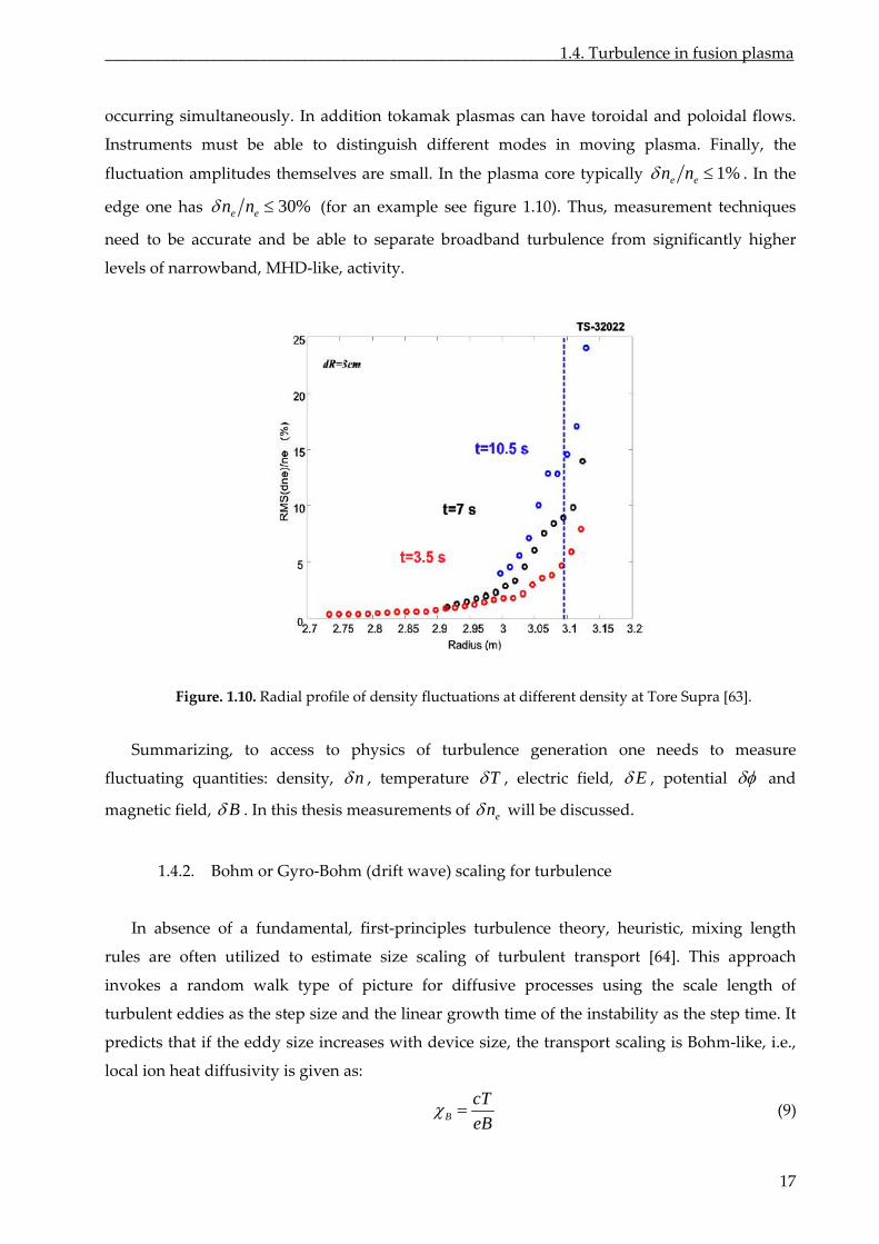
mselves are small. In the plasma core typically 1%e en n . In the
edge one has 30%e en n (for an example see figure 1.10). Thus, measurement techniques
need to be accurate and be able to separate broadband turbulence from significantly higher
levels of narrowband, MHD‐like, activity.
Figure. 1.10. Radial profile of density fluctuations at different density at Tore Supra [63].
Summarizing, to access to physics of turbulence generation one needs to measure
fluctuating quantities: density, n , temperature T , electric field, E , potential a
ic
nd
magnet field, B . In this thesis measurements of en will be discussed.
1.4.2. Bohm or Gyro‐Bohm (drift wave) scaling for turbulence
In absence of a fundamental, first‐principles turbulence theory, heuristic, mixing length
rules are often utilized to estimate size scaling of turbulent transport [64]. This approach
invokes a random walk type of picture for diffusive processes using the scale length of
turbulent eddies as the step size and the linear growth time of the instabilit
predi
y as the step time. It
cts that if the eddy size increases with device size, the transport scaling is Bohm‐like, i.e.,
local ion heat diffusivity is given as:
B
cT
eB (9)
17
Chapter I. Introduction________________________________________________________________
On the other hand, if the eddy size is microscopic (on the order of the ion gyroradius), the
transport scaling is gyro‐Bohm, i.e., local ion heat diffusivity is given as:
*GB B (10)
where *i radius ia is ion gyro normalized by the tokamak minor radius a. There is a
long history of confinement scaling studies that have correlated the thermal and/or particle
confinement with either Bohm or drift wave scaling laws. The issue is still actively debated as to
which transport scaling is to occur under given confinement conditions [65].
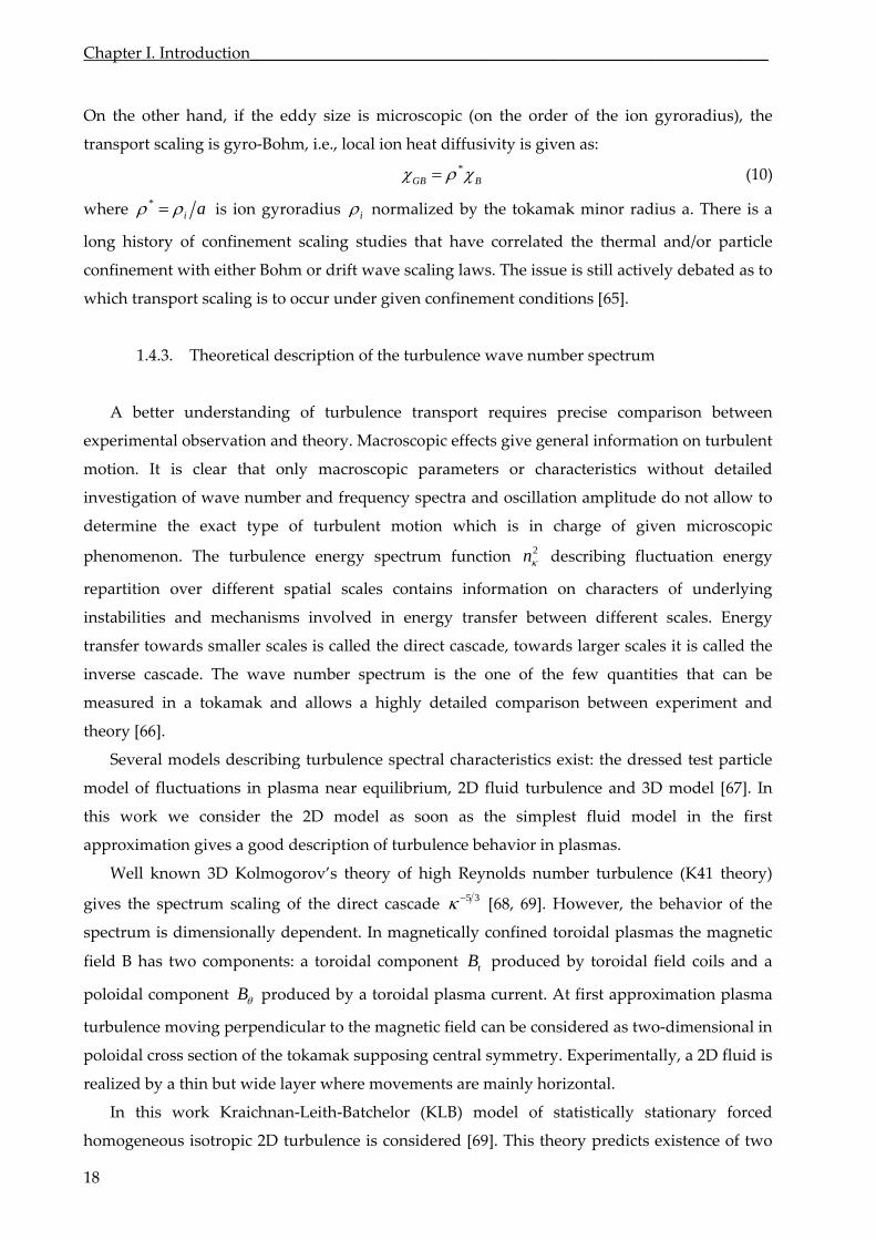
1.4.3. Theoretical description of the turbulence wave number spectrum
A better understanding of turbulence transport requires precise comparison between
experimental observation and theory. Macroscopic effects give general information on turbulent
motion. It is clear that only macroscopic parameters or characteristics without detailed
investigation of wave number and frequency spectra and oscillation amplitude do not allow to
determine the exact type of turbulent motion which is in charge of given microscopic
phenomenon. The turbulence energy spectrum function 2n describing fluctuation energy
repartition over different spatial scales contains information on characters of underlying
instabilities and mechanisms involved in energy transfer between different scales. Energy
transfer towards smaller scales is called the direct cascade, towards larger scales it is called the
inverse cascade. The wave number spectrum is the one of the few quantities that can be
measured and
theory [66].
spectral dressed
nea 2D and [67].
con as model in the first
approximation gives a good description of turbulence behavior in plasmas.
turbulence (K41 theory)
ives the spectrum scaling of the direct cascade
in a tokamak and allows a highly detailed comparison between experiment
Several models describing turbulence characteristics exist: the test particle
model of fluctuations in plasma r equilibrium, fluid turbulence 3D model In
this work we sider the 2D model as soon the simplest fluid
Well known 3D Kolmogorov’s theory of high Reynolds number
5 3 g [68, 69]. However, the behavior of the
spectrum is dimensionally dependent. In magnetically confined toroidal plasmas the magnetic
field B has two components: a toroidal component tB produced by toroidal field coils and a
poloidal component B produced a toroidal plasma current. At approximation plasma
turbulence moving perpendicular to the magnetic field can be considered as two‐dimensional in
poloidal cross section of the tokamak
by first
supposing central symmetry. Experimentally, a 2D fluid is
realized by a thin but wide layer where movements are mainly horizontal.
In is work Kraichnan‐Leith‐Batchelor (KLB) odel of statistically stationary forc
homogeneous isotropic 2D turbulence is considered [69]. This theory predicts existence of two
th m ed
18
________________________________________________________1.4. Turbulence in fusion plasma
inertial ranges: an energy inertial range with an energy spectrum scaling of 5 3 and an
enstrophy inertial range with an energy spectrum scaling 3 . The existence of two conserved
quantities complicates the construction of theory. Energy enstrophy are injected into
some ex e
and the
flow by ternal forcing at som intermediate wave number range min maxf . The
most of energy transfers towards low and forms the inverse cascade, the most of enstrophy
transfers downscale towards high and is called the enstrophy cascade of direct cascade. Energy dissipates at large scale due to friction between the box size vortices and the boundary,
e enstrophy dissipates at small scales due to molecular viscosity [71]. The inverse enstrophy
all fractions of
upscale enstrophy flux and downscale energy flux.
th
and forward energy cascades are neglected however in reality there are sm
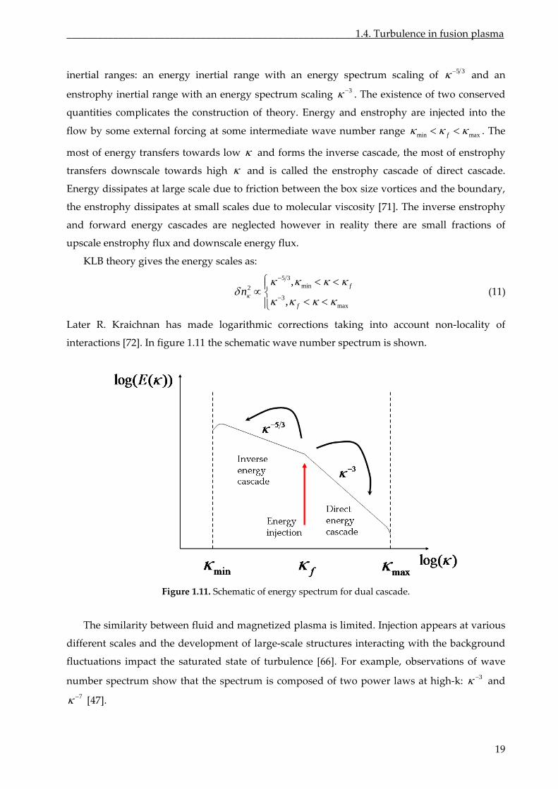
KLB theory gives the energy scales as:
5 3min2
3max
,
,
f
f
n
(11)
Later R. Kraichnan has made logarithmic corrections taking into account non‐locality of
interactions [72 In figure 1.11 the schematic wave spectrum is shown.
]. number
Figure 1.11. Schematic of energy spectrum for dual cascade.
The similarity between fluid and magnetized plasma is limited. Injection appears at various
fluctuations impact the saturated state of turbulence [
different scales and the development of large‐scale structures interacting with the background
66]. For example, observations of wave
number spectrum show that the spectrum is composed of two power laws at high‐k: 3 and
7 [47].
19
Chapter I. Introduction________________________________________________________________
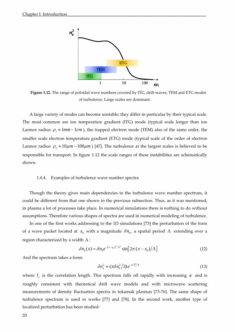
Figure 1.12. The range of poloidal wave numbers covered by ITG, drift‐waves, TEM and ETG modes
of turbulence. Large scales are dominant.
A large variety of modes can become unstable; they differ in particular by their typical scale.
The most common are ion temperature gradient (ITG) mod (typical scale longer than
Larmor radius
e ion
1 1i mm cm
e
), the trapped electron mode (TEM) also of the same order, the
smaller scale electron temperature gradient (ETG) mode (typical scale of the order of electron
Larmor radius 10 100m m ) [47]. The turbulence at the largest scales is believed to be
responsible for transport. In figure 1.12 the scale ranges of these instabilities are schematically
shown.
1.4.4. Examples of turbulence wave number spectra
Though the theory gives main dependencies in the turbulence wave number spectrum, it
could be different from that one shown in the previous subsection. Thus, as it was mentioned,
in plasma a lot of processes take place. In numerical simulations there is nothing to do without
assumptions. Therefore various shapes of spectra are used in numerical modeling of turbulence.
In one of the first works addressing to the 1D simulations [73] the perturbation of the form
of a wave packet located at 0x with a magnitude 0n , a spatial period extending over a
region characterized by a width
:
2 20( )
0 0( ) sin 2 ( )x xen x n e x x (12)
And the spectrum takes a form:
2 2 42 2
0( 3) cln n e (13)
where cl is the correlation length. This spectrum falls off rapidly with increasing and is
roughly consistent with theoretical drift wave models and with microwave scattering
measurements of density fluctuation spectra in tokamak plasmas [73‐76]. The same shape of
turbulence spectrum is used in works [77] and [78]. In the second work, another type of
localized perturbation has been studied:
20
________________________________________________________1.4. Turbulence in fusion plasma
0 sin[ ( )],( )
0,
f f f
f f
n k x x x x wn x
x x w
f
(14)
where fw is the half‐width of the perturbation centered around fw and fk is the fluctuating
wave number.
In [77] in case of spatio‐temporal turbulence the spectrum is introduced in the following
way:
2 2 2 20
,
( ) ( ) sin( )sin( )exp( 8)exp( 8)e j xj m tm j c m cj m
n x n g x k x t k l t (15)
correlation function for a set of samples is also Gaussian,
( )g x
temporal
accounts for a smooth inhomogeneous distribution of the fluctuation amplitude. The
2 2exp( )ct t .
urbulence supp
ved confinement re
close to the plasma edge. The H‐mode formation is still not clearly understood as well
as turbulence suppression or properties modifications of fluctuations. Some of mechanisms of
spo
fluid like motion is known as
Some other kinds of turbulence spectra will be presented and commented in Chapter IV.
1.4.5. T ression
In the impro gime (H‐mode) [79] cross‐field losses of particles and energy
are reduced due to transport barriers which are formed by sheared poloidal plasma flows and
located
such an effect are briefly described in this subsection.
1.4.5.1. Radial electric field shear
In 1988 S.‐I. Itoh and K. Itoh have introduced the radial electric field rE into the explanation
of the H‐mode confinement regime [80] and therefore have shown its importance. A
ntaneous bifurcation of rE nowadays is used as a theoretical model to explain the improved
confinement.
The electric field created a E B
drift. The E B
drift
velocity is given by the expression:
2E B
E B
B
(16)
The field can be determined from the radial force alance:
electric b
, ,
1 jr j
j
dpE B B
e dr (17)
where j is any plasma species and the last term is often called the diamagnetic contribution to
the rE .
j
21
Chapter I. Introduction________________________________________________________________
In 1990 Biglari, Diamond and Terry have developed a model showing analytically that a
possibl turbulence quench echanism is a sufficiently strong shear the radial electric f
[81]. The BDT model explains H‐mode reduced turbulent transport due to accumulated
perimental evidence. It shows that the electric field stabilizes nonlinearly turbulent modes in
odel also explains the formation of edge and core transport barriers. The
radial shear The BDT‐criterion for shear decorrelation (when shearing rate exceeds
decorrelation time) takes a form:
e m in ield
r
plasma. The m
E
ex
important result of this work is that turbulence suppression does not depend on the sign of r
E
or its rE .
r t
r
E
B k L
(18)
where t is the turbulent decorrelation frequency, rL is the radial correlation length, k
dicular
is
the o wave number of turbulence. If the is strong, it can drive perpen
nt structures into smaller ones, thus reducing radial
correlation lengths and suppressing turbulence.
c, they do not drive radial or cross‐field
transport. ZFs gain their energy from all types of microinstabilities through ‐ nonlinearity
and shearing them. Since ZFs are electrostatic
uctuations, the caused velocity shear is time varying, however the time scale stays accessible
to fr
i
The importance of plasma turbulence in plasma magnetic confinement has been cle
shown in the previous subsection. It is a strong motivation for researchers to develop
dia ectroscopy (BES), Heavy
Ion Beam Probes (HIBP), Langmuir probes, electromagnetic wave scattering and reflectom
systems are measuring plasma density fluctuations. In this section we shortly discuss
p loidal rE shear
plasma shear flows that break turbule
1.4.5.2. Zonal Flows
Zonal flows (ZFs) are low frequency electrostatic fluctuations with finite radial wave
number [54, 55]. Since they are poloidally symmetri
v v
regulate the amplitude of the latter by
fl
diagnostics studied in this thesis. The increase in the zonal flow action in turbulence
contributes to a lessening of anomalous transport. The interaction between zonal flows and drift
waves plays an essential role n determining plasma turbulence and transport [54].
1.5. Turbulence diagnostics
arly
gnostics to measure fluctuations in tokamaks. Beam Emission Sp
etry
advantages and disadvantages of these methods.
22
____________________________________________________________1.5. Turbulence diagnostics
23
Langmuir probes are the oldest and most well described diagnostic [82, 83 and 84]. Probes
measure simultaneously electron density en , temperature eT , plasma potential and their
ctuations. Probes are used routinely to estimate fluctuation driven energy and particle flux in
the tokamak edge and the shear layer in diverted plasmas. Application of probes is restricted to
the low temperature plasma boundary where the level of fluctuations is significantly high, the
impact of impurities is rather noticeable as well; this leaves a lot of questions to researche .
Good spatial resol n and slow time scale due to capacity do not take into account the
turbulent flux on the interpretatio
flu
rs
utio
n model as it should be [85].
HIBP are used to measure simultaneously fluctuations of plasma potential and electron
density 86‐88]. This is a collimated beam of neutrals or singly charged ions which ionize
plasma producing secondary ions that have orbits larger than the minor radius. HIBP is not as
e to ty
BES is a technique measuring density fluctuations by observing the light emitted from beam
atoms by collisions with constituents of the bulk plasma [89]. The
detectable fluctuation level is limited by photon statistics, atomic excitation process and beam
stab
e frequency
tends to be so low that the beam suffers from considerable refraction by the plasma. Also,
ze obtainable. Moreover, fluctuation wave numbers
greater than 2ki are not obtainable so relevant parts of the
[ s in
sensitiv high fluctuations due to its finite sample volume. There is also uncertain in
radial location measurements. Furthermore, the HIBP systems are complex and rather
expensive and do not really permit to have absolute measurement due to lack of knowledge
during the particle trajectory.
or ions that have been excited
ility, and due to this fact the absolute value of density fluctuations is not accessible. Wave
number spectra in radial and poloidal directions can be acquired from cross correlation
measurements in these directions. Unfortunately the diagnostic is rather sensitive to the MHD
activity.
Coherent scattering of electromagnetic waves is used to measure properties of electron
density autocorrelation function [84]. The diagnostic is based on refractive index principles. The
calibration of scattering systems is not straightforward and introduces uncertainty in estimates
of electron density fluctuations. The main drawback of the diagnostic is that th
diffraction limits the minimum beam si
spectrum may not be accessible
wit
ghtforward to perform but rather hard to
interpret. The phase delay is most sensitive to density fluctuations located near the reflection
layer. However, it is also sensitive to fluctuations along the entire radiation path, and so the
h low ki microwaves. Measurements are limited primarily by low spatial resolution at low
values of and by practical requirements on machine access to sample a variety of plasma
locations and .
Reflectometry refers to the reflection of an electromagnetic wave from a plasma cut‐off
where the plasma refractive index vanishes [90, 91]. Fluctuation measurements in the plasma
interior using reflectometry are relatively strai
Chapter I. Introduction________________________________________________________________
loca
e
this method was used for
ion
density of plasma and turbulence properties in tokamak [56, 84,
95‐
lization of the measurement is not the same as if one were probing an oscillating mirror at
the cut‐off position. Moreover, standart on channel reflectometry methods provide no wave
number resolution.
1.6. Radial correlation reflectometry
On purpose to determine wave number spectrum or at least the turbulence correlation
length radial correlation reflectometry (RCR) was proposed. Firstly
osphere [92]. Although the first experiments using microwave reflectometry were carried
out many years ago [93, 94] it is only in recent years that the technique has been developed to
the point where quantitative information can be routinely obtained on tokamak plasmas. R.
Cano and A. Cavallo in 1980 [90] proposed to apply it for tokamaks and first experiments were
held on the TFR tokamak using the ordinary mode of propagation in 1985 by F. Simonet [91]
and later was widely spread all over the world fusion devices. Nowadays RCR is a widely used
method for measuring electron
97].
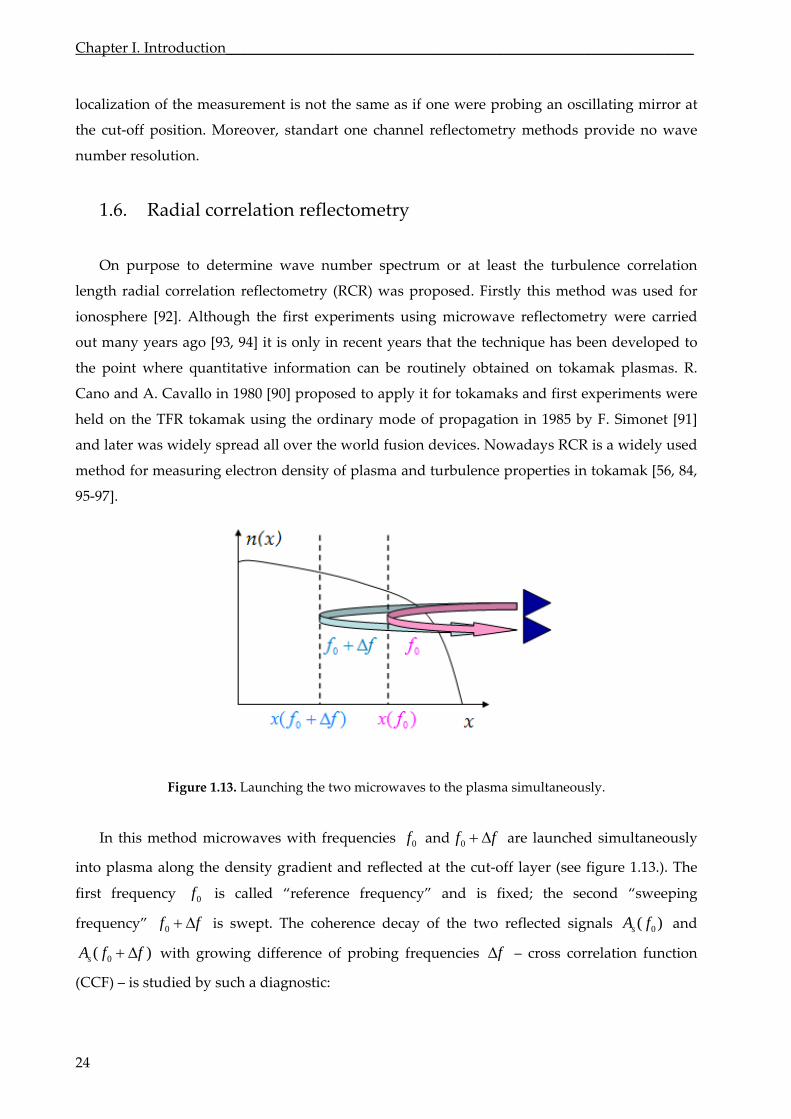
Figure 1.13. unching the two microwaves to the plasma simultaneously.
In this method microwaves with frequencies
La
0f and 0f f are launched simultaneously
into plasma along the density gradient and reflected at the cut‐off layer (see figure The
first frequency
1.13.).
0f is called “reference freque fixed; the second “sweeping
freq
ncy” and is
uency” 0f f is swept. The coherence decay of the two reflected signals 0( )sA f and
0( )sA f f with growing difference of probing frequencies f – cross correlation function
(CCF) – is studied by such a diagnostic:
24
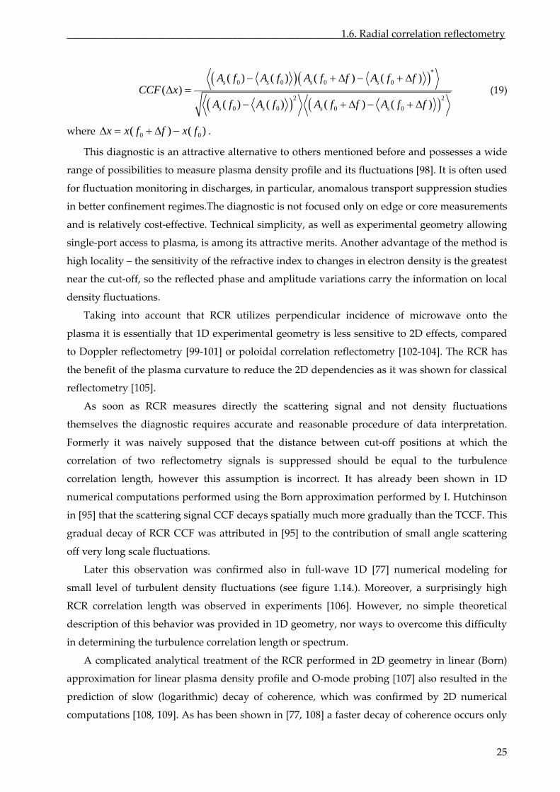
_____________________________________________________1.6. Radial correlation reflectometry
25
*
0 0 0 0
2 2
( ) ( ) ( ) ( )( )
s s s sA f A f A f f A f fCCF x
(19)
0 0 0 0( ) ( ) ( ) ( )s s s sA f A f A f f A f f
where ) 0 0( ) (x x f f x f .
rs mentioned before and possesses a wide
range of possibilities to measure plasma density profile and its fluctuations [98]. It is often used
for
ler reflectometry [99‐101] or poloidal correlation reflectometry [102‐104]. The RCR has
the benefit of the plasma curvature to reduce the 2D dependencies as it was shown for classical
reflectometry [105].
As soon as RCR measures directly the scattering signal and not density fluctuations
themselves the diagnostic requires accurate and reasonable procedure of data interpretation.
Formerly it was naively supposed that the distance between cut‐off positions at which the
correlation of two reflectometry signals is suppressed should be equal to the turbulence
correlation length, however this assumption is incorrect. It has already been shown in 1D
numerical computations performed using the Born approximation performed by I. Hutchinson
in [95] that the scattering signal CCF decays spatially much more gradually the TCCF. This
gradual decay of RCR CCF was attributed in [95] the contribution of small angle scattering
off very long s
ater this observation was confirmed also in full‐wave 1D [77] numerical modeling for
sm fi 1.14.). M
behavior in
in determining the turbulence correlation length or spectrum.
icated a (
approximat
of coherence, which was confirmed by 2D numerical
computations [108, 109]. As has been shown in [77, 108] a faster decay of coherence occurs only
This diagnostic is an attractive alternative to othe
fluctuation monitoring in discharges, in particular, anomalous transport suppression studies
in better confinement regimes.The diagnostic is not focused only on edge or core measurements
and is relatively cost‐effective. Technical simplicity, as well as experimental geometry allowing
single‐port access to plasma, is among its attractive merits. Another advantage of the method is
high locality – the sensitivity of the refractive index to changes in electron density is the greatest
near the cut‐off, so the reflected phase and amplitude variations carry the information on local
density fluctuations.
Taking into account that RCR utilizes perpendicular incidence of microwave onto the
plasma it is essentially that 1D experimental geometry is less sensitive to 2D effects, compared
to Dopp
than
to
cale fluctuations.
L
all level of turbulent density fluctuations (see gure oreover, a surprisingly high
RCR correlation length was observed in experiments [106]. However, no simple theoretical
description of this was provided 1D geometry, nor ways to overcome this difficulty
A compl nalytical treatment of the RCR performed in 2D geometry in linear Born)
ion for linear plasma density profile and O‐mode probing [107] also resulted in the
prediction of slow (logarithmic) decay
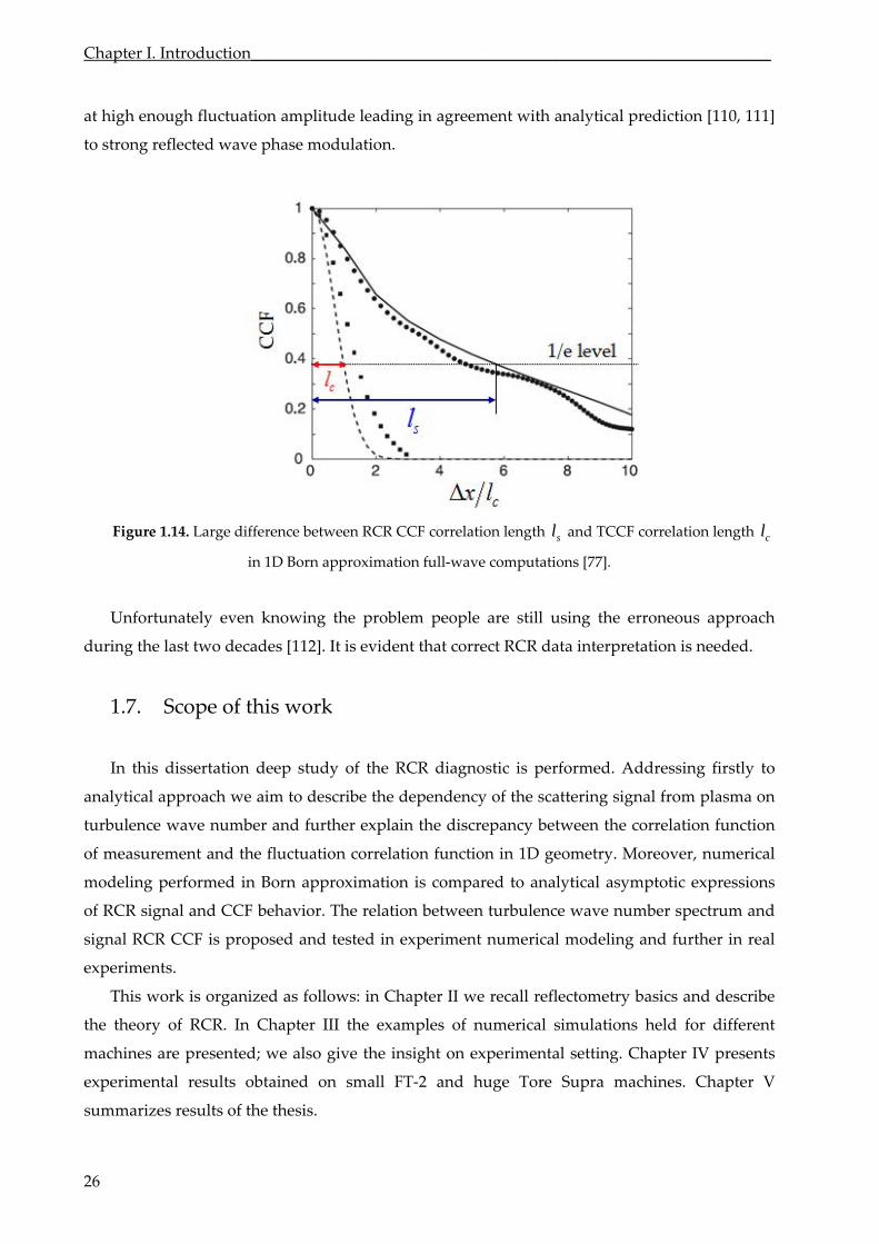
Chapter I. Introduction________________________________________________________________
at high enough fluctuation amplitude leading in agreement with analytical prediction [110, 111]
to strong reflected wave phase modulation.
Figure 1.14. Large difference between RCR CCF correlation length sl and TCCF correlation length cl
in 1D Born approximation full‐wave computations [77].
Unfortunately even knowing the problem people are still using the erroneous approach
dur
n correlation function in 1D geometry. Moreover, numerical
modeling compared
and
reflectometry basics and describe
the
ing the last two decades [112]. It is evident that correct RCR data interpretation is needed.
1.7. Scope of this work
In this dissertation deep study of the RCR diagnostic is performed. Addressing firstly to
analytical approach we aim to describe the dependency of the scattering signal from plasma on
turbulence wave number and further explain the discrepancy between the correlation function
of measurement and the fluctuatio
performed in Born approximation is to analytical asymptotic expressions
of RCR signal CCF behavior. The relation between turbulence wave number spectrum and
signal RCR CCF is proposed and tested in experiment numerical modeling and further in real
experiments.
This work is organized as follows: in Chapter II we recall
theory of RCR. In Chapter III the examples of numerical simulations held for different
machines are presented; we also give the insight on experimental setting. Chapter IV presents
experimental results obtained on small FT‐2 and huge Tore Supra machines. Chapter V
summarizes results of the thesis.
26
27
Chapter II
radial correlation reflectometry
___ ______________________________________________________________________________
nal theory of radial correlation reflectometry is presented. The analytical
exp
Theoretical background
of
____
In this Chapter we firstly describe propagation of electromagnetic waves in inhomogeneous
plasma, reflectometry basics and the way to introduce plasma density fluctuations. Further, the
one dimensio
ression for the RCR CCF is given. The simple relation between the RCR CCF and the
turbulence wave number spectrum is derived. We also present formlue aloowing direct
transformations between RCR CCF and TCCF.

28
_____________________________________2.1. Propagation of electromagnetic waves in plasmas
29
2.1. Propagation of electromagnetic waves in plasmas
This section is based on V. L. Ginzburg development in CGS units [92].
Propagation of an electromagnetic wave in a medium is described by Maxwell equations:
4D
(20)
0B
(21)
1 B
Ec t
(22)
4 1 D
H jc c
t
(23)
Where and are electric and magnetic fields of the wave correspondingly; E H
and j
P
are
charge cur correspondingly created by external sources related to the and rent polarization in
the usual way:
P (24)
P
jt
(25)
These relations enforce charge conservation:
0jt
(26)
In plasma as in any dielectric, the relations between fields and their induction take the
following form:
4D E P
(27)
4B H M
(28)
where M is magnetization. The linear relation between j
and E
is given by Ohm law:
j E (29)
where is the conductivity tensor.
2.1.1. Approximations and restrictions used
To obtain a general description of electromagnetic wave propagation in plasma it is needed
to use simplifying hypotheses and approximations.
2.1.1.1. Stationary plasma
Temporal variations of the plasma occur on a time scale considerably bigger than the period
of the waves signifying that the plasma is stationary on the wave time reference.
Chapter II. Theoretical background of radial correlation reflectometry_______________________
2.1.1.2. Cold plasma approximation
elow 5 keV. Waves
trav al
velocity of electrons is much less than the phas velocity
At present, most fusion experiments operate at plasma temperature b
eling at phase velocities close to the speed of light are concerned. In this case the therm
1Te ph .e Cold pla
approximation is used to describe the propagation o most electromagnetic waves in toka
plasma. The meaning of the approximation is that thermal motion of particles is neglected
comparing to the motion caused by propagating electromagnetic wave [113, 114].
It is also assumed that there is no collisional damping (or Landau damping) on the time
scale of plasma electrons as required for cold plasma approximation. Electrons are init
st
.3. High frequencies
Ion and neutral particle motion is neglected as well due the relation
sma
f mak
ially
considered at re , except for movement induced by wave fields.
2.1.1
1e im m as soon as
hig frequency electromagnetic waves ci h are udied. Only electrons contribute to
t.
2.1.1.4. Anisotropy
the anisotropy is introduced only by external magnetic field
st the
plasma dielectric tensor over the time of fligh
We suppose 0B. In this work
inhomogeneous anisotropic plasma is considered where refractive index depends on
propagation direction.
2.1.1.5. Propagationg waves
The electromagnetic wave propagating into plasma is supposed to be monochromatic. It
the
could be described in usual way:
0 exp( )E E i t
(30)
where 2 f is the microwave angular frequency of the wave. The phase velocity,
ph k gives the rate of propagation of a point of constant phase on the wave. If the wave
or amplitude is modulated the wave possesses the group velocityfrequency gr k . The
dispersion relation ( )k contains information on phase and group velocities, propagation
region, reflection points, resonance points, damping, wave growth. Another property of the
30
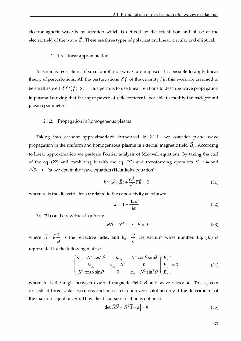
_____________________________________2.1. Propagation of electromagnetic waves in plasmas
ele defined by the orientation and phase of the
electric field of the wave There are three types of polarization: linear, circular and elliptical.
ctromagnetic wave is polarization which is
E.
2.1.1.6. Linear approximation
As soon as restrictions of small‐amplitude waves are imposed it is possible to apply linear
theory of perturbations. All the perturbations f of the quantity f in this work are assumed to
be small as well 1f f . This permits to use linear relations to describe wave propagation
in p
2.1.2. Propagation in homogeneous plasma
aking into account approximations introduced in 2.1.1., we consider plane wave
pro ic field
lasma knowing that the input power of reflectometer is not able to modify the background
plasma parameters.
T
0B.
pagation in the uniform and homogeneous plasma in external magnet According
to linear approximation we perform Fou lysis of Maxwell equations. By taking the curl
of the eq. (22) and combining it with the eq
rier ana
. (23) and transforming operators and ik
t i we obtain wave equation (Helmholtz equation):
the
2
2( )k k E E
c
0
(31)
where is the dielectric tensor related to the conductivity as follows:
4
1i
(32)
Eq. (31) can be rewritten in a form:
2 1 0N ENN
(33)
where c
N k
is the refractive index an
d 0kc
the vacuum wave number. Eq. (33) is
represented by the following matrix:
2
2 0 0
cos sin 0 sinxy xx y
zz z
i N E
N N E
2 2 2
2 2
cos cos sinxy xN i N E
xx
(34)
where
is the angle between external magnetic field B and wave vector stem
consists of three scalar and possesses non‐zero solution on if the determinant of
This sy
equations a ly
the matrix is equal to zero. Thus, the dispersion relation is obtained:
k.
2det 1 0NN N
(35)
31
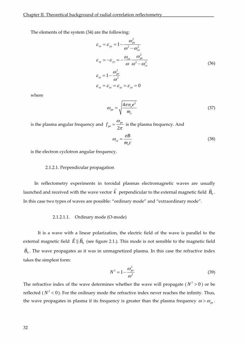
Chapter II. Theoretical background of radial correlation reflectometry_______________________
The elements of the system (34) are the following:
2
1 pe
2 2
2
2 2
2
xx yyce
pecexy yx
ce
2
1
0
pezz
xz zx zy yz
(36)
where
24 e
pee
n e
m
(37)
is the plasma angular frequency and 2
pepef
is the plasma frequency. And
cee
eB (38)
.1. Perpendicular propagation
m c
is the electron cyclotron angular frequency.
2.1.2
In reflectometry experiments in toroidal plasmas electromagnetic waves are usually
launched and received with the wave vector k perpendicular to the external magnetic field 0B
.
In this case two types of waves are possible: “ordinary mode” and “extraordinary mode”.
e (O‐mode)
It is a wave with a linear polarization, the electric field of the wave is parallel to the
l magnet
2.1.2.1.1. Ordinary mod
externa ic field 0E B (see figure 2.1.) ode is not sensible to the magnetic field
0
. This m
B. The wave propagates as it was in unmagnetized plasma. In this case the refractive index
takes the simplest form:
22
21 peN
(39)
The refractive index of the wave determines whether the ave will propagate 0N ) or be
reflected ( 2 0N ). For the ordinary mode the refractive index never reaches the infinity. Thus,
the wave propagates in plasma if its frequency is greater than the plasma
w
( 2
frequency pe .
32
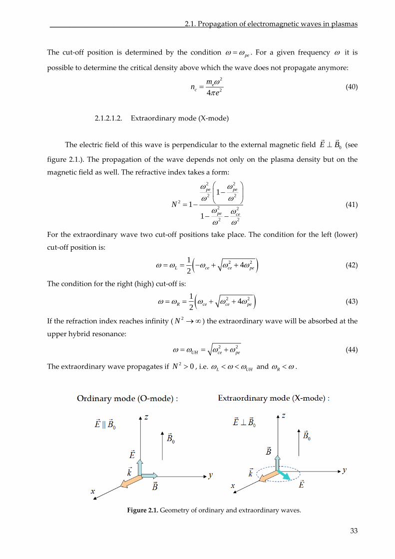
_____________________________________2.1. Propagation of electromagnetic waves in plasmas
The cut‐off position is determined by the condition pe . For a given frequency
anymore:
it is
possible to determine the critical density above which does not propagate
the wave
2
24e
c
mn
e
to the ex
(40)
2.1.2.1.2. Extraordinary mode (X‐mode)
The electric field of this wave is perpendicular ternal magnetic field E 0B
on
(see
figu The propagation of the wave depends not the plasma density but the
magnetic field as well. The refractive index takes a form:
re 2.1.). only on
2 2
2 22N
2 2
2 2
1
1
1
pe pe
pe ce
(41)
For the extraordinary wave two cut‐off positions take place. The condition for the left (lower)
cut
‐off position is:
2 214
2L ce ce pe (42)
The condition for the right (high) cut‐off is:
2 214
2 (43)
If the refraction index reaches infinity ( N ) the extraordinary wave will be absorbed
R ce ce pe
the
uppe hybrid resonance:
2 at
r
2 2UH ce pe (44)
The ex wave propagates if i.e. H 2 0N , L U and R .traordinary
Figure 2.1. Geometry of ordinary and extraordinary waves.
33
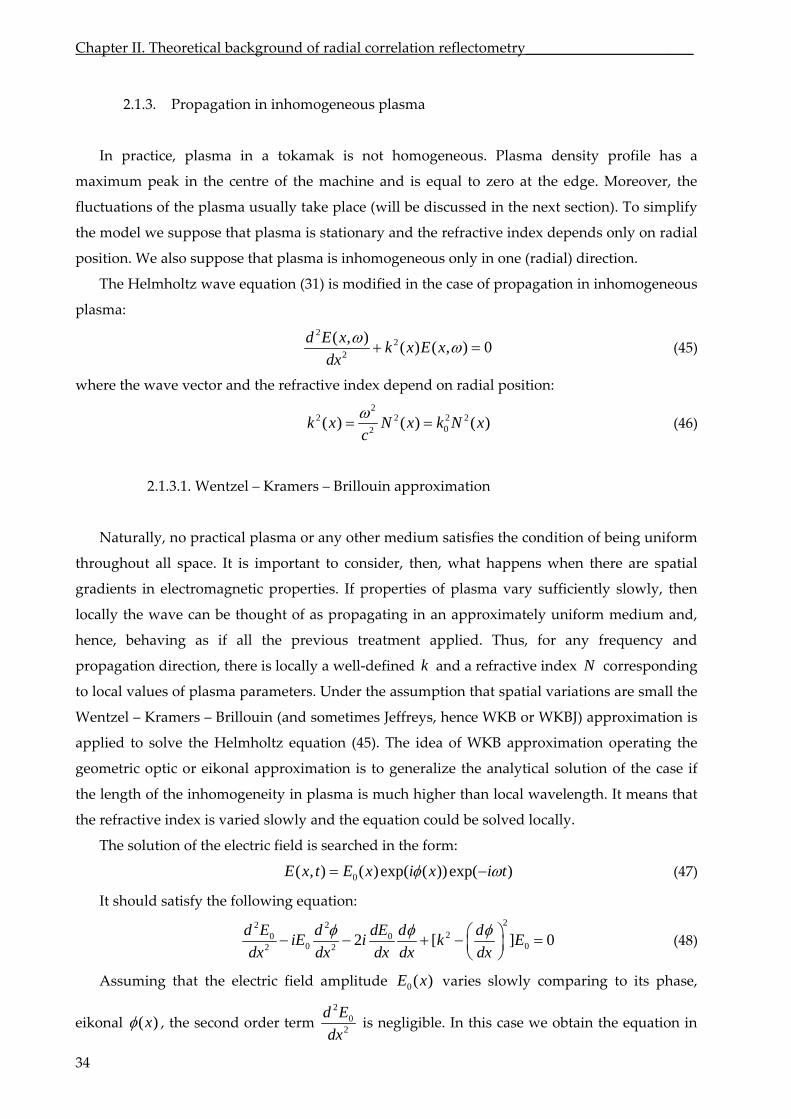
Chapter II. Theoretical background of radial correlation reflectometry_______________________
2.1.3. Propagation in inhomogeneous plasma
In practice, plasma in a tokamak is not homogeneous. Plasma density profile has a
maximum peak in the centre of the machine and is equal to zero at the edge. Moreover,
uctuations of the plasma usually take place (will be discussed in the next section). To simplify
the model efractive index depends only on radial
position. We also suppose that plasma is inhomogeneous only in one (radial) direction.
T mogen
the
fl
we suppose that plasma is stationary and the r
he Helmholtz wave equation (31) is modified in the case of propagation in inho eous
plasma:
2
22
( , )( ) (
d E xk x E x
, ) 0
dx (45)
where the wave vector and the refractive index depend on radial position:
2
2 2 202
( ) ( ) ( )k x N x k N xc
2 (46)
– Kramers – Brillouin approximation
aturally, no practical plasma or any other medium satisfies e condition of being unif
sider, then, what happens when there are spatial
gradients in electromagnetic properties. If properties of plasma vary sufficiently slowly, then
locally the wave can be thought of as propagating in an approximately uniform medium a
us trea
re is locally a well‐defined and a refractive index corresponding
to local values of plasma parameters. Under the assumption spatial variations are small
Wentzel – Kramers – Brillouin (and sometimes Jeffreys, hence WKB or WKBJ) approximation is
on (45 idea of WK roximation operating the
eometric optic or eikonal approximation is to generalize the analytical solution of the case if
the length of the inhomogeneity in plasma is much higher than local wavelength. It means that
the refractive index is varied slowly and the equation could be solved locally.
The solution of the electric field is searched in the form:
2.1.3.1. Wentzel
N th orm
throughout all space. It is important to con
nd,
hence, behaving as if all the previo tment applied. Thus, for any frequency and
propagation direction, the k N
that the
applied to solve the Helmholtz equati ). The B app
g
0( , ) ( )exp( ( ))exp( )E x t E x i x i t (47)
It should satisfy the following equation:
22 220 0
0 02 22 [ ]
d E d dE d diE i k E
dx dx dx dx dx
0 (48)
Assuming that the electric field amplitude varies slowly comparing to its phase,
eikonal
0 ( )E x
( )x , the second order term 2
02
d E is negligible. In this case we obtain
dx the equation in
34
_________________________________________________________2.2. Plasma density fluctuations
35
which each is equal to zero. Namely, term
22 d 0k
dx
results in expression for the electric
field phase:
( ) ( )x k x dx (49)
The solution of the remaining equation 2
00 2
2 0d dE d
Edx dx dx
gives the expression for the
electric field amplitude 0 00( )
( )E x
d k x , in terms of wave vector:
E E
dx
0( , ) [exp[ ( ) ]exp ]( )
EE x t i k x dx i t
k x (50)
In terms of the refractive index:
00( , ) exp[ ( ) ]exp[ ]
( )
EE x t ik N x dx i t
N x
This approximation is valid if the second order term is negligible comparing to other terms:
(51)
2 2 20 0
02 2 2 and
d E d d E dE dE
dx dx dx dx dx0
(52)
it means:
2
22
and d k dk dk
k kdx dx dx
(53)
In terms of wavelength:
2 2
21
d d
dx dx
(54)
These conditions are conditions of the geometric optics and are valid if the wavelength
varies slowly at the distance equal to the wavelength. The plasma properties should vary
slowly at the scale of the wavelength.
The WKB approximation is valid far from the cut‐off. In the vicinity of the cut‐off layer
when the refractive index goes to zero the WKB approximation is no more valid and to find the
solu
We ntroduce density fluctuations to plasma as:
tion it is necessary to treat the equation numerically.
2.2. Plasma density fluctuations
i
( ) ( ) ( )n r n n rr (55)
Chapter II. Theoretical background of radial correlation reflectometry_______________________
In inhomogeneous plasmas density fluctuations are described by the function ( )n r . Plasma
density fluctuations are described by magnitude 0( )n r , wave number , frequency 2 .
ain spatial characteristics is correlation
The frequencies of microturbulence involved are of th order of the diamagnetic freque
i.e. very low compared to
length cl .One of the m
e ncy,
ci . Thus the impact on the frequency shift on the dispersion relation
of the scattered wave can be neglected.
density fluctuations toWe suppose plasma be small ( ) / 1cn x n and slowly changing in
time. In this case the fluctuation part can be treated as a approximation). The
Fourier transform gives the relation between fluctuations and their image in wave
numbe space
perturbation (Born
in real space
n :r
dx (56) ( ) i xn n x e
1( )
2i xn x n e d
(57)
We
we obtain the expression for the correlation function of random Fourier‐harmonics averaged
over time or over ensemble (random phase samples):
')
also suppose that turbulence is statistically homogeneous. Using Wiener–Khinchin theorem
* 2', 2 (n n n (58)
where ‐ conjugate Fourier‐harmonic; *'kn 2
kn wave number spectrum; )( 'k k ‐ Dirac’s
delta‐function. Taking into account the relations (56) and (58) we obtain the expression for the
function (or TCCF): turbulence spatial cross correlation
2 (( ) ( ) ( ')2
ik x xk
dkTCCF x n x n x n e
') (59)
2.3. Mechanism of back and forward Bragg scattering
In 1D geometry the scattering processes are forward scattering and backscattering [78, 115].
The injected wave into the plasma described by wave vector ik and angular frequency i
interacts with the fluctuations characterized by wave vector and frequency 2 . Part
is subtracted from the wave and redistributed into space. mechanism of scattering
scattered wave s a new wave vector
of
is
energy The
possesse sk similar to Bragg scattering in crystals. The
which determines its propagation direction:
s ik k
(60)
The scattering angle (between sk and ik
) obeys the Bragg rule:
36
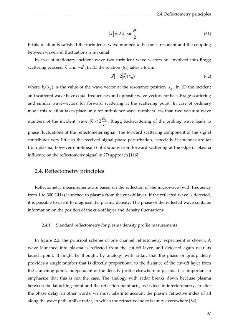
___________________________________________________________2.4. Reflectometry principles
2 sink 2i
(61)
If this relation is satisfied the turbulence wave number becomes resonant and the coupling
between wave and fluctuations is maximal.
In case of stationary incident wave two turbulent wave vectors are involved into Bragg
scattering process, and . In 1D the relation (61) takes a form:
2 ( )i Bk x
(62)
where ( )i Bk x
is the value of the wave vector at the resonance position Bx . In 1D the incident
and scattered wave have equal frequencies and opposite wave‐vectors for back Bragg scattering
and similar wa ‐veve ctors for forward scattering at the scattering point. In case of ordinary
mode relation takes place only for turbulence wave numbers less two vacuum wave
numbers incident wave
than this
of the
2 i
c
. Bragg backscattering of the wave leads to
phase fluctuations of the reflectometer signal. The forward scattering component of the signal
116].
. Re
tion of the microwave (with frequency
from 1 300 GHz) launched to plasma from the cut‐off layer. If the reflected wave is detec
it is possible to use it to diagnose the plasma density. The phase of the reflected wave contains
information on the position of the cut‐off layer and density fluctuations.
.4.1. Standard reflectometry for plasma density profile masurements
A
again
provides a single number that is directly proportional to the distance of the cut‐off layer from
to
nalogy with radar breaks down because plasma
between the launching point and the reflection point acts, as it does in interferometry, to a
t w st refractive index of all
along the wave path, unlike radar, in which the refractive index is unity everywhere [84].
probing
contributes very little to the received signal phase perturbation, especially if antennas are far
from plasma, however non‐linear contributions from forward scattering at the edge of plasma
influence on the reflectometry signal in 2D approach [
2.4 flectometry principles
Reflectometry measurements are based on the reflec
to ted,
2
In figure 2.2. the principal scheme of one channel reflectometry experiment is shown.
wave launched into plasma is reflected from the cut‐off layer, and detected near its
launch point. It might be thought, by analogy with radar, that the phase or group delay
the launching point, independent of the density profile elsewhere in plasma. It is important
emphasize that this is not the case. The a
lter
the phase delay. In o her words, e mu take into account the plasma
37
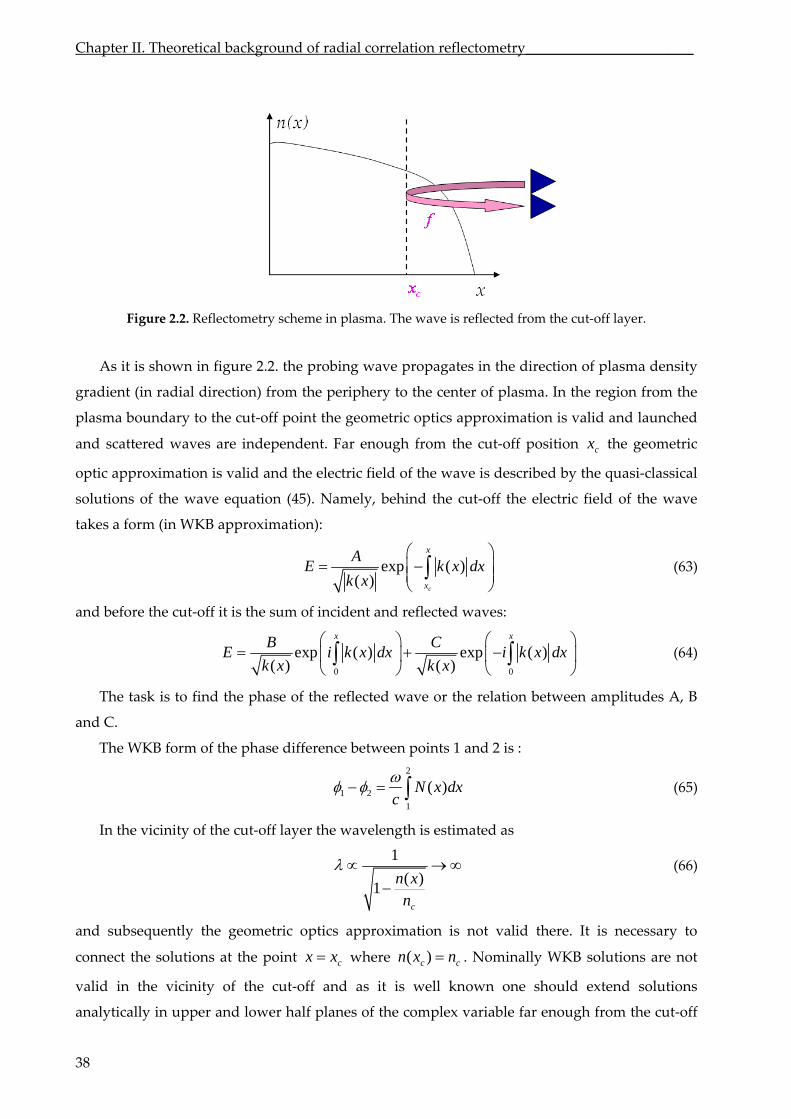
Chapter II. Theoretical background of radial correlation reflectometry_______________________
38
Figure 2.2. Reflectometry scheme in plasma. The wave is reflected from the cut‐off layer.
As it is shown in figure 2.2. the probing wave propagates in the direction of plasma density
plasma boundary to the cut‐off po geometric optics approximation is valid and launched
and scattered waves are independent. Far enough from the cut‐off position
gradient (in radial direction) from the periphery to the center of plasma. In the region from the
int the
cx the geometric
optic approximation is valid and the electric field of the wave is described by the quasi‐classical
solutions of the wave equation (45). Namely, behind the cut‐off the electric field of the wave
takes a form (in WKB approximation):
exp ( )( )
c
x
x
AE k
k x
x dx (63)
and the cut‐off it is the sum of incident and reflected waves: before
0 0
exp ( ) exp ( )( ) ( )
x xB CE i k x dx i k x dx
k x k x
(64)
The task is to find the phase of the reflected wave or the relation between amplitudes A, B
and C.
The WKB form of the phase difference between points 1 and 2 is :
2 1 2 ( )N x dx
c (65)
1
In the vicinity of the cut‐off layer the wavelength is estimated as
1
( )1
c
n xn
(66)
and subsequently the geometric optics approximation is not valid there. It is necessary to
connect the solutions at the point cx x where ( )c cn x n . Nominally WKB solutions are not
valid in the vicinity of the cut‐off and as it is well known one should extend solutions
analytically in upper and lower half planes of the complex variable far enough from the cut‐off
___________________________________________________________2.4. Reflectometry principles
point [117, 118]. The squared wave number is linearized around an interval centered on the
reflection point and the solution of equation (45) is expressed in terms of Airy function [119].
Phase shift between launched and reflected waves occurs to be equal to 2 and
correspondingly the full phase shift at the plasma boundary is [92]:
0
2 ( )2
cx
N x dxc
(67)
This equation states that the phase is just what would be obtained from simple‐minded
application of the WKBJ approach, regarding the cut‐off layer as a mirror, except that an
additional 2 phase change at reflection must be included.
To determine the cut‐off position using the phase shift generally speaking it is necessary to
know the plasma density profile. However for close to linear plasma density profiles the
integral in the phase expression could be estimated as:
0
( )1 0.5
cx
cc
n xdx x
c n c
(68)
in case of O‐mode reflectometry using
2
2
( )pe n x
n
.
Plasma density profile along the reflectometer’s
c
wave path can be deducted from phase
measurements at different frequencies. For ordinary mode the integral transform is u
to obtain an explicit analytic solution. For all relevant frequencies the function
Abel sed
( )
for
could be
de expression N(x) into
expression (67) after differentiating with respect to
constructed by interpolation for example. Substituting the O‐mo
we express the result in vacuum
wave length
terms of
2 c :
* *
2 cd dx d* *2 2d cd
wh
(69)
ere ** 2 c . The most convenient expression for the cut‐off position for a given
frequency can be determined:
*
* 2 *20
( )cx ad
c d d
(70)
The position of the cut‐off is deduced from phase delay for all frequencies less than .
We would like to notice also that the quantity we require for the inversion is actually the
derivative of the phase delay with respect to frequency. This quantity is precisely the group
delay, that is, the round‐trip time it would take a pulse or a modulation envelope to propagate
out to the reflection layer and back:
1
2
dt
d
(71)
39
Chapter II. Theoretical background of radial correlation reflectometry_______________________
In case of X‐mode reflectometry there is no analytical formula for the cut‐off positions and
the equation (67) should be treated numerically using Bottlier‐Curtet method [120].
Sweeping reflectometry providing information on plasma density profile in th dient
region along the path of the reflectometry wave is based on this prin
e gra
ciple, for example [121].
.4.2. Fluctuation reflectometry
Te only single access to plasma.
Ho
wever, it is also sensitive to fluctuations
along the entire radiation path, and so the localization of the measurement is not the same as if
one were probing an oscillating mirror at the cut‐off position (despite the fact that m
published analyses have adopted this analogy).
on measurements could be described as following. In
presence of plasma density fluctuations (55) the relation between the fluctuation characteristics
and
2
Fixed frequency fluctuation reflectometry provides information on tokamak low frequency
turbulence. chnically this method is simple and requires
wever due to one dimensional scattering geometry interpretation of fluctuation
reflectometry results, in general, is a very complicated task. The phase delay is most sensitive to
density fluctuations located near the reflection layer. Ho
any
Roughly the principle of fluctuati
received signal characteristics can be found. The received signal phase contains two
components as well:
( ) ( ) ( )t t t (72)
The expression (67) describes the first slow changing phase term. Supposing that fluctuation
amplitude is small c c c
by calcul the slow phase variation [73]:
n n l r fluctuating part of the phase is obtained in the frame of WKB
approximation ating
2
200
( , )( , )
( , )
cx
c
n x t dxt
c n k x
ally the inte
backscattering in the vicinity of the cut‐off layer. Thus it is
possibl to obtain the relation between density fluctuation and scattering signal characteri
and estimate turbulence frequency spectrum and its level. The attempt to confirm this
1 of the
refl
as assumed there that the singular (inverse proportional to
fluctuation wave number
(73)
Usu rpretation of fluctuation reflectometry results is based on the assumption
that the signal originates due to
e stics
assumption was undertaken by numerical [73] and analytical treatment [1 5]
ectometry problem performed in 1D model. In [115] the fluctuation reflectometry has been
addressed analytically, in the framework of the one dimensional WKB analysis. A singular
dependence of scattering efficiency on the fluctuation wave number was demonstrated for the
linear density profile. However it w
1sA ) behavior of the scattering efficiency saturates due to the
40
_______________________________________2.4. Basic assumptions and equations in 1D analysis
41
violation of the WKB approximation at so called Airy wave number 1 32 2nc L , where Ln
is the density gradient scale length. This conclusion appears to be erroneous that predetermines
2.5 Basic assumptions and equations in 1D analysis
x
magnetic field. The electromagnetic wave
pro
the subsequent difficulties of one‐dimensional theory in interpretation of experiments and
numerical modeling.
.
Taking into account that RCR uses perpendicular incidence of microwave onto plasma and
essentially 1D e perimental geometry is less sensitive to 2D effects, compared with Doppler
reflectometry or poloidal correlation reflectometry, we analyze it in the frame of 1D model
simplifying calculations and allowing investigation of the arbitrary density profile case.
As it was already introduced in subsection 2.1.1., we use cold plasma approximation to
describe microwave propagation in plasmas. Plasma is supposed to be an isotropic media;
anisotropy is introduced only by external
pagating into plasma is supposed to be monochromatic and stationary. Plasma density
fluctuations are supposed to be small 1%n n and the linear (Born) approximation and the
perturbation theory could be applied. Plasma is supposed to be “frozen”, i.e. the turbulence
correlation time 1c 0 s exceeds the probing time 1ns .
Supposing probing wave propagation strictly in the direction of plasma density gradient we
describe the O‐mode probing by Helmholtz equation (45), where 2 2 2 2 2( ) 1 pek x c is
a probing wave vector, 2 )pe ee n x n x m is the plasma frequency; ( )n x is the 4 (
background density profile; represented as (57) stands for turbulent density
perturbations, where
n x
is a density fluctuation wave number andturbulence n is turbu
fluc
lent
tuation amplitude; is a probing angular frequency. Under assumption that density
fluctuations are small the perturbation theory methods are used. Equation (45) can be rewritten
in the form:
2 2 2
2 2 2
( ) ( )1 z z
c c
d n x n xE E
dx c n c n
(74)
where the critical density at the cut‐off position is given by (40).
2.5.1. Reciprocity theorem
In particular, the scatte amplitude in linear (Born) approximation can be obtained ring signal
with the help of straightforward approach based upon the reciprocity theorem in the form
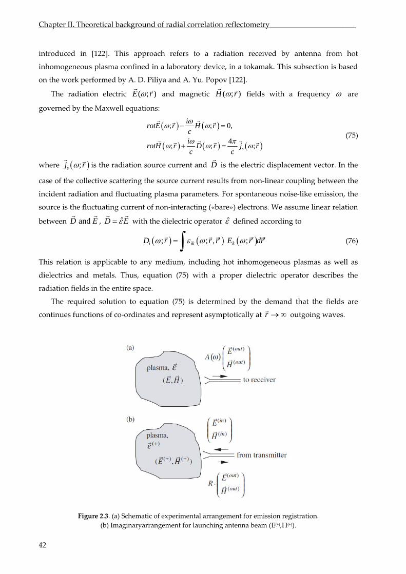
Chapter II. Theoretical background of radial correlation reflectometry_______________________
introduced in [122]. This approach refers to a radiation receive from hot
inhomogeneous plasma confined in a laboratory device, in a tokamak. This subsection is based
on the work performed by A. D. Piliya and A. Yu. Popov [
d by antenna
and magnetic
122].
The radiation electric ( ; )E r ( ; )H r
fields with a frequency are
overned by the Maxwell equations:
g
4; ; ;
irotH r D r j r
; ; 0, i
rotE r H rc
sc c
(75)
where ;sj r
is the radiation source current and D is the electric displacement vector. In the
case of the collective scattering the source current results from non‐linear coupling between the
incident radiation and fluctuating plasma parameters. For spontaneous noise‐like emission, the
source is the fluctuating current of non‐interacting («bare») electrons. We assume linear relation
between and D E
, ˆD E
with the dielectric operator ̂ defined according to
i ik kD r r r E r d ; ; , ; r (76)
This relation is applicable to any med ding hot inhomogeneous plasmas as well as
dielectrics and metals. Thus, equation (75) with a proper dielectric operator describes the
radiation fields in re space.
ium, inclu
the enti
The required solution to equation (75) is determined by the demand that the fields are
continues functions of co‐ordinates and represent asymptotically at r
outgoing waves.
Figure 2.3. (a) Schematic of experimental arrangement for emission registration.
(b) Imaginaryarrangement for launching antenna beam (E(+),H(+)).
42
_______________________________________2.5. Basic assumptions and equations in 1D analysis
Suppose that the radiation is received by a microwave antenna and transmitted through a
plasma‐free single mode wave‐guide to a registration device (see figure 2.3). Then far from the
antenna mouth within the wave‐guide,
( )
( )( )
out
out
EA
H H
E (77)
where ( )A is the signal amplitude and ( ) ( ),out outE H
are the electric and magnetic fields of
the fundamental wave‐guide mode propagating outward from plasma volume and normalized
to unit energy flux by
( ) ( ) *( )[ ] 1outE H dS8
outc
(78)
where dS is the surface element in the wave‐guide cross‐section. The symbol of the real part
before the integral is omitted because the integrand is a real function due to the wave‐guide
mode pro (s example, [123]). Equation (78) implies perfect matperties ee, for ching with the
receive .
At sufficiently small source current, the scalar amplitude
r
( )A depends linearly on the
vector sj. The most general form of this relation is
( ) ( ; ) ( ; )A j r g r dr s
(79)
where integration is over the plasma volume. The vector weight function ( ; )g r is, obviously,
related to the Green function of equations (75). Finding this n satisfying propfunctio er
oundary conditions represents the main difficulty in the signal calculation.
Alternatively the amplitude can be calculated in the following way. Imagine that the plasma
in the experiment on the emission measurement is replaced by a fictitious medium whose
dielectric operator,
b
ˆ ,T is obtained by transposition of the dielectric operator of the real plasma:
; , ; ,Tik kir r r r
(80)
Suppose, further, that an electromagnetic field r( ) ( )( ; ), ( ; )E r H
power at the frequency
is produced in this
«transposed» plasma by radiating unite microwave through the receiving antenna, (see figure 2.3.(b)). Then
( )1
4g E
(81)
To prove this claim, note, that according to its definition, Tik satisfies, as a function of ,
the Krammers‐Kronig relations and vanishes at r r
. features guarantee that
transposed plasma is physically realisable. Suppose, further, that in the real plasma
scillations at the frequency
These
the
all
are damped, i.e. for any field Here
0Q electric E.o
ˆ( ) ( ; ) ( ; , ) ( ; )8
AQ E r r r E r drdr
(82)
43
Chapter II. Theoretical background of radial correlation reflectometry_______________________
is the RF power dissipated in the whole plasma volume with
ˆ ˆ ˆ( ; , ) ( ; , ) ( ( ; , )) / 2A Tr r r r r r i
being the ʺanti‐Hermitianʺ part of ˆ( ; , )r r .
Writing similar relation for the transpose
integral, we obtain again equation (82) with
d plasma and changing variables r r in the
E replaced by E
. Thus the tr
possesses the same property of stability as the real plasma.
ing in ures of the tra
ansposed plasma
Tak to account these general feat nsposed plasma we can conclude that
the wave equation
ˆ
; ;
; ;T E
irotE r H r
ci
rotH r rc
0,
0
(83)
la
operator kernel
in this p sma has physically reasonable solutions determined unambiguously by the boundary
conditions.
In metallic and dielectric objects surrounding the plasma, including the chamber walls, the
dielectric ( , )ik r r has the form ( , ) ( )ik ikr r r r
,
where is a scalar.
Hence, ˆ ˆT here and Eq. (9), similar to equations (75), is valid entire space.
The particular solution ( ) ( ),E H
to equati
in the
ons (83) which determines, according to
equation (79), the signal asymptotically, atamplitude has r
, the form
) elsewhere. Here
( ) ( ) ( )
( ) ( ) ( )
in out
in out
E E ER
H H H
(84)
in the antenna wave‐guide and represents outgoing waves (or vanishes
( ) ( ), )in inH
is the incident (traveling toward the plasma) wave‐guide mode normalised similar
to equation (78) and the coefficient of reflection
(E
R is a constant with 1R . Now multiply both
( )E
equations (75) by and respectively, equations (83) by ( )H
, and H and Summing
four obtained equalities term by term obtain
E .
( ) ( ) ( )sE H H E i E
c c( ) ( ) 4
( )div D DE j E
(85)
me bounded by a surface assuming
formally that the wave‐guide feeding the antenna oes through the surface. The volu
integral in the left‐hand side of the equation transform into the surface integral:
Integrate this equation over a large volu V 0S
g me
0
)( ) ( ) 3 ( ( )
V Sdiv dSE H H E d r E H H E
(86)
Outside the wave‐guide, solutions of equations (83) can be considered in a small
area of the surface as plane waves propagating in the same direction. Then two terms in the
surface integral cancel out each other. The only tribution comes from e part
(75) and
con th of the
surface inside the wave‐guide where the fields
wgS
0S ( ) ( ),E H
include waves propagating
44
________________________________2.6. Scattering signal in case of linear plasma density profile
45
opposite to This contribution can be easily evaluated using known properties of
wave‐guide (see, for example, [123]) and equation (78):
,E H
.
modes
the
( ) ) 16 / ) )dSE H с( ( (wgS
H E A
(87)
( ( ) 3
In the right‐ side, the volume integral
hand
)( )ED DE d r
vanishes due to the relations (2) and (6). Now, equating rema
(88)
ining terms, obtain
( )1( )
4 sA j E dr
(89)
Comparing this expression with equation (79) obtain equation (81). Because of its relation to the
fictitious radiation, will be referred to as the antenna beam. Equation (89)
represents a formulation of reciprocity theorem for the case of emission and relates
weight of a point in the al formation to the antenna ability to illuminate this point in
has been e except general non‐local relation (76) between and
( )E
the
sign
mad
antenna
given
substance
the
the «transposed» plasma. In obtaining equation (89), no assumptions concerning the nature of
the emitting E D
.
Thus equation (89) is valid for any medium, including arbitrary inhomogeneous hot
magnetized plasma. The ( )function ( )E r
in eq solution f the wave
equation which can include cut‐offs and resonances.
uation (89) is an exact o
(83)
kes in one
,
The reciprocity theorem ta ‐dimensional case the form:
(0)1( ) ( )A j x E x 4s s dx
(90)
The nonline ent entering the expression is given by ar curr
2
(0)( )( )s i
e
e n xj i S E x
m
(91)
iwhere S and 2
sA is an incident and scattered wave energy flux density correspondingly.
Finally the expression for the scattering signal amplitude takes a form
2(0)
0
( )( )
16i
s
i SA
( , )c
n xE x dx
n
(92)
where e integration is made from the plasma edge (x=0).
Firstly, we consider the linear density profile case
th
2.6. Scattering signal in case of linear plasma density profile
( ) cn x n x L . The classical solution of
unpertur
the
bed equation (45) takes a form:
(0) 4( ) 2E x Ai x L
c
(93)
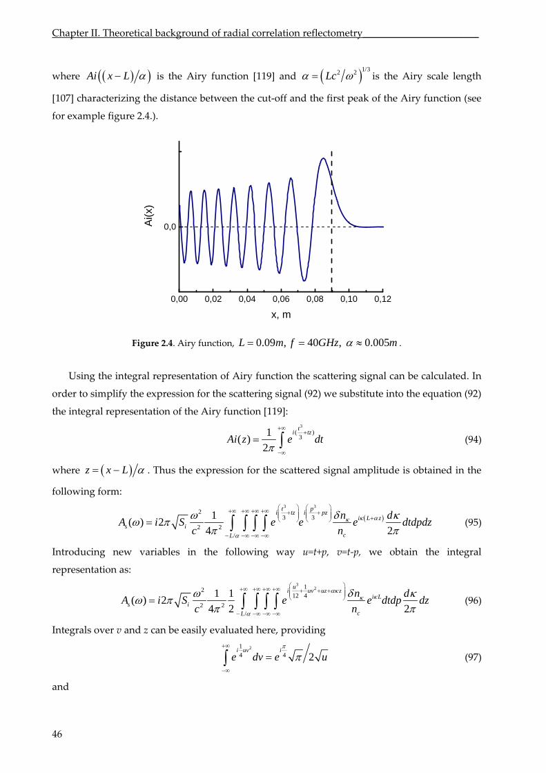
Chapter II. Theoretical background of radial correlation reflectometry_______________________
where Ai x L is the Airy function [119] and 1/32 2Lc is the Airy sc length
[107
ale
ra the first] cha cterizing the distance between the cut‐off and peak of the Airy function (see
for example figure 2.4.).
0,00 0,02 0,04 0,06 0,08 0,10 0,12
0,0 Ai(x
)
x, m
Figure 2.4. Airy function, 0.09 , 40 , 0.005L m f GHz m .
Using the integral representation of Airy functio the scattering signal can be calculated. In
order to simplify the expression for tering signal (92)
n
the scat we substitute into the equation (92)
the integral representation of the Airy function [119]:
3
( )31
( )t
i tzAi z e dt
2
(94)
where z x L . Thus the expression for the scattered signal amplitude is obtained in the
following form:
3 32
3 3
2 2/
1( ) 2
4 2
t pi tz i pz
i L zs i
cL
n dA i S e e e dtdpdz
c n
(95)
variablesIntroducing new in the following way u=t+p, v=t‐p, we obtain the integral
representation as:
3212
12 4
2 2/
1 1( ) 2
4 2 2
ui uv uz z
i Ls i
cL
n dA i S e e dtdp
c n
dz
g
(96)
Integrals over v and z can be easily evaluated here, providin
21
4 4 2i uv i
e dv e u
(97)
nd a
46
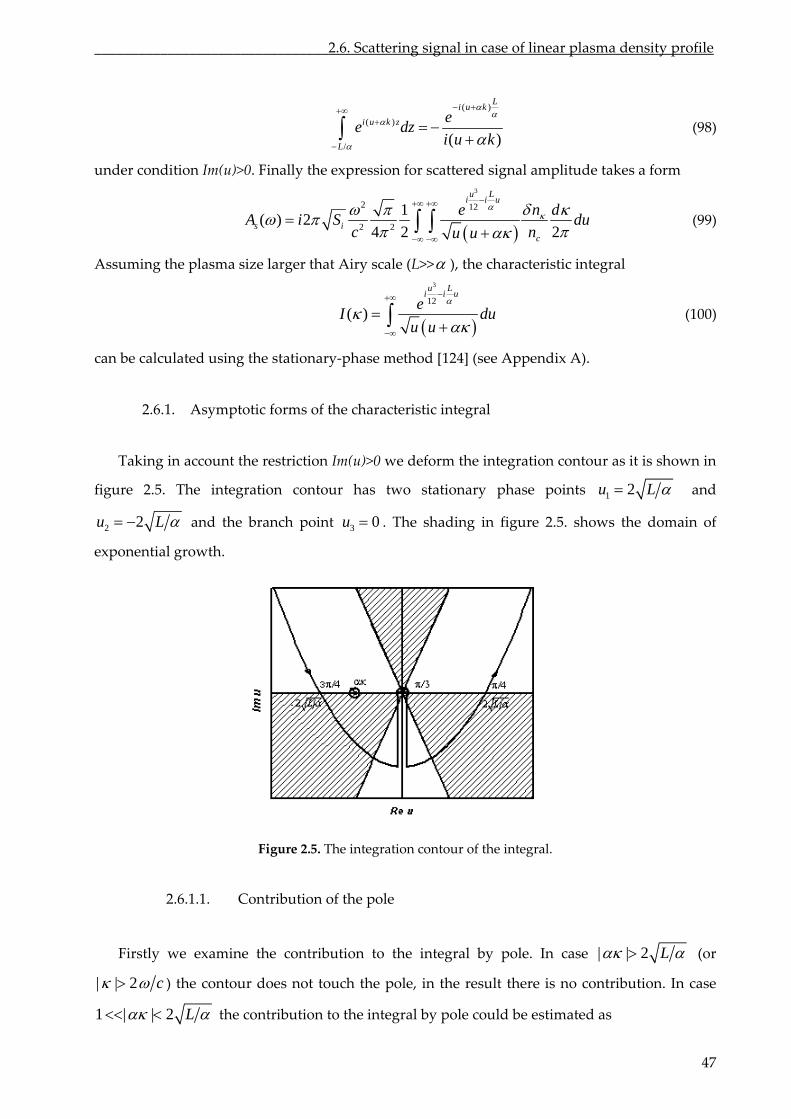
________________________________2.6. Scattering signal in case of linear plasma density profile
( )
( )
/ ( )
Li u k
i u k z
L
e e dz
i u k
(98)
under tion Im(u)>0. Finally the expression for scattered signal takes a form
condi amplitude
3
2 1( ) 2
4 2 2c
A i S duc nu u
(99)
Assuming the plasma siz
12
2 2
u Li i u
s i
e n d
e larger that Airy scale (L>> ), the characteristic integral
3
12
( )
u Li i u
eI du
u u
(100)
can be calculated using the stationary‐phase method [124] (see Appendix A).
2.6.1. Asymptotic forms of the characteristic integral
Taking in account the restriction Im(u)>0 we deform the integration contour as it is shown in
figure 2.5. The integration contour has two stationary phase points 1 2 u L and
2 2u L and the branch point 3 0u . The shading in figure 2.5. shows the domain of
exponential growth.
Figure 2.5. The integration contour of the integral.
Firstly we examine the contribution to the integral by pole. In case
2.6.1.1. Contribution of the pole
| | 2 L (or
| | 2 c ) the contour does not touch the pole, in the result there is no contribution. In case
1 | | 2 L the contribution to the integral by pole could be estimated as
47
Chapter II. Theoretical background of radial correlation reflectometry_______________________
3( )
12
( ) 2i i
eI
L
(101)
expression is proportional to
1 This and describes the Bragg backscattering contribution to
the scattering signal. In case | | 2 L the Bragg backscattering takes place directly at
plasma boundary with a wave number
the
| | 2 c .
2.6.1.2. Contribution of the branch point
o
When calculating the contribution of the branch p int 3 0u it is necessary to note that the
phase is different at two sides of the cut. In case | | 1 it is possible to neglect u in
denominator of the integral (100), than we obtain the integral in the form
3 3
2 2 41 2 3( ) 2
i i ie eI I I e dt e dt e
0 04 4
1L L
t t
i i Le t e t
(102)
The integral scales as 1 with the wave number and is much smaller than contribution of the
pole. Otherwise if 1 | | the parameter in denominator could not be neglected, nevertheless
we
may assume the cubic term in the exponent to be small. Under this assumption it is possible
to express the integral in terms of the error function
( ) i LI e erf i L (103)
where we use for the
4
error function the definition This expression can be
further simplified, for instance for
2
0( )
xserf x e ds .
1 1 L we obtain
2 i LI e (104)
whereas at 1 the integral takes a value:
| |L
44i i LI e e L
(105)
2.6.1.3. Contribution of the stationary phase points
The stationary phase points contribution 1 2u L and 2 2u L is given by the
expression
3 242 cos
3 4I i L
L
(106)
48
________________________________2.6. Scattering signal in case of linear plasma density profile
wh e noticed that
item is mu
ich physically describes the scattering from plasma boundary. It could b this
ch smaller than contribution of the pole because of the large parameter / 1L in
denominator.
2.6.2. Asymptotic forms of scattering signal
ationChange of variables and integr leads to the expression for the scattering signal in the
form
( )2s
c
n dA R
n
(107)
where
3
2 124
3 2 28 ( )( )
u Li i u
iii S eR e du
(108) c u u
As a result of the part 2.6.1, the partial amplitude ( )R tak rm es the following simple fo
3i
12
24
3 2 2
2 , 1 2( )
8
4 , 1
i i Li
eci S
R e ec erf i L
9) descr
(109)
The expression (10 ibes Bragg back scattering; it scales as 1 with the turbulence
wave number as it was predicted in [115]. In case | | 2 L the Bragg condition is fulfilled
( 2 ( )k x ) for 2 c and the scattering takes place directly at the plasma boundary.
The expression for the partial amplitude ( )R
,
can be mplified using asymp
in the interva
si totic
representation for the error function. Furthermore ls 1 1L and
1 L corresponding to small angle can be writ scattering ten accordingly it
2
43 2 2
( )8
i i LiR e ec
4
2, 1 1
4 , 1i
Li S
e L L
(110)
As it is seen from equation (110) for wave numbers of Airy range and smaller the singular
de
pendence 1 persists as well, in contradiction with unjustified assumption made in [115]
by B. B. Afeyan in 1994:
1, 1
, 1sA
Const
(111)
49
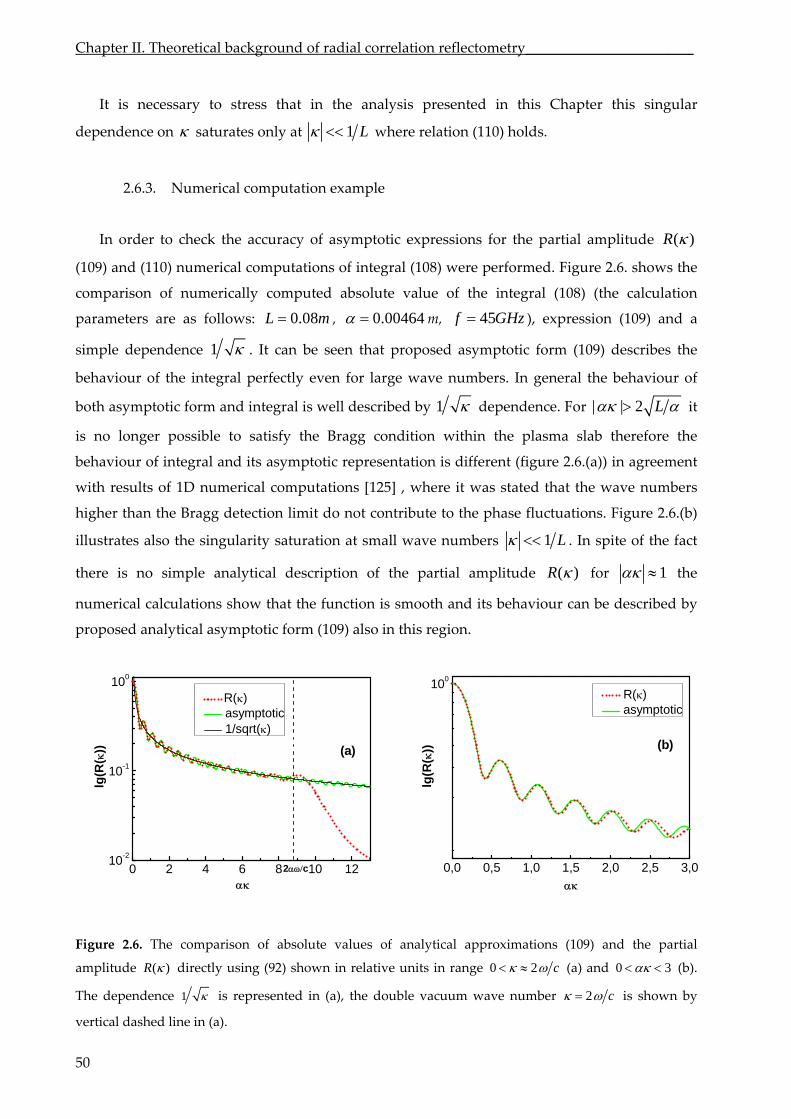
Chapter II. Theoretical background of radial correlation reflectometry_______________________
It is necessary to stress that in the analysis presented in this Chapter this singular
dependence on saturates only at
1 L where relation (110) holds.
In order to check the accuracy of asymptotic expressions for the partial amplitude
2.6.3. Numerical computation example
( )R
the
calculation
(109) and (110) numerical computations of integral (108) were performed. Figure 2.6. shows
omparison of numerically computed absolute value of the integral (108) (the
par
c
ameters are as follows: 0.08L m , 0.00464 m, 45f GHz ), expression (109) and a
simple dependence 1 . seen form (109) describes
behaviour of the integral general the behavi
otic form and
It can be
perfectly even
integral is well
that proposed
for large wave
described by
asymptotic
numbers. In
the
our of
1 dependence. For | | 2 L both asympt it
is no longer possible to within the plasma slab therefore the
behaviour of integral and its is different (figure 2.6.(a)) in agree
with results of 1D numerical ere it was stated that the wave numbers
2.6.(b)
illustrates also the singularity numbers
satisfy the
asymptotic
computations
saturation
Bragg condition
representation
[125] , wh
ribut
at small wave
ment
higher than the Bragg detection limit do not cont e to the phase fluctuations. Figure
1 L . In spite of the fact
there is no simple analytical partial amplitude for description of the ( )R 1 the
numerical calculations show that the function is smooth and its behaviour can be described by
proposed analytical asymptotic form (109) also in this region.
0 2 4 6 8 10 1210-2
10-1
100
R()
0,0 0,5 1,0 1,5 2,0 2,5 3,0
100
(b)
2c
(a)
asymptotic 1/sqr
R(
))
t()
R() asymptotic
())
lg(R
lg(
Fig
dir
ure 2.6. The comparison of absolute values of analytical approximations (109) and the partial
amplitude (R ectly using (92)) shown in relative units in range 0 2 c (a) and 0 3 (b).
The dependence 1 is represented in (a), the double vacuum wave number 2 c is shown by
vertical dashed line in (a).
50
________________________________2.6. Scattering signal in case of linear plasma density profile
2.6.4. WKB representation of Airy function
Unfortunately the above simple asymptotic expressions for the partial amplitude were
obt
r e. Never sentations (109) and
10) can be derived in the framework of more general approaches not utilising the integral
la (108). Namely, the asymptotic form (109)
orresponding to the Bragg backscattering can be obtained using the WKB representation of
Air
ained using the technique specific for the linear density profile, which is not applicable
directly to the a bitrary profile cas theless, the asymptotic repre
(1
representation for the Airy function and formu
c
y function which provides for the field (0)E the following expressions
3/2
(0)
4
2sin( | | )4 2 3 4( ) , 1
| |E
c
(112)
3/22
3(0) 2 2
( ) , 1e
Ec
4
(113)
Here it is assumed that the experimental scheme is calib to provide the sam ve
for the RCR experiment.
Substituting this formula into equation (92)
rated e probing wa
phase at the cut‐off not depending on frequency. This kind of calibration is the most beneficial
and performing integration there using the
stationary phase method we obtain for partial amplitude ( )R the expression (109) valid for
1 . In the opposite case the stationary phase method is no le. The entire
integration interval uding cut‐off vicinity ( is not contrib the
( )R However in this case we approximate in the tran
longer applicab
incl the where valid ute to
may
110)
sparency.
2(0) 216 , E c 0 (114)
and obtain after the integration over this region expression (110) for ( )R .
2.6.5. Long wavelength limit
It should be noted that in the long wavelength limit 1 we may also directly apply
the WKB approximation to describe the fluctuation contribution to the reflected wave phase.
The solution of (45) may be written in this case as a superposition of incident and reflected
waves:
( ) ( ) 31 1
4 4 0
4
4 2e e
( )1
x x
c cL L
x n x x n xi dx i i dx i
c L n c L n
z
c
EE
c x n xL n
(115)
51
Chapter II. Theoretical background of radial correlation reflectometry_______________________
52
nce ase perturb re small
This form is valid everywhere except the very neighbourhood of the cut‐off point. In the case
the turbule level is low enough, so that the reflected wave ph ations a
0
( )cxn x dx
( ) 11cc n x L
(116)
ple expression
( ) zE i E .the fluctuation reflectometry signal is given by sim When we
substitute the density perturbation Fourier spectrum there we obtain the phase perturbation in
the following form
0
( )( )
21
L i x
c
n e dx d
c n x L
(117)
We utilize the substitution 1s x L to calculate this integral. Finally, the corresponding
expression for ( )R obtained from (117) coincides with the expression (109).
2.7. Scattering signal in case of arbitrary plasma density profile
Plasma density profile in a tokamak in general is not linear; therefore the theoretical
description of the wave propagation into the realistic plasma density profile is required.
We analyze the arbitrary profile case by means of approximate methods introduced in
n in the form
previous sections for investigation of the linear density profile case. Supposing the density
profile to be monotonous, we find the solution of the unperturbed Helmholtz equation (45)
using WKB approximatio
(0) 4 2( ) sin
c
x
x
cE x k x dx k x
c
(118)
ives the distribution of the probing wave electric field in plasma in the case of unit
incident energy flux density as it was shown in part 2.5
4
g
integ
(0) ( )E x
. When substituting (0) ( )E x into the
ral (92) we derive
( ) 2cns
n dA R
where e partial amplitude may be represented as
(119)
( )R th
32 ( ')
x
i ' 2 ( ') '2 22
0
( ))
x
c c cx xc c
dx i i k x dx ix x xi x i
i x i xii S e e ek x
3 2 2
0 08 4 ( ) 2 ( 4 ( )R e dx dx e dx
(120)
c k x k x k x
Here we integrate from the plasma edge to the cut‐off ( cx x ). The largest contribution to
(120) at 1 2n c is provided by the first or the under the integral (120). third item
_____________________________2.7. Scattering signal in case of arbitrary plasma density profile
Here 1/3
nL c and2 2
11 ( )
c
nc x x
dn xL
n dx
.n
We use the stationary phase method (see Appendix A) analogous to part 2.6.2. for an
asymptotic evaluation of the integral (120) in this case. Stationary phase point Bx is determined
by the equation
22
2
( )4 1 B
c
n x
c n
(121)
corresponding to Bragg backscattering conditions.
Neglecting the contribution of the second term we obtain the expression for the partial
amplitude in the form:
2 ( ') '2
2
1 ( )2
Bc x
i
dn xn dxi S i
R
3 2 2
2 ( ') '2
1, 1 2
( )8 4 2
1 ( )2
xB
B
xc
xB
B
i k x dx i x i
n
i k x dx i x i
ec
c
dn xn d
1, 2 1
xc
n
ec
Bc x
x
(122)
In the opposite case of long scale fluctuations, at 1 , the second term in (120) provides
the dominant contribution to the integral which is given by
2
3 2 2( ) , 1
8 4 2 ( )
cx i xi
n
i S i e dxR dx
c n x
(123) 0 1
cn
It is significant that for 1 1n nL the main contribution to the integral over coord
in (123) is provided by the vicinity of the cut‐off, where the density profile is linear and it is
quite naturally that the partial amplitude in this case is given by the expression
inate
1
n
( )R
For
.
1 L the signal scattering does not take place only in the cut‐off vicinity so that the
profile n not be supposed linear, therefore taking in accoun ca t 1i xe for 1 nL , we o
the expression (123) in the form
btain
2 cx
3 2 20
( ) , 18 4 2 ( )
1
in
c
i S i dxR dx L
c n xn
(124)
53
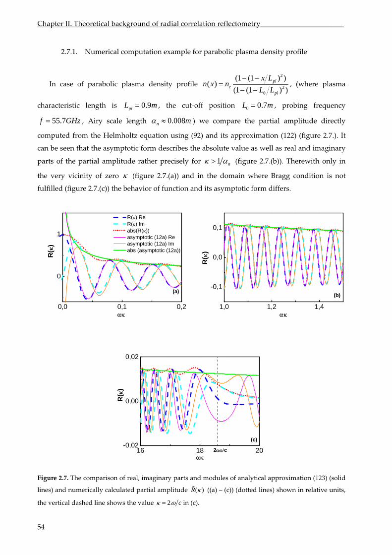
Chapter II. Theoretical background of radial correlation reflectometry_______________________
2.7.1. Numerical computation example for parabolic plasma density profile
In case of parabolic plasma density profile
2
20
(1 (1 ) )( )
(1 (1 ) )pl
cpl
x Ln x n
L L
, (where plasma
cha racteristic length is 0.9L m , the cut‐off position 0.7mpl 0L , probing frequency
55.7f GHz , length 0.008m Airy scale n ) we compare the partial amplitude directly
the Helmholtz (92) and its (122) (figure 2.7.). It
the asym the absolute as real and imaginary
compu gted from
can be seen that
par
equation
ptotic form
usin
describes
approximation
value as well
ts of the partial amplitude rather precisely for 1 n (figure 2.7.(b)). Therewith only in
the very vicinity of zero (figure 2.7.(a)) and in the domain where Bragg ndition is not
fulfilled (figure 2
co
.7.(c)) the behavior of function and its asymptotic form differs.
0,0 0,1 0,2
0
1
(a)
)
1,0 1,2 1,4
-0,1
0,0
0,1
(b)
R(
)
R() Re R() Im abs(R()) asymp otic 2a) Ret (1 asymptotic (12a) Im
R( abs (asymptotic (12a))
16 18 20-0,02
0,02
0,00
2c
(c)
)
R(
Figure 2.7. The comparison of real, imaginary parts and modules of analytical approxim d
lines) and numerically calculated partial amplitude ( )R
ation (123) (soli
((a) – (c)) (dotted lines) shown in relative units,
the vertical dashed line shows the value 2 c in (c).
54
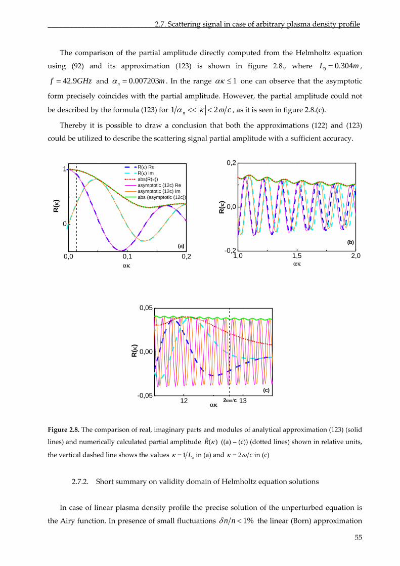
_____________________________2.7. Scattering signal in case of arbitrary plasma density profile
The ison of the partial amplitude directly computed from the Helmholtz equation
using (92)
compar
ure 2 where and its approximation (123) is shown in fig .8., 0 0.304 ,
42.9
L m
f GHz and 0.00720n 3m . In the range 1
However,
one can observe that
rtial amplitude. the partial amplitud
the
the asymptotic
e could notform precisely
be described by
coincides with the pa
formula (123) for 1 2 cn , as it is seen in figure 2.8.(c).
Thereby it is possible to draw a conclusion that both the approximations (122) and (123)
could be utilized to describe the scattering signal partial amplitude with a sufficient accuracy.
0,0 0,1 0,2
0
1
(a)
R(
)
R() Re R() Im abs(R()) asymptotic (12c) Re asymptotic (12c) Im abs (asymptotic (12c))
1,0 1,5 2,0-0,2
0,0
0,2
(b)
R(
)
12 13-0,05
0,00
0,05
2c
(c)
R(
)
Figure 2.8. The comparison of real, imaginary parts and modules of analytical approximation (123) (solid
lines) and numerically calculated partial amplitude ( )R ((a) – (c)) (dotted lines) shown in relative units,
the vertical dashed line shows the values 1 nL in (a) and 2 c in (c)
2.7.2. Short summary on validity domain of Helmholtz equation solutions
In case of linear plasma density profile the precise solution of the unperturbed equation is
the Airy function. In presence of small fluctuations 1%n n the linear (Born) approximation
55
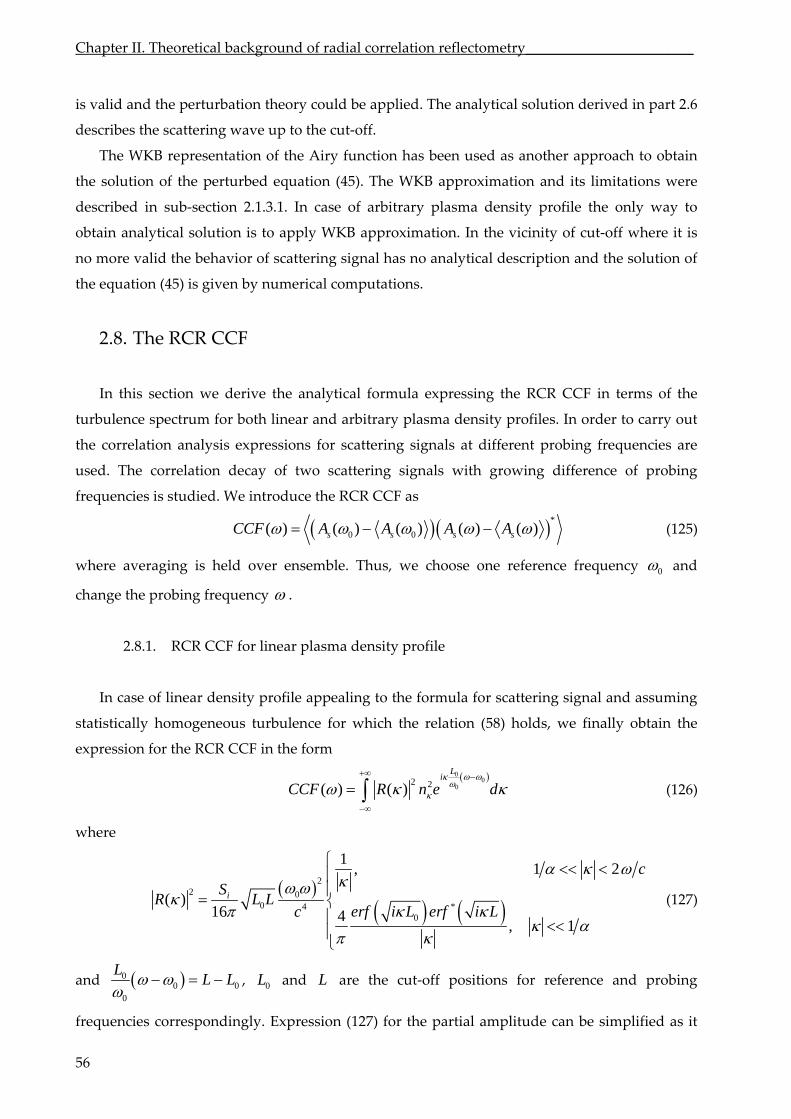
Chapter II. Theoretical background of radial correlation reflectometry_______________________
is valid and the perturbation theory could be applied. The analytical solution derived in part 2.6
describes the scattering wave up to the cut‐off.
The WKB representation of the Airy function has been used as another approach to obtain
the solution of the perturbed equation (45). The WKB approximation and its limitations were
described in sub‐section 2.1.3.1. In case of arbitrary plasma density profile the only way to
obtain analytical solution is to apply WKB approximation. In the vicinity of cut‐off where it is
no more valid the behavior of scattering signal has no analytical description and the solution of
the equation (45) is given by numerical computations.
2.8. The RCR CCF
arbi lasma density profiles. In order to carry out
the
T of probin
frequencies is d. We introduce
In this section we derive the analytical formula expressing the RCR CCF in terms of the
turbulence spectrum for both linear and trary p
correlation analysis expressions for scattering signals at different probing frequencies are
used. he correlation decay of two scattering signals with growing difference g
studie the RCR CCF as
*
ble. Thus, we ch
0 0( ) ( ) ( ) ( ) ( )s s s sCCF A A A A (125)
where averaging is held over ensem oose one reference frequency 0 and
change the probing frequency .
2.8.1. RCR CCF for linear plasma density profile
In case of linear density profile appealing to the formula for scattering signal and assuming
statistically homogeneous turbulence for which the relation (58) holds, we finally obtain the
expression for the RCR CCF in the form
0
00
2 2( ) ( )L
i
CCF R n e d
(126)
where
2
2 00 *4
0
1, 1 2
( )16 4
, 1
i
cS
R L Lerf
i L erf i Lc
(127)
and 00 0
0
LL L
, and L are the cut‐off positions for reference and probing
frequencies correspondingly. Expression (127) for the partial amplitude can be simplified as it
0L
56
_____________________________________________________________________2.8. The RCR CCF
57
was done for the equation (109) using asymptotic representation (110) in the intervals
1 1L and 1 L it can be written accordingly
2
2 00 4
0
1, 1 1
( )16 4
, 1
i
LS
R L Lc
L L L
(128)
The 1
scattering
asymptotic
factor in the function is responsible for underlining the contribution of small angle
off long scale fluctuations into the RCR signal. It is important to stress here that
expression (128) correctly describes the behaviour of 2
( )R also at higher wave
numbers 1 2 c . Using the proposed asymptotic form (109) for scattering signal we
terobtain the following representation of the CCF in ms of the turbulence spectrum
0( )1 2 *( ) i L LD CCF L e er erf 0
dn f i L i L
(129)
where
2
002 44 c
iSD L L
(130)
The 1 singularity in this formula saturates wave numbers due to the term for small
*0erf i L erf i L . The dependence of CCF on the probing wave cut‐off position can be
obtained in experiment by sweeping the probing frequency.
0,0 0,2 0,4 0,6 0,8
0,0
0,2
0,4
0,6
0,8
1,0
CC
F
CCF Re CCF Im Asymptotic Re Asymptotic Im
L, m
Figure 2.9. The comparison of analytical approximations (127) (dashed line real part and dotted line
imaginary part) and the CCF (solid line real part and thin dotted line imaginary part) numerically
calculated in Born approximation. 0 0.4L m , 0 95f GHz , Gaussian spectrum,
0.02cl m .
Chapter II. Theoretical background of radial correlation reflectometry_______________________
To check the approximate formula (128) we compare it after normalization to the CCF
calculated using the Born appr imox ation formula (92). The random density fluctuation is taken
the form in
( ) c0
)jq jj
xos(sj N
n x n jq
(131)
in which 2 2
40 e
cjq l
jqn n
corresponds to the Gaussian turbulence correlation function
possessing correlation length 0.02cl m
and phases j were randomly distributed in the
interval [0,2 ] .
ulation
The averaging d over ensemble of Ns=1000 random phase samples.
The calc parameters are
is performe
as follows: 0 0.4L m ; 950f GHz . on is The result of comparis
figure 2.9. illustrating the applicability of the proposed formula for the wide probing
range.
Formula (128) can be used to compute the signal CCF for different spectra in order to
compare to CCF obtained in experiments and to determine real turbulence spectra as a s
fitting procedure. However we demonstrate in section 2.9 the possibility of strict analytical
inversion of the integral relation (128) and derive a formula which allows correct wave number
rum reconstruction from xp
In case of the arbitrary profile we derive the expression for the signal CCF referring to the
formulae (122)‐(124) for scattering signals in arbitrary profile case. Thus, we multiply the
scattering signals for reference and probing frequencies. Subject to short wave case l
consider the difference of two signal exponents.
shown in
re ult of
spect RCR e erimental data.
2.8.2. RCR CCF for arbitrary plasma density profile
‐ et us
0
0 02 ( ') ' ( ') ' ( )BB
c c
B B
x x
k x dx k x dx i x x
(132)
Utilizing Taylor series expansion we obtain
xx
0 0
0 00 0 0
( ')' ( ', ) ( ) ( ', ) '
c c cx x x
dk x dxdx k x k x dx
d d
(133)
( )
( ', ) 'B BB x xx
k x dx
Using Bragg condition we consider 2 ( ', )k x . Mention that 0 0( )B Bx x and
0
0
0
B Bdx x x
d B
we derive:
0
00 0
( ')2( ) ' 2 ( )( )
B
c
x
d
x
dk xdx t
d
(134)
where
58
_____________________________________________________________________2.8. The RCR CCF
( )( ')B
c
x
d
x
k x
is the probing wave propagation time between the cut‐off and
( ) 't dx (135)
the Bragg resonance point. In
case of long scale fluctuations satisfying condition 2 2 nc the density profile
between the cut‐off and the Bragg resonance point can be considered as linear, so that the delay
time in expression (134) takes a form
0
0
( )2d
Lt
(136)
The expression for RCR CCF takes the form:
02 2 ( )( )2( ) ( ) di tCCF R n e d
(137)
where
02 4
0
20484 1 1 1
,
B Bx x
n nn n
c
L LL
0 0
22 0
0
1 1, 2
( ) ( )
( )
c c
ni
n ndn x dn x c
S dx dxR
(138)
to formulae (122)‐(124) we consider limits of the long scale fluctuations and obtain
the
Analogous
expression for the partial amplitude in the form:
0 0 02 ( ) 2 ( )0 1 1
, c cd d
x xi x t i x te dx e dx
0 0
0 002
2 02 4 2 ( ) 2 ( )
0
0 00
( ) ( )1 1
( )2048 1
, ( ) ( )
1 1
n nd d
nc n
c ci
x xt t
nc
xn x n xn nS
Rc e dx e dx
xn x n x
c cn n
ber
(139)
At small fluctuation wave num 2 c 2 n th Bragg backscattering point is located
close to t‐off (
e
the cu 1c B cx x x ), where we may approximate the density profile by the
linear dependence. The propagation time i e is expression (136). In (139) the
additional dependence on wave number is hidden in the dependence of the Bragg
backsca
n this cas given by
ttering point However at ( )Bx . 2 2 nc in case the density profile can be
supposed linear, formula (139) in the region 1 1nc nx smoothly transforms into the
region 1 ncx and coincides with (122)‐(124). In this wave number domain equation (137)
appears to be similar to (126).
59
Chapter II. Theoretical background of radial correlation reflectometry_______________________
2.9 Turbulence spectrum reconstruction from the RCR CCF
this section the main result of this thesis is derived.
.
In
Essentially, the formula (129) shows that the expression for CCF in case of linear density
profile looks similar to Fourier transform of the function 2n . It differs from Fourier transform of
turbulence spectrum only because of weak dependence the error functionof erf i L on the
probing wave cut‐off position. Inversion of integral equation (129) giving the expression for
turbulence wave number spectrum can be obtained after converting it into the Abel equatio
Fourier transform and obtain
n.
We treat the integral equation (129) by applying
20
14( )2 *
0
0
1 ( )
2 2
i
i L pi L LiLy iLyCCF L e de dL n e erf i L e dp e dL
L
(140)
Left part of the quation (140) can be denot e ed as
1 ( )
( )2
iLyCCF LF y e dL
L
(141)
Expressing the internal L as the Dirac 2( )iL y pe d
function we find
0
1 242 *
0 20
1( )
2 1
i
i L
ype d
F y n erf i L e dpdp
(142)
Using the Dirac function features we substitute 21
y
p
and obtain
02
2
* 0214 1
( )i yL
yLerf i
peF y 2 1
20 1
2
2 1
1
ip
y
p
dpn e
pyp
(143)
Aft
er variable exchange 21
yt
p the equation (
143) takes a form of the Abel equation:
0
0
*02
4
*02
, 0
( )4
, 0
itLti
y
yitL
t
erf itLn e dt
t t yeF y
erf itLn e dt
t y t
y
y
(144)
The solution of the Abel equation is found as
60
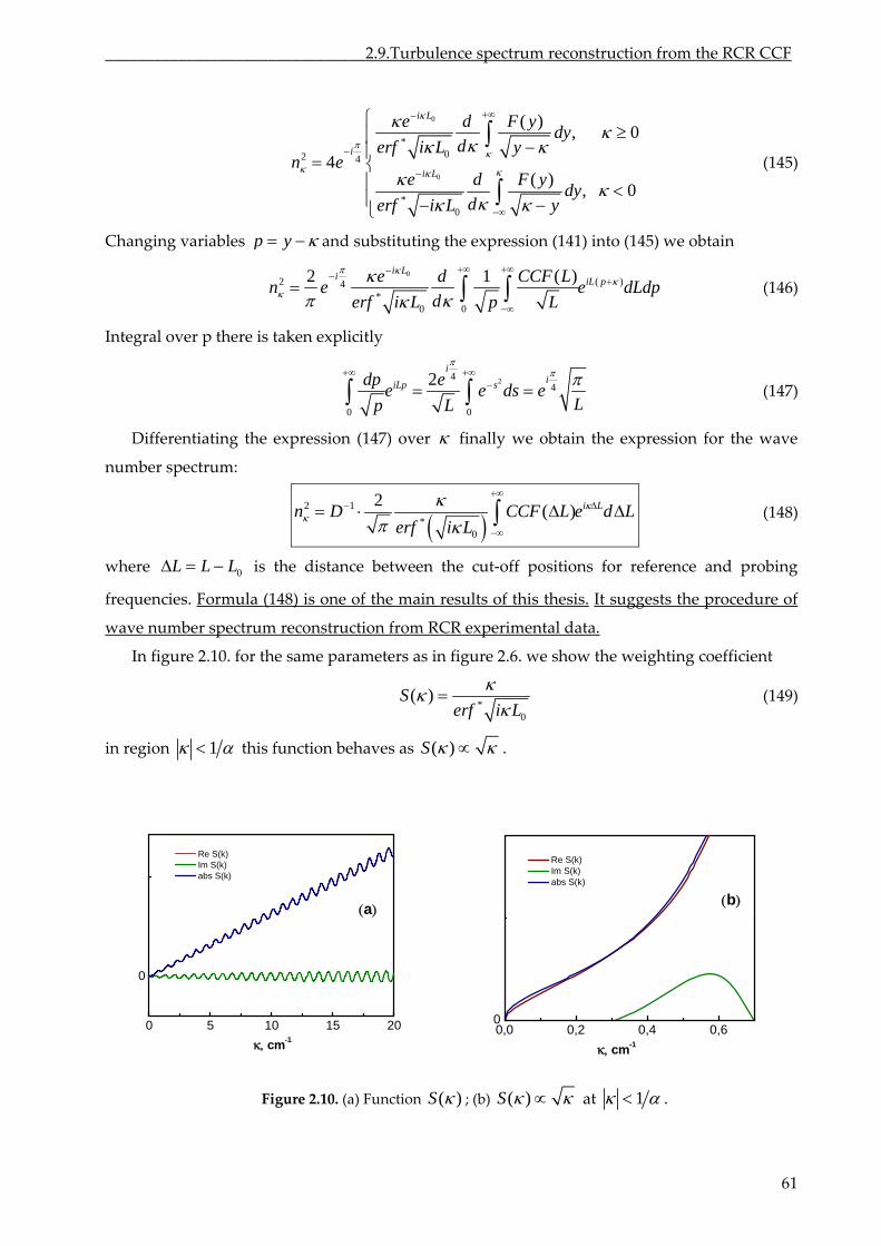
________________________________2.9.Turbulence spectrum reconstruction from the RCR CCF
61
0
*02 4
( )i L
i
e d F y
derf i L
0
*0
, 0
4( )
, 0i L
dyy
n ee d F y
dyderf i L y
(145)
Changing variables p y and substituting the expression (141) into (145) we obtain
0
2 (4*
00
2 1 ( )i Li iL pe d CCF L
n e e dLdderf i L p L
) p (146)
tly Integral over p there is taken explici
24
4
0 0
2 iiLp sp ee e ds e
id
Lp L
(147)
Differentiating the expression (147) over finally we obtain the expression for the wave
number spectrum:
2 1
*) i Ln D e d L
erf
0
2(CCF L
i L
(148)
0
frequencies. Formula
where is the distance between the cut‐off positions for reference and probing L L L
(148) is one of the main results of this thesis. It suggests the procedure of
wave number spectrum reconstruction from RCR experimental data.
coefficient In figure 2.10. for the same parameters as in figure 2.6. we show the weighting
*
0
( )Serf i L
(149)
in region 1 this function behaves as ( )S .
0,0 0,2 0,4 0,60
0 5 10 15 20
0
a
cm-1
Re (k)S Im S(k) abs S(k)
Re S(k) Im S(k) abs S(k)
b
cm-1
e 2.10. (a) FunctionFigur ( )S ; (b) ( )S at 1 .
Chapter II. Theoretical background of radial correlation reflectometry_______________________
Multiplication by the function will result in shortcoming of 1D theory as ( )S 2 (0) 0n
leading to inaccuracy of spectrum reconstruction. Nevertheless as we show i Chapter I
numerical simulations in most RCR experiments the suggested formula gives rather precise
tu
So far as we use the Born approximation to derive the formula (148) it is applicable only at
low enough fluctuation amplitude when the reflected wave phase modulation is not strong. The
corresponding criteria of the linear regime proposed in [110] and [111] takes a form:
n II by
reconstruction of rbulence properties.
2 2
2 2ln 1c c c
c c
x l n x
c n l
(150)
It should be noted that the expression for CCF (137) obtained in arbitrary profile case takes a
transform Fourier
transform of CCF given by
form of nearly Fourier as well. Therefore one may expect that inverse
0
00
0( ) ( )eiqL
S q CCF d
(151)
can be used for turbulence spectrum reconstruction from experimental data.
for RCR
Thi section addresses the theoretical expression for integral kernel, which converts dir
the correlation function into the two‐point CCF of plasma turbulence should
be quite useful for experimentalists in order to compute TCCF avoiding error accumulation
ersion. I
2.10.1. Forward transformation kernel
Expression (148) allows to compute the turbulence radial wave number spectrum from the
signal CF measured in experiment. The TCCF is related the spectrum by Fo
transformati
2.10. Direct transform formulae
s ectly
( )CCF L ( )C r
during two‐step conv nverse transformation is also discussed.
C to urier ( )C r
on
/c2
2
2 /
( ) i r
c
C r n e d
(152)
where is held within Bragg backscattering limits 2 2c c .integration
We propose the integral transformation to compute the TCCF straight from the signal CCF
ose to avoion purp d the error accumulated during numerical procedure of turbulence spectrum
reconstruction and further Fourier transformation and to provide a simple formula determining
TCCF directly from reflectometry measurements.
62
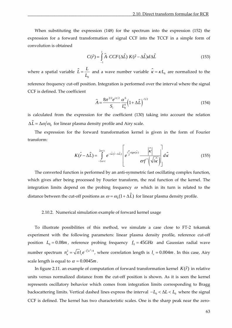
_________________________________________________2.10. Direct transform formulae for RCR
63
When substituting the expression (148) for the spectrum into the expression (152
expression for a forward transformation of signal CCF into the TCCF in a simple form of
n is obt
ˆ
) the
convolutio ained
1
1
ˆ ˆˆ ˆ( ) ( ) ( )C r A CCF L K r L d L
(153)
where a spatial variable 0
LL
L and a wave number variable 0L are normalized to the
reference frequency cut‐off position. Integration is performed over the interval where the signal
CCF is defined. The coefficient
3 2 2 6 5 2
40
81
i
i
eA L
S L
(154)
is calculated from the expression for the coefficient (130) taking into account the relation
0L for linear plasma density profile and Airy scale.
The expression for the forward transformation kernel is given in the form of Fourie
transform:
r
( ) 2
*( ) i r LK r L e e d
2 /( )
2 /
ci sign
c erf i
The converted function is performed by an anti‐symmetric fast oscillating complex function,
which gives after being processed by F
(155)
ourier transform, the real function of the kernel. The
integration limits depend on the probing frequency which in its turn is related to the
distance between the cut‐off positions as 0(1 )L for linear plasma density profile.
2.10.2. Numerical simulation example of forward kernel usage
ence probing frequency
To illustrate possibilities of this method, we simulate a case close to FT‐2 tokamak
experiment with the following parameters: linear plasma density profile, reference cut‐off
position 0 0.08L m , refer 0 45f GHz and Gaussian radial wave
number spectrum 2 2 /42
cl
cn l e , where correlation length is c 0.004l m . In this case,
scale length
Airy
is equal to 0.0045m .
el in relative
versus normalized distance from the cut‐off position is shown. As it is the kernel
ion limits co to Bragg
backscattering limits. Vertical dashed lines express the interval
In figure 2.11. an example of computation of forward transformation kern ˆ( )K r
seen
rresponding
L
units
represents oscillatory behavior which comes from integrat
0 0L L where the signal
CCF is defined. The kernel has two characteristic scales. One is the sharp peak near the zero‐
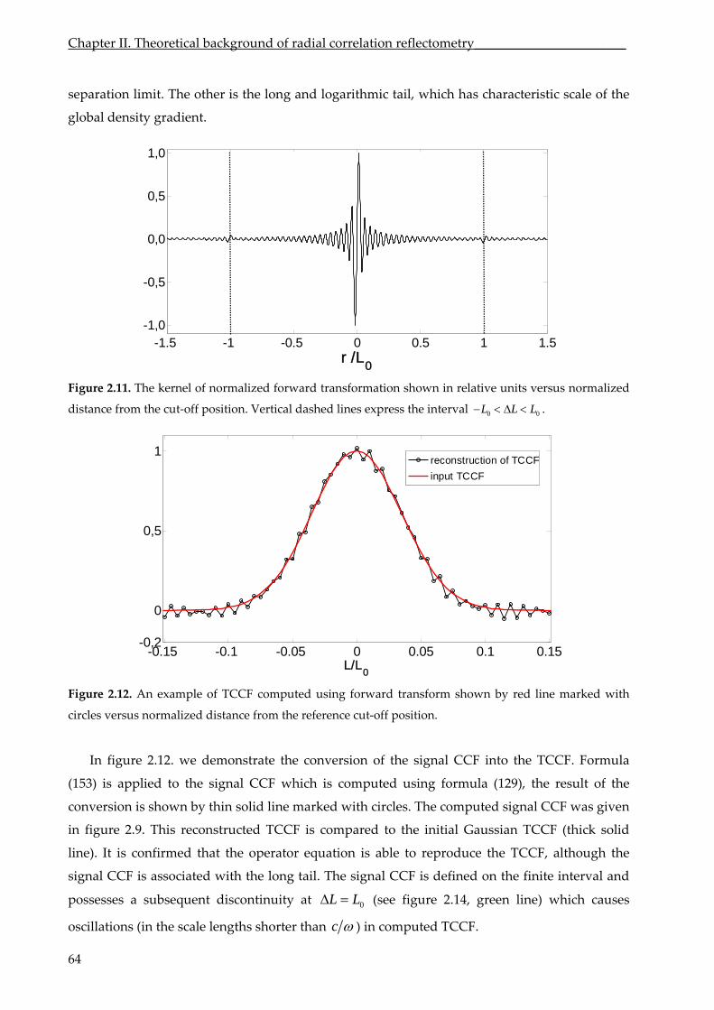
Chapter II. Theoretical background of radial correlation reflectometry_______________________
separation limit. The other is the long and logarithmic tail, which has characteristic scale of the
global density gradient.
-1.5 -1 -0.5 0 0.5 1
1,0
1.5-1,0
-0,5
0,0
0,5
r /L0
n in relative units sus normalized
dist
Figure 2.11. The kernel of normalized forward transformation show ver
ance from the cut‐off position. Vertical dashed lines express the interval 0 0L L L .
-0.15 -0.1 -0.05 0 0.05 0.1 0.15-0,2
0
0,5
1
reconstruction of TCCFinput TCCF
L/L0
computed using forward transform shown by red line marked with
circles versus normalized distance from the reference cut‐off position.
(153) is appl formula (129), the result of the
con
9. This reconstructed TCCF is compared to the initial Gaussian TCCF (thick solid
line). It is confirmed that the operator equation is able to reproduce the TCCF, although the
signal CCF is associated with the long tail. The signal CCF is defined on finite interva
possesses a subsequent discontinuity at
Figure 2.12. An example of TCCF
In figure 2.12. we demonstrate the conversion of the signal CCF into the TCCF. Formula
ied to the signal CCF which is computed using
version is shown by thin solid line marked with circles. The computed signal CCF was given
in figure 2.
the l and
0L L
(see figure 2.14, green line) which causes
oscillations (in the scale lengths shorter than c ) in computed TCCF.
64
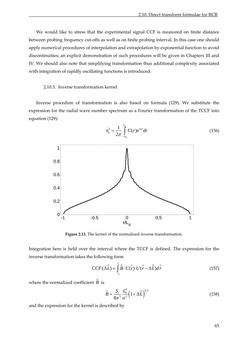
_________________________________________________2.10. Direct transform formulae for RCR
We would like to stress that the experimental signal CCF is measured on finite distance
between probing frequency cut‐offs as well as on finite probing interval. In this case one should
apply numerical procedures of interpolation and extrapolation by exponential function to avoid
discontinuities; an explicit demonstration dures will be given in Chapters III of such proce and
IV. e should also note that simplifying transformation thus additional complexity associated
e procedu ed on form
expression for the radial wave number spectrum as a Fourier transformation of the TCCF into
W
with integration of rapidly oscillating functions is introduced.
2.10.3. Inverse transformation kernel
Invers re of transformation is also bas ula (129). We substitute the
equation (129):
0
0
2 1( )
2i r
L
n C r e dr
(156)
L
-1 -0.5 0 0.5 10
0.2
0.4
1
0.8
0.6
r/L0
Figure 2.13. The kernel of the normalized inverse transformation.
Integration here is held over the interval where the TCCF is defined. The expression for the
inverse transformation takes the following form
(157) 1
( ) ( ) ( )CCF L B C r U r L dr 1
where the normalized coefficient B is
4 5 20
3 21
8iS L
B L
(158)
and the expression for the kernel is described by
65
Chapter II. Theoretical background of radial correlation reflectometry_______________________
66
2 /
( ) *0 0
2 /
( ) (c
i r L
c
dU r L e erf i L erf i L L
) (159)
that seems to be similar to Fourier transformation however this kernel possesses the
dependence on in the argument of complex conjugate error function. Integration is
performed in Bragg backscattering limits as was mentioned in the previous sub‐section.
Figure 2.13. shows the normalized inverse transformation kernel in relative units
versus normalized distance from the cut‐off position. The function decays logarithmically
therefore the long range tail is introduced into the signal CCF computed using formula (157).
2.11. Ideas for a combined diagnostic using reflectometry and other
In section we consider correlation between the reflectometry signal and other local
fluc
L
( )U r
density fluctuation diagnostic
this
tuation measurement such as HIBP in order to simplify the procedure of data processing
and to open new approaches of reflectometry usage. The reason for this prediction is provided
by different behavior of complementary diagnostic sensitivity to long wave length fluctuations,
which was supposed homogeneous, whereas for reflectometry it is growing towards small
wave numbers. It is also necessary to stress that nowadays no experiment exists for applying
this new kind of turbulence characterization.
We represent the correlation by inter–correlation function (ICF) ( )ICF L where 0L denotes
the position of local measurement and indicates the positionL of the for
refl
reflection
ectometry. It is shown that the long range tail of correlation which is much longer than the
correlation length of turbulence persists in ( )ICF L (see figure 2.14.), however it decays faster
than that of ( )CCF L . We propose formulae to compute wave number spectrum and spatial
TCCF from these measurements.
The interest to define expressions of ICF is to change the dependencies of CCF, and if it is
possible to reduce the contribution of the long wavelength in the CCF as it will be shown. In
this sub‐section we develop theoretically the method of data interpretation of combined
HIBP). We introduce ICF as
reflectometry and other local diagnostics (e.g.
*0 0( ) ( ) ( )sICF L n L A L L (160)
between e the reflectom try signal 0( )sA L L and one other local measurement
0( )n L
fluctuation
in linea 0 0( ) 1%n Lr regime, ( )n L . We also assume that reflectometry and other
fluctuation diagnostic measurements can be held simultaneously.
e modify formula (129) according to the expression for in the following way: W ICF
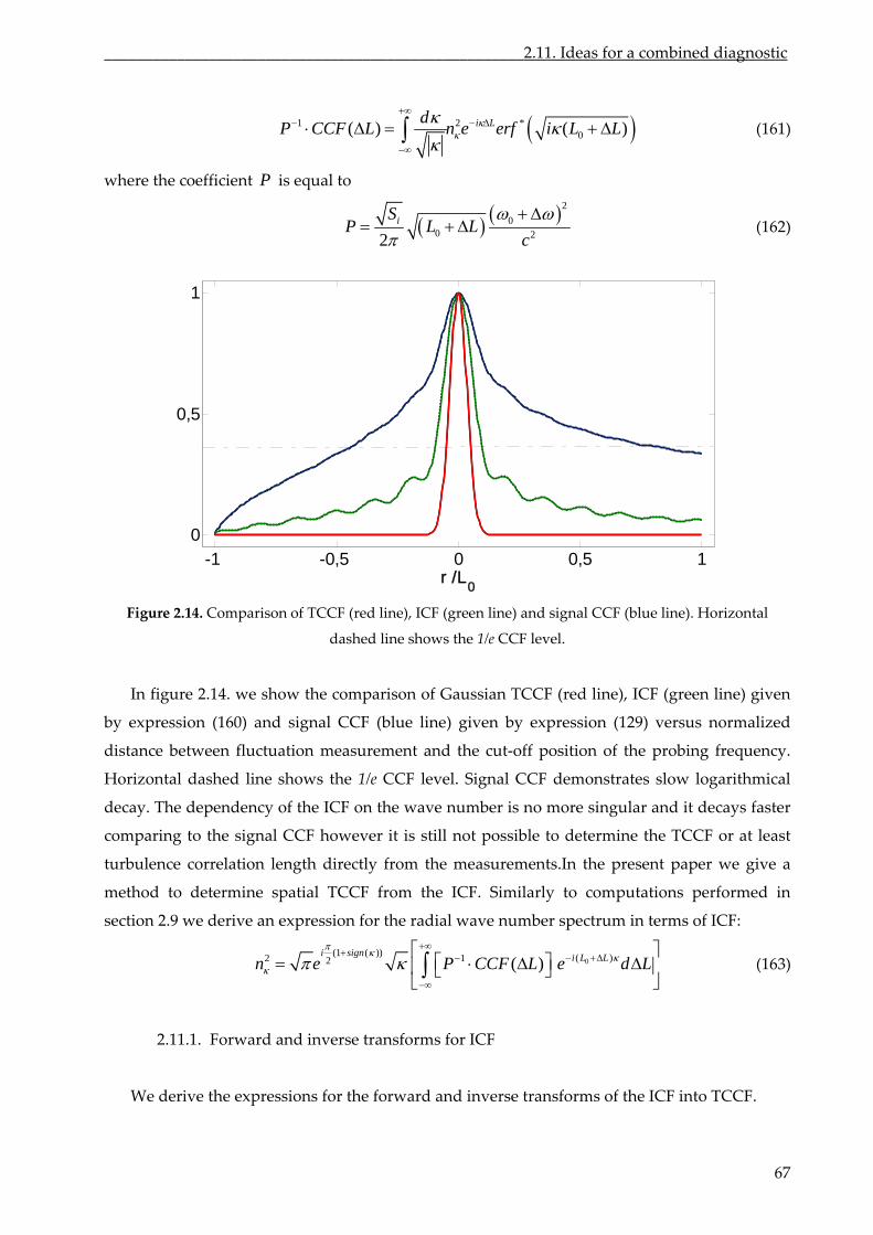
____________________________________________________2.11. Ideas for a combined diagnostic
1 2 *0( ) ( )i Ld
P CCF L n e erf i L L
(161)
where the coefficient is equal to
P
2
00 22
iSP L L
c
(162)
-1 -0,5 0 0,5 10
0,5
1
r /L0
Figure 2.14. Comparison of TCCF ed line (r ), ICF (green line) and signal CCF (blue line). Horizontal
dashed line shows the 1/e CCF level.
ussian TCCF (red line), ICF (green line) given
by expression (160) and signal CCF (blue line) given by expression (129) versus normalized
distance between fluctuation measurement and the cut‐off position of the probing frequency.
line CC
at least
give a
me utatio
In figure 2.14. we show the comparison of Ga
Horizontal dashed shows the 1/e CCF level. Signal F demonstrates slow logarithmical
decay. The dependency of the ICF on the wave number is no more singular and it decays faster
comparing to the signal CCF however it is still not possible to determine the TCCF or
turbulence correlation length directly from the measurements.In the present paper we
thod to determine spatial TCCF from the ICF. Similarly to comp ns performed in
section 2.9 we derive an expression for the radial wave number spectrum in terms of ICF:
0(1 ( )) ( )2 12 ( )
i sign i L Ln e P CCF L e d L
(163)
ICF
2.11.1. Forward and inverse transforms for
We derive the expressions for the forward and inverse transforms of the ICF into TCCF.
67
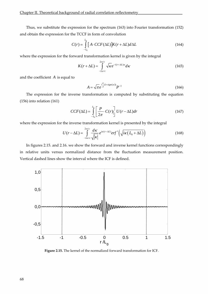
Chapter II. Theoretical background of radial correlation reflectometry_______________________
Thus, we substitute the expression for the spectrum (163) into Fourier transformation (152)
and obtain the expression for the TCCF in form of convolution
0
0
( ) ( ) ( )L
L
C r A CCF L K r L d L
(164)
where the expression for the forward transformation kernel is given by the integral
2 /
2 /
( )c
c
K r L e d
( )i r L
(165)
and the coefficient
A is equal to
(1 ( ))
2gn
A e P
1i si
(166)
The expression for the inverse transformation is computed by substituting the equation
(156) into relation (161)
0
0
( ) ( ) ( )2
L
L
PCCF L C r U r L dr
(167)
where the expression for the inverse transformation kernel is presented by the integral
2 /
( ) *0
2 /
( )c
i r L
c
dU r L e erf i L L
(168)
In f . we show the forw
measurement position.
Vertical
igures 2.15. and 2.16 ard and inverse kernel functions correspondingly
in relative units versus normalized distance from the fluctuation
dashed lines show the interval where the ICF is defined.
-1.5 -1 -0.5 0 0.5 1 1.5
-0,5
0,0
0,5
1,0
r /L0
Figure 2.15. The kernel of the normalized forward transformation for ICF.
68
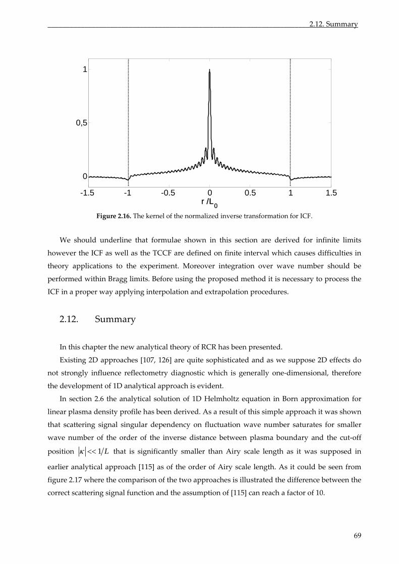
_______________________________________________________________________2.12. Summary
69
-1.5 -1 -0.5 0 0.5 1 1.5
0
0,5
1
r /L0
should underline that formulae shown in this section are derived for infinite limits
however
number
proposed
Existing 2D approaches [107, 126] are quite sophisticated and as we suppose 2D effects do
not influence reflectometry diagnostic which is generally one‐dimensional, ther
development of 1D analytical approach is evident.
equation in Born approximation for
linear plasma density profile has been derived. As a result of this simple approach it was shown
that
wave
Figure 2.16. The kernel of the normalized inverse transformation for ICF.
We
the ICF as well as the TCCF are defined on finite interval which causes difficulties in
theory applications to the experiment. Moreover integration over wave should be
performed within Bragg limits. Before using the method it is necessary to process the
ICF in a proper way applying interpolation and extrapolation procedures.
2.12. Summary
In this chapter the new analytical theory of RCR has been presented.
strongly efore
the
In section 2.6 the analytical solution of 1D Helmholtz
scattering signal singular dependency on fluctuation wave number saturates for smaller
number of the order of the inverse distance between plasma boundary and the cut‐off
position 1 L that is significantly smaller than Airy scale length as it was supposed in
earlier analytical approach [115] as of the order of Airy scale length. As it could be seen from
figure 2.17 where the compari on of the two approaches is illustrated difference betwee
s the n the
correct scattering signal function and the assumption of [115] can reach a factor of 10.
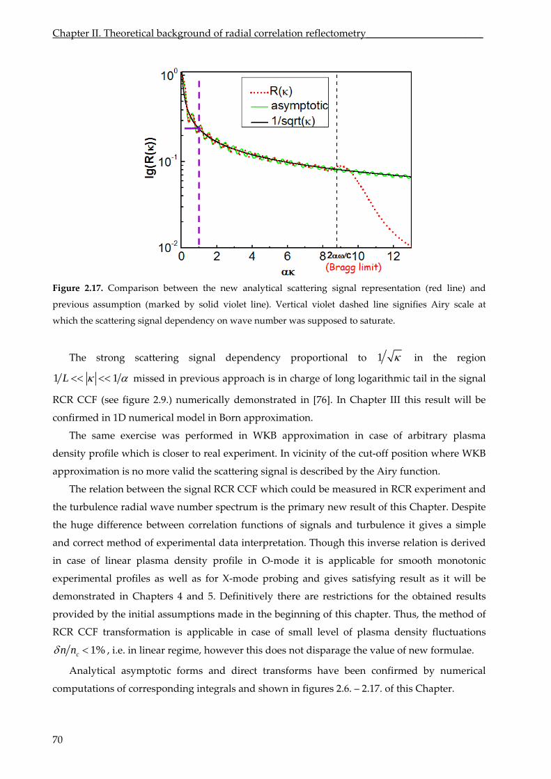
Chapter II. Theoretical background of radial correlation reflectometry_______________________
Fig
to saturate.
The strong scattering signal dependency proportional to
ure 2.17. Comparison between the new analytical scattering signal representation (red line) and
previous assumption (marked by solid violet line). Vertical violet dashed line signifies Airy scale at
which the scattering signal dependency on wave number was supposed
1 in the region
1 1L missed in previous approach is in charge of long logarithmic tail in the signal
RCR CCF (see figure 2.9.) numerically demonstrated in [76]. In Chapter III this result will be
confirmed in 1D numerical model in Born approximation.
The same exercise was performed in WKB approximation in case of arbitrary plasma
density profile which is closer to real experiment. In vicinity of the cut‐off position where WKB
approximation is no more valid the scattering signal is described by the Airy function.
The relation between the signal RCR CCF which could be measured in RCR experiment and
the turbulence radial wave number spectrum is the primary new result of this Chapter. Despite
the huge difference between correlation functions of signals and turbulence it gives a simple
and correct method of experimental data interpretation. Though this inverse relation is derived
in case of linear plasma density profile in O‐mode it is applicable for smooth monotonic
experimental profiles as it will be
demonstrated in Chapters 4 and 5. Definitively there are restrictions for the obtained results
provided by the initial assumptions made in the beginning of this chapter. Thus, the method of
RCR CCF transformation is applicable in case of small level of plasma density fluctuations
as well as for X‐mode probing and gives satisfying result
1%cn n , i.e. in linear regime, however this does not disparage the value of new formulae.
Analytical asymptotic forms and direct transforms have been confirmed by numerical
computations of corresponding integrals and shown in figures 2.6. – 2.17. of this Chapter.
70
_______________________________________________________________________2.12. Summary
71
Direct transforms simplifying the calculation of turbulence spatial properties were also
proposed in section 2.10.
Another breakthrough of the developed analytical theory is the expansion of its applications
on other fluctuation diagnostics such as for example HIBP. The analytical basis of the diagnostic
based on simultaneous usage of one reflectometry channel and HIBP data is developed in
section 2.11. At present day there is no experiment exploiting such a method. Certainly, when
setting up the experiment, one would face difficulties in data collection and interpretation
nevertheless the ICF gives a commencement of this kind of investigation.
Obviously there is wide field for further research and analytical theory improvement
namely connection between 1D and 2D expressions, corrections to the inverse relation due to
2D effects which are the subject of future research.

72
73
Chapter III
Numerical modeling
_____________________________________________________________________________________
In this Chapter simulation results are given firstly, to validate the new theory of RCR able to
access to turbulence characteristics, secondly to determine the limits and the sensitivity of the
radial correlation reflectometer to different parameters encountered in experiments and
possibilities of this diagnostic to detect relevant events existing in fusion plasmas. Results of
reflectometry experiment numerical modeling in simplest linear plasma density profile as well
as in conditions close to real experiments are presented.

74
__________________________________________________________________3.1.Numerical model
3.1. Numerical model
In this sub‐section the numerical code is described. The numerical model is based on the
eoretical approach developed in Chapter II resulting in unperturbed differential equation (45)
to be solved and further integral (99) and inversion relation (148) to be computed. The
rogramming language Fortran is used to develop the code.
Analytical formulae are derived in Born approximation linear regime and possess no
ependence on fluctuation amplitude therefore the numerical code is not sensitive to
uctuation amplitude and gives only linear solution of the Helmholtz equation.
As soon as our goal is to study the RCR diagnostic from the experimental point of view we
oose the set of input parameters of the code close to experimental. The numerical procedure
nsists of four parts: solution of the unperturbed Helmholtz equation; partial amplitude
lculation (calculation of the integral over
th
p
d
fl
ch
co
ca ); signal CCF calculation; turbulence wave
and CCF reconstruction.
3.1.1. Numerical solution of unperturbed Helmholtz equation.
Firstly, the unperturbed Helmholtz equation (45) with
number
( ) 0n x
unperturbed
is solved numerically
applying finite difference scheme based on forth‐orde
quidistant grid with the step h is used. The solution is the electric field
r Numerov method. Finite difference
method is selected due to its simplicity (less computing time) and easiness to implement. The
0 ( , )j jE x e
for the set of probing frequencies where j is the index of probing frequency. Initially the
elmholtz equation takes a form:
H
(2) 2 20( ) 4 ( ) ( ) 0z zE x N x E x (169)
To solve the Helmholtz equation the 4th order Numerov scheme (see Appendix B) is used:
2 22 2 2 2
0 0
2
0
5( ) 1 4 ( ) ( ) 2 4 ( )
12 6
( ) 1 4 ( ) 012
z z
z
h hE x h N x h E x N x
hE x h N x h
The Helmholtz equation is finally represented by a matrix equation:
E B
2 2
(170)
(171)
where is a tridiagonal matrix defined by equation (170). B
.0
is the vector defined by
boundary conditions of finite amplitude in vacuum ( ) 1E xL and the evanescence of the
wave the cut‐off ( ) 0.0E xR thus behind ,2
12
h 21 0 ( )( ) 1 N xL
B E xL
, The 2.. 0.0
xNB .
75
Chapter III. Numerical modeling_______________________________________________________
76
dimension of the matrix is ,x xN N , of the vectors E and B
is ,1xN . The solution of the
equation is found by inverting matrix the .
plasma
In it done means of “DLSLTR”
function.
In this part we also oduce following physical parameters computation:
xL plasma boundary
xR boundary
Fortran
is by
of intr the
left
right
probing step
( )j xL j
utation
probing
plasma
the
x‐grid
is the
freq
density
field
step
uency
ne(x)
B(x) magnetic profile
and numerical parameters:
Nx number of
hx
The result of this comp matrix
profile
integration
N
x‐grid points
1,...,E E
containing N vectors of length xN
and the matrix , L containing the vector of probing and the vector frequencies L
of
cut‐off positions, both of length xN .
signal partial
for the
Equidistant f positions.
3.1.2. Reflectometry amplitude
Substituting the (56) the rmula obtain:
interval is
integral
to
chosen
fo
for cut‐of
computation
(92) weexpression fluctuations
2)(0
0
,j j i xi
c
nA E e d dx ) (
2( )
32
i S j xs n
changing
compute the
of
( ,
(172)
In the second part we al over wave numbers the integration
limits according to the c nditions computations:
x
integr
1
x
firstly
o
,k i 2(0)) ( )i N
j j j
i
k ii xI E x e h
computations
of
(173)
The x‐grid of integration by previous of the matrix
The grid this with points in the
is
is already
defined in
defined
part
resolution1,..., NE E
.
wave number
‐
interval
the 2 1N
2 2
the
j jc c specified Bragg cond we define the
following parameters:
number of
by
integration
itions. Here
2 1N ‐grid
grid
points
‐ steph

__________________________________________________________________3.1.Numerical model
The result of this computation is the matrix 1, ( , ),..., ( , )NM I I
containing the
vector of wave numbers , 2 j
k c k h , ...i N N and vectors of the integrals for
each frequency j and wave number .
Plasma fluctuations are modeled in the following way:
2( )s
k k
k Ni x i
k N
n x n e e
(174)
where amplitude 2n is dist in accordance with the input turbulence spectrum, random
phases
ributed
sk are generated anti‐symmetrically for the wave numbers k of opposite sign and to
the number of samples of averaging s.
Further we compute the partial amplitudes as
2( ) ( , )s
k k
k Ni x ij j
s kk N
A I n e e
(175)
Here we introduce one more parameter:
sN the number of sets of samples of averaging
The result of this part of computations is a matrix 1( ) ,..., ( ) sNA A s s
containing sN vectors of
par ltial amplitudes for each sample of random phase. Finally, is represented in terms
of real and imaginary parts as ( ) ( ( )) ( ( ))s s sA re A im A
the signa
.
3.1.3. Signal CCF computation
In the third part we compute the signal CCF according to formula (125). Simplifying
calculations, we normalize it in the following way:
*
22
0 0( ) ( ) ( ) ( )j js s s s
s
0 0( ) ( ) ( ) ( )( )
j js s s s
j s
s
A A A ACCF
(176)
A A A A
We chose one of the frequencies j to set as reference. We also chose the interval of pro
which corresponds to experimental. Therefore new parameters are used:
bing
0 reference probing frequency
probing interval
N number of probing frequencies
Essentially, to compute the CCF we make the av erically over random phase
eraging num
samples and therefore we allow numerical modeling of experimental noise. The result of the
77
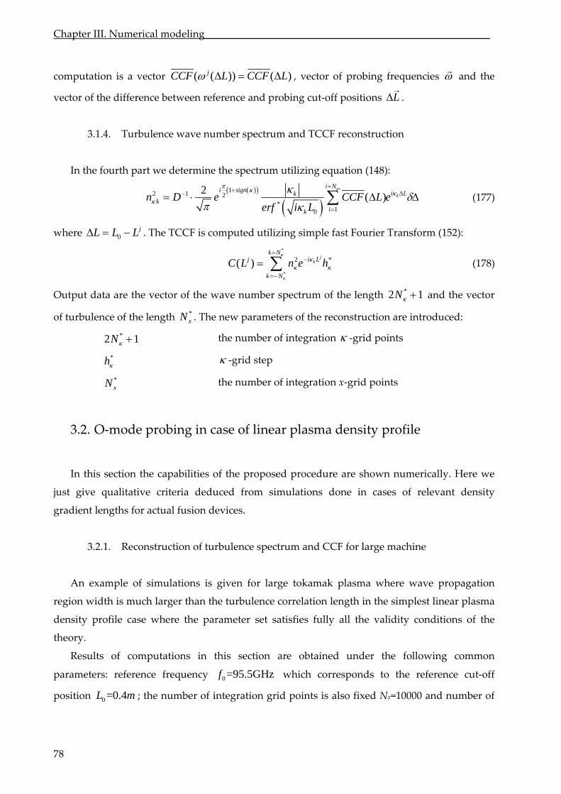
Chapter III. Numerical modeling_______________________________________________________
computation is a vector ( ( ( )F CCF L , vector of quencies ))jCC L probing fre and the
vector of the difference between reference an probing cut‐off positions Ld .
3.1.4. Turbulence wave number spectrum and TCCF reconstruction
In the part we determine uation (148):
fourth the spectrum utilizing eq
1
2i sign 2 1
10
2( ) k
i Ni Lk
ki
n D e CCF L eL
*
kerf i
(177)
where The TCCF is co fast Fourier Transform (152):
jL L L .0 mputed utilizing simple
*
*k N
2 *( )j
k
k Ni LjC L n e h
(178)
Output data the vector of the w spectrum of the length and the vector are ave number *2 1N
of turbulence of the length *xN . The new param reconstructi are introduced:
2N the number of
eters of the o
1 integration
n
* ‐grid points
h ‐grid step *
*xN the number of integration x‐grid points
3.2. O‐mode probing in case of linear plasma density profile
In this section the capabilities of the proposed procedure are shown numerically. Her
just give qualitative criteria deduced from simulations done in cases of relevant density
.2.1. Reconstruction of turbulence spectrum and CCF for large machine
An examp
region width ch
ere the parameter
Results of computations in t llowing common
parameters: ference frequency which corresponds to the reference cut‐off
position the number of points is also fixed Nx=10000 and number of
e we
gradient lengths for actual fusion devices.
3
le of simulations is given for large tokamak plasma where wave propagation
is mu larger than the turbulence correlation length in the simplest linear plasma
density profile case wh set satisfies fully all the validity conditions of the
theory.
his section are obtained under the fo
re 0f
integration grid
=95.5GHz
0 =0.4L m ;
78
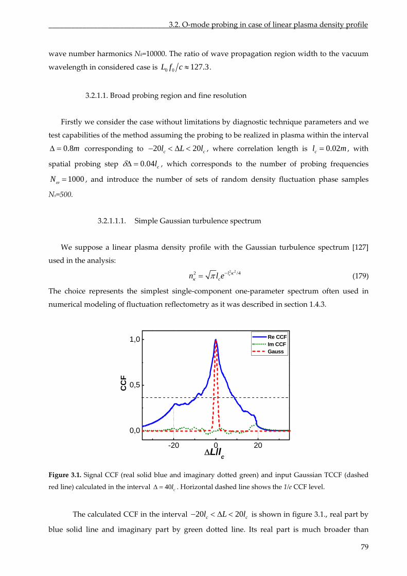
________________________________3.2. O‐mode probing in case of linear plasma density profile
79
wave propagation region width
case is
wave number harmonics Nk=10000. The ratio of to the vacuum
wavelength in considered 0 0 127.3L f c .
1. Broad d fine resolution
irstly we consider the case without limitations by diagnostic technique parameters an
test capabilities of the method assuming the probing to be realized in plasma within the interval
ond
3.2.1. probing region an
F d we
0.8m corresp ing to 20 20c cl L l , where correlation length is 0.02cl m , with
spatial obing step 0.04 clpr , which corresponds to the numb of probing frequencies
1000N , and introduce the number
er
of random density fluctuatio samples
Ns=
3.2.1.1.1. Simple Gaussian turbulence spectrum
We suppose a linear plasma d spectrum [127]
of sets n phase
500.
ensity profile with the Gaussian turbulence
used in the analysis:
2 2 /42 cl
cn l e (179)
The choice represents the sim
plest single‐component one‐parameter spectrum often used in
modeling of fluctuation reflectometry as it was described in section 1.4.3. numerical
-20 0 20
0,0
0,5
1,0
CC
F
Re CCF Im CCF Gauss
L/lc
Figure 3.1. Signal CCF (real solid blue input Gaussian TCCF (dashed
red line) calculated in the interval Horizontal dashed line shows the 1/e CCF level.
The calculated CCF in the interval l
and imaginary dotted green) and
40 cl .
20 20c cl L is shown in figure 3.1., real part by
blue solid line and imaginary part by green dotted line. Its real part is much broader than
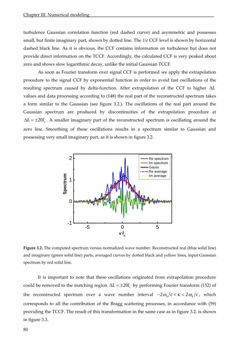
Chapter III. Numerical modeling_______________________________________________________
turbulence Gaussian corr hed curve) and asymmetric and ossesses
small, but finite imaginary part, shown by dotted line. The 1/e CCF level sh
elation function (red das p
is own by horizontal
ashed black line. As it is obvious, the CCF contains information on turbulence but does not
peaked about
ero and shows slow logarithmic decay, unlike the initial Gaussian TCCF.
ply the extrapolation
procedure to the signal CCF by exponential function in order to avoid fast oscillations of the
resulting spectrum caused by delta‐function. After extrapolation of the CCF to higher
d
provide direct information on the TCCF. Accordingly, the calculated CCF is very
z
As soon as Fourier transform over signal CCF is performed we ap
L
values and data processing according to (148) the real part of the reconstructed spectrum
similar to d
Gaussian spectrum are produced by discontinuities of the extrapolation procedu
A smaller imaginary part of the reconstructed spectrum is oscillating around
ilar to
takes
the
the
a form the Gaussian (see figure 3.2.). The oscillations of the real part aroun
re at
20 cL l .
zero line. Smoothing of these oscillations results in a spectrum sim Gaussian and
possessing very small imaginary part, as it is shown in figure 3.2.
-5 0 5-1
0
1
2
Sp
ec
Re spectrum Im spectrum Gauss
trum
l
Re average
c
Im average
igure 3.2. The computed spectrum versus normalized wave number. Reconstructed real (blue solid line)
and
is important to note that these oscillations originated from extrapolation procedure
cou
F
imaginary (green solid line) parts, averaged curves by dotted black and yellow lines, input Gaussian
spectrum by red solid line.
It
ld be removed to the matching region 20 cL l by performing Fourier transform (152) of
the reconstructed spectrum ove umber interval r a wave n 0 02 2c c , which
correspon the contribution of the Bragg scattering processes, in accordance with (59) ds to all
providing the TCCF. The result of this transformation in the same case as in figure 3.2. is shown
in figure 3.3.
80
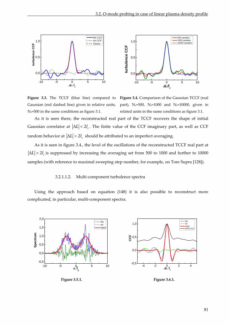
________________________________3.2. O‐mode probing in case of linear plasma density profile
-10 5 10-5 0
0,0
0,5
1,0
Llc
Re CCF Im CCF Gauss
turb
ulen
ce C
CF
-10 -5 0 05 1
0,0
0,5
1,0
ulen
CF
c
500 samples 1000 samples
ce C
turb
L/l
10000 samples
Figure 3.3. r
Gaussian (re in
the same conditions as figure 3.1.
rt), 100
related units in the same conditions as figure 3.1.
s it is seen there, the reconstructed real part of the TCCF recovers the shape of initial
Gaussian
The TCCF (blue line) compa ed to
d dashed line) given relative units,
Ns=500 in
Figure 3.4. Comparison of the Gaussian TCCF (real
pa Ns=500, Ns=1000 and Ns= 00, given in
A
correlator at 2 cL l . The finite value of the CCF imaginary part, as well as CCF
behavior at 2random c
As it is seen in fig
L l should be attributed to an imperfect averaging.
ure 3.4., the level of the oscillations of the reconstructed TCCF real part at
2 cL l is suppressed by increasing the averaging set from 500 to 1000 and further to 1
3.2.1.1.2. Multi‐component turbulence spectra
Using the approach based on equation (148) it is also possible to reconstruct more
complicated, in particular, multi‐component spectra.
0000
samples (with reference to maximal sweeping step number, for example, on Tore Supra [128]).
-10 -5 0 5 10-0,5
0,0
0,5
1,0
1,5
2,0
lc
Spec
trum
Re Im input
-4 -2 0 2 4-0,5
0,0
0,5
1,0
Re Im input
Ll
c
RCR CCF
CC
F
Figure 3.5.1. Figure 3.6.1.
81
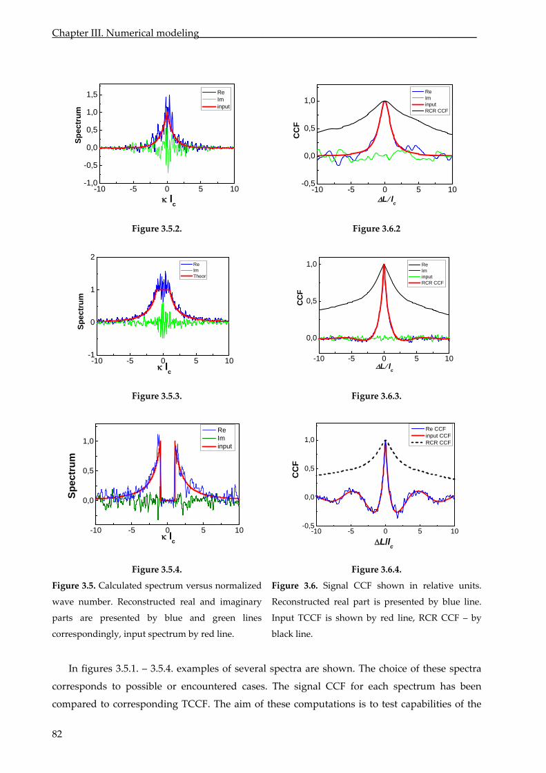
Chapter III. Numerical modeling_______________________________________________________
-10 -5 0 5 10-1,0
-0,5
0,0
0,5
1,0
1,5 Re Im input
Spec
trum
lc
-10 -5 0 5 10-0,5
0,0
0,5
1,0
CC
F
Re Im input RCR CCF
Llc
Figure 3.5.2. Figure 3.6.2
-10 -5 0 5 10-1
0
1
2
lc
Sp
ectr
um
Re Im
-10 -5 0 5 10
0,0
0,5
1,0
CC
F
Re Im
Theor
input RCR CCF
Llc
Figure 3.5.3. Figure 3.6.3.
-10 -5 0 5 10
0,0
0,5
1,0
Spec
trum
lc
Re Im input
-10 -5 0 5 10-0,5
0,0
0,5
1,0
L/l
c
Re CCF input CCF RCR CCF
CC
F
versus normalized
ave number. Reconstructed real and imaginary
parts a
Figure 3.6. Signal CCF shown in relative units.
Reconstructed real part is presented by blue line.
black
sho
corresponding TCCF. The aim of these computations is to test capabilities of the
Figure 3.5.4. Figure 3.6.4.
Figure 3.5. Calculated spectrum
w
re presented by blue and green lines
correspondingly, input spectrum by red line.
Input TCCF is shown by red line, RCR CCF – by
line.
In figures 3.5.1. – 3.5.4. examples of several spectra are wn. The choice of these spectra
corresponds to possible or encountered cases. The signal CCF for each spectrum has been
compared to
82
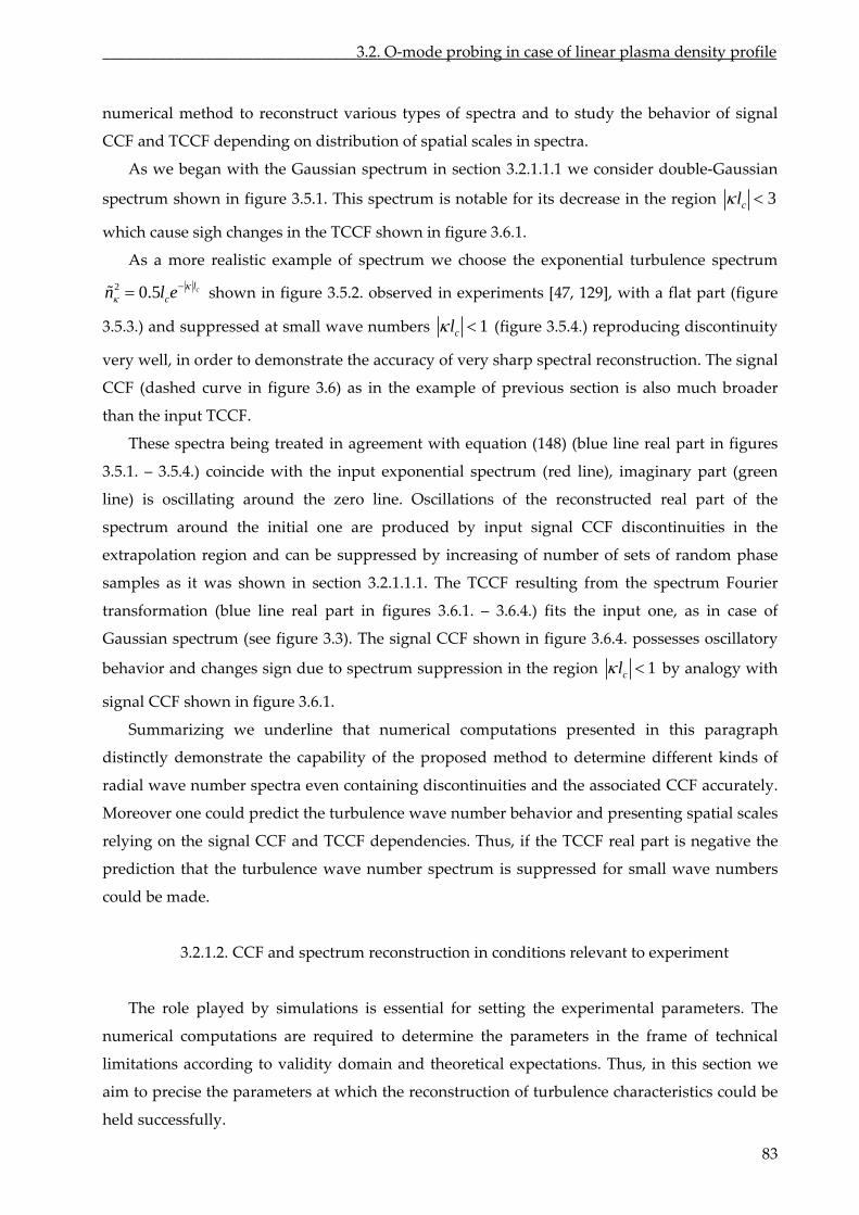
________________________________3.2. O‐mode probing in case of linear plasma density profile
numerical method to reconstruct various types of spectra and to study the behavior of signal
CCF and TCCF depending on distribution of spatial scales in spectra.
As we began with the Gaussian spectrum in section 3.2.1.1.1 we consider double‐Gaussian
spectrum shown in figure 3.5.1. This spectrum is notable for its decrease in the region 3cl
which cause sigh changes in the TCCF shown in figure 3.6.1.
As a more realistic example of spectrum we choose the exponential turbulence spectrum
2 0.5 clcn l e
3.5.3.) and
shown in figure 3.5.2. observed in experiments [47, 129], with a flat part (figure
suppressed at small wave numbers 1cl (figure 3.5.4.) reproducing discontinuity
o
m
with the
t real part of the
spectrum
extrapolation
samples as
f
Gaussian spectrum (see figure 3.3). The signal CCF shown in figure 3.6.4. possesses oscillatory
behavior region
very well, in order to demonstrate the accuracy
CCF (dashed curve in figure 3.6) as in the exa
than the input TCCF.
f very sharp spectral reconstruction. The signal
ple of previous section is also much broader
These spectra being treated in agreement with equation (148) (blue line real part in figures
3.5.1. – 3.5.4.) coincide input exponential spectrum (red line), imaginary part (green
line) is oscillating around he zero line. Oscillations of the reconstructed
around the initial one are produced by input signal CCF discontinuities in the
region and can be suppressed by increasing of number of sets of random phase
it was shown in section 3.2.1.1.1. The TCCF resulting from the spectrum Fourier
transformation (blue line real part in figures 3.6.1. – 3.6.4.) fits the input one, as in case o
1cl and changes sign due to spectrum suppression in the by analogy with
signal
presented in this paragraph
distinctly demonstrate the capability of the proposed method to determine different kinds of
radial wave number spectra even containing discontinuities and the associated CCF accurately.
Moreover one could predict the turbulence wave number behavior and presenting spatial scales
relying on the signal CCF and TCCF dependencies. Thus, if the TCCF real part is negative the
prediction that the turbulence wave number spectrum is suppressed for small wave numbers
could be made.
3.2.1.2. CCF and spectrum reconstruction in conditions relevant to experiment
The role played by simulations is essential for setting the experimental parameters. The
numerical compu required to determine the paramete me of technical
limitations according to validity domain and theoretical expectations. Thus, in this section we
aim to precise the parameters at which the reconstruction of turbulence characteristics could be
held successfully.
CCF shown in figure 3.6.1.
Summarizing we underline that numerical computations
tations are rs in the fra
83
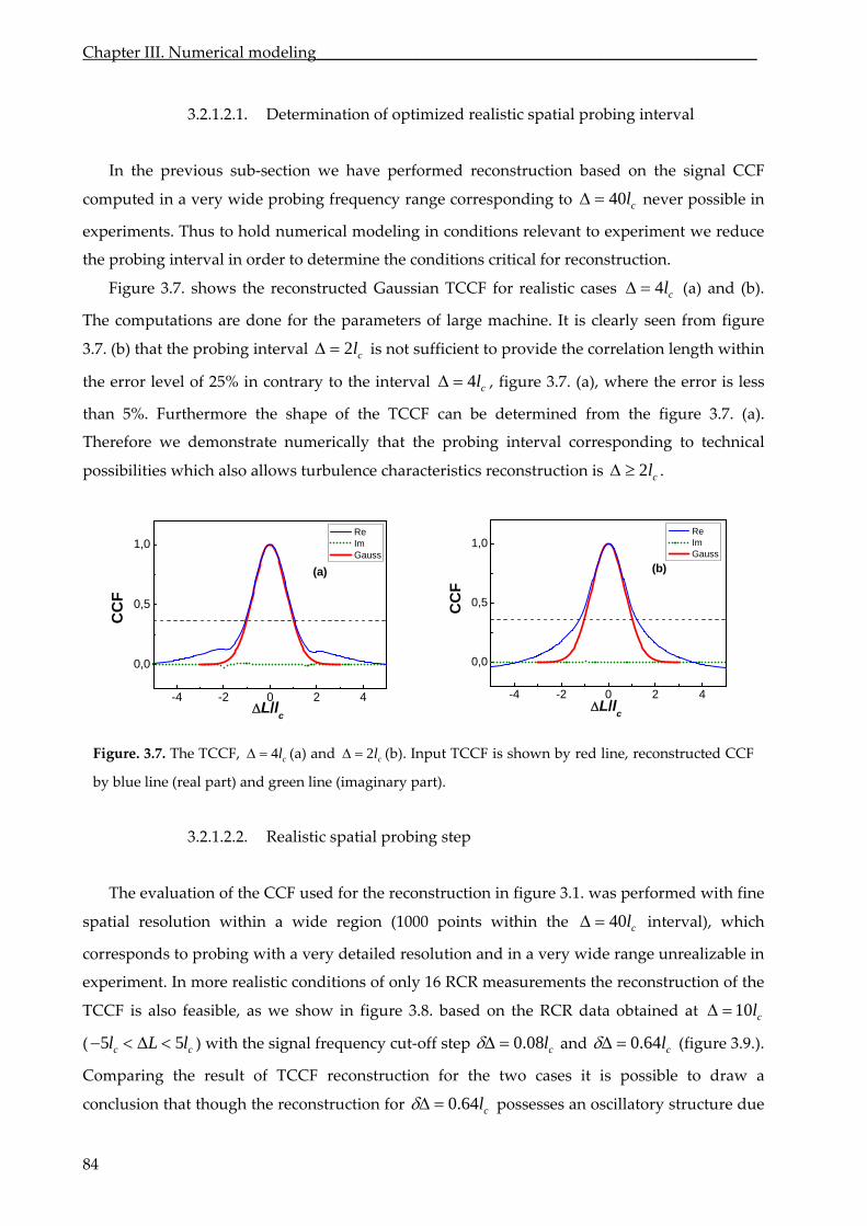
Chapter III. Numerical modeling_______________________________________________________
3.2.1.2.1. Determination of optimized realistic spatial probing interval
In the previous sub‐section we have performed reconstruction based on the signal CCF
computed in a very wide probing frequency range corresponding to 40 cl never possible in
experiments. Thus to hold numerical modeling in conditions relevant to experiment we reduce
the probing interval in order to determine the conditions critical for reconstruction.
Figure 3.7. shows the reconstructed Gaussian TCCF for realistic cases (a) and (b).
The computations are done for the parameters of large machine. It is clearly from figure
3.7. (b) that the probing interval is no sufficient to provide the length with
the error level of 25% in contrary interval
4 cl
seen
correlation 2 cl
to the
t in
4 cl ,
can be
probing
characteristics
figure 3.7. (a), error is less
than 5%. Furthermore the shape TCCF determined from 3.7. (a).
Therefore we demonstrate that the interval co to technical
possibilities which also allows reconstruction is
where the
the figure
rresponding
2 cl
of the
numerically
turbulence .
-4 -2 0 2 4
0,0
0,5
1,0
L/lc
CC
F
Re Im Gauss
(a)
-4 -2 0 2 4
0,0
0,5
1,0
L/lc
CC
F
Re Im Gauss
(b)
Figure. 3.7. The TCCF, (a) and (b). Input TCCF is shown by red line, reconstructed CCF
by blue line (real part) and green line (imaginary part).
3.2.1.2.2. Realistic spatial probing step
The evaluation used for the reconstruction in figure with fine
4 cl 2 cl
of the CCF 3.1. was performed
spatial resolution within a wide region (1000 points within the 40 cl interval), which
lution and in a very wide range unrealizable in
6 RCR measurements the reconstruction of the
. based on
corresponds to probing with a very detailed reso
experiment. In more realistic conditions of only
TCCF is also feasible, as we show in fig
1
ure 3.8 the RCR obtained at
l with the signal frequency cut‐off step
data 10 cl
( 5 5L )c c cl 0.08l and 0.64lc
it is
possible
(figure 3.9.).
Comparing the result of TCCF reconstruction for the two cases to draw a
conclusion that though the reconstruction for 0.64 cl
possesses an oscillatory structure due
84

________________________________3.2. O‐mode probing in case of linear plasma density profile
to spatial discretezation effect and discrepancy caused by extrapolation procedure, nevertheless
it is still conceivable to determine the TCCF and correlation length therefore we consider the
probing step 0.64 cl to be enough for reconstruction.
-4 -2 0 2 4
0,0
1,0
0,5
L/lc
CC
F
Re, 0.08lc Im, 0.08lc
Re, 0.64lc Im, 0.64lc Gauss
-10 -5 0 5 10
0,0
0,5
1,0 0.08lc
L/l
CC
F
c
0.64lc
Figure 3.8. CCF shown in relative units for
0.08 cl (blue crosses real part and green crosses
imaginary part) and 0.64 cl (cyan squares real
part and green triangles imaginary part). Input
TCCF is shown by red line.
Figure 3.9. TCCF reconstructed at 10 cl ,
0.08 cl (blue line) and 0.64 cl (cyan line).
3.2.1.2.3. Reconstruction in presence of uncorrelated noise
In this sub‐section we study limitations of the reconstruction pro associated with
broadband noise. We model it a
cedure
s the white noise in the following way ( )ji
sN s sA A A e
where sNA is the measured signal, sA is the scattering signal, is the noise level, ( )j –
random uncorrelated phase.
Here we represent the numerical simulation results obtained only for noise level of
1.0 , whereas for the wide range of parameters (noise level 0.1 1.5 ) the simulations
were held as well. Figure 10 shows the CCF computed for Gaussian spectrum 2 2 42 cl
cn l e
in the case of 1.0 and N =500 random phase samples by the solid line the real part and s
dotted the imaginary part. The CCF oscillations could be reduced by increasing the number
of lue of
CF is damped due to the presence of noise in comparison with figure 3.1.
line
sets of samples up to Ns=10000 (see figure 3.10.). It could be seen that the maximum va
C
In figure 3.12. we represent the turbulence radial wave number spectrum for Ns=500. The
Gaussian spectrum kernel is observable there at 5 5cl (shown by vertical dashed lines)
however the noise level at wings is very high, not allowing the TCCF reconstruction (see huge
oscillations in figure 3.13). We overcome the oscillations by decreasing the spectrum interval
used for the Fourier transform. Thus, to obtain the TCCF shown in figure 3.14, we process the
85
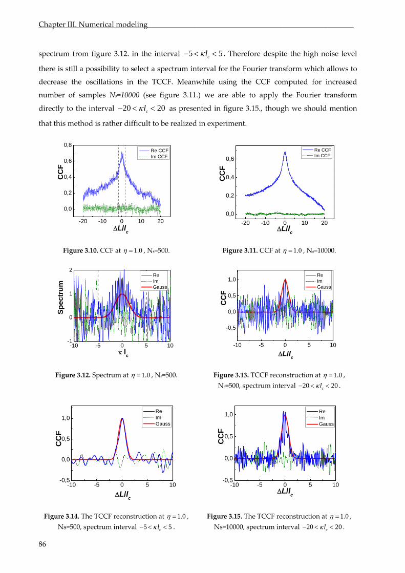
Chapter III. Numerical modeling_______________________________________________________
spectrum from figure 3.12. in the interval 5 5cl . Therefore despite the high noise level
ere is still a possibility to select a spectrum the Fourier transform which allows to
dec
ly the
th interval for
rease the oscillations in the TCCF. Meanwhile using the CCF computed for increased
number of samples Ns=10000 (see figure 3.11.) we are able to app Fourier transform
directly to the interval 20 20cl as presented in figure 3.15., though we should mention
that this method is rather difficult to be realized in experiment.
-20 -10 0 10 20
0,0
0,2
0,4
0,6
0,8
Re CCF
L/lc
Im CCF
CC
F
-20 -10 0 10 200,0
0,2
,4
0,6
0
Re CCF Im CCF
C
CF
L/lc
Figure 3.10. CCF at 1.0 , Ns=500. Figure 3.11. CCF at 1.0 , Ns=10000.
-10 -5 0 5 10-1
0
1
2
lc
Re Im Gauss
Spec
trum
-10 -5 0 5 10
-0,5
0,0
0,5
1,0
L/l
c
Re Im
C
CF
Gauss
Figure 3.12. Spectrum at 1.0 , Ns=500. Figure 3.13. TCCF reconstruction at 1.0 ,
20cl .
=500, spectrum intervalNs 20
-10 -5 0 5 10-0,5
0,0
0,5
1,0
L/lc
Re Im Gauss
CC
F
-10 -5 0 5 10
-0,5
0,0
0,5
1,0
L/lc
Re Im
Gauss
CC
F
Figure 3.14. The TCCF reconstruction at 1.0 ,
Ns=500, spectrum interval 5 5cl .
Figure 3.15. The TCCF reconstruction at 1.0 ,
0000, spectrum interval 20 20cl . Ns=1
86
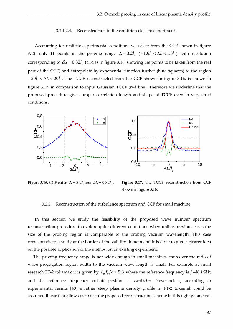
________________________________3.2. O‐mode probing in case of linear plasma density profile
3.2.1.2.4. Reconstruction in the condition close to experiment
Accountin stic experimental conditions we g for reali select from the CCF shown in figure
3.12. only 11 points in the probing range 3.2 cl ( 1.6 1.6c cl L l ) with resolution
corresponding to 0.32 cl
and extrapolate
l . The TCCF
(circles in figure taken from the real
part of the CCF) by exponential uares) to the region
reconstructed CCF 3.16. is shown in
figure 3.17. in comparison to input Gaussian TCCF (red line). Therefore we underline that the
proposed procedure gives proper correlation length and shape of TCCF even in very strict
conditions.
3.16. showing
function
from the
the points to be
further (blue sq
shown in figure 20 20c cl L
-4 -2 0 2 4
0,0
0,2
0,4
0,6
0,8
L/lc
Re Im
CC
F
-10 -5 0 5 10-0,5
0,0
0,5
1,0
L/lc
CC
F
Re Im Gauss
e 16. CCF cut at 3.2 clFigur 3. and 0.32 cl . Figure 3.17. The TCCF reconstruction from CCF
shown in figure 3.16.
3.2.2. Reconstruction
of the turbulence spectrum and CCF for small machine
In d wave n
cases the
h. This case
a stud
r example at small
researc
this section we study the feasibility of the propose umber spectrum
reconstruction procedure to explore quite different conditions when unlike previous
size of the probing region is comparable to the probing vacuum wavelengt
corresponds to y at the border of the validity domain and it is done to give a clearer idea
on the possible application of the method on an existing experiment.
The probing frequency range is not wide enough in small machines, moreover the ratio of
wave propagation region width to the vacuum wave length is small. Fo
h FT‐2 tokamak it is given by 0 0 5.3L f c where the reference frequency is f0=40.1GHz
and the reference frequency cut‐off position . Nevertheless, according to
experimental results [40] a rather steep plasma density profile in FT‐2 tokamak could be
assumed linear that allows us to test the proposed reconstruction scheme in this tight geometry.
is L0=0.04m
87
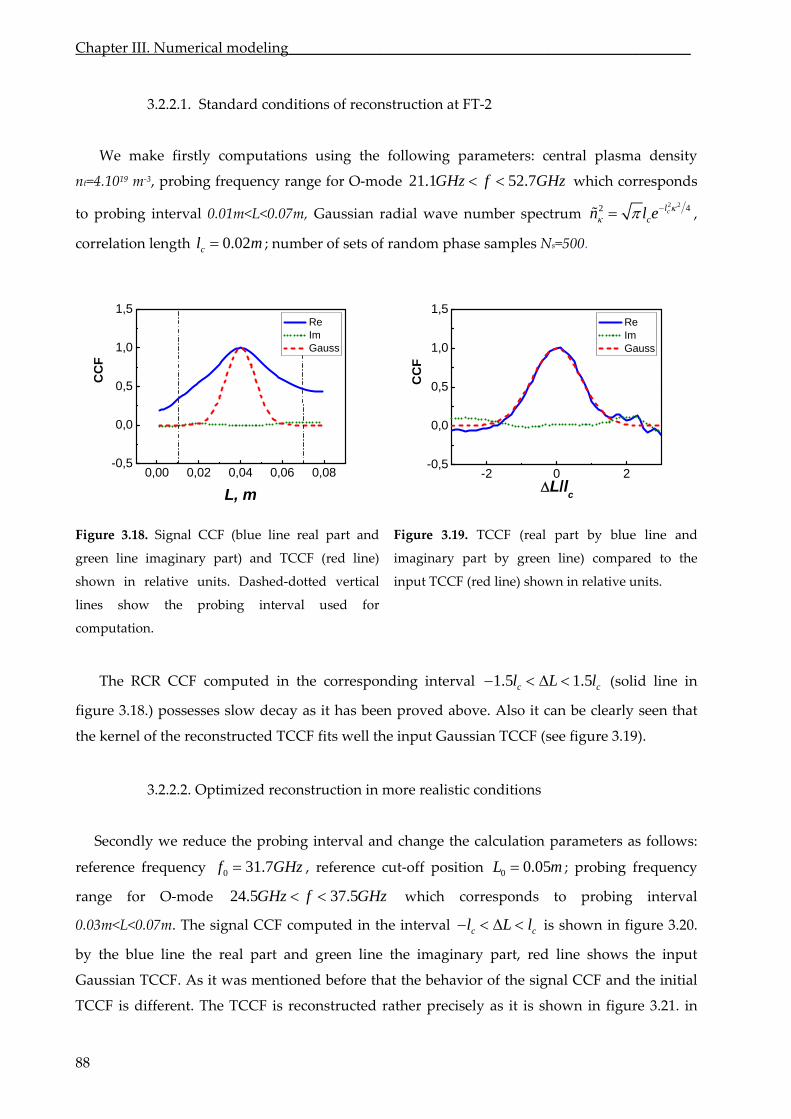
Chapter III. Numerical modeling_______________________________________________________
3.2.2.1. Standard conditions of reconstruction at FT‐2
We make firstly computations using the following parameters: central plasma density
nt=4.1019 m‐3, probing frequency range for O‐mode 21.1 52.7GHz f GHz which corresponds
to probing interval 0.01 aussian radial wave number spectrum m<L<0.07m, G2 2 42 cl
cn l e ,
correlation length 0.02cl m ; number of sets of random phase samples Ns=500.
0,00 0,02 0,04 0,06 0,08-0,5
0,0
0,5
1,0
1,5
CC
F
-2 0 2-0,5
0,0
0,5
1,0
1,5
L, m
Re Im Gauss
L/lc
CC
F
Re Im Gauss
Figure 3.18. Signal CCF (blue line real part and
green line imaginary part) and TCCF (red line)
shown in relative units. Dashed‐dotted vertical
lines show the probing interval used for
computation.
Figure 3.19. TCCF (real part by blue line and
imaginary part by green line) compared to the
input TCCF (red line) shown in relative units.
The RCR CCF computed in the corresponding interval l1.5 1.5c cl L (solid line in
figure 3.18.) possesses slow decay as it has proved above. Also it can be clearly seen
the k ed TC ell the inp ).
3.2.2.2. Optimized reconstruction in more realistic conditions
Secondly we reduce the probing interval and change the calculation parameters as follows:
reference frequency
been that
ernel of the reconstruct CF fits w ut Gaussian TCCF (see figure 3.19
0 31.7f GHz , reference cut‐off position 0 0.05L m ;
corresponds to
c cl L l
probing frequency
range for O‐mode which probing interval
0.03m<L<0.07m. The interval
24.5GHz f
signal CCF
37.5GHz
computed in the is shown in figure 3.20.
by the blue line the real part and green line the imaginary part, red line shows the input
Gaussian TCCF. As it was mentioned before the behavior of the signal CCF and the initial
T truct rat 3.21.
that
CCF is different. The TCCF is recons ed her precisely as it is shown in figure in
88
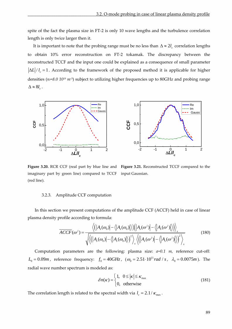
________________________________3.2. O‐mode probing in case of linear plasma density profile
spite of lence correlation
ngth is only twice larger then it.
the fact the plasma size in FT‐2 is only 10 wave lengths and the turbu
le
It is important to note that the probing range must be no less than 2 cl correlation lengths
to obtain 10% error reconstruction on FT ncy between the
reconstructed TCC input one could be explained as a consequence of small parameter
‐2 tokamak. The
F and the
discrepa
/ 1cL l . According to the framework of the proposed method it is applicable for higher
019 m‐3) subject to utilizing higher frequencies up to 80GHz and probing range
8 cl .
densities (nt=8.0 1
-2 -1 0 1 20,0
0,5
1,0
L/lc
CC
F
Re Im Gauss
-2 -1 0 1 2
0,0
0,5
1,0
L/lc
CC
F
Re Im Gauss
Figure 3.20. RCR CCF (real part by blue line and
imaginary part by green line) compared to TCCF
Figure 3.21. Reconstructed TCCF compared to the
input Gaussian.
3.2.3. Amplitude CCF computation
In this section we present computations of the amplitude CCF (ACCF) held in case of linear
plasma
(red line).
density profile according to formula:
0 0
22
0 0
( ) ( ) ( ) ( )( )
( ) ( ) ( ) ( )
j js s s s
j s
j js s s s
s s
A A A AACCF
A A A A
(180)
Computation parameters are the following: plasma size: a=0.1 m, reference cut‐off:
0 0.09m , reference frequency: 0 40L f GHz , ( 110 2.51 10 /rad s , 0 0.0075m ). The
radial wave number spectrum is modeled as:
max( )0, otherwise
n1, 0
(181)
The correlation length is related to the spectral width via max2.1 /cl .
89
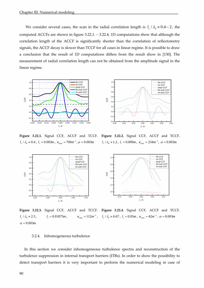
Chapter III. Numerical modeling_______________________________________________________
We consider several cases, the scan in the radial correlation length is 2 0/ 0.4cl , the
omputed ACCFs are shown in figure 3.22.1. – 3.22.4. 1D computations show that although the
cor
cases in linear regime. I
w in [130]. Th
dial corre e signal in the
linear regime.
c
relation length of the ACCF is significantly shorter than the correlation of reflectometry
signals, the ACCF decay is slower than TCCF for all t is possible to draw
a conclusion that the result of 1D computations differs from the result sho e
measurement of ra lation length can not be obtained from the amplitud
-0,020 -0,015 -0,010 -0,005 0,000 0,005 0,010 0,015 0,020
-0,2
0,0
0,2
0,4
0,6
0,8
1,0 Re CCF Im CCF ampl CCF Re turb CCF Im turb CCF
CC
F
L, m-0,06 -0,04 -0,02 0,00 0,02 0,04 0,06
-0,4
-0,2
0,0
0,2
0,4
0,6
0,8
1,0
1,2 Re CCF Im CCF ampl CCF Re turb CCF Im turb CCF
CC
F
L, m
Figure 3.22.1. Signal CCF, ACCF and TCCF.
0/ 0.4cl , 0.003cl m , 1max 700m , 0.003m
Figure 3.22.2. Signal CCF, ACCF and TCCF.
0/ 1.2cl , 0.009cl m , 1max 234m , 0.003m
-0,10 -0,05 0,00 0,05 0,10-0,10 -0,05 0,00 0,05 0,10-0,4
-0,2
0,0
0,2
0,4
0,6
1
0,8
,0
CC
F
L, m
Re C FC Im CCF ampl CCF Re turb CCF Im turb CCF
0,0
0,2
0,4
0,6
0,8
1,0
CC
F
Re CCF Im CCF ampl CCF Re turb CCF
L, m
Im turb CCF
Figure 3.22.3. Signal CCF, ACCF and TCCF.
0 2.5/cl , 0.01875cl m , 1max 112m ,
0.003m
0/ 6.67cl
Figure 3.22.4. Signal CCF, ACCF and TCCF.
, 0.05cl m , 1max 42m , 0.003m
3.2.4. Inhomogeneous turbulence
In this section we consider inhomogeneous turbulence spectra and reconstruction of the
turbulence suppression in internal transport barriers (ITBs). In order to show the possibility to
detect transport barriers it is very important to perform the numerical modeling in case of
90
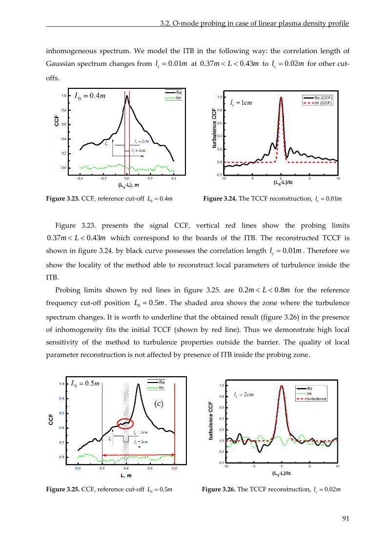
________________________________3.2. O‐mode probing in case of linear plasma density profile
inhomogeneous spectrum. We model the ITB in the following way: the correlation length of
Gaussian spectrum changes from 0.01cl m at 0.37 0.43m L m to for other cut‐
off
0.02cl m
s.
Figure 3.23. CCF, reference cut‐off Figure 3.24. The TCCF reconstruction, 0 0.4L m 0.01cl m
Figure 3.23. presents the signal CCF, vertical red lines show the probing limits
which correspond to the boards of the ITB. The reconstructed TCCF is
by black curve possesses the correlation length Therefore we
show the locality of the method able to reconstruct local parameters of turbulence inside the
0.37 0.43m L m
shown in figure 3.24. 0.01cl m .
ITB.
Probing limits shown by red lines in figure 3.25. are 0.2 0.8m L m
ows the zone where
for the reference
cut‐off position The shaded area sh the turbulence
spectrum changes. It is worth to underline that the obtained result (figure 3.26) in the presence
by red line). Thus we demonstrate high local
parameter
0 0.5L m .frequency
of inhomogeneity fits the initial TCCF (shown
sensitivity of the method to turbulence properties outside the barrier. The quality of local
reconstruction is not affected by presence of ITB inside the probing zone.
Figure 3.25. CCF, reference cut‐off 0 0.5L m Figure 3.2 re6. The TCCF construction, 0.02cl m
91
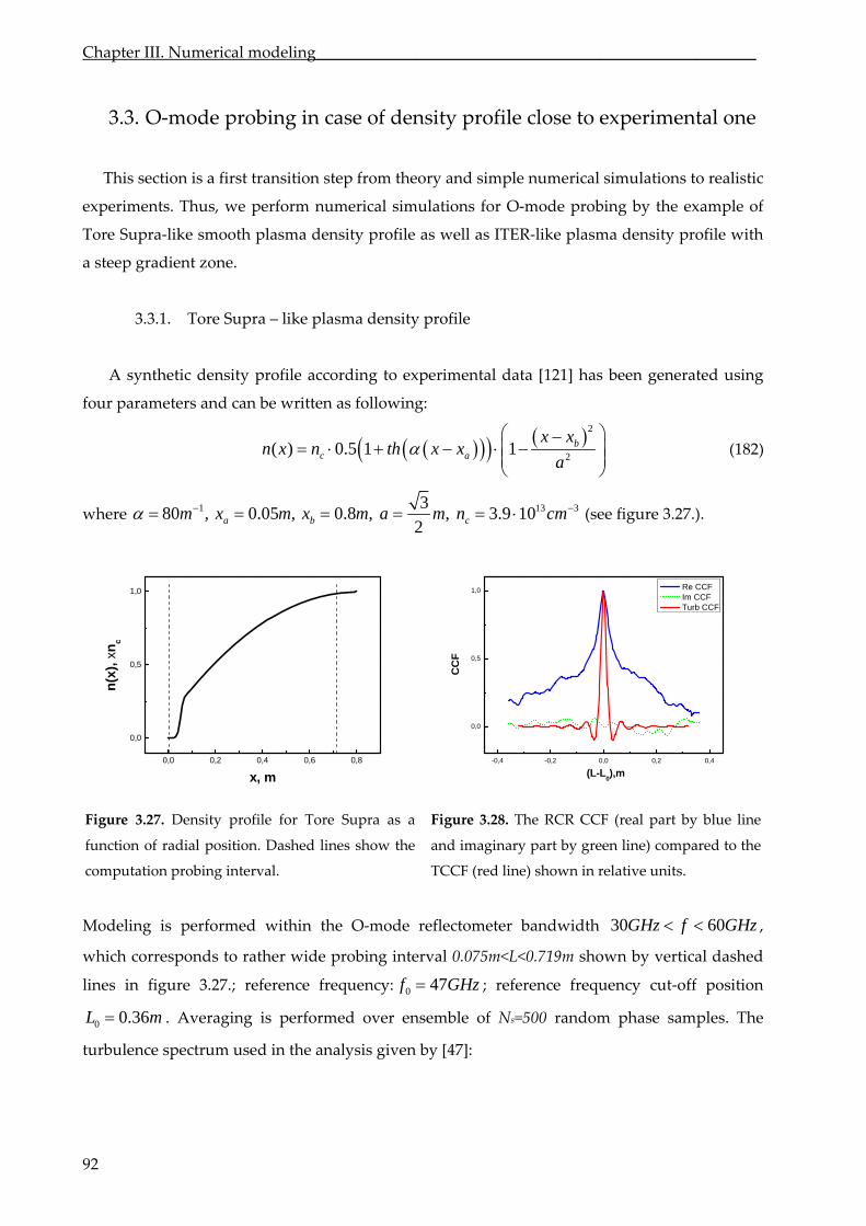
Chapter III. Numerical modeling_______________________________________________________
92
erimental o
3.3.1. Tore Supra – like plasma density profile
A synthetic density profile according to experimental data [121] has been generated using
four parameters and can be written as following:
3.3. O‐mode probing in case of density profile close to exp ne
This section is a first transition step from theory and simple numerical simulations to realistic
experiments. Thus, we perform numerical simulations for O‐mode probing by the example of
Tore Supra‐like smooth plasma density profile as well as ITER‐like plasma density profile with
a steep gradient zone.
2
2( ) 0.5 1 1 b
c a
x xn x n th x x
a
(182)
where 1 13 3380 , 0.05 , 0.8 , , 3.9 10
2a b cm x m x m a m n cm (see figure 3.27.).
0,0 0,2 0,4 0,6 0,8
0,0
0,5
1,0
n(x)
, xn c
x, m
-0,4 -0,2 0,0 0,2 0,4
0,0
0,5
1,0
CC
F
(L-L0),m
Re CCF Im CCF Turb CCF
Figure 3.27. Density profile for Tore Supra as a
function of radial position. Dashed lines show the
computation probing interval.
Figure 3.28. The RCR CCF (real part by blue line
and imaginary part by green line) compared to the
TCCF (red line) shown in relative units.
Modeling performed within the O‐mode eflectomete bandwidth
which corresponds to rather wide probing interval 0.075m<L<0.719m sh
lines in figure 3.27.; reference frequency:
is r r 30 60GHz f GHz ,
own by vertical dashed
0 47f GHz ;
ensemble of
reference
Ns=500 random
tur
frequency cut‐off position
phase samples. The0 0.36L m . Averaging is performed over
bulence spectrum used in the analysis given by [47]:
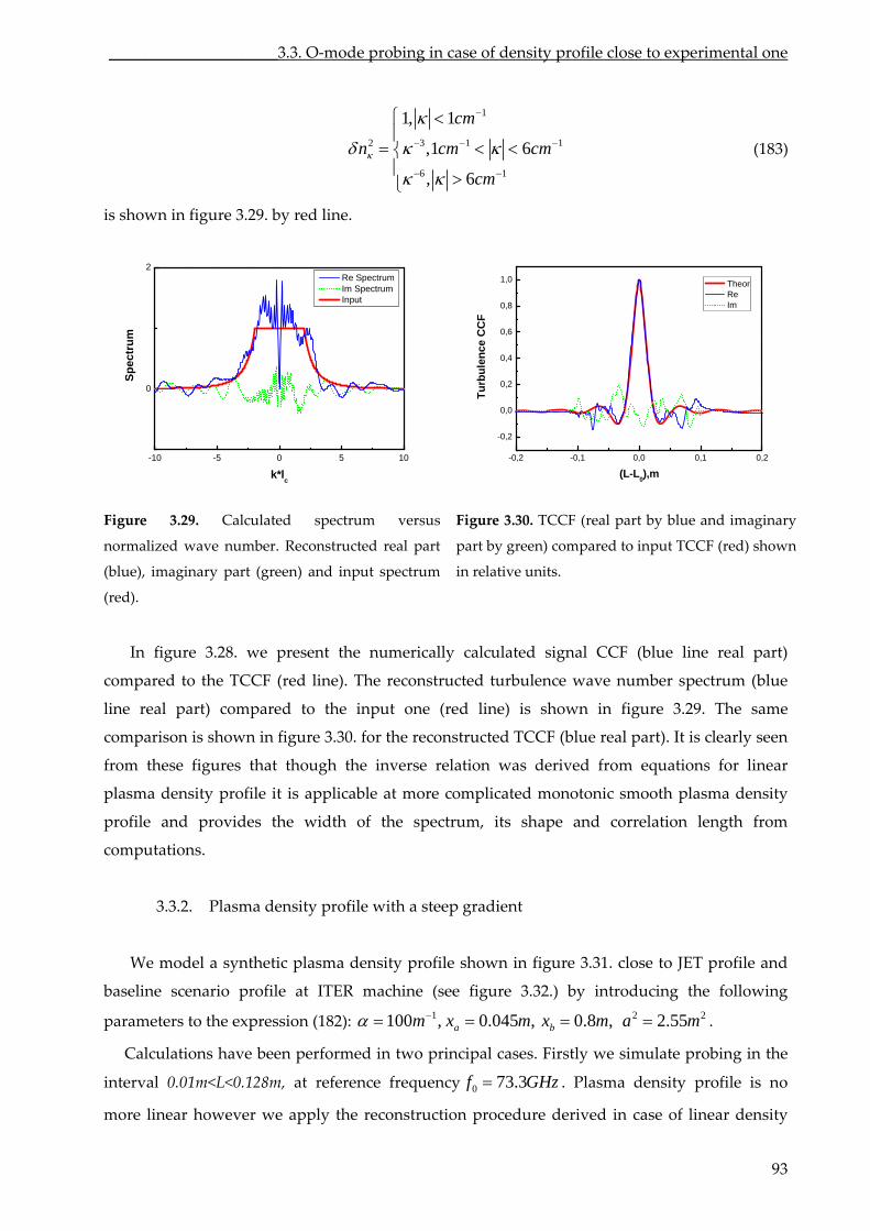
_____________________3.3. O‐mode probing in case of density profile close to experimental one
11, 1
,1
cm
m
2 3 1 1
6 1
6
, 6
n c cm
cm
is shown in figure 3.29. by red line.
(183)
-10 -5 0 5 10
0
2
Spec
trum
k*lc
Re Spectrum Im Spectrum Input
-0,2 -0,1 0,0 0,1 0,2
-0,2
0,0
0,2
0,4
0,6
0,8
1,0
Turb
ulen
ce C
CF
(L-L0),m
Theor Re Im
Figur 2 Calcula
normalized wave nu
3. TCCF (re t
signal CCF (b
line). Th
ma density
profile and provides the width of the spectrum, its shape and correlation length from
computations.
3.3.2. Plasma density profile with a steep gradient
We model a synthetic plasma density profile shown in figure 3.31. close to JET profile and
baseline scenario profile at ITER machine (see figure 3.32.) by introducing the following
parameters to the expression (182):
Calculations have been performed in two principal cases. Firstly we simulate probing in the
interval 0.01m<L<0.128m, at reference frequency
e 3. 9. ted spectrum versus
mber. Reconstructed real part
(blue), imaginary part (green) and input spectrum
(red).
Figure 30. al par by blue and imaginary
part by green) compared to input TCCF (red) shown
in relative units.
In figure 3.28. we present the numerically calculated lue line real part)
compared to the TCCF (red e reconstructed turbulence wave number spectrum (blue
line real part) compared to the input one (red line) is shown in figure 3.29. The same
comparison is shown in figure 3.30. for the reconstructed TCCF (blue real part). It is clearly seen
from these figures that though the inverse relation was derived from equations for linear
plasma density profile it is applicable at more complicated monotonic smooth plas
1100 , 0.045 , 0.8 ,a bm x m x m 2 22.55a m .
0 73.3f GHz . Plasma density profile is no
the reco structio ear density more linear however we apply n n procedure derived in case of lin
93
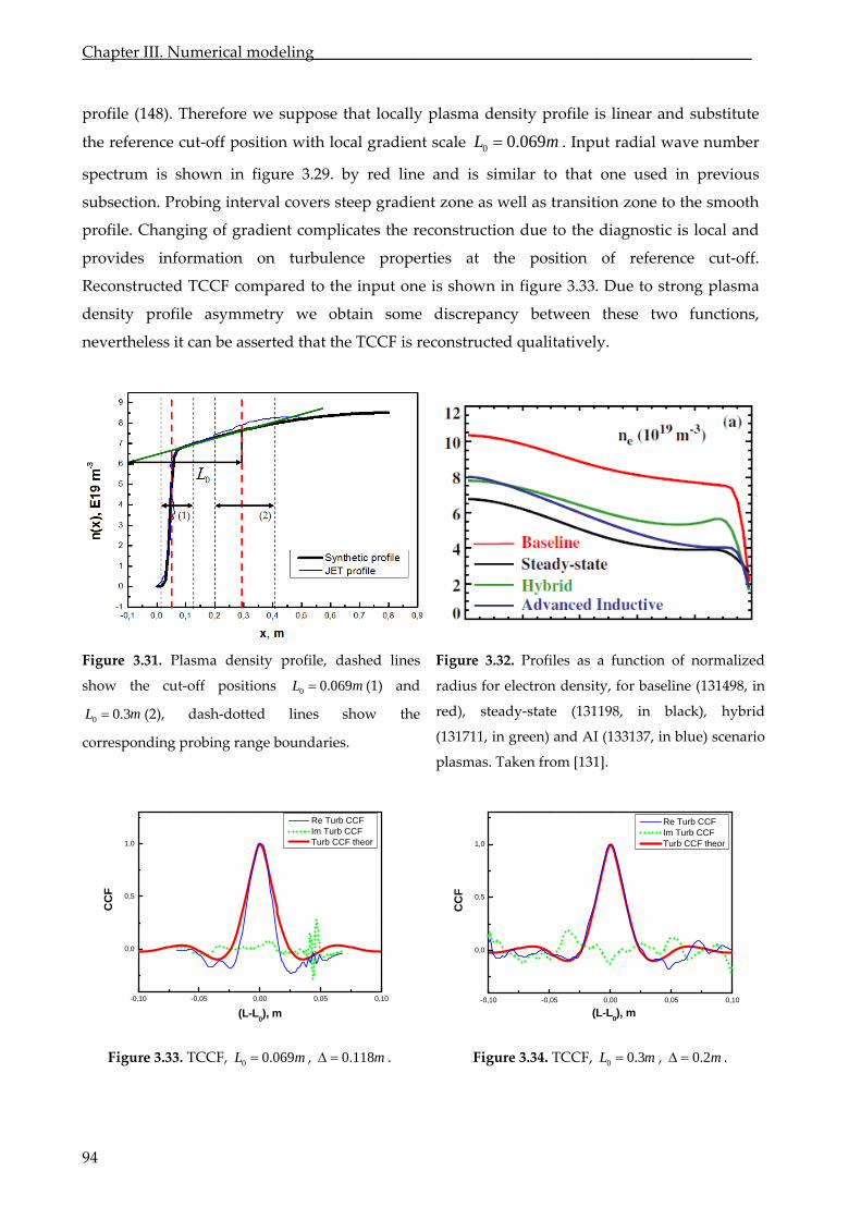
Chapter III. Numerical modeling_______________________________________________________
profile (148). Therefore we suppose that locally plasma density profile is linear and substitute
the eference cut‐off position with local gradient scale 0 0.069L m .
at the position
shown in figure
pancy between
qu
r Input radial wave number
sp
on turbulence properties of reference cut‐off.
Reconstructed TCCF compared to the input one is 3.33. Due to strong plasma
these two functions,
nevertheless it can be asserted that the TCCF is reconstructed alitatively.
ectrum is shown in figure 3.29. by red line and is similar to that one used in previous
subsection. Probing interval covers steep gradient zone as well as transition zone to the smooth
profile. Changing of gradient complicates the reconstruction due to the diagnostic is local and
provides information
density profile asymmetry we obtain some discre
Figure 3.31. Plasma density profile, dashed lines
show the cut‐off positions (1) and
(2), dash‐dotted the
corresponding probing range boundaries.
Figur s as a function of normalized
radi density, for baseline (131498, in
red), (131198, in black), hybrid
(131 d AI (133137, in blue) scenario
plas [131].
0 0.069L m
lines show0 0.3L m
e 3.32. Profile
us for electron
steady‐state
711, in green) an
mas. Taken from
-0,10 -0,05 0,00 0,05 0,10
0,0
0,5
1,0
(L-L0), m
CC
F
Re Turb CCF Im Turb CCF Turb CCF theor
-0,10 -0,05 0,00 0,05 0,10
0,0
0,5
1,0
CC
F
Re Turb CCF Im Turb CCF Turb CCF theor
(L-L0), m
e 3.34. TCCF,
Figure 3.33. TCCF, 0.118m . Figur0 0.069L m , 0 0.3L m , 0.2m .
94
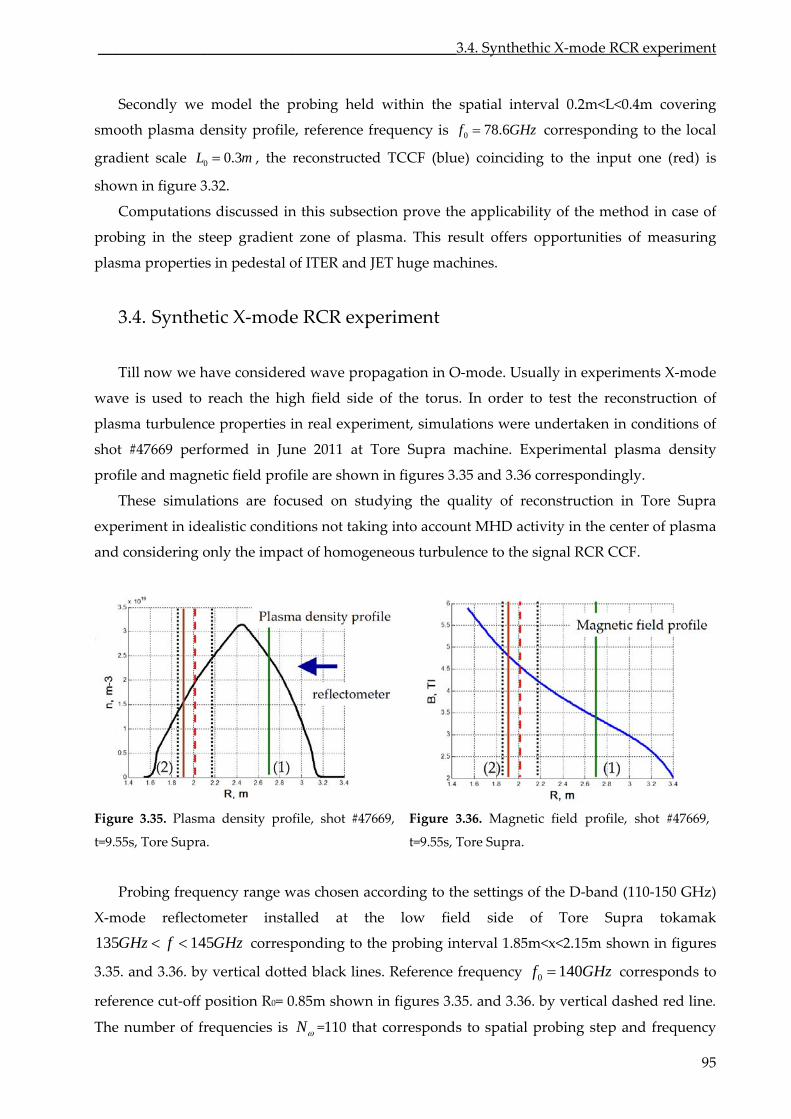
_________________________________________________3.4. Synthethic X‐mode RCR experiment
95
Secondly we model the probing held within the spatial interval 0.2m<L<0.4m covering
smooth plasma density profile, reference frequency is 0 78.6f GHz
) coinciding
corresponding to the
gradient scale the reconstructed TCCF (blue to the input one (red) is
Computations discussed in this subsection prove the applicability of the method in case of
probing in the steep gradient zone of plasma. This result offers opportunities of measuring
plasma properties in pedestal of ITER and JET huge machines.
3.4. Synthetic X‐mode RCR experiment
Till now we have considered wave propagation in O‐mode. Usually in experiments X‐mode
wave is used to reach the high field side of the torus. In order to test the reconstruction of
plasma turbulence properties in real experiment, simulations were undertaken in conditions of
shot #47669 performed in June 2011 at Tore Supra machine. Experimental plasma density
an g
o activity in the center of plasma
nsidering only the impact of homogeneous turbulence to the signal RCR CCF.
local
0 0.3L m ,
shown in figure 3.32.
profile d magnetic field profile are shown in fi
These simulations are focused on studying
experiment in idealistic conditions not taking int
and co
ures 3.35 and 3.36 correspondingly.
the quality of reconstruction in Tore Supra
account MHD
Figure 3.35. Plasma density profile, shot #47669, Figure 3.36.
t=9.55s, ore Supra.
Magnetic field profile, shot #47669,
t=9.55s, Tore Supra.
at the low field side of Supra tokamak
corresponding to the probing interval 1.85m<x<2.15m shown in figures
T
Probing frequency range was chosen according to the settings of the D‐band (110‐150 GHz)
X‐mode reflectometer installed Tore
135 145GHz f GHz
3.35. and 3.36. by vertical dotted black lines. Reference frequency 0 140f GHz corresponds to
0reference cut‐off position
The number of frequencies
R = 0.85m shown in figures 3.35. and 3.3 dashed red line.
is
6. by vertical
N =110 that corresponds to spatial and frequency probing step
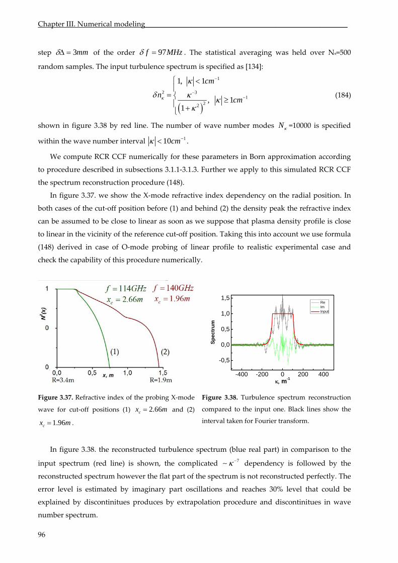
Chapter III. Numerical modeling_______________________________________________________
step 3mm of the order 97f MHz . The statistical averaging was held over Ns=500
random samples. The input turbulence spectrum is specified as [134]:
1
2 31
22
1, 1
, 11
cm
ncm
(184)
shown in figure 3.38 by red line. The number of wave number modes N =10000 is specified
within the wave number interval 110cm .
We compute RCR CCF numerically for these parameters in Born approximation according
to r described in subsections 3.1.1‐3.1.3. Further we apply to this simulated RCR CCF
the reconstruction procedure (148).
7. we show the X‐mode refractive index dependency on the radial position. In
both cut‐off position before (1) and behind (2) the density peak the refractive index
can to be close to linear as soon as we suppose that plasma density profile is close
to vicinity of the reference cut‐off position. Taking this into account we use formula
(148) case of O‐mode probing of linear profile to realistic experimental case and
check of this procedure numerically.
p ocedure
spectrum
In figure 3.3
cases of the
be assumed
linear in the
derived in
the capability
-400 -200 0 200 400
-0,5
0,0
0,5
1,0
1,5
Re Im Input
Spec
trum
m-1
Figur active index of the probing X‐mode
wave positions (1)
e 3.37. Refr
for cut‐off 2.66cx m and (2)
1.96cx m .
In figure 3.38.
spectrum
Figure 3.38. Turbulence spectrum reconstruction
compared to the input one. Black lines show the
interval taken for Fourier transform.
the reconstructed turbulence spectrum (blue real part) in comparison to the
input (red line) is shown, the complicated 7 dependency is followed by the
spectrum however the flat part o the spectrum is not reconstructed perfectly. The
erro ed by imaginary pa oscillation % level at cou be
ex discontinitues produces by extrapolation procedure and discontinitues in wave
number
reconstructed
by
spectrum.
f
r level is estimat rt s and reaches 30 th ld
plained
96
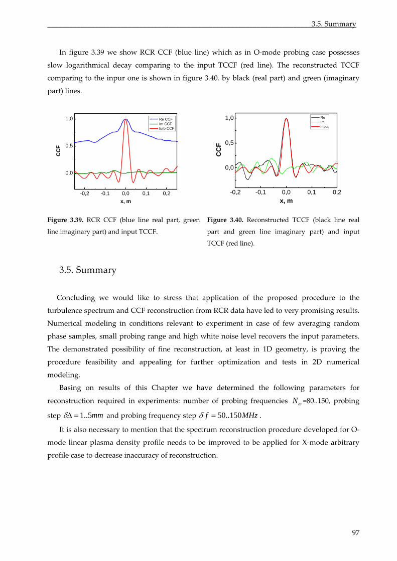
________________________________________________________________________3.5. Summary
97
CF (red line
e inpur
In figure 3.39 we show RCR CCF (blue line) which as in O‐mode probing case possesses
slow logarithmical decay comparing to the input TC ). The reconstructed TCCF
comparing to th one is shown in figure 3.40. by black (real part) and green (imaginary
part) lines.
-0,2 -0,1 0,0 0,1 0,2
0,0
0,5
1,0
Re CCF Im CCF turb CCF
CC
F
x, m
-0,2 -0,1 0,0 0,1 0,2
0,0
0,5
1,0 Re Im
CC
F
x, m
Input
e u li rt, line
Concluding we would like to stress that application of the proposed procedure to the
turbulence spectrum and CCF reconstruction from RCR data have led to very promising results.
Numerical modeling in conditions relevant to experiment in case of few averaging random
phase samples, small probing range and high white noise level recovers the input parameters.
The demonstrated possibility of fine reconstruction, at least in 1D geometry, is proving the
procedure feasibility and appealing for further optimization and tests in 2D numerical
modeling.
Basing on results of this Chapter we have determined the following parameters for
reconstruction required in experiments: number of probing frequencies
Figur 3.39. RCR CCF (bl e ne real pa green
line imaginary part) and input TCCF.
Figure 3.40. Reconstructed TCCF (black real
part and green line imaginary part) and input
TCCF (red line).
3.5. Summary
N =80..150, probing
step 1..5mm and probing frequency step 50..150f MHz .
It is also necessary to mention that the spectrum reconstruction procedure developed for O‐
mo
de linear plasma density profile needs to be improved to be applied for X‐mode arbitrary
profile case to decrease inaccuracy of reconstruction.

98
99
Chapter IV
Applications to experiments
_______________________________________ __________________________________________
revious Chapters of this thesis covered theoretical background of RCR applications and
nu
construction undertaken before results described in this section are preliminary and
are
c
l wave num atial CCF in sma and large machines and give
an
software and data interpretation methods
r each experiment.
his part of the thesis is devoted to three separate methods of data processing obtained at
three different machines – FT‐2, Tore Supra and JET. Furthermore experimental results using
the proposed method of turbulence properties determination are discussed.
____
P
merical modeling of experiments which are certainly convincing however experimental
approbation of the method is also required. How to move from the theory and simulations to
the real world? Passing from theoretical models to real experiments we face plenty of additional
tasks and problems: hardware volatility, additional noise, shot conditions, technical problems of
data acquisition and huge volumes of data to be processed…
Since there were no RCR experiments applying the new method of radial wave number
spectrum re
focused on estimation of experimental parameters and settings. Besides that the more
ambitious task was to estimate and compare turbulence parameters such as orrelation length,
radia ber spectrum and turbulence sp ll
insight into capabilities of RCR diagnostic. We would like to notice as well that there is no
universal method applicable to all machines; different hardware and different plasmas demand
unique approach and it is needed to develop specific
fo
T

100
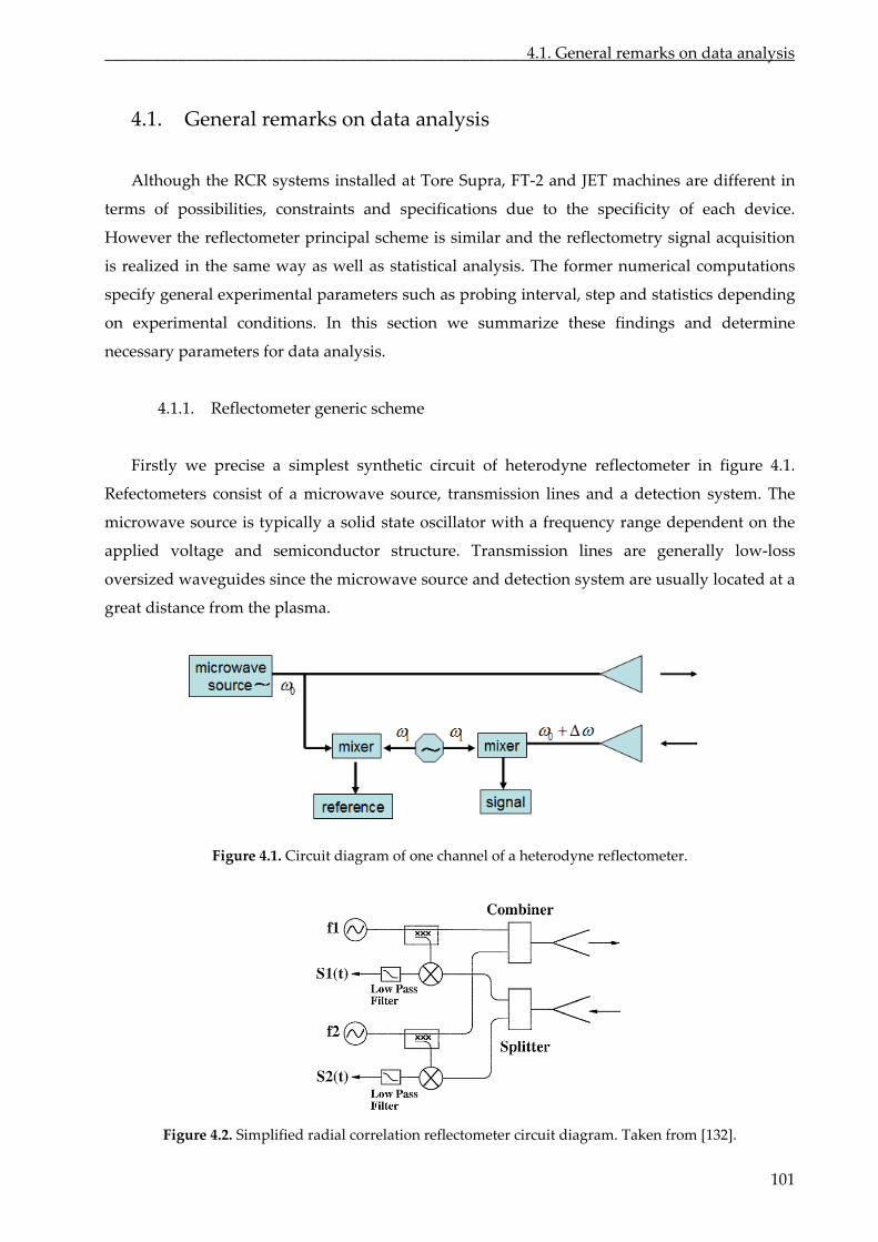
____________________________________________________4.1. General remarks on data analysis
4.1. General remarks on data analysis
Although the RCR systems installed at Tore Supra, FT‐2 and JET machines are different in
terms of possibilities, constraints and specifications due to the specificity of each device.
owever the reflectometer principal scheme is similar and the reflectometry signal acquisition
realized in the same way as well as statistical analysis. The former numerical computations
ecify general experimental parameters such as probing interval, step and statistics depending
on experimental conditions. In this section we summarize these findings
necessary parameters for data analysis.
4.1.1. Reflectometer generic schem
efectometers consist of a microwave source, transmission lines and a detection system. The
icrowave source is typically a solid state oscillator with a frequency range dependent on the
pplied voltage and semiconductor structure. Transmission lines are generally low‐loss
versized waveguides since the microwave source and detection system are usually located at a
reat distance from the plasma.
H
is
sp
and determine
e
Firstly we precise a simplest synthetic circuit of heterodyne reflectometer in figure 4.1.
R
m
a
o
g
Figure 4.1. Circuit diagram of one channel of a heterodyne reflectometer.
Figure 4.2. Simplified radial correlation reflectometer circuit diagram. Taken from [132].
101
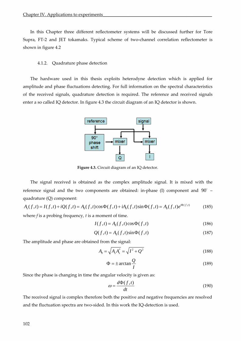
Chapter IV. Applications to experiments_________________________________________________
102
this Chapter three different reflectometer systems will be discussed further for Tore
Supra, FT‐2 and JET tokamaks. Typical scheme of two‐channel correlation reflectometer is
shown in figure 4.2
4.1.2. Quadrature phase detection
The hardware used in this thesis exploits heterodyne detection which is applied for
amplitude and phase fluctuations detecting. For full information on the spectral characteristics
of the received signals, quadrature detection is required. The reference and received signals
enter a so called IQ detector. In figure 4.3 the circuit diagram of an IQ detector is shown.
In
Figure 4.3. Circuit diagram of an IQ detector.
The signal received is obtained as the complex amplitude signal. It is mixed with the
reference signal and the two components are obtained: in‐phase (I) component and –
quadrature (Q) component:
(185)
where f is a probing frequency, t is a moment of time.
90
( , )0 0 0( , ) ( , ) ( , ) ( , )cos ( , ) ( , )sin ( , ) ( , ) i f t
sA f t I f t iQ f t A f t f t iA f t f t A f t e
0( , ) ( , )cos ( , )I f t A f t f t (186)
0( , ) ( , )sin ( , )Q f t A f t f t (187)
The amplitude and phase are obtained from the signal:
* 20 s s
2A A A I Q (188)
arctanQ
I (189)
Since the phase is changing in time the angular velocity is given as:
( , )d f t
dt (190)
The received signal is complex therefore both the positive and negative frequencies are resolved
and the fluctuation spectra are two‐sided. In this work the IQ‐detection is used.
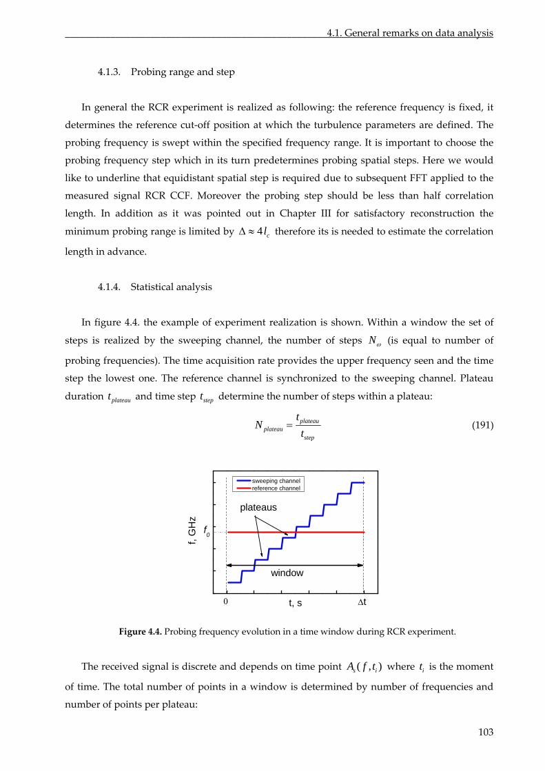
____________________________________________________4.1. General remarks on data analysis
4.1.3. Probing range and step
out in Chapter III for satisfactory reconstruction the
minimum probing range is limited by
In general the RCR experiment is realized as following: the reference frequency is fixed, it
determines the reference cut‐off position at which the turbulence parameters are defined. The
probing frequency is swept within the specified frequency range. It is important to choose the
probing frequency step which in its turn predetermines probing spatial steps. Here we would
like to underline that equidistant spatial step is required due to subsequent FFT applied to the
measured signal RCR CCF. Moreover the probing step should be less than half correlation
length. In addition as it was pointed
4 cl therefore its is needed to estimate the correlation
length in advance.
4.1.4. Statistical analysis
In figure 4.4. the example of experiment realization is shown. Within a window the set of
steps is realized by the sweeping channel, the number of steps N (is equal to number of
probing frequencies). The time acquisition rate provides the upper frequency seen and the time
step the lowest one. The reference channel is synchronized to the eeping channel. Plateau
duration and time step
sw
plateaut stept determine the number of steps a plateau:
within
plateauplateau
step
tN
t (191)
f0
t
plateaus
window
GH
z
f,
t, s
sweeping channel reference channel
Figure 4.4. Probing frequency evolution in a time window during RCR experiment.
The received signal is discrete and depends on time point ( , )s iA f t where is the moment
of time. The total number of points in a window is determined by number of frequencies and
number
it
of points per plateau:
103
Chapter IV. Applications to experiments_________________________________________________
window plateauN N N (192)
To analyze turbulence frequencies presenting in a signal we should transform the signal using
FFT into turbulence frequency space. It is evident that the number of points in plateau is formed
by of samples of averaging sN and number of turbulence frequencies
N
N :number
plateau sN N (193)
The summation is carried out over sN , this determines statistical averaging. The resolution in
turbulence frequency space is given by N . The number of points in a plateau is determined by
technical settings of experiment however it is limited by plasma conditions. When probing we
assume that the plasma is “frozen”. Thus, the total window duration should be less than plasma
correlation time. Therefore, the total of points in a window is limited and we should
balance between increasing
number
sN , N or N :
Nwindow sN N N (194)
In other words, N is dictated by probing range and step limits, N should correspond the
required turbul frequency resolution, ence sN should be enough satisfactory statistical
averaging. Finally, having fixed the parameters, we obtain the RCR CCF depending on
probing frequency cut‐off) difference
for
signal
(or f for each turbulence separately.
All these parameters ar etry system.
4.2. Results of RCR experiment at Tore Supra
Experiments on Tore Supra were the first attempt to apply the theoretical tho
turbulence properties determination at real machine.
. In this section we discuss experimental
results obtained during the campaigns on the 24th of November 2010 and on the 23rd of
201 . The aim of experiments is to determine plasma turbulence characteristics using the
ra.
4.2.1. Reflectometers at Tore Supra
iven in table 4.1. For more
detailed information the reader is referred to [34].
g range
frequency
e determined individually for each reflectom
me d of
Tore Supra machine was described in section 1.3.1.1
June
1 fast‐
sweeping correlation reflectometer installed on Tore Sup
A list of the reflectometer systems installed at Tore Supra is g
Table 4.1. List of reflectometers installed at Tore Supra
Reflectometer type Year Probin
O‐mode 1995 [121] 26‐36 GHz
104
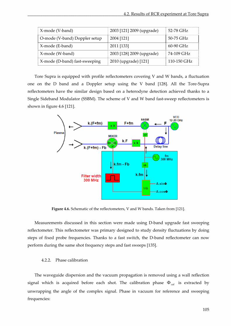
_____________________________________________4.2. Results of RCR experiment at Tore Supra
2003 [121] 2009 (upgrade) 52‐78 GHz X‐mode (V‐band)
O‐mode (V‐band) Doppler setup 2004 [121] 50‐75 GHz
X‐mode (E‐band) 2011 [133] 60‐90 GHz
X‐mode (W‐band) 2003 [128] 2009 (upgrade) 74‐109 GHz
X‐mode (D‐band) fast‐sweeping 2010 (upgrade) [121] 110‐150 GHz
Tore Supra is equipped with profile reflectometers covering V and W bands, a fluctuation
one on the D band and a Doppler setup using the V band [128]. All the Tore‐Supra
reflectometers have the similar design based on a heterodyne detection achieved thanks to a
Single Sideband Modulator (SSBM). Th me of V and W band fast‐sweep reflectometers is
shown in figure 4.6
e sche
[121].
Figure 4.6. Schematic of the reflectometers, V and W bands. Taken from [121].
Measurements discussed in this section were made using D‐band upgrade fast sweeping
reflectometer. This reflectometer was primary designed to study density fluctuations by doing
steps of fixed probe frequencies. Thanks to a fast switch, the D‐band reflectometer can now
perform during the same shot frequency steps and fast sweeps [135].
4.2.2. Phase calibration
he waveguide dispersion and the vacuum propagation is removed using a wall reflection
sign n phas is
T
al which is acquired before each shot. The calibratio e cal extracted by
unwrapping the angle of the complex signal. Phase in vacuum for reference and sweeping
frequencies:
105
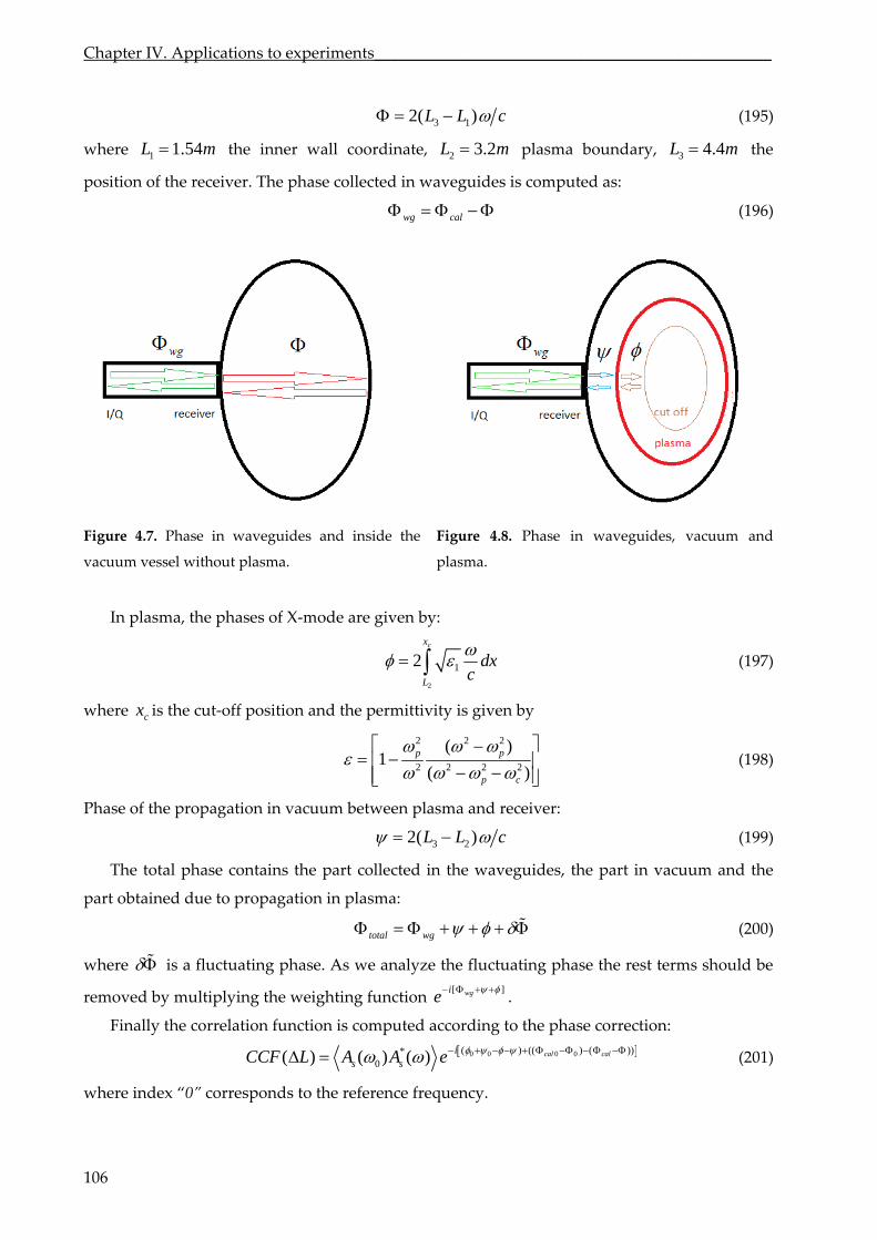
Chapter IV. Applications to experiments_________________________________________________
106
3 12( )L L c (195)
where 1 1.54L m the inner wall coordinate, 2 3.2L m plasma boundary, 3 4.4L m the
position of the receiver. The phase collected in waveguides is computed as:
wg cal (196)
Figure 4.7. Phase in waveguides and inside the
vacuum vessel without plasma.
Figure 4.8. Phase in waveguides, vacuum and
plasma.
In plasma, the phases of X‐mode are given by:
2
12L
dxc
cx (197)
here cxw is the cut‐off position and the permittivity is given by
2 2 2
2 2
( )1
(p p
2 2 )p c
(198)
Phase of the propagation in vacuum between plasma and receiver:
3 22( )L L c
The total phase contains the part collected in the waveguides,
(199)
the part in vacuum and the
obtained due to propagation in plasma: part
wg total (200)
here w is a fluctuating phase. As we analyze the fluctuating phase the rest terms should be
removed by multiplying the weighting function [ ]wgie
.
Finally the correlation function is computed according to the phase correction:
0 0 0 0( ) (( ) ( ))*0( ) ( ) ( ) cal cali
s sCCF L A A e (201)
where index “0” corresponds to the reference frequency.
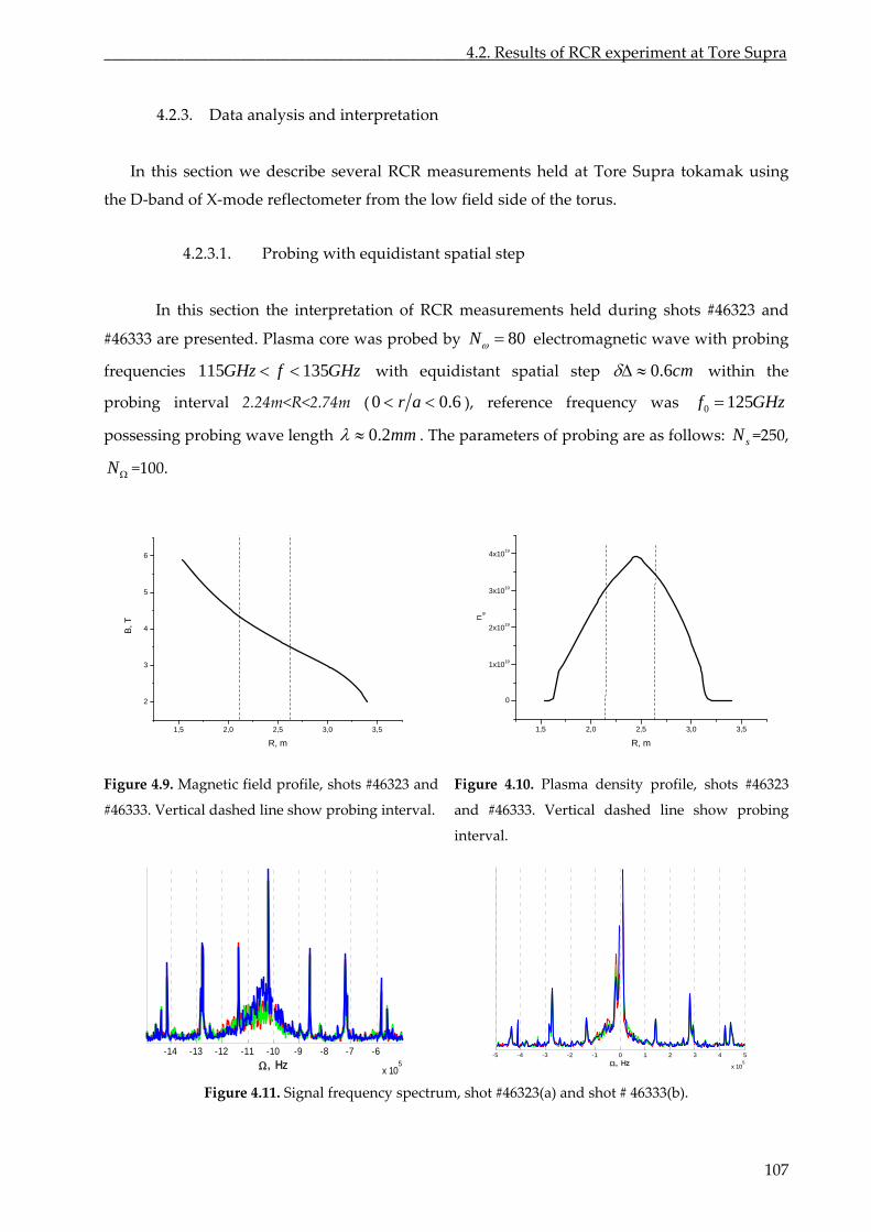
_____________________________________________4.2. Results of RCR experiment at Tore Supra
4.2.3. Data analysis and interpreta
In scribe several RC ents held at Tore ak using
the D‐ lectometer from th s.
4.2.3.1. Probing with equidistant spatial step
tion
this section we de R measurem Supra tokam
band of X‐mode ref e low field side of the toru
In this section the interpretation of RCR measurements held during shots #46323 and
#46333 are presented. Plasma core was probed by 80N electromagnetic wave with probing
frequencies 115 135GHz f GHz with equidistant spatial step 0.6cm within the
probing interval 2.24m<R<2.74m (0 0.6r a frequency), reference was 0 125f GHz
possessing probing wave length 0.2mm . The of probinparameters g are as follows: sN =250,
N =100.
1,5 2,0 2,5 3,0 3,5
2
3
4
5
6
B, T
R, m
1,5 2,0 2,5 3,0 3,5
0
1x10¹⁹
2x10¹⁹
3x10¹⁹
4x10¹⁹
n e
R, m
Figure 4.9. M
#46333. Vertical dashed line show probing interval.
ots #46323
and #46333. Vertical dashed line show probing
agnetic field profile, shots #46323 and Figure 4.10. Plasma density profile, sh
interval.
-14 -13 -12 -11 -10 -9 -8 -7 -6
x 105, Hz
-5 -4 -3 -2 -1 0 1 2 3 4 5
x 105, H
Figure 4.11. Signal frequency spectrum, shot #46323(a) and shot # 46333(b).
z
107
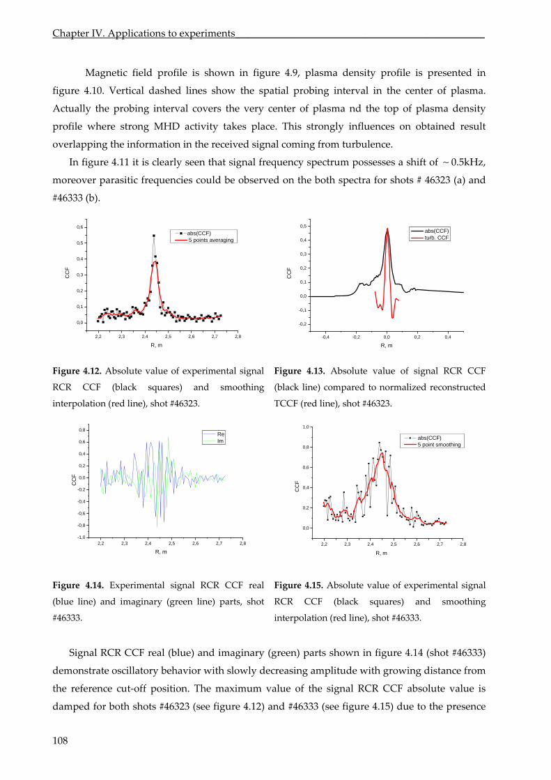
Chapter IV. Applications to experiments_________________________________________________
M ed in agnetic field profile is shown in figure 4.9, plasma density profile is present
Vertical tial probin ter of pla
of plasma density
profile strong MHD activity takes place. This strongly influences on obtained r
overlapping the information in the received signal coming from turbulence.
In figure 4.11 it is clearly seen that signal frequency spectrum possesses a shift of 0.5kHz,
moreover parasitic frequencies could be observed on the both spectra for shots # 46323 (a) and
#46333 (b).
figure 4.10. dashed lines show the spa g interval in the cen sma.
Actually the probing interval covers the very center of plasma nd the top
where esult
2,2 2,3 2,4 2,5 2,6 2,7 2,8
0,0
0,1
0,2
0,3
0,4
0,5
0,6
CC
F
R, m
abs(CCF) 5 points averaging
-0,4 -0,2 0,0 0,2 0,4
-0,2
-0,1
0,0
0,1
0,2
0,3
0,4
0,5 abs(CCF) turb. CCF
CC
F
R, m
Figure 4.12. Absolute value of experimental signal
RCR
interpolation (red line), shot #46323.
Figure 4.13. Absolute value of signal RCR CCF
lack line) compared to normalized reconstructed
TCCF (red line), shot #46323.
CCF (black squares) and smoothing (b
2,2 2,3 2,4 2,5 2,6 2,7 2,8-1,0
-0,8
-0,6
-0,4
-0,2
0,
0,2
4
0,8
0
0,
0,6
0,4
0,6
1,0
CC
F
R, m
Re Im
2,2 2,3 2,4 2,5 2,6 2,7 2,8
0,0
0,2
0,8
abs(CCF)
CC
F
R, m
5 point smoothing
Figure .14. Experimental signal RCR CCF real
#46333.
Figure 4.15. Absolute value of experimental
interpolation (red line), shot #46333.
(shot #46333)
demonstrate oscillatory behavior with slowly decreasing amplitude with growing distance
signal RCR CCF absolute value is
amped for both shots #46323 (see figure 4.12) and #46333 (see figure 4.15) due to the presence
4 signal
(blue line) and imaginary (green line) parts, shot RCR CCF (black squares) and smoothing
Signal RCR CCF real (blue) and imaginary (green) parts shown in figure 4.14
from
the reference cut‐off position. The maximum value of the
d
108
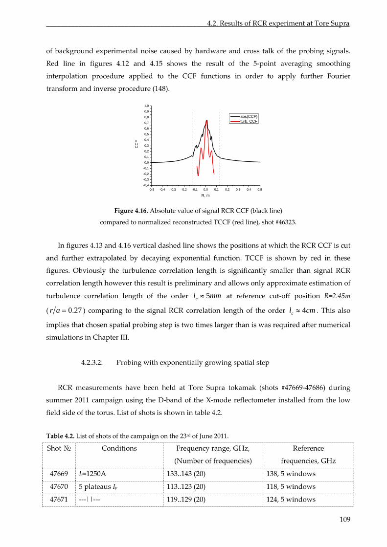
_____________________________________________4.2. Results of RCR experiment at Tore Supra
of background experimental noise caused by hardware and cross talk of the probing signals.
ed line in figures 4.12 and 4.15 shows the result of the 5‐point averaging smoothing
inte
R
rpolation procedure applied to the CCF functions in order to apply further Fourier
transform and inverse procedure (148).
0,8
0,9
1,0
-0 -0,1 0,0 0,1 0,2 0,3 0,4 0,5,5 -0,4 -0,3 -0,2-0,4
-0,3
-0,2
0,2
0,3
0,4
0,5
-0,1
0,0
0,1
0,6
0,7
CC
F
R, m
abs(CCF) turb. CCF
Figure 4.16. Absolute value of signal RCR CCF (black line)
compared to normalized reconstructed TCCF (red line), shot #46323.
In figures 4.13 and 4.16 vertical dashed line shows the positions at which the RCR CCF is cut
and further extrapolated by decaying exponential function. TCCF is shown by red in these
figures. Obviously the turbulence correlation length is significantly smaller than signal RCR
correlation length however this result is preliminary and allows only approximate estimation of
turbulence correlation length of the order m5cl m at reference cut‐off position R=2.45m
( 0.27r a ) comparing to the signal RCR length of the order m This also
implies that chosen spatial probing step is two times larger than is was required after numerical
simulations in Chapter III.
ly
RCR measurements have been held at Tore Supra tokamak (shots #47669‐47686) during
summer 2011 campaign using the D‐band of the X‐mode reflectometer installed from the low
field side of the torus. List of shots is shown in table 4.2.
Table 4.2. List of shots of the campaign on the 23rd of June 2011.
Shot № Conditions Frequency range, GHz,
(Number of frequencies)
Reference
frequencies, GHz
correlation 4cl c .
4.2.3.2. Probing with exponential growing spatial step
47669 It=1250A 133..143 138, 5 windows (20)
47670 5 p s lateaus Ip 113..123 (20) 118, 5 window
47671 ‐‐‐||‐‐‐ 119..129 (20) 124, 5 windows
109
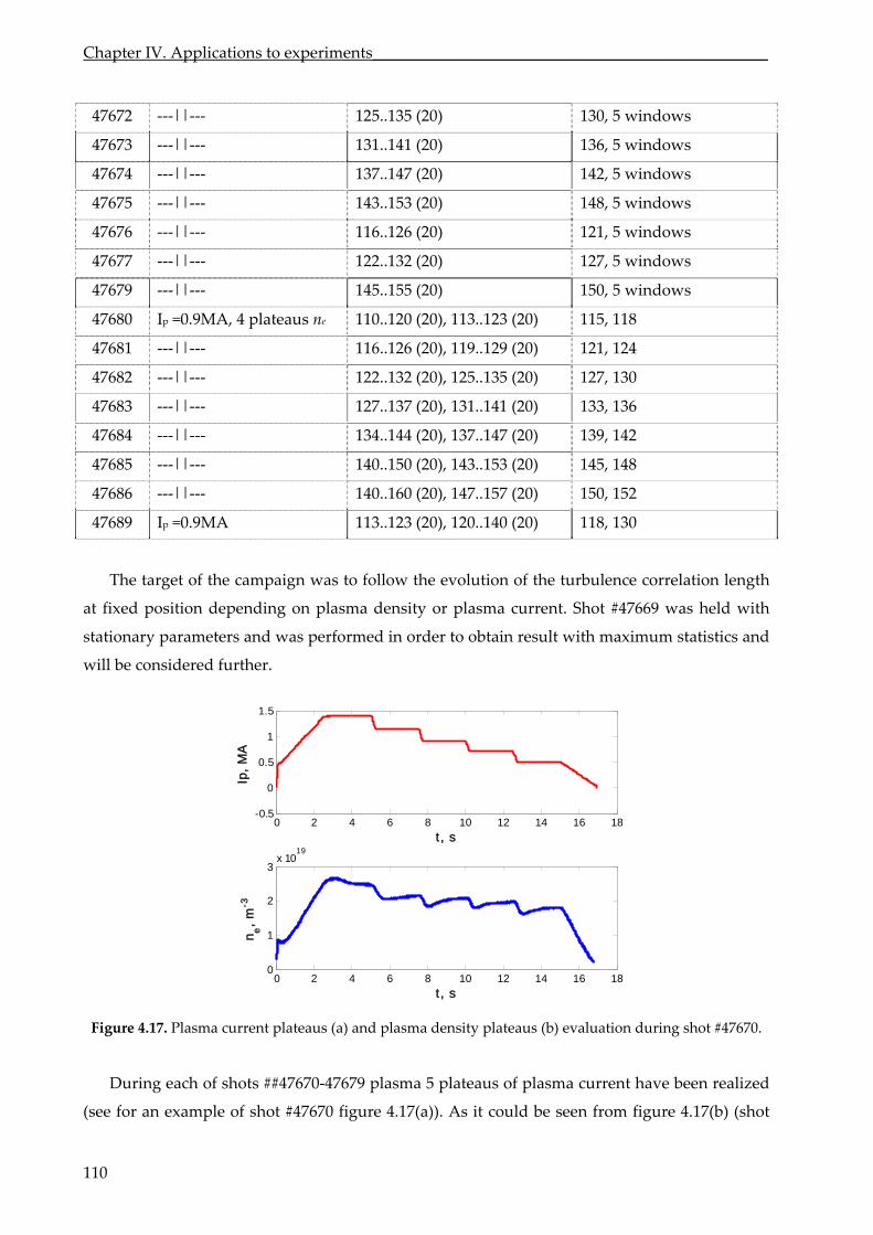
Chapter IV. Applications to experiments_________________________________________________
47672 ‐‐‐||‐‐‐ 125..135 (20) 130, 5 windows
47673 ‐‐‐||‐‐‐ 131..141 (20) 136, 5 windows
47674 ‐‐‐||‐‐‐ 137..147 (20) 142, 5 windows
47675 ‐‐‐||‐‐‐ 143..153 (20) 148, 5 windows
47676 ‐‐‐||‐‐‐ 116..126 (20) 121, 5 windows
47677 ‐‐‐||‐‐‐ 122..132 (20) 127, 5 windows
47679 ‐‐‐||‐‐‐ 145..155 (20) 150, 5 windows
47680 Ip =0.9MA, 4 plateaus ne 110..120 (20), 113..123 (20) 115, 118
47681 ‐‐‐||‐‐‐ 116..126 (20), 119..129 (20) 121, 124
47682 ‐‐‐||‐‐‐ 122..132 (20), 125..135 (20) 127, 130
47683 ‐‐‐||‐‐‐ 127..137 (20), 131..141 (20) 133, 136
47684 ‐‐‐||‐‐‐ 134..144 (20), 137..147 (20) 139, 142
47685 ‐‐‐||‐‐‐ 140..150 (20), 143..153 (20) 145, 148
47686 ‐‐‐||‐‐‐ 140..160 (20), 147..157 (20) 150, 152
47689 Ip =0.9MA 113..123 (20), 120..140 (20) 118, 130
e
i n s
rformed in ord imum statistics and
will be considered further.
The target of the campaign was to follow th
at fixed pos tion depending o pla ma density
stationary parameters and was pe
evolution of the turbulence correlation length
or plasma current. Shot #47669 was held with
er to obtain result with max
0 2 4 6 8 10 12 14 16 18-0.5
0
0.5
1
1.5
t, s
Ip, M
A
0 2 4 6 8 10 12 14 16 18
3x 10
19
0
1
2
t, s
-3n e, m
Figure 4.17. Plasma current plateaus (a) and plasma density plateaus (b) evaluation during shot #47670.
During each of shots ##47670‐47679 plasma 5 plateaus of plasma current have been realized
(see for an example of shot #47670 figure 4.17(a)). As it could be seen from figure 4.17(b) (shot
110
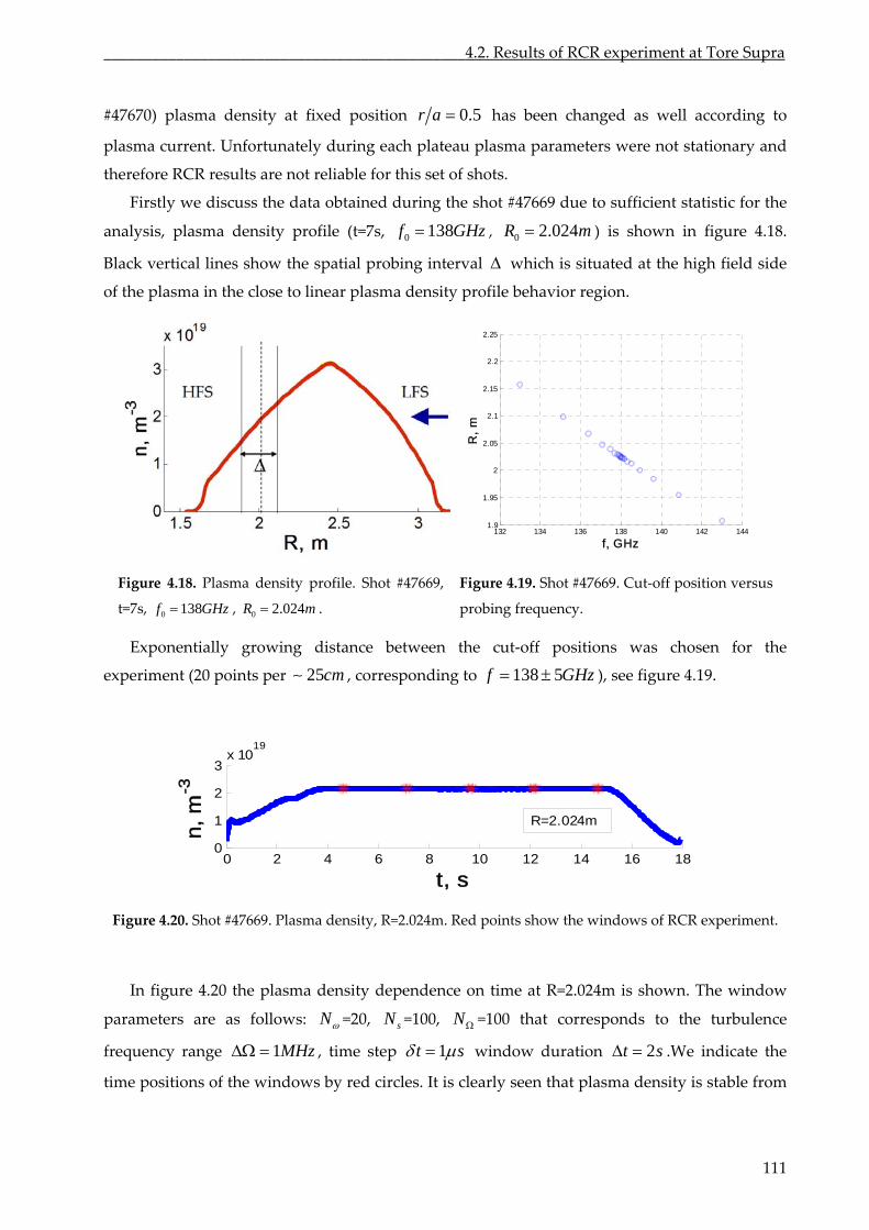
_____________________________________________4.2. Results of RCR experiment at Tore Supra
#47670) plasma density at fixed position 0.5r a has been changed as well according to
plasma current. Unfortunately during each plateau plasma parameters were not stationary and
therefore RCR results are not reliable for this set of shots.
Firstly we discuss the data obtained during the shot #47669 due to sufficient statistic for the
analysis, plasma density profile (t=7s, 0 138f GHz , 0 2.024R m ) is shown in figure 4.18.
Black vertical lines show the spatial probing interval which is situated at the high field side
of the plasma in the close to linear plasma density profile behavior region.
132 134 136 138 140 142 1441.9
2.25
2.2
2.15
2.1
2.05
2
1.95
f, GHz
R, m
Figure 4.18. Plasma density profile. Shot #47669,
t=7s, 0 138f GHz , 0 2.024R m .
Figure 4.19. Shot #47669. Cut‐off position versus
probing frequency.
Exponentially growing distance between the cut‐off positions was chosen for the
experiment (20 points per 25cm , corresponding 138 5 to f GHz ), see figure 4.19.
0 2 4 6 8 10 12 14 16 180
1
2
3x 10
19
n,-3
m R=2.024m
t, s
Figure 4.20. Shot #47669. Plasma density, R=2.024m. Red points show the windows of RCR experiment.
at R=2.024m is shown. The window
rs are
In figure 4.20 the plasma density dependence on time
paramete as follows: N =20, sN =100, N =100 that corresponds ulence
frequency range
to the turb
1MHz , time step 1t s window duration 2t s .We indicate the
t it ndows by red early seen that pla able from ime pos ions of the wi circles. It is cl sma density is st
111
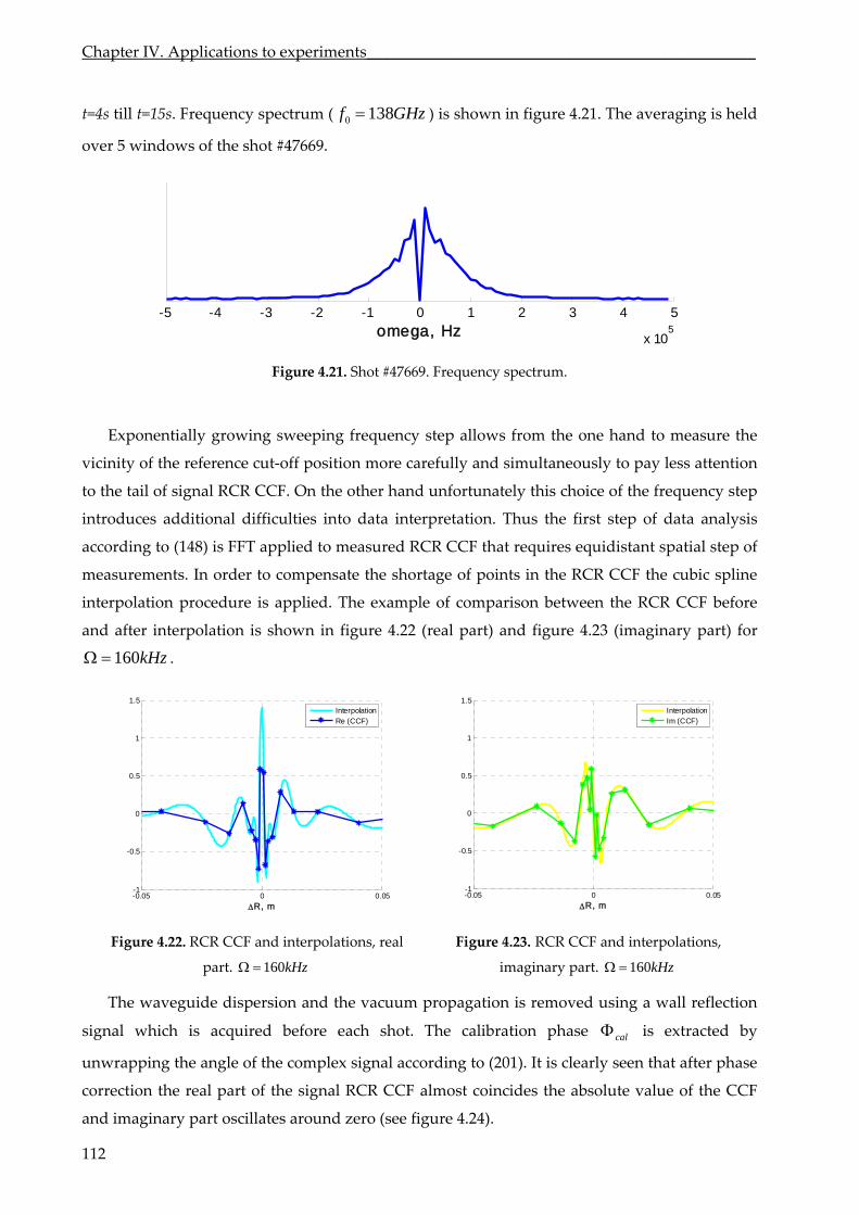
Chapter IV. Applications to experiments_________________________________________________
t t=1 uency spectrum =4s till 5s. Freq ( 0 138f GHz ) is shown in figure ng is held
o in the shot #47669.
4.21. The averagi
ver 5 w dows of
-5 -4 -3 -2 -1 0 1 2 3 4 5
x 105omega, Hz
Figure 4.21.
n growing sweeping the d to measure the
v of rence cut‐off positio ltane pay less attention
t il l RCR CCF. On the is c e frequency step
introduces difficulties into the of data analysis
according to (148) is FFT applied to measured RCR CCF that requires equidistant spatial step of
me
Shot #47669. Frequency spectrum.
Expo entially frequency step allows from one han
icinity the refe n more carefully and simu ously to
o the ta of signa other hand unfortunately th hoice of th
additional data interpretation. Thus first step
asurements. In order to compensate the shortage of points in the RCR CCF the cubic spline
interpolation procedure is applied. The example of comparison between the RCR CCF before
and after interpolation is shown in figure 4.22 (real part) and figure 4.23 (imaginary part) for
160kHz .
-0.05 0 0.05-1
-0.5
0
0.5
1
1.5
R, m
InterpolationRe (CCF)
-0.05 0 0.05-1
-0.5
0
0.5
1
1.5
R, m
InterpolationIm (CCF)
Figure 4.22. RCR CCF and interpolations, real
part.
Figure 4.23. RCR CCF and interpolations,
imaginary part. 160kHz 160kHz
The waveguide dispersion and the vacuum propagation is removed using a wall reflection
signal which is acquired before each shot. The calibration phase cal is extracted by
unw
and imaginary part oscillates around zero (see figure 4.24).
rapping the angle of the complex signal according to (201). It is clearly seen that after phase
correction the real part of the signal RCR CCF almost coincides the absolute value of the CCF
112
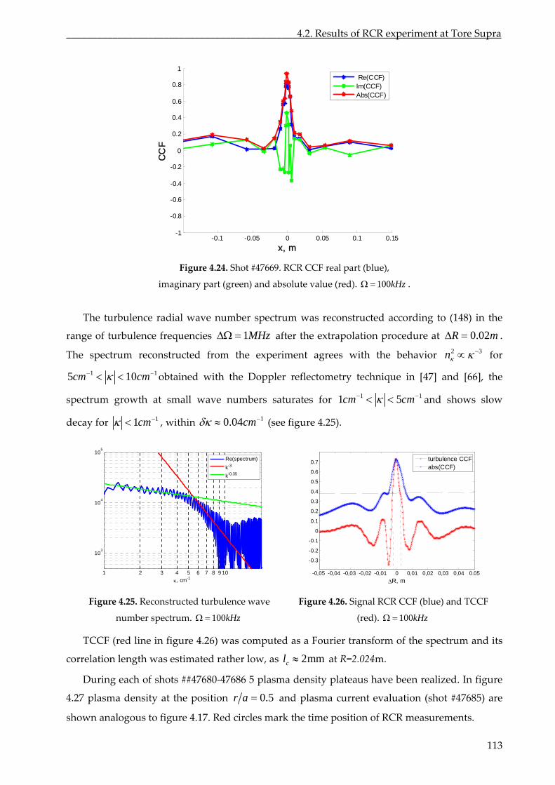
_____________________________________________4.2. Results of RCR experiment at Tore Supra
Figure 4.24. Shot #47669. RCR CCF real part (blue),
imaginary part (green) and absolute value (red). 100kHz .
The turbulence radial wave number spectrum was reconstructed according to (148) in the
range of turbulence frequencies 1MHz after the extrapolation procedure at 0.02R m .
2 3n
The spectrum reconstructed experiment agrees with the behavior from the for
1 110cm cm obtained with the Doppler 5
spectrum growth at small wave saturates for
reflectometry technique in [47] and [66], the
numbers 1 11 5cm cm and shows slow
decay for 11cm , within 10.04cm (see figure 4.25).
1 2 3 4 5 6 7 8 9 10
103
104
105
, cm-1
Re(spectrum)k-3
k-0.35
-0,05 -0,04 -0,03 -0,02 -0,01 0 0,01 0,02 0,03 0,04 0.05
-0.3
-0.2
-0.1
0
0.1
0.2
0.3
0.4
0.5
0.6
0.7
R, m
turbulence CCFabs(CCF)
Figure 4.25. Reconstructed turbulence wave
number spectrum.
Figure 4.26. Signal RCR CCF (blue) and TCCF
(red). 100kHz 100kHz
TCCF (red line in figure 4.26) was computed as a Fourier transform of the spectrum and its
correlation length was estimated rather low, as 2mmcl at R=2.024m.
During each of shots ##47680‐47686 5 plasma density plateaus have been realized. In figure
4.27 plasma density at the position 0.5r a and plasma current evaluation (shot #47685) are
shown analogous to figure 4.17. Red circles mark the time position of RCR measurements.
-0.1 -0.05 0 0.05 0.1 0.15-1
-0.8
-0.6
-0.4
-0.2
0
0.2
0.4
0.6
0.8
1 Re(CCF)Im(CCF)Abs(CCF)
CC
F
x, m
113
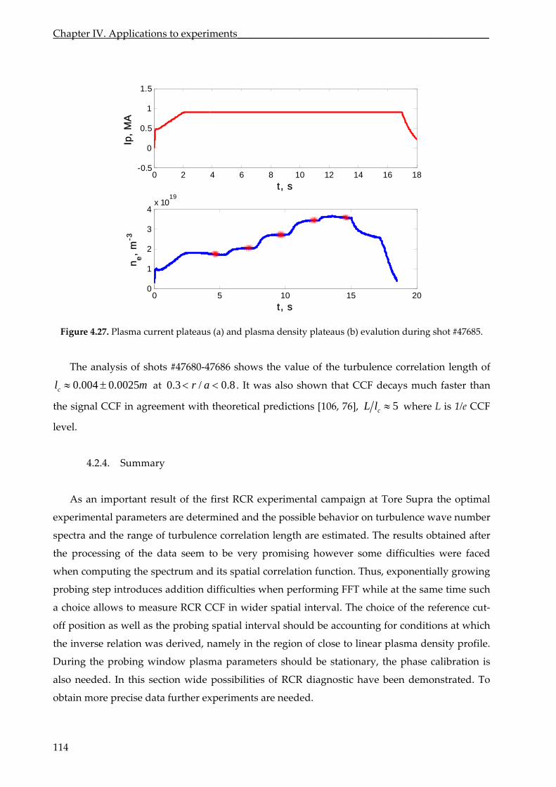
Chapter IV. Applications to experiments_________________________________________________
0 2 4 6 8 10 12 14 16 18-0.5
0
0.5
1
1.5
t, s
Ip, M
A
0 5 10 15 200
4x 10
19
3
2
1
t, s
n e, m-3
Figure 4.27. Plasma current plateaus (a) and plasma density plateaus (b) evalution during shot #47685.
The analysis of shots #47680‐47686 shows the value of the turbulence correlation length of
0.004 0.0025cl m at 0.3 / 0.8r a . It was also shown that CCF decays much faster than
the signal CCF in agreement with theoretical predictions [106, 76], 5cL l where L is 1/e CCF
level.
4.2.4. Summary
As an important result of the first RCR experimental campaign at Tore Supra the optimal
experimental parameters are determined and the possible behavior on turbulence wave number
spectra and the range of turbulence correlation length are estimated. The results obtained after
the processing of the data seem to be very promising however some difficulties were faced
when computing the spectrum and its spatial correlation function. Thus, exponentially growing
probing step introduces addition difficulties when performing FFT while at the same time such
a ch spati cut‐
off position as w the probing spatial interval should b r conditio s at which
the
p
oice allows to measure RCR CCF in wider
ell as
al interval. The choice of the reference
e accounting fo n
inverse relation was derived, namely in the region of close to linear plasma density profile.
During the probing window plasma parameters should be stationary, the hase calibration is
also needed. In this section wide possibilities of RCR diagnostic have been demonstrated. To
obtain more precise data further experiments are needed.
114
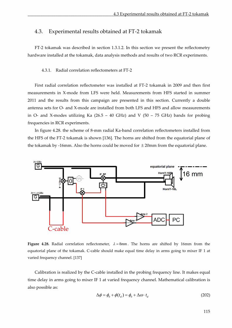
________________________________________4.3 Experimental results obtained at FT‐2 tokamak
4.3. Experimental results obtained at FT‐2 tokamak
FT‐2 tokamak was described in section 1.3.1.2. In this section we present the reflectometry
hardware installed at the tokamak, data analysis methods and results of two RCR experiments.
4.3.1. Radial correlation reflectometers at FT‐2
First radial correlation reflectometer was installed at FT‐2 tokamak in 2009 and then first
measurements in X‐mode from LFS were held. Measurements from HFS started in summer
2011 and the results from this campaign are presented in this section. Currently a double
antenna sets for O‐ and X‐mode are installed from both LFS and HFS and allow measurements
in O‐ and X‐modes uti z) bands for probing
frequencies in RCR experiments.
hown [136]. rial plane o
‐
lizing Ka (26.5 – 40 GHz) and V (50 – 75 GH
In figure 4.28. the scheme of 8‐mm radial Ka‐band correlation reflectometers installed from
the HFS of the FT‐2 tokamak is s The horns are shifted from the equato f
the tokamak by 16mm. Also the horns could be moved for 20mm plane.
Figure 4.28. Radial correlation reflectometer,
from the equatorial
C‐cable
8mm . The horns are shifted by 16mm from the
equa make at
varied frequ
in the line. It makes equal
frequency atical calibration is
also
torial plane of the tokamak. C‐cable should
ency channel. [137]
equal time delay in arms going to mixer IF 1
Calibration is realized by the C‐cable installed probing frequency
time delay in arms going to mixer IF 1 at varied channel. Mathem
possible as:
0 0( )d dt t (202)
115
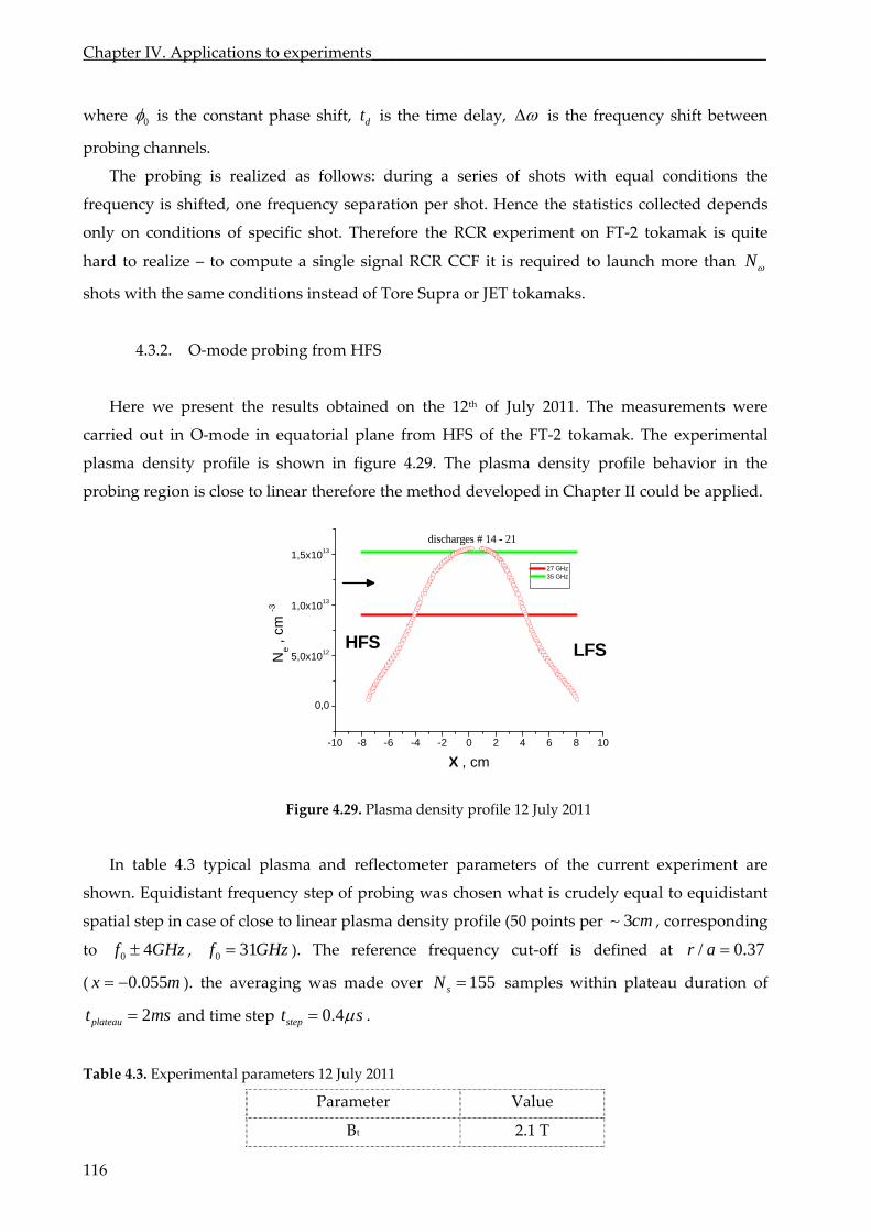
Chapter IV. Applications to experiments_________________________________________________
116
where 0 is the constant phase shift, is the time delay, dt is the frequency shift between
probing channels.
The probing is realized as follows: during a series of shots with equal conditions the
frequency is shifted, one frequency separation per shot. Hence the statistics collected depends
only on conditions of specific shot. Therefore the RCR experiment on FT‐2 tokamak is quite
hard to realize – to compute a single signal RCR CCF it is required to launch more than N
shots with the same conditions instead of Tore Supra or JET tokamaks.
4.3.2. O‐mode probing from HFS
Here we present the results obtained on the 12th of July 2011. The measurements were
carried out in O‐mode in equatorial plane from HFS of the FT‐2 tokamak. The experimental
plasma density profile is shown in figure 4.29. The plasma density profile behavior in the
probing region is close to linear therefore the method developed in Chapter II could be pplied. a
-10 -8 -6 -4 -2 0 2 4 6 8 10
0,0
5,0x10¹²
1,0x10¹³
1,5x10¹³
HFS , cm
LFS
discharges # 14 - 21
Ne
-3
X , cm
27 GHz 35 GHz
Figure 4.29. Plasma density profile 12 July 2011
In table 4.3 typical plasma and reflectometer parameters of the current experiment are
shown. Equidistant frequency step of probing was chosen what is crudely equal to equidistant
spatial step in case of close to linear plasma density profile (50 points per 3cm , corresponding
to 0 4f GHz , 0 31f GHz ). The reference frequency cut‐off is defined at / 0.37r a
( 0.055x m ). the averaging was made over 155sN samples within plateau duration of
2plateaut ms and time step 0.4stept s .
Table 4.3. Experimental parameters 12 July 2011
Parameter Value
Bt 2.1 T
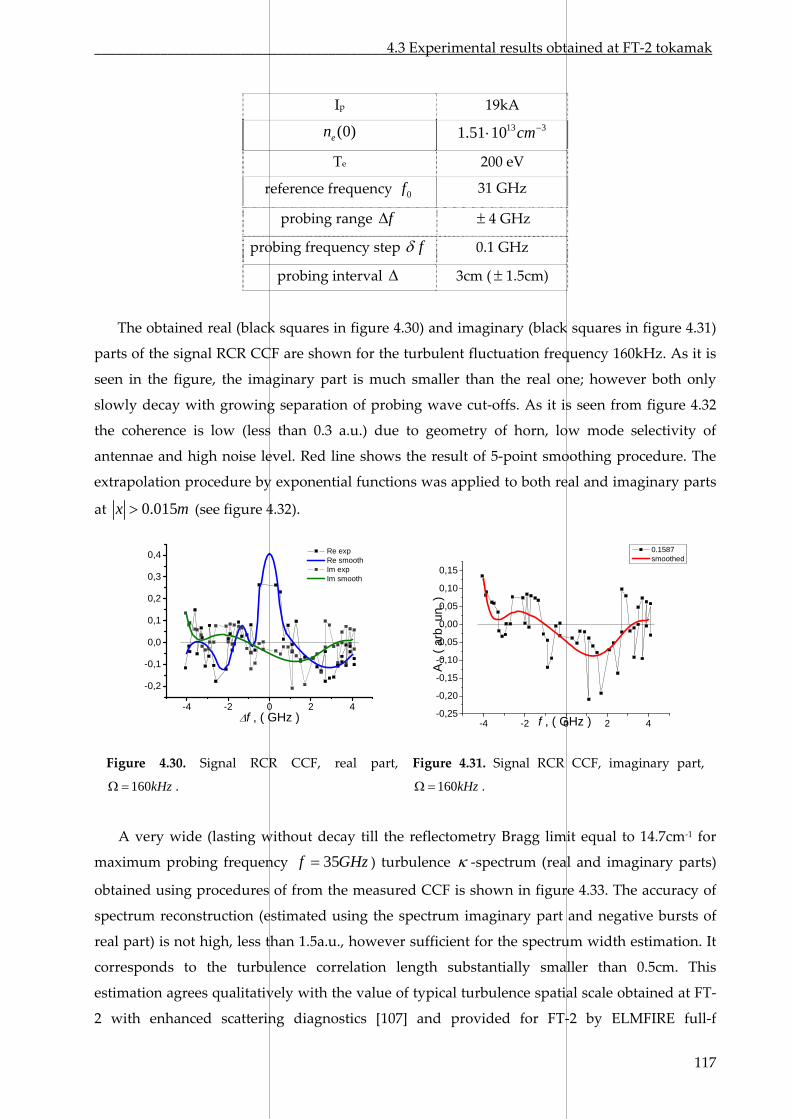
________________________________________4.3 Experimental results obtained at FT‐2 tokamak
Ip 19kA
(0)en 13 31.51 10 cm
Te 200 eV
reference frequency 0f 31 GHz
probing range f 4 GHz
probing frequency step f 0.1 GHz
probing interval 3cm ( 1.5cm)
The obtained real (black squares in figure 4.30) and imaginary (black squares in figure 4.31)
parts of the signal RCR CCF are for turbulent fluctuation frequency 160kHz. As it is
seen in the figure, the imaginary part is much smaller than the real one; however both only
slowly decay with growing separation of wave ‐offs. is seen from figure 4.32
the coherence is low (less than
shown the
probing cut As it
0.3 a.u.) due to geometry of horn, low mode selectivity of
antennae and high noise level. Red line shows the result of 5‐point smoothing procedure. The
extrapolation procedure by exponential functions was applied to both real and imaginary parts
at 0.015x m (see figure 4.32).
-4 -2 0 2 4
-0,2
-0,1
0,0
0,1
0,2
0,3
0,4 Re exp Re smooth Im exp Im smooth
f , ( GHz )
-4 -2 0 2 4-0,25
-0,20
-0,15
-0,10
-0,05
0,00
0,05
0,10
0,15
f , ( GHz )
A ,
( arb
. un.
)
0.1587 smoothed
Figure 4. RCR CCF, real part, Figure 4.31. Signal RCR CCF, imaginary part, 30. Signal
z . 160kH 160kHz .
the reflA very wide (lasting without decay till ectometry Bragg limit equal to 14.7cm‐1 for
maximum probing frequency 35f GHz ) turbulence ‐spectrum (real and imaginary parts)
obtained using procedures of from the measured CCF is shown in figure 4.33. The accuracy of
spectrum
real
qualitatively with the value of typical turbulence spatial scale obtained at FT‐
2 with enhanced scattering diagnostics [107] and provided for FT‐2 by ELMFIRE
reconstruction (estimated using the spectrum imaginary part and negative bursts of
part) is not high, less than 1.5a.u., however sufficient for the spectrum width estimation. It
corresponds to the turbulence correlation length substantially smaller than 0.5cm. This
estimation agrees
full‐f
117
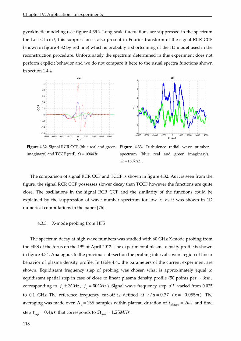
Chapter IV. Applications to experiments_________________________________________________
gyrokinetic modeling (see figure 4.39.) Long‐scale fluctuatio are suppressed in the spectrum
for | | < 1 cm‐1, th
. ns
is suppression is also present in Fourier transform of the signal RCR CCF
(shown in figure 4.32 by red line) which is probably a shortcoming of the 1D model used in the
reconstruction procedure. Unfortunately the spectrum determined in this experiment does not
perform explicit behavior and we do not compare it here to the usual spectra functions shown
in section 1.4.4.
-0.04 -0.03 -0.02 -0.01 0 0.01 0.02 0.03 0.04-0.6
-0.4
-0.2
0
0.2
0.4
0.6
0.8
1
CCF8
6
4
x, m
CC
F 2
-4000 -3000 -2000 -1000 0 1000 2000 3000 4000-4
-2
0
sp
sp
4.32. Signal RCR CCF (blue real and green
ary) and TCCF (red),
Figure 4.33. Turbulence radial wave number
spectrum (blue real and green imaginary),
k, m-1
Figure
imagin 160kHz .
160kHz .
comparison of signal RCR CCF and TCCF is shown in figure 4.32. As it is seen from the
figure, the signal RCR CCF possesses slower decay than TCCF however the functions are quite
close. The oscillations in the signal RCR CCF and the similarity of the functions could be
ex by the suppression of wave number spectrum for low
The
plained as it was shown in 1D
computations in the paper [76].
4.3.3. X‐mode prob
vers
r of plasma density e eriment are
own. Equid was cho
equidistant spatial of close to linear plasma density profile (50 points per
corresponding to
numerical
avio
ing from HFS
The spectrum decay at high wave numbers was studied with 60 GHz X‐mode probing from
the HFS of the torus on the 19th of April 2012. The experimental plasma density profile is shown
in figure 4.34. Analogous to the previous sub‐section the probing interval co region of linear
beh profile. In table 4.4., the parameters of th current exp
sh istant frequency step of probing sen what is approximately equal to
step in case 3cm ,
0 3f GHz , 0 60f GHz ). Signal wave frequency step f
.37
varied from
ff is defined at
0.025
/ 0r a ( 0.055x m ). The
s and time
2t m
to 0.1 GHz The reference frequency cut‐o
averaging was s within plateau
step
made over N 155 samples duration of plateau
0.4stept s that corresponds to max 1.25MHz .
118
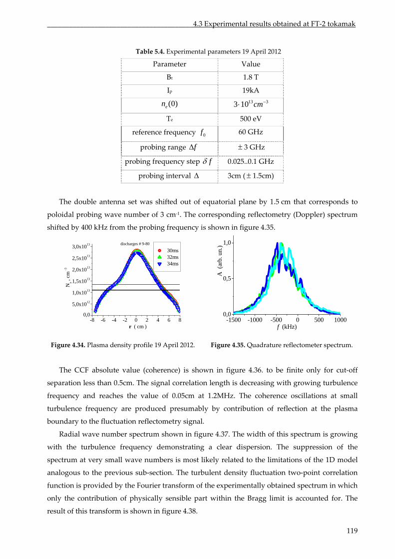
________________________________________4.3 Experimental results obtained at FT‐2 tokamak
Table 5.4. parameters l 2012
Parameter Value
Experimental 19 Apri
Bt 1.8 T
Ip 19kA
(0)en 13 33 10 cm
Te 500 eV
reference frequency 0f 60 GHz
probing range f 3 GHz
probing frequency step f 0.025..0.1 GHz
probing interval 3cm ( 1.5cm)
The double antenna set was shifted out of equatorial plane by 1.5 cm that corresponds to
poloidal probing wave number of 3 cm‐1. The corresponding reflectometry (Doppler) spectrum
shifted by 400 kHz from the probing frequency is shown in figure 4.35.
13 1,0
-8 -6 -4 -2 0 2 4 6 80,0
5,0x10¹²
1,0x10¹³
1,5x10¹³
2,0x10¹³
2,5x10¹³
3,0x10discharges # 9-80
Ne ,
cm -3
r ( cm )
30ms 32ms 34ms
-1500 -1000 -500 0 500 10000,0
0,5
A (
arb.
un.
)
f (kHz)
Figure 4.34. Plasma density profile 19 April 2012. Figure 4.35. Quadrature reflectometer spectrum.
The CCF absolute value (coherence) is in figure 4.36. to be finite only for cut‐ f
se n t n
frequency and reaches the value of 0.05cm at 1.2MHz. e coherence oscillations at small
turbulence frequency are produced presumably by contribution of reflection at the plasma
bou
um shown . T
shown of
paratio less han 0.5cm. The signal correlatio length is decreasing with growing turbulence
Th
ndary to the fluctuation reflectometry signal.
Radial wave number spectr in figure 4.37 he width of this spectrum is growing
with the turbulence frequency demonstrating a clear dispersion. The suppression of the
spectrum at very small wave numbers is most likely related to the limitations of the 1D model
analogous to the previous sub‐section. The turbulent density fluctuation two‐point correlation
function is provided by the Fourier transform of the experimentally obtained spectrum in which
only the contribution of physically sensible part within the Bragg limit is accounted for. The
result of this transform is shown in figure 4.38.
119
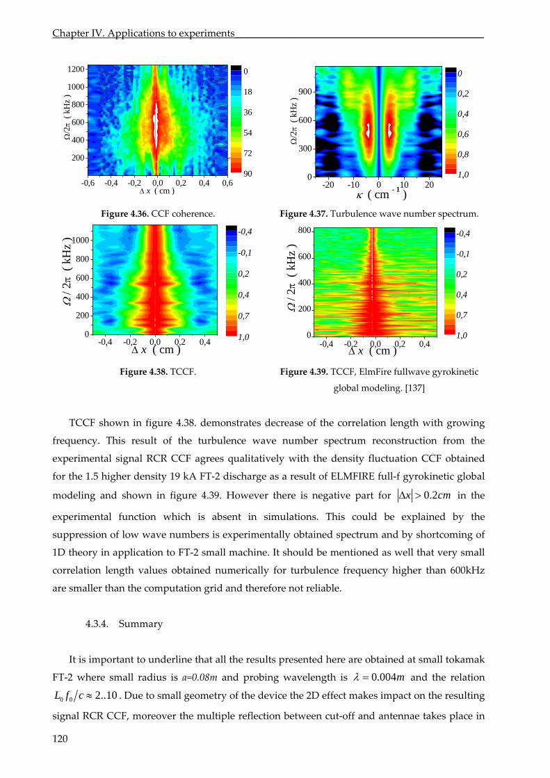
Chapter IV. Applications to experiments_________________________________________________
-0,6 -0,4 -0,2 0,0 0,2 0,4 0,6
200
400
600
800
10
1200
00
0
18
36
54/2
( k
Hz
)
-20 -10 0 10 200
300
600
900
/2
( k
Hz
)
( cm - 1 )
0
0,2
0,4
0,6
72
90
x ( cm )
0,8
1,0
Figure 4.36. CCF coherence. Figure 4.37. Turbulence wave number spectrum.
-0,4 -0,2 0,0 0,2 0,40
200
400
600
800
1000
x ( cm )
/
2 (
kH
z )
-0,4
-0,1
0,2
0,4
0,7
1,0-0,4 -0,2 0,0 0,2 0,4
200
400
600
800
0
/
2 (
kH
z )
x ( cm )
-0,4
-0,1
0,2
0,4
0,7
Figure 4.38. TCCF. Figure 4.3 TCCF, ElmFire fullwave gyrokinetic
global modeling. [137]
f
arge as a result of ELMFIRE full‐f gyrokinetic global
modeling and shown in figure 4.39. However there is negative part for
1,0
9.
TCCF shown in figure 4.38. demonstrates decrease of the correlation length with growing
frequency. This result of the turbulence wave number spectrum reconstruction from the
experimental signal RCR CCF agrees qualitatively with the density luctuation CCF obtained
for the 1.5 higher density 19 kA FT‐2 disch
0.2x cm in the
in simulations. This could be explained by the
suppression of low wave numbers is experimentally obtained spectrum and by shortcoming of
1D
to underline that all the
is
experimental function which is absent
theory in application to FT‐2 small machine. It should be mentioned as well that very small
correlation length values obtained numerically for turbulence frequency higher than 600kHz
are smaller than the computation grid and therefore not reliable.
4.3.4. Summary
It is important results presented here are obtained at small tokamak
FT‐2 where small radius is a=0.08m and probing wavelength 0.004m and the relation
0 0 2..10L f c . Due to sma try of the device the 2D effect makes im resulting
signa moreover the multip
ll geome t on the
l RCR CCF, le reflection between cut‐off and antennae takes place in
pac
120
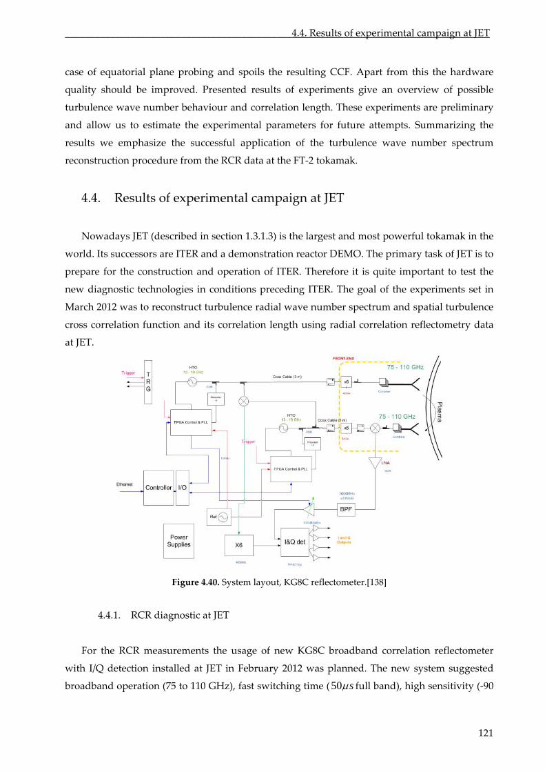
_____________________________________________4.4. Results of experimental campaign at JET
121
case of equatorial plane pr om this the hardware
quality should be improved. P ults of experim ive an overview of possible
turbulence wave number behaviour correlation length. experiments are preliminary
and allow us to estimate the experimental parameters for attempts. Summarizing the
results we emphasize the successful application of the turbulence wave number spectrum
reconstruction procedure from the R data at the FT‐2 tok
4.4. Results of exp m aign at JE
Nowadays JET (describe 3) the la n powerful tokamak in the
world. Its successors are ITER and a demonstration reactor DEMO. The primary task of JET is to
prepare
and spatial turbulence
cross correlation function and its correlation length using radial correlation reflectometry data
at JET.
obing and spoils the resulting CCF. Apart fr
resented res ents g
and These
future
CR amak.
erimental ca p T
d in section 1.3.1. is rgest a d most
for the construction and operation of ITER. Therefore it is quite important to test the
new diagnostic technologies in conditions preceding ITER. The goal of the experiments set in
March 2012 was to reconstruct turbulence radial wave number spectrum
Figure 4.40. System layout, KG8C reflectometer.[138]
4.4.1. RCR diagnostic at JET
For the RCR measurements the usage of new KG8C broadband correlation reflectometer
with I/Q detection installed at JET in February 2012 was planned. The new system suggested
broadband operation (75 to 110 GHz), fast switching time (50 s full band), high sensitivity (‐90
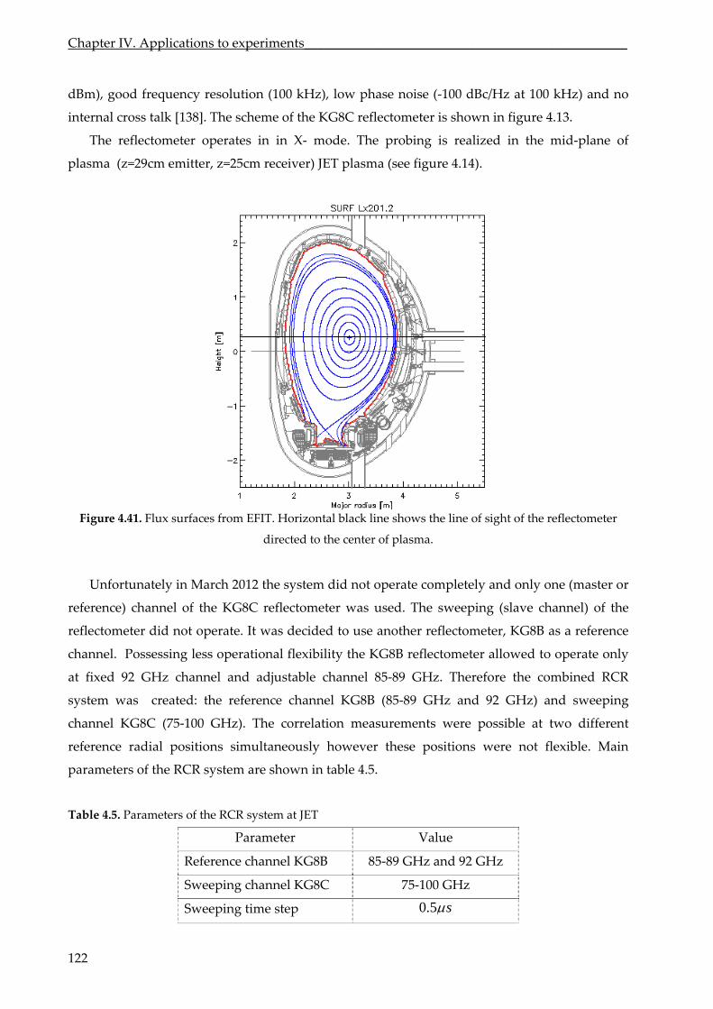
Chapter IV. Applications to experiments_________________________________________________
122
dBm), good frequency resolution (100 kHz), low phase noise (‐100 dBc/Hz at 100 kHz) and no
internal cross talk [138]. The scheme of the KG8C reflectometer is shown in figure 4.13.
The reflectometer operates in in X‐ mode. The probing is realized in the mid‐plane of
plasma (z=29cm emitter, z=25cm receiver) JET plasma (see figure 4.14).
Figure 4.41. Flux surfaces from EFIT. Horizontal black line shows the line of sight of the reflectometer
KG8B as a reference
channel. Possessing less operational flexibility the KG8B reflectometer allowed to operate only
RCR system at JET
Parameter Value
directed to the center of plasma.
Unfortunately in March 2012 the system did not operate completely and only one (master or
reference) channel of the KG8C reflectometer was used. The sweeping (slave channel) of the
reflectometer did not operate. It was decided to use another reflectometer,
at fixed 92 GHz channel and adjustable channel 85‐89 GHz. Therefore the combined RCR
system was created: the reference channel KG8B (85‐89 GHz and 92 GHz) and sweeping
channel KG8C (75‐100 GHz). The correlation measurements were possible at two different
reference radial positions simultaneously however these positions were not flexible. Main
parameters of the RCR system are shown in table 4.5.
Table 4.5. Parameters of the
Reference channel KG8B 85‐89 GHz and 92 GHz
Sweeping channel KG8C 75‐100 GHz
Sweeping time step 0.5 s
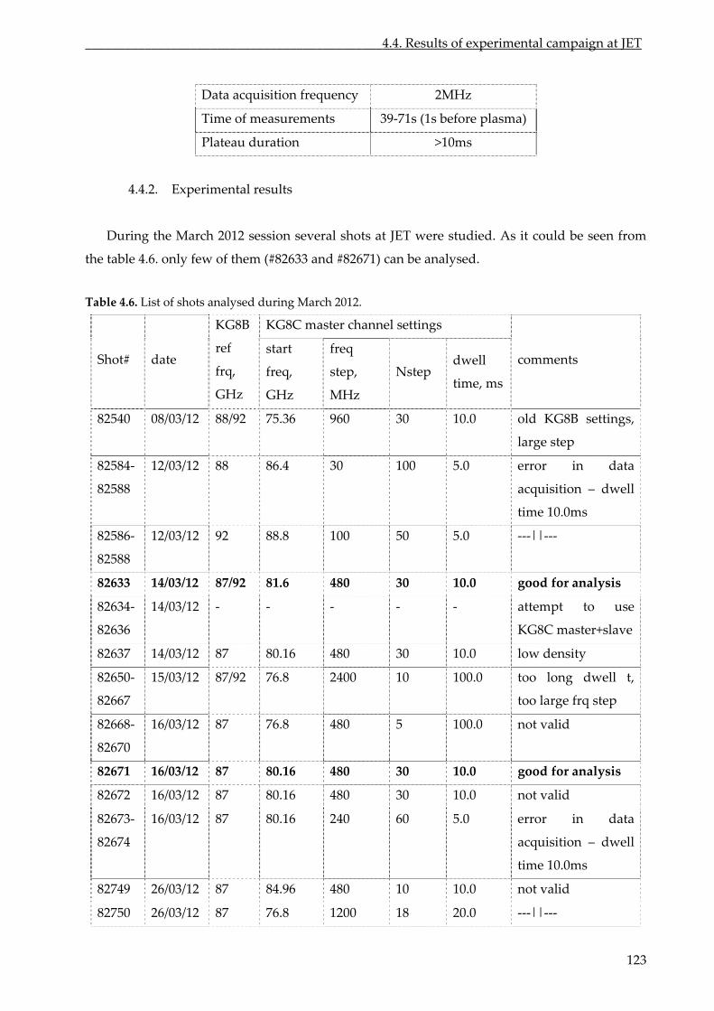
_____________________________________________4.4. Results of experimental campaign at JET
Data acquisition frequency 2MHz
Time of measurements 39‐71s (1s before plasma)
Plateau duration >10ms
4.4.2. Experimental results
During the March 2012 session several shots at JET were studied. As it could be seen from
ed.
Tab
the table 4.6. only few of them (#82633 and #82671) can be analys
le 4.6. List of shots analysed during March 2012.
KG8C master channel settings
Shot# date
KG8B
ref
frq,
GHz
start
freq,
GHz
freq
step,
MHz
Nstep dwell
time, ms
comments
82540 08/03/12 88/92 75.36 960 30 10.0 old KG8B settings,
large step
82584‐
82588
12/03/12 88 86.4 30 100 5.0 error in data
acquisition – dwell
time 10.0ms
82586‐
82588
12/03/12 92 88.8 100 50 5.0 ‐‐‐||‐‐‐
82633 14/03/12 87/92 81.6 480 30 10.0 good for analysis
82634‐
82636
14/03/12 ‐ ‐ ‐ ‐ ‐ attempt to use
KG8C master+slave
82637 14/03/12 87 80.16 480 30 10.0 low density
82650‐
82667
15/03/12 87/92 76.8 2400 10 100.0 too long dwell t,
too large frq step
82668‐
82670
16/03/12 87 76.8 480 5 100.0 not valid
82671 16/03/12 8 good for analysis 7 80.16 480 30 10.0
82672 16/03/12 87 80.16 480 30 10.0 not valid
82673‐
8267
16/03/12 87 80.16 240 60 5.0 error in data
4 acquisition – dwell
time 10.0ms
82749 26/03/12 87 84.96 480 10 not valid 10.0
82750 26/03/12 87 76.8 1200 18 20.0 ‐‐‐||‐‐‐
123
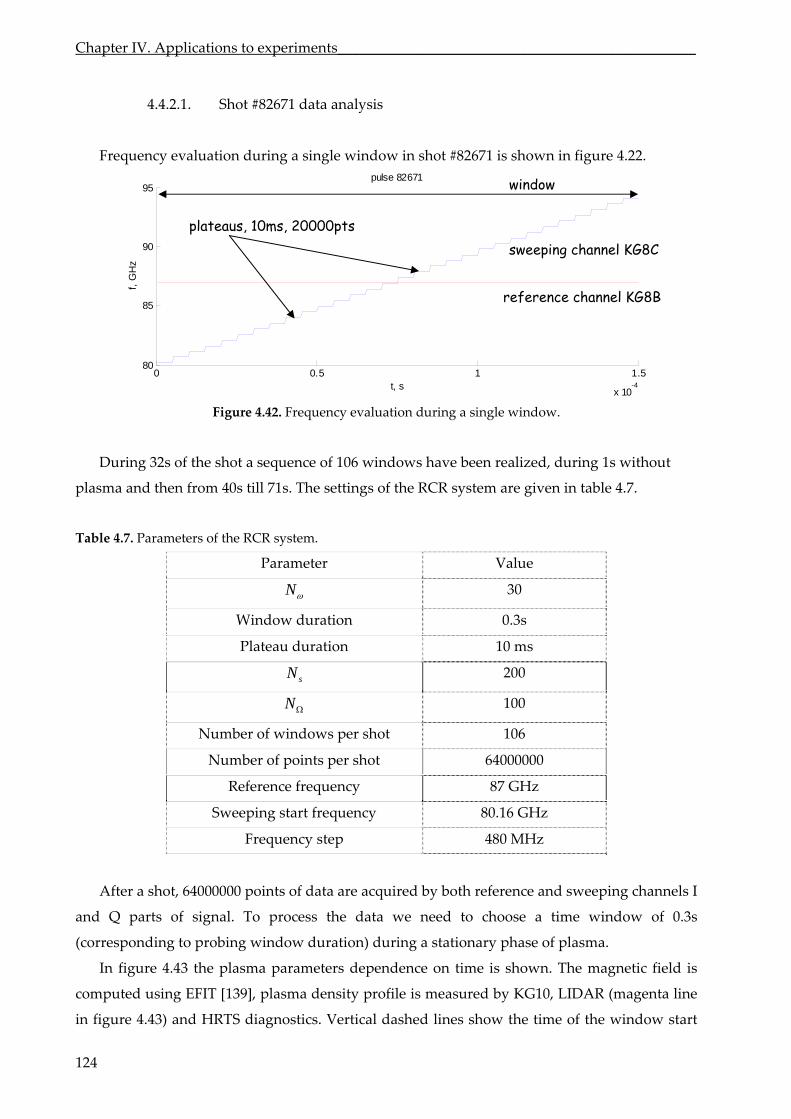
Chapter IV. Applications to experiments_________________________________________________
4.4.2.1. Shot #82671 data analysis
Frequency evaluation during a single window in shot #82671 is shown in figure 4.22.
pulse 82671
Figure 4.42. Frequency evaluation during a single window.
During 32s of the shot a sequence of 106 windows have been realized, during 1s without
plasma and then from 40s till 71s. The settings of the RCR system are given in table 4.7.
Table 4.7. Parameters of the RCR system.
Parameter Value
N 30
Window duration 0.3s
Plateau duration 10 ms
sN 200
N 100
Number of windows per shot 106
Number of points per shot 64000000
Reference frequency 87 GHz
Sweeping start frequency 80.16 GHz
Frequency step 480 MHz
After a shot, 64000000 points of data are acquired by both reference and sweeping channels I
and Q parts of signal. To data we need to a time window of 0.3s
(corresponding to probing during
In figure 4.43 the magnetic field is
computed using EFIT is measu LIDAR (magenta line
in figure 4.43) and HRT dashed lines show time of the window start
process the choose
window duration)
plasma parameters dependence
a stationary phase of plasma.
on time is shown. The
[139], plasma density profile red by KG10,
S diagnostics. Vertical the
0 0.5 1 1.5
x 10-4
80
85
90
95 window
t, s
f, G
Hz
plateaus, 10ms, 20000pts sweeping channel KG8C
reference channel KG8B
124
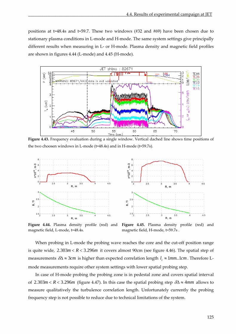
_____________________________________________4.4. Results of experimental campaign at JET
positions at t=48.4s dows (#32 9) have been chosen due to
stationary plasma c H‐mo gs give principally
different results wh ‐ or H‐mode. Plasma and magnetic field profiles
are hown in figures 4.44 (L‐mode) and 4.45 (H‐mode).
Fi . on g a s window ertical line f
the two choosen windows in L‐mode (t=48.4s) and in H‐mode (t=59.7s).
Fi 44 d p (red)
m field, L‐mode, t=48.4s.
Figu 45. P den
magnetic field, H‐mode, t=5
probing L de the reaches the cor the range
is
and t=59.7. These two win and #6
onditions in L‐mode and de. The same system settin
en measuring in L density
s
shows time positions ogure 4.43 Frequency evaluati durin ingle . V dached
gure 4.
agnetic
. Plasma ensity rofile and re 4. lasma sity profile (red) and
9.7s .
When
quite wide,
in ‐mo probing wave e and cut‐off position
2.303 3.296m R m
3cm
it covers almost 90cm (see figure 4.46). The spatial step of
measurements is higher than expected correlation length 1 ..1cl mm cm . Therefore L‐
mode require other with lower spatial probing
of H‐mode probing the probing zone is in pedestal zone and
of (figure 4.47). In this case the spatial probing step
measurements
In case
system settings step.
covers spatial interval
4mm 2.303 3.296m R m allows to
measure qualitatively turbulence cor n length. Unfortunately the probing
frequency step possible to ce due technical limitations of the
the relatio
to
currently
system. is not redu
2 2.5 3 3.5 4 4.51.5
2
2.5
3
R, m
B, T
l
2 2.5 3 3.5 4 4.50
2
4
6
8
R, m
n*10
19, m
-3
2 2.5 3 3.5 4 4.51.5
2
2.5
3
R, m
B, T
l
2
6
8
4
2.5 3 3.5 40
2
R, m
019, m
-
4.5
n*1
3
125
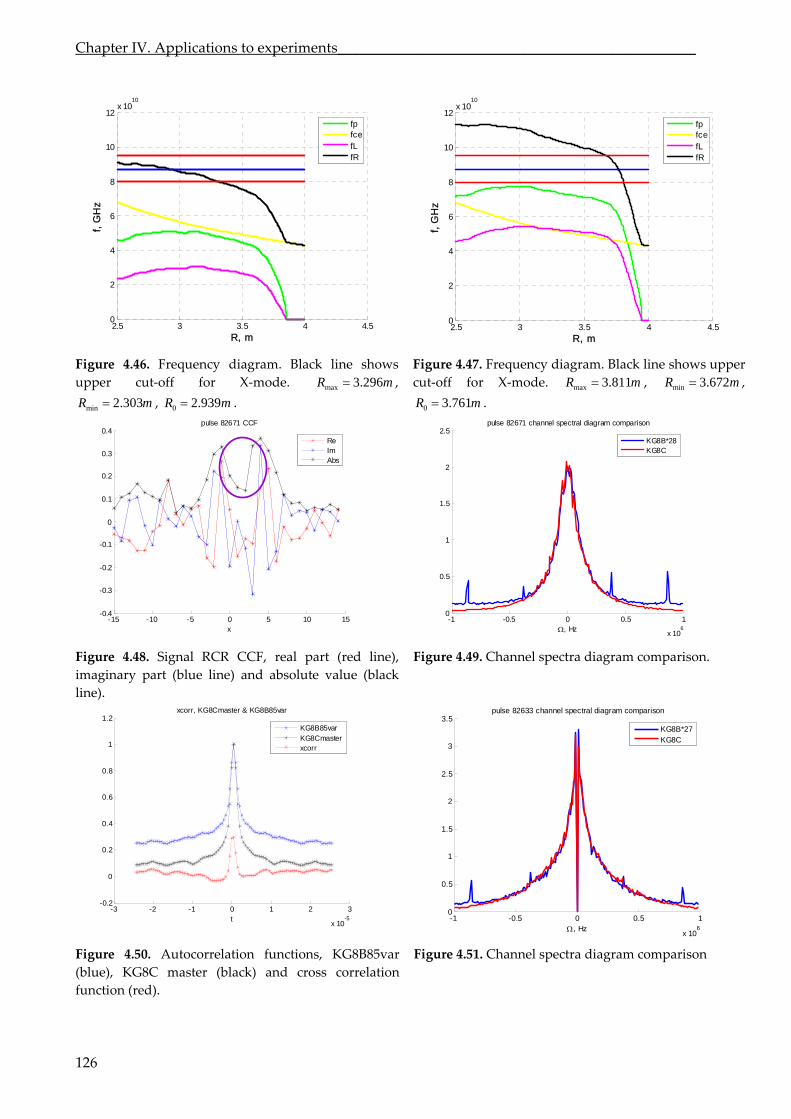
Chapter IV. Applications to experiments_________________________________________________
Figure 4.46. Frequency diagram. Black line shows
upper cut‐off for X‐mode. max 3.296R m ,
Figure 4.47. Frequency diagram. Black line shows upper
cut‐off for X‐mode.
min 2.303R m , 0 2.9R 39m .
max 3.811R m , min .672R m3 ,
0 3.761R m .
Figure 4.48. Signal RCR line),
imaginary part (blue line) and absolute value (black
line).
Figure 4.49. C spectra diagram comparison. CCF, real part (red hannel
-3 -2 -1 0 1 2 3
x 10-5
-0.2
0
0.2
0.4
0.6
0.8
1
1.2
t
xcorr, KG8Cmaster & KG8B85var
KG8B85varKG8Cmasterxcorr
-1 -0.5 0 0.5 1
6x 10
0
0.5
1
1.5
2
2.5
3
3.5
, H
z
pu channel spectral diagram comparison
lse 82633
KG8B*27KG8C
(blu
am comparison Figure 4.50. Autocorrelation functions, KG8B85var Figure 4.51. Channel spectra diagr
e), KG8C master (black) and cross correlation
function (red).
2.5 3 3.5 4 4.50
2
4
6
8
10
12x 10
10
R, m
f, G
Hz
fpfcefLfR
2.5 3 3.5 4 4.50
2
4
6
8
10
12x 10
10
R, m
f, G
Hz
fpfcefLfR
-1 -0.5 0 0.5 1
x 106
0
0.5
1
1.5
2
2.5
, Hz
ectral diagram comparison
pulse 82671 channel sp
KG8B*28KG8C
-15 -10 -5 0 5 10 15-0.4
-0.3
-0.2
-0.1
0
0.1
0.2
0.3
0.4
x
pul
se 82671 CCF
ReImAbs
126
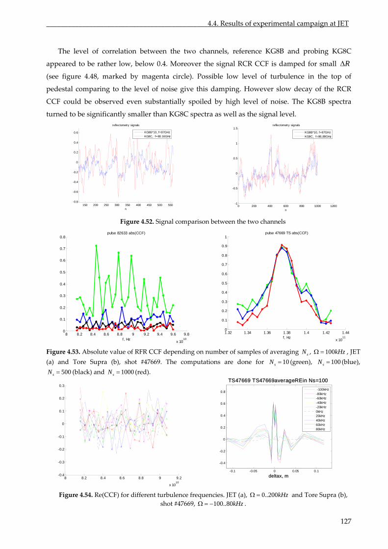
_____________________________________________4.4. Results of experimental campaign at JET
The level of correlation between the two channels, reference KG8B and probing KG8C
appeared to be rather low, below 0.4. Moreover the signal RCR CCF is damped for small R
(see figure 4.48, marked by magenta circle). Possible low level of turbulence in the top of
pedestal comparing to the level of noise give this damping. However slow decay of the RCR
CC could be observed even substantially spoiled by high level of noise. The KG8B spectra
turned to be significantly smaller than KG8C spectra as well as the signal level.
F
150 200 250 300 350 400 450 500 550-0.8
-0.6
-0.4
-0.2
0
0.2
0.4
0.6
n
reflectometry signals
KG8B*10, f=87GHzKG8C, f=80.16GHz
0 200 400 600 800 1000 1200
-1
-0.5
0
0.5
1
1.5
n
reflectometry signals
KG8B*10, f=87GHzKG8C, f=86,88GHz
Figure 4.52. Signal comparison between the two channels
8 8.2 8.4 8.6 8.8 9 9.2 9.4 9.6 9.8
x 1010
0
0.1
0.2
0.3
0.4
0.5
0.6
0.7
0.8pulse 82633 abs(CCF)
1.32 1.34 1.36 1.38 1.4 1.42 1.44
x 1011
0
0.1
0.2
0.3
0.4
0.5
0.6
0.7
0.8
0.9
1pulse 47669 TS abs(CCF)
f, Hzf, Hz
Figure 4.53. Absolute value of RFR CCF depending on number of samples of averaging sN ,
een),
100kHz ,
100sN
JET
(a) and Tore Supra (b), shot #47669. The computations are done for (gr10sN (blue),
500sN (black) and 1000sN (red). TS47669 TS47669averageR
8 8.2 8.4 8.6 8.8 9 9.2
x 1010
-0.4
-0.3
-0.2
-0.1
0
0.1
0.2
0.3
-0.1 -0.05 0 0.05 0.1
-0.4
-0.2
0
0.2
0.4
0.6
0.8
Ein Ns=100
-100kHz-80kHz-60kHz-40kHz-20kHz0kHz20kHz40kHz60kHz80kHz
deltax, m
Figure 4.54. Re(CCF) for different turbulence frequencies. JET (a), 0..200kHz and Tore Supra (b),
shot #47669, 100..80kHz .
127
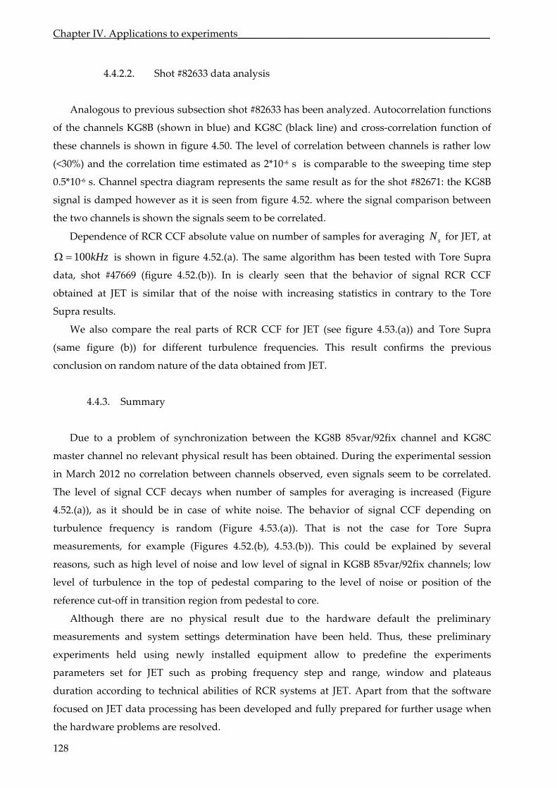
Chapter IV. Applications to experiments_________________________________________________
4.4.2.2. Shot #82633 data analysis
Analogous to previous subsection shot #82633 has been analyzed. Autocorrelation functions
of the channels KG8B (shown in blue) and KG8C (black line) and cross‐correlation function of
these channels is shown in figure 4.50. The level of correlation between channels is rather low
(<30%) and the correlation time estimated as 2*10‐6 s is comparable to the sweeping time step
0.5*10‐6 s. Channel spectra diagram represents the same result as for the shot #82671: the KG8B
signal is damped however as it is seen from figure 4.52. where the signal comparison between
the two channels is shown the signals seem to be correlated.
Dependence of RCR CCF absolute value on number of samples for averaging sN for JET, at
ho 9 ). In is clearly t of signal RCR CCF
obtained at is similar that of the noise with increasing statistics in contrary to the Tore
Supra results.
We also compare the real parts of RCR CCF for JET (see figure 4.53.(a)) and Tore Supra
(same figure (b)) for different turbulence frequencies. This result confirms the previous
conclusion on random nature of the data obtained from JET.
4.4.3. Summary
Due to a problem of synchronization between the KG8B 85var/92fix channel and KG8C
relevant a
served, even signals seem to be correlated.
vel of signal CCF decays when number of samples for averaging is increased (Figure
4.52.(a)), as it should be in case of white noise. The behavior of signal CCF depending on
turbulence frequency is random (Figure 4.53.(a)). That is not the case for Tore Supra
measurements, for example (Figures 4.52.(b), 4.53.(b)). This could be explained by several
reasons, such as high level of noise and low level of signal in KG8B 85var/92fix channels; low
level of turbulence in the top of pedestal comparing to the level of noise or position of the
reference cut‐off in transition region from pedestal to core.
Although there are no physical result due to the hardware default the preliminary
measurements and system settings determination have been held. Thus, these preliminary
experiments held using newly installed equipment allow to predefine the experiments
c
stems at JET. Apart from that the software
focused on JET data processing has been developed and fully prepared for further usage when
the hardware problems are resolved.
100kHz is shown in figure 4.52.(a). The same
data, s t #4766 (figure 4.52.(b) s
JET
algorithm has been tested with Tore Supra
een tha the behavior
master channel no physical result h been
in March 2012 no correlation between channels ob
The le
s obtained. During the experimental session
parameters set for JET such as probing frequen
duration according to technical abilities of RCR sy
y step and range, window and plateaus
128
____________________________________Conclusion
Turbulence is considered to be the main source of anomalous transport in tokamaks which
leads to faster loss of heating than it was predicted by neoclassical theory. Consequently it
makes measurements of turbulence properties important for better understanding of turbulence
nature. Measurements of plasma density fluctuations are the easiest and provide information
not only on the turbulence amplitude but also on its dispertion relation, frequency and wave
number spectra and phase. Although plenty of turbulence diagnostic tools are already
developed the problem of high quality turbulence properties measurements is still especially
acute.
Reflectometry is a widely used method of plasma diagnostic in tokamaks. It provides
information on averaged plasma density profile and on fluctuation properties as well. One of its
applications, radial correlation reflectometry (RCR), studies correlation between the two signals
received from plasma equency difference
with growing frequency difference. This correlation decay possesses a logarithmic slow
behavior observed in majority of experiments looking at the plasma core [106]. However,
numerical computations show that it differs from the turbulence correlation function
dependency. The discrepancy predetermined subsequent erroneous approach in experiment
data interpretation however it could be explained analytically.
This thesis is focused on new correct RCR data interpretation and covers the development
of the innovative method providing from RCR data the turbulence characteristics such as radial
wave number spectrum and turbulence radial correlation length from the theoretical model to
experimental validation on various machines with completely different parameters.
l
plains tail of
signal R one dimensional geometry in linear regime. Furthermore the simple relation
between measured in experiment signal RCR CCF and turbulence radial wave number
spectrum is developed from the integral equation obtained for RCR CCF. The direct transform
forward and inverse kernels are also proposed in order to simplify the calculation of turbulence
parameters and reduce errors accumulating during numerical computations.
Numerical simulation is an intermediate step between the theoretical approach and the real
world allowing to model real experiment and estimate required experimental settings. It is the
first step in developing the methods of experimental data processing.
First application of the method has been realized at Tore Supra tokamak. As the prevalent
results was estimated
lc=0.5..0.8cm and the behavior of number spe rum for small wave numbers
one at fixed frequency and the other with growing fr
Theoretical basis in Born approximation framework gives a correct analytica description of
RCR signal dependency on turbulence radial wave number and ex the long the
CR CCF in
of the experiment turbulence radial rrelation length in the range ofco
radial wave ct
129
Conclusion___________________________________________________________________________
130
15cm with good resolution of 0.04cm 1 which agrees with two‐fluid model discussed
subsection 1.4.3 was studied as well. in
Later RCR experiments was realized at small FT‐2 tokamak and gave results consistent to
the results obtained at Tore Supra: the estimated radial correlation length was in the order of
lc=0.1..0.8cm. However additional difficulties were faced at FT‐2 due to small geometry of the
machine and subsequent curvature of the cut‐off layer. Obviously one dimensional approach
gives rough description of electromagnetic wave propagation in the case of 0 0 2..10L f c and
does not take into account two dimensional effects such as small angle scattering. The inverse
transform of the RCR CCF gives the general shape of radial wave number spectrum and does
not
The last
used. The problem of synchronization between the two channels of different
refl
een developed.
Addressing to applications to ITER we should also discuss the limitations of RCR. On ITER
es are flat that means long probing wave path up to several meters.
herefore the reflectometer can suffer from destructive influence of plasma turbulence which
ma
allow us to exhibit a clear dependency.
, JET experiment was planned as a test of the proposed method for further
development for ITER reflectometry systems. Unfortunately the installation of the new RCR
system was not finished and great capabilities of new fast sweeping correlation reflectometer
have not been
ectometers was not resolved however even having no physical result the experimental
campaign was quite fruitful. As a result of the experiment the equipments settings have been
determined and necessary software for data processing has b
the plasma density profil
T
y lead on one hand to multiple small angle scattering or strong phase modulation and on the
other hand to a strong Bragg backscattering (BBS) or to an anomalous reflection [140]. This
introduces additional difficulties of reflectometry data interpretations. Fortunately RCR is
useful in case of strong phase modulation and in strong non‐linear regime due to local
monitoring of turbulence behaviour [141].
The contribution of the author to this work is in developing of the theoretical basis of the
RCR, performing of the numerical modeling, participating the experimental sessions at three
machines, Tore Supra in Cadarache, JET in Culham and FT‐2 in Saint‐Petersburg and all the
data processing for these machines.
_________________________________________________________________________Future plans
Future plans
would like to underline that although the theoretical approach provides a strong basis
for
the
Born
applications of the method should be established. Future plans include
application
machine
We
turbulence properties reconstruction it is not complete. Thus, the description of the
scattering signal and expression for RCR CCF in two dimensional model should be
described and the 2D corrections for the inverse relation for turbulence radial wave number
spectrum are required as well. This should explain the RCR CCF behavior in a small machine
and discover the influence of 2D effects in huge machine such as ITER. Further the comparison
between numerical 1D and 2D computations in approximation as well as full wave are
needed.
Experimental
of the method to study the suppression of radial correlation length due to L‐H
transition or shear flows. The evolution of the wave number spectrum by the RCR technique
could be measured as well.
After the hardware improvement at JET the attempt to apply the diagnostic should be
continued as soon as conditions at JET are the closest to ITER.
131

132
_____________________________________Appendix
Appendix A. Stationary phase method
The main idea of stationary phase methods relies on the cancellation of sinusoids with
rapidly‐varying phase. It is a generalization of Laplace method for the following integrals:
( )( ) ( )b
ix t
a
I x g t e dt (203)
where ( )g t and are real functions. If inside the interval of integration a point ( )t [ , ]a b t c
where '( ) 0c exists this point is called “stationary point” and it is possible to obtain an
asymptotic integral ( )form of the I x using the Laplace method. The stationary point provides
the main contribution to the
integral ( )I x in the vicinity of the stationary point.
If '( ) 0a and '( ) 0t for a t b the integral ( )I x can be splitted in two:
( )( ) ( ) ( ) ( ) ( )a b
ix t ix ( )1 2
t
a a
I x I x I x g t e dt g t e
d
t (204)
he second integral 2 ( )I x nullifies as 1 x if x T because there is no stationary point in the
interval ] [ ,a b . the asymptotica representation, the functions andTo obtain l ( )g t ( )t are
replaced by their Taylor series:
( )( ) ( )exp[ ( )] exp[ ( ) ( )] , !
ap p
a
xI x g a ix a i t a a dt x
p
(205)
The integration interval is enlarged by replacing by , however the error introduced by this
replacement nullifies as 1 x if x and is Substitutingnegligible. ( )s t a :
( )
0
( ) ( )exp[ ( )] exp[ ( )] , !
p pxI x g a ix a i s a ds x
p
(206)
If the contour of integration id turned for ( ) ( ) 0p a 2 p otherwise 2 p .Using the
substitution
1/
( )
( )
!exp[ sgn( ( ))]
2 ( )
p
p
p
p us i a
p x a
(207)
the asymptotic form for x is obtained:
1/
( )
( )
! (1 )( ) ( )exp ( ) sgn( ( )) ,
2 ( )
p
p
p
p u pI x g a i x a a x
p px a
(208)
For the stationary point '' ( ) 0a :
133
Appendix____________________________________________________________________________
''
1/2
1/2''
exp ( ) sgn( ( ))4
( ) 2 ( ) , ( )
i x a a
I x g a xx a
(209)
Appendix B. 4th order Numerov scheme
For the second‐order derivative we use Taylor series:
2 3 4(1) (2) (3) (4) 4
2 3 4(1) (2) (3) (4) 4
( ) ( ) ( ) ( ) ( ) ( ) ( )2 6 24
( ) ( ) ( ) ( ) ( ) ( ) ( )2 6 24
z z z z z z
z z z z z z
h h hE x h E x hE x E x E x E x O h
h h hE x h E x hE x E x E x E x O h
(210)
After adding the two expansions:
2
(2) (4) 42
( ) 2 ( ) ( )( ) ( ) ( )
12z z z
z z
E x h E x E x h hE x E x O h
h
(211)
We obtain from here:
2
(2) (4) 42
( ) 2 ( ) ( )( ) ( ) ( )
12z z z
z z
E x h E x E x h hE x E x O h
h
(212)
We substitute this expression for the second‐order derivative (212) to the Helmholtz equation
(169):
2
2 2 (4) 402
( ) 2 ( ) ( )4 ( ) ( ) ( ) (
12z z z
z z
E x h E x E x h hN x E x E x O h
h
) (213)
The key point of the method is to apply the operator 2 2
21
12
h d
dx
to the Helmholtz equation
(169):
2 2 2 2
(2) 2 2 2 20 02 2
1 ( ) 4 ( ) ( ) 4 ( ) ( ) 012 12z z z
h d h dE x N x E x N x E x
dx dx
(214)
Again, using (211) we obtain:
4 2 202
2 22 2
02
( ) 2 ( ) ( )( ) 4 ( ) ( )
4 ( ) ( ) 012
z z zz
z
E x h E x E x hO h N x E x
h
h dN x E x
dx
(215)
All the terms of the fourth‐order and higher are negligible. The term 2 2
2 202
4 ( ) (12 z
h dN x E x
dx
the factor 2h . After the
)
is approximated by using the second‐order scheme due to it has
expansion into Taylor series:
134
____________________________________________________________________________Appendix
22 (1) (2) 20 ( ) ( ) ( ) ( ) ( ) ( )
2z z z z
hN x h E x h E x hE x E x O h
22 (1) (2) 20 ( ) ( ) ( ) ( ) ( ) ( )
2z z z z
hN x h E x h E x hE x E x O h
(216)
quation (215) obtaining:
we add the two expansions and substitute to the e
2 202
2 2 22 0 0 0
4 ( ) ( )
( ) ( ) 2 ( ) ( ) ( ) ( )4 0
z z zz
z z z
N x E xh
N x h E x h N x E x N x h E x h
( ) 2 ( ) ( )
12
E x h E x E x h
(217)
This is a discreet equation with a fourth‐order error term.
135

136
____________________________________References
1. United Nations, Department of Economic and Social Affairs, Population Division,
2. Statistical tables from the International Energy Agency (IEA),
http://www.iea.org/stats/docs/statistics_manual.pdf
3. The World Energy Council, http://www.worldenergy.org/publications
4. Statistical Review of World Energy, http://www.bp.com/statisticalreview
Prospects for fusion power as a future
energy source”, Trans. Fusion Sci. Technol., February 2012 – Vol. 61, No. 2T, Proceedings of the Tenth
Carolus Magnus Summer School on Plasma and Fusion Energy Physics, September, 4‐16, 2011,
Weert, The Netherlands
6. F. Joos, “The Atmospheric Carbon Dioxide Perturbation”, Europhysics News, 27, 6, 213‐218, 1996
7. J. Wesson, “Tokamaks”, Third Edition, Clarendon Press, Oxford, 2004
8. H. A. Bethe, “Energy Production in Stars”, Physical Review, Vol. 55, Issue 1: 103, January 1, 1939
9. L. A. Arzimovich, “Controlled thermonuclear reactions” (in Russian), М., 1963
10. P. A. Sturrock, T. E. Holzer, D. M. Mihalas and R. K. Ulrich, “Physics of the Sun, Vol. I: The solar
interior”, B. M. McCormac, Ed., Loockheed Palo Alto Research Laboratory, California, USA, 1986
11. An Abundance of Lithium, March 2008, http://www.worldlithium.com
12. University of Wisconsin‐Madison, http://www.iec.neep.wisc.edu/operation.php
13. I. Langmuir, ʺOscillations in ionized gasesʺ, Proc. Nat. Acad. Sci. U.S., vol. 14, p. 628, 1928; also
available in The Collected Works of Irving Langmuir, vol. 5, C. G. Suits, Ed. New York: Pergamon,
pp. 111‐120, 1961
14. V. E. Golant, A. P. Zhilinskiy, I. E. Sakharov, “Plasma physics basis” (in Russian), 2011
15. “Plasma Physics: an Introductory Course”, edited by R. O. Dendy, Cambridge University Press, 1993
16. G. Van Oost and R. Jaspers, “Thermonuclear burn criteria”, Trans. Fusion Sci. Technol., February
2012 – Vol. 61, No. 2T, Proceedings of the Tenth Carolus Magnus Summer School on Plasma and
Fusion Energy Physics, September, 4‐16, 2011, Weert, The Netherlands
17. J. D. Lawson, ʺSome Criteria for a Power Producing Thermonuclear Reactorʺ, Proceedings of the
Physical Society B, Volume 70, p. 6, 1957
18. J. Lindl, “Development of the indirect‐drive approach to inertial confinement fusion and the target
physics basis for ignition and gain”, Phys. Plasmas 2, 3933, 1995
19. J. D. Lindl et al., “The physics basis for ignition using indirect‐drive targets on the National Ignition
Facility”, Phys. Plasmas 11, 339, 2004
20. J. Ongena and A. M. Messiaen, “Heating, Confinement and Extrapolation to Reactors”, Trans. Fusion
Sci. Technol. 49, 2T, 425, 2006
21. W. M. Stacey, “Fusion. An Introduction to Physics and Technology of Magnetic Confinement Fusion.
Second, Completely Revised and Enlarged Edition”, WILEY‐VCH Verlag Gmbh&Co. KGaA,
Weinheim, 2010
http://www.un.org/esa/population
5. J. Ongena and G. Van Oost, “Energy for future centuries.
137
References___________________________________________________________________________
22. L. Spitzer, Jr., “A Proposed Stellarator”, PM‐S‐l, USAEC NYO‐ 993, 1951
3. I. E. Tamm,“Theory of the magnetic thermonuclear reactor, part 1”, Plasma Physics and the Problem
of Controlled Thermonuclear Reactions (transl), New York: Pergamon, pp 3–19, 1959
24. A. D. Sakharov, “Theory of magnetic thermonuclear reactor, part 2”, Plasma Physics and the Problem
of Controlled Thermonuclear Reactions (transl), New York: Pergamon, pp 20–30, 1959
25. I. E. Tamm, “Theory of magnetic thermonuclear reactor, part 3”, Plasma Physics and the Problem of
Controlled Thermonuclear Reactions (transl), New York: Pergamon, pp 31–41, 1959
26. V. P. Smirnov, “Tokamak foundation in USSR/Russia 1950–1990”, Nucl. Fusion 50 014003 8pp, 2010
27. L. A. Artzimovich, “Controlled Thermonuclear Reactions” (in Russian), 1963
28. S. Yu. Lukianov, “Hot plasma and controlled nuclear fusion” (in Russian), M., 1975
29. B. B. Kadomtsev, “Tokamak plasma, a complex physical system”, Institute of Physics Publishing,
Bristol, 1992
30. Culham Centre for Fusion Energy, http://www.ccfe.ac.uk
31. All‐the‐Worldʹs Tokamaks, http://www.tokamak.info
32. National Research Centre “Kurchatov Institute”, http://www.kiae.ru
33. Ioffe Physical‐Technical Institute of the Russian Academy of Sciences, http://www.ioffe.ru
34. Commissariat à lʹÉnergie Atomique (CEA) Cadarache,
http://www.cea.fr/le‐cea/les‐centres‐cea/cadarache
35. EAST tokamak homepage, http://english.hf.cas.cn/ic/ip/east
36. KSTAR tokamak homepage, http://www.nfri.re.kr
37. Japan Atomic Energy Agency, Naka Fusion Institute, http://www‐jt60.naka.jaea.go.jp
38. B. Saoutic et al.,“Contribution of Tore Supra in preparation of ITER” Nucl. Fusion 51 094014, 2011
39. T. Kurki‐Suonio et al., “Formation and detection of internal transport barriers in low‐current
tokamaks”, Plasma Phys. Control. Fusion 44 301–323, 2002
40. D. V. Kouprienko et al., “Dynamics of the Electron Thermal Diffusivity at Improved Energy
Confinement during Lower Hybrid Plasma Heating in the FT‐2 Tokamak”, Plasma Physics Reports,
Vol. 36, No. 5, pp. 371–380, 2010
41. S. I. Lashkul et al., “Effect of the Radial Electric Field on Lower Hybrid Plasma Heating in the FT‐2
Tokamak”, Physics Reports, Vol. 27, No. 12, pp. 1001–1010, 2001
42. S. I. Lashkul et al.,“Analysis of the Efficiency of Lower Hybrid Current Drive in the FT‐2 Tokamak”,
Plasma Physics Reports, Vol. 36, No. 9, pp. 751–761, 2010
43. V. N. Budnikov and M. A. Irzak, “Mechanism of ion and electron LH heating on the FT‐2 tokamak”,
Plasma Phys. Control. Fusion 12A A135, 1996
44. V. N. Budnikov, V. V. D’yachenko, L. A. Esipov et al., “Improved confinement by lower‐hybrid
heating in the FT‐2 tokamak”, JETP Lett. 59, 685, 1994
45. European Fusion Development Agreement, http://www.efda.org
46. ITER official website, http://www.iter.org
47. P. Hennequin et al., “Scaling laws of density fluctuations at high‐k on Tore Supra”, Plasma Phys.
Control. Fusion. 46 B121, 2004
2
138
___________________________________________________________________________References
4
9. S.‐I. Itoh, “Project Review Plasma Turbulence ‐ Structure Formation, Selection Rule, Dynamic
10
50. ng‐Distance Radial Correlation in Toroidal Plasma Turbulence”,
51. ena in a Magnetically Confined Plasma”, Phys.
Phys. Rev. Lett. 93 165002,
f zonal flow experiments“, Nucl. Fusion 49 013001, 2009
997
hys.
659, 1960
agnetic field“, JETP
24, 1987
e Supra with
, Phys. Rev. Lett. 88 195004,
m of micro‐turbulence in tokamak plasmas”, C R Physique
ics. Volume 1: Physical Kinetics of
k SSSR 30 301, 1941, (reprinted in Proc. R. Soc. Lond. A434 9,
d. Nauk SSSR 32 16, 1941, (reprinted in Proc. R. Soc. Lond. A434 15,
8. A. Gurchenko and E. Gusakov, “Evolution of ETG mode scale turbulence and anomalous electron
transport in dynamic tokamak experiments”, Plasma Phys. Control. Fusion. 52 124035, 2010
4
Response and Dynamics Transport“ (in Japaneese), J. Plasma Fusion Res. 86 334, 20
S. Inagaki et al., “Observation of Lo
Phys. Rev. Lett. 107 115001, 2011
P. A. Politzer, “Observation of Avalanchelike Phenom
Rev. Lett. 84 1192, 2000
52. A. Fujisawa et al., “Identification of Zonal Flows in a Toroidal Plasma”,
2004
53. T. Yamada et al., “Anatomy of plasma turbulence”, Nature Phys. 4 721‐725, 2008
54. P. Diamond et al., “Zonal flows in plasma—a review”, Plasma Phys. Control. Fusion 47 3 R35, 2005
55. A. Fujisawa, “A review o
56. N. Bretz, “Diagnostic instrumentation for microturbulence in tokamaks”, Rev. Sci. Instrum. 68 8, 1
57. D. W. Ross, Commenta Plasma Phys. Control Fusion XII 155, 1989
58. D. W. Ross, “On standard forms for transport equations and quasilinear fluxes”, Plasma P
Control. Fusion 34 137, 1992
59. W. Horton and R. D. Estes, “Anomalous drift‐wave transport analysis of tokamak discharges”, Nucl.
Fusion 19 203, 1979
60. L. Spitzer, Jr., “Particle Diffusion across a Magnetic Field“, Phys. Fluids 3
61. B. B. Kadomtsev and O. P. Pogutse, ”Theory of electron transport in a strong m
Lett. 39 269, 1984
62. D. R. Thayer and P. H. Diamond, “Thermally driven convective cells and tokamak edge turbulence”,
Phys. Fluids 30 37
63. R. Sabot et al., “Measurements of density profile and density fluctuations in Tor
reflectometry”, Proc. 20th IAEA Fusion Energy Conference 1st‐6th November 2004, Villamoura,
Portugal EX/P6‐25
64. W. Horton, “Drift waves and transport”, Rev. Modern Physics 71 735, 1999
65. Z. Lin et al., “Size Scaling of Turbulent Transport in Tokamak Plasmas”
2002
66. L. Vermare et al., “Wavenumber spectru
12 115‐122, 2011
67. P. H. Diamond, S.‐I. Itoh and K. Itoh, “Modern Plasma Phys
Turbulent Plasmas”, Cambridge University Press, 2010
68. A. N. Kolmogorov, Dokl. Akad. Nau
1991)
69. A. N. Kolmogorov, Dokl. Aka
1991)
70. R. H. Kraichnan, “Inertial Ranges in Two‐Dimensional Turbulence“, Phys. Fluids 10 1417, 1967
139
References___________________________________________________________________________
71. G. Boffetta, A. Celani, S. Musacchio and M. Vergassola, “Intermittency in two‐dimensional Ekman‐
Fluid Mech. 47
correlation in
ssor”, Phys. Rev.
y small‐angle CO2 laser
990 edited by K. Bethge (EPS, Petit‐Lancy, Switzerland 1990),Vol. IV, p. 1544
eflectometry analytical theory in linear and
389, 2006
scattering and cut‐off responses
30, 1996
d High Beta in Neutral‐Beam‐Heated Divertor
t. 49 1408, 1982
kamak“, Phys. Rev. Lett. 60 2276, 1988
nfluence of sheared poloidal rotation on edge
ic,
r“, J. Nucl. Mater. 111&112, 109, 1982
sel’skii, Sov. J. Plasma Phys. 12 130,
1994
ordinaire et extraordinaire pour la
locales de la densité electronique dans les tokamaks“, PhD
on of Electromagnetic Waves in Plasmas”, Pergamon, Oxford, 1964
93. A. I. Anisimov et al., Soviet Phys. Technical Phys. 5 9, 1961
Navier‐Stokes turbulence”, Phys. Rev. E 66 026304, 2002
72. R. H. Kraichnan, “Inertial‐range transfer in two‐ and three‐dimensional turbulence”, J.
525, 1971
73. N. Bretz, “One‐dimensional modeling of the wavelength sensitivity, localization, and
reflectometry measurements of plasma fluctuations”, Physical Fluids B4(8) 2414, 1992
74. E. Mazzucato, “Small‐Scale Density Fluctuations in the Adiabatic Toroidal Compre
Lett. 36 792, 1976
75. R. E. Slusher and C. M. Surko, “Study of density fluctuations in plasmas b
scattering”, Phys. FIuids 23 472, 1980
76. N. Bretz et al., Proc. 17th European Conference on Controlled Fusion and Plasma Physics,
Amsterdam, 1
77. G. Leclert et al., “Full‐wave test of the radial correlation r
nonlinear regimes”, Plasma Phys. Control. Fusion 48 1
78. C. Fanack et al., “Ordinary‐mode reflectometry: modification of the
due to the shape of localized density fluctuations”, Plasma Phys. Control Fusion 38 1915‐19
79. F. Wagner et al., “Regime of Improved Confinement an
Discharges of the ASDEX Tokamak“, Phys. Rev. Let
80. S.‐I. Itoh and K. Itoh, “Model of L to H‐Mode Transition in To
81. H. Biglari, P. H. Diamond and P. W. Terry, “I
turbulence“, Phys. Fluids B2 1, 1990
82. F. Chen, “Plasma Diagnostic Techniques”, edited by R. H. Huddleston and S. L. Leonard, Academ
New York, p. 113, 1975
83. P. Staib, “Probe measurements in the plasma boundary laye
84. I. Hutchinson, “Principles of Plasma Diagnostics”, Second Edition, Cambridge University Press, 2002
85. M. Stanojevic et al., “Fluid model of the magnetic presheath in a turbulent plasma”, Plasma Phys.
Contr. Fusion 47 (2005) 685
86. R. L. Hickok, IEEE Trans. Nucl. Sci. NS‐28 18, 1981
87. Yu. N. Dnestrovskii, L. I. Krupnik, A. V. Mel’nikov and I. S. Ned
1986
88. L. I. Krupnik and V. I. Tereshin, Plasma Phys. Rep. 20 146,
89. R. C. Isler, “An overview of charge‐exchange spectroscopy as a plasma diagnostic“, Plasma Phys.
Control. Fusion 36 171, 1994
90. R. Cano and A. Cavallo, Proceedings of the 5th International Conference on Infrared and Millimeter
Waves, Wurtzburg (1980)
91. F. Simonet, “Etude de la réflectométrie hyperfréquence en modes
mesure du profil radial et des fluctuations
thesis, Université de Nancy I, 1985
92. V. L. Ginzburg, “The Propagati
140
___________________________________________________________________________References
94. R. J. Colchin ORMAK Technical Memo 93/105, 1973
95. I. Hutchinson, “One‐dimensional full‐wave analysis of reflectometry sensitivity and correlations”,
ted)“, Rev. Sci.
V. Nguyen, “Investigation of dual mode (O‐X) correlation
as“, Phys. Rev. Lett. 71 1840, 1993
Upgrade”, 5th Intl.
ectometry”, Plasma
g effect in Doppler reflectometry”,
, “Spatial Resolution of Poloidal Correlation Reflectometry”, 32nd EPS
l., “Direct Comparison of Turbulence Measurements with Langmuir Probes and
ns with 2D Full‐
A. Yu. Popov, “Measurements localization in poloidal correlation reflectometry”,
vature effects on microwave reflectometry fluctuation measurements”,
e Fusion Plasma”, Phys. Rev. Lett. 94 135002, 2005
correlation reflectometry
Kramer et al., “Correlation reflectometry for turbulence and magnetic field measurements in
Bulanin, O. Rozhdestvensky, “Modelling of Radial Correlation Reflectometry in
ation reflectometry”, Plasma Phys. Control.
akov and A. Popov, “Two‐dimensional non‐linear theory of radial correlation reflectometry”,
tional Atomic Energy Agency, Conference Proceedings,
Plasma Phys. Control. Fusion 34 1225, 1992
96. A. E. Costley et al., “Recent developments in microwave reflectometry at JET (invi
Instr. 61 2823, 1990
97. M. Gilmore, W. A. Peebles, X.
reflectometry for determination of magnetic field strength”, Plasma Phys. Control. Fusion 42 655,
2000
98. E. Mazzucato and R. Nazikian, “Radial scale length of turbulent fluctuations in the main core of TFTR
plasm
99. G. D. Conway et al., “Fluctuation and reflectometer simulation studies on ASDEX
Reflectometry Workshop, IRW5 NIFS Japan, March 5th‐7th, 2001
100. E. Gusakov and A. Surkov, “Spatial and wave number resolution of Doppler refl
Phys. Control. Fusion 46 (2004) 1143
101. E. Z. Gusakov, A. V. Surkov and A. Yu. Popov, “Multiple scatterin
Plasma Phys. Control. Fusion 47 959, 2005
102. A. Yu. Popov, E. Z. Gusakov
Conference on Plasma Phys. Tarragona, 27 June ‐ 1 July 2005 ECA Vol.29C P‐1.088, 2005
103. V. A. Vershkov et a
Reflectometry at the same Radial Locations in T‐10 and Reflectometry Simulatio
Wave Code”, Proc. 30th Conf. Control. Fusion Plasma Phys. ECA Vol. 27A P‐2.56, 2003
104. E. Z. Gusakov and
Nucl. Fusion 46 S829–S835, 2006
105. Y. Lin et al., “Plasma cur
Plasma Phys. Control. Fusion 43 L1, 2001
106. R. Nazikian et al., “Measurement of Turbulence Decorrelation during Transport Barrier Evolution in
a High‐Temperatur
107. E. Gusakov and B. Yakovlev, “Two‐dimensional linear theory of radial
diagnostics”, Plasma Phys. Control. Fusion 44 2525, 2002
108. G. J.
fusion plasmas (invited)”, Rev. Sci. Instrum. 74 1421, 2003
109. E. Gusakov, V.
Cylinder Geometry”, Proc. of 3rd France‐Russian Seminar NAMES 2007 Metz EDP Sciences 133, 2008
110. E. Gusakov and A. Popov, “Non‐linear theory of fluctu
Fusion 44 2327, 2002
111. E. Gus
Plasma Phys. Control. Fusion 46 1393, 2004
112. Interna
http://www‐naweb.iaea.org/napc/physics/PS/conf.htm
141
References___________________________________________________________________________
113. E. Mazzucato, “Microwave reflectometry for magnetically confined plasmas”, Rev. Sci. Instrum. 69
2201, 1998
114. H. Bindslev, “Dielectric effects on Thomson scattering in a relativistic magnetized plasma“, Plasma
Phys. Control. Fusion 33 1775, 1991
23, 2006
quantum theory” (in Russian), M. Nauka, 1975
ci. Instrum. 58 539, 1987
smas”, Plasma Phys. Control.
ew York: Springer, 1984
Instrum. 74 1501, 2003
ma
Nucl. Fusion 47 245–250, 2007
‐Supra: from edge density profile to core density
rchenko et al., “Observation of turbulence exponential wave number spectra at ion sub‐Larmor
, 2010
nal Reflectometry Workshop (IRW9) Lisbon, Portugal, 4th ‐ 6th May
tration of ITER operational scenarios on DIII‐D“, Nucl. Fusion 50 075005,
flectometry and a Langmuir probe array”, Plasma Phys. Control.
115. B. B. Afeyan, A. E. Chou, B. I. Cohen, “The scattering phase shift due to Bragg resonance in one‐
dimensional fluctuation reflectometry“, Plasma Phys. Control. Fusion 37 315, 1994
116. F. da Silva, “Studies on O‐mode reflectometry spectra simulations with velocity shear layer”, Nucl.
Fusion 46 S816–S8
117. L. D. Landau and E. M. Lifshitz, “Quantum Mechanics” (in Russian), 1963
118. A. B. Migdal, “Qualitative methods in
119. M. Abramovitz and I. Stegun, “Handbook of Mathematical Functions with Formulas, Graphs, and
Mathematical Tables”, New York: Dover Publications, 1970
120. H. Bottolier and G. Ichtchenko, “Microwave reflectometry with the extraordinary mode on tokamaks:
Determination of the electron density profile of Petula‐B“, Rev. S
121. F. Clairet et al., “Fast sweeping reflectometry upgrade on Tore Supra”, Rev. Sci. Instrum. 81 10D903,
2010
122. A. D. Piliya and A. Yu. Popov, “On application of the reciprocity theorem to calculation of a
microwave radiation signal in inhomogeneous hot magnetized pla
Fusion 44 467, 2002
123. L. D. Landau and E. M. Lifshitz, “Electrodynamics of Continuous Media”, Oxford: Pergamon, 1981
124. J. Murray, “Asymptotic Analysis”, N
125. S. Heuraux et al., “Radial wave number spectrum of density fluctuations deduced from reflectometry
phase signals“, Rev. Sci.
126. E. Gusakov and M. Tyntarev, ”The two‐dimensional theory of reflectometry diagnostics of plas
fluctuations”, Fusion Engineering and Design 34‐35 501‐505, 1997
127. A. Gurchenko et al., “Observation of the ETG mode component of tokamak plasma turbulence by the
UHR backscattering diagnostics“,
128. R. Sabot et al., “Advances of reflectometry on Tore
fluctuations”, Int. J. Infrared Millim. Waves 25 229–46, 2004
129. A. Gu
scales in FT‐2 tokamak“, Plasma Phys. Control. Fusion 52 035010
130. E. Blanco, T. Estrada and T. Happel, “Study of radial correlation reflectometry using a 2D full‐wave
code”, Proc. of 9th Internatio
2009
131. E. J. Doyle et al., “Demons
2010
132. M. Gilmore et al., Letter to the editor “Detailed comparison of plasma turbulence correlation length
measurements using microwave re
Fusion 42 L1–L7, 2000
142
___________________________________________________________________________References
133. F. Clairet et al., “New signal processing technique for density profile reconstruction using
ng system for measuring fluctuations and their
ensity and fluctuation profiles obtained with the D‐band reectometer in Tore‐
ations in a helicon‐produced plasma“, Plasma Phys. Control. Fusion 49 A167–A175, 2007
oc. of the 39th EPS Conference on Plasma Physics, Vol.36F,
ry
e on Plasma Physics, Vol. 34A, P5.110, 2010
reflectometry”, Rev. Sci. Instrum. 82, 083502, 2011
134. P. Hennequin et al., “Doppler backscatteri
perpendicular velocity on Tore Supra”, Rev. Sci. Instrum., 75(10): 3881‐3883, 2004
135. A. Sirinelli et al., “D
Supra”, Proc. of 7th International Reflectometry Workshop 4‐6 May 2007 Saint‐Petersburg, Russia
136. M. Kramer et al., “Anomalous helicon wave absorption and parametric excitation of electrostatic
fluctu
137. A. Altukhov et al., “Turbulence wave number spectra reconstruction from radial correlation
reflectometry data at FT‐2 tokamak”, Pr
P4.092, 2012
138. L. Meneses, Group meeting talk 10/02/2012 Culham, UK
139. General Atomics Fusion Theory and Computational Sciences,
https://fusion.gat.com/theory/Efithisto
140. E. Gusakov et al., “Reflectometry diagnostics operation limitations caused by strong Bragg back
scattering”, Proc. of the 37th EPS Conferenc
141. K. Syisoeva, “Propagation of electromagnetic waves in turbulent inhomogeneous plasma” (in
Russian), Master thesis, Saint‐Petersburg State Polytechnical University, 2012
143

144
145
___________________________________Publications
1. Papers:
1.1. N. Kosolapova, E. Gusakov and S. Heuraux,
“Numerical modeling of microturbulence wave number spectra reconstruction using radial
correlation reflectometry: I. O‐mode reflectometry at the linear plasma density profile”,
Plasma Phys. Control. Fusion 54 (2012) 035008, doi: 10.1088/0741‐3335/54/3/035008
1.2. E. Gusakov and N. Kosolapova,
“Fluctuation reflectometry theory and the possibility of turbulence wave number spectrum
rec reflectometry data”,
Plasma Turbulence
haracteristics and Its Dynamics”,
Contrib. Plasma Phys. 51, No. 2‐3, (2011) 126–130, doi: 10.1002/ctpp.201000050
1.4. N. Kosolapova, K. Itoh, S.‐I. Itoh, E. Gusakov, S. Heuraux, S. Inagaki, M. Sasaki,
T. Kobayashi, Y. Nagashima, S. Oldenbürger, A. Fujisawa,
“On turbulence‐correlation analysis based on correlation reflectometry”,
submitted to Phys. Scripta
2. Conference proceedings:
2.1. N. Kosolapova, A. Altukhov, A. Gurchenko, E. Gusakov , S. Heuraux, R. Sabot, F. Clairet,
“Turbulence wave number spectra reconstruction from radial correlation reflectometry data at
Tore Supra and FT‐2 tokamaks”, // 24th IAEA Fusion Energy Conference, October 8‐13, 2012,
San Diego, California, USA
2.2. A. Altukhov, A. Gurchenko, E. Gusakov, N. Kosolapova, S. Leerink, L. Esipov,
“Turbulence wave number spectra reconstruction from radial correlation reflectometry data at
FT‐2 tokamak”, // 39th EPS Conference on Plasma Phys. Strasbourg, 2‐6 July 2012, ECA Vol.
36F, P4.092 (2012) (4pp), http://ocs.ciemat.es/EPSICPP2012PAP/pdf/P4.092.pdf
onstruction using the radial correlation
Plasma Phys. Control. Fusion 53 (2011) 045012, doi: 10.1088/0741‐3335/53/4/045012
1.3. S. Heuraux, F. da Silva, E. Gusakov, A. Popov, E. Beauvier, N. Kosolapova and K. Syisoeva,
“Reflectometry Simulations on Different Methods to Extract Fusion
C
Publications__________________________________________________________________________
2.3. E. Gusakov, N. Kosolapova and S. Heuraux,
Modeling of the turbulence wave number reconstruction using radial correlation reflectometry
data with applications to FT‐2, JET, Tore Supra like cases”, // 39th Conference on plasma
physics and controlled fusion, Zvenigorod (Moscow reg.), February 6—10, 2012
2.4. E. Gusakov, N. Kosolapova and S. Heuraux,
“On possibility of turbulence wave number spectra reconstruction using radial correlation
reflectometry in Tore Supra and FT‐2 tokamaks”, // 38th EPS Conference on Plasma Phys.,
Strasbourg, 27 June – 1 July, 2011, ECA Vol. 35G, P2.060 (2011) (4pp),
http://ocs.ciemat.es/EPS2011PAP/pdf/P2.060.pdf
2.5. E. Gusakov, N. Kosolapova and S. Heuraux,
“On possibility of turbulence wave number spectra reconstruction using radial correlation
reflectometry in Tore Supra and FT‐2 tokamaks”, // 10th International Reflectometry Workshop
(IRW10), Padova, Italy, 4th‐6th May 2011, proceedings (6pp),
http://www.igi.cnr.it/irw10/proceedings/KosolapovaNV.pdf
2.6. E. Gusakov, N. Kosolapova and S. Heuraux,
“Numerical modelling of tokamak plasma microturbulence wave number spectrum
reconstruction using radial correlation reflectometry data”, // New Achievements in Materials
and Environmental Sciences (NAMES 2010) Nancy, France October 27‐29, 2010, to be published
in Journal of Physics: Conference Series (JPCS)
2.7. S. Heuraux, F. da Silva, E. Gusakov, A. Popov, N. Kosolapova, K.V. Syisoeva,
ʺNumerical modeling of tokamak plasma microturbulence wave number spectrum
reconstruction using radial correlation reflectometry dataʺ, // New Achievements in Materials
and Environmental Sciences (NAMES 2010) Nancy, France October 27‐29, 2010, to be published
in Journal of Physics: Conference Series (JPCS)
2.8. E. Gusakov, N. Kosolapova and S. Heuraux,
“Numerical modelling of microturbulence wave number spectra reconstruction using radial
correlation reflectometry data”, // International Conference on Plasma Diagnostics, April 12‐16,
2010, Pont‐à‐Mousson, France,http://plasma2010.ijl.nancy‐universite.fr
2.9. E. Gusakov, N. Kosolapova and S. Heuraux,
“Numerical modelling of microturbulence wave number spectra reconstruction using radial
correlation reflectometry data”, // 37th Conference on plasma physics and controlled fusion,
“
146
__________________________________________________________________________Publications
Z
.10. E. Gusakov, N. Kosolapova and S. Heuraux,
of the turbulence wave number spectra reconstruction using the radial correlation
eflectometry data”, // 9th International Reflectometry Workshop (IRW9), Lisbon, Portugal, 4th‐
.ist.utl.pt/irw9/papers/egusakov_paper.pdf
l correlation
eflectometry data”, // 36th EPS Conference on Plasma Phys., Sofia, June 29 ‐ July 3, 2009, ECA
psppd.epfl.ch/Sofia/pdf/P4_217.pdf
using radial
orrelation reflectometry data”, // 36th Conference on plasma physics and controlled fusion,
d S. Heuraux,
//
5th EPS Conference on Plasma Phys. Hersonissos, 9 ‐ 13 June 2008 ECA Vol.32D, P‐1.082 (2008)
nce wave number spectra reconstruction using radial correlation
eflectometry data”, // 34th EPS Conference on Plasma Phys. Warsaw, 2 ‐ 6 July 2007 ECA
http://epsppd.epfl.ch/Warsaw/pdf/P5_100.pdf
roceedings (8pp),
ttp://plasma.ioffe.ru/irw8/proceedings/Gusakov_paper.pdf
venigorod (Moscow reg.), February 8—12, 2010
2
”Procedure
r
6th May 2009, proceedings (7pp), http://www.ipfn
2.11. E. Gusakov, N. Kosolapova and S. Heuraux,
“Modelling of the turbulence wave number spectra reconstruction from the radia
r
Vol.33E, P‐4.217 (2009) (4pp), http://e
2.12. E. Gusakov, N. Kosolapova and S. Heuraux,
“Numerical modeling of microturbulence wave number spectra reconstruction
c
Zvenigorod (Moscow reg.), February 9—13, 2009
2.13. E. Gusakov, N. Kosolapova an
“Turbulence wave number spectra reconstruction using radial correlation reflectometry”,
3
(4pp), http://epsppd.epfl.ch/Hersonissos/pdf/P1_082.pdf
2.14. E. Gusakov, V. Bulanin, O. Rozhdestvenskiy, N. Kosolapova,
“On possibility of turbule
r
Vol.31F, P‐5.100 (2007) (4pp),
2.15. E. Gusakov, V. Bulanin, O. Rozhdestvenskiy, N. Kosolapova,
“On possibility of turbulence wave number spectra reconstruction using radial correlation
reflectometry data”, // 8th International Reflectometry Workshop (IRW9), Saint‐Petersburg,
Russia, 2nd‐4th May 2007, p
h
147

148
149
_______________Awards________________________
ul. 2011
ulence at the 38th European Physical Society
warded the medal ʺFor the best scientific workʺ of students of Universities of the Russian
.2010)
Oct. 2011
Grant of Russian Ministry of Education (Order #2477 14.10.2011)
J
Winner of the 7th Itoh Project Prize in Plasma Turb
Conference on Plasma Physics, 27th June – 1st July 2011, Strasbourg, France
May 2010
A
Federation and the CIS countries (Order #470 27.05

150
____________________________Acknowledgements
During the three years of my work on the thesis I have taken efforts in this project, however
lp of a large number of people.
would like to thank all of them.
rs, for their patient
uidance, enthusiastic encouragement and useful critiques; their valuable and constructive
s during the planning and development of this research work. Their willingness to
I would like to thank the Administration and staff of Institute Jean Lamour, Université de
Lorraine; Nancy, France and Ioffe Institute, Saint‐Petersburg, Russia for the great opportunity
to work on the thesis as a student of two countries.
I wish to thank the FT‐2 tokamak team, especially Aleksey Altukhov and Aleksey
Gurchenko for providing me with results of reflectometry experiments, for detailed
explanations and enlightening discussions.
I am highly indebted to Roland Sabot for giving me a great opportunity to work with him
on Tore Supra and JET reflectometry experiments.
Without explanations of Antoine Sirinelli I would not have managed to perform my work at
JET reflectometers and obtain required data.
Thanks to Frédéric Clairet who has thoughtfully revised my papers and gave me essential
advices.
I would like to thank Jean‐Claude Giacalone and Sébastian Hacquin for all their valuable
assistance in the experimental work.
I am also grateful to all the staff of Tore Supra and JET tokamaks for helping me to
participate in experiments and feel comfortable during my work there.
I am obliged to Filipe da Silva for his significant help with numerical computations
performed in 2D.
it would not have been possible without the kind support and he
I
First of all I would like to express my profound gratitude and deep regards to Professor
Stéphane Heuraux and Professor Evgeniy Gusakov, my research superviso
g
suggestion
give their time so generously has been very much appreciated.
151

Acknowledgements___________________________________________________________________
152
I highly appreciate the invitation of Professor Sanae‐I. Itoh and Professor Kimitaka Itoh to
isit Kyushu University and National Institute for Fusion Science in Japan. This visit became a
great discovery for me and the reception I recived was exceptionally warm. I would like also to
thank Stella Oldenbürger, Shigeru Inagaki and all the members of Itoh Plasma Turbulence
Laboratory for their help and collaboration during my stay in Japan.
I would like to thank Roger Jaspers, Greg de Temmerman, Tony Donné and all 10th Carolus
Magnus Summer School team for great organization of education process and time spent
during two weeks in September 2011 in Weert, the Netherlands.
I could not manage to complete the work without the invaluable support of my beloved
parents and family.
I would like to express my heartfelt thanks to my husband Dmitry. Your faith and loving
patience colored my life and made me feel your support through distance and time.
Natalia Kosolapova,
16th of November, 2012
v
Related Documents