Lie Group Formulation of Articulated Rigid Body Dynamicsjunggon/tools/liegroupdynamics.pdf · Lie Group Formulation of Articulated Rigid Body Dynamics Junggon Kim 12/10/2012, Ver

Lie Group Formulation of Articulated Rigid Body Dynamics

Junggon Kim

12/10/2012, Ver 2.01

Abstract

It has been usual in most old-style text books for dynamics to treat the formulas describinglinear(or translational) and angular(or rotational) motion of a rigid body separately. Forexample, the famous Newton’s 2nd law, f = ma, for the translational motion of a rigidbody has its partner, so-called the Euler’s equation which describes the rotational motionof the body. Separating translation and rotation, however, causes a huge complexity inderiving the equations of motion of articulated rigid body systems such as robots.

In Section 1, an elegant single equation of motion of a rigid body moving in 3D space isderived using a Lie group formulation. In Section 2, the recursive Newton-Euler algorithm(inverse dynamics), Articulated-Body algorithm (forward dynamics) and a generalizedrecursive algorithm (hybrid dynamics) for open chains or tree-structured articulated bodysystems are rewritten with the geometric formulation for rigid body. In Section 3, dynamicsof constrained systems such as a closed loop mechanism will be described. Finally, inSection 4, analytic derivatives of the dynamics algorithms, which would be useful foroptimization and sensitivity analysis, are presented.1

1 Dynamics of a Rigid Body

This section describes the equations of motion of a single rigid body in a geometric manner.

1.1 Rigid Body Motion

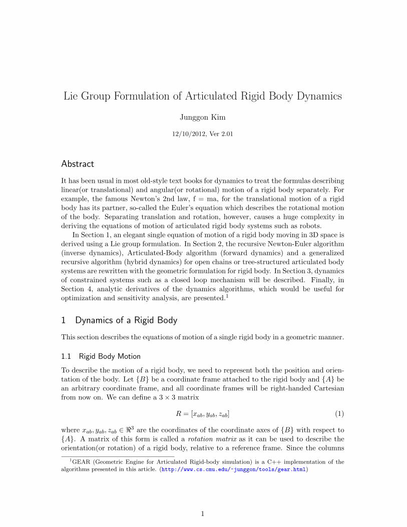
To describe the motion of a rigid body, we need to represent both the position and orien-tation of the body. Let {B} be a coordinate frame attached to the rigid body and {A} bean arbitrary coordinate frame, and all coordinate frames will be right-handed Cartesianfrom now on. We can define a 3× 3 matrix

R = [xab, yab, zab] (1)

where xab, yab, zab ∈ <3 are the coordinates of the coordinate axes of {B} with respect to{A}. A matrix of this form is called a rotation matrix as it can be used to describe theorientation(or rotation) of a rigid body, relative to a reference frame. Since the columns

1GEAR (Geometric Engine for Articulated Rigid-body simulation) is a C++ implementation of thealgorithms presented in this article. (http://www.cs.cmu.edu/~junggon/tools/gear.html)

1

Figure 1: Coordinates frames for a rigid body

of a rotation matrix are mutually orthonormal and the coordinate frame is right-handed,the rotation matrix has two properties,

RRT = RTR = I, detR = 1, (2)

and it is denoted by SO(3)2.Let p ∈ <3 be the position vector of the origin of {B} from the origin of {A}, and

R ∈ SO(3) be the rotation matrix of {B} relative to {A}. The configuration space of therigid body motion can be represented with the pair (R, p), which is denoted as SE(3). A4× 4 matrix,

T =

[R p0 1

](3)

is called the homogeneous representation of T = (R, p) ∈ SE(3), and its inverse can beobtained with

T−1 =

[RT −RTp0 1

]. (4)

From now on, a simple declaration, T ∈ SE(3) : {A} → {B}, will be used to notify thatT ∈ SE(3) represents the orientation and position of a coordinate frame {B} with respectto another coordinate frame {A}.

The Lie algebra of SE(3), denoted as se(3), is identified as a 6-dimensional vectorspace (w, v) ∈ <6 where w ∈ so(3), the Lie algebra of SO(3). ξ = (w, v) ∈ se(3) can alsobe represented as a 4× 4 matrix,

ξ =

[[w] v0 0

](5)

where [w] =

[0 −w3 w2w3 0 −w1−w2 w1 0

]∈ <3×3 is a skew-symmetric matrix.

The adjoint action of T ∈ SE(3) on ξ ∈ se(3), Ad : SE(3)× se(3)→ se(3), is definedas

AdT ξ = T ξ T−1. (6)

2 The notation SO abbreviates special orthogonal and ‘special’ refers to the fact that detR = +1 ratherthan ±1. See [2] for more details.

2

From (3), (4) and (5), AdT can be regarded as a linear transformation, AdT : se(3) →se(3), which is defined by a 6× 6 matrix

AdT =

[R 0

[p]R R

](7)

where T = (R, p) ∈ SE(3). The coadjoint action of T on ξ∗ ∈ dse(3) which is the dual ofξ, Ad∗T : dse(3)→ dse(3), is defined by a 6× 6 matrix

Ad∗T = AdTT . (8)

1.2 Generalized Velocity and Force

Let T (t) = (R(t), p(t)) ∈ SE(3) be a motion trajectory of a coordinate frame attached toa rigid body with respect to an inertial frame. The generalized velocity of the rigid bodyis defined as

V = T−1T =

[[w] v0 0

](9)

where [w] = RTR and v = RTp. The physical meaning of w ∈ <3 is the rotational(or an-gular) velocity of the coordinate frame attached to the body relative to the inertial frame,but expressed in the body coordinate frame. Similarly, v ∈ <3 represents the velocity ofthe origin of the coordinate frame relative to the inertial frame, and still expressed in thebody frame. The generalized velocity is an element of se(3), and can be simply regardedas a 6-dimensional vector, i.e.,

V =

(wv

). (10)

As the generalized velocity is an instance of se(3), it follows the adjoint transformationrule defined in (7). Let {A}, {B} be two different coordinate frames attached to the samerigid body, and Ta, Tb ∈ SE(3) represent the orientation and position of the two frameswith respect to an inertial frame. Then, from (6) and (9), the generalized velocities of{A} and {B} have the following relation:

Vb = AdTbaVa (11)

where Tba ∈ SE(3) : {B} → {A}.With a coordinate frame attached to a rigid body, the generalized force acting on the

body can be defined as

F =

(mf

)(12)

where m ∈ <3 and f ∈ <3 represent a moment and force acting on the body respectively,viewed in the body frame. The generalized force is known as the member of dse(3), andhas the following transformation rule,

Fb = Ad∗TabFa (13)

where Fa and Fb denote a generalized force viewed from different body frames {A} and{B}, and Tab ∈ SE(3) : {A} → {B}.

3

1.3 Generalized Inertia and Momentum

The kinetic energy of a rigid body is given by the following volume integral

e =

∫vol

1

2‖v‖2 dm (14)

which means the sum of the kinetic energies of all the mass particles constituting the body.By introducing a coordinate frame attached to the body, (14) can be restructured as thefollowing simple quadratic form,

e =1

2V TIV (15)

where V ∈ <6 is the generalized velocity of the body and I ∈ <6×6, which is known asgeneralized inertia, represents the mass and mass distribution with respect to the bodyframe.

To obtain an explicit form of the generalized inertia of a rigid body, let r ∈ <3 bethe position of a body point relative to the body frame and (R, p) ∈ SE(3) representsorientation and position of the body frame with respect to an inertial frame respectively.Using ||v||2 = ||p+ Rr||2, RTR = [w] and RTp = v, (14) can be rewritten as

e =1

2

∫vol

(||p||2 + 2pTRr + ||Rr||2

)dm (16)

=1

2

{pTp

∫voldm− 2pTR

(∫vol

[r]dm

)w + wT

(∫vol

[r]T[r]dm

)w

}(17)

=1

2

{mvTv − 2vT

(∫vol

[r]dm

)w + wT

(∫vol

[r]T[r]dm

)w

}(18)

=1

2V TIV (19)

where V = (w, v) is the generalized velocity of the body and the generalized inertia, I,has the following explicit matrix form:

I =

[ ∫vol [r]T[r]dm

∫vol[r]dm∫

vol [r]Tdm m1

]. (20)

The generalized inertia is symmetric positive definite, and its upper diagonal term, I =∫vol [r]T[r]dm, is the definition of the well-known 3 × 3 inertia matrix of the rigid body

with respect to the body frame. If the origin of the body frame is located on the center ofmass, then the generalized inertia becomes a block diagonal matrix because

∫vol[r]dm = 0.

In addition, if the orientation of the body frame also coincides with the principle axes ofthe body, then the generalized inertia becomes a diagonal matrix.

Let {A} and {B} be coordinate frames attached to a rigid body, Ia and Ib be thegeneralized inertias of the body corresponding to the two frames. Using (11), (15), andthe fact that the kinetic energy of the body should remain under change of coordinateframe, the following transformation rule between the generalized inertias can be obtained:

Ib = Ad∗TabIaAdTab (21)

4

where Tab ∈ SE(3) : {A} → {B}. If the mass, m, and the inertia matrix in a center ofmass frame3, Ic ∈ <3×3, are given, one can get the generalized inertia in an arbitrary bodyframe from (21), rather than using (20), as

I =

[RIcR

T+m[p]T[p] m[p]

m[p]T m1

](22)

where (R, p) ∈ SE(3) represents the orientation and position of the center of mass framewith respect to the body frame.

The generalized momentum of a rigid body is defined as

L = IV (23)

where I and V are the generalized inertia and velocity of the body expressed in a coordi-nate frame attached to the body.

La and Lb be the generalized momentum of a rigid body expressed in different bodyframes, {A} and {B}, respectively. Using (11) and (21) one can derive the followingtransformation rule for generalized momentums:

Lb = Ad∗TabLa (24)

which is same to that of generalized forces, and indeed, the generalized momentum is alsoknown as dse(3).

1.4 Time Derivatives of se(3) and dse(3)

Recall that the time derivative of a 3-dimensional vector x =∑3

i=1 xiei, expressed in amoving coordinate frame {ei}, can be obtained as

d

dtx =

3∑i=1

{(d

dtxi

)ei + xi

(d

dtei

)}= x+ w × x (25)

where x =∑3

i=1

(ddtxi

)ei =

(dx1dt ,

dx2dt ,

dx3dt

)is the component-wise time derivative of x

and w is the angular velocity of the moving frame.The time derivatives of se(3) and dse(3) which are expressed in a moving frame have

more generalized form. A simple approach to obtain the derivatives is to transform se(3)(ordse(3)) to a stationary coordinate frame, differentiate it there, and transform the derivativeback to the original moving coordinate frame with the (correct) assumption that thederivative of se(3)(or dse(3)) can be transformed with the rule of se(3)(or dse(3)).4Notethat differentiating a vector in a stationary coordinate frame with respect to time is justgetting the component-wise derivative of it.

Lemma 1. Let X ∈ se(3) be expressed in a moving frame attached to a rigid body. Thenthe time derivative of X can be obtained by

d

dtX = X + adVX (26)

3 A coordinate frame whose origin is located on the center of mass of the body.4 In [1] the time derivative of a spatial velocity which is similar to the generalized velocity in this article

was obtained with this approach.

5

where X is the component-wise time derivative of X and adV : se(3) → se(3) is a lineartransformation defined as

adV =

[[w] 0[v] [w]

](27)

where V = (w, v) ∈ se(3) is the generalized velocity of the body.

Proof. Let T = (R, p) ∈ SE(3) denote the orientation and position of the moving framewith respect to an inertial frame which is stationary in the space. By transforming X tothe inertial frame, differentiating it there, and then transforming the result back to theoriginal body frame, one can get

d

dtX = AdT−1

d′

dt(AdTX) = X + AdT−1

d′

dt(AdT )X

where d′

dt represents the component-wise differentiation and X = d′

dtX. Using (7) and

V = (w, v) = (RTR, RTp), one can show AdT−1d′

dt (AdT ) = adV as follows:

AdT−1

d′

dtAdT =

[RT 0

−RT [p] RT

] [R 0

[p]R+ [p] R R

]=

[[w] 0[v] [w]

]

Lemma 2. Let Y ∈ dse(3) be expressed in a moving frame attached to a rigid body. Thenthe time derivative of Y can be obtained by

d

dtY = Y − ad∗V Y (28)

where Y is the component-wise time derivative of Y and ad∗V : dse(3)→ dse(3) is a lineartransformation defined as

ad∗V = adTV =

[[w] 0[v] [w]

]T

(29)

where V = (w, v) ∈ se(3) is the generalized velocity of the body.

Proof. Similarly to the proof of Lemma 1, the derivative of Y ∈ dse(3) can be obtainedby

d

dtY = Ad∗T

d′

dt

(Ad∗T−1Y

)= Y + Ad∗T

d′

dt

(Ad∗T−1

)Y.

Using (8) and V = (w, v) = (RTR, RTp), one can show Ad∗Td′

dtAd∗T−1 = −ad∗V as follows:

Ad∗Td′

dtAd∗T−1 =

[RT −RT [p]0 RT

] [R [p]R+ [p] R

0 R

]=

[[w] [v]0 [w]

]= −adT

V = −ad∗V

6

1.5 Geometric Dynamics of a Rigid Body

Equations of motion of a rigid body can be written as

F =d

dtL (30)

where F represents the net sum of the generalized forces acting on the rigid body and Lis the generalized momentum of the body. Using (23) and (28), the equations of motionof the rigid body can be written as

F = IV − ad∗V IV (31)

where V is the component-wise time derivative of the generalized velocity of the body.Note that L = IV + IV = IV because the components of I doesn’t vary.

The dynamics equation of a rigid body is coordinate invariant, i.e., the structure of theequation still remains under change of coordinate frame. Let {A} and {B} be coordinateframes attached to a body, Va and Vb be the generalized velocities, Fa and Fb be thegeneralized forces, and Ia and Ib be the generalized inertias corresponding to {A} and{B} respectively. Using the transformation rules, (11), (13), and (21), one can easilytransform the dynamics equations with respect to {A}, Fa = IaVa − ad∗VaIaVa, to the

equations in {B}, Fb = IbVb − ad∗VbIbVb, and this shows the coordinate invariance of (31)under change of coordinate frame.

2 Dynamics of Open Chain Systems

Let q ∈ <n denote the set of coordinates of all joints in a system, and for open chainsystems, n is equal to the degree-of-freedom of the system. The dynamics equations ofthe system can be written as

Mq + b = τ (32)

where M(q) ∈ <n×n is a symmetric mass matrix of the system, b(q, q) ∈ <n representsCoriolis, centrifugal, and gravity terms, and τ ∈ <n denotes torque(or force) vector corre-sponding to the system coordinates q.

We assume the current system state (q, q) is fully known. Calculating the joint torques(or forces for translational coordinates) τ with prescribe accelerations q is called inversedynamics. It is typically used to obtain the required joint torques which make the systemmove along a prescribed joint trajectory. On the other hand, calculating the resulting jointaccelerations q from the given joint torques τ is called forward dynamics, and this is usuallyused to simulate the system motion in time by integrating the computed acceleration toobtain the system state at the next time step.

In general, the command input to a joint coordinate can be either torque or accelerationduring the simulation and the command type does not have to be same for all coordinates.Let’s rewrite the equations of motion as

M

(quqv

)+ b =

(τuτv

)(33)

where the subscript ‘u’ denotes the joint coordinates with prescribed acceleration andthe subscript ‘v’ represents the coordinates with given or known torque. We can obtain

7

Inverse dynamics q → τ

Forward dynamics τ → q

Hybrid dynamics (qu, τv)→ (τu, qv)

Table 1: Input and output of dynamics algorithms

(τu, qv) from the prescribed (qu, τv) by solving the equations of motion, which is calledhybrid dynamics.5 One possible solution for hybrid dynamics is to rearrange (33) andsolve it with a direct matrix inversion. For example, the resulting accelerations of thetorque-specified joint coordinates can be obtained as

qv = M−1vv (τv − bv −Muv qu) (34)

where M =[Muu MuvMuv Mvv

], b =

(bubv

), and q = ( quqv ). The method, however, is not efficient for

a complex system because it requires building the mass matrix and inverting the submatrixcorresponding to the unprescribed joints, which leads to an O(n2)+O(n3

b) algorithm wheren and nv denote the number of all coordinates and the number of unprescribed coordinatesrespectively.

In Table 1 the input and output of inverse, forward, and hybrid dynamics are sum-marized. Note that hybrid dynamics is a generalization of traditional inverse and forwarddynamics, i.e., they can be regarded as the extreme cases of hybrid dynamics when qu = q(inverse dynamics) and qv = q (forward dynamics).

2.1 Recursive Inverse Dynamics

A recursive Newton-Euler inverse dynamics algorithm using the geometric notations shownin Section 1 was presented in [3]. Here the algorithm is slightly modified to support multi-degree-of-freedom joints in the formulation.

Let {0} be an inertial frame which is stationary in the space, {i} be a coordinate frameattached to the i-th rigid body of the open chain system, and {λ(i)} be a coordinate frameattached to the parent body of the i-th rigid body. Also, let Ti ∈ SE(3) : {0} → {i},Tλ(i) ∈ SE(3) : {0} → {λ(i)}, and Tλ(i),i ∈ SE(3) : {λ(i)} → {i}. From Ti = Tλ(i)Tλ(i),i

and (6), the generalized velocity of the i-th body can be rewritten as

Vi = T−1i Ti (35)

= T−1λ(i),iT

−1λ(i)

(Tλ(i)Tλ(i),i + Tλ(i)Tλ(i),i

)(36)

= AdT−1λ(i),i

Vλ(i) + Siqi (37)

where Siqi = T−1λ(i),iTλ(i),i ∈ se(3) represents the relative velocity of the i-th body with

respect to its parent. Si = Si(qi) ∈ (se(3) × ni) is called the Jacobian of the jointconnecting the i-th body and its parent and qi ∈ <ni represents the coordinate vector ofthe joint.

As shown in (31), component-wise time derivatives of the generalized velocities of allbodies in the system are needed to build the dynamics equations for each body. Recalling

5We follow [1] for the terminology.

8

that A−1 = −A−1AA−1 for an arbitrary matrix A, and adξ1ξ2 = ξ1ξ2 − ξ2ξ1 for arbi-trary ξ1, ξ2 ∈ se(3), one can derive the following formula for Vi, the component-wise timederivative of Vi:

Vi =d′

dt

(T−1λ(i),iVλ(i)Tλ(i),i

)+ Siqi + Siqi (38)

= −T−1λ(i),iTλ(i),iT

−1λ(i),iVλ(i)Tλ(i),i + T−1

λ(i),iVλ(i)Tλ(i),i

+ T−1λ(i),iVλ(i)Tλ(i),i + Siqi + Siqi (39)

= AdT−1λ(i),i

Vλ(i) + adAdT−1λ(i),i

Vλ(i)Siqi + Siqi + Siqi (40)

= AdT−1λ(i),i

Vλ(i) + adViSiqi + Siqi + Siqi (41)

(37) and (41) are well suited to calculate the generalized velocity and its component-wise time derivative of each body in a open chain system from the ground to the end ofthe system recursively, as the velocity and acceleration of the ground are known in mostcases.6 Note that Si 6= 0 as the joint Jacobian Si is a function of qi in general.

Let Fi ∈ dse(3) be the generalized force transmitted to i-th body from its parentthrough the connecting joint, and F ext

i ∈ dse(3) be a generalized force acting on the i-thbody from environment. Both Fi and F ext

i are expressed in {i}. From (31), the equationsof motion for the i-th body can be written as

Fi + F exti −

∑k∈µ(i)

Ad∗T−1i,k

Fk = IiVi − ad∗ViIiVi (42)

where the left hand side of the equations represents the net force acting on the body,µ(i) is the set of child bodies of the i-th body, and −Ad∗

T−1i,k

Fk is the generalized force,

transmitted from k-th child body, expressed in {i}. It should be noted that the generalizedforce, Fi, for each body can be calculated by (42) from the ends to the ground recursively,as the end bodies have no child.

A recursive inverse dynamics algorithm for open chain systems is shown in Table 2,and the following is a list of symbols for the geometric inverse dynamics:

• i = index of the i-th body.

• λ(i) = index of the parent body of the i-th body.

• µ(i) = set of indexes of the child bodies of the i-th body.

• qi ∈ <ni = coordinates of the i-th joint which connects the i-th body with its parentbody.

• τi ∈ <ni = torque(or force) exerted by the i-th joint.

• Tλ(i),i ∈ SE(3) : {λ(i)} → {i}, a function of qi.

• Vi ∈ se(3) = the generalized velocity of the i-th body, viewed in the body frame {i}.6One can assume that V0 = 0 and V0 = (0, g) where g ∈ <3 denote the gravity vector, viewed in the

inertial frame, with appropriate direction and magnitude.

9

• Vi ∈ se(3) = component-wise time derivative of Vi.

• Si ∈ (se(3)× ni) = Jacobian of Tλ(i),i viewed in {i}.

Si =

[T−1λ(i),i

∂T−1λ(i),i

∂q1i, · · · , T−1

λ(i),i

∂T−1λ(i),i

∂qnii

], where qki ∈ < denotes the k-th coordinate of

the i-th joint, i.e., qi = (q1i , · · · , q

nii ).

• Ii = the generalized inertia of the i-th body, viewed in {i}.

• Fi ∈ dse(3) = the generalized force transmitted to the i-th body from its parentthrough the connecting joint, viewed in {i}.

• F exti ∈ dse(3) = the generalized force acting on the i-th body from environment,

viewed in {i}.

Table 2: Recursive Inverse Dynamics

while forward recursion doTλ(i),i = function of qiVi = AdT−1

λ(i),iVλ(i) + Siqi

Vi = AdT−1λ(i),i

Vλ(i) + adViSiqi + Siqi + Siqi

end whilewhile backward recursion do

Fi = IiVi − ad∗ViIiVi − Fexti +

∑k∈µ(i) Ad∗

T−1i,k

Fk

τi = STi Fi

end while

2.2 Recursive Forward Dynamics

Featherstone [1] found that the dynamics equations of the i-th body can be reformulatedto have the following form,

Fi = IiVi + Bi, (43)

where Ii is called as the articulated body inertia of the body and Bi is an associatedbias force. He also showed that the articulated body inertia and bias force correspondingto each body in open chain systems can be calculated recursively, and by using thesenew quantities, forward dynamics can be solved with an O(n) algorithm. A Lie groupformulation of the articulated body inertia method was reported in [4]. Here, a moregeneral form of the geometric formulation supporting multi-degree-of-freedom joint modelsis presented.

Starting from (43), we’ll show that the same form of dynamics equations still holds forthe parent of the i-th body(λ(i)-th body), and Iλ(i) and Bλ(i) can be calculated from Iiand Bi, which leads a backward recursion process for them.

Let’s assume that the equations of motion for i-th body can be written as (43). By

10

substituting (41) for Vi in (43), one can get

Fi = Ii(

AdT−1λ(i),i

Vλ(i) + adViSiqi + Siqi + Siqi

)+ Bi, (44)

and from STi Fi = τi, the unknown qi can be written as

qi =(STi IiSi

)−1{τi − ST

i Ii(

AdT−1λ(i),i

Vλ(i) + adViSiqi + Siqi

)− ST

i Bi}. (45)

From (42) the dynamics equations for the λ(i)-th body becomes

Fλ(i) = Iλ(i)Vλ(i) − ad∗Vλ(i)Iλ(i)Vλ(i) − F extλ(i) +

∑k∈µ(λ(i))

Ad∗T−1λ(i),k

Fk, (46)

and by substituting (44) for Fk in (46), one can get

Fλ(i) = Iλ(i)Vλ(i) − ad∗Vλ(i)Iλ(i)Vλ(i) − F extλ(i)

+∑

k∈µ(λ(i))

Ad∗T−1λ(i),k

{Ik(

AdT−1λ(i),k

Vλ(i) + adVkSkqk + Skqk + Skqk

)+ Bk

}.

(47)

By substituting (45) for the unknown qk in (47) and arranging the equations in terms ofVλ(i), one can have the dynamics equations for the λ(i)-th body with the following desiredform:

Fλ(i) = Iλ(i)Vλ(i) + Bλ(i) (48)

where

Iλ(i) = Iλ(i) +∑

k∈µ(λ(i))

Ad∗T−1λ(i),k

{Ik − IkSk

(STk IkSk

)−1STk Ik

}AdT−1

λ(i),k(49)

Bλ(i) = −ad∗Vλ(i)Iλ(i)Vλ(i) − F extλ(i)

+∑

k∈µ(λ(i))

Ad∗T−1λ(i),k

{Bk + Ik

(adVkSkqk + Skqk

)+ IkSk

(STk IkSk

)−1 (τk − ST

k Ik(adVkSkqk + Skqk)− STk Bk

)}.

(50)

In summary, the O(n) algorithm for forward dynamics of open chain systems consistsof the following three main recursion process:

1. Forward recursion: recursively calculates Vi for each body with (37).

2. Backward recursion: recursively calculates Ii and Bi for each body with (49) and(50).

3. Forward recursion: recursively calculates qi and Vi for each body with (45) and (41).

Table 3 shows the forward dynamics algorithm for open chain systems with a fewadditional intermediate variables, such as ηi,Ψi,Πi, and βi, for the simplicity and efficiencyof the equations.

11

Table 3: Recursive Forward Dynamics

while forward recursion doTλ(i),i = function of qiVi = AdT−1

λ(i),iVλ(i) + Siqi

ηi = adViSiqi + Siqiend whilewhile backward recursion do

Ii = Ii +∑

k∈µ(i) Ad∗T−1i,k

ΠkAdT−1i,k

Bi = −ad∗ViIiVi − Fexti +

∑k∈µ(i) Ad∗

T−1i,k

βk

Ψi = (STi IiSi)−1

Πi = Ii − IiSiΨiSTi Ii

βi = Bi + Ii{ηi + SiΨi

(τi − ST

i

(Iiηi + Bi

))}end whilewhile forward recursion do

qi = Ψi

{τi − ST

i Ii(

AdT−1λ(i),i

Vλ(i) + ηi

)− ST

i Bi}

Vi = AdT−1λ(i),i

Vλ(i) + Siqi + ηi

Fi = IiVi + Biend while

2.3 Recursive Hybrid Dynamics

A geometric recursive algorithm for hybrid dynamics of open chain systems was reportedin [5], but the formulation was based on 1-dof joints. Here, more general form of thegeometric hybrid dynamics is presented to support multi-degree-of-freedom joints moreconveniently.

One can derive the hybrid dynamics for open chain systems with a similar way as in2.2 for forward dynamics. Let’s go back to (47). Unlike the case of forward dynamics, asqk in (47) corresponding to an active joint is already known, one can arrange (47) in termsof Vλ(i) by substituting (45) into (47) for qk of passive joints only as follows:

Fλ(i) = Iλ(i)Vλ(i) + Bλ(i) (51)

12

where

Iλ(i) = Iλ(i) +∑

k∈{µ(λ(i))∩u}

Ad∗T−1λ(i),k

IkAdT−1λ(i),k

+∑

k∈{µ(λ(i))∩v}

Ad∗T−1λ(i),k

{Ik − IkSk

(STk IkSk

)−1STk Ik

}AdT−1

λ(i),k

(52)

Bλ(i) = −ad∗Vλ(i)Iλ(i)Vλ(i) − F extλ(i)

+∑

k∈{µ(λ(i))∩u}

Ad∗T−1λ(i),k

{Bk + Ik

(adVkSkqk + Skqk + Skqk

)}

+∑

k∈{µ(λ(i))∩v}

Ad∗T−1λ(i),k

{Bk + Ik

(adVkSkqk + Skqk

)+ IkSk

(STk IkSk

)−1 (τk − ST

k Ik(adVkSkqk + Skqk)− STk Bk

)}.

(53)

where ‘u’ and ‘v’ denote the sets of the acceleration-prescribed and torque-specified jointsin the system respectively. Table 4 shows the hybrid dynamics algorithm for open chainsystems.

Table 4: Recursive Hybrid Dynamics

while forward recursion doTλ(i),i = function of qiVi = AdT−1

λ(i),iVλ(i) + Siqi

ηi = adViSiqi + Siqiend whilewhile backward recursion do

Ii = Ii +∑

k∈µ(i) Ad∗T−1i,k

ΠkAdT−1i,k

Bi = −ad∗ViIiVi − Fexti +

∑k∈µ(i) Ad∗

T−1i,k

βk

if i ∈ u then

Πi = Iiβi = Bi + Ii (ηi + Siqi)

else

Ψi = (STi IiSi)−1

Πi = Ii − IiSiΨiSTi Ii

βi = Bi + Ii{ηi + SiΨi

(τi − ST

i

(Iiηi + Bi

))}end if

end whilewhile forward recursion do

if i ∈ u then

Vi = AdT−1λ(i),i

Vλ(i) + Siqi + ηi

Fi = IiVi + Biτi = ST

i Fi

13

else

qi = Ψi

{τi − ST

i Ii(

AdT−1λ(i),i

Vλ(i) + ηi

)− ST

i Bi}

Vi = AdT−1λ(i),i

Vλ(i) + Siqi + ηi

Fi = IiVi + Biend if

end while

3 Dynamics of Constrained Systems

Let q ∈ <n denote a set of joint coordinates in an unconstrained open chain system, andA(q)q = 0 represents a set of m constraints enforced to the system (A ∈ <m×n). Fora closed loop system, for example, a (virtual) unconstrained open chain system can beobtained by cutting the joint loops, and the closed loop constraints to be enforced can bewritten as f(q) = 0, which can be linearized as the form of Aq = 0 where A = ∂f

∂q is theJacobian matrix of the constraints.

The equations of motion of the constrained system can be written as:

Mq + b = τ +ATλ (54)

Aq = 0 (55)

where (54) represents the equations of motion of the unconstrained open chain system withan additional constraint force JTλ acting on the configuration space q, and the Lagrangemultipliers λ ∈ <m give the relative magnitudes of the constraint forces.

Similarly to the previous section (§2) we will derive inverse dynamics (q → τ), forwarddynamics (τ → q) and hybrid dynamics ((qu, τv) → (τu, qv)) for the constrained systemwhere q = (qu, qv). We assume the current system state (q, q) is known and consistentwith the constraints, and A is full rank.

3.1 Inverse Dynamics of Constrained Systems

Inverse dynamics finds the joint torques (τ) satisfying the equations of motion when thecurrent system state (q, q) and the acceleration (q) are given. We assume the stateand prescribed acceleration (q, q, q) satisfy the constraints Aq = 0 and its differentialAq + Aq = 0, and focus on solving the equations of motion of the unconstrained systemwith the additional constraint force in (54).

The inverse dynamics solution for a constrained system may not be unique dependingon the number of constraints and actuators. For example, when all joints can be actuated,any arbitrary constraint force λ and its corresponding joint torques τ = Mq + b − ATλbecomes a solution of (54), and one particular solution is τ = Mq+ b and λ = 0 where thesystem acts as if it were a unconstrained open-loop system. In general, if the system isredundantly actuated or there are too many actuators, the joint torques that are requiredto make the system move in a prescribed way are not unique, and in this case, we oftenwant to choose an optimal one. On the contrary, if the number of actuators is fewer thanthe minimum necessary to move the system, there would be no solution as expected.

14

Let q = (qa, qp) where qa and qp denote the actuated joint coordinates and non-actuatedor passive joint coordinates respectively. The passive joint torques τp need not to be zerobut they are assumed to be determined by the system state. We want to find the activejoint torques (τa) satisfying (54) or(

τarτpr

)=

(τa +AT

a λτp +AT

p λ

)(56)

where τr = Mq + b is the inverse dynamics solution for the unconstrained open chainsystem and the subscripts ‘a’ and ‘p’ denote the components for the active and passivecoordinates respectively and the subscript ‘r’ is for a solution of unconstrained dynamics.Since we already know τp, we can obtain the constraint force λ by solving the lower rowof (56) or

ATp λ = τpr − τp. (57)

If m = np where m and np denote the numbers of constraints and the non-actuated

coordinates respectively (Ap ∈ <m×np), a unique solution λ =(ATp

)−1(τpr − τp) exists7.

From the upper row of (56), the active joint torques can be obtained as

τa = τar −ATa

(ATp

)−1(τpr − τp) . (58)

For example, in a planar five-bar linkage system where the closed loop constrains twotranslation and one rotation axes (m = 3), if there are two active joints (i.e., three of thefive joints are passive and np = 3), we can obtain unique active joints from (58) as longas Ap is full rank or the configuration is not singular.

However, if m > np (e.g., a planar five-bar linkage with three or more active joints)8,there are infinite number of solutions for (57) which can be written as

λ =(ATp

)†(τpr − τp) +N (AT

p ) (59)

where (·)† andN (·) denote the Moore-Penrose pseudoinverse and the null space of a matrixrespectively, and this leads to a general solution for the active joint torques as follows.

τa = τar −ATa λ (60)

= τar −ATa

{(ATp

)†(τpr − τp) +N (AT

p )}

(61)

We can choose an optimal solution here:

• Constraint force minimization: The solution becomes τa = τar − ATa λ∗ where

λ∗ =(ATp

)†(τpr − τp).

• Minimum active joint torques: We can find this by exploring the null space of ATp

in (61). For example, in the case of n > m > np,

τa =(1−AT

aN(ATaN)†){

τar −ATa

(ATp

)†(τpr − τp)

}(62)

λ =(ATp

)†(τpr − τp) +Ns∗ (63)

s∗ =(ATaN)† {

τar −ATa

(ATp

)†(τpr − τp)

}(64)

7We assume A is full rank.8We call this a redundantly actuated system.

15

minimizes ‖τa‖2 where 1 ∈ <na×na denotes the identity matrix and N ∈ <m×(m−np)

represents a basis of the null space of ATp ∈ <np×m. As a special case of this, if all

joints are actuated (n > m,np = 0), N becomes an identity matrix and thus theminimum joint torques and the corresponding constraint forces can be written as

τ = τr −ATλ (65)

λ =(AT)†τr =

(AAT

)−1Aτr, (66)

which can also be directly deduced from (56). In the case of n < m, τa = 0 becomesthe minimal torque solution, which means the system forms an immobile structuredue to too many constraints.

In the case of m < np (e.g., a planar five-bar linkage with only one active joint), wecannot find active joint torques making the system move exactly as prescribed (q, q, q).However, even in such a system, we can still find a solution for the active joint torques,that must be applied in order to make the active joints follow a prescribed acceleration (qa)exactly, while letting the other passive joints move in a passive way. See hybrid dynamicsof constrained systems (§3.3) for this.

3.2 Forward Dynamics of Constrained Systems

In contrast to the inverse dynamics of constrained systems whose solution depends on thesystem property and configuration, forward dynamics which finds the resulting acceleration(q) in response to the applied joint torques (τ) always has a unique solution.

By differentiating the constraint equations (55) to get Aq+ Aq = 0 and combining thiswith (54), we can obtain the constraint forces as

λ = −(AM−1AT

)−1(Aqr + Aq

)(67)

where qr = M−1 (τ − b) is the forward dynamics solution of the unconstrained open chainsystem with assuming there is no constraint [2]. Once the constraint forces are obtainedfrom (67), we can get the joint acceleration by solving the forward dynamics of the un-constrained open chain system (54) with considering the constraint forces.

In order to improve the computational efficiency in (67), we can exploit the O(n)recursive forward dynamics algorithm for open chain systems described in §2.2. Therecursive algorithm can be used not only for obtaining qr but also for calculating M−1AT

by running the algorithm m times. More specifically, we can set the joint torque with thei-th column of AT call the forward dynamics algorithm (but with ignoring the term b, i.e.,the term related with gravitation and joint velocities) to calculate M−1AT

i , and repeatthis for all columns. Note that, during the repetition, we can save much computation byreusing the intermediate quantities calculated in the dynamics algorithm.

We can additionally save computation by splitting (54) into two equations

Mq + b = τ +ATλ −→

{Mqr + b = τ

Mqc = ATλ(68)

16

and this reveals that the solution of the forward dynamics of a constrained system can beobtained by summing the two solutions from the unconstrained open chain system, i.e.,

q = qr + qc (69)

where qr is the solution of the unconstrained open chain system with assuming there isno constraint, and qc is the solution when applied the constraint forces to the open chainsystem with ignoring the term b as described above. In total, we need a single call ofthe full version of the recursive open-chain forward dynamics algorithm (q = M−1(τ − b))and m + 1 calls of the simplified version of the dynamics algorithm (q = M−1τ). Thecomplexity of the resulting algorithm becomes O(n)+O(m3) where m denotes the numberof constraints and O(m3) is for inverting AM−1AT .

3.3 Hybrid Dynamics of Constrained Systems

Let q = (qu, qv) where qu and qv are the joint coordinates with prescribed accelerations andgiven or known torques respectively. The equations of motion of the constrained systemcan be rewritten as

M

(quqv

)+ b =

(τuτv

)+ATλ (70)

A

(quqv

)+ Aq = 0, (71)

and an hybrid dynamics algorithm finds (τu, qv) from given (qu, τv) by solving the con-strained dynamics equations.

We first show the constraint forces λ can be obtained in a similar form as in (67).From (70) we get

qv = M−1vv

(τv − bv −Muv qu +AT

v λ)

(72)

where M =[Muu MuvMuv Mvv

], b =

(bubv

)and A = [Au Av ]. Plugging this to (71) leads to

(AvM

−1vv A

Tv

)λ = −

{Auqu +AvM

−1vv (τv − bv −Muv qu) + Aq

}. (73)

If m ≤ nv where m and nv denote the numbers of constraints and the torque-specifiedcoordinates (Av ∈ <m×nv ,Mvv ∈ <nv×nv), there exists a unique solution for the constraintforces λ, and this leads to a unique solution for (τu, qv).

9 In this case, the constraint forcescan be obtained as follows.

λ = −(AvM

−1vv A

Tv

)−1{Auqu +AvM

−1vv (τv − bv −Muv qu) + Aq

}(74)

= −(AvM

−1vv A

Tv

)−1{Auqu +Av qrv + Aq

}(75)

= −(AvM

−1vv A

Tv

)−1(Aqr + Aq

)(76)

whereqrv = M−1

vv (τv − bv −Muv qu) (77)

9Again, we assume A is full rank.

17

denotes the resulting acceleration of the torque-specified coordinates in the unconstrainedopen chain system and qr = (qu, qrv) denotes the acceleration of the unconstrained system.Note that qu is the prescribed acceleration and qrv can be efficiently obtained by using therecursive algorithm described in §2.3.

Similarly to the case of forward dynamics (§3.2), M−1vv A

Tv can be efficiently obtained

by calling a simplified version of the recursive open chain hybrid dynamics algorithm mtimes. More specifically, as can be easily recognized from (77), M−1

vv ATvi can be interpreted

as the resulting acceleration of the torque-specified coordinates when the term related togravity and joint velocities is ignored and the joint command input to the unconstrainedopen chain system is set to (qu = 0, τv = AT

vi) where ATvi denotes the i-th column of AT

v .Once we obtain the constraint forces λ from (76), we can obtain (τu, qv) by solving (70)

using the recursive hybrid dynamics algorithm for open chain systems. However, splitting(70) into two equations can lead to more efficient computation as we already discussed in§3.2. The equation can be rewritten as

M

(quqv

)+ b =

(τuτv

)+ATλ −→

M

(qu

qvr

)+ b =

(τur

τv

)

M

(0

qvc

)=

(τuc

ATv λ

) (78)

where (qu, τv) and (0, ATv λ) are the inputs of the two hybrid dynamics problems for the

unconstrained open chain system respectively. This separation reveals that the solutionof the original hybrid dynamics problem for the constrained system can be obtained as

τu = τur + τuc (79)

qv = qvr + qvc (80)

where τuc = τuc−ATuλ. Note that the hybrid dynamics solution exactly matches with the

forward dynamics solution in §3.2 when qv = q.If m > nv, the constraint forces are not uniquely determined, which is similar to the

case of inverse dynamics when there are more actuators than necessary (m > np). In thiscase, if qu was set arbitrary, there may not exist a solution for qv satisfying the constraintequations (71) or Av qv = −Auqu − Aq. If qu has been set carefully so that there existaccelerations satisfying the constraints, the joint torques for the acceleration-prescribedcoordinates (τu) has an infinite number of solutions and an optimal solution can be chosenby exploring the null space of AT

v . The inverse dynamics solution (61) provides a simplerformulation where the subscripts ‘a’ and ‘p’ must be replaced with ‘u’ and ‘v’ respectivelyfor the notation in hybrid dynamics.

4 Differentiation of the Geometric Dynamics

4.1 Basic Derivatives

It is useful to have the following derivatives for differentiating the recursive dynamicsalgorithms with the chain rule.

18

Lemma 3. Let p ∈ < be an arbitrary scalar variable and T ∈ SE(3) be a function of p.Then

∂

∂pAdT = ad ∂T

∂pT−1AdT . (81)

Proof. Let ξ be an arbitrary se(3). If AdT is regarded as a 6× 6 matrix, then

∂

∂p(AdT ξ) =

∂

∂p(AdT ) ξ + AdT

∂ξ

∂p. (82)

AdT can also be regarded as a linear mapping, AdT : ξ → TξT−1, and in this case,

∂

∂p(AdT ξ) =

∂

∂p

(TξT−1

)(83)

=∂T

∂pξT−1 + T

∂ξ

∂pT−1 + Tξ

∂T−1

∂p(84)

=∂T

∂pT−1TξT−1 − TξT−1∂T

∂pT−1 + T

∂ξ

∂pT−1 (85)

= ad ∂T∂pT−1AdT ξ + AdT

∂ξ

∂p. (86)

As ξ ∈ se(3) is arbitrary, one can see ∂∂pAdT = ad ∂T

∂pT−1AdT from (82) and (86).

Corollary 1. Let p ∈ < be an arbitrary scalar variable and Tλ(i),i ∈ SE(3) : {λ(i)} → {i}.Then

∂

∂pAdT−1

λ(i),i= −ad ∂hi

∂p

AdT−1λ(i),i

(87)

∂

∂pAd∗

T−1λ(i),i

= −Ad∗T−1λ(i),i

ad∗∂hi∂p

(88)

where ∂hi∂p ∈ se(3) is defined as

∂hi∂p

= T−1λ(i),i

∂Tλ(i),i

∂p. (89)

Corollary 2. If p = qki where qki denotes the k-th coordinate of the i-th joint, then

∂hi∂p

= Ski (90)

where Ski ∈ se(3) denotes the k-th column of the i-th joint Jacobian, Si ∈ (se(3)× ni). Ifp /∈ qi = {q1

i , · · · , qnii }, then

∂hi∂p

= 0. (91)

19

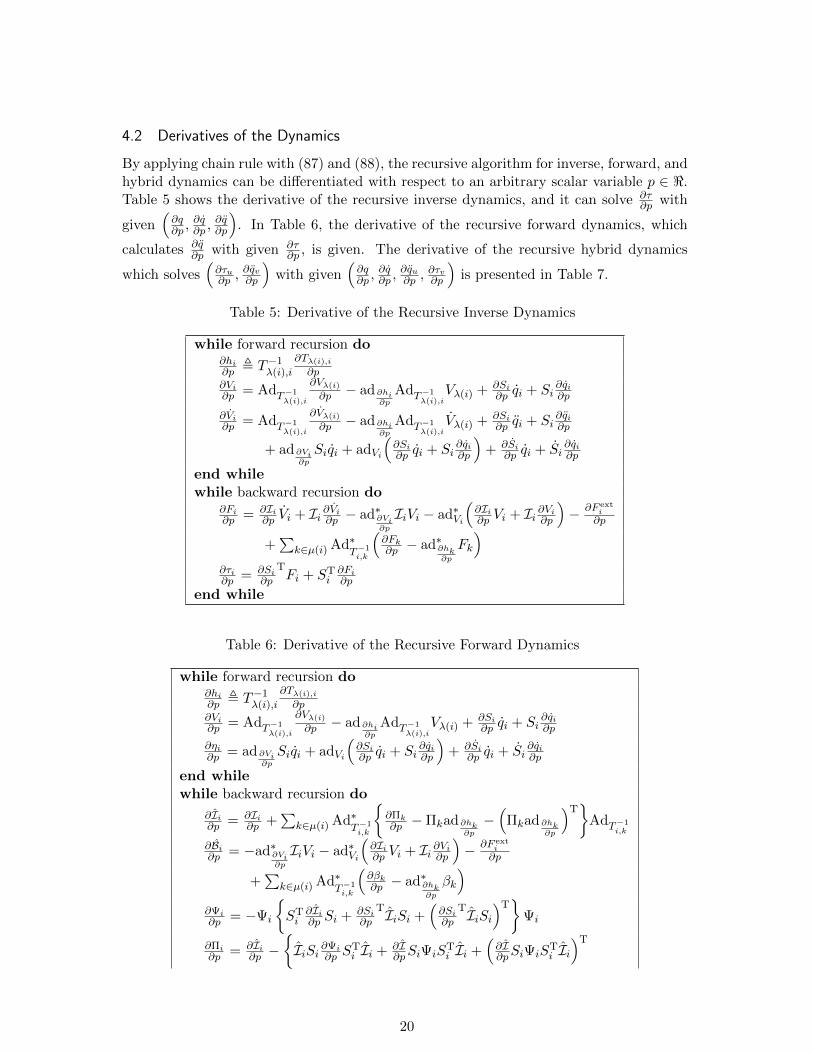
4.2 Derivatives of the Dynamics

By applying chain rule with (87) and (88), the recursive algorithm for inverse, forward, andhybrid dynamics can be differentiated with respect to an arbitrary scalar variable p ∈ <.Table 5 shows the derivative of the recursive inverse dynamics, and it can solve ∂τ

∂p with

given(∂q∂p ,

∂q∂p ,

∂q∂p

). In Table 6, the derivative of the recursive forward dynamics, which

calculates ∂q∂p with given ∂τ

∂p , is given. The derivative of the recursive hybrid dynamics

which solves(∂τu∂p ,

∂qv∂p

)with given

(∂q∂p ,

∂q∂p ,

∂qu∂p ,

∂τv∂p

)is presented in Table 7.

Table 5: Derivative of the Recursive Inverse Dynamics

while forward recursion do∂hi∂p , T−1

λ(i),i

∂Tλ(i),i∂p

∂Vi∂p = AdT−1

λ(i),i

∂Vλ(i)∂p − ad ∂hi

∂p

AdT−1λ(i),i

Vλ(i) + ∂Si∂p qi + Si

∂qi∂p

∂Vi∂p = AdT−1

λ(i),i

∂Vλ(i)∂p − ad ∂hi

∂p

AdT−1λ(i),i

Vλ(i) + ∂Si∂p qi + Si

∂qi∂p

+ ad ∂Vi∂p

Siqi + adVi

(∂Si∂p qi + Si

∂qi∂p

)+ ∂Si

∂p qi + Si∂qi∂p

end whilewhile backward recursion do

∂Fi∂p = ∂Ii

∂p Vi + Ii ∂Vi∂p − ad∗∂Vi∂p

IiVi − ad∗Vi

(∂Ii∂p Vi + Ii ∂Vi∂p

)− ∂F ext

i∂p

+∑

k∈µ(i) Ad∗T−1i,k

(∂Fk∂p − ad∗∂hk

∂p

Fk

)∂τi∂p = ∂Si

∂p

TFi + ST

i∂Fi∂p

end while

Table 6: Derivative of the Recursive Forward Dynamics

while forward recursion do∂hi∂p , T−1

λ(i),i

∂Tλ(i),i∂p

∂Vi∂p = AdT−1

λ(i),i

∂Vλ(i)∂p − ad ∂hi

∂p

AdT−1λ(i),i

Vλ(i) + ∂Si∂p qi + Si

∂qi∂p

∂ηi∂p = ad ∂Vi

∂p

Siqi + adVi

(∂Si∂p qi + Si

∂qi∂p

)+ ∂Si

∂p qi + Si∂qi∂p

end whilewhile backward recursion do

∂Ii∂p = ∂Ii

∂p +∑

k∈µ(i) Ad∗T−1i,k

{∂Πk∂p −Πkad ∂hk

∂p

−(

Πkad ∂hk∂p

)T}

AdT−1i,k

∂Bi∂p = −ad∗∂Vi

∂p

IiVi − ad∗Vi

(∂Ii∂p Vi + Ii ∂Vi∂p

)− ∂F ext

i∂p

+∑

k∈µ(i) Ad∗T−1i,k

(∂βk∂p − ad∗∂hk

∂p

βk

)∂Ψi∂p = −Ψi

{STi∂Ii∂p Si + ∂Si

∂p

TIiSi +(∂Si∂p

TIiSi)T}

Ψi

∂Πi∂p = ∂Ii

∂p −{IiSi ∂Ψi

∂p STi Ii + ∂I

∂pSiΨiSTi Ii +

(∂I∂pSiΨiS

Ti Ii)T

20

+ Ii ∂Si∂p ΨiSTi Ii +

(Ii ∂Si∂p ΨiS

Ti Ii)T}

∂βi∂p = ∂Bi

∂p + ∂Ii∂p

{ηi + SiΨi

(τi − ST

i

(Iiηi + Bi

))}+ I

{∂ηi∂p +

(∂Si∂p Ψi + Si

∂Ψi∂p

)(τi − ST

i

(Iiηi + Bi

))+ SiΨi

(∂τi∂p −

∂Si∂p

T(Iiηi + Bi)− ST

i

(∂Ii∂p ηi + Ii ∂ηi∂p + ∂Bi

∂p

))}end whilewhile forward recursion do

∂qi∂p = ∂Ψi

∂p

{τi − ST

i Ii(AdT−1

λ(i),iVλ(i) + ηi

)− ST

i Bi}

+ Ψi

{∂τi∂p −

(∂Si∂p

TIi + STi∂Ii∂p

)(AdT−1

λ(i),iVλ(i) + ηi

)− ST

i Ii(

AdT−1λ(i),i

∂Vλ(i)∂p − ad ∂hi

∂p

AdT−1λ(i),i

Vλ(i) + ∂ηi∂p

)− ∂Si

∂p

TBi − STi∂Bi∂p

}∂Vi∂p = AdT−1

λ(i),i

∂Vλ(i)∂p − ad ∂hi

∂p

AdT−1λ(i),i

Vλ(i) + ∂Si∂p qi + Si

∂qi∂p + ∂ηi

∂p

∂Fi∂p = ∂Ii

∂p Vi + Ii ∂Vi∂p + ∂Bi∂p

end while

Table 7: Derivative of the Recursive Hybrid Dynamics

while forward recursion do∂hi∂p , T−1

λ(i),i

∂Tλ(i),i∂p

∂Vi∂p = AdT−1

λ(i),i

∂Vλ(i)∂p − ad ∂hi

∂p

AdT−1λ(i),i

Vλ(i) + ∂Si∂p qi + Si

∂qi∂p

∂ηi∂p = ad ∂Vi

∂p

Siqi + adVi

(∂Si∂p qi + Si

∂qi∂p

)+ ∂Si

∂p qi + Si∂qi∂p

end whilewhile backward recursion do

∂Ii∂p = ∂Ii

∂p +∑

k∈µ(i) Ad∗T−1i,k

{∂Πk∂p −Πkad ∂hk

∂p

−(

Πkad ∂hk∂p

)T}

AdT−1i,k

∂Bi∂p = −ad∗∂Vi

∂p

IiVi − ad∗Vi

(∂Ii∂p Vi + Ii ∂Vi∂p

)− ∂F ext

i∂p

+∑

k∈µ(i) Ad∗T−1i,k

(∂βk∂p − ad∗∂hk

∂p

βk

)if i ∈ u then

∂Πi∂p = ∂Ii

∂p∂βi∂p = ∂Bi

∂p + ∂Ii∂p (ηi + Siqi) + Ii

(∂ηi∂p + ∂Si

∂p qi + Si∂qi∂p

)else

∂Ψi∂p = −Ψi

{STi∂Ii∂p Si + ∂Si

∂p

TIiSi +(∂Si∂p

TIiSi)T}

Ψi

∂Πi∂p = ∂Ii

∂p −{IiSi ∂Ψi

∂p STi Ii + ∂I

∂pSiΨiSTi Ii +

(∂I∂pSiΨiS

Ti Ii)T

21

+ Ii ∂Si∂p ΨiSTi Ii +

(Ii ∂Si∂p ΨiS

Ti Ii)T}

∂βi∂p = ∂Bi

∂p + ∂Ii∂p

{ηi + SiΨi

(τi − ST

i

(Iiηi + Bi

))}+ I

{∂ηi∂p +

(∂Si∂p Ψi + Si

∂Ψi∂p

)(τi − ST

i

(Iiηi + Bi

))+ SiΨi

(∂τi∂p −

∂Si∂p

T(Iiηi + Bi)− ST

i

(∂Ii∂p ηi + Ii ∂ηi∂p + ∂Bi

∂p

))}end if

end whilewhile forward recursion do

if i ∈ u then∂Vi∂p = AdT−1

λ(i),i

∂Vλ(i)∂p − ad ∂hi

∂p

AdT−1λ(i),i

Vλ(i) + ∂Si∂p qi + Si

∂qi∂p + ∂ηi

∂p

∂Fi∂p = ∂Ii

∂p Vi + Ii ∂Vi∂p + ∂Bi∂p

∂τi∂p = ∂Si

∂p

TFi + ST

i∂Fi∂p

else

∂qi∂p = ∂Ψi

∂p

{τi − ST

i Ii(AdT−1

λ(i),iVλ(i) + ηi

)− ST

i Bi}

+ Ψi

{∂τi∂p −

(∂Si∂p

TIi + STi∂Ii∂p

)(AdT−1

λ(i),iVλ(i) + ηi

)− ST

i Ii(

AdT−1λ(i),i

∂Vλ(i)∂p − ad ∂hi

∂p

AdT−1λ(i),i

Vλ(i) + ∂ηi∂p

)− ∂Si

∂p

TBi − STi∂Bi∂p

}∂Vi∂p = AdT−1

λ(i),i

∂Vλ(i)∂p − ad ∂hi

∂p

AdT−1λ(i),i

Vλ(i) + ∂Si∂p qi + Si

∂qi∂p + ∂ηi

∂p

∂Fi∂p = ∂Ii

∂p Vi + Ii ∂Vi∂p + ∂Bi∂p

end ifend while

To obtain the derivatives of the dynamics, it is needed to run the associated recursivedynamics in advance, and in addition, the following quantities

∂Si∂p

,∂Si∂p

,∂F ext

i

∂p,∂Ii∂p

, and∂hi∂p

(92)

for each body should be set properly in the initialization step.The algorithms for the derivatives of the dynamics are so general that they can be

applied to differentiating the equations of motion with respect to any arbitrary scalarvariable. It should be noted that, by implementing the algorithms cleverly, the calculationspeed can be much faster than its naive implementation, because, in some cases, many ofthe quantities in (92) are zero. For example,

• if p = qk where qk ∈ < denotes the k-th coordinate of system, then

– ∂Ii∂p = 0

– ∂Si∂p = ∂Si

∂p = ∂hi∂p = 0 when qk /∈ qi

22

• if p = qk, then

– ∂Si∂p = ∂Ii

∂p = ∂hi∂p = 0

– ∂Si∂p = 0 when qk /∈ qi

• if p = qk, then

– ∂Si∂p = ∂Si

∂p = ∂Ii∂p = ∂hi

∂p = 0.

References

[1] Roy Featherstone, Robot Dynamics Algorithms, Kluver Academic Publishers, 1987.

[2] Richard M. Murray, Zexiang Li and and S. Shankar Sastry, A Mathematical Intro-duction to Robotic Manipulation, CRC Press, 1994.

[3] F. C. Park, J. E. Bobrow and S. R. Ploen, “A Lie group formulation of robot dynam-ics,” International Journal of Robotics Research, vol. 14, no. 6, pp. 609-618, 1995.

[4] S. R. Ploen and F. C. Park, “Coordinate-invariant algorithms for robot dynamics,”IEEE Transactions on Robotics and Automation, vol. 15, no. 6, pp. 1130-1136, 1999.

[5] Garett A. Sohl and James E. Bobrow, “A recursive multibody dynamics and sensi-tivity algorithm for branched kinematic chains,” Journal of Dynamic Systems, Mea-surement, and Control, vol. 123, pp. 391-399, 2001.

23