Charles University, Prague Faculty of Mathematics and Physics Institute of Formal and Applied Linguistics Pavel Pecina Lexical Association Measures Collocation Extraction Doctoral Thesis Prague, 2008

Welcome message from author
This document is posted to help you gain knowledge. Please leave a comment to let me know what you think about it! Share it to your friends and learn new things together.
Transcript
Charles University, Prague
Faculty of Mathematics and Physics
Institute of Formal and Applied Linguistics
Pavel Pecina
Lexical Association MeasuresCollocation Extraction
Doctoral Thesis
Prague, 2008

Author: Mgr. Pavel Pecina
Advisor: Prof. RNDr. Jan Hajic Dr.
Opponent: Timothy Baldwin Ph.D., University of Melbourne, Australia
Opponent: Mgr. Jirı Semecky Ph.D., Google, Krakow, Poland
Defense: Prague, September 2008

to my family
iii

iv
v
Abstract
This thesis is devoted to an empirical study of lexical association measures and theirapplication to collocation extraction. We focus on two-word (bigram) collocationsonly. We compiled a comprehensive inventory of 82 lexical association measures andpresent their empirical evaluation on four reference data sets: dependency bigramsfrom the manually annotated Prague Dependency Treebank, surface bigrams from thesame source, instances of surface bigrams from the Czech National Corpus providedwith automatically assigned lemmas and part-of-speech tags, and distance verb-nounbigrams from the automatically part-of-speech tagged Swedish Parole corpus. Col-location candidates in the reference data sets were manually annotated and labeledas collocations and non-collocations. The evaluation scheme is based on measuringthe quality of ranking collocation candidates according to their chance to form col-locations. The methods are compared by precision-recall curves and mean averageprecision scores adopted from the field of information retrieval. Tests of statistical sig-nificance were also performed. Further, we study the possibility of combining lexicalassociation measures and present empirical results of several combination methodsthat significantly improved the performance in this task. We also propose a modelreduction algorithm significantly reducing the number of combinedmeasures withouta statistically significant difference in performance.
Keywords: collocations, multiword expressions, collocation extraction, multiwordexpression extraction, lexical association measures, machine learning, empirical evaluation

vi

vii
Declaration
I hereby declare that this doctoral thesis is the result of my own work, except wherereference is made to the work of others.
In Prague, August 10, 2008 Pavel Pecina

viii
ix
Acknowledgements
This work would not have succeeded without the support of many exceptionalpeople who deserve my special thanks (names in alphabetical order):
• My supervisor JanHajic, for his support duringmy study and for his outstandingleadership of the Institute of Formal and Applied Linguistics.
• Bill Byrne for hosting me at the Center for Language and Speech Processingand other colleagues and friends from the Johns Hopkins University: JasonEisner, Erin Fitzgerald, Arnab Goshal, Laura Graham, Frederick Jelinek, SanjeevKhudanpur, Shankar Kumar, Veera Venkatramani, Paola Virga, Peng Xu, DavidYarowsky.
• My mentor Chris Quirk at Microsoft Research, Redmond and others from theNatural Language Processing group for the great internship I spent with them,namely Bill Dolan, Arul Menezes, Lucy Vanderwende, and others.
• My colleagues from the University of Maryland, College Park and University ofWest Bohemia, Pilsen participating in the Malach project: Xiaoli Huang, PavelIrcing, Craig Murray, Douglas Oard, Josef Psutka, Dagobert Soergel, JianqiangWang, and RyenWhite.
• Allmy colleagues from the Institute of Formal andAppliedLinguistics,especiallythosewho contributed tomy research: SilvieCinkova, JaroslavaHlavacova, PetraHoffmannova, Martin Holub, Michal Marek, Petr Podvesky, Pavel Schlesinger,Otakar Smrz, Miroslav Spousta, Drahomıra Spoustova, and Pavel Stranak.
• My loving wife Eliska, my dear parents Pavel and Hana, and the whole of myfamily.
The work was supported by the Ministry of Education of the Czech Republic,project MSM 0021620838.

x
Contents
1 Introduction 1
1.1 Word association . . . . . . . . . . . . . . . . . . . . . . . . . . . . . . . . 1
1.1.1 Collocational association . . . . . . . . . . . . . . . . . . . . . . . . 2
1.1.2 Semantic association . . . . . . . . . . . . . . . . . . . . . . . . . . 3
1.1.3 Cross-language association . . . . . . . . . . . . . . . . . . . . . . 3
1.2 Motivation and applications . . . . . . . . . . . . . . . . . . . . . . . . . . 4
1.3 Goals, objectives, and limitations . . . . . . . . . . . . . . . . . . . . . . . 7
2 Theory and Principles 11
2.1 Notion of collocation . . . . . . . . . . . . . . . . . . . . . . . . . . . . . . 11
2.1.1 Lexical combinatorics . . . . . . . . . . . . . . . . . . . . . . . . . 11
2.1.2 Historical perspective . . . . . . . . . . . . . . . . . . . . . . . . . 13
2.1.3 Diversity of definitions . . . . . . . . . . . . . . . . . . . . . . . . . 15
2.1.4 Typology and classification . . . . . . . . . . . . . . . . . . . . . . 19
2.1.5 Conclusion . . . . . . . . . . . . . . . . . . . . . . . . . . . . . . . 23
2.2 Collocation extraction . . . . . . . . . . . . . . . . . . . . . . . . . . . . . 24
2.2.1 Extraction principles . . . . . . . . . . . . . . . . . . . . . . . . . . 24
2.2.2 Extraction pipeline . . . . . . . . . . . . . . . . . . . . . . . . . . . 27
2.2.3 Linguistic preprocessing . . . . . . . . . . . . . . . . . . . . . . . . 28
2.2.4 Collocation candidates . . . . . . . . . . . . . . . . . . . . . . . . . 30
2.2.5 Occurrence statistics . . . . . . . . . . . . . . . . . . . . . . . . . . 33
2.2.6 Filtering candidate data . . . . . . . . . . . . . . . . . . . . . . . . 38
xi
xii CONTENTS
3 Association Measures 41
3.1 Statistical association . . . . . . . . . . . . . . . . . . . . . . . . . . . . . . 42
3.2 Context analysis . . . . . . . . . . . . . . . . . . . . . . . . . . . . . . . . . 48
4 Reference Data 53
4.1 Requirements . . . . . . . . . . . . . . . . . . . . . . . . . . . . . . . . . . 53
4.1.1 Candidate data extraction . . . . . . . . . . . . . . . . . . . . . . . 54
4.1.2 Annotation process . . . . . . . . . . . . . . . . . . . . . . . . . . . 55
4.2 Prague Dependency Treebank . . . . . . . . . . . . . . . . . . . . . . . . . 55
4.2.1 Treebank details . . . . . . . . . . . . . . . . . . . . . . . . . . . . . 56
4.2.2 Candidate data sets . . . . . . . . . . . . . . . . . . . . . . . . . . . 58
4.2.3 Manual annotation . . . . . . . . . . . . . . . . . . . . . . . . . . . 61
4.3 Czech National Corpus . . . . . . . . . . . . . . . . . . . . . . . . . . . . . 64
4.3.1 Corpus details . . . . . . . . . . . . . . . . . . . . . . . . . . . . . . 64
4.3.2 Automatic preprocessing . . . . . . . . . . . . . . . . . . . . . . . 65
4.3.3 Candidate data set . . . . . . . . . . . . . . . . . . . . . . . . . . . 67
4.4 Swedish Parole corpus . . . . . . . . . . . . . . . . . . . . . . . . . . . . . 67
4.4.1 Corpus details . . . . . . . . . . . . . . . . . . . . . . . . . . . . . . 68
4.4.2 Support-verb constructions . . . . . . . . . . . . . . . . . . . . . . 68
4.4.3 Manual extraction . . . . . . . . . . . . . . . . . . . . . . . . . . . 69
5 Empirical Evaluation 73
5.1 Evaluation methods . . . . . . . . . . . . . . . . . . . . . . . . . . . . . . . 73
5.1.1 Precision-recall curves . . . . . . . . . . . . . . . . . . . . . . . . . 75
5.1.2 Mean average precision . . . . . . . . . . . . . . . . . . . . . . . . 77
5.1.3 Significance testing . . . . . . . . . . . . . . . . . . . . . . . . . . . 78
5.2 Experiments . . . . . . . . . . . . . . . . . . . . . . . . . . . . . . . . . . . 79
5.2.1 Prague Dependency Treebank . . . . . . . . . . . . . . . . . . . . 80
5.2.2 Czech National Corpus . . . . . . . . . . . . . . . . . . . . . . . . 82
5.2.3 Swedish Parole Corpus . . . . . . . . . . . . . . . . . . . . . . . . 83
5.3 Comparison . . . . . . . . . . . . . . . . . . . . . . . . . . . . . . . . . . . 85
CONTENTS xiii
6 Combining Association Measures 87
6.1 Motivation . . . . . . . . . . . . . . . . . . . . . . . . . . . . . . . . . . . . 87
6.2 Methods . . . . . . . . . . . . . . . . . . . . . . . . . . . . . . . . . . . . . 88
6.2.1 Linear logistic regression . . . . . . . . . . . . . . . . . . . . . . . 89
6.2.2 Linear discriminant analysis . . . . . . . . . . . . . . . . . . . . . 89
6.2.3 Support vector machines . . . . . . . . . . . . . . . . . . . . . . . 89
6.2.4 Neural networks . . . . . . . . . . . . . . . . . . . . . . . . . . . . 90
6.3 Experiments . . . . . . . . . . . . . . . . . . . . . . . . . . . . . . . . . . . 90
6.3.1 Prague Dependency Treebank . . . . . . . . . . . . . . . . . . . . 91
6.3.2 Czech National Corpus . . . . . . . . . . . . . . . . . . . . . . . . 92
6.3.3 Swedish Parole Corpus . . . . . . . . . . . . . . . . . . . . . . . . 93
6.4 Linguistic features . . . . . . . . . . . . . . . . . . . . . . . . . . . . . . . . 95
6.5 Model reduction . . . . . . . . . . . . . . . . . . . . . . . . . . . . . . . . . 96
6.5.1 Algorithm . . . . . . . . . . . . . . . . . . . . . . . . . . . . . . . . 97
6.5.2 Experiments . . . . . . . . . . . . . . . . . . . . . . . . . . . . . . . 98
7 Conclusions 103
A MWE 2008 Shared Task Results 107
A.1 Introduction . . . . . . . . . . . . . . . . . . . . . . . . . . . . . . . . . . . 107
A.2 System overview . . . . . . . . . . . . . . . . . . . . . . . . . . . . . . . . 108
A.3 German Adj-Noun collocations . . . . . . . . . . . . . . . . . . . . . . . . 109
A.3.1 Data description . . . . . . . . . . . . . . . . . . . . . . . . . . . . 109
A.3.2 Experiments and results . . . . . . . . . . . . . . . . . . . . . . . . 109
A.4 German PP-Verb collocations . . . . . . . . . . . . . . . . . . . . . . . . . 110
A.4.1 Data description . . . . . . . . . . . . . . . . . . . . . . . . . . . . 110
A.4.2 Experiments and results . . . . . . . . . . . . . . . . . . . . . . . . 111
A.5 Czech PDT-Dep collocations . . . . . . . . . . . . . . . . . . . . . . . . . . 113
A.5.1 Data description . . . . . . . . . . . . . . . . . . . . . . . . . . . . 113
A.5.2 Experiments and results . . . . . . . . . . . . . . . . . . . . . . . . 114
A.6 Conclusion . . . . . . . . . . . . . . . . . . . . . . . . . . . . . . . . . . . . 114
xiv CONTENTS
B Complete Evaluation Results 117
B.1 PDT-Dep . . . . . . . . . . . . . . . . . . . . . . . . . . . . . . . . . . . . . 118
B.2 PDT-Surf . . . . . . . . . . . . . . . . . . . . . . . . . . . . . . . . . . . . . 119
B.3 CNC-Surf . . . . . . . . . . . . . . . . . . . . . . . . . . . . . . . . . . . . . 120
B.4 PAR-Dist . . . . . . . . . . . . . . . . . . . . . . . . . . . . . . . . . . . . . 121
Bibliography 123

“You shall know a word by the company it keeps!”— John Rupert Firth 1890–1960
xv

xvi
Chapter 1
Introduction
1.1 Word association
Word association is a popular word game based on exchanging words that are in some
way associated together. The game is initialized by a randomly or arbitrarily chosen
word. A player then finds another word associated with the initial one, usually the
first word that comes to his or her mind, and writes it down. A next player does the
same with this word and the game continues in turns until a time or word limit is met.
The amusement of the game comes from the analysis of the resulting chain of words
– how far one can get from the initial word and what the logic behind the individual
associations is. An example of a possible run of the gamemight be this word sequence:
dog, cat, meow, woof, bark, tree, plant, green, grass, weed, smoke, cigarette, lighter, fluid.1
Similar concepts are commonly used in psychology to study a subconscious mind
based on subject’s word associations and disassociations, and in psycholinguistics to
study the way knowledge is structured in the human mind, e.g. by word association
norms measured as subject’s responses to words when preceded by associated words
(Palermo and Jenkins, 1964). “Generally speaking, subjects respond quicker than nor-
mal to the word nurse if it follows a highly associated word such as doctor” (Church
and Hanks, 1989).
Our interest in word association is linguistic and hence we use the term lexical as-
sociation to refer to association between words. In general, we distinguish between three
types of association betweenwords: collocational association restricting combination
of words into phrases (e.g. crystal clear, cosmetic surgery, weapons of mass destruction),
1examples from http://www.wordassociation.org/
1
2 CHAPTER 1. INTRODUCTION
semantic association reflecting semantic relationship between words (e.g. sick – ill,
baby – infant, dog – cat), and cross-language association corresponding to potential
translations of words between different languages (e.g.maison (FR) – house (EN), baum
(GER) – tree (EN), kvetina (CZ) – flower (EN)).
In the word association game and the fields mentioned above, it is a human mind
what directly provides evidence for exploring word associations. In this work, our
source of such evidence is a corpus – a collection of texts containing examples of
word usages. Based on such data and its statistical interpretation, we attempt to
estimate lexical associations automatically by means of lexical association measures
determining the strength of association between two or more words based on their
occurrences and cooccurrences in a corpus. Although our study is focused on the
association on the collocational level only, most of these measures can be easily used
to explore also other types of lexical association.
1.1.1 Collocational association
The process of combining words into phrases and sentences of natural language is
governed by a complex system of rules and constraints. In general, basic rules are
given by syntax, however there are also other restrictions (semantic and pragmatic)
that must be adhered to in order to produce correct, meaningful, and fluent utterances.
These constrains form important linguistic and lexicographic phenomena generally
denoted by the term collocation. They range from lexically restricted expressions
(strong tea, broad daylight), phrasal verbs (switch off, look after), technical terms (car oil,
stock owl), and proper names (New York, Old Town), to idioms (kick the bucket, hear
through the grapevine), etc. As opposed to free word combinations, collocations are
not entirely predictable only on the basis of syntactic rules. They should be listed in
a lexicon and learned in the same way as single words are.
Components of collocations are involved in a syntactic relation and tend to cooc-
cur (in this relation) more often than would be expected. This empirical aspect dis-
tinguishes them from free word combinations. Collocations are often characterized
by semantic non-compositionality – the exact meaning of a collocation cannot be
(fully) inferred from the meaning of its components (kick the bucket), syntactic non-
modifiability – their syntactic structure cannot be freely modified, e.g. by changing
the word order, inserting another word, or changing morphological categories (poor
as a church mouse vs. *poor as a big church mouse), and lexical non-substitutability –
collocation components cannot be substituted by synonyms or other related words
1.1. WORD ASSOCIATION 3
(stiff breeze vs. *stiff wind) (Manning and Schutze, 1999, Chapter 5). Another property
of some collocations is their translatability into other languages: a translation of a
collocation cannot generally be performed blindly, word by word (e.g. the two-word
collocation ice cream in English should be translated as one word zmrzlina, or perhaps
as zmrzlinovy krem (rarely) but not as ledovy krem which would be a straightforward
word-by-word translation).
1.1.2 Semantic association
Semantic association between words is, in a sense, a broader concept then colloca-
tional association because in this type of association no grammatical boundedness
between words is required. It is concerned with words that are used in similar con-
texts and domains – word pairs whosemeanings are in some kind of semantic relation.
Compiled information of such type is usually presented in the form of a thesaurus
and includes the following types of relationships: synonyms with exactly or nearly
equivalent meaning (car – automobile, glasses – spectacles), antonymswith the opposite
meaning (high – low, love – hate), meronyms with the part-whole relationship (door –
house, page –book), hyperonyms based on superordination (building – house, tree – oak),
hyponymsbased on subordination (lily – flower, car –machine), and perhaps otherword
combinations with even looser relations (table – chair, lecture – teach).
Semantic association is closest to the process involved in the word gamementioned
in the beginning of this chapter. Although presented as a relation between words
themselves, the actual association exists between their meanings (concepts). Before
a word association emerges in the human mind, the initial word is semantically dis-
ambiguated and only one selected sense of the word participates in the association,
e.g. theword bark has different meaning in association withwoof and tree. For the same
reason, semantic association exists not only between single words but also between
multiword expressions constituting indivisible semantic units (collocations).
Similarly to collocational association, semantically associated words cooccur in
the same context more often than would be expected, but in this case the context is
understood as a much wider span of words and, as we have already mentioned, no
direct syntactic relation between the words is necessary.
1.1.3 Cross-language association
Cross-language association correspond to possible translations of a word in one lan-
guage to another. This information is usually presented in a form of a bilingual
4 CHAPTER 1. INTRODUCTION
dictionary, where each word with all its senses is provided with all its equivalents in
the other language. Although every word (in one of its meanings) usually has one or
two common and generally accepted translations sufficient to understand itsmeaning,
it can be potentially expressed by a larger number of (more or less equivalent but in
a certain context entirely adequate) options. For example, the Czech adjective dulezity
is in most dictionaries translated into English as important or significant, but in a text
it can be translated also as: considerable, material, momentous, high, heavy, relevant, solid,
considerably, live, substantial, serious, notable, pompous, responsible, consequential, gutty,
great, grand, big, major, solemn, guttily, fateful, grave, weighty, vital, fundamental,2 and pos-
sibly also as other options depending on context. Not even a highly competent speaker
of both languages could not be expected to enumerate them exhaustively. Similarly
to the case of semantic association, dictionary items are not only single words but
also multiword expressions which cannot be translated in a word-by-word manner
(collocations).
Cross-language association can be acquired not only from the human mind, it can
also be extracted from examples of already realized translations, e.g. in the form of
parallel texts – where texts (sentences) are placed alongside their translations. In such
data, associated word pairs (translation equivalents) cooccur more often that would
be expected in the case of non-associated (random) pairs.
1.2 Motivation and applications
A monolingual lexicon enriched by collocations, a thesaurus comprised of semanti-
cally related words, and a bilingual dictionary containing translation equivalents –
all of these are important (and mutually interlinked) resources not only for language
teaching but in a machine-readable form also for many tasks of computational linguistics
and natural language processing.
The traditional manual approaches to building these resources are in many ways
insufficient (especially for computational use). The major problem is their lack of ex-
haustiveness and completeness. They are only “snapshots of a language”.3 Although
modern lexicons, dictionaries, and thesauri are developed with the help of language
corpora, utilization of these corpora is usually quite shallow and reduced to analysis
of the most frequent and typical word usages. Natural language is a live system and
no such resource can perhaps be ever be expected to be complete and fully reflect
actual language use. All these resources must also deal with the problem of domain
2translations from http://slovnik.seznam.cz/3quote by Yorick Wilks, LREC 2008, Marrakech, Morocco
1.2. MOTIVATION AND APPLICATIONS 5
specificity. Either they are general, domain-independent and thus in special domains
usable only to a certain extent, or they are specialized, domain-specific and exist only
for certain areas. Considerable limitations lie in the fact that the manually built re-
sources are discrete in character, while lexical association, as presented in this work,
should be perceived as a continuous phenomenon. Manually built language resources
are usually reliable and contain a small number of errors andmistakes. However, their
development is an expensive and time-consuming process.
Automatic approaches extract association data on the basis of statistical interpre-
tation of corpus evidence (by lexical association measures). They should eliminate (to
a certain extent) all the mentioned disadvantages (lack of exhaustiveness and com-
pleteness, domain-specificity, continuousness). However, they heavily rely on the
quality and extent of the source corpora the associations are extracted from. Com-
pared to manually built resources, the automatically built ones contain certain errors
and this fact must be taken into account in the tasks these resources are applied. The
following passages we will present some tasks that can make use of such resources.
Applications of lexical association measures
Generally, collocation extraction is the most popular application of lexical association
measures and quite a lot of significant studies have been published on this topic,
e.g. (Dunning, 1993; Smadja, 1993; Pedersen, 1996; Weeber et al., 2000; Schone and
Jurafsky, 2001; Pearce, 2002; Krenn, 2000; Bartsch, 2004; Evert, 2004). In computational
lexicography, automatic identification of collocations is employed to help human
lexicographers in compiling lexicographic information (identification of possible word
senses, lexical preferences, usage examples, etc.) for traditional lexicons (Church and
Hanks, 1990) or for special lexicons of idioms or collocations (Klegr et al., 2005; Cermak
et al., 2004), used e.g. in translation studies (Fontenelle, 1994a), bilingual dictionaries,
or for language teaching (Smadja et al., 1996; Haruno et al., 1996; Tiedemann, 1997;
Kita and Ogata, 1997; Baddorf and Evens, 1998). Collocations play an important role
in systems of natural language generationwhere lexicons of collocations and frequent
phrases are used during the process of word selection in order to enhance fluency
of the automatically generated text (Smadja and McKeown, 1990; Smadja, 1993; Stone
and Doran, 1996; Edmonds, 1997; Inkpen and Hirst, 2002).
There are two principles applicable for word sense disambiguation: First, a word
with a certain meaning tends to cooccur with different words than when it is used
in another sense, e.g. bank as a financial institution occurs in context with words
6 CHAPTER 1. INTRODUCTION
like money, loan, interest, etc., while bank as land along the side of a river or lake
occurs with words like river, lake, water, etc. (Justeson and Katz, 1995; Resnik, 1997;
Pedersen, 2001; Rapp, 2004). Second, according to Yarowsky’s (1995) “one sense per
collocation”hypothesis, all occurrences of aword in the same collocation have the same
meaning, e.g. the sense of the word river in the collocation river bank is the same across
all its occurrences. There has also been some research on unsupervised discovery
of word senses from text (Pantel and Lin, 2002; Tamir and Rapp, 2003). Association
measures are used also for detecting semantic similarity between words, either on
a general level (Biemann et al., 2004) or with a focus to specific relationships, such as
synonymy (Terra and Clarke, 2003) or antonymy (Justeson and Katz, 1991).
An important application of collocations is in machine translation. Collocations
often cannot be translated in a word-by-word fashion. In translation, they should
be treated rather as lexical units distinct from syntactically and semantically regular
expressions. In this environment, association measures are employed in the identi-
fication of translation equivalents from sentence aligned parallel corpora (Church
and Gale, 1991; Smadja et al., 1996; Melamed, 2000) and also from non-parallel corpora
(Rapp, 1999; Tanaka and Matsuo, 1999). In statistical machine translation, associa-
tion measures are used over sentence aligned, parallel corpora to perform bilingual
word alignment to identify translation pairs of words and phrases (or more complex
structures) stored in the form of translation tables and used for constructing possible
translation hypotheses (Mihalcea and Pedersen, 2003; Moore et al., 2006).
Application of collocations in information retrieval has been studied as a nat-
ural extension of indexing single word terms to multiword units (phrases). Early
studies were focused on small domain-specific collections (Lesk, 1969; Fagan, 1987;
Fagan, 1989) and yielded inconsistent and minor performance improvement. Later,
similar techniques were applied over larger, more diverse collections within the Text
Retrieval Conference (TREC)4 but still with only minor success (Evans and Zhai, 1996;
Mittendorf et al., 2000; Khoo et al., 2001). Other studies were only motivated by infor-
mation retrievalwith no actual application presented (Dias et al., 2000). Recently, some
researchers have attempted to incorporate cooccurrence information in probabilistic
models (Vechtomova, 2001) but no consistent improvement in performance has been
demonstrated (Alvarez et al., 2004; Jiang et al., 2004). Despite these results, using collo-
cations in information retrieval is still of relatively high interest (Arazy andWoo, 2007).
Collocational phrases have also been employed also in cross-lingual information re-
trieval (Ballesteros and Croft, 1996; Hull and Grefenstette, 1996). A significant amount
4http://www.trec.org/
1.3. GOALS, OBJECTIVES, AND LIMITATIONS 7
of work has been done in the area of identification of technical terminology (Anani-
adou, 1994; Justeson and Katz, 1995; Fung et al., 1996; Maynard and Ananiadou, 1999)
and its translation (Dagan and Church, 1994; Fung and McKeown, 1997).
Lexical association measures have been applied to various other tasks from which
we select the following examples: named entity recognition (Lin, 1998), syntactic con-
stituent boundary detection (Magerman and Marcus, 1990), syntactic parsing (Church
et al., 1991; Alshawi and Carter, 1994), syntactic disambiguation (Basili et al., 1993),
discourse categorization (Wiebe and McKeever, 1998), adapted language modeling
(Beefermam et al., 1997), extracting Japanese-English morpheme pairs from bilingual
terminological corpora (Tsuji and Kageura, 2001), sentence boundary detection (Kiss
and Strunk, 2002b), identification of abbreviations (Kiss and Strunk, 2002a), computa-
tion of word associations norms (Rapp, 2002), topic segmentation and link detection
(Ferret, 2002), discoveringmorphologically relatedwords based on semantic similarity
(Baroni et al., 2002) and possibly others.
1.3 Goals, objectives, and limitations
This thesis is devoted to lexical association measures and their application to collo-
cation extraction. The importance of this research was demonstrated in the previous
section by the large range of applications in natural language processing and com-
putational linguistics where the role of lexical association measures in general, or
collocation extraction in particular, is essential. This significance was emphasized
already in 1964 at the Symposium on Statistical Association Methods ForMechanized Docu-
mentation (Stevens et al., 1965), where Giuliano advocated better understanding of the
measures and their empirical evaluation (as cited by Evert (2004), p. 19):
[First,] it soon becomes evident [to the reader] that at least a dozen
somewhat different procedures and formulae for association are suggested
[in the book]. One suspects that each has its own possible merits and
disadvantages, but the line between the profound and the trivial often
appears blurred. One thing which is badly needed is a better understand-
ing of the boundary conditions under which the various techniques are
applicable and the expected gains to be achieved through using one or
the other of them. This advance would primarily be one in theory, not
in abstract statistical theory but in a problem-oriented branch of statistical
theory. (Giuliano, 1965, p. 259)
8 CHAPTER 1. INTRODUCTION
[Secondly,] it is clear that carefully controlled experiments to evaluate
the efficacy and usefulness of the statistical association techniques have
not yet been undertaken except in a few isolated instances . . . Nonetheless,
it is my feeling that the time is now ripe to conduct carefully controlled
experiments of an evaluative nature, . . . (Giuliano, 1965, p. 259).
Since that time, the issue of lexical association has attracted many researchers and
a number of works have been published in this field. Among those related to collo-
cation extraction we point out especially: Chapter 5 in (Manning and Schutze, 1999),
Chapter 15 by McKeown and Radev in (Dale et al., 2000), theses of Krenn (2000), Vech-
tomova (2001), Bartsch (2004), Evert (2004), and Moiron (2005). Our work attempts to
enrich the current state of the art in this field in by achieving the following goals:
1) Compilation of a comprehensive inventory of lexical association measures
The range of various association measures proposed to estimate lexical association
based on corpus evidence is enormous. They originate mostly in mathematical statis-
tics, but also in other (both theoretical and applied) fields. Most of them were tar-
geted mainly for collocation extraction, e.g. (Church and Hanks, 1990; Dunning, 1993;
Smadja, 1993; Pedersen, 1996). The early publicationswere devoted to individual asso-
ciation measures, their formal and practical properties, and to the analysis of their ap-
plication to a corpus. The first overview text appeared in (Manning and Schutze, 1999,
Chapter 5). It described the three most popular association measures (and also other
techniques for collocation extraction). Later, other authors, e.g. Weeber et al. (2000),
Schone and Jurafsky (2001), and Pearce (2002), attempted to describe (and compare)
multiple measures. However, none of them, at the time our research started, had as-
pired to compile a comprehensive inventory of possible lexical association measures.
A significant contribution in this direction was made by Stephan Evert, who set up
a web page to “provide a repository for the large number of association measures that
have been suggested in the literature, together with a short discussion of their math-
ematical background and key references”5. This effort, however, has focused only on
measures applied to 2-by-2 contingency tables representing cooccurrence frequencies
ofword pairs, see details in (Evert, 2004). Our goal is to provide amore comprehensive
list of measures without this restriction. Such measures should be applicable to deter-
mine various types of lexical association but our key application and main research
interest are in collocation extraction. The theoretical background to the concept of
5http://www.collocations.de/
1.3. GOALS, OBJECTIVES, AND LIMITATIONS 9
collocation and principles of collocation extraction from text corpora are covered in
Chapter 2, and the inventory of lexical association measures is presented in Chapter 3.
2) Acquisition of reference data for collocation extraction
At the time we started our research, no widely acceptable evaluation resources for
collocation extraction were available. In order to evaluate our experiments we were
compelled to develop appropriate gold standard reference data sets on our own. This
comprised several important steps: to specify the task precisely, select a suitable
source corpus, define annotation guidelines, perform annotation by multiple subjects,
and combine their judgments. The entire process and details of the acquired reference
data sets are discussed in Chapter 4.
3) Empirical evaluation of association measures for collocation extraction
A request for empirical evaluation of association measures in specific tasks was made
already by Giuliano in (1965). Later, other authors also emphasized the importance of
such evaluation in order to determine “efficacy and usefullness” of different measures
in different tasks and suggested various evaluation schemes for comparative evalua-
tion of collocation extraction methods, e.g. Kita et al. (1994) or Evert and Krenn (2001).
Empirical evaluation studies were published e.g. by Pearce (2002) and Thanopoulos et
al. (2002). A comprehensive study of statistical aspects of word cooccurrences can be
found in Evert (2004) or Krenn (2000).
Our evaluation scheme should be based on ranking, not classification, and it should
reflect the ability of association measure to rank potential collocations according to
their chance to form true collocations (judged by human annotators). Special attention
should be paid to statistical significance tests of the evaluation results. Evaluation
experiments, their results, and comparison are described in Chapter 5.
4) Combination of association measures for collocation extraction
The major contribution of our work lies in the investigation of the possibility for com-
bining associationmeasures intomore complexmodels and thus improve performance
in collocation extraction. Our approach is based on application of supervisedmachine
learning techniques and the fact that different measures discover different colloca-
tions. This novel insight into the application of association measures for collocation
extraction is explored in Chapter 6.
10 CHAPTER 1. INTRODUCTION
Limitations
In this work, no special attention is paid to semantic and cross-language association as
discussed earlier in this chapter. We focus entirely on collocational association and the
study of methods for automatic collocation extraction from text corpora. However, the
inventory of association measures presented in this work, the evaluation scheme, as
well as the principle of combining associationmeasures can be easily adapted and used
for other types of lexical association. As can be judged from the volume of published
works in this field, collocation extraction has been the most popular application of
lexical association measures. The high interest in this field is also expressed in the
activities of the ACL Special Interest Group on the Lexicon (SIGLEX) and the long
tradition of workshops focused on problems related to this field.6
Further, our attention is restricted exclusively to two-word (bigram) collocations –
primarily for the limited scalability of somemethods to higher-order n-grams and also
for the reason that experiments with longer expressions would require processing of
a much larger corpus to obtain enough evidence of the observed events. For example,
the Prague Dependency Treebank (see Chapter 4) contains about 623 000 different depen-
dency bigrams – about 27 000 of them occur with frequency greater then five, which
we consider sufficient evidence for our purposes. The same data contains more then
twice as many trigrams (1 715 000), but only half the number (14 000) occurring more
than five times.
The methods we propose in our work are language independent, although some
language-specific tools are required for linguistic preprocessing of source corpora
(e.g. part-of-speech taggers, lemmatizers, and syntactic parsers). However, the eval-
uation results are certainly language dependent and cannot be easily generalized for
other languages. Mainly due to time and source constraints, we perform our experi-
ments only on a limited selection of languages: Czech, Swedish, and German.
Somepreliminary results of this research have already beenpublished (Pecina, 2005;
Pecina and Schlesinger, 2006; Cinkova et al., 2006; Pecina, 2008a; Pecina, 2008b).
6ACL 2001 Workshop on Collocations, Toulouse, France; 2002 Workshop on Computational Ap-proaches to Collocations, Vienna, Austria; ACL 2003 Workshop on Multiword Expressions: Analysis,Acquisition and Treatment, Sapporo, Japan; ACL 2004Workshop onMultiword Expressions: IntegratingProcessing, Barcelona, Spain; COLING/ACL 2006Workshop onMultiword Expressions: Identifying andExploiting Underlying Properties, Sydney, Australia; EACL 2006 Workshop on Multi-word-expressionsin a multilingual context, Trento, Italy; 2006 Workshop on Collocations and idioms: linguistic, computa-tional, and psycholinguistic perspectives, Berlin, Germany; ACL 2007Workshopon aBroaderPerspectiveon Multiword Expressions, Prague, Czech Republic; LREC 2008 Workshop, Towards a Shared Task forMultiword Expressions, Marrakech, Morocco.
Chapter 2
Theory and Principles
This chapter is devoted to the theoretical background to collocations and principles
of collocation extraction from text corpora. First, we present the notion of colloca-
tion based on the work of F. Cermak who introduced this concept into Czech lin-
guistics (1982). It is followed by an overview of various other approaches to this
phenomenon presented from the perspective of theoretical and also applied linguis-
tics. In the second half of the chapter, we describe details of the process of collocation
extraction employed in the experimental part of this thesis.
2.1 Notion of collocation
The term collocation is derived from the Latin collorale (to place side by side, to co-
locate). In linguistics it is usually related to co-location of words, and the fact that
they can not be combined freely and randomly only by the rules of grammar. It is
a borderline phenomenon ranging between lexicon and grammar and as such it is
quite difficult to define and treat systematically. The folowing sections are intended to
illustrate the diverse notions of collocation advocated by various researchers.
2.1.1 Lexical combinatorics
Although in traditional linguistics, lexis (vocabulary) and grammar (morphology and
syntax)were perceived as separate anddistinct components of a natural language, they
are nowadays considered inseparable and completely interdependent. Syntactic rules
are not the only restrictions imposed on arranging words into meaningful expressions
11
12 CHAPTER 2. THEORY AND PRINCIPLES
and sentences. Cermak (2006) emphasizes that semantic rules are thosewhich primar-
ily govern the combination of words. These rules determine semantic compatibility,
i.e. whether a lexical combination is meaningful or not (or to what extent), which
combinations are (proto)typical and most frequent, which are common and ordinary,
marginal and abnormal, orwhich are impossible. Syntax then plays only a subordinate
role in the process of lexical selection. Omitting the semantic rules generally leads to
grammatically correct but meaningless expressions and sentences. As a well-taken ex-
ample, Cermak (2006) gives the famous sentence composed byNoamChomsky (1957):
Colorless green ideas sleep furiously. Each word combination in this sentence (and thus
the sentence itself) is grammatically correct but nonsensical in meaning1.
In general, the ability of a word to combine with other words in text (or speech) is
called collocability. It is governed by both semantic and grammatical (and pragmatic)
rules and expressed in terms of paradigms – sets of words substitutable (functionally
equivalent) in a specific context (as a combination with a given word). It can be
specified either intensionally – by a description of the same syntactic and semantic
properties, which forms valency or extensionally – by enumeration, where no summary
specification can be applied. On this basis, Cermak and Holub (1982, p. 10) defined
collocation as a realization of collocability in text, and later (2001) as a “meaningful
combinationofwords [...] respecting theirmutual collocability andalso compatibility”.
Naturally, different words have a different degree of collocability (examples from
Cermak, 1982): On one hand, words like be, good, and thing can be combined with
a wide range of otherwords and only general (syntactic) rules are required for produc-
ing correct expressionswith such words. On the other hand, the collocability of words
like bark, cubic, and hypertension is more restricted and knowledge of these (semantic)
constraints is quite useful (togetherwith the general rules) to produce a more cohesive
text. Furthermore, there are words that can be combined with only one or a select few
others; their knowledge (lexical and pragmatic) is absolutely essential for their correct
usage in language, and they cannot be used otherwise (no general rules apply).
The scale of collocability ranges from free word combinations whose component
words can be substituted by anotherword (i.e. synonym)without significant change in
the overallmeaning and if omitted, they can not be easily predicted from the remaining
components, to idiomswhose semantics can not be inferred from the meanings of the
components. Cermak’s notion of collocation based on mutual collocability and com-
patibility spans a wide range of this scale. The resarch in natural language processing
1Although the expression green ideas can nowadays have a figurative meaning and be interpreted asideas that are ”environmentally friendly.”
2.1. NOTION OF COLLOCATION 13
is usually focused on the narrower concept: word combinations with extensionally
restricted collocability – in literature described as significant (Sinclair, 1966), habit-
ual, fixed, anomalous and holistic (Moon, 1998), unpredictable, mutually expected
(Palmer, 1968), mutually selective (Cruse, 1986), or idiosyncratic (Sag et al., 2002).
2.1.2 Historical perspective
The idea of collocation was first introduced into linguistics by Harold E. Palmer (1938),
an English linguist and teacher. As a concept, however, collocations were studied by
Greek Stoic philosophers as early as in the third century B.C. They believed that “word
meanings do not exist in isolation, andmay differ according to the collocation in which
they are used” (Robins, 1967). Palmer (1938) defined collocations as “successions of
two or more words the meaning of which can hardly be deduced from a knowledge
of their component words” and pointed out that such concepts “must each be learnt
as one learns single words”, e.g. at least, give up, let alone, as a matter of fact, how do you
do. See also (Palmer and Hornby, 1937). Collocations as a linguistic phenomenonwere
studied mostly in British linguistics (Firth, Halliday, Sinclair) and rather neglected in
structural linguistics (Saussure, Chomsky).
An important contribution to the theoretical research of collocations was made by
John R. Firth who used the concept of collocation in his study of lexis to define amean-
ing of a single word (Firth, 1951; Firth, 1957). He introduced the term meaning by
collocation as a new mode of meaning of words and distinguished it from both the
“conceptual or idea approach to the meaning of words” and “contextual meaning”.
Uniquely, he attempted to explain it at the syntagmatic, not the traditional paradig-
matic, level (by semantic relations such as synonymyor antonymy)2. With the example
dark night, he claimed that one of themeanings of night is its collocability with dark, and
one of the meanings of dark is its collocability with night. Thus, a complete analysis
of the meaning of a word would have to include all its collocations. In (1957, p. 181),
he defined “collocations of a given word” as “statements of the habitual or customary
places of that word.” Later (1968), he used a more famous definition and described
collocation as “the company a word keeps”.
Firth’s students and disciples, known as Neo-Firthians, further developed his the-
ory. They regarded lexis as complementary to grammar and used collocations as the
basis for a lexical analysis of language alternative to (and independent from) the gram-
2The paradigmatic relationship of lexical items consists of sets of words belonging to the same classthat can be substituted for one another in a certain grammatical and semantic context. The syntagmaticrelationship of lexical items refers to the ability of a word to combine with other words (collocability).
14 CHAPTER 2. THEORY AND PRINCIPLES
matical analysis. They argued that grammatical description does not account for all
the patterns in a language, and promoted the study of lexis on the basis of corpus-
based observations. Halliday (1966) defined collocation as “a linear co-occurrence
relationship among lexical items which co-occur together” and introduced the term
set as “the grouping of members with like privilege of occurrence in collocation”. For
example, bright, hot, shine, light, and come out belong to the same lexical set, since they
all collocate with the word sun (Halliday, 1966, p. 158).
Sinclair (1966) also regardedgrammar and lexicon as “twodifferent interpenetrating
aspects”. Hedealt with quite general “tendencies” of lexical items to collocatewith one
anotherwhich “ought to tell us facts about language that cannot be got by grammatical
analysis”. He introduced the following terminology for the structure of collocations:
a node as the item whose collocations are studied, a span as the number of lexical
items on each side of a node that are considered relevant to that node, and collocates
as the items occurring within the span. He even argued that “there are virtually no
impossible collocations, but some are much more likely than others” (1966, p. 411) but
later distinguished between casual collocations and significant collocations that “occur
more frequently than would be expected on the basis of the individual items”. In
(1991, p. 170), he defined collocation directly as “occurrence of two or more words
within a short space of each other in a text”, where “short space” is suggested as
a maximum of four words intervening together. He also added that “Collocations can
be dramatic and interesting because unexpected, or they can be important in the lexical
structure of the language because of being frequently repeated.”
Halliday and Hasan (1967, p. 287) described collocation as “a cover term for the
cohesion that results from the cooccurrence of lexical items that are in some way or
other typically associated with one another, because they tend to occur in similar
environments” and gave examples such as: sky – sunshine – cloud – rain or poetry –
literature – reader – writer – style, etc.
Mitchell (1971) considered lexis and grammar as interdependent, not separate and
discrete, but forming a continuum. He argued for the “oneness of grammar, lexis and
meaning” (p. 43) and suggested collocations “to be studiedwithin grammatical matri-
ces [which] in turndepend for their recognition on the observation of collocational sim-
ilarities” (p. 65). By the grammatical matrices he understood patterns such as adjective
– noun, verb – adverb, or verb – gerund. Fontenelle (1994b), on the other hand, perceived
the concept of collocation as “independent of grammatical categories: the relationship
which holds between the verb argue and the adverb strongly is the same as that holding
between the noun argument and the adjective strong” (Fontenelle, 1994b, p. 43).
2.1. NOTION OF COLLOCATION 15
2.1.3 Diversity of definitions
The disagreement on the notion of collocation among different linguists is quite re-
markable not only in historical context but also in current research. Noneof the existing
definitions of collocation is commonly accepted either in formal or computational lin-
guistics. In general, the definitions are based on five fundamental aspects, which we
will address in the following passages (cf. Moon (1998) and Bartsch (2004)):
1) grammatical boundedness,
2) lexical selection,
3) semantic cohesion,
4) language institutionalization,
5) frequency and recurrence.
1) Grammatical boundedness
By grammatical boundedness we mean a (direct) syntactic relationsip between com-
ponents of collocation. This criterion was omitted in early studies on collocations.
Sinclair’s concept of collocation presented in the previous section (Sinclair, 1966) sug-
gests that all occurrences (including those not grammatically bounded) of two or more
words can be considered collocations. More notably, Halliday’s and Hasan’s (1967)
definition describing words which ”tend to occur in similar environments“ directly
implies that collocations do not necessarily appear as grammatical units with a specific
word order, e.g. hair, comb, curl, wave or candle, flame, flicker (see also above). Halliday
and Hasan (1967, p. 287) even emphasized that they are ”largely independent of the
grammatical structure“. For such classes of words that are “likely to be used in the
same context” (semantically related but not syntactically dependent) Manning and
Schutze (1999, p. 185) suggested to use the terms association or co-occurrence, e.g. doc-
tor, nurse, hospital. In his later work, Hasan (1984) rejected his previous definition of
collocation as too broad and used the term lexical chain for this concept.
The grammatical aspect became important in the notion of collocation based on
lexical collocability (see below). Also Kjellmer (1994, p. xiv) explicitly defined col-
locations as “reccuring sequences that are grammatically well formed”. Similarly,
Choueka (1988) used the expression “a syntactic and semantic unit” in his definition of
collocation. Although, most of the current definitions are not explicit about grammati-
cal boundedness, they usually assume that collocations form grammatical expressions
implicitly.
16 CHAPTER 2. THEORY AND PRINCIPLES
2) Lexical selection
The process of lexical selection in natural language production (generation) is closely
related to collocability (expressing the ability of words to be combined with other
words, see Section 2.1.1). Collocations (as opposed to freeword combinations) are often
characterized by restricted (or preferred) lexical selection, i.e. not-easily-explainable
patterns of word usage (Manning and Schutze, 1999, p. 141). For example, Meals will
be served outside on the terrace, weather permitting. vs. *Meals will be served outside on the
terrace, weather allowing. Although to allow and to permit have very similar meanings,
in this combination, only permitting is correct. For the same reason (examples from
Manning andSchutze,1999): stiff breeze is correct but *stiffwind is not, strong tea is correct
and *powerful tea not, although powerful drugs and strong cigarette are correct too.
Constrained lexical selection (morpho-syntactic preference) is what distinguishes
free word combinations from collocations, which Bahns (1993, p. 253) depicted as
“springing to mind in such a way as to be said to be psychologically salient”. Kjellmer
(1991, p. 112) claimed that “the occurrence of one of the words in such combination
can be said to predict the occurrence of the other(s)”. Similarly Bartsch (2004, p. 11)
claimed that “the choice of one of the constituents appears to automatically trigger
the selection of one or more other constituents in their immediate context” and “block
the selection of other lexical items that, according to their meaning and morpho-
syntactic properties, appear to be eligible choices in the same expression”. Bartsch
(2004, p. 60) also discussed directionality of the process of co-selection, but for the
notion of collocation it seems not important.
3) Semantic cohesion
The criterion of semantic cohesion reflects the semantic transparency or opacity (com-
positionality or non-compositionality) of word combinations. Many researchers use
cohesion to distinguish between idioms and collocations as different lexical phenom-
ena. Benson (1985, p. 62) clearly stated that “the collocations [...] are not idioms:
their meanings are more or less inferrable from the meanings of their parts”. Idioms
do not reflect the meanings of their component parts at all, whereas the meaning of
collocations does reflect the meanings of the parts (Benson et al., 1986, p. 253).
Cruse (1986, p. 37–41) also distinguished between collocations and idioms. He
perceived idioms as “lexically complex” units, constituting a “single minimal semantic
constituent”, “whose meaning cannot be inferred from the meaning of its parts”.
He used the term collocation to “refer to sequences of lexical items which habitually
co-occur, but which are nonetheless fully transparent in the sense that each lexical
2.1. NOTION OF COLLOCATION 17
constituent is also a semantic constituent” an gave examples such as fine weather,
torrential rain, light drizzle, and high winds. He also added that they are “easy to
distinguish from idioms; nonetheless they do have a kind of semantic cohesion – the
constituent elements are, to varying degrees, mutually selective”. The cohesion is
especially evident when “the meaning carried by one (or more) of the constituent
elements is highly restricted contextually, and different from its meaning in more
neutral contexts”. He also introduces “bound collocations” as expressions “whose
constituents do not like to be separated” and “transitional area bordering on idiom”
(e.g. foot the bill and curry flavour).
Fontenelle (1994b) stated that collocations are both “non-idiomatic expressions” as
well as “non-free combinations”. He characterized idiomatic expressions by “the fact
that they constitute a single semantic entity and that theirmeaning is not tantamount to
the sum of the meanings of the words they are made up of” (e.g. to lick somebody’s boots
which is neither about licking nor about boots). To illustrate the difference between
collocations and free-combinations he gave an example of adjectives sour, bad, addled,
rotten, and rancid that all can be combined with nouns denoting food, but they are
no freely interchangeable. Only sour milk, bad/addled/rotten egg, and rancid butter are
correct collocations in English. Other combinations such as *rancid egg, *sour butter,
and *addled milk are unacceptable.
Some researchers, however, do not explicitly exclude idioms from collocations –
Wallace (1979) even perceived collocations (and proverbs) as subcategories of idioms.
Carter (1987, p. 58) considered idioms and fixed expressions as subclasses of collo-
cations. He described idioms as “restricted collocations which cannot normally be
understood from the literal meaning of the words which make them up” such as have
cold feet and to let the cat out of the bag. He argued that among collocations there are also
other fixed expressions, such as as far as I know, as a matter of fact, and if I were you that
are not idioms but are also “semantically and structurally restricted”.
Similarly, Kjellmer (1994, p. xxxiii) used collocation as an inclusive term and pre-
sented idiom as a “subcategory of the class of collocations” defined as “a collocation
whose meaning cannot be deduced from the combined meanings of its constituents”.
Choueka (1988) also included idioms in his definition of collocation: “[A collocation
expression] has a characteristics of a syntactic and semantic unit whose exact and
unambiguous meaning or connotation cannot be derived directly from the meaning
or connotation of its components.” Manning and Schutze (1999, p. 151) claimed that
“collocations are often characterized by limited compositionality“ and that ”idioms
are the most extreme examples of non-compositionality. Also Cermak (2001) explicitly
conceived idioms as a subtype of collocations (see Section 2.1.4).
18 CHAPTER 2. THEORY AND PRINCIPLES
4) Language institutionalization
Language institutionalization is a process bywhich a phrase becomes “recognized and
accepted as a lexical item of the language” (Bauer, 1983). Institutionalized phrases,
originally fully compositional and free word combinations, become significant and
idiosyncratic by their frequent and consistent usage (particularly in comparison with
other alternative lexicalizations of the same concept). Baldwin andVillavicencio (2002)
illustrate this phenomenon on the example of machine translation: “There is no partic-
ular reason why one could not say computer translation [...] but people do not.“ Bauer
(1983) gave examples such as telephone booth (correct in American English) vs. tele-
phone box (correct in British English), salt and pepper, etc. Institutionalized phrases are
domain-dependent – they can be adopted only within a certain domain and not else-
where, e.g. carriage return in computer science, or white water in outdoor sports, etc.
5) Frequency of occurrence
Frequency of occurrence plays an important role in many attempts to describe and de-
fine collocations. Benson et al. (1986, p. 253) characterized collocation as being “used
frequently”, Bartsch (2004) defined collocations as “frequently recurrent, relatively
fixed syntagmatic combinations of two or more words”. Frequency is closely related
to institutionalization but it is difficult to be quantified. Kjellmer’s (1987, p. 133) re-
striction on sequences “of words that occur more than once in identical form and is
grammatically well-structured” is apparently insufficient. The key issue is corpus rep-
resentativeness – which is, in general, insufficient and therefore no absolute constraint
can be imposed on a phrase as a frequency limit to become recognized as a collocation.
Sinclair (1991) defined a collocation as the “occurrence of two or more words within
a short space of each other in a text” that makes potentially any cooccurrence of two
or more words a collocation – which is also questionable.
Some more statistically motivated definitions are not based on the absolute fre-
quency of occurrence but rather on its statistical significance, where frequency of
component words is also taken into account: Church and Hanks (1989) defined a col-
location as “a word pair that occurs together more often than expected”, McKeown
and Radev (2000) as “a group of words that occur togethermore often than by chance”,
Kilgarriff (1992, p. 29) as words co-occuring “significantly more often then one would
predict, given the frequencyof occurence of eachword taken individualy”, and Sinclair
(1966, p. 411) defined significant collocations as combinations occuring “more frequently
than would be expected on the basis of the individual items”. This approach is fun-
damental for methods of automatic collocation extraction but it also deals with the
problem of a limited corpus representativeness and data sparsity in general.
2.1. NOTION OF COLLOCATION 19
2.1.4 Typology and classification
Several attempts have been made to design a topology or classification of collocations
and related concepts. All of them are closely tied to the definition of the studied
concept and the criteria used for its classification. We present four representative
approaches to illustrate the diversity of the notion of collocation among theoretical
and also applied linguists.
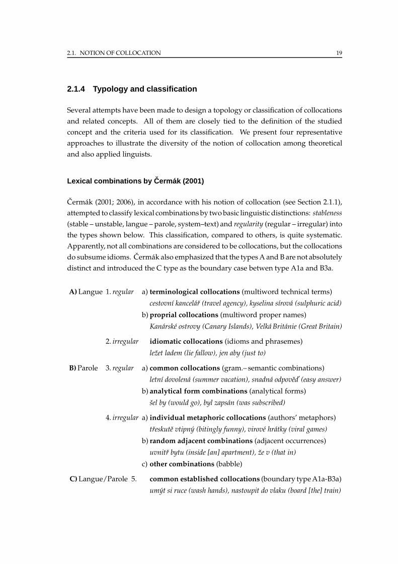
Lexical combinations by Cermak (2001)
Cermak (2001; 2006), in accordance with his notion of collocation (see Section 2.1.1),
attempted to classify lexical combinations by twobasic linguistic distinctions: stableness
(stable – unstable, langue – parole, system–text) and regularity (regular – irregular) into
the types shown below. This classification, compared to others, is quite systematic.
Apparently, not all combinations are considered to be collocations, but the collocations
do subsume idioms. Cermak also emphasized that the typesA and B are not absolutely
distinct and introduced the C type as the boundary case betwen type A1a and B3a.
A)Langue 1. regular a) terminological collocations (multiword technical terms)
cestovnı kancelar (travel agency), kyselina sırova (sulphuric acid)
b) proprial collocations (multiword proper names)
Kanarske ostrovy (Canary Islands), Velka Britanie (Great Britain)
2. irregular idiomatic collocations (idioms and phrasemes)
lezet ladem (lie fallow), jen aby (just to)
B)Parole 3. regular a) common collocations (gram.– semantic combinations)
letnı dovolena (summer vacation), snadna odpoved’ (easy answer)
b) analytical form combinations (analytical forms)
sel by (would go), byl zapsan (was subscribed)
4. irregular a) individual metaphoric collocations (authors’ metaphors)
treskute vtipny (bitingly funny), virove hratky (viral games)
b) random adjacent combinations (adjacent occurrences)
uvnitr bytu (inside [an] apartment), ze v (that in)
c) other combinations (babble)
C)Langue/Parole 5. common established collocations (boundary typeA1a-B3a)
umyt si ruce (wash hands), nastoupit do vlaku (board [the] train)
20 CHAPTER 2. THEORY AND PRINCIPLES
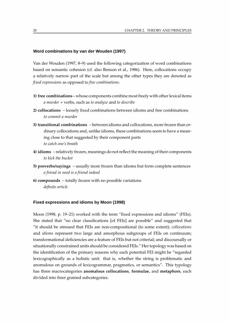
Word combinations by van der Wouden (1997)
Van der Wouden (1997, 8–9) used the following categorization of word combinations
based on semantic cohesion (cf. also Benson et al., 1986). Here, collocations occupy
a relatively narrow part of the scale but among the other types they are denoted as
fixed expressions as opposed to free combinations.
1) free combinations–whose components combinemost freelywithother lexical items
a murder + verbs, such as to analyze and to describe
2) collocations – loosely fixed combinations between idioms and free combinations
to commit a murder
3) transitional combinations – between idioms and collocations, more frozen than or-
dinary collocations and, unlike idioms, these combinations seem to have amean-
ing close to that suggested by their component parts
to catch one’s breath
4) idioms – relatively frozen,meanings donot reflect themeaning of their components
to kick the bucket
5) proverbs/sayings – usually more frozen than idioms but form complete sentences
a friend in need is a friend indeed
6) compounds – totally frozen with no possible variations
definite article
Fixed expressions and idioms by Moon (1998)
Moon (1998, p. 19–21) worked with the term “fixed expressions and idioms” (FEIs).
She stated that ”no clear classifications [of FEIs] are possible” and suggested that
”it should be stressed that FEIs are non-compositional (to some extent); collocations
and idioms represent two large and amorphous subgroups of FEIs on continuum;
transformational deficiencies are a feature of FEIs but not criterial; and discoursally or
situationally constrained units should be considered FEIs.”Her topologywas based on
the identification of the primary reasons why each potential FEI might be ”regarded
lexicographically as a holistic unit: that is, whether the string is problematic and
anomalous on grounds of lexicogrammar, pragmatics, or semantics”. This typology
has three macrocategories anomalous collocations, formulae, and metaphors, each
divided into finer grained subcategories.
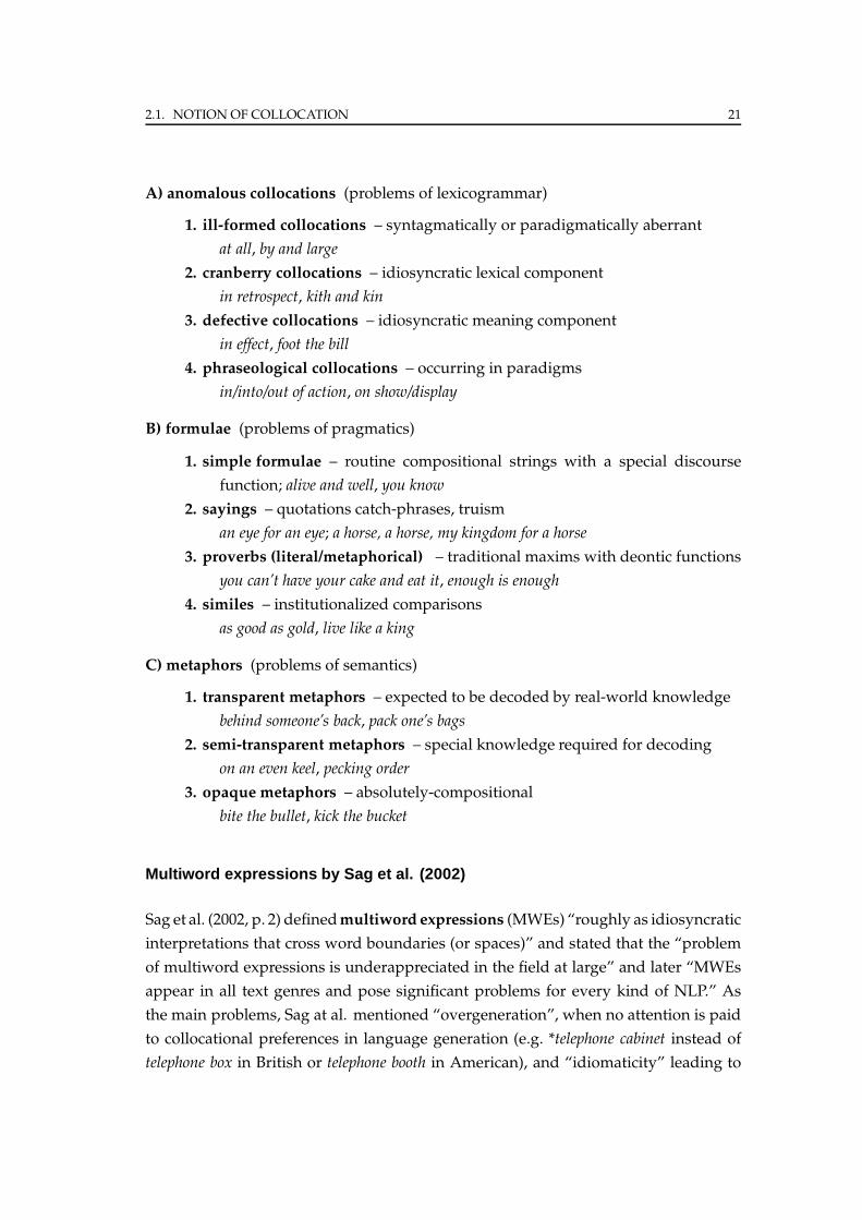
2.1. NOTION OF COLLOCATION 21
A) anomalous collocations (problems of lexicogrammar)
1. ill-formed collocations – syntagmatically or paradigmatically aberrant
at all, by and large
2. cranberry collocations – idiosyncratic lexical component
in retrospect, kith and kin
3. defective collocations – idiosyncratic meaning component
in effect, foot the bill
4. phraseological collocations – occurring in paradigms
in/into/out of action, on show/display
B) formulae (problems of pragmatics)
1. simple formulae – routine compositional strings with a special discourse
function; alive and well, you know
2. sayings – quotations catch-phrases, truism
an eye for an eye; a horse, a horse, my kingdom for a horse
3. proverbs (literal/metaphorical) – traditional maxims with deontic functions
you can’t have your cake and eat it, enough is enough
4. similes – institutionalized comparisons
as good as gold, live like a king
C) metaphors (problems of semantics)
1. transparent metaphors – expected to be decoded by real-world knowledge
behind someone’s back, pack one’s bags
2. semi-transparent metaphors – special knowledge required for decoding
on an even keel, pecking order
3. opaque metaphors – absolutely-compositional
bite the bullet, kick the bucket
Multiword expressions by Sag et al. (2002)
Sag et al. (2002, p. 2) definedmultiword expressions (MWEs) “roughly as idiosyncratic
interpretations that cross word boundaries (or spaces)” and stated that the “problem
of multiword expressions is underappreciated in the field at large” and later “MWEs
appear in all text genres and pose significant problems for every kind of NLP.” As
the main problems, Sag at al. mentioned “overgeneration”, when no attention is paid
to collocational preferences in language generation (e.g. *telephone cabinet instead of
telephone box in British or telephone booth in American), and “idiomaticity” leading to
22 CHAPTER 2. THEORY AND PRINCIPLES
missinterpretation of idiomatic and metaphoric expressions (e.g. kick the bucket). The
terminology used in the proposed classification is adopted from Bauer (1983).
The term collocation is not used at any level of the classification. It is used to refer
to “any statistically significant cooccurrence, including all forms of MWE as described
above and compositional phraseswhich are predictably frequent (because of realworld
events or other nonlinguistic factors).” For example: sell and house appear more often
than one can predict from the frequency of the two words, but “there is no reason to
think that this is due to anything other than real world facts.”
A) lexicalized phrases – have at least partially idiosyncratic syntax or semantics, or
contain ’words’ which do not occur in isolation:
1. fixed expressions – immutable expressions that defy conventions of grammar
and compositional interpretation, e.g. by and large, in short, kingdom come,
every which way; they are fully lexicalized and undergo neither morphosyn-
tactic variation (cf. *in shorter) nor internal modification (cf. *in very short)
2. semi-fixed expressions – adhere to strict constraints on word order and com-
position, but undergo some degree of lexical variation, e.g. in the form of
inflection, variation in reflexive form, and determiner selection
a) non-decomposable idioms – kick the bucket, trip the light
b) compound nominals – car park, attorney general, part of speech
c) proper names – San Francisco, Oakland Riders
3. syntactically-flexible expressions – exhibit a much wider range of syntactic
variability
a) verb-particle constructions – write up, look up, brush up on
b) decomposable idioms – let the cat out of the bag, sweep under the rug
Idioms such as spill the beans, for example, can be analyzed as being
made up of spill in a reveal sense and the beans in a secret(s) sense,
resulting in the overall compositional reading of reveal the secret(s)
c) light verbs – make a mistake, give a demo
B) institutionalized phrases – syntactically and semantically compositional but sta-
tistically idiosyncratic, they occur with remarkably high frequency (in a given
context), e.g. traffic light.
2.1. NOTION OF COLLOCATION 23
2.1.5 Conclusion
There is no commonly accepted definition of collocation and we do not aim to cre-
ate one. Based on Cermak’s notion of compatibility and collocability (Section 2.1.1),
we understand collocation as a meaningful and grammatical word combination con-
strained by extensionally specified restrictions and preferences. This approach has
two important aspects: First, it restricts collocations only to meaningful grammatical
expressions, and therefore combinations of incompatible words (e.g. yellow idea) and
combinations of words without direct syntactic relationship (e.g. doctor – nurse) cannot
form collocations. Second, combination of words in a collocation must be governed
not only by syntactic and semantic rules but also by some other restrictions that cannot
be based on the description of syntactic and semantic properties of the components –
they must be specified explicitly by enumeration (i.e. extensionally).
This approach is quite similar to that preesnted by Evert (2004). His notion of
collocation is based on the definition by Choueka (1988) saying that “[A collocation
expression] has a characteristics of a syntactic and semantic unit whose exact and
unambiguous meaning or connotation cannot be derived directly from the meaning
or connotation of its components.” Evert added only an explicit criterion that should
help to distinguish between collocational and non-collocational expressions: “Does it
deserve a special entry in a dictionary or lexical database of the language?” and de-
fined collocation as “a word combination whose semantic and/or syntactic properties
cannot be fully predicted from those of its components, and which therefore has to be
listed in a lexicon” (Evert, 2004, p. 9), which only emphasizes the extensional character
of collocations – to be enumerated, listed in a lexicon.
Also, in a similar manner to Evert (2004), we use collocation as “a generic term
whose specific meaning can be narrowed down according to the requirements of
a particular research question or application” (Evert, 2004, p. 9). However, each ex-
periment presented in this work is performed on a specific data set and bounded with
a particular definition of the studied concept (or its subtype) and thus it is always clear
what phenomenon we deal with.
The presented notion of collocation is possibly interchangable with the concept
of multiword expression (MWE) that has became commonly prefered and accepted
by many authors and researchers. Baldwin (2006) defined it as an expression that is
“1) decomposable into multiple simplex words and 2) lexically, syntactically, seman-
tically, pragmatically and/or statistically idiosyncratic”. Mainly for historical and
traditional reasons, we keep using the term collocation in this work.
24 CHAPTER 2. THEORY AND PRINCIPLES
2.2 Collocation extraction
Collocation extraction is a traditional task of corpus linguistics. The goal is to extract
a list of collocations from a text corpus. Generally, it is not required to identify
particular occurrences (instances, tokens) of collocations, but rather to produce a list of
all collocations (types) appearing anywhere in the corpus – a collocation lexicon. The
task is often restricted to a particular subtype or subset of collocations (defined e.g. by
grammatical constraints), but we will deal with it in a general sense. The first research
attempts in this area are dated back to the era of “mechanized documentation” (Stevens
et al., 1965). Thefirstwork focusedparticularly on collocation extractionwaspublished
by Berry-Rogghe (1973), and later followed by studies by Choueka et al. (1983), Church
and Hanks (1990), Smadja (1993), Kita et al. (1994), Shimohata et al. (1997), and many
others, especially in the last ten years (Krenn, 2000; Evert, 2004; Bartsch, 2004)
In the following sections we will briefly discuss the basic principles of collocation
extraction and then, in more detail, we will describe individual steps of the whole
extraction process. The reference corpus we will use in our examples in this section is
thePragueDependencyTreebank, version 2.0 (PDT), described indetail later in Section 4.2.
2.2.1 Extraction principles
Methods for collocation extraction are based on several different extraction principles.
These principles exploit characteristic properties of collocations and are formulated as
hypotheses (assumptions) aboutword occurrence and cooccurrence statistics extracted
from a text corpus. Mathematically, they are expressed as formulas that determine the
degree of collocational association between words. These formulas are commonly
called lexical association measures. In this thesis, we focus our attention onmeasures
based on the following extraction principles:
1) Collocation components occur together more often than by chance
The simplest approach to discover collocations in a text corpus is counting – if two
words occur together a lot, then that might be the evidence that they have a special
function that is not simply explained as a result of their combination (Manning and
Schutze, 1999, p. 153). The assumption that collocations occur more frequently than
arbitrary combinations is reflected in many definitions of collocation (see Section 2.1.3)
but in practice it presents certain difficulties:
2.2. COLLOCATION EXTRACTION 25
First, natural language contains some highly frequent word combinations that are
not considered collocations, e.g. various combinations of function words (words with
little lexical meaning, expressing only grammatical relationships with other words).
For example, the most frequent word combination (with a direct syntactic relation
between components) in PDT is by mel (would have) with frequency 2 124, while the
most frequent combination that can be considered a collocation is Ceska republika (Czech
Republic) occurring only 527 times. Such “uninteresting” combinations should be
identified and eliminated during the extraction process.
Second, high frequency of certain word combinations can be purely accidental –
very frequent words are expected to occur together a lot just by chance, even if they
do not form a collocation. For example, the expression novy zakon (new law) is among
the 35 most frequent adjective-noun combinations although it is not a collocation (not
surprisingly, the words novy (new) and zakon (law) are indeed very frequent; in PDT,
the word novy (as masculine inanimate) occurs 777 times and the word zakon occurs
1575 times – both are among the most frequent adjectives and nouns).
The basic principle of collocation extraction is based on distinguishing between
random (free) word combinations that occur together just by chance, and those that are
not accidental and possibly form collocations. Herein, not only the frequency of word
cooccurrences but also the frequencies of words occurring independently are taken
into account. The corpus is observed as a sequence of randomly and independently
generated word bigrams (a random sample), and their joint and marginal occurrence
frequencies are then employed in various association measures to estimate howmuch
the word cooccurrence is accidental.
One class of associationmeasures using this principle is based on statistical hypoth-
esis testing: The null hypothesis is formulated such that there is no association between
the words beyond chance occurrences. The association measures are, in fact, the test
statistics used in these hypothesis tests. Other classes of measures using this princi-
ple are likelihood ratios (expressing how much more likely one hypothesis is against
the other), and other (mostly heuristic) measures of statistical association or measures
adopted from other fields, such as information theory (Church et al., 1991) and others.
2) Collocations occur as units in an information-theoretically noisy environment
While the previous principle deals with the relationship of words inside collocations,
in this approach we analyse the outside relationships of collocations, i.e. words which
immediately precede or follow the collocation in the text stream (immediate contexts).
26 CHAPTER 2. THEORY AND PRINCIPLES
By determining the entropy of these contexts, we can discover points in the word
streamwith either low or high uncertainty (disorder) what the next (or previous) word
will be. “Points with high uncertainty are likely to be phrase boundaries, which in
turn are candidates for points where a collocation may start or end, whereas points
with low uncertainty are likely to be located within a collocation.” (Manning and
Schutze, 1999, p. 181). In other words, entropy inside collocations is expected to be
lower (low uncertainty, high association) and outside collocations to be higher (high
uncertainty, low association). Methods based on this principle has been employed
e.g. by Evans and Zhai (1996), Shimohata et al. (1997), and Pearce (2002).
The corpus is again interpreted as a sequence of randomly (and independently)
generated words. For each collocation candidate we estimate probability distribution
of words occurring in its immediate contexts (left and right) and determine its lexical
association based on measuring entropy of these contexts.
3) Collocations occur in different contexts to their components
Limited compositionality is a typical property of collocations – the meaning of a collo-
cation cannot be fully inferred from the meanings of its components. In other words,
meaning of a collocation must (to some extent) differ from the “union” of the mean-
ing of its components (see Section 2.1.3). Traditional examples of this property are
idiomatic expressions (e.g. kick the bucket – there is no bucket nor kicking in the meaning
of this idiom).
A typical way of modeling senses in natural language processing is by empirical
contexts, i.e. by a bag of words occurring within a specified context window of a word
or an expression. The more different the contexts are, the higher the chance is that
the expression is a collocation (Zhai, 1997). Lexical association measures based on this
principle are adopted from mathematics (vector distance), information theory (cross-
entropy, divergence) and from the field of information retrieval (vector similarity).
A major weakness of most lexical association measures lies in their unreliability
whenapplied to low frequencydata. They either assumewordoccurrenceprobabilities
to be approximately normally distributed (e.g. t-test), which is not true in general
(Church and Mercer, 1993) and unensurable to assume when dealing with frequencies
aroundfive or less. Or they are just sensitive to estimates that are inaccurate due to data
sparseness (e.g. Pointwise mutual information), see (Manning and Schutze, 1999, p. 181).
2.2. COLLOCATION EXTRACTION 27
Other extraction principles
Various other extraction principles have been proposed, however, they are not of
our interest in this work – they either require additional linguistic resources or they
are not based on measuring lexical association. For example, Manning and Schutze
(1999, Chapter 5) described a technique based on analysis of the mean and variance
of distance between the components of word combinations. Pearce (2002) exploited
another characteristic property of collocation – non-substitutability and measured
whether collocation components can be replaced by their synonyms, where Wordnet
(Fellbaum, 1998) was used as a source of such (lexical) synonyms. Several researchers
have also attempted to extract collocations (and their translations) from bilingual
parallel corpora, e.g. Ohmori and Higashida (1999) or Wu and Zhou (2003).
2.2.2 Extraction pipeline
Automatic collocation extraction is usually performedas a process consisting of several
steps, called the extraction pipeline (Evert and Kermes, 2003; Krenn, 2000):
First, the corpus as a collection of machine-readable texts in one language is lin-
guistically pre-processed – morphologically and syntactically analyzed and disam-
biguated. Second, all collocation candidates (potential collocations) are identified and
their occurrence statistics extracted from the corpus. Third, the candidates are filtered
to improve precision (based on grammatical patterns and/or occurrence frequency).
Fourth, a lexical association measure is chosen and applied to the occurrence statistics
obtained from the corpus. Finally, the collocation candidates are classified according
to their association scores and a certain threshold – candidates above this threshold
are classified as collocations and candidates below the threshold as non-collocations.
There is no principled way of finding the optimal classification threshold (Inkpen
and Hirst, 2002) – it depends primarily on the intended application (whether high
precision or broad coverage is preferred) and is usually set empirically. To avoid this
step, the task of collocation extraction is usually reformulated as ranking collocation
candidates – the goal is not to extract a discreet set of collocations from a given corpus,
but instead to rank all potential collocations according to their degree of association so
that the most associated ones are concentrated at the top of the list. This approach to
collocation extraction will be applied in the rest of our work. The extraction pipeline
for bigram collocation extraction will be described in detail in the following sections,
and lexical association measures will be presented separately in the next chapter.
28 CHAPTER 2. THEORY AND PRINCIPLES
2.2.3 Linguistic preprocessing
By linguistic preprocessing we mean the analysis and disambiguation at the level of
morphology and surface syntax. Higher levels of linguistic processing (e.g. deep syn-
tax) are not useful since we are interested only in the association at the lexical level.
In this step, information about word base forms, morphological categories, and sentence
syntax is obtained in order to identify collocation candidates and all their occurrences
– regardless of inflectional variance and sentence position.
Formally, a source corpus W is expected in the form of a linearly ordered set
of n word tokens wi identified as contiguous, non-overlapping strings vi over an
alphabet Σ distinguished by their position i = 1, . . . , n in the corpus, so the i-th word
token wi is a pair 〈i, vi〉. The ordering of W is defined by the natural ordering of the
positions. The items vi are called word forms and the set of all possible word forms is
called the vocabulary V.
W = {w1, . . . , wn} , wi := 〈i, vi〉, vi ∈ V ⊂ Σ∗, i = 1, . . . , n.
During morphological analysis and disambiguation, each word tokenwi from W is
assigned (by mapping φ) a (basic) word type u (from a set of all such word types U ).
The word types define equivalence classes of word tokens based on inflection, so all
inflectional variants are assigned the same value u. We denote ui as the word type
assigned to the word token wi.
φ : W → U, ui := φ(wi), i = 1, . . . , n.
Technically, each u∈U is usually a pair 〈l, t〉 where l is a lemma – a word base form
as it appears in the lexicon L – and t is a tag from the tag set T specifying detailed
morphological characteristics (e.g. derivational) shared by all the inflectional variants.
u = 〈l, t〉, l ∈ L, t ∈ T.
Theword types are defined to conflate all word tokens not only with the sameword
base form but also with the same lexical meaning – which may not be fully reflected in
the word base form. Details strongly depend on the system employed for encoding
the morphological information in the corpus. For example, in the Czech system
used in PDT, the information about the morphological categories negation or grade
(degree of comparison) which are considered derivational and which discriminate
word meanings, is encoded in the tag, not in the lemma. For this reason, e.g. the word
types of nebezpecny (insecure) and nejvyssı (highest) must be encoded as 〈bezpecny, 1N〉(secure, 1stgrade, negative) and 〈vysoky, 3A〉 (high, 3rdgrade, affirmative), respectively (for
details, see also Section 4.2.1).
2.2. COLLOCATION EXTRACTION 29
During syntactic analysis and disambiguation, each word tokenwi from the corpus
W is assigned (by a function δ applied to its index i) an index j of its head word wj
(in terms of dependency syntax, wj governs wi) and (by a mapping α) the analytical
function a (from the set A of all possible analytical functions enriched by a special
value HEAD, see details bellow) specifying the type of syntactic relation between the
word token and its head word. The head word of a word token wi is either another
word token wj , i 6= j from the same sentence, or the value NULL if wi is the root of the
sentence (j = 0). We denote ai as the analytical function assigned to theword tokenwi.
δ : {1, . . . , n} → {0, . . . , n}, δ(i) 6= i,
α : W → A, ai := α(wi), i = 1, . . . , n.
In order to identify word tokens that are not only inflectional variants but also
have the same syntactic function, eachword tokenwi can be assigned (by amappingϕ)
an extendend word type 〈ui, ai〉, which consists of its word type ui and its analytical
function ai.
ϕ : W → U×A, ϕ(wi) = 〈ui, ai〉, ui = φ(wi), ai = α(wi), i = 1, . . . , n.
For technical reasons, we also define a special extendedword type that can be assigned
(by amapping ϕ′) to any word tokenwi and consists of its word type ui and the special
value of analytical function ai = HEAD. This extendedword type will be used to label
head words appearing in a dependency relation with other words.
ϕ′ : W → U×A, ϕ(wi) = 〈ui,HEAD〉, ui = φ(wi), i = 1, . . . , n.
Generally, linguistic preprocessing is not necessarily required for collocation ex-
traction, especially when working with languages with simple morphology (such as
English) and if we focus e.g. only on fixed adjacent and non-modifiable collocations.
However, if we have to deal with complex morphology (e.g. in Czech) and if we
want to extract syntactically bounded word combinations with free word order, this
information is quite useful.
Linguistic information can also be used in the subsequent steps of the extraction
pipeline for filtering collocation candidates (see Section 2.2.6) and to construct ad-
ditional features in methods combining statistical and linguistic evidence in more
complex classification and ranking models (see Chapter 6).
30 CHAPTER 2. THEORY AND PRINCIPLES
2.2.4 Collocation candidates
Collocation candidates represent the set of all potential collocations appearing in the
corpus, i.e. the word combinations that satisfy some basic requirements imposed on
collocations (e.g. components to be in a direct syntactic relation or to occur within
a given distance in the text). Collocation candidates are examined with respect to the
degree their components are associated, and ranked according to their strength of
association, as specified in the task description. The goal of this step of the extraction
pipeline is to identify all collocation candidates and their instances (occurrences) in
the corpus. First, we will describe this step on a general level, then with details of
specific approaches.
First, the corpus W is by some means transformed to a set B consisting of bigram
tokens bk = 〈wi, wj〉, i.e. pairs of word tokens from the corpus satisfying some given
conditions. Elements of B are indexed by k ∈ {1, . . . , N}, where N = |B|, althoughthe actual ordering of this set is not important.
B = {b1, . . . , bN}, B ⊂ W×W, bk = 〈wi, wj〉, k = 1, . . . , N.
Second, each bigram token bk from the set B is assigned (by a mapping Φ) a bigram
type c (from a set C∗ of all possible bigram types) defining equivalence classes of
bigram tokens based on inflection – all bigram tokens that differ only in inflection
are assigned the same bigram type c. Bigram types identified by Φ in B are called
collocation candidates and a set of all such bigram types is denoted by C . Each
bigram token is thus an instance of a collocation candidate. We denote ck as the
bigram type of the bigram token bk.
Φ : B → C∗, ck := Φ(bk), k = 1, . . . , N, C := Φ(B), C ⊂ C∗.
Third, a multiset (allowing repeated elements, also called a bag) D, referred to as
the candidate occurrence data (or candidate data), is acquired as a result of Φ applied
on all the elements from B, i.e. bigram types assigned to all bigram tokens. This data
serves as a basis for the extraction of occurrence statistics described in the following
section.D = {c1, . . . , cN}, ck = Φ(bk), bk ∈ B, k = 1, . . . , N.
The collocation candidate data can be obtained in several alternative ways, depend-
ing on the level of linguistic preprocessing of the corpus. These ways differ in how the
set of bigram tokens B is constructed and how the mapping Φ is defined to produce
the elements of D. In the following paragraphs, we will describe three approaches we
employed in our experiments.
2.2. COLLOCATION EXTRACTION 31
Dependency bigrams
The generic notion of collocation presented in Section 2.1.5 requires collocations to
be syntactic units. In dependency syntax, as it is applied in PDT, this constraint can
be interpreted as the presence of a direct dependency relation between the collocation
components. Collocation candidates can then be identified as dependency bigrams.
The set Bdep then consists of dependency bigram tokens defined as pairs 〈wi, wj〉 ofword tokens from the corpus W in a direct dependency relation of a certain type and
in a certain word order.
Bdep = {〈wi, wj〉∈ W×W : i < j ∧ (j = δ(i) ∨ i = δ(j))} .
In general, word order can discriminate between the collocation candidates, and it
should be distinguished between bigrams with the first component as the head word
and the second one as the modifier and vice versa. For illustration, see the following
example: dependency bigrams velky vyr and vyr velky differ only in word order; the
component vyr is in both the cases the head word and velky is its attribute but the
meanings of these expressions are different – the first refers to a big owl and the latter
denotes stock owl as a biological species. On the other hand, in some collocations, word
order is not that important: For example, naklepat maso (to tenderize meat) can occur
in this and also in the reverse word order: Petr naklepal maso and Maso jsem naklepal
vcera are both correct sentences containing the collocation naklepat maso. Since it is not
clear how to determine when word order is important and when it is not, we decided
to preserve word order in all collocation candidates. This is done by the condition
i < j (the first component must always precede the second one in the corpus). For this
reason, dependency relations are possible in both directions, either j = δ(i) or i = δ(j).
The mapping Φdep that assigns to each bigram token from Bdep its bigram type is
for dependency bigrams defined by extended word types in the following way:
Φdep (〈wi, wj〉) =
{ 〈ϕ(wi), ϕ′(wj)〉 for j = δ(i),
〈ϕ′(wi), ϕ(wj)〉 for i = δ(j).
One component of a dependency bigram appearing in a sentence always acts as
the head and the other one as the modifier. The head word, however, also participates
in another relation outside the bigram as a modifier. This relation is ignored in the
dependency bigram and the analytical function of the bigram head word is set to the
value HEAD (by the mapping ϕ′).
32 CHAPTER 2. THEORY AND PRINCIPLES
Surface bigrams
Extracting the collocation candidates as dependency bigrams is quite a reasonable ap-
proach. It is guaranteed that each potential collocation is a syntactic unit. However,
the source corpus is expected to be syntactically analyzed and disambiguated in order
to identify such bigrams. If this is not the case, we can detect collocation candidates
heuristically, based just on the surface word order. We can assume that most colloca-
tions occur as adjacent word expressions that cannot be modified by the insertion of
anotherword, and identify bigram collocation candidates as surface bigrams – pairs of
adjacent words. The set Bsurf of surface bigram tokens is formally defined as follows:
Bsurf = {〈wi, wj〉∈ W×W : j = i + 1} .
The mapping Φsurf that assigns a surface bigram type to each surface bigram token
from Bsurf is defined by word types of both components in the following way:
Φsurf (〈wi, wj〉) = 〈φ(wi), φ(wj)〉 .
Distance bigrams
The constraint that collocation candidates are only adjacent word pairs might be too
restrictive. Obviously, it is not valid for certain types of collocations, such as support-
-verb constructions or verb–noun combinations in general. Collocations of these (and
perhaps other) types can often be modified by the insertion of another word and
their components can occur at various distances, as in the example naklepat maso (to
tenderize meat) mentioned earlier. In Czech, it can occur not only with free word order
but also with various distances between the components. These cases can, of course,
be captured by dependency bigrams, but if the syntactic information is not available
in the source corpus, we can identify collocation candidates as distance bigrams –
word pairs occurring within a given distance specified by a distance function db and
a threshold tb. The set Bdist is then defined by this formula:
Bdist = {〈wi, wj〉∈ W×W : i < j ∧ db(i, j) ≤ tb} .
The mapping Φdist that assigns a bigram type to each distance bigram token from
Bdist is then defined in the same way as for surface bigrams:
Φdist (〈wi, wj〉) = Φsurf (〈wi, wj〉) = 〈φ(wi), φ(wj)〉 .
2.2. COLLOCATION EXTRACTION 33
By one of the mentioned approaches, the candidate data D is constructed as follows:
〈B,Φ〉 ∈ {〈Bdep,Φdep〉, 〈Bsurf ,Φsurf 〉, 〈Bdist,Φdist〉},
D = {Φ(b1), . . . ,Φ(bN )}, bk ∈ B, k = 1, . . . , N, N = |B|.
The candidate data of dependency and surface bigrams are of approximately the same
size as the corpus (the number of bigram tokens roughly corresponds to the number of
word tokens in the corpus), but the candidate data of distance bigrams is larger, depend-
ing on the distance function and the threshold (usually set to 3–5 intervening words).
2.2.5 Occurrence statistics
In this step of the extraction pipeline, the occurrence statistics of bigrams and their
components are obtained from the candidate occurrence data D and the corpus W .
We assume that D is a multiset of generic bigram types (either dependency, surface, or
distance) whose components are generic word types (either basic or extended), elements
of U∗. For simplicity of notation, we further denote the elements of D as pairs 〈xk, yk〉:
D = {〈xk, yk〉 : k ∈ {1, . . . , N}} , xk, yk ∈ U∗
The statistics extracted for each collocation candidate (bigram type) 〈x, y〉 ∈ C
(for simpler notation further denoted as xy) and its components (word types) x, y from
the candidate data, range from simple frequency counts and contingency tables to more
complex models such as immediate or empirical contexts.
Frequency counts
The basic occurrence model consists of the frequency counts of the bigram xy, its
components x, y, and the size of the candidate data N = |D|.
f(xy) := |{k : xk = x ∧ yk = y}|f(x∗) := |{k : xk = x}|f(∗y) := |{k : yk = y}|
The bigram frequency f(xy) (also called the joint frequency) denotes the number
of pairs 〈xk, yk〉 = 〈x, y〉 in the canidate data D. The component frequencies f(x∗)and f(∗y) (also called the marginal frequencies) denote the number of pairs where
the first component is x and pairs where the second component is y, respectively.
N denotes the number of all pairs in D. Evert (2004, p. 28) refers to the quadruple
(f(xy), f(x∗), f(∗y), N) as the frequency signature of the bigram xy.
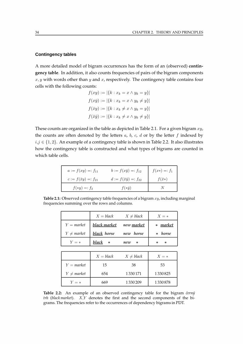
34 CHAPTER 2. THEORY AND PRINCIPLES
Contingency tables
A more detailed model of bigram occurrences has the form of an (observed) contin-
gency table. In addition, it also counts frequencies of pairs of the bigram components
x, y with words other than y and x, respectively. The contingency table contains four
cells with the following counts:
f(xy) := |{k : xk = x ∧ yk = y}|f(xy) := |{k : xk = x ∧ yk 6= y}|f(xy) := |{k : xk 6= x ∧ yk = y}|f(xy) := |{k : xk 6= x ∧ yk 6= y}|
These counts are organized in the table as depicted in Table 2.1. For a given bigram xy,
the counts are often denoted by the letters a, b, c, d or by the letter f indexed by
i,j ∈ {1, 2}. An example of a contingency table is shown in Table 2.2. It also illustrates
how the contingency table is constructed and what types of bigrams are counted in
which table cells.
a := f(xy) =: f11 b := f(xy) =: f12 f(x∗) =: f1
c := f(xy) =: f21 d := f(xy) =: f22 f(x∗)
f(∗y) =: f2 f(∗y) N
Table 2.1: Observed contingency table frequencies of a bigram xy, includingmarginalfrequencies summing over the rows and columns.
X = black X 6= black X = ∗
Y = market black market new market ∗ market
Y 6= market black horse new horse ∗ horse
Y = ∗ black ∗ new ∗ ∗ ∗
X = black X 6= black X = ∗
Y = market 15 38 53
Y 6= market 654 1 330 171 1 330 825
Y = ∗ 669 1 330 209 1 330 878
Table 2.2: An example of an observed contingency table for the bigram cernytrh (blackmarket). X,Y denotes the first and the second components of the bi-grams. The frequencies refer to the occurrences of dependency bigrams in PDT.
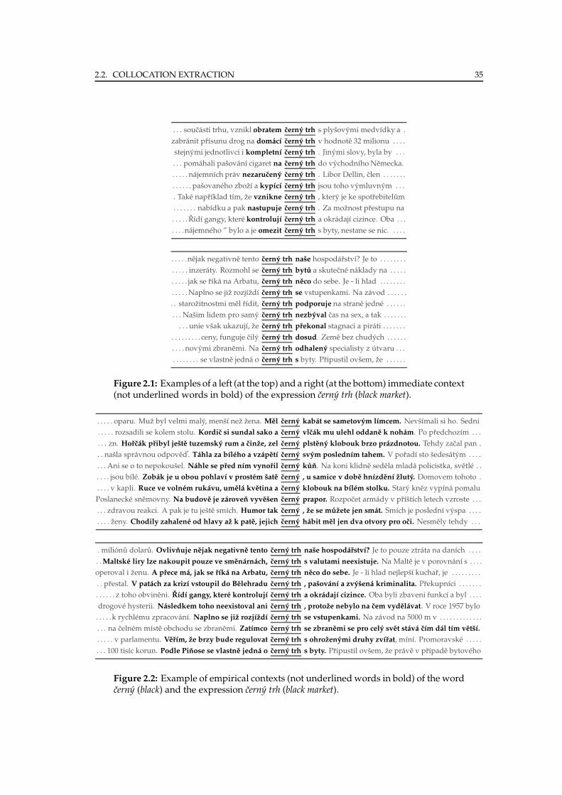
2.2. COLLOCATION EXTRACTION 35
. . . soucastı trhu, vznikl obratem cerny trh s plysovymi medvıdky a .
zabranit prısunu drog na domacı cerny trh v hodnote 32 milionu . . . .
stejnymi jednotlivci i kompletnı cerny trh . Jinymi slovy, byla by . . .
. . . pomahali pasovanı cigaret na cerny trh do vychodnıho Nemecka.
. . . . . najemnıch prav nezaruceny cerny trh . Libor Dellin, clen . . . . . . .
. . . . . . pasovaneho zbozı a kypıcı cerny trh jsou toho vymluvnym . . .
. Take naprıklad tım, ze vznikne cerny trh , ktery je ke spotrebitelum
. . . . . . . nabıdku a pak nastupuje cerny trh . Za moznost prestupu na
. . . . . Rıdı gangy, ktere kontrolujı cerny trh a okradajı cizince. Oba . . .
. . . .najemneho ” bylo a je omezit cerny trh s byty, nestane se nic. . . . .
. . . . .nejak negativne tento cerny trh nase hospodarstvı? Je to . . . . . . . .
. . . . . inzeraty. Rozmohl se cerny trh bytu a skutecne naklady na . . . . .
. . . . . jak se rıka na Arbatu, cerny trh neco do sebe. Je - li hlad . . . . . . . .
. . . . .Naplno se jiz rozjızdı cerny trh se vstupenkami. Na zavod . . . . . .
. . starozitnostmi mel rıdit, cerny trh podporuje na strane jedne . . . . . .
. . . Nasim lidem pro samy cerny trh nezbyval cas na sex, a tak . . . . . . .
. . . unie vsak ukazujı, ze cerny trh prekonal stagnaci a pirati . . . . . . .
. . . . . . . . . ceny, funguje cily cerny trh dosud. Zeme bez chudych . . . . . .
. . . . novymi zbranemi. Na cerny trh odhaleny specialisty z utvaru . . .
. . . . . . . . se vlastne jedna o cerny trh s byty. Pripustil ovsem, ze . . . . . .
Figure 2.1: Examples of a left (at the top) and a right (at the bottom) immediate context(not underlined words in bold) of the expression cerny trh (black market).
. . . . . oparu. Muz byl velmi maly, mensı nez zena. Mel cerny kabat se sametovym lımcem. Nevsımali si ho. Sedni
. . . . . rozsadili se kolem stolu. Kordic si sundal sako a cerny vlcak mu ulehl oddane k noham. Po predchozım . . .
. . . zn. Horcak pribyl jeste tuzemsky rum a cinze, zel cerny plsteny klobouk brzo prazdnotou. Tehdy zacal pan .
. . nasla spravnou odpoved’. Tahla za bıleho a vzapetı cerny svym poslednım tahem. V poradı sto sedesatym . . . .
. . . Ani se o to nepokousel. Nahle se pred nım vynoril cerny kun. Na koni klidne sedela mlada policistka, svetle . .
. . . . jsou bıle. Zobak je u obou pohlavı v prostem sate cerny , u samice v dobe hnızdenı zluty. Domovem tohoto .
. . . . v kapli. Ruce ve volnem rukavu, umela kvetina a cerny klobouk na bılem stolku. Stary knez vypına pomalu
Poslanecke snemovny. Na budove je zaroven vyvesen cerny prapor. Rozpocet armady v prıstıch letech vzroste . . .
. . . zdravou reakci. A pak je tu jeste smıch. Humor tak cerny , ze se muzete jen smat. Smıch je poslednı vyspa . . . .
. . . . zeny. Chodily zahalene od hlavy az k pate, jejich cerny habit mel jen dva otvory pro oci. Nesmely tehdy . . .
. milionu dolaru. Ovlivnuje nejak negativne tento cerny trh nase hospodarstvı? Je to pouze ztrata na danıch . . . .
. .Maltske liry lze nakoupit pouze ve smenarnach, cerny trh s valutami neexistuje. Na Malte je v porovnanı s . . . .
operoval i zenu. A prece ma, jak se rıka na Arbatu, cerny trh neco do sebe. Je - li hlad nejlepsı kuchar, je . . . . . . . . .
. . prestal. V patach za krizı vstoupil do Belehradu cerny trh , pasovanı a zvysena kriminalita. Prekupnıci . . . . . . .
. . . . . . z toho obvineni. Rıdı gangy, ktere kontrolujı cerny trh a okradajı cizince. Oba byli zbaveni funkcı a byl . . . .
drogove hysterii. Nasledkem toho neexistoval ani cerny trh , protoze nebylo na cem vydelavat. V roce 1957 bylo
. . . . .k rychlemu zpracovanı. Naplno se jiz rozjızdı cerny trh se vstupenkami. Na zavod na 5000 m v . . . . . . . . . . . . .
. . . na celnem mıste obchodu se zbranemi. Zatımco cerny trh se zbranemi se pro cely svet stava cım dal tım vetsı.
. . . . . v parlamentu. Verım, ze brzy bude regulovat cerny trh s ohrozenymi druhy zvırat, mını. Promoravske . . . . .
. . . 100 tisıc korun. Podle Pinose se vlastne jedna o cerny trh s byty. Pripustil ovsem, ze prave v prıpade bytoveho
Figure 2.2: Example of empirical contexts (not underlined words in bold) of the wordcerny (black) and the expression cerny trh (black market).
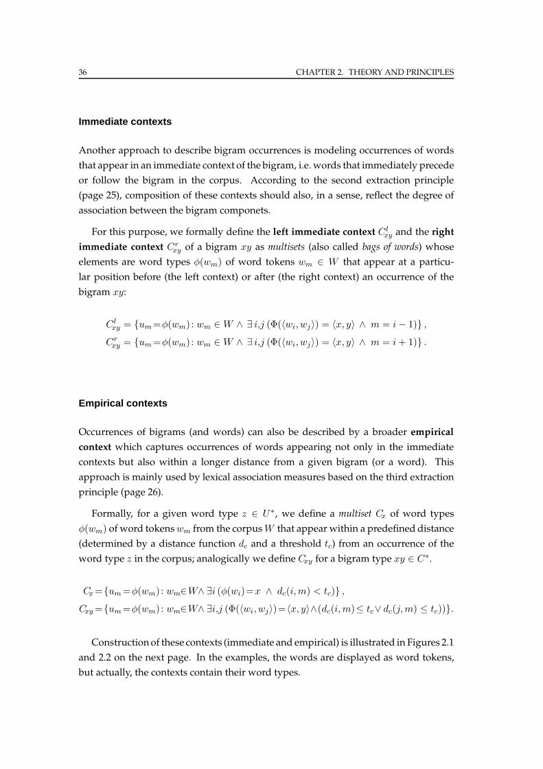
36 CHAPTER 2. THEORY AND PRINCIPLES
Immediate contexts
Another approach to describe bigram occurrences is modeling occurrences of words
that appear in an immediate context of the bigram, i.e. words that immediately precede
or follow the bigram in the corpus. According to the second extraction principle
(page 25), composition of these contexts should also, in a sense, reflect the degree of
association between the bigram componets.
For this purpose, we formally define the left immediate context C lxy and the right
immediate context Crxy of a bigram xy as multisets (also called bags of words) whose
elements are word types φ(wm) of word tokens wm ∈ W that appear at a particu-
lar position before (the left context) or after (the right context) an occurrence of the
bigram xy:
C lxy = {um =φ(wm) : wm ∈ W ∧ ∃ i,j (Φ(〈wi, wj〉) = 〈x, y〉 ∧ m = i − 1)} ,
Crxy = {um =φ(wm) : wm ∈ W ∧ ∃ i,j (Φ(〈wi, wj〉) = 〈x, y〉 ∧ m = i + 1)} .
Empirical contexts
Occurrences of bigrams (and words) can also be described by a broader empirical
context which captures occurrences of words appearing not only in the immediate
contexts but also within a longer distance from a given bigram (or a word). This
approach is mainly used by lexical association measures based on the third extraction
principle (page 26).
Formally, for a given word type z ∈ U∗, we define a multiset Cx of word types
φ(wm) of word tokenswm from the corpusW that appear within a predefined distance
(determined by a distance function dc and a threshold tc) from an occurrence of the
word type z in the corpus; analogically we define Cxy for a bigram type xy ∈ C∗.
Cx ={um =φ(wm) : wm∈W∧ ∃i (φ(wi)=x ∧ dc(i,m) < tc)} ,
Cxy ={um =φ(wm) : wm∈W∧ ∃i,j (Φ(〈wi, wj〉)=〈x, y〉∧(dc(i,m)≤ tc∨ dc(j,m) ≤ tc))}.
Constructionof these contexts (immediate and empirical) is illustrated in Figures 2.1
and 2.2 on the next page. In the examples, the words are displayed as word tokens,
but actually, the contexts contain their word types.
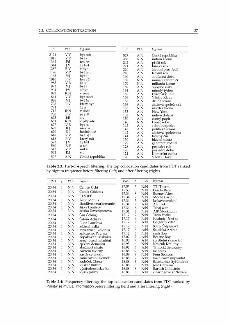
2.2. COLLOCATION EXTRACTION 37
f POS bigram
2124 V:V byt mıt1815 V:R byt v1362 P:J ten ze1344 J:V ze byt1287 R:V v byt1196 V:P byt ten1165 V:J byt a1010 P:V ten byt985 V:R jıt o973 V:J byt a904 J:V a byt883 R:N v roce841 V:V byt moci826 V:J byt ze798 P:V ktery byt771 J:J ze a712 R:N v dobe700 P:V se stat675 J:R a v661 R:N v prıpade627 V:R byt na627 R:J mezi a620 D:J hodne nez618 V:V byt byt618 P:V ktery mıt573 J:V ze byt560 R:P o ten543 V:R mıt v542 R:J v a527 A:N Ceska republika
f POS bigram
527 A:N Ceska republika488 N:N milion korun242 A:N prıstı rok221 A:N lonsky rok220 A:N zivotnı prostredı210 A:N letosnı rok190 A:N soucasna doba182 N:N ministr zahranicı179 N:N miliarda korun169 A:N Spojene staty164 A:N minuly tyden162 A:N Evropsky unie156 N:N Vaclav Klaus156 A:N druha strana156 A:N akciova spolecnost155 N:N navrh zakona155 A:N New York152 N:N milion dolaru150 A:N cenny papır148 N:N konec roku145 A:N statnı rozpocet142 A:N politicka strana142 A:N akciova spolecnost141 A:N trestny cin130 A:N hlavnı mesto129 A:N generalnı reditel128 A:N poslednı rok126 A:N poslednı doba121 A:N Komercnı banka120 N:N Vaclav Havel
Table 2.3: Part-of-speech filtering: the top collocation candidates from PDT rankedby bigram frequency before filtering (left) and after filtering (right).
PMI f POS bigram
20.34 1 N:N Cchien Cchi20.34 1 N:N Canek Gridoux20.34 1 N:N CLS JEP20.34 1 N:N Aron Monus20.34 1 N:N skodlivost narkomanie20.34 1 N:N siska konifery20.34 1 N:N sestka Davenportova20.34 1 N:N San Cching20.34 1 N:N Salom Achsav20.34 1 N:N L’uba Lauffova20.34 1 N:N zuzenı hrdla20.34 1 N:N zvyraznenı koloritu20.34 1 N:N zplozenec Paynea20.34 1 N:N zopakovanı seskoku20.34 1 N:N znechucenı naladenı20.34 1 N:N zjevenı demantu20.34 1 N:N zboznost cısare20.34 1 N:N zavrenı tavırny20.34 1 N:N zastance vhodu20.34 1 N:N zamerovanı zlomek20.34 1 N:N zadecek Chera20.34 1 N:N vyskar Ruffıni20.34 1 N:N vystrednost slavıka20.34 1 N:N vysev jariny
PMI f POS bigram
17.53 7 N:N TTI Therm17.53 6 N:N Guido Reni17.34 8 N:N Buenos Aires17.34 7 N:N Monte Carlo17.34 7 A:N laskave svolenı17.34 7 A:N AG Flek17.34 6 A:N Tchaj wan17.31 6 N:N AIK Stockholm17.17 9 N:N Twin Peaks17.17 9 N:N Kazimır Janoska17.17 7 A:N Geigeruv cıtac17.17 6 N:N Karol Stepanova17.17 6 A:N Saudska Arabie17.12 6 N:N cash flow17.02 7 A:N Beastie Boy16.98 7 A:N ctvrtletnı slosovanı16.95 6 N:N Kaucuk Kralupy16.92 6 A:N Trinecke zelezarny16.88 9 N:N tie break16.88 9 N:N Four Seasons16.88 7 A:N kochlearnı implantat16.88 6 N:N Saccheriho ctyruhelnık16.88 6 N:N Jose Carreras16.88 6 N:N Baruch Goldstein16.85 8 A:N clearingove zuctovanı
Table 2.4: Frequency filtering: the top collocation candidates from PDT ranked byPointwise mutual information before filtering (left) and after filtering (right).
38 CHAPTER 2. THEORY AND PRINCIPLES
2.2.6 Filtering candidate data
Filtering is often used to improve the precision of the extraction process by eliminating
such data as does not help discover true collocations or can bias their extraction. It can
be performed either before the occurrence statistics are obtained or after this step. Evert
(2004, p. 32–33) described these two approaches as token filtering and type filtering:
Token filtering is applied before the extraction of occurrence statistics and can be
understood as a set of additional constraints on the identification of bigram tokens in
the set B. Token filtering affects the candidate occurrence data D and the statistics
obtained from it. This step must be theoretically substantiated and must not bias
the occurrence models. Appropriately designed type filtering can even improve the
validity of assumptions requiredby certain extractionprinciples (e.g. the Independence
of randomlygeneratedwordpairs). According toEvert (2004, p. 33), it is quite adequate
e.g. to restrict the bigram tokens only to adjective-noun combinations, if we focus only
on collocations of this type, however, we cannot remove bigrams with certain general
adjectives that ”usually produce uninteresting results“. Such a step would decrease
marginal frequencies of nouns appearing in the affected bigrams which could unjustly
prioritize other combinations of these nouns in ranking. Quite reasonable, on the other
hand, is to restrict the bigram tokens only to combinations without punctuationmarks.
Type filtering is applied after the extraction of occurrence statistics and has no effect on
the candidate occurrence data D and the extracted statistics. It divides the collocation
candidates into subsets which are then handled separately. A typical case of type
filtering is the commonly used part-of-speech filtering based on themorphological in-
formation obtained during linguistic preprocessing, see e.g. (Justeson and Katz, 1995;
Manning and Schutze, 1999; Evert, 2004). With the knowledge of morphological char-
acteristics of collocation candidates and their components, we can identify those that
are not very likely to form collocations, and exclude them from further analysis. They
can be explicitly classified as non-collocations or, in the case of ranking, placed at the
end of the list or discard them entirely.
As an example, Table 2.3 shows the top 20 collocation candidates from PDT, ranked
by bigram frequency obtained before part-of-speech filtering (on the left), and the
top 20 candidates from the same set, obtained after the filter was applied where only
adjective-noun and noun-noun combinations were kept. The first table contains only
one true collocation Ceska republika, which appears at the very bottom of the list (Czech
Republic). After the application of the filter, almost all top candidates, as they appear
in the other table, can be considered collocations.
2.2. COLLOCATION EXTRACTION 39
Another case of type filtering is frequency filtering. It is based on setting a limit
on the minimal frequency of collocation candidates before association measures are
applied. It is a well-known fact, that many association measures are unreliable when
applied to low-frequency data and that certain minimal frequency is required in order
to expect meaningful results. This issue was thoroughly studied by Evert in his thesis
(2004) where he demonstrated that ”it is impossible in principle to computemeaningful
association scores for the lowest-frequency data“ (p. 22, 95–108).
The effect of frequency filtering is illustrated in Table 2.4. The top positions in
the list of collocation candidates from PDT, ranked according to scores of Pointwise
mutual information, are occupied by bigrams whose components appear in PDT just
once, that is, in this bigram. There is no way to distinguish between collocations and
non-collocations in this list – from the perspective of statistics, they have the same
properties (occurrence frequency) and cannot be differentiated. The top candidates
obtained after applying the frequency filter that discarded candidates occurring 5 times
or less is shown on the right – almost all of them can be considered to be collocations.
Context filtering is a special case of filtering that can be employed during the
construction of empirical contexts. These structures are intended for modeling the-
semantics of collocation candidates and their components (see the third extraction
principle in Section 2.2.1). The way they are defined in Section 2.2.5 implies that they
contain types of all word tokens occurring within specified context windows which
also includes wordswith a little or no semantic content that do not determinemeaning
of a given bigram or word. In empirical contexts, such word tokens can be ignored.
This idea, however, cannot be applied to immediate contexts that model an immediate
word environment from an information-theoretical point of view, and therefore the
occurrence of all word tokens should be taken into account.

40
Chapter 3
Association Measures
The last step of the extraction pipeline involves applying a chosen lexical association
measure to the occurrence and context statistics extracted from the corpus for all
collocation candidates and obtaining their association scores. A list of the candidates
ranked according to their association scores is then the desired result of the entire
process.
In this chapter, we introduce an inventory of 82 such lexical association measures.
Thesemeasures are based on the extraction principles described in Section 2.2.1 which
correspond to three basic approaches to determine collocational association: by mea-
suring the statistical association between the components of the collocation candidates,
by measuring the quality of context of the collocation candidates, and by measuring the
dissimilarity of contexts of the collocation candidates and their components.
For each of these approaches, we will first present its mathematical foundations
and then a list of the measures including their formulas and key references. We will
not discuss each of the measures in detail. An exhaustive description of many of them
(applied to collocation extraction)was published in the dissertation of Evert (2004) and
is also available on-line1. A general description (not applied to collocation extraction)
of other measures can be find e.g. in the thesis of Warrens (2008) or in the provided
references.
1http://www.collocations.de
41

42 CHAPTER 3. ASSOCIATION MEASURES
3.1 Statistical association
In order to measure the statistical association, the candidate occurrence data D ex-
tracted from the corpus is interpreted as a random sample obtained by sampling (with
replacement) from the (unknown) population of all possible bigram types xy ∈ C∗.
The random sample consists of N realizations (observed values) of a pair of discrete
random variables 〈X,Y 〉 which represent the component types x, y ∈ U∗. The popu-
lation is characterized by the occurrence probability (also called joint probability) of
the bigram types:
P (xy) := P (X = x ∧ Y = y).
The probabilities P (X = x) and P(Y = y) of the components types x and y are called
themarginal probabilities and can be computed from the joint probabilities as:
P (x∗) := P (X = x) =∑
y′
P (X = x ∧ Y = y′),
P (∗y) := P (Y = y) =∑
x′
P (X = x′ ∧ Y = y).
Similarly as for the occurrence frequencies, the population can also be described by
the following probabilities that can be organized into a contingency table (Table 3.1):
P (xy) := P (X = x ∧ Y = y)
P (xy) := P (X = x ∧ Y 6= y) =∑
y′ 6=y
P (X = x ∧ Y = y′),
P (xy) := P (X 6= x ∧ Y = y) =∑
x′ 6=x
P (X = x′ ∧ Y = y),
P (xy) := P (X 6= x ∧ Y 6= y) =∑
x′ 6=x,y′ 6=y
P (X = x′ ∧ Y = y′).
These probabilities are considered unknown parameters of the population. Any in-
ferences concerning these parameters can be made only on the basis of the observed
frequencies obtained from the random sample D.
P (xy) =: P11 P (xy) =: P12 P (x∗) =: P1
P (xy) =: P21 P (xy) =: P22 P (x∗)
P (∗y) =: P2 P (∗y) N
Table 3.1: A contingency table of the probabilities associated with a bigram xy.
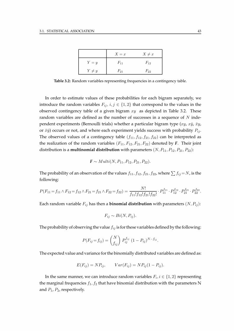
3.1. STATISTICAL ASSOCIATION 43
X = x X 6= x
Y = y F11 F12
Y 6= y F21 F22
Table 3.2: Random variables representing frequencies in a contingency table.
In order to estimate values of these probabilities for each bigram separately, we
introduce the random variables Fij , i, j ∈ {1, 2} that correspond to the values in the
observed contingency table of a given bigram xy as depicted in Table 3.2. These
random variables are defined as the number of successes in a sequence of N inde-
pendent experiments (Bernoulli trials) whether a particular bigram type (xy, xy, xy,
or xy) occurs or not, and where each experiment yields success with probability Pij .
The observed values of a contingency table (f11, f12, f21, f22) can be interpreted as
the realization of the random variables (F11, F12, F21, F22) denoted by F. Their joint
distribution is amultinomial distributionwith parameters (N,P11, P12, P21, P22):
F ∼ Multi(N,P11, P12, P21, P22).
The probability of an observation of the values f11, f12, f21, f22, where∑
fij =N , is the
following:
P (F11 =f11∧F12 =f12 ∧F21 =f21∧F22 =f22) =N !
f11!f12!f21!f22!·P f11
11 ·P f12
12 ·P f21
21 ·P f22
22 .
Each random variable Fij has then a binomial distribution with parameters (N,Pij):
Fij ∼ Bi(N,Pij).
Theprobability of observing the value fij is for these variables definedby the following:
P (Fij =fij) =
(N
fij
)P
fij
ij (1 − Pij)N−fij .
The expected value andvariance for the binomially distributed variables are defined as:
E(Fij) = NPij , V ar(Fij) = NPij(1 − Pij).
In the same manner, we can introduce random variables Fi, i ∈ {1, 2} representing
the marginal frequencies f1, f2 that have binomial distribution with the parameters N
and P1, P2, respectively.
44 CHAPTER 3. ASSOCIATION MEASURES
Under the binomial distribution of Fij , the maximum-likelihood estimates of the
population parameters Pij that maximize the probability of the data (the observed
contingency table) are defined as:
p11 :=f11
N≈ P11, p21 :=
f21
N≈ P21,
p12 :=f12
N≈ P12, p22 :=
f22
N≈ P22.
And, analogically, themaximum-likelihood estimates of themarginal probabilities are:
p1 :=f1
N≈ P1 p2 :=
f2
N≈ P2
The last step to measuring statistical association is to define this concept by the
notion of statistical independence. We say that there is no statistical association
between the components of a bigram type if the occurrence of one component has no
influence on the occurrence of the other one, i.e. the occurrences of the components (as
random events) are statistically independent.
In the terminologyof statistical hypothesis testing, this can be formulated as thenull
hypothesis of independence H0 where the probability of observing the components
together (as a bigram) is just the product of their marginal probabilities:
H0 : P = P1 · P2
We are then interested in those bigram types (collocation candidates) for which this
hypothesis can be (based on the evidence obtained from the random sample) rejected
in favor of the alternative hypothesis H1 stating the observed bigram occurrences
have not resulted from random chance:
H1 : P 6= P1 · P2
With the maximum-likelihood estimates p1 ≈ P1 and p2 ≈ P2, we can determine the
probabilities Pij under the null hypothesis H0 as:
H0 : P11 = p1 · p2,
P12 = p1 · (1−p2),
P21 = (1−p1) · p2,
P21 = (1−p1) · (1−p2).
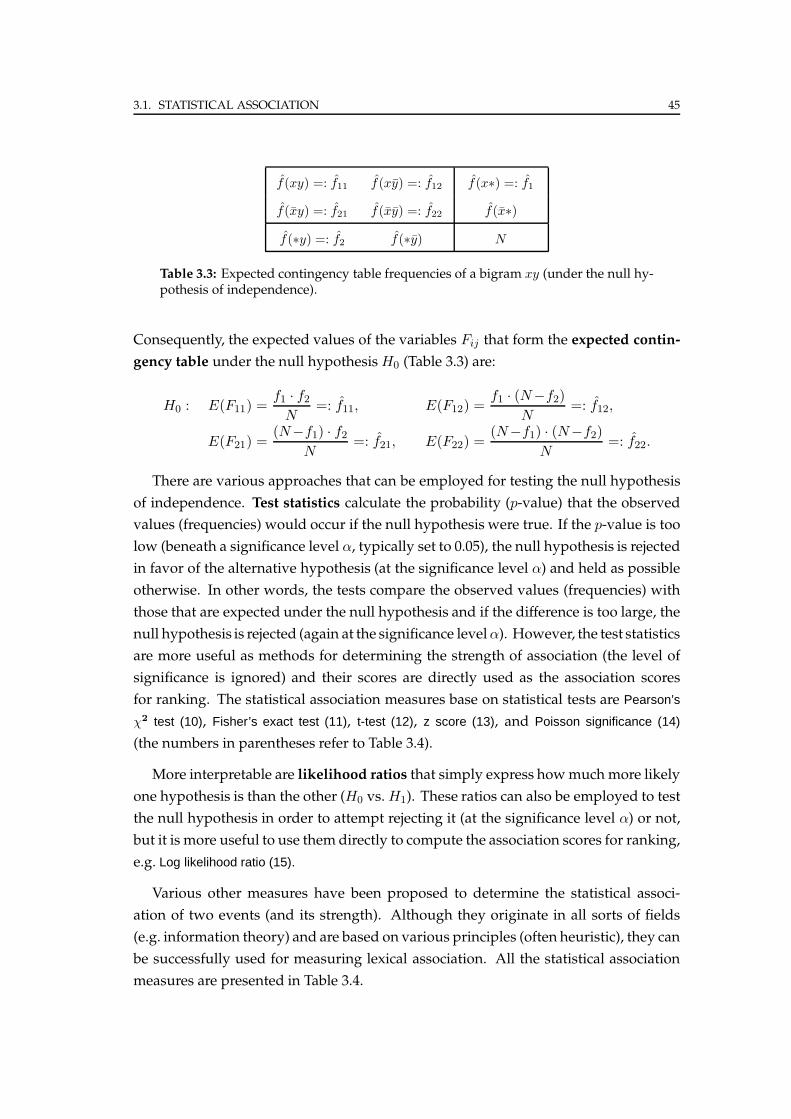
3.1. STATISTICAL ASSOCIATION 45
f(xy) =: f11 f(xy) =: f12 f(x∗) =: f1
f(xy) =: f21 f(xy) =: f22 f(x∗)
f(∗y) =: f2 f(∗y) N
Table 3.3: Expected contingency table frequencies of a bigram xy (under the null hy-pothesis of independence).
Consequently, the expected values of the variables Fij that form the expected contin-
gency table under the null hypothesis H0 (Table 3.3) are:
H0 : E(F11) =f1 · f2
N=: f11, E(F12) =
f1 · (N−f2)
N=: f12,
E(F21) =(N−f1) · f2
N=: f21, E(F22) =
(N−f1) · (N−f2)
N=: f22.
There are various approaches that can be employed for testing the null hypothesis
of independence. Test statistics calculate the probability (p-value) that the observed
values (frequencies) would occur if the null hypothesis were true. If the p-value is too
low (beneath a significance level α, typically set to 0.05), the null hypothesis is rejected
in favor of the alternative hypothesis (at the significance level α) and held as possible
otherwise. In other words, the tests compare the observed values (frequencies) with
those that are expected under the null hypothesis and if the difference is too large, the
null hypothesis is rejected (again at the significance levelα). However, the test statistics
are more useful as methods for determining the strength of association (the level of
significance is ignored) and their scores are directly used as the association scores
for ranking. The statistical association measures base on statistical tests are Pearson’s
χ2 test (10), Fisher’s exact test (11), t-test (12), z score (13), and Poisson significance (14)
(the numbers in parentheses refer to Table 3.4).
More interpretable are likelihood ratios that simply express howmuch more likely
one hypothesis is than the other (H0 vs. H1). These ratios can also be employed to test
the null hypothesis in order to attempt rejecting it (at the significance level α) or not,
but it is more useful to use them directly to compute the association scores for ranking,
e.g. Log likelihood ratio (15).
Various other measures have been proposed to determine the statistical associ-
ation of two events (and its strength). Although they originate in all sorts of fields
(e.g. information theory) and are based on various principles (often heuristic), they can
be successfully used for measuring lexical association. All the statistical association
measures are presented in Table 3.4.
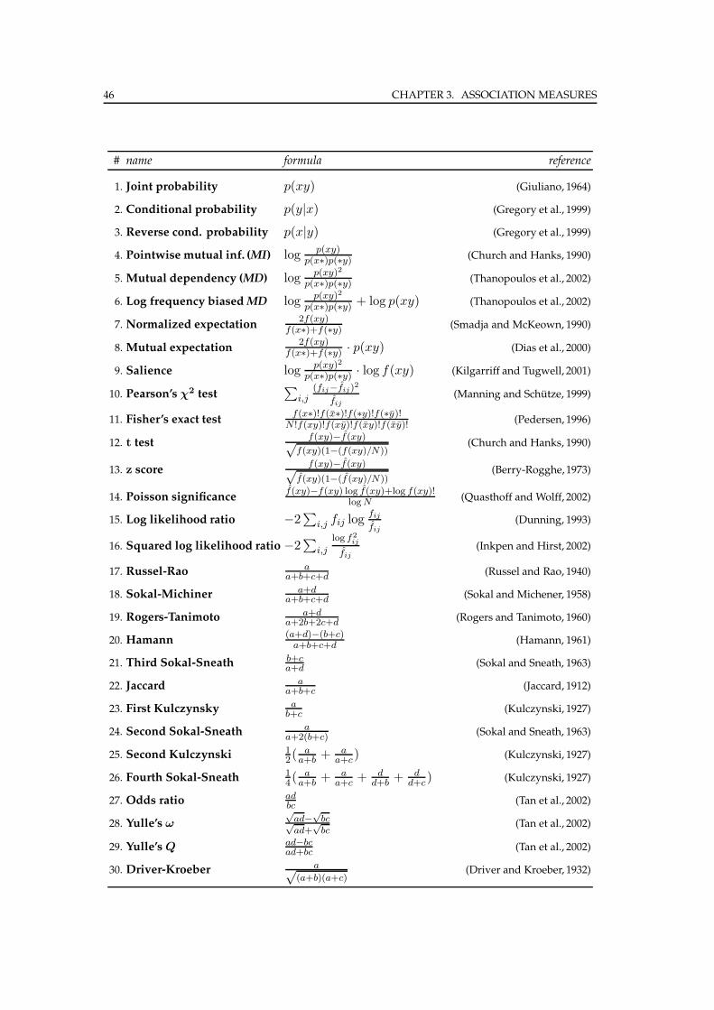
46 CHAPTER 3. ASSOCIATION MEASURES
# name formula reference
1. Joint probability p(xy) (Giuliano, 1964)
2. Conditional probability p(y|x) (Gregory et al., 1999)
3. Reverse cond. probability p(x|y) (Gregory et al., 1999)
4. Pointwise mutual inf. (MI) log p(xy)p(x∗)p(∗y) (Church and Hanks, 1990)
5. Mutual dependency (MD) log p(xy)2
p(x∗)p(∗y) (Thanopoulos et al., 2002)
6. Log frequency biasedMD log p(xy)2
p(x∗)p(∗y) + log p(xy) (Thanopoulos et al., 2002)
7. Normalized expectation2f(xy)
f(x∗)+f(∗y) (Smadja and McKeown, 1990)
8. Mutual expectation2f(xy)
f(x∗)+f(∗y) · p(xy) (Dias et al., 2000)
9. Salience log p(xy)2
p(x∗)p(∗y) · log f(xy) (Kilgarriff and Tugwell, 2001)
10. Pearson’s χ2 test∑
i,j(fij−fij)
2
fij
(Manning and Schutze, 1999)
11. Fisher’s exact testf(x∗)!f(x∗)!f(∗y)!f(∗y)!
N !f(xy)!f(xy)!f(xy)!f(xy)! (Pedersen, 1996)
12. t testf(xy)−f(xy)√
f(xy)(1−(f(xy)/N))(Church and Hanks, 1990)
13. z scoref(xy)−f(xy)√
f(xy)(1−(f (xy)/N))(Berry-Rogghe,1973)
14. Poisson significancef(xy)−f(xy) log f(xy)+log f(xy)!
log N (Quasthoff and Wolff, 2002)
15. Log likelihood ratio −2∑
i,j fij logfij
fij
(Dunning, 1993)
16. Squared log likelihood ratio −2∑
i,j
log f2
ij
fij
(Inkpen and Hirst, 2002)
17. Russel-Rao aa+b+c+d (Russel and Rao, 1940)
18. Sokal-Michiner a+da+b+c+d (Sokal and Michener, 1958)
19. Rogers-Tanimoto a+da+2b+2c+d (Rogers and Tanimoto, 1960)
20. Hamann(a+d)−(b+c)
a+b+c+d (Hamann, 1961)
21. Third Sokal-Sneath b+ca+d (Sokal and Sneath, 1963)
22. Jaccard aa+b+c (Jaccard, 1912)
23. First Kulczynsky ab+c (Kulczynski, 1927)
24. Second Sokal-Sneath aa+2(b+c) (Sokal and Sneath, 1963)
25. Second Kulczynski 12( a
a+b + aa+c) (Kulczynski, 1927)
26. Fourth Sokal-Sneath 14( a
a+b + aa+c + d
d+b + dd+c) (Kulczynski, 1927)
27. Odds ratio adbc (Tan et al., 2002)
28. Yulle’s ω√
ad−√
bc√ad+
√bc
(Tan et al., 2002)
29. Yulle’s Q ad−bcad+bc (Tan et al., 2002)
30. Driver-Kroeber a√(a+b)(a+c)
(Driver and Kroeber, 1932)
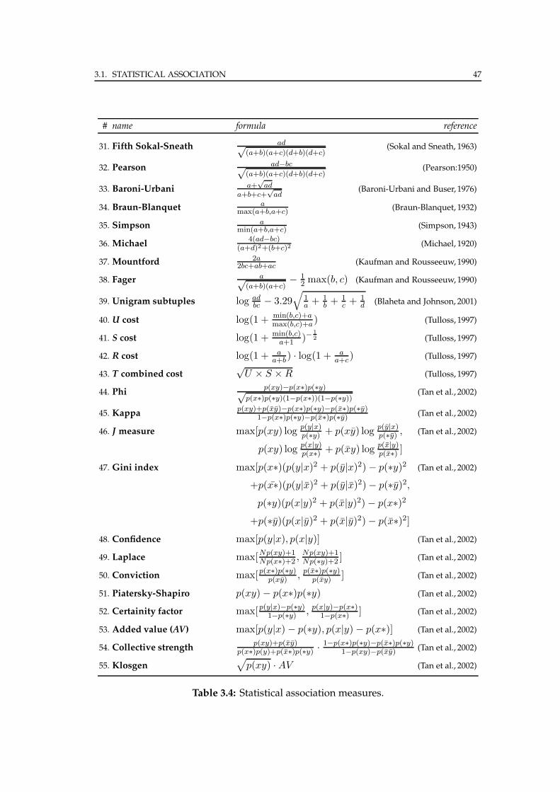
3.1. STATISTICAL ASSOCIATION 47
# name formula reference
31. Fifth Sokal-Sneath ad√(a+b)(a+c)(d+b)(d+c)
(Sokal and Sneath, 1963)
32. Pearson ad−bc√(a+b)(a+c)(d+b)(d+c)
(Pearson:1950)
33. Baroni-Urbani a+√
ada+b+c+
√ad
(Baroni-Urbani and Buser, 1976)
34. Braun-Blanquet amax(a+b,a+c) (Braun-Blanquet, 1932)
35. Simpson amin(a+b,a+c) (Simpson, 1943)
36. Michael4(ad−bc)
(a+d)2+(b+c)2(Michael, 1920)
37. Mountford 2a2bc+ab+ac (Kaufman and Rousseeuw, 1990)
38. Fager a√(a+b)(a+c)
− 12 max(b, c) (Kaufman and Rousseeuw, 1990)
39. Unigram subtuples log adbc − 3.29
√1a + 1
b + 1c + 1
d (Blaheta and Johnson, 2001)
40. U cost log(1 + min(b,c)+amax(b,c)+a) (Tulloss, 1997)
41. S cost log(1 + min(b,c)a+1 )−
1
2 (Tulloss, 1997)
42. R cost log(1 + aa+b) · log(1 + a
a+c) (Tulloss, 1997)
43. T combined cost√
U × S × R (Tulloss, 1997)
44. Phip(xy)−p(x∗)p(∗y)√
p(x∗)p(∗y)(1−p(x∗))(1−p(∗y))(Tan et al., 2002)
45. Kappap(xy)+p(xy)−p(x∗)p(∗y)−p(x∗)p(∗y)
1−p(x∗)p(∗y)−p(x∗)p(∗y) (Tan et al., 2002)
46. J measure max[p(xy) log p(y|x)p(∗y) + p(xy) log p(y|x)
p(∗y) , (Tan et al., 2002)
p(xy) log p(x|y)p(x∗) + p(xy) log p(x|y)
p(x∗) ]
47. Gini index max[p(x∗)(p(y|x)2 + p(y|x)2) − p(∗y)2 (Tan et al., 2002)
+p(x∗)(p(y|x)2 + p(y|x)2) − p(∗y)2,
p(∗y)(p(x|y)2 + p(x|y)2) − p(x∗)2
+p(∗y)(p(x|y)2 + p(x|y)2) − p(x∗)2]48. Confidence max[p(y|x), p(x|y)] (Tan et al., 2002)
49. Laplace max[Np(xy)+1Np(x∗)+2 , Np(xy)+1
Np(∗y)+2 ] (Tan et al., 2002)
50. Conviction max[p(x∗)p(∗y)p(xy) , p(x∗)p(∗y)
p(xy) ] (Tan et al., 2002)
51. Piatersky-Shapiro p(xy) − p(x∗)p(∗y) (Tan et al., 2002)
52. Certainity factor max[p(y|x)−p(∗y)1−p(∗y) , p(x|y)−p(x∗)
1−p(x∗) ] (Tan et al., 2002)
53. Added value (AV) max[p(y|x) − p(∗y), p(x|y) − p(x∗)] (Tan et al., 2002)
54. Collective strengthp(xy)+p(xy)
p(x∗)p(y)+p(x∗)p(∗y) ·1−p(x∗)p(∗y)−p(x∗)p(∗y)
1−p(xy)−p(xy) (Tan et al., 2002)
55. Klosgen√
p(xy) · AV (Tan et al., 2002)
Table 3.4: Statistical association measures.
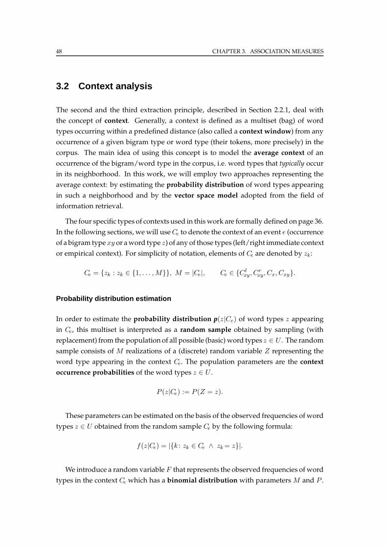
48 CHAPTER 3. ASSOCIATION MEASURES
3.2 Context analysis
The second and the third extraction principle, described in Section 2.2.1, deal with
the concept of context. Generally, a context is defined as a multiset (bag) of word
types occurring within a predefined distance (also called a context window) from any
occurrence of a given bigram type or word type (their tokens, more precisely) in the
corpus. The main idea of using this concept is to model the average context of an
occurrence of the bigram/word type in the corpus, i.e. word types that typically occur
in its neighborhood. In this work, we will employ two approaches representing the
average context: by estimating the probability distribution of word types appearing
in such a neighborhood and by the vector space model adopted from the field of
information retrieval.
The four specific types of contexts used in thiswork are formally definedonpage 36.
In the following sections, wewill useCe to denote the context of an event e (occurrence
of a bigram typexy or aword type z) of any of those types (left/right immediate context
or empirical context). For simplicity of notation, elements of Ce are denoted by zk:
Ce = {zk : zk ∈ {1, . . . ,M}}, M = |Ce|, Ce ∈ {C lxy, C
rxy, Cx, Cxy}.
Probability distribution estimation
In order to estimate the probability distribution p(z|Ce) of word types z appearing
in Ce, this multiset is interpreted as a random sample obtained by sampling (with
replacement) from the population of all possible (basic) word types z ∈ U . The random
sample consists of M realizations of a (discrete) random variable Z representing the
word type appearing in the context Ce. The population parameters are the context
occurrence probabilities of the word types z ∈ U .
P (z|Ce) := P (Z = z).
These parameters can be estimated on the basis of the observed frequencies of word
types z ∈ U obtained from the random sample Ce by the following formula:
f(z|Ce) = |{k : zk ∈ Ce ∧ zk = z}|.
We introduce a random variable F that represents the observed frequencies of word
types in the context Ce which has a binomial distribution with parameters M and P .
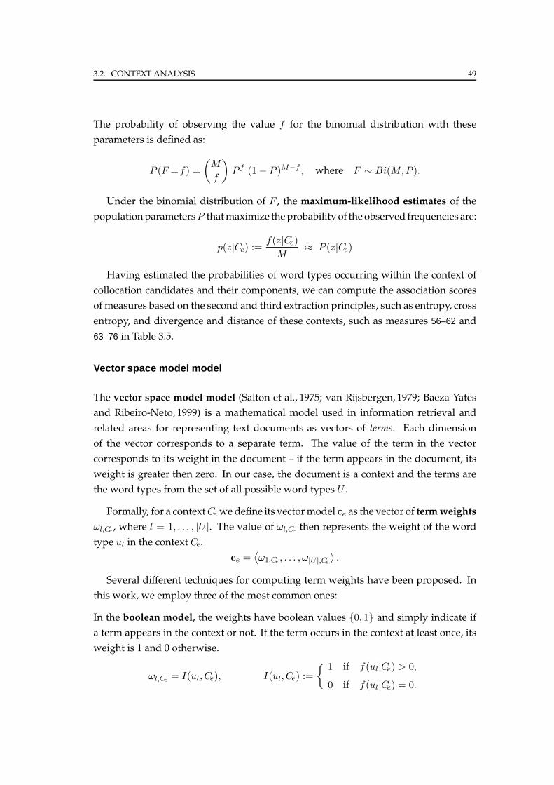
3.2. CONTEXT ANALYSIS 49
The probability of observing the value f for the binomial distribution with these
parameters is defined as:
P (F =f) =
(M
f
)P f (1 − P )M−f , where F ∼ Bi(M,P ).
Under the binomial distribution of F , the maximum-likelihood estimates of the
populationparametersP thatmaximize theprobability of the observed frequencies are:
p(z|Ce) :=f(z|Ce)
M≈ P (z|Ce)
Having estimated the probabilities of word types occurring within the context of
collocation candidates and their components, we can compute the association scores
of measures based on the second and third extraction principles, such as entropy, cross
entropy, and divergence and distance of these contexts, such as measures 56–62 and
63–76 in Table 3.5.
Vector space model model
The vector space model model (Salton et al., 1975; van Rijsbergen, 1979; Baeza-Yates
and Ribeiro-Neto, 1999) is a mathematical model used in information retrieval and
related areas for representing text documents as vectors of terms. Each dimension
of the vector corresponds to a separate term. The value of the term in the vector
corresponds to its weight in the document – if the term appears in the document, its
weight is greater then zero. In our case, the document is a context and the terms are
the word types from the set of all possible word types U .
Formally, for a contextCe we define its vectormodel ce as the vector of termweights
ωl,Ce, where l = 1, . . . , |U |. The value of ωl,Ce
then represents the weight of the word
type ul in the context Ce.
ce =⟨ω1,Ce
, . . . , ω|U |,Ce
⟩.
Several different techniques for computing term weights have been proposed. In
this work, we employ three of the most common ones:
In the boolean model, the weights have boolean values {0, 1} and simply indicate if
a term appears in the context or not. If the term occurs in the context at least once, its
weight is 1 and 0 otherwise.
ωl,Ce= I(ul, Ce), I(ul, Ce) :=
{ 1 if f(ul|Ce) > 0,
0 if f(ul|Ce) = 0.
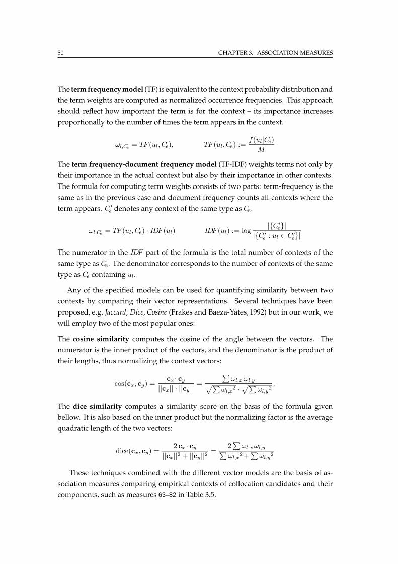
50 CHAPTER 3. ASSOCIATION MEASURES
The term frequencymodel (TF) is equivalent to the context probability distribution and
the term weights are computed as normalized occurrence frequencies. This approach
should reflect how important the term is for the context – its importance increases
proportionally to the number of times the term appears in the context.
ωl,Ce= TF (ul, Ce), TF (ul, Ce) :=
f(ul|Ce)
M
The term frequency-document frequency model (TF-IDF) weights terms not only by
their importance in the actual context but also by their importance in other contexts.
The formula for computing term weights consists of two parts: term-frequency is the
same as in the previous case and document frequency counts all contexts where the
term appears. C ′e denotes any context of the same type as Ce.
ωl,Ce= TF (ul, Ce) · IDF (ul) IDF (ul) := log
|{C ′e}|
|{C ′e : ul ∈ C ′
e}|
The numerator in the IDF part of the formula is the total number of contexts of the
same type as Ce. The denominator corresponds to the number of contexts of the same
type as Ce containing ul.
Any of the specified models can be used for quantifying similarity between two
contexts by comparing their vector representations. Several techniques have been
proposed, e.g. Jaccard, Dice, Cosine (Frakes and Baeza-Yates, 1992) but in our work, we
will employ two of the most popular ones:
The cosine similarity computes the cosine of the angle between the vectors. The
numerator is the inner product of the vectors, and the denominator is the product of
their lengths, thus normalizing the context vectors:
cos(cx, cy) =cx · cy
||cx|| · ||cy ||=
∑ωl,x ωl,y√∑
ωl,x2 ·
√∑ωl,y
2.
The dice similarity computes a similarity score on the basis of the formula given
bellow. It is also based on the inner product but the normalizing factor is the average
quadratic length of the two vectors:
dice(cx, cy) =2 cx · cy
||cx||2 + ||cy ||2=
2∑
ωl,x ωl,y∑ωl,x
2+∑
ωl,y2
These techniques combined with the different vector models are the basis of as-
sociation measures comparing empirical contexts of collocation candidates and their
components, such as measures 63–82 in Table 3.5.
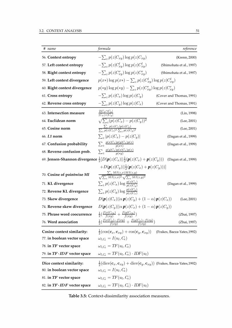
3.2. CONTEXT ANALYSIS 51
# name formula reference
56. Context entropy −∑z p(z|Cxy) log p(z|Cxy) (Krenn, 2000)
57. Left context entropy −∑z p(z|C l
xy) log p(z|C lxy) (Shimohata et al., 1997)
58. Right context entropy −∑
z p(z|Crxy) log p(z|Cr
xy) (Shimohata et al., 1997)
59. Left context divergence p(x∗) log p(x∗) − ∑z p(z|C l
xy) log p(z|C lxy)
60. Right context divergence p(∗y) log p(∗y) − ∑z p(z|Cr
xy) log p(z|Crxy)
61. Cross entropy −∑z p(z|Cx) log p(z|Cy) (Cover and Thomas, 1991)
62. Reverse cross entropy −∑
z p(z|Cy) log p(z|Cx) (Cover and Thomas, 1991)
63. Intersection measure2|Cx∩Cy ||Cx|+|Cy| (Lin, 1998)
64. Euclidean norm√∑
z(p(z|Cx) − p(z|Cy))2 (Lee, 2001)
65. Cosine normP
z p(z|Cx)p(z|Cy)P
z p(z|Cx)2·P
z p(z|Cy)2(Lee, 2001)
66. L1 norm∑
z |p(z|Cx) − p(z|Cy)| (Dagan et al., 1999)
67. Confusion probability∑
zp(x|Cz)p(y|Cz)p(z)
p(x∗) (Dagan et al., 1999)
68. Reverse confusion prob.∑
zp(y|Cz)p(x|Cz)p(z)
p(∗y)
69. Jensen-Shannon divergence 12 [D(p(z|Cx)||12 (p(z|Cx) + p(z|Cy))) (Dagan et al., 1999)
+D(p(z|Cy)||12 (p(z|Cx) + p(z|Cy)))]
70. Cosine of pointwiseMIP
z MI(z,x)MI(z,y)√P
z MI(z,x)2·√
P
z MI(z,y)2
71. KL divergence∑
z p(z|Cx) log p(z|Cx)p(z|Cy) (Dagan et al., 1999)
72. Reverse KL divergence∑
z p(z|Cy) logp(z|Cy)p(z|Cx)
73. Skew divergence D(p(z|Cx)||α p(z|Cy) + (1 − α) p(z|Cx)) (Lee, 2001)
74. Reverse skew divergence D(p(z|Cy)||α p(z|Cx) + (1 − α) p(z|Cy))
75. Phrase word coocurrence 12(
f(x|Cxy)f(xy) +
f(y|Cxy)f(xy) ) (Zhai, 1997)
76. Word association 12(
f(x|Cy)−f(xy)f(xy) + f(y|Cx)−f(xy)
f(xy) ) (Zhai, 1997)
Cosine context similarity: 12(cos(cx, cxy) + cos(cy , cxy)) (Frakes, Baeza-Yates,1992)
77. in boolean vector space ωl,Ce= I(ul, Ce)
78. in TF vector space ωl,Ce= TF (ul, Ce)
79. in TF ·IDF vector space ωl,Ce= TF (ul, Ce) · IDF (ul)
Dice context similarity: 12(dice(cx, cxy) + dice(cy, cxy)) (Frakes, Baeza-Yates,1992)
80. in boolean vector space ωl,Ce= I(ul, Ce)
81. in TF vector space ωl,Ce= TF (ul, Ce)
82. in TF ·IDF vector space ωl,Ce= TF (ul, Ce) · IDF (ul)
Table 3.5: Context-dissimilarity association measures.

52
Chapter 4
Reference Data
Gold standard reference data is absolutely essential for empirical evaluation. For many
tasks of computational linguistics and natural language processing (such as machine
translation or word sense disambiguation), standard and well designed reference data
sets are widely available for evaluation and development purposes, often developed
for shared task evaluation campaigns (e.g. the NIST MT Evaluation1 or Senseval2).
Since this has not been the case for the task of collocation extraction (at the time of
writing of this thesis) we decided to develop a complete testbed of our own. In the fol-
lowing sections, we describe requirements we imposed on such data, actual reference
data sets used in our experiments, and source corpora the data was extracted from.
The main set of our experiments was conducted on the Czech Prague Dependency
Treebank, a medium-sized corpus featuring manual morphological and syntactic an-
notation. In additional experiments, we used the Czech National Corpus, a much larger
data automaticaly processedby a part-of-speech tagger. In order to compare the results
with experiments on a different language, we also carried out some experiments on
the Swedish PAROLE corpus provided with automatic part-of-speech tagging.
4.1 Requirements
With respect to the nature of the task (ranking collocation candidates; see Chapter 2),
and the evaluation method (based on precision and recall; see Chapter 5) the reference
data should be composed of a set of collocation candidates indicated (annotated) as
1http://www.nist.gov/speech/tests/mt/2http://www.senseval.org/
53
54 CHAPTER 4. REFERENCE DATA
true collocations and false collocations (non-collocations). The design and development
of the reference data is thus influenced by two main factors: 1) how and from where
to extract the candidate data and 2) how to perform the annotation.
4.1.1 Candidate data extraction
When choosing the source corpus and preparing the candidate data for annotation,
we considered the following requirements (or recommendations):
1. Czech, similar to many other languages, has very complex morphology. Ap-
propriate morphological normalization is required to conflate all morphological
variants of individual collocation candidates so all occurrences of a collocation
candidate in the source corpus are correctly recognized regardless of their actual
surface forms.
2. According to our notion of collocation (see Section 2.1.5), collocations are gram-
matically bounded. Syntactic information is required to identify collocation
candidates solely as syntactic units (and not as other non-syntactic word com-
binations). Also, each occurrence of a collocation candidate must be correctly
recognized regardless of its actual word order.
3. Tominimize the bias caused by underlying linguistic data preprocessing (such as
part-of-speech tagging, lemmatization, and parsing) the source corpus should be
provided with manual linguistic annotation (on a morphological and syntactic
level).
4. Most of the extraction methods assume normal distribution of observations or
become unreliable when dealing with rare events for other reasons (see Chap-
ter 3). The source corpus must be large enough to provide enough occurrence
evidence for sufficient numbers of collocation candidates.
5. Ideally, the annotation should be performed on a full candidate data extracted
from the corpus (e.g. all occurring n-grams) to avoid sampling (taking only
a subset of the full data) and potential problems with estimating performance
over the full data based on the sample estimation.
6. The amount of collocation candidates must be small enough that the annotation
process is feasible for a human annotator, and at the same time large enough to
provide good and reliable estimation of the performance scores.
4.2. PRAGUE DEPENDENCY TREEBANK 55
4.1.2 Annotation process
The annotation process should result in a set of collocation candidates, each judged
either as a true collocation or as a false collocation. The entire procedure must follow
a-priori established guidelines covering the following points:
1. Clear and exact definition of annotated phenomena must be provided. All the
participating annotators must share the same notion of these phenomena and be
able to achieve maximum agreement.
2. Subjectivity and other factors play an important role in the notion of collocation
and have a negative influence on the process quality. The annotation should be
performed independently by multiple annotators in parallel in order to estimate
the output quality and to minimize the subjectivity of the work by combining
annotators’ judgments.
3. There are many possible approaches to combine multiple annotators’ outcomes:
at least one positive judgment required, taking a majority vote, full agreement
required etc. Due to the nature of the annotated phenomena, this should also be
considered in advance.
4. There are two possible approaches to the actual annotation processs: Annotators
can assess each occurrence of a collocation candidate (as a token) with com-
plete knowledge of its current context, or judge collocation candidates as types
independently on their occurrences and without actual contextual information,
under the assumption that every occurrence of a given collocation is exclusively
true or false collocation.
4.2 Prague Dependency Treebank
To accomplish all requirements imposed in the previous section, we chose the Prague
Dependency Treebank 2.0 (PDT) as the source corpus of our candidate data. It is a mod-
erate sized corpus provided with manual morphological and syntactic annotation. By
focusing only on two-word collocations, PDT provides sufficient evidence of observa-
tions for a soundevaluation. Bydefault, thedata is divided into training, development,
and evaluation sets. We ignored this split and used all data annotated on the morpho-
logical and analytical layer: a total of 1 504 847 tokens in 87 980 sentences and 5 338
documents.
56 CHAPTER 4. REFERENCE DATA
4.2.1 Treebank details
The Prague Dependency Treebank has been developed by the Institute of Formal and
Applied Linguistics and the Center for Computational Linguistics, Charles University,
Prague3 and it is available fromLDC4 (catalognumberLDC2006T01). It contains a large
amount of Czech texts with complex and interlinked annotation on morphological,
analytical (surface syntax), and tectogrammatical (deep syntax) layer. The textmaterial
comprises samples fromdaily newspapers, aweekly businessmagazine, and a popular
scientific magazine. The annotation is based on the long-standing Praguian linguistic
tradition, adapted for the current computational linguistics research needs.5
Morphological layer
On the morphological layer, each word form (token) is assigned a lemma and a mor-
phological tag. Combination of the lemma and the tag uniquely identifies the word
form. Two different word forms differ either in their lemmas or in morphological tags.
A lemma has two parts. The first part, the lemma proper, is a unique identifier of
the lexical item. Usually it is the base form (e.g. first case singular for a noun, infinitive
for a verb, etc.) of the word, possibly followed by a number distinguishing different
lemmas, with the same base forms (different word senses). Second part is optional. It
contains additional information about the lemma (e.g. semantic or derivational infor-
mation). Amorphological tag is a string of 15 characters where every position encodes
one morphological category using one character. Description of the categories and
range of their possible values are summarized in Table 4.1. Details of morphological
annotation can be found in (Zeman et al., 2005).
Analytical layer
Analytical layer of PDT serves to encode sentence dependency structures. Each word
is linked to itsheadword and assigned its analytical function (dependency type). Ifwe
think of a sentence as a graph with words as nodes and dependency relation as edges,
the dependency structure is a tree – a directed acyclic graph having one root. Possible
values of analytical functions are listed in Table 4.2. Details of analytical annotation
can be found in (Hajic et al., 1997) and a small example of an annotated text in Table 4.3.
3http://ufal.mff.cuni.cz/4http://www.ldc.upenn.edu/5http://ufal.mff.cuni.cz/pdt2.0/
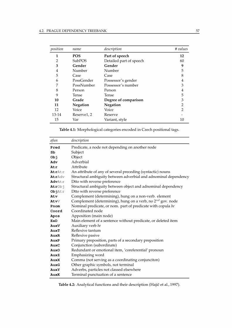
4.2. PRAGUE DEPENDENCY TREEBANK 57
position name description # values
1 POS Part of speech 12
2 SubPOS Detailed part of speech 60
3 Gender Gender 9
4 Number Number 55 Case Case 8
6 PossGender Possessor’s gender 47 PossNumber Possessor’s number 3
8 Person Person 4
9 Tense Tense 510 Grade Degree of comparison 3
11 Negation Negation 212 Voice Voice 2
13-14 Reserve1, 2 Reserve -
15 Var Variant, style 10
Table 4.1: Morphological categories encoded in Czech positional tags.
afun description
Pred Predicate, a node not depending on another node
Sb SubjectObj Object
Adv Adverbial
Atr AttributeAtrAtr An attribute of any of several preceding (syntactic) nouns
AtrAdv Structural ambiguity between adverbial and adnominal dependencyAdvAtr Dtto with reverse preference
AtrObj Structural ambiguity between object and adnominal dependency
ObjAtr Dtto with reverse preferenceAtv Complement (determining), hung on a non-verb. element
AtvV Complement (determining), hung on a verb, no 2nd gov. nodePnom Nominal predicate, or nom. part of predicate with copula be
Coord Coordinated node
Apos Apposition (main node)ExD Main element of a sentence without predicate, or deleted item
AuxV Auxiliary verb beAuxT Reflexive tantum
AuxR Reflexive pasive
AuxP Primary preposition, parts of a secondary prepositionAuxC Conjunction (subordinate)
AuxO Redundant or emotional item, ’coreferential’ pronoun
AuxZ Emphasizing wordAuxX Comma (not serving as a coordinating conjunciton)
AuxG Other graphic symbols, not terminalAuxY Adverbs, particles not classed elsewhere
AuxK Terminal punctuation of a sentence
Table 4.2: Analytical functions and their description (Hajic et al., 1997).
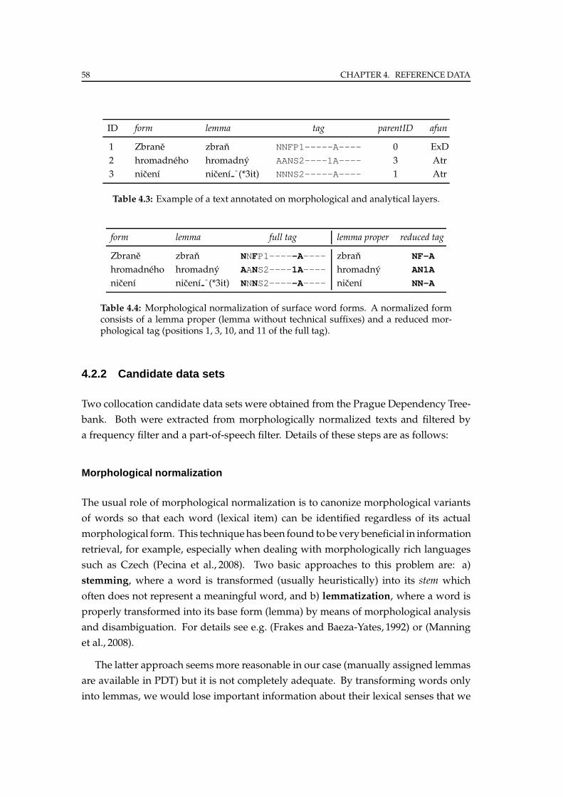
58 CHAPTER 4. REFERENCE DATA
ID form lemma tag parentID afun
1 Zbrane zbran NNFP1-----A---- 0 ExD
2 hromadneho hromadny AANS2----1A---- 3 Atr
3 nicenı nicenı ˆ(*3it) NNNS2-----A---- 1 Atr
Table 4.3: Example of a text annotated on morphological and analytical layers.
form lemma full tag lemma proper reduced tag
Zbrane zbran NNFP1-----A---- zbran NF-A
hromadneho hromadny AANS2----1A---- hromadny AN1A
nicenı nicenı ˆ(*3it) NNNS2-----A---- nicenı NN-A
Table 4.4: Morphological normalization of surface word forms. A normalized formconsists of a lemma proper (lemma without technical suffixes) and a reduced mor-phological tag (positions 1, 3, 10, and 11 of the full tag).
4.2.2 Candidate data sets
Two collocation candidate data sets were obtained from the Prague Dependency Tree-
bank. Both were extracted from morphologically normalized texts and filtered by
a frequency filter and a part-of-speech filter. Details of these steps are as follows:
Morphological normalization
The usual role of morphological normalization is to canonize morphological variants
of words so that each word (lexical item) can be identified regardless of its actual
morphological form. This techniquehas been found tobevery beneficial in information
retrieval, for example, especially when dealing with morphologically rich languages
such as Czech (Pecina et al., 2008). Two basic approaches to this problem are: a)
stemming, where a word is transformed (usually heuristically) into its stem which
often does not represent a meaningful word, and b) lemmatization, where a word is
properly transformed into its base form (lemma) by means of morphological analysis
and disambiguation. For details see e.g. (Frakes and Baeza-Yates, 1992) or (Manning
et al., 2008).
The latter approach seemsmore reasonable in our case (manually assigned lemmas
are available in PDT) but it is not completely adequate. By transforming words only
into lemmas, we would lose important information about their lexical senses that we
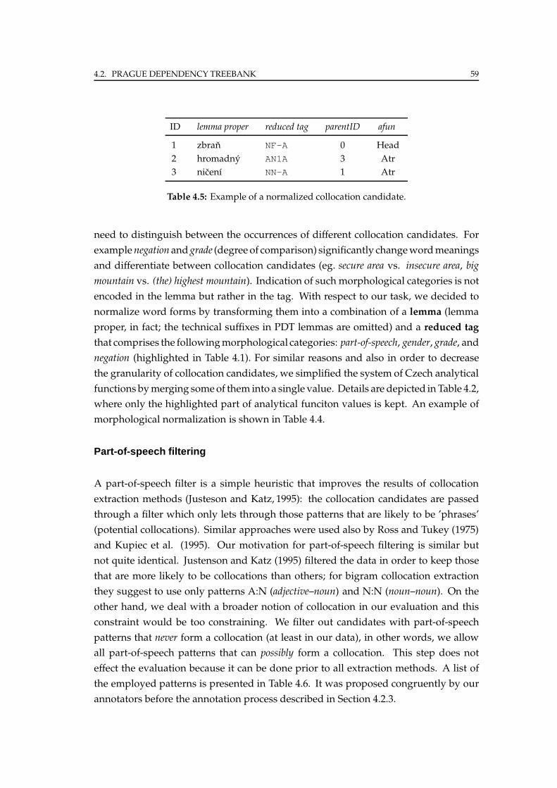
4.2. PRAGUE DEPENDENCY TREEBANK 59
ID lemma proper reduced tag parentID afun
1 zbran NF-A 0 Head
2 hromadny AN1A 3 Atr
3 nicenı NN-A 1 Atr
Table 4.5: Example of a normalized collocation candidate.
need to distinguish between the occurrences of different collocation candidates. For
examplenegation and grade (degree of comparison) significantly changewordmeanings
and differentiate between collocation candidates (eg. secure area vs. insecure area, big
mountain vs. (the) highest mountain). Indication of such morphological categories is not
encoded in the lemma but rather in the tag. With respect to our task, we decided to
normalize word forms by transforming them into a combination of a lemma (lemma
proper, in fact; the technical suffixes in PDT lemmas are omitted) and a reduced tag
that comprises the followingmorphological categories: part-of-speech, gender, grade, and
negation (highlighted in Table 4.1). For similar reasons and also in order to decrease
the granularity of collocation candidates, we simplified the system of Czech analytical
functions bymerging someof them into a single value. Details are depicted in Table 4.2,
where only the highlighted part of analytical funciton values is kept. An example of
morphological normalization is shown in Table 4.4.
Part-of-speech filtering
A part-of-speech filter is a simple heuristic that improves the results of collocation
extraction methods (Justeson and Katz, 1995): the collocation candidates are passed
through a filter which only lets through those patterns that are likely to be ’phrases’
(potential collocations). Similar approaches were used also by Ross and Tukey (1975)
and Kupiec et al. (1995). Our motivation for part-of-speech filtering is similar but
not quite identical. Justenson and Katz (1995) filtered the data in order to keep those
that are more likely to be collocations than others; for bigram collocation extraction
they suggest to use only patterns A:N (adjective–noun) and N:N (noun–noun). On the
other hand, we deal with a broader notion of collocation in our evaluation and this
constraint would be too constraining. We filter out candidates with part-of-speech
patterns that never form a collocation (at least in our data), in other words, we allow
all part-of-speech patterns that can possibly form a collocation. This step does not
effect the evaluation because it can be done prior to all extraction methods. A list of
the employed patterns is presented in Table 4.6. It was proposed congruently by our
annotators before the annotation process described in Section 4.2.3.
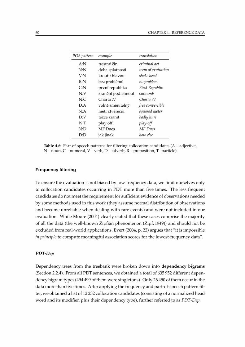
60 CHAPTER 4. REFERENCE DATA
POS pattern example translation
A:N trestny cin criminal act
N:N doba splatnosti term of expiration
V:N kroutit hlavou shake head
R:N bez problemu no problem
C:N prvnı republika First Republic
N:V zranenı podlehnout succumb
N:C Charta 77 Charta 77
D:A volne smenitelny free convertible
N:A metr ctverecnı squared meter
D:V tezce zranit badly hurt
N:T play off play-off
N:D MF Dnes MF Dnes
D:D jak jinak how else
Table 4.6: Part-of-speech patterns for filtering collocation candidates (A – adjective,N – noun, C – numeral, V – verb, D – adverb, R – preposition, T– particle).
Frequency filtering
To ensure the evaluation is not biased by low-frequency data, we limit ourselves only
to collocation candidates occurring in PDT more than five times. The less frequent
candidates do not meet the requirement for sufficient evidence of observations needed
by some methods used in this work (they assume normal distribution of observations
and become unreliable when dealing with rare events) and were not included in our
evaluation. While Moore (2004) clearly stated that these cases comprise the majority
of all the data (the well-known Zipfian phenomenon (Zipf, 1949)) and should not be
excluded from real-world applications, Evert (2004, p. 22) argues that ”it is impossible
in principle to compute meaningful association scores for the lowest-frequency data“.
PDT-Dep
Dependency trees from the treebank were broken down into dependency bigrams
(Section 2.2.4). From all PDT sentences, we obtained a total of 635 952 different depen-
dency bigram types (494 499 of themwere singletons). Only 26 450 of themoccur in the
data more than five times. After applying the frequency and part-of-speech pattern fil-
ter, we obtained a list of 12 232 collocation candidates (consisting of a normalized head
word and its modifier, plus their dependency type), further referred to as PDT-Dep.
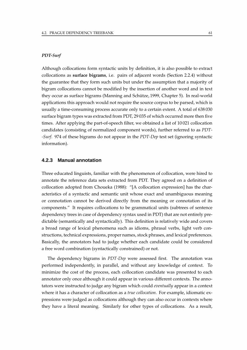
4.2. PRAGUE DEPENDENCY TREEBANK 61
PDT-Surf
Although collocations form syntactic units by definition, it is also possible to extract
collocations as surface bigrams, i.e. pairs of adjacent words (Section 2.2.4) without
the guarantee that they form such units but under the assumption that a majority of
bigram collocations cannot be modified by the insertion of another word and in text
they occur as surface bigrams (Manning and Schutze, 1999, Chapter 5). In real-world
applications this approach would not require the source corpus to be parsed, which is
usually a time-consuming process accurate only to a certain extent. A total of 638 030
surface bigram typeswas extracted from PDT, 29 035 of which occurred more then five
times. After applying the part-of-speech filter, we obtained a list of 10 021 collocation
candidates (consisting of normalized component words), further referred to as PDT-
-Surf. 974 of these bigrams do not appear in the PDT-Dep test set (ignoring syntactic
information).
4.2.3 Manual annotation
Three educated linguists, familiar with the phenomenon of collocation, were hired to
annotate the reference data sets extracted from PDT. They agreed on a definition of
collocation adopted from Choueka (1988): “[A collocation expression] has the char-
acteristics of a syntactic and semantic unit whose exact and unambiguous meaning
or connotation cannot be derived directly from the meaning or connotation of its
components.” It requires collocations to be grammatical units (subtrees of sentence
dependency trees in case of dependency syntax used in PDT) that are not entirely pre-
dictable (semantically and syntactically). This definition is relatively wide and covers
a broad range of lexical phenomena such as idioms, phrasal verbs, light verb con-
structions, technical expressions, proper names, stock phrases, and lexical preferences.
Basically, the annotators had to judge whether each candidate could be considered
a free word combination (syntactically constrained) or not.
The dependency bigrams in PDT-Dep were assessed first. The annotation was
performed independently, in parallel, and without any knowledge of context. To
minimize the cost of the process, each collocation candidate was presented to each
annotator only once although it could appear in various different contexts. The anno-
tators were instructed to judge any bigram which could eventually appear in a context
where it has a character of collocation as a true collocation. For example, idiomatic ex-
pressions were judged as collocations although they can also occur in contexts where
they have a literal meaning. Similarly for other types of collocations. As a result,
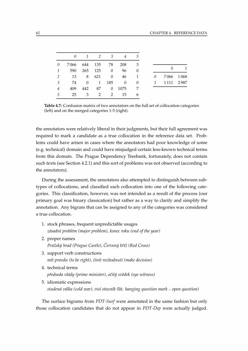
62 CHAPTER 4. REFERENCE DATA
0 1 2 3 4 5
0 7 066 644 135 78 208 3
1 590 265 125 0 96 0
2 13 8 621 0 46 1
3 74 0 1 185 0 0
4 409 442 87 0 1075 7
5 25 3 2 2 15 6
0 1
0 7 066 1 068
1 1 111 2 987
Table 4.7: Confusion matrix of two annotators on the full set of collocation categories(left) and on the merged categories 1-5 (right).
the annotators were relatively liberal in their judgments, but their full agreement was
required to mark a candidate as a true collocation in the reference data set. Prob-
lems could have arisen in cases where the annotators had poor knowledge of some
(e.g. technical) domain and could have misjudged certain less-known technical terms
from this domain. The Prague Dependency Treebank, fortunately, does not contain
such texts (see Section 4.2.1) and this sort of problems was not observed (according to
the annotators).
During the assessment, the annotators also attempted to distinguish between sub-
types of collocations, and classified each collocation into one of the following cate-
gories. This classification, however, was not intended as a result of the process (our
primary goal was binary classication) but rather as a way to clarify and simplify the
annotation. Any bigram that can be assigned to any of the categories was considered
a true collocation.
1. stock phrases, frequent unpredictable usages
zasadnı problem (major problem), konec roku (end of the year)
2. proper names
Prazsky hrad (Prague Castle), Cerveny krız (Red Cross)
3. support verb constructions
mıt pravdu (to be right), cinit rozhodnutı (make decision)
4. technical terms
predseda vlady (prime minister), ocity svedek (eye witness)
5. idiomatic expressions
studena valka (cold war), visı otaznık (lit. hanging question mark ∼ open question)
The surface bigrams from PDT-Surf were annotated in the same fashion but only
those collocation candidates that do not appear in PDT-Dep were actually judged.
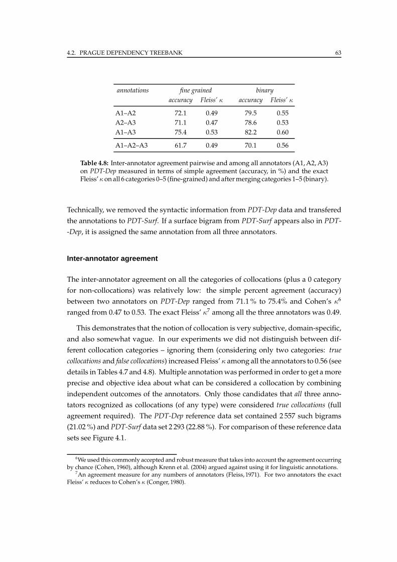
4.2. PRAGUE DEPENDENCY TREEBANK 63
annotations fine grained binary
accuracy Fleiss’ κ accuracy Fleiss’ κ
A1–A2 72.1 0.49 79.5 0.55
A2–A3 71.1 0.47 78.6 0.53
A1–A3 75.4 0.53 82.2 0.60
A1–A2–A3 61.7 0.49 70.1 0.56
Table 4.8: Inter-annotator agreement pairwise and among all annotators (A1,A2,A3)on PDT-Dep measured in terms of simple agreement (accuracy, in %) and the exactFleiss’κonall 6 categories 0–5 (fine-grained) andaftermerging categories 1–5 (binary).
Technically, we removed the syntactic information from PDT-Dep data and transfered
the annotations to PDT-Surf. If a surface bigram from PDT-Surf appears also in PDT-
-Dep, it is assigned the same annotation from all three annotators.
Inter-annotator agreement
The inter-annotator agreement on all the categories of collocations (plus a 0 category
for non-collocations) was relatively low: the simple percent agreement (accuracy)
between two annotators on PDT-Dep ranged from 71.1% to 75.4% and Cohen’s κ6
ranged from 0.47 to 0.53. The exact Fleiss’ κ7 among all the three annotators was 0.49.
This demonstrates that the notion of collocation is very subjective, domain-specific,
and also somewhat vague. In our experiments we did not distinguish between dif-
ferent collocation categories – ignoring them (considering only two categories: true
collocations and false collocations) increased Fleiss’ κ among all the annotators to 0.56 (see
details in Tables 4.7 and 4.8). Multiple annotationwas performed in order to get amore
precise and objective idea about what can be considered a collocation by combining
independent outcomes of the annotators. Only those candidates that all three anno-
tators recognized as collocations (of any type) were considered true collocations (full
agreement required). The PDT-Dep reference data set contained 2 557 such bigrams
(21.02%) and PDT-Surf data set 2 293 (22.88%). For comparison of these reference data
sets see Figure 4.1.
6Weused this commonly accepted and robustmeasure that takes into account the agreement occurringby chance (Cohen, 1960), although Krenn et al. (2004) argued against using it for linguistic annotations.
7An agreement measure for any numbers of annotators (Fleiss, 1971). For two annotators the exactFleiss’ κ reduces to Cohen’s κ (Conger, 1980).
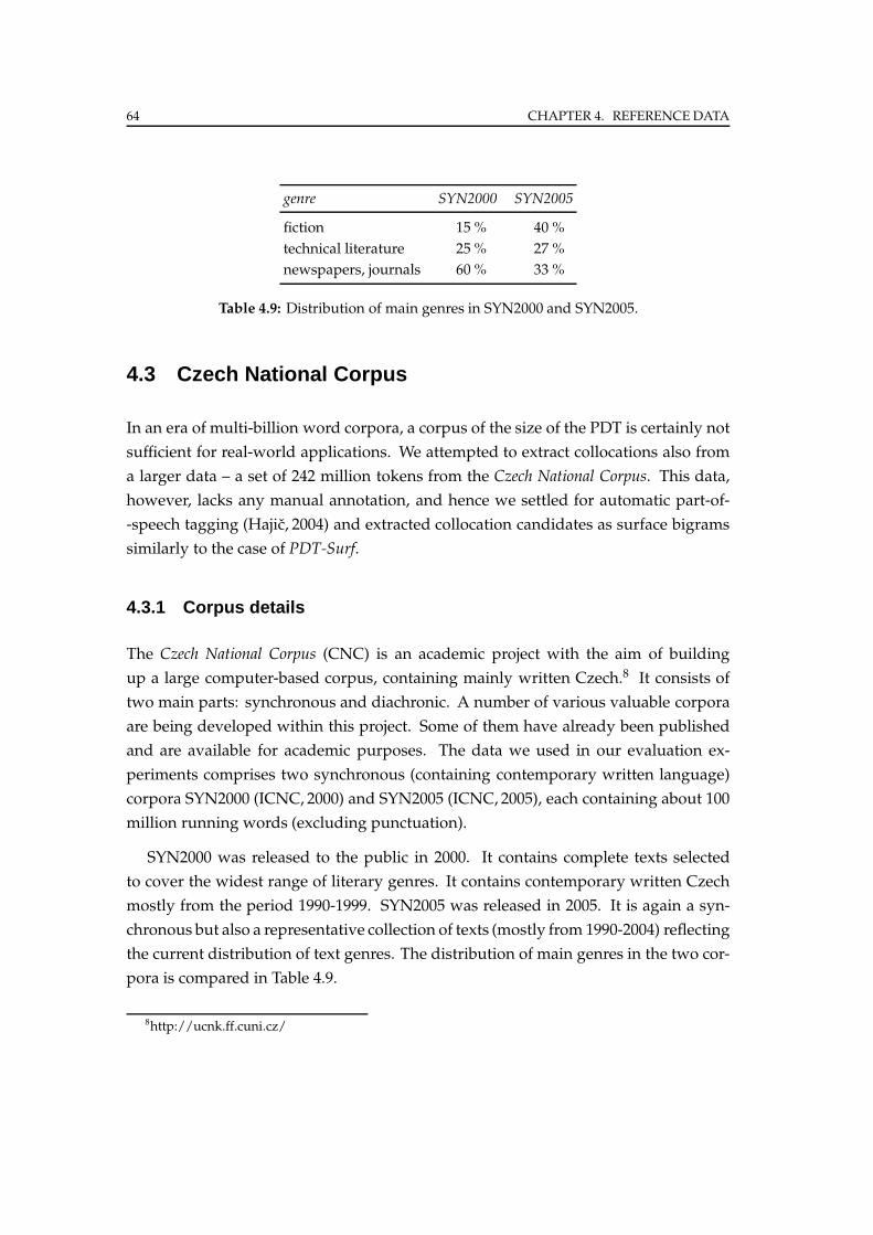
64 CHAPTER 4. REFERENCE DATA
genre SYN2000 SYN2005
fiction 15 % 40 %
technical literature 25 % 27 %
newspapers, journals 60 % 33 %
Table 4.9: Distribution of main genres in SYN2000 and SYN2005.
4.3 Czech National Corpus
In an era of multi-billion word corpora, a corpus of the size of the PDT is certainly not
sufficient for real-world applications. We attempted to extract collocations also from
a larger data – a set of 242 million tokens from the Czech National Corpus. This data,
however, lacks any manual annotation, and hence we settled for automatic part-of-
-speech tagging (Hajic, 2004) and extracted collocation candidates as surface bigrams
similarly to the case of PDT-Surf.
4.3.1 Corpus details
The Czech National Corpus (CNC) is an academic project with the aim of building
up a large computer-based corpus, containing mainly written Czech.8 It consists of
two main parts: synchronous and diachronic. A number of various valuable corpora
are being developed within this project. Some of them have already been published
and are available for academic purposes. The data we used in our evaluation ex-
periments comprises two synchronous (containing contemporary written language)
corpora SYN2000 (ICNC, 2000) and SYN2005 (ICNC, 2005), each containing about 100
million running words (excluding punctuation).
SYN2000 was released to the public in 2000. It contains complete texts selected
to cover the widest range of literary genres. It contains contemporary written Czech
mostly from the period 1990-1999. SYN2005 was released in 2005. It is again a syn-
chronous but also a representative collection of texts (mostly from 1990-2004) reflecting
the current distribution of text genres. The distribution of main genres in the two cor-
pora is compared in Table 4.9.
8http://ucnk.ff.cuni.cz/
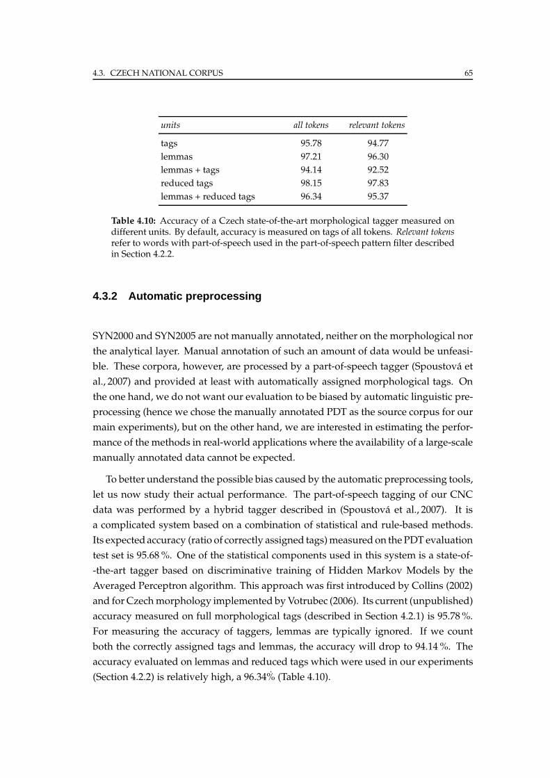
4.3. CZECH NATIONAL CORPUS 65
units all tokens relevant tokens
tags 95.78 94.77
lemmas 97.21 96.30
lemmas + tags 94.14 92.52
reduced tags 98.15 97.83
lemmas + reduced tags 96.34 95.37
Table 4.10: Accuracy of a Czech state-of-the-art morphological tagger measured ondifferent units. By default, accuracy is measured on tags of all tokens. Relevant tokensrefer to words with part-of-speech used in the part-of-speech pattern filter describedin Section 4.2.2.
4.3.2 Automatic preprocessing
SYN2000 and SYN2005 are not manually annotated, neither on the morphological nor
the analytical layer. Manual annotation of such an amount of data would be unfeasi-
ble. These corpora, however, are processed by a part-of-speech tagger (Spoustova et
al., 2007) and provided at least with automatically assigned morphological tags. On
the one hand, we do not want our evaluation to be biased by automatic linguistic pre-
processing (hence we chose the manually annotated PDT as the source corpus for our
main experiments), but on the other hand, we are interested in estimating the perfor-
mance of the methods in real-world applications where the availability of a large-scale
manually annotated data cannot be expected.
To better understand the possible bias caused by the automatic preprocessing tools,
let us now study their actual performance. The part-of-speech tagging of our CNC
data was performed by a hybrid tagger described in (Spoustova et al., 2007). It is
a complicated system based on a combination of statistical and rule-based methods.
Its expectedaccuracy (ratio of correctly assigned tags)measured on the PDT evaluation
test set is 95.68%. One of the statistical components used in this system is a state-of-
-the-art tagger based on discriminative training of Hidden Markov Models by the
Averaged Perceptron algorithm. This approach was first introduced by Collins (2002)
and for Czechmorphology implemented by Votrubec (2006). Its current (unpublished)
accuracy measured on full morphological tags (described in Section 4.2.1) is 95.78%.
For measuring the accuracy of taggers, lemmas are typically ignored. If we count
both the correctly assigned tags and lemmas, the accuracy will drop to 94.14%. The
accuracy evaluated on lemmas and reduced tags which were used in our experiments
(Section 4.2.2) is relatively high, a 96.34% (Table 4.10).
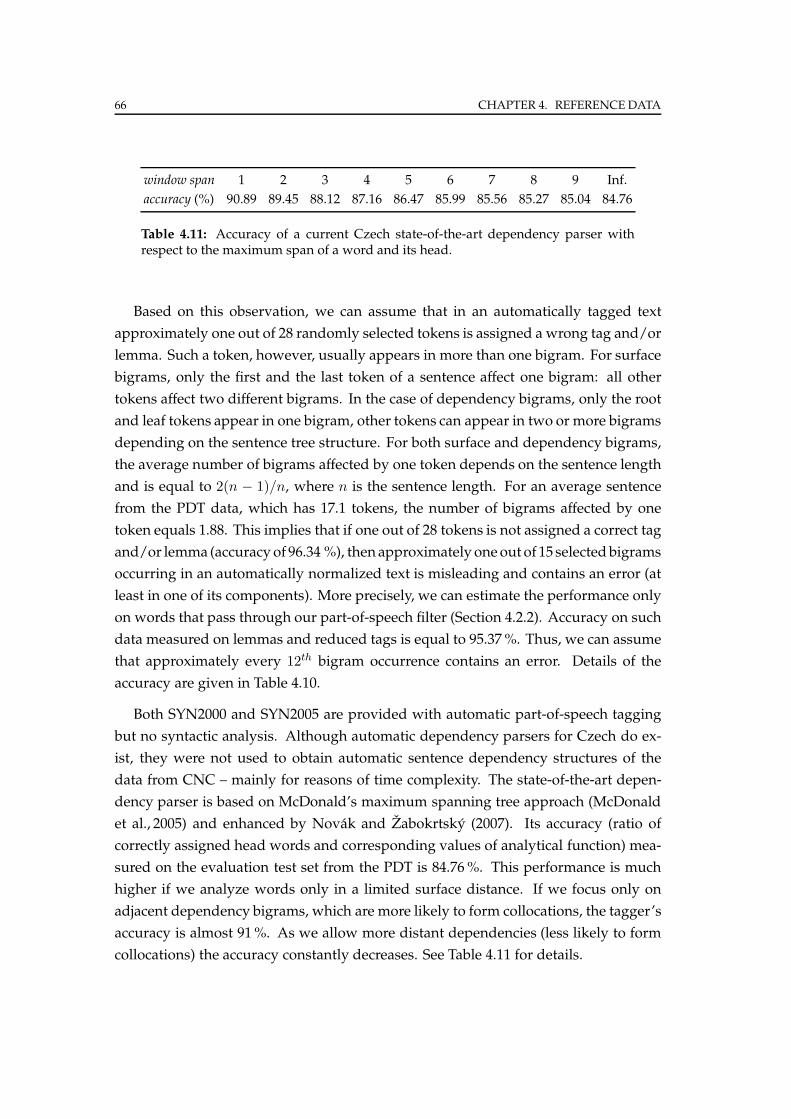
66 CHAPTER 4. REFERENCE DATA
window span 1 2 3 4 5 6 7 8 9 Inf.
accuracy (%) 90.89 89.45 88.12 87.16 86.47 85.99 85.56 85.27 85.04 84.76
Table 4.11: Accuracy of a current Czech state-of-the-art dependency parser withrespect to the maximum span of a word and its head.
Based on this observation, we can assume that in an automatically tagged text
approximately one out of 28 randomly selected tokens is assigned a wrong tag and/or
lemma. Such a token, however, usually appears in more than one bigram. For surface
bigrams, only the first and the last token of a sentence affect one bigram: all other
tokens affect two different bigrams. In the case of dependency bigrams, only the root
and leaf tokens appear in one bigram, other tokens can appear in two or more bigrams
depending on the sentence tree structure. For both surface and dependency bigrams,
the average number of bigrams affected by one token depends on the sentence length
and is equal to 2(n − 1)/n, where n is the sentence length. For an average sentence
from the PDT data, which has 17.1 tokens, the number of bigrams affected by one
token equals 1.88. This implies that if one out of 28 tokens is not assigned a correct tag
and/or lemma (accuracy of 96.34 %), then approximately one out of 15 selectedbigrams
occurring in an automatically normalized text is misleading and contains an error (at
least in one of its components). More precisely, we can estimate the performance only
on words that pass through our part-of-speech filter (Section 4.2.2). Accuracy on such
data measured on lemmas and reduced tags is equal to 95.37%. Thus, we can assume
that approximately every 12th bigram occurrence contains an error. Details of the
accuracy are given in Table 4.10.
Both SYN2000 and SYN2005 are provided with automatic part-of-speech tagging
but no syntactic analysis. Although automatic dependency parsers for Czech do ex-
ist, they were not used to obtain automatic sentence dependency structures of the
data from CNC – mainly for reasons of time complexity. The state-of-the-art depen-
dency parser is based on McDonald’s maximum spanning tree approach (McDonald
et al., 2005) and enhanced by Novak and Zabokrtsky (2007). Its accuracy (ratio of
correctly assigned head words and corresponding values of analytical function) mea-
sured on the evaluation test set from the PDT is 84.76%. This performance is much
higher if we analyze words only in a limited surface distance. If we focus only on
adjacent dependency bigrams, which are more likely to form collocations, the tagger’s
accuracy is almost 91%. As we allow more distant dependencies (less likely to form
collocations) the accuracy constantly decreases. See Table 4.11 for details.
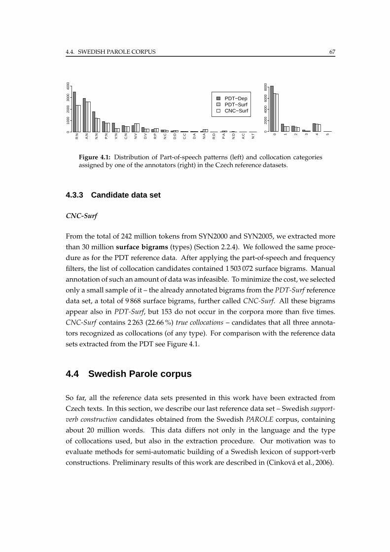
4.4. SWEDISH PAROLE CORPUS 67
R:N
A:N
N:N
P:N
V:N
C:N
N:V
D:V
R:P
N:C
D:D
C:C
D:A
N:A
R:D
P:A
N:D
A:C
N:T
PDT−DepPDT−SurfCNC−Surf
010
0020
0030
0040
00
0 1 2 3 4 5
020
0040
0060
0080
00
Figure 4.1: Distribution of Part-of-speech patterns (left) and collocation categoriesassigned by one of the annotators (right) in the Czech reference datasets.
4.3.3 Candidate data set
CNC-Surf
From the total of 242 million tokens from SYN2000 and SYN2005, we extracted more
than 30 million surface bigrams (types) (Section 2.2.4). We followed the same proce-
dure as for the PDT reference data. After applying the part-of-speech and frequency
filters, the list of collocation candidates contained 1 503 072 surface bigrams. Manual
annotation of such an amount of datawas infeasible. Tominimize the cost, we selected
only a small sample of it – the already annotated bigrams from the PDT-Surf reference
data set, a total of 9 868 surface bigrams, further called CNC-Surf. All these bigrams
appear also in PDT-Surf, but 153 do not occur in the corpora more than five times.
CNC-Surf contains 2 263 (22.66%) true collocations – candidates that all three annota-
tors recognized as collocations (of any type). For comparison with the reference data
sets extracted from the PDT see Figure 4.1.
4.4 Swedish Parole corpus
So far, all the reference data sets presented in this work have been extracted from
Czech texts. In this section, we describe our last reference data set – Swedish support-
verb construction candidates obtained from the Swedish PAROLE corpus, containing
about 20 million words. This data differs not only in the language and the type
of collocations used, but also in the extraction procedure. Our motivation was to
evaluate methods for semi-automatic building of a Swedish lexicon of support-verb
constructions. Preliminary results of this work are described in (Cinkova et al., 2006).
68 CHAPTER 4. REFERENCE DATA
4.4.1 Corpus details
The Swedish Parole corpus is a collection of modern Swedish texts comprising 20 mil-
lion running words. It belongs to Sprakbanken, the set of corpora at Sprakdata,
University in Gothenburg, Sweden.9 The corpus was built within the EU project
PAROLE (finished 1997), which aimed at creating a European network of language
resources (corpora and lexicons). It has automatic morphological annotation but lacks
of lemmatization. In order to deal with morphological normalization, an automatic
lemmatizer developed by Cinkova and Pomikalek (2006) was employed to transform
all word forms into their lemmas.
4.4.2 Support-verb constructions
Support-verb constructions (SVCs) are combinations of a lexical verb and a noun
or a nominal group containing a predication and denoting an event or a state, e.g. to
take/make a decision, to undergo a change. From the semanticpoint of view, thenoun seems
to be part of a complex predicate rather than the object of the verb, whatever the surface
syntax may suggest (Cinkova et al., 2006). The meaning of SVC is concentrated in the
predicate noun, whereas the semantic content of the verb is reduced or generalized.
The notion of SVC and related concepts has already been studied elsewhere, e.g. by
Grefenstette and Teufel (1995), Tapanainen et al. (1998), Lin (1999), McCarthy et al.
(2003), and Bannard et al. (2003).
Our interest in SVCs is mainly in the perspective of foreign language learners and
building a lexicon, see (Cinkova et al., 2006). Although SVCs are easily understood
by foreign language learners, they pose substantial problems for foreign language
production (Heid, 1998) due to the unpredictability of the support verb. For example,
the predicate noun question in an SVC meaning to ask takes different support verbs
in Czech and in Swedish: Czech uses the verb polozit (i.e. to put horizontally) while
Swedish uses the verb stalla (i.e. to put vertically). The translation equivalent to the
support verb is unpredictable, though the common semantic motivation can be traced
back. The unpredictability of the support verb places SVCs into the lexicon, while the
semantic generality of support verbs and their productivity move them to the very
borders of grammar (Cinkova et al., 2006).
9http://spraakbanken.gu.se/PAROLE/
4.4. SWEDISH PAROLE CORPUS 69
4.4.3 Manual extraction
The reference data was obtained by the following manual extraction procedure. It was
inspired by several similar approaches, e.g. by Heid (1998), and comprises these steps:
1. extraction of word expressions whose morphosyntactic character suggests that
they are potential support-verb constructions,
2. subsequent manual elimination of non-collocations,
3. sorting of collocations into three groups: SVCs, quasimodals, and phrasemes.
Step 1 involved formulating several corpus queries and obtaining the results. The
queries basically varied the distance between the verb and the noun (ranging from 1
to 3). Some queries introduced article, number, and adjective insertion restrictions. To
ensure that the noun was the object of the verb, the verbs had to follow a modal or an
auxiliary verb.
In step 2, the collocation candidates were ordered according to their frequency in
the corpus. Each collocation interval (the distance between the noun and the verb)
was processed separately. Equally frequent collocation candidates were sorted alpha-
betically according to their verbs. This facilitated manual processing, as some very
frequent verbs could be instantly recognized as never forming support verbs, and
ignored in blocks, i.e. kapa (to buy) or saga (to say).
Step 3 included a fine-grained semantic classification. Three groups were set at the
beginning: SVCs, quasimodals, and phrasemes. The SVCs group included collocations
with nouns denoting an event (also a state) or containing a predication, e.g. fa hjalp
(to get help) and fa betydelse (lit. to get significance - to become significant). In the SVCs
group, it is the event described by the predicate noun that actually ”takes place”. In
quasimodals, on the other hand, the verb and the predicate noun form one semantic
unit that resembles a modal verb (e.g. to get the chance to V = to start to be able to V
etc.) (Cinkova and Kolarova, 2004) and must be completed by the event in question
(here marked as V). Phrasemes include frequent collocations in which the noun is not
a predicate noun and the meaning of the entire unit is idiomatic (e.g. ta hand om X , lit.
to take hand about X - to take care of X).
Naturally, this sorting was strongly based on intuition. Basically, the phraseme
and quasimodal groups also allow for nouns which do not contain any predication
(e.g. hand), while the ”pure SVCs” are intended to be denoting events and states. With
respect to this, we were not able to find a consistent solution for constructions like bega
en dummhet (lit. to commit a stupidity), which underspecify the given event.
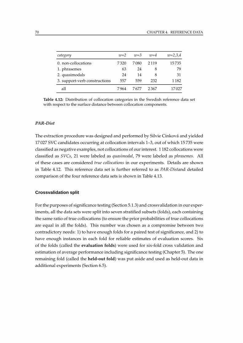
70 CHAPTER 4. REFERENCE DATA
category w=2 w=3 w=4 w=2,3,4
0. non-collocations 7 320 7 080 2 119 15 735
1. phrasemes 63 24 8 79
2. quasimodals 24 14 8 31
3. support-verb constructions 557 559 232 1 182
all 7 964 7 677 2 367 17 027
Table 4.12: Distribution of collocation categories in the Swedish reference data setwith respect to the surface distance between collocation components.
PAR-Dist
The extraction procedure was designed and performed by Silvie Cinkova and yielded
17 027 SVC candidates occurring at collocation intervals 1–3, out of which 15 735 were
classified as negative examples, not collocations of our interest. 1 182 collocations were
classified as SVCs, 21 were labeled as quasimodal, 79 were labeled as phrasemes. All
of these cases are considered true collocations in our experiments. Details are shown
in Table 4.12. This reference data set is further referred to as PAR-Distand detailed
comparison of the four reference data sets is shown in Table 4.13.
Crossvalidation split
For the purposes of significance testing (Section 5.1.3) and crossvalidation in our exper-
iments, all the data sets were split into seven stratified subsets (folds), each containing
the same ratio of true collocations (to ensure the prior probabilities of true collocations
are equal in all the folds). This number was chosen as a compromise between two
contradictory needs: 1) to have enough folds for a paired test of significance, and 2) to
have enough instances in each fold for reliable estimates of evaluation scores. Six
of the folds (called the evaluation folds) were used for six-fold cross validation and
estimation of average performance including significance testing (Chapter 5). The one
remaining fold (called the held-out fold) was put aside and used as held-out data in
additional experiments (Section 6.5).
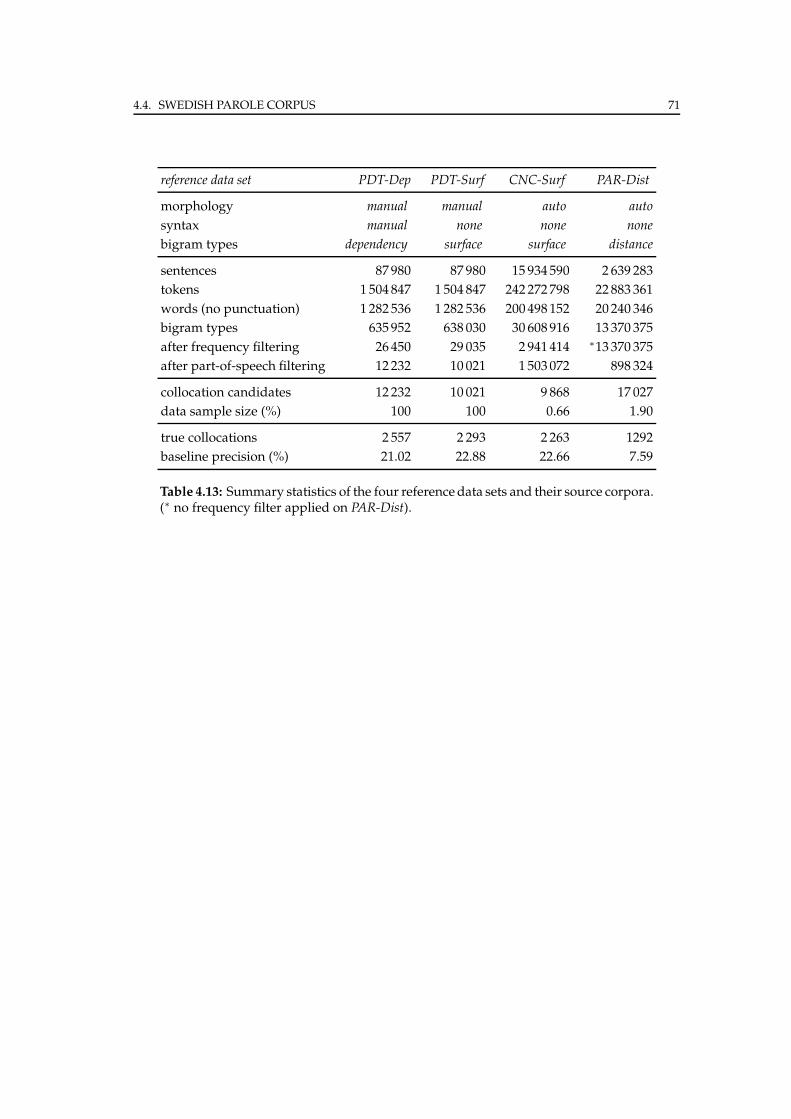
4.4. SWEDISH PAROLE CORPUS 71
reference data set PDT-Dep PDT-Surf CNC-Surf PAR-Dist
morphology manual manual auto auto
syntax manual none none none
bigram types dependency surface surface distance
sentences 87 980 87 980 15 934 590 2 639 283
tokens 1 504 847 1 504 847 242 272 798 22 883 361
words (no punctuation) 1 282 536 1 282 536 200 498 152 20 240 346
bigram types 635 952 638 030 30 608 916 13 370 375
after frequency filtering 26450 29 035 2 941 414 ∗13 370 375
after part-of-speech filtering 12232 10 021 1 503 072 898 324
collocation candidates 12 232 10 021 9 868 17 027
data sample size (%) 100 100 0.66 1.90
true collocations 2 557 2 293 2 263 1292
baseline precision (%) 21.02 22.88 22.66 7.59
Table 4.13: Summary statistics of the four referencedata sets and their source corpora.(∗ no frequency filter applied on PAR-Dist).

72
Chapter 5
Empirical Evaluation
In this chapter, we present a comparative performance evaluation of the 82 associa-
tion measures discussed in Chapter 3. The evaluation experiments were performed
on the four data sets described in Chapter 4: dependency bigrams from the Prague
Dependency Treebank (PDT-Dep), surface bigrams from the same source (PDT-Surf),
instances of surface bigrams from theCzechNational Corpus (CNC-Surf), and distance
verb-noun combinations from the Swedish Parole Corpus (PAR-Dist).
In the first section, we will introduce our evaluation scheme based on precision
and recall. Then, we will evaluate performance of the association measures separately
on the individual data sets and attempt to compare the obtained results across the
different data sets.
5.1 Evaluation methods
From the statistical point of view, collocation extraction can be viewed as a classifica-
tion problem, where each collocation candidate from a given data setmust be assigned
to one of two categories: collocation or non-collocation. By setting a threshold, any as-
sociation measure becomes a binary classifier: the candidates with higher association
scores fall into one class (collocation), the rest into the other class (non-collocation).
Effectiveness of such a classifier can be visualized in the form of a confusion matrix
(Kohavi and Provost, 1998), also called a table of confusion, or a matching matrix. This
matrix contains information about the actual and predicted classifications done by the
classifier on a given data set. An example of a confusion matrix for a classifier of
collocations is shown in Table 5.1.
73
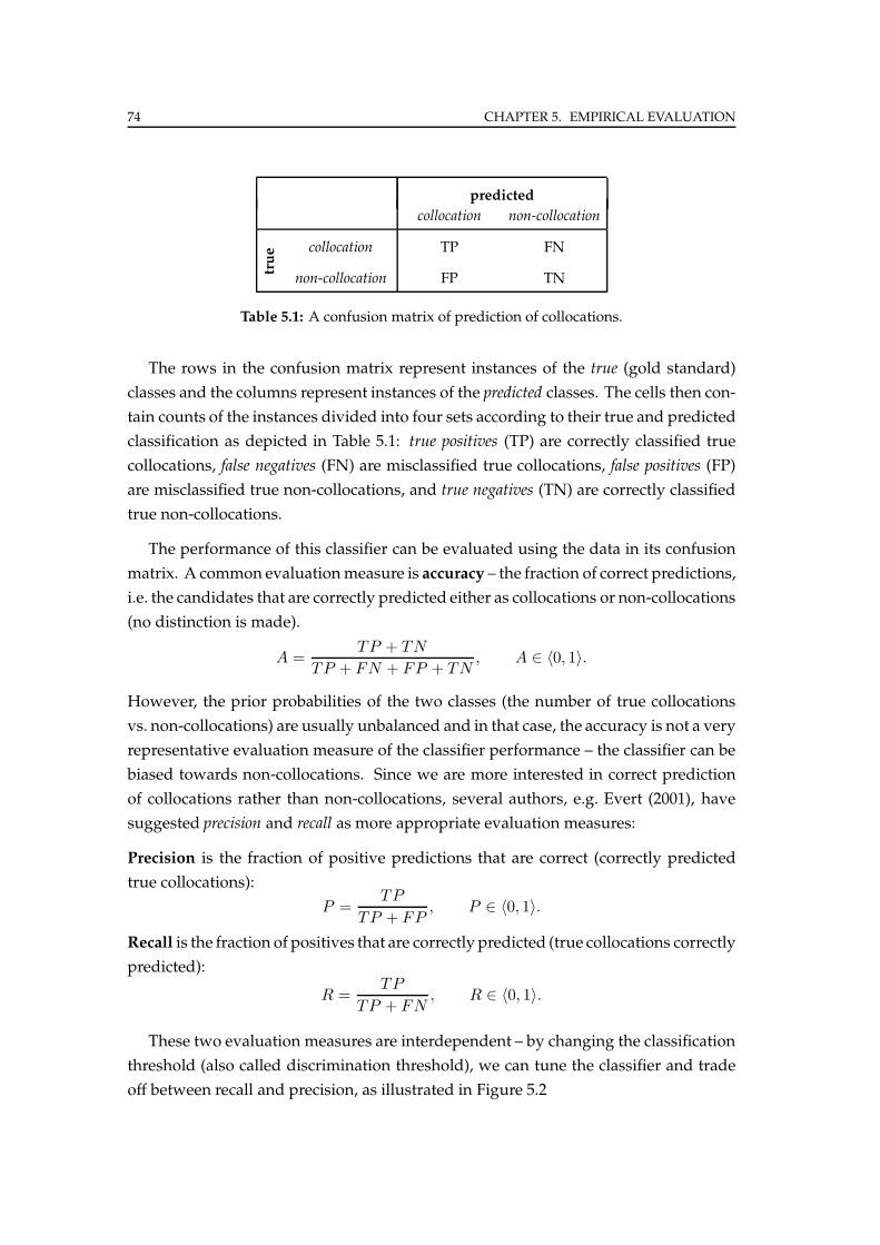
74 CHAPTER 5. EMPIRICAL EVALUATION
predicted
collocation non-collocation
true collocation TP FN
non-collocation FP TN
Table 5.1: A confusion matrix of prediction of collocations.
The rows in the confusion matrix represent instances of the true (gold standard)
classes and the columns represent instances of the predicted classes. The cells then con-
tain counts of the instances divided into four sets according to their true and predicted
classification as depicted in Table 5.1: true positives (TP) are correctly classified true
collocations, false negatives (FN) are misclassified true collocations, false positives (FP)
are misclassified true non-collocations, and true negatives (TN) are correctly classified
true non-collocations.
The performance of this classifier can be evaluated using the data in its confusion
matrix. A common evaluationmeasure is accuracy – the fraction of correct predictions,
i.e. the candidates that are correctly predicted either as collocations or non-collocations
(no distinction is made).
A =TP + TN
TP + FN + FP + TN, A ∈ 〈0, 1〉.
However, the prior probabilities of the two classes (the number of true collocations
vs. non-collocations) are usually unbalanced and in that case, the accuracy is not a very
representative evaluation measure of the classifier performance – the classifier can be
biased towards non-collocations. Since we are more interested in correct prediction
of collocations rather than non-collocations, several authors, e.g. Evert (2001), have
suggested precision and recall as more appropriate evaluation measures:
Precision is the fraction of positive predictions that are correct (correctly predicted
true collocations):
P =TP
TP + FP, P ∈ 〈0, 1〉.
Recall is the fraction of positives that are correctly predicted (true collocations correctly
predicted):
R =TP
TP + FN, R ∈ 〈0, 1〉.
These two evaluation measures are interdependent – by changing the classification
threshold (also called discrimination threshold), we can tune the classifier and trade
off between recall and precision, as illustrated in Figure 5.2
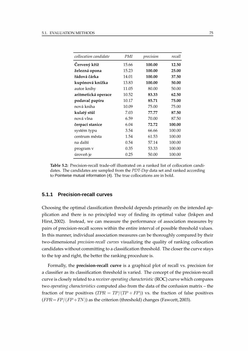
5.1. EVALUATIONMETHODS 75
collocation candidate PMI precision recall
Cerveny krız 15.66 100.00 12.50
zelezna opona 15.23 100.00 25.00
radova carka 14.01 100.00 37.50
kuponova knızka 13.83 100.00 50.00
autor knihy 11.05 80.00 50.00
aritmeticka operace 10.52 83.33 62.50
podavac papıru 10.17 85.71 75.00
nova kniha 10.09 75.00 75.00
kulaty stul 7.03 77.77 87.50
nova vlna 6.59 70.00 87.50
cerpacı stanice 6.04 72.72 100.00
system typu 3.54 66.66 100.00
centrum mesta 1.54 61.53 100.00
na dalsı 0.54 57.14 100.00
program v 0.35 53.33 100.00
uroven je 0.25 50.00 100.00
Table 5.2: Precision-recall trade-off illustrated on a ranked list of collocation candi-dates. The candidates are sampled from the PDT-Dep data set and ranked accordingto Pointwise mutual information (4). The true collocations are in bold.
5.1.1 Precision-recall curves
Choosing the optimal classification threshold depends primarily on the intended ap-
plication and there is no principled way of finding its optimal value (Inkpen and
Hirst, 2002). Instead, we can measure the performance of association measures by
pairs of precision-recall scores within the entire interval of possible threshold values.
In this manner, individual association measures can be thoroughly compared by their
two-dimensional precision-recall curves visualizing the quality of ranking collocation
candidates without committing to a classification threshold. The closer the curve stays
to the top and right, the better the ranking procedure is.
Formally, the precision-recall curve is a graphical plot of recall vs. precision for
a classifier as its classification threshold is varied. The concept of the precision-recall
curve is closely related to a receiver operating characteristic (ROC) curve which compares
two operating characteristics computed also from the data of the confusion matrix – the
fraction of true positives (TPR = TP/(TP +FP )) vs. the fraction of false positives
(FPR=FP/(FP +TN)) as the criterion (threshold) changes (Fawcett, 2003).
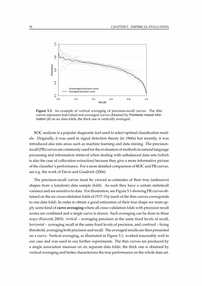
76 CHAPTER 5. EMPIRICAL EVALUATION
Recall
Pre
cisi
on
0.0 0.2 0.4 0.6 0.8 1.0
0.2
0.4
0.6
0.8
1.0
Unaveraged precision curveAveraged precison curve
Figure 5.1: An example of vertical averaging of precision-recall curves. The thincurves represent individual non-averaged curves obtained by Pointwise mutual infor-mation (4) on six data folds, the thick one is vertically averaged.
ROC analysis is a popular diagnostic tool used to select optimal classification mod-
els. Originally, it was used in signal detection theory (in 1960s) but recently, it was
introduced also into areas such as machine learning and data mining. The precision-
recall (PR) curves are commonlyused for the evaluationofmethods innatural language
processing and information retrieval when dealing with unbalanced data sets (which
is also the case of collocation extraction) because they give a more informative picture
of the classifier’s performance. For amore detailed comparison of ROC and PR curves,
see e.g. the work of Davis and Goadrich (2006).
The precision-recall curves must be viewed as estimates of their true (unknown)
shapes from a (random) data sample (fold). As such they have a certain statisticall
variance andare sensitive todata. For illustration, see Figure 5.1 showingPRcurves ob-
tained on the six crossvalidation folds of PDT-Dep (each of the thin curves corresponds
to one data fold). In order to obtain a good estimation of their true shape we must ap-
ply some kind of curve averagingwhere all cross-validation foldswith precision-recall
scores are combined and a single curve is drawn. Such averaging can be done in three
ways (Fawcett, 2003): vertical – averaging precision at the same fixed levels of recall,
horizontal – averaging recall at the same fixed levels of precision, and combined – fixing
threshold, averaging bothprecision and recall. The averaged results are thenpresented
on a curve. Vertical averaging, as illustrated in Figure 5.1, worked reasonably well in
our case and was used in our further experiments. The thin curves are produced by
a single association measure on six separate data folds; the thick one is obtained by
vertical averaging and better characterizes the true performance on the whole data set.
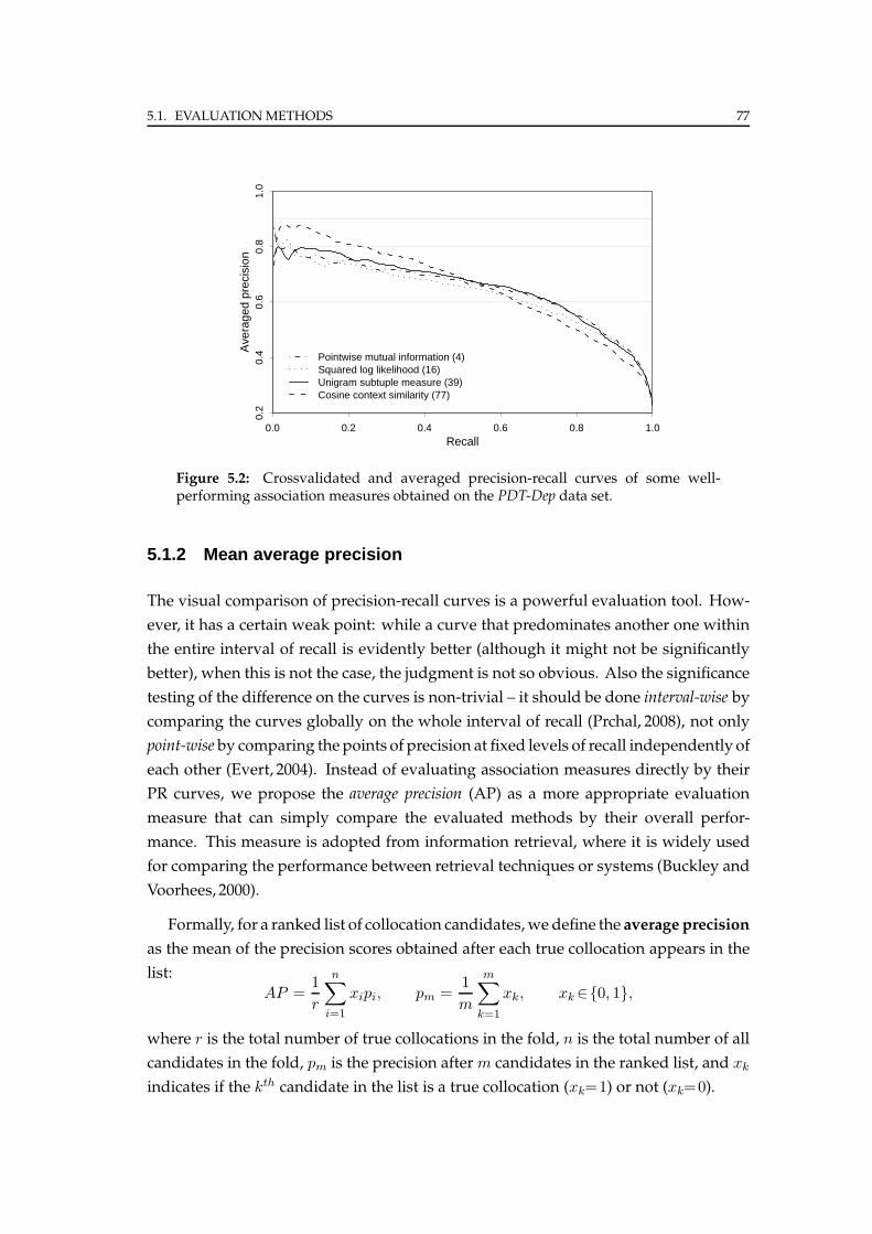
5.1. EVALUATIONMETHODS 77
Recall
Ave
rage
d pr
ecis
ion
0.0 0.2 0.4 0.6 0.8 1.0
0.2
0.4
0.6
0.8
1.0
Pointwise mutual information (4)Squared log likelihood (16)Unigram subtuple measure (39)Cosine context similarity (77)
Figure 5.2: Crossvalidated and averaged precision-recall curves of some well-performing association measures obtained on the PDT-Dep data set.
5.1.2 Mean average precision
The visual comparison of precision-recall curves is a powerful evaluation tool. How-
ever, it has a certain weak point: while a curve that predominates another one within
the entire interval of recall is evidently better (although it might not be significantly
better), when this is not the case, the judgment is not so obvious. Also the significance
testing of the difference on the curves is non-trivial – it should be done interval-wise by
comparing the curves globally on the whole interval of recall (Prchal, 2008), not only
point-wise by comparing the points of precision at fixed levels of recall independently of
each other (Evert, 2004). Instead of evaluating association measures directly by their
PR curves, we propose the average precision (AP) as a more appropriate evaluation
measure that can simply compare the evaluated methods by their overall perfor-
mance. This measure is adopted from information retrieval, where it is widely used
for comparing the performance between retrieval techniques or systems (Buckley and
Voorhees, 2000).
Formally, for a ranked list of collocation candidates, we define the average precision
as the mean of the precision scores obtained after each true collocation appears in the
list:AP =
1
r
n∑
i=1
xipi, pm =1
m
m∑
k=1
xk, xk∈{0, 1},
where r is the total number of true collocations in the fold, n is the total number of all
candidates in the fold, pm is the precision after m candidates in the ranked list, and xk
indicates if the kth candidate in the list is a true collocation (xk=1) or not (xk=0).
78 CHAPTER 5. EMPIRICAL EVALUATION
The average precision can also be understood as the expected value of precision for
all possible values of recall, assuming uniform distribution of recall (all possible values
of recall are equally probable). In the example in Table 5.2, the average precisionwould
be computed from the precision scores highlighted in bold. Another interpretation of
the average precision is the area under the (PR) curve (AUC). Nevertheless, our approach
does not require the precision-recall values to be transformed into a (continuous) curve
in order to estimate the area under it.
Based on the average precision scores APj computed for N data folds, we define
the mean average precision (MAP) as the sample mean of these scores and use it as
the main evaluation measures in our work:
MAP =1
N
N∑
j=1
APj
Note: In order to reduce the bias caused by the unreliable precision scores for low recall
and their fast changes for high recall (see again Figure 5.1), we limit the estimation of
AP to a narrower range of recall 〈0.1, 0.9〉 anduse this estimation in all our experiments.
5.1.3 Significance testing
Statistical tests of the difference between the rankingmethods are necessary to examine
whether the observed differences in the evaluation scores (MAP) are measurable or
whether they occur only by chance. Because MAP is averaged over a number of AP
values computed on the separate (independent) data folds, we can employ tests based
on estimating the error of this measure.
As we mentioned earlier, the precision-recall curves are quite sensitive to the data
and thus, we can expect differences in the AP values to be greater between data folds
than between methods. Therefore, when comparing two ranking methods, we should
analyze their AP difference for each matched pair of data folds (Di) rather than the
difference between AP values averaged over all the folds (D). This problem is usually
solved by the paired Student’s t-test which compares the average difference of AP
between two methods on the separate data folds to the variation of the difference
across the folds. If the average difference is large enough compared to its standard
error, then the methods are significantly different.
t =D
SD/√
N, D =
1
N
N∑
i=1
Di, SD =
√√√√ 1
N − 1
N∑
i=1
(Di − D)2,
5.2. EXPERIMENTS 79
where Di is the AP difference on the ith data fold, D is the average difference over all
folds (i = 1, . . . , N ), and SD is the sample standard deviation.
Although the t-test requires the differences to be normally distributed, itworks quite
well even if this assumption is not completely valid. However, as a non-parametric
alternative, we can apply thepairedWilcoxon signed-ranked testswhich is commonly
used in information retrieval. This test is more conservative and takes into account
only the sign of the difference and ignores the actual magnitude. The differences in AP
on each data fold are replaced with the ranks of their absolute values and each rank is
multiplied by the sign of the difference (Ri). The sum of the signed-ranks is compared
to its expected value under the assumption that the two groups are equal. For details
and description of other possible tests, see e.g. (Hull, 1993).
T =
∑Ni=1Ri√∑Ni=1R
2i
, Ri = sign(Di) · rank|Di|.
5.2 Experiments
In order to evaluate the performance of the individual association measures, we per-
formed the following experiment on each of the four data sets introduced in Chapter 4.
For all collocation candidates, we extracted their frequency information (the observed
contingency tables) and context information (the immediate and empirical contexts)
from their source corpora as described in Section 2.2.5. The empirical contexts were
limited to a context window of 3 sentences (the actual one, the one preceding, and
the one following) and filtered to include only open-class word types as described in
Section 2.2.6. Based on this information, we computed the scores for all 82 association
measures for all the candidates in each evaluation data fold. Then, for each associa-
tion measure and each fold, we ranked the candidates according to their descending
association scores, computed values of precision and recall after each true collocation
appearing in the ranked list, plotted the averaged precision-recall curve, and com-
puted the average precision on the recall interval 〈0.1, 0.9〉. The AP values obtained
on the evaluation data folds were used to estimate the mean average precision as the
main evaluation measure. Further, we ranked the association measures according to
their MAP values in descending order and depicted the results in a graph. Finally, we
applied the paired Student’s and Wilcoxon test to the detected measures with statisti-
cally indistinguishable performance. The actual results are presented in the following
subsections.
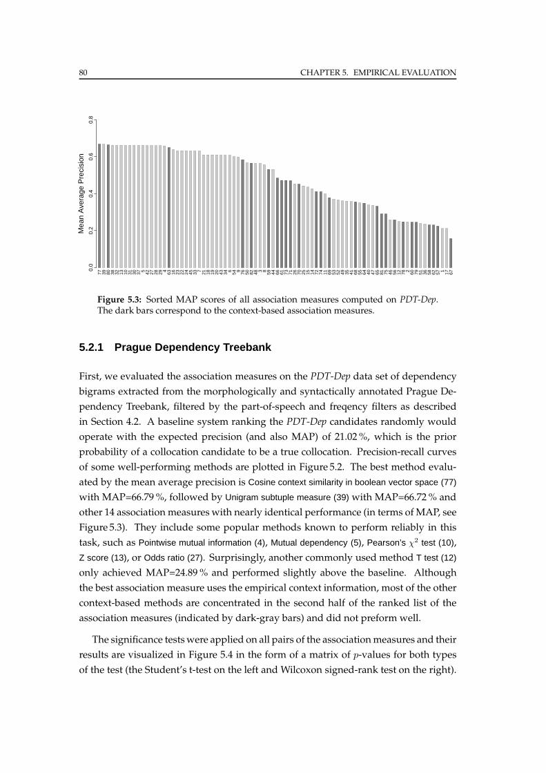
80 CHAPTER 5. EMPIRICAL EVALUATION
77 39 80 38 32 13 10 31 30 37 5 42 27 28 29 4 63 16 23 22 24 45 33 7 21 18 19 20 43 34 6 54 9 76 50 82 48 3 8 59 44 66 61 73 71 26 70 25 15 14 72 74 11 69 53 52 49 35 41 68 55 64 40 47 65 81 75 46 56 12 78 2 60 79 51 36 58 62 57 1 17 67
Mea
n A
vera
ge P
reci
sion
0.0
0.2
0.4
0.6
0.8
Figure 5.3: Sorted MAP scores of all association measures computed on PDT-Dep.The dark bars correspond to the context-based association measures.
5.2.1 Prague Dependency Treebank
First, we evaluated the association measures on the PDT-Dep data set of dependency
bigrams extracted from the morphologically and syntactically annotated Prague De-
pendency Treebank, filtered by the part-of-speech and freqency filters as described
in Section 4.2. A baseline system ranking the PDT-Dep candidates randomly would
operate with the expected precision (and also MAP) of 21.02%, which is the prior
probability of a collocation candidate to be a true collocation. Precision-recall curves
of some well-performing methods are plotted in Figure 5.2. The best method evalu-
ated by the mean average precision is Cosine context similarity in boolean vector space (77)
with MAP=66.79%, followed by Unigram subtuple measure (39) with MAP=66.72% and
other 14 association measures with nearly identical performance (in terms ofMAP, see
Figure 5.3). They include some popular methods known to perform reliably in this
task, such as Pointwise mutual information (4), Mutual dependency (5), Pearson’s χ2 test (10),
Z score (13), or Odds ratio (27). Surprisingly, another commonly used method T test (12)
only achieved MAP=24.89% and performed slightly above the baseline. Although
the best association measure uses the empirical context information, most of the other
context-based methods are concentrated in the second half of the ranked list of the
association measures (indicated by dark-gray bars) and did not preform well.
The significance testswere applied on all pairs of the associationmeasures and their
results are visualized in Figure 5.4 in the form of a matrix of p-values for both types
of the test (the Student’s t-test on the left and Wilcoxon signed-rank test on the right).
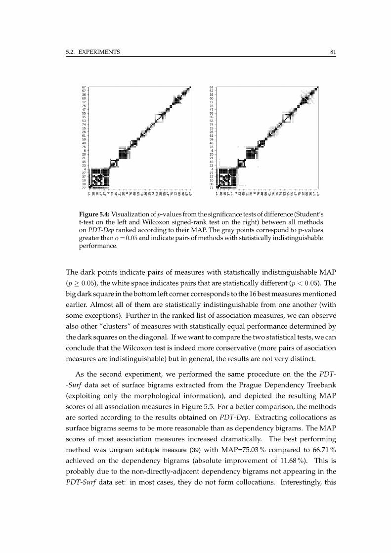
5.2. EXPERIMENTS 81
77 38 10 37 27 4 23 45 21 20 6 76 48 59 61 26 15 74 53 35 55 47 75 12 60 36 57 677738103727
423452120
67648596126157453355547751260365767
77 38 10 37 27 4 23 45 21 20 6 76 48 59 61 26 15 74 53 35 55 47 75 12 60 36 57 67
7738103727
423452120
67648596126157453355547751260365767
Figure 5.4: Visualization of p-values from the significance tests of difference (Student’st-test on the left and Wilcoxon signed-rank test on the right) between all methodson PDT-Dep ranked according to their MAP. The gray points correspond to p-valuesgreater thanα=0.05 and indicate pairs of methodswith statistically indistinguishableperformance.
The dark points indicate pairs of measures with statistically indistinguishable MAP
(p ≥ 0.05), the white space indicates pairs that are statistically different (p < 0.05). The
bigdark square in the bottom left corner corresponds to the 16bestmeasuresmentioned
earlier. Almost all of them are statistically indistinguishable from one another (with
some exceptions). Further in the ranked list of association measures, we can observe
also other “clusters” of measures with statistically equal performance determined by
the dark squares on the diagonal. Ifwewant to compare the two statistical tests,we can
conclude that the Wilcoxon test is indeed more conservative (more pairs of asociation
measures are indistinguishable) but in general, the results are not very distinct.
As the second experiment, we performed the same procedure on the the PDT-
-Surf data set of surface bigrams extracted from the Prague Dependency Treebank
(exploiting only the morphological information), and depicted the resulting MAP
scores of all association measures in Figure 5.5. For a better comparison, the methods
are sorted according to the results obtained on PDT-Dep. Extracting collocations as
surface bigrams seems to be more reasonable than as dependency bigrams. The MAP
scores of most association measures increased dramatically. The best performing
method was Unigram subtuple measure (39) with MAP=75.03% compared to 66.71%
achieved on the dependency bigrams (absolute improvement of 11.68%). This is
probably due to the non-directly-adjacent dependency bigrams not appearing in the
PDT-Surf data set: in most cases, they do not form collocations. Interestingly, this
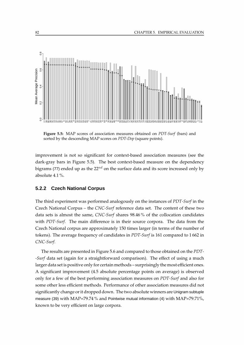
82 CHAPTER 5. EMPIRICAL EVALUATION
77 39 80 38 32 13 10 31 30 37 5 42 27 28 29 4 63 16 23 22 24 45 33 7 21 18 19 20 43 34 6 54 9 76 50 82 48 3 8 59 44 66 61 73 71 26 70 25 15 14 72 74 11 69 53 52 49 35 41 68 55 64 40 47 65 81 75 46 56 12 78 2 60 79 51 36 58 62 57 1 17 67
Mea
n A
vera
ge P
reci
sion
0.0
0.2
0.4
0.6
0.8
Figure 5.5: MAP scores of association measures obtained on PDT-Surf (bars) andsorted by the descending MAP scores on PDT-Dep (square points).
improvement is not so significant for context-based association measures (see the
dark-gray bars in Figure 5.5). The best context-based measure on the dependency
bigrams (77) ended up as the 22nd on the surface data and its score increased only by
absolute 4.1%.
5.2.2 Czech National Corpus
The third experiment was performed analogously on the instances of PDT-Surf in the
Czech National Corpus – the CNC-Surf reference data set. The content of these two
data sets is almost the same, CNC-Surf shares 98.46% of the collocation candidates
with PDT-Surf. The main difference is in their source corpora. The data from the
Czech National corpus are approximately 150 times larger (in terms of the number of
tokens). The average frequency of candidates in PDT-Surf is 161 compared to 1 662 in
CNC-Surf.
The results are presented in Figure 5.6 and compared to those obtained on the PDT-
-Surf data set (again for a straightforward comparison). The effect of using a much
larger data set is positive only for certainmethods – surprisingly themost efficient ones.
A significant improvement (4.5 absolute percentage points on average) is observed
only for a few of the best performing association measures on PDT-Surf and also for
some other less efficient methods. Performance of other association measures did not
significantly change or it droppeddown. The twoabsolutewinners areUnigram subtuple
measure (39) with MAP=79.74% and Pointwise mutual information (4) with MAP=79.71%,
known to be very efficient on large corpora.
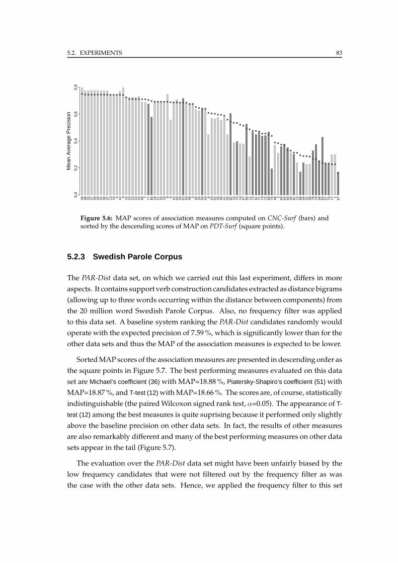
5.2. EXPERIMENTS 83
39 38 32 27 28 29 31 30 37 13 10 5 42 4 16 24 22 23 33 45 7 77 80 18 21 20 19 9 6 43 50 34 63 54 48 3 26 25 59 44 8 53 52 35 49 41 55 82 15 70 14 47 66 11 73 61 71 74 72 69 76 46 2 60 64 65 40 81 12 68 56 51 36 78 79 58 62 57 75 17 1 67
Mea
n A
vera
ge P
reci
sion
0.0
0.2
0.4
0.6
0.8
Figure 5.6: MAP scores of association measures computed on CNC-Surf (bars) andsorted by the descending scores of MAP on PDT-Surf (square points).
5.2.3 Swedish Parole Corpus
The PAR-Dist data set, on which we carried out this last experiment, differs in more
aspects. It contains support verb construction candidates extracted as distance bigrams
(allowing up to three words occurring within the distance between components) from
the 20 million word Swedish Parole Corpus. Also, no frequency filter was applied
to this data set. A baseline system ranking the PAR-Dist candidates randomly would
operate with the expected precision of 7.59%, which is significantly lower than for the
other data sets and thus the MAP of the association measures is expected to be lower.
SortedMAP scores of the associationmeasures are presented in descending order as
the square points in Figure 5.7. The best performing measures evaluated on this data
set are Michael’s coefficient (36) with MAP=18.88%, Piatersky-Shapiro’s coefficient (51) with
MAP=18.87%, and T-test (12) withMAP=18.66%. The scores are, of course, statistically
indistinguishable (the pairedWilcoxon signed rank test, α=0.05). The appearance of T-
test (12) among the best measures is quite suprising because it performed only slightly
above the baseline precision on other data sets. In fact, the results of other measures
are also remarkably different and many of the best performing measures on other data
sets appear in the tail (Figure 5.7).
The evaluation over the PAR-Dist data set might have been unfairly biased by the
low frequency candidates that were not filtered out by the frequency filter as was
the case with the other data sets. Hence, we applied the frequency filter to this set
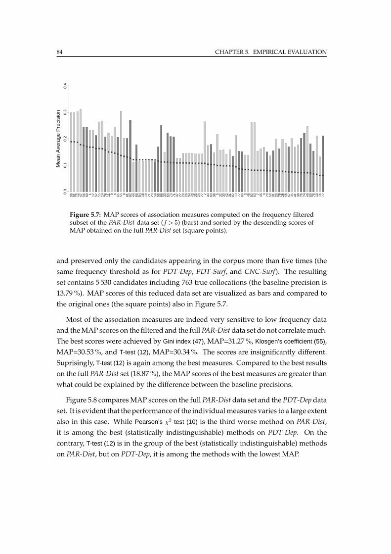
84 CHAPTER 5. EMPIRICAL EVALUATION
36 51 12 47 56 69 1 17 57 15 14 78 11 9 6 65 55 8 61 62 44 68 54 18 19 21 20 59 58 66 33 64 73 71 37 27 28 29 34 43 23 24 22 2 40 63 38 5 32 30 42 31 82 13 77 80 3 48 52 53 7 45 4 70 50 81 26 79 25 46 67 35 41 39 76 74 49 60 75 10 16 72
Mea
n A
vera
ge P
reci
sion
0.0
0.1
0.2
0.3
0.4
Figure 5.7: MAP scores of association measures computed on the frequency filteredsubset of the PAR-Dist data set (f > 5) (bars) and sorted by the descending scores ofMAP obtained on the full PAR-Dist set (square points).
and preserved only the candidates appearing in the corpus more than five times (the
same frequency threshold as for PDT-Dep, PDT-Surf, and CNC-Surf). The resulting
set contains 5 530 candidates including 763 true collocations (the baseline precision is
13.79%). MAP scores of this reduced data set are visualized as bars and compared to
the original ones (the square points) also in Figure 5.7.
Most of the association measures are indeed very sensitive to low frequency data
and theMAP scores on the filtered and the full PAR-Dist data set do not correlatemuch.
The best scores were achieved by Gini index (47), MAP=31.27%, Klosgen’s coefficient (55),
MAP=30.53%, and T-test (12), MAP=30.34%. The scores are insignificantly different.
Suprisingly, T-test (12) is again among the best measures. Compared to the best results
on the full PAR-Dist set (18.87%), theMAP scores of the best measures are greater than
what could be explained by the difference between the baseline precisions.
Figure 5.8 comparesMAP scores on the full PAR-Dist data set and the PDT-Dep data
set. It is evident that theperformance of the individualmeasures varies to a large extent
also in this case. While Pearson’s χ2 test (10) is the third worse method on PAR-Dist,
it is among the best (statistically indistinguishable) methods on PDT-Dep. On the
contrary, T-test (12) is in the group of the best (statistically indistinguishable) methods
on PAR-Dist, but on PDT-Dep, it is among the methods with the lowest MAP.
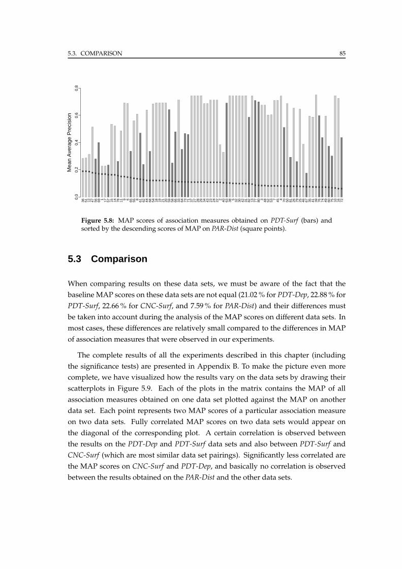
5.3. COMPARISON 85
36 51 12 47 56 69 1 17 57 15 14 78 11 9 6 65 55 8 61 62 44 68 54 18 19 21 20 59 58 66 33 64 73 71 37 27 28 29 34 43 23 24 22 2 40 63 38 5 32 30 42 31 82 13 77 80 3 48 52 53 7 45 4 70 50 81 26 79 25 46 67 35 41 39 76 74 49 60 75 10 16 72
Mea
n A
vera
ge P
reci
sion
0.0
0.2
0.4
0.6
0.8
Figure 5.8: MAP scores of association measures obtained on PDT-Surf (bars) andsorted by the descending scores of MAP on PAR-Dist (square points).
5.3 Comparison
When comparing results on these data sets, we must be aware of the fact that the
baseline MAP scores on these data sets are not equal (21.02% for PDT-Dep, 22.88% for
PDT-Surf, 22.66% for CNC-Surf, and 7.59% for PAR-Dist) and their differences must
be taken into account during the analysis of the MAP scores on different data sets. In
most cases, these differences are relatively small compared to the differences in MAP
of association measures that were observed in our experiments.
The complete results of all the experiments described in this chapter (including
the significance tests) are presented in Appendix B. To make the picture even more
complete, we have visualized how the results vary on the data sets by drawing their
scatterplots in Figure 5.9. Each of the plots in the matrix contains the MAP of all
association measures obtained on one data set plotted against the MAP on another
data set. Each point represents two MAP scores of a particular association measure
on two data sets. Fully correlated MAP scores on two data sets would appear on
the diagonal of the corresponding plot. A certain correlation is observed between
the results on the PDT-Dep and PDT-Surf data sets and also between PDT-Surf and
CNC-Surf (which are most similar data set pairings). Significantly less correlated are
the MAP scores on CNC-Surf and PDT-Dep, and basically no correlation is observed
between the results obtained on the PAR-Dist and the other data sets.
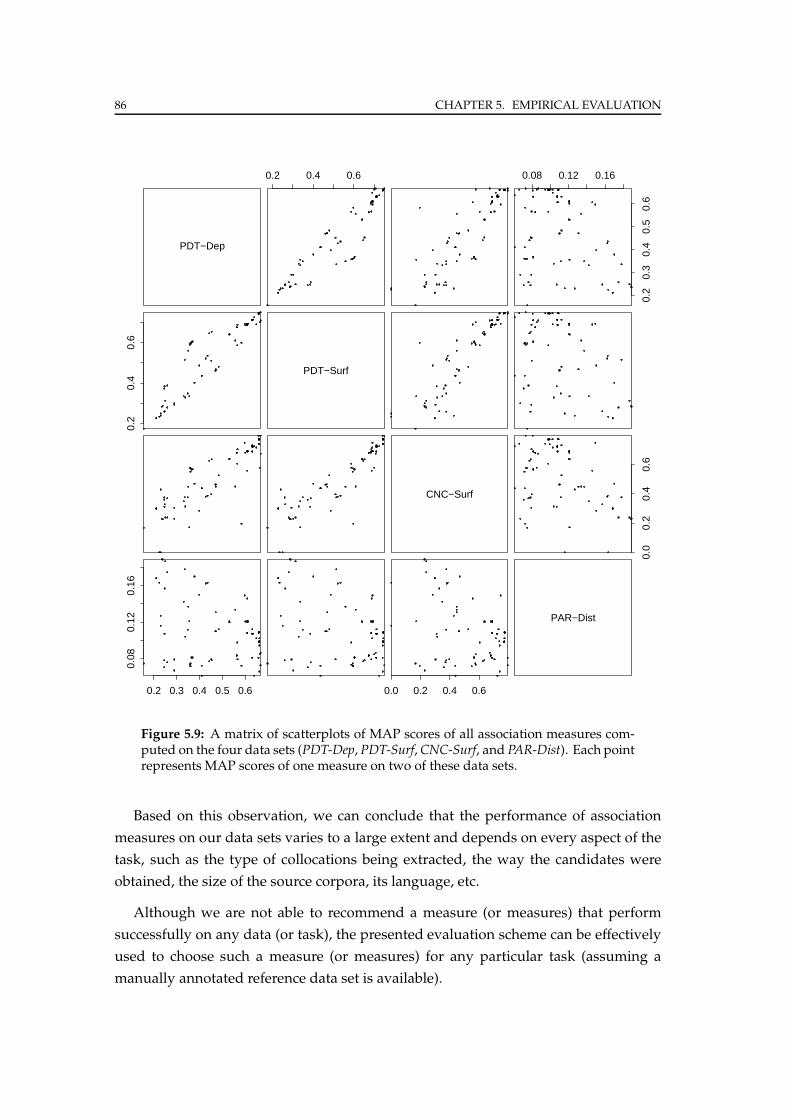
86 CHAPTER 5. EMPIRICAL EVALUATION
PDT−Dep
0.2 0.4 0.6 0.08 0.12 0.16
0.2
0.3
0.4
0.5
0.6
0.2
0.4
0.6
PDT−Surf
CNC−Surf
0.0
0.2
0.4
0.6
0.2 0.3 0.4 0.5 0.6
0.08
0.12
0.16
0.0 0.2 0.4 0.6
PAR−Dist
Figure 5.9: A matrix of scatterplots of MAP scores of all association measures com-puted on the four data sets (PDT-Dep, PDT-Surf, CNC-Surf, and PAR-Dist). Each pointrepresents MAP scores of one measure on two of these data sets.
Based on this observation, we can conclude that the performance of association
measures on our data sets varies to a large extent and depends on every aspect of the
task, such as the type of collocations being extracted, the way the candidates were
obtained, the size of the source corpora, its language, etc.
Although we are not able to recommend a measure (or measures) that perform
successfully on any data (or task), the presented evaluation scheme can be effectively
used to choose such a measure (or measures) for any particular task (assuming a
manually annotated reference data set is available).
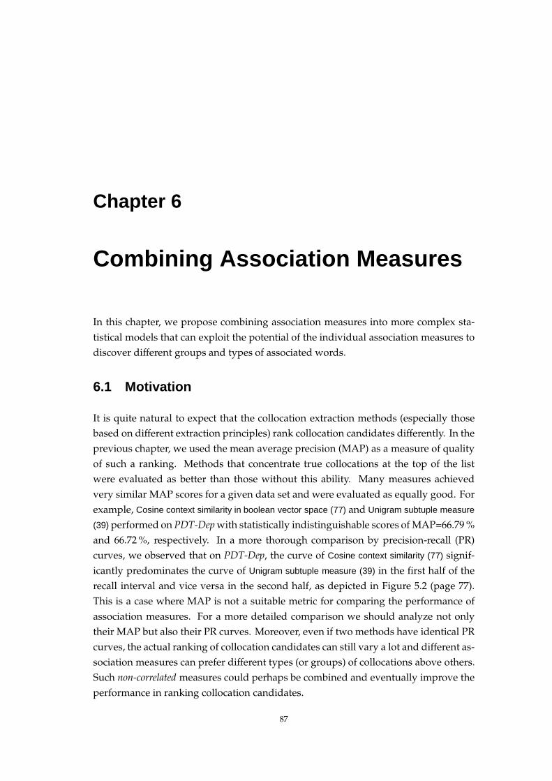
Chapter 6
Combining Association Measures
In this chapter, we propose combining association measures into more complex sta-
tistical models that can exploit the potential of the individual association measures to
discover different groups and types of associated words.
6.1 Motivation
It is quite natural to expect that the collocation extraction methods (especially those
based on different extraction principles) rank collocation candidates differently. In the
previous chapter, we used the mean average precision (MAP) as a measure of quality
of such a ranking. Methods that concentrate true collocations at the top of the list
were evaluated as better than those without this ability. Many measures achieved
very similar MAP scores for a given data set and were evaluated as equally good. For
example, Cosine context similarity in boolean vector space (77) and Unigram subtuple measure
(39) performed on PDT-Depwith statistically indistinguishable scores of MAP=66.79%
and 66.72%, respectively. In a more thorough comparison by precision-recall (PR)
curves, we observed that on PDT-Dep, the curve of Cosine context similarity (77) signif-
icantly predominates the curve of Unigram subtuple measure (39) in the first half of the
recall interval and vice versa in the second half, as depicted in Figure 5.2 (page 77).
This is a case where MAP is not a suitable metric for comparing the performance of
association measures. For a more detailed comparison we should analyze not only
their MAP but also their PR curves. Moreover, even if two methods have identical PR
curves, the actual ranking of collocation candidates can still vary a lot and different as-
sociation measures can prefer different types (or groups) of collocations above others.
Such non-correlated measures could perhaps be combined and eventually improve the
performance in ranking collocation candidates.
87
88 CHAPTER 6. COMBINING ASSOCIATION MEASURES
0.9
0.5
0.1
16.98.80.7
Cos
ine
cont
ext s
imila
rity
in b
oole
an v
ecto
r sp
ace
Pointwise mutual information
collocationsnon-collocationslinear discriminant
Figure 6.1: Visualization of scores of two association measures. The dashed linedenotes a linear discriminant obtained by logistic linear regression. By moving thisboundary, we can tune the classifier output (a 5% stratified sample of the evaluationdata folds is displayed).
An example of existence of suchmeasures is shown in Figure 6.1. Association scores
of Pointwise mutual information (4) and Cosine context similarity (77) seem independent
enough to be (linearly) combined into one model and possibly achieve better per-
formance. In the following sections we will deal with models combining all the
association measures described in Chaper 3.
6.2 Methods
Formally, each collocation candidate xi can be empirically described by the feature
vector xi = (xi
1, . . . , xi82)
T consisting of scores of all 82 association measures from Ta-
bles 3.4 and 3.5 in Chapter 3 and assigned a label yi∈{0, 1}which indicateswhether the
bigram is considered to be a true collocation (y = 1) or not (y = 0). We look for a ranker
function f(xi) determining the strength of collocational association between compo-
nents of collocation candidates (xi) and hence can be used for their ranking in the same
manner as the individual association measures. Performance of such a method could
be evaluated in the same way as the individual association measures: MAP scores
and PR curves. In this section, we briefly introduce several statistical-classification
methods and demonstrate how we used them as such rankers. For further details, see
e.g. Venables and Ripley (2002).
6.2. METHODS 89
6.2.1 Linear logistic regression
An additive model for a binary response is represented by a generalized linear model
(GLM) in a form of logistic regression:
logit(π) = β0 + β1x1 + . . . + βpxp,
where logit(π) = log(π/(1−π)) is a canonical link function for odds-ratio and π∈(0, 1)
is a conditional probability of a positive response given a vector x. The estimation
of β0 and βββ is computed by the maximum likelihood method which is solved by the
iteratively reweighted least squares algorithm. The ranker function in this case is defined
as the predicted value π or equivalently (due to the monotonicity of the logit link
function) as the linear combination β0 + βββ Tx.
6.2.2 Linear discriminant analysis
The basic idea of Fisher’s linear discriminant analysis (LDA) is to find a one-dimensio-
nal projection defined by a vector c so that for the projected combination cTx the ratio
of the between variance BBB to the within variance WWW is maximized. After the projection,
cTx can be used directly as a ranker.
maxc
cTBBB c
cTWWW c.
6.2.3 Support vector machines
For technical reasons, we now change the labels yi ∈ {−1,+1}. The goal in support
vector machines (SVM) is to estimate a function f(x) = β0 + βββ Tx and find a classifier
y(x) = sign(f(x)
)which can be solved through the following convex optimization:
minβ0,βββ
n∑
i=1
[1 − yi(β0 + βββT
xi)
]++
λ
2||βββ||2.
with λ as a regularization parameter. The hinge loss function L(y, f(x)) = [1 − yf(x)]+
is active only for positive values (i.e. bad predictions) and is therefore very suitable
for ranking models with β0 + βββ Tx as a ranker function. Setting the regularization
parameter λ is crucial for both the estimators β0, βββ and further classification (or rank-
ing). As an alternative to the often inappropriate grid search, Hastie (2004) proposed
an effective algorithm which fits the entire SVM regularization path [β0(λ),βββ(λ)] and
provided an option to choose the optimal value of λ. As an objective function, we used
the total amount of loss on training data rather than the number of false predicted
training instances.
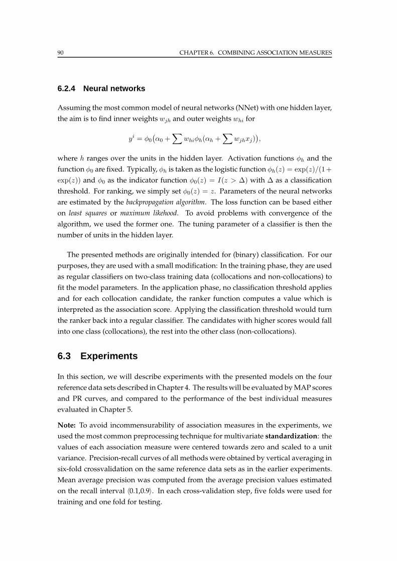
90 CHAPTER 6. COMBINING ASSOCIATION MEASURES
6.2.4 Neural networks
Assuming the most commonmodel of neural networks (NNet) with one hidden layer,
the aim is to find inner weights wjh and outer weights whi for
yi = φ0
(α0 +
∑whiφh(αh +
∑wjhxj)
),
where h ranges over the units in the hidden layer. Activation functions φh and the
function φ0 are fixed. Typically, φh is taken as the logistic function φh(z) = exp(z)/(1+
exp(z)) and φ0 as the indicator function φ0(z) = I(z > ∆) with ∆ as a classification
threshold. For ranking, we simply set φ0(z) = z. Parameters of the neural networks
are estimated by the backpropagation algorithm. The loss function can be based either
on least squares or maximum likehood. To avoid problems with convergence of the
algorithm, we used the former one. The tuning parameter of a classifier is then the
number of units in the hidden layer.
The presented methods are originally intended for (binary) classification. For our
purposes, they are usedwith a small modification: In the training phase, they are used
as regular classifiers on two-class training data (collocations and non-collocations) to
fit the model parameters. In the application phase, no classification threshold applies
and for each collocation candidate, the ranker function computes a value which is
interpreted as the association score. Applying the classification threshold would turn
the ranker back into a regular classifier. The candidates with higher scores would fall
into one class (collocations), the rest into the other class (non-collocations).
6.3 Experiments
In this section, we will describe experiments with the presented models on the four
reference data sets described in Chapter 4. The resultswill be evaluated byMAP scores
and PR curves, and compared to the performance of the best individual measures
evaluated in Chapter 5.
Note: To avoid incommensurability of association measures in the experiments, we
used the most common preprocessing technique for multivariate standardization: the
values of each association measure were centered towards zero and scaled to a unit
variance. Precision-recall curves of all methodswere obtained by vertical averaging in
six-fold crossvalidation on the same reference data sets as in the earlier experiments.
Mean average precision was computed from the average precision values estimated
on the recall interval 〈0.1,0.9〉. In each cross-validation step, five folds were used for
training and one fold for testing.
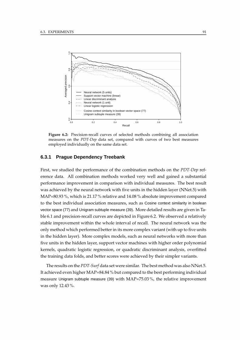
6.3. EXPERIMENTS 91
Recall
Ave
rage
d pr
ecis
ion
0.0 0.2 0.4 0.6 0.8 1.0
0.2
0.4
0.6
0.8
1.0
Neural network (5 units)Support vector machine (linear)Linear discriminant analysisNeural network (1 unit)Linear logistic regression
Cosine context similarity in boolean vector space (77)Unigram subtuple measure (39)
Figure 6.2: Precision-recall curves of selected methods combining all associationmeasures on the PDT-Dep data set, compared with curves of two best measuresemployed individually on the same data set.
6.3.1 Prague Dependency Treebank
First, we studied the performance of the combination methods on the PDT-Dep ref-
erence data. All combination methods worked very well and gained a substantial
performance improvement in comparison with individual measures. The best result
was achieved by the neural network with five units in the hidden layer (NNet.5) with
MAP=80.93%, which is 21.17% relative and 14.08% absolute improvement compared
to the best individual association measures, such as Cosine context similarity in boolean
vector space (77) and Unigram subtuple measure (39). More detailed results are given in Ta-
ble 6.1 and precision-recall curves are depicted in Figure 6.2. We observed a relatively
stable improvement within the whole interval of recall. The neural network was the
onlymethodwhich performed better in its more complex variant (with up to five units
in the hidden layer). More complex models, such as neural networks with more than
five units in the hidden layer, support vector machines with higher order polynomial
kernels, quadratic logistic regression, or quadratic discriminant analysis, overfitted
the training data folds, and better scores were achieved by their simpler variants.
The results on thePDT-Surf data setwere similar. The bestmethodwas alsoNNet.5.
It achieved even higherMAP=84.84% but compared to the best performing individual
measure Unigram subtuple measure (39) with MAP=75.03%, the relative improvement
was only 12.43%.
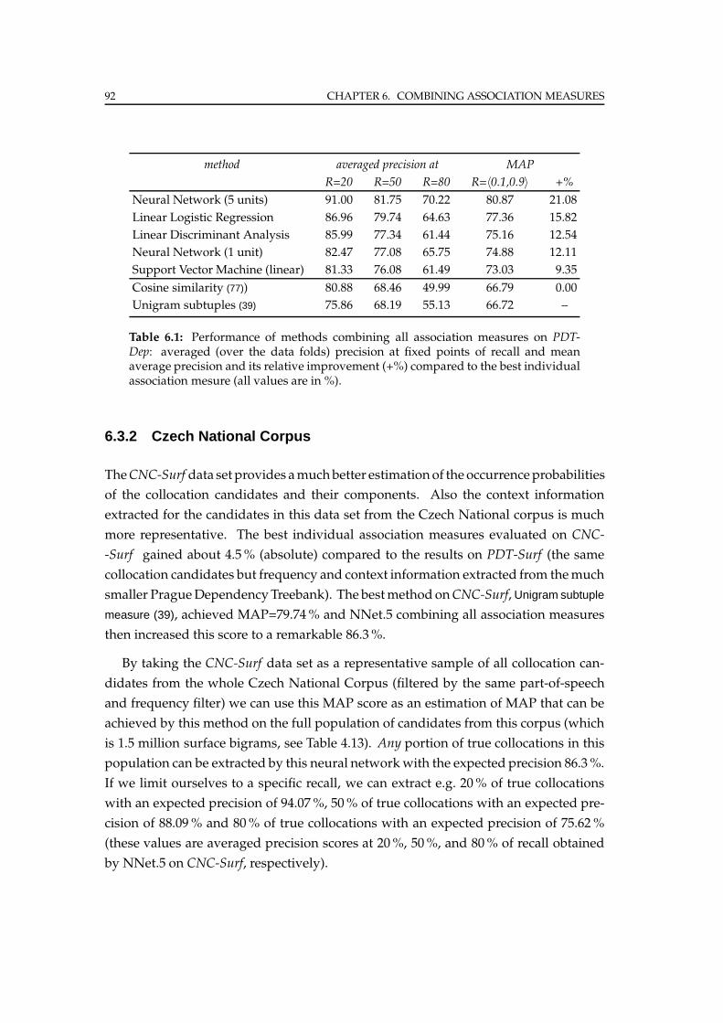
92 CHAPTER 6. COMBINING ASSOCIATION MEASURES
method averaged precision at MAP
R=20 R=50 R=80 R=〈0.1,0.9〉 +%
Neural Network (5 units) 91.00 81.75 70.22 80.87 21.08
Linear Logistic Regression 86.96 79.74 64.63 77.36 15.82
Linear Discriminant Analysis 85.99 77.34 61.44 75.16 12.54
Neural Network (1 unit) 82.47 77.08 65.75 74.88 12.11
Support Vector Machine (linear) 81.33 76.08 61.49 73.03 9.35
Cosine similarity (77)) 80.88 68.46 49.99 66.79 0.00
Unigram subtuples (39) 75.86 68.19 55.13 66.72 –
Table 6.1: Performance of methods combining all association measures on PDT-Dep: averaged (over the data folds) precision at fixed points of recall and meanaverage precision and its relative improvement (+%) compared to the best individualassociation mesure (all values are in %).
6.3.2 Czech National Corpus
TheCNC-Surf data set provides amuchbetter estimationof the occurrenceprobabilities
of the collocation candidates and their components. Also the context information
extracted for the candidates in this data set from the Czech National corpus is much
more representative. The best individual association measures evaluated on CNC-
-Surf gained about 4.5% (absolute) compared to the results on PDT-Surf (the same
collocation candidates but frequency and context information extracted from themuch
smaller PragueDependencyTreebank). The bestmethod onCNC-Surf, Unigram subtuple
measure (39), achieved MAP=79.74% and NNet.5 combining all association measures
then increased this score to a remarkable 86.3%.
By taking the CNC-Surf data set as a representative sample of all collocation can-
didates from the whole Czech National Corpus (filtered by the same part-of-speech
and frequency filter) we can use this MAP score as an estimation of MAP that can be
achieved by this method on the full population of candidates from this corpus (which
is 1.5 million surface bigrams, see Table 4.13). Any portion of true collocations in this
population can be extracted by this neural networkwith the expected precision 86.3%.
If we limit ourselves to a specific recall, we can extract e.g. 20% of true collocations
with an expected precision of 94.07%, 50% of true collocations with an expected pre-
cision of 88.09% and 80% of true collocations with an expected precision of 75.62%
(these values are averaged precision scores at 20%, 50%, and 80% of recall obtained
by NNet.5 on CNC-Surf, respectively).
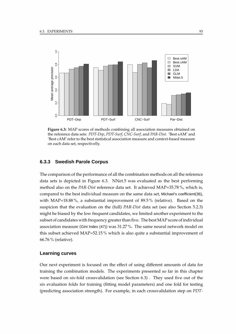
6.3. EXPERIMENTS 93
PDT−Dep PDT−Surf CNC−Surf Par−Dist
Best sAMBest cAMSVMLDAGLMNNet.5
Mea
n av
erag
e pr
ecis
ion
0.0
0.2
0.4
0.6
0.8
1.0
Figure 6.3: MAP scores of methods combining all association measures obtained onthe reference data sets: PDT-Dep, PDT-Surf, CNC-Surf, and PAR-Dist. ’Best sAM’ and’Best cAM’ refer to the best statistical association measure and context-basedmeasureon each data set, respectivelly.
6.3.3 Swedish Parole Corpus
The comparison of the performance of all the combination methods on all the reference
data sets is depicted in Figure 6.3. NNet.5 was evaluated as the best performing
method also on the PAR-Dist reference data set. It achieved MAP=35.78%, which is,
compared to the best individual measure on the same data set, Michael’s coefficient(36),
with MAP=18.88%, a substantial improvement of 89.5% (relative). Based on the
suspicion that the evaluation on the (full) PAR-Dist data set (see also Section 5.2.3)
might be biased by the low frequent candidates, we limited another experiment to the
subset of candidateswith frequencygreater thanfive. ThebestMAPscore of individual
association measure (Gini Index (47)) was 31.27%. The same neural network model on
this subset achieved MAP=52.15% which is also quite a substantial improvement of
66.76% (relative).
Learning curves
Our next experiment is focused on the effect of using different amounts of data for
training the combination models. The experiments presented so far in this chapter
were based on six-fold crossvalidation (see Section 6.3) . They used five out of the
six evaluation folds for training (fitting model parameters) and one fold for testing
(predicting association strength). For example, in each crossvalidation step on PDT-
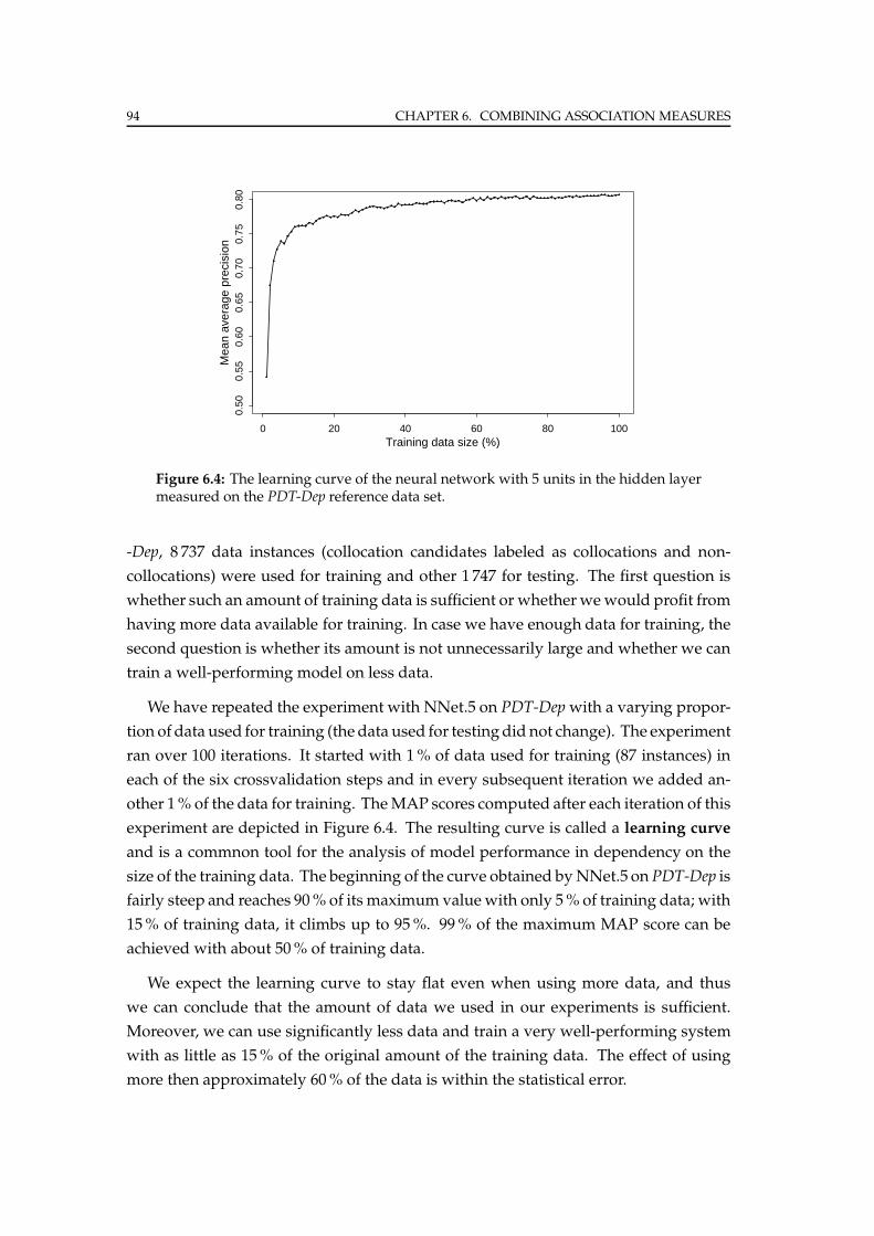
94 CHAPTER 6. COMBINING ASSOCIATION MEASURES
Training data size (%)
Mea
n av
erag
e pr
ecis
ion
0 20 40 60 80 100
0.50
0.55
0.60
0.65
0.70
0.75
0.80
Figure 6.4: The learning curve of the neural network with 5 units in the hidden layermeasured on the PDT-Dep reference data set.
-Dep, 8 737 data instances (collocation candidates labeled as collocations and non-
collocations) were used for training and other 1 747 for testing. The first question is
whether such an amount of training data is sufficient or whetherwewould profit from
having more data available for training. In case we have enough data for training, the
second question is whether its amount is not unnecessarily large and whether we can
train a well-performing model on less data.
We have repeated the experiment with NNet.5 on PDT-Depwith a varying propor-
tion of data used for training (the data used for testingdid not change). The experiment
ran over 100 iterations. It started with 1% of data used for training (87 instances) in
each of the six crossvalidation steps and in every subsequent iteration we added an-
other 1% of the data for training. TheMAP scores computed after each iteration of this
experiment are depicted in Figure 6.4. The resulting curve is called a learning curve
and is a commnon tool for the analysis of model performance in dependency on the
size of the training data. The beginning of the curve obtained byNNet.5 on PDT-Dep is
fairly steep and reaches 90% of its maximum value with only 5% of training data; with
15% of training data, it climbs up to 95%. 99% of the maximum MAP score can be
achieved with about 50% of training data.
We expect the learning curve to stay flat even when using more data, and thus
we can conclude that the amount of data we used in our experiments is sufficient.
Moreover, we can use significantly less data and train a very well-performing system
with as little as 15% of the original amount of the training data. The effect of using
more then approximately 60% of the data is within the statistical error.
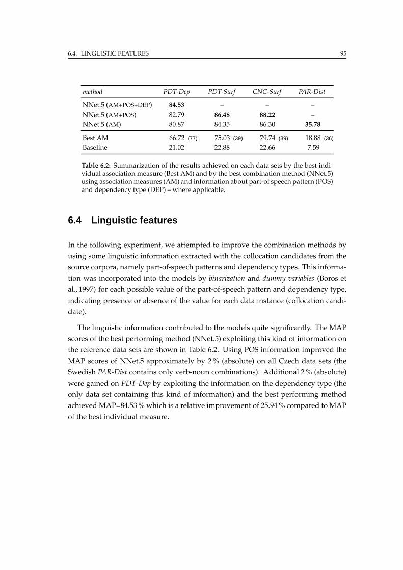
6.4. LINGUISTIC FEATURES 95
method PDT-Dep PDT-Surf CNC-Surf PAR-Dist
NNet.5 (AM+POS+DEP) 84.53 – – –
NNet.5 (AM+POS) 82.79 86.48 88.22 –
NNet.5 (AM) 80.87 84.35 86.30 35.78
Best AM 66.72 (77) 75.03 (39) 79.74 (39) 18.88 (36)
Baseline 21.02 22.88 22.66 7.59
Table 6.2: Summarization of the results achieved on each data sets by the best indi-vidual association measure (Best AM) and by the best combination method (NNet.5)using association measures (AM) and information about part-of speech pattern (POS)and dependency type (DEP) – where applicable.
6.4 Linguistic features
In the following experiment, we attempted to improve the combination methods by
using some linguistic information extracted with the collocation candidates from the
source corpora, namely part-of-speech patterns and dependency types. This informa-
tion was incorporated into the models by binarization and dummy variables (Boros et
al., 1997) for each possible value of the part-of-speech pattern and dependency type,
indicating presence or absence of the value for each data instance (collocation candi-
date).
The linguistic information contributed to the models quite significantly. The MAP
scores of the best performing method (NNet.5) exploiting this kind of information on
the reference data sets are shown in Table 6.2. Using POS information improved the
MAP scores of NNet.5 approximately by 2% (absolute) on all Czech data sets (the
Swedish PAR-Dist contains only verb-noun combinations). Additional 2% (absolute)
were gained on PDT-Dep by exploiting the information on the dependency type (the
only data set containing this kind of information) and the best performing method
achieved MAP=84.53% which is a relative improvement of 25.94% compared to MAP
of the best individual measure.
96 CHAPTER 6. COMBINING ASSOCIATION MEASURES
6.5 Model reduction
In the previous sections, we have demonstrated that combining association measures
is generally very reasonable and significantly helps in the task of ranking collocation
candidates. However, methods which employ all 82 association measures in linear
combination (or more complex models, such as the neural networks with multiple
units in the hidden layer) are unnecessarily complex (in the number of the variables
used). There are two problems:
First, some of the association measures are too similar (analytically or empirically)
– when combined they do not bring any new information and become redundant.
Such highly correlated measures make the training (fitting the models) quite diffi-
cult and should be eliminated. After applying principal component analysis (see e.g.
(Jolliffe, 2002)) to the all 82 association scores of collocation candidates from the PDT-
-Dep reference data, we observed that 95% of the total variance is explained by only 17
principal components and 99.9% is explained by 42 components. We should be able
to reduce the number of variables in our models significantly, possibly with a very
limited degradation of their performance.
Second, some of themeasures are improper for ranking collocation candidates at all
– they do not determine well the strength of association, bring unnecessary noise to
the combination models, and eventually, they can also hurt their performance. Also
such measures should be identified and removed from the model. In this section, we
will attempt to propose an algorithm, which reduces the combination models by re-
moving such redundant (in terms of correlation) and useless (in terms of effectiveness)
variables.
A straightforward, but in our case hardly feasible (due to the high number of the
model variables), approach would be an exhaustive search through the space of all
possible subsets of all the association measures. Another option is a heuristic step-
-wise algorithm iteratively removing one variable at a time until a stopping criterion
is met. Such algorithms are not very robust: they are particularly sensitive to data
and generally not recommended. However, we tried to minimize these problems by
initializing the algorithm by clustering similar variables and choosing one variable
from each cluster as a representative of variables with the same contribution to the
model. Thus we can remove the highly correlated variables and continue with the
step-wise procedure.
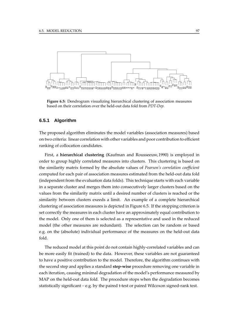
6.5. MODEL REDUCTION 97
6978 79
57 56 58 12 1 17 51 36 55 478
15 14 23 37 2716
24 42 10 43 34 22 45 7 63 13 38 32 31 30 68 59 44 33 19 18 20 21 54 29 28 6 9 539 4
5061 73 71 48 3 77 80 26 25 49 35 53 52
4146 2
60 6776 11
70 40 7562 74 72 82 81 66 64 65
Figure 6.5: Dendrogram visualizing hierarchical clustering of association measuresbased on their correlation over the held-out data fold from PDT-Dep.
6.5.1 Algorithm
The proposed algorithm eliminates the model variables (association measures) based
on two criteria: linear correlationwith other variables andpoor contribution to efficient
ranking of collocation candidates.
First, a hierarchical clustering (Kaufman and Rousseeuw,1990) is employed in
order to group highly correlated measures into clusters. This clustering is based on
the similarity matrix formed by the absolute values of Pearson’s correlation coefficient
computed for each pair of association measures estimated from the held-out data fold
(independent from the evaluation data folds). This technique starts with each variable
in a separate cluster and merges them into consecutively larger clusters based on the
values from the similarity matrix until a desired number of clusters is reached or the
similarity between clusters exeeds a limit. An example of a complete hierarchical
clustering of association measures is depicted in Figure 6.5. If the stopping criterion is
set correctly the measures in each cluster have an approximately equal contribution to
the model. Only one of them is selected as a representative and used in the reduced
model (the other measures are redundant). The selection can be random or based
e.g. on the (absolute) individual performance of the measures on the held-out data
fold.
The reduced model at this point do not contain highly-correlated variables and can
be more easily fit (trained) to the data. However, these variables are not guaranteed
to have a positive contribution to the model. Therefore, the algorithm continues with
the second step and applies a standard step-wise procedure removing one variable in
each iteration, causing minimal degradation of the model’s performance measured by
MAP on the held-out data fold. The procedure stops when the degradation becomes
statistically significant – e.g. by the paired t-test or paired Wilcoxon signed-rank test.
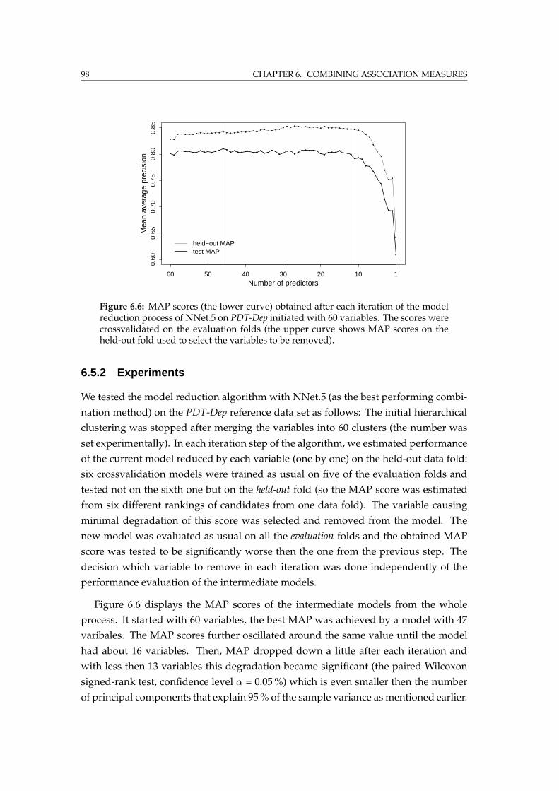
98 CHAPTER 6. COMBINING ASSOCIATION MEASURES
Number of predictors
Mea
n av
erag
e pr
ecis
ion
60 50 40 30 20 10 1
0.60
0.65
0.70
0.75
0.80
0.85
held−out MAPtest MAP
Figure 6.6: MAP scores (the lower curve) obtained after each iteration of the modelreduction process of NNet.5 on PDT-Dep initiated with 60 variables. The scores werecrossvalidated on the evaluation folds (the upper curve shows MAP scores on theheld-out fold used to select the variables to be removed).
6.5.2 Experiments
We tested the model reduction algorithm with NNet.5 (as the best performing combi-
nation method) on the PDT-Dep reference data set as follows: The initial hierarchical
clustering was stopped after merging the variables into 60 clusters (the number was
set experimentally). In each iteration step of the algorithm, we estimated performance
of the current model reduced by each variable (one by one) on the held-out data fold:
six crossvalidation models were trained as usual on five of the evaluation folds and
tested not on the sixth one but on the held-out fold (so the MAP score was estimated
from six different rankings of candidates from one data fold). The variable causing
minimal degradation of this score was selected and removed from the model. The
new model was evaluated as usual on all the evaluation folds and the obtained MAP
score was tested to be significantly worse then the one from the previous step. The
decision which variable to remove in each iteration was done independently of the
performance evaluation of the intermediate models.
Figure 6.6 displays the MAP scores of the intermediate models from the whole
process. It started with 60 variables, the best MAP was achieved by a model with 47
varibales. The MAP scores further oscillated around the same value until the model
had about 16 variables. Then, MAP dropped down a little after each iteration and
with less then 13 variables this degradation became significant (the paired Wilcoxon
signed-rank test, confidence level α = 0.05%) which is even smaller then the number
of principal components that explain 95% of the sample variance as mentioned earlier.
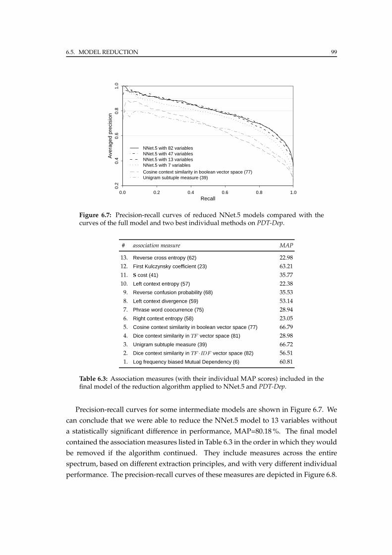
6.5. MODEL REDUCTION 99
Recall
Ave
rage
d pr
ecis
ion
0.0 0.2 0.4 0.6 0.8 1.0
0.2
0.4
0.6
0.8
1.0
NNet.5 with 82 variablesNNet.5 with 47 variablesNNet.5 with 13 variablesNNet.5 with 7 variables
Cosine context similarity in boolean vector space (77)Unigram subtuple measure (39)
Figure 6.7: Precision-recall curves of reduced NNet.5 models compared with thecurves of the full model and two best individual methods on PDT-Dep.
# association measure MAP
13. Reverse cross entropy (62) 22.98
12. First Kulczynsky coefficient (23) 63.21
11. S cost (41) 35.77
10. Left context entropy (57) 22.38
9. Reverse confusion probability (68) 35.53
8. Left context divergence (59) 53.14
7. Phrase word coocurrence (75) 28.94
6. Right context entropy (58) 23.05
5. Cosine context similarity in boolean vector space (77) 66.79
4. Dice context similarity in TF vector space (81) 28.98
3. Unigram subtuple measure (39) 66.72
2. Dice context similarity in TF ·IDF vector space (82) 56.51
1. Log frequency biased Mutual Dependency (6) 60.81
Table 6.3: Association measures (with their individual MAP scores) included in thefinal model of the reduction algorithm applied to NNet.5 and PDT-Dep.
Precision-recall curves for some intermediate models are shown in Figure 6.7. We
can conclude that we were able to reduce the NNet.5 model to 13 variables without
a statistically significant difference in performance, MAP=80.18%. The final model
contained the association measures listed in Table 6.3 in the order in which theywould
be removed if the algorithm continued. They include measures across the entire
spectrum, based on different extraction principles, and with very different individual
performance. The precision-recall curves of these measures are depicted in Figure 6.8.
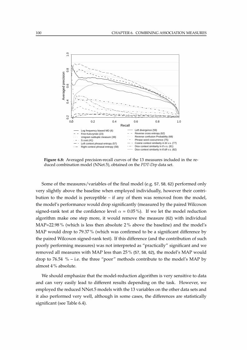
100 CHAPTER 6. COMBINING ASSOCIATION MEASURES
Recall
Ave
rage
d pr
ecis
ion
0.0 0.2 0.4 0.6 0.8 1.0
0.2
0.4
0.6
0.8
1.0
Log frequency biased MD (6)First Kulczynski (23)Unigram subtuple measure (39)S cost (41)Left context phrasal entropy (57)Right context phrasal entropy (58)
Left divergence (59)Reverse cross entropy (62)Reverse confusion Probability (68)Phrase word coocurrence (75)Cosine context similarity in bl v.s. (77)Dice context similarity in tf v.s. (81)Dice context similarity in tf.idf v.s. (82)
Figure 6.8: Averaged precision-recall curves of the 13 measures included in the re-duced combination model (NNet.5), obtained on the PDT-Dep data set.
Some of the measures/variables of the final model (e.g. 57, 58, 62) performed only
very slightly above the baseline when employed individually, however their contri-
bution to the model is perceptible – if any of them was removed from the model,
the model’s performance would drop significantly (measured by the paired Wilcoxon
signed-rank test at the confidence level α = 0.05%). If we let the model reduction
algorithm make one step more, it would remove the measure (62) with individual
MAP=22.98% (which is less then absolute 2% above the baseline) and the model’s
MAP would drop to 79.37% (which was confirmed to be a significant difference by
the paired Wilcoxon signed-rank test). If this difference (and the contribution of such
poorly performing measures) was not interpreted as “practically” significant and we
removed all measures with MAP less than 25% (57, 58, 62), the model’s MAP would
drop to 76.54 % – i.e. the three “poor” methods contribute to the model’s MAP by
almost 4% absolute.
We should emphasize that the model-reduction algorithm is very sensitive to data
and can very easily lead to different results depending on the task. However, we
employed the reduced NNet.5 models with the 13 variables on the other data sets and
it also performed very well, although in some cases, the differences are statistically
significant (see Table 6.4).
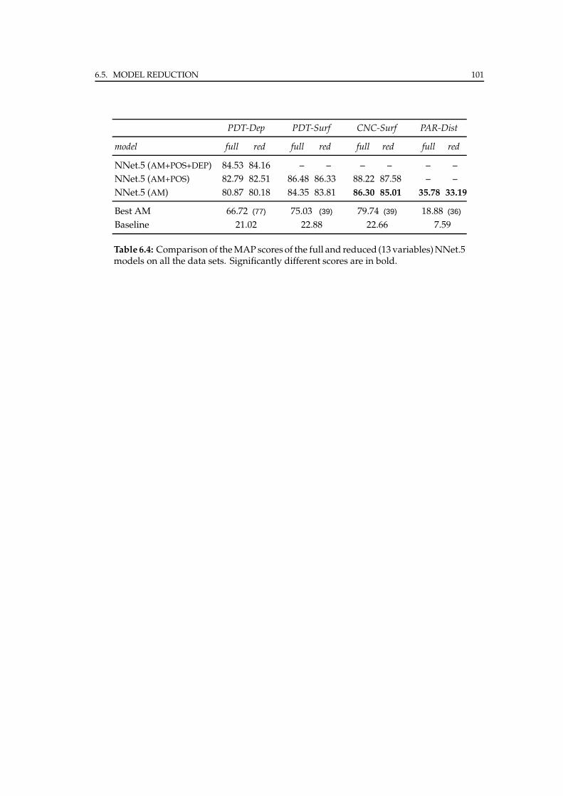
6.5. MODEL REDUCTION 101
PDT-Dep PDT-Surf CNC-Surf PAR-Dist
model full red full red full red full red
NNet.5 (AM+POS+DEP) 84.53 84.16 – – – – – –
NNet.5 (AM+POS) 82.79 82.51 86.48 86.33 88.22 87.58 – –
NNet.5 (AM) 80.87 80.18 84.35 83.81 86.30 85.01 35.78 33.19
Best AM 66.72 (77) 75.03 (39) 79.74 (39) 18.88 (36)
Baseline 21.02 22.88 22.66 7.59
Table 6.4: Comparison of theMAP scores of the full and reduced (13 variables)NNet.5models on all the data sets. Significantly different scores are in bold.

102
Chapter 7
Conclusions
In this work, we studied lexical association measures and their application to colloca-
tion extraction. First, we compiled a comprehensive inventory of 82 lexical association
measures for two-word (bigram) collocation extraction based on three different ex-
traction principles. These measures are divided into two groups: statistical association
measures and context-based association measures.
Second, we developed four reference data sets for the task of identifying colloca-
tion candidates. All of them consist of bigram collocation candidates. PDT-Dep and
PDT-Surf were extracted from the manually annotated Czech Prague Dependency Tree-
bank and differ only in the character of the bigrams: PDT-Dep consists of dependency
bigrams and PDT-Surf of surface bigrams. Both the setswere filtered by the same part-
of-speech pattern and frequency filters. Manual annotation was done exhaustively by
three annotators, true collocations were indicated in all the data. The CNC-Surf refer-
ence data setwas extracted from amuch larger data from theCzech National Corpus and
consists of surface bigrams also appearing in PDT-Surf. It can be considered as a ran-
dom sample from the full set of collocation candidates in this corpus filtered by the
same part-of-speech pattern filter and frequency filter as the PDT-Surf reference data.
The PAR-Dist reference data set is quite different. It consists of Swedish verb-noun
combinations manually extracted from the Swedish Parole corpus in a nonexhaustive
fashion with an indication of true support-verb constructions.
These four reference data sets were designed to allow comparison of effectiveness
of the association measures in different settings. On PDT-Dep and PDT-Surf, we com-
pared twoways of extracting collocation candidates (dependency vs. surface bigrams).
On PDT-Surf and CNC-Surf, we explored the effect of using a much larger source cor-
103

104 CHAPTER 7. CONCLUSIONS
pus (1.5 million vs. 242 million tokens). PAR-Dist complements these three sets with
the data that differs in more aspects: the language (Swedish vs. Czech), the way the
candidates were obtained (distance vs. dependency and surface bigrams), the type of
collocations being extracted (support verb constructions vs. general collocations), the
size of the source corpora (20million vs. 1.5million and 242million tokens), and finally,
the frequency filter (all candidates vs. those occurring more than five times).
We implemented all the 82 lexical association measures and evaluated their perfor-
mance in ranking collocation candidates over the four reference data sets by averaged
precision-recall (PR) curves andmean average precision (MAP) scores in six-fold cross val-
idation. The baseline scores were set as the expectedMAP of a system that would rank
the collocation candidates in each the reference data set randomly, which corresponds
to the prior probability of a collocation candidate to be a true collocation: 21.02% for
PDT-Dep, 22.88% for PDT-Surf, 22.66% for CNC-Surf, and 7.59% for PAR-Dist.
The best result on the PDT-Dep reference data was achieved by a context-based
method measuring Cosine context similarity in boolean vector space with MAP=66.79%
followed by 15 other association measures with statistically indistinguishable per-
formance. Extracting collocations as surface bigrams was observed to be the more
efficient approach (in terms of higher MAP). The results of almost all measures ob-
tained over thePDT-Surf reference data significantly improved: the bestMAP=75.03%
was achieved with Unigram subtuple measure followed by 13 other measures with sta-
tistically insignificant differences in MAP. The experiments carried out on the CNC-
-Surf reference data showed that processing of a larger corpus had a positive effect
on the quality of collocation extraction; the MAP score of the best measures, Unigram
subtuple measure and Pointwise mutual information, increased up to 79.7%. The results
on the PAR-Dist reference data set were remarkably different not only in the absolute
MAP scores of the best methods (Michael’s coefficient, Piatersky-Shapiro’s coefficient, and
T-test with statistically indistinguishable MAP=18.66–18.88%) but also in the relative
difference of their performance over the other data sets. For example, T-test, one of
the best measures on PAR-Dist, performed only slightly above the baseline across all
PDT-Dep, PDT-Surf, and CNC-Surf. These results demonstrate that performance of
lexical association measures strongly depends on the actual data and task. None of
the measures can be selected as the “best” measure that would perform efficiently on
any data set. However, the proposed evaluation scheme (based on MAP scores and
eventually also on PR curves) can be effectively used to choose such a measure (or
measures) for any particular task (if a manually annotated data is available).
105
Further, we demonstrated that by combining association measures, we can achieve
a substantial performance improvement in ranking collocation candidates. The inven-
tory of the lexical association measures presented in this work are used as ranking
functions. Their scores are uncorrelated to such an extent that a linear combination
of all of them produces better association scores than any of the measures employed
individually. All investigated combination methods (Linear logistic regression, Linear
discriminant analysis, Support vector machines, andNeural networks) significantly outper-
formed all individual association measures on all the reference data sets. The best
results were achieved by a simple neural network with five units in the hidden layer.
ItsMAP=80.87% thatwas achieved on thePDT-Depdata set represents 21.53% relative
improvement with respect to the best individual measure on the same set. In the ex-
periments on the CNC-Surf data set, the same neural network achieved MAP=86.30%.
After adding linguistic features (information about part-of-speech and dependency
type) to this model, the MAP score on PDT-Dep increased to 84.53% (25.94% relative
improvement) and on CNC-Surf to 88.22%.
Moreover, we observed that it is not necessary to combine all the 82 association
measures, but only a small subset of about 13 selected measures that performs statis-
tically indistinguishably from the full model (with the neural network with five units
in the hidden layer, measured by MAP on PDT-Dep) is sufficient. This subset contains
measures from the entire spectrum, based on different extraction principles, and with
very different individual performance. Although, the combination of the 13 measures
is not guaranteed to be efficient also on other data sets, the proposed algorithm can
be easily used to select the right measures for any specific data set and task (assuming
a manually annotated data is available).
All the goals specified in Section 1.3 of this work were achieved. Performance
of lexical association measures in the task of ranking collocation extraction heavily
depends on many aspects and must be evaluated on particular data and task. Com-
bining association measures is meaningful and improves precision and recall of the
extraction procedure and substantial performance improvements can be achievedwith
a relatively small number of measures combined in a relatively simple model.

106
Appendix A
MWE 2008 Shared Task Results
In this appendix, we describe our participation in theMWE 2008 evaluation campaign
focused on rankingMWEcandidates published in (Pecina, 2008a). The systemweused
for this shared taks differed in several aspects: we employed only 55 statistical associa-
tion measures (no context-based measures were used), the results were crossvalidated
in 7-fold crossvalidation and comparedbymean average precision (MAP) estimatedon
the full interval of recall 〈0, 1〉. We used the same combination methods and observed
significant performance improvement by combining multiple association measures.
A.1 Introduction
Four gold standard data sets were provided for the MWE 2008 shared task. The goal
was to re-rank each list such that the “best” candidates are concentrated at the top of the
list1. Our experimentswere carried out over only three data sets – those providedwith
corpus frequency data by the shared task organizers: German Adj-Noun collocation
candidates, German PP-Verb collocation candidates, and Czech dependency bigrams
from the Prague Dependency Treebank. For each set of experiments, we present the
best performing association measure (AM) and results of our own system based on
the combination of multiple association measures (AM).
1http://multiword.sf.net/mwe2008/
107
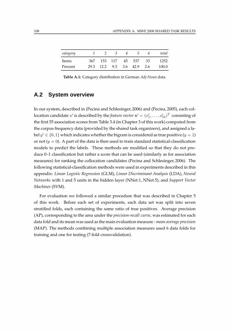
108 APPENDIX A. MWE 2008 SHARED TASK RESULTS
category 1 2 3 4 5 6 total
Items 367 153 117 45 537 33 1252
Percent 29.3 12.2 9.3 3.6 42.9 2.6 100.0
Table A.1: Category distribution in German Adj-Noun data.
A.2 System overview
In our system, described in (Pecina and Schlesinger, 2006) and (Pecina, 2005), each col-
location candidate xi is described by the feature vector xi = (xi
1, . . . , xi55)
T consisting of
the first 55 association scores from Table 3.4 (in Chapter 3 of this work) computed from
the corpus frequency data (provided by the shared task organizers), and assigned a la-
bel yi ∈ {0, 1}which indicateswhether the bigram is considered as true positive (y = 1)
or not (y = 0). A part of the data is then used to train standard statistical-classification
models to predict the labels. These methods are modified so that they do not pro-
duce 0–1 classification but rather a score that can be used (similarly as for association
measures) for ranking the collocation candidates (Pecina and Schlesinger, 2006). The
following statistical-classification methods were used in experiments described in this
appendix: Linear Logistic Regression (GLM), Linear Discriminant Analysis (LDA), Neural
Networks with 1 and 5 units in the hidden layer (NNet.1, NNet.5), and Support Vector
Machines (SVM).
For evaluation we followed a similar procedure that was described in Chapter 5
of this work. Before each set of experiments, each data set was split into seven
stratified folds, each containing the same ratio of true positives. Average precision
(AP), corresponding to the area under the precision-recall curve, was estimated for each
data fold and itsmeanwas used as themain evaluationmeasure -mean average precision
(MAP). The methods combining multiple association measures used 6 data folds for
training and one for testing (7-fold crossvalidation).
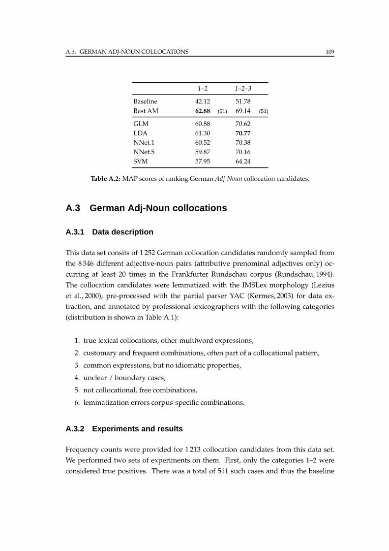
A.3. GERMAN ADJ-NOUN COLLOCATIONS 109
1–2 1–2–3
Baseline 42.12 51.78
Best AM 62.88 (51) 69.14 (51)
GLM 60.88 70.62
LDA 61.30 70.77
NNet.1 60.52 70.38
NNet.5 59.87 70.16
SVM 57.95 64.24
Table A.2: MAP scores of ranking German Adj-Noun collocation candidates.
A.3 German Adj-Noun collocations
A.3.1 Data description
This data set consits of 1 252 German collocation candidates randomly sampled from
the 8 546 different adjective-noun pairs (attributive prenominal adjectives only) oc-
curring at least 20 times in the Frankfurter Rundschau corpus (Rundschau, 1994).
The collocation candidates were lemmatized with the IMSLex morphology (Lezius
et al., 2000), pre-processed with the partial parser YAC (Kermes, 2003) for data ex-
traction, and annotated by professional lexicographers with the following categories
(distribution is shown in Table A.1):
1. true lexical collocations, other multiword expressions,
2. customary and frequent combinations, often part of a collocational pattern,
3. common expressions, but no idiomatic properties,
4. unclear / boundary cases,
5. not collocational, free combinations,
6. lemmatization errors corpus-specific combinations.
A.3.2 Experiments and results
Frequency counts were provided for 1 213 collocation candidates from this data set.
We performed two sets of experiments on them. First, only the categories 1–2 were
considered true positives. There was a total of 511 such cases and thus the baseline
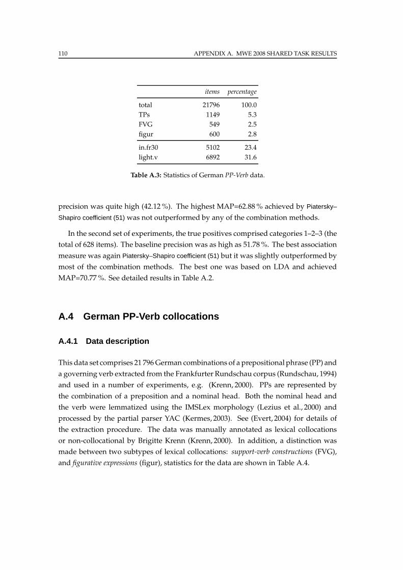
110 APPENDIX A. MWE 2008 SHARED TASK RESULTS
items percentage
total 21796 100.0
TPs 1149 5.3
FVG 549 2.5
figur 600 2.8
in.fr30 5102 23.4
light.v 6892 31.6
Table A.3: Statistics of German PP-Verb data.
precision was quite high (42.12%). The highest MAP=62.88% achieved by Piatersky–
Shapiro coefficient (51) was not outperformed by any of the combination methods.
In the second set of experiments, the true positives comprised categories 1–2–3 (the
total of 628 items). The baseline precision was as high as 51.78%. The best association
measure was again Piatersky–Shapiro coefficient (51) but it was slightly outperformed by
most of the combination methods. The best one was based on LDA and achieved
MAP=70.77%. See detailed results in Table A.2.
A.4 German PP-Verb collocations
A.4.1 Data description
This data set comprises 21 796German combinations of a prepositional phrase (PP) and
a governing verb extracted from the Frankfurter Rundschau corpus (Rundschau, 1994)
and used in a number of experiments, e.g. (Krenn, 2000). PPs are represented by
the combination of a preposition and a nominal head. Both the nominal head and
the verb were lemmatized using the IMSLex morphology (Lezius et al., 2000) and
processed by the partial parser YAC (Kermes, 2003). See (Evert, 2004) for details of
the extraction procedure. The data was manually annotated as lexical collocations
or non-collocational by Brigitte Krenn (Krenn, 2000). In addition, a distinction was
made between two subtypes of lexical collocations: support-verb constructions (FVG),
and figurative expressions (figur), statistics for the data are shown in Table A.4.
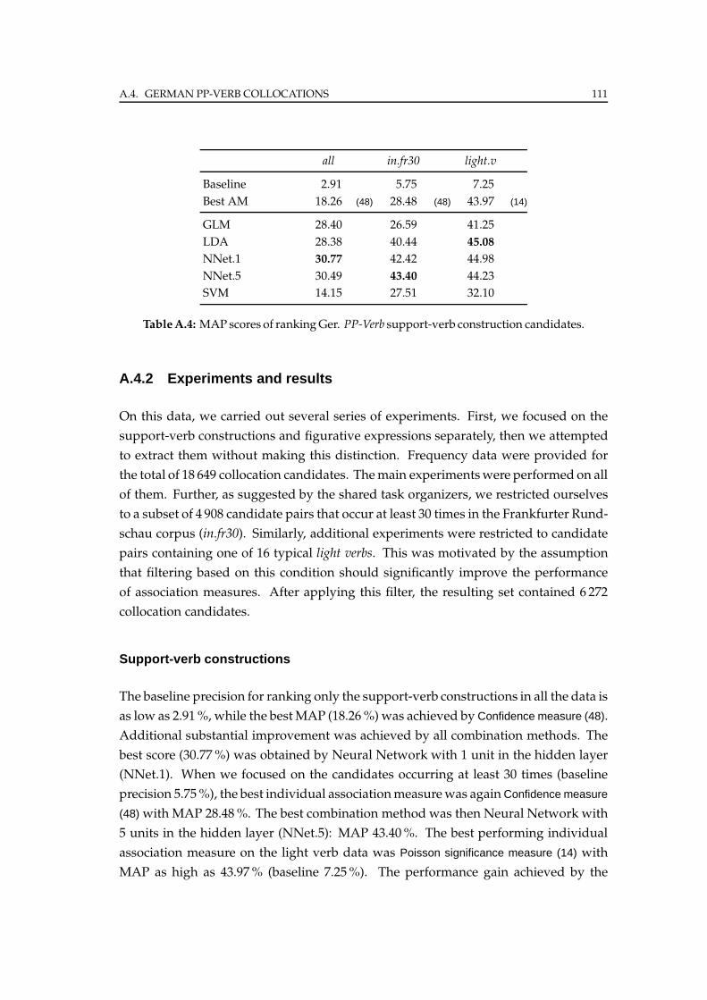
A.4. GERMAN PP-VERB COLLOCATIONS 111
all in.fr30 light.v
Baseline 2.91 5.75 7.25
Best AM 18.26 (48) 28.48 (48) 43.97 (14)
GLM 28.40 26.59 41.25
LDA 28.38 40.44 45.08
NNet.1 30.77 42.42 44.98
NNet.5 30.49 43.40 44.23
SVM 14.15 27.51 32.10
TableA.4: MAPscores of rankingGer. PP-Verb support-verb construction candidates.
A.4.2 Experiments and results
On this data, we carried out several series of experiments. First, we focused on the
support-verb constructions and figurative expressions separately, then we attempted
to extract them without making this distinction. Frequency data were provided for
the total of 18 649 collocation candidates. Themain experimentswere performed on all
of them. Further, as suggested by the shared task organizers, we restricted ourselves
to a subset of 4 908 candidate pairs that occur at least 30 times in the Frankfurter Rund-
schau corpus (in.fr30). Similarly, additional experiments were restricted to candidate
pairs containing one of 16 typical light verbs. This was motivated by the assumption
that filtering based on this condition should significantly improve the performance
of association measures. After applying this filter, the resulting set contained 6 272
collocation candidates.
Support-verb constructions
The baseline precision for ranking only the support-verb constructions in all the data is
as low as 2.91%, while the bestMAP (18.26%) was achieved by Confidence measure (48).
Additional substantial improvement was achieved by all combination methods. The
best score (30.77%) was obtained by Neural Network with 1 unit in the hidden layer
(NNet.1). When we focused on the candidates occurring at least 30 times (baseline
precision 5.75%), the best individual associationmeasurewas again Confidence measure
(48) with MAP 28.48%. The best combination method was then Neural Network with
5 units in the hidden layer (NNet.5): MAP 43.40%. The best performing individual
association measure on the light verb data was Poisson significance measure (14) with
MAP as high as 43.97% (baseline 7.25%). The performance gain achieved by the
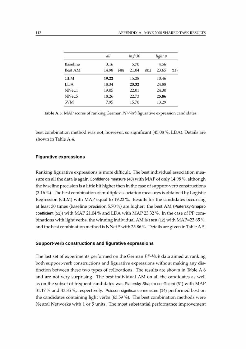
112 APPENDIX A. MWE 2008 SHARED TASK RESULTS
all in.fr30 light.v
Baseline 3.16 5.70 4.56
Best AM 14.98 (48) 21.04 (51) 23.65 (12)
GLM 19.22 15.28 10.46
LDA 18.34 23.32 24.88
NNet.1 19.05 22.01 24.30
NNet.5 18.26 22.73 25.86
SVM 7.95 15.70 13.29
Table A.5: MAP scores of ranking German PP-Verb figurative expression candidates.
best combination method was not, however, so significant (45.08%, LDA). Details are
shown in Table A.4.
Figurative expressions
Ranking figurative expressions is more difficult. The best individual association mea-
sure on all the data is again Confidence measure (48) withMAP of only 14.98%, although
the baseline precision is a little bit higher then in the case of support-verb constructions
(3.16%). The best combination ofmultiple associationmeasures is obtained by Logistic
Regression (GLM) with MAP equal to 19.22%. Results for the candidates occurring
at least 30 times (baseline precision 5.70%) are higher: the best AM (Piatersky-Shapiro
coefficient (51)) with MAP 21.04% and LDA with MAP 23.32%. In the case of PP com-
binations with light verbs, the winning individual AM is t test (12) with MAP=23.65%,
and the best combinationmethod isNNet.5with 25.86%. Details are given inTableA.5.
Support-verb constructions and figurative expressions
The last set of experiments performed on the German PP-Verb data aimed at ranking
both support-verb constructions and figurative expressions without making any dis-
tinction between these two types of collocations. The results are shown in Table A.6
and are not very surprising. The best individual AM on all the candidates as well
as on the subset of frequent candidates was Piatersky-Shapiro coefficient (51) with MAP
31.17% and 43.85%, respectively. Poisson significance measure (14) performed best on
the candidates containing light verbs (63.59%). The best combination methods were
Neural Networks with 1 or 5 units. The most substantial performance improvement
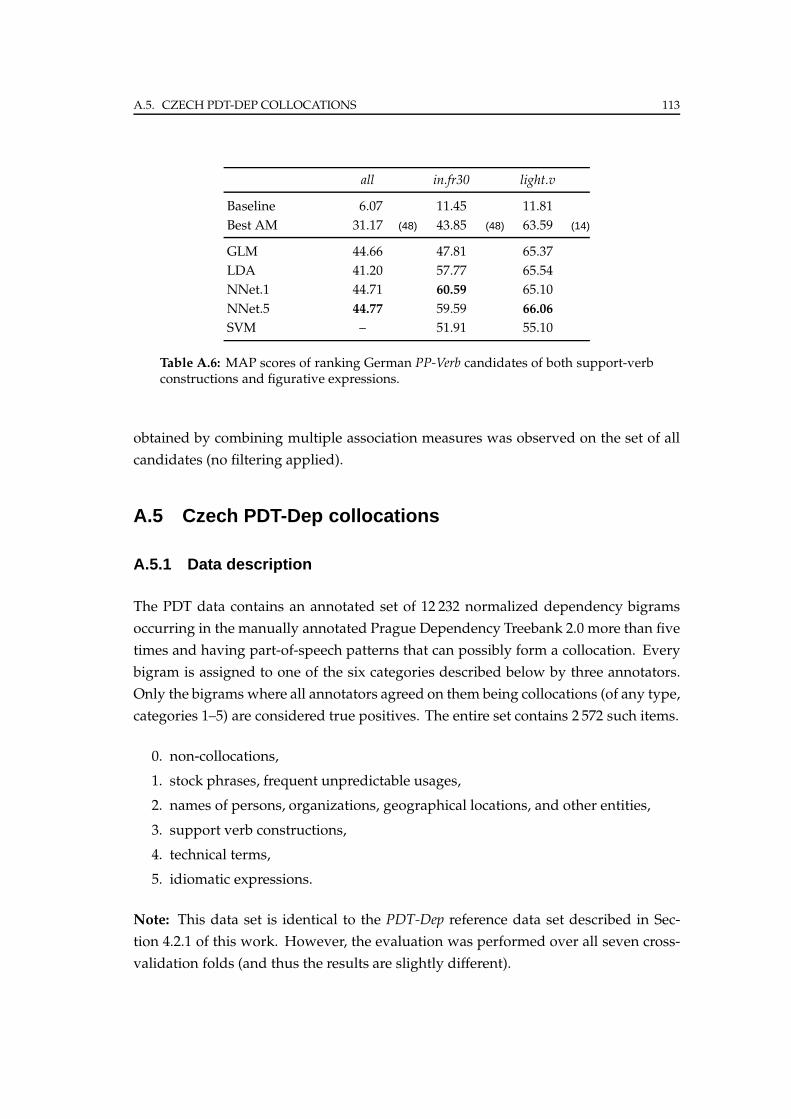
A.5. CZECH PDT-DEP COLLOCATIONS 113
all in.fr30 light.v
Baseline 6.07 11.45 11.81
Best AM 31.17 (48) 43.85 (48) 63.59 (14)
GLM 44.66 47.81 65.37
LDA 41.20 57.77 65.54
NNet.1 44.71 60.59 65.10
NNet.5 44.77 59.59 66.06
SVM – 51.91 55.10
Table A.6: MAP scores of ranking German PP-Verb candidates of both support-verbconstructions and figurative expressions.
obtained by combining multiple association measures was observed on the set of all
candidates (no filtering applied).
A.5 Czech PDT-Dep collocations
A.5.1 Data description
The PDT data contains an annotated set of 12 232 normalized dependency bigrams
occurring in the manually annotated Prague Dependency Treebank 2.0 more than five
times and having part-of-speech patterns that can possibly form a collocation. Every
bigram is assigned to one of the six categories described below by three annotators.
Only the bigrams where all annotators agreed on them being collocations (of any type,
categories 1–5) are considered true positives. The entire set contains 2 572 such items.
0. non-collocations,
1. stock phrases, frequent unpredictable usages,
2. names of persons, organizations, geographical locations, and other entities,
3. support verb constructions,
4. technical terms,
5. idiomatic expressions.
Note: This data set is identical to the PDT-Dep reference data set described in Sec-
tion 4.2.1 of this work. However, the evaluation was performed over all seven cross-
validation folds (and thus the results are slightly different).
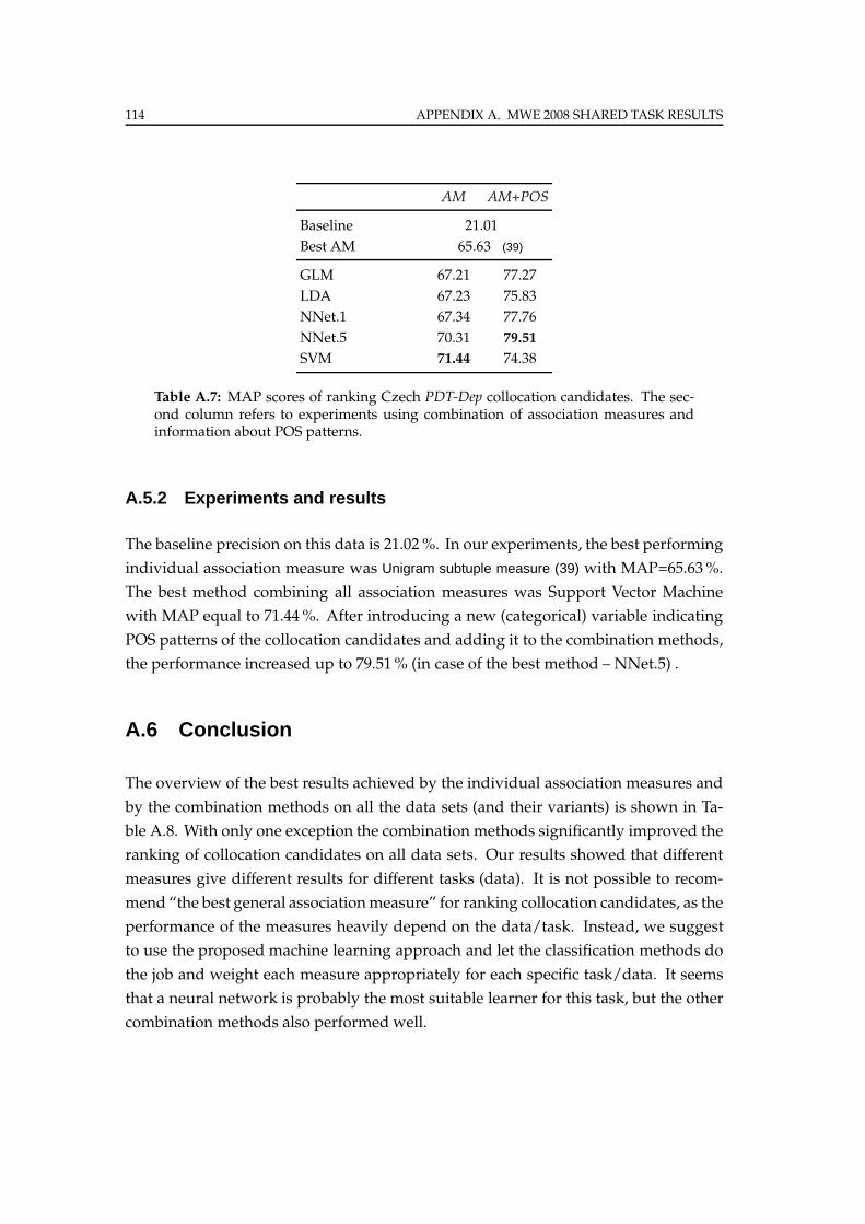
114 APPENDIX A. MWE 2008 SHARED TASK RESULTS
AM AM+POS
Baseline 21.01
Best AM 65.63 (39)
GLM 67.21 77.27
LDA 67.23 75.83
NNet.1 67.34 77.76
NNet.5 70.31 79.51
SVM 71.44 74.38
Table A.7: MAP scores of ranking Czech PDT-Dep collocation candidates. The sec-ond column refers to experiments using combination of association measures andinformation about POS patterns.
A.5.2 Experiments and results
The baseline precision on this data is 21.02%. In our experiments, the best performing
individual association measure was Unigram subtuple measure (39) with MAP=65.63%.
The best method combining all association measures was Support Vector Machine
with MAP equal to 71.44%. After introducing a new (categorical) variable indicating
POS patterns of the collocation candidates and adding it to the combination methods,
the performance increased up to 79.51% (in case of the best method – NNet.5) .
A.6 Conclusion
The overview of the best results achieved by the individual association measures and
by the combination methods on all the data sets (and their variants) is shown in Ta-
ble A.8. With only one exception the combination methods significantly improved the
ranking of collocation candidates on all data sets. Our results showed that different
measures give different results for different tasks (data). It is not possible to recom-
mend “the best general associationmeasure” for ranking collocation candidates, as the
performance of the measures heavily depend on the data/task. Instead, we suggest
to use the proposed machine learning approach and let the classification methods do
the job and weight each measure appropriately for each specific task/data. It seems
that a neural network is probably the most suitable learner for this task, but the other
combination methods also performed well.
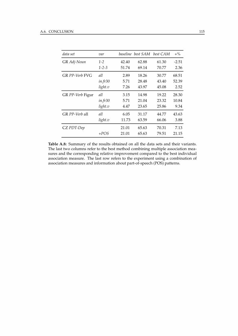
A.6. CONCLUSION 115
data set var baseline best SAM best CAM +%
GR Adj-Noun 1-2 42.40 62.88 61.30 -2.51
1-2-3 51.74 69.14 70.77 2.36
GR PP-Verb FVG all 2.89 18.26 30.77 68.51
in.fr30 5.71 28.48 43.40 52.39
light.v 7.26 43.97 45.08 2.52
GR PP-Verb Figur all 3.15 14.98 19.22 28.30
in.fr30 5.71 21.04 23.32 10.84
light.v 4.47 23.65 25.86 9.34
GR PP-Verb all all 6.05 31.17 44.77 43.63
light.v 11.73 63.59 66.06 3.88
CZ PDT-Dep 21.01 65.63 70.31 7.13
+POS 21.01 65.63 79.51 21.15
Table A.8: Summary of the results obtained on all the data sets and their variants.The last two columns refer to the best method combining multiple association mea-sures and the corresponding relative improvement compared to the best individualassociation measure. The last row refers to the experiment using a combination ofassociation measures and information about part-of-speech (POS) patterns.

116
Appendix B
Complete Evaluation Results
This appendix contains an overview of the results of all evaluation experiments per-
formed in this work. For each data set, we present: 1) the MAP scores of all individual
association measures, 2) the results of significance tests of difference between all in-
dividual association measures (by the paired Student’s t-test and paired Wilcoxon
signed-ranked test), and 3) the MAP scores of combination of all association measures
in different models and their relative performance improvement compared to the best
individual measures.
117
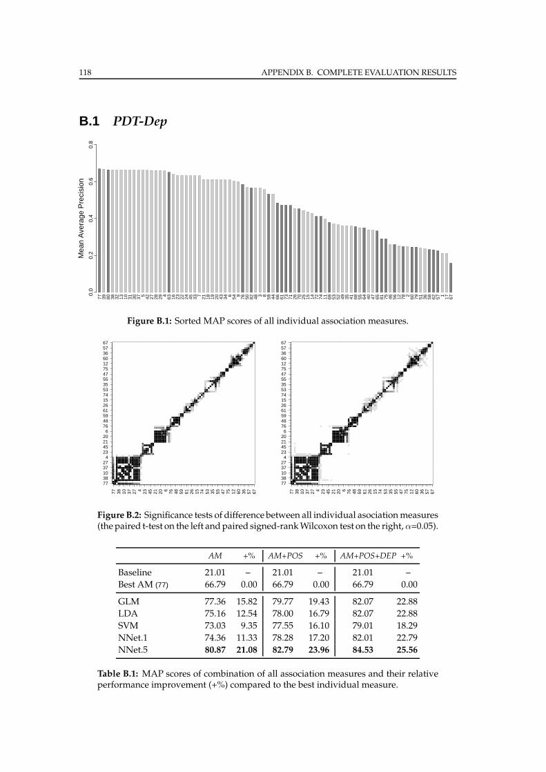
118 APPENDIX B. COMPLETE EVALUATION RESULTS
B.1 PDT-Dep
77 39 80 38 32 13 10 31 30 37 5 42 27 28 29 4 63 16 23 22 24 45 33 7 21 18 19 20 43 34 6 54 9 76 50 82 48 3 8 59 44 66 61 73 71 26 70 25 15 14 72 74 11 69 53 52 49 35 41 68 55 64 40 47 65 81 75 46 56 12 78 2 60 79 51 36 58 62 57 1 17 67
Mea
n A
vera
ge P
reci
sion
0.0
0.2
0.4
0.6
0.8
Figure B.1: Sorted MAP scores of all individual association measures.
77 38 10 37 27 4 23 45 21 20 6 76 48 59 61 26 15 74 53 35 55 47 75 12 60 36 57 67
7738103727
423452120
67648596126157453355547751260365767
77 38 10 37 27 4 23 45 21 20 6 76 48 59 61 26 15 74 53 35 55 47 75 12 60 36 57 67
7738103727
423452120
67648596126157453355547751260365767
Figure B.2: Significance tests of difference between all individual asociationmeasures(the paired t-test on the left andpaired signed-rankWilcoxon test on the right, α=0.05).
AM +% AM+POS +% AM+POS+DEP +%
Baseline 21.01 – 21.01 – 21.01 –
Best AM (77) 66.79 0.00 66.79 0.00 66.79 0.00
GLM 77.36 15.82 79.77 19.43 82.07 22.88
LDA 75.16 12.54 78.00 16.79 82.07 22.88
SVM 73.03 9.35 77.55 16.10 79.01 18.29
NNet.1 74.36 11.33 78.28 17.20 82.01 22.79
NNet.5 80.87 21.08 82.79 23.96 84.53 25.56
Table B.1: MAP scores of combination of all association measures and their relativeperformance improvement (+%) compared to the best individual measure.
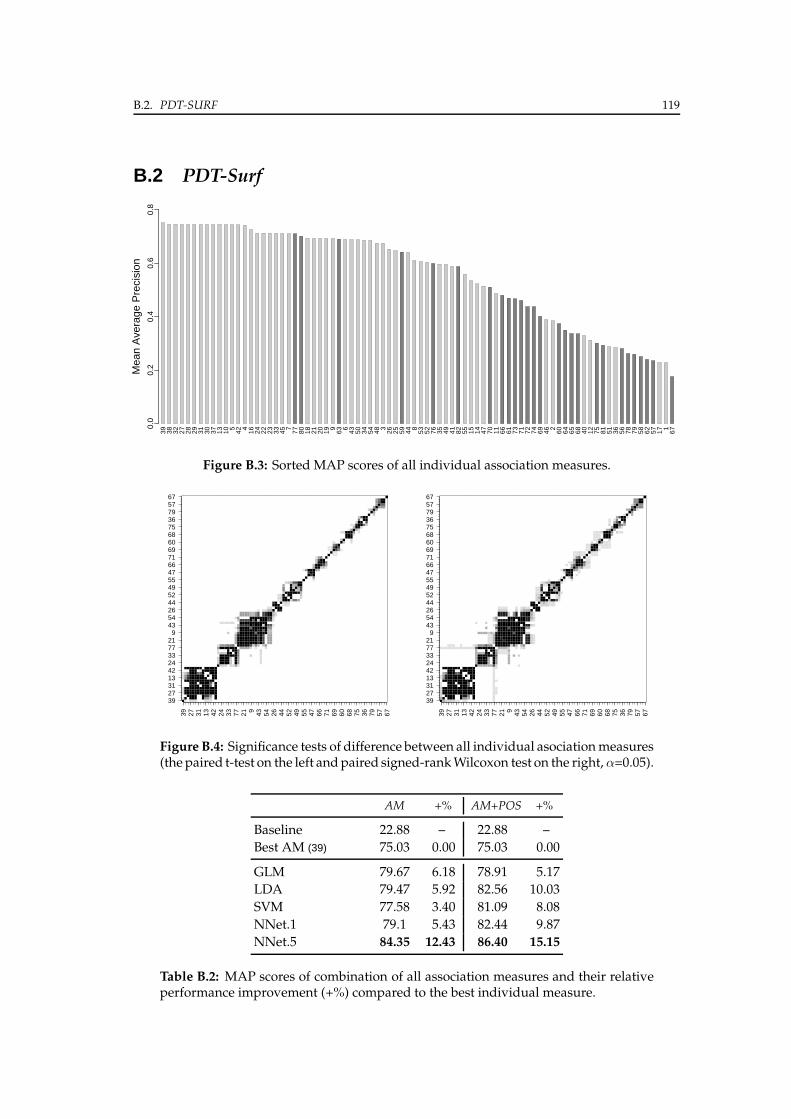
B.2. PDT-SURF 119
B.2 PDT-Surf39 38 32 27 28 29 31 30 37 13 10 5 42 4 16 24 22 23 33 45 7 77 80 18 21 20 19 9 63 6 43 50 34 54 48 3 26 25 59 44 8 53 52 76 35 49 41 82 55 15 14 47 70 11 66 61 73 71 72 74 69 46 2 60 64 65 68 40 12 75 81 51 36 56 78 79 58 62 57 17 1 67
Mea
n A
vera
ge P
reci
sion
0.0
0.2
0.4
0.6
0.8
Figure B.3: Sorted MAP scores of all individual association measures.
39 27 31 13 42 24 33 77 21 9 43 54 26 44 52 49 55 47 66 71 69 60 68 75 36 79 57 67
392731134224337721
9435426445249554766716960687536795767
39 27 31 13 42 24 33 77 21 9 43 54 26 44 52 49 55 47 66 71 69 60 68 75 36 79 57 67
392731134224337721
9435426445249554766716960687536795767
Figure B.4: Significance tests of difference between all individual asociationmeasures(the paired t-test on the left andpaired signed-rankWilcoxon test on the right, α=0.05).
AM +% AM+POS +%
Baseline 22.88 – 22.88 –
Best AM (39) 75.03 0.00 75.03 0.00
GLM 79.67 6.18 78.91 5.17
LDA 79.47 5.92 82.56 10.03
SVM 77.58 3.40 81.09 8.08
NNet.1 79.1 5.43 82.44 9.87
NNet.5 84.35 12.43 86.40 15.15
Table B.2: MAP scores of combination of all association measures and their relativeperformance improvement (+%) compared to the best individual measure.
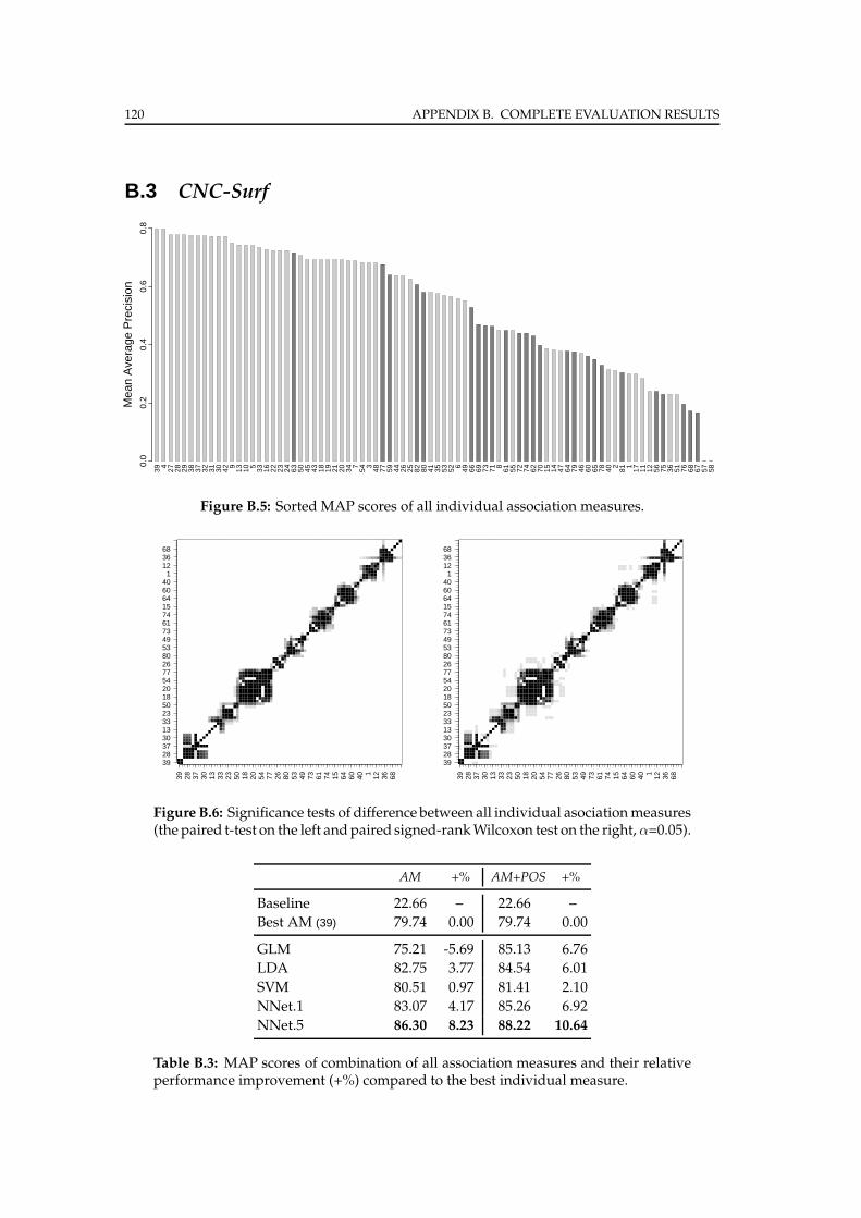
120 APPENDIX B. COMPLETE EVALUATION RESULTS
B.3 CNC-Surf
39 4 27 28 29 38 37 32 31 30 42 9 13 10 5 33 16 22 23 24 63 50 45 43 18 19 21 20 34 7 54 3 48 77 59 44 26 25 82 80 41 35 53 52 6 49 66 69 73 71 8 61 55 72 74 62 70 15 14 47 64 79 46 60 65 78 40 2 81 1 17 11 12 56 75 36 51 76 68 67 57 58
Mea
n A
vera
ge P
reci
sion
0.0
0.2
0.4
0.6
0.8
Figure B.5: Sorted MAP scores of all individual association measures.
39 28 37 30 13 33 23 50 18 20 54 77 26 80 53 49 73 61 74 15 64 60 40 1 12 36 68
3928373013332350182054772680534973617415646040
1123668
39 28 37 30 13 33 23 50 18 20 54 77 26 80 53 49 73 61 74 15 64 60 40 1 12 36 68
3928373013332350182054772680534973617415646040
1123668
Figure B.6: Significance tests of difference between all individual asociationmeasures(the paired t-test on the left andpaired signed-rankWilcoxon test on the right, α=0.05).
AM +% AM+POS +%
Baseline 22.66 – 22.66 –
Best AM (39) 79.74 0.00 79.74 0.00
GLM 75.21 -5.69 85.13 6.76
LDA 82.75 3.77 84.54 6.01
SVM 80.51 0.97 81.41 2.10
NNet.1 83.07 4.17 85.26 6.92
NNet.5 86.30 8.23 88.22 10.64
Table B.3: MAP scores of combination of all association measures and their relativeperformance improvement (+%) compared to the best individual measure.
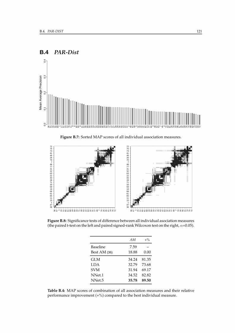
B.4. PAR-DIST 121
B.4 PAR-Dist36 51 12 47 56 69 1 17 57 15 14 78 11 9 6 65 55 8 61 62 44 68 54 18 19 21 20 59 58 66 33 64 73 71 37 27 28 29 34 43 23 24 22 2 40 63 38 5 32 30 42 31 82 13 77 80 3 48 52 53 7 45 4 70 50 81 26 79 25 46 67 35 41 39 76 74 49 60 75 10 16 72
Mea
n A
vera
ge P
reci
sion
0.0
0.1
0.2
0.3
0.4
Figure B.7: Sorted MAP scores of all individual association measures.
36 47 1 15 11 65 61 68 19 59 33 71 28 43 22 63 32 31 77 48 7 70 26 46 41 74 75 72
3647
11511656168195933712843226332317748
770264641747572
36 47 1 15 11 65 61 68 19 59 33 71 28 43 22 63 32 31 77 48 7 70 26 46 41 74 75 72
3647
11511656168195933712843226332317748
770264641747572
Figure B.8: Significance tests of difference between all individual asociationmeasures(the paired t-test on the left andpaired signed-rankWilcoxon test on the right, α=0.05).
AM +%
Baseline 7.59 –
Best AM (36) 18.88 0.00
GLM 34.24 81.35
LDA 32.79 73.68
SVM 31.94 69.17
NNet.1 34.52 82.82
NNet.5 35.78 89.50
Table B.4: MAP scores of combination of all association measures and their relativeperformance improvement (+%) compared to the best individual measure.
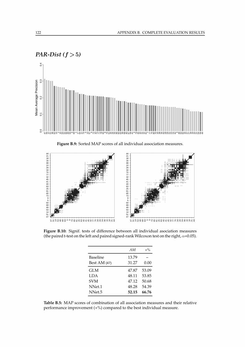
122 APPENDIX B. COMPLETE EVALUATION RESULTS
PAR-Dist (f >5)
47 55 12 51 36 62 14 2 15 53 52 66 49 56 6 69 1 17 64 11 74 5 13 57 9 72 10 73 71 78 65 8 76 61 35 26 25 46 60 63 39 68 40 67 58 41 4 79 45 30 31 32 81 7 77 75 80 70 33 38 34 43 28 29 22 23 24 42 3 48 50 82 16 37 27 18 19 20 21 54 59 44
Mea
n A
vera
ge P
reci
sion
0.0
0.1
0.2
0.3
0.4
Figure B.9: Sorted MAP scores of all individual association measures.
47 51 14 53 49 69 64 5 9 73 65 61 25 63 40 41 45 32 77 70 34 29 24 48 16 18 21 44
47511453496964
59
73656125634041453277703429244816182144
47 51 14 53 49 69 64 5 9 73 65 61 25 63 40 41 45 32 77 70 34 29 24 48 16 18 21 44
47511453496964
59
73656125634041453277703429244816182144
Figure B.10: Signif. tests of difference between all individual asociation measures(the paired t-test on the left andpaired signed-rankWilcoxon test on the right,α=0.05).
AM +%
Baseline 13.79 –
Best AM (47) 31.27 0.00
GLM 47.87 53.09
LDA 48.11 53.85
SVM 47.12 50.68
NNet.1 48.28 54.39
NNet.5 52.15 66.76
Table B.5: MAP scores of combination of all association measures and their relativeperformance improvement (+%) compared to the best individual measure.
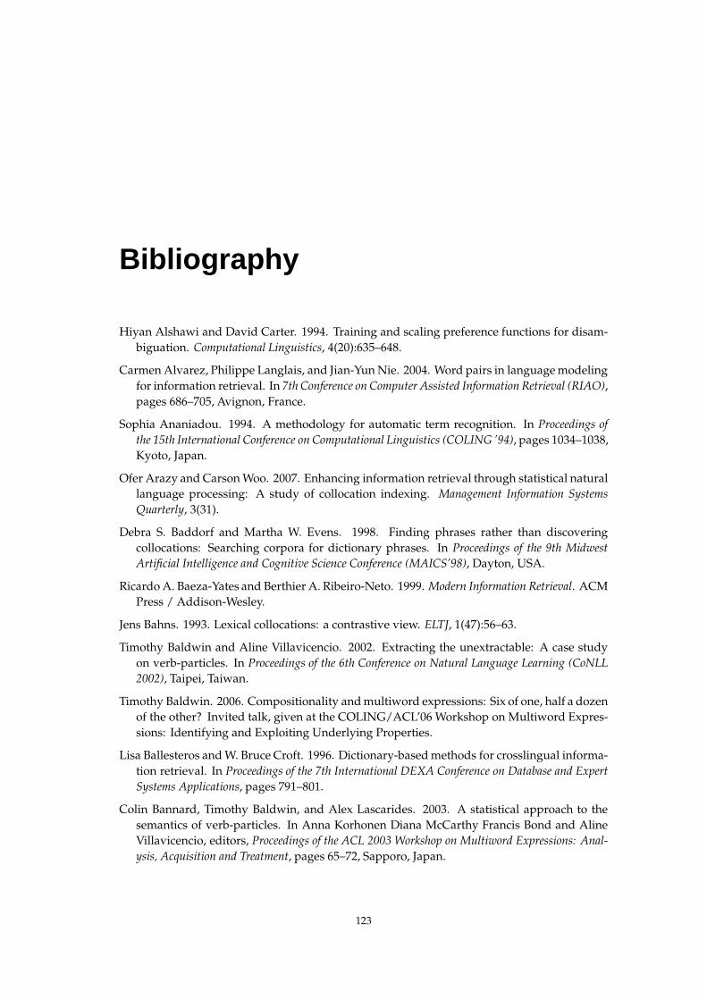
Bibliography
Hiyan Alshawi and David Carter. 1994. Training and scaling preference functions for disam-
biguation. Computational Linguistics, 4(20):635–648.
CarmenAlvarez, Philippe Langlais, and Jian-YunNie. 2004. Word pairs in languagemodeling
for information retrieval. In 7th Conference on Computer Assisted Information Retrieval (RIAO),
pages 686–705, Avignon, France.
Sophia Ananiadou. 1994. A methodology for automatic term recognition. In Proceedings of
the 15th International Conference on Computational Linguistics (COLING ’94), pages 1034–1038,
Kyoto, Japan.
Ofer Arazy and CarsonWoo. 2007. Enhancing information retrieval through statistical natural
language processing: A study of collocation indexing. Management Information Systems
Quarterly, 3(31).
Debra S. Baddorf and Martha W. Evens. 1998. Finding phrases rather than discovering
collocations: Searching corpora for dictionary phrases. In Proceedings of the 9th Midwest
Artificial Intelligence and Cognitive Science Conference (MAICS’98), Dayton, USA.
RicardoA. Baeza-Yates and Berthier A. Ribeiro-Neto. 1999. Modern Information Retrieval. ACM
Press / Addison-Wesley.
Jens Bahns. 1993. Lexical collocations: a contrastive view. ELTJ, 1(47):56–63.
Timothy Baldwin and Aline Villavicencio. 2002. Extracting the unextractable: A case study
on verb-particles. In Proceedings of the 6th Conference on Natural Language Learning (CoNLL
2002), Taipei, Taiwan.
Timothy Baldwin. 2006. Compositionality andmultiword expressions: Six of one, half a dozen
of the other? Invited talk, given at the COLING/ACL’06 Workshop on Multiword Expres-
sions: Identifying and Exploiting Underlying Properties.
Lisa Ballesteros andW. Bruce Croft. 1996. Dictionary-basedmethods for crosslingual informa-
tion retrieval. In Proceedings of the 7th International DEXA Conference on Database and Expert
Systems Applications, pages 791–801.
Colin Bannard, Timothy Baldwin, and Alex Lascarides. 2003. A statistical approach to the
semantics of verb-particles. In Anna Korhonen Diana McCarthy Francis Bond and Aline
Villavicencio, editors, Proceedings of the ACL 2003 Workshop on Multiword Expressions: Anal-
ysis, Acquisition and Treatment, pages 65–72, Sapporo, Japan.
123
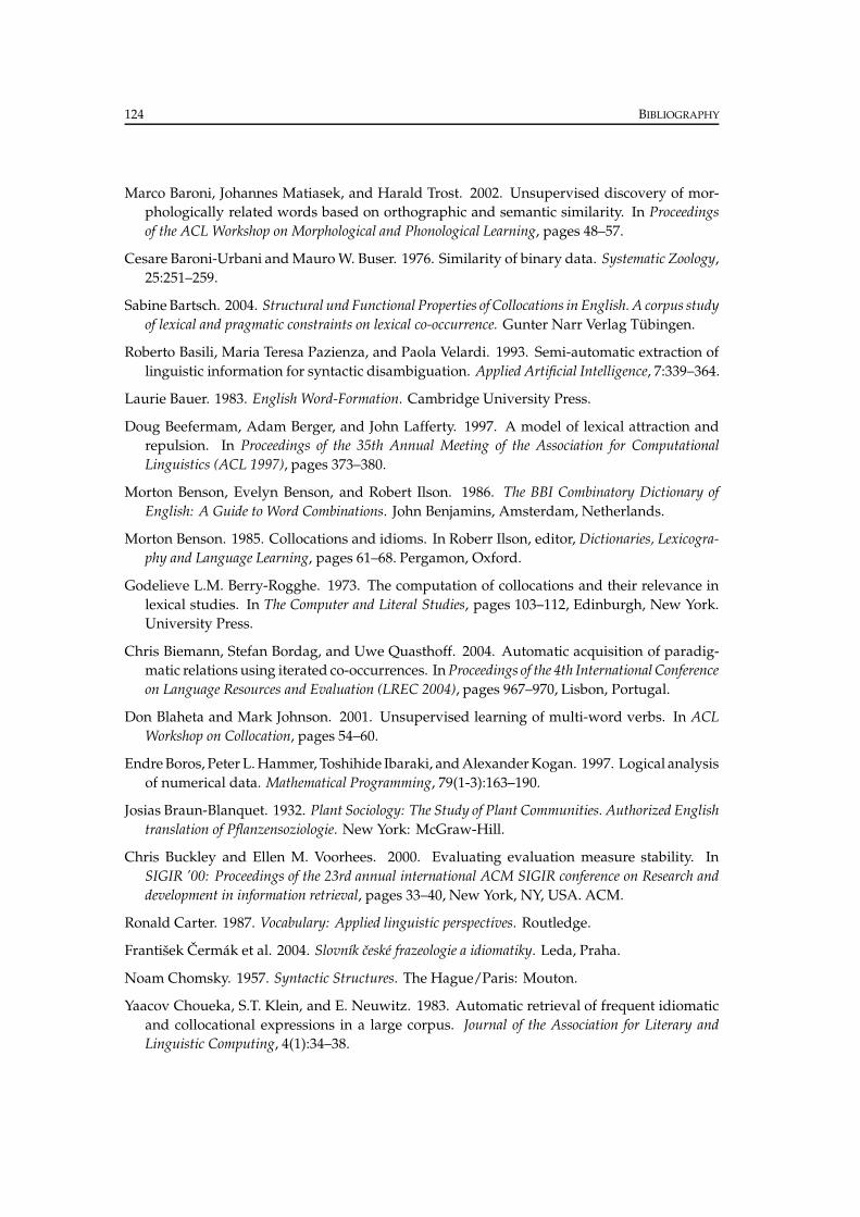
124 BIBLIOGRAPHY
Marco Baroni, Johannes Matiasek, and Harald Trost. 2002. Unsupervised discovery of mor-
phologically related words based on orthographic and semantic similarity. In Proceedings
of the ACL Workshop on Morphological and Phonological Learning, pages 48–57.
Cesare Baroni-Urbani andMauroW. Buser. 1976. Similarity of binary data. Systematic Zoology,
25:251–259.
Sabine Bartsch. 2004. Structural und Functional Properties of Collocations in English. A corpus study
of lexical and pragmatic constraints on lexical co-occurrence. Gunter Narr Verlag Tubingen.
Roberto Basili, Maria Teresa Pazienza, and Paola Velardi. 1993. Semi-automatic extraction of
linguistic information for syntactic disambiguation. Applied Artificial Intelligence, 7:339–364.
Laurie Bauer. 1983. English Word-Formation. Cambridge University Press.
Doug Beefermam, Adam Berger, and John Lafferty. 1997. A model of lexical attraction and
repulsion. In Proceedings of the 35th Annual Meeting of the Association for Computational
Linguistics (ACL 1997), pages 373–380.
Morton Benson, Evelyn Benson, and Robert Ilson. 1986. The BBI Combinatory Dictionary of
English: A Guide to Word Combinations. John Benjamins, Amsterdam, Netherlands.
Morton Benson. 1985. Collocations and idioms. In Roberr Ilson, editor, Dictionaries, Lexicogra-
phy and Language Learning, pages 61–68. Pergamon, Oxford.
Godelieve L.M. Berry-Rogghe. 1973. The computation of collocations and their relevance in
lexical studies. In The Computer and Literal Studies, pages 103–112, Edinburgh, New York.
University Press.
Chris Biemann, Stefan Bordag, and Uwe Quasthoff. 2004. Automatic acquisition of paradig-
matic relations using iterated co-occurrences. InProceedings of the 4th International Conference
on Language Resources and Evaluation (LREC 2004), pages 967–970, Lisbon, Portugal.
Don Blaheta and Mark Johnson. 2001. Unsupervised learning of multi-word verbs. In ACL
Workshop on Collocation, pages 54–60.
EndreBoros, Peter L.Hammer, Toshihide Ibaraki, andAlexanderKogan. 1997. Logical analysis
of numerical data. Mathematical Programming, 79(1-3):163–190.
Josias Braun-Blanquet. 1932. Plant Sociology: The Study of Plant Communities. Authorized English
translation of Pflanzensoziologie. New York: McGraw-Hill.
Chris Buckley and Ellen M. Voorhees. 2000. Evaluating evaluation measure stability. In
SIGIR ’00: Proceedings of the 23rd annual international ACM SIGIR conference on Research and
development in information retrieval, pages 33–40, New York, NY, USA. ACM.
Ronald Carter. 1987. Vocabulary: Applied linguistic perspectives. Routledge.
Frantisek Cermak et al. 2004. Slovnık ceske frazeologie a idiomatiky. Leda, Praha.
Noam Chomsky. 1957. Syntactic Structures. The Hague/Paris: Mouton.
Yaacov Choueka, S.T. Klein, and E. Neuwitz. 1983. Automatic retrieval of frequent idiomatic
and collocational expressions in a large corpus. Journal of the Association for Literary and
Linguistic Computing, 4(1):34–38.
BIBLIOGRAPHY 125
Yaacov Choueka. 1988. Looking for needles in a haystack or locating interesting collocational
expressions in large textual databases. In Proceedings of the RIAO.
Kenneth Church and William A. Gale. 1991. Concordances for parallel text. In Proceedings of
the 7th Annual Conference of the UW Center for the New OED and Text Research, Oxford, UK.
Kenneth Church and Patrick Hanks. 1989. Word association norms, mutual information and
lexicography. In Proceedings of the 27th Annual Meeting of the Association for Computational
Linguistics, pages 76–83.
Kenneth Church and Patrick Hanks. 1990. Word association norms, mutual information and
lexicography. Computational Linguistics, pages 22–29.
KennethChurch andRobert L.Mercer. 1993. Introduction to the special issue on computational
linguistics using large corpora. Computational Linguistics, 19(1):1–24.
Kenneth Church, William Gale, Patrick Hanks, and Donald Hindle. 1991. Parsing, word
associations and typical predicate-argument relations. In M. Tomita, editor, Current Issues
in Parsing Technology. Kluwer Academic, Dordrecht, Netherlands.
Silvie Cinkova and Veronika Kolarova. 2004. Nouns as components of support verb construc-
tions in the Prague Dependency Treebank. In Korpusy a korpusova lingvistika v zahranicı a na
Slovensku.
Silvie Cinkova and Jan Pomikalek. 2006. Lempas: A make-do lemmatizer for the Swedish
PAROLE corpus. Prague Bulletin of Mathematical Linguistics, 86.
Silvie Cinkova, Petr Podvesky, Pavel Pecinal, and Pavel Schlesinger. 2006. Semi-automatic
building of Swedish collocation lexicon. In Proceedings of the 5th International Conference on
Language Resources and Evaluation (LREC), pages 1890–1893, Genova, Italy.
Jacob Cohen. 1960. A coefficient of agreement for nominal scales. Educational and Psychological
Measurement, 20(1).
Michael Collins. 2002. Discriminative training methods for Hidden Markov Models: Theory
and experiments with Perceptron algorithms. In Proceedings of EMNLP 2002, Philadelphia.
Anthony J. Conger. 1980. Integration and generalisation of Kappas for multiple raters. Psy-
chological Bulletin, 88:322–328.
ThomasM. Cover and Joy A. Thomas. 1991. Elements of Information Theory. JohnWiley & Sons,
Inc., New York.
David A. Cruse. 1986. Lexical Semantics. Cambridge University Press, Cambridge.
Ido Dagan and Kenneth Church. 1994. Termight: Identifying and translation technical termi-
nology. In Proceedings of the 4th Conference on Applied Natural Language Processing (ANLP),
pages 34–40, Stuttgart, Germany.
Ido Dagan, Lillian Lee, and Fernando Pereira. 1999. Similarity-basedmodels of word cooccur-
rence probabilities. Machine Learning, 34(1).
Robert Dale, Hermann Moisl, and Harold Somers, editors. 2000. A Handbook of Natural
Language Processing. Marcel Dekker.
126 BIBLIOGRAPHY
JesseDavis andMarkGoadrich. 2006. The relationship betweenprecision-recall curves and the
ROC curve. InProceedings of the 23rd International Conference onMachine Learning, Pittsburgh,
PA.
Gael Dias, Sylvie Guillore, Jean-Claude Bassano, and Jose Gabriel Pereira Lopes. 2000. Com-
bining linguistics with statistics for multiword term extraction: A fruitful association? In
Proceedings of Recherche d’Informations Assistee par Ordinateur 2000 (RIAO 2000).
Harold E. Driver and Alfred Louis Kroeber. 1932. Quantitative expression of cultural re-
lationship. The University of California Publications in American Archaeology and Ethnology,
31:211–256.
Ted E. Dunning. 1993. Accurate methods for the statistics of surprise and coincidence. Com-
putational Linguistics, 19(1):61–74.
Philip Edmonds. 1997. Choosing the wordmost typical in context using a lexical cooccurrence
network. In Proceedings of the 8th Conference of the European Chapter of the Association for
Computational Linguistics (EACL 1997), pages 507–509, Madrid, Spain.
David A. Evans and Chengxiang Zhai. 1996. Noun-phrase analysis in unrestricted text for
information retrieval. InProceedings of the 34th annual meeting onAssociation for Computational
Linguistics, pages 17–24, Santa Cruz, California.
Stefan Evert and Hannah Kermes. 2003. Experiments on candidate data for collocation extrac-
tion. In Companion Volume to the Proceedings of the 10th Conference of The European Chapter of
the Association for Computational Linguistics, pages 83–86.
Stefan Evert and Brigitte Krenn. 2001. Methods for the qualitative evaluation of lexical associ-
ation measures. In Proceedings of the 39th Annual Meeting of the Association for Computational
Linguistics, pages 188–195.
Stefan Evert. 2004. The Statistics of Word Cooccurrences:Word Pairs and Collocations. Ph.D. thesis,
University of Stuttgart.
Joel L Fagan. 1987. Experiments in automatic phrase indexing for document retrieval: A com-
parisonof syntactic andnon-syntacticmethods. Technical report, CornellUniversity, Ithaca,
NY, USA.
Joel L. Fagan. 1989. The effectiveness of a nonsyntactic approach to automatic phrase indexing
for document retrieval. Journal of the American Society for Information Science, 40:115–32.
Tom Fawcett. 2003. ROC graphs: Notes and practical considerations for data mining re-
searchers. Technical report, HPL 2003–4. HP Laboratories, Palo Alto, CA.
Christiane Fellbaum, editor. 1998. WordNet, An Electronic Lexical Database. Bradford Books.
Olivier Ferret. 2002. Using collocations for topic segmentation and link detection. InProcedings
of COLING 2002, Taipei, Taiwan.
John Rupert Firth. 1951. Modes of meanings. In Papers in Linguistics 1934–1951, pages 190–215.
Oxford University Press.
JohnRupert Firth. 1957. A synopsis of linguistic theory, 1930–55. In Studies in linguistic analysis,
Special volume of the Philological Society, pages 1–32. Philogical Society, Oxford.
BIBLIOGRAPHY 127
Joseph L. Fleiss. 1971. Measuring nominal scale agreement among many raters. Psychological
Bulletin, 76:378–382.
Thierry Fontenelle. 1994a. Towards the construction of a collocational database for translation
students. Meta, 1(39):47–56.
Thierry Fontenelle. 1994b. What on earth are collocations? English Today, 4(10):42–48.
William B. Frakes and Ricardo A. Baeza-Yates, editors, 1992. Information Retrieval: Data Struc-
tures and Algorithms, chapter Stemming algorithms. Prentice-Hall, Englewood Cliffs, NJ.
Pascale Fung and Kathleen McKeown. 1997. Finding terminology translations from non-
parallel corpora. In Proceedings of the 5th Annual Workshop on Very Large Corpora, pages
192–202.
Pascale Fung, Min yen Kan, and Yurie Horita. 1996. Extracting Japanese domain and technical
terms is relatively easy. In Proceedings of the 2nd International Conference on New Methods in
Natural Language Processing, pages 148–159.
Vincent E. Giuliano. 1964. The interpretation of word asociations. In M. E. Stevens et al.,
editor, Statistical association methods for mechanized documentation, pages 25–32.
Vincent E. Giuliano. 1965. Postscript: A personal reaction to reading the conference
manuscripts. In Mary ElizabethStevens, Vincent E. Giuliano, and Laurence B. Heilprin,
editors, Proceedings of the Symposium on Statistical Association Methods For Mechanized Docu-
mentation, volume 269 of National Bureau of Standards Miscellaneous Publication, pages 259–
260, Washington, DC.
Gregory Grefenstette and Simone Teufel. 1995. A corpus-based method for automatic identi-
fication of support verbs for nominalisations. In Proceedings of the EACL, Dublin, Ireland.
Michelle L. Gregory, William D. Raymond, Alan Bell, Eric Fosler-Lussier, and Daniel Jurafsky.
1999. The effects of collocational strength and contextual predictability in lexical production.
In CLS 35, University of Chicago.
Jan Hajic, Jarmila Panevova, Eva Buranova, Zdenka Uresova, and Alla Bemova. 1997. A
manual for analytic layer tagging of the prague dependency treebank. Technical Report
TR–1997–03, UFAL MFF UK, Prague, Czech Republic.
Jan Hajic. 2004. Disambiguation of Rich Inflection (Computational Morphology of Czech), volume 1.
Charles University Press, Prague.
Michael Halliday and Ruqaiya Hasan. 1967. Cohesion in English. Longman, London.
Michael A. K. Halliday. 1966. Lexis as a linguistic level. In C. Bazell, J. Catford, M. Halliday,
and R. Robins, editors, In Memory of J.R. Firth, pages 148–162. Longman, London.
Ute Hamann. 1961. Merkmalsbestand und Verwandtschaftsbeziehungen der Farinose. Ein
Betrag zum System der Monokotyledonen. Willdenowia, 2:639–768.
Masahiko Haruno, Satoru Ikehara, and Takefumi Yamazaki. 1996. Learning bilingual colloca-
tions byword-level sorting. InProceedings of the 16th International Conference onComputational
Linguistics (COLING ’96), Copenhagen, Denmark.
Ruqaiya Hasan. 1984. Coherence and cohesive harmony. In J. Flood, editor, Understanding
Reading Comprehension, pages 181–219. Newark, Del: International Reading Association.
128 BIBLIOGRAPHY
TrevorHastie, Saharon Rosset, Rob Tibshirani, and Ji Zhu. 2004. The entire regularization path
for the support vector machine. Journal of Machine Learning Research, 5.
Ulrich Heid. 1998. Towards a corpus-based dictionary of german noun-verb collocations. In
Actes EURALEX’98 Proceedings, volume 1, pages 301–312, Universite de Liege, Departe-
ments d’anglais et de neerlandai.
David Hull and Gregory Grefenstette. 1996. Querying across languages: a dictionary-based
approach to multilingual information retrieval. In SIGIR ’96: Proceedings of the 19th Annual
International ACM SIGIR Conference on Research and Development in Information Retrieval,
pages 49–57, New York, NY, USA.
David Hull. 1993. Using statistical testing in the evaluation of retrieval experiments. In
Proceedings of the 16thAnnual International ACMSIGIRConference onResearch andDevelopment
in Information Retrieval, New York, NY.
ICNC. 2000. Czech National Corpus – SYN2000. Institute of the Czech National Corpus
Faculty of Arts, Charles University, Praha, http://ucnk.ff.cuni.cz.
ICNC. 2005. Czech National Corpus – SYN2005. Institute of the Czech National Corpus
Faculty of Arts, Charles University, Praha, http://ucnk.ff.cuni.cz.
Diana Inkpen and Graeme Hirst. 2002. Acquiring collocations for lexical choice between near
synonyms. In SIGLEX Workshop on Unsupervised Lexical Acquisition, 40th meeting of the ACL,
Philadelphia.
Paul Jaccard. 1912. The distribution of the flora in the alpine zone. The New Phytologist,
11:37–50.
Maojin Jiang, Eric Jensen, Steve Beitzel, and Shlomo Argamon. 2004. Effective use of phrases
in language modeling to improve information retrieval. In Symposium on AI &Math Special
Session on Intelligent Text Processing, Florida, USA.
Ian T. Jolliffe. 2002. Principal Component Analysis. Springer Series in Statistics, 2nd ed. Springer,
NY.
John S. Justeson and Slava M. Katz. 1991. Co-occurrences of antonymous adjectives and their
contexts. Computational Linguistics, 1:1–19.
John S. Justeson and Slava M. Katz. 1995. Technical terminology: Some linguistic properties
and an algorithm for identification in text. Natural Language Engineering, 1:9–27.
Leonard Kaufman and Peter J. Rousseeuw. 1990. Finding Groups in Data: An Introduction to
Cluster Analysis. Wiley Series in Probability and Mathematical Sciences.
Hannah Kermes. 2003. Off-line (and On-line) Text Analysis for Computational Lexicography. Ph.D.
thesis, IMS, University of Stuttgart.
Christopher S. G. Khoo, Sung Hyon Myaeng, and Robert N. Oddy. 2001. Using cause-
effect relations in text to improve information retrieval precision. Information Processing and
Management, 37(1):119–145.
Adam Kilgarriff and David Tugwell. 2001. WORD SKETCH: Extraction and display of sig-
nificant collocations for lexicography. In Proceedings of the ACL 2001 Collocations Workshop,
pages 32–38, Toulouse, France.
BIBLIOGRAPHY 129
Adam Kilgarriff. 1992. Polysemy. Ph.D. thesis, University of Sussex, UK.
Tibor Kiss and Jan Strunk. 2002a. Scaled log likelihood ratios for the detection of abbreviations
in text corpora. In Proceedings of COLING 2002, pages 1228–1232, Taipeh, Taiwan.
Tibor Kiss and Jan Strunk. 2002b. Viewing sentence boundary detection as collocation iden-
tification. In S. Busemann, editor, Tagungsband der 6. Konferenz zur Verarbeitung naturlicher
Sprache (KONVENS 2002), pages 75–82, Saarbrucken, Germany.
Kenji Kita and Hiroaki Ogata. 1997. Collocations in language learning: Corpus-based auto-
matic compilation of collocations and bilingual collocation concordancer. Computer Assisted
Language Learning: An International Journal, 10(3):229–238.
Kenji Kita, Yasuhiro Kato, Takashi Omoto, and Yoneo Yano. 1994. A comparative study of
automatic extraction of collocations from corpora: Mutual information vs. cost criteria.
Journal of Natural Language Processing, 1(1):21–33.
Goran Kjellmer. 1987. Aspects of english collocations. In W. Meijs, editor, Corpus Linguistics
and Beyond. Proceedings of the Seventh International Conference on English Language Research on
Computerised Corpora, pages 133–40, Amsterdam.
Goran Kjellmer. 1991. A mint of phrases. Longman, Harlow.
Goran Kjellmer. 1994. A Dictionary of English Collocations. Clarendon Press.
Ales Klegr, Petra Key, and Norah Hronkova. 2005. Cesko-anglicky slovnık spojenı: podstatne
jmeno a sloveso. Karolinum, Praha.
Ron Kohavi and Foster Provost. 1998. Glossary of terms. Special Issue on Applications ofMachine
Learning and the Knowledge Discovery Process, 30(2/3):271–274.
BrigitteKrenn, StephanEvert, andHeikeZinsmeister. 2004. Determining intercoder agreement
for a collocation identification task. In Proceedings of Konvens’04, pages 89–96, Vienna,
Austria.
Brigitte Krenn. 2000. The Usual Suspects: Data-Oriented Models for Identification and Representa-
tion of Lexical Collocations. Ph.D. thesis, Saarland University.
S. Kulczynski. 1927. Die Pflanzenassociationen der Pienenen. Bulletin International de
L’Acad’emie Polonaise des Sciences et des Letters, Classe des Sciences Mathematiques et Naturelles,
Serie B, Supplement II, 2:57–203.
Julian Kupiec, Jan O. Pedersen, and Francine Chen. 1995. A trainable document summarizer.
In Research and Development in Information Retrieval, pages 68–73.
Lillian Lee. 2001. On the effectiveness of the skew divergence for statistical language analysis.
Artificial Inteligence, pages 65–72.
Michael Lesk. 1969. Word-word associations in document retrieval systems. American Docu-
mentation, 1(20):27–38.
Wolfgang Lezius, StefanieDipper, andArne Fitschen. 2000. IMSLex - representingmorpholog-
ical and syntactical information in a relational database. InU. Heid, S. Evert, E. Lehmann, and
C. Rohrer (eds.): Proceedings of the 9th EURALEX International Congress, Stuttgart, Germany.
Dekang Lin. 1998. Using collocation statistics in information extraction. In Proceedings of the
Seventh Message Understanding Conference (MUC 7).
130 BIBLIOGRAPHY
Dekang Lin. 1999. Automatic identification of non-compositional phrases. In Proc. of the 37th
Annual Meeting of the ACL, pages 317–24, College Park, USA.
David M. Magerman and Mitchell P. Marcus. 1990. Parsing a natural language using mutual
information statistics. In Proceedings of the 8th National Conference on Artificial Intelligence,
pages 984–989, Boston, MA.
Christopher D. Manning and Hinrich Schutze. 1999. Foundations of Statistical Natural Language
Processing. The MIT Press, Cambridge, Massachusetts.
Christopher D. Manning, Prabhakar Raghavan, and Hinrich Schutze. 2008. Introduction to
Information Retrieval. Cambridge University Press.
Diana Maynard and Sophia Ananiadou. 1999. Identifying contextual information for multi-
word term extraction. In 5th International Congress on Terminology and Knowledge Engineering
(TKE 99), pages 212–221.
DianaMcCarthy, Bill Keller, and JohnCarroll. 2003. Detecting a continuumof compositionality
in phrasal verbs. In Anna Korhonen DianaMcCarthy Francis Bond andAline Villavicencio,
editors, Proceedings of the ACL 2003 Workshop on Multiword Expressions: Analysis, Acquisition
and Treatment, pages 73–80.
Ryan McDonald, Fernando Pereira, Kiril Ribarov, and Jan Hajic. 2005. Non-projective de-
pendency parsing using spanning tree algorithms. In Human Language Technologies and
Empirical Methods in Natural Language Processing (HLT-EMNLP), Vancouver, Canada.
Kathleen R. McKeown and Dragomir R. Radev. 2000. Collocations. In Robert Dale, Hermann
Moisl, and Harold Somers, editors, A Handbook of Natural Language Processing. Marcel
Dekker.
Dan I. Melamed. 2000. Models of translational equivalence among words. Computational
Linguistics, 26(2):221–249.
Ellis L. Michael. 1920. Marine ecology and the coefficient of association. Journal of Animal
Ecology, 8:54–59.
Rada Mihalcea and Ted Pedersen. 2003. An evaluation exercise for word alignment. In
Proceedings of HLT-NAACL Workshop, Building and Using Parallel Texts: Data Driven Machine
Translation and Beyond, Edmonton, Alberta.
T.F. Mitchell. 1971. Linguistic ‘goings on’: Collocations and other lexical matters arising on
the syntactic record. Archivum Linguisticum, 2:35–69.
Elke Mittendorf, Bojidar Mateev, and Peter Schauble. 2000. Using the co-occurrence of words
for retrieval weighting. Information Retrieval, 3(3):243–251.
Marıa Begona Villada Moiron. 2005. Data-driven identification of fixed expressions and their
modifiability. Ph.D. thesis, University of Groningen.
Rosamund Moon. 1998. Fixed Expressions and Idioms in English. Clarendon Press, Oxford.
Robert C. Moore, Wen tau Yih, and Andreas Bode. 2006. Improved discriminative bilingual
word alignment. In ACL ’06: Proceedings of the 21st International Conference on Computational
Linguistics and the 44th annual meeting of the ACL, pages 513–520, Sydney, Australia.
BIBLIOGRAPHY 131
Robert C. Moore. 2004. On log-likelihood-ratios and the significance of rare events. In
Proceedings of the 2004 Conference on EMNLP, Barcelona, Spain.
Vaclav Novak and Zdenek Zabokrtsky. 2007. Feature engineering in maximum spanning
tree dependency parser. In Proceedings of the 10th International Conference on Text, Speech and
Dialogue, Pilsen, Czech Republic.
Kumiko Ohmori and Masanobu Higashida. 1999. Extracting bilingual collocations from
non-aligned parallel corpora. In Proceedings of the 8th International Conference on Theoretical
and Methodological Issues in Machine Translation, pages 88–97, University College, Chester,
England.
David S. Palermo and James J. Jenkins. 1964. Word Association norms. University of Minnesota
Press, Mineapolis.
Harold E. Palmer andAlbert S.Hornby. 1937. Thousand-Word English. GeorgeHarrap, London.
Harold E. Palmer. 1938. A Grammar of English Words. Longman, London.
Frank R. Palmer, editor. 1968. Selected Papers of J.R. Firth 1952–1959. Bloomington: Indiana
University Press.
Patrick Pantel and Dekang Lin. 2002. Discovering word senses from text. In Proceedings of the
8th ACM SIGKDD International Conference on Knowledge Discovery and Data Mining, pages
613–619, Edmonton, Canada.
Darren Pearce. 2002. A comparative evaluation of collocation extraction techniques. In Third
International Conference on language Resources and Evaluation, Las Palmas, Spain.
Pavel Pecina and Pavel Schlesinger. 2006. Combining association measures for collocation
extraction. In Proceedings of the 21th International Conference on Computational Linguistics
and 44th Annual Meeting of the Association for Computational Linguistics (COLING/ACL 2006),
Sydney, Australia.
Pavel Pecina, Petra Hoffmannova, Gareth J.F. Jones, Jianqiang Wang, and Douglas W. Oard.
2008. Overview of the CLEF 2007 Cross-Language Speech Retrieval Track. Evaluation of
Multilingual andMulti-modal InformationRetrieval (CLEF 2007), Revised Selected Papers. Lecture
Notes in Computer Science.
Pavel Pecina. 2005. An extensive empirical study of collocation extraction methods. In
Proceedings of the ACL 2005 Student Research Workshop, Ann Arbor, USA.
Pavel Pecina. 2008a. Machine learning approach to mutliword expression extraction. In
Proceedings of the sixth International Conference on Language Resources and EvaluationWorkshop:
Towards a Shared Task for Multiword Expressions (MWE 2008), Marrakech, Morocco.
Pavel Pecina. 2008b. Reference data for Czech collocation extraction. In Proceedings of the Sixth
International Conference on Language Resources and EvaluationWorkshop: Towards a Shared Task
for Multiword Expressions (MWE 2008), Marrakech, Morocco.
Ted Pedersen. 1996. Fishing for exactness. In Proceedings of the South Central SAS User’s Group
Conference, pages 188–200, Austin, TX.
Ted Pedersen. 2001. A decision tree of bigrams is an accurate predictor of word sense. In
Proceedings of the 2ndMeeting of the North American Chapter of the Association for Computational
Linguistics (NAACL 2001), Pittsburgh, PA.
132 BIBLIOGRAPHY
Lubos Prchal. 2008. Selected aspects of functional estimation and testing: Functional response in
regression models and statistical analysis of ROC curves with applications. Ph.D. thesis, Charles
Univeristy of Prague and Paul Sabatier Univeristy - Toulouse III.
Uwe Quasthoff and Christian Wolff. 2002. The Poisson collocation measure and its ap-
plications. In Proceedings ofSecond International Workshop on Computational Approaches to
Collocations, Wien.
Reinhard Rapp. 1999. Automatic identification of word translations from unrelated English
and German corpora. In Proceedings of the 37th Annual Meeting of the Association for Compu-
tational Linguistics, College Park, Maryland.
Reinhard Rapp. 2002. The computation of word associations: Comparing syntagmatic and
paradigmatic approaches. In Proceedings of COLING 2002, Taipeh, Taiwan.
Reinhard Rapp. 2004. Utilizing the one-sense-per-discourse constraint for fully unsupervised
word sense induction anddisambiguation. In In Proceedings of the 4th International Conference
on Language Resources and Evaluation (LREC 2004), pages 951–954, Lisbon, Portugal.
Philip Resnik. 1997. Selectional preferences and sense disambiguation. In Proceedings of the
ACL SIGLEX Workshop on Tagging Text with Lexical Semantics, Washington, D.C.
Robert Robins. 1967. A Short History of Linguistics. Longman, London.
David J. Rogers and Taffee T. Tanimoto. 1960. A computer program for classifying plants.
Science, 132:1115–1118.
Ian C. Ross and John W. Tukey. 1975. Introduction to these volumes. In Index to Statistics and
Probability, Los Altos, CA. The RandD Press.
Frankfurter Rundschau. 1994. The FR corpus is part of the ECI Multilingual Corpus I dis-
tributed by ELSNET. See http://www.elsnet.org/eci.html for more information and licens-
ing conditions.
P. F. Russel and T. R. Rao. 1940. On habitat and association of species of anopheline larvae in
south-eastern madras. Journal of Malaria Institute India, 3:153–178.
Ivan A. Sag, Timothy Baldwin, Francis Bond, Ann Copestake, and Dan Flickinger. 2002.
Multiword expressions: A pain in the neck for NLP. In Computational Linguistics and
Intelligent Text Processing: Third International Conference, CICLing, volume 2276 of Lecture
Notes in Computer Science. Springer Berlin / Heidelberg.
Gerard Salton, Anita Wong, and Chung-Shu Yang. 1975. A vector space model for automatic
indexing. Communications of the ACM, 18(11):613–620.
Patrick Schone and Daniel Jurafsky. 2001. Is knowledge-free induction of multiword unit
dictionary headwords a solved problem? In In Proceedings of the 2001 Conference on Empirical
Methods in Natural Language Processing, pages 100–108.
Sayori Shimohata, Toshiyuki Sugio, and Junji Nagata. 1997. Retrieving collocations by co-
occurrences and word order constraints. In Proceedings of the 35th Meeting of ACL/EACL,
pages 476–481, Madrid, Spain.
George Gaylord Simpson. 1943. Mammals and the nature of continents. American Journal of
Science, 241:1–31.
BIBLIOGRAPHY 133
John Sinclair. 1966. Beginning the study of lexis. In C. Bazell, J. Catford, M. Halliday, and
R. Robins, editors, In Memory of J.R. Firth, pages 410–430. Longman, London.
John Sinclair. 1991. Corpus, Concordance, Collocation. Oxford University Press, Oxford.
Frank A. Smadja and Kathleen R. McKeown. 1990. Automatically extracting and representing
collocations for language generation. In Proceedings of the 28th Annual Meeting of the ACL,
pages 252–259.
Frank A. Smadja, Kathleen R. McKeown, and Vasileios Hatzivassiloglou. 1996. Translating
collocations for bilingual lexicons: A statistical approach. Computational Linguistics, 22(1):1–
38.
Frank Smadja. 1993. Retrieving collocations from text: Xtract. Computational Linguistics,
19:143–177.
Robert R. Sokal and Charles D. Michener. 1958. A statistical method for evaluating systematic
relationships. University of Kansas Science Bulletin, 38:1409–1438.
Robert R. Sokal and Peter H. Sneath. 1963. Principles of Numerical Taxonomy. W. H. Freeman
and Company, San Francisco, USA.
Drahomıra Spoustova, Jan Hajic, Jan Votrubec, Pavel Krbec, and Pavel Kveton. 2007. The best
of two worlds: Cooperation of statistical and rule-based taggers for Czech. In Proceedings of
theWorkshop on Balto-SlavonicNatural Language Processing, ACL 2007, Praha, CzechRepublic.
Mary Elizabeth Stevens, Vincent E. Giuliano, and Laurence B. Heilprin, editors. 1965. Pro-
ceedings of the Symposium on Statistical Association Methods For Mechanized Documentation,
volume 269. National Bureau of Standards Miscellaneous Publication, Washington, DC.
Matthew Stone and Christine Doran. 1996. Paying heed to collocations. In Proceedings of the
International Language Generation Workshop (INLG 96), pages 91–100, Herstmonceux Castle,
Sussex, UK.
RazTamir andReinhardRapp. 2003. Mining theweb todiscover themeaningsof anambiguous
word. In Proceedings of the Third IEEE International Conference onDataMining, pages 645–648,
Melbourne, FL.
Pang-Ning Tan, Vipin Kumar, and Jaideep Srivastava. 2002. Selecting the right interestingness
measure for association patterns. In Proceedings of the Eight A CM SIGKDD International
Conference on Knowledge Discovery and Data Mining.
Takaaki Tanaka and Yoshihiro Matsuo. 1999. Extraction of translation equivalents from non-
parallel corpora. In Proceedings of the 8th International Conference on Theoretical and Method-
ological Issues in Machine Translation (TMI 1999), pages 109–119.
Pasi Tapanainen, Jussi Piitulainen, and Timo Jarvinen. 1998. Idiomatic object usage and
support verbs. In COLING/ACL, pages 1289–1293,Montreal.
Egidio Terra and Charles L. A. Clarke. 2003. Frequency estimates for statistical word similarity
measures. In Proceedings of HLT-NAACL 2003, pages 244–251, Edmonton, Alberta.
Aristomenis Thanopoulos, Nikos Fakotakis, and George Kokkinakis. 2002. Comparative
evaluation of collocation extraction metrics. In 3rd International Conference on Language
Resources and Evaluation, volume 2, pages 620–625, Las Palmas, Spain.
134 BIBLIOGRAPHY
Jorg Tiedemann. 1997. Automated lexicon extraction from aligned bilingual corpora. Master’s
thesis, Otto-von-Guericke-Universitat Magdeburg.
Keita Tsuji and Kyo Kageura. 2001. Extracting morpheme pairs from bilingual terminological
corpora. Terminology, 7(1):101–114.
Rodham E. Tulloss. 1997. Assessment of Similarity Indices for Undesirable Properties and New Tri-
partite Similarity Index Based on Cost Functions. Parkway Publishers, Boone, North Carolina.
Tem van der Wouden. 1997. Negative contexts: collocations, polarity and multiple negation.
Routledge, London/New York.
Cornelis Joost van Rijsbergen. 1979. Information Retrieval. Butterworths, London.
Frantisek Cermak and Jan Holub. 1982. Syntagmatika a paradigmatika cesk eho slova: Valence
a kolokabilita. Statnı pedagogicke nakladatelstvı, Praha.
Frantisek Cermak and Michal Sulc, editors. 2006. Kolokace. Nakladatelstvıi Lidove noviny.
Frantisek Cermak. 2001. Syntagmatika slovnıku: typy lexikalnıch kombinacı. In Zdenka
Hladka and Petr Karlık, editors, Cestina - univerzalia a specifika 3, pages 223–232.Masarykova
Univerzita, Brno.
Frantisek Cermak. 2006. Kolokace v lingvistice. In Frantisek Cermak andMichal Sulc, editors,
Kolokace. Nakladatelstvıi Lidove noviny.
Olga Vechtomova. 2001. Approaches to using word collocation in Information Retrieval. Ph.D.
thesis, City University, London, UK.
William N. Venables and B.D. Ripley. 2002. Modern Applied Statistics with S. 4th ed. Springer
Verlag, New York.
Jan Votrubec. 2006. Morphological tagging based on averaged Perceptron. InWDS’06 Proceed-
ings of Contributed Papers, Prague. MFF UK.
Michael Wallace. 1979. What is an idiom? An applied linguistic approach. In R. Hartmann,
editor, Dictionaries and Their Users: Papers from the 1978 B. A. A. L. Seminar on Lexicography,
pages 63–70. University of Exeter, Exeter.
Matthijs Joost Warrens. 2008. Similarity coefficients for binary data: properties of coefficients, coeffi-
cient matrices, multi-way metrics and multivariate coefficients. Ph.D. thesis, Leiden University.
Marc Weeber, Rein Vos, and R. Harald Baayen. 2000. Extracting the lowest-frequency words:
Pitfalls and possibilities. Computational Linguistics, 3(26):301–317.
Janyce M. Wiebe and Kenneth J. McKeever. 1998. Collocational properties in probabilistic
classifiers for discourse categorization.
Hua Wu and Ming Zhou. 2003. Synonymous collocation extraction using translation infor-
mation. In ACL ’03: Proceedings of the 41st Annual Meeting on Association for Computational
Linguistics, pages 120–127.
David Yarowsky. 1995. Unsupervised word sense disambiguation rivaling supervised meth-
ods. In Meeting of the Association for Computational Linguistics, pages 189–196, Cambridge,
MA.

BIBLIOGRAPHY 135
Dan Zeman, Jirı Hana, Hana Hanova, Jan Hajic, Emil Jerabek, and Barbora Vidova Hladka.
2005. A manual for morphological annotation, 2nd edition. UFAL technical report. Techni-
cal Report TR–2005–27, UFALMFF UK, Prague, Czech Republic.
Chengxiang Zhai. 1997. Exploiting context to identify lexical atoms: A statistical view of
linguistic context. In International and Interdisciplinary Conf. on Modeling and Using Context.
Georg Kingsley Zipf. 1949. Human Behavior and the Principle of Least-Effort. Addison-Wesley,
Cambridge, MA.
Related Documents