Levine, Yanai et al: Optimizing environmental monitoring designs

Optimizing Environmental Monitoring Designs using Uncertainty Analysis

Carrie R. Levine, UC BerkeleyRuth D. Yanai, SUNY College of Environmental Science and Forestry

Gregory Lampman, NYSERDADouglas A. Burns, US Geologic SurveyCharles T. Driscoll, Syracuse University

Gregory B. Lawrence, U.S. Geological SurveyJason A. Lynch, US Environmental Protection Agency

Nina Schoch, Biodiversity Research Institute   

Optimizing Environmental Monitoring Designs Carrie R. Levine, Ruth D. Yanai, Gregory G. Lampman, Douglas A. Burns, Charles T. Driscoll, Gregory B. Lawrence, Jason A. Lynch, Nina Schoch Submitted to Ecological Indicators

QUANTIFYING UNCERTAINTY IN ECOSYSTEM STUDIES

This study was supported by the New York State Energy Research and Development Authority, which supports environmental monitoring for air pollutants associated with the electric power industry.

QUANTIFYING UNCERTAINTY IN ECOSYSTEM STUDIES

Environmental monitoring consumes resources and can be criticized for being unscientific.

We need an objective way to evaluate monitoring plans, including the spatial and temporal intensity of sampling.

Analysis of Case Studies

Question:

• How often should stream chemistry samples be collected to detect long-term chemistry trends?

Data sets used in analysis:

• Biscuit Brook weekly stream chemistry (1996-2003).

Analytical approach:

• We simulated reduced sampling efforts and evaluated confidence in the detection of change over time, using linear regression.

• Weekly, biweekly, monthly, bimonthly.

Uncertainty in Linear Regression

NYSDEC: http://ny.cf.er.usgs.gov/nyc/site_page.cfm?ID=01434025

SO

4 (μ

mo

l L

-1)

Date

Weekly (100%)

Biweekly (50%

Monthly (25%)

Bimonthly (13%)

Subsampling the data set affects the slope and intercept of the regression of long-term data.

Sampling Scheme

For full model:p<0.0001, R2 = 0.08

The error in the slope increases as sampling intensity decreases.

12.5%: Bimonthly

25%: Monthly

50%: Biweekly100%: Weekly

SE

of

the

slo

pe

(μg

NO

3 L

-1 y

r-1)

Effect of reduced sampling schemes on detectability of long-term trends in stream chemistry at Biscuit Brook (1996-2003)

# of significant regressions / Total # of possible regressions

Weekly Biweekly Monthly Bimonthly

SO42- 1/1 2/2 3/4 3/8

NO3- 1/1 2/2 3/4 4/8

H+ 1/1 1/2 2/4 2/8

Al 1/1 2/2 4/4 7/8

Question:

• How many samples would be required to detect a change in mercury in loons at a future sampling date?

Data sets used in analysis:

• One-time survey, 42 lakes, different numbers of loons per lake

Analytical approach:

The detectable difference δ for a two-sample t-test is:

where s is the standard deviation of the paired differences, n= sample size, t α,v is the (1- α/2) x 100 percentile of the t-distribution, t β,v is the 100 x (power) percentile of the t-distribution, ν = 2n-2 degrees of freedom, α is the probability of a Type I error, and β is the probability of a Type II error.

Detectable Difference (T-test)

http://images.nationalgeographic.com/wpf/media-live/photos/000/007/cache/common-loon_794_600x450.jpg

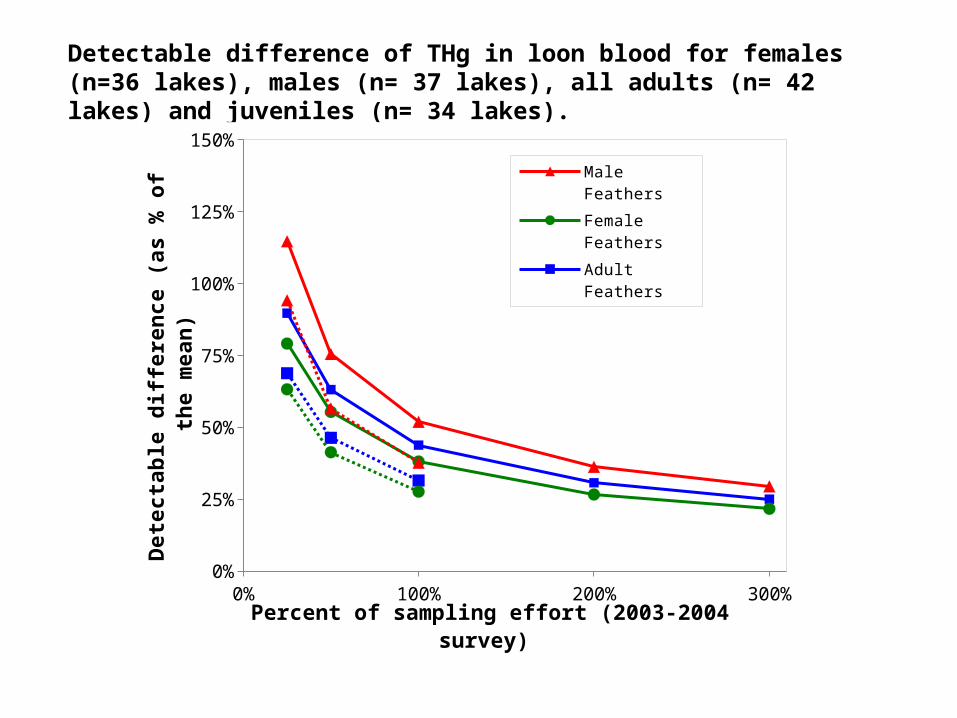
Detectable difference of THg in loon blood for females (n=36 lakes), males (n= 37 lakes), all adults (n= 42 lakes) and juveniles (n= 34 lakes).

0% 100% 200% 300%0%

25%

50%

75%

100%

125%

150%

Male Feathers

Female Feathers

Adult Feathers

Unpaired test

Paired test

Percent of sampling effort (2003-2004 survey)

De

tec

tab

le d

iffe

ren

ce

(a

s %

of

the

me

an

)

0% 50% 100% 150% 200% 250% 300%0%

20%

40%

60%

80%

100%

120%

140%

160%

180%

200%Ca (mg/kg)

K (mg/kg)

Mg (mg/kg)

Na (mg/kg)

Percent of Current Effort

De

tec

tab

le D

iffe

ren

ce

(%

of

me

an

)

Detectable difference of exchangeable cation concentrations (mg kg-1 dry soil) in mineral soil samples collected by the FIA in 56 plots in the

Adirondack region.

These case studies illustrate the effect of sampling intensity on statistical power and the selection of a sampling interval likely to detect an expected change over time

Question:

• How many plots should be sampled to report forest biomass with known confidence?

Data sets used in analysis:

• Hubbard Brook Watershed 6, where every tree is measured on each of 208 plots (each 25m x 25 m) every 5 years. We used data from 2002.

Analytical approach:

• We randomly selected subsets of plots and reported uncertainty in the estimates of forest biomass.

Subsampling

www.plymouth.edu

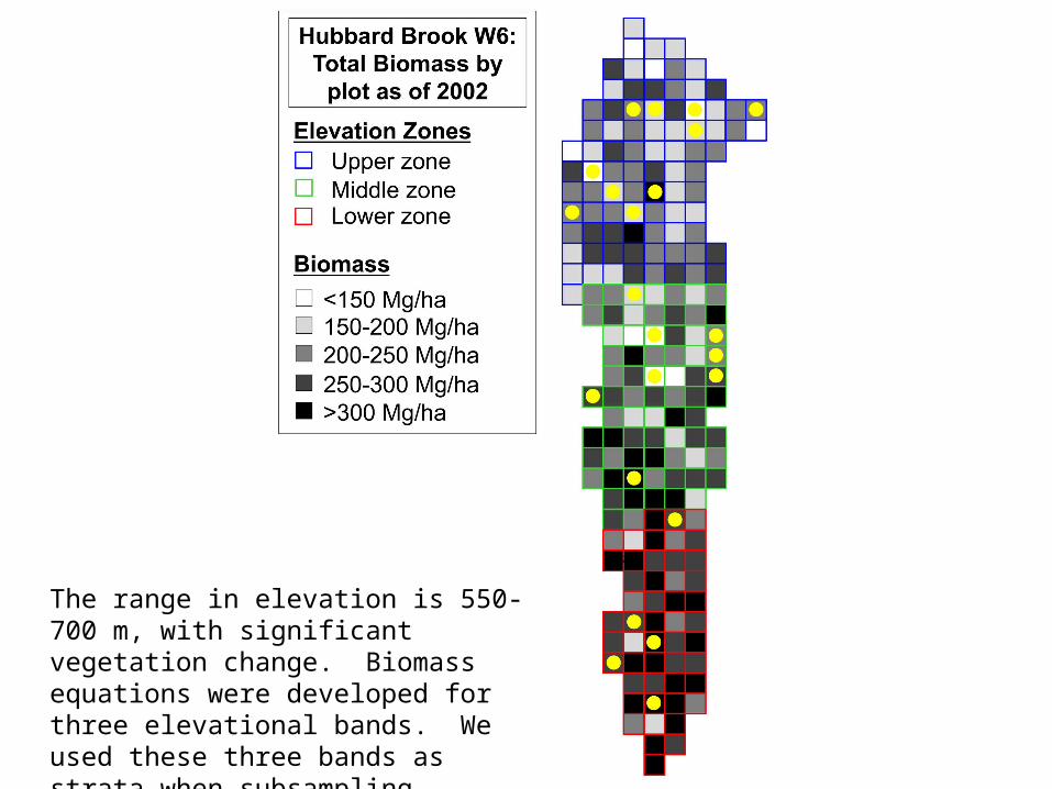
The range in elevation is 550-700 m, with significant vegetation change. Biomass equations were developed for three elevational bands. We used these three bands as strata when subsampling.

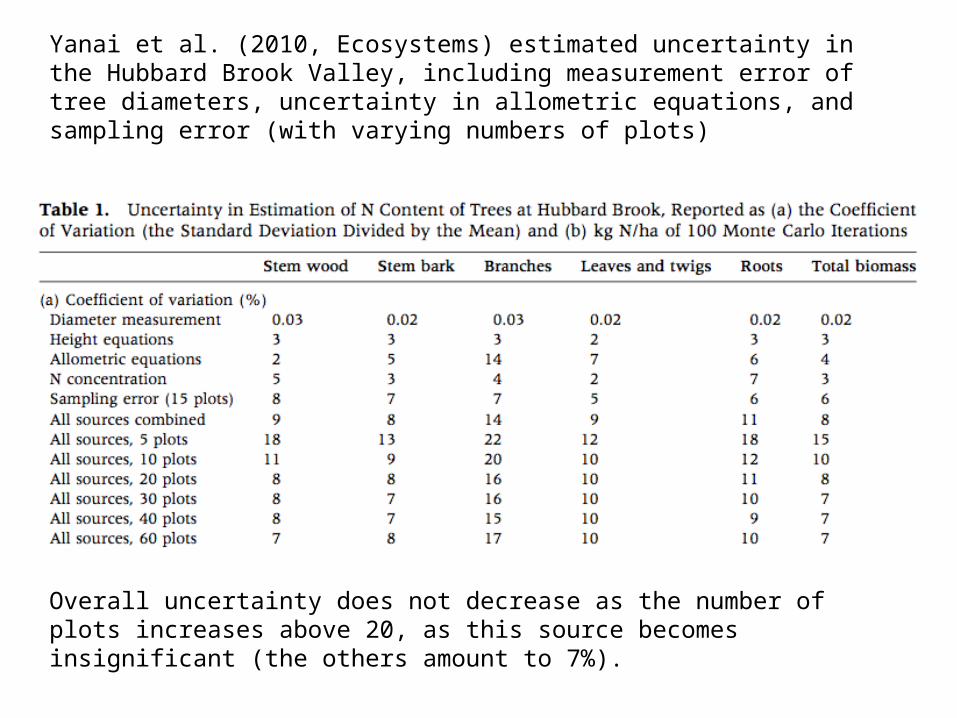
Yanai et al. (2010, Ecosystems) estimated uncertainty in the Hubbard Brook Valley, including measurement error of tree diameters, uncertainty in allometric equations, and sampling error (with varying numbers of plots)

Overall uncertainty does not decrease as the number of plots increases above 20, as this source becomes insignificant (the others amount to 7%).

Question:

• When monitoring Adirondack lakes, how many lakes should be monitored, and how often?

Data sets used in analysis:

• The Adirondack Lake Survey Corporation monthly lake water samples for a full suite of chemistry analyses from 48 lakes from 1992-2010.

Analytical approach:

• We randomly selected subsets of the data and applied a repeated-measures mixed-effects model to describe uncertainty in the estimates.

Repeated Measures Mixed Effects Model

http://www.adirondacklakessurvey.org/

Number of Lakes Showing Significant Trends Over Time (of a total of 48)Percent of

Current Sampling

Effort

Sampling Scheme

SO4 NO3 NH4 Ca2+ ANC H+ SUM

100 All months* 48 42 26 45 43 36 240

67 Mar-Oct 48 15 0 36 27 15 141

58 Mar-Sept 48 14 0 33 25 17 137

50 Even months 48 9 0 34 23 11 125

50 Odd months 48 9 0 36 25 13 131

42Mar-Apr,

June, Sept-Oct

47 6 0 31 22 9 115

33Seasonal (Feb, May, Aug, Nov)

46 6 0 27 18 10 107

33Seasonal (Jan, Apr, July, Oct)

48 6 0 29 15 7 105

33Seasonal (Mar, Jun, Sept, Dec)

46 5 0 29 22 9 111

33 Mar, Apr, Sept, Oct 47 5 0 31 17 6 106

The number of lakes showing significant trends over time in mixed model tests decreases as sampling effort decreases

Summary and Recommendations

Uncertainty analysis can provide an objective way to evaluate monitoring plans, including the spatial and temporal intensity of sampling.

Comparing sources of uncertainty can help identify where best to direct effort to improve knowledge.

Statistical models can handle complex designs, including mixed intensities and unbalanced designs.

When reducing sampling intensity, the information from past sampling is not lost or wasted.

It is important to provide enough information that other researchers can represent the uncertainty in your results.

•Visit our website (www.quantifyinguncertainty.org)

• Download papers and presentations• Get sample code• Stay updated with QUEST News

•Join our mailing list ([email protected])

•Meet us for dinner tonight (7 pm - Hell’s Kitchen)

Become a part of QUEST!