Lesson 8 Introduction to Statistics

Lesson 8Introduction to Statistics

What statistics is Statistics is the branch of mathematics

that examines ways to process and analyze data.

Statistics, branch of mathematics that deals with the collection, organization, and analysis of numerical data and with such problems as experiment design and decision making.

A Statistic is any quantity whose value can be calculated from sample data.

Activities of statistics Make interested from data Application with unrealism Sampling Relation analysis Forecasting Decision under unrealism

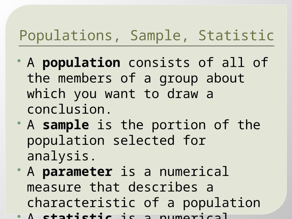
Populations, Sample, Statistic A population consists of all of the

members of a group about which you want to draw a conclusion.

A sample is the portion of the population selected for analysis.

A parameter is a numerical measure that describes a characteristic of a population

A statistic is a numerical measure that describes a characteristic of a sample

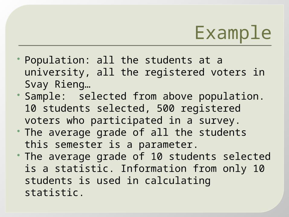
Example Population: all the students at a university,

all the registered voters in Svay Rieng… Sample: selected from above population.

10 students selected, 500 registered voters who participated in a survey.

The average grade of all the students this semester is a parameter.

The average grade of 10 students selected is a statistic. Information from only 10 students is used in calculating statistic.

2 types of statistics Descriptive statistics focuses on

collecting, summarizing, and presenting a set of data. These activities are also known as primary analyses.

Inferential statistics uses sample data to draw conclusion about a population. These activities are also known as secondary analyses.

Descriptive Statistics Example: The final score of students are

84 49 61 40 83 67 45 66 70 6980 58 68 60 67 72 73 70 57 6370 78 52 67 53 67 75 61 70 8176 79 75 76 58 95

Without any organization, it is difficult to get a sense of what a typical or representative score might be, whether the values are highly concentrated about a typical value or quite spread out, whether there are any gaps in the data, what percentage of the values…

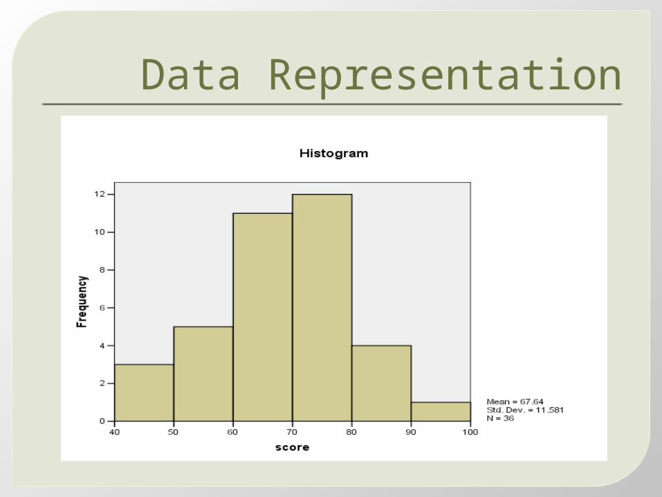
Data Representation

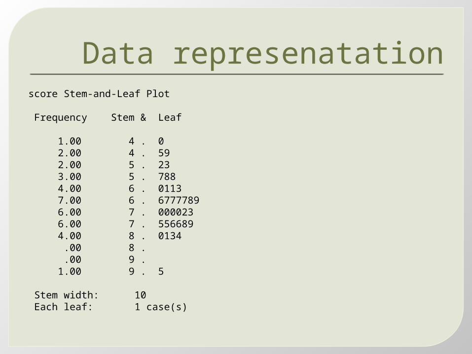
Data represenatationscore Stem-and-Leaf Plot

Frequency Stem & Leaf

1.00 4 . 0 2.00 4 . 59 2.00 5 . 23 3.00 5 . 788 4.00 6 . 0113 7.00 6 . 6777789 6.00 7 . 000023 6.00 7 . 556689 4.00 8 . 0134 .00 8 . .00 9 . 1.00 9 . 5

Stem width: 10 Each leaf: 1 case(s)

Inferential statistics Having obtained a sample from a

population, an investigator would frequently like to use sample information to draw some type of conclusion (make an inference of some sort) about the population.

That is, the sample is a means to an end rather than an end in itself.

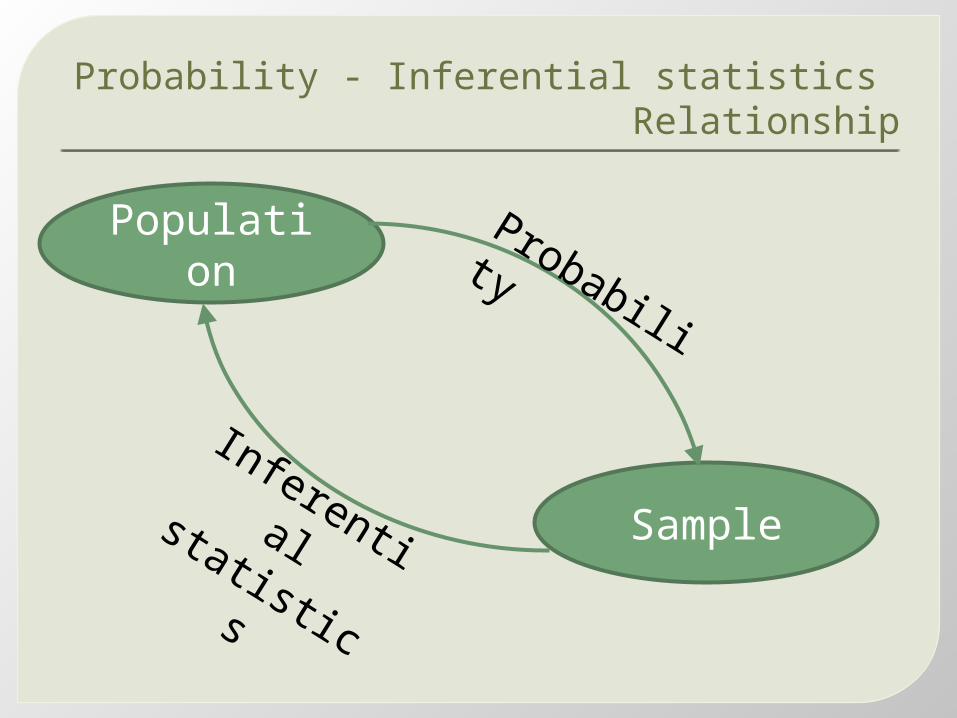
Probability - Inferential statistics Relationship

Population

Sample

Probability

Inferential statistics

Variable Variables are characteristics of

items or individuals.E.g. Variables are your gender, your

major field of study, the amount of money you have in your wallet… So the key aspect of variable is the idea that items differ and people differ.

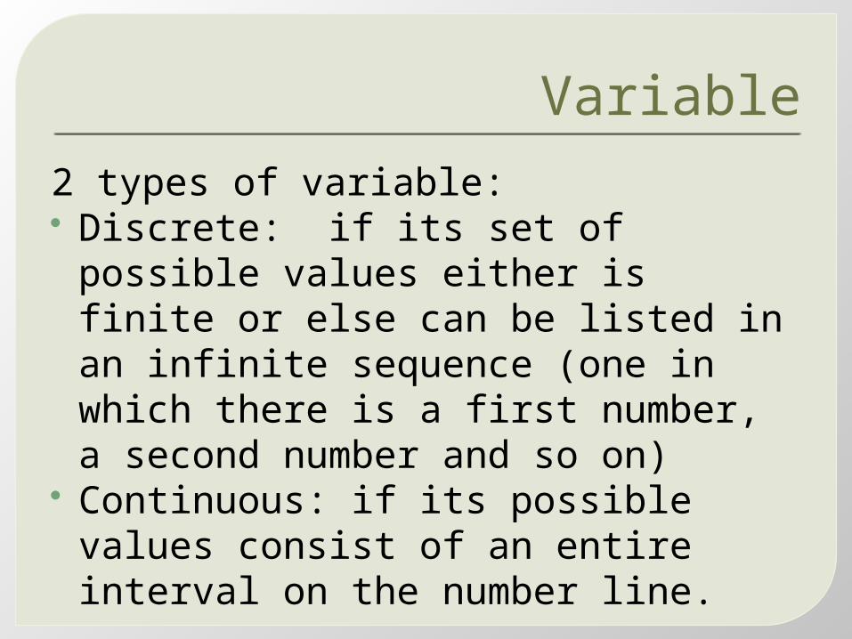
Variable2 types of variable: Discrete: if its set of possible values

either is finite or else can be listed in an infinite sequence (one in which there is a first number, a second number and so on)

Continuous: if its possible values consist of an entire interval on the number line.

VariableVariable is also divided into 2 types: Quantitative variable: Variable that

can be presented in number like income of people, weight of boxers, etc.

Qualitative variable: variable that cannot be presented in number like gender, living standard, etc.

Data Primary data: Original data collected

from source – experiments, survey, etc.

Secondary data: Data extracted from other reports or documents in which the data has already been collected.

Methods of Organizing data Descriptive statistics can be divided

into two general subject areas: visual techniques and numerical summary measures for data sets.

Visual techniques: Frequency table, histograms, pie charts, bar graphs, scatter diagrams, etc.

Numerical summary measures: Mean, variance, standard deviation, etc.

Frequency distribution Frequency : The number of times

something ( xi ) occurs noted by fi . Total Frequency: Sum of all frequencies

noted by N or n. Total Frequency=N=n=fi

Relative Frequency: the ratio of the absolute frequency to the total frequency.

Relative Frequency of a category= Nfi

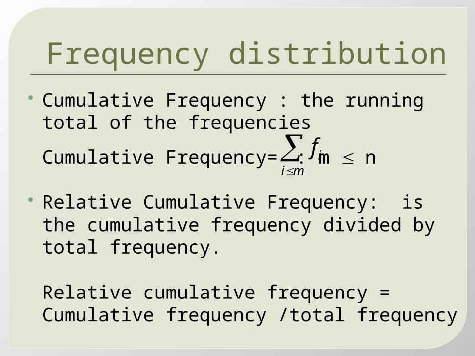
Frequency distribution Cumulative Frequency : the running total

of the frequenciesCumulative Frequency= : m n

Relative Cumulative Frequency: is the cumulative frequency divided by total frequency.

Relative cumulative frequency = Cumulative frequency /total frequency

mi

if

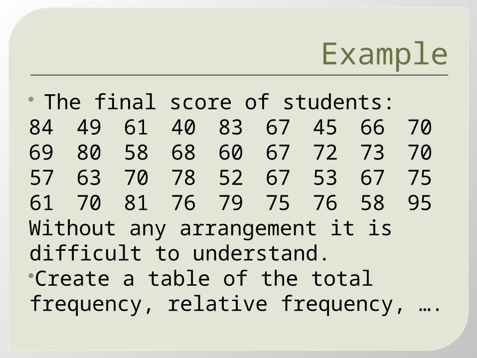
Example The final score of students:84 49 61 40 83 67 45 66 7069 80 58 68 60 67 72 73 7057 63 70 78 52 67 53 67 7561 70 81 76 79 75 76 58 95Without any arrangement it is difficult to understand. Create a table of the total frequency, relative frequency, ….

Stem-and-Leaf displaysSteps for constructing a Stem-and-Leaf: Select one or more leading digits for the

stem values. The trailing digits become the leaves.

List possible stem values in a vertical column.

Record the leaf for every observation beside the corresponding stem value.

Indicate the units for stems and leaves some place in the display.

Stem-and-Leaf example Suppose salary of staffs are: 120

215 170 135 216 216 181 222 150210 225 209 175 167 130 190 155145 177 162 197 182 215 187 172169 205 165 144 199

Stem…Stem Leaf Frequency Accumulated

frequency1213141516171819202122

00,54,50,52,5,7,90,2,5,71,2,70,7,95,90,5,5,6,62,5

12224433252

135711151821232830

Total 30

Stem width: 10Leaf: one case

Stem…By using SPSS, the stem-and-leaf shows:salary Stem-and-Leaf Plot

Frequency Stem & Leaf

.00 1 . 3.00 1 . 233 4.00 1 . 4455 8.00 1 . 66667777 6.00 1 . 888999 7.00 2 . 0011111 2.00 2 . 22

Stem width: 100 Each leaf: 1 case(s)

Dot/Lines Counts

Class Class refers to a group of objects with

some common property. Class boundary: is give by the

midpoint of the upper limit of one class and the lower limit of the next class.

Class width = Upper boundary - Lower boundary

Classes CLASS MIDPOINT or MARK=(Lower limit

+ Upper limit )/2 Number of classes: generally is given by

k= Number of Classesn= Number of Observations

Create a frequency distribution of student score with Class of Tens (110,1120…)

nkn2 2k log

Histogram Consider data consisting of

observations on a discrete variable x. the frequency of any particular x value is the number of times that the value occurs in the data set.

The relative frequency of a value is the fraction or proportion of times the value occurs.

Histogram

Histogram for qualitative data Frequency distribution and histogram

can be constructed when the data set is qualitative categorical in nature.

Some classes have natural ordering – eg. BAC2, Bachelor, Master, Doctor – and the other case the order will be arbitrary – eg. Cambodian, England, American, French, Japanese…

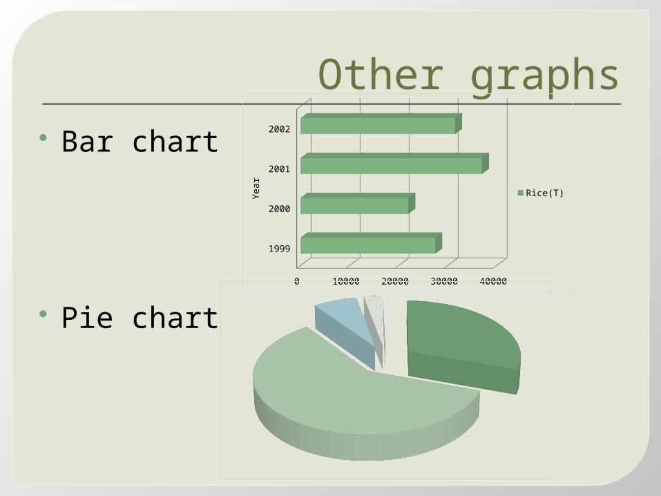
Other graphs Bar chart

Pie chart

1999

2000

2001

2002

Year

0 10000 20000 30000 40000

Rice(T)

Other graphs Frequency

Polygon or line

Stock chart ( Low-High-Close chart)

[20-30] ]30-40] ]40-50] ]50-60] ]60-70]0

10

20

30

40

50

60

70

39608 10 11 12 13175176177178179180181182183184

Close

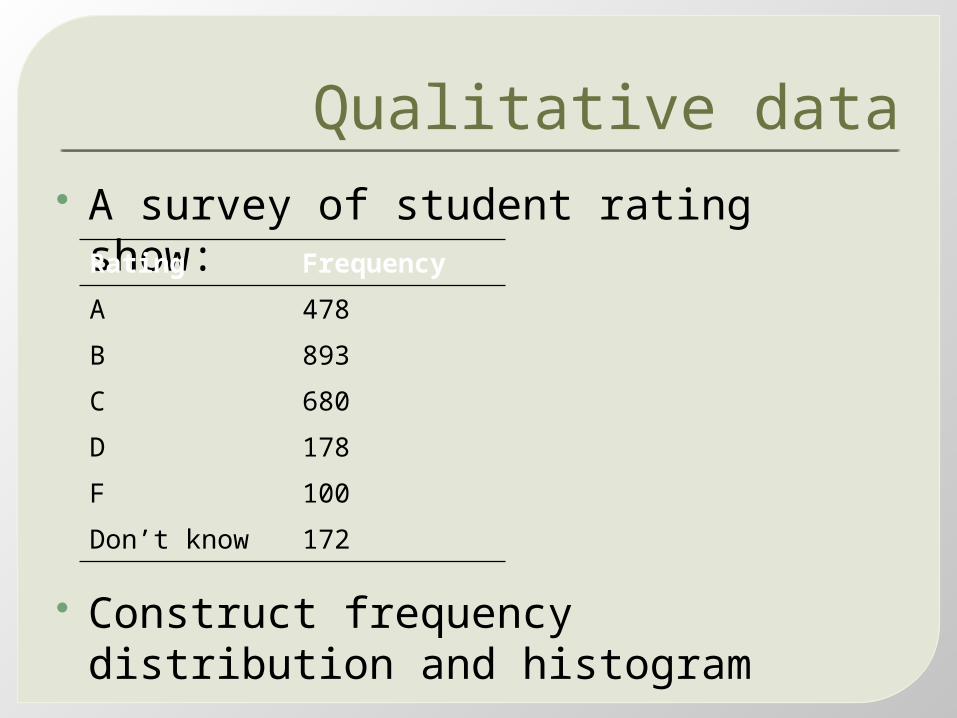
Qualitative data A survey of student rating show:

Construct frequency distribution and histogram

Rating FrequencyA 478B 893C 680D 178F 100Don’t know 172

Contingency table For two variables, we use

contingency table:Age Number of Flight per Year

1-2 3-5 Over 5 Total

Less than 2525-4040-65

65 and OverTotal

1 (0.02)2 (0.04)1 (0.02)1 (0.02)5 (0.10)

1 (0.02)8 (0.16)6 (0.12)2 (0.04)17 (0.35)

2 (0.04)10 (0.20)15 (0.30)1 (0.02)28 (0.56)

4 (0.08)20 (0.40)22 (0.44)4 (0.08)50 (1.00)

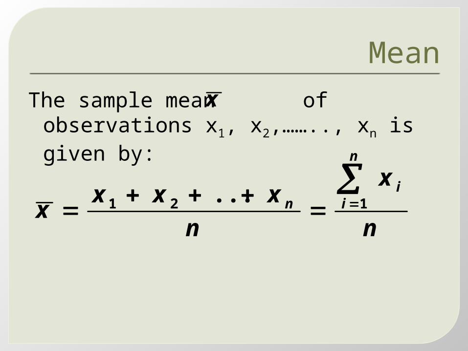
MeanThe sample mean of observations

x1, x2,…….., xn is given by:x

n

x

nxxx

x

n

ii

n

121 ...

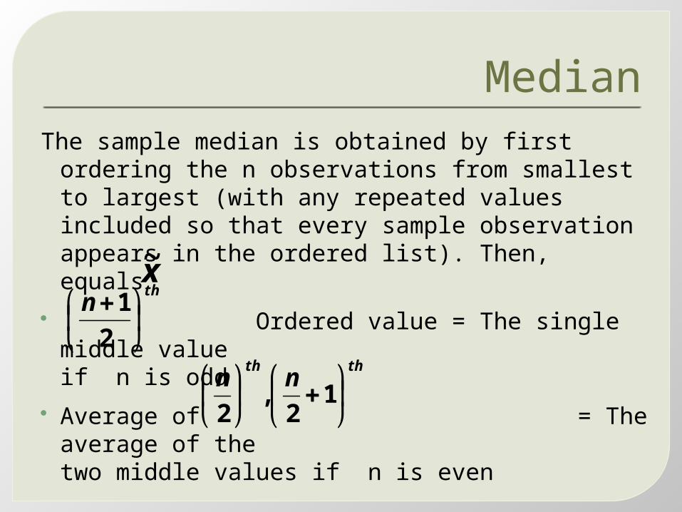
MedianThe sample median is obtained by first ordering

the n observations from smallest to largest (with any repeated values included so that every sample observation appears in the ordered list). Then, equals

Ordered value = The single middle value if n is odd

Average of = The average of the two middle values if n is even

thth nn

1

2,

2

x~thn

21

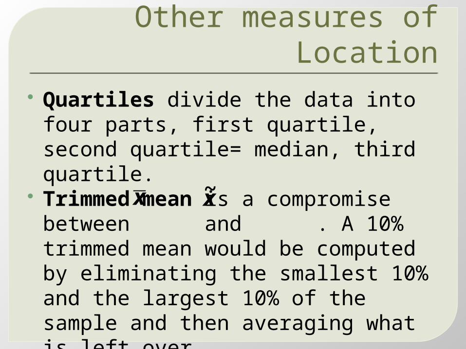
Other measures of Location

Quartiles divide the data into four parts, first quartile, second quartile= median, third quartile.

Trimmed mean is a compromise between and . A 10% trimmed mean would be computed by eliminating the smallest 10% and the largest 10% of the sample and then averaging what is left over.

x x~

Measures of Variability Mean and median give only partial

information about data set or distribution

Different samples or populations may have identical measure of center yet differ from one another in other important ways.

The simplest measure of variability in a sample is the range – the smallest and the largest.

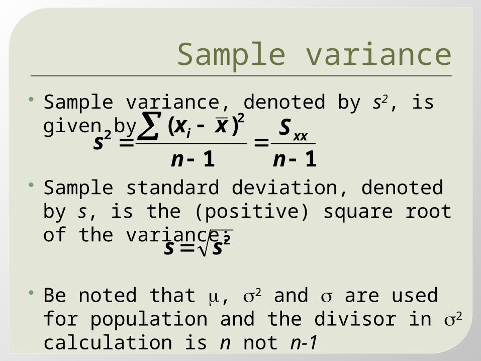
Sample variance Sample variance, denoted by s2, is given

by

Sample standard deviation, denoted by s, is the (positive) square root of the variance:

Be noted that , 2 and are used for population and the divisor in 2

calculation is n not n-1

11)( 2

2

nS

nxx

s xxi

2ss

BoxplotsBoxplot has been used successfully to

describe several of a data set’s most prominent features:

center spread the extent and nature of any departure

from symmetry and identification of outliers (observations

that lie usually far from the main body of the data).

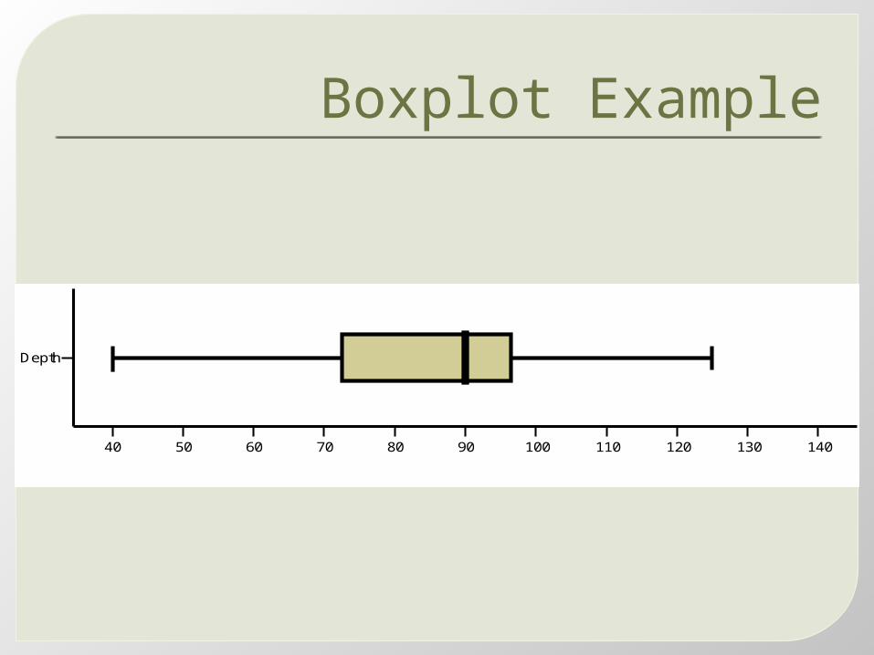
Boxplots Example Example 1.17 give the data of pit

depth in the crude oil plate as follows:40 52 55 60 70 75 85 85 90 90 92 94 94 95 98 100 115 125 125

The five-number summary is as follows:

Smallest=40 Lower fourth=72.5 = 90 Upper fourth=96.5Largest =125

x~

Boxplot Example

Depth

140130120110100908070605040