Less is More: Nyström Computational Regularization

Less is More: Nystrom Computational Regularization

Alessandro Rudi1, Raffaello Camoriano1,2, Lorenzo Rosasco 1,3

1 Universita degli Studi di GenovaDIBRIS, Via Dodecaneso 35, Genova, Italy

ale [email protected]

2 Istituto Italiano di TecnologiaiCub facility, Via Morego 30, Genova, Italy

[email protected]

3 Massachusetts Institute of Technology and Istituto Italiano di TecnologiaLaboratory for Computational and Statistical Learning, Cambridge, MA 02139, USA

[email protected]

July 21, 2015

Abstract

We study Nystrom type subsampling approaches to large scale kernel methods,and prove learning bounds in the statistical learning setting, where random samplingand high probability estimates are considered. In particular, we prove that these ap-proaches can achieve optimal learning bounds, provided the subsampling level is suit-ably chosen. These results suggest a simple incremental variant of Nystrom KernelRegularized Least Squares, where the subsampling level implements a form of com-putational regularization, in the sense that it controls at the same time regularizationand computations. Extensive experimental analysis shows that the considered ap-proach achieves state of the art performances on benchmark large scale datasets.

1 Introduction

Kernel methods provide an elegant and effective framework to develop nonparametric sta-tistical approaches to learning [1]. However, memory requirements make these methodsunfeasible when dealing with large datasets. Indeed, this last observation has motivateda variety of computational strategies to develop large scale kernel methods [2, 3, 4, 5, 6,7, 8].In this paper we study subsampling methods, that we broadly refer to as Nystrom ap-proaches. These methods replace the empirical kernel matrix, needed by standard kernelmethods, with a smaller matrix obtained by (column) subsampling [2, 3]. Such proce-dures are shown to often dramatically reduce memory/time requirements while preserv-ing good practical performances [9, 10, 11, 12]. The goal of our study is two-fold. First,and foremost, we aim at providing a theoretical characterization of the generalization

1

properties of such learning schemes in a statistical learning setting. Second, we wish tounderstand the role played by the subsampling level both from a statistical and a compu-tational point of view. As discussed in the following, this latter question leads to a naturalvariant of Kernel Regularized Least Squares, where the subsampling level controls bothregularization and computations. From a theoretical perspective, the effect of Nystromapproaches has been primarily characterized considering the discrepancy between a givenempirical kernel matrix and its subsampled version [13, 14, 15, 16, 17, 18, 19]. Whileinteresting in their own right, these latter results do not directly yield information on thegeneralization properties of the obtained algorithm. Results in this direction, albeit sub-optimal, were first derived in [20] (see also [21, 22]), and more recently in [23, 24].In these latter papers, sharp error analyses in expectation are derived in a fixed designregression setting for a form of Kernel Regularized Least Squares. In particular, in [23] abasic uniform sampling approach is studied, while in [24] a subsampling scheme based onthe notion of leverage score is considered. The main technical contribution of our study isan extension of these latter results considering the statistical learning setting, where thedesign is random and high probability estimates are considered. The more general set-ting makes the analysis considerably more complex. Our main result gives optimal finitesample bounds for both uniform and leverage score based subsampling strategies. Ourmain result gives optimal finite sample bounds for both uniform and leverage score basedsubsampling strategies. These methods are shown to achieve the same (optimal) learn-ing error as kernel regularized least squares, recovered as a special case, while allowingsubstantial computational gains. Our analysis highlights the interplay between the regu-larization and subsampling parameters, suggesting that the latter can be used to controlsimultaneously regularization and computations. This strategy, to which we refer to as aninstance of computational regularization, has the advantage of tailoring the computationalresources to the generalization properties in the data rather than their raw amount. Thisidea is developed considering an incremental strategy to efficiently compute learning so-lutions for different subsampling levels. The procedure thus obtained, which is a simplevariant of classical Nystrom Kernel Regularized Least Squares (KRLS) with uniform sam-pling, allows for efficient model selection and achieves state of the art results on a varietyof benchmark large scale datasets.The rest of the paper is organized as follows. In Section 2, we introduce the setting andalgorithms we consider. In Section 3, we present our main theoretical contributions. InSection 4, we discuss computational aspects and experimental results.

2 Supervised Learning with KRLS and Nystrom Approaches

Let X × R be a probability space with distribution ρ, where we view X and R as theinput and output spaces, respectively. Let ρX denote the marginal distribution of ρ on Xand ρ(·|x) the conditional distribution on R given x ∈ X. Given a hypothesis space H ofmeasurable functions from X to R, the goal is to minimize the expected risk,

minf∈HE(f), E(f) =

∫X×R

(f(x) − y)2dρ(x, y) (1)

2

provided ρ is known only through a training set of (xi, yi)ni=1 of samples identically and in-dependently distributed with respect to ρ. A basic example of the above setting is randomdesign regression with the square loss, in which case

yi = f∗(xi) + εi, i = 1, . . . , n, (2)

with f∗ a fixed regression function, ε1, . . . , εn a sequence of random variables seen asnoise, and x1, . . . , xn random inputs. In the following, we consider kernel methods, basedon choosing a hypothesis space which is a reproducing kernel Hilbert space. The latter isa Hilbert space H of functions, with inner product 〈·, ·〉H, such that there exists a functionK : X×X→ R with the following two properties: 1) for all x ∈ X, Kx(·) = K(x, ·) belongs toH, and 2) the so called reproducing property holds: f(x) = 〈f, Kx〉H, for all f ∈ H, x ∈ X[25]. The function K, called reproducing kernel, is easily shown to be symmetric andpositive definite, that is the kernel matrix (KN)i,j = K(xi, xj) is positive semidefinite for allx1, . . . , xN ∈ X, N ∈ N. A classical way to derive an empirical solution to problem (1) is toconsider a Tikhonov regularization approach, based on the minimization of the penalizedempirical functional given by

minf∈H

1

n

n∑i=1

(f(xi) − yi)2 + λ‖f‖2H, λ ≥ 0. (3)

The above approach is referred to as Kernel Regularized Least Squares (KRLS) or KernelRidge Regression (KRR). It is easy to see that a solution fλ to problem (3) exists, it isunique and the representer theorem [1] shows that it can be written as

fλ(x) =

n∑i=1

αiK(xi, x) with α = (Kn + λnI)−1y, (4)

where y = (y1, . . . , yn) and Kn is the empirical kernel matrix. Note that this result impliesthat we can restrict the minimization in (3) to the space,

Hn = {f ∈ H | f =

n∑i=1

αiK(xi, ·), α1, . . . , αn ∈ R}.

Storing the kernel matrix Kn, and solving the linear system in (4), can become computa-tionally unfeasible as n increases. In the following, we consider strategies to find moreefficient solutions, based on the idea of replacing Hn with

Hm = {f | f =

m∑i=1

αiK(xi, ·), α ∈ Rm},

wherem ≤ n and {x1, . . . , xm} is a subset of the input points in the training set. It is easy tosee that the solution fλ,m of the corresponding minimization problem can now be writtenas,

fλ,m(x) =

m∑i=1

αiK(xi, x) with α = (K>nmKnm + λnKmm)†Kmny, (5)

3

whereA† denotes the Moore-Penrose pseudoinverse of a matrixA, and (Knm)ij = K(xi, xj),(Kmm)kj = K(xk, xj) with i ∈ {1, . . . , n} and j, k ∈ {1, . . . ,m} [2]. The above approach isrelated to Nystrom methods and different approximation strategies correspond to differ-ent ways to select the inputs subset. While our framework applies to a broader class ofstrategies, see Section B.1, in the following we primarily consider two techniques.Plain Nystrom. The points {x1, . . . , xm} are sampled uniformly at random without replace-ment from the training set.Approximate leverage scores (ALS) Nystrom. Recall that the leverage scores associatedto the training set points x1, . . . , xn are

(li(t))ni=1, li(t) = (Kn(Kn + tnI)

−1)ii, i = 1, . . . , n (6)

for any t > 0, where (Kn)ij = K(xi, xj). In practice, leverage scores are onerous to com-pute and approximations (li(t))

ni=1 can be considered [16, 24, 17] . In particular, in the

following we are interested in suitable approximations defined as follows:

Definition 1 (T -approximate leverage scores). Let (li(t))ni=1 be the leverage scores associ-ated to the training set for a given t. Let δ > 0, λ0 > 0 and T ≥ 1. We say that (li(t))ni=1 areT -approximate leverage scores with confidence δ, when with probability at least 1− δ,

1

Tli(t) ≤ li(t) ≤ Tli(t) ∀i ∈ {1, . . . , n}, t ≥ λ0.

Given T -approximate leverage scores for t > λ0, {x1, . . . , xm} are sampled from thetraining set independently with replacement, and with probability to be selected given byPt(i) = li(t)/

∑j lj(t).

In the next section, we state and discuss our main result showing that the KRLS formu-lation based on plain or approximate leverage scores Nystrom provides optimal empiricalsolutions to problem (1).

3 Theoretical Analysis

In this section, we state and discuss our main results. We need several assumptions.

3.1 Assumptions

The first basic assumption is that problem (1) admits at least a solution.

Assumption 1. There exists an fH ∈ H such that

E(fH) = minf∈HE(f).

Note that, while the minimizer might not be unique, our results apply to the case inwhich fH is the unique minimizer with minimal norm. Also, note that the above conditionis weaker than assuming the regression function in (2) to belong to H. Finally, we notethat the study of the paper can be adapted to the case in which minimizers do not exist,but the analysis is considerably more involved and left to a longer version of the paper.The second assumption is a basic condition on the probability distribution.

4

Assumption 2. Let zx be the random variable zx = y− fH(x), with x ∈ X, and y distributedaccording to ρ(y|x). Then, there exists M,σ > 0 such that E|zx|p ≤ 1

2p!Mp−2σ2 for any

p ≥ 2, almost everywhere on X.

The above assumption is needed to control random quantities and is related to a noiseassumption in the regression model (2). It is clearly weaker than the often consideredbounded output assumption [25], and trivially verified in classification.The last two assumptions describe the capacity (roughly speaking the “size”) of the hy-pothesis space induced by K with respect to ρ and the regularity of fH with respect to Kand ρ. To discuss them, we first need the following definition.

Definition 2 (Covariance operator and effective dimensions). We define the covarianceoperator as

C : H→ H, 〈f, Cg〉H =

∫X

f(x)g(x)dρX(x) , ∀ f, g ∈ H.

Moreover, for λ > 0, we define the random variableNx(λ) =⟨Kx, (C+ λI)−1Kx

⟩H with x ∈ X

distributed according to ρX and let

N (λ) = ENx(λ), N∞(λ) = supx∈XNx(λ).

We add several comments. Note that C corresponds to the second moment operator,but we refer to it as the covariance operator with an abuse of terminology. Moreover, notethat it is easy to see that N (λ) = Tr(C(C + λI)−1). This latter quantity, called effectivedimension or degrees of freedom, can be seen as a measure of the capacity of the hypoth-esis space. The quantity N∞(λ) can be seen to provide a uniform bound on the leveragescores (6). Clearly, N (λ) ≤ N∞(λ) for all λ > 0.

Assumption 3. The kernel K is measurable and C is bounded. Moreover, for all λ > 0,

N∞(λ) <∞, (7)

andN (λ) ≤ Qλ−γ, 0 < γ ≤ 1, (8)

where Q is a constant.

Measurability of K and boundedness of C are minimal conditions to ensure that thecovariance operator is a well defined linear, bounded, self-adjoint, positive operator [25].Condition (7) is satisfied if the kernel is bounded supx∈X K(x, x) = κ

2 <∞, indeed in thiscase N∞(λ) ≤ κ2/λ for all λ > 0. Conversely, it can be seen that condition (7) togetherwith boundedness of C imply that the kernel is bounded, indeed 1

κ2 ≤ 2‖C‖N∞(‖C‖).

Boundedness of the kernel implies in particular that the operator is trace class and allowsto use tools from spectral theory. Condition (8) quantifies the capacity assumption and is

1If N∞(λ) is finite, then N∞(‖C‖) = supx∈X‖(C + ‖C‖I)−1Kx‖2 ≥ 1/2‖C‖−1supx∈X‖Kx‖2, therefore

K(x, x) ≤ 2‖C‖N∞(‖C‖).

5

related to covering/entropy number conditions (see [25] for further details). In particular,it is known that condition (8) is ensured if the eigenvalues (σi)i of C satisfy a polynomial

decaying condition σi ∼ i− 1γ . Note that, since the operator C is trace class, such condition

always holds for γ = 1. Here, for space constraints and in the interest of clarity werestrict to such a polynomial condition, but the analysis directly applies to other conditionsincluding exponential decay or a finite rank conditions [26]. Finally, we have the followingregularity assumption.

Assumption 4. There exists s ≥ 0, 1 ≤ R <∞, such that ‖C−sfH‖H < R.

The above condition is fairly standard, and can be equivalently formulated in terms ofclassical concepts in approximation theory such as interpolation spaces [25]. Intuitively,it quantifies the degree to which fH can be well approximated by functions in the RKHSH and allows to control the bias/approximation error of a learning solution. For s = 0, itis always satisfied. For larger s, we are assuming fH to belong to subspaces of H that arethe images of the fractional compact operators Cs. Such spaces contain functions which,expanded on a basis of eigenfunctions of C, have larger coefficients in correspondenceto large eigenvalues. Such an assumption is natural in view of using techniques suchas (4), which can be seen as a form of spectral filtering, that estimate stable solutions bydiscarding the contribution of small eigenvalues [27]. In the next section, we are goingto quantify the quality of empirical solutions of problem (1) obtained by schemes of theform (5), in terms of the quantities in Assumptions 2, 3, 4.

3.2 Main Results

In this section, we state and discuss our main results, starting with optimal finite sampleerror bounds for regularized least squares based on plain and approximate leverage scorebased Nystrom subsampling.

Theorem 1. Under Assumptions 1, 2, 3, and 4, let δ > 0, v = min(s, 1/2), p = 1+1/(2v+γ)and assume

n ≥ 1655κ2 + 223κ2 log6κ2

δ+

(38p

‖C‖log

114κ2p

‖C‖δ

)p.

Then, the following inequality holds with probability at least 1− δ,

E(fλ,m) − E(fH) ≤ q2 n− 2v+12v+γ+1 , with q = 6R

(2‖C‖+ Mκ√

‖C‖+

√Qσ2

‖C‖γ

)log

6

δ, (9)

with fλ,m as in (5), λ = ‖C‖n− 12v+γ+1 and

1. for plain Nystrom

m ≥ (67∨ 5N∞(λ)) log12κ2

λδ;

2. for ALS Nystrom, with probabilities Pt for t = λ, T -approximate leverage scores for anyt ≥ 19κ2

n log 12nδ , and

m ≥ (334∨ 78T 2N (λ)) log48n

δ.

6

We add several comments. First, the above results can be shown to be optimal in aminmax sense. Indeed, minmax lower bounds proved in [26, 28] show that the learningrate in (9) is optimal under the considered assumptions. Second, the obtained boundscan be compared to those obtained for other regularized learning techniques. Techniquesknown to achieve optimal error rates include Tikhonov regularization [26, 28, 29], itera-tive regularization by early stopping [30, 31], spectral cut-off regularization (a.k.a. prin-cipal component regression or truncated SVD) [30, 31], as well as regularized stochasticgradient methods [32]. All these techniques are essentially equivalent from a statisticalpoint of view and differ only in the required computations. For example, iterative meth-ods allow for the computation of solutions corresponding to different regularization levelswhich is more efficient than Tikhonov or SVD based approaches. The key observationis that all these methods have the same O(n2) memory requirement. In this view, ourresults show that randomized subsampling methods can break such a memory barrier,and consequently achieve much better time complexity, while preserving optimal learningguarantees. Finally, we can compare our results with previous analysis of randomizedkernel methods. As mentioned already, results close to those in Theorem 1 are given in[23, 24] in a fixed design setting. Our results, extend and generalize the conclusions ofthese papers to a general learning statistical learning setting. Relevant results are givenin [8] for a different approach, based on averaging KRLS solutions obtained splitting thedata in m groups (divide and conquer RLS). The analysis in [8] is only in expectation,but considers random design and show that the the proposed methods is indeed opti-mal provided the number of split is chosen depending on the effective dimension N (λ).This is the only other work we are aware of establishing optimal learning rates for ran-domized kernel approaches in a statistical learning setting. In comparison with Nystromcomputational regularization the main disadvantage of the divide and conquer approachis computational and in the model selection phase where solutions corresponding to dif-ferent regularization parameters and number of splits usually need to be computed.The proof of Theorem 1 is fairly technical and lengthy. It incorporates ideas from [26]and techniques developed to study spectral filtering regularization [30, 33]. In the nextsection, we briefly sketch some main ideas and discuss how they suggests an interestingperspective on regularization techniques including subsampling.

3.3 A Peak involving the Proof & a Computational Regularization Perspec-tive

A key step in the proof of Theorem 1 is an error decomposition, and corresponding bound,for any fixed λ andm. Indeed, it is proved in Theorem 2 and Proposition 2 that, for δ > 0,with probability at least 1− δ,

∣∣E(fλm) − E(fH)∣∣1/2 . R(M√N∞(λ)

n+

√σ2N (λ)

n

)log

6

δ+RC(m)1/2+v+Rλ1/2+v. (10)

The first and last term in the right hand side of the above inequality can be seen as formsof sample and approximation errors [25] and are studied in Lemma 4 and Theorem 2. Themid term can be seen as a computational error and depends on the subsampling scheme

7

considered. Indeed, it is shown in Proposition 2 that C(m) can be taken as,

Cpl(m) = min{t > 0

∣∣∣∣ (67∨ 5N∞(t)) log12κ2

tδ≤ m},

for the plain Nystrom approach, and

CALS(m) = min{19κ2

nlog

12n

δ≤ t ≤ ‖C‖

∣∣∣∣ 78T 2N (t) log48n

δ≤ m},

for the approximate leverage scores approah. The bounds in Theorem 1 follow by: 1)choosing m so that the computational error is of the same order as the other terms, and2) optimizing with respect to λ. Computational resources and regularization are thentailored to the generalization properties of the data at hand. We add a few comments.First, it is easy to see that the error bound in (10) holds for a large class of subsamplingschemes, as discussed in Section B.1. Specific error bounds can be then derived developingcomputational error estimates. Second, the error bounds in Theorem 2 and Proposition 2,and hence in Theorem 1, easily generalize to a larger class of regularization schemesbeyond Tikhonov approaches, namely spectral filtering [30]. For space constraints, theseextensions are deferred to a longer version of the paper. Third, we note that, in practice,optimal data driven parameter choices, e.g. based on hold-out estimates [31], can be usedto adaptively achieve optimal learning bounds.Finally we observe that a different perspective is derived starting from inequality (10),and noting that the role played bym and λ can also be exchanged. Lettingm play the roleof a regularization parameter, λ can be set as a function of m and m tuned adaptively. Forexample, in the case of a plain Nystrom approach, it is easy to see that if we set

λ =logmm

, and m = 3n1

2v+γ+1 logn,

then the obtained learning solution achieves the error bound in Eq. (9). As above, the sub-sampling level can also be chosen by cross-validation. Interestingly, in this case by tuningm we naturally control computational resources and regularization. An advantage of thislatter parameterization is that, as described in the following, the solution correspondingto different subsampling levels is easy to update using block matrix inversion formulas.As discussed in the next section, in practice, a joint tuning over m and λ can be donestarting from small m and appears to be advantageous both for error and computationalperformances.

4 Incremental Updates and Experimental Analysis

In this section, we first describe an incremental strategy to efficiently explore differentsubsampling levels and then perform extensive empirical tests aimed in particular at: 1)investigating the statistical and computational benefits of considering varying subsamplinglevels, and 2) compare the performance of the algorithm with respect to state of the artsolutions on several large scale benchmark datasets. Throughout this section, we onlyconsider a plain Nystrom approach, deferring to future work the analysis of leverage scoresbased sampling techniques. Interestingly, we will see that such a basic approach can oftenprovide state of the art performances.

8

4.1 Efficient Incremental Updates

We describe a strategy using block matrix inverse formula to compute efficiently solutionscorresponding to different subsampling levels. The proposed procedure allows to effi-ciently compute a whole regularization path of solutions, and hence perform fast modelselection. Let (xi)mi=1 the selected Nystrom points. We want to compute α of Eq.5, incre-mentally in m. Towards this goal we split the m points in T = m/l sets of dimension l.Consider the following family of matrices,

At ∈ Rn×l (At)ij = K(xi, xlt+j−l)

Lt ∈ Rl(t−1)×l (Lt)ij = K(xi, xlt+j−1)Rt ∈ Rl×l (Rt)ij = K(xlt+j−1, xlt+j−1)

The update rule is the following: αt = Mt(Cty), M1 = D1 = (A>1 A1 + λR1)−1, C2 = A1

and

Mt+1 =

(Mt +MtBtDtB

>t Mt −MtBtDt

−DtB>t Mt Dt

)and

Dt = (A>t At + λnRt − B>t MtB

t)−1,Bt = C

>t At + λnLt,

Ct+1 = (Ct At).

The algorithm is an application of the recursive block matrix inversion formula [34] andrequires O(nm2 +m3) time to compute a1, . . . , aT , while a naive non-iterative algorithmwould require O(Tnm2 + Tm3). We note that a similar strategy is discussed in [34] tocompute an approximation of the kernel matrix Kn.

4.2 Experimental Analysis

We empirically study the properties of the considered learning scheme, considering aGaussian kernel of width σ. The data is split in training, validation and test sets2. Wehold out 20% of the training points for parameter tuning via cross-validation and reportthe performance of the selected model on the test set, repeating the process for severaltrials.Interplay between λ and m. We begin with a set of results showing that incrementallyexploring different subsampling levels can yield very good performance while substan-tially reducing the computational requirements. We consider the pumadyn32nh (n = 8192,d = 32), the breast cancer (n = 569, d = 30), and the cpuSmall (n = 8192, d = 12)datasets3. In Figure 1, we report the validation errors associated to a 20 × 20 grid of val-ues for λ and m. The λ values are logarithmically spaced, while the m values are linearlyspaced. The ranges, chosen according to preliminary tests on the data, are σ = 2.66,λ ∈

[10−7, 1

], m ∈ [10, 1000] for pumadyn32nh, σ = 0.9, λ ∈

[10−12, 10−3

], m ∈ [5, 300] for

breast cancer, and σ = 0.1, λ ∈[10−15, 10−12

], m ∈ [100, 5000] for cpuSmall. The main

observation that can be derived from this first series of tests is that a small m is sufficientto obtain the same results achieved with the largestm. For example, for pumadyn32nh it issufficient to choose m = 62 and λ = 10−7 to obtain an average test RMSE of 0.33 over 10trials, which is the same as the one obtained using m = 1000 and λ = 10−3, with a 3-fold

2In the following we denote by n the total number of points and by d the number of dimensions.3www.cs.toronto.edu/~delve and archive.ics.uci.edu/ml/datasets

9

m

200 400 600 800 1000

λ

10-6

10-4

10-2

100

RMSE

0.032 0.0325 0.033 0.0335 0.034 0.0345 0.035

m

50 100 150 200 250 300

λ

10-12

10-10

10-8

10-6

10-4

Classification Error

0.04 0.05 0.06 0.07 0.08 0.09 0.1

m

1000 2000 3000 4000 5000

λ

10-15

10-14

10-13

10-12

RMSE

15 20 25

Figure 1: Validation errors associated to 20 × 20 grids of values for m (x axis) and λ (yaxis) on pumadyn32nh (left), breast cancer (center) and cpuSmall (right).

speedup of the joint training and validation phase. Also, it is interesting to observe thatfor given values of λ, large values of m can decrease the performance. This observation isconsistent with the results in Section 3.2, showing thatm can play the role of a regulariza-tion parameter. Similar results are obtained for breast cancer, where for λ = 4.28×10−6and m = 300 we obtain a 1.24% average classification error on the test set over 20 trials,while for λ = 10−12 and m = 67 we obtain 1.86%. For cpuSmall, with m = 5000 andλ = 10−12 the average test RMSE over 5 trials is 12.2, while for m = 2679 and λ = 10−15

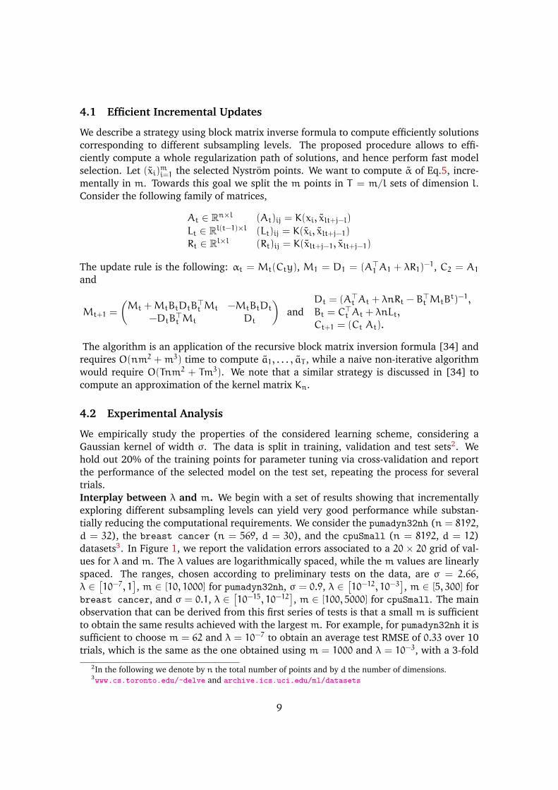
it is only slightly higher, 13.3, but computing its associated solution requires less than halfof the time and approximately half of the memory.Regularization path computation. If the subsampling level m is used as a regularizationparameter, the computation of a regularization path corresponding to different subsam-pling levels becomes crucial during the model selection phase. A naive approach, thatconsists in recomputing the solutions of Eq. 5 for each m, would require O(m2n+m3L)Tcomputational time, where T is the number of m values to be evaluated and L is the num-ber of Tikhonov regularization parameters. On the other hand, by using the incrementalNystrom algorithm the model selection time complexity is O(m2n+m3L). We experimen-tally verify this speedup on cpuSmall with 10 repetitions, settingm ∈ [1, 5000] and T = 50.The model selection times, measured on a server with 12 × 2.10GHz Intelr Xeonr E5-2620 v2 CPUs and 132 GB of RAM, are reported in Figure 2. The result clearly confirmsthe beneficial effects of incremental Nystrom model selection on the computational time.Predictive performance comparison Finally, we consider the performance of the algo-rithm on several large scale benchmark datasets considered in [6], see Table 1. σ has beenchosen on the basis of preliminary data analysis. m and λ have been chosen by cross-validation, starting from small subsampling values up to mmax = 2048, and consideringλ ∈

[10−12, 1

]. After model selection, we retrain the best model on the entire training set

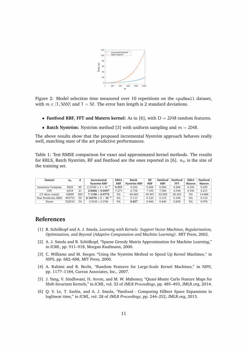
and compute the RMSE on the test set. We consider 10 trials, reporting the performancemean and standard deviation. The results in Table 1 compare Nystrom computationalregularization with the following methods (as in [6]):

• Kernel Regularized Least Squares (KRLS): Not compatible with large datasets.

• Random Fourier features (RF): As in [4], with a number of random features D =2048.

10

m1 201 401 600 800 1000

Tim

e (

s)

0

20

40

60

80

100

120

Incremental NyströmBatch Nyström

Figure 2: Model selection time measured over 10 repetitions on the cpuSmall dataset,with m ∈ [1, 5000] and T = 50. The error bars length is 2 standard deviations.

• Fastfood RBF, FFT and Matern kernel: As in [6], with D = 2048 random features.

• Batch Nystrom: Nystrom method [3] with uniform sampling and m = 2048.

The above results show that the proposed incremental Nystrom approach behaves reallywell, matching state of the art predictive performances.

Table 1: Test RMSE comparison for exact and approximated kernel methods. The resultsfor KRLS, Batch Nystrom, RF and Fastfood are the ones reported in [6]. ntr is the size ofthe training set.

Dataset ntr d Incremental KRLS Batch RF Fastfood Fastfood KRLS FastfoodNystrom RBF RBF Nystrom RBF RBF RBF FFT Matern Matern

Insurance Company 5822 85 0.23180± 4× 10−5 0.231 0.232 0.266 0.264 0.266 0.234 0.235CPU 6554 21 2.8466± 0.0497 7.271 6.758 7.103 7.366 4.544 4.345 4.211

CT slices (axial) 42800 384 7.1106± 0.0772 NA 60.683 49.491 43.858 58.425 NA 14.868Year Prediction MSD 463715 90 0.10470± 5× 10−5 NA 0.113 0.123 0.115 0.106 NA 0.116

Forest 522910 54 0.9638± 0.0186 NA 0.837 0.840 0.840 0.838 NA 0.976

References

[1] B. Scholkopf and A. J. Smola, Learning with Kernels: Support Vector Machines, Regularization,Optimization, and Beyond (Adaptive Computation and Machine Learning). MIT Press, 2002.

[2] A. J. Smola and B. Scholkopf, “Sparse Greedy Matrix Approximation for Machine Learning,”in ICML, pp. 911–918, Morgan Kaufmann, 2000.

[3] C. Williams and M. Seeger, “Using the Nystrom Method to Speed Up Kernel Machines,” inNIPS, pp. 682–688, MIT Press, 2000.

[4] A. Rahimi and B. Recht, “Random Features for Large-Scale Kernel Machines,” in NIPS,pp. 1177–1184, Curran Associates, Inc., 2007.

[5] J. Yang, V. Sindhwani, H. Avron, and M. W. Mahoney, “Quasi-Monte Carlo Feature Maps forShift-Invariant Kernels,” in ICML, vol. 32 of JMLR Proceedings, pp. 485–493, JMLR.org, 2014.

[6] Q. V. Le, T. Sarlos, and A. J. Smola, “Fastfood - Computing Hilbert Space Expansions inloglinear time,” in ICML, vol. 28 of JMLR Proceedings, pp. 244–252, JMLR.org, 2013.

11

[7] S. Si, C.-J. Hsieh, and I. S. Dhillon, “Memory Efficient Kernel Approximation,” in ICML, vol. 32of JMLR Proceedings, pp. 701–709, JMLR.org, 2014.

[8] Y. Zhang, J. C. Duchi, and M. J. Wainwright, “Divide and Conquer Kernel Ridge Regression,”in COLT, vol. 30 of JMLR Proceedings, pp. 592–617, JMLR.org, 2013.

[9] S. Kumar, M. Mohri, and A. Talwalkar, “Ensemble Nystrom Method,” in NIPS, pp. 1060–1068,Curran Associates, Inc., 2009.

[10] M. Li, J. T. Kwok, and B.-L. Lu, “Making Large-Scale Nystrom Approximation Possible,” inICML, pp. 631–638, Omnipress, 2010.

[11] K. Zhang, I. W. Tsang, and J. T. Kwok, “Improved Nystrom Low-rank Approximation andError Analysis,” ICML, pp. 1232–1239, ACM, 2008.

[12] B. Dai, B. X. 0002, N. He, Y. Liang, A. Raj, M.-F. Balcan, and L. Song, “Scalable KernelMethods via Doubly Stochastic Gradients,” in NIPS, pp. 3041–3049, 2014.

[13] P. Drineas and M. W. Mahoney, “On the Nystrom Method for Approximating a Gram Matrixfor Improved Kernel-Based Learning,” JMLR, vol. 6, pp. 2153–2175, Dec. 2005.

[14] A. Gittens and M. W. Mahoney, “Revisiting the Nystrom method for improved large-scalemachine learning.,” vol. 28, pp. 567–575, 2013.

[15] S. Wang and Z. Zhang, “Improving CUR Matrix Decomposition and the Nystrom Approxima-tion via Adaptive Sampling,” JMLR, vol. 14, no. 1, pp. 2729–2769, 2013.

[16] P. Drineas, M. Magdon-Ismail, M. W. Mahoney, and D. P. Woodruff, “Fast approximation ofmatrix coherence and statistical leverage,” JMLR, vol. 13, pp. 3475–3506, 2012.

[17] M. B. Cohen, Y. T. Lee, C. Musco, C. Musco, R. Peng, and A. Sidford, “Uniform Sampling forMatrix Approximation,” in ITCS, pp. 181–190, ACM, 2015.

[18] S. Wang and Z. Zhang, “Efficient Algorithms and Error Analysis for the Modified NystromMethod,” in AISTATS, vol. 33 of JMLR Proceedings, pp. 996–1004, JMLR.org, 2014.

[19] S. Kumar, M. Mohri, and A. Talwalkar, “Sampling Methods for the Nystrom Method,” JMLR,vol. 13, no. 1, pp. 981–1006, 2012.

[20] C. Cortes, M. Mohri, and A. Talwalkar, “On the Impact of Kernel Approximation on LearningAccuracy,” in AISTATS, vol. 9 of JMLR Proceedings, pp. 113–120, JMLR.org, 2010.

[21] R. Jin, T. Yang, M. Mahdavi, Y.-F. Li, and Z.-H. Zhou, “Improved Bounds for the NystromMethod With Application to Kernel Classification,” Information Theory, IEEE Transactions on,vol. 59, pp. 6939–6949, Oct 2013.

[22] T. Yang, Y.-F. Li, M. Mahdavi, R. Jin, and Z.-H. Zhou, “Nystrom Method vs Random FourierFeatures: A Theoretical and Empirical Comparison,” in NIPS, pp. 485–493, 2012.

[23] F. Bach, “Sharp analysis of low-rank kernel matrix approximations,” in COLT, vol. 30 of JMLRProceedings, pp. 185–209, JMLR.org, 2013.

[24] A. Alaoui and M. W. Mahoney, “Fast Randomized Kernel Methods With Statistical Guaran-tees,” arXiv, 2014.

[25] I. Steinwart and A. Christmann, Support Vector Machines. Information Science and Statistics,Springer New York, 2008.

[26] A. Caponnetto and E. De Vito, “Optimal rates for the regularized least-squares algorithm,”Foundations of Computational Mathematics, vol. 7, no. 3, pp. 331–368, 2007.

12

[27] L. L. Gerfo, L. Rosasco, F. Odone, E. D. Vito, and A. Verri, “Spectral Algorithms for SupervisedLearning,” Neural Computation, vol. 20, no. 7, pp. 1873–1897, 2008.

[28] I. Steinwart, D. R. Hush, and C. Scovel, “Optimal Rates for Regularized Least Squares Re-gression,” in COLT, 2009.

[29] S. Mendelson and J. Neeman, “Regularization in kernel learning,” The Annals of Statistics,vol. 38, no. 1, pp. 526–565, 2010.

[30] F. Bauer, S. Pereverzev, and L. Rosasco, “On regularization algorithms in learning theory,”Journal of complexity, vol. 23, no. 1, pp. 52–72, 2007.

[31] A. Caponnetto and Y. Yao, “Adaptive rates for regularization operators in learning theory,”Analysis and Applications, vol. 08, 2010.

[32] Y. Ying and M. Pontil, “Online gradient descent learning algorithms,” Foundations of Compu-tational Mathematics, vol. 8, no. 5, pp. 561–596, 2008.

[33] A. Rudi, G. D. Canas, and L. Rosasco, “On the Sample Complexity of Subspace Learning,” inNIPS, pp. 2067–2075, 2013.

[34] A. K. Farahat, A. Ghodsi, and M. S. Kamel, “A novel greedy algorithm for Nystrom approxi-mation,” in AISTATS, vol. 15 of JMLR Proceedings, pp. 269–277, JMLR.org, 2011.

13

A Preliminary Definitions

We begin introducing several operators that will be useful in the following. Let z1, . . . , zm ∈H and for all f ∈ H, a ∈ Rm, let

Zm : H→ Rm, Zmf = (〈z1, f〉H , . . . , 〈zm, f〉H),Z∗m : Rm → H, Z∗ma =

∑mi=1 aizi.

Let Sn = 1√nZm and S∗n = 1√

nZ∗m the operators obtained taking m = n and zi = Kxi ,

∀i = 1, . . . , n in the above definitions. Moreover, for all f, g ∈ H let

Cn : H→ H, 〈f, Cng〉H =1

n

n∑i=1

f(xi)g(xi).

It is easy to see that the above operators are linear and finite rank. Moreover, it is easyto see that Cn = S∗nSn and Kn = nSnS

∗n, and further Bnm =

√nSnZ

∗m ∈ Rn×m, Gmm =

ZmZ∗m ∈ Rm×m and Kn = BnmG

†mmB

>nm ∈ Rn×n.

B Representer theorem for Nystrom Computational Regulariza-tion and Extensions

In this section we consider explicit representations of the estimator obtained via Nystromcomputational regularization and extensions. Indeed, we consider a general subspace Hmof H, and the following problem

fλ,m = argminf∈Hm

1

n

n∑i=1

(f(xi) − yi)2 + λ‖f‖2H. (11)

In the following lemmas, we show three different characterizations of fλ,m.

Lemma 1. Let fλ,m be the solution of the problem in Eq. (11). Then it is characterized by thefollowing equation

(PmCnPm + λI)fλ,m = PmS∗nyn, (12)

with Pm the projection operator with range Hm and yn = 1√ny.

Proof. The proof proceeds in three steps. First, note that, by rewriting Problem (11) withthe notation introduced in the previous section, we obtain,

fλ,m = argminf∈Hm

‖Snf− yn‖2 + λ‖f‖2H. (13)

This problem is strictly convex and coercive, therefore admits a unique solution. Second,we show that its solution coincide to the one of the following problem,

f∗ = argminf∈H

‖SnPmf− yn‖2 + λ‖f‖2H. (14)

14

Note that the above problem is again strictly convex and coercive. To show that fλ,m = f∗,let f∗ = a + b with a ∈ Hm and b ∈ H⊥m. A necessary condition for f∗ to be optimal, isthat b = 0, indeed, considering that Pmb = 0, we have

‖SnPmf∗ − yn‖2+λ‖f∗‖2H = ‖SnPma− yn‖2+λ‖a‖2H+λ‖b‖2H ≥ ‖SnPma− yn‖2+λ‖a‖2H.

This means that f∗ ∈ Hm, but on Hm the functionals defining Problem (13) and Prob-lem (14) are identical because Pmf = f for any f ∈ Hm and so fλ,m = f∗. Therefore, bycomputing the derivative of the functional of Problem (14), we see that fλ,m is given byEq. (12).

Using the above results, we can give an equivalent representations of the function fλ,m.Towards this end, let Zm be a linear operator as in Sect. A such that the range of Z∗m isexactly Hm. Morever, let

Zm = UΣV∗

be the SVD of Zm where U : Rt → Rm, Σ : Rt → Rt, V : Rt → H, t ≤ m and Σ =diag(σ1, . . . , σt) with σ1 ≥ · · · ≥ σt > 0, U∗U = It and V∗V = It. Then the orthogonalprojection operator Pm is given by Pm = VV∗ and the range of Pm is exactly Hm. In thefollowing lemma we give a characterization of fλ,m that will be useful in the proof of themain theorem.

Lemma 2. Given the above definitions , fλ,m can be written as

fλ,m = V(V∗CnV + λI)−1V∗S∗nyn. (15)

Proof. By Lemma 1, we know that fλ,m is written as in Eq. (12). Now, note that fλ,m =Pmfλ,m and Eq. (12) imply (PmCmPm + λI)Pmfλ,m = PmS

∗nyn, that is equivalent to

V(V∗CnV + λI)V∗fλ,m = VV∗S∗nyn,

by substituting Pm with VV∗. Thus by premultiplying the previous equation by V∗ anddividing by V∗CmV + λI, we have

V∗fλ,m = (V∗CmV + λI)−1V∗S∗nyn.

Finally, by premultiplying by V,

fλ,m = Pmfλ,m = V(V∗CmV + λI)−1V∗S∗nyn.

Finally, the following result provide a characterization of the solution useful for com-putations.

Lemma 3 (Representer theorem for fλ,m). Given the above definitions, we have that fλ,mcan be written as

fλ,m(x) =

m∑i=1

αizi(x), with α = (B>nmBnm + λnGmm)†B>nmy ∀ x ∈ X. (16)

15

Proof. According to the definitions of Bnm and Gmm we have that

α = (B>nmBnm + λnGmm)†B>nmy = ((ZmS

∗n)(SnZ

∗m) + λ(ZmZ

∗m))†(ZmS

∗n)yn.

Moreover, according to the definition of Zm we have

fλm(x) =

m∑i=1

αi 〈zi, Kx〉 = 〈ZmKx, α〉Rm = 〈Kx, Z∗mα〉H ∀ x ∈ X,

so that

fλ,m = Z∗m((ZmS∗n)(SnZ

∗m) + λ(ZmZ

∗m))†(ZmS

∗n)yn = Z∗m(ZmCnλZ

∗m)†(ZmS

∗n)yn,

where Cnλ = Cn + λI. Let F = UΣ, G = V∗CnV + λI, H = ΣU>, and note that F, GH,G and H are full-rank matrices, then we can perform the full-rank factorization of thepseudo-inverse (see Eq.24, Thm. 5, Chap. 1 of [1]) obtaining

(ZmCnλZ∗m)† = (FGH)† = H†(FG)† = H†G−1F† = UΣ−1(V∗CnV + λI)−1Σ−1U∗.

Finally, simplyfing U and Σ, we have

fλ,m = Z∗m(ZmCnλZ∗m)†(ZmS

∗n)yn

= VΣU∗UΣ−1(V∗CnV + λI)−1Σ−1U∗UΣV∗S∗nyn

= V(V∗CnV + λI)−1V∗S∗nyn.

B.1 Extensions

Inspection of the proof shows that our analysis extends beyond the class of subsamplingschemes in Theorem 1. Indeed, the error decomposition Theorem 2 directly applies to alarge family of approximation schemes. Several further examples are described next.

KRLS and Generalized Nystrom In general we could choose an arbitrary Hm ⊆ H. LetZm : H→ Rm be a linear operator such that

Hm = ranZ∗m = {f | f = Z∗mα, α ∈ Rm}. (17)

Without loss of generality, Z∗m is expressible as Z∗m = (z1, . . . , zm)> with z1, . . . , zm ∈ H,

therefore, according to Section A and to Lemma 3, the solution of KRLS approximatedwith the generalized Nystrom scheme is

fλ,m(x) =

m∑i=1

αizi(x), with α = (B>nmBnm + λnGmm)†B>nmy (18)

with Bnm ∈ Rn×m, (Bnm)ij = zj(xi) and Gmm ∈ Rm×m, (Gmm)ij = 〈zi, zj〉H, or equiva-lently

fλ,m(x) =

m∑i=1

αizi(x), α = G†mmB>nm(Kn + λnI)

†yn, Kn = BnmG†mmB

>nm (19)

The following are some examples of Generalized Nystrom approximations.

16

Plain Nystrom with various sampling schemes [2, 3, 4] For a realization s : N →{1, . . . , n} of a given sampling scheme, we choose Zm = Sm with S∗m = (Kxs(1) , . . . , Kxs(m)

)>

where (xi)ni=1 is the training set. With such Zm we obtain Kn = Knm(Kmm)

†K>nm and soEq. (18) becomes exactly Eq. (5).

Reduced rank Plain Nystrom [5] Let p ≥ m, Sp as in the previous example, the linearoperator associated to p points of the dataset. Let Kpp = SpS

>p ∈ Rp×p, that is (Kpp)ij =

K(xi, xj). Let Kpp =∑pi=1 σiuiu

>i its eigenvalue decomposition and Um = (u1, . . . , um).

Let (Kpp)m = U>mKppUm be the m-rank approximation of Kpp. We approximate the thisfamily by choosing Zm = U>mSp, indeed we obtain Kn = KnmUm(U

>mKppUm)

†U>mK>nm =

Knm(Kpp)†mK>nm.

Nystrom with sketching matrices [6] We cover this family by choosing Zm = RmSn,where Sn is the same operator as in the plain Nystrom case where we select all thepoints of the training set and Rm a m × n sketching matrix. In this way we have Kn =KnR

∗m(RmKnR

∗m)†RmKn, that is exactly the SPSD sketching model.

C Probabilistic Inequalities

In this section we collect five main probabilistic inequalities needed in the proof of themain result. We let ρX denote the marginal distribution of ρ on X and ρ(·|x) the conditionaldistribution on R given x ∈ X. Lemmas 6, 7 and especially Proposition 1 are new and ofinterest in their own right.

The first result is essentially taken from [7].

Lemma 4 (Sample Error). Under Assumptions 1, 2 and 3, for any δ > 0, the followingholds with probability 1− δ

‖(C+ λI)−1/2(Snyn − CnfH)‖ ≤ 2

(M√N∞(λ)

n+

√σ2N (λ)

n

)log

2

δ.

Proof. The proof is given in [7] for bounded kernels and the slightly stronger condition∫(e

|y−fH(x)|

M − |y−fH(x)|M − 1)dρ(y|x) ≤ σ2/M2 in place of Assumption 2. More precisely, note

that

(C+ λI)−1/2(Snyn − CnfH) =1

n

n∑i=1

ζi,

where ζ1, . . . , ζn are i.i.d. random variables, defined as ζi = (C+ λI)−1/2Kxi(yi − fH(xi)).It is easy to see that, for any 1 ≤ i ≤ n,

Eζi =∫X×R

(C+ λI)−1/2Kxi(yi − fH(xi))dρ(xi, yi)

=

∫X

(C+ λI)−1/2Kxi

∫R(yi − fH(xi))dρ(yi|xi)dρX(xi) = 0,

17

almost everywhere by Assumption 1 (see Step 3.2 of Thm. 4 in [7]). In the same way wehave

E‖ζi‖p =∫X×R‖(C+ λI)−1/2Kxi(yi − fH(xi))‖

pdρ(xi, yi)

=

∫X

‖(C+ λI)−1/2Kxi‖p

∫R|yi − fH(xi)|

pdρ(yi|xi)dρX(xi)

≤ supx∈X‖(C+ λI)−1/2Kx‖p−2

∫X

‖(C+ λI)−1/2Kxi‖2

∫R|yi − fH(xi)|

pdρ(yi|xi)dρX(xi)

≤ 12p!√σ2N (λ)

2

(M√N∞(λ))p−2,

where supx∈X‖(C+ λI)−1/2Kx‖ =√N∞(λ) and

∫X‖(C+ λI)−1/2Kxi‖2 = N (λ) by Assump-

tion 3, while the bound on the moments of y − f(x) is given in Assumption 2. Finally, toconcentrate the sum of random vectors, we apply Prop. 11.

The next result is taken from [8].

Lemma 5. Under Assumption 3, for any δ ≥ 0 and 9κ2

n log nδ ≤ λ ≤ ‖C‖, the following

inequality holds with probability at least 1− δ,

‖(Cn + λI)−1/2C1/2‖ ≤ ‖(Cn + λI)−1/2(C+ λI)1/2‖ ≤ 2.

Proof. Lemma 7 of [8] gives an the extended version of the above result. Our bound on λis scaled by κ2 because in [8] it is assumed κ ≤ 1.

Lemma 6 (plain Nystrom approximation). Under Assumption 3, let J be a partition of{1, . . . , n} chosen uniformly at random from the partitions of cardinality m. Let λ > 0, forany δ > 0, such that m ≥ 67 log 4κ2

λδ ∨ 5N∞(λ) log 4κ2

λδ , the following holds with probability1− δ

‖(I− Pm)C1/2‖2 ≤ 3λ,where Pm is the projection operator on the subspace Hm = span{Kxj | j ∈ J}.

Proof. Define the linear operator Cm : H→ H, as Cm = 1m

∑j∈J Kxj ⊗Kxj . It is easy to see

that the range of Cm is exactly Hm. Therefore, by applying Prop. 3 and 7, we have that

‖(I− Pm)C1/2λ ‖2 ≤ λ‖(Cm + λI)−1/2C1/2‖2 ≤ λ

1− β(λ),

with β(λ) = λmax

(C−1/2λ (C− Cm)C

−1/2λ

). To upperbound λ

1−β(λ) we need an upperboundfor β(λ). Considering that, given the partition J, the random variables ζj = Kxj ⊗ Kxj arei.i.d., then we can apply Prop. 8, to obtain

β(λ) ≤ 2w

3m+

√2wN∞(λ)

m,

where w = log 4Tr(C)λδ with probability 1− δ. Thus, by choosing m ≥ 67w∨ 5N∞(λ)w, we

have that β(λ) ≤ 2/3, that is‖(I− Pm)C1/2λ ‖

2 ≤ 3λ.Finally, note that by definition Tr(C) ≤ κ2.

18

Lemma 7 (Nystrom approximation for ALS selection method). Let (li(t))ni=1 be the collec-tion of approximate leverage scores. Let λ > 0 and Pλ be defined as Pλ(i) = li(λ)/

∑j∈N lj(λ)

for any i ∈ N with N = {1, . . . , n}. Let I = (i1, . . . , im) be a collection of indices indepen-dently sampled with replacement from N according to the the probability distribution Pλ. LetPm be the projection operator on the subspace Hm = span{Kxj |j ∈ J} and J be the subcollec-tion of I with all the duplicates removed. Under Assumption 3, for any δ > 0 the followingholds with probability 1− 2δ

‖(I− Pm)(C+ λI)1/2‖ ≤ 3λ,

when the following conditions are satisfied:

1. there exists a T ≥ 1 and a λ0 > 0 such that (li(t))ni=1 are T -approximate leverage scoresfor any t ≥ λ0 (see Def. 1),

2. n ≥ 1655κ2 + 223κ2 log 2κ2

δ ,

3. λ0 ∨ 19κ2

n log 2nδ ≤ λ ≤ ‖C‖,

4. m ≥ 334 log 8nδ ∨ 78T 2N (λ) log 8n

δ .

Proof. Define τ = δ/4. Next, define the diagonal matrix H ∈ Rn×n with (H)ii = 0 whenPλ(i) = 0 and (H)ii =

nq(i)mPλ(i)

when Pλ(i) > 0, where q(i) is the number of times the indexi is present in the collection I. We have that

S∗nHSn =1

m

n∑i=1

q(i)

Pλ(i)Kxi ⊗ Kxi =

1

m

∑j∈J

q(j)

Pλ(j)Kxj ⊗ Kxj .

Now, considering that q(j)Pλ(j)

> 0 for any j ∈ J, it is easy to see that ranS∗nHSn = Hm.Therefore, by using Prop. 3 and 7, we exploit the fact that the range of Pm is the same ofS∗nHSn, to obtain

‖(I− Pm)(C+ λI)1/2‖2 ≤ λ‖(S∗nHSn + λI)−1/2C1/2‖2 ≤λ

1− β(λ),

with β(λ) = λmax

(C−1/2λ (C− S∗nHSn)C

−1/2λ

). Considering that the function (1 − x)−1 is

increasing on −∞ < x < 1, in order to bound λ/(1 − β(λ)) we need an upperbound forβ(λ). Here we split β(λ) in the following way,

β(λ) ≤ λmax

(C−1/2λ (C− Cn)C

−1/2λ

)︸ ︷︷ ︸

β1(λ)

+ λmax

(C−1/2λ (Cn − S

∗nHSn)C

−1/2λ

)︸ ︷︷ ︸

β2(λ)

.

Considering that Cn is the linear combination of independent random vectors, for the firstterm we can apply Prop. 8, obtaining a bound of the form

β1(λ) ≤2w

3n+

√2wκ2

λn,

19

with probability 1 − τ, where w = log 4κ2

λτ (we used the fact that N∞(λ) ≤ κ2/λ). Then,

after dividing and multiplying by C1/2nλ , we split the second term β2(λ) as follows:

β2(λ) ≤ ‖C−1/2λ (Cn − S

∗nHSn)C

−1/2λ ‖

≤ ‖C−1/2λ C

1/2nλ C

−1/2nλ (Cn − S

∗nHSn)C

−1/2nλ C

1/2nλ C

−1/2λ ‖

≤ ‖C−1/2λ C

1/2nλ ‖

2‖C−1/2nλ (Cn − S

∗nHSn)C

−1/2nλ ‖.

Let

β3(λ) = ‖C−1/2nλ (Cn − S

∗nHSn)C

−1/2nλ ‖ = ‖C

−1/2nλ S∗n(I−H)SnC

−1/2nλ ‖. (20)

Note that SnC−1nλS∗n = Kn(Kn + λnI)−1 indeed C−1

nλ = (S∗nSn + λI)−1 and Kn = nSnS∗n.

Therefore we have

SnC−1nλS∗n = Sn(S

∗nSn + λI)

−1S∗n = (SnS∗n + λI)

−1SnS∗n = (Kn + λnI)

−1Kn.

Thus, if we let UΣU> be the eigendecomposition of Kn, we have that (Kn + λnI)−1Kn =U(Σ+ λnI)−1ΣU> and thus SnC−1

nλS∗n = U(Σ+ λnI)−1ΣU>. In particular this implies that

SnC−1nλS∗n = UQ

1/2n Q

1/2n U> with Qn = (Σ+ λnI)−1Σ. Therfore we have

β3(λ) = ‖C−1/2nλ S∗n(I−H)SnC

−1/2nλ ‖ = ‖Q

1/2n U>(I−H)UQ

1/2n ‖,

where we used twice the fact that ‖ABA∗‖ = ‖(A∗A)1/2B(A∗A)1/2‖ for any bounded linearoperators A,B.

Consider the matrix A = Q1/2n U> and let ai be the i-th colum of A, and ei be the i-th

canonical basis vector for each i ∈ N. We prove that ‖ai‖2 = li(λ), the true leverage score,since

‖ai‖2 = ‖Q1/2n U>ei‖2 = e>i UQnU>ei = ((Kn + λnI)

−1Kn)ii = li(λ).

Noting that∑nk=1

q(k)Pλ(k)

aka>k =∑i=I

1Pλ(i)

aia>i , we have

β3(λ) = ‖AA> −1

m

∑i∈I

1

Pλ(i)aia>i ‖.

Moreover, by the T -approximation property of the approximate leverage scores (see Def. 1),we have that for all i ∈ {1, . . . , n}, when λ ≥ λ0, the following holds with probability 1− δ

Pλ(i) =li(λ)∑j lj(λ)

≥ T−2 li(λ)∑j lj(λ)

= T−2‖ai‖2

TrAA>.

Then, we can apply Prop. 9, so that, after a union bound, we obtain the following inequal-ity with probability 1− δ− τ:

β3(λ) ≤2‖A‖2 log 2n

τ

3m+

√2‖A‖2T 2 TrAA> log 2n

τ

m≤2 log 2n

τ

3m+

√2T 2N (λ) log 2n

τ

m,

20

where the last step follows from ‖A‖2 = ‖(Kn + λnI)−1Kn‖ ≤ 1 and Tr(AA>) = Tr(C−1nλCn) :=

N (λ). Applying Proposition 1, we have that N (λ) ≤ 1.3N (λ) with probability 1− τ, when19κ2

n log n4τ ≤ λ ≤ ‖C‖ and n ≥ 405κ2 ∨ 67κ2 log κ2

2τ . Thus, by taking a union bound again,we have

β3(λ) ≤2 log 2n

τ

3m+

√5.3T 2N (λ) log 2n

τ

m,

with probability 1− 2τ− δ when λ0 ∨ 19κ2

n log nδ ≤ λ ≤ ‖C‖ and n ≥ 405κ2 ∨ 67κ2 log 2κ2

δ .

The last step is to bound ‖C−1/2λ C

1/2nλ ‖

2, as follows

‖C−1/2λ C

1/2nλ ‖

2 = ‖C−1/2λ CnλC

−1/2λ ‖ = ‖I+ C−1/2

λ (Cn − C)C−1/2λ ‖ ≤ 1+ η,

with η = ‖C−1/2λ (Cn − C)C

−1/2λ ‖. Note that, by applying Prop. 8 we have that η ≤

2(κ2+λ)θ3λn +

√2κ2θ3λn with probability 1 − τ and θ = log 8κ2

λτ . Finally, by collecting the aboveresults and taking a union bound we have

β(λ) ≤ 2w3n

+

√2wκ2

λn+ (1+ η)

2 log 2nτ

3m+

√5.3T 2N (λ) log 2n

τ

m

,with probability 1 − 4τ − δ = 1 − 2δ when λ0 ∨ 19κ2

n log nδ ≤ λ ≤ ‖C‖ and n ≥ 405κ2 ∨

67κ2 log 2κ2

δ . Note that, if we select n ≥ 405κ2 ∨ 223κ2 log 2κ2

δ , m ≥ 334 log 8nδ , λ0 ∨

19κ2

n log 2nδ ≤ λ ≤ ‖C‖ and 78T2N (λ) log 8n

δm ≤ 1 the conditions are satisfied and we have

β(λ) ≤ 2/3, so that‖(I− Pm)C1/2‖2 ≤ 3λ,

with probability 1− 2δ.

Proposition 1 (Empirical Effective Dimension). Let N (λ) = TrCnC−1nλ. Under the Assump-

tion 3, for any δ > 0 and n ≥ 405κ2 ∨ 67κ2 log 6κ2

δ , if 19κ2

n log n4δ ≤ λ ≤ ‖C‖, then the

following holds with probability 1− δ,

|N (λ) −N (λ)|

N (λ)≤ 4.5q+ (1+ 9q)

√3q

N (λ)+q+ 13.5q2

N (λ)≤ 1.65,

with q =4κ2 log 6

δ3λn .

Proof. Let τ = δ/3. Define Bn = C−1/2λ (C−Cn)C

−1/2λ . Choosing λ in the range 19κ2

n log n4τ ≤

λ ≤ ‖C‖, Prop. 8 assures that λmax(Bn) ≤ 1/3 with probability 1 − τ. Then, using the factthat C−1

nλ = C−1/2λ (I− Bn)

−1C−1/2λ (see the proof of Prop. 7) we have

|N (λ) −N (λ)| = |TrC−1nλCn − CC

−1λ = λTrC−1

nλ(Cn − C)C−1λ |

= |λTrC−1/2λ (I− Bn)

−1C−1/2λ (Cn − C)C

−1/2λ C

−1/2λ |

= |λTrC−1/2λ (I− Bn)

−1 BnC−1/2λ |.

21

Considering that for any symmetric linear operator X : H→ H the following identity holds

(I− X)−1X = X+ X(I− X)−1X,

when λmax(X) ≤ 1, we have

λ|TrC−1/2λ (I− Bn)

−1 BnC−1/2λ | ≤ λ|TrC−1/2

λ BnC−1/2λ |︸ ︷︷ ︸

A

+ λ|TrC−1/2λ Bn (I− Bn)

−1 BnC−1/2λ |︸ ︷︷ ︸

B

.

To find an upperbound for A define the i.i.d. random variables ηi =⟨Kxi , λC

−2λ Kxi

⟩∈

R with i ∈ {1, . . . , n}. By linearity of the trace and the expectation, we have M = Eη1 =E⟨Kxi , λC

−2λ Kxi

⟩= ETr(λC−2

λ Kx1 ⊗ Kx1) = λTr(C−2λ C). Therefore,

λ|TrC−1/2λ BnC

−1/2λ | =

∣∣∣∣∣M−1

n

n∑i=1

ηi

∣∣∣∣∣ ,and we can apply the Bernstein inequality (Prop. 10) with

|M− η1| ≤ λ‖C−2λ ‖‖Kx1‖

2 +M ≤ κ2

λ+M ≤ 2κ

2

λ= L,

E(η1 −M)2 = Eη21 −M2 ≤ Eη21 ≤ LM = σ2.

An upperbound for M is M = Tr(λC−2λ C) = Tr((I− C−1

λ C)C−1λ C) ≤ N (λ). Thus, we have

λ|TrC−1/2λ BnC

−1/2λ | ≤

4κ2 log 2τ

3λn+

√4κ2N (λ) log 2

τ

λn,

with probability 1− τ.To find an upperbound for B, let L be the space of Hilbert-Schmidt operators on H. L

is a Hilbert space with scalar product 〈U,V〉HS = Tr (UV∗) for all U,V ∈ L. Next, notethat B = ‖Q‖2HS where Q = λ1/2C

−1/2λ Bn (I− Bn)

−1/2, moreover

‖Q‖2HS ≤ ‖λ1/2C−1/2λ ‖2‖Bn‖2HS‖(I− Bn)

−1/2‖2 ≤ 1.5‖Bn‖2HS,

since ‖(I− Bn)−1/2‖2 = (1 − λmax(Bn))−1 ≤ 3/2 and (1 − σ)−1 is increasing and positive

on [−∞, 1).To find a bound for ‖Bn‖HS consider that Bn = T− 1

n

∑ni=1 ζi where ζi are i.i.d. random

operators defined as ζi = C−1/2λ (Kxi ⊗ Kxi)C

−1/2λ ∈ L for all i ∈ {1, . . . , n}, and T = Eζ1 =

C−1λ C ∈ L. Then we can apply the Bernstein’s inequality for random vectors on a Hilbert

space (Prop. 11), with the following L and σ2:

‖T − ζ1‖HS ≤ ‖C−1/2λ ‖2‖Kx1‖

2H + ‖T‖HS ≤

κ2

λ+ ‖T‖HS ≤

2κ2

λ= L,

E‖ζ1 − T‖2 = ETr(ζ21 − T2) ≤ ETr(ζ21) ≤ LETr(ζ1) = σ2,

22

where ‖T‖HS ≤ ETr(ζ1) = N (λ), obtaining

‖Bn‖HS ≤4κ2 log 2

τ

λn+

√4κ2N (λ) log 2

τ

λn,

with probability 1− τ. Then, by taking a union bound for the three events we have

|N (λ) −N (λ)| ≤ q+√3qN (λ) + 1.5

(3q+

√3qN (λ)

)2,

with q =4κ2 log 6

δ3λn , and with probability 1− δ. Finally, if the second assumption on λ holds,

then we have q ≤ 4/57. Noting that n ≥ 405κ2, and that N (λ) ≥ ‖CC−1λ ‖ =

‖C‖‖C‖+λ ≥ 1/2,

we have that

|N (λ) −N (λ)| ≤

q

3N (λ)+

√q

N (λ)+ 1.5

(q√N (λ)

+√q

)2N (λ) ≤ 1.65N (λ).

D Proofs of Main Theorem

A key step to derive the proof of Theorem 1 is the error decomposition given by thefollowing theorem, together with the probabilistic inequalities in the previous section.

Theorem 2 (Error decomposition for KRLS+Ny). Under Assumptions 1, 3, 4, let v =min(s, 1/2) and fλ,m a KRLS + generalized Nystrom solution as in Eq. (18). Then for anyλ,m > 0 the error is bounded by∣∣E(fλ,m) − E(fH)∣∣1/2 ≤ q( S(λ, n)︸ ︷︷ ︸

Sample error

+ C(m)1/2+v︸ ︷︷ ︸Computational error

+ λ1/2+v︸ ︷︷ ︸Approximation error

) (21)

where S(λ, n) = ‖(C+ λI)−1/2(Snyn − CnfH)‖ and C(m) = ‖(I− Pm)(C+ λI)1/2‖2 withPm = Z∗m(ZmZ

∗m)†Zm. Moreover q = R(β2 ∨ (1 + θβ)), β = ‖(Cn + λI)−1/2(C+ λI)1/2‖,

θ = ‖(Cn + λI)1/2(C+ λI)−1/2‖.

Proof. Let Cλ = C + λI and Cnλ = Cn + λI for any λ > 0. Let fλ,m as in Eq. (18).By Lemma 1, Lemma 2 and Lemma 3 we know that fλ,m is characterized by fλ,m =gλm(Cn)S

∗nyn with gλ,m(Cn) = V(V∗CnV + λI)−1V∗. By using the fact that E(f)− E(fH) =

‖C1/2(f− fH)‖2H for any f ∈ H (see Prop. 1 Point 3 of [7]), we have

|E(fλ,m) − E(fH)|1/2 = ‖C1/2(fλ,m − fH)‖H = ‖C1/2(gλ,m(Cn)S∗nyn − fH)‖H= ‖C1/2(gλ,m(Cn)S∗n(yn − SnfH + SnfH) − fH)‖H≤ ‖C1/2gλ,m(Cn)S∗n(yn − SnfH)‖H︸ ︷︷ ︸

A

+ ‖C1/2(I− gλ,m(Cn)Cn)fH‖H︸ ︷︷ ︸B

.

23

Bound for the term A Multiplying and dividing by C1/2nλ and C1/2λ we have

A ≤ ‖C1/2C−1/2nλ ‖‖C

1/2nλ gλ,m(Cn)C

1/2nλ ‖‖C

−1/2nλ C

1/2λ ‖‖C

−1/2λ S∗n(yn − SnfH)‖H ≤ β2 S(λ, n),

where the last step is due to Lemma 8 and the fact that

‖C1/2C−1/2nλ ‖ ≤ ‖C

1/2C−1/2λ ‖‖C1/2λ C

−1/2nλ ‖ ≤ ‖C

1/2λ C

−1/2nλ ‖.

Bound for the term B Noting that gλ,m(Cn)CnλVV∗ = VV∗, we have

I− gλ,m(Cn)Cn = I− gλ,m(Cn)Cnλ + λgλ,m(Cn)

= I− gλ,m(Cn)CnλVV∗ − gλ,m(Cn)Cnλ(I− VV

∗) + λgλ,m(Cn)

= (I− VV∗) + λgλ,m(Cn) − gλ,m(Cn)Cnλ(I− VV∗).

Therefore, noting that by Ass. 4 we have ‖C−vλ fH‖H ≤ ‖C

−sλ fH‖H ≤ ‖C

−sfH‖H ≤ R, then,by reasoning as in A, we have

B ≤ ‖C1/2(I− gλ,m(Cn)Cn)Cvλ‖‖C−vλ fH‖H

≤ R‖C1/2C−1/2λ ‖‖C1/2λ (I− VV∗)Cvλ‖+ Rλ‖C1/2C

−1/2nλ ‖‖C

1/2nλ gλ,m(Cn)C

vλ‖

+ R‖C1/2C−1/2nλ ‖‖C

1/2nλ gλ,m(Cn)C

1/2nλ ‖‖C

1/2nλ C

−1/2λ ‖‖C1/2λ (I− VV∗)Cvλ‖

≤ R(1+ βθ) ‖C1/2λ (I− VV∗)Cvλ‖︸ ︷︷ ︸B.1

+Rβλ‖C1/2nλ gλ,m(Cn)Cvλ‖︸ ︷︷ ︸

B.2

,

where in the second step we applied the decomposition of I− gλm(Cn)Cn.Bound for the term B.1 Since VV∗ is a projection operator, we have that (I− VV∗) =

(I− VV∗)s, for any s > 0, therefore

B.1 = ‖C1/2λ (I− VV∗)2Cvλ‖ ≤ ‖C1/2λ (I− VV∗)‖‖(I− VV∗)Cvλ‖.

By applying Cordes inequality (Prop. 4) to ‖(I− VV∗)Cvλ‖ we have,

‖(I− VV∗)Cvλ‖ = ‖(I− VV∗)2vC122v

λ ‖ = ‖(I− VV∗)C

1/2λ ‖

2v.

Bound for the term B.2 We have

B.2 ≤ λ‖C1/2nλ gλ,m(Cn)Cvnλ‖‖C−v

nλCvλ‖

≤ λ‖C1/2nλ gλ,m(Cn)Cvnλ‖‖C

−1/2nλ C

1/2λ ‖

2v

≤ β2vλ‖(V∗CnλV)1/2(V∗CnλV)−1(V∗CnλV)v‖= β2vλ‖(V∗CnV + λI)−(1/2−v)‖ ≤ βλ1/2+v,

where the first step is obtained multipling and dividing by Cvnλ, the second step by apply-ing Cordes inequality (see Prop. 4), the third step by Prop. 6.

24

Proposition 2 (Bounds for plain and ALS Nystrom). For any δ > 0, let n ≥ 1655κ2 +

223κ2 log 6κ2

δ , let 19κ2

n log 6nδ ≤ λ ≤ ‖C‖ and define

Cpl(m) = min{t > 0

∣∣∣∣ (67∨ 5N∞(t)) log12κ2

tδ≤ m},

CALS(m) = min{19κ2

nlog

12n

δ≤ t ≤ ‖C‖

∣∣∣∣ 78T 2N (t) log48n

δ≤ m}.

Under the assumptions of Thm. 2 and Assumption 2, 3, if one of the following two conditionshold

1. plain Nystrom is used,

2. ALS Nystrom is used with

(a) T -approximate leverage scores, for any t ≥ 19κ2

n log 12nδ (see Def. 1),

(b) resampling probabilities Pt where t = CALS(m) (see Sect. 2),

(c) m ≥ 334 log 48nδ ,

then the following holds with probability 1− δ

∣∣E(fλm) − E(fH)∣∣1/2 ≤ 6R(M√N∞(λ)

n+

√σ2N (λ)

n

)log

6

δ+ 3RC(m)1/2+v + 3Rλ1/2+v

(22)

where C(m) = Cpl(m) in case of plain Nystrom and C(m) = CALS(m) in case of ALS Nystrom.

Proof. In order to get explicit bounds from Thm. 2, we have to control four quantitiesthat are β, θ,S(λ, n) and C(m). In the following we bound such quantities in probabilityand then taking a union bound. Let τ = δ/3. We can control both β and θ, by boundingb(λ) = ‖C−1/2

λ (Cn − C)C−1/2λ ‖. Indeed, by Prop. 7, we have that β ≤ 1/(1− b(λ)), while

θ2 = ‖C−1/2λ CnλC

−1/2λ ‖ = ‖I+ C−1/2

λ (Cn − C)C−1/2λ ‖ ≤ 1+ b(λ).

Exploiting Prop. 8, with the fact that N (λ) ≤ N∞(λ) ≤ κ2

λ and TrC ≤ κ2, we have that

b(λ) ≤ 2(κ2+λ)w3λn +

√2wκ2

λn forw = log 4κ2

τλ with probability 1−τ. Simple computations showthat with n and λ as in the statement of this corollary, we have b(λ) ≤ 1/3. Thereforeβ ≤ 1.5, while θ ≤ 1.16 and q = R(β2 ∨ (1 + θβ)) < 2.75R with probability 1 − τ. Next,we bound S(λ, n). Here we exploit Lemma 4 which gives, with probability 1− τ,

S(λ, n) ≤ 2

(M√N∞(λ)

n+

√σ2N (λ)

n

)log

2

τ.

To bound C(m) for plain Nystrom, Lemma 6 gives C(m) ≤ 3t with probability 1 − τ, fora t > 0 such that (67 ∨ 5N∞(t)) log 4κ2

tτ ≤ m. In particular, we choose t = Cpl(m) tosatisfy the condition. Next we bound C(m) for ALS Nystrom. Using Lemma 7 with λ0 =

25

19κ2

n log 2nτ , we have C(m) ≤ 3t with probability 1 − τ under some conditions on t,m,n,

on the approximate leverage scores and on the resampling probability. Here again therequirement on n is satisfied by the hypotesis on n of this proposition, while the conditionon the approximate leverage scores and on the resampling probabilities are satisfied byconditions (a), (b) of this proposition. The remaining two conditions are 19κ2

n log 4nτ ≤ t ≤

‖C‖ and (334 ∨ 78T 2N (t)) log 16nτ ≤ m. They are satisfied by choosing t = CALS(m) and

by assuming thatm ≥ 334 log 16nτ . Finally, the proposition is obtained by substituting each

of the four quantities β, θ,S(λ, n), C(m) with the corresponding upperbounds in Eq. (21),and by taking the union bounds on the associated events.

Poof of Theorem 1. By exploiting the results of Prop. 2, obtained from the error decompo-sition of Thm. 2 we have that

∣∣E(fλm) − E(fH)∣∣1/2 ≤ 6R(M√N∞(λ)

n+

√σ2N (λ)

n

)log

6

δ+ 3RC(m)1/2+v + 3Rλ1/2+v

(23)

with probability 1 − δ, under conditions on λ,m,n, on the resampling probabilities andon the approximate leverage scores. The last is satisfied by condition (a) in this theorem.The conditions on λ, n are n ≥ 1655κ2 + 223κ2 log 6κ2

δ and 19κ2

n log 12nδ ≤ λ ≤ ‖C‖. If we

assume that n ≥ 1655κ2 + 223κ2 log 6κ2

δ +(38p‖C‖ log 114κ2p

‖C‖δ

)pwe satisfy the condition on n

and at the same time we are sure that λ = ‖C‖n−1/(2v+γ+1) satisfies the condition on λ. Inthe plain Nystrom case, if we assume thatm ≥ 67 log 12κ2

λδ + 5N∞(λ) log 12κ2

λδ , then C(m) =

Cpl(m) ≤ λ. In the ALS Nystrom case, if we assume that m ≥ (334 ∨ 78T 2N (λ)) log 48nδ

the condition on m is satisfied, then C(m) = CALS(m) ≤ λ, moreover the conditions on theresampling probabilities is satisfied by condition (b) of this theorem. Therefore, by settingλ = ‖C‖n−1/(2v+γ+1) in Eq. (23) and considering that N∞(λ) ≤ κ2λ−1 we easily obtain theresult of this theorem.

The following lemma is a technical result needed in the error decomposition (Thm. 2).

Lemma 8. For any λ > 0, let V be such that V∗V = I and Cn be a positive self-adjointoperator. Then, the following holds,

‖(Cn + λI)1/2V(V∗CnV + λI)−1V∗(Cn + λI)1/2‖ ≤ 1.

Proof. Let Cnλ = Cn + λI and gλm(Cn) = V(V∗CnV + λI)−1V∗, then

‖C1/2nλ gλm(Cn)C1/2nλ ‖

2 = ‖C1/2nλ gλm(Cn)Cnλgλm(Cn)C1/2nλ ‖

= ‖C1/2nλ V(V∗CnλV)

−1(V∗CnλV)(V∗CnλV)

−1V∗C1/2nλ ‖

= ‖C1/2nλ gλm(Cn)C1/2nλ ‖,

and therefore the only possible values for ‖C1/2nλ gλm(Cn)C1/2nλ ‖ are 0 or 1.

26

E Auxiliary results

Proposition 3. Let H,K,F three separable Hilbert spaces, let Z : H → K be a boundedlinear operator and let W be a projection operator on H such that ranP = ranZ∗. Then forany bounded linear operator F : F → H and any λ > 0 we have

‖(I− P)X‖ ≤ λ1/2‖(Z∗Z+ λI)−1/2X‖

Proof. First of all note that λ(Z∗Z + λI)−1 = I − Z∗(ZZ∗ + λI)−1Z, that Z = ZP and that‖Z∗(ZZ∗ + λI)−1Z‖ ≤ 1 for any λ > 0. Then for any v ∈ H we have⟨

v, Z∗(ZZ∗ + λI)−1Zv⟩=⟨v, PZ∗(ZZ∗ + λI)−1ZPv

⟩= ‖(ZZ∗ + λI)−1/2ZPv‖2

≤ ‖(ZZ∗ + λI)−1/2Z‖2‖Pv‖2 ≤ ‖Pv‖2 = 〈v, Pv〉

therefore P−Z∗(ZZ∗ + λI)−1Z is a positive operator, and (I−Z∗(ZZ∗ + λI)−1Z) − (I− P)too. Now we can apply Prop. 5.

Proposition 4 (Cordes Inequality [9]). Let A,B two positive semidefinite bounded linearoperators on a separable Hilbert space. Then

‖AsBs‖ ≤ ‖AB‖s when 0 ≤ s ≤ 1

Proposition 5. Let H,K,F ,G be three separable Hilbert spaces and let X : H → K andY : H → F be two bounded linear operators. For any bounded linear operator Z : G → H, ifY∗Y − X∗X is a positive self-adjoint operator then ‖XZ‖ ≤ ‖YZ‖.

Proof. If Y∗Y − X∗X is a positive operator then Z∗(Y∗Y − X∗X)Z is positive too. Thus forall f ∈ H we have that 〈f, (Q− P)f〉 ≥ 0, where Q = Z∗Y∗YZ and P = Z∗X∗XZ. Thus, bylinearity of the inner product, we have

‖Q‖ = supf∈G〈f,Qf〉 = sup

f∈G{〈f, Pf〉+ 〈f, (Q− P)f〉} ≥ sup

f∈G〈f, Pf〉 = ‖P‖.

Proposition 6. Let H,K be two separable Hilbert spaces, let A : H → H be a positivelinear operator, V : H → K a partial isometry and B : K → K a bounded operator. Then‖ArVBV∗As‖ ≤ ‖(V∗AV)rB(V∗AV)s‖, for all 0 ≤ r, s ≤ 1/2.

Proof. By Hansen’s inequality (see [10]) we know that (V∗AV)2t − V∗A2tV is positiveselfadjoint operator for any 0 ≤ t ≤ 1/2, therefore we can apply Prop. 5 two times,obtaining

‖ArV(BV∗As)‖ ≤ ‖(V∗AV)r(BV∗As)‖ = ‖((V∗AV)rB)V∗As‖ ≤ ‖((V∗AV)rB)(V∗AV)s‖.

27

Proposition 7. Let H be a separable Hilbert space, let A,B two bounded self-adjoint positivelinear operators and λ > 0. Then

‖(A+ λI)−1/2B1/2‖ ≤ (1− β)−1/2

whenβ = λmax

[(B+ λI)−1/2(B−A)(B+ λI)−1/2

]< 1.

Proof. Let Bλ = B+ λI. Note that

(A+ λI)−1 = [(B+ λI) − (B−A)]−1

=[B1/2λ

(I− B

−1/2λ (B−A)B

−1/2λ

)B1/2λ

]−1= B

−1/2λ

[I− B

−1/2λ (B−A)B

−1/2λ

]−1B−1/2λ .

Now let X = (I− B−1/2λ (B−A)B

−1/2λ )−1. We have that,

‖(A+ λI)−1/2B1/2‖ = ‖B1/2(A+ λI)−1B1/2‖1/2

= ‖B1/2B−1/2λ XB

−1/2λ B1/2‖1/2

= ‖X1/2B−1/2λ B1/2‖,

because ‖Z‖ = ‖Z∗Z‖1/2 for any bounded operator Z. Note that

‖X1/2B−1/2λ B1/2‖ ≤ ‖X‖1/2‖B−1/2

λ B1/2‖ ≤ ‖X‖1/2.

Finally let Y = B−1/2λ (B−A)B

−1/2λ and assume that λmax(Y) < 1, then

‖X‖ = ‖(I− Y)−1‖ = (1− λmax(Y))−1,

since X = w(Y) with w(σ) = (1 − σ)−1 for −∞ ≤ σ < 1, and w is positive and monotoni-cally increasing on the domain.

F Tail bounds

Let denote ‖·‖HS the Hilbert-Schmidt norm.

Proposition 8. Let v1, . . . , vn with n ≥ 1, be independent and identically distributed randomvectors on a separable Hilbert spaces H such that Q = E v ⊗ v exists, is trace class, and forany λ > 0 there exists a constant N∞(λ) < ∞ such that

⟨v, (Q+ λI)−1v

⟩≤ N∞(λ) almost

everywhere. Let name , Qn = 1n

∑ni=1 vi ⊗ vi and take 0 < λ ≤ ‖Q‖. Then for any δ ≥ 0, the

following holds

‖(Q+ λI)−1/2(Q−Qn)(Q+ λI)−1/2‖ ≤ 2β(1+N∞(λ))

3n+

√2βN∞(λ)

n

with probability 1− 2δ. Here β = log 4TrQλδ . Moreover it holds that

λmax

((Q+ λI)−1/2(Q−Qn)(Q+ λI)−1/2

)≤ 2β3n

+

√2βN∞(λ)

n

with probability 1− δ.

28

Proof. Let name Qλ = Q + λI. Here we apply Prop. 12 on the random variables Zi =M −Q

−1/2λ vi ⊗Q

−1/2λ vi with M = Q

−1/2λ QQ

−1/2λ for 1 ≤ i ≤ n. Note that the expectation

of Zi is 0. The random vectors are bounded by

‖Q−1/2λ QQ

−1/2λ −Q

−1/2λ vi ⊗Q

−1/2λ vi‖ ≤

⟨v,Q−1

λ v⟩+ ‖Q−1/2

λ QQ−1/2λ ‖ ≤ N∞(λ) + 1

and the second orded moment is

E(Z1)2 = E⟨v1, Q

−1λ v1

⟩Q

−1/2λ v1 ⊗Q

−1/2λ v1 − Q−2

λ Q2

≤ N∞(λ)EQ−1/2λ v1 ⊗Q

−1/2λ v1 = N∞(λ)Q = S.

Now we can apply Prop. 12. Now some considerations on β. It is β = log 4Tr S‖S‖δ =

4TrQ−1λ Q

‖Q−1λ Q‖δ ,

now TrQ−1λ Q ≤

1λ TrQ. We need a lowerbound for ‖Q−1

λ Q‖ = σ1σ1+λ

where σ1 = ‖Q‖ is

the biggest eigenvalue of Q, now λ ≤ σ1 thus TrQλδ .

For the second bound of this proposition, the analysis remains the same except for L,indeed

supf∈H〈f, Z1f〉 = sup

f∈H

⟨f,Q−1

λ Qf⟩−⟨f,Q

−1/2λ vi

⟩2≤ supf∈H

⟨f,Q−1

λ Qf⟩≤ 1.

Remark 1. In Prop. 8, let define κ2 = infλ>0N∞(λ)(‖Q‖+λ). When n ≥ 405κ2∨67κ2 log κ2

2δ

and 9κ2

n log n2δ ≤ λ ≤ ‖Q‖ we have that

λmax

((Q+ λI)−1/2(Q−Qn)(Q+ λI)−1/2

)≤ 12,

with probability 1− δ, while it is less than 1/3 with the same probability, if 19κ2

n log n4δ ≤ λ ≤

‖Q‖.

Proposition 9 (Theorem 2 [11]. Approximation of matrix products.). Let n,n be positiveintegers. Consider a matrix A ∈ Rn×n and denote by ai the i-th column of A. Letm ≤ n andI = {i1, . . . , im} be a subset of N = {1, . . . , n} formed by m elements chosen randomly withreplacement, according to a distribution that associates the probability P(i) to the elementi ∈ N. Assume that there exists a β ∈ (0, 1] such that the probabilities P(1), . . . , P(n) satisfyP(i) ≥ β ‖ai‖

2

TrAA> for all i ∈ N. For any δ > 0 the following holds

‖AA> −1

m

∑i∈I

1

P(i)aia>i ‖ ≤

2L log 2nδ

3m+

√2LS log 2n

δ

m

with probability 1− δ. Here L = ‖A‖2 and S = 1β TrAA>.

Proposition 10 (Bernstein’s inequality for sum of random variables). Let x1, . . . , xn be asequence of independent and identically distributed random variables on R with zero mean.

29

If there exists an L, S ∈ R such that x1 ≤ L almost everywhere and Ex21 ≤ S. For any δ > 0the following holds with probability 1− δ:

1

n

n∑i=1

xi ≤2L log 1

δ

3n+

√2S log 1

δ

n.

If there exists an L ′ ≥ |x1| almost everywhere, then the same bound, computed with L ′ insteadof L, holds for the for the absolute value of the left hand side, with probability 1− 2δ.

Proof. It is a restatement of Theorem 3 of [12].

Proposition 11 (Bernstein’s inequality for sum of random vectors). Let z1, . . . , zn be asequence of independent identically distributed random vectors on a separable Hilbert spaceH. Assume µ = Ez1 exists and let σ,M ≥ 0 such that

E‖z1 − µ‖pH ≤1

2p!σ2Lp−2

for all p ≥ 2. Then for any τ ≥ 0:

‖ 1n

n∑i=1

zi − µ‖H ≤2L log 2

δ

n+

√2σ2 log 2

δ

n

with probability greater or equal 1− δ.

Proof. restatement of Theorem 3.3.4 of [13].

Proposition 12 (Bernstein’s inequality for sum of random operators). LetH be a separableHilbert space and let X1, . . . , Xn be a sequence of independent and identically distributed self-adjoint positive random operators on H. Assume that there exists EX1 = 0 and λmax(X1) ≤ Lalmost everywhere for some L > 0. Let S be a positive operator such that E(X1)2 ≤ S. Thenfor any δ ≥ 0 the following holds

λmax

(1

n

n∑i=1

Xi

)≤ 2Lβ3n

+

√2‖S‖βn

with probability 1− δ. Here β = log 2Tr S‖S‖δ .

If there exists an L ′ such that L ′ ≥ ‖X1‖ almost everywhere, then the same bound, com-puted with L ′ instead of L, holds for the operatorial norm with probability 1− 2δ.

Proof. The theorem is a restatement of Theorem 7.3.1 of [14] generalized to the separableHilbert space case by means of the technique in Section 4 of [15].

30

References

[1] A. Ben-Israel and T. N. Greville, Generalized inverses: theory and applications. Springer, 2003.

[2] A. J. Smola and B. Scholkopf, “Sparse Greedy Matrix Approximation for Machine Learning,”in ICML, pp. 911–918, Morgan Kaufmann, 2000.

[3] C. Williams and M. Seeger, “Using the Nystrom Method to Speed Up Kernel Machines,” inNIPS, pp. 682–688, MIT Press, 2000.

[4] S. Kumar, M. Mohri, and A. Talwalkar, “Sampling Methods for the Nystrom Method,” JMLR,vol. 13, no. 1, pp. 981–1006, 2012.

[5] P. Drineas and M. W. Mahoney, “On the Nystrom Method for Approximating a Gram Matrixfor Improved Kernel-Based Learning,” JMLR, vol. 6, pp. 2153–2175, Dec. 2005.

[6] A. Gittens and M. W. Mahoney, “Revisiting the Nystrom method for improved large-scalemachine learning.,” vol. 28, pp. 567–575, 2013.

[7] A. Caponnetto and E. De Vito, “Optimal rates for the regularized least-squares algorithm,”Foundations of Computational Mathematics, vol. 7, no. 3, pp. 331–368, 2007.

[8] A. Rudi, G. D. Canas, and L. Rosasco, “On the Sample Complexity of Subspace Learning,” inNIPS, pp. 2067–2075, 2013.

[9] J. Fujii, M. Fujii, T. Furuta, and R. Nakamoto, “Norm inequalities equivalent to Heinz in-equality,” Proceedings of the American Mathematical Society, vol. 118, no. 3, 1993.

[10] F. Hansen, “An operator inequality,” Mathematische Annalen, vol. 246, no. 3, 1980.

[11] A. Alaoui and M. W. Mahoney, “Fast Randomized Kernel Methods With Statistical Guaran-tees,” arXiv, 2014.

[12] S. Boucheron, G. Lugosi, and O. Bousquet, “Concentration inequalities,” in Advanced Lectureson Machine Learning, 2004.

[13] V. V. Yurinsky, Sums and Gaussian vectors. 1995.

[14] J. A. Tropp, “User-Friendly Tools for Random Matrices: An Introduction,” 2012.

[15] S. Minsker, “On some extensions of Bernstein’s inequality for self-adjoint operators,” arXiv,2011.

31