arXiv:hep-th/0511114v2 5 Dec 2006 Lectures on Fuzzy and Fuzzy SUSY Physics ∗ A.P. Balachandran † Department of Physics, Syracuse University, Syracuse NY, 13244-1130, USA S. K¨ urk¸ c¨ uoˇglu ‡ Dublin Institute for Advanced Studies, 10 Burlington Road, Dublin 4, Ireland S. Vaidya § Centre for High Energy Physics, Indian Institute of Science, Bangalore, 560012, India. November 2005 * SU-4252-819, DIAS-STP-05-12, IISc/CHEP/11/05 † e-mail:[email protected] ‡ e-mail:[email protected] § e-mail:[email protected]

Welcome message from author
This document is posted to help you gain knowledge. Please leave a comment to let me know what you think about it! Share it to your friends and learn new things together.
Transcript
arX
iv:h
ep-t
h/05
1111
4v2
5 D
ec 2
006
Lectures on Fuzzy and Fuzzy SUSY Physics ∗
A.P. Balachandran†
Department of Physics, Syracuse University, Syracuse NY, 13244-1130, USA
S. Kurkcuoglu‡
Dublin Institute for Advanced Studies, 10 Burlington Road, Dublin 4, Ireland
S. Vaidya§
Centre for High Energy Physics, Indian Institute of Science, Bangalore, 560012, India.
November 2005
∗SU-4252-819, DIAS-STP-05-12, IISc/CHEP/11/05†e-mail:[email protected]‡e-mail:[email protected]§e-mail:[email protected]

Dedicated to Rafael Sorkin,
our friend and teacher,and a true and creative seeker of knowledge.
Preface
One of us (Balachandran) gave a course of lectures on “Fuzzy Physics” during spring, 2002for students of Syracuse and Brown Universities. The course which used video conferencingtechnology was also put on the websites [1]. Subsequently A.P. Balachandran, S. Kurkcuoglu andS.Vaidya decided to edit the material and publish them as lecture notes. The present book is theoutcome of that effort.
The recent interest in fuzzy physics begins from the work of Madore [2, 3] and others eventhough the basic mathematical ideas are older and go back at least to Kostant and Kirillov [4]and Berezin [5]. It is based on the fundamental observation that coadjoint orbits of Lie groupsare symplectic manifolds which can therefore be quantized under favorable circumstances. Whenthat can be done, we get a quantum representation of the manifold. It is the fuzzy manifold forthe underlying “classical manifold”. It is fuzzy because no precise localization of points thereon ispossible. The fuzzy manifold approaches its classical version when the effective Planck’s constantof quantization goes to zero.
Our interest will be in compact simple and semi-simple Lie groups for which coadjoint andadjoint orbits can be identified and are compact as well. In such a case these fuzzy manifold is afinite-dimensional matrix algebra on which the Lie group acts in simple ways. Such fuzzy spacesare therefore very simple and also retain the symmetries of their classical spaces. These are someof the reasons for their attraction.
There are several reasons to study fuzzy manifolds. Our interest has its roots in quantum fieldtheory (qft). Qft’s require regularization and the conventional nonperturbative regularization islattice regularization. It has been extensively studied for over thirty years. It fails to preservespace-time symmetries of quantum fields. It also has problems in dealing with topological sub-tleties like instantons, and can deal with index theory and axial anomaly only approximately.Instead fuzzy physics does not have these problems. So it merits investigation as an alternativetool to investigate qft’s.
A related positive feature of fuzzy physics, is its ability to deal with supersymmetry(SUSY) ina precise manner [6, 7, 8, 9]. (See however,[10]). Fuzzy SUSY models are also finite-dimensionalmatrix models amenable to numerical work, so this is another reason for our attraction to thisfield.
Interest in fuzzy physics need not just be utilitarian. Physicists have long speculated thatspace-time in the small has a discrete structure. Fuzzy space-time gives a very concrete andinteresting method to model this speculation and test its consequences. There are many genericconsequences of discrete space-time, like CPT and causality violations, and distortions of thePlanck spectrum. Among these must be characteristic signals for fuzzy physics, but they remainto be identified.
iii

iv PREFACE
These lecture notes are not exhaustive, and reflect the research interests of the authors. It isour hope that the interested reader will be able to learn about the topics we have not coveredwith the help of our citations.
Acknowledgements The work of A.P.B. was supported by DOE under grant number DE-FG02-85ER40231. S.K. acknowledges financial support from Irish Research Council Science En-gineering and Technology(IRCSET) under the postdoctoral fellowship program.
Contents
Preface iii
1 Introduction 1
2 Fuzzy Spaces 5
2.1 Fuzzy C2 . . . . . . . . . . . . . . . . . . . . . . . . . . . . . . . . . . . . . . . . . 5
2.2 Fuzzy S3 and Fuzzy S2 . . . . . . . . . . . . . . . . . . . . . . . . . . . . . . . . . 5
2.3 The Fuzzy Sphere S2F . . . . . . . . . . . . . . . . . . . . . . . . . . . . . . . . . . 6
2.4 Observables of S2F . . . . . . . . . . . . . . . . . . . . . . . . . . . . . . . . . . . . 7
2.5 Diagonalizing Li . . . . . . . . . . . . . . . . . . . . . . . . . . . . . . . . . . . . . 8
2.6 Scalar Fields on S2F . . . . . . . . . . . . . . . . . . . . . . . . . . . . . . . . . . . . 8
2.7 Holstein-Primakoff Construction . . . . . . . . . . . . . . . . . . . . . . . . . . . . 9
2.8 CPN and Fuzzy CPN . . . . . . . . . . . . . . . . . . . . . . . . . . . . . . . . . . 10
2.9 The CPN Holstein-Primakoff Construction . . . . . . . . . . . . . . . . . . . . . . 12
3 Star Products 15
3.1 Introduction . . . . . . . . . . . . . . . . . . . . . . . . . . . . . . . . . . . . . . . . 15
3.2 Properties of Coherent States . . . . . . . . . . . . . . . . . . . . . . . . . . . . . . 17
3.3 The Coherent State or Voros ∗-product on the Moyal Plane . . . . . . . . . . . . . 18
3.4 The Moyal Product on the Moyal Plane . . . . . . . . . . . . . . . . . . . . . . . . 20
3.4.1 The Weyl Map and the Weyl Symbol . . . . . . . . . . . . . . . . . . . . . 20
3.5 Properties of ∗-Products . . . . . . . . . . . . . . . . . . . . . . . . . . . . . . . . . 21
3.5.1 Cyclic Invariance . . . . . . . . . . . . . . . . . . . . . . . . . . . . . . . . . 21
3.5.2 A Special Identity for the Weyl Star . . . . . . . . . . . . . . . . . . . . . . 22
3.5.3 Equivalence of ∗C and ∗W . . . . . . . . . . . . . . . . . . . . . . . . . . . . 22
3.5.4 Integration and Tracial States . . . . . . . . . . . . . . . . . . . . . . . . . . 23
3.5.5 The θ-Expansion . . . . . . . . . . . . . . . . . . . . . . . . . . . . . . . . . 23
3.6 The ∗-Product for the Fuzzy Sphere . . . . . . . . . . . . . . . . . . . . . . . . . . 24
3.6.1 The Coherent State ∗-Product ∗C . . . . . . . . . . . . . . . . . . . . . . . 24
3.6.2 The Weyl ∗-Product ∗W . . . . . . . . . . . . . . . . . . . . . . . . . . . . . 27
4 Scalar Fields on the Fuzzy Sphere 31
4.1 Loop Expansion . . . . . . . . . . . . . . . . . . . . . . . . . . . . . . . . . . . . . 33
4.2 The One-Loop Two-Point Function . . . . . . . . . . . . . . . . . . . . . . . . . . . 34
v
vi CONTENTS
5 Instantons, Monopoles and Projective Modules 39
5.1 Free Modules, Projective Modules . . . . . . . . . . . . . . . . . . . . . . . . . . . 39
5.2 Projective Modules on A = C∞(S2) . . . . . . . . . . . . . . . . . . . . . . . . . . 40
5.3 Equivalence of Projective Modules . . . . . . . . . . . . . . . . . . . . . . . . . . . 42
5.4 Projective Modules on Fuzzy Sphere . . . . . . . . . . . . . . . . . . . . . . . . . . 44
5.4.1 Fuzzy Monopoles and Projectors P(k)F . . . . . . . . . . . . . . . . . . . . . 44
5.4.2 Fuzzy Module for Tangent Bundle . . . . . . . . . . . . . . . . . . . . . . . 46
6 Fuzzy Nonlinear Sigma Models 49
6.1 Introduction . . . . . . . . . . . . . . . . . . . . . . . . . . . . . . . . . . . . . . . . 49
6.2 CP 1 Models and Projectors . . . . . . . . . . . . . . . . . . . . . . . . . . . . . . . 50
6.3 An Action . . . . . . . . . . . . . . . . . . . . . . . . . . . . . . . . . . . . . . . . 52
6.4 CP 1-Models and Partial Isometries . . . . . . . . . . . . . . . . . . . . . . . . . . . 53
6.4.1 Relation Between P(κ) and Pκ . . . . . . . . . . . . . . . . . . . . . . . . . 56
6.5 Fuzzy CP 1-Models . . . . . . . . . . . . . . . . . . . . . . . . . . . . . . . . . . . . 57
6.5.1 The Fuzzy Projectors for κ > 0 . . . . . . . . . . . . . . . . . . . . . . . . . 57
6.5.2 The Fuzzy Projector for κ < 0 . . . . . . . . . . . . . . . . . . . . . . . . . . 58
6.5.3 Fuzzy Winding Number . . . . . . . . . . . . . . . . . . . . . . . . . . . . . 58
6.5.4 The Generalized Fuzzy Projector : Duality or BPS States . . . . . . . . . . 59
6.5.5 The Fuzzy Bound. . . . . . . . . . . . . . . . . . . . . . . . . . . . . . . . . 59
6.6 CPN -Models . . . . . . . . . . . . . . . . . . . . . . . . . . . . . . . . . . . . . . . 60
7 Fuzzy Gauge Theories 63
7.1 Limits on Gauge Groups . . . . . . . . . . . . . . . . . . . . . . . . . . . . . . . . . 64
7.2 Limits on Representations of Gauge Groups . . . . . . . . . . . . . . . . . . . . . . 65
7.3 Connection and Curvature . . . . . . . . . . . . . . . . . . . . . . . . . . . . . . . . 65
7.4 Instanton Sectors . . . . . . . . . . . . . . . . . . . . . . . . . . . . . . . . . . . . . 66
7.5 The Partition Function and the θ-parameter . . . . . . . . . . . . . . . . . . . . . . 67
8 The Dirac Operator and Axial Anomaly 69
8.1 Introduction . . . . . . . . . . . . . . . . . . . . . . . . . . . . . . . . . . . . . . . . 69
8.2 A Review of the Ginsparg-Wilson Algebra. . . . . . . . . . . . . . . . . . . . . . . 69
8.3 Fuzzy Models . . . . . . . . . . . . . . . . . . . . . . . . . . . . . . . . . . . . . . . 72
8.3.1 Review of the Basic Algebra . . . . . . . . . . . . . . . . . . . . . . . . . . . 72
8.3.2 The Fuzzy Dirac Operator (No Instantons or Gauge Fields) . . . . . . . . . 72
8.3.3 The Fuzzy Gauged Dirac Operator (No Instanton Fields) . . . . . . . . . . 74
8.4 The Basic Instanton Coupling . . . . . . . . . . . . . . . . . . . . . . . . . . . . . . 75
8.4.1 Mixing of Spin and Isospin . . . . . . . . . . . . . . . . . . . . . . . . . . . 76
8.4.2 The Spectrum of the Dirac operator . . . . . . . . . . . . . . . . . . . . . . 76
8.5 Gauging the Dirac Operator in Instanton Sectors . . . . . . . . . . . . . . . . . . 77
8.6 Further Remarks on the Axial Anomaly . . . . . . . . . . . . . . . . . . . . . . . . 78
CONTENTS vii
9 Fuzzy Supersymmetry 79
9.1 osp(2, 1) and osp(2, 2) Superalgebras and their Representations . . . . . . . . . . . 799.2 Passage to Supergroups . . . . . . . . . . . . . . . . . . . . . . . . . . . . . . . . . 859.3 On the Superspaces . . . . . . . . . . . . . . . . . . . . . . . . . . . . . . . . . . . 85
9.3.1 The Superspace C2,1 and the Noncommutative C2,1F . . . . . . . . . . . . . . 85
9.3.2 The Supersphere S(3,2) and the Noncommutative S(3,2) . . . . . . . . . . . . 869.3.3 The Commutative Supersphere S(2,2) . . . . . . . . . . . . . . . . . . . . . . 87
9.3.4 Fuzzy Supersphere S(2,2)F . . . . . . . . . . . . . . . . . . . . . . . . . . . . . 89
9.4 More on Coherent States . . . . . . . . . . . . . . . . . . . . . . . . . . . . . . . . . 919.5 The Action on Supersphere S(2,2) . . . . . . . . . . . . . . . . . . . . . . . . . . . . 93
9.6 The Action on the Fuzzy Supersphere S(2,2)F . . . . . . . . . . . . . . . . . . . . . . 96
9.6.1 The Integral and Supertrace . . . . . . . . . . . . . . . . . . . . . . . . . . . 969.6.2 OSp(2, 1) IRR’s with Cut-Off N . . . . . . . . . . . . . . . . . . . . . . . . 979.6.3 The Highest Weight States and the osp(2, 2) Action . . . . . . . . . . . . . 989.6.4 The Spectrum of V . . . . . . . . . . . . . . . . . . . . . . . . . . . . . . . . 989.6.5 The Fuzzy SUSY Action . . . . . . . . . . . . . . . . . . . . . . . . . . . . . 100
9.7 The ∗-Products . . . . . . . . . . . . . . . . . . . . . . . . . . . . . . . . . . . . . . 1019.7.1 The ∗-Product on S
(2,2)F . . . . . . . . . . . . . . . . . . . . . . . . . . . . . 101
9.7.2 ∗-Product on Fuzzy “Sections of Bundles” . . . . . . . . . . . . . . . . . . . 1029.8 More on the Properties of Kab . . . . . . . . . . . . . . . . . . . . . . . . . . . . . . 1049.9 The O(3) Nonlinear Sigma Model on S(2,2) . . . . . . . . . . . . . . . . . . . . . . 106
9.9.1 The Model on S(2,2) . . . . . . . . . . . . . . . . . . . . . . . . . . . . . . . 1069.9.2 The Model on S
(2,2)F . . . . . . . . . . . . . . . . . . . . . . . . . . . . . . . 107
9.9.3 Supersymmetric Extensions of Bott Projectors . . . . . . . . . . . . . . . . 1079.9.4 SUSY Action Revisited . . . . . . . . . . . . . . . . . . . . . . . . . . . . . 1089.9.5 Fuzzy Projectors and Sigma Models . . . . . . . . . . . . . . . . . . . . . . 109
10 Fuzzy Spaces as Hopf Algebras 111
10.1 Overview . . . . . . . . . . . . . . . . . . . . . . . . . . . . . . . . . . . . . . . . . 11110.2 Basics . . . . . . . . . . . . . . . . . . . . . . . . . . . . . . . . . . . . . . . . . . . 11210.3 The Group and the Convolution Algebras . . . . . . . . . . . . . . . . . . . . . . . 11310.4 A Prelude to Hopf Algebras . . . . . . . . . . . . . . . . . . . . . . . . . . . . . . . 11410.5 The ∗-Homomorphism G∗ → S2
F . . . . . . . . . . . . . . . . . . . . . . . . . . . . 11710.6 Hopf Algebra for the Fuzzy Spaces . . . . . . . . . . . . . . . . . . . . . . . . . . . 11910.7 Interpretation . . . . . . . . . . . . . . . . . . . . . . . . . . . . . . . . . . . . . . . 12210.8 The Presnajder Map . . . . . . . . . . . . . . . . . . . . . . . . . . . . . . . . . . . 124

viii CONTENTS
Chapter 1
Introduction
We can find few fundamental physical models amenable to exact treatment. Approximationmethods like perturbation theory are necessary and are part of our physics culture.
Among the important approximation methods for quantum field theories (qft’s) are strongcoupling methods based on lattice discretization of underlying space-time or perhaps its time-slice. They are among the rare effective approaches for the study of confinement in QCD and fornon-perturbative regularization of qft’s. They enjoyed much popularity in their early days andhave retained their good reputation for addressing certain fundamental problems.
One feature of naive lattice discretizations however can be criticized. They do not retain thesymmetries of the exact theory except in some rough sense. A related feature is that topologyand differential geometry of the underlying manifolds are treated only indirectly, by limiting thecouplings to “nearest neighbors”. Thus lattice points are generally manipulated like a trivialtopological set, with a point being both open and closed. The upshot is that these models haveno rigorous representation of topological defects and lumps like vortices, solitons and monopoles.The complexities in the ingenious solutions for the discrete QCD θ-term [11] illustrate suchlimitations. There do exist radical attempts to overcome these limitations using partially orderedsets [12], but their potentials are yet to be adequately studied.
As mentioned in the preface, a new approach to discretization, under the name of “fuzzyphysics” inspired by non-commutative geometry (NCG), is being developed since a few years.The key remark here is that when the underlying space-time or spatial cut can be treated as aphase space and quantized, with a parameter ~ assuming the role of ~, the emergent quantumspace is fuzzy, and the number of independent states per (“classical”) unit volume becomes finite.We have known this result after Planck and Bose introduced such an ultraviolet cut-off andquantum physics later justified it. A “fuzzified” manifold is expected to be ultraviolet finite,and if the parent manifold is compact too, supports only finitely many independent states. Thecontinuum limit is the semi-classical h→ 0 limit. This unconventional discretization of classicaltopology is not at all equivalent to the naive one, and we shall see that it does significantlyovercome the previous criticisms.
There are other reasons also to pay attention to fuzzy spaces, be they space-times or spatialcuts. There is much interest among string theorists in matrix models and in describing D-branesusing matrices. Fuzzy spaces lead to matrix models too and their ability to reflect topology betterthan elsewhere should therefore evoke our curiosity. They let us devise new sorts of discrete modelsand are interesting from that perspective. In addition,as mentioned in the preface, it has now
1
2 CHAPTER 1. INTRODUCTION
been discovered that when open strings end on D-branes which are symplectic manifolds, thenthe branes can become fuzzy. In this way one comes across fuzzy tori, CPN and many such spacesin string physics.
The central idea behind fuzzy spaces is discretization by quantization. It does not alwayswork. An obvious limitation is that the parent manifold has to be even dimensional. If it is not,it has no chance of being a phase space. But that is not all. Successful use of fuzzy spaces for qft’srequires good fuzzy versions of the Laplacian, Dirac equation, chirality operator and so forth, andtheir incorporation can make the entire enterprise complicated. The torus T 2 is compact, admitsa symplectic structure and on quantization becomes a fuzzy, or a non-commutative torus. Itsupports a finite number of states if the symplectic form satisfies the Dirac quantization condition.But it is impossible to introduce suitable derivations without escalating the formalism to infinitedimensions.
But we do find a family of classical manifolds elegantly escaping these limitations. They arethe co-adjoint orbits of Lie groups. For semi-simple Lie groups, they are the same as adjointorbits. It is a theorem that these orbits are symplectic. They can often be quantized whenthe symplectic forms satisfy the Dirac quantization condition. The resultant fuzzy spaces aredescribed by linear operators on irreducible representations (IRR’s) of the group. For compactorbits, the latter are finite-dimensional. In addition, the elements of the Lie algebra define naturalderivations, and that helps to find Laplacian and the Dirac operator. We can even define chiralitywith no fermion doubling and represent monopoles and instantons. (See chapters 5, 6 and 8).These orbits therefore are altogether well-adapted for QFT’s.
Let us give examples of these orbits:
• S2 ≃ CP 1: This is the orbit of SU(2) through the Pauli matrix σ3 or any of its multiples λσ3
(λ 6= 0). It is the set λ g σ3 g−1 : g ∈ SU(2). The symplectic form is j d cos θ ∧ dφ with
θ, φ being the usual S2 coordinates. Quantization gives the spin j SU(2) representations.
• CP 2: CP 2 is of particular interest being of dimension 4. It is the orbit of SU(3) throughthe hypercharge Y = 1/3 diag(1, 1,−2) (or its multiples):
CP 2 : g Y g−1 : g ∈ SU(3). (1.1)
The associated representations are symmetric products of 3’s or 3’s.
In a similar way CPN are adjoint orbits of SU(N + 1) for any N ≤ 3. They too can bequantized and give rise to fuzzy spaces.
• SU(3)/[U(1) × U(1)]: This 6-dimensional manifold is the orbit of SU(3) through λ3 =diag(1,−1, 0) and its multiples. These orbits give all the IRR’s containing a zero hyper-charge state.
In this book, we focus on the fuzzy spaces emerging from quantizing S2. They are called thefuzzy spheres S2
F and depend on the integer or half integer j labelling the irreducible representa-tions of SU(2). Physics on S2
F is treated in detail. Scalar and gauge fields, the Dirac operator,instantons, index theory, and the so-called UV-IR mixing [13, 14, 15, 16, 17, 18, 19] are all covered.Supersymmetry can be elgantly discretized in the approach of fuzzy physics by replacing the Liealgebra su(2) of SU(2) by the superalgebras osp(2, 1) and osp(2, 2). Fuzzy supersymmetry is alsodiscussed here including its instanton and index theories. We also briefly discuss the fuzzy spaces
3
associated with CPN (N ≤ 2). These spaces, especially CP 2, are of physical interest. We referto the literature [20, 21, 22, 23, 24] for their more exhaustive treatment.
Fuzzy physics draws from many techniques and notions developed in the context of noncom-mutative geometry. There are excellent books and reviews on this vast subject some of which weinclude in the bibliography [3, 25, 26, 27, 28, 29].

4 CHAPTER 1. INTRODUCTION
Chapter 2
Fuzzy Spaces
In the present chapter, we approach the problem of quantization of classical manifolds like S2 andCPN using harmonic oscillators. The method is simple and transparent, and enjoys generalitytoo. The point of departure in this approach is the quantization of complex planes. We focus onquantizing C2 and its associated S2 first. We will consider other manifolds later in the chapter.
2.1 Fuzzy C2
The two-dimensional complex plane C2 has coordinates z = (z1, z2) where zi ∈ C. We want toquantize C2 turning it into fuzzy C2 ≡ C2
F .This is easily accomplished. After quantization, zi become harmonic oscillator annihilation
operators ai and z∗i become their adjoint. Their commutation relations are
[ai aj ] = [a†i a†j ] = 0 , [ai a
†j] = ~δij , (2.1)
where the ~ need not be the “Planck’s constant/2π”. The classical manifold emerges as ~ → 0.We set the usual Planck’s constant ~ to 1 hereafter unless otherwise stated.
In the same way, we can quantize CN+1 for any N using an appropriate number of oscillatorsand that gives us fuzzy CPN as we shall later see.
2.2 Fuzzy S3 and Fuzzy S2
There is a well-known descent chain from C2 to the 3-sphere S3 and thence to S2. Our tactics toobtain fuzzy S2 ≡ S2
F is to quantize this chain, obtaining along the way fuzzy S3 ≡ S3F .
Let us recall this chain of manifolds. Consider C2 with the origin removed, C2\0. As z 6= 0,z|z| with |z| =
(∑ |zi|2) 1
2 makes sense here. Since∣∣ z|z|∣∣ is normalized to 1, z
|z| = 1, it gives the
3-sphere S3. Thus we have the fibration
R→ C2 \ 0 → S3 =
⟨ξ =
z
|z|
⟩, z → z
|z| . (2.2)
Now S3 is a U(1)-bundle (“Hopf fibration”) [36] over S2. If ξ ∈ S3, then ~x(ξ) = ξ†~τξ (whereτi , i = 1, 2, 3 are the Pauli matrices) is invariant under the U(1) action ξ → ξeiθ and is a real
5
6 CHAPTER 2. FUZZY SPACES
normalized three-vector:
~x(ξ)∗ = ~x(ξ) , ~x(ξ) · ~x(ξ) = 1 . (2.3)
So ~x(ξ) ∈ S2 and we have the Hopf fibration
U(1)→ S3 → S2 , ξ → ~x(ξ) . (2.4)
Note that ~x(ξ) = 1|z|z∗~τz 1
|z| .
The fuzzy S3 is obtained by replacing zi
|z| by ai1√N
where N = a†jaj is the number operator:
zi|z| → ai
1√N,
z∗i|z| →
1√Na†i , N = a†jaj , N 6= 0 . (2.5)
The quantum condition N 6= 0 means that the vacuum is omitted from the Hilbert space, so thatit is the orthogonal complement of the vacuum in Fock space. This omission is like the deletionof 0 from C2.
There is a problem with this omission as ai1√
bNand its polynomials will create it from any
N = n state. For this reason, and because ai1√
bNand its adjoint need the infinite-dimensional
Fock space to act on and do not give finite-dimensional models for S3F , we will not dwell on this
space.
2.3 The Fuzzy Sphere S2F
The problems of S3F melt away for S2
F . Quantization of S2 gives S2F with xi(ξ) becoming the
operator xi:
xi(ξ)→ xi =1√Na†~τa
1√N
=1
Na†~τa , N 6= 0 . (2.6)
Since
[xi , N ] = 0 , (2.7)
we can restrict xi to the subspace Hn of the Fock space where N = n (6= 0). This space is(n+ 1)-dimensional and is spanned by the orthogonal vectors
(a†1)n1
√n1!
(a†2)n2
√n2!|0〉 ≡ |n1 n2〉 , n1 + n2 = n . (2.8)
xi act irreducibly on this space and generate the full matrix algebra Mat(n + 1).
The SU(2) angular momentum operators Li are given by the Schwinger construction:
Li = a†τi2a , [Li , Lj ] = iǫijkLk . (2.9)
a†i transform as spin 12 spinors and (2.8) spans the n-fold symmetric product of these spinors. It
has angular momentum n2 :
LiLi∣∣Hn
=n
2
(n2
+ 1)1∣∣Hn
. (2.10)
2.4. OBSERVABLES OF S2F 7
Since
xi∣∣Hn
=2
nLi∣∣Hn
, (2.11)
we find
[xi , xj]∣∣Hn
=2
niǫijkxk
∣∣Hn
,
(∑x2i
)∣∣Hn
=(1 +
2
n
)1∣∣Hn
. (2.12)
S2F has radius
(1 + 1
n
) 12 which becomes 1 as n→∞.
We generally write the equations in (2.12) as [xi , xj ] = 2niǫijkxk ,
(∑x2i
)=(1 + 2
n
), omitting
the indication of Hn. S2F should have an additional label n, but that too is usually omitted.
The xi’s are seen to commute in the naive continuum limit n→∞ giving back the commutativealgebra of functions on S2.
The fuzzy sphere S2F is a “quantum” object. It has wave functions which are generated by xi
restricted to Hn. Its Hilbert space is Mat(n+ 1) with the scalar product
(m1,m2) =1
n+ 1Trm†1m2 , mi ∈Mat(n+ 1) . (2.13)
We denote Mat(n + 1) with this scalar product also as Mat(n + 1).
2.4 Observables of S2F
The observables of S2F are associated with linear operators on Mat(n + 1). We can associate
two linear operators αL and αR to each α ∈ Mat(n + 1). They have left- and right-actions onMat(n+ 1);
αLm = αm , αRm = mα , ∀ m ∈Mat(n+ 1) (2.14)
and fulfill(αβ)L = αLβL , (αβ)R = βRαR . (2.15)
Such left- and right- operators commute:
[αL , βR] = 0 , ∀ α , β ∈Mat(n + 1) . (2.16)
We denote the two commuting matrix algebras of left- and right- operators by MatL,R(n + 1).
Mat(n + 1) is generated by a†iaj with the understanding that their domain is Hn. Accordingly,
MatL,R(n+ 1) are generated by (a†iaj)L,R.
We can also define operators aL,Ri , (a†j)L,R:
aLi m = aim, aRi m = maia†Lj m = a†jm, a†Rj m = ma†j .
(2.17)
They are operators changing n:
aL,Ri : Hn →Hn−1
a†L,Rj : Hn →Hn+1 . (2.18)
8 CHAPTER 2. FUZZY SPACES
Such operators are important for discussions of bundles.(See chapter 5)With the help of these operators, we can write
(a†iaj)L = a†Li a
Lj , (a†iaj)
R = aRj a†Ri . (2.19)
Of particular interest are the three angular momentum operators
LLi , LRi , Li = LLi − LRi . (2.20)
Of these, Li annihilates 1 as does the continuum orbital angular momentum. It is the fuzzysphere angular momentum approaching the orbital angular momentum of S2 as n→∞:
Li → −i(~x(ξ) ∧ ~∇
)≡ −iǫijkx(ξ)j
∂
∂x(ξ)kas n→∞. (2.21)
2.5 Diagonalizing LiWe have
∑(LLi )2 =
∑(LRi )2 = n
2
(n2 + 1
)so that orbital angular momentum is the sum of two
angular momenta with values n2 . Hence the spectrum of L2 is
〈ℓ(ℓ+ 1) : ℓ ∈ 0, 1, 2, ..., n〉. (2.22)
A function f in C∞(S2) has the expansion
f =∑
aℓmYℓm (2.23)
in terms of the spherical harmonics. The spectrum of orbital angular momentum is thus 〈ℓ(ℓ+1) :ℓ ∈ 0, 1, 2, . . . , n, , . . .〉.
The spectrum of L2 is thus precisely that of the continuum orbital angular momentum cutoff at n. There is no distortion of eigenvalues upto n.
The eigenstates T ℓm ,m ∈ −ℓ,−ℓ + 1, ..., ℓ of L2 are known as polarization operators [37].They are eigenstates of L3 and also orthonormal:
L2T ℓm = ℓ(ℓ+ 1)T ℓm ,
L3Tℓm = mT ℓm ,(
T ℓ′
m′ , Tℓm
)= δℓℓ′δm′m . (2.24)
2.6 Scalar Fields on S2F
We will be brief here as they are treated in detail in chapter 4. A complex scalar field Φ on S2
is a power series in the coordinate functions mi := xi,
Φ =∑
ai1...inmi1 · · ·min . (2.25)
(Note again that ~m · ~m = 1) The Laplacian on S2 is ∆ := −(−i~x ∧ ~∇)2 and a simple Euclideanaction is
S = −∫dΩ
4πΦ∗∆Φ dΩ = d cos(θ)dψ . (2.26)
2.7. HOLSTEIN-PRIMAKOFF CONSTRUCTION 9
We can simplify (2.26) by the expansion
Φ(~x) =∑
ΦℓmYℓm(~m) . (2.27)
Then since ∆Yℓm(~m) = −ℓ(ℓ+ 1)Yℓm(~m), and∫dΩ4π Yℓ′m′(~m)∗Yℓm(~m) = δℓℓ′δmm′ ,
S =∑
ℓ(ℓ+ 1)Φ∗ℓmΦℓm . (2.28)
From (2.25), we infer that the fuzzy scalar field ψ is a power series in the matrices xi and ishence itself a matrix. The Euclidean action replacing (2.26) is
S = (Liψ ,Liψ) = −(ψ ,∆ψ) . (2.29)
On expanding ψ according to
ψ =∑
ℓ≤n+1
ψℓmTℓm , (2.30)
this reduces toS =
∑
ℓ≤nℓ(ℓ+ 1)|ψℓm|2 . (2.31)
2.7 Holstein-Primakoff Construction
There is an interesting construction of Li for fixed n using just one oscillator due to Holstein andPrimakoff. We outline this construction here [38]
In brief, since N commutes with Li, we can eliminate a2 from Li and restrict Li to Hn withoutspoiling their commutation relations. The result is the Holstein-Primakoff construction.
We now give the details. (2.5) gives the following polar decomposition of a2:
a2 = U
√N − a†1a1 , U †U = UU † = 1 , (2.32)
where we choose the positive square root:
√N − a†1a1 ≥ 0 . (2.33)
We can understand U better by examining the action of a2 on the orthonormal states (2.8)spanning Hn. We find
a2|n1 , n2〉 =√n2|n1 , n2 − 1〉
= U
√N − a†1a1|n1 , n2〉
=√n2U |n1 , n2〉 (2.34)
orU |n1 , n2〉 = |n1 , n2 − 1〉 (2.35)
Thus ifA† = a†1U , A = U †a1 , (2.36)
10 CHAPTER 2. FUZZY SPACES
then
A†|n1 , n2〉 =√n1 + 1|n1 + 1 , n2 − 1〉 ,
A|n1 , n2〉 =√n1|n1 − 1 , n2 − 1〉 , (2.37)
and
[A ,A†] = 1 , [A† , A†] = [A ,A] = 0 , (2.38)
[A ,N ] = [A† , N ] = 0 . (2.39)
a2 vanishes on |n , 0〉 and U and A† are undefined on that vector. That is A and A† can not bedefined onHn. In any case the oscillator algebra of (2.39) has no finite-dimensional representation.But this is not the case for Li. We have
L+ = L1 + iL2 = a†1a2 = A†√N −A†A
L− = L1 − iL2 = a†2a1 =√N −A†AA
L3 = a†1a1 − a†2a2 = A†A−N (2.40)
On Hn (2.40) gives the Holstein-Primakoff realization of the SU(2) Lie algebra for angular mo-mentum n
2 .
2.8 CPN and Fuzzy CPN
S2 is CP 1 as a complex manifold. The additional structure for CP 1 as compared to S2 is onlythe complex structure. So we can without great harm denote S2 and S2
F also as CP 1 and CP 1F .
In chapter 3 we will in fact consider the complex structure and its quantization.
Generalizations of CP 1 and CP 1F are CPN and CPNF . They are associated with the groups
SU(N + 1).
Classically CPN is the complex projective space of complex dimension N . It can describedas follows. Consider the (2N + 1)-dimensional sphere
S2N+1 =⟨ξ =
(ξ1 , ξ2 · · · , ξN+1
): ξi ∈ C , |ξ|2 :=
∑|ξi|2 = 1
⟩. (2.41)
It admits the U(1) action
ξ → eiθξ . (2.42)
CPN is the quotient of S2N+1 by this action giving rise to the fibration
U(1) → S2N+1 → CPN . (2.43)
If λi are the Gell-Mann matrices of SU(N + 1), a point of CPN is
~X(ξ) = ξ†~λξ , ξ ∈ S2N+1 . (2.44)
For N = 1, these become the previously constructed structures.
2.8. CPN AND FUZZY CPN 11
There is another description of S2N+1 and CPN . SU(N + 1) acts transitively on S2N+1 andthe stability group at (1 ,~0) is
SU(N) =
⟨u ∈ SU(N + 1) : u =
(1 00 u
)⟩. (2.45)
HenceS2N+1 = SU(N + 1)
/SU(N) . (2.46)
Consider the equivalence class
〈(1 ,~0)〉 =⟨(eiθ ,~0)
∣∣eiθ ∈ U(1)⟩
(2.47)
of all elements connected to (1 ,~0) by the U(1) action (2.42). Its orbit under SU(N + 1) is CPN .The stability group of (2.47) is
S[U(1) × U(N)
]=
[υ ∈ SU(N + 1) : υ =
(eiθ 00 υ
)]. (2.48)
ThusCPN = SU(N + 1)
/S[U(1)× U(N)
]. (2.49)
S[U(1)× U(N)
]is commonly denoted as U(N). The two groups are isomorphic.
To obtain CPNF , we think of S2N+1 as a submanifold of CN+1 \ 0:
S2N+1 =⟨ξ =
z
|z| , z = (z1 , z2 , · · · , zN+1) ∈ CN+1 \ 0
⟩. (2.50)
Just as before, we can quantize CN+1 by replacing zi by annihilation operators ai and z∗i by
a†i :
[ai , aj ] = [a†i , a†j ] = 0 , [ai , a
†j ] = δij . (2.51)
WithN = a†iai (2.52)
as the number operator, the quantized ξ is given by the correspondence
ξi =zi|z| −→ ai
1√N, N 6= 0 . (2.53)
Then as in (2.6), we get the CPNF coordinates
Xi(z) −→ Xi =1
Na†λia , N 6= 0 . (2.54)
The rest of the discussion follows that of CP 1 with SU(N + 1) replacing SU(2). Because of(the analogue of) (2.7), Xi can be restricted to Hn, the subspace of the Fock space with N = n.It is spanned by the orthonormal vectors
N+1∏
i=1
(a†i )ni
√ni!|0〉 := |n1 n2 , · · · , N + 1〉 ,
∑ni = n , (2.55)
12 CHAPTER 2. FUZZY SPACES
and is of dimension
M =N+1+n Cn =(N + n)!
n!N !. (2.56)
The SU(N + 1) angular momentum operators are given by a generalized Schwinger construc-tion :
Li = a†λi2a , [Li , Lj ] = ifijkLk . (2.57)
a†i transform by the unitary irreducible representation (UIR) (N + 1) of SU(N + 1) and (2.55)span the space of n fold symmetric product of ther UIR’s (N +1) of SU(N +1). It carries a UIRof dimension (2.56) and the quadratic Casimir operator
∑L2i =
N
2
(n2
N + 1+ n
)1 (2.58)
Its remaining Casimir operators are fixed by (2.58). As before
Xi
∣∣Hn
=2
nLi∣∣Hn
,
[Xi ,Xj ]∣∣Hn
=2
nifijkXk
∣∣Hn
,
(∑X2i
)∣∣Hn
=
(2N
N + 1+
2N
n
)1∣∣Hn
(2.59)
The “size” of CPNF is measured by the “radius”
√(2NN+1 + 2N
n
). In the N → ∞ limit, the Xi’s
also commute and generate C∞(CPN ).The wave function of CPNF are polynomials in Xi, that is they are elements of Mat(M), with
a scalar product like (2.13). As before, for each α ∈Mat(M), we have two observables αL,R andthey constitute the matrix algebras ML,R(M).
The discussions leading up to (2.18) and (2.20) can be adapted also to CPNF . As for (2.21),it generalizes to
Li −→ −ifijkX(ξ)j∂
∂X(ξ)k. (2.60)
Diagonalization of Li involves the reduction of the product of the UIR’s of SU(N + 1) given byLLi and its complex conjugate given by LRi to their irreducible components. The correspondingpolarization operators can also in principle be constructed.
The scalar field action (2.28) generalizes easily to CPNF .
2.9 The CPN Holstein-Primakoff Construction
The generalization of this construction to CPN and SU(N + 1) is due to Sen [39].Consider for specificity N = 2 and SU(3) first. SU(3) has 3 oscillators a1 , a2 , a3. There are
also the SU(2) algebras with generators
2∑
i=j=1
a†i
(~σ2
)
ijaj ,
3∑
i,j=2
a†i
(~σ2
)
ijaj , (2.61)
2.9. THE CPN HOLSTEIN-PRIMAKOFF CONSTRUCTION 13
acting on the indices 1, 2 and 2, 3 respectively, of a’s and a†’s. Taking their commutators, we cangenerate the full SU(3) Lie algebra.
We will eliminate a2 , a†2 from both these sets using the previous Holstein-Primakoff construc-
tion. In that way, we will obtain the SU(3) Holstein-Primakoff construction.As previously we write the polar decompositions
a2 = U2
√N2 , a†2 =
√N2U
†2 , N2 = a†2a2 , U †2U2 = 1 . (2.62)
The oscillators act on the Fock space ⊕NHN spanned by (2.55) for N = 2. The actions of U2 and
A†12 = a†1U2 , A12 = U †2a1 , (2.63)
follow (2.36). They do not affect n3. Using (2.40), we can write the SU(2) generators acting on(12) indices as
I+ = a†1a2 = A†12√N2 ,
I− = a†2a1 =√N2A12 ,
I3 =1
2
(a†1a1 − a†2a2
)=
1
2
(A†12A12 −N2
). (2.64)
We follow the I , U , V spin notation of SU(3) in particle physics [40]. They are connected byWeyl reflections.
In a similar manner, the SU(3) generators acting on 23 indices are constructed from
A†32 = a†3U2 , A32 = U †2a3 , (2.65)
and read
U+ = a†3a2 = A†32√N2
U− = a†2a3 =√N2A32
U3 =1
2
(a†2a2 − a†3a3
)=
1
2
(N2 −A†32A32
). (2.66)
In a UIR of SU(3), the total number operator N = N1 +N2 +N3 is fixed. Acting on on Hn,it becomes n. Keeping this in mind, we now substitute
N2 = N −N1 −N3 = N −A†12A12 −A†32A32 (2.67)
in (2.64) and (2.66) to eliminate the second oscillator. That gives
I+ = A†12√N −N1 −N3 , I− =
√N −N1 −N3A12 , I3 = N1 + N3
2 − N2
U+ = A†32√N −N1 −N3 , U− =
√N −N1 −N2A32 , U3 = N3 + N1
2 − N2
(2.68)
These operators and their commutators generate the full SU(3) Lie algebra when restricted toHn. That is the SU(3) Holstein-Primakoff construction.
If the restriction to Hn is not made, N is a new operator and we get instead the U(3) Liealgebra with N generating its central U(1).
14 CHAPTER 2. FUZZY SPACES
The Holstein-Primakoff construction for CPN is much the same. One introduces N + 1oscillators ai , a
†i (i ∈ [1 , · · ·N ]) with which SU(N + 1) Lie algebra can be realized using the
Schwinger construction. The SU(N + 1) UIR’s we get therefrom are symmetric products of thefundamental representation (N + 1). The number operator N = a† · a has a fixed value in one
such UIR. Next a2 , a†2 are eliminated from SU(N +1) generators in favor of N and the remaining
operators to obtain the generalized Holstein-Primakoff construction.SU(N + 1) is of rank N , and we can realize its Lie algebra with N oscillators. There is a
similar result in quantum field theory where with the help of the vertex operator construction, a(simply laced) rank N , Lie algebra can be realized with N scalar fields on S1 × R valued on S1
[41]. This resemblance perhaps is not an accident.
Chapter 3
Star Products
3.1 Introduction
The algebra of smooth functions on a manifoldM under point-wise multiplication is commutative.In deformation quantization [42], this point-wise product is deformed to a non-commutative (butstill associative) product called the ∗-product. It has a central role in many discussions of non-commutative geometry. It has been fruitfully used in quantum optics for a long time.
The existence of such deformations was understood many years ago by Weyl, Wigner, Groe-newold and Moyal [43, 31, 34]. They noted that if there is a linear injection (one-to-one map) ψof an algebra A into smooth functions C∞(M) on a manifold M, then the product in A can betransported to the image ψ(A) of A in C∞(M) using the map. That is then a ∗-product.
Let us explain this construction with greater completeness and generality [22]. For concrete-ness we can consider A to be an algebra of bounded operators on a Hilbert space closed underthe hermitian conjugation of ∗. It is then an example of a ∗-algebra.
More generally, A can be a generic “∗-algebra’, that is an algebra closed under an anti-linearinvolution:
a , b ∈ A , λ ∈ C ⇒ a∗ , b∗ ∈ A , (ab)∗ = b∗a∗ , (λa)∗ = λ∗a∗ . (3.1)
A two-sided ideal A0 of A is a subalgebra of A with the property
a0 ∈ A0 ⇒ αa0 and a0α ∈ A0 , ∀α ∈ A . (3.2)
That is AA0 ,A0A ⊆ A0. A two-sided ∗-ideal A0 by definition is itself closed under ∗ as well.An element of the quotient A/A0 is the equivalence class
α+A0 ⊂ A =[α+ a0]
∣∣a0 ∈ A0
. (3.3)
If A0 is a two-sided ideal, A/A0 is itself an algebra with the sum and the product
(α+A0) + (β +A0) = α+ β +A0 ,
(α+A0)(β +A0) = αβ +A0 (3.4)
If A0 is a two-sided ∗-ideal, then A/A0 is a ∗-algebra with the ∗-operation
(α+A0)∗ = α∗ +A0 . (3.5)
15
16 CHAPTER 3. STAR PRODUCTS
We note that the product and ∗ are independent of the choice of the representatives α , β fromthe equivalence classes α +A0 and β +A0 because A0 is a two-sided ideal. So they make sensefor A/A0.
Let C∞(M) denote the complex-valued smooth functions on a manifold M. Complex con-jugation −(bar) is defined on these functions. It sends a function f to its complex conjugatef .
We consider the linear maps
ψ : A −→ C∞(M) (3.6)
ψ(∑
λiai
)=∑
λiψ(ai) , ai ∈ A , λi ∈ C . (3.7)
The kernel of such a map is the set of all α ∈ A for which ψ(α) is the zero function 0 (Itsvalue is zero at all points of M):
Ker ψ = 〈α0 ∈ A∣∣ψ(α0) = 0〉 . (3.8)
ψ descends to a linear map, called Ψ, from A/Ker ψ = α+Ker ψ : α ∈ A to C∞(M):
Ψ(α+Ker ψ) = ψ(α) (3.9)
ψ(α) does not depend on the choice of the representative α from α + Ker ψ because of (3.8).Clearly Ψ is an injective map from A/Ker ψ to C∞(M).
If Ker ψ is also a two sided ideal, Ψ is a linear map from the algebra A/Ker ψ to C∞(M).Using this fact, we define a product, also denoted by ∗, on Ψ(A/Ker ψ) = ψ(A) ⊆ C∞(M) :
Ψ(α+Ker ψ) ∗Ψ(β +Ker ψ) = Ψ((α+Ker ψ) (β +Ker ψ)
). (3.10)
orψ(α) ∗ ψ(β) = ψ(αβ) . (3.11)
With this product, ψ(A) is an algebra (ψ(A) , ∗) isomorphic to A/Ker ψ. (The notation meansthat ψ(A) is considered with product ∗ and not say point-wise product).
We assume that A/Ker ψ is a ∗-algebra and that Ψ preserves the stars on A/Ker ψ andC∞(M), the ∗ on the latter being complex conjugation denoted by bar:
Ψ((α+Ker ψ)∗
)= Ψ(α+Ker ψ) ,
ψ(α∗) = ψ(α) . (3.12)
Such ψ and Ψ are said to be ∗-morphisms from A and A/Ker ψ to (ψ(A) , ∗). The two algebrasA/Ker ψ and (ψ(A) , ∗) are ∗-isomorphic.
Remark: Star (∗) occurs with two meanings.
1. It refers to involution on algebras in the phrase ∗-morphism.
2. It refers to the new product on functions in (ψ(A) , ∗).These confusing notations, designed to keep the reader alert, are standard in the literature.
The above is the general framework. In applications, we encounter more than one linearbijection (one-to-one, onto map) from an a algebra A to C∞(M) and that produces different-looking ∗’s on C∞(M) and algebras (C∞(M) , ∗), (C∞(M) , ∗′) etc. As they are ∗-isomorphic toA, they are mutually ∗-isomorphic as well. A simple example we encounter below is C∞(C) withMoyal- and coherent-state-induced ∗-products. These algebras are ∗-isomorphic.
3.2. PROPERTIES OF COHERENT STATES 17
3.2 Properties of Coherent States
It is useful to have the Campbell-Baker-Hausdorff (CBH) formula written down. It reads
eAeB = eA+Be12[A ,B] (3.13)
for two operators A , B if
[A , [A , B]] = [B , [A , B]] = 0 . (3.14)
For one oscillator with annihilation-creation operators a,a†, the coherent state
|z〉 = eza†−za|0〉 = e−
12|z|2eza
† |0〉 , z ∈ C (3.15)
has the properties
a|z〉 = z|z〉 ; 〈z′|z〉 = e12|z−z′|2 . (3.16)
The coherent states are overcomplete, with the resolution of identity
1 =
∫d2z
π|z〉〈z| , d2z = dx1dx2 , where z =
x1 + ix2√2
. (3.17)
The factor 1π is easily checked: Tr 1|0〉〈0| = 1 while
∫d2z|〈0|z〉|2 is π in view of (3.16).
A central property of coherent states is the following: an operator A is determined just by itsdiagonal matrix elements
A(z , z) = 〈z|A|z〉 , (3.18)
that is by its “symbol” A, a function on C with values A(z , z) = 〈z|A|z〉 ∗. An easy proof usesanalyticity [45]. A is certainly determined by the collection of all its matrix elements 〈η|A|ξ〉 orequally by
e12(|η|2+|ξ|2)〈η|A|ξ〉 = 〈0|eηaAeξa† |0〉 . (3.19)
The right hand side (at least for appropriate A) is seen to be a holomorphic function of η and ξ,or equally well of
u =η + ξ
2, v =
η − ξ2i
. (3.20)
Holomorphic functions are globally determined by their values for real arguments. Hence thefunction A defined by
A(u, v) = 〈0|eηa† Aeξa† |0〉 (3.21)
is globally determined by its values for u, v real or η = ξ. Thus 〈ξ|A|ξ〉 determines A as claimed.
There are also explicit formulas for A in terms of 〈ξ|A|ξ〉[46].
∗The z argument in A(z , z) is redundant. It is there to emphasize that A is not necessarily a holomorphicfunction of the complex variable z.
18 CHAPTER 3. STAR PRODUCTS
3.3 The Coherent State or Voros ∗-product on the Moyal Plane
As indicated above, we can map an operator A to a function A using coherent states as follows:
A −→ A , A(z , z) = 〈z|A|z〉. (3.22)
This map is linear and also bijective by the previous remarks and induces a product ∗C onfunctions (C indicating “coherent state”). With this product, we get an algebra (C∞(C) , ∗C) offunctions. Since the map A→ A has the property A∗ → A∗ ≡ A, this map is a ∗-morphism fromoperators to (C∞(C) , ∗C ).
Let us get familiar with this new function algebra.
The image of a is the function α where α(z , z) = z. The image of an has the value zn at(z , z), so by definition,
α ∗C α . . . ∗C α(z , z) = zn . (3.23)
The image of a∗ ≡ a† is α where α(z, z) = z and that of (a∗)n is α ∗C α · · · ∗C α where
α ∗C α · · · ∗C α(z , z) = zn . (3.24)
Since 〈z|a∗a|z〉 = zz and 〈z|aa∗|z〉 = zz + 1, we get
α ∗C α = αα , α ∗C α = αα + 1 , (3.25)
where αα = αα is the pointwise product of α and α, and 1 is the constant function with value 1for all z.
For general operators f , the construction proceeds as follows. Consider
: eξa†−ξa : (3.26)
where the normal ordering symbol : · · · : means as usual that a†’s are to be put to the left of a’s.Thus
: aa†a†a : = a†a†aa ,
: eξa†−ξa : = eξa
†
e−ξa . (3.27)
Hence
〈z| : eξa†−ξa : |z〉 = eξz−ξz . (3.28)
Writing f as a Fourier transform,
f =
∫d2ξ
π: eξa
†−ξa : f(ξ , ξ) , f(ξ , ξ) ∈ C , (3.29)
its symbol is seen to be
f =
∫d2ξ
πeξz−ξz f(ξ , ξ) . (3.30)
This map is invertible since f determines f .
3.3. THE COHERENT STATE OR VOROS ∗-PRODUCT ON THE MOYAL PLANE 19
Consider also the second operator
g =
∫d2η
π: eηa
†−ηa : g(η , η) , (3.31)
and its symbol
g =
∫d2η
πeηz−ηz g(η , η) . (3.32)
The task is to find the symbol f ∗C g of f g.
Let us first find
eξz−ξz ∗C eηz−ηz . (3.33)
We have
: eξa†−ξa : : eηa
†−ηa :=: eξa†−ξa eηa
†−ηa : e−ξη (3.34)
and hence
eξz−ξz ∗C eηz−ηz = e−ξηeξz−ξz eηz−ηz
= eξz−ξze←−∂ z−→∂ zeηz−ηz . (3.35)
The bidifferential operators(←−∂ z−→∂ z)k, (k = 1, 2, ...) have the definition
α(←−∂ z−→∂ z)kβ (z , z) =
∂kα(z , z)
∂zk∂kβ(z , z)
∂zk. (3.36)
The exponential in (3.35) involving them can be defined using the power series.
f ∗C g follows from (3.35):
f ∗C g (z , z) =(fe←−∂ z−→∂ zg)(z , z) . (3.37)
(3.37) is the coherent state ∗-product [47]
We can explicitly introduce a deformation parameter θ > 0 in the discussion by changing(3.37) to
f ∗C g (z , z) =(feθ
←−∂ z−→∂ zg)(z , z) . (3.38)
After rescaling z′ = z√θ, (3.38) gives (3.37). As z′ and z′ after quantization become a , a†, z and
z become the scaled oscillators aθ , a†θ:
[aθ , aθ] = [a†θ , a†θ] = 0 , [aθ , a
†θ] = θ . (3.39)
(3.39) is associated with the Moyal plane with Cartesian coordiante functions x1 , x2. If aθ =x1+ix2√
2, a†θ = x1−ix2√
2,
[xi , xj ] = iθεij , εij = −εji , ε12 = 1 . (3.40)
The Moyal plane is the plane R2, but with its function algebra deformed in accordance with(3.40). The deformed algebra has the product (3.38) or equivalently the Moyal product derivedbelow.
20 CHAPTER 3. STAR PRODUCTS
3.4 The Moyal Product on the Moyal Plane
We get this by changing the map f → f from operators to functions. For a given function f , theoperator f is thus different for the coherent state and Moyal ∗’s. The ∗-product on two functionsis accordingly also different.
3.4.1 The Weyl Map and the Weyl Symbol
The Weyl map of the operator
f =
∫d2ξ
πf(ξ , ξ)eξa
†−ξa , (3.41)
to the function f is defined by
f(z , z) =
∫d2ξ
πf(ξ , ξ)eξz−ξz . (3.42)
(3.42) makes sense since f is fully determined by f as follows:
〈z|f |z〉 =
∫d2ξ
πf(ξ , ξ)e−
12ξξeξz−ξz . (3.43)
f can be calculated from here by Fourier transformation.The map is invertible since f follows from f by Fourier transform of (3.42) and f fixes f by
(3.41). f is called the Weyl symbol of f .As the Weyl map is bijective, we can find a new ∗ product, call it ∗W , between functions by
setting f ∗W g = Weyl Symbol of f g.For
f = eξa†−ξa , g = eηa
†−ηa , (3.44)
to find f ∗W g, we first rewrite f g according to
f g = e12(ξη−ξη)e(ξ+η)a
†−(ξ+η)a . (3.45)
Hence
f ∗W g (z , z) = eξz−ξze12(ξη−ξη)eηz−ηz
= fe12
(←−∂ z−→∂ z−
←−∂ z−→∂ z
)g (z , z) . (3.46)
Multiplying by f(ξ , ξ), g(η , η) and integrating, we get (3.46) for arbitrary functions:
f ∗W g (z , z) =(fe
12
(←−∂ z−→∂ z−
←−∂ z−→∂ z
)g)(z , z) . (3.47)
Note that ←−∂ z−→∂ z −
←−∂ z−→∂ z = i(
←−∂ 1−→∂ 2 −
←−∂ 2−→∂ 1) = iεij
←−∂ i−→∂ j . (3.48)
Introducing also θ, we can write the ∗W -product as
f ∗W g = feiθ2εij←−∂ i−→∂ jg . (3.49)
3.5. PROPERTIES OF ∗-PRODUCTS 21
By (3.40), θεij = ωij fixes the Poisson brackets, or the Poisson structure on the Moyal plane.(3.49)is customarily written as
f ∗W g = fei2ωij←−∂ i−→∂ jg . (3.50)
using the Poisson structure. (But we have not cared to position the indices so as to indicate theirtensor nature and to write ωij.)
3.5 Properties of ∗-Products
A ∗-product without a subscript indicates that it can be either a ∗C or a ∗W .
3.5.1 Cyclic Invariance
The trace of operators has the fundamental property
TrAB = TrBA (3.51)
which leads to the general cyclic identities
Tr A1 . . . An = Tr AnA1 . . . An−1 . (3.52)
We now show that
Tr AB =
∫d2z
πA ∗B (z , z) , ∗ = ∗C or ∗W . (3.53)
(The functions on R.H.S. are different for ∗C and ∗W if A , B are fixed). From this follows theanalogue of (3.52):
∫d2z
π
(A1 ∗ A2 ∗ · · · ∗ An) (z , z
)=
∫d2z
π
(An ∗ A1 ∗ · · · ∗An−1) (z , z
). (3.54)
For ∗C , (3.53) follows from (3.17).
The coherent state image of eξa†−ξa is the function with value
eξz−ξze−12ξξ (3.55)
at z, with a similar correspondence if ξ → η. So
Tr eξa†−ξa eηa
†−ηa =
∫d2z
π
(eξz−ξze−
12ξξ)(eηz−ηze−
12ηη)e−ξη (3.56)
The integral produces the δ-function
∏
i
2δ(ξi + ηi) , ξi =ξ1 + ξ2√
2, ηi =
η1 + η2√2
. (3.57)
We can hence substitute e−(
12ξξ+ 1
2ηη+ξη
)by e
12(ξη−ξη) and get (3.53) for Weyl ∗ for these expo-
nentials and so for general functions by using (3.41).
22 CHAPTER 3. STAR PRODUCTS
3.5.2 A Special Identity for the Weyl Star
The above calculation also gives, the identity
∫d2z
πA ∗W B (z , z) =
∫d2z
πA(z , z)B (z , z) . (3.58)
That is because ∏
i
δ(ξi + ηi) e12(ξη−ξη) =
∏
i
δ(ξi + ηi) . (3.59)
In (3.54), A and B in turn can be Weyl ∗-products of other functions. Thus in integrals of Weyl∗-products of functions, one ∗W can be replaced by the pointwise (commutative) product:
∫d2z
π
(A1 ∗W A2 ∗W · · ·AK
)∗W (B1 ∗W B2 ∗W · · ·BL
)(z , z)
=
∫d2z
π
(A1 ∗W A2 ∗W · · ·AK
)(B1 ∗W B2 ∗W · · ·BL
)(z , z) . (3.60)
This identity is frequently useful.
3.5.3 Equivalence of ∗C and ∗WFor the operator
A = eξa†−ξa , (3.61)
the coherent state function AC has the value (3.55) at z, and the Weyl symbol AW has the value
AW (z , z) = eξz−ξz . (3.62)
As both(C∞(R2) , ∗C
)and
(C∞(R2) , ∗W
)are isomorphic to the operator algebra, they too
are isomorphic. The isomorphism is established by the maps
AC ←→ AW (3.63)
and their extension via Fourier transform to all operators and functions A , AC ,W .
Clearly
AW = e−12∂z∂zAC , AC = e
12∂z∂zAW ,
AC ∗C BC ←→ AW ∗W BW . (3.64)
The mutual isomorphism of these three algebras is a ∗-isomorphism since (AB)† −→ BC ,W∗C ,WAC ,W .
3.5. PROPERTIES OF ∗-PRODUCTS 23
3.5.4 Integration and Tracial States
This is a good point to introduce the ideas of a state and a tracial state on a ∗-algebra A withunity 1.
A state ω is a linear map from A to C, ω(a) ∈ C for all a ∈ A with the following properties:
ω(a∗) = ω(a) ,
ω(a∗a) ≥ 0 ,
ω(1) = 1 . (3.65)
If A consists of operators on a Hilbert space and ρ is a density matrix, it defines a state ωρvia
ωρ(a) = Tr(ρa) . (3.66)
If ρ = e−βH/Tr(e−βH) for a Hamiltonian H, it gives a Gibbs state via (3.66).
Thus the concept of a state on an algebra A generalizes the notion of a density matrix. Thereis a remarkable construction, the Gel’fand- Naimark-Segal (GNS) construction which shows howto associate any state with a rank-1 density matrix [48].
A state is tracial if it has cyclic invariance [48]:
ω(ab) = ω(ba) . (3.67)
The Gibbs state is not tracial, but fulfills an identity generalizing (3.67). It is a Kubo-Martin-Schwinger (KMS) state [48].
A positive map ω′ is in general an unnormalized state: It must fulfill all the conditions thata state fulfills, but is not obliged to fulfill the condition ω′(1) = 1.
Let us define a positive map ω′ on (C∞(R2) , ∗) (∗ = ∗C or ∗W ) using integration:
ω′(A) =
∫d2z
πA(z , z) . (3.68)
It is easy to verfy that ω′ fulfills the properties of a positive map.
A tracial positive map ω′ also has the cyclic invariance (3.67).
The cyclic invariance (3.67) of ω′(A ∗B) means that it is a tracial positive map.
3.5.5 The θ-Expansion
On introducing θ, we have (3.38) and
f ∗W g(z , z) = feθ2
(←−∂ z−→∂ z−
←−∂ z−→∂ z
)g (z , z) . (3.69)
The series expansion in θ is thus
f ∗C g (z , z) = fg (z , z) + θ∂f
∂z(z , z)
∂g
∂z(z , z) +O(θ2) , (3.70)
f ∗W g (z , z) = fg(z , z) +θ
2
(∂f∂z
∂g
∂z− ∂f
∂z
∂g
∂z
)(z , z) +O(θ2) . (3.71)
24 CHAPTER 3. STAR PRODUCTS
Introducing the notation
[f , g]∗ = f ∗ g − g ∗ f , ∗ = ∗C or ∗W , (3.72)
We see that
[f , g]∗C = θ(∂f∂z
∂g
∂z− ∂f
∂z
∂g
∂z
)(z , z) +O(θ2) ,
[f , g]∗W = θ(∂f∂z
∂g
∂z− ∂f
∂z
∂g
∂z
)(z , z) +O(θ2) , (3.73)
We thus see that[f , g]∗ = iθf , gP.B. +O(θ2) , (3.74)
where f , g is the Poisson Bracket of f and g and the O(θ2) term depends on ∗C ,W . Thusthe ∗-product is an associative product which to leading order in the deformation parameter(“Planck’s” constant) θ is compatible with the rules of quantization of Dirac. We can say thatwith the ∗-product, we have deformation quantization of the classical commutative algebra offunctions.
But it should be emphasized that even to leading order in θ, f ∗C g and f ∗W g do not agree.Still the algebras
(C∞(R2 , ∗C)
)and
(C∞(R2 , ∗W )
)are ∗-isomorphic.
Suppose we are given a Poisson structure on a manifold M with Poisson bracket . , .. ThenKontsevich ([49]) has given the ∗-product f ∗ g as a formal power series in θ such that (3.74)holds.
3.6 The ∗-Product for the Fuzzy Sphere
Star products for Kahler manifolds have been known for a long time. The approach we take herewas initiated by Presnajder, it produces particularly compact expressions.
Let Pn be the orthogonal projection operator to the subspace with N = n. The fuzzy spherealgebra is then the algebra with elements Pnγ(a
†iaj)Pn where γ is any polynomial in (a†iaj). As
any such polynomial commutes with N , if γ and δ are two of these polynomials,
Pnγ(a†iaj)PnPnδ(a
†iaj)Pn = Pnγ(a
†iaj)δ(a
†iaj)Pn (3.75)
This algebra, more precisely, is the orthogonal direct sum Mat(n+ 1)⊕ 0 where Mat(n+ 1)acts on the N = n subspace and is the fuzzy sphere. But the extra 0 here is entirely harmless.
3.6.1 The Coherent State ∗-Product ∗CThere are now two oscillators a1 , a2, so the coherent states are labeled by two complex variables,being
|Z1 , Z2〉 = eZa†−Za|0〉 , Z = (Z1 , Z2) . (3.76)
We use capital Z’s for unnormalized Z’s and z’s for normalized ones: z = Z|Z| , |Z|2 =
∑ |Zi|2.The normalized coherent states |z〉n for S2
F , as one can guess, are obtained by projection from|Z〉,
|z〉n =Pn|Z〉|〈Pn|Z〉|
=
(∑i zia
†i
)n√n!
|0〉 . (3.77)
3.6. THE ∗-PRODUCT FOR THE FUZZY SPHERE 25
where we have used
Pn|Z〉 =(Zia
†i )n
n!|0〉 . (3.78)
They are called Perelomov coherent states [45]
For an operator PnAPn, the coherent state symbol has the value
〈Z|PnAPn|Z〉 = e−|z|2 |z|2nn!〈z|A|z〉n (3.79)
at Z. By a previous result, the diagonal coherent state expectation values 〈z|PnAPn|z〉n deter-mines PnAPn uniquely and there is a ∗-product for S2
F . We call it a ∗C-product in analogy tothe notation used before.
We can find it explicitly as follows [50, 22, 8]. For n = 1 (spin n2 = 1
2), a basis for 2 × 2matrices is
σA : σ0 = 1 , σi (i = 1, 2, 3) = Pauli Matrices , T rσAσB = 2δAB
. (3.80)
Let
|i〉 = a†i |0〉 , i = 1, 2 (3.81)
be an orthonormal vector for n = 1. A general operator is
F = fAσA , σA = a†σAa∣∣n=1
, fA ∈ C . (3.82)
and σA|i〉 = |j〉(σA)ji. In above by a†σAa∣∣n=1
, we mean the restriction of a†σAa to the subspacewith n = 1.
Call the coherent state symbol of σA for n = 1 as χA:
χA(z) = 〈z|σA|z〉 , χ0(z) = 1 , χi = zσiz , i = 1, 2, 3 . (3.83)
The ∗-product for n = 1 now follows:
χA ∗C χB(z) = 〈z|σAσB |z〉1 . (3.84)
Write
σAσB = δAB + EABiσi (3.85)
to get
χA ∗C χB(z) = δAB + EABiχi(z)
:= χA(z)χB(z) +KAB(z) . (3.86)
Let us use the notation
ni = χi(z) , n0 = 1 . (3.87)
~n is the coordinate on S2: ~n · ~n = 1. Then (3.86) is
nA ∗C nB(z) = nAnB +KAB(n) , KAB(z) := KAB(n) . (3.88)
26 CHAPTER 3. STAR PRODUCTS
This KAB has a particular significance for complex analysis. Since χ0(z) = 1, χ0(z) ∗ χA =χ0χA by (3.86) and
K0A = 0 . (3.89)
The components Kij(n) of K can be calculated from (3.85), (3.86). Let θ(α) be the spin 1 angularmomentum matrices:
θ(α)ij = −iεαij . (3.90)
Then
Kij(~n) =~θ · ~n (~θ · ~n− 1)ij
2~θ · ~n := θ(α)nα . (3.91)
The eigenvalues of ~θ·~n are ±1 , 0 andKij(~n) is the projection operator to the eigenspace ~θ·~n = −1,
K(~n)2 = K(~n) . (3.92)
It is related to the complex structure of S2 in the projective module picture treated in chapter 5.
The vector space for angular momentum n2 is the n-fold symmetric tensor product of the
spin-12 vector spaces. The general linear operator on this space can be written as
F = fA1A2···AnσA1 ⊗ σA2 ⊗ · · · σAn (3.93)
where f is totally symmetric in its indices. Its symbol is thus
F (~n) = fA1A2···AnnA1 ⊗ nA2 ⊗ · · ·nAn , n0 := 1 . (3.94)
The symbol of another operator
G = gB1B2···Bn σB1 ⊗ σB2 ⊗ · · · σBn , (3.95)
where g is symmetric in its indices, is
G(~n) = gB1B2···BnnB1 ⊗ nB2 ⊗ · · ·nBn . (3.96)
Since
F G = fA1A2···An gB1B2···Bn σA1 σB1 ⊗ σA2 σB2 ⊗ · · · ⊗ σAn σBn , (3.97)
we have that
F ∗G(~n) = fA1A2···An gB1B2···Bn
∏
i
(nAi
nBi+KAiBi
)(3.98)
or
F ∗G(~n) = FG(~n) +
n∑
m=1
n!
m!(n−m)!fA1A2···AmAm+1···AnnAm+1 nAm+2 · · · nAn
×KA1B1(~n)KA2B2(~n) · · ·KAmBm(~n)gB1B2···BmBm+1···BnnBm+1 nBm+2 · · · nBn . (3.99)
3.6. THE ∗-PRODUCT FOR THE FUZZY SPHERE 27
Now as f and g are symmetric in indices, there is the expression
∂A1∂A2 · · · ∂AmF (~n) =n!
(n−m)!fA1A2···AmAm+1···AnnAm+1 nAm+2 · · ·nAn (3.100)
for F and a similar expression for G. Hence
F ∗C G(~n) =
n∑
m=0
(n−m)!
m!n!
(∂A1∂A2 · · · ∂AmF
)(~n)
×KA1B1(~n)KA2B2(~n) · · ·KAmBm(~n)(∂B1∂B2 · · · ∂BmG
)(~n) . (3.101)
which is the final answer. Here the m = 0 terms is to be understood as FG(~n), the pointwiseproduct of F and G evaluated at ~n. This formula was first given in [50]. It was derived by asimilar method.
Differentiating on nA ignoring the constraint ~n · ~n = 1 is justified in the final answer (3.101)(although not in (3.100), since KAB(~n)∂A(~n · ~n) = KAB(~n)∂B(~n · ~n) = 0. (3.100) being only anintermediate step on the way to (3.101), this sloppiness is immaterial.
For large n, (3.101) is an expansion in powers of 1n , the leading term giving the commutative
product. Thus the algebra S2F is in some sense a deformation of the commutative algebra of
functions C∞(S2). But as the maximum angular momentum in F and G is n, we get only thespherical harmonics Yℓm , ℓ ∈ 0, 1, · · · n in their expansion. For this reason, F and G span afinite-dimensional subspace of C∞(S2) and S2
F is not properly a deformation of the commutativealgebra C∞(S2).
3.6.2 The Weyl ∗-Product ∗WThe Weyl ∗-products are characterized by the special identity described before. For this reasonthey are very convenient for use in loop expansions in quantum field theory (see chapter 4).
A simple way to find ∗M is to find it via its connection to ∗C . For this purpose let us consider
Tr(T ℓm)†T ℓ′
m′ =n+ 1
4π
∫dΩ[Tn(ℓ)
12Y ℓm
]∗C[Tn(ℓ
′)12Yℓ′m′
](~x) , (3.102)
where〈z, n|T ℓm|z, n〉 = Tn(ℓ)
12Yℓm(n) . (3.103)
The factor Tn(ℓ)12 is independent of m by rotational invariance. It is real as shown by complex
conjugating (3.103) and using
(T ℓm)† = (−1)mT ℓ−m , Yℓm(n) = (−1)mYℓ ,−m(~n) . (3.104)
It can be chosen to be positive as well. We shall evaluate it later.The normalization of T ℓm and Yℓm are
Tr(T ℓm)†T ℓ′
m′ =
∫dΩY ℓm(~x)Yℓ′m′(~x) = δℓℓ′δmm′ . (3.105)
Hence using (3.102)
δℓℓ′δmm′ =
∫dΩY ℓm(~x)Yℓ′m′(~x) =
n+ 1
4π
∫dΩ(Tn(ℓ)
12Y ℓm
)(~x) ∗C
(Tn(ℓ
′)12Yℓ′m′
)(~x) . (3.106)

28 CHAPTER 3. STAR PRODUCTS
Equation (3.106) suggests that the fuzzy sphere algebra (S2F , ∗M ) with the Weyl-Moyal product
∗M is obtained from the fuzzy sphere algebra (S2F , ∗C) with the coherent state ∗C product from
the map
χ : (S2F , ∗C) −→ (S2
F , ∗W )
χ
(√n+ 1
4πTn(ℓ)
12Yℓm
)= Yℓm (3.107)
The induced ∗, call it for a moment as ∗′, on the image of χ is
Yℓm ∗′ Yℓ′m′ = χ
(√n+ 1
4πTn(ℓ)
12Yℓm ∗C
√n+ 1
4πTn(ℓ
′)12Yℓ′m′
). (3.108)
For the evaluation of (3.108), Yℓm ∗C Yℓ′m′ has to be written as a series in Yℓ′′m′′ and χ appliedto it term-by-term. We will not need its full details here.
Now replace Yℓm by Y ℓm and integrate. As χ commutes with rotations, only the angular
momentum 0 component of√
n+14π Tn(ℓ)
12Y ℓm ∗C
√n+14π Tn(ℓ
′)12Yℓ′m′ contributes to the integral.
This component is δℓℓ′δmm′Y 00 ∗C Y00 = δℓℓ′δmm′14π . Using (3.107), for ℓ = 0 and the value
Tn(0)12 =
√4πn+1 to be derived below, we get
∫dΩY ℓm ∗′ Yℓ′m′ = δℓℓ′δmm′ =
∫dΩY ℓmYℓ′m′ . (3.109)
Hence ∗′ enjoys the special identity characterizing the Weyl-Moyal product for the basis of func-tions in our algebra and hence for all functions. ∗′ is the Weyl-Moyal product ∗M .
Tn is a function Tn of ℓ(ℓ + 1). The latter is the eigenvalue of L2, the square of angularmomentum. The map χ can hence be defined directly on all functions α by
χ(α) =
√n+ 1
4πTn(L2)
12α (3.110)
where R.H.S. can be calculated for example by expanding α in spherical harmonics.
The evaluation of T12n (ℓ) can be done as follows. It is enough to compare the two sides of
(3.103) for m = ℓ. For m = ℓ,
Yℓℓ(~x) =
√(2ℓ+ 1)!
ℓ!zℓ2z
ℓ1 (3.111)
The operator T ℓℓ being the highest weight state commutes with L+ = a†2a1 while [L3 , Tℓℓ ] =
ℓ T ℓℓ . Hence in terms of ai and a†j,
T ℓℓ = Nℓa†ℓ2 a
ℓ1 (3.112)
where the constant Nℓ is to be fixed by the condition
Tr(T ℓℓ )†T ℓℓ = 1 . (3.113)
3.6. THE ∗-PRODUCT FOR THE FUZZY SPHERE 29
Evaluating L.H.S. in the basis(a†1)n1 (a†2)n2√
n1!n2!|0〉 , n1 + n2 = n+ 1, we get after a choice of sign,
Nℓ =
√4π
n+ 1
(n− ℓ)!(n + 1)!√
(2ℓ+ 1)!
n!ℓ!(n + ℓ+ 1)!(3.114)
and
T ℓℓ =
√4π
n+ 1
(n− ℓ)!(n+ 1)!√
(2ℓ+ 1)!
n!ℓ!(n+ ℓ+ 1)!a†ℓ2 a
ℓ1 . (3.115)
Inserting (3.115) in (3.103) and using (3.111), we get, after a short calculation,
Tn(ℓ)12 =
√4π
n+ 1
n!(n+ 1)!
(n− ℓ)!(n+ ℓ+ 1)!(3.116)
which gives Tn(0)12 =
√4πn+1 as claimed earlier.

30 CHAPTER 3. STAR PRODUCTS
Chapter 4
Scalar Fields on the Fuzzy Sphere
The free Euclidean action for the fuzzy sphere for a scalar field is
S0 =1
n+ 1Tr
[−1
2[Li, φ][Li, φ] +
µ2
2φ2
](4.1)
where we will now hat all operators or (n+ 1)× (n+ 1) matrices.As we saw in chapter 2, the scalar field can be expanded in terms of the polarization tensors
T ℓm:
φ =∑
ℓ,m
φℓmTℓm (4.2)
where φℓm are complex numbers. For concreteness, we will restrict our attention to hermitianscalar fields φ† = φ. Since (T ℓm)† = (−1)mT ℓm, this implies that φℓ,m = (−1)mφℓ,−m.
In terms of φℓm’s, the action (4.1) is
S0 =
n+1∑
ℓ,m
|φℓm|22
(ℓ(ℓ+ 1) + µ2) =
n+1∑
ℓ=0
φ2ℓ,0
2(ℓ(ℓ+ 1) + µ2) + 2
n+1∑
ℓ=0
ℓ∑
m=1
|φℓm|22
(ℓ(ℓ+ 1) + µ2) (4.3)
The generating function for correlators in this model is
Z0(J) = N0
∫Dφe−S0+ 1
n+1TrJφ (4.4)
where J , the “external current” is an (n+ 1)× (n+ 1) hermitian matrix. Also
N0 =
[∫Dφe−S0
]−1
(4.5)
is the usual normalization chosen so that
Z0(0) = 1 (4.6)
while
Dφ =∏
ℓ≤n/2
dφℓ0√2π
∏
m≥1
dφℓmdφℓm2πi
. (4.7)
31
32 CHAPTER 4. SCALAR FIELDS ON THE FUZZY SPHERE
Let us writeJ =
∑
ℓ,m
JℓmTℓm . (4.8)
Then
TrJ φ =∑
ℓ,m
Jℓmφℓm =
n+1∑
ℓ=0
Jℓ0φℓ0 +∑
ℓ
ℓ∑
m≥1
(Jℓmφℓm + Jℓmφℓm) (4.9)
and
Z0(J) = N0
∫dφ exp
[∑
ℓ
(−φ2
ℓ,0
2(ℓ(ℓ+ 1) + µ2) + Jℓ0φℓ0
)+
n+1∑
ℓ=0
ℓ∑
m=1
−|φℓm|2(ℓ(ℓ+ 1) + µ2) + Jℓmφℓm + Jℓmφℓm
](4.10)
It is a product of Gaussians. Substituting
φℓm = χℓm +Jℓm
ℓ(ℓ+ 1) + µ2(4.11)
and fixing N0 by the condition Z(0) = 1, we get
Z0(J) =∏
ℓm
exp
[JℓmJℓm
2[ℓ(ℓ+ 1) + µ2]
]= exp
[Tr
1
2J†
1
(−∆ + µ2)J
](4.12)
Using (4.10) and (4.12) we can compute all correlators (Schwinger functions) of φ’s. Forexample,
〈φℓ′m′φℓm〉 := N0
∫Dφφℓ′m′φℓme
−S =∂2Z0(J)
∂Jℓ′m′∂Jℓm
∣∣∣∣∣J=0
=δℓ′ℓδm′mℓ(ℓ+ 1)µ2
(4.13)
All the correlators of φ follow from (4.13). For instance
〈φ2〉 =∑
ℓ,m,ℓ′,m′
T ℓ′†m′ T
ℓm〈φℓ′m′φℓm〉 =
∑
ℓ,m
T ℓmT†ℓm
ℓ(ℓ+ 1) + µ2(4.14)
From this follow the correlators under the coherent state or Weyl maps. The latter (or workingwith matrices) is more convenient for current purposes. We have not given ∗W explicitly earlierfor S2
F . But we will give the needed details here.
The image φW under the Weyl map of φ has been defined earlier using the coherent statesymbol φc of φ, φc(z) being 〈z|φ|z〉. Since T ℓm becomes Y ℓ
m under the Weyl map, we get, usingY ℓm = (−1)mY ℓ
m, and dropping the subscript W ,
〈φ(~x)φ(~x′)〉 ≡ Gn(~x, ~x′) =
n∑
ℓ=0
ℓ∑
m=−ℓ
Y ℓm(~x)Y ℓ
m(~x′)ℓ(ℓ+ 1) + µ2
=
n∑
ℓ=0
ℓ∑
m=−ℓ(−1)m
Y ℓm(~x)Y ℓ
−m(~x′)
ℓ(ℓ+ 1) + µ2. (4.15)
So as(−1)m = (−1)−m, (4.16)
Gn(~x, ~x′) = Gn(~x′, ~x) . (4.17)
The symmetry of Gn is important for calculations.
4.1. LOOP EXPANSION 33
4.1 Loop Expansion
There is a standard method to develop the loop expansion in the presence of interactions. Supposethe partition function is
Z(J) = N∫Dφe−S+ 1
n+1TrJ φ, (4.18)
S = S0 +1
n+ 1
λ
4!Trφ4 := S0 + SI , λ > 0, (4.19)
N =
[∫Dφe−S
]⇒ Z(0) = 1. (4.20)
Let
V (ℓ1m1; ℓ2m2; ℓ3m3; ℓ4m4) = Tr(T ℓ1m1
T ℓ2m2T ℓ3m3
T ℓ4m4
). (4.21)
We can further abbreviate L.H.S. as follows:
V (ℓ1m1; ℓ2m2; ℓ3m3; ℓ4m4) := V (1234) . (4.22)
Now since
SI =1
n+ 1
λ
4!Tr(T ℓ1m1
T ℓ2m2T ℓ3m3
T ℓ4m4
)φℓ1m1φℓ2m2φℓ3m3φℓ4m4 , (4.23)
≡ λ
4!V (l1,m1; l2,m2; l3,m3; l4,m4; j)φℓ1m1φℓ2m2φℓ3m3φℓ4m4 , (4.24)
≡ λ
4!V (1234)φℓ1m1φℓ2m2φℓ3m3φℓ4m4 (4.25)
we can write, using (4.9),
Z(J) = N exp
[− λ
4!V (1234)
∂
∂Jℓ1m1
∂
∂Jℓ2m2
∂
∂Jℓ3m3
∂
∂Jℓ4m4
] ∫Dφe−S0+ 1
n+1TrJφ
=NN0
exp
[− λ
4!V (1234)
∂
∂Jℓ1m1
∂
∂Jℓ2m2
∂
∂Jℓ3m3
∂
∂Jℓ4m4
]
exp
1
2
∑
ℓ,m
Jℓm1
−∆ℓ + µ2Jℓm
,
(−∆ℓ + µ2)−1 =1
ℓ(ℓ+ 1) + µ2(4.26)
Even before proceeding to calculate the one-loop two-point function, one can see that theinteraction V (1234) in (4.25) has invariance only under cyclic permutation of its factors ℓi,mi
and is not invariant under transpositions of adjacent factors. This means that we have to takecare to distingiush between “planar” and “non-planar” graphs while doing perturbation theoryas we shall see later below.
34 CHAPTER 4. SCALAR FIELDS ON THE FUZZY SPHERE
The function V (1234) may be conveniently written as
V (1234) = (n+ 1)
4∏
i=1
(2ℓi + 1)1/2×
l=n∑
l,m
ℓ1 ℓ2 ln2
n2
n2
ℓ3 ℓ4 ln2
n2
n2
(−1)mCℓ1 ℓ2 ℓ
m1m2mCℓ3 ℓ4 ℓm3m4−m. (4.27)
The C l1 l2 lm1m2m are the Clebsch-Gordan (C-G) coefficients and the objects with 6 entries within
brace brackets are the 6j symbols. Although less obvious, from the R.H.S of (4.27), it too stillhas cyclic symmetry, as can be verified using properties of 6j symbols and C-G coefficients.
The loop expansion of Z(J) is its power series expansion in λ. By differentiating it withrespect to the currents followed by setting them zero, we can generate the loop expansion ofcorrelators. The K-loop term is the λK-th term, the zero loop being referred to as the tree term.We can write
Z(J) =
∞∑
0
λKzK(J) (4.28)
where λKzK(J) is the K-loop term.The factor N/N0 contributes multiplicative vacuum fluctuation diagrams to the correlation
functions. It is a common factor to all correlators, and is a phase in Minkowski (real time) regime.
4.2 The One-Loop Two-Point Function
Of particular interest is the one-loop two-point function where one can see a “non-planar” graphunique to noncommutative theories.
Expanding its numerator and denominator to O(λ), we get for Z(J),
Z(J) ≈
(1− λ
4!V (1234) ∂∂Jℓ1m1
∂∂Jℓ2m2
∂∂Jℓ3m3
∂∂Jℓ4m4
)exp
[12
∑ℓ,m Jℓm
1−∆ℓ+µ2Jℓm
]
1− λ4!V (1234)〈φℓ1m1φℓ2m2φℓ3m3φℓ4m4〉
. (4.29)
Here, the argument i ∈ (1, 2, 3, 4) in V (1234) is to be interpreted as ℓimi and ℓi,mi are to besummed over. Also the denominator comes from expanding N as power series in λ:
N = N (λ) :=
∞∑
K=0
λKNK . (4.30)
This contributes disconnected diagrams, two of which are planar and one is non-planar. Thedisconnected diagrams are precisely cancelled by other terms of (4.26) as we shall see.
The O(λ) term of (4.26) or (4.29) is λz1(J) where
z1(J) =
[N1
N0− 1
4!V (1234)
∂
∂Jℓ1m1
∂
∂Jℓ2m2
∂
∂Jℓ3m3
∂
∂Jℓ4m4
]exp
1
2
∑
ℓ,m
Jℓm1
−∆ℓ + µ2Jℓm
,
(4.31)
4.2. THE ONE-LOOP TWO-POINT FUNCTION 35
The two-point function follows by differentiation as in (4.13).Expanding the exact two-point function 〈φℓmφℓ′m′〉 in powers of λ,
〈φℓmφℓ′m′〉 = 〈φℓmφℓ′m′〉0 + λ〈φℓmφℓ′m′〉1 + . . . (4.32)
we get
〈φℓmφℓ′m′〉1 =∂
∂Jℓm∂Jℓ′m′z1(J)
∣∣∣∣J=0
=N1
N0〈φℓmφℓ′m′〉0 −
∂
∂Jℓm
∂
∂Jℓ′m′
∂
∂Jℓ1m1
∂
∂Jℓ2m2
∂
∂Jℓ3m3
∂
∂Jℓ4m4
[λ
4!V (1234)
exp
1
2
∑
ℓ,m
Jℓm1
−∆ℓ + µ2Jℓm
J=0
(4.33)
(4.33) has both disconnected and connected diagrams. We briefly examine them.
i. Disconnected Diagrams:
They come when the differentiations ∂∂Jℓ′m′
, ∂∂Jℓm
both hit the same factor in the product
of (4.33) to produce the free propagator. There are three such terms, two of which are planardiagrams and one non-planar diagram. These add up to −N/N0[−∆ℓ + µ2]−1δℓℓ′δmm′ :
〈φℓmφℓ′m′〉D1 = −N1
N0[∆ℓ + µ2]−1δℓℓ′δmm′ (4.34)
thus cancelling the first term of (4.33).
ii. Connected Diagrams:
They arise when the differentiation on external currents is applied to different factors in theproduct. There are 4× 3 = 12 such terms, giving
〈φℓmφℓ′m′〉C1 = − λ4!
[8δℓℓ4δm+m4,0(−1)m4
−∆ℓ + µ2
δℓ′ℓ3δm+m3,0(−1)m3
−∆ℓ′ + µ2
δℓ1ℓ2δm1+m2,0(−1)m2
−∆ℓ1 + µ2V (1234)+
4δℓℓ2δm+m2,0(−1)m2
−∆ℓ + µ2
δℓ′ℓ4δm+m4,0(−1)m4
−∆ℓ′ + µ2
δℓ1ℓ3δm1+m3,0(−1)m3
−∆ℓ1 + µ2V (1234)
](4.35)
where, keeping in mind the symmetries of the trace, we have decomposed (4.35) into planar andnonplanar contributions. In the planar case, the indices of an adjacent T ’s get contracted. Thereare 8 such terms. In the non-planar case, it is the indices of the alternate T ’s that get contracted,and there are 4 such terms.
The planar term can be further simplified, by observing that T ℓ1m1T ℓ1−m1
(−1)m1 = T ℓ1m1T ℓ1†m1 is
rotationally invariant, and thus proportional to 1, the constant of proportionality being 1/(n+1)(as seen by taking the trace). Incising the external legs, the one loop planar contribution is thus
(−∆ℓ + µ2)−1〈φℓmφℓ′m′〉C,planar1 (−∆ℓ′ + µ2)−1 = −1
3δℓℓ′δm+m′,0(−1)m
n∑
ℓ=0
2ℓ+ 1
ℓ(ℓ+ 1) + µ2(4.36)
36 CHAPTER 4. SCALAR FIELDS ON THE FUZZY SPHERE
In the non-planar case, the indices of nonadjacent T ’s get contracted. To evaluate the non-planar term, we need to make explicit use of the form (4.27). There are four such terms giving
(−∆ℓ + µ2)−1〈φℓmφℓ′m′〉C,nonplanar1 (−∆ℓ′ + µ2)−1 = (4.37)
−1
6(n+ 1)
∑
ℓ1,m1,ℓ3,m3
4∏
i=1
(2ℓi + 1)1/2l=n∑
l,m
ℓ1 ℓ2 ln2
n2
n2
ℓ3 ℓ4 ln2
n2
n2
×
×(−1)mCℓ1 ℓ2 ℓm1m2mC
ℓ3 ℓ4 ℓm3m4−m
δℓ1ℓ3δm1+m3,0(−1)m3
ℓ1(ℓ1 + 1) + µ2, (4.38)
= −1
6(n+ 1)
√(2ℓ2 + 1)(2ℓ4 + 1)
∑
ℓ,m,ℓ1,m1
(2ℓ+ 1)
ℓ1 ℓ2 ln2
n2
n2
ℓ1 ℓ4 ln2
n2
n2
×
×(−1)m−m1Cℓ1 ℓ2 ℓm1m2mC
ℓ1 ℓ4 ℓ−m1m4−m (4.39)
We first perform the sum ∑
m,m1
(−1)m−m1Cℓ1 ℓ2 ℓm1m2mC
ℓ1 ℓ4 ℓ−m1m4−m (4.40)
for which we need the identities
Cℓ1 ℓ2 ℓm1m2m = (−1)ℓ1−m1
√2ℓ+ 1
2ℓ2 + 1Cℓ1 ℓ ℓ2m1−m−m2
, (4.41)
C ℓ1 ℓ4 ℓ−m1m4−m = (−1)ℓ−ℓ4+m1
√2ℓ+ 1
2ℓ2 + 1C ℓ1 ℓ ℓ4m1−mm4
, (4.42)
∑
m1,m2
C ℓ1 ℓ2 ℓ3m1m2m3
C ℓ1 ℓ2 ℓ4m1m2m4
= δℓ3ℓ4δm3m4 . (4.43)
This simplifies the non-planar contribution to
(−∆ℓ + µ2)−1〈φℓmφℓ′m′〉C,nonplanar1 (−∆ℓ′ + µ2)−1 = −1
6(n + 1)δℓ2ℓ4δm2+m4(−1)m2−ℓ2
×∑
ℓ,ℓ1
(−1)ℓ1+ℓ (2ℓ+ 1)(2ℓ1 + 1)
ℓ1(ℓ1 + 1) + µ2
ℓ1 ℓ2 ln2
n2
n2
ℓ1 ℓ4 ln2
n2
n2
. (4.44)
This can be simplified even further, using the following identity involving the 6j symbols:
∑
ℓ
(−1)n+ℓ(2ℓ+ 1)
ℓ1 ℓ2 ln2
n2
n2
ℓ1 ℓ4 ln2
n2
n2
=
ℓ1
n2
n2
ℓ4n2
n2
(4.45)
We finally get
(−∆ℓ + µ2)−1〈φℓmφℓ′m′〉C,nonplanar1 (−∆ℓ′ + µ2)−1 =
−1
6(n+ 1)δℓ2ℓ4δm2+m4(−1)m2(−1)ℓ4+n
∑
ℓ1
(−1)ℓ1(n+ 1)(2ℓ1 + 1)
ℓ1(ℓ1 + 1) + µ2
ℓ1
n2
n2
ℓ4n2
n2
(4.46)
The surprising fact is that this nonplanar contribution to the one-loop two-point functiondoes not vanish even in the limit of n→∞ [15]. In particular the difference between planar and
4.2. THE ONE-LOOP TWO-POINT FUNCTION 37
non-planar contributions remains finite. To see this, we can use the Racah formula [37]
ℓ1
n2
n2
ℓ4n2
n2
≃ (−1)ℓ1+ℓ4+n
nPℓ1
(1− 2ℓ4
2
n2
)(4.47)
where Pℓ are the usual Legendre polynomials. Recall that the planar contribution from eachFeynman diagram is ∑
ℓ=0
2ℓ+ 1
ℓ(ℓ+ 1) + µ2(4.48)
which is logarithmically divergent. The difference
δ ≡∑
ℓ1=0
2ℓ1 + 1
ℓ1(ℓ1 + 1) + µ2−∑
ℓ1
(−1)ℓ1(n+ 1)(2ℓ1 + 1)
ℓ1(ℓ1 + 1) + µ2
ℓ1
n2
n2
ℓ4n2
n2
(4.49)
between planar and nonplanar terms then simplifies to
δ =n∑
ℓ=0
2ℓ+ 1
ℓ(ℓ+ 1) + µ2
[1− Pℓ1
(1− 2ℓ4
2
n2
)](4.50)
It is easy to see that
δ ≃∫
1− Pℓ4(x)1− x = 2
ℓ4∑
k=1
(1k
)(4.51)
This is the the celebrated UV-IR mixing [15, 16, 17]: integrating out high energy (or UV) modesin the loop produces non-trivial effects even at low (or IR) external momenta.
This mixing has the potential to pose a serious challange to any lattice program that usesmatrix models on S2
F to discretize continuum models on the sphere. It is therefore important toask if its effect can effectively be restricted to a class of n-point functions. To this end, one cancalculate the four-point function at one-loop. Interestingly in this case, careful analysis shows thatthe difference between planar and the non-planar diagrams vanishes in the limit of large n [17].Since only the quadratic term is affected by UV-IR mixing (albeit by a complicated momentumdependence), it suggests that appropriately “normal-ordered” vertices may completely eliminatethis problem. That this is indeed the case was shown by Dolan, O’Connor and Presnajder [17].Working with a modified action
S0 =1
n+ 1Tr
[−1
2[Li, φ][Li, φ] +
µ2
2φ2 +
λ
4!: φ4 :
](4.52)
where
Tr : φ4 := Tr
φ4 − 12∑
ℓ,m
φT †ℓmTℓmφ
ℓ(ℓ+ 1) + µ2+ 2
∑
ℓ,m
[φ, Tℓm]†[φ, Tℓm]
ℓ(ℓ+ 1) + µ2
, (4.53)
they showed that one gets the standard action on the sphere in the continuum limit n→∞.One may ask if normal-ordering can help cure the UV-IR mixing problem in higher dimensions,
say, on S2F × S2
F . Here the problem is much more severe, and unfortunately persists [18, 19].

38 CHAPTER 4. SCALAR FIELDS ON THE FUZZY SPHERE
Chapter 5
Instantons, Monopoles andProjective Modules
The two-sphere S2 admits many nontrivial field configurations.
One such configuration is the instanton. It occurs when S2 is Euclidean space-time. It is ofparticular importance as a configuration which tunnels between distinct “classical vacua” of aU(1) gauge theory. An instanton can be regarded as the curvature of a connection for a U(1)-bundle on S2. As there are an infinite number of U(1)-bundles on S2 characterized by an integerk (Chern number), there are accordingly an infinite number of instantons as well.
We can also think of S2 as the spatial slice of space-time S2×R. In that case, the instantonsbecome monopoles (The monopoles can be visualized as sitting at the center of the sphere em-bedded in R3. If a charged particle moves in its field, k is the product of its electric charge andmonopole charge [36, 53].).
In algebraic language, what substitutes for bundles are “projective modules” [3]. Here wedescribe what they mean and find them for monopoles and instantons.
5.1 Free Modules, Projective Modules
Consider Mat(N + 1) = Mat(2L + 1). It carries the left- and right-regular representations ofthe fuzzy algebra. Thus for each a ∈ Mat(2L + 1) there are two operators aL and aR acting onMat(2L+ 1) (thought of as a vector space) defined by
aLb = ab, aRb = ba, b ∈Mat(N + 1) (5.1)
with aLbL = (ab)L and aRbR = (ba)R.
Definition: A module V for an algebra A is a vector space which carries a representation ofA.
Thus V = Mat(N + 1) is an A- (= Mat(N + 1)−) module. As this V carries two actions ofA, it is a bimodule. (But note that aRbR = (ba)R.)
For an A-module, linear combinations of vectors in V can be taken with coefficients in A.Thus if vi ∈ V and ai ∈ A, aivi ∈ V . A vector space over complex numbers in this language is aC-module.
39
40 CHAPTER 5. INSTANTONS, MONOPOLES AND PROJECTIVE MODULES
We consider onlyA-modules V whose elements are finite-dimensional vectors vi = (vi1, · · · viK)with vij ∈ A. The action of a ∈ A on V is then vi → avi = (avi1, · · · , avik).
Consider the identity 1 belonging to this V . Then all its elements can be got by (left- or right-)A-action. As an A-module, it is one-dimensional. It is also “generated” by 1 as an A-module. Itis a “free” module as it has a basis.
Generally, an A-module V is said to be free if it has a basis ei, ei ∈ V . That means thatany x ∈ V can be uniquely written as
∑aiei, ai ∈ A. Uniqueness implies linear independence:∑
aiei = 0⇔ all ai = 0.
The phrase “free” merits comment. It just means that there is no (additional) condition ofthe form biei = 0, bi ∈ A, with at least one bj 6= 0. In other words, ei is a basis.
A class of free Mat(N + 1)-bimodules we can construct from V = Mat(N + 1) are V ⊗CK ≡V K . Elements of V K are v := (v1, . . . vK), vi ∈ V . The left- and right- actions of a ∈ A on V K
are the natural ones: aLv = (av1, . . . , avK), aRv = (v1a, . . . , vKa).
V K is a free module as it has the basis 〈ei : ei = (0, . . . , 0, 1︸︷︷︸ithentry
, 0, . . . , 0)〉.
A projector P on the A-module V K is an N × N matrix P = (Pij) with entries Pij ∈ A,
fulfilling P † = P,P 2 = P where P †ij = P ∗ji. Consider PV K . (We can also apply P on the right:
ξ ∈ V KP ⇒ ξi = ξjPji). On PV K we can generally act only on the right with A, so it is only aright- A-module and not a left one.
Any vector in PV K is a linear combination of Pei with coefficients in A (acting on the right):ξ ∈ PV K ⇒ ξ =
∑i(Pei)ai, a ∈ A. But Pei = fi cannot be regarded as a basis as fi are not
linearly independent. There exist ai ∈ A, not all equal to zero, such that∑
i Peiai = 0, that is∑eiai is in the kernel of P , without
∑eiai being 0. PV K is an example of a projective module.
A module projective or otherwise is said to be trivial if it is a free module.
Note that PV K is a summand in the decomposition V K = PV K ⊕ (1 − P )V K of the trivialmodule V K .
These ideas are valid (with possible technical qualifications) for any algebra A and an A-module V . In particular they are valid if A is the commutative algebra C∞(M) of smoothfunctions on a manifold with point-wise multiplication. We now show that elements of A-modulesare sections of bundles on M , picking M = S2 for concreteness. In this picture, sections of twistedbundles on S2, such as twisted U(1)-bundles, are elements of nontrivial projective modules. Suchsections have a natural interpretation as charge-monopole wave functions.
It is a theorem of Serre and Swan [27] that all such sections can be obtained from projectivemodules using preceding algebraic constructions.
5.2 Projective Modules on A = C∞(S2)
Consider the free module A2 = A⊗C2. If x is the coordinate function, (xia)(x) = xia(x), a ∈ A,we can define the projector
P (1) =1 + ~τ · x
2(5.2)
where τi are the Pauli matrices. P (1)A2 is an example of a projective module. P (1)A2 carries anA-action, left- and right- actions being the same.
5.2. PROJECTIVE MODULES ON A = C∞(S2) 41
The projector P (1) occurs routinely when discussing the charge-monopole system [57, 58] orthe Berry phase [54]. We will now establish that P (1)A2 is a nontrivial projective module. Itselements are known to be the wave functions for Chern number k (= product of electric andmagnetic charges) = 1. For k = −1, we can use the projector P (−1) = 1−~τ ·x
2 .
At each x, P (1)(x) is of rank 1. If P (1)A2 has a basis e, then e(x) is an eigenstate ofP (1)(x), P (1)(x)e(x) = e(x), and smooth in x. But there is no such e. For suppose that isnot so. Let us normalize e(x) : e†(x)e(x) = 1. Let fa = ǫabeb(εab = −εba , ε12 = +1). Then f is asmooth normalized vector perpendicular to e and annihilated by P (1) : P (1)f = 0. The operator
U =
(e1 f1
e2 f2
). (5.3)
is unitary at each x (U †(x)U(x) = 1) and
U †P (1)U =1 + τ3
2(5.4)
So we have rotated the hedgehog (winding number 1) map x : x → x(x) to the constant mapx→ (0, 0, 1). As that is impossible [36], e does not exist.
For higher k, we can proceed as follows. Take k copies of C2 and consider C2k= C2⊗· · ·⊗C2.
Let ~τ (i) be the Pauli matrices acting on the ith slot in C2k. That is ~τ (i) = 1 ⊗ · · · ⊗ ~τ ⊗ · · · ⊗ 1.
Then the projector for k is
P (k) =
k∏
i=1
1 + ~τ (i) · x2
(5.5)
and the projective module is
P (k)[A⊗ C2k
] := P (k)A2k
. (5.6)
For k = −|k|, the projector in (5.5) gets replaced by
P (−|k|) =
|k|∏
i=1
1− ~τ (i) · x2
. (5.7)
We can also construct the modules in another way. Let k > 0. Consider z = (z1, z2) with∑i |zi|2 = 1. These are the z’s of Chapter 2. For k > 0, let
vk(z) =1√Zk
(zk1zk2
), Zk =
∑
i
|zi|2k. (5.8)
It is legitimate to put Zk in the denominator: it cannot vanish without both zi = 0, and that isnot possible. vk(z) is normalized:
v†k(z)vk(z) = 1. (5.9)
So vk(z)⊗v†k(z) is a projector. Under zi → zieiθ, vk(z)→ vk(z)e
ikθ and the projector is invariant,so it depends only on x = z†~τz ∈ S2. In this way, we get the projector P ′(k)
P ′(k)(x) = vk(z)⊗ v†k(z) (5.10)
For k = −|k| < 0, such a projector is
P ′(−|k|)(x) = v|k|(z)⊗ v†|k|(z) (5.11)
The projectors (5.10 , 5.11) are sometimes refered to as “Bott” projectors.
42 CHAPTER 5. INSTANTONS, MONOPOLES AND PROJECTIVE MODULES
5.3 Equivalence of Projective Modules
We briefly explain the sense in which the projectors P (k), P ′(k) and the modules P (k)A2kand
P ′(k)A2 are equivalent.Two modules are said to be equivalent if the corresponding projectors are equivalent. But
there are several definitions of equivalence of projectors [55]. We pick one which appears best forphysics.
The 22k × 22kmatrix P (k) or the 2 × 2 matrix P ′(k) can be embedded in the space of
linear operators on an infinite-dimensional Hilbert space H. The elements of H consist ofa = (a1, a2, . . .), ai ∈ C∞(S2). The scalar product for H is (b, a) =
∫S2 dΩ
∑l b∗l (x)al(x). H
is clearly an A-module.The embedding is accomplished by putting P (k) and P ′(k) in the top left- corner of an “∞×∞”
matrix. The result is
P(k) =
(P (k) 0
0 0
), P ′(k) =
(P ′(k) 0
0 0
). (5.12)
A matrix U acting on H has “coefficients” in A : Uij ∈ C∞(S2). It is said to be unitary ifU †U = 1 where each diagonal entry in 1 is the constant function on S2 with value 1 ∈ C.
The projectors P (k) and P ′(k) are said to be equivalent if there exists a unitary U such thatUP(k)U † = P ′(k). If there is such a U , then UP(k)a = P ′(k)Ua , a ∈ H. That means that wavefunctions given by P(k)H and P ′(k)H are unitarily related. It is then reasonable to regard P (k)A2k
and P ′(k)A2 as equivalent.
Illustration:
We now illustrate this notion of equivalence using P (k) and P ′(k). Since P (±1) = P ′(±1),k = ±2 is the first nontrivial example.
Let zi be as above. Then the matrix with components zizj is a projector. It is invariant underzi → zie
iθ and is a function of x. In fact
P (1)(x)ij = zizj . (5.13)
Similarly,P (−1)(x)ij = zizj . (5.14)
Inspection shows that z and ǫz = (ǫij zj) are eigenvectors of P (1)(x) with eigenvalues 1 and 0,whereas z and ǫz are those of P (−1)(x) with the same eigenvalues.
Previous remarks on the impossibility of diagonalizing P (k)(x) using a unitary U(x) for all xdo not contradict the existence of these eigenvectors: their domain is not S2, but S3.
Just as P (±1), P ′(k) has eigenvectors vk, ǫvk for k > 0, and v|k|, ǫv−|k| for k < 0.
As P (k) is 2|k|×2|k|, let us embed P ′(k) inside a 2|k|×2|k| matrix P ′(k) in the manner describedabove.
Let us first assume that k > 0.Let ξ(k)(j)be orthonormal eigenvectors of P (k) constructed as follows: For ξ(k)(1), we set
ξ(k)(1) =z ⊗ z · · · ⊗ z1 2 k
(5.15)
5.3. EQUIVALENCE OF PROJECTIVE MODULES 43
The integers 1, 2, · · · , k below z’s label the vector space C2 which contains the z above it: the zabove j belongs to the C2 of the j-th slot in the tensor product C2 ⊗ C2 ⊗ · · · ⊗ C2 = C2k
.
The next set of vectors ξ(k)(j) (j = 2, · · · , k+ 1) is obtained by replacing z above j by ǫz andnot touching the remaining z’s. We say we have “flipped” one z at a time to get these vectors.
Next we flip 2 z’s at a time: there are kC2 of these.
We proceed in this manner, flipping 3,4, etc z’s. When all are flipped, we get the vector
ξ(k)(2k) = ǫz ⊗ ǫz ⊗ · · · ⊗ ǫz. (5.16)
The following is important: a basis vector after j flips has the property
ξ(k)(l)→ ei(k−2j)θξ(k)(l), when z → eiθz. (5.17)
Our task is to find an orthonormal basis η(k)(l) where η(k)(1) is the eigenvector of P ′(k)(x) witheigenvalue 1,
η(k)(1) = (vk,~0),
P ′(k)(x)η(k)(1) = η(k)(1). (5.18)
Then the rest are in the null space of P ′(k)(x):
P ′(k)(x)η(k)(j) = 0, j 6= 1. (5.19)
We require in addition that η(k)(l) transforms in exactly the same manner as ξ(k)(l):
η(k)(l)→ ei(k−2j)θη(k)(l), when z → eiθz. (5.20)
Then the operator
U(z) =∑
l
ξ(k)(l)⊗ η(k)(l) (5.21)
is unitary,
U(z)†U(z) = 1, (5.22)
and invariant under z → zeiθ:
U(zeiθ) = U(z). (5.23)
Hence we can write
U(z) = U(x) (5.24)
and U provides the equivalence between P ′(k) and P (k):
UP ′(k)U † = P(k) (5.25)
There are indeed such orthonormal vectors. η(k)(1) clearly has the required property. As forthe rest, we show how to find them from k = 2 and 3. The general construction is similar.
If k = −|k| < 0, the same considerations apply after changing z to ǫz in P (k) and vk to v|k| in
P ′(k).
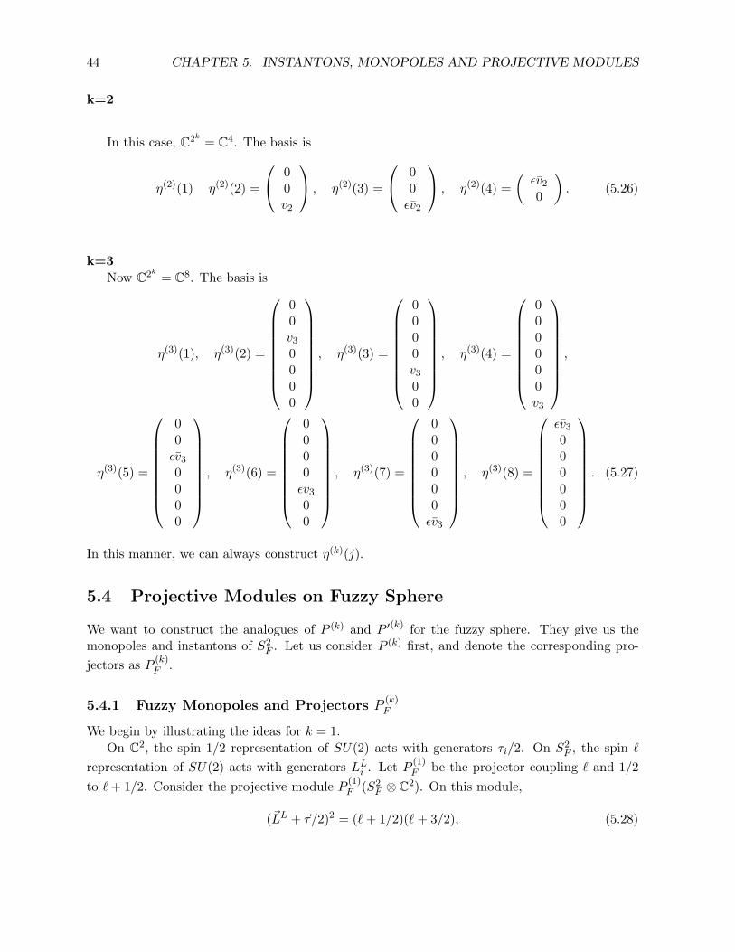
44 CHAPTER 5. INSTANTONS, MONOPOLES AND PROJECTIVE MODULES
k=2
In this case, C2k= C4. The basis is
η(2)(1) η(2)(2) =
00v2
, η(2)(3) =
00ǫv2
, η(2)(4) =
(ǫv20
). (5.26)
k=3
Now C2k= C8. The basis is
η(3)(1), η(3)(2) =
00v30000
, η(3)(3) =
0000v300
, η(3)(4) =
000000v3
,
η(3)(5) =
00ǫv30000
, η(3)(6) =
0000ǫv300
, η(3)(7) =
000000ǫv3
, η(3)(8) =
ǫv3000000
. (5.27)
In this manner, we can always construct η(k)(j).
5.4 Projective Modules on Fuzzy Sphere
We want to construct the analogues of P (k) and P ′(k) for the fuzzy sphere. They give us themonopoles and instantons of S2
F . Let us consider P (k) first, and denote the corresponding pro-
jectors as P(k)F .
5.4.1 Fuzzy Monopoles and Projectors P(k)F
We begin by illustrating the ideas for k = 1.
On C2, the spin 1/2 representation of SU(2) acts with generators τi/2. On S2F , the spin ℓ
representation of SU(2) acts with generators LLi . Let P(1)F be the projector coupling ℓ and 1/2
to ℓ+ 1/2. Consider the projective module P(1)F (S2
F ⊗ C2). On this module,
(~LL + ~τ/2)2 = (ℓ+ 1/2)(ℓ + 3/2), (5.28)
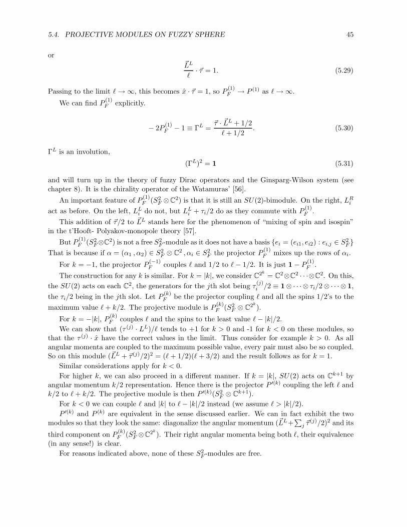
5.4. PROJECTIVE MODULES ON FUZZY SPHERE 45
or~LL
ℓ· ~τ = 1. (5.29)
Passing to the limit ℓ→∞, this becomes x · ~τ = 1, so P(1)F → P (1) as ℓ→∞.
We can find P(1)F explicitly.
− 2P(1)F − 1 ≡ ΓL =
~τ · ~LL + 1/2
ℓ+ 1/2. (5.30)
ΓL is an involution,
(ΓL)2 = 1 (5.31)
and will turn up in the theory of fuzzy Dirac operators and the Ginsparg-Wilson system (seechapter 8). It is the chirality operator of the Watamuras’ [56].
An important feature of P(1)F (S2
F ⊗C2) is that it is still an SU(2)-bimodule. On the right, LRiact as before. On the left, LLi do not, but LLi + τi/2 do as they commute with P
(1)F .
This addition of ~τ/2 to ~LL stands here for the phenomenon of “mixing of spin and isospin”in the t’Hooft- Polyakov-monopole theory [57].
But P(1)F (S2
F⊗C2) is not a free S2F -module as it does not have a basis ei = (ei1, ei2) : ei,j ∈ S2
FThat is because if α = (α1 , α2) ∈ S2
F ⊗ C2 , αi ∈ S2F the projector P
(1)F mixes up the rows of αi.
For k = −1, the projector P(−1)F couples ℓ and 1/2 to ℓ− 1/2. It is just 1− P (1)
F .
The construction for any k is similar. For k = |k|, we consider C2k= C2⊗C2 · · ·⊗C2. On this,
the SU(2) acts on each C2, the generators for the jth slot being τ(j)i /2 ≡ 1⊗ · · · ⊗ τi/2⊗ · · · ⊗ 1,
the τi/2 being in the jth slot. Let P(k)F be the projector coupling ℓ and all the spins 1/2’s to the
maximum value ℓ+ k/2. The projective module is P(k)F (S2
F ⊗ C2k).
For k = −|k|, P (k)F couples ℓ and the spins to the least value ℓ− |k|/2.
We can show that (τ (j) · LL)/ℓ tends to +1 for k > 0 and -1 for k < 0 on these modules, sothat the τ (j) · x have the correct values in the limit. Thus consider for example k > 0. As allangular momenta are coupled to the maximum possible value, every pair must also be so coupled.So on this module (~LL + ~τ (j)/2)2 = (ℓ+ 1/2)(ℓ + 3/2) and the result follows as for k = 1.
Similar considerations apply for k < 0.
For higher k, we can also proceed in a different manner. If k = |k|, SU(2) acts on Ck+1 byangular momentum k/2 representation. Hence there is the projector P ′(k) coupling the left ℓ andk/2 to ℓ+ k/2. The projective module is then P ′(k)(S2
F ⊗ Ck+1).
For k < 0 we can couple ℓ and |k| to ℓ− |k|/2 instead (we assume ℓ > |k|/2).P ′(k) and P (k) are equivalent in the sense discussed earlier. We can in fact exhibit the two
modules so that they look the same: diagonalize the angular momentum (~LL+∑
j ~τ(j)/2)2 and its
third component on P(k)F (S2
F ⊗C2k). Their right angular momenta being both ℓ, their equivalence
(in any sense!) is clear.
For reasons indicated above, none of these S2F -modules are free.
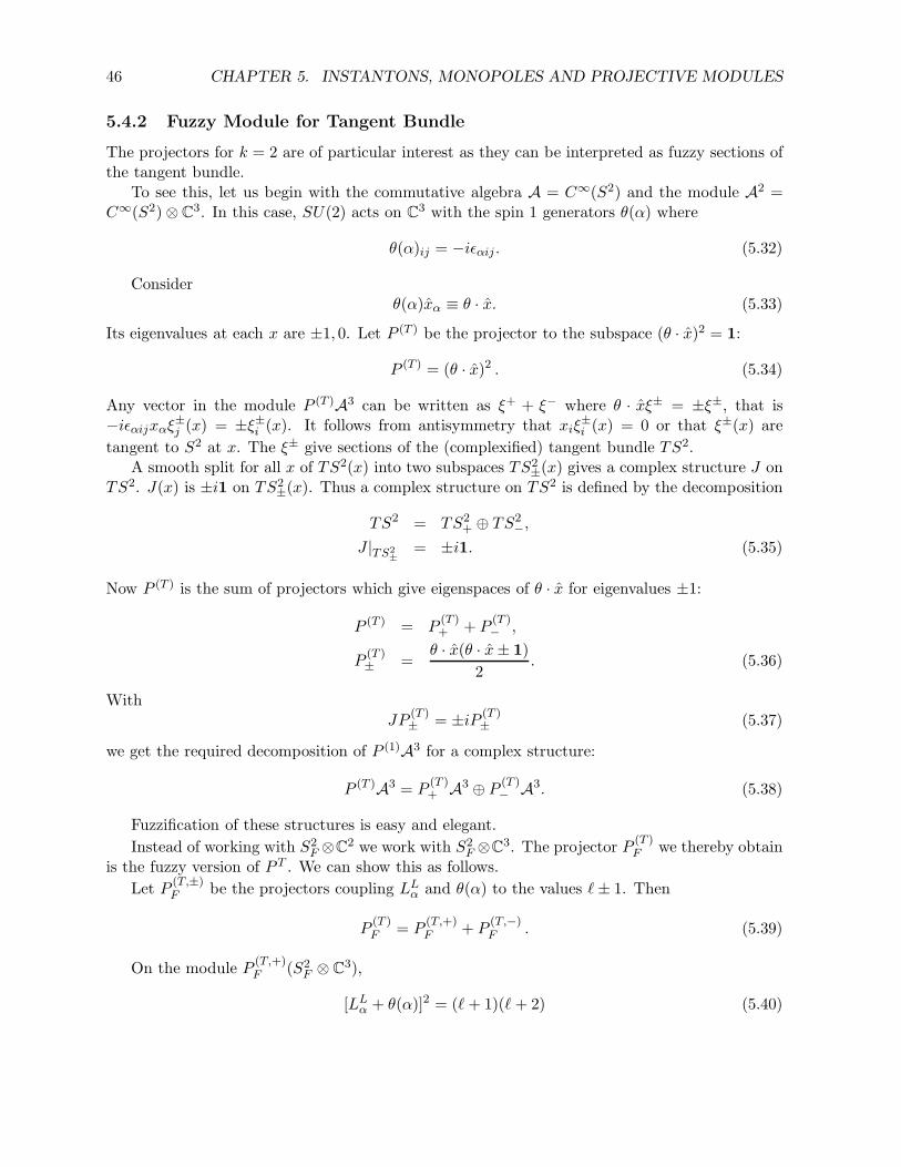
46 CHAPTER 5. INSTANTONS, MONOPOLES AND PROJECTIVE MODULES
5.4.2 Fuzzy Module for Tangent Bundle
The projectors for k = 2 are of particular interest as they can be interpreted as fuzzy sections ofthe tangent bundle.
To see this, let us begin with the commutative algebra A = C∞(S2) and the module A2 =C∞(S2)⊗C3. In this case, SU(2) acts on C3 with the spin 1 generators θ(α) where
θ(α)ij = −iǫαij . (5.32)
Considerθ(α)xα ≡ θ · x. (5.33)
Its eigenvalues at each x are ±1, 0. Let P (T ) be the projector to the subspace (θ · x)2 = 1:
P (T ) = (θ · x)2 . (5.34)
Any vector in the module P (T )A3 can be written as ξ+ + ξ− where θ · xξ± = ±ξ±, that is−iǫαijxαξ±j (x) = ±ξ±i (x). It follows from antisymmetry that xiξ
±i (x) = 0 or that ξ±(x) are
tangent to S2 at x. The ξ± give sections of the (complexified) tangent bundle TS2.A smooth split for all x of TS2(x) into two subspaces TS2
±(x) gives a complex structure J onTS2. J(x) is ±i1 on TS2
±(x). Thus a complex structure on TS2 is defined by the decomposition
TS2 = TS2+ ⊕ TS2
−,
J |TS2±
= ±i1. (5.35)
Now P (T ) is the sum of projectors which give eigenspaces of θ · x for eigenvalues ±1:
P (T ) = P(T )+ + P
(T )− ,
P(T )± =
θ · x(θ · x± 1)
2. (5.36)
WithJP
(T )± = ±iP (T )
± (5.37)
we get the required decomposition of P (1)A3 for a complex structure:
P (T )A3 = P(T )+ A3 ⊕ P (T )
− A3. (5.38)
Fuzzification of these structures is easy and elegant.
Instead of working with S2F ⊗C2 we work with S2
F ⊗C3. The projector P(T )F we thereby obtain
is the fuzzy version of P T . We can show this as follows.
Let P(T,±)F be the projectors coupling LLα and θ(α) to the values ℓ± 1. Then
P(T )F = P
(T,+)F + P
(T,−)F . (5.39)
On the module P(T,+)F (S2
F ⊗ C3),
[LLα + θ(α)]2 = (ℓ+ 1)(ℓ+ 2) (5.40)
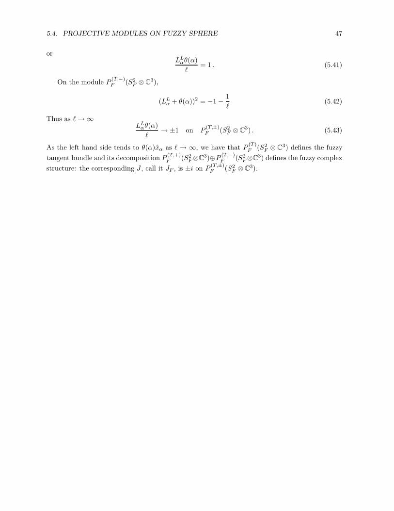
5.4. PROJECTIVE MODULES ON FUZZY SPHERE 47
orLLαθ(α)
ℓ= 1 . (5.41)
On the module P(T,−)F (S2
F ⊗ C3),
(LLα + θ(α))2 = −1− 1
ℓ(5.42)
Thus as ℓ→∞LLαθ(α)
ℓ→ ±1 on P
(T,±)F (S2
F ⊗ C3) . (5.43)
As the left hand side tends to θ(α)xα as ℓ → ∞, we have that P(T )F (S2
F ⊗ C3) defines the fuzzy
tangent bundle and its decomposition P(T,+)F (S2
F⊗C3)⊕P (T,−)F (S2
F⊗C3) defines the fuzzy complex
structure: the corresponding J , call it JF , is ±i on P(T,±)F (S2
F ⊗ C3).

48 CHAPTER 5. INSTANTONS, MONOPOLES AND PROJECTIVE MODULES
Chapter 6
Fuzzy Nonlinear Sigma Models
6.1 Introduction
In space-time dimensions larger than 2, whenever a global symmetry G is spontaneously brokento a subgroup H, and G and H are Lie groups, there are massless Nambu-Goldstone modes withvalues in the coset space G/H. Being massless, they dominate low energy physics as is the casewith pions in strong interactions and phonons in crystals. Their theoretical description containsnew concepts because G/H is not a vector space.
Such G/H models have been studied extensively in 2 − d physics, even though in that casethere is no spontaneous breaking of continuous symmetries. A reason is that they are oftentractable nonperturbatively in the two-dimensional context, and so can be used to test ideassuspected to be true in higher dimensions. A certain amount of numerical work has also beendone on such 2−d models to control conjectures and develop ideas, their discrete versions havingbeen formulated for this purpose.
This chapter develops discrete fuzzy approximations to G/H models. We focus on two-dimensional Euclidean quantum field theories with target space G/H = SU(N + 1)/U(N) =CPN . The novelty of this approach is that it is based on fuzzy physics [3] and non-commutativegeometry [25, 26, 27, 28, 29]. Although fuzzy physics has striking elegance because it preservesthe symmetries of the continuum and because techniques of non-commutative geometry give uspowerful tools to describe continuum topological features, still its numerical efficiency has notbeen fully tested. This chapter approaches σ-models with this in mind, the idea being to writefuzzy G/H models in a form adapted to numerical work.
This is not the only approach on fuzzy G/H. In [68], a particular description based onprojectors and their orbits was discretized. We shall refine that work considerably in this paper.Also in the continuum there is another way to approach G/H, namely as gauge theories withgauge invariance under H and global symmetry under G [59]. This approach is extended hereto fuzzy physics. Such a fuzzy gauge theory involves the decomposition of projectors in terms ofpartial isometries [55] and brings new ideas into this field. It is also very pretty. It is equivalentto the projector method as we shall also see.
Related work on fuzzy G/H model and their solitons is due to Govindarajan and Harikumar[60]. A different treatment, based on the Holstein-Primakoff realization of the SU(2) algebra,has been given in [61]. A more general approach to these models on noncommutative spaces was
49
50 CHAPTER 6. FUZZY NONLINEAR SIGMA MODELS
proposed in [62].
The first two sections describe the standard CP 1-models on S2. In section 2 we discuss itusing projectors, while in section 3 we reformulate the discussion in such a manner that transitionto fuzzy spaces is simple. Sections 4 and 5 adapt the previous sections to fuzzy spaces.
Long ago, general G/H-models on S2 were written as gauge theories [59]. Unfortunately theirfuzzification for generic G and H eludes us. Generalization of the considerations here to the casewhere S2 ≃ CP 1 is replaced with CPN , or more generally Grassmannians and flag manifoldsassociated with (N + 1) × (N + 1) projectors of rank ≤ (N + 1)/2, is easy as we briefly show inthe concluding section 6. But extension to higher ranks remains a problem.
6.2 CP 1 Models and Projectors
Let the unit vector x = (x1, x2, x3) ∈ R3 describe a point of S2. The field n in the CP 1-model isa map from S2 to S2:
n = (n1, n2, n3) : x→ n(x) ∈ R3, n(x) · n(x) :=
∑
a
na(x)2 = 1 . (6.1)
These maps n are classified by their winding number κ ∈ Z:
κ =1
8π
∫
S2
ǫabc na(x) dnb(x) dnc(x) . (6.2)
That κ is the winding of the map can be seen taking spherical coordinates (Θ,Φ) on the targetsphere (n2 = 1) and using the identity sin ΘdΘ dΦ = 1
2ǫabcnadnb dnc. We omit wedge symbols inproducts of forms.
We can think of n as the field at a fixed time t on a (2+1)-dimensional manifold where thespatial slice is S2. In that case, it can describe a field of spins, and the fields with κ 6= 0 describesolitonic sectors. We can also think of it as a field on Euclidean space-time S2. In that case, thefields with κ 6= 0 describe instantonic sectors.
Let τa be the Pauli matrices. Then each n(x) is associated with the projector
P (x) =1
2(1 + ~τ · ~n(x)) . (6.3)
Conversely, given a 2× 2 projector P (x) of rank 1, we can write
P (x) =1
2(α0(x) + ~τ · ~α(x)) . (6.4)
Using TrP (x) = 1, P (x)2 = P (x) and P (x)† = P (x), we get
α0(x) = 1, ~α(x) · ~α(x) = 1, α∗a(x) = αa(x) . (6.5)
Thus CP 1-fields on S2 can be described either by P or by na = Tr(τa P ) [63].
In terms of P , κ is
κ =1
2πi
∫
S2
TrP (dP ) (dP ) . (6.6)
6.2. CP 1 MODELS AND PROJECTORS 51
There is a family of projectors, called Bott projectors [64, 65] which play a central role in ourapproach. Let
z = (z1, z2), |z|2 := |z1|2 + |z2|2 = 1 . (6.7)
The z’s are points on S3. We can write x ∈ S2 in terms of z:
xi(z) = z†τiz (6.8)
The Bott projectors are
Pκ(x) = vκ(x)v†κ(z), vκ(z) =
[zκ1zκ2
]1√Zκ
if κ ≥ 0 ,
Zk ≡ |z1|2|κ| + |z2|2|κ| ,
vκ(z) =
[z∗|κ|1
z∗|κ|2
]1√Zκ
if κ < 0 . (6.9)
The field n(κ) associated with Pκ is given by
n(κ)a (x) = Tr τaPκ(x) = v†κ(z)τavκ(z) . (6.10)
Under the phase change z → zeiθ, vκ(z) changes vκ(z) → vκ(z)eiκθ, whereas x is invariant. As
this phase cancels in vκ(z)v†κ(z), Pκ is a function of x as written.
The κ that appears in eqs.(6.9)(6.10) is the winding number as the explicit calculation ofsection 3 will show. But there is also the following argument.
In the map z → vκ(z), for κ = 0, all of S3 and S2 get mapped to a point, giving zero windingnumber. So, consider κ > 0. Then the points
(z1e
i 2πκ
(l+m), z2ei 2π
κm), l,m ∈ 0, 1, .., κ − 1
have the same image. But the overall phase ei2πκm of z cancels out in x. Thus, generically κ points
of S2 (labeled by l) have the same projector Pκ(x), giving winding number κ. As for κ < 0, we get|κ| points of S2 mapped to the same Pκ(x). But because of the complex conjugation in eq.(6.9),there is an orientation-reversal in the map giving −|κ| = κ as winding numbers. One way to seethis is to use
P−|κ|(x) = P|κ|(x)T (6.11)
Substituting this in (6.6), we can see that P±|κ| have opposite winding numbers.
The general projector Pκ(x) is the gauge transform of Pκ(x):
Pκ(x) = U(x)Pκ(x)U(x)† (6.12)
where U(x) is a unitary 2 × 2 matrix. Its n(κ) is also given by (6.10), with Pκ replaced by Pκ.The winding number is unaffected by the gauge transformation. That is because U is a map fromS2 to U(2) and all such maps can be deformed to identity since π2(U(2)) = identity e.
The identity
Pκ(dPκ) = (dPκ)(1l− Pκ) (6.13)
52 CHAPTER 6. FUZZY NONLINEAR SIGMA MODELS
which follows from P2κ = Pκ, is valuable when working with projectors.
The soliton described by Pκ have the action (below) peaked at the north pole x3 = 1 orx1+ix21+x3
= 0 and a fixed width and shape. The solitons with energy density peaked at x1+ix21+x3
= ηand variable width and shape are given by the projectors
Pκ(x , η , λ) = vκ(z, η, λ)vκ(z, η, λ)†
vκ(z, η, λ) =
(λzκ1
zκ2 − ηzκ1
)1
(|λz1|2κ + |zκ2 − ηzκ1 |2)12
(6.14)
For κ > 0, they correspond to the choice
U(x) = vκ(z, η, λ)vκ(z)† (6.15)
in (6.12). We call the field associated with Pκ(., η, λ) as n(κ)(., η, λ):
n(κ)(x, λ, η) = vκ(z, η, λ)†vκ(z, η, λ) . (6.16)
We can use vκ(z, η, λ) = v|κ|(z, η, λ) to write the solitons for κ < 0.
6.3 An Action
Let Li = −i(x ∧ ∇)i be the angular momentum operator. Then a Euclidean action in the κ-thtopological sector for n(κ) (or a static Hamiltonian in the (2+1) picture) is
Sκ = − c2
∫
S2
dΩ (Lin(κ)b )(Lin(κ)
b ) , c = a positive constant, (6.17)
where dΩ is the S2 volume form d cos θ dϕ. We can also write
Sκ = −c∫
S2
dΩ Tr (LiPκ)(LiPκ) . (6.18)
The following identities, based on (6.13), are also useful:
Tr Pκ(LiPκ)2 = Tr (LiPκ)(1l − Pκ)(LiPκ) = Tr(1l− Pκ)(LiPκ)2 =1
2Tr(LiPκ)2 (6.19)
Hence
Sκ = −2c
∫
S2
dΩ TrPκ LiPκ LiPκ (6.20)
The Euclidean functional integral for the actions Sκ is
Z(ψ) =∑
κ
eiκψ∫DPκe−Sκ (6.21)
where the angle ψ is induced by the instanton sectors as in QCD.

6.4. CP 1-MODELS AND PARTIAL ISOMETRIES 53
Using the identity dP = −ǫijk dxi xj iLkP , we can rewrite the definition (6.2) or (6.6) of thewinding number as
κ =1
8π
∫
S2
dΩ ǫijkxi ǫabcn(κ)a iLjn(κ)
b iLkn(κ)c (6.22)
=1
2πi
∫
S2
dΩ TrPκ ǫijk xi iLjPκ iLkPκ . (6.23)
The Belavin-Polyakov bound [66]Sκ ≥ 4π c |κ| (6.24)
follows from (6.22) on integration of
(iLin(κ)a ± ǫijkxj ǫabc n(κ)
b iLkn(κ)c )2 ≥ 0 , (6.25)
or from (6.23) on integration of
Tr(Pκ(iLiPκ)± iǫijk xjPκ(iLkPκ)
)†(Pκ(iLiPκ)± iǫij′k′ xj′Pκ(iLk′Pκ))≥ 0 . (6.26)
From this last form it is easy to rederive the bound in a way better adapted to fuzzification.Using Pauli matrices σi we first rewrite (6.20) and (6.23) as
Sκ = c
∫
S2
dΩ Tr Pκ(iσ · LPκ)(iσ · LPκ) ,
κ =−1
4π
∫
S2
dΩ Tr(σ · xPk(iσ · LPk)(iσ · LPk)
). (6.27)
The trace is now over C2 × C2 = C4, where τa acts on the first C2 and σi on the second C2 (sothey are really τa ⊗ 1l and 1l⊗ σi) Then, with ǫ1, ǫ2 = ±1,
1 + ǫ2τ · n(κ)
2σi((iLiPκ) + ǫ1iǫijk xj(iLkPκ)
)= (1 + ǫ1σ · x)
1 + ǫ2τ · n(κ)
2(iσ · LPκ) , (6.28)
since x · L = 0. The inequality (6.26) is equivalent to
Tr
[1 + ǫ1σ · x
2
1 + ǫ2τ · n(κ)
2(iσ · LPκ)
]† [1 + ǫ1σ · x
2
1 + ǫ2τ · n(κ)
2(iσ · LPκ)
]≥ 0 , (6.29)
from which (6.24) follows by integration.
6.4 CP 1-Models and Partial Isometries
If P(x) is a rank 1 projector at each x, we can find its normalized eigenvector u(z):
P(x)u(z) = u(z) , u†(z)u(z) = 1 . (6.30)
ThenP(x) = u(z)u†(z) . (6.31)
54 CHAPTER 6. FUZZY NONLINEAR SIGMA MODELS
If P = Pκ, an example of u is vκ. u can be a function of z, changing by a phase under z → zeiθ.Still, P will depend only on x.
We can regard u(z)† (or a slight generalization of it) as an example of a partial isometry [55]in the algebra A = C∞(S3) ⊗C Mat2×2(C) of 2 × 2 matrices with coefficients in C∞(S3). Apartial isometry in a ∗−algebra A is an element U† ∈ A such that U U† is a projector; U U† is thesupport projector of U†. It is an isometry if U† U = 1l. With
U =
(u1 0u2 0
)∈ A, (6.32)
we haveP = U U† (6.33)
so that U† is a partial isometry.We will be free with language and also call u† as a partial isometry.The partial isometry for Pκ is v†κ.Now consider the one-form
Aκ = v†κ dvκ . (6.34)
Under zi → zieiθ(x), Aκ transforms like a connection:
Aκ → Aκ + iκ dθ
(Aκ are connections for U(1) bundles on S2 for Chern numbers κ, see later.) Therefore
Dκ = d+Aκ (6.35)
is a covariant differential, transforming under z → zeiθ as
Dκ → eiκθDκe−iκθ (6.36)
andD2κ = dAκ (6.37)
is its curvature.At each z, there is a unit vector wκ(z) perpendicular to vκ(z). An explicit realization of wκ(z)
is given bywκ,α = iτ2αβ v
∗κ,β := ǫαβ v
∗κ,β (6.38)
Since w†κvκ = 0,Bκ = w†κ dvκ , B∗κ = (dv†κ)wκ = −v†κ dwκ (6.39)
are gauge covariant,
Bκ(z)→ eiθ(x)Bκeiθ(x) , Bκ(z)
∗ → e−iθ(x)B∗κe−iθ(x) (6.40)
under z → zeiθ.We can account for U(x) by considering
Vκ = Uvκ , Aκ = V†κ dVκ , Dκ = d+Aκ , D2κ = dAκ ,
Wκ = (τ2U∗τ2)wκ , Bκ =W†κ dVκ . (6.41)
6.4. CP 1-MODELS AND PARTIAL ISOMETRIES 55
Aκ is still a connection, and the properties (6.40) are not affected by U . Pκ is the support
projector of V†κ, andWκW†κ = 1l− Pκ , (1l− Pκ)Vκ = 0 . (6.42)
Gauge invariant quantities being functions on S2, we can contemplate a formulation of theCP 1-model as a gauge theory. Let Ji be the lift of Li to angular momentum generators appro-priate for functions of z,
(eiθiJif)(z) = f(e−iθiτi/2z) , (6.43)
and letBκ,i =W†κ JiVκ . (6.44)
Now, WκBκ,iV†κ is gauge invariant, and should have an expression in terms of Pκ. Indeed it is, inview of (6.42),
WκBκ,iV†κ =WκW†κ(JiVκ)V†κ = (1l− Pκ)Ji(VκV†κ) = (1l− Pκ)(LiPκ) = (LiPκ)Pκ . (6.45)
Therefore we can write the action (6.18, 6.20) in terms of the Bκ,i:
Sκ = −2c
∫
S2
dΩ Tr Pκ(LiPκ)(LiPκ) = 2c
∫
S2
dΩ Tr ((LiPκ)Pκ)†((LiPκ)Pκ) =
= 2c
∫
S2
dΩ Tr(WκBκ,iV†κ)†(WκBκ,iV†κ) = 2c
∫
S2
dΩ B∗κ,iBκ,i . (6.46)
It is instructive also to write the gauge invariant (dAκ) in terms of Pκ and relate its integralto the winding number (6.6). The matrix of forms
Vκ(d+Aκ)V†κ (6.47)
is gauge invariant. HeredV†κ = (dV†κ) + V†κ d
where d in the first term differentiates only V†κ. Now
Vκ(d+ V†κ(dVκ))V†κand
Pκ dPκ = VκV†κ d (VκV†κ) = VκV†κ(dVκ)V†κ + Vκ(dV†κ) + VκV†κ d (6.48)
are equal. Hence, squaring
Vκ(d+Aκ)2V†κ = Vκ (dAκ)V†κ = Pκ (dPκ) (dPκ) (6.49)
on using d2 = 0, eq.(6.48) and Pκ(dPκ)Pκ = 0 . Thus∫
S2
(dAκ) =
∫
S2
Tr Vκ(dAκ)V†κ =
∫
S2
Tr Pκ (dPκ) (dPκ) . (6.50)
We can integrate the LHS. For this we write (taking a section of the bundle U(1) → S3 → S2
over S2\north pole(0, 0, 1)),
z(x) = e−iτ3ϕ/2e−iτ2θ/2e−iτ3ϕ/2(
10
)=
(e−iϕ cos θ2
sin θ2
). (6.51)
56 CHAPTER 6. FUZZY NONLINEAR SIGMA MODELS
Taking into account the fact that U(~x) is independent of ϕ at θ = 0, we get∫
S2
(dAκ) = −∫eiκϕ de−iκϕ = 2πiκ . (6.52)
This and eq.(6.50) reproduce eq.(6.6).The Belavin-Polyakov bound [66] for Sκ can now be got from the inequality
Tr C†κ,iCκ,i ≥ 0 , Cκ,i =WκBκ,iV†κ ±Wκ(ǫijlxjBκ,l)V†κ . (6.53)
6.4.1 Relation Between P(κ) and PκThe treatment in [68], for κ > 0, the fuzzy σ-model was based on the continuum projector
P (κ)(x) = P1(x)⊗ ...⊗ P1(x) =
κ∏
i=1
1
2(1 + τ (i) · x) (6.54)
and its unitary transform
P(κ)(x) = U (κ)(x)P (κ)(x)U (κ)(x)−1 , U (κ)(x) = U(x)⊗ ...⊗ U(x) (κ factors). (6.55)
At each x, the stability group of P (κ)(x) is U(1) with generator 12
∑κi=1 τ
(i) ·x, and we get a sphere
S2 as U(x) is varied. Thus U (κ)(x) gives a section of a sphere bundle over a sphere, leading usto identify P(κ) with a CP 1-field. Furthermore, the R.H.S. of eq.(6.50) (with P(κ) replacing Pκ)gives κ as the invariant associated with P(κ), suggesting a correspondence between κ and windingnumber.
We can writeP(κ) = V(κ)V(κ)† , V(κ) = V1 ⊗ ...⊗ V1 κ factors), (6.56)
its connection A(κ) and an action as previously. A computation similar to the one leading toeq.(6.50) shows that
− i
2π
∫dA(κ) = κ . (6.57)
So κ is the Chern invariant of the projective module associated with P(κ).For κ < 0, we must change x to −x in (6.54), and accordingly change other expressions.We note that κ cannot be identified with the winding number of the map x → Pκ(x). To
see this, say for κ > 0, we show that there is a winding number κ map from P(κ) to Pκ(x). Asthat is also the winding number of the map x→ Pκ(x), the map x→ P(κ)(x) must have windingnumber 1.
The map P(κ) → Pκ(x) is induced from the map
V(κ) → Vκ =
(V(κ)
11...1
V(κ)22...2
)(6.58)
and their expressions in terms of V(κ) and Vκ. In (6.58) all the pointsV(κ)(z1e
2πi j/κ, z2e2πi l/κ), j, l ∈ 0, 1, ..., κ − 1, have the same image, but in the passage to P(κ)
and Pκ the overall phase of z is immaterial. However, the projectors for V(κ)(z1e2πij/κ, z2) and
V†κ(z1, z2e2πij/κ) are distinct and map to the same Pκ, giving winding number κ.We have not understood the relation between the models based on P(κ) and Pκ.
6.5. FUZZY CP 1-MODELS 57
6.5 Fuzzy CP 1-Models
The advantage of the preceding formulation using zα is that the passage to fuzzy models isrelatively transparent. Thus let ξ = (ξ1, ξ2) ∈ C2\0. We can then identify z and x as
z =ξ
|ξ| , |ξ| =√|ξ1|2 + |ξ2|2 , xi = z†τiz . (6.59)
Quantization of the ξ’s and ξ∗’s consists in replacing ξα by annihilation operators aα and ξ∗αby a†α. |ξ| is then the square root of the number operator:
N = N1 + N2 , N1 = a†1a1 , N2 = a†2a2 ,
z†α =1√Na†α = a†α
1√N + 1
, zα =1√N + 1
aα = aα1√N,
xi =1√Na†τia . (6.60)
(We have used hats on some symbols to distinguish them as fuzzy operators).We will apply these operators only on the subspace of the Fock space with eigenvalue n ≥ 1
of N , where 1√N
is well-defined. This restriction is natural and reflects the fact that ξ cannot be
zero.
6.5.1 The Fuzzy Projectors for κ > 0
On referring to (6.9), we see that if κ > 0, for the quantized versions vκ, v†κ of vκ, v
∗κ, we have
vκ =
[aκ1aκ2
]1√Zκ
, v†κ =1√Zκ
[(a†1)
κ (a†2)κ], v†κvκ = 1l ,
Zκ = Z(1)κ + Z(2)
κ , Z(α)κ = Nα(Nα − 1)...(Nα − κ+ 1) .. (6.61)
The fuzzy analogue of U is a 2 × 2 unitary matrix U whose entries Uij are polynomials in
a†aab. As for Vκ, the quantized version of Vκ, it is just
Vκ = U vκ (6.62)
and fulfillsV†κ Vκ = 1l , (6.63)
V†κ being the quantized version of V†κ. We thus have the fuzzy projectors
Pκ = vκ v†κ , Pκ = Vκ V†κ . (6.64)
Unlike vκ, Vκ and their adjoints, Pκ and Pκ commute with the number operator N . So wecan formulate a finite-dimensional matrix model for these projectors as follows. Let Fn be thesubspace of the Fock space where N = n. It is of dimension n + 1, and carries the SU(2)representation with angular momentum n/2, the SU(2) generators being
Li =1
2a†τia . (6.65)
58 CHAPTER 6. FUZZY NONLINEAR SIGMA MODELS
Its standard orthonormal basis is |n2 ,m > , m = −n2 ,−n
2 +1, ..., n2 . Now consider Fn⊗CC2 := F (2)n ,
with elements f = (f1, f2), fa ∈ Fn. Then Pκ, Pκ act on F (2)n in the natural way. For example
f → Pκf, (Pκf)a = (Pκ)abfb = (Vκ,aV†κ,b)fb . (6.66)
We can now write explicit matrices for Pκ and Pκ. We have:
Pκ =
(aκ1
1Zκa†κ1 aκ1
1Zκa†κ2
aκ21Zκa†κ1 aκ2
1Zκa†κ2
), (6.67)
aκ11
Zκ=
1
(N1 + κ)...(N1 + 1) + Z(2)κ
aκ1 , aκ1a†κ1 = (N1 + κ)...(N1 + 1) ,
from which its matrix Pκ(n) for N = n can be obtained.
The matrix Pκ is the unitary transform U Pκ(n)U † where U is a 2× 2 matrix and Uab is itselfan (n+ 1)× (n+ 1) matrix. As for the fuzzy analogue of Li, we define it by
LiPκ = [Li, Pκ] . (6.68)
The fuzzy action
SF,κ(n) =c
2(n + 1)TrN=n (LiPκ)†(LiPκ) , c = constant , (6.69)
follows, the trace being over the space F (2)n .
6.5.2 The Fuzzy Projector for κ < 0 .
For κ < 0, following an early indication, we must exchange the roles of aa and a†a.
6.5.3 Fuzzy Winding Number
In the literature [67], there are suggestions on how to extend (6.6) to the fuzzy case. They donot lead to an integer value for this number except in the limit n→∞.
There is also an approach to topological invariants using Dirac operator and cyclic cohomology.Elsewhere this approach was applied to the fuzzy case [68, 69] and gave integer values, and evena fuzzy analogue of the Belavin-Polyakov bound. However they were not for the action SF,κ, butfor an action which approaches it as n→∞. In the subsection below, we present an alternativeapproach to this bound which works for SF,κ. It looks like (6.24), except that κ becomes aninteger only in the limit n→∞.
There is also a very simple way to associate an integer to Vκ [67, 73, 69]. It is equivalent tothe Dirac operator approach. We can assume that the domain of Vκ are vectors with a fixed valuen of N . Then after applying Vκ, n becomes n − κ if κ > 0 and n + |κ| is κ < 0.Thus κ is justthe difference in the value of N , or equivalently twice the difference in the value of the angularmomentum, between its domain and its range.
We conclude this section by deriving the bound for SF,κ(n).
6.5. FUZZY CP 1-MODELS 59
6.5.4 The Generalized Fuzzy Projector : Duality or BPS States
We introduced the projectors Pκ(·, η, λ) and their fields n(κ)(·, η, λ) earlier. They describe solitonslocalized at x1+ix2
1+x3= η and a shape and width controlled by λ. As inspection shows, they are
very easy to quantize by replacing ξi by ai and ξj by a†j.
The fields n(κ)(·, η, λ) and their projectors Pκ(·, η, λ) have a particular significance. P|κ|(·, η, λ)saturates the bounds (6.26) with the plus sign, P−κ(·, η, λ) saturates it with the minus sign.This result is due to their holomorphicity (anti-holomorphicity) properties as has been explainedelsewhere [53].
It is very natural to identify their fuzzy versions as fuzzy BPS states. But as we note below,they do not saturate the bound on the fuzzy action.
6.5.5 The Fuzzy Bound.
A proper generalization of the Belavin-Polyakov bound to its fuzzy version involves a slightlymore elaborate approach. This is because the straightforward fuzzification of ~σ · ~x and ~τ · ~n(κ)
and their corresponding projectors do not commute, and the product of such fuzzy projectors isnot a projector. We use this elaborated approach only in this section. It is not needed elsewhere.In any case, what is there in other sections is trivially adapted to this formalism.
The operators a†αaβ acting on the vector space with N = n generate the algebra Mat(n + 1)of (n+ 1)× (n+ 1) matrices. The extra structure comes from regarding them not as observables,but as a Hilbert space of matrices m, m′, ... with scalar product (m′,m) = 1
n+1 TrCn+1 m′† m,with the observables acting thereon.
To each α ∈Mat(n+1), we can associate two linear operators αL,R on Mat(n+1) accordingto
αLm = αm , αRm = mα , m ∈ Mat(n+ 1) . (6.70)
αL − αR has a smooth commutative limit for operators of interest. It actually vanishes, andαL,R → 0 if α remains bounded during this limit.
Consider the angular momentum operators Li ∈Mat(n+ 1). The associated ‘left’ and ‘right’angular momenta LL,Ri fulfil
(LLi )2 = (LRi )2 =n
2(n
2+ 1) . (6.71)
We now regard aα, a†α of section 6.5.1 as left operators aLα and a†Lα . PLκ thus becomes a
2 × 2 matrix with each entry being a left multiplication operator. It is the linear operatorPLκ on Mat(n + 1) ⊗ C2. We tensor this vector space with another C2 as before to get H =Mat(n+1)⊗C2⊗C2, with σi acting on the last C2, and σ ·LPLκ denoting the operator σi(LiPκ)L.
We can repeat the previous steps if there are fuzzy analogues γ and Γ of continuum ‘worldvolume’ and ‘target space’ chiralities ~σ · ~x and ~τ · ~n(κ) which mutually commute. Then 1
2(1± γ),12(1±Γ) are commuting projectors and the expressions derived at the end of Section 3 generalize,as we shall see.
There is such a γ, due to Watamuras[56], and discussed further by [68]. Following [68], wetake
γ ≡ γL =2σ · LL + 1
n+ 1. (6.72)
The index L has been put to emphasize its left action on Mat(n+ 1).
60 CHAPTER 6. FUZZY NONLINEAR SIGMA MODELS
As for Γ, we can do the following. Pκ acts on the left on Mat(n+ 1), let us call it PLκ . It hasa PRκ acting on the right and an associated
Γ ≡ ΓRκ = 2PRκ − 1 , (ΓRκ )2 = 1 . (6.73)
As it acts on the right and involves τ ’s while γ acts on the left and involves σ’s,
γLΓRκ = ΓRκ γL . (6.74)
The bound for (6.69) now follows from
TrH
(1 + ǫ1γ
L
2
1 + ǫ2ΓRκ
2σ · LPLκ
)†(1 + ǫ1γ
L
2
1 + ǫ2ΓRκ
2σ · LPLκ
)≥ 0 (6.75)
(ǫ1, ǫ2 = ±1), and reads
SF,κ =c
4(n+ 1)TrH(σ · LPLκ )†(σ · LPLκ )
≥ c
4(n+ 1)TrH
((ǫ1γ
L + ǫ2ΓRκ )(σ · LPLκ )(σ · LPLκ )
)
+c
4(n+ 1)TrH
(ǫ1ǫ2γ
LΓR(σ · LPLκ )(σ · LPLκ ))
(6.76)
The analogue of the first term on the R.H.S. is zero in the continuum, being absent in (6.24), butnot so now. As n → ∞, (6.76) reproduces (6.24) to leading order n, but has corrections whichvanish in the large n limit.
A minor clarification: if τ ’s are substituted by σ’s in 2PL1 − 1, then it is γL. The differentprojectors are thus being constructed using the same principles.
6.6 CPN -Models
We need a generalization of the Bott projectors to adapt the previous approach to all CPN .
Fortunately this can be easily done. The space CPN is the space of (N + 1) × (N + 1) rank1 projectors. The important point is the rank. So we can write
CPN = 〈U (N+1)P0U(N+1)† : P0 = diag. (0, ...., 0, 1)︸ ︷︷ ︸
N+1 entries
U (N+1) ∈ U(N + 1)〉 . (6.77)
As before, let z = (z1, z2), |z1|2 + |z2|2 = 1, and xi = z†τiz. Then we define
v(N)κ (z) =
zκ1zκ20..0
1√Zκ
, κ > 0 ; v(N)κ (z) =
z∗κ1z∗κ20..0
1√Zκ
, κ < 0 . (6.78)
6.6. CPN -MODELS 61
Since
v(N)κ (z)†v(N)
κ (z) = 1 ,
P (N)κ (x) = v(N)
κ (z)v(N)κ (z)† ∈ CPN . (6.79)
We can now easily generalize the previous discussion, using P(N)κ for Pκ and U (N+1) for U ,
and subsequently quantizing zα, z∗α. In that way we get fuzzy CPN -models.
CPN -models can be generalized by replacing the target space by a general Grassmannian ora flag manifold. They can also be elegantly formulated as gauge theories [59]. But we are able toformulate only a limited class of such manifolds in such a way that they can be made fuzzy. Thenatural idea would be to look for several vectors
v(N)(i)ki
(z) , i = 1, .., N (6.80)
in (N + 1)-dimensions which are normalized and orthogonal,
v(N)(i)†ki
(z)v(N)(j)kj
(z) = δij (6.81)
and have the equivariance property
v(N)(i)ki
(zeiθ) = v(N)(i)ki
(z)ei kiθ . (6.82)
The orbit of the projector∑M
i=1 v(N)(i)ki
(z)v(N)(i)†ki
(z) under U (N+1) will then be a Grassmannian
for each M ≤ N , while the orbit of∑
i λiv(N)(i)ki
(z)v(N)(i)†ki
(z) with possibly unequal λi under
U (N+1) will be a flag manifold.
But we can find such v(N)(i)ki
only for i = 1, 2, ...,M ≤ N+12 .
For instance in an (N + 1) = 2L-dimensional vector space, for integer L, we can form thevectors
v(N)(1)k1
(z) =
zk11
zk12
0·0
1√Zk1
, v(N)(2)k2
(z) =
00
zk21
zk22
0·0
1√Zk2
, ... , v(N)(L)kL
(z) =
0·0
zkL1
zkL
2
1√ZkL
(6.83)
for ki > 0. For those ki which are negative, we replace v(N)(i)ki
(z) here by v(N)(i)|ki| (z)∗:
v(N)(i)ki
(z) = v(N)(i)|ki| (z)∗ , ki < 0 . (6.84)
These v(N)(i)ki
are orthonormal for all z with∑
α |zα|2 = 1, so that we can handle Grassmanniansand flag manifolds involving projectors up to rank L.
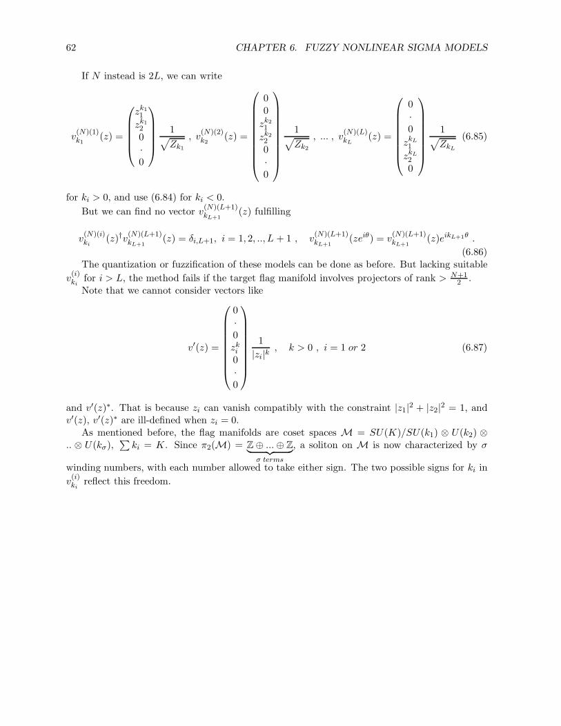
62 CHAPTER 6. FUZZY NONLINEAR SIGMA MODELS
If N instead is 2L, we can write
v(N)(1)k1
(z) =
zk11
zk12
0·0
1√Zk1
, v(N)(2)k2
(z) =
00
zk21
zk22
0·0
1√Zk2
, ... , v(N)(L)kL
(z) =
0·0
zkL1
zkL
2
0
1√ZkL
(6.85)
for ki > 0, and use (6.84) for ki < 0.
But we can find no vector v(N)(L+1)kL+1
(z) fulfilling
v(N)(i)ki
(z)†v(N)(L+1)kL+1
(z) = δi,L+1, i = 1, 2, .., L + 1 , v(N)(L+1)kL+1
(zeiθ) = v(N)(L+1)kL+1
(z)eikL+1θ .
(6.86)The quantization or fuzzification of these models can be done as before. But lacking suitable
v(i)ki
for i > L, the method fails if the target flag manifold involves projectors of rank > N+12 .
Note that we cannot consider vectors like
v′(z) =
0·0zki0·0
1
|zi|k, k > 0 , i = 1 or 2 (6.87)
and v′(z)∗. That is because zi can vanish compatibly with the constraint |z1|2 + |z2|2 = 1, andv′(z), v′(z)∗ are ill-defined when zi = 0.
As mentioned before, the flag manifolds are coset spaces M = SU(K)/SU(k1) ⊗ U(k2) ⊗.. ⊗ U(kσ),
∑ki = K. Since π2(M) = Z⊕ ...⊕ Z︸ ︷︷ ︸
σ terms
, a soliton on M is now characterized by σ
winding numbers, with each number allowed to take either sign. The two possible signs for ki in
v(i)ki
reflect this freedom.
Chapter 7
Fuzzy Gauge Theories
Gauge transformations on commutative spaces are based on transformations which depend onspace-time points P . Thus if G is a conventional global group, the associated gauge group is thegroup of maps G from space-time to G, the group multiplication being point-wise multiplication.For each irreducible representation (IRR) σ of G, there is an IRR Σ of G given by Σ(g ∈ G)(p) =σ(g(p)). The construction works for any connected Lie groupG. There is no problem in composingrepresentations of G either: if Σi are representations of G associated with representations of σiof G, then we can define the representations Σ1⊗Σ2 which has the same relation to σ1 ⊗ σ2 thatΣi have to σi: Σ1⊗Σ2(g)(p) = [σ1 ⊗ σ2](g(p)) = σ1(g(p)) ⊗ σ2(g(p)). Thus such products of Σare defined using those of G at each p. Existence of these products is essential to describe gaugetheories of particles and fields transforming by different representations of G.
An additional point of significance is that there is no condition on G, except that it is acompact connected Lie group.
For general noncommutative manifolds, several of these essential features of G are absent.Thus in particular
• Noncommutative manifolds require G to be a U(N) group,
• Only a very limited and quite inadequate number of representations of the gauge group canbe defined.
We shall illustrate these points below for the fuzzy gauge groups GF based on S2F , but one
can see the generalities of the considerations.
There is an important map, the Seiberg-Witten(SW), map for a noncommutative deformationof RN . In that case the deformed algebra RN
θ depends continously on a parameter θ, becomingthe commutative algebra for θ = 0. If a certain gauge group on RN
θ is Gθ, it becomes a standardgauge group G0 on RN
0 = RN . The SW map is based on a homomorphism from RNθ to RN
0
and connects gauge theories for different θ. The aforementioned problems can be more or lessovercome on RN
θ using this map.
But fuzzy spheres have no continuous parameter like θ. What plays the role of θ is 1L where
2L is the cut-off angular momentum, and 1L assumes discrete values. Fuzzy spheres have no SW
map as originally conceived, and we can not circumvent its gauge-theoretic problems along thelines for RN
θ .
63
64 CHAPTER 7. FUZZY GAUGE THEORIES
There is however a complementary positive feature of fuzzy spaces. While S2F for example
presents problems in describing particles of charge 13 and 2
3 at the same time (because we cannot “tensor” representations of the fuzzy U(1) gauge group GF (U(1))), we can describe particleswith differing magnetic charges. The projective modules for all magnetic charges were alreadyexplained in Chapter 5 and 6. There is no symmetry (“duality”) here between electric andmagnetic charges.
7.1 Limits on Gauge Groups
The conditions on gauge groups on the fuzzy sphere arise algebraically. They can be understoodat the Lie algebraic level.
If λa are the basis for the Lie algebra of G in a representation σ, the Lie algebra of GF , thefuzzy gauge group of G are generated by
λaξa (7.1)
where ξa are (2L+ 1)× (2L+ 1) matrices. ξa become functions on S2 in the large L-limit.
Now consider the commutator
[λaξa , λbηb] , ηb = (2L+ 1)× (2L+ 1) matrix (7.2)
of two such Lie algebra elements. We get
[λa , λb]ξaηb + λaλb[ξa , ηb] = iCcabξaηbλc + λaλb[ξa , ηb] ,
Ccab = structure constants of the Lie algebra of G . (7.3)
Since Ccabξaηb ∈ S2F , the first term is of the appropriate form for a fuzzy gauge group of G. But
the last term is not, it involves λaλb which is a product of two generators. By taking repeatedcommutators, we will generate products of all orders and their commutators. If σ is irreducibleand of dimension d, we will get all the d × d hermitian matrices this way and not just the λa.That means that the fuzzy gauge group is that of U(d).
In the commutative limit, [ξa , ηb] is zero and this problem does not occur.
This escalation of the gauge group to U(d) is difficult to control. No convincing proposal tominimize its effect exists. [But see [71]].
In any case, U(d) gauge theories without matter fields can be consistently formulated on fuzzyspheres.
For applications, there is one mitigating circumstance: In the standard model, if we gaugejust SU(3)C and U(1)EM , namely the SU(3) of colour and U(1) of electromagnetism, the groupis actually U(3) [72]. Likewise, the weak group is not SU(2)×U(1), but U(2). Thus gauge fieldswithout matter in these sectors can be studied on fuzzy spheres.
Unfortunately, this does not mean that these gauge theories can be formulated satisfactorilyon S2
F or (for a four-dimensional continuum limit) on S2F × S2
F say, when quarks and leptons areincluded. For example with different flavours, different charges like 2/3 and −1/3 occur, and thereis no good way to treat arbitrary representations of gauge groups in noncommutative geometry[71]. We explain this problem now.
7.2. LIMITS ON REPRESENTATIONS OF GAUGE GROUPS 65
7.2 Limits on Representations of Gauge Groups
For the fuzzy U(d) gauge group on fuzzy sphere S2F (2L+ 1), we consider S2
F (2L+ 1)⊗ Cd. Thefuzzy U(d) gauge group U(d)F consists of d×d matrices U with coefficients in S2
F (2L+1) : Uij ∈S2F (2L + 1). The U(d)F can act in three different ways on S2
F (2L + 1) ⊗ Cd : on left, right andboth:
i. Left action : U → UL where ULX = UX for X ∈ S2F (2L+ 1)⊗ Cd ,
ii. Right action : U → (U †)R : (U †)RX = xU † ,
iii. Adjoint action : U → AdU : AdU X = UxU † .
If i . gives representation Λ, then ii . is its complex conjugate λ∗ and iii . is its adjoint representationAdλ. We are guaranteed that these representations can always be constructed.
But can we construct other representations such as the one corresponding to Σ1⊗Σ2? Theanswer appears to be no.
The reason is as follows ⊗ is not the tensor product ⊗. In Σ ⊗ Σ, we get functions of twovariables p and q: (Σ(g)⊗Σ(g))(p, q) = σ(g(p))⊗σ(g(q)). We must restrict (Σ(g)⊗Σ(g)) to thediagonal points (p, p) to get ⊗.
In noncommutative geometry, the tensor product Λ1⊗Λ2 exists of course since Λ1(U)⊗Λ2(U)is defined, and gives a representation of U(d)F . But noncommutative geometry has no sharppoints. That obstructs the construction of an analogue of diagonal points, or the restriction of ⊗to an analogue of ⊗.
There exist proposals [71] to get around this problem using Higgs fields.
7.3 Connection and Curvature
As a convention we choose the gauge potential to act on the left of S2F (2L + 1) ⊗ Cd. So the
components of the gauge potentials are
ALi = (ALi )aλa , (ALi )a ∈ S2F (2l + 1) . (7.4)
where λa , (a = 1 , · · · , d2) are the d× d basis matrices for the Lie algebra of U(d). They can bethe Gell-Mann matrices.
The covariant derivative ∇ is then the usual one:
∇i = Li +ALi (7.5)
The curvature is
Fij = [∇i ,∇j ]− iεijk∇k= [Li ,Lj ] + LiALj − LjALi + [ALi , A
Lj ]− iεijk(Lk +ALk )
= LiALj − LjALi + [ALi , ALj ]− iεijkALk . (7.6)
The subtraction of iεijk∇k is needed to cancel the [Li ,Lj] term in [∇i ,∇j].
66 CHAPTER 7. FUZZY GAUGE THEORIES
There is one important condition on ∇i. On S2, AL becomes a commutative gauge field aand its components ai have to be tangent to S2:
xiai = 0 . (7.7)
We need a condition on ∇i which becomes this condition for large L.
A simple condition of such a nature is due to Nair and Polychronakos [74] and reads
(LLi +ALi )2 = L(L+ 1) . (7.8)
This is compatible with gauge invariance. Its expansion is
LLi ALi +ALi L
Li +ALi A
Li = 0 . (7.9)
We have thatAL
i
L → 0 as L→∞. Dividing (7.9) by L and passing to the limit, we thus get (7.7).
The fuzzy Yang-Mills action is
SF =1
4e2TrF 2
ij + λ(∇2i − L(L+ 1)) , λ ≥ 0 , (7.10)
where the second term is a Lagrange multiplier: it enforces the constraint (7.8) as λ→∞.
7.4 Instanton Sectors
The above action is good in the sector with no instantons. But U(d) gauge theories on S2 haveinstantons, or equivalently, twisted U(1)-bundles on S2. We outline how to incorporate instantonson the fuzzy sphere, taking d = 1 for simplicity.
The projective modules for instanton sectors were constructed previously. We review it brieflyconstructing the modules in a different (but Morita equivalent) manner.
The instanton sectors on S2 correspond to U(1) bundles thereon. To build the correspondingprojective module for Chern number 2T ∈ Z+, introduce C2T+1 carrying the angular momentumT representation of SU(2). Let Ti be the angular momentum operators in this representationwith standard commutation relations. Let Mat(2L + 1) ⊗ C(2T+1) ≡ Mat(2L + 1)(2T+1). Welet PL+T be the projector coupling left angular momentum operators LL and T to producemaximum angular momentum L+ T . Then the projective module PL+TMat(2L + 1)(2T+1) is afuzzy analogue of sections of U(1) bundles on S2 with Chern number 2T > 0 [68]. If instead wecouple LL and T to produce the least angular momentum L− T using the projector PL−T , thenthe projective module PL−TMat(2L+ 1)(2T+1) corresponds to Chern number −2T . (We assumethat L ≥ T ).
The derivation Li does not commute with PL±T and has no action on these modules. But,Ji = Li + Ti does commute with PL±T . Thus Li must be replaced with Ji in further consider-ations. Ji is to be considered the total angular momentum . The addition of Ti to Li here isthe algebraic analogue of “mixing of spin and isospin”. [58, 57]. It is interesting that the mixingof ‘spin and isospin’ occurs already in our finite-dimensional matrix model and does not neednoncompact spatial slices and spontaneous symmetry breaking.
7.5. THE PARTITION FUNCTION AND THE θ-PARAMETER 67
We must next gauge Ji. In the zero instanton sector, the fuzzy gauge fields ALi were functionsof LLi . But that is not possible now since ALi does not commute with PL±T . Instead we require
ALi to be a function of ~LL + ~T and write for the covariant derivative
∇i = Ji +ALi . (7.11)
When L→∞, ~T can be ignored, and then ALi becomes a function of just x as we want.The transversality condition must be modified. It is now
(LLi + Ti +ALi )2 = (LLi + Ti)2 (7.12)
where(LLi + Ti)
2 = (L± T )(L± T + 1) (7.13)
on PL±TMat(2L+ 1)(2T+1).The curvature Fij and the action SF are as in (7.6) and (7.10).
7.5 The Partition Function and the θ-parameter
Existence of instanton bundles on a commutative manifold brings in a new parameter, generallycalled θ as, in QCD. The partition function Zθ depends on θ.
Let us denote the action in the instanton number K ∈ Z sector by SKF . Then
Zθ =∑
k
∫DALi e
−SKF +iKθ . (7.14)
We thus have a matrix model for U(d) gluons.In the continuum, K can be written as the integral of curvature trF (where trace tr (with
lower case t) is over the internal indices). In four dimensions it is the integral of trF ∧ F . Buton S2
F , TrεijFij is not an integer. A similar difficulty arises for S2F × S2
F or CP 2.In continuum gauge theory, F and F∧F play a role in discussions of chiral symmetry breaking.
They arise as the local anomaly term in the continuity equation for chiral current. Thereforealthough Zθ defines the theory, it is still helpful to have fuzzy analogues of the topological densitiestrF and trF ∧ F .
It is possible to construct fuzzy topological densities using cyclic cohomology [25]. We willnot review cyclic cohomology here.

68 CHAPTER 7. FUZZY GAUGE THEORIES
Chapter 8
The Dirac Operator and AxialAnomaly
8.1 Introduction
The Dirac operator is central for fundemental physics. It is also central in noncommutativegeometry. In Connes’ approach [25], it is possible to formulate metrical, differential geometricand bundle-theoretic ideas using the Dirac operator in a form generalisable to noncommutativemanifolds.
In this chapter, we explain the theory of the fuzzy Dirac operator basing it on the Ginsparg-Wilson (GW) algebra [75]. This algebra appeared first in the context of lattice gauge theories asa device to write the Dirac operator overcoming the well-known fermion-doubling problem. Thesame algebra appears naturally for the fuzzy sphere. The theory of the fuzzy Dirac operator canbe based on this algebra. It has no fermion doubling and correctly and elegantly reproduces theintegrated U(1)A-(axial) anomaly.
Incidentally the association of the GW-algebra with the fuzzy sphere is surprising as the latteris not designed with this algebra in mind.
Below we review the GW-algebra in its generality. We then adapt it to S2F . Our discussion
here closely follows [76].
8.2 A Review of the Ginsparg-Wilson Algebra.
In its generality, the Ginsparg-Wilson algebra A can be defined as the unital ∗-algebra over C
generated by two ∗-invariant involutions Γ and Γ′:
A =⟨Γ,Γ′ : Γ2 = Γ′2 = 1l, Γ∗ = Γ, Γ′∗ = Γ′
⟩, (8.1)
∗ denoting the adjoint. The unity of A has been indicated by 1l.
In any such algebra, we can define a Dirac operator
D′ =1
aΓ(Γ + Γ′) , (8.2)
69
70 CHAPTER 8. THE DIRAC OPERATOR AND AXIAL ANOMALY
where a is the “lattice spacing”. It fulfills
D′∗ = ΓD′ Γ, Γ,D′ = aD′ ΓD′ . (8.3)
(8.2) and (8.3) give the original formulation [75]. But they are equivalent to (8.1), since (8.2) and(8.3) imply that
Γ′ = Γ(aD′)− Γ (8.4)
is a ∗-invariant involution [79] [77].
Each representation of (8.1) is a particular realization of the Ginsparg-Wilson algebra. Rep-resentations of physical interest are reducible.
Here we choose
D =1
a(Γ + Γ′) , (8.5)
instead of D′ as our Dirac operator, as it is self-adjoint and has the desired continuum limit.
From Γ and Γ′, we can construct the following elements of A:
Γ0 =1
2Γ,Γ′ , (8.6)
Γ1 =1
2(Γ + Γ′) , (8.7)
Γ2 =1
2(Γ− Γ′) , (8.8)
Γ3 =1
2i[Γ,Γ′] . (8.9)
Let us first look at the centre C(A) of A in terms of these operators. It is generated by Γ0
which commutes with Γ and Γ′ and hence with every element of A . Γ2i , i = 1, 2, 3 also commute
with every element of A, but they are not independent of Γ0. Rather,
Γ21 =
1
2(1l + Γ0) , (8.10)
Γ22 =
1
2(1l− Γ0) , (8.11)
→ Γ21 + Γ2
2 = 1l , (8.12)
Γ20 + Γ2
3 = 1l . (8.13)
Notice also that
Γi,Γj = 0 , i, j = 1, 2, 3, i 6= j . (8.14)
From now on by A we will mean a representation of A.
The relations (8.10)-(8.13) contain spectral information. From (8.13) we see that
− 1 ≤ Γ0 ≤ 1 , (8.15)
where the inequalities mean that the eigenvalues of Γ0 are accordingly bounded. By (8.10), thisimplies that the eigenvalues of Γ1 are similarly bounded.
We now discuss three cases associated with (8.15).
8.2. A REVIEW OF THE GINSPARG-WILSON ALGEBRA. 71
Case 1 :
Γ0 = 1l. Call the subspace where Γ0 = 1l as V+1. On V+1, Γ21 = 1l and Γ2 = Γ3 = 0 by
(8.10-8.13). This is subspace of the top modes of the operator |D|.
Case 2 :
Γ0 = −1l. Call the subspace where Γ0 = −1l as V−1. On V−1, Γ22 = 1l and Γ1 = Γ3 = 0 by
(8.10-8.13). This is the subspace of zero modes of the Dirac operator D.
Case 3 :
Γ20 6= 1l. Call the subspace where Γ2
0 6= 1l as V . On this subspace, Γ2i 6= 0 for i = 1, 2, 3 by
(8.9-8.12), and therefore
signΓi =Γi|Γi|
, |Γi| = positive square root of Γ2i (8.16)
are well defined and by (8.14) generate a Clifford algebra on V :
signΓi, signΓj = 2δij . (8.17)
Consider Γ2. It anticommutes with Γ1 and D. Also
Tr Γ2 = (TrV + TrV+1 + TrV−1)Γ2 , (8.18)
where the subscripts refer to the subspaces over which the trace is taken. These traces can becalculated:
TrV Γ2 = TrV (signΓi)Γ2(signΓi) (i fixed, 6= 2)
= −TrV Γ2 by(8.17)
= 0, (8.19)
TrV+1 Γ2 = 0, as Γ2 = 0 on V+1 . (8.20)
So
Tr Γ2 = TrV−1 Γ2 = TrV−1(1 + Γ2
2− 1− Γ2
2) = index of Γ1 . (8.21)
Following Fujikawa [77], we can use Γ2 as the generator of chiral transformations. It is notinvolutive on V ⊕ V+1
Γ22 = 1l− 1l + Γ0
2. (8.22)
But this is not a problem for fuzzy physics. In the fuzzy model below, in the continuum limit,Γ0 → −1l on all states with |D| ≤ a fixed ‘energy’ E0 independent of a (and is −1l on V−1 whereD = 0). We can see this as follows. Γ1 = aD, so that if |D| ≤ E0, Γ1 → 0 as a → 0. Hence by(8.10,8.12), Γ0 → −1l and Γ2
2 → 1l on these levels.There are of course states, such as those of V+1, on which Γ2
2 does not go to 1l as a→ 0. Buttheir (Euclidean) energy diverges and their contribution to functional integrals vanishes in thecontinuum limit.
72 CHAPTER 8. THE DIRAC OPERATOR AND AXIAL ANOMALY
We can interpret (8.22) as follows. The chiral charge of levels with D 6= 0 gets renormalizedin fuzzy physics. For levels with |D| ≤ E0, this renormalization vanishes in the naive continuumlimit.
We note that the last feature is positive: it resolves a problem in faced in [80], where all thetop modes had to be projected out because of insistence that chirality squares to 1l on V+1 (seebelow).
For Dirac operators of maximum symmetry, Γ0 is a function of the conserved total angularmomentum ~J as we shall show. It increases with ~J2 so that V+1 consists of states of maximum~J2. This maximum value diverges as a→ 0 as the general argument above shows.
8.3 Fuzzy Models
8.3.1 Review of the Basic Algebra
Let us briefly recollect the basic algebraic details.
The algebra for the fuzzy sphere characterized by cut-off 2L is the full matrix algebraMat(2L+1) ≡M2L+1 of (2L+ 1)× (2L+ 1) matrices. On M2L+1, the SU(2) Lie algebra acts either on theleft or on the right. Call the operators for left action as LLi and for right action as LRi . We have
LLi a = Lia , LRi a = aLi , a ∈M2L+1 ,
[LLi , LLj ] = iǫijkL
Lk , [LRi , L
Rj ] = −iǫijkLRk , (LLi )2 = (LRi )2 = L(L+ 1)1l , (8.23)
where Li is the standard matrix for the i-th component of the angular momentum in the the(2L + 1)-dimensional irreducible representation (IRR). The orbital angular momentum whichbecomes −i(~r ∧ ~∇)i as L→∞ is
Li = LLi − LRi , Lia = [Li, a] . (8.24)
As L→∞, both ~LL/L and ~LR/L approach the unit vector x with commuting components:
~LL,R
L−→L→∞ x , x · x = 1 , [xi, xj ] = 0 . (8.25)
x labels a point on the sphere S2 in the continuum limit.
8.3.2 The Fuzzy Dirac Operator (No Instantons or Gauge Fields)
Consider M2L+1 ⊗ C2. C2 is the carrier of the spin 1/2 representation of SU(2) with generators12σi, σi = Pauli matrices. We can couple its spin 1/2 and the angular momentum L of LLi to thevalue L+ 1/2. If (1 + Γ)/2 is the corresponding projector, then [80] [56] [68]
Γ =~σ · ~LL + 1/2
L+ 1/2. (8.26)
Γ is a self-adjoint involution,
Γ∗ = Γ , Γ2 = 1l . (8.27)
8.3. FUZZY MODELS 73
There is likewise the projector (1l + Γ′)/2 coupling the spin 1/2 of C2 and the right angularmomentum −LRi to L+ 1/2, where
Γ′ =−~σ · ~LR + 1/2
L+ 1/2= Γ′∗ Γ′2 = 1l . (8.28)
The algebra A is generated by Γ and Γ′.The fuzzy Dirac operator of Grosse et al.[6] is
D =1
a(Γ + Γ′) =
2
aΓ1 = ~σ · (~LL − ~LR) + 1 , a =
1
L+ 1/2. (8.29)
Thus the Dirac operator is in this case an element of the Ginsparg-Wilson algebra A.We can calculate Γ0 in terms of ~J = ~L+ ~σ/2:
Γ0 =a2
2[ ~J2 − 2L(L+ 1)− 1
4] . (8.30)
Thus the eigenvalues of Γ0 increase monotonically with the eigenvalues j(j + 1) of ~J2 startingwith a minimum for j = 1/2 and attaining a maximum of 1 for j = 2L+ 1/2.
Γ2 is the chirality. It anticommutes with D. For fixed j, as L → ∞, Γ0 → −1l and Γ22 = 1l
as expected. In fact, Γ2 in the naive continuum limit is the standard chirality for fixed j. AsL → ∞, Γ2 → σ · x. As mentioned earlier, use of Γ2 as chirality resolves a difficulty addressedelsewhere [80], where sign (Γ2) was used as chirality. That necessitates projecting out V+1 andcreates a very inelegant situation.
Finally we note that there is a simple reconstruction of Γ and Γ′ from their continuum limits
[85]. If ~x is not normalized, ~σ · x = ~σ·~x|~σ·~x| , |~σ · ~x| ≡ |
((~σ · ~x)2
)1/2|. As ~x can be represented by
~LL or ~LR in fuzzy physics, natural choices for Γ and Γ′ are sign (~σ · LL) and −sign (~σ · LR).The first operator is +1 on vectors having ~σ · ~LL > 0 and −1 if instead ~σ · ~LL < 0. But if(~LL+~σ/2)2 = (L+1/2)(L+3/2), then ~σ · ~LL = L > 0, while if (~LL+~σ/2)2 = (L−1/2)(L+1/2),~σ · ~LL = −(L+ 1) < 0. Γ is +1 on former states and −1 on latter states. Thus
sign (~σ · ~LL) = Γ , (8.31)
and similarlysign (~σ · ~LR) = −Γ′ . (8.32)
It is easy to calculate the spectrum of D. We can write
aD = ~J 2 − ~L2 − 3
4+ 1 (8.33)
We observe that [ ~J 2 , ~L2] = 0. The spectrum of ~L2 is
spec ~L2 = ℓ(ℓ+ 1) : ℓ = 0, 1, · · · , 2L , (8.34)
whereas that of ~J 2 is
spec ~J 2 =
j(j + 1) : j =
1
2,3
2, · · · , 2L+
1
2
. (8.35)
74 CHAPTER 8. THE DIRAC OPERATOR AND AXIAL ANOMALY
Here each j can come from ℓ = j ± 12 by adding spin, except j = 2L + 1
2 which comes onlyfromℓ = 2L. It follows that the eigenvalue of D for ℓ = j − 1
2 is j + 12 = ℓ + 1 , ℓ ≤ 2L and for
ℓ = j + 12 is −(j + 1
2) = −ℓ , ℓ ≤ 2L.The spectrum found here agrees exactly with what is found in the continuum for j ≤ 2L− 3
2 .For j = 2L+ 1
2 we get the positive eigenvalue correctly, but the negative one is missing. That isan edge effect caused by cutting off the angular momentum at 2L.
8.3.3 The Fuzzy Gauged Dirac Operator (No Instanton Fields)
We adopt the convention that gauge fields are built from operators on Mat(2L + 1) which actby left multiplication. For U(k) gauge theory, we start from Mat(2L+ 1)⊗Ck. The fuzzy gaugefields ALi are k × k matrices [(ALi )mn] where each entry is the operator of left-multiplication by(Ai)mn ∈ Mat(2L + 1) on Mat(2L + 1). ALi thus acts on ξ = (ξ1, . . . , ξk), ξi ∈ Mat(2L + 1)according to
(ALi ξ)m = (Ai)mnξn . (8.36)
The gauge-covariant derivative is then
∇i(AL) = Li +ALi = LLi − LRi +ALi . (8.37)
Note how only the left angular momentum is augmented by a gauge field.The hermiticity condition on ALi is
(ALi )∗ = ALi , (8.38)
where((ALi )∗ξ)m = (A∗i )nmξn , (8.39)
(A∗i )nm being hermitean conjugate of (Ai)nm. The corresponding field strength Fij is defined by
[(L+A)Li , (L+A)Lj ] = iǫijk(L+A)Lk + iFij . (8.40)
There is a further point to attend to. We need a gauge-invariant condition which in thecontinuum limit eliminates the component of Ai normal to S2. There are different such conditions,the following simple one was disccussed in chapter 7, (cf. 7.8):
(LLi +ALi )2 = (LLi )2 = L(L+ 1) . (8.41)
The Ginsparg-Wilson system can be introduced as follows. As Γ squares to 1l, there are nozero modes for Γ and hence for ~σ · ~LL + 1/2. By continuity, for generic ~AL, its gauged version~σ · (~LL + ~AL) + 1/2 also has no zero modes. Hence we can set
Γ(AL) =~σ · (~LL + ~AL) + 1/2
|~σ · (~LL + ~AL) + 1/2|, Γ(AL)∗ = Γ(AL) , Γ(AL)2 = 1l . (8.42)
It is the gauged involution which reduces to Γ = Γ(0) for zero ~AL.As for the second involution Γ′(AL), we can set
Γ′(AL) = Γ′(0) ≡ Γ′ (8.43)
8.4. THE BASIC INSTANTON COUPLING 75
On following (8.6-8.9), these idempotents generate the Ginsparg-Wilson algebra with opera-tors Γλ(A
L), where Γλ(0) = Γλ.The operators ~LL,R do not individually have continuum limits as their squares L(L+1) diverge
as L → ∞. In contrast ~L and ~AL do have continuum limits. This was remarked earlier on forthe latter, while ~L just becomes orbital angular momentum.
To see more precisely how D(AL), the Dirac operator for gauge field AL, (D(0) being D of(8.29)), and Γ2(A
L), behave in the continuum limit, we note that from (8.40),(8.41)
(~σ · (~LL + ~AL) +
1
2
)2= (L+
1
2)2 − 1
2ǫijkσiFij , (8.44)
and therefore we have the expansions
1
|~σ · (~LL + ~AL) + 12 |
=2√π
∫ ∞
0ds e−s
2(~σ·(~LL+ ~AL)+ 12)2 =
1
L+ 12
+1
4(L+ 12 )3
ǫijkσiFjk + ..., (8.45)
D(AL) = (2L+ 1)Γ1(AL) = ~σ · (~LL − ~LR + ~AL) + 1 +
~σ · (~LL + ~AL) + 12
4(L+ 12)2
ǫijkσkFij + ..
Γ2(AL) =
~σ · (~LL + ~AL) + 12
2(L+ 12)
− −~σ ·~LR + 1
2
2(L+ 12)
+~σ · (~LL + ~AL) + 1
2
8(L+ 12)3
ǫijkσkFij + ... .
(8.46)
So in the continuum limit, D(AL)→ ~σ · ( ~L+ ~A) + 1 , and Γ2(A)→ ~σ · x, exactly as we want.It is remarkable that even in the presence of gauge field, there is the operator
Γ0( ~AL) =
1
2[Γ( ~AL),Γ′( ~AL)]+ (8.47)
which is in the centre of A. It assumes the role of ~J2 in the presence of ~AL. In the continuumlimit, it has the following meaning. With D(AL) denoting the Dirac operator for gauge field AL,(D(0) being D of (8.29)), sign (D(AL)) and Γ2(A
L) generate a Clifford algebra in that limit andthe Hilbert space splits into a direct sum of subspaces, each carrying its IRR. Γ0(A
L) is a labelfor these subspaces.
8.4 The Basic Instanton Coupling
The instanton sectors on S2 correspond to U(1) bundles thereon. The connection on thesebundles is not unique. Those with maximum symmetry have a particular simplicity and aretherefore important for analysis.
In a similar way, on S2F , there are projective modules which in the algebraic approach substi-
tute for sections of bundles [25] [65] [68](see chapter 5 and 6). There are particular connectionson these modules with maximum symmetry and simplicity. In this section we build the Ginsparg-Wilson system for such connections. The Dirac operator then is also simple. It has zero modeswhich are responsible for the axial anomaly. Their presence will also be shown by simple reason-ing.
76 CHAPTER 8. THE DIRAC OPERATOR AND AXIAL ANOMALY
To build the projective module for Chern number 2T , T > 0, we follow chapters 6 and 7 andintroduce C2T+1 carrying the angular momentum T representation of SU(2). Let Tα, α = 1, 2, 3be the angular momentum operators in this representation with standard commutation relations.Let Mat(2L + 1)2T+1 ≡ Mat(2L + 1) ⊗ C2T+1. We let P (L+T ) be the projector coupling leftangular momentum operators ~LL with ~T to produce maximum angular momentum L+ T . Thenthe projective module P (L+T )Mat(2L+ 1)2T+1 is the fuzzy analogue of sections of U(1) bundleson S2 with Chern number 2T > 0 [68]. If instead we couple ~LL and ~T to produce the leastangular momentum (L− T ) using the projector P (L−T ), P (L−T )Mat(2L+ 1)2T+1 corresponds toChern number −2T (we assume that L ≥ T ).
We go about as follows to set up the Ginsparg-Wilson system. For Γ we now choose
Γ± =~σ · (~LL + ~T ) + 1/2
L± T + 1/2, (8.48)
The domain of Γ± is P (L±T )Mat(2L+ 1)2T+1 ⊗ C2 with σ acting on C2. On this module (~LL +~T )2 = (L± T )(L± T + 1) and (Γ±)2 = 1l.
As for Γ′, we choose it to be the same as in eq.(8.28).Γ± and Γ′ generate the new Ginsparg-Wilson system. The operators Γλ are defined as before
as also the new Dirac operator D(L±T ) = 2aΓ1. For T > 0 it is convenient to choose
a =1√
(L+ 12)(L± T + 1
2 ). (8.49)
8.4.1 Mixing of Spin and Isospin
The total angular momentum ~J which commutes with P (L±T ) and hence acts onP (L±T )Mat(2L+ 1)⊗C2 is not ~LL− ~LR + ~σ/2, but ~LL + ~T − ~LR + ~σ/2. The addition of ~T hereis the algebraic analogue of the ‘mixing of spin and isospin’ [57] as remarked in chapter 7. Sucha term is essential in ~J since ~LL − ~LR + ~σ/2, not commuting with P (L±T ), would not preservethe modules.
8.4.2 The Spectrum of the Dirac operator
The spectrum of Γ1 andD(L±T ) can be derived simply by angular momentum addition, confirmingthe results of section 2. On the P (L±T )Mat(2L+ 1)2T+1 modules, (~LL + ~T )2 has the fixed values(L± T )(L± T + 1), and
(Γ1)2 =
1
(2(L ± T ) + 1)(2L + 1)
((~LL + ~T − ~LR +
1
2~σ)2 +
1
4− T 2
), (8.50)
Γ± =(~LL + ~T + 1
2~σ)2 − (L± T )(L± T + 1)− 14
(L± T ) + 12
, (8.51)
Γ′ =(−~LR + 1
2~σ)2 − L(L+ 1)− 14
L+ 12
. (8.52)
Comparing (8.50) with (8.10) we see that the ‘total angular momentum’ ( ~J)2 = (~LL+~T−~LR+12~σ)2
is linearly related to Γ0 = 12 [Γ±,Γ′]+. The eigenvalues (γ1)
2 of (Γ1)2 are determined by those of
( ~J)2, call them j(j + 1).
8.5. GAUGING THE DIRAC OPERATOR IN INSTANTON SECTORS 77
For j = jmax = L ± T + L + 12 we have (Γ1)
2 = 1, so this is V+1, and the degeneracy is2jmax + 1 = 2(2L ± T + 1). The maximum value of j can be achieved only if
(~LL + ~T +1
2~σ)2 = (L± T +
1
2)(L± T +
3
2) , (−~LR +
1
2~σ)2 = (L+
1
2)(L+
3
2) . (8.53)
Replacing these values in (8.51,8.52) we see that on V+1 we have γ1 = 1, and Γ2 = 0.The case T = 0 has been treated before [6][68][80].So we here assume that T > 0. In that
case, for either module jmin = T − 12 , which gives an eigenvalue (γ1)
2 = 0 with degeneracy 2T ;we are in V−1, the space of the zero modes. To realize this minimum value of j we must have
(~LL + ~T +1
2~σ)2 = (L± T ∓ 1
2)(L± T ∓ 1
2+ 1) , (−~LR +
1
2~σ)2 = (L± 1
2)(L± 1
2+ 1) . (8.54)
Replacing these values in (8.51, 8.52) we find that on the corresponding eigenstates Γ2 = ∓1:they are all either chiral left or chiral right. These are the results needed by continuum indextheory and axial anomaly.
For jmin < j < jmax, that is on V , we have 0 < (γ1)2 < 1, and by (8.12), Γ2 6= 0. Since
[Γ1,Γ2]+ = 0, to each state ψ such that Γ1ψ = γ1ψ corresponds a state ψ′ = Γ2ψ such thatΓ1ψ
′ = −γ1ψ′.
For any value of j we can write j = n+ T − 12 with n = 0, 1, ..., 2L + 1 when the projector is
P (L+T ), and n = 0, 1, ..., 2(L − T ) + 1 when the projector is P (L−T ), while correspondingly,
(γ1)2 =
n(n+ 2T )
(2(L± T ) + 1)(2L+ 1). (8.55)
With the choice (8.49) for a this gives for the squared Dirac operator the eigenvalues ρ2 =n(n + 2T ). This spectrum agrees exactly with what one finds in the continuum [81], except atthe top value of n. Such a result is true also for T = 0 [80][68]. For the top value of n, Γ2 = 0,and we get only the eigenvalue γ1 = 1, whereas in the continuum, Γ2 6= 0 and both eigenvaluesγ1 = ±1 occur. This result [80][68], valid also for T = 0, has been known for a long time.
Finally, we can check that summing the degeneracies of the eigenvalues we have found, we getexactly the dimension of the corresponding module. In fact:
2T + 22L∑
n=1
(2(n + T − 1
2) + 1
)+ 2(2L+ T + 1) = 2(2L + 1)(2(L + T ) + 1) ,
2T + 2
2(L−T )∑
n=1
(2(n + T − 1
2) + 1
)+ 2(2L− T + 1) = 2(2L + 1)(2(L − T ) + 1) .
(8.56)
We show below that the axial anomaly on S2F is stable against perturbations compatible with
the chiral properties of the Dirac operator, and is hence a ‘topological’ invariant.
8.5 Gauging the Dirac Operator in Instanton Sectors
The operator ~L + ~T commutes with P (L±T ) and hence preserves the projective modules. It isimportant to preserve this feature on gauging as well. So the gauge field ~AL is taken to be a
78 CHAPTER 8. THE DIRAC OPERATOR AND AXIAL ANOMALY
function of ~LL + ~T (which remains bounded as L → ∞). For L → ∞, it becomes a function ofx. The limiting transversality of ~T + ~AL can be guaranteed by imposing the condition
(~LL + ~T + ~AL)2 = (~LL + ~T )2 = (L± T )(L± T + 1) , (8.57)
which generalizes (8.41).We can now construct the Ginsparg-Wilson system using
Γ(AL) =σ · (~LL + ~T + ~AL) + 1/2
|σ · (~LL + ~T + ~AL) + 1/2|(8.58)
and the Γ′ of (8.28), Γ(0) being Γ of(8.48). σ · (~LL + ~T ) + 1/2 has no zero modes, and therefore(8.58) is well-defined for generic ~AL. We can now use section 2 to construct the Dirac theory.
We have a continuous number of Ginsparg-Wilson algebras labeled by ~AL. For each, (8.21)holds:
Tr Γ2(AL) = n(AL) . (8.59)
Here as n(AL) ∈ Z, it is in fact a constant by continuity. The index of the Dirac operator and theglobal U(1)A axial anomaly implied by (8.59) are thus independent of ~AL as previously indicated.[See Fujikawa [77] and [78] for the connection of (8.59) to the global axial anomaly.]
The expansions (8.44-8.46) are easily extended to the instanton sectors, and imply the desiredcontinuum limit of D(L±T )( ~AL) and chirality Γ2( ~A
L)
D(L±T )( ~AL) → ~σ · ( ~L+ ~T + ~A) + 1 ,
Γ2(AL) → ~σ · x . (8.60)
Chirality is thus independent of the gauge field in the limiting case, but not otherwise.
8.6 Further Remarks on the Axial Anomaly
The local form of U(1)A-anomaly has not been treated in the present approach. (See however[50][81][82].) As for gauge anomalies, the central and familiar problem is that noncommutativealgebras allow gauging only by the particular groups U(N), and that too by their particularrepresentations (see chapter 7). This is so in a naive approach. There are clever methods toovercome this problem on the Moyal planes [83] using the Seiberg-Witten map [84], but they failfor the fuzzy spaces. Thus gauge anomalies can be studied for fuzzy spaces only in a very limitedmanner, but even this is yet to be done. More elaborate issues like anomaly cancellation in afuzzy version of the standard model have to wait till the above mentioned problems are solved.
Chapter 9
Fuzzy Supersymmetry
Another important feature we encounter in studying fuzzy discretizations is their ability to pre-serve supersymmetry (SUSY) exactly: They allow the formulation of regularized and exactlysupersymmetric field theories. It is very difficult to formulate models with exact SUSY in con-ventional lattice discretizations. At least for this reason, fuzzy supersymmetric spaces meritcareful study.
The original idea of a fuzzy supersphere is due to Grosse et al.[6, 7]. A slightly differentapproach for its construction, which is closer to ours is given in [100].
We start this chapter describing the supersphere S(2,2) and its fuzzy version S(2,2)F . Although,
the mathematical structure underlying the formulation of the supersphere is a generalization ofthat of the 2-sphere, it is not widely known. Therefore, we here collect the necessary informationon representation theory and basic properties of Lie superalgebras osp(2, 1) and osp(2, 2) and theircorresponding supergroups OSp(2, 1) and OSp(2, 2): they underlie the construction of S(2,2) and
consequently that of S(2,2)F .
In section 9.4 construction of generalized coherent states is extended to the supergroupOSp(2, 1).
In section 9.5 we outline the SUSY action of Grosse et al. [6] on S(2,2). It is a quadraticaction in scalar and spinor fields. It is the simplest SUSY action one can formulate and is closestto the quadratic scalar field action on S2. We then discuss its fuzzy version. The latter has exactSUSY.
Following three sections discuss the construction and differential geometric properties of an
associative ∗-product of functions on S(2,2)F and on “sections of bundles” on S
(2,2)F .
We conclude the chapter by a brief discussion on construction of non-linear sigma models on
S(2,2)F .
Our discussion in this chapter follows and expands upon [8].
9.1 osp(2, 1) and osp(2, 2) Superalgebras and their Representations
Here we review some of the basic features regarding the Lie superalgebras osp(2, 1) and osp(2, 2).For detailed discussions, the reader is refered to the references [86, 87, 88, 89, 90].
The Lie superalgebras osp(2, 1) and osp(2, 2) can be defined in terms of 3× 3 matrices actingon C3. The vector space C3 is graded: it is to be regarded as C2 ⊕C1 where C2 is the even- and
79
80 CHAPTER 9. FUZZY SUPERSYMMETRY
C1 is the odd-subspace. As C3 is so graded, it is denoted by C(2, 1) while linear operators onC(2,1) are denoted by Mat(2, 1). (C(2, 1) is to be distinguished from the superspace C(2,1) whichwill appear in section 9.3) By convention the above C2 and C1 are embedded in C3 as follows:
C2 = (ξ1, ξ2, 0) : ξi ∈ C ⊂ C
(2,1) ,
C1 = (0, 0, η) : η ∈ C ⊂ C
(2,1) . (9.1)
The grade of C2 is 0 (mod 2) and that of C1 is 1 (mod 2). The grading of C(2, 1) induces agrading of Mat(2, 1). A linear operator L ∈ Mat(2, 1) has grade |L| = 0 (mod 2) or is “even”. Ifit does not change the grade of underlying vectors of definite grade. Such an L is block-diagonal:
L =
ℓ1 ℓ2 0ℓ3 ℓ4 00 0 ℓ
ℓi , ℓ ∈ C if |L| = 0 (mod 2) . (9.2)
If L instead changes the grade of an underlying vector of definite grade by 1 (mod 2) unit, itsgrade is |L| = 1 (mod 2) or it is “odd”. Such an L is off-diagonal:
L =
0 0 s10 0 s2t1 t2 0
si , ti ∈ C if |L| = 1 (mod 2) . (9.3)
A generic element of C(2, 1) and Mat(2, 1) will be a sum of elements of both grades and willhave no definite grade.
If M,N ∈Mat(2, 1) have definite grades |M |, |N | their graded Lie bracket [M,N is definedby
[M ,N = MN − (−1)|M ||N |NM . (9.4)
The even part of osp(2, 1) is the Lie algebra su(2) for which C2 has spin 12 and C1 has spin 0.
su(2) has the usual basis Λ( 12)
i
Λ( 12)
i =1
2
(σi 00 0
), σi = Pauli matrices . (9.5)
The superscript 12 here denotes this representation: irreducible representations of osp(2, 1) are
labelled by the highest angular momentum.
osp(2, 1) has two more generators Λ( 12)
α (α = 4, 5) in its basis:
Λ( 12)
4 =1
2
0 0 −10 0 00 −1 0
, Λ( 12)
5 =1
2
0 0 00 0 −11 0 0
. (9.6)
The full osp(2, 1) superalgebra is defined by the graded commutators
[Λ( 12)
i ,Λ( 12)
j ] = iǫijkΛ( 12)
k , [Λ( 12)
i ,Λ( 12)
α ] =1
2(σi)βαΛ
( 12)
β , Λ( 12)
α ,Λ( 12)
β =1
2(Cσi)αβΛ
( 12)
i , (9.7)
where Cαβ = −Cβα is the Levi-Civita symbol with C45 = 1. (Here the rows and columns of σiand C are being labeled by 4, 5).
9.1. OSP (2, 1) AND OSP (2, 2) SUPERALGEBRAS AND THEIR REPRESENTATIONS 81
The abstract osp(2, 1) Lie superalgebra has basis Λi,Λα (i = 1, 2, 3 , α = 4, 5) with gradedcommutators obtained from (9.7) by dropping the superscript 1
2 :
[Λi,Λj ] = iǫijkΛk , [Λi,Λα] =1
2(σi)βαΛβ , Λα,Λβ =
1
2(Cσi)αβΛi . (9.8)
Thus Λα transforms like an su(2) spinor.
The Lie algebra su(2) is isomorphic to the Lie algebra osp(2) of the ortho-symplectic groupOSp(2). The above graded Lie algebra has in addition one spinor in its basis. For this reason, itis denoted by osp(2, 1).
In customary Lie algebra theory, compactness of the underlying group is reflected in theadjointness properties of its Lie algebra elements. Thus these Lie algebras allow a star ∗ oradjoint operation † and their elements are invariant under † (in the convention of physicists) ifthe underlying group is compact. As † complex conjugates complex numbers, the Lie algebras ofcompact Lie groups are real as vector spaces: they are real Lie algebras.
In graded Lie algebras, the operation † is replaced by the grade adjoint (or grade star) oper-ation ‡. Its relation to the properties of the underlying supergroup will be indicated later. Theproperties and definition of ‡ are as follows.
First, we note that the grade adjoint of an even (odd) element is even (odd). Next, one has(A‡)‡ = (−1)|A|A for an even or odd (that is homogeneous) element A of degree |A| (mod 2), orequally well, integer (mod 2). (So, depending on |A|, |A| itself can be taken 0 or 1.) Thus, it isthe usual † on the even part, while on an odd element A, it squares to −1. Further (AB)‡ =(−1)|A||B|B‡A‡ so that, [A,B‡ = (−1)|A||B|[B‡, A‡ for homogeneous elements A,B.
Henceforth, we will denote the degree of a (which may be a Lie superalgebra element, a linearoperator or an index) by |a|(mod 2), |a| denoting any integer in its equivalence class 〈|a| + 2n :n ∈ Z〉.
The basis elements of the osp(2, 1) (and osp(2, 2), see later) graded Lie algebras are taken tofulfill certain “reality” properties implemented by ‡. For the generators of osp(2, 1), these aregiven by
Λ‡i = Λ†i = Λi, Λ‡α = −∑
β=4,5
CαβΛβ α = 4, 5 . (9.9)
Let V be a graded vector space V so that V = V0 ⊕ V1 where V0 and V1 are even and oddsubspaces [90]. In a (grade star) representation of a graded Lie algebra on V , V0 and V1 areinvariant under the even elements of the graded Lie algebra while its odd elements map one tothe other.
This representation becomes a grade-∗ representation if the following is also true. Let usassume that V is endowed with the inner product 〈u|v〉 for all u, v ∈ V . Now if L is a linearoperator acting on V , then the grade adjoint of L is defined by
〈L‡ u|v〉 = (−1)|u| |L| 〈u|Lv〉 (9.10)
for homogenous elements u, L. In a basis adapted to the above decomposition of V , a generic Lhas the matrix representation
ML =
(α1 α2
α3 α4
)= M0 +M1 , M0 =
(α1 00 α4
), M1 =
(0 α2
α3 0
)(9.11)
82 CHAPTER 9. FUZZY SUPERSYMMETRY
where M0 and M1 are the even and odd parts of ML. The formula for ‡ is then
M ‡L =
(α†1 −α†3α†2 α†4
), (9.12)
α†i being matrix adjoint of αi.
Then in a grade-∗ representation, the image of L‡ is M ‡L.We note that the supertrace str of ML is by definition
strML = Trα1 − Trα4 . (9.13)
The irreducible representations of osp(2, 1) are characterized by an integer or half-integer non-negative quantum number Josp(2,1) called superspin. From the point of view of the irreduciblerepresentations of su(2), the superspin Josp(2,1) representation has the decomposition
Josp(2,1) = Jsu(2) ⊕(J − 1
2
)
su(2)
, (9.14)
where Jsu(2) is the su(2) representation for angular momentum Jsu(2). All these are grade-∗representations : the relations (9.9) are preserved in the representation.
The fundamental and adjoint representations of osp(2, 1) correspond to Josp(2,1) = 12 and
Josp(2,1) = 1 respectively, being 3 and 5 dimensional. The quadratic Casimir operator is
Kosp(2,1)2 = ΛiΛi + CαβΛαΛβ. (9.15)
It has eigenvalues Josp(2,1)(Josp(2,1) + 12).
It is also worthwhile to make the following technical remark. The superspin multiplets inJosp(2,1) representation may be denoted by |Josp(2,1) , Jsu(2) , J3〉, and |Josp(2,1) ,
(J − 1
2
)su(2)
, J3〉.One of the multiplets generates the even and the other generates the odd subspace of the repre-sentation space. Although, this can be arbitrarily assigned, the choice consistent with the realityconditions we have chosen in (9.9) and the definition of grade adjoint operation in (9.10) fixesthe multiplet |Josp(2,1) , Jsu(2) , J3〉 to be of even degree while |Josp(2,1) ,
(J − 1
2
)su(2)
, J3〉 is odd.
The osp(2, 2) superalgebra can be defined by introducing an even generator Λ8 commutingwith the Λi and odd generators Λα with α = 6, 7 in addition to the already existing ones forosp(2, 1). The graded commutation relations for osp(2, 2) are then
[Λi,Λj ] = iǫijkΛk , [Λi,Λα] =1
2(σi)βαΛβ , [Λi,Λ8] = 0 ,
[Λ8,Λα] = εαβΛβ , Λα,Λβ =1
2(Cσi)αβΛi +
1
4(εC)αβΛ8 , (9.16)
where i, j = 1, 2, 3 and α, β = 4, 5, 6, 7. In above we have used the matrices
σi =
(σi 00 σi
), C =
(C 00 −C
), ε =
(0 I2×2
I2×2 0
). (9.17)
Their matrix elements are indexed by 4, . . . , 7.
9.1. OSP (2, 1) AND OSP (2, 2) SUPERALGEBRAS AND THEIR REPRESENTATIONS 83
In addition to (9.9), the new generators satisfy the “reality” conditions
Λ‡α = −∑
β=6,7
CαβΛβ , α = 6, 7 , Λ‡8 = Λ†8 = Λ8 . (9.18)
So we can write the osp(2, 2) reality conditions for all α as Λ‡α = −CαβΛβ .Irreducible representations of osp(2, 2) fall into two categories, namely the typical and non-
typical ones. Both are grade ∗-representations which preserve the reality conditions (9.9) and(9.18). Typical ones are reducible with respect to the osp(2, 1) superalgebra (except for the trivialrepresentation) whereas non-typical ones are irreducible. Typical representations are labeledby an integer or half integer non-negative number Josp(2,2), called osp(2, 2) superspin and themaximum eigenvalue k of Λ8 in that IRR. They can be denoted by (Josp(2,2), k). Independently
of k, these have the osp(2, 1) content Josp(2,2) = Josp(2,1) ⊕ (J − 12)osp(2,1) for Josp(2,2) ≥ 1
2 while(0)osp(2,2) = (0)osp(2,1). Hence
(Josp(2,2), k
)=
Jsu(2) ⊕
(J − 1
2
)su(2)
⊕(J − 1
2
)su(2)
⊕ (J − 1)su(2) , Josp(2,2) ≥ 1 ;
(12 )su(2) + (0)su(2) + (0)su(2) , Josp(2,2) = 1
2 .(9.19)
osp(2, 2) has the quadratic Casimir operator
Kosp(2,2)2 = ΛiΛi + CαβΛαΛβ −
1
4Λ2
8
= Kosp(2,1)2 −
∑
α,β=6,7
−CαβΛαΛβ +1
4Λ2
8
. (9.20)
It has also a cubic Casimir operator [86, 91]. We do not show it here , as we will not use it.
Note that since all the generators of osp(2, 1) commute with Kosp(2,2)2 and K
osp(2,1)2 , they also
commute with
Kosp(2,1)2 −Kosp(2,2)
2 = −∑
α,β=6,7
CαβΛαΛβ +1
4Λ2
8 . (9.21)
The osp(2, 2) Casimir Kosp(2,2)2 vanishes on non-typical representations:
Kosp(2,2)2
∣∣∣nontypical
= 0 . (9.22)
The substitutions
Λi → Λi, Λα → Λα, α = 4, 5; Λα → −Λα, α = 6, 7; Λ8 → −Λ8 (9.23)
define an automorphism of osp(2, 2). This automorphism changes the irreducible representation(Josp(2,2), k) into an inequivalent one (Josp(2,2),−k) (except for the trivial representation withJ = 0), while preserving the reality conditions given in (9.9) and (9.18) [87]. In the nontypicalcase, we discriminate between these two representations associated with Josp(2,1) as follows: ForJ > 0, Josp(2,2)+ will denote the representation in which the eigenvalue of the representative ofΛ8 on vectors with angular momentum J is positive and Josp(2,2)− will denote its partner where
84 CHAPTER 9. FUZZY SUPERSYMMETRY
this eigenvalue is negative. (This eigenvalue is zero only in the trivial representation with J = 0.)Here while considering nontypical IRR’s we concentrate on Josp(2,2)+. The results for Josp(2,2)−are similar and will be occasionally indicated.
Another important result in this regard is that every non-typical representation Josp(2,2)± ofosp(2, 2), is at the same time an irreducible representation of osp(2, 1) with superspin Josp(2,1).For this reason the osp(2, 2) generators Λ6,7,8 can be nonlinearly realized in terms of the osp(2, 1)generators. Repercussions of this result will be seen later on.
Below we list some of the well-known results and standard notations that are used throughoutthe text. The fundamental representation of osp(2, 2) is non-typical and we concentrate on the
one given by Josp(2,2)+ = (12)osp(2,2)+. It is generated by the (3 × 3) supertraceless matrices Λ
( 12)
a
satisfying the “reality” conditions of (9.9) and (9.18):
Λ( 12)
i =1
2
(σi 00 0
), Λ
( 12)
4 =1
2
(0 ξηT 0
), Λ
( 12)
5 =1
2
(0 η−ξT 0
),
Λ( 12)
6 =1
2
(0 −ξηT 0
), Λ
( 12)
7 =1
2
(0 −η−ξT 0
), Λ
( 12)
8 =
(I2×2 0
0 2
), (9.24)
where
ξ =
(−10
)and η =
(0−1
). (9.25)
These generators satisfy
Λ( 12)
a Λ( 12)
b = Sab1 +1
2
(dabc + ifabc
)Λ
( 12)
c (a, b, c = 1, 2, . . . 8) . (9.26)
It is possible to write
Sab = str(Λ
( 12)
a Λ( 12)
b
), fabc = str
(− i[Λ( 1
2)
a ,Λ( 12)
b Λ( 12)
c
), dabc = str
(Λ( 1
2)
a ,Λ( 12)
b ]Λ( 12)
c
).
(9.27)Here a = i = 1, 2, 3, and a = 8 label the even generators whereas a = α = 4, 5, 6, 7 labelthe odd generators. In above [A,B, A,B] denote the graded commutator and the gradedanticommutator respectively. The former is already defined, while the latter is given by A,B] =AB + (−1)|A||B|BA for homogenous elements A and B.
Sab defines the invariant metric of the Lie superalgebra osp(2, 2). In their block diagonal form,S and its inverse read
S =
12 I
−12 C
−2
8×8
, S−1 =
2 I
2 C−1
2
8×8
. (9.28)
The explicit values of the structure constants fabc can be read from (9.17), since [Λa,Λb = ifabcΛc.Those of dabc are as follows∗:
dij8 = −1
2δij , dαβ8 =
3
4Cαβ , dα8β = 3δαβ , di8j = 2δij ,
dαβi = −1
2(εCσi)αβ , diαβ = −1
2(εσi)βα , d888 = 6 . (9.29)
∗The tensor dabc given explicitly in (9.29) for Josp(2,2)+ becomes −dabc for Josp(2,2)−.
9.2. PASSAGE TO SUPERGROUPS 85
We close this subsection with a final remark. Discussion in the subsequent sections will involvethe use of linear operators acting on the adjoint representation of osp(2, 2). These are linearoperators Q acting on Λa according to QΛa = ΛbQba, Q being the matrix representation of Q.They are graded because Λa’s are, and hence the linear operators on the adjoint representationare graded. The degree (or grade) of a matrix Q with only the nonzero entry Qab is (|Λa| +|Λb|) (mod 2) ≡ (|a|+|b|) (mod 2). The grade star operation on Q now follows from the sesquilinearform (
α = αaΛA, β = βbΛb)
= αaS−1ab βb, αa, βb ∈ C (9.30)
and is given by
(Q‡α, β) = (−1)|α| |bQ|(α, Qβ) . (9.31)
9.2 Passage to Supergroups
We recollect here the passage from these superalgebras to their corresponding supergroups [90, 92].Let ξ ≡ (ξ1 , · · · , ξ8) be the elements of the superspace R(4,4). Here ξa for a = i = 1, 2, 3 anda = 8 label the even and for a = α = 4, 5, 6, 7 label the odd elements of a real Grassmann algebraG. ξa’s satisfy the graded commutation relations mutually and with the algebra elements:
[ξa, ξb = 0 , [ξa,Λb = 0 . (9.32)
We assume that ξ‡i = ξi, ξ‡8 = ξ8 and ξ‡α = −Cαβξβ. Then ξaΛa is grade-∗ even:
(ξaΛa)‡ = ξaΛa. (9.33)
An element of OSp(2, 2) is given by g = eiξaΛa , while for a restricted to a ≤ 5, g gives an elementof OSp(2, 1). (9.33) corresponds to the usual hermiticity property of Lie algebras which yieldsunitary representations of the group.
9.3 On the Superspaces
9.3.1 The Superspace C2,1 and the Noncommutative C2,1F
C2,1 is the (2 , 1)-dimensional superspace specified by two even and one odd element of a complexGrassmann algebra G. Let G0 and G1 denote the even and odd subspaces of G. We write
C2,1 ≡ ψ ≡ (z1 , z2 , θ) , (9.34)
where z1 , z2 ∈ G0 and θ ∈ G1 satisfy
θ , θ ≡ θθ + θθ = 0 , θθ = θθ = 0 . (9.35)
We note that under ‡ operation
z‡i = z†i = zi , θ‡ = θ , θ‡ = −θ . (9.36)
86 CHAPTER 9. FUZZY SUPERSYMMETRY
The noncommutative C2,1, denoted by C2,1F hereafter, is obtained by replacing ψ ∈ C2,1,
by Ψ ≡ (a1 , a2 , b), where the operators ai and b obey the commutation and anticommutationrelations
[ai aj ] = [a†i a†j ] = 0 , [ai a
†j] = δij , [ai , b] = [ai , b
†] = 0
b , b = b† , b† = 0 , b , b† = 1 . (9.37)
Under † they fulfill a‡i = ai, (a†i )‡ = ai, b
‡ = b†, (b†)‡ = −b.Using the notation
(Ψ1 ,Ψ2 ,Ψ0) ≡ (a1 , a2 , b) , (9.38)
the commutation relations can be more compactly expressed as
[Ψµ ,Ψν = [Ψ†µ ,Ψ†ν = 0 , [Ψµ ,Ψ
†ν = δµν , (9.39)
where µ = 1, 2, 0. Ψµ, Ψ†µ and the identity operator 1 span the graded Heisenberg-Weyl algebra,with 1 being its center.
9.3.2 The Supersphere S(3,2) and the Noncommutative S(3,2)
Dividing ψ by its modulus |ψ| ≡ |z1|2 + |z2|2 + θθ, we define ψ′ = ψ|ψ| ∈ C2,1 \ 0 with |ψ′| = 1.
The (3, 2) dimensional supersphere S(3,2) can then be defined as
S(3,2) ≡⟨ψ′ =
ψ
|ψ| ∈ C2,1 \ 0
⟩. (9.40)
Obviously S(3,2) has the 3-sphere S3 as its even part.The noncommutative S(3,2) is obtained by replacing ψ′ by Ψ 1√
bNwhere N = a†iai + b†b is the
number operator. We have
ψ′µ −→ Sµ := Ψµ1√N
=1√N + 1
Ψµ ,
ψ′†µ −→ S†µ :=1√N
Ψ†µ = Ψ†µ1√N + 1
, (9.41)
where N 6= 0. Furthermore, we have that [Sµ, Sν = [S†µ, S†ν = 0, while after a small calculation
we get
[Sµ, S†ν =
1
N + 1
(δµν − (−1)|Sµ||Sν | S†νSµ
). (9.42)
We note that as the eigenvalue of N approaches to infinity we recover S(3,2) back.
Noncommutative S(3,2) suffers from the same problem as noncommutative S3 does: Sµ an S†µact on an infinite-dimensional Hilbert space so that we do not obtain finite-dimensional modelsfor noncommutative S(3,2) either. Nevertheless, the structure of the non-commutative S(3,2)
described above is quite useful in the construction of S(2,2)F as well as for obtaining ∗-products on
the “sections of bundles” over S(2,2)F as we will discuss later in this chapter.
9.3. ON THE SUPERSPACES 87
9.3.3 The Commutative Supersphere S(2,2)
There is a supersymmetric generalization of the Hopf fibration. In this subsection we constructthis (super)-Hopf fibration through studying the actions of OSp(2, 1) and OSp(2, 2) on S(3,2).We also establish that S(2,2) is the adjoint orbit of OSp(2, 1), while it is a closely related (butnot the adjoint) orbit of OSp(2, 2). We elaborate on the subtle features of the latter, which areimportant for future developments in this chapter.
We first note that the group manifold of OSp(2, 1) is nothing but S(3,2). Also note that |ψ|2 ispreserved under the group action ψ −→ gψ for g ∈ OSp(2, 1). Let us then consider the followingmap Π from the functions on (3, 2)-dimensional supersphere S(3,2) to functions on S(2,2):
Π : ψ′ −→ wa(ψ , ψ) := ψ′Λ( 12)
a ψ′ =2
|ψ|2 ψΛ( 12)
a ψ . (9.43)
The fibres in this map are U(1) as the overall phase in ψ → ψeiγ cancels out while no otherdegree of freedom is lost on r.h.s. Quotienting S(3,2) ≡ OSp(2, 1) by the U(1) fibres we get the(2, 2) dimensional base space †
S(2,2) := S(3,2)/U(1) ≡w(ψ) =
(w1(ψ), · · · , w5(ψ)
). (9.44)
Π is thus the projection map of the “super-Hopf fibration” over S(2,2) [95, 96, 65], and S(2,2) canbe thought as the supersphere generalizing S2.
We now characterize S(2,2) as an adjoint orbit of OSp(2, 1). First observe that w(ψ) is a(super)-vector in the adjoint representation of OSp(2, 1). Under the action
w → gw, (gw)(ψ) = w(g−1ψ), g ∈ OSp(2, 1) , (9.45)
it transforms by the adjoint representation g → Adg :
wa(g−1ψ) = wb (ψ) (Adg)ba . (9.46)
The generators of osp(2, 1) in the adjoint representation are adΛa where
(adΛa)cb = ifabc . (9.47)
From this and the infinitesimal variations δw(ψ) = εa adΛa w(ψ) of w(ψ) under the adjoint action,where εi’s are even and εα’s are odd Grassmann variables, we can verify that
δ(wi(ψ)2 + Cαβwα(ψ)wβ(ψ)) = 0 . (9.48)
Hence, S(2,2) is an OSp(2, 1) orbit with the invariant
1
2(wa(S
−1)abwb) = wi(ψ)2 + Cαβwα(ψ)wβ(ψ) . (9.49)
The value of the invariant can of course be changed by scaling. Now the even components ofwa(ψ) are real while its odd entries depend on both θ and θ:
wi(ψ) =1
|ψ|2 zσiz , w4(ψ) = − 1
|ψ|2 (z1θ + z2θ) , w5(ψ) =1
|ψ|2 (−z2θ + z1θ) . (9.50)
†In what follows we do not show the ψ dependence of wa to abbreviate the notation a little bit.
88 CHAPTER 9. FUZZY SUPERSYMMETRY
From (9.36) and (9.50), one deduces the reality conditions
wi(ψ)‡ = wi(ψ) wα(ψ)‡ = −Cαβ wβ(ψ) . (9.51)
The OSp(2, 1) orbit is preserved under this operation as can be checked directly using (9.51)in (9.49). The reality condition (9.51) reduces the degrees of freedom in wα(ψ) to two. The (3, 2)number of variables wa(ψ) are further reduced to (2, 2) on fixing the value of the invariant (9.49).As (2, 2) is the dimension of S(2,2), there remains no further invariant in this orbit. Thus
S(2,2) =⟨η ∈ R
(3,2)∣∣∣ η2i + Cαβ η
(−)α η
(−)β = 1 , (ηi)
‡ = ηi , (η(−)α )‡ = −Cαβη(+)
β
⟩, (9.52)
where we have chosen 14 for the value of the invariant. It is important to note that the superspace
R(3,2) in (9.52) is defined as the algebra of polynomials in generators ηi and η(−)α satisfying the
reality conditions η‡i = ηi , η(−)‡ = −Cαβη(+)
β . Thus S(2,2) is embedded in R(3,2) as described by(9.52).
As OSp(2, 2) acts on ψ, that is on S(3,2), preserving the U(1) fibres in the map S(3,2) → S(2,2),it has an action on the latter. It is not the adjoint action, but closely related to it, as we nowexplain.
The nature of the OSp(2, 2) action on S(2,2) has elements of subtlety. If g ∈ OSp(2, 2) andψ ∈ S(3,2) then g ψ ∈ S(3,2) and hence w(g ψ) ∈ S(2,2) :
wi(g ψ)2 + Cαβ wα(g ψ)wβ(g ψ) = 1 ,
wi(g ψ)‡ = wi(g ψ) , w‡α(g ψ) = −Cαβ wβ(g ψ) . (9.53)
But the expansion of wα(g ψ) for infinitesimal g contains not only the odd Majorana spinors η(−)α ,
but also the even ones η(+)α , where (η
(+)α )‡ = −∑β=6,7 Cαβ η
(+)β (α = 6, 7). We cannot thus think
of the OSp(2, 2) action as an adjoint action on the adjoint space of OSp(2, 1). The reason ofcourse is that the Lie superalgebra osp(2, 1) is not invariant under graded commutation with thegenerators Λ6,7,8 of osp(2, 2).
Now consider the generalization of the map (9.43) to the osp(2, 2) Lie algebra,
ψ′ −→ Wa(ψ) := ψ′Λ( 12)
a ψ′ =2
|ψ|2 ψΛ( 12)
a ψ , a = (1, . . . , 8) , (9.54)
where the ψ dependence of Wa has been suppressed for notational brevity. Just as for OSp(2, 1),we find,
Wa(g−1ψ) =Wb(ψ)(Adg)ba , a, b = 1, . . . , 8 , g ∈ OSp(2, 2) . (9.55)
Thus this extended vectorW(ψ) = (W1(ψ) ,W2(ψ), . . . ,W8(ψ)) transforms as an adjoint (super)-vector of osp(2, 2) under OSp(2, 2) action. The formula given in (9.50) extends to this case whenindex a there also takes the values (6, 7, 8). Explicitly we have
W6(ψ) =1
|ψ|2 (z1θ − z2θ) , W7(ψ) =1
|ψ|2 (z2θ + z1θ) ,
W8(ψ) = 21
|ψ|2 (zizi + 2θθ) = 2(2− 1
|ψ|2 zizi). (9.56)
9.3. ON THE SUPERSPACES 89
The reality conditions for W6(ψ) ,W7(ψ) ,W8(ψ) are
W8(ψ)‡ =W8(ψ) , Wα(ψ)‡ = −∑
β=6,7
CαβWβ(ψ) , α = 6, 7 , (9.57)
showing that the new spinor Wα(ψ), (α = 6, 7) is an even Majorana spinor as previous remarkssuggested.
As W(ψ) transforms as an adjoint vector under OSp(2, 2), the OSp(2, 2) Casimir functionevaluated at W(ψ) is a constant on this orbit:
1
2(Wa(S
−1)abWb) =W2i (ψ) + CαβWα(ψ)Wβ(ψ) − 1
4W2
8 (ψ) = constant . (9.58)
But we saw that the sum of the first term, and the second term with α , β = 4, 5 only, is invariantunder OSp(2, 1). Hence so are the remaining terms:
∑
α,β=6,7
CαβWα(ψ)Wβ(ψ)− 1
4W8(ψ)2 = constant . (9.59)
Its value is −1 as can be calculated by setting ψ = (1, 0, 0).In fact, since the OSp(2, 1) orbit has the dimension of S(3,2)/U(1) and Wa(ψ) = Wa(ψ e
iγ)are functions of this orbit, we can completely express the latter in terms of w(ψ). We find‡
Wα(ψ) = −wβ(σ · w(ψ)
r
)
β ,α−2
W8(ψ) =2
r(r2 + Cαβwαwβ) , r2 = wiwi . (9.60)
9.3.4 Fuzzy Supersphere S(2,2)F
We are now ready to construct the fuzzy supersphere S(2,2)F . We do so by replacing the coordinates
wa of S(2,2) by wa:
wa −→ wa = S†Λ( 12)
a S =1√N
Ψ†Λ( 12)
a Ψ1√N
=1
NΨ†Λ
( 12)
a Ψ . (9.61)
Obviously, we have wa commuting with the number operator N :
[wa , N ] = 0 . (9.62)
Consequently, we can confine wa to the subspace Hn of the Fock space of dimension (2n + 1)spanned by the kets
|n1 , n2 , n3〉 ≡(a†1)
n1
√n1!
(a†2)n2
√n2!
(b†)n3|0〉 , n1 + n2 + n3 = n , (9.63)
where n3 takes on the values 0 and 1 only. The Hilbert space Hn splits into the even subspaceHen and the odd subspace Hon of dimensions n+ 1 and n, respectively.
‡W6,7,8 become −W6,7,8 for Josp(2,2)−.
90 CHAPTER 9. FUZZY SUPERSYMMETRY
Linear operators, and hence wa, acting on Hn generate the algebra of supermatrices Mat(n+1, n) of dimension (2n + 1)2 which is customarily identified with the fuzzy supersphere. Similar
to the fuzzy sphere, S(2,2)F also has a “quantum” structure: Mat(n + 1, n) is its inner product
space with the inner product
(m1 ,m2) = Strm‡1m2 , mi ∈Mat(n+ 1, n) , (9.64)
where the identity matrix is already normalized to have the unit norm in this form.In order to be more explicit, we first note that the osp(2, 1) (and hence osp(2, 2)) Lie su-
peralgebras can be realized as a supersymmetric generalization of the Schwinger constructionby
λa = Ψ†(Λ( 12)
a )Ψ , [λa , λb = ifabcλc . (9.65)
The vector states in (9.63) for n = 1 give the superspin J = 12 representation of osp(2, 1), while
for generic n they correspond to the n-fold graded symmetric tensor product of J = 12 superspins
that span the superspin J = n2 representation of osp(2, 1). Therefore, on the Hilbert space Hn,
we have (λiλi +Cαβλαλβ
)Hn =
n
2
(n2
+1
2
)Hn . (9.66)
Using the relation
waHn =2
nλaHn , (9.67)
we obtain
[wa , wbHn =2
nifabcwcHn (9.68)
(wiwi + Cαβwαwβ
)Hn =
(1 +
1
n
)Hn . (9.69)
The radius
√(1 + 1
n
)of S
(2,2)F goes to 1 as n tends to infinity. The graded commutative limit is
recovered when J →∞⇒ [wa , wb → 0.The Schwinger construction above naturally extends to the generators of osp(2, 2) as well. In
general we can write
Wa :=2
nλa , a = (1 , · · · , 8) . (9.70)
(9.70) generate the osp(2, 2) algebra where
Wa →Wa as n→∞. (9.71)
The generators W6,7,8 can be realized in terms of the osp(2, 1) generators. This fact becomes
important for field theories on both S(2,2) and S(2,2)F ; Even though, these field theories have the
OSp(2, 1) invariance, osp(2, 2) structure is needed to uncover it as we will see later in the chapter.
The observables of S(2,2)F are defined as the linear operators α ∈ Mat(n + 1, n) acting on
Mat(n + 1, n). They have the graded right- and left- action on the Hilbert space Mat(n + 1, n)given by
αLm = αm , αRm = (−1)|α||m|mα , ∀m ∈Mat(n + 1, n) . (9.72)
9.4. MORE ON COHERENT STATES 91
They satisfy
(αβ)L = αLβL , (αβ)R = (−1)|α||β|βα , (9.73)
and commute in the graded sense:
[αL , βR = 0 , ∀α , β ∈Mat(n+ 1, n) . (9.74)
In particular osp(2, 1) and osp(2, 2) act on Mat(n + 1, n) by the (super)-adjoint action:
adΛam =(ΛLa − ΛRa
)m = [Λa ,m , (9.75)
which is a graded derivation on the algebra Mat(n+ 1, n).
Before closing this section we note that left- and right-action of Ψµ and Ψ†µ can also be definedon Mat(n + 1, n). They shift the dimension of the Hilbert space by an increment of 1 and willnaturally arise in discussions of “fuzzy sections of bundles” in section 9.7.
9.4 More on Coherent States
In this section we construct the OSp(2, 1) supercoherent states (SCS) by projecting them fromthe coherent states associated to C2,1 [8]. In the literature the construction of OSp(2, 1) coherentstates has been discussed [92, 93]. Here we explicitly show that our SCS is equivalent to theone obtained using the Perelomov’s construction of the generalized coherent states, considered inchapter 3.
We start our discussion by introducing the coherent state including the bosonic and fermionicdegrees of freedom [45, 44]:
|ψ〉 ≡ |z, θ〉 = e−1/2 |ψ|2 ea†αzα+b†θ |0〉 . (9.76)
We can see from section 9.3 that the labels ψ of the states |ψ〉 are in one to one correspondencewith points of the superspace C(2,1). We recall that |ψ|2 ≡ |z1|2 + |z2|2 + θθ. Hence |ψ〉’s arenormalized to 1 as written.
The projection operator to the subspace Hn of the Fock space can be written as
Pn =∑
n=n1+n2+n3
1
n1!n2!(a†1)
n1(a†2)n2(b†)n3 |0〉〈0|(b)n3(a2)
n2(a1)n1 , (9.77)
where n3 = 0or 1. Clearly P 2n = Pn , P
†n = Pn.
Projecting |ψ〉 with Pn and renormalizing the result by the factor (〈ψ|Pn|ψ〉)−1/2, we get
|ψ′, n〉 =1√n!
(a†αzα + b†θ)n
(|ψ|)n |0〉 =(Ψ†µψ′µ)
n
√n!
|0〉 . (9.78)
This is the supercoherent state associated to OSp(2, 1). It is normalized to unity :
〈ψ′, n|ψ′, n〉 = 1 . (9.79)
92 CHAPTER 9. FUZZY SUPERSYMMETRY
We first establish the relation of (9.78) to the Perelomov’s construction of coherent states. Tothis end consider the following highest weight state in the Josp(2,1) = 1
2 representation of osp(2, 1)
for which N = 1:
|Josp(2,1) Jsu(2) , J3〉 = |12,1
2,1
2〉 . (9.80)
This is also the highest weight state in the associated non-typical representation Josp(2,2)+ =
(12 )osp(2,2)+ of osp(2, 2). Consider now the action of the OSp(2, 1) on (9.80). This can be real-
ized by taking g ∈ OSp(2, 1) and U(g) as the corresponding element in the 3 × 3 fundamentalrepresentation. Thus let
|g〉 = U(g)|12,1
2,1
2〉 , (9.81)
where |g〉 is the super-analogue of the Perelomov coherent state [45]. We can write
|12,1
2,1
2〉 = Ψ†1|0〉 (9.82)
where Ψ† =(Ψ†1 , Ψ†2 , Ψ†0
)≡(a†1 , a
†2 , b
†)
as given in (9.38). In the basis spanned by the
Ψ†µ|0〉, (µ = 1, 2, 0) the matrix of U(g) can be expressed as [92]
D(g) =
z′1 −z′2 −θ′z′2 z′1 −θ′χ −χ λ
,∑
i
|z′i|2 + θ′θ′ = 1 . (9.83)
Then
|g〉 =(D(g)
)1µ
Ψ†µ|0〉=
(a†αz
′α + b†θ′
)|0〉 = Ψ†µ ψ
′µ|0〉 . (9.84)
Clearly (9.84) is exactly equal to |ψ′ , 1〉 in (9.78).For the case of general n, we start from the highest weight state |n2 , n2 , n2 〉 in the n-fold
graded symmetric tensor product ⊗nG of the Josp(2,1) = 12 representation and the corresponding
representative U⊗nG(g) of g:
|n2,n
2,n
2〉 := |1
2,1
2,1
2〉 ⊗G · · · · · · ⊗G |
1
2,1
2,1
2〉 ,
U⊗nG (g) := U (g)⊗G · · · · · · ⊗G U (g) . (9.85)
Note that, since U (g) is an element of OSp(2, 1), it is even. The corresponding coherent state is
|g; n2〉 = U⊗n
G |n2,n
2,n
2〉 = U (g) |1
2,1
2,1
2〉 ⊗G · · · · · · ⊗G U (g) |1
2,1
2,1
2〉 . (9.86)
Upon using (9.84) this becomes equal to (9.78) as we intended to show.The coherent state in (9.76) can be written as a sum of its even and odd components by
expanding it in powers of b†:
|ψ〉 ≡ |z, θ〉 = e−1/2 |ψ|2 ea†αzα(|0 , 0〉 − θ |0 , 1〉
)
= |z , 0〉 − θ |z , 1〉 . (9.87)
9.5. THE ACTION ON SUPERSPHERE S(2,2) 93
We proved in chapter 2 that the diagonal matrix elements of an operator K in the coherentstates |z〉 completely determine K. That proof can be adapted to |ψ〉 as can be infered from(9.87). It can next be adapted to |ψ′, n〉 for operators leaving the the subspace N = n invariant.The line of reasoning is similar to the one used for SU(2) coherent states in chapter 2.
9.5 The Action on Supersphere S(2,2)
The simplest Osp(2, 1)-invariant Lagrangian density L can be written as Φ‡V Φ, where Φ is thescalar superfield and V an appropriate differential operator. We focus on L in what follows.
The superfield Φ is a function on S(2,2), that is , it is a function of wa , (a = 1, 2, · · · , 5)fulfilling the constraint in (9.51).
For functional integrals, what is important is not L, but the action S. Thus we need a methodto integrate L over S(2,2) maintaining SUSY.
We also need a choice of V to find S. The appropriate choice is not obvious, and was discoveredby Fronsdal [97]. It was adapted to Osp(2, 1) by Grosse et al. [6].
We now describe these two aspects of S and indicate also the calculation of S.
i. Integration on S(2,2)
Let K be a scalar superfield on S(2,2). It is a function of wi and wα. We can write it as
K = k0 +Cαβkαwβ + k1Cαβwαwβ (9.88)
where k0 and k1 are even, kα(α = 4, 5) is odd and k′s do not depend on wα’s, but can depend onwi’s.
There is no need to include w6,7 in (9.88) as they are nonlinearly related to w4,5.The integral of K over S(2,2) (of radius R) can be defined as
I(K) =
∫dΩr2 dr dw4 dw5 δ(r
2 + Cαβwαwβ −R2)K (9.89)
where R > 0 and dΩ = d cos(θ)dψ is the volume form on S2.In the coefficients of K in the integrand of I(K), we do not constrain wi , wα to fulfil w2
i +Cαβwαwβ = R2.
The grade-adjoint representation of osp(2, 1) is 5-dimensional. It acts on R3,2 := R3⊕R2 withan even subspace R3 (spanned by wi) and an odd subspace R2 (spanned by wα). Integration in(9.89) uses the OSp(2, 1)-invariant volume form on R3,2 and the OSp(2, 1)-invariant δ-functionto restrict the integral to S(2,2). Thus I(K) is invariant under the action of SUSY on K.
I(K) is in fact OSp(2, 2) invariant. That is because OSp(2, 2) leaves the argument of theδ-function invariant as we already saw. The volume form as well is invariant because of thenonlinear realization of W6,7,8 as is easily checked.
We can write
δ(r2 + Cαβwαwβ −R2) = δ(r2 −R2) + 2w4w5d
dr2δ(r2 −R2)
=1
2Rδ(r −R) +
1
2Rrw4w5
d
drδ(r −R) , (9.90)
94 CHAPTER 9. FUZZY SUPERSYMMETRY
where we have dropped terms involving δ(r+R) and ddr δ(r+R) as they do not contribute to the
[0 ,∞), dr-integral. Thus using also
∫dw4 dw5 w4 w5 = −1 , (9.91)
we get
I(K) =
∫dΩ
[d
dr(rk0)−Rk1
]
r=R
. (9.92)
This is a basic formula.
ii. The OSp(2, 1)-invariant operator V
The first guess would be the Casimir K2 of OSp(2, 1), written in terms of differential andsuperdifferential operators [97, 6]. But this choice is not satisfactory. The simplest OSp(2, 1)-invariant action is that of the Wess-Zumino model [98] and contains just the standard quadratic(“kinetic energy”) terms of the scalar and spinor fields. But K2 gives a different action withnonstandard spinor field terms [97, 6].
But the OSp(2, 1) representation is also the nontypical representation of OSp(2, 2) and itsOSp(2, 2) Casimir K ′2 is certainly OSp(2, 1) invariant. Thus so is V :
V := K ′2 −K2 = Λ6Λ7 − Λ7Λ6 +1
4Λ2
8 . (9.93)
It happens that this V correctly reproduces the needed simple action.
iii. How to calculate : A sketch
SUSY calculations are typically a bit tedious. For that reason, we just sketch the details andgive the final answer.
We first expand the superfield Φ in the standard manner:
Φ(wi, wα) = ϕ0(wi) + Cαβψαwβ + χ(wi)Cαβwαwβ . (9.94)
Here (α, β = 4, 5), ϕ0 and χ are even fields (commuting with wα) and ψα are odd fields (anti-commuting with wα).
The aim is to calculate
S = I(Φ‡V Φ) . (9.95)
For V we take (9.93) where Λ6,7,8 represent the OSp(2, 2) generators acting on wi, wα. Thuswe need to know how they act on the constituents of Φ in (9.94).
The action of Λα on wβ follows from (9.16) since wβ transform like osp(2, 2) generators:
Λαwi =1
2wβ(σi)βα , Λαwβ−2 =
1
2Cαβw8 , α , β = 6, 7 . (9.96)
9.5. THE ACTION ON SUPERSPHERE S(2,2) 95
We now write w6,7 in terms of w4,5 using the relation (9.60) to find
Λαwi = −1
2wγ−2(σ · w)γβ(σi)βα ,
Λαwβ−2 =1
2Cαβ
2
r(r2 + 2w4w5) , α, β, γ = 6, 7 . (9.97)
The action of of Λα on the fields of (9.94) follows from the chain rule. For example,
Λαϕ0(wi) = (Λαwi)∂
∂wiϕ0(wi) . (9.98)
The ingredients for working out the action are now at hand. The calculation can be conve-niently done for a real superfield:
Φ‡ = Φ . (9.99)
Φ can be decomposed in component fields as follows:
Φ = ψ0 + Cαβψαθβ +1
2χCαβθαβ (9.100)
Then with θα an odd Majorana spinor,
θ‡α = −Cαβθβ , (9.101)
we find that so is ψ:ψ‡α = −Cαβψβ . (9.102)
We give the answer for the action
S(Φ) =
∫dΩ r2 dr δ(r2 + Cαβwαwβ − 1)ΦV Φ . (9.103)
We have set R = 1 whereas in previous sections we had R = 12 . We have
S(Φ) =
∫dΩ
−1
4(Lϕ0)
2 +1
4(χ− ϕ′0)2 −
1
4(Cψ)α(Dψ)α
ϕ′0 =1
r
d
drψ0 , D = −σ · L+ 1 , Li = i(~r × ~∇)i . (9.104)
The Dirac operator D here is unitarily equivalent to the Dirac operator in chapter 8.(χ0−ϕ′0) is the auxiliary field F . Having no kinetic energy term, it can be eliminated. SUSY
transformations mix all the fields.A complex superfield Φ can be decomposed into two real superfields:
Φ = Φ(1) + iΦ(2) (9.105)
Φ =Φ + Φ‡
2,Φ(2) =
Φ− Φ‡
2i(9.106)
The action for Φ is the sum of actions for Φ(i). We can use (9.104) to write it. No separatecalculation is needed.
96 CHAPTER 9. FUZZY SUPERSYMMETRY
9.6 The Action on the Fuzzy Supersphere S(2,2)F
Finding the action on S(2,2)F is the crucial step for regularizing supersymmetric field theories using
finite-dimensional matrix models, preserving OSp(2, 1)-invariance.We have seen that S2 and S2
F allow instanton sectors. They affect chiral symmetry and areimportant for physics.
There are SUSY generalizations of these instantons. They are discussed in [99].
9.6.1 The Integral and Supertrace
In fuzzy physics with no SUSY, trace substitutes for SU(2)-invariant integration. The trace trMof an (n+ 1)× (n+ 1) matrix M is invariant under the SU(2) action M → U(g)MU(g)−1 by itsangular momentum n
2 representation SU(2) : g → U(g). It becomes the invariant integration inthe large n -limit.
In fuzzy SUSY physics, the corresponding OSp(2, 2) invariant trace is supertrace str.But (9.104) gives invariant integration in the (graded) commutative limit. We now establish
that str goes over to the invariant integration as the cut-off n→∞.A simple way to establish this is to use the supercoherent states. We have already defined
them in (9.78). Here we drop the ′ on ψ and write
|ψ, n〉 =(a†αzα + b†θ)n√
n!|0〉 . (9.107)
Then as we saw, to every operator K commuting with N = a†iai + b†b, we can define itssymbol K, a function of w′s, by
K(w) = 〈ψ,N |K |ψ,N〉 . (9.108)
An invariant “integral” I on K can then be defined as
I(K) = I(K) . (9.109)
With the normalization ∫dΩ = 1 or dΩ =
dcosθ ∧ dφ4π
, (9.110)
we can show that
I(K) =1
2strK . (9.111)
It is then clear that str becomes 2I as n→∞.The proof is easy. First note that for the non-SUSY coherent state
|z , n〉 = (a† · zn)√n!|0〉 , z · z = 1 . (9.112)
∫dω〈z, n|A|z, n〉 = 1
n+ 1TrA (9.113)
if A is an operator on the subspace spanned by |z, n〉 for fixed n.
9.6. THE ACTION ON THE FUZZY SUPERSPHERE S(2,2)F 97
Terms linear in b and b† have zero str. Hence we can assume that
K = M0 +M1b†b (9.114)
where Mj are polynomials in a†iaj.It can be easily checked that strK is OSp(2, 2)-invariant as well.In the OSp(2, 1) IRR
[N2
]osp(2,1)
, the even subspace of its carrier space has angular momentumN2 and the odd subspace has angular momentum N−1
2 . Hence
strK = trN+1M0 − trNM0 − trNM1 (9.115)
where trm indicates trace over an m-dimensional space.As for I(K), we note that
|ψ,N〉 = |z,N〉+√Nb†θ|z,N − 1〉 . (9.116)
Hence
K(w) = 〈z ,N |M0|z ,N〉+Nθθ〈z ,N − 1|M0|z,N − 1〉+Nθθ〈z ,N − 1|M1|z ,N − 1〉 . (9.117)
But by (9.50), θθ = w4w5. So on using (9.92), we get
I(K) = −1
2
∫dΩN 〈z ,N − 1|M0|z ,N − 1〉+N 〈z ,N − 1|M1|z ,N − 1〉
−(N + 1) 〉z ,N |M0|z ,N
=1
2strK . (9.118)
9.6.2 OSp(2, 1) IRR’s with Cut-Off N
The Clebsh-Gordan series for OSp(2, 1) is
[J ]osp(2,1) ⊗ [K]osp(2,1) = [J +K]osp(2,1) ⊕[J +K − 1
2
]
osp(2,1)
⊕ · · · ⊕ [|J −K|]osp(2,1) . (9.119)
The series on R.H.S thus descends in steps of 12 (and not in steps of 1 as for su(2)) from J+K
to |J −K|.Under the (graded) adjoint action of osp(2, 1), the linear operators in the representation space
of[N+1
2
]osp(2,1)
transform as[N+1
2
]osp(2,1)
⊗[N+1
2
]osp(2,1)
. Hence the osp(2, 1) content of the fuzzy
supersphere is[N + 1
2
]
osp(2,1)
⊗[N + 1
2
]
osp(2,1)
=
[N + 1]osp(2,1) ⊕[N + 1
2
]
osp(2,1)
⊕[N +
1
2
]
osp(2,1)
⊕ · · · ⊕ [0]osp(2,1) . (9.120)
We now discuss
• The highest weight angular momentum states in each of these IRR’s and the realization ofosp(2, 2) on these osp(2, 1) multiplets, and
• The spectrum of V and the free supersymmetric scalar field action on the fuzzy supersphere.
98 CHAPTER 9. FUZZY SUPERSYMMETRY
9.6.3 The Highest Weight States and the osp(2, 2) Action
The graded Lie algebra osp(2, 1) is of rank 1. We can diagonalize (a multiple of) one operator inosp(2, 1) in each IRR. We choose it to be Λ3, the third component of angular momentum.
Λ4 is a raising operator for Λ3, raising its eigenvalues by 12 . The vector state annihilated by
Λ4 in an IRR of osp(2, 1) is it highest weight state.Λ+ = Λ1 + iΛ2 is also a raising operator for Λ3, raising its eigenvalue by +1. Vector states
annihilated by Λ4 are the highest weight states for the su(2) IRR’s contained in an osp(2, 1) IRR.A vector state in an IRR annihilated by Λ4 is also annihilated by Λ+.
The matrices of the fuzzy supersphere are polynomials in a†iaj , a†i b, b
†ai restricted to the
subspace with N = a†iai + b†b fixed. Supersymmetry acts on them by adjoint action. Theexpression for Λ4 is given in (9.65) while
Λ+ = a†1a2 . (9.121)
It follows that for J integral,
The highest weight state for [J ]osp(2,1) = (a†1a2)J ,
the highest weight state for [J − 1
2]osp(2,1) = (a†1a2)
J−1Λ6 . (9.122)
The fact that (a†1a2)J−1Λ6 anticommutes with Λ4 follows from Λ4 ,Λ6 = 0.
The states with angular momentum J − 12 in [J ]osp(2,1) and J − 1 in [J − 1
2 ]osp(2,1) which aresu(2)-highest weight states can be got acting with adΛ5 on heigest weight states in (9.122).
[J ]osp(2,1) : (a†1a2)J adΛ5−→ (a†1a2)
J−1Λ4
adΛ7 ↓ ւ adΛ8 adΛ7 ↓
[J − 12 ]osp(2,1) : (a†1a2)
J−1Λ6adΛ5−→ X
(9.123)
where
X =1 +N − J
4(a†1a2)
J−1 +2J − 1
4(a†1a2)
J−1b†b (9.124)
As usual, ad denotes graded adjoint action as in 9.75. The vectors are not normalized. Thearrows indicate the adjoint actions of Λ5,7,8. They establish that osp(2, 2) acts irreducibly on[J ]osp(2,1) ⊕ [J−1
2 ]osp(2,1).We also see that
J =
(0,
1
2, · · · , N + 1
2
). (9.125)
9.6.4 The Spectrum of V
We show that for J integer
V∣∣[J ]osp(2,1)
=J
21 , (9.126a)
V∣∣[J− 1
2]osp(2,1)
= −J21 . (9.126b)
9.6. THE ACTION ON THE FUZZY SUPERSPHERE S(2,2)F 99
Proof of (9.126a)
It is enough to evaluate V on the highest weight state (a†1a2)J . Since
adΛ8 (a†1a2)J = adΛ6 (a†1a2)
J = 0 , (9.127)
we have
V (a†1a2)J = (adΛ6adΛ7 − adΛ7adΛ6)(a
†1a2)
J
= (adΛ6adΛ7 + adΛ7adΛ6)(a†1a2)
J
= adΛ6 ,Λ7 (a†1a2)J
= −1
2(εσi)67 adΛi(a
†1a2)
J
=1
2adΛ3 (a†1a2)
J
=J
2(a†1a2)
J . (9.128)
Proof of (9.126b)
We evaluate V on (a†1a2)J−1Λ6. We have
adΛ8 (a†1a2)J−1Λ6 = (a†1a2)
J−1Λ4 . (9.129)
Thus1
4(adΛ8)
2(a†1a2)J−1Λ6 =
1
4(a†1a2)
J−1Λ6 . (9.130)
Now the osp(2, 1) Casimir K2 has value J(J + 12)1 in the IRR [J ]osp(2,1) while
(adΛi)2(a†1a2)
J−1Λ4 = (J − 1
2)(J +
1
2) (a†1a2)
J−1Λ4 (9.131)
Hence with α , β ∈ [4, 5],
(εαβ adΛα adΛβ) (a†1a2)J−1Λ4 =
2J + 1
4(a†1a2)
J−1Λ4 . (9.132)
Butei
π2Λ8 Λ4,5 e
−iπ2Λ8 = iΛ6,7 . (9.133)
Hence
eiπ2Λ8 (εαβ adΛα adΛβ (a†1a2)
J−1Λ4) e−iπ
2Λ8 = −(εαβ adΛα′ adΛβ′) (i(a†1a2)
J−1Λ6)
=2J + 1
4i (a†1a2)
J−1Λ6 . (9.134)
(9.126b) follows upon using this and (9.131).
100 CHAPTER 9. FUZZY SUPERSYMMETRY
9.6.5 The Fuzzy SUSY Action
Let J be integral. We can write the highest weight component in angular momentum J of thesuperfield in the IRR [J ]osp(2,1) as
ΦJ = cj(a†1a2)
J + (a†1a2)J−1ξJ− 1
2Λ4 (9.135)
where cj is a (commuting) complex number and ξJ− 12
is a Grasmmann number. The osp(2, 2)
transformations map [J ]osp(2,1) to [J − 12 ]osp(2,1). The highest weight component in the latter can
be written asΦJ− 1
2= ηJ− 1
2(a†1a2)
J−1Λ5 + dJ−1X , (9.136)
where ηJ− 12
is a Grassmann and dJ−1 a complex number.
The fuzzy action for the heighest weight state in [J ]osp(2,1) is
SJF (M = J) =J
2strΦ‡JΦJ
=J
2
[|cJ |2str[(a†2a1)
J(a†1a2)J ] + ξ‡
J− 12
ξJ− 12str[Λ‡4 (a†2a1)
J−1 (a†1a2)J−1]
], Λ‡4 = −Λ5 , (9.137)
since the two terms in ΦJ are str-orthogonal. For [J − 12 ]osp(2,1), instead,
SJ− 1
2F (M = J − 1
2) =
J
2strև
J− 12
ΦJ− 12
= −J2
[η‡J− 1
2
ηJ− 12str[Λ‡5(a
†2a1)
J−1(a†1a2)J−1Λ5] + |dJ−1|2 strX‡X
], Λ‡5 = Λ4 , (9.138)
since the two terms in ΦJ− 12
are also str-orthogonal. The second term here is the integral spin
term. It is positive sincestrX‡X < 0 (9.139)
as can be verified.Str-orthogonality extends also to ΦJ and ΦJ− 1
2:
strΦ‡ΦJ− 12
= 0 . (9.140)
Hence for the heighest weight states of [J ]osp(2,2) = [J ]osp(2,1) ⊕ [J − 12 ]osp(2,1), the actions add
up:
SJ⊕(J− 1
2)
F for heighest weight states = SJF (J) + SJ− 1
2F (J − 1
2) . (9.141)
The superfield Φ is a superposition of such terms. We must first include all angular momentumdesecendents of ΦJ and ΦJ− 1
2. We must also sum on J from 0 to N in steps of 1
2 .
For the fuzzy sphere S2F , such calculations are best performed using spherical tensors TLM (N)
and their properties. Similarly, perhaps such calculations are best performed on the fuzzy super-sphere using supersymmetric spherical tensors. But as yet only certain basic results about thesetensor are available [7].
Reality conditions like Φ‡ = Φ constrain the Fourier coefficents cj , ξJ− 12, ηJ− 1
2, dJ−1.
9.7. THE ∗-PRODUCTS 101
9.7 The ∗-Products
9.7.1 The ∗-Product on S(2,2)F
The diagonal matrix elements of operators in the supercoherent state |ψ′ , n〉 define functions on
S(2,2)F . The ∗-product of functions on S
(2,2)F is induced by this map of operators to functions. To
determine this map explicitly it is sufficient to compute the matrix elements of the operators Wa.Generalization to arbitrary operators can then be made easily as we will see.
The diagonal coherent state matrix element for Wa’s are
Wa (ψ′ , ψ′ , n) = 〈ψ′, n|Wa|ψ′, n〉 =2
|ψ|2 ψΛ( 12)
a ψ = ψ′ Λ( 12)
a ψ′ . (9.142)
This defines the mapWa −→Wa (9.143)
of the operator Wa to functions Wa. Wa is a superfunction on S(2,2)F since it is invariant under
the U(1) phase ψ′ → ψ′eiγ .We are now ready to define and compute the ∗-product of two functions of the form Wa and
Wb. It depends on n, and to emphasise this we include it in the argument of the product. It isgiven by
Wa ∗ Wb (ψ′, ψ′ , n) = 〈ψ′ , n|Wa Wb|ψ′ , n〉 (9.144)
which becomes, after a little manipulation
Wa ∗nWb
(ψ′, ψ′, n
)=
1
nψ′(Λ
( 12)
a Λ( 12)
b
)ψ′ +
n− 1
n
(ψ′ Λ
( 12)
a ψ′)(ψ′ Λ
( 12)
b ψ′). (9.145)
Furthermore, since ψ′Λ( 12)
a Λ( 12)
b ψ′ is Wa ∗ Wb(ψ′ , ψ′ , 1), (9.145) can be rewritten as
Wa ∗nWb
(ψ′, ψ′, n
)=
1
nWa ∗1Wb (ψ
′, ψ′, 1) +n− 1
nWa (ψ′, ψ′)Wb (ψ
′, ψ′) . (9.146)
Introducing the matrix K with
Kab :=Wa ∗1Wb −WaWb , (9.147)
we can express (9.146) as
Wa ∗n Wb =1
nKab +WaWb . (9.148)
In this form it is apparent that in the graded commutative limit n → ∞, we recover the gradedcommutative product of functions Wa and Wb.
The ∗-product of arbitrary functions on S(2,2)F can also be obtained via a similar procedure
used to derive that on S2F . In this case, one also needs to pay attention to the graded structure
of the operators. Thus we can start from the generic operators F and G in the representation(n2 )osp(2,2)+ expressed as
F = F a1a2···an Wa1 ⊗G · · · ⊗G Wan ,
G = Gb1b2···bn Wb1 ⊗G · · · ⊗G Wbn , (9.149)
102 CHAPTER 9. FUZZY SUPERSYMMETRY
where for example F a1···aiaj ···an = (−1)|ai||aj |F a1···ajai···an , |ai| (mod 2) being the degree of theindex ai. After a long but a straightforward calculation, the following finite-series formula isobtained (details can be found in [8]):
Fn ∗n Gn(W) = Fn Gn(W) +
n∑
m=1
(n−m)!
n!m!Fn(W)
...(∂←
K ∂→) · · ·
(∂←
K ∂→
)︸ ︷︷ ︸
mfactors
...Gn(W). (9.150)
Here we have introduced the ordering... · · · ..., in which ∂
←
Wai
(∂→
Wbi
)are moved to the left (right)
extreme and ∂←
Wai’s (∂
→
Wbi)’s act on everything to their left (right). In doing so one always has
to remember to include the overall factor coming from graded commutations. Thus for exam-
ple,...(∂←K ∂→)(
∂←K ∂→
)... = (−1)|a||c|+|b|(|c|+|d|)∂
←
Wa∂←
WcKabKcd∂
→
Wb∂→
Wd. From (9.150) it is apparent
that, in the graded commutative limit (n→∞), we get back the ordinary point-wise multiplica-tion Fn Gn(W). This formula was first derived in [8].
A consequence of (9.146) is the graded commutator of the ∗-product
[Wa,Wb∗n =i
nfabcWc (9.151)
which generalizes a familiar result for the usual ∗-products.A special case of our result for the ∗-product follows if we restrict ourselves to the even
subspace S2F of S
(2,2)F , namely the fuzzy sphere. In this case, Fn(W) and Gn(W) become Fn(~x)
and Gn(~x) and we get from (9.150):
Fn ∗n Gn(~x) = Fn Gn(~x) +
n∑
m=1
(n−m)!
n!m!2m∂i1 · · · ∂imFn (~x)
×(1
2
)mK+i1j1· · · K+
imjm2m∂j1 · · · ∂jmGn (~x) , (9.152)
which is the formula given in (3.99).
9.7.2 ∗-Product on Fuzzy “Sections of Bundles”
Let us first remark that the left- and right-action of ΨL,Rµ and (Ψ†µ)L,R on Mat(n + 1, n) are
defined and changes n by an increment of 1:
ΨL,Rµ Mat(n+ 1, n) : Hn → Hn−1 ,
(ΨL,Rµ )†Mat(n+ 1, n) : Hn → Hn+1 . (9.153)
On |ψ′ , n〉 we find
Sµ|ψ′, n〉 = ψ′µ|ψ′, n − 1〉 , 〈ψ′, n|S†µ = 〈ψ′, n− 1|ψµ′ . (9.154)
Thus we get the matrix elements
〈ψ′, n− 1|Sµ|ψ′, n〉 = ψ′µ , 〈ψ′, n|S†µ|ψ′, n − 1〉 = ψµ′. (9.155)
9.7. THE ∗-PRODUCTS 103
We observe that the r.h.s. of the equations in (9.155) defines functions on S(3,2). Thus thesematrix elements correspond to fuzzy sections of bundles on S(2,2). It is possible to obtain the∗-product for these fuzzy sections of bundles. The results below also provide an alternative wayto compute the ∗-products in (9.146) and (9.150).
For the ∗-product of ψ′ with ψ′ we find
ψ′µ ∗ ψ′ν = 〈ψ′, n|SµS†ν|ψ†′, n〉
= 〈ψ′, n|(−1)|Sµ||Sν | n
n+ 1S†νSµ +
1
n+ 1δµν |ψ′, n〉
=n
n+ 1ψ′µψ
′ν +
1
n+ 1δµν . (9.156)
Here we have used (9.42) and the fact that ψ′µψ′ν = (−1)|Sµ||Sν | ψ′ν ψ
′µ to get rid of (−1)|Sµ||Sν |.
Rearranging the last result we can write
ψ′µ ∗ ψ′ν =1
n+ 1Ωµν + ψ′µψ
′ν ,
Ωµν ≡ δµν − ψ′µ ψ′ν . (9.157)
The significance of Ωµν will be be discussed shortly. Before that, as a check of our results of theprevious section, we can compute Wa ∗nWb, using the method above. First note that
Wa = ψ′ Λ( 12)
a ψ′ = 〈ψ′, n|S† Λ( 12)
a S|ψ′, n〉 . (9.158)
Hence
Wa ∗nWb = 〈ψ′, n|S†µ (Λ( 12)
a )µν SνS†α (Λ
( 12)
b )αβ Sβ|ψ′, n〉
= ψ′µ (Λ( 12)
a )µν
(1
nΩνα + ψ′νψ
′α
)(Λ
( 12)
b )αβ ψ′β
= ψ′µ (Λ( 12)
a )µν
(1
nδνα +
n− 1
nψ′νψ
′α
)(Λ
( 12)
b )αβ ψ′β
=1
nWa ∗1Wb +
n− 1
nWaWb , (9.159)
which is (9.146).Comparing the second line of the last equation with (9.148) we get the important result
Kab = (Wa ∂←
µ)Ωµν (~∂νWb)
≡ Wa ∂←
Ω ~∂Wb , (9.160)
where ∂←
Ω ~∂ ≡ ∂←µ Ωµν~∂ and ∂µ = ∂
∂ ψ′µ.
We would like to note that this result can be used to write (9.150) in terms of ∂←
Ω ~∂. To thisend we write
Fn ∗n Gn(W) = (−1)P
j>i |aj ||bi| F a1a2···an∏
i
(Wai(1 + ∂
←
Ω ~∂)Wbi)Gb1b2···bn . (9.161)
104 CHAPTER 9. FUZZY SUPERSYMMETRY
Carrying out a similar calculation that lead to (9.150), one finally finds
Fn ∗n Gn(W) = Fn Gn(W) +
n∑
m=1
(n−m)!
n!m!Fn(W)
... (∂←
Ω ~∂) · · · (∂← Ω ~∂)︸ ︷︷ ︸mfactors
...Gn(W) , (9.162)
where now... · · · ... takes ∂
←and ~∂ to the left and right extreme respectively. (When ∂
←’s and ~∂’s are
moved in this fashion, the phases coming from the graded commutators should be included justas for (9.150)).
It can be explicitly shown that Ω = (Ωµν) is a projector, i.e.,
Ω2 = Ω and Ω‡ = Ω . (9.163)
Due to (9.160), the last equation implies similar properties for §
Kab ≡ (K S−1)ab . (9.164)
which we discuss next.
9.8 More on the Properties of KabA closer look at the properties of Kab ≡ (K S−1)ab, where
Kab(ψ) =Wa ∗1Wb(ψ)−Wa(ψ)Wb(ψ)
= 〈ψ′, 1|WaWb|ψ′, 1〉 − 〈ψ′, 1|Wa|ψ′, 1〉〈ψ′, 1|Wb|ψ′, 1〉 , (9.165)
will give us more insight on the structure of the ∗-product found in the previous section. Firstnote that Kab depends on both ψ and ψ. We denote this dependence by Kab(ψ) for short, omittingto write the ψ dependence. Now we would like to show that the matrix K(ψ) = (Kab(ψ)) is aprojector.
We first recall that the (12 )osp(2,2)+, representation of osp(2, 2) is at the same time the Josp(2,1) =
12 irreducible representation of osp(2, 1). Their highest and lowest weight states are given by
|Josp(2,1), Jsu(2), J3〉 =|12 , 1
2 ,12 〉 ≡ highest weight state,
|12 , 12 ,−1
2〉 ≡ lowest weight state(9.166)
We note that, starting from the lowest weight state |1/2, 1/2,−1/2〉 = Ψ†2|0〉, one can con-struct another supercoherent state, expressed by a formula similar to (9.84). Now consider thefollowing fiducial point for W(ψ) at ψ = ψ0 = (1, 0, 0) obtained from computing Wa(ψ
0) in thesupercoherent states induced from the states given in (9.166):
W±(ψ0) = (W1(ψ0) · · ·W8(ψ
0)) =(0, 0,±1
2, 0, 0, 0, 0, 1
). (9.167)
In (9.167) +(−) corresponds to upper(lower) entries in (9.166) and the calculation is done using(9.50) and (9.60).
§ We consider all the indices down through out this chapter. In the following section the relevant object underinvestigation is Kab corresponding to Ka
b in a notation where indices are raised and lowered by the metric.
9.8. MORE ON THE PROPERTIES OF KAB 105
Although not essential in what follows, we remark thatW−(ψ = (1, 0, 0)) =W+(ψ = (0, 1, 0)),that is,
W−a (ψ0) =W+b (ψ0) (AdeiπΛ
( 12 )
2 )ba . (9.168)
Note that all other points in S(2,2)F can be obtained from W±(ψ0) by the adjoint action of the
group, i.e.,
W±a (ψ) =W±b (ψ0)(Adg−1)ba (9.169)
where ψ = gψ0.
We define K±(ψ0) using W±(ψ0) for W, and the equations (9.164), (9.165). The matricesK±(ψ0) when computed at the fiducial points (using for instance (9.24), (9.145), (9.147)) havethe block diagonal forms
K± (ψ0) = (K±ab (ψ0)) =
(12 δij ± i
2 ǫij3 − 2W±i (ψ0) (W±j (ψ0)))
3×30 0
0(Σ±αβ
)
4×40
0 0 0
(9.170)with
Σ± = (Σ±αβ) =1
4
(1± σ3 −(1± σ3)−(1± σ3) 1± σ3
)(9.171)
where the upper (lower) sign stands for the upper (lower) sign in W± (ψ0). The supermatricesK± (ψ0) are even and consequently do not mix the 1, 2, 3, 8 and 4, 5, 6, 7 entries of a (super)vector.Its grade adjoint is its ordinary adjoint †. Now from (9.170), it is straightforward to check thatthe relations
(K± (ψ0))2 = K± (ψ0) ,
(K± (ψ0))‡ = K± (ψ0) ,
K+ (ψ0)K− (ψ0) = 0 (9.172)
are fulfilled. (9.172) establishes that K± (ψ0) are orthogonal projectors. By the adjoint action ofthe group, we have
K±ab (ψ) = ((Adg)T )−1ad K±de (ψ0) (Adg)Teb , (9.173)
with T denoting the transpose. (9.173) implies that K± (ψ) are projectors for all g ∈ OSp(2, 2).
We further observe that a super-analogue J of the complex structure can be defined overthe supersphere. To show this, we first observe that the projective module for “sections of thesupertangent bundle” TS(2,2) over S(2,2) is PA8, where A is the algebra of superfunctions overS(2,2), A8 = A⊗C C8 and
P(ψ) = K+ (ψ) +K− (ψ) (9.174)
is a projector. The super-complex structure is the operator with eigenvalues ±i on the subspaces
TS(2,2)± of TS(2,2) with TS(2,2) = TS
(2,2)+ ⊕ TS(2,2)
− . It is given by the matrix J with elements
Jab(ψ) = −i (K+ −K−)ab(ψ) , (9.175)
106 CHAPTER 9. FUZZY SUPERSYMMETRY
and acts on PA8. SinceJ 2 (ψ)
∣∣∣PA8
= −P(ψ)∣∣∣PA8
= −1
∣∣∣PA8
(9.176)
(δ∣∣∣ε
denoting the restriction of δ to ε), it indeed defines a super complex structure. Furthermore,
due to the relationJ∣∣∣K±A8
= ∓i∣∣∣K±A8
, (9.177)
K±A8 give the “holomorphic” and “anti-holomorphic” parts of PA8. Finally, we can also write
K± (ψ) =1
2(−J 2 ± iJ )(ψ) . (9.178)
9.9 The O(3) Nonlinear Sigma Model on S(2,2)
As a final topic in this chapter, we describe the “O(3) nonlinear SUSY sigma model” on S(2,2)
and S(2,2)F . We follow the discussion in [101].
9.9.1 The Model on S(2,2)
On S(2,2) it is defined by the action
SSUSY = − 1
4π
∫dµ(CαβdαΦ
adβΦa +
1
4γΦaγΦa
), (9.179)
where Φa = Φa(xi , θα), (a = 1, 2, 3) is a real triplet superfield fulfilling the constraint
ΦaΦa = 1 , (a = 1, 2, 3) . (9.180)
Obviously, the world sheet for this theory is S(2,2) while the target manifold is a 2-sphere.A closely related model, is the one formulated on the standard (2, 1)-dimensional superspace
C(2,1), first studied by Witten, and Di Vecchia et al.[102, 103].The triplet superfield Φa can be expanded in powers of θα as
Φa(xi , θα) = na(xi) + Cαβθβψaα(xi) +
1
2F a(xi)Cαβθαθβ (9.181)
where ψa(xi) are two component Majorana spinors : ψa‡α = Cαβψaβ , and F a(xi) are auxiliary
scalar fields. In terms of the component fields the constraint equation (9.180) splits to
nana = 1 , (9.182a)
naF a =1
2ψa‡ψa , (9.182b)
naψaα = 0 . (9.182c)
(9.182a) is the usual constraint of O(3) non-linear sigma model defined earlier in chapter 6 bythe action [53]
S = − 1
8π
∫
S2
dΩ(Lina)(Lina) . (9.183)
Thus, we see that bosonic sector of the SSUSY coincides with the CP 1 sigma model. The othertwo constraints are additional. We note that (9.182b) can be used along with the equations ofmotion for F a to eliminate F a’s from the action. The techniques for performing such calculationscan be found for instance in [103].
9.9. THE O(3) NONLINEAR SIGMA MODEL ON S(2,2) 107
9.9.2 The Model on S(2,2)F
The fuzzy action approaching the (9.179) for large n is [101]
SSUSY = str(Cαβ [Dα , Φ
a [Dβ , Φa+
1
4[Γ , Φa] [Γ , Φa]
), (9.184)
whereΦaΦa = 12n+1 , 12n+1 ∈Mat(n+ 1, n) . (9.185)
(9.185) can be expressed in terms of the ∗-product on S(2,2)F as
Φa ∗ Φa(ψ′, ψ′, n) = 1 . (9.186)
This expression involves the product of derivatives of Φa up to nth order, and not easy to workwith. Alternatively we can construct supersymmetric extensions of “Bott Projectors” introducedin chapter 6 to study this model, as we indicate below.
9.9.3 Supersymmetric Extensions of Bott Projectors
A possible supersymmetric extension of the projector Pκ(x) can be obtained in the followingmanner. Let U(xi , θα) be a graded unitary operator :
UU‡ = U‡U = 1 . (9.187)
U(xi , θα) can be thought as a 2× 2 supermatrix whose entries are functions on S(2,2). U(xi , θα)acts on Pκ by conjugation and generates a set of supersymmetric projectors Qκ(xi , θα):
Qκ(xi , θα) = U‡ Pκ(x)U . (9.188)
It is easy to see that Qκ(xi , θα) satisfies
Q2κ(xi , θα) = Qκ(xi , θα) , and Q‡κ(xi , θα) = Qκ(xi , θα) . (9.189)
Thus Qκ(xi , θα) is a (super)projector. The real superfields on S(2,2) associated to Qκ(xi , θα) aregiven by
Φ′a(xi , θα) = Tr τaQκ . (9.190)
In order to check that Qκ(xi , θα) reproduces the superfields on S(2,2) subject to
Φ′aΦ′a = 1 , (9.191)
we proceed as follows. First we expand U(xi , θα) in powers of Grassmann variables as
U(xi , θα) = U0(xi) + CαβθβUα(xi) +1
2U2(xi)Cαβθαθβ (9.192)
where U0 ,Uα(α = ±) and U2 are all 2 × 2 graded unitary matrices. The requirement of gradedunitarity for U(xi , θα) implies the following for the component matrices:
i. U0(xi) is unitary,
108 CHAPTER 9. FUZZY SUPERSYMMETRY
ii. Uα(xi) are uniquely determined by
Uα(xi) = Hα(xi)U0(xi) , (9.193)
where Hα are 2× 2 odd supermatrices satisfying the reality condition H‡α = −CαβHβ,
iii. U2 is of the form U2 = AU0 with A being an 2× 2 even supermatrix, whose symmetric partsatisfies
A+A† = −CαβHαHβ . (9.194)
Using (9.192) in (9.188) and the conditions listed above, we can extract the component fields ofthe superfield Φ′a(xi , θα). We find
nκ′a := Tr τaU†0PκU0 , (9.195)
ψa′α := Tr τaU†0 [Hα ,Pκ]U0 = −2i(~nκ′ × ~H ′α)
a , (9.196)
and, after using (9.194),
F ′a := Tr τaU†0 (PκA+A†Pκ − CαβHβPκHα)U0 (9.197)
= 4( ~H ′+ · ~H ′−)nκ′a − 2 ~Ha′+ (~nκ′ · ~H ′−)− (~nκ′ · ~H ′+)2 ~Ha′
− + i(~nκ′ × ( ~A′ − ~A†′))a ,
where ~H ′α = H1′α τ
1 +H2′α τ
2 and ~A′ = A3′τ3. By direct computation from above it follows that
nκ′a nκ′a = 1 , nκ′a F
′a =
1
2ψ‡′a ψ
′a , nκ′a ψ
a′± = 0 . (9.198)
Comparing (9.198) with (9.182) we observe that they are identical. Therefore, we concludethat the superfield associated to the super-projector Qκ is the same as the superfield of thesupersymetric non-linear sigma model discussed previously.
9.9.4 SUSY Action Revisited
We now extend (9.129) by including winding number sectors.Equipped with the supersymmetric projector Qκ we can write, in close analogy with the CP 1
model, the action for the supersymmetric nonlinear O(3) sigma model for winding number κ as
SSUSYκ = − 1
2π
∫dµTr
[Cαβ (dαQκ)(dβQκ) +
1
4(γQκ)(γQκ)
]. (9.199)
The even part of this action, as well as the one given in (9.179) is nothing but the action Sκ ofthe CP 1 theory given in (6.18) and (9.183), respectively. In other words, the action SSUSYκ is thesupersymmetric extension of Sκ on S2 to S(2,2). Consequently, in the supersymmetric theory, it ispossible to interpret the index κ carried by the action as the winding number of the correspondingCP 1 theory. For κ = 0 we get back (9.129).
We recall that dα and γ are both graded derivations in the superalgebra osp(2, 2). Therefore,they obey a graded Leibnitz rule. From Q2
κ = Qκ, we find
QκdαQκ = dαQκ(1−Qκ) . (9.200)
9.9. THE O(3) NONLINEAR SIGMA MODEL ON S(2,2) 109
This enables us to write
TrdαQκ(1−Qκ)dαQκ = Tr(1−Qκ)(dαQκ)2 =1
2Tr(dαQκ)2 . (9.201)
Equations (9.200) and (9.201) continue to hold when dα is replaced by γ as well. The action canalso be written as
SSUSYκ = − 1
π
∫dµTr
[CαβQκ(dαQκ)(dβQκ) +
1
4Qκ(γQκ)(γQκ)
]. (9.202)
9.9.5 Fuzzy Projectors and Sigma Models
In much the same way that the supersymmetric projectors Qκ have been constructed from Pκin the previous section, we can construct the supersymmetric extensions of Pκ by the gradedunitary transformation
Qκ = U‡PκU (9.203)
where now U is a 2 × 2 supermatrix whose entries are polynomials in not only a†αaβ but also inb†b. The domain of Uij is Hn.Qκ acts on the finite-dimensional space H2
n = Hn ⊗ C2. We can check that
[Qκ , N = 0 , (9.204)
where N = a†αaα+b†b is the number operator on Hn. In close analogy with the fuzzy CP 1 model,it is now possible to write down a finite-dimensional (super)matrix model for the (super)projectorsQκ.
The action for the fuzzy supersymmetric model becomes
SSUSYF ,κ =1
2πStr
bN=n
(Cαβ[Dα , Qκ [Dβ , Qκ+
1
4[Γ , Qκ] [Γ , Qκ]
), (9.205)
Str in the above expression is the supertrace over H2n. In the large N = n limit (9.205) approxi-
mates the action given in (9.199).
This concludes our discussion of the non-linear sigma model on S(2,2)F .

110 CHAPTER 9. FUZZY SUPERSYMMETRY
Chapter 10
Fuzzy Spaces as Hopf Algebras
10.1 Overview
So far we have studied the formal structure of fuzzy supersymmetric spaces, as well as the
structure of field theories on such spaces, focusing our attention to the fuzzy supersphere, S(2,2)F .
In this chapter we will explore yet another intriguing aspect of fuzzy spaces, namely their potentialuse as quantum symmetry algebras. To be more precise we will establish, through studying fuzzysphere as an example, that fuzzy spaces possess a Hopf algebra structure.
It is a fact that for an algebra A, it is not always possible to compose two of its representationsρ and σ to obtain a third one. For groups we can do so and obtain the tensor product ρ ⊗ σ.Such a composition of representations is also possible for coalgebras C [104]. A coalgebra C has acoproduct ∆ which is a homomorphism from C to C⊗C and the composition of its representationsρ and σ is the map (ρ ⊗ σ)∆. If C has a more refined structure and is a Hopf algebra, then itclosely resembles a group, in fact sufficiently so that it can be used as a “quantum symmetrygroup” [105].
We follow the reference [106] in this chapter. In order to make our discussin self containedwe review some of the basic definitions about coalgebras, bialgebras and Hopf algebras in termsof the language of commutative diagrams and set our notations and conventions, which are thestandard ones used in the literature. A well known example of a Hopf algebra is the groupalgebra G∗ associated to a group G. Our interest mainly lies on the compact Lie groups G, asthey are the ones whose adjoint orbits once quantized yield fuzzy spaces. The group algebra G∗
of such G consists of elements∫G dµ(g)α(g)g where α(g) is a smooth complex function and dµ(g)
is the G-invariant measure. It is isomorphic to the convolution algebra of functions on G. Basicdefinitions and properties related to G∗ will be given in section 10.3.
In section 10.5 and 10.6, we establish that fuzzy spaces are irreducible representations ρ ofG∗ and inherit its Hopf algebra structure. For fixed G, their direct sum is homomorphic to G∗.For example both S2
F (J) and ⊕JS2F (J) ≃ SU(2)∗ are Hopf algebras. This means that we can
define a coproduct on S2F (J) and ⊕JS2
F (J) and compose two fuzzy spheres preserving algebraicproperties intact.
A group algebra G∗ and a fuzzy space from a group G carry several actions of G. G acts onG and G∗ by left and right multiplications and by conjugation. Also for example, the fuzzy spaceS2F (J) consists of (2J + 1) × (2J + 1) matrices and the spin J representation of SU(2) acts on
111
112 CHAPTER 10. FUZZY SPACES AS HOPF ALGEBRAS
these matrices by left and right multiplication and by conjugation. The map ρ of G∗ to a fuzzyspace and the coproduct ∆ are compatible with all these actions: they are G-equivariant.
Elements m of fuzzy spaces being matrices, we can take their hermitian conjugates. They are∗-algebras if ∗ is hermitian conjugation. G∗ also is a ∗-algebra. ρ and ∆ are ∗-homomorphismsas well: ρ(α∗) = ρ(α)†, ∆(m∗) = ∆(m)∗.
The last two properties of ∆ on fuzzy spaces also derive from the same properties of ∆ forG∗.
All this means that fuzzy spaces can be used as symmetry algebras. In that context however,G-invariance implies G∗- invariance and we can substitute the familiar group invariance for fuzzyspace invariance.
The remarkable significance of the Hopf structure seems to lie elsewhere. Fuzzy spaces ap-proximate space-time algebras. S2
F (J) is an approximation to the Euclidean version of (causal)de Sitter space homeomorphic to S1 × R, or for large radii of S1, of Minkowski space [107]. TheHopf structure then gives orderly rules for splitting and joining fuzzy spaces. The decompositionof (ρ ⊗ σ)∆ into irreducible ∗-representations (IRR’s) τ gives fusion rules for states in ρ and σcombining to become τ , while ∆ on an IRR such as τ gives amplitudes for τ becoming ρ and σ. Inother words, ∆ gives Clebsch-Gordan coefficients for space-times joining and splitting. Equivari-ance means that these processes occur compatibly with G-invariance: G gives selection rules forthese processes in the ordinary sense. The Hopf structure has a further remarkable consequence:An observable on a state in τ can be split into observables on its decay products in ρ and σ.
There are similar results for field theories on τ , ρ and σ, indicating the possibility of manyorderly calculations.
These mathematical results are very suggestive, but their physical consequences are yet to beexplored.
The coproduct ∆ on the matrix algebra Mat(N + 1) is not unique. Its choice depends on thegroup actions we care to preserve, that of SU(2) for S2
F , SU(N + 1) for the fuzzy CPN algebraCPNF and so forth. It is thus the particular equivariance that determines the choice of ∆.
We focus attention on the fuzzy sphere for specificity in what follows, but one can see thatthe arguments are valid for any fuzzy space. Proofs for the fuzzy sphere are thus often assumedto be valid for any fuzzy space without comment.
Fuzzy algebras such as CPNF can be further “q-deformed” into certain quantum group algebrasrelevant for the study of D-branes. This theory has been developed in detail by Pawelczyk andSteinacker [108].
10.2 Basics
Here we collect some of the basic formulae related to the group SU(2) and its representationswhich will be used later in the chapter.
The canonical angular momentum generators of SU(2) are Ji (i = 1, 2, 3). The unitary irre-ducible representations (UIRR’s) of SU(2) act for any half-integer or integer J on Hilbert spacesHJ of dimension 2J + 1. They have orthonormal basis |J,M〉, with J3|J,M〉 = M |J,M〉 andobeying conventional phase conventions. The unitary matrix DJ(g) of g ∈ SU(2) acting on HJhas matrix elements 〈J,M |DJ(g)|J,N〉 = DJ(g)MN in this basis.
10.3. THE GROUP AND THE CONVOLUTION ALGEBRAS 113
Let
V =
∫
SU(2)dµ(g) (10.1)
be the volume of SU(2) with respect to the Haar measure dµ. It is then well-known that [109]∫
SU(2)dµ(g)DJ (g)ij D
K(g)†kl =V
2J + 1δJK δil δjk , (10.2a)
2J + 1
V
∑
J ,ij
DJij(g) D
Jij(g
′) = δg(g′) , (10.2b)
where bar stands for complex conjugation and δg is the δ-function on SU(2) supported at g:∫
SU(2)dµ(g′) δg(g
′)α(g′) = α(g) (10.3)
for smooth functions α on G.We have also the Clebsch-Gordan series
DKµ1m1
DLµ2m2
=∑
J
C(K ,L , J ; µ1 , µ2)C(K ,L , J ;m1 ,m2)DJµ1+µ2 ,m1+m2
(10.4)
where C’s are the Clebsch-Gordan coefficients.
10.3 The Group and the Convolution Algebras
The group algebra consists of the linear combinations∫
Gdµ(g)α(g) g , dµ(g) = Haar measure on G (10.5)
of elements g of G, α being any smooth C-valued function on G. The algebra product is inducedfrom the group product:
∫
Gdµ(g)α(g) g
∫
Gdµ(g′)β(g′) g′ :=
∫
Gdµ(g)
∫
Gdµ(g′)α(g)β(g′)(gg′) . (10.6)
We will henceforth omit the symbol G under integrals.The right hand side of (10.6) is
∫dµ(s) (α ∗c β)(s) s (10.7)
where ∗c is the convolution product:
(α ∗c β)(s) =
∫dµ(g)α(g)β(g−1s) . (10.8)
The convolution algebra consists of smooth functions α on G with ∗c as their product. Underthe map ∫
dµ(g)α(g)g → α , (10.9)
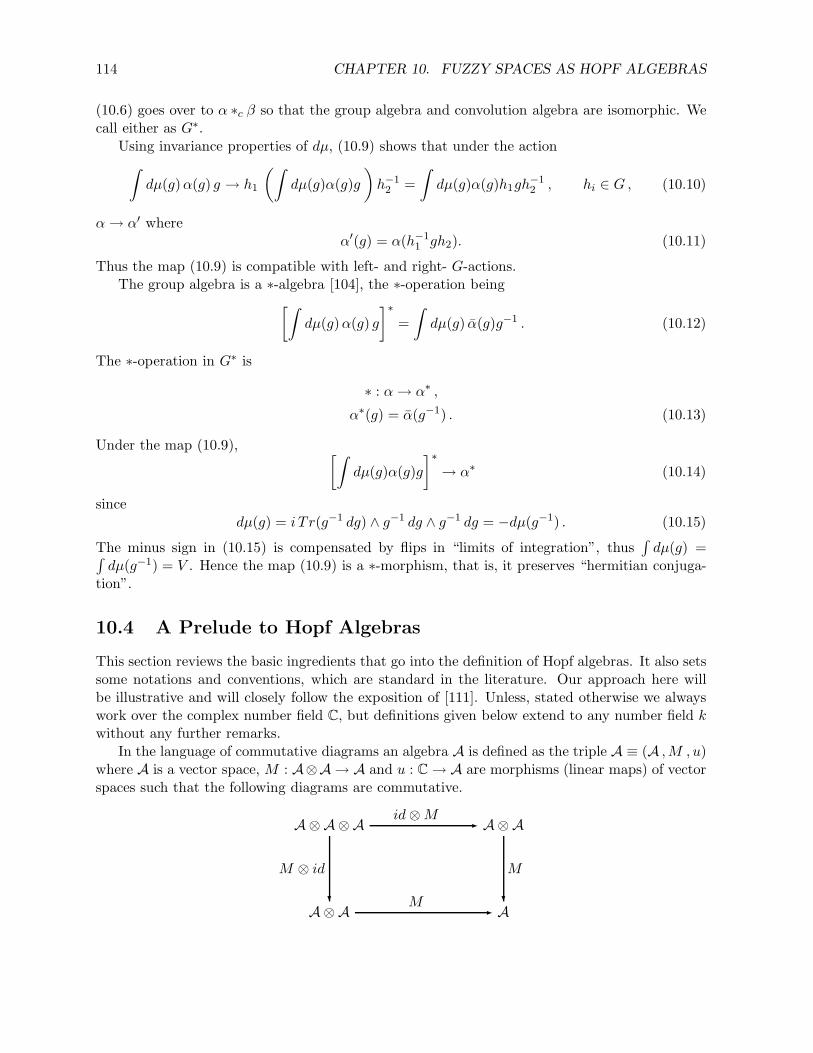
114 CHAPTER 10. FUZZY SPACES AS HOPF ALGEBRAS
(10.6) goes over to α ∗c β so that the group algebra and convolution algebra are isomorphic. Wecall either as G∗.
Using invariance properties of dµ, (10.9) shows that under the action
∫dµ(g)α(g) g → h1
(∫dµ(g)α(g)g
)h−1
2 =
∫dµ(g)α(g)h1gh
−12 , hi ∈ G , (10.10)
α→ α′ whereα′(g) = α(h−1
1 gh2). (10.11)
Thus the map (10.9) is compatible with left- and right- G-actions.The group algebra is a ∗-algebra [104], the ∗-operation being
[∫dµ(g)α(g) g
]∗=
∫dµ(g) α(g)g−1 . (10.12)
The ∗-operation in G∗ is
∗ : α→ α∗ ,
α∗(g) = α(g−1) . (10.13)
Under the map (10.9), [∫dµ(g)α(g)g
]∗→ α∗ (10.14)
sincedµ(g) = i T r(g−1 dg) ∧ g−1 dg ∧ g−1 dg = −dµ(g−1) . (10.15)
The minus sign in (10.15) is compensated by flips in “limits of integration”, thus∫dµ(g) =∫
dµ(g−1) = V . Hence the map (10.9) is a ∗-morphism, that is, it preserves “hermitian conjuga-tion”.
10.4 A Prelude to Hopf Algebras
This section reviews the basic ingredients that go into the definition of Hopf algebras. It also setssome notations and conventions, which are standard in the literature. Our approach here willbe illustrative and will closely follow the exposition of [111]. Unless, stated otherwise we alwayswork over the complex number field C, but definitions given below extend to any number field kwithout any further remarks.
In the language of commutative diagrams an algebra A is defined as the triple A ≡ (A ,M , u)where A is a vector space, M : A⊗A→ A and u : C→ A are morphisms (linear maps) of vectorspaces such that the following diagrams are commutative.
A⊗A⊗A id⊗M - A⊗A
A⊗A
M ⊗ id
? M - A
M
?
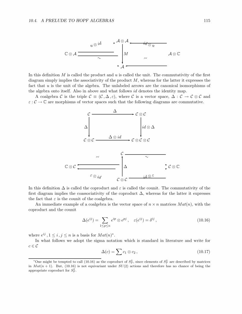
10.4. A PRELUDE TO HOPF ALGEBRAS 115
A⊗A
C⊗Au⊗ id -
A⊗ C
id⊗ u
A
M
?
∼∼-
In this definition M is called the product and u is called the unit. The commutativity of the firstdiagram simply implies the associativity of the product M , whereas for the latter it expresses thefact that u is the unit of the algebra. The unlabeled arrows are the canonical isomorphisms ofthe algebra onto itself. Also in above and what follows id denotes the identity map.
A coalgebra C is the triple C ≡ (C ,∆ , ε), where C is a vector space, ∆ : C → C ⊗ C andε : C → C are morphisms of vector spaces such that the following diagrams are commutative.
C ∆ - C ⊗ C
C ⊗ C
∆
? ∆⊗ id - C ⊗ C ⊗ C
id⊗∆
?
C
C⊗ C
∼
C ⊗ C
∼-
C ⊗ C
∆
6
id⊗ ε-
ε⊗ id
In this definition ∆ is called the coproduct and ε is called the counit. The commutativity of thefirst diagram implies the coassociativity of the coproduct ∆, whereas for the latter it expressesthe fact that ε is the counit of the coalgebra.
An immediate example of a coalgebra is the vector space of n× n matrices Mat(n), with thecoproduct and the counit
∆(eij) =∑
1≤p≤neip ⊗ epj , ε(eij) = δij , (10.16)
where eij , 1 ≤ i , j ≤ n is a basis for Mat(n)∗.In what follows we adopt the sigma notation which is standard in literature and write for
c ∈ C∆(c) =
∑c1 ⊗ c2 , (10.17)
∗One might be tempted to call (10.16) as the coproduct of S2F , since elements of S2
F are described by matricesin Mat(n + 1). But, (10.16) is not equivariant under SU(2) actions and therefore has no chance of being theappropriate coproduct for S2
F .
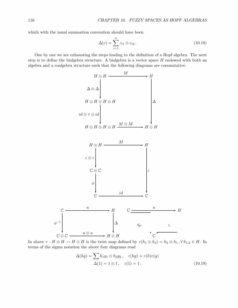
116 CHAPTER 10. FUZZY SPACES AS HOPF ALGEBRAS
which with the usual summation convention should have been
∆(c) =
n∑
i=1
ci1 ⊗ ci2 . (10.18)
One by one we are exhausting the steps leading to the definition of a Hopf algebra. The nextstep is to define the bialgebra structure. A bialgebra is a vector space H endowed with both analgebra and a coalgebra structure such that the following diagrams are commutative.
H ⊗H M - H
H ⊗H ⊗H ⊗H
∆⊗∆
?
H ⊗H ⊗H ⊗H
id⊗ τ ⊗ id
? M ⊗M - H ⊗H
∆
?
H ⊗H M - H
C⊗ C
ε⊗ ε?
C
φ
? id - C
ε
?
Cu - H
C⊗ C
φ−1
? u⊗ u - H ⊗H
∆
?
Cu - H
C
εid-
In above τ : H ⊗H → H ⊗H is the twist map defined by τ(h1 ⊗ h2) = h2 ⊗ h1 ,∀h1,2 ∈ H. Interms of the sigma notation the above four diagrams read
∆(hg) =∑
h1g1 ⊗ h2g2 , ε(hg) = ε(h)ε(g)
∆(1) = 1⊗ 1 , ε(1) = 1 . (10.19)
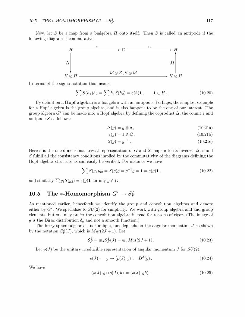
10.5. THE ∗-HOMOMORPHISM G∗ → S2F 117
Now, let S be a map from a bialgebra H onto itself. Then S is called an antipode if thefollowing diagram is commutative.
Hε - C
u - H
H ⊗H
∆
? id⊗ S , S ⊗ id - H ⊗H
M
6
In terms of the sigma notation this means∑
S(h1)h2 =∑
h1S(h2) = ε(h)1 , 1 ∈ H . (10.20)
By definition a Hopf algebra is a bialgebra with an antipode. Perhaps, the simplest examplefor a Hopf algebra is the group algebra, and it also happens to be the one of our interest. Thegroup algebra G∗ can be made into a Hopf algebra by defining the coproduct ∆, the counit ε andantipode S as follows:
∆(g) = g ⊗ g , (10.21a)
ε(g) = 1 ∈ C , (10.21b)
S(g) = g−1 . (10.21c)
Here ε is the one-dimensional trivial representation of G and S maps g to its inverse. ∆, ε andS fulfill all the consistency conditions implied by the commutativity of the diagrams defining theHopf algebra structure as can easily be verified. For instance we have
∑S(g1)g2 = S(g)g = g−1g = 1 = ε(g)1 , (10.22)
and similarly∑g1S(g2) = ε(g)1 for any g ∈ G.
10.5 The ∗-Homomorphism G∗ → S2F
As mentioned earlier, henceforth we identify the group and convolution algebras and denoteeither by G∗. We specialize to SU(2) for simplicity. We work with group algebra and and groupelements, but one may prefer the convolution algebra instead for reasons of rigor. (The image ofg is the Dirac distribution δg and not a smooth function.)
The fuzzy sphere algebra is not unique, but depends on the angular momentum J as shownby the notation S2
F (J), which is Mat(2J + 1). Let
S2F = ⊕JS2
F (J) = ⊕JMat(2J + 1) . (10.23)
Let ρ(J) be the unitary irreducible representation of angular momentum J for SU(2):
ρ(J) : g → 〈ρ(J), g〉 := DJ(g) . (10.24)
We have〈ρ(J), g〉 〈ρ(J), h〉 = 〈ρ(J), gh〉 . (10.25)
118 CHAPTER 10. FUZZY SPACES AS HOPF ALGEBRAS
Choosing the ∗-operation on DJ(g) as hermitian conjugation, ρ(J) extends by linearity to a∗-homomorphism on G∗:
⟨ρ(J),
∫dµ(g)α(g)g
⟩=
∫dµ(g)α(g)DJ (g)
⟨ρ(J),
( ∫dµ(g)α(g)g
)∗⟩=
∫dµ(g)α(g)DJ (g)† . (10.26)
ρ(J) is also compatible with group actions on G∗ (that is, it is equivariant with respect to theseactions):
⟨ρ(J),
∫dµ(g)α(g)h1gh
−12
⟩=
∫dµ(g)α(g)DJ (h1)D
J(g)DJ (h−12 ) hi ∈ SU(2) . (10.27)
As by (10.2a),
⟨ρ(J),
2K + 1
V
∫dµ(g)(DK
ij )†(g)g
⟩= eji(J)δKJ ,
eji(J)rs = δjrδis , i, j, r, s ∈ [−J , · · · 0 , · · · , J ] , (10.28)
we see by (10.25) and (10.26) that ρ(J) is a ∗-homomorphism from G∗ to S2F (J)⊕ 0, where 0
denotes the zero elements of ⊕K 6=JS2F (K), the ∗-operation on S2
F (J) being hermitian conjugation.Identifying S2
F (J) ⊕ 0 with S2F (J), we thus get a ∗-homomorphism ρ(J) : G∗ → S2
F (J). It isalso seen to be equivariant with respect to SU(2) actions, they are given on the basis eji(J) byDJ(h1)e
ji(J)DJ (h2)−1.
We can think of (10.26) as giving a map
ρ : g → 〈ρ(.) , g〉 := g(.) (10.29)
to a matrix valued function g(.) on the space of UIRR’s of SU(2) where
g(J) = 〈ρ(J) , g〉 . (10.30)
The homomorphism property (10.26) is expressed as the product g(.)h(.) of these functions where
g(.)h(.)(J) = g(J)h(J) (10.31)
is the point-wise product of matrices. This point of view is helpful for later discussions.As emphasized earlier, this discussion works for any group G, its UIRR’s, and its fuzzy spaces
barring technical problems. ThusG∗ is ∗-isomorphic to the ∗-algebra of functions g(.) on the spaceof its UIRR’s τ , with g(τ) = Dτ (g), the linear operator of g in the UIRR τ and g∗(τ) = Dτ (g)†.
A fuzzy space is obtained by quantizing an adjoint orbit G/H, H ⊂ G and approximatesG/H. It is a full matrix algebra associated with a particular UIRR τ of G. There is thus aG-equivariant ∗-homomorphism from G∗ to the fuzzy space.
At this point we encounter a difference with S2F (J). For a given G/H we generally get only
a subset of UIRR’s τ . For example CP 2 = SU(3)/U(2) is associated with just the symmetricproducts of just 3’s (or just 3∗’s) of SU(3). Thus the direct sum of matrix algebras from a givenG/H is only homomorphic to G∗.
10.6. HOPF ALGEBRA FOR THE FUZZY SPACES 119
Henceforth we call the space of UIRR’s of G as G. For a compact group, G can be identifiedwith the set of discrete parameters specifying all UIRR’s.
The properties of a group G are captured by the algebra of matrix-valued functions g(.) onG with point-wise multiplication, this algebra being isomorphic to G∗. In terms of g(.), (10.21)translate to
∆(g(.))
= g(.) ⊗ g(.) , (10.32a)
ε(g(.)) = 1 ∈ C , (10.32b)
S(g(.))
= g−1(.) . (10.32c)
Note that g(.)⊗ g(.) is a function on G⊗ G.
10.6 Hopf Algebra for the Fuzzy Spaces
Any fuzzy space has a Hopf algebra, we show it here for the fuzzy sphere.
Let δJ be the δ-function on SU(2):
δJ (K) := δJK . (10.33)
(Since the sets of J and K are discrete we have Kronecker delta and not a delta function).
Then
eji(J) δJ =2J + 1
V
∫dµ(g)DJ
ij(g)†g(.) (10.34)
Hence
∆(eji(J)δJ ) =2J + 1
V
∫dµ(g)DJ
ij(g)†g(.) ⊗ g(.) . (10.35)
At (K,L) ∈ SU(2)⊗ SU(2), this is
∆(eji(J)
)(K,L) =
2J + 1
V
∫dµ(g)DJ
ij(g)†DK(g)⊗DL(g) . (10.36)
As δ2J = δJ and δJeji(J) = eji(J)δJ , we can identify eji(J)δJ with eji(J):
eji(J)δJ ≃ eji(J) . (10.37)
Then (10.35) or (10.36) show that there are many coproducts ∆ = ∆KL we can define and theyare controlled by the choice of K and L:
∆(eji(J)δJ
)(K,L) := ∆KL
(eji(J)
). (10.38)
From section (10.4) we know that technically a coproduct ∆ is a homomorphism from Cto C ⊗ C so that only ∆JJ is a coproduct. But, we will be free of language and call all ∆KL
as coproducts. Indeed, it is the very fact that K 6= L in general in (10.38) that gives S2F its
“generalized” Hopf alegbra structure.
120 CHAPTER 10. FUZZY SPACES AS HOPF ALGEBRAS
Let us now simplify the RHS of (10.36). Using (10.4), (10.36) can be written as
∆(eji(J)δJ
)µ1µ2 ,m1m2
= 2J+1V
∫dµ(g)DJ
ij(g)† ∑J ′C(K,L, J ′;µ1 , µ2)×
C(K,L, J ′;m1 ,m2)DJ ′µ1+µ2 ,m1+m2
, (10.39)
with µ1 , µ2 and m1 ,m2 being row and column indices. The RHS of (10.39) is
C(K,L, J ;µ1 , µ2)C(K,L, J ;m1 ,m2)δj ,µ1+µ2δi,m1+m2
=∑
µ′1+µ′2=jm′1+m′2=i
C(K,L, J ;µ′1 , µ′2)C(K,L, J ;m′1 ,m
′2)(eµ′1m′1(K)
)µ1m1
⊗(eµ′2m′2(L)
)µ2m2
. (10.40)
Hence we have the coproduct
∆KL
(eji(J)
)=
∑
µ1+µ2=jm1+m2=i
C(K,L, J ;µ1 , µ2)C(K,L, J ;m1 ,m2) eµ1m1(K)⊗ eµ2m2(L) . (10.41)
Writing C(K,L, J ;µ1 , µ2 , j) = C(K,L, J ;µ1 , µ2)δµ1+µ2 ,j for the first Clebsch-Gordan coeffi-cient, we can delete the constraint j = µ1+µ2 in summation. C(K,L, J ; µ1 , µ2 , j) is an invarianttensor when µ1 , µ2 and j are transformed appropriately by SU(2). Hence (10.41) is preserved bySU(2) action on j, µ1, µ2. The same is the case for SU(2) action on i,m1,m2. In other words,the coproduct in (10.41) is equivariant with respect to both SU(2) actions.
Since any M ∈Mat(2J + 1) is∑
i,jMjieji(J), (10.41) gives
∆KL(M) =∑
µ1 ,µ2m1 ,m2
C(K,L, J ;µ1 , µ2)C(K,L, J ;m1 ,m2)
×Mµ1+µ2 ,m1+m2eµ1m1(K)⊗ eµ2m2(L) . (10.42)
This is the basic formula. It preserves conjugation ∗ (induced by hermitian conjugation of ma-trices):
∆(M †) = ∆(M)† . (10.43)
It is instructive to check directly that ∆KL is a homomorphism, that is that ∆KL(MN) =∆KL(M)∆KL(N). Starting from (10.41) we have
∆KL
(eji(J)
)∆KL
(ej′i′(J)
)=∑
µ1 ,µ2m1 ,m2
∑
µ′1µ′2
m′1 ,m′2
C(K,L, J ;µ1 , µ2 , j)C(K,L, J ;m1 ,m2 , i)
× C(K,L, J ;µ′1 , µ′2 , j′)C(K,L, J ;m′1 ,m
′2 , i′)(eµ1m1(K)⊗ eµ2m2(L)
)
×(eµ′1m′1(K)⊗ eµ′2m′2(L)
). (10.44)
Using (A⊗B)(C ⊗D) = AC ⊗BD, we have
(eµ1m1(K)⊗ eµ2m2(L)
)(eµ′1m′1(K)⊗ eµ′2m′2(L)
)
= eµ1m1(K)eµ′1m′1(K)⊗ eµ2m2(L)eµ
′2m′2(L) = δm1µ′1
δm2µ′2eµ1m′1(K)⊗ eµ2m′2(L) . (10.45)
10.6. HOPF ALGEBRA FOR THE FUZZY SPACES 121
To get the second line in (10.45) we have made use of
(eµ1m1(K)eµ
′1m′1(K)
)
αβ= eµ1m1(K)αγe
µ′1m′1(K)γβ = δm1µ′1
eµ1m′1(K)αβ . (10.46)
Inserting (10.45) in (10.44) we get
∆KL
(eji(J)
)∆KL
(ej′i′(J)
)=∑
µ1 ,µ2m1 ,m2
∑
µ′1µ′2
m′1 ,m′2
C(K,L, J ;µ1 , µ2 , j)C(K,L, J ;m1 ,m2 , i)
× C(K,L, J ;µ′1 , µ′2 , j′)C(K,L, J ;m′1 ,m
′2 , i′)δm1µ′1
δm2µ′2eµ1m′1(K)⊗ eµ2m′2(L)
=∑
µ1 ,µ2
∑
m′1 ,m′2
C(K,L, J ;µ1 , µ2 , j)C(K,L, J ;m′1 ,m′2 , i′)
×( ∑
m1 ,m2
C(K,L, J ;m1 ,m2 , i)C(K,L, J ;m1 ,m2 , j′))
︸ ︷︷ ︸=δij′
eµ1m′1(K)⊗ eµ2m′2(L) , (10.47)
where the orthogonality of Clebsch-Gordan coefficients is used to obtain δij′ for the factor withthe under brace. Thus,
∆KL
(eji(J)
)∆KL
(ej′i′(J)
)
=∑
µ1 ,µ2m1 ,m2
C(K,L, J ;µ1 , µ2 , j)C(K,L, J ;m′1 ,m′2 , i′)δij′e
µ1m′1(K)⊗ eµ2m′2(L)
= δij′∆KL(eji′
) . (10.48)
Upon multiplying both sides of (10.48) by the coefficients MjiNj′i′ we finally get
∆KL
(∑
ji
Mjieji(J)
)∆KL
(∑
j′i′
Nj′i′ej′i′(J)
)= ∆KL(M)∆KL(N)
= (MN)ji′∆KL(eji′
) = ∆KL(MN) , (10.49)
as we intended to demonstrate.
It remains to record the fuzzy analogues of counit ε and antipode S. For the counit we have
ε(eji(J)δJ
)=
2J + 1
V
∫dµ(g)DJ
ij(g)†ε(g(.))
=2J + 1
V
∫dµ(g)DJ
ij(g)†1
=2J + 1
V
∫dµ(g)DJ
ij(g)†D0(g) . (10.50)
Using equation (10.2a) and the fact that D0(g) is a unit matrix with only one entry which wedenote by 00, we have
ε(eji(J)δJ
)00
(K) = δ0Jδj0δi0 , ∀K ∈ SU(2) . (10.51)
122 CHAPTER 10. FUZZY SPACES AS HOPF ALGEBRAS
For the antipode, we have
S(eji(J)δJ
)=
2J + 1
V
∫dµ(g)DJ
ij(g)†S(g(.))
=2J + 1
V
∫dµ(g)DJ
ij(g)†g−1(.) (10.52)
or
S(eji(J)δJ
)(K) =
2J + 1
V
∫dµ(g)DJ
ij(g)†DK(g−1) . (10.53)
In an UIRR K we have C = e−iπJ2 as the charge conjugation matrix. It fulfills CDK(g)C−1 =DK(g). Then since DK(g−1) = DK(g)†,
DK(g−1) = CDK(g)TC−1 , (10.54)
where T denotes transposition. We insert this in (10.53) and use (10.2a) to find
S(eji(J)δJ
)kℓ
(K) =2J + 1
V
∫dµ(g)DJ
ij(g)†(CkuDK(g)TuυC
−1υℓ
)
=2J + 1
V
∫dµ(g)DJ
ij(g)†CkuD
K(g)υuC−1υℓ
= δJKCkuδuiδυjC−1υℓ
= δJKCkiC−1jℓ . (10.55)
This can be simplified further. Since in the UIRR K,
(e−iπJ2
)ki
= δ−ki(−1)K+k = δ−ki(−1)K−i , (10.56)
and C−1 = CT , we find
S(eji(J)δJ
)kℓ
(K) = δJKδ−kiδ−ℓj(−1)2K−i−j
= δJK(−1)2J−i−je−i ,−j(J)kℓ . (10.57)
ThusS(eji(J)δJ
)(K) = δJK(−1)2J−i−je−i ,−j(J) . (10.58)
10.7 Interpretation
We recall from chapter 2 that the matrix M ∈ Mat(2J + 1) can be interpreted as the wavefunction of a particle on the spatial slice S2
F (J). The Hilbert space for these wave functions isMat(2J + 1) with the scalar product given by (M,N) = TrM †N , M,N ∈ S2
F (J).We can also regard M as a fuzzy two-dimensional Euclidean scalar field as we did earlier or
even as a field on a spatial slice S2F (J) of a three dimensional space-time S2
F (J)× R.Let us look at the particle interpretation. Then (10.42) gives the amplitude, up to an overall
factor, for M ∈ S2F (J) splitting into a superposition of wave functions on S2
F (K) ⊗ S2F (L). It
models the process where a fuzzy sphere splits into two others [110]. The overall factor is thereduced matrix element much like the reduced matrix elements in angular momentum selectionrules. It is unaffected by algebraic operations on S2
F (J), S2F (K) or S2
F (L) and is determined bydynamics.
10.7. INTERPRETATION 123
Now (10.42) preserves trace and scalar product:
Tr∆KL(M) = TrM ,(∆KL(M),∆KL(N)
)= (M,N) . (10.59)
So (10.42) is a unitary branching process. This means that the overall factor is a phase.∆KL(S2
F (J)) has all the properties of S2F (J). So (10.42) is also a precise rule on how S2
F (J) sitsin S2
F (K)⊗S2F (L). We can understand “how ∆KL(M) sits” as follows. A basis for S2
F (K)⊗S2F (L)
is eµ1m1(K)⊗eµ2m2(L). We can choose another basis where left- and right- angular momenta areseparately diagonal by coupling µ1 and µ2 to give angular momentum σ ∈ [0, 1
2 , 1, . . . ,K + L],and m1 and m2 to give angular momentum τ ∈ [0, 1
2 , 1, . . . ,K + L]. In this basis, ∆KL(M) iszero except in the block with σ = τ = J .
So the probability amplitude for M ∈ S2F (J) splitting into P ⊗ Q ∈ S2
F (K) ⊗ S2F (L) for
normalized wave functions is
phase× Tr(P ⊗Q)†∆KL(M) . (10.60)
Branching rules for different choices of M,P and Q are independent of the constant phase andcan be determined.
Written in full, (10.60) is seen to be just the coupling conserving left- and right- angularmomenta of P †, Q† and M . That alone determines (10.60).
An observable A is a self-adjoint operator on a wave function M ∈ S2F (J). Any linear operator
on S2F (J) can be written as
∑BLαC
Rα where Bα , Cα ∈ S2
F (J) and BLα and CRα act by left- and
right- multiplication: BLαM = BαM ,CRαM = MCα. Any observable on S2
F (J) has an action onits branched image ∆KL(S2
F (J)):
∆KL(A)∆KL(M) := ∆KL(AM) . (10.61)
By construction, (10.61) preserves algebraic properties of operators. ∆KL(A) can actually act onall of S2
F (K) ⊗ S2F (L), but in the basis described above it is zero on vectors with σ 6= J and/or
τ 6= J .This equation is helpful to address several physical questions. For example ifM is a wave func-
tion with a definite eigenvalue for A, then ∆KL(M) is a wave function with the same eigenvalue for∆KL(A). This follows from ∆KL(BM) = ∆KL(B)∆KL(M) and ∆KL(MB) = ∆KL(M)∆KL(B).Combining this with (10.59) and the other observations, we see that mean value of ∆KL(A) in∆KL(M) and of A in M are equal.
In summary all this means that every operator on S2F (J) is a constant of motion for the
branching process (10.42).Now suppose R ∈ S2
F (K) ⊗ S2F (L) is a wave function which is not necessarily of the form
P ⊗Q. Then we can also give a formula for the probability amplitude for finding R in the statedescribed by M . Note that R and M live in different fuzzy spaces. The answer is
constant× TrR†∆KL(M) . (10.62)
If M,P,Q are fields with S2F (I) (I = J,K,L) a spatial slice or space-time, (10.60) is an
interaction of fields on different fuzzy manifolds. It can give dynamics to the branching processof fuzzy topologies discussed above.
124 CHAPTER 10. FUZZY SPACES AS HOPF ALGEBRAS
10.8 The Presnajder Map
This section is somewhat disconnected from the material in the rest of the chapter.We recall that S2
F (J) can be realized as an algebra generated by the spherical harmonicsYlm (l ≤ 2J) which are functions on the two-sphere S2. Their product can be the coherent state∗c or Moyal ∗M product.
But we saw that S2F (J) is isomorphic to the convolution algebra of functionsDJ
MN on SU(2) ≃S3.
It is reasonable to wonder how functions on S2 and S3 get related preserving the respectivealgebraic properties.
The map connecting these spaces is described by a function on SU(2) × S2 ≈ S3 × S2 andwas first introduced by Presnajder [52, 50]. We give its definition and introduce its propertieshere. It generalizes to any group G.
Let ai , a†j (i = 1, 2) be Schwinger oscillators for SU(2) and let us also recall that for J = n
2
|z , 2J〉 =(zia
†i )
2J
√2J !
|0〉 ,∑|zi|2 = 1 (10.63)
are the normalized Perelomov coherent states. If U(g) is the unitary operator implementingg ∈ SU(2) in the spin J UIRR, the Presnajder function [52, 50] PJ is given by
PJ(g, ~n) = 〈z , 2J |U(g)|z , 2J〉 = DJJJ(h
−1gh) ,
~n = z†~τz , ~n · ~n = 1 ,
h =
(z1 −z2z2 z1
). (10.64)
Now ~n ∈ S2. As the phase change zi → zieiθ does not effect PJ , besides g, it depends only on ~n.
It is a function on (SU(2) ≃ S3
)×[SU(2)/U(1)
]≃ S3 × S2 . (10.65)
A basis of SU(2) functions for spin J is DJij . A basis of S2 functions for spin J is Eij(J , .)
where
Eij(J , ~n) = 〈z , 2J |eij(J)|z , 2J〉 = DJ(h−1)JiDJ(h)jJ , no sum on J . (10.66)
The transform of DJij to Eij(J, .) is given by
Eij(J , ~n) =(2J + 1)
V
∫dµ(g)PJ (g, ~n)DJ
ij(g) . (10.67)
This can be inverted by constructing a function QJ on SU(2)× S2 such that∫
S2
dΩ(~n)QJ(g′ , ~n)PJ (g , ~n) =
∑
ij
DJij(g′)DJ
ij(g) , dΩ(~n) =d cos θdϕ
4π, (10.68)
θ and ϕ being the polar and azimuthal angles on S2. Then using (2), we get
DJij(g′) =
∫
S2
dΩ(~n)QJ(g′ , ~n)Eij(J , ~n) . (10.69)
10.8. THE PRESNAJDER MAP 125
Consider first J = 12 . In that case
P 12(g , ~n) = gklzkzl = gkl
(1 + ~σ · ~n2
)
lk(10.70)
where g is a 2× 2 SU(2) matrix and σi are Pauli matrices. Since
∫
S2
dΩ(~n)ninj =1
3δij , (10.71)
we find
Q 12(g′ , ~n) = Trg′(1 + 3~σ · ~n) , (10.72)
g′ = 2× 2 SU(2) matrix ,
g′ = transpose of g′ .
For J = n2 , DJ(g) acts on the symmetric product of n C2’s and can be written as g ⊗ g ⊗ · · · ⊗ g︸ ︷︷ ︸
N factors
and (10.70) gets replaced by
PJ (g , ~n) =[Trg
(1 + ~σ · ~n2
)]N. (10.73)
Then QJ(g′ , ~n) is defined by (10.68). It exists, but we have not found a neat formula for it.
As the relation between Eij and Ylm can be worked out, it is possible to suitably substituteYlm for Eij in these formulae.
These equations establish an isomorphism (with all the nice properties like preserving ∗ andSU(2)-actions) between the convolution algebra ρ(J) (G∗) at spin J and the ∗-product algebraof S2
F (J). That is because we saw that ρ(J)(G∗) and S2F (J) ≃Mat(2J +1) are isomorphic, while
it is known that Mat(2J + 1) and the ∗-product algebra of S2 at level J are isomorphic.There are evident generalizations of PJ for other groups and their orbits.

126 CHAPTER 10. FUZZY SPACES AS HOPF ALGEBRAS
Bibliography
[1] A. P. Balachandran, video conference course on “Fuzzy Physics”, athttp://www.phy.syr.edu/courses/Fuzzy Physics and http://bach.if.usp.br/FUZZY/.
[2] J. Madore, The Fuzzy Sphere, Class. Quant. Grav. 9, 69 (1992).
[3] J. Madore, An Introduction to Non-commutative Differential Geometry and its Physical Ap-plications, Cambridge University Press, Cambridge (1995);
[4] A.A. Kirillov, Encyclopedia of Mathematical Sciences,vol 4, p.230; B. Kostant, Lecture Notesin Mathematics, vol.170, Springer-Verlag(1970), p.87.
[5] F. A. Berezin, General Concept of Quantization, Commun. Math. Phys. 40, 153 (1975).
[6] H. Grosse, C. Klimcik, P. Presnajder, Field Theory on a Supersymmetric Lattice, Commun.Math. Phys., 185 (1997) 155-175 and hep-th/9507074;
H. Grosse, C. Klimcik, P. Presnajder, N=2 Superalgebra and Non-Commutative Geometry,hep-th/9603071;
[7] H. Grosse, G. Reiter, The Fuzzy Supersphere, J. Geom. and Phys., 28 (1998) 349-383 andmath-ph/9804013.
[8] A. P. Balachandran, S. Kurkcuoglu and E. Rojas, The Star Product on the Fuzzy Super-sphere, JHEP 0207, 056 (2002) [arXiv:hep-th/0204170];
[9] S. Kurkcuoglu, Ph.D. Thesis, Syracuse University, Syracuse NY, 2004.
[10] J. Ambjorn and S. Catterall, Stripes from (Noncommutative) Stars, Phys. Lett. B 549, 253(2002) [arXiv:hep-lat/0209106].
[11] See for example, P. H. Frampton Gauge Field Theories, The Benjamin Cummings PublishingCompany, Menlo Park CA, (1987).
[12] R.D. Sorkin Int.J. Theory. Phys. 30 (1991) 923;
A. P. Balachandran, G. Bimonte, E. Ercolessi, G. Landi, F. Lizzi, G. Sparano andP. Teotonio-Sobrinho, Finite Quantum Physics and Noncommutative Geometry, Nucl. Phys.Proc. Suppl. 37C, 20 (1995) [arXiv:hep-th/9403067].
[13] S. Minwalla, M. Van Raamsdonk and N. Seiberg, Noncommutative Perturbative Dynamics,JHEP 0002, 020 (2000) [arXiv:hep-th/9912072].
127
128 BIBLIOGRAPHY
[14] B. Ydri, Non-commutative geometry as a regulator, Phys. Rev. D 63, 025004 (2001)[arXiv:hep-th/0003232].
[15] S. Vaidya, Perturbative dynamics on fuzzy S(2) and RP(2), Phys. Lett. B 512, 403 (2001)[arXiv:hep-th/0102212];
[16] C. S. Chu, J. Madore and H. Steinacker, Scaling limits of the fuzzy sphere at one loop, JHEP0108, 038 (2001) [arXiv:hep-th/0106205].
[17] B. P. Dolan, D. O’Connor and P. Presnajder, Matrix φ4 models on the fuzzy sphere andtheir continuum limits”, JHEP 0203, 013 (2002) [arXiv:hep-th/0109084];
[18] S. Vaidya and B. Ydri, On the origin of the UV-IR mixing in non-commutative matrixgeometry, Nucl. Phys. B 671, 401 (2003) [arXiv:hep-th/0305201].
[19] S. Vaidya and B. Ydri, New scaling limit for fuzzy spheres, arXiv:hep-th/0209131.
[20] H. Grosse and A. Strohmaier, Noncommutative geometry and the regularization problem of4D quantum field theory, Lett. Math. Phys. 48, 163 (1999) [arXiv:hep-th/9902138].
[21] G. Alexanian, A. P. Balachandran, G. Immirzi and B. Ydri, Fuzzy CP(2), J. Geom. Phys.42, 28 (2002) [arXiv:hep-th/0103023].
[22] A. P. Balachandran, B. P. Dolan, J. H. Lee, X. Martin and D. O’Connor, Fuzzy complex pro-jective spaces and their star-products, J. Geom. Phys. 43, 184 (2002) [arXiv:hep-th/0107099].
[23] D. Karabali and V. P. Nair, Quantum Hall effect in higher dimensions, Nucl. Phys. B 641,533 (2002) [arXiv:hep-th/0203264];
D. Karabali and V. P. Nair, The effective action for edge states in higher dimensional quan-tum Hall systems, Nucl. Phys. B 679, 427 (2004) [arXiv:hep-th/0307281];
D. Karabali and V. P. Nair, Edge states for quantum Hall droplets in higher dimensions anda generalized WZW model, Nucl. Phys. B 697, 513 (2004) [arXiv:hep-th/0403111];
D. Karabali, V. P. Nair and S. Randjbar-Daemi, Fuzzy spaces, the M(atrix) model and thequantum Hall effect, arXiv:hep-th/0407007.
[24] J. Medina and D. O’Connor, Scalar field theory on fuzzy S(4), JHEP 0311, 051 (2003),[arXiv:hep-th/0212170].
[25] A. Connes, Non-commutative Geometry San Diego, Academic Press, 1994.
[26] G. Landi, An Introduction to Non-commutative Spaces and their Geometries (Springer-Verlag, 1997);
[27] J.M. Gracia-Bondıa, J.C. Varilly and H. Figueroa, Elements of Non-commutative Geometry(Birkhauser, 2000).
[28] R. J. Szabo, Quantum field theory on non-commutative spaces, Phys. Rept. 378, 207 (2003)[arXiv:hep-th/0109162].
BIBLIOGRAPHY 129
[29] M. R. Douglas and N. A. Nekrasov, Non-commutative field theory, Rev. Mod. Phys. 73, 977(2001) [arXiv:hep-th/0106048].
[30] Letter of Heisenberg to Peierls (1930), Wolfgang Pauli, Scientific Correspondence, Vol. II,p.15, Ed. Karl von Meyenn, Springer-Verlag, 1985;
Letter of Pauli to Oppenheimer (1946), Wolfgang Pauli, Scientific Correspondence, Vol. III,p.380, Ed. Karl von Meyenn, Springer-Verlag, 1993.
[31] H. J. Groenewold, On The Principles Of Elementary Quantum Mechanics, Physica 12, 405(1946).
[32] H. S. Snyder, Quantized Space-Time, Phys. Rev. 71, 38 (1947); The Electromagnetic Fieldin Quantized Spacetime, Phys. Rev.72 (1947) 68;
[33] C. N. Yang, On Quantized Space-Time, Phys. Rev. 72, 874 (1947).
[34] J. E. Moyal, Quantum Mechanics As A Statistical Theory, Proc. Cambridge Phil. Soc. 45,99 (1949).
[35] R. Jackiw, Physical Instances of Noncommuting Coordinates, Nucl.Phys.Proc.Suppl. 108,30 (2002) [hep-th/0110057];
[36] A. P. Balachandran, G. Marmo, B. S. Skagerstam, A. Stern, Classical Topology and QuantumStates, World Scientific, Singapore, 1991.
[37] D. A. Varshalovich, A. N. Moskalev and V. K. Khersonsky, Quantum Theory of AngularMomentum, World Scientific, New Jersey, 1998.
[38] T. Holstein and H. Primakoff, Field Dependence Of The Intrinsic Domain Magnetization OfA Ferromagnet, Phys. Rev. 58, 1098 (1940).
[39] D. Sen, Quantum-spin-chain realizations of conformal field theories Phys. Rev. B 44,2645(1991)
[40] H. J. Lipkin Lie Groups for Pedestrians , Dover Publications, 2002.
[41] P. Goddard and D. I. Olive, Kac-Moody And Virasoro Algebras In Relation To QuantumPhysics, Int. J. Mod. Phys. A 1, 303 (1986).
[42] F. Bayen, M. Flato, C. Fronsdal, A. Lichnerowicz and D. Sternheimer, Deformation TheoryAnd Quantization. 1. Deformations Of Symplectic Structures, Annals Phys. 111, 61 (1978);
F. Bayen, M. Flato, C. Fronsdal, A. Lichnerowicz and D. Sternheimer, Quantum MechanicsAs A Deformation Of Classical Mechanics, Lett. Math. Phys. 1, 521 (1977).
[43] H. Weyl Gruppentheorie und Quantenmechanik The theory of groups and quantum mechan-ics, New York, Dover Publications, 1950;
H. Weyl, Quantum Mechanics And Group Theory, Z. Phys. 46, 1 (1927).
[44] J. R. Klauder and B. S. Skagerstam, Coherent States: Applications in Physics and Mathe-matical Physics, World Scientific (1985).
130 BIBLIOGRAPHY
[45] A. M. Perelomov Generalized Coherent States and their Applications, Springer-Verlag (1986).
[46] G. Alexanian, A. Pinzul and A. Stern, Generalized Coherent State Approach to StarProducts and Applications to the Fuzzy Sphere, Nucl. Phys. B 600, 531 (2001),[arXiv:hep-th/0010187].
[47] A. Voros, Wentzel-Kramers-Brillouin method in the Bargmann representation Phys. Rev.A40, 6814 (1989).
[48] R. Haag, Local quantum physics : fields, particles, algebras. Berlin, Springer-Verlag (1996).
[49] M. Kontsevich, Deformation quantization of Poisson manifolds, I, Lett. Math. Phys. 66, 157(2003) [arXiv:q-alg/9709040].
[50] P. Presnajder, The origin of chiral anomaly and the non-commutative geometry, J. Math.Phys. 41, 2789 (2000) [arXiv:hep-th/9912050];
[51] H. Grosse, C. Klimcik and P. Presnajder, Towards finite quantum field theory in non-commutative geometry, Int. J. Theor. Phys. 35, 231 (1996) [arXiv:hep-th/9505175].
[52] H. Grosse and P. Presnajder, The Construction on non-commutative manifolds using coher-ent states, Lett. Math. Phys. 28, 239 (1993);
[53] A. P. Balachandran and G. Immirzi, Fuzzy Nambu-Goldstone physics, Int. J. Mod. Phys. A
18 (2003) 5981,arXiv:hep-th/0212133.
[54] M. V. Berry, Quantal Phase Factors Accompanying Adiabatic Changes, Proc. Roy. Soc.Lond. A 392, 45 (1984).
[55] N.E. Wegge Olsen, K-theory and C∗-Algebras-a Friendly Approach, Oxford University Press,Oxford, 1993.
[56] U. Carow-Watamura and S. Watamura, Chirality and Dirac operator on noncommutativesphere,, Commun. Math. Phys. 183, 365 (1997) [arXiv:hep-th/9605003].
[57] R. Jackiw and C. Rebbi, Spin From Isospin In A Gauge Theory, Phys. Rev. Lett. 36, 1116(1976).
[58] P. Hasenfratz and G. ’t Hooft, A Fermion - Boson Puzzle In A Gauge Theory, Phys. Rev.Lett. 36, 1119 (1976).
[59] A. P. Balachandran, A. Stern and C. G. Trahern, Nonlinear Models As Gauge Theories,Phys. Rev. D 19, 2416 (1979).
[60] T. R. Govindarajan and E. Harikumar, O(3) sigma model with Hopf term on fuzzy sphere,Nucl. Phys. B 655, 300 (2003) [arXiv:hep-th/0211258].
[61] Chuan-Tsung Chan, Chiang-Mei Chen, Feng-Li Lin, Hyun Seok Yang, ‘CPn Model on FuzzySphere’, Nucl.Phys. B625 (2002) 327 and hep-th/0105087;
Chuan-Tsung Chan, Chiang-Mei Chen, Hyun Seok Yang, “Topological ZN+1 Charges onFuzzy Sphere”, hep-th/0106269.
BIBLIOGRAPHY 131
[62] Ludwik Dabrowski, Thomas Krajewski, Giovanni Landi, ‘Some Properties of Non-linearσ-Models in Noncommutative Geometry’, Int. J. Mod. Phys. B14 (2000) 2367 andhep-th/0003099.
[63] W.J. Zakrzewski, ‘Low dimensional sigma models’, Adam Hilger, Bristol 1997.
[64] J. A. Mignaco, C. Sigaud, A. R. da Silva and F. J. Vanhecke, ‘The Connes-Lott program onthe sphere’, Rev. Math. Phys. 9 (1997) 689 and hep-th/9611058;
J. A. Mignaco, C. Sigaud, A. R. da Silva and F. J. Vanhecke, ‘Connes-Lott model buildingon the two-sphere’, Rev. Math. Phys. 13 (2001) 1 and hep-th/9904171.
[65] G. Landi, Projective Modules of Finite Type over the Supersphere S2,2, Differ. Geom. Appl.14 (2001) 95-111 and math-ph/9907020.
[66] A. M. Polyakov, Interaction Of Goldstone Particles In Two-Dimensions. Applications ToFerromagnets And Massive Yang-Mills Fields, Phys. Lett. B 59, 79 (1975);
A. M. Polyakov and A. A. Belavin, Metastable States Of Two-Dimensional Isotropic Ferro-magnets, JETP Lett. 22, 245 (1975) [Pisma Zh. Eksp. Teor. Fiz. 22, 503 (1975)].
[67] H. Grosse, C. Klimcik and P. Pressnajder, Topologically nontrivial field configurations innon-commutative geometry, Commun. Math. Phys. 178, 507 (1996) [arXiv:hep-th/9510083].
[68] S. Baez, A. P. Balachandran, B. Ydri and S. Vaidya, Monopoles and solitons in fuzzy physics,Commun. Math. Phys. 208, 787 (2000) [arXiv:hep-th/9811169].
[69] A. P. Balachandran and S. Vaidya, Instantons and chiral anomaly in fuzzy physics, Int. J.Mod. Phys. A 16, 17 (2001) [arXiv:hep-th/9910129].
[70] H. Grosse and J. Madore, A Non-commutative version of the Schwinger model, Phys. Lett.B 283, 218 (1992).
H. Grosse and P. Presnajder, A non-commutative regularization of the Schwinger model,Lett. Math. Phys. 46, 61 (1998).
[71] M. Chaichian, P. Presnajder, M. M. Sheikh-Jabbari and A. Tureanu, Noncommutative stan-dard model: Model building,Eur. Phys. J. C 29, 413 (2003) [arXiv:hep-th/0107055];
M. Chaichian, P. Presnajder, M. M. Sheikh-Jabbari and A. Tureanu, Noncommutative gaugefield theories: A no-go theorem, Phys. Lett. B 526, 132 (2002) [arXiv:hep-th/0107037].
M. Chaichian, A. Kobakhidze and A. Tureanu, Spontaneous reduction of noncommutativegauge symmetry and model building,arXiv:hep-th/0408065.
[72] A. P. Balachandran, G. Marmo, N. Mukunda, J. S. Nilsson, E. C. G. Sudarshan and F. Za-ccaria, Monopole Topology And The Problem Of Color, Phys. Rev. Lett. 50, 1553 (1983);
A. P. Balachandran, G. Marmo, N. Mukunda, J. S. Nilsson, E. C. G. Sudarshan and F. Za-ccaria, Nonabelian Monopoles Break Color. 1. Classical Mechanics, Phys. Rev. D 29, 2919(1984);
132 BIBLIOGRAPHY
A. P. Balachandran, G. Marmo, N. Mukunda, J. S. Nilsson, E. C. G. Sudarshan and F. Zac-caria, Nonabelian Monopoles Break Color. 2. Field Theory And Quantum Mechanics, Phys.Rev. D 29, 2936 (1984).
[73] S. Vaidya, Scalar multi-solitons on the fuzzy sphere, JHEP 0201, 011 (2002)[arXiv:hep-th/0109102].
[74] D. Karabali, V. P. Nair and A. P. Polychronakos, Spectrum of Schroedinger field in a non-commutative magnetic monopole, Nucl. Phys. B 627, 565 (2002) [arXiv:hep-th/0111249].
[75] P. H. Ginsparg and K. G. Wilson, A Remnant Of Chiral Symmetry On The Lattice, Phys.Rev. D 25, 2649 (1982).
[76] A. P. Balachandran and G. Immirzi, The fuzzy Ginsparg-Wilson algebra: A solution of thefermion doubling problem, Phys. Rev. D 68, 065023 (2003) [arXiv:hep-th/0301242];
[77] K. Fujikawa, Path Integral Measure For Gauge Invariant Fermion Theories, Phys. Rev. Lett.42, 1195 (1979);
K. Fujikawa, Path Integral For Gauge Theories With Fermions, Phys. Rev. D 21, 2848 (1980)[Erratum-ibid. D 22, 1499 (1980)].
[78] A. P. Balachandran, G. Marmo, V. P. Nair and C. G. Trahern, A Nonperturbative Proof OfThe Nonabelian Anomalies, Phys. Rev. D 25, 2713 (1982).
[79] S. Randjbar-Daemi and J. A. Strathdee, On the overlap formulation of chiral gauge theory,Phys. Lett. B 348, 543 (1995) [arXiv:hep-th/9412165];
S. Randjbar-Daemi and J. A. Strathdee, Gravitational Lorentz anomaly from the overlapformula in two-dimensions, Phys. Rev. D 51, 6617 (1995) [arXiv:hep-th/9501012];
S. Randjbar-Daemi and J. A. Strathdee, Chiral fermions on the lattice, Nucl. Phys. B 443,386 (1995) [arXiv:hep-lat/9501027];
S. Randjbar-Daemi and J. A. Strathdee, Consistent and covariant anomalies in the overlapformulation of chiral gauge theories, Phys. Lett. B 402, 134 (1997) [arXiv:hep-th/9703092];
M. Luscher, Exact chiral symmetry on the lattice and the Ginsparg-Wilson relation, Phys.Lett. B 428, 342 (1998) [arXiv:hep-lat/9802011];
M. Luscher, Weyl fermions on the lattice and the non-abelian gauge anomaly, Nucl. Phys. B568, 162 (2000) [arXiv:hep-lat/9904009];
H. Neuberger, Chiral symmetry outside perturbation theory, arXiv:hep-lat/9912013;
W. Kerler, Dirac operator normality and chiral fermions, Chin. J. Phys. 38, 623 (2000)[arXiv:hep-lat/9912022];
J. Nishimura and M. A. Vazquez-Mozo, Noncommutative chiral gauge theories on the latticewith manifest star-gauge invariance, JHEP 0108, 033 (2001) [arXiv:hep-th/0107110].
[80] A. P. Balachandran, T. R. Govindarajan and B. Ydri, The fermion doubling problem andnoncommutative geometry, Mod. Phys. Lett. A 15, 1279 (2000) [arXiv:hep-th/9911087].
A. P. Balachandran, T. R. Govindarajan and B. Ydri, The fermion doubling problem andnoncommutative geometry. II, arXiv:hep-th/000621.
BIBLIOGRAPHY 133
[81] A. Bassetto and L. Griguolo, Journ. of Math. Phys. 32 (1991) 3195.
[82] H. Aoki, S. Iso and K. Nagao, Chiral anomaly on fuzzy 2-sphere, Phys. Rev. D 67, 065018(2003) [arXiv:hep-th/0209137].
[83] J. Madore, S. Schraml, P. Schupp and J. Wess, Gauge theory on noncommutative spaces,Eur. Phys. J. C 16, 161 (2000) [arXiv:hep-th/0001203];
X. Calmet, B. Jurco, P. Schupp, J. Wess and M. Wohlgenannt, The standard model onnon-commutative space-time, Eur. Phys. J. C 23, 363 (2002) [arXiv:hep-ph/0111115].
[84] N. Seiberg and E. Witten, String theory and noncommutative geometry, JHEP 9909, 032(1999) [arXiv:hep-th/9908142].
[85] B. Ydri, Ph.D. Thesis, Syracuse University, NY,2001, arXiv:hep-th/0110006;
B. Ydri, Noncommutative chiral anomaly and the Dirac-Ginsparg-Wilson operator, JHEP0308, 046 (2003) [arXiv:hep-th/0211209].
[86] M. Scheunert, W. Nahm and V. Rittenberg, Graded Lie Algebras: Generalization Of Her-mitian Representations, J. Math. Phys. 18, 146 (1977).
[87] M. Scheunert, W. Nahm and V. Rittenberg, Irreducible Representations Of The Osp(2,1)And Spl(2,1) Graded Lie Algebras, J. Math. Phys. 18, 155 (1977).
[88] A. Pais and V. Rittenberg, Semisimple Graded Lie Algebras, J. Math. Phys. 16, 2062 (1975)[Erratum-ibid. 17, 598 (1976)].
[89] B. Dewitt, Supermanifolds, Cambridge University Press, Cambridge (1985);
M. Scheunert, The Theory of Lie Superalgebras, Springer-Verlag, Berlin (1979).
[90] J. F. Cornwell, Group Theory in Physics Vol. III, Academic Press, San Diego (1989).
[91] L. Frappat, A. Sciarrino, P. Sorba, Dictionary on Lie Superalgebras, hep-th/9607161.
[92] M. Chaichian, D. Ellinas and P. Presnajder, Path Integrals And Supercoherent States, J.Math. Phys. 32, 3381 (1991).
[93] A. El Gradechi and L. M. Nieto, Supercoherent states, superKahler geometry and geometricquantization, Commun. Math. Phys.,175 (1996) 521, and hep-th/9403109;
A. M. El Gradechi, On the supersymplectic homogeneous superspace underlying theOSp(1/2) coherent states,” J. Math. Phys. 34, 5951 (1993).
[94] M. Bordemann, M. Brischle, C. Emmrich and S. Waldmann, subalgebras with convering starproducts in deformation quantization: An algebraic construction for CPn, J. Math. Phys.,37 (1996) 6311; q-alg/9512019;
M. Bordemann, M. Brischle, C. Emmrich and S. Waldmann, Lett. Math. Phys., 36 (1996)357;
S. Waldmann, Lett. Math. Phys., 44 (1998) 331.
134 BIBLIOGRAPHY
[95] F. A. Berezin and V. N. Tolstoi, The Group With Grassmann Structure Uosp(1,2), Commun.Math. Phys. 78, 409 (1981).
F. A. Berezin, Introduction to Superanalysis, D.Reidel Publishing Company, Dordrecht, Hol-land (1987).
[96] A. P. Balachandran, G.Marmo, B. S. Skagerstam and A. Stern, Supersymmetric Point Par-ticles And Monopoles With No Strings, Nucl. Phys. B164 (1980) 427;
G. Landi and G. Marmo, Phy. Lett. B193 (1987) 61-66. Extensions Of Lie SuperalgebrasAnd Supersymmetric Abelian Gauge Fields,
[97] C. Fronsdal Essays on Supersymmetry. Mathematical Physics Studies Volume 8, Editor:Fronsdal, C. , Dordrecht, Reidel Pub.Co. 1986.
[98] J. Wess, J. Bagger Princeton series in physics: supersymmetry and supergravity, Princeton,Princeton University Press, 1983.
[99] A. P. Balachandran, A. Pinzul and B. Qureshi, SUSY anomalies break N = 2 to N = 1: Thesupersphere and the fuzzy supersphere, arXiv:hep-th/0506037.
[100] C. Klimcik, A nonperturbative regularization of the supersymmetric Schwinger model,Commun. Math. Phys. 206, 567 (1999) [arXiv:hep-th/9903112];
C. Klimcik, An extended fuzzy supersphere and twisted chiral superfields, Commun. Math.Phys. 206, 587 (1999) [arXiv:hep-th/9903202].
[101] S. Kurkcuoglu, Non-linear sigma models on the fuzzy supersphere, JHEP 0403, 062 (2004)[arXiv:hep-th/0311031].
[102] E. Witten, A Supersymmetric Form Of The Nonlinear Sigma Model In Two-Dimensions,Phys. Rev. D 16, 2991 (1977).
[103] P. Di Vecchia and S. Ferrara, Classical Solutions In Two-Dimensional Supersymmetric FieldTheories, Nucl. Phys. B 130, 93 (1977);
[104] M. E. Sweedler Hopf Algebras, W. A. Benjamin, New York, 1969. A. A. Kirillov, Elementsof the Theory of Representations, Springer-Verlag, Berlin, 1976.
[105] G. Mack and V. Schomerus, QuasiHopf quantum symmetry in quantum theory, Nucl. Phys.B 370, 185 (1992);
G. Mack and V. Schomerus in New symmetry principles in Quantum Field Theory, Editedby J.Frohlich et al., Plenum Press, New York, 1992;
G. Mack and V. Schomerus, Quantum symmetry for pedestrians, preprint, DESY-92-053.
[106] A. P. Balachandran and S. Kurkcuoglu, Topology change for fuzzy physics: Fuzzy spacesas Hopf algebras, arXiv:hep-th/0310026.
[107] R. Figari, R. Hoegh-Krohn and C. R. Nappi, Interacting relativistic boson fields in the deSitter universe with two space-time dimensions, Commun. Math. Phys. 44, 265 (1975).
BIBLIOGRAPHY 135
[108] J. Pawelczyk and H. Steinacker, A quantum algebraic description of D-branes on groupmanifolds, Nucl. Phys. B 638, 433 (2002) [arXiv:hep-th/0203110].
[109] A. P. Balachandran and C. G. Trahern Lectures on Group Theory for Physicists, Mono-graphs and Textbooks in Physical Science, Bibliopolis, Napoli, 1984.
[110] A. P. Balachandran, E. Batista, I. P. Costa e Silva and P. Teotonio-Sobrinho, Quantumtopology change in (2+1)d, Int. J. Mod. Phys. A 15, 1629 (2000) [arXiv:hep-th/9905136];
A. P. Balachandran, E. Batista, I. P. Costa e Silva and P. Teotonio-Sobrinho,The spin-statistics connection in quantum gravity, Nucl. Phys. B 566, 441 (2000)[arXiv:hep-th/9906174];
A. P. Balachandran, E. Batista, I. P. Costa e Silva and P. Teotonio-Sobrinho, A novel spin-statistics theorem in (2+1)d Chern-Simons gravity, Mod. Phys. Lett. A 16, 1335 (2001)[arXiv:hep-th/0005286];
[111] S. Dascalescu, C. Nastasescu, S. Raianu Hopf algebras : an introduction, New York, MarcelDekker, 2001 .
Relation of Fuzzy Physics to Brane physics have been investigated. Some articles on thissubject are:
[112] A. Y. Alekseev, A. Recknagel and V. Schomerus, Non-commutative world-volume geome-tries: Branes on SU(2) and fuzzy spheres, JHEP 9909, 023 (1999) [arXiv:hep-th/9908040].
A. Y. Alekseev, A. Recknagel and V. Schomerus, Open strings and non-commutative geome-try of branes on group manifolds, Mod. Phys. Lett. A 16, 325 (2001) [arXiv:hep-th/0104054].
[113] C. Klimcik and P. Severa, Open strings and D-branes in WZNW models, Nucl. Phys. B488, 653 (1997) [arXiv:hep-th/9609112].
[114] A. Y. Alekseev and V. Schomerus, D-branes in the WZW model, Phys. Rev. D 60, 061901(1999) [arXiv:hep-th/9812193].
[115] K. Gawedzki, Conformal field theory: A case study, arXiv:hep-th/9904145.
[116] H. Garcia-Compean and J. F. Plebanski, D-branes on group manifolds and deformationquantization, Nucl. Phys. B 618, 81 (2001) [arXiv:hep-th/9907183].
[117] R. C. Myers, Dielectric-branes, JHEP 9912, 022 (1999) [arXiv:hep-th/9910053].
[118] S. P. Trivedi and S. Vaidya, Fuzzy cosets and their gravity duals, JHEP 0009, 041 (2000)[arXiv:hep-th/0007011].
[119] S. R. Das, S. P. Trivedi and S. Vaidya, Magnetic moments of branes and giant gravitons,JHEP 0010, 037 (2000) [arXiv:hep-th/0008203].
Quantum field theories on fuzzy spaces are also studied via numerical methods. Some articleson this subject are:
[120] X. Martin, A matrix phase for the phi**4 scalar field on the fuzzy sphere, JHEP 0404, 077(2004) [arXiv:hep-th/0402230].

136 BIBLIOGRAPHY
[121] T. Azuma, S. Bal, K. Nagao and J. Nishimura, Nonperturbative studies of fuzzy spheres in amatrix model with the Chern-Simons term,” JHEP 0405, 005 (2004) [arXiv:hep-th/0401038].
Related Documents