Lecture Notes in Financial Economics c by Antonio Mele London School of Economics & Political Science May 2011

Welcome message from author
This document is posted to help you gain knowledge. Please leave a comment to let me know what you think about it! Share it to your friends and learn new things together.
Transcript

Lecture Notes in Financial Economics
c© by Antonio Mele
London School of Economics & Political Science
May 2011

Contents
Preface . . . . . . . . . . . . . . . . . . . . . . . . . . . . . . . . . . . . . . . . . . . . 13
I Foundations 14
1 The classic capital asset pricing model 15
1.1 Portfolio selection . . . . . . . . . . . . . . . . . . . . . . . . . . . . . . . . . . . 15
1.1.1 The wealth constraint . . . . . . . . . . . . . . . . . . . . . . . . . . . . 15
1.1.2 Portfolio choice . . . . . . . . . . . . . . . . . . . . . . . . . . . . . . . . 16
1.1.3 Without the safe asset . . . . . . . . . . . . . . . . . . . . . . . . . . . . 17
1.1.4 The market portfolio . . . . . . . . . . . . . . . . . . . . . . . . . . . . . 19
1.2 The CAPM . . . . . . . . . . . . . . . . . . . . . . . . . . . . . . . . . . . . . . 21
1.3 The APT . . . . . . . . . . . . . . . . . . . . . . . . . . . . . . . . . . . . . . . 23
1.3.1 A first derivation . . . . . . . . . . . . . . . . . . . . . . . . . . . . . . . 23
1.3.2 The APT with idiosyncratic risk and a large number of assets . . . . . . 25
1.3.3 Empirical evidence . . . . . . . . . . . . . . . . . . . . . . . . . . . . . . 26
1.4 Appendix 1: Some analytical details for portfolio choice . . . . . . . . . . . . . . 27
1.4.1 The primal program . . . . . . . . . . . . . . . . . . . . . . . . . . . . . 27
1.4.2 The dual program . . . . . . . . . . . . . . . . . . . . . . . . . . . . . . . 28
1.5 Appendix 2: The market portfolio . . . . . . . . . . . . . . . . . . . . . . . . . . 30
1.5.1 The tangent portfolio is the market portfolio . . . . . . . . . . . . . . . . 30
1.5.2 Tangency condition . . . . . . . . . . . . . . . . . . . . . . . . . . . . . . 30
1.6 Appendix 3: An alternative derivation of the SML . . . . . . . . . . . . . . . . . 32
1.7 Appendix 4: Broader definitions of risk - Rothschild and Stiglitz theory . . . . . 33
References . . . . . . . . . . . . . . . . . . . . . . . . . . . . . . . . . . . . . . . . . . 35
2 The CAPM in general equilibrium 36
2.1 Introduction . . . . . . . . . . . . . . . . . . . . . . . . . . . . . . . . . . . . . . 36
Contents c©by A. Mele
2.2 The static general equilibrium in a nutshell . . . . . . . . . . . . . . . . . . . . . 36
2.2.1 Walras’ Law . . . . . . . . . . . . . . . . . . . . . . . . . . . . . . . . . . 37
2.2.2 Competitive equilibrium . . . . . . . . . . . . . . . . . . . . . . . . . . . 37
2.2.3 Optimality . . . . . . . . . . . . . . . . . . . . . . . . . . . . . . . . . . . 38
2.3 Time and uncertainty . . . . . . . . . . . . . . . . . . . . . . . . . . . . . . . . . 42
2.4 Financial assets . . . . . . . . . . . . . . . . . . . . . . . . . . . . . . . . . . . . 43
2.5 Absence of arbitrage . . . . . . . . . . . . . . . . . . . . . . . . . . . . . . . . . 43
2.5.1 How to price a financial asset? . . . . . . . . . . . . . . . . . . . . . . . . 43
2.5.2 The Land of Cockaigne . . . . . . . . . . . . . . . . . . . . . . . . . . . . 45
2.6 Equivalent martingales and equilibrium . . . . . . . . . . . . . . . . . . . . . . . 49
2.6.1 The rational expectations assumption . . . . . . . . . . . . . . . . . . . . 49
2.6.2 Stochastic discount factors . . . . . . . . . . . . . . . . . . . . . . . . . . 50
2.6.3 Optimality and equilibrium . . . . . . . . . . . . . . . . . . . . . . . . . 51
2.7 Consumption-CAPM . . . . . . . . . . . . . . . . . . . . . . . . . . . . . . . . . 55
2.7.1 The risk premium . . . . . . . . . . . . . . . . . . . . . . . . . . . . . . . 55
2.7.2 The beta relation . . . . . . . . . . . . . . . . . . . . . . . . . . . . . . . 56
2.7.3 CCAPM & CAPM . . . . . . . . . . . . . . . . . . . . . . . . . . . . . . 56
2.8 Infinite horizon . . . . . . . . . . . . . . . . . . . . . . . . . . . . . . . . . . . . 56
2.9 Further topics on incomplete markets . . . . . . . . . . . . . . . . . . . . . . . . 57
2.9.1 Nominal assets and real indeterminacy of the equilibrium . . . . . . . . . 57
2.9.2 Nonneutrality of money . . . . . . . . . . . . . . . . . . . . . . . . . . . 58
2.10 Appendix 1 . . . . . . . . . . . . . . . . . . . . . . . . . . . . . . . . . . . . . . 59
2.11 Appendix 2: Proofs of selected results . . . . . . . . . . . . . . . . . . . . . . . . 60
2.12 Appendix 3: The multicommodity case . . . . . . . . . . . . . . . . . . . . . . . 63
References . . . . . . . . . . . . . . . . . . . . . . . . . . . . . . . . . . . . . . . . . . 65
3 Infinite horizon economies 66
3.1 Introduction . . . . . . . . . . . . . . . . . . . . . . . . . . . . . . . . . . . . . . 66
3.2 Consumption-based asset evaluation . . . . . . . . . . . . . . . . . . . . . . . . . 66
3.2.1 Recursive plans: introduction . . . . . . . . . . . . . . . . . . . . . . . . 66
3.2.2 The marginalist argument . . . . . . . . . . . . . . . . . . . . . . . . . . 67
3.2.3 Intertemporal elasticity of substitution . . . . . . . . . . . . . . . . . . . 68
3.2.4 Lucas’ model . . . . . . . . . . . . . . . . . . . . . . . . . . . . . . . . . 69
3.2.5 Arrow-Debreu state prices, the CCAPM and the CAPM . . . . . . . . . 72
3.3 Production: foundational issues . . . . . . . . . . . . . . . . . . . . . . . . . . . 72
3.3.1 Decentralized economy . . . . . . . . . . . . . . . . . . . . . . . . . . . . 73
3.3.2 Centralized economy . . . . . . . . . . . . . . . . . . . . . . . . . . . . . 74
3.3.3 Dynamics . . . . . . . . . . . . . . . . . . . . . . . . . . . . . . . . . . . 75
3.3.4 Stochastic economies . . . . . . . . . . . . . . . . . . . . . . . . . . . . . 77
3.4 Production-based asset pricing . . . . . . . . . . . . . . . . . . . . . . . . . . . . 81
3.4.1 Firms . . . . . . . . . . . . . . . . . . . . . . . . . . . . . . . . . . . . . 81
3.4.2 Consumers . . . . . . . . . . . . . . . . . . . . . . . . . . . . . . . . . . . 85
3.4.3 Equilibrium . . . . . . . . . . . . . . . . . . . . . . . . . . . . . . . . . . 86
2
Contents c©by A. Mele
3.5 Money, production and asset prices in overlapping generations models . . . . . . 86
3.5.1 Introduction: endowment economies . . . . . . . . . . . . . . . . . . . . . 86
3.5.2 Diamond’s model . . . . . . . . . . . . . . . . . . . . . . . . . . . . . . . 89
3.5.3 Money . . . . . . . . . . . . . . . . . . . . . . . . . . . . . . . . . . . . . 89
3.5.4 Money in a model with real shocks . . . . . . . . . . . . . . . . . . . . . 93
3.6 Optimality . . . . . . . . . . . . . . . . . . . . . . . . . . . . . . . . . . . . . . . 94
3.6.1 Models with productive capital . . . . . . . . . . . . . . . . . . . . . . . 94
3.6.2 Models with money . . . . . . . . . . . . . . . . . . . . . . . . . . . . . . 95
3.7 Appendix 1: Finite difference equations, with economic applications . . . . . . . 96
3.8 Appendix 2: Neoclassic growth in continuous-time . . . . . . . . . . . . . . . . . 100
3.8.1 Convergence from discrete-time . . . . . . . . . . . . . . . . . . . . . . . 100
3.8.2 The model . . . . . . . . . . . . . . . . . . . . . . . . . . . . . . . . . . . 101
3.9 Appendix 3: Control . . . . . . . . . . . . . . . . . . . . . . . . . . . . . . . . . 103
References . . . . . . . . . . . . . . . . . . . . . . . . . . . . . . . . . . . . . . . . . . 104
4 Continuous time models 105
4.1 Lambdas and betas in continuous time . . . . . . . . . . . . . . . . . . . . . . . 105
4.1.1 The pricing equation . . . . . . . . . . . . . . . . . . . . . . . . . . . . . 105
4.1.2 Expected returns . . . . . . . . . . . . . . . . . . . . . . . . . . . . . . . 106
4.1.3 Expected returns and risk-adjusted discount rates . . . . . . . . . . . . . 106
4.2 An introduction to continuous time methods in finance . . . . . . . . . . . . . . 108
4.2.1 Partial differential equations and Feynman-Kac probabilistic representa-
tions of the solution . . . . . . . . . . . . . . . . . . . . . . . . . . . . . . 108
4.2.2 The Girsanov theorem with applications to finance . . . . . . . . . . . . 111
4.3 An introduction to no-arbitrage and equilibrium . . . . . . . . . . . . . . . . . . 113
4.3.1 Self-financed strategies . . . . . . . . . . . . . . . . . . . . . . . . . . . . 113
4.3.2 No-arbitrage in Lucas tree . . . . . . . . . . . . . . . . . . . . . . . . . . 114
4.3.3 Equilibrium with CRRA . . . . . . . . . . . . . . . . . . . . . . . . . . . 115
4.3.4 Bubbles . . . . . . . . . . . . . . . . . . . . . . . . . . . . . . . . . . . . 117
4.3.5 Reflecting barriers and absence of arbitrage . . . . . . . . . . . . . . . . 118
4.4 Martingales and arbitrage in a diffusion model . . . . . . . . . . . . . . . . . . . 119
4.4.1 The information framework . . . . . . . . . . . . . . . . . . . . . . . . . 119
4.4.2 Viability . . . . . . . . . . . . . . . . . . . . . . . . . . . . . . . . . . . . 120
4.4.3 Market completeness . . . . . . . . . . . . . . . . . . . . . . . . . . . . . 122
4.5 Equilibrium with a representative agent . . . . . . . . . . . . . . . . . . . . . . . 124
4.5.1 Consumption and portfolio choices: martingale approaches . . . . . . . . 124
4.5.2 The older, Merton’s approach: dynamic programming . . . . . . . . . . . 126
4.5.3 Equilibrium . . . . . . . . . . . . . . . . . . . . . . . . . . . . . . . . . . 127
4.5.4 Continuous-time Consumption-CAPM . . . . . . . . . . . . . . . . . . . 128
4.6 Market imperfections and portfolio choice . . . . . . . . . . . . . . . . . . . . . 129
4.7 Jumps . . . . . . . . . . . . . . . . . . . . . . . . . . . . . . . . . . . . . . . . . 130
4.7.1 Poisson jumps . . . . . . . . . . . . . . . . . . . . . . . . . . . . . . . . . 130
4.7.2 Interpretation . . . . . . . . . . . . . . . . . . . . . . . . . . . . . . . . . 131
3
Contents c©by A. Mele
4.7.3 Properties and related distributions . . . . . . . . . . . . . . . . . . . . . 132
4.7.4 Some asset pricing implications . . . . . . . . . . . . . . . . . . . . . . . 133
4.7.5 An option pricing formula . . . . . . . . . . . . . . . . . . . . . . . . . . 134
4.8 Continuous-time Markov chains . . . . . . . . . . . . . . . . . . . . . . . . . . . 134
4.9 Appendix 1: Self-financed strategies . . . . . . . . . . . . . . . . . . . . . . . . . 135
4.10 Appendix 2: An introduction to stochastic calculus for finance . . . . . . . . . . 136
4.10.1 Stochastic integrals . . . . . . . . . . . . . . . . . . . . . . . . . . . . . . 136
4.10.2 Stochastic differential equations . . . . . . . . . . . . . . . . . . . . . . . 145
4.11 Appendix 3: Proof of selected results . . . . . . . . . . . . . . . . . . . . . . . . 151
4.11.1 Proof of Theorem 4.2 . . . . . . . . . . . . . . . . . . . . . . . . . . . . . 151
4.11.2 Proof of Eq. (4.48). . . . . . . . . . . . . . . . . . . . . . . . . . . . . . . 151
4.11.3 Walras’s consistency tests . . . . . . . . . . . . . . . . . . . . . . . . . . 152
4.12 Appendix 4: The Green’s function . . . . . . . . . . . . . . . . . . . . . . . . . . 153
4.12.1 Setup . . . . . . . . . . . . . . . . . . . . . . . . . . . . . . . . . . . . . 153
4.12.2 The PDE connection . . . . . . . . . . . . . . . . . . . . . . . . . . . . . 154
4.13 Appendix 5: Portfolio constraints . . . . . . . . . . . . . . . . . . . . . . . . . . 155
4.14 Appendix 6: Models with final consumption only . . . . . . . . . . . . . . . . . . 157
4.15 Appendix 7: Topics on jumps . . . . . . . . . . . . . . . . . . . . . . . . . . . . 159
4.15.1 The Radon-Nikodym derivative . . . . . . . . . . . . . . . . . . . . . . . 159
4.15.2 Arbitrage restrictions . . . . . . . . . . . . . . . . . . . . . . . . . . . . . 160
4.15.3 State price density: introduction . . . . . . . . . . . . . . . . . . . . . . . 160
4.15.4 State price density: general case . . . . . . . . . . . . . . . . . . . . . . . 161
References . . . . . . . . . . . . . . . . . . . . . . . . . . . . . . . . . . . . . . . . . . 163
5 Taking models to data 164
5.1 Introduction . . . . . . . . . . . . . . . . . . . . . . . . . . . . . . . . . . . . . . 164
5.2 Data generating processes . . . . . . . . . . . . . . . . . . . . . . . . . . . . . . 164
5.2.1 Basics . . . . . . . . . . . . . . . . . . . . . . . . . . . . . . . . . . . . . 164
5.2.2 Restrictions on the DGP . . . . . . . . . . . . . . . . . . . . . . . . . . . 165
5.2.3 Parameter estimators . . . . . . . . . . . . . . . . . . . . . . . . . . . . . 166
5.2.4 Basic properties of density functions . . . . . . . . . . . . . . . . . . . . 166
5.2.5 The Cramer-Rao lower bound . . . . . . . . . . . . . . . . . . . . . . . . 167
5.3 Maximum likelihood estimation . . . . . . . . . . . . . . . . . . . . . . . . . . . 167
5.3.1 Basics . . . . . . . . . . . . . . . . . . . . . . . . . . . . . . . . . . . . . 167
5.3.2 Factorizations . . . . . . . . . . . . . . . . . . . . . . . . . . . . . . . . . 167
5.3.3 Asymptotic properties . . . . . . . . . . . . . . . . . . . . . . . . . . . . 168
5.4 M-estimators . . . . . . . . . . . . . . . . . . . . . . . . . . . . . . . . . . . . . 170
5.5 Pseudo, or quasi, maximum likelihood . . . . . . . . . . . . . . . . . . . . . . . 171
5.6 GMM . . . . . . . . . . . . . . . . . . . . . . . . . . . . . . . . . . . . . . . . . 172
5.7 Simulation-based estimators . . . . . . . . . . . . . . . . . . . . . . . . . . . . . 175
5.7.1 Three simulation-based estimators . . . . . . . . . . . . . . . . . . . . . . 176
5.7.2 Asymptotic normality . . . . . . . . . . . . . . . . . . . . . . . . . . . . 178
5.7.3 A fourth simulation-based estimator: Simulated maximum likelihood . . 181
4

Contents c©by A. Mele
5.7.4 Advances . . . . . . . . . . . . . . . . . . . . . . . . . . . . . . . . . . . 182
5.7.5 In practice? Latent factors and identification . . . . . . . . . . . . . . . . 182
5.8 Asset pricing, prediction functions, and statistical inference . . . . . . . . . . . . 183
5.9 Appendix 1: Proof of selected results . . . . . . . . . . . . . . . . . . . . . . . . 187
5.10 Appendix 2: Collected notions and results . . . . . . . . . . . . . . . . . . . . . 188
5.11 Appendix 3: Theory for maximum likelihood estimation . . . . . . . . . . . . . . 191
5.12 Appendix 4: Dependent processes . . . . . . . . . . . . . . . . . . . . . . . . . . 192
5.12.1 Weak dependence . . . . . . . . . . . . . . . . . . . . . . . . . . . . . . . 192
5.12.2 The central limit theorem for martingale differences . . . . . . . . . . . . 192
5.12.3 Applications to maximum likelihood . . . . . . . . . . . . . . . . . . . . 192
5.13 Appendix 5: Proof of Theorem 5.4 . . . . . . . . . . . . . . . . . . . . . . . . . . 194
References . . . . . . . . . . . . . . . . . . . . . . . . . . . . . . . . . . . . . . . . . . 195
II Asset pricing and reality 198
6 Kernels and puzzles 199
6.1 A single factor model . . . . . . . . . . . . . . . . . . . . . . . . . . . . . . . . . 199
6.1.1 The model . . . . . . . . . . . . . . . . . . . . . . . . . . . . . . . . . . . 199
6.1.2 Extensions . . . . . . . . . . . . . . . . . . . . . . . . . . . . . . . . . . . 202
6.2 The equity premium puzzle . . . . . . . . . . . . . . . . . . . . . . . . . . . . . 202
6.3 Hansen-Jagannathan cup . . . . . . . . . . . . . . . . . . . . . . . . . . . . . . . 204
6.4 Multifactor extensions . . . . . . . . . . . . . . . . . . . . . . . . . . . . . . . . 207
6.4.1 Exponential affine pricing kernels . . . . . . . . . . . . . . . . . . . . . . 207
6.4.2 Lognormal returns . . . . . . . . . . . . . . . . . . . . . . . . . . . . . . 209
6.5 Pricing kernels and Sharpe ratios . . . . . . . . . . . . . . . . . . . . . . . . . . 210
6.5.1 Market portfolios and pricing kernels . . . . . . . . . . . . . . . . . . . . 210
6.5.2 Pricing kernel bounds . . . . . . . . . . . . . . . . . . . . . . . . . . . . . 212
6.6 Conditioning bounds . . . . . . . . . . . . . . . . . . . . . . . . . . . . . . . . . 214
6.7 Appendix . . . . . . . . . . . . . . . . . . . . . . . . . . . . . . . . . . . . . . . 215
References . . . . . . . . . . . . . . . . . . . . . . . . . . . . . . . . . . . . . . . . . . 218
7 The stock market 219
7.1 Introduction . . . . . . . . . . . . . . . . . . . . . . . . . . . . . . . . . . . . . . 219
7.2 The empirical evidence: bird’s eye view . . . . . . . . . . . . . . . . . . . . . . . 219
7.3 Volatility: a business cycle perspective . . . . . . . . . . . . . . . . . . . . . . . 226
7.3.1 Volatility cycles . . . . . . . . . . . . . . . . . . . . . . . . . . . . . . . . 226
7.3.2 Understanding the empirical evidence . . . . . . . . . . . . . . . . . . . . 228
7.3.3 What to do with stock market volatility? . . . . . . . . . . . . . . . . . . 232
7.3.4 What did we learn? . . . . . . . . . . . . . . . . . . . . . . . . . . . . . . 238
7.4 Rational stock market fluctuations . . . . . . . . . . . . . . . . . . . . . . . . . 239
7.4.1 A decomposition . . . . . . . . . . . . . . . . . . . . . . . . . . . . . . . 239
7.4.2 Asset prices and state variables . . . . . . . . . . . . . . . . . . . . . . . 239
5

Contents c©by A. Mele
7.4.3 Volatility, options and convexity . . . . . . . . . . . . . . . . . . . . . . . 241
7.5 Time-varying discount rates or uncertain growth? . . . . . . . . . . . . . . . . . 246
7.5.1 Markov pricing kernels . . . . . . . . . . . . . . . . . . . . . . . . . . . . 246
7.5.2 External habit formation . . . . . . . . . . . . . . . . . . . . . . . . . . . 247
7.5.3 Large price swings as a learning induced phenomenon . . . . . . . . . . . 252
7.6 The cross section of stock returns and volatilities . . . . . . . . . . . . . . . . . 257
7.6.1 Returns . . . . . . . . . . . . . . . . . . . . . . . . . . . . . . . . . . . . 257
7.6.2 Volatilities . . . . . . . . . . . . . . . . . . . . . . . . . . . . . . . . . . . 258
7.7 Appendix 1: Calibration of the tree in Section 7.3 . . . . . . . . . . . . . . . . . 259
7.8 Appendix 2: Arrow-Debreu PDEs . . . . . . . . . . . . . . . . . . . . . . . . . . 261
7.9 Appendix 3: The maximum principle . . . . . . . . . . . . . . . . . . . . . . . . 262
7.10 Appendix 4: Dynamic stochastic dominance and proof of Proposition 7.1 . . . . 264
7.11 Appendix 5: Habit dynamics in Campbell and Cochrane (1999) . . . . . . . . . 265
7.12 Appendix 6: An algorithm to simulate discrete-time pricing models . . . . . . . 267
7.13 Appendix 7: Heuristic details on learning in continuous time . . . . . . . . . . . 268
7.14 Appendix 8: Bond price convexity revisited . . . . . . . . . . . . . . . . . . . . . 269
References . . . . . . . . . . . . . . . . . . . . . . . . . . . . . . . . . . . . . . . . . . 270
8 Tackling the puzzles 275
8.1 Introduction . . . . . . . . . . . . . . . . . . . . . . . . . . . . . . . . . . . . . . 275
8.2 Non-expected utility . . . . . . . . . . . . . . . . . . . . . . . . . . . . . . . . . 275
8.2.1 The recursive formulation . . . . . . . . . . . . . . . . . . . . . . . . . . 275
8.2.2 Testable restrictions . . . . . . . . . . . . . . . . . . . . . . . . . . . . . 276
8.2.3 Equilibrium risk premiums and interest rates . . . . . . . . . . . . . . . . 277
8.2.4 Campbell-Shiller approximation . . . . . . . . . . . . . . . . . . . . . . . 278
8.2.5 Risks for the long-run . . . . . . . . . . . . . . . . . . . . . . . . . . . . 279
8.3 Heterogeneous agents and “catching up with the Joneses” . . . . . . . . . . . . . 279
8.4 Idiosyncratic risk . . . . . . . . . . . . . . . . . . . . . . . . . . . . . . . . . . . 281
8.5 Limited stock market participation . . . . . . . . . . . . . . . . . . . . . . . . . 284
8.6 Economies with production . . . . . . . . . . . . . . . . . . . . . . . . . . . . . 286
8.7 The term-structure of interest rates . . . . . . . . . . . . . . . . . . . . . . . . . 288
8.8 Prices, quantities and the separation hypothesis . . . . . . . . . . . . . . . . . . 290
8.9 Leverage and volatility . . . . . . . . . . . . . . . . . . . . . . . . . . . . . . . . 290
8.9.1 Model . . . . . . . . . . . . . . . . . . . . . . . . . . . . . . . . . . . . . 291
8.10 The cross-section of asset returns . . . . . . . . . . . . . . . . . . . . . . . . . . 295
8.11 Appendix 1: Non-expected utility . . . . . . . . . . . . . . . . . . . . . . . . . . 296
8.11.1 Detailed derivation of optimality conditions and selected relations . . . . 296
8.11.2 Details for the risks for the lung-run . . . . . . . . . . . . . . . . . . . . 298
8.11.3 Continuous time . . . . . . . . . . . . . . . . . . . . . . . . . . . . . . . 299
8.12 Appendix 2: Economies with heterogenous agents . . . . . . . . . . . . . . . . . 300
References . . . . . . . . . . . . . . . . . . . . . . . . . . . . . . . . . . . . . . . . . . 304
9 Information and other market frictions 307
6

Contents c©by A. Mele
9.1 Introduction . . . . . . . . . . . . . . . . . . . . . . . . . . . . . . . . . . . . . . 307
9.2 Prelude: imperfect information in macroeconomics . . . . . . . . . . . . . . . . . 308
9.3 Grossman-Stiglitz paradox . . . . . . . . . . . . . . . . . . . . . . . . . . . . . . 310
9.4 Noisy rational expectations equilibrium . . . . . . . . . . . . . . . . . . . . . . . 310
9.4.1 Differential information . . . . . . . . . . . . . . . . . . . . . . . . . . . . 310
9.4.2 Asymmetric information . . . . . . . . . . . . . . . . . . . . . . . . . . . 310
9.4.3 Information acquisition . . . . . . . . . . . . . . . . . . . . . . . . . . . . 310
9.5 Strategic trading . . . . . . . . . . . . . . . . . . . . . . . . . . . . . . . . . . . 310
9.6 Dealers markets . . . . . . . . . . . . . . . . . . . . . . . . . . . . . . . . . . . . 311
9.7 Noise traders . . . . . . . . . . . . . . . . . . . . . . . . . . . . . . . . . . . . . 311
9.8 Demand-based derivative prices . . . . . . . . . . . . . . . . . . . . . . . . . . . 311
9.8.1 Options . . . . . . . . . . . . . . . . . . . . . . . . . . . . . . . . . . . . 311
9.8.2 Preferred habitat and the yield curve . . . . . . . . . . . . . . . . . . . . 311
9.9 Over-the-counter markets . . . . . . . . . . . . . . . . . . . . . . . . . . . . . . 311
References . . . . . . . . . . . . . . . . . . . . . . . . . . . . . . . . . . . . . . . . . . 312
III Applied asset pricing theory 313
10 Options and volatility 314
10.1 Introduction . . . . . . . . . . . . . . . . . . . . . . . . . . . . . . . . . . . . . . 314
10.2 Forwards . . . . . . . . . . . . . . . . . . . . . . . . . . . . . . . . . . . . . . . . 314
10.2.1 Pricing . . . . . . . . . . . . . . . . . . . . . . . . . . . . . . . . . . . . . 314
10.2.2 Forwards as a means to borrow money . . . . . . . . . . . . . . . . . . . 314
10.2.3 A pricing formula . . . . . . . . . . . . . . . . . . . . . . . . . . . . . . . 315
10.2.4 Forwards and volatility . . . . . . . . . . . . . . . . . . . . . . . . . . . . 315
10.3 Options: no-arb bounds, convexity and hedging . . . . . . . . . . . . . . . . . . 315
10.4 Evaluation and hedging . . . . . . . . . . . . . . . . . . . . . . . . . . . . . . . . 321
10.4.1 Spanning and cloning . . . . . . . . . . . . . . . . . . . . . . . . . . . . . 322
10.4.2 Black & Scholes . . . . . . . . . . . . . . . . . . . . . . . . . . . . . . . 323
10.4.3 Surprising cancellations and “preference-free” formulae . . . . . . . . . . 323
10.4.4 Hedging . . . . . . . . . . . . . . . . . . . . . . . . . . . . . . . . . . . . 324
10.4.5 Endogenous volatility . . . . . . . . . . . . . . . . . . . . . . . . . . . . . 324
10.4.6 Marking to market . . . . . . . . . . . . . . . . . . . . . . . . . . . . . . 325
10.4.7 Properties of options in diffusive models . . . . . . . . . . . . . . . . . . 326
10.5 Stochastic volatility . . . . . . . . . . . . . . . . . . . . . . . . . . . . . . . . . . 327
10.5.1 Statistical models of changing volatility . . . . . . . . . . . . . . . . . . . 327
10.5.2 ARCH and diffusive models . . . . . . . . . . . . . . . . . . . . . . . . . 328
10.5.3 Implied volatility and smiles . . . . . . . . . . . . . . . . . . . . . . . . . 329
10.5.4 Stochastic volatility and market incompleteness . . . . . . . . . . . . . . 332
10.5.5 Trading volatility . . . . . . . . . . . . . . . . . . . . . . . . . . . . . . . 334
10.5.6 Pricing formulae . . . . . . . . . . . . . . . . . . . . . . . . . . . . . . . 337
10.6 Local volatility . . . . . . . . . . . . . . . . . . . . . . . . . . . . . . . . . . . . 339
7
Contents c©by A. Mele
10.6.1 Issues . . . . . . . . . . . . . . . . . . . . . . . . . . . . . . . . . . . . . 339
10.6.2 The perfect fit . . . . . . . . . . . . . . . . . . . . . . . . . . . . . . . . . 339
10.6.3 Relations with implied volatility . . . . . . . . . . . . . . . . . . . . . . . 341
10.7 Variance swaps . . . . . . . . . . . . . . . . . . . . . . . . . . . . . . . . . . . . 342
10.7.1 Pricing . . . . . . . . . . . . . . . . . . . . . . . . . . . . . . . . . . . . . 343
10.7.2 Forward volatility trading . . . . . . . . . . . . . . . . . . . . . . . . . . 344
10.7.3 Marking to market . . . . . . . . . . . . . . . . . . . . . . . . . . . . . . 345
10.7.4 Stochastic interest rates . . . . . . . . . . . . . . . . . . . . . . . . . . . 345
10.7.5 Hedging . . . . . . . . . . . . . . . . . . . . . . . . . . . . . . . . . . . . 346
10.8 American options . . . . . . . . . . . . . . . . . . . . . . . . . . . . . . . . . . . 347
10.8.1 Real options theory . . . . . . . . . . . . . . . . . . . . . . . . . . . . . . 347
10.8.2 Perpetual puts . . . . . . . . . . . . . . . . . . . . . . . . . . . . . . . . 348
10.8.3 Perpetual calls . . . . . . . . . . . . . . . . . . . . . . . . . . . . . . . . 349
10.9 A few exotics . . . . . . . . . . . . . . . . . . . . . . . . . . . . . . . . . . . . . 349
10.10Market imperfections . . . . . . . . . . . . . . . . . . . . . . . . . . . . . . . . . 349
10.11Appendix 1: The original arguments underlying the Black & Scholes formula . . 350
10.12Appendix 2: Stochastic volatility . . . . . . . . . . . . . . . . . . . . . . . . . . 351
10.12.1Proof of the Hull and White (1987) equation . . . . . . . . . . . . . . . . 351
10.12.2Simple smile analytics . . . . . . . . . . . . . . . . . . . . . . . . . . . . 351
10.13Appendix 3: Local volatility and volatility contracts . . . . . . . . . . . . . . . . 352
References . . . . . . . . . . . . . . . . . . . . . . . . . . . . . . . . . . . . . . . . . . 356
11 The engineering of fixed income securities 358
11.1 Introduction . . . . . . . . . . . . . . . . . . . . . . . . . . . . . . . . . . . . . . 358
11.1.1 Relative pricing in fixed income markets . . . . . . . . . . . . . . . . . . 358
11.1.2 Complexity of fixed income securities . . . . . . . . . . . . . . . . . . . . 358
11.1.3 Many evaluation paradigms . . . . . . . . . . . . . . . . . . . . . . . . . 359
11.2 Markets and interest rate conventions . . . . . . . . . . . . . . . . . . . . . . . . 359
11.2.1 Markets for interest rates . . . . . . . . . . . . . . . . . . . . . . . . . . . 359
11.2.2 Mathematical definitions of interest rates . . . . . . . . . . . . . . . . . . 361
11.2.3 Yields to maturity on coupon bearing bonds . . . . . . . . . . . . . . . . 363
11.3 Bootstrapping, curve fitting and absence of arbitrage . . . . . . . . . . . . . . . 363
11.3.1 Extracting zeros from bond prices . . . . . . . . . . . . . . . . . . . . . . 363
11.3.2 Bootstrapping . . . . . . . . . . . . . . . . . . . . . . . . . . . . . . . . . 364
11.3.3 Curve fitting . . . . . . . . . . . . . . . . . . . . . . . . . . . . . . . . . . 365
11.3.4 Arbitrage . . . . . . . . . . . . . . . . . . . . . . . . . . . . . . . . . . . 366
11.4 Duration, convexity and asset-liability management . . . . . . . . . . . . . . . . 369
11.4.1 Duration . . . . . . . . . . . . . . . . . . . . . . . . . . . . . . . . . . . . 370
11.4.2 Convexity . . . . . . . . . . . . . . . . . . . . . . . . . . . . . . . . . . . 371
11.4.3 Asset-liability management . . . . . . . . . . . . . . . . . . . . . . . . . . 371
11.5 Foundational issues on interest rate modeling . . . . . . . . . . . . . . . . . . . 378
11.5.1 Tree representation of the short-term rate . . . . . . . . . . . . . . . . . 380
11.5.2 Tree pricing . . . . . . . . . . . . . . . . . . . . . . . . . . . . . . . . . . 382
8
Contents c©by A. Mele
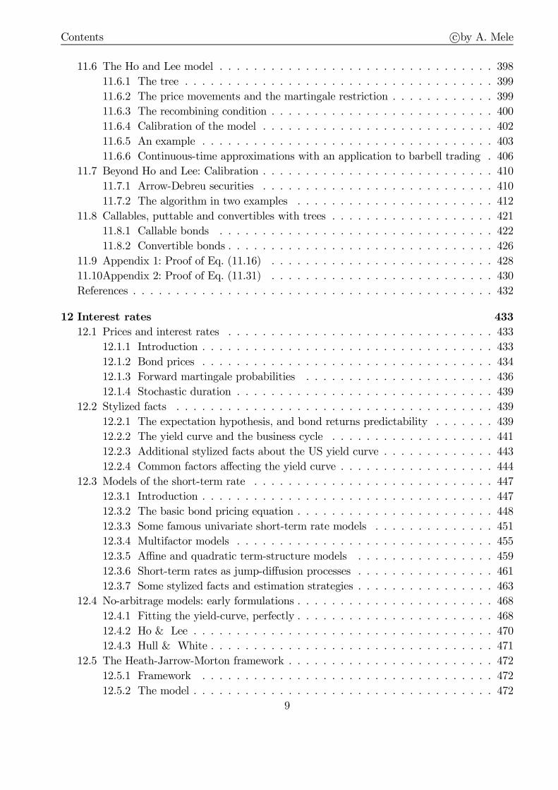
11.6 The Ho and Lee model . . . . . . . . . . . . . . . . . . . . . . . . . . . . . . . . 398
11.6.1 The tree . . . . . . . . . . . . . . . . . . . . . . . . . . . . . . . . . . . . 399
11.6.2 The price movements and the martingale restriction . . . . . . . . . . . . 399
11.6.3 The recombining condition . . . . . . . . . . . . . . . . . . . . . . . . . . 400
11.6.4 Calibration of the model . . . . . . . . . . . . . . . . . . . . . . . . . . . 402
11.6.5 An example . . . . . . . . . . . . . . . . . . . . . . . . . . . . . . . . . . 403
11.6.6 Continuous-time approximations with an application to barbell trading . 406
11.7 Beyond Ho and Lee: Calibration . . . . . . . . . . . . . . . . . . . . . . . . . . . 410
11.7.1 Arrow-Debreu securities . . . . . . . . . . . . . . . . . . . . . . . . . . . 410
11.7.2 The algorithm in two examples . . . . . . . . . . . . . . . . . . . . . . . 412
11.8 Callables, puttable and convertibles with trees . . . . . . . . . . . . . . . . . . . 421
11.8.1 Callable bonds . . . . . . . . . . . . . . . . . . . . . . . . . . . . . . . . 422
11.8.2 Convertible bonds . . . . . . . . . . . . . . . . . . . . . . . . . . . . . . . 426
11.9 Appendix 1: Proof of Eq. (11.16) . . . . . . . . . . . . . . . . . . . . . . . . . . 428
11.10Appendix 2: Proof of Eq. (11.31) . . . . . . . . . . . . . . . . . . . . . . . . . . 430
References . . . . . . . . . . . . . . . . . . . . . . . . . . . . . . . . . . . . . . . . . . 432
12 Interest rates 433
12.1 Prices and interest rates . . . . . . . . . . . . . . . . . . . . . . . . . . . . . . . 433
12.1.1 Introduction . . . . . . . . . . . . . . . . . . . . . . . . . . . . . . . . . . 433
12.1.2 Bond prices . . . . . . . . . . . . . . . . . . . . . . . . . . . . . . . . . . 434
12.1.3 Forward martingale probabilities . . . . . . . . . . . . . . . . . . . . . . 436
12.1.4 Stochastic duration . . . . . . . . . . . . . . . . . . . . . . . . . . . . . . 439
12.2 Stylized facts . . . . . . . . . . . . . . . . . . . . . . . . . . . . . . . . . . . . . 439
12.2.1 The expectation hypothesis, and bond returns predictability . . . . . . . 439
12.2.2 The yield curve and the business cycle . . . . . . . . . . . . . . . . . . . 441
12.2.3 Additional stylized facts about the US yield curve . . . . . . . . . . . . . 443
12.2.4 Common factors affecting the yield curve . . . . . . . . . . . . . . . . . . 444
12.3 Models of the short-term rate . . . . . . . . . . . . . . . . . . . . . . . . . . . . 447
12.3.1 Introduction . . . . . . . . . . . . . . . . . . . . . . . . . . . . . . . . . . 447
12.3.2 The basic bond pricing equation . . . . . . . . . . . . . . . . . . . . . . . 448
12.3.3 Some famous univariate short-term rate models . . . . . . . . . . . . . . 451
12.3.4 Multifactor models . . . . . . . . . . . . . . . . . . . . . . . . . . . . . . 455
12.3.5 Affine and quadratic term-structure models . . . . . . . . . . . . . . . . 459
12.3.6 Short-term rates as jump-diffusion processes . . . . . . . . . . . . . . . . 461
12.3.7 Some stylized facts and estimation strategies . . . . . . . . . . . . . . . . 463
12.4 No-arbitrage models: early formulations . . . . . . . . . . . . . . . . . . . . . . . 468
12.4.1 Fitting the yield-curve, perfectly . . . . . . . . . . . . . . . . . . . . . . . 468
12.4.2 Ho & Lee . . . . . . . . . . . . . . . . . . . . . . . . . . . . . . . . . . . 470
12.4.3 Hull & White . . . . . . . . . . . . . . . . . . . . . . . . . . . . . . . . . 471
12.5 The Heath-Jarrow-Morton framework . . . . . . . . . . . . . . . . . . . . . . . . 472
12.5.1 Framework . . . . . . . . . . . . . . . . . . . . . . . . . . . . . . . . . . 472
12.5.2 The model . . . . . . . . . . . . . . . . . . . . . . . . . . . . . . . . . . . 472
9

Contents c©by A. Mele
12.5.3 The dynamics of the short-term rate . . . . . . . . . . . . . . . . . . . . 473
12.5.4 Embedding . . . . . . . . . . . . . . . . . . . . . . . . . . . . . . . . . . 474
12.6 Stochastic string shocks models . . . . . . . . . . . . . . . . . . . . . . . . . . . 475
12.6.1 Addressing stochastic singularity . . . . . . . . . . . . . . . . . . . . . . 475
12.6.2 No-arbitrage restrictions . . . . . . . . . . . . . . . . . . . . . . . . . . . 476
12.7 Interest rate derivatives . . . . . . . . . . . . . . . . . . . . . . . . . . . . . . . . 477
12.7.1 Introduction . . . . . . . . . . . . . . . . . . . . . . . . . . . . . . . . . . 477
12.7.2 The put-call parity in fixed income markets . . . . . . . . . . . . . . . . 478
12.7.3 European options on bonds . . . . . . . . . . . . . . . . . . . . . . . . . 478
12.7.4 Callable and puttable bonds . . . . . . . . . . . . . . . . . . . . . . . . . 482
12.7.5 Related fixed income products . . . . . . . . . . . . . . . . . . . . . . . . 484
12.7.6 Market models . . . . . . . . . . . . . . . . . . . . . . . . . . . . . . . . 490
12.8 Appendix 1: The FTAP for bond prices . . . . . . . . . . . . . . . . . . . . . . . 496
12.9 Appendix 2: Certainty equivalent interpretation of forward prices . . . . . . . . 498
12.10Appendix 3: Additional results on T -forward martingale probabilities . . . . . . 499
12.11Appendix 4: Principal components analysis . . . . . . . . . . . . . . . . . . . . . 500
12.12Appendix 5: A few analytics for the Hull and White model . . . . . . . . . . . . 501
12.13Appendix 6: Expectation theory and embedding in selected models . . . . . . . 502
12.14Appendix 7: Additional results on string models . . . . . . . . . . . . . . . . . . 504
12.15Appendix 8: Changes of numéraire . . . . . . . . . . . . . . . . . . . . . . . . . 505
References . . . . . . . . . . . . . . . . . . . . . . . . . . . . . . . . . . . . . . . . . . 507
13 Risky debt and credit derivatives 511
13.1 Introduction . . . . . . . . . . . . . . . . . . . . . . . . . . . . . . . . . . . . . . 511
13.2 The classics: Modigliani-Miller irrelevance results . . . . . . . . . . . . . . . . . 511
13.3 Conceptual approaches to valuation of defaultable securities . . . . . . . . . . . 513
13.3.1 Firm’s value, or structural, approaches . . . . . . . . . . . . . . . . . . . 513
13.3.2 Reduced form approaches: rare events, or intensity, models . . . . . . . . 523
13.3.3 Ratings . . . . . . . . . . . . . . . . . . . . . . . . . . . . . . . . . . . . 528
13.4 Convertible bonds . . . . . . . . . . . . . . . . . . . . . . . . . . . . . . . . . . . 532
13.5 Credit-risk shifting derivatives and structured products . . . . . . . . . . . . . . 535
13.5.1 Securitization, and a brief history of credit risk and financial innovation . 535
13.5.2 Total Return Swaps (TRS) . . . . . . . . . . . . . . . . . . . . . . . . . . 538
13.5.3 Spread Options (SOs) . . . . . . . . . . . . . . . . . . . . . . . . . . . . 539
13.5.4 Credit spread options (CSOs) . . . . . . . . . . . . . . . . . . . . . . . . 539
13.5.5 Credit Default Swaps (CDS) . . . . . . . . . . . . . . . . . . . . . . . . . 539
13.5.6 Collateralized Debt Obligations (CDOs) . . . . . . . . . . . . . . . . . . 551
13.5.7 One stylized numerical example of a structured product . . . . . . . . . . 560
13.6 A few hints on the risk-management practice . . . . . . . . . . . . . . . . . . . . 567
13.6.1 Value at Risk (VaR) . . . . . . . . . . . . . . . . . . . . . . . . . . . . . 567
13.6.2 Backtesting . . . . . . . . . . . . . . . . . . . . . . . . . . . . . . . . . . 571
13.6.3 Stress testing . . . . . . . . . . . . . . . . . . . . . . . . . . . . . . . . . 571
13.6.4 Credit risk and VaR . . . . . . . . . . . . . . . . . . . . . . . . . . . . . 572
10

Contents c©by A. Mele
13.7 Appendix 1: Present values contingent on future bankruptcies . . . . . . . . . . 575
13.8 Appendix 2: Proof of selected results . . . . . . . . . . . . . . . . . . . . . . . . 576
13.9 Appendix 3: Details on transition probability matrixes and pricing . . . . . . . . 577
13.10Appendix 4: Derivation of bond spreads with stochastic default intensity . . . . 579
13.11Appendix 5: Conditional probabilities of survival . . . . . . . . . . . . . . . . . . 580
13.12Appendix 6: Modeling correlation with copulae functions . . . . . . . . . . . . . 581
13.13Appendix 7: Details on CDO pricing with imperfect correlation . . . . . . . . . 583
References . . . . . . . . . . . . . . . . . . . . . . . . . . . . . . . . . . . . . . . . . . 584
11

“Many of the models in the literature are not general equilibrium models in my sense. Of
those that are, most are intermediate in scope: broader than examples, but much narrower
than the full general equilibrium model. They are narrower, not for carefully-spelled-out
economic reasons, but for reasons of convenience. I don’t know what to do with models
like that, especially when the designer says he imposed restrictions to simplify the model
or to make it more likely that conventional data will lead to reject it. The full general
equilibrium model is about as simple as a model can be: we need only a few equations to
describe it, and each is easy to understand. The restrictions usually strike me as extreme.
When we reject a restricted version of the general equilibrium model, we are not rejecting
the general equilibrium model itself. So why bother testing the restricted version?”
Fischer Black, 1995, p. 4, Exploring General Equilibrium, The MIT Press.

Preface
The present Lecture Notes in Financial Economics are based on my teaching notes for advanced
undergraduate and graduate courses in financial economics, macroeconomic dynamics, financial
econometrics and financial engineering. Part I, “Foundations,” develops the fundamentals tools
of analysis used in Part II and Part III. These tools span such disparate topics as classical
portfolio selection, dynamic consumption- and production- based asset pricing, in both discrete
and continuous-time, the intricacies underlying incomplete markets and some other market
imperfections and, finally, econometric tools comprising maximum likelihood, methods of mo-
ments, and the relatively more modern simulation-based inference methods. Part II, “Asset
pricing and reality,” is about identifying the main empirical facts in finance and the challenges
they pose to financial economists: from excess price volatility and countercyclical stock market
volatility, to cross-sectional puzzles such as the value premium. This second part reviews the
main models aiming to take these puzzles on board. Part III, “Applied asset pricing theory,”
aims just to this: to use the main tools in Part I and cope with the main challenges occurring
in actual capital markets, arising from option pricing and trading, interest rate modeling and
credit risk and their associated derivatives. In a sense, Part II is about the big puzzles we face
in fundamental research, while Part III is about how to live within our current and certainly
unsatisfactory paradigms, so as to cope with demand for intellectual expertise.
These notes are still underground. The economic motivation and intuition are not always devel-
oped as deeply as they deserve, some derivations are inelegant, and sometimes, the English is a
bit informal. Moreover, I still have to include material on asset pricing with asymmetric informa-
tion, monetary models of asset prices, recent macroeconomic theories about the determination
of the nominal and real term structure of interest rates, bubbles, asset prices implications of
overlapping generations models, or financial frictions. Finally, I need to include more extensive
surveys for each topic I cover, especially in Part II. I plan to revise these notes to fill these gaps.
Meanwhile, any comments on this version are more than welcome.
Antonio Mele
May 2011

Part I
Foundations
14

1
The classic capital asset pricing model
1.1 Portfolio selection
An investor is concerned with choosing a number of assets to include in his portfolio. Which
weigths each asset must bear for the investor to maximize some utility criterion? This section
deals with this problemwhen our investor maximizes a mean-variance criterion, as in the seminal
approach of Markovitz (1952). First, we derive the wealth constraint. Second, we illustrate the
main results of the model, with and without a safe asset. Third, we introduce the notion of
market portfolio.
1.1.1 The wealth constraint
The space choice comprises m risky assets, and some safe asset. Let S = [S1, · · · , Sm] be the
risky assets price vector, and let S0 be the price of the riskless asset. We wish to evaluate the
value of a portfolio that contains all these assets. Let θ = [θ1, · · · , θm], where θi is the number
of the i-th risky asset, and let θ0 be the number of the riskless assets, in this portfolio. The
initial wealth is, w = S0θ0 + S · θ. Terminal wealth is w+ = x0θ0 + x · θ, where x0 is the payoff
promised by the riskless asset, and x = [x1, · · · , xm] is the vector of the payoffs pertaining to
the risky assets, i.e. xi is the payoff of the i-th asset.
The following pieces of notation considerably simplify the presentation. Let R ≡ x0
S0, and
Ri ≡ xiSi. In words, R is the gross interest rate obtained by investing in a safe asset, and Ri is
the gross return obtained by investing in the i-th risky asset. Accordingly, we define r ≡ R− 1as the safe interest rate; b = [b1, · · · , bm], where bi ≡ Ri − 1 is the rate of return on the i-th
asset; and b ≡ E(b), the vector of the expected returns on the risky assets. Finally, we let
π = [π1, · · · , πm], where πi ≡ θiSi is the wealth invested in the i-th asset. We have,
w+ = x0θ0 +m∑
i=1
xiθi ≡ Rπ0 +m∑
i=1
Riπi and w = π0 +m∑
i=1
πi. (1.1)

1.1. Portfolio selection c©by A. Mele
Combining the two expressions for w+ and w, we obtain, after a few simple computations,
w+ = π⊤(R− 1mR) +Rw = π⊤(b− 1mr) +Rw + π⊤(b− b).
We use the decomposition, b − b = a · u, where a is a m × d “volatility” matrix, with m ≤ d,
and u is a random vector with expectation zero and variance-covariance matrix equal to the
identity matrix. With this decomposition, we can rewrite the budget constraint in Eq. (1.1) as
follows:
w+ = π⊤(b− 1mr) +Rw + π⊤au. (1.2)
We now use Eq. (1.2) to compute the expected return and the variance of the portfolio value.
We have,
E[w+(π)
]= π⊤ (b− 1mr) +Rw and var
[w+(π)
]= π⊤Σπ (1.3)
where Σ ≡ aa⊤. Let σ2i ≡ Σii. We assume that Σ has full-rank, and that,
σ2i > σ
2j ⇒ bi > bj all i, j,
which implies that r < minj(bj).
1.1.2 Portfolio choice
We assume that the investor maximizes the expected return on his portfolio, given a certain
level of the variance of the portfolio’s value, which we set equal to w2 · v2p. We use Eq. (1.3) to
set up the following program
π (vp) = arg maxπ∈Rm
E[w+(π)
]s.t. var
[w+(π)
]= w2 · v2p. [1.P1]
The first order conditions for [1.P1] are,
π (vp) = (2ν)−1Σ−1 (b− 1mr) and π⊤Σπ = w2 · v2p,
where ν is a Lagrange multiplier for the variance constraint. By plugging the first condition
into the second, we obtain, (2ν)−1 = ∓w·vp√Sh, where
Sh ≡ (b− 1mr)⊤Σ−1 (b− 1mr) , (1.4)
is the Sharpe market performance. To ensure efficiency, we take the positive solution. Substitut-
ing the positive solution for (2ν)−1 into the first order condition, we obtain that the portfolio
that solves [1.P1] isπ (vp)
w≡ Σ−1 (b− 1mr)√
Sh· vp. (1.5)
We are now ready to calculate the value of [1.P1], E [w+(π (vp))] and, hence, the expected
portfolio return, defined as,
µp(vp) ≡E [w+(π(vp))]− w
w= r +
√Sh · vp, (1.6)
where the last equality follows by simple computations. Eq. (1.6) describes what is known as
the Capital Market Line (CML).
16

1.1. Portfolio selection c©by A. Mele
1.1.3 Without the safe asset
Next, let us suppose the investor’s space choice does not include the riskless asset. In this case,
his current wealth is w =∑m
i=1 πi, and his terminal wealth is w+ =∑m
i=1 Riπi. By the definition
of bi ≡ Ri − 1, and by a few simple computations,
w+ =m∑
i=1
biπi +m∑
i=1
πi = π⊤b+ w + π⊤au, (1.7)
where a and u are as defined as in Eq. (1.2). We can use Eq. (1.7) to compute the expected
return and the variance of the portfolio value, which are:
E[w+(π)
]= π⊤b+ w, where w = π⊤1m and var
[w+(π)
]= π⊤Σπ. (1.8)
The program our investor solves, now, is:
π (vp) = argmaxπ∈R
E[w+(π)
]s.t. var
[w+(π)
]= w2 · v2p and w = π⊤1m. [1.P2]
In the appendix, we show that provided αγ − β2 > 0 (a second order condition), the solution
to [1.P2] is,π (vp)
w=γµp(vp)− βαγ − β2 Σ−1b+
α− βµp(vp)αγ − β2 Σ−1
1m, (1.9)
where α ≡ b⊤Σ−1b, β ≡ 1⊤mΣ−1b and γ ≡ 1⊤mΣ−11m, and µp(vp) is the expected portfolio return,
defined as in Eq. (1.6). In the appendix, we also show that,
v2p =1
γ
[1 +
1
αγ − β2
(γµp(vp)− β
)2]. (1.10)
Therefore, the global minimum variance portfolio achieves a variance equal to v2p = γ−1 and an
expected return equal to µp = β/ γ.
Note that for each vp, there are two values of µp(vp) that solve Eq. (1.10). The optimal choice
for our investor is that with the highest µp. We define the efficient portfolio frontier as the set
of values (vp, µp) that solve Eq. (1.10) with the highest µp. It has the following expression,
µp(vp) =β
γ+1
γ
√(γv2p − 1
) (αγ − β2
). (1.11)
Clearly, the efficient portfolio frontier is an increasing and concave function of vp. It can be
interpreted as a sort of “production function,” one that produces “expected returns” through
inputs of “levels of risk” (see, e.g., Figure 1.1). The choice of which portfolio has effectively to
be selected depends on the investor’s preference toward risk.
E 1.1. Let the number of risky assets m = 2. In this case, we do not need to
optimize anything, as the budget constraint, π1
w+ π2
w= 1, pins down an unique relation between
the portfolio expected return and the variance of the portfolio’s value. So we simply have,
µp =E[w+(π)]−w
w= π1
wb1 +
π2
wb2, or,
µp = b1 + (b2 − b1)
π2
w
v2p =(1− π2
w
)2
σ21 + 2
(1− π2
w
) π2
wσ12 +
(π2
w
)2
σ22
17

1.1. Portfolio selection c©by A. Mele
0 0.05 0.1 0.15 0.2 0.250.09
0.1
0.11
0.12
0.13
0.14
0.15
Volatility, vp
Exp
ecte
d re
turn
, mu p
ρ = −1
ρ = − 0.5
ρ = 0
ρ = 0.5
ρ = 1
FIGURE 1.1. From top to bottom: portfolio frontiers corresponding to ρ = −1,−0.5, 0, 0.5, 1. Para-meters are set to b1 = 0.10, b2 = 0.15, σ1 = 0.20, σ2 = 0.25. For each portfolio frontier, the efficient
portfolio frontier includes those portfolios which yield the lowest volatility for a given expected return.
whence:
vp =1
b2 − b1
√(b2 − µp
)2σ21 + 2
(b2 − µp
) (µp − b1
)ρσ1σ1 +
(µp − b1
)2σ22
When ρ = 1,
µp = b1 +(b1 − b2) (σ1 − vp)
σ2 − σ1.
In the general case, diversification pays when the asset returns are not perfectly positively
correlated (see Figure 1.1). As Figure 1.1 reveals, it is even possible to obtain a portfolio that
is less risky than than the less risky asset. Moreover, risk can be zeroed when ρ = −1, whichcorresponds to π1
w= σ2
σ2−σ1and π2
w= − σ1
σ2−σ1or, alternatively, to π1
w= − σ2
σ2−σ1and π2
w= σ1
σ2−σ1.
Let us return to the general case. The portfolio in Eq. (1.9) can be decomposed into two
components, as follows:
π (vp)
w= ℓ (vp)
πdw+ [1− ℓ (vp)]
πgw, ℓ (vp) ≡
β(µp (vp) γ − β
)
αγ − β2 ,
where
πdw≡ Σ−1b
β,
πgw≡ Σ−1
1m
γ.
18

1.1. Portfolio selection c©by A. Mele
Hence, we see thatπgw
is the global minimum variance portfolio, for we know from Eq. (1.10)
that the minimum variance occurs at (vp, µp) =(√
1γ, βγ
), in which case ℓ (vp) = 0.1 More
generally, we can span any portfolio on the frontier by just choosing a convex combination ofπdw
andπgw, with weight equal to ℓ (vp). It’s a mutual fund separation theorem.
1.1.4 The market portfolio
The market portfolio is the portfolio at which the CML in Eq. (1.6) and the efficient portfolio
frontier in Eq. (1.11) intersect. In fact, the market portfolio is the point at which the CML is
tangent at the efficient portfolio frontier. For this reason, the market portfolio is also referred
to as the “tangent” portfolio. In Figure 1.2, the market portfolio corresponds to the point M
(the portfolio with volatility equal to vM and expected return equal to µM), which is the point
at which the CML is tangent to the efficient portfolio frontier, AMC.2
As Figure 1.2 illustrates, the CML dominates the efficient portfolio frontier AMC. This is
because the CML is the value of the investor’s problem, [1.P1], obtained using all the risky
assets and the riskless asset, and the efficient portfolio frontier is the value of the investor’s
problem, [1.P2], obtained using only all the risky assets.3 For the same reason, the CML and
the efficient portfolio frontier can only be tangent with each other. For suppose not. Then,
there would exist a point on the efficient portfolio frontier that dominates some portfolio on the
CML, a contradiction. Likewise, the CML must have a portfolio in common with the efficient
portfolio frontier - the portfolio that does not include the safe asset. Below, we shall use this
insight to characterize, analytically, the market portfolio.
Why is the market portfolio called in this way? Figure 1.2 reveals that any portfolio on the
CML can be obtained as a combination of the safe asset and the market portfolioM (a portfolio
containing only the risky assets). An investor with high risk-aversion would like to choose a
point such as Q, say. An investor with low risk-aversion would like to choose a point such as P ,
say. But no matter how risk averse an individual is, the optimal solution for him is to choose
a combination of the safe asset and the market portfolio M . Thus, the market portfolio plays
an instrumental role. It obviously does not depend on the risk attitudes of any investor - it is a
mere convex combination of all the existing assets in the economy. Instead, the optimal course
of action for any investor is to use those proportions of this portfolio that make his overall
exposure to risk consistent with his risk appetite. It’s a two fund separation theorem.
The equilibrium implications if this separation theorem as follows. As we have explained,
any portfolio can be attained by lending or borrowing funds in zero net supply, and in the
portfolio M . In equilibrium, then, every investor must hold some proportions of M . But since
in aggregate, there is no net borrowing or lending, one has that in aggregate, all investors
must have portfolio holdings that sum up to the market portfolio, which is therefore the value-
1 It is easy to show that the covariance of the global minimum variance portfolio with any other portfolio equals γ−1.2The existence of the market portfolio requires a restriction on r, derived in Eq. (1.12) below.3Figure 1.2 also depicts the dotted line MZ, which is the value of the investor’s problem when he invests a proportion higher
than 100% in the market portfolio, leveraged at an interest rate for borrowing higher than the interest rate for lending. In this case,
the CML coincides with rM , up to the point M . From M onwards, the CML coincides with the highest between MZ and MA.
19
1.1. Portfolio selection c©by A. Mele
vM
CML
r
MµM
A
C
P
Q
Z
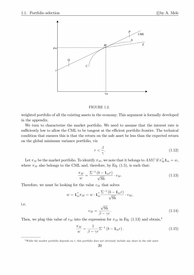
FIGURE 1.2.
weighted portfolio of all the existing assets in the economy. This argument is formally developed
in the appendix.
We turn to characterize the market portfolio. We need to assume that the interest rate is
sufficiently low to allow the CML to be tangent at the efficient portfolio frontier. The technical
condition that ensures this is that the return on the safe asset be less than the expected return
on the global minimum variance portfolio, viz
r <β
γ. (1.12)
Let πM be the market portfolio. To identify πM , we note that it belongs toAMC if π⊤M1m = w,
where πM also belongs to the CML and, therefore, by Eq. (1.5), is such that:
πMw
=Σ−1 (b− 1mr)√
Sh· vM . (1.13)
Therefore, we must be looking for the value vM that solves
w = 1⊤mπM = w · 1⊤mΣ−1 (b− 1mr)√
Sh· vM ,
i.e.
vM =
√Sh
β − γr . (1.14)
Then, we plug this value of vM into the expression for πM in Eq. (1.13) and obtain,4
πMw
=1
β − γrΣ−1 (b− 1mr) . (1.15)
4While the market portfolio depends on r, this portfolio does not obviously include any share in the safe asset.
20

1.2. The CAPM c©by A. Mele
Once again, the market portfolio belongs to the efficient portfolio frontier. Indeed, on the
one hand, the market portfolio can not be above the efficient portfolio frontier, as this would
contradict the efficiency of the AMC curve, which is obtained by investing in the risky assets
only; on the other hand, the market portfolio can not be below the efficient portfolio frontier, for
by construction, it belongs to the CML which, as shown before, dominates the efficient portfolio
frontier. In the appendix, we confirm, analytically, that the market portfolio does indeed enjoy
the tangency condition.
1.2 The CAPM
The Capital Asset Pricing Model (CAPM) provides an asset evaluation formula. In this section,
we derive the CAPM through arguments that have the same flavor as the original derivation of
Sharpe (1964). The first step is the creation of a portfolio including a proportion α of wealth
invested in any asset i and the remaining proportion 1 − α invested in the market portfolio.
Mathematically, we are considering an α-parametrized portfolio, with expected return and
volatility given by: µp ≡ αbi + (1− α)µMvp ≡
√(1− α)2σ2
M + 2(1− α)ασiM + α2σ2i
(1.16)
where we have defined σM ≡ vM . Clearly, the market portfolio,M , belongs to the α-parametrized
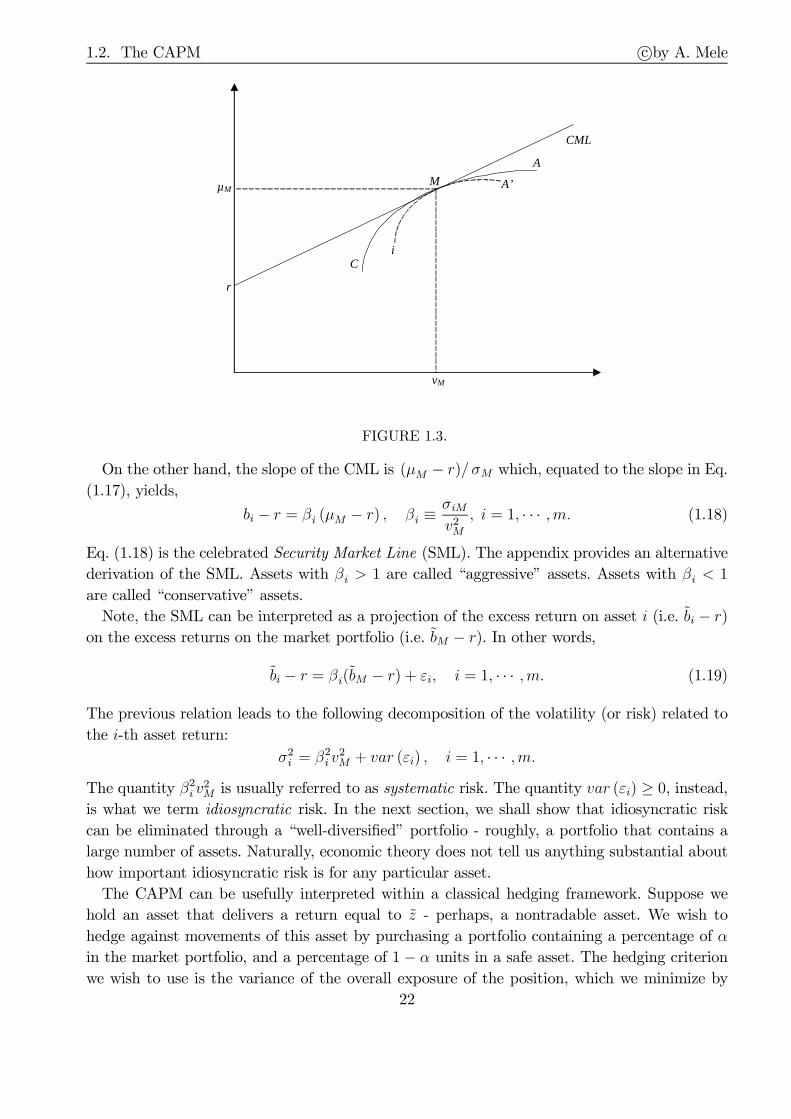
portfolio. By the Example 1.1, the curve in (1.16) has the same shape as the curve A′Mi in
Figure 1.3. The curve A′Mi lies below the efficient portfolio frontier AMC. This is because
the efficient portfolio frontier is obtained by optimizing a mean-variance criterion over all the
existing assets and, hence, dominates any portfolio that only comprises the two assets i andM .
Suppose, for example, that the A′Mi curve intersects the AMC curve; then, a feasible combi-
nation of assets (including some proportion α of the i-th asset and the remaining proportion
1− α of the market portfolio) would dominate AMC, a contradiction, given that AMC is the
most efficient feasible combination of all the assets. On the other hand, the A′Mi curve has a
point in common with the AMC, which isM , in correspondence of α = 0. Therefore, the curve
A′Mi is tangent to the efficient portfolio frontier AMC at M , which in turn, as we already
know, is tangent to the CML at M .
Let us equate, then, the two slopes of the A′Mi curve and the efficient portfolio frontier
AMC at M . We shall show that this condition provides a restriction on the expected return bion any asset i. Because (1.16) is, mathematically, an α-parametrized curve, we may compute
its slope at M through the computation of dµp/dα and dvp/ dα, at α = 0. We have,
dµpdα
= bi − µM ,dvpdα
∣∣∣∣α=0
= −−(1− α)σ2M + (1− 2α)σiM + ασ2
i |α=0
vp|α=0
=1
σM
(σiM − σ2
M
).
Therefore,
dµp(α)
dvp(α)
∣∣∣∣α=0
=bi − µM
1σM
(σiM − σ2M). (1.17)
21
1.2. The CAPM c©by A. Mele
vM
CML
r
M
A
Ci
A’µM
FIGURE 1.3.
On the other hand, the slope of the CML is (µM − r)/σM which, equated to the slope in Eq.
(1.17), yields,
bi − r = βi (µM − r) , βi ≡σiMv2M
, i = 1, · · · ,m. (1.18)
Eq. (1.18) is the celebrated Security Market Line (SML). The appendix provides an alternative
derivation of the SML. Assets with βi > 1 are called “aggressive” assets. Assets with βi < 1
are called “conservative” assets.
Note, the SML can be interpreted as a projection of the excess return on asset i (i.e. bi − r)on the excess returns on the market portfolio (i.e. bM − r). In other words,
bi − r = βi(bM − r) + εi, i = 1, · · · ,m. (1.19)
The previous relation leads to the following decomposition of the volatility (or risk) related to
the i-th asset return:
σ2i = β
2i v
2M + var (εi) , i = 1, · · · ,m.
The quantity β2i v
2M is usually referred to as systematic risk. The quantity var (εi) ≥ 0, instead,
is what we term idiosyncratic risk. In the next section, we shall show that idiosyncratic risk
can be eliminated through a “well-diversified” portfolio - roughly, a portfolio that contains a
large number of assets. Naturally, economic theory does not tell us anything substantial about
how important idiosyncratic risk is for any particular asset.
The CAPM can be usefully interpreted within a classical hedging framework. Suppose we
hold an asset that delivers a return equal to z - perhaps, a nontradable asset. We wish to
hedge against movements of this asset by purchasing a portfolio containing a percentage of α
in the market portfolio, and a percentage of 1− α units in a safe asset. The hedging criterion
we wish to use is the variance of the overall exposure of the position, which we minimize by
22

1.3. The APT c©by A. Mele
minα var[z − ((1− α) r + αbM)]. It is straight forward to show that the solution to this basic
problem is, α ≡ βz ≡ cov(z, bM)/v2m. That is, the proportion to hold is simply the beta of the
asset to hedge with the market portfolio.
The CAPM is a model for the required return for any asset and so, it is a very first tool we
can use to evaluate risky projects. Let
V = value of a project =E (C+)
1 + rC,
where C+ is future cash flow and rC is the risk-adjusted discount rate for this project. We have:
E (C+)
V= 1 + rC
= 1 + r + βC (µM − r)
= 1 + r +cov
(C+
V− 1, xM
)
v2M(µM − r)
= 1 + r +1
V
cov (C+, xM)
v2M(µM − r)
= 1 + r +1
Vcov
(C+, xM
) λ
vM,
where λ ≡ µM−rvM
, the unit market risk-premium.
Rearranging terms in the previous equation leaves:
V =E (C+)− λ
vMcov (C+, xM)
1 + r. (1.20)
The certainty equivalent C is defined as:
C : V =E (C+)
1 + rC=
C
1 + r,
or,
C = (1 + r)V,
and using Eq. (1.20),
C = E(C+
)− λ
vMcov
(C+, xM
).
1.3 The APT
1.3.1 A first derivation
Suppose that the m asset returns we observe are generated by the following linear factor model,
bm×1
= am×1
+ Bm×k
· fk×1
≡ a+ cov(b, f)[var(f)]−1 · f (1.21)
23

1.3. The APT c©by A. Mele
where a and B are a vector and a matrix of constants, and f is a k-dimensional vector of factors
supposed to affect the asset returns, with k ≤ m. Let us normalize [var(f)]−1 = Ik×k, so that
B = cov(b, f). With this normalization, we have,
b = a+
cov(b1, f)
...
cov(bm, f)
· f = a+
∑kj=1 cov(b1, fj)fj
...∑kj=1 cov(bm, fj)fj
.
Next, let us consider a portfolio π including the m risky assets. The return of this portfolio
is,
π⊤b = π⊤a+ π⊤Bf,
where as usual, π⊤1m = 1. An arbitrage opportunity arises if there exists some portfolio π
such that the return on the portfolio is certain, and different from the safe interest rate r, i.e. if
∃π : π⊤B = 0 and π⊤a = r. Mathematically, this is ruled out whenever ∃λ ∈ Rk : a = Bλ+1mr.
Substituting this relation into Eq. (1.21) leaves,
b = 1mr +Bλ+Bf = 1mr + cov(b, f)λ+ cov(b, f)f.
Taking the expectation,
bi = r + (Bλ)i = r +∑k
j=1cov(bi, fj)︸ ︷︷ ︸
≡βi,j
λj , i = 1, · · · ,m. (1.22)
The APT collapses to the CAPM, once we assume that the only factor affecting the returns
is the market portfolio. To show this, we must normalize the market portfolio return so that its
variance equals one, consistently with Eq. (1.22). So let rM be the normalized market return,
defined as rM ≡ v−1M bM , so that var(rM) = 1. We have,
bi = a+ βirM , i = 1, · · · ,m,
where βi = cov(bi, rM) = v−1M cov(bi, bM). Then, we have,
bi = r + βiλ, i = 1, · · · ,m. (1.23)
In particular, βM = cov(bM , rM) = v−1M var(bM) = vM , and so, by Eq. (1.23),
λ =bM − rvM
,
which is known as the Sharpe ratio for the market portfolio, or the market price of risk.
By replacing βi = v−1M cov(bi, bM) and the expression for λ above into Eq. (1.23), we obtain,
bi = r +cov(bi, bM)
v2M(bM − r) , i = 1, · · · ,m.
This is simply the SML in Eq. (1.18).
24

1.3. The APT c©by A. Mele
1.3.2 The APT with idiosyncratic risk and a large number of assets
[Ross (1976), and Connor (1984), Huberman (1983).]
How can idiosyncratic risk be eliminated? Consider, for example, Eq. (1.19). Intuitively, we
may form portfolios with a large number of assets, so as to make idiosyncratic risk negligible, by
the law of large numbers. But would the beta-relation still hold, in this case? More in general,
would the APT relation in Eq. (1.22) be still valid? The answer is in the affirmative, although
it deserves some qualifications.
Consider the APT equation (1.21), and “add” a vector of idiosyncratic returns, ε, which are
independent of f , and have mean zero and variance σ2ε:
b = a+B · f + ε.
We wish to show that in the absence of arbitrage, to be defined below, it must be that the
number of assets such that Eq. (1.22) does not hold, N (m) say, is bounded as m gets large,
i.e.:
|ai − ((Bλ)i + r)| > 0, i = 1, · · · ,N (m) , (1.24)
where
limm→∞
N (m) <∞. (1.25)
In other words, we wish to show that in a “large” market, Eq. (1.22) does indeed hold for most
of the assets, an approach close to that in Huang and Litzenberger (1988, p. 106-108).
By the same arguments leading to Eq. (1.1), the wealth generated by a portfolio of the assets
satisfying (1.24), w+N(m) say, is,
w+N(m) = π
⊤N(m)
(aN(m) − 1N(m)r
)+RwN(m) + π
⊤N(m)
(BN(m)f + εN(m)
),
where aN , BN and εN are (i) the vector of the expected returns, (ii) the return volatility (or
factor exposures) matrix and (iii) the vector of idiosyncratic return components affecting these
assets, and, finally, πN and wN are the portfolio and the initial wealth invested in these assets.
In this context, we may define an arbitrage as the portfolio πN(m) that in the limit, as the
number of all the existing assets m gets large, is riskless and yet delivers an expected return
strictly larger than the safe interest rate, viz
limm→∞
E[w+N(m)]
wN(m)
> R, and limm→∞
var[w+N(m)]→ 0. (1.26)
We want to show that this situation does not arises, under the condition in (1.25), thereby
establishing that the linear APT relation in Eq. (1.22) is valid for most of the assets, in a large
market.
So suppose the linear relation, aN − 1Nr = BNλ, doesn’t hold. Then, there exists a portfolio
π such that,
π⊤BN = 0 and π⊤ (aN − 1Nr) = 0. (1.27)
Consider the portfolio:
πN =1
N· sign
(π⊤ (aN − 1Nr)
)· π,
25
1.3. The APT c©by A. Mele
where π is as in (1.27). With this portfolio we have, clearly, that E[w+N ] = π⊤N (aN − 1Nr) +
RwN > RwN , for each N , and even for N large. That is, limm→∞E[w+N(m)]/wN(m) > R, which
is the first condition in (1.26). As regards the second condition in (1.26), we have that
var[w+N ] = π
⊤N
(BNB
⊤N + σ
2εIN×N
)πN = σ
2επ⊤N πN ,
where the second equality follows by the first relation in (1.27). Clearly, limm→∞ var[w+N(m)]→ 0
as N (m)→∞. Hence, in the absence of arbitrage, the condition in (1.25) must hold.
1.3.3 Empirical evidence
How to estimate Eq. (1.19)? Consider a slightly more general version of Eq. (1.19), where the
safe interest rate is time-varying:
bi,t − rt = βi(bM,t − rt) + εi,t, i = 1, · · · ,m,
where εi,t denote “time-series residuals.” Fama and MacBeth (1973) consider the following
procedure. In a first step, one obtains estimates of the exposures to the market, βi say, for all
stocks, using, for example, monthly returns, and approximating the market portfolio with some
broad stock market index.5 In a second step, one runs cross-sectional regressions, one for each
month,
bi,t − rt = αit + λtβi + ηi,t, t = 1, · · · , T,where T is the sample size and ηi,t denote “cross-sectional residuals.” The time-series of cross-
sectional estimates of the intercept αi,t and the price of risk λt, αi,t and λt say, are, then, used
to make statistical inference. For example, time-series averages and standard errors of αi,t and
λt lead to point estimates and standard errors for αi,t and λt. If the CAPM holds, estimates of
αi should not be significantly different from zero.
Chen, Roll and Ross (1986) use the Fama-MacBeth two-step procedure to estimate a multi-
factor APT model, such as that in Section 1.3. They identify “macroeconomic forces” driving
asset returns with the innovations in variables such as the term spread, expected and unex-
pected inflation, industrial production growth, or the corporate spread. They find that these
sources of variation in the cross-section of asset returns are significantly priced.
5 In tests of the CAPM, one uses proxies of the market portfolio, such as, say, the S&P 500. However, the market portfolio is
unobservable. Roll (1977) points out that as a result, the CAPM is inherently untestable, as any test of the CAPM is a joint test
of the model itself and of the closeness of the proxy to the market portfolio.
26

1.4. Appendix 1: Some analytical details for portfolio choice c©by A. Mele
1.4 Appendix 1: Some analytical details for portfolio choice
We derive Eq. (1.9), which provides the solution for the portfolio choice when the space choice does notinclude a safe asset. We derive the solution by proceeding with two programs: (i) the primal program[1.P2] in the main text, which consists in maximizing the portfolio expected return, given a certainlevel of the variance of the portfolio’s value; and (ii) a dual program, to be introduced below, by whichone minimizes the variance of the portfolio’s value, given a certain level of the portfolio expectedreturn.
1.4.1 The primal program
Given Eq. (1.8), the Lagrangian function associated to [1.P2] is,
L = π⊤b+w − ν1(π⊤Σπ −w2 · v2p)− ν2(π
⊤1m −w),
where ν1 and ν2 are two Lagrange multipliers. The first order conditions are,
π =1
2ν1Σ−1 (b− ν21m) , π⊤Σπ = w2 · v2p, π⊤1m = w. (1A.1)
Using the first and the third conditions, we obtain,
w = 1⊤mπ =1
2ν1(1⊤mΣ
−1b︸ ︷︷ ︸≡β
− ν21⊤mΣ
−11m︸ ︷︷ ︸
≡γ
) ≡ 1
2ν1(β − ν2γ).
We can solve for ν2, obtaining,
ν2 =β − 2wν1
γ.
By replacing the solution for ν2 into the first condition in (1A.1) leaves,
π =w
γΣ−1
1m +1
2ν1Σ−1
(b− β
γ1m
). (1A.2)
Next, we derive the value of the program [1.P2]. We have,
E[w+(π)
]−w = π⊤b =
w
γ1⊤mΣ
−1b︸ ︷︷ ︸≡β
+1
2ν1(b⊤Σ−1b︸ ︷︷ ︸
≡α− β
γ1⊤mΣ
−1b︸ ︷︷ ︸≡β
) =w
γβ +
1
2ν1
(α− β2
γ
). (1A.3)
It is easy to check that
var[w+(π)
]= w2 · v2p= π⊤Σπ
=
[w
γ1⊤mΣ
−1 +1
2ν1
(b⊤ − β
γ1⊤m
)Σ−1
] [w
γ1m +
1
2ν1
(b− β
γ1m
)]
=w2
γ+
(1
2ν1
)2(α− β2
γ
). (1A.4)
Let us gather Eqs. (1A.3) and (1A.4),
µp(vp) ≡E [w+(π)]−w
w=
β
γ+
1
2ν1w
(α− β2
γ
)
v2p =1
γ+
(1
2ν1w
)2 (α− β2
γ
) (1A.5)
27

1.4. Appendix 1: Some analytical details for portfolio choice c©by A. Mele
where we have emphasized the dependence of µp on vp, which arises through the presence of theLagrange multiplier ν1.
Let us rewrite the first equation in (1A.5) as follows,
1
2ν1w=
(αγ − β2
)−1 (γµp(vp)− β
). (1A.6)
We can use this expression for ν1 to express π in Eq. (1A.2) in terms of the portfolio expected return,µp(vp). We have,
π
w=
Σ−11m
γ+
(αγ − β2
)−1 (γµp(vp)− β
)(Σ−1b− Σ−1β
γ1m
).
By rearranging terms in the previous equation, we obtain Eq. (1.9) in the main text.Finally, we substitute Eq. (1A.6) into the second equation in (1A.5), and obtain:
v2p =1
γ
[1 +
(αγ − β2
)−1 (γµp(vp)− β
)2],
which is Eq. (1.10) in the main text. Note, also, that the second condition in (1A.5) reveals that,
(1
2ν1w
)2
=γv2p − 1
αγ − β2 .
Given that αγ−β2 > 0, the previous equation confirms the properties of the global minimum varianceportfolio stated in the main text.
1.4.2 The dual program
We now solve the dual program, defined as follows,
π = arg minπ∈Rm
var
[w+(π)
w
]s.t. E
[w+(π)
]= Ep and w = π⊤1m, [1A.P2-dual]
for some constant Ep. The first order conditions are
π
w=
ν1w
2Σ−1b+
ν2w
2Σ−1
1m ; π⊤b = Ep −w ; w = π⊤1m; (1A.7)
where ν1 and ν2 are two Lagrange multipliers. By replacing the first condition in (8A.14) into thesecond one,
Ep −w = π⊤b = w2(ν12b⊤Σ−1b︸ ︷︷ ︸≡α
+ν221⊤mΣ
−1b︸ ︷︷ ︸≡β
) ≡ w2(ν12α+
ν22β). (1A.8)
By replacing the first condition in (8A.14) into the third one,
w = π⊤1m = w2(ν12b⊤Σ−1
1m︸ ︷︷ ︸≡β
+ν221⊤mΣ
−11m︸ ︷︷ ︸
≡γ
) ≡ w2(ν12β +
ν22γ). (1A.9)
Next, let µp ≡ Ep−ww . By Eqs. (1A.8) and (1A.9), the solutions for ν1 and ν2 are,
ν1w
2=
µpγ − β
αγ − β2 ;ν2w
2=
α− βµp
αγ − β2
28

1.4. Appendix 1: Some analytical details for portfolio choice c©by A. Mele
Therefore, the solution for the portfolio in Eq. (8A.14) is,
π
w=
γµp − β
αγ − β2Σ−1b+
α− βµp
αγ − β2Σ−11m.
Finally, the value of the program is,
var
[w+(π)
w
]=
1
w2π⊤Σπ =
1
wπ⊤
µpγ − β
αγ − β2 b+1
wπ⊤
α− µpβ
αγ − β21m =γµ2
p − 2βµp + α
αγ − β2 =(γµp − β)2
(αγ − β2)γ+
1
γ,
which is exactly Eq. (1.10) in the main text.
29

1.5. Appendix 2: The market portfolio c©by A. Mele
1.5 Appendix 2: The market portfolio
1.5.1 The tangent portfolio is the market portfolio
Let us define the market capitalization for any asset i as the value of all the assets i that are outstandingin the market, viz
Capi ≡ θiSi, i = 1, · · · ,m,
where θi is the number of assets i outstanding in the market. The market capitalization of all theassets is simply
CapM ≡m∑
i=1
Capi.
The market portfolio, then, is the portfolio with relative weights given by,
πM,i ≡CapiCapM
, i = 1, · · · ,m.
Next, suppose there are N investors and that each investor j has wealth wj , which he invests in two
funds, a safe asset and the tangent portfolio. Let wfj be the wealth investor j invests in the safe asset
and wj −wfj the remaining wealth the investor invests in the tangent portfolio. The tangent portfolio
is defined as πT ≡(πTwj
), for some πT solution to [1.P2], and is obviously independent of wj (see Eq.
(1.15) in the main text). The equilibrium in the stock market requires that
CapM · πM =N∑
j=1
(wj −wf
j
)πT =
N∑
j=1
wj · πT = CapM · πT .
where the second equality follows because the safe asset is in zero net supply and, hence,∑N
j=1wfj = 0;
and the third equality holds because all the wealth in the economy is invested in stocks, in equilibrium.
1.5.2 Tangency condition
We check that the CML and the efficient portfolio frontier have the same slope in correspondenceof the market portfolio. Let us impose the following tangency condition of the CML to the efficientportfolio frontier in Figure 1.2, AMC, at the point M :
√Sh =
αγ − β2
γµM − βvM . (1A.10)
The left hand side of this equation is the slope of the CML, obtained through Eq. (1.6). The right handside is the slope of the efficient portfolio frontier, obtained by differentiating µp(v) in the expressionfor the portfolio frontier in Eq. (1.11), and setting v = vM in
dµp(v)
dv=
√(γv2 − 1)−1 (αγ − β2
)v =
αγ − β2
γµp(v)− βv,
and where the second equality follows, again, by Eq. (1.11). By Eqs. (1A.10) and (1.14), we need toshow that,
γµM − β
αγ − β2 =1
β − γr.
By plugging µM = r +√Sh · vM into the previous equality and rearranging terms,
vM =
√Sh
β − γr,
30

1.5. Appendix 2: The market portfolio c©by A. Mele
where we have made use of the equality Sh = α−2βr+γr2, obtained by elaborating on the definitionof the Sharpe market performance Sh given in Eq. (1.4). This is indeed the variance of the marketportfolio given in Eq. (1.14).
31

1.6. Appendix 3: An alternative derivation of the SML c©by A. Mele
1.6 Appendix 3: An alternative derivation of the SML
The vector of covariances of the m asset returns with the market portfolio are:
cov (x, xM) = cov(x, x · πM
w
)= Σ
πMw
=1
β − γr(b− 1mr) , (1A.11)
where we have used the expression for the market portfolio given in Eq. (1.15). Next, premultiply the
previous equation byπ⊤Mw to obtain:
v2M =π⊤Mw
ΣπMw
=π⊤Mw
1
β − γr(b− 1mr) =
1
(β − γr)2Sh, (1A.12)
or vM =√Sh
β−γr , which confirms Eq. (1.14).Let us rewrite Eq. (1A.11) component by component. That is, for i = 1, · · · ,m,
σiM ≡ cov (xi, xM) =1
β − γr(bi − r) =
vM√Sh
(bi − r) =v2M
µM − r(bi − r) ,
where the last two equalities follow by Eq. (1A.12) and by the relation,√Sh = µM−r
vM. By rearranging
terms, we obtain Eq. (1.18).
32

1.7. Appendix 4: Broader definitions of risk - Rothschild and Stiglitz theory c©by A. Mele
1.7 Appendix 4: Broader definitions of risk - Rothschild and Stiglitz theory
The papers are Rothschild and Stiglitz (1970, 1971). Notation, any variable with a tilde is a randomvariable. Let us consider the following definition of stochastic dominance:
D A.1 (Second-order stochastic dominance). x2 dominates x1 if, for each utility functionu satisfying u′ ≥ 0, we have also that E [u (x2)] ≥ E [u (x1)].
We have:
T A.2. The following statements are equivalent:
a) x2 dominates x1, or E [u (x2)] ≥ E [u (x1)];
b) ∃ random variable η > 0 : x2 = x1 + η;
c) ∀x > 0, F1(x) ≥ F2(x).
P. We provide the proof when the support is compact, say [a, b]. First, we show that b)⇒ c).We have: ∀t0 ∈ [a, b], F1(t0) ≡ Pr (x1 ≤ t0) = Pr (x2 ≤ t0 + η) ≥ Pr (x2 ≤ t0) ≡ F2(t0). Next, we showthat c)⇒ a). By integrating by parts,
E [u (x)] =
∫ b
au(x)dF (x) = u(b)−
∫ b
au′(x)F (x)dx,
where we have used the fact that: F (a) = 0 and F (b) = 1. Therefore,
E [u (x2)]−E [u (x1)] =
∫ b
au′(x) [F1(x)− F2(x)] dx.
Finally, it is easy to show that a)⇒ b). ‖
Next, we turn to the definition of “increasing risk”:
D A.3. x1 is more risky than x2 if, for each function u satisfying u′′ < 0, we have alsothat E [u (x1)] ≤ E [u (x2)] for x1 and x2 having the same mean.
This definition of “increasing risk” does not rely on the sign of u′. Furthermore, if var (x1) >var (x2), x1 is not necessarily more risky than x2, according to the previous definition. The standardcounterexample is the following one. Let x2 = 1 w.p. 0.8, and 100 w.p. 0.2. Let x1 = 10 w.p. 0.99, and1090 w.p. 0.01. We have, E (x1) = E (x2) = 20.8, but var (x1) = 11762.204 and var (x2) = 1647.368.However, consider u(x) = log x. Then, E (log (x1)) = 2.35 > E (log (x2)) = 0.92. It is easily seen thatin this particular example, the distribution function F1 of x1 “intersects” F2, which is in contradictionwith the following theorem.
T A.4. The following statements are equivalent:
a) x1 is more risky than x2;
b) x1 has more weight in the tails than x2, i.e. ∀t,∫ t−∞ [F1(x)− F2(x)] dx ≥ 0;
c) x1 is a mean preserving spread of x2, i.e. there exists a random variable ǫ : x1 has the samedistribution as x2 + ǫ, and E (ǫ| x2 = x2) = 0.
33

1.7. Appendix 4: Broader definitions of risk - Rothschild and Stiglitz theory c©by A. Mele
P. Let us begin with c)⇒ a). We have,
E [u (x1)] = E [u (x2 + ǫ)]
= E [E (u (x2 + ǫ)| x2 = x2)]
≤ E [u (E ( x2 + ǫ| x2 = x2))]
= E [u (E ( x2| x2 = x2))]
= E [u (x2)] .
As regards a)⇒ b), we have that:
E [u (x1)]−E [u (x2)] =
∫ b
au(x) [f1(x)− f2(x)] dx
= u(x) [F1(x)− F2(x)]|ba −∫ b
au′(x) [F1(x)− F2(x)] dx
= −∫ b
au′(x) [F1(x)− F2(x)] dx
= −[u′(x)
[F1(x)− F2(x)
]∣∣ba−
∫ b
au′′(x)
[F1(x)− F2(x)
]dx
]
=
∫ b
au′′(x)
[F1(x)− F2(x)
]dx− u′(b)
[F1(b)− F2(b)
],
where Fi(x) =∫ xa Fi(u)du. Now, x1 is more risky than x2 means that E [u (x1)] < E [u (x2)] for u
′′ < 0.By the previous relation, then, F1(x) > F2(x). Finally, see Rothschild and Stiglitz (1970) p. 238 forthe proof of b)⇒ c). ‖
34

1.7. Appendix 4: Broader definitions of risk - Rothschild and Stiglitz theory c©by A. Mele
References
Chen, N-F., R. Roll and S.A. Ross (1986): “Economic Forces and the Stock Market.” Journalof Business 59, 383-403.
Connor, G. (1984): “A Unified Beta Pricing Theory.” Journal of Economic Theory 34, 13-31.
Fama, E.F. and J.D. MacBeth (1973): “Risk, Return, and Equilibrium: Empirical Tests.”Journal of Political Economy 38, 607-636.
Huang, C-f. and R.H. Litzenberger (1988): Foundations for Financial Economics. New York:North-Holland.
Huberman, G. (1983): “A Simplified Approach to Arbitrage Pricing Theory.” Journal of Eco-nomic Theory 28, 1983-1991.
Markovitz, H. (1952): “Portfolio Selection.” Journal of Finance 7, 77-91.
Roll, R. (1977): “A Critique of the Asset Pricing Theory’s Tests Part I: On Past and PotentialTestability of the Theory.” Journal of Financial Economics 4, 129-176.
Ross, S. (1976): “Arbitrage Theory of Capital Asset Pricing.” Journal of Economic Theory13, 341-360.
Rothschild, M. and J. Stiglitz (1970): “Increasing Risk: I. A Definition.” Journal of EconomicTheory 2, 225-243.
Rothschild, M. and J. Stiglitz (1971): “Increasing Risk: II. Its Economic Consequences.” Jour-nal of Economic Theory 5, 66-84.
Sharpe, W. F. (1964): “Capital Asset Prices: A Theory of Market Equilibrium under Condi-tions of Risk.” Journal of Finance 19, 425-442.
35

2The CAPM in general equilibrium
2.1 Introduction
This chapter develops the general equilibrium foundations to the CAPM, within a frameworkthat abstracts from the production sphere of the economy. For this reason, we usually referthe resulting model to as the “Consumption-CAPM.” First, we review the static model ofgeneral equilibrium, without uncertainty. Then, we illustrate the economic rationale behind theexistence of financial assets in an uncertain world. Finally, we derive the Consumption-CAPM.
2.2 The static general equilibrium in a nutshell
We consider an economy with n agents and m commodities. Let wij denote the amount of thei-th commodity the j-th agent is endowed with, and let wj = [w1j , · · · , wmj]. Let the pricevector be p = [p1, · · · , pm], where pi is the price of the i-th commodity. Let wi =
∑nj=1wij
be the total endowment of the i-th commodity in the economy, and W = [w1, · · · , wm] thecorresponding endowments bundle in the economy.The j-th agent has utility function uj (c1j, · · · , cmj), where (cij)mi=1 denotes his consumption
bundle. We assume the following standard conditions for the utility functions uj:
A 2.1 (Preferences). The utility functions uj satisfy the following properties:(i) Monotonicity; (ii) Continuity; and (iii) Quasi-concavity: uj(x) ≥ uj(y), and ∀α ∈ (0, 1),
uj (αx+ (1− α)y) > uj(y) or, ∂uj∂cij
(c1j, · · · , cmj) ≥ 0 and ∂2uj∂c2ij
(c1j , · · · , cmj) ≤ 0.
Let Bj (p1, · · · , pm) = (c1j , · · · , cmj) :∑m
i=1 picij ≤∑m
i=1 piwij ≡ Rj, a bounded, closed andconvex set, hence a convex set. Each agent maximizes his utility function subject to the budgetconstraint:
maxcij
uj(c1j, · · · , cmj) subject to (c1j, · · · , cmj) ∈ Bj (p1, · · · , pm) . [P1]
2.2. The static general equilibrium in a nutshell c©by A. Mele
This problem has certainly a solution, for Bj is compact set and by Assumption 2.1, uj iscontinuous, and a continuous function attains its maximum on a compact set. Moreover, theAppendix shows that this maximum is unique.The first order conditions to [P1] are, for each agent j,
∂uj∂c1j
p1=
∂uj∂c2j
p2= · · · =
∂uj∂cmj
pmm∑
i=1
picij =m∑
i=1
piwij
(2.1)
These conditions form a system of m equations with m unknowns. Let us denote the solutionto this system with [c1j(p,w
j), · · · , cmj(p, wj)]. The total demand for the i-th commodity is,
ci(p,w) =n∑
j=1
cij(p, wj), i = 1, · · · ,m.
We emphasize the economy we consider in this chapter is one that completely abstracts fromproduction. Here, prices are the key determinants of how resources are allocated in the end. Theperspective is, of course, radically different from that taken by the Classical school (Ricardo,Marx and Sraffa), for which prices and resources allocation cannot be disentangled from theproduction side of the economy. In the next chapter and more advanced parts of the lectures,we consider the asset pricing implications of production, following the Neoclassical perspective.
2.2.1 Walras’ Law
Let us plug the demand functions of the j-th agent into the constraint of [P1], to obtain,
∀p, 0 =m∑
i=1
pi(cij(p, w
j)− wij
). (2.2)
Next, define the total excess demand for the i-th commodity as ei(p,w) ≡ ci(p, w) − wi. Byaggregating the budget constraint across all the agents,
∀p, 0 =n∑
j=1
m∑
i=1
pi(cij(p, w
j)− wij
)=
m∑
i=1
piei(p,w).
The previous equality is the celebrated Walras’ law.Next, multiply p by λ ∈ R++. Since the constraint to [P1] does not change, the excess demand
functions are the same, for each value of λ. In other words, the excess demand functions arehomogeneous of degree zero in the prices, or ei(λp,w) = ei(p, w), i = 1, · · · ,m. This propertyof the excess demand functions is also referred to as absence of monetary illusion.
2.2.2 Competitive equilibrium
A competitive equilibrium is a vector p in Rm+ such that ei(p, w) ≤ 0 for all i = 1, · · · ,m, with at
least one component of p being strictly positive. Furthermore, if there exists a j : ej(p, w) < 0,then pj = 0.
37
2.2. The static general equilibrium in a nutshell c©by A. Mele
2.2.2.1 Back to Walras’ law
Walras’ law holds by the mere aggregation of the agents’ constraints. But the agents’ constraintsare accounting identities. In particular, Walras’ law holds for any price vector and, a fortiori,it holds for the equilibrium price vector,
0 =
m∑
i=1
piei(p, w) =m−1∑
i=1
piei(p, w) + pmem(p, w). (2.3)
Now suppose that the firstm−1markets are in equilibrium, or ei(p, w) ≤ 0, for i = 1, · · · ,m−1.By the definition of an equilibrium, we have that sign (ei(p, w)) pi = 0. Therefore, by Eq. (2.3),we conclude that if m − 1 markets are in equilibrium, then, the remaining market is also inequilibrium.
2.2.2.2 The notion of numéraire
The excess demand functions are homogeneous of degree zero. Walras’ law implies that if m−1markets are in equilibrium, then, the m-th remaining market is also in equilibrium. We wishto link these two results. A first remark is that by Walras’ law, the equations that define acompetitive equilibrium are not independent. Once m − 1 of these equations are satisfied, them-th remaining equation is also satisfied. In other words, there are m−1 independent relationsand m unknowns in the equations that define a competitive equilibrium. So, there exists aninfinity of solutions.Suppose, then, that we choose the m-th price to be a sort of exogeneous datum. The result
is that we obtain a system of m − 1 equations with m − 1 unknowns. Provided it exists, sucha solution is a function f of the m-th price, pi = fi(pm), i = 1, · · · ,m − 1. Then, we mayrefer to the m-th commodity as the numéraire. In other words, general equilibrium can onlydetermine a structure of relative prices. The scale of these relative prices depends on the pricelevel of the numéraire. It is easily checked that if the functions fi are homogeneous of degreeone, multiplying pm by a strictly positive number λ does not change the relative price structure.Indeed, by the equilibrium condition, for all i = 1, · · · ,m,
0 ≥ ei (p1, p2, · · · , λpm, w) = ei (f1(λpm), f2(λpm), · · · , λpm, w)= ei (λp1, λp2 · · · , λpm, w) = ei (p1, p2 · · · , pm, w) ,
where the second equality is due to the homogeneity property of the functions fi, and thelast equality holds because the excess demand functions ei are homogeneous of degree zero. Inparticular, by defining relative prices as pj = pj/ pm, one has that pj = pj · pm is a functionthat is homogeneous of degree one. In other words, if λ ≡ p−1
m , then,
0 ≥ ei (p1, · · · , pm, w) = ei (λp1, · · · , λpm, w) ≡ ei
(p1pm, · · · , 1, w
).
2.2.3 Optimality
Let cj = (c1j , · · · , cmj) be the allocation to agent j, j = 1, · · · , n. The following definition isthe well-known concept of a desirable resource allocation within a society, according to Pareto.
38

2.2. The static general equilibrium in a nutshell c©by A. Mele
D 2.2 (Pareto optimum). An allocation c = (c1, · · · , cn) is a Pareto optimum if itis feasible,
∑nj=1 (c
j − wj) ≤ 0, and if there are no other feasible allocations c = (c1, · · · , cn)such that uj(c
j) ≥ uj(cj), j = 1, · · · , n, with one strict inequality for at least one agent.
We have the following fundamental result:
T 2.3 (First welfare theorem). Every competitive equilibrium is a Pareto optimum.
P. Let us suppose on the contrary that c is an equilibrium but not a Pareto optimum.Then, there exists a c : uj∗(c
j∗) > uj∗(cj∗), for some j∗. Because cj
∗
is optimal for agent j∗,cj∗
/∈ Bj(p), or pcj∗ > pwj and, by aggregating: p
∑nj=1 c
j > p∑n
j=1wj, which is unfeasible. It
follows that c can not be an equilibrium. ‖
Next, we show that any Pareto optimal allocation can be “decentralized.” That is, corre-sponding to a given Pareto optimum c, there exist ways of redistributing endowments around,and a price vector p : pc = pw, which is an equilibrium for the initial set of resources.
T 2.4 (Second welfare theorem). Every Pareto optimum can be decentralized.
P. In the appendix.
The previous theorem can be interpreted as one that supports an equilibrium with transferpayments. For any given Pareto optimum cj, a social planner can always give pwj to eachagent (with pcj = pwj, where wj is chosen by the planner), and agents choose cj. Figure 2.1illustratres such a decentralization procedure within the Edgeworth’s box. Suppose that theobjective is to achieve c. Given an initial allocation w chosen by the planner, each agent isgiven pwj. Under laissez faire, c will obtain. In other words, agents are given a constraint ofthe form pcj = pwj. If wj and p are chosen so as to induce each agent to choose cj, then p is asupporting equilibrium price. In this case, the marginal rates of substitutions are identical, asestablished by the following celebrated result:
T 2.5 (Characterization of Pareto optima: I). A feasible allocation c = (c1, · · · , cn)is a Pareto optimum if and only if there exists a φ ∈ Rm−1
++ such that
uj = φ, j = 1, · · · , n, where uj ≡( ∂uj
∂c2j
∂uj∂c1j
, · · · ,∂uj∂cmj
∂uj∂c1j
). (2.4)
P. A Pareto optimum satisfies:
c ∈ arg maxc∈Rm·n+
u1(c1)
subject to
uj(cj) ≥ uj , j = 2, · · · , n (λj, j = 2, · · · , n)
n∑
j=1
(cj − wj) ≤ 0 (φi, i = 1, · · · ,m)
The Lagrangian function associated with this program is
L = u1(c1) +
n∑
j=2
λj(uj(c
j)− uj)−
m∑
i=1
φi
n∑
j=1
(cij − wij) ,
39
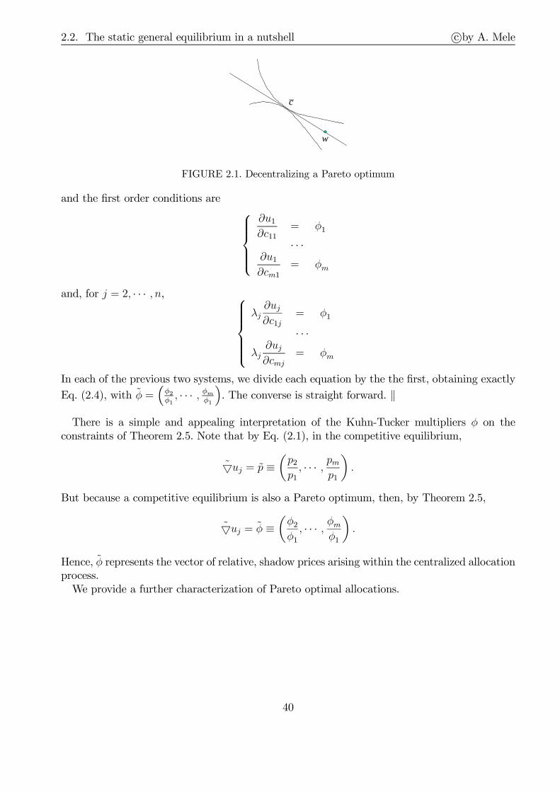
2.2. The static general equilibrium in a nutshell c©by A. Mele
c
w
FIGURE 2.1. Decentralizing a Pareto optimum
and the first order conditions are
∂u1∂c11
= φ1
· · ·∂u1∂cm1
= φm
and, for j = 2, · · · , n,
λj∂uj∂c1j
= φ1
· · ·λj∂uj∂cmj
= φm
In each of the previous two systems, we divide each equation by the the first, obtaining exactly
Eq. (2.4), with φ =(φ2
φ1, · · · , φm
φ1
). The converse is straight forward. ‖
There is a simple and appealing interpretation of the Kuhn-Tucker multipliers φ on theconstraints of Theorem 2.5. Note that by Eq. (2.1), in the competitive equilibrium,
uj = p ≡(p2p1, · · · , pm
p1
).
But because a competitive equilibrium is also a Pareto optimum, then, by Theorem 2.5,
uj = φ ≡(φ2
φ1
, · · · , φmφ1
).
Hence, φ represents the vector of relative, shadow prices arising within the centralized allocationprocess.We provide a further characterization of Pareto optimal allocations.
40

2.2. The static general equilibrium in a nutshell c©by A. Mele
T 2.6 (Characterization of Pareto optima: II). A feasible allocation c = (c1, · · · , cn)is a Pareto optimum if and only if there exists ℓ > 0 such that c is solution to the followingprogram:
u (w, ℓ) = maxc1,··· ,cn
n∑
j=1
ℓjuj(cj)
subject ton∑
j=1
cj ≤ w (ψj, j = 1, · · · ,m) [P2]
P. The if part is simple and at the same time instructive. Let us solve the program in[P2]. The Lagrangian is,
L =
n∑
j=1
ℓjuj(cj)−
m∑
i=1
ψi
n∑
j=1
(cij − wij) ,
and the first order conditions are, for j = 1, · · · , n,
ℓj∇uj = ψ ≡ (ψ1, · · · , ψm)⊤ , ∇uj ≡(∂uj∂c1j
, · · · , ∂uj∂cmj
)⊤. (2.5)
That is, ∇uj equals the same vector of constants for all the agents, just as in Theorem 2.5. Theconverse to this theorem follows by an application of the usual separating theorem, as in Duffie(2001, Chapter 1). ‖
Note, if ℓ1 = 1 and ℓj = λj for j = 2, · · · , n, then, ψi = φi (i = 1, · · · ,m) and so the firstorder conditions in Theorem 2.5 and 2.6 would lead to the same allocation. More generally, wehave:
T 2.7 (Centralization of competitive equilibrium through Pareto weightings). Theoutcome of any competitive equilibrium can be obtained, through a central planner who maxi-mizes the program in [P2], with system of social weights equal to ℓj = 1/κj, where κj is themarginal utility of income for agent j.
So agents with high marginal utility of income for a given price vector, will receive little socialweight in the centralized planner allocation procedure. This result is particularly useful whenit comes to study financial markets in economies with heterogeneous agents. Theorem 2.7 isalso a point of reference, where to move from, when it comes to study asset prices in a worldof incomplete markets. Chapter 8 contains several examples of these applications.
P T 2.7. In the competitive equilibrium,
∇uj = κjp, p ≡ (p1, · · · , pm) , (2.6)
where κj are the Lagrange multipliers for the agents budget constraint, so that κj is the agentj marginal utility of income:
κj =∂
∂mj
uj (c1j (p, w1j, · · · , wmj) , · · · , cmj (p, w1j , · · · , wmj)) , mj ≡m∑
i=1
piwij.
By comparing the competitive equilibrium solution in Eq. (2.6) with the Pareto optimalityproperty of the equilibrium in Eq. (2.5), we deduce that, a competitive equilibrium (c, p) can
41

2.3. Time and uncertainty c©by A. Mele
be implemented, by a social planner acting as in Theorem 2.6, when ℓj = 1/κj. Then, it alsofollows that, necessarily, ψ = p, by the resources constraint,
∑nj=1 c
j ≤ w, which has to holdboth in the competitive economy and the centralized one. Indeed, we have:
wi =n∑
j=1
fij (κjψ) =m∑
j=1
fij (κjp) , i = 1, · · · ,m,
where fij and fij are the inverse functions for consumption, as implied by Eq. (2.5) and Eq. (2.6),
respectively. The previous equality holds when ψ = p, in which case fij = fij. This is indeedthe only solution for ψ in the previous equation, given that fij is monotonically decreasing. ‖
2.3 Time and uncertainty
“A commodity is characterized by its physical properties, the date and the place at which
it will be available.”
Gerard Debreu (1959, Chapter 2)
General equilibrium theory can be used to study a variety of fields, by making an appropriateuse of the previous definition - from the theory of international commerce to finance. To dealwith uncertainty, Debreu (1959, Chapter 7) extended the previous definition, by emphasizingthat a commodity should be described through a list of physical properties, with the structureof dates and places replaced by some event structure. The following example illustrates thedifference between two contracts underlying delivery of corn arising under conditions of certainty(case A) and uncertainty (case B):
A The first agent will deliver 5000 tons of corn of a specified type to the second agent, whowill accept the delivery at date t and in place ℓ.
B The first agent will deliver 5000 tons of corn of a specified type to the second agent, whowill accept the delivery in place ℓ and in the event st at time t. If st does not occur attime t, no delivery will take place.
In both cases, the contract is paid at the time it is actually agreed.The model of the previous section can be used to deal with contracts containg statements such
as that in case B above. For example, consider a two-period economy. Suppose that in the secondperiod, sn mutually exhaustive and exclusive states of nature may occur. Then, we may recoverthe model of the previous section, once we replace m (the number of commodities describedby physical properties, dates and places) with m∗, where m∗ = sn ·m. With m∗ replacing m,the competitive equilibrium in this economy is defined as the competitive equilibrium in theeconomy of the previous section.The important assumption underlying the previous simplifying trick is that markets exists,
where commodities for all states of nature are traded. Such “contingent” markets are completein that a market is open for every commodity in all states of nature. Therefore, the agents mayimplement any feasible action plan and, therefore, the resource allocation is Pareto-optimal.The presumed existence of sn · m contingent markets is, however, very strong. We now showhow the presence of financial assets helps us mitigate this assumption.
42

2.4. Financial assets c©by A. Mele
2.4 Financial assets
What role might be played by financial assets in an uncertainty world? Arrow (1953) developedthe following interpretation. Rather than signing commodity-based contracts that are contin-gent on the realization of events, the agents might wish to sign contracts generating payoffsthat are contingent on the realization of events. The payoffs delivered by the assets in the var-ious states of the world could then be collected and used to satisfy the needs related to theconsumption plans.The simplest financial asset is the so-called Arrow-Debreu asset, i.e. an asset that payoffs
some amount of numéraire in the state of nature s if the state s will prevail in the future, andnil otherwise. More generally, a financial asset is a function x : S → R, where S is the setof all future events. Then, let m be the number of financial assets. To link financial assets tocommodities, we note that if the of nature s will occurs, then, any agent could use the payoffxi(s) promised by the i-th assets Ai to finance net transactions on the commodity markets, viz
p (s) · e (s) =m∑
i=1
θixi(s), ∀s ∈ S, (2.7)
where p(s) and e(s) denote some vectors of prices and excess demands related to the commodi-ties, contingent on the realization of state s, and θi is the number of assets i held by the agent.In other words, the role of financial assets, here, is to transfer value from a state of nature toanother to finance state-contingent consumption.Unfortunately, Eq. (2.7) does not hold, in general. A condition is that the number of assets,
m, be sufficiently high to let each agent cope with the number of future events in S, sn. Marketcompleteness merely reduces to a size problem - the assets have to be sufficiently diverse tospan all possible events in the future. Indeed, we shall show that if there are not payoffs thatare perfectly correlated, then, markets are complete if and only if m = sn. Note, also, thatthis reduces the dimension of our original problem, for we are then considering a competitiveequilibrium in sn +m markets, instead of a competitive equilibrium in sn ·m markets.
2.5 Absence of arbitrage
2.5.1 How to price a financial asset?
Consider an economy in which uncertainty is resolved through the realization of the event:“Tomorrow it will rain.” A decision maker, an hypothetical Mr Law, must implement thefollowing contingent plan: if tomorrow will be sunny, he will need cs > 0 units of money, tobuy sun-glasses; if tomorrow it will rain, Mr Law will need cr > 0 units of money, to buy anumbrella. Mr Law has access to a financial market on which m assets are traded. He builds upa portfolio θ aimed to reproduce the structure of payments that he will need tomorrow:
m∑i=1
θiSi(1 + xi (r)) = crm∑i=1
θiSi(1 + xi (s)) = cs(2.8)
where Si is the price of the i-th asset, θi is the number of assets to put in the portfolio, andxi (r) and xi (s) are the net returns of asset i in the two states of nature, which of course are
43

2.5. Absence of arbitrage c©by A. Mele
known by Mr Law. For now, we do need to assume anything as regards the resources neededto buy the assets, but we shall come back to this issue below (see Remark 2.6). Finally, andremarkably, we are not making any assumption regarding Mr Law’s preferences.Eqs. (2.8) form a system of two equations with m unknowns (θ1, · · · θm). If m < 2, no perfect
hedging strategy is possible - that is, the system (2.8) can not be solved to obtain the desiredpair (ci)i=r,s. In this case, markets are incomplete. More generally, we may consider an economywith sn states of nature, in which markets are complete if and only if Mr Law has access to snassets. More precisely, let us define the following “payoff matrix,” defined as
X =
S1(1 + x1 (s1)) Sm(1 + xm (s1))
. . .
S1(1 + x1 (sn)) Sm(1 + xm (sn))
,
where xi (sj) is the payoff promised by the i-th asset in the state sj. Then, to implement anystate contingent consumption plan c ∈ Rsn, Mr Law has to be able to solve the following system,
c = X · θ,
where and θ ∈ Rm, the portfolio. A unique solution to the previous system exists if rank(X) =sn = m, and is given by θ = X−1c. Consider, for example, the previous case, in which sn = 2.Let us assume that m = 2, for any additional assets would be redundant here. Then, we have,
θ1 =(1 + x2 (r))cs − (1 + x2 (s))cr
S1 [(1 + x1 (s))(1 + x2 (r))− (1 + x1 (r))(1 + x2 (s))]θ2 =
(1 + x1 (s))cr − (1 + x1 (r))csS2 [(1 + x1 (s))(1 + x2 (r))− (1 + x1 (r))(1 + x2 (s))]
Finally, assume that the second asset is safe, or that it yields the same return in the two statesof nature: x2 (r) = x2 (s) ≡ r. Let xs = x1 (s) and xr = x1 (r). Then, the pair (θ1, θ2) can berewritten as,
θ1 =cs − cr
S1 (xs − xr), θ2 =
(1 + xs) cr − (1 + xr) csS2 (1 + r) (xs − xr)
.
As is clear, the issues we are dealing with relate to the replication of random variables. Here,the random variable is a state contingent consumption plan (ci)i=r,s, where cr and cp are known,which we want to replicate for hedging purposes. (Mr Law will need to buy either a pair ofsun-glasses or an umbrella, tomorrow.)In the previous two-state example, two assets with independent payoffs are able to generate
any two-state variable. The next step, now, is to understand what happens when we assumethat there exists a third asset, A say, that delivers the same random variable (ci)i=r,s we can
obtain by using the previous pair (θ1, θ2).We claim that if the current price of the third asset A is H, then, it must be that,
H = V ≡ θ1S1 + θ2S2, (2.9)
for the financial market to be free of arbitrage opportunities, to be defined informally below.Indeed, if V < H, we can buy θ and sell at the same time the third asset A. The result is a sureprofit, or an arbitrage opportunity, equal to H − V , for θ generates cr if tomorrow it will rainand cr if tomorrow it will not rain. In both cases, the portfolio θ generates the payments that
44
2.5. Absence of arbitrage c©by A. Mele
are necessary to honour the contract committments related to the selling of A. By a symmetricargument, the inequality V > H would also generate an arbitrage opportunity. Hence, Eq. (2.9)must hold true.It remains to compute the right hand side of Eq. (2.9), which in turn leads to an evaluation
formula for the asset A. We have:
H =1
1 + r[P ∗cs + (1− P ∗)cr] , P ∗ =
xr − rxs − xr
. (2.10)
Importantly, then, H can be understood as the discounted (by 1 + r) expectation of payoffspromised by A, taken under some “artificial” probability P ∗.
R 2.8. In this introductory example, the asset A can be priced without makingreference to any agents’ preferences. The key observation to obtain this result is that thepayoffs promised by A can be obtained through the portfolio θ. This fact does not obviouslymean that any agent should use this portfolio. For example, it may be the case that Mr Lawis so poor that his budget constraint would not even allow him to implement the portfolio θ.The point underlying the previous example is that the portfolio θ could be used to construct anarbitrage opportunity, arising when Eq. (2.9) does not hold. In this case, any penniless agentcould implement the arbitrage described above.
The next step is to extend the results in Eq. (2.10) to a dynamic setting. Suppose thatan additional day is available for trading, with the same uncertainty structure: the day aftertomorrow, the asset A will pay off css if it will be sunny (provided the previous day was sunny),and crs if it will be sunny (provided the previous day was raining). By using the same argumentsleading to Eq. (2.10), we obtain that:
H =1
(1 + r)2[P ∗2css + P
∗(1− P ∗)csr + (1− P ∗)P ∗crs + P ∗2crr].
Finally, by extending the same reasoning to T trading days,
H =1
(1 + r)TE∗ (cT ) , (2.11)
where E∗ denotes the expectation taken under the probability P ∗.The key assumption we used to derive Eq. (2.11) is that markets are complete at each trading
day. True, at the beginning of the trading period Mr Law faced 2T mutually exclusive possiblestates of nature that would occur at the T -th date, which would seem to imply that we wouldneed 2T assets to replicate the asset A. However, we have just seen that to price A, we onlyneed 2 assets and T trading days. To emphasize this fact, we say that the structure of assetsand transaction dates makes the markets dynamically complete in the previous example. Thepresence of dynamically complete markets allows one to implement dynamic trading strategiesaimed at replicating the value of the asset A, period by period. Naturally, the asset A could bepriced without any assumption about the preferences of any agent, due to the assumption ofdynamically complete markets.
2.5.2 The Land of Cockaigne
We provide a precise definition of the notion of absence of arbitrage opportunities, as wellas a connection between this notion and the notion and properties of the competitive equi-librium described in Section 2.2. For simplicity, we consider a multistate economy with only
45

2.5. Absence of arbitrage c©by A. Mele
one commodity. The extension to the multicommodities case is dealt with very briefly in theappendix.Let vi(ωs) be the payoff of asset i in the state ωs, i = 1, · · · ,m and s = 1, · · · , d. Consider
the payoff matrix:
V ≡
v1 (ω1) vm (ω1)
. . .
v1 (ωd) vm (ωd)
.
Let vsi ≡ vi(ωs), vs,· ≡ [vs1, · · · , vsm], v·,i ≡ [v1i, , · · · , vdi]⊤. We assume that rank(V ) = m ≤ d.The budget constraint of each agent has the form:
c0 − w0 = −Sθ = −m∑
i=1
Siθi
cs − ws = vs·θ =m∑
i=1
vsiθi, s = 1, · · · , d
Let x1 = [x1, · · · , xd]⊤. The second constraint can be written as:
c1 − w1 = V θ.
We define an arbitrage opportunity as a portfolio that has a negative value at the first period,and a positive value in at least one state of world in the second period, or a positive value inall states of the world in the second period and a nonpositive value in the first period.Notation: ∀x ∈ Rm, x > 0 means that at least one component of x is strictly positive while
the other components of x are nonnegative. x≫ 0 means that all components of x are strictlypositive. [Insert here further notes]
D 2.9. An arbitrage opportunity is a strategy θ that yields1 either V θ ≥ 0 withan initial investment Sθ < 0, or a strategy θ that produces2 V θ > 0 with an initial investmentSθ ≤ 0.
As we shall show below (Theorem 2.11), an arbitrage opportunity can not exist in a com-petitive equilibrium, for the agents’ program would not be well defined in this case. Introduce,then, the (d+ 1)×m matrix,
W =
[−SV
],
the vector subspace of Rd+1,
〈W 〉 =z ∈ Rd+1 : z =Wθ, θ ∈ Rm
,
and, finally, the null space of 〈W 〉,
〈W 〉⊥ =x ∈ Rd+1 : xW = 0m
.
1V θ ≥ 0 means that [V θ]j ≥ 0, j = 1, · · ·, d, i.e. it allows for [V θ]j = 0, j = 1, · · ·, d.2V θ > 0 means [V θ]j ≥ 0, j = 1, · · ·, d, with at least one j for which [V θ]j > 0.
46
2.5. Absence of arbitrage c©by A. Mele
The economic interpretation of the vector subspace 〈W 〉 is that of the excess demand space forall the states of nature, generated by the “wealth transfers” generated by the investments in theassets. Naturally, 〈W 〉⊥ and 〈W 〉 are orthogonal, as 〈W 〉⊥ =
x ∈ Rd+1 : xz = 0m, z ∈ 〈W 〉
.
Mathematically, the assumption that there are no arbitrage opportunities is equivalent to thefollowing condition,
〈W 〉⋂Rd+1+ = 0 . (2.12)
The interpertation of (2.12) is in fact very simple. In the absence of arbitrage opportunities,there should be no portfolios generating “wealth transfers” that are nonnegative and strictlypositive in at least one state, i.e. ∄θ : Wθ > 0. Hence, 〈W 〉 and the positive orthant Rd+1
+ cannot intersect.The following result provides a general characterization of how the no-arbitrage condition in
(2.12) restricts the price of all the assets in the economy.
T 2.10. There are no arbitrage opportunities if and only if there exists a φ ∈ Rd++ :
S = φ⊤V . If m = d, φ is unique, and if m < d, dim(φ ∈ Rd
++ : S = φ⊤V
)= d−m.
P. In the appendix.
The previous theorem provides the foundations for many developments in financial economics.To provide its intuition, let us pre-multiply the second constraint by φ⊤, obtaining,
φ⊤(c1 − w1) = φ⊤V θ = Sθ = − (c0 − w0) ,
where the second equality follows by Theorem 2.10, and the third equality is due to the firstperiod budget constraint. Critically, then, Theorem 2.10 shows that in the absence of arbitrageopportunities, each agent has access to the following budget constraint,
0 = c0 − w0 + φ⊤ (c1 − w1
)= c0 − w0 +
d∑
s=1
φs (cs − ws) , with(c1 − w1
)∈ 〈V 〉 . (2.13)
The budget constraints in (2.13) reveal that φ can be interpreted as the vector of prices tothe commodity in the future d states of nature, and that the numéraire in this economy isthe first-period consumption. We usually refer φ to as the state price vector, or Arrow-Debreustate price vector. However, it would be misleading to say that the budget constraint in (2.13)is that we are used to see in the static Arrow-Debreu type model of Section 2.2. In fact, theArrow-Debreu economy of Section 2.2 obtains when m = d, in which case 〈V 〉 = Rd in (2.13).This case, which according to Theorem 2.10 arises when markets are complete, also implies theremarkable property that there exists a unique φ that is compatible with the asset prices weobserve.The situation is radically different if m < d. In other terms, 〈V 〉 is the subspace of excess
demands agents have access to in the second period and can be “smaller” than Rd if marketsare incomplete. Indeed, 〈V 〉 is the subspace generated by the payoffs obtained by the portfoliochoices made in the first period,
〈V 〉 =e ∈ Rd : e = V θ, θ ∈ Rm
.
Consider, for example, the case d = 2 andm = 1. In this case, 〈V 〉 = e ∈ R2 : e = V θ, θ ∈ R,with V = V1, where V1 =
(v1
v2
)say, and dim 〈V 〉 = 1, as illustrated by Figure 2.2.
47

2.5. Absence of arbitrage c©by A. Mele
v1
v2
<V>
FIGURE 2.2. Incomplete markets, d = 2, m = 1.
v1
v2
v3
v4
V1
V2
V3
V4
FIGURE 2.3. Complete markets, 〈V 〉 = R2.
Next, suppose we open a new market for a second financial asset with payoffs given by: V2 =(v3
v4
). Then, m = 2, V = (v1
v2
v3
v4), and 〈V 〉 =
e ∈ R2 : e =
(θ1v1+θ2v3
θ1v2+θ2v4
), θ ∈ R2
, i.e. 〈V 〉 = R2. As
a result, we can now generate any excess demand in R2, just as in the Arrow-Debreu economyof Section 2.2. To generate any excess demand, we multiply the payoff vector V1 by θ1 and thepayoff vector V2 by θ2. For example, suppose we wish to generate the payoff the payoff vectorV4 in Figure 2.3. Then, we choose some θ1 > 1 and θ2 < 1. (The exact values of θ1 and θ2are obtained by solving a linear system.) In Figure 2.3, the payoff vector V3 is obtained withθ1 = θ2 = 1.To summarize, if markets are complete, then, 〈V 〉 = Rd. If markets are incomplete, 〈V 〉
is only a subspace of Rd, which makes the agents’ choice space smaller than in the completemarkets case.We now present a fundamental result, about the “viability of the model.” Define the second
period consumption c1j ≡ [c1j , · · · , cdj ]⊤, where csj is the second-period consumption in state s,and let,
(c0j, c
1j
)∈ argmax
c0j ,c1j
[uj (c0j) + βjE(νj(c
1j))
], subject to
c0j − w0j = −Sθjc1j − w1
j = V θj[P3]
48

2.6. Equivalent martingales and equilibrium c©by A. Mele
where uj and νj are utility functions, both satisfying Assumption 2.1. Naturally, we could usemore general formulations of utilities than that in [P3], and in fact we shall in more advancedparts of this book. For the sake of this introductory chapter, we only consider additive utility.We have:
T 2.11. The program [P3] has a solution if and only if there are no arbitrage oppor-tunities.
P. Let us suppose on the contrary that the program [P3] has a solution c0j, c1j , θj, but
that there exists a θ : Wθ > 0. The program constraint is, with straight forward notation,cj = wj +Wθj. Then, we may define a portfolio θj = θj + θ, such that cj = wj +W (θj + θ) =cj +Wθ > cj, which contradicts the optimality of cj. For the converse, note that the absence ofarbitrage opportunities implies that ∃φ ∈ Rd
++ : S = φ⊤V , which leads to the budget constraint
in (2.13), for a given φ. This budget constraint is clearly a closed subset of the compact budgetconstraint Bj in [P1] (in fact, it is Bj restricted to 〈V 〉). Therefore, it is a compact set and,hence, the program [P3] has a solution, as a continuous function attains its maximum on acompact set. ‖
2.6 Equivalent martingales and equilibrium
We provide the definition of an equilibrium with financial markets, when the financial assetsare in zero net supply.
D 2.12. An equilibrium is given by allocations and prices (c0j)nj=1, ((csj)nj=1)
ds=1,
(Si)mi=1 ∈ Rn
+ ×Rnd+ ×Rd
+, where the allocations are solutions of the program [P3] and satisfy:
0 =n∑
j=1
(c0j − w0j) , 0 =n∑
j=1
(csj − wsj) (s = 1, · · · , d) , 0 =n∑
j=1
θij (i = 1, · · · , d) .
We now express demand functions in terms of the stochastic discount factor, and then lookfor an equilibrium by looking for the stochastic discount factor that clears the commoditymarkets. By Walras’ law, this also implies the equilibrium on the financial market. Indeed, byaggregating the agent’s constraints in the second period,
n∑
j=1
(c1j − w1
j
)= V
n∑
j=1
θij(m).
For simplicity, we also assume that u′j(x) > 0, u′′j (x) < 0 ∀x > 0 and limx→0 u′j(x) = ∞,
limx→∞ u′j(x) = 0 and that νj satisfies the same properties.
2.6.1 The rational expectations assumption
Lucas, Radner, Green. Every agent correctly anticipates the equilibrium price in each state ofnature.[Consider for example the models with asymmetric information that we will see later in these
lectures. At some point we will have to compute, E ( v| p (y) = p). That is, the equilibrium is a
49
2.6. Equivalent martingales and equilibrium c©by A. Mele
pricing function which takes some values p (y) depending on the state of nature. In this kind ofmodels, λθI (p (y) , y) + (1− λ) θU (p (y) , y) + y = 0, and we look for a solution p (y) satisfyingthis equation.]
2.6.2 Stochastic discount factors
Theorem 2.10 states that in the absence of arbitrage opportunities,
Si = φ⊤v·,i =
d∑
s=1
φsvs,i, i = 1, · · · ,m. (2.14)
Let us assume that the first asset is a safe asset, i.e. vs,1 = 1 ∀s. Then, we have
S1 ≡1
1 + r=
d∑
s=1
φs. (2.15)
Eq. (2.15) confirms the economic interpretation of the state prices in (2.13). Recall, the statesof nature are exhaustive and mutually exclusive. Therefore, φs can be interpreted as the priceto be paid today for obtaining, for sure, one unit of numéraire, tomorrow, in state s. This isindeed the economic interpretation of the budget constaint in (2.13). Eq. (2.15) confirms thisas it says that the prices of all these rights sum up to the price of a pure discount bond, i.e. anasset that yields one unit of numéraire, tomorrow, for sure.Eq. (2.15) can be elaborated to provide us with a second interpretation of the state prices in
Theorem 2.10. Define,
P ∗s ≡ (1 + r)φs,
which satisfies, by construction,d∑
s=1
P ∗s = 1.
Therefore, we can interpret P ∗ ≡ (P ∗s )ds=1 as a probability distribution. Moreover, by replacing
P ∗ in Eq. (11.16) leaves,
Si =1
1 + r
d∑
s=1
P ∗s vs,i =1
1 + rEP ∗ (v·,i) , i = 1, · · · ,m. (2.16)
Eq. (2.16) confirms Eq. (2.10), obtained in the introductory example of Section 2.5. It saysthat the price of any asset is the expectation of its future payoffs, taken under the proba-bility P ∗, discounted at the risk-free interest rate r. For this reason, we usually refer to theprobability P ∗ as the risk-neutral probability. Eq. (2.16) can be extended to a dynamic con-text, as we shall see in later chapters. Intuitively, consider an asset that distributes dividendsin every period, let S (t) be its price at time t, and D (t) the dividend paid off at time t.Then, the “payoff” it promises for the next period is S (t+ 1) + D (t+ 1). By Eq. (2.16),S (t) = (1 + r)−1EP ∗ (S (t+ 1) +D (t+ 1)) or, by rearranging terms,
EP ∗(S (t+ 1) +D (t+ 1)− S (t)
S (t)
)= r. (2.17)
50

2.6. Equivalent martingales and equilibrium c©by A. Mele
That is, the expected return on the asset under P ∗ equals the safe interest rate, r. In a dynamiccontext, the risk-neutral probability P ∗ is also referred to as the risk-neutral martingale measure,or equivalent martingale measure, for the following reason. Define a money market account asan asset with value evolving over time as M (t) ≡ (1 + r)t. Then, Eq. (2.17) can be rewrittenas S (t) /M (t) = EP ∗ [(S (t+ 1) +D (t+ 1)) /M (t+ 1)]. This shows that if D (t+ 1) = 0 forsome t, then, the discounted process S (t) /M (t) is a martingale under P ∗.Next, let us replace P ∗ into the budget constraint in (2.13), to obtain, for (c1 − w1) ∈ 〈V 〉,
0 = c0−w0+d∑
s=1
φs (cs − ws) = c0−w0+1
1 + r
d∑
s=1
P ∗s (cs − ws) = c0−w0+1
1 + rEP∗
(c1 − w1
).
(2.18)For reasons developed below, it is also useful to derive an alternative representation of thebudget constraint, in terms of the objective probability P (say). Let us introduce, first, theratio ζ, defined as,
ζs =P ∗sPs, s = 1, · · · , d.
The ratio ζs indicates how far P ∗ and P are. We assume ζs is strictly positive, which meansthat P ∗ and P are equivalent measures, i.e. they assign the same weight to the null sets. Finally,let us introduce the stochastic discount factor, m = (ms)
ds=1, defined as,
ms ≡ (1 + r)−1ζs.
We have,
1
1 + rEP∗
(c1 − w1
)=
d∑
s=1
1
1 + rP ∗s (cs − ws) =
d∑
s=1
1
1 + rζs
︸ ︷︷ ︸=ms
(cs − ws)Ps = E[m ·
(c1 − w1
)].
Hence, we can rewrite Eq. (2.18) as,
0 = c0 − w0 + E[m ·
(c1 − w1
)],
(c1 − w1
)∈ 〈V 〉 .
Similarly, by replacing the stochastic discount factor m into Eq. (2.16) we obtain,
Si =1
1 + rEP∗ (v·,i) = E (m · v·,i) , i = 1, · · · ,m. (2.19)
Naturally, despite all such different ways to express budget constraints and asset prices, thekey of the model is still φ,
ms = (1 + r)−1 ζs = (1 + r)−1 P∗s
Ps=φsPs,
which can be recovered, once we solve for the equilibrium stochastic discount factor m, as weshall illustrate in the next section.
2.6.3 Optimality and equilibrium
We have argued that in the absence of arbitrage opportunities, the program of any agent j is
max(c0,c1)
[uj(c0j) + βj · E(νj(c1j))
]subject to 0 = c0j−w0j+E
[m · (c1j − w1
j )],
(c1 − w1
)∈ 〈V 〉 .
[P4]
51
2.6. Equivalent martingales and equilibrium c©by A. Mele
2.6.3.1 Complete markets and risk sharing
In the complete markets case, 〈V 〉 = Rd, so that the first order conditions to the program [P4]are,
u′j (c0j) = λj , βjν′j (csj) = λjms, s = 1, · · · , d,
where λj is a Lagrange multiplier. So, really, the properties of this model are the same as thoseof the static model in Section 2.2. Formally, the complete markets economy in this section is thesame as the static economy in Section 2.2, once we set m = d, where m is the dimension of thecommodity space, in Section 2.2, and ps = φs, where ps is the price of the s-th commodity inSection 2.2, with p1 = 1 (the numéraire), and φs is the Arrow-Debreu state price in the unifiedbudget constraint of Eq. (2.18).These simple observations have profound implications: an economy subject to uncertainty can
be understood through a static model, in the presence of complete markets! Under the conditionsstated in Section 2.2, even complicated models with heterogeneous agents, with potentiallyinteresting asset pricing implications, and still, apparently, so hopelessly difficult to analyze,can actually be “centralized,” through a dedicated design of Pareto’s weights, as formalizedin Theorem 2.7. We can actually do much more. First, this centralization property is easilyextended to a dynamic context, as we shall see in more advanced parts of these lectures (seeChapter 8), provided markets satisfy the property of being dynamically complete, a propertyexplained in the next two chapters. Second, the assumption agents can exchange Arrow-Debreusecurities for all future states of the world, is clearly unrealistic: markets are pretty likely tobe incomplete, one possible reason why financial innovation is so pervasive, in practice. Yetthe theory about centralization can be extended to an incomplete markets setting, through asystem of “stochastic Pareto weights,” as we discuss in detail in Chapter 8. For now, let usproceed with the next simple and fundamental steps.To illustrate the equilibrium implications of the first order conditions in a simple case, consider
an economy with a single agent. In this economy, the first order conditions immediately lead tothe following stochastic discount factor,
ms = βν ′(ws)
u′(w0).
The economic interpretation of this stochastic discount factor is the following. In the autarchicstate,
−dc0dcs
∣∣∣∣c0=w0,cs=ws
= βν′(ws)
u′(w0)Ps = msPs = φs
is the present consumption the agent is willing to give up to at t = 0, in order to obtainadditional consumption at time t = 1, in state s. In other words, φs is the price, in terms of thepresent consumption numéraire, of one additional unit of consumption at time t = 1 and states. So it is a state price, such that, the agent is happy to consume his own endowment, withoutany incentives to trade in the financial markets. The risk-neutral probability is,
P ∗s = ζsPs = (1 + r)msPs = (1 + r)βν′(ws)
u′(w0)Ps.
By the first order conditions, and the pure discount bond evaluation formula, it is easily checkedthat 1 =
∑ds=1 P
∗s . Moreover,
P ∗sPs
= ms (1 + r) = ms
[βE
(ν′(ws)
u′(w0)
)]−1
= msβ−1 u′(w0)
E [ν′(ws)]=
ν′(ws)
E [ν ′(ws)],
52
2.6. Equivalent martingales and equilibrium c©by A. Mele
where the second equality follows by the pure discount bond evaluation formula: 11+r
= E(m).In the multi-agent case, the situation is similar as soon as markets are complete. Indeed,
consider the first order conditions of each agent,
βjν′j (csj)
u′j (c0j)= ms, s = 1, · · · , d, j = 1, · · · , n.
The previous relation reveals that as soon as markets are complete, agents must have the samemarginal rate of substitution, in equilibrium. This is because by Theorem 2.10, the state pricevector φ is unique if and only if markets are complete, which then implies uniqueness ofms =
φsPs
and, hence, the fact that each marginal rate of substitution βjν′j(csj)
u′j(c0j)is independent of j. In this
case, the equilibrium allocation is clearly a Pareto optimum, by the discussion at the beginningof this section, and Theorem 2.5.The result that agents have the same marginal rate of substitution for each state of the world
is known as risk sharing. It means that, given an initial endowment distribution among theagents, the market mechanism, through to a system of complete securities markets, is such thatconsumption risk is shifted around the economy, so that it is borne by the agents most willing totake it. For example, suppose that two agents 1 and 2 have the same discount rate, and utilityfunctions uj = νj, with CRRA given by η1 and η2, where η1 < η2. Then, Grs1 = (Grs2)
η2/η1 ,where Grsi is consumption growth for the i-th agent in state s. In good times, when Grs2 > 1,the more risk-averse agent experiences, ex-post, a lower consumption growth rate, Grs2 < Grs1.In bad times, however, when Grs2 < 1, the more risk-averse agent experiences, ex-post, a higherconsumption growth rate, Grs2 > Grs1. In other words, capital markets, when complete, operatein such a way to have the more risk-averse agent face a less volatile consumption growth.
2.6.3.2 Incomplete markets
If markets are incomplete, marginal rates of substitution cannot be equal, among agents, exceptperhaps on a set of endowments distribution with measure zero. The best outcome in this case,is a set of equilibria called constrained Pareto optima, i.e. constrained by ... the states of nature.As it turns out, there might not even exist constrained Pareto optima in multiperiod economieswith incomplete markets–except perhaps those arising on a set of endowments distributionswith zero measure.When market are incomplete, the state price vector φ is not unique. That is, suppose that
φ⊤ is an equilibrium state price. Then, all the elements of
Φ = φ′ ∈ Rd++ : (φ
′ − φ)⊤V = 0 (2.20)
are also equilibrium state prices - there exists an infinity of equilibrium state prices that areconsistent with absence of arbitrage opportunities. In other words, there exists an infinity ofequilibrium state prices guaranteeing the same observable assets price vector S, for φ′⊤V =φ⊤V = S.How do we proceed in this case? Introduce the following budget constraint:
C =c ∈ Rd
++ : 0 = c0 − w0 + φ⊤ (c1 − w1
),
(c1 − w1
)∈ 〈V 〉 , ∀φ ∈ Rd
++ : S = φ⊤V
.
(2.21)This budget constraint, and the previous reasoning about the set Φ in (2.20) shows that in thecontext of incomplete markets, there exists many constraints to take care of, and the previous“martingale methods,” do not apply.
53
2.6. Equivalent martingales and equilibrium c©by A. Mele
Yet let Val (PI) be the value of the following program in the incomplete markets at hand:
maxc∈C
[uj (c0j) + βjE(νj(c
1j))
]. [PI]
Consider, next, the following constraint:
Cφ =c ∈ Rd
++ : 0 = c0 − w0 + φ⊤ (c1 − w1) , (c1 − w1) ∈ Rd,
for some given φ ∈ Rd++ : S = φ
⊤V
,
and let Val (Pφ) be the value of the program in some abstract complete markets case:
maxc∈Cφ
[uj (c0j) + βjE(νj(c
1j))
]. [Pφ]
Clearly, we have, Val (PI) ≤ Val (Pφ) for all φ, for the constraint in the incomplete marketscase, C, is more stringent than that in any complete market setting, Cφ: the solution to theprogram in the incomplete markets case [PI], must satisfy the budget constraints in C, formedusing all of the possible Arrow-Debreu state prices (including the Arrow-Debreu state price φgiven in Cφ), as the constraint of Eq. (2.21) shows. Moreover, (c1 − w1) ∈ 〈V 〉. These remarkssuggest to define the following “min-max” Arrow-Debreu state price:
φ∗ = argminφ∈Φ
Val (Pφ) .
The natural question is to know whether
Val (PI) = Val (Pφ∗) . (2.22)
This is indeed the case, given some regularity conditions. For the characterization of φ∗, supposethere exists φ : Val (PI) = Val(Pφ). Then, φ = φ
∗. Indeed, suppose the contrary, i.e. there exists
φ′ : Val(Pφ′) < Val(Pφ). Then, we would have,
Val (PI) ≤ Val(Pφ′) < Val(Pφ) = Val (PI) ,
a contradiction. Note, again, this is a characterization result about φ∗, not an existence proof.But as mentioned earlier, Eq. (2.22) holds true, as shown in a dynamic setting by He andPearson (1991). Chapter 4 provides general guidance about an even more general approach tosolving problems of this kind, arising in a broader context of market imperfections, includingincomplete markets as a special case.
2.6.3.3 Computation of the equilibrium
The first order conditions satisfied by any agent’s program are:
c0j = Ij (λj) , csj = Hj
(β−1j λjms
), (2.23)
where Ij and Hj denote the inverse functions of u′j and ν′j. By the assumptions we made on uj
and ν ′j, Ij and Hj inherit the same properties of u′j and ν′j. By replacing these functions into
the constraint,
0 = c0j − w0j + E[m · (c1j − w1
j )]= Ij (λj)− w0j +
d∑
s=1
Ps[ms ·
(Hj(β
−1j λjms)− wsj
)].
54
2.7. Consumption-CAPM c©by A. Mele
Define the function,
zj (λj) ≡ Ij (λj) + E[mHj(β
−1j λjm)
]= w0j + E
(m · w1
j
).
We see that limx→0 z(x) =∞, limx→∞ z(x) = 0 and z′ (x) < 0. Therefore, there exists a uniquesolution for λj:
λj ≡ Λj[w0j + E(m · w1
j )],
where Λ(·) denotes the inverse function of z. By replacing back into Eqs. (2.23), we obtain:
c0j = Ij(Λj
(w0j + E(m · w1
j ))), csj = Hj
(β−1j msΛj
(w0j + E(m · w1
j ))).
It remains to compute the general equilibrium. The kernelmmust be determined. This meansthat we have d unknowns (ms, s = 1, · · · , d). We have d+ 1 equilibrium conditions (holding inthe d+ 1 markets). By Walras’ law, only d of these are independent. Consider the equilibriumconditions in the d markets at the second period:
gs
(ms; (ms′)s′ =s
)≡
n∑
j=1
Hj
(β−1j msΛj
(w0j + E(m · w1
j )))=
n∑
j=1
wsj ≡ ws, s = 1, · · · , d.
These conditions determine the kernel (ms)ds=1 which leads to compute prices and equilibrium
allocations. Finally, once the optimal cs are computed, for s = 0, 1, · · · , d, the portoflio θgenerated them can be inferred through θ = V −1(c1 − w1).
2.7 Consumption-CAPM
Consider the pricing equation (2.19). It states that for every asset with gross return R ≡S−1 · payoff,
1 = E(m · R), (2.24)
where m is some pricing kernel.In the previous section, we learnt that in a complete markets economy, equilibrium leads to
the following identification of the pricing kernel,
ms = βν ′(ws)
u′(w0).
For a riskless asset, 1 = E(m ·R). By combining this equality with Eq. (2.24), leaves E[m ·(R−R)] = 0. By rearranging terms,
E(R) = R − cov(ν′(w+), R)
E [ν′(w+)]. (2.25)
2.7.1 The risk premium
Eq. (2.25) can be rewritten as,
E(R)−R = −cov(m, R)E(m)
= −R · cov(m, R). (2.26)
The risk-premium to invest in the asset is high for securities which pay high returns whenconsumption is high (i.e. when we don’t need high returns) and low returns when consumptionis low (i.e. when we need high returns).All in all, if the price p = E (m · payoff) = E (m)E (payoff)+cov (m, payoff) = R−1E (payoff)
- Premium, where Premium =− cov (m, payoff), a discounting effect.
55

2.8. Infinite horizon c©by A. Mele
2.7.2 The beta relation
Suppose there is a Rm such that
Rm = −γ−1 · ν ′ (ws) , all s.
In this case,
E(R) = R+γ · cov(Rm, R)
E [ν′(w+)]and E(Rm) = R+
γ · var(Rm)
E [ν ′(w+)].
These relations can be combined to yield,
E(R)−R = β · [E(Rm)−R], β ≡ cov(Rm, R)
var(Rm).
2.7.3 CCAPM & CAPM
Let Rp be the portfolio return which is the most highly correlated with the pricing kernel m.We have,
E(Rp)−R = −R · cov(m, Rp). (2.27)
Using Eqs. (2.26) and (2.27),E(R)−RE(Rp)−R
=cov(m, R)
cov(m, Rp),
and by rearranging terms,
E(R)−R =βR,mβRp,m
[E(Rp)−R] [CCAPM].
If Rp is perfectly correlated with m, i.e. if there exists γ : Rp = −γm, then
βR,m = −γ cov(Rp, R)
var(Rp)and βRp,m = −γ
and thenE(R)−R = βR,Rp[E(R
p)−R] [CAPM].
This is not the only way the CAPM obtains. As we shall explain in Chapter 6, the CAPM alsoobtains through the so-called “maximum correlation portfolio,” which is the portfolio that isthe most highly correlated with the pricing kernel m.
2.8 Infinite horizon
We consider d states of the nature and m = d Arrow securities. We write a unified budgetconstraint, as in the valuation equilibria approach of Debreu (1954).We have,
p0 (c0 − w0) = −S(0)θ(0) = −
m∑
i=1
S(0)i θ
(0)i
p1s (c1s − w1
s) = θ(0)s , s = 1, · · · , d56

2.9. Further topics on incomplete markets c©by A. Mele
or,
p0(c0 − w0) +m∑
i=1
S(0)i
[p1i
(c1i − w1
i
)]= 0.
The previous relation holds in a two-period economy. In a multiperiod economy, in the secondperiod (as in the following periods) agents save indefinitively for the future. In the appendix,we show that,
0 = E
[ ∞∑
t=0
m0,t · pt(ct − wt
)], (2.28)
where m0,t are the state prices. From the perspective of time 0, at time t there exist dt statesof nature and, thus, dt possible prices.
2.9 Further topics on incomplete markets
2.9.1 Nominal assets and real indeterminacy of the equilibrium
The equilibrium is a set of prices (p, S) ∈ Rm·(d+1)++ × Ra
++ such that:
0 =n∑
j=1
e0j(p, S), 0 =n∑
j=1
e1j(p, S), 0 =n∑
j=1
θj(p, S),
where the previous functions are the results of optimal plans of the agents. This system hasm · (d + 1) + a equations and m · (d + 1) + a unknowns, where a ≤ d. Let us aggregate theconstraints of the agents,
p0
n∑
j=1
e0j = −Sn∑
j=1
θj , p1n∑
j=1
e1j = Bn∑
j=1
θj.
Suppose the financial markets clearing condition is satisfied, i.e.∑n
j=1 θj = 0. Then,
0 = p0n∑j=1
e0j ≡ p0e0 =m∑ℓ=1
p(ℓ)0 e
(ℓ)0
0d = p1n∑j=1
e1j ≡ p1e1 =
[m∑ℓ=1
p(ℓ)1 (ω1)e
(ℓ)1 (ω1), · · · ,
m∑ℓ=1
p(ℓ)1 (ωd)e
(ℓ)1 (ωd)
]⊤
Therefore, there is one redundant equation for each state of nature, or d + 1 redundantequations, in total. As a result, the equilibrium has less independent equations (m · (d+1)− 1)than unknowns (m ·(d+1)+d), i.e., an indeterminacy degree equal to d+1. This result does notrely on whether markets are complete or not. In a sense, it is even not an indeterminacy resultwhen markets are complete, as we may always assume agents would organize the exchangesat the beginning. In this case, onle the suitably normalized Arrow-Debreu state prices wouldmatter for agents.The previous indeterminacy can be reduced to d − 1, as we may use two additional homo-
geneity relations. To pin down these relations, let us consider the budget constaint of each agentj,
p0e0j = −Sθj, p1e1j = Bθj.
57

2.9. Further topics on incomplete markets c©by A. Mele
The first-period constraint is still the same if we multiply the spot price vector p0 and thefinancial price vector S by a positive constant, λ (say). In other words, if (p0, p1, S) is an equi-librium, then, (λp0, p1, λS) is also an equilibrium, which delivers a first homogeneity relation.To derive the second homogeneity relation, we multiply the spot prices of the second period bya positive constant, λ and increase at the same time the first period agents’ purchasing power,by dividing each asset price by the same constant, as follows:
p0e0j = −Sλλθj , λp1e1j = Bλθj .
Therefore, if (p0, p1, S) is an equilibrium, then,(p0, λp1,
Sλ
)is also an equilibrium.
2.9.2 Nonneutrality of money
The previous indeterminacy arises because financial contracts are nominal, i.e. the asset payoffsare expressed in terms of some unité de compte that, among other things, we did not makeprecise. Such an indeterminacy vanishes if we were to consider real contracts, i.e. contractswith payoffs expressed in terms of the goods. To show this, note that in the presence of realcontracts, the agents’ constraints are
p0e0j = −Sθjp1(ωs)e1j(ωs) = p1(ωs)Asθj, s = 1, · · · , d
where As = [A1s, · · · , Aa
s] is the m × a matrix of the real payoffs. The previous constraintnow reveals how to “recover” d + 1 homogeneity relations. For each strictly positive vectorλ = [λ0, λ1 · · · , λd], we have that if [p0, S, p1(ω1), · · · , p1(ωs), · · · , p1(ωd)] is an equilibrium, then,[λ0p0, λ0S, p1(ω1), · · · , p1(ωs), · · · , p1(ωd)] is also an equilibrium, and so is[p0, S, p1(ω1), · · · , λsp1(ωs), · · · , p1(ωd)], for λs, s = 1, · · · , d.As is clear, the distinction between nominal and real assets has a precise meaning, when
one considers a multi-commodity economy. Even in this case, however, such a distinctions isnot very interesting without a suitable introduction of a unité de compte. These considerationsled Magill and Quinzii (1992) to solve the indetermincay while still remaining in a frameworkwith nominal assets. They simply propose to introduce money as a mean of exchange. Theindeterminacy can then be resolved by “fixing” the prices via the d+ 1 equations defining themoney market equilibrium in all states of nature:
Ms = ps ·n∑
j=1
wsj , s = 0, 1, · · · , d.
Magill and Quinzii showed that the monetary policy (Ms)ds=0 is generically nonneutral.
58

2.10. Appendix 1 c©by A. Mele
2.10 Appendix 1
In this appendix we prove that the program [P1] has a unique maximum. Indeed, suppose on thecontrary that we have two maxima:
c = (c1j, · · · , cmj) and c =(c1j, · · · , cmj
).
These two maxima would satisfy uj(c) = uj(c), with∑m
i=1 picij =∑m
i=1 picij = Rj. To check that thisclaim is correct, suppose on the contrary that
∑mi=1 picij < Rj. Then, the consumption bundle,
c =(c1j + ε, · · · , cmj
), ε > 0,
would be preferred to c, by Assumption 2.1, and, at the same time, it would hold that, for sufficientlysmall ε,
m∑
i=1
picij = εp1 +m∑
i=1
picij < Rj .
[Indeed, we have, A ≡∑mi=1 picij. A < Rj ⇒ ∃ε > 0 : A+εp1 < Rj . E.g., εp1 = Rj−A−η, η > 0. The
condition is then: ∃η > 0 : Rj − A > η.] Hence, c would be a solution to [P1], thereby contradictingthe optimality of c. Therefore, the existence of two optima would imply a full use of resources. Next,consider a point y lying between c and c, viz y = αc+ (1− α)c, α ∈ (0, 1). By Assumption 2.1,
uj(y) = uj(αc+ (1− α)c
)> uj(c) = uj(c).
Moreover,
m∑
i=1
piyi =m∑
i=1
pi(αcij + (1− α)cij
)= α
m∑
i=1
picij +∑m
i=1 cij − α∑m
i=1 cij = αRj +Rj − αRj = Rj.
Hence, y ∈ Bj(p) and is also strictly preferred to c and c, which means that c and c are not optima,as initially conjectured. This establishes uniqueness of the solution to [P1].
59

2.11. Appendix 2: Proofs of selected results c©by A. Mele
2.11 Appendix 2: Proofs of selected results
We first provide a useful result, a well-known theorem on separation of two convex sets. We use thistheorem to deal with the proof of the second welfare theorem (Theorem 2.4) and the existence of stateprices tying up all asset prices together (Theorem 2.10). A final proof we provide in this appendix isthat of Eq. (2.28).
M #’ . Let A and B be two non-empty convex subsets of Rd. If Ais closed, B is compact and A
⋂B = ∅, then there exists a φ ∈ Rd and two real numbers d1, d2 such
that:a⊤φ ≤ d1 < d2 ≤ b⊤φ, ∀a ∈ A, ∀b ∈ B.
We are now ready to prove Theorems 2.4 and 2.10.
P T 2.4. Let c be a Pareto optimum and Bj =cj : uj(c
j) > uj(cj). Let us
consider the two sets B =⋃nj=1 Bj and A =
(cj)nj=1 : c
j ≥ 0 ∀j, ∑nj=1 c
j = w. A is the set of all
possible combinations of feasible allocations. By the definition of a Pareto optimum, there are noelements in A that are simultaneously in B, or A
⋂B = ∅. In particular, this is true for all compact
subsets B of B, or A⋂B = ∅. Because A is closed, then, by the Minkowski’s separating theorem,
there exists a p ∈ Rm and two distinct numbers d1, d2 such that
p⊤a ≤ d1 < d2 ≤ p⊤b, ∀a ∈ A, ∀b ∈ B.
This means that for all allocations(cj)nj=1
preferred to c, we have:
p⊤n∑
j=1
wj < p⊤n∑
j=1
cj,
or, by replacing∑n
j=1wj with
∑nj=1 c
j ,
p⊤n∑
j=1
cj < p⊤n∑
j=1
cj. (2A.1)
Next we show that p > 0. Let ci =∑n
j=1 cij, i = 1, · · · ,m, and partition c = (c1, · · · , cm). Let us applythe inequality in (2A.1) to c ∈ A and, for µ > 0, to c = (c1 + µ, · · · , cm) ∈ B. We have p1µ > 0, orp1 > 0. By reiterating the argument, pi > 0 for all i. Finally, we choose cj = cj + 1m
ǫn , j = 2, · · · , n,
ǫ > 0 in (2A.1), p⊤c1 < p⊤c1 + p⊤1mǫ or,
p⊤c1 < p⊤c1,
for ǫ sufficiently small. This means that u1(c1) > u1(c
1) ⇒ p⊤c1 > p⊤c1. This means that c1 =argmaxc1 u1(c
1) s.t. p⊤c1 = p⊤c1. By symmetry, cj = argmaxcj uj(cj) s.t. p⊤cj = p⊤cj for all j. ‖
P T 2.10. The condition in (2.12) holds for any compact subset of Rd+1+ , and
therefore it holds when it is restricted to the unit simplex in Rd+1+ ,
〈W 〉⋂Sd = 0 .
By the Minkowski’s separation theorem, ∃φ ∈ Rd+1 : w⊤φ ≤ d1 < d2 ≤ σ⊤φ, w ∈ 〈W 〉, σ ∈ Sd.By walking along the simplex boundaries, one finds that d1 < φs, s = 1, · · · , d. On the other hand,
60
2.11. Appendix 2: Proofs of selected results c©by A. Mele
0 ∈ 〈W 〉, which reveals that d1 ≥ 0, and φ ∈ Rd+1++ . Next we show that w⊤φ = 0. Assume the contrary,
i.e. ∃w∗ ∈ 〈W 〉 that satisfies at the same time w⊤∗ φ = 0. In this case, there would be a real number ǫwith sign(ǫ) = sign(w⊤∗ φ) such that ǫw∗ ∈ 〈W 〉 and ǫw⊤∗ φ > d2, a contradiction. Therefore, we have
0 = φ⊤Wθ = (φ
⊤(−S V )⊤)θ = (−φ0S+ φ
⊤(d)V )θ, ∀θ ∈ Rm, where φ(d) contains the last d components
of φ. Whence S = φ⊤V , where φ⊤ =(φ1
φ0, · · · , φd
φ0
).
The proof of the converse is immediate (hint: multiply by θ): shown in further notes.The proof of the second part is the following one. We have that “each point of Rd+1 is equal to
each point of 〈W 〉 plus each point of 〈W 〉⊥,” or dim 〈W 〉 + dim 〈W 〉⊥ = d + 1. Since dim 〈W 〉 =rank(W ), dim 〈W 〉⊥ = d+1−dim 〈W 〉, and since S = φ⊤V in the absence of arbitrage opportunities,dim 〈W 〉 = dim 〈V 〉 = m, whence:
dim 〈W 〉⊥ = d−m+ 1.
In other terms, before we showed that ∃φ : φ⊤W = 0, or φ
⊤ ∈ 〈W 〉⊥. Whence dim 〈W 〉⊥ ≥ 1 inthe absence of arbitrage opportunities. The previous relation provides more information. Specifically,
dim 〈W 〉⊥ = 1 if and only if d = m. In this case, dimφ ∈ Rd+1+ : φ
⊤W = 0 = 1, which means that
the relation −φ0S+ φ⊤d V = 0 also holds true for φ
∗= φ ·λ, for every positive scalar λ, but there are no
other possible candidates. Therefore, φ⊤ =(φ1
φ0, · · · , φd
φ0
)is such that φ = φ(λ), and then it is unique.
By a similar reasoning, dimφ ∈ Rd+1+ : φ
⊤W = 0 = d−m+1⇒ dim
φ ∈ Rd++ : S = φ⊤V
= d−m.
‖
P E$. (2.28). Let S(2)(ℓ)s′,s be the price at t = 2 in state s′ if the state in t = 1 was s, for the
Arrow security promising 1 unit of numéraire in state ℓ at t = 3. Let S(2)s′,s = [S
(2)(1)s′,s , · · · , S(2)(m)
s′,s ]. Let
θ(1)(s)i be the quantity purchased at t = 1 in state i of Arrow securities promising 1 unit of numéraireif s at t = 2. Let p2s,i be the price of the good at t = 2 in state s if the previous state at t = 1 was i.
Let S(0)(i) and S(1)(i)s correspond to S
(2)(ℓ)s′,s ; S(0) and S
(1)s correspond to S
(2)s′,s.
The budget constraint is
p0 (c0 −w0) = −S(0)θ(0) = −m∑
i=1
S(0)(i)θ(0)(i)
p1s(c1s −w1
s
)= θ(0)(s) − S
(1)s θ
(1)s = θ(0)(s) −
m∑
i=1
S(1)(i)s θ
(1)(i)s , s = 1, · · · , d.
where S(1)(i)s is the price to be paid at time 1 and in state s, for an Arrow security giving 1 unit of
numéraire if the state at time 2 is i.By replacing the second equation of (3.9) in the first one:
p0 (c0 −w0) = −m∑
i=1
S(0)(i)[p1i
(c1i −w1
i
)+ S
(1)i θ
(1)i
]
⇐⇒0 = p0 (c0 −w0) +
m∑
i=1
S(0)(i)p1i(c1i −w1
i
)+
m∑
i=1
S(0)(i)S(1)i θ
(1)i
= p0 (c0 −w0) +m∑
i=1
S(0)(i)p1i(c1i −w1
i
)+
m∑
i=1
S(0)(i)m∑
i=1
S(1)(j)i θ
(1)(j)i
= p0 (c0 −w0) +m∑
i=1
S(0)(i)p1i(c1i −w1
i
)+
m∑
i=1
m∑
j=1
S(0)(i)S(1)(j)i θ
(1)(j)i
61

2.11. Appendix 2: Proofs of selected results c©by A. Mele
At time 2,
p2s,i(c2s,i −w2
s,i
)= θ
(1)(s)i − S
(2)s,i θ
(2)s,i = θ
(1)(s)i −
m∑
ℓ=1
S(2)(ℓ)s,i θ
(2)(ℓ)s,i , s = 1, · · · , d.
Here S(2)s,i is the price vector, to be paid at time 2 in state s if the previous state was i, for the Arrow
securities expiring at time 3. The other symbols have a similar interpretation.By plugging (???) into (???),
0 = p0 (c0 −w0) +m∑i=1
S(0)(i)p1i(c1i −w1
i
)+
m∑i=1
m∑j=1
S(0)(i)S(1)(j)i
[p2j,i
(c2j,i −w2
j,i
)+ S
(2)j,i θ
(2)j,i
]
= p0 (c0 −w0) +m∑i=1
S(0)(i)p1i(c1i −w1
i
)+
m∑i=1
m∑j=1
S(0)(i)S(1)(j)i p2j,i(c
2j,i −w2
j,i)
+m∑i=1
m∑j=1
m∑ℓ=1
S(0)(i)S(1)(j)i S
(2)(ℓ)j,i θ
(2)(ℓ)j,i .
In the absence of arbitrage opportunities, ∃φt+1,s′ ∈ Rd++ - the state prices vector for t + 1 if thestate in t is s′ - such that:
S(t)(ℓ)s′,s = φ′t+1,s′ · eℓ, ℓ = 1, · · · ,m,
where eℓ ∈ Rd+ and has all zeros except in the ℓ-th component which is 1. Next, we restate the
previous relation in terms of the kernelmt+1,s′ = (m(ℓ)t+1,s′)
dℓ=1 and the probability distribution Pt+1,s′ =
(P(ℓ)t+1,s′)
dℓ=1 of the events in t+ 1 when the state in t is s′:
S(t)(ℓ)s′,s = m
(ℓ)t+1,s′ · P
(ℓ)t+1,s′ , ℓ = 1, · · · ,m.
By replacing in (???), and imposing the transversality condition:
m∑
ℓ1=1
m∑
ℓ2=1
m∑
ℓ3=1
m∑
ℓ4=1
· · ·m∑
ℓt=1
· · ·S(0)(ℓ1)S(1)(ℓ2)ℓ1
S(2)(ℓ3)ℓ2,ℓ1
S(3)(ℓ4)ℓ3,ℓ2
· · ·S(t−1)(ℓt)ℓt−1,ℓt−2
· · · →t→∞
0,
we get eq. (2.28). ‖
62
2.12. Appendix 3: The multicommodity case c©by A. Mele
2.12 Appendix 3: The multicommodity case
The multicommodity case is interesting, but at the same time is extremely delicate to deal with whenmarkets are incomplete. While standard regularity conditions ensure the existence of an equilibriumin the static and complete markets case, only “generic” existence results are available for the incopletemarkets cases. Hart (1974) built up well-chosen examples in which there exist sets of endowmentsdistributions for which no equilibrium can exist. However, Duffie and Shafer (1985) showed that suchsets have zero measure, which justifies the terminology of “generic” existence.
Here we only provide a derivation of the contraints.mt commodities are traded in period t (t = 0, 1).The states of nature in the second period are d, and the number of traded assets is a. The first periodbudget constraint is:
p0e0j = −Sθj , e0j ≡ c0j −w0j
where p0 = (p(1)0 , · · · , p(m1)
0 ) is the first period price vector, e0j = (e(1)0j , · · · , e
(m1)0j )′ is the first period
excess demands vector, S = (S1, · · · , Sa) is the financial asset price vector, and θj = (θ1j, · · · , θaj)′ isthe vector of assets quantities that agent j buys at the first period.
The second period budget constraint is,
E1d×d·m2
p′1 = B · θj
where
E1d×d·m2
=
e1(ω1)1×m2
01×m2
· · · 01×m2
01×m2
e1(ω2)1×m2
· · · 01×m2
01×m2
01×m2
· · · e1(ωd)1×m2
is the matrix of excess demands, p1 = (p1(ω1)m2×1
, · · · , p1(ωd)m2×1
) is the matrix of spot prices, and
Bd×a
=
v1(ω1) va(ω1)
. . .
v1(ωd) va(ωd)
is the payoffs matrix. We can rewrite the second period constraint as p1e1j = B · θj , where e1j isdefined similarly as e0j , and p1e1j ≡ (p1(ω1)e1j(ω1), · · · , p1(ωd)e1j(ωd))′. The budget constraints arethen,
p0e0j = −Sθj, p1e1j = Bθj.
Now suppose that markets are complete, i.e., a = d and B can be inverted. The second constraintis then: θj = B−1p1e1j. Consider without loss of generality Arrow securities, or B = I. We haveθj = p1e1j , and by replacing into the first constraint,
0 = p0e0j + Sθj
= p0e0j + Sp1e1j
= p0e0j + S · (p1(ω1)e1j(ω1), · · · , p1(ωd)e1j(ωd))′
= p0e0j +d∑i=1
Si · p1(ωi)e1j(ωi)
=m1∑h=1
p(h)0 e
(h)0j +
d∑i=1
Si ·m2∑ℓ=1
p(ℓ)1 (ωi)e
ℓ1j(ωi)
=m1∑h=1
p(h)0 e
(h)0j +
d∑i=1
m2∑ℓ=1
p(ℓ)1 (ωi)e
ℓ1j(ωi)
63

2.12. Appendix 3: The multicommodity case c©by A. Mele
where p(ℓ)1 (ωi) ≡ Si ·p(ℓ)1 (ωi). The price to be paid today for the obtention of a good ℓ in state i is equal
to the price of an Arrow asset written for state imultiplied by the spot price p(ℓ)1 (ωi) of this good in this
state; here the Arrow-Debreu state price is p(ℓ)1 (ωi). The general equilibrium can be analyzed by making
reference to such state prices. From now on, we simplify and set m1 = m2 ≡ m. Then we are left with
determining m(d+ 1) equilibrium prices, i.e. p0 = (p(1)0 , · · · , p(m)
0 ), p1(ω1) = (p(1)1 (ω1), · · · , p(m)
1 (ω1)),
· · · , p1(ωd) = (p(1)1 (ωd), · · · , p(m)
1 (ωd)). By exactly the same arguments of the previous chapter, thereexists one degree of indeterminacy. Therefore, there are only m(d+1)−1 relations that can determinethe m(d+ 1) prices. (Price normalization can be done by letting one of the first period commoditiesbe the numéraire.) On the other hand, in the initial economy we have to determine m(d+1)+d prices
(p, S) ∈ Rm·(d+1)++ ×Rd++ which are the solution to the system:
n∑j=1
e0j(p, S) = 0,n∑j=1
e1j(p, S) = 0,n∑j=1
θj(p, S) = 0,
where the previous functions are obtained as solutions to the agents’ programs. When we solve forArrow-Debreu prices, in a second step we have to determine m(d + 1) + d prices starting from theknowledge of m(d + 1) − 1 relations defining the Arrow-Debreu prices, which implies a price inde-terminacy of the initial economy equal to d + 1. In fact, it is possible to show that the degree ofindeterminacy is only d− 1.
64

2.12. Appendix 3: The multicommodity case c©by A. Mele
References
Arrow, K. J. (1953): “Le rôle des valeurs boursières pour la répartitition la meilleure desrisques.” Econométrie 41-48. CNRS, Paris. Translated and reprinted in 1964: “The Roleof Securities in the Optimal Allocation of Risk-Bearing.” Review of Economic Studies 31,91-96.
Debreu, G. (1954): “Valuation Equilibrium and Pareto Optimum.” Proceedings of the NationalAcademy of Sciences 40, 588-592.
Debreu, G. (1959): Theory of Value: An Axiomatic Analysis of Economic Equilibrium. NewHaven: Yale University Press.
Duffie, D. (2001): Dynamic Asset Pricing Theory. Princeton: Princeton University Press.
Duffie, D. and W. Shafer (1985): “Equilibrium in Incomplete Markets: I. A Basic Model ofGeneric Existence.” Journal of Mathematical Economics 13 285-300.
Hart, O. (1974): “On the Existence of Equilibrium in a Securities Model.” Journal of EconomicTheory 9, 293-311.
He, H. and N. Pearson (1991): “Consumption and Portfolio Policies with Incomplete Marketsand Short-Sales Constraints: The Infinite Dimensional Case.” Journal of Economic Theory54, 259-304.
65

3Infinite horizon economies
3.1 Introduction
We study asset prices in multiperiod economies, where agents either live forever, and have accessto a set of complete markets, or belong to overlapping generations. We consider models withoutand with production, without and with money, and develop the fundamental tools we need insubsequent chapters, to analyze financial frictions, bubbles and sunspots in capital markets.
3.2 Consumption-based asset evaluation
3.2.1 Recursive plans: introduction
We consider a simple, benchmark case, arising in the absence of any risks for a decision maker.Consider an agent endowed with initial wealth equal to w0, who solves the following problem:
V (w0) ≡ max(ct)
∞t=0
∞∑
t=0
βtu (ct)
s.t. wt+1 = (wt − ct)Rt+1, (Rt)∞t=0 given
[3.P1]
The previous problem can be reformulated in a recursive format:
V (wt) = maxct
[u (ct) + βV (wt+1)] s.t. wt+1 = (wt − ct)Rt+1. (3.1)
By replacing the wealth constraint into the maximand, it is easily checked that the first-ordercondition for c leads to, u′(ct) = βV
′(wt+1)Rt+1. Therefore, the consumption policy is a functionof both wealth and the interest rate, which for sake of simplicity we denote as c (wt). The valuefunction and the first-order condition, then, can be written as:
V (wt) = u (c(wt)) + βV ((wt − c (wt))Rt+1) , u′ (c (wt)) = βV′ ((wt − c (wt))Rt+1)Rt+1.
By differentiating the value function, and using the first-order condition,
V ′ (wt) = u′ (c (wt)) c
′ (wt) + βV′ ((wt − c (wt))Rt+1) (1− c′ (wt))Rt+1 = u
′ (c (wt)) .

3.2. Consumption-based asset evaluation c©by A. Mele
Therefore, V ′(wt+1) = u′ (c (wt+1)) too, and by substituting back into the first-order condition,
βu′ (c (wt+1))
u′ (c (wt))=
1
Rt+1
. (3.2)
The economic intuition underlying Eq. (3.2) is the same as that we saw in the two-periodeconomy analyzed in Chapter 2. Eq. (3.2) says that the present consumption I give up, att, to obtain additional consumption at t + 1, has to equal a pure discount bond issued at tand expiring the next period, along an optimal consumption path. Therefore, the bond pricerepresents the relative price of consumption tomorrow, relative to consumption today.We can arrive to this conclusion through an alternative approach, based on Lagrange multi-
pliers. This approach is useful when dealing with more intricate issues relating to productioneconomies or economies with financial frictions, as we shall see in this and further chapters.So consider the constraint in program [3.P1]. Savings at time t are savt ≡ wt − ct. Using thisdefinition, the constraint in [3.P1] is: ct+1 + savt+1 = Rt+1savt, with sav−1 = w0, given. Let λtbe a sequence of Lagrange multipliers associated to these constraints. Consider the program,
L (sav−1) ≡ max(ct,savt)
∞t=0
∞∑
t=0
[βtu (ct)− λt (ct + savt −Rtsavt−1)
],
where λt is a sequence of Lagrange multipliers. The first-order condition for consumption ct is,βtu′ (ct) = λt, and the first-order condition for savings savt leads to: λt = λt+1Rt+1. Putting alltogether yields precisely Eq. (3.2). Note that the same program can be cast, and solved, in arecursive format,
L (savt−1) = maxct,savt,λt
[u (ct)− λt (ct + savt −Rtsavt−1) + βL (savt)] .
The first-order condition for consumption and savings are u′ (ct) = λt and λt = βL′ (savt),respectively. By replacing the first-order condition for λt, i.e. the budget constraint, and differ-entiating L (savt−1), leaves L′ (savt−1) = βL′ (savt)Rt. These conditions lead to Eq. (3.2).As a simple example, consider the case of a logarithmic utility function, u (c) = ln c. Let us
guess that the value function is V (wt) ≡ V (wt;Rt) = at + b lnwt. The first-order conditionthen yields c (w) = b−1w. By Eq. (3.2), then, wt+1 = βwtRt+1. Comparing the right handside of this equation with the right hand side of the constraint in the program [3.P1], leavesc (wt) = (1− β)wt; in other terms, b = (1− β)−1.1
Next, we introduce uncertainty.
3.2.2 The marginalist argument
Consider the following thought experiment. At time t, I give up to a small quantity of con-sumption equal to ∆ct. The reduction in the (current) utility is, then, equal to βtu′(ct)∆ct.But by investing ∆ct in a safe asset, I can have access to ∆ct+1 = Rt+1∆ct additional units ofconsumption at time t+1. These additional consumption units lead to an expected utility gainequal to βt+1Et (u
′ (ct+1)∆ct+1), where Et denote the expectation conditional upon the infor-mation up to time t. If ct and ct+1 are part of an optimal consumption plan, I should be left
1To pin down the coefficient series at, use the definition of the value function, V (wt;Rt) ≡ u (c (wt)) + βV (wt+1;Rt+1). Byplugging V (w,Rt) = at + b logw and c (w) = (1− β)−1 w into this definition leaves, at = ln (1− β) + βat+1 + β
1−βln (βRt+1). If
R is constant, at is also constant, and equal to (ln (1− β) + β1−β
ln (βR))/ (1− β).
67

3.2. Consumption-based asset evaluation c©by A. Mele
with no incentives to implement these intertemporal consumption transfers. Therefore, alongan optimal consumption plan, any reductions and gains in the welfare of the type consideredabove need to be identical:
u′(ct) = βEt (u′(ct+1)Rt+1) .
This relation generalizes Eq. (3.2). Next, suppose that at time t,∆ct can be invested in a riskyasset whose price is St. I can buy ∆ct/St units of this asset. Come time t+ 1, I could sell theasset for St+1, pocket its divend Dt+1, if any, and finance additional units of consumption equalto ∆ct+1 = (∆ct/St) · (St+1 +Dt+1). The reduction in the current utility is βtu′(ct)∆ct, andthe boost in the expected utility at time t+1 is βt+1Et (u
′(ct+1)∆ct+1). Again, if I am followingan optimal consumption policy, the incentives for these kind of intertemporal transfers shouldnot exist. Therefore, the celebrated Lucas asset pricing equation holds:
u′(ct) = βEt
[u′(ct+1)
St+1 +Dt+1
St
]. (3.3)
Section 3.2.3 derives Eq. (3.3) through dynamic programming methods, which are essential,once we wish to work through more complex models such as those including financial frictions.The next section, instead, elaborates on Eq. (3.2).
3.2.3 Intertemporal elasticity of substitution
The elasticity of substitution between two consumption goods, cA and cB, is defined as EIS (cA, cB)
= − ∂(cBcA
)
∂(pBpA
)
(pBpA
)
(cBcA
) , where pA and pB are the prices of the two goods. We may define EIS (ct, cs),
the elasticity of intertemporal substitution of consumption ct and cs at any two points in timet and s ≥ t, by identifying ct = cA and cs = cB, and replacing β u′(cB)
u′(cA)= pB
pAin the previous
expression for EIS (cA, cB), leaving:
EIS (ct, cs) = −d (cs/ ct)
d (u′ (cs)/ u′ (ct))
u′ (cs)/ u′ (ct)
cs/ ct= − d (cs/ ct)/ (cs/ ct)
db/ b,
where the zero coupon price, b = βu′ (cs) /u′ (ct) ≡ R−1, R denotes the gross interest rate from
t to s, and the second equality holds in the deterministic case.The elasticity, EIS (ct, cs), tracks, approximately, the percentage increase in the desired con-
sumption tomorrow relative to today, after a percentage decrease of the price of consumptiontomorrow relative to today. Intuitively, high values of EIS (ct, cs) describe a situation where theagent is quite sensitive about consuming at t and s: even a small increase in the interest rateR from t to s and, hence, a small percentage drop in b, can induce him to a substantial relativeincrease of consumption in the future.In fact, as s→ t, EIS (ct, cs) collapses to the inverse of the elasticity of marginal utility with
respect to consumption or, simply, the relative risk-aversion,
1
EIS (ct)≡ lim
s→t
1
EIS (ct, cs)= − lim
s→t
cs/ ctu′ (cs)/ u′ (ct)
d (u′ (cs)/u′ (ct))
d (cs/ ct)
= − lims→t
d(1 + ct
u′′(ct)u′(ct)
(csct− 1
))
d(csct
)
= −ctu′′ (ct)
u′ (ct),
68

3.2. Consumption-based asset evaluation c©by A. Mele
where the second equality follows by a first-order Taylor’s expansion of the marginal utilityof consumption at time s, u′ (cs) = u′ (ct) + u′′ (ct) (cs − ct) + O((cs − ct)2). The expression,EIS (ct), is called “instantaneous elasticity of intertemporal substitution.”For example, in the CRRA case, and in the deterministic case, we have that along an optimal
consumption path, ct+1
ct= (βR)1/η, where η is the CRRA: as R increases, it becomes more
attractive to save and postpone consumption. In equilibrium, lnR = − ln β + ηg, where gdenotes the growth rate of the economy, say. When g is high, more consumption will be availablein the future, which creates disincentives to save: in this case, the agent is happy to consumerelatively more in the future when the price of consumption in the future, relative to today,b = R−1, is low, that is when R is high.An agent with a low EIS has a quite inelastic demand for bonds. Intuitively, when the price
of consumption in the future relative to today, b, drops, desired consumption tomorrow relativeto today increases. But for an agent with a low EIS, the desired relative increase in futureconsumption is quite limited, and so is his demand for bonds–the instruments that allow himto re-allocate intertemporal consumption.
3.2.4 Lucas’ model
3.2.4.1 The optimality condition
We consider markets for m “trees,” and assume that the only source of risk stems from thedividends related to these trees: D = (D1, · · · , Dm). We assume D is a Markov process anddenote its conditional distribution function with P (Dt+1|Dt). A representative agent solvesthe following program:
V (θt) = max(ct+i,θt+i)
∞i=0
Et
[ ∞∑
i=0
βiu(ct+i)
∣∣∣∣∣Ft
]
s.t. ct + Stθt+1 = (St +Dt) θt
[3.P2]
where Ft denotes the information set as of time t, θt+1 ∈ Rm is Ft-measurable, that is, θt+1 needsto be chosen at time t. We can solve the program [3.P2], using the same recursive approach inSection 3.2.1, once due account is made of uncertainty. The Bellman’s equation is:
V (θt, Dt) = maxct,θt+1
E [u(ct) + βV (θt+1,Dt+1)| Ft] s.t. ct + Stθt+1 = (St +Dt) θt.
Similarly as we did for Eq. (3.1), let us replace the budget constraint into the maximand. Thefollowing first-order condition holds for θi:
0 = E [−u′ ((St +Dt) θt − Stθt+1)Si,t + βV1i (θt+1,Dt+1)| Ft] , (3.4)
where the subscript in the value function on the right hand side denotes a partial derivative:V1i (θ,D) = ∂ (θ,D) /∂θi. The optimal policy, θt+1 is a function of the current state, (θt,Dt),say θt+1 = T (θt, Dt). By differentiating the value function with respect to θi, and using theprevious first-order condition, leaves:
V1i (θt,Dt) = Et
[u′ (ct)
(Si,t +Di,t −
m∑j=1
Sj,tT i1j (θt,Dt)
)+ β
m∑j=1
V1i (θt+1, Dt+1)T i1j (θt,Dt)
]
= u′ (ct) (Si,t +Di,t) ,
69

3.2. Consumption-based asset evaluation c©by A. Mele
where for brevity, we use Et to denote the expectation operator conditional upon Ft, andwe have defined T i
1j (θt, Dt) = ∂Ti (θ,D) /∂θj and Ti is the i-th component of the vector T .Substituting this result into Eq. (3.4) yields precisely the Lucas equation (3.3), holding for eachasset i:
u′ (ct) = βEt
[u′ (ct+1)
Si,t+1 +Di,t+1
Si,t
]. (3.5)
3.2.4.2 Rational expectations equilibrium
The asset market clears when for each t, θt = 1m and θ(0)t = 0, where θ(0) denotes the amount
of the riskless asset. By the budget constraint, then, the market for goods also clears, ct =∑mi=1Dit ≡ Dt. A rational expectation equilibrium is a sequence of asset prices (St)
∞t=0 such that
the optimality condition in Eq. (3.5) holds, the markets clear, ct = Dt, and each asset price isa function of the state, Si,t = Si (Dt) say. All in all,
u′(Dt)Si (Dt) = β
∫u′(Dt+1)
(Si(Dt+1) +Di,t+1
)dP (Dt+1|Dt) . (3.6)
This is a functional equation in Si (·). Let us focus, first, on the IID case: P (Dt+1|Dt) =P (Dt+1).
IID shocks
Eq. (3.6) simplifies to:
u′(Dt)Si (Dt) = β
∫u′(Dt+1)
(Si(Dt+1) +Di,t+1
)dP (Dt+1) .
Note that the right hand side of this equation is independent of D. Therefore, u′(Dt)Si (Dt)equals some constant κi (say), which we can easily find by substituting it back into the previousequation, leaving:
κi =β
1− β
∫u′(Dt+1)Di,t+1dP (Dt+1) .
The solution for Si(D) is then:
Si (Dt) =κi
u′(Dt).
Note, the elasticity of the price to dividend equals −u′′(D)
u′(D)Di, which collapses to relative risk-
aversion, once we assume only one tree exists. For example, if relative risk-aversion is constantand equal to η,
S(Dt) = κ ·Dηt , κ ≡ β
1− β
∫D1−ηdP (D) .
Figure 3.1 depicts the behavior of the asset price function S (D), under the assumption thatκ is not increasing in η.Only when the representative agents are risk-neutral, η = 0, does the asset price collapse to
the constant β(1− β)−1E(D).
Dependent shocks
Define gi (D) ≡ u′(D)Si(D) and hi(D) ≡ β∫u′(Dt+1)Di,t+1dP (Dt+1|D). In terms of these new
functions, Eq. (3.6) is:
gi(D) = hi(D) + β
∫gi (Dt+1) dP (Dt+1|D) .70

3.2. Consumption-based asset evaluation c©by A. Mele
Dt
S(Dt)
1
η > 1
0 < η < 1
η = 1β(1−β)−1
FIGURE 3.1. The asset pricing function S (Dt) in the IID case and constant relative risk-aversion,equal to η.
It is a functional equation in gi, which we can show it admits a unique solution, under theconditions contained in the celebrated Blackwell’s theorem below:
T 3.1. Let B(X) the Banach space of continuous bounded real functions on X ⊆ Rn
endowed with the norm ‖f‖ = supX |f |, f ∈ B(X). Introduce an operator T : B(X) → B(X)with the following properties:
(i) T is monotone: ∀x ∈ X and f1, f2 ∈ B(X), f1 (x) ≤ f2 (x)⇐⇒ T [f1] (x) ≤ T [f2] (x);(ii) ∀x ∈ X and c ≥ 0, ∃β ∈ (0, 1) : T [f + c] (x) ≤ T [f ] (x) + βc.
Then, T is a β-contraction and, ∀f0 ∈ B(X), it has a unique fixed point limτ→∞ Tτ [f0] = f =
T [f ].
So let us introduce the following operator:
T [gi] (D) = hi (D) + β
∫gi (D
′) dP (D′|D) .
The existence of gi and, hence, Si, relies on the existence of a fixed point of T : gi = T [gi].It is easily checked that conditions (i) and (ii) in Theorem 3.1 hold here. To establish thatT : B(D) → B(D) as well, it is sufficient to show that hi ∈ B(D). A sufficient condition givenby Lucas (1978) is that u is bounded, and bounded away by a constant u.2 Note, a log-utilityagent would not satisfy this condition, yet, this case can be easily solved in the case of a singletree, as shown next.Suppose, then, that u (c) = ln c, and that there is one single asset, such that Eq. (3.6) collapses
to
S (Dt)
Dt
= β
∫ (S(Dt+1)
Dt+1
+ 1
)dP (Dt+1|Dt) .
2 In this case, concavity of u implies that for each D, 0 = u (0) ≤ u (D) + u′ (D) (−D) ≤ u − Du′ (D), which implies thatfor each D, Du′ (D) ≤ u and, hence, hi (D) ≤ βu. Then, it is possible to show that the solution is in B(D), which implies thatT : B(D) → B(D).
71

3.3. Production: foundational issues c©by A. Mele
The solution to this equation is a constant price-dividend ratio,
S (Dt)
Dt
=β
1− β .
Note that at this level of generality, it cannot be said more about the price-dividend ratio,in the general CRRA case, even in the single asset case. Indeed, by Eq. (3.6),
S (Dt)
Dt
= β
∫ (Dt+1
Dt
)1−η (S(Dt+1)
Dt+1
+ 1
)dP (Dt+1|Dt) .
It is easily seen that the solution to this functional equation is:
S (Dt)
Dt=
β∫ (
Dt+1
Dt
)1−ηdP (Dt+1|Dt)
1− β∫ (
Dt+1
Dt
)1−ηdP (Dt+1|Dt)
,
such that the price-dividend ratio is constant whenever the distribution of the consumptionendowment growth rate is independent of Dt. Part II of these lectures develops this case inmore detail, assuming a log-normal distribution for Dt+1/Dt.
3.2.5 Arrow-Debreu state prices, the CCAPM and the CAPM
Let us consider the case of a single tree. We have the following consumption-based asset pricingequation:
St = Et [mt+1(St+1 +Dt+1)] , mt+1 ≡ βu′(Dt+1)
u′(Dt).
By using the same arguments as those in Section 2.6 of the previous chapter, we can show thatthe Radon-Nikodym derivative of the risk-neutral probability, P ∗, with respect to P , is:
dP ∗
dP(Dt+1|Dt) =
u′(Dt+1)
E [u′ (Dt+1|Dt)].
In the Lucas model, then, the Arrow-Debreu state-price density is:
dP ∗ (Dt+1|Dt) = dP∗ (Dt+1|Dt)R
−1t .
It is the price to pay, in state Dt, to obtain one unit of the good the next period in state Dt+1.Finally, define the gross return R as, Rt+1 ≡ St+1+Dt+1
St. Then, all the considerations made in
Section 2.7 of the previous chapter, are also valid here.
3.3 Production: foundational issues
In the economy of the previous section, the asset “reward,” is an exogenous datum. In thischapter, we lay down the foundations for the analysis of production-based economies, wherefirms maximize their value and set dividends endogenously. In these economies, production andcapital accumulation are endogenous. In this section, we review the foundational issues thatarise in economies with productive capital. In the next section, we develop the asset pricingimplications of these economies, in absence of frictions. In Part II, we extend the frameworkin this and the next section, and examine the asset price implications deriving from financialfrictions.
72
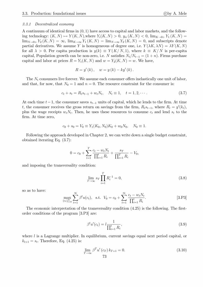
3.3. Production: foundational issues c©by A. Mele
3.3.1 Decentralized economy
A continuum of identical firms in (0, 1) have access to capital and labor markets, and the follow-ing technology: (K,N) → Y (K,N),where Yi(K,N) > 0, yii (K,N) < 0, limK→0+ Y1 (K,N) =limN→0+ Y2 (K,N) = ∞, limK→∞ Y1 (K,N) = limN→∞ Y2 (K,N) = 0, and subscripts denotepartial derivatives. We assume Y is homogeneous of degree one, i.e. Y (λK, λN) = λY (K,N)for all λ > 0. Per capita production is y(k) ≡ Y (K/N, 1), where k ≡ K/N is per-capitacapital, Population growth can be non-zero, i.e. N satisfies Nt/Nt−1 = (1 + n). Firms purchasecapital and labor at prices R = Y1(K,N) and w = Y2(K,N) = w. We have,
R = y′ (k) , w = y (k)− ky′ (k) .
The Nt consumers live forever. We assume each consumer offers inelastically one unit of labor,and that, for now, that N0 = 1 and n = 0. The resource constraint for the consumer is:
ct + st = Rtst−1 + wtNt, Nt ≡ 1, t = 1, 2, · · · . (3.7)
At each time t−1, the consumer saves st−1 units of capital, which he lends to the firm. At timet, the consumer receives the gross return on savings from the firm, Rtst−1, where Rt = y′(kt),plus the wage receipts wtNt. Then, he uses these resources to consume ct and lend st to thefirm. At time zero,
c0 + s0 = V0 ≡ Y1(K0, N0)K0 + w0N0, N0 ≡ 1.
Following the approach developed in Chapter 2, we can write down a single budget constraint,obtained iterating Eq. (3.7):
0 = c0 +T∑
t=1
ct − wtNt∏ti=1Ri
+sT∏Ti=1Ri
− V0,
and imposing the transversality condition:
limT→∞
sT
T∏
i=1
R−1i = 0, (3.8)
so as to have:
max(ct)
∞t=0
∞∑
t=1
βtu(ct), s.t. V0 = c0 +∞∑
t=1
ct − wtNt∏ti=1Ri
. [3.P3]
The economic interpretation of the transversality condition (4.25) is the following. The first-order conditions of the program [3.P3] are:
βtu′(ct) = l1∏t
i=1Ri
, (3.9)
where l is a Lagrange multiplier. In equilibrium, current savings equal next period capital, orkt+1 = st. Therefore, Eq. (4.25) is:
limT→∞
βTu′ (cT ) kT+1 = 0. (3.10)
73

3.3. Production: foundational issues c©by A. Mele
That is, the economic value of capital is capital weighted by discounted marginal utility, whichneeds to be zero, eventually.The first-order condition (3.9) leads to the usual optimality condition in Eq. (3.2), where this
time, Rt+1 = y′ (kt+1). In this economy, an equilibrium is a sequence ((c, k)t)
∞t=0 satisfying
kt+1 = y (kt)− ctβu′(ct+1)
u′(ct)=
1
y′(kt+1)
(3.11)
and the transversality condition in Eq. (3.10). The first equation in this system is simply this:capital available for producing the next period, kt+1, is equal to savings, st ≡ y (kt)− ct.
3.3.2 Centralized economy
The market solution in (3.11) can be implemented by a social planner, who solves the followingprogram:
V (k0) ≡ max(ct,kt)
∞t=0
∞∑
i=0
βiu (ct)
s.t. kt+1 = y (kt)− ct, k0 given
[3.P4]
under the further transversality condition in Eq. (3.10).The program in [3.P4] is easily solved. By replacing the constraint into the utility func-
tion, and taking derivatives with respect to kt, leads directly to the second equation in (3.11).Alternatively, let us introduce the Lagrangian,
L (k0) = max(ct,kt+1)
∞t=0
∞∑
t=0
[βtu(ct)− λt (kt+1 − y(kt) + ct)
].
The first-order condition with respect to consumption is λt = βtu′ (ct), and the condition forcapital is λt−1 = λty
′ (kt). Putting these conditions together, leads to the second equation in(3.11). The same argument can be made, following a recursive approach. We have:
L (kt) = maxct,kt+1,λt
[u (ct)− λt (kt+1 − y (kt) + ct) + βL (kt+1)] .
The first-order condition for consumption is λt = u′ (ct), and that for capital is λt = βL′ (kt+1).
By replacing the first-order condition for λt (i.e., the constraint in program [3.P4]), and dif-ferentiating with respect to kt, yields L′ (kt) = βL′ (kt+1) y
′ (kt). These three conditions lead,again, to the second equation in (3.11).Finally, consider the Bellman’s equation:
V (kt) = maxct
[u (ct) + βV (kt+1)] , s.t. kt+1 = y (kt)− ct.
The first-order condition leads to, u′ (ct) = βV ′ (y (kt)− ct). Let us denote the policy withct = c (kt). In terms of the policy c function, the value function and the first-order conditionsare:
V (kt) = u (c (kt)) + βV (y (kt)− c (kt)) , u′ (c (kt)) = βV′ (y (kt)− c (kt)) .
By differentiating the value function:
V ′ (kt) = u′ (c (kt)) c
′ (kt) + βV′ (y (kt)− c (kt)) (y′ (kt)− c′ (kt)) = u′ (c (kt)) y′ (kt) .
By replacing back into the first-order condition, we obtain the second equation in (3.11).
74
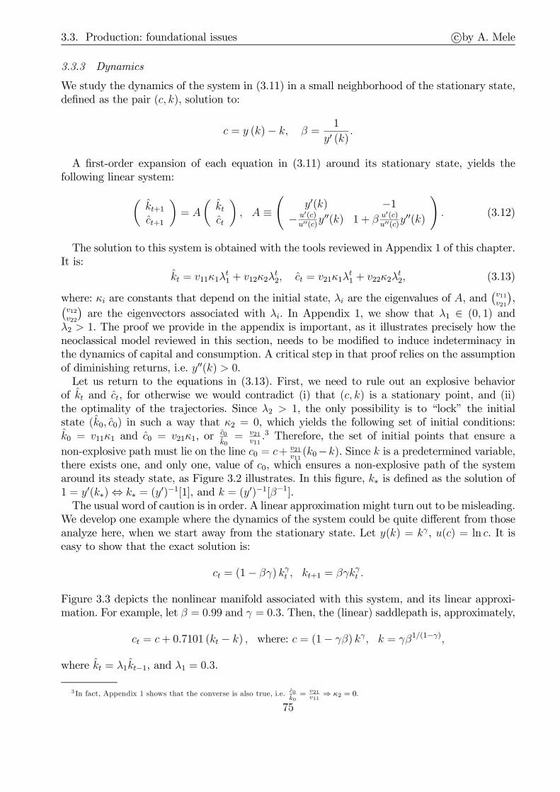
3.3. Production: foundational issues c©by A. Mele
3.3.3 Dynamics
We study the dynamics of the system in (3.11) in a small neighborhood of the stationary state,defined as the pair (c, k), solution to:
c = y (k)− k, β =1
y′ (k).
A first-order expansion of each equation in (3.11) around its stationary state, yields thefollowing linear system:
(kt+1
ct+1
)= A
(ktct
), A ≡
(y′(k) −1
− u′(c)u′′(c)
y′′(k) 1 + β u′(c)u′′(c)
y′′(k)
). (3.12)
The solution to this system is obtained with the tools reviewed in Appendix 1 of this chapter.It is:
kt = v11κ1λt1 + v12κ2λ
t2, ct = v21κ1λ
t1 + v22κ2λ
t2, (3.13)
where: κi are constants that depend on the initial state, λi are the eigenvalues of A, and(v11
v21
),(
v12
v22
)are the eigenvectors associated with λi. In Appendix 1, we show that λ1 ∈ (0, 1) and
λ2 > 1. The proof we provide in the appendix is important, as it illustrates precisely how theneoclassical model reviewed in this section, needs to be modified to induce indeterminacy inthe dynamics of capital and consumption. A critical step in that proof relies on the assumptionof diminishing returns, i.e. y′′(k) > 0.Let us return to the equations in (3.13). First, we need to rule out an explosive behavior
of kt and ct, for otherwise we would contradict (i) that (c, k) is a stationary point, and (ii)the optimality of the trajectories. Since λ2 > 1, the only possibility is to “lock” the initialstate (k0, c0) in such a way that κ2 = 0, which yields the following set of initial conditions:k0 = v11κ1 and c0 = v21κ1, or
c0k0= v21
v11.3 Therefore, the set of initial points that ensure a
non-explosive path must lie on the line c0 = c+v21
v11(k0−k). Since k is a predetermined variable,
there exists one, and only one, value of c0, which ensures a non-explosive path of the systemaround its steady state, as Figure 3.2 illustrates. In this figure, k∗ is defined as the solution of1 = y′(k∗)⇔ k∗ = (y′)−1[1], and k = (y′)−1[β−1].The usual word of caution is in order. A linear approximation might turn out to be misleading.
We develop one example where the dynamics of the system could be quite different from thoseanalyze here, when we start away from the stationary state. Let y(k) = kγ , u(c) = ln c. It iseasy to show that the exact solution is:
ct = (1− βγ) kγt , kt+1 = βγkγt .
Figure 3.3 depicts the nonlinear manifold associated with this system, and its linear approxi-mation. For example, let β = 0.99 and γ = 0.3. Then, the (linear) saddlepath is, approximately,
ct = c+ 0.7101 (kt − k) , where: c = (1− γβ) kγ, k = γβ1/(1−γ),
where kt = λ1kt−1, and λ1 = 0.3.
3 In fact, Appendix 1 shows that the converse is also true, i.e. c0k0
= v21v11
⇒ κ2 = 0.
75

3.3. Production: foundational issues c©by A. Mele
kt
ct
c0 = c + (v21/v11) (k0 –k)
k
c
k*k0
c0
c = y(k) – k
FIGURE 3.2.
kt
ct
nonlinear stable manifold
linear approximation
steady state
FIGURE 3.3.
76

3.3. Production: foundational issues c©by A. Mele
3.3.4 Stochastic economies
“Real business cycle theory is the application of general equilibrium theory to the quan-
titative analysis of business cycle fluctuations.” Edward Prescott (1991, p. 3)
“The Kydland and Prescott model is a complete markets set-up, in which equilibrium and
optimal allocations are equivalent. When it was introduced, it seemed to many–myself
included–to be much too narrow a framework to be useful in thinking about cyclical
issues.” Robert Lucas (1994, p. 184)
In its simplest version, real business cycle theory is an extension of the neoclassical modelof Section 3.3.3, in which random productivity shocks are added. The engine of fluctuations,then, comes from the real sphere of the economy. This approach is in contrast with the Lucasapproach of the 1970s, based on information and money, where fluctuations arise due to infor-mation delays with which agents discover the nature of a shock (real or monetary). As furtherreviewed in Chapter 9, the Lucas information-theoretic approach has been, instead, more suc-cessful in inspiring work on the formation of asset prices, leading to the development of marketmicrostructure theory and, more generally, to information driven explanations of asset prices.Despite the remarkable switch in the economic motivation, the paradigm underlying real
business cycle theory is the same as the information-based approach of Lucas, as it relies onrational expectations: macroeconomic fluctations and, then, as we shall explain, asset pricesfluctuations, stem from the optimal response of the agents vis-à-vis exogeneous shocks: agentsimplement action plans that are state-contingent, i.e. they decide to consume, to work and toinvest according to the history of shocks as well as the present shocks they observe.
3.3.4.1 Basic model
We consider an economy with complete markets and no frictions, such that its equilibriumallocations are Pareto-optimal. To characterize these allocations, we implement them throughthe following program of a social planner:
V (k0, s0) = max(ct)
∞t=0
E
[ ∞∑
t=0
βtu(ct)
], (3.14)
subject to a capital accumulation constraint, with capital depreciation. Let It denote newinvestment. It is:
It = Kt+1 − (1− δ)Kt. (3.15)
At time t− 1, the available productive capital is Kt. At time t, a portion δKt of this capital islost, due to depreciation. Therefore, at time t, the productive system is left with (1− δ)Kt unitsof capital. The capital available at time t, Kt+1, equals the capital already in place, (1− δ)Kt,plus new investments, which is exactly what Eq. (3.15) says.Next, normalize population normalized to one, such that Kt = kt. The goods market clearing
condition is:y (kt, st) = ct + It,
where y(kt, st) is the production function, which is Ft-measurable, and s is the source ofrandomness–the engine for random fluctuations of the endogeneous variables. By replacingEq. (3.15) into the equilibrium condition,
kt+1 = y (kt, st)− ct + (1− δ) kt. (3.16)
77

3.3. Production: foundational issues c©by A. Mele
So the planner maximizes the utility in Eq. (3.14), under the capital accumulation constraintin Eq. (3.16).We assume that y (kt, st) ≡ sty (kt), where y is as in Section 3.2, and (st)
∞t=0 is solution to:
st+1 = sρt ǫt+1, (3.17)
where ρ ∈ (0, 1), and (ǫt)∞t=0 is a IID sequence with support s.t. st ≥ 0. In this economy, everyasset is priced as in the Lucas model of the previous section. Therefore, the gross return onsavings s·y
′(k·) satisfies:
u′ (ct) = βEt (u′ (ct+1) (st+1y
′ (kt+1) + 1− δ)) . (3.18)
A rational expectation equilibrium is a stochastic process (ct, kt)∞t=0, satisfying Eq. (3.16), the
Euler equation in (3.18), for given k0 and s0.We show the existence of a saddlepoint path for the linearized version of Eqs. (3.16)-(3.17)-
(3.18), which implies determinacy of the stochastic (linearized) equilibrium.4 We study thebehavior of (c, k, s)t in a neighborhood of ǫ ≡ E(ǫt). Let (c, k, s) be consumption, capital andproductivity shock, corresponding to ǫ, obtained replacing ǫ into Eqs. (3.16)-(3.17)-(3.18), andassuming no uncertainty takes place:
c = sy (k)− δk, s = ǫ1
1−ρ , β =1
sy′(k) + 1− δ .
A first-order approximation to Eqs. (3.16)-(3.17)-(3.18) around (k, c, s), leaves:
zt+1 = Φzt +Rut+1, (3.19)
where we have defined xt ≡ xt−xx
, and zt = (kt, ct, st)⊤, ut = (uc,t, us,t)
⊤, uc,t = ct − Et−1(ct),us,t = st − Et−1(st) = ǫt, and, finally,
Φ =
β−1 − ck
sy(k)k
− u′(c)cu′′(c)
sky′′(k) 1 + βu′(c)u′′(c)
sy′′(k) − βu′(c)cu′′(c)
s(sy(k)y′′(k) + ρy′(k))
0 0 ρ
, R =
0 01 00 1
.
Let us consider the characteristic equation:
0 = det (Φ− λI) = (ρ− λ)[λ2 −
(β−1 + 1 + β
u′(c)
u′′(c)sy′′(k)
)λ+ β−1
].
A solution is λ1 = ρ. By the same arguments produced for the deterministic case of Section3.3.3 (see Appendix 1), one finds that λ2 ∈ (0, 1) and λ3 > 1.5 As for the deterministic case inSection 3.3.3, we can diagonalize the system by rewriting Φ = PΛP−1, where Λ is a diagonal
4A stochastic equilibrium is the situation where there is a stationary measure (definition: p(+) =∫π(+/−)dp(−), where π is
the transition measure) generating (ct, kt)∞t=1.5The linearized model in this section has state variables expressed in growth rates here. However, we can always reformulate this
model in terms of first differences, by pre- and post- multiplying Φ by appropriate normalizing matrices. As an example, if G i the3× 3 matrix that has 1
k, 1cand 1
son its diagonal, (3.19) can be written as: E(zt+1 − z) = G−1ΦG · (zt − z), where zt = (kt, ct, st),
and we would arrive at the same conclusions. It is tedious but easy to check that the model in this section collapses to that inSection 3.3.3, once we set ǫt = 1, for each t, and s0 = 1.
78
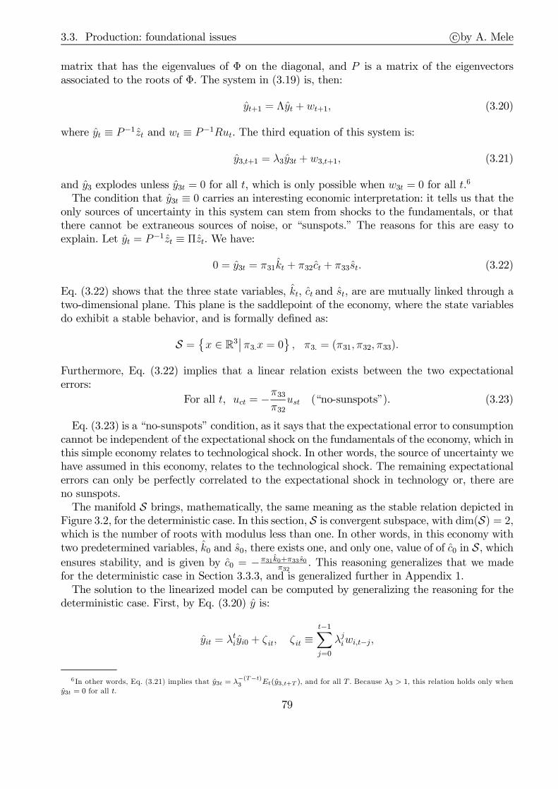
3.3. Production: foundational issues c©by A. Mele
matrix that has the eigenvalues of Φ on the diagonal, and P is a matrix of the eigenvectorsassociated to the roots of Φ. The system in (3.19) is, then:
yt+1 = Λyt + wt+1, (3.20)
where yt ≡ P−1zt and wt ≡ P−1Rut. The third equation of this system is:
y3,t+1 = λ3y3t + w3,t+1, (3.21)
and y3 explodes unless y3t = 0 for all t, which is only possible when w3t = 0 for all t.6
The condition that y3t ≡ 0 carries an interesting economic interpretation: it tells us that theonly sources of uncertainty in this system can stem from shocks to the fundamentals, or thatthere cannot be extraneous sources of noise, or “sunspots.” The reasons for this are easy toexplain. Let yt = P
−1zt ≡ Πzt. We have:
0 = y3t = π31kt + π32ct + π33st. (3.22)
Eq. (3.22) shows that the three state variables, kt, ct and st, are are mutually linked through atwo-dimensional plane. This plane is the saddlepoint of the economy, where the state variablesdo exhibit a stable behavior, and is formally defined as:
S =x ∈ R3
∣∣ π3.x = 0, π3. = (π31, π32, π33).
Furthermore, Eq. (3.22) implies that a linear relation exists between the two expectationalerrors:
For all t, uct = −π33
π32ust (“no-sunspots”). (3.23)
Eq. (3.23) is a “no-sunspots” condition, as it says that the expectational error to consumptioncannot be independent of the expectational shock on the fundamentals of the economy, which inthis simple economy relates to technological shock. In other words, the source of uncertainty wehave assumed in this economy, relates to the technological shock. The remaining expectationalerrors can only be perfectly correlated to the expectational shock in technology or, there areno sunspots.The manifold S brings, mathematically, the same meaning as the stable relation depicted in
Figure 3.2, for the deterministic case. In this section, S is convergent subspace, with dim(S) = 2,which is the number of roots with modulus less than one. In other words, in this economy withtwo predetermined variables, k0 and s0, there exists one, and only one, value of of c0 in S, whichensures stability, and is given by c0 = −π31k0+π33s0
π32. This reasoning generalizes that we made
for the deterministic case in Section 3.3.3, and is generalized further in Appendix 1.The solution to the linearized model can be computed by generalizing the reasoning for the
deterministic case. First, by Eq. (3.20) y is:
yit = λtiyi0 + ζit, ζit ≡
t−1∑
j=0
λjiwi,t−j,
6 In other words, Eq. (3.21) implies that y3t = λ−(T−t)3 Et(y3,t+T ), and for all T . Because λ3 > 1, this relation holds only when
y3t = 0 for all t.
79
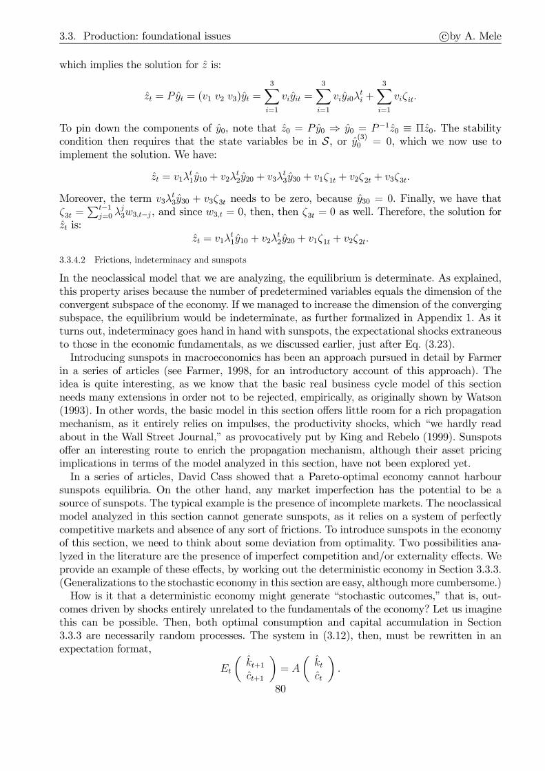
3.3. Production: foundational issues c©by A. Mele
which implies the solution for z is:
zt = Pyt = (v1 v2 v3)yt =3∑
i=1
viyit =3∑
i=1
viyi0λti +
3∑
i=1
viζit.
To pin down the components of y0, note that z0 = P y0 ⇒ y0 = P−1z0 ≡ Πz0. The stabilitycondition then requires that the state variables be in S, or y(3)0 = 0, which we now use toimplement the solution. We have:
zt = v1λt1y10 + v2λ
t2y20 + v3λ
t3y30 + v1ζ1t + v2ζ2t + v3ζ3t.
Moreover, the term v3λt3y30 + v3ζ3t needs to be zero, because y30 = 0. Finally, we have that
ζ3t =∑t−1
j=0 λj3w3,t−j, and since w3,t = 0, then, then ζ3t = 0 as well. Therefore, the solution for
zt is:zt = v1λ
t1y10 + v2λ
t2y20 + v1ζ1t + v2ζ2t.
3.3.4.2 Frictions, indeterminacy and sunspots
In the neoclassical model that we are analyzing, the equilibrium is determinate. As explained,this property arises because the number of predetermined variables equals the dimension of theconvergent subspace of the economy. If we managed to increase the dimension of the convergingsubspace, the equilibrium would be indeterminate, as further formalized in Appendix 1. As itturns out, indeterminacy goes hand in hand with sunspots, the expectational shocks extraneousto those in the economic fundamentals, as we discussed earlier, just after Eq. (3.23).Introducing sunspots in macroeconomics has been an approach pursued in detail by Farmer
in a series of articles (see Farmer, 1998, for an introductory account of this approach). Theidea is quite interesting, as we know that the basic real business cycle model of this sectionneeds many extensions in order not to be rejected, empirically, as originally shown by Watson(1993). In other words, the basic model in this section offers little room for a rich propagationmechanism, as it entirely relies on impulses, the productivity shocks, which “we hardly readabout in the Wall Street Journal,” as provocatively put by King and Rebelo (1999). Sunspotsoffer an interesting route to enrich the propagation mechanism, although their asset pricingimplications in terms of the model analyzed in this section, have not been explored yet.In a series of articles, David Cass showed that a Pareto-optimal economy cannot harbour
sunspots equilibria. On the other hand, any market imperfection has the potential to be asource of sunspots. The typical example is the presence of incomplete markets. The neoclassicalmodel analyzed in this section cannot generate sunspots, as it relies on a system of perfectlycompetitive markets and absence of any sort of frictions. To introduce sunspots in the economyof this section, we need to think about some deviation from optimality. Two possibilities ana-lyzed in the literature are the presence of imperfect competition and/or externality effects. Weprovide an example of these effects, by working out the deterministic economy in Section 3.3.3.(Generalizations to the stochastic economy in this section are easy, although more cumbersome.)How is it that a deterministic economy might generate “stochastic outcomes,” that is, out-
comes driven by shocks entirely unrelated to the fundamentals of the economy? Let us imaginethis can be possible. Then, both optimal consumption and capital accumulation in Section3.3.3 are necessarily random processes. The system in (3.12), then, must be rewritten in anexpectation format,
Et
(kt+1
ct+1
)= A
(ktct
).
80

3.4. Production-based asset pricing c©by A. Mele
Next, let us introduce the expectational error process uc,t ≡ ct − Et−1(ct), which we plug backinto the previous system, to obtain:
(kt+1
ct+1
)= A
(ktct
)+
(0
uc,t+1
).
Naturally, we still have λ1 ∈ (0, 1) and λ2 > 1, as in Section 3.3.3. Therefore, we decompose Aas PΛP−1, and have:
yt+1 = Λyt + P−1(0 uc,t+1)
⊤.
Moreover, for y2t = λ−T2 Et(y2,t+T ) to hold for all T , we need to have y2t = 0, for all t. Therefore,
the second element of the vector P−1(0 uc,t+1)⊤ must be zero, or, for all t,
0 = π22uc,t ⇐⇒ 0 = uc,t.
There is no room for expectational errors and, hence, sunspots, in this model. The fact thatλ2 > 1 implies the dimension of the saddlepoint is less than the number of predeterminedvariables. So a viable route to pursue here, is to look for economies such that the saddlepointhas a dimension larger than one, i.e. such that λ2 < 1. In these economies, indeterminancyand sunspots will be two facets of the same coin. As shown in the appendix, the reasons forwhich λ2 > 1 relate to the classical assumptions about the shape of the utility function u andthe production function y. We now modify the production function, to see the effect on theeigenvalues of A.[Economy with increasing returns][Asset pricing implications in further chapters]
3.4 Production-based asset pricing
3.4.1 Firms
For each firm, capital accumulation does satisfy the identity in Eq. (3.15), reproduced here forconvenience:
Kt+1 = (1− δ)Kt + It. (3.24)
The additional assumption we make, is that capital adjustment is costly: investing It per unitof capital already in place, Kt, entails a cost φ( It
Kt), expressed in terms of the price of the final
good, which we take to be the numéraire, thereby allowing the investment goods to differ fromthe final good the firm produces. An investment of It, then, leads to a cost φ( It
Kt)Kt, such that
the profit the firm makes at time t is,
D (Kt, It) ≡ y (Kt, N (Kt))− wtN (Kt)− ptIt − φ(ItKt
)Kt, (3.25)
where y (Kt, Nt) is the firm’s production at time t, obtained with capital Kt and labor Nt, andsubject to the productivity shocks described in Section 3.3.4, wt is the real wage, N (K) is thelabor demand schedule, solution to the optimality condition, yN (Kt, N (Kt)) = wt for all t,and pt is the real price of the investment goods, or uninstalled capital. Finally, the adjustment-cost function satisfies φ ≥ 0, φ′ ≥ 0, φ′′ ≥ 0. In words, capital adjustment is costly when theadjustment is made fastly. Naturally, φ is zero in the absence of adjustment costs.
81

3.4. Production-based asset pricing c©by A. Mele
What is the value of the profit, from the perspective of time zero? This question can beanswered, by utilizing the Arrow-Debreu state prices introduced in Chapter 2. At time t, andin state s, the profit Dt (s) (say) is worth,
φ0,t (s)D (Kt (s) , It (s)) = m0,t (s)Dt (Kt (s) , It (s))P0,t (s) ,
with the same notation as in Chapter 2.
3.4.1.1 The value of the firm
We assume that in each period, the firm distributes all the profits it makes, and that for a givencapital K0, it maximizes its cum-dividend value,
Vc (K0) = max(Kt,It−1)
∞t=1
[D (K0, I0) + E
( ∞∑
t=1
m0,tD (Kt, It)
)],
subject to the capital accumulation law of Eq. (3.24).The value of the firm at time t, Vc (Kt), can be found recursively, through the Bellman’s
equation,Vc (Kt) = max
It[D (Kt, It) + Et (mt+1Vc (Kt+1))] ,
where the expectation is taken with respect to the information set as of time t. The first-orderconditions for It lead to,
−DI (Kt, It) = Et [mt+1V′c (Kt+1)] . (3.26)
That is, along the optimal capital accumulation path, the marginal cost of new installed capitalat time t, −DI , must equal the expected marginal return on the investment, i.e. the expectedvalue of the marginal contribution of capital to the value of the firm at time t+ 1, V ′c (Kt+1).By Eq. (3.26), optimal investment is a function I (Kt), and the value of the firm satisfies,
Vc (Kt) = D (Kt, I (Kt)) + Et [mt+1Vc (Kt+1)] .
Differentiating the value function in the previous equation, with respect to Kt, and using Eq.(3.26), yields the following envelope condition:
V ′c (Kt) = DK (Kt, I (Kt)) +DI (Kt, I (Kt)) I′ (Kt) + Et [mt+1V
′c (Kt+1) ((1− δ) + I ′ (Kt))]
= DK (Kt, I (Kt))− (1− δ)DI (Kt, I (Kt)) .
By replacing this expression for the value function back into Eq. (3.26), leaves:
−DI (Kt, I (Kt)) = Et [mt+1 (DK (Kt+1, I (Kt+1))− (1− δ)DI (Kt+1, I (Kt+1)))] . (3.27)
Along the optimal capital accumulation path, the marginal cost of new installed capitalat time t, which by Eq. (3.26) is the expected marginal return on the investment, equals theexpected value of (i) the very same marginal cost at time t+1, corrected for capital depreciation,(1− δ), and (ii) capital productivity, net of adjustment costs. Analytically,
DK (Kt, It) = yK (Kt, N (Kt)) + yN (Kt, N (Kt))N′ (Kt)− wtN
′ (Kt)−∂
∂K
(φ
(ItKt
)Kt
)
= yK (Kt, N (Kt))−∂
∂K
(φ
(ItKt
)Kt
),
−DI (Kt, I (Kt)) = pt + φ′(ItKt
).
We now introduce a fundamental concept in investment theory.
82

3.4. Production-based asset pricing c©by A. Mele
3.4.1.2 q theory
The Tobin’s marginal q is defined as the ratio of the expected marginal value of an additionalunit of capital over its replacement cost:
TQt ≡ Tobin’s marginal q ≡ E [mt+1V′c (Kt+1)]
pt.
We show that the numerator, E [mt+1V′c (Kt+1)], is, simply, the shadow price of installed capital.
Consider the Lagrangian at time t,
L (Kt) = maxIt,Kt+1,qt
[D (Kt, It)− qt (Kt+1 − (1− δ)Kt − It) + Et (mt+1L (Kt+1))] , (3.28)
which, integrated, gives rise to the value of the firm:
L (K0) = max(It,Kt+1qt)
∞t=0
E
[ ∞∑
t=0
m0,t (D (Kt, It)− qt (Kt+1 − (1− δ)Kt − It))].
The first-order condition for investment, It, is, qt = −DI (Kt, It), and that for capital, Kt+1,is qt = E (mt+1L′ (Kt+1)). By Eq. (3.26), then, L′ (Kt) = V ′c (Kt+1) and, therefore, qt is theexpected marginal return on the investment, that is, the shadow price of installed capital.Therefore, Tobin’s marginal q is the ratio of the shadow price of installed capital to its replace-ment cost:
TQt =qtpt.
Next, replace the first-order condition for qt, i.e. Eq. (3.24), into Eq. (3.28), differentiate L (Kt)with respect toKt, and use the first-order condition forKt+1, obtaining, L′ (Kt) = DK (Kt, It)+qt (1− δ). These conditions imply that qt satisfies the valuation equation (3.27):
qt = Et [mt+1 (DK (Kt+1, It+1) + (1− δ) qt+1)] , (3.29)
and therefore that:
qt = pt + φ′(ItKt
). (3.30)
The shadow price of installed capital, qt, has to equal the marginal cost of new installed capital,and is larger than the price of uninstalled capital, pt. It is natural: to install new capitalrequires some (marginal) adjustment costs, which add to the “row” price of uninstalled capital,pt. Therefore, in the presence of adjustment costs, Tobin’s marginal q is larger than one.Eq. (3.29) can be solved forward, leaving:
qt = E
[ ∞∑
s=1
(1− δ)s−1m0,t+sDK (Kt+s, It+s)
].
The shadow price of installed capital is worth the sum of all its future marginal net productivity,discounted at the depreciation rate. Moreover, Eq. (3.30) can be inverted for It/Kt, to deliver:
ItKt
= φ′−1 (qt − pt) , (3.31)
83

3.4. Production-based asset pricing c©by A. Mele
where φ′−1 denotes the inverse of φ′, and is increasing, since φ′ is increasing. Given Kt, and thefact that Kt+1 is predetermined, the firm evaluates qt through Eq. (3.29), and then determinesthe level of new investments through Eq. (3.31). These investments are increasing in the dif-ference between the shadow price of installed capital, qt, and that of uninstalled capital, pt, asoriginally assumed by Tobin (1969).In the absence of adjustement costs, when qt = pt, Eq. (3.29) delivers the condition,
1 = Et [mt+1 (yK (Kt+1, N (Kt+1)) + (1− δ))] ,
where we have set pt ≡ 1 for all t, meaning that the firm’s production is just the uninstalled cap-ital. Empirically, however, the marginal productivity of capital, yK (Kt, N (Kt)), is not volatileenough, to rationalize asset returns, as explained in more detail in Chapter 8. Moreover, as weargue in a moment, Tobin’s marginal q can be approximated by market-to-book ratios, whichare typically time-varying. Therefore, adjustment costs are important for asset pricing.A difficulty with Tobin’s marginal q is that it is quite difficult to estimate. Yet in the special
case we are analyzing in this section, where firms act competitively and have access to anhomogeneous production function and adjustment costs, Tobin’s marginal q can be proxied bythe market-to-book ratio of a given firm. Let V (Kt) denote the ex-dividend value of the firm,which is its stock market value, since it nets out the dividend it pays to its holder in the currentperiod. It is:
V (Kt) ≡ Vc (Kt)−D (Kt, I (Kt)) = Et [mt+1Vc (Kt+1)] .
The Tobin’s average q is defined as the ratio of the stock market value of the firm over thereplacement cost of the capital:
Tobin’s average q ≡ Stock Mkt Value of the Firm
Replacement Cost of Capital=V (Kt)
ptKt+1.
The next result was originally obtained by Hayashi (1982) in a continuous-time setting.
T 3.2. Tobin’s marginal q and average q coincide. That is, we have,
V (Kt) = qtKt+1.
P. By the homogeneity properties of the production function and the adjustment costs,
D (Kt, It) = DK (Kt, It)Kt +DI (Kt, It) It.
Therefore, the ex-dividend value of the firm is:
V (K0, I0) = E
[ ∞∑
t=1
m0,tD (Kt, It)
]
= E
[ ∞∑
t=1
m0,t (DK (Kt, It)− (1− δ)DI (Kt, It))Kt
]+ E
[ ∞∑
t=1
m0,tDI (Kt, It)Kt+1
],
where the second line follows by Eq. (3.24). By Eq. (3.27), and the law of iterated expectations,
E
[ ∞∑
t=1
m0,t (DK (Kt, It)− (1− δ)DI (Kt, It))Kt
]= −DI (K0, I0)K1−E
[ ∞∑
t=1
m0,tKt+1DI (Kt, It)
].
84

3.4. Production-based asset pricing c©by A. Mele
Hence, V (K0, I0) = −DI (K0, I0)K1 = q0K1. ‖
This result, in conjunction with that in Eq. (3.30), provides a simple rule of thumb forinvestement decisions. Consider, for example, the case of quadratic adjustment costs, whereφ (x) = 1
2κ−1x2, for some κ > 0. Then, Eq. (3.31) is:
It = κ (qt − pt)Kt = κ
(Stock Mkt Value of the Firm
Replacement Cost of Capital− 1
)ptKt,
where the second equality follows by Theorem 3.2. Thus, according to q theory, we expect firmswith a market value larger than the cost of reproducing their capital to grow, and firms whichare not worth the cost of reproducing their capital to shrink. This basic observation constitutesa first assessment that we can use to assess developments of firms.
3.4.2 Consumers
We now generalize the budget constraint obtained in the program [3.P3], to the uncertaintycase. We claim that in this case, the relevant budget constraint is,
V0 = c0 + E
[ ∞∑
t=1
m0,t (ct − wtNt)
]. (3.32)
We have: ct + Stθt+1 = (St +Dt) θt + wtNt and, then:
E
[ ∞∑
t=1
m0,t (ct − wtNt)
]= E
[ ∞∑
t=1
m0,t (St +Dt) θt
]− E
[ ∞∑
t=1
m0,tStθt+1
]
= E
[ ∞∑
t=1
Et−1
(m0,t
mt−1,tmt−1,t (St +Dt) θt
)]− E
[ ∞∑
t=2
m0,t−1St−1θt
]
= E
[ ∞∑
t=1
m0,t−1St−1θt
]− E
[ ∞∑
t=2
m0,t−1St−1θt
]
= S0θ1 = V0 − c0.
where the third line follows by the properties of the discount factor, m0,t
mt−1,t= m0,t−1 and mt ≡
mt−1,t.Therefore, the program consumers solve is:
max(ct)
∞t=0
E
[ ∞∑
t=1
βtu (ct)
], s.t. Eq. (3.32).
We now have two optimality conditions, one intertemporal and another, intratemporal:
mt+1 = βu1 (ct+1, Nt+1)
u1 (ct, Nt)(intertemporal); wt = −u2 (ct, Nt)
u1 (ct, Nt)(intratemporal).
85

3.5. Money, production and asset prices in overlapping generations models c©by A. Mele
3.4.3 Equilibrium
For all t,
y (Kt, Nt) = ct + ptIt + φ
(ItKt
)Kt. (3.33)
It is easily seen that the condition θt = 1 in the financial market, implies that ct = Dt + wtNt,which, upon substitution of the profits in Eq. (3.25), delivers the equilibrium condition in Eq.(3.33). Implicit in this reasoning, is the idea the adjustment costs are not paid to anyone. Theyrepresent, so to speak, capital losses incurred along the way of growth.
3.5 Money, production and asset prices in overlapping generations models
3.5.1 Introduction: endowment economies
3.5.1.1 A deterministic model
We initially assume the population is constant, and made up of one young and one old. Theyoung agent maximizes his intertemporal utility subject to his budget constraint:
max(c1t,c2,t+1)
[u (c1t) + βu (c2,t+1)] subject to
savt + c1t = w1t
c2,t+1 = savtRt+1 + w2,t+1[3.P5]
where w1t and w2,t+1 are the endowments the agent receives at his young and old age.The agent born at time t − 1, then, faces the constraints: savt−1 + c1,t−1 = w1,t−1 and c2t =
savt−1Rt + w2t. By combining his second period constraint with the first period constraint ofthe agent born at time t,
savt−1Rt + wt = savt + c1t + c2t, wt ≡ w1t + w2t. (3.34)
The equilibrium in the intergenerational lending market is, naturally:
savt = 0, (3.35)
and implies that the goods market is also in equilibrium, in that wt =∑2
i=1 ci,t, and for all t.Therefore, we can analyze the model, by just analyzing the autarkic equilibrium.As Figure 3.4 illustrates, the first-order condition for the program [3.P5] requires that the
slope of the indifference curve be equal to the slope of the lifetime budget constraint, c2,t+1 =−Rt+1c1,t +Rt+1w1t + w2,t+1, and leads to:
βu′(c2,t+1)
u′(c1,t)=
1
Rt+1. (3.36)
The equilibrium, then, is a sequence of gross returns Rt satisfying Eqs. (3.34), (3.35) and (3.36),or:
bt ≡1
Rt+1= β
u′(w2,t+1)
u′(w1t). (3.37)
In this relation, bt is the shadow price of a bond issued at t, and promising one unit of numéraireat t+1: the sequence of prices, bt, satisfying Eq. (3.37), is such that agents are happy with notbeing able to lend and borrow, intergenerationally.
86
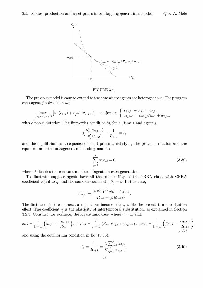
3.5. Money, production and asset prices in overlapping generations models c©by A. Mele
c1,t
c2,t+1
c2,t+1 = − Rt+1 c1,t + Rt+1 w1t + w2,t+1
w1,t
w2,t+1
FIGURE 3.4.
The previous model is easy to extend to the case where agents are heterogeneous. The programeach agent j solves is, now:
max(c1j,t,c2j,t+1)
[uj (c1j,t) + βjuj (c2j,t+1)
]subject to
savj,t + c1j,t = w1j,t
c2j,t+1 = savj,tRt+1 + w2j,t+1
with obvious notation. The first-order condition is, for all time t and agent j,
βju′j (c2j,t+1)
u′j (c1j,t)=
1
Rt+1≡ bt,
and the equilibrium is a sequence of bond prices bt satisfying the previous relation and theequilibrium in the intrageneration lending market:
J∑
j=1
savj,t = 0, (3.38)
where J denotes the constant number of agents in each generation.To illustrate, suppose agents have all the same utility, of the CRRA class, with CRRA
coefficient equal to η, and the same discount rate, βj = β. In this case,
savj,t =(βRt+1)
1η w1t − w2,t+1
Rt+1 + (βRt+1)1η
.
The first term in the numerator reflects an income effect, while the second is a substitutioneffect. The coefficient 1
ηis the elasticity of intertemporal substitution, as explained in Section
3.2.3. Consider, for example, the logarithmic case, where η = 1, and:
c1j,t =1
1 + β
(w1j,t +
w2j,t+1
Rt+1
), c2j,t+1 =
β
1 + β(Rt+1w1j,t +w2j,t+1) , savj,t =
1
1 + β
(βw1j,t −
w2j,t+1
Rt+1
),
(3.39)
and using the equilibrium condition in Eq. (3.38),
bt =1
Rt+1=β∑J
j=1w1j,t∑Jj=1w2j,t+1
. (3.40)
87

3.5. Money, production and asset prices in overlapping generations models c©by A. Mele
3.5.1.2 A tree in a stochastic economy
Suppose, next, that we introduce a tree, which yields a stochastic dividend Dt in each period.Each agent solves the following program:
max(c1t,c2,t+1)
[u (c1t) + βE (u(c2,t+1)| Ft)] subject to
Stθt + c1t = w1t
c2,t+1 = (St+1 +Dt+1)θt + w2,t+1[3.P6]
where St denotes the asset price and θ the units of the asset the agent chooses in his young age.The agent born at time t − 1 faces the constraints St−1θt−1 + c1,t−1 = w1,t−1 and w2t + (St +Dt)θt−1 = c2,t. By combining the second period constraint of the agent born at time t− 1 withthe first period constraint of the agent born at time t,
(St +Dt) θt−1 − Stθt + wt = c1,t + c2,t.
The clearing condition in the asset market, θt = 1, implies that the market for goods also clears,for all t: Dt + w1t + w2t = c1,t + c2,t. A characterization of the solution to the program [3.P6]can be obtained by eliminating c from the constraint,
maxθ[u (w1t − Stθ) + βE (u ((St+1 +Dt+1) θ)| Ft)] .
The equilibrium is one where θt = 1, implying that (i) c1t = w1t − St and (ii) c2,t+1 = St+1 +Dt+1 + w2,t+1. Using (i) and (ii), the first-order condition for the program [3.P6] leads to:
u′ (w1t − St)St = βE [u′ (St+1 +Dt+1 + w2,t+1) (St+1 +Dt+1)| Ft] .
Consider, for example, the case where u (c) = ln c, and set Rt+1 = (St+1 +Dt+1) /St. Wehave:
1
w1t − sav∗t= βE
[1
sav∗t Rt+1 + w2,t+1
Rt+1
∣∣∣∣∣Ft
], where sav∗t ≡ Stθt, θt = 1. (3.41)
In a deterministic setting,
1
w1t − savt= β
1
savtRt+1 + w2,t+1Rt+1, where savt = 0, (3.42)
which leads to the equilibrium bond price in Eq. (3.40). Eqs. (3.41) and (3.42) are formallyequivalent. Their fundamental difference is that in the tree economy, savings have to staypositive, as the tree must be held by the young agent, in equilibrium: sav∗t ≡ St ≥ 0. In aneconomy without a tree, instead, the interest rate, Rt, has to be such that savings are zero forall t, savt = 0.Eq. (3.41) can be solved explicitly for the price of the tree, St, once we assume w2t = 0 for
all t. In the absence of a tree, we cannot assume endowments are zero in the old age, sincethe autarkic economy in this case would be such that the old generation would not consumeanything. In the presence of a tree, instead, this assumption is innocuous, conceptually, as theautarkic equilibrium in this case is such that the old generation could consume the fruits of thetree, as well as the proceedings arising from selling the tree to the young generation. SolvingEq. (3.41) for St when w2t = 0, then, leads to a price for the tree, equal to:
St =β
1 + βw1t.
88

3.5. Money, production and asset prices in overlapping generations models c©by A. Mele
3.5.2 Diamond’s model
Kt+1 = NtSt, St = S (r (Kt) , w (Kt)).[Bubbles]
3.5.3 Money
We consider a version of the previous model with endowment (not with capital), and assumethat agents can now transfer value through a piece of paper, interpreted as money. The youngagent, then, maximizes his intertemporal utility, subject to a new budget constraint:
max(c1t,c2,t+1)
[u (c1t) + βu (c2,t+1)] subject to
mt
pt+ c1t = w1t
c2,t+1 =mt
pt+1
+ w2,t+1
[3.P7]
where mt is the amount of money he holds at time t, and pt is the price of the consumptiongood as of time t.Let
savt ≡mt
pt, Rt+1 ≡
ptpt+1
. (3.43)
Then, the budget constraint for program [3.P7] is formally identical to that for program [3.P5].The difference is that in the monetary economy of this section, the young agent may wish totransfer value over time, by saving money, earning a gross “interest rate” equal to the rateof deflation: the lower the price level the next period, the higher the purchasing power of themoney he transfers from the young to the old age. Naturally, then, by aggregating the budgetconstraints of the young and the old generation, we obtain, formally, Eq. (3.34), where now,savt and Rt+1 are as in (3.43). However, in the setting of this section, savt is not necessarilyzero, as money can be transferred from a generation to another one. In equilibrium, savt =
mtpt,
where mt denotes money supply. Therefore, the real value of money is strictly positive, if theequilibrium price pt stays bounded over time, which might actually occur, as we shall studybelow. As we see, the role of money as a medium for transferring value, is, in this context,similar to that of a tree in the stochastic overlapping generations economy of Section 3.5.1.2.Substituting the equilibrium savings savt =
mtpt
and Rt+1 =ptpt+1
into Eq. (3.34), we obtain,
mt−1 = mt + pt (c1t + c2t − wt), which used again in Eq. (3.34), delivers,
savt−1Rt = savt −∆mt
pt. (3.44)
We need a law of movement for money creation. We assume that:7 ∆mtmt−1
= µt, for some bounded
sequence µt. Replacing this into Eq. (3.44), leaves:
(1 + µt) savt−1Rt = savt. (3.45)
The last relation can be obtained even more simply, noting that by definition, (1 + µt)mt−1
pt−1
pt−1
pt=
mtpt. The previous relation can be generalized when population grows. Suppose that at time t,
7 In this section, we assume that money transfers are made to the young generation: the money the young generation has toabsorb is that from the old generation, mt−1, and that created by the “central bank,” µtmt−1. One might consider an alternativemodel in which transfers are made to old.
89
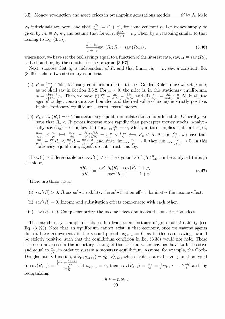
3.5. Money, production and asset prices in overlapping generations models c©by A. Mele
Nt individuals are born, and that NtNt−1
= (1 + n), for some constant n. Let money supply be
given byMt ≡ Ntmt, and assume that for all t, ∆MtMt−1
= µt. Then, by a reasoning similar to that
leading to Eq. (3.45),1 + µt1 + n
sav (Rt)Rt = sav (Rt+1) , (3.46)
where now, we have set the real savings equal to a function of the interest rate, savt−1 ≡ sav (Rt),as it should be, by the solution to the program [3.P7].Next, suppose that µt is independent of R, and that limt→∞ µt = µ, say, a constant. Eq.
(3.46) leads to two stationary equilibria:
(a) R = 1+n1+µ
. This stationary equilibrium relates to the “Golden Rule,” once we set µ = 0,as we shall say in Section 3.6.2. For µ = 0, the price is, in this stationary equilibrium,
pt =(1+µ1+n
)tp0. Then, we have: (i)
mtpt= Mt
Ntpt= M0
N0p0, and (ii) mt
pt+1= M0
N0p0
1+n1+µ
. All in all, theagents’ budget constraints are bounded and the real value of money is strictly positive.In this stationary equilibrium, agents “trust” money.
(b) Ra : sav (Ra) = 0. This stationary equilibrium relates to an autarkic state. Generally, wehave that Ra < R: prices increase more rapidly than per-capita money stocks. Analyti-cally, sav (Ra) = 0 implies that limt→∞
mtpt→ 0, which, in turn, implies that for large t,
mt+1
pt+1< mt
pt⇐⇒ mt+1
mt= Mt+1/Mt
Nt+1/Nt= 1+µ
1+n< pt+1
pt⇐⇒ Ra < R. As for mt
pt+1, we have that
mtpt+1
= mtptRa <
mtptR = mt
pt1+n1+µ
, and since limt→∞mtpt→ 0, then limt→∞
mtpt+1
→ 0. In thisstationary equilibrium, agents do not “trust” money.
If sav(·) is differentiable and sav′(·) = 0, the dynamics of (Rt)∞t=0 can be analyzed through
the slope,dRt+1
dRt
=sav′(Rt)Rt + sav(Rt)
sav′(Rt+1)
1 + µt1 + n
. (3.47)
There are three cases:
(i) sav′(R) > 0. Gross substituability: the substitution effect dominates the income effect.
(ii) sav′(R) = 0. Income and substitution effects compensate with each other.
(iii) sav′(R) < 0. Complementarity: the income effect dominates the substitution effect.
The introductory example of this section leads to an instance of gross substituability (seeEq. (3.39)). Note that an equilibrium cannot exist in that economy, once we assume agentsdo not have endowments in the second period, w2,t+1 = 0, as in this case, savings wouldbe strictly positive, such that the equilibrium condition in Eq. (3.38) would not hold. Theseissues do not arise in the monetary setting of this section, where savings have to be positiveand equal to mt
pt, in order to sustain a monetary equilibrium. Assume, for example, the Cobb-
Douglas utility function, u(c1t, c2,t+1) = cl11t · cl22,t+1, which leads to a real saving function equal
to sav(Rt+1) =l2l1w1t−
w2,t+1Rt+1
1+l2l1
. If w2,t+1 = 0, then, sav(Rt+1) =mtpt= 1
νw1t, ν ≡ l1+l2
l2and, by
reorganizing,
mtν = ptw1t,
90

3.5. Money, production and asset prices in overlapping generations models c©by A. Mele
0.0 0.2 0.4 0.6 0.8 1.0 1.20.0
0.5
1.0
1.5
R
f(R)
FIGURE 3.5. f (R) = (R−η +R−1 − 1)−1, with η = 2.
an equation supporting the Quantitative Theory of money. In this economy, the sequence ofgross returns satisfies, Rt+1 =
ptpt+1
= mtmt+1
w1,t+1
w1,t, or
Rt+1 =(1 + n) · (1 + gt+1)
1 + µt+1
, gt+1 ≡w1,t+1
w1,t− 1.
Gross inflation, R−1t , equals the monetary creation factor, corrected for the growth rate of the
economy as measured by gt+1, the youngs’ endowments growth rate.
As a final example, consider the utility function u(c1t, c2,t+1) =(lc
(η−1)/η1t + (1− l)c(η−1)/η
2,t+1
)η/(η−1)
,
which collapses to Cobb-Douglas once η → 1. We have:
c1t =Rt+1w1t + w2,t+1
Rt+1 +KηRηt+1
, c2,t+1 =Rt+1w1t + w2,t+1
1 +K−ηR1−ηt+1
, sav (Rt+1) =KηRη
t+1w1t − w2,t+1
Rt+1 +KηRηt+1
,
where K ≡ 1−ll. To simplify, set (i) K = 1, (ii) w2t = µt = n = 0, and (iii) w1t = w1,t+1. It can
be shown that in this case, sign (sav′(R)) = sign (η − 1). Moreover, the dynamics of the grossinterest rate, R, are given by:
Rt+1 = f (Rt) ≡ (R−ηt +R−1 − 1)1/(1−η). (3.48)
The stationary equilibria are solutions to R = f (R), and it is easily seen that one of them isR = 1, and corresponds to the monetary steady state.When η > 1, the slope in Eq. (3.47) has always the same sign, and the mapping f in Eq.
(3.48) has two fixed points, Ra = 0 and R = 1, with Ra being stable and R being unstable, asillustrated by Figure 3.5 when η = 2.When η < 1, the situation is quite delicate. In this case, Ra is not well-defined, and R = 1 is
not necessarily unstable. We may have sequences of gross interest rates, Rt, converging towardsR, or even the emergence of cycles. Mathematically, these properties can be understood by
examining the slope of the map in Eq. (3.47), for R = 1, dRt+1
dRt
∣∣∣Rt+1=Rt=1
= ηη−1
.
In the general case, Figure 3.6 depicts an hypothetical shape of the map Rt → Rt+1, whichis that we might expect to arise in the presence of gross substituability or, in fact, even in thecase of complementary, provided sav′(R)R
sav(R)< −1 for all R. In both cases, the slope, dRt+1
dRt> 0.
91
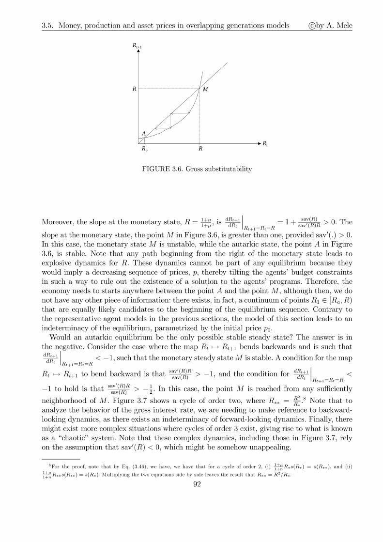
3.5. Money, production and asset prices in overlapping generations models c©by A. Mele
Rt
Rt+1
R
R M
A
Ra
FIGURE 3.6. Gross substitutability
Moreover, the slope at the monetary state, R = 1+n1+µ
, is dRt+1
dRt
∣∣∣Rt+1=Rt=R
= 1+ sav(R)sav′(R)R
> 0. The
slope at the monetary state, the pointM in Figure 3.6, is greater than one, provided sav′(.) > 0.In this case, the monetary state M is unstable, while the autarkic state, the point A in Figure3.6, is stable. Note that any path beginning from the right of the monetary state leads toexplosive dynamics for R. These dynamics cannot be part of any equilibrium because theywould imply a decreasing sequence of prices, p, thereby tilting the agents’ budget constraintsin such a way to rule out the existence of a solution to the agents’ programs. Therefore, theeconomy needs to starts anywhere between the point A and the pointM , although then, we donot have any other piece of information: there exists, in fact, a continuum of points R1 ∈ [Ra, R)that are equally likely candidates to the beginning of the equilibrium sequence. Contrary tothe representative agent models in the previous sections, the model of this section leads to anindeterminacy of the equilibrium, parametrized by the initial price p0.Would an autarkic equilibrium be the only possible stable steady state? The answer is in
the negative. Consider the case where the map Rt → Rt+1 bends backwards and is such thatdRt+1
dRt
∣∣∣Rt+1=Rt=R
< −1, such that the monetary steady stateM is stable. A condition for the map
Rt → Rt+1 to bend backward is that sav′(R)Rsav(R)
> −1, and the condition for dRt+1
dRt
∣∣∣Rt+1=Rt=R
<
−1 to hold is that sav′(R)Rsav(R)
> −12. In this case, the point M is reached from any sufficiently
neighborhood of M . Figure 3.7 shows a cycle of order two, where R∗∗ =R2
R∗.8 Note that to
analyze the behavior of the gross interest rate, we are needing to make reference to backward-looking dynamics, as there exists an indeterminacy of forward-looking dynamics. Finally, theremight exist more complex situations where cycles of order 3 exist, giving rise to what is knownas a “chaotic” system. Note that these complex dynamics, including those in Figure 3.7, relyon the assumption that sav′(R) < 0, which might be somehow unappealing.
8For the proof, note that by Eq. (3.46), we have, we have that for a cycle of order 2, (i) 1+µ1+n
R∗s(R∗) = s(R∗∗), and (ii)1+µ1+n
R∗∗s(R∗∗) = s(R∗). Multiplying the two equations side by side leaves the result that R∗∗ = R2/R∗.
92

3.5. Money, production and asset prices in overlapping generations models c©by A. Mele
Rt
Rt+1
R
R M
R**R*
A
FIGURE 3.7.
3.5.4 Money in a model with real shocks
Lucas (1972) is the first attempt to address issues relating the neutrality of money in contextswith overlapping generations and uncertainty. This section is a simplified version of Lucasmodel as explained by Stokey et Lucas (1989) (p. 504). Every agent works when young, so asto produce a consumption good, and consumes when he is old, and experiences a disutility ofwork equal to −v (nt), where nt is his labor supply, and v is assumed to satisfy v′, v′′ > 0.Utility drawn from second period consumption is denoted with u (ct+1), and has the standardproperties. The agent faces the following program:
maxn,c
[−v(nt) + βE (u(ct+1)|Ft)] subject to
m = ptyt, yt = ǫtntpt+1ct+1 = m
where Ft denotes the information set as of time t, m is money holdings; yt is the agent’s pro-duction, obtained through his labor supply nt, and (ǫt)t=0,1,··· is a sequence of positive shocksaffecting his productivity. Finally, pt is the price of the consumption good as of time t. Byreplacing the first constraint into the second leaves, ct+1 = ǫtntRt+1, where Rt+1 ≡ pt
pt+1. There-
fore, the program the agent solves is to maxn [−v(nt) + βE (u(ǫtntRt+1)|Ft))]. The first-ordercondition leads to,
v′(nt) = βE [u′(ǫtntRt+1)ǫtRt+1|Ft] .
We have, ct+1 = ǫt+1nt+1 = ǫtntRt+1, where the first equality follows by the equilibrium in thegood market. Replacing this relation into the previous equation leaves,
v′(nt)nt = βE [u′(ǫtntRt+1)ǫt+1nt+1|Ft] . (3.49)
A rational expectation equilibrium is one where nt = η (ǫt), with η satisfying Eq. (3.49), i.e.
v′ (η (ǫ) η (ǫ)) = β
∫
Eu′
(ǫ+η(ǫ+)
)ǫ+η(ǫ+)dP (ǫ+
∣∣ ǫ),
where E denotes the support of ǫ+. This equation simplifies as soon as productivity shocks areIID, P (ǫ+| ǫ) = P (ǫ+), in which case, v′ (η (ǫ) η (ǫ)) is independent of ǫ+, and n is a constant
93
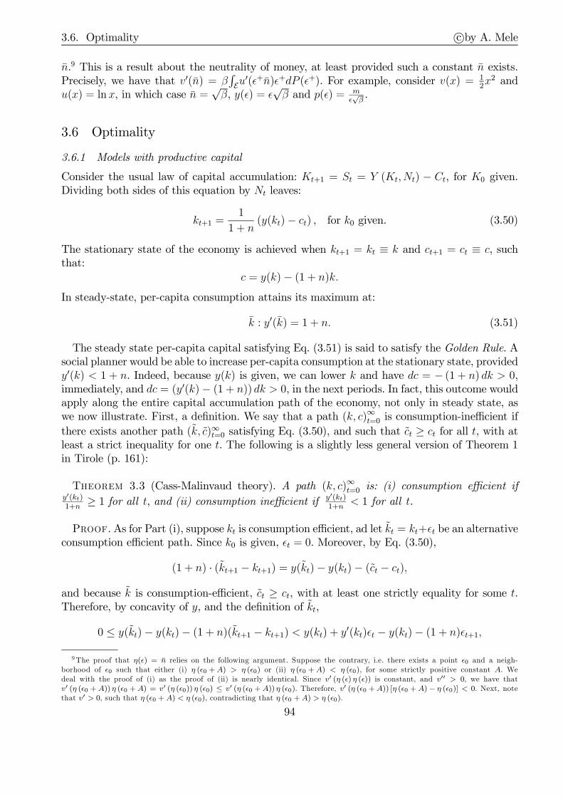
3.6. Optimality c©by A. Mele
n.9 This is a result about the neutrality of money, at least provided such a constant n exists.Precisely, we have that v′(n) = β
∫Eu′(ǫ+n)ǫ+dP (ǫ+). For example, consider v(x) = 1
2x2 and
u(x) = ln x, in which case n =√β, y(ǫ) = ǫ
√β and p(ǫ) = m
ǫ√β.
3.6 Optimality
3.6.1 Models with productive capital
Consider the usual law of capital accumulation: Kt+1 = St = Y (Kt,Nt) − Ct, for K0 given.Dividing both sides of this equation by Nt leaves:
kt+1 =1
1 + n(y(kt)− ct) , for k0 given. (3.50)
The stationary state of the economy is achieved when kt+1 = kt ≡ k and ct+1 = ct ≡ c, suchthat:
c = y(k)− (1 + n)k.In steady-state, per-capita consumption attains its maximum at:
k : y′(k) = 1 + n. (3.51)
The steady state per-capita capital satisfying Eq. (3.51) is said to satisfy the Golden Rule. Asocial planner would be able to increase per-capita consumption at the stationary state, providedy′(k) < 1 + n. Indeed, because y(k) is given, we can lower k and have dc = − (1 + n) dk > 0,immediately, and dc = (y′(k)− (1 + n)) dk > 0, in the next periods. In fact, this outcome wouldapply along the entire capital accumulation path of the economy, not only in steady state, aswe now illustrate. First, a definition. We say that a path (k, c)∞t=0 is consumption-inefficient if
there exists another path (k, c)∞t=0 satisfying Eq. (3.50), and such that ct ≥ ct for all t, with atleast a strict inequality for one t. The following is a slightly less general version of Theorem 1in Tirole (p. 161):
T 3.3 (Cass-Malinvaud theory). A path (k, c)∞t=0 is: (i) consumption efficient ify′(kt)1+n
≥ 1 for all t, and (ii) consumption inefficient if y′(kt)1+n
< 1 for all t.
P. As for Part (i), suppose kt is consumption efficient, ad let kt = kt+ǫt be an alternativeconsumption efficient path. Since k0 is given, ǫt = 0. Moreover, by Eq. (3.50),
(1 + n) · (kt+1 − kt+1) = y(kt)− y(kt)− (ct − ct),
and because k is consumption-efficient, ct ≥ ct, with at least one strictly equality for some t.Therefore, by concavity of y, and the definition of kt,
0 ≤ y(kt)− y(kt)− (1 + n)(kt+1 − kt+1) < y(kt) + y′(kt)ǫt − y(kt)− (1 + n)ǫt+1,
9The proof that η(ǫ) = n relies on the following argument. Suppose the contrary, i.e. there exists a point ǫ0 and a neigh-borhood of ǫ0 such that either (i) η (ǫ0 +A) > η (ǫ0) or (ii) η (ǫ0 +A) < η (ǫ0), for some strictly positive constant A. Wedeal with the proof of (i) as the proof of (ii) is nearly identical. Since v′ (η (ǫ) η (ǫ)) is constant, and v′′ > 0, we have thatv′ (η (ǫ0 +A)) η (ǫ0 +A) = v′ (η (ǫ0)) η (ǫ0) ≤ v′ (η (ǫ0 +A)) η (ǫ0). Therefore, v′ (η (ǫ0 +A)) [η (ǫ0 +A)− η (ǫ0)] < 0. Next, notethat v′ > 0, such that η (ǫ0 +A) < η (ǫ0), contradicting that η (ǫ0 +A) > η (ǫ0).
94

3.6. Optimality c©by A. Mele
or ǫt+1 <y′(kt)1+n
ǫt. Evaluating this inequality at t = 0 yields ǫ1 <y′(k0)1+n
ǫ0, and since ǫ0 = 0, one
has that ǫ1 < 0. Since y′(kt)1+n
≥ 1 for all t, then ǫt → −∞ as t → ∞, which contradicts kt hasbounded trajectories. The proof of Part (ii) is nearly identical, except that, obviously, in thiscase, lim inf ǫt >> −∞. Note, in general, there are infinitely many sequences that allow forefficiency improvements. ‖
The reasoning in this section holds independently of whether the economy has a finite numberof agents living forever, or overlapping generations. For example, in the case of overlappinggenerations, Eq. (3.50) is the capital accumulation path for Diamond’s model, once we set ct ≡CtNt= c1t +
c2,t+1
1+n. An important issue is to establish whether actual economies are dynamically
efficient? Abel, Mankiw, Summers and Zeckhauser (1989) provide a framework to address thisquestion, which includes uncertainty, and conclude that the US economy does satisfy dynamicefficiency requirements.
3.6.2 Models with money
We wish to find first-best optima, that is, equilibria that a social planner may choose, by actingdirectly on agents’ consumption, without needing to force the agents to make use of money.10
Let us analyze, first, the stationary state, R = 1+n1+µ
. We show that this state corresponds tothe stationary state where consumptions and endowments are constants, and that the agents’utility is maximized when µ = 0. Indeed, since the social planner allocates resources withouthaving regard to money, the only constraint is: wn ≡ w1+
w2
1+n= c1+
c21+n
, such that the utilityof the “stationary agent” is:
u (c1, c2) = u
(wn −
c21 + n
, c2
).
The first-order condition is uc2uc1
= 11+n
. Instead, the first-order condition in the market equi-
librium is uc2uc1
= 1R. Therefore, the Golden Rule is attained in the market equilibrium, if and
only if µ = 0. The social planner policy converges towards the Golden Rule. Indeed, the socialplanner solves:
max∞∑
t=0
ϑtu(t) (c1t, c2,t+1) , subject to wnt ≡ w1t +w2t
1 + n= c1t +
c2t1 + n
,
or max∑∞
t=0 ϑtu(t)
(wnt − c2t
1+n, c2,t+1
), where ϑ is the weight the planner gives to the generation
as of time t, and the notation u(t) is meant to emphasize that that endowments may change
from one generation to another. The first-order conditions,u
(t−1)c2
u(t)c1
= ϑ1+n
, lead to the “modified”
Golden Rule in stead-state state (modified by the weight ϑ).
10 In a second-best equilibrium, a social planner would let the market “play” first, by allowing the agents to use money and, then,would parametrize such virtual equilibria by µt. The indirect utility functions that arise as a result would then be expressed interms of these growth rates µt. The social planner would then maximize an an aggregator of these utilities with respect to µt.
95

3.7. Appendix 1: Finite difference equations, with economic applications c©by A. Mele
3.7 Appendix 1: Finite difference equations, with economic applications
Let z0 ∈ Rd, and consider the following linear system of finite difference equations:
zt+1 = A · zt, t = 0, 1, · · · , (3A.1)
for some matrix A. The solution to Eq. (3A.1) is:
zt = v1κ1λt1 + · · ·+ vdκdλ
td, (3A.2)
where λi and vi are eigenvalues and eigenvectors of A, and κi are constants, which will be determinedbelow. The standard proof of this result relies on the so-called diagonalization of Eq. (3A.1). Let usconsider the system of characteristic equations for A, (A− λiI) vi = 0d×1, where λi is scalar and vi ad× 1 column vector, for i = 1, · · · , n, or, in matrix form, AP = PΛ, where P = (v1, · · · , vd) and Λ isa diagonal matrix with λi on its diagonal. We assume that P⊤ = P−1. By post-multiplying by P−1
leaves the spectral decomposition of A:A = PΛP−1. (3A.3)
By replacing Eq. (3A.3) into Eq. (3A.1), and rearranging terms,
yt+1 = Λ · yt, where yt ≡ P−1zt.
The solution for y is yit = κiλti, and the solution for z is: zt = Pyt = (v1, · · · , vd)yt =
∑di=1 viyit =∑d
i=1 viκiλti, which is Eq. (3A.2).
To determine the vector of constants κ = (κ1, · · · , κd)⊤, we first evaluate the solution at t = 0,
z0 = (v1, · · · , vd)κ = Pκ,
whenceκ ≡ κ(P ) = P−1z0, (3A.4)
where the columns of P are vectors belonging to the space of the eigenvectors. Naturally, there isan infinity of these vectors. However, the previous formula shows how the constants κ (P ) need to“adjust” so as to guarantee the stability of the solution with respect to changes in P .
3A.1 E. Let d = 2, and suppose that λ1 ∈ (0, 1), λ2 > 1. The resulting system is unstablefor any initial condition, except perhaps for a set with measure zero. This set of measure zero givesrise to the so-called saddlepoint path. We can calculate the coordinates of such a set. We wish to findthe set of initial conditions such that κ2 = 0, so as to rule out an explosive behavior related to theunstable root λ2 > 1. The solution at t = 0 is:
(x0y0
)= z0 = Pκ = (v1, v2)
(κ1κ2
)=
(v11κ1 + v12κ2
v21κ1 + v22κ2
),
where we have set z = (x, y)⊤. By replacing the second equation into the first, and solving for κ2,yields:
κ2 =v11y0 − v21x0v11v22 − v12v21
,
which is zero wheny0 =
v21v11
x0.
For this system, the saddlepoint is a line with a slope equal to the ratio of the two components ofeigenvector for λ1–the stable root. Figure 3A.1 depicts the phase diagram for this system, with the“divergent” line satisfying the equation y0 =
v22v12
x0.
96
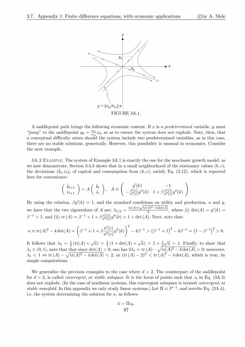
3.7. Appendix 1: Finite difference equations, with economic applications c©by A. Mele
x
y
x0
y0
y = (v21/v11) x
FIGURE 3A.1.
A saddlepoint path brings the following economic content. If x is a predetermined variable, y must“jump” to the saddlepoint y0 = v21
v11x0, so as to ensure the system does not explode. Note, then, that
a conceptual difficulty arises should the system include two predetermined variables, as in this case,there are no stable solutions, generically. However, this possibility is unusual in economics. Considerthe next example.
3A.2 E. The system of Example 3A.1 is exactly the one for the neoclassic growth model, aswe now demonstrate. Section 3.3.3 shows that in a small neighborhood of the stationary values (k, c),the deviations (kt, ct)t of capital and consumption from (k, c), satisfy Eq. (3.12), which is reportedhere for convenience:
(kt+1
ct+1
)= A
(ktct
), A ≡
(y′(k) −1
− u′(c)u′′(c)y
′′(k) 1 + β u′(c)u′′(c)y
′′(k)
).
By using the relation, βy′(k) = 1, and the standard conditions on utility and production, u and y,
we have that the two eigenvalues of A are: λ1/2 =tr(A)∓
√tr(A)2−4 det(A)
2 , where (i) det(A) = y′(k) =
β−1 > 1, and (ii) tr (A) = β−1 + 1+ β u′(c)u′′(c)y
′′(k) > 1 + det (A). Next, note that:
a ≡ tr(A)2 − 4det(A) =
(β−1 + 1 + β
u′(c)u′′(c)
y′′(k)
)2
− 4β−1 >(β−1 + 1
)2 − 4β−1 =(1− β−1
)2> 0.
It follows that λ2 = 12 (tr(A) +
√a) > 1
2 (1 + det(A) +√a) > 1 + 1
2
√a > 1. Finally, to show that
λ1 ∈ (0, 1), note that that since det(A) > 0, one has 2λ1 = tr (A)−√tr(A)2 − 4det(A) > 0; moreover,
λ1 < 1 ⇔ tr (A) −√tr(A)2 − 4 det(A) < 2, or (tr (A) − 2)2 < tr (A)2 − 4 det(A), which is true, by
simple computations.
We generalize the previous examples to the case where d > 2. The counterpart of the saddlepointfor d = 2, is called convergent, or stable subspace. It is the locus of points such that zt in Eq. (3A.3)does not explode. (In the case of nonlinear systems, this convergent subspace is termed convergent, orstable manifold. In this appendix we only study linear systems.) Let Π ≡ P−1, and rewrite Eq. (3A.4),i.e. the system determining the solution for κ, as follows:
κ = Πz0.
97

3.7. Appendix 1: Finite difference equations, with economic applications c©by A. Mele
We assume the elements of z and A are ordered in such a way that ∃s : |λi| < 1, for i = 1, · · · , s and|λi| > 1 for i = s+ 1, · · · , d. Then, we partition Π as follows:
κ =
Πss×dΠu
(d−s)×d
z0.
Proceeding similarly as in Example 3A.1, we aim to make sure the system stays “trapped” in theconvergent space and, accordingly, require that: κs+1 = · · · = κd = 0, or,
κs+1...κd
= Πu
(d−s)×dz0 = 0(d−s)×1.
Let d ≡ k+k∗, where k is the number of free variables and k∗ is the number of predetermined variables.Partition Πu and z0 in such a way to disentangle free from predetermined variables, as follows:
0(d−s)×1 = Πu(d−s)×d
z0 =
(Π
(1)u
(d−s)×kΠ
(2)u
(d−s)×k∗
)
zfree0k×1
zpre0k∗×1
= Π(1)
u(d−s)×k
zfree0k×1
+ Π(2)u
(d−s)×k∗zpre0k∗×1
,
or,
Π(1)u
(d−s)×kzfree0k×1
= − Π(2)u
(d−s)×k∗zpre0k∗×1
.
This system has d− s equations with k unknowns, the components of zfree0 : indeed, zpre0 is known, as
it the k∗-dimensional vector of predetermined variables, and Π(1)u ,Π
(2)u depend on the primitive data
of the economy, through their relation with A. We assume that Π(1)u
(d−s)×khas full rank.
We shall refer to s as the dimension of the convergent subspace, S say. The reason for this termi-nology is the following. Consider the solution for zt,
zt = v1κ1λt1 + · · ·+ vsκsλ
ts + vs+1κs+1λ
ts+1 + · · ·+ vdκdλ
td.
For zt to remain stuck in S, it must be the case that
κs+1 = · · · = κd = 0,
in which case,
ztd×1
= v1d×1
κ1λt1 + · · ·+ vs
d×1κsλ
ts = (v1κ1, · · · , vsκs) ·
(λt1, · · · , λts
)⊤,
i.e.,
ztd×1
= Vd×s
· λts×1
,
where V ≡ (v1κ1, · · · , vsκs) and λt ≡(λt1, · · · , λts
)⊤. Finally, for each t, introduce the vector subspace:
〈V 〉t ≡ zt ∈ Rd : ztd×1
= Vd×s
· λts×1
, λt ∈ Rs.
Clearly, for each t, dim〈V 〉t = rank(V ) = s.There are three cases to consider:
98

3.7. Appendix 1: Finite difference equations, with economic applications c©by A. Mele
(i) d − s = k, or s = k∗. The dimension of the divergent subspace is equal to the number of thefree variables or, equivalently, the dimension of the convergent subspace is equal to the numberof predetermined variables. In this case, the system is determined. The previous conditionsare interpreted as follows. The predetermined variables identify one and only one point in theconvergent space, which gives rise to only one possible jump that the free variables can make to
ensure the system remain in the convergent space: zfree0 = −Π(1)−1u Π
(2)u zpre0 . This case is exactly
as in Example 3A.1, where d = 2, k = 1, and the predetermined variable is x. In this example,x0 identifies one and only one point in the saddlepoint path, such that starting from that point,there is one and only one value of y0 guaranteeing that the system does not explode.
(ii) d − s > k, or s < k∗. There are generically no solutions lying in the convergent space–a casementioned just before Example 3A.2.
(iii) d − s < k, or s > k∗. There are infinitely many solutions lying in the convergent space, aphenomenon typically referred to as indeterminacy. Note that in this case, sunspots equilibriamay arise. In Example 3A.1, s = 1, and so in order for this case to emerge when d = 2, we mightneed to rule out the existence of predetermined variables.
99

3.8. Appendix 2: Neoclassic growth in continuous-time c©by A. Mele
3.8 Appendix 2: Neoclassic growth in continuous-time
3.8.1 Convergence from discrete-time
[To be revised]Consider chopping time in the law of population growth as follows:
Nhk −Nh(k−1) = nNh(k−1)h, k = 1, · · · , ℓ,
where n is an instantaneous rate, and ℓ = th is the number of subperiods in which we have chopped
a given time period t. The solution is Nhℓ = (1 + nh)ℓN0, or Nt = (1 + nh) t/hN0. By taking limitsleaves:
N(t) = limh↓0
(1 + nh) t/hN(0) = entN(0).
On the other hand, an exact discretization yields: N(t − ∆) = en(t−∆)N(0), or N(t)N(t−∆) = en∆ ≡
1 + n∆ ⇔ n = 1∆ ln (1 + n∆). Take, for example, ∆ = 1, n∆ = n1 ≡ n : n = ln (1 + n).
We apply the same discretization scheme to the law of capital accumulation:
Kh(k+1) =(1− δh
)Khk + Ih(k+1)h, k = 0, · · · , ℓ− 1,
where δ is an instantaneous rate, and ℓ = th . By iterating,
Kt =(1− δh
) t/hK0 +
t/h∑
j=1
(1− δh
) t/h−jIhjh.
Taking the limits for h ↓ 0 yields:
K(t) = e−δtK0 + e−δt∫ t
0eδuI(u)du,
or in differential form:K(t) = −δK(t) + I(t). (3A.5)
By replacing the IS equation,
Y (t) = F (K (t) , N (t)) = C(t) + I(t), (3A.6)
into Eq. (3A.5), we obtain the law of capital accumulation:
K (t) = F (K (t) , N (t))−C (t)− δK (t) .
There are a few discretization issues to discuss. First, an exact discretization gives:
K(t+ 1) = e−δK(t) + e−δ(t+1)
∫ t+1
teδuI(u)du. (3A.7)
By identifying with the standard capital accumulation law in the discrete time setting:
Kt+1 = (1− δ)Kt + It,
we get: δ = ln 1(1−δ) . It follows that δ ∈ (0, 1)⇒ δ > 0 and δ = 0⇒ δ = 0. Hence, while δ can take on
only values on [0, 1), δ can take on values on the entire real line. In the continuous time model, then,limδ→1− ln 1
(1−δ) =∞. In continuous time, we cannot imagine a “maximal rate of capital depreciation,”as this would be infinite!
100

3.8. Appendix 2: Neoclassic growth in continuous-time c©by A. Mele
Let us replace δ into the exact discretization in Eq. (3A.7):
K(t+ 1) = (1− δ)K(t) + e−δ(t+1)
∫ t+1
teδuI(u)du,
such that investments at t+ 1 are simply, e−δ(t+1)∫ t+1t eδuI(u)du.
Finally, we derive per-capita dynamics. Consider dividing both sides of the capital accumulationequation (3A.6) by N(t):
K(t)
N(t)=
F (K(t), N(t))
N(t)− c(t)− δk(t) = y(k(t))− c(t)− δk(t).
By using the relation k = d (K(t)/N(t)) = K(t)/N(t)− nk(t) into the previous equation leads to:
k = y(k(t))− c(t)−(δ + n
)· k(t).
It is the capital accumulation contraint used to solve the program of the next section.
3.8.2 The model
Consider the following social planner problem:
maxc
∫ ∞
0e−ρtu(c(t))dt
s.t. k(t) = y(k(t))− c(t)−(δ + n
)· k(t)
[3A.P1]
where all variables are per-capita. We assume there is no capital depreciation. (Note that the discretetime model, we assumed, instead, a total capital depreciation.) The Hamiltonian is,
H(t) = u(c(t)) + λ(t)[y(k(t))− c(t)−
(δ + n
)· k(t)
],
where λ is a co-state variable. As explained in Appendix 4 of this chapter, the first-order conditionsfor this problem are:
0 =∂H
∂c(t) ⇔ λ(t) = u′ (c(t))
∂H
∂λ(t) = k(t)
∂H
∂k(t) = −λ(t) + ρλ(t) ⇔ λ(t) =
[ρ+ δ + n− y′ (k(t))
]λ(t)
(3A.8)
By differentiating the first of equations (3A.8) with respect to time:
λ(t) =
(u′′(c(t))u′(c(t))
c(t)
)λ(t).
By identifying through the third of equations (3A.8),
c(t) =u′ (c(t))u′′ (c(t))
(ρ+ δ + n− y′ (k(t))
). (3A.9)
The equilibrium is the solution of the system consisting of the constraint of the program [3A.P1],and Eq. (3A.9). Similarly as in Section 3.3.3, we analyze the dynamics of the system in a small
101

3.8. Appendix 2: Neoclassic growth in continuous-time c©by A. Mele
neighborhood of the stationary state, defined as the solution (c, k) of the constraint of the program[3A.P1], and Eq. (3A.9), when c(t) = k(t) = 0,
c = y(k)−
(δ + n
)k
ρ+ δ + n = y′(k)
Warning! these are instantaneous figures, so its okay if they are not such that y′(k) ≥ 1+n!.A first-order approximation of both sides of the constraint of the program [3A.P1], and Eq. (3A.9),near (c, k), yields:
c(t) = − u′(c)u′′(c)
y′′(k) (k(t)− k)
k(t) = ρ · (k(t)− k)− (c(t)− c)
where we used the equality ρ+ δ+ n = y′(k). By setting x(t) ≡ c(t)−c and y(t) ≡ k(t)−k the previoussystem can be rewritten as:
z(t) = A · z(t), A ≡
0 − u′(c)
u′′(c)y′′(k)
−1 ρ
,
where z ≡ (x, y)⊤.Warning! There must be some mistakes somewhere. Let us diagonalize this system by setting
A = PΛP−1, where P and Λ are as in Appendix 1. We have:
ν(t) = Λ · ν(t),where ν ≡ P−1z. The eigenvalues are solutions of the following quadratic equation:
0 = λ2 − ρλ− u′(c)u′′(c)
y′′(k).
We see that λ1 < 0 < λ2, and λ1 ≡ ρ2 − 1
2
√ρ2 + 4 u′(c)
u′′(c)y′′(k). The solution for ν(t) is:
νi(t) = κieλit, i = 1, 2,
whencez(t) = P · ν(t) = v1κ1e
λ1t + v2κ2eλ2t,
where the vis are 2× 1 vectors. We have,
x(t) = v11κ1eλ1t + v12κ2e
λ2t
y(t) = v21κ1eλ1t + v22κ2e
λ2t
Let us evaluate this solution in t = 0,(
x(0)y(0)
)= Pκ =
(v1 v2
)( κ1κ2
).
By repeating the reasoning of the previous appendix,
κ2 = 0⇔ y(0)
x(0)=
v21v11
.
As in the discrete time model, the saddlepoint path is located along a line that has as a slopethe ratio of the components of the eigenvector associated with the negative root. We can explicitelycompute such ratio. By definition, A · v1 = λ1v1 ⇔
− u′(c)u′′(c)
y′′(k) = λ1v11
−v11 + ρv21 = λ1v21
i.e., v21v11
= − λ1u′(c)
u′′(c)y′′(k)
and simultaneously, v21v11
= 1ρ−λ1
.
102

3.9. Appendix 3: Control c©by A. Mele
3.9 Appendix 3: Control
103
3.9. Appendix 3: Control c©by A. Mele
References
Abel, A.B., N.G. Mankiw, L.H. Summers and R.J. Zeckhauser (1989): “Assessing DynamicEfficiency: Theory and Evidence.” Review of Economic Studies 56, 1-20.
Farmer, R. (1998): The Macroeconomics of Self-Fulfilling Prophecies. Boston: MIT Press.
Hayashi, F. (1982): “Tobin’s Marginal q and Average q: A Neoclassical Interpretation.” Econo-metrica 50, 213-224.
Kamihigashi, T. (1996): “Real Business Cycles and Sunspot Fluctuations are ObservationallyEquivalent.” Journal of Monetary Economics 37, 105-117.
King, R. G. and S. T. Rebelo (1999): “Resuscitating Real Business Cycles.” In: J. B. Taylorand M. Woodford (Editors): Handbook of Macroeconomics, Elsevier.
Lucas, R. E. (1972): “Expectations and the Neutrality of Money.” Journal of Economic Theory4, 103-124.
Lucas, R. E. (1978): “Asset Prices in an Exchange Economy.” Econometrica 46, 1429-1445.
Lucas, R. E. (1994): “Money and Macroeconomics.” In: General Equilibrium 40th AnniversaryConference, CORE DP no. 9482, 184-187.
Prescott, E. (1991): “Real Business Cycle Theory: What Have We Learned?” Revista de Anal-isis Economico 6, 3-19.
Stokey, N. L. and R. E. Lucas, (with E.C. Prescott) (1989): Recursive Methods in EconomicDynamics. Harvard University Press.
Tirole, J. (1988): “Efficacité intertemporelle, transferts intergénérationnels et formation duprix des actifs: une introduction.” Melanges économiques. Essais en l’honneur de EdmondMalinvaud. Paris: Editions Economica & Editions EHESS, 157-185.
Tobin, J. (1969): “A General Equilibrium Approach to Monetary Policy.” Journal of Money,Credit and Banking 1, 15-29.
Watson, M. (1993): “Measures of Fit for Calibrated Models.” Journal of Political Economy101, 1011-1041.
104

4Continuous time models
4.1 Lambdas and betas in continuous time
4.1.1 The pricing equation
Let St be the price of a long lived asset as of time t, and let Dt the dividend paid by the assetat time t. In the previous chapters, we learned that in the absence of arbitrage opportunities,
St = Et [mt+1 (St+1 +Dt+1)] , (4.1)
where Et is the conditional expectation given the information set at time t, and mt+1 is theusual stochastic discount factor.Next, let us introduce the pricing kernel, or state-price process,
ξt+1 = mt+1ξt, ξ0 = 1.
In terms of the pricing kernel ξ, Eq. (4.1) is,
0 = Et
(ξt+1St+1 − Stξt
)+ Et
(ξt+1Dt+1
).
For small trading periods h, this is,
0 = Et
(ξt+hSt+h − Stξt
)+ Et
(ξt+hDt+hh
).
As h ↓ 0,0 = Et [d (ξ (t)S (t))] + ξ (t)D (t) dt. (4.2)
Eq. (4.2) can now be integrated to yield,
ξ (t)S (t) = Et
[∫ T
t
ξ (u)D (u) du
]+ Et [ξ (T )S (T )] .
Finally, let us assume that limT→∞Et [ξ (T )S (T )] = 0. Then, provided it exists, the price Stof an infinitely lived asset price satisfies,
ξ (t)S (t) = Et
[∫ ∞
t
ξ (u)D (u) du
]. (4.3)

4.1. Lambdas and betas in continuous time c©by A. Mele
4.1.2 Expected returns
Let us elaborate on Eq. (4.2). We have,
d (ξS) = Sdξ + ξdS + dξdS = ξS
(dξ
ξ+dS
S+dξ
ξ
dS
S
).
By replacing this expansion into Eq. (4.2) we obtain,
Et
(dS
S
)+D
Sdt = −Et
(dξ
ξ
)− Et
(dξ
ξ
dS
S
). (4.4)
This evaluation equation holds for any asset and, hence, for the assets that do not distribute
dividends and are locally riskless, i.e. D = 0 and Et
(dξξdS0
S0
)= 0, where S0 (t) is the price of
these locally riskless assets, supposed to satisfy dS0(t)S0(t)
= r (t) dt, for some short term rate process
rt. By Eq. (4.4), then,
Et
(dξ
ξ
)= −r (t) dt.
By replacing this into eq. (4.4) leaves the following representation for the expected returnsEt
(dSS
)+ D
Sdt,
Et
(dS
S
)+D
Sdt = rdt− Et
(dξ
ξ
dS
S
). (4.5)
In a diffusion setting, Eq. (4.5) gives rise to a partial differential equation. Moreover, in adiffusion setting,
dξ
ξ= −rdt− λ · dW,
where W is a vector Brownian motion, and λ is the vector of unit risk-premia. Naturally, theprice of the asset, S, is driven by the same Brownian motions driving r and ξ. We have,
Et
(dξ
ξ
dS
S
)= −Vol
(dS
S
)· λdt,
which leaves,
Et
(dS
S
)+D
Sdt = rdt+ Vol
(dS
S
)
︸ ︷︷ ︸“betas”
· λ︸︷︷︸“lambdas”
dt.
4.1.3 Expected returns and risk-adjusted discount rates
The difference between expected returns and risk-adjusted discount rates is subtle. If dividendsand asset prices are driven by only one factor, expected returns and risk-adjusted discount ratesare the same. Otherwise, we have to make a distinction. To illustrate the issue, let us make asimplification, and assume that the price-dividend ratio, p, is independent of the dividends D,and driven by a vector of state variables, y, such that:
S (y,D) = p (y)D. (4.6)
106

4.1. Lambdas and betas in continuous time c©by A. Mele
This “scale-invariant” property arises in many economies, as we shall discuss in detail in thesecond part of these lectures. For example, it arises if the state variables, y, do not depend onD, and if the dividends satisfy:
dD
D= g0dt+ σDdW,
for two constants g0 and σD. By Eq. (4.6), dSS= dp
p+ dD
D, which replaced into Eq. (4.5) leaves,
Et
(dS
S
)+D
Sdt = Disc dt− Et
(dp
p
dξ
ξ
), (4.7)
where:
Disc = r −Et
(dDD
dξξ
)
dt.
We define Disc as the “risk adjusted discount rate.” It equals the safe interest rate r, plus the
premium, −Et
(dDD
dξξ
), arising to compensate agents for the uncertain fluctuations of future
dividends, and equal to:
Et
(dD
D
dξ
ξ
)= − Vol
(dD
D
)
︸ ︷︷ ︸“cash-flow beta”
· λCF︸︷︷︸“cash-flow lambda”
dt.
If the price-dividend ratio, p, is constant, then, by Eq. (4.7), the “risk adjusted discount rate”Disc, is the same as the expected returns, just as in the simple one-factor Lucas economy of theprevious chapter, as shown in Section 4.3. In the second part of these lecttures, however, weshall learn that consumption, which in equilibrium equals aggregate dividends in this model,is too smooth to make the expected returns predicted by this model in line with the data. Eq.(4.7) reveals that expected returns might actually be boosted, in the presence of additionalstate variables affecting the price-dividend ratio, provided the risk inherent in these variablesis compensated,
Et
(dp
p
dξ
ξ
)= −Vol
(dp
p
)
︸ ︷︷ ︸“price-betas”
· λp︸︷︷︸“price lambdas”
dt.
This term introduces a wedge between expected returns and the risk-adjusted discount ratesof Eq. (4.7), thereby potentially mitigating the empirical issues relating to excessively smoothconsumption. Time variation in risk-adjusted discount rates also plays a critical role in theexplanation of return volatility, as we shall see in Chapter 7. This role arises because return
volatility is simply the beta related to the fluctuations of the price-dividend ratio, Vol(dpp
). But
risk-adjusted discount rates affect prices through rational evaluation and, hence, price-dividendratios and, ultimately, the volatility of price-dividend ratios. To illustrate, note that Eq. (4.3)can be rewritten as,
p (y (t)) = E
[∫ ∞
t
D∗ (τ)
D (t)· e−
∫ τt Disc(y(u))du
∣∣∣∣ y (t)],
D∗ (τ)
D (t)= e(g0−1
2σ2D)t+σW (τ), (4.8)
where W (τ) is a Brownian motion under the risk-neutral probability. Eq. (4.8) is a presentvalue formula where a fictitious risk-unadjusted dividend growth, D∗ (τ) /D (t), is discounted
107
4.2. An introduction to continuous time methods in finance c©by A. Mele
using the risk-adjusted discount rates, (Disc (yt))t≥0. According to Eq. (4.8), changes in pricesreflect the investors’ risk-adjusted expectation about the future state of the economy, and thepace at which these changes take place–volatility–depends crucially on how the risk-adjusteddiscount rates are expected to change in reaction to changes in the state variables y. In fact, ifrisk-adjusted rates exhibit large swings, the return volatility predicted by Eq. (4.8) is likely toexhibit some of the interesting countercyclical statistics that we see in the data, as we shall seein Chapter 7.
4.2 An introduction to continuous time methods in finance
4.2.1 Partial differential equations and Feynman-Kac probabilistic representations of thesolution
4.2.1.1 Background: Black & Scholes
Why are partial differential equations so important in finance? Suppose that the price of a stockfollows a geometric Brownian motion:
dS (t)
S (t)= µdt+ σdW (t) , µ, σ > 0,
and that there exists a riskless accounting technology making spare money evolve as:
dB (t)
B (t)= rdt,
where r > 0. Finally, suppose that there exists another asset, a “call option,” which gives rise toa payoff equal to (S (T )−K)+ at some future date T , where K is the “strike,” or exercise priceof the option. Let c (t) , t ∈ [0, T ], be the price process of the option. We wish to figure out whatthis price looks like by formulating as few assumptions as possible. We ignore dividend issues,and assume there are no transaction costs, and rule out any other forms of frinctions. We assumerational expectations, that is, there exists a function f ∈ C1,2 ([0, T ]×R++) : c (t) = f(t, S (t)).By the previous assumption and Itô’s lemma,
dc =
(Lf +
∂f
∂t
)dt+ fSσSdW,
where Lf = 12σ2S2fSS + µSfS and subscripts denote partial derivatives. Nextwe , create the
following portfolio: α quantities of the risky asset and β quantities of the riskless accountingtechnology. Section 4.3 explains that for any portfolio strategy to be “self-financed” and for thevalue V of the resulting portfolio, V (t) = α (t)S (t) + β (t)B (t), to be well-defined, it must bethat:
dV (t) = α (t) dS (t) + β (t) dB (t)
= (α (t)µS (t) + rβ (t)B (t)) dt+ α (t)σS (t) dW (t) .
Next, set V0 = c0 and find α, β such that drift and diffusion terms of V and c be the same.This is done with α = fS. Replace then this into the previous stochastic differential equation.we have:
dV (t) = (µSfS + rβB) dt+ fSσSdW.
108

4.2. An introduction to continuous time methods in finance c©by A. Mele
Now find β : drift(V ) = drift (c), which after simple calculations is:
β =Lf + ∂f
∂t− µfSS
rB.
Since V0 = c0 and the previous α, β make drifts and diffusion terms of V and c the same, then,by the Unique Decomposition Property for stochastic differential equations stated in Appendix1, we have that V (t) = c (t), or:
f = c = V ≡ αS + βB = fSS +Lf + ∂f
∂t− µfSSr
.
By the definition of L and rearranging,
∂f
∂t+1
2σ2S2fSS + rSfS − rf = 0 ∀(t, S) ∈ [0, T )×R++, (4.9)
with the “boundary condition” f(T, S) = (S −K)+, ∀S ∈ R++. This is an example of a PartialDifferential Equation. The “unknown” is a function f , which has to be such that it and itspartial derivatives are plugged into the left hand side of the first line, we obtain zero. Moreover,the same functions must pick up the boundary condition. The solution to this is the celebratedBlack and Scholes (1973) formula.
4.2.1.2 Absence of arbitrage opportunities
Suppose that c0 > f0 = α0S0+ β0B0. Then sell the option for c0, invest α0S0+ β0B0, followthe (α (t) , β (t))-trading strategy until time T and at time T , obtain (S (T )−K)+ from theportfolio - which is exactly what is due to the buyer of the option. This generates a risklessprofit = c0−f0 without further expenses in the future - Recall, the α, β strategy is self-financingand there are no transaction costs). This is an arbitrage opportunity.Suppose then the opposite, i.e. that c0 < f0 = α0S0+ β0B0. Then buy the option for c0 and
hence claim for (S (T )−K)+ at T . At the same time, “short-sell” the portfolio for f0 = α0S0+
β0B0, and subsequently update the short-selling through the strategy α, β. The short-sellingposition is (−α (t))S (t) + (−β (t))B (t) for all t. At time T , the same short-selling position is(−α (T ))S (T )+(−β (T ))B (T ) = −(α (T )S (T )+ β (T )B (T )) = −(S (T )−K)+. This amountof money is exactly the payoff of the option purchased at time zero. Thus use the option payoffto close the short selling position. The whole strategy generate a riskless profit = f0−c0 withoutfurther expenses in the future. This is an arbitrage opportunity.Therefore, absence of arbitrage opportunities are ruled out with c0 = f0. Note, the previous
argument does not hinge upon the existence of a market for the option during the life of theoption.
4.2.1.3 Some technical definitions
The Black-Scholes equation (4.9) is a typical (in fact the first) example of partial differentialequations in finance. It leads to an equation of the so-called parabolic type, as we shall explainsoon. More generally, let us be given,
a0 + a1Ft + a2FS + a3FSS + a4Ftt + a5FSt = 0,
subject to some boundary condition. This partial differential equation is called: (i) elliptic,if a25 − 4a3a4 < 0; (ii) parabolic, if a25 − 4a3a4 = 0; (iii) hyperbolic, if a25 − 4a3a4 > 0. The
109
4.2. An introduction to continuous time methods in finance c©by A. Mele
typical partial differential equations arising in finance are of the parabolic type. For example,the Black-Scholes function F = ertf is parabolic. The following section explains how to providea probabilitsic representation to these parabolic partial differential equations.
4.2.1.4 Partial differential equations and Feynman-Kac probabilistic representations
The typical situation encountered in finance is when a function F , typically the price of someasset, is solution to a parabolic partial differential equation:
−r (x, t)F (x, t) + Ft (x, t) + µ (x, t)Fx (x, t) +1
2σ2 (x, t)Fxx (x, t) = 0, ∀(t, x) ∈ [0, T )× R
(4.10)with the boundary condition, F (x, T ) = g (x, T ), ∀x ∈ R, where the function g is interpretedas the final payoff.Somehow surprisingly, define a SDE that has drift and diffusion µ and σ in Eq. (10.17),
dZ (t) = µ (Z (t) , t) dt+ σ (Z (t) , t) dW (t) , Z0 = x. (4.11)
where W (t) is a Brownian motion. Under regularity condition on µ, σ, r, the solution F to Eq.(10.17) is:
F (x, t) = E
[e−
∫ T
0r(Z(s),s)dsg (Z (T ) , T )
], (4.12)
where Z is solution to Eq. (4.11), and the expectation is taken with respect to the distribu-tion of Z in Eq. (4.11). As a technical remark, note that the existence of the Feynman-Kacrepresentation does not ensure per se the existence of a solution to a given partial differentialequation.The Feynman-Kac representation of the solution to partial differential equations is quite
useful. First, computing expectations is generally both easier and more intuitive than findinga solution to partial differential equations through guess and trial. Second, except for specificcases, the solution to asset prices is unknown, and a natural way to cope with this problem isto go for Monte-Carlo methods (i.e. approximating the expectation in Eq. (4.12) through sim-ulations and using the law of large numbers. Finally, the Feynman-Kac representation theoremis useful for some theoretical reasons we shall see later in this chapter.
4.2.1.5 A few heuristic proofs
It is beyond the purpose of this book to develop detailed proof of the Feynman-Kac repre-sentation theorem. In addition to Karatzas and Shreve (1991, p.366), an excellent source to isstill Friedman (1975), which relaxes many sufficient conditions given in Karatzas and Shrevethrough opportune localizations of linear and growth conditions. The heuristic proof providedbelow covers the slightly more general case in which
Lf +∂f
∂t+ q − rf = 0, (4.13)
with some boundary condition. Here q is some function q (x, t) ≡ qt. The typical role of q is theone of instantaneous dividend rate promised by the asset. As usual, Lf = µfx +
12σ2fxx.
So suppose there exists a solution to Eq. (12.31). To see what a Feynman-Kac representationof such a solution looks like in this case, define
y (t) ≡ e−∫ t
0r(u)duf (t) +
∫ t
0
e−∫ u
0r(s)dsq (u) du,
110
4.2. An introduction to continuous time methods in finance c©by A. Mele
where again, f (t) = f (t, z (t)), and:
dz (t) = µ (t) dt+ σ (t) dW (t) , z0 = x.
By Itô’s lemma,
dy = e−∫ t0 r(u)duqdt− re−
∫ t0 r(u)dufdt+ e−
∫ t0 r(u)dudf
= e−∫ t0r(u)duqdt− re−
∫ t0r(u)dufdt+ e−
∫ t0r(u)du
[(Lf +
∂f
∂t)dt+ fzσdW
]
= e−∫ t0 r(u)du[(Lf +
∂f
∂t+ q − rf)
︸ ︷︷ ︸= 0
dt+ fzσdW ]
= e−∫ t0r(u)dufzσdW.
Therefore y (T ) = y0 + e−∫ t
0r(u)dufzσdW . Assuming σfz ∈ H2, then, y is martingale, viz y0 =
E(y (T )). We have,
y (T ) = e−∫ T
0r(t)dtf (T ) +
∫ T
0
e−∫ u
0r(s)dsq (u) du, and y0 = f0.
Hence,
f0 = y0 = E(y (T )) = E
[e−
∫ T
0r(t)dtf (T )
]+ E
[∫ T
0
e−∫ u
0r(s)dsq (u) du
].
4.2.2 The Girsanov theorem with applications to finance
4.2.2.1 Motivation
Consider again the Black-Scholes partial differential equation:
∂f
∂t+ Lf − rf = 0, ∀(t, S) ∈ [0, T ]× R++,
with boundary condition, f(T, S) = (S −K)+ for all S ∈ R++, where Lf =12σ2S2fSS + rSfS,
and subscripts denote partial derivatives. By the Feynman-Kac theorem,
f (t) = f(t, S (t)) = e−r(T−t)EQ (S (T )−K)+ ,
where the expectationEQ is taken with respect to the probabilityQ, say, on the σ-field generatedby S (t), and S (t) is solution to
dS (t)
S (t)= rdt+ σdW (t) ,
where W is a Brownian motion defined underQ. For obvious reasons, such a probability measureis usually referred to as risk-neutral measure, as we shall explain in detail further in this chapter.As it turns out, the probability Q is related to the physical probability B on the σ-field
generated by S (t), where S (t) is solution to:
dS (t)
S (t)= µdt+ σdW (t) ,
111

4.2. An introduction to continuous time methods in finance c©by A. Mele
and W is now a Brownian motion defined under B. To see heuristically that this is true, let usconsider the following equalities:
EQ (S (T )−K)+ =∫[S (T ) (ω)−K]+Q (dω)
=
∫ζ (T ) (ω) [S (T ) (ω)−K]+B(dω)
≡ EP
[ζ (T ) (ω) (S (T )−K)+
],
where ζ (T ) ≡ Q(dω)P (dω)
, and ζ (t) is solution to:
dζ (t)
ζ (t)= −λdW (t) , ζ0 = 1,
and λ is necessarily equal to, λ = µ−rσ. To show this, let y (t) ≡ ζ (t) f (t). We have, f0 =
e−rTE[ζ (T ) (S (T )−K)+
]. Therefore, and because y (T ) = (S (T )−K)+, we have that:
y0 = f0 = e−rTEP (y (T )) .
That is, e−rty (t) is a P -martingale. Now we have, by Itô’s lemma:
d(e−rty
)= −re−rtydt+ e−rtdy
=
(e−rtζ
∂f
∂t+1
2σ2S2fSS + µSfS − λσSfS − rf
)dt+ e−rtζ (σSfS − λf) dW.
Under the usual pathwise integrability conditions, this is a martingale when,
0 =∂f
∂t+1
2σ2S2fSS + µSfS − λσSfS − rf. (4.14)
On the other hand, we know that f is solution of the Black-Scholes partial differential equation:
0 =∂f
∂t+1
2σ2S2fSS + rSfS − rf. (4.15)
Comparing Eq. (4.14) with Eq. (4.15) reveals that the representation EP
[ζ (T ) (S (T )−K)+
]
is possible with, λ = µ−rσ, as originally claimed. λ has the simple interpretation of unit risk-
premium for investing in stocks.The point of the previous computations is that it looks like as if we could start from the
original probability space under which
dS
S= µdt+ σdW, (4.16)
and, then, we could define a new Brownian motion dW = dW + λdt, such that Eq. (4.16) canbe written as, dS
S= (µ− λσ) dt+ σdW = rdt+ σdW , under some new probability space. And
vice-versa. We formalize this idea in the next subsection, although the following clarificationis in order. The definition of Brownian motion you were originally given obviously depends onthe underlying probability measure P . As an example, for the definition of the independent,stationary increments of a Brownian motion and for its Gaussian distribution, we must knowthe probability measure on the σ-field F . Usually, we do not pay attention to this fact, althoughthis very same fact can be crucial as the previous example demonstrates.
112

4.3. An introduction to no-arbitrage and equilibrium c©by A. Mele
4.2.2.2 The theorem
Let W (t) be a P -Brownian motion, and λ be some measurable process satisfying the so-called
Novikov’s condition: E[exp(12
∫ T
0‖λ (t)‖2 dt)] < 0. Then there exists another probability measure
Q equivalent to P with the following properties:
(i) Radon-Nikodym derivative, dQdP= ζ (T ) = exp
(−1
2
∫ T
0‖λ (t)‖2 dt−
∫ T
0λ (t) dW (t)
).1
(ii) W (t) =W (t) +∫ T
0λ (t) dt is a Q-Brownian motion.
To grasp intuition, consider the following example. Suppose that some random variable x isstandard normal: P (dx) = 1√
2πexp
(−1
2x2
)dx, and that, next, we tilt that distribution by a
factor ζ (x) = exp(−1
2λ2 − λz
). Precisely, the new random variable has distribution, Q (dx) =
ζ (x)P (dx) = 1√2πexp
(−1
2x2 − 1
2λ2 − λz
)dx = 1√
2πexp
(−1
2x2
)dx, where x = x + λ. Note
that the new density Q is still normal with unit variance. Yet under this new probability, itis x = x + λ to have zero expectation. In other words, we have that under Q, x is standardnormal, or that alternatively, x is normal with unit variance but drift −λ.The fact that changing probability does not lead to change volatility is a well known fact in
continuous-time finance where asset prices are driven by Brownian motions. This property doesnot need to hold in other models, or even in discrete time settings. The typical counterexampleis that of a binomial distribution, as in the infinite horizon tree model of Chapter 7, and in allthe trees dealt with in Chapter 13.We conclude this section by discussing a few technical details. The Novikov condition is
needed for a variety of reasons. Technically, we need it to ensure that E(dQdP
)= E (ζ (T )) =
E[exp(−12
∫ T
0‖λ (t)‖2 dt−
∫ T
0λ (t) dW (t))] = 1⇔
∫dQ = 1. This condition rules out extremely
ill-behaved λs which could not allow the equality∫dQ = 1 to hold. Thus, it ensures Q is
indeed a probability. We may also define the Radon-Nikodym density process of dQdP
. First,some intuition. Suppose we have a claim at time T . Heuristically, we have
EQ [X (T )] =
∫X (T ) dQ =
∫X (T )
(dQ
dP
)dP = EP
[(dQ
dP
)X (T )
]= EP [ζ (T )X (T )] .
Similarly, we can “update” the previous formula as time unfolds. The formula to use is,
EQ [X (T )| F (t)] = ζ (t)−1EP [ζ (T )X (T )] ,
wheredζ (t)
ζ (t)= −λ (t) dW (t) , ζ0 = 1.
4.3 An introduction to no-arbitrage and equilibrium
4.3.1 Self-financed strategies
A self-financed portfolio leads to a situation where the change in value of the portfolio betweentwo instants t and t+ dt is computed as a mark-to-market P&L: the change in the asset prices
1This is short-hand notation for the more rigorous definition: ν1 (A) =∫Aξ (ω) ν2 (dω) ∀A ∈ F for any two measure ν1 and ν2.
113

4.3. An introduction to no-arbitrage and equilibrium c©by A. Mele
times the quantities of the same assets held at time t: there is no injection or withdrawal offunds between any two instants. For example, let θ1 and S be the number of shares and theprice of some risky asset, and θ2 and b be the number of some riskless assets and its price. Then,the value of a self-financed portfolio, V = Sθ1 + θ2b, satisfies:
dV = θ1dS + θ2db = π
(dS
S− db
b
)+db
bV,
where π ≡ Sθ1 and the second equality follows by simple computations. If the portfolio strategyinvolves risky assets distributing a dividend process, and consumption, then, in Appendix 1,we show that value of the self-financed portfolio satisfies:
dV (τ) =
(dS(τ )
S(τ)+D(τ )
S(τ)dτ − rdτ
)π(τ ) + rV dτ − c(τ )dτ , (4.17)
where D (τ) is the dividend process.
4.3.2 No-arbitrage in Lucas tree
Let us consider the Lucas (1978) model with one tree and a perishable good taken as thenuméraire. We assume that the dividend process is solution to:
dD
D= µDdτ + σDdW,
for two positive constants µD and σD. We assume no-sunspots, and denote the rational pricingfunction with S ≡ S(D). By Itô’s lemma,
dS
S= µSdτ + σSdW,
where
µS =µDDS
′(D) + 12σ2DD
2S ′′(D)
S(D); σS =
σDDS′(D)
S(D).
Then, by Eq. (4.17), the value of wealth satisfies,
dV =
[π
(µS +
D
S− r
)+ rV − c
]dτ + πσSdW.
Below, we shall show that in the absence of arbitrage, there must be some process λ, the “unitrisk-premium”, such that,
µS +D
S− r = λσS. (4.18)
Let us assume that the short-term rate, r, and the risk-premium, λ, are both constant. Below,we shall show that such an assumption is compatible with a general equilibrium economy. Bythe definition of µS and σS, Eq. (4.18) can be written as,
0 =1
2σ2DD
2S′′ (D) + (µD − λσD)DS′ (D)− rS (D) +D. (4.19)
114
4.3. An introduction to no-arbitrage and equilibrium c©by A. Mele
Eq. (4.19) is a second order differential equation. Its solution, provided it exists, is the therational price of the asset. To solve Eq. (4.19), we initially assume that the solution, SF say,tales the following simple form,
SF (D) = K ·D, (4.20)
where K is a constant to be determined. Next, we verify that this is indeed one solution toEq. (4.19). Indeed, if Eq. (4.20) holds, then, by plugging this guess and its derivatives into Eq.(4.19) leaves, K = (r − µD + λσD)−1 and, hence,
SF (D) =1
r + λσD − µDD. (4.21)
This is a Gordon-type formula. It merely states that prices are risk-adjusted expectations offuture expected dividends, where the risk-adjusted discount rate is given by r + λσD. Hence,in a comparative statics sense, stock prices are inversely related to the risk-premium, a quiteintuitive conclusion.Eq. (4.21) can be thought to be the Feynman-Kac representation to Eq. (4.19), viz
SF (D (t)) = Et
[∫ ∞
t
e−r(τ−t)D (τ) dτ
], (4.22)
where Et [·] is the conditional expectation taken under the risk neutral probability Q (say), thedividend process follows,
dD
D= (µD − λσD) dτ + σDdW ,
and W (τ) =W (τ)+λ (τ − t) is a another standard Brownian motion defined underQ. Formally,the true probability, P , and the risk-neutral probability, Q, are tied up by the Radon-Nikodymderivative,
ζ =dQ
dP= e−λ(W (τ)−W (t))− 1
2λ2(τ−t). (4.23)
4.3.3 Equilibrium with CRRA
How do precisely preferences affect asset prices? In Eq. (4.21), the asset price relates to theinterest rate, r, and the risk-premium, λ. But in equilibrium, agents preferences affect r and λ.However, such an impact can have a non-linear pattern. For example, when the risk-aversion islow, a small change of risk-aversion can make the interest rate and the risk-premium change inthe same direction. If the risk-aversion is high, the effects may be different, as the interest ratereflects a variety of factors, including precautionary motives.To illustrate these features within the simple case of CRRA preferences, let us rewrite, first,
Eq. (4.17) under the risk-neutral probability Q. We have,
dV = (rV − c) dτ + πσSdW . (4.24)
We assume that the following transversality condition holds,
limτ→∞
Et[e−r(τ−t)V (τ)
]= 0. (4.25)
By integrating Eq. (4.24), and using the previous transversality condition,
V (t) = Et
[∫ ∞
t
e−r(τ−t)c (τ) dτ
]. (4.26)
115

4.3. An introduction to no-arbitrage and equilibrium c©by A. Mele
By comparing Eq. (4.22) with Eq. (4.26) reveals that the equilibrium in the real markets,D = c,also implies that S = V . Next, rewrite (4.26) as,
V (t) = Et
[∫ ∞
t
e−r(τ−t)c(t)dτ
]= Et
[∫ ∞
t
mt(τ )c(t)dτ
],
where
mt(τ ) ≡ξ (τ)
ξ (t)= e−(r+
12λ2)(τ−t)−λ(W (τ)−W (t)).
We assume that a representative agent solves the following intertemporal optimization prob-lem,
maxcEt
[∫ ∞
t
e−ρ(τ−t)u (c(τ)) dτ
]s.t. V (t) = Et
[∫ ∞
t
mt(τ )c(τ)dτ
][P1]
for some instantaneous utility function u (c) and some subjective discount rate ρ.To solve the program [P1], we form the Lagrangean
L = Et
[∫ ∞
t
e−ρ(τ−t)u(c(τ ))dτ
]+ ℓ ·
[V (t)−Et
(∫ ∞
t
mt(τ)c(τ )dτ
)],
where ℓ is a Lagrange multiplier. The first order conditions are,
e−ρ(τ−t)u′ (c(τ)) = ℓ ·mt(τ).
Moreover, by the equilibrium condition, c = D, and the definition of mt(τ),
u′ (D (τ)) = ℓ · e−(r+ 12λ2−ρ)(τ−t)−λ(W (τ)−W (t)). (4.27)
That is, by Itô’s lemma,
du′(D)
u′(D)=
[u′′(D)D
u′(D)µD +
1
2σ2DD
2u′′′(D)
u′(D)
]dτ +
u′′(D)D
u′(D)σDdW. (4.28)
Next, let us define the right hand side of Eq. (8A.14) as U (τ ) ≡ ℓ ·e−(r+ 12λ2−ρ)(τ−t)−λ(W (τ)−W (t)).
By Itô’s lemma, again,dU
U= (ρ− r) dτ − λdW. (4.29)
By Eq. (8A.14), drift and volatility components of Eq. (4.28) and Eq. (4.29) have to be thesame. This is possible if
r = ρ− u′′ (D)D
u′ (D)µD −
1
2σ2DD
2u′′′ (D)
u′ (D); and λ = −u
′′ (D)D
u′ (D)σD.
Let us assume that λ is constant. After integrating the second of these relations two times, weobtain that besides some irrelevant integration constant,
u (D) =D1−η − 11− η , η ≡ λ
σD,
where η is the CRRA. Hence, under CRRA preferences we have that,
r = ρ+ ηµD −1
2η (η + 1)σ2
D, λ = ησD.
116
4.3. An introduction to no-arbitrage and equilibrium c©by A. Mele
Finally, by replacing these expressions for the short-term rate and the risk-premium into Eq.(4.21) leaves,
S(D) =1
ρ− (1− η)(µD − 1
2ησ2
D
)D,
provided the following conditions holds true:
ρ > (1− η)(µD −
1
2ησ2
D
). (4.30)
We are only left to check that the transversality condition (4.25) holds at the equilibriumS = V . We have that under the previous inequality,
limτ→∞
Et[e−r(τ−t)V (τ)
]= lim
τ→∞Et
[e−r(τ−t)S(τ)
]
= limτ→∞
Et [mt(τ )S(τ )]
= limτ→∞
Et
[e−(r+
12λ2)(τ−t)−λ(W (τ)−W (t))S(τ)
]
= S (t) limτ→∞
Et
[e(µD−
12σ2D−r− 1
2λ2)(τ−t)+(σD−λ)(W (τ)−W (t))
]
= S (t) limτ→∞
e−(r−µD+σDλ)(τ−t)
= S (t) limτ→∞
e−(ρ−(1−η)(µD− 12ησ2D))(τ−t)
= 0. (4.31)
4.3.4 Bubbles
The transversality condition in Eq. (4.25) is often referred to as a no-bubble condition. Toillustrate the reasons underlying this definition, note that Eq. (4.19) admits an infinite numberof solutions. Each of these solutions takes the following form,
S(D) = KD +ADδ, K,A, δ constants. (4.32)
Indeed, by plugging Eq. (4.32) into Eq. (4.19) reveals that Eq. (4.32) holds if and only if thefollowing conditions holds true:
0 = K (r + λσD − µD)− 1, and 0 = δ (µD − λσD) +1
2δ (δ − 1) σ2
D − r. (4.33)
The first condition implies that K equals the price-dividend ratio in Eq. (4.21), i.e. K =SF (D)/D. The second condition leads to a quadratic equation in δ, with the two solutions,
δ1 < 0 and δ2 > 0.
Therefore, the asset price function takes the following form:
S(D) = SF (D) +A1Dδ1 +A2D
δ2 .
117

4.3. An introduction to no-arbitrage and equilibrium c©by A. Mele
It satisfies:
limD→0
S (D) = ∓∞, if A1 ≶ 0, limD→0
S (D) = 0 if A1 = 0.
To rule out an explosive behavior of the price as the dividend level, D, gets small, we must setA1 = 0, which leaves,
S (D) = SF (D) + B (D) , B (D) ≡ A2Dδ2. (4.34)
The component, SF (D), is the fundamental value of the asset, as by Eq. (4.22), it is therisk-adjusted present value of the expected dividends. The second component, B (D), is simplythe difference between the market value of the asset, S (D), and the fundamental value, SF (D).Hence, it is a bubble.We seek conditions under which Eq. (4.34) satisfies the transversality condition in Eq. (4.25).
We have,
limτ→∞
Et[e−r(τ−t)S(τ )
]= lim
τ→∞Et
[e−r(τ−t)SF (D (τ))
]+ lim
τ→∞Et
[e−r(τ−t)B (D (τ ))
].
By Eq. (4.31), the fundamental value of the asset satisfies the transversality condition, underthe condition given in Eq. (4.30). As regards the bubble, we have,
limτ→∞
Et[e−r(τ−t)B (D (τ ))
]= A2 · lim
τ→∞Et
[e−r(τ−t)D (τ)δ2
]
= A2 ·D (t)δ2 · limτ→∞
Et[e(δ2(µD−λσD)+ 1
2δ2(δ2−1)σ2
D−r)(τ−t)]
= A2 ·D (t)δ2 , (4.35)
where the last line holds as δ2 satisfies the second condition in Eq. (4.33). Therefore, the bubblecan not satisfy the transversality condition, except in the trivial case in which A2 = 0. In otherwords, in this economy, the transversality condition in Eq. (4.25) holds if and only if there areno bubbles.
4.3.5 Reflecting barriers and absence of arbitrage
Next, suppose that insofar as the dividend D (τ ) fluctuates above a certain level D > 0, every-thing goes as in the previous section but that, as soon as the dividends level hits a “barrier”D, it is “reflected” back with probability one. In this case, we say that the dividend follows aprocess with reflecting barriers. How does the price behave in the presence of such a barrier?First, if the dividend is above the barrier, D > D, the price is still as in Eq. (4.32),
S(D) =1
r − µD + λσDD +A1D
δ1 +A2Dδ2 .
First, and as in the previous section, we need to set A2 = 0 to satisfy the transversality conditionin Eq. (4.25) (see Eq. (4.35)). However, in the new context of this section, we do not need to setA1 = 0. Rather, this constant is needed to pin down the behavior of the price function S (D)in the neighborhood of the barrier D.We claim that the following smooth pasting condition must hold in the neighborhood of D,
S ′(D) = 0. (4.36)
118

4.4. Martingales and arbitrage in a diffusion model c©by A. Mele
This condition is in fact a no-arbitrage condition. Indeed, after hitting the barrier D, the divi-dend is reflected back for the part exceeding D. Since the reflection takes place with probabilityone, the asset is locally riskless at the barrier D. However, the dynamics of the asset price is,
dS
S= µSdτ +
σDDS′
S︸ ︷︷ ︸σS
dW.
Therefore, the local risklessness of the asset at D is ensured if S ′ (D) = 0. [Warning: We needto add some local time component here.] Furthermore, rewrite Eq. (4.18) as,
µS +D
S− r = λσS = λ
σDDS′ (D)
S (D).
If D = D then, by Eq. (4.36), S′ (D) = 0. Therefore,
µS +D
S= r.
This relations tells us that holding the asset during the reflection guarantees a total returnequal to the short-term rate. This is because during the reflection, the asset is locally risklessand, hence, arbitrage opportunities are ruled out when holding the asset will make us earn nomore than the safe interest rate, r. Indeed, by previous relation into the wealth equation (4.17),and using the condition that σS = 0, we obtain that
dV =
[π
(µS +
D
S− r
)+ rV − c
]dτ + πσSdW = (rV − c) dτ.
This example illustrates how the relation in Eq. (4.18) works to preclude arbitrage opportunities.Finally, we solve the model. We have, K ≡ SF (D)/D, and
0 = S ′ (D) = K + δ1A1Dδ1−1; Q ≡ S (D) = KD +A1D
δ1 ,
where the second condition is the value matching condition, which needs to be imposed toensure continuity of the pricing function with respect to D and, hence absence of arbitrage.The previous system can be solved to yield2
Q =1− δ1−δ1
KD and A1 =K
−δ1D1−δ1 .
Note, the price is an increasing and convex function of the fundamentals, D.
4.4 Martingales and arbitrage in a diffusion model
4.4.1 The information framework
We still consider a Lucas’ type economy, but consider a finite horizon T < ∞. The primitivesinclude a probability space (Ω,F , P ). Let W be a standard Brownian motion in Rd. Define
2 In this model, we take the barrier D as given. In other context, we might be interested in “controlling” the dividend D in sucha way that as soon as the price, q, hits a level Q, the dividend level D is activate to induce the price q to increase. The solution for
Q reveals that this situation is possible when D =−δ1
1− δ1K−1Q, where Q is an exogeneously given constant.
119

4.4. Martingales and arbitrage in a diffusion model c©by A. Mele
F = F(t)t∈[0,T ] as the P -augmentation of the natural filtration FW (τ ) = σ (W (s), s ≤ τ)generated by W , with F = F(T ).We consider m trees and a monet market account. These assets, in addition to further as-
sets in zero net supply, or “inside money” assets, to be introduced later, are exchanged with-out frictions. The trees entitle to receive the usual fruits, or dividends, Di(τ ), i = 1, · · · ,m,which are positive F(τ )-adapted bounded processes. Fruits are the numéraire. Let S+(τ) =[S0(τ ), · · · , Sm(τ )]⊤ be the positive F(τ)-adapted asset price process. The price S0 is that of
a unit money market account, and sarisfies: S0(τ ) = e
∫ τ
tr(u)du, where r(τ) is F(τ)-adapted
process satisfying E(∫ T
tr(τ )du) <∞. Moreover, we assume that
dSi(τ)
Si(τ)= ai(τ)dt+ σi(τ )dW (τ ), i = 1, · · · ,m, (4.37)
where ai(τ ) and σi(τ) are processes satisfying the same properties as r, with σi(τ ) ∈ Rd. Weassume that rank (σ(τ ;ω)) = m ≤ d a.s., where σ(τ) ≡ [σ1(τ), · · · , σm(τ )]⊤.We assume that Di is solution to
dDi(τ )
Di(τ)= aDi(τ )dτ + σDi(τ )dW (τ ),
where aDi(τ ) and σDi(τ ) are F(τ )-adapted, with σDi ∈ Rd.A strategy is a predictable process in Rm+1, denoted as: [θ0(τ ), · · · , θm(τ )]⊤, and satisfying
E(∫ T
t‖θ(τ)‖2 dτ) < ∞. The value of a strategy, net of dividends, is: V ≡ S+ · θ, where S+ is
a row vector. By generalizing Section 4.4.1, we say a strategy is self-financing if its value V , isthe solution to:
dV =(π⊤ (a− 1mr) + V r − c
)dt+ π⊤σdW, (4.38)
where 1m is a m-dimensional vector of ones, π ≡ (π1, · · · , πm)⊤, πi ≡ θiSi, i = 1, · · · ,m,a ≡ (a1 +
D1
S1, · · · , am + Dm
Sm)⊤. The solution to the previous equation is, for each τ ∈ [t, T ],
V x,π,c (τ )
S0 (τ)= x−
∫ τ
t
c (u)
S0 (u)du+
∫ τ
t
π⊤ (u) (a (u)− 1mr (u))S0 (u)
du+
∫ τ
t
π⊤ (u)σ (u)
S0 (u)dW (u), (4.39)
where x denotes the initial wealth. We require V to be strictly positive.
4.4.2 Viability
Let gi =SiS0+ zi, i = 1, · · · ,m, where dzi =
1S0dzi and zi(τ) =
∫ τ
tDi(u)du. Let us generalize the
definition of the risk-neutral probability in Eq. (4.23), and introduce the set Q of risk-neutral,or equivalent martingale, probabilities, defined as:
Q ≡ Q ≈ P : gi is a Q-martingale .
The aim of this section is to show the equivalent of Theorem 2.8 in Chapter 2: Q is not emptyif and only if there are not arbitrage opportunities.Associated to every F(t)-adapted process λ(t) satisfying some basic regularity conditions
(essentially, the Novikov’s condition),
W0(t) = W (t) +
∫ τ
t
λ(u)du, τ ∈ [t, T ], (4.40)
120

4.4. Martingales and arbitrage in a diffusion model c©by A. Mele
is a standard Brownian motion under a probability Q which is equivalent to P , with Radon-Nikodym derivative equal to,
ζ(T ) ≡ dQ
dP= exp
(−12
∫ T
t
‖λ(τ)‖2 dτ −∫ T
t
λ⊤(τ )dW (τ)
). (4.41)
The process (η(τ ))τ∈[t,T ] is a martingale under P . This result is the celebrated Girsanov’stheorem.Now let us rewrite Eq. (4.37) under such a new probability by plugging W0 in it. Under Q,
dSi(τ )
Si (τ )= (ai(τ )− σi (τ)λ (τ )) dt+ σi(τ)dW0(τ ), i = 1, · · · ,m.
We also have
dgi(τ ) = d
(Si (τ)
S0 (τ )
)+ dzi(τ ) =
Si(τ)
S0(τ )((ai(τ )− r(τ )) dτ + σi(τ)dW (τ )) .
If gi is a Q-martingale, i.e.
Si(τ ) = EQτ
[S0(τ)
S0(T )Si(T ) +
∫ T
τ
S0(τ )
S0(s)Di(s)ds
∣∣∣∣F(τ )], i = 1, · · · ,m, (4.42)
it is necessary and sufficient that ai − σiλ = r, i = 1, · · · ,m, or
a(τ)− 1mr(τ ) = σ (τ)λ (τ ) . (4.43)
Therefore, by Eqs. (4.38), (4.40) and (4.43), we have that, for τ ∈ [t, T ],
V x,π,c(τ )
S0 (τ)= x−
∫ τ
t
c (u)
S0 (u)du+
∫ τ
t
π⊤ (u) σ (u)
S0 (u)dW0(u). (4.44)
Consider the following definition:
D 4.1 (Arbitrage opportunity).A portfolio π is an arbitrage opportunity if V x,π,0(t) ≤S−10 (T )V x,π,0 (T ) and Pr
(S−10 (T )V x,π,0 (T )− x > 0
)> 0.
We have:
T 4.2. There are no arbitrage opportunities if and only if Q is not empty.
A proof of this theorem is in the Appendix. The if part follows easily, by Eq. (4.44). Theonly if part is more elaborated, but its basic structure can be understood as follows. By theGirsanov’s theorem, the statement “absence of arbitrage opportunities⇒∃Q ∈ Q” is equivalentto “absence of arbitrage opportunities⇒ ∃λ satisfying Eq. (4.43).” If Eq. (4.43) didn’t hold, onecould implement an arbitrage, and find a nonzero π : π⊤σ = 0 and π⊤(a−1mr) = 0. Once couldthen use π when a− 1mr > 0 and −π when a− 1mr < 0, and obtain an appreciation rate of Vgreater than r in spite of having zeroed uncertainty through π⊤σ = 0. If Eq. (4.43) holds, suchan arbitrage opportunity would never occur, as in this case for each π, π⊤(a − 1mr) = π⊤σλ.Let
〈σ⊤〉⊥ ≡x ∈ L2
t,T,m : σ⊤x = 0d
121
4.4. Martingales and arbitrage in a diffusion model c©by A. Mele
and〈σ〉 ≡
z ∈ L2
t,T,m : z = σu, for u ∈ L2t,T,d
.
Then, we may formalize the previous reasoning as follows. The excess return vector, a − 1mr,must be orthogonal to all vectors in 〈σ⊤〉⊥, and since 〈σ〉 and 〈σ⊤〉⊥ are orthogonal, a− 1mr ∈〈σ〉, or ∃λ ∈ L2
t,T,d : a− 1mr = σλ.3
4.4.3 Market completeness
Let Y ∈ L2(Ω,F , P ). Consider the following definition:
D 4.3 (Market completeness). Markets are dynamically complete if for each ran-dom variable Y ∈ L2 (Ω,F , P ), we can find a portfolio process π : V x,π,0(T ) = Y a.s.
The previous definition is the natural continuous-time counterpart to that we gave in thediscrete-time case (see Chapter 2). In analogy with the conclusions in Chapter 2, we shall provethat in continuous-time, markets are dynamically complete if and only if (i) m = d and (ii) theprice volatility matrix of the available assets (primitives and derivatives) is nonsingular. We shallprovide a sketch of the proof for the sufficiency part of this statement (see, e.g., Karatzas (1997pp. 8-9) for the converse), which relates to the existence of fully spanning dynamic strategies.So given a Y ∈ L2 (Ω,F , P ), let m = d and suppose the volatility matrix σ is nonsingular. Letus consider the Q-martingale:
M(τ) ≡ EQ(S0(T )
−1 · Y∣∣F(τ)
). (4.45)
By the representation theorem of continuous local martingales as stochastic integrals withrespect to Brownian motions (e.g., Karatzas and Shreve (1991) (thm. 4.2 p. 170)), there existsϕ ∈ L2
0,T,d(Ω,F , Q) such that M can be written as:
M(τ) =M(t) +
∫ τ
t
ϕ⊤(u)dW0(u).
We wish to find out a portfolio process π such that the discounted wealth process, net ofconsumption, S−1
0 (τ)V x,π,0 (τ) equals M (τ ) under P (or, equivalently, under Q) a.s. By Eq.(4.44),
V x,π,0 (τ )
S0 (τ )= x+
∫ τ
t
π⊤ (u)σ (u)
S0 (u)dW0(u),
and so, by identifying, the portfolio we are looking for is π⊤ = S0ϕ⊤σ−1. Set, then, x =M (t).
Then, M(τ) = S−10 (τ )V M(t),π,0(τ ), and in particular, M(T ) = S−1
0 (T )V M(t),π,0 (T ) a.s. Bycomparing with Eq. (4.45), V M(t),π,0(T ) = Y .Armed with this result, we can now easily state:
3To see that 〈σ〉 and 〈σ′〉⊥ are orthogonal spaces, note that:x ∈ L2
t,T,m : x⊤z = 0, z ∈ 〈σ〉
=x ∈ L2
t,T,m : x⊤σu = 0, u ∈ L2t,T,d
=x ∈ L2
t,T,m : x⊤σ = 0d
=x ∈ L2
t,T,m : σ⊤x = 0d
≡ 〈σ⊤〉⊥.
122

4.4. Martingales and arbitrage in a diffusion model c©by A. Mele
T 4.4. Q is a singleton if and only if markets are complete.
P. There exists a unique λ : a − 1mr = σλ ⇐⇒ m = d. The result follows by theGirsanov’s theorem. ‖
When markets are incomplete, there is an infinity of risk-neutral probabilities belonging toQ. Absence of arbitrage does not allow us to “recover” a unique risk-neutral probability, just asin the discrete time model of Chapter 2. One could make use of general equilibrium arguments,but in this case we go beyond the edge of knowledge, although we shall see something in PartII of these lectures on “Asset pricing and reality.”The next results, provide a further representation of the set of risk-neutral probabilities Q,
in the incomplete markets case. Let L20,T,d(Ω,F , P ) be the space of all F(t)-adapted processes
x in Rd satisfying: 0 <∫ T
0‖x(u)‖2 du <∞, and define,
〈σ〉⊥ ≡x ∈ L2
0,T,d(Ω,F , P ) : σ(t)x(t) = 0m a.s.,
where 0m is a vector of zeros in Rm. Let
λ = σ⊤(σσ⊤
)−1(a− 1mr) .
Under the usual regularity conditions, λ can be interpreted as the process of unit risk-premia.In fact, all processes belonging to the set:
Z =λ : λ(t) = λ(t) + ν(t), η ∈ 〈σ〉⊥
are bounded and, hence, can be interpreted as unit risk-premia processes. More precisely, definethe Radon-Nikodym derivative of Q with respect to P on F(T ):
ζ(T ) ≡ dQ
dP= exp
(−12
∫ T
0
∥∥∥λ(t)∥∥∥2
dt−∫ T
0
λ⊤(t)dW (t)
),
and the density process of all Q ≈ P on (Ω,F),
ζ(t) = ζ(t) · exp(1
2
∫ t
0
‖ν(u)‖2 du−∫ t
0
ν⊤(u)dW (u)
), t ∈ [0, T ]),
a strictly positive P -martingale. We have the following results, which follows for example byHe and Pearson (1991, Proposition 1 p. 271) or Shreve (1991, Lemma 3.4 p. 429):
P 4.5. Q ∈ Q if and only if it is of the form: Q(A) = E(1Aζ(T )), ∀A ∈ F(T ).
To summarize, we have that dim(〈σ〉⊥) = d−m. The previous result shows quite nitidly thatmarkets incompleteness implies the existence of an infinity of risk-neutral probabilities. Such aresult was shown in great generality by Harrison and Pliska (1983).4
4The so-called Föllmer and Schweizer (1991) measure, or minimal equivalent martingale measure, is defined as: P∗(A) ≡E(1Aξ (T )), for each A ∈ F(T ).
123

4.5. Equilibrium with a representative agent c©by A. Mele
4.5 Equilibrium with a representative agent
4.5.1 Consumption and portfolio choices: martingale approaches
For now, we assume that markets are complete, m = d, and that there are no portfolio con-straints or any other frictions. We consider the problem of an agent, who maximizes the expectedutility from his consumption flows, u (·), plus the expected utility from terminal wealth, U (·),under the constraint in Eq. (4.39):5
J(0, V0) = max(π,c,v)
E
[U(V x,π,c (T )) +
∫ T
t
u(c(τ ))dτ
], s.t. Eq. (4.39) holds.
The first approach to solve this problem was introduced by Merton, which we shall see later.We wish to present another approach, which makes use of Arrow-Debreu state prices, similarlyas in Chapter 2. Our first task is to derive a budget constraint paralleling the budget constraintin Chapter 2:
0 = c0 − w0 + E[m ·
(c1 − w1
)], (4.46)
where c· and w· are consumption and endowments, and m is the discount factor m. In Chapter2, such a budget constraint arises after having multiplied the initial budget constraint by theArrow-Debreu state prices,
φs = ms · Ps, ms ≡ (1 + r)−1 ζs, ζs =Qs
Ps,
and after “having taken the sum over all the states of nature”. We wish to apply the same logichere. First, we define Arrow-Debreu state price densities:
φt,T ≡ mt,T · dP, mt,T = S0(T )−1ζ(T ), ζ(T ) =
dQ
dP. (4.47)
As in the finite state space of Chapter 2, we multiply the budget constraint in Eq. (4.39) bythese Arrow-Debreu densities, and then, we “take the integral over all states of nature.” Theoriginal problem, one with an infinity of trajectory constraints, will then be reduced to one withonly one constraint, just as for the budget constraint in Eq. (4.46). Accordingly, multiply bothsides in Eq. (4.39) by φ0,T = S0 (T )
−1 · dQ, and rearrange terms, to obtain:
0 =
[V x,π,c(T )
S0 (T )+
∫ T
t
c(u)
S0(u)du− x
]dQ−
[∫ T
t
(π⊤(a− 1mr)
)(u)du+ (π⊤σ)(u)dW (u)
S0(u)
]dQ.
Next, take the integral over all states of nature. By the Girsanov’s theorem,
0 = E
[V x,π,c (T )
S0 (T )+
∫ T
t
c(u)
S0 (u)du− x
].
We can retrieve back the budget constraint under the probability P . We have, by a change ofmeasure and computations in the Appendix, that:
x = E
[V x,π,c (T )
S0 (T )+
∫ T
t
c(u)
S0(u)du
]= E
[mt,T · V x,π,c(T ) +
∫ T
t
mt,u · c(u)du]. (4.48)
5Moreover, we assume that the agent only considers the choice space in which the control functions satisfy the elementaryMarkov property and belong to L2
0,T,m(Ω,F , P ) and L20,T,1(Ω,F , P ).
124

4.5. Equilibrium with a representative agent c©by A. Mele
So the program is,
J(t, x) = max(c,v)
E
[e−ρ(T−t)U(V x,π,c (T )) +
∫ T
t
u(τ , c(τ))dτ
],
s.t. x = E
[mt,T · V x,π,c (T ) +
∫ T
t
mt,τ · c(τ)dτ].
Because of its emphasis on the equivalent martingale measure, this approach to solve the originalproblem is known as relying on martingale methods. Critically, market completeness is neededto use these methods, as in this case, there is one and only one Arrow-Debreu density process.However, the same martingale methods can be applied in the presence of portfolio constraints(which include incomplete markets as a special case) too, although in a slightly modified manner,as we shall see in Section 4.6.To solve the problem, consider the Lagrangean,
max(c,v)
E
[∫ T
t
[u (τ , c(τ))− ψ ·mt,τ · c(τ )] dτ + U(v)− ψ ·mt,T · v + ψ · x],
where ψ is the constraint’s multiplier, and by Eqs. (4.41) and (4.47),
mt,τ = exp
(−∫ τ
t
(r (u) +
1
2‖λ (u)‖2
)du−
∫ τ
t
λ⊤ (u) dW (u)
). (4.49)
The first order conditions are:
uc (τ , c(τ )) = ψ ·mt,τ , for τ ∈ [t, T ), and U ′ (V x,π,c (T )) = ψ ·mt,T . (4.50)
To compute the portfolio-consumption policy, note that for c (τ ) ≡ 0, the proof is just thatleading to Theorem 4.4. In the general case, define,
M(τ) ≡ EQ
[S−10 (T ) · v +
∫ T
t
S0(u)−1c(u)du
∣∣∣∣F(τ )].
Notice that:
M(τ ) = EQ
[S−10 (T ) · v +
∫ T
t
S0(u)−1c(u)du
∣∣∣∣F(τ)]= E
[mt,T · v +
∫ T
t
mt,u · c(u)du∣∣∣∣F(τ)
].
By the predictable representation theorem, ∃φ such that:
M(τ ) =M(t) +
∫ τ
t
φ⊤(u)dW (u).
Consider the process m0,tVx,π,c(τ )τ∈[t,T ]. By Itô’s lemma,
m0,tVx,π,c(τ ) +
∫ τ
t
mt,u · c(u)du = x+∫ τ
t
mt,u ·(π⊤σ − V x,π,cλ
)(u)dW (u).
By identifying,
π⊤(τ) =
[V x,π,c (τ )λ (τ) +
φ⊤ (τ)
mt,τ
]σ−1 (τ ) , (4.51)
125

4.5. Equilibrium with a representative agent c©by A. Mele
where V x,π,c(τ) can be computed from the constraint:
V x,π,c(τ ) = E
[mτ,T · v +
∫ T
τ
mτ,u · c(u)du∣∣∣∣F(τ)
],
once that the optimal trajectory of c has been computed.As an example, let U(v) = ln v and u(x) = ln x. By the first order conditions (4.50), 1
c(τ)=
ψ ·mt,τ ,1v= ψ ·mτ,T . By plugging these conditions into the constraint, one obtains the solution
for the Lagrange multiplier: ψ = T+1x
. By replacing this back into the previous first orderconditions, one eventually obtains: c(t) = x
T+11
mt,τ, and v = x
T+11
mt,T. As regards the portfolio
process, one has that:
M(τ) = E
[mτ,T · v +
∫ T
t
mt,uc(u)du
∣∣∣∣F(τ )]= x,
which shows that φ = 0 in the representation of Eq. (4.51). So by replacing φ = 0 into (4.51),
π⊤(τ) = V x,π,c (τ)λ (τ )σ−1 (τ ) .
We can compute V x,π,c in (4.14) by using c:
V x,π,c(τ) =x
T + 1E
[mτ,T
mt,T+
∫ T
τ
mτ,u
mt,udu
∣∣∣∣F(τ)]=
x
mt,τ
T + 1− (τ − t)T + 1
,
where we used the property that m satisfies: mt,a ·mt,b = mt,b, t ≤ a ≤ b. The solution is:
π⊤ (τ) =x
mt,τ
T + 1− (τ − t)T + 1
λ (τ )σ−1 (τ )
whence, by taking into account the relation: a− 1mr = σλ,
π (τ) =x
mt,τ
T + 1− (τ − t)T + 1
[(σσ⊤)−1(a− 1mr)
](τ ).
4.5.2 The older, Merton’s approach: dynamic programming
The Merton’s approach derives optimal consumption and portfolio through Bellman’s dynamicprogramming. Let us see how it works in the infinite horizon case. The problem the agent facesis:
J (V (t)) = maxcE
[∫ ∞
t
e−ρ(τ−t)u (c(τ)) dτ
]
s.t. dV =[π⊤(a− 1m) + rV − c
]dτ + π⊤σdW
Under regularity conditions,
0 = maxcE
[u(c) + J ′(V )
(π⊤(a− 1mr) + rV − c
)+1
2J ′′(V )π⊤σσ⊤π − ρJ(V )
]. (4.52)
The first order conditions lead to:
u′(c) = J ′ (v) and π =
(−J ′(V )J ′′(V )
)(σσ⊤
)−1(a− 1mr) . (4.53)
126
4.5. Equilibrium with a representative agent c©by A. Mele
By plugging these expressions back to the Bellman’s Equation (4.52) leaves:
0 = u(c) + J ′(V )
[−J ′(V )J ′′(V )
· Sh+ rV − c]+1
2J ′′(V )
[−J ′(V )J ′′(V )
]2
Sh− ρJ(V ), (4.54)
where:Sh ≡ (a− 1mr)⊤(σσ⊤)−1(a− 1mr),
with limT→∞ e−ρ(T−t)E [J (V (T ))] = 0.
As an example, consider the CRRA utility u (c) = (c1−η − 1) / (1− η). Conjecture that:
J(x) = Ax1−η −B1− η ,
where A,B are constants to be determined. Using the first condition in (4.53), leaves c =A−1/ηV . By plugging this expression into Eq. (4.54), and using the conjectured analytical formof J , we obtain:
0 = AV 1−η(
η
1− ηA−1/η +
1
2
Sh
η+ r − ρ
1− η
)− 1
1− η (1− ρAB) .
This equation must hold for every V . Therefore
A =
(ρ− r(1− η)
η− (1− η)Sh
2η2
)−η, B =
1
ρ
(ρ− r(1− η)
η− (1− η)Sh
2η2
)η
Clearly, limη→1 J(V ) = ρ−1 lnV .
4.5.3 Equilibrium
In a complete markets setting, an equilibrium is (i) a consumption plan satisfying the first orderconditions (4.50); (ii) a portfolio process having the form in Eq. (4.51), and (iii) the followingmarket clearing conditions:
c (τ) = D(τ) ≡m∑
i=1
Di(τ), for τ ∈ [t, T ), q(T ) ≡m∑
i=1
Si(T ) (4.55)
θ0(τ) = 0, π(τ ) = S(τ ), for τ ∈ [t, T ] . (4.56)
We now derive equilibrium allocations and Arrow-Debreu state price densities. First, notethat the dividend process, D, satisfies:
dD(τ) = aD(τ)D(τ)dτ + σD(τ )D(τ )dW (τ ),
where aDD ≡∑mi=1 aDiDi and σDD ≡∑m
i=1 σDiDi.We have:
d ln uc (τ ,D(τ )) = d ln uc (τ , c(τ))
= d lnmt,τ
= −(r(τ) +
1
2‖λ(τ )‖2
)dt− λ⊤(τ )dW (τ ), (4.57)
127

4.5. Equilibrium with a representative agent c©by A. Mele
where the first equality holds in an equilibrium, the second equality follows by the first orderconditions in (4.50), and the third equality is true by the definition of mt,τ in Eq. (4.49).Finally, by Itô’s lemma, ln uc (τ ,D(τ)) is solution to:
d lnuc =
[uτcuc
+ aDDuccuc
+1
2σ2DD
2
(ucccuc
−(uccuc
)2)]
dt+uccucDσDdW. (4.58)
By identifying drifts and diffusion terms in Eqs. (4.57)-(4.58), we obtain, after a few simplifi-cations, the expression for the equilibrium short term rate and the prices of risk:
r(τ) = −[uτc(τ ,D(τ))
uc(τ ,D(τ ))+ aD(τ )D(τ )
ucc(τ ,D(τ ))
uc(τ ,D(τ))+1
2σD(τ )
2D(τ)2uccc(τ ,D(τ))
uc(τ ,D(τ ))
]
λ⊺ (τ) = −ucc(τ ,D(τ))uc(τ ,D(τ))
σD (τ)D (τ ) .
For example, consider the CRRA utility function, if u (τ , c) = e−(τ−t)ρ (c1−η − 1) / (1− η), andm = 1. Then,
r(τ) = ρ+ ηaD(τ )−1
2η(η + 1)σD(τ)
2, λ (τ ) = ησD (τ) .
Appendix 2 performs Walras’s consistency tests: Eq. (4.55)⇐⇒ Eq. (4.56).
4.5.4 Continuous-time Consumption-CAPM
By Eq. (4.42),
Si(τ) = EQ
[S0(τ)
S0(T )Si(T ) +
∫ T
τ
S0(τ )
S0(s)Di(s)ds
∣∣∣∣F(τ)]
= E
[mt,T
mt,τ
Si(T ) +
∫ T
τ
mt,s
mt,τ
Di(s)ds
∣∣∣∣F(τ )],
where the second line follows by the same arguments leading to Eq. (4.48). Replacing thefirst order condition in (4.50), and the equilibrium conditions in Eq. (4.55), we obtain theconsumption CAPM evaluation of each asset:
Si(τ) = E
[u′
(q(T )
)
u′ (D(τ))Si(T ) +
∫ T
τ
u′ (D(s))
u′ (D(τ ))Di(s)ds
∣∣∣∣∣F(τ)], i = 0, 1, · · · ,m.
As an example, consider a pure discount bond, with price b. We have that its dividend is zeroand that b(T ) = 1. Therefore,
b(τ ) = E
[u′
(q(T )
)
u′ (D(τ ))
∣∣∣∣∣F(τ )]= E
[mt,T
mt,τ
∣∣∣∣F(τ)],
where mt,τ is as in Eq. (4.49).
128
4.6. Market imperfections and portfolio choice c©by A. Mele
4.6 Market imperfections and portfolio choice
The setup is as in Section 4.4, where we fix m = d. To allow for frictions such as marketincompleteness or short sale constraints, we assume that the vector of normalized portfolioshares in the risky assets, p (t) ≡ π (t) /V x,π,c (t), is constrained to lie in a closed convex setK ∈ Rd.We follow the approach put forward by Cvitanic and Karatzas (1992), which consists in
“embedding” the constrained portfolio choice of the investor in a set of unconstrained portfoliooptimization problems. Under regularity conditions that we shall not deal with in these lectures,it is shown that in this set of unconstrained problems, there exists one, which happens to be thesolution to the original constrained portfolio problem. So the constrained portfolio problem issolved, once we solve for the unconstrained, which we can do through the martingale methods inSection 4.4. This approach is closely related to the discrete time minimax probability mentionedin Chapter 2. It is a systematic approach to consumption and portfolio policies in a context ofconstrained portfolio choices, and generalizes results from He and Pearson (1991).The starting point is the definition of the support function,
ζ (ν) = supp∈K
(−p⊤ν), ν ∈ Rd, (4.59)
and its effective domain,K = ν ∈ Rd : ζ (ν) <∞.
The role of the support function ζ is to “tilt” the dynamics of the price system in Section 4.4,as follows:
dS0 (t)
S0 (t)= rν (t) dt,
dSi (t)
Si (t)= aνi (t) dt+ σi (t) dW (t) (i = 1, · · · , d) (4.60)
where:rν ≡ r + ζ (ν) , aνi ≡ ai + ν + ζ (ν) ,
and ai is as in Section 4.4.The main result is as follows. Denote with Val (x;K) the value of the problem faced by an
investor facing a portfolio constraint K ∈ Rd, when his initial wealth is x. Let Valν (x) be thecorresponding value of the problem faced by an unconstrained investor in the market (4.60).Clearly, this value is just Val0 (x) for the market considered in Sections 4.4 and 4.5. Moreover,for each ν ∈ Rd, the unconstrained program the investor faces in the market (4.60), can besolved through martingale methods, using the unique risk-neutral probability Qν, equivalent toP , with Radon-Nikodym derivative equal to,
ζη(T ) ≡ dQν
dP= ζ0(T ) exp
(−
∫ T
0
(σ−1 (t) ν (t)
)⊤dW (t)− 1
2
∫ T
0
∥∥σ−1 (t) ν (t)∥∥2dt
). (4.61)
Then, under regularity conditions, we have that:
Val (x;K) = infν∈K
(Valν (x)) , (4.62)
and optimal consumption and portfolio choices for this unconstrained problem are exactly thosechosen by the investor constrained to have p ∈ K. Appendix 4 provides an informal sketch ofthe arguments leading to Eq. (4.62).
129

4.7. Jumps c©by A. Mele
Examples of the support function ζ in Eq. (4.59) are the unconstrained case: K = Rd, inwhich case K = 0 and ζ = 0 on K; prohibition of short-selling: K = [0,∞)d, in which caseK = K and ζ = 0 on K, or: incomplete markets: K = p ∈ Rd : pM+1 = · · · = pD = 0 (i.e.the first M assets can only be traded), in which case K = ν ∈ Rd : ν1 = · · · = νM = 0 andζ = 0 on K.In the context of log-utility functions, we have that,
ν = argminν∈K
(2ζ (ν) +
∥∥λ+ σ−1ν∥∥2
),
where λ = σ−1 (a− 1dr). Applications of this will be worked out in Part II on “Asset pricingand reality.”
4.7 Jumps
Brownian motions are well suited to model the price behavior of liquid assets or assets issued bynames or Governments not subject to default risk. There is, however, a fair amount of interest inmodeling discontinuous changes in asset prices. Fixed income instruments may undergo liquiditydry-ups, or even default, causing price discontinuities that we wish to model. This section isan introduction to Poisson models, a class of processes that is particularly useful in addressingthese issues.
4.7.1 Poisson jumps
Let (t, T ) be a given interval, and consider events in that interval which display the followingproperties:
(i) The random number of events arrivals on any disjoint time intervals of (t, T ) are inde-pendent.
(ii) Given two arbitrary disjoint but equal time intervals in (t, T ), the probability of a givenrandom number of events arrivals is the same in each interval.
(iii) The probability that at least two events occur simultaneously in any time interval is zero.
Next, let Pk(τ − t) be the probability that k events arrive during the time interval τ − t. Wemake use of the previous three properties to determine the functional form of Pk(τ − t). First,Pk(τ − t) must satisfy:
P0 (τ + dτ − t) = P0 (τ − t)P0 (dτ) , (4.63)
and we imposeP0(0) = 1, Pk(0) = 0 for k ≥ 1. (4.64)
Eq. (4.63) and the first condition in (4.64) are satisfied by P0(τ) = e−vτ , for some constant v,which we take to be positive, so as to ensure that P0 ∈ [0, 1]. Furthermore, we have that:
P1 (τ + dτ − t) = P0 (τ − t)P1 (dτ) + P1 (τ − t)P0 (dτ)...
Pk (τ + dτ − t) = Pk−1 (τ − t)P1 (dτ ) + Pk (τ − t)P0 (dτ )...
(4.65)
130

4.7. Jumps c©by A. Mele
The first equation in (4.65) can be rearranged as follows:
P1 (τ + dτ − t)− P1 (τ − t)dτ
= −1− P0 (dτ )
dτP1 (τ − t) +
P1 (dτ)
dτP0 (τ − t) .
For small dτ , P1 (dτ ) ≈ 1 − P0 (dτ) and P0 (dτ) = 1 − vdτ + O (dτ2) ≈ 1 − vdτ . Therefore,P ′1 (τ − t) = −vP1 (τ − t) + vP0 (τ − t). By a similar reasoning,
P ′k (τ − t) = −vPk (τ − t) + vPk−1 (τ − t) .
The solution to this equation is:
Pk (τ − t) =vk (τ − t)k
k!e−v(τ−t).
4.7.2 Interpretation
A Poisson model is one of rare events. Moreover, by:
E (event arrival in dτ) = P1 (dτ ) = vdτ .
For this reason, we usually refer to the parameter v as the intensity of event arrivals.To provide additional intuition about the mathematics of rare events, consider the expression
for the probability of k “arrivals” in n trials, predicted by a binomial distribution:
Pn,k =
(n
k
)pkqn−k =
n!
k! (n− k)!pkqn−k, p, q > 0, p+ q = 1,
where p is the probability of arrival for each trial. We want to model the probability p as afunction of n, with the feature that limn→∞ p(n) = 0, so as to make each arrival “rare.” Onepossible choice is p (n) = a
n, for some constant a > 0. Under this assumption, we have:
Pn,k =n!
k! (n− k)!p(n)k (1− p(n))n−k
=n!
k! (n− k)!(an
)k (1− a
n
)n−k
=n!
k! (n− k)!(an
)k (1− a
n
)n (1− a
n
)−k
=n!
nk (n− k)!ak
k!
(1− a
n
)n (1− a
n
)−k
=n
n· n− 1
n· · · n− k + 1
n︸ ︷︷ ︸k times
ak
k!
(1− a
n
)n (1− a
n
)−k,
leaving,
limn→∞
Pn,k ≡ Pk =ak
k!e−a.
Next, we split the interval (τ − t) into n subintervals of length τ−tn, and then make the proba-
bility of one arrival in each sub-interval proportional to each sub-interval length, as illustratedin Figure 4.1,
p(n) = vτ − tn
≡ a
n, a ≡ v(τ − t).
131

4.7. Jumps c©by A. Mele
t τ
n−1 (τ − t)
n subintervals
FIGURE 4.1. Heuristic construction of a Poisson process from a binomial distribution.
The Poisson model in the previous section is thus as that we consider here, with n → ∞,which is continuous-time, as each sub-interval in Figure 4.1 shrinks to dτ . The probability thereis one arrival in dτ is vdτ , which is also the expected number of events in dτ as shown below:
E (# arrivals in dτ )
= Pr (one arrival in dτ )× one arrival+ Pr (zero arrivals in dτ)× zero arrivals
= Pr (one arrival in dτ )× 1+ Pr (zero arrivals in dτ )× 0= vdτ.
The heuristic construction in this section opens the way to how we can simulate Poissonprocesses. We can just simulate a Uniform random variable U (0, 1), with the continuous-timeprocess being approximated by Y , where:
Y =
0 if 0 ≤ U < 1− vh1 if 1− vh ≤ U < 1
where h is a discretization interval.
4.7.3 Properties and related distributions
We ckeck that Pk is a probability. We have:
∞∑
k=0
Pk = e−a
∞∑
k=0
ak
k!= 1,
since∑∞
k=0 ak/k! is the McLaurin expansion of ea. Second, we compute the mean,
Mean =∞∑
k=0
k · Pk = e−a∞∑
k=0
k · ak
k!= a.
A related distribution is the exponential (or Erlang) distribution. Remember, the probabilityof zero arrivals in τ − t predicted by the Poisson model is P0 (τ − t) = e−v(τ−t), from which itfollows that:
G (τ − t) ≡ 1− P0 (τ − t) = 1− e−v(τ−t)
is the probability of at least one arrival in τ − t. The function G can be also interpreted as theprobability the first arrival occurred before τ , starting from t. The density function of G is:
g (τ − t) = ∂
∂τG (τ − t) = ve−v(τ−t).
The first two moments of the exponential distribution are:
Mean =
∫ ∞
0
xve−vxdx = v−1, Variance =
∫ ∞
0
(x− v−1
)2ve−vxdx = v−2.
132

4.7. Jumps c©by A. Mele
The expected time of the first arrival occurred before τ starting from t equals v−1. More gen-erally, v−1 can be interpreted as the average time from an arrival to another.6
A more general distribution than the exponential is the Gamma distribution with density:
gγ (τ − t) = ve−v(τ−t)(v (τ − t))γ−1
(γ − 1)! .
The exponential distribution obtains when γ = 1.
4.7.4 Some asset pricing implications
This section is a short introduction to modeling asset prices as being driven by Brownianmotions and jumps processes. We model jumps by interpreting the “arrivals” in the previoussections as those events upon which a certain random variable experiences a jump of size S,where S is another random variable with a fixed probability p. A simple model is:
dS(τ) = b(S(τ))dτ + σ(S(τ ))dW (τ) + ℓ(S(τ)) · S · dZ(τ ), (4.66)
where b, σ, ℓ are given functions (with σ > 0), W is a standard Brownian motion, and Z is aPoisson process with intensity equal to v, i.e.
(i) Pr (Z(t)) = 0.
(ii) ∀t ≤ τ 0 < τ 1 < · · · < τN < ∞, Z(τ 0) and Z(τk) − Z(τk−1) are independent for eachk = 1, · · · , N .
(iii) ∀τ > t, Z(τ) − Z(t) is a random variable with Poisson distribution and expected valuev(τ − t), i.e.:
Pr (Z(τ)− Z(t) = k) = vk (τ − t)kk!
e−v·(τ−t).
In this framework, k is the number of jumps over the time interval τ − t.7 From this, we havethat Pr (Z(τ )− Z(t) = 1) = v (τ − t) e−v·(τ−t) and for τ − t small,
Pr (dZ(τ ) = 1) ≡ Pr (Z(τ )− Z(t)|τ→t = 1) = v (τ − t) e−v·(τ−t)∣∣τ→t
≃ vdτ .
More generally, the process Z(τ)− v (τ − t)τ≥t is a martingale.Armed with these preliminary facts, we can provide a heuristic derivation of Itô’s lemma for
jump-diffusion processes. Consider any function f with enough regularity conditions, a rationalfunction of time and S in Eq. (4.66), i.e. f(τ) ≡ f (S(τ), τ). Consider the following expansionof f :
df(τ ) =
(∂
∂τ+ L
)f (S(τ), τ) dτ + fS (S(τ ), τ) σ(S(t))dW (τ)
+ [f (S(τ) + ℓ(S(τ)) · S, τ)− f (S(τ), τ)] · dZ(τ).
6Suppose arrivals are generated by Poisson processes, and consider the random variable “time interval elapsing from one arrivalto next one.” Let τ ′ be the instant at which the last arrival occurred. Then, the probability the time τ − τ ′ which will elapse fromthe last arrival to the next is less than ∆ is the same as the probability that during the time interval τ − τ ′, there is at least onearrival.
7For simplicity, we take v to be constant. If v is a deterministic function of time, we have that
Pr (Z(τ)− Z(t) = k) =
(∫ τt v(u)du
)k
k!exp
(−∫ τ
tv(u)du
), k = 0, 1, · · ·
and there is also the possibility to model v as a function of the state: v = v(q), for example. Cox processes.
133

4.8. Continuous-time Markov chains c©by A. Mele
The first two terms in are the usual Itô’s lemma terms, with ∂∂τ·+L· denoting the infinitesimal
generator for diffusions. The third term accounts for jumps. If there are no jumps from time τ−to time τ (where dτ = τ − τ−), then dZ(τ ) = 0. If there is a jump then dZ(τ) = 1, and in thiscase f , as a “rational” function, needs also instantaneously jump to f (S(τ ) + ℓ(S(τ)) · S, τ ).The jump will be exactly f (S(τ ) + ℓ(S(τ)) · S, τ ) − f (S(τ), τ ), where S is another randomvariable with a fixed probability measure. Clearly, if f(S, τ ) = S, we are back to the initialjump-diffusion model in Eq. (4.66).To derive the infinitesimal generator for jumps-diffusion, LJf say, note that:
E (df) =
(∂
∂τ+ L
)fdτ + E [(f (S + ℓS, τ)− f (S, τ )) · dZ(τ)]
=
(∂
∂τ+ L
)fdτ + E [(f (S + ℓS, τ)− f (S, τ )) · v · dτ ] ,
or
LJf = Lf + v ·∫
supp(S)[f (S + ℓS, τ )− f (S, τ)] p (dS) ,
where supp (S) denotes the support of S. Therefore, the infinitesimal generator for jumps-diffusion is simply,
(∂∂τ+ LJ
)f .
4.7.5 An option pricing formula
Merton (1976, JFE), Bates (1988, working paper), Naik and Lee (1990, RFS) are the seminalpapers.
4.8 Continuous-time Markov chains
Needed to model credit risk.
134

4.9. Appendix 1: Self-financed strategies c©by A. Mele
4.9 Appendix 1: Self-financed strategies
We have,ct + Stθ1,t+1 + btθ2,t+1 = (St +Dt) θ1,t + btθ2,t ≡ Vt +Dtθ1,t,
where Vt ≡ Stθ1,t + btθ2,t is wealth net of dividends. We have,
Vt − Vt−1 = Stθ1,t + btθ2,t − Vt−1
= Stθ1,t + btθ2,t − (ct−1 + St−1θ1,t + bt−1θ2,t −Dt−1θ1,t−1)
= (St − St−1) θ1,t + (bt − bt−1) θ2,t − ct−1 +Dt−1θ1,t−1,
and more generally,
Vt − Vt−∆ = (St − St−∆) θ1,t + (bt − bt−∆) θ2,t − (ct−∆ ·∆) + (Dt−∆ ·∆) θ1,t−∆.
Now let ∆ ↓ 0 and assume that θ1 and θ2 are constant between t and t−∆. We have:
dV (τ) = (dS(τ) +D(τ)dτ) θ1(τ) + db(τ)θ2(τ)− c(τ)dτ.
Assume thatdb(τ )
b(τ)= rdτ.
The budget constraint can then be written as:
dV (τ) = (dS(τ) +D(τ)dτ ) θ1(τ) + rb(τ)θ2(τ)dτ − c(τ)dτ
= (dS(τ) +D(τ)dτ ) θ1(τ) + r (V − S(τ)θ1(τ))dτ − c(τ)dτ
= (dS(τ) +D(τ)dτ − rS(τ )dτ) θ1(τ) + rV dτ − c(τ)dτ
=
(dS(τ)
S(τ)+D(τ)
S(τ)dτ − rdτ
)θ1(τ)S(τ) + rV dτ − c(τ)dτ
=
(dS(τ)
S(τ)+D(τ)
S(τ)dτ − rdτ
)π(τ) + rV dτ − c(τ)dτ.
135

4.10. Appendix 2: An introduction to stochastic calculus for finance c©by A. Mele
4.10 Appendix 2: An introduction to stochastic calculus for finance
4.10.1 Stochastic integrals
4.10.1.1 Motivation
Given is a Brownian motion W (t) ≡Wt(ω), t ≥ 0, and the associated natural filtration F (t). We aimto give a sense to the “integral”
It(ω) ≡∫ t
0f(s)dWs (ω) , (4A.1)
where f is a given function. More generally, this appendix aims to provide explanations about thesense to give to “integrals” which look like:
It(ω) ≡∫ t
0g(s;ω)dWs (ω) ,
where g is now a progressively F (t)-measurable function.The motivation for this aim is that we can build up a class of useful processes from Brownian
motions. Let us illustrate. Given (Ω, F, P ) on which W is Brownian motion, and let T < ∞. Letus write dW for the increment of W over an infinitesimal amount of time. In some sense, dW (t)equals W (t+∆t)−W (t) as ∆t → 0. We may think of “increment” dW (t) as normally distributed:dW (t) ∼ N (0, dt). From here, we may consider some richer processes X (say)
dXt (ω) = µt (ω) dt+ σt (ω)dW (t) (4A.2)
for some objects µt (·) and σt (·) to be defined later. Later on we will call these processes Itô’s processes.The intuition on µt (·) and σt (·) is as follows. Heursitically, we have that E [dXt (ω)] = E [µt (ω)] dt+σE (dW (t)) = E [µt (ω)] dt, such that µt (·) is related to the instantaneous expected changes of dX.So this model is richer than Brownian motions because µ can be different from identically zero. Usefulfor asset pricing. Think of X as an asset price process. Hard to imagine that we would be willing toinvest if the expected variation of X (that is the expected capital gain) over some time horizon is justzero. Following the interpretation of X as an asset price, we now compute the variance of dX. Wehave, var (dX (t)) = E [dX (t)−E (dX (t))]2 = E (σdW (t))2 which turns out to equal σ2dt.
A quite important terminology issue. The “process” µ is called the drift and the “process” σ iscalled the diffusion coefficient, or the volatility of X. Clearly, the drift µ determines the trend, and thevolatility determines the noisiness of X around that trend. Both drift and diffusion coefficients needto be adapted processes, as we shall explain. One example of drift and diffusion coefficients. Assumethat µ ≡W (t) and σ ≡ 0. In this case, we have that: dX (t) =W (t) dt, which shows that X (t) is stilla truly random process. Here µ is a stochastic process and so is X (t). Its infinitesimal variations canbe predicted. But its further evolution cannot. In finance jargon, we would say that X (t) is locallyriskless in this example.
Let us proceed with a more delicate example, relating to strategies and trading gains. Supposethat a stock price is just a Brownian motion. Assume it does not distribute dividends over sometime-horizon of interest, and that we hold θ (t) units of it at time t. What are our trading gainsfrom 0 to t? We will see later that the intuitive expression
∫ t0 θ (s)dWs(ω) is indeed the answer to
this question. Under certain conditions, that expression will be called stochastic integral. But then,why are we insisting in modeling asset prices through Brownian motions? As we shall see, Brownianmotions are wild in some sense, i.e. they are of unbounded variation on any interval. So why don’twe go for smoother processes? The answer is that “smoother” processes would give rise to arbitrageopportunities. Harrison, Pitbladdo and Schaefer (1984) showed that in continuous time models, assetprices must be “wild.” Intuitively, if stock-prices are continuous in time and have finite variation, wecould predict them over the immediate future, thus cashing-in the capital gains.
136

4.10. Appendix 2: An introduction to stochastic calculus for finance c©by A. Mele
Let us mention a few technicalities. We already know W (t) is nowhere differentiable. So the expres-sion in Eq. (8.19) should be only understood as a shorthand for,
Xt (ω) = X0 +
∫ t
0µs (ω)ds+
∫ t
0σs (ω) dWs (ω) .
The question, then, is what does the “stochastic integral”∫ t0σs (ω) dWs (ω) mean, and why we need
it. In standard calculus, the integral can be defined from its differential. To anticipate, in stochasticcalculus this is no longer the case, in that the stochastic integral is the real thing.
In the following sections, we provide short reviews of the ordinary Riemann integral, the Riemann-Stieltjes integral and explain why these two approaches to pathwise integration generically fail toprovide a solid foundation to the “expression” It (ω) in Eq. (4A.1). To anticipate, the main issuerelates to unboundedness of Brownian motions:
∀ω ∈ Ω, supτ
n∑
i=1
∣∣Wti(ω)−Wti−1(ω)∣∣ =∞,
where the supremum is taken over all partitions of [0, T ]. We shall state conditions on “how muchbounded” the integrator and integrands in It(ω) should be in order for the Riemann-Stieltjes theoryto hold. As it turns out, these conditions are unfortunately restrictive in the context of interest here.We shall explain that in general, no Riemann or Riemann-Stieltjes explanation can be given to “ex-pressions” such as
∫ t0f(s;ω)dWs(ω). However, there are still cases where the Riemann-Stieltjes theory
works. For example, consider the functions f(t) = 1, or f(t) = t. But in general, the Riemann-Stieltjestheory doesn’t work, so we have to attack the problem with a more general approach. Intuitively, wecan only consider a probabilistic representation of It (ω).
4.10.1.2 Riemann
Given is x → f(x), x ∈ (0, 1). We consider two standard definitions. First, we define a partition asτn : 0 = t0 < t1 < · · · < tn−1 < tn = 1 and ∆i = ti − ti−1, i = 1, · · · , n, as in the following picture.
00 =t 1t
876
LL 1∆
LL 1−nt 1=nt
Second, we define an intermediate partition as σn : any collection of values yi satisfying ti−1 ≤ yi < ti,i = 1, · · · , n. Then, for a given partition τn and intermediate partition σn, the Riemann sum is definedas:
Sn(τn, σn) ≡n∑
i=1
f(yi)∆i.
It’s a “weighted average of the values f(yi).” Next, let Mesh (τn) ≡ maxi=1,··· ,n∆i. Consider lettingMesh (τn) → 0 by sending n → ∞. If the limit, limn→∞ Sn(τn, σn), exists, and is independent of τnand σn, then it is called the Riemann integral of f on (0, 1) and it is written:
∫ 1
0f(t)dt.
Two properties are worth mentioning:
1. Linearity: Given two constants c1 and c2,∫ 10 (c1f1(t) + c2f2(t))dt = c1
∫ 10 f1(t)dt+ c2
∫ 10 f2(t)dt.
2. Linearity on adjacent intervals:∫ 10 f(t)dt =
∫ a0 f(t)dt+
∫ 1a f(t)dt for every a ∈ (0, 1).
137

4.10. Appendix 2: An introduction to stochastic calculus for finance c©by A. Mele
4.10.1.3 Riemann-Stieltjes
The main idea is to “integrate one function f with respect to another function g.” One standardexample relates to the computation of the expectation of a random variable with distribution functiong. Heuristically, we have that:
∫ 1
0tdg(t) ≈
∑
i
ti [g (ti)− g (ti−1)] .
In general, let us be given two functions f and g. Consider, again, the definitions of τn, σn givenearlier, and set: ∆gi = g(ti)− g(ti−1), i = 1, · · · , n. The Riemann-Stieltjes sum is defined as:
Sn (τn, σn) =n∑
i=1
f(yi)∆gi.
Clearly the Riemann sum is a special case obtained with the identity function g(t) = t. Similarly asin the definition of the Riemann sum, here we have that if the limit, limn→∞ Sn (τn, σn), exists, andis independent of τn and σn, then is called the Riemann-Stieltjes integral of f with respect to g on(0, 1) and it is written: ∫ 1
0f (t)dg (t) .
The crucial issue is, can we now use Riemann-Stieltjes theory to define integrals of functions w.r.tBrownian motions? That is, can we interpret
∫ 10 f (t)dWt (ω) as a Riemann-Stieltjes integral, path
by path, i.e. ∀ω ∈ Ω? The answer is in the negative, except in very special cases. Indeed, a naturalexample of an integral of functions with respect to Brownian motion is It(ω) ≡
∫ t0f(s)dWs(ω). But
what does this representation mean? We know that a ω-Wt path is non differentiable. However, themain point here is even not differentiability, but the property of unboundedness of Brownian motions.Let us formalize this reasoning. Consider the following definition:
D 4A.1. A real function h on (0, 1) has bounded p-variation, p > 0, if
supτ
n∑
i=1
|h(ti)− h(ti−1)|p <∞,
where the supremum is taken over all partitions of (0, 1).
We have:
T 4A.2. The Riemann-Stieltjes integral,∫ 10 f(t)dg(t), exists under the following conditions:
(i) Functions f and g don’t have discontinuities at the same points.
(ii) f has bounded p-variation and g has bounded q-variation, with 1p +
1q > 1, that is, f, g satisfy
supτ∑n
i=1 |f (ti)− f (ti−1)|p <∞ and supτ∑n
i=1 |g (ti)− g (ti−1)|q <∞ with 1p +
1q > 1.
Now, it is well-known that almost every ω-Wt path has bounded p-variation for p ≥ 2. And, asexpected, unbounded p-variation for p < 2, as further argued below. Consider, then, the integral,∫ 10 f (t)dWt (ω), and suppose f is differentiable with bounded derivatives. By the mean value theorem,there exists aK > 0 such that: |f(t)− f(s)| ≤ K (t− s) for s < t. Therefore, supτ
∑ni=1 |f (ti)− f (ti−1)|
≤ K∑n
i=1 (ti − ti−1) = K. That is, f has bounded p-variation, with p = 1.
138

4.10. Appendix 2: An introduction to stochastic calculus for finance c©by A. Mele
By Theorem 4A.2, we now have that for almost every ω-Wt path, the Riemann-Stieltjes integral off with respect to Brownian motions,
It (ω) ≡∫ t
0f (s)dWs (ω) ,
exists for every deterministic function f which is differentiable with bounded first-order derivative.For example, f (t) = 1, or f (t) = t. We aren’t done. Consider ft (ω) =Wt (ω) and, then:
I (W ) (ω) =
∫ 1
0Wt (ω) dWt (ω) .
Let p = 2 + ǫ, for some ǫ > 0. Hence p = q = 2 + ǫ, and so 1p + 1
q = 22+ǫ < 1. The Riemann-Stieltjes
theory doesn’t work even with this simple example. This is where the theory of Itô’s stochastic integralscomes in.
4.10.1.4 A digression on unboundedness of Brownian motions
Why do Brownian motions display unbounded variation? Consider the “Brownian tree” in the picturebelow.
0W h∆−
21 2
1
21
h∆+
t∆
LL
Time is ∆t and space is ∆h. In the Brownian tree, we must have,
∆h =√∆t. (4A.3)
Indeed, and heuristically, we have that var (∆W ) = (∆h)2, which matched to var (∆W ) = ∆t, leavesprecisely Eq. (4A.3). Therefore, E (|∆W |) = ∆h =
√∆t. Next let us chop a time interval of length t
in n ≡ t∆t parts. The total expected length traveled by a Brownian motion is,
t
∆t∆h =
t
∆t
√∆t→∞ as ∆t→ 0.
A more substantive proof is one for example of Corollary 2.5 p. 25 in Revuz and Yor (1999). Asketch of this proof proceeds as follows. We have:
∑
i
(Wti −Wti−1
)2 ≤ maxi
∣∣Wti −Wti−1
∣∣ ·∑
i
∣∣Wti −Wti−1
∣∣ .
139

4.10. Appendix 2: An introduction to stochastic calculus for finance c©by A. Mele
Moreover, maxi∣∣Wti −Wti−1
∣∣ converges to zero ∀ω ∈ Ω because W· is continuous, and by the Heine-Cantor theorem, continuous functions are uniformly continuous on finite intervals. Then, suppose thatWt· has bounded variation, which would imply that
∀ω ∈ Ω,∑
i
(Wti −Wti−1
)2 → 0, Mesh ↓ 0,
which is impossible. It is impossible because we know that Ln ≡∑
i
(Wti −Wti−1
)2 q.m→ t = 1, asestablished below, which implies that plimn Ln = 1, hence there exists a sequence nk : Lnk → 1 forall ω ∈ Ω. (Convergence in probability does not imply almost sure convergence, yet it implies that ∃a suitable subsequence nk s.t. ∃ a.s. convergence, which is what we just need here.)
4.10.1.5 Itô
Let us begin with a first example, which can help grasp the nature of the issues under study. Consider
I(W )(ω) =
∫ 1
0Wt(ω)dWt(ω).
Consider, then, the following Riemann-Stieltjes sum:
Sn =n∑
i=1
Wti−1∆iW, ∆iW =Wti −Wti−1 ,
where the intermediate partition makes simply use of the left-end points yi = ti−1, i = 1, · · · , n. Simplecomputations leave:
Sn =1
2
[W 2
t −Qn(t)], Qn(t) ≡
n∑
i=1
(∆iW )2 .
The quantity Qn(t) is known as the Quadratic Variation, a quite useful concept in financial econo-metrics. We have
E [Qn(t)] =n∑
i=1
E (∆iW )2 =n∑
i=1
∆i = t.
Moreover, var[(∆iW )2] = var[( 1√∆i
∆iW√∆i)2] = ∆2
i var[(∆iW√
∆i)2] = 2∆2
i , where the last equality
follows because ∆iW√∆i
∼ N(0, 1), which implies that ∆iW√∆i
∼ χ2 (1). Hence,
var [Qn(t)] =n∑
i=1
var[(∆iW )2
]= 2
n∑
i=1
∆2i ≤ 2
n∑
i=1
Mesh(τn) ·∆i = 2t ·Mesh(τn)→ 0.
But var [Qn (t)] = E [Qn(t)−E (Qn (t))]2 = E [Qn (t)− t]2. Therefore,
var [Qn (t)] = E [Qn(t)− t]2 → 0 t-pointwise.
This type of convergence is called convergence in quadratic mean of Qn(t) to t and it is written
Qn(t)q.m.→ t, as we shall explain in the appendix of the next chapter. By the celebrated Chebyshev’s
inequality, convergence in quadratic mean implies convergence in probability:
∀δ > 0, Pr |Qn(t)− t| > δ ≤ E [Qn(t)− t]2
δ2.
Issues related to uniform convergence issues will be dealt with later.
140

4.10. Appendix 2: An introduction to stochastic calculus for finance c©by A. Mele
To sumup,∫ ·0Ws(ω)dWs(ω) doesn’t exist as a Riemann-Stieltjes integral. Nevertheless, the previous
facts suggest that a good definition of it could hinge upon the notion of a mean square limit, viz
Sn =n∑
i=1
Wti−1∆iW =1
2
[W 2
t −Qn(t)] q.m.→ 1
2
(W 2
t − t),
or, as we shall explain,
Sn =n∑
i=1
Wti−1∆iWq.m.→
∫ t
0WsdWs,
where∫ t0 WsdWs =
12
(W 2
t − t)has the Itô’s sense.
Clearly,∫ t0WsdWs does not satisfy the usual Riemann-Stieltjes rule of integration. (For any smooth
function f such that f (0) = 0, the Riemann-Stieltjes integral∫ t0f(u)df(u) = 1
2f(t)2.) This doesn’t
work here because we have yet to see what the chain-rule for functions of ω-Wt is. This will lead usto the celebrated Itô’s lemma, which shall confirm that
∫ t0WsdWs =
12
(W 2
t − t). This example vividly
illustrated that standard integration methods fails. In fact, the timing of the integrands is quite critical.For example, in Riemann integration, the integrand can be evaluated at any point in the interval. Ifwe apply this to the kind of integrals we are studying here we obtain, lim
∑i f
(Wti−1
) (Wti −Wti−1
)
(for the left boundary) and lim∑
i f (Wt)(Wti −Wti−1
)(for the right boundary). But the two limits
do not agree. The expectation of the first is zero (by the law of iterated expectations), while theexpectation of the second is not necessarily zero. Finally, Riemann integration theory differs from theintegration theory underlying the previous example because of the mode of convergence utilized in thetwo theories.
A short digression is onder. The so-called Stratonovich stochastic integral selects as points of theintermediate partion the central ones:
Sn =n∑
i=1
f (Wyi)∆iW, yi =1
2(ti−1 + ti) .
For the Stratonovich integral, the usual Riemann-Stieltjes rule applies, yet the Stratonovich stochasticintegral isn’t Riemann-Stieltjes.
4.10.1.6 The Itô’s stochastic integral for simple processes
Let F be the P -augmentation of the filtration of W . Consider [0, T ] and partitions τn : 0 = t0 < t1 <· · · < tn = T , and the following definition:
D 4A.3 (S (). The process C = (Ct, t ∈ [0, T ]) is simple if
(i) There exists a partition τn and a sequence of r.v. Zi, i = 1, · · · , n, s.t
Ct =
Zn, if t = TZi, if ti−1 ≤ t < ti, i = 1, · · · , n
(ii) The sequence (Zi) is Fti−1-adapted, i = 1, · · · , n.
(iii) E(Z2i ) <∞ all i (L2).
As an example, consider Ct =Wtn−1, if t = T , and Ct =Wti−1 , if ti−1 ≤ t < ti, i = 1, · · · , n. Next,we have:
141

4.10. Appendix 2: An introduction to stochastic calculus for finance c©by A. Mele
D 4A.4. The Itô’s stochastic integral of a simple process C is,
∫ T
0CsdWs =
n∑
i=1
Cti−1
(Wti −Wti−1
)=
n∑
i=1
Zi(Wti −Wti−1
), on [0, T ]
∫ t
0CsdWs =
k−1∑
i=1
Cti−1
(Wti −Wti−1
)+ Zk
(Wt −Wtk−1
), t ∈ [tk−1, tk] .
with the notation∑0
i=1mi ≡ 0.
It is a Riemann-Stieltjes sum of C with respect to Brownian motions evaluated at left-end points.Finally, we proceed with listing a set of useful properties.
P) 4A.P1. It(C) =∫ t0CsdWs, t ∈ [0, T ] is a Ft-martingale and has expectation equal to
zero.
Proof. Let us check that It(C) is a Ft-martingale. We have to check three conditions: (i) E |It (C)| <∞,all t ∈ [0, T ]; (ii) It (C) is Ft-adapted; (iii) E [It (C)| Fs] = Is (C), s < t. Condition (i) follows by theisometry property to be introduced below. Condition (ii) is trivial. To show (iii), suppose, initially,that s, t ∈ [tk−1, tk], s < t. We have:
It (C) =k−1∑
i=1
Zi(Wti −Wti−1
)+ Zk
(Wt −Wtk−1
)
=k−1∑
i=1
Zi(Wti −Wti−1
)+ Zk
(Ws −Wtk−1
)+ Zk (Wt −Ws)
= Is (C) + Zk (Wt −Ws)
E [It (C)| Fs] = E [Is (C)| Fs] +E [Zk (Wt −Ws)| Fs]= Is (C) + ZkE [ (Wt −Ws)| Fs] = Is (C) .
The case s ∈ [tl−1, tl] and t ∈ [tk−1, tk], l < k is proven similarly. Finally, It(C) has zero expectationbecause it starts from the origin by the definition: I0(C) = 0 ⇒ E (It(C)) = 0 all t. That is, ∀t,E [It (C)] = E [I0 (C)] = I0 (C) = 0.
P) 4A.P2 (I)). E(∫ t
0CsdWs
)2=
∫ t0E
(C2s
)ds, for all t ∈ [0, T ].
Proof. Without loss of generality, set t = tk. We have:
E
[∫ t
0CsdWs
]2= E
[k∑
i=1
Cti−1
(Wti −Wti−1
)]2
= E
k∑
i=1
k∑
j=1
Cti−1
(Wti −Wti−1
)Ctj−1
(Wtj −Wtj−1
)
= E
[k∑
i=1
C2ti−1
(Wti −Wti−1
)2],
142
4.10. Appendix 2: An introduction to stochastic calculus for finance c©by A. Mele
where the last equality follows because(Wti −Wti−1
)and
(Wtj −Wtj−1
)are independent for all i = j.
Then,
E
[∫ t
0CsdWs
]2= E
[k∑
i=1
C2ti−1
(Wti −Wti−1
)2]
= E
[k∑
i=1
E(C2ti−1
(Wti −Wti−1
)2∣∣∣Fti−1
)]
= E
[k∑
i=1
E(C2ti−1
∣∣∣Fti−1
)(ti − ti−1)
]
=k∑
i=1
E(C2ti−1
)(ti − ti−1)
=
∫ t
0E
(C2s
)ds.
P) 4A.P3 (L ) , ) ,-( .).
P) 4A.P4. It(C) has continuous ω-paths.
4.10.1.7 The general Itô’s stochastic integral
We now consider a more general class of integrand F-adapted processes Ct, t ∈ [0, T ] satisfying∫ T0 E
(C2s
)ds <∞, and ∈ L2 (P ⊗ dt), which is obviously satisfied by simple processes, although now
we are now moving to continuous time. Clearly, H2 is a closed linear subspace of L2 (P ⊗ dt). So let‖·‖L2(P⊗dt) be the norm of L2 (P ⊗ dt). Let H2
0 be the subset of H2 consisting of all simple processes.We now outline how to construct the stochastic integral, in four steps.
Step 1: (H20 is dense in H2). For any C ∈ H2, there exists a sequence of simple processes C(n) s.t∥∥C −C(n)
∥∥L2(P⊗dt) → 0, i.e.
∫ T0 E(Cs −C
(n)s )2ds→ 0.
Step 2: By step 1,C(n)
is a Cauchy sequence in L2 (P ⊗ dt). By the isometry property of the Itô’s
integral for simple processes
∥∥∥IT (C(n))− IT (C(n′))
∥∥∥L2(P )
=∥∥∥C(n) −C(n′)
∥∥∥L2(P⊗dt)
.
Therefore, IT(C(n)
)is a Cauchy sequence in L2 (P ). Now it is well-known that L2 (P ) is com-
plete, and so IT(C(n)
)must converge to some element of L2 (P ), denoted as IT (C).
Step 3: This limit is called the Itô’s stochastic integral of C, and is written as
IT (C) =
∫ T
0CsdWs.
Finally, the limit is well-defined: if there is another C(n)∗ :
∥∥∥C −C(n)∗
∥∥∥L2(P⊗dt)
→ 0, then
lim IT (C(n)∗ ) = lim IT (C
(n)) = IT (C) in the L2(P ) norm.
Step 4: (Itô’s integral as a process) We wish to create a whole “continuum” of Itô’s integrals at asingle glance. Step 3 is not enough because we need uniform convergence on [0, T ]. To show
143

4.10. Appendix 2: An introduction to stochastic calculus for finance c©by A. Mele
that it’s feasible lies beyond the aim of these introductory lectures. The final result is, For anyC ∈ H2, there exists a process (It, t ∈ [0, T ]) which is a continuous Ft-martingale s.t
It =
∫ t
0CsdWs, t ∈ [0, T ], P ⊗ dt-a.s.
To summarize, then, let θ ∈ H2. The stochastic integral It (θ) =∫ t0θsdWs satisfies the following
properties: (i) Continuous sample paths, and It (θ) is a Ft-martingale; (ii) Expectation equal to zero;
(iii) Itô’s isometry on H2, i.e. E[∫ t0θsdWs]
2 =∫ t0E
(θ2s)ds < ∞, t ∈ [0, T ], hence E[
∣∣∣∫ t0CsdWs
∣∣∣]2 ≤E[
∫ t0CsdWs]
2 =∫ t0E(C2
s )ds <∞; (iv) Linearity and linearity on adjacent intervals.A few remarks are in order. If θ ∈ H2, thenX solution to dXt = θtdWt is a martingale. If θ ∈ H2, but
∈ L2, X is, instead, called a local martingale. The converse is the Martingale Representation Theorem.This theorem states that if X is a Ft-martingale, then there exists a θ ∈ H2 : dXt = θtdWt. This resultis utilized in the main text of this chapter, when it helps us tell whether we live in a world with completeor incomplete markets. Moreover, in continuous-time finance, θ is often a portfolio strategy. It mustbe in H2 to avoid doubling strategies, which are a kind of arbitrage opportunities (at least in absenceof frictions such as short-selling constraints). Assume, for example, that an asset price is W , and thatthis asset does not distribute dividends from 0 to T . Then dW is the instantaneous gain from holdingone unit of this asset. The condition θ ∈ H2 implies that these strategies cannot become arbitrarilylarge according to the H2 criterion. Moreover, the previous properties of It (θ) =
∫ t0 θsdWs suggest
that the “cumulative” gain process Gt = G0 + It (θ) is a martingale (not only a “local” martingale).Therefore, no investor expects to make profits from investing in this asset.
4.10.1.8 Itô’s lemma: Introduction
We develop, heuristically, a basic version of Itô’s lemma, with its most general version stated furtherin this appendix. Let f : R → R be twice continuously differentiable. We have:
f (Wt) = f (W0) +
∫ t
0f ′ (Ws) dWs +
1
2
∫ t
0f ′′ (Ws)ds, (4A.4)
where the first integral is an Itô’s stochastic integral, and second one is a Riemann’s one. For example,let f(x) = x2. Then,
W 2t = 2
∫ t
0WsdWs +
∫ t
0ds⇔
∫ t
0WsdWs =
1
2
(W 2
t − t). (4A.5)
To provide a sketchy proof of Eq. (4A.4), note that:
f(Wt)− f(W0) =k−1∑
i=0
[f(Wti+1
)− f (Wti)
].
By Taylor,
f(Wti+1
)− f (Wti) = f ′ (Wti)
(Wti+1 −Wti
)+
1
2f ′′ (ξi)
(Wti+1 −Wti
)2,
144
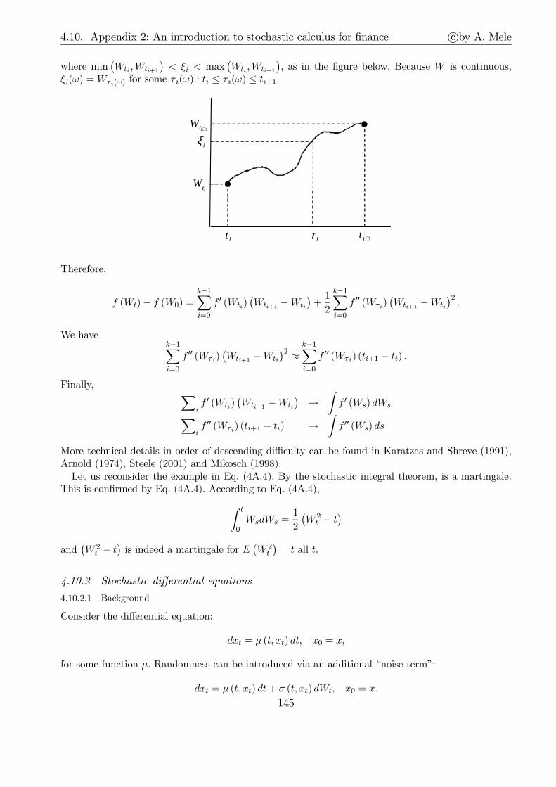
4.10. Appendix 2: An introduction to stochastic calculus for finance c©by A. Mele
where min(Wti ,Wti+1
)< ξi < max
(Wti ,Wti+1
), as in the figure below. Because W is continuous,
ξi(ω) =Wτ i(ω) for some τ i(ω) : ti ≤ τ i(ω) ≤ ti+1.
it 1+it iτ
1+itW
iξ
itW
Therefore,
f (Wt)− f (W0) =k−1∑
i=0
f ′ (Wti)(Wti+1 −Wti
)+
1
2
k−1∑
i=0
f ′′ (Wτ i)(Wti+1 −Wti
)2.
We havek−1∑
i=0
f ′′ (Wτ i)(Wti+1 −Wti
)2 ≈k−1∑
i=0
f ′′ (Wτ i) (ti+1 − ti) .
Finally,∑
if ′ (Wti)
(Wti+1 −Wti
)→
∫f ′ (Ws) dWs
∑if ′′ (Wτ i) (ti+1 − ti) →
∫f ′′ (Ws) ds
More technical details in order of descending difficulty can be found in Karatzas and Shreve (1991),Arnold (1974), Steele (2001) and Mikosch (1998).
Let us reconsider the example in Eq. (4A.4). By the stochastic integral theorem, is a martingale.This is confirmed by Eq. (4A.4). According to Eq. (4A.4),
∫ t
0WsdWs =
1
2
(W 2
t − t)
and(W 2
t − t)is indeed a martingale for E
(W 2
t
)= t all t.
4.10.2 Stochastic differential equations
4.10.2.1 Background
Consider the differential equation:
dxt = µ (t, xt)dt, x0 = x,
for some function µ. Randomness can be introduced via an additional “noise term”:
dxt = µ (t, xt) dt+ σ (t, xt)dWt, x0 = x.
145
4.10. Appendix 2: An introduction to stochastic calculus for finance c©by A. Mele
We already know that a ω-Wt is not differentiable, so this is only a short-hand notation for:
xt = x0 +
∫ t
0µ (s, xs)ds+
∫ t
0σ (s, xs)dWs, (4A.6)
where the first integral is Riemann and the second integral is an Itô’s stochastic integral.We have the following definitions. First, we say that an Itô’s process is,
dxt (ω) = µt (ω) dt+ σt (ω) dWt, x0 = x.
Moreover, we say that an Itô’s diffusion process is,
dx (t) = µ (t, x (t)) dt+ σ (t, x (t))dW (t) , x0 = x.
It is known that an Itô’s diffusion process is a Markov process. The previous equation is also called astochastic differential equation (SDE). In a SDE, µ and σ “depend” on ω only through x. Finally, wesay that a time-homogeneous diffusion process is,
dx (t) = µ (x (t)) dt+ σ (x (t))dW (t) , x0 = x.
There is a beautiful property that is used to price financial derivatives, using replication arguments,as explained in the main text, called the Unique Decomposition Property. Suppose we were given twoprocesses x and y with x0 = y0, and that:
dxt = µxt dt+ σxt dWt and dyt = µyt dt+ σyt dWt.
Then xt = yt almost surely if and only if µxt = µyt and σxt = σyt almost everywhere, in the sense that
E[∫ T0 |axt − ayt | = 0] = E[
∫ T0 |bxt − byt | dt] = 0.
4.10.2.2 Basic definitions, properties and regularity conditions
How do we know whether the various integrals given before are well-defined. As an example, the Itô’sintegral representation
∫ t0σ(s, xs)dWs works if σ is Ft-adapted and
∫ t0E
[σ(s, xs)2
]ds < ∞. But how
can be sure that these two basic conditions are satisfied if we don’t know yet the solution of x? And,above all, what is a solution to a SDE? We have two concepts of such a solution, strong and weak.
D 4A.5. (S / SDE) A strong solution to Eq. (4A.6) is a stochasticprocess x = (xt, t ∈ [0, T ]) such that:
(i) x is Ft-adapted.
(ii) The integrals in Eq. (4A.6) are well-defined in the Riemann’s and Itô’s sense and Eq. (4A.6)holds P ⊗ dt-almost surely
(iii) E(∫ T
0 |xs|2 ds
)<∞.
In other words, the definition of a strong solution requires that a Brownian motion be “given inadvance,” and that the solution xt constructed from it be then Ft-adapted.
Next, suppose, instead, that we were only given x0 and the functions σ(t, x) and µ(t, x), and that wewere asked to find a pair of processes (x, W ) on some probability space (Ω, F , P ) such that Eq. (4A.6)holds with x being Ft-adapted on some space, not necessarily the one in Eq. (4A.6). (Clearly such a xneeds not to be Ft-adapted.) In this case (x, W ) is called a weak solution on (Ω, F , P ). In the case of aweak solution, we are given x, µ, σ and then “we have to find” two things: a Brownian motion W and
146
4.10. Appendix 2: An introduction to stochastic calculus for finance c©by A. Mele
a Ft-adapted process x such that xt = x0 +∫ t0µ (s, xs) ds+
∫ t0σ (s, xs)dWs holds P ⊗ dt-almost surely.
Clearly, a strong solution is also weak, but the converse is not true. Consider the following example.
E 4A.6. (T $ ) Let x (t) satisfy:
dx (t) = sign(x (t))dW (t) , x0 = 0. (4A.7)
This equation has no strong solutions, for define
y (t) =
∫ t
0sign(W (s))dW (s) , (4A.8)
where W is a Brownian motion. It can be shown that y (t) is G (t)-measurable, where G (t) is theσ-algebra generated by |W (t)|. Clearly G (t) ⊂ F (t), where F (t) is the σ-algebra generated by W (t).Therefore, the σ-algebra generated by y (t) is also strictly contained in F (t). Armed with this result,we can easily show that there are no strong solutions to Eq. (4A.7). To show this, suppose the contrary.There is a theorem saying that x (t) would then be a Brownian motion. On the other hand, Eq. (4A.7)can also be written
dW (t) = sign(x (t))dx (t) , x0 = 0,
or
W (t) =
∫ t
0sign(x (s))dx (s) .
By the same reasoning produced to show that the σ-algebra generated by y (t) is strictly containedin F (t) in Eq. (4A.8), we conclude that the σ-algebra generated by W (t) is strictly contained in theσ-algebra generated by x (t). But this contradicts that x (t) is a strong solution to Eq. (4A.7).
Clearly we must be able to impose some conditions enabling one to distinguish weak from strongsolutions. However, the only focus of the following is to provide regularity conditions ensuring existenceand uniqueness for the restrictive case of strong solutions, which is the case of interest in continuous-time finance. We need to restrictions on µ and σ. For a given function f , we say that it satisfies aLipschitz condition in x if there exists a constant L such that for all (x, y) ∈ Rd ×Rd,
‖f (x, t)− f (y, t)‖ ≤ L ‖x− y‖ uniformly in t.
where ‖A‖ ≡√Tr (AA⊤). In other words, f cannot change too widely. We also say f satisfies a growth
condition in x if there exists a constant G such that for all (x, y) ∈ Rd ×Rd,
‖f (x, t)‖2 ≤ G(1 + ‖x‖2
)uniformly in t.
That is, f cannot grow too much.Next, we turn to the concepts of existence and uniqueness of a solution to a stochastic differential
equation. We say that if x(1)t (ω) and x
(2)t (ω) are both strong solutions to Eq. (4A.6), then x
(1)t (ω) =
x(2)t (ω) P ⊗ dt-a.s. We have:
T 4A.7. Suppose that µ, σ satisfy Lipschitz and growth conditions in x, then there existsa unique Itô’s process x satisfying Eq. (4A.6) which is continuous adapted Markov.
Consider the following stochastic differential equation:
dx (t) = µ (a− x (t)) dt+ σ√x (t)dW (t) ,
147

4.10. Appendix 2: An introduction to stochastic calculus for finance c©by A. Mele
for some constants µ, a, σ. This is the so-called square-root process utilized to model equity volatility(see Chapter 10), the short-term rate (see Chapters 11) or instantaneous probabilities of default ofdebt issuers (see Chapter 12). The point here, for now, is that the diffusion component does not satisfythe conditions in Theorem 4A.7. Yet it is possible to show that under suitable parameter restrictionsthere exists a strong solution. Incidentally, the solution to this simple equation is still unknown.
What about uniqueness of the solution? It is well-known that if µ, σ are locally Lipschitz continuousin x, then strong uniqueness holds. But even for ordinary differential equations, a local Lipschitzcondition is not necessarily enough to guarantee global existence (i.e. for all t) of a solution. Forexample, consider the following equation:
dx (t)
dt= µ (x (t)) ≡ x2 (t) , x0 = 1,
has as unique solution:
x (t) =1
1− t, 0 ≤ t < 1.
Yet is impossible to find a global solution, i.e. one defined for all t. This is exactly the kind of pathologyruled out by linear-growth conditions. More generally, linear-growth conditions ensure that |xt (ω)| isunique and doesn’t explode in finite time. Naturally, Lipschitz and growth conditions are only sufficientconditions to guarantee the previous conclusions.
A final remark. The uniqueness concept used here refers to strong or pathwise uniqueness. Thereare also definitions of weak uniqueness to mean that any two solutions (weak or strong) have the samefinite-dimensional distributions. For example, the Tanaka’s equation introduced earlier has no strongsolution, yet it can be shown that it has a (weakly) unique weak solution.
4.10.2.3 Itô’s lemma
Itô’s lemma is a fundamental tool of analysis in continuous-time finance. It helps to build up newprocesses from given processes. Two examples might clarify.
(i) A share price is certainly a function of its dividend process. If the dividend process is solutionto some SDE, then the asset price is a solution to another SDE. Which SDE? Itô’s lemma willgive us the answer.
(ii) Derivative products, reviewed in the third part of the book, are financial instruments the value ofwhich depends on some underlying factors (hence the terminology “derivative”). In other words,derivative prices are functions of these factors. Then if factors are solutions to SDE, derivativeprices are also solutions to SDE. Once again, Itô’s lemma will provide us with right SDE.
Naturally, the functional form linking the dividend process (or the factors) to the asset prices isunknown. But in situations of interest, simple no-arbitrage restrictions will help to pin down such afunctional form.
Let us proceed with a few preliminary heuristic considerations. A useful heuristic definition is thatthe increments of a Brownian motion, dW (t), can be thought of as being equal to W (T +∆t)−W (t)as∆t→ 0. We may think of the “increments” dW (t) as being normally distributed, dW (t) ∼ N (0, dt).Heuristically, indeed, ∆W (t) ≡W (t+∆t)−W (t) ∼ N (0,∆t). But then, by the previous normalityproperty of ∆W (t),
E [∆W (t)] = 0 and E[(∆W (t))2
]= ∆t, hence var [∆W (t)] = ∆t, and var
[(∆W (t))2
]= 2(∆t)2 ,
where the second equality follows by the property χ2 distributions.The point of the previous computations is that for small ∆t, the variance of (∆W (t))2, which is
proportional to (∆t)2, is negligible if compared to its expectation, which is∆t. Heuristically, Qn (t)q.m.→
148

4.10. Appendix 2: An introduction to stochastic calculus for finance c©by A. Mele
t and (dW (t))2 ≡ Qn (dt)q.m.→ dt. These heuristic considerations lead to the following, celebrated table
below.
Itô’s multiplication table
(dt)n = 0 for n > 1dt · dW = 0
(dW )2 = dt(dW )n = 0 for n > 2dW1dW2 = 0 for two independent Brownian motions
We now heuristically derive Itô’s lemma by hinging upon this table. Let x (t) be the solution to,
dx (t) = µ (t)dt+ σ (t) dW (t) ,
and suppose we are given a function f (x, t), which we assume to be as differentiable in (x, t) as manytimes we shall need below. We expand f as follows:
df (x, t) = ft (x, t)dt+ fx (x, t)dx+1
2fxx (x, t) (dx)
2 +Remainder,
where the remainder contains only terms of order higher than (dx)2 and (dt)2. So for reasons whichwill be clear in one moment we will discard it. We have,
df = ftdt+ fxdx+1
2fxx (dx)
2
= ftdt+ fx (µdt+ σdW ) +1
2fxx (µdt+ σdWt)
2
= ftdt+ fxµdt+ fxσdW +1
2fxx
[µ2 (dt)2 + σ2 (dW )2 + 2µσ (dt · dW )
].
By the Itô’s multiplication table,
df = ftdt+ fxµdt+ fxσdW +1
2fxx
[µ2 (dt)2 + σ2 (dW )2 + 2µσ (dt · dW )
]
= ftdt+ fxµdt+ fxσdW +1
2fxx
[0 + σ2 · dt + 0
]
By rearranging terms,
df (x, t) =
[ft (x, t)dt+ fx (x, t)µ+
1
2fxx (x, t)σ
2
]dt+ fx (x, t)σdW,
and the remainder is also zero by the Itô’s multiplication table. This is Itô’s lemma.Naturally, Itô’s lemma also holds when x is a multidimensional process. A heuristic derivation of it
can be obtained through the Itô’s multiplication table applied to the following expansion:
df (x, t) = ftdt+ fxdx+1
2
∑
i,j
fxixjdxidxj.
Then, we have:
T 4A.8. (Iô’ , , ) Let us be given a multidimensional processx ∈ Rn solution to,
dx (t) = µ (x (t) , t)dt+ σ (x (t) , t) dW (t) , (4A.9)
149

4.10. Appendix 2: An introduction to stochastic calculus for finance c©by A. Mele
where µ is in Rn, σ is in Rn×d and W is a d-dimensional vector of independent Brownian motions.Moreover, let us be given a function f (x, t) which is twice differentiable in x and differentiable in t.Then f is an Itô’s process, solution to:
df (x (t) , t) = Lf (x (t) , t)dt+ fx (x (t) , t)σ (t) dW (t)
or more formally,
f (x (t) , t) = f (x0, 0) +
∫ t
0Lf (x (s) , s)ds+
∫ t
0fx (x (s) , s)σ (x (s) , s) dW (s) , (4A.10)
where
Lf (x, t) = ft (x, t) + fx (x, t)µ+1
2Tr
[σσ⊤fxx (x, t)
]
and fx (x, t) and fxx (x, t) are the gradient and Hessian of f with respect to x.
Note that by Eq. (4A.10), and provided fxσ ∈ H2, f is a martingale whenever Lf (x, t) = 0, for allx, t. Moreover, on a terminology standpoint, the operator Af (x, t) = fx (x, t)µ+ 1
2Tr[σσ⊤fxx (x, t)
]
is usually referred to as the infinitesimal generator of the diffusion process in Eq. (4A.9).
150

4.11. Appendix 3: Proof of selected results c©by A. Mele
4.11 Appendix 3: Proof of selected results
4.11.1 Proof of Theorem 4.2
As mentioned in the main text, we have that by by the Girsanov’s theorem, Q is non-empty if andonly if Eq. (4.43) holds true. Therefore, the proof will rely on Eq. (4.43). If part. With c ≡ 0, Eq.(4.44) is:
V x,π,0 (τ)
S0 (τ)= x+
∫ τ
t
π⊤ (u)σ (u)
S0 (u)dW0(u), τ ∈ [t, T ],
which implies, x = EQτ [S0 (T )
−1 V x,π,0 (T )]. An arbitrage opportunity is V x,π,0(t) ≤ S0 (T )−1 V x,π,0 (T )
a.s., which combined with the previous equality leaves: V x,π,0(t) = S0 (T )−1 V x,π,0 (T ) Q-a.s. (if a r.v.
y ≥ 0 and Et(y) = 0, this means that y = 0 a.s.) and, hence, P -a.s. The last equality is in contradiction
with Pr(S0 (T )
−1 V x,π,0 (T )− x > 0)> 0, as required by Definition 4.3.
Only if part. We combine portions of proofs in Karatzas (1997, thm. 0.2.4 pp. 6-7) and Øksendal(1998, thm. 12.1.8b, pp. 256-257). We let:
Z (τ) = ω ∈ Ω : Eq. (4.43) has no solutions= ω ∈ Ω : a(τ ;ω)− 1mr(τ ;ω) /∈ 〈σ〉=
ω ∈ Ω : ∃π(τ ;ω) : π(τ ;ω)⊤σ(τ ;ω) = 0 and π(τ ;ω)⊤ (a(τ ;ω)− 1mr(τ ;ω)) = 0
,
and consider the following portfolio,
π(τ ;w) =
k · sign
[π(τ ;ω)⊤ (a(τ ;ω)− 1mr(τ ;ω))
]· π(τ ;ω) for ω ∈ Z(τ)
0 for ω /∈ Z(τ)
Clearly π is (τ ;ω)-measurable, and generates, by Eq. (4.39),
V x,π,0 (τ)
S0 (τ)= x+
∫ τ
t
π (u)⊤ (a (u)− 1mr (u))S0 (u)
IZ(u)du+
∫ τ
t
π⊤ (u)σ (u)
S0 (u)IZ(u)dW (u)
= x+
∫ τ
t
(π (u)⊤ (a (u)− 1mr (u))
S0 (u)
)IZ(u)du
≥ x.
So the market has no arbitrage only if IZ(u) = 0, i.e. only if Eq. (4.43) has at least one solution. ‖
4.11.2 Proof of Eq. (4.48).
We have:
x = E
[V x,π,c (T )
S0 (T )+
∫ T
t
c(u)
S0(u)du
]
= ζ(t)−1E
[ζ (T )V x,π,c (T )
S0 (T )+
∫ T
t
ζ(T )c(u)
S0(u)du
]
= ζ(t)−1E
[ζ (T )V x,π,c (T )
S0 (T )+
∫ T
tE
(ζ(T )c(u)
S0(u)
∣∣∣∣F(u)
)du
]
= ζ(t)−1E
[ζ (T )V x,π,c (T )
S0 (T )+
∫ T
t
E (ζ(T )| F(u)) c (u)
S0 (u)du
]
= ζ(t)−1E
[ζ (T )V x,π,c (T )
S0 (T )+
∫ T
t
ζ (u) c (u)
S0 (u)du
]
= E
[mt,T · V x,π,c(T ) +
∫ T
tmt,u · c(u)du
],
151

4.11. Appendix 3: Proof of selected results c©by A. Mele
where we used the fact that c is adapted, the law of iterated expectations, the martingale property ofζ, and the definition of m0,t.
4.11.3 Walras’s consistency tests
First, we show that Eq. (4.55)⇒ Eq. (4.56). To grasp intuition about the ongoing proof, consider thetwo-period economy of Chapter 2. In that economy, absence of arbitrage opportunities implies that∃φ ∈ Rd : φ⊤(c1 −w1) = Sθ = −(c0 −w0), whence cs = ws, s = 0, · · · , d⇐⇒ θ = 0m. In the model ofthis chapter, absence of arbitrage opportunities implies that there exists a unique Q ∈ Q such that:
V x,π,c (τ)
S0 (τ)≡ θ0(τ)S0(τ) + π⊤(τ)1m
S0(τ)= 1⊤mS(t) +
∫ τ
t
π⊤σ (u)S0 (u)
dW0(u)−∫ τ
t
c (u)
S0 (u)du.
That is,
θ0(τ)S0(τ) +(π⊤(τ)− S⊤(τ)
)1m
S0(τ)+S⊤(τ)1mS0(τ)
= 1⊤mS(t) +∫ τ
t
(π⊤(u)− S⊤(u)
)σ(u)
S0(u)dW0(u)−
∫ τ
t
c (u)
S0(u)du+
∫ τ
t
S⊤(u)σ(u)S0(u)
dW0(u).
Plugging the solution(SiS0
)(τ) = Si(t)+
∫ τt
(S−10 Si
)(u)σi(u)dW0(u)−
∫ τt
(S−10 Di
)(u)du in the previous
relation,
θ0(T )S0(T ) +(π⊤(T )− S⊤(T )
)1m
S0(T )=
∫ T
t
π⊤(u)− S⊤(u)S0(u)
σ(u)dW0(u) +
∫ T
t
D(u)− c(u)
S0(u)du.
(4A.11)When Eq. (4.55) holds, we have that V x,π,c(T ) = θ0(T )S0(T ) + π⊤(T )1m = q(T ) = S⊤(T )1m, andD = c, and Eq. (4A.11) becomes:
0 = x(T ) ≡∫ T
t
π⊤(u)− S⊤(u)S0(u)
σ(u)dW0(u),
a martingale starting at zero, satisfying:
dx(τ) =π⊤(τ)− S⊤(τ)
S0(τ)σ(τ)dW0(τ) = 0.
Since ker(σ) = ∅ then, we have that π(τ) = S(τ) a.s. for τ ∈ [t, T ] and, hence, π(τ) = S(τ) a.s. forτ ∈ [t, T ]. It is easily checked that this implies θ0(T ) = 0 P -a.s. and that in fact, θ0(τ) = 0 a.s.
Next, we show that Eq. (4.56)⇒ Eq. (4.55). When Eq. (4.56) holds, Eq. (4A.11) becomes:
0 = y(T ) ≡∫ T
t
D(u)− c(u)
S0(u)du,
a martingale starting at zero. We conclude by the same arguments used in the proof of the previouspart. ‖
152

4.12. Appendix 4: The Green’s function c©by A. Mele
4.12 Appendix 4: The Green’s function
4.12.1 Setup
In Section 4.6, it is shown that in frictionless markets, the value of a security as of time τ is:
V (x(τ), τ) = E
[mt,T
mt,τV (x(T ), T ) +
∫ T
τ
mt,s
mt,τh (x(s), s) ds
], (4A.12)
where mt,τ is the stochastic discount factor,
mt,τ =ζ(t, τ)
S0(τ)=
1
S0(τ)· dQdP
∣∣∣∣F(τ)
.
The Arrow-Debreu state price density is:
φt,T = mt,TdP =S0(t)
S0(T )dQ.
Our aim is to characterize this density in terms of partial differential equations. By the same reasoningproduced in Section 4.6, Eq. (4A.12) can be rewritten as:
V (x(τ), τ ) = E
[a (τ, T )V (x(T ), T ) +
∫ T
τa (τ , s)h (x(s), s) ds
], a
(t′, t′′
)≡ S0(t
′)S0(t′′)
. (4A.13)
Next, consider the state vector, y(u) ≡ (a (τ, u) , x(u)), τ ≤ u ≤ T , and let q (y(t′)| y(τ)) be therisk-neutral density of y. We have,
V (x(τ), τ) = E
[a (τ, T )V (x(T ), T ) +
∫ T
τa (τ, s)h (x(s), s)ds
]
=
∫a (τ, T )V (x(T ), T ) q (y(T )| y(τ)) dy(T ) +
∫ T
τ
∫a (τ, s)h (x(s), s) q (y(s)| y(τ))dy(s)ds.
If V (x(T ), T ) and a (τ, T ) are independent,∫
a (τ, T )V (x(T ), T ) q (y(T )| y(τ)) dy(T ) =∫
XG(τ, T )V (x(T ), T ) dx(T )
where:
G(τ, T ) ≡∫
Aa (τ, T ) q (y(T )| y(τ ))dy(T ).
Assuming the same for h,
V (x(τ), τ) =
∫
XG(τ, T )V (x(T ), T ) dx(T ) +
∫ T
τ
∫
XG(τ, s)h (x(s), s) dx(s)ds.
The function G is known as the Green’s function:
G (t, ℓ) ≡ G (x, t; ξ, ℓ) =
∫
Aa (t, ℓ) q (y(ℓ)| y(t)) da.
It is the value in state x ∈ Rd as of time t of a unit of numéraire at ℓ > t if future states lie in aneighborhood (in Rd) of ξ. It is thus the Arrow-Debreu state-price density.
For example, a pure discount bond has V (x, T ) = 1 ∀x, and h(x, s) = 1 ∀x, s, and
V (x(τ), τ) =
∫
XG (x(τ), τ ; ξ, T )dξ, with lim
τ↑TG (x(τ), τ ; ξ, T ) = δ (x(τ)− ξ) ,
where δ is the Dirac’s delta.
153

4.12. Appendix 4: The Green’s function c©by A. Mele
4.12.2 The PDE connection
We show the Green’s function satisfies the same partial differential equation (PDE) satisfied by thesecurity price, but with a different boundary condition, and with the instantaneous dividend takenout. We have:
V (x (t) , t) =
∫
XG (x(t), t; ξ (T ) , T )V (ξ (T ) , T )dξ (T ) +
∫ T
t
∫
XG(x(t), t; ξ(s), s)h (ξ(s), s) dξ(s)ds.
(4A.14)Consider the scalar case. By Eq. (4A.13), and the Feynman-Kac connection between PDEs and con-ditional expectations reviewed in Section 4.2, we have that under regularity conditions, V is solutionto:
0 = Vt + µVx +1
2σ2Vxx − rV + h, (4A.15)
where µ is the risk-neutral drift of x. Next, take the following partial derivatives of V (x, t) in Eq.(4A.14):
Vt =
∫
XGtV dξ −
∫
Xδ(x− ξ)hdξ +
∫ T
t
∫
XGthdξds =
∫
XGtV dξ − h+
∫ T
τ
∫
XGthdξds
Vx =
∫
XGxV dξ +
∫ T
t
∫
XGxhdξds
Vxx =
∫
XGxxV dξ +
∫ T
t
∫
XGxxhdξds
and replace them into Eq. (4A.15) to obtain:
0 =
∫
X
[Gt + µGx +
1
2σ2Gxx − rG
]V (ξ (T ) , T )dξ(T )
+
∫ T
t
∫
X
[Gt + µGx +
1
2σ2Gxx − rG
]h (ξ (s) , s) dξ (s) ds.
This shows that G is solution to
0 = Gt + µGx +1
2σ2Gxx − rG, with lim
t↑TG (x, t; ξ, T ) = δ (x− ξ) .
154

4.13. Appendix 5: Portfolio constraints c©by A. Mele
4.13 Appendix 5: Portfolio constraints
We are looking for a portfolio-consumption policy (pν , cν) such that
Val (x;K) = E
[∫ T
0u (t, cν (t))dt+ U (V x,pν ,cν (T ))
]≡ Valν (x) , (4A.16)
and pν (t) ∈ K for all t ∈ [0, T ].Note that becauseK contains the origin, then, the support function ζ in Eq. (4.59) satisfies ζ (ν) ≥ 0
for each ν ∈ K. Moreover, an intuitive and important property of ζ is that,
p ∈ K ⇐⇒ ζ (ν) + p⊤ν ≥ 0, ∀ν ∈ K. (4A.17)
Next, define the standard Brownian motion under the probability Qν , defined through the Radon-Nikodym in Eq. (4.61):
Wν (t) =W (t) +
∫ t
0
(λ (u) + σ−1 (u) ν (u)
)du ≡W0 (t) +
∫ t
0
(σ−1 (u) ν (u)
)du,
where λ = σ−1 (a− 1dr), and W0 is the usual Brownian under the risk-neutral probability in a marketwithout any frictions. If the price system is as in Eqs. (4.60), then, for any unconstrained portfolio-consumption (p, c), the dynamics of wealth, V x,p,c
ν say, are easily seen to be:
dV x,p,cν =
(p⊤ν + ζ (ν)V x,p,c
ν + rV x,p,cν − c
)dt+ p⊤σdW0.
So we have that under Q0,
V x,p,cν (T )
S0 (T )+
∫ T
0
c (t)
S0 (t)dt
= x+
∫ T
0
V x,p,cν (t)
S0 (t)
[p⊤ (t) ν (t) + ζ (ν (t))
]dt+
∫ T
0
V x,p,cν (t)
S0 (t)p⊤ (t)σ (t)dW0 (t) .
Therefore, for any normalized portfolio-consumption (p, c), we have that the wealth difference, ∆(t) ≡V x,π,cν (T )−V x,π,c(T )
S0(T ) , satisfies:
d∆(t) =V x,π,cν (t)
S0 (t)
[p⊤ (t) ν (t) + ζ (ν (t))
]
︸ ︷︷ ︸≡m(t)
dt+∆(t) p⊤ (t)σ (t)dW (t) , ∆(0) = 0.
Next, consider, the simpler equation,
d∆ (t) = ∆ (t) p⊤ (t)σ (t)dW (t) , ∆ (0) = 0. (4A.18)
Because m (t) ≥ 0 by Eq. (4A.17), then, by a comparison theorem (e.g., Karatzas and Shreve (1991,p. 291-295)), ∆(t) ≥ ∆ (t) = 0, where the last equality follows because the solution to Eq. (4A.18) is∆ (t) = ∆ (0)L (t), for some positive process L (t). Therefore, we have,
V x,p,cν (t) ≥ V x,p,c (t) , with an equality if ζ (ν (t)) + p⊤ν (t) = 0 for all t. (4A.19)
Finally, suppose there is a constrained portfolio-consumption pair (pν , cν), such that
ζ (ν (t)) + p⊤ (t) ν (t) = 0. (4A.20)
155

4.13. Appendix 5: Portfolio constraints c©by A. Mele
Naturally, we have that Val (x;K) ≤ Valν (x) for all ν and, hence,
Val (x;K) ≤ infν∈K
(Valν (x)) . (4A.21)
Moreover, we have,
Val (x;K) = E
[∫ T
0u (t, c (t))dt+U (V x,p,c (T ))
], p (t) ∈ K
≥ E
[∫ T
0u (t, cν (t))dt+ U (V x,pν ,cν (T ))
]
= E
[∫ T
0u (t, cν (t))dt+ U
(V x,pν ,cνν (T )
)]
= Valν (x) , (4A.22)
where the second line follows, because the value of the unconstrained problem is, of course, the largestwe may have, once we consider any arbitrary constrained portfolio-consumption (pν , cν). The third linefollows by Eq. (4A.20) and (4A.19). The fourth line is the definition of Valν (x). Combining (4A.21)with (4A.22) leaves,
Val (x;K) = Valν (x) .
The converse, namely “if there exists a ν ∈ K that minimizes Valν (x), then, the correspondingportfolio-consumption process (pν , cν) is optimal for the constrained problem,” is also true, but itsarguments (even informal) are omitted here.
156
4.14. Appendix 6: Models with final consumption only c©by A. Mele
4.14 Appendix 6: Models with final consumption only
Sometimes, we may be interested in models with consumption taking place in at the end of the periodonly. Let S =
(S(0), S
)⊺and θ = (θ(0), θ), where θ and S are both m-dimensional. Define as usual
wealth as of time t as Vt ≡ Stθt. There are no dividends. A self-financing strategy θ satisfies,
S+t θt+1 = Stθt ≡ Vt, t = 1, · · · , T.
Therefore,
Vt = Stθt + St−1θt−1 − St−1θt−1
= Stθt + St−1θt−1 − St−1θt (because θ is self-financing)
= Vt−1 +∆Stθt, ∆St ≡ St − St−1, t = 1, · · · , T,or,
Vt = V1 +t∑
n=1
∆Snθn.
Next, suppose that
∆S(0)t = rtS
(0)t−1, t = 1, · · · , T,
with rtTt=1 given and to be defined more precisely below. The term ∆Stθ+t can then be rewritten as:
∆Stθt = ∆S(0)t θ
(0)t +∆Stθt
= rtS(0)t−1θ
(0)t +∆Stθt
= rtS(0)t−1θ
(0)t + rtSt−1θt − rtSt−1θt +∆Stθt
= rtSt−1θt − rtSt−1θt +∆qtθt
= rtSt−1θt−1 − rtSt−1θt +∆Stθt (because θ is self-financing)
= rtVt−1 − rtSt−1θt +∆Stθt,
and we obtainVt = (1 + rt)Vt−1 − rtSt−1θt +∆Stθt,
or,
Vt = V1 +t∑
n=1
(rnVn−1 − rnSn−1θn +∆Snθn) .
Next, considering “small” time intervals. In the limit we obtain:
dV (t) = r(t)V (t)dt− r(t)S(t)θ(t)dt+ dS(t)θ(t).
Such an equation can also be arrived at by noticing that current wealth is nothing but initial wealthplus gains from trade accumulated up to now:
V (t) = V (0) +
∫ t
0dS(u)θ(u).
⇔dV (t) = dS(t)θ(t)+
= dS0(t)θ0(t) + dS(t)θ(t)
= r(t)S0(t)θ0(t)dt+ dS(t)θ(t)
= r(t) (V (t)− S(t)θ(t)) dt+ dS(t)θ(t)
= r(t)V (t)dt− r(t)S(t)θ(t)dt+ dS(t)θ(t).
157

4.14. Appendix 6: Models with final consumption only c©by A. Mele
Now consider the sequence of problems of terminal wealth maximization:
For t = 1, · · · , T, Pt :
maxθt E [u(V (T ))| Ft−1] ,s.t. Vt = (1 + rt)Vt−1 − rtSt−1θt +∆Stθt
Even if markets are incomplete, agents can solve the sequence of problems PtTt=1 as time unfolds.Each problem can be written as:
maxθt
E
[u
(V1 +
T∑
t=1
(rtVt−1 − rtSt−1θt +∆Stθt)
)∣∣∣∣∣Ft−1
].
The FOC for t = 1 is:E
[u′(V (T )) (S1 − (1 + r0)S0)
∣∣F0
],
whence
S0 = (1 + r0)−1 E [u′(V (T )) · S1| F0]
E [u′(V (T ))| F0].
In general
St = (1 + rt)−1 E [u′(V (T )) · St+1| Ft]
E [u′(V (T ))| Ft], t = 0, · · · , T − 1.
The previous relations suggest that we can define a martingale measure Q for the discounted priceprocess by defining
dQ
dP
∣∣∣∣Ft
=u′(V (T ))
E [u′(V (T ))| Ft].
Connections with the CAPM. It’s easy to show that:
E (rt+1)− rt = cov
[u′(V (T ))
E [u′(V (T ))| Ft], rt+1
],
where rt+1 ≡ (St+1 − St)/St.
158

4.15. Appendix 7: Topics on jumps c©by A. Mele
4.15 Appendix 7: Topics on jumps
4.15.1 The Radon-Nikodym derivative
This appendix derives, heuristically, results about Radon-Nikodym derivatives for jump-diffusionprocesses. Precise mathematical details can be found in Brémaud (1981). Consider the jump times0 < τ1 < τ2 < · · · < τn = T . The probability of a jump in a neighborhood of τ i is v(τ i)dτ . To definethe same probability under the risk-neutral world, write vQ(τ i)dτ under Q, and set vQ = vλJ , forsome λJ . The probability that no-jump would occur between any two adjacent random points τ i−1
and τ i and a jump would at time τ i−1 is, for i ≥ 2, proportional to:
v(τ i−1)e−∫ τiτi−1
v(u)duunder P,
and to
vQ(τ i−1)e−∫ τiτi−1
vQ(u)du= v(τ i−1)λ
J(τ i−1)e−∫ τiτi−1
v(u)λJ (u)duunder Q.
As explained in Section 4.7, these are in fact densities of time intervals elapsing from one arrival tothe next one.
Next, let A be the event of marks at time τ1, τ2, · · · , τn. The Radon-Nikodym derivative is thelikelihood ratio of the two probabilities Q and P of A:
Q(A)
P (A)=
e−∫ τ1t v(u)λJ (u)du · v(τ1)λJ(τ1)e−
∫ τ2τ1
v(u)λJ (u)du · v(τ2)λJ(τ2)e−∫ τ3τ2
v(u)λJ (u)du · · · ·e−
∫ τ1t v(u)du · v(τ1)e−
∫ τ2τ1
v(u)du · v(τ2)e−∫ τ3τ2
v(u)du · · · ·,
where we have used the fact that given that at τ0 = t, there are no-jumps, the probability that no-jumps would occur from t to τ1 is e−
∫ τ1t v(u)du under P , and e−
∫ τ1t v(u)λJ(u)du under Q. Simple algebra
yields,
Q(A)
P (A)= λJ(τ1) · λJ(τ2) · e−
∫ τ1t v(u)(λJ (u)−1)du · e−
∫ τ2τ1
v(u)(λJ(u)−1)due−∫ τ3τ2
v(u)(λJ (u)−1)du · · · ·
=n∏
i=1
λJ(τ i) · e−∫ τnt v(u)(λJ (u)−1)du
= exp
[ln
(n∏
i=1
λJ(τ i) · e−∫ τnt v(u)(λJ (u)−1)du
)]
= exp
[n∑
i=1
lnλJ(τ i)−∫ τn
tv(u)
(λJ(u)− 1
)du
]
= exp
[∫ T
tlnλJ(u)dZ (u)−
∫ T
tv(u)
(λJ(u)− 1
)du
],
where the last equality follows from the definition of the Stieltjes integral.Consider, finally, the following definition. Let M be a martingale. The unique solution to the equa-
tion:
L(τ) = 1 +
∫ τ
tL (u)dM (u) ,
is named the Doléans-Dade exponential semimartingale and is denoted as E(M). We now turn to thearbitrage restrictions arising whilst dealing with asset prices driven by jump-diffusion processes.
159

4.15. Appendix 7: Topics on jumps c©by A. Mele
4.15.2 Arbitrage restrictions
As in the main text, let now S be the price of a primitive asset, solution to:
dS
S= bdτ + σdW + ℓSdZ= bdτ + σdW + ℓS (dZ − vdτ) + ℓSvdτ= (b+ ℓSv) dτ + σdW + ℓS (dZ − vdτ) .
Next, define
dZ = dZ − vQdτ(vQ = vλJ
); dW = dW + λdτ.
Both Z and W are Q-martingales. We have:
dS
S=
(b+ ℓSvQ − σλ
)dτ + σdW + ℓSdZ.
The characterization of the equivalent martingale measure for the discounted price is given by thefollowing Radon-Nikodym density of Q with respect to P :
dQ
dP= E
(−∫ T
tλ(τ)dW (τ) +
∫ T
t
(λJ(τ)− 1
)(dZ(τ)− v(τ)) dτ
),
where E (·) is the Doléans-Dade exponential semimartingale, and so:
b = r + σλ− ℓvQES(S) = r + σλ− ℓvλJES(S).
Clearly, markets are incomplete here. It is possible to show that if S is deterministic, a representativeagent with utility function u(x) = x1−η−1
1−η makes λJ(S) = (1 + S)−η.
4.15.3 State price density: introduction
We have:
L(T ) = exp
[−∫ T
tv(τ)
(λJ(τ)− 1
)dτ +
∫ T
tlnλJ(τ)dZ(τ)
].
The objective here is to use Itô’s lemma for jump processes to express L in differential form. Definethe jump process y as:
y(τ) ≡ −∫ τ
tv(u)
(λJ(u)− 1
)du+
∫ τ
tlnλJ(u)dZ(u).
In terms of y, L is L(τ ) = l(y(τ)) with l(y) = ey. We have:
dL(τ) = −ey(τ)v(τ)(λJ(τ)− 1
)dτ +
(ey(τ) + jump − ey(τ)
)dZ(τ)
= −ey(τ)v(τ)(λJ(τ)− 1
)dτ + ey(τ)
(elnλ
J (τ) − 1)dZ(τ)
or,dL(τ)
L(τ )= −v(τ)
(λJ(τ)− 1
)dτ +
(λJ(τ)− 1
)dZ(τ) =
(λJ(τ)− 1
)(dZ(τ)− v(τ)dτ) .
The general case (with stochastic distribution) is covered in the following subsection.
160

4.15. Appendix 7: Topics on jumps c©by A. Mele
4.15.4 State price density: general case
Assume that the primitive is:
dx(τ) = µ(x(τ−))dτ + σ(x(τ−))dW (τ) + dZ(τ),
and let u denote the price of a derivative. Introduce the P -martingale,
dM(τ) = dZ(τ)− v(x(τ))dτ.
By Itô’s lemma for jump-diffusion processes,
du(x(τ), τ)
u(x(τ−), τ)= µu(x(τ−), τ)dτ + σu(x(τ−), τ)dW (τ) + Ju (∆x, τ)dZ(τ)
= (µu(x(τ−), τ) + v(x(τ−))Ju (∆x, τ)) dτ + σu(x(τ−), τ)dW (τ) + Ju (∆x, τ)dM(τ),
where µu = 1u
(∂∂t +L
)u, σu = 1
u
(∂u∂xσ
), ∂∂t + L is the generator for pure diffusion processes and,
finally:
Ju (∆x, τ) ≡ u(x(τ), τ)− u(x(τ−), τ)u(x(τ−), τ)
.
To generalize the steps made to deal with the standard diffusion case, let
dW = dW + λdτ, dZ = dZ − vQdτ.
We wish to find restrictions on both λ and vQ, such that both W and Z are Q-martingales. Let Jξ bethe jump component for the state price density ξ:
dξ(τ)
ξ(τ−)= −λ(x(τ−))dW (τ) + Jξ (∆x, τ) dM(τ), ξ(t) = 1.
We shall show that:
vQ = v(1 + Jξ
).
Note that in this case,
dξ(τ)
ξ(τ−)= −λ(x(τ−))dW (τ ) +
(λJ − 1
)dM(τ), ξ(t) = 1,
a clear generalization of the pure diffusion case.As for the derivative price:
du
u= (µu + vJu) dτ + σudW + Ju (dZ − vdτ)
=(µu + vQJu − σuλ
)dτ + σudW + JudZ
=(µu + v(1 + Jξ)Ju − σuλ
)dτ + σudW + JudZ.
Finally, by the Q-martingale property of the discounted u,
µu − r = σuλ− vQ ·E∆x (Ju) = σuλ− v ·E∆x
((1 + Jξ)Ju
),
where E∆x is taken with respect to the jump-size distribution, which is the same under Q and P .
161

4.15. Appendix 7: Topics on jumps c©by A. Mele
P vQ = v(1 + Jξ
). As usual, the state-price density ξ has to be a P -martingale in order
to be able to price bonds (in addition to all other assets). In addition, ξ clearly “depends” on W andZ. Therefore, it satisfies:
dξ(τ)
ξ(τ−)= −λ(x(τ−))dW (τ) + Jξ (∆x, τ)dM(τ), ξ(t) = 1.
We wish to find vQ in dZ = dZ − vQdτ such that Z is a Q-martingale, viz
Z(τ) = E[Z(T )],
i.e.,
E(Z(t)) =E
(ξ(T ) · Z(T )
)
ξ(t)= Z(t) ⇔ ξ(t)Z(t) = E[ξ(T )Z(T )],
i.e.,ξ(t)Z(t) is a P -martingale.
By Itô’s lemma,
d(ξZ) = dξ · Z + ξ · dZ + dξ · dZ= dξ · Z + ξ
(dZ − vQdτ
)+ dξ · dZ
= dξ · Z + ξ[dZ − vdτ︸ ︷︷ ︸dM
+(v − vQ
)dτ ] + dξ · dZ
= dξ · Z + ξ · dM + ξ(v − vQ
)dτ + dξ · dZ.
Because ξ, M and ξZ are P -martingales,
∀T , 0 = E
[∫ T
tξ(τ) ·
(v(τ)− vQ(τ)
)dτ +
∫ T
tdξ(τ) · dZ(τ)
].
But
dξ · dZ = ξ(−λdW + JξdM
)(dZ − vQdτ
)= ξ
[−λdW + Jξ (dZ − vdτ)
] (dZ − vQdτ
),
and since (dZ)2 = dZ,E(dξ · dZ) = ξ · Jξv · dτ,
and the previous condition collapses to:
∀T , 0 = E
[∫ T
tξ(τ) ·
(v(τ)− vQ(τ) + Jξ(∆x)v(τ)
)dτ
],
which implies
vQ(τ) = v(τ)(1 + Jξ(∆x)
), a.s.
‖
162

4.15. Appendix 7: Topics on jumps c©by A. Mele
References
Arnold, L. (1974): Stochastic Differential Equations: Theory and Applications, New York:Wiley.
Black, F. and M. Scholes (1973): “The Pricing of Options and Corporate Liabilities.” Journalof Political Economy 81, 637-659.
Brémaud, P. (1981): Point Processes and Queues: Martingale Dynamics. Berlin: Springer Ver-lag.
Cvitanic, J. and I. Karatzas (1992): “Convex Duality in Constrained Portfolio Optimization.”Annals of Applied Probability 2, 767-818.
Föllmer, H. and M. Schweizer (1991): “Hedging of Contingent Claims under Incomplete Infor-mation.” In: Davis, M. and R. Elliott (Editors): Applied Stochastic Analysis. New York:Gordon & Breach, 389-414.
Friedman, A. (1975): Stochastic Differential Equations and Applications (Vol. I). New York:Academic Press.
Harrison, J.M. and S. Pliska (1983): “A Stochastic Calculus Model of Continuous Trading:Complete Markets.” Stochastic Processes and Their Applications 15, 313-316.
Harrison, J.M, R. Pitbladdo and S.M. Schaefer (1984): Continuous Price Processes in Fric-tionless Markets Have Infinite Variation.” Journal of Business 57, 353-365.
He, H. and N. Pearson (1991): “Consumption and Portfolio Policies with Incomplete Marketsand Short-Sales Constraints: The Infinite Dimensional Case.” Journal of Economic Theory54, 259-304.
Karatzas, I. and S.E. Shreve (1991): Brownian Motion and Stochastic Calculus. New York:Springer Verlag.
Mikosch, T. (1998): Elementary Stochastic Calculus with Finance in View. Singapore: WorldScientific.
Revuz, D. and M. Yor (1999): Continuous Martingales and Brownian Motion. New York:Springer Verlag.
Shreve, S. (1991): “A Control Theorist’s View of Asset Pricing.” In: Davis, M. and R. Elliot(Editors): Applied Stochastic Analysis. New York: Gordon & Breach, 415-445.
Steele, J.M. (2001): Stochastic Calculus and Financial Applications. New York: Springer-Verlag.
163

5Taking models to data
5.1 Introduction
This chapter surveys methods to estimate and test dynamic models of asset prices. It beginswith foundational issues on identification, specification and testing. Then, it surveys classicalestimation and testing methodologies such as the Method of Moments, where the number ofmoment conditions equals the dimension of the parameter vector (Pearson, 1894); MaximumLikelihood (ML) (Gauss, 1816; Fisher, 1912); the Generalized Method of Moments (GMM),where the number of moment conditions exceeds the dimension of the parameter vector, leadingto the minimum chi-squared (Neyman and Pearson, 1928; Hansen, 1982); and, finally, the recentdevelopments relying on simulations, which aim to implement ML and GMM estimation formodels that are analytically quite complex, but that can be simulated. The chapter concludeswith an illustration of how joint estimation of fundamentals and asset prices in arbitrage-freemodels can lead to statistical efficiency, asymptotically.
5.2 Data generating processes
5.2.1 Basics
Given is a multidimensional stochastic process yt, a data generating process (DGP). Whilewe do not know the probability distribution underlying yt, we use the available data to getinsights into its nature. A few definitions. A DGP is a conditional law, say the law of yt giventhe set of past values yt−1 = yt−1, yt−2, · · · , and some exogenous [define] variable z, withzt = zt, zt−1, zt−2, · · · ,
DGP : ℓ0(yt| xt),
where xt = (yt−1, zt), and ℓ0 denotes the conditional density of the data, the true law. Then,we have three basic definitions. First, we define a parametric model as a set of conditional lawsfor yt, indexed by a parameter vector θ ∈ Θ ⊆ Rp,
(M) = ℓ (yt|xt; θ) , θ ∈ Θ ⊆ Rp .

5.2. Data generating processes c©by A. Mele
Second, we say that the model (M) is well-specified if,
∃θ0 ∈ Θ : ℓ (yt| xt; θ0) = ℓ0 (yt| xt) .
Third, we say that the model (M) is identifiable if θ0 is unique. The main goal of this chapter isto review tools aimed at drawing inference about the true parameter θ0, given the observations.
5.2.2 Restrictions on the DGP
The previous definition of DGP is too rich to be of practical relevance. This chapter dealswith estimation methods applying to DGPs satisfying a few restrictions. Two fundamentalrestrictions are usually imposed on the DGP:
• Restrictions on the heterogeneity of the stochastic process, which lead to stationary ran-dom processes.
• Restrictions on the memory of the stochastic process, which pave the way to ergodicprocesses.
5.2.2.1 Stationarity
Stationary processes describe phenomena leading to long run equilibria, in some statisticalsense: as time unfolds, the probability generating the observations settles down to some “long-run” probability density, a time invariant probability. As Chapter 3 explains, in the early1980s, theorists begun to define a long-run equilibrium as a well-defined stationary, probabilitydistribution generating economic outcomes. We have two notions of stationarity: (i) Strong,or strict, stationarity. Definition: Homogeneity in law; (ii) Weak stationarity, or stationarity oforder p. Definition: Homogeneity in moments.Even with stationary DGP, there might be situations where the number of parameters to
be estimated increases with the sample size. As an example, consider two stochastic processes:one, for which cov(yt, yt+τ ) = τ 2; and another, for which cov(yt, yt+τ ) = exp (− |τ |). In bothcases, the DGP is stationary. Yet for the first process, the dependence increases with τ , andfor the second, the dependence decreases with τ . As this simple example reveals, a stationarystochastic process may have “long memory.” “Ergodicity” further restricts DGP, so as to makethis memory play a more limited role.
5.2.2.2 Ergodicity
We shall deal with DGPs where the dependence between yt1 and yt2 decreases with |t2 − t1|.To introduce some concepts and notation, say two events A and B are independent, whenP (A∩B) = P (A)P (B). A stochastic process is asymptotically independent if, for some functionβτ ,
βτ ≥ |F (yt1 , · · · , ytn , yt1+τ , · · · , ytn+τ )− F (yt1 , · · · , ytn)F (yt1+τ , · · · , ytn+τ )| ,we also have that limτ→∞ βτ → 0. A stochastic process is p-dependent if ∀τ ≤ p, βτ = 0.A stochastic process is asymptotically uncorrelated if there exists ρτ such that for all t, ρτ ≥cov(yt, yt+τ )/
√var(yt) · var(yt+τ ), and that 0 ≤ ρτ ≤ 1 with
∑∞τ=0 ρτ < ∞. For example,
ρτ = τ−(1+δ), δ > 0, in which case ρτ ↓ 0 as τ ↑ ∞.
Let Bt1 denote the σ-algebra generated by y1, · · · , yt and A ∈ Bt−∞, B ∈ B∞t+τ , and define:
ατ = supτ|P (A ∩B)− P (A)P (B)| , ϕ(τ ) = sup
τ|P (B | A)− P (B)| , P (A) > 0.
165

5.2. Data generating processes c©by A. Mele
We say that (i) y is strongly mixing, or α-mixing if limτ→∞ ατ → 0; (ii) y is uniformly mixingif limτ→∞ ϕτ → 0. Clearly, a uniformly mixing process is also strongly mixing. A second orderstationary process is ergodic if limT→∞
∑Tτ=1 cov (yt, yt+τ ) < ∞. If a second order stationary
process is strongly mixing, it is also ergodic.
5.2.3 Parameter estimators
Consider an estimator of the parameter vector θ of the model,
(M) = ℓ(yt|xt; θ), θ ∈ Θ ⊂ Rp .Naturally, any estimator does necessarily depend on the sample size, which we write as θT ≡tT (y). Of a given estimator θT , we say that it is:
• Correct, or unbiased, if E(θT ) = θ0. The difference E(θT )− θ0 is called distortion, or bias.
• Weakly consistent if plimθT = θ0. And strongly consistent if θTa.s.→ θ0.
Finally, an estimator θ(1)
T is more efficient than another estimator θ(2)
T if, for any vector of
constants c, we have that c⊤ · var(θ(1)T ) · c < c⊤ · var(θ(2)
T ) · c.
5.2.4 Basic properties of density functions
We have T observations y1T = y1, · · · , yT. Suppose these observations are the realizationof a T -dimensional random variable with joint density, f (y1, · · · , yT ; θ) = f
(yT1 ; θ
). We have
momentarily put tildes on yi, to emphasize that we view each yi as a random variable.1 How-ever, to ease notation, from now on, we write yi instead of yi. By construction,
∫f (y| θ) dy ≡∫
···∫f(yT1
∣∣ θ)dyT1 = 1 or,
∀θ ∈ Θ,∫f (y; θ) dy = 1.
Now suppose that the support of y doesn’t depend on θ. Under regularity conditions,
∇θ
∫f (y; θ) dy =
∫∇θf (y; θ) dy = 0p,
where 0p is a column vector of zeros in Rp. Moreover, for all θ ∈ Θ,
0p =
∫∇θf (y; θ) dy = Eθ [∇θ ln f (y; θ)] . (5.1)
Finally, we have,
0p×p = ∇θ
∫[∇θ ln f (y; θ)] f (y; θ) dy
=
∫[∇θθ ln f (y; θ)] f (y; θ) dy +
∫|∇θ ln f (y; θ)|2 f (y; θ) dy,
where |x|2 denotes the outer product, i.e. |x|2 = x · x⊤. Hence, by Eq. (5.1),
Eθ [∇θθ ln f (y; θ)] = −Eθ |∇θ ln f (y; θ)|2 = −varθ [∇θ ln f (y; θ)] ≡ −J (θ), ∀θ ∈ Θ.The matrix J is known as the Fisher’s information matrix.
1Therefore, we follow a classical perspective. A Bayesian statistician would view the sample as given. We do not review Bayesianmethods in this chapter.
166

5.3. Maximum likelihood estimation c©by A. Mele
5.2.5 The Cramer-Rao lower bound
Let t(y) some unbiased estimator of θ, and set the dimension of the parameter space to p = 1.We have,
E [t(y)] =
∫t(y)f (y; θ) dy.
Under regularity conditions,
∇θE [t(y)] =
∫t(y) [∇θ ln f (y; θ)] f (y; θ) dy = cov (t(y),∇θ ln f (y; θ)) .
By Cauchy-Schwartz inequality, [cov (t(y),∇θ ln f (y; θ))]2 ≤ var [t(y)]·var [∇θ ln f (y; θ)]. There-
fore,
[∇θE (t(y))]2 ≤ var [t(y)] · var [∇θ ln f (y; θ)] = −var [t(y)] · E [∇θθ ln f (y; θ)] .
But if t(y) is unbiased, or E [t(y)] = θ,
var [t(y)] ≥ [−E (∇θ ln f (y; θ))]−1 ≡ J (θ)−1 .
This is the celebrated Cramer-Rao bound. The same results holds in the multidimensionalcase, through a mere change in notation (see, e.g., Amemiya, 1985, p. 14-17).
5.3 Maximum likelihood estimation
5.3.1 Basics
The density of the data, f(yT1∣∣ θ), maps every possible sample and parameter values of θ on
to positive numbers, the “likelihood” of occurence of any given sample, given the parameterθ: RnT×Θ → R+. We trace the joint density of the entire sample through a thought experiment,in which we change the sample yT1 . So the sample is viewed as the realization of a randomvariable, a view opposite to the Bayesian perspective. We ask: Which value of θ makes thesample we observed the most likely to have occurred? We introduce the “likelihood function,”L(θ| yT1 ) ≡ f(yT1 ; θ). It is the function θ → f(y; θ) for yT1 given and equal to y, say:
L(θ| y) ≡ f(y; θ).
Then, we maximize L(θ| yT1 ) with respect to θ. That is, we look for the value of θ, whichmaximizes the probability to observe the sample we have effectively observed. The resultingestimator is called maximum likelihood estimator (MLE). As we shall see, the MLE attains theCramer-Rao lower bound, provided the model is not misspecified.
5.3.2 Factorizations
Consider a series of events Ai. In the Appendix, we show that,
Pr
(n⋂i=1
Ai
)=
n∏
i=1
Pr
(Ai
∣∣∣∣∣i−1⋂j=1
Aj
). (5.2)
167

5.3. Maximum likelihood estimation c©by A. Mele
By Eq. (5.2), then, the MLE satisfies:
θT = argmaxθ∈Θ
LT (θ) = argmaxθ∈Θ
(1
TlnLT (θ)
),
where, assuming IID data,
lnLT (θ) ≡ lnT∏
t=1
f(yt∣∣yt−1
1 ; θ)=
T∑
t=1
ln f(yt∣∣yt−1
1 ; θ)≡
T∑
t=1
ln f (yt; θ) ≡T∑
t=1
ℓt(θ), (5.3)
and ℓt(θ) is the “log-likelihood” of a single observation.
5.3.3 Asymptotic properties
We consider the i.i.d. case only, as in Eq. (5.3). Moreover, we provide heuristic arguments,leaving more rigorous proofs and general results in the Appendix.
5.3.3.1 The limiting problem
The MLE satisfies the following first order conditions,
0p = ∇θ lnLT (θ)|θ=θT ≡ ∇θ lnLT (θT ).
Consider a Taylor expansion of the first order conditions around θ0,
0p = ∇θ lnLT (θT )d= ∇θ lnLT (θ0) +∇θθ lnLT (θ0)(θT − θ0), (5.4)
where the notation xTd= yT means that the difference xT − yT = op (1), and θ0 is defined as the
solution to the limiting problem,
θ0 = argmaxθ∈Θ
[limT→∞
(1
TlnLT (θ)
)]= argmax
θ∈Θ[E (ℓ (θ))] ,
and, finally, ℓ satisfies regularity conditions needed to ensure that,
θ0 : E [∇θℓ (θ0)] = 0p.
To show that this is indeed the solution, suppose θ0 is identified; that is, θ = θ0 and θ, θ0 ∈Θ ⇐ f(y| θ) = f(y| θ0). Suppose, further, that for each θ ∈ Θ, Eθ [ln f(y| θ)] < ∞. Then, wehave that θ0 = argmaxθ∈ΘEθ [ln f(y| θ)], and this value of θ is unique. The proof is, indeed,very simple. We have,
Eθ0
[− ln
(f(y| θ)f(y| θ0)
)]> − lnEθ0
(f(y| θ)f(y| θ0)
)
= − ln∫
f(y| θ)f(y| θ0)
f(y| θ0)dy
= − ln∫f(y| θ)dy = 0.
168
5.3. Maximum likelihood estimation c©by A. Mele
5.3.3.2 Consistency and asymptotic normality
Provided the model is well-specified, we have that θTp→ θ0 and even θT
a.s.→ θ0, under regularityconditions. One example of conditions required to obtain weak consistency is that the followinguniform weak law of large numbers holds,
limT→∞
Pr
[supθ∈Θ
|ℓT (θ)−E (ℓ (θ))|]→ 0.
Next, consider again the asymptotic expansion in Eq. (5.4), which can be elaborated, so as tohave,
√T (θT − θ0) d
= −[1
T∇θθ lnLT (θ0)
]−11√T∇θ lnLT (θ0)
= −[1
T
T∑
t=1
∇θθℓt(θ0)
]−1
1√T
T∑
t=1
∇θℓt(θ0).
By the law of large numbers reviewed in the Appendix (weak law no. 1),
1
T
T∑
t=1
∇θθℓt(θ0)p→ Eθ0 [∇θθℓt(θ0)] = −J (θ0) .
Therefore, asymptotically,
√T (θT − θ0) d
= J (θ0)−1 1√
T
T∑
t=1
∇θℓt(θ0).
We also have,
1√T
T∑
t=1
∇θℓt(θ0)d→ N (0,J (θ0)) .
Indeed, let ∇θℓ(θ0)T =1T
∑Tt=1∇θℓt(θ0), and note that E (∇θℓt(θ0)) = 0. Then, by the central
limit theorem reviewed in the Appendix:
1√T
∑Tt=1∇θℓt(θ0)√var [∇θℓt(θ0)]
=
√T(∇θℓ(θ0)T − E (∇θℓt(θ0))
)
√var [∇θℓt(θ0)]
,
where, for each t, var [∇θℓt(θ0)] = J (θ0).Finally, by the Slutzky’s theorem reviewed in the Appendix,
√T (θT − θ0) d→ N
(0,J (θ0)
−1) .
Therefore, the ML estimator attains the Cramer-Rao lower bound.
169

5.4. M-estimators c©by A. Mele
5.4 M-estimators
Consider a function g of the unknown parameters θ. Given a function Ψ, a M-estimator of thefunction g(θ) is the solution to,
maxg∈G
T∑
t=1
Ψ(xt, yt; g) ,
where y and x are as in Section 5.2.1. We assume that a solution to this problem exists, that itis interior and that it is unique. Let us denote the M-estimator with gT (x
T1 , y
T1 ). Naturally, the
M-estimator satisfies the following first order conditions,
0 =1
T
T∑
t=1
∇gΨ(yt, xt; gT (x
T1 , y
T1 )
).
To simplify the presentation, we assume that (x, y) are independent in time, and that they havethe same law. By the law of large numbers,
1
T
T∑
t=1
Ψ(yt, xt; g)p→
∫∫Ψ(y, x; g) dF (x, y) =
∫∫Ψ(y, x; g) dF (y|x) dZ (x) ≡ ExE0 [Ψ (y, x; g)] ,
where E0 is the expectation operator taken with respect to the true conditional law of y givenx and Ex is the expectation operator taken with respect to the true marginal law of x. Thelimit problem is,
g∞ = g∞ (θ0) = argmaxg∈G
ExE0 [Ψ (y, x; g)] .
Under standard regularity conditions,2 there exists a sequence of M-estimators gT (x, y) con-verging a.s. to g∞ = g∞ (θ0). Under additional regularity conditions, the M-estimator is alsoasymptotic normal:
T 5.1: Let I ≡ ExE0
(∇gΨ(y, x; g∞ (θ0)) [∇gΨ(y, x; g∞ (θ0))]
⊤)
and assume that the
matrix J ≡ ExE0 [−∇ggΨ(y, x; g)] exists and has an inverse. We have,
√T (gT − g∞ (θ0)) d→ N
(0,J −1IJ −1
).
S( . The M-estimator satisfies the following first order conditions,
0 =1√T
T∑
t=1
∇gΨ(yt, xt; gT )
d=
1√T
T∑
t=1
∇gΨ(yt, xt; g∞) +√T
[1
T
T∑
t=1
∇ggΨ(yt, xt; g∞)
]· (gT − g∞) .
2G is compact; Ψ is continuous with respect to g and integrable with respect to the true law, for each g; 1T
∑Tt=1 Ψ(yt, xt; g)
a.s.→ExE0 [Ψ (y, x; g)] uniformly on G; the limit problem has a unique solution g∞ = g∞ (θ0).
170

5.5. Pseudo, or quasi, maximum likelihood c©by A. Mele
By rearranging terms,
√T (gT − g∞) d
=
[− 1T
T∑
t=1
∇ggΨ(yt, xt; g∞)
]−1
· 1√T
T∑
t=1
∇gΨ(yt, xt; g∞)
d= [ExE0 (−∇ggΨ(y, x; g))]
−1 · 1√T
T∑
t=1
∇gΨ(yt, xt; g∞)
d= J −1 · 1√
T
T∑
t=1
∇gΨ(yt, xt; g∞) .
By the limiting problem, ExE0 [∇gΨ(y, x; g∞)] = 0. Then, var (∇gΨ) = E(∇gΨ · [∇gΨ]
⊤)=
I, and, then,1√T
T∑
t=1
∇gΨ(yt, xt; g∞)d→ N (0,I) .
The result follows by the Slutzky’s theorem and the symmetry of J . ‖
One simple example of M-estimator is the Nonlinear Least Squares estimator,
θT = argminθ∈Θ
T∑
t=1
[yt −m (xt; θ)]2 ,
for some function m. In this case, Ψ(x, y; θ) = [y −m (x; θ)]2.
5.5 Pseudo, or quasi, maximum likelihood
The maximum likelihood estimator is an M-estimator: set Ψ = lnL, the log-likelihood function.Indeed, assume the model is well-specified, in which case J = I, which confirms we are backto the MLE.Next, suppose that we implement the MLE to estimate a model, when in fact the model is
misspecified in that the true DGP ℓ0 (yt| xt) does not belong to the family of laws spanned byour model,
ℓ0 (yt|xt) /∈ (M) = f (yt|xt; θ) , θ ∈ Θ .Suppose we insist in maximizing Ψ = lnL, where L =
∑t f (yt|xt; θ). In this case,
√T (θT − θ∗0)
d→ N(0,J −1IJ −1
),
where θ∗0 is the “pseudo-true” value,3 and
J = −ExE0
[∇θθ ln f(yt| yt−1; θ
∗0)], I = ExE0
(∇θ ln f(yt| yt−1; θ
∗0) ·
[∇θ ln f(yt| yt−1; θ
∗0)]⊤)
.
In the presence of specification errors, J = I. By comparing the two estimated matricesleads to detect specification errors. Finally, note that in this general case, the variance-covariance
3That is, θ∗0 is, clearly, the solution to some misspecified limiting problem. This θ∗0 has an appealing interpretation in terms ofsome entropy distance minimizer.
171

5.6. GMM c©by A. Mele
matrix J −1IJ −1 depends on the unknown law of (yt, xt). To assess the precision of the estimatesof gT , one needs to estimate such a variance-covariance matrix. A common practice is to usethe following a.s. consistent estimators,
J = − 1T
T∑
t=1
∇ggΨ(yt, xt; gT ), and I = − 1T
T∑
t=1
(∇gΨ(yt, xt; gT )
[∇gΨ(yt, xt; gT )
⊤]) .
5.6 GMM
Economic theory often places restrictions on models that have the following format,
E [h (yt; θ0)] = 0q, (5.5)
where h : Rn × Θ → Rq, θ0 is the true parameter vector, yt is the n-dimensional vector ofthe observable variables and Θ ⊆ Rp. Typically, then, the MLE cannot be used to estimateθ0. Moreover, MLE requires specifying a density function. Hansen (1982) proposed the fol-lowing Generalized Method of Moments (GMM) estimation procedure. Consider the samplecounterpart to the population in Eq. (5.5),
h(yT1 ; θ
)=1
T
T∑
t=1
h (yt; θ) , (5.6)
where we have rewritten h as a function of the parameter vector θ ∈ Θ. The basic idea of GMMis to find a θ which makes h
(y⊤1 ; θ
)as close as possible to zero. Precisely, we have,
D (GMM estimator): The GMM estimator is the sequence θT satisfying,
θT = arg minθ∈Θ⊆Rp
h(yT1 ; θ
)⊤1×q
·WTq×q
· h(yT1 ; θ
)q×1
,
where WT is a sequence of weighting matrices, with elements that may depend on the obser-vations.
When p = q, we say the GMM is just-identified, and is, simply, the MM, satisfying:
θT : h(yT1 ; θT ) = 0q.
When p < q, we say the GMM estimator imposes overidentifying restrictions.We analyze the i.i.d. case only. Under regularity conditions, there exists a matrix WT that
minimizes the asymptotic variance of the GMM estimator, which satisfies asymptotically,
W =[limT→∞
T · E(h(yT1 ; θT ) · h(yT1 ; θT )⊤
)]−1
≡ Σ−10 . (5.7)
An estimator of Σ0 can be:
ΣT =1
T
T∑
t=1
[h(yt; θT ) · h(yt; θT )⊤
].
172
5.6. GMM c©by A. Mele
Note that θT depends on the weighting matrix ΣT , and the weighting matrix ΣT depends on θT .Therefore, we need to implement an iterative procedure. The more one iterates, the less likelythe final outcome depends on the initial weighting matrix Σ
(0)T . For example, one can start with
Σ(0)T = Iq.We have:
T 5.2: Suppose to be given a sequence of GMM estimators θT with weigthing matrixas in Eq. (5.7), and such that : θT
p→ θ0. We have,
√T (θT − θ0) d→ N
(0p,
[E (hθ)Σ
−10 E (hθ)
⊤]−1
), where hθ ≡ ∇θh(y; θ0).
S( : The assumption that θTp→ θ0 is easy to check under mild regularity
conditions. Moreover, the GMM satisfies,
0p = ∇θh(yT1 ; θT )
p×qΣ−1T
q×qh(yT1 ; θT )
q×1
. (5.8)
Eq. (5.8) confirms that if p = q, the GMM satisfies θT : h(yT1 ; θT ) = 0. Indeed, ∇θhΣ−1T is
full-rank with p = q, and Eq. (5.8) can only be satisfied with h = 0. In the general case, q > p,we have,
√Th(yT1 ; θT )
q×1
=√T h
(yT1 ; θ0
)+
q×1
[∇θh
(yT1 ; θ0
)]⊤q×p
√T (θT − θ0) + op(1).
By premultiplying both sides of the previous equality by ∇θh(yT1 ; θT )Σ
−1T ,
√T∇θh(y
T1 ; θT )Σ
−1T · h(yT1 ; θT )
=√T∇θh(y
T1 ; θT )Σ
−1T · h
(yT1 ; θ0
)+∇θh(y
T1 ; θT )Σ
−1T ·
[∇θh
(yT1 ; θ0
)]⊤√T (θT − θ0) + op(1).
The l.h.s. of this equality is zero by the first order conditions in Eq. (5.8). By rearrangingterms,
√T (θT − θ0)
d= −
(∇θh
(yT1 ; θ0
)Σ−1T
[∇θh
(yT1 ; θ0
)]⊤)−1∇θh(y
T1 ; θT )Σ
−1T ·
√T h
(yT1 ; θ0
)
= −(1
T
T∑t=1
∇θh(yt; θT )Σ−1T
1
T
T∑t=1
[∇θh(yt; θT )]⊤)−1
1
T
T∑
t=1
∇θh(yt; θT )Σ−1T
√T h
(yT1 ; θ0
)
d= −
(E (hθ)Σ
−10 E (hθ)
⊤)−1
E (hθ)Σ−10 · 1√
T
T∑
t=1
h (yt; θ0) .
We have: 1√T
∑Tt=1 h (yt; θ0)
d→ N (E(h), var(h)), where, by Eq. (5.5), E(h) = 0, and var(h) =
E(h · h⊤
)= Σ0. Hence:
1√T
T∑
t=1
h (yt; θ0)d→ N (0,Σ0) .
Therefore,√T (θT − θ0) is asymptotically normal with expectation 0p, and variance,
(E (hθ)Σ
−10 E (hθ)
⊤)−1
E (hθ)Σ−10 Σ0Σ
−10 E (hθ)
⊤(E (hθ)Σ
−10 E (hθ)
⊤)⊤−1
=(E (hθ)Σ
−10 E (hθ)
⊤)−1
.
173

5.6. GMM c©by A. Mele
‖
A widely used global specification test is that of the celebrated “overidentifying restrictions.”Consider the following intuitive result:
√T h
(yT1 ; θ0
)⊤Σ−1
0
√T h
(yT1 ; θ0
)⊤ d→ χ2(q).
Would we be expecting the same, if we were to replace the true parameter θ0 with the GMMestimator θT , which is, anyway, a consistent estimator for θ0? The anwer is no. Define:
CT =√T h(yT1 ; θT )
⊤Σ−1T ·
√Th(yT1 ; θT ).
We have,
√T h(yT1 ; θT )
d=√T h
(yT1 ; θ0
)+∇θh
(yT1 ; θ0
)√T (θT − θ0)
d=√T h
(yT1 ; θ0
)−
[∇θh
(yT1 ; θ0
)]⊤ [E (hθ)Σ
−10 E (hθ)
⊤]−1
E (hθ) Σ−10 ·
√Th
(yT1 ; θ0
)
d=√T h
(yT1 ; θ0
)−E (hθ)⊤
[E (hθ)Σ
−10 E (hθ)
⊤]−1
E (hθ) Σ−10 ·
√Th
(yT1 ; θ0
)
= (Iq −Pq)q×q
√T h
(yT1 ; θ0
)q×1
,
and
Pq ≡ E (hθ)⊤[E (hθ) Σ
−10 E (hθ)
⊤]−1
E (hθ) Σ−10
is the orthogonal projector in the space generated by the columns of E (hθ) by the inner productΣ−1
0 . Thus, we have shown that,
CT d=√Th
(yT1 ; θ0
)⊤(Iq −Pq)
⊤Σ−1T (Iq −Pq)
√T h
(yT1 ; θ0
).
But, √T h
(yT1 ; θ0
) d→ N (0,Σ0) ,
and, by a classical result,
CT d→ χ2 (q − p) .
Hansen and Singleton (1982, 1983) started the literature on the estimation and testing of dy-namic asset pricing models within a fully articulated rational expectations framework. Considerthe classical system of Euler equations arising in the Lucas tree,
E
[βu′(ct+1)
u′(ct)(1 + ri,t+1)− 1
∣∣∣∣Ft
]= 0, i = 1, · · · ,m,
where u is the utility function of the representative agent, ri is the return on asset i, β is thetime-discount factor, Ft is the information set as of time t, and m is the number of assets.Consider the CRRA utility function, u(x) = x1−η/ (1− η). If the model is well-specified, then,there exist some β0 and η0 such that:
E
[β0
(ct+1
ct
)−η0
(1 + ri,t+1)− 1∣∣∣∣∣Ft
]= 0, i = 1, · · · ,m.
174

5.7. Simulation-based estimators c©by A. Mele
To sumup, the dimension of the parameter vector is p = 2. To estimate the true parametervector θ0 ≡ (β0, η0), we may build up a system of orthogonality conditions. This system canbe based on projecting observable variables predicted by the model onto other variables, some“instruments” included in the information set Ft:
E [h (yt; θ0)] = 0,
where, for some vector of z instruments, say, Int = [i1,t, · · · , iz,t]⊤,
h (yt; θ)q×1
=
[β(ct+1
ct
)−η(1 + r1,t+1)− 1
]· Int
...[β(ct+1
ct
)−η(1 + rm,t+1)− 1
]· Int
, q = m · z. (5.9)
The instruments used to produce the orthogonality restrictions, may include constants, pastvalues of consumption growth, ct+1
ct, or even past returns.
5.7 Simulation-based estimators
Ideally, MLE should be the preferred estimation method of parametric Markov models, as itleads to first-order efficiency. Yet economic theory places restrictions that make these modelsproblematic to estimate through maximum ML. In these cases, GMM is a natural estimationmethod. But GMM can be unfeasible as well, in situations of interest. Assume, for example, thatthe data generating process is not i.i.d. Instead, data are generated by the transition function,
yt+1 = H (yt, ǫt+1; θ0) , (5.10)
where H : Rn × Rd × Θ → Rn, and ǫt is a vector of i.i.d. disturbances in Rd. Assume theeconometrician knows the function H. Let zt = (yt, yt−1, · · · , yt−l+1), l < ∞. In many cases ofinterest, the function h in Eq. (5.6) can be written as,
h(yT1 ; θ
)=1
T
T∑
t=1
[f∗t − E (f (zt, θ))]︸ ︷︷ ︸≡h(zt,θ)
, (5.11)
where,
f∗t = f (zt, θ0) ,
is a vector-valued moment function, or “observation function,” a function that summarizessatisfactorily the data, so to speak. Consider, for example, Eq. (5.9) without the instrumentsInt, where f
∗t = (1 + ri,t+1)
−1 and E (f (zt, θ)) = βE(( ct+1
ct)−η). Once we identify consumption
growth with yt+1, yt+1 = ln ct+1
ct, and take the transition law in Eq. (5.10) to be log-normally
distributed, as in some basic models we shall see in Part II of these lectures, we can computeE (f (zt, θ)) in closed form. Needless to say, the GMM estimator is unfeasible, if we are not ableto compute the expectation E (f (zt, θ)) in closed form, for each θ. Simulation-based methodscan make the method of moments feasible in this case.
175

5.7. Simulation-based estimators c©by A. Mele
5.7.1 Three simulation-based estimators
The basic idea underlying simulation-based methods is quite simple. While the moment condi-tions are too complex to be evaluated analytically, the model in Eq. (5.10) can be simulated.Accordingly, draw ǫt from its distribution, and save the simulated values ǫt. Compute recursively,
yθt+1 = H(yθt , ǫt+1, θ
),
and create simulated moment functions as follows,
f θt ≡ f(zθt , θ
).
Consider the following parameter estimator,
θT = argminθ∈Θ
GT (θ)⊤WTGT (θ) , (5.12)
where WT is some weigthing matrix, GT (θ) is the simulated counterpart to h in Eq. (5.11),
GT (θ) =1
T
T∑
t=1
(f ∗t −
1
S (T )
S(T )∑s=1
f θs
),
and S (T ) is the simulated sample size, which we write as a function of the sample size T , forthe purpose of the asymptotic theory.The estimator θT , also known as the Simulated Method of Moments (SMM) estimator, aims to
match the sample properties of the actual and simulated processes f ∗t and f θt . It was introducedin a series of works, by McFadden (1989), Pakes and Pollard (1989), Lee and Ingram (1991)and Duffie and Singleton (1993). The simulated pseudo-maximum likelihood method of Laroqueand Salanié (1989, 1993, 1994) can also be interpreted as a SMM estimator.A second simulation-based estimator relies on the indirect inference principle (IIP), and was
proposed by Gouriéroux, Monfort and Renault (1993) and Smith (1993). Instead of minimizingthe distance of some moment conditions, the IIP relies on minimizing the parameters of anauxiliary, possibly misspecified model. For example, consider the following auxiliary parameterestimator,
βT = argmaxβlnL
(yT1 ;β
), (5.13)
where L is the likelihood of some possibly misspecified model. Consider simulating S times theprocess yt in Eq. (5.10), and computing,
βsT (θ) = argmaxβlnL(ys (θ)
T1 ; β), s = 1, · · · , S,
where ys (θ)T1 = (yθ,st )
Tt=1 are the simulated variables (for s = 1, · · · , S) when the parameter
vector is θ. The IIP-based estimator is defined similarly as θT in Eq. (5.12), but with thefunction GT given by,
GT (θ) = βT −1
S
S∑
s=1
βsT (θ) . (5.14)
The diagram in Figure 5.1 illustrates the main ideas underlying the IIP.
176
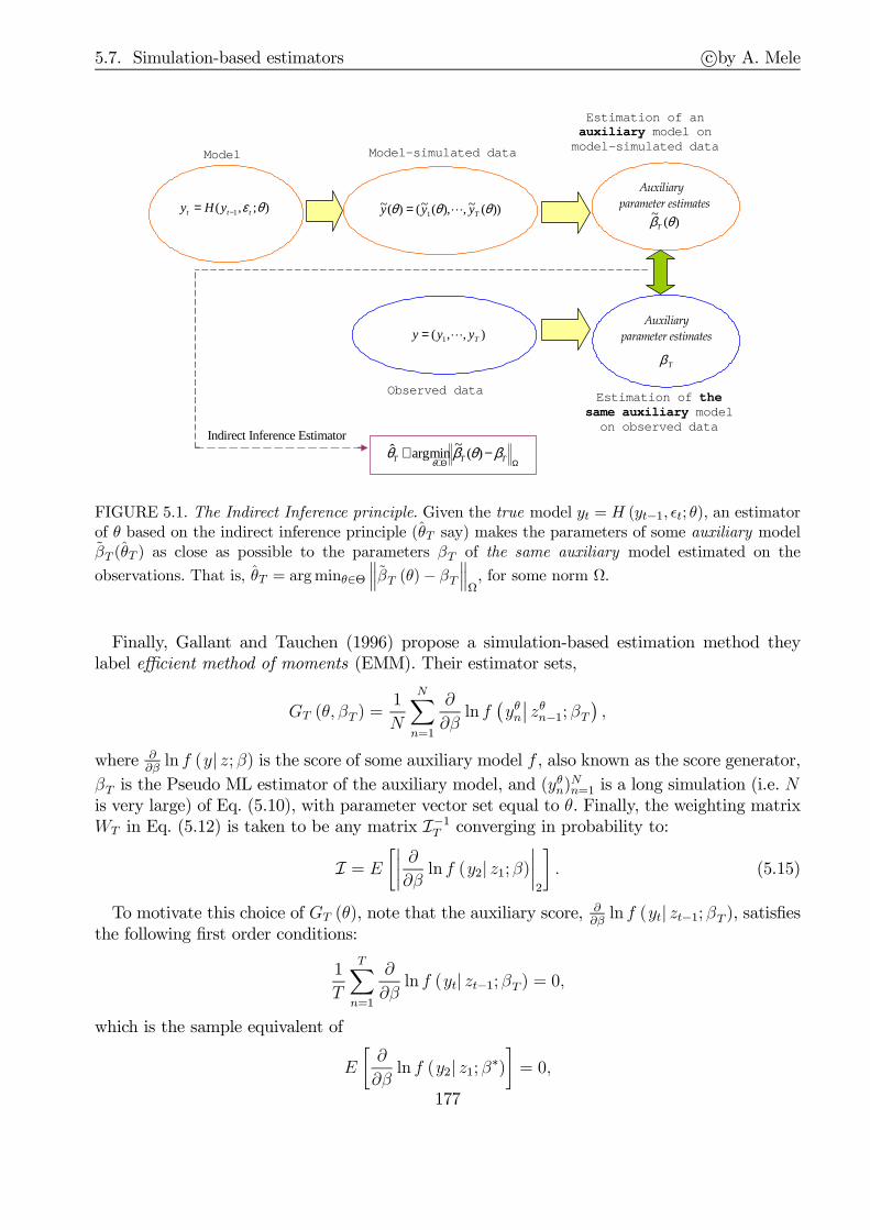
5.7. Simulation-based estimators c©by A. Mele
),,( 1 Tyyy L=
);,( 1 θεttt yHy −=
Model
Auxiliary
parameter estimates
)(~ θβT
Sss
ΩΘ∈
−∈ TTT βθβθθ
)(~
minargˆ
))(~,),(~()(~1 θθθ Tyyy L=
Model-simulated data
Estimation of an auxiliary model on model-simulated data
Observed data
Auxiliary
parameter estimates
Tβ
Estimation of the
same auxiliary model on observed data
Indirect Inference Estimator
FIGURE 5.1. The Indirect Inference principle. Given the true model yt = H (yt−1, ǫt; θ), an estimatorof θ based on the indirect inference principle (θT say) makes the parameters of some auxiliary modelβT (θT ) as close as possible to the parameters βT of the same auxiliary model estimated on the
observations. That is, θT = argminθ∈Θ∥∥∥βT (θ)− βT
∥∥∥Ω, for some norm Ω.
Finally, Gallant and Tauchen (1996) propose a simulation-based estimation method theylabel efficient method of moments (EMM). Their estimator sets,
GT (θ, βT ) =1
N
N∑
n=1
∂
∂βln f
(yθn
∣∣ zθn−1; βT),
where ∂∂βln f (y| z; β) is the score of some auxiliary model f , also known as the score generator,
βT is the Pseudo ML estimator of the auxiliary model, and (yθn)Nn=1 is a long simulation (i.e. N
is very large) of Eq. (5.10), with parameter vector set equal to θ. Finally, the weighting matrixWT in Eq. (5.12) is taken to be any matrix I−1
T converging in probability to:
I = E[∣∣∣∣∂
∂βln f (y2| z1;β)
∣∣∣∣2
]. (5.15)
To motivate this choice of GT (θ), note that the auxiliary score, ∂∂βln f (yt| zt−1; βT ), satisfies
the following first order conditions:
1
T
T∑
n=1
∂
∂βln f (yt| zt−1;βT ) = 0,
which is the sample equivalent of
E
[∂
∂βln f (y2| z1;β∗)
]= 0,
177
5.7. Simulation-based estimators c©by A. Mele
for some β∗. Likewise, we must have that with θ = θ0, GT (θ0, βT ) = 0, for large N . All in all,we want to find a stochastic process H (yt, ǫt+1; ·) in Eq. (5.10), or a parameter vector θ suchthat the expectation of the score of the auxiliary model is zero, a very property of the score,arising even when the model is misspecified.
5.7.2 Asymptotic normality
We show, heuristically, how asymptotic normality obtains for the three estimators of Section5.7.1, and then, define conditions under which asymptotic efficiency might obtain for the EMM.
5.7.2.1 SMM
Let,
Σ0 =∞∑
j=−∞E
[(f ∗t − E (f∗t ))
(f ∗t−j − E
(f ∗t−j
))⊤],
and suppose thatWT
p→ W0 = Σ−10 .
We now demonstrate that under this condition, as T →∞ and S (T )→∞,
√T (θT − θ0) d→ N
(0p, (1 + τ)
(D⊤0 Σ
−10 D0
)−1), (5.16)
where τ = limT→∞T
S(T ), D0 = E (∇θG∞ (θ0)) = E
(∇θf
θ0∞), and the notation G∞ means that
G. is drawn from its stationary distribution.Indeed, the first order conditions satisfied by the SMM in Eq. (5.12) are,
0p = [∇θGT (θT )]⊤WTGT (θT ) = [∇θGT (θT )]
⊤WT · [GT (θ0) +∇θGT (θ0) (θT − θ0)] + op (1) .
That is,
√T (θT − θ0) d
= −([∇θGT (θT )]
⊤WT∇θGT (θ0))−1
[∇θGT (θT )]⊤WT ·
√TGT (θ0)
d= −
(D⊤0 W0D0
)−1D⊤0 W0 ·
√TGT (θT )
= −(D⊤0 Σ
−10 D0
)−1D⊤0 Σ
−10 ·
√TGT (θ0) . (5.17)
We have,
√TGT (θ0) =
√T · 1
T
T∑
t=1
(f ∗t −
1
S (T )
S(T )∑s=1
f θ0s
)
=1√T
T∑
t=1
(f ∗t −E (f∗∞))−√T√
S (T )· 1√
S (T )
S(T )∑
s=1
(fθ0s − E
(f θ0∞))
d→ N (0, (1 + τ )Σ0) ,
where we have used the fact that E (f ∗∞) = E(f θ0∞). By using this result into Eq. (5.17) produces
the convergence in Eq. (5.16). If τ = limT→∞T
S(T )= 0 (i.e. if the number of simulations grows
more fastly than the sample size), the SMM estimator is as efficient as the GMM estimator.Finally, and obviously, we need that τ = limT→∞
TS(T )
< ∞: the number of simulations S (T )cannot grow more slowly than the sample size.
178
5.7. Simulation-based estimators c©by A. Mele
5.7.2.2 Indirect inference
The IIP-based estimator works slightly differently. For this estimator, even if the number ofsimulations S is fixed, asymptotic normality obtains without requiring S to go to infinity morefastly than the sample size. Basically, what really matters here is that ST goes to infinity.By Eq. (5.17), and the discussion in Section 5.7.1, we know that asymptotically, the first
order conditions satisfied by the IIP-based estimator are,
√T (θT − θ0) d
= −(D⊤0 W0D0
)−1D⊤0 W0 ·
√TGT (θ0) ,
where GT is as in Eq. (5.14), D0 = ∇θb (θ), and b (θ) is solution to the limiting problemcorresponding to the estimator in Eq. (5.13), viz
β (θ) = argmaxβ
(limT→∞
1
TlnL
(yT1 ; β
)).
We need to find the distribution of GT in Eq. (5.14). We have,
√TGT (θ0) =
1
S
S∑
s=1
√T (βT − βsT (θ0))
=1
S
S∑
s=1
√T [(βT − β0)− (βsT (θ0)− β0)]
=√T (βT − β0)−
1
S
S∑
s=1
√T (βsT (θ0)− β0) ,
where β0 = β (θ0). Hence, given the independence of the sample and the simulations,
√TGT (θ0)
d→ N
(0,
(1 +
1
S
)·Asy.Var
(√TβT
)).
That is, asymptotically S can be fixed with respect to T .
5.7.2.3 Efficient method of moments
We have,
θT = argminθGT (θ, βT )
⊤WTGT (θ, βT ) , GT (θ, βT ) =1
N
N∑
n=1
∂
∂βln f
(yθn∣∣ zθn−1;βT
).
The first order conditions are:
0 = ∇θGT (θT , βT )⊤WTGT (θT , βT )
d= ∇θGT (θ0, βT )
⊤WT (GT (θ0, βT ) +∇θGT (θ0, βT ) (θT − θ0)) ,
or
√T (θT − θ0) d
= −(∇θGT (θ0, βT )
⊤WT∇θGT (θ0, βT ))−1
∇θGT (θ0, βT )⊤WT
√TGT (θ0, βT ) .
179

5.7. Simulation-based estimators c©by A. Mele
We have, for some β∗,√TGT (θ0, βT )
d= J
√T (βT − β∗)
d→ N (0, I) ,
where J = E(
∂∂β∂β⊺
ln f (y2| y1; β))and I is as in Eq. (5.15). Hence,
√T (θT − θ0) d→ N (0, V ) ,
where,
V =(∇θG
⊤W∇θG)−1∇θG
⊤WIW⊤∇θG(∇θG
⊤W∇θG)−1
.
With W = I−1, this variance collapses to,
V =(∇θG
⊤I−1∇θG)−1
. (5.18)
5.7.2.4 Spanning scores
This section provides a heuristic discussion of the conditions under which the EMM achieves theCramer-Rao lower bound. Consider the following definition, which is similar to that in Tauchen(1997). Of a given span of moment conditions sf , say that of the EMM, we say that it alsospans the true score if,
var (s| sf ) = 0, (5.19)
where s denotes the true score. From Eq. (5.18), we know that the asymptotic variance of theEMM, say varEMM, satisfies:
var−1EMM ≡ V −1 = ∇θG
⊤var (sf)−1∇θG.
By the linear projection,
s = Bsf + ǫ, B = cov (s, sf) var (sf)−1 ,
we have,
var−1MLE = var (s) = Bvar (sf )B
⊤+ var (s| sf) = cov (s, sf ) var (sf )−1 cov (s, sf )⊤+ var (s| sf) ,
(5.20)where varMLE denotes the asymptotic variance of the MLE. We claim that:
cov (s, sf)⊤ = ∇θG. (5.21)
Indeed, under regularity conditions,
∇θG (θ0, β∗) =
[∂
∂θ
(∫∂
∂βln f (y; β∗) p (y, θ) dy
)]
θ=θ0
=
∫∂
∂βln f (y;β∗)
∂
∂θp (y, θ0) dy
=
∫ (∂
∂βln f (y; β∗)
∂
∂θln p (y, θ0)
)p (y, θ0) dy
= cov (s, sf)⊤ ,
where p (y, θ0) is the true density. Next, replace Eq. (5.21) into Eq. (5.20),
var−1MLE = ∇θG
⊤var (sf)−1∇θG+ var (s| sf) = var−1
EMM + var (s| sf) .Therefore, the EMM estimator achieves the Cramer-Rao lower bound under the spanning con-dition in Eq. (5.19).
180

5.7. Simulation-based estimators c©by A. Mele
5.7.3 A fourth simulation-based estimator: Simulated maximum likelihood
Estimating the parameters of stochastic differential equations is a recurrent theme in empiricalfinance. Consider a continuous time model,
dy (τ ) = b (y (τ ) ; θ) dτ +Σ(y (τ) ; θ) dW (τ ) , (5.22)
whereW (τ) is a Brownian motion and b and Σ are two functions guaranteeing a strong solutionto Eq. (5.22). Except in special cases (e.g., the affine models reviewed in Chapter 12), thelikelihood function of the data generated by this process is unknown. We can then use one ofthe three estimators we have presented in section 5.7.1. Alternatively, we might use simulatedmaximum likelihood, a method introduced in finance by Santa-Clara (1995) (see, also, Brandtand Santa-Clara, 2002). We only provide the idea of the method, not the asymptotic theory.Suppose, then, that we observe discretely sample data generated by Eq. (5.22): y0, y1,· · · , yt,
· · · , yT , where T is the sample size. We need to know the transition density, say p (yt+1| yt; θ),to implement maximum likelihood, which we assume we do not know. Consider, then, the Eulerapproximation to Eq. (5.22),
y(k+1)/n = yk/n + b(yk/n; θ
) 1n+Σ
(yk/n; θ
)√1
nǫk+1, (5.23)
where ǫk is a sequence of i.i.d. random variables with expectation zero and unit variance. Thisstochastic process is defined at the dates k
n, for k integer. Let [Tn] denote the integer part of
Tn, and for k = 1, · · · , [Tn], set
y(n)τ = yk/n, ifk
n≤ τ ≤ k + 1
n.
In other words, we are chopping the time interval between two observations, [t, t+ 1], in n
pieces, and then take n to be large. We know that as n → ∞, y(n)t ⇒ y (t) as n → ∞,
where⇒ denotes “weak convergence,” or “convergence in distribution,” meaning that all finitedimensional distributions of y
(n)t converge to those of y (t) as n → ∞. The idea underlying
simulated maximum likelihood, then, is to estimate the transition density, p (yt+1| yt; θ), throughsimulations of Eq. (5.23), performed using a large value of n. Note, we cannot guarantee thetransition density is recovered by simulating Eq. (5.23), not even for a large value of n. We canonly perform an imperfect simulation of Eq. (5.23).The likelihood function is,
L = p (y0; θ)T−1∏
t=0
p (yt+1| yt; θ) ,
where p (y0; θ) denotes the marginal density of the first observation, y0.Let pn (y′| y; θ) the transition density of the data generated by Eq. (5.23). Then, if ǫ is
normally distributed,
pn(y(k+1)/n
∣∣ yk/n; θ)= ϕ
(y(k+1)/n; yk/n + b
(yk/n; θ
) 1n; Σ2
(yk/n; θ
) 1n
),
181

5.7. Simulation-based estimators c©by A. Mele
where ϕ (u;µ; σ2) denotes the Gaussian density with mean µ and variance σ2. Moreover, wehave, approximately,
pn (yt+1| yt; θ) =∫pn (yt+1| x; θ) pn (x| yt; θ) dx
=
∫ϕ
(yt+1;x+ b (x; θ)
1
n; Σ2 (x; θ)
1
n
)pn (x| yt; θ) dx,
where we have set x = yt+1− 1n. We may, now, draw values of x from pn (x| yt; θ), as explained
in a moment, and estimate pn (yt+1| yt; θ) through:
pn,S (yt+1| yt; θ) ≡1
S
S∑
j=1
ϕ
(y(k+1)/n; x
j + b(xj; θ
) 1n; Σ2
(xj; θ
) 1n
),
where xj is obtained by iterating Eq. (5.23) from time t to time t + 1 − 1n. Under regularity
conditions, we have that for all θ ∈ Θ, supy′,y∣∣pn,S (y′| y; θ)− p (y′| y; θ)
∣∣ → 0 as n and S get
large, with√Sn→ 0.
5.7.4 Advances
The three estimators that we have examined in Sections 5.7.1-5.7.2, are general-purpose, but ingeneral, they do not lead to to asymptotic efficiency, unless the true score belongs to the spanof the moment conditions, as explained in Section 5.7.2.4. There exist other simulation-basedmethods, which aim to approximate the likelihood function through simulations (e.g., Lee, 1995;Hajivassiliou and McFadden, 1998): for example, the simulated maximum likelihood estimatorin Section 5.7.2.3 can be used to estimate the parameters of stochastic differential equations.While methods based on simulated likelihood lead to asymptotically efficient estimators, theyaddress specific estimation problems, just as the example of Section 5.7.2.3 illustrates.There exist estimators that are both general purpose and that can lead to asymptotic effi-
ciency. Fermanian and Salanié (2004) consider an estimator that relies on approximating thelikelihood function through kernel estimates obtained simulating the model of interest. Carrasco,Chernov, Florens and Ghysels (2007) rely on a “continuum of moment conditions” matchingmodel-based (simulated) characteristic functions to data-based characteristic functions. Al-tissimo and Mele (2009) propose an estimator based on a continuum of moment conditions,which minimizes a certain distance between conditional densities estimated with the true dataand conditional densities estimated with data simulated from the model, where both conditionaldensities are estimated through kernel methods.
5.7.5 In practice? Latent factors and identification
The estimation theory of this section does not rule out the situation where some of the variablesin Eq. (5.10) are unobservable. The principle to follow is very simple, one applies any of themethods we have discussed to those variables simulated out of Eq. (5.10), which correspond tothe observed ones. For example, we may want to estimate the following model of the short-termrate r (τ), discussed at length in Chapter 12:
dr (τ) = κr (r − r (τ)) dτ +√v (τ)dW1 (τ )
dv (τ) = κv (v − v (τ)) dτ + ξ√v (τ )dW2 (τ)
(5.24)
182

5.8. Asset pricing, prediction functions, and statistical inference c©by A. Mele
where v (τ) is the short-term rate instantaneous, stochastic variance, W1 and W2 are two stan-dard Brownian motions, and the parameter vector of interest is θ = [κr r κv v ξ]. Let us considerone of the methods discussed so far, say indirect inference. The logical steps to follow, then,are (i) to simulate Eqs. (5.24), and (ii) to calibrate an auxiliary model to the short term ratedata simulated out of Eqs. (5.24) which is as close as possible to the very same auxiliary modelfitted on true data. Note, in doing so, we just have to neglect the volatility data simulated outof Eqs. (5.24), as these data are obviously unobservable.The question arises, therefore, as to whether the auxiliary model one chooses is rich enough
to allow identifying the model’s parameter vector θ. There might be many combinations ofunobserved random processes v (τ) that are consistent with the likelihood of any given auxiliarymodel. So which auxiliary model to fit, in practice? Gallant and Tauchen (1996) asked thisquestion long time ago. Needless to mention, there are no general answers to this question.Very simply, one requires the model to be identifiable, which is likely to happen once theauxiliary model is “rich enough.” In an impressive series of applied work, Gallant and Tauchenand their co-authors have proposed semi-nonparametric score generators, as a way to get asclose as possible to a “rich” model. Intuitively, by increasing the order of Hermite expansions,semi-nonparametric scores might converge to the true ones. Alternatively, one might use acontinuum of moment conditions, as explained in Section 5.7.4. For example, the nonparametricdensity estimates in Altissimo and Mele (2009) converge to the true ones, once the bandwidthparameters used to smooth out these these estimates is sufficiently fine. In the next section,we provide a discussion of how asset prices might help convey information about unobservedprocesses and lead to statistical efficiency.
5.8 Asset pricing, prediction functions, and statistical inference
We develop conditions, which ensure the feasibility of estimation methods in a context wherean unobservable multidimensional process is estimated in conjunction with prediction func-tions suggested by asset pricing models.4 We assume that the data generating process is amultidimensional partially observed diffusion process solution to,
dy (τ ) = b (y (τ ) ; θ) dτ +Σ(y (τ) ; θ) dW (τ ) , (5.25)
where W is a multidimensional process and (b,Σ) satisfy some regularity conditions we singleout below. We analyze situations where the original partially observed system in Eq. (5.25)can be estimated by augmenting it with a number of observable deterministic functions of thestate. In many situations, such deterministic functions are suggested by asset pricing theoriesin a natural way. Typical examples include the price of derivatives or in general, any functionalof asset prices (such as asset returns, bond yields, implied volatilities).The idea to use asset pricing predictions to improve the fit of models with unobservable
factors has been explored at least by, e.g., Christensen (1992), Pastorello, Renault and Touzi(2000), Chernov and Ghysels (2000), Singleton (2001), and Pastorello, Patilea and Renault(2003).We consider a standard Markov pricing setting. For fixed t ≥ 0, we let M be the expiration
date of a contingent claim with rational price process c = c(y(τ ),M − τ )τ∈[t,M), and letz(y(τ))τ∈[t,M ] andΠ(y) be the associated intermediate payoff process and final payoff function,
4This section is based on an unpublished appendix of Altissimo and Mele (2009).
183
5.8. Asset pricing, prediction functions, and statistical inference c©by A. Mele
respectively. Let ∂/ ∂τ+L be the usual infinitesimal generator of the system in Eq. (5.25), takenunder the risk-neutral probability. Then, as we saw in Chapter 4, we have that in a frictionless,arbitrage-free market, c is the solution to the following partial differential equation:
0 =
(∂
∂τ+ L−R
)c(y,M − τ) + z(y), ∀(y, τ ) ∈ Y × [t,M)
c(y, 0) = Π(y), ∀y ∈ Y(5.26)
where R ≡ R(y) is the short-term rate. We call prediction function any continuous and twicedifferentiable function c (y;M − τ) solution to the partial differential equation and boundarycondition in (5.26). Examples of contingent claims with prices satisfying (5.26) are derivatives,typically.Next, we augment the system in Eq. (5.25) with d− q prediction functions, where q denotes
the number of the observable variables in Eq. (5.25). Precisely, we let:
C(τ ) ≡ (c (y(τ),M1 − τ) , · · · , c (y(τ),Md−q − τ )) , τ ∈ [t,M1]
where Mid−qi=1 is an increasing sequence of fixed maturity dates. Furthermore, we define themeasurable vector valued function:
φ (y(τ ); θ, γ) ≡ (yo(τ ), C (y(τ ))) , τ ∈ [t,M1], (θ, γ) ∈ Θ× Γ, (5.27)
where yo(τ) denotes the vector of observable variables in Eq. (5.25), and Γ ⊂ Rpγ is a compactparameter set containing additional parameters. These new parameters arise from the change ofmeasure leading to the pricing model in Eq. (5.27), and are now part of our estimation problem.We assume that the pricing model in Eq. (5.27) is correctly specified. That is, all contingent
claim prices in the economy are taken to be generated by the prediction function c(y,M−τ ) forsome (θ0, γ0) ∈ Θ×Γ. For simplicity, we also consider a stylized situation in which all contingentclaims have the same contractual characteristics specified by C ≡ (z,Π). More generally, onemay define a series of classes of contingent claims CjJj=1, where the class of contingent claimsj has provisions specified by Cj ≡ (zj,Πj). As an example, assets belonging to the class C1 canbe European options, assets belonging to the class C1 can be bonds. The number of predictionfunctions that we would introduce in this case would be equal to d− q =∑J
j=1Mj, where M j
is the number of prediction functions within class of assets j. To keep the presentation simple,we do not consider such a more general situation.
The objective is to define estimators of the parameter vector (θ0, γ0), under which obser-vations were generated. We want to use any of the simulation methods reviewed in Section5.7 to produce an estimator of (θ0, γ0). The idea, as usual, is to make the finite dimensionaldistributions of φ implied by the pricing model in Eq. (5.27) and the fundametals in Eq. (5.26)as close as possible to the sample counterparts of φ. Let Φ ⊆ Rd be the domain on which φtakes values. As illustrated by Figure 5.2, we want to move from the unfeasible domain Y ofthe original state variables in Eq. (5.25) (observables and not) to the domain Φ on which onlyobservable variables take value. Ideally, we would like to implement such a change in domainin order to recover as much information as possible about the original unobserved process in(5.25). Clearly, φ is fully revealing whenever it is globally invertible. However, we will show thatestimation is feasible even when φ is only locally one-to-one.An important feature of the theory in this section is that it does not hinge upon the avail-
ability of contingent prices data covering the same sample period covered by the observables
184

5.8. Asset pricing, prediction functions, and statistical inference c©by A. Mele
ΦY
φ−1(y; θ0,γ0)
φ(y; θ0,γ0)
FIGURE 5.2. Asset pricing, the Markov property, and statistical efficiency. Y is the domain on whichthe partially observed primitive state process y ≡ (yo yu)⊤ takes values, Φ is the domain on whichthe observed system φ ≡ (yo C(y))⊤ takes values in Markovian economies, and C(y) is a contingent
claim price process in Rd−q∗
. Let φc = (yo, c(y, ℓ1), · · ·, c(y, ℓd−q∗)), where c(y, ℓj)d−q∗
j=1 forms anintertemporal cohort of contingent claim prices, as in Definition 5.3. If the local restrictions of φ areone-to-one and onto, statistical inference about θ and γ can be made, using information about the priceof derivative contracts, φc. If φ is also globally invertible, statistical inference can lead to first-orderasymptotic efficiency, once conditioned upon φc.
in Eq. (5.25). First, the price of a given contingent claim is typically not available for a longsample period. As an example, available option data often include option prices with a life spansmaller than the usual sample span of the underlying asset prices. By contrast, it is commonto observe long time series of option prices having the same maturity. Second, the price of asingle contingent claim depends on the time-to-maturity of the claim; therefore, it does notsatisfy the stationarity assumptions maintained in this paper. To address these issues, we dealwith data on assets having the same characteristics at each point in time. Precisely, considerthe data generated by the following random processes:
D 5.3. (Intertertemporal (ℓ,N)-cohort of contingent claim prices) Given a predictionfunction c (y;M − τ) and a N-dimensional vector ℓ ≡ (ℓ1, · · · , ℓN ) of fixed time-to-maturity,an intertemporal (ℓ,N)-cohort of contingent claim prices is any collection of contingent claimprice processes c (τ , ℓ) ≡ (c(y(τ), ℓ1), · · · , c(y(τ), ℓN)) (τ ≥ 0) generated by the pricing model(5.27).
Consider for example a sample realization of three-months at-the-money option prices, ora sample realization of six-months zero-coupon bond prices. Long sequences such as the onesin these examples are common to observe. If these sequences were generated by the pricingmodel in Eq. (5.27), as in Definition 5.3, they would be deterministic functions of y, and hencestationary. We now develop conditions ensuring both feasibility and first-order efficiency of theclass of simulation-based estimators, as applied to this kind of data. Let a denote the matrixhaving the first q rows of Σ, the diffusion matrix in Eq. (5.25). Let ∇C denote the Jacobian ofC with respect to y. We have:
T 5.4. (Asset pricing and Cramer-Rao lower bound) Suppose to observe an intertem-poral (ℓ, d−q)-cohort of contingent claim prices c (τ , ℓ), and that there exist prediction functionsC in Rd−q with the property that for θ = θ0 and γ = γ0,
(a(τ ) · Σ(τ)−1
∇C(τ)
) = 0, P ⊗ dτ -a.s. all τ ∈ [t, t+ 1], (5.28)
185

5.8. Asset pricing, prediction functions, and statistical inference c©by A. Mele
where C satisfies the initial condition C(t) = c (t, ℓ) ≡ (c(y(t), ℓ1), · · · , c(y(t), ℓd−q)). Letφct = (yo(t), c(y(t), ℓ1), · · · , c(y(t), ℓd−q)). Then, any simulation-based estimator applied to φctis feasible. Moreover, asssume φct is also Markov. Then, any estimator with a span of momentconditions for φct that also spans the true score, attains the Cramer-Rao lower bound, withrespect to the fields generated by φct.
According to Theorem 5.4, any estimator is feasible, whenever φ is locally invertible for atime span equal to the sampling interval. As Figure 5.2 illustrates, condition (5.28) is satisfiedwhenever φ is locally one-to-one and onto.5 If φ is also globally invertible for the same timespan, φc is Markov. The last part of this theorem says that in this case, any estimator isasymptotically efficient. We emphasize that this conclusion is about first-order efficiency in thejoint estimation of θ and γ given the observations on φc.Naturally, condition (5.28) does not ensure that φ is globally one-to-one and onto: φ might
have many locally invertible restrictions.6 In practice, φ might fail being globally invertiblebecause monotonicity properties of φ may break down in multidimensional diffusion models.For example, in models with stochastic volatility, option prices can be decreasing in the under-lying asset price (see Bergman, Grundy and Wiener, 1996). In models of the yield curve withstochastic volatility, to cite a second example, medium-long term bond prices can be increasingin the short-term rate (see Mele, 2003). These cases might arise as there is no guarantee thatthe solution to a stochastic differential system is nondecreasing in the initial condition of oneif its components, which is, instead, always true in the scalar case.When all components of vector yo represent the prices of assets actively traded in frictionless
markets, (5.28) corresponds to a condition ensuring market completeness in the sense of Harrisonand Pliska (1983). As an example, condition (5.28) for Heston’s (1993) model is ∂c/ ∂σ =0 P ⊗ dτ -a.s, where σ denotes instantaneous volatility of the price process. This condition issatisfied by the Heston’s model. In fact, Romano and Touzi (1997) showed that within a fairlygeneral class of stochastic volatility models, option prices are always strictly increasing in σwhenever they are convex in Q. Theorem 5.4 can be used to implement efficient estimators inother complex multidimensional models. Consider for example a three-factor model of the yieldcurve. Consider a state-vector (r, σ, ℓ), where r is the short-term rate and σ, ℓ are additionalfactors (such as, say, instantaneous short-term rate volatility and a central tendency factor). Letu(i) = u (r(τ ), σ(τ ), ℓ(τ );Mi − τ) be the time τ rational price of a pure discount bond expiringat Mi ≥ τ , i = 1, 2, and take M1 < M2. Let φ ≡ (r, u(1), u(2)). Condition (5.28) for this modelis then,
u(1)σ u(2)ℓ − u(1)ℓ u
(2)σ = 0, P ⊗ dt-a.s. τ ∈ [t, t+ 1], (5.29)
where subscripts denote partial derivatives. It is easily checked that this same condition must besatisfied by models with correlated Brownian motions and by yet more general models. Classesof models of the short-term rate for which condition (5.29) holds are more intricate to identifythan in the European option pricing case seen above (see Mele, 2003).
5Local invertibility of φ means that for every y ∈ Y , there exists an open set Y∗ containing y such that the restriction of φ toY∗ is invertible. Let Jφ denote the Jacobian of φ. Then, we have that φ is locally invertible on Y∗ if detJφ = 0 on Y∗, which iscondition (5.28).
6As an example, consider the mapping R2 → R2 defined as φ(y1, y2) = (ey1 cos y2, ey1 sin y2). The Jacobian satisfiesdetJφ(y1, y2) = e2y1 , yet φ is 2π-periodic with respect to y2. For example, φ(0, 2π) = φ(0, 0).
186

5.9. Appendix 1: Proof of selected results c©by A. Mele
5.9 Appendix 1: Proof of selected results
P E$. (5.2). We have: P (A1⋂A2) = P (A1) · P (A2 |A1 ). Consider the event E ≡ A1
⋂A2.
We still have,
Pr (A3 |A1⋂A2 ) = Pr (A3 |E ) =
Pr (A3⋂E)
Pr (E)=
Pr (A3⋂A1
⋂A2)
Pr (A1⋂A2)
.
That is,
Pr
(3⋂i=1
Ai
)= Pr (A1
⋂A2) · Pr (A3 |A1
⋂A2 ) = Pr (A1) · Pr (A2 |A1 ) · Pr (A3 |A1
⋂A2 ) .
Continuing, we obtain Eq. (5.2). ‖
187

5.10. Appendix 2: Collected notions and results c©by A. Mele
5.10 Appendix 2: Collected notions and results
C ./ ( 22). A sequence of random vectors xT converges in probability to therandom vector x if for each ǫ > 0, δ > 0 and each i = 1, 2, · · · ,N , there exists a Tǫ,δ such that forevery T ≥ Tǫ,δ,
Pr (|xTi − xi| > δ) < ǫ.
This is succinctly written as xTp→ x, or plim xT = x, if x ≡ x, a constant.
Convergence in probability generalizes the standard notion of a limit of a deterministic sequence.Of a deterministic sequence xT , we say it converges to some limit x if, for κ > 0, there exists a Tκ :for each T ≥ Tκ we have that |xT − x| < κ. Convergence in probability can also be restated as sayingthat:
limT→∞
Pr (|xTi − xi| > δ) = 0.
The following is a stronger notion of convergence:
A ( ./ (. A sequence of random vectors xT converges almost surely to therandom vector x if, for each i = 1, 2, · · · ,N , we have:
Pr (ω : xTi(ω)→ xi) = 1,
where ω denotes the entire random sequence xTi. This is succinctly written as xTa.s.→ x.
Almost sure convergence implies convergence in probability. Convergence in probability meansthat for each ǫ > 0, limT→∞ Pr (ω : |xTi(ω)− xi| < ǫ) = 1. Almost sure convergence requires thatPr (limT→∞ xTi → xi) = 1 or that
limT ′→∞
Pr
(supT≥T ′
|xTi − xi| > δ
)= lim
T ′→∞Pr
(⋃
T≥T ′|xTi − xi| > δ
)= 0.
Next, assume that the second order moments of all xi are finite. We have:
C ./ ( $,( . A sequence of random vectors xT converges in quadraticmean to the random vector x if for each i = 1, 2, · · · , N , we have:
limT ′→∞
E[(xTi − xi)
2]→ 0.
This is succinctly written as xTq.m.→ x.
R. By Chebyshev’s inequality,
Pr (|xTi − xi| > δ) ≤ E[(xTi − xi)2]
δ2,
which shows that convergence in quadratic mean implies convergence in probability.We now turn to a weaker notion of convergence:
C ./ ( ,2 . Let fT (·)T be the sequence of probability distributions (that is,fT (x) = pr (xT ≤ x)) of the sequence of the random vectors xT. Let x be a random vector withprobability distribution f(x).A sequence xT converges in distribution to x if, for each i = 1, 2, · · · , N ,we have:
limT→∞
fT (x) = f(x).
188

5.10. Appendix 2: Collected notions and results c©by A. Mele
This is succinctly written as xTd→ x.
The following two results are useful to the purpose of this chapter:
S3)’ . If yTp→ y and xT
d→ x, then:
yT · xT d→ y · x.
C-W, ,.(. Let λ be a N-dimensional vector of constants. We have:
xTd→ x⇔ λ⊤ · xT d→ λ⊤ · x.
The following example illustrates the Cramer-Wold device. If λ⊤ · xT d→ N(0;λ⊤Σλ
), then xT
d→N (0;Σ).
We now state two laws about convergence in probability.
W # (N. 1) (Khinchine). Let xT be a i.i.d. sequence satistfying E(xT ) = µ < ∞ ∀T . Wehave:
xT ≡1
T
T∑
t=1
xtp→ µ.
W # (N. 2) (Chebyshev). Let xT be a sequence independent but not identically distributed,satisfying E(xT ) = µT <∞ and E
[(xT − µT )
2]= σ2
T <∞. If limT→∞ 1T 2
∑Tt=1 σ
2t → 0, then:
xT ≡1
T
T∑
t=1
xtp→ µT ≡
1
T
T∑
t=1
µt.
We now state and provide a proof of the central limit theorem in a simple setting.
C L T. Let xT be a i.i.d. sequence, satisfying E(xT ) = µ <∞ and E[(xT − µ)2
]
= σ2 <∞ ∀T . Let xT ≡ 1T
∑Tt=1 xt. We have,
√T (xT − µ)
σd→ N(0, 1).
The multidimensional version of this theorem requires a mere change in notation. For the proof, theclassic method relies on the characteristic functions. Let:
ϕ(t) ≡ E(eitx
)=
∫eitxf(x)dx, i ≡
√−1.
We have ∂r
∂trϕ(t)∣∣t=0
= irm(r), where m(r) is the r-th order moment. By a Taylor’s expansion,
ϕ(t) = ϕ(0) +∂
∂tϕ(t)
∣∣∣∣t=0
t+1
2
∂2
∂t2ϕ(t)
∣∣∣∣t=0
t2 + · · · = 1+ im(1)t−m(2)1
2t2 + · · · .
Next, let xT = 1T
∑Tt=1 xt, and consider the random variable,
YT ≡√T (xT − µ)
σ=
1√T
T∑
t=1
xt − µ
σ.
189

5.10. Appendix 2: Collected notions and results c©by A. Mele
The characteristic function of YT is the product of the characteristic functions of at ≡ xt−µ√Tσ
, which are
all the same: ϕYT (t) = (ϕa (t))T , where ϕa (t) = 1− t2
2T + · · · . Therefore,
ϕYT (t) = ϕ
(t√T
)T
=
(1− 1
2
t2
T+ o
(T−1
))T
.
Clearly, limT→∞ ϕYT (t) = e−12t2 , which is the characteristic function of a standard Gaussian variable.
190

5.11. Appendix 3: Theory for maximum likelihood estimation c©by A. Mele
5.11 Appendix 3: Theory for maximum likelihood estimation
Assume that θTa.s.→ θ0, and that H(y, θ) ≡ ∇θθ lnL(θ| y) exists, it is continuous in θ uniformly in y
and that we can differentiate twice inside the integral∫L(θ| y)dy = 1. We have:
sT (θ) =1
T
T∑
t=1
∇θ lnL (θ| y) .
Consider the c-parametrized curves θ(c) = c(θ0 − θT ) + θT where, for all c ∈ (0, 1)p and θ ∈ Θ, cθdenotes a vector in Θ where the ith element is c(i)θ(i). By the intermediate value theorem, there existsthen a c∗ in (0, 1)p such that we have almost surely:
sT (θT ) = sT (θ0) +HT (θ∗) · (θT − θ0),
where θ∗ ≡ θ(c∗) and:
HT (θ) =1
T
T∑
t=1
H(θ| yt).
The first order conditions tell us that sT (θT ) = 0. Hence,
0 = sT (θ0) +HT (θ∗T ) · (θT − θ0).
We also have that:
|HT (θ∗T )−HT (θ0)| ≤1
T
T∑
t=1
|H (θ∗T )−HT (θ0)| ≤ sup |H (θ∗T )−HT (θ0)| , (5A.1)
where the supremum is taken over the set of all the observations. Since θTa.s.→ θ0, we also have that
θ∗Ta.s.→ θ0. Moreover, by the law of large numbers,
HT (θ0) =1
T
T∑
t=1
H (θ0| yt) p→ E [H (θ0| yt)] = −J (θ0) . (5A.2)
Since H is continuous in θ uniformly in y, the inequality in (5A.1), and (5A.2) both imply that:
HT (θ∗T )a.s.→ −J (θ0) .
Therefore, as T →∞,
√T(θT − θ0
)= −H−1
T (θ0) · sT (θ0)√T = J−1 ·
√TsT (θ0).
By the central limit theorem, and E (sT ) = 0, the score, sT (θ0) =1T
∑Tt=1 s (θ0, yt), is such that
√T · sT (θ0)
d→ N (0, var (s (θ0, yt))) ,
wherevar (s (θ0, yt)) = J .
The result follows by the Slutzky’s theorem and the symmetry of J .Finally, one should show the existence of a sequence θT converging a.s. to θ0. Proofs on this type
of convergence can be found in Amemiya (1985), or in Newey and McFadden (1994).
191

5.12. Appendix 4: Dependent processes c©by A. Mele
5.12 Appendix 4: Dependent processes
5.12.1 Weak dependence
Let σ2T = var(
∑Tt=1 xt), and assume that that σ2
T = O(T ), and that σ2T = O
(T−1
). If
σ−1T
T∑
t=1
(xt −E(xt))d→ N (0, 1) ,
we say that xt is weakly dependent. Of a process, we say it is “nonergodic,” when it exhibits such astrong dependence that it does not even satisfy the law of large numbers.
• Stationarity
• Weak dependence
• Ergodicity
5.12.2 The central limit theorem for martingale differences
Let xt be a martingale difference sequence with E(x2t
)= σ2
t <∞ for all t, and define xT ≡1
T
∑Tt=1 xt,
and σ2T ≡
1
T
∑Tt=1 σ
2t . Let,
∀ǫ > 0, limT→∞
1
T σ2T
T∑
t=1
x2t I|xt|≥ǫ·T ·σ2T= 0, and
1
T
T∑
t=1
x2t − σ2T
p→ 0.
Under the previous condition, √T · xTσT
d→ N (0, 1) .
5.12.3 Applications to maximum likelihood
We use the central limit theorem for martingale differences to prove asymptotic normality of the MLE,in the case of weakly dependent processes. We have,
lnLT (θ) =T∑
t=1
ℓt (θ) , ℓt (θ) ≡ ℓ (θ; yt|xt) .
The MLE satisfies the following first order conditions,
0p = ∇θ lnLT (θ)|θ=θTd=
T∑
t=1
∇θℓt(θ)|θ=θ0+
T∑
t=1
∇θθℓt(θ)|θ=θ0(θT − θ0),
whence√T (θT − θ0)
d= −
[1
T
T∑
t=1
∇θθℓt(θ0)
]−11√T
T∑
t=1
∇θℓt(θ0). (5A.3)
We have:Eθ0 [∇θℓt+1(θ0)|Ft] = 0p,
which shows that ∂ℓt(θ0)∂θ is a martingale difference. Naturally, here we also have that:
Eθ0 ( |∇θℓt+1(θ0)|2|Ft) = −Eθ0 (∇θθℓt+1(θ0)|Ft) ≡ Jt (θ0) .192
5.12. Appendix 4: Dependent processes c©by A. Mele
Next, for a given constant c ∈ Rp, let:
xt ≡ c⊤∇θℓt(θ0).
Clearly, xt is also a martingale difference. Furthermore,
Eθ0
(x2t+1
∣∣Ft)= −c⊤Jt (θ0) c,
and because xt is a martingale difference, E (xtxt−i) = E [E (xt · xt−i|Ft−i)] = E [E (xt|Ft−i) · xt−i] =0, for all i. That is, xt and xt−i are mutually uncorrelated. It follows that,
var
(T∑
t=1
xt
)=
T∑
t=1
E(x2t
)
=T∑
t=1
c⊤Eθ0 (|∇θℓt(θ0)|2) c
=T∑
t=1
c⊤Eθ0 [Eθ0 ( |∇θℓt(θ0)|2|Ft−1)] c
= −T∑
t=1
c⊤Eθ0 [Jt−1 (θ0)] c
= −c⊤[
T∑
t=1
Eθ0 (Jt−1 (θ0))
]c.
Next, define:
xT ≡1
T
T∑
t=1
xt and σ2T ≡
1
T
T∑
t=1
E(x2t
)= −c⊤
[1
T
T∑
t=1
Eθ0 (Jt−1 (θ0))
]c.
Under the conditions underlying the central limit theorem for weakly dependent processes providedearlier, to be spelled out below, √
TxTσT
d→ N (0, 1) .
By the Cramer-Wold device,
[1
T
T∑
t=1
Eθ0 (Jt−1 (θ0))
]−1/21√T
T∑
t=1
∇θℓt(θ0)d→ N (0, Ip) .
The conditions that need to be satisfied are,
1
T
T∑
t=1
∇θθℓt (θ0)−1
T
T∑
t=1
Eθ0 [Jt−1 (θ0)]p→ 0, and plim
1
T
T∑
t=1
Eθ0 [Jt−1 (θ0)] ≡ J∞ (θ0) .
Under the previous conditions, it follows from Eq. (5A.3) that,
√T (θT − θ0)
d→ N(0p,J∞ (θ0)
−1).
193

5.13. Appendix 5: Proof of Theorem 5.4 c©by A. Mele
5.13 Appendix 5: Proof of Theorem 5.4
Let πt ≡ πt (φ (y(t+ 1),M− (t+ 1)1d−q)|φ (y(t),M− t1d−q)) denote the transition density of
φ (y(t),M− t1d−q) ≡ φ (y(t)) ≡ (yo(t), c(y(t),M1 − t), · · · , c(y(t),Md−q − t)),
where we have emphasized the dependence of φ on the time-to-maturity vector:
M− t1d−q ≡ (M1 − t, · · · ,Md−q − t).
By Σ(τ) full rank P ⊗ dτ -a.s., and Itô’s lemma, φ satisfies, for τ ∈ [t, t+ 1],
dyo(τ) = bo(τ)dτ + F (τ)Σ(τ)dW (τ)dc(τ) = bc(τ)dτ +∇c(τ)Σ(τ )dW (τ)
where bo and bc are, respectively, q-dimensional and (d − q)-dimensional measurable functions, andF (τ) ≡ a(τ)·Σ(τ)−1 P⊗dτ -a.s. Under condition (5.28), πt is not degenerate. Furthermore, C (y(t); ℓ) ≡C(t) is deterministic in ℓ ≡ (ℓ1, · · · , ℓd−q). That is, for all (c, c+) ∈ Rd ×Rd, there exists a function µsuch that for any neighbourhood N(c+) of c+, there exists another neighborhood N(µ(c+)) of µ(c+)such that,
ω ∈ Ω : φ (y(t+ 1),M− (t+ 1)1d−q) ∈ N(c+)
∣∣ φ (y(t),M− t1d−q) = c
=ω ∈ Ω : (yo(t+ 1), c(y(t+ 1),M1 − t)), · · · , c(y(t+ 1),Md−q − t)) ∈ N(µ(c+))
|φ (y(t),M− t1d−q) = c=
ω ∈ Ω : (yo(t+ 1), c(y(t+ 1),M1 − t)), · · · , c(y(t+ 1),Md−q − t)) ∈ N(µ(c+))
|(yo(t), c(y(t),M1 − t), · · · , c(y(t),Md−q − t)) = c
where the last equality follows by the definition of φ. In particular, the transition laws of φct givenφct−1 are not degenerate; and φct is stationary. The feasibility of simulation based method of momentsestimation is proved. The efficiency claim follows by the Markov property of φ, and the usual scoremartingale difference argument.
194

5.13. Appendix 5: Proof of Theorem 5.4 c©by A. Mele
References
Altissimo, F. and A. Mele (2009): “Simulated Nonparametric Estimation of Dynamic Models.”Review of Economic Studies 76, 413-450.
Amemiya, T. (1985): Advanced Econometrics. Cambridge, Mass.: Harvard University Press.
Bergman, Y. Z., B. D. Grundy, and Z. Wiener (1996): “General Properties of Option Prices.”Journal of Finance 51, 1573-1610.
Brandt, M. and P. Santa-Clara (2002): “Simulated Likelihood Estimation of Diffusions with anApplications to Exchange Rate Dynamics in Incomplete Markets.” Journal of FinancialEconomics 63, 161-210.
Carrasco, M., M. Chernov, J.-P. Florens and E. Ghysels (2007): “Efficient Estimation of Gen-eral Dynamic Models with a Continuum of Moment Conditions.” Journal of Econometrics140, 529-573.
Chernov, M. and E. Ghysels (2000): “A Study towards a Unified Approach to the Joint Esti-mation of Objective and Risk-Neutral Measures for the Purpose of Options Valuation.”Journal of Financial Economics 56, 407-458.
Christensen, B. J. (1992): “Asset Prices and the Empirical Martingale Model.” Working paper,New York University.
Duffie, D. and K. J. Singleton (1993): “Simulated Moments Estimation of Markov Models ofAsset Prices.” Econometrica 61, 929-952.
Fermanian, J.-D. and B. Salanié (2004): “A Nonparametric Simulated Maximum LikelihoodEstimation Method.” Econometric Theory 20, 701-734.
Fisher, R. A. (1912): “On an Absolute Criterion for Fitting Frequency Curves.” Messages ofMathematics 41, 155-157.
Gallant, A. R. and G. Tauchen (1996): “Which Moments to Match?” Econometric Theory 12,657-681.
Gauss, C. F. (1816): “Bestimmung der Genanigkeit der Beobachtungen.” Zeitschrift für As-tronomie und Verwandte Wissenschaften 1, 185-196.
Gouriéroux, C., A. Monfort and E. Renault (1993): “Indirect Inference.” Journal of AppliedEconometrics 8, S85-S118.
Hajivassiliou, V. and D. McFadden (1998): “The Method of Simulated Scores for the Estima-tion of Limited-Dependent Variable Models.” Econometrica 66, 863-896.
Hansen, L. P. (1982): “Large Sample Properties of Generalized Method of Moments Estima-tors.” Econometrica 50, 1029-1054.
Hansen, L. P. and K. J. Singleton (1982): “Generalized Instrumental Variables Estimation ofNonlinear Rational Expectations Models.” Econometrica 50, 1269-1286.
195
5.13. Appendix 5: Proof of Theorem 5.4 c©by A. Mele
Hansen, L. P. and K. J. Singleton (1983): “Stochastic Consumption, Risk Aversion, and theTemporal Behavior of Asset Returns.” Journal of Political Economy 91, 249-265.
Harrison, J. M. and S. R. Pliska (1983): “A Stochastic Calculus Model of Continuous Trading:Complete Markets.” Stochastic Processes and their Applications 15, 313-316.
Heston, S. (1993): “A Closed-Form Solution for Options with Stochastic Volatility with Ap-plications to Bond and Currency Options.” Review of Financial Studies 6, 327-343.
Laroque, G. and B. Salanié (1989): “Estimation of Multimarket Fix-Price Models: An Appli-cation of Pseudo-Maximum Likelihood Methods.” Econometrica 57, 831-860.
Laroque, G. and B. Salanié (1993): “Simulation-Based Estimation of Models with LaggedLatent Variables.” Journal of Applied Econometrics 8, S119-S133.
Laroque, G. and B. Salanié (1994): “Estimating the Canonical Disequilibrium Model: Asymp-totic Theory and Finite Sample Properties.” Journal of Econometrics 62, 165-210.
Lee, B-S. and B. F. Ingram (1991): “Simulation Estimation of Time-Series Models.” Journalof Econometrics 47, 197-207.
Lee, L. F. (1995): “Asymptotic Bias in Simulated Maximum Likelihood Estimation of DiscreteChoice Models.” Econometric Theory 11, 437-483.
McFadden, D. (1989): “A Method of Simulated Moments for Estimation of Discrete ResponseModels without Numerical Integration.” Econometrica 57, 995-1026.
Mele, A. (2003): “Fundamental Properties of Bond Prices in Models of the Short-Term Rate.”Review of Financial Studies 16, 679-716.
Newey, W. K. and D. L. McFadden (1994): “Large Sample Estimation and Hypothesis Test-ing.” In: Engle, R. F. and D. L. McFadden (Editors): Handbook of Econometrics, Vol. 4,Chapter 36, 2111-2245. Amsterdam: Elsevier.
Neyman, J. and E. S. Pearson (1928): “On the Use and Interpretation of Certain Test Criteriafor Purposes of Statistical Inference.” Biometrika 20A, 175-240, 263-294.
Pakes, A. and D. Pollard (1989): “Simulation and the Asymptotics of Optimization Estima-tors.” Econometrica 57, 1027-1057.
Pastorello, S., E. Renault and N. Touzi (2000): “Statistical Inference for Random-VarianceOption Pricing.” Journal of Business and Economic Statistics 18, 358-367.
Pastorello, S., V. Patilea, and E. Renault (2003): “Iterative and Recursive Estimation inStructural Non Adaptive Models.” Journal of Business and Economic Statistics 21, 449-509.
Pearson, K. (1894): “Contributions to the Mathematical Theory of Evolution.” PhilosophicalTransactions of the Royal Society of London, Series A 185, 71-78.
Romano, M. and N. Touzi (1997): “Contingent Claims and Market Completeness in a Sto-chastic Volatility Model.” Mathematical Finance 7, 399-412.
196

5.13. Appendix 5: Proof of Theorem 5.4 c©by A. Mele
Santa-Clara, P. (1995): “Simulated Likelihood Estimation of Diffusions With an Applicationto the Short Term Interest Rate.” Ph.D. dissertation, INSEAD.
Singleton, K. J. (2001): “Estimation of Affine Asset Pricing Models Using the Empirical Char-acteristic Function.” Journal of Econometrics 102, 111-141.
Smith, A. (1993): “Estimating Nonlinear Time Series Models Using Simulated Vector Autore-gressions.” Journal of Applied Econometrics 8, S63-S84.
Tauchen, G. (1997): “New Minimum Chi-Square Methods in Empirical Finance.” In D. Krepsand K. Wallis (Editors): Advances in Econometrics, 7th World Congress, EconometricsSociety Monographs, Vol. III. Cambridge UK: Cambridge University Press, 279-317.
197

Part II
Asset pricing and reality
198
6Kernels and puzzles
This chapter discusses methods to perform statistical inference on asset pricing models. Wedevelop restrictions that any asset pricing model should satisfy, were it to be true, and applythem to the neoclassical Lucas model, and some of its variants. Further chapters rely on thismethodology to shed light into the quantitative implications of models going beyond Lucas.
6.1 A single factor model
6.1.1 The model
We consider an economy with a single agent endowed with a CRRA utility, u (x) = x1−η/ (1−η).We assume cum-dividends gross returns, (St +Dt)/St−1, are generated by the following model:
ln(St +Dt) = lnSt−1 + µS −1
2σ2S + ǫS,t
lnDt = lnDt−1 + µD −1
2σ2D + ǫD,t
(6.1)
where [ǫS,tǫD,t
]∼ NID
(02;
[σ2S σSDσSD σ2
D
]).
Naturally, the coefficients µS, µD, σ2S, σ
2D and σSD need to satisfy restrictions compatible with
an optimizing behavior of the agent, and an equilibrium. The key intertemporal restrictionapplying to the asset price is the standard Euler equation, which is, as seen in Part I,
St = E
[βu′(Dt+1)
u′(Dt)(St+1 +Dt+1)
∣∣∣∣Ft],
where Ft is the information set as of time t, and β is the usual discount factor. Given ourassumption on the utility u, the previous Euler equation is:
1 = E(eZt+1+Qt+1
∣∣Ft), Zt+1 = ln
(β
(Dt+1
Dt
)−η), Qt+1 = ln
(St+1 +Dt+1
St
). (6.2)

6.1. A single factor model c©by A. Mele
Naturally, Eq. (6.2) holds for any asset. In particular, it holds for a one-period bond withprice Sbt ≡ bt, S
bt+1 ≡ 1 and Db
t+1 ≡ 0. Define, then, Qbt+1 ≡ ln
(b−1t
)≡ lnRt. By replacing Rt
into Eq. (6.2), one gets R−1t = E
(eZt+1
∣∣Ft), such that we are left with the following system:
1
Rt
= E(eZt+1
∣∣Ft), 1 = E
(eZt+1+Qt+1
∣∣Ft). (6.3)
The following result helps solve analytically the two equations (6.3).
L 6.1: Let Z be conditionally normally distributed. Then, for any γ ∈ R,
E(e−γZt+1
∣∣Ft)= e−γE(Zt+1|Ft)+ 1
2γ2var(Zt+1|Ft)
√var (e−γZt+1|Ft) = e−γE(Zt+1|Ft)+γ2var(Zt+1|Ft)
√1− e−γ2var(Zt+1|Ft)
By the definition of Z, Eq. (6.1), and Lemma 6.1,
1
Rt= E
(eZt+1
∣∣Ft)= eE(Zt+1|Ft)+1
2var(Zt+1|Ft) = elnβ−η(µD−
12σ2D)+ 1
2η2σ2
D .
Therefore, the equilibrium interest rate is constant, and its expression is given in the second ofEqs. (6.4) below.The second of equations (6.3) can be written as,
1 = E (exp (Zt+1 +Qt+1)|Ft) = elnβ−η(µD−12σ2D)+µS− 1
2σ2S · E
(ent+1
∣∣Ft),
where nt+1 ≡ ǫS,t+1−ηǫD,t+1 ∼ N(0, σ2S+η
2σ2D−2ησSD). The expectation in the above equation
can be computed using Lemma 6.1. The result is,
0 = ln β − ηµD +1
2η (η + 1)σ2
D︸ ︷︷ ︸
− lnRt
+ µS − ησSD.
By defining Rt ≡ ert, and rearranging terms,
µS − r︸ ︷︷ ︸risk premium
= ησSD.
To sum up,
µS = r + ησSD, r = − lnβ + ηµD −1
2η (η + 1)σ2
D, (6.4)
and the expected gross return on the risky asset is,
E
[St+1 +Dt+1
St
∣∣∣∣Ft]= eµS−
12σ2S · E [eǫS,t+1 |Ft] = eµS = er+ησSD .
Therefore, if σSD > 0, then E ( (St+1 +Dt+1)/St|Ft) > E(b−1t
∣∣Ft), as expected.
The expressions for the equity premium and the short-term rate are the discrete-time coun-terpart of those derived in Chapter 4. Consider, for example, the interest rate. The, the secondterm, ηµD, reflects “intertemporal substitution” effects: consumption endowment increases, on
200

6.1. A single factor model c©by A. Mele
average, as µD increases, which reduces the demand for bonds, thereby increasing the interestrate. The last term, instead, relates to “precautionary” motives: an increase in the uncertaintyrelated to consumption endowment, σD, raises concerns with the our representative agent, whothen increases his demand for bonds, thereby leading to a drop in the equilibrium interest rate.We finally check the internal consistency of the model. The coefficients of the model satisfy
some restrictions. In particular, the asset price volatility must be determined endogeneously.Let us conjecture, first, that the following “no-sunspots” condition holds, for each period t:
ǫS,t = ǫD,t. (6.5)
Below, we shall show this condition does hold. By Eq. (6.5), then,
µS = r + λσD, λ ≡ ησD, (6.6)
and
Zt+1 = −(r +
1
2λ2
)− λuD,t+1, uD,t+1 ≡
ǫD,t+1
σD.
Under no-sunspots, then, we have a quite instructive way to represent the pricing kernel. Pre-cisely, define recursively,
mt+1 =ξt+1
ξt≡ exp (Zt+1) , ξ0 = 1,
which is the discrete-time counterpart of the continuous-time representation of Arrow-Debreustate prices given in Chapter 4. Next, let us iterate the asset price equation (6.2),
St = E
[(n∏
j=1
eZt+i
)· St+n
∣∣∣∣∣Ft]+
n∑
i=1
E
[(i∏
j=1
eZt+j
)·Dt+i
∣∣∣∣∣Ft]
= E
(ξt+nξt
· St+n∣∣∣∣Ft
)+
n∑
i=1
E
(ξt+iξt
·Dt+i
∣∣∣∣Ft).
By letting n→∞ and assuming the first term in the previous equation goes to zero, we get:
St =∞∑
i=1
E
(ξt+iξt
·Dt+i
∣∣∣∣Ft). (6.7)
Eq. (6.7) holds, as just mentioned, under a transversality condition, similar to that analyzed inChapter 4, Section 4.3.3, which always holds, under the inequalities given in (6.8) below.The expectations in Eq. (6.7) are, by Lemma 6.1,
E
(ξt+iξt
·Dt+i
∣∣∣∣Ft)= E
(e∑i
j=1Zt+j ·Dt+i
∣∣∣∣Ft)= Dte
(µD−r−σDλ)i.
Suppose the “risk-adjusted” discount rate r+σDλ is higher than the growth rate of the economy,viz
r + σDλ > µD ⇔ k ≡ eµD−r−σDλ < 1. (6.8)
Under this condition, the summation in Eq. (6.7) converges, leaving:
StDt
=k
1− k . (6.9)
201

6.2. The equity premium puzzle c©by A. Mele
This pricing equation relates to the celebrated Gordon’s formula (Gordon, 1962). The price-dividend ratio increases with the expected dividend growth, µD, and decreases with the (risk-adjusted) discount rate, r+ σDλ. It predicts that price-dividend ratios are constant, a counter-factual prediction addressed in the next two chapters. Finally, the solution for the price-dividendratio in Eq. (6.9) is, of course, consistent with that of the Lucas model in Chapter 3, Section3.2.4, as shown below.We now check that the no-sunspots condition in Eq. (6.5) holds, and derive the variance of
the asset price. Note then, that Eq. (6.9) and the second equation in (6.1) imply that:
ln(St +Dt)− lnSt−1 = − ln k + µD −1
2σ2D + ǫD,t.
By the first equation in (6.1),
µS −1
2σ2S = µD −
1
2σ2D − ln k, ǫS,t = ǫD,t, for each t. (6.10)
The second condition confirms the no-sunspots condition in Eq. (6.5) holds. It also informs usthat, σ2
S = σSD = σ2D. By replacing this into the first condition, delivers back µS = µD− ln k =
r + σDλ.Note, finally, that by replacing the expression for the interest rate in the second of Eqs.
(6.4) and the equity premium in Eq. (6.6) into Eq. (6.8), the constant k simplifies to k ≡β exp(η−1)(−µD+ 1
2ησ2D), such that the price-dividend ratio in the log-utility, η = 1, collapses to
β/ (1− β), as established in Chapter 3. This section provides a solution to the general CRRAcase, under the additional assumption that dividends are normally distributed.
6.1.2 Extensions
Chapter 3 shows that within a IID environment, prices are convex (resp. concave) in the dividendrate whenever η > 1 (resp. η < 1). The pricing formula in Eq. (6.9) reveals that this propertymay be lost in a dynamic environment. In Eq. (6.9), prices are always linear in the dividends’rate. By using techniques developed in the next chapter, we may show that within a dynamiccontext, convexity properties of the price function are inherited by those of the dividend processin the following sense: if the expected dividend growth under the risk-neutral measure is a convex(resp. concave) function of the initial dividend rate, then prices are convex (resp. concave) inthe initial dividend rate. In the model analyzed here, the expected dividend growth under therisk-neutral measure is linear in the dividends’ rate, which explains the linear property in Eq.(6.9).
6.2 The equity premium puzzle
“Average excess returns on the US stock market [the equity premium] is too high to be
easily explained by standard asset pricing models.” Mehra and Prescott
To be consistent with data, the equity premium,
µS − r = λσD, λ = ησD, (6.11)
202

6.2. The equity premium puzzle c©by A. Mele
must be “high” enough. For example, as regards US data, it might be an approximate 6%or even 7%, annualized, as explained in the next chapter. If the asset we are trying to priceis literally a consumption claim, then, σD would be consumption volatility, which is very low(approximately 3.3%). To have the equity premium, µS − r, high, we would need high levelsof relative risk-aversion, say a value of η around 55 ≈ 0.06
0.0332 , where this simple formula arisesby reverse-engineering the two equations in (6.11). Section 6.3 explains this number, 55, canbe slightly improved to 35, once we also condition on the volatility of short-term bonds. Thisdifficulty with the Lucas model gives rise to what is known as the equity premium puzzle. Thepuzzle was originally raised by Mehra and Prescott (1985).Naturally, one critical assumption is that the aggregate dividend equals aggregate consump-
tion, which is not the case, in the real world. Note that dividend growth volatility is around6%, and the implied η would then be, 17 ≈ 0.06
0.062 , thereby considerably mitigating the equitypremium puzzle. Still, the model would fail deliver realistic predictions about return volatility.In this case, return volatility is, by Eq. (6.10), equal to 0.06, less than a half of what we seein the data, as explained in the next chapter. Moreover, the model would fail predict counter-cyclical statistics, such as countercyclical expected returns or dividend yields. We shall returnto these topics in the next chapter.
10 20 30 40
-0.1
0.0
0.1
eta
r
FIGURE 6.1. The risk-free rate puzzle: the two curves depict the graph η → r(η) =
− lnβ+0.0183 ·η− 12 (0.0328)
2 ·η (η + 1), with β = 0.95 (solid line) and β = 1.05 (dashed
line). Even if risk aversion were to be as high as η = 30, the equilibrium short-term rate
would behave counterfactually, reaching a level as high as 10%. In order for r to be lower
when η is high, it might be required that β > 1.
The equity premium is not the only puzzle. Even if we are willing to consider that a CRRAas large as η = 30 is plausible, another puzzle arises–an interest rate puzzle. As the expressionfor r in equations (6.4) shows, a large value of η can lead the interest rate to take very highvalues, as illustrated by Figure 6.1. Finally, related to the interest rate puzzle is an interest ratevolatility puzzle. In the model of this chapter, the safe rate is constant. However, in modelswhere both the equity premium and interest rates change over time, driven by state variablesrelated to, say, preference shocks or market imperfections, the short-term rate is too volatile.For example, in the presence of time-varying expected dividend growth, the expression for theshort-term rate is the same as in Eq. (6.4), but with µD,t replacing the constant µD, as explainedin the next chapters. It is easily seen, then, that the interest rate is quite volatile for high valuesof η.
203
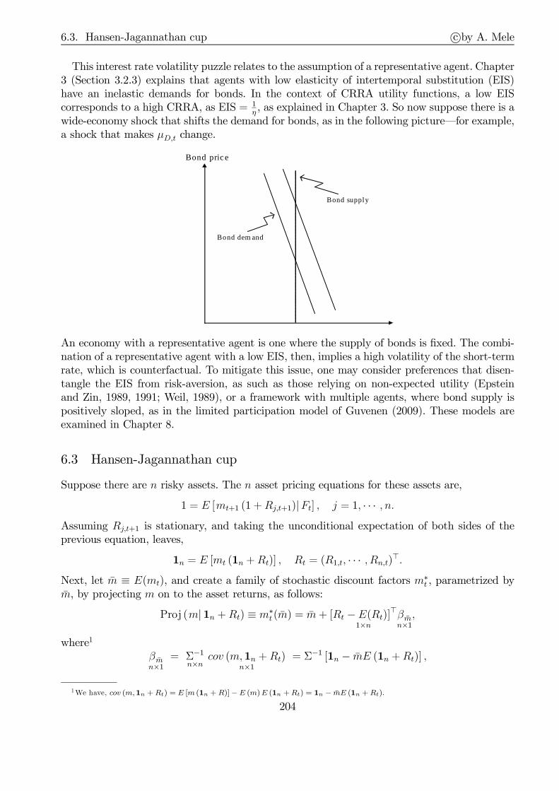
6.3. Hansen-Jagannathan cup c©by A. Mele
This interest rate volatility puzzle relates to the assumption of a representative agent. Chapter3 (Section 3.2.3) explains that agents with low elasticity of intertemporal substitution (EIS)have an inelastic demands for bonds. In the context of CRRA utility functions, a low EIScorresponds to a high CRRA, as EIS = 1
η, as explained in Chapter 3. So now suppose there is a
wide-economy shock that shifts the demand for bonds, as in the following picture–for example,a shock that makes µD,t change.
Bond supply
Bond dem and
Bond price
An economy with a representative agent is one where the supply of bonds is fixed. The combi-nation of a representative agent with a low EIS, then, implies a high volatility of the short-termrate, which is counterfactual. To mitigate this issue, one may consider preferences that disen-tangle the EIS from risk-aversion, as such as those relying on non-expected utility (Epsteinand Zin, 1989, 1991; Weil, 1989), or a framework with multiple agents, where bond supply ispositively sloped, as in the limited participation model of Guvenen (2009). These models areexamined in Chapter 8.
6.3 Hansen-Jagannathan cup
Suppose there are n risky assets. The n asset pricing equations for these assets are,
1 = E [mt+1 (1 +Rj,t+1)|Ft] , j = 1, · · · , n.Assuming Rj,t+1 is stationary, and taking the unconditional expectation of both sides of theprevious equation, leaves,
1n = E [mt (1n +Rt)] , Rt = (R1,t, · · · , Rn,t)⊤.
Next, let m ≡ E(mt), and create a family of stochastic discount factors m∗t , parametrized bym, by projecting m on to the asset returns, as follows:
Proj (m| 1n +Rt) ≡ m∗t (m) = m+ [Rt − E(Rt)]⊤
1×nβmn×1
,
where1
βmn×1
= Σ−1
n×ncov (m,1n +Rt)
n×1
= Σ−1 [1n − mE (1n +Rt)] ,
1We have, cov (m,1n +Rt) = E [m (1n +R)]− E (m)E (1n +Rt) = 1n − mE (1n +Rt).
204

6.3. Hansen-Jagannathan cup c©by A. Mele
and Σ ≡ E[(Rt −E(Rt)) (Rt −E(Rt))
⊤]. As shown in the Appendix, we also have that,
1n = E [m∗t (m) · (1n +Rt)] . (6.12)
We have,
√var (m∗t (m)) =
√β⊤mΣβm =
√(1n − mE (1n +Rt))
⊤Σ−1 (1n − mE (1n +Rt)). (6.13)
Eq. (6.13), provides the expression for the celebrated Hansen-Jagannathan “cup”–after thework of Hansen and Jagannathan (1991). It leads to an important tool of analysis, as thefollowing theorem shows.
T 6.2: Among all stochastic discount factors with fixed expectation m, m∗t (m) is theone with the smallest variance.
P: Consider another discount factor indexed by m, i.e.mt(m). Naturally,mt(m) satisfies1n = E [mt(m) (1n +Rt)]. Moreover, by Eq. (6.12),
0n = E [(mt(m)−m∗t (m)) (1n +Rt)]
= E [(mt(m)−m∗t (m)) ((1n + E(Rt)) + (Rt − E(Rt)))]
= E [(mt(m)−m∗t (m)) (Rt − E(Rt))]
= cov [mt(m)−m∗t (m), Rt]
where the third line follows because E [mt(m)] = E [m∗t (m)] = m, and the fourth line holds by
E [(mt(m)−m∗t (m))] = 0. But m∗t (m) is a linear combination of Rt. By the previous equation,then, it must be that 0 = cov [mt(m)−m∗t (m),m∗t (m)]. Therefore:
var [mt(m)] = var [m∗t (m) +mt(m)−m∗t (m)]
= var [m∗t (m)] + var [mt(m)−m∗t (m)] + 2 · cov [mt(m)−m∗t (m),m∗t (m)]= var [m∗t (m)] + var [mt(m)−m∗t (m)]≥ var [m∗t (m)] .
‖
Hansen and Jagannathan (1991) consider an extension of this result, where the pricing kernelsatisfies the non-negativity constraint, m > 0.Consider, then, the space, (m, var [m∗t (m)]), and anymodel giving rise to a pair (m, var [mt(m)]).
By Theorem 6.1, the pair (m, var [mt(m)]) has to lie above the cup (m, var [m∗t (m)]), for eachpossible m. As an example, apply the Hansen-Jagannathan bounds in Eq. (6.13) to the neo-classical model of Section 6.1. The stochastic discount factor for this model is:
mt+1 =ξt+1
ξt= exp (Zt+1) , Zt+1 = −
(r +
1
2λ2
)− λuD,t+1, uD,t+1 ≡
ǫD,t+1
σD.
By Lemma 6.1, the first two moments of this stochastic discount factor are:
m = E(mt) = e−r and σm =
√var (mt(m)) = e
−r+12λ2√1− e−λ2
, (6.14)
205

6.3. Hansen-Jagannathan cup c©by A. Mele
where
r = − ln β + ηµD −1
2η (η + 1) σ2
D and λ = ησD.
For given µD and σ2D, these two equations in (6.14) form a η-parametrized curve in the space (m-
σm). The issue is to check whether this curve enters the Hansen-Jagannathan cup for plausiblevalues of η. It is not the case. Rather, we have the situation depicted in Figure 6.2.
0.8 0.85 0.9 0.95 1 1.05 1.1 1.150
0.5
1
1.5
2
2.5
3
3.5
4
4.5
5
Expected value of the pricing kernel
Sta
ndar
d de
viat
ion
of th
e pr
icin
g ke
rnel
Hansen−Jagannathan bounds
Predictions ofthe Lucas model
FIGURE 6.2. The solid line depicts the Hansen-Jagannathan bounds, obtained through
Eq. (6.13), through aggregate stock market data and the short-term rate. The average
return and standard deviation of the stock market are taken to be 0.07 and 0.14. The
average short-term rate (three-month bill) and its volatility are, instead, 0.01 and 0.02.
These estimates relate to the sample period from January 1948 to December 2002. The
circles are predictions of the Lucas model in Eq. (6.14), with β = 0.95, µD = 0.0183,
σD = 0.0328 and η ranging from 1 to 35. The two circles inside the cup are the pairs
(m, σm) in Eq. (6.14) obtained with η = 35 and 33. Progressively lower values of η lead
the pairs (m, σm) to lie outside the cup, nonlinearly.
The Lucas model predicts that the pricing kernel is quite moderately volatile. The followingchapters discuss models with both heterogeneous agents or more general preferences, which canhelp boost the volatility of the pricing kernel.
206

6.4. Multifactor extensions c©by A. Mele
6.4 Multifactor extensions
A natural way to increase the variance of the pricing kernel is to increase the number of factors.We consider two possibilities: one in which returns are normally distributed, and one in whichreturns are lognormally distributed.
6.4.1 Exponential affine pricing kernels
Consider again the simple model in Section 6.1. In this section, we shall make a differentassumption regarding the returns distributions. But we shall maintain the hypothesis that thepricing kernel satisfies an exponential-Gaussian type structure,
mt+1 = exp (Zt+1) , Zt+1 = −(r +
1
2λ2
)− λuD,t+1, uD,t+1 ∼ NID (0, 1) ,
where r and λ are some constants. We have,
1 = E(mt+1 · Rt+1) = E (mt+1)E(Rt+1) + cov(mt+1, Rt+1), Rt+1 ≡St+1 +Dt+1
St.
By rearranging terms,2 and using the fact that E (mt+1) = R−1,
E(Rt+1)−R = −R · cov(mt+1, Rt+1). (6.15)
Consider the following result, which we shall use later:
L 6.3 (Stein’s lemma): Suppose that two random variables x and y are jointly normal.Then,
cov [g (x) , y] = E [g′ (x)] · cov (x, y) ,for any function g : E (|g′ (x)|) <∞.
Next, suppose R is normally distributed. This assumption is inconsistent with the model inSection 6.1, where R is lognormally distributed, in equilibrium, being equal to ln R = µD −12σ2D + ǫS, where ǫS is normal. Let us explore, however, the asset pricing implications of the
assumption R is normally distributed. Because Rt+1 and Zt+1 are both normal, and mt+1 =m (Zt+1) = exp (Zt+1), we may apply Lemma 6.3 and obtain,
cov(mt+1, Rt+1) = E [m′ (Zt+1)] · cov(Zt+1, Rt+1) = −λR−1 · cov(uD,t+1, Rt+1).
Replacing this expression for the covariance, cov(mt+1, Rt+1), into Eq. (6.15), leaves:
E(Rt+1)−R = λ · cov(uD,t+1, Rt+1).
2With a portfolio return that is perfectly correlated with m, we have:
Et(RMt+1)−
1
Et (mt+1)= − σt (mt+1)
Et (mt+1)σt(R
Mt+1).
In more general setups than the ones considered in this introductory example, bothσt(mt+1)Et(mt+1)
and σt(RMt+1) should be time-varying.
207

6.4. Multifactor extensions c©by A. Mele
We wish to extend the previous observations to a more general setup. Clearly, the pricingkernel is some function of K factors m (ǫ1t, · · · , ǫKt). A particularly convenient analytical as-sumption is to make m exponential-affine and the factors (ǫi,t)
Ki=1 normal, as in the following
definition:
D 6.4 (EAPK: Exponential Affine Pricing Kernel): Let,
Zt ≡ φ0 +K∑
i=1
φiǫi,t.
A EAPK is a function,mt = m(Zt) = exp(Zt). (6.16)
If (ǫi,t)Ki=1 are jointly normal, and each ǫi,t has mean zero and variance σ2
i , i = 1, · · · , K, theEAPK is called a Normal EAPK (NEAPK).
In the previous definition, we assumed each ǫi,t has a mean equal to zero, which entails noloss of generality insofar as φ0 = 0. Next, suppose R is normally distributed. By Lemma 6.3and the NEAPK assumption,
cov(mt+1, Rt+1) = cov[exp (Zt+1) , Rt+1] = R−1cov(Zt+1, Rt+1) = R
−1K∑
i=1
φicov(ǫi,t+1, Rt+1).
By replacing this into Eq. (6.15) leaves the linear factor representation,
E(Rt+1)−R = −K∑
i=1
φicov(ǫi,t+1, Rt+1)︸ ︷︷ ︸“betas”
. (6.17)
We have thus shown the following result:
P 6.5: Suppose that R is normally distributed. Then, NEAPK ⇒ linear factorrepresentation for asset returns.
The APT representation in Eq. (6.17), is similar to a result in Cochrane (1996).3 Cochrane(1996) assumes thatm is affine, i.e.m (Zt) = Zt where Zt is as in Definition 6.1. This assumptionimplies that cov(mt+1, Rt+1) =
∑Ki=1 φicov(ǫi,t+1, Rt+1). By replacing this expression for the
covariance, cov(mt+1, Rt+1), into Eq. (6.15), leaves
E(Rt+1)−R = −RK∑
i=1
φicov(ǫi,t+1, Rt+1), where R =1
E (m)=
1
φ0
.
The NEAPK assumption, compared to Cochrane’s, carries the obvious advantage to guaranteethe pricing kernel is strictly positive–a theoretical condition we need to rule out arbitrageopportunities.
3To recall why eq. (6.17) is indeed a APT equation, suppose that R is a n-(column) vector of returns and that R = a+bf , wheref is K-(column) vector with zero mean and unit variance and a, b are some given vector and matrix with appropriate dimension.Then clearly, b = cov(R, f). A portfolio π delivers π⊤R = π⊤a + π⊤cov(R, f)f . Arbitrage opportunity is: ∃π : π⊤cov(R, f) = 0and π⊤a = r. To rule that out, we may show as in Part I of these Lectures that there must exist a K-(column) vector λ s.t.a = cov(R, f)λ+ r. This implies R = a+ bf = r + cov(R, f)λ+ bf . That is, E(R) = r + cov(R, f)λ.
208

6.4. Multifactor extensions c©by A. Mele
6.4.2 Lognormal returns
Next, we assume that R is lognormally distributed, and that the NEAPK holds. We have,
1 = E(mt+1 · Rt+1
)⇐⇒ e−φ0 = E
(e∑Ki=1 φiǫi,t+1 · Rt+1
). (6.18)
Consider, first, the case K = 1, and let yt = ln Rt be normally distributed. The previousequation can be written as,
e−φ0 = E[eφ1ǫt+1+yt+1
]= eE(yt+1)+
12(φ2
1σ2ǫ+σ
2y+2φ1σǫy).
This is,
E (yt+1) = −[φ0 +
1
2(φ2
1σ2ǫ + σ
2y + 2φ1σǫy)
].
By applying the pricing equation (6.18) to a zero coupon bond,
e−φ0 = E(eφ1ǫt+1
)elnRt+1 = elnRt+1+
12φ2
1σ2ǫ ,
which we can solve for Rt+1:
lnRt+1 = −(φ0 +
1
2φ21σ
2ǫ
).
The expected excess return is,
E (yt+1)− lnRt+1 +1
2σ2y = −φ1σǫy. (6.19)
Eq. (6.19) shows that the theory in Section 6.1 through a different angle. Apart from Jensen’sinequality effects (1
2σ2y), this is indeed the Lucas model of Section 6.1 once φ1 = −η. As is clear,
this is a poor model, as it is bound to explain returns with only one “stochastic discount-factorparameter,” i.e. φ1.Next consider the general case. Assume as usual that dividends are as in (6.1). To find the
price function in terms of the state variable ǫ, we may proceed as in Section 6.1. In the absenceof bubbles,
St =∞∑
i=1
E
[ξt+iξt
·Dt+i
]= Dt ·
∞∑
i=1
e(µD+φ0+12
∑Ki=1 φi(φiσ2
i+2σi,D))·i, σi,D ≡ cov (ǫi, ǫD) .
Thus, if
k ≡ µD + φ0 +1
2
K∑
i=1
φi(φiσ
2i + 2σi,D
)< 0,
then,StDt
=k
1− k.
Even in this multi-factor setting, price-dividend ratios are constant, a counterfactual prediction,as explained in the next chapter. Note, then, the following facts. The first two moments ofthe pricing kernel satisfying a NEAPK structure can be easily found, by Eq. (6.16), and anapplication of Lemma 6.1:
E (mt) = eE(Zt)+
12var(Zt),
√var (mt) = e
E(Zt)+var(Zt)√1− e−var(Zt).
209

6.5. Pricing kernels and Sharpe ratios c©by A. Mele
We can always calibrate the parameters of this model, so as to make sure the pricing kernel enterinto the Hansen-Jagannathan cup. However, remember, the model still predicts price-dividendratios to be constant: the model does not really work, even if we are able to arbitrarily increasethe variance of the pricing kernel underlying it. A model that satisfies the Hansen-Jagannathanbounds is not necessarily a good one. We need further theoretical test conditions. The nextchapter illustrates theoretical test conditions addressing these concerns, and attempting toanswer questions such as: (i) when are price-dividend ratios procyclical? (ii) when is returnsvolatility countercyclical? etc.
6.5 Pricing kernels and Sharpe ratios
6.5.1 Market portfolios and pricing kernels
Can the market portfolio be ever perfectly correlated with the pricing kernel? It is not the case,in general (see, also, Cecchetti, Lam, and Mark, 1994). Let rei,t+1 = Ri,t+1 −Rt+1 be the excessreturn on a risky asset. We have:
0 = Et
(mt+1r
ei,t+1
)= Et (mt+1)Et
(rei,t+1
)+ ρi,t · Stdt (mt+1) · Stdt
(rei,t+1
),
where Stdt (ut+1) denotes the standard deviation of a variable ut+1, conditionally upon theinformation available at time t, and ρi,t ≡ corrt(mt+1, r
ei,t+1), a conditional correlation. Hence,
the Sharpe Ratio, S ≡ Et(rei,t+1)Stdt(rei,t+1)
, satisfies:
|S| ≤ Stdt (mt+1)
Et (mt+1)= Stdt (mt+1) ·Rt+1, (6.20)
The highest possible Sharpe ratio is bounded. The equality holds for a hypothetical portfolioM , say, yielding excess returns perfectly conditionally negatively correlated with the pricingkernel, ρM,t = −1. We shall say of M that it is a β-CAPM generating portfolio. Is it also amarket portfolio? After all, a feasible and attainable portfolio lying on the kernel volatilitybounds is clearly mean-variance efficient. The answer is subtle. As explained in the context ofthe static model of Chapter 1, the Sharpe ratio, S, equals the slope of the Capital Market Line,and bears the interpretation of unit market risk-premium. If ρM,t = −1, then, by Eq. (6.20),
the slope of the Capital Market Line reduces to Stdt(mt+1)Et(mt+1)
. For example, with the Lucas modelin Section 6.1,
Stdt (mt+1)
Et (mt+1)=
√eη
2σ2D − 1 ≈ ησD.
In Section 6.1, we also explained that (µS − r)/σD = ησD, which is only approximately true,according to the previous relation. Not even a simple model with a single tree, such as thatin Section 6.1, would be capable of leading to a β-CAPM generating portfolio, or a market
portfolio! Indeed, for this model, we have that E(R) = eµS , R = e− lnβ+η(µD− 12σ2D)−1
2η2σ2
D , andvar(R) = e2µS(eσ
2D − 1), with a Sharpe ratio equal to:
S = 1− e−ησ2D
√eσ
2D − 1
.
By simple computations, ρ = − 1−e−ησ2D√
eη2σ2
D−1
√eσ2D−1
, which is not precisely “−1”–only approxi-
mately equal to −1, for low values of σD.
210

6.5. Pricing kernels and Sharpe ratios c©by A. Mele
A further complication arises, a β-CAPM generating portfolio is not necessarily the tangencyportfolio. We can show that there is another portfolio leading to the very same β-pricing relationpredicted by the tangency portfolio. Such a portfolio is referred to as the maximum correlationportfolio, for reasons developed below. Let R = 1
E(m). By the CCAPM in Chapter 2,
E(Ri
)− R =
βRi,mβRp,m
(E (Rp)− R
),
where Rp is a portfolio return. Next, let Rp = Rm ≡ m
E(m2), which is clearly perfectly correlated
with the pricing kernel. By results in Chapter 2,
E(Ri
)− R = βRi,Rm
(E (Rm)− R
).
This is not yet the β-representation of the CAPM, because we have yet to show that thereis a way to construct Rm as a portfolio return. In fact, there is a natural choice: pick m = m∗,where m∗ is the minimum-variance kernel leading to the Hansen-Jagannathan bounds. Sincem∗ is linear in all asset retuns, Rm∗
can be thought of as a return that can be obtained byinvesting in all assets. Furthermore, in the appendix we show that Rm∗
satisfies,
1 = E(m ·Rm∗)
.
Where is this portfolio located? The Appendix shows that there is no portfolio yielding thesame expected return with lower variance, that is, Rm∗
is mean-variance efficient), and that:
E(Rm∗)− 1 = r − Sh
1 + Sh= r − 1 + r
1 + ShSh < r.
Mean-variance efficiency of Rm∗
and the previous inequality imply that this portfolio lies inthe lower branch of the mean-variance efficient portfolios. And this is so because this portfoliois positively correlated with the true pricing kernel. Naturally, the fact that this portfolio isβ-CAPM generating doesn’t necessarily imply that it is also perfectly correlated with the truepricing kernel. As shown in the appendix, Rm∗
has only the maximum possible correlationwith all possible m. Perfect correlation occurs exactly in correspondence of the pricing kernelm = m∗ (i.e. when the economy exhibits a pricing kernel exactly equal to m∗).
P Rm∗
β-( / /. The relations, 1 = E(m∗Ri) and 1 = E(m∗Rm∗
),imply:
E(Ri)−R = −R · cov(m∗, Ri
), E(Rm∗
)−R = −R · cov(m∗, Rm∗)
,
or,E(Ri)−RE(Rm∗)−R =
cov (m∗, Ri)
cov (m∗, Rm∗).
By construction, Rm∗
is perfectly correlated with m∗. Precisely, Rm∗
= m∗/E(m∗2) ≡ γ−1m∗,γ ≡ E(m∗2). Therefore,
cov (m∗, Ri)
cov (m∗, Rm∗)=
cov(γRm∗
, Ri)
cov (γRm∗, Rm∗)=γ · cov
(Rm∗
, Ri)
γ · var (Rm∗)= βRi,Rm∗ .
‖211
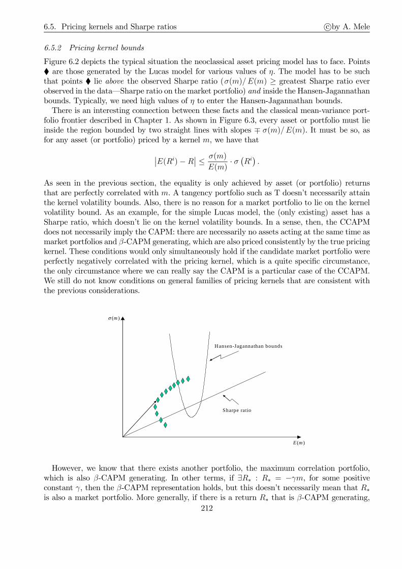
6.5. Pricing kernels and Sharpe ratios c©by A. Mele
6.5.2 Pricing kernel bounds
Figure 6.2 depicts the typical situation the neoclassical asset pricing model has to face. Points are those generated by the Lucas model for various values of η. The model has to be suchthat points lie above the observed Sharpe ratio (σ(m)/E(m) ≥ greatest Sharpe ratio everobserved in the data–Sharpe ratio on the market portfolio) and inside the Hansen-Jagannathanbounds. Typically, we need high values of η to enter the Hansen-Jagannathan bounds.There is an interesting connection between these facts and the classical mean-variance port-
folio frontier described in Chapter 1. As shown in Figure 6.3, every asset or portfolio must lieinside the region bounded by two straight lines with slopes ∓ σ(m)/E(m). It must be so, asfor any asset (or portfolio) priced by a kernel m, we have that
∣∣E(Ri)−R∣∣ ≤ σ(m)
E(m)· σ
(Ri
).
As seen in the previous section, the equality is only achieved by asset (or portfolio) returnsthat are perfectly correlated with m. A tangency portfolio such as T doesn’t necessarily attainthe kernel volatility bounds. Also, there is no reason for a market portfolio to lie on the kernelvolatility bound. As an example, for the simple Lucas model, the (only existing) asset has aSharpe ratio, which doesn’t lie on the kernel volatility bounds. In a sense, then, the CCAPMdoes not necessarily imply the CAPM: there are necessarily no assets acting at the same time asmarket portfolios and β-CAPM generating, which are also priced consistently by the true pricingkernel. These conditions would only simultaneously hold if the candidate market portfolio wereperfectly negatively correlated with the pricing kernel, which is a quite specific circumstance,the only circumstance where we can really say the CAPM is a particular case of the CCAPM.We still do not know conditions on general families of pricing kernels that are consistent withthe previous considerations.
E(m)
σ (m)
Sharpe ratio
Hansen-Jagannathan bounds
However, we know that there exists another portfolio, the maximum correlation portfolio,which is also β-CAPM generating. In other terms, if ∃R∗ : R∗ = −γm, for some positiveconstant γ, then the β-CAPM representation holds, but this doesn’t necessarily mean that R∗is also a market portfolio. More generally, if there is a return R∗ that is β-CAPM generating,
212

6.5. Pricing kernels and Sharpe ratios c©by A. Mele
then,
ρi,R∗ =ρi,mρR∗,m
, all i. (6.21)
Therefore, we don’t need an asset or portfolio return that is perfectly correlated withm to makethe CCAPM collapse to the CAPM. All in all, the existence of an asset return that is perfectlynegatively correlated with the price kernel is a sufficient condition for the CCAPM to collapseto the CAPM, not a necessary condition. The proof of Eq. (6.21) is simple. By the CCAPM,
E(Ri)−R = −ρi,mσ(m)
E(m)σ(Ri), and E(R∗)−R = −ρR∗,m
σ(m)
E(m)σ(R∗).
That is,
E(Ri)−RE(R∗)−R =
ρi,mρR∗,m
σ(Ri)
σ(R∗)(6.22)
But if R∗ is β-CAPM generating,
E(Ri)−RE(R∗)−R =
cov(Ri, R∗)
σ(R∗)2= ρi,R∗
σ(Ri)
σ(R∗). (6.23)
Comparing Eq. (6.22) with Eq. (6.23) produces Eq. (6.21).
kernel volatility bounds
mean-variance efficient portfolios
efficient portfolios frontier
T
tangency portfolio
maximum correlation portfolio
1 / E(m)
E(R)
σ(R)
A final thought. In many pieces of applied research, we often read that because we observetime-varying Sharpe ratios on (proxies of) the market portfolio, we should also model the market
risk-premium πt ≡√V art (mt+1)
/Et (mt+1) as time-varying. While Chapter 7 explains that
the evidence for time-varying risk-premiums is overwhelming, a criticism to this motivationis that πt is only an upper bound to the Sharpe ratio of the market portfolio. On a strictlytheoretical point of view, then, a time-varying πt is neither a necessary or a sufficient conditionto have time-varying Sharpe ratios, as Figure 6.3 illustrates.
213

6.6. Conditioning bounds c©by A. Mele
6.6 Conditioning bounds
The Hansen-Jagannathan bounds in Eq. (6.13) can be improved by using conditioning infor-mation, as originally shown by Gallant, Hansen and Tauchen (1990) and in Ferson and Siegel(2003). A difficulty with these bounds is that they may diplay a finite sample bias, in thatthey tend to overstate the true bounds and thus reject too often a given model. Finite samplecorrections are considered by Ferson and Siegel (2003). [Discuss, analytically]Alvarez and Jermann (2005). [Discuss, analytically]
214

6.7. Appendix c©by A. Mele
6.7 Appendix
P E$ , 1n = E [m∗t (m) · (1n +Rt)]. We have,
E [m∗t (m) · (1n +Rt)] = E[(m+ (Rt −E(Rt))
⊤ βm)(1n +Rt)
]
= mE (1n +Rt) +E[(Rt −E(Rt))
⊤ βm (1n +Rt)]
= mE (1n +Rt) +E[(1n +Rt) (Rt −E(Rt))
⊤]βm
= mE (1n +Rt) +E[((1n +E(Rt)) + (Rt −E(Rt))) (Rt −E(Rt))
⊤]βm
= mE (1n +Rt) +E[(Rt −E(Rt)) (Rt −E(Rt))
⊤]βm
= mE (1n +Rt) + Σβm
= mE (1n +Rt) + 1n − mE (1n +Rt) ,
where the last line follows by the definition of βm.
P Rm∗
( 2 / , 2) 2
P E$ , 1 = E(m ·Rm∗)
. We have,
E(m ·Rm∗
) =1
E [(m∗)2]E (m ·m∗) ,
where
E (m ·m∗) = m2 +E[m (Rt −E(Rt))
⊤ βm]
= m2 +E[m (1 +Rt)
⊤]βm −E
[m (1 +E(Rt))
⊤]βm
= m2 + βm −E (m) [1 +E(Rt)]⊤ βm
= m2 +[1n − m (1 +E(Rt))
⊤]βm
= m2 +[1n − m (1 +E(Rt))
⊤]Σ−1 [1n − m (1n +E(Rt))]
= m2 + var (m∗) ,
where the last line is due to the definition of m∗.
P Rm∗ -. ( ( . Let p = (p0, p1, · · · , pn)⊤ the vector of n + 1
portfolio weights (here pi ≡ πi/w is the portfolio weight of asset i, i = 0, 1, · · · , n. We have,
p⊤1n+1 = 1.
The returns we consider are rt =(m−1 − 1, r1,t, · · · , rn,t
)⊤. We denote our “benchmark” portfolio
return as rbt = rm∗ − 1. Next, we build up an arbitrary portfolio yielding the same expected return
E(rbt) and then we show that this has a variance greater than the variance of rbt. Since this portfolio
215

6.7. Appendix c©by A. Mele
is arbitrary, the proof will be complete. Let rpt = p⊤rt such that E(rpt) = E(rbt). We have:
cov (rbt, rpt − rbt) = E [rbt · (rpt − rbt)]
= E [Rbt · (Rpt −Rbt)]
= E (Rbt ·Rpt)−E(R2bt
)
=1
E (m∗2)E
[m∗
(1 + p⊤rt
)]− 1
[E (m∗2)]2E
(m∗2
)
=1
E (m∗2)
[p⊤E [m∗ (1n+1 + rt)]− 1
]
= 0.
The first line follows by construction since E(rpt) = E(rbt). The last line follows because
p⊤E [m∗ (1n+1 + rt)] = p⊤1n+1 = 1.
Given this, the claim follows directly from the fact that
var (Rpt) = var [Rbt + (Rpt −Rbt)] = var (Rbt) + var (Rpt −Rbt) ≥ var (Rbt) .
P E$ , E(Rm∗)− 1 = r − 1+r
1+ShSh. We have,
E(Rm∗
)− 1 =m
E[(m∗)2]− 1.
In terms of the notation introduced in Section 6.8, m∗ is:
m∗ = m+ (aǫ)⊤ βm, βm = σ−1 [1n − m (1n + b)] .
We have,
E[(m∗)2] =[m+ (aǫ)⊤ βm
]2
= m2 +E[(aǫ)⊤ βm
]2
= m2 +E[(aǫ)⊤ βm · (aǫ)⊤ βm
]2
= m2 +E[(β⊤maǫ
)(ǫ⊤a⊤βm
)]
= m2 + β⊤m · σ · βm= m2 +
[1⊤n − m
(1⊤n + b⊤
)]σ−1 [1n − m (1n + b)]
= m2 + 1⊤n σ−11n − m
(1⊤n σ
−11n + 1
⊤n σ
−1b)
− m[1⊤n σ
−11n + b⊤σ−1
1n − m(1⊤n σ
−11n + b⊤σ−1
1n + 1⊤n σ
−1b+ b⊤σ−1b)]
Again in terms of the notation of Section 6.8 (γ ≡ 1⊤n σ−11n and β ≡ 1⊤n σ−1b), this is:
E[(m∗)2
]= γ − 2m (γ + β) + m2
(1 + γ + 2β + b⊤σ−1b
).
The expected return is thus,
E(Rm∗
)− 1 =
E (m∗)
E[(m∗)2
] − 1 =m− γ + 2m (γ + β)− m2
(1 + γ + 2β + b⊤σ−1b
)
γ − 2m (γ + β) + m2 (1 + γ + 2β + b⊤σ−1b).
216
6.7. Appendix c©by A. Mele
Now recall two definitions:
m =1
1 + r, Sh = (b− 1mr)⊤ σ−1 (b− 1mr) = b⊤σ−1b− 2βr + γr2.
In terms of r and Sh, we have,
E(Rm∗
)− 1 =
E (m∗)
E[(m∗)2
] − 1
= −γ (1 + r)2 − (1 + r) (1 + 2γ + 2β) + 1 + γ + 2β + b⊤σ−1b
γ (1 + r)2 − (1 + r) (2γ + 2β) + 1 + γ + 2β + b⊤σ−1b
=r − Sh
1 + Sh
= r − 1 + r
1 + ShSh
< r.
This is positive if r− Sh > 0, i.e. if b⊤σ−1b− (2β + 1) r+ γr2 < 0, which is possible for sufficientlylow (or sufficiently high) values of r.
P Rm∗ m- ( . We have to show that for any
price kernel m, |corr(m,Rbt)| ≥ |corr(m,Rpt)|. Define a ℓ-parametrized portfolio such that:
E [(1− ℓ)Ro + ℓRpt] = E (Rbt) , Ro ≡ m−1.
We have
corr (m,Rpt) = corr [m, (1− ℓ)Ro + ℓRpt]
= corr [m,Rbt + ((1− ℓ)Ro + ℓRpt −Rbt)]
=cov (m,Rbt) + cov (m, (1− ℓ)Ro + ℓRpt −Rbt)
σ(m) ·√var ((1− ℓ)Ro + ℓRpt)
=cov (m,Rbt)
σ(m) ·√var ((1− ℓ)Ro + ℓRpt)
The first line follows because (1 − ℓ)Ro + ℓRpt is a nonstochastic affine translation of Rpt. The lastequality follows because
cov (m, (1− ℓ)Ro + ℓRpt −Rbt) = E [m · ((1− ℓ)Ro + ℓRpt −Rbt)]
= (1− ℓ) · E (mRo)︸ ︷︷ ︸=1
+ ℓ ·E (mRpt)︸ ︷︷ ︸=1
− E (m ·Rbt)︸ ︷︷ ︸=1
= 0.
where the first line follows because E((1− ℓ)Ro + ℓRpt) = E(Rbt).Therefore,
corr (m,Rpt) =cov (m,Rbt)
σ(m) ·√var ((1− ℓ)Ro + ℓRpt)
≤ cov (m,Rbt)
σ(m) ·√var(Rbt)
= corr (m,Rbt) ,
where the inequality follows because Rbt is mean-variance efficient (i.e. ∄ feasible portfolios with thesame expected return as Rbt and variance less than var(Rbt)), and then var((1 − ℓ)Ro + ℓRpt) ≥var(Rbt), all Rpt.
217
6.7. Appendix c©by A. Mele
References
Alvarez, F. and U.J. Jermann (2005): “Using Asset Prices to Measure the Persistence of theMarginal Utility of Wealth.” Econometrica 73, 1977-2016.
Cecchetti, S., Lam, P-S. and N. C. Mark (1994): “Testing Volatility Restrictions on Intertem-poral Rates of Substitution Implied by Euler Equations and Asset Returns.” Journal ofFinance 49, 123-152.
Cochrane, J. (1996): “A Cross-Sectional Test of an Investment-Based Asset Pricing Model.”Journal of Political Economy 104, 572-621.
Epstein, L.G. and S.E. Zin (1989): “Substitution, Risk-Aversion and the Temporal Behavior ofConsumption and Asset Returns: A Theoretical Framework.” Econometrica 57, 937-969.
Epstein, L.G. and S.E. Zin (1991): “Substitution, Risk-Aversion and the Temporal Behavior ofConsumption and Asset Returns: An Empirical Analysis.” Journal of Political Economy99, 263-286.
Ferson, W. E. and A. F. Siegel (2003): “Stochastic Discount Factor Bounds with ConditioningInformation.” Review of Financial Studies 16, 567-595.
Gallant, R. A., L. P. Hansen and G. Tauchen (1990): “Using the Conditional Moments of AssetPayoffs to Infer the Volatility of Intertemporal Marginal Rates of Substitution.” Journalof Econometrics 45, 141-179.
Gordon, M. (1962): The Investment, Financing, and Valuation of the Corporation. Homewood,IL: Irwin.
Guvenen, F. (2009): “A Parsimonious Macroeconomic Model for Asset Pricing.” Econometrica77, 1711-1740.
Hansen, L. P. and R. Jagannathan (1991): “Implications of Security Market Data for Modelsof Dynamic Economies.” Journal of Political Economy 99, 225-262.
Mehra, R. and E. C. Prescott (1985): “The Equity Premium: A Puzzle.” Journal of MonetaryEconomics 15, 145-161.
Weil, Ph. (1989): “The Equity Premium Puzzle and the Risk-Free Rate Puzzle.” Journal ofMonetary Economics 24, 401-421.
218

7The stock market
7.1 Introduction
This chapter documents a few empirical regularities affecting the aggregate stock market be-havior but also some properties arising at a disaggregated level. It also points to general issuesabout what we need to do with the neoclassical asset pricing model in Part I of these Lectures,so as to address these empirical puzzles. Section 7.2 provides a succinct overview of the mainempirical regularities of aggregate stock market fluctuations. For example, we shall explainthat price-dividend ratios and stock returns are procyclical, and that stock volatility and risk-premiums are both time-varying and countercyclical. Section 7.3 analyzes in deeper detail theempirical behavior of aggregate stock market volatility, and puts forward some explanationsfor it. Section 7.4 develops a framework of analysis aiming to explore the extent to which theempirical behavior of price-dividend ratios, stock returns, risk-premiums and volatility can berationalized within the neoclassical framework. Section 7.5 provides two examples of economies,which illustrate the predictions in Section 7.4: one economy, with habit formation, and a sec-ond, with uncertain fundamentals and a learning process about them. Section 7.6 concludes thechapter, and surveys the properties of the stock market at a disaggregated level.
7.2 The empirical evidence: bird’s eye view
Aggregate stock market fluctuations are intimately related to the business cycle. The evidenceis striking and well-known (see, e.g., the survey in Campbell, 2003), although the emphasis inthis section is to streamline how these fluctuations relate to general macroeconomic conditions.We use data sampled at a monthly frequency, covering the period from January 1948 throughDecember 2002. We compute ex-post, yearly returns at month t as
∑12i=1 Rt+1−i, where Rt =
ln(St+DtSt−1
), St is the S&P Composite index as of month t, and Dt is the aggregate dividend,as calculated by Robert Shiller. Table 7.1 provides basic statistics for both row data such asP/D ratios, P/E ratios and ex-post returns, and stock volatility and expected returns. Stock

7.2. The empirical evidence: bird’s eye view c©by A. Mele
volatility is computed as:
Volt ≡√6π · σt, σt ≡
1
12
12∑
i=1
∣∣∣Rt+1−i −Rt+1−i
∣∣∣ , (7.1)
where Rt is the risk-free rate, taken to be the one month bill return. The rationale behind thiscalculation is as follows. First, σt is an estimate of the average volatility occurring over the last12 months. We annualize σt by multiplying it by
√12. The term
√6π arises for the following
reason. If we assume that a given return R = σu, where σ is a positive constant and u is a
standard unit normal, then E (|R|) = σ√
2π. The definition Volt in Eq. (8.12), then, follows
by multiplying√12σt (ℓ) by
√π2. This correction term,
√π2, has been suggested by Schwert
(1989a) in a related context.Expected returns are computed through the Fama and French (1989) predictive regressions
of Rt on to default-premium, term-premium and the previously defined return volatility, Volt.With the exception of the P/D and P/E ratios, all figures are annualized percent.We note the first main set of stylized facts:
F( I. P/D, P/E ratios and ex-post returns are procylical, although variations inthe business cycle conditions do not seem to be the only driving force for them.
For example, Figure 7.1 reveals that price-dividend ratios decline during all of the economicslowdowns, as signaled by the recession indicator calculated by the National Bureau of EconomicResearch (NBER)–the NBER recessions. At the same time, during NBER expansions, price-dividend ratios seem to be driven by additional factors not necessarily related to the businesscycle. For example, during the “roaring” 1960s, price-dividend ratios experienced two majordrops with the same magnitude as the decline at the very beginning of the “chaotic” 1970s.Ex-post returns follow approximately the same pattern, although they are more volatile thanprice-dividend ratios (see Figure 7.2).What about the first two conditional moments of asset returns?
F( II. Stock volatility and expected returns are countercyclical. However, busi-ness cycle conditions do not seem to be the only forces explaining the swings ofthese variables.
Figures 7.3 through 7.5 are suggestive. For example, Figure 7.4 depicts the statistical relationbetween stock volatility and the industrial production growth rate over the last sixty years,which shows that stock volatility is largely countercyclical, being larger in bad times than ingood.1 There are, of course, exceptions. For example, stock volatility rocketed to almost 23%during the 1987 crash–a crash occurring during one of the most enduring post-war expansionsperiod. Countercyclical volatility is a stylized fact extensively discussed in Sections 7.3 and7.4. In those sections, we shall learn that within the neoclassical modeling framework, thisproperty does likely arise as soon as the volatility of the P/D ratios changes is countercyclical.Table 7.1 reveals, then, that the P/D ratios variations are more volatile in bad times than ingood. Finally, and interestingly, Figure 7.4 suggests that stock volatility behaves asymmetrically
1The predictive regressions in Figures 7.4, 7.5 and 7.7 are obtained through least absolute deviations regressions, a techniqueknown to be more robust to the presence of outliers than ordinary least squares (see Bloomfield and Steiger, 1983).
220
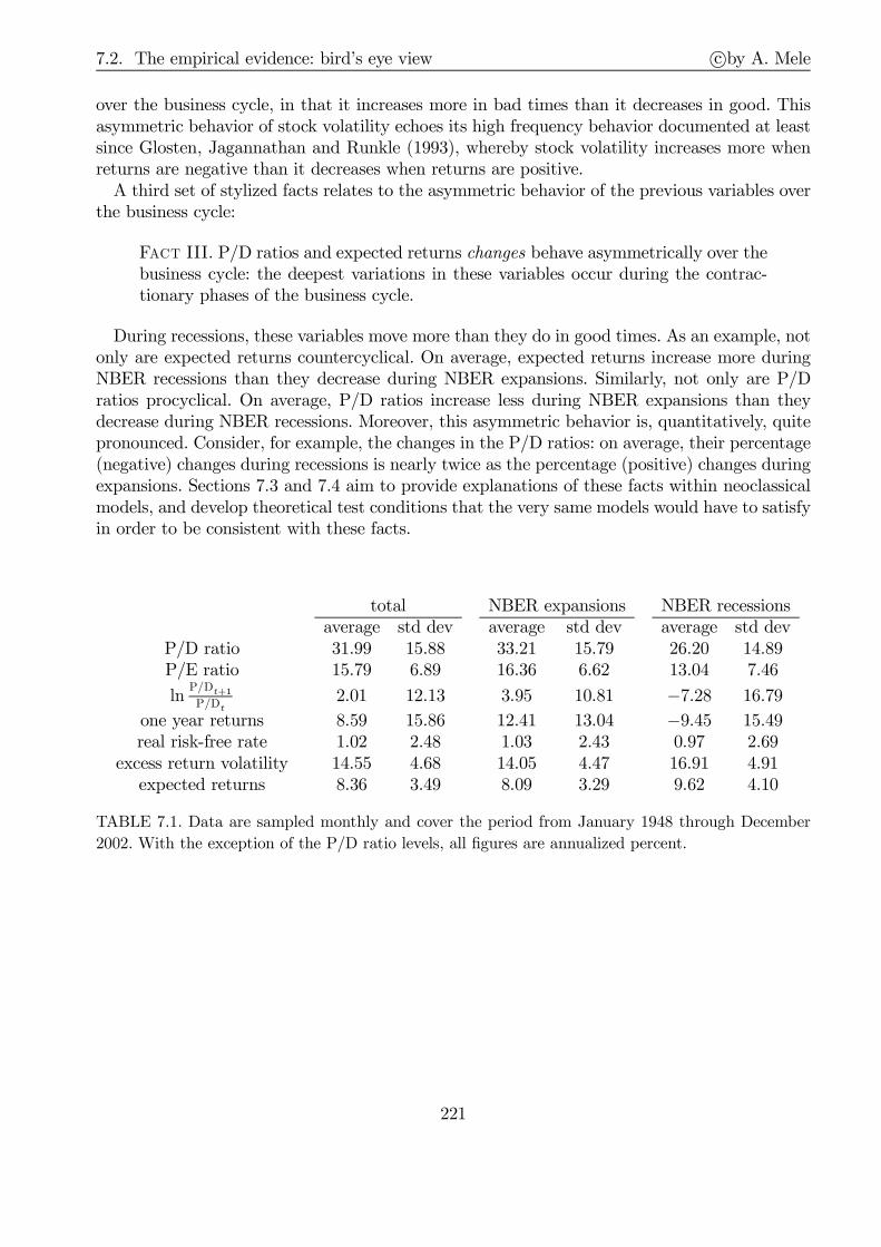
7.2. The empirical evidence: bird’s eye view c©by A. Mele
over the business cycle, in that it increases more in bad times than it decreases in good. Thisasymmetric behavior of stock volatility echoes its high frequency behavior documented at leastsince Glosten, Jagannathan and Runkle (1993), whereby stock volatility increases more whenreturns are negative than it decreases when returns are positive.A third set of stylized facts relates to the asymmetric behavior of the previous variables over
the business cycle:
F( III. P/D ratios and expected returns changes behave asymmetrically over thebusiness cycle: the deepest variations in these variables occur during the contrac-tionary phases of the business cycle.
During recessions, these variables move more than they do in good times. As an example, notonly are expected returns countercyclical. On average, expected returns increase more duringNBER recessions than they decrease during NBER expansions. Similarly, not only are P/Dratios procyclical. On average, P/D ratios increase less during NBER expansions than theydecrease during NBER recessions. Moreover, this asymmetric behavior is, quantitatively, quitepronounced. Consider, for example, the changes in the P/D ratios: on average, their percentage(negative) changes during recessions is nearly twice as the percentage (positive) changes duringexpansions. Sections 7.3 and 7.4 aim to provide explanations of these facts within neoclassicalmodels, and develop theoretical test conditions that the very same models would have to satisfyin order to be consistent with these facts.
total NBER expansions NBER recessionsaverage std dev average std dev average std dev
P/D ratio 31.99 15.88 33.21 15.79 26.20 14.89P/E ratio 15.79 6.89 16.36 6.62 13.04 7.46
lnP/Dt+1
P/Dt2.01 12.13 3.95 10.81 −7.28 16.79
one year returns 8.59 15.86 12.41 13.04 −9.45 15.49real risk-free rate 1.02 2.48 1.03 2.43 0.97 2.69
excess return volatility 14.55 4.68 14.05 4.47 16.91 4.91expected returns 8.36 3.49 8.09 3.29 9.62 4.10
TABLE 7.1. Data are sampled monthly and cover the period from January 1948 through December
2002. With the exception of the P/D ratio levels, all figures are annualized percent.
221

7.2. The empirical evidence: bird’s eye view c©by A. Mele
1954 1958 1962 1966 1970 1974 1978 1982 1986 1990 1994 1998 20020
25
50
75
100
P/D ratio
P/E ratio
ptpt p t p t p t p t p t p t p t p t
FIGURE 7.1. P/D and P/E ratios
1954 1958 1962 1966 1970 1974 1978 1982 1986 1990 1994 1998 2002-60
-40
-20
0
20
40
60 ptpt p t p t p t p t pt p t p t p t
FIGURE 7.2. Monthly smoothed excess returns (%)
222
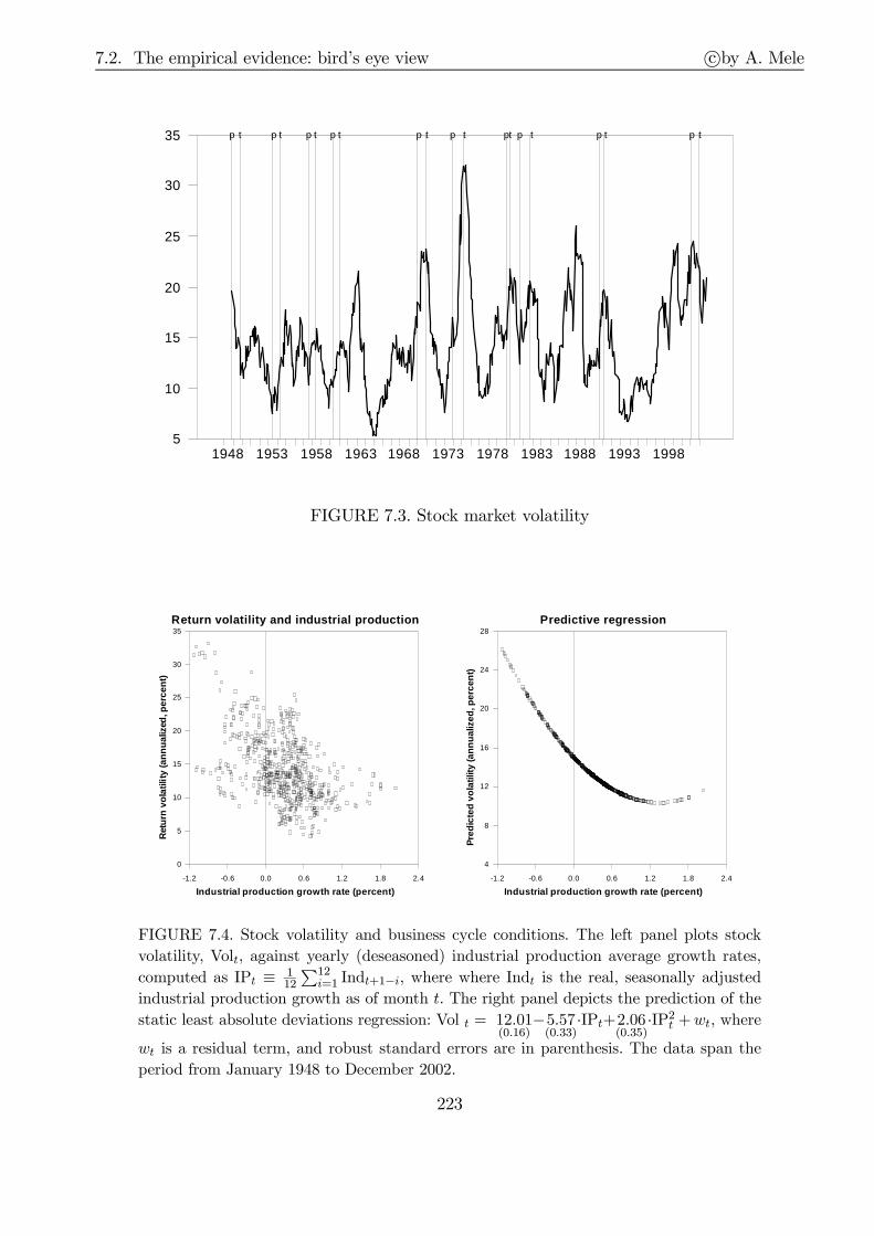
7.2. The empirical evidence: bird’s eye view c©by A. Mele
1948 1953 1958 1963 1968 1973 1978 1983 1988 1993 19985
10
15
20
25
30
35 p t p t p t p t p t p t pt p t p t p t
FIGURE 7.3. Stock market volatility
Return volatility and industrial production
Industrial production growth rate (percent)
Ret
urn
vola
tility
(ann
ualiz
ed, p
erce
nt)
-1.2 -0.6 0.0 0.6 1.2 1.8 2.4
0
5
10
15
20
25
30
35Predictive regression
Industrial production growth rate (percent)
Pre
dict
ed v
olat
ility
(ann
ualiz
ed, p
erce
nt)
-1.2 -0.6 0.0 0.6 1.2 1.8 2.4
4
8
12
16
20
24
28
FIGURE 7.4. Stock volatility and business cycle conditions. The left panel plots stock
volatility, Volt, against yearly (deseasoned) industrial production average growth rates,
computed as IPt ≡ 112
∑12i=1 Indt+1−i, where where Indt is the real, seasonally adjusted
industrial production growth as of month t. The right panel depicts the prediction of the
static least absolute deviations regression: Vol t = 12.01(0.16)
−5.57(0.33)
·IPt+2.06(0.35)
·IP2t +wt, where
wt is a residual term, and robust standard errors are in parenthesis. The data span the
period from January 1948 to December 2002.
223

7.2. The empirical evidence: bird’s eye view c©by A. Mele
Expected Returns & Industrial Production
Industrial Production Growth Rate (%)
Exp
ecte
d S
tock
Ret
urns
(ann
ualiz
ed, %
)
-1.2 -0.6 0.0 0.6 1.2 1.8 2.4
0
5
10
15
20
25Predictive regression
Industrial Production Growth Rate (%)
Pre
dict
ed E
xpec
ted
Ret
urns
(ann
ualiz
ed, %
)
-1.2 -0.6 0.0 0.6 1.2 1.8 2.4
4
6
8
10
12
14
16
FIGURE 7.5. The left-hand side of this picture plots estimates of the expected returns
(annualized, percent) (Et say) against yearly (deseasoned) industrial production average
growth rates, computed as IPt ≡ 112
∑12i=1 Indt+1−i, where where Indt is the real, seasonally
adjusted industrial production growth as of month t. Expected returns are estimated
through the predictive regression of S&P returns on to default-premium, term-premium
and return volatility, Volt. The right-hand side of this picture depicts the prediction of the
static Least Absolute Deviations regression: Et = 8.56(0.15)
− 4.05(0.30)
· IPt+ 1.18(0.31)
· IP2t +wt, where
wt is a residual term, and robust standard errors are in parenthesis. Data are sampled
monthly, and span the period from January 1948 to December 2002.
Fact I entails a quite intuitive consequence: price-dividend ratios might convey informationrelating to future returns. After all, expansions are followed by recessions. Therefore, in goodtimes, the stock market predicts that in the future, returns will be negative. Define the excessreturn for the time period [t, t+ n] as Re
t,t+n ≡ Rt,t+n −Rt,t+n, where Rt,t+n is the asset returnover [t, t+ n], and Rt,t+n is the sum of the one-month Treasury bill rate, taken over [t, t+ n].Consider the following regressions,
Ret,t+n = an + bn × P/Dt + un,t, n ≥ 1, (7.2)
where un is a residual term. Typically, then, the estimates of bn are significantly negative,and the R2 for these regressions increases with n. In turn, the previous regressions imply that
E[Ret+n
∣∣∣P/Dt] = an + bn × P/Dt. They thus suggest that price-dividend ratios are driven by
expected excess returns. In this restrictive sense, countercyclical expected returns (Fact II) andprocyclical price-dividend ratios (Fact I) might be two sides of the same coin. To link thesepredictability results more closely to developments of the business cycle, consider the followingregression, performed with monthly data from 1948:01 to 2002:12,
Ret−12,t = 14.64
(1.04)− 9.09
(1.37)× IPt−12 − 14.27
(2.67)× Inflt−12 + ut, with R2 = 11%, (7.3)
where robust standard errors are in parenthesis, u is a residual term, Ret−12,t is the excess return
from t−12 to t, IPt is the average industrial production growth over the previous twelve months,
224

7.2. The empirical evidence: bird’s eye view c©by A. Mele
as defined in Figure 7.4, and Inflt is defined similarly as IPt. The negative signs are quite tobe expected. Economic activity does display mean-reverting behavior, in that bad times arefollowed by good, in the sample size we consider. But good times are those where the stockmarket goes up. Therefore, a slowdown in economic activity is a predictor of high returns inthe future. Note that the nature of the regression results in Eq. (7.3) is quite the same as thatin Eq. (7.2), for the simple reason that the price-dividend ratio is procyclical. Finally, note thatat a contemporaneous level, excess returns are positively related to industrial production andnegatively realted to inflation,
Ret−12,t = 10.47
(1.07)+ 7.27
(1.19)× IPt − 16.33
(2.91)× Inflt + wt, with R2 = 14%, (7.4)
with robust standard errors in parenthesis, and w is a residual term. Corradi, Distaso andMele (2010) estimate a continuous time model where the aggregate stock price is driven byboth industrial production and inflation, and one unobserved factor, and show that the linksbetween returns and the two macroeconomic factors are similar to those summarized by thelinear regression in Eq. (7.4).Finally, an apparently puzzling feature is that price-dividend ratios do not predict future
dividend growth. Let gt ≡ ln(Dt/Dt−1). In regressions taking the following format,
gt+n = an + bn × P/Dt + un,t, n ≥ 1,
the predictive content of price-dividend ratios is poor, and estimates of bn might often comewith a wrong sign.The previous regressions thus suggest that: (i) price-dividend ratios are driven by time-varying
expected returns (i.e. by time-varying risk-premiums); and (ii) the role played by expecteddividend growth is somewhat limited. As we shall see later in this chapter, this view can bechallenged along several dimensions. First, it seems that expected earning growth does helppredicting price-dividend ratios. Second, the fact expected dividend growth does not seem toaffect price-dividend ratios can be a property to be expected in equilibrium.Naturally, because expected returns and stock volatility are both strongly countercyclical,
they then positively relate, at the business cycle frequency considered in this chapter, as illus-trated by Figure 7.6 below.
Expected Returns & Stock Volatility
Stock Volatility (annualized, %)
Exp
ect
ed
retu
rns
(ann
ualiz
ed,
%)
0 5 10 15 20 25 30 35
0
5
10
15
20
25
FIGURE 7.6.
225

7.3. Volatility: a business cycle perspective c©by A. Mele
7.3 Volatility: a business cycle perspective
A prominent feature of the U.S. stock market is the close connection between aggregate stockvolatility and business cycle developments, as Figure 7.4 vividly illustrates. Understandingthe origins and implications of these facts is extremely relevant to policy makers. Indeed, ifstock market volatility is countercyclical, it must necessarily be encoding information aboutthe development of the business cycle. Policy makers could then attempt at extracting thesignals stock volatility brings about the development of the business cycle.This section accomplishes three tasks. First, it delivers more details about stylized facts
relating stock volatility, expected returns and P/D ratios over the business cycle (in Section7.3.1). Second, it provides a few preliminary theoretical explanations of these facts (in Section7.3.2). Third, it investigates whether stock volatility contains any useful information about thebusiness cycle development (in Section 7.3.3). There are other exciting topics left over fromthis section. For example, we do not tackle statistical issues related to volatility measurement(see, e.g., Andersen, Bollerslev and Diebold, 2002, for a survey on the many available statisti-cal techniques to estimate volatility). Nor do we consider the role of volatility in applied assetevaluation: Chapter 10, instead, provides details about how time-varying volatility affects deriv-ative pricing. At a more fundamental level, the focus of this section is to explore the extent towhich stock market volatility movements can be given a wider business cycle perspective, andto highlight some of the rational mechanisms underlying them.
7.3.1 Volatility cycles
Why is stock market volatility related to the business cycle? Financial economists seem tohave overlooked this issue for decades. A notable exception is an early contribution by Schwert(1989a,b), who demonstrates how difficult it is to explain low frequency fluctuations in stockmarket volatility through low frequency variation in the volatility of other macroeconomicvariables. A natural exercise at this juncture, is to look into the statistical properties of industrialproduction volatility and check whether this correlates with stock volatility. Accordingly, wecompute industrial production volatility as, VolG,t ≡ 1√
12
∑12i=1 |Gt+1−i|, where Gt is the real,
seasonally adjusted industrial production growth rate as of month t, similarly as in Eq. (8.12).Figure 7.7 plots stock volatility against the volatility of industrial production growth, and doesnot reveal any statistically discernible pattern between these two variables. These results are instriking contrast with those available from Figure 7.4, where, instead, stock volatility exhibits aquite clear countercyclical behavior. More in detail, Table 7.1 reveals that stock market volatilityis almost 30% higher during NBER recessions than during NBER expansions.In fact, Schwert, also shows that stock volatility is countercyclical. The main focus of this
section is to provide a few explanations for this seemingly puzzling evidence, in support of theview stock market volatility relates to the business cycle, although not precisely related to thevolatility of other macroeconomic variables.A seemingly separate, yet very well-known, stylized fact is that risk-premiums (i.e. the in-
vestors’ expected return to invest in the stock market) are countercyclical (see, e.g., Fama andFrench, 1989, and Ferson and Harvey, 1991), as summarized by Fact II. Particularly importantis also Fact III, that expected returns lower much less during expansions than they increaseduring recessions. Using post-war data, we find that compared to an average of 8.36%, the ex-pected returns increase by nearly 19% during recessions and drop by a mere 3% during NBERexpansions (see Table 7.1). A final stylized fact relates to the behavior of the price-dividend
226
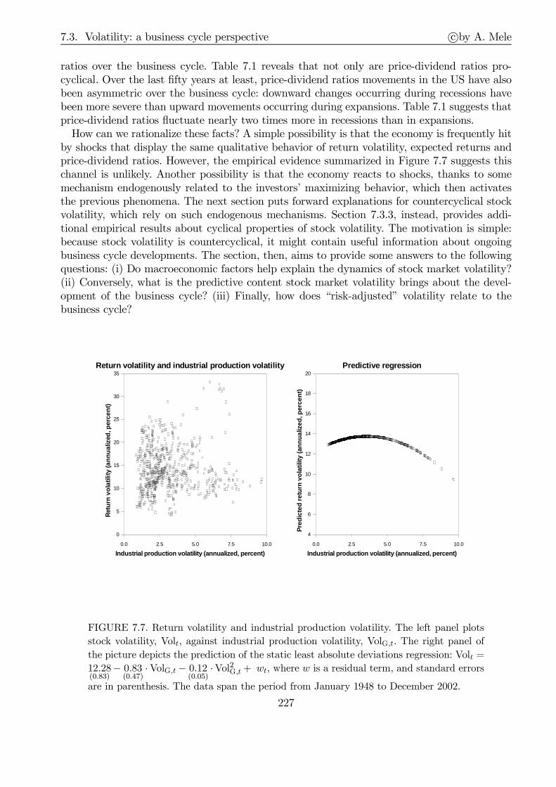
7.3. Volatility: a business cycle perspective c©by A. Mele
ratios over the business cycle. Table 7.1 reveals that not only are price-dividend ratios pro-cyclical. Over the last fifty years at least, price-dividend ratios movements in the US have alsobeen asymmetric over the business cycle: downward changes occurring during recessions havebeen more severe than upward movements occurring during expansions. Table 7.1 suggests thatprice-dividend ratios fluctuate nearly two times more in recessions than in expansions.How can we rationalize these facts? A simple possibility is that the economy is frequently hit
by shocks that display the same qualitative behavior of return volatility, expected returns andprice-dividend ratios. However, the empirical evidence summarized in Figure 7.7 suggests thischannel is unlikely. Another possibility is that the economy reacts to shocks, thanks to somemechanism endogenously related to the investors’ maximizing behavior, which then activatesthe previous phenomena. The next section puts forward explanations for countercyclical stockvolatility, which rely on such endogenous mechanisms. Section 7.3.3, instead, provides addi-tional empirical results about cyclical properties of stock volatility. The motivation is simple:because stock volatility is countercyclical, it might contain useful information about ongoingbusiness cycle developments. The section, then, aims to provide some answers to the followingquestions: (i) Do macroeconomic factors help explain the dynamics of stock market volatility?(ii) Conversely, what is the predictive content stock market volatility brings about the devel-opment of the business cycle? (iii) Finally, how does “risk-adjusted” volatility relate to thebusiness cycle?
Return volatility and industrial production volatil ity
Industrial production volatility (annualized, perce nt)
Ret
urn
vola
tility
(ann
ualiz
ed, p
erce
nt)
0.0 2.5 5.0 7.5 10.0
0
5
10
15
20
25
30
35Predictive regression
Industrial production volatility (annualized, perce nt)
Pre
dict
ed re
turn
vol
atili
ty (a
nnua
lized
, per
cent
)
0.0 2.5 5.0 7.5 10.0
4
6
8
10
12
14
16
18
20
FIGURE 7.7. Return volatility and industrial production volatility. The left panel plots
stock volatility, Volt, against industrial production volatility, VolG,t. The right panel of
the picture depicts the prediction of the static least absolute deviations regression: Volt =
12.28(0.83)
− 0.83(0.47)
·VolG,t− 0.12(0.05)
·Vol2G,t+ wt, where w is a residual term, and standard errors
are in parenthesis. The data span the period from January 1948 to December 2002.
227
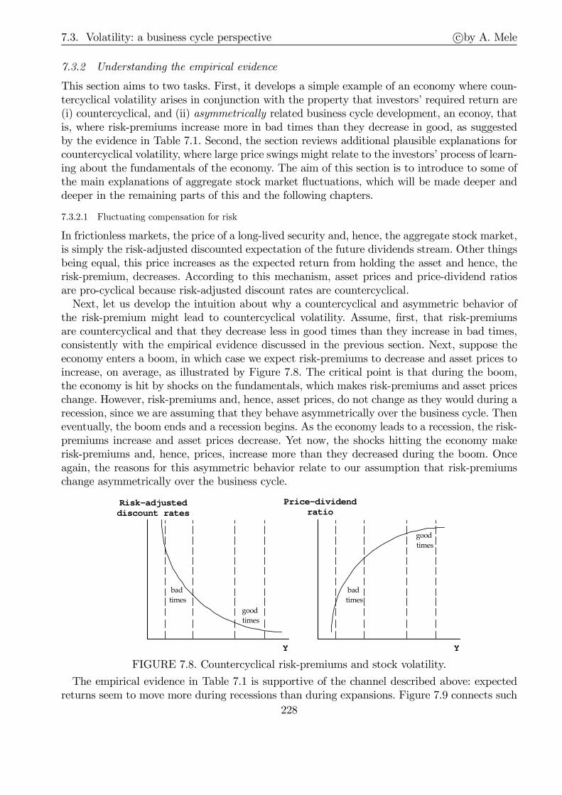
7.3. Volatility: a business cycle perspective c©by A. Mele
7.3.2 Understanding the empirical evidence
This section aims to two tasks. First, it develops a simple example of an economy where coun-tercyclical volatility arises in conjunction with the property that investors’ required return are(i) countercyclical, and (ii) asymmetrically related business cycle development, an econoy, thatis, where risk-premiums increase more in bad times than they decrease in good, as suggestedby the evidence in Table 7.1. Second, the section reviews additional plausible explanations forcountercyclical volatility, where large price swings might relate to the investors’ process of learn-ing about the fundamentals of the economy. The aim of this section is to introduce to some ofthe main explanations of aggregate stock market fluctuations, which will be made deeper anddeeper in the remaining parts of this and the following chapters.
7.3.2.1 Fluctuating compensation for risk
In frictionless markets, the price of a long-lived security and, hence, the aggregate stock market,is simply the risk-adjusted discounted expectation of the future dividends stream. Other thingsbeing equal, this price increases as the expected return from holding the asset and hence, therisk-premium, decreases. According to this mechanism, asset prices and price-dividend ratiosare pro-cyclical because risk-adjusted discount rates are countercyclical.Next, let us develop the intuition about why a countercyclical and asymmetric behavior of
the risk-premium might lead to countercyclical volatility. Assume, first, that risk-premiumsare countercyclical and that they decrease less in good times than they increase in bad times,consistently with the empirical evidence discussed in the previous section. Next, suppose theeconomy enters a boom, in which case we expect risk-premiums to decrease and asset prices toincrease, on average, as illustrated by Figure 7.8. The critical point is that during the boom,the economy is hit by shocks on the fundamentals, which makes risk-premiums and asset priceschange. However, risk-premiums and, hence, asset prices, do not change as they would during arecession, since we are assuming that they behave asymmetrically over the business cycle. Theneventually, the boom ends and a recession begins. As the economy leads to a recession, the risk-premiums increase and asset prices decrease. Yet now, the shocks hitting the economy makerisk-premiums and, hence, prices, increase more than they decreased during the boom. Onceagain, the reasons for this asymmetric behavior relate to our assumption that risk-premiumschange asymmetrically over the business cycle.
Risk-adjusted discount rates
Price-dividend ratio
Y
good
times
bad
times
Y
good
times
bad
times
FIGURE 7.8. Countercyclical risk-premiums and stock volatility.
The empirical evidence in Table 7.1 is supportive of the channel described above: expectedreturns seem to move more during recessions than during expansions. Figure 7.9 connects such
228
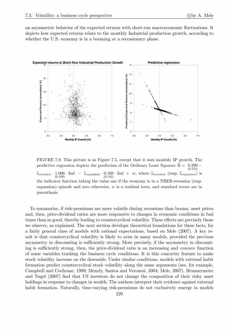
7.3. Volatility: a business cycle perspective c©by A. Mele
an asymmetric behavior of the expected returns with short-run macroeconomic fluctuations. Itdepicts how expected returns relate to the monthly Industrial production growth, according towhether the U.S. economy is in a booming or a recessionary phase.
Expected returns & Short-Run Industrial Production Growth
Monthly IP Growth (%)
Exp
ect
ed
Re
turn
s (a
nnua
lize
d, %
)
-5.0 -2.5 0.0 2.5 5.0 7.5
0
5
10
15
20
25Predictive regression
Monthly IP Growth (%)
Pre
dict
ed
Exp
ect
ed
Re
turn
s (a
nnua
lize
d, %
)
-5.0 -2.5 0.0 2.5 5.0 7.5
6
7
8
9
10
11
12
13
FIGURE 7.9. This picture is as Figure 7.5, except that it uses monthly IP growth. The
predictive regression depicts the prediction of the Ordinary Least Squares: E = 8.299(0.155)
−Irecession · 1.006
(0.339)· Ind − Iexpansion · 0.169
(0.153)· Ind + w, where Irecession (resp. Iexpansion) is
the indicator function taking the value one if the economy is in a NBER-recession (resp.
expansion) episode and zero otherwise, w is a residual term, and standard errors are in
parenthesis.
To summarize, if risk-premiums are more volatile during recessions than booms, asset pricesand, then, price-dividend ratios are more responsive to changes in economic conditions in badtimes than in good, thereby leading to countercyclical volatility. These effects are precisely thosewe observe, as explained. The next section develops theoretical foundations for these facts, fora fairly general class of models with rational expectations, based on Mele (2007). A key re-sult is that countercyclical volatility is likely to arise in many models, provided the previousasymmetry in discounting is sufficiently strong. More precisely, if the asymmetry in discount-ing is sufficiently strong, then, the price-dividend ratio is an increasing and concave functionof some variables tracking the business cycle conditions. It is this concavity feature to makestock volatility increase on the downside. Under similar conditions, models with external habitformation predict countercyclical stock volatility along the same arguments (see, for example,Campbell and Cochrane, 1999; Menzly, Santos and Veronesi, 2004; Mele, 2007). Brunnermeierand Nagel (2007) find that US investors do not change the composition of their risky assetholdings in response to changes in wealth. The authors interpret their evidence against externalhabit formation. Naturally, time-varying risk-premiums do not exclusively emerge in models
229

7.3. Volatility: a business cycle perspective c©by A. Mele
with external habit formation. Barberis, Huang and Santos (2001) develop a theory distinctfrom habit formation that leads to time-varying risk-premiums.These theoretical explanations for countercyclical volatility, which are further developed in
the next section, hold within a fairly general continuous-time framework. Although their proofsmight be technical, the intuition is precisely that illustrated by Figure 7.8. This section, then,aims to provide a quantitative illustration of these results, which hinges upon a simple analyticalframework, relying on a tree. This model is very simple, but it can be solved analytically and,as shown below, is able to reproduce some of the main stylized features of the actual aggregatestock market behavior.We consider an infinite horizon economy with a representative investor who in equilibrium
consumes (state by state) all the dividends promised by some asset. We assume that there existsa safe asset elastically supplied such that the safe interest rate is some constant r > 0. In theinitial state, a dividend process takes a unit value (see Figure 7.10). In the second period, thedividend equals either e−δ (δ > 0) with probability p (the bad state) or eδ with probability 1−p(the good state). In the initial state, the investor’s coefficient of constant relative risk-aversion(CRRA) is η > 0. In the good (resp., the bad) state, the investor’s CRRA is ηG (resp., ηB)> 0. In the third period, the investor receives the final payoffs in Figure 7.10, where MS is theprice of a claim to all future dividends, discounted at a CRRA ηS, with S ∈ G,B,GB andηGB = η (the “hybrid” state). This model is thus one with constant expected dividend growth,but random risk-aversion. Note that both random risk-aversion and dividend growth are actingas sources of “long-run risks”–once these risk are resolved, both risk-aversion and dividendgrowth remain fixed at their levels forever.
δe
δ−e
BMe +− δ2
GMe +δ2
GBM+1
p
q
p
p
Bq
Gq Good state
Bad state
1
FIGURE 7.10. A tree model of random risk-aversion and countercyclical volatility. The
dividend process takes a unit value at the initial node. With probability p, the dividend
then decreases to e−δ in the bad state. The corresponding risk-neutral probability is
denoted as q. The risk-neutral probability of further dividends movements differs according
to whether the economy is in the good or bad state (i.e. qG or qB). At the end of the tree,
the investor receives the dividends plus the right to the stream of all future dividends. In
the upper node, this right is worth MG (the evaluation obtained through the risk-neutral
probability qG). In the central node it is worth MGB (the evaluation obtained through
230

7.3. Volatility: a business cycle perspective c©by A. Mele
the risk-neutral probability q). In the lower node it is worth MB (the evaluation obtained
through the risk-neutral probability qB). The safe interest rate is taken to be constant.
The model is calibrated using the same U.S. data as in Table 7.1, and calibration resultsare in Table 7.2. Appendix A provides details about the solution and the calibration of themodel. One important issue is that the calibration is made using data for aggregate dividendgrowth, which has a volatility around 6% annualized, almost the double as that on consumptiongrowth. Consider, then, the simple calibration of the Lucas model in Section 6.2 of the previouschapter. As noted, this volatility would imply a relative risk-aversion of around 17 ≈ 0.06
0.062 , tomatch an equity premium of 6%. However, it was argued, the Lucas model of Chapter 6 cannotreproduce the high return volatility we observe in the data. In the simple model of the previouschapter, return volatility is simply dividend growth volatility and equals 6%, less than a halfof the average volatility in the data, 14.55%. Nor would that model predict the countercyclicalstatistics in Table 7.1, as it predicts a constant price-dividend ratio.
Dataexpansions average recessions
P/D ratio 33.21 31.99 26.20excess return volatility 14.05 14.55 16.91
Model calibrationgood state average bad state
P/D ratio 32.50 31.81 28.15excess return volatility 7.29 8.20 13.03
risk-adjusted rate 8.95 9.07 9.71expected returns 10.16 11.46 18.42
implied risk-aversion 13.69 13.89 14.96
TABLE 7.2. This table reports calibration results for the infinite horizon tree model in
Figure 3. The expected returns and excess return volatility predicted by the model are
computed using log-returns. The risk-adjusted rate is computed as r + σDλS, where: r is
the continuously compounded riskless rate; σD is the dividend volatility; λS is the Sharpe
ratio on gross returns in state S, computed as λS ≡ (qS − p)÷√p (1− p) for S = G (the
good state) and S = B (the bad state); p is the probability of the bad state; and qS is
the state dependent risk-adjusted probability of a bad state (for S ∈ G,B). Implied
risk-aversion is the coefficient of relative risk aversion ηS in the good state (S = G) and
in the bad state (S = B), implied by the calibrated model. The figures in the “average”
column are the averages of the corresponding values in the good and bad states taken
under the probability p = 0.158.
The model in this section is capable of addressing these issues. First, it predicts returnvolatility equal to 8% percent on average. Second, the implied risk-aversion decreases to levelsaround 11, and at the same time, quite sustained average expected excess returns. For example,fitting the Lucas model in the Section 6.2 of the previous chapter would lead to an implied
231

7.3. Volatility: a business cycle perspective c©by A. Mele
risk-aversion of about 22 ≈ 0.080.062 , once we fix the expected excess returns to 8%. Third, and in
spite of its overly simplifying assumptions, the model does reproduce volatility swings similar tothose we observe in the data, with return volatility increasing to up to 13% in the bad state ofthe world, although in this same state, it might overstate expected returns by a few percentagepoints. Importantly, this calibration exercise illustrates in an exemplary manner the asymmetricfeature of expected returns and risk aversion. In this simple experiment, both expected returnsand risk-aversion increase much more in bad times than they decrease in good times.
7.3.2.2 Alternative stock market volatility channels
Rational explanations of stock market fluctuations must necessarily rely on some underlyingstate variable affecting the investors’ decision environment. Two natural ways to accomplishthis task are obtained through the introduction of (i) time-varying risk-premiums; and (ii) time-varying expected dividend growth. The previous tree model is one simple example addressingthe first extension. More substantive examples of models predicting time-varying risk-premiumsare the habit formation models mentioned in Section 7.3, and in Section 7.5 below.Models addressing the second extension have also been produced. For example, Veronesi
(1999, 2000) and Brennan and Xia (2001) have proposed models in which stock market volatilityfluctuates as a result of a learning induced phenomenon. In these models, the growth rate ofthe economy is unknown and investors attempt to infer it from a variety of public signals. Thisinference process makes asset prices also depend on the investors’ guesses about the dividendsgrowth rate, and thus induces high return volatility. (In Veronesi, 1999, stock market volatilityis also countercyclical.)Finally, Bansal and Yaron (2004) formulate a model in which expected dividend growth is
affected by some unobservable factor. This model, which will be discussed in detail in the nextchapter, is also capable to generate countercyclical stock volatility. This property follows by themodel’s assumption that the volatilities of dividend growth and consumption are countercycli-cal. In contrast, in models with time-varying risk-premiums (such as the previous tree model),countercyclical stock market volatility emerges without the need to impose similar featureson the fundamentals of the economy. Remarkably, in models with time-varying risk-premiums,countercyclical stock market volatility can be endogenously induced by rational fluctuations inthe price-dividend ratio.
7.3.3 What to do with stock market volatility?
Both data and theory suggest that stock market volatility has a quite pronounced businesscycle pattern. A natural purpose at this juncture is to exploit these patterns to perform somebasic forecasting exercises. We consider three in-sample exercises. First, we forecast stock mar-ket volatility from past macroeconomic data (six month inflation, and six month industrialproduction growth). Second, we forecast industrial production growth from past stock marketvolatility. Third, we forecast the VIX index, an index of the risk-adjusted expectation of fu-ture volatility, from macroeconomic data, and attempt to measure the volatility risk-premium,which is the excess amount of money a risk-averse investor is willing to pay to avoid the risk ofvolatility fluctuations.
7.3.3.1 Macroeconomic constituents of stock market volatility
Table 7.3 reports the results for the first forecasting exercise. Volatility is positively related topast growth, a finding we can easily interpret. Bad times are followed by good times. Precisely,
232

7.3. Volatility: a business cycle perspective c©by A. Mele
in our samples, high growth is inevitably followed by low growth. Since stock market volatility iscountercyclical, high growth is followed by high stock market volatility. Stock market volatilityis also related to past inflation, but in a more complex manner. Note that once we control forpast values of volatility, the results remain highly significant. Figure 7.11 (top panel) depictsstock market volatility and its in-sample forecasts when the regression model is fed with pastmacroeconomic data only. This fit can even be improved through the joint use of both pastvolatility and macroeconomic factors. Nevertheless, it is remarkable that the fit from using pastmacro information is more than 60% better than just using past volatility (see the R2s in Table7.3). These results are somewhat in contrast with those reported in Schwert (1989). The keyissue, here, however, is that stock market volatility is being predicted using a lower frequencyscale.
Forecasting stock market volatility
1948 1952 1956 1960 1964 1968 1972 1976 1980 1984 1988 1992 1996 20000
5
10
15
20
25
30
35 p t p t p t p t p t p t p t p t p t p t
Forecasting economic activity
1948 1952 1956 1960 1964 1968 1972 1976 1980 1984 1988 1992 1996 2000-3
-2
-1
0
1
2
3 p t p t p t p t p t p t p t p t p t p t
FIGURE 7.11. Forecasts. The top panel depicts stock market volatility (solid line) and
stock market volatility forecasts obtained through the sole use of the macroeconomic
indicators in Table 7.3 (dashed line). The bottom panel depicts 6-month moving average
industrial production growth (solid line) and its forecasts based on the 6th regression in
Table 7.4 (dashed line).
The previous findings, while certainly informal and preliminary, suggest that relating stockmarket volatility to macroeconomic factors might be a fertile avenue of research. The main ques-tion is, of course, how precisely stock market volatility should relate to past macroeconomicfactors? Indeed, the regressions in Table 7.3 capture mere statistical relations between stockmarket volatility and macroeconomic factors. Yet, in the absence of arbitrage opportunities,stock market volatility is certainly related to how the price responds to shocks in the funda-mentals and, hence, the macroeconomic conditions. Therefore, there should exist a no-arbitragenexus between stock market volatility and macroeconomic factors. Corradi, Distaso and Mele
233
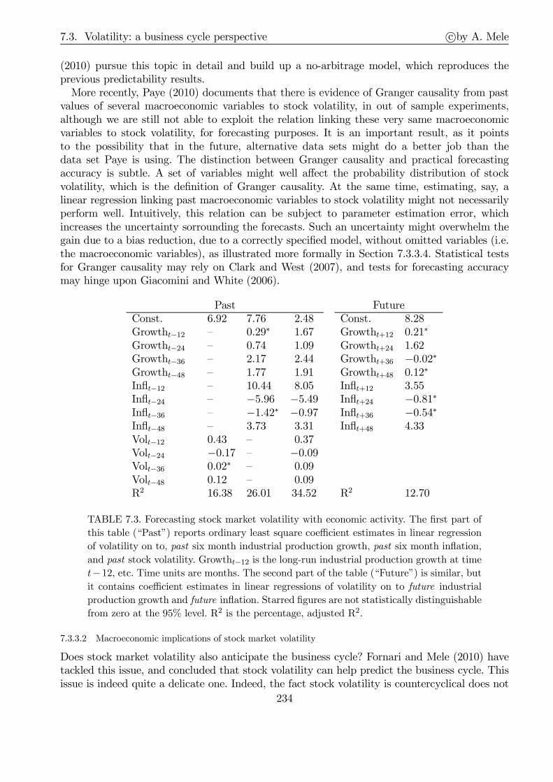
7.3. Volatility: a business cycle perspective c©by A. Mele
(2010) pursue this topic in detail and build up a no-arbitrage model, which reproduces theprevious predictability results.More recently, Paye (2010) documents that there is evidence of Granger causality from past
values of several macroeconomic variables to stock volatility, in out of sample experiments,although we are still not able to exploit the relation linking these very same macroeconomicvariables to stock volatility, for forecasting purposes. It is an important result, as it pointsto the possibility that in the future, alternative data sets might do a better job than thedata set Paye is using. The distinction between Granger causality and practical forecastingaccuracy is subtle. A set of variables might well affect the probability distribution of stockvolatility, which is the definition of Granger causality. At the same time, estimating, say, alinear regression linking past macroeconomic variables to stock volatility might not necessarilyperform well. Intuitively, this relation can be subject to parameter estimation error, whichincreases the uncertainty sorrounding the forecasts. Such an uncertainty might overwhelm thegain due to a bias reduction, due to a correctly specified model, without omitted variables (i.e.the macroeconomic variables), as illustrated more formally in Section 7.3.3.4. Statistical testsfor Granger causality may rely on Clark and West (2007), and tests for forecasting accuracymay hinge upon Giacomini and White (2006).
Past FutureConst. 6.92 7.76 2.48 Const. 8.28Growtht−12 — 0.29∗ 1.67 Growtht+12 0.21∗
Growtht−24 — 0.74 1.09 Growtht+24 1.62Growtht−36 — 2.17 2.44 Growtht+36 −0.02∗Growtht−48 — 1.77 1.91 Growtht+48 0.12∗
Inflt−12 — 10.44 8.05 Inflt+12 3.55Inflt−24 — −5.96 −5.49 Inflt+24 −0.81∗Inflt−36 — −1.42∗ −0.97 Inflt+36 −0.54∗Inflt−48 — 3.73 3.31 Inflt+48 4.33Volt−12 0.43 — 0.37Volt−24 −0.17 — −0.09Volt−36 0.02∗ — 0.09Volt−48 0.12 — 0.09R2 16.38 26.01 34.52 R2 12.70
TABLE 7.3. Forecasting stock market volatility with economic activity. The first part of
this table (“Past”) reports ordinary least square coefficient estimates in linear regression
of volatility on to, past six month industrial production growth, past six month inflation,
and past stock volatility. Growtht−12 is the long-run industrial production growth at time
t−12, etc. Time units are months. The second part of the table (“Future”) is similar, but
it contains coefficient estimates in linear regressions of volatility on to future industrial
production growth and future inflation. Starred figures are not statistically distinguishable
from zero at the 95% level. R2 is the percentage, adjusted R2.
7.3.3.2 Macroeconomic implications of stock market volatility
Does stock market volatility also anticipate the business cycle? Fornari and Mele (2010) havetackled this issue, and concluded that stock volatility can help predict the business cycle. Thisissue is indeed quite a delicate one. Indeed, the fact stock volatility is countercyclical does not
234
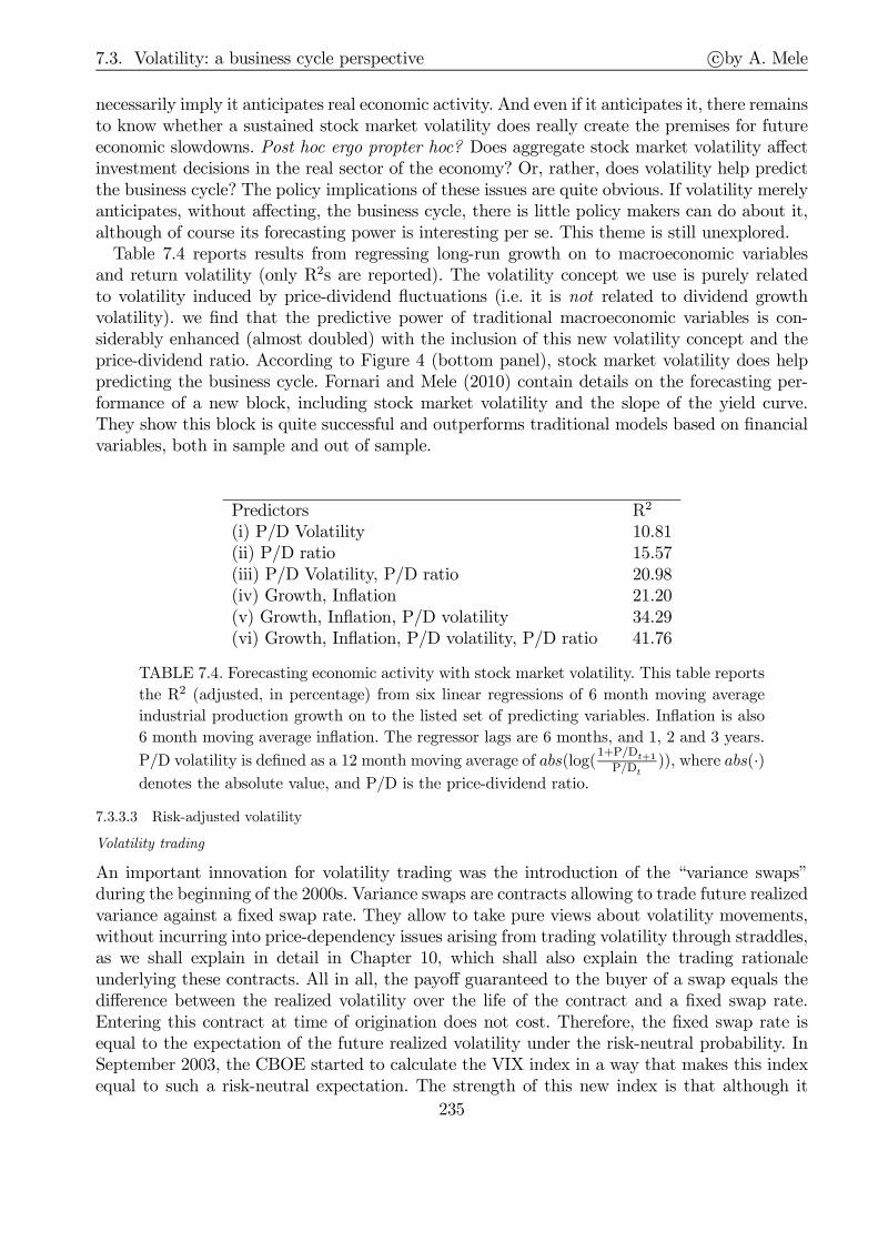
7.3. Volatility: a business cycle perspective c©by A. Mele
necessarily imply it anticipates real economic activity. And even if it anticipates it, there remainsto know whether a sustained stock market volatility does really create the premises for futureeconomic slowdowns. Post hoc ergo propter hoc? Does aggregate stock market volatility affectinvestment decisions in the real sector of the economy? Or, rather, does volatility help predictthe business cycle? The policy implications of these issues are quite obvious. If volatility merelyanticipates, without affecting, the business cycle, there is little policy makers can do about it,although of course its forecasting power is interesting per se. This theme is still unexplored.Table 7.4 reports results from regressing long-run growth on to macroeconomic variables
and return volatility (only R2s are reported). The volatility concept we use is purely relatedto volatility induced by price-dividend fluctuations (i.e. it is not related to dividend growthvolatility). we find that the predictive power of traditional macroeconomic variables is con-siderably enhanced (almost doubled) with the inclusion of this new volatility concept and theprice-dividend ratio. According to Figure 4 (bottom panel), stock market volatility does helppredicting the business cycle. Fornari and Mele (2010) contain details on the forecasting per-formance of a new block, including stock market volatility and the slope of the yield curve.They show this block is quite successful and outperforms traditional models based on financialvariables, both in sample and out of sample.
Predictors R2
(i) P/D Volatility 10.81(ii) P/D ratio 15.57(iii) P/D Volatility, P/D ratio 20.98(iv) Growth, Inflation 21.20(v) Growth, Inflation, P/D volatility 34.29(vi) Growth, Inflation, P/D volatility, P/D ratio 41.76
TABLE 7.4. Forecasting economic activity with stock market volatility. This table reports
the R2 (adjusted, in percentage) from six linear regressions of 6 month moving average
industrial production growth on to the listed set of predicting variables. Inflation is also
6 month moving average inflation. The regressor lags are 6 months, and 1, 2 and 3 years.
P/D volatility is defined as a 12 month moving average of abs(log(1+P/Dt+1
P/Dt)), where abs(·)
denotes the absolute value, and P/D is the price-dividend ratio.
7.3.3.3 Risk-adjusted volatility
Volatility trading
An important innovation for volatility trading was the introduction of the “variance swaps”during the beginning of the 2000s. Variance swaps are contracts allowing to trade future realizedvariance against a fixed swap rate. They allow to take pure views about volatility movements,without incurring into price-dependency issues arising from trading volatility through straddles,as we shall explain in detail in Chapter 10, which shall also explain the trading rationaleunderlying these contracts. All in all, the payoff guaranteed to the buyer of a swap equals thedifference between the realized volatility over the life of the contract and a fixed swap rate.Entering this contract at time of origination does not cost. Therefore, the fixed swap rate isequal to the expectation of the future realized volatility under the risk-neutral probability. InSeptember 2003, the CBOE started to calculate the VIX index in a way that makes this indexequal to such a risk-neutral expectation. The strength of this new index is that although it
235
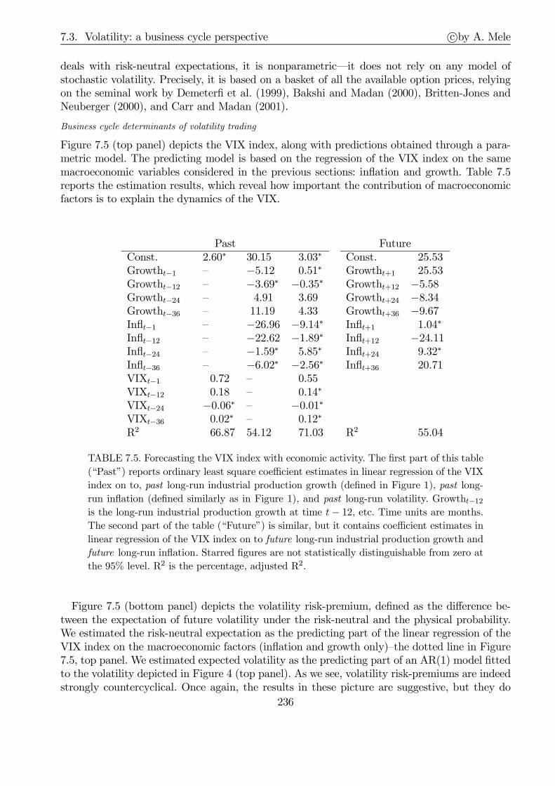
7.3. Volatility: a business cycle perspective c©by A. Mele
deals with risk-neutral expectations, it is nonparametric–it does not rely on any model ofstochastic volatility. Precisely, it is based on a basket of all the available option prices, relyingon the seminal work by Demeterfi et al. (1999), Bakshi and Madan (2000), Britten-Jones andNeuberger (2000), and Carr and Madan (2001).
Business cycle determinants of volatility trading
Figure 7.5 (top panel) depicts the VIX index, along with predictions obtained through a para-metric model. The predicting model is based on the regression of the VIX index on the samemacroeconomic variables considered in the previous sections: inflation and growth. Table 7.5reports the estimation results, which reveal how important the contribution of macroeconomicfactors is to explain the dynamics of the VIX.
Past FutureConst. 2.60∗ 30.15 3.03∗ Const. 25.53Growtht−1 — −5.12 0.51∗ Growtht+1 25.53Growtht−12 — −3.69∗ −0.35∗ Growtht+12 −5.58Growtht−24 — 4.91 3.69 Growtht+24 −8.34Growtht−36 — 11.19 4.33 Growtht+36 −9.67Inflt−1 — −26.96 −9.14∗ Inflt+1 1.04∗
Inflt−12 — −22.62 −1.89∗ Inflt+12 −24.11Inflt−24 — −1.59∗ 5.85∗ Inflt+24 9.32∗
Inflt−36 — −6.02∗ −2.56∗ Inflt+36 20.71VIXt−1 0.72 — 0.55VIXt−12 0.18 — 0.14∗
VIXt−24 −0.06∗ — −0.01∗VIXt−36 0.02∗ — 0.12∗
R2 66.87 54.12 71.03 R2 55.04
TABLE 7.5. Forecasting the VIX index with economic activity. The first part of this table
(“Past”) reports ordinary least square coefficient estimates in linear regression of the VIX
index on to, past long-run industrial production growth (defined in Figure 1), past long-
run inflation (defined similarly as in Figure 1), and past long-run volatility. Growtht−12
is the long-run industrial production growth at time t− 12, etc. Time units are months.
The second part of the table (“Future”) is similar, but it contains coefficient estimates in
linear regression of the VIX index on to future long-run industrial production growth and
future long-run inflation. Starred figures are not statistically distinguishable from zero at
the 95% level. R2 is the percentage, adjusted R2.
Figure 7.5 (bottom panel) depicts the volatility risk-premium, defined as the difference be-tween the expectation of future volatility under the risk-neutral and the physical probability.We estimated the risk-neutral expectation as the predicting part of the linear regression of theVIX index on the macroeconomic factors (inflation and growth only)—the dotted line in Figure7.5, top panel. We estimated expected volatility as the predicting part of an AR(1) model fittedto the volatility depicted in Figure 4 (top panel). As we see, volatility risk-premiums are indeedstrongly countercyclical. Once again, the results in these picture are suggestive, but they do
236
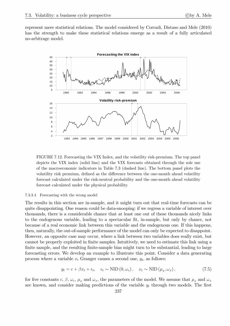
7.3. Volatility: a business cycle perspective c©by A. Mele
represent mere statistical relations. The model considered by Corradi, Distaso and Mele (2010)has the strength to make these statistical relations emerge as a result of a fully articulatedno-arbitrage model.
Forecasting the VIX index
1990 1992 1994 1996 1998 2000 2002 2004 20065
10
15
20
25
30
35
40
45 p t p t
Volatility risk-premium
1993 1994 1995 1996 1997 1998 1999 2000 2001 2002 2003 2004 2005 20062
4
6
8
10
12
14
16 p t
FIGURE 7.12. Forecasting the VIX Index, and the volatility risk-premium. The top panel
depicts the VIX index (solid line) and the VIX forecasts obtained through the sole use
of the macroeconomic indicators in Table 7.3 (dashed line). The bottom panel plots the
volatility risk premium, defined as the difference between the one-month ahead volatility
forecast calculated under the risk-neutral probability and the one-month ahead volatility
forecast calculated under the physical probability.
7.3.3.4 Forecasting with the wrong model
The results in this section are in-sample, and it might turn out that real-time forecasts can bequite disappointing. One reason could be data-snooping: if we regress a variable of interest overthousands, there is a considerable chance that at least one out of these thousands nicely linksto the endogenous variable, leading to a spectacular fit, in-sample, but only by chance, notbecause of a real economic link between this variable and the endogenous one. If this happens,then, naturally, the out-of-sample performance of the model can only be expected to disappoint.However, an opposite case may occur, where a link between two variables does really exist, butcannot be properly exploited in finite samples. Intuitively, we need to estimate this link using afinite sample, and the resulting finite-sample bias might turn to be substantial, leading to largeforecasting errors. We develop an example to illustrate this point. Consider a data generatingprocess where a variable xt Granger causes a second one, yt, as follows:
yt = c+ βxt + ǫt, ǫt ∼ NID (0, ωǫ) , xt ∼ NID (µx, ωx) , (7.5)
for five constants c, β, ωǫ, µx and ωx, the parameters of the model. We assume that µx and ωxare known, and consider making predictions of the variable yt through two models. The first
237

7.3. Volatility: a business cycle perspective c©by A. Mele
model is misspecified, one where we simply neglect that xt Granger causes yt, i.e. yt = ψ + ut,for some constant ψ and some residual term ut. We estimate the constant ψ of this misspecifiedmodel through ordinary least squares (OLS), obtaining:
ψ − c = βxT + ǫT ,
where xT and ǫT denote the sample averages of xt and ǫt, and T is the sample size. The predictionerror generated by this model for time T + 1 is:
η1,T+1 ≡ yT+1 − ψ = β (xT+1 − xT ) + ǫT+1 − ǫT .
Note that although ψ is biased for c, even asymptotically, the predictor of this misspecifiedmodel is unbiased, as we have that E
(η1,T+1
)= 0, where E is the unconditional expectation
operator.Next, condider using as a predictor, the predictive part of Eq. (7.5), obtained through the
OLS estimators of c and β, say c and β. The resulting prediction error is,
η2,T+1 ≡ yT+1 − c− βxT+1
= c− c+ (β − β)xT+1 + ǫT+1
= (β − β) (xT+1 − xT ) + ǫT+1 − ǫT , (7.6)
where the second equality follows by (i) c = yT − βxT , with yT denoting the sample average ofyt, and (ii) Eq. (7.5), and:
β − β = −CovT (xt, ǫt)VT (xt)
,
and CovT and VT stand for the sample covariance and variance of their arguments. The correctlyspecified model does, naturally, lead to an unbiased predictor, in that E
(η2,T+1
)= 0, by the
second line in Eq. (7.6). Therefore, the two models we consider–the misspecified and thecorrectly specified–both lead to unbiased predictors. However, the second predictor is plaguedby parameter estimation error, and might actually lead to mean-squared prediction errors higherthan those generated by the first predictor, especially when the the sample variance of β− β islarge. In other words, for large samples, β − β is, of course, quite small, as β is consistent forβ. In finite samples, however, this term can adversely affect the performance of the correctlyspecified model.
7.3.4 What did we learn?
Stock market volatility is higher in bad times than in good times. Explaining this basic factis challenging. Indeed, economists know very well how to model risk-premiums and how thesepremiums should relate to the business cycle. We feel more embarrassed when we come toexplain volatility. The ambition in this short essay is to explain that countercyclical volatilitycan be made consistent with the prediction of the neoclassical model of asset pricing - inwhich asset prices are (risk-adjusted) expectations of future dividends. One condition activatingcountercyclical volatility is very simple: risk-premiums must swing sharply as the economymoves away from good states, just as the data seem to suggest.The focus in this section was stock market volatility fluctuations, not the average levels of
stock volatility and the risk-premiums, which could make them consistent with plausible levels of
238

7.4. Rational stock market fluctuations c©by A. Mele
investors’ risk-aversion, two themes so controversial, as many topics at the intersection betweenfinancial economics and macroeconomics (see, e.g., Campbell, 2003; Mehra and Prescott, 2003).However, a simple model relying on a tree suggests the neoclassical model might deliver resultsexplaining how volatility switches across states. Finally, this section investigates whether thesetheoretical insights have some additional empirical content. Three empirical issues have beenexplored, which are currently being investigated in the literature. It was explained that (i) stockvolatility can be forecast through macroeconomic variables; (ii) stock market volatility doescontain relevant information related to business cycle developments; and (iii) volatility tradingdoes relate to the business cycle and that volatility risk-premiums are strongly countercyclical.
7.4 Rational stock market fluctuations
We aim to explain the stylized facts in Section 7.2 through the neoclassical model, and relyingon a framework of analysis as general as possible. This section draws on Mele (2005, 2007).
7.4.1 A decomposition
We have:
ln Rt+1 ≡ lnSt+1 +Dt+1
St= gt+1 + ln
pt+1 + 1
pt, where gt ≡ ln
Dt
Dt−1and pt ≡
StDt.
This decomposition reveals that the properties of asset returns can be understood through thoseof the dividend growth, gt, and the price-dividend ratio pt. The empirical evidence in Section7.2 suggests that explanations based on rational evaluation should exhibit at least two features.First, we need volatile price-dividend ratios. Second we need price-dividend ratios to be, onaverage, more volatile in bad times than in good. Let us consider, for example, a model whereasset prices are affected by some key state variables related to the business cycle conditions (asin the habit models of Section 7.5) A basic property we should require from this particular modelis that the price-dividend ratio be increasing and concave in the state variables related to thebusiness cycle conditions, as explained in Section 7.3.2. In particular, such a concavity propertyensures stock volatility increases on the downside, which is the very definition of countercyclicalvolatility.The ultimate scope in this section is to search for classes of models ensuring this and related
properties. A word of caution is needed at this juncture. The Gordon’s model (Gordon, 1962)reviewed in Chapter 6 predicts price-dividend ratios are constant, a counterfactual feature,pointing to the need of multifactor models. At the same time, multifactor model might notnecessarily lead to the properties we observe in the data. For example, the previous chapterhas shown how we can build up models where: (i) we can arbitrarily increase the variance ofthe pricing kernel by adding more and more factors, and (ii) with the unfortunate feature thatprice-dividend ratios are still constant. What is needed, then, is to impose discipline on how toincrease the dimension of a model.
7.4.2 Asset prices and state variables
7.4.2.1 A multifactor model
Consider the following reduced-form model, where an asset price, Si say, is a twice-differentiablefunction of a number of factors, Si = Si(y), i = 1, · · · ,m, and y = [y1, · · · , yd]⊤ is the vector of
239
7.4. Rational stock market fluctuations c©by A. Mele
factors deeming to affect asset prices. We assume that the i-th asset pays off an instantaneousdividend Di = Di(y), and that y is a diffusion process:
dy (t) = ϕ (y (t)) dt+ v (y (t)) dW (t) ,
where ϕ is d-valued, v is d× d valued, and W is a d-dimensional Brownian motion. We assumethe number of assets does not exceed the number of factors, m ≤ d, consistently with theframework in Chapter 4. By Itô’s lemma:
dSiSi
=LSiSidt+
1×d︷︸︸︷∇SiSi
d×d︷︸︸︷v dW, (7.7)
where LSi is the infinitesimal operator. Let r (t) be the instantaneous short-term rate. By theFTAP, we have that under regularity conditions, there exists a measurable d-vector process λ,the vector of unit prices of risk associated with the fluctuations of the factors, such that,
LS1
S1− r + D1
S1...
LSmSm
− r + DmSm
= σ︸︷︷︸
m×dλ︸︷︷︸d×1
, where σ =
∇S1
S1...
∇SmSm
· v. (7.8)
We restrict this economy to be Markov, for the mere scope to simplify, and suppose that,
r (t) ≡ r (y (t)) and λ (t) ≡ λ (y (t)) . (7.9)
In the appendix, we provide examples of pricing kernels such that the short-term rate andrisk-premiums having the same functional form as in Eqs. (7.9).Eqs. (7.8) add up to a system ofm uncoupled partial differential equations, and the solution is
one no-arbitrage price system, assuming no bubbles. This section aims to a reverse-engineeringapproach, a search for the primitives ϕ, v, r and λ, such that the asset prices in (7.8) exhibitsome properties given in advance, such as those surveyed in the previous section. As an example,Eq. (7.7) predicts the volatility of stock i is,
Volt
(dSi (t)
Si (t)
)≡ ∇Si(y (t))
Si (t)v(y (t)),
which is, typically, time-varying. One fundamental question, then, is: which restrictions do weneed to impose to ϕ, v, r and λ, so as to ensure that Volt is countercyclical? The next sectionintroduces a simple model potentially apt to address this and related questions, through time-variation in the expected returns expected dividend growth.
7.4.2.2 A canonical economy
We consider a pure exchange economy endowed with a flow of a single consumption good, whichequals the dividend paid by a single long-lived asset. Let d = 2, such that the dividend, D, andsome state variable, y, are solution to:
dD (τ )
D (τ )= m (y(τ)) dτ + σ0dW1 (τ )
dy (τ) = ϕ (y (τ)) dτ + v1 (y (τ)) dW1 (τ) + v2 (y (τ)) dW2 (τ)(7.10)
240

7.4. Rational stock market fluctuations c©by A. Mele
whereW1 andW2 are standard Brownian motions. By the Feynman-Kac representation theoremreviewed in Chapter 4, Eqs. (7.8) imply that under regularity conditions, the asset price satisfies:
S (D, y) =
∫ ∞
0
C (D, y, τ) dτ , C (D, y, τ) ≡ E[exp
(−∫ τ
0
r (D (t) , y (t)) dt
)·D (τ)
∣∣∣∣D, y],
(7.11)where E is the expectation operator taken under the risk-neutral probability Q, where thedrifts m and ϕ in Eqs. (7.10) have to be replaced by m (y) ≡ m (y) − σ0λ1 (y) and ϕ (y) ≡ϕ (y)− v1 (y)λ1 (y)− v2 (y)λ2 (y).2
7.4.3 Volatility, options and convexity
7.4.3.1 Issues
This section analyzes properties of asset prices, which can be streamlined into three categories:(i) “monotonicity,” (ii) “convexity,” and (iii) “dynamic stochastic dominance” properties.
(i) Monotonicity. Consider a model where the asset price is: S (D, y) = D · p (y), for some
positive function p ∈ C2(Y). By Itô’s lemma, stock volatility is Vol (D)+ p′(y)p(y)
Vol (y), where
Vol (D) > 0 is consumption growth volatility and Vol (y) has a similar interpretation. Asexplained in the Chapter 6, the volatility in the data is too high to be explained byconsumption volatility. Additional state variables may increase return volatility. In thissimple example, the state variable y inflates volatility if p is increasing in y, p′ > 0. Such amonotonicity property is also important for a purely theoretical reason, as it would ensureasset volatility is strictly positive, a crucial condition guaranteeing that the agents’ budgetconstraints are well-defined.
(ii.1) Negative convexity. Next, suppose that y is a state variable related to the business cycleconditions. If S(D, y) = D · p(y) and Vol(y) is constant, stock volatility, then, is counter-cyclical whenever p is a concave in y. Second-order properties of the price-dividend ratioare, then, critical to the understanding of time variation in returns volatility, as illustratedby Figure 7.8.
(ii.2) Convexity. Alternatively, suppose that expected dividend growth is positively affected bysome state variable g. If p is increasing and convex in y ≡ g, price-dividend ratios wouldtypically display “overreaction” to small changes in g. The empirical relevance of this pointwas first recognized by Barsky and De Long (1990, 1993). More recently, Veronesi (1999)addressed similar convexity issues by means of a fully articulated equilibrium model oflearning.
(iii) Dynamic stochastic dominance. An old issue in financial economics is the relation betweenlong-lived asset prices and the volatility of fundamentals (see, e.g., Malkiel, 1979; Pindyck,1984; Poterba and Summers, 1985; Abel, 1988; Barsky, 1989). The standard focus of theliterature has been the link between dividend (or consumption) volatility and stock prices.A further question is the relation between the volatility of additional state variables (suchas the dividend growth rate) and stock prices.
2See, for example, Huang and Pagès (1992, Theorem 3 p. 53) and Wang (1993, Lemma 1, p. 202), for regularity conditionsunderlying the Feynman-Kac theorem in infinite horizon settings; and Huang and Pagès (1992, Proposition 1, p. 41) for regularityconditions ensuring that the Girsanov’s theorem holds in infinite horizon settings.
241
7.4. Rational stock market fluctuations c©by A. Mele
The next section provides a characterization of these properties, by extending some insightsfrom the option pricing literature. This literature attempts to explain the qualitative behaviorof a contingent claim price functions with as few assumptions as possible. Unfortunately, someof the conceptual foundations in this literature are not well-suited to pursue the purposes of thischapter. As an example, many available results are based on the assumption that at least onestate variable is tradable. This is not the case of the “European-type option” pricing problem(7.11). The next section, then, introduces an abstract asset pricing problem which is appropriateto these purposes, which encompasses existing results in the option pricing literature.
7.4.3.2 General properties of models
Consider a two-period, risk-neutral economy, where there is a right to receive a cash premiumψ at the second period. Assume that interest rates are zero, and that the cash premium is afunction of some random variable x, viz ψ = ψ(x). Finally, let c ≡ E[ψ(x)] be the price of thisright. What is the relation between the volatility of x and c? By classical second-order stochasticdominance arguments, as reviewed in Appendix 4 to Chapter 1, c is inversely related to meanpreserving spreads in x, provided ψ is concave. Intuitively, a concave function “exaggerates”poor realizations of x and “dampens” the favorable ones.Do stochastic dominance properties still hold in a dynamic setting? Consider a multiperiod,
continuous time extension of the previous risk-neutral environment. Assume the cash premiumψ is paid off at some future date T , and that x = x (T ), where X = x (τ), x(0) = x, is someunderlying state process. If the yield curve is flat at zero, c (x) ≡ E[ψ(x(T ))| x] is the priceof the right. Clearly, the pricing problem, E[ψ(x(T ))|x], is different from the pricing problem,E[ψ(x)]. However, there are analogies. First, if X is a proportional process, i.e. one for which
the risk-neutral distribution of x(T )x
is independent of x, then,
c(x) = E [ψ(x ·G(T ))] , G(T ) ≡ x(T )
x, x > 0.
As this simple formula reveals, standard stochastic dominance arguments still apply: c decreases(resp. increases) after a mean-preserving spread in G whenever ψ is concave (resp. convex),consistently with the prediction of the Black and Scholes (1973) formula. This point was firstmade by Jagannathan (1984, p. 429-430). In two independent papers, Bergman, Grundy andWiener (1996) and El Karoui, Jeanblanc-Picqué and Shreve (1998) generalize these resultsto any diffusion process, i.e., not necessarily a proportional process. Bajeux-Besnainou andRochet (1996, Section 5) and Romano and Touzi (1997) contain further extensions pertainingto stochastic volatility models.3
These extensions rely on the assumption X is the price of a traded asset that does not paydividends. This assumption is crucial, as it makes the risk-neutraliz drift X proportional to x.As a result, c inherits convexity properties of ψ, as in the proportional process case. As shownbelow, the presence of nontradable state variables might make interesting nonlinearites emerge.As an example, Proposition 7.1 reveals that convexity of ψ is neither a necessary or a sufficient
3The proofs in these two articles are markedly distinct but they both rely on the convexity of the price function. We may consideran alternative proof, which directly hinges upon the convexity of the payoff function, and a result due to Hajek’s (1985). This resultsays that if ψ is increasing and convex, and x1 and x2 are two diffusion processes, both starting off from the same origin, withintegrable drifts b1 and b2 and volatilities a1 and a2, then, E[ψ(x1(τ))] ≤ E[ψ(x2(τ))], whenever b1(t) ≤ b2(t) and a1(t) ≤ a2(t)for all t ∈ (0, τ). This result allows for a more general approach than that in Bergman, Grundy and Wiener (1996) and El Karoui,Jeanblanc-Picqué and Shreve (1998), as it considers shifts in both b and a, which are particularly relevant thought-experiments infinance. Note that Hajek’s result generalizes the classic comparison theorem as given by Karatzas and Shreve (1991, p. 291-295),where ψ is an increasing function and a1 ≡ a2.
242

7.4. Rational stock market fluctuations c©by A. Mele
condition for convexity of c.4 Furthermore, “dynamic” stochastic dominance properties aremore intricate than in the classical second order stochastic dominance theory, as revealed byProposition 7.1.To substantiate these claims, introduce the following pricing problem.
C ( ( / 2. Let X be the solution to:
dx(τ) = b (x(τ)) dτ + a (x(τ )) dW (τ),
where W is a multidimensional P -Brownian motion (for some P ), and b, a are some givenfunctions. Let ψ and ρ be two twice continuously differentiable positive functions, and define
c(x, T ) ≡ E[exp
(−∫ T
0
ρ(x(t))dt
)· ψ(x(T ))
∣∣∣∣ x]
(7.12)
to be the price of an asset which promises to pay ψ(x(T )) at time T .
In this pricing problem, X can be the price of a traded asset. In this case b(x) = xρ(x). If inaddition, ρ′ = 0, the problem collapses to the classical European option pricing problem withconstant discount rate. If instead,X is not a traded risk, b(x) = b0(x)−a(x)λ(x), where b0 is thephysical drift function of X and λ is a risk-premium. The previous framework then encompassesa number of additional cases. As an example, set ψ(x) = x. Then, one may 1) interpret X asconsumption process; 2) restrict a long-lived asset price S to be driven by consumption only,and set S =
∫∞0c(x, τ )dτ . As another example, set ψ(x) = 1 and ρ(x) = x. Then, c is a zero-
coupon bond price as predicted by a simple univariate short-term rate model. The importanceof these specific cases will be clarified in the following sections.In the appendix (see Proposition 7.A.1), we provide a result linking the volatility of the state
variable x to the price c. We now characterize slope (cx) and convexity (cxx) properties of c.We have:
P 7.1. The following statements are true:(i) If ψ′ > 0, then c is increasing in x whenever ρ′ ≤ 0. Furthermore, if ψ′ = 0, then c is
decreasing (resp. increasing) whenever ρ′ > 0 (resp. < 0).(ii) If ψ′′ ≤ 0 (resp. ψ′′ ≥ 0) and c is increasing (resp. decreasing) in x, then c is concave
(resp. convex) in x whenever b′′ < 2ρ′ (resp. b′′ > 2ρ′) and ρ′′ ≥ 0 (resp. ρ′′ ≤ 0). Finally, ifb′′ = 2ρ′, c is concave (resp. convex) whenever ψ′′ < 0 (resp. > 0) and ρ′′ ≥ 0 (resp. ≤ 0).
Proposition 7.1-(i) generalizes previous monotonicity results obtained by Bergman, Grundyand Wiener (1996). By the so-called “no-crossing property” of a diffusion, X is not decreasingin its initial condition x. Therefore, c inherits the same monotonicity features of ψ if discountingdoes not operate adversely. This simple observation allows us to address monotonicity propertiesof long-lived asset prices, as we shall see in Section 7.5.Proposition 7.1-(ii) generalizes a number of existing results on option price convexity. First,
assume that ρ is constant and thatX is the price of a traded asset. In this case, ρ′ = b′′ = 0. The
4Kijima (2002) produces a counterexample in which convexity of option prices may break down, in the presence of convex payofffunctions. His counterexample is based on an extension of the Black-Scholes model where due to the presence of dividends, theunderlying asset price has a concave drift function. Among other things, the proof of Proposition 7.1 reveals the origins of thiscounterexample.
243

7.4. Rational stock market fluctuations c©by A. Mele
last part of Proposition 7.1-(ii) then says that convexity of ψ propagates to convexity of c. Thisresult reproduces the findings in the literature surveyed earlier. Proposition 7.1-(ii) characterizesoption price convexity within more general contingent claims models. As an example, supposethat ψ′′ = ρ′ = 0, and that X is not a traded risk. Then, Proposition 7.1-(ii) reveals that cinherits the same convexity properties of the drift of X. As a final example, Proposition 7.1-(ii)extends a result in Mele (2003) relating to bond pricing: let ψ(x) = 1 and ρ(x) = x. Accordingly,c is the price of a zero-coupon bond predicted by a short-term rate model such as those we shalldeal with in Chapter 11. By Proposition 7.1-(ii), then, c is convex in x whenever b′′(x) < 2 (seeAppendix 6 for further details and intuition on this bounding number). In analyzing propertiesof asset prices with non-traded fundamentals, such as stock prices, both discounting and driftnonlinearities might come to play a prominent role. We now turn to illustrate the gist of theproofs underlying Proposition 7.1, by developing an example.[Gabaix (2009) —> Linearity-generating processes, quadratic drifts]
7.4.3.3 A “macro-asset” option
We discuss an example, that of a “macro-asset” option, to illustrate a few facts Proposition 7.1can predict. Let c (t) be the aggregate consumption process. The owner of the option has theright to receive a payoff ψ(c (T )), ψ ∈ C2, at some date T , where ψ is increasing and convex.We assume that c (t) is solution to:
dc (t)
c (t)= g (t) dt,
where the consumption growth rate g (t) satisfies
dg (t) = ϕ(g (t))dt+ v(g (t))dW (t) ,
where ϕ and v are some well-behaved functions, and W is a standard Brownian motion. Letp(c, g, t) be the rational price of the option when the state of the economy as of time t ∈ [0, T ]is c (t) = c and g (t) = g. Let p ∈ C2,2,1. Assume that interest rates are constant and that allagents are risk-neutral.By the usual connection between partial differential equations and conditional expectations,
the price p(c, g, t) is solution to the following partial differential equation:
0 =∂p
∂t+ gcpc +
1
2v2pgg + ϕpg − rp, for all c, g and t ∈ [0, T ), (7.13)
with boundary condition p(c, g, T ) = ψ(c), all c, g, where subscripts denote partial differentia-tion. Monotonicity properties of the price function p(c, g, t), with respect to both c and g, canbe understood through two approaches. The first approach relies on the so-called no-crossingproperty of diffusion processes, and proceeds as follows. We have:
p(c, g, t) = e−r(T−t)E
[ψ
(c (t) · e
∫ T
tg(u)du
)∣∣∣∣ c (t) = c, g (t) = g]. (7.14)
Since ψ is increasing, p is increasing in c as well. Furthermore, the no-crossing property of gimplies that g (u) is increasing in the initial condition g (t). Therefore, p (c, g) is also increasingin g.
244

7.4. Rational stock market fluctuations c©by A. Mele
To analyze convexity of p with respect to g, differentiate Eq. (7.13), and its boundary condi-tion, with respect to c, and find that w ≡ pc is solution to:
0 =∂w
∂t+ gcwc +
1
2v2wgg + ϕwg − (r − g)w, for all c, g and t ∈ [0, T ),
with boundary condition w(c, g, T ) = ψ′(c), all c, g. The Feynman-Kac representation of thesolution to the previous equation is:
pc(c, g, t) = e−r(T−t)E
[e∫ T
tg(u)du · ψ′(c (T ))
∣∣∣∣ c (t) = c, g (t) = g], (7.15)
which is positive, by the assumption that ψ′ > 0, thereby confirming the monotonicity propertiesestablished previously through no-crossing arguments. So when is p(c, g, t) convex in g? Bydifferentiating Eq. (7.13) with respect to g, one obtains that u ≡ pg is solution to:
0 =∂u
∂t+ gcuc +
1
2v2ugg + (ϕ+
1
2(v2)′)ug − (r− ϕ′)u+ cpc, for all c, g and t ∈ [0, T ), (7.16)
with boundary condition u(c, g, T ) = 0, all c, g. By the Feynman-Kac representation theorem,
pg(c, g, t) = e−r(T−t)E
[∫ T
t
e−r(u−t)+∫ u
tϕ′(g(s))dsc (u) · pc(c (u) , g (u) , u)du
∣∣∣∣ c (t) = c, g (t) = g].
By Eq. (7.15), pc > 0. Hence, p is increasing in g. We can now apply Proposition 7.1 andconclude that p is strictly convex in g whenever the drift function of g is weakly convex. Indeed,by differentiating Eq. (10.17) with respect to g, we obtain that ω ≡ pgg is solution to:
∂ω
∂t+gcωc+
1
2v2ωgg+(ϕ+(v
2)′)ωg−(r−2ϕ′−1
2(v2)′′)ω+k, for all c, g and t ∈ [0, T ), (7.17)
where
k(c, g, t) ≡ 2cpcg(c, g, t) + ϕ′′(g)pg(c, g, t), (7.18)
and boundary condition ω(c, g, T ) = 0 all c, g. By Eq. (7.15), we have thatpc (c, g, t) c = e−r(T−t)Et [c (T )ψ
′(c (T ))], which is increasing in g, by the assumption that ψ isincreasing and convex, and the no-crossing property of a diffusion, by which g (u) is increasingin the initial condition g (t). Therefore, pcg > 0. Furthermore, pg > 0. Therefore, k(c, g, t) > 0whenever ϕ′′(g) ≥ 0. By the Feynman-Kac theorem, then, p is convex in g whenever ϕ′′(g) ≥ 0.The previous conclusions would hold even with a concave payoff function, say ψ (c) = ln c. In
this case, Eq. (7.15) implies that pc(c, g, t) = e−r(T−t) 1c, such that the function k in Eq. (7.18)
collapses to, k(c, g, t) = ϕ′′(g)pg(c, g, t). That is, the price function is convex (resp. concave) ing whenever ϕ is convex (concave) in g. Note, then, that the price is linear in g whenever ϕ′′ = 0,as it can easily be verified by replacing ψ(c) = ln c into Eq. (7.14), leaving:
p(c, g, t) = e−r(T−t) ln c+ e−r(T−t)E
[∫ T
t
g (u) du
∣∣∣∣ g (t) = g].
245

7.5. Time-varying discount rates or uncertain growth? c©by A. Mele
7.5 Time-varying discount rates or uncertain growth?
Predictions about asset prices do necessarily have to rely upon assumptions relating to both thepricing kernel (i.e. interest rates and risk-premiums) and the statistical distribution of dividendgrowth. As Figure 7.13 illustrates, we may seek for two basic types of predictions. A firsttype, shown by the two solid arrows, where we begin with a fully specified assumption for thedividends, e.g. the assumption dividend growth is independent and identically distributed, andthen seek for properties of the pricing kernel consistent with a given set of dynamic properties ofasset prices (i.e. expected returns and return volatility). A second type of prediction, shown bythe dashed arrows, relies, instead, on a search process where we ask which properties of dividendswe expect to be consistent with a given properties of asset prices and a pricing kernel. Thissection hinges upon the methodology of the previous section to implement both approaches. Weconsider two types of economies: one, where changes in the economic fundamentals determinecyclical variations in the discount rates (in Section 7.5.2); and a second, where the economicfundamentals leads to time-varying expected dividend growth (in Section 7.5.3). The nextsection provides preliminary results about pricing kernels, which we use to illustrate these twoapproaches.
Dynamic properties of asset prices
Pricing Kernel
Dividends distribution
1. Interest rates 2. Risk-premium
1. Expected returns 2. Returns volatility
FIGURE 7.13.
7.5.1 Markov pricing kernels
This section derives interest rates and unit risk-premiums in a setting where the instantaneousutility function depends on additional state variables, on top of instantaneous consumption,thereby extending the foundations about pricing with a representative agent of Section 4.5 inChapter 4. Consider the stochastic discount factor introduced in Chapter 4,mt (τ) ≡ ξ(τ)
ξ(t), where
the pricing kernel process, ξ (τ), is taken to satisfy:
ξ (τ ) ≡ ξ (D (τ) , y (τ ) , τ) = e−∫ τ0 δ(D(s),y(s))dsΥ(D (τ ) , y (τ)) , ξ (0) = 1, (7.19)
246
7.5. Time-varying discount rates or uncertain growth? c©by A. Mele
and y (τ ) is a state variable, assumed to be solution to the second of Eqs. (7.10). Naturally, ξsatisfies,
dξ (τ)
ξ (τ )= −R (τ ) dτ − λ1 (τ ) dW1 (τ)− λ2 (τ ) dW2 (τ) , (7.20)
where R is the short-term rate and [λ1, λ2] is the vector of unit risk-premiums. We assume δ isa bounded positive function δ, and that the function Υ(D, y) ∈ C2,2(R×R). By applying Itô’slemma to ξ in Eq. (7.19), and identifying the terms in Eq. (7.20), one finds that the interestrates and risk-premiums are functions of the current values of the variables D and y,
R(D, y) = δ(D, y)− LΥ(D, y)
Υ(D, y)
λ1 (D, y) = −σ0D∂
∂DlnΥ(D, y)− v1(D, y)
∂
∂ylnΥ(D, y)
λ2 (D, y) = −v2(D, y)∂
∂ylnΥ(D, y)
Consider, for example, an infinite horizon economy, where total consumption is solution toEq. (7.10), with v2 ≡ 0, and v ≡ v1, and a single agent solves the following program:
maxc(τ)τ≥0
E
[∫ ∞
0
e−δτu(c(τ ), x(τ))dτ
]s.t. V0 = E
[∫ ∞
0
ξ(τ)c(τ)dτ
], V0 > 0,
where δ > 0, the instantaneous utility u is continuous and three times continuously differentiablein its arguments, and x ≡ y, solution to
dx(τ ) = ϕ(D(τ ), g(τ), x(τ ))dτ + v(D(τ ), g(τ ), x(τ))dW1(τ ).
In equilibrium, C = D, where C is optimal consumption. In terms of ξ in Eq. (7.19), we havethat δ (D, x) = δ, and Υ(D(τ ), x(τ)) = u1(D(τ), x(τ ))/u1(D(0), x(0)). Consequently, λ2 = 0,and: λ ≡ λ1, and,
R(D, g, x) = δ − u11(D,x)
u1(D, x)m0(D, g)−
u12(D,x)
u1(D, x)ϕ(D, g, x)
− 1
2σ2(D, g)
u111(D, x)
u1(D, x)− 1
2v2(D, g, x)
u122(D, x)
u1(D,x)− v(D, g, x)σ(D, g)u112(D, x)
u1(D,x)(7.21)
λ(D, g, x) = −u11(D, x)u1(D,x)
σ(D, g)− u12(D,x)
u1(D, x)v(D, g, x). (7.22)
7.5.2 External habit formation
We might think time-varying risk-premiums to be a plausibly natural engine of asset pricefluctuations. Indeed, within the neoclassical asset pricing framework, the very properties ofasset prices must necessarily inherit by those of the risk-premiums, when dividend growth isindependent and identically distributed, as illustrated by Figure 7.13. Campbell and Cochrane(1999) model of external habit formation is certainly one of the most well-known attempts atexplaining some of the empirical features outlined in Section 7.2, thoughout the channel of
247
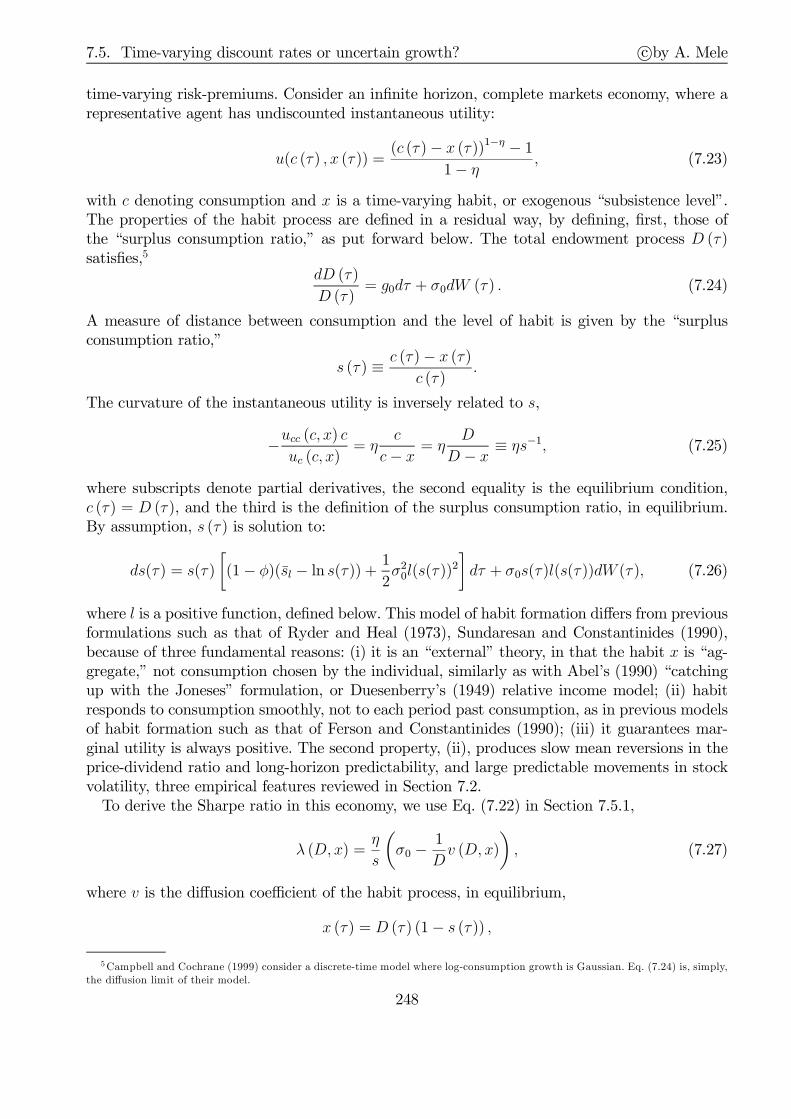
7.5. Time-varying discount rates or uncertain growth? c©by A. Mele
time-varying risk-premiums. Consider an infinite horizon, complete markets economy, where arepresentative agent has undiscounted instantaneous utility:
u(c (τ) , x (τ )) =(c (τ )− x (τ ))1−η − 1
1− η , (7.23)
with c denoting consumption and x is a time-varying habit, or exogenous “subsistence level”.The properties of the habit process are defined in a residual way, by defining, first, those ofthe “surplus consumption ratio,” as put forward below. The total endowment process D (τ)satisfies,5
dD (τ)
D (τ )= g0dτ + σ0dW (τ ) . (7.24)
A measure of distance between consumption and the level of habit is given by the “surplusconsumption ratio,”
s (τ ) ≡ c (τ)− x (τ)c (τ )
.
The curvature of the instantaneous utility is inversely related to s,
−ucc (c, x) cuc (c, x)
= ηc
c− x = ηD
D − x ≡ ηs−1, (7.25)
where subscripts denote partial derivatives, the second equality is the equilibrium condition,c (τ) = D (τ ), and the third is the definition of the surplus consumption ratio, in equilibrium.By assumption, s (τ ) is solution to:
ds(τ) = s(τ )
[(1− φ)(sl − ln s(τ)) +
1
2σ20l(s(τ ))
2
]dτ + σ0s(τ)l(s(τ ))dW (τ ), (7.26)
where l is a positive function, defined below. This model of habit formation differs from previousformulations such as that of Ryder and Heal (1973), Sundaresan and Constantinides (1990),because of three fundamental reasons: (i) it is an “external” theory, in that the habit x is “ag-gregate,” not consumption chosen by the individual, similarly as with Abel’s (1990) “catchingup with the Joneses” formulation, or Duesenberry’s (1949) relative income model; (ii) habitresponds to consumption smoothly, not to each period past consumption, as in previous modelsof habit formation such as that of Ferson and Constantinides (1990); (iii) it guarantees mar-ginal utility is always positive. The second property, (ii), produces slow mean reversions in theprice-dividend ratio and long-horizon predictability, and large predictable movements in stockvolatility, three empirical features reviewed in Section 7.2.To derive the Sharpe ratio in this economy, we use Eq. (7.22) in Section 7.5.1,
λ (D, x) =η
s
(σ0 −
1
Dv (D, x)
), (7.27)
where v is the diffusion coefficient of the habit process, in equilibrium,
x (τ) = D (τ ) (1− s (τ )) ,
5Campbell and Cochrane (1999) consider a discrete-time model where log-consumption growth is Gaussian. Eq. (7.24) is, simply,the diffusion limit of their model.
248

7.5. Time-varying discount rates or uncertain growth? c©by A. Mele
and s (τ ) is solution to Eq. (7.26). By Itô’s lemma, v (D, x) = (1− s− sl(s))Dσ0, which re-placed into Eq. (7.27), leaves:
λ(s) = ησ0 (1 + l(s)) . (7.28)
The real interest rate is, by Eq. (7.21),
R(s) = δ + η
(g0 −
1
2σ20
)+ η (1− φ) (sl − ln s)−
1
2η2σ2
0 (1 + l(s))2 . (7.29)
The third term reflects usual intertemporal substitution effects: bad times, when s is low, arethose when agents expect the very same future surplus consumption ratio s will improve, due tomean reversion. Therefore, in bad times, agents expect their marginal utility to decrease in thefuture and to compensate for this fall, they will try to boost future consumption by borrowingmore, thereby pushing interest rates up. The last term is a precautionary savings term.Campbell and Cochrane (1999) choose the function l so as to satisfy three conditions: (i) the
short-term rate R is constant; and habit is predetermined both (ii) at the steady state, and(iii) near the steady state. The reason they choose R constant is motivated by the empiricalfeatures surveyed in Section 7.2, that real interest rates are really not volatile, compared tostock returns. Making habit predetermined at and near the steady state formalizes the ideathat it takes time for consumption shocks to affect habit, at least at the steady state. TheAppendix shows that under these conditions, the function l is:
l (s) = s−1√1 + 2(sl − ln s)− 1, (7.30)
where s = σ0
√η
1−φ = esl. In turn, this function implies that the short-term rate in Eq. (7.29)
is: R = δ + η(g0 − 1
2σ20
)− 1
2η(1− φ).
The next picture depicts the function l in Eq. (7.30), computed through the parameter valuesutilized by Campbell and Cochrane, η = 2, σ0 = 0.0150, φ = 0.870. It is decreasing in s, andconvex in s, over the empirically relevant range of variation of s.
0.00 0.01 0.02 0.03 0.04 0.05 0.06 0.07 0.08 0.090
10
20
30
40
50
surplus consumption ratio, s
l(s)
Note that, then, these properties are inherited by the Sharpe ratio in Eq. (7.27). Quitesimply, these fundamental properties of the Sharpe ratio arise simply because we want habit to
249
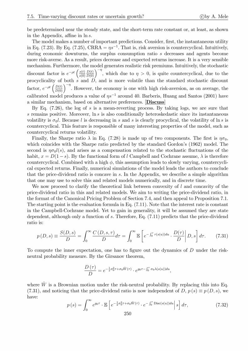
7.5. Time-varying discount rates or uncertain growth? c©by A. Mele
be predetermined near the steady state, and the short-term rate constant or, at least, as shownin the Appendix, affine in ln s.The model makes a number of important predictions. Consider, first, the instantaneous utility
in Eq. (7.23). By Eq. (7.25), CRRA = ηs−1. That is, risk aversion is countercyclical. Intuitively,during economic downturns, the surplus consumption ratio s decreases and agents becomemore risk-averse. As a result, prices decrease and expected returns increase. It is a very sensiblemechanism. Furthermore, the model generates realistic risk premiums. Intuitively, the stochastic
discount factor is e−ρt(s(t)s(0)
D(t)D(0)
)−η, which due to η > 0, is quite countercyclical, due to the
procyclicality of both s and D, and is more volatile than the standard stochastic discount
factor, e−ρt(D(t)D(0)
)−η. However, the economy is one with high risk-aversion, as on average, the
calibrated model produces a value of ηs−1 around 40. Barberis, Huang and Santos (2001) havea similar mechanism, based on alternative preferences. [Discuss]By Eq. (7.26), the log of s is a mean-reverting process. By taking logs, we are sure that
s remains positive. Moreover, ln s is also conditionally heteroskedastic since its instantaneousvolatility is σ0l. Because l is decreasing in s and s is clearly procyclical, the volatility of ln s iscountercyclical. This feature is responsible of many interesting properties of the model, such ascountercyclical returns volatility.Finally, the Sharpe ratio λ in Eq. (7.28) is made up of two components. The first is ησ0,
which coincides with the Sharpe ratio predicted by the standard Gordon’s (1962) model. Thesecond is ησ0l(s), and arises as a compensation related to the stochastic fluctuations of thehabit, x = D(1− s). By the functional form of l Campbell and Cochrane assume, λ is thereforecountercyclical. Combined with a high φ, this assumption leads to slowly varying, countercycli-cal expected returns. Finally, numerical simulations of the model leads the authors to concludethat the price-dividend ratio is concave in s. In the Appendix, we describe a simple algorithmthat one may use to solve this and related models numerically, and in discrete time.We now proceed to clarify the theoretical link between convexity of l and concavity of the
price-dividend ratio in this and related models. We aim to writing the price-dividend ratio, inthe format of the Canonical Pricing Problem of Section 7.4, and then appeal to Proposition 7.1.The starting point is the evaluation formula in Eq. (7.11). Note that the interest rate is constantin the Campbell-Cochrane model. Yet to gain in generality, it will be assumed they are statedependent, although only a function of s. Therefore, Eq. (7.11) predicts that the price-dividendratio is:
p (D, s) ≡ S(D, s)
D=
∫ ∞
0
C (D, s, τ )
Ddτ =
∫ ∞
0
E
[e−
∫ τ0 r(s(u))du · D(τ)
D
∣∣∣∣D, s]dτ . (7.31)
To compute the inner expectation, one has to figure out the dynamics of D under the risk-neutral probability measure. By the Girsanov theorem,
D (τ)
D= e−
12σ2
0τ+σ0W (τ) · eg0τ−∫ τ0 σ0λ(s(u))du,
where W is a Brownian motion under the risk-neutral probability. By replacing this into Eq.(7.31), and noticing that the price-dividend ratio is now independent of D, p (s) ≡ p (D, s), wehave:
p (s) =
∫ ∞
0
eg0τ · E[e−
12σ2
0τ+σ0W (τ) · e−∫ τ0 Disc(s(u))du
∣∣∣ s]dτ, (7.32)
250

7.5. Time-varying discount rates or uncertain growth? c©by A. Mele
where
Disc (s) ≡ r (s) + σ0λ (s)
is the “risk-adjusted” discount rate. Note also, that under the risk-neutral probability measure,
ds(τ) = ϕ (s(τ)) dτ + v(s (τ ))dW (τ ),
where ϕ (s) = ϕ (s)− v (s)λ (s), ϕ (s) = s(1− φ)(sl − ln s) + 12σ20l
2(s), and v (s) = σ0sl(s).
We aim to obtain a neat formula, by getting rid of term, e−12σ2
0τ+σ0W (τ), which, intuitively,arises, as consumption and habit are correlated. We can conveniently change measure. Definea new probability P through the Radon-Nikodym derivative dP
/dP = e−
12σ2
0τ+σ0W (τ). UnderP , the price-dividend ratio p (s) satisfies,
p (s) =
∫ ∞
0
eg0τ · E[e−
∫ τ0 Disc(s(u))du
∣∣∣ s]dτ , (7.33)
and
ds(τ) = ϕ (s(τ)) dτ + v(s (τ ))dW (τ ),
where W (τ) = W (τ)− σ0τ is a P -Brownian motion, and ϕ (s) = ϕ (s)− v (s)λ (s) + σ0v (s).The inner expectation in Eq. (7.33) comes in exactly the same format as in the canonical
pricing problem of Section 7.4. Therefore, we can apply Proposition 7.1, and make the followingconclusions:
(i) Suppose that risk-adjusted discount rates are countercyclical, viz ddsDisc(s) ≤ 0. Then
price-dividend ratios are procyclical, viz ddsp (s) > 0.
(ii) Suppose that price-dividend ratios are procyclical. Then price-dividend ratios are con-cave in s whenever risk-adjusted discount rates are convex in s, viz d2
ds2Disc(s) > 0, andd2
ds2 ϕ (s) ≤ 2 ddsDisc(s).
So we have found joint restrictions on the primitives such that the pricing function p isconsistent with properties given in advance. What is the economic interpretation related tothe convexity of risk-adjusted discount rates? If price-dividend ratios are concave in some statevariable Y tracking the business cycle condititions, stock volatility increases on the downside,and is thus countercyclical, as illustrated by Figure 7.6. According to the previous predictions,price-dividend ratios are concave in Y whenever risk-adjusted discount rates are decreasing andsufficiently convex in Y . The economic significance of convexity in this context is that in goodtimes, risk-adjusted discount rates are substantially constant. As a result, the evaluation offuture dividends does not vary too much, and price-dividend ratios remain relatively constant.In bad times, however, risk-adjusted discount rates increase sharply, thus making price-dividendratios more responsive to changes in the economic conditions.One defect of this model is that the variables of interest are all driven by the same state
variable, s. For this reason, the correlation between consumption growth and stock returns is,conditionally, one, whereas in the data, it is much less. Naturally, the correlation predicted bythis model is less than one, unconditionally, but still too high, if compared with that in thedata.
251
7.5. Time-varying discount rates or uncertain growth? c©by A. Mele
7.5.3 Large price swings as a learning induced phenomenon
7.5.3.1 Framework
Time variation in stock volatility may also arise as a result of the agents’ learning process aboutthe economic fundamentals. In models along these lines, public signals about the fundamentalshit the market, and agents make inference about them, thereby creating new state variablesdriving price fluctuations, which relate to the agents own guesses about the economic fundamen-tals. Timmermann (1993, 1996) provides models with exogenous discount rates, where learningeffects increase stock volatility over and above that we might observe in a world without uncer-tainty, and learning effects, about the fundamentals. Brennan and Xia (2001) generalize thesemodels to a stochastic general equilibrium. Veronesi (1999) provides a rational expectationsmodel with learning about the fundamentals, with quite nonlinear learning effects. This sectionprovides details about the mechanisms through which learning affects asset prices in general,and stock volatility in particular.We shall assume that information about the fundamentals is incomplete, but symmetrically
distributed among agents. The assumption of symmetric information might appear quite strong.It should not. The models of this section aim to capture the idea that markets function in acontext of “incompressible” uncertainty, where agents are all unaware of the crucial aggregate,macroeconomic developments affecting asset prices. Chapter 9, instead, reviews models withboth differential and asymmetric information, which are more useful whilst thinking about thefunctioning of markets for individual stocks, where it is, then, more plausible to have agentswith different information sets, who acquire information in a dedicated information market.Acquiring crucial information about, say, the direction of the business cycle, and having agentsasymmetrically informed about it, and affecting thereby asset prices, seems implausible–thecost of acquiting such information is infinite. Note that the assumption of symmetric informationsimplifies the analysis, as the agents do not need to base their decisions upon the observation ofthe equilibrium price. For example, in a context with asymmetric information, agents can learnpieces of information other agents have, by “reading the equilibrium price,” because agents withsuperior information impinge part of their information on the asset price, through trading, asexplained in Chapter 9. This complication does not arise in the context of this section: agents,then, need only to condition upon the realization of signals, which convey information aboutthe fundamentals. There is no need for any agent to condition on prices, because prices merelyconvey the same information any such agent already has.A final consideration pertains to the very nature of aggregate stock market fluctuations, which
seems to be quite stable, historically, as reviewed in Section 7.2. It is an interesting aspect,because it is quite obvious that capital markets have undergone significant changes over time,which affected various aspects of their microstructure, such as the technology of transactions,the price discovery process, liquidity, and transaction volumes, to mention a few examples. Howis it that the properties of the aggregate stock market reviewed in Section 7.2 do not appear tobe affected by these changes? One possibility is, simply, that market microstructure is about thevery high frequency behavior of markets, whereas the properties in Section 7.2 relate to slow,low frequency movements. The models in this section, and in this chapter, aim to rationalizesome of these movements. Models addressing the previous market microstructure issues arereviewed in Chapter 9, as mentioned.
252
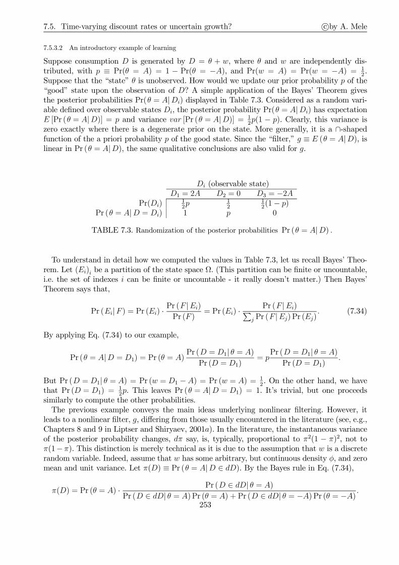
7.5. Time-varying discount rates or uncertain growth? c©by A. Mele
7.5.3.2 An introductory example of learning
Suppose consumption D is generated by D = θ + w, where θ and w are independently dis-tributed, with p ≡ Pr(θ = A) = 1 − Pr(θ = −A), and Pr(w = A) = Pr(w = −A) = 1
2.
Suppose that the “state” θ is unobserved. How would we update our prior probability p of the“good” state upon the observation of D? A simple application of the Bayes’ Theorem givesthe posterior probabilities Pr(θ = A|Di) displayed in Table 7.3. Considered as a random vari-able defined over observable states Di, the posterior probability Pr(θ = A|Di) has expectationE [Pr (θ = A|D)] = p and variance var [Pr (θ = A|D)] = 1
2p(1 − p). Clearly, this variance is
zero exactly where there is a degenerate prior on the state. More generally, it is a ∩-shapedfunction of the a priori probability p of the good state. Since the “filter,” g ≡ E (θ = A|D), islinear in Pr (θ = A|D), the same qualitative conclusions are also valid for g.
Di (observable state)D1 = 2A D2 = 0 D3 = −2A
Pr(Di)12p 1
212(1− p)
Pr (θ = A|D = Di) 1 p 0
TABLE 7.3. Randomization of the posterior probabilities Pr (θ = A|D) .
To understand in detail how we computed the values in Table 7.3, let us recall Bayes’ Theo-rem. Let (Ei)i be a partition of the state space Ω. (This partition can be finite or uncountable,i.e. the set of indexes i can be finite or uncountable - it really doesn’t matter.) Then Bayes’Theorem says that,
Pr (Ei|F ) = Pr (Ei) ·Pr (F |Ei)
Pr (F )= Pr (Ei) ·
Pr (F |Ei)∑j Pr (F |Ej) Pr (Ej)
. (7.34)
By applying Eq. (7.34) to our example,
Pr (θ = A|D = D1) = Pr (θ = A)Pr (D = D1| θ = A)
Pr (D = D1)= p
Pr (D = D1| θ = A)Pr (D = D1)
.
But Pr (D = D1| θ = A) = Pr (w = D1 −A) = Pr (w = A) = 12. On the other hand, we have
that Pr (D = D1) =12p. This leaves Pr (θ = A|D = D1) = 1. It’s trivial, but one proceeds
similarly to compute the other probabilities.The previous example conveys the main ideas underlying nonlinear filtering. However, it
leads to a nonlinear filter, g, differing from those usually encountered in the literature (see, e.g.,Chapters 8 and 9 in Liptser and Shiryaev, 2001a). In the literature, the instantaneous varianceof the posterior probability changes, dπ say, is, typically, proportional to π2(1 − π)2, not toπ(1−π). This distinction is merely technical as it is due to the assumption that w is a discreterandom variable. Indeed, assume that w has some arbitrary, but continuous density φ, and zeromean and unit variance. Let π(D) ≡ Pr (θ = A|D ∈ dD). By the Bayes rule in Eq. (7.34),
π(D) = Pr (θ = A) · Pr (D ∈ dD| θ = A)Pr (D ∈ dD| θ = A) Pr (θ = A) + Pr (D ∈ dD| θ = −A) Pr (θ = −A) .
253
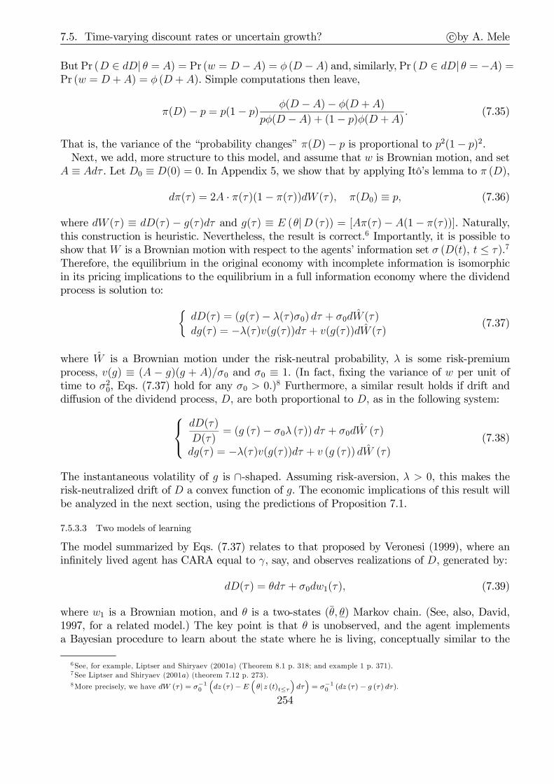
7.5. Time-varying discount rates or uncertain growth? c©by A. Mele
But Pr (D ∈ dD| θ = A) = Pr (w = D −A) = φ (D −A) and, similarly, Pr (D ∈ dD| θ = −A) =Pr (w = D +A) = φ (D +A). Simple computations then leave,
π(D)− p = p(1− p) φ(D − A)− φ(D +A)
pφ(D −A) + (1− p)φ(D +A). (7.35)
That is, the variance of the “probability changes” π(D)− p is proportional to p2(1− p)2.Next, we add, more structure to this model, and assume that w is Brownian motion, and set
A ≡ Adτ . Let D0 ≡ D(0) = 0. In Appendix 5, we show that by applying Itô’s lemma to π (D),
dπ(τ) = 2A · π(τ)(1− π(τ))dW (τ ), π(D0) ≡ p, (7.36)
where dW (τ ) ≡ dD(τ ) − g(τ )dτ and g(τ) ≡ E (θ|D (τ)) = [Aπ(τ)− A(1− π(τ ))]. Naturally,this construction is heuristic. Nevertheless, the result is correct.6 Importantly, it is possible toshow thatW is a Brownian motion with respect to the agents’ information set σ (D(t), t ≤ τ ).7
Therefore, the equilibrium in the original economy with incomplete information is isomorphicin its pricing implications to the equilibrium in a full information economy where the dividendprocess is solution to:
dD(τ) = (g(τ)− λ(τ)σ0) dτ + σ0dW (τ )
dg(τ ) = −λ(τ )v(g(τ))dτ + v(g(τ ))dW (τ)(7.37)
where W is a Brownian motion under the risk-neutral probability, λ is some risk-premiumprocess, v(g) ≡ (A − g)(g + A)/σ0 and σ0 ≡ 1. (In fact, fixing the variance of w per unit oftime to σ2
0, Eqs. (7.37) hold for any σ0 > 0.)8 Furthermore, a similar result holds if drift anddiffusion of the dividend process, D, are both proportional to D, as in the following system:
dD(τ )
D(τ )= (g (τ)− σ0λ (τ)) dτ + σ0dW (τ)
dg(τ ) = −λ(τ )v(g(τ ))dτ + v (g (τ )) dW (τ)(7.38)
The instantaneous volatility of g is ∩-shaped. Assuming risk-aversion, λ > 0, this makes therisk-neutralized drift of D a convex function of g. The economic implications of this result willbe analyzed in the next section, using the predictions of Proposition 7.1.
7.5.3.3 Two models of learning
The model summarized by Eqs. (7.37) relates to that proposed by Veronesi (1999), where aninfinitely lived agent has CARA equal to γ, say, and observes realizations of D, generated by:
dD(τ ) = θdτ + σ0dw1(τ), (7.39)
where w1 is a Brownian motion, and θ is a two-states (θ, θ) Markov chain. (See, also, David,1997, for a related model.) The key point is that θ is unobserved, and the agent implementsa Bayesian procedure to learn about the state where he is living, conceptually similar to the
6See, for example, Liptser and Shiryaev (2001a) (Theorem 8.1 p. 318; and example 1 p. 371).7See Liptser and Shiryaev (2001a) (theorem 7.12 p. 273).8More precisely, we have dW (τ) = σ−1
0
(dz (τ)−E
(θ| z (t)t≤τ
)dτ)= σ−1
0 (dz (τ)− g (τ) dτ).
254

7.5. Time-varying discount rates or uncertain growth? c©by A. Mele
updating in Eq. (7.34). It is possible to show, then, the price in this economy is the same asthe price in a full information economy where:
dD(τ) = (g(τ )− γσ2
0) dτ + σ0dW (τ)
dg(τ ) = (k(g − g(τ ))− γσ0v (g(τ ))) dτ + v (g(τ)) dW (τ )(7.40)
where W is a Brownian motion under the risk-neutral probability, v(g) = (θ − g)(g − θ)/σ0,
k, g are some positive constants. Veronesi (1999) also assumes the riskless asset is infinitelyelastically supplied, and therefore that the interest rate r is a constant. Note that while thediffusion functions in Eq. (7.37) and Eq. (7.40) have the same functional form, expected dividendis a martingale in Eq. (7.37), and mean-reverting in Eq. (7.40), under the physical probability.These two properties arise as the model underlying Eq. (7.37) is one where θ is drawn at time0, forever, whereas θ is a Markov chain.Finally, we examine the properties of the equilibrium price. In terms of the representation in
Eq. (7.11), this model predicts that S(D, g) =∫∞0C(D, g, τ )dτ , where:
C(D, g, τ) = e−rτ (D − σ0γτ ) +G (g, τ ) , and G (g, τ ) ≡ e−rτ∫ τ
0
E [g(u)| g] du, τ ≥ 0.
(7.41)We can now apply Proposition 7.1 to study convexity properties of G. Precisely, the functionE [g(u)| g] is a special case of the canonical price in Eq. (7.12) (namely, for ρ ≡ 1 and ψ(g) = g).By Proposition 7.1-b), E [g(u)| g] is convex in g whenever the drift of g in Eq. (7.37) is convex.This condition is automatically guaranteed by γ > 0. Technically, Proposition 7.1 implies thatthe conditional expectation of a diffusion process inherits the very same second order properties(concavity, linearity, and convexity) of the drift function.The economic implications of this result are striking. In this economy prices are convex in
the expected dividend growth. This means that in good times, prices may well rocket to veryhigh values with relatively small movements in the underlying fundamentals.The economic interpretation of this convexity property is that risk-aversion correction is nil
during extreme situations (i.e. when the dividend growth rate is at its boundaries), and it is thehighest during relatively more “normal” situations. More formally, the risk-adjusted drift of gis ϕ (y) = ϕ (g)− γσ0v (g), and it is convex in g because v is concave in g. These nonlinearitiesarise, because we are assuming agents are learning about a discrete state space in a continuoustime world. Moreover, it is possible to show that if the short-term rate is endogenous, convexityproperties might be lost (Veronesi, 2000; copy-paste Mele, 2005, to show this).Finally, we examine the model described by Eqs. (7.38), as well as others. Note, indeed,
that Eqs. (7.38) follow as a result of a specific learning mechanism. Yet alternative learningmechanisms can lead to dynamics for dividends and expected dividend growth similar to Eqs.(7.38), although with different coefficients ϕ and v. For example, the Brennan and Xia (2001)model assumes an information structure where an infinitely lived agent observes D, solution to:
dD(τ )
D(τ )= g(τ )dτ + σ0dw1(τ ),
and g(τ ) is unobserved. Brennan and Xia do not assume that g(τ) evolve on a countable numberof states. Rather, they assume it is an Ornstein-Uhlenbeck process:
dg(τ) = k(g − g(τ))dτ + σ1dw1(τ) + σ2dw2(τ),
255

7.5. Time-varying discount rates or uncertain growth? c©by A. Mele
where g, σ1 and σ2 are positive constants. The agent, now, is also allowed to implement aBayesian learning procedure, conceptually similar to that described earlier on. In detail, if ouragent has a Gaussian prior on g(0) with variance γ2∗, as defined below, the asset price takesthe form S(D, g), where D and g are solution to Eq. (7.38), with m0(D, g) = gD, σ(D) =σ0D, ϕ0 (D, g) = k(g − g), v2 = 0, and v1 ≡ v1(γ∗) = (σ1 +
1σ0γ∗)
2, where γ∗ is the positive
solution to v1(γ) = σ21 + σ
22 − 2kγ.9
Finally, models where expected consumption is another observed diffusion may have an in-terest in their own (see for example, Campbell, 2003; Bansal and Yaron, 2004), and will beexamined in Chapter 8.Next, we analyze these models, by relying on Proposition 7.1. To simplify the exposition, we
assume λ is constant. By the same reasoning leading to Eq. (7.33), the price-dividend ratio isindependent of D, and is given by:
p (g) =
∫ ∞
0
E(e∫ τ0 [g(u)−r(g(u))]du−σ0λτ
∣∣∣ g)dτ, (7.42)
where,
dD(τ )
D(τ)= (g(τ)− σ0λ) dτ + σ0dW (τ)
dg(τ) = (ϕ (g(τ)) + σ0v (g(τ ))) dτ + v (g(τ )) dW (τ )
and W (τ) = W (τ)− σ0τ is a P -Brownian motion. Under regularity conditions, monotonicityand convexity properties are inherited by the inner expectation in Eq. (7.42). Precisely, in thenotation of the canonical pricing problem,
ρ (g) = −g +R (g) + σ0λ and b (g) = ϕ0 (g) + (σ0 − λ) v (g) ,
where ϕ0 is the physical probability measure. Therefore,
(i) The price-dividend ratio is increasing in the dividend growth rate whenever ddgR (g) < 1.
(ii) Suppose that the price-dividend ratio is increasing in the dividend growth rate. Then it isconvex whenever d2
dg2R (g) > 0, and d2
dg2 [ϕ0 (g) + (σ0 − λ) v (g)] ≥ −2 + 2 ddgR (g).
For example, if the riskless asset is constant (because for example it is infinitely elasticallysupplied), then the price-dividend ratio is always increasing and it is convex whenever,
d2
dg2(ϕ0 (g) + (σ0 − λ) v (g)) ≥ −2.
The reader can now use these conditions to check predictions made by all models with stochasticdividend growth presented before.
9Brennan and Xia (2001) actually consider a slightly more general model where consumption and dividends differ. They derivea model with a reduced-form identical to that in this example. In the calibrated model, Brennan and Xia found that the varianceof the filtered g is higher than the variance of the expected dividend growth in an economy with complete information. The resultson γ∗ in this example can be obtained through an application of theorem 12.1 in Liptser and Shiryaev (2001) (Vol. II, p. 22). Theygeneralize results in Gennotte (1986) and are a special case of results in Detemple (1986). Both Gennotte and Detemple did notemphasize the impact of learning on the pricing function.
256
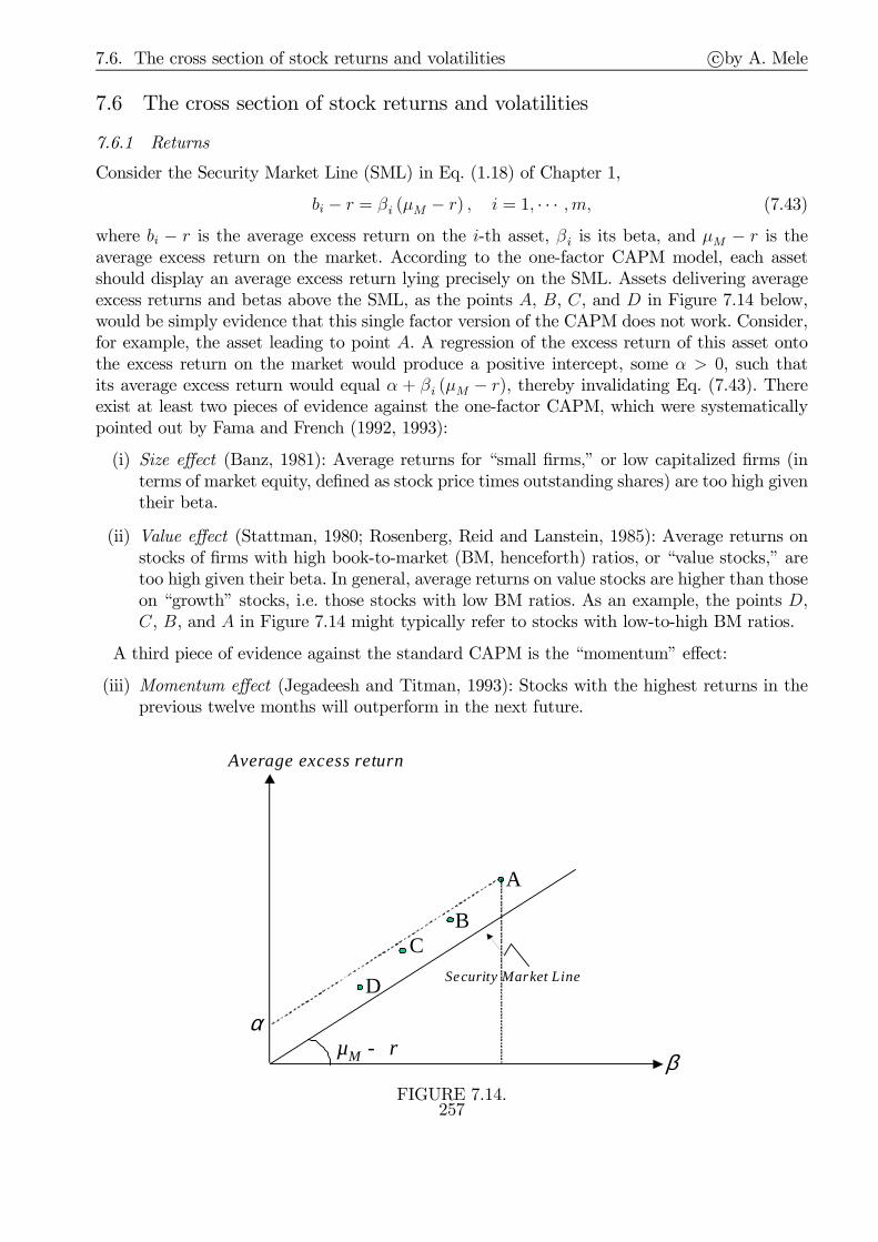
7.6. The cross section of stock returns and volatilities c©by A. Mele
7.6 The cross section of stock returns and volatilities
7.6.1 Returns
Consider the Security Market Line (SML) in Eq. (1.18) of Chapter 1,
bi − r = βi (µM − r) , i = 1, · · · ,m, (7.43)
where bi − r is the average excess return on the i-th asset, βi is its beta, and µM − r is theaverage excess return on the market. According to the one-factor CAPM model, each assetshould display an average excess return lying precisely on the SML. Assets delivering averageexcess returns and betas above the SML, as the points A, B, C, and D in Figure 7.14 below,would be simply evidence that this single factor version of the CAPM does not work. Consider,for example, the asset leading to point A. A regression of the excess return of this asset ontothe excess return on the market would produce a positive intercept, some α > 0, such thatits average excess return would equal α + βi (µM − r), thereby invalidating Eq. (7.43). Thereexist at least two pieces of evidence against the one-factor CAPM, which were systematicallypointed out by Fama and French (1992, 1993):
(i) Size effect (Banz, 1981): Average returns for “small firms,” or low capitalized firms (interms of market equity, defined as stock price times outstanding shares) are too high giventheir beta.
(ii) Value effect (Stattman, 1980; Rosenberg, Reid and Lanstein, 1985): Average returns onstocks of firms with high book-to-market (BM, henceforth) ratios, or “value stocks,” aretoo high given their beta. In general, average returns on value stocks are higher than thoseon “growth” stocks, i.e. those stocks with low BM ratios. As an example, the points D,C, B, and A in Figure 7.14 might typically refer to stocks with low-to-high BM ratios.
A third piece of evidence against the standard CAPM is the “momentum” effect:
(iii) Momentum effect (Jegadeesh and Titman, 1993): Stocks with the highest returns in theprevious twelve months will outperform in the next future.
Average excess return
µM - rβ
CB
A
α
D Security Market Line
FIGURE 7.14.257

7.6. The cross section of stock returns and volatilities c©by A. Mele
The one-factor CAPM has no power in explaining the cross-section of asset returns, sorted bysize, BM or momentum. Assets sorted in this way command a size premium, a value premium,and a momentum premium. For example, one can create portfolios sorted by size and BM, say25 portfolios, out of a 5× 5 matrix with dimensions given by size and BM. The puzzle, then,at least from the standard CAPM perspective, is that this model cannot explain the returnson these porfolios. Fama and French (1993) show that the returns on these portfolios can bevery much better understood by means of a multifactor model, where both size and valuepremiums are explicitly taken into account. They consider three factors: (i) the excess returnon the market; (ii) an “HML” factor, defined as the monthly difference between the returnson assets with high and low BM ratios (“high minus low”); an “SMB” factor, defined as thedifference between the asset returns of firms with small and big size (“small minus big”). TheHML and SMB factors are defined as the differences between the returns on the appropriatecells of a 2×3 matrix, obtained through percentiles of the distribution of asset returns over theprevious year.
Book-to-MarketSize L M HSL
The resulting model is the celebrated Fana-French three factor model. Carhart (1997) extendsthis model to a four-factor model with a momentum factor: the monthly difference between thereturns on the high and low prior return portfolios.
7.6.2 Volatilities
258

7.7. Appendix 1: Calibration of the tree in Section 7.3 c©by A. Mele
7.7 Appendix 1: Calibration of the tree in Section 7.3
S , (2 ,. The initial step of the calibration reported in Table2 involves estimating the two parameters p and δ of the dividend process. Let G be the dividendgross growth rate, computed at a yearly frequency. We calibrate p and δ by a perfect matching of themodel’s expected dividend growth, µD ≡ E (G) = pe−δ+(1− p) eδ, and the model’s dividend variance,
σ2D ≡ var (G) =
(eδ − e−δ
)2p (1− p), to their sample counterparts µD = 1.0594 and σD = 0.0602
obtained on US aggregate dividend data. The result is (p, δ) = (0.158, 0.082). Given these calibratedvalues of (p, δ), we fix r = 1.0%, and proceed to calibrate the probabilities q, qB and qG.
To calibrate (q, qB, qG), we need an explicit expression for all the payoffs at each node. By standardrisk-neutral evaluation, we obtain a closed form solution for the price of the claim MS , as follows. Foreach state S ∈ G,B,GB, MS is solution to,
MS
DS= e−rES
(D′SDS
+M ′
S
D′S
D′SDS
), (7A.1)
where ES (·) is the expectation taken under the risk-neutral probability qS in state S, S ∈ G,B,GB,and qGB = q, DG = e2δ, DB = e−2δ, DGB = 1, and D′S and M ′
S are the dividend and the price of theclaim as of the next period. Since risk-aversion is constant from the third period on, the price-dividend
ratio is constant as well, from the third period on, which implies that MSDS
=M ′S
D′S. By using the equality
MSDS
=M ′S
D′Sin Eq. (7A.1), and solving for MS , yields,
MS = DSqSe
−δ + (1− qS) eδ
er − [qSe−δ + (1− qS) eδ], S ∈ G,B,GB . (7A.2)
We calibrate (qG, qB, qGB = q) to make the “hybrid” price-dividend (P/D henceforth) ratio MGB,the “good” P/D ratio MG
e2δand the “bad” P/D ratio MB
e−2δ in Eq. (7A.2) perfectly match the averageP/D ratio, the average P/D ratio during NBER expansion periods, and the average P/D ratio duringNBER recession periods (i.e. 31.99, 33.21 and 26.20, from Table 7.1). Given (p, δ, r, q, qS , qG), wecompute the P/D ratios in states G and B. For example, the price of the asset in state B is, PB =e−r[qB
(e−2δ +MB
)+ (1− qB) (1 +MGB)]. Given PB, we compute the log-return in the bad state as
log( ΠPB
), where either Π = e−2δ +MB with probability p, or Π = 1 +MGB with probability 1 − p.Then, we compute the return volatility in state B. The P/D ratios, the expected log-return andreturn volatility in state G are computed similarly. (Please notice that volatilities under p and underqSS∈G,B,GB are not the same.)
Next, we recover the risk-aversion parameter ηS in the three states S ∈ G,B,GB implied by thepreviously calibrated probabilities q, qG and q = qGB. As we shall show below, the relevant formulato use is,
qSp
=eηSδ
peηSδ + (1− p) e−ηSδ, S ∈ G,B,GB . (7A.3)
The values for the “implied” risk-aversion parameter in Table 7.2 are obtained by inverting Eq. (7A.3)for ηS, given the calibrated values of (p, δ, qS, qG).
Finally, we compute the risk-adjusted discount rate as r + σDλS , where λS is the Sharpe ratio,which we shall show below to equal,
λS =qS − p√p (1− p)
, S ∈ G,B,GB . (7A.4)
P E$. (7A.3). We only provide the derivation of the risk-neutral probability qB, sincethe proofs for the expressions of the risk-neutral probabilities qG and q = qGB are nearly identical. In
259

7.7. Appendix 1: Calibration of the tree in Section 7.3 c©by A. Mele
equilibrium, the Euler equation for the stock price at the “bad” node is,
PB = βE
[u′B(DS)
u′B (e−δ)
(DS +MS
)]= βE
[G−ηBS
(DS +MS
)], S ∈ B,GB , (7A.5)
where: (i) β is the discount rate; (ii) the utility function for consumption C is state dependent and equalto, uB (C) = C1−ηB
/(1− ηB); (iii) E (·) is the expectation taken under the probability p; and (iv)
the dividend DS and the gross dividend growth rate GS are either DB = e−2δ and GB = e−2δ
e−δ= e−δ
with probability p, or DGB = 1 and GGB = 1e−δ
= eδ with probability 1− p.The model we set up assumes that the asset is elastically supplied or, equivalently, that there exists
a storage technology with a fixed rate of return equal to r = 1%. Let us derive the agent’s privateevaluation of this asset. The Euler equation for the safe asset is,
e−rB = βE[G−ηBS ] = β
∑S∈B,GB
pSG−ηBS , (7A.6)
where the safe interest rate, rB, is state dependent, pB = p and pGB = 1− p. Therefore,
qB = βerBpG−ηBB , 1− qB = βerB (1− p) G
−ηBGB (7A.7)
is a probability distribution. In fact, by plugging qB and 1 − qB into Eq. (7A.5), one sees that itis the risk-neutral probability distribution. To obtain Eq. (7A.3), note that by Eq. (7A.6), βerB =1/E[G
−ηBS ], which replaced into Eq. (7A.7) yields,
qBp
=G−ηBB
E[G−ηBS ]
.
Eq. (7A.3) follows by the definition of GS given above.
P E$. (7A.4). Let eµ the gross expected return of the risky asset. The asset return cantake two values: eRℓ with probability p, and eRh with probability 1− p, and Rh > Rℓ. Therefore, foreach state, we have that:
eµ = peRℓ + (1− p) eRh , er = qeRℓ + (1− q) eRh , (7A.8)
where we have omitted the dependence on the state S to alleviate the presentation. The standarddeviation of the asset return is StdR =
(eRh − eRℓ
)√p (1− p). The Sharpe ratio is defined as
λ =eµ − er
StdR.
By substracting the two equations in (7A.8),
q = p+eµ − er
(eRh − eRℓ)√p (1− p)
√p (1− p) = p− λ
√p (1− p),
from which Eq. (7A.4) follows immediately. Note, also, that in terms of this definition of the Sharperatio, the risk-neutral expectation of the dividend growth is, E (G) = E (G)− λσD.
260

7.8. Appendix 2: Arrow-Debreu PDEs c©by A. Mele
7.8 Appendix 2: Arrow-Debreu PDEs
We consider an interesting connection. Note that by Eq. (7.8), S is solution to,
LS +D = rS + (SDσ0D + Syv1)λ1 + Syv2λ2, ∀(D, y) ∈ R×R. (7A.9)
Under regularity conditions, the Feynman-Kac representation of the solution to Eq. (7A.9) is exactlyEq. (7.11).Naturally, Eq. (7.11) can also be rewritten under the physical measure. We have:
C (D, y, τ) = E
[exp
(−∫ τ
0r (y (t))dt
)·D (τ)
∣∣∣∣D, y]= E [m (τ) ·D (τ)|D, y] ,
where m is the stochastic discount factor: m (τ) = ξ(τ)ξ(0) , ξ (0) = 1. Given the previous assumptions, ξ
necessarily satisfies,
dξ (τ)
ξ (τ)= −r (y (τ)) dτ − λ1 (y (τ)) dW1 (τ) + λ2 (y (τ))dW2 (τ) . (7A.10)
Eq. (7A.9) can also be derived through the undiscounted “Arrow-Debreu adjusted” asset priceprocess, defined as:
w(D, y) ≡ Υ(D, y) · S(D, y),where Υ(D, y) is as in Eq. (7.19),
Υ(D (τ) , y (τ)) = ξ (τ) e∫ τ0 δ(D(s),y(s))ds.
By results in Section 7.4.2, we know that the following price representation holds true:
S(τ)ξ(τ) = E
[∫ ∞
τξ(s)D(s)ds
], τ ≥ 0.
Under regularity conditions, the previous equation can then be understood as the unique Feynman-Kacstochastic representation of the solution to the following partial differential equation
Lw(D, y) + f(D, y) = δ(D, y)w(D, y), ∀(D, y) ∈ R×R,
where f ≡ ΥD. Eq. (7A.9) then follows by the definition of Lw(τ) ≡ ddsE [ΥS]
∣∣s=τ
.
261
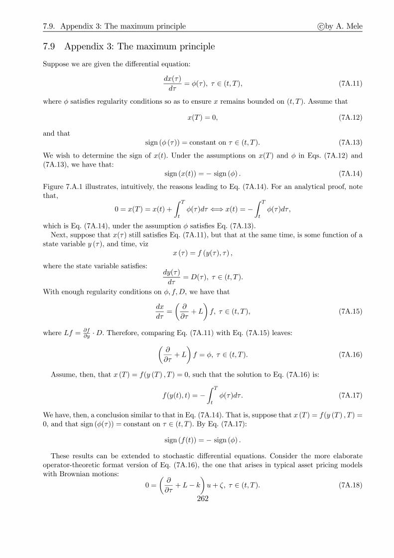
7.9. Appendix 3: The maximum principle c©by A. Mele
7.9 Appendix 3: The maximum principle
Suppose we are given the differential equation:
dx(τ)
dτ= φ(τ), τ ∈ (t, T ), (7A.11)
where φ satisfies regularity conditions so as to ensure x remains bounded on (t, T ). Assume that
x(T ) = 0, (7A.12)
and thatsign (φ (τ)) = constant on τ ∈ (t, T ). (7A.13)
We wish to determine the sign of x(t). Under the assumptions on x(T ) and φ in Eqs. (7A.12) and(7A.13), we have that:
sign (x(t)) = − sign (φ) . (7A.14)
Figure 7.A.1 illustrates, intuitively, the reasons leading to Eq. (7A.14). For an analytical proof, notethat,
0 = x(T ) = x(t) +
∫ T
tφ(τ)dτ ⇐⇒ x(t) = −
∫ T
tφ(τ)dτ,
which is Eq. (7A.14), under the assumption φ satisfies Eq. (7A.13).Next, suppose that x(τ ) still satisfies Eq. (7A.11), but that at the same time, is some function of a
state variable y (τ), and time, vizx (τ) = f (y(τ), τ) ,
where the state variable satisfies:dy(τ)
dτ= D(τ), τ ∈ (t, T ).
With enough regularity conditions on φ, f,D, we have that
dx
dτ=
(∂
∂τ+ L
)f, τ ∈ (t, T ), (7A.15)
where Lf = ∂f∂y ·D. Therefore, comparing Eq. (7A.11) with Eq. (7A.15) leaves:
(∂
∂τ+ L
)f = φ, τ ∈ (t, T ). (7A.16)
Assume, then, that x (T ) = f(y (T ) , T ) = 0, such that the solution to Eq. (7A.16) is:
f(y(t), t) = −∫ T
tφ(τ)dτ. (7A.17)
We have, then, a conclusion similar to that in Eq. (7A.14). That is, suppose that x (T ) = f(y (T ) , T ) =0, and that sign (φ(τ)) = constant on τ ∈ (t, T ). By Eq. (7A.17):
sign (f(t)) = − sign (φ) .
These results can be extended to stochastic differential equations. Consider the more elaborateoperator-theoretic format version of Eq. (7A.16), the one that arises in typical asset pricing modelswith Brownian motions:
0 =
(∂
∂τ+ L− k
)u+ ζ, τ ∈ (t, T ). (7A.18)
262
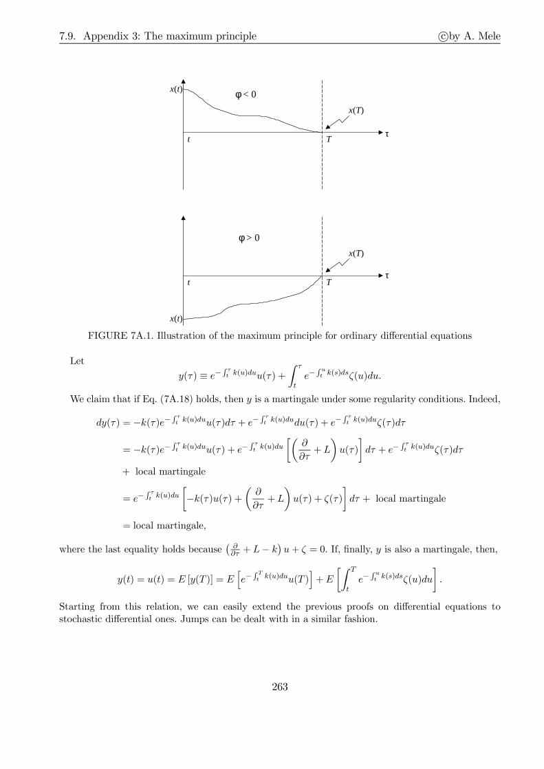
7.9. Appendix 3: The maximum principle c©by A. Mele
τ
τ
Tt
t T
x(t)
x(t)
x(T)
x(T)
φ> 0
φ< 0
FIGURE 7A.1. Illustration of the maximum principle for ordinary differential equations
Let
y(τ) ≡ e−∫ τt k(u)duu(τ) +
∫ τ
te−
∫ ut k(s)dsζ(u)du.
We claim that if Eq. (7A.18) holds, then y is a martingale under some regularity conditions. Indeed,
dy(τ) = −k(τ)e−∫ τt k(u)duu(τ)dτ + e−
∫ τt k(u)dudu(τ) + e−
∫ τt k(u)duζ(τ)dτ
= −k(τ)e−∫ τt k(u)duu(τ) + e−
∫ τt k(u)du
[(∂
∂τ+ L
)u(τ)
]dτ + e−
∫ τt k(u)duζ(τ)dτ
+ local martingale
= e−∫ τt k(u)du
[−k(τ)u(τ) +
(∂
∂τ+ L
)u(τ) + ζ(τ)
]dτ + local martingale
= local martingale,
where the last equality holds because(∂∂τ + L− k
)u+ ζ = 0. If, finally, y is also a martingale, then,
y(t) = u(t) = E [y(T )] = E[e−
∫ Tt k(u)duu(T )
]+E
[∫ T
te−
∫ ut k(s)dsζ(u)du
].
Starting from this relation, we can easily extend the previous proofs on differential equations tostochastic differential ones. Jumps can be dealt with in a similar fashion.
263

7.10. Appendix 4: Dynamic stochastic dominance and proof of Proposition 7.1 c©by A. Mele
7.10 Appendix 4: Dynamic stochastic dominance and proof of Proposition 7.1
P 7.A.1. (Dynamic Stochastic Dominance) Consider two economies A and B with twofundamental volatilities aA and aB and let πi(x) ≡ ai(x)·λi(x) and ρi(x) (i = A,B) the correspondingrisk-premium and discount rate. If aA > aB, the price cA in economy A is lower than the price pricecB in economy B whenever for all (x, τ) ∈ R× [0, T ],
V (x, τ) ≡ − [ρA(x)− ρB(x)] cB(x, τ)− [πA(x)− πB(x)] c
Bx (x, τ) +
1
2
[a2A(x)− a2B(x)
]cBxx(x, τ) < 0.
(7A.19)
If X is the price of a traded asset, πA = πB. If in addition ρ is constant, c is decreasing (increasing)in volatility whenever it is concave (convex) in x. This phenomenon is tightly related to the “convexityeffect” discussed earlier. If X is not a traded risk, two additional effects are activated. The first onereflects a discounting adjustment, and is apparent through the first term in the definition of V . Thesecond effect reflects risk-premiums adjustments and corresponds to the second term in the definitionof V . Both signs at which these two terms show up in Eq. (7A.19) are intuitive.
P. The function c(x, T − s) ≡ E[exp(−∫ Ts ρ(x(t))dt) · ψ(x(T ))
∣∣∣x(s) = x] is solution to the
following partial differential equation:
0 = −c2(x, T − s) + L∗c(x, T − s)− ρ(x)c(x, T − s), ∀(x, s) ∈ R× [0, T )c(x, 0) = ψ(x), ∀x ∈ R (7A.20)
where L∗c(x, u) = 12a(x)
2cxx(x, u) + b(x)cx(x, u) and subscripts denote partial derivatives. Clearly, cA
and cB are both solutions to the partial differential equation (7A.20), but with different coefficients.Let bA(x) ≡ b0(x) − πA(x). The price difference ∆c(x, τ) ≡ cA(x, τ) − cB(x, τ) is solution to thefollowing partial differential equation: ∀(x, s) ∈ R× [0, T ),
0 = −∆c2(x, T − s)+1
2σB(x)2∆cxx(x, T − s)+ bA(x)∆cx(x, T − s)− ρA(x)∆c(x, T − s)+V (x, T − s),
with ∆c(x, 0) = 0 for all x ∈ R, and V is as in Eq. (7A.19) of the proposition. The result follows bythe maximum principle for partial differential equations.
P 7.1. By differentiating twice the partial differential equation (7A.20) withrespect to x, We find that c(1)(x, τ) ≡ cx(x, τ) and c(2)(x, τ) ≡ cxx(x, τ) are solutions to the followingpartial differential equations: ∀(x, s) ∈ R++ × [0, T ),
0 = −c(1)2 (x, T − s) +1
2a(x)2c(1)xx (x, T − s) + [b(x) +
1
2(a(x)2)′]c(1)x (x, T − s)
−[ρ(x)− b′(x)
]c(1)(x, T − s)− ρ′(x)c(x, T − s),
with c(1)(x, 0) = ψ′(x) ∀x ∈ R, and ∀(x, s) ∈ R× [0, T ),
0 = −c(2)2 (x, T − s) +1
2a(x)2c(2)xx (x, T − s) + [b(x) + (a(x)2)′]c(2)x (x, T − s)
−[ρ(x)− 2b′(x)− 1
2(a(x)2)′′
]c(2)(x, T − s)
−[2ρ′(x)− b′′(x)
]c(1)(x, T − s)− ρ′′(x)c(x, T − s),
with c(2)(x, 0) = ψ′′(x) ∀x ∈ R. By the maximum principle for partial differential equations, c(1)(x, T−s) > 0 (resp. < 0) ∀(x, s) ∈ R×[0, T ) whenever ψ′(x) > 0 (resp. < 0) and ρ′(x) < 0 (resp. > 0) ∀x ∈ R.This completes the proof of part a) of the proposition. The proof of part b) is obtained similarly.
264

7.11. Appendix 5: Habit dynamics in Campbell and Cochrane (1999) c©by A. Mele
7.11 Appendix 5: Habit dynamics in Campbell and Cochrane (1999)
We derive Eq. (7.30), by making a slightly more general assumption that the short-term rate we wishto come up with, is affine in ln s, meaning that, the last two terms in Eq. (7.29) sum up to,
η (1− φ) (sl − ln s)− 1
2η2σ2
0 (1 + l (s))2 = −const.+ b (s− ln s) , (7A.21)
for some b, and where const. is to be determined. The working paper version of Campbell and Cochrane(1999) considers exactly this case.
Define the log of the surplus ratio as
sl (τ) ≡ ln(1− exl(τ)−cl(τ)
), (7A.22)
where sl ≡ ln s, xl ≡ lnx and cl ≡ ln c, and consider its first-order Taylor’s expansion around thesteady state xl − cl ≡ E (xl (τ)− cl (τ)),
sl (τ) ≈ sl +
(1− 1
s
)(xl (τ)− cl (τ)− xl − cl) , (7A.23)
where sl ≡ ln(1− exl−cl
)and s ≡ esl . Consider the discrete-time version of Eq. (7.26),
sl,t+1 − sl ≈ φ (sl,t − sl) + l (st)
(cl,t+1 − cl,t −
(g0 −
1
2σ20
)), (7A.24)
where sl,t ≡ sl (τ). Replacing Eq. (7A.23), evaluated at τ = t and τ = t + 1, into both sides of theprevious approximation, and rearranging terms, leaves:
xl,t+1 − cl,t+1 − xl − cl = φ (xl,t − cl,t − xl − cl) +l (st)
1− 1s
(cl,t+1 − cl,t −
(g0 −
1
2σ20
)). (7A.25)
The function l in Eq. (7.30) is found by imposing the following three conditions, where the first isa slight generalization of that mentioned in the main text, and the remaining two are the last twoconditions in the main text:
• First, the short-term rate in Eq. (7.29) is affine in ln s, i.e. Eq. (7A.21) holds, such that:
l (s) =
√2
1
η2σ20
(η (1− φ)− b) (sl − ln s) +2
η2σ20
const.− 1. (7A.26)
• Second, habit is predetermined at the steady state, meaning that xl,t+1 does not change withcl,t+1, which by Eq. (7A.25), it does not, when:
l (s) =1
s− 1. (7A.27)
Evaluating Eq. (7A.26) at the steady state s, and using the previous condition delivers, 2η2σ2
0const.
= 1s2, such that Eq. (7A.26) is,
l (s) =
√2
1
η2σ20
(η (1− φ)− b) (sl − ln s) +1
s2− 1. (7A.28)
265
7.11. Appendix 5: Habit dynamics in Campbell and Cochrane (1999) c©by A. Mele
• Third, habit is predetermined near the steady state, meaning that,
d
dsl
(dxldcl
)∣∣∣∣s=sl
= 0. (7A.29)
We, then, need to find the dynamics of xl,t+1, expressed as a function of cl,t+1. By the definition of
the log-surplus consumption ratio in Eq. (7A.22), we have that xl,t+1 = ln(1− eσ(cl,t+1)
)+cl,t+1,
where σ (cl,t+1) ≡ sl,t+1 and sl,t+1 is as in Eq. (7A.24), such that, using Eq. (7A.24):
dxl,t+1
dcl,t+1= 1− 1
e−σ(cl,t+1) − 1σ′ (cl,t+1) = 1− lo (sl,t)
e−sl,t+1 − 1,
where we have set lo (sl) ≡ l (s). Therefore, Eq. (7A.29) is: ddsl
(1− lo(sl)
e−sl
)∣∣∣s=sl
= 0, which leaves,
after simple computation, and using Eq. (7A.27),
l′o (sl) = −1
s.
By taking the derivative in Eq. (7A.28), and replacing into the left hand side of the previousequation, and solving for sl, yields,
s = σ0
√η2
η (1− φ)− b,
which is the expression of the main text, for b = 0. By replacing this expression of s into Eq.(7A.28), leaves Eq. (7.30) in the main text.
Finally, note that, now, the expression of the short-term rate can be found after simple computations:
R (s) = δ + η
(g0 −
1
2σ20
)− 1
2(η (1− φ)− b) + b (s− ln s) .
266

7.12. Appendix 6: An algorithm to simulate discrete-time pricing models c©by A. Mele
7.12 Appendix 6: An algorithm to simulate discrete-time pricing models
Consider the pricing equation,
S = E[m ·
(S′ +D′
)], m = β
uc (D′, x′)
uc (D,x)= β
(s′
s
)−η (D′
D
)−η.
The price-dividend ratio, p ≡ S/D say, satisfies:
p = E
[mD′
D
(1 + p′
)],
D′
D= eg0+w.
The previous equation is a functional equation in p (s), say:
p(s) = E[g(s′, s
) (1 + p
(s′))∣∣ s
], g
(s′, s
)= β
(s′
s
)−η (D′
D
)1−η.
A numerical solution can be implemented as follows. Create a grid and define pj = p (sj), j =1, · · · , N , for some N . We have,
p1...pN
=
b1...bN
+
a11 · · · aN1...
. . ....
a1N · · · aNN
p1...pN
,
bi =N∑j=1
aji, aji = gji · pji, gji = g (sj, si) , pji = Pr (sj | si) ·∆s,
where ∆s is the integration step, s1 = smin, sN = smax, smin and smax are the boundaries in theapproximation, and Pr (sj| si) is the transition density from state i to state j - in this case, a Gaussiantransition density. Let p = [p1 · · · pN ]⊤, b = [b1 · · · bN ]⊤, and let A be a matrix with elements aji.The solution is,
p = (I −A)−1 b. (7A.30)
The model can be simulated in the following manner. Let s and s be the boundaries of the underlying
state process. Fix ∆s =s− s
N. Draw states. State s∗ is drawn. Then,
1. If min s∗ − s, s− s∗ = s∗− s, let k be the smallest integer close to s∗−s∆s . Let smin = s∗− k∆s,
and smax = smin +N ·∆s.
2. If min s∗ − s, s− s∗ = s− s∗, let k be the biggest integer close to s∗−s∆s . Let smax = s∗ + k∆s,
and smin = smax −N ·∆s.
The previous algorithm avoids interpolations, and ensures that during the simulations, p is computedin correspondence of exactly the state s∗ that is drawn. Precisely, once s∗ is drawn, we proceed tothe following two steps: (i) create the corresponding grid s1 = smin, s2 = smin + ∆s, · · · , sN = smax
according to the previous rules; and (ii) compute the solution from Eq. (7A.30). In this way, one hasp (s∗) at hand–the simulated P/D ratio when state s∗ is drawn.
267

7.13. Appendix 7: Heuristic details on learning in continuous time c©by A. Mele
7.13 Appendix 7: Heuristic details on learning in continuous time
We derive Eq. (7.36). We have,dD = gdτ + dW,
and, by Eq. (7.35),
π(D) =pφ(D −A)
pφ(D −A) + (1− p)φ(D +A)=
p
p+ (1− p)e−2AD
where the second equality follows by the Gaussian distribution assumption φ (x) ∝ e−12x2, and straight
forward simplifications. By simple computations,
1− π (D)
π (D)=
(1− p) e−2AD
p, π′ (D) = 2Aπ (D)2
(1− p) e−2AD
p, π′′ (D) = 2Aπ′ (D) [1− 2π (D)] .
(7A.31)By construction,
g = π (D)A+ [1− π (D)] (−A) = A [2π (D)− 1] .
Therefore, by Itô’s lemma,
dπ = π′dD +1
2π′′dτ = π′dD +Aπ′ (1− 2π)dτ = π′ [g +A (1− 2π)] dτ + π′dW = π′dW.
By using the relations in (7A.31) once again,
dπ = 2Aπ (1− π)dW.
268
7.14. Appendix 8: Bond price convexity revisited c©by A. Mele
7.14 Appendix 8: Bond price convexity revisited
Consider a short-term rate process r(τ), and let u(r0, T ) be the price of a bond expiring at time Twhen the current short-term rate is r0:
u(r0, T ) = E
[exp
(−∫ T
0r(τ)dτ
)∣∣∣∣ r0].
As pointed out in Section 7.6, Proposition 7.1-(ii) implies that in scalar diffusion models of the short-term rate, such as those dealt with in Chapter 12, one has u11(r0, T ) < 0 whenever b′′ < 2, whereb is the risk-neutralized drift of r. This result, obtained by Mele (2003), can be proved through theFeynman-Kac representation of u11, and a similar proof can be used to show Proposition 7.1-(ii). Thisappendix provides a more intuitive derivation under a set of simplifying assumptions. By Eq. (6) p.685 in Mele (2003),
u11(r0, T ) = E
[((∫ T
0
∂r
∂r0(τ)dτ
)2
−∫ T
0
∂2r
∂r20(τ)dτ
)exp
(−∫ T
0r(τ)dτ
)].
Hence u11(r0, T ) > 0 whenever
∫ T
0
∂2r
∂r20(τ)dτ <
(∫ T
0
∂r
∂r0(τ)dτ
)2
. (7A.32)
To keep the presentation simple, assume r (τ) is solution to:
dr(τ) = b(r(τ))dt+ a0r(τ)dW (τ),
where a0 is a constant. We have,
∂r
∂r0(τ) = exp
(∫ τ
0b′(r(u))du− 1
2a20τ + a0W (τ)
),
and∂2r
∂r20(τ) =
∂r(τ )
∂r0
[∫ τ
0b′′(r(u))
∂r(u)
∂r0du
].
Therefore, if b′′ < 0, then ∂2r(τ)/∂r20 < 0, and by inequality (12.51), u11 > 0. Note that this resultcan considerably be improved. Suppose that b′′ < 2, instead of b′′ < 0. By the previous equality,
∂2r
∂r20(τ) < 2
∂r(τ)
∂r0
∫ τ
0
∂r(u)
∂r0du,
and consequently,
∫ T
0
∂2r
∂r20(τ)dτ < 2
∫ T
0
∂r(τ)
∂r0
(∫ τ
0
∂r(u)
∂r0du
)dτ =
(∫ T
0
∂r(u)
∂r0du
)2
,
which is inequality (12.51).
269
7.14. Appendix 8: Bond price convexity revisited c©by A. Mele
References
Abel, A.B. (1988): “Stock Prices under Time-Varying Dividend Risk: An Exact Solution inan Infinite-Horizon General Equilibrium Model.” Journal of Monetary Economics 22,375-393.
Abel, A.B. (1990): “Asset Prices under Habit Formation and Catching Up with the Joneses.”American Economic Review Papers and Proceedings 80, 38-42.
Andersen, T. G., T. Bollerslev and F. X. Diebold (2002): “Parametric and NonparametricVolatility Measurement.” Forthcoming in Aït-Sahalia, Y. and L. P. Hansen (Eds.): Hand-book of Financial Econometrics.
Bakshi, G. and D. Madan (2000): “Spanning and Derivative Security Evaluation.” Journal ofFinancial Economics 55, 205-238.
Bajeux-Besnainou, I. and J.-C. Rochet (1996): “Dynamic Spanning: Are Options an Appro-priate Instrument?” Mathematical Finance 6, 1-16.
Bansal, R. and A. Yaron (2004): “Risks for the Long Run: A Potential Resolution of AssetPricing Puzzles.” Journal of Finance 59, 1481-1509.
Banz, R.W. (1981): “The Relationship Between Return andMarket Value of Common Stocks.”Journal of Financial Economics 9, 3-18.
Barberis, N., M. Huang and T. Santos (2001): “Prospect Theory and Asset Prices.” QuarterlyJournal of Economics 116, 1-53.
Barsky, R. B. (1989): “Why Don’t the Prices of Stocks and Bonds Move Together?” AmericanEconomic Review 79, 1132-1145.
Barsky, R. B. and J. B. De Long (1990): “Bull and Bear Markets in the Twentieth Century.”Journal of Economic History 50, 265-281.
Barsky, R. B. and J. B. De Long (1993): “Why Does the Stock Market Fluctuate?” QuarterlyJournal of Economics 108, 291-311.
Bergman, Y. Z., B. D. Grundy, and Z. Wiener (1996): “General Properties of Option Prices.”Journal of Finance 51, 1573-1610.
Black, F. and M. Scholes (1973): “The Pricing of Options and Corporate Liabilities.” Journalof Political Economy 81, 637-659.
Bloomfield, P. and Steiger, W. L. (1983): Least Absolute Deviations. Boston: Birkhäuser.
Brennan, M. J. and Y. Xia (2001): “Stock Price Volatility and Equity Premium.” Journal ofMonetary Economics 47, 249-283.
Britten-Jones, M. and A. Neuberger (2000): “Option Prices, Implied Price Processes andStochastic Volatility.” Journal of Finance 55, 839-866.
270
7.14. Appendix 8: Bond price convexity revisited c©by A. Mele
Brunnermeier, M. K. and S. Nagel (2007): “Do Wealth Fluctuations Generate Time-VaryingRisk Aversion? Micro-Evidence on Individuals’ Asset Allocation.” Forthcoming in Amer-ican Economic Review.
Campbell, J. Y. (2003): “Consumption-Based Asset Pricing.” In: Constantinides, G.M., M.Harris and R. M. Stulz (Editors): Handbook of the Economics of Finance (Volume 1B:Chapter 13), 803-887.
Campbell, J. Y., and J. H. Cochrane (1999): “By Force of Habit: A Consumption-BasedExplanation of Aggregate Stock Market Behavior.” Journal of Political Economy 107,205-251.
Carhart, M. (1997): “On Persistence of Mutual Fund Performance.” Journal of Finance 52,57-82.
Carr, P. and D. Madan (2001): “Optimal Positioning in Derivative Securities.” QuantitativeFinance 1, 19-37.
Clark, T.E. and K.D. West (2007): “Approximately Normal Tests for Equal Predictive Accu-racy in Nested Models.” Journal of Econometrics 138, 291-311.
Constantinides, G.M. (1990): “Habit Formation: A Resolution of the Equity Premium Puzzle.”Journal of Political Economy 98, 519-543.
Corradi, V., W. Distaso and A. Mele (2010): “Macroeconomic Determinants of Stock MarketVolatility and Volatility Risk-Premia.” Working paper University of Warwick, ImperialCollege, and London School of Economics.
David, A. (1997): “Fluctuating Confidence in Stock Markets: Implications for Returns andVolatility.” Journal of Financial and Quantitative Analysis 32, 427-462.
Demeterfi, K., E. Derman, M. Kamal and J. Zou (1999): “A Guide to Volatility and VarianceSwaps.” Journal of Derivatives 6, 9-32.
Detemple, J. B. (1986): “Asset Pricing in a Production Economy with Incomplete Informa-tion.” Journal of Finance 41, 383-391.
Duesenberry, J.S. (1949): Income, Saving, and the Theory of Consumer Behavior. Cambridge,Mass.: Harvard University Press.
El Karoui, N., M. Jeanblanc-Picqué and S. E. Shreve (1998): “Robustness of the Black andScholes Formula.” Mathematical Finance 8, 93-126.
Fama, E. F. and K. R. French (1989): “Business Conditions and Expected Returns on Stocksand Bonds.” Journal of Financial Economics 25, 23-49.
Fama, E.F. amd K.R. French (1992): “The Cross-Section of Expected Stock Returns.” Journalof Finance 47, 427-465.
Fama, E.F. amd K.R. French (1993): “Common Risk Factors in the Returns on Stocks andBonds.” Journal of Financial Economics 33, 3-56.
271

7.14. Appendix 8: Bond price convexity revisited c©by A. Mele
Ferson, W. E. and C. R. Harvey (1991): “The Variation of Economic Risk Premiums.” Journalof Political Economy 99, 385-415.
Fornari, F. and A. Mele (2010): “Financial Volatility and Real Economic Activity.” Workingpaper European Central Bank and London School of Economics.
Gabaix, X. (2009): “Linearity-Generating Processes: A Modelling Tool Yielding Closed Formsfor Asset Prices.” Working paper New York University.
Gennotte, G. (1986): “Optimal Portfolio Choice Under Incomplete Information.” Journal ofFinance 41, 733-746.
Giacomini, R. and H. White (2006): “Tests of Conditional Predictive Ability.” Econometrica74, 1545-1578.
Glosten, L., R. Jagannathan and D. Runkle (1993): “On the Relation between the ExpectedValue and the Volatility of the Nominal Excess Return on Stocks,” Journal of Finance48, 1779-1801.
Gordon, M. (1962): The Investment, Financing, and Valuation of the Corporation. Homewood,IL: Irwin.
Hajek, B. (1985): “Mean Stochastic Comparison of Diffusions.” Zeitschrift fur Wahrschein-lichkeitstheorie und Verwandte Gebiete 68, 315-329.
Huang, C.-F. and Pagès, H. (1992): “Optimal Consumption and Portfolio Policies with anInfinite Horizon: Existence and Convergence.” Annals of Applied Probability 2, 36-64.
Jagannathan, R. (1984): “Call Options and the Risk of Underlying Securities.” Journal ofFinancial Economics 13, 425-434.
Jegadeesh, N. and S. Titman (1993): “Returns to Buying Winners and Selling Losers: Impli-cations for Stock Market Efficiency.” Journal of Finance 48, 65-91.
Karatzas, I. and S.E. Shreve (1991): Brownian Motion and Stochastic Calculus. Berlin: SpringerVerlag.
Kijima, M. (2002): “Monotonicity and Convexity of Option Prices Revisited.” MathematicalFinance 12, 411-426.
Liptser, R. S. and A. N. Shiryaev (2001): Statistics of Random Processes. Berlin, Springer-Verlag. [2001a: Vol. I (General Theory). 2001b: Vol. II (Applications).]
Malkiel, B. (1979): “The Capital Formation Problem in the United States.” Journal of Finance34, 291-306.
Mehra, R. and E.C. Prescott (2003): “The Equity Premium in Retrospect.” In Constanti-nides, G.M., M. Harris and R. M. Stulz (Editors): Handbook of the Economics of Finance(Volume 1B, chapter 14), 889-938.
Mele, A. (2003): “Fundamental Properties of Bond Prices in Models of the Short-Term Rate.”Review of Financial Studies 16, 679-716.
272
7.14. Appendix 8: Bond price convexity revisited c©by A. Mele
Mele, A. (2005): “Rational Stock Market Fluctuations.” WP FMG-LSE.
Mele, A. (2007): “Asymmetric Stock Market Volatility and the Cyclical Behavior of ExpectedReturns.” Journal of Financial Economics 86, 446-478.
Menzly, L., T. Santos and P. Veronesi (2004): “Understanding Predictability.” Journal ofPolitical Economy 111, 1, 1-47.
Pindyck, R. (1984): “Risk, Inflation and the Stock Market.” American Economic Review 74,335-351.
Paye, B.P. (2010): “Do Macroeconomic Variables Forecast Aggregate Stock Market Volatil-ity?” Working Paper, Rice University.
Poterba, J. and L. Summers (1985): “The Persistence of Volatility and Stock Market Fluctu-ations.” American Economic Review 75, 1142-1151.
Romano, M. and N. Touzi (1997): “Contingent Claims and Market Completeness in a Sto-chastic Volatility Model.” Mathematical Finance 7, 399-412.
Rosenberg, B. K. Reid and R. Lanstein (1985): “Persuasive Evidence of Market Inefficiency.”Journal of Portfolio Management 11, 9-17.
Rothschild, M. and J. E. Stiglitz (1970): “Increasing Risk: I. A Definition.” Journal of Eco-nomic Theory 2, 225-243.
Ryder, H.E. and G.M. Heal (1973): “Optimal Growth with Intertemporally Dependent Pref-erences.” Review of Economic Studies 40, 1-33.
Schwert, G. W. (1989a): “Why Does Stock Market Volatility Change Over Time?” Journal ofFinance 44, 1115-1153.
Schwert, G.W. (1989b): “Business Cycles, Financial Crises and Stock Volatility.” Carnegie-Rochester Conference Series on Public Policy 31, 83-125.
Stattman, D. (1980): “Book Values and Stock Returns.” The Chicago MBA: A Journal ofSelected Papers 4, 25-45.
Sundaresan, S.M. (1989): “Intertemporally Dependent Preferences and the Volatility of Con-sumption and Wealth.” Review of Financial Studies 2, 73-89.
Timmermann, A. (1993): “How Learning in Financial Markets Generates Excess Volatilityand Predictability in Stock Prices.” Quarterly Journal of Economics 108, 1135-1145.
Timmermann, A. (1996): “Excess Volatility and Return Predictability of Stock Returns inAutoregressive Dividend Models with Learning.” Review of Economic Studies 63, 523-577.
Veronesi, P. (1999): “Stock Market Overreaction to Bad News in Good Times: A RationalExpectations Equilibrium Model.” Review of Financial Studies 12, 975-1007.
Veronesi, P. (2000): “HowDoes Information Quality Affect Stock Returns?” Journal of Finance55, 807-837.
273

7.14. Appendix 8: Bond price convexity revisited c©by A. Mele
Wang, S. (1993): “The Integrability Problem of Asset Prices.” Journal of Economic Theory59, 199-213.
274

8Tackling the puzzles
8.1 Introduction
This section explores a number of models that can address the main puzzles surveyed in theprevious two chapters. [To be completed]
8.2 Non-expected utility
The standard intertemporal additive separable utility function confounds intertemporal substi-tution effects and attitudes towards risk. This fact is problematic. Epstein and Zin (1989, 1991)and Weil (1989) consider a class of recursive, but not necessarily expected utility, preferences.In this section, we present some details of this approach, without insisting on the theoretic un-derpinnings, which the reader will find in Epstein and Zin (1989). We provide a basic definitionand derivation of this class of preferences, and analyze its asset pricing implications.
8.2.1 The recursive formulation
Let utility as of time t be vt. We take vt to be:
vt = W (ct, vt+1) ,
where W is the aggregator and vt+1 is the certainty-equivalent utility at t+ 1 defined as,
h (vt+1) = Et [h (vt+1)] ,
and h is a von Neumann-Morgenstern utility function. That is, the certainty equivalent dependson some agent’s risk-attitudes encoded into h. Therefore,
vt =W(ct, h
−1 [Et (h (vt+1))]).
The analytical example used in the asset pricing literature is,
W (c, v) = (cρ + βvρ)1/ρ and h (v) = v1−η, (8.1)
8.2. Non-expected utility c©by A. Mele
for three positive constants ρ, η and β. In this formulation, risk-attitudes for static wealthgambles have still the classical CRRA flavor. More precisely, we say that η is the RRA forstatic wealth gambles and ψ ≡ (1− ρ)−1 is the intertemporal elasticity of substitution (IES,henceforth). We have,
vt+1 = h−1 [Et (h (vt+1))] = h
−1[Et
(v1−ηt+1
)]=
[Et
(v1−ηt+1
)] 11−η .
Naturally, in the absence of uncertainty, vρt = cρt + βvρt+1, which clearly reveals ψ is the IES.
The parametrization for the aggregator in Eq. (8.1) implies that:
vt =[cρt + β
(Et(v
1−ηt+1 )
) ρ1−η
]1/ρ. (8.2)
This collapses to the standard intertemporal additively separable case when ρ = 1 − η ⇔RRA = IES−1. Indeed, it is straight forward to show that in this case,
vt =
[E
( ∞∑n=0
βnc1−ηt+n
)] 11−η
.
Let us go back to Eq. (8.2). The function V = v1−η/ (1− η) is obviously ordinally equivalentto v, and satisfies,
Vt =1
1− η[cρt + β ((1− η)Et(Vt+1))
ρ1−η
] 1−ηρ
. (8.3)
The previous formulation makes even more transparent that these utils collapse to standardintertemporal additive utils as soon as RRA = IES−1.
8.2.2 Testable restrictions
Let us define cum-dividend wealth as xt ≡∑m
i=1 (Pit +Dit) θit. In the Appendix, we show thatxt evolves as follows:
xt+1 = (xt − ct)ω⊤t (1m + rt+1) ≡ (xt − ct) (1 + rM,t+1) , (8.4)
where ω is the vector of proportions of wealth invested in them assets, rt+1 is the vector of assetreturns, with any component i being equal to, rit+1 ≡ Pit+1+Dit+1−Pit
Pit, and rM,t is the return on
the market portfolio, defined as,
rM,t+1 =m∑
i=1
rit+1ωit, ωit ≡Pitθit+1∑i Pitθit+1
,
where Pit and Dit are the price and the dividend of asset i at time t.Let us consider a Markov economy in which the underlying state is some process y. We
consider stationary consumption and investment plans. Accordingly, let the stationary util bea function V (x, y) when current wealth is x and the state is y. By Eq. (8.3),
V (x, y) = maxc,ω
W (c,E (V (x′, y′))) ≡ 1
1− η maxc,ω
[cρ + β ((1− η)E(V (x′, y′)))
ρ1−η
] 1−ηρ. (8.5)
In the Appendix, we show that the first order conditions for the representative agent lead tothe following Euler equation,
E [m (x, y; x′y′) (1 + ri (y′))] = 1, i = 1, · · · ,m, (8.6)
276

8.2. Non-expected utility c©by A. Mele
where the stochastic discount factor m is,
m (x, y; x′y′) = βθ(c (x′, y′)
c (x, y)
)− θψ
(1 + rM (y′))θ−1
, θ ≡ 1− η1− 1
ψ
.
This pricing kernel displays the interesting property to be affected by the market portfolioreturn, rM , at least as soon as η = 1
ψ. In particular, when θ < 1, the stochastic discount
factor is countercyclical: it leads to larger cash-flows discounts when rM is low than when rMis high, which will make asset returns decrease when the market drops, and increase when themarket grows. Potentially, the pricing kernel may inherit the excess volatility of market returnsquite naturally. At the same time, these properties arise as a result of a fixed point problem:market returns affect the stochastic discount factor, which, then, affects market returns! It is notsurprising, then, that except for isolated exceptions, asset prices predicted by these models arenot known in closed-form. Moreover, these interesting properties need to be further qualified,as discussed in the next section.
8.2.3 Equilibrium risk premiums and interest rates
So the Euler equation is,
E
[βθ
(c′
c
)− θψ
(1 + r′M)θ−1
(1 + r′i)
]= 1. (8.7)
Eq. (8.7) obviously holds for the market portfolio and the risk-free asset. Therefore, by takinglogs in Eq. (8.7) for i =M , and for the risk-free asset, i = 0 say, yields the following conditions:
0 = lnE
[exp
(−δθ − θ
ψln
(c′
c
)+ θRM
)], RM = ln (1 + r′M) , (8.8)
the constant δ ≡ − ln β, and,
−Rf = − ln (1 + r0) = lnE
[exp
(−δθ − θ
ψln
(c′
c
)+ (θ − 1)RM
)]. (8.9)
Next, suppose that consumption growth, ln(c′
c
), and the market portfolio return, RM , are
jointly normally distributed. In the appendix, we show that the expected excess return on themarket portfolio is given by,
E(RM)−Rf +1
2σ2RM
=θ
ψσRM ,c + (1− θ)σ2
RM(8.10)
where σ2RM
= var(RM) and σRM ,c = cov(RM , ln (c′/c)), and the term 1
2σ2RM
in the left hand sideis a Jensen’s inequality term. Note, Eq. (8.10) is a mixture of the Consumption CAPM (for thepart θ
ψσRM ,c) and the CAPM (for the part (1− θ) σ2
RM).
The risk-free rate is given by,
Rf = δ +1
ψE
[ln
(c′
c
)]− 1
2(1− θ)σ2
RM− 1
2
θ
ψ2σ2c , (8.11)
where σ2c = var(ln (c
′/c)).
277
8.2. Non-expected utility c©by A. Mele
Eqs. (8.10) and (8.11) can be elaborated further. In equilibrium, the asset price and, hence,the return, is certainly related to consumption volatility. Precisely, let us assume that,
σ2RM
= σ2c + σ
2∗, σRM ,c = σ
2c , (8.12)
where σ2∗ is a positive constant that may arise when the asset return is driven by some additional
state variable. (This is the case, for example, in the Bansal and Yaron (2004) model describedbelow.) Under the assumption that the asset return volatility is as in Eq. (8.12), the equitypremium in Eq. (8.10) is:
E(RM)−Rf +1
2σ2RM
= ησ2c + (1− θ)σ2
∗ = ησ2c +
η − 1ψ
1− 1ψ
σ2∗.
Disentangling risk-aversion from intertemporal substitution is not enough for the equity pre-mium puzzle to be resolved. To raise the equity premium, we need that σ2
∗ > 0, meaning thatadditional state variables are needed, to drive variation of asset returns. At the same time, thevolatility of these state variables has the power to affect asset returns only when risk-aversionis distinct from the inverse of the IES. As an example, suppose that σ2
∗ does not depend on ηand ψ and that ψ > 1. Then, the equity premium increases with σ2
∗ whenever η > ψ−1. In other
words, these state variables have the power to affect the equity premium insofar as they enterthe pricing kernel, which it happens with the Epstein-Zin-Weil preferences.Next, let us derive the risk-free rate. Assume that E [ln (c′/c)] = g0 − 1
2σ2c , where g0 is the
expected consumption growth, a constant. Furthermore, use the assumptions in Eq. (8.12) toobtain that the risk-free rate in Eq. (8.11) is,
Rf = δ +1
ψg0 −
1
2η
(1 +
1
ψ
)σ2c −
1
2
η − 1ψ
1− 1ψ
σ2∗.
As we can see, we may increase the level of relative risk-aversion, η, without substantiallyaffecting the level of the risk-free rate, Rf . This is because the effects of η on Rf are of asecond-order importance (they multiply variances, which are orders of magnitude less than theexpected consumption growth, g0).
8.2.4 Campbell-Shiller approximation
Consider the definition of the return on the market portfolio,
RM,t+1 = ln
(Pt+1 + Ct+1
Pt
)= ln
(ezt+1 + 1
ezt
)+ gt+1 ≡ f (zt+1, zt) + gt+1,
where Pt is the value of the market portfolio, gt+1 = ln Ct+1
Ctis the aggregate dividend growth,
and zt = ln PtCt
is the log of the aggregate price-dividend ratio. A first-order linear approximationof f (zt+1, zt) around the “average” level of z leaves,
RM,t+1 ≈ κ0 + κ1zt+1 − zt + gt+1, (8.13)
where κ0 = ln(ez+1ez
)+ z
ez+1, κ1 =
ez
ez+1and z is the average level of the log price-dividend ratio.
Typically, κ1 ≈ 0.997 for US data. The approximation in Eq. (8.13) appears for the first timein Campbell and Shiller (1988). We now use this approximation to illustrate how non-expectedutility and long-run risks impart on the equity premium puzzle.
278

8.3. Heterogeneous agents and “catching up with the Joneses” c©by A. Mele
8.2.5 Risks for the long-run
Bansal and Yaron (2004) consider a model where persistence in the expected consumptiongrowth can explain the equity premium puzzle. To caputre the main points of this explanation,assume that consumption growth is solution to,
gt+1 = lnCt+1
Ct= g0 −
1
2σ2c + xt + ǫt+1, ǫt+1 ∼ N
(0, σ2
c
), (8.14)
where xt is a “small” persistent component in consumption growth, solution to,
xt+1 = ρxt + ηt+1, ηt+1 ∼ N(0, σ2
x
). (8.15)
To find an approximate solution to the log of the price-dividend ratio, replace the Campbell-Shiller approximation in Eq. (8.13) into the Euler equation (8.8) for the market portfolio,
0 = lnEt
[exp
(−δθ − θ
ψln
(Ct+1
Ct
)+ θ (κ0 + κ1zt+1 − zt + gt+1)
)]. (8.16)
Conjecture that the log of the price-dividend ratio takes the simple form, zt = a0+ a1xt, wherea0 and a1 are two coefficients to be determined. Substituting this guess into Eq. (8.16), andidentifying terms, leaves:
zt = a0 +1− 1
ψ
1− κ1ρxt, (8.17)
for some constant a0 in the Appendix. Next, use RM,t+1 ≈ κ0+κ1zt+1−zt+gt+1 (or alternatively,the stochastic discount factor) to compute σ2
∗, volatility, risk-premium, etc. [In progress]
8.3 Heterogeneous agents and “catching up with the Joneses”
The attractive feature of the Campbell and Cochrane (1999) model reviewed in Chapter 7 isthat it has the potential to generate the right properties of asset prices and volatilities, throughthe channel of a countercyclical price of risk. The main issue of this model is that its propertiesrely on a high risk-averse economy. Chan and Kogan (2002) show that a countercyclical priceof risk might arise, without assuming the existence of a representative agent with a high risk-aversion. They consider an economy where heterogeneous agents have preferences displaying the“catching up with the Joneses” features introduced by Abel (1990, 1999). There is a continuumof agents, indexed by a parameter η ∈ [1,∞) in the instantaneous utility function,
uη(c, x) =
(cx
)1−η
1− η ,
where c is consumption, and x is the “standard living of others”, to be defined below.The total endowment in the economy, D, follows a geometric Brownian motion,
dD (τ)
D (τ )= g0dτ + σ0dW (τ ) . (8.18)
By assumption, the standard of living of others, x (τ), is a weighted geometric average of thepast realizations of the aggregate consumption D, viz
lnx (τ ) = ln x (0) e−θτ + θ
∫ τ
0
e−θ(τ−s) lnD (s) ds, with θ > 0.
279

8.3. Heterogeneous agents and “catching up with the Joneses” c©by A. Mele
Therefore, x (τ) satisfies,
dx (τ) = θs (τ )x (τ ) dτ, where s (τ) ≡ ln
(D (τ )
x (τ )
). (8.19)
By Eqs. (8.18) and (8.19), s (τ) is solution to,
ds (τ) =
[g0 −
1
2σ20 − θs (τ )
]dτ + σ0dW (τ) .
As explained in the Appendix, in this economy with complete markets, one can rely on thecentralization of competitive equilibrium through Pareto weigthings, along lines similar to thosein Theorem 2.7 of Chapter 2 in Part I, and show that the equilibrium price process is the sameas that in an economy with a representative agent with the following utility function,
u (D, x) ≡ maxcη
∫ ∞
1
uη (cη, x) f (η) dη s.t.
∫ ∞
1
cηdη = D, [P1]
where f(η)−1 is the marginal utility of income for agent η. The appendix provides further detailsabout the derivation of the value function of the program [P1], which is:
U (s) ≡∫ ∞
1
1
1− ηf(η)1ηV (s)
η−1η dη, (8.20)
where V is a Lagrange multiplier, a function of the state s, satisfying:
es =
∫ ∞
1
f (η)1η V (s)−
1η dη. (8.21)
The Appendix also shows that the unit risk-premium predicted by this model is,
λ(s) = σ0exp(s)
∫∞1
1ηf (η)
1η V (s)−
1η dη
. (8.22)
All in all, Eq. (8.21) determines the Lagrange multiplier, V (s), which then feeds λ(s) throughEq. (8.22). Empirically, the Pareto weighting function, f (η), can be parametrized by a function,which can be calibrated to match selected characteristics of the asset returns and volatility. Note,finally, that this economy collapses to an otherwise identical homogeneous economy, once thesocial weighting function f (η) = δ (η − η0), the Dirac’s mass at η0. In this case, λ (s) = σ0η
0,a constant.A crucial assumption in this model is that the standard of living X is a process with bounded
variation, as Eq. (8.19) clearly shows. As a consequence, the standard living of others is not arisk agents require to be compensated for. The unit risk-premium in Eq. (8.22), then, is drivenby s, through agents heterogeneity. By calibrating their model to US data, Chan and Koganfind that the risk-premium, λ (s), is decreasing and convex in s.1 The mechanism at the heartof this result relates to an endogenous redistribution of wealth. Note that the less risk-averseagents obviously invest a higher proportion of their wealth in risky assets, compared to the morerisk-averse. In the poor states of the world, then, when stock prices decrease, the wealth of theless risk-averse agents lowers more than that of the more risk-averse. The result is a reductionin the fraction of wealth held by the less risk-averse individuals in the whole economy. Thus,in bad times, the contribution of these less risk-averse individuals to aggregate risk-aversiondecreases and, hence, aggregate risk-aversion increases in the economy.
1Their numerical results also revealed that in their model, the log of the price-dividend ratio is increasing and concave in s.Finally, their lemma 5 (p. 1281) establishes that in a homogeneous economy, the price-dividend ratio is increasing and convex in s.
280
8.4. Idiosyncratic risk c©by A. Mele
8.4 Idiosyncratic risk
Aggregate risk is too small to justify the extent of the equity premium through a low level ofrisk-aversion. Do individuals bear some idiosyncratic risk, one that cannot be diversified awayby trading in capital markets? And then, how can this risk affect asset evaluation? Shouldn’tidiosyncratic risk be neutral to asset pricing? The answer to these questions is indeed subtle,and relies upon whether idiosyncratic risk affects agents’ portfolio choices and, then, the pricingkernel.Mankiw (1986) is the first contribution to point out asset pricing implications of idiosyncratic
risks. In his model, aggregate shocks to consumption do not affect individuals in the same way,ex-post. Ex-ante, individuals know that the business cycle may adversely change–an aggregateshock–although they also anticipate that the very same same shock might be particularly se-vere to only a portion of them–an idiosyncratic shock. To illustrate, everyone faces a positiveprobability of experiencing a job loss during a recession, although then, only a part of thepopulation will actually suffer from a job loss. These circumstances might significantly affectthe agents’ portfolio choice and, therefore, rational asset evaluation. Naturally, in the presenceof contingent claims able to insure against these shocks, idiosyncratic risk would not matter.But the point is that in reality, these contingent claims do not exist yet, due perhaps to moralhazard or adverse selection reasons. This source of market incompleteness might then poten-tially explain the aggregate stock market behavior in a way that the model with a standardrepresentative agent cannot.Mankiw considers the pricing of risky asset in a two-period model, with the first period
budget constraint given by pθ +m = w, and the second period consumption equal to:
c = w +Rθ + (w − pθ) (1 + r) ≡ w + Xθ,
where m is the amount to invest in a money market account, r is the safe interest rate onthe money market account, normalized to zero, w is the initial endowment, also normalized tozero, p is the price of the risky asset, R is the payoff promised by the risky asset and, finally,X ≡ R − p is the asset “net payoff.” We may either endogenize the price p, given the payoffR, or, then, just the net payoff, X, as described next. The assets are in zero net supply, andbecause agents are ex-ante identical, we have that θ = 0, such that in equilibrium, w equals percapita consumption, c.There are two states of nature for the aggregate economy, which are equally likely. In the
good state, the net asset payoff is X = 1 + π, and per capita consumption is w = µ. In thebad state, where the net asset payoff is X = −1, per capita consumption is w = (1− φ)µ.The payoff in the good state of the world, π, equals 2E(X), and thus, it is a measure of therisk premium, which is determined in equilibrium. Table 8.1 summarizes payoffs, per capitaconsumption and individual consumption in this economy. Individual consumption is definedas the level of consumption pertaining to different individuals in different states of nature. Inthe good state of nature, everyone consumes µ. In the bad state of nature, a fraction 1− λ ofindividuals are not hit by the aggregate shock, and consume µ. The fraction λ of individualshit by the shock consume µ
(1− φ
λ
). The ratio, φ
λ, is the per capita fall in consumption for
any individual hit by the shock in the bad state of nature. If λ = 1, the aggregate shockhits everyone. The highest concentration of the shock arises when λ = φ, i.e. when the fall inconsumption is borne by the lowest possible fraction of the population.
281

8.4. Idiosyncratic risk c©by A. Mele
NetAsset Payoff
Per capitaconsumption
Individualconsumption
Bad state −1 (1− φ)µ µ(1− φ
λ
)
µ(consumed by λ)(consumed by 1− λ)
Good state 1 + π µ µ
TABLE 8.1. Aggregate fluctuations and idiosyncratic risk
The first order conditions for any individual are:
0 = E[Xu′(w + Xθ)]
= E[Xu′ (w)]
= −1 · [u′(µ(1− φ
λ
))λ+ u′ (µ) (1− λ)] + (1 + π)u′ (µ)
where the second equality follows by the equilibrium condition, θ = 0, and u is an utilityfunction satisfying standard regularity conditions. The premium, π, equals:
π = λu′
(µ(1− φ
λ
))+ u′ (µ)
u′ (µ).
Mankiw shows that for utility functions leading to prudent behavior, u′′′ > 0, one has that π isdecreasing in λ: an increase in the concentration of aggregate shocks leads to higher premiums.Moreover, it is easy to see that π can be made arbitrarily large, for λ arbitrarily close to φ,once the utility function satisfies the Inada’s condition, limc→0 u
′ (c) = ∞, as we have thatlimλ→φ π =∞. For example, in the log-utility case, we have that π = λφ
λ−φ .The critical assumption underlying Mankiw’s model is that once agents are hit by an idiosyn-
cratic shock, the game is over. What happens once we allow the agents to act in a multiperiodhorizon? Intuitively, agents might try to self-insure in such a dynamic context, by accumu-lating financial assets after good shocks and selling or short-selling after bad shocks have oc-curred. Telmer (1993) and Lucas (1994) show that if idiosyncratic shocks are not persistent,self-insurance is quite effective and asset prices behave substantially the same as they woulddo in a world without idiosyncratic risk. Therefore, to have asset prices significantly deviatefrom those arising within a complete market setting, one has to either (i) reduce the extentof risk-sharing, by assuming frictions such as transaction costs, short-selling constraints or ingeneral severe forms of market incompleteness, or (ii) make idiosyncratic shocks persistent.With (i), we just merely eliminate the possibility that agents may self-insure through capitalmarket transactions. With (ii), we make idiosyncratic shocks so severe that no capital markettransaction might allow agents to self-insure and achieve portfolio solutions close to the com-plete market solution; intuitively, once any individual is hit by an idiosyncratic shock, he mayshort-sell financial assets in the short-run, although then, he cannot persistently do so, givenhis wealth constraints.Heaton and Lucas (1996) calibrate a model with idiosyncratic shocks using PSID (Panel
Study of Income Dynamics) and NIPA (National Income and Product Accounts) data. Theyfind that idiosyncratic shocks are not quite persistent, and that a large amount of transactioncosts is needed to generate sizeable levels of the equity premium. Constantinides and Duffie(1996), instead, take the issue of persistence in idiosyncratic risk to the extreme, and consider a
282

8.4. Idiosyncratic risk c©by A. Mele
model without any transaction costs, but with permanent idiosyncratic risk. They show that infact, given an asset price process, it is always possible to find a cross-section of idiosyncratic riskprocesses compatible with the asset price given in advance. We now present this elegant model,which has a quite substantial theoretical importance per se, because of its feature to make sotransparent how some state variables affecting consumer choices can be reverse-engineered fromthe observation of an asset price process.Central to Constantinides and Duffie analysis is the assumption that each individual i has a
consumption equal to ci,t at time t, given by:
ci,t = γi,tct, γi,t = exp
(t∑
s=1
(ζi,sys −
1
2y2s
)),
where ζi,t are independent and standard normally distributed, and yt is a sequence of randomvariables, interpreted as standard deviation of the cross-sectional distribution of the individualconsumption growth shares, ln
γi,tγi,t−1
, i.e.,
ln
(ci,t+1/ct+1
ci,t/ct
)∣∣∣∣Ft∪yt+1
∼ N
(−12y2t+1, y
2t+1
),
where Ft is the information set as of time t.The meaning of the consumption share γi,t is that of an idiosyncratic shock every agent i
receives in his consumption share at time t. From the perspective of each agent, this shockis uninsurable, in that it is unrelated to the asset returns. Moreover, by construction, theconsumption share has a unit root, as ln γi,t − ln γi,t−1 = ζi,tyt − 1
2y2t : a change in yt and/or a
shock in ζ i,t have a permanent effect on the future path of γi,t. All agents have a CRRA utilityfunction. We want to make sure this setup is consistent with any given equilibrium asset priceprocess, by requiring two conditions: (i)
∫ci,tdµ (i) = ct, i.e.
∫γi,tdµ (i) = 1, where µ (i) is the
measure of agent i, a condition satisfied by the law of large numbers; (ii) the cross-sectionalvariances y2t are reverse-engineered so as to be consistent with any pricing kernel and, hence,any asset price process given in advance. To achieve (ii), note that for any agent i, the value ofan asset delivering a payoff equal to X at time t+ 1 is, by the law of iterated expectations,
E
[e−ρ
(ct+1
ct
)−ηE
(e−η(ζi,t+1yt+1− 1
2y2t+1)
∣∣∣Ft ∪ yt+1)· X
∣∣∣∣∣Ft]
= E
[e−ρ
(ct+1
ct
)−ηe
12η(η+1)y2
t+1 · X∣∣∣∣∣Ft
],
where ρ is the discount rate and η is the CRRA coefficient. It is independent of any agent i,and so the stochastic discount factor is:
ξt+1
ξt≡ mt+1 ≡ e−ρ
(ct+1
ct
)−ηe
12η(η+1)y2
t+1 .
That is, given an aggregate consumption process, and an arbitrage free asset price process, thereexists a cross-section of idiosyncratic risk processes that supports the given price process. Asa trivial example, consider the standard Lucas stochastic discount factor, which obtains whenyt ≡ 0.
283
8.5. Limited stock market participation c©by A. Mele
Which properties of the stochastic discount factor are we looking for? Naturally, we wish tomake sure mt is as countercyclical as ever, which might be the case should the dispersion ofthe cross-sectional distribution of the log-consumption growth, y2t , be countercyclical. However,Lettau (2002) shows that empirically, such a dispersion seems to be not enough, even whenmultiplied by 1
2η (η + 1), unless of course, we are willing to assume, again, a high level of
risk-aversion. Note that Lettau analyzes a situation that favourably biases his final outcometowards not rejecting the null that idiosyncratic risk matters, as he assumes agents cannotself-insure at all: once they are hit by an idiosyncratic shock, they just have to consume theirincome. Constantinides, Donaldson and Mehra (2002) consider an OLG to mitigate the issueof persistence in the idiosyncratic risk process.
8.5 Limited stock market participation
Basak and Cuoco (1998) consider a model with two agents. One of these agents does notinvest in the stock market, and has logarithmic instantaneous utility, un (c) = ln c. From hisperspective, markets are incomplete. The second agent, instead, invests in the stock market, andhas instantaneous utility equal to up (c) = (c1−η − 1)/ (1− η). Both agents are infinitely lived.The competitive equilibrium of this economy cannot be Pareto efficient, and so aggregationresults such as those underlying the economy in Section 8.2 cannot obtain. However, Basak andCuoco show that aggregation still obtains in this economy, once we define social weights in ajudicious way.Let ci (τ) be the general equilibrium allocation of agent i, i = p, n. In equilibrium, cp+cn = D,
where D is the instantaneous aggregate consumption, taken to be a geometric Brownian motionwith parameters g0 and σ0,
dD (τ)
D (τ )= g0dτ + σ0dW (τ ) . (8.23)
Define
s (τ) ≡ cp (τ )
D (τ ), (8.24)
which is the consumption share of the market participant.The first order conditions pertaining to the two agents intertemporal consumption plans are:
u′p(cp (τ)) = wpeδτξ (τ) , cn (τ )
−1 = wneδτ−
∫ τ0 R(s)ds, (8.25)
where wp, wn are two constants, ξ is the pricing kernel process, solution to,
dξ (τ )
ξ (τ)= −R (τ) dt− λ (τ ) · dW (τ ) , (8.26)
and, finally, R is the short-term rate and λ is the unit risk-premium, which equal:
R (s) = δ +ηg0
s+ η (1− s) −1
2
1
s (s+ η (1− s))σ20η (1 + η) , (8.27)
and
λ (s) = ησ0s−1. (8.28)
284

8.5. Limited stock market participation c©by A. Mele
The expressions for R and λ in Eqs. (8.27)-(8.28) are derived below. Appendix 2 provides afurther derivation relying on the existence of a representative agent, as originally put forwardby Basak and Cuoco (1998), and explained below.In this economy, the marginal investor bears the entire macroeconomic risk. The risk premium
he requires to invest in the aggregate stock market is large when his consumption share, s (τ ),is small. With just a risk aversion of η = 2, and a consumption volatility of 1%, this modelcan explain the equity premium, as the plot of Eq. (8.28) in the Figure 8.1 illustrates. Forexample, Mankiw and Zeldes (1991) estimate that the share of aggregate consumption held bystock-holders is approximately 30%, which in terms of this model, would translate to an equitypremium of more than 6.5%.Guvenen (2009) makes an interesting extension of the Basak and Cuoco model. He consider
two agents in which only the “rich” invests in the stock market, and is such that EISrich >EISpoor. He shows that for the rich, a low EIS is needed to match the equity premium. However,US data show that the rich have a high EIS, which can not do the equity premium. (Guvenenconsiders an extension of the model where we can disentangle EIS and CRRA for the rich.)
0.2 0.3 0.4 0.5 0.6
0.04
0.05
0.06
0.07
0.08
0.09
0.10
s
lambda
FIGURE 8.1. The equity premium in the Basak and Cuoco (1998) model, for η = 2 and
σ0 = 1%.
To derive Eqs. (8.27)-(8.28), note that the consumption of the agent not participating in thestock market satisfies, by Eq. (8.25):
dcn (τ )
cn (τ)= (R (τ )− δ) dτ. (8.29)
Therefore, the consumption of the marginal investor, cp = D − cn, satisfies,
dcp (τ )
cp (τ)=dD (τ)
D (τ )
D (τ )
cp (τ )− dcn (τ)
cn (τ )
cn (τ )
cp (τ)
=1
s (τ )(g0 − (R (τ)− δ) (1− s (τ ))) dτ + σ0
1
s (τ )dW (τ) , (8.30)
285

8.6. Economies with production c©by A. Mele
where the second equality follows by the definition of s in Eq. (8.24), and the third by Eq.(8.23) and Eq. (8.29), and by rearranging terms. Moreover, by the first order conditions of themarket participant in Eq. (8.25), and the CRRA assumption for up,
ηd ln cp (τ) = −δdτ − d ln ξ (τ) = −(δ −R (τ )− 1
2λ2 (τ)
)dτ + λ (τ ) dW (τ ) . (8.31)
Using the relation, d ln c = dcc− 1
2
(dcc
)2, then identifying terms in Eq. (8.30) and Eq. (8.31),
delivers the two expressions for R and λ in Eqs. (8.27)-(8.28).How do these results technically relate to aggregation? Basak and Cuoco define the utility of
a representative agent, a social planner, as:
U (D, x) ≡ maxcp+cn=D
[up (cp) + x · un (cn)] , (8.32)
where
x ≡ u′p(cp)
u′n(cn)= u′p(cp)cn,
is a stochastic social weight and, once again, cp and cn are the private allocations, satisfying thefirst order conditions in Eqs. (8.25). By the definition of ξ, and Eqs. (8.25), x (τ) is solution to,
dx (τ) = −x (τ)λ (τ ) dW (τ ) . (8.33)
Then, the equilibrium in this economy is supported by a fictitious representative agent withutility U (D, x). Intuitively, the social planner “allocations” satisfy, by construction,
u′p(c∗p(τ))
u′n(c∗n(τ))
=u′p(cp(τ ))
u′n(cn(τ))= x (τ ) ,
where the starred variables denote social planner’s “allocations.” In other words, Basak andCuoco approach is to find a stochastic social weight process x (τ ) such that the first orderconditions of the representative agent leads to the market allocations. The utility in Eq. (8.32)can then be used to compute the short-term rate and risk premium, and lead precisely to Eqs.(8.27)-(8.28), as shown in Appendix 2.
8.6 Economies with production
Consider an economy with one representative firm producing one single good, as in Section3.4.1.2 of Chapter 3, and paying off a dividend D (Kt, It) in each period t, expressed as afunction of capital Kt and investment It, with partial with respect to capital Kt equal toDK (Kt, It):
D (Kt, It) ≡ y (Kt,N (Kt))− wtN (Kt)− ptIt − φ(ItKt
)Kt
DK (Kt, It) ≡ yK (Kt, N (Kt))−∂
∂K
(φ
(ItKt
)Kt
)
Remember, Tobin’s marginal q and average q are the same, by Theorem 3.2, meaning that thestock market value of the firm, V (Kt), coincides with the value of installed capital, V (Kt) =
286
8.6. Economies with production c©by A. Mele
qtKt+1, where qt collapses to Tobin’s q, once we fix the price of uninstalled capital to one, pt ≡ 1,which is the case as soon as the firm produces uninstalled capital, simply. A few calculationsallow us to define equity returns in this economy. First, we note that:
V (Kt) = qtKt+1
= Et [mt+1 (DK (Kt+1, It+1)Kt+1 + (1− δ) qt+1Kt+1)]
= Et [mt+1 (DK (Kt+1, It+1)Kt+1 + qt+1 (Kt+2 − It+1))]
= Et [mt+1 (DK (Kt+1, It+1)Kt+1 − qt+1It+1 + V (Kt+1))]
= Et [mt+1 (D (Kt+1, It+1) + V (Kt+1))] ,
where the second line follows by the q theory, as developed in Chapter 3, the third and fourthlines by the law of capital accumulation, and the expression for V (Kt+1), the fifth line by thecondition qt+1 = −DI (Kt+1, It+1), and the homogeneity of the function D. Therefore, equityreturns are:
Rt+1 − 1 ≡D (Kt+1, It+1) + V (Kt+1)− V (Kt)
V (Kt)
=DK (Kt+1, It+1)Kt+1 − qt+1It+1 + V (Kt+1)− V (Kt)
V (Kt).
In the absence of adjustment costs, φ ≡ 0, Tobin’s q collapses to one, qt = 1, such that thecapital gains, V (Kt+1) /V (Kt)− 1 = −δ + It+1/Kt+1, bringing equity returns to:
Rt+1 − 1 = yK (Kt, N (Kt))− δ.
To match the volatility of equity returns, a model without adjustment costs would requirea counterfactually large volatility of the marginal product of capital. Therefore, not only areadjustment costs needed to rationalize the existence of time-varying market-to-book ratios.Adjustment costs would have the potential to boost return volatility. But then, the equitypremium puzzle can only be exacerbated in a setting without adjustment costs. Note, indeed,that by the usual representation of the equity premium in Section 6.5 of Chapter 6,
Et
(ret+1
)= −corrt(mt+1, r
et+1) ·
Stdt (mt+1)
Et (mt+1)· Stdt
(ret+1
),
where re denotes the equity return in excess of the risk-free rate. Unless the excess returnspredicted by the model co-vary substantially, and negatively, with the pricing kernel, the equitypremium can only be small, when Stdt
(ret+1
)is very small. One route to inflate the equity pre-
mium might seem to be one where risk-aversion is increased. However, in equilibrium, equityreturns obviously relate to consumption, and in models with production, consumption smooth-ing may make the equity premium puzzle worsen: as originally pointed out by Rouwenhorst(1995), if consumption is endogenous, it becomes smoother as risk-aversion increases, therebymaking Stdt
(ret+1
)smaller and smaller, in equilibrium.
The main issue with the neoclassical model is that capital supply is perfectly elastic, suchthat the price of capital and, hence, capital gains, are roughly constant, consistently withthe previous arguments. As Jermann (1998) and Boldrin, Christiano and Fisher (2001) note,we need to introduce some sort of hindrance to the adjustment of capital supply to shocks.For example, Jermann (1998), assumes the presence of adjustment costs. Instead, Boldrin,
287
8.7. The term-structure of interest rates c©by A. Mele
Christiano and Fisher assume, among other things, that investment decisions can be thoughtto be determined prior to the realization of the shocks. Both Jermann (1998) and Boldrin,Christiano and Fisher (2001) consider economies with habit persistence anyway, which allowsthem to generate variability in the demand for capital and, hence, boost price volatility.
8.7 The term-structure of interest rates
What are the term-structure implications of the main paradigms considered so far? Considerthe habit formation model introduced by Campbell and Cochrane (1999). While Campbell andCochrane consider an economy where interest rates are constant, in their working paper theyallow the short-term rate to be time-varying, and as explained in the Appendix 5 of Chapter7, equal to:
R (s) = δ + η
(g0 −
1
2σ20
)− 1
2(η (1− φ)− b) + b (s− ln s) , (8.34)
where s is the surplus consumption ratio, b is a constant, and all the remaining parameters areas in Section 7.5.2 of Chapter 7. Wachter (2006) analyzes the term-structure implications ofthis model in detail, both real and nominal, within an environment with time-varying expectedinflation.Note, the constant b does not depend on anything relating to the agents’ preferences. Its mere
role is to make interest rates time-varying. How to ensure that Eq. (8.34) is consistent withoptimizing behavior? As explained in Chapter 7, the short-term rate depends on the sensitivityof habit to consumption shocks, a function of s, l (s), through an effect due to precautionarysavings: the higher this sensitivity, the higher the volatility of habit and, hence, the propensity tosave, which drives interest rates down. This sensitivity l (s) is “free,” in that it is not restrictedby theory–Campbell and Cochrane simply guide us with heuristic considerations leading to it.One of these considerations is that the short-term rate also relates to habit, due to intertemporalsubstitution effects, and negatively, due to mean-reversion. Campbell and Cochrane recipe isto choose l (s) such that intertemporal substitution effects exactly offset precautionary savings,thereby making the short-term rate constant or, at most, affine in the log surplus consumptionratio, as in Eq. (8.34). Naturally, the sensitivity, l (s), is a function of b, once this reverseengineering has unfold, as shown in Appendix 5 of Chapter 7.The question then arises as to which sign we should expect from the parameter b, empirically.
Are real interest rates countercyclical? They are. It is somehow puzzling, from the perspective ofthe basic production economies analyzed in Chapter 3, where real interest rates are procyclical,being positively related to the marginal product of capital and, hence, to productivity shocks.However, economies with habit formation might be capable of generating countercyclical realrates, due to intertemporal substitution effects–It is the case, for example, for the models withfrictions in the adjustment of capital supply to shocks of Boldrin, Christiano and Fisher (2001).In endowment economies and habit formation, countercyclical real rates are, then, quite likelyto arise. Consider, for example, the Menzly, Santos and Veronesi (2004) model of external habitformation, where a representative agents maximizes,
U = E
(∫ ∞
0
e−δt ln (c (t)− x (t)) dt), (8.35)
where x (t) is external habit, and relative risk-aversion equals the inverse of the surplus con-
sumption ratio, 1s(t)
, where s (t) = c(t)−x(t)c(t)
, which in equilibrium equals D(t)−x(t)δ(t)
, where D is the
288
8.7. The term-structure of interest rates c©by A. Mele
consumption endowment. To obtain closed-form solutions for the price-dividend ratio, Menzly,Santos and Veronesi assume that the surplus consumption ratio is a continuous-time autore-gressive process, solution to,
d
(1
s (t)
)= β
(1
s− 1
s (t)
)dt− ω
(1
s (t)− 1
υ
)σ0dW (t) , (8.36)
for some constants β, s, ω and υ. It can be shown that if ω is small enough, then, 0 < s (t) < υ.The authors show that this modeling trick leads to closed-form solutions for the price-dividendratio. (Ljungqvist and Uhlig (2000) use a similar device to model productivity shocks.) Theshort-term rate predicted by this model is:
R (s (t))
= δ + ηg0 −1
2σ20η (η + 1) + ηβ
(1− s (t)
s
)− η2σ2
0ω
(1− s (t)
υ
)− 1
2η
(1− s (t)
υ
)2
ω2σ20 (η − 1) .(8.37)
The next picture depicts the short-term rate as a function of s, obtained using the parametervalues in Table 8.2, which are similar to those used by Menzly, Santos and Veronesi.
0.010 0.015 0.020 0.025 0.030 0.035 0.0400.02
0.04
0.06
0.08
0.10
0.12
0.14
0.16
surplus consumption ratio, s
R(s)
FIGURE 8.2. The short-term rate predicted by Menzly, Santos and Veronesi (2004) model
of external habit formation, with parameter values as in Table 8.2.
η g0 σ0 δ β s ω υ q1 0.03 0.01 0.04 0.15 0.03 40 0.05 0.60
TABLE 8.2. Parameter values utilized for the Menzly, Santos and Veronesi (2004) model
of external habit formation.
289
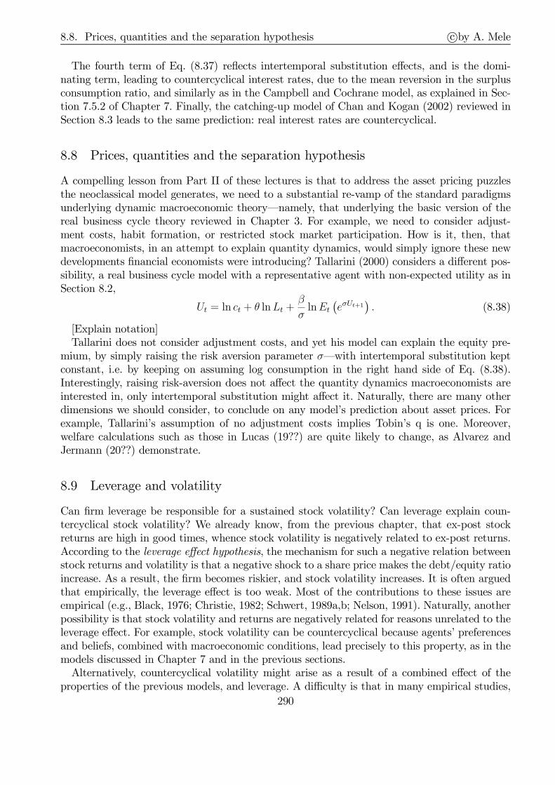
8.8. Prices, quantities and the separation hypothesis c©by A. Mele
The fourth term of Eq. (8.37) reflects intertemporal substitution effects, and is the domi-nating term, leading to countercyclical interest rates, due to the mean reversion in the surplusconsumption ratio, and similarly as in the Campbell and Cochrane model, as explained in Sec-tion 7.5.2 of Chapter 7. Finally, the catching-up model of Chan and Kogan (2002) reviewed inSection 8.3 leads to the same prediction: real interest rates are countercyclical.
8.8 Prices, quantities and the separation hypothesis
A compelling lesson from Part II of these lectures is that to address the asset pricing puzzlesthe neoclassical model generates, we need to a substantial re-vamp of the standard paradigmsunderlying dynamic macroeconomic theory–namely, that underlying the basic version of thereal business cycle theory reviewed in Chapter 3. For example, we need to consider adjust-ment costs, habit formation, or restricted stock market participation. How is it, then, thatmacroeconomists, in an attempt to explain quantity dynamics, would simply ignore these newdevelopments financial economists were introducing? Tallarini (2000) considers a different pos-sibility, a real business cycle model with a representative agent with non-expected utility as inSection 8.2,
Ut = ln ct + θ lnLt +β
σlnEt
(eσUt+1
). (8.38)
[Explain notation]Tallarini does not consider adjustment costs, and yet his model can explain the equity pre-
mium, by simply raising the risk aversion parameter σ–with intertemporal substitution keptconstant, i.e. by keeping on assuming log consumption in the right hand side of Eq. (8.38).Interestingly, raising risk-aversion does not affect the quantity dynamics macroeconomists areinterested in, only intertemporal substitution might affect it. Naturally, there are many otherdimensions we should consider, to conclude on any model’s prediction about asset prices. Forexample, Tallarini’s assumption of no adjustment costs implies Tobin’s q is one. Moreover,welfare calculations such as those in Lucas (19??) are quite likely to change, as Alvarez andJermann (20??) demonstrate.
8.9 Leverage and volatility
Can firm leverage be responsible for a sustained stock volatility? Can leverage explain coun-tercyclical stock volatility? We already know, from the previous chapter, that ex-post stockreturns are high in good times, whence stock volatility is negatively related to ex-post returns.According to the leverage effect hypothesis, the mechanism for such a negative relation betweenstock returns and volatility is that a negative shock to a share price makes the debt/equity ratioincrease. As a result, the firm becomes riskier, and stock volatility increases. It is often arguedthat empirically, the leverage effect is too weak. Most of the contributions to these issues areempirical (e.g., Black, 1976; Christie, 1982; Schwert, 1989a,b; Nelson, 1991). Naturally, anotherpossibility is that stock volatility and returns are negatively related for reasons unrelated to theleverage effect. For example, stock volatility can be countercyclical because agents’ preferencesand beliefs, combined with macroeconomic conditions, lead precisely to this property, as in themodels discussed in Chapter 7 and in the previous sections.Alternatively, countercyclical volatility might arise as a result of a combined effect of the
properties of the previous models, and leverage. A difficulty is that in many empirical studies,
290

8.9. Leverage and volatility c©by A. Mele
tests of the leverage effect hypothesis are performed without regard to a well specified economicmodel. Gallmeyer, Aydemir, Hollifield (2007) show that the reasoning underlying this hypothesiscan be made rigorous. They formulate a general equilibrium model with levered firms, whichthey realistically calibrate, to disentangle leverage effects from “real” effects such as habitformation. They make use of a stochastic discount factor known to price assets fairly well, andconclude that leverage effects do indeed have little effects in general equilibrium. This sectiondevelops a variant of their model, which has the mere merit to admit a closed-form solution.
8.9.1 Model
8.9.1.1 Primitives
Exogeneous aggregate output follows:
dδ (t)
δ (t)= g0dt+ σ0dW (t) ,
where σ0 > 0 and g0 are two constants. Many households maximize the intertemporal utilityin Eq. (8.35). To obtain closed-form solutions, we assume the equilibrium surplus consumption
ratio, s (t) = δ(t)−x(t)δ(t)
is solution to Eq. (8.36). This economy is one with countercyclical Sharperatios, as we now show. Using the results in Section 7.5.1, the Sharpe ratio for the marketis λ (D, x) = 1
s(σ0 − v(D,x)
D), where v (D, x) is the instantaneous volatility of the habit level
x = D (1− s) and, by Itô’s lemma, equals v (D, x) = Dσ0 (1− s) −DVol (s), where, again byItô’s lemma, Vol (s) = ασ0s
(1− s
υ
). Therefore, λ (s) ≡ λ (D,x) equals
λ (s) = σ0
(1 + α
(1− s
υ
)),
and is countercyclical, as mentioned.The value of the representative firm is:
V = E +D,
where E is equity and D is debt. Denote the debt maturity with Td, which in the calibrationexercise below will be taken to equal 10 years. The payoffs of the firm are such that δ (t) =δE (t) + δD (t), with obvious notation.
8.9.1.2 Model’s predictions
We now show that a calibration of the model leads to the following results: (i) price/dividendratios and price of debt are procyclical; (ii) return volatility is countercyclical; (iii) the leverageratio is countercyclical; (iv) the contribution of leverage to equity returns volatility is quitelimited.
8.9.1.3 Variation in volatility
Equity volatility is,
vol
(dE
E
)= σV + (σV − σD)
D
E.
Let T =∞, and assume debt services are δD = qδ, for some q ∈ (0, 1). Maturity of debt Td = 10years. For the aggregate consumption claim, we have that the price-dividend ratio, p (s) say, is
p (s (t)) = a+ bs (t)
291

8.9. Leverage and volatility c©by A. Mele
for some constants a, b given below. A similar expression holds for debt. We may, then, easilydeduce volatility. We have,
σV (s (t)) = σ0 +b
a+ bs (t)vol (ds (t)) , σD (s (t)) = σ0 +
bTdaTd + bTds (t)
vol (ds (t))
vol (ds (t)) = ωσ0st
(1− 1
υst
),
where,
aTd =1− e−(ρ+β)Td
ρ+ β, bTd =
β(1− e−ρTd
)+ ρ
(e−(ρ+β)Td − e−ρTd
)
ρ (ρ+ β) s, a = lim
l→∞al, b = lim
l→∞bl.
8.9.1.4 Equity volatility: a decomposition formula
Equity volatility is,
vol
(dE (t)
E (t)
)= σ0 +
b
a+ bs (t)︸ ︷︷ ︸= endog. P/D fluct.
· σ0ωs (t)
(1− 1
υs (t)
)
︸ ︷︷ ︸=vol(ds(t))
+
(b
a+ bs (t)− bTdaTd + bTds (t)
)
︸ ︷︷ ︸= leverage multiplier
· σ0ωs (t)
(1− 1
υs (t)
)
︸ ︷︷ ︸=vol(ds(t))
· D (t)E (t)
. (8.39)
Note that the leverage ratio, D(t)E(t)
, is endogeneous and equal to,
D (t)
E (t)=
(aTd + bTds (t)) q
a+ bs (t)− (aTd + bTds (t)) q
so we can only “see” what happens to D(t)E(t)
and vol(dE(t)E(t)
)as the surplus s (t) changes. We
calibrate the model using the values in Table 8.2 of Section 8.7. To anticipate, much of theaction in this model is activated by the large swings in the price-dividend ratio, p
′(s(t))p(s(t))
= ba+bs(t)
.Precisely, we have:
vol
(dE (t)
E (t)
)
︸ ︷︷ ︸≈0.15
= σ0︸︷︷︸=0.01
+b
a+ bs (t)︸ ︷︷ ︸= endog. P/D fluct.≈26.31
· σ0ωs (t)
(1− 1
υs (t)
)
︸ ︷︷ ︸=vol(ds(t)) ≈ 5·10−3
+
(b
a+ bs (t)− bTdaTd + bTds (t)
)
︸ ︷︷ ︸= leverage multiplier ≈11.08
· σ0ωs (t)
(1− 1
υs (t)
)
︸ ︷︷ ︸=vol(ds(t)) ≈ 5·10−3
· D (t)E (t)︸ ︷︷ ︸≈ 0.24
.
These computations might suggest that debt maturity might lead to have obtain a greaterleverage contribution to volatility. However, it is not the case, as we shall show.
292

8.9. Leverage and volatility c©by A. Mele
0.00 0.01 0.02 0.03 0.04 0.055
10
15
20
25
30
35
surplus ratio
P/D ratio
FIGURE 8.3. Price-dividend ratio for the aggregate consumption claim.
0.015 0.020 0.025 0.030 0.035 0.040 0.045 0.0500.00
0.05
0.10
0.15
0.20
surplus ratio
Eq. Vol.
FIGURE 8.4. Equity volatility for Td = 10. The solid line is total volatility. The top
dashed is the contribution from “unlevered” volatility to total volatility, σV . The bottom
dashed line is the contribution from “levered” volatility to total volatility, (σV − σ0)DE .
293
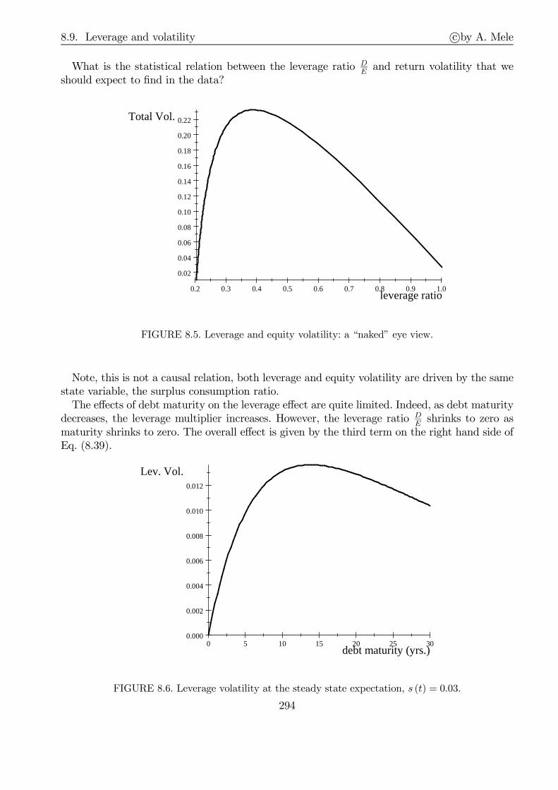
8.9. Leverage and volatility c©by A. Mele
What is the statistical relation between the leverage ratio DE
and return volatility that weshould expect to find in the data?
0.2 0.3 0.4 0.5 0.6 0.7 0.8 0.9 1.0
0.02
0.04
0.06
0.08
0.10
0.12
0.14
0.16
0.18
0.20
0.22
leverage ratio
Total Vol.
FIGURE 8.5. Leverage and equity volatility: a “naked” eye view.
Note, this is not a causal relation, both leverage and equity volatility are driven by the samestate variable, the surplus consumption ratio.The effects of debt maturity on the leverage effect are quite limited. Indeed, as debt maturity
decreases, the leverage multiplier increases. However, the leverage ratio DE
shrinks to zero asmaturity shrinks to zero. The overall effect is given by the third term on the right hand side ofEq. (8.39).
0 5 10 15 20 25 300.000
0.002
0.004
0.006
0.008
0.010
0.012
debt maturity (yrs.)
Lev. Vol.
FIGURE 8.6. Leverage volatility at the steady state expectation, s (t) = 0.03.
294

8.10. The cross-section of asset returns c©by A. Mele
8.9.1.5 The role of no-bankruptcy, and some model’s implications
In the previous model, there was no role for bankruptcy. Let us consider bankruptcy in a simplesetting. Consider a two date economy, and suppose that the value of the firm in one year is,
V =
Vbad < Nominal debt, wp pVgood > Nominal debt, wp 1− p
We assume risk-neutrality and that are no bankruptcy costs. Let R = S1−S0
S0be the equity
return, where S1 is the equity value at the second period. Then, we have that vol(R) =√
p1−p .
For example, if p = 2%, then vol(R) = 14%!
8.10 The cross-section of asset returns
295

8.11. Appendix 1: Non-expected utility c©by A. Mele
8.11 Appendix 1: Non-expected utility
8.11.1 Detailed derivation of optimality conditions and selected relations
D. E$. (8.4). We have,
xt+1 =∑
i(Pit+1 +Dit+1) θit+1
=∑
i(Pit+1 +Dit+1 − Pit) θit+1 +
∑iPitθit+1
=
(1 +
∑i
Pit+1 +Dit+1 − PitPit
Pitθit+1∑i Pitθit+1
)∑iPitθit+1
=(1 +
∑irit+1ωit
)(xt − ct)
where the last line follows by the standard budget constraint ct +∑
Pitθit+1 = xt, the definition ofrit+1 and the definition of ωit given in the main text.
O). Consider Eq. (8.5). The first order condition for c yields,
W1
(c, E
(V
(x′, y′
)))=W2
(c, E
(V
(x′, y′
)))·E
[V1
(x′, y′
) (1 + rM
(y′))]
, (8A.1)
where subscripts denote partial derivatives. Thus, optimal consumption is some function c (x, y). Hence,
x′ = (x− c (x, y))(1 + rM
(y′))
We have,V (x, y) =W
(c (x, y) , E
(V
(x′, y′
))).
By differentiating the value function with respect to x,
V1 (x, y) = W1
(c (x, y) , E
(V
(x′, y′
)))c1 (x, y)
+W2
(c (x, y) , E
(V
(x′, y′
)))E
[V1
(x′, y′
) (1 + rM
(y′))]
(1− c1 (x, y)) ,
where subscripts denote partial derivatives. By replacing Eq. (8A.1) into the previous equation we getthe Envelope Equation for this dynamic programming problem,
V1 (x, y) =W1
(c (x, y) , E
(V
(x′, y′
))). (8A.2)
By replacing Eq. (8A.2) into Eq. (8A.1), and rearranging terms,
E
[W2 (c (x, y) , ν (x, y))
W1 (c (x, y) , ν (x, y))W1
(c(x′, y′
), ν
(x′, y′
)) (1 + rM
(y′))]
= 1, ν (x, y) ≡ E(V
(x′, y′
)).
Below, we show that by a similar argument the same Euler equation applies to any asset i,
E
[W2 (c (x, y) , ν (x, y))
W1 (c (x, y) , ν (x, y))W1
(c(x′, y′
), ν
(x′, y′
)) (1 + ri
(y′))]
= 1, i = 1, · · · ,m. (8A.3)
D. E$. (8A.3). We have,
V (x, y) = maxc,ω
W(c,E
(V
(x′, y′
)))= max
θ′W
(x−∑
Piθ′i, E
(V
(x′, y′
))); x′ =
∑(P ′i +D′i
)θ′i.
The set of first order conditions is,
θ′i : 0 = −W1 (·)Pi +W2 (·)E[V1
(x′, y′
) (P ′i +D′i
)], i = 1, · · · ,m.
296

8.11. Appendix 1: Non-expected utility c©by A. Mele
Optimal consumption is c (x, y). Let ν (x, y) ≡ E (V (x′, y′)), as in the main text. By replacing Eq.(8A.2) into the previous equation,
E
[W2 (c (x, y) , ν (x, y))
W1 (c (x, y) , ν (x, y))W1
(c(x′, y′
), ν
(x′, y′
)) P ′i +D′iPi
]= 1, i = 1, · · · ,m.
D. E$. (8.6). We need to compute explicitly the stochastic discount factor in Eq.(8A.3),
m(x, y;x′y′
)=W2 (c (x, y) , ν (x, y))
W1 (c (x, y) , ν (x, y))W1
(c(x′, y′
), ν
(x′, y′
)).
We have,
W (c, ν) =1
1− η
[cρ + β ((1− η) ν)
ρ1−η
] 1−ηρ.
From this, it follows that,
W1 (c, ν) =[cρ + β ((1− η) ν)
ρ1−η
] 1−ηρ−1
cρ−1
W2 (c, ν) =[cρ + β ((1− η) ν)
ρ1−η
] 1−ηρ−1
β ((1− η) ν)ρ
1−η−1 ,
and,
W1
(c′, ν′
)=
[c′ρ + β
((1− η) ν′
) ρ1−η
] 1−ηρ−1
c′ρ−1 =W(c′, ν′
)1−η−ρ1−η (1− η)
1−η−ρ1−η c′ρ−1, (8A.4)
where ν′ ≡ ν (x′, y′). Therefore,
m(x, y;x′y′
)=W2 (c, ν)
W1 (c, ν)W1
(c′, ν′
)= β
(ν
W (c′, ν′)
) ρ1−η
−1 (c′
c
)ρ−1
.
Along any optimal consumption path, V (x, y) =W (c (x, y) , ν (x, y)). Therefore,
m(x, y;x′y′
)= β
(E (V (x′, y′))V (x′, y′)
) ρ1−η
−1 (c′
c
)ρ−1
. (8A.5)
We are left with evaluating the term E(V (x′,y′))V (x′,y′) . The conjecture to make is that v (x, y) = b (y)1/(1−η) x,
for some function b. From this, it follows that V (x, y) = b (y)x1−η/(1− η). We have,
V1 (x, y)
=W1
(c (x, y) , E
(V
(x′, y′
)))=W (c, ν)
1−η−ρ1−η (1− η)
1−η−ρ1−η cρ−1 = V (x, y)
1−η−ρ1−η (1− η)
1−η−ρ1−η cρ−1.
where the first equality follows by Eq. (8A.2), the second equality follows by Eq. (8A.4), and the lastequality follows by optimality. By making use of the conjecture on V , and rearraning terms,
c (x, y) = a (y)x, a (y) ≡ b (y)ρ
(1−η)(ρ−1) . (8A.6)
Hence, V (x′, y′) = b (y′)x′1−η/(1− η), where
x′ = (1− a (y))x(1 + rM
(y′)), (8A.7)
and
E (V (x′, y′))V (x′, y′)
=E
[ψ (y′) (1 + rM (y′))1−η
]
ψ (y′) (1 + rM (y′))1−η. (8A.8)
297

8.11. Appendix 1: Non-expected utility c©by A. Mele
Along any optimal path, V (x, y) =W (c (x, y) , E (V (x′, y′))). By plugging in W (from Eq. 8.5)) andthe conjecture for V ,
E[ψ(y′) (
1 + rM(y′))1−η]
= β− 1−η
ρ
(a (y)
1− a (y)
) (1−η)(ρ−1)ρ
. (8A.9)
Moreover,
ψ(y′) (
1 + rM(y′))1−η
=[a(y′) (
1 + rM(y′)) ρρ−1
] (1−η)(ρ−1)ρ
. (8A.10)
By plugging Eqs. (8A.9)-(8A.10) into Eq. (8A.8),
E (V (x′, y′))V (x′, y′)
= β−1−ηρ
[a (y)
(1− a (y)) a (y′) (1 + rM (y′))ρρ−1
] (1−η)(ρ−1)ρ
= β− 1−η
ρ
[(c′
c
)−1 x′
(1− a (y))x (1 + rM (y′))ρρ−1
] (1−η)(ρ−1)ρ
= β−1−ηρ
[(c′
c
)−1 1
(1 + rM (y′))1ρ−1
] (1−η)(ρ−1)ρ
where the first equality follows by Eq. (8A.6), and the second equality follows by Eq. (8A.7). Theresult follows by replacing this into Eq. (8A.5).
P E$. (8.10) , (8.11). By using the standard property that lnE(ey) = E(y)+12var (y),
for y normally distributed, in Eq. (8.8), we obtain,
0 = lnE
[exp
(−δθ − θ
ψln
(c′
c
)+ θRM
)]
= −δθ − θ
ψE
[ln
(c′
c
)]+ θE(RM) +
1
2
[(θ
ψ
)2
σ2c + θ2σ2
RM− 2
θ2
ψσRM ,c
]. (8A.11)
We do the same in Eq. (8.9), and obtain,
Rf = δθ +θ
ψE
[ln
(c′
c
)]− (θ − 1)E(RM)− 1
2
[(θ
ψ
)2
σ2c + (θ − 1)2 σ2
RM − 2θ (θ − 1)
ψσRM ,c
].
(8A.12)By replacing Eq. (8A.12) into Eq. (8A.11), we obtain Eq. (8.10) in the main text.
To obtain the risk-free rate Rf in Eq. (8.11), we replace the expression for E(RM) in Eq. (8.10) intoEq. (8A.12).
8.11.2 Details for the risks for the lung-run
P E$. (8.17). By substituting the guess zt = a0 + a1xt into Eq. (8.16),
0 = (κ0 − (1− κ1)a0 − δ) θ + lnEt
[exp
(− θ
ψln
(Ct+1
Ct
)+ θκ1a1xt+1 − θa1xt + θgt+1
)]
= θ
[((κ0 − (1− κ1)a0 − δ) +
(1− 1
ψ
)(g0 −
1
2σ2c
))]+ lnEt
[exp
(θ
(1− 1
ψ
)ǫt + θκ1a1ηt
)]
+
[(κ1ρ− 1) a1 +
(1− 1
ψ
)]xt
≡ const1 + const2 · xt,298

8.11. Appendix 1: Non-expected utility c©by A. Mele
where the second equality follows by Eqs. (8.14) and (8.15). Note, then, that this equality can onlyhold if the two constants, const1 and const2 are both zero. Imposing const2 = 0 yields,
a1 =1− 1
ψ
1− κ1ρ,
as in Eq. (8.17) in the main text. Imposing const1 = 0, and using the solution for a1, yields the solutionfor the constant a0.
8.11.3 Continuous time
Duffie and Epstein (1992a,b) extend the framework on non-expected utility to continuous time. Heuris-tically, the continuation utility is the continuous time limit of,
vt =
[cρt∆t+ e−δ∆t
(E(v1−ηt+∆t)
) ρ1−η
]1/ρ.
Continuation utility vt solves the following stochastic differential equation,
dvt =
[−f (ct, vt)−
1
2A (vt) ‖σvt‖2
]dt+ σvtdBt, with vT = 0
Now, (f,A) is the aggregator, with A being a variance multiplier, placing a penalty proportional toutility volatility ‖σvt‖2. The aggregator (f,A) corresponds somehow to the aggregator (W, v) of thediscrete time case.
The solution to the previous “stochastic differential utility” is:
vt = E
[∫ T
t
(f (cs, vs) +
1
2A (vs) ‖σvs‖2
)ds
],
which collapses to the standard additive utility case once f (c, v) = u (c)− βv and A = 0.
299
8.12. Appendix 2: Economies with heterogenous agents c©by A. Mele
8.12 Appendix 2: Economies with heterogenous agents
E( # ( / . Next, we assume each agent faces a system of completemarkets, in which case the equilibrium can be computed along the lines of Huang (1987), an extensionof the classical approach described in Chapter 2 of Part I of these Lectures. We consider a continuum ofagents indexed by an instantaneous utility function ua (c, x), where c is consumption, a is a parameterbelonging to some set A, and x is some state variable affecting the utility function. For example, x isthe “standard of living of others” in the Chan and Kogan (2002) model. Since agents access a completemarket systems, the equilibrium allocation is Pareto efficient. By the second welfare theorem, then,we know that for each Pareto allocation (ca)a∈A, there exists a social weighting function f such thatthe Pareto allocation can be “implemented” by means of the following program,
maxca
E
[∫ ∞
0e−δt
(∫
a∈Aua (ca (t) , x (t)) f (a) da
)dt
], s.t.
∫
a∈Aca (t)da = D (t) ,
or, given that there is no intertemporal transfer of resources,
u (D,x) = maxca
∫
a∈Aua (ca, x) f (a)da, s.t.
∫
a∈Acada = D, [8A.P1]
where D is the aggregate endowment in the economy. Then, the equilibrium price system can becomputed as the Arrow-Debreu state price density in an economy with a single agent endowed withthe aggregate endowment D, instantaneous utility function u (c, x), and where for a ∈ A, the socialweighting function f (a) equals the reciprocal of the marginal utility of income of the agent a.
The practical merit of this approach is that while the marginal utility of income is unobservable, thethusly constructed Arrow-Debreu state price density depends on the “infinite dimensional parameter”,f , which can be calibrated to reproduce the main quantitative features of consumption and asset pricedata. We now apply this approach and derive the equilibrium conditions in the Chan and Kogan (2002)model.
“(( / # J ” (C , K/ , 2002). In this model, markets arecomplete, and we have that A = [1,∞] and uη (cη, x) = (cη/x)
1−η / (1− η). The static optimizationproblem for the social planner in [8A.P1] can be written as,
u (D,x) = maxcη
∫ ∞
1
(cη/x)1−η
1− ηf (η)dη, s.t.
∫ ∞
1(cη/x) dη = D/x. (8A.13)
The first order conditions for this problem lead to,
(cηx
)−ηf (η) = V (D/x) , (8A.14)
where V is a Lagrange multiplier, a function of the aggregate endowment D, normalized by x. It isdetermined by Eq. (8.21), which is obtained by replacing Eq. (8A.14) into the budget constraint of thesocial planner, the second of Eqs. (8A.13). The value function in Eq. (8.20) of the main text followsby replacing Eq. (8A.14) into the maximed value of the intertemporal utility, the first of Eqs. (8A.13).General equilibrium allocations, and prices, are obtained by setting f (η) equal to the reciprocal of themarginal utility of income for agent η.
The expression for the unit risk-premium in Eq. (8.22) follows by results given in Section 7.5.1 ofChapter 7,
λ (s (D,x)) = −(∂2U (s (D,x))
∂D2
/∂U (s (D,x))
∂D
)σ0D, s (D,x) ≡ ln
D
x, (8A.15)
300
8.12. Appendix 2: Economies with heterogenous agents c©by A. Mele
where U (s) is the value function in Eq. (8.20). To evaluate the previous expression for λ, note, first,that:
∂U (s (D,x))
∂D= −V
′ (s (D,x))D
∫ ∞
1
1
ηf (η)
1η V (s (D,x))−
1η dη. (8A.16)
Moreover, by differentiating Eq. (8.21) with respect to D, using Eq. (8A.16), and rearranging terms,leads to ∂U (s (D,x)) /∂D = V (s (D,x)) /x. Differentiating this expression for ∂U/∂D with respectto D again, produces:
∂2U (s (D,x))
∂D2=
V ′ (s (D,x))x
1
D. (8A.17)
Replacing Eqs. (8A.16)-(8A.17) into Eq. (8A.15) yields Eq. (8.22) in the main text. The short-termrate is the expectation of the pricing kernel in this fictitious representative agent economy. It equals,again by results given in Section 7.5.1 of Chapter 7,
R(D, s, x) = ρ− g0∂2U (s (D,x)) /∂D2
∂U (s (D,x)) /∂DD − θ
∂2U (s (D,x)) /∂D∂x
∂U (s (D,x)) /∂Dsx− 1
2σ20
∂3U (s (D,x)) /∂D3
∂U (s (D,x)) /∂DD2
= ρ+g0σ0λ (s (D,x))− θ
(1 +
V ′ (s (D,x))V (s (D,x))
)s (D,x)− 1
2σ20
(V ′′ (s (D,x))− V ′ (s (D,x))
V (s (D,x))
).
It is instructive to compare the first order conditions of the social planner in Eq. (8A.14) with thosein the decentralized economy. Since markets are complete, we have that the first order conditions inthe decentralized economy satisfy:
e−δt (cη (t)/x (t))−η = κ (η) ξ (t)x (t) , (8A.18)
where κ (η) is the marginal utility of income for agent η, and ξ (t) is the usual pricing kernel.By aggregating the market equilibrium allocations in Eq. (8A.18),
D (t) =
∫ ∞
1cη (t)dη = x (t)
∫ ∞
1
[eδtξ (t)x (t)
]− 1ηκ (η)
− 1η dη.
By aggregating the social weighted allocations in Eq. (8A.14), with f = κ−1,
D (t) = x (t)
∫ ∞
1V (D (t)/x (t))−
1η κ (η)−
1η dη.
Hence, it must be that,x (t)−1 V (D (t)/x (t)) = eδtξ (t) . (8A.19)
That is, if f = κ−1, then, Eq. (8A.19) holds. The converse to this result is easy to obtain: eliminating(cη/x)
−η from Eq. (8A.14) and Eq. (8A.18) leaves:
eδtx (t) ξ (t)
V (D (t)/x (t))=
1
f (η)κ (η), (t, η) ∈ [0,∞)× [1,∞).
Hence if Eq. (8A.19) holds, then, f = κ−1.To summarize, the equilibrium allocations and prices can be “centralized” through the social planner
program in (8A.13), with f = κ−1.
R(, ( ( (B , C(, 1998). Given Eq. (8.33), andresults given in Section 7.5.1 of Chapter 7, the unit risk-premium, λ(D,x), solves a fixed point problem:
λ(D,x) = −U11(D,x)
U1(D,x)σ0D +
U12(D,x)x
U1(D,x)λ(D,x).
301

8.12. Appendix 2: Economies with heterogenous agents c©by A. Mele
That is,
λ(D,x) = − U1(D,x)U11(D,x)
U1(D,x)− U12(D,x)x· σ0D
U1(D,x). (8A.20)
We claim that:
U1(D,x) = u′p(c∗p), and
U1(D,x)U11(D,x)
U1(D,x)− U12(D,x)x= u′′p(c
∗p), (8A.21)
where c∗p and c∗n are the social planner consumption allocations. By replacing Eqs. (8A.21) into Eq.(8A.20), and using the definition of up and s, leads to the expression for λ in Eq. (8.28). The expressionfor short-term rate R in Eq. (8.27) can be found similarly, and again, through the results given inSection 7.5.1 of Chapter 7.
We now show that Eq. (8A.21) hold true. Consider the Lagrangean for the maximization problemin Eq. (8.32),
L = up (cp) + xun (cn) + ν (c− cp − cn) ,
where ν is a Lagrange multiplier, x =u′p(cp)
u′n(cn), and cp and cn are the market consumption allocations.
The first order conditions for the social planner lead to social allocation functions c∗p = cp (D,x) andc∗p = cn (D,x), and Lagrange multiplier ν (D,x), satisfying:
u′p (cp (D,x)) = ν (D,x) = xu′n (cn (D,x)) . (8A.22)
Accordingly, the value of the problem in Eq. (8.32) is:
U (D,x) = up (cp (D,x)) + xun (cn (D,x)) ,
such that
U1 (D,x) = u′p (cp (D,x))∂cp (D,x)
∂D+ xu′n (cn (D,x))
∂cn (D,x)
∂D
= u′p (cp (D,x))
(∂cp (D,x)
∂D+∂cn (D,x)
∂D
)
= u′p (cp (D,x)) , (8A.23)
where the second equality follows by the first order conditions in Eq. (8A.22), and the third equalityholds by differentiating the equilibrium condition
D = cp (D,x) + cn (D,x) , (8A.24)
with respect to D.Eq. (8A.23) establishes the first claim in Eqs. (8A.21). To prove the second claim, invert, first,
the first order condition with respect to ν, obtaining, cp (D,x) = u′−1p [ν (D,x)] and cn (D,x) =
u′−1n [ν (D,x) /x]. Replace, then, these inverse functions into Eq. (8A.24),
D = u′−1p [ν (D,x)] + u′−1
n [ν (D,x) /x] , (8A.25)
where, by Eq. (8A.24) and Eq. (8A.23),
ν (D,x) = u′p (cp (D,x)) = U1 (D,x) . (8A.26)
Differentiating Eq. (8A.25) with respect to x and D, and using Eq. (8A.26), leaves:
0 =1
u′′p (cp (D,x))U12 (D,x) +
1
u′′n (cn (D,x))U12 (D,x)x− U1 (D,x)
x2, (8A.27)
302

8.12. Appendix 2: Economies with heterogenous agents c©by A. Mele
and
1 =1
u′′p (cp (D,x))U11 (D,x) +
1
u′′n (cn (D,x))U11 (D,x)
x. (8A.28)
Replacing Eq. (8A.28) into Eq. (8A.27) leaves:
0 =U12 (D,x)
u′′p (cp (D,x))+
(1
U11 (D,x)− 1
u′′p (cp (D,x))
)U12 (D,x)x− U1 (D,x)
x.
The second relation in Eqs. (8A.21) follows by rearranging terms in the previous relation.
303
8.12. Appendix 2: Economies with heterogenous agents c©by A. Mele
References
Abel, A.B. (1990): “Asset Prices under Habit Formation and Catching Up with the Joneses.”American Economic Review Papers and Proceedings 80, 38-42.
Abel, A.B. (1999): “Risk Premia and Term Premia in General Equilibrium.” Journal of Mon-etary Economics 43, 3-33.
Alvarez, F. and U.J. Jermann (20??):
Bansal, R. and A. Yaron (2004): “Risks for the Long Run: A Potential Resolution of AssetPricing Puzzles.” Journal of Finance 59, 1481-1509.
Basak, S. and D. Cuoco (1998): “An Equilibrium Model with Restricted Stock Market Par-ticipation.” Review of Financial Studies 11, 309-341.
Black, F. (1976): “Studies of Stock Price Volatility Changes.” Proceedings of the 1976 Meetingof the American Statistical Association, 177-81.
Boldrin, M., L. Christiano and J. Fisher (2001): “Habit Persistence, Asset Returns and theBusiness Cycle.” American Economic Review 91, 149-166.
Campbell, J. Y., and J. H. Cochrane (1999): “By Force of Habit: A Consumption-BasedExplanation of Aggregate Stock Market Behavior.” Journal of Political Economy 107,205-251.
Campbell, J. and R. Shiller (1988): “The Dividend-Price Ratio and Expectations of FutureDividends and Discount Factors.” Review of Financial Studies 1, 195—228.
Chan, Y.L. and L. Kogan (2002): “Catching Up with the Joneses: Heterogeneous Preferencesand the Dynamics of Asset Prices.” Journal of Political Economy 110, 1255-1285.
Christie, A.A. (1982): “The Stochastic Behavior of Common Stock Variances: Value, Leverage,and Interest Rate Effects.” Journal of Financial Economics 10, 407-432.
Constantinides, G.M. and D. Duffie (1996): “Asset Pricing with Heterogeneous Consumers.”Journal of Political Economy 104, 219-240.
Constantinides, G.M., J.B. Donaldson and R. Mehra (2002): “Juniors Can’t Borrow: a NewPerspective on the Equity Premium Puzzle.” Quarterly Journal of Economics 117, 269-296.
Duffie, D. and L.G. Epstein (1992a): “Asset Pricing with Stochastic Differential Utility.” Re-view of Financial Studies 5, 411-436.
Duffie, D. and L.G. Epstein (with C. Skiadas) (1992b): “Stochastic Differential Utility.” Econo-metrica 60, 353-394.
Epstein, L.G. and S.E. Zin (1989): “Substitution, Risk-Aversion and the Temporal Behavior ofConsumption and Asset Returns: A Theoretical Framework.” Econometrica 57, 937-969.
304
8.12. Appendix 2: Economies with heterogenous agents c©by A. Mele
Epstein, L.G. and S.E. Zin (1991): “Substitution, Risk-Aversion and the Temporal Behavior ofConsumption and Asset Returns: An Empirical Analysis.” Journal of Political Economy99, 263-286.
Gallmeyer, M., Aydemir, A.C. and B. Hollifield (2007): “Financial Leverage and the LeverageEffect: A Market and a Firm Analysis.” working paper Carnegie Mellon.
Guvenen, F. (2009): “A Parsimonious Macroeconomic Model for Asset Pricing.” Econometrica77, 1711-1740.
Heaton, J. and D.J. Lucas (1996): “Evaluating the Effects of Incomplete Markets on RiskSharing and Asset Pricing.” Journal of Political Economy 104, 443-487.
Huang, C.-f. (1987): “An Intertemporal General Equilibrium Asset Pricing Model: the Caseof Diffusion Information.” Econometrica 55, 117-142.
Jermann, U.J. (1998): “Asset Pricing in Production Economies.” Journal of Monetary Eco-nomics 41, 257-276.
Lettau, M. (2002): “Idiosyncratic Risk and Volatility Bounds, or, Can Models with Idiosyn-cratic Risk Solve the Equity Premium Puzzle?” Review of Economics and Statistics 84,376-380.
Ljungqvist, L. and H. Uhlig (2000): “Tax Policy and Aggregate Demand Management underCatching Up with the Joneses.” American Economic Review 90, 356-366.
Lucas, R.E. (19??):
Lucas, D.J. (1994): “Asset Pricing with Undiversifiable Income Risk and Short Sales Con-straints: Deepening the Equity Premium Puzzle.” Journal of Monetary Economics 34,325-341.
Mankiw, N.G. (1986): “The Equity Premium and the Concentration of Aggregate Shocks.”Journal of Financial Economics 17, 211-219.
Mankiw, N.G. and S.P. Zeldes (1991): “The Consumption of Stockholders and Non-Stockholders.”Journal of Financial Economics 29, 97-112.
Menzly, L., T. Santos and P. Veronesi (2004): “Understanding Predictability.” Journal ofPolitical Economy 112, 1, 1-47.
Nelson, D.B. (1991): “Conditional Heteroskedasticity in Asset Returns: A New Approach.”Econometrica 59, 347-370.
Rouwenhorst, G.K. (1995): “Asset Returns and Business Cycles.” In Cooley, T.F. (Ed.): Fron-tiers of Business Cycle Research, Princeton University Press, 294-330.
Schwert, G.W. (1989a): “Why Does Stock Market Volatility Change Over Time?” Journal ofFinance 44, 1115-1153.
Schwert, G.W. (1989b): “Business Cycles, Financial Crises and Stock Volatility.” Carnegie-Rochester Conference Series on Public Policy 31, 83-125.
305

8.12. Appendix 2: Economies with heterogenous agents c©by A. Mele
Tallarini, T. (2000): “Risk-Sensitive Real Business Cycles.” Journal of Monetary Economics45, 507-32.
Telmer, C.I. (1993): “Asset-Pricing Puzzles and Incomplete Markets.” Journal of Finance 48,1803-1832.
Wachter, J.A. (2006): “A Consumption-Based Model of the Term Structure of Interest Rates.”Journal of Financial Economics 79, 365-399.
Weil, Ph. (1989): “The Equity Premium Puzzle and the Risk-Free Rate Puzzle.” Journal ofMonetary Economics 24, 401-421.
306

9Information and other market frictions
9.1 Introduction
In the models of the previous chapters, agents do not need to learn about the equilibriumprice because information, whilst sometimes incomplete, is disseminated symmetrically acrossdecision makers. This chapter considers settings where agents have access to differential oreven asymmetric information about some attributes relating to economic developments. Inthese settings with imperfect information, there are gains to be made by learning about theequilibrium price, because the very same price, conveys some information every agents transmitwhile he trades, thereby making it public so to speak. Naturally, the price cannot convey allprivate information when information is costly, for otherwise there would not be any incentiveto purchase information. To avoid this information paradox, prices need to convey “noisy,” orimperfect signals about the information private investors have. As Black (1986) discussed, noisemakes markets function when information problems would otherwise lead them not to arise inthe first place.The assumption agents have imperfect information about the fundamentals of the economy
was first used by Phelps (1970) and Lucas (1972), to explain the relation between monetary pol-icy and the business cycle. This information-based approach to the business cycle, summarizedin Lucas (1981), was, in fact, abandoned in favour of the real business cycle theory, reviewedin Chapter 3, partly because imperfect information cannot be considered as the sole engine ofmacroeconomic fluctuations. Instead, it is widely acknowledged that the merit of Lucas’ ap-proach was the introduction of a systematic way of thinking about fluctuations, in a contextwith rational expectations. Moreover, his information approach has inspired work in financialeconomics, where imperfect information is likely to play a quite fundamental role. In Section9.2, we provide a succinct account of the Lucas framework, and solve a model relying on a sim-plified version of Lucas (1973). We solve this model, following the perspective we think a financetheorist would typically have. It is quite useful to present this model, as this is very simple andat the same time, contributes to give us a big picture of where imperfect information can leadus, in general. Section 9.2 through 9.7 review the many models in financial economics that havebeen used to explain the price formation mechanism in contexts with imperfect information, beit asymmetric or differential, as we shall make precise below.

9.2. Prelude: imperfect information in macroeconomics c©by A. Mele
Sections 9.7 and 9.9 conclude this chapter, and present additional market frictions that arepotentially apt to explain certain features in the asset price formation process.
9.2 Prelude: imperfect information in macroeconomics
There are n islands, where n goods are produced. Let ysi denote log-production supplied in thei-th island. (All prices and quantities are in logs, in this section.) It is assumed that this supplyis set so as to equal the expected wedge of the price in the island, pi, over the average price inthe economy, p,
ysi = E (pi − p| pi) , where p =1
n
n∑
j=1
pj .
The previous equation can be easily derived, once we assume p is common knowledge, as forexample in the model of monopolistic competion of Blanchard and Kiyotaki (1987). If, instead,p is not common knowledge, it is more problematic to derive the exact functional form assumedfor ysi , although this describes a quite plausible decision mechanism.Information is disseminated differentially, not asymmetrically, in that producers in the i-th
island do not know the price in the remaining islands, and guess economic developments inthe other islands with the same precision. We assume and, later, verify, that all variables,exogeneous and endogeneous, are normally distributed. Under this presumption, we shall show,the price index p gathers all the available information in the economy efficiently, i.e. it is asufficient statistics for all that information.We have, by the Projection theorem,
ysi = E (pi − p| pi) ≡ β (pi −E (p)) ,
where we have used the fact that information is symmetrically disseminated and, then, (i)the expectation E (pi) = E (pj) = E (p) for every i and j, and (ii) both the numerator and
denominator of the ratio, β ≡ cov(pi−p,pi)var(pi)
, are the same across all islands. This coefficient willbe determined below, as a result of the equilibrium.Aggregating across all islands, yields the celebrated Lucas supply equation:
ys ≡ 1
n
n∑
j=1
ysj = β (p− E (p)) . (9.1)
Next, assume the demand for the good produced in the i-th island is given by:
ydi = m− p+ ui − θ (pi − p) , where ui ∼ N(0, σ2
u
)
where money ism = E (m) + ǫ, where ǫ ∼ N
(0, σ2
ǫ
). (9.2)
Finally, we assume that E (uiǫ) = 0, and that ui are a sectoral shocks, in that:∑n
j=1 uj = 0.
The functional form assumed for the demand function, ydi , can be easily derived, assuming thegoods in the islands are imperfect substitutes, as for example in Blanchard and Kiyotaki (1987).In this context, the equilibrium price in the islands plays two roles. A first, standard role, is
to clear the market in each island, being such that ysi = ydi , or:
β (pi − E (p)) = m− p+ ui − θ (pi − p) , for all i. (9.3)
308

9.2. Prelude: imperfect information in macroeconomics c©by A. Mele
Its second role is to convey information about the two shocks, the macroeconomic, monetaryshock, ǫ, and the real shocks in all the islands, uj, j = 1, · · · , n. Let us assume, then, that theonly real shock that matters for the price in the i-th island is ui. Below, we shall verify thisconjecture holds, in equilibrium. Then, the price is a function pi = P (ǫ, ui), which we conjectureto be affine, in ǫ and ui, viz
P (ǫ, ui) = a+ bǫ+ cui, (9.4)
where the coefficients a, b and c have to be determined, in equilibrium. Under these conditions,the average price is a function p = P (ǫ), equal to:
P (ǫ) = a+ bǫ. (9.5)
Let us replace Eqs. (9.4), (9.5) and (9.2) into Eq. (9.3). By rearranging terms, we obtain:
0 = (βb+ b− 1) ǫ+ (βc+ θc− 1) ui + a− E (m) .
This equation has to hold for all ǫ and ui. Therefore,
a = E (m) ,
and the coefficients for ǫ and ui must both equal zero, leading to the following expressions forb and c:
b =1
1 + β, c =
1
θ + β. (9.6)
We are left with determining β, which given Eqs. (9.4)-(9.5), and Eq. (9.6), is easily shown toequal:
β =σ2u
σ2u +
(θ+β1+β
)2
σ2ǫ
. (9.7)
The positive fixed point to this equation, which is easily shown to exist, delivers β, which canthen be replaced back into Eqs. (9.6), to yield the solutions for b and c, which are both positive.We can now figure out the implications of this equilibrium. By replacing Eqs. (9.4)-(9.5) into
the Lucas supply equation (9.1), leaves:
ys = βbǫ.
This is Lucas celebrated neutrality result. Anticipated monetary policy, E (m), does not affectthe equilibrium outcome, ys. Instead, it is the monetary shock that affects ys. Agents in anyone island do not observe the price in the remaining islands and, hence, the aggregate pricelevel, p. Therefore, they are unable to tell whether an increase in the price of the good theyproduce, pi, is due to a real shock, ui, or to a monetary shock, ǫ. In other words, they cannotdisentangle a monetary shock from a real shock. If the agents were informed about the realshocks in the other islands, they would of course infer ǫ, and a monetary shock would notexert any effect on the equilibrium production. Formally, in equilibrium, the price difference,pi − p = cui, which does not depend on ǫ, a standard “dichotomy” prediction reminiscent ofclassical theory. But pi−p is not observed, as p is not observed. Instead, the producers in the i-thisland can only guess pi−E (p| pi) = bǫ+cui, which co-varies positively with the observed price,pi, cov (pi − p, pi) = c2σ2
u. This covariance is zero precisely when we remove the assumption ofimperfect knowledge about the real shocks, so that σ2
u = 0, in which case β = 0. By contrast,
309

9.3. Grossman-Stiglitz paradox c©by A. Mele
with imperfect knowledge, producers act so as to compensate for their partial lack of knowledge,and produce to the maximum extent they can justify, on the basis of the positive statisticalco-movements, cov (pi − p, pi) > 0. Note, if E (m) = m−1, i.e. money supply in the previousperiod, then from Eq. (9.5), the inflation rate, p−p−1 = bǫ+(1− b) ǫ−1. Therefore, output andinflation are positively correlated, and generate a Phillips curve, which policy makers cannotexploit anyway, as anticipated monetary policy, E (m), is rationally “factored out,” and doesnot affect output. This is the essence of the Lucas critique (Lucas, 1977).In the next sections, we present a number of models that work due to a similar mechanism.
Why should we ever purchase an asset from any one else, who is insisting in selling it to themarket? Trading seems to be a difficult phenomenon to explain, in a world with imperfectinformation. Yet trading does occur, if imperfect information has the same nature as that ofthe Phelps-Lucas model. Agents might well be imperfectly informed about the nature of, say,unusually high market orders. For example, huge sell orders might arrive to the market, eitherbecause the asset is a lemon or because the agents selling it are hit by a liquidity shock. Inthe models of this section, an equilibrium with rational expectation exists, precisely because ofthis “noise”–liquidity, in this example. There is a chance the sell order arrives to the market,simply because the agents selling it are hit by a liquidy shock. Imperfectly informed agents,therefore, might be willing to buy, if it is in their interest to do so.
9.3 Grossman-Stiglitz paradox
Fama (1970) considers three forms of informational efficiency: (i) Weak efficiency, arising whenasset prices convey all information relating to the past time-series of data; (ii) Semi-strongefficiency, relating to the situation where asset prices convey all public information, not only thepast time series of data; (iii) Strong efficiency, whereby asset prices reflect private information.The third form of efficiency cannot exist, indefinitely, unless of course information is not costly.For it were costly, there would not incentive to purchase it in a world with informationallystrong efficient markets. And if it were not costly, it would not, then, be private information.It is the Grossman-Stiglitz paradox
9.4 Noisy rational expectations equilibrium
9.4.1 Differential information
Hellwig (1980). Diamond and Verrecchia (1981).
9.4.2 Asymmetric information
Grossman and Stiglitz (1980).
9.4.3 Information acquisition
9.5 Strategic trading
Kyle (1985). Foster and Viswanathan (1996).
310

9.6. Dealers markets c©by A. Mele
9.6 Dealers markets
Glosten and Milgrom (1985).
9.7 Noise traders
DeLong, Shleifer, Summers and Waldman (1990).
9.8 Demand-based derivative prices
9.8.1 Options
Gârleanu, Pedersen and Poteshman (2007).
9.8.2 Preferred habitat and the yield curve
Vayanos and Vila (2007), Greenwood and Vayanos (2008).
9.9 Over-the-counter markets
Duffie, Gârleanu and Pedersen (2005, 2007).
311

9.9. Over-the-counter markets c©by A. Mele
References
Black, F. (1986): “Noise.” Journal of Finance 41, 529-543.
Blanchard, O. and N. Kiyotaki (1987): “Monopolistic Competition and the Effects of AggregateDemand.” American Economic Review 77, 647-666.
Fama, E. (1970): “Efficient Capital Markets: A Review of Theory and Empirical Work.” Jour-nal of Finance 25, 383-417.
Lucas, R.E. (1972): “Expectations and the Neutrality of Money.” Journal of Economic Theory4, 103-124.
Lucas, R.E. (1973): “Some International Evidence on Output-Inflation Tradeoffs.” AmericanEconomic Review 63, 326-334.
Lucas, R.E. (1977): “Econometric Policy Evaluation: A Critique.” Carnegie-Rochester Con-ference Series on Public Policy 1: 19-46.
Lucas, R.E. (1981): Studies in Business-Cycle Theory. Boston, MIT Press.
Phelps, E.S. (1970): “Introduction.” In: Phelps, E. S. (Editor): Microeconomic Foundations ofEmployment and Inflation Theory, New York: W. W. Norton.
312

Part III
Applied asset pricing theory
313
10Options and volatility
10.1 Introduction
This chapter is under construction. Will include exotics, evaluation through trees and cali-bration. Will cover some details on how to deal with market imperfections. Will improve thepresentation.
10.2 Forwards
10.2.1 Pricing
Forwards can be synthesized, as follows. Let P (t, T ) be the price of a bond expiring at timeT . Assuming the short-term rate r is constant, we have P (t, T ) = e−r(T−t). At time t, borrowP (t, T )F ∗ and buy a stock, with market price St, with F
∗ : P (t, T )F ∗ − S (t) = 0. Then, thepayoff of this portfolio at time T is F ∗ − S (T ). But the portfolio is worthless at time t, so thistrading is the same as a forward. Therefore, we have F ∗ = F (t) (say), where:
F (t) = S (t) er(T−t). (10.1)
Forwards are insensitive to volatility, in general, although they might, under some circumstancesclarified below.
10.2.2 Forwards as a means to borrow money
Forward contracts can be used to borrow money. We can do the following: (i) long a forward,which at time T , delivers the payoff −F + S (T ); (ii) short-sell the underlying asset, which attime T , will give rise to a payoff of −S (T ). So, (i) and (ii) are such that now, we access to S (t)dollars, due to (ii), and at time T , we need to pay −F , which is the sum of the two payoffsresulting from (i) and (ii). By Eq. (10.1), this is tantamount to borrowing money at the interestrate r.
10.3. Options: no-arb bounds, convexity and hedging c©by A. Mele
10.2.3 A pricing formula
Consider, again, a contract similar to that in Section 10.2.1, where at time T , the payoff is givenby S (T )−K, for some constant value of K. We know that the current value of this payoff is:
e−r(T−t)Et (S (T )−K) = S (t)− e−r(T−t)K, (10.2)
which is zero, for K = F ∗. We want to consider the situation where such a current value is notnecessarily zero, and show that the previous expression is a special case of a quite importantpricing formula. Consider a payoff at time T , equal to S (T )−K, provided the stock price atT is at least as large as some positive constant ℓ ≥ 0,
(S (T )−K) IS(T )≥ℓ.
For ℓ = 0, this payoff is just that of a forward, and for ℓ = K, the payoff is that of Europeancall. To price this payoff, we proceed as follows:
e−r(T−t)Et[(S (T )−K) IS(T )≥ℓ
]= S (t)Et
(ηt (T ) IS(T )≥ℓ
)− e−r(T−t)KEt
(IS(T )≥ℓ
)
= S (t) Et(IS(T )≥ℓ
)− e−r(T−t)KEt
(IS(T )≥ℓ
)
= S (t) · Qt (S (T ) ≥ ℓ)− e−r(T−t)K ·Q (S (T ) ≥ ℓ) , (10.3)
where ηt (T ) ≡ e−r(T−t)S(T )S(t)
, Qt is the risk-neutral probability given the information at time t,
Qt is a new probability, with Radon-Nykodim derivative given by
dQt
dQt= ηt (T ) , (10.4)
and, finally, Et denotes the expectation under Qt, and Et the expectation under Qt. Naturally,Eq. (10.3) collapses to Eq. (10.2), once ℓ = 0, and to the celebrated Black and Scholes (1973)formula, once we take S (t) to be a geometric Brownian Motion, and ℓ = K, as explained inSection 10.4. It is a general formula, and a quite useful one, whilst dealing with difficult modelswhere, for example, the volatility of the underlying asset return is not constant, as illustratedin Section 10.5.
10.2.4 Forwards and volatility
10.3 Options: no-arb bounds, convexity and hedging
A European call (put) option is a contract by which the buyer has the right, but not theobligation, to buy (sell) a given asset at some price, called the strike, or exercise price, at somefuture date. Let C and p be the prices of the call and the put option. Let S be the price ofthe asset underlying the contract, and K and T be the exercise price and the expiration date.Finally, let t be the current evaluation time. The following relations hold true,
C(T ) =
0 if S(T ) ≤ KS(T )−K if S(T ) > K
p(T ) =
K − S(T ) if S(T ) ≤ K0 if S(T ) > K
or more succinctly, C(T ) = (S(T )−K)+ and p(T ) = (K − S(T ))+.315

10.3. Options: no-arb bounds, convexity and hedging c©by A. Mele
Figure 10.1 depicts the net profits generated by portfolios including one asset, a share, say,and/or one option written on the same very share. To simplify the presentation, we take theshort-term rate r = 0. The first rows in Figure 10.1 illustrate that the exposure to lossesgenerated by longing or shorting a share drops by purchasing an appropriate options. Consider,for example, consider the first row, which depicts the two net profits related to (i) longing ashare and (ii) longing a call option written on the share. Both cases generate positive net profitswhen S (T ) is high. However, the call option provides “protection” when S(T ) is low, providedC(t) < S(t), which is indeed a no-arbitrage condition we prove demonstrate later. It is thisinsurance feature that makes the option economically valuable.The prices of the call and put options are intimately related by the put-call parity. Let P (t, T )
be the time t price of a zero maturing at time T > t. We have:
T 10.1 (Put-call parity). Consider a put and a call option with the same exerciseprice K and the same expiration date T . Their prices p(t) and C(t) satisfy, p (t) = C (t) −S (t) +KP (t, T ).
P. Consider two portfolios: (A) Long one call, short one underlying asset, and investKP (t, T ); (B) Long one put. The table below gives the value of the two portfolios at time tand at time T .
Value at TValue at t S(T ) ≤ K S(T ) > K
Portfolio A C (t)− S (t) +KP (t, T ) −S(T ) +K S(T )−K − S(T ) +KPortfolio B p (t) K − S (T ) 0
The two portfolios have the same value in each state of nature at time T . Therefore, their valuesat time t must be identical to rule out arbitrage.
316

10.3. Options: no-arb bounds, convexity and hedging c©by A. Mele
S(t)S(T)
KS(T)
K + c(t)
− c(t)
Buy share Buy call
π(S)T = S (T) − S (t) π(c)T = c(T) − c(t)
− S(t)
S(t)S(T)
KS(T)
K - p(t)
-p(t)
Short-sell shareBuy put
π(-S)T = S(t) - S(T) π(p)T = p(T) - p(t)S(t)
KS(T)
KS(T)
K - p(t)p(t) - K
Sell call Sell put
π(-c)T = c(t) - c(T) π(-p)T = p(t) - p(T)
K + c(t)
c(t) p(t)
FIGURE 10.1.
317
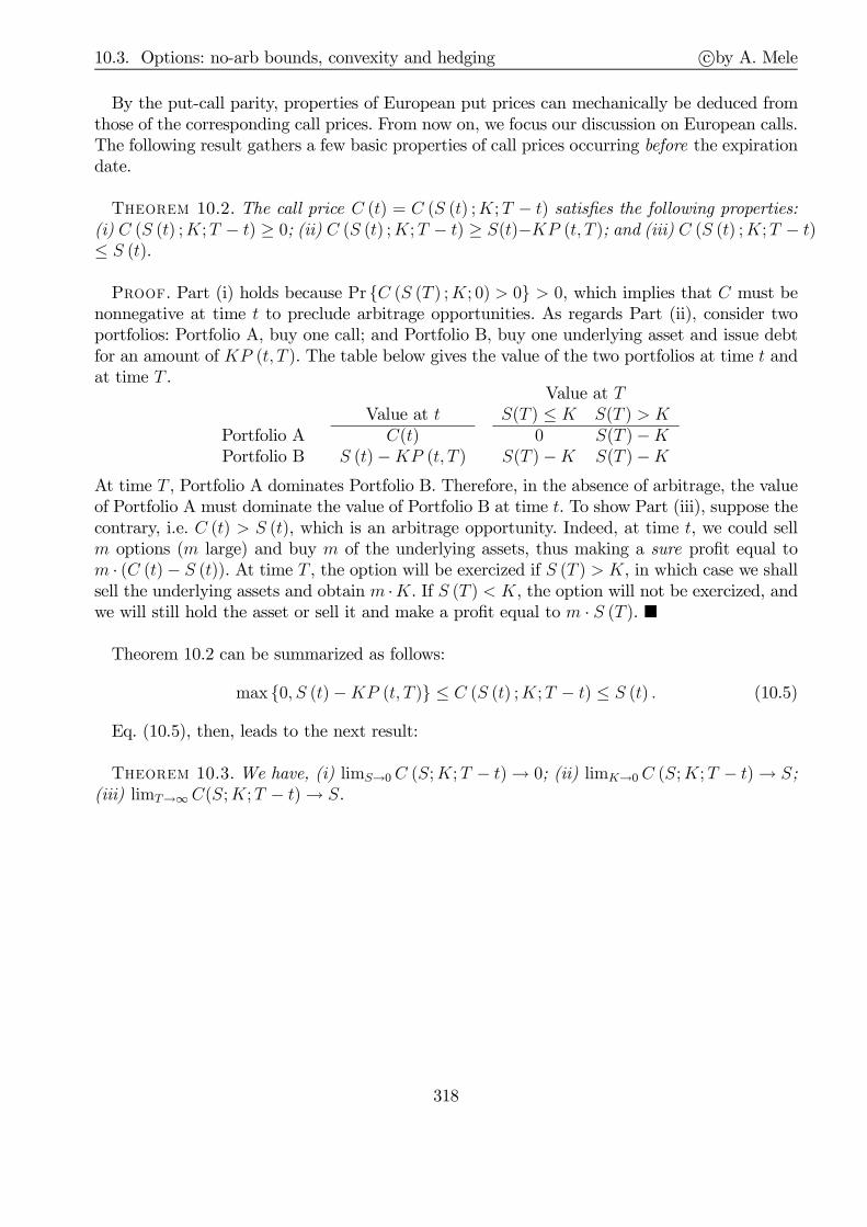
10.3. Options: no-arb bounds, convexity and hedging c©by A. Mele
By the put-call parity, properties of European put prices can mechanically be deduced fromthose of the corresponding call prices. From now on, we focus our discussion on European calls.The following result gathers a few basic properties of call prices occurring before the expirationdate.
T 10.2. The call price C (t) = C (S (t) ;K;T − t) satisfies the following properties:(i) C (S (t) ;K;T − t) ≥ 0; (ii) C (S (t) ;K;T − t) ≥ S(t)−KP (t, T ); and (iii) C (S (t) ;K;T − t)≤ S (t).
P. Part (i) holds because Pr C (S (T ) ;K; 0) > 0 > 0, which implies that C must benonnegative at time t to preclude arbitrage opportunities. As regards Part (ii), consider twoportfolios: Portfolio A, buy one call; and Portfolio B, buy one underlying asset and issue debtfor an amount of KP (t, T ). The table below gives the value of the two portfolios at time t andat time T .
Value at TValue at t S(T ) ≤ K S(T ) > K
Portfolio A C(t) 0 S(T )−KPortfolio B S (t)−KP (t, T ) S(T )−K S(T )−K
At time T , Portfolio A dominates Portfolio B. Therefore, in the absence of arbitrage, the valueof Portfolio A must dominate the value of Portfolio B at time t. To show Part (iii), suppose thecontrary, i.e. C (t) > S (t), which is an arbitrage opportunity. Indeed, at time t, we could sellm options (m large) and buy m of the underlying assets, thus making a sure profit equal tom · (C (t)− S (t)). At time T , the option will be exercized if S (T ) > K, in which case we shallsell the underlying assets and obtain m ·K. If S (T ) < K, the option will not be exercized, andwe will still hold the asset or sell it and make a profit equal to m · S (T ).
Theorem 10.2 can be summarized as follows:
max 0, S (t)−KP (t, T ) ≤ C (S (t) ;K;T − t) ≤ S (t) . (10.5)
Eq. (10.5), then, leads to the next result:
T 10.3. We have, (i) limS→0C (S;K;T − t)→ 0; (ii) limK→0C (S;K;T − t)→ S;(iii) limT→∞C(S;K;T − t)→ S.
318

10.3. Options: no-arb bounds, convexity and hedging c©by A. Mele
S(t) S(t)
c(t) c(t)
S(t)
c(t)
A
B C
45°K b(t,T)
A
A
B
B
FIGURE 10.2.
The previous results basic arbitrage bounds option prices satisfy. Consider the top panel ofFigure 10.2. Eq. (10.5) tells us that C (t) must lie inside the AA and the BB lines. Moreover,by Theorem 10.3(i), C (t) is zero when the price of the asset underlying the contract is zero.Finally, by Eq. (10.5), the option price goes to zero as the price of the underlying asset getslarge; but because C cannot lie outside the the region bounded by the AA line and the BBlines, C will go to infinity by “sliding up” through the BB line.How does the option price behave within AA and BB? We cannot tell. Given the boundary
behavior of the option price C (t), we can only say that provided C (t) is convex in S (t), then, itis also increasing in S. In this case, C (t) would behave as as in the left-hand side of the bottompanel of Figure 10.2. This case seems to be the most relevant, empirically. It is predicted bythe celebrated Black and Scholes (1973) formula reviewed in Section 10.4. However, this isnot a general property of option prices. Bergman, Grundy and Wiener (1996) show that inone-dimensional diffusive models, the price of a contingent claim written on a tradable assetis convex in the underlying asset price if the payoff of the claim is convex in the underlyingasset price (as in the case of a Europen call option). In our context, the boundary conditionsguarantee that the price of the option is then increasing and convex in the price of the underlyingasset. However, Bergman, Grundy and Wiener provide several counter-examples in which theprice of a call option can be decreasing over some range of the price of the asset underlyingthe option contract. These counter-examples include models with jumps, or the models withstochastic volatility that we shall describe later in this chapter. Therefore, there are no reasonsto exclude that the option price behavior could be as that in right-hand side of the bottompanel of Figure 10.2. [We have seen some of these things in Chapter 7, actually, so I don’t needto overlap too much here, on the contrary, need to show how the thing seen in Chapter 7 canbe used here. Moreover, I have to mention this is a general qualitative thing, and that I have amore technical treatment in Section 10.5.]
319

10.3. Options: no-arb bounds, convexity and hedging c©by A. Mele
S(t)
c(t)
45°Kb(t,T)
T1 T2 T3
FIGURE 10.3.
By convexity, the option is unlikely to be exercized when S is small. Therefore, changes inthe price of the underlying asset produce little effect on the call price, C. However, the optionis likely to be exercized when S is large. In fact, a given percentage increase in S is then tobe followed by an even higher percentage increase in C: the elasticity of the option price withrespect to the asset price is larger than one, ǫ ≡ dC
dS· SC> 1, as for an increasing and convex
function, which is zero at the origin, the first order derivative is always higher than the secant.In other words, option returns are more volatile than the returns on the underlying asset. Afinal property is that call options are also “wasting assets,” in that their value decreases overtime, as illustrated by an hypothetical example in Figure 10.3, which plots the option pricearising for three maturity dates, T1 > T2 > T3.The previous properties illustrate in a simple way the general principles underlying a portfolio
aimed to “mimick” the option price. For example, investment banks sell options that they wantto hedge against, to avoid the exposure to losses illustrated in Figure 10.1. As emphasizedfurther in Section 10.4.4, hedging is important when the only objective is to receive fees fromthe sale of derivatives. Then, and at a very least, the portfolio that “mimics” the option pricemust exhibit the previous properties. For example, suppose we wish our portfolio to exhibit thebehavior in the left-hand side of the bottom panel of Figure 10.2, which as we argues is themost relevant, empirically. We require the portfolio to exhibit a number of properties.
(p-i) The portfolio value, V , must be increasing in the underlying asset price, S.
(p-ii) The sensitivity of the portfolio value with respect to the underlying asset price must bestrictly positive and bounded by one, 0 < dV
dS< 1.
(p-iii) The elasticity of the portfolio value with respect to the underlying asset price must bestrictly greater than one, dV
dS· SV> 1.
The previous properties hold under the following conditions:
(c-i) The portfolio includes the asset underlying the option contract.
(c-ii) The number of assets underlying the option contract is less than one.
(c-iii) The portfolio includes debt to create a sufficiently large elasticity. Indeed, let V = θS−D,where θ is the number of assets underlying the option contract, with θ ∈ (0, 1), and D is
320
10.4. Evaluation and hedging c©by A. Mele
debt. Then, dVdS> θ and dV
dS· SV= θ · S
V> 1⇔ θS > V = θS −D, which holds if and only
if D > 0.
In fact, the hedging problem is dynamic in nature, and we would expect θ to be a functionof the underlying asset price, S, and time to expiration. Therefore, we require the portfolio todisplay the following additional property:
(p-iv) The number of assets underlying the option contract must increase with S. Moreover,when S is low, the value of the portfolio must be virtually insensitive to changes inS. When S is high, the portfolio must include mainly the assets underlying the optioncontract, to make the portfolio value “slide up” through the BB line in Figure 10.3.
The previous property holds under the following condition:
(c-iv) θ is an increasing function of S, with limS→0 θ (S)→ 0 and limS→∞ θ (S)→ 1.
Finally, the purchase of the option does not entail any additional inflows or outflows until timeto expiration. Therefore, we require that the “mimicking” portfolio display a similar property:
(p-v) The portfolio must be implemented as follows: (i) any purchase of the asset underlyingthe option contract must be financed by issue of new debt; and (ii) any sells of the assetunderlying the option contract must be used to shrink the existing debt:
The previous property of the portfolio just says that the portfolio has to be self-financed, inthe sense described in the first Part of these lectures.
(c-v) The portfolio is implemented through a self-financed strategy.
We now proceed to add more structure to the problem.
10.4 Evaluation and hedging
We consider a continuous-time model in which asset prices are driven by a d-dimensional Brown-ian motion W .1 We consider a multivariate state process
dY (h) (t) = ϕh (y (t)) dt+∑d
j=1 ℓhj (y (t)) dW(j) (t) ,
for some functions ϕh and ℓhj(y), satisfying the usual regularity conditions.The price of the primitive assets satisfies the regularity conditions in Chapter 4. The value
of a portfolio strategy, V , is V (t) = θ (t) · S+ (t). We consider a self-financed portfolio, i.e. onewhere no injection of withdrawal of money is required to finance trading the security underlyingthe portfolio, such that dV (t) = θ (t) · dS+ (t), as explained in Section 4.3.1 of Chapter 4. Thevalue of this self-financed portfolio satisfies:
dV (t) =[π (t)⊤ (µ (t)− 1mr (t)) + r (t)V (t)− C (t)
]dt+ π (t)⊤ σ (t) dW (t) , (10.6)
where π ≡ (π1, · · · , πm)⊤, πi ≡ θiSi, µ ≡ (µ1, · · · , µm)⊤, Si is the price of the i-th asset, µiis its drift and σ (t) is the volatility matrix of the price process. We impose that V satisfy theregularity conditions reviewed in Chapter 4.
1As usual, we let F (t)t∈[0,T ] be the P -augmentation of the natural filtration FW (t) = σ (W (s) , s ≤ t) generated by W , withF = F (T ).
321
10.4. Evaluation and hedging c©by A. Mele
10.4.1 Spanning and cloning
A set of securities “spans” a given vector space, say a set of payoffs, if any point in that space canbe generated by a linear combination of the security prices. The set of payoffs may include thosepromised by a contingent claim, say e.g. that promised by a European call, or final consumption,as in Harrison and Kreps (1979) and Duffie and Huang (1985) (see Chapter 4). Chapter 4 relieson this “spanning” property to solve for consumption-portfolio choices through martingaletechniques. This section shows how spanning helps define replicating strategies with the purposeof pricing “redundant” assets. Technically, and as in Chapter 4, let V x,π (t) denote the solutionto Eq. (10.6) when the initial wealth is x, the portfolio policy is π, and the intermediateconsumption is C ≡ 0. We say that the portfolio policy π spans F (T ) if V x,π (T ) = X almostsurely, where X is any square-integrable F(T )-measurable random variable.In Chapter 4, the risk-neutral probability, Q, is used to span securities. This section char-
acterizes properties of security spanning under the physical probability, P . In a diffusion en-vironment, asset prices are semimartingales under P . More generally, consider the followingrepresentation of a F(t)-P semimartingale,
dA(t) = dF (t) + γ(t)dW (t), (10.7)
where F is a process with finite variation, and γ ∈ L20,T,d(Ω,F , P ). We wish to replicate A
through a portfolio. First, then, we must look for a portfolio π satisfying
γ(t) = π⊤ (t)σ (t) . (10.8)
Second, we equate the drift of V to the drift of F , obtaining,
dF (t)
dt= π (t)⊤ (µ (t)− 1mr (t)) + r (t)V (t) = π (t)⊤ (µ (t)− 1mr (t)) + r (t)F (t) . (10.9)
The second equality holds because if drift and diffusion terms of F and V are identical, thenF (t) = V (t).Clearly, ifm < d, there are no solutions for π in Eq. (10.8). The economic interpretation is that
in this case, the number of assets is so small that we cannot create a portfolio able to replicateall possible events in the future. Mathematically, if m < d, then V x,π (T ) ∈M ⊂ L2 (Ω,F , P ).As Chapter 4 emphasizes, there is also a converse to this result, which motivates the definitionof market incompleteness given in Chapter 4 (Definition 4.5).Let H (t) the price of a European call option, which we take to be rationally formed, in that
H (t) = C (t, y (t)), for some C ∈ C1,2([0, T )×Rk
). By Itô’s lemma,
dC = µCCdt+ (CY · J) dW,
where µCC = ∂C∂t+
∑kl=1
∂C∂ylϕl (t, y) +
12
∑kl,j=1
∂2C∂yl∂yj
cov (yl, yj); CY is 1 × d, and J is d × d.
Finally,
C (T, y) = X ∈ L2 (Ω,F , P ) .
In this context, µCC and CY · J are the same as dF/ dt and γ in Eqs. (10.7) and (10.9). Inparticular, we identify the volatility in Eq. (10.8) as CY J = π
⊤σ.
322

10.4. Evaluation and hedging c©by A. Mele
10.4.2 Black & Scholes
Let m = d = 1, and suppose the only state variable is the price of a stock, and that ϕ(s) = µs,cov(s) = σ2s2, and µ and σ2 are constants. Then CY · J = CSσS, π = CSS, and by Eq. (10.9),
∂C
∂t+∂C
∂SµS +
1
2
∂2C
∂S2σ2S2 = π (µ− r) + rC =
∂C
∂SS (µ− r) + rC, (10.10)
subject to the boundary condition, C (T, s) = (s−K)+. [See also Chapter 4!]. The solutionto Eq. (10.10) is the celebrated Black and Scholes (1973) formula,
CB&S (t, S) = SΦ(d)−Ke−r(T−t)Φ(d− σ√T − t), d =
ln( SK) + (r + 1
2σ2)(T − t)
σ√T − t , (10.11)
where Φ denotes the cumulative Normal distribution. Appendix 1 derives Eq. (10.10) hingingupon the original arguments developed by Black and Scholes (1973), and Merton (1973), whereone considers a portfolio comprising the option, the underlying asset, and a portfolio strategyaiming to make the portfolio locally riskless.The original derivation of Black and Scholes (1973) and Merton (1973) relies on the assump-
tion that an option market exists. However, Eq. (10.11) holds even without requiring that a mar-ket exists for the option, or that the pricing function C (t, S) is differentiable. We wish to showthat the option price is differentiable, and that this is a result, not an assumption. Let us definethe function C (t, S) that solves Eq. (10.10), with boundary condition C (T, S) = (S −K)+.Note, we are not assuming this function is the option price. Rather, we shall show this is theoption price. Consider a self-financed portfolio of bonds and stocks, with π = CSS. Its valuesatisfies,
dV = [CSS(µ− r) + rV ] dt+ CSσSdW.
Moreover, by Itô’s lemma, C (t, s) is solution to
dC =
(Ct + µSCS +
1
2σ2S2CSS
)dt+ CSσSdW.
By subtracting the previous two equations, leaves:
dV − dC = [−Ct − rSCS −1
2σ2S2CSS
︸ ︷︷ ︸=−rC
+ rV ]dt = r (V − C) dt.
Hence, we have that V (τ ) − C (τ , S (τ)) = [V (0)− C (0, S (0))] erτ , for all τ ∈ [0, T ]. Next,assume that V (0) = C (0, S (0)). Then, V (τ ) = C (τ , S (τ )) and V (T ) = C (T, S (T )) =(S (T )−K)+. That is, the portfolio π = CSS replicates the payoff underlying the optioncontract. Therefore, V (τ) equals the market price of the option. But V (τ) = C (τ , S (τ )).
10.4.3 Surprising cancellations and “preference-free” formulae
Due to what Heston (1993a) (p. 933) very aptly terms “a surprising cancellation,” the constantµ doesn’t show up in the final formula. Heston (1993a) shows that this property is not robustto modifications in the assumptions for the underlying asset price process. Gamma processes,incomplete markets.
323

10.4. Evaluation and hedging c©by A. Mele
10.4.4 Hedging
The “cloning” arguments suggest themselves as a mechanism to replicate a derivative instru-ments through the asset prices underlying the derivative contract. Why do derivatives need tobe replicated, in practice? Because most of them are dealt with by investment banks, whichsimply act as financial intermediaries, trading derivatives on behalf of third parties, being com-pensated through fees. Suppose, for instance, an investment bank receives an order to sell aput. Then, the bank would want to hedge against this put, by creating a replicating portfoliosuch that the value of this portfolio is the same as the final payoff the investment bank has topay to its buyer to honour its sale. So hedging is needed to replicate the final payoffs requiredto honour the contracts giving rise to these payoffs. For example, if the world moved accordingto the Black-Scholes model,
Delta =∂CB&S
∂S= CS = Φ(d), (10.12)
where Φ and d are as in Eq. (10.11). Indeed, the Black-Scholes formula is homogenous of degreeone in S and K, that is, CB&S (λS, λK) = λCB&S (S,K). Therefore, by Euler’s theorem,
CB&S (S,K) =∂CB&S
∂SS +
∂CB&S
∂KK,
and Eq. (10.12) then follows by identifying terms in the Black-Scholes formula.Naturally, investment banks can undertake speculative trading activities, aimed at taking
views, such as those described in Section 10.5.5 below, in which case hedging does not have tobe implemented, in general. However, even in this case, hedging might be required to isolate theparticular views a trading desk of the bank is taking. For example, Section 10.5.5 will explainthat to express the view that equity volatility will raise, say, we cannot simply buy Europeanoptions, because options are increasing both in volatility and the asset underlying the option.A better solution, then, is long an option, delta-hedged through Black-Scholes.
10.4.5 Endogenous volatility
Hedges and crashes. The presence of delta-hedging can lead to financial turmoil. Brady com-mission.Gamma is always positive for long calls and puts, as these contracts have positive convexity,
as illustrated by Figure 10.1. Naturally, short calls and puts have negative gamma. In orderfor the statement “when gamma is negative, delta hedging involves buying on the way up andselling on the way down” to be true, we also have to consider whether the delta is positiveor not (that is, whether the derivative price is increasing or decreasing in the underlying assetprice). So we have four instances of hedging portfolios:
(i) Positive gamma: Buying on the way up and selling on the way down.
(i.1) Hedging portfolios with positive delta, as required, for example, to hedge against thesale of a call. Positive delta means that the hedging portfolio relies on buying theassets underlying the call. When the price of these assets are up, then, the delta is alsoup, which implies we need to keep on buying even more of the assets underlying thehedging portfolio. On the other hand, when prices are down, the delta is also down,which implies holding less of the assets underlying the hedging portfolio, therebyleading to sell some these assets precisely when the market is down.
324

10.4. Evaluation and hedging c©by A. Mele
(i.2) Hedging portfolios with negative delta, as required, for example, to hedge againstthe sale of a put. Negative delta means that the hedging portfolio relies on sellingthe assets underlying the put. In this case, delta is up when when prices are up.However, this now simply means that we need to sell less! For example delta mighthave been −2 before the market was up and now delta is −1: that is, we need to buyback some of the assets underlying the hedging portfolio. When, instead, prices aredown, delta is also down, which means we need to sell even more into a depressedmarket.
(ii) Negative gamma: Buying on the way down and selling on the way up.
(ii.1) Hedging portfolios with positive delta, as required, for example, to hedge againsthaving gone long a put. Positive delta means that the hedging portfolio relies onbuying assets underlying the put. Negative gamma now means that as soon as theprice of these asset goes up (resp. down), we need to buy less (resp. buy more), sowe sell when prices go up and buy when prices go down.
(ii.2) Hedging portfolios with positive delta, as required, for example, to hedge againsthaving gone long a call. We are now selling the assets underlying the call. Negativegamma, here, means that as the price of these assets goes up (resp. down), we needto sell more (resp. sell less), so once again, we sell when prices go up and buy whenprices go down.
How to implement these hedging portfolios, in practice, is still an open question, as this issue isnecessarily model-based. Section 10.5.4, for example, shows that delta hedging under the Black-Scholes assumptions would lead the bank to eliminate the risk of fluctuations in the underlyingstock price. At the same time, however, hedging through Black-Scholes leads the derivativesbook quite messy once the fundamental assumption underlying the Black-Scholes world doesnot hold, namely that volatility changes randomly. In this case, “hedging” would rather looklike a volatility view. To appropriately hedge, then, one has to rely on more complicated hedgingstrategies. For example, to hedge against an option in a world of stochastic volatility, we wouldneed to use a stock, a bond, and, another ... option!
10.4.6 Marking to market
Consider a derivative, which we go long at time t = 0, when it is worthless. As time unfolds,its value will change, which calls for marking to market it. Suppose the derivative paysoffψ (S (T ))−K (0) at time T , where S (T ) is the price of some asset as of time T , and K (0) is setso as to make the derivative worthless at time zero. Assuming that interest rates are constant,we have that K (0) : e−rTE0 [ψ (S (T ))−K (0)] = 0, where E0 is the expectation at time t = 0,taken under the risk-neutral probability. That is, K (0) = E0 [ψ (S (T ))]. The market value ofthe derivative at time t, then, say MtM(t), is simply the present value of the expected payoffat T , under the risk-neutral probability, e−r(T−t)Et [ψ (S (T ))−K (0)], or
MtM(t) = e−r(T−t) [K (t)−K (0)] . (10.13)
For more elaborated payoffs, such as those depending on the realizations of the underlying risksover the life of the contract, the market to market updates might be more intricate than thatin Eq. (10.13), as the case of variance contracts illustrates in Section 10.7.3.
325

10.4. Evaluation and hedging c©by A. Mele
10.4.7 Properties of options in diffusive models
10.4.7.1 Price reaction to random changes in the state variables
We now derive some general properties of option prices arising in the context of diffusionprocesses. The discussion in this section hinges upon the seminal contribution of Bergman,Grundy and Wiener (1996). At the same time, Eqs. (10.16), (10.17) and (10.18) below can beseen as particular cases of general results provided in Chapter 7.We take as primitive the price of a share, solution to:
dS (t)
S (t)= µ (S (t)) dt+ σ (S (t)) dW (t) , σ (s) =
√2v (s) (10.14)
and develop some properties of a European-style option price at time t, denoted asC (S (t) , t, T ),where T is time-to-expiration. Let the payoff of the option be the function ψ(S), where ψ satis-fies ψ′ (S) > 0. In the absence of arbitarge, C satisfies the following partial differential equation
0 = Ct + CSrS + CSSv(S)− rC for all (τ , S) ∈ [t, T )×R++
C(S, T, T ) = ψ(S) for all S ∈ R++(10.15)
Let us differentiate the previous partial differential equation with respect to S. The result isthat H ≡ CS satisfies another partial differential equation,0 = Ht + (rS + v
′(S))HS +HSSσ(S)− rH for all (τ , S) ∈ [t, T )× R++
H(S, T, T ) = ψ′(S) > 0 for all S ∈ R++
(10.16)By technical results for partial differential equations reviewed in Chapter 7 (Appendix 1), wehave that H (S, τ , T ) > 0 for all (τ , S) ∈ [t, T ] × R++. That is, in the scalar diffusion setting,the option price is always increasing in the underlying asset price.Next, let us tilt the asset price volatility: consider twomarkets A and Bwith prices (Ci, Si)i=A,B,
with the asset price volatility being larger in market A than in market B, viz
dSi (τ )
Si (τ)= rdτ + σi
(Si (τ)
)dW (τ) , i = A,B,
where W is Brownian motion under the risk-neutral probability, σi is as σ in Eq. (10.14), andσA (s) > σB (s), for all s. It is easy to see that the price difference, ∆C ≡ CA − CB, satisfies,
0 =
[∆Cτ + r∆CS +∆CSS · σA (S)− r∆C
]+
(σA − σB
)CBSS, for all (τ , S) ∈ [t, T )×R++
∆C = 0, for all S(10.17)
By the same results reviewed in Chapter 7 (Appendix 1), used to analyze Eq. (10.16), we havethat ∆C > 0 whenever CSS > 0. Therefore, it follows that if option prices are convex in theunderlying asset price, then they are also always increasing in the volatility of the underlyingasset prices. Volatility changes are mean-preserving spread in this context. We are left to showthat CSS > 0. Let us differentiate Eq. (10.16) with respect to S. The result is that Z ≡ HS =CSS satisfies the following partial differential equation,
0 = Zτ + (r + 2v
′(S))ZS + ZSSσ(S)− (r − σ′′(S))Z for all (τ , S) ∈ [t, T )× R++
H(S, T, T ) = ψ′′(S) for all S ∈ R++
(10.18)
326

10.5. Stochastic volatility c©by A. Mele
By the usual results in Chapter 7 (Appendix 1), we have, again that H (S, τ , T ) > 0 for all(τ , S) ∈ [t, T ]×R++, whenever ψ
′′(S) > 0 ∀S ∈ R++. That is, in the scalar diffusion setting, theoption price is always convex in the underlying asset price if the terminal payoff is convex in theunderlying asset price. In other terms, the convexity of the terminal payoff propagates to theconvexity of the pricing function. Therefore, if the terminal payoff is convex in the underlyingasset price, then the option price is always increasing in the volatility of the underlying assetprice.
10.4.7.2 Passage of time
Sometimes we claim that options are “wasting” assets, in that their value decreases over time,due to a decrease in the value of optionality. For call options, this is definitely true, at leastwithin diffusive models. By the first equation in (10.15), we have:
Ct = −rC (ǫ− 1)− CSSv(S) < 0, (10.19)
where ǫ ≡ SCCS is the elasticity of the option price with respect to the asset price, which
for a call option, is larger than one, as noted in Section 10.3. However, for a put option, thiselasticity is negative, and can make the right hand side of Eq. (10.19) change sign, especiallyfor far out-of-the-money options.
10.4.7.3 Recovering risk-neutral probabilities
Consider the price of a European call,
C (S(t), t, T ;K) = P (t, T )
∫ ∞
0
[S(T )−K]+ dQ (S(T )|S(t)) = P (t, T )∫ ∞
K
(x−K) q (x|S(t)) dx,
where Q is the risk-neutral probability and q(x+|x)dx ≡ dQ(x+| x). Assuming thatlimx→∞ xq (x|S) = 0, and differentiating with respect to K leaves:
er(T−t)∂C (S(t), t, T ;K)
∂K= −
∫ ∞
K
q (x|S(t)) dx.
Let us differentiate again,
er(T−t)∂2C (S(t), t, T ;K)
∂K2= q (K|S(t)) . (10.20)
Eq. (10.20) allows one to “recover” the risk-neutral density using option prices. The Arrow-Debreu state density, AD (S+ = u|S(t)), is given by,
AD(S+ = u
∣∣S(t))= er(T−t) q
(S+
∣∣S (t))∣∣S+=u
= e2r(T−t)∂2C (S(t), t, T ;K)
∂K2
∣∣∣∣K=u
.
These results are quite useful in applied work. They also help deal with the pricing of volatilitycontracts reviewed in Section 10.6, as explained in Appendix 3.
10.5 Stochastic volatility
10.5.1 Statistical models of changing volatility
A prominent step in empirical finance was the understanding that financial returns exhibitboth temporal dependence in their second order moments and heavy-peaked and tailed distri-butions. This empirical feature of financial returns was known at least since the seminal work
327
10.5. Stochastic volatility c©by A. Mele
of Mandelbrot (1963) and Fama (1965). However, it was only with the introduction of the au-toregressive conditionally heteroscedastic (ARCH) model of Engle (1982) and Bollerslev (1986)that econometric models of changing volatility have been intensively fitted to data.An ARCH model works as follows. Let ytNt=1 be a record of observations on some asset
returns. That is, yt = lnSt/St−1, where St is the asset price, and where we are ignoring divi-dend issues. The empirical evidence suggests that the dynamics of yt are well-described by thefollowing model:
yt = a+ ǫt, ǫt|Ft−1 ∼ N(0, σ2t ), σ2
t = w + αǫ2t−1 + βσ
2t−1, (10.21)
where a, w, α and β are parameters and Ft denotes the information set as of time t. This modelis known as the GARCH(1,1) model (Generalized ARCH). It was introduced by Bollerslev(1986), and collapses to the ARCH(1) model introduced by Engle (1982) once we set β = 0.ARCH models have played a prominent role in the analysis of many aspects of financial
econometrics, such as the term structure of interest rates, the pricing of options, or the presenceof time varying risk premiums in the foreign exchange market. The classic survey is that inBollerslev, Engle and Nelson (1994).The quintessence of ARCH models is to make volatility dependent on the variability of past
observations. An alternative formulation, initiated by Taylor (1986), makes volatility drivenby some unobserved components. This formulation gives rise to the stochastic volatility model.Consider, for example, the following stochastic volatility model,
yt = a+ ǫt, ǫt|Ft−1 ∼ N(0, σ2t );
ln σ2t = w + α ln ǫ2t−1 + β lnσ
2t−1 + ηt; ηt|Ft−1 ∼ N(0, σ2
η)
where a, w, α, β and σ2η are parameters. The main difference between this model and the
GARCH(1,1) model in Eq. (10.21) is that the volatility as of time t, σ2t , is not predetermined
by the past forecast error, ǫt−1. Rather, this volatility depends on the realization of the stochasticvolatility shock ηt at time t. This makes the stochastic volatility model considerably richer thana simple ARCH model. As for the ARCH models, SV models have also been intensively used,especially following the progress accomplished in the corresponding estimation techniques. Theseminal contributions related to the estimation of this kind of models are mentioned in Meleand Fornari (2000). Early contributions that relate changes in volatility of asset returns toeconomic intuition include Clark (1973) and Tauchen and Pitts (1983), who assume that astochastic process of information arrival generates a random number of intraday changes of theasset price.
10.5.2 ARCH and diffusive models
Under regularity conditions, ARCH models and stochastic volatility models behave essentiallythe same as the sampling frequency gets sufficiently high. Precisely, Nelson (1990) shows thatARCHmodels converge in distribution to the solution of the stochastic differential equations, inthe sense that the finite-dimensional distributions of the volatility process generated by ARCHmodels converge towards the finite-dimensional distributions of some diffusion process, as thesampling frequence goes to infinity. Mele and Fornari (2000) (Chapter 2) contain a review ofresults relating to this type of convergence, and Corradi (2000) develops a critique related tothe conditions underlying these convergence results. To illustrate, heuristically, consider the
328
10.5. Stochastic volatility c©by A. Mele
following model,
d lnS(τ) = (· · · ) dτ + σ (τ ) dW (τ )dσ2 (τ) = (ω − ϕσ2 (τ)) dτ + ψσ2 (τ ) dWσ (τ)
(10.22)
where dW (τ) and dWσ (τ ) are correlated, with correlation ρ, and ω, ϕ, and ψ are some con-stants. Consider, further, the ARCH model:
y∆,n+1 = ǫ∆,n+1, ǫ∆,n = σ∆,n · u∆,n, u∆,n ∼ NID (0, 1)
σ2∆,n+1 = w∆ + α∆ (|ǫ∆,n| − γǫ∆,n)2 + β∆σ
2∆,n
(10.23)
where y∆,n+1 = ln (S∆,n+1/S∆,n) − E (ln (S∆,n+1/S∆,n)), n and ∆ refer to the indexing of ob-served data and the sampling frequency (weekly, say), and w∆, α∆, β∆ are positive parameters,possibly depending on the sampling frequency, and γ ∈ (−1, 1). The parameter γ allows tocapture the Black-Christie-Nelson leverage effect (Black, 1976; Christie, 1982; Nelson, 1991)discussed in Chapter 8. Note that the second of Eqs. (10.23) can be written as:
σ2∆,n+1 − σ2
∆,n =[∆t−1w∆ −∆t−1
(1− α∆E (|u∆,n| − γu∆,n)2 − β∆
)σ2∆,n
]∆t
+∆t−12α∆ · σ2
∆,n
√∆t ·∆Wσ,n, (10.24)
and ∆Wσ,n ≡ (|u∆,n| − γu∆,n)2 − E (|u∆,n| − γu∆,n)2. The first two terms define the driftterm for the variance process, and the last term is the diffusive component. Suppose thatlim∆t↓0∆t
−1w∆ = ω, lim∆t↓0∆t−1
(1− α∆E (|u∆,n| − γu∆,n)2 − β∆
)= ϕ, and, finally,
lim∆t↓0∆t−1/2
√α∆ = ψ < ∞, where ≡ var (∆W2,n). Then, under regularity conditions,
the sample paths of S and σ2 in Eqs. (10.23) converge to those of S and σ2 in Eqs. (10.22),with a well-defined correlation coefficient ρ (see Fornari and Mele, 2006).2
10.5.3 Implied volatility and smiles
Parallel to the empirical research into asset returns volatility, practitioners and academics re-alized that the assumption of constant volatility underlying the Black and Scholes (1973) andMerton (1973) formulae was too restrictive. The Black-Scholes model assumes that the price ofthe asset underlying the option contract follows a geometric Brownian motion,
dS (t)
S (t)= µdτ + σdW (t) ,
where W is a Brownian motion, and µ, σ are constants. As explained earlier, σ is the onlyparameter to enter the Black-Scholes-Merton formulae.The assumption that σ is constant is inconsistent with the empirical evidence reviewed in
the previous section. This assumption is also inconsistent with the empirical evidence on thecross-section of option prices. Let CBS (St, t;K,T, σ) be the option price predicted by the Black-Scholes formula, when the stock price is S (t), the option contract has a strike price equal to K,and the maturity is K, and let the market price be C$
t (K,T ). Then, empirically, the implied
2For example, if γ = 0, the random component of the diffusive term in Eq. (10.24) collapses to ∆Wσ,n = u2∆,n − E(u2
∆,n), and
the moment condition for the diffusive component is ψ = lim∆t↓0 ∆t−1/2√2α∆. Intuitively, in this case ∆Wσ is an IID sequence of
centered chi-square variates with one degree of freedom (and variance = 2), and stands for the discrete version of the Brownianmotion increments dWσ in the second of Eqs. (10.22).
329
10.5. Stochastic volatility c©by A. Mele
volatility,” i.e. the value of σ that equates the Black-Scholes formula to the market price of theoption, IV say,
CBS (S (t) , t;K,T, IV) = C$t (K,T ) (10.25)
depends on the “moneyness of the option,” defined as,
mo ≡ S (t) er(T−t)
K,
where r is the short-term rate, K is the strike of the option, and T is the maturity date ofthe option contract. By the results in Section 10.4.1, we know the Black-Scholes option price isstrictly increasing in σ. Therefore, the previous definition makes sense, in that there exists anunique value for IV such that Eq. (10.25) holds true. In fact, the market practice is to quoteoptions in terms of implied volatilities, not prices. Moreover, this same implied volatility relatesto both the call and the put option prices. Consider the put-call parity in Theorem 10.1,
Pt (K,T ) = Ct (K,T )− S (t) +Ke−r(T−t).
Naturally, for each σ, this same equation must necessarily hold for the Black-Scholes model,i.e. PBS (S (t) , t;K,T, σ) = CBS (S (t) , t;K,T, σ)−S (t)+Ke−r(T−t). Subtracting this equationfrom the previous one, we see that, the implied volatilities for a call and for a put options arethe same.A crucial point is that implied volatility exhibits a clear empirical pattern, at least since 1987.
Prior to 1987, the pattern was unclear or ∪-shaped in 1mo
at best, a “smile.” After the 1987crash, the smile pattern turned into a “smirk,” also referred to as “volatility skew.” What arethe orgins of this empirical regularity? One plausible explanation is that options (be they callor puts) that are deep-in-the-money and options (be they call or puts) that are deep-out-of themoney are relatively less liquid and, therefore, command a liquidity risk-premium. Since theBlack-Scholes option price is increasing in volatility, the implied volatility is, then, ∪-shaped in1mo
.A second explanation relates to the Black-Scholes assumption that asset returns are log-
normally distributed. This assumption may not be correct, as the market might be pricing usingan alternative distribution. One possibility is that such an alternative distribution puts moreweight on the tails, as a result of the market fears about the occurrence of extreme outcomes.For example, the market might fear the stock price will decrease under a certain level, say K.As a result, the market density should then have a left tail ticker than that of the log-normaldensity, for values of S < K. This implies that the probability deep-out-of-the-money puts (i.e.,those with low strike prices) will be exercized is higher under the market density than underthe log-normal one. In other words, the volatility needed to price deep-out-of-the-money putsis larger than that needed to price at-the-money calls and puts.At the other extreme, if the market fears that the stock price will be above some K, then, the
market density should exhibit a right tail ticker than that of the log-normal density, for valuesof S > K, which implies a larger probability (compared to the log-normal) that deep-out-of-the-money calls (i.e., those with high strike prices) will be exercized. Then, the implied volatilityneeded to price deep-out-of-the-money calls is larger than that needed to price at-the-moneycalls and puts. The second effect has disappeared since the 1987 crash, leaving the “smirk.”Ball and Roma (1994) and Renault and Touzi (1996) first noted that a smile effect might be
rationalized by the presence of stochastic volatility in asset returns. To illustrate, consider the
330

10.5. Stochastic volatility c©by A. Mele
continuous time model,
dS (t)
S (t)= µdt+ σ (t) dW (t)
dσ2 (t) = b(S (t) , σ (t))dt+ a(S (t) , σ (t))dWσ (t)(10.26)
where Wσ is Brownian motion correlated with W , with instantaneous correlation equal to ρ,and b and a are some functions satisfying regularity conditions. By the FTAP, the option priceis given by,
C(S (t) , σ2 (t) , t, T
)= e−r(T−t)EQ
[(S(T )−K)+
∣∣S(t), σ2 (t)],
where EQ [·] is the expectation taken under some risk-neutral probability Q. By inverting theBlack-Scholes formula for the implied volatility,
IV : C(S (t) , σ2 (t) , t, T
)= CBS (S (t) , t;K,T, IV) ,
the function IV (mo, σ2 (t)) is ∪-shaped with respect to 1mo
. This property is to be expected, be-cause stochastic volatility is known to lead to a return distribution with tails thicker thanthe normal–one with kurtosis larger than three (Nelson, 1990; Mele and Fornari, 2000).For example, we know from Nelson (1990), that even if unexpected returns are condition-ally normally distributed, they are, approximately, unconditionally Student’s t, once we as-sume their variance follows a GARCH(1,1) process. Intuitively, denote the unexpected returnsas of time t with ǫt, and suppose that ǫt = utσt, where ut ∼ NID (0, 1) and σt, the con-ditional volatility of ǫt, is some random process. Then we have, by Jensen’s inequality, thatE (ǫ4t ) = E (z4t )E (σ
4t ) ≥ E (z4t ) [E (σ
2t )]
2= E (z4t ) [E (ǫt)]
2, which is, in fact, an equality when-
ever σt is not random. It follows that the kurtosis, Kurt ≡ E(ǫ4t)[E(ǫt)]
2 ≥ E (z4t ) = 3: that is, due to
random volatility, the unconditional distribution of the unexpected returns is leptokurtotic evenif the conditional is normal. Therefore, the probability out-of-the money options is exercizedis larger than that implied by the log-normal distribution, given the leptokurtotic nature ofthe distribution of returns generated by stochastic volatility–the smile effect. As for the smirkeffect, we need ρ < 0. Intuitively, when ρ < 0, the left tail of the return distribution is thickerthan the right, thereby making out-of-the money puts most valuable.The model in Eqs. (10.26) has been extended to one with jumps, where the variance process
follows a mean-reverting process such as:
dσ2 (t) = κ(θ − σ2 (t)
)dt+ ψσ (t) dWσ (t) + S · dJ (t) ,
where J (t) is a Poisson process with intensity v (see Section 4.7 in Chapter 4), S > 0 is thesize of the jump, which we suppose to be constant for illustration purposes only, and, finally,κ, θ and ψ are constants. In this model, the presence of positive jumps, v > 0, makes the lefttail of the return distribution thicker, when ρ < 0. Therefore, we need a high κ to avoid a toothicker distribution. With v = 0, instead, a thicker distribution can only be obtained throughlower values of κ.Hull and White (1987), Scott (1987) and Wiggins (1987) develop the first option pricing
models where asset returns exhibit stochastic volatility. Heston (1999b) provides an analyticalsolution assuming an affine model for the variance process, as explained in Section 10.5.6. Incases where no solutions are available, one typically proceeds through numerical methods suchas Montecarlo simulation or the numerical solution to partial differential equations. On top
331

10.5. Stochastic volatility c©by A. Mele
of these critical computational issues, models with stochastic volatility lead to an economicissue, relating to market incompleteness. As we know, market incompleteness entails that wecannot hedge against future contingencies by trading all the available securities. In our context,market incompleteness arises because the number of the assets available for trading (one) isless than the sources of risk (i.e. the two Brownian motions): there are no portfolios includingonly the underlying asset and a money market account with which to replicate the value ofthe option at the expiration date.3 Precisely, let C be the option price as of time t, C (τ ) =C (S (τ) , σ2 (τ) , τ , T ), where σ2 (τ ) is driven by the Brownian motion Wσ. The value of aportfolio that only includes the underlying asset is driven by the BrownianW driving the priceof the underlying asset price, notWσ. Therefore, the portfolio does not factor in all the randomfluctuations that move return volatility, σ2 (τ ). On the other hand, the option price depends onσ2 (τ), as we have assumed the option price has the form C (τ) = C (S (τ ) , σ2 (τ ) , τ , T ).In other words, trading with only the underlying asset cannot lead to a perfect replication of
the option price, C. In turn, rembember, a perfect replication of C is the condition we need toobtain a unique preference-free price for the option, as explained in a general context in Chapter4. To summarize, the presence of stochastic volatility introduces two inextricable consequences:4
• There is an infinity of option prices consistent with the requirement that there are noarbitrage opportunities.
• Perfect hedging strategies are impossible. Instead, we might, alternatively, either (i) usea strategy, which is not self-financed, but that allows for a perfect replication of the claimor (ii) a self-financed strategy for some misspecified model. In case (i), the strategy leadsto a hedging cost process. In case (ii), the strategy leads to a tracking error process, butthere can be situations in which the claim can be “super-replicated,” as explained below.
10.5.4 Stochastic volatility and market incompleteness
Let us suppose that the asset price is solution to Eqs. (10.26). To simplify, we assume that Wand Wσ are independent. Since C is rationally formed, C(τ) = C(S(τ ), σ2 (τ ) , τ , T ). By Itô’slemma,
dC =
[∂C
∂t+ µSCS + bCσ2 +
1
2σ2S2CSS +
1
2a2Cσ2σ2
]dτ + σSCSdW + aCσ2dWσ.
Next, let us consider a self-financed portfolio that includes (i) one call, (ii) −α shares, and(iii) −β units of the money market account (MMA, henceforth). The value of this portfolio isV = C − αS − βP , and satisfies
dV = dC − αdS − βdP
=
[∂C
∂t+ µS (CS − α) + bCσ2 +
1
2σ2S2CSS +
1
2a2Cσ2σ2 − rβP
]dτ + σS (CS − α) dW + aCσ2dWσ.
3Naturally, markets can be “completed” by the presence of the option. However, in this case the option price is not preferencefree.
4Stochastic volatility is not a source of market incompleteness per se. Mele (1998) (p. 88) considers a “circular” market withm asset prices, where (i) asset price no. i exhibits stochastic volatility, and (ii) this stochastic volatility is driven by the Brownianmotion driving the (i− 1)-th asset price. Therefore, in this market, each asset price is solution to Eqs. (10.26) and yet markets arecomplete.
332

10.5. Stochastic volatility c©by A. Mele
As is clear, only when a = 0, we could zero the volatility of the portfolio value. In this case,we could set α = CS and βP = C − αS − V , leaving
dV =
(∂C
∂t+ bCσ2 +
1
2σ2S2CSS − rC + rSCS + rV
)dτ ,
where we have used the equality V = C. The previous equation shows that the portfolio islocally riskless. Therefore, by the FTAP,
0 =∂C
∂t+ bCσ2 +
1
2σ2S2CSS − rC + rSCS + rV = rV.
The previous equation generalizes the Black-Scholes equation to the case in which volatilityis time-varying and non-stochastic, as a result of the assumption that a = 0. If a = 0, returnvolatility is stochastic and, hence, there are no hedging portfolios to use to derive a uniqueoption price. However, we still have the possibility to characterize the price of the option.Indeed, consider a self-financed portfolio with (i) two calls with different strike prices andmaturity dates (with weights 1 and γ), (ii) −α shares, and (iii) −β units of the MMA. Wedenote the price processes of these two calls with C1 and C2. The value of this portfolio isV = C1 + γC2 − αS − βP , and satisfies,
dV = dC1 + γdC2 − αdS − βdP=
[LC1 + γLC2 − αµS − rβP
]dτ + σS
(C1S + γC
2S − α
)dW + a
(C1σ2 + γC2
σ2
)dWσ,
where LCi ≡ ∂Ci
∂t+ µSCi
S + bCiσ2 +
12σ2S2Ci
SS +12a2Ci
σ2σ2 , for i = 1, 2. In this context, risk canbe eliminated. Indeed, set
γ = −C1σ2
C2σ2
and α = C1S + γC
2S.
The value of this portfolio is solution to,
dV =(LC1 + γLC2 − αµS + rV + αrS − rC1 − γrC2
)dτ .
Therefore, by the FTAP,
0 = LC1 + γLC2 − αµS + αrS − rC1 − γrC2
=[LC1 − rC1 − C1
S (µS − rS)]+ γ
[LC2 − rC2 − C2
S (µS − rS)]
where the second equality follows by the definition of α, and by rearranging terms. Finally, byusing the definition of γ, and by rearranging terms,
LC1 − rC1 − C1S (µS − rS)
C1σ2
=LC2 − rC2 − C2
S (µS − rS)C2σ2
. (10.27)
These ratios agree. So they must be equal to some process a ·Λσ (say) independent of both thestrike prices and the maturity of the options. Therefore, we obtain that,
∂C
∂t+ rSCS + [b− aΛσ]Cσ2 +
1
2σ2S2CSS +
1
2a2Cσ2σ2 = rC. (10.28)
The economic interpretation of Λσ is that of the unit risk-premium required to face the riskof stochastic fluctuations in the return volatility. The problem, the requirement of absence of
333

10.5. Stochastic volatility c©by A. Mele
arbitrage opportunities does not suffice to recover a unique Λσ. In other words, by the Feynman-Kac stochastic representation of a solution to a PDE, we have that the solution to Eq. (10.28)is,
C(S(t), σ2 (t) , t, T ) = e−r(T−t)EQΛ
[(S(T )−K)+
∣∣S(t), σ2 (t)], (10.29)
where QΛ is a risk-neutral probability.Eqs. (10.27) and (10.28) can be interpreted as APT relations. Indeed, let us define the unit
risk-premium related to the fluctuations of the asset price, λ = (µ− r) /σ. Then, Eq. (10.27)or Eq. (10.28) imply that,
LCC
= E
(dC
C
)= r +
CSCσS
︸ ︷︷ ︸≡βS
· λ+ Cσ2
Ca
︸ ︷︷ ︸≡βσ2
· Λσ,
where βS is the beta related to the volatility of the option price induced by fluctuations inthe stock price, S, and βσ2 is the beta related to the volatility of the option price induced byfluctuations in the return volatility.
10.5.5 Trading volatility
Buying volatility is a trading strategy relying on the expectation future volatility will increase.There are option-based trading strategies that allow us to have views about volatility, such asstraddles, strangles or some delta-hedged option strategies, as we shall explain below. Thesestrategies consist in portfolios of options and/or the assets underlying these options, aiming tomake P&Ls consistent with views about volatility developments. A natural question arises. Weknow option prices are, generally, increasing in volatility. So why do we need to create portfoliosof options and underlyings, in order to trade volatility? The reason is that option prices areincreasing in both volatility and the asset price. For example, in a stochastic volatility setting,the option price is C (St, σ
2t , t), and if the volatility σt increases, the option price C (St, σ
2t , t)
increases as well, in general. However, it might be possible that the increase in volatility occursexactly when the asset price decreases. Incidentally, this circumstance is quite likely to occur,given the empirical evidence about the negative correlation between σt and St reviewed inSection 10.5. The implication would be that the increase in C determined by an increase in σtmight be offset by the fall in C following the drop in St. To isolate movements in the asset pricevolatility, we need to consider portfolios reverse-engineered so as to be insensitive to changes inthe underlying asset price.To neutralize the effects of asset price movements, we may consider Black-Scholes hedges,
such that the long position in the call option be offset by the short-position in the “Black-Scholes replicating” portfolio–which, by construction, only neutralizes movements in St, notσt. An alternative is a portfolio comprising options with final payoffs driven by the stock price,and negatively correlated, such as a European put and call options. For example, a straddleis a portfolio of one call option and one put option that have the same strike price and thesame maturity. The logic behind a straddle is that a long call and a long put have deltas thatcompensate with each other, thereby allowing this portfolio to change primarily because ofvolatility movements. A strangle is the same as a straddle, with the difference that the strike ofthe call differs from that of the put. Straddles bear some inglorious history. In 1995, the 233-year old Barings Bank collapsed, because of the famous short-straddle one of its traders, NickLeeson, was implementing on the Nikkei Index. A short-straddle is, of course, a view volatility
334

10.5. Stochastic volatility c©by A. Mele
will not raise. However, in January 1995, a violent earthquake made the Nikkei index crash byalmost 7% in a week. The straddle was “naked,” i.e. delta-hedged, at most, which leads to lossesLeeson was not only unable to absorb, but also to amplify, given he was insisting on havingviews the Index would stabilize. The Index did not.5
Straddles, or Black-Scholes hedged strategies are not necessarily the best way to take viewsabout volatility developments. To understand volatility trading through option-based strategies,and their related shortcomings, consider the simplest strategy, where one buys an option andhedges it through the Black and Scholes formula.6 Suppose to live in a world with stochasticvolatility, where the asset price moves as in Eqs. (10.26). Assume that at time t, we go longa call option with market price equal to C (St, σ
2t , t). Let us build up a self-financed portfolio
with value Vt,Vt = atSt + btBt, (10.30)
where Bt = ert is the money market account,
V0 = C(S0, σ
20, 0
), at = ∆BS (St, t; IV0) , (10.31)
and IV0 is the Black-Scholes implied volatility as of time t = 0, i.e. the time at which we areto take a view on future volatility.Consider, first, the following heuristic arguments. Assume the short-term rate, r, is zero and
that µ is also zero. Assume we live in the Black-Scholes world, where volatility is constant.
However, there might be periods where realized volatility, say(
∆StSt
)2
is larger than IV20. What
is the daily (say) profit and loss (P&L, henceforth) of call options valued at Πt? Since µ = r = 0,we have, approximately,
P&Lt = ∆Πt = Θt∆t+1
2Γt (∆St)
2 =
(−12ΓtS
2t IV
20
)∆t+
1
2Γt (∆St)
2 =1
2ΓtS
2t
[(∆StSt
)2
− IV20∆t
],
where Θ = ∂Π∂t, Γ = ∂2Π
∂S2 , the Gamma, and the third equality follows by a well-known propertyof the Black-Scholes pricing equation. Aggregating the daily P&L until the maturity of theoption, we obtain:
P< =1
2
T∑
t=1
ΓtS2t
[(∆StSt
)2
− IV20∆t
]. (10.32)
Hence, a portfolio of options is a quite basic way to have views about the movements of future
volatility,(
∆StSt
)2
. It may lead to difficulties, however, as described below. Moreover, the P&L
in Eq. (10.32) should, also, consist of a term like ∆tSt∆StSt
, where ∆t is the delta∂Π∂S
: the realizedappreciation rate for the asset price should matter, in general. We may safely neglect this
5Losses from shorting straddles might considerably be reduced, through an additional portfolio comprising: (i) an out-of-themoney put, which pays exactly when the underlying goes down, and (ii) an out-of-the money call, which pays when the underlyinggoes up. Combining this portfolio with a short-straddle leads to what is known as butterfly spread. Alternatives to straddles are
calendar spreads, which are portfolios long one call with maturity T1 and short one call with maturity T2, where T1 < T2, andwhere the two calls have the same strike price. If the underlying asset price does not move too much, then, the calendar spreadvalue drops, because the price decay due to the passage of time (see Section 10.4.6.2) is more severe for the call with lower time tomaturity. Naturally, if the price of the underlying increases, the value of the calendar spread increases as well, due to the positionsin the two call options.
6The following arguments also apply to the hypothetical situation where an investment bank, say, purchases an option for amere market making scope, and then tries to hedge against it through Black-Scholes. It is, however, an unrealistic situation, asinvestment banks hedge through books, not through the single units adding up to the books.
335

10.5. Stochastic volatility c©by A. Mele
term here, as this is in average small, due to the assumption that µ = 0. But if µ > 0, thisadditional term contributes positively to the P&L, when ∆t > 0, and negatively otherwise. Itis natural: call option prices, for example, can go up because volatility goes up or because theunderlying stock prices go up. To isolate pure views about volatility, we need to hedge, as inthe continuous-time case analyzed below.So consider a general situation where volatility is not constant, such that the model is misspec-
ified. El Karoui, Jeanblanc-Picqué and Shreve (1998) make the following observation. Considerthe value of the self-financed portfolio in Eq (10.30). Because this portfolio is self-financed,
dVt = atdSt + rbtBtdt
= rVtdt+ at (dSt − rStdt)= [rVt + at (µ− r)St] dt+ atσtStdWt.
Moreover, by Itô’s lemma,
dCBS (St, t;K,T, IV0) =
(∂CBS
∂t+ µSt
∂CBS
∂S+1
2σ2tS
2t
∂2CBS
∂S2
)dt+ σtSt
∂CBS
∂SdWt,
where,
∂CBS
∂t+ µSt
∂CBS
∂S+1
2σ2tS
2t
∂2CBS
∂S2
=∂CBS
∂t+ rSt
∂CBS
∂S+ IV2
0S2t
∂2CBS
∂S2︸ ︷︷ ︸≡ rCBS
+ (µ− r)St∂CBS
∂S+1
2
(σ2t − IV2
0
)S2t
∂2CBS
∂S2
= rCBS + (µ− r)St∂CBS
∂S+1
2
(σ2t − IV2
0
)S2t
∂2CBS
∂S2.
Therefore, the tracking error, or P&Lt, defined as the difference between the Black-Scholes priceand the portfolio value,
P&Lt ≡ CBS (St, t;K,T, IV0)− Vt,satisfies,
dP&Lt =
(rP&Lt +
1
2
(σ2t − IV2
0
)S2t
∂2CBS
∂S2
)dt.
At maturity T :
P< ≡ CBS (ST , T ;K,T, IV0)− VT= max ST −K, 0 − VT
=1
2erT
∫ T
0
e−rt(σ2t − IV2
0
)S2t
∂2CBS
∂S2dt. (10.33)
This expression is the “neat” version of Eq. (10.32). It is possible to show that a (delta-hedged)straddle strategy leads to twice the expression in Eq. (10.33), with the second partial of thestraddle replacing the Black-Scholes Gamma. Eq. (10.33) has the following implications. Weknow the Black-Scholes price is convex. Hence, Eq. (10.33) tells us that even if we do not exactlyknow the law of movement for volatility, but still hold the view it will increase in the future,we could: (i) buy a call option; (ii) short the Black-Scholes replicating portfolio. The P&L in
336

10.5. Stochastic volatility c©by A. Mele
Eq. (10.33) shows that this strategy leads to positive profits. Naturally, this is not an arbitrageopportunity. The critical assumption is that volatility will increase.Eq. (10.33) shows a disturbing feature. Even if the volatility σt is larger than IV0 for most of
the time, the final P&L may not necessarily lead to a profit. The reason is that each volatilityview, σ2
t−IV20, is weighted by the “Dollar Gamma,” S2
t∂2CBS
∂S2 . It may be that “bad” realization ofthe volatility views, i.e. σ2
t < IV20, occur precisely when the Dollar Gamma is large. This feature
is known as “price-dependency.” Moreover, the strategy is costly, as it relies on expensive ∆-hedging. (Naturally, this issue does not apply to straddles.) Volatility contracts overcome thesedifficulties, and are described in Section 10.6 below.
10.5.6 Pricing formulae
10.5.6.1 The first pricing formula: Hull and White (1987)
Hull and White (1987) derive the first pricing formula in the stochastic volatility literature.They assume that the return volatility is independent of the asset price, and show that,
C(S (t) , σ2 (t) , t, T ) = EV
[BS(S(t), t, T ; V )
],
where BS(S(t), t, T ; V ) is the Black-Scholes formula obtained by replacing the constant σ2 withV , and
V =1
T − t
∫ T
t
σ2 (τ ) dτ .
This formula tells us that the option price is simply the Black-Scholes formula averaged overall the possible “values” taken by the future average volatility V . A proof of this equation isgiven in the appendix.7
10.5.6.2 Heston (1993)
The most celebrated formula is Heston’s (1993b), which holds when the return volatility is asquare-root process:
d lnS (t) =
(r − 1
2σ2 (t)
)dt+ σ (t) dW (t)
dσ2 (t) = κ (ω − σ2 (t)) dt+ ξσ (t) dWσ (t)(10.34)
where W and Wσ are two correlated Brownian motions, with instantaneous correlation ρ.It is instructive to go through a derivation of this formula, as this reveals some general
properties of option prices. Let us develop the price of a call option, similarly to what we havedone for Eq. (10.3), as follows:
e−r(T−t)Et[(S (T )−K)+
]
= e−r(T−t)∫ ∞
0
∫ ∞
0
(S (T )−K)+ qt(S (T ) , σ2 (T )
)dS (T ) dσ2 (T )
= e−r(T−t)∫ ∞
0
IS(T )≥KS (T ) qmt (S (T )) dS (T )− e−r(T−t)K
∫ ∞
0
IS(T )≥Kqmt (S (T )) dS (T ) ,
= S (t)
∫ ∞
0
IS(T )≥K qmt (S (T )) dS (T )− e−r(T−t)K
∫ ∞
0
IS(T )≥Kqmt (S (T )) dS (T )
= S (t) · Qt (S (T ) ≥ K)− e−r(T−t)K ·Qt (S (T ) ≥ K) , (10.35)
7The result does not hold in the general case in which the asset price and volatility are correlated. However, Romano and Touzi(1997) prove that a similar result holds in such a more general case.
337

10.5. Stochastic volatility c©by A. Mele
where qt (S (T ) , σ2 (T )) is the risk-neutral joint density of the stock price and variance at T ,
qmt (S (T )) is the risk-neutral marginal density of the stock price at T , and finally, qmt (S (T )) isa new marginal density of the stock price at T , with Radon-Nykodim derivative with respectto qmt (S (T )) given by the expression in Eq. (10.4):
ηt (T ) =qmt (S (T ))
qmt (S (T ))=e−r(T−t)S (T )
S (t),
and finally, Qt (S (T ) ≥ K) and Qt (S (T ) ≥ K) are two probabilities with densities qmt and qmt ,respectively. All these densities and probabilities are conditional upon the information at timet.It is easy to see that the state process, ητ (T ), is solution to:
dητ (T )
ητ (T )= − (−σ (τ )) dW (τ ) ,
such that the stock price is solution to:
d lnS (t) =
(r + 1
2σ2 (t)
)dt+ σ (t) dW (t)
dσ2 (t) = κ (ω − σ2 (t)) dt+ ξσ (t) dWσ (t)(10.36)
under qmt .Let x ≡ lnS. In the Black-Scholes case, σ2 (t) is a constant, and the two probabilities,
Qt (x (T ) ≥ lnK) and Qt (x (T ) ≥ lnK), can be expressed in closed-form, using Eq. (10.36)and Eq. (10.34), respectively, leading to the celebrated formula in Eq. (10.11).In the Heston’s model, the two probabilities, P1 (x (t) , σ
2 (t) , t) ≡ Qt (x (T ) ≥ lnK) andP2 (x (t) , σ
2 (t) , t) ≡ Qt (x (T ) ≥ lnK), are solutions to:
LP1
(x, σ2, t
)= 0, LP2
(x, σ2, t
)= 0, (10.37)
with the same boundary condition Pj (x, σ2, T ) = Ix≥lnK, j = 1, 2, and where L and L are the
infinitesimal generators associated to Eq. (10.36) and Eq. (10.34). While the solution to theseprobabilities is unknown in closed-form, their characteristic functions are exponential affine inx and σ2. Precisely, define the two characteristic functions:
f1(x, σ2, t;φ
)= Et
(e−iφx(T )
), f2
(x, σ2, t;φ
)= Et
(e−iφx(T )
), i =
√−1,
where Et denotes the expectation taken with respect to qmt , and Et denotes the conditionalexpectation taken against qmt .The two functions fj satisfy the same partial differential equations (10.37), but they can be
solved in closed-form, because their boundary conditions are simply fj (x, σ2, T ) = e−iφx. Indeed,
a fundamental definition is that a model is affine if its characteristic function is exponential-affine in its state variables. Affine models were already in use to analyze the term structureof interest rates, since at least Vasicek (1977) and Cox, Ingersoll and Ross (1985), as we shalldiscuss in Chapter 12. Heston’s model is the counterpart to those models in the option pricingdomain.The solution to the two characteristic functions is given by:
fj(x, σ2, t;φ
)= eCj(T−t;φ)+Dj(T−t;φ)σ
2+iφx,
338
10.6. Local volatility c©by A. Mele
where
Cj (T − t;φ) = rφi (T − t) + κω
ξ2
[(bj − ρξφi + dj) (T − t)− 2 ln
(1− gjedj(T−t)
1− gj
)]
Dj (T − t;φ) =bj − ρξφi + dj
ξ2
(1− edj(T−t)1− gjedj(T−t)
)
gj =bj − ρξφi + djbj − ρξφi− dj
, dj =√(bj − ρξφi)2 − ξ2
(2ujφi− φ2
)
b1 = κ− ξρ, b2 = κ, u1 =1
2, u2 = −1
2
such that,
Pj(x (t) , σ2 (t) , t
)=1
2+1
π
∫ ∞
0
Re
[e−iφ lnKfj (x (t) , σ
2 (t) , t;φ)
iφ
]dφ.
[Provide a small technical Appendix on inversions of characteristic functions] Replacing thesetwo probabilities into Eq. (10.35), yields the celebrated Heston’s formula.
10.6 Local volatility
10.6.1 Issues
Stochastic volatility models might provide interesting explanations for the smile effect, as dis-cussed in Section 10.5.2. However, the very same models cannot allow for a perfect fit of thesmile. Towards the end of 1980s and the beginning of the 1990s, a modeling approach emergedto cope with issues relating to a perfect fit of the yield curve. As reviewed in Chapters 11 and13, this approach is needed, as it makes the pricing of interest rate derivatives rely on modelswhere the underlying assets in the books of the banks, bonds for instance, are priced withoutany error, as for the simple European options reviewed in this chapter. In 1993 and 1994, Der-man & Kani, Dupire and Rubinstein [cite exact references] come up with a technology thatcould be applied to options on tradable assets.Why is it important to exactly fit the structure of already existing plain vanilla options?
Banks trade both plain vanilla and less liquid, or “exotic” derivatives. Suppose we wish to priceexotic derivatives. We want to make sure the model we use to price the illiquid option mustpredict that the plain vanilla option prices are identical to those we are trading. How can wetrust a model that is not even able to pin down all outstanding contracts? A model like thiscould give rise to arbitrage opportunities to unscrupulous users.
10.6.2 The perfect fit
As usual in this context, we model asset prices under the risk-neutral probability. Accordingly,let W be a Brownian motion under the risk-neutral probability, and E the expectation operatorunder the risk-neutral probability. The logical steps leading to pricing take place as follows:
(i) We take as given the prices of a set of actively traded European options. Let K and T bestrikes and time-to-maturity of these liquid options. We aim to match the model to thedata:
C$ (K,T ) = C (K,T ) , K,T varying, (10.38)
where C$ (K,T ) are market data, and C (K,T ) are the model’s prediction.
339

10.6. Local volatility c©by A. Mele
(ii) Is it mathematically possible to consider a diffusive model for the stock price such thatsuch that the initial collection of European option prices, C$ (K,T ), is predicted withouterrors by the resulting model, as in Eq. (10.38)? The answer is in the affirmative. Considera diffusion process for the stock price:
dStSt
= rdt+ σ (St, t) dWt.
The only function to “calibrate” to make Eq. (10.38) hold is the volatility function,σ (St, t).
(iii) The Appendix shows that Eq. (10.38) holds when σ (St, t) = σloc (St, t), where:
σloc (K,T ) =
√√√√√√2
∂C(K,T )
∂T+ rK
∂C(K,T )
∂K
K2∂2C(K,T )
∂K2
. (10.39)
The function σloc (S, t) is referred to as “local volatility.”
(iv) Finally, we can price the illiquid options through numerical methods, say via simulations.In the simulations, we use
dStSt
= rdt+ σloc (St, t) dWt.
Empirically, the local volatility surface, σloc (S, t) is typically decreasing in S for fixed t, aphenomenon known as the Black-Christie-Nelson leverage effect discussed in Chapter 8 andSection 10.5.2. This fact might lead to assume from the outset that σ(x, t) = xαf(t), for somefunction f and some constant α < 0, as simplification leading to the so-called CEV (ConstantElasticity of Variance) model. Practitioners are increasing relying on the so-called SABR model,which combines “local vols” with “stoch vol,” as follows:
dStSt
= rdt+ σ(St, t) · vt · dWt
dvt = φ(vt)dt+ ψ(vt)dWvt
(10.40)
where W v is another Brownian motion, and φ, ψ are some functions. [Provide references.] Theappendix shows that in this specific case, the initial structure of European options prices ispinned down by:
σloc (K,T ) =σloc (K,T )√E (v2T |ST )
, (10.41)
where σloc (K,T ) is the same as in Eq. (10.39). For this model, we simulate
dStSt
= rdt+ σloc(St, t) · vt · dWt
dvt = φ(vt)dt+ ψ(vt)dWvt
A note on recalibration. Clearly, local surfaces are obviously functions of the initial statewhere the calibration starts off. The calibration has to be re-performed all the time to reflectnew information.
340

10.6. Local volatility c©by A. Mele
10.6.3 Relations with implied volatility
Section 10.5.5 provides the expression for the P&L relating to a long position in a call option,delta-hedged with Black and Scholes using an implied volatility fixed at an initial level IV0,
P< ≡ CBS (ST , T ;K,T, IV0)− VT =1
2erT
∫ T
0
e−rt(σ2t − IV2
0
)S2t
∂2CBS
∂S2dt. (10.42)
Naturally, e−rTE (P< ) = 0 ⇔ CBS (S0, 0;K,T, IV0) = V0 = C (S0, σ20, 0), the true market
price, consistently with Eq. (10.31), such that, setting the expression of the last equality of Eq.(10.42), and solving for IV0, delivers:
IV20 =
E[∫ T
0e−rtS2
t∂2CBS
∂S2 · σ2tdt
]
E[∫ T
0e−rtS2
t∂2CBS
∂S2 dt] .
Alternatively, we may consider another hedging positioning, suggested by Gatheral (2006,Chapter 3), where the delta-hedging is made through some fictitious time-varying instantaneous,but deterministic, volatility, equal to σt, say, where
σ2t =
1
T − t
∫ T
t
νudu, σ20 = IV2
0, (10.43)
for some deterministic vt. In this case, the P&L would be similar as that in Eq. (10.42), with
P< =1
2erT
∫ T
0
e−rt(σ2t − νt
)S2t
∂2CBS
∂S2dt.
Imposing the zero profit condition under Q, leaves:
νt =E(S2t∂2CBS
∂S2 σ2t
)
E(S2t∂2CBS
∂S2
) = EQΓ
(σ2t
), (10.44)
where EQΓ is the expectation taken under the probability QΓ, defined as,
dQΓ
dQ=
S2t∂2CBS
∂S2
E(S2t∂2CBS
∂S2
) .
We term QΓ “Dollar-Gamma” probability. By Eqs. (10.43) and (10.44),
IV20 =
1
T
∫ T
0
EQΓ
(σ2t
)dt. (10.45)
So of course, implied vols are expectations of future realized vols, but only under the Dollar-Gamma probability.
341

10.7. Variance swaps c©by A. Mele
We can elaborate on Eq. (10.45). We have:
EQΓ
(σ2t
)= E
[E
(σ2t
dQΓ
dQ
∣∣∣∣St)]
= E
[dQΓ
dQE(σ2t
∣∣St)]
= E
[dQΓ
dQσ2loc (St, t)
]
= EQΓ
[σ2loc (St, t)
]
=
∫σ2loc (St, t)
S2t∂2CBS
∂S2 q (St|S0)
E(S2t∂2CBS
∂S2
) dSt
≈ σ2loc(St, t), (10.46)
where the first equality follows by the law of iterated expectations, q (St|S0) denotes the con-ditional density of St given S0, and σ
2loc (St, t) is the local variance, as defined in Section 10.6.2.
Finally, St is a deterministic, “most likely path” of St, after Gatheral (2006, Chapter 6), asort of certainty equivalent for the local variance, for a fixed t. We also know that at t = T ,∂2CBS/∂C
2 is Dirac’s delta centred at K, such that we may safely condition ST = K, and, then,
view St as a bridge starting from S0 and ending at K. As a simple example, St ≈ S0 (K/S0)t/T .
As a second example, E (St|ST = K), which we may approximate assuming St is a Geometric
Brownian motion with parameters r and σ, in which case St ≈ S0ert(
KS0erT
)t/Te
12σ2. Gatheral
argues, with a numerical example, that these approximations are quite reasonable, at least foroptions with time to maturity less than a year.Using the approximation in Eq. (10.46) delivers:
IV20 =
1
T
∫ T
0
σ2loc(St, t)dt. (10.47)
Surfaces depend on the initial state, as mentioned in Section 10.6.2. “Sticky smiles” mightbe defined as those where the skew does not depend on the initial state, roughly. Suppose
a very simple example, where IV (t, T,K;St) = a − b (K + St) = a − b(KSt+ 1
)St. As St
falls, the skews goes up, consistent with the leverage effect. This skew does not depend on theinitial price S0. We can generate this skew, by assuming the local variance does not dependon time, σ2
loc (K, t) = a − b (K + S0). Indeed, in light of Eq. (10.47), we would then have thatIV2 (0, T,K;S0) = IV2
0 = a− b (K + S0) and then, IV (t, T,K;St) = a− b (K + St) for each t.
10.7 Variance swaps
How much volatility do we expect to prevail in the future, after controlling for risk? An informalanswer to this question has long been the volatility implied by at-the-money options. In fact,it is not. Expected volatility, adjusted for risk, is a weighted average of implied volatilities of acontinuum of options, as explained below. It is not mere academic purism. Knowing expectedvolatility under the risk-neutral probability allows to trade assets with payoffs linked to futurerealized volatility, known as variance swaps. In fact, in September 2003, the Chicago Board
342

10.7. Variance swaps c©by A. Mele
Option Exchange (CBOE) changed its volatility index VIX to approximate the variance swaprate of the S&P 500 index return (for 30 days), as in Eq. (10.50) below. In March 2004, theCBOE launched the CBOE Future Exchange for trading futures on the new VIX. Options onVIX are also available for trading.There are a number of compelling reasons explaining the interest investors may have in
these contracts. One is, undeniably, related to the possibility to take views about developmentsin stock market volatility, without incurring into the price-dependency issues pointed out inSection 10.5.4. Passive funds managers might also find these contracts useful, as in times ofhigh volatility, tracking errors widen and, then, index tracking performance deteriorates. Hedgefunds might find this type of contracts attractive as well, as they invest in “relative value”strategies, attempting to profit from temporary price discrepancies. In times of high volatility,price discrepancies typically widen, and volatility contracts help these institutions hedge againstthese events.
10.7.1 Pricing
Let us consider the following price process St under the risk-neutral probability:
dStSt
= rdt+ σtdWt,
where σt is Ft-adapted: i.e. Ft can be larger than FSt ≡ σ (Sτ : τ ≤ t). Then,
e−r(T−t)E(σ2T
)= 2
∫ ∞
0
∂C(K,T )∂T
+ rK ∂C(K,T )∂K
K2dK. (10.48)
Next, let us define the realized “integrated” variance within the time interval [T1, T2], withT1 > t:
var (T1, T2) ≡∫ T2
T1
σ2udu.
Let us, then, compute the risk-neutral expectation of such a “realized” variance. If r = 0, then,by Eq. (10.48),
E [var (T1, T2)] = 2
∫ ∞
0
Ct (K,T2)− Ct (K,T1)
K2dK, (10.49)
where Ct (K,T ) is the price as of time t of a call option expiring at T and struck at K. A proofof Eq. (10.49) is in the Appendix.In the general case where r > 0, we have, for T1 = t, T2 ≡ T ,
E [var (t, T )] = 2er(T−t)
[∫ F (t)
0
Pt (K,T )
K2dK +
∫ ∞
F (t)
Ct (K,T )
K2dK
], (10.50)
where F (t) is the forward price: F (t) = er(T−t)S (t), and Pt (K,T ) is the price as of time t ofa put option expiring at T and struck at K. A proof of Eq. (10.50) is in the Appendix.As mentioned, the new VIX index is just an approximation to E [var (t, T )], where the ap-
proximation arises due to the finite number of out-of-the-money options underlying Eq. (10.50).The VIX index, then, can be used to price and, then, trade, variance swaps. A variance swapis a contract that has zero value at entry (at t). At maturity T , the buyer of the swap receives,
πvarT = (var (t, T )− var-p (t, T ))× Notional, (10.51)
343

10.7. Variance swaps c©by A. Mele
where Notional is the notional value of the contract, and var-p (t, T ) is the swap rate agreedat t, and paid off at time T .8 Therefore, this contract is a forward, not a swap really. If r isdeterministic,
var-p (t, T ) = E [var (t, T )] ,
where E [var (t, T )] is given by Eq. (10.50). Therefore, (10.50) is used to evaluate these varianceswaps. Finally, it is worth mentioning that the previous contracts rely on some notions ofrealized volatility as a continuous record of returns is obviously unavailable. Sometimes it issaid that variance swaps are profitable to protection sellers, because “The derivative house hasthe statistical edge,” meaning that realized variance from t to T , say, is general lower thanfuture expected variance under the risk-neutral probability, reflecting variance risk-premiums.Section 10.6.3 explains how the skew relates to local volatility, but how is the expected
variance in Eq. (10.50) related to the skew? Demeterfi, Derman, Kamal and Zou (1999) showthat if the implied volatility varies linearly with the strike,
IV = IVatm − bK − SS
,
for some constant b, then,
1
T − tE [var (t, T )] ≈ IV2atm ·
(1 + 3 (T − t) b2
).
That is, the existence of a skew, b = 0, increases the value of the fair variance above theat-the-money implied volatility.
10.7.2 Forward volatility trading
Let us consider the following example of structured volatility trading. Suppose we hold the viewthat market volatility will rise in one year time, to an extent that is inefficiently priced in bythe term structure of the currently traded variance swaps. Precisely, our view is that the spotprice of the variance swap in one year will exceed the “implied forward variance swap price,”i.e.
var-p (1, 2) > var-p (0, 2)− var-p (0, 1) . (10.52)
To implement a trade consistent with this view, we may proceed as follows:
(i) long a two year variance swap, struck at var-p (0, 2) , with notional one(ii) short a one year variance swap, struck at var-p (0, 1), with notional e−r
[10.Pfolio.1]Obviously, this strategy does not cost, at time zero.The strategy in [10.Pfolio.1] generates profits whenever Eq. (10.52) holds true. Indeed, sup-
pose Eq. (10.52) holds true at time 1. Then, come time 1, we can short another one year varianceswap, struck at var-p (1, 2). Intuitively, we do so because “we bought it cheap,” according toEq. (10.52). Shorting this variance swap at time 1 generates the following payoff at time 2:
π1 (2) ≡ var-p (1, 2)− var (1, 2) . (10.53)
8A market practice has long been to define the variance notional in such a way that Notional = Vega Notional/2√var-p,
where Vega Notional is the notional expressed in volatility percentage points. Suppose, for example, that realized volatility is 1“vega” (i.e., one volatility point) above the square root of the variance swap rate, var (t, T ) = (
√var-p (t, T ) + 1)2, such that
πvarT = (1+ 1
2√
var-p(t,T ))×Vega Notional ≈ Vega Notional. The Vega Notional is, then, approximately, the notional for each vega
realized volatility exceeds the square root of the variance swap rate.
344

10.7. Variance swaps c©by A. Mele
Moreover, the two year variance swap we went long at time zero (component (i) of [10.Pfolio.1])gives rise to the following payoff at time 2:
π2 (2) ≡ var (0, 2)− var-p (0, 2) . (10.54)
Adding Eq. (10.53) and Eq. (10.54), and using the relation, var (0, 2) = var (0, 1) + var (1, 2),leads to:
π (2) ≡ π1 (2) + π2 (2) = var-p (1, 2) + var (0, 1)− var-p (0, 2) .Finally, the one year variance swap with notional e−r we shorted at time zero (component (ii)of [10.Pfolio.1]) leads to the following payoff at time 1:
π (1) ≡ (var-p (0, 1)− var (0, 1)) e−r. (10.55)
Investing π (1) for a further year at the safe interest rate delivers π (1) er at time 2, such thatthe total profits at time 2 are:
πtot ≡ π (2) + π (1) er = var-p (1, 2)− var-p (0, 2) + var-p (0, 1) > 0, (10.56)
where the inequality follows by Eq. (10.52).
10.7.3 Marking to market
Suppose a variance contract expiring at time T is issued at time t, when it is costless. How is thiscontract worth at time τ ∈ (t, T )? Let us take the time τ risk-neutral discounted expectationof πvar
T in Eq. (10.51),
Eτ (πvarT )
Notional= e−r(T−τ)Eτ (var (t, τ ) + var (τ , T )− var-p (t, T ))= e−r(T−τ) (var (t, τ ) + var-p (τ , T )− var-p (t, T )) . (10.57)
where Eτ denotes the risk-neutral expectation conditional upon the information available attime τ .Marking to market suggests an alternative way to implement the forward volatility trading
exercise of the previous section. Suppose, then, again, to have the view that markets for volatilitywill make Eq. (10.52) hold true at time 1, and, accordingly, consider the strategy in [10.Pfolio.1].If Eq. (10.52) holds true at time 1, then, we may close the position (i) in [10.Pfolio.1] at time1. By Eq. (10.57), the market value of the two year variance swap we were long at time 0 is,
π (1) ≡ (var (0, 1) + var-p (1, 2)− var-p (0, 2)) e−r. (10.58)
Adding π (1) to π (1) in Eq. (10.55) leads to a total profit of e−rπtot at time 1, where πtot is asin Eq. (10.56).
10.7.4 Stochastic interest rates
When interest rates are stochastic, but still independent of volatility, the expressions given forthe contract and indexes are still the same, with the bond price P (t, T ) replacing e−r(T−t), asmentioned in Remark A.1 in Appendix 3. However, the forward volatility trading strategy in[10.Pfolio.1] should be modified. For example, we might use the following strategy:
(i) long a two year variance swap, struck at var-p (0, 2) , with notional one
(ii) short a one year variance swap, struck at var-p (0, 1), with notional P (0,2)P (0,1)
345

10.7. Variance swaps c©by A. Mele
If come time 1, Eq. (10.52) holds true, we may, then, liquidate (i), thereby accessing the payoffrelating to (ii), for a total payoff equal to:
(var (0, 1) + var-p (1, 2)− var-p (0, 2))P (1, 2) + (var-p (0, 1)− var (0, 1)) P (0, 2)P (0, 1)
= (var-p (1, 2)− var-p (0, 2) + var-p (0, 1))P (1, 2)
+ (var (0, 1)− var-p (0, 1))(P (1, 2)− P (0, 2)
P (0, 1)
),
where the first term on the left hand side arises by the liquidation of (i) and by Eq. (10.58),and the second term on the left hand side arises by (ii). By Eq. (10.52), the first term on the
right hand side is positive. If the short-term interest rate was deterministic, P (1, 2) = P (0,2)P (0,1)
,and the second term on the right hand side would be zero. When interest rates are stochastic,the second term can take on any sign although then, its absolute value should be quite low,compared to the first term on the right hand side.
10.7.5 Hedging
A financial institution might be merely interested in intermediating the contract, which thenneeds to be hedged against. Suppose, for example, that the financial institution sells protectionat time t, thereby promising to pay the realized integrated variance var (t, T ) at time T . Wewant to replicate this integrated variance. By Itô’s lemma:
var (t, T ) = 2
∫ T
t
1
SudSu − 2 ln
(STSt
)= 2
(∫ T
t
1
SudSu − r (T − t)
)− 2 ln FT
Ft. (10.59)
The first term can be replicated by continuously rebalancing a stock position so that it isalways long θt =
2St
shares of the stock, adjusted for time value of money. More precisely, weconsider a self-financed portfolio (θτ , ψτ ), such that its value satisfies:
Vτ = θτSτ + ψτMτ ,
where Mτ denotes the money market account. We choose:
θτ =1
Sτ
Mτ
MT, ψτ =
[∫ τ
t
1
SudSu − 1− r (τ − t)
]1
MT. (10.60)
It is easy to see that
Vτ =
[∫ τ
t
1
SudSu − r (τ − t)
]Mτ
MT, (10.61)
such that: (i) Vt = 0, and (ii) VT =∫ T
t1SudSu−r (T − t). In the appendix, we show that (θτ , ψτ )
is self-financed. The bottom line is that we can hedge the first term in Eq. (10.59) through aself-financed portfolio that costs nothing at time t. This portfolio is simply (2θτ , 2ψτ ).To replicate the second term in Eq. (10.59), the payoff of the so-called log-contract, note
that, by Eq. (10A.8) in the Appendix,
−2 ln FTFt
= −2 1Ft(FT − Ft) + 2
(∫ Ft
0
(K − ST )+1
K2dK +
∫ ∞
Ft
(ST −K)+1
K2dK
).
346

10.8. American options c©by A. Mele
Therefore, the log-contract can be replicated by shorting 2/Ft units of forwards, which are ofcourse costless at time t, and going long a continuum of out-of-the-money options with weights2/K2, which cost
2
∫ Ft
0
Pt (K,T )
K2dK + 2
∫ ∞
Ft
Ct (K,T )
K2dK = e−r(T−t)E [var (t, T )]
where the equality follows by Eq. (10.50). We borrow e−r(T−t)E [var (t, T )] to purchase theseoptions, and once this is done, we are guaranteed var (t, T ) is replicated at time T , as we nowhave replicated both the first term and the second term in Eq. (10.59). Finally, come time T ,we pay back the loan, worth E [var (t, T )], and receive a payoff equal to var (t, T )−E [var (t, T )],due to the sale of insurance. Since var (t, T ) is replicated, no additional funds are needed attime T .
10.8 American options
10.8.1 Real options theory
The option can be exercised at any time before the expiry date, T . When the option is exercised,it yields a payoff equal to a function of the underlying asset price, say ψ (S (t)). Let Ct be theprice of an American option as of time t. In discrete time, we have:
Ct = maxψ (St) , e
−r∆tE [Ct+∆t].
We suppose that the nature of the option, summarized by the payoff ψ (St), is such that thereare two regions, a stopping region and a continuation region, defined as follows:
(i) Stopping region, where time-to-maturity and the price of the asset underlying the optionare such that it is optimal to exercise, Ct = max
ψ (St) , e
−r∆tE [Ct+∆t]= ψ (St), in
which case, of course, Ct ≥ e−r∆tE [Ct+∆t]. By rearranging terms
0 ≥ e−r∆tE [Ct+∆t]− Ct
∆t− 1− e−r∆t
∆tCt.
The expected return on the option under the risk-neutral probability is less than that ona bank deposit, which further clarifies why it is optimal to exercise early. Naturally, thefact the option is yielding less than the safe interest rate is not an arbitrage. We couldsimply not short the derivative, as no one else is willing to buy it, as it is not optimal todo so.
(ii) Continuation region, where time-to-maturity and the price of the asset underlying the op-tion are such that it is optimal to wait, Ct = max
ψ (St) , e
−r∆tE [Ct+∆t]= e−r∆tE [Ct+∆t],
or
0 = e−r∆tE [Ct+∆t]− Ct
∆t− 1− e−r∆t
∆tCt.
The expected return on the option under the risk-neutral probability is the same as thaton a bank deposit.
347
10.8. American options c©by A. Mele
Note that the existence of these two regions is not guaranteed. For example, we shall seethat it is never optimal to exercise early American calls written on assets that do not distributedividends. When the two regions are, instead, well-defined, they define an exercise “envelope,” afunction of the asset price underlying the option and time-to-maturity. It is a “free boundary”problem: we need to find a boundary that triggers some action, in this case, exercising theoption, and the boundary is free in that it is not given in advance as in the case of, say, thebarrier options of the following section.This problem can be quite complex, but sometimes, simplifies for those derivatives with an
infinite expiry date, T . This simplification arises as in this case, the option price and, hence,the envelope, only depends on the underlying asset price. Under this assumption, and theassumption that the price of the asset underlying the option is a geometric Brownian motionwith volatility parameter σ, we have that the option price satisfies, in the limit ∆t→ 0:
Stopping region: L [C]− rC ≤ 0 and C = ψ (S) (10.62)
Continuation region: L [C]− rC = 0 (10.63)
where L [C] = 12σ2S2CSS+rSCS. To Eqs. (10.62)-(10.63), we have to add a number of conditions,
discussed in the two examples in the subsections below.
10.8.2 Perpetual puts
Consider an American perpetual put, where ψ (S) = (K − S)+, and the price p is, accordingly,a function of the underlying asset price S only. This price satisfies Eqs. (10.62)-(10.63), withsome additional conditions and qualifications. First, we assume, and later verify, that thereexists a value for the asset price, the free boundary, S∗ say, such that, it is optimal to exercisethe option whenever S < S∗. In other terms, Eqs. (10.62)-(10.63) can be written as:
Stopping region (S ≤ S∗): p (S∗) = K − S∗ (10.64)
Continuation region (S > S∗): L [p]− rp = 0 (10.65)
where K is the strike price of the option. Eq. (10.64) is, then, a “value-matching” condition, asexplained in Chapter 4 in a related context. It ensures that the pricing function p is continuousas we move from the continuation towards the stopping region.Second, we require the following boundary condition:
limS→∞
p (S) = 0. (10.66)
That is, as the asset price gets large, the value of the put option needs to approach zero, as theprobability the derivative is ever exercised becomes negligible.Finally, the pricing function, p (S), satisfies the following “smooth-pasting” condition, ob-
tained after taking the derivative in Eq. (10.64), as also explained in Chapter 4:
pS (S∗) = −1. (10.67)
We conjecture that in the continuation region, the pricing function p that solves Eq. (10.65) hasthe form p (S) = ASγ, for two constants A and γ. Plugging this guess into Eq. (10.65) revealsthat actually, the pricing function satisfying it has the following form:
p (S) = A+Sγ+ +A−S
γ− , (10.68)
348

10.9. A few exotics c©by A. Mele
where A+ and A− are two constants, to be pinned down, γ+ = 1 and γ− = − 2rσ2 . To satisfy
the boundary condition in Eq. (10.66), we need that A+ = 0, which leaves p (S) = A−Sγ−.
Evaluating this function at S∗, as in Eq. (10.64), and using the smooth pasting condition inEq. (10.67), yields:
p (S∗) = A−Sγ−∗ = K − S∗
pS (S∗) = γ−A−Sγ−−1∗ = −1 (10.69)
The endogenous variables of this system are the two constants A− and S∗. We have:
S∗ =2r
2r + σ2K, (10.70)
and A− = (K − S∗)S−γ−∗ , such that
p (S) = (K − S∗)(S
S∗
)γ−
.
A few comments are in order. First, Eq. (10.70) shows that the value to wait increases withσ2. Second, when the short-term rate is zero, S∗ = 0, meaning it is never optimal to exercise,and the option is worthless. Intuitively, in the stopping region, the expected return on theoption under the risk-neutral probability is less than that on a bank deposit. When r = 0, thisexpected return is negative, which destroys the time-value of money argument underpinningearly exercise.
10.8.3 Perpetual calls
As anticipated, not any payoff gives rise to well-defined stopping and continuation regions, suchas those in Eqs. (10.62)-(10.63). For call options, where ψ (S) = (S −K)+, it is never optimalto exercise early, when the underlying assets do not pay dividends. To illustrate, we follow thesame reasoning in the previous subsection, and find that the call price, c (S), has the samefunctional form as in Eq. (10.68), with the same values of γ− and γ+. However, it satisfies theboundary condition limS→0 c (S) = 0, rather than limS→∞ c (S) = 0, as the put price does in Eq.(10.66). Therefore, we must have that c (S) = A+S
γ+, where, recall, γ∗ = 1. The counterpartsto the two Eqs. (10.69), then, are c (S∗) = A+ = S∗ −K and cS (S∗) = A+ = 1, such that theoption price fails to satisfy the smooth pasting condition.[With dividends]
10.9 A few exotics
10.10 Market imperfections
349

10.11. Appendix 1: The original arguments underlying the Black & Scholes formulac©by A. Mele
10.11 Appendix 1: The original arguments underlying the Black & Scholesformula
The original arguments in Black and Scholes (1973) and Merton (1973) rely on the assumption theoption is already traded. Let dS/S = µdτ + σdW . Create a self-financed portfolio of nS units of theunderlying asset and nC units of the European call option, where nS is an arbitrary number. Such aportfolio is worth V = nSS + nCC and since it is self-financed it satisfies:
dV = nSdS + nCdC
= nSdS + nC
[CSdS +
(Cτ +
1
2σ2S2CSS
)dτ
]
= (nS + nCCS)dS + nC
(Cτ +
1
2σ2S2CSS
)dτ
where the second line follows by Itô’s lemma. Therefore, the portfolio is locally riskless whenever
nC = −nS1
CS,
in which case V must appreciate at the r-rate
dV
V=
nC(Cτ +
12σ
2S2CSS
)dτ
nSS + nCC=− 1CS
(Cτ +
12σ
2S2CSS
)
S − 1CSC
dτ = rdτ.
The last equality, plus the boundary condition, lead to the Black-Scholes partial differential equation.
350
10.12. Appendix 2: Stochastic volatility c©by A. Mele
10.12 Appendix 2: Stochastic volatility
10.12.1 Proof of the Hull and White (1987) equation
By the law of iterated expectations, (10.29) can be written as:
C(S(t), σ2 (t) , t, T ) = e−r(T−t)E[[S(T )−K]+
∣∣S(t), σ2 (t)]
= E[E(e−r(T−t) [S(T )−K]+
∣∣S(t),σ2 (τ )
τ∈[t,T ]
)∣∣∣S(t), σ2 (t)]
= E[BS
(S(t), t, T ; V
)∣∣∣S(t), σ2 (t)]
= E[BS
(S(t), t, T ; V
)∣∣∣σ2 (t)]
=
∫BS
(S(t), t, T ; V
)Pr
(V∣∣∣σ2 (t)
)dV
≡ EV[BS
(S(t), t, T ; V
)], (10A.1)
where Pr(V | σ2 (t)) is the density of V conditional on the current volatility value σ2 (t).In other terms, the price of an option on an asset with stochastic volatility is the expectation of
the Black-Scholes formula over the distribution of the average (random) volatility V . To understandbetter this result, all we have to understand is that conditionally on the volatility path
σ2 (τ)
τ∈[t,T ]
,
ln(S(T )S(t)
)is normally distributed under the risk-neutral probability measure. To see this, note that
under the risk-neutral probability measure,
ln
(S(T )
S(t)
)= r(T − t)− 1
2
∫ T
tσ2 (τ)dτ +
∫ T
tσ(τ)dW (τ).
Therefore, conditionally upon the volatility path σ (τ)τ∈[t,T ],
E
[ln
(S(T )
S(t)
)]= r(T − t)− 1
2(T − t) V and var
[ln
(S(T )
S(t)
)]=
∫ T
tσ2(τ)dτ = (T − t) V .
This shows the claim. It also shows that the Black-Scholes formula can be applied to compute theinner expectation of the second line of Eq. (10A.1). And this produces the third line of Eq. (10A.1).The fourth line is trivial to obtain. Given the result of the third line, the only thing that matters inthe remaining conditional distribution is the conditional probability Pr(V | σ2 (t)), and we are done.
10.12.2 Simple smile analytics
351

10.13. Appendix 3: Local volatility and volatility contracts c©by A. Mele
10.13 Appendix 3: Local volatility and volatility contracts
In all the proofs to follow, all expectations are taken to be expectations conditional on Ft. However,to simplify notation, we simply write E ( ·| ·) ≡ E ( ·| ·,Ft).
P E$. (10.41) , (10.48). We first derive Eq. (10.41), a result encompassing Eq.(10.39). By assumption,
dStSt
= rdt+ σtdWt,
where σt is some Ft-adapted process. For example, σt ≡ σ(St, t) · vt, all t, where vt is solution to the2nd equation in (10.40). Next, by assumption we are observing a set of option prices C (K,T ) with acontinuum of strikes K and maturities T . We have,
C (K,T ) = e−r(T−t)E (ST −K)+ , (10A.2)
and∂
∂KC (K,T ) = −e−r(T−t)E (IST≥K) . (10A.3)
For fixed K,
dT (ST −K)+ =
[IST≥KrST +
1
2δ (ST −K)σ2
TS2T
]dT + IST≥KσTSTdWT ,
where δ is the Dirac’s delta. Hence, by the decomposition (ST −K)+ +KIST≥K = ST IST≥K ,
dE (ST −K)+
dT= r
[E (ST −K)+ +KE (IST≥K)
]+
1
2E[δ (ST −K)σ2
TS2T
].
By multiplying throughout by e−r(T−t), and using (10A.2)-(10A.3),
e−r(T−t)dE (ST −K)+
dT= r
[C (K,T )−K
∂C (K,T )
∂K
]+
1
2e−r(T−t)E
[δ (ST −K)σ2
TS2T
]. (10A.4)
We have,
E[δ (ST −K)σ2
TS2T
]=
∫∫δ (ST −K)σ2
TS2T φT (σT |ST )φT (ST )︸ ︷︷ ︸≡ joint density of (σT ,ST )
dSTdσT
=
∫σ2T
[∫δ (ST −K)S2
TφT (ST )φT (σT |ST )dST]dσT
= K2φT (K)
∫σ2TφT (σT |ST = K) dσT
≡ K2φT (K)E[σ2T
∣∣ST = K].
By replacing this result into Eq. (10A.4), and using the famous relation
∂2C (K,T )
∂K2= e−r(T−t)φT (K) (10A.5)
(which easily follows by differentiating once again Eq. (10A.3)), we obtain
e−r(T−t)dE (ST −K)+
dT= r
[C (K,T )−K
∂C (K,T )
∂K
]+
1
2K2∂
2C (K,T )
∂K2E[σ2T
∣∣ST = K]. (10A.6)
352

10.13. Appendix 3: Local volatility and volatility contracts c©by A. Mele
We also have,
∂
∂TC (K,T ) = −rC (K,T ) + e−r(T−t)
∂E (ST −K)+
∂T.
Therefore, by replacing the previous equality into Eq. (10A.6), and by rearranging terms,
∂
∂TC (K,T ) = −rK∂C (K,T )
∂K+
1
2K2∂
2C (K,T )
∂K2E[σ2T
∣∣ST = K].
This is,
E[σ2T
∣∣ST = K]= 2
∂C (K,T )
∂T+ rK
∂C (K,T )
∂K
K2∂2C (K,T )
∂K2
≡ σloc (K,T )2 . (10A.7)
As an example, let σt ≡ σ (St, t) · vt, where vt is solution to the 2nd equation in (10.40). Then,
σloc (K,T )2 = E[σ2T
∣∣ST = K]
= E[σ(ST , T )
2 · v2T∣∣ST = K
]
= σ(K,T )2E[v2T
∣∣ST = K]
≡ σloc (K,T )2 E[v2T
∣∣ST = K],
which proves Eq. (10.41).Next, we prove Eq. (10.48). We have,
E(σ2T
)=
∫ ∞
0E[σ2T
∣∣ST = K]φT (K)dK
= 2
∫ ∞
0
∂C(K,T )∂T + rK ∂C(K,T )
∂K
K2 ∂2C(K,T )∂K2
φT (K)dK
= 2er(T−t)∫ ∞
0
∂C(K,T )∂T + rK ∂C(K,T )
∂K
K2dK,
where the 2nd line follows by Eq. (10A.7), and the third line follows by Eq. (10A.5). This proves Eq.(10.48).
P E$. (10.49). If r = 0, Eq. (10.48) collapses to,
E(σ2T
)= 2
∫ ∞
0
∂C(K,T )∂T
K2dK.
Then, we have,
E [var (T1, T2)] =
∫ T2
T1
E(σ2u
)du = 2
∫ ∞
0
1
K2
[∫ T2
T1
∂C (K,u)
∂Tdu
]dK = 2
∫ ∞
0
C (K,T2)−C (K,T1)
K2dK.
P E$. (10.50). By the standard Taylor expansion with remainder, we have that for anyfunction f smooth enough,
f (x) = f (x0) + f ′ (x0) (x− x0) +
∫ x
x0
(x− t) f ′′ (t) dt.
353

10.13. Appendix 3: Local volatility and volatility contracts c©by A. Mele
Let Ft be the forward rate, Ft = er(T−t)St. By applying this formula to lnFT ,
lnFT = lnFt +1
Ft(FT − Ft)−
∫ FT
Ft
(FT − t)1
t2dt
= lnFt +1
Ft(FT − Ft)−
∫ Ft
0(K − FT )
+ 1
K2dK −
∫ ∞
Ft
(FT −K)+1
K2dK
= lnFt +1
Ft(FT − Ft)−
∫ Ft
0(K − ST )
+ 1
K2dK −
∫ ∞
Ft
(ST −K)+1
K2dK, (10A.8)
where the second equality follows because∫ xx0
(x− t) 1t2dt =
∫ x0
0 (t− x)+ 1t2dt+
∫∞x0
(x− t)+ 1t2dt, and
the third equality follows because the forward price at T satisfies FT = ST . Hence, by E (FT ) = Ft,
−E(lnFTFt
)= er(T−t)
[∫ Ft
0
Pt (K,T )
K2dK +
∫ ∞
Ft
Ct (K,T )
K2dK
]. (10A.9)
On the other hand, by Itô’s lemma,
E
(∫ T
tσ2udu
)= −2E
(lnFTFt
). (10A.10)
By replacing Eq. (10A.10) this formula into Eq. (10A.9) yields Eq. (10.50).
R A1. The previous proof results hold when the short-term rate is constant. The case ofstochastic interest rates is easily dealt with, when they are independent of the asset price. In this case,Eq. (10A.9) is replaced by:
−E(lnFTFt
)= P (t, T )
[∫ Ft
0
Pt (K,T )
K2dK +
∫ ∞
Ft
Ct (K,T )
K2dK
],
where P (t, T ) is the price of a zero at time t and expiring at time T . If interest rates and assetprices are not independent, the variance contracts examined in this chapter cannot be expressed in amodel-free format.
R A2. For simplicity, let r = 0. The proof in this appendix reveal that if dC(K,T )dT =
dE(ST−K)+
dT , then, volatility must be restricted in a way to make σ2 = 2 ∂C(K,T )∂T
/K2 ∂
2C(K,T )∂K2 . We
show the converse is true. The Fokker-Planck equation for the risk-neutral density is:
1
2
∂2
∂x2(x2σ2φ
)=
∂
∂tφ, t, x forward.
For simplicity, we may ignore those ill-posedness issues related to Eq. (10A.5), dealt with in Tikhonov
and Arsenin (1977), and then, we have that φ = ∂2C∂x2 . Replacing σ2 = 2 ∂C(x,T )
∂T
/x2 ∂
2C(x,T )∂x2 into the
Fokker-Planck equation leaves:
∂2
∂x2
(∂C(x,T )
∂T∂2C(x,T )
∂x2
φ
)=
∂
∂tφ.
This equation is satisfied by φ = ∂2C∂x2 .
P (θτ ,ψτ) E$. (10.60) - (,. For a portfolio strategy to be self-financed,we need to have ψτMτ = Vτ − θτSτ and dVτ = θτdSτ + ψτdMτ , or:
dVτ = θτSτdSτSτ
+ ψτMτdMτ
Mτ= θτSτ
(dSτSτ
− rdτ
)+ rVτdτ, (10A.11)
354

10.13. Appendix 3: Local volatility and volatility contracts c©by A. Mele
where the second line follows by ψτMτ = Vτ − θτSτ . With(θτ , ψτ
), we have that:
dVτ = θτdSτ + ψτdMτ
=Mτ
MT
dSτSτ
+ ψτMτrdτ
=Mτ
MT
dSτSτ
+
(Vτ −
Mτ
MT
)rdτ
=Mτ
MT
(dSτSτ
− rdτ
)+ rVτdτ, (10A.12)
where we have used the portfolio weights in Eq. (10.60) and the expression for the portfolio value Vin Eq. (10.61). Eq. (10A.12) is the same as Eq. (10A.11), once we use the portfolio weight θτ in Eq.(10.60). Therefore, (θτ , ψτ ) is self-financed.
355
10.13. Appendix 3: Local volatility and volatility contracts c©by A. Mele
References
Ball, C.A. and A. Roma (1994): “Stochastic Volatility Option Pricing.” Journal of Financialand Quantitative Analysis 29, 589-607.
Bergman, Y. Z., B. D. Grundy, and Z. Wiener (1996): “General Properties of Option Prices.”Journal of Finance 51, 1573-1610.
Black, F. (1976): “Studies of Stock Price Volatility Changes.” Proceedings of the 1976 Meetingof the American Statistical Association, 177-81.
Black, F. and M. Scholes (1973): “The Pricing of Options and Corporate Liabilities.” Journalof Political Economy 81, 637-659.
Bollerslev, T. (1986): “Generalized Autoregressive Conditional Heteroskedasticity.” Journal ofEconometrics 31, 307-327.
Bollerslev, T., Engle, R. and D. Nelson (1994): “ARCH Models.” In: McFadden, D. and R.Engle (Editors): Handbook of Econometrics (Volume 4), 2959-3038. Amsterdam, North-Holland
Christie, A.A. (1982): “The Stochastic Behavior of Common Stock Variances: Value, Leverage,and Interest Rate Effects.” Journal of Financial Economics 10, 407-432.
Clark, P. K. (1973): “A Subordinated Stochastic Process Model with Fixed Variance for Spec-ulative Prices.” Econometrica 41, 135-156.
Corradi, V. (2000): “Reconsidering the Continuous Time Limit of the GARCH(1,1) Process.”Journal of Econometrics 96, 145-153.
Cox, J. C., J. E. Ingersoll and S. A. Ross (1985): “A Theory of the Term Structure of InterestRates.” Econometrica 53, 385-407.
Demeterfi, K., E. Derman, M. Kamal and J. Zou (1999): “More Than You Ever Wanted ToKnow About Volatility Swaps.” Goldman Sachs Quantitative Strategies Research Notes.
El Karoui, N., M. Jeanblanc-Picqué and S. Shreve (1998): “Robustness of the Black and ScholesFormula.” Mathematical Finance 8, 93-126.
Engle, R.F. (1982): “Autoregressive Conditional Heteroskedasticity with Estimates of the Vari-ance of United Kingdom Inflation.” Econometrica 50, 987-1008.
Fama, E. (1965): “The Behaviour of Stock Market Prices.” Journal of Business 38, 34-105.
Fornari, F. and A. Mele (2006): “Approximating Volatility Diffusions with CEV-ARCH Mod-els.” Journal of Economic Dynamics and Control 30, 931-966.
Gatheral, J. (2006): The Volatility Surface: A Practioner’s Guide. New York: John Wiley andSons.
Heston, S.L. (1993a): “Invisible Parameters in Option Prices.” Journal of Finance 48, 933-947.
356

10.13. Appendix 3: Local volatility and volatility contracts c©by A. Mele
Heston, S.L. (1993b): “A Closed Form Solution for Options with Stochastic Volatility withApplications to Bond and Currency Options.” Review of Financial Studies 6, 327-344.
Hull, J. and A. White (1987): “The Pricing of Options with Stochastic Volatilities.” Journalof Finance 42, 281-300.
Mandelbrot, B. (1963): “The Variation of Certain Speculative Prices.” Journal of Business36, 394-419.
Mele, A. (1998): Dynamiques non linéaires, volatilité et équilibre. Paris: Editions Economica.
Mele, A. and F. Fornari (2000): Stochastic Volatility in Financial Markets. Crossing the Bridgeto Continuous Time. Boston: Kluwer Academic Publishers.
Merton, R. (1973): “Theory of Rational Option Pricing.” Bell Journal of Economics andManagement Science 4, 637-654.
Nelson, D.B. (1990): “ARCH Models as Diffusion Approximations.” Journal of Econometrics45, 7-38.
Nelson, D.B. (1991): “Conditional Heteroskedasticity in Asset Returns: A New Approach.”Econometrica 59, 347-370.
Renault, E. (1997): “Econometric Models of Option Pricing Errors.” In: Kreps, D., Wallis, K.(Editors): Advances in Economics and Econometrics (Volume 3), 223-278. Cambridge:Cambridge University Press.
Romano, M. and N. Touzi (1997): “Contingent Claims and Market Completeness in a Sto-chastic Volatility Model.” Mathematical Finance 7, 399-412.
Scott, L. (1987): “Option Pricing when the Variance Changes Randomly: Theory, Estimation,and an Application.” Journal of Financial and Quantitative Analysis 22, 419-438.
Tauchen, G. and M. Pitts (1983): “The Price Variability-Volume Relationship on SpeculativeMarkets.” Econometrica 51, 485-505.
Taylor, S. (1986): Modeling Financial Time Series. Chichester, UK: Wiley.
Tikhonov, A. N. and V. Y. Arsenin (1977): Solutions to Ill-Posed Problems. New York: JohnWiley and Sons.
Vasicek, O. (1977): “An Equilibrium Characterization of the Term Structure.” Journal ofFinancial Economics 5, 177-188.
Wiggins, J. (1987): “Option Values and Stochastic Volatility: Theory and Empirical Esti-mates.” Journal of Financial Economics 19, 351-372.
357

11The engineering of fixed income securities
This chapter is an introduction to fixed income securities, relying on discrete time models andtree evaluation, and avoiding as many conceptual intricacies as possible. Chapter 12 deals withmore advanced topics arising in interest rate modeling and derivative evaluation, including theempirical motivation underlying them. Chapter 13 deals with credit risk.
11.1 Introduction
11.1.1 Relative pricing in fixed income markets
This chapter lies down foundational issues relating to financial engineering for fixed incomesecurities. Fixed income securities can be particularly complex, as outlined in the previoustwo chapters. Many instruments in the fixed income markets differ substantially from those inthe remaining portions of the capital markets. For example, a simple instrument such a purediscount bond is very difficult to price. Intuitively, the price of a pure discount bond reflectsthe time value for money. It is related to the intertemporal preferences and beliefs of themarket participants, which are unobservable. The situation is different in the case of traditional“relative pricing,” i.e. when we price a number of assets given the price of some other assets,while ensuring that there are no arbitrage opportunities “left on the table.” In this case, wecan evaluate derivatives without reference to any preferences or beliefs. The Black & Scholesformula, for example, is a preference free formula, although this type of formula or reasoningcannot exactly be applied to evaluate fixed income securities, as explained below.
11.1.2 Complexity of fixed income securities
The rapid growth in the fixed income markets was also led by many new instruments thatare substantially more complex than the traditional plain vanilla bonds (i.e. default-free, non-callable bonds, defaultable bonds), or other instruments related to credit risk transfers, orbaskets of fixed income instruments or callable bonds, where the borrower can “call” the contractto anticipate the payment of the principal, as we have seen in the previous chapter.We have seen that the standard tools of asset evaluation are unlikely to work in this context.
For example, we cannot even hope to “adapt” such models as the Black & Scholes model to

11.2. Markets and interest rate conventions c©by A. Mele
price interest rate derivatives. Indeed, the Black & Scholes model relies on the assumptionof a constant volatility of the asset price underlying the contract. In the context of interestrate derivatives, instead, the volatility of the underlying asset price depends on the maturityof the underlying (tends to zero as the maturity goes to zero). More generally, pricing andhedging interest rate derivatives requires a model that describes the evolution of the entire termstructure of interest rates. Academics and practitioners have proposed a variety of solutions tothis problem, from the mid 80s to the beginning of the 90s. Today, dozens of new methods areavailable to price fixed income products. The general principles underlying the APT are stillthe same, though.
11.1.3 Many evaluation paradigms
While dozens of new methods are available to price fixed income products, we do not seethe emergence of a “single” model to price all of the extant fixed income products! Marketparticipants use different models to price interest rate derivatives. Typically, a single investmentbank has a “battery” of different models to “fight” in the market. Pieces of this “battery” mayfight for different goals. For example, an investment bank might display a preference for acertain type of models as a result of (i) its culture and history (see, e.g., the intellectual legacyof Fisher Black and Emanuel Derman in Goldman), (ii) the particular business the bank ispursuing. For example, we have seen that to price options on interest rates such as “caps,” wemay use the market model, which relies on the “Black 76” formula. However, using this modelimplies that we do not have a closed-form solution for the price of “swaptions”, which can onlybe solved through numerical methods. If the “swaptions” business is not important for the bankthen, we may safely adopt the market model. This chapter presents the main challenges to solvefor complicated models, while ensuring that all the products in the books are perfectly fitted.
11.2 Markets and interest rate conventions
11.2.1 Markets for interest rates
There are three main types of markets for interest rates: (i) LIBOR; (ii) Treasure rate; (iii)Repo rate (or repurchase agreement rate).
11.2.1.1 LIBOR (London Interbank Offer Rate) and other interbank rates
Many large financial institutions trade with each other deposits for maturities ranging fromjust overnight to one year at a given currency. The LIBOR is the rate at which financialinstitutions are willing to lend, on average. It is an average indicative quote of the interbanklending market. It is calculated by Thomson Reuters for ten currencies, and published daily bythe British Bankers Association. Instead, the LIBID (London Interbank Bid Rate) is the ratethat these financial institutions are prepared to pay to borrow money, on average. Normally,LIBID < LIBOR. The LIBOR is a fundamental point of reference to financial institutions,which look at it as an opportunity cost of capital. Moreover, many fixed income instrumentsare indexed to the LIBOR: forward rate agreements, interest rate swaps, or variable mortgagerates.The LIBOR is distinct from the US Federal Funds rate. Banks have to maintain reserves with
the Federal Reserve to partially back deposits and to clear financial transactions. Transactionsinvolve banks with excess reserves with the Fed, which earn no interest, to banks with reserve
359

11.2. Markets and interest rate conventions c©by A. Mele
deficiencies. The Federal Funds rate is the overnight rate at which banks lend these reservesto each other. The Federal Funds rate is affected by the FDRBNY, which aims to make it liewithin a range of the target rate decided by the governors at Federal Open Market Committeemeetings. This range is “maintained” through open market operations.
11.2.1.2 Treasury rate
It is the rate at which a given Government can borrow at a given currency.
11.2.1.3 Repo rate (or repurchase agreement rate)
A Repo agreement is a contract by which one counterparty sells some assets to another one,with the obligation to buy these assets back at some future date. The assets act as collateral.The rate at which such a transaction is made is the repo rate. One day repo agreements giverise to overnight repos. Longer-term agreements give rise to term repos.
11.2.1.4 Spreads
Interest rate spreads isolate interesting pieces of information, as they remove common com-ponents of the interest rates generating the spreads, which we might not be interested in. Animportant example stems from the overnight interest swap rate (OIS), which is the swap rate ina swap agreement of fixed against variable interest rate payments, where the variable interestrate payments are made of an overnight reference, typically an average, unsecured interbankovernight rate, such as the Federal Funds rate in the US, SONIA in the UK or EONIA in theEuro area. (See the next chapter, Section 12.8.5 for definitions of swaps and swap rates.) Aninteresting indicator, then, is the “3-month LIBOR − 3-month OIS” spread, also known as theLIBOR-OIS spread. Because payments relating to overnight rates are not subject to defaultrisk, and the overnight rate is “anchored” to monetary policy, the LIBOR-OIS spread is capableof isolating credit views about financial institutions. It is generally flat, although then it reachedhigh record levels during the 2007 subprime crisis (see Figure 11.1). Instead, the so-called TED(Treasury bill rate minus Eurodollar LIBOR) spread, also captures “flight to quality” effectsoccurring during times of crisis, when Treasury bonds are considered particularly valuable. Forthis “flight to quality” reason, the TED spread might fail isolate views about developments inthe interbank market.
360
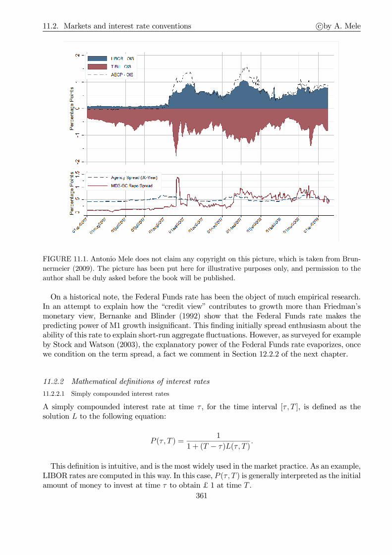
11.2. Markets and interest rate conventions c©by A. Mele
FIGURE 11.1. Antonio Mele does not claim any copyright on this picture, which is taken from Brun-
nermeier (2009). The picture has been put here for illustrative purposes only, and permission to the
author shall be duly asked before the book will be published.
On a historical note, the Federal Funds rate has been the object of much empirical research.In an attempt to explain how the “credit view” contributes to growth more than Friedman’smonetary view, Bernanke and Blinder (1992) show that the Federal Funds rate makes thepredicting power of M1 growth insignificant. This finding initially spread enthusiasm about theability of this rate to explain short-run aggregate fluctuations. However, as surveyed for exampleby Stock and Watson (2003), the explanatory power of the Federal Funds rate evaporizes, oncewe condition on the term spread, a fact we comment in Section 12.2.2 of the next chapter.
11.2.2 Mathematical definitions of interest rates
11.2.2.1 Simply compounded interest rates
A simply compounded interest rate at time τ , for the time interval [τ , T ], is defined as thesolution L to the following equation:
P (τ , T ) =1
1 + (T − τ )L(τ , T ) .
This definition is intuitive, and is the most widely used in the market practice. As an example,LIBOR rates are computed in this way. In this case, P (τ , T ) is generally interpreted as the initialamount of money to invest at time τ to obtain £ 1 at time T .
361

11.2. Markets and interest rate conventions c©by A. Mele
11.2.2.2 Yield curves
The yield-to-maturity, or spot rate, for some maturity date T is the yield on the zero maturingat T , denoted as r (T ). This spot rate r (T ) is the solution to the following equation,
P (t, T ) =1
(1 + r (t, T ))T.
With semi-annual compounding, we have that P (t, T ) = (1 + r(t,T )2)−2T . In general, we have
that if the interest is compounded m times in a year, at the annual rate r, then, investing for T
years gives(1 + r
m
)mT. Continuous compounding is obtained by letting m→∞ in the previous
expression, leaving erT . Therefore, the continuously compounded spot rate is obtained as:
R (t, T ) = − 1TlnP (t, T ) .
It is a sort of “average rate” for investing from time t to time T > t. The function, T → R (t, T ),is called the yield curve, or the term structure of interest rates.A related, and widely used concept, is the the par yield curve. Let B (t, T ) be the current
price of a coupon bearing bond. This bond pays off the principal of £1 at expiry T , as well as aknown sequence of coupons C (t, T ) at t+1, t+2, · · · , T , such that, in the absence of arbitrageand any other frictions, its price is:
B (t, T ) = C (t, T ) ·T−t∑
i=1
P (t, t+ i) + P (t, T ) .
Please note, C (t, T ) is fixed at time t. A par bond, then, is one such that B (t, T ) = 100%, andthe par yield curve is the resulting sequence of the coupon rates C (t, T ), for T varying, viz
C (t, T ) =B (t, T )− P (t, T )∑T−t
i=1 P (t, t+ i), B (t, T ) = 1.
In other words, the coupon rates C (t, T ) have to “adjust” to make the market happy to havethe coupon bearing bond quote at par, B (t, T ) = 1.
11.2.2.3 Forward rates
In a forward rate agreement (FRA, henceforth), two counterparties agree that the interestrate on a given principal in a future time-interval [T, S] will be fixed at some level K. Letthe principal be normalized to one. The FRA works as follows: at time T , the first counter-party receives $1 from the second counterparty; at time S > T , the first counterparty paysback $ [1 + 1 · (S − T )K] to the second counterparty. The amount K is agreed upon at timet. Therefore, the FRA makes it possible to lock-in future interest rates. We consider simplycompounded interest rates because this is the standard market practice.The amountK for which the current value of the FRA is zero is called the simply-compounded
forward rate as of time t for the time-interval [T, S], and is usually denoted as F (t, T, S). Wecan use absence of arbitrage to express F (t, T, S) in terms of bond prices, as follows:
P (t, T )
P (t, S)= 1 + (S − T )F (t, T, S) . (11.1)
362
11.3. Bootstrapping, curve fitting and absence of arbitrage c©by A. Mele
Indeed, an investor in a zero from time t to time S is one who simultaneously makes (i) aspot loan from t to T , and (ii) a forward loan from T to S. In the absence of arbitrage, it mustbe the case that,
[1 + r (t, S)]S−t︸ ︷︷ ︸zero loan
= [1 + r (t, T )]T−t︸ ︷︷ ︸spot loan
× [1 + (S − T )F (t, T, S)]︸ ︷︷ ︸forward loan
,
where r (t, S) is the spot rate at time t, defined as the solution to, P (t, S) = 1/ [1 + r (t, S)]S−t.Eq. (11.1) follows by the definition of r (t, S), and by rearranging terms of the previous equal-ity. Alternatively, consider the following portfolio implemented at time t. Go long one bondmaturing at T and short P (t, T )/P (t, S) bonds maturing at S, for the time period [t, S]. Theinitial cost of this portfolio is zero because,
−P (t, T ) + P (t, T )
P (t, S)P (t, S) = 0.
At time T , the portfolio yields $1, originating from the bond purchased at time t. At time S,the P (t, T )/P (t, S) bonds shorted at t, and maturing at S, must be purchased. But at timeS, the cost of purchasing P (t, T )/P (t, S) bonds maturing at S is obviously $ P (t, T )/P (t, S).The portfolio, therefore, is acting as a FRA: it pays $1 at time T , and −$ P (t, T )/P (t, S) attime S. In addition, the portfolio costs nothing at time t. Therefore, the interest rate implicitlypaid in the time-interval [T, S] must be equal to the forward rate F (t, T, S), as stated in Eq.(11.1).
11.2.3 Yields to maturity on coupon bearing bonds
Finally, the yield to maturity y (YTM, henceforth) on a bond is simply its rate of return. It isthe discount rate that would equate the present value of the stream of payoffs with its marketprice,
y : B (T ) =n∑
i=1
Cti
(1 + y)ti+
1
(1 + y)T. (11.2)
This formula differs from the price formula B (T ) =∑n
i=1
Cti(1+r(ti))
ti+ 1
(1+r(T ))T, as Eq. (11.2)
uses the same discount rate y to discount the future payements. Clearly, for zeros we have thatspot rates coincide with YTM, i.e. y = R (T ).
11.3 Bootstrapping, curve fitting and absence of arbitrage
11.3.1 Extracting zeros from bond prices
In principle, the zeros can be “extracted” from the market price of the bonds, provided there isa sufficient spread of bonds across maturities. As an example, consider three bonds. The firstbond pays off at T1, the second bond pays off at T1, T2, the third bond pays off at T1, T2, T3. Byno-arbitrage,
B (T1)B (T2)B (T3)
=
C11 + 1 0 0C21 C22 + 1 0C31 C32 C33 + 1
P (T1)P (T2)P (T3)
,
363
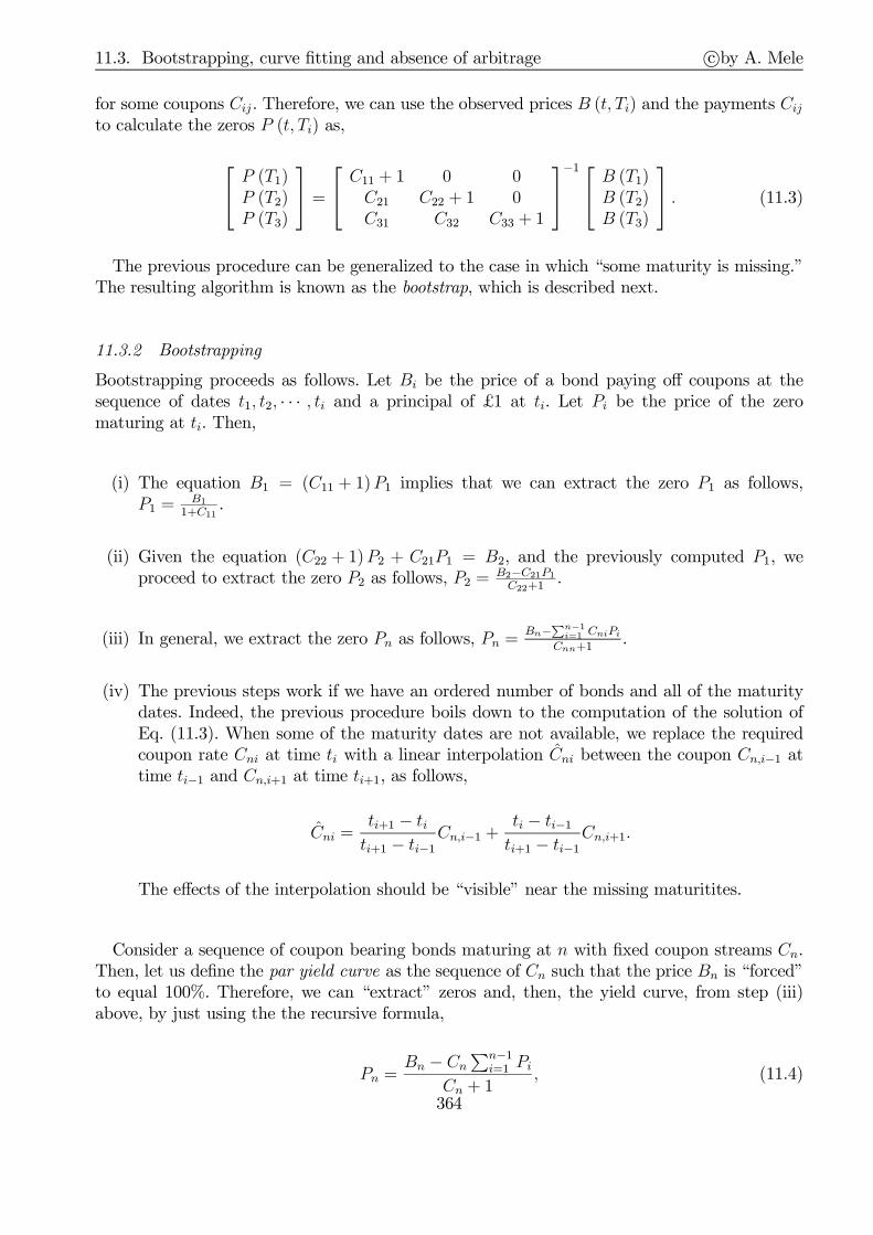
11.3. Bootstrapping, curve fitting and absence of arbitrage c©by A. Mele
for some coupons Cij. Therefore, we can use the observed prices B (t, Ti) and the payments Cijto calculate the zeros P (t, Ti) as,
P (T1)P (T2)P (T3)
=
C11 + 1 0 0C21 C22 + 1 0C31 C32 C33 + 1
−1
B (T1)B (T2)B (T3)
. (11.3)
The previous procedure can be generalized to the case in which “some maturity is missing.”The resulting algorithm is known as the bootstrap, which is described next.
11.3.2 Bootstrapping
Bootstrapping proceeds as follows. Let Bi be the price of a bond paying off coupons at thesequence of dates t1, t2, · · · , ti and a principal of £1 at ti. Let Pi be the price of the zeromaturing at ti. Then,
(i) The equation B1 = (C11 + 1)P1 implies that we can extract the zero P1 as follows,P1 =
B1
1+C11.
(ii) Given the equation (C22 + 1)P2 + C21P1 = B2, and the previously computed P1, weproceed to extract the zero P2 as follows, P2 =
B2−C21P1
C22+1.
(iii) In general, we extract the zero Pn as follows, Pn =Bn−
∑n−1i=1 CniPi
Cnn+1.
(iv) The previous steps work if we have an ordered number of bonds and all of the maturitydates. Indeed, the previous procedure boils down to the computation of the solution ofEq. (11.3). When some of the maturity dates are not available, we replace the requiredcoupon rate Cni at time ti with a linear interpolation Cni between the coupon Cn,i−1 attime ti−1 and Cn,i+1 at time ti+1, as follows,
Cni =ti+1 − titi+1 − ti−1
Cn,i−1 +ti − ti−1
ti+1 − ti−1Cn,i+1.
The effects of the interpolation should be “visible” near the missing maturitites.
Consider a sequence of coupon bearing bonds maturing at n with fixed coupon streams Cn.Then, let us define the par yield curve as the sequence of Cn such that the price Bn is “forced”to equal 100%. Therefore, we can “extract” zeros and, then, the yield curve, from step (iii)above, by just using the the recursive formula,
Pn =Bn − Cn
∑n−1i=1 Pi
Cn + 1, (11.4)
364
11.3. Bootstrapping, curve fitting and absence of arbitrage c©by A. Mele
where Bn = 100%. The following table provides a numerical example.
Coupon Maturity, n Zero price∑n
i=1 Pi Yield curve∗
6.00% 1 0.9434 0.9434 6.00%7.00% 2 0.8728 1.8162 7.04%8.00% 3 0.7914 2.6076 8.11%9.50% 4 0.6870 3.2946 9.84%9.00% 5 0.6454 3.9400 9.15%10.50% 6 0.5306 4.4706 11.14%11.00% 7 0.4579 4.9285 11.81%11.25% 8 0.4005 5.3290 12.12%11.50% 9 0.3472 5.6762 12.47%11.75% 10 0.2980 not useful 12.87%∗Discretely compounded
11.3.3 Curve fitting
We may use statistical techniques alternative to bootstrapping, to cope with situations in whichthe number of bonds does not equal the number of maturity dates. Suppose we observeN bonds,where the i-th bond entitles to receive the coupons Cij, for j = 1, · · · ,Mi. We assume that thebond prices are observed with errors, or
B (Mi) =
Mi∑
j=1
CijP (tj) + P (tMi) + ǫi, i = 1, · · · , N,
where ǫi is the measurement error for the i-th bond.We aim to find the curve T → P (T ) that minimizes the errors, in some statistical sense. The
natural device is to “parametrize” the function P (T ), with a number of k parameters, wherek < N . To parametrize the function P (tj) for a generic tj, we can use polynomials, as originallysuggested by McCulloch (1971, 1975),
P (tj) = 1 + a1tj + a2t2j + · · ·+ aktkj ,
where the ai are the parameters. Cubic splines are polynomials up to the third order, andare very popular. The parameters ai can be estimated by minimizing the sum of the squarederrors,
∑Ni=1 ǫ
2i . A well-known pitfall of polynomials is that a high k might imply that while the
polynomial approximation works reasonably well near the observed maturities, it may exhibitan erratic behavior in between. To avoid this problem, we can use local polynomials, which arelow-order polynomials (typically splines) fitted to non-overlapping subintervals.Naturally, we may also want to parametrize the spot rates, R (T ), as polynomials. Alterna-
tively, Nelson and Siegel (1987) propose the following parametrization,
R (T ) = β1 + β2
(1− e−λTλT
)+ β3
(1− e−λTλT
− e−λT),
where βi and λ are the parameters. These coefficients may be given an interpretation, in termsof economic factors driving the yield curve, as reviewed in the next chapter. The coefficientβ1 governs the level of the yield curve. The coefficient β2 relates to the slope, as an increase
365

11.3. Bootstrapping, curve fitting and absence of arbitrage c©by A. Mele
in this coefficient increases short yields more than long yields. The coefficient β3 shapes thecurvature, as an increase in this coefficient has little effect on very short and very long yields,but increases the middle of the yield curve. Moreover, the coefficient λ controls the exponentialdecay of the yield curve: small values of λ translate to slow decay and can better fit the curve atlong maturities; large values of λ, instead, lead to a fast decay, which helps fit the short-end ofthe yield curve. Finally, λ determines where the loading on β3 achieves its maximum. Dieboldand Li (2006) have used this setting to estimate βi for each date, and then used these estimatedtime series of βi to forecast future values of βi through vector autoregressions and, then, thefuture yield curve.
11.3.4 Arbitrage
Bond prices need, naturally, to satisfy restrictions preventing arbitrage. We illustrate how anarbitrage opportunity can be exploited, using data in Tuckman (2002) (p. 8-12).
11.3.4.1 Data
Suppose that on some hypothetical date, say February 3009, we observe the bond prices inTable 11.1.
TABLE 11.1.
Treasury Bond Prices on February 15, 3009
Coupon Maturity Price7.875% 8/15/09 101.4014.250% 2/15/10 108.986.375% 8/15/10 102.166.250% 2/15/11 102.575.250% 8/15/11 100.84
We can bootstrap the price of the zeros implicit in Table 11.1, proceeding as described inSections 11.3.1 and 11.3.2, obtaining the figures in Table 11.2.
TABLE 11.2.
Implicit zeros on February 15, 3009
Time to maturity Implicit zero
0.5 p (0, 0.5) = 0.975571 p (0, 1) = 0.952471.5 p (0, 1.5) = 0.930452 p (0, 2) = 0.907962.5 p (0, 2.5) = 0.88630
Next, suppose to observe additional bond prices, those in Table 11.3:
TABLE 11.3.
Treasury Bond Prices on February 15, 3009
Coupon Maturity Market price13.375% 8/15/09 104.08010.750% 2/15/11 110.9385.750% 8/15/11 102.02011.125% 8/15/11 114.375
366

11.3. Bootstrapping, curve fitting and absence of arbitrage c©by A. Mele
Are these additional bond prices, those in Table 11.3, compatible with the prices in Table 11.3,in terms of absence of arbitrage opportunities? How could we profit, in a frictionless world, ofany arbitrage opportunities “left on the table”?
11.3.4.2 A basic no arbitrage condition in the fixed income market
Let us cast the problem in a more general format. Suppose we observe a vector of N bondprices, with a N×N matrix C of coupons, where each row of C gives the stream of the couponspromised by a given asset. We know that the N × 1 vector of zeros P , satisfies, B = CP . Thatis, assuming that the matrix C is invertible,
P = C−1B. (11.5)
Next, suppose there exists some asset that: (i) promises to pay:
c∗ =[c∗1 c∗2 · · · c∗N + 100
],
and (ii) has a price, b∗, such that:b∗ < c∗P. (11.6)
The right hand side of this inequality, c∗P , is the “no-arbitrage price” of the asset, whichin this example is greater than the market price of the asset. The inequality gives rise toarbitrage opportunity, which can be exploited by going long the asset, and shorting a portfolio“synthesizing” it. To synthesize the asset to go long for, we solve the following system of Nequations with N unknowns,
πC = c∗, (11.7)
where the vector of unknowns, π, contains the number of assets in the synthesizing portfolio:by purchasing the portfolio π, one is entitled to receive πC in the future, which we want toequal c∗. The solution to Eq. (11.7) is:
π = c∗C−1. (11.8)
Accordingly, the value of this portfolio, V say, is given by,
V = πB = c∗C−1B = c∗P > b∗,
where the last equality follows by the “zero pricing equation” (11.5), and the inequality holdsby the inequality (11.6).To summarize, we now have the following situation: (i) the asset we hold produces the cash
flows that are needed to pay out the coupons of the “synthesizing” portfolio we sold, and (ii)the price of the asset we go long is less than the value of the portfolio we short. This situationis an arbitrage opportunity, as initially claimed. We now use these insights to check whetherarbitrage opportunities exist and, maybe, exploited, using the data in Tables 11.1 through 11.3.
First step: detecting arbitrage opportunities in the market
In a first step, we compute the no-arbitrage prices of the bonds in Table 11.3, using the zerosextracted from Table 11.1, and reported in Table 11.2. Denote these prices with B1 (for the sixmonth 13.375%), B2 (for the two year 10.750%), B3 (for the 2.5 year 5.750%), and B4 (for the2.5 year 11.125%). For the 13.375% six month bond, we have:
B1 =
(13.375
2+ 100
)p (0, 0.5) = 104.08,
367

11.3. Bootstrapping, curve fitting and absence of arbitrage c©by A. Mele
which matches the market price in Table 11.3. As for the two 10.750% year bond,
B2 =10.750
2[p (0, 0.5) + p (0, 1) + p (0, 1.5)] +
(10.750
2+ 100
)p (0, 2) = 111.04.
The no-arbitrage price of the 5.75% bond expiring in 2.5 years is:
B3 =5.75
2[p (0, 0.5) + p (0, 1) + p (0, 1.5) + p (0, 2)] +
(5.75
2+ 100
)p (0, 2.5) = 102.007.
Finally, the no-arbitrage price of the 11.125% bond expiring in 2.5 years is:
B4 =11.125
2[p (0, 0.5) + p (0, 1) + p (0, 1.5) + p (0, 2)] +
(11.25
2+ 100
)p (0, 2.5) = 114.511.
To summarize,
Treasury Bond Prices on February 15, 3009
Coupon Maturity Market price No-arbitrage price13.375% 8/15/09 104.080 104.08010.750% 2/15/11 110.938 111.0415.750% 8/15/11 102.020 102.00711.125% 8/15/11 114.375 114.511
While there are no arbitrage opportunities for the 13.375% bond expiring in six months, theprice of the 10.750% bond expiring in 2 years is less than its no-arbitrage price: this bond“trades cheap.” In contrast, the 2.5 year 5.750% bond “trades rich,” although the resultingarbitrage does not seem to be quite sensible.
Second step: implementing the arbitrage trade
We now proceed to exploit the mispricing related to the 10.750% bond expiring in 2 years. Weuse the insights developed in Section 11.3.4.2 to implement the arbitrage. We have, N = 4,and c∗ =
[10.750
210.750
210.750
210.750
2+ 100
], and we use the first four bonds in Table 11.1 to
construct an arbitrage portfolio. In terms of the coupon matrix C, we have,
C =
7.8752+ 100 0 0 0
14.2502
14.2502
+ 100 0 06.3752
6.3752
6.3752+ 100 0
6.2502
6.2502
6.2502
6.2502+ 100
.
We implement the following trade: (i) buy x 10.750% bonds expiring in 2 years, which cost110.938 · x; (ii) create x portfolios satisfying Eq. (11.8),
π = c∗C−1 =[0.0189 0.0197 0.0212 1.0218
].
If we short x of these portfolios, then, by construction, the coupons we need to pay are exactlymatched by the coupons we receive from the x 10.750% bonds expiring in 2 years. However,the market value of the x portfolios we short equals,
x · V = x · πB = x ·[0.0189 0.0197 0.0212 1.0218
]
101.40108.98102.16102.57
= x · 111.041,
368

11.4. Duration, convexity and asset-liability management c©by A. Mele
where the vector of the market prices, B, is taken from Table 11.1. Therefore, the gains fromthis trade are, x · (111.041− 110.938) = 0.103 · x. For example, by trading £1,000,000 at facevalue, i.e. x = 10000, then, arbitrage profits equal £1030.
11.4 Duration, convexity and asset-liability management
The risk of going long a default-free bond is that the future bond price is uncertain, due to thepossibility that the spot interest rates could change in the future. Synthetically, we can say thatthe risk of a bond is related to the changes in the required bond return, or the YTM. Considerthe definition of the YTM y in Eq. (11.2). Next, consider the following function B (y;T ),
B (y;T ) =n∑
i=1
Cti
(1 + y)ti+
1
(1 + y)T.
This function aims to “mimic” how the market price B (T ) would behave if the YTM y changedto some value y. Naturally,
B (y;T ) = B (T ) .
Motivated by the previous remarks, we can define a measure of risk of the bond based onthe sensitivity of the bond price with respect to changes in y. Economically, we are tryingto answer the following question: What happens to the bond price once we perturb the onerate y that discounts all the payoffs? Mathematically, this sensitivity is the first partial of the“bond-pricing” formula B (y;T ) with respect to y,
By (y;T ) = − 1
1 + y
[n∑
i=1
ti · Cti
(1 + y)ti+
T · 1(1 + y)T
]
where the subscript denotes a partial derivative, i.e. By (y;T ) =∂∂yB (y;T ). Graphically, this
sensitivity measure By (y;T ) is the tangent to the price-yield relation, Figure 11.2 illustrates inthe case of a zero-coupon bond with time to maturity equal to 10 years.
369

11.4. Duration, convexity and asset-liability management c©by A. Mele
FIGURE 11.2. The relation between the YTM and the bond price, and its first-order
(duration) and second-order (convexity) approximations. The solid line depicts the price
of a zero coupon bond expiring in 10 years, as a function of the YTM, (1 + YTM)−10,
and the two dashed lines are first-order and second-order Taylor’s expansions around
YTM = 5%.
11.4.1 Duration
We define the “Macaulay duration” as,
DMac ≡−By (y;T )
B (y;T )(1 + y) =
n∑
i=1
ωti · ti + ωT · T,
where
ωti =Cti/ (1 + y)
ti
B (y;T ), ωT =
1/ (1 + y)T
B (y;T ).
In words, the Macaulay duration is a weighted average of the payment dates. The weights ωti
are the discounted coupons at the various payment dates, Cti/ (1 + y)ti , related to the current
market value of these coupons, i.e. the bond price B (y;T ) when the YTM is y. That is, theweights are the proportions of the bond’s present value that is attributable to the payoff atdate t. The weights satisfy
∑ni=1 ωti + ωT = 1. Therefore, DMac ≤ T . The Macaulay duration is
a measure of how far in the future the bond pays off. For zeros, DMac = T .For small y, DMac (y) is simply the semi-elasticity of the bond price with respect to the YTM.
This semi-elasticity is also referred to as “modified duration”:
D ≡ −By
B=
DMac
1 + y.
A simple computation reveals that the modified duration, D, satisfies: ∂D∂y
= −ByyB
+(ByB
)2
.
Therefore, the modified duration is decreasing in the YTM when the bond price is sufficientlyconvex in the YTM, which is surely the case for long-term maturity dates.Interestingly, the modified duration is increasing in the YTM when the bond price is concave
in the YTM, a property that arises for callable bonds and mortgage-backed securities (MBS,henceforth), as explained in the next chapters (see also, Section 11.8.1 of this chapter, for anumerical exercise). Intuitively, the incentives to proceed to early repayments “kick in” as theYTM decreases, which makes the duration of the MBS decrease.The Macaulay duration for continuously compounded rates is even simpler to compute. First,
define the continuously compounded YTM as the single number x such that
B(x;T ) =n∑
i=1
ctie−x·ti + e−x·T ,
where B(x;T ) is the market price of a bond paying off the principal of one at maturity and thestream of payoffs cti . Next, consider, the function x → B (x;T ). Compute the semi-elasticity ofthe bond price B (x;T ) with respect to the continuously compounded YTM x,
−Bx (x;T )
B (x;T )=
∑ni=1 ctitie
−x·ti + T · e−x·TB (x;T )
=n∑
i=1
wti · ti + wT · T,
370
11.4. Duration, convexity and asset-liability management c©by A. Mele
where Bx (x;T ) =∂B(x;T )
∂x, wti =
ctie−x·ti
B(x;T )and wT = e−x·T
B(x;T ). Note, the weights are such that∑n
i=1wti + wT = 1. Therefore, the “Macaulay duration” for continuously compounded ratesis equal to the semi-elasticity of the bond price with respect to the continuously compoundedYTM x.1 This result may simplify some calculations.
11.4.2 Convexity
Convexity measures how the sensitivity,By, changes with y. Mathematically, convexity is relatedto the second partial of the bond price with respect to y, Byy. If the second partial, Byy, ispositive, then, the interest rate sensitivity declines as y increases (see Figure 11.1). This isbecause ∂
∂y(−By) = −Byy < 0. Formally, convexity is defined as,
C ≡ Byy
B.
We may, then, consider the following expansion of the bond price:
∆B
B≈ −D ·∆y + 1
2C · (∆y)2 . (11.9)
That is, for very “convex securities”, duration may not be a safe measure of return, as alsoshown in Figure 11.1.
11.4.3 Asset-liability management
11.4.3.1 Introductory issues
We can use duration to assess how exposed a bond portfolio is to movements in the interestrates. We can then “immunize” a portfolio of bonds to changes in the interest rates. Durationis relevant for asset-liability management. For example, pension funds have known streams ofliabilities that must be matched by the assets they hold. In words, the duration of the assetsmust equal the duration of the liabilities. In the UK, pension funds must mark-to-market theliabilities. Therefore, one objective of these funds is to “immunize” their liabilities againstmovements in the interest rates.Alternatively, consider the following basic example. A bank borrows £100 at 2% for a year
and lends this money at 4% for 5 years, where the higher rate compensates for many thingssuch as risk, the bank’s market power, etc. Assuming that the bank’s borrower does not default,in the first year, the bank generates profits equal to £(4% − 2%) · 100 = 2, according to itsbooks. However, the right computation to make should not relate to past market (interest rate)conditions, but to the current ones. Suppose, for example, that in one year, the interest rate forborrowing raises from 2% to 5%, and remains such for 4 additional years. This assumption is,of course, a bit unrealistic, but it gives the idea of where the action is. In this case, the marketvalue of the assets is: 100·1.045
1.054 = 100.09. Note, we discount using the 5% interest rate, as this isthe cost of capital for the bank.2 The market value of the liabilities is, of course, 100·1.02 = 102.The bank’s problem is a duration mismatch.
1Mathematically, we could have obtained this result in a straightforward manner, as follows. Define the bond price function asB (y (x)), where by definition, y (x) = ex − 1. Hence, Bx (y (x)) = By (y (x)) y′ (x) = By (y (x)) ex = By (y (x)) (1 + y). It follows
that DMac =−By(1+y)
B= −Bx
B.
2Suppose, for example, that the bank wants to borrow £102 to pay off its liabilities, and for 4 additional years, then the proft
at time 1 is100(1.04)5−102(1.05)4
(1.05)4= −1.9057. Alternatively, the 5% interest rate is just an opportunity cost of capital, defined as
max borrowing cost, lending rate.
371

11.4. Duration, convexity and asset-liability management c©by A. Mele
Let us consider a second example, relating to the asset-liability management of pension funds.Consider the following extreme example. In 30 years from now, a pension fund is due to deliver£100,000 to some future retiree. Suppose the current market situation is such that the yieldcurve is flat at 4%, such that the market value of this liability is $100, 000·(1.04)−30 = $30, 832.Accordingly, the would-be retiree invests $30.832 in the pension fund. So we have the followingsituation:
Cash Pensions$30, 832 $30, 832
Suppose, now, that the pension fund does not invest this cash. This is of course inefficient, butit is precisely the point of this simple exercise to see why the strategy is inefficient.Consider two extreme cases, occurring under two scenarios underlying developments in the
fixed income market. In one week,
(i) Scenario ↑: the yield curve shifts up parallely to 5%. Accordingly, the value of the liabilityfor the pension fund is: $100, 000 · (1.05)−30 = 23, 138.
Cash Profit$30, 832 $7, 694
Pensions$23, 138
(ii) Scenario ↓: the yield curve shifts down parallely to 3%. Accordingly, the value of theliability for the pension fund is: $100, 000 · (1.03)−30 = 41, 199.
Cash Loss$30, 832 −$10, 367
Pensions$41, 199
Therefore, a drop in the yield curve results in a loss for the pension fund: when interest ratesgo down, the pension fund faces a challenging situation as it has to honour its obligations in30 years, but the financial market “yields less” than one week ago.Naturally, the pension fund would face the opposite situation were interest rates to go up.
In some countries, we do not like pension funds to experience volatility. The previous volatilityarises simply because the pension fund, receives $30, 832, and then it just puts this money“under the pillow.” The most efficient way to kill volatility is, of course, to invest $30, 832 ina 30 bond as soon as we receive this money–at the market conditions of 4%. This is perfecthedging! But, we do not necessarily have access to such a bond. How do we proceed, then?We now develop examples that illustrate how to deal systematically with issues relating to
asset-liability management.
372

11.4. Duration, convexity and asset-liability management c©by A. Mele
11.4.3.2 Hedging
Let us consider a portfolio of two bonds with different durations. Its value is given by,
V = B1 (y1) θ1 +B2 (y2) θ2,
where B1 (y1) and B2 (y2) are the market value of the bonds, y1 and y2 are the YTM on thebonds and, finally, θ1 and θ2 are the quantities of bonds in the portfolio. Let us consider a smallchange in the two YTM y1 and y2. We have,
dV = − [D (y1)B1 (y1) θ1dy1 +D (y2)B2 (y2) θ2dy2] .
The question is: How should we choose θ1 and θ2 so as to make the value of the portfolio remainconstant after a change in y1 and y2?Let us assume a parallel shift in the term structure of interest rates. In this case, dy1 = dy2.
The portfolio is said to be immunized if its value V does not change as y1 and y2 change, i.e.dV = 0, which is true when,
θ1 = −D(y2)B2 (y2)
D (y1)B1 (y1)θ2. (11.10)
A useful interpretation of this portfolio is that we may be holding a bond with some duration,say we hold θ2 units of the second bond. Given these holdings, we may wish to sell anotherbond, possibly with a lower duration, to hedge against movements in the price of the bond wehold.Alternatively, we can think of the second asset as a liability the value of which fluctuates after
a change in the interest rates. Then, we may wish to purchase some asset to hedge against theliability. Mathematically, θ2 < 0 and θ1 > 0. Moreover, Eq. (11.10) reveals that the number ofassets to hold to hedge against the liability is high if the ratio of the two durations of the assets,D(y2)/D (y1), is large. In this case, the hedging position is obviously inefficient. Asset-liabilitymanagement, and “immunization”, is costly when we hedge high-duration liabilities with lowduration assets. We now illustrate these cases through a few basic examples.
11.4.3.3 A first example: hedging zeros with zeros
Suppose that we hold one bond, a zero with maturity equal to 5 years. We want to hedge therisk of this bond through another bond, a zero with maturity equal to 1 year. Let us assumethat the term-structure is flat at 5%, discretely compounded. Then,
B1 (y1) =1
1 + y1=
1
1 + 0.05= 0.95238, D(y1) =
DMac (y1)
1 + y1=
1
1 + 0.05= 0.95238
B2 (y2) =1
(1 + y2)5 =
1
(1 + 0.05)5= 0.78353, D (y2) =
DMac (y2)
1 + y2=
5
1 + 0.05= 4.7619
and:
θ1 = −D(y2)B2 (y2)
D (y1)B1 (y1)θ2 = −
4.7619 · 0.783530.95238 · 0.95238 · 1 = −4.1135.
That is, to hedge the 5Y zero, we need to short-sell approximately four 1Y zeros. The balanceof this hedging position is,
B1 (y1) θ1 +B2 (y2) θ2 = (−4.1135) · 0.95238 + 0.78353 = −3.1341, (11.11)
373

11.4. Duration, convexity and asset-liability management c©by A. Mele
a quite inefficient hedge. The reason this is inefficient is clear. Hedging high maturity bondswith short maturity ones implies we should rebalance too often. Moreover, as time goes on,the sensitivity of the short-term bonds to changes in the YTM is very small (at the extreme,the price equals face value plus coupon, at maturity), compared to that of long-term bonds.Therefore, rebalancing becomes increasingly severe as time unfolds.Next, we study how the value of this portfolio changes after large changes in the YTM.
By the assumption that the initial term-structure is flat at 5%, y1 = y2 = 5%. Moreover, byrearranging Eq. (11.11),
B2 (y = 5%) = 4.1135 ·B1 (y = 5%)− 3.1341. (11.12)
The left hand side of this equation is the price of the 5Y bond. The right hand side is the valueof the “replicating” portfolio, which consists of (i) approximately 4 units of the 1Y bond, and(ii) the balance of the hedging position. Precisely, the right hand side is simply a net obligation:the value of the assets we need to purchase back (approximately 4 units of the 1Y bond), netof some cash we already have, which we can use to partially purchase these assets (£3.1341).If interest rates do not change, then, approximately, and abstracting from passage of time,
there will be no profits or losses, once we liquidate, or mark-to-market, this positioning. Ifinterest rates change, y = 5%, Eq. (11.12) can only approximately hold,
B2 (y) ≈ 4.1135 ·B1 (y)− 3.1341.
Figure 11.3 plots the left hand side and the right hand side of this relation.
0.00 0.01 0.02 0.03 0.04 0.05 0.06 0.07 0.08 0.09 0.100.6
0.7
0.8
0.9
1.0
YTM
$
FIGURE 11.3. Dashed line (top): The price of the 5Y zero, B2 (y) = 1(1+y)5
, where y is
the YTM. Solid line (bottom): The value of the “replicating” portfolio consisting of (i)
4.1135 units of the 1Y zero, and (ii) the balance of the hedging position, which is equal
to −£3.1341, i.e. 4.1135 ·B1 (y)− 3.1341, where B1 (y) =1
1+y is the 1Y zero price.
What is going on? We are hedging the 5Y zero by selling approximately four 1Y zeros. In aneighborhood of y = 5%, the value of the “synthetic” 5Y zero we sold, 4.1135 ·B1 (y)− 3.1341,behaves as B2 (y). However, the 5Y zero displays more convexity than the “synthetic” bond.This larger convexity implies that:
374

11.4. Duration, convexity and asset-liability management c©by A. Mele
• If interest rates go down, the price of the 5Y zero bond we hold increases more than thevalue of the “synthetic” bond we sold. As a result, we make profits.
• If interest rates go up, the price of the 5Y zero bond we hold decreases less than the valueof the “synthetic” bond we sold. As a result, we make profits.
In all cases, we make profits. Mathematically, profits are equal to (B+2 −θ1B+
1 )−(B2 − θ1B1) ≡∆B2 − θ1∆B1, where B
+2 is the price of the 5Y bond, B1 is the price of the 1Y bond. Then,
by convexity, B2 increases more than θ1B1 when interest rates go down, and B2 decreases lessthan θ1B1 when interest rates go up, or ∆B2 − θ1∆B1 ≥ 0. However, this is not an arbitrageopportunity! The previous reasoning hinges on the assumption of a parallel shift in the term-structure of interest rates, that is dy1 = dy2, where y1 = spot rate for 1 year, and y2 = spotrate for 5 years. While parallel shifts in the term-structure seem empirically relevant, they arenot the only shifts that are likely to occur, as we shall explain in the next chapter.To sumup, duration hedging is a useful tool, but with quite important limitations. As Eq.
(11.9) makes clear, duration is only a first-order approximation to the price of a bond. Moreover,duration hedging obviously requires rebalancing, which might be substantial. As we now, aconventional bond is strictly convex in the YTM. Therefore, for large changes in the YTM,the duration-based hedging ratios should be updated. Re-adjustments are in order anyway,independently of whether YTM change or not, as the duration of conventional fixed incomesecurities obviously decreases over time.
11.4.3.4 Duration trading: Barbell and bullet hedges
As a second example of duration hedging, consider the “barbell” trading strategy, which is away to hedge some liability (a “bullet”) with duration D2 through two assets with durationsD1 and D3, where D1 < D2 < D3. This trading strategy is expected to work when we expectthe yield curve to flatten, with its short-end part not going too much high. Moreover, investingin the short-term segment of the yield curve, allows one to invest elsewhere relatively rapidlyonce the first asset expires, were the bond market to go down.Let us consider the previous example, and suppose there is another bond available for trading,
a zero with maturity equal to 10 years. We aim to hedge against movements in the price of the5Y zero with a portfolio consisting of (i) one 1Y zero and (ii) the 10Y zero. We continue toassume that the yield-curve is flat at 5%, and only consider parallel shifts in the term-structureof interest rates.Such a “butterfly” trade can be implemented as follows. We look for a portfolio of the 1Y and
10Y zero with the following properties: (i) the market value of the portfolio equals the marketprice of the 5Y zero,
B2 (y2) = B1 (y1) θ1 +B3 (y3) θ3; (11.13)
and (ii) the local risk of the portfolio equals the local risk of the 5Y zero, ∂B2 (y2) /∂y2 =−D (y2)B2 (y2), i.e.:
D(y2)B2 (y2) = D (y1)B1 (y1) θ1 +D(y3)B3 (y3) θ3. (11.14)
The solution to Eqs. (11.13) and (11.14) is given by,
θ1 =D(y3)−D(y2)D (y3)−D(y1)
B2 (y2)
B1 (y1), θ3 =
D(y2)−D(y1)D (y3)−D(y1)
B2 (y2)
B3 (y3). (11.15)
375
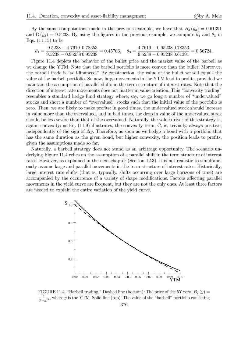
11.4. Duration, convexity and asset-liability management c©by A. Mele
By the same computations made in the previous example, we have that B3 (y3) = 0.61391and D(y3) = 9.5238. By using the figures in the previous example, we compute θ1 and θ3 inEqs. (11.15) to be
θ1 =9.5238− 4.76199.5238− 0.95238
0.78353
0.95238= 0.45706, θ3 =
4.7619− 0.952389.5238− 0.95238
0.78353
0.61391= 0.56724.
Figure 11.4 depicts the behavior of the bullet price and the market value of the barbell aswe change the YTM. Note that the barbell portfolio is more convex than the bullet! Moreover,the barbell trade is “self-financed.” By construction, the value of the bullet we sell equals thevalue of the barbell portfolio. So now, large movements in the YTM lead to profits, provided wemaintain the assumption of parallel shifts in the term-structure of interest rates. Note that thedirection of interest rate movements does not matter in value creation. This “convexity trading”resembles a standard hedge fund strategy where, say, we go long a number of “undervalued”stocks and short a number of “overvalued” stocks such that the initial value of the portfolio iszero. Then, we are likely to make profits: in good times, the undervalued stock should increasein value more than the overvalued, and in bad times, the drop in value of the undervalued stockshould be less severe than that of the overvalued. Naturally, the value driver of this strategy is,again, convexity: as Eq. (11.9) illustrates, the convexity term, C, is, trivially, always positive,independently of the sign of ∆y. Therefore, as soon as we hedge a bond with a portfolio thathas the same duration as the given bond, but higher convexity, the position leads to profits,given the assumptions made so far.Naturally, a barbell strategy does not stand as an arbitrage opportunity. The scenario un-
derlying Figure 11.4 relies on the assumption of a parallel shift in the term structure of interestrates. However, as explained in the next chapter (Section 12.3), it is not realistic to simultane-ously assume large and parallel movements in the term-structure of interest rates. Historically,large interest rate shifts (that is, typically, shifts occurring over large horizons of time) areaccompanied by the occurrence of a variety of shape modifications. Factors affecting parallelmovements in the yield curve are frequent, but they are not the only ones. At least three factorsare needed to explain the entire variation of the yield curve.
0.00 0.01 0.02 0.03 0.04 0.05 0.06 0.07 0.08 0.09 0.10
0.7
0.8
0.9
1.0
YTM
$
FIGURE 11.4. “Barbell trading.” Dashed line (bottom): The price of the 5Y zero, B2 (y) =1
(1+y)5, where y is the YTM. Solid line (top): The value of the “barbell” portfolio consisting
376

11.4. Duration, convexity and asset-liability management c©by A. Mele
of (i) 0.45706 units of the 1Y zero and (ii) 0.56724 of the 10Y zero, i.e. B1 (y1) · 0.45706+B3 (y3) · 0.56724, where B1 (y) =
11+y is the 1Y zero price and B3 (y) =
1(1+y)10 is the 10Y
zero price.
Table 11.4 considers the case of non-parallel shifts in the term-structure. We assume that theinitial term-structure is not flat. Then, we consider two scenarios: (i) A “twist” in the term-structure, i.e. long-term rates lower than short-term; (ii) a “steepening” of the term-structure.
TABLE 11.4.Barbell value =
YTM Bullet price Mod. dur. θ1B1 (y1) + θ3B3 (y3)Initial term-structure1Y y1 = 4% B1 (y1) = 0.961 D (y1) = 0.9615Y y2 = 5% B2 (y2) = 0.783 D (y2) = 4.76210Y y3 = 6% B3 (y3) = 0.558 D (y3) = 9.434
Barbell value = 0.783“Twist”1Y y1 = 6% B1 (y1) = 0.943 D (y1) = 0.9435Y y2 = 5% B2 (y2) = 0.783 D (y2) = 4.76210Y y3 = 4% B3 (y3) = 0.675 D (y3) = 9.615
Barbell value = 0.847
“Steepening”1Y y1 = 4% B1 (y1) = 0.961 D (y1) = 0.9615Y y2 = 5% B2 (y2) = 0.783 D (y2) = 4.76210Y y3 = 7% B3 (y3) = 0.508 D (y3) = 9.346
Barbell value = 0.751
We use the portfolio in Eq. (11.15), and find that in correspondence of the initial term-structure (y1 = 4%, y2 = 5%, y3 = 6%), θ1 = 0.449 and θ3 = 0.629. We keep this portfolio fixed,and compute the barbell value, θ1B1 (y1) + θ3B3 (y3), occurring at the two scenarios “twist”and “steepening,” with B2 (y2) = 0.783 in all cases. The trade is as follows: at time zero, wesale short the five year bond, which we hedge through the barbell portfolio (θ1, θ3), using theproceeds of the short-sale. Then, at some future date, we purchase back the five year bondand sell back the portfolio (θ1, θ3). The convexity of the barbell trade is, in fact, a view aboutmovements of long-term bond prices, and leads to profits in the “twist” scenario. That is, byconvexity, the price B3 varies more than the price of shorter maturity zeros, thus leading toprofits. Note, however, that this strategy leads to losses in the “steepening” scenario.We need to state an inportant caveat. The previous conclusions need to be submitted to
a more severe scrutiny. They rely on a static analysis, and abstract from the fact that term-structure movements should occur under the assumption of no-arbitrage. For example, the valueof the zeros changes over the horizons we are designing scenarios for, even without any changesin the yield curve. Whether this effect is minor depends on the horizon and the model we use togenerate scenarios! In Section 11.6.6, we shall revisit the example of this section and illustratehow passage of time and absence of arbitrage can be factored into the analysis, and changesome of the quantitative results emanating from Table 11.4.
377

11.5. Foundational issues on interest rate modeling c©by A. Mele
11.4.3.5 Fixed income arbitrage strategies
The previous “convexity trades” are examples of yield curve arbitrage strategies. They maypurely rely on convexity or, as discussed in the previous section, on directional views aboutinterest rate movements. For example, we have explained, we may short five year bonds, and golong two- and ten-year bonds, as we view that short-term interest raise will raise and mediumterm interest rates will lower. This “butterfly” strategy is somehow cheap, intellectually, andnot necessarily rewarding, and will be further analyzed in Section 11.6.6. Swap spread arbitrageis a popular strategy. It was responsible of leading LTCM to a loss of about $1.6 billion in 1997.The strategy works as follows: (i) enter a swap paying the floating LIBOR, Lt, and receiving afixed rate C; (ii) short a par Treasury with the same maturity as the swap, thus paying the fixedcoupon rate CT , and invest the proceeds at the repo rate rt. Thus, the payoff of the strategy isthe fixed spread to be received, F = C−CT , and the floating spread to be paid, St = Lt−rt. Sowe go long or short this strategy according to whether we view F to be larger or smaller thanthe average floating spread St over the strategy horizon. Historically, the spread St has certainlybeen volatile, but quite stable, so it is a reasonable strategy. The problem occasionally, though,St can attain quite large values. More sophisticated strategies rely on models, which identifywhich points of the yield curve are misaligned from those predicted by the model. The strategy,substantially, is: buy the cheap and short the model-based rich, where the model-based richis replicated through a portfolio with cash and the bonds that are well-priced by the model,weighted with model-based delta, as in the derivation of the bond pricing formula in Section12.4.2.2 of the next chapter.
11.4.3.6 Negative convexity
What happens when bond prices have “negative convexity”? In the next chapter, we shall seethat the value of a callable bond can be concave in the short-term rate. A similar feature isdisplayed by mortgage-backed-securities (MBS, henceforth), which can now be concave in theYTM! The reason for this negative convexity is that early repayments are likely to occur as theYTM decreases, which entails two inextricable consequences: (i) the price of the MBS “increasesless” than a conventional bond price after a decline in the YTM, especially when the YTM islow; (ii) the duration of the MBS decreases as the YTM decreases.MBS may be responsible of financial turmoil. The mechanism is well-known. Institutions
that hold MBS typically short conventional bonds for hedging purposes. But the MBS dura-tion increases as interest rate increase, due to the negative convexity: ∂Duration
∂r= −Convexity.
Therefore, an interest rate increase can lead these institutions to short additional conventionalbonds, which worsens liquidity and leads to a further increase in the interest rates, therebyfeeding a vicious circle. Perli and Sack (2003) estimate that in 2002 and 2003, this mechanismmay have amplified the volatility of the long-term US rates by a factor between 15% and 30%.
11.5 Foundational issues on interest rate modeling
In principle, the classical ideas underlying contingent claim analysis through binomial trees,can be put at work in the context of fixed income instruments. In this context, however, weneed to revise quite a few methodological details. Let us illustrate the general issues. First, letus review how binomial trees are constructed, in general:
378

11.5. Foundational issues on interest rate modeling c©by A. Mele
(i) We begin with a probabilistic representation of how the price develops over time, using atree-like information structure.
(ii) For example, at the time of evaluation, we observe the state. In the next period, therecan be two mutually exclusive states of the world: (a) the state “up,” occurring withprobability p; and (b) the state “down,” occurring with probability 1− p.
(iii) After two periods, there can be three mutually exclusive states of the world, as in thefollowing diagram. We label the tree in this diagram a “recombining” tree, to emphasizethat the “up & down” and the “down & up” nodes are the same.
Today
p
“up”, “up”
F irst period Second period
“up”state
“dow n”state
“up”, “dow n”“dow n”, “up”
“dow n”, “dow n”
1-p
1-p
1-p
p
p
The previous diagram can be used to price options written on stocks. The stock price unfoldsthrough the branches of the tree. Then, we figure out the no-arbitrage movements of the optionprice along the tree. Suppose, however, we wish to price an option written on a zero, a 3 Yearzero say. Can we apply the same methodology to price the option? The answer is no, and thereason is that we cannot exogenously “track” the movements of the prices of the zero, as in thecase of the stock price. Instead, after one year, the 3 Year zero becomes a 2 Year zero, i.e. quitea different asset.These issues can be mitigated by modeling the movements of the entire yield curve. There are
two approaches, as in the diagram below. In the first, we model the dynamics of the short-termrate, defined as the interest rate on a loan with maturity equal to the time intervals in the tree.The resulting model, referred to as model of the short-term rate, has implications in terms ofthe movements of the entire term-structure. This approach, developed in the next section, leadsto evaluation formulae in which the current price of the zeros predicted by the model are notnecessarily equal to the market prices. A second approach leads to the so-called no-arbitrage, orcalibration, models, where we model the dynamics of the entire term-structure. This approachgives rise to option evaluation formulae in which the current prices of the zeros predicted bythe model are equal to the market prices. We develop this approach in the last sections of thischapter. The models we see in this chapter are solved through trees, while the next chapterdevelops their continuous time counterparts.
379

11.5. Foundational issues on interest rate modeling c©by A. Mele
Interest rates
No-arbitrage Models of the short-term rate e Estimator
Market prices
rates
No-arb models Estimator
No-arbitrage
Prices, not
market prices
Interest rates
Input Output
11.5.1 Tree representation of the short-term rate
11.5.1.1 Recursive evaluation
Consider a two-period and two-state tree in which the current short-term rate is r. The devel-opment of the short-term rate is uncertain. That is, the future short-term rate, r, is random,and can take two values: either r+ with probability p, or r− with probability 1− p. We assumethat r+ > r−. We emphasize p is the physical probability:
r+ ⇒ P (r+, T )p ր
r
1−p ցr− ⇒ P (r−, T )
Suppose, also, that two zeros with distinct maturities are available for trading. A money marketaccounting technology is also available (MMA, in the sequel). Investing £1 in the MMA gener-ates £1·(1+ r) in the second period. We aim to derive an evaluation formula for the zero basedon the previous probabilistic model for the short-term rate dynamics. The general idea is tobuild up a portfolio that contains one zero and the MMA. We shall make sure the value of thisportfolio in the second period replicate the value of the zero we wish to price. By no-arbitrage,then, the value of the portfolio in the first period must equal the value of the zero we wishto price, and we shall be done. The appendix develops the arguments, and shows that in theabsence of arbitrage, there is a constant λ, such that the following relation holds true:
Ep [P (r, T )]− (1 + r)P (r, T ) =∆P (r, T )
∆r·Vol (r − r)
︸ ︷︷ ︸= volatility of the price
· λ︸︷︷︸= unit risk premium
, (11.16)
where Vol(r − r) = |r+ − r−|, and Ep [P (r, T )] denotes the expectation of the bond price underthe probability p.Eq. (11.16) is an APT relation. It says that the excess return on the zero equals the volatility
of its price multiplied by the unit price of risk. We call the term,
∆P (r, T )
∆r·Vol (r − r) ,
“price volatility” because it measures the amplitude of the price variation due to changes in theshort-term rate in the future, ∆P (r,T )
∆r, i.e. the “price-sensitivity”, where this price sensitivity is
normalized by the volatility of the short-term rate, Vol(r − r).Eq. (11.16) can now be cast in a format that we can use to make it more “operational”. After
rearranging terms, we obtain:
P (r, T ) =(p− λ)P (r+, T ) + [1− (p− λ)]P (r−, T )
1 + r=Eq [P (r, T )]
1 + r(11.17)
380

11.5. Foundational issues on interest rate modeling c©by A. Mele
where q ≡ p− λ is the risk-neutral probability.A few considerations. We “expect” that λ < 0 because bond prices are decreasing in the
short-term rate here. Then, q ≡ p − λ > p.3 Hence, the risk-neutral probability of an upwardmovement of the short-term rate, q, is higher than the true probability, p. An investor whogoes long a bond, is concerned by an increase of the short-term rate in the future and, hence,“corrects” the true probability p by assigning a higher risk-adjusted probability to the “upward”state.
11.5.1.2 One example
Assume the current short-term rate equals 10%. We know that with (physical) probability p,the short-term rate as of the next year will increase by 2 percentage points, and with probability1−p, it will decrease by 2 percentage points. Finally, with the same probability p, the short-termrate prevaling from the next year to two years time, will increase by 2 further percentage pointsfrom its previous value in one year time. Suppose that the probability of an upward movementis 20% and that the the absolute value of the Sharpe ratio is 30%.
Risk-neutral probability
These data suffice to provide an estimate of the risk-neutral probability of an upward movementof the short-term rate. We simply use the formula, q = p− λ, and obtain q = 20%− (−30%) =50%.
Pricing zeros
Next, we can price, say, a zero maturing in two years. We can set up the following tree:
r = 10%
12%
8%
q=1/2
14%
10%
6%
1 Year 2 Years
We can use Eq. (11.17) to “fill-in” each node of the tree. We start from the end of the tree,where the price of the two years zero is £1, and then use Eq. (11.17) to fill every node, as
3To be able to interpret q as a probability, we must have that (i) q ≡ p− λ > 0⇔ −λ > −p and q ≡ p− λ < 1⇔ −λ < 1− p.That is, −λ ∈ (−p, 1− p)
381

11.5. Foundational issues on interest rate modeling c©by A. Mele
illustrated in Figure 11.5.
0 .8 2 6 7
q= 1 /2
P = 1
1 Y ea r 2 Y ea rs
P = 1
P = 1
0 .892 8= 1 /1 .12
0 .925 9= 1 /1 .08
FIGURE 11.5.
The price of the zero, in one year, is simply one divided by the interest relevant at thebeginning of the year, next year. The price we are looking for is obtained by applying Eq.(11.17) yielding,
Eq [P (r, 2)]
1 + r=qP (r+, 2) + (1− q)P (r−, 2)
1 + r=
12(0.8928) + 1
2(0.9259)
1.10= 0.8267.
Convexity effects
What is the discretely compounded two-years spot rate? Does it equal 10%? Why or why not?The two-year spot rate, r (0, 2), satisfies,
0.8266 =1
[1 + r (0, 2)]2⇔ r (0, 2) =
√1
0.8266− 1 = 9.98%.
Even though r = 10% and Eq(r) = 10%, we have that two years spot rate equals, 9.98%. Thatis,
0.8266 =1
1 + rEq
(1
1 + r
)>
1
1 + r
1
1 + Eq(r)= 0.8264.
Prices increase after activation of uncertainty. It’s a convexity effect, similar to that we shallhave to explain in the next chapter (Section 12.4.5.1, Figure 12.3).
11.5.2 Tree pricing
We can simply generalize the tree to a multiperiod case. We use Eq. (11.17) to evaluate zerosat all nodes of the tree and maturities. Given q, which can be estimated once we estimate pand λ, we use recursively Eq. (11.17). Then, we may price options on zeros. The weakness ofthe approach is that the initial term structure is predicted with error! Let us illustrate thisapproach with a concrete numerical example. Consider the following tree, in which the current
382

11.5. Foundational issues on interest rate modeling c©by A. Mele
short-term rate for one year is r = 4%.
9 4 3 3.00 6.1/1
%6
===
P
r
9 6 1 5.00 4.1/1
%4
===
P
r
1=P
1=P
1=P
9 8 0 4.00 2.1/1
%2
===
P
r
1=P
%5=r
%3=r
%4=r
1=t 2=t 3=t0=t
FIGURE 11.6. The dynamics of the short-term rate
At time t = 1, the short-term rate is either 5%, with probability p (the true probability) or3%, with probability 1− p. At time t = 2, the short-term rate behaves as follows:
If at time t = 1, r = 5% then, at time t = 2, r =
6% with probability p4% with probability 1− p
If at time t = 1, r = 3% then, at time t = 2, r =
4% with probability p2% with probability 1− p
Also shown in the previous diagram is the price of a hypothetical 3 Year zero, P , at timet = 3 and at time t = 2. At time t = 3, the expiration date, P = 1 in all states of nature. Attime t = 2, the price P is P (r, T ) = Eq[P (r, T )]/ (1 + r) = 1/ (1 + r), for r = 6%, 4% and 2%.The issue, now, is how to compute the price of the zero in correspondence of the remaining
nodes. We should use the formula, P (r, T ) = Eq[P (r, T )]/ (1 + r) to populate the tree, butwe do not know p, λ, and q. Suppose we “estimate” p and λ. In this case, we compute q asq = p−λ, as in Eq. (11.17). (For example, p = 20% and λ = −30%, so that q = 50%.) Supposethat we come up with q = 1
2. Then, the following diagram gives the price of the zero at all the
383

11.5. Foundational issues on interest rate modeling c©by A. Mele
nodes as of time t = 1, and at the evaluation time t = 0.
9433.0=P
9615.0=P
1=P
1=P
1=P
9804.0=P
1=P
( ) 9070.005.1/9615.09433.0
%5
21
21 =+=
=P
r
1=t 2=t 3=t0=t
( ) 9427.003.1/9804.09615.0
%3
21
21 =+=
=P
r
( ) 8893.004.1/9427.09070.0
%4
21
21 =+=
=P
r
21=q
21=q
21=q
So the price of the 3 Year zero equals 0.8893. Next, consider a European call option writtenon the 3 Year zero, with expiration date equal to 2 and strike price K = 0.95. The followingdiagram gives the value of the option predicted by the model at each node of the tree.
00,max
9500.0,9433.0
=−===
KPC
KP
( ) 0055.005.1/0115.00
%5
21
21 =+⋅=
=C
r
1=t 2=t0=t
( ) 0203.003.1/0304.00115.0
%3
21
21 =+=
=C
r
( ) 0124.004.1/0203.00055.0
%4
21
21 =+=
=C
r
21=q
21=q
21=q 0115.00,max
9500.0,9615.0
=−===
KPC
KP
0304.00,max
9500.0,9804.0
=−===
KPC
KP
The model predicts that the current price of the call option is 0.0124.
11.5.2.1 Calibration
The model we are dealing with predicts that the price of the 3 Year zero is equal to 0.8893.However, there is no guarantee that this model-implied price equals the market price of the 3Year zero. Suppose, instead, that the market price of the 3 Year zero, P$ say, equals 0.8700.What should we do to make the model-implied price of the 3 Year zero equal to the marketprice? The question is important: how can we trust an option pricing model that is not evenable to pin down the initial market value of the underlying zero?
384

11.5. Foundational issues on interest rate modeling c©by A. Mele
To make the model-implied price of the 3 Year zero equal to the market price, P$ = 0.8700,we cannot take the risk-neutral probability q as given, i.e. independent of the observed priceP$ = 0.8700, as we did before. Rather, we should calibrate the probability q, as follows,
P$ = 0.8700 =1
1.04[q · P1 (5%) + (1− q) · P1 (3%)] (11.18)
where P1 (5%) and P1 (3%) are the prices of the zero at time t = 1, in the events that theshort-term rate is up to 5% or down to 3%.The previous equation follows, again, by Eq. (11.17). But here, the unknown is not the
price, which is instead given by the market price. Rather, we are looking for, or calibrating,the probability q that makes the RHS of Eq. (11.18) equal to its LHS. Naturally, we need tocompute the prices of the zeros P1 (5%) and P1 (3%). These prices can be found by anotherapplication of Eq. (11.17), as follows,
P1 (5%) =q · 0.9433 + (1− q) · 0.9615
1.05, P1 (3%) =
q · 0.9615 + (1− q) · 0.98041.03
.
By replacing the previous expressions for P1 (5%) and P1 (3%) into Eq. (11.18), we obtain,
P$ = 0.8700 =1
1.04
(q · q · 0.9433 + (1− q) · 0.9615
1.05+ (1− q) · q · 0.9615 + (1− q) · 0.9804
1.03
).
This is a nonlinear equation in q, that we can easily solve, to obtain, q = 0.8779. Hence, wefind:
P1 (5%) = 0.9005 and P1 (3%) = 0.9357.
The next diagram depicts the implied binomial tree, i.e. the tree that results after matchingthe model-implied price of the 3 Year zero to the market price, P$ = 0.8700.
9433.0=P
9615.0=P
1=P
1=P
1=P
9804.0=P
1=P
1=t 2=t 3=t0=t
( ) ( )[ ] 9357.003.1/9804.019615.0%3
%3
1 =−+==
qqP
r
( ) ( ) ( )[ ] 04.1/%31%58700.0
%4
11$ PqqPP
r
−+===
8779.0=q
( ) ( )[ ] 9005.005.1/9615.019433.0%5
%5
1 =−+==
qqP
r
8779.0=q
8779.0=q
Note how different P1 (5%) and P1 (3%) are from those we found earlier by imposing thatq = 1
2. In the “implied” tree, they are smaller than those obtained with q = 1
2, state by state.
This is because in the implied tree, q = 0.8779. The implied tree puts more weight on those
385
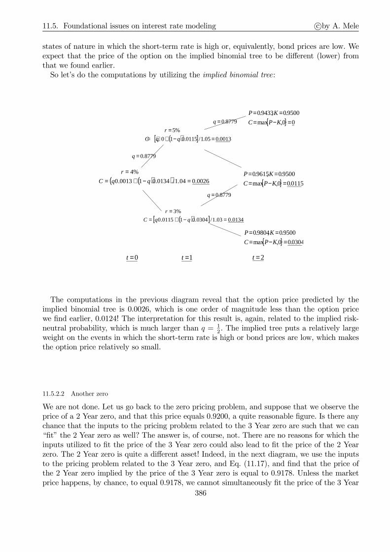
11.5. Foundational issues on interest rate modeling c©by A. Mele
states of nature in which the short-term rate is high or, equivalently, bond prices are low. Weexpect that the price of the option on the implied binomial tree to be different (lower) fromthat we found earlier.So let’s do the computations by utilizing the implied binomial tree:
00,max
9500.0,9433.0
=−===
KPC
KP
( )[ ] 0013.005.1/0115.010
%5
=−+⋅==
qqC
r
1=t 2=t0=t
( )[ ] 0134.003.1/0304.010115.0
%3
=−+==
qqC
r
( )( ) 0026.004.1/0134.010013.0
%4
=−+==
qqC
r
8779.0=q
0115.00,max
9500.0,9615.0
=−===
KPC
KP
0304.00,max
9500.0,9804.0
=−===
KPC
KP
8779.0=q
8779.0=q
The computations in the previous diagram reveal that the option price predicted by theimplied binomial tree is 0.0026, which is one order of magnitude less than the option pricewe find earlier, 0.0124! The interpretation for this result is, again, related to the implied risk-neutral probability, which is much larger than q = 1
2. The implied tree puts a relatively large
weight on the events in which the short-term rate is high or bond prices are low, which makesthe option price relatively so small.
11.5.2.2 Another zero
We are not done. Let us go back to the zero pricing problem, and suppose that we observe theprice of a 2 Year zero, and that this price equals 0.9200, a quite reasonable figure. Is there anychance that the inputs to the pricing problem related to the 3 Year zero are such that we can“fit” the 2 Year zero as well? The answer is, of course, not. There are no reasons for which theinputs utilized to fit the price of the 3 Year zero could also lead to fit the price of the 2 Yearzero. The 2 Year zero is quite a different asset! Indeed, in the next diagram, we use the inputsto the pricing problem related to the 3 Year zero, and Eq. (11.17), and find that the price ofthe 2 Year zero implied by the price of the 3 Year zero is equal to 0.9178. Unless the marketprice happens, by chance, to equal 0.9178, we cannot simultaneously fit the price of the 3 Year
386
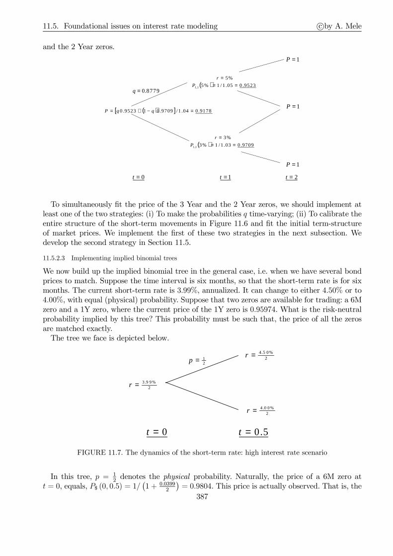
11.5. Foundational issues on interest rate modeling c©by A. Mele
and the 2 Year zeros.
0=t
1=P
1=t 2=t
1=P
1=P
8779.0=q( ) 9523.005.1/1%5
%5
1,1 ===
P
r
( ) 9709.003.1/1%3
%3
1,1 ===
P
r
( )[ ] 0.917804.1/9709.019523.0 =−+= qqP
To simultaneously fit the price of the 3 Year and the 2 Year zeros, we should implement atleast one of the two strategies: (i) To make the probabilities q time-varying; (ii) To calibrate theentire structure of the short-term movements in Figure 11.6 and fit the initial term-structureof market prices. We implement the first of these two strategies in the next subsection. Wedevelop the second strategy in Section 11.5.
11.5.2.3 Implementing implied binomial trees
We now build up the implied binomial tree in the general case, i.e. when we have several bondprices to match. Suppose the time interval is six months, so that the short-term rate is for sixmonths. The current short-term rate is 3.99%, annualized. It can change to either 4.50% or to4.00%, with equal (physical) probability. Suppose that two zeros are available for trading: a 6Mzero and a 1Y zero, where the current price of the 1Y zero is 0.95974. What is the risk-neutralprobability implied by this tree? This probability must be such that, the price of all the zerosare matched exactly.The tree we face is depicted below.
2%9 9.3=r
2%0 0.4=r
2%5 0.4=r
0=t 5.0=t
21=p
FIGURE 11.7. The dynamics of the short-term rate: high interest rate scenario
In this tree, p = 12denotes the physical probability. Naturally, the price of a 6M zero at
t = 0, equals, P$ (0, 0.5) = 1/(1 + 0.0399
2
)= 0.9804. This price is actually observed. That is, the
387
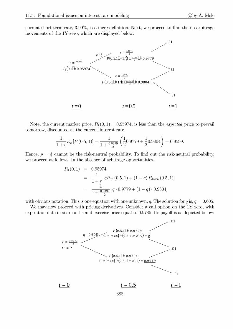
11.5. Foundational issues on interest rate modeling c©by A. Mele
current short-term rate, 3.99%, is a mere definition. Next, we proceed to find the no-arbitragemovements of the 1Y zero, which are displayed below.
( ) 95974.01,0$
2%99.3
==
P
r
0=t 5.0=t
21=p
( ) ( ) 9779.01/11,5.0 2045.0
2%50.4
=+==
P
r
1=t
1£
1£
1£
( ) ( ) 9804.01/11,5.0 2040.0
2%00.4
=+==
P
r
Note, the current market price, P$ (0, 1) = 0.95974, is less than the expected price to prevailtomorrow, discounted at the current interest rate,
1
1 + rEp [P (0.5, 1)] =
1
1 + 0.03992
(1
20.9779 +
1
20.9804
)= 0.9599.
Hence, p = 12cannot be the risk-neutral probability. To find out the risk-neutral probability,
we proceed as follows. In the absence of arbitrage opportunities,
P$ (0, 1) = 0.95974
=1
1 + r[qPup (0.5, 1) + (1− q)Pdown (0.5, 1)]
=1
1 + 0.03992
[q · 0.9779 + (1− q) · 0.9804]
with obvious notation. This is one equation with one unknown, q. The solution for q is, q = 0.605.We may now proceed with pricing derivatives. Consider a call option on the 1Y zero, with
expiration date in six months and exercise price equal to 0.9785. Its payoff is as depicted below:
?2
%9 9.3
==
C
r
0=t 5.0=t
6 0 5.0=q( )
( ) 00,1,5.0m a x
9 7 7 9.01,5.0
=−==
KPC
P
1=t
1£
1£
1£
( )( ) 0 0 1 9.00,1,5.0m a x
9 8 0 4.01,5.0
=−==
KPC
P
388

11.5. Foundational issues on interest rate modeling c©by A. Mele
So the option price is, by risk-neutral evaluation,
C =1
1 + 0.03992
[q · 0 + (1− q) · 0.0019] = 0.9804 [0.395 · 0.0019] = 7.3579× 10⁻⁴. (11.19)
What happens when the short-term rate does not evolve as in the diagram of Figure 11.7but, instead, as in Figure 11.8?
2%99.3=r
2%00.4=r
2%4.4154=r
0=t 5.0=t
FIGURE 11.8. The dynamics of the short-term rate: low interest rate scenario
The previous tree is one in which the short-term in the upper state of the world is equal tor = 4.4154%, not 4.50%, as in Figure 11.7. It implies that:
Pup (0.5, 1) =1
1 + r2
=1
1 + 4.4154%2
= 0.9784.
Then, the risk-neutral probability, q, solves the following pricing equation,
P$ (0, 1) = 0.95974
=1
1 + r[qPup (0.5, 1) + (1− q)Pdown (0.5, 1)]
=1
1 + 0.03992
[q · 0.9784 + (1− q) · 0.9804] .
The solution is, q = 0.756, which is higher than the solution we found earlier using the tree inFigure 11.7 (i.e., q = 0.605). The option price is, now,
C =1
1 + 0.03992
[q · 0 + (1− q) · 0.0019] = 0.9804 [0.244 · 0.0019] = 4.5451× 10⁻⁴.
Why is this price smaller than that computed in Eq. (11.19)? In the tree of Figure 11.8, theup-state of the world is, so to speak, less severe than the up-state of the world in the tree ofFigure 11.7. To be able to match the initial price P$ (0, 1) = 0.95974, the model in Figure 11.8must put more weight on the up-state of the world, i.e. a larger implied risk-neutral probability.This implies a larger risk-neutral probability that low bond prices will arise in the future and,hence, a lower option price.4
4Mathematically, we have that P$ (0, 1) = 11+r
(Pup + (1− q)∆P ), where ∆P ≡ Pdown−Pup > 0. The difference, ∆P , is higherin the tree of Figure 11.8 than in that of Figure 11.7. Therefore, the tree in Figure 11.8 is consistent with the market price, P$ (0, 1),only when q increases from 0.605 to 0.756.
389
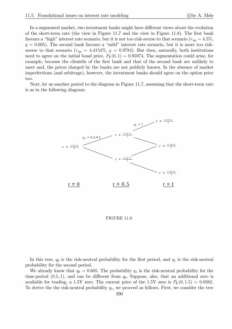
11.5. Foundational issues on interest rate modeling c©by A. Mele
In a segmented market, two investment banks might have different views about the evolutionof the short-term rate (the view in Figure 11.7 and the view in Figure 11.8). The first bankfavours a “high” interest rate scenario, but it is not too risk-averse to that scenario (rup = 4.5%,q = 0.605). The second bank favours a “mild” interest rate scenario, but it is more too risk-averse to that scenario (rup = 4.4154%, q = 0.9784). But then, naturally, both institutionsneed to agree on the initial bond price, P$ (0, 1) = 0.95974. The segmentation could arise, forexample, because the clientèle of the first bank and that of the second bank are unlikely tomeet and, the prices charged by the banks are not publicly known. In the absence of marketimperfections (and arbitrage), however, the investment banks should agree on the option pricetoo.Next, let us another period to the diagram in Figure 11.7, assuming that the short-term rate
is as in the following diagram:
2%9 9.3=r
0=t 5.0=t
6 0 5.00 =q
1=t
2%5 0.4=r
2%0 0.4=r
2%9 0.4=r
2%3 0.4=r
2%9 0.3=r
?1 =q
FIGURE 11.9.
In this tree, q0 is the risk-neutral probability for the first period, and q1 is the risk-neutralprobability for the second period.We already know that q0 = 0.605. The probability q1 is the risk-neutral probability for the
time-period (0.5, 1), and can be different from q0. Suppose, also, that an additional zero isavailable for trading, a 1.5Y zero. The current price of the 1.5Y zero is P$ (0, 1.5) = 0.9382.To derive the the risk-neutral probability q1, we proceed as follows. First, we consider the tree
390

11.5. Foundational issues on interest rate modeling c©by A. Mele
below.
( ) 9382.05.1,0$
2%99.3
==
P
r
0=t 5.0=t
605.00 =q
1=t
1£
( ) ?5.1,5.02
%50.4
==
UP
r
( ) ?5.1,5.02
%00.4
==
DP
r
?1 =q( ) ( ) 9761.01/15.1,1 2
049.0
2%90.4
=+==
P
r
( ) ( ) 9789.01/15.1,1 2043.0
2%30.4
=+==
P
r
( ) ( ) 9808.01/15.1,1 2039.0
2%90.3
=+==
P
r
?1 =q
1£
1£
1£
5.1=t
We need to compute the prices PU (0.5, 1.5) and PD (0.5, 1.5). Once we compute these prices,we shall use the no-arbitrage property of the zero, and the previously computed q0 = 0.605, torecover q1. By the usual no-arbitrage property of the zero, we have that:
PU (0.5, 1.5) =1
1 + 0.0452
[q1 · 0.9761 + (1− q1) · 0.9789] (11.20)
PD (0.5, 1.5) =1
1 + 0.0402
[q1 · 0.9789 + (1− q1) · 0.9808] (11.21)
The problem, q1 is not known. Therefore, Eqs. (11.20)-(11.21) do not allow us to pin downthe prices PU (0.5, 1.5) and PD (0.5, 1.5). But here is where calibration comes in! We know thecurrent price of the 1.5Y zero, which is, P$ (0, 1.5) = 0.9382. In the absence of arbitrage,
P$ (0, 1.5) = 0.9382 =1
1 + 0.03992
[q0 · PU (0.5, 1.5) + (1− q0) · PD (0.5, 1.5)] ,
where PU (0.5, 1.5) and PD (0.5, 1.5) are as in Eqs. (11.20)-(11.21), and where q0 = 0.605. So wehave,
0.9382 =1
1 + 0.03992
[0.605 · PU (0.5, 1.5) + 0.395 · PD (0.5, 1.5)] , (11.22)
where PU (0.5, 1.5) and PD (0.5, 1.5) are as in Eqs. (11.20)-(11.21). Hence, by replacing Eqs.(11.20)-(11.21) into Eq. (11.22) leaves one equation with exactly one unknown, q1. Solving,yields, q1 = 0.8412, which implies that,
PU (0.5, 1.5) = 0.9549, PD (0.5, 1.5) = 0.9600.
391
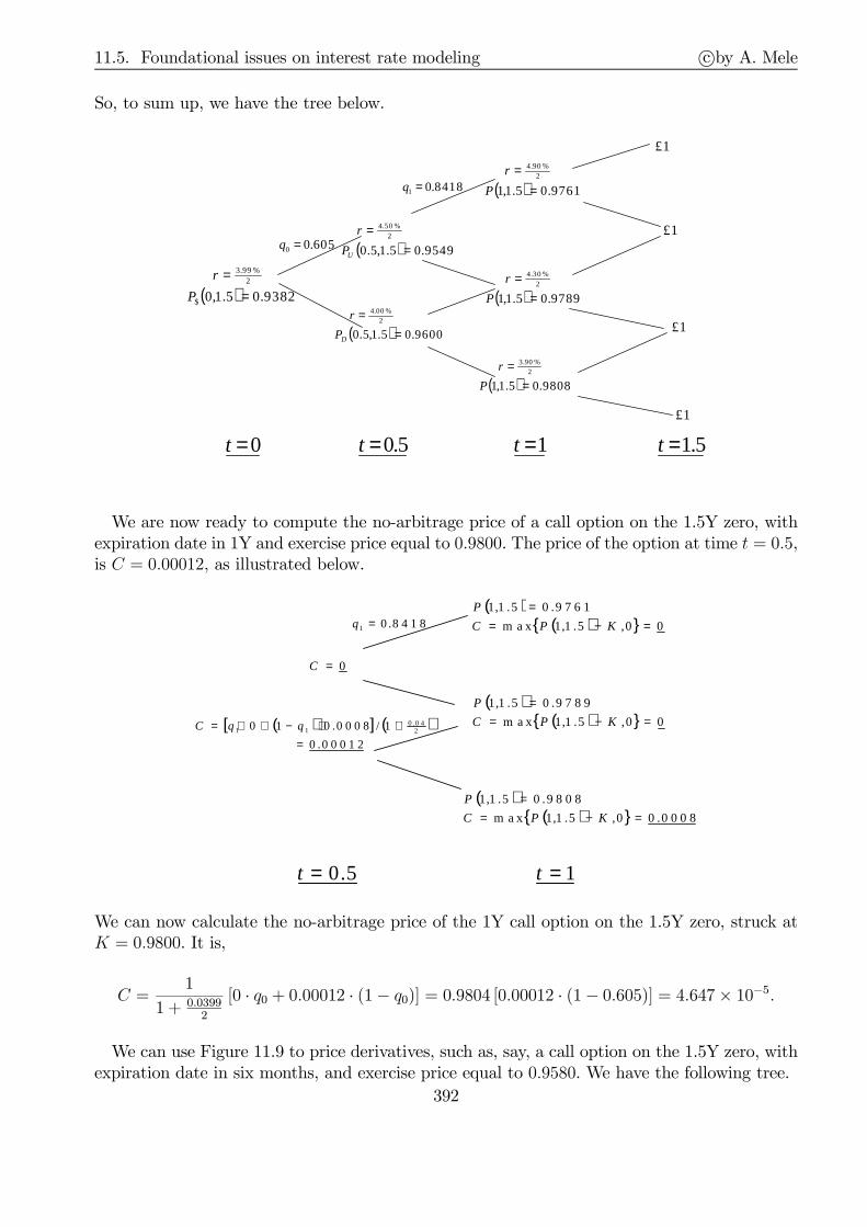
11.5. Foundational issues on interest rate modeling c©by A. Mele
So, to sum up, we have the tree below.
( ) 9382.05.1,0$
2%99.3
==
P
r
0=t 5.0=t
605.00 =q
1=t
1£
( ) 9549.05.1,5.02
%50.4
==
UP
r
( ) 9600.05.1,5.02
%00.4
==
DP
r
8418.01 =q ( ) 9761.05.1,12
%90.4
==
P
r
( ) 9789.05.1,12
%30.4
==
P
r
( ) 9808.05.1,12
%90.3
==
P
r
1£
1£
1£
5.1=t
We are now ready to compute the no-arbitrage price of a call option on the 1.5Y zero, withexpiration date in 1Y and exercise price equal to 0.9800. The price of the option at time t = 0.5,is C = 0.00012, as illustrated below.
5.0=t 1=t
0=C
( )[ ] ( )0 0 0 1 2.0
1/0 0 0 8.010 20 4.0
11
=+⋅−+⋅= qqC
8 4 1 8.01 =q( )
( ) 00,5.1,1m a x
9 7 6 1.05.1,1
=−==
KPC
P
( )( ) 00,5.1,1m a x
9 7 8 9.05.1,1
=−==
KPC
P
( )( ) 0 0 0 8.00,5.1,1m a x
9 8 0 8.05.1,1
=−==
KPC
P
We can now calculate the no-arbitrage price of the 1Y call option on the 1.5Y zero, struck atK = 0.9800. It is,
C =1
1 + 0.03992
[0 · q0 + 0.00012 · (1− q0)] = 0.9804 [0.00012 · (1− 0.605)] = 4.647× 10⁻⁵.
We can use Figure 11.9 to price derivatives, such as, say, a call option on the 1.5Y zero, withexpiration date in six months, and exercise price equal to 0.9580. We have the following tree.
392

11.5. Foundational issues on interest rate modeling c©by A. Mele
0=t 5.0=t
?2
%99.3
==
C
r
605.00 =q( )
( ) 00,5.1,5.0m ax
9549.05.1,5.0
=−==
KPC
P
U
U
( )( ) 0020.00,5.1,5.0m ax
960 0.05.1,5.0
=−==
KPC
P
D
D
Therefore, the no-arbitrage price of the option is,
C =1
1 + 0.0392
[q0 · 0 + (1− q0) · 0.0020] = 0.9804 [0.395 · 0.0020] = 7.745× 10⁻⁴.
11.5.2.4 Summing up
So let’s sum up what we’ve done. Given is the “evolution” of the short-term rate in Figure 11.9,which we use to recover the two risk-neutral probabilities q0 (for the time span (0, 0.5)) and q1(for the time span (0.5, 1)), starting from the knowledge of the market prices of two zeros, the1Y zero and the 1.5Y zero. Precisely, given P$ (0, 1), the price of the 1Y zero, we recover q0, asillustrated below:
( )1,0$P
0=t 5.0=t
0q( )1,5.0UP
1=t
1£
1£
1£
( )1,5.0DP
This is possible as PU (0.5, 1) and PD (0.5, 1) do not “depend” on q0 and so they are obtainedin a straightforward manner. Given q0, then, we compute q1, using P$ (0, 1.5), the price of the
393

11.5. Foundational issues on interest rate modeling c©by A. Mele
1.5Y zero, as illustrated below:
( )5.1,0$P
0=t 5.0=t
0q( )5.1,5.0UP
1=t
1£
1£
1£
( )5.1,5.0DP
( )5.1,1D DP
( )5.1,1U UP
( )5.1,1U DP
1£
5.1=t
1q
Again, the risk-neutral probability, q1, can be recovered because PUU (1, 1.5), PUD (1, 1.5) andPDD (1, 1.5) do not “depend” on q1, and are easily obtained. So, given PUU (1, 1.5), PUD (1, 1.5)and PDD (1, 1.5), we can express PU (0.5, 1.5) and PD (0.5, 1.5) as two (linear) functions of q1.Finally, we impose the no-arbitrage property to P$ (0, 1.5), which makes the observed price,P$ (0, 1.5), a (linear) function of PU (0.5, 1.5) and PD (0.5, 1.5) and, hence, q1, thereby allowingus to “recover” q1.We can continue, and consider an additional time period, as in the tree in Figure 11.10 below.
We can recover q2, once we are given the market price of a 2Y zero, P$ (0, 2), as follows:
• The prices of the 2Y zero at time t = 1.5 (the filled nodes in Figure 11.10) (say P (1.5, 2))are easily computed, given an assumption about the numerical values of the short-termrate in those nodes.
• Then, given the prices P (1.5, 2) at time t = 1.5, and the previously calibrated probabilitiesq0 and q1, we can express the current market price P$ (0, 2) as a (linear) function of q2.Then, we solve for q2.
( )2,0$P
0=t
0q
1£
1£
1£
1£1q
5.0=t 1=t 5.1=t 2=t
2q
1£
394

11.5. Foundational issues on interest rate modeling c©by A. Mele
FIGURE 11.10.
The calibration can continue. We extend the tree to one period more. Then, we use theprice of one additional zero to “recover” time varying risk-neutral probabilities. An alternativeprocedure consists in: (i) fixing the risk-neutral probabilities q to some value at all times (e.g.,q = 1
2), and (ii) figuring out the “implied” values for the short-term rate in each node of the
tree. The next section develops a systematic approach for implementing this procedure.
11.5.2.5 Calibrating probabilities throught derivatives data
In fact, we can use derivative data to calibrate risk-neutral probabilities, as illustrated in thenext example. Suppose that a two year zero coupon bond is traded for a price equal to P$ (0, 2) =0.95500. We assume that the short-term rate evolves over time according to the tree describedin the following diagram.
%2=r
0=t 1=t 2=t
%3=r
%2=r
%5.3=r
%3=r
%2=r
%1=r
%2=r
%3=r
%5.3=r
3=t
Suppose, then, that a European call option written on a three year zero coupon bond istraded. This option has a strike price equal to 0.97000, expires in two years, and quotes forC$ (0, 2) = 1.0141 · 10−3. We can use the price of this derivative, to find the no-arbitrage priceof a three year bond which, every year, pays off 3% of the principal of 1.00. Precisely, we usethe price of the two year zero coupon bond to recover the risk-neutral probability applying forthe first year, and the price of the option to recover the risk-neutral probability applying forthe second year. With these probabilities, we shall determine the no-arbitrage price of the threeyear bond. (We assume the two probabilities are state-independent, for otherwise we would needthe price of additional assets to reverse-engineer state independent risk-neutral probabilities.)
395
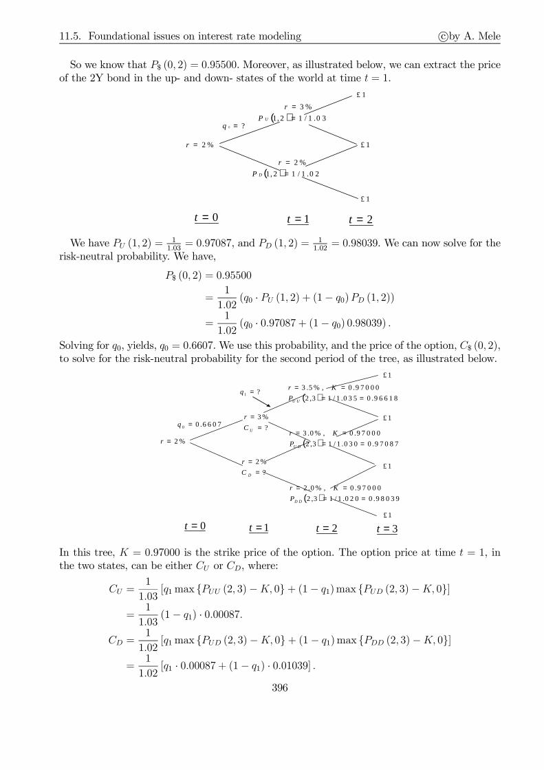
11.5. Foundational issues on interest rate modeling c©by A. Mele
So we know that P$ (0, 2) = 0.95500. Moreover, as illustrated below, we can extract the priceof the 2Y bond in the up- and down- states of the world at time t = 1.
%2=r
0=t 1=t 2=t
( ) 0 3.1/12,1
%3
==
UP
r
( ) 0 2.1/12,1
%2
==
DP
r
1£
1£
1£
?0 =q
We have PU (1, 2) =1
1.03= 0.97087, and PD (1, 2) =
11.02
= 0.98039. We can now solve for therisk-neutral probability. We have,
P$ (0, 2) = 0.95500
=1
1.02(q0 · PU (1, 2) + (1− q0)PD (1, 2))
=1
1.02(q0 · 0.97087 + (1− q0) 0.98039) .
Solving for q0, yields, q0 = 0.6607. We use this probability, and the price of the option, C$ (0, 2),to solve for the risk-neutral probability for the second period of the tree, as illustrated below.
%2=r
0=t 1=t 2=t
?
%3
==
UC
r
?
%2
==
DC
r
( ) 9 6 6 1 8.00 3 5.1/13,2
9 7 0 0 0.0% ,5.3
====
U UP
Kr
1£
3=t
6 6 0 7.00 =q
?1 =q
1£
1£
1£
( ) 9 7 0 8 7.00 3 0.1/13,2
9 7 0 0 0.0% ,0.3
====
U DP
Kr
( ) 9 8 0 3 9.00 2 0.1/13,2
9 7 0 0 0.0% ,0.2
====
D DP
Kr
In this tree, K = 0.97000 is the strike price of the option. The option price at time t = 1, inthe two states, can be either CU or CD, where:
CU =1
1.03[q1max PUU (2, 3)−K, 0+ (1− q1)max PUD (2, 3)−K, 0]
=1
1.03(1− q1) · 0.00087.
CD =1
1.02[q1max PUD (2, 3)−K, 0+ (1− q1)max PDD (2, 3)−K, 0]
=1
1.02[q1 · 0.00087 + (1− q1) · 0.01039] .
396

11.5. Foundational issues on interest rate modeling c©by A. Mele
Hence, the option price satisfies,
C$ (0, 2) = 1.0141 · 10−3
=1
1.02(q0CU + (1− q0)CD)
=1
1.02(0.6607CU + 0.3393CD)
=1
1.02
(0.6607
1
1.03(1− q1) · 0.00087 + 0.3393
1
1.02[q1 · 0.00087 + (1− q1) · 0.01039]
).
Solving for q1 yields, q = 0.8000.Next, we compute the price of the zero maturing at time 3, P (0, 3). We use the diagram in
Figure 11.11.
%2=r
0=t 1=t 2=t
( ) ?3,1
%3
==
UP
r
( ) ?3,1
%2
==
DP
r
( ) 9 6 6 1 8.03,2 =U UP
1£
3=t
6 6 0 7.00 =q
8 0 0 0.01 =q
1£
1£
1£
( ) 9 7 0 8 7.03,2 =U DP
( ) 9 8 0 3 9.03,2 =D DP
FIGURE 11.11.
We have,
PU (1, 3) =1
1.03[q1PUU (2, 3) + (1− q1)PUD (2, 3)]
=1
1.03(0.80 · 0.96618 + 0.20 · 0.97087) = 0.93895.
PD (1, 3) =1
1.02[q1PUD (2, 3) + (1− q1)PDD (2, 3)]
=1
1.02(0.80 · 0.97087 + 0.20 · 0.98039) = 0.95370.
The price of a 3Y zero coupon bond, embedded in the market prices, P$ (0, 2) and C$ (0, 2), istherefore:
P (0, 3) =1
1.02[q0PU (1, 3) + (1− q0)PD (1, 3)]
=1
1.02(0.6607 · 0.93895 + 0.3393 · 0.95370) = 0.92545.
We are now ready to evaluate the 3Y bond with 3% coupon rate. It is,
Pcoupon=3% (0, 3) = 0.03 · [P$ (0, 1) + P$ (0, 2) + P (0, 3)] + P (0, 3)
= 0.03 · (0.98039 + 0.95500 + 0.92545) + 0.92545 = 1.0113.
397

11.6. The Ho and Lee model c©by A. Mele
Note, finally, that the discretely compounded yield curve implied by the previous calculationsis given by r0,1 = 2.00% (1Y); r0,2 : 0.95500 = (1 + r0,2)
−2, or r0,2 = 2.328% (2Y); and r0,3 :0.92545 = (1 + r0,3)
−3, or r0,3 = 2.616% (3Y). Note, we are capable of computing the yieldcurve, without knowing all bond data, but inverting some of them from the price of an option!We can go further. Suppose the price of the “missing” bond becomes available, so to speak.We want to make sure this price is consistent with absence of arbitrage. Suppose, for example,that the market price is P$ (0, 3) > P (0, 3) = 0.92545, say. Then, we can sell short the 3Y zero,and set up a dynamic, self-financing strategy aiming to replicate the 3Y zero, i.e. capable ofdelivering £1 at maturity. We would proceed as follows. Consider the tree in Figure 11.11. Webuild up a portfolio, which is long the option and a MMA. We assume the 3Y bond “converges”to the values PUU , PUD and PDD in Figure 11.11, for otherwise we might implement a trivialarbitrage from time t = 2 to t = 3.So at time t = 0, we go long ∆0 options and M0 units of the MMA, to replicate PU (1, 3)
and PD (1, 3). The value of this replicating strategy is, of course, P (0, 3), so by short-sellingthe 3Y bond at t = 0, we realize an initial profit, equal to P$ (0, 3) − P (0, 3). Suppose, then,that at time t = 1, we are in the up-node, such that the bond price is PU (1, 3). In thisnode, we can build up another portfolio long ∆1 options and M1 units of the MMA, aimingto replicate the price of the bond at time t = 2–either PUU (2, 3) or PUD (2, 3). The value ofthis replicating portfolio would be just PU (1, 3), which is what is obtained by the replicatingstrategy at implemented at time t = 0. The strategy is clearly self-financed, as the followingcalculations reveal. By construction, ∆0CU (1)+M0 (1 + r) = PU (1, 3) = ∆1CU (1)+M1 (withr = 2%), and ∆1CU · (2) +M1 (1 + r) = PU · (2, 3), where r = 3%, and: CU · (2) , PU · (2, 3) areeither CUU (2) , PUU (2, 3), or CUD (2) , PUD (2, 3), at time t = 2, with straight forward notation.Therefore, we have that,
PU· (2, 3)− PU (1, 3) = ∆1
(CU · (2)− CU (1)
)+ rM1
= ∆1
(CU · (2)− CU (1)− rCU (1)
)+ rPU (1, 3) .
Likewise, if, instead, at time t = 1, we end up in the down-node, where the bond price (and thevalue of the strategy implemented at time t = 0) is PD (1, 3), we can invest PD (1, 3) in optionsand MMA so as to replicate the price of the bond at time t = 2–either PUD (2, 3) or PDD (2, 3).The presence of dynamically complete markets allows us to implement an arbitrage.
11.6 The Ho and Lee model
Ho and Lee (1986) introduce a revolutionary approach to modeling yield curve movements.Their model is not about an economic theory of determination of the yield curve. Rather, theirapproach is to take the yield curve as given, and then to model the movements of the entireyield curve in order to price interest rate derivatives. As explained in the previous section, weneed to “match” prices, to avoid having derivatives with underlyings deviating from marketprices. In the next chapter, we shall derive the Ho and Lee model in continuous time, as thisshall allow us to illustrate the general methodology underlying a general approach to interestrate modeling, due to Heath, Jarrow and Morton (1992). The original formulation of the modelwas, however, in discrete time. In this section, we present the discrete time version of the modeland some of its extensions, as well as the general philosophy underlying matching the initialyield curve within a discrete time framework, which represents indeed the industry practice.
398

11.6. The Ho and Lee model c©by A. Mele
The main idea underlying the Ho and Lee model is to model the movements of the yieldcurve along a binomial tree, much in the spirit of the Cox, Ross and Rubenstein (1979) treerepresentation of the Black and Scholes (1973) model. The main issues can be summarized asfollows. In Black and Scholes (1973) and Cox, Ross and Rubenstein (1979), the asset underlyingthe option contract is a traded risk. So the underlying asset price satisfies the martingalecondition. Interest rate derivatives, instead, generally depend on non-traded risks. The merepresence of boundary conditions induce bond return volatility to be time-varying.
11.6.1 The tree
The price of any zero evolves randomly over time, according to a binomial tree. Let Pj (t, T )be the price of a pure discount bond as of time t, with time to maturity T − t, after j upstateprice movements. Let j ∼ B (t, q), a binomial random variable,
E (j) = tq, V ar (j) = tq (1− q) ,
where q is the risk-neutral probability of a single upstate movement. Therefore we have,
Pj+1 (t+ 1, T )q ր
Pj (t, T )
1−q ցPj (t+ 1, T )
That is, if at time t, the number of upstate movements is equal to j then, at time t + 1, thenumber of upstate movements can either jump to j + 1, with probability q, or stay at j, withprobability 1− q. Note also that after one period, the price of any zero is one period closer tomaturity. At maturity, t = T , the price of any zero is worth one unit of numéraire, viz
Pj (T, T ) = 1, for all j and T.
Note, in the previous tree, it shall not necessarily hold that Pj (t+ 1, T ) < Pj (t, T ). Onthe contrary, we would expect that especially when the maturity approaches, Pj (t+ 1, T ) >Pj (t, T ), as the price of the zero needs to converge to par.
11.6.2 The price movements and the martingale restriction
In the absence of arbitrage opportunities, the expected return on the zero at t must equal theshort-term rate, viz Pj (t, T ) = e
−rj(t)Eq (P· (t+ 1, T )), or
Pj (t, T ) = Pj (t, t+ 1) [qPj+1 (t+ 1, T ) + (1− q)Pj (t+ 1, T )] , (11.23)
where Pj (t, t+ 1) = e−rj(t), and rj (t) is the continuously compounded short-term rate at time
t after j upward movements. We call this condition the martingale restriction.Let us introduce notation for the movements of the price of any zero along the tree,
Pj+1 (t+ 1, T )
Pj (t, T )= u (T − t) 1
Pj (t, t+ 1)︸ ︷︷ ︸up at t
andPj (t+ 1, T )
Pj (t, T )= d (T − t) 1
Pj (t, t+ 1)︸ ︷︷ ︸down at t
. (11.24)
399
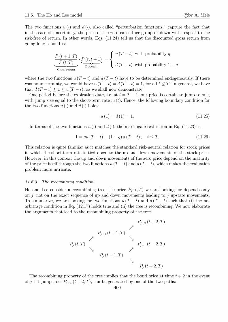
11.6. The Ho and Lee model c©by A. Mele
The two functions u (·) and d (·), also called “perturbation functions,” capture the fact thatin the case of uncertainty, the price of the zero can either go up or down with respect to therisk-free of return. In other words, Eqs. (11.24) tell us that the discounted gross return fromgoing long a bond is:
P (t+ 1, T )
P (t, T )︸ ︷︷ ︸Gross return
· P (t, t+ 1)︸ ︷︷ ︸Discount
=
u (T − t) with probability q
d (T − t) with probability 1− q
where the two functions u (T − t) and d (T − t) have to be determined endogeneously. If therewas no uncertainty, we would have u (T − t) = d (T − t) = 1, for all t ≤ T . In general, we havethat d (T − t) ≤ 1 ≤ u (T − t), as we shall now demonstrate.One period before the expiration date, i.e. at t = T − 1, our price is certain to jump to one,
with jump size equal to the short-term rate rj (t). Hence, the following boundary condition forthe two functions u (·) and d (·) holds:
u (1) = d (1) = 1. (11.25)
In terms of the two functions u (·) and d (·), the martingale restriction in Eq. (11.23) is,
1 = qu (T − t) + (1− q) d (T − t) , t ≤ T. (11.26)
This relation is quite familiar as it matches the standard risk-neutral relation for stock pricesin which the short-term rate is tied down to the up and down movements of the stock price.However, in this context the up and down movements of the zero price depend on the maturityof the price itself through the two functions u (T − t) and d (T − t), which makes the evaluationproblem more intricate.
11.6.3 The recombining condition
Ho and Lee consider a recombining tree: the price Pj (t, T ) we are looking for depends onlyon j, not on the exact sequence of up and down movements leading to j upstate movements.To summarize, we are looking for two functions u (T − t) and d (T − t) such that (i) the no-arbitrage condition in Eq. (12.17) holds true and (ii) the tree is recombining. We now elaboratethe arguments that lead to the recombining property of the tree.
Pj+2 (t+ 2, T )ր
Pj+1 (t+ 1, T )ր ց
Pj (t, T ) Pj+1 (t+ 2, T )ց ր
Pj (t+ 1, T )ց
Pj (t+ 2, T )
The recombining property of the tree implies that the bond price at time t+ 2 in the eventof j + 1 jumps, i.e. Pj+1 (t+ 2, T ), can be generated by one of the two paths:
400

11.6. The Ho and Lee model c©by A. Mele
(i) The path Pj (t, T )→ Pj+1 (t+ 1, T )→ Pj+1 (t+ 2, T ) → “up & down”
(ii) The path Pj (t, T )→ Pj (t+ 1, T )→ Pj+1 (t+ 2, T ) → “down & up”
We can use the two relations in Eqs. (11.24), to figure out the two paths leading to the bondprice at time t+ 2 in the event of j + 1 jumps, i.e. Pj+1 (t+ 2, T ). We have that along the firstpath,
Pj+1 (t+ 1, T )
Pj (t, T )= u (T − t) 1
Pj (t, t+ 1)︸ ︷︷ ︸up at t
,Pj+1 (t+ 2, T )
Pj+1 (t+ 1, T )= d (T − t− 1) 1
Pj+1 (t+ 1, t+ 2)︸ ︷︷ ︸down at t+1
,
and along the second path,
Pj (t+ 1, T )
Pj (t, T )= d (T − t) 1
Pj (t, t+ 1)︸ ︷︷ ︸,
down at t
Pj+1 (t+ 2, T )
Pj (t+ 1, T )= u (T − t− 1) 1
Pj (t+ 1, t+ 2)︸ ︷︷ ︸up at t+1
.
To sum up:
Pj+1 (t+ 2, T ) = d (T − t− 1)1
Pj+1 (t+ 1, t+ 2)·
≡ Pj+1(t+1,T )︷ ︸︸ ︷u (T − t)
1
Pj (t, t+ 1)Pj (t, T ) (up & down)
Pj+1 (t+ 2, T ) = u (T − t− 1)1
Pj (t+ 1, t+ 2)· d (T − t)
1
Pj (t, t+ 1)Pj (t, T )
︸ ︷︷ ︸≡ Pj(t+1,T )
(down & up)
By equating the previous two equations, we obtain,
u (T − t)d (T − t) =
u (T − t− 1)d (T − t− 1)
Pj+1 (t+ 1, t+ 2)
Pj (t+ 1, t+ 2)(11.27)
By evaluating Eq. (11.27) at T = t+ 2,
u (2)
d (2)=u (1)
d (1)
Pj+1 (t+ 1, t+ 2)
Pj (t+ 1, t+ 2)=Pj+1 (t+ 1, t+ 2)
Pj (t+ 1, t+ 2)≡ δ−1,
where we assume that δ is constant. Clearly, 0 ≤ δ ≤ 1. Substituting back into Eq. (11.27),
u (T − t)d (T − t) =
u (T − t− 1)d (T − t− 1)δ
−1.
Therefore, given that u (1) = d (1) = 1,
u (T − t)d (T − t) = δ
−(T−t−1). (11.28)
Eq. (11.28) gives us the condition under which the tree is recombining. To rule out arbitrageopportunities, the martingale restriction in Eq. (12.17) must also hold true. Therefore, we have
401
11.6. The Ho and Lee model c©by A. Mele
to solve the following system of two equations (Eq. (11.28) and Eq. (12.17)) with two unknowns(u (·) and d (·)),
u (T − t) = δ−(T−t−1)d (T − t)qu (T − t) + (1− q) d (T − t) = 1
The solution to this system is,
u (T − t) = 1
q + (1− q) δT−t−1, d (T − t) = δT−t−1
q + (1− q) δT−t−1. (11.29)
So we have solved the problem. We know how to “populate” the tree. Suppose we know howto assign values to q and δ. Given q and δ, and an initial bond price P (t, T ), we can use Eqs.(11.24) to populate the tree, using the solution for u (T − t) and d (T − t) given in Eqs. (11.29).In this way, we can figure out the exact bond prices to insert in each node of the tree. Oncewe have computed the bond prices in each node, we can price interest rate derivatives, i.e. theasset the payoff of which depend on the particular value taken by the bond price on a given setof nodes. Below, we provide the closed-form solution for the bond price in this model.What is the interpretation of δ? We have defined δ to be, δ−1 ≡ Pj+1(t+1,t+2)
Pj(t+1,t+2), or,
ln δ−1 = ln
(Pj+1 (t+ 1, t+ 2)
Pj (t+ 1, t+ 2)
)= − [rj+1 (t+ 1)− rj (t+ 1)] . (11.30)
But we know that conditionally upon time t and (price) jumps equal to j ≤ t, the short-termrate is binomially distributed, and can take on two values: (i) rj+1 (t+ 1) with probability qand rj (t+ 1) with probability 1− q. Then, the conditional variance of the short-term rate is,
vart[r (t+ 1)] = q (1− q) [rj+1 (t+ 1)− rj (t+ 1)]2 ,
where vart[r (t+ 1)] is the conditional variance at time t, of the short-term rate one-periodahead. Then, we may use Eq. (11.30), and the previous equation, to obtain,
√vart[r (t+ 1)] =
√q (1− q) · ln δ−1.
That is, δ is a parameter related to the volatility of the short-term rate, which in this basicmodel, is constant. In general, δ could be time-varying, although it is then difficult to findclosed-form solutions for the model.The Appendix shows that the solution to the Ho and Lee model (i.e. with fixed δ), is:
Pj (t, T ) =P (0, T )
P (0, t)δ(T−t)(t−j)
T−1∏
S=t
q + (1− q) δS−tq + (1− q) δS
. (11.31)
From the perspective of time 0, the price of the zero at t, is only a function of the initial yieldcurve, the volatility parameter δ, and of course the risk-neutral probability q.
11.6.4 Calibration of the model
We need to “estimate” the value of δ. We can proceed as follows. Consider Eq. (11.31), and letT = t+ 1. We have,
Pj (t, t+ 1) =P (0, t+ 1)
P (0, t)δt−j
1
q + (1− q) δt .402
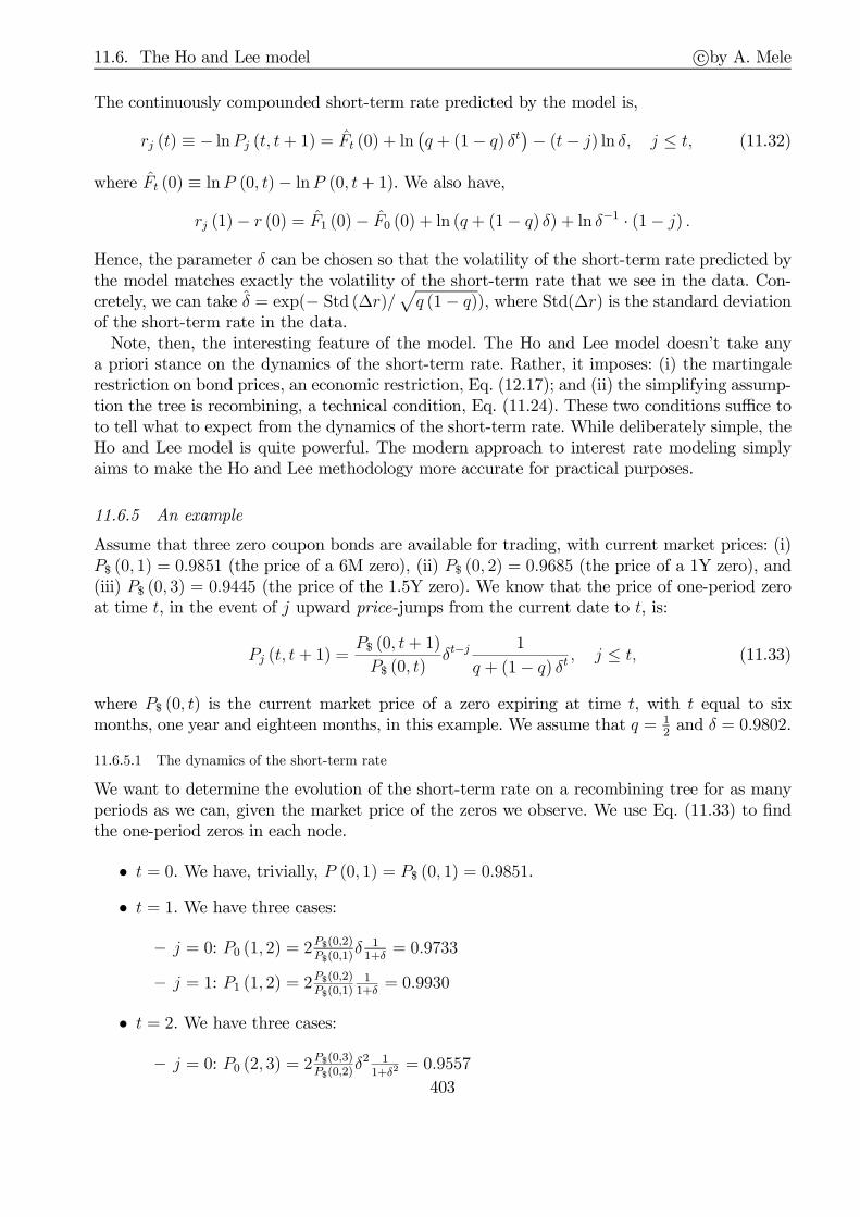
11.6. The Ho and Lee model c©by A. Mele
The continuously compounded short-term rate predicted by the model is,
rj (t) ≡ − lnPj (t, t+ 1) = Ft (0) + ln(q + (1− q) δt
)− (t− j) ln δ, j ≤ t, (11.32)
where Ft (0) ≡ lnP (0, t)− lnP (0, t+ 1). We also have,
rj (1)− r (0) = F1 (0)− F0 (0) + ln (q + (1− q) δ) + ln δ−1 · (1− j) .
Hence, the parameter δ can be chosen so that the volatility of the short-term rate predicted bythe model matches exactly the volatility of the short-term rate that we see in the data. Con-cretely, we can take δ = exp(− Std (∆r)/
√q (1− q)), where Std(∆r) is the standard deviation
of the short-term rate in the data.Note, then, the interesting feature of the model. The Ho and Lee model doesn’t take any
a priori stance on the dynamics of the short-term rate. Rather, it imposes: (i) the martingalerestriction on bond prices, an economic restriction, Eq. (12.17); and (ii) the simplifying assump-tion the tree is recombining, a technical condition, Eq. (11.24). These two conditions suffice toto tell what to expect from the dynamics of the short-term rate. While deliberately simple, theHo and Lee model is quite powerful. The modern approach to interest rate modeling simplyaims to make the Ho and Lee methodology more accurate for practical purposes.
11.6.5 An example
Assume that three zero coupon bonds are available for trading, with current market prices: (i)P$ (0, 1) = 0.9851 (the price of a 6M zero), (ii) P$ (0, 2) = 0.9685 (the price of a 1Y zero), and(iii) P$ (0, 3) = 0.9445 (the price of the 1.5Y zero). We know that the price of one-period zeroat time t, in the event of j upward price-jumps from the current date to t, is:
Pj (t, t+ 1) =P$ (0, t+ 1)
P$ (0, t)δt−j
1
q + (1− q) δt , j ≤ t, (11.33)
where P$ (0, t) is the current market price of a zero expiring at time t, with t equal to sixmonths, one year and eighteen months, in this example. We assume that q = 1
2and δ = 0.9802.
11.6.5.1 The dynamics of the short-term rate
We want to determine the evolution of the short-term rate on a recombining tree for as manyperiods as we can, given the market price of the zeros we observe. We use Eq. (11.33) to findthe one-period zeros in each node.
• t = 0. We have, trivially, P (0, 1) = P$ (0, 1) = 0.9851.
• t = 1. We have three cases:
— j = 0: P0 (1, 2) = 2P$(0,2)P$(0,1)
δ 11+δ
= 0.9733
— j = 1: P1 (1, 2) = 2P$(0,2)P$(0,1)
11+δ
= 0.9930
• t = 2. We have three cases:
— j = 0: P0 (2, 3) = 2P$(0,3)P$(0,2)
δ2 11+δ2 = 0.9557
403
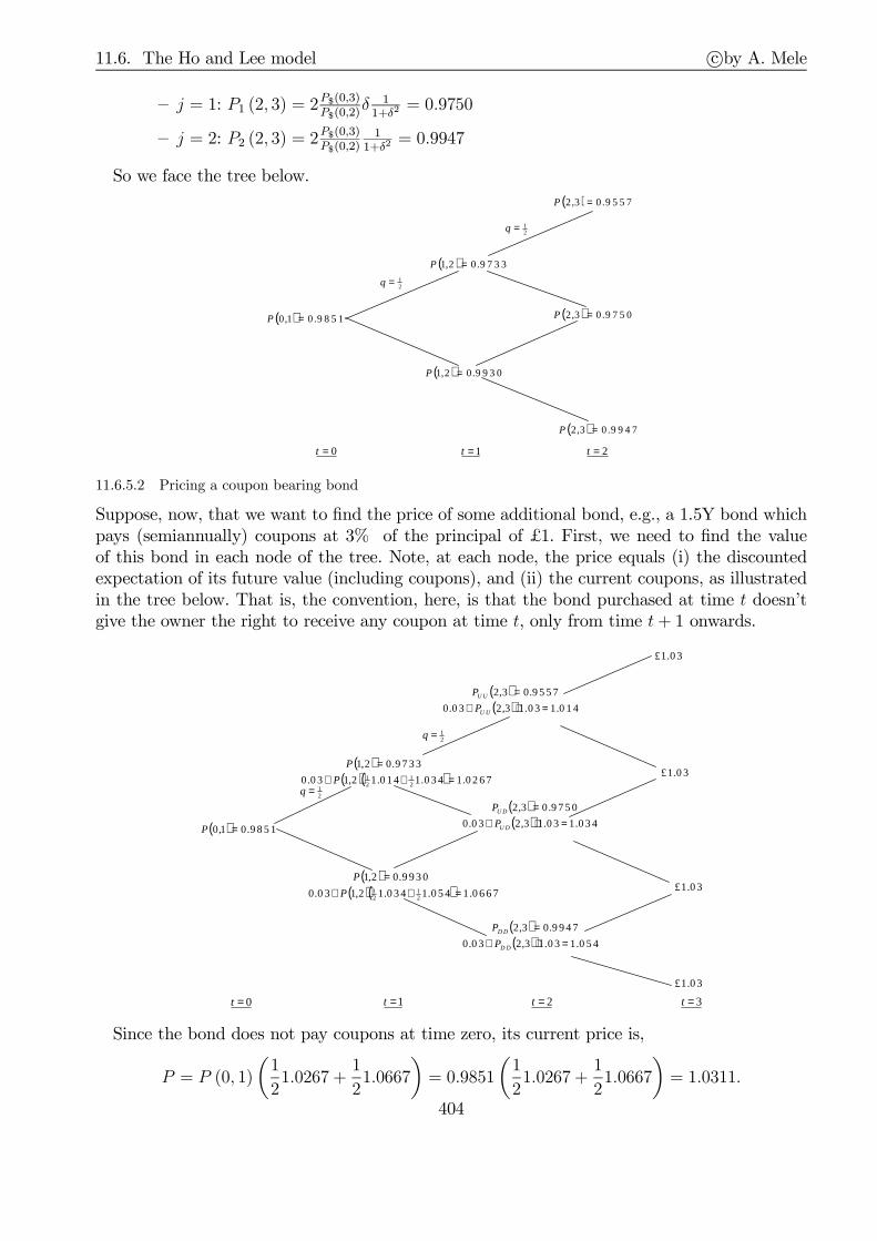
11.6. The Ho and Lee model c©by A. Mele
— j = 1: P1 (2, 3) = 2P$(0,3)P$(0,2)
δ 11+δ2 = 0.9750
— j = 2: P2 (2, 3) = 2P$(0,3)P$(0,2)
11+δ2 = 0.9947
So we face the tree below.
( ) 9 7 3 3.02,1 =P
0=t
21=q
1=t
( ) 9 9 3 0.02,1 =P
( ) 9 8 5 1.01,0 =P
21=q
( ) 9 5 5 7.03,2 =P
( ) 9 7 5 0.03,2 =P
( ) 9 9 4 7.03,2 =P
2=t
11.6.5.2 Pricing a coupon bearing bond
Suppose, now, that we want to find the price of some additional bond, e.g., a 1.5Y bond whichpays (semiannually) coupons at 3% of the principal of £1. First, we need to find the valueof this bond in each node of the tree. Note, at each node, the price equals (i) the discountedexpectation of its future value (including coupons), and (ii) the current coupons, as illustratedin the tree below. That is, the convention, here, is that the bond purchased at time t doesn’tgive the owner the right to receive any coupon at time t, only from time t+ 1 onwards.
( )( )( ) 0 2 6 7.10 3 4.10 1 4.12,10 3.0
9 7 3 3.02,1
21
21 =++
=P
P
0=t
21=q
1=t
( )( )( ) 0 6 6 7.10 5 4.10 3 4.12,10 3.0
9 9 3 0.02,1
21
21 =++
=P
P
( ) 9 8 5 1.01,0 =P
21=q
( )( ) 0 1 4.10 3.13,20 3.0
9 5 5 7.03,2
=⋅+=
U U
U U
P
P
2=t
( )( ) 0 3 4.10 3.13,20 3.0
9 7 5 0.03,2
=⋅+=
U D
U D
P
P
( )( ) 0 5 4.10 3.13,20 3.0
9 9 4 7.03,2
=⋅+=
D D
D D
P
P
3=t
0 3.1£
0 3.1£
0 3.1£
0 3.1£
Since the bond does not pay coupons at time zero, its current price is,
P = P (0, 1)
(1
21.0267 +
1
21.0667
)= 0.9851
(1
21.0267 +
1
21.0667
)= 1.0311.
404

11.6. The Ho and Lee model c©by A. Mele
Naturally, this price could been obtained by simply adding [P$ (0, 1) + P$ (0, 2) + P$ (0, 3)] ∗0.03 + P$ (0, 3), although the results in the tree above are going to matter while pricing deriv-atives written on the coupon bearing bond.
11.6.5.3 Pricing European options
Next, we wish to find the price of options, say the price of two call options on the 1.5Y bondconsidered in the previous subsection, when the strike price is £1 and the maturities of theoptions are 6 months and 1 year. Again, we need to figure out the no-arbitrage movements ofthe ex-coupons bond price. (This is because if we purchase the bond today, we are not entitledto receive any coupon, today. The flow of coupons we are entitled to receive starts from thenext period.) We easily obtain the tree below. We must just subtract the coupon, 0.03, fromeach cum-coupons price in each node of the tree. Then, we obtain:
997.003.00267.1 =−=P
0=t
21=q
1=t
0367.103.00667.1 =−=P
( ) 9851.01,0 =P
984.003.0014.1 =−=P
2=t
004.103.0034.1 =−=P
024.103.0054.1 =−=P
21=q
We are ready to price the two options. As for the call option on the 1.5Y bond, with 6 monthsmaturity, and strike price K = $1, we have the following tree:
00,max
997.0
=−==
KPC
P
0=t
21=q
1=t
0367.00,max
0367.1
=−==
KPC
P
( )?
9851.01,0
==
C
P
Therefore,
C = 0.9851
(1
2· 0 + 1
2· 0.0367
)= 1.808× 10⁻².
405

11.6. The Ho and Lee model c©by A. Mele
The call option on the 1.5Y bond with 1 year maturity, and strike price K = $1, is dealtwith similarly. We have the following tree:
0=t
21=q
1=t
( )( )( ) 014.0024.0004.02,1
9930.02,1
21
21 =+=
=PC
P
( )?
9851.01,0
==
C
P
00,max
984.0
=−==
KPC
P
2=t
21=q
004.00,max
004.1
=−==
KPC
P
024.00,max
024.1
=−==
KPC
P
( )( )( ) 0019.0004.002,1
9733.02,1
21
21 =+⋅=
=PC
P
Therefore, the price of the option is,
C = P (0, 1)
(1
20.0019 +
1
20.014
)= 0.9851
(1
20.0019 +
1
20.014
)= 7.831× 10⁻³.
11.6.6 Continuous-time approximations with an application to barbell trading
11.6.6.1 The approximation
Consider Eq. (11.32), and define r = −∆t−1 lnP , and r∆j (t) ≡ rj (t)∆t, such that:
r∆j (t) = ζt − (tq − j) ln δ, ζt ≡ Ft (0) + ln(δ−(1−q)tq + δqt (1− q)
).
We have,
E0
[r∆j (t)
]= ζt, and σ2t ≡ V0
[r∆j (t)
]=
(ln δ−1
)2q (1− q) t,
such that we may define ℓ ≡ σ/√q (1− q), and, then, δ = e−ℓ. Replacing this into the definition
of ζt, yields, after expanding terms to the second order,
ζt = Ft (0) + ln(eℓ(1−q)tq + e−ℓqt (1− q)
)
≈ Ft (0) + ln
(1 +
1
2ℓ2q (1− q) t2
)
≈ Ft (0) +1
2ℓ2q (1− q) t2
= Ft (0) +1
2σ2t2.
Note, this expansion is accurate when ℓt is small, which is indeed, as we have that, empirically,ℓt ≈ 10−2t, which then works for t up to at least 50 years! However, these calculations might
406

11.6. The Ho and Lee model c©by A. Mele
also be considered as the starting point for the initial drift of the short-term rate from zero totime t. So, we have, approximately, that,
E0
[r∆j (t)
]= Ft (0) +
1
2σ2t2, and V0
[r∆j (t)
]= σ2t. (11.34)
In the next chapter (Section 12.4.2), we shall show, consistently with the previous calculations,that in continuous time, the Ho and Lee model predicts the short-term rate to be solution to:
dr (t) =
[∂
∂tf$ (0, t) + σ
2t
]dt+ σdW (t) ,
where f$ (0, t) is the instantaneous continuously compounded forward rate, and W (t) is aBrownian motion defined under the risk-neutral probability. In fact, in the next chapter, it willbe shown that the instantaneous forward rate predicted by the Ho & Lee model is:
f (s′, t)− f (s, t) = σ2
∫ s′
s
(t− τ) dτ + σ(W (t)− W (s)
), (11.35)
such that, for r (s′) = f (s′, s′),
r (s′)− f (s, s′) = σ2
∫ s′
s
(s′ − τ ) dτ + σ(W (s′)− W (s)
), (11.36)
the continuous time counterpart to the two conditions in Eqs. (11.34). By combining Eqs.(11.35)-(11.36), we obtain, after simple computations, that:
f (s′, t)− f (s, t) = σ2 (s′ − s) (t− s′) + r (s′)− f (s, s′) . (11.37)
As the next chapter shows (see Section 12.5.1), we have that for any model, including Ho &Lee,5 the following representation holds true:
P (t, T ) =P (0, T )
P (0, t)· e−
∫ Tt [f(t,u)−f(0,u)]du. (11.38)
Using the expression for f (s′, t)− f (s, t) in Eq. (11.37), and integrating,
∫ T
t
[f(t, u)− f(0, u)] du = 1
2σ2 (T − t)2 t+ (T − t) (r (t)− f (0, t)) .
Replacing this expression into Eq. (11.38) leaves:
P (t, T ) =P (0, T )
P (0, t)· exp
(−12σ2 (T − t)2 t− (r (t)− f (0, t)) (T − t)
). (11.39)
It is a quite neat expression, which we may use, for a variety of purposes, such as option pricing.The next section develops an example relating to barbell trading.
5For example, Eq. (11A.6) in the Appendix provides the discrete time counterpart to Eq. (11.38).
407

11.6. The Ho and Lee model c©by A. Mele
11.6.6.2 Application to barbell trading
We revisit the barbell trading strategy of Section 11.4.3.5, where we argued that this strategyleads to positive profits due to “convexity,” as summarized by Figure 11.4. The key point inthis argument is that it abstracts from passage of time, and may, in fact, lead us to misinterpretwhat is a merely static analysis. We may use the Ho and Lee model to analyze the profit andlosses of a barbell trade, in a dynamic context free from arbitrage. We consider two situations:one, where the initial yield curve is flat, and a second, where the initial yield curve is upwardsloping.As for the flat yield curve, we use the continuously compounded rate corresponding to the flat
5% of Section 11.4.3.5, delivering r = ln 1.05 = 0.04879. The number of assets to include intothe portfolio, θ1 and θ2, are as in Eq. (11.15), i.e. θ1 = 0.45706 and θ3 = 0.56724. Instantaneousforward rates are f (0, T ) = limS↓T F (0, T, S) = −∂ lnP (0, T ) /∂T = r. Using Eq. (11.39),with volatility parameter σ = 0.03, we calculate the value of the strategy a few months later,as follows:
Barb (t) = 100 ∗ (θ1P (t, 1) + θ3P (t, 10)− P (t, 5)) . (11.40)
Figure 11.12 depicts the value of the barbell, Barb (t), for investment horizons equal to 1 month,3 months, 6 months and one year.
0 0.02 0.04 0.06 0.08 0.1−0.5
0
0.5
1
1.5
2
2.5
short−term rate in one month0 0.02 0.04 0.06 0.08 0.1
−0.5
0
0.5
1
1.5
2
short−term rate in six months
0 0.02 0.04 0.06 0.08 0.1−0.5
0
0.5
1
1.5
2
2.5
short−term rate in three months0 0.02 0.04 0.06 0.08 0.1
−1
−0.5
0
0.5
1
1.5
short−term rate in one year
FIGURE 11.12. Profit and losses arising from barbell trading, Barb (t) in Eq. (11.40),
under the assumption the yield curve is driven by the Ho and Lee model, Eq. (11.39).
The initial yield curve is assumed to be flat at r = 4.8790%. Investment horizons are
t = 1/12 (NW quadrant), t = 3/12 (SW quadrant), t = 6/12 (NE quadrant) and, t = 1
(SE quadrant). The vertical dashed lines pass through r = 4.8790%, and the horizontal
dashed lines pass through zero.
408

11.6. The Ho and Lee model c©by A. Mele
This trading is quite risky. For long investment horizons, it pays off when the short-term ratefluctuates significantly away from the initial value, r = 4.8790%. The amount of fluctuations inthe short-term rate diminishes as we shrink the investment horizon. Nevertheless, this amountappears to be considerable: for example, at one-month horizon, we should require the short-term rate to move from r = 4.8790% to either values larger than r = 6% or lower than r = 4%,in order to claim for positive profits. Actually, these results suggest that a short position in thebarbell trade (i.e., sell the barbell portfolio and go long the 5Y bond) should be an interestingstrategy to implement in periods where we do not expect high volatility of interest rates. Forexample, for investment horizons of 6 months, the profits from a short position in the barbelltrade are positive within a quite significant range of variation of the short-term rate, [2.5%,6.8%].Finally, we consider the scenario where the initial yield curve is upward sloping, and generate
prices as P (0, t) = e−tY (t), where Y (t) ≡ 0.01(1+ ln t). We still compute the portfolio accordingto Eq. (11.15), i.e. we rely on the self-financing condition in Eq. (11.13) and both (i) the locallyriskless condition in Eq. (11.14), dB2 (y2) = θ1dB1 (y1) + θ3dB3 (y3), and (ii) the (generically
incorrect) assumption of parallel shifts in the yield curve, ∂B2(y2)∂y2
= ∂B1(y1)∂y1
θ1+∂B3(y3)∂y3
θ3. Figure11.13 depicts the profit and losses arising from the trade.
0 0.01 0.02 0.03 0.04 0.05 0.06−0.5
0
0.5
1
1.5
2
2.5
short−term rate in one month0 0.01 0.02 0.03 0.04 0.05 0.06
−0.5
0
0.5
1
1.5
2
short−term rate in six months
0 0.01 0.02 0.03 0.04 0.05 0.06−0.5
0
0.5
1
1.5
2
2.5
short−term rate in three months0 0.01 0.02 0.03 0.04 0.05 0.06
−1
−0.5
0
0.5
1
1.5
short−term rate in one year
FIGURE 11.13. Profit and losses arising from barbell trading, Barb (t) in Eq. (11.40), under the
assumption the yield curve is driven by the Ho and Lee model, Eq. (11.39). The initial yield curve
is assumed to be upward sloping, generated by the equation, Y (t) = 0.01(1 + ln t), with prices given
by P (0, t) = e−tY (t). Investment horizons are t = 1/12 (NW quadrant), t = 3/12 (SW quadrant),
t = 6/12 (NE quadrant) and, t = 1 (SE quadrant). The vertical dashed lines pass through the current
short-term rate, r = 1.0%, and the horizontal dashed lines pass through zero.
409
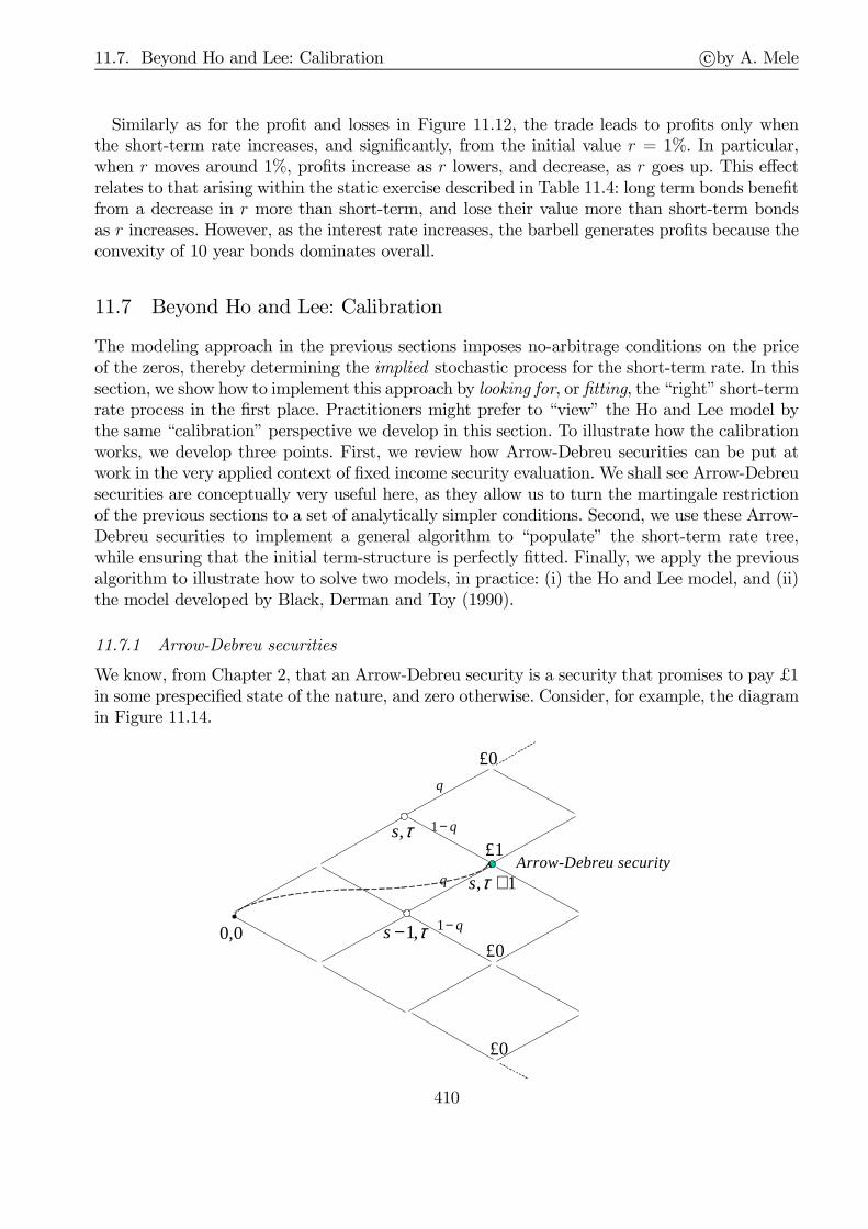
11.7. Beyond Ho and Lee: Calibration c©by A. Mele
Similarly as for the profit and losses in Figure 11.12, the trade leads to profits only whenthe short-term rate increases, and significantly, from the initial value r = 1%. In particular,when r moves around 1%, profits increase as r lowers, and decrease, as r goes up. This effectrelates to that arising within the static exercise described in Table 11.4: long term bonds benefitfrom a decrease in r more than short-term, and lose their value more than short-term bondsas r increases. However, as the interest rate increases, the barbell generates profits because theconvexity of 10 year bonds dominates overall.
11.7 Beyond Ho and Lee: Calibration
The modeling approach in the previous sections imposes no-arbitrage conditions on the priceof the zeros, thereby determining the implied stochastic process for the short-term rate. In thissection, we show how to implement this approach by looking for, or fitting, the “right” short-termrate process in the first place. Practitioners might prefer to “view” the Ho and Lee model bythe same “calibration” perspective we develop in this section. To illustrate how the calibrationworks, we develop three points. First, we review how Arrow-Debreu securities can be put atwork in the very applied context of fixed income security evaluation. We shall see Arrow-Debreusecurities are conceptually very useful here, as they allow us to turn the martingale restrictionof the previous sections to a set of analytically simpler conditions. Second, we use these Arrow-Debreu securities to implement a general algorithm to “populate” the short-term rate tree,while ensuring that the initial term-structure is perfectly fitted. Finally, we apply the previousalgorithm to illustrate how to solve two models, in practice: (i) the Ho and Lee model, and (ii)the model developed by Black, Derman and Toy (1990).
11.7.1 Arrow-Debreu securities
We know, from Chapter 2, that an Arrow-Debreu security is a security that promises to pay £1in some prespecified state of the nature, and zero otherwise. Consider, for example, the diagramin Figure 11.14.
τ,s
τ,1−s
1, +τs
1£
0£
0£
0£
Arrow-Debreu security
q
q
q−1
q−10,0
410
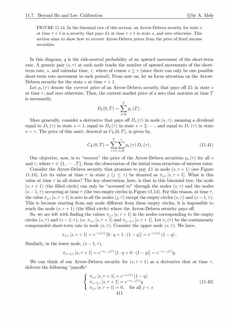
11.7. Beyond Ho and Lee: Calibration c©by A. Mele
FIGURE 11.14. In the binomial tree of this section, an Arrow-Debreu security for state s
at time τ +1 is a security that pays £1 at time τ +1 in state s, and zero otherwise. This
section aims to show how to recover Arrow-Debreu prices from the price of fixed income
securities.
In this diagram, q is the risk-neutral probability of an upward movement of the short-termrate. A generic pair (s, τ) at each node tracks the number of upward movements of the short-term rate, s, and calendar time, τ , where of course s ≤ τ (since there can only be one possibleshort-term rate movement in each period). From now on, let us focus attention on the Arrow-Debreu security for the state s at time τ + 1.Let ps (τ) denote the current price of an Arrow-Debreu security that pays off £1 in state s
at time τ , and zero otherwise. Then, the current market price of a zero that matures at time Tis necessarily,
P$ (0, T ) =T∑
s=0
ps (T ) .
More generally, consider a derivative that pays off Ds (τ) in node (s, τ), meaning a dividendequal to D1 (τ) in state s = 1, equal to D2 (τ ) in state s = 2, · · · , and equal to Dτ (τ) in states = τ . The price of this asset, denoted as C$ (0, T ), is given by,
C$ (0, T ) =T∑
τ=1
τ∑
s=0
ps (τ)Ds (τ ) . (11.41)
Our objective, now, is to “recover” the price of the Arrow-Debreu securities ps (τ) for all sand τ , where τ ∈ 1, · · · , T, from the observation of the initial term-structure of interest rates.Consider the Arrow-Debreu security that promises to pay £1 in node (s, τ + 1) (see Figure
11.14). Let its value at time τ in state j (j ≤ τ) be denoted as πj,τ [s, τ + 1]. What is thisvalue at time τ in all states? The key observation, here, is that in this binomial tree, the node(s, τ + 1) (the filled circle) can only be “accessed to” through the nodes (s, τ ) and the nodes(s− 1, τ ) occurring at time τ (the two empty circles in Figure 11.14). For this reason, at time τ ,the value πj,τ [s, τ + 1] is zero in all the nodes (j, τ) except the empty circles (s, τ ) and (s− 1, τ ).This is because starting from any node different from these empty circles, it is impossible toreach the node (s, τ + 1) (the filled circle) where the Arrow-Debreu security pays off.So, we are left with finding the values πj,τ [s, τ + 1] in the nodes corresponding to the empty
circles (s, τ) and (s− 1, τ ), i.e. πs,τ [s, τ + 1] and πs−1,τ [s, τ + 1]. Let rs (τ ) be the continuouslycompounded short-term rate in node (s, τ). Consider the upper node (s, τ ). We have,
πs,τ [s, τ + 1] = e−rs(τ) [0 · q + 1 · (1− q)] = e−rs(τ) (1− q) .
Similarly, in the lower node, (s− 1, τ),
πs−1,τ [s, τ + 1] = e−rs−1(τ) [1 · q + 0 · (1− q)] = e−rs−1(τ)q.
We can think of our Arrow-Debreu security for (s, τ + 1) as a derivative that at time τ ,delivers the following “payoffs“
πs,τ [s, τ + 1] = e
−rs(τ) (1− q)πs−1,τ [s, τ + 1] = e
−rs−1(τ)qπj,τ [s, τ + 1] = 0, for all j < s
(11.42)
411

11.7. Beyond Ho and Lee: Calibration c©by A. Mele
These “payoffs” are simply the market value of the Arrow-Debreu security for (s, τ + 1), in thevarious states occurring at time τ , i.e. the money the holder can make by selling the asset attime τ , in the various states. Therefore, we can apply Eq. (11.41) to obtain,
ps (τ + 1) =τ∑
j=0
pj (τ) πj,τ [s, τ + 1]
= ps (τ) πs,τ [s, τ + 1] + ps−1 (τ )πs−1,τ [s, τ + 1] .
By replacing the Arrow-Debreu prices in (11.42) into the previous equation, we obtain theso-called forward equation for the Arrow-Debreu prices,
ps (τ + 1) = ps (τ) e−rs(τ) (1− q) + ps−1 (τ) e
−rs−1(τ)q (11.43)
11.7.2 The algorithm in two examples
The algorithm aims to populate the interest rate tree by making a repeated use of the forwardequation (11.43) and the zero pricing equation,
P$ (0, τ + 1) =τ∑
s=0
ps (τ) e−rs(τ).
The input is, of course, a number of zeros equal to the largest maturity date the tree extendsto. We describe how the algorithm works by developing two concrete model examples.
11.7.2.1 Two model examples
We begin with Ho and Lee. We assume continuous compounding, for analytical reasons clarifiedbelow. By Eq. (11.32), the short-term rate predicted by the Ho and Lee model is:
rj (τ ) = Fτ (0) + ln (q + (1− q) δτ )− (τ − j) ln δ. (11.44)
where Fτ (0) is the continuously compounded forward rate, at time zero, for maturity [τ , τ + 1],and j is the number of upward movements of the entire set of bond prices. Naturally, then,s ≡ (t− j) is the number of downward movements of the bond prices or, equivalently, thenumber of upward movements of the short-term rate. Hence, we may equivalently index theshort-term rate by s, instead than by j, and rewrite Eq. (11.44) as follows:
rs (τ) = Fτ (0) + ln (q + (1− q) δτ )︸ ︷︷ ︸≡ r0(τ)
+ ln δ−1 · s, (11.45)
such that r0 (τ) is the short-term rate at time τ , in the event of zero upward movements in the
short-term rate, and δ is a volatility parameter, i.e. such that ln δ−1 = Std(∆r)√q(1−q)
, with Std (∆r)
denoting the standard deviation of the short-term rate in the data.6 At time zero, the price ofa zero maturing at time τ + 1 is:
P$ (0, τ + 1) =τ∑
s=0
ps (τ ) e−rs(τ) = e−r0(τ)
τ∑
s=0
δsps (τ ) ,
6 Incidentally, note that the short-term rate movements do depend on the value of the risk-neutral probability q used in thecalibration.
412

11.7. Beyond Ho and Lee: Calibration c©by A. Mele
where the second equality follows by the assumption that the short-term rate is solution to Eq.(11.45).By rearranging terms in the previous equation, we obtain a closed-form expression for the
future short-term rate at time τ , in the event of zero upward movements,
r0 (τ ) = ln
(∑τs=0 δ
sps (τ )
P$ (0, τ + 1)
). (11.46)
We use Eq. (11.46) and the forward equation (11.43) to populate the interest rate tree, underthe assumption that q = 1
2. Precisely, the algorithm proceeds as follows:
(i) Given the boundary condition for the Arrow-Debreu price, p0 (0) = 1, compute the initialvalue of the short-term rate, r0 (0), using Eq. (11.46), as r0 (0) = ln(1/P$ (0, 1)).
(ii) Suppose we know the future value of the short-term rate at time τ − 1, in the event ofno upward movements, i.e. r0 (τ − 1). Then, given the value of r0 (τ − 1), and the priceof the Arrow-Debreu securities ps (τ − 1) for s ≤ τ − 1, compute ps (τ) for s ≤ τ , throughthe forward equation (11.43),
ps (τ) = ps (τ − 1) δse−r0(τ−1) (1− q) + ps−1 (τ − 1) δs−1e−r0(τ−1)q, q =1
2,
where the last equation follows by plugging Eq. (11.45) into Eq. (11.43).
(iii) Given the Arrow-Debreu prices ps (τ ) for s ≤ τ , use Eq. (11.46) to compute the futurevalue of the short-term rate at time τ , in the event of no upward movements, i.e. r0 (τ).
(iv) If τ = T , stop. Otherwise, go to (ii).
As a second example, consider the Black, Derman and Toy (1990) model. In this model, theshort-term rate is solution to,
rs (τ) = δsr0 (τ ) , (11.47)
where δ is, once again, a volatility parameter.7 For computational convenience, this modelassumes that the short-term rate in Eq. (11.47) is discretely compounded. Accordingly, werewrite the forward equation (11.43) in terms of discretely compounded rates,
ps (τ + 1) = ps (τ )1
1 + rs (τ )(1− q) + ps−1 (τ )
1
1 + rs−1 (τ)q. (11.48)
The algorithm proceeds as follows:
(i) Compute the initial value of the short-term rate, r0 (0), as the solution to,
P$ (0, 1) =1
1 + r0 (0).
7 In its most general form, this model assumes that rs (τ) = δsτ r0 (τ), where δτ is a volatility parameter that varies determinis-tically over time. This more general formulation leads to more flexibility, which is useful to fit the term structure of volatility.
413

11.7. Beyond Ho and Lee: Calibration c©by A. Mele
(ii) Suppose we know the future value of the short-term rate at time τ − 1, in the event ofno upward movements, i.e. r0 (τ − 1). Then, given the value of r0 (τ − 1), and the priceof the Arrow-Debreu securities ps (τ − 1) for s ≤ τ − 1, compute ps (τ) for s ≤ τ , throughthe forward equation (11.48),
ps (τ) = ps (τ − 1)1
1 + δsr0 (τ − 1)(1− q) + ps−1 (τ − 1)
1
1 + δs−1r0 (τ − 1)q, q =
1
2,
where the last equation follows by plugging Eq. (11.47) into Eq. (11.48).
(iii) Given the boundary condition p0 (0) = 1, and the Arrow-Debreu prices, ps (τ ) for s ≤ τ ,use the pricing equation for the zero,
P$ (0, τ + 1) =τ∑
s=0
ps (τ )1
1 + δsr0 (τ),
to solve, numerically, for the future value of the short-term rate at time τ , in the eventof no upward movements, i.e. r0 (τ ). Note, we did not need this additional step for thesolution of the Ho and Lee model, as the short-term rate r0 (τ) is known in closed formin the Ho and Lee model (see Eq. (11.46)).
(iv) If τ = T , stop. Otherwise, go to (ii).
11.7.2.2 A numerical example
Consider, again the Ho and Lee model example in Section 11.5.5, where three zeros were traded:(i) one zero maturing in 6 months, (ii) one zero maturing in 1 year, and (iii) one zero maturingin 1.5 years, with market prices P$ (0, 1) = 0.9851, P$ (0, 2) = 0.9685, P$ (0, 3) = 0.9445. ByEq. (11.45), the Ho and Lee model assumes that,
rs (τ) = r0 (τ ) +(ln δ−1
)· s. (11.49)
We use Eq. (11.49) and find the values of the short-term rate rs (τ) in each node, underthe assumption that q = 1
2, and that the standard deviation of the short-term rate is 0.014,
annualized. To find δ, we may use the relation, ln δ−1 = Std(∆r)√q(1−q)
, where q = 12and Std(∆r)
is the standard deviation of the short-term rate, which equals Std(∆r) = 0.014, annualized.Therefore ln δ−1 = 0.014√
2/12= 0.02 or δ = 0.9802.
For the Ho & Lee model, we know the closed-form expression for r0 (τ),
r0 (τ ) = ln
(∑τs=0 δ
sps (τ )
P$ (0, τ + 1)
), (11.50)
where ps (τ ) denotes the price of an Arrow-Debreu security which pays of £1 in state s at time τ ,and zero otherwise. Given the term-structure of prices P$ (0, τ + 1), τ = 0, 1, 2, we “populate”the tree using Eq. (11.50) and the forward equation for the Arrow-Debreu prices developed inthe lecture notes,
ps (τ ) =1
2e−r0(τ−1)
[δsps (τ − 1) + δs−1ps−1 (τ − 1)
], (11.51)
with the appropriate boundary conditions.So we have to compute interest rates and Arrow-Debreu prices for τ = 0, 1, 2.
414

11.7. Beyond Ho and Lee: Calibration c©by A. Mele
• τ = 0. Eq. (11.50) is trivial. It leads to,
r0 (0) = ln
(1
P$ (0, 1)
)= 0.015.
The forward equation for the Arrow-Debreu prices, Eq. (11.51), is also trivial,
p0 (0) = 1.
• τ = 1. Let us use Eq. (11.51), the forward equation for the Arrow-Debreu prices, to findp0 (1) and p1 (1). We have two cases:
— s = 0. We have:
p0 (1) =1
2e−r0(0) [p0 (0) + 0] =
1
2e−r0(0) = 0.4925.
The previous relation holds because p0 (1) is the current price of the Arrow-Debreusecurity which pays off £1 in state 0 at time 1, as illustrated by the tree in the Figure1 below,
1=s
0=τ
21=q
0=s1£
1=τ
— s = 1. By a similar reasoning,
p1 (1) =1
2e−r0(0) [0 + p0 (0)] =
1
2e−r0(0) = 0.4925.
Eq. (11.50) is, now,
r0 (1) = ln
(p0 (1) + δp1 (1)
P$ (0, 2)
)= ln
(0.4925 · (1 + 0.9802)
0.9685
)= 0.0069.
Hence, by Eq. (11.49),
r1 (1) = r0 (1) +(ln δ−1
)= 0.0069 + 0.02 = 0.0270.
415
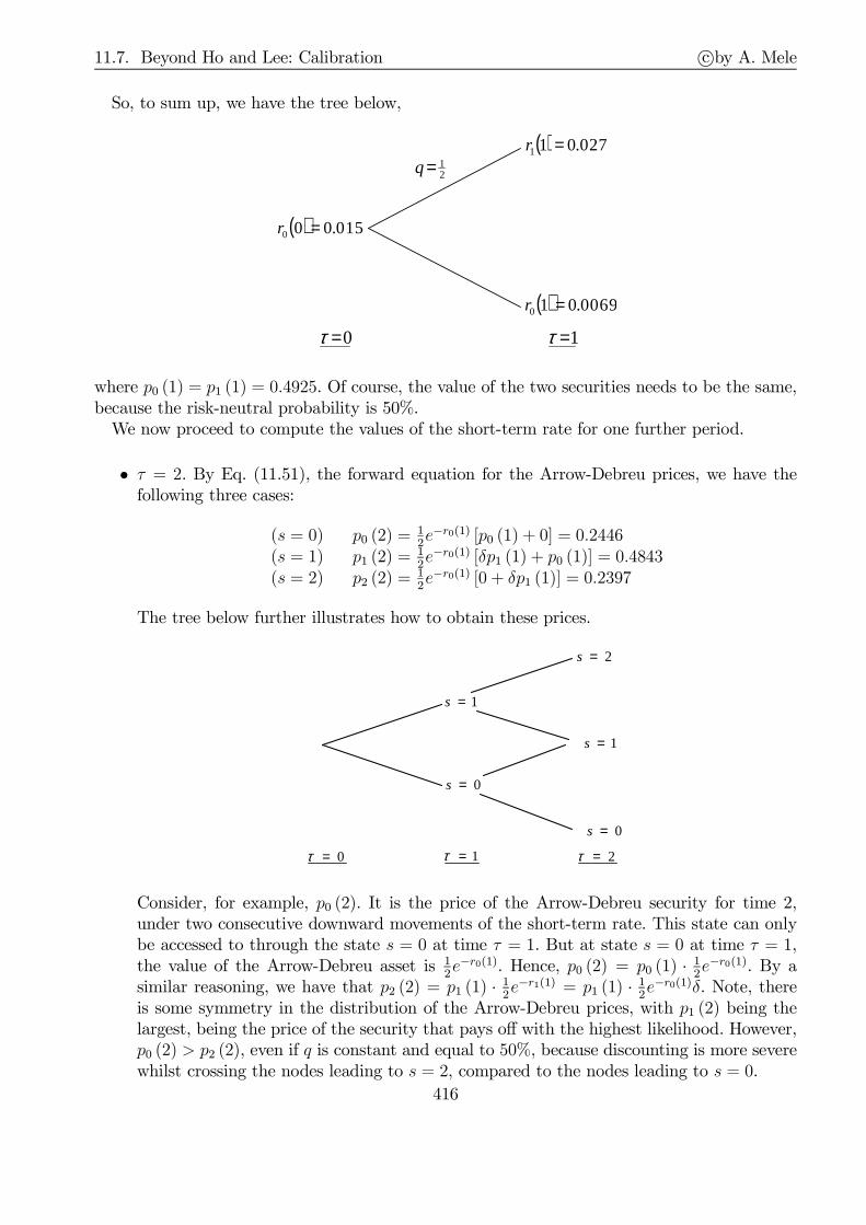
11.7. Beyond Ho and Lee: Calibration c©by A. Mele
So, to sum up, we have the tree below,
( ) 027.011 =r
0=τ
21=q
1=τ
( ) 0069.010 =r
( ) 015.000 =r
where p0 (1) = p1 (1) = 0.4925. Of course, the value of the two securities needs to be the same,because the risk-neutral probability is 50%.We now proceed to compute the values of the short-term rate for one further period.
• τ = 2. By Eq. (11.51), the forward equation for the Arrow-Debreu prices, we have thefollowing three cases:
(s = 0) p0 (2) =12e−r0(1) [p0 (1) + 0] = 0.2446
(s = 1) p1 (2) =12e−r0(1) [δp1 (1) + p0 (1)] = 0.4843
(s = 2) p2 (2) =12e−r0(1) [0 + δp1 (1)] = 0.2397
The tree below further illustrates how to obtain these prices.
1=s
0=τ
0=s
1=τ
0=s
1=s
2=s
2=τ
Consider, for example, p0 (2). It is the price of the Arrow-Debreu security for time 2,under two consecutive downward movements of the short-term rate. This state can onlybe accessed to through the state s = 0 at time τ = 1. But at state s = 0 at time τ = 1,the value of the Arrow-Debreu asset is 1
2e−r0(1). Hence, p0 (2) = p0 (1) · 1
2e−r0(1). By a
similar reasoning, we have that p2 (2) = p1 (1) · 12e−r1(1) = p1 (1) · 1
2e−r0(1)δ. Note, there
is some symmetry in the distribution of the Arrow-Debreu prices, with p1 (2) being thelargest, being the price of the security that pays off with the highest likelihood. However,p0 (2) > p2 (2), even if q is constant and equal to 50%, because discounting is more severewhilst crossing the nodes leading to s = 2, compared to the nodes leading to s = 0.
416

11.7. Beyond Ho and Lee: Calibration c©by A. Mele
We can now compute the values of the short-term rate for each node. Eq. (11.50) is, now,
r0 (2) = ln
(p0 (2) + δp1 (2) + δ
2p2 (2)
P$ (0, 3)
)
= ln
(0.2446 + 0.9802 · 0.4843 + (0.9802)2 · 0.2397
0.9445
)= 0.0054.
Hence, by Eq. (11.49),
rs (2) = r0 (2) +(ln δ−1
)· s = 0.0054 + 0.02 · s, s = 0, 1, 2.
This yields the following values for the short-term rate: r0 (2) = 0.0054, r1 (2) = 0.0253,and r2 (2) = 0.0452.
The diagram below summarizes the implied tree for the short-term rate in this model.
( ) 0 27.011 =r
0=τ
21=q
1=τ
( ) 0 0 6 9.010 =r
( ) 0 1 5.000 =r
21=q
( ) 0 4 5 2.022 =r
( ) 0 2 5 3.021 =r
( ) 0 0 5 4.020 =r
2=τ
Naturally, the prices P = e−r in the nodes of the previous tree match those calculated inSection 11.6.5, apart from discrepancies arising due to rounding errors.
11.7.2.3 A second numerical example
Assume that the spot yield curve is 2.5% for t = 1 year, 4.5% for t = 2 years, and 6% for t = 3years, continuously compounded and annualized. Consider the following model:
rs (t) = r0 (t) + a ∗ s, (11.52)
where a is a constant and equal to 0.01, rs (t) is the continuously compounded short-term rateas of time t, after s upward movements and, finally, the unit period of time is taken to be oneyear. As we know, the Ho & Lee model predicts that the price as of time zero of an Arrow-Debreu security paying off in state s at time t, denoted as ps (t), satisfies the following forwardequation, for t > 1, s ≥ 0 and s ≤ t:
ps (t) = e−r0(t−1)
[(1− q)
(e−a
)sps (t− 1) + q
(e−a
)s−1ps−1 (t− 1)
], (11.53)
417

11.7. Beyond Ho and Lee: Calibration c©by A. Mele
where q is the risk-neutral probability of an upward movement in the short-term rate. Further-more, according to this model, the price of a zero coupon bond, paying £1 at time t, P$ (0, t),equals,
P$ (0, t) = e−r0(t−1)
t−1∑
s=0
(e−a
)sps (t− 1) . (11.54)
Suppose, next, that the risk-neutral probability of an upward movement at any time t is nota constant q, but a function of calendar time, say qt: qt is, then, the probability of an upwardmovement in the short-term rate from time t to time t + 1. Naturally, the assumption that qtis time-varying, makes this model markedly distinct from Ho & Lee model. To calibrate thismodel, we consider the recursive equation for the Arrow-Debreu security prices:
ps (t) = e−r0(t−1)
[(1− qt−1)
(e−a
)sps (t− 1) + qt−1
(e−a
)s−1ps−1 (t− 1)
], (11.55)
where qt−1 denotes the risk-neutral probability of an upward movement in the short-term ratefrom time t − 1 to time t. The boundary conditions are the usual ones: p0 (0) = 1, ps (t) = 0,for s ≥ t and s < 0. Eq. (11.55) can be derived through the same arguments in Section 11.7.1.Next, suppose the risk-neutral probability of an upward movement in the short-term rate in
the first period equals 12. Suppose, further, that available for trading is a derivative, which pays
off an amount of £1 in state s = 2 and an amount of £1 in state s = 0, both at time t = 2.The current price of this derivative equals 0.45514. The interpretation of the derivative is thatof a contract that pays off when the interest rate experiences extreme movements (up-up ordown-down)–a raw volatility contract. Its price can be expressed as the sum of the two Arrow-Debreu securities for these extreme interest rate movements. Let us set the nominal values ofthe zero coupon bonds to £1. To populate the interest rate tree, we need to compute the threezero prices, which are:
P$ (0, 1) = e−0.025 = 0.97531, P$ (0, 2) = e
−0.045∗2 = 0.91393, P$ (0, 3) = e−0.06∗3 = 0.83527.
We can start populating the tree. Eq. (11.54) can be rewritten as:
r0 (t) = ln
(∑ts=0 (e
−a)s ps (t)
P$ (0, t+ 1)
). (11.56)
We have,
• t = 0. In this case, Eq. (11.56) is:
r0 (0) = ln
(1
0.97531
)= 0.025.
• t = 1. We have two nodes to fill: s = 0 & s = 1. We use Eq. (11.55), as follows:
— s = 0: We have,
p0 (1) = e−r0(0) (1− q0) p0 (0) = 0.97531 ∗ 0.5 ∗ 1 = 0.48766.
— s = 1: We have,
p1 (1) = e−r0(0)q0p0 (0) = 0.97531 ∗ 0.5 ∗ 1 = 0.48766.
418
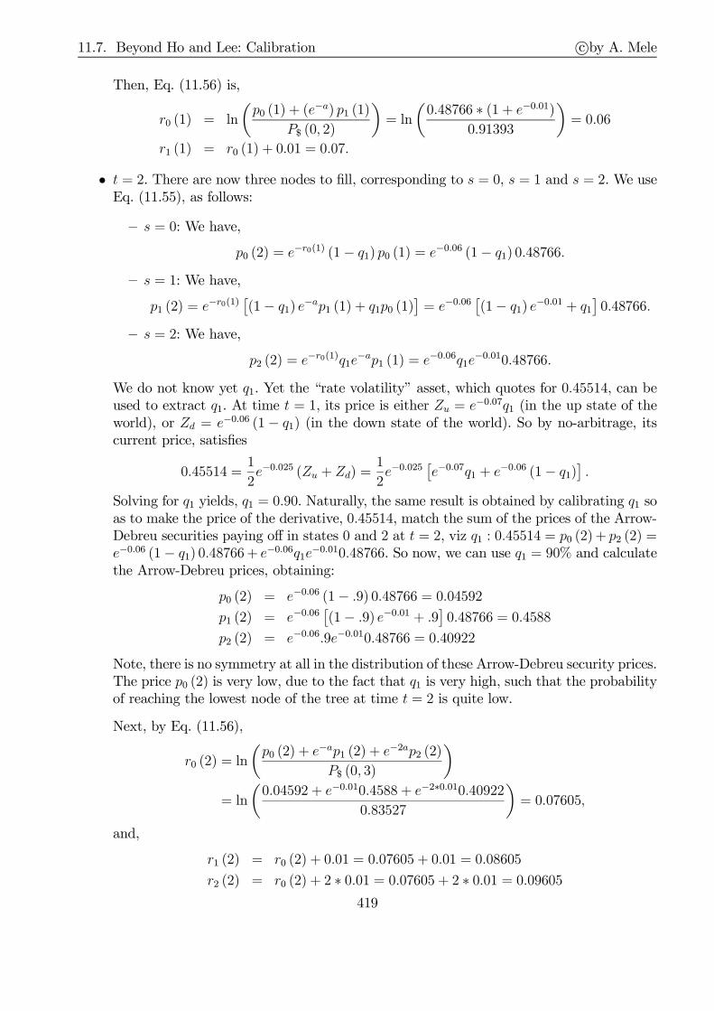
11.7. Beyond Ho and Lee: Calibration c©by A. Mele
Then, Eq. (11.56) is,
r0 (1) = ln
(p0 (1) + (e
−a) p1 (1)
P$ (0, 2)
)= ln
(0.48766 ∗ (1 + e−0.01)
0.91393
)= 0.06
r1 (1) = r0 (1) + 0.01 = 0.07.
• t = 2. There are now three nodes to fill, corresponding to s = 0, s = 1 and s = 2. We useEq. (11.55), as follows:
— s = 0: We have,
p0 (2) = e−r0(1) (1− q1) p0 (1) = e−0.06 (1− q1) 0.48766.
— s = 1: We have,
p1 (2) = e−r0(1) [(1− q1) e−ap1 (1) + q1p0 (1)
]= e−0.06
[(1− q1) e−0.01 + q1
]0.48766.
— s = 2: We have,
p2 (2) = e−r0(1)q1e
−ap1 (1) = e−0.06q1e
−0.010.48766.
We do not know yet q1. Yet the “rate volatility” asset, which quotes for 0.45514, can beused to extract q1. At time t = 1, its price is either Zu = e−0.07q1 (in the up state of theworld), or Zd = e−0.06 (1− q1) (in the down state of the world). So by no-arbitrage, itscurrent price, satisfies
0.45514 =1
2e−0.025 (Zu + Zd) =
1
2e−0.025
[e−0.07q1 + e
−0.06 (1− q1)].
Solving for q1 yields, q1 = 0.90. Naturally, the same result is obtained by calibrating q1 soas to make the price of the derivative, 0.45514, match the sum of the prices of the Arrow-Debreu securities paying off in states 0 and 2 at t = 2, viz q1 : 0.45514 = p0 (2) + p2 (2) =e−0.06 (1− q1) 0.48766+ e−0.06q1e
−0.010.48766. So now, we can use q1 = 90% and calculatethe Arrow-Debreu prices, obtaining:
p0 (2) = e−0.06 (1− .9) 0.48766 = 0.04592
p1 (2) = e−0.06[(1− .9) e−0.01 + .9
]0.48766 = 0.4588
p2 (2) = e−0.06.9e−0.010.48766 = 0.40922
Note, there is no symmetry at all in the distribution of these Arrow-Debreu security prices.The price p0 (2) is very low, due to the fact that q1 is very high, such that the probabilityof reaching the lowest node of the tree at time t = 2 is quite low.
Next, by Eq. (11.56),
r0 (2) = ln
(p0 (2) + e
−ap1 (2) + e−2ap2 (2)
P$ (0, 3)
)
= ln
(0.04592 + e−0.010.4588 + e−2∗0.010.40922
0.83527
)= 0.07605,
and,
r1 (2) = r0 (2) + 0.01 = 0.07605 + 0.01 = 0.08605
r2 (2) = r0 (2) + 2 ∗ 0.01 = 0.07605 + 2 ∗ 0.01 = 0.09605
419

11.7. Beyond Ho and Lee: Calibration c©by A. Mele
Finally, we wish to evaluate a European call option at time zero, written on the three yearzero coupon bond with nominal value equal to £1. This option expires at t = 2 and has a strikeprice equal to £ 0.91000. At expiry, the option pays off:
C2 (2) ≡(e−r2(2) − 0.99
)+=
(e−0.09605 − 0.91
)+= 0
C1 (2) ≡(e−r1(2) − 0.99
)+=
(e−0.08605 − 0.91
)+= 0.00755
C0 (2) ≡(e−r0(2) − 0.99
)+=
(e−0.07605 − 0.91
)+= 0.01677
Then,
Cu = e−r1(1) (q1C2 (2) + (1− q1)C1 (2))
= e−0.07 ∗ (0.9 ∗ 0 + 0.1 ∗ 0.00755) = 7.0396× 10⁻⁴
Cd = e−r0(1) (q1C1 (2) + (1− q1)C0 (2))
= e−0.06 ∗ (0.9 ∗ 0.00755 + 0.1 ∗ 0.01677) = 7.9786× 10⁻³
which leads to C = e−0.025 12(Cu + Cd) = 4.2341× 10⁻³.
Finally, using all the market data so far, we wish to evaluate a second European call optionwritten on the three year bond, expiring in one year, and struck at £ 0.85. Its no-arbitrageprice, denoted with CT , is:
CT = e−0.0251
2
((Pu (1, 3)− 0.85)+ + (Pd (1, 3)− 0.85)+
),
where
Pu (1, 3) = e−r1(1) (q1e−r2(2) + (1− q1) e−r1(2)
)
= e−0.07 ∗(0.90 ∗ e−0.09605 + 0.10 ∗ e−0.08605
)= 0.84786
Pd (1, 3) = e−r0(1) (q1e−r1(2) + (1− q1) e−r0(2)
)
= e−0.06 ∗(0.90 ∗ e−0.08605 + 0.10 ∗ e−0.07605
)= 0.86498
That is, CT = e−0.025 12(0.01498) = 0.00730 × 10⁻³. Suppose, now, that the market value of
this option diverges from CT , i.e. CT = C$, where C$ is the market value of the option. Forexample, CT < C$. To implement this arbitrage opportunity, we can sell the option, and usethe proceeds to build up a portfolio comprising the bond expiring in three years and a moneymarket account, with initial value:
V0 = ∆P$ (0, 3) +M,
where ∆ and M are chosen to match the payoffs promised by the option at time 1:
(∆,M) :
∆Pu (1, 3) +Me
r0 = πu∆Pd (1, 3) +Me
r0 = πd
where πu and πd are the payoffs of the one year option. The solution is,
∆ =πu − πd
Pu (1, 3)− Pd (1, 3), M = e−r0
πdPu (1, 3)− πuPd (1, 3)Pu (1, 3)− Pd (1, 3)
.
420

11.8. Callables, puttable and convertibles with trees c©by A. Mele
Using the numerical values obtained so far, πu = 0, πd = 0.01498, Pu (1, 3) = 0.84786, Pd (1, 3) =0.86498, we have:
∆ =−0.01498
0.84786− 0.86498 = 0.875, M = e−0.025 0.01498 ∗ 0.847860.84786− 0.86498 = −0.72356.
The current value of this portfolio is,
V0 = ∆P$ (0, 3) + M = 0.875 ∗ 0.83527− 0.72356 = 0.00730 = CT .
11.8 Callables, puttable and convertibles with trees
This section provides an introductory discussion about the pricing of callable, puttable andconvertible bonds, with and without credit risk, and develops basic pricing examples for callableand convertibles, relying on binomial trees. Chapter 12 develops a continuous time evaluationframework for callable and puttable bonds, while Chapter 13, contains a continuous time modelto evaluate convertible bonds.
Callable bonds are assets that can be called back by the issuer at a pre-specified strike price,either at a fixed maturity date or at any fixed date before the expiration. The rationale behindthis optionality is that at the date of issuance, the market might not, perhaps, share the sameoptimism as the issuer as regards the issuer’s future creditworthiness. By inserting the indentureto call the bonds, the issuer gives itself the option to refinance at some future date, at bettermarket condition. Although this specific example might link to agency problems or differencein beliefs between the bond issuer and market participants, the indenture to call the bond isan option that might generally arise as a result of pure hedging motives, arising by a concernthat future interest rates might lower.Naturally, the right to call the bonds rises the cost of capital, to the extent of the value of
this (call) option to redeem the bonds. Mathematically, for each point in time τ say, when theoption to redeem the bonds can be exercised at strike K, the value of the bond is:
min Dτ , K = Dτ −max Dτ −K, 0 ,
where Dτ is the time τ present value of the future expected discounted cash flows promised attime τ , by a callable bond with the same strike price K. Indeed, suppose that at τ , interestrates have decreased to an extent to make Dτ > K. In this case, the issuer may proceed toredeem the bonds for K, and issue new callable debt, exercisable at any fixed date before theexpiration, for a price Dτ , thereby cashing in the difference Dτ−K. In doing so, the bond-issueris left with the same optionalities he would have by not exercising the option to call, but withthe additional “money-shower,” Dτ −K. It is, therefore, in the interest of the bond-issuer toexercise at τ , when Dτ > K, and it is obviously not otherwise.
Puttable bonds, instead, are assets that give the holder the right to sell the bonds back tothe issuer at some exercise price, either at a fixed maturity date or any fixed date before theexpiration. The bondholders would exercise their option to tender the bonds to the issuer whenmarket conditions improve from their perspective, i.e. when interest rates are high enough, soas to make bond prices lower than than the exercise price. Issuing puttable bonds, therefore,lowers the cost of capital, to the extend of the value of the (put) option given to the bondholdersto tender the bonds at the strike K. Suppose for example, that the bondholders can exercise
421

11.8. Callables, puttable and convertibles with trees c©by A. Mele
their option at some pre-specified date. In this case, the payoff of the puttable bond is givenby:
max P,K = P +max K − P, 0 ,where P is the price of a non-puttable bond. Indeed, suppose that this price, P , lowers to a levelless than the strike price K. The bondholders, then, will find convenient to tender the bonds atK, buying conventional bonds at P , thereby cashing in K − P , and then wait until maturity.This trade would provide bondholders with a “money-shower” of K − P , at the exercise date.Alternatively, the bondholders would not exercise, and wait until maturity, in which case theywould not receive the profit K − P , at the exercise date. Therefore, it is optimal to exercisewhen K > P , and it is obviously not when K < P .
Convertible bonds are assets that give the holder the right to convert them into a prespecifiednumber of shares of the firm. Their value at each date when the conversion can take place ismax CV, P = P + max CV− P, 0, where CV denotes the conversion value of the bonds,expressed in terms of the valud of the firm’s shares: issuing convertible bonds now lowers thecost of capital to the extent of the option given to the bondholders to convert the bonds intoshares. Convertible bonds can be made callable by the bond-issuers, at a strike K. Usually, ifthe bonds are called, the convertible bondholders have the option to either tender the bonds tothe firm, or to convert them. On the other hand, the only reason the bond-issuers might callis that the price of the convertibles is up, compared to the strike price. Therefore, the optionto make convertible bonds also callable puts a ceiling to the price of the convertibles bonds,given by the exercise price, K. Mathematically, in the presence of callability, the value of aconvertible bond at each potential conversion date is max CV,min P,K: the option to callback takes away some of the optionality from the bondholders, who are, in effect, forced toconvert, as soon as the price P increases to a level beyond K.
11.8.1 Callable bonds
11.8.1.1 Copying with credit risk
To evaluate callable bonds through trees, we may simply follow the methodology in this chapter,corrected for the presence of credit risk.
(i) First, we “populate” a short-term rate tree through one of the models described in thischapter (say, for example, through the Black, Derman and Toy (1990) model).
(ii) Second, we use this tree to find the value of some coupon bearing bond of interest, byjust using the short-term rate process of the previous step.
(iii) Third, we use the results obtained in the second step and build up a tree for the callablebond. In each node immediately preceding the maturity, we compare the strike price withthe non-callable coupon bearing bond price (ex-coupon) and take the minimum of thetwo. We add the coupon to this minimum and find, then, the payoff of the non-callablebond at the relevant node. This gives us V = minK,Brolled-back(ex-coupon) + coupon,where K is the call price, and Brolled-back(ex-coupon) is the ex-coupon bond price, foundfrom the values of the bond V in the next nodes (by using, as usual, recursive, backwardsolution, i.e. the risk-neutral expectation of the future payoffs).
(iv) Fourth, we go backward, discounting the values obtained in the previous steps, V say,obtaining, for each node, V− = minK,V + coupon, etc. Hence, we find the price. If the
422

11.8. Callables, puttable and convertibles with trees c©by A. Mele
callable bond is not subject to default risk, we stop. Otherwise, we proceed to the nextstep.
(v) Fifth, we correct for credit risk. The price we found in the fourth step is typically differentthan the market price. One issue is that the market price reflects the credit risk of thefirm, and should be typically less than the price obtained in the fourth step. The trick,here, is to search for an additional spread to add to the short-term rate process obtainedin the first step, such that the theoretical bond price equals the market price of the bond.This is done numerically, and of course alters the results obtained in steps 3 and 4.
At this point, we may price options written on callable bonds. Ho and Lee (2004) (Chapter8, Section 8.3 p. 274-278) develop a number of useful exercises on the pricing of options oncallable bonds, through tree methods.
11.8.1.2 A numerical example: without credit
To illustrate, let us consider a simpler situation, relating to the pricing of a callable bondwithout credit risk. Assume that the discretely compounded six-month rate, or the “short-termrate,” evolves over time according to the tree described in the following diagram:
%3=r
0=t yearst 5.0= yea rt 1=
%5.3: =ru
%2: =rd
%4: =ru u
%3: =ru d
%5.1: =rd d
%2 5.1: =rdd d
%2: =ru d d
%5.3: =ruu d
%75.4: =ruu u
yea rst 5.1=
FIGURE 11.15.
Next, consider a bond expiring in two years, paying off coupon rates of 3% of the principalof £1 every six months, and callable at any time by the issuer, at par value. Let this bondbe labeled “BCX.” Suppose that the prices of three zero coupon bonds expiring in one year,eighteen months and two years are, respectively, 0.94632, 0.91876 and 0.89166. We can usethese market data to calibrate the risk-neutral probabilities of upward movements in the short-term rate implied by the binomial tree in Figure 11.15, provided these risk-neutral probabilitiesdepend only on calendar time t, not on the specific state of nature at time t.We assume that available for trading is also a conventional, (i.e. non-callable) bond maturing
in two years and paying coupons semiannually, at 3% of the principal of £1. We wish tocalculate the price movements of the non-callable coupon-bearing two year bond. We have,
423

11.8. Callables, puttable and convertibles with trees c©by A. Mele
P$ (0, 0.5) =1
1.03= 0.97087. Furthermore, as regards the zero expiring in one year:
P$ (0, 1) = 0.94632 = P$ (0, 0.5) ∗(q0
1
1.035+ (1− q0)
1
1.02
),
which solved for q0 delivers q0 = 0.40. As for the zero expiring in 1.5 years,
P$ (0, 1.5) = 0.91876 = P$ (0, 0.5) ∗ (q0PU (0.5, 1.5) + (1− q0)PD (0.5, 1.5))= 0.97087 ∗ (0.40 ∗ PU (0.5, 1.5) + 0.60 ∗ PD (0.5, 1.5)) ,
where
PU (0.5, 1.5) =1
1.035
(q1
1
1.04+ (1− q1)
1
1.03
), PD (0.5, 1.5) =
1
1.02
(q1
1
1.03+ (1− q1)
1
1.015
)
Solving for q1 leaves q1 = 0.70. As for the zero expiring in 2 years:
P$ (0, 2) = 0.89166 = P$ (0, 0.5) ∗ (q0PU (0.5, 2) + (1− q0)PD (0.5, 2))= 0.97087 ∗ (0.40 ∗ PU (0.5, 2) + 0.60 ∗ PD (0.5, 2)) ,
where
PU (0.5, 2) =1
1.035(q1PUU (1, 2) + (1− q1)PUD (1, 2))
=1
1.035(0.70 ∗ PUU (1, 2) + 0.30 ∗ PUD (1, 2))
PD (0.5, 2) =1
1.02(q1PUD (1, 2) + (1− q1)PDD (1, 2))
=1
1.02(0.70 ∗ PUD (1, 2) + 0.30 ∗ PDD (1, 2))
and:
PUU (1, 2) =1
1.04
(q2
1
1.0475+ (1− q2)
1
1.035
)
PUD (1, 2) =1
1.03
(q2
1
1.035+ (1− q2)
1
1.02
)
PDD (1, 2) =1
1.015
(q2
1
1.02+ (1− q2)
1
1.0125
)
Solving for q2 leaves q2 = 0.60.The price of a coupon bearing bond yielding 3% of the principal every six months is easy to
calculate,
B (0, 2) = 0.03 ∗ (0.97087 + 0.94632 + 0.91876 + 0.89166) + 0.89166 = 1.0035. (11.57)
Given the market data and the previously calibrated risk-neutral probabilities, we now pro-ceed with the calculation of the price of the callable coupon bearing bond. We discount theexpected cash flows, through the evaluation formula, minD, 1+ 0.03, where D is the presentvalue of the future expected discounted cash flows promised at each node by a callable bondwith the same strike price K. We have:
424

11.8. Callables, puttable and convertibles with trees c©by A. Mele
(i) At t = 1.5 years,
— uuu: 1.031.0475
= 0.98329 vs 1⇒ wait, and the value of the callable bond is 0.98329.
— uud: 1.031.035
= 0.99517 vs 1⇒ wait, and the value of the callable bond is 0.99517.
— udd: 1.031.02
vs 1⇒ exercise, and the value of the callable bond is 1.
— ddd: 1.031.0125
vs 1⇒ exercise, and the value of the callable bond is 1.
(ii) At t = 1 year, we have that q = 60%, and, then:
— uu: 11.04
[0.6
(1.03
1.0475+ 0.03
)+ 0.4
(1.031.035
+ 0.03)]= 0.97889 vs 1⇒ wait, and the value
of the callable bond is 0.97889.
— ud: 11.03
[0.6
(1.031.035
+ 0.03)+ 0.4 (1 + 0.03)
]= 0.99719 vs 1 ⇒ wait, and the value of
the callable bond is 0.99719.
— dd: 11.0015
[0.6 (1 + 0.03) + 0.4 (1 + 0.03)] = 1.0285 vs 1 ⇒ exercise, and the value ofthe callable bond is 1.
(iii) At t = 0.5 years, we have that q = 70%, and, then:
— u: 11.035
[(0.7 ∗ 0.97889 + 0.3 ∗ 0.99719) + 0.03] = 0.98008 vs 1 ⇒ wait, and the valueof the callable bond is 0.98008.
— d: 11.02
[(0.7 ∗ 0.99719 + 0.3 ∗ 1) + 0.03] = 1.0079 vs 1 ⇒ exercise, and the value ofthe callable bond is 1.
Finally, at the time of evaluation, we have that q = 40%, and, then, the price of the callablebond is:
P c =1
1.03(0.40 ∗ 0.98008 + 0.60 ∗ 1 + 0.03) = 0.99226.
Naturally, the callable bond is valued less than the conventional bond B (0, 2) in Eq. (11.57):the difference is the value of the option given to the issuer to redeem these bonds, and ariseswhen the interest rates go sufficiently down–negative convexity.How would one proceed to price the BCX bond, if we the previous market data were unavail-
able, and, then, we assumed that: (i) the risk-neutral probabilities of upward movements in theshort-term rate are: (i.a) unknown from time zero to 0.5 years; (i.b) 70%, from 0.5 to one year;and (i.c) 60%, from one to 1.5 years; (ii) available for trading is a European call option writtenon the BCX bond; (iii) this option, which quotes for £ 1.7226 × 10⁻³, expires in 1.5 years, isstruck at £ 0.99000, and becomes worthless as soon as the underlying callable bond is calledback by the issuer? First, note that at the expiration, t = 1.5 years, the payoffs of the optionare:
Cuuu = 0, Cuud = 0.00517,
and, because of the sudden death assumption,
Cudd = Cddd = 0.00000.
425

11.8. Callables, puttable and convertibles with trees c©by A. Mele
At t = 1 year, we have that q = 60%, and, then:
Cuu =1
1.04(0.6 ∗ 0 + 0.4 ∗ 0.00517) = 1.9885× 10⁻³
Cud =1
1.03(0.6 ∗ 0.00517 + 0.4 ∗ 0) = 3.0117× 10⁻³
Cdd = 0
At t = 0.5 years, we have that q = 70%, and, then:
Cu =1
1.035(0.70 ∗ Cuu + 0.30 ∗ Cud)
=1
1.035
(0.70 ∗ 1.9885× 10−3 + 0.30 ∗ 3.0117× 10−3
)= 2.2178× 10⁻³.
Cd = 0, by the sudden death assumption.
At the time of evaluation, the price of the call is,
C = 1.7226× 10−3 =1
1.03(qCu + (1− q)Cd) =
1
1.03∗ q ∗ 2.2178× 10⁻³,
where q is the risk-neutral probability of an upward movement in the short-term rate duringthe first six months. We can solve for this q, obtaining q = 80%. Finally, given this probability,we can calculate the price of the callable bond. We have:
P c =1
1.03(0.80 ∗ 0.98008 + 0.20 ∗ 1 + 0.03) = 0.98453.
It is lower than the price calculated earlier, because the price of the option is giving more weight(80%) than before (40%) to the occurrence of the state of the world where the interest rategoes up.
11.8.2 Convertible bonds
11.8.2.1 Evaluation issues
Consider the following convertible and callable bond. Let K be the strike at which the bondcan be called by the bond-issuer, and let the parity, or conversion value, be CV = CR × S,where S is the price of the common share. To evaluate this bond through a binomial tree, wemay proceed through the following three steps:
(i) First, we set the life of the tree equal to the life of the callable convertible bond.
(ii) Second, we assess the evolution of the stock price along the tree, under the risk-neutralprobability. This is done following the standard Cox, Ross and Rubinstein (1979) ap-proach.
(iii) Third, in each node, we compute the value of the bond as maxCV,minB,K, whereB is the value of the bond, “rolled-back” from the values of the bond in the next nodesthrough the usual recursive, backward method–relying on calculating the present valueof the risk-neutral expectation of the future payoffs. That is, assuming the bondholderdoes not convert, the value is B∗ = min B,K, where B is the “rolled-back” value ofthe bond. Then, the value is maxCV, B∗.
426

11.8. Callables, puttable and convertibles with trees c©by A. Mele
Note, this procedure leads to fill in the nodes, once we know the appropriate interest rate.If the firm was not subject to default risk, we would simply use the riskless interest rate.However, the firm is obviously subject to default risk. In practice, we proceed as follows. Ineach node, the value of the bond is decomposed into two parts. One part, related to the “puredebt component,” discounted at the defaultable interest rate; and one part related to the “pureequity component,” discounted at the default-free interest rate. Exercise 25.7 in Hull (2003) (p.653-654) illustrates a specific example.
11.8.2.2 A numerical example: without credit
[The example is in this file:C:\antonio\lectures\drafts & related\Convertibles_exercise\Convertible_exercise.rap]
427

11.9. Appendix 1: Proof of Eq. (11.16) c©by A. Mele
11.9 Appendix 1: Proof of Eq. (11.16)
Let P (r, Ti) denote the price of a zero with maturity Ti, i = 1, 2, when the interest rate is equal tor. We wish to replicate a zero with maturity T2 by means of a portfolio that includes a zero withmaturity T1. Consider the following portfolio: (i) Go long ∆ zeros with maturity T1 and (ii) investM in the MMA. Let V0 be the current value of this portfolio. V0 is clearly a function of the currentshort-term rate r, and equals,
V0 (r) = ∆ · P (r, T1) +M.
In the second period, the value of the portfolio is random, as it depends on the development of theshort-term rate r. Precisely, the value of the portfolio in the second period, is
V (r) =
V (r+) = ∆ · P (r+, T1) +M · (1 + r), with probability pV (r−) = ∆ · P (r−, T1) +M · (1 + r), wit probability 1− p
We also know that in the second period, the value of the second zero is,
P (r, T2) =
P (r+, T2) , with probability pP (r−, T2) , with probability 1− p
Next, we select ∆ and M to make the value of the portfolio equal the value of the second zero, in eachstate of nature, viz
V (r) = P (r, T2) , in each state.
Mathematically, this is tantamount to solving the following system of two equations with two unknowns(∆ and M),
V (r+) = ∆ · P (r+, T1) +M · (1 + r) = P (r+, T2)V (r−) = ∆ · P (r−, T1) +M · (1 + r) = P (r−, T2)
(11A.1)
The solution is,
∆ =P (r+, T2)− P (r−, T2)
P (r+, T1)− P (r−, T1), M =
P (r−, T2)P (r+, T1)− P (r+, T2)P (r−, T1)
[P (r+, T1)− P (r−, T1)] (1 + r).
By construction, the previous portfolio, (∆, M), replicates the value of the second zero in the secondperiod. But if two assets (the portfolio, and the second zero) yield the same payoffs in each state ofthe nature, they must be worth the same, in the absence of arbitrage. Therefore, we must have,
V0 (r)|∆=∆,M=M = ∆ · P (r, T1) + M = P (r, T2) ,
or,
(1 + r) M = (1 + r)P (r, T2)− (1 + r) ∆ · P (r, T1) . (11A.2)
Next, let us figure out the prediction of the model in terms of the expected return it generates forthe price of the bond maturing at T1, when (∆,M) = (∆, M). To do this, multiply the first equation in(11A.1) by p, and multiply the second equation in (11A.1) by 1−p. Add the result for ∆ = ∆,M = Mto obtain,
∆ ·[pP (r+, T1) + (1− p)P (r−, T1)
]+ M · (1 + r) = pP (r+, T2) + (1− p)P (r−, T2).
Replacing (11A.2) into the previous equation yields,
∆ ·[(pP (r+, T1) + (1− p)P (r−, T1)
)− (1 + r)P (r, T1)
]
=[pP (r+, T2) + (1− p)P (r−, T2)
]− (1 + r)P (r, T2) .
428

11.9. Appendix 1: Proof of Eq. (11.16) c©by A. Mele
Finally, replacing the solution for ∆ into the previous equation leaves,
[pP (r+, T1) + (1− p)P (r−, T1)]− (1 + r)P (r, T1)
P (r+, T1)− P (r−, T1)=
[pP (r+, T2) + (1− p)P (r−, T2)]− (1 + r)P (r, T2)
P (r+, T2)− P (r−, T2).
The previous equation is easy to interpret. The numerators are the expected excess returns fromholding the assets. They equal Ep [P (r, Ti)]− (1 + r)P (r, Ti), where Ep [P (r, Ti)] is what the investorsexpect to receive, the next period, by investing £P (r, Ti) today, in the bond; and (1 + r)P (r, Ti)is what the investors expect to receive, the next period, by investing £P (r, Ti) today, in the MMA.The denominators constitute a measure of volatility related to holding the assets. Then, the previousequation tells us that the Sharpe ratios, or the unit risk premiums, on the two zeros agree.
Let the Sharpe ratio on any zero be equal to some function λ of the short-term rate r only (andpossibly of calendar time). This function, λ, does not clearly depend on the maturity of the zeros.Then, we have,
[pP (r+, T1) + (1− p)P (r−, T1)
]− (1 + r)P (r, T1) =
[P (r+, T1)− P (r−, T1)
]λ
=P (r+, T1)− P (r−, T1)
r+ − r−· [(r+ − r−)λ]. (11A.3)
We can interpret (r+ − r−) as a measure of interest rate volatility, and define Vol(r − r) ≡ (r+ − r−).Eq. (11.16) follows by rewriting Eq. (11A.3) for a generic maturity date T > 2.
429
11.10. Appendix 2: Proof of Eq. (11.31) c©by A. Mele
11.10 Appendix 2: Proof of Eq. (11.31)
Define the discretely compounded forward rate, as the number FT (τ) ≡ F (τ, T, T + 1), satisfying:P (τ,T+1)P (τ,T ) = 1
1+FT (τ), as in Eq. (11.1) of the main text. Iterating this equation leaves:
P (τ, T ) =T−1∏
S=τ
1
1 + FS (τ)=
P (t, T )
P (t, τ)
P (t, τ)
P (t, T )
T−1∏
S=τ
1
1 + FS (τ).
Therefore, at any instant of time t : t < τ < T , we have that,
P (τ, T ) =P (t, T )
P (t, τ)
T−1∏
S=τ
1 + FS (t)
1 + FS (τ). (11A.4)
Eq. (11A.4) gives us the price of the bond at a future date τ . It reveals that the price P (τ, T ) as oftime τ can be expressed as a function of the current bond prices P (t, T ) and P (t, τ), and how forwardrates will change from the current time t to the time τ at which the derivative payoff will be paid,i.e. 1+FS(t)
1+FS(τ), for S = τ, · · · , T − 1. Hence, once we model the evolution of forward rates, we also have
a model of the future bond price movements, P (τ, T ), which we can use to price, at the evaluationtime t, interest rate derivatives, with payoffs depending on the realization of the bond price P (τ, T )at time τ .
To normalize the time-line, we now set t = 0. Redefining τ = t, Eq. (11A.4) then reduces to,
P (t, T ) =P (0, T )
P (0, t)
T−1∏
S=τ
1 + FS (0)
1 + FS (t). (11A.5)
It is quite natural, at this juncture, to search for the model’s predictions about the evolution offuture forward rates. Not only is this task theoretically important, it is also relevant as a matter ofthe practical implementation of the model. Indeed, if the model’s predictions about the evolution offuture forward rates yields a closed-form solution, the bond price at the future date t, P (t, T ), couldbe expressed in a closed-form, which might facilitate the implementation details of the model.
Let us introduce some further notation. Let F jS (t) be the forward rate as of time t after the occur-
rence of j upward movements in the bond price, and let the continuously compounded forward rateF jS (t) be defined as,
F jS (t) ≡ ln
(1 + F j
S (t)), j ≤ t.
By Eq. (11A.5), then,
Pj (t, T ) =P (0, T )
P (0, t)
T−1∏
S=t
1 + FS (0)
1 + F jS (t)
=P (0, T )
P (0, t)e−
∑T−1S=t (F
jS(t)−FS(0)). (11A.6)
We have the following important result, which we shall prove later on:
F jS (t) = FS (0) + ln
u (S + 1− t)
u (S + 1)− (t− j) ln δ, j ≤ t. (11A.7)
By replacing Eq. (11A.7) into Eq. (11A.6), and using the solution for the perturbation function u (·)in Eqs. (11.29), we get Eq. (11.31).
So we are left with proving Eq. (11A.7). The proof proceeds by induction. Eq. (11A.7) holds truefor t = 0. Next, suppose that it holds at time t. We wish to show that in this case, Eq. (11A.7) wouldalso hold at time t+ 1. At time t+ 1, we have two cases.
430

11.10. Appendix 2: Proof of Eq. (11.31) c©by A. Mele
Case 1 : A positive price jump occurs between time t and time t+ 1. In this case,
F j+1S (t+ 1) = ln
Pj+1 (t+ 1, S)
Pj+1 (t+ 1, S + 1)
= ln
[u (S − t)
Pj (t, S)
Pj (t, t+ 1)
]− ln
[u (S + 1− t)
Pj (t, S + 1)
Pj (t, t+ 1)
]
= lnu (S − t)
u (S + 1− t)+ F j
S (t)
= lnu (S + 1− (t+ 1))
u (S + 1)+ FS (0)− [(t+ 1)− (j + 1)] ln δ,
where the first equality and the third follow by the definition of F j+1S (t), the second equality holds by
the definition of the jump in Eq. (11.24), the fourth equality follows by using Eq. (11A.7). Hence, Eq.(11A.7) holds at time t+ 1 in the occurrence of a positive price jump between time t and time t+ 1.
Case 2 : A negative price jump occurs between time t and time t+ 1. In this case,
F jS (t+ 1) = ln
Pj (t+ 1, S)
Pj (t+ 1, S + 1)
= ln
[d (S − t)
Pj (t, S)
Pj (t, t+ 1)
]− ln
[d (S + 1− t)
Pj (t, S + 1)
Pj (t, t+ 1)
]
= lnd (S − t)
d (S + 1− t)+ F j
S (t)
= lnd (S − t) δ−(S−t)+1
d (S + 1− t) δ−(S+1−t)+1δ−1 + FS (0) + ln
u (S + 1− t)
u (S + 1)− (t− j) ln δ
= lnu (S − t)
u (S + 1)+ FS (0)− [(t+ 1)− j] ln δ,
where the first four equalities follow by the same arguments produced in Case 1, the fifth equalityholds by the relation u (T ) = d (T ) δ−(T−1) in Eq. (11.28) and the last equality follows by rearrangingterms. Hence, Eq. (11A.7) holds at time t+1 in the occurrence of a negative price jump between timet and time t+ 1.
These two cases reveal that if Eq. (11A.7) holds at time t for any j ≤ t, it also holds at time t+ 1,in each state of nature. By induction, Eq. (11A.7) is therefore true.
431

11.10. Appendix 2: Proof of Eq. (11.31) c©by A. Mele
References
Bernanke, B. S. and A. Blinder (1992): “The Federal Funds Rate and the Channels of MonetaryTransmission.” American Economic Review 82, 901-921.
Black, F. and M. Scholes (1973): “The Pricing of Options and Corporate Liabilities.” Journalof Political Economy 81, 637-659.
Black, F., E. Derman and W. Toy (1990): “A One Factor Model of Interest Rates and itsApplication to Treasury Bond Options.” Financial Analysts Journal (January-February),33-39.
Cox, J. C., S. A. Ross and M. Rubinstein (1979): “Option Pricing: A Simplified Approach.”Journal of Financial Economics 7, 229-263.
Diebold, F. X. and C. Li (2006): “Forecasting the Term Structure of Government Bond Yields.”Journal of Econometrics 130, 337-364.
Heath, D., R. Jarrow and A. Morton (1992): “Bond Pricing and the Term-Structure of InterestRates: a New Methodology for Contingent Claim Valuation.” Econometrica 60, 77-105.
Ho, T. S. Y. and S.-B. Lee (1986): “Term Structure Movements and the Pricing of InterestRate Contingent Claims.” Journal of Finance 41, 1011-1029.
Ho, T. S. Y. and S.-B. Lee (2004): The Oxford Guide to Financial Modeling. Oxford UniversityPress.
Hull, J. C. (2003): Options, Futures, and Other Derivatives. Prentice Hall. 5th edition (Inter-national Edition).
Hull, J. C. and A. White (1990): “Pricing Interest Rate Derivative Securities.” Review ofFinancial Studies 3, 573-592.
McCulloch, J. (1971): “Measuring the Term Structure of Interest Rates.” Journal of Business44, 19-31.
McCulloch, J. (1975): “The Tax-Adjusted Yield Curve.” Journal of Finance 30, 811-830.
Nelson, C.R. and A.F. Siegel (1987): “Parsimonious Modeling of Yield Curves.” Journal ofBusiness 60, 473-489.
Tuckman, B. (2002): Fixed Income Securities. Wiley Finance.
Vasicek, O. (1977): “An Equilibrium Characterization of the Term Structure.” Journal ofFinancial Economics 5, 177-188.
432
12Interest rates
12.1 Prices and interest rates
12.1.1 Introduction
A pure-discount, or zero-coupon, bond is a contract that guarantees one unit of numéraire atsome maturity date. Apart from isolated exceptions, we only consider pure-discount bonds,which we will then simply call bonds, to simplify the exposition. Except for Section 12.3.6,we assume no default risk. Default risk is, instead, more systematically dealt with in the nextchapter.Let [t, T ] be a fixed time interval, and for each τ ∈ [t, T ], let P (τ , T ) be the price as of
time τ of a bond maturing at T > t. The information in this chapter is Brownian, exceptfor the jump-diffusion models in Section 12.3.6. The price of a bond in this chapter, then, isdriven by some multidimensional diffusion process (y (τ))τ≥t, which we emphasize by writingP (y (τ) , τ , T ) ≡ P (τ , T ). As an example, y can be a scalar diffusion, and r = y can be theshort-term rate. In this particular example, bond prices are driven by short-term rate movementsthrough the bond pricing function P (r, τ , T ). The exact functional form of the pricing functionis determined by (i) the assumptions made as regards the short-term rate dynamics and (ii)the Fundamental Theorem of Asset Pricing (henceforth, FTAP). The bond pricing function inthe general multidimensional case is obtained following the same route. Models of this kind arepresented in Section 12.3.A second class of models is one where bond prices cannot be expressed as a function of
any state variable. Rather, current bond prices are taken as primitives, and forward rates(i.e., interest rates prevailing today for borrowing in the future) are multidimensional diffusionprocesses. There is a relation linking bond prices to forward rates. The FTAP restricts thedynamic behavior of future bond prices and forward rates. Models belonging to this secondclass are analyzed in Section 12.4.The aim of this chapter is to develop the simplest foundations of the previously described
two approaches to interest rate modeling. In the next section, we provide definitions of interestrates and markets. Section 12.1.2 develops the two basic representations of bond prices: one interms of the short-term rate; and the other in terms of forward rates. Section 11.2.3 develops

12.1. Prices and interest rates c©by A. Mele
the foundations of the so-called forward martingale probability, which is a probability measureunder which forward interest rates are martingales. It is an important tool of analysis. [ ... ]
12.1.2 Bond prices
12.1.2.1 A first representation of bond prices
Consider the relation linking bond prices, P , to discretely compounded interest rates, L for thetime interval [τ , T ], introduced in Section 11.2.2.1 of the previous chapter:
P (τ , T ) =1
1 + (T − τ )L(τ , T ) . (12.1)
Given L(τ , T ), the short-term rate process r is obtained as:
r (τ ) ≡ limT↓τ
L (τ , T ) .
Next, let Q be a risk-neutral probability probability, and Eτ [·] denote the time τ conditionalexpectation under Q. By the FTAP, there are no arbitrage opportunities if and only if P (τ , T )satisfies, for all τ ∈ [t, T ],
P (τ , T ) = Eτ[e−
∫ Tτ r(ℓ)dℓ
], (12.2)
Appendix 1 provides the proof of the if-part–there is no arbitrage if bond prices are as in Eq.(12.2). This proof is quite standard, in fact similar to those encountered in the first part of theseLectures. It is provided here, as it is capable of highlighting specific issues relating to interestrate modeling.
12.1.2.2 Forward rates, and a second representation of bond prices
Forward rates are interest rates that make the value of a forward rate agreement (FRA, hence-forth) equal to zero at origination. Section 11.2.2.3 of the previous chapter provides the def-inition of a forward rate agreement, although the very same definition is restated below, forreasons clarified in a moment. Forward rates as of time t, for a forward rate agreement relatingto a future time-interval [T, S], are denoted with F (t, T, S), and link to bond prices through aprecise relation, derived in Section 11.2.2.3 of the previous chapter:
P (t, T )
P (t, S)= 1 + (S − T )F (t, T, S) . (12.3)
Clearly, the forward rate agreed at T for the time interval [T, S] is the short-term rate applyingto the same period:
F (T, T, S) = L (T, S) . (12.4)
Consider, next, a more general FRA, where a first counterparty agrees: (i) to pay an interestrate on a given principal at time T , fixed at some K = F (t, T, S), and (ii) to receive, inexchange, the future interest rate prevailing at time T for the time interval [T, S], L (T, S),from a second counterparty. The profit at T , arising from this “interest rate swap” is:
(S − T ) [L (T, S)−K] . (12.5)
It is the same as the profit to a party who is long a FRA, who therefore enters the FRA, at timet, for the time-interval [T, S], as a future borrower. Come time T , the party shall honour the
434

12.1. Prices and interest rates c©by A. Mele
FRA by borrowing $1 for the time-interval [T, S] at a cost of K. At the same time, the partycan lend this very same $1 at the random interest rate L (T, S). The time S payoff derivingfrom this trade is, of course, the same as that in Eq. (12.5).The value of the FRA, which we denote as IRS(t, T, S;K), is the current market value of this
future, random payoff. By the FTAP,
IRS (t, T, S;K) = Et[e−
∫ St r(τ)dτ (S − T ) [L (T, S)−K]
]
= (S − T )Et[e−
∫ St r(τ)dτL (T, S)
]− (S − T )P (t, S)K
= Et
[e−
∫ St r(τ)dτ
P (T, S)
]− [1 + (S − T )K]P (t, S)
= P (t, T )− [1 + (S − T )K]P (t, S) , (12.6)
where the second line holds by the definition of L and the third line follows by the followingrelation:1
P (t, T ) = Et
[e−
∫ St r(τ)dτ
P (T, S)
]. (12.7)
Finally, by replacing Eq. (12.3) into Eq. (12.6),
IRS (t, T, S;K) = (S − T ) [F (t, T, S)−K]P (t, S) . (12.8)
As is clear, IRS can take on any sign, and is exactly zero whenK = F (t, T, S), where F (t, T, S)solves Eq. (12.3). The notation, IRS (·), is used to emphasize that we are dealing with interestrate swaps, although more rigorously, interest rate swaps are those where payment exchangeswill occur, repeatedly, over a given time horizon–the tenor of the swap, as explained in Section12.5.7.A useful remark. Comparing the second line in Eq. (12.6) with Eq. (12.8) reveals that:
F (t, T, S) = Et
[e−
∫ St r(τ)dτ
P (t, S)L (T, S)
].
That is, forward rates are not unbiased expectations of future interest rates, not even underthe risk-neutral probability. We shall return to this point in Section 12.1.3.2.Bond prices can be expressed in terms of these forward interest rates, namely in terms of the
“instantaneous” forward rates. First, rearrange terms in Eq. (12.3) so as to obtain:
F (t, T, S) = −P (t, S)− P (t, T )(S − T )P (t, S) .
1To show that Eq. (12.7) holds, suppose that at time t, $P (t, T ) are invested in a bond maturing at time T . At time T , thisinvestment will obviously pay off $1. And at time T , $1 can be further rolled over another bond maturing at time S, thus yielding$ 1/P (T, S) at time S. Therefore, it is always possible to invest $P (t, T ) at time t and obtain a “payoff” of $ 1/P (T, S) at timeS. By the FTAP, there are no arbitrage opportunities if and only if Eq. (12.7) holds true. Alternatively, use the law of iterated
expectations to obtain
Et
[e−
∫ Str(τ)dτ
P (T, S)
]
= Et
[
E
(e−
∫Ttr(τ)dτ e−
∫STr(τ)dτ
P (T, S)
∣∣∣∣∣F(T )
)]
= P (t, T ).
435

12.1. Prices and interest rates c©by A. Mele
The instantaneous forward rate f(t, T ) is defined as
f(t, T ) ≡ limS↓T
F (t, T, S) = −∂ lnP (t, T )∂T
. (12.9)
It can be interpreted as the marginal rate of return from committing a bond investment for anadditional instant. To express bond prices in terms of f , integrate Eq. (12.9), f(t, ℓ) = −∂ lnP (t,ℓ)
∂ℓ,
with respect to the maturity date ℓ, use the condition that P (t, t) = 1, and obtain:
P (t, T ) = e−∫ Tt f(t,ℓ)dℓ. (12.10)
12.1.2.3 The marginal nature of forward rates
Consider the yield-to-maturity introduced in Section 11.2.2.2 of the previous chapter, definedto be the function R (t, T ) such that:
P (t, T ) ≡ e−(T−t)·R(t,T ). (12.11)
Comparing Eq. (12.11) with Eq. (12.3) yields:
R(t, T ) =1
T − t
∫ T
t
f(t, τ )dτ . (12.12)
By differentiating Eq. (12.12) with respect to T yields:
∂R(t, T )
∂T=
1
T − t [f(t, T )−R(t, T )] .
This relation underscores the “marginal nature” of forward rates: the yield-curve, R (t, T ), isincreasing in, decreasing in, or stationary at T , according to whether f (t, T ) exceeds, is lower,or equal the spot rate for maturity T .
12.1.3 Forward martingale probabilities
12.1.3.1 Definition
Let ϕ(t, T ) be the T -forward price of a claim S(T ) at T . That is, ϕ(t, T ) is the price agreed att, which will be paid at T for delivery of the claim at T . Nothing has to be paid at t. By theFTAP, there are no arbitrage opportunities if and only if:
0 = Et[e−
∫ Tt r(u)du · (S(T )− ϕ(t, T ))
].
But since ϕ(t, T ) is known at time t,
Et[e−
∫ Tt r(u)du · S(T )
]= ϕ(t, T ) · Et
[e−
∫ Tt r(u)du
]. (12.13)
For example, assume S is the price process of a traded asset. By the FTAP, Et[e−∫ T
tr(u)duS(T )] =
S(t), such that Eq. (12.13) collapses to the well-known formula: ϕ(t, T )P (t, T ) = S(t). However,entering the forward contract originated at t, at a later date τ > t, costs. To calculated themarking-to-market of the forward at time τ , note that the final payoff at time T is S(T )−ϕ(t, T ).Discounting this payoff at τ ∈ [t, T ] delivers P (τ , T ) · [ϕ(τ , T )− ϕ(t, T )].
436
12.1. Prices and interest rates c©by A. Mele
Next, let us elaborate on Eq. (12.13). We can use the bond pricing equation (12.2), andrearrange terms in Eq. (12.13), to obtain:
ϕ(t, T ) = Et
[e−
∫ Tt r(u)du
P (t, T )· S(T )
]= Et [ηT (T ) · S(T )] , (12.14)
where
ηT (T ) ≡e−
∫ Tt r(u)du
P (t, T ).
Eq. (12.14) suggests that we can define a new probability QTF , as follows,
ηT (T ) =dQT
F
dQ≡ e−
∫ Ttr(u)du
Et[e−
∫ Ttr(u)du
] . (12.15)
Naturally, Et[ηT (T )] = 1. Moreover, if the short-term rate process is deterministic, ηT (T ) equalsone and Q and QT
F are the same.In terms of this new probability QT
F , the forward price ϕ(t, T ) is:
ϕ(t, T ) = Et [ηT (T ) · S(T )] =∫[ηT (T ) · S(T )] dQ =
∫S(T )dQT
F = EQTF [S(T )] , (12.16)
where EQTF [·] denotes the time t conditional expectation taken under QTF . For reasons that will
be clear in a moment, QTF is referred to as the T -forward martingale probability. The forward
martingale probability is a useful tool, which helps price interest-rate derivatives, as we shallexplain in Section 12.7. It was introduced by Geman (1989) and Jamshidian (1989), and furtheranalyzed by Geman, El Karoui and Rochet (1995). The appendix provides additional details:Appendix 2 relates forward prices to their certainty equivalent, and Appendix 3 illustratesadditional technicalities about the forward martingale probability.
12.1.3.2 Martingale properties
Forward prices
Clearly, ϕ(T, T ) = S(T ). Therefore, Eq. (12.16) is, also,
ϕ(t, T ) = EQTF [ϕ(T, T )] .
Forward rates, and the expectation theory
Forward rates display a similar property:
f(t, T ) = EQTF [r(T )] = EQTF [f(T, T )] . (12.17)
437
12.1. Prices and interest rates c©by A. Mele
where the last equality holds as r(t) = f(t, t). The proof is also simple. We have,
f(t, T ) = −∂ lnP (t, T )∂T
= −∂P (t, T )∂T
/P (t, T )
= Et
[e−
∫ Tt r(τ)dτ
P (t, T )· r(T )
]
= Et [ηT (T ) · r(T )]
= EQTF [r(T )] .
Finally, the simply-compounded forward rate satisfies the same property: given a sequenceof dates Tii=0,1,···,
F (τ , Ti, Ti+1) = EQTi+1F
[L (Ti, Ti+1)] = EQTi+1F
[F (Ti, Ti+1)] , τ ∈ [t, Ti] , (12.18)
where the second equality follows by Eq. (12.4). To show Eq. (12.18), note that by definition,the simply-compounded forward rate F (t, T, S) satisfies:
IRS(t, T, S;F (t, T, S)) = 0,
where IRS(t, T, S;K) is the value as of time t of a FRA struck at K for the time-interval [T, S].By rearranging terms in the second equality of Eq. (12.6),
F (t, T, S)P (t, S) = Et[e−
∫ St r(τ)dτL(T, S)
].
By the definition of ηS(S),F (t, T, S) = EQSF [L(T, S)] .
A well-known hypothesis in empirical finance is that known as the expectation theory, whichstates that forward rates equal future expected short-term rates. The empirical evidence aboutthe expectation theory is reviewed in Section 12.2.1, but the previous relation already pointsto a difficulty in this theory. It shows that it is under the forward martingale probability thatthe expectation theory holds true. A similar result holds for the instantaneous forward rate.Consider Eq. (12.17). We have,
f (t, T ) = EQTF (r(T ))
= EQ (ηT (T ) r(T ))
= E (ηT (T ))︸ ︷︷ ︸=1
E (r(T )) + covQ (ηT (T ) , r(T ))
= Et (r(T )) + covt (Ker (T ) , r(T )) + covQ,t (ηT (T ) , r(T )) , (12.19)
where Ker(T ) denotes the pricing kernel in the economy. That is, forward rates in generaldeviate from future expected short-term rates because of risk-aversion corrections (the secondterm in the last equality) and because interest rates are stochastic (the third term in the lastequality).
438
12.2. Stylized facts c©by A. Mele
12.1.4 Stochastic duration
Cox, Ingersoll and Ross (1979) introduce the notion of stochastic duration, which generalizesthat of modified duration discussed in Chapter 11. Suppose the bond price is a function of theshort term rate only, P (r, T − t). Duration is a measure of risk for fixed income instruments.Define the basis risk as the semi-elasticity of the bond price with respect to the short-term rate,
Ψ(r, T − t) ≡ −Pr (r, T − t)P (r, T − t) ,
where the subscript r denotes a partial derivative. Naturally, we want to make sure that themeasure of duration for a zero coupon bond equals time-to-maturity, such that Ψ cannot rep-resent a measure of duration, since in general, it does not equal T − t, except in the trivial casethe short-term rate, r, is constant.The idea underlying “stochastic duration” is to find a zero coupon bond with basis risk equal
to the basis risk of a coupon bearing bond, or in general, any other bond, say for instance acallable bond, as follows:
Ψ(r, T ∗ − t) = −Br (r, S − t)B (r, S − t) ,
where B (r, S − t) is the price of any bond at time t, possibly different from a mere zero couponbond, which delivers the face value at time S, if no events preventing this occur prior to time S,such as the exercise of the callability provision, or even default. Stochastic duration is definedas the time-to-maturity T ∗ − t of the zero coupon bond:
D (r, S − t) = Ψ−1
(−Br (r, T − t)B (r, T − t)
), (12.20)
where Ψ−1 is the inverse function of Ψ(r, τ ) with respect to time to maturity τ . Naturally,D (r, T − t) = T − t, for a pure discount bond. Moreover, the stochastic duration, D (r, T − t),collapses to the modified duration introduced in the previous chapter, Section 11.4, once theshort-term rate is a constant. The reason is that if r is constant, then, P (r, T − t) = e−r(T−t),and Ψ−1 (r, x) = x.
12.2 Stylized facts
12.2.1 The expectation hypothesis, and bond returns predictability
The expectation theory holds that forward rates equal expected future short-term rates, or
f (t, T ) = Et (r (T )) ,
where Et(·) denotes expectation under the physical probability. By Eq. (12.12), then, the ex-pectation theory implies that,
R (t, T ) =1
T − t
∫ T
t
Et (r (τ )) dτ. (12.21)
A natural question arises as to whether the forward rate for maturity T , f (t, T ), is higherthan the short-term rate expected to prevail at time T , Et (r (T )). It is quite an old issue. Onepossibility might be that in the presence of risk-adverse investors,
f(t, T ) ≥ Et (r (T )) . (12.22)
439
12.2. Stylized facts c©by A. Mele
By Jensen’s inequality,
e−∫ Tt f(t,τ)dτ ≡ P (t, T ) = Et
[e−
∫ Tt r(τ)dτ
]≥ e−
∫ Tt Et[r(τ)]dτ =⇒
∫ T
t
Et[r(τ )]dτ ≥∫ T
t
f(t, τ)dτ.
Therefore, in a risk-neutral market, the inequality in (12.22) cannot hold. The inequality in(12.22) relates to the Hicks-Keynesian normal backwardation hypothesis.2 According to theexplanation of Hicks, firms demand long-term funds but fund suppliers prefer to lend at shortermaturity dates. The market is cleared by intermediaries, who require a liquidity premium to becompensated for their risky activity of borrowing at short and lending at long maturities.A final definition. The term-premium is defined as the difference between the spot rate and
the future expected average short-term rate, for the same horizon, and equals,
TP (t, T ) ≡ R (t, T )− 1
T − t
∫ T
t
Et (r(τ )) dτ =1
T − t
∫ T
t
[f (t, τ )− Et (r(τ))] dτ ,
where the second equality follows by Eq. (12.12).What does the empirical evidence suggest about the expectation hypothesis? Denote the
continuously compounded returns on a zero expiring at some date T as rTt+1 = ln P (t+1,T )P (t,T )
. Using
the definition of spot rates, R (t, T ), the excess returns, rTt+1 say, can be expressed as:
rTt+1 ≡ lnP (t+ 1, T )
P (t, T )− ln 1
P (t, t+ 1)
= lnP (t+ 1, T )
P (t, T )−R (t, t+ 1)
= − (T − t− 1)R (t+ 1, T ) + (T − t)R (t, T )−R (t, t+ 1) ,
such that the expected change in the yield curve relates negatively to the expected excessreturns and positively to the slope of the yield curve:
Et [R (t+ 1, T )−R (t, T )] = − 1
T − t− 1Et
(rTt+1
)+
1
T − t− 1 [R (t, T )−R (t, t+ 1)] .
The expectation hypothesis implies that the risk-premium, Et
(rTt+1
), is, roughly, constant.
Indeed, we have:
Et (r(t+ 1)) = f (t, t+ 1) = Et (r(t+ 1))+covt (Ker (t+ 1) , r(t+ 1))+covQ,t (ηT (t+ 1) , r(t+ 1)) ,
where the first equality holds by the expectation hypothesis, and the second equality is Eq.(12.19). Therefore, the sum of the last two terms in the last equality is zero, implying thatEt
(rTt+1
)is, roughly, constant. (Veronesi (2010, Chapter 7) builds up an example where these
relations hold exactly, within an affine model.) [Work in progress: Illustrate these relationsby imposing restrictions into the Vasicek’s model, and put the results in Appendix6.]Empirically, then, we can test for the expectation theory, by running the following regression:
R (t+ 1, T )−R (t, T ) = αT + βT1
T − t− 1 [R (t, T )−R (t, t+ 1)] + Residualt,
2Note, the normal backwardation (contango) hypothesis states that forward prices are lower (higher) than future expected spotprices. In the case of the inequality in (12.22), the normal backwardation hypothesis is stated in terms of interest rates.
440
12.2. Stylized facts c©by A. Mele
and test for the null of αT = 0 and βT = 1. A widely known empirical feature of US data isthat the estimates of βT are typically negative for all maturities T , and somewhat increasingwith T in absolute value. In fact, Fama and Bliss (1987) show that the risk-premium Et
(rTt+1
)
relates to the forward spreads, defined as fTt −R (t, t+ 1), in that regressing
rTt+1 = αT + βT(fTt −R (t, t+ 1)
)+ Residualt,
delivers statistically significant and positive values of βT for many maturities T .Cochrane and Piazzesi (2005) go one step further and consider the following regressions:
rTt+1 = αT + β1TR (t, t+ 1) +5∑
j=2
βj,Tfjt +Residualt,
where fTt is the forward rate for maturity T − 1, fTt = − ln P (t,T )P (t,T−1)
. They document a “tent
shape” for the estimates of the coefficients(βj,T
)5j=1
, for bond maturities T ∈ 1, · · · , 5, andwhere t is in years so as to make returns calculated on a yearly basis. They document this tentshape is robust to estimating a factor model in that this shape persists in the estimates of thecoefficients (bj)
5j=1 in:
rTt+1 = αT + β1TZt +Residualt, Zt = b1R (t, t+ 1) +5∑
j=2
bjfjt ,
where Zt is the common factor among the bond maturities T ∈ 1, · · · , 5. Moreover, theyargue that using the traditional factors known to explain movements in the yield curve (seeSection 12.2.4) does not destroy the predicting power of their factors, in sample.
12.2.2 The yield curve and the business cycle
There is a simple prediction about the shape the yield-curve that we can make. By Jensen’s
inequality, e−(T−t)R(t,T ) ≡ P (t, T ) = Et[e−∫ Tt r(τ)dτ ] ≥ e−
∫ Tt Et(r(τ))dτ . Therefore, the yield curve
satisfies: R(t, T ) ≤ 1T−t
∫ T
tEt (r(τ)) dτ . For example, suppose that the short-term rate is a mar-
tingale under the risk-neutral probability, viz Et (r(τ)) = r(t). Then, the yield curve is bound tobe: R (t, T ) ≤ r (t). That is, the yield curve is not increasing in time-to-maturity, T . Positivelysloped yield curve, then, arise because the short-term rate is not a martingale under the risk-neutral probability, which happens because of two fundamental, and not necessarily mutuallyexclusive, reasons: (i) interest rates are expected to increase, (ii) investors are risk-averse. Onaverage, the US yield curve is upward sloping at maturity from one up to ten years.There exists strong empirical evidence since at least Kessel (1965) or, later, Laurent (1988,
1989), Stock and Watson (1989), Estrella and Hardouvelis (1991) and Harvey (1991, 1993),that inverted yield curves predict recessions with a lead time of about one to two years. Figure12.1 illustrates these empirical facts through a plot of the the difference between long-term andshort-term yields on Treasuries–in short, the “term spread.”
441

12.2. Stylized facts c©by A. Mele
FIGURE 12.1. This picture depicts the time series of the term spread, defined as the
difference between the 10 year yield minus the 3 month yield on US Treasuries. Sample
data cover the period from January 1957 to December 2008. The shaded areas mark
recession periods, as defined by the National Bureau of Economic Research. The end of
the last recession was announced to have occurred on June 2009.
Naturally, there are recession episodes preceded by mild yield curve inversions. But the reallystriking empirical regularity is the sharp movements of the term spread towards a negativeterritory, occurring prior to any recession episode. Note, it is not really important that theshort-term rate goes up and the long-term segment of the yield curve goes down. The crucialempirical regularity, simply, relates to the term spread going down and eventually becomingnegative prior to a recession. The explanations for these statistical facts are challenging, andmight hinge upon both (i) the conduct of monetary policy and the expectations about it, and(ii) the risk-premiums agents require to invest in long-term bonds. We discuss these two pointsbelow.
(i) The monetary channel :
(i.1) During expansions, monetary policy tends to be restrictive, to prevent the economyfrom heating up. At the height of an expansion, then, short-term yields go up.
(i.2) Moreover, during recessions, monetary policy tends to keep interest rates low. At theheight of an expansion, agents might be anticipating an incoming recession and, then,
442

12.2. Stylized facts c©by A. Mele
expecting central banks to lower future interest rates. Therefore, at the height of anexpansion, future interest rates might be expected to lower. The expectation hypoth-esis in Eq. (12.21) would then predict the slope of the yield curve to decrease. Notethat in the previous subsection, we have just learnt that the expectation hypothesisdoes not hold, empirically. Bond markets command risk-premiums. However, a risk-premium channel would reinforce the conclusion that the slope of the yield curvedecreases during expansions, as argued in the next point.
(ii) The risk-premium channel : From Chapter 7, we know that risk-premiums are counter-cyclical, being high during recessions and low during expansions. The conditional equitypremium is countercyclical, and so is the long-bond premium. In fact, long-term yield andequity expected returns are likely to be driven by the same state variables affecting thepricing kernel of the economy.3
To sum up, we have that on the one hand, countercyclical monetary policy might be responsi-ble for the negative price pressure on short-term bonds. On the other hand, expectations aboutcountercyclical monetary policy as well as procyclical risk-appetite might be responsible for apositive price pressure on long-term bonds. These price pressures, we have argued, should occurat the height of an expansion. But the sample data we have are those where expansions arefollowed by recessions. Whence, the statistical facts about the predictive content of the yieldcurve.Are these explanations plausible? It is important to note that these inversions used to occur
prior to the creation of the Federal Reserve system as well. Therefore, the creation of the USCentral Bank might constitute a “Natural Experiment” to perform formal statistical inferenceabout the importance of the gaming between central banks and the market about future conductof monetary policy. Moreover, the inversion of the yield curve, which started to occur at aroundthe beginning of 2006, might be attributable to a strong demand for long-term bonds, aswarned by some policy-makers at the time (see, e.g., the European Central Bank MonthlyBulletin, February 2006, p. 27). It is clearly challenging to quantify the extent of this demandpressure, arising, perhaps, from institutional investors such as Pension Funds whilst performingasset-liability management duties. It is undeniable, though, that the Federal Reserve at thetime would target higher and higher interest rates, to cope with inflation concerns generatedby a previous loose policy following the 2001 recession, Twin Towers attacks and maybe alsothe Corporate scandals in 2003. It is an open question as to whether the markets thoughtthat this increased tightening was, maybe, marking the end of an expansion, thereby feedingan expectation future interest rates would drop again in the near future. Equally undeniably,the sharp tightening of the FED policy at the time would carry implications about financialdevelopments such as the 2007 subprime crisis and, then, economic developments, as explainedin the next chapter.
12.2.3 Additional stylized facts about the US yield curve
There are three additional features of data, which need to be noted.
3That long term bonds and stock market are acknowledged to be tightly related is witnessed by a very heuristic rule of thumb,whereby a stock market correction, such as a crash say, is deemed to be imminent when the spread 30 year bond yield minus theearning-price ratio is larger than 3%. This spread, which is usually around 1% or 2%–and on average, zero, once corrected forinflation–was indeed larger than 3% in 1987 and in 1997.
443

12.2. Stylized facts c©by A. Mele
(i) Yields are highly correlated (say three year yields with four year yields, with five yearyields, etc.), and suggest the existence of common factors driving all of them, discussedin Section 12.2.4 below.
(ii) Yields are also highly persistent, and this persistence bears important consequences onderivative pricing, as explained in Section 12.7.4.
(iii) The term-structure of unconditional volatility is downward sloping, a feature Section12.7.4 attempts to rationalize.
12.2.4 Common factors affecting the yield curve
Which systematic risks affect the entire term-structure of interest rates? How many factors areneeded to explain the variation of the yield curve? The standard “duration hedging” practice,reviewed in detail in Chapter 13, relies on the idea that most of the variation of the yield curveis successfully captured by a single factor that produces parallel shifts in the yield curve. Howreliable is this idea, in practice?Litterman and Scheinkman (1991) demontrate that most of the variation (more than 95%)
of the term-structure of interest rates can be attributed to the variation of three unobservablefactors, which they label (i) a “level” factor, (ii) a “steepness” (or “slope”) factor, and (iii)a “curvature” factor. To disentangle these three factors, the authors make an unconditionalanalysis based on a fixed-factor model. Succinctly, this methodology can be described as follows.Suppose that p returns computed from bond prices at p different maturities are generated by
a linear factor structure, with a fixed number k of factors,
Rtp×1
= Rp×1
+ Bp×k
Ftk×1
+ ǫtp×1, (12.23)
where Rt is the vector of returns, Ft is the zero-mean vector of common factors affecting thereturns, assumed to be zero mean, R is the vector of unconditional expected returns, ǫt is a vectorof idiosyncratic components of the return generating process, and B is a matrix containing thefactor loadings. Each row of B contains the factor loadings for all the common factors affectinga given return, i.e. the sensitivities of a given return with respect to a change of the factors.Each comumn of B contains the term-structure of factor loadings, i.e. how a change of a givenfactor affects the term-structure of excess returns.
12.2.4.1 Methodological details
Estimating the model in Eq. (12.23) leads to econometric challenges, mainly because the vec-tor of factors Ft is unobservable.4 However, there exists a simple method, known as principal
4Suppose that in Eq. (12.23), F ∼ N (0, I), and that ǫ ∼ N (0,Ψ), where Ψ is diagonal. Then, R ∼ N(R,Σ
), where Σ = BB⊤+Ψ.
The assumptions that F ∼ N (0, I) and that Ψ is diagonal are necessary to identify the model, but not sufficient. Indeed, anyorthogonal rotation of the factors yields a new set of factors which also satisfies Eq. (12.23). Precisely, let T be an orthonormalmatrix. Then, (BT ) (BT )⊤ = BTT⊤B⊤ = BB⊤. Hence, the factor loadings B and BT have the same ability to generate the matrixΣ. To obtain a unique solution, one needs to impose extra constraints on B. For example, Jöreskog (1967) develop a maximumlikelihood approach in which the log-likelihood function is, − 1
2N[ln |Σ|+Tr
(SΣ−1
)], where S is the sample covariance matrix of
R, and the constraint is that B⊤ΨB be diagonal with elements arranged in descending order. The algorithm is: (i) for a given Ψ,maximize the log-likelihood with respect to B, under the constraint that B⊤ΨB be diagonal with elements arranged in descendingorder, thereby obtaining B; (ii) given B, maximize the log-likelihood with respect to Ψ, thereby obtaining Ψ, which is fed back intostep (i), etc. Knez, Litterman and Scheinkman (1994) describe this approach in their paper. Note that the identification device theydescribe at p. 1869 (Step 3) roughly corresponds to the requirement that B⊤ΨB be diagonal with elements arranged in descendingorder. Such a constraint is clearly related to principal component analysis.
444
12.2. Stylized facts c©by A. Mele
components analysis (PCA, henceforth), which leads to empirical results qualitatively similarto those holding for the general model in Eq. (12.23). We discuss these empirical results in thenext subsection. We now describe the main methodological issues arising within PCA.The main idea underlying PCA is to transform the original p correlated variables R into a set
of new uncorrelated variables, the principal components. These principal components are linearcombinations of the original variables, and are arranged in order of decreased importance: thefirst principal component accounts for as much as possible of the variation in the original data,etc. Mathematically, we are looking for p linear combinations of the demeaned excess returns,
Yi = C⊤i
(R− R
), i = 1, · · · , p, (12.24)
such that, for p vectors C⊤i of dimension 1×p, (i) the new variables Yi are uncorrelated, and (ii)their variances are arranged in decreasing order. The logic behind PCA is to ascertain whethera few components of Y = [Y1 · · ·Yp]⊤ account for the bulk of variability of the original data.Let C⊤ = [C⊤1 · · ·C⊤p ] be a p× p matrix such that we can write Eq. (12.24) in matrix format,
Yt = C⊤ (Rt − R
)or, by inverting,
Rt − R = C⊤−1Yt. (12.25)
Next, suppose that the vector Y (k) = [Y1 · · · Yk]⊤ accounts for most of the variability in theoriginal data,5 and let C⊤(k) denote a p × k matrix extracted from the matrix C⊤−1 throughthe first k rows of C⊤−1. Since the components of Y (k) are uncorrelated and they are deemedlargely responsible for the variability of the original data, it is natural to “disregard” the lastp− k components of Y in Eq. (12.25),
Rt − Rp×1
≈ C⊤(k)
p×kY
(k)tk×1
.
If the vector Y(k)t really accounts for most of the movements of Rt, the previous approximation
to Eq. (12.25) should be fairly good.Let us make more precise what the concept of variability is in the context of PCA. Suppose
that the variance-covariance matrix of the returns, Σ, has p distinct eigenvalues, ordered fromthe highest to the lowest, as follows: λ1 > · · · > λp. Then, the vector Ci in Eq. (12.24) is theeigenvector corresponding to the i-th eigenvalue. Moreover,
var (Yi) = λi, i = 1, · · · , p.
Finally, we have that
RPCA =
∑ki=1 var (Yi)∑pi=1 var (Ri)
=
∑ki=1 λi∑pi=1 λi
. (12.26)
(Appendix 4 provides technical details and proofs of the previous formulae.) It is in the senseof Eq. (12.26) that in the context of PCA, we say that the first k principal components accountfor RPCA% of the total variation of the data.
5There are no rigorous criteria to say what “most of the variability” means in this context. Instead, a likelihood-ratio test ismost informative in the context of the estimation of Eq. (12.23) by means of the methods explained in the previous footnote.
445

12.2. Stylized facts c©by A. Mele
12.2.4.2 The empirical facts
The striking feature of the empirical results uncovered by Litterman and Scheinkman (1991)is that they have been confirmed to hold across a number of countries and sample periods.Moreover, the economic nature of these results is the same, independently of whether thestatistical analysis relies on a rigorous factor analysis of the model in Eq. (12.23), or a moreback-of-envelope computation based on PCA. Finally, the empirical results that hold for bondreturns are qualitatively similar to those that hold for bond yields.
Level Slope Curvature
FIGURE 12.2. Changes in the term-structure of interest rates generated by changes in
the “level,” “slope” and “curvature” factors.
Figure 12.2 visualizes the effects that the three factors have on the movements of the term-structure of interest rates.
• The first factor is called a “level” factor as its changes lead to parallel shifts in the term-structure of interest rates. Thus, this “level” factor produces essentially the same effectson the term-structure as those underlying the “duration hedging” portfolio practice. Thisfactor explains approximately 80% of the total variation of the yield curve.
• The second factor is called a “steepness” factor as its variations induce changes in theslope of the term-structure of interest rates. After a shock in this steepness factor, theshort-end and the long-end of the yield curve move in opposite directions. The movementsof this factor explain approximately 15% of the total variation of the yield curve.
• The third factor is called a “curvature” factor as its changes lead to changes in thecurvature of the yield curve. That is, following a shock in the curvature factor, the middleof the yield curve and both the short-end and the long-end of the yield curve move inopposite directions. This curvature factor accounts for approximately 5% of the totalvariation of the yield curve.
Understanding the origins of these three factors is still a challenge to financial economists andmacroeconomists. For example, macroeconomists explain that central banks affect the short-end of the yield curve, e.g. by inducing variations in Federal Funds rate in the US. However, the
446

12.3. Models of the short-term rate c©by A. Mele
Federal Reserve decisions rest on the current macroeconomic conditions. Therefore, we shouldexpect that the short-end of the yield-curve is related to the development of macroeconomicfactors. Instead, the development of the long-end of the yield curve should largely depend on themarket average expectation and risk-aversion surrounding future interest rates and economicconditions. Financial economists, then, should expect to see the long-end of the yield curve asbeing driven by expectations of future economic activity, and by risk-aversion. Indeed, Ang andPiazzesi (2003) demonstrate that macroeconomic factors such as inflation and real economicactivity are able to explain movements at the short-end and the middle of the yield curve.Interestingly, they show that the long-end of the yield curve is driven by unobservable factors.However, it is not clear whether such unobservable factors are driven by time-varying risk-aversion or changing expectations. The compelling lesson, in general, is that models of the yieldcurve driven by only one factor are likely to be misspecified, due to the complexity of rolesplayed by many institutions participating in the fixed income markets, and the links with themacroeconomy that decisions taken by these instititions have.
12.3 Models of the short-term rate
The short-term rate represents the velocity at which “locally” riskless investments appreciateover the next instant. This velocity, or growth rate, is of course not a traded asset. What it istraded is a bond and/or a MMA.
12.3.1 Introduction
The fundamental bond pricing equation in Eq. (12.2),
P (t, T ) = Et[e−
∫ Tt r(u)du
], (12.27)
suggests to model the arbitrage-free bond price P by using as an input an exogenously givenshort-term rate process r. In the Brownian information structure considered in this chapter, rwould then be the solution to a stochastic differential equation. As an example,
dr(τ) = b(r(τ), τ)dτ + a(r(τ ), τ )dW (τ ), τ ∈ (t, T ], (12.28)
where b and a are well-behaved functions guaranteeing the existence of a strong-form solutionto the previous equation.This approach to modeling interest rates was the first to emerge, after the seminal papers of
Merton (1973) (in a footnote!) and Vasicek (1977). This section illustrates the main modelingand empirical challenges related to this approach. We examine one-factor “models of the short-term rate,” such as that in Eqs. (12.27)-(12.28), and also multifactor models, where the short-term rate is a function of a number of factors, r (τ ) = R(y (τ)), where R is some function andy is solution to a multivariate diffusion process.Two fundamental issues for the model’s users are that the models they deal with be (i)
fast to compute, and (ii) accurate. As regards the first point, the obvious target would be tolook for models with a closed form solution, such as for example, the so-called “affine” models(see Section 12.3.6). The second point is more subtle. Indeed, “perfect” accuracy can never beachieved with models such as that in Eqs. (12.27)-(12.28) - even when this model is extendedto a multifactor diffusion. After all, the model in Eqs. (12.27)-(12.28) can only be taken as it
447
12.3. Models of the short-term rate c©by A. Mele
really is - a model of determination of the observed yield curve. As such the model in Eqs.(12.27)-(12.28) cannot exactly fit the observed term structure of interest rates.As we shall explain, the requirement to exactly fit the initial term-structure of interest rates
is important when the concern of the model’s user is the pricing of options or other derivativeswritten on the bonds. And the good news is that such a perfect fit can be obtained indeed, oncewe “augment” Eq. (12.28) with an infinite dimensional parameter calibrated to the observedterm-structure. The bad news, such a calibration leads to some “intertemporal inconsistencies,”which we shally duly explain in a moment.The models leading to perfect accuracy are often referred to as “no-arbitrage” models. These
models work by making the short-term rate process exactly pin down the term-structure weobserve at a given instant. The intertemporal inconsistencies arise because the parameters ofthe short-term rate pinning down the term structure today, say, are likely to differ from from thevery same parameters as of tomorrow. Clearly, this methodology goes to the opposite extremeof the original approach, where the short-term rate is the input of all subsequent movementsof the term-structure of interest rates. This original approach is consistent with the rationalexpectations paradigm that permeates modern economic analysis: economically admissible, i.e.no-arbitrage, bond prices move as a result of random changes in the state variables. Economiststry to explain broad phenomena with the help of a few inputs, a science reduction principle.Practitioners, instead, implement models to solve pricing problems where bond prices have tomatch market data. In these models used by practitioners, it is derivatives written on thesebond prices to “move” in reaction to changes in the underlying fundamentals, not bond prices,which instead are perfectly fitted, as we shall say. Both activities are important, and the choiceof the “right” model to use rests on the ultimate objective of the model’s user.
12.3.2 The basic bond pricing equation
12.3.2.1 A first derivation
Suppose bond prices are solutions to the following stochastic differential equation:
dPiPi
= µbidτ + σbidW, (12.29)
where W is a standard Brownian motion in Rd, µbi and σbi are some progressively measurablefunctions (σbi is vector-valued), and Pi ≡ P (τ , Ti). The exact functional form of µbi and σbiis not given, as in the BS case. Rather, it is endogenous and must be found as a part of theequilibrium.As shown in Appendix 1, the price system in (12.29) is arbitrage-free if and only if
µbi = r + σbiλ, (12.30)
for some Rd-dimensional process λ satisfying some basic regularity conditions. The meaning of(12.30) can be understood by replacing it into Eq. (12.29), and obtaining:
dPiPi
= (r + σbiλ) dτ + σbidW.
The previous equation tells us that the growth rate of Pi is the short-term rate plus a term-premium equal to σbiλ. In the bond market, there are no obvious economic arguments enablingus to sign term-premia. Empirical evidence suggests that term-premia did take both signs over
448

12.3. Models of the short-term rate c©by A. Mele
the last twenty years. But term-premia would be zero in a risk-neutral world. In other terms,bond prices are solutions to:
dPiPi
= rdτ + σbidW ,
where W = W +∫λdτ is a Q-Brownian motion and Q is the risk-neutral probability.
To derive Eq. (12.30) with the help of a specific version of theory developed in Appendix 1,we now work out the case d = 1. Consider two bonds, and the dynamics of the value V of aself-financed portfolio in these two bonds and a money market account:
dV = [π1(µb1 − r) + π2(µb2 − r) + rV ] dτ + (π1σ1b + π2σb2) dW,
where πi is wealth invested in bond maturing at Ti: πi = θiPi. We can zero uncertainty bysetting
π1 = −σb2σb1π2.
By replacing this into the dynamics of V ,
dV =
[−µb1 − r
σb1σb2 + (µb2 − r)
]π2dτ + rV dτ.
Notice that π2 can always be chosen so as to make the value of this portfolio appreciate at arate strictly greater than r. It is sufficient to set:
sign(π2) = sign
[−µb1 − r
σb1σb2 + (µb2 − r)
].
Therefore, to rule out arbitrage opportunities, it must be the case that:
µb1 − rσb1
=µb2 − rσb2
.
The previous relation tells us that the Sharpe ratio for any two bonds has to equal a process λ,say, and Eq. (12.30) immediately follows. Clearly, this function, λ, does not depend on none ofthe two maturity dates, T1 or T2. Since T1 and T2 are arbitrary, then, λ is independent of timeto maturity, T . It is natural, as λ is the unit price of risk agents require to be compensated forthe fluctuations of the short-term rate, and it must be independent of the assets they trade on,i.e. the maturity.In models of the short-term rate such as (12.28), the two functions µbi and σbi in Eq. (12.29)
can be determined through Itô’s lemma. Let P (r, τ , T ) be the rational bond price function, i.e.,the price as of time τ of a bond maturing at T when the state at τ is r. Since r is solution to(12.28), Itô’s lemma then implies that:
dP =
(∂P
∂τ+ bPr +
1
2a2Prr
)dτ + aPrdW,
where subscripts denote partial derivatives.Comparing this equation with Eq. (12.29) then reveals that:
µbP =∂P
∂τ+ bPr +
1
2a2Prr, σbP = aPr.
449

12.3. Models of the short-term rate c©by A. Mele
Now replace these functions into Eq. (12.30) to obtain the the bond price satisfies the followingpartial differential equation (PDE, henceforth):
∂P
∂τ+ bPr +
1
2a2Prr = rP + λaPr, for all (r, τ) ∈ R++ × [t, T ), (12.31)
with the boundary condition P (r, T, T ) = 1 for all r ∈ R++.Eq. (12.31) shows that the bond price, P , depends on both the drift of the short-term rate, b,
and the risk-aversion correction, λ. This circumstance occurs as the initial asset market structureis incomplete, in the following sense. In the Black-Scholes model, the option is redundant, giventhe initial market structure. In the context we analyze here, the short-term rate r is not atraded asset. In other words, the initial market structure has one untraded risk (r) and zeroassets: the factor generating uncertainty in the economy, r, is not traded. Therefore, the driftof the short-term rate cannot be equal to r · r = r2 under the risk-neutral probability, butrather b−λa, thereby leading to Eq. (12.31). Therefore, the bond price depends on the specificfunctional forms b, a and λ.While this kind of dependence might be seen as a kind of hindrance to practitioners, it can
also be viewed as a good piece of news. Indeed, information about agents’ risk-appetite λ can bebacked out, after having estimated the two functions (b, a). In turn, information about agents’risk-appetite can, for example, help central bankers to take decisions about the interest ratesto set.By specifying the drift and diffusion functions b and a, and by identifying the risk-premium
λ, the PDE in Eq. (12.31) can explicitly be solved, either analytically or numerically. Choicesconcerning the exact functional form of b, a and λ are often made on the basis of either ana-lytical or empirical reasons. In the next section, we will examine the first, famous short-termrate models where b, a and λ have a particularly simple form. We will discuss the analyticaladvantages of these models, but we will also highlight the major empirical problems associatedwith these models. In Section 12.3.4 we provide a very succinct description of models exhibitingjump (and default) phenomena. In Section 12.3.5, we introduce multifactor models: we willexplain why do we need such more complex models, and show that even in this more complexcase, arbitrage-free bond prices are still solutions to PDEs such as (12.31). In Section 12.3.6, wewill present a class of analytically tractable multidimensional models, known as affine models.We will discuss their historical origins, and highlight their importance as regards the economet-ric estimation of bond pricing models. Finally, Section 12.3.7 presents the “perfectly fitting”models, and Appendix 5 provides a few technical details about the solution of one of thesemodels.
12.3.2.2 Derivation based on duration
The idea, here, is to replicate the price of a bond expiring at some time T1, say P1 ≡ P (r, τ , T1),
with a self-financed portfolio comprising a money market account and a second bond expiringat time T2 > T1. The value of the self-financed portfolio is V = ∆ · P 2 +M , where ∆ is thenumber of bonds maturing at T2 to be put in the portfolio, P 2 = P (r, τ , T2), and M is theamount of resources put in the money market account. Since the portfolio is self-financed, wehave, by the usual arguments, that,
dV = ∆ · dP 2 + dM =(∆ · LP 2 + rM
)dτ +∆ · aP 2
r dW, (12.32)
where LP 2 = ∂P 2
∂τ+ bP 2
r +12a2P 2
rr. And, obviously,
dP 1 = LP 1dτ + aP 1r dW. (12.33)
450

12.3. Models of the short-term rate c©by A. Mele
Let the initial value of the portfolio match the bond price. Then, comparing the diffusive termsin Eq. (12.32) and Eq. (12.33), we find the delta to be:
∆ =∂P (r, τ , T1)/ ∂r
∂P (r, τ , T2)/ ∂r.
Comparing the drift terms in Eq. (12.32) and Eq. (12.33),
LP 1 = ∆ · LP 2 + rM = ∆ · LP 2 + r(V −∆P 2
)= ∆ · LP 2 + r
(P 1 −∆P 2
),
where the last line follows as we’re using the values (∆,M) such that the portfolio matches thevalue of the first bond. Rearranging terms yields, LP 1−rP 1 = ∆ ·(LP 2 − rP 2), and evaluatingthis for ∆ = ∆,
LP 1 − rP 1
P 1r
=LP 2 − rP 2
P 2r
≡ Λ ≡ λa,
for some Λ and λ independent of calendar time.The delta, ∆, can be interpreted as the ratio of the durations of the two bonds, as explained
in Chapter 13.
12.3.3 Some famous univariate short-term rate models
12.3.3.1 Vasicek and CIR
Vasicek (1977) develops what is to be considered the seminal contribution to the literature. Inthis model, it is assumed that the short-term rate is solution to:
dr(τ) = κ (r − r (τ)) dτ + σdW (τ ), τ ∈ (t, T ], (12.34)
where r, κ and σ are positive constants. This model generalizes that of Merton (1973), wherethe drift was µdτ for some constant µ > 0. The intuition behind Eq. (12.34) is simple. Suppose,first, that σ = 0. In this case, the solution is:
r(τ) = r + e−κ(τ−t) (r(t)− r) .
The previous equation reveals that if the current level of the short-term rate r(t) = r, it will be“locked-in” at r forever. If, instead, r(t) < r, then, for all τ > t, r(τ ) < r too, but |r(τ)− r| willeventually shrink to zero as τ → ∞. An analogous property holds when r(t) > r. In all cases,the “speed” of convergence of r to its “long-term” value r is determined by κ: the higher is κ,the higher is the speed of convergence to r. In other terms, r is the long-term value towardswhich r tends to converge, and κ determines the speed of such a convergence.Eq. (12.34) generalizes the previous ideas to the stochastic differential case. It can be shown
that a “solution” to Eq. (12.34) can be written in the following format:
r(τ ) = r + e−κ(τ−t) (r(t)− r) + σe−κτ∫ τ
t
eκsdW (s),
where the integral has the so-called Itô’s sense meaning. The interpretation of this solution issimilar to the one given above. The short-term rate tends to a sort of “central tendency” r.Actually, it will have the tendency to fluctuate around it. In other terms, there is always thetendency for shocks to be absorbed with a speed dictated by the value of κ. In this case, the
451

12.3. Models of the short-term rate c©by A. Mele
short-term rate process r is said to exhibit a mean-reverting behavior. Precisely, it can be shownthat the expected future value of r is given by the solution given above for the deterministiccase, viz
E [r(τ)| r (t)] = r + e−κ(τ−t) (r(t)− r) .Moreover, the variance of the value taken by r at time τ is:
var [r(τ)| r (t)] = σ2
2κ
[1− e−2κ(τ−t)] .
Finally, it can be shown that r is normally distributed (with expectation and variance given bythe two functions given above).The previous properties of r are certainly instructive. Yet the main objective here is to find
the price of a bond. As it turns out, the assumption that the risk premium process λ is aconstant allows one to obtain a closed-form solution. Indeed, replace this constant and thefunctions b(r) = κ (r − r) and a(r) = σ into the PDE (12.31), and let r∗ ≡ r − λσ
κ. The result
is that the bond price P is solution to the following partial differential equation:
0 =∂P
∂τ+ κ (r∗ − r)Pr +
1
2σ2Prr − rP, for all (r, τ ) ∈ R× [t, T ), (12.35)
with the usual boundary condition. Intuitively, κ (r∗ − r) is the drift of the short-term rateunder Q, which is higher than under P for λ < 0, reflecting higher Arrow-Debreu state pricesfor the bad states of the world arising when interest rates are high.It is instructive to see how this kind of PDE can be solved. Guess a solution of the form:
P (r, τ , T ) = eA(τ,T )−B(τ,T )·r, (12.36)
where A and B have to be found. The boundary condition is P (r, T, T ) = 1, which implies thatthe two functions A and B must satisfy:
A(T, T ) = 0 and B(T, T ) = 0. (12.37)
Now suppose that the guess is true. By differentiating Eq. (12.36), ∂P∂τ= (A1−B1r)P , Pr = −PB
and Prr = PB2, where A1(τ , T ) ≡ ∂A(τ , T )/ ∂τ and B1(τ , T ) ≡ ∂B(τ , T )/ ∂τ . By replacingthese partial derivatives into the PDE (12.35) we get:
0 =
[A1 − κr∗B +
1
2σ2B2
]+ (κB −B1 − 1)r, for all (r, τ) ∈ R++ × [t, T ).
This implies that for all τ ∈ [t, T ),
0 = A1 − κr∗B +1
2σ2B2, 0 = κB −B1 − 1,
subject to the boundary conditions (12.37). The solutions are
B(τ , T ) =1
κ
(1− e−κ(T−τ)
), A (τ , T ) =
1
2σ2
∫ T
τ
B(s, T )2ds− κr∗∫ T
τ
B(s, T )ds.
By the definition of the yield curve given in Eq. (12.11),
R (τ , T ) ≡ − lnP (r, t, T )T − t =
−A(t, T )T − t +
B(t, T )
T − t r.452

12.3. Models of the short-term rate c©by A. Mele
It is possible to show the existence of a finite “asymptotic” spot rate, i.e. limT→∞R(t, T ) =
limT→∞−A(t,T )T−t <∞.
The model has a number of features capable of matching some empirical fatcs, such as afew typical shapes of the yield-curve. However, this model is known to suffer from two maindrawbacks. The first drawback is that the short-term rate is Gaussian and, hence, can take onnegative values with positive probability. That is a counterfactual feature of the model. However,it should be stressed that on a practical standpoint, this feature is practically irrelevant. If σ islow compared to r, this probability is really very small. However, interest rate derivatives arenonlinear object and a small modeling error may result in serious mispricing, as pointed outlong time ago by Dybvig [cite reference]. The second drawback, related to the first, is that theshort-term rate volatility is independent of the level of the short-term rate. It is well-knownthat short-term rates changes become more and more volatile as the level of the short-term rateincreases. In the empirical literature, this phenomenon is usually referred to as the level-effect.The model proposed by Cox, Ingersoll and Ross (1985) (CIR, henceforth) addresses these
two drawbacks at once, as it assumes that the short-term rate is solution to,
dr(τ) = κ(r − r(τ ))dτ + σ√r(τ )dW (τ ), τ ∈ (t, T ].
The CIR model is also referred to as “square-root” process to emphasize that the diffusionfunction is proportional to the square-root of r. This feature makes the model address the level-effect phenomenon. Moreover, this property prevents r from taking negative values. Intuitively,when r wanders just above zero, it is pulled back to the stricly positive region at a strengthof the order dr = κrdτ .6 The transition density of r is noncentral chi-square. The stationarydensity of r is a gamma distribution. The expected value is as in Vasicek.7 However, the varianceis different, although its exact expression is really not important here.CIR formulated a set of assumptions on the primitives of the economy (e.g., preferences) that
led to a risk-premium function λ = ℓ√r, where ℓ is a constant. By replacing this, b(r) = κ (r − r)
and a(r) = σ√r into the PDE (12.31), one gets (similarly as in the Vasicek model), that the
bond price function takes the form in Eq. (12.36), but with functions A and B satisfying thefollowing differential equations:
0 = A1 − κrB, 0 = −B1 + (κ+ ℓσ)B +1
2σ2B2 − 1,
subject to the boundary conditions in Eq. (12.37).In their article, CIR also showed how to compute options on bonds. They even provided
hints on how to “invert the term-structure,” a popular technique that we describe in detail inSection 12.3.6. For all these features, the CIR model and paper have been used in the industryfor many years. And many of the more modern models are mere multidimensional extensionsof the basic CIR model. (See Section 12.3.6).
12.3.3.2 Nonlinear drifts
Models that are analytically tractable are certainly quite valuable. Vasicek and CIR modelsdo lead to closed-form solutions, because they have a linear drift, among other things. Is the
6This is only intuition. The exact condition under which the zero boundary is unattainable by r is κr > 12σ2. See Karlin and
Taylor (1981, vol II chapter 15) for a general analysis of attainability of boundaries for scalar diffusion processes.7The expected value of linear mean-reverting processes is always as in Vasicek, independently of the functional form of the
diffusion coefficient. This property follows by a direct application of a general result for diffusion processes given in Chapter 6(Appendix A).
453
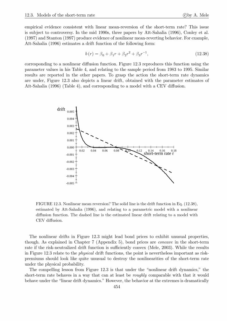
12.3. Models of the short-term rate c©by A. Mele
empirical evidence consistent with linear mean-reversion of the short-term rate? This issueis subject to controversy. In the mid 1990s, three papers by Aït-Sahalia (1996), Conley et al.(1997) and Stanton (1997) produce evidence of nonlinear mean-reverting behavior. For example,Aït-Sahalia (1996) estimates a drift function of the following form:
b (r) = β0 + β1r + β2r2 + β3r
−1, (12.38)
corresponding to a nonlinear diffusion function. Figure 12.3 reproduces this function using theparameter values in his Table 4, and relating to the sample period from 1983 to 1995. Similarresults are reported in the other papers. To grasp the action the short-term rate dynamicsare under, Figure 12.3 also depicts a linear drift, obtained with the parameter estimates ofAït-Sahalia (1996) (Table 4), and corresponding to a model with a CEV diffusion.
0.02 0.04 0.06 0.08 0.10 0.12 0.14 0.16 0.18
-0.005
-0.004
-0.003
-0.002
-0.001
0.000
0.001
0.002
0.003
0.004
0.005
short-term rate r
drift
FIGURE 12.3. Nonlinear mean reversion? The solid line is the drift function in Eq. (12.38),
estimated by Aït-Sahalia (1996), and relating to a parametric model with a nonlinear
diffusion function. The dashed line is the estimated linear drift relating to a model with
CEV diffusion.
The nonlinear drifts in Figure 12.3 might lead bond prices to exhibit unusual properties,though. As explained in Chapter 7 (Appendix 5), bond prices are concave in the short-termrate if the risk-neutralized drift function is sufficiently convex (Mele, 2003). While the resultsin Figure 12.3 relate to the physical drift functions, the point is nevertheless important as risk-premiums should look like quite unusual to destroy the nonlinearities of the short-term rateunder the physical probability.The compelling lesson from Figure 12.3 is that under the “nonlinear drift dynamics,” the
short-term rate behaves in a way that can at least be roughly comparable with that it wouldbehave under the “linear drift dynamics.” However, the behavior at the extremes is dramatically
454
12.3. Models of the short-term rate c©by A. Mele
different. As the short-term rate moves to the extremes, it is pulled back to the “center” in avery abrupt way. At the moment, it is not clear whether these preliminary empirical results arereliable or not. New econometric techniques are currently being developed to address this andrelated issues.One possibility is that such single factor models of the short-term rate are simply misspecified.
For example, there is strong empirical evidence that the volatility of the short-term rate is time-varying, as we shall discuss in the next section. Moreover, the term-structure implications of asingle factor model are counterfactual, since we know that a single factor cannot explain theentire variation of the yield curve, as explained in Section 12.2.4. We now describe more realisticmodels driven by more than one factor.
12.3.4 Multifactor models
The empirical evidence reviewed in Section 12.2.4 suggests that one-factor models cannot ex-plain the entire variation of the term-structure of interest rates. Factor analysis suggests we needat least three factors. In this section, we succinctly review the advances made in the literatureto address this important empirical issue.
12.3.4.1 Stochastic volatility
In the CIR model, the instantaneous short-term rate volatility is stochastic, as it depends on thelevel of the short-term rate, which is obviously stochastic. However, empirical evidence suggeststhat the short-term rate volatility depends on some additional factors. A natural extension ofthe CIR model is one where the instantaneous volatility of the short-term rate depends on (i)the level of the short-term rate, similarly as in the CIR model, and (ii) some additional randomcomponent. Such an additional random component is what we shall refer to as the “stochasticvolatility” of the short-term rate. It is the term-structure counterpart to the stochastic volatilityextension of the Black and Scholes (1973) model (see Chapter 10).Fong and Vasicek (1991) write the first paper in which the volatility of the short-term rate
is stochastic. They consider the following model:
dr (τ ) = κr (r − r (τ )) dτ +√v (τ)r (t)γ dW1 (τ )
dv (τ ) = κv (v − v (τ )) dτ + ξv√v (τ)dW2 (τ )
(12.39)
where κr, r, κv, v and ξv are constants, and [W1 W2] is a vector Brownian motion. To obtaina closed-form solution, Fong and Vasicek set γ = 0. The authors also make assumptions aboutrisk aversion corrections. Namely, they assume that the unit-risk-premia for the stochastic fluc-tuations of the short-term rate, λr, and the short-term rate volatility, λv, are both proportionalto
√v (τ), and then they find a closed-form solution for the bond price as of time t and maturing
at time T , P (r (t) , v (t) , T − t).Longstaff and Schwartz (1992) propose another model of the short-term rate where the
volatility of the short-term rate is stochastic. The remarkable feature of their model is thatit is a general equilibrium model. Naturally, the Longstaff & Schwartz model predicts, as theFong-Vasicek model, that the bond price is a function of both the short-term rate and itsinstantaneous volatility.Note, then, the important feature of these models. The pricing function, P (r (t) , v (t) , T − t)
and, hence, the yield curve R (r (t) , v (t) , T − t) ≡ − (T − t)−1 lnP (r (t) , v (t) , T − t), dependson the level of the short-term rate, r (t), and one additional factor, the instantaneous variance
455
12.3. Models of the short-term rate c©by A. Mele
of the short-term rate, v (t). Hence, these models predict that we now have two factors thathelp explain the term-structure of interest rates, R (r (t) , v (t) , T − t).What is the relation between the volatility of the short-term rate and the term-structure of
interest rates? Does this volatility help “track” one of the factors driving the variations of theyield curve? To develop intuition, consider the following binomial example. In the next period,the short-term rate is either r+ = r + d or r+ = r − d with equal probability, where r is thecurrent interest rate level and d > 0. The price of a two-period bond is P (r, d) = m(r, d)/ (1+r),where m(r, d) = E [1/ (1 + r+)] is the expected discount factor of the next period. By Jensen’sinequality, m(r, d) > 1/ (1 + E [r+]) = 1/ (1 + r) = m(r, 0). Therefore, two-period bond pricesincrease upon activation of randomness. More generally, two-period bond prices are alwaysincreasing in the “volatility” parameter d in this example, as illustrated in Figure 12.4. Theintuition is that the bond price is inversely related to the short-term rate and it is convex in it.Therefore, an increase in the volatility of the interest rate may only increase the price, as theloss in value of the price in bad times, when the interest rate increases, is less than the gainin value in good times, when the interest rate decreases. This property relates to an insight ofJagannathan (1984) (p. 429-430) that in a two-period economy with identical initial underlyingasset prices, a terminal underlying asset price y is a mean preserving spread of another terminalunderlying asset price x, in the Rothschild and Stiglitz (1970) sense, if and only if the price ofa call option on y is higher than the price of a call option on x. This is because if y is a meanpreserving spread of x, then E [f(y)] > E [f(x)] for f increasing and convex.8
These properties arise because the expected short-term rate is independent of d. In an alter-native setting, say a multiplicative setting, where either r+ = r (1 + d) or r+ = r/ (1 + d) withequal probability, bond prices are decreasing in volatility at short maturities and increasing involatility at longer maturities, as originally pointed out by Litterman, Scheinkman and Weiss(1991). It’s because expected future interest rates increase over time at a strength positivelyrelated to d. That is, the expected variation of the short-term rate is increasing in the volatilityof the short-term rate, d, a property that can be re-interpreted as one arising in an economywith risk-averse agents. At short maturity dates, such an effect dominates the convexity effectillustrated in Figure 12.4. At longer maturity dates, convexity effects dominate.
8 In our case, let md(i+) = 1/ (1 + i+) denote the random discount factor when i+ = i ∓ d. We have that x → −md(x) is
increasing and concave and, hence, E [−md′′(x)] < E [−md′(x)] ⇔ d′ < d′′, as shown in Figure 12.3. In Jagannathan (1984), f isincreasing and convex, and so we must have: E [f(y)] > E [f(x)]⇔ y is riskier than, or a mean preserving spread of x.
456
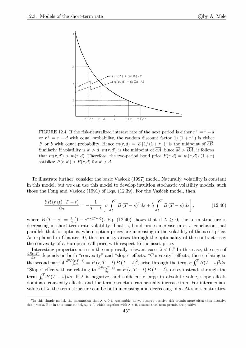
12.3. Models of the short-term rate c©by A. Mele
a
b
r
B
A
r +dr −d r +d’r −d’
1
m( r,d’) = ( a+A)/2
m( r, d) = ( b+B)/2
FIGURE 12.4. If the risk-neutralized interest rate of the next period is either r+ = r + d
or r+ = r − d with equal probability, the random discount factor 1/ (1 + r+) is either
B or b with equal probability. Hence m(r, d) = E [1/ (1 + r+)] is the midpoint of bB.
Similarly, if volatility is d′ > d, m(r, d′) is the midpoint of aA. Since ab > BA, it follows
that m(r, d′) > m(r, d). Therefore, the two-period bond price P (r, d) = m(r, d)/ (1 + r)
satisfies: P (r, d′) > P (r, d) for d′ > d.
To illustrate further, consider the basic Vasicek (1997) model. Naturally, volatility is constantin this model, but we can use this model to develop intuition stochastic volatility models, suchthose the Fong and Vasicek (1991) of Eqs. (12.39). For the Vasicek model, then,
∂R (r (t) , T − t)∂σ
= − 1
T − t
[σ
∫ T
t
B (T − s)2 ds+ λ∫ T
t
B (T − s) ds]. (12.40)
where B (T − s) = 1κ
(1− e−κ(T−s)
). Eq. (12.40) shows that if λ ≥ 0, the term-structure is
decreasing in short-term rate volatility. That is, bond prices increase in σ, a conclusion thatparallels that for options, where option prices are increasing in the volatility of the asset price.As explained in Chapter 10, this property arises through the optionality of the contract–saythe convexity of a European call price with respect to the asset price.Interesting properties arise in the empirically relevant case, λ < 0.9 In this case, the sign of
∂R(t,T )∂σ
depends on both “convexity” and “slope” effects. “Convexity” effects, those relating to
the second partial ∂2P (r,T−t)
∂r2 = P (r, T − t)B (T − t)2, arise through the term σ∫ T
tB(T −s)2ds.
“Slope” effects, those relating to ∂P (r,T−t)∂r
= P (r, T − t)B (T − t), arise, instead, through the
term∫ T
tB (T − s) ds. If λ is negative, and sufficiently large in absolute value, slope effects
dominate convexity effects, and the term-structure can actually increase in σ. For intermediatevalues of λ, the term-structure can be both increasing and decreasing in σ. At short maturities,
9 In this simple model, the assumption that λ < 0 is reasonable, as we observe positive risk-premia more often than negativerisk-premia. But in this same model, ur < 0, which together with λ < 0, ensures that term-premia are positive.
457

12.3. Models of the short-term rate c©by A. Mele
the convexity effects in Eq. (12.40) are typically dominated by slope effects, and the short-end ofthe term-structure can be increasing in σ. At longer maturity dates, however, convexity effectsare more important and, sometimes, dominate slope effects.More generally, changes in fixed income volatility are not mean-preserving spreads for the
risk-neutral distribution, as Eq. (12.40) illustrates in the case of the Vasicek model. In a worldwith complete markets, say Black-Scholes, the asset underlying the contract is traded. But in ourcase, the short-term rate is not a traded asset. Therefore, its risk-neutral drift depends on theshort-term volatility through some risk-adjustement–in Vasicek, for example, this dependenceis channeled through the risk-premium parameter λ.The previous reasoning, while relying on comparative statics for models with constant volatil-
ity model, goes through even when volatility is random. Mele (2003) shows that in more complexstochastic volatility cases, provided the risk-premium required to bear the interest rate risk isnegative, and sufficiently large in absolute value, slope effects dominate convexity effects at anyfinite maturity date, thus making bond prices decrease with volatility at any arbitrary maturitydate. In general, we would expect that in bad times, i.e. when interest rate volatility is high, therisk-premium effects dominate the convexity effects, with the yield curve increasing followingan increase in volatility. In good times, however, we would expect convexity effects to dominate,with the yield curve decreasing following an increase in volatility.What are the implications of in terms of the factors reviewed in Section 12.2.4? Clearly, the
very short-end of yield curve is not affected by movements of the volatility, aslimT→tR (r (t) , v (t) , T − t) = r (t), for all v (t). Moreover, these models predict thatlimT→∞R (r (t) , v (t) , T − t) = R, where R is a constant and, hence, independent of v (t).Therefore, movements in the short-term volatility can only produce their effects on the middleof the yield curve. For example, if the risk-premium required to bear the interest rate risk isnegative and sufficiently large, an upward movement in v (t) can produce an effect on the yieldcurve qualitatively similar to that depicted in Figure 12.2 (“Curvature” panel), and would thusroughly mimic the “curvature” factor that we reviewed in Section 12.2.4.
12.3.4.2 Three-factor models
We need at least three factors to explain the entire variation in the yield-curve. A model wherethe interest rate volatility is stochastic may be far from being exhaustive in this respect. Anatural extension is a model where the drift of the short-term rate contains some predictablecomponent, r (τ), which acts as a third factor, as in the following model:
dr (τ ) = κr (r (τ)− r (τ )) dτ +√v (τ )r (t)γ dW1 (τ )
dv (τ ) = κv (v − v (τ )) dτ + ξv√v (τ)dW2 (τ )
dr (τ ) = κr (ı− r (τ)) dτ + ξ r√r (τ )dW3 (τ )
(12.41)
where κr, γ, κv, v, ξv, κr, ı and ξr are constants, and [W1 W2 W3] is vector Brownian motion.Balduzzi et al. (1996) develop the first model for which the drift of the short-term rate
changes stochastically, as in Eqs. (12.41). Dai and Singleton (2000) estimate a number of modelsthat generalize that in Eqs. (12.41) (See Section 12.3.7 for details on the estimation strategy).The term-structure implications of these models can be understood very simply. First, underregularity conditions about the risk-premia, the yield curve is R (r (t) , r (t) , v (t) , T − t) ≡− (T − t)−1 lnP (r (t) , r (t) , v (t) , T − t). Second, and intuitively, changes in the new factor r (t)should primarily affect the long-end of the yield curve. This is because empirically, the usualfinding is that the short-term rate reverts relatively quickly to the long-term factor r (τ ) (i.e. κr
458

12.3. Models of the short-term rate c©by A. Mele
is relatively large), where r (τ ) mean-reverts slowly (i.e. κr is relatively low). This mechanismmakes the short-term rate quite persistent anyway. Ultimately, then, the slow mean-reversion ofr (τ ) means that changes in r (τ ) last for the relevant part of the term-structure we are usuallyinterested in (i.e. up to 30 years), despite the fact that limT→∞R (r (t) , r (t) , v (t) , T − t) isindependent of the movements of the three factors r (t), r (t) and v (t).However, it is difficult to see how to reconcile such a behavior of the long-end of the yield curve
with the existence of any of the factors discussed in Section 12.2.4. First, the short-term ratecannot be taken as a “level factor,” since we know its effects die off relatively quickly. Instead, ajoint change in both the short-term rate, r (t), and the “long-term” rate, r (t), should be reallyneeded to mimic the “Level” panel of Figure 12.2 in Section 12.2.4. However, this interpretationis at odds with the assumption that the factors discussed in Section 12.2.4 are uncorrelated!Moreover, and crucially, the empirical results in Dai and Singleton reveal that if any, r (t) andr (t) are negatively correlated.Finally, to emphasize how exacerbated these puzzles are, consider the effects of changes in
the short-term rate r (t). We know that the long-end of the term-structure is not affected bymovements of the short-term rate. Hence, the short-term rate acts as a “steepness” factor, asin Figure 12.2 (“Slope” panel). However, this interpretation is restrictive, as factor analysisreveals that the short-end and the long-end of the yield curve move in opposite directions aftera change in the steepness factor. Here, instead, a change in the short-term rate only modifiesthe short-end (and, perhaps, the middle) of the yield curve and, hence, does not produce anyvariation in the long-end curve.
12.3.4.3 Unspanned stochastic volatility
Unspanned stochastic volatility arises when
∂
∂vP (r (t) , r (t) , v (t) , T − t) = 0.
The hypothesis that fixed income markets have unspanned stochastic volatility has been putforward by Collin-Dufresne and Goldstein (2002). Mele (2003) provides conditions under whichthis occurs.[In progress]
12.3.5 Affine and quadratic term-structure models
12.3.5.1 Affine
The Vasicek and CIR models predict that the bond price is exponential-affine in the short-term rate r. This property is the expression of a general phenomenon. Indeed, it is possibleto show that bond prices are exponential-affine in r if, and only if, the functions b and a2 areaffine in r. Models that satisfy these conditions are known as affine models. More generally,these basic results extend to multifactor models, where bond prices are exponential-affine inthe state variables.10 In these models, the short-term rate is a function r (y) such that
r (y) = r0 + r1 · y,
10More generally, we say that affine models are those that make the characteristic function exponential-affine in the state variables.In the case of the multifactor interest rate models of the previous section, this condition is equivalent to the condition that bondprices are exponential affine in the state variables.
459

12.3. Models of the short-term rate c©by A. Mele
where r0 is a constant, r1 is a vector, and y is a multidimensional diffusion, in Rn, and is solutionto.
dy (τ) = κ (µ− y (t)) dt+ΣV (y (τ )) dW (τ ) , (12.42)
where W is a d-dimensional Brownian motion, Σ is a full rank n × d matrix, and V is a fullrank d× d diagonal matrix with elements,
V (y)(ii) =
√αi + β
⊤i y, i = 1, · · · , d, (12.43)
for some scalars αi and vectors βi. Langetieg (1980) develops the first multifactor model of thiskind, in which βi = 0.Next, Let V − (y) be a d× d diagonal matrix with elements
V − (y)(ii) =
1
V (y)(ii)if PrV (y (t))(ii) > 0 all t = 1
0 otherwise
and set,Λ (y) = V (y)λ1 + V
− (y)λ2y, (12.44)
for some d-dimensional vector λ1 and some d× n matrix λ2. Duffie and Kan (1996) explainedin a comprehensive way the benefit of this model. In their formulation λ2 = 0d×n, and the bondprice is exponential-affine in the state variables y. That is, the price of the zero has the followingfunctional form,
P (y, T − t) = exp [A (T − t) +B (T − t) · y] , (12.45)
for some functions A and B of time to maturity, T − t (B is vector-valued), such that A (0) = 0and B (0)(i) = 0.The more general functional form for Λ in Eq. (12.44) has been suggested by Duffee (2002).
Duffee noticed that in bond markets, risk-premiums, defined as Λ (y)V (y) = V 2 (y)λ1 + λ2y,are related not only to the volatility of fundamentals, but also to the level of the fundamentals,which justifies the inclusion of the additional term λ2y. In this case, bond prices still havean exponential affine form, just as in Eq. (12.45). When λ2 = 0d×n, we say that the modelis “completely affine,” and “essentially affine,” otherwise. The clear advantage of these affinemodels, then, is that they considerably simplify statistical inference, as explained in Section12.3.7 below.Ang and Piazzesi (2003) (AP, henceforth) and Hördahl, Tristani and Vestin (2006) (HTS,
henceforth) introduce “no-arbitrage” regressions, to model the relations linking macroeconomicvariables to the yield curve. In their models, the factors are taken to be a discrete-time versionof Eq. (12.42), where some components of y are observable, and others are unobservable. Theobservables relate to macroeconomic factors such as inflation or industrial production. Theauthors, then, study how all these factors affect the yield curve, predicted by a pricing equationsuch as that in Eq. (12.45). While HTS have a structural model of the macroeconomy, AP havea reduced-form model.Reduced-form model can be exposed to the critique that some of the parameters are not
“variation-free.” [Explain what variation-free parameters are, in mathematical statis-tics] For example, in the simple Lucas economy of Part I, we know that the short-term rate isr = ρ+ ηµ+ 1
2σ2η (1− η), so by “tilting” η (risk-aversion), we should also have a change in the
interest rate. This simple example shows that the parameters related to risk-aversion correctionin Eq. (12.44) are not free to be “tilted,” in that tilting them has an effect on the parameters
460

12.3. Models of the short-term rate c©by A. Mele
of the factor dynamics in Eq. (12.42). At the same time, reduced-form model offer a great dealof flexibility, as they do not restrict, so to speak, the model to track any market or economysuch as the Lucas economy, say. Moreover, we can always find a theoretical market supportingthe no-arb market underlying the reduced-form model. No-arb regressions such as those in APgive the data the power to say which parameter constellation make the model likely to per-form, without imposing theoretical restrictions which the data might, then, be likely to reject.For example, the Lucas model, while clearly illustrates that some of the parameters are notvariation-free, can be simply wrong, and might impose unreasonable restrictions on the data.For no-arb models, instead, cross-equations restrictions arise through the weaker requirementof absence of arbitrage opportunities.
12.3.5.2 Quadratic
Affine models are known to impose tight conditions on the structure of the volatility of thestate variables. These restrictions arise to keep the square root in Eq. (12.43) real valued. Butthese constraints may hinder the actual performance of the models. There exists another classof models, known as quadratic models, that partially overcome these difficulties.
12.3.6 Short-term rates as jump-diffusion processes
Ahn and Thompson (1988) is the first contribution where the CIR general equilibrium modelis extended to jumps-diffusion processes. Suppose that the short-term rate is a jump-diffusionprocess:
dr(τ ) = bJ(r(τ ))dτ + a(r(τ ))dW (τ ) + ℓ(r(τ )) · S · dZ(τ ),where W and Z are under the risk-neutral probability, and bJ is, then, a jump-adjusted risk-neutral drift. The bond price P (r, τ , T ) is solution to,
0 =
(∂
∂τ+ L− r
)P (r, τ , T ) + vQ
∫
supp(S)[P (r + ℓS, τ , T )− P (r, τ , T )] p (dS) , (12.46)
for all (r, τ ) ∈ R++× [t, T ), and satisfies the boundary condition, P (r, T, T ) = 1 ∀r ∈ R++. Eq.
(12.46) follows because, as usual, e−∫ τ
tr(u)duP (r, τ , T ) is a martingale under the risk-neutral
probability. This model can also be extended to one where there are different quality, or types,of jumps, in which case Eq. (12.46) is:
0 =
(∂
∂τ+ L− r
)P (r, τ , T ) +
N∑
j=1
vQj
∫
supp(S)[P (r + ℓS, τ , T )− P (r, τ , T )] pj (dS) ,
where N is the number of jump types. However, to simplify the exposition, we just set N = 1.To identify risk-premiums related to jumps, we simply note that vQ = v · λJ , where v is the
intensity of the short-term rate jump under the physical distribution, and λJ is the risk-premiumdemanded by agents to be compensated for the presence of jumps.Bonds subject to default-risk can be modeled through partial differential equations as well,
once we assume default is an exogeously given rare event, driven by a Poisson process. Chapter13 develops a comprehensive account of this approach, known as “reduced-form” approach–tobe distinct from the “structural approach,” where the event of default is modeled in regard tothe books of the issuer. However, it is instructive to anticipate some of the main features ofthis reduced-form approach. Assume, then, that the event of default at each instant of time is a
461

12.3. Models of the short-term rate c©by A. Mele
Poisson process Z with intensity v, and that in the event of default at point τ , the bondholderreceives a recovery payment P (τ). This recovery payment can be a bounded deterministicfunction of time, or more generally a bounded process adapted to the short-term rate. Next, letτ be the random default time, and let’s create an auxiliary state variable g with the followingfeatures:
g =
0 if t ≤ τ < τ1 otherwise
Therefore, we have that under the risk-neutral probability,dr(τ ) = b(r(τ))dτ + a(r(τ ))dW (τ)dg(τ) = S · dN(τ ), where S ≡ 1, with probability one
(12.47)
Denote the rational bond price function with P (r, g, τ , T ), τ ∈ [t, T ], and assume that ∀τ ∈ [t, T ]and ∀v ∈ (0,∞), P (r, 1, τ , T ) = P (τ) < P (r, 0, τ , T ) and that P (τ ; v′) ≥ P (τ ; v)⇔ v′ ≥ v a.s.These assumptions, guarantee that default-free bond prices are higher than defaultable bondprices, as shown below. In the absence of arbitrage, the pre-default bond price P (r, 0, τ , T ) =P pre (r, τ , T ) satisfies:
0 =
(∂
∂τ+ L− r
)P (r, 0, τ , T ) + v(r) · [P (r, 1, τ , T )− P (r, 0, τ , T )]
=
(∂
∂τ+ L− (r + v(r))
)P (r, 0, τ , T ) + v(r)P (τ), (12.48)
for all τ ∈ [t, T ), and the boundary condition P (r, 0, T, T ) = 1. The solution is, formally:
P pre (x, t, T ) = E∗t
[exp
(−
∫ T
t
(r(τ) + v(r(τ)))dτ
)]
+ E∗t
[∫ T
t
exp
(−∫ τ
t
(r(u) + v(r(u)))du
)· v(r(τ ))P (τ)dτ
],
where E∗t [·] is the expectation taken with resepct to only the first equation of system (12.47).This formulat coincides with that in Duffie and Singleton (1999, Eq. (10) p. 696), once we definea percentage loss process l in [0, 1] such that P = (1− l) · P . Indeed, inserting P = (1− l) · Pinto Eq. (12.48) leaves:
0 =
(∂
∂τ+ L− (r + l(τ )v(r))
)P (r, 0, τ , T ), ∀(r, τ) ∈ R++ × [t, T ),
with the usual boundary condition, the solution of which is:
P pre (x, t, T ) = E∗t
[exp
(−∫ T
t
(r(τ) + l(τ) · v(r(τ )))dτ)]
.
To validate the claim that P pre is decreasing in v, consider two markets A and B, where thedefault intensities are vA and vB, and assume that the coefficients of L are independent of vi.The pre-default bond price function in economy i is P i(r, τ , T ), i = A,B, and satisfies:
0 =
(∂
∂τ+ L− r
)P i + vi · (P i − P i), i = A,B,
462

12.3. Models of the short-term rate c©by A. Mele
with the usual boundary condition. Assuming that PA = PB, subtracting these two equations,and rearranging terms, shows that the price difference ∆P (r, τ , T ) ≡ PA(r, τ , T )− PB(r, τ , T )satisfies,
0 =
(∂
∂τ+ L− (r + vA)
)∆P (r, τ , T ) +
(vA − vB
)·[PB (τ)− PB (r, τ , T )
],
with boundary condition, ∆P (r, T, T ) = 0 for all r. Because, clearly, PB < PB, we have that∆P (r, τ , T ) < 0 whenever vA > vB, by an application of the maximum principle reviewed inAppendix 3 of Chapter 7.
12.3.7 Some stylized facts and estimation strategies
We begin with a simple model addressing the issue of correlation between the short-term rateand its instantaneous volatility. Let r (t) be the short-term rate process, solution to the followingstochastic differential equation,
dr (t) = κ (µ− r (t)) dt+√v (t)r (t)η dW (t) , t ≥ 0, (12.49)
where W (t) is a standard Brownian motion under the physical probability, and κ, µ and η arethree positive constants. Suppose, also, that the instantaneous volatility process
√v (t)r (t)η is
such that v (t) is solution to,
dv (t) = β (α− v (t)) dt+ ξv (t)ϑ(ρdW (t) +
√1− ρ2dU (t)
), t ≥ 0, (12.50)
where U (t) is another standard Brownian motion; β, α, ξ and ϑ are four positive constants,and ρ is a constant such that |ρ| < 1. This model generalizes the two-factor model discussed inSection 12.3.4.1, as it allows r and v to be instantaneously correlated.
12.3.7.1 The level effect
Which empirical regularities would the short-term rate model in Eqs. (12.49)-(12.50) address?Which sign of the correlation coefficient ρ would be consistent with historical episodes such asthe Monetary Experiment of the Federal Reserve System between October 1979 and October1982? The following picture depicts the time series behavior of the nominal short-term rate,as measured by the three month TB rate, as well as the volatility of its changes, as measuredthrough a formula similar to that in Section 7.2 of Chapter 7: Volr,t ≡ 1002
√6π·σr,t, where σr,t ≡
112
∑12i=1 |rt+1−i − rt−i|, and rt is the short-term rate as of month t. The multiplicative factor
1002 arises because: (i) the short-rate is converted into percentage points, and (ii) volatility isconverted into basis points, as in market conventions.
463

12.3. Models of the short-term rate c©by A. Mele
This picture depicts the time-series behavior of the 3 month TB rate (top panel, in percent)
and its rolling, basis point volatility, Volr,t (bottom panel), over the sampling period
spanning 1957:01 through 2008:12.
The next picture plots a scatterplot of the short-term rate basis point volatility, Volr,t, againstrt, for two sampling periods.
464
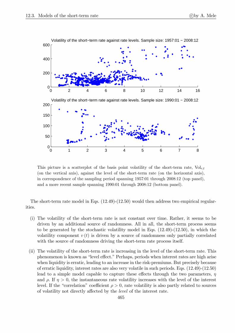
12.3. Models of the short-term rate c©by A. Mele
0 2 4 6 8 10 12 14 160
200
400
600Volatility of the short−term rate against rate levels. Sample size: 1957:01 − 2008:12
0 1 2 3 4 5 6 7 80
50
100
150
200Volatility of the short−term rate against rate levels. Sample size: 1990:01 − 2008:12
This picture is a scatterplot of the basis point volatility of the short-term rate, Volr,t(on the vertical axis), against the level of the short-term rate (on the horizontal axis),
in correspondence of the sampling period spanning 1957:01 through 2008:12 (top panel),
and a more recent sample spanning 1990:01 through 2008:12 (bottom panel).
The short-term rate model in Eqs. (12.49)-(12.50) would then address two empirical regular-ities.
(i) The volatility of the short-term rate is not constant over time. Rather, it seems to bedriven by an additional source of randomness. All in all, the short-term process seemsto be generated by the stochastic volatility model in Eqs. (12.49)-(12.50), in which thevolatility component v (t) is driven by a source of randomness only partially correlatedwith the source of randomness driving the short-term rate process itself.
(ii) The volatility of the short-term rate is increasing in the level of the short-term rate. Thisphenomenon is known as “level effect.” Perhaps, periods when interest rates are high arisewhen liquidity is erratic, leading to an increase in the risk-premiums. But precisely becauseof erratic liquidity, interest rates are also very volatile in such periods. Eqs. (12.49)-(12.50)lead to a simple model capable to capture these effects through the two parameters, ηand ρ. If η > 0, the instantaneous rate volatility increases with the level of the interestlevel. If the “correlation” coefficient ρ > 0, rate volatility is also partly related to sourcesof volatility not directly affected by the level of the interest rate.
465

12.3. Models of the short-term rate c©by A. Mele
During the Monetary Experiment, the FED target was essentially money supply, rather thaninterest rates. As a result, high volatility of money demand mechanically translated to high ratevolatility, through market clearing. Moreover, the monetary base was kept deliberately low, asan attempt to fight against inflation. These facts lead to a period where both rate volatilityand interest rates very high. Note that one additional reason for the high nominal rates at thetime might link to a compensation for high inflation volatility–not only high inflation.The previous picture is also suggestive of a change in regime that possibly occurred over a
more recent past. From 1990 on, rate volatility does not necessarily appear to positively link torate levels, and there is evidence of the opposite. The next picture suggests that “percentage”
volatility, defined as Vol%r,t ≡ 100√6π · σ%
r,t, where σ%r,t ≡ 1
12
∑12i=1
∣∣∣ln rt+1−i
rt−i
∣∣∣, is inversely related
to the level rates, over the more recent sample periods too.
0 2 4 6 8 10 12 14 160
50
100
150Volatility of the short−term rate against rate levels. Sample size: 1957:01 − 2008:12
0 1 2 3 4 5 6 7 80
50
100
150Volatility of the short−term rate against rate levels. Sample size: 1990:01 − 2008:12
This picture is a scatterplot of the percentage volatility of the short-term rate Vol%r,t (on
the vertical axis), against the level of the short-term rate (on the horizontal axis), in
correspondence of the sampling period spanning 1957:01 through 2008:12 (top panel),
and a more recent sample spanning 1990:01 through 2008:12 (bottom panel).
12.3.7.2 A simple case
Next, suppose we wish to estimate the parameter vector θ = [κ, µ, η, β, α, ξ, ϑ, ρ]⊤ of the modelin Eqs. (12.49)-(12.50). Under which circumstances would Maximum Likelihood be a feasibleestimation method?The ML estimator would be feasible under two sets of conditions. First, the model in Eqs.
(12.49)-(12.50) should not have stochastic volatility at all, viz, β = ξ = 0; in this case, the
466
12.3. Models of the short-term rate c©by A. Mele
short-term rate would be solution to,
dr (t) = κ (µ− r (t)) dt+ σr (t)η dW (t) , t ≥ 0,
where σ is now a constant. Second, the value of the elasticity parameter η is important. If η = 0,the short-term rate process is the Gaussian one proposed by Vasicek (1977). If η = 1
2, we obtain
the square-root process of Cox, Ingersoll and Ross (1985). In the Vasicek case, the transitiondensity of r is Gaussian, and in the CIR case, the transition density of r is a noncentral chi-square. So in both the Vasicek and CIR, we may write down the likelihood function of thediffusion process. Therefore, ML estimation is possible in these two cases. In more generalcases, such those in the next section, one needs to go for simulation methods, such as thosedescribed in Chapter 5.
12.3.7.3 More general models
Estimating the model in Eqs. (12.49)-(12.50) is certainly instructive. Yet a more importantquestion is to examine the term-structure implications of this model. More generally, how wouldthe estimation procedure outlined in the previous subsection change if the task is to estimatea Markov model of the term-structure of interest rates? There are three steps.
Step 1
Collect data on the term structure of interest rates. We will need to use data on three maturities,say a time series of riskless 6 month, 5 year and 10 year yields.
Step 2
Let us consider the three-factor model in Eqs. (12.41) of Section 12.3.4.2, where the threeBrownian motions Wi are now allowed to be correlated. The bond price predicted by thismodel is:
P j (r (t) , v (t) , r (t)) ≡ P (r (t) , v (t) , r (t) , Nj − t) = E(e−
∫ Njt
r(s)ds
∣∣∣∣ r (t) , v (t) , r (t)),
(12.51)where Nj is a sequence of expiration dates. Naturally, this price depends on the risk-aversioncorrections needed to turn the dynamics the short-term rate in Eqs. (12.41) into the risk-neutralone. As discussed, one may impose analytically convenient conditions on the risk-adjustments,but we do not need to be more precise at this juncture. No matter the nature of the risk-adjustments, we have that they entail that Eq. (12.51) depends not only on the “physical”parameter vector θ = [κr, κv, κr, γ, v, ξv, ι, ξr, ρ]
⊤ , where ρ is a vector containing all the cor-relation coefficients of Wi, but also on these very same risk-adjustment parameter vector, sayλ. Precisely, the Radon-Nykodim derivative of the risk-neutral probability with respect to thephysical probability is exp
(−1
2
∫‖Λ (t)‖2 dt−
∫Λ (t) dZ (t)
), for some vector Brownian motion
Z, and Λ (t) is some process, assumed to take the form Λ (t) ≡ Λm (r (t) , v (t) , r (t) ;λ), for
some vector-valued function Λm and some parameter vector λ. The function Λm makes risk-adjustment corrections depend on the current value of the state vector [r (t) , v (t) , r (t)], whichmakes the model Markov, thereby simplifying statistical inference.To summarize, the issue is now one where we need to estimate both the physical parameter
vector θ and the “risk-adjustment” parameter vector λ. Next, we consider the yield curve incorrespondence of three maturities,
Rj (r (t) , v (t) , r (t) ;θ,λ) ≡ − 1
Nj
lnP j (r (t) , v (t) , r (t)) , j = 1, 2, 3, (12.52)
467

12.4. No-arbitrage models: early formulations c©by A. Mele
where the notation Rj (r, v, r;θ,λ) emphasizes that the theoretical yield curve depends onthe parameter vector (θ,λ). We can now use actual data, Rj
$ say, and the model predictionsabout the data, Rj, create moment conditions, and proceed to estimate the parameter vector(θ,λ) through some method of moments–provided of course the moments are enough to make(θ,λ) identifiable. But there are two difficulties. The first is that the volatility process v (t)and the long-term, moving value of the short-term rate, r (t), are not directly observable by theeconometrician. We can use inference methods based on simulations to cope with this issue.Very simply, we simulate Eqs. (12.41), and apply moment conditions or auxiliary models toobservable variables, as explained in Chapter 5. For example, we simulate Eqs. (12.41) for agiven value of (θ,λ). For each simulation, we compute a time series of interest rates Rj from Eq.(12.52). Then, we use these simulated data to create moment conditions or fit some auxiliarymodel to these artificial data that is as close as possible to the very same auxilary model fit toreal data. The parameter estimator, then, is the value of (θ,λ) minimizing some norm of thesemoment conditions, obtained through the simulations, with any of the methods explained inChapter 5. According to Theorem 5.4 in Chapter 5, fitting a sufficiently rich auxiliary modelshould result in a quite efficient estimator.A second difficulty is that the bond pricing formula in Eq. (12.51) does not generally admit
a closed-form, an issue we can address using affine models, as explained next.
Step 3
The use of affine models would considerably simplify the analysis. Affine models place restric-tions on the data generating process in Eqs. (12.41) and in the risk-aversion corrections in Eq.(12.51), as originally illustrated by Dai and Singleton (2000), in such a way that the yield curvein Eq. (12.52) is,
Rj (r (t) , v (t) , r (t) ;θ,λ) = A (j;θ,λ) +B (j;θ,λ) · [r (t) , v (t) , r (t)]⊤, j = 1, 2, 3, (12.53)
where A (j; θ, λ) and B (j; θ, λ) are some functions of the maturity Nj (B is vector valued),and generally depend on the parameter vector (θ,λ). Once Eqs. (12.41) are simulated, thecomputation of a time series of yields Rj, then, straightforward, given Eq. (12.53).11
12.4 No-arbitrage models: early formulations
12.4.1 Fitting the yield-curve, perfectly
When it comes to price interest rate derivatives consistent with the price of already existingfixed income instruments, we do not really wish to explain the yield curve. Rather, as explainedin Chapter 11, we wish to take it as given. To illustrate, consider a European option writtenon a bond. We may find it unsatisfactory to have a model that only “explains” the bond price.A model’s error on the bond price might generate a large error for the option price, due to thenonlinearities induced by the optionality. How can we trust an option pricing model, which isnot even capable to pin down the value of the underlying asset? To begin address these pointswith a simple case, let again P (r (τ ) , τ , S) be the price of a zero coupon bond maturing at
11Dai and Singleton (2000) implement this estimation strategy, although they make use of data on swap rates. The models theyconsider predict theoretical values for the swap rates, obtained through the formula in Eq. (12.91) of Section 12.7.5.4 below, wherethe bond prices in that formula are replaced by the pricing functions predicted by the models. Dai & Singleton consider three ratespredicted by their models: two swap rates (with tenures of two and ten years), plus the six month Libor rate, − 1
2lnP
(t, t+ 1
2
),
where P is the pricing function predicted by the models they consider.
468
12.4. No-arbitrage models: early formulations c©by A. Mele
some S. By the FTAP, the price, Cb say, of a European option written on this bond, struck atK and expiring at T < S, is:
Cb (r(t), t, T, S) = Et[e−
∫ Tt r(τ)dτ · (P (r (T ) , T, S)−K)+
].
For example, affine models predict that the bond price P is conditionally lognormally distrib-uted, provided r is conditionally normally distributed, as in the case of Vasicek model. Insightsfrom the Black and Scholes (1973) formula suggest, then, that in this case, the previous ex-pectation is a nonlinear function of the current bond price P (r (t) , t, T ). To elaborate thisissue more precisely, we cannot make use of the standard tools leading to the Black & Scholesformula. The main issue arising whilst evaluating fixed-income instruments is that their payoffat expiry, (P (r (T ) , T, S)−K)+, depends on the short-term rate at T , and yet the discount-
ing e−∫ Tt r(τ)dτ also obviously depends on the realization of the short-term rate. The problem
is tractable, however, and can be addressed through the forward martingale probability toolsintroduced in Section 12.1. Precisely, let Iexe be the indicator function which is always zero, orone when the option is exercized, i.e. when P (r(T ), T, S) ≥ K. We have:
Cb (r(t), t, T, S)
= Et[e−
∫ Tt r(τ)dτP (r(T ), T, S) · Iexe
]−K · Et
[e−
∫ Tt r(τ)dτ · Iexe
]
= P (r(t), t, S) · Et[e−
∫ St r(τ)dτ
P (r(t), t, S)· Iexe
]−KP (r(t), t, T ) · Et
[e−
∫ Tt r(τ)dτ
P (r(t), t, T )· Iexe
]
= P (r(t), t, S) · EQSF [Iexe]−KP (r(t), t, T ) · EQTF [Iexe]
= P (r(t), t, S) ·QSF [P (r(T ), T, S) ≥ K]−KP (r(t), t, T ) ·QT
F [P (r(T ), T, S) ≥ K] , (12.54)
where the second equality follows by an argument nearly identical to that produced in Section12.1.2.2 (see Footnote 1);12 Qi
F (i = T, S) is the i-forward probability; and, finally, EQiF [·] isthe expectation taken under the i-forward martingale probability, as defined in Section 12.1.3.Section 12.7 explains how the two probabilities in Eq. (12.54) are computed. The important
issue, now, is to emphasize that the bond option price does depend on the theoretical bondprices P (r(t), t, T ) and P (r(t), t, S), which, in turn, cannot equal the current, observed marketprices. Theoretical prices are, after all, the output of a rational expectations model. This fact isobviously not a source of concern to those who wish to predict future term-structure movementswith the help of a few, key state variables, as in the multifactor models discussed earlier.However, a source of concern to sell-side practitioners might be that the option should be pricedwith a model that simultaneously matches the yield curve, at the time of evaluation. The aimof this section is to introduce a class of models that fit the yield curve without errors, whichwe call “perfectly fitting models.” These models are simply a more elaborated, continuous-timeversion of the no-arbitrage models introduced in Chapter 11. They predict that the price of anybond, say a bond expiring at some S, is, of course, random, at time T < S, but also exactly
12By the Law of Iterated Expectations,
Et[e−
∫Tt r(τ)dτP (r(T ), T, S)Iexe
]= Et
[e−
∫Tt r(τ)dτ IexeE
(e−
∫ST r(τ)dτ
∣∣∣F (T ))]
= Et[e−
∫St r(τ)dτ Iexe
].
469
12.4. No-arbitrage models: early formulations c©by A. Mele
equal to the current market price, that of time t. Finally, and naturally, this price must bearbitrage-free. We now show that conditions can be met by augmenting the models seen in theprevious sections with a set of “infinite dimensional parameters.” We begin with a discussion oftwo specific and old, and yet famous examples addressing these issues: the Ho and Lee (1986)model, and one generalization of it, introduced by Hull and White (1990). In Section 12.5, wemove on towards a general model-building principle.A final remark. In Section 12.7, we shall show that at least for the Vasicek model, Eq. (12.54)
does not explicitly depend on r because it only “depends” on P (r(t), t, T ) and P (r(t), t, S). Sowhy do we look for perfectly fitting models in the first place? Wouldn’t it be enough, then,to just replace the theoretical prices P (r(t), t, T ) and P (r(t), t, S) with the market values, sayP $(t, T ) and P $(t, S)? This way, the model is perfectly fitting. Apart from being logicallyinconsistent (you would have a model predicting something generically different from prices),this way of proceeding also has practical drawbacks. Section 12.7 shows that option pricingformulae for European options, might well agree “in notation” with those relating to perfectlyfitting models. However, Section 12.7.3 explains that as we move towards more complex interestrate derivatives products, such as options on coupon bonds and swaption contracts, the situationgets dramatically different. Finally, it can be the case that some maturity dates are actuallynot traded at some point in time. For example, it may happen that P $(t, T ) is not observedand that we could still be interested in pricing more “exotic” or less liquid bonds or optionson these bonds. An intuitive procedure to deal with this this difficulty is to “interpolate” thetraded maturities. In fact, the objective of perfectly fitting models is to allow for such an“interpolation” while preserving absence of arbitrage opportunities.
12.4.2 Ho & Lee
The original Ho and Lee (1986) model is in discrete-time and is analyzed in the context ofChapter 11, along with other models. The model below, represents the “diffusion limit” of theoriginal Ho & Lee model, as put forward in Section 11.6.6 of Chapter 11:
dr (τ ) = θ (τ) dτ + σdW (τ ) , τ ≥ t, (12.55)
where t is the time of evaluation, W is a Brownian motion under Q, σ is a constant, and θ (τ)is an “infinite dimensional” parameter, which we need to pin down the initial, observed yieldcurve, as we now explain. The reason we refer to θ (τ) as “infinite dimensional” parameter isthat we assume θ (τ) is a function of calendar time τ ≥ t. We assume this function is knownat t. Clearly, Eq. (12.55) defines an affine model. Therefore, the bond price takes the followingform,
P (r (τ ) , τ , T ) = eA(τ,T )−B(τ,T )·r(τ), (12.56)
for two functions A and B to be determined below. It is easy to show that,
A (τ , T ) =
∫ T
τ
θ (s) (s− T ) ds+ 1
6σ2 (T − τ )3 , B (τ , T ) = T − τ .
Let f$ (t, τ ) denote the instantaneous, observed forward rate. By matching the instantaneousforward rate f (τ , T ) predicted by the model to f$ (τ , T ) yields:
f$ (t, T ) = f (t, T ) = −∂ lnP (r (t) , t, T )∂T
=
∫ T
t
θ (s) ds− 1
2σ2 (T − t)2 + r (t) . (12.57)
470

12.4. No-arbitrage models: early formulations c©by A. Mele
Because P (t, T ) = exp(−∫ T
tf (t, τ ) dτ
), the drift term θ (s) satisfying Eq. (12.57) guarantees
an exact fit of the yield curve. By differentiating Eq. (12.57) with respect to T , leaves θ (T ) =∂∂Tf$ (t, T ) + σ
2 (T − t), or:
θ (τ ) =∂
∂τf$ (t, τ) + σ
2 (τ − t) . (12.58)
To check that θ is indeed the solution we were looking for, we replace Eq. (12.58) into Eq.(12.57) and verify indeed that Eq. (12.57) holds as an identity. By Eqs. (12.55) and (12.58),the short-term rate is, then:
r (t) = f$ (0, t) +1
2σ2t+ σW (t) .
Moreover, by Eq. (12.57), and Eq. (12.55), the instantaneous forward rate satisfies,
dτf (τ , T ) = −θ (τ ) dτ + σ2 (T − τ ) dτ + dr (τ) = σ2 (T − τ) dτ + σdW (t) .
These results are the continuous time counterparts to those introduced in Section 11.6.6 ofthe previous chapter. In Section 12.5, they will be shown to be a particular case of a generalframework, known as the HJM.
12.4.3 Hull & White
Hull and White (1990) consider the following model:
dr(τ ) = κ
(θ (τ)
κ− r (τ )
)dτ + σdW (τ) , (12.59)
where W is a Q-Brownian motion, and κ, σ are constants. The model generalizes the Ho andLee model (1986) in Eq. (12.55) and the Vasicek (1977) model in Eq. (12.34). In the originalformulation of Hull and White, κ and σ are both time-varying, but the main points of thismodel can be learnt by working out this particularly simple case.Eq. (12.59) also gives rise to an affine model. Therefore, the solution for the bond price is
given by Eq. (12.56). It is easy to show that the functions A and B are given by
A(τ , T ) =1
2σ2
∫ T
τ
B(s, T )2ds−∫ T
τ
θ(s)B(s, T )ds, (12.60)
and
B(τ , T ) =1
κ
[1− e−κ(T−τ)
]. (12.61)
By reiterating the same reasoning produced to show (12.58), one shows that the solution forθ is:
θ(τ) =∂
∂τf$(t, τ ) + κf$(t, τ ) +
σ2
2κ
[1− e−2κ(τ−t)] . (12.62)
A proof of this result is in Appendix 5.Why did we need to go for this more complex model? After all, the Ho & Lee model is
already able to pin down the entire yield curve. The answer is that in practice, investmentbanks typically prices a large variety of derivatives. The yield curve is not the only thing to beexactly fit. Rather it is only the starting point. In general, the more flexible a given perfectlyfitting model is, the more successful it is to price more complex derivatives.
471

12.5. The Heath-Jarrow-Morton framework c©by A. Mele
12.5 The Heath-Jarrow-Morton framework
12.5.1 Framework
The bond price representation in Eq. (12.3),
P (τ , T ) = e−∫ Tτ f(τ,ℓ)dℓ, all τ ∈ [t, T ], (12.63)
underlies the modeling approach started by Heath, Jarrow and Morton (1992) (HJM, hence-forth). Given Eq. (12.63), this approach takes as a primitive the stochastic evolution of theentire structure of forward rates, not only the special case of the short-term rate, r (t) =limℓ↓t f (t, ℓ) ≡ f (t, t). The goal is to start with Eq. (12.63) and take the initial, observedstructure of forward rates f (t, ℓ)ℓ∈[t,T ], as given, and find, then, no-arb, “cross-equation”restrictions on the stochastic behavior of f (τ , ℓ)τ∈(t,ℓ], for any ℓ ∈ [t, T ].By construction, the HJM approach allows for a perfect fit of the initial term-structure. This
point can be illustrated quite simply, as the bond price P (τ , T ) is,
P (τ , T ) = e−∫ Tτ f(τ,ℓ)dℓ
=P (t, T )
P (t, τ)· P (t, τ)P (t, T )
e−∫ Tτ f(τ,ℓ)dℓ
=P (t, T )
P (t, τ)· e−
∫ τt f(t,ℓ)dℓ+
∫ Tt f(t,ℓ)dℓ−
∫ Tτ f(τ,ℓ)dℓ
=P (t, T )
P (t, τ)· e∫ Tτ f(t,ℓ)dℓ−
∫ Tτ f(τ,ℓ)dℓ
=P (t, T )
P (t, τ)· e−
∫ Tτ [f(τ,ℓ)−f(t,ℓ)]dℓ.
The key point of the HJM methodology is to take the current forward rates structure f(t, ℓ) asgiven, i.e. perfectly fitted, and to model, then, the future forward rate movements,
f(τ , ℓ)− f(t, ℓ).
Therefore, the HJM methodology takes the current term-structure as perfectly fitted, as we weobserve both P (t, T ) and P (t, τ ). In contrast, the approach to interest rate modeling in Section13.2, is to model the current bond price P (t, T ) through assumptions relating to developmentsin the short-term rate. For this reason, these models of the short-term rate do not fit the initialterm structure. As explained in the previous chapter, and in the previous section, fitting theinitial term-structure is, instead, critical, when it comes to price interest-rate derivatives.
12.5.2 The model
12.5.2.1 Primitives
Because the primitive is still a Brownian information structure, once we want to model futuremovements of f (τ , T )τ∈[t,T ], we also have to accept that for every T , f (τ , T )τ∈[t,T ] is F (τ )-adapted. There thus exist functionals α and σ such that, for a given T ,
dτf (τ , T ) = α (τ , T ) dτ + σ (τ , T ) dW (τ) , τ ∈ (t, T ], (12.64)
472
12.5. The Heath-Jarrow-Morton framework c©by A. Mele
where f(t, T ) is given. The solution to Eq. (12.64) is:
f (τ , T ) = f(t, T ) +
∫ τ
t
α(s, T )ds+
∫ τ
t
σ(s, T )dW (s), τ ∈ (t, T ]. (12.65)
In other terms,W “doesn’t depend” on T . In some sense, however, we may also want to “index”W by T . The so-called stochastic string models are capable of doing that, and are discussed inSection 12.7.
12.5.2.2 No-arb restrictions
The next step is to derive restrictions on α that rule out arbitrage. Let X(τ ) ≡ −∫ T
τf(τ , ℓ)dℓ.
We have
dX(τ) = f(τ , τ )dτ −∫ T
τ
(dτf(τ , ℓ)) dℓ =[r(τ)− αI(τ , T )
]dτ − σI(τ , T )dW (τ ),
where
αI(τ , T ) ≡∫ T
τ
α(τ , ℓ)dℓ, σI(τ , T ) ≡∫ T
τ
σ(τ , ℓ)dℓ.
By Eq. (12.63), P = eX . By Itô’s lemma,
dτP (τ , T )
P (τ , T )=
[r(τ)− αI(τ , T ) + 1
2
∥∥σI(τ , T )∥∥2
]dτ − σI(τ , T )dW (τ).
By the FTAP, there are no arbitrage opportunties if and only if
dτP (τ , T )
P (τ , T )=
[r(τ )− αI(τ , T ) + 1
2
∥∥σI(τ , T )∥∥2+ σI(τ , T )λ(τ)
]dτ − σI(τ , T )dW (τ),
where W (τ ) = W (τ) +∫ τ
tλ(s)ds is a Q-Brownian motion, and λ satisfies:
αI(τ , T ) =1
2
∥∥σI(τ , T )∥∥2+ σI(τ , T )λ(τ). (12.66)
By differentiating the previous relation with respect to T gives us the arbitrage restriction thatwe were looking for:
α(τ , T ) = σ(τ , T )
∫ T
τ
σ(τ , ℓ)⊤dℓ+ σ(τ , T )λ(τ). (12.67)
12.5.3 The dynamics of the short-term rate
By Eq. (12.65), the short-term rate satisfies:
r(τ ) ≡ f(τ , τ) = f(t, τ) +
∫ τ
t
α(s, τ)ds+
∫ τ
t
σ(s, τ )dW (s), τ ∈ (t, T ]. (12.68)
Differentiating with respect to τ yields
dr(τ) =
[f2(t, τ) + σ(τ , τ )λ(τ) +
∫ τ
t
α2(s, τ )ds+
∫ τ
t
σ2(s, τ)dW (s)
]dτ + σ(τ , τ )dW (τ),
473

12.5. The Heath-Jarrow-Morton framework c©by A. Mele
where
α2(s, τ ) = σ2(s, τ )
∫ τ
s
σ(s, ℓ)⊤dℓ+ σ(s, τ )σ(s, τ )⊤ + σ2(s, τ )λ(s).
As is clear, the short-term rate is in general non-Markov. However, the short-term rate canbe “risk-neutralized,” and used to price exotics through simulations. A special case of Eq.(12.68) is the Ho and Lee model, where σ (s, τ ) = σ, a constant, such that, by Eq. (12.67),α (s, τ) = σ2 (τ − s) + σλ(τ).
12.5.4 Embedding
At first glance, it might be guessed that HJM models are quite distinct from the models of theshort-term rate introduced in Section 12.3. However, there exist “embeddability” conditionsturning HJM into short-term rate models, and viceversa, a property known as “universality”of HJM models.
12.5.4.1 Markovianity
One natural question to ask is whether there are conditions under which HJM-type modelspredict the short-term rate to be a Markov process. The question is natural insofar as it relatesto the early literature where the whole yield curve was assumed to be driven by a scalar Markovprocess: the short-term rate. The answer to this question is in the contribution of Carverhill(1994). Another important contribution in this area is due to Ritchken and Sankarasubramanian(1995), who studied conditions under which it is possible to enlarge the original state vector insuch a manner that the resulting “augmented” state vector is Markov and at the same time,includes that short-term rate as a component. The resulting model quite resembles some of theshort-term rate models surveyed in Section 12.3. In these models, the short-term rate is notMarkov, yet it is part of a system that is Markov. Here we only consider the simple Markovscalar case.Assume the forward-rate volatility is deterministic and takes the following form:
σ(t, T ) = g1(t)g2(T ) all t, T . (12.69)
By Eq. (12.68), r is then:
r(τ) = f(t, τ ) +
∫ τ
t
α(s, τ )ds+ g2(τ) ·∫ τ
t
g1(s)dW (s), τ ∈ (t, T ],
such that
dr(τ)
=
[f2(t, τ) + σ(τ, τ)λ(τ) +
∫ τ
tα2(s, τ)ds+ g′2(τ)
∫ τ
tg1(s)dW (s)
]dτ + σ(τ, τ)dW (τ)
=
[f2(t, τ) + σ(τ, τ)λ(τ) +
∫ τ
tα2(s, τ)ds+
g′2(τ)g2(τ)
g2(τ)
∫ τ
tg1(s)dW (s)
]dτ + σ(τ, τ)dW (τ)
=
[f2(t, τ) + σ(τ, τ)λ(τ) +
∫ τ
tα2(s, τ)ds+
g′2(τ)g2(τ)
(r(τ)− f(t, τ)−
∫ τ
tα(s, τ)ds
)]dτ + σ(τ, τ)dW (τ).
Done. This is Markov. Precisely, the condition in Eq. (12.69) ensures the HJMmodel predictsthe short-term rate is Markov. Mean reversion, then, obtains assuming that g′2 (T ) < 0 for allT . For example, take λ to be a constant, and:
g1(t) = σ · eκt, σ > 0, g2(t) = e−κt, κ ≥ 0.
474

12.6. Stochastic string shocks models c©by A. Mele
This is the Hull-White model discussed in Section 12.3, and of course, the Ho and Lee modelobtains in the special case κ = 0.
12.5.4.2 Short-term rate reductions
We prove everything in the Markov case. Let the short-term rate be solution to:
dr(τ ) = b(τ , r(τ ))dτ + a(τ , r(τ))dW (τ ),
where W is a Q-Brownian motion, and b is some risk-neutralized drift function. The rationalbond price function is P (r(t), t, T ), and the forward rate implied by the model is:
f(r(t), t, T ) = − ∂
∂TlnP (r(t), t, T ) .
By Itô’s lemma,
df =
[∂
∂tf + bfr +
1
2a2frr
]dτ + afrdW .
But for f(r, t, T ) to be consistent with the solution to Eq. (12.65), it must be the case that
α(t, T )− σ(t, T )λ(t) =∂
∂tf(r, t, T ) + b(t, r)fr(r, t, T ) +
1
2a(t, r)2frr(r, t, T )
σ(t, T ) = a(t, r)fr(t, r)(12.70)
andf(t, T ) = f(r, t, T ). (12.71)
In particular, the last condition can only be satisfied if the short-term rate model under con-sideration is of the perfectly fitting type.
12.6 Stochastic string shocks models
The first papers are Kennedy (1994, 1997), Goldstein (2000) and Santa-Clara and Sornette(2001). Heaney and Cheng (1984) are also very useful to read.
12.6.1 Addressing stochastic singularity
Let σ (τ , T ) = [σ1 (τ , T ) , · · · , σN (τ , T )] in Eq. (12.64). For any T1 < T2,
E [df (τ , T1) df (τ , T2)] =N∑
i=1
σi (τ , T1)σi (τ , T2) dτ ,
and,
c (τ , T1, T2) ≡ corr [df (τ , T1) df (τ , T2)] =
∑Ni=1 σi (τ , T1)σi (τ , T2)
‖σ (τ , T1)‖ · ‖σ (τ , T2)‖. (12.72)
By replacing this result into Eq. (12.67),
α(τ , T ) =
∫ T
τ
σ(τ , T ) · σ(τ , ℓ)⊤dℓ+ σ(τ , T )λ(τ)
=
∫ T
τ
‖σ (τ , ℓ)‖ ‖σ (τ , T )‖ c (τ , ℓ, T ) dℓ+ σ(τ , T )λ(τ).475

12.6. Stochastic string shocks models c©by A. Mele
One drawback of this model is that the correlation matrix of any (N +M)-dimensional vectorof forward rates is degenerate for M ≥ 1. Stochastic string models overcome this difficulty bymodeling in an independent way the correlation structure c (τ , τ 1, τ2) for all τ1 and τ2 ratherthan implying it from a given N-factor model (as in Eq. (12.72)). In other terms, the HJMmethodology uses functions σi to accommodate both volatility and correlation structure offorward rates. This is unlikely to be a good model in practice. As we will now see, stochasticstring models have two separate functions with which to model volatility and correlation.The starting point is a model where the forward rate is solution to,
dτf (τ , T ) = α (τ , T ) dτ + σ (τ , T ) dτZ (τ , T ) ,
where the string Z satisfies the following five properties:
(i) For all τ , Z (τ , T ) is continuous in T ;
(ii) For all T , Z (τ , T ) is continuous in τ ;
(iii) Z (τ , T ) is a τ -martingale and, hence, a local martingale i.e. E [dτZ (τ , T )] = 0;
(iv) var [dτZ (τ , T )] = dτ ;
(v) cov [dτZ (τ , T1) dτZ (τ , T2)] = ψ (T1, T2) (say).
Properties (iii), (iv) and (v) make Z Markovian. The functional form for ψ is crucially impor-tant to guarantee this property. Given the previous properties, we can deduce a key propertyof the forward rates. We have,
√var [df (τ , T )] = σ (τ , T )
c (τ , T1, T2) ≡ corr [df (τ , T1) df (τ , T2)] =σ (τ , T1) σ (τ , T2)ψ (T1, T2)
σ (τ , T1)σ (τ , T2)= ψ (T1, T2)
As claimed before, we now have two separate functions with which to model volatility andcorrelation.
12.6.2 No-arbitrage restrictions
Similarly as in the HJM-Brownian case, let X (τ) ≡ −∫ T
τf (τ , ℓ) dℓ. We have,
dX (τ ) = f (τ , τ ) dτ −∫ T
τ
dτf (τ , ℓ) dℓ =[r (τ )− αI (τ , T )
]dτ −
∫ T
τ
[σ (τ , ℓ) dτZ (τ , ℓ)] dℓ,
where as usual, αI (τ , T ) ≡∫ T
τα (τ , ℓ) dℓ. But P (τ , T ) = exp (X (τ )). Therefore,
dP (τ , T )
P (τ , T )= dX (τ) +
1
2var [dX (τ )]
=
[r (τ )− αI (τ , T ) + 1
2
∫ T
τ
∫ T
τ
σ (τ , ℓ1)σ (τ , ℓ2)ψ (ℓ1, ℓ2) dℓ1dℓ2
]dτ
−∫ T
τ
[σ (τ , ℓ) dτZ (τ , ℓ)] dℓ.
476

12.7. Interest rate derivatives c©by A. Mele
Next, suppose that the pricing kernel ξ satisfies:
dξ (τ )
ξ (τ)= −r (τ ) dτ −
∫
T
φ (τ , T ) dτZ (τ , T ) dT,
where T denotes the set of all “risks” spanned by the string Z, and φ is the correspondingfamily of “unit risk-premia.”By absence of arbitrage opportunities,
0 = E [d (Pξ)] = E
[Pξ ·
(drift
(dP
P
)+ drift
(dξ
ξ
)+ cov
(dP
P,dξ
ξ
))].
By exploiting the dynamics of P and ξ,
αI (τ , T ) =1
2
∫ T
τ
∫ T
τ
σ (τ , ℓ1) σ (τ , ℓ2)ψ (ℓ1, ℓ2) dℓ1dℓ2 + cov
(dP
P,dξ
ξ
),
where
cov
(dP
P,dξ
ξ
)= E
[∫
T
φ (τ , S) dτZ (τ , S) dS ·∫ T
τ
σ (τ , ℓ) dτZ (τ , ℓ) dℓ
]
=
∫ T
τ
∫
T
φ (τ , S) σ (τ , ℓ)ψ (S, ℓ) dSdℓ.
By differentiating αI with respect to T we obtain,
α (τ , T ) =
∫ T
τ
σ (τ , ℓ) σ (τ , T )ψ (ℓ, T ) dℓ+ σ (τ , T )
∫
T
φ (τ , S)ψ (S, T ) dS. (12.73)
A proof of Eq. (12.73) is in the Appendix.
12.7 Interest rate derivatives
12.7.1 Introduction
Options on bonds, caps and swaptions are the main interest rate derivatives traded in themarket. The purpose of this section is to price these assets. In principle, the pricing problemcould be solved very elegantly. Let w denote the value of any of such instrument, and π be theinstantaneous payoff process paid by it. Consider any model of the short-term rate consideredin Section 12.3. To simplify, assume that d = 1, and that all uncertainty is subsumed by theshort-term rate process in Eq. (12.28). By the FTAP, w is then the solution to the followingpartial differential equation:
0 =∂w
∂τ+ bwr +
1
2a2wrr + π − rw, for all (r, τ) ∈ R++ × [t, T ) (12.74)
subject to some appropriate boundary conditions. In the previous PDE, b is some risk-neutralizeddrift function of the short-term rate. The additional π term arises because to the average instan-taneous increase rate of the derivative, viz ∂w
∂τ+ bwr +
12a2wrr, one has to add its payoff π. The
sum of these two terms must equal rw to avoid arbitrage opportunities. In many applications
477

12.7. Interest rate derivatives c©by A. Mele
considered below, the payoff π can be approximated by a function of the short-term rate itselfπ (r). However, such an approximation is at odds with standard practice. Market participantsdefine the payoffs of interest-rate derivatives in terms of LIBOR discretely-compounded rates.Moreover, intermediate payments do not occur continuously, only discretely. The aim of thissection is to present more models that are more realistic than those emananating from Eq.(12.74).The next section introduces notation to cope expeditiously with the pricing of these interest
rate derivatives. Section 12.7.3 shows how to price options within the Gaussian models discussedin Section 12.3. Section 12.7.4 provides precise definitions of the remaining most importantfixed-income instruments: fixed coupon bonds, floating rate bonds, interest rate swaps, caps,floors and swaptions. It also provides exact solutions based on short-term rate models. Finally,Section 12.7.5 presents the “market model,” which is a HJM-style model intensively used bypractitioners.
12.7.2 The put-call parity in fixed income markets
Consider the identity,
[K − P (T, S)]+ ≡ [P (T, S)−K]+ +K − P (T, S) , T ≤ S.
Taking risk-neutral, discounted expectations of both sides of this equation leaves,
Et
[e−
∫ T
tr(τ)dτ (K − P (T, S))+
]
= Et
[e−
∫ T
tr(τ)dτ (P (T, S)−K)
]+
+ P (t, T )K − Et[e−
∫ T
tr(τ)dτP (T, S)
]
= Et
[e−
∫ T
tr(τ)dτ (P (T, S)−K)
]+
+ P (t, T )K − P (t, S) ,
where the last equality follows by the same argument leading to Eq. (12.54). Therefore, we havethe put-call parity relation:
Put (t, T ;P (t, S) , K) = Call (t, T ;P (t, S) , K) + P (t, T )K − P (t, S) , (12.75)
where Put (t, T ;P (t, S) , K) is the price of a European put written on a zero expiring at timeS, expiring at time T < S, and struck at K, and Call (·) denotes the corresponding call price.
12.7.3 European options on bonds
Let T be the expiration date of a European call option on a bond and S > T be the expirationdate of the bond. We consider a simple model of the short-term rate with d = 1, and a rationalbond pricing function of the form P (τ) ≡ P (r, τ , S). We also consider a rational option pricefunction Cb(τ ) ≡ Cb(r, τ , T, S). By the FTAP, there are no arbitrage opportunities if and onlyif,
Cb(t) = Et[e−
∫ Tt r(τ)dτ (P (r(T ), T, S)−K)+
], (12.76)
where K is the strike of the option. In terms of PDEs, Cb is solution to Eq. (12.74) with π ≡ 0and boundary condition Cb(r, T, T, S) = (P (r, T, S)−K)+, where P (r, τ , S) is also the solution
478

12.7. Interest rate derivatives c©by A. Mele
to Eq. (12.74) with π ≡ 0, but with boundary condition P (r, S, S) = 1. In terms of PDEs, thesituation seems hopeless. As we show below, the problem can considerably be simplified withthe help of the T -forward martingale probability introduced in Section 12.1.3. In fact, we shallshow that under the assumption that the short-term rate is a Gaussian process, Eq. (12.76)has a closed-form expression. We now present two models enabling this. The first one is thatdeveloped in a seminal paper by Jamshidian (1989), and the second one is, simply, its perfectlyfitting extension.
12.7.3.1 Jamshidian & Vasicek
Suppose that the short-term rate is solution to the Vasicek model considered in Section 12.3(see Eq. (12.34)):
dr(τ ) = κ (r∗ − r (τ )) dτ + σdW ,
where W is a Q-Brownian motion and r∗ ≡ r − λσκ. As shown in Section 12.3, Eq. (12.36), the
bond price is:P (r(τ), τ , S) = eA(τ,S)−B(τ,S)r(τ),
for some function A, and for B (t, T ) = 1κ
(1− e−κ(T−t)
)(see Eq. (12.61)).
In Section 12.3, Eq. (12.54), it was also shown that
Et[e−
∫ Tt r(τ)dτ (P (r(T ), T, S)−K)+
]
= P (r(t), t, S) ·QSF [P (r(T ), T, S) ≥ K]−KP (r(t), t, T ) ·QT
F [P (r(T ), T, S) ≥ K] , (12.77)
where QTF denotes the T -forward martingale probability introduced in Section 12.1.3.
In Appendix 8, we show that the two probabilities in Eq. (12.77) can be evaluated by thechanges of numéraire described in Section 12.1.3, such that the solution for P (r, T, S) is:
P (r, T, S) =P (r, T, S)
P (r, t, T )e−
12σ2∫ Tt [B(τ,S)−B(τ,T )]2dτ−σ
∫ Tt [B(τ,S)−B(τ,T )]dWQTF (τ) under QT
F
P (r, T, S) =P (r, T, S)
P (r, t, T )e
12σ2∫ Tt [B(τ,S)−B(τ,T )]2dτ−σ
∫ Tt [B(τ,S)−B(τ,T )]dWQSF (τ) under QS
F
(12.78)where WQTF is a Brownian motion under the forward probability QT
F . Therefore, simple algebranow reveals that:
QSF [P (T, S) ≥ K] = Φ (d1) , QT
F [P (T, S) ≥ K] = Φ (d1 − v) , d1 =ln
[P (r(t),t,S)KP (r(t),t,T )
]+ 1
2v2
v,
where
v2 = σ2
∫ T
t
[B(τ , S)−B(τ , T )]2 dτ = σ21− e−2κ(T−t)
2κB(T, S)2. (12.79)
12.7.3.2 Perfectly fitting extension
We now consider the perfectly fitting extension of the previous results. Namely, we considermodel in Eq. (12.59) of Section 12.3, viz
dr(τ) = (θ(τ )− κr(τ ))dτ + σdW (τ ),
where θ(τ) is now the infinite dimensional parameter that is used to “invert the term-structure.”The solution to Eq. (12.76) is the same as in the previous section. However, in Section 12.7.3
we shall argue that the advantage of using such a perfectly fitting extension arises as soon asone is concerned with the evaluation of more complex options on fixed coupon bonds.
479

12.7. Interest rate derivatives c©by A. Mele
12.7.3.3 Bond price volatility and the persistence of the short-term rate
The implied vol on options on bonds is typically very large, in fact comparable to that onstocks. Why is it that this implied vol is so large, when in fact, the volatility of the short-termrate is one order of magnitude less than that on stock markets? The answer is that the short-term rate is very persistent, and it is “a risk for the long-run,” pretty much in the same spiritof the explanations attempting to explain the equity premium puzzle, reviewed in Chapter8. To make this point precise, define, first, the term-structure of volatility. It is the function,τ → Vol (R (τ )), where R (τ ) is the spot rate for the maturity τ , and Vol (R (τ )) is the standarddeviation of this spot-rate. By the definition of R (τ ), the term-structure of volatility can alsobe written as the function
τ → Vol
(−1τlnP (τ)
),
where P (τ) is the price of a zero with maturity equal to τ . It is instructive to see what thisvolatility looks like, for a concrete model. Consider again the Vasicek model. This model assumesthat the short-term rate is solution to,
drt = κ (µ− rt) dt+ σdWt,
whereWt is a Brownian motion, and κ, µ and σ are three positive constants. By previous resultsgiven in this chapter, we know that for this model,
R (τ ) =A (τ )
τ+1
τB (τ ) r, B (τ ) =
1− e−κτκ
.
for some function A (τ). Therefore, we have that,
Vol [R (τ )] =1
τB (τ )Vol∞ (r) , (12.80)
where Vol∞ (r) is the “ergodic” volatility of the short-term rate, defined as, Vol∞ (r) =√σ2/2κ.
For example, if κ = 0.2 and σ = 0.03, then Vol∞ (r) ≈ 4.7%. Given the previous values for κand σ, Figure 12.5 depicts the term-structure of volatility, i.e. Eq. (12.80).
0 1 2 3 4 50.030
0.035
0.040
0.045
Maturity (years)
Vol(R)
FIGURE 12.5. The term-structure of volatility predicted by the Vasicek model.
480

12.7. Interest rate derivatives c©by A. Mele
As we can see, the term-structure of volatility is decreasing in the maturity of the zero, andattains its maximum at Vol∞ (r) ≈ 4.7%. It is natural, as the yield curve in this model flattensout, converging towards a constant long-term value, the asymptotic interest rate, as we saysometimes.Despite this, the volatility of bond returns can be much higher, as we now illustrate. We need
to figure out the dynamics of the bond price, for the Vasicek model. By Itô’s lemma,
dP (τ )
P (τ)= [· · · ] dt+ [−σ ·B (τ)] dWt
Therefore, the volatility of bond returns is,
Vol
(dP
P
)= σB (τ) . (12.81)
Compare Eq. (12.81) with Eq. (12.80). The main difference between the two equations isthat the right hand side of Eq. (12.80) is divided by τ , which makes Vol [R (τ )] decreasing in τ .(Otherwise, Vol∞ (r) and σ have roughly the same order of magnitude.) The point is, indeed,that the yield, R (τ), is simply an average return which we obtain were we to decide not to sellthe bond until its expiry. This average return is, of course, progressively less volatile as time tomaturity gets large and it becomes a constant, eventually. The return dP
Pis, instead, measuring
the capital gains we may obtain by trading the bond, and tends to be more and more volatileas time to maturity gets large. Indeed, even if σ is very small, the volatility of bond return,Vol
(dPP
), can be quite high. For example, if κ is close to zero, then, Vol
(dPP
)≈ σ · τ , which is
15% for a 5Y zero. This fact is illustrated by Figure 12.6, which depicts Eq. (12.81), evaluatedat the previous parameter values, κ = 0.2 and σ = 0.03.
0 1 2 3 4 5 6 7 80.00
0.05
0.10
0.15
Maturity (years)
Vol(dP/P)
FIGURE 12.6. The dashed line depicts the bond return volatility, Vol(dPP
), arising when
the persistence parameter κ = 0, and the solid line is the bond return volatility for κ = 0.2.
The high persistence of the short-term rate, as measured by the low value of κ, makes returnson long maturity bond quite volatile. Intuitively, this high persistence implies that a shock in
481

12.7. Interest rate derivatives c©by A. Mele
the short-term rate has longtime effects on to the future path of the short-term rate. Thismakes the short-term rate very volatile in the long-run, which makes the value of long maturityzeros very volatile as a result. These facts are confirmed through the “implicit” (not implied)option-based volatility in Eq. (12.79),
v =√T − t · VolO, VolO ≡ σ
√1− e−2κ(T−t)
2κ (T − t)1− e−κ(S−T )
κ.
As κ gets small, VolO tends to σ × (S − T ), which increases with the bond’s time to maturityleft at its expiration, S − T .The previous reasoning does, of course, still hold in the more realistic case of a three-factor
model, such as that in Eqs. (12.41). In that case, as explained, κr is large and κr is small:the short-term rate is quite persistent because it mean-reverts, quickly, to a persistent process,which we denoted as r (τ ). Naturally, in such as a three-factor model, Eq. (12.81) does not holdanymore, as we should add two more volatility components, related to stochastic volatility,v (τ ), and the persistent process r (τ). However, the bond return volatility would be boostedby the high persistence of r (τ ).
12.7.4 Callable and puttable bonds
Callable bonds are assets that give the issuer the right to buy them back at certain times andpredetermined prices. Puttable bonds, on the other hand, give the investor the right to sell themback to the issuer at a certain strike price. In the previous chapter, Section 11.8.1, illustrateshow to evaluate callable bonds, using binomial trees. In this section, we illustrate some usefulproperties of both callable and puttable bonds, with the help of a simple continuous-time model.For simplicity, we consider non-defaultable, and zero coupon, bonds.Consider, first, the case callable bonds, and let K be the strike price of the callable bond
maturing at time S, and suppose that the date of exercise, if any, is some future time T < S.In Section 11.8 of the previous chapter, the bond-issuer has the option to call the bond atany fixed date before the expiration, such that at each time τ , the value of the callable bondis min Dτ , K, where, as explained, Dτ is the time τ present value of the future expecteddiscounted cash flows promised at time τ , by a callable bond with the same strike price K.When the option to exercise occurs at only one maturity date, at T < S, the callable bond is,instead, worth min K,P, where P is the price of a non-callable bond. Indeed, if K < P , then,the issuer can buy its bonds back at K and re-issue the same bond at better market conditions,P . The difference, P −K, is just a net gain for the issuer. Therefore, the callable bond is worthjust K when K < P . Instead, if K > P , the issuer does not have any incentives to exercise and,then, the value of the callable bond is just that of a non-callable bond. Therefore, the callablebond is worth P when K > P .It easy to see that,
min P,K = P −max P −K, 0 .Therefore, we see that the price of a callable bond with maturity date S, equals the price ofa non-callable bond with the same maturity date S, minus the value to call the bond, whichequals the price of an hypothetical option on the non-callable bond, struck at K.We can apply these insights to price a callable option in a concrete example. Consider, for
example, the short-term rate in the Vasicek model. Then, if the short-term rate is r (t) at time
482
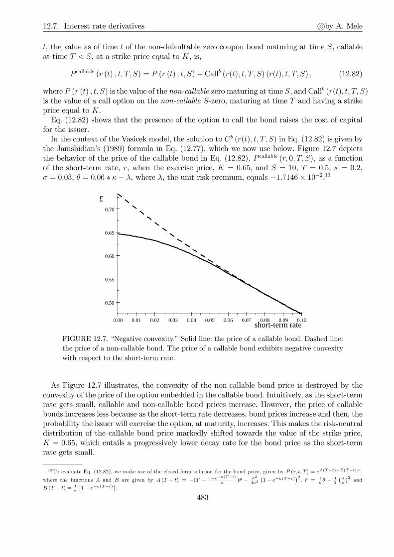
12.7. Interest rate derivatives c©by A. Mele
t, the value as of time t of the non-defaultable zero coupon bond maturing at time S, callableat time T < S, at a strike price equal to K, is,
P callable (r (t) , t, T, S) = P (r (t) , t, S)− Callb (r(t), t, T, S) (r(t), t, T, S) , (12.82)
where P (r (t) , t, S) is the value of the non-callable zero maturing at time S, andCallb (r(t), t, T, S)is the value of a call option on the non-callable S-zero, maturing at time T and having a strikeprice equal to K.Eq. (12.82) shows that the presence of the option to call the bond raises the cost of capital
for the issuer.In the context of the Vasicek model, the solution to Cb (r(t), t, T, S) in Eq. (12.82) is given by
the Jamshidian’s (1989) formula in Eq. (12.77), which we now use below. Figure 12.7 depictsthe behavior of the price of the callable bond in Eq. (12.82), P callable (r, 0, T, S), as a functionof the short-term rate, r, when the exercise price, K = 0.65, and S = 10, T = 0.5, κ = 0.2,σ = 0.03, θ = 0.06 ∗ κ− λ, where λ, the unit risk-premium, equals −1.7146× 10−2.13
0.00 0.01 0.02 0.03 0.04 0.05 0.06 0.07 0.08 0.09 0.10
0.50
0.55
0.60
0.65
0.70
short-term rate
£
FIGURE 12.7. “Negative convexity.” Solid line: the price of a callable bond. Dashed line:
the price of a non-callable bond. The price of a callable bond exhibits negative convexity
with respect to the short-term rate.
As Figure 12.7 illustrates, the convexity of the non-callable bond price is destroyed by theconvexity of the price of the option embedded in the callable bond. Intuitively, as the short-termrate gets small, callable and non-callable bond prices increase. However, the price of callablebonds increases less because as the short-term rate decreases, bond prices increase and then, theprobability the issuer will exercise the option, at maturity, increases. This makes the risk-neutraldistribution of the callable bond price markedly shifted towards the value of the strike price,K = 0.65, which entails a progressively lower decay rate for the bond price as the short-termrate gets small.
13To evaluate Eq. (12.82), we make use of the closed-form solution for the bond price, given by P (r, t, T ) = eA(T−t)−B(T−t)·r,
where the functions A and B are given by A (T − t) = −(T − 1−e−κ(T−t)
κ)r − σ2
4κ3
(1− e−κ(T−t)
)2, r = 1
κθ − 1
2
(σκ
)2and
B (T − t) = 1κ
[1− e−κ(T−t)
].
483

12.7. Interest rate derivatives c©by A. Mele
What is the duraton of a callable bond? Naturally, a five year bond with fixed-coupons issuedwhen interest rates are relatively high might resemble, so to speak, a three year conventionalbond, as a likely decrease in the interest rates would lead the bond-issuer to reedem its debtat the strike price. To formalize this intuition, we can compute the stochastic duration of thecallable bond predicted by this model, using Eq. (12.20). For the Vasicek model, we have that thesemi-elasticity of the non-callable bond price with respect to r is Ψ(r, T − t) = 1
κ
(1− e−κ(T−t)
),
and its inverse with respect to time-to-maturity is given by:
Ψ−1 (x) = −1κln (1− κx) .
Therefore, the stochastic duration for the callable bond predicted by the Vasicek model is, byEq. (12.20):
D (r, S − t) = −1κln
(1 + κ
Pr (r, t, S)− Cbr (r, t, T, S)
P (r, t, S)− Cb (r, t, T, S)
),
where subscripts denote partial derivatives.[In progress]Next, we proceed with pricing the puttable bond. As explained in the previous chapter,
Section 11.8, the payoff at the expiration of the bondholders right to tender the bonds is:
max P,K = P +max K − P, 0 ,where P is the price of a non-puttable bond. We can use, again, the Vasicek model to pricethe previous payoff. The price at t of a non-defaultable zero-coupon bond maturing at time S,puttable at time T < S, at a strike price equal to K, when the short-term rate is r (t), is:
P puttable (r (t) , t, T, S) = P (r (t) , t, S)+Putb (r (t) , t, T, S) = Callb (r(t), t, T, S)+P (r (t) , t, T )K,
where P (r (t) , t, S) is the value of the non-puttable zero maturing at time S; Putb (r(t), t, T, S)is the value of a put option on the non-puttable zero maturing at S, maturing at T , struckable atK; and the second equality follows by the put-call parity of Eq. (12.75), with Callb (r(t), t, T, S)defined as in Eq. (12.82).[In progress]
12.7.5 Related fixed income products
12.7.5.1 Fixed coupon bonds
Given a set of dates Tini=0, a fixed coupon bond pays off a fixed coupon ci at Ti, i = 1, · · · , nand one unit of numéraire at time Tn. Ideally, one generic coupon at time Ti pays off for thetime-interval Ti − Ti−1. It is assumed that the various coupons are known at time t < T0. Bythe FTAP, the value of a fixed coupon bond is
Pfcb (t, Tn) = P (t, Tn) +n∑
i=1
ciP (t, Ti) .
12.7.5.2 Floating rate bonds
A floating rate bond works as a fixed coupon bond, with the important exception that thecoupon payments are defined as:
ci = δi−1L (Ti−1, Ti) =1
P (Ti−1, Ti)− 1, (12.83)
484

12.7. Interest rate derivatives c©by A. Mele
where δi ≡ Ti+1−Ti, and where the second equality is the definition of the simply-compoundedLIBOR rates introduced in Section 12.1.2.1 (see Eq. (12.1)). By the FTAP, the price pfrb as oftime t of a floating rate bond is:
pfrb(t) = P (t, Tn) +n∑
i=1
Et[e−
∫ Tit r(τ)dτδi−1L (Ti−1, Ti)
]
= P (t, Tn) +n∑
i=1
Et
[e−
∫ Tit r(τ)dτ
P (Ti−1, Ti)
]−
n∑
i=1
P (t, Ti)
= P (t, Tn) +n∑
i=1
P (t, Ti−1)−n∑
i=1
P (t, Ti)
= P (t, T0).
where the second line follows from Eq. (12.83) and the third line from Eq. (12.7) given in Section12.1.The same result can be obtained by assuming an economy where the floating rates contin-
uously pay off the instantaneous short-term rate r. Let T0 = t for simplicity. In this case, pfrbis solution to the PDE (12.74), with π(r) = r, and boundary condition pfrb(T ) = 1. As it canverified, pfrb = 1, all r and τ , is indeed solution to the PDE (12.74).
12.7.5.3 Options on fixed coupon bonds
The payoff of an option maturing at T0 on a fixed coupon bond paying off at dates T1, · · · , Tnis given by:
[Pfcb(T0, Tn)−K]+ =[P (T0, Tn) +
n∑
i=1
ciP (T0, Ti)−K]+
. (12.84)
At first glance, the expectation of the payoff in Eq. (12.84) seems very difficult to evaluate.Indeed, even if we end up with a model that predicts bond prices at time T0, P (T0, Ti), to belognormal, we know that the sum of lognormals is not lognormal. This issue can be dealt within an elegant manner. Suppose we wish to model the bond price P (t, T ) through any one ofthe models of the short-term rate reviewed in Section 12.3. In this case, the pricing function isobviously P (t, T ) = P (r, t, T ). Assume, further, that
For all t, T,∂P (r, t, T )
∂r< 0, (12.85)
and thatFor all t, T, lim
r→0P (r, t, T ) > K and lim
r→∞P (r, t, T ) = 0. (12.86)
Under conditions (12.85) and (12.86), there is one and only one value of r, say r∗, that solvesthe following equation:
P (r∗, T0, Tn) +n∑
i=1
ciP (r∗, T0, Ti) = K. (12.87)
Then, the payoff in Eq. (12.84) can be written as:
[n∑
i=1
ciP (r(T0), T0, Ti)−K]+
=
[n∑
i=1
ci (P (r(T0), T0, Ti)− P (r∗, T0, Ti))]+
,
485
12.7. Interest rate derivatives c©by A. Mele
where ci = ci, i = 1, · · · , n− 1, and cn = 1 + cn.Next, note that by condition (12.85), the terms P (r(T0), T0, Ti) − P (r∗, T0, Ti) have all the
same sign for all i.14 Therefore, the payoff in Eq. (12.84) is,
[n∑
i=1
ciP (r(T0), T0, Ti)−K]+
=n∑
i=1
ci [P (r(T0), T0, Ti)− P (r∗, T0, Ti)]+ . (12.88)
Note that each term of the sum in Eq. (12.88) can be evaluated as an option on a pure discountbond with strike price equal to P (r∗, T0, Ti), where the threshold r∗ is found numerically. Thedevice to reduce the problem of an option on a fixed coupon bond to a problem involving thesum of options on zero coupon bonds was invented by Jamshidian (1989).15 The price of thecall on the fixed coupon bond is, therefore,
Call (t, T0;Pfcb (t, Tn) ,K, v) =n∑
i=1
ciCall (t, T0;P (t, Ti) , P (r∗, T0, Ti) , vi) , (12.89)
where r∗ solves Eq. (12.87), and,
Call (t, T0;Pi, P∗i , vi) = PiΦ (d1,i)− P ∗i P (t, T0)Φ (d1,i − vi) ,
d1,i =ln
PiP∗i P (t,T0)
+ 12v2i
vi, vi = σ
√1−e−2κ(T0−t)
2κB (T0, Ti) , B (t, T ) = 1
κ
(1− e−κ(T−t)
).
Why are perfectly fitting models so important, in practice? Suppose that in Eq. (12.87), thecritical value r∗ is computed by means of the Vasicek model. This assumption is attractivebecause it allows to evaluate the payoff in Eq. (12.88) with the Jamshidian’s formula of Section12.7.2. However, this way to proceed does not ensure that the yield curve is perfectly fitted.The natural alternative is to use the corresponding perfectly fitting extension, as in Eq. (12.89).However, such a perfectly fitting extension gives rise to a zero-coupon bond option price thatis perfectly equal to the one that can be obtained through the Jamshidian’s formula. However,things differ as far as options on zero coupon bonds are concerned. Indeed, by using the perfectlyfitting model (12.59), one obtains bond prices such that the solution r∗ in Eq. (12.87) is radicallydifferent from the one obtained when bond prices are obtained with the simple Vasicek model.
12.7.5.4 Interest rate swaps
A Savings and Loan (S&L, henceforth) is an institution that makes mortgage, car and personalloans to individual members, financed through savings. During the 1980s through the beginningof the 1990s, these forms of cooperative ventures entered into a deep and persistent crisis, leadingto a painful Government bailout of about $125b under George H.W. Bush administration.There are many causes of this crisis, but one of them was certainly the rise in short-term ratesarising as a result of inflation and the attempts at fighting against it–the so-called MonetaryExperiment mentioned in Section 12.3.7. But banking is risky precisely because it involveslending at horizons longer than those relating to borrowing, and S&L “banking” was not anexception to such modus operandi. Certainly, interest rate swaps could have helped copyingwith the inversion of the yield curve of the time.
14Suppose that P (r(T0), T0, T1) > P (r∗, T0, T1). By Eq. (12.85), r(T0) < r∗. Hence P (r(T0), T0, T2) > P (r∗, T0, T2), etc.15The conditions in Eqs. (12.85) and (12.86) hold, within the Vasicek’s model that Jamshidian considered in his paper. In fact,
the condition in Eq. (12.85) holds for all one-factor stationary, Markov models of the short-term rate. However, the condition inEq. (12.85) is not a general property of bond prices in multi-factor models (see Mele (2003)).
486

12.7. Interest rate derivatives c©by A. Mele
An interest rate swap is simply an exchange of interest rate payments. Typically, one coun-terparty exchanges a fixed against a floating interest rate payment. The floating payment istypically a short-term interest rate. For example, the counterparty receiving a floating interestrate payment has “good” (or only) access to markets for “variable” interest rates, but wishes topay fixed interest rates. Alternatively, the counterparty receiving a floating interest rate wantsto hedge itself against changes in short-term rates, as it might have been the case for S&Linstitutions during the 1980s. The counterparty receiving a floating interest rate payment andpaying a fixed interest rate Kirs has a payoff equal to,
δi−1 [L (Ti−1, Ti)−Kirs]
at time Ti, i = 1, · · · , n. Each of this payment is a FRA really, and can be evaluated as inSection 12.1. By convention, we say that the swap payer is the counterparty who pays the fixedinterest rate Kirs, and that the swap receiver is the counterparty receiving the fixed interestrate Kirs.With a dedicated interest swap of this kind, a S&L institution would have locked-in the
yield curve: at time t, the payoff for the financial institution is, in this stylized example,δi−1
[Llong (Ti−1, Ti)− L (Ti−1, Ti)
]+ δi−1 [L (Ti−1, Ti)−Kirs] = δi−1
[Llong (Ti−1, Ti)−Kirs
],
where Llong (Ti−1, Ti) is the interest rate gained over long-term assets. Naturally, if short-term in-terest rates had to go down, relative toKirs, a S&L institution would not have benefited from theincreased long-term/short-term spread, δi−1
[Llong (Ti−1, Ti)− L (Ti−1, Ti)
]. But clearly insuring
against yield curve inversions is the thing to do, if yield curve inversions lead to bankruptcy andbankruptcy is costly. We shall see, below, that other products exist, such as caps or swaptions,which ensure against the upside while at the same time freeing up the downside.By the FTAP, the price as of time t of an interest rate swap payer, pirs (t), say, is:
pirs (t) =n∑
i=1
Et[e−
∫ Tit r(τ)dτδi−1 (L (Ti−1, Ti)−Kirs)
]=
n∑
i=1
IRS(t, Ti−1, Ti;Kirs), (12.90)
where IRS is the value of a FRA and, by Eq. (12.8) in Section 12.1, is:
IRS (t, Ti−1, Ti;Kirs) = δi−1 [F (t, Ti−1, Ti)−Kirs]P (t, Ti) .
The forward swap rate Rswap is the value of Kirs such that pirs(t) = 0. Simple computationsyield:
Rswap (t) =
∑ni=1 δi−1F (t, Ti−1, Ti)P (t, Ti)∑n
i=1 δi−1P (t, Ti)=P (t, T0)− P (t, Tn)∑n
i=1 δi−1P (t, Ti), (12.91)
where the last equality is due to Eq. (12.3) in Section 12.1: δi−1F (t, Ti−1, Ti)P (t, Ti) = P (t, Ti−1)−P (t, Ti).16 This expression is quite similar to the par coupon rate derived in Section 11.2.2.2of the previous chapter.
16To cast this problem in terms of continuous time swap exchanges and, then, PDEs, we set pirs(T ) ≡ 0 as a boundary condition,and π(r) = r − k, where k plays the same role as Kirs above. Then, if the bond price P (τ) is solution to Eq. (12.74), the following
function, pirs(τ) = 1− P (τ)− k∫ Tτ P (s)ds, does also satisfy Eq. (12.74).
487

12.7. Interest rate derivatives c©by A. Mele
By plugging the expression for the forward swap rate in Eq. (12.91) into Eq. (12.90), weobtain the following intuitive expression for the swap payer:
pirs (t) =n∑
i=1
δi−1F (t, Ti−1, Ti)P (t, Ti)−Kirs
n∑
i=1
δi−1P (t, Ti)
=
n∑
i=1
δi−1P (t, Ti) (Rswap (t)−Kirs)
≡ PVBPt (T1, · · · , Tn) (Rswap (t)−Kirs) , (12.92)
where PVBPT (T1, · · · , Tn) is the so-called swap’s “Present Value of the Basis Point” (see, e.g.,Brigo and Mercurio, 2006), i.e. the present value impact of one basis point move in the forwardswap rate at T .
12.7.5.5 Caps & floors
A cap works as an interest rate swap, with the important exception that the exchange of interestrates payments takes place only if actual interest rates are higher thanK. A cap protects againstupward movements of the interest rates, freeing up the downside. By going long a cap, the S&Linstitution in the example of the previous section, then, would benefit from the downside inthe short-term interest rates through a cap on them, literally. Precisely, a cap is made up ofcaplets. The payoff as of time Ti of a caplet is:
δi−1 [L (Ti−1, Ti)−K]+ , i = 1, · · · , n.
Floors are defined in a similar way, with a single floorlet paying off,
δi−1 [K − L (Ti−1, Ti)]+
at time Ti, i = 1, · · · , n.We will only focus on caps. By the FTAP, the value pcap of a cap as of time t is:
pcap(t) =n∑
i=1
Et[e−
∫ Tit r(τ)dτδi−1 (L (Ti−1, Ti)−K)+
]. (12.93)
We can develop explicit solutions to this problem, relying upon models of the short-termrate. First, we use the standard definition of simply compounded rates given in Section 12.1(see Eq. (12.1)), viz δi−1L (Ti−1, Ti) =
1P (Ti−1,Ti)
− 1, and rewrite the caplet payoff as follows:
(δi−1L (Ti−1, Ti)− δi−1K)+ =
1
P (Ti−1, Ti)(1− (1 + δi−1K)P (Ti−1, Ti))
+ .
We have,
pcap (t) =n∑
i=1
Et
[e−
∫ Tit r(τ)dτ
P (Ti−1, Ti)(1− (1 + δi−1K)P (Ti−1, Ti))
+
]
=n∑
i=1
Et
[e−
∫ Ti−1t r(τ)dτ 1
Ki
(Ki − P (Ti−1, Ti))+
], Ki = (1 + δi−1K)
−1 , (12.94)
488
12.7. Interest rate derivatives c©by A. Mele
where the last equality follows by a simple computation.17 For the models of Jamshidian orin Hull & White, bond prices are such that the cap price in Eq. (12.94) can be expressed inclosed-form. Indeed, Eq. (12.94) makes clear a cap is a basket of puts on zero coupon bonds,with strikes Ki. As such, it can be priced in closed form, using the models in Sections 12.7.4.1and 12.7.4.2. We have:
pcap (t) =n∑
i=1
1
KiPut (t, Ti−1;P (t, Ti) ,Ki, v) , (12.95)
where Put (·) satisfies the put-call parity in Eq. (12.75), and, by the pricing formulae in Section12.7.4.1,
Call (t, Ti−1;P (t, Ti) ,Ki, v) = P (t, Ti) Φ (d1,i)−KiP (t, Ti−1)Φ (d1,i − v) ,
d1,i =ln
P(t,Ti)KiP(t,Ti−1)
+ 12v2
v, v = σ
√1−e−2κ(Ti−1−t)
2κB (Ti−1, Ti) , B (t, T ) = 1
κ
(1− e−κ(T−t)
).
(12.96)Naturally, caps on interest rates, which are nothing but baskets of calls, are portfolios of putson fixed coupon bonds, due to the inverse relation between prices and interest rates.18
12.7.5.6 Swaptions
Let us proceed with the example of the S&L institution in the previous sections. The benefits fora S&L institution long of caps is to be protected against upward movements in the short-termrates while ensuring the downside is freed up. These benefits arise, so to speak, period per periodin that, a cap is a basket of options with different maturities. A swaption works differently, inthat the optionality kicks in “all together.” Suppose at time t, the S&L institution is stillconcerned about future inversions of the yield curve and, therefore, anticipates it might needto go for going long a swap payer at some future date. At the same time, the institution mightfear that in the future, swap rates will be lower relative to some reference strike. Swaptionsallow to free up such a downside risk, in that they simply are options to enter a swap contracton a future date. Let the maturity date of this option be T0. Then, at time T0, the payoff fora payer swaption is the maximum between zero and the value of a payer interest rate swap atT0, pirs(T0), viz
(pirs (T0))+ =
[n∑
i=1
IRS (T0, Ti−1, Ti;Kirs)
]+
=
[n∑
i=1
δi−1 (F (T0, Ti−1, Ti)−Kirs)P (T0, Ti)
]+
.
(12.97)
17By the law of iterated expectations,
Et
e−∫Tit r(τ)dτ
P (Ti−1, Ti)[1−KiP (Ti−1, Ti)]
+
= Et
E
e−∫ Tit r(τ)dτ
P (Ti−1, Ti)(1−KiP (Ti−1, Ti))
+
∣∣∣∣∣∣F (Ti)
= Et
[
E
(
e−∫Tit r(τ)dτ e
∫ TiTi−1
r(τ)dτ(1−KiP (Ti−1, Ti))
+
∣∣∣∣∣F (Ti)
)]
= Et
[E
(e−
∫Ti−1t r(τ)dτ (1−KiP (Ti−1, Ti))
+
∣∣∣∣F (Ti)
)]
= Et
[e−
∫Ti−1t r(τ)dτ (1−KiP (Ti−1, Ti))
+
]
18We might also price caps and floors through the partial differential equation (12.74), after setting π (r) = (r − k)+ (caps) andπ (r) = (k − r)+ (floors), for some strike k. However, this type of contracts, where payoffs are paid continuously in time, is highlystylized, and does not exist in the markets.
489
12.7. Interest rate derivatives c©by A. Mele
By the FTAP, the value of the payer swaption at time t is:
pswaption (t) = Et
[e−
∫ T0t r(τ)dτ
(n∑
i=1
δi−1 (F (T0, Ti−1, Ti)−Kirs)P (T0, Ti)
)+]
= Et
[e−
∫ T0t r(τ)dτ
(1− P (T0, Tn)−Kirs
n∑
i=1
δi−1P (T0, Ti)
)+], (12.98)
where we used the relation δi−1F (T0, Ti−1, Ti) =P (T0,Ti−1)P (T0,Ti)
− 1.Eq. (12.98) is the expression for the price of a put option on a fixed coupon bond struck at
one. Therefore, we can price this contract in closed-form, through the models in Section 12.7.4.1and 12.7.4.2, similarly to that we did in the previous section for caps pricing. We have:
pswaption (t) = Put (t, T0;Pfcb (t, Tn) , 1, v) ,
where Put (·) satisfies the put-call parity in Eq. (12.75). By the pricing formulae in Section12.7.4.1,
Call (t, T0;Pfcb (t, Tn) , 1, v) = Kirs
n∑
i=1
δi−1Call (t, T0;P (t, Ti) , P∗i , v)+Call (t, T0;P (t, Tn) , P
∗n , v) ,
where Call (t, T0;P (t, Ti) , P∗i , v) is as in Eq. (12.96), with P ∗i = P (r∗, T0, Ti), and r
∗ solutionto Eq. (12.87) for K = 1.
12.7.6 Market models
12.7.6.1 Models and market practice
As illustrated in the previous sections, models of the short-term rate can be used to obtainclosed-form solutions of virtually every important interest rate derivative product. The typicalexamples are the Vasicek model and its perfectly fitting extension. Yet practitioners evaluatecaps through the Black’s (1976) formula. The assumption underlying the market practice is thatthe simply-compounded forward rate is lognormally distributed. As it turns out, the analyticallytractable (Gaussian) short-term rate models are not consistent with this assumption. Clearly,the (Gaussian) Vasicek model does not predict that the simply-compounded forward rates areGeometric Brownian motions.19
Is it be possible to address these issues through a non-Markovian HJM? The answer is inthe affirmative, although some qualifications are necessary. A practical difficulty with HJMis that instantaneous forward rates are not observed, which at a first sight seems to be anhindrance to realistic pricing of caps and swaptions, a so important portion of the interestrate derivative markets. This point.has been addressed by Brace, Gatarek and Musiela (1997),Jamshidian (1997) and Miltersen, Sandmann and Sondermann (1997), who observed that theHJM framework can be somehow “forced” to produce models ready to be used consisentlywith the market practice. The key feature of these models is the emphasis on the dynamics ofthe simply-compounded forward rates. One additional, and technical, assumption is that these
19 Indeed, 1 + δiFi (τ) = P (τ,Ti)
P(τ,Ti+1)= exp [∆Ai (τ)−∆Bi (τ) r (τ)], where ∆Ai (τ) = A (τ, Ti) − A (τ, Ti+1), and ∆Bi (τ) =
B (τ, Ti)−B (τ, Ti+1). Hence, Fi (τ) is not a Geometric Brownian motion, despite the fact that the short-term rate r is Gaussianand, hence, the bond price is log-normal. Black ’76 can not be applied in this context.
490
12.7. Interest rate derivatives c©by A. Mele
simply-compounded forward rates are lognormal under the risk-neutral probability Q. That is,given a non-decreasing sequence of reset times Tii=0,1,···, each simply-compounded rate, Fi, issolution to the following stochastic differential equation:20
dFi(τ )
Fi(τ)= mi(τ )dτ + γi(τ )dW (τ), τ ∈ [t, Ti] , i = 0, · · · , n− 1, (12.99)
where to simplify notation, we have set, Fi (τ ) ≡ F (τ , Ti, Ti+1), and mi and γi are some de-terministic functions of time (γi is vector valued). On a mathematical point of view, thatassumption that Fi follows Eq. (12.99) is innocuous.
21
As we shall show, this simple framework can be used to use the simple Black’s (1976) formulato price caps and floors. However, we need to emphasize that there is nothing wrong with theshort-term rate models analyzed in previous sections. The real advance of the so-called marketmodel is to give a rigorous foundation to the standard market practice to price caps and floorsby means of the Black’s (1976) formula.
12.7.6.2 Simply-compounded forward rate dynamics, and no-arb restrictions
By the definition of the simply-compounded forward rates in Eq. (12.3),
ln
[P (τ , Ti)
P (τ , Ti+1)
]= ln [1 + δiFi(τ)] . (12.100)
The logic we follow, now, is the same as that underlying the HJM representation of Section12.4. We wish to express the volatility of bond prices in terms of the volatility of forward rates.To achieve this task, we first assume that bond prices are driven by Brownian motions andexpand the l.h.s. of Eq. (12.100) (step 1). Then, we expand the r.h.s. of Eq. (12.100) (step 2).Finally, we identify the two diffusion terms derived from the previous two steps (step 3).
Step 1: Let Pi ≡ P (τ , Ti), and assume that under the risk-neutral probability Q, Pi is solutionto:
dPiPi
= rdτ + σbidW .
In terms of the HJM framework in Section 12.4,
σbi(τ ) = −σI(τ , Ti) = −∫ Ti
τ
σ(τ , ℓ)dℓ, (12.101)
where σ(τ , ℓ) is the instantaneous volatility of the instantaneous ℓ-forward rate as of timeτ . By Itô’s lemma,
d ln
[P (τ , Ti)
P (τ , Ti+1)
]= −1
2
[‖σbi‖2 − ‖σb,i+1‖2
]dτ + (σbi − σb,i+1) dW . (12.102)
20Brace, Gatarek and Musiela (1997) derived their model by specifying the dynamics of the spot simply-compounded Liborinterest rates. Since Fi(Ti) = L(Ti) (see Eq. (??)), the two derivations are essentially the same.
21 It is well-known that lognormal instantaneous forward rates create mathematical problems to the money market account (see, forexample, Sandmann and Sondermann (1997) for a succinct overview on how this problem is easily handled with simply-compoundedforward rates).
491
12.7. Interest rate derivatives c©by A. Mele
Step 2: Applying Itô’s lemma to ln [1 + δiFi(τ)], and using Eq. (12.99), yields:
d ln [1 + δiFi(τ )] =δi
1 + δiFidFi −
1
2
δ2i(1 + δiFi)2
(dFi)2
=
[δimiFi1 + δiFi
− 1
2
δ2iF2i ‖γi‖2
(1 + δiFi)2
]dτ +
δiFi1 + δiFi
γidW . (12.103)
Step 3: By Eq. (12.100), the diffusion terms in Eqs. (12.102) and (12.103) have to be the same.Therefore,
σbi(τ)− σb,i+1(τ ) =δiFi(τ)
1 + δiFi(τ)γi(τ), τ ∈ [t, Ti] .
By summing over i, we get the following no-arbitrage restriction applying to the volatilityof the bond prices:
σbi(τ )− σb,0(τ ) = −i−1∑
j=0
δjFj(τ )
1 + δjFj(τ)γj(τ). (12.104)
As is clear, Eq. (12.104) is merely a restriction to the general HJM framework. In otherwords, assume the instantaneous forward rates are as in Eq. (12.64) of Section 12.4. As wedemonstrated in Section 12.4, then, the bond prices volatility is given by Eq. (12.101). But ifwe also assume that simply-compounded forward rates are solution to Eq. (12.99), then, thebond prices volatility is also equal to Eq. (12.104). Comparing Eq. (12.101) with Eq. (12.104)produces,
∫ Ti
T0
σ(τ , ℓ)dℓ =i−1∑
j=0
δjFj(τ )
1 + δjFj(τ)γj(τ).
The practical interest to restrict the forward-rate volatility dynamics in this way lies in thepossibility to obtain closed-form solutions for some of the interest rates derivatives surveyed inSection 12.7.3.
12.7.6.3 Pricing formulae
Caps & floors
We provide analytical results for the price of caps only. We have:
pcap (t) =n∑
i=1
Et[e−
∫ Tit r(τ)dτδi−1 (L (Ti−1, Ti)−K)+
]
=n∑
i=1
Et[e−
∫ Tit r(τ)dτδi−1 (F (Ti−1, Ti−1, Ti)−K)+
]
=n∑
i=1
δi−1P (t, Ti) · EQTiF [F (Ti−1, Ti−1, Ti)−K]+ , (12.105)
where EQTiF[·] denotes, as usual, the expectation taken under the Ti-forward martingale proba-
bility QTiF ; the first equality is Eq. (12.93); and the second equality has been obtained through
the usual change of probability technique introduced Section 12.2.4.
492
12.7. Interest rate derivatives c©by A. Mele
The key point is that
Fi−1(τ ) ≡ Fi−1(τ , Ti−1, Ti), τ ∈ [t, Ti−1], is a martingale under QTiF .
A proof of this statement was given in Section 12.1. By Eq. (12.99), this means that Fi−1(τ) issolution to:
dFi−1 (τ )
Fi−1 (τ)= γi−1 (τ) dW
QTiF (τ ) , τ ∈ [t, Ti−1] , i = 1, · · · , n,
under QTiF . Therefore, the cap price in Eq. (12.105) reduces to that of Black (1976), once we
assume γ is deterministic:
EQTiF[F (Ti−1, Ti−1, Ti)−K]+ = Fi−1 (t)Φ (d1,i−1)−KΦ (d1,i−1 − si) , (12.106)
where
d1,i−1 =ln Fi−1(t)
K+ 1
2s2i
si, s2i =
∫ Ti−1
t
γi−1(τ)2dτ .
A derivation of the Black’s formula is provided in Appendix 8.
Swaptions
By Eq. (12.92), the payoff of a payer swaption expiring at time T0 is:
[pirs (T0)]+ = PVBPT0 (T1, · · · , Tn) (Rswap(T0)−Kirs)
+ , PVBPT0 (T1, · · · , Tn) =n∑
i=1
δi−1P (T0, Ti).
Therefore, by the FTAP, and a change of measure,
pswaption(t) = Et[e−
∫ T0t r(τ)dτPVBPT0 (T1, · · · , Tn) (Rswap(T0)−Kirs)
+]
= PVBPt (T1, · · · , Tn) · EQswap (Rswap(T0)−Kirs)+ , (12.107)
where EQswap denotes the expectation taken under the so-called forward swap probability, definedby:
dQswap
dQ
∣∣∣∣FT0
= e−∫ T0
tr(τ)dτ PVBPT0 (T1, · · · , Tn)
PVBPt (T1, · · · , Tn).
It is easy to see that E
(dQswap
dQ
∣∣∣FT0
)= 1, by using the definition of PVBPT0 (T1, · · · , Tn), and
the pricing equation, P (t, Ti) = Et[e−
∫ T0t r(τ)dτP (T0, Ti)
]. The key point underlying this change
of measure is that the forward swap rate Rswap is a Qswap-martingale,22 and clearly, positive.Therefore, it must satisfy:
dRswap (τ)
Rswap (τ)= γswap (τ) dWswap (τ ) , τ ∈ [t, T0] , (12.108)
22By Eq. (12.91), and one change of measure,
EQswap [Rswap(τ)] = EQswap
[P (τ, T0)− P (τ, Tn)
PVBPτ (T1, · · ·, Tn)
]= Et
e−∫ τt r(τ)dτ (P (τ, T0)− P (τ, Tn))
PVBPt (T1, · · ·, Tn)
=P (t, T0)− P (t, Tn)
PVBPt (T1, · · ·, Tn)= Rswap(t).
493

12.7. Interest rate derivatives c©by A. Mele
where Wswap is a Qswap-Brownian motion, and γswap (τ) is adapted.If the volatility γswap (τ) in Eq. (12.108) is deterministic, we can use Black 76 to price the
payer swaption in Eq. (12.107) in closed-form. We have:
pswaption(t) = PVBPt (T1, · · · , Tn) · Black76(Rswap (t) ;T0, Kirs,√V ), (12.109)
where Black76 (·) is given by Black’s (1976) formula:
Black76(Rswap (t) ;T0, Kirs,√V ) = Rswap (t)Φ (dt)−KirsΦ(dt −
√V ),
dt =lnRswap(t)
Kirs+ 1
2V
√V
, V =∫ T0
tγswap (τ )
2 dτ .
Inconsistencies
If the forward rate is solution to Eq. (12.99), γswap cannot be deterministic. Unfortunately, ifforward swap rates are lognormal, then, Eq. (12.99) does not hold. Therefore, we may use Black’sformula to price either caps or swaptions, not both. This might limit the importance of marketmodels. A couple of tricks that seem to work in practice. The best known is based on a suggestionby Rebonato (1998), to replace the true pricing problem with an approximating pricing problemwhere γswap is deterministic. That works in practice, but in a world with stochastic volatility,we should expect that trick to generate unstable things in periods experiencing highly volatilevolatility. See, also, Rebonato (1999) for an essay on related issues. The next section suggeststo use numerical approximation based on Montecarlo techniques.
12.7.6.4 Numerical approximations
Suppose forward rates are lognormal. Then, we can price caps using Black’s formula. As forswaptions, Montecarlo integration should be implemented as follows. By a change of measure,
pswaption (t) = Et
[e−
∫ T0t r(τ)dτ
(n∑
i=1
δi−1 (F (T0, Ti−1, Ti)−K)P (T0, Ti))+]
= P (t, T0)EQT0F
[n∑
i=1
δi−1 (F (T0, Ti−1, Ti)−K)P (T0, Ti)]+
,
where F (T0, Ti−1, Ti), i = 1, · · · , n, can be simulated under QT0F .
Details are as follows. We know that
dFi−1(τ )
Fi−1(τ)= γi−1(τ )dW
QTiF (τ ). (12.110)
By results in Appendix 3, we also know that:
dWQTiF (τ ) = dWQ
T0F (τ)− [σbi(τ)− σb0(τ )] dτ
= dWQT0F (τ) +
i−1∑
j=0
δjFj(τ)
1 + δjFj(τ )γj(τ)dτ,
where the second line follows from Eq. (12.104) in the main text. Replacing this into Eq. (12.110)leaves:
dFi−1(τ )
Fi−1(τ)= γi−1(τ )
i−1∑
j=0
δjFj(τ )
1 + δjFj(τ)γj(τ )dτ + γi−1(τ )dW
QT0F (τ), i = 1, · · · , n.
494

12.7. Interest rate derivatives c©by A. Mele
These can easily be simulated with the methods described in any standard textbook such asKloeden and Platen (1992).
12.7.6.5 Volatility surfaces
Caps & floors
The market practice quotes volatility surfaces by relying on the models of this section, ratherthan those of Sections 12.7.4.1-12.7.4.2. In the models of Sections 12.7.4.1-12.7.4.2, volatilitysurfaces might be produced, but only indirectly, after calibration of the two parameters κ andσ, as Eq. (12.95) indicates. It is easier, however, to provide volatility surfaces in the first place,through the models of this section. Quite simply, practitioners use Eq. (12.106) and quotevolatilities such that the market price of a cap equals to the value predicted by Eq. (12.106)using the desired implied volatility si. In Eq. (12.106),
si =√Ti−1 − t · γ (i) ,
for some γ (i), although, then, practitioners simply quote the value of γn that satisfies:
γn : p$cap (t;n) =
n∑
i=1
δi−1P (t, Ti) · Black76 (Fi−1 (t) ;K, si,n) ,
where p$cap (t;n) is the market price of the cap, and:
Black76 (Fi−1 (t) ;K, si,n) = Fi−1 (t) Φ(dn1,i−1
)−KΦ
(dn1,i−1 − si,n
),
dn1,i−1 =lnFi−1(t)
K+ 1
2s2i,n
si,n, si,n =
√Ti−1 − t · γn
Given n, we can bootstrap γ (i), i.e. we can recursively solve for γ (i), as follows:
0 =n∑
i=1
δi−1P (t, Ti) · [Black76 (Fi−1 (t) ;K, si,n)− Black76 (Fi−1 (t) ;K, si)] , n = 1, · · · , N,
where N is the latest available maturity, and si =√Ti−1 − t · γ (i). The values of γ (i) constitute
what is known as the term structure of caps volatilities.
Swaptions
As for swaptions, the situation is much simpler. The market practice is to quote swaptionsthrough standard implied vols, i.e. those vols IVt such that, once inserted into Eq. (12.109),delivers the swaption market price:
pswaption(t) = PVBPt (T1, · · · , Tn) · Black76 (Rswap (t) ;T0, Kirs, IVt) .
495
12.8. Appendix 1: The FTAP for bond prices c©by A. Mele
12.8 Appendix 1: The FTAP for bond prices
Suppose there exist m pure discount bond prices Pi ≡ P (τ, Ti)mi=1τ∈[t,T ] satisfying:
dPiPi
= µbi · dτ + σbi · dW, i = 1, · · · ,m, (12A.1)
where W is a Brownian motion in Rd, and µbi and σbi are progressively F(τ)-measurable functionsguaranteeing the existence of a strong solution to the previous system (σbi is vector-valued). The valueprocess V of a self-financing portfolio in these m bonds and a money market technology satisfies:
dV =(π⊤(µb − 1mr) + rV
)dτ + π⊤σbdW,
where π is some portfolio, 1m is a m-dimensional vector of ones, and
µb = [µb1, · · · , µb2]⊤ , σb = [σb1, · · · , σb2]⊤ .
Next, suppose that there exists a portfolio π such that π⊤σb = 0. This is an arbitrage opportunity ifthere exist events for which at some time, µb − 1mr = 0 (use π when µb − 1mr > 0, and −π whenµm − 1dr < 0: the drift of V will then be appreciating at a deterministic rate that is strictly greaterthan r). Therefore, arbitrage opportunities are ruled out if:
π⊤(µb − 1mr) = 0 whenever π⊤σb = 0.
In other terms, arbitrage opportunities are ruled out when every vector in the null space of σb isorthogonal to µb−1mr, or when there exists a λ taking values in Rd satisfying some basic integrabilityconditions, and such that
µb − 1mr = σbλ
or,µbi − r = σbiλ, i = 1, · · · ,m. (12A.2)
In this case,dPiPi
= (r + σbiλ) · dτ + σbi · dW, i = 1, · · · ,m.
Now define W = W +∫λdτ , dQ
dP = exp(−∫ Tt λ⊤dW − 1
2
∫ Tt ‖λ‖
2 dτ). The Q-martingale property ofthe “normalized” bond price processes now easily follows by Girsanov’s theorem. Indeed, define for ageneric i, P (τ, T ) ≡ P (τ, Ti) ≡ Pi, and:
g(τ) ≡ e−∫ τt r(u)du · P (τ, T ), τ ∈ [t, T ] .
By Girsanov’s theorem, and an application of Itô’s lemma,
dg
g= σbi · dW , under Q.
Therefore, for all τ ∈ [t, T ], g(τ) = Et [g(T )], implying that:
g(τ) ≡ e−∫ τt r(u)du · P (τ, T ) = Et [g(T )] = Et[e
−∫ Tt r(u)du · P (T, T )︸ ︷︷ ︸]
=1
= Et[e−
∫ Tt r(u)du
],
orP (τ, T ) = e
∫ τt r(u)du · Et
[e−
∫ Tt r(u)du
]= Et
[e−
∫ Tτ r(u)du
], all τ ∈ [t, T ],
496
12.8. Appendix 1: The FTAP for bond prices c©by A. Mele
which is Eq. (12.2).Notice that no assumption has been made on m. The previous result holds for all m, be they less
or greater than d. Suppose, for example, that there are no other traded assets in the economy. Then,if m < d, there exists an infinite number of risk-neutral proabilities Q. If m = d, there exists one andonly one risk-neutral probability Q. If m > d, there exists one and only one risk-neutral probabilitybut then, the various bond prices have to satisfy some basic no-arbitrage restrictions. As an example,take m = 2 and d = 1. Eq. (12A.2) then becomes
µb1 − r
σb1= λ =
µb2 − r
σb2.
In other terms, the Sharpe ratio of any two bonds must be identical. Relation (12A.2) will be usedseveral times in this chapter.
• In Section 12.3, the primitive of the economy is the short-term rate, solution of a multidimen-sional diffusion process, and µbi and σbi will be derived via Itô’s lemma.
• In Section 12.4, µbi and σbi are restricted by a model for the forward rates.
497

12.9. Appendix 2: Certainty equivalent interpretation of forward prices c©by A. Mele
12.9 Appendix 2: Certainty equivalent interpretation of forward prices
Multiply both sides of the bond pricing equation (12.2) by the amount S(T ):
P (t, T ) · S(T ) = Et[e−
∫ Ttr(τ)dτ
]· S(T ).
Suppose momentarily that S(T ) is known at T . In this case, we have:
P (t, T ) · S(T ) = Et[e−
∫ Tt r(τ)dτ · S(T )
].
But in the applications we have in mind, S(T ) is random. Define then its certainty equivalent by thenumber S(T ) that solves:
P (t, T ) · S(T ) = Et[e−
∫ Ttr(τ)dτ · S(T )
],
orS(T ) = Et [ηT (T ) · S(T )] , (12A.3)
where ηT (T ) has been defined in (12.15).Comparing Eq. (12A.3) with Eq. (12.14) reveals that forward prices can be interpreted in terms of
the previously defined certainty equivalent.
498

12.10. Appendix 3: Additional results on T -forward martingale probabilities c©by A. Mele
12.10 Appendix 3: Additional results on T -forward martingale probabilities
Eq. (12.15) defines ηT (T ) as:
ηT (T ) =e−
∫ Tt r(τ)dτ · 1
Et[e−
∫ Tt r(τ)dτ
]
More generally, we can define a density process as:
ηT (τ) ≡e−
∫ τtr(u)du · P (τ, T )
Et[e−
∫ Tt r(τ)dτ
] , τ ∈ [t, T ] .
By the FTAP, exp(−∫ τt r(u)du) · P (τ, T )τ∈[t,T ] is a Q-martingale (see Appendix 1 to this chapter).
Therefore, E[dQTFdQ
∣∣∣Fτ ] = E[ηT (T )| Fτ ] = ηT (τ) all τ ∈ [t, T ], and in particular, ηT (t) = 1. We now
show that this works. And at the same time, we show this by deriving a representation of ηT (τ) thatcan be used to find “forward premia.”
We begin with the dynamic representation (12A.1) given for a generic bond price # i, P (τ, T ) ≡P (τ, Ti) ≡ Pi:
dP
P= µ · dτ + σ · dW,
where we have defined µ ≡ µbi and σ ≡ σbi.Under the risk-neutral probability Q,
dP
P= r · dτ + σ · dW ,
where W =W +∫λ is a Q-Brownian motion.
By Itô’s lemma,dηT (τ)
ηT (τ)= − [−σ(τ, T )] · dW (τ), ηT (t) = 1.
The solution is:
ηT (τ) = exp
[−1
2
∫ τ
t‖σ(u, T )‖2 du−
∫ τ
t(−σ(u, T )) · dW (u)
].
Under the usual integrability conditions, we can now use the Girsanov’s theorem and conclude that
WQTF (τ) ≡ W (τ) +
∫ τ
t
(−σ(u, T )⊤
)du (12A.4)
is a Brownian motion under the T -forward martingale probability QTF .
Finally, note that for all integers i and non decreasing sequences of dates Tii=0,1,··· ,,
WQTiF (τ) = W (τ) +
∫ τ
t
(−σ(u, Ti)⊤
)du, i = 0, 1, · · · .
Therefore,
WQTiF (τ) =WQ
Ti−1F (τ)−
∫ τ
t
[σ(u, Ti)
⊤ − σ(u, Ti−1)⊤]du, i = 1, 2, · · · , (12A.5)
is a Brownian motion under the Ti-forward martingale probability QTiF . Eqs. (12A.5) and (12A.4) are
used in Section 12.7 on interest rate derivatives.
499

12.11. Appendix 4: Principal components analysis c©by A. Mele
12.11 Appendix 4: Principal components analysis
Principal component analysis transforms the original data into a set of uncorrelated variables, theprincipal components, with variances arranged in descending order. Consider the following program,
maxC1
[var (Y1)] s.t. C⊤1 C1 = 1,
where var (Y1) = C⊤1 ΣC1, and the constraint is an identification constraint. The first order conditionslead to,
(Σ− λI)C1 = 0,
where λ is a Lagrange multiplier. The previous condition tells us that λ must be one eigenvalue ofthe matrix Σ, and that C1 must be the corresponding eigenvector. Moreover, we have var (Y1) =C⊤1 ΣC1 = λ which is clearly maximized by the largest eigenvalue. Suppose that the eigenvalues of Σare distinct, and let us arrange them in descending order, i.e. λ1 > · · · > λp. Then,
var (Y1) = λ1.
Therefore, the first principal component is Y1 = C⊤1(R− R
), where C1 is the eigenvector corresponding
to the largest eigenvalue, λ1.Next, consider the second principal component. The program is, now,
maxC2
[var (Y2)] s.t. C⊤2 C2 = 1 and C⊤2 C1 = 0,
where var (Y2) = C⊤2 ΣC2. The first constraint, C⊤2 C2 = 1, is the usual identification constraint. Thesecond constraint, C⊤2 C1 = 0, is needed to ensure that Y1 and Y2 are orthogonal, i.e. E (Y1Y2) = 0.The first order conditions for this problem are,
0 = ΣC2 − λC2 − νC1
where λ is the Lagrange multiplier associated with the first constraint, and ν is the Lagrange multiplierassociated with the second constraint. By pre-multiplying the first order conditions by C⊤1 ,
0 = C⊤1 ΣC2 − ν,
where we have used the two constraints C⊤1 C2 = 0 and C⊤1 C1 = 1. Post-multiplying the previousexpression by C⊤1 , one obtains, 0 = C⊤1 ΣC2C⊤1 − νC⊤1 = −νC⊤1 , where the last equality follows byC⊤1 C2 = 0. Hence, ν = 0. So the first order conditions can be rewritten as,
(Σ− λI)C2 = 0.
The solution is now λ2, and C2 is the eigenvector corresponding to λ2. (Indeed, this time we cannotchoose λ1 as this choice would imply that Y2 = C⊤1
(R− R
), implying that E (Y1Y2) = 0.) It follows
that var (Y2) = λ2.In general, we have,
var (Yi) = λi, i = 1, · · · , p.Let Λ be the diagonal matrix with the eigenvalues λi on the diagonal. By the spectral decompositionof Σ, Σ = CΛC⊤, and by the orthonormality of C, C⊤C = I, we have that C⊤ΣC = Λ and, hence,
∑pi=1 var (Ri) = Tr (Σ) = Tr
(ΣCC⊤
)= Tr
(C⊤ΣC
)= Tr (Λ) .
Hence, Eq. (12.26) follows.
500
12.12. Appendix 5: A few analytics for the Hull and White model c©by A. Mele
12.12 Appendix 5: A few analytics for the Hull and White model
As in the Ho and Lee model, the instantaneous forward rate f(τ, T ) predicted by the Hull and Whitemodel is as in Eq. (12.57), where functions A2 and B2 can be easily computed from Eqs. (12.60) and(12.61) as:
A2(τ, T ) = σ2
∫ T
τB(s, T )B2(s, T )ds−
∫ T
τθ(s)B2(s, T )ds, B2(τ , T ) = e−κ(T−τ).
Therefore, the instantaneous forward rate f(τ, T ) predicted by the Hull and White model is obtainedby replacing the previous equations in Eq. (12.57). The result is then equated to the observed forwardrate f$(t, τ) so as to obtain:
f$(t, τ) = − σ2
2κ2
[1− e−κ(τ−t)
]2+
∫ τ
tθ(s)e−κ(τ−s)ds+ e−κ(τ−t)r(t).
By differentiating the previous equation with respect to τ , and rearranging terms,
θ(τ ) =∂
∂τf$(t, τ) +
σ2
κ
(1− e−κ(τ−t)
)e−κ(τ−t) + κ
[∫ τ
tθ(s)e−κ(τ−s)ds+ e−κ(τ−t)r(t)
]
=∂
∂τf$(t, τ) +
σ2
κ
(1− e−κ(τ−t)
)e−κ(τ−t) + κ
[f$(t, τ) +
σ2
2κ2
(1− e−κ(τ−t)
)2],
which reduces to Eq. (12.62) after using simple algebra.
501

12.13. Appendix 6: Expectation theory and embedding in selected models c©by A. Mele
12.13 Appendix 6: Expectation theory and embedding in selected models
A. Expectation theory
Suppose that
σ(·, ·) = σ and λ(·) = λ, (12A.6)
where σ and λ are constants. We derive the dynamics of r and compare them with f to deducesomething about the expectation theory. We have:
r(τ) = f(t, τ) +
∫ τ
tα(s, τ)ds+ σ (W (τ)−W (t)) ,
where
α(τ, T ) = σ(τ, T )
∫ T
τσ(τ, ℓ)dℓ+ σ(τ, T )λ(τ) = σ2(T − τ) + σλ.
Hence, ∫ τ
tα(s, τ )ds =
1
2σ2 (τ − t)2 + σλ(τ − t).
Finally,
r(τ) = f(t, τ) +1
2σ2 (τ − t)2 + σλ(τ − t) + σ (W (τ)−W (t)) ,
and since E (W (τ)| F(t)) =W (t),
E [r(τ)| F(t)] = f(t, τ) +1
2σ2 (τ − t)2 + σλ(τ − t).
Even with λ < 0, this model is not able to always generate E[r(τ)| F(t)] < f(t, τ). As shown in thefollowing exercise, this is due to the nonstationary nature of the volatility function. Indeed, suppose,next, that instead of Eq. (12A.6), we have that
σ(t, T ) = σ · exp(−γ(T − t)) and λ(·) = λ,
where σ, γ and λ are constants. In this case, we have:
r(τ) = f(t, τ) +
∫ τ
tα(s, τ)ds+ σ
∫ τ
te−γ(τ−s) · dW (s),
where
α(s, τ) = σ2e−γ(τ−s)∫ τ
se−γ(ℓ−s)dℓ+ σλe−γ(τ−s) =
σ2
γ
[e−γ(τ−s) − e−2γ(τ−s)
]+ σλe−γ(τ−s).
Finally,
E [r(τ)| F(t)] = f(t, τ) +
∫ τ
tα(s, τ)ds = f(t, τ) +
σ
γ
(1− e−γ(τ−t)
)[σ
2γ
(1− e−γ(τ−t)
)+ λ
].
Therefore, it is sufficient to have a risk-premium such that −λ > σ2γ , to generate the prediction that:
E [r(τ)| F(t)] < f(t, τ) for any τ .
In other words, λ < 0 is a necessary condition, not sufficient. Notice that when λ = 0, it always holdsthat E (r(τ)| F(t)) > f(t, τ).
502

12.13. Appendix 6: Expectation theory and embedding in selected models c©by A. Mele
B. Embedding
We now embed the Ho and Lee model in Section 12.5.2 in the HJM format. In the Ho and Lee model,
dr(τ) = θ(τ)dτ + σdW (τ),
where W is a Q-Brownian motion. By Eq. (12.57) in Section 12.4,
f(r, t, T ) = −A2(t, T ) +B2(t, T )r,
where A2(t, T ) =∫ Tt θ(s)ds− 1
2σ2(T − t)2 and B2(t, T ) = 1. Therefore, by Eqs. (12.70),
σ(t, T ) = B2(t, T ) · σ = σ,
α(t, T )− σ(t, T )λ(t) = −A12(t, T ) +B12(t, T )r +B2(t, T )θ(t) = σ2(T − t).
Next, we embed the Vasicek model in Section 12.4 in the HJM format. The Vasicek model is:
dr(τ) = (θ − κr(τ))dτ + σdW (τ),
where W is a Q-Brownian motion. By results in Section 12.3,
f(r, t, T ) = −A2(t, T ) +B2(t, T )r,
where −A2(t, T ) = −σ2∫ Tt B(s, T )B2(s, T )ds + θ
∫ Tt B2(s, T )ds, B2(t, T ) = e−κ(T−t) and B(t, T )
= 1κ
[1− e−κ(T−t)
]. By Eqs. (12.70),
σ(t, T ) = σ ·B2(t, T ) = σ · e−κ(T−t);
α(t, T )− σ(t, T )λ(t) = −A12(t, T ) +B12(t, T )r + (θ − κr)B2(t, T ) =σ2
κ
[1− e−κ(T−t)
]e−κ(T−t).
Naturally, this model can never be embedded within a HJM model because it is not of the perfectlyfitting type. In practice, condition (12.71) can never hold in the simple Vasicek model. However, themodel is embeddable once θ is turned into an infinite dimensional parameter à la Hull and White (seeSection 12.3).
503

12.14. Appendix 7: Additional results on string models c©by A. Mele
12.14 Appendix 7: Additional results on string models
Here we prove Eq. (12.73). We have, αI (τ, T ) = 12
∫ Tτ g (τ, T, ℓ2)dℓ2 + cov(dPP , dξξ ), where
g (τ, T, ℓ2) ≡∫ T
τσ (τ, ℓ1)σ (τ, ℓ2)ψ (ℓ1, ℓ2)dℓ1.
Differentiation of the cov term is straight forward. Moreover,
∂
∂T
∫ T
τg (τ, T, ℓ2) dℓ2 = g (τ, T, T ) +
∫ T
τ
∂g (τ, T, ℓ2)
∂Tdℓ2
= σ (τ, T )
[∫ T
τσ (τ, x) [ψ (x, T ) + ψ (T, x)] dx
]
= 2σ (τ, T )
[∫ T
τσ (τ, x)ψ (x, T )dx
].
504

12.15. Appendix 8: Changes of numéraire c©by A. Mele
12.15 Appendix 8: Changes of numéraire
A. Jamshidian (1989)
Consider the following change-of-numéraire result. Let
dA
A= µAdτ + σAdW,
and consider a similar process B with coefficients µB and σB. We have:
d(A/B)
A/B=
(µA − µB + σ2
B − σAσB)dτ + (σA − σB)dW. (12A.7)
We apply this result to the process y (τ, S) ≡ P (τ,S)P (τ,T ) , under Q
SF as well as under QT
F . The objective
is to obtain the solution as of time T of y (τ, S) viz
y(T, S) ≡ P (T, S)
P (T, T )= P (T, S) under QS
F as well as under QTF .
This allows us to calculate the two probabilities in Eq. (12.77).By Itô’s lemma, the PDE (12.35) and the fact that Pr = −BP ,
dP (τ, x)
P (τ , x)= rdτ − σB(τ, x)dW (τ), x ≥ T.
By applying Eq. (12A.7) to y(τ, S),
dy(τ , S)
y(τ, S)= σ2
[B(τ, T )2 −B(τ, T )B(τ, S)
]dτ − σ [B(τ, S)−B(τ, T )] dW (τ). (12A.8)
All we need to do now is to change measure with the tools of Appendix 3. We have that:
dWQxF (τ) = dW (τ) + σB(τ, x)dτ
is a Brownian motion under the x-forward martingale probability. Replace thenWQxF into Eq. (12A.8),then integrate, and obtain:
y(T, S)
y(t, S)= P (T, S)
P (t, T )
P (t, S)= e−
12σ2∫ Tt [B(τ,S)−B(τ,T )]2dτ−σ
∫ Tt [B(τ,S)−B(τ,T )]dWQTF (τ),
y(T, S)
y(t, S)= P (T, S)
P (t, T )
P (t, S)= e
12σ2∫ Tt [B(τ,S)−B(τ,T )]2dτ−σ
∫ Tt [B(τ,S)−B(τ,T )]dWQSF (τ).
Rearranging terms gives Eqs. (12.78) in the main text.
B. Black (1976)
To prove Eq. (12.106), we need to evaluate the following expectation:
E [x(T )−K]+ ,
where
x(T ) = x(t)e−12
∫ Tt γ(τ)2dτ+
∫ Tt γ(τ)dW (τ). (12A.9)
505

12.15. Appendix 8: Changes of numéraire c©by A. Mele
Let Iexe be the indicator of all events s.t. x(T ) ≥ K. We have
Et [x(T )−K]+ = Et [x(T ) · Iexe]−K · Et [Iexe]
= x(t) · Et[x(T )
x(t)· Iexe
]−K · Et [Iexe]
= x(t) · EQx [Iexe]−K · Et [Iexe]= x(t) ·Qx (x(T ) ≥ K)−K ·Q (x(T ) ≥ K) .
where the probability Qx is defined as:
dQx
dQ=
x(T )
x(t)= e−
12
∫ Tt γ(τ)2dτ+
∫ Tt γ(τ)dW (τ),
a Q-martingale starting at one. Under Qx,
dWx(τ) = dW (τ)− γdτ
is a Brownian motion, and x in Eq. (12A.9) can be written as:
x (T ) = x (t) e12
∫ Tt γ(τ)2dτ+
∫ Tt γ(τ)dWx(τ).
It is straightforward that Q (x(T ) ≥ K) = Φ(d2) and Qx (x(T ) ≥ K) = Φ(d1), where
d2/1 =ln
(x(t)K
)∓ 1
2
∫ Tt γ(τ)2dτ
√∫ Tt γ(τ)2dτ
.
Applying this to EQTiF
[Fi−1(Ti−1)−K]+ gives the formulae of the text.
506

12.15. Appendix 8: Changes of numéraire c©by A. Mele
References
Aït-Sahalia, Y. (1996): “Testing Continuous-Time Models of the Spot Interest Rate.” Reviewof Financial Studies 9, 385-426.
Ahn, C.-M. and H.E. Thompson (1988): “Jump-Diffusion Processes and the Term Structureof Interest Rates.” Journal of Finance 43, 155-174.
Ang, A. and M. Piazzesi (2003): “A No-Arbitrage Vector Autoregression of Term StructureDynamics with Macroeconomic and Latent Variables.” Journal of Monetary Economics50, 745-787.
Balduzzi, P., S. R. Das, S. Foresi and R. K. Sundaram (1996): “A Simple Approach to ThreeFactor Affine Term Structure Models.” Journal of Fixed Income 6, 43-53.
Black, F. (1976): “The Pricing of Commodity Contracts.” Journal of Financial Economics 3,167-179.
Black, F. and M. Scholes (1973): “The Pricing of Options and Corporate Liabilities.” Journalof Political Economy 81, 637-659.
Brace, A., D. Gatarek and M. Musiela (1997): “The Market Model of Interest Rate Dynamics.”Mathematical Finance 7, 127-155.
Brigo, D. and F. Mercurio (2006): Interest Rate Models–Theory and Practice, with Smile,Inflation and Credit. Springer Verlag (2nd Edition).
Brunnermeier, M. (2009): “Deciphering the Liquidity and Credit Crunch 2007-08.” Journal ofEconomic Perspectives 23, 77-100.
Carverhill, A. (1994): “When is the Short-Rate Markovian?”Mathematical Finance 4, 305-312.
Cochrane, J. H. and M. Piazzesi (2005): “Bond Risk Premia.” American Economic Review 95,138-160.
Collin-Dufresne, P. and R. S. Goldstein (2002): “Do Bonds Span the Fixed-Income Markets?Theory and Evidence for Unspanned Stochastic Volatility.” Journal of Finance 57, 1685-1729.
Conley, T. G., L. P. Hansen, E. G. J. Luttmer and J. A. Scheinkman (1997): “Short-TermInterest Rates as Subordinated Diffusions.” Review of Financial Studies 10, 525-577.
Cox, J. C., J. E. Ingersoll and S. A. Ross (1979): “Duration and the Measurement of BasisRisk.” Journal of Business 52, 51-61.
Cox, J. C., J. E. Ingersoll and S. A. Ross (1985): “A Theory of the Term Structure of InterestRates.” Econometrica 53, 385-407.
Dai, Q. and K. J. Singleton (2000): “Specification Analysis of Affine Term Structure Models.”Journal of Finance 55, 1943-1978.
Duffie, D. and R. Kan (1996): “A Yield-Factor Model of Interest Rates.”Mathematical Finance6, 379-406.
507
12.15. Appendix 8: Changes of numéraire c©by A. Mele
Duffie, D. and K. J. Singleton (1999): “Modeling Term Structures of Defaultable Bonds.”Review of Financial Studies 12, 687-720.
Estrella, A. and G. Hardouvelis (1991): “The Term Structure as a Predictor of Real EconomicActivity.” Journal of Finance 46, 555-76.
Fama, E. F. and R. R. Bliss (1987): “The Information in Long-Maturity Forward Rates.”American Economic Review 77, 680-692.
Fong, H. G. and O. A. Vasicek (1991): “Fixed Income Volatility Management.” The Journalof Portfolio Management (Summer), 41-46.
Geman, H. (1989): “The Importance of the Forward Neutral Probability in a Stochastic Ap-proach to Interest Rates.” Unpublished working paper, ESSEC.
Geman H., N. El Karoui and J. C. Rochet (1995): “Changes of Numeraire, Changes of Prob-ability Measures and Pricing of Options.” Journal of Applied Probability 32, 443-458.
Goldstein, R. S. (2000): “The Term Structure of Interest Rates as a Random Field.” Reviewof Financial Studies 13, 365-384.
Harvey, C. R. (1991): “The Term Structure and World Economic Growth.” Journal of FixedIncome 1, 4-17.
Harvey, C. R. (1991): “The Term Structure Forecasts Economic Growth.” Financial AnalystsJournal May/June 6-8.
Heaney, W. J. and P. L. Cheng (1984): “Continuous Maturity Diversification of Default-FreeBond Portfolios and a Generalization of Efficient Diversification.” Journal of Finance 39,1101-1117.
Heath, D., R. Jarrow and A. Morton (1992): “Bond Pricing and the Term-Structure of InterestRates: a New Methodology for Contingent Claim Valuation.” Econometrica 60, 77-105.
Ho, T. S. Y. and S.-B. Lee (1986): “Term Structure Movements and the Pricing of InterestRate Contingent Claims.” Journal of Finance 41, 1011-1029.
Hördahl, P., O. Tristani and D. Vestin (2006): “A Joint Econometric Model of Macroeconomicand Term Structure Dynamics.” Journal of Econometrics 131, 405-444.
Hull, J. C. (2003): Options, Futures, and Other Derivatives. Prentice Hall. 5th edition (Inter-national Edition).
Hull, J. C. and A. White (1990): “Pricing Interest Rate Derivative Securities.” Review ofFinancial Studies 3, 573-592.
Jagannathan, R. (1984): “Call Options and the Risk of Underlying Securities.” Journal ofFinancial Economics 13, 425-434.
Jamshidian, F. (1989): “An Exact Bond Option Pricing Formula.” Journal of Finance 44,205-209.
508

12.15. Appendix 8: Changes of numéraire c©by A. Mele
Jamshidian, F. (1997): “Libor and Swap Market Models and Measures.” Finance and Stochas-tics 1, 293-330.
Jöreskog, K. G. (1967): “Some Contributions to Maximum Likelihood Factor Analysis.” Psy-chometrica 32, 443-482.
Karlin, S. and H. M. Taylor (1981): A Second Course in Stochastic Processes. San Diego:Academic Press.
Kennedy, D. P. (1994): “The Term Structure of Interest Rates as a Gaussian Random Field.”Mathematical Finance 4, 247-258.
Kennedy, D. P. (1997): “Characterizing Gaussian Models of the Term Structure of InterestRates.” Mathematical Finance 7, 107-118.
Kessel, R. A. (1965): “The Cyclical Behavior of the Term Structure of Interest Rates.” NationalBureau of Economic Research Occasional Paper No. 91.
Kloeden, P. and E. Platen (1992): Numeric Solutions of Stochastic Differential Equations.Berlin: Springer Verlag.
Knez, P. J., R. Litterman and J. Scheinkman (1994): “Explorations into Factors ExplainingMoney Market Returns.” Journal of Finance 49, 1861-1882.
Langetieg, T. (1980): “A Multivariate Model of the Term Structure of Interest Rates.” Journalof Finance 35, 71-97.
Laurent, R. D. (1988): “An Interest Rate-Based Indicator of Monetary Policy.” Federal ReserveBank of Chicago Economic Perspectives 12, 3-14.
Laurent, R. D. (1989): “Testing the Spread.” Federal Reserve Bank of Chicago EconomicPerspectives 13, 22-34.
Litterman, R. and J. Scheinkman (1991): “Common Factors Affecting Bond Returns.” Journalof Fixed Income 1, 54-61.
Litterman, R., J. Scheinkman, and L. Weiss (1991): “Volatility and the Yield Curve.” Journalof Fixed Income 1, 49-53.
Longstaff, F. A. and E. S. Schwartz (1992): “Interest Rate Volatility and the Term Structure:A Two-Factor General Equilibrium Model.” Journal of Finance 47, 1259-1282.
Mele, A. (2003): “Fundamental Properties of Bond Prices in Models of the Short-Term Rate.”Review of Financial Studies 16, 679-716.
Mele, A. and F. Fornari (2000): Stochastic Volatility in Financial Markets: Crossing the Bridgeto Continuous Time. Boston: Kluwer Academic Publishers.
Merton, R. C. (1973): “Theory of Rational Option Pricing.” Bell Journal of Economics andManagement Science 4, 141-183.
Miltersen, K., K. Sandmann and D. Sondermann (1997): “Closed Form Solutions for TermStructure Derivatives with Lognormal Interest Rate.” Journal of Finance 52, 409-430.
509
12.15. Appendix 8: Changes of numéraire c©by A. Mele
Rebonato, R. (1998): Interest Rate Option Models. Wiley.
Rebonato, R. (1999): Volatility and Correlation. Wiley.
Ritchken, P. and L. Sankarasubramanian (1995): “Volatility Structure of Forward Rates andthe Dynamics of the Term Structure.” Mathematical Finance 5, 55-72.
Rothschild, M. and J. E. Stiglitz (1970): “Increasing Risk: I. A Definition.” Journal of Eco-nomic Theory 2, 225-243.
Sandmann, K. and D. Sondermann (1997): “A Note on the Stability of Lognormal InterestRate Models and the Pricing of Eurodollar Futures.” Mathematical Finance 7, 119-125.
Santa-Clara, P. and D. Sornette (2001): “The Dynamics of the Forward Interest Rate Curvewith Stochastic String Shocks.” Review of Financial Studies 14, 149-185.
Stanton, R. (1997): “A Nonparametric Model of Term Structure Dynamics and the MarketPrice of Interest Rate Risk.” Journal of Finance 52, 1973-2002.
Stock, J. H. and M. W. Watson (1989): “New Indexes of Coincident and Leading EconomicIndicators.” In: Blanchard, O. J. and S. Fischer (Eds.): NBER Macroeconomics Annual1989, MIT Press, 352-394.
Stock, J. H. and M. W. Watson (2003): “Forecasting Output and Inflation: The Role of AssetPrices,” Journal of Economic Literature 41, 788-829.
Vasicek, O. (1977): “An Equilibrium Characterization of the Term Structure.” Journal ofFinancial Economics 5, 177-188.
Veronesi, P. (2010): Fixed Income Securities: Valuation, Risk and Risk Management. JohnWiley and Sons.
510

13Risky debt and credit derivatives
13.1 Introduction
13.2 The classics: Modigliani-Miller irrelevance results
Firms are divided into equivalent returns classes. Returns are perfectly correlated within thesame class. Let π be the constant expected profit paid off by the each firm within class k, andEU be the price of an unlevered firm’s share. Under the conditions reviewed in Chapter 7, wehave that EU =
∑∞t=1 (1 + ρk)
−t π, where ρk is the risk-adjusted discount rate prevailing insector k, such that the return on equity (ROE) for the unlevered firm is,
ρk =π
EU,
a constant for all unlevered firms belonging to the asset class k. Naturally, the value of the firmis equal to the value of equity, VU = EU , say. Next, let us introduce debt: for any arbitrary firmin the k-th sector that issues D nominal value of debt, we have that its value, denoted as VL,is the sum of equity and debt, VL = EL +D. [Assumptions: ]We have:
T 13.1 (Modigliani & Miller theorem). In the absence of arbitrage and frictions, themarket value of any firm is independent of its capital structure and is given by capitalizing itsexpected dividend at the discount rate appropriate to its class: Vj =
πρk, for any firm j ∈ U,L
in class k.
In other words, the return on investment (ROI), defined as ρk =πVj, is the same for two firms
that earn the same expected profit, π, and that only differ as regards their capital structure.Naturally, the ROE and ROI are the same for the unlevered firm.The proof of Theorem 13.1 can be obtained with the modern tools reviewed in Chapter 2
through 4, but for sake of completeness, we produce the arguments in Modigliani and Miller(1958), as these are very simple. Consider two firms: a first, unlevered and a second, levered.They both earn the same expected profit, π. Suppose to purchase the shares of the unlevered

13.2. The classics: Modigliani-Miller irrelevance results c©by A. Mele
firm and borrow the same amount of money issued by the levered firm. In the absence ofarbitrage or any frictions, the value of this portfolio should equal the value of the levered firm,which is possible as soon as the values of the levered and the unlevered firm are the same.Mathematically, given an arbitrary α ∈ (0, 1), we do the following trade: (i) we buy NU =
αEL+DEU
= α VLVU
of the unlevered firm; (ii) we sell NL = α shares of the levered firm. Thesetwo trades make the balance of the position worth −NUEU + NLEL = −αD, and so (iii) weborrow αD at the interest rate r, to make this initial position worthless. This portfolio yields:(i) +NUπ, due to the purchase of the shares of the unlevered firm, (ii) −NL (π − rD), due to thesale of the shares of the levered firm, which of course has to pay interests on its debt, and (iii)−rαD, arising to honour the debt we are making to build up the worthless portfolio. Summing
up, NUπ −NL (π − rD)− rαD = α(VLVU− 1
)π. If VL > VU , we have an arbitrage opportunity
as we may make money out of a worthless portfolio, and if VL < VU , we have an arbitrageas well, as we could reverse the positions of the worthless portfolio. So we need to have thatVL = VU = EU =
πρk.
[As mentioned, Theorem 13.1 can be proved through the modern tools in Chapters 2 through4]
We have: π = ROI · V . Therefore,
ROE =π − rDE
=ROI · (E +D)− rD
E= ROI + (ROI− r) D
E.
If the financial conditions of the firm do not affect the interest rate on debt, then, the ROE isincreasing in the leverage ratio, D
E, provided ROI > r. This situation arises when the arbitrage
arguments underlying Theorem 13.1 assume no-arbitrage trades can be implemented with acost of borrowing money equal to that of the firm. In the presence of market frictions suchas asymmetric information between borrowers and lenders, this needs not to be the case. Forexample, debt markets might be concerned about the size of the leverage ratio. Assume, forexample, that r = f (ℓ), where ℓ = D
E, and in particular that f (ℓ) = 0.03ℓ. Then, we have that:
ROE = ROI + (ROI− 0.03ℓ) ℓ. The picture below depicts the behavior of ROE as a functionof ℓ, assuming that ROI = 5% and that the risk-free rate in case of no such frictions is r = 3%.
512

13.3. Conceptual approaches to valuation of defaultable securities c©by A. Mele
0.0 0.2 0.4 0.6 0.8 1.0 1.2 1.4 1.6 1.8 2.00.03
0.04
0.05
0.06
0.07
0.08
0.09
Leverage ratio
ROE
The solid line depicts the ROE for a firm sustaining a cost of debt independent of the
leverage ratio, with ROI = 5% and r = 2%. The dashed line is the ROE for a firm that
has a cost of debt increasing in the leverage ratio ℓ, r (ℓ) = 0.03ℓ.
Consider the firm with cost of capital depending on the current leverage rato, ℓ. For a lowlevel of ℓ, the ROE increases with ℓ, so as to magnify the difference ROI − 0.03ℓ through themultiplying effect (ROI− 0.03ℓ) ℓ. However, for higher leverage ratios, the differenceROI−0.03ℓbecomes thinner and thinner, and an increase in ℓ then leads to marginal lower ROE. In thisexample, there is an interior value for the leverage ratio that maximizes the ROE, which is,approximately, ℓ = 0.83.
13.3 Conceptual approaches to valuation of defaultable securities
13.3.1 Firm’s value, or structural, approaches
Relies on the structure of the firm. Shares and bonds as derivatives on the firm’s assets.
Stylized balance sheet
Assets (A)
Equity (E)(Shares)
Debt (D)(Bonds)
Therefore, we have the accounting identity: Assets = Equity + Debt, or
A = E +D.
At the time of debt expiration, debtholders receive the minimum between the debt nominal valueand the value of the assets the firm can liquidate to honour the debt obligation. Debtholders aresenior claimants. Equity holders are residual claimants to the firm’s assets –> Junior claimants
513

13.3. Conceptual approaches to valuation of defaultable securities c©by A. Mele
We can use these basic insights to illustrate the first model about the risk-structure of interestrates, the Merton - KMV approach. Equity is like a European call option written on the firm’sassets, with expiration equal to the debt expiration, and strike equal to the nominal value ofdebt. Current value of debt equals the value of the assets minus the value of equity, i.e. thevalue of a risk-free discount bond minus the value of a put option on the firm with strike priceequal to the nominal value of debt, as shown by Eq. (13.3) below.Merton (1974) uses the Black and Scholes (1973) formula to derive the price of debt. The
main assumption underlying this model is that the assets of the firm can be traded, and thattheir value At satisfies,
1
dAt
At
= rdt+ σdWt, (13.1)
where Wt is a Brownian motion under the risk-neutral probability, σ is the instantaneousstandard deviation, and r is the short-term rate on riskless bonds.Let N be the nominal value of debt, T be time of expiration of debt; Dt the debt value as
of at time t ≤ T . As argued earlier, shareholders have long a European call option, and thebondholders are residual claimants. Mathematically,
DT =
AT ,N,
if the firm defaults, i.e. AT < Nif the firm is solvent, i.e. AT ≥ N
We can decompose the assets value at time T , into the sum of the value of equity and the valueof debt, at time T ,
DT = min AT ,N = AT − max AT −N, 0 .≡ Equity at T
(13.2)
Note, also, that,
DT = min AT , N = N − max N −AT , 0 .≡ Put on the firm
(13.3)
That is, credit risk raises the cost of capital.
0.0 0.2 0.4 0.6 0.8 1.0 1.2 1.4 1.6 1.8 2.0 2.20.0
0.2
0.4
0.6
0.8
1.0
1.2
A_T
1Eq. (13.1) could be generalized to one in which dAt = (rAt − δt) dt+ σAtdWt, where δt is the instantaneous cash flow to thefirm. This would make the firm value equal to A0 = E
(∫∞0 e−rtδtdt
). For example, one could take δt to be a geometric Brownian
motion with parameters g and σ, in which case At = (r − g)−1 δt, forever, but we’re just ignoring this complication.
514
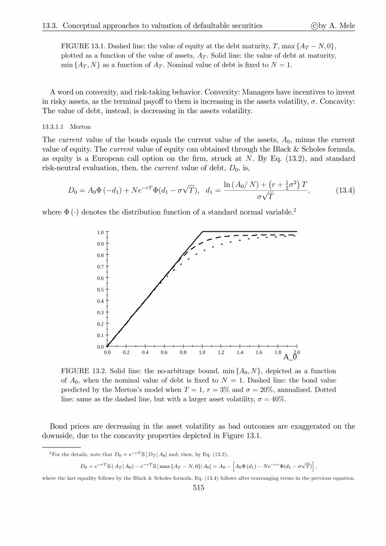
13.3. Conceptual approaches to valuation of defaultable securities c©by A. Mele
FIGURE 13.1. Dashed line: the value of equity at the debt maturity, T , max AT −N, 0,plotted as a function of the value of assets, AT . Solid line: the value of debt at maturity,
min AT , N as a function of AT . Nominal value of debt is fixed to N = 1.
A word on convexity, and risk-taking behavior. Convexity: Managers have incentives to investin risky assets, as the terminal payoff to them is increasing in the assets volatility, σ. Concavity:The value of debt, instead, is decreasing in the assets volatility.
13.3.1.1 Merton
The current value of the bonds equals the current value of the assets, A0, minus the currentvalue of equity. The current value of equity can obtained through the Black & Scholes formula,as equity is a European call option on the firm, struck at N . By Eq. (13.2), and standardrisk-neutral evaluation, then, the current value of debt, D0, is,
D0 = A0Φ (−d1) +Ne−rTΦ(d1 − σ√T ), d1 =
ln (A0/N) +(r + 1
2σ2
)T
σ√T
, (13.4)
where Φ (·) denotes the distribution function of a standard normal variable.2
0.0 0.2 0.4 0.6 0.8 1.0 1.2 1.4 1.6 1.8 2.00.0
0.1
0.2
0.3
0.4
0.5
0.6
0.7
0.8
0.9
1.0
A_0
FIGURE 13.2. Solid line: the no-arbitrage bound, min A0,N, depicted as a function
of A0, when the nominal value of debt is fixed to N = 1. Dashed line: the bond value
predicted by the Merton’s model when T = 1, r = 3% and σ = 20%, annualized. Dotted
line: same as the dashed line, but with a larger asset volatility, σ = 40%.
Bond prices are decreasing in the asset volatility as bad outcomes are exaggerated on thedownside, due to the concavity properties depicted in Figure 13.1.
2For the details, note that D0 = e−rTE [DT |A0] and, then, by Eq. (13.2),
D0 = e−rTE (AT |A0)− e−rTE [max AT −N, 0|A0] = A0 −[A0Φ(d1)−Ne−rτΦ(d1 − σ
√T )],
where the last equality follows by the Black & Scholes formula. Eq. (13.4) follows after rearranging terms in the previous equation.
515

13.3. Conceptual approaches to valuation of defaultable securities c©by A. Mele
The risk-structure of interest rates is obtained with the standard formula for continuouslycompounded interest rates as,
R = − 1Tln
(D0
N
)= r + Spread,
where the term-spread or, simply, the spread, is
Spread = − 1Tln
(A0
NerTΦ (−d1) + Φ (d2)
). (13.5)
Figure 13.3 depicts the spread predicted by this model. Credit spreads shrink to zero astime-to-maturity becomes smaller and smaller. This property of the model stands in sharpcontrast with the empirical behavior of credit spreads, which are high even for short-maturitybonds. This property arises because the model is driven by Brownian motions, which have havecontinuous sample paths, such that given an assets value A > N , the probability of bankruptcy,arising when A hits N from above, approaches zero very fast as time-to-maturity goes to zero.Because credit spreads reflect, of course, default probabilities, as we shall explain below (seeEq. (13.9)), credit spreads, then, shrink to zero quickly as time-to-maturity approaches zero.Naturally, one might end up with credit spreads sufficiently high at short maturities, by
assuming the assets value is sufficiently small. For example, in Figure 13.3.1, credit spreadsare “high” at short maturities, when A = 1.1. However, even with A = 1.1, credit spreads arestill zero at very short maturities. More fundamentally, requiring such a small value for A isproblematic. Firms with such a low assets value would command a much higher spread thanthat in Figure 13.3.1. All in all, the Brownian motion model in this section lacks some sourceof risk driving the behavior of short-term spreads. In Section 13.3.2, we will show that thisproblem can succesfully be addressed assuming the firm’s default can be triggered by “jumps.”
0 1 2 3 4 50
100
200
300
Time to maturity
Spread
FIGURE 13.3.1. The term structure of spreads, s0, in basis points, predicted by Merton’s
model, obtained with initial asset values A0 = 1.1 (solid line), A0 = 1.2 (dashed line),
and A0 = 1.3 (dotted line). The short-term rate, r = 3%, and asset volatility is σ = 0.20.
Nominal debt N = 1.
516
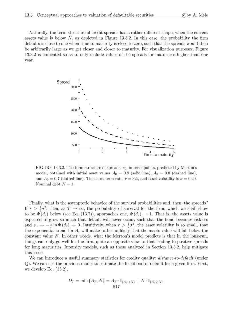
13.3. Conceptual approaches to valuation of defaultable securities c©by A. Mele
Naturally, the term-structure of credit spreads has a rather different shape, when the currentassets value is below N , as depicted in Figure 13.3.2. In this case, the probability the firmdefaults is close to one when time to maturity is close to zero, such that the spreads would thenbe arbitrarily large as we get closer and closer to maturity. For visualization purposes, Figure13.3.2 is truncated so as to only include values of the spreads for maturities higher than oneyear.
1 2 3 4 5
500
1000
1500
2000
2500
3000
Time to maturity
Spread
FIGURE 13.3.2. The term structure of spreads, s0, in basis points, predicted by Merton’s
model, obtained with initial asset values A0 = 0.9 (solid line), A0 = 0.8 (dashed line),
and A0 = 0.7 (dotted line). The short-term rate, r = 3%, and asset volatility is σ = 0.20.
Nominal debt N = 1.
Finally, what is the asymptotic behavior of the survival probabilities and, then, the spreads?If r > 1
2σ2, then, as T → ∞, the probability of survival for the firm, which we shall show
to be Φ (d2) below (see Eq. (13.7)), approaches one, Φ (d2) → 1. That is, the assets value isexpected to grow so much that default will never occur, such that the bond becomes risklessand s0 → − 1
Tln Φ (d2) → 0. Intuitively, when r > 1
2σ2, the asset volatility is so small, that
the exponential trend for At will make rather unlikely that the assets value will fall below theconstant value N . In other words, what the Merton’s model predicts is that in the long-run,things can only go well for the firm, quite an opposite view to that leading to positive spreadsfor long maturities. Intensity models, such as those analyzed in Section 13.3.2, help mitigatethis issue.We can introduce a useful summary statistics for credity quality: distance-to-default (under
Q). We can use the previous model to estimate the likelihood of default for a given firm. First,we develop Eq. (13.2),
DT = min AT ,N = AT · IAT<N +N · IAT≥N,517

13.3. Conceptual approaches to valuation of defaultable securities c©by A. Mele
where IE is the indicator function, i.e. IE = 1 if the event E is true and IE = 0 if the eventE is false. Second, we have,
D0 = e−rTE (DT )
= e−rT[E(AT · IAT<N
)+N · E
(IAT≥N
)]
= e−rT [E (AT |Default)Q (Default) +N ·Q (Survival)] , (13.6)
where E (AT |Default) is the expected asset value given the event of default, Q (Default) is theprobability of default, and Q (Survival) = 1 − Q (Default) is the probability the firms doesnot default. The last equality follows by the Law of Iterated Expectations, E
(AT · IAT<N
)=
E(E(AT · IAT<N
)∣∣Default)= E
(IAT<N · E (AT |Default)
).
Comparing Eq. (13.6) with Eq. (13.4) reveals that for the Merton’s model,
Q (Survival) = Φ (d2) . (13.7)
0.0 0.1 0.2 0.3 0.40.5
0.6
0.7
0.8
0.9
1.0
sigma
Pr(surv)
FIGURE 13.4. Probability of survival for a given firm predicted by the Merton’s model,
Φ(d2), depicted as a function of the asset volatility, σ. Assets value is fixed at A0 = 1.1,
and plotted are survival probabilities for bonds maturing at T = 0.5 years (solid line),
T = 1 year (dashed line) and T = 2 years (dotted line). The short-term rate, r = 3%.
Nominal debt N = 1.
The probability of survival, (i) decreases with debt maturity and (ii) the asset volatility.Property (i) is not a general property, though. With lower values of A0, the relation betweenmaturity and probability of survival can be increasing or decreasing, according to the values ofσ, as shown in Figure 13.5. Intuitively, when A0 ≈ N , the probability of survival is:
Q (Survival) = Φ (d2) , with d2 =ln
(A0
N
)+
(r − 1
2σ2
)T
σ√T
≈(r − 1
2σ2
)
σ
√T,
such that the survival probability decreases in T for large σ although then it increases in T forsmall σ. The intuition underlying this property is that for large σ, the probability the asset value
518
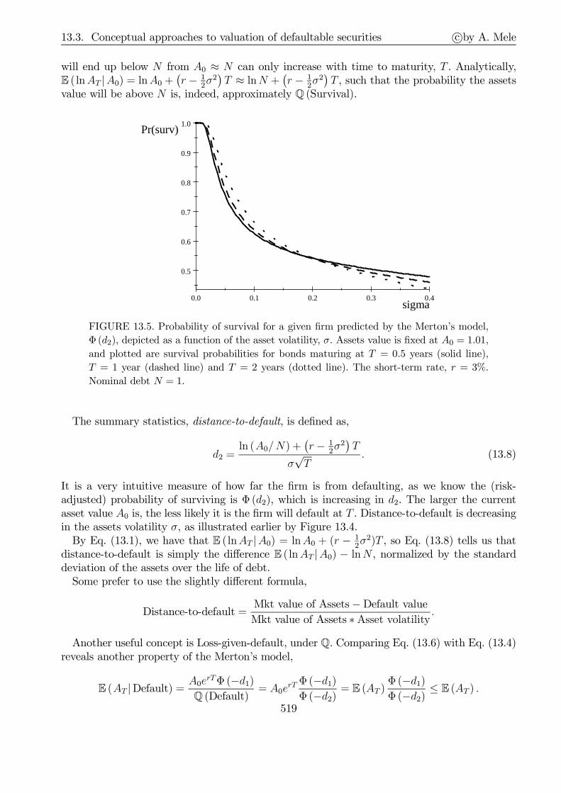
13.3. Conceptual approaches to valuation of defaultable securities c©by A. Mele
will end up below N from A0 ≈ N can only increase with time to maturity, T . Analytically,E ( lnAT |A0) = lnA0 +
(r − 1
2σ2
)T ≈ lnN +
(r − 1
2σ2
)T , such that the probability the assets
value will be above N is, indeed, approximately Q (Survival).
0.0 0.1 0.2 0.3 0.4
0.5
0.6
0.7
0.8
0.9
1.0
sigma
Pr(surv)
FIGURE 13.5. Probability of survival for a given firm predicted by the Merton’s model,
Φ(d2), depicted as a function of the asset volatility, σ. Assets value is fixed at A0 = 1.01,
and plotted are survival probabilities for bonds maturing at T = 0.5 years (solid line),
T = 1 year (dashed line) and T = 2 years (dotted line). The short-term rate, r = 3%.
Nominal debt N = 1.
The summary statistics, distance-to-default, is defined as,
d2 =ln (A0/N) +
(r − 1
2σ2
)T
σ√T
. (13.8)
It is a very intuitive measure of how far the firm is from defaulting, as we know the (risk-adjusted) probability of surviving is Φ (d2), which is increasing in d2. The larger the currentasset value A0 is, the less likely it is the firm will default at T . Distance-to-default is decreasingin the assets volatility σ, as illustrated earlier by Figure 13.4.By Eq. (13.1), we have that E (lnAT |A0) = lnA0 + (r − 1
2σ2)T , so Eq. (13.8) tells us that
distance-to-default is simply the difference E ( lnAT |A0) − lnN , normalized by the standarddeviation of the assets over the life of debt.Some prefer to use the slightly different formula,
Distance-to-default =Mkt value of Assets−Default value
Mkt value of Assets ∗ Asset volatility .
Another useful concept is Loss-given-default, under Q. Comparing Eq. (13.6) with Eq. (13.4)reveals another property of the Merton’s model,
E (AT |Default) =A0e
rTΦ (−d1)Q (Default)
= A0erT Φ (−d1)Φ (−d2)
= E (AT )Φ (−d1)Φ (−d2)
≤ E (AT ) .
519

13.3. Conceptual approaches to valuation of defaultable securities c©by A. Mele
Recovery rates are defined as the fraction of the bond value the bondholders expect to obtainin the event of default, at maturity:
Recovery Rate =E (AT |Default)
N=A0
NerT
Φ (−d1)Φ (−d2)
.
Loss-given-default is defined as the fraction of the bond value the bondholders expect to losein the event of default, at maturity:
Loss-given-default = 1− Recovery Rate.
Finally, by Eq. (13.5), we can write,
s0 = − 1Tln
(A0
NerTΦ (−d1) + Φ (d2)
)
= − 1Tln (Recovery Rate ·Q (Default) +Q (Survival))
≈ 1
T[Loss-given-default ·Q (Default)] . (13.9)
This is actually a general formula, which goes through beyond the Merton’s model). It caneasily be obtained through Eq. (13.6).An important note. Previously, we defined survival probabilities, distance-to-default, and
loss-given-default, under the risk-adjusted probability Q. To calculate the same objects underthe true probability P, we replace r with the asset growth rate under the physycal probability,µ, in the formulae for the survival probabilities, Φ (d2), distance-to-default, d2, and loss-given-default.However, it is hard to estimate µ for many single names. Moody’s KMV EDFTM are based
on dynamic structural models like these, although the details are not publicly known. Finally,we could use historical data about default frequencies to estimate the probability that a givensingle name within a certain industry will default. These frequencies are based on samples offirms that have defaulted in the past, with similar characteristics to those of the firm underevaluation (in terms, for instance, of distance-to-default).How to estimate At and σ? One algorithm is to start with some σ equal to the volatility
of equity returns, say σ(0), and use Merton’s formula for equity, to extract A(0)t for each date
t ∈ 1, · · · ,T , where T is the sample size. Then, use A(0)t to compute the standard deviation of
ln(A(0)t /A
(0)t−1). This gives say σ
(1), which can be used as the new input to the Merton’s formula
to extract say A(1)t . We obtain a sequence of (A
(i)t )
Tt=1 and σ(i), and we stop for i sufficiently
large, according to some criterion.
13.3.1.2 One example
Assume the assets value of a given firm is A0 = 110, and that the instantaneous volatility of theassets value growth is σ = 30%, annualized. The safe interest rate is r = 2%, annualized, andthe expected growth rate of the assets value is µ = 5%, annualized. The firm has outstandingdebt with nominal value N = 100, which expires in two years.First, we compute the distance-to-default implied by the Merton’s model, which is,
D-t-D =ln
(A0
N
)+
(r − 1
2σ2
)T
σ√T
=ln (1.1) +
(0.02− 1
20.32
)2
0.3√2
= 0.10680.
520

13.3. Conceptual approaches to valuation of defaultable securities c©by A. Mele
Accordingly, the probability of default is,
1− Φ (0.10680) = 1− 0.54253 = 0.45747.
We can compute the same probability, under the physical measure, by simply replacingr = 2% with µ = 5%, in the formula for D-t-D. We have,
D-t-Dphysical =ln
(A0
N
)+
(µ− 1
2σ2
)T
σ√T
=ln (1.1) +
(0.05− 1
20.32
)2
0.3√2
= 0.24822.
Therefore, the probability of default under the physical distribution is,
1− Φphysical (0.24822) = 1− 0.59802 = 0.40198.
It is, of course, lower under the physical probability than under the risk-neutral probability,due to the larger asset growth rate, µ > r.Finally, we can compute the spread on this bond, which is given by:
Spread = − 1Tln
(A0
NerTΦ (−d1) + Φ (d2)
),
where d2 = D-t-D, and d1 = d2 + σ√T . So we have,
Spread = −12ln
(1.1e0.02∗2Φ
(−(0.10680 + 0.30 ∗
√2))
+Φ(0.10680))
= −12ln
(1.1e0.02∗2 ∗ 0.29769 + 0.54253
)
= 6.20%.
13.3.1.3 First passage
The timing of default can be triggered by some exogeneously specified events. For example,default occurs if the value of the assets hits some exogenously lower bound even before theexpiration of debt. These models are known as “first passage” models, because they rely onmathematical techniques that solve for the probability the first time the asset value hit someexogenous “barrier,” as in Black and Cox (1976).
13.3.1.4 Strategic defaulting
The timing of default can be endogenous. Managers choose the defaulting barrier (i.e. theasset value that triggers bankruptcy) so as to maximize the firm’s value. Naturally, strategicdefaulting works if the assumptions underlying the Modigliani-Miller theorem do not hold. Themechanism is the following: on the one hand, debt is a tax-shielding device. On the other hand,issuing too much debt increases the likelihood of default, which triggers bankruptcy costs. Thefirst effect raises the value of the firm while the second, decreases the value of the firm. Equityholders choose the value of the asset that triggers bankruptcy to maximize the value of equity.Leland (1994): Long-term debt. Leland and Toft (1996): Extension to finite maturity debt.Anderson and Sundaresan (1996): Debt re-negotiation.The Leland’s model considers liquidation of the firm as a strategic choice of the equity
holders. In fact, the US bankruptcy code includes both a liquidation process (Chapter 7) anda reorganization process (Chapter 11), but Leland’s model only considers firm’s liquidation at
521

13.3. Conceptual approaches to valuation of defaultable securities c©by A. Mele
bankruptcy. Broadie, Chernov and Sundaresan (2007) generalize this setting to one where thefirm may choose to default through a reorganization process, in which case no equity is issuedto honour debt services, i.e. coupon payments, as it is instead the case in Leland, as we nowexplain.The terms leading to the strategic defaulting in Leland’s model are as follows. First, the value
of the assets, At, is solution, as usual, to Eq. (13.1). Second, debt is infinitely lived in that, itpays off an instantaneous coupon equal to Cdt; in the absence of default risk, then, debt wouldsimply equal C/r. Third, tax benefits are assumed to be proportional to the coupon, τCdt.Fourth, there are bankruptcy costs: if the firm defaults at A = AB, recovery is (1− α)AB.Equity holders choose AB. Naturally, AB < A0.The value of debt is a function of the assets value, A, say D (A). Moreover, the firm finances
the net cost of the coupon C by issuing additional equity, until the equity value is zero, i.e.until A = AB, as seen below. Therefore, under the risk-neutral probability, the value of debtsatisfies:
d
dTE [D (AT )|A0]
∣∣∣∣T=t︸ ︷︷ ︸
=Expected capital gains
+ C︸︷︷︸=coupon
= rD (At) .
By Itô’s lemma, this is an ordinary differential equation, subject to the following boundaryconditions. First, at bankruptcy,D
(AB
)= (1− α)AB. Second, for largeA, debt is substantially
riskless, i.e. limA→∞D (A) =Cr.
The solution to this is,
D (A) = (1− pB (A))C
r+ pB (A)
[(1− α)AB
], (13.10)
where
pB (A) ≡(AB
A
) 2rσ2
. (13.11)
Note, we may interpret pB (A) as the present value of £1, contingent on future bankruptcy, asfurther explained in Appendix 1. Accordingly, (1− pB (A)) /r is the expected present value ofthe coupon payments up to bankruptcy.The total benefits arising from tax shielding are,
TB (A) = (1− pB (A)) τC
r.
and the present value of bankruptcy costs is,
BC (A) = pB (A)αAB.
We have,
Value of the firm = Equity + Debt
= Value of Assets ( = A) + TB (A)−BC (A) .
Summing up,
E (A) ≡ Equity = A− (1− pB (A)) (1− τ)C
r− pB (A)AB.
522

13.3. Conceptual approaches to valuation of defaultable securities c©by A. Mele
Equity equals (i) the value of the assets, A; minus (ii) the present value of debt contingent onno-bankruptcy net of tax benefits, (1− pB (A)) (1− τ ) Cr ; minus (iii) the present value of debtcontingent on bankruptcy net of bankruptcy costs, pB (A)A
B. The second term decreases withthe default boundary, AB or, equivalently, pB (A). The third term, instead, increases with AB.So the time equityholders wait before declaring bankruptcy, which is inversely related to AB,affects in opposite ways the last two terms. Equityholders choose AB to maximize the value ofequity. Their solution is a default boundary, AB, such that the value of equity does not changefor small changes in the value of the assets A around AB, or AB : E′ (A)|A=AB = 0, a smoothpasting condition. The result is,
AB = (1− τ) C
r + 12σ2.
Similarly as in the American option case, the value of the option to wait increases with uncer-tainty, σ2. Finally, and consistent with the real option theory, it is easy to check that this valueAB does maximize the value E
(A;AB
)≡ E (A) in that AB : 0 = ∂E
(A;AB
)/∂AB = 0.
How is it that tax shielding does not seem to affect the existence of a solution to this problem?That is, the default boundary, AB, still exists, even with τ = 0. This issue is easily resolved.If τ = 0, there are no reasons to issue debt in the first place, as no tax benefits would flowto the firm, thereby increasing its value! In fact, when τ > 0, there is a value of leverage thatmaximizes the value of the firm, according to simulations reported in Leland (1994).
13.3.1.5 Pros and cons of structural approaches to risky debt assessment
Pros. First, they allow to think about more complicated structures or instruments easily (e.g.,convertibles). Second, they lead to simple yet consistent relations between different securitiesissued by the same name. Structural approaches were very useful for theoretical research in the1990s.Cons. The firm’s asset value and asset volatility are not observed. Must rely on calibra-
tion/estimation methods. Bond prices generated by the model = market prices. These modelsare a bit difficult to use in practice, for trading or hedging purposes, as we know that in thiscase we need theoretical prices that exactly match market prices. Finally, how do we go forsovereign issuers?Most important. Structural models predict unrealistically low short-term spreads: see, e.g.,
Figure 13.3. The intuition is that diffusion processes are smooth: the probability of default tendsto zero as time to maturity approaches zero, because default cannot just jump in an unexpectedway. This is not what we exactly observe. Jumps seem to be a more realistic device to modelingspreads.
13.3.2 Reduced form approaches: rare events, or intensity, models
Default often displays a few strong characteristics. It arrives unexpectedly, it is rare, and causescauses discontinuous price changes. The structural models in the previous section do not ac-commodate for these features −→ diffusion processes are continuous: passage times are known,“locally.” This feature is responsible for the low short-term spreads.
13.3.2.1 Poisson-driven defaults
We model the arrival of defaults through the Poisson processes introduced in Chapter 4, asfollows. Suppose to “count” the number of times some event happens. Denote with Nt thecorresponding “counting process.”
523

13.3. Conceptual approaches to valuation of defaultable securities c©by A. Mele
tN
Default
0t 1t 2t 3t
FIGURE 13.6.
Default time is simply defined as t0, i.e. the first time Nt “jumps,” as in Figure 13.6. Soassume we chop a given interval [0, T ] in n pieces, and consider each resulting interval ∆t = T
n.
Assume jump probability over each of these small intervals of time ∆t is proportional to ∆t,with proportionality factor equal to λ,
p ≡ Pr One jump over ∆t = λ∆t. (13.12)
Assume the number of jumps over the n intervals follows a binomial distribution:
Pr k jumps over [0, T ] =(n
k
)pk (1− p)n−k , where p = λ
T
n.
For n large (or, equivalently, for small intervals ∆t),
Pr k jumps over [0, T ] ≈ (λT )k
k!
(1− λT
n
)n−k≈ (λT )k
k!e−λT .
We can use the previous basic computations to come up with a few fundamental propertiesfor the distribution of default. We have,
Pr Survival = Pr 0 jumps over [0, T ] = e−λTPr Default = 1− Pr Survival = 1− e−λT
Pr Default occurs at some t = λe−λtdt
Expected Time-to-Default =1
λ
We can now use these probabilities to assess the value of debt subject to default risk. ConsiderEq. (13.6):
D0 = e−rT [Rec ·Q (Default) +N ·Q (Survival)]︸ ︷︷ ︸
≡B0
,
524
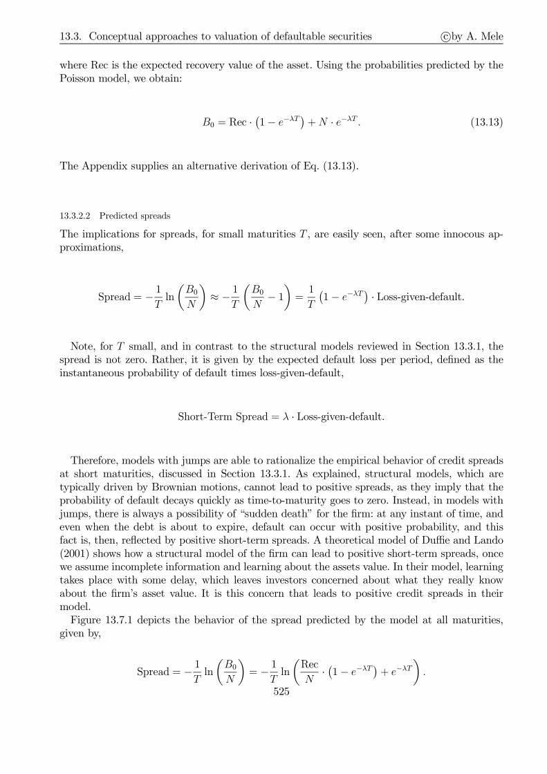
13.3. Conceptual approaches to valuation of defaultable securities c©by A. Mele
where Rec is the expected recovery value of the asset. Using the probabilities predicted by thePoisson model, we obtain:
B0 = Rec ·(1− e−λT
)+N · e−λT . (13.13)
The Appendix supplies an alternative derivation of Eq. (13.13).
13.3.2.2 Predicted spreads
The implications for spreads, for small maturities T , are easily seen, after some innocous ap-proximations,
Spread = − 1Tln
(B0
N
)≈ − 1
T
(B0
N− 1
)=1
T
(1− e−λT
)· Loss-given-default.
Note, for T small, and in contrast to the structural models reviewed in Section 13.3.1, thespread is not zero. Rather, it is given by the expected default loss per period, defined as theinstantaneous probability of default times loss-given-default,
Short-Term Spread = λ · Loss-given-default.
Therefore, models with jumps are able to rationalize the empirical behavior of credit spreadsat short maturities, discussed in Section 13.3.1. As explained, structural models, which aretypically driven by Brownian motions, cannot lead to positive spreads, as they imply that theprobability of default decays quickly as time-to-maturity goes to zero. Instead, in models withjumps, there is always a possibility of “sudden death” for the firm: at any instant of time, andeven when the debt is about to expire, default can occur with positive probability, and thisfact is, then, reflected by positive short-term spreads. A theoretical model of Duffie and Lando(2001) shows how a structural model of the firm can lead to positive short-term spreads, oncewe assume incomplete information and learning about the assets value. In their model, learningtakes place with some delay, which leaves investors concerned about what they really knowabout the firm’s asset value. It is this concern that leads to positive credit spreads in theirmodel.Figure 13.7.1 depicts the behavior of the spread predicted by the model at all maturities,
given by,
Spread = − 1Tln
(B0
N
)= − 1
Tln
(Rec
N·(1− e−λT
)+ e−λT
).
525
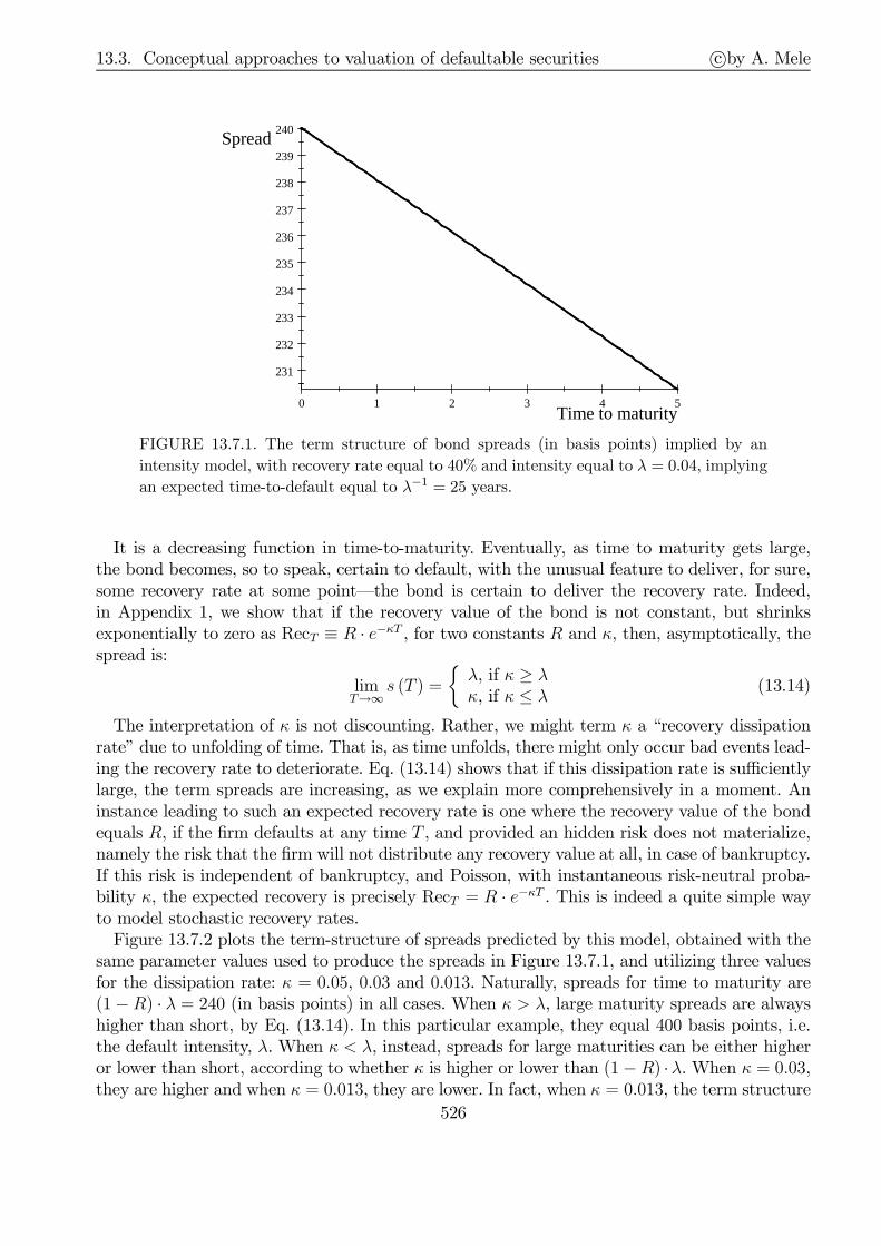
13.3. Conceptual approaches to valuation of defaultable securities c©by A. Mele
0 1 2 3 4 5
231
232
233
234
235
236
237
238
239
240
Time to maturity
Spread
FIGURE 13.7.1. The term structure of bond spreads (in basis points) implied by an
intensity model, with recovery rate equal to 40% and intensity equal to λ = 0.04, implying
an expected time-to-default equal to λ−1 = 25 years.
It is a decreasing function in time-to-maturity. Eventually, as time to maturity gets large,the bond becomes, so to speak, certain to default, with the unusual feature to deliver, for sure,some recovery rate at some point–the bond is certain to deliver the recovery rate. Indeed,in Appendix 1, we show that if the recovery value of the bond is not constant, but shrinksexponentially to zero as RecT ≡ R · e−κT , for two constants R and κ, then, asymptotically, thespread is:
limT→∞
s (T ) =
λ, if κ ≥ λκ, if κ ≤ λ
(13.14)
The interpretation of κ is not discounting. Rather, we might term κ a “recovery dissipationrate” due to unfolding of time. That is, as time unfolds, there might only occur bad events lead-ing the recovery rate to deteriorate. Eq. (13.14) shows that if this dissipation rate is sufficientlylarge, the term spreads are increasing, as we explain more comprehensively in a moment. Aninstance leading to such an expected recovery rate is one where the recovery value of the bondequals R, if the firm defaults at any time T , and provided an hidden risk does not materialize,namely the risk that the firm will not distribute any recovery value at all, in case of bankruptcy.If this risk is independent of bankruptcy, and Poisson, with instantaneous risk-neutral proba-bility κ, the expected recovery is precisely RecT = R · e−κT . This is indeed a quite simple wayto model stochastic recovery rates.Figure 13.7.2 plots the term-structure of spreads predicted by this model, obtained with the
same parameter values used to produce the spreads in Figure 13.7.1, and utilizing three valuesfor the dissipation rate: κ = 0.05, 0.03 and 0.013. Naturally, spreads for time to maturity are(1−R) · λ = 240 (in basis points) in all cases. When κ > λ, large maturity spreads are alwayshigher than short, by Eq. (13.14). In this particular example, they equal 400 basis points, i.e.the default intensity, λ. When κ < λ, instead, spreads for large maturities can be either higheror lower than short, according to whether κ is higher or lower than (1−R) ·λ. When κ = 0.03,they are higher and when κ = 0.013, they are lower. In fact, when κ = 0.013, the term structure
526
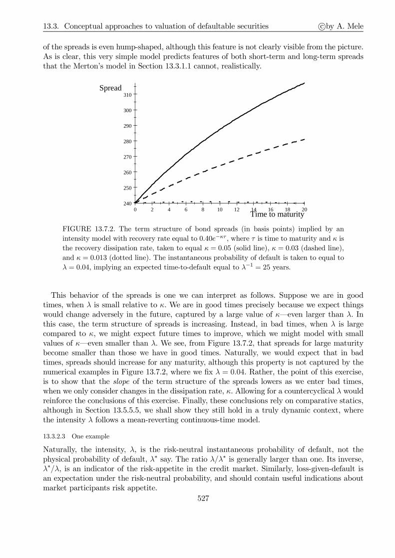
13.3. Conceptual approaches to valuation of defaultable securities c©by A. Mele
of the spreads is even hump-shaped, although this feature is not clearly visible from the picture.As is clear, this very simple model predicts features of both short-term and long-term spreadsthat the Merton’s model in Section 13.3.1.1 cannot, realistically.
0 2 4 6 8 10 12 14 16 18 20240
250
260
270
280
290
300
310
Time to maturity
Spread
FIGURE 13.7.2. The term structure of bond spreads (in basis points) implied by an
intensity model with recovery rate equal to 0.40e−κτ , where τ is time to maturity and κ is
the recovery dissipation rate, taken to equal κ = 0.05 (solid line), κ = 0.03 (dashed line),
and κ = 0.013 (dotted line). The instantaneous probability of default is taken to equal to
λ = 0.04, implying an expected time-to-default equal to λ−1 = 25 years.
This behavior of the spreads is one we can interpret as follows. Suppose we are in goodtimes, when λ is small relative to κ. We are in good times precisely because we expect thingswould change adversely in the future, captured by a large value of κ–even larger than λ. Inthis case, the term structure of spreads is increasing. Instead, in bad times, when λ is largecompared to κ, we might expect future times to improve, which we might model with smallvalues of κ–even smaller than λ. We see, from Figure 13.7.2, that spreads for large maturitybecome smaller than those we have in good times. Naturally, we would expect that in badtimes, spreads should increase for any maturity, although this property is not captured by thenumerical examples in Figure 13.7.2, where we fix λ = 0.04. Rather, the point of this exercise,is to show that the slope of the term structure of the spreads lowers as we enter bad times,when we only consider changes in the dissipation rate, κ. Allowing for a countercyclical λ wouldreinforce the conclusions of this exercise. Finally, these conclusions rely on comparative statics,although in Section 13.5.5.5, we shall show they still hold in a truly dynamic context, wherethe intensity λ follows a mean-reverting continuous-time model.
13.3.2.3 One example
Naturally, the intensity, λ, is the risk-neutral instantaneous probability of default, not thephysical probability of default, λ∗ say. The ratio λ/λ∗ is generally larger than one. Its inverse,λ∗/λ, is an indicator of the risk-appetite in the credit market. Similarly, loss-given-default isan expectation under the risk-neutral probability, and should contain useful indications aboutmarket participants risk appetite.
527

13.3. Conceptual approaches to valuation of defaultable securities c©by A. Mele
Assume that under the risk-neutral probability, the instantaneous intensity of default for agiven firm is λ = 4%, annualized, and that under the physical probability, the instantaneousprobability of default for the same firm is λ∗ = 2%, annualized. From here, we can compute theprobability of survival of the firm within 5 years, under both probabilities. They are:
e−5λ = e−5∗0.04 = 0.81873, e−5λ∗ = e−5∗0.02 = 0.90484.
Naturally, the probability of survival is lower under the risk-neutral measure.Next, assume that the spread on a 5 year bond with face value N = 1, equals 3%. What is
the implied expected recovery rate from this spread? We have,
D0 = e−rT [Rec ·Q (Default) +N ·Q (Survival)] = e−rT [Rec ∗ (1− 0.81873) + 1 ∗ 0.81873] .
The spread is,
s0 = 3% = −15ln
(Rec ∗ (1− 0.81873) + 1 ∗ 0.81873
1
).
Solving for Rec, gives, Rec = 23.16%.
13.3.3 Ratings
In practice, corporate debt is rated by rating agencies, such as Moodys and Standard and Poors.Depending on the rating, corporate debt may be either investment grade or non-investmentgrade (“junk”). Moodys ratings range from Aaa to C. Standard and Poor’s range from Aaa toD. One can compute the probability of “migrations” based on past experience −→ Transitionprobabilities. Consider, for example, the following table:
AAA AA A BBB BB B CCC DAAA 89.1 9.63 0.78 0.19 0.3 0 0 0AA 0.86 90.1 7.47 0.99 0.29 0.29 0 0A 0.09 2.91 88.94 6.49 1.01 0.45 0 0.09
BBB 0.06 0.43 6.56 84.27 6.44 1.6 0.18 0.45BB 0.04 0.22 0.79 7.19 77.64 10.43 1.27 2.41B 0 0.19 0.31 0.66 5.17 82.46 4.35 6.85
CCC 0 0 1.16 1.16 2.03 7.54 64.93 23.19D 0 0 0 0 0 0 0 100
To
Fro
m
One year rating transition probabilities (%), S&P's 1981-1991
TABLE 12.1
13.3.3.1 Foundations
A natural approach, then, is to assess credit risk by making reference to probabilities of defaultbuilt up on transition probabilities like those in Table 13.1.Such an approch, also known as a migration approach, is somewhat less drastic than that
based on rare events, and hopefully more realistic. However, it is also technically more complexthan the intensity approach of the previous section. We provide the most foundational issuesrelated to this approach, leaving some details in the Appendix.At time t, there exists several rating classes, N say, denoted as Ratt,
Ratt ∈ 1, 2, · · · , N .528

13.3. Conceptual approaches to valuation of defaultable securities c©by A. Mele
Transition probabilities of rating from time t to time T are,
P (T − t)ij ≡ Pr (RatT = j|Ratt = i) , i, j ≤ N.
We can build a Markov chain from here, by assuming that P (T − t)ij only depends on T − t.Finally, we must have that,
P (T − t)ij ≥ 0 andN∑
j=1
P (T − t)ij = 1.
For example, the probability of transition from rating Ratt = i to rating Ratt+1 = j in oneyear is, P (1)ij. Table 13.1 contains one possible example of P (1)ij. The probability of transitionfrom rating Ratt = i to rating Ratt+2 = j in two years is P (2)ij, and is obtained as follows,
P (2)ij =N∑
k=1
P (1)ik︸ ︷︷ ︸Pr(transition from i to k in one year)
· P (1)kj︸ ︷︷ ︸Pr(transition from k to j in one further year)
More generally, we have, P (T ) = P (1)T , where P (T ) is the matrix with elements P (T )ij.For example, the probability transition matrix P in Table 13.1 is,
P =
89.1 9.63 0.78 0.19 0.3 0 0 00.86 90.1 7.47 0.99 0.29 0.29 0 00.09 2.91 88.94 6.49 1.01 0.45 0 0.090.06 0.43 6.56 84.27 6.44 1.6 0.18 0.450.04 0.22 0.79 7.19 77.64 10.43 1.27 2.410 0.19 0.31 0.66 5.17 82.46 4.35 6.850 0 1.16 1.16 2.03 7.54 64.93 23.190 0 0 0 0 0 0 100
The 15 year transition matrix is:
P (15) ≈
20.01 35.82 23.91 9.92 4.05 3.06 0.43 2.663.38 30.28 32.71 15.91 6.38 5.11 0.77 5.341.17 13.12 34.21 21.93 9.69 8.01 1.29 10.330.64 6.76 22.21 22.40 12.42 11.93 2.09 21.390.33 3.22 10.71 13.616 11.36 14.68 2.78 43.160.14 1.65 5.01 6.75 7.48 13.17 2.64 63.040 1.08 3.54 3.90 3.51 5.60 1.22 81.020 0 0 0 0 0 0 100
13.3.3.2 Evaluation
The previous probabilities, P (T )ij, are meant to be taken under the physical world, notthe risk-neutral world. They can be used for risk-management purposes, but certainly not forpricing. Indeed, historical default rates are too low to explain the price of defaultable securities.A natural explanation relies on the presence of risk-premia. To use migration data for pricing,it is vital to implement a number of steps.First, clean up the data – smoothing. For example, it might well be that downgrades from
class i to class i + 2 are more frequent than downgrades from class i to class i + 1. Moreover,
529

13.3. Conceptual approaches to valuation of defaultable securities c©by A. Mele
remove zero entries: although some rating event did not happen in the past, they might welloccur in the future. Second, add positive risk-premia to the previous smoothed data so as toobtain realistic asset prices.As regards pricing, according to the migration model, there are N classes of assets. Each
single asset may migrate from one class to another. Because evaluation is a dynamic business,we cannot evaluate defaultable securities within a given asset class without simultaneouslyevaluate the defaultable securities in the remaining classes. For example, there could be achance that a given asset will “mutate” into a different one in the next year. Given this, theprice of this asset, today, must reflect the price of the asset in the other classes where it canpossibly migrate. Hence, we must simultaneously solve for all the asset prices in all the ratingclasses. This approach, developed by Jarrow, Lando and Turnbull (1997), is quite complex andis given a succinct account in the Appendix.Consider the simplest case, which arises when the expected recovery rate is zero. In this case,
by Eq. (13.6),D0,i
N= e−rT (1−Qi (T − t)) ,
where Qi (T − t) is the risk-neutral probability the firm defaults, by time T , given it belongsto rating i at time T .More generally, by Eq. (13.6),
D0,i
N= e−rT
[Rec
NQi (T − t) + (1−Qi (T − t))
].
The risk neutral probabilities, Qi (T − t), must be found using migration frequencies such asthose in Table 13.1, which we must “clean up” and corrct with appropriate risk-premia, asdiscussed.
13.3.3.3 One example
Consider the following transition matrix:
To
From
A B DefA 0.9 0.07 0.03B 0.15 0.75 0.10Def 0 0 1
where Def denotes the state of default. What is the probability that a name A will remain nameA in two years? What is the probability that a name A will default in two years?Consider the following two year transition matrix:
Q (2) =
0.90 0.07 0.030.15 0.75 0.100 0 1
︸ ︷︷ ︸≡ Q(1)
·
0.90 0.07 0.030.15 0.75 0.100 0 1
︸ ︷︷ ︸≡ Q(1)
,
such that:
Pr A is A in 2 years = 0.90 ∗ 0.90︸ ︷︷ ︸A→A→A
+ (0.07) ∗ (0.15)︸ ︷︷ ︸A→B→A
+ 0.03 ∗ 0︸ ︷︷ ︸A→Def→A
= 0.8205,
530

13.3. Conceptual approaches to valuation of defaultable securities c©by A. Mele
and
Pr A defaults in 2 years = 0.90 ∗ 0.03︸ ︷︷ ︸A→A→Def
+ (0.07) ∗ (0.10)︸ ︷︷ ︸A→B→Def
+ 0.03 ∗ 1︸ ︷︷ ︸A→Def→Def
= 0.064.
In general, we have that:
Q (2)ij =3∑
k=1
Q (1)ik ·Q (1)kj ,
and for any T ,
Q (T ) = Q (1)T =
0.90 0.07 0.030.15 0.75 0.100 0 1
T
.
Next, consider the following transition matrix, under the risk-neutral probability:
To
From
A B DefA 0.80 0.20 0B 0.15 0.75 0.10Def 0 0 1
From here, we may easily compute, again, the (risk-neutral) probability A will default in twoyears, and the probability B will default in two years. We have,
Q (2) =
0.80 0.20 00.15 0.75 0.100 0 1
︸ ︷︷ ︸≡ Q(1)
·
0.80 0.20 00.15 0.75 0.100 0 1
︸ ︷︷ ︸≡ Q(1)
,
such that:
Pr A defaults in 2 years = Q (2)13= 0.80 ∗ 0︸ ︷︷ ︸
A→A→Def
+ (0.20) ∗ (0.10)︸ ︷︷ ︸A→B→Def
+ 0 ∗ 1︸︷︷︸A→Def→Def
= 0.02.
(multiply first row by the third column), and,
Pr B defaults in 2 years = Q (2)23= 0.15 ∗ 0︸ ︷︷ ︸
B→A→Def
+ (0.75) ∗ (0.10)︸ ︷︷ ︸B→B→Def
+ 0.10 ∗ 1︸ ︷︷ ︸B→Def→Def
= 0.175.
(multiply second row by the third column).Finally, suppose that the bonds issued by both A and B mature in two years. Furthermore,
assume that if these two bonds default, they pay off the same recovery rate, equal to 30%, and
531
13.4. Convertible bonds c©by A. Mele
only at the end of the second period. From here, we can compute the credit spreads for the twobonds. We have,
erT ∗ Price_A = (0.30) ∗ (0.02) + (1− 0.02) = 0.986
⇒ Spread_A = −12ln (0.986) = 7.0495× 10⁻³.
and,
erT ∗ Price_B = (0.30) ∗ (0.175) + (1− 0.175) = 0.8775
⇒ Spread_B = −12ln (0.8775) = 6.5339× 10⁻².
13.4 Convertible bonds
Convertible bonds offer bondholders the option to convert their bonds into shares of the firm.Chapter 11 (Section 11.8.2) provides an introductory discussion of these convertible bonds, anda numerical example of how to price them through a binomial tree. This section analyzes withinthe context of a continuous time model. We assume the option to convert can be exercized atany time up to maturity. By definition, the face value of the convertible is,
Face value = £1 ≡ CR× CP, (13.15)
where CR is the conversion ratio, i.e. the number of shares this face value converts into, andCP is the conversion price, i.e. the stock price implicitly defined by Eq. (13.15).Typically, the bond is any like other fixed income instrument, with coupon payments, callable
features, credit risk, etc. Callable features are almost invariably embedded into this type ofcontracts. The parity, or conversion value, is the value of the bond if the bondholders decide toconvert. It is defined as,
CV = CR× S,where S is the price of the common share. Not only is the convertible bond price affected byinterest rates, credit risk, timing risk, etc. This price is also affected by the movements of theunderlying stock price. This is quite natural as there is a positive probability that the bond will“become” a share in the future. To emphasize this fact, we also say that convertible bonds arehybrid instruments. The embedded option offers the bondholders the possibility to obtain equityreturns (not just bond returns) in good times, while offering protection against the downside.As mentioned in Chapter 11 (Section 11.8), convertible bonds are usually callable as well. Inthis case, bond-holders are usually given the right to convert the bonds, once they are called.The rationale behind callability is to induce the bondholder to convert the bond earlier.Useful to trade volatility. Simplest example of convertible arbitrage is going long a convertible
and shorting a Treasury, which is the same as going long an option on the firm. Useful whenthere are no available options on the firm to trade, and/or when these are very illiquid.Pricing convertible bonds is a topic that has been intensively studied, theoretically. Ingersoll
(1977) provides the first theoretical article which lays down the foundations to rational evalua-tion of convertible callable bonds. Let us define the dilution factor, denoted as γ, as the fractionof common equity that would be held by the convertible bondowners if the entire issue was
532

13.4. Convertible bonds c©by A. Mele
converted. If there are nout shares outstanding, and the convertible bond can be exchanged forn shares, then, in aggregate,
γ =n
n+ nout.
Let the market value of the firm be equal to the value of its assets, A, which we assumefollows a Geometric Brownian motion, as in Eq. (13.1). Let Bconv (A, τ ;N) be the aggregatevalue of the convertible bond with time to maturity τ and balloon payment N . To simplify thepresentation, we do not consider callability issues. However, we shall provide some intuitionabout this issue later. Let us assume that the stocks and the convertible bonds are the only twoclaims in the capital structure of the firm. Since, after conversion, only the stocks will remain,then, the post-conversion value of the convertible bonds is simply the conversion value of theconvertible, i.e. γA. Moreover, we have, for any τ ≥ 0,
γA ≤ Bconv (A, τ ;N) ≤ A. (13.16)
The first inequality in (13.16) is simple to understand. Indeed, suppose that Bconv (A, τ ;N) <γA. Then, we can purchase the convertibles, convert them into shares and, finally, sell the sharesfor γA. The second inequality follows by limited liability equity holders, and the Modigliani-Miller theorem.At maturity, we have that,
Bconv (A, 0;N) = min A,max N, γA . (13.17)
Indeed, B ≡ max N, γA is the value of the convertible, in case of no-default. Then,minA, Bis what the firm will pay, to the bondholders: A in case of default, and B in case of no-default.We can re-express the terminal payoff in Eq. (13.17) in a manner that allows a better un-
derstanding of the issues underlying the exercise of the convertibles. In particular, we havethat,
Bconv (A, 0;N) = min A,max N, γA = max γA,min A,N . (13.18)
Indeed, let B ≡ minA,N, which is what the firm is ready to pay, to the bondholders, if thebondholders do not exercise the option to convert. Then, maxγA, B is obviously the payoffprofile to the bondholders.The terminal payoff in Eq. (13.18) illustrates very clearly that convertible bonds embed an
option to convert - on top of the plain vanilla non-convertible bond. Intuitively, at maturity, anon-convertible bond is worth min A,N, and the option to convert is either worthless (in caseof non conversion) or γA−N (in case of conversion), i.e. it is max γA−N, 0. This intuitionis confirmed, mathematically, as we have that:
max γA,min A,N = min A,N+max γA−N, 0 .
Therefore, the value of the terminal payoff is, by Eq. (13.18),
Bconv (A, 0;N) = min A,N+ γmax A−N/γ, 0 . (13.19)
It is possible to show that it is never optimal to exercize the option to convert before maturity.Therefore, to price the convertible bond, we only need to be concerned with the risk-neutralevaluation of the terminal payoff in Eq. (13.19).Eq. (13.19) shows that the current value of the convertible bond is the sum of the value
of a “straight” bond plus the value of γ options on the firm with strike price equal to N/γ.
533

13.4. Convertible bonds c©by A. Mele
Accordingly, let B (A, τ ;N) andW (A, τ ;N/γ) be the prices of the straight bond and the optionon the firm. We have,
Bconv (A, τ ;N) = B (A, τ ;N) + γW (A, τ ;N/γ) . (13.20)
We may use the Merton’s (1974) model to find the price of the straight bond, B (A, τ ;N). Bythe results in Section 13.2, it is:
B (A, τ ;N) = AΦ (−d1) +Ne−rτΦ(d1 − σ
√τ), d1 =
ln (A/N) +(r + 1
2σ2
)τ
σ√τ
, (13.21)
where σ is the instantaneous volatility of the assets, r is the (constant) instantaneous short-term rate, and Φ is the cumulative distribution of a standard normal. Similarly, we may usethe Black-Scholes formula to compute the function W :
W (A, τ ;N/γ) = AΦ (d1)−N
γe−rτΦ
(d1 − σ
√τ). (13.22)
Eq. (13.21) reveals the intuitive property that as A gets large, B (A, τ ;N) ≈ Ne−rτ : the prob-ability of default gets extremely tiny as the value of the assets gets large. Moreover, the Black-Scholes formula, Eq. (13.22), suggests thatW (A, τ ;N/γ) ≈ A−e−rτN/γ as A gets large. There-fore, by Eq. (13.20), we have that, for large A,Bconv (A, τ ;N) ≈ Ne−rτ+γ (A− e−rτN/γ) = γA.Eq. (13.21) also shows that for small values of A, Bconv (A, τ ;N) ≈ 0. To sum-up, the value ofthe convertible bond is less than the value of the firm, A, and larger than the conversion value,γA. Moreover, it approaches γA, as the value of the firm gets large. Figure 13.8 depicts theprice of the convertible bond as function of the value of the firm, as predicted by Eq. (13.20),for a particular example. It is possible to show that the value of a callable convertible bond isbetween the value of the straight and that of the convertible.
0 1 2 3 4 50.0
0.5
1.0
1.5
2.0
A
£
FIGURE 13.8. The value of convertible and straight bonds as a function of the current
assets value, A, when the short-term rate r = 3%, the asset volatility σ = 0.20, time to
maturity τ = 3 years, the dilution factor γ = 10%, and nominal debt N = 1. The solid
line depicts the value of the convertible bond. The dashed straight line starting from the
origins, and flattening out to the constant Ne−rτ = 0.91393, is the value of the straight
bond. The two dashed straight lines starting from the origins are the no-arbitrage bounds
γA and A in Eq. (13.16).
534

13.5. Credit-risk shifting derivatives and structured products c©by A. Mele
13.5 Credit-risk shifting derivatives and structured products
13.5.1 Securitization, and a brief history of credit risk and financial innovation
Securitization is a process by which some illiquid assets are transformed into a package of securi-ties backed by these assets, through packaging, credit and liquidity enhancements. Two leadingexamples are: (i) mortgages and (ii) receivables. Financial institutions find the securitizationprocess attractive, as they can carve out certain items in their balance sheet, thus boostingtheir return on investments or simply because by securitizing assets, less capital is needed tomeet capital-requirements standards. For example, the accounts receivables of a corporationmay be used to back the issue of commercial paper known as asset-backed commercial paper.Securitization is a way (not the only way) to trade/transfer credit risk, in principle.What are the origins of credit derivatives and financial innovation? The first interest rates
derivatives were created around the mid 80s. In the late ’80s the business proliferated andbecome fairly complex. But financial innovation is easy to imitate, which led banks to becomeincreasingly creative, so as to exploit their initial competitive advantage as longer as possible.During the early 1990s, just after the 1991 recession, interest rates were quite low, and thevolatility of capital markets extraordinarily low. Derivatives, then, could be used as devicesto boost investors’ returns. JPMorgan introduced many structures such as, “LIBOR squared,”“inverse floaters,” “power options,” “convexity forwards,” etc.However, after the 1994 financial turmoil, the interest rate climate suddenly changed, and
many of the derivatives contracts produced large losses. There was a call for regulation by publicopinion and certain policy makers. At the same time, the International Swaps and DerivativesAssociation argued that more regulation would destroy markets creativity. These regulatorypressures vanished by the mid 1990s.During the mid 1990s, the markets started to innovate, again, with a view that risks could
be assessed, and controlled, through market discipline, rather than through regulation. Swapsmarkets recovered. They did do slowly though, as these products were already in the end of theinnovation cycle. They had been massively imitated, and margins for profits had consequentlybeen eroded. They had become, so to speak, a “mass-product.” The markets, then, were readyfor a new major innovation wave. The natural innovation had to with credit. Market playerssuch as JPMorgan, Credit Suisse, Bankers Trust soon realized that borrower defaulting was asource of substantial risk, which could be conveniently reallocated through the use of dedicatedderivatives. Credit risks could be transferred in pretty much the same way as market riskscan be transferred through the underwriting of options written on stocks, or on interest rates.JPMorgan had serious motivations to innovate, as its books contained vast pools of loans, whichcould be used as practical material to experiment with. Importantly, these loans required toomany reserves and were consequently expensive.The main idea, then, was to repackage the loans into derivatives, in a way that default risk
and/or part of the securitized loans, or both, could be sold to outside investors. In a sense,then, credit derivatives were also a regulatory mitigation device, partly useful as a response toregulation. The idea was simple: turn loans into derivatives that could be sold, and/or createnew insurance product such as credit default swaps. At the very beginning, derivatives were justdesigned to have single loans as underlying. Afterwards, the idea emerged to create structuresorganized in derivatives bundles, with cash flow indexed in some way to baskets of loans–theancestors to collateralized debt obligations. For example, JPMorgan created “Bistro” (BroadIndex Secured Trust Offering), a structure relying on a variety of assets, ranging from corporate
535
13.5. Credit-risk shifting derivatives and structured products c©by A. Mele
debt to student loans. ABN - Amro created similar structures, “Heineken” and “Amstel”. Butthen, competition increased and profit margins fell, which triggered the need for new innovation.As explained in Section 13.4.7, these products were channeled through off-balance-sheet vehiclesescaping national supervision, a sort of “shadow banking system.” Basel II was not yet in place.The response to increased competition was the creation of structured products having riskier
and riskier assets. For example, in the mid 1990s, derivatives teams begun to interact withteams managing loans extended to borrowers with poor credit history–subprime mortgages.As a result, subprime loans begun to be securitized and then structured into CDOs. JPMorganwas not the leader in the creation of these products, compared to other institutions such asMerrill Lynch or UBS. Ironically, JPMorgan bought Bear Stearns during the 2008 springtime.The subprime turmoil arose out of mechanics that are by now well-understood. First, there
was a boom, sustained by (i) low interest rates and house price appreciation and (ii) a businessmodel that changes from buy to hold to originate and distribute, as explained earlier.After the boom, the burst, caused by increasing interest rates and falling housing prices.
Evaluation models, if any, relied on the assumption delinquencies would remain the same, andsmall risk-aversion adjustments to the calculation of expected actuarial losses were made (ifany). The picture below shows this wasn’t true and that in fact, the pieces of informationemanating from those simple pictures could have helped predict the crisis. Finally, correlationissues were simply ignored or, at best, badly calibrated.Section 13.4.7 provides a more systematic analysis of these issues, but it is instructive to
discuss since now, some of the causes leading to the burst and the 2007 crisis. One of them iscertainly related to “model misspecification,” or an inappropriate rating “mapping” system, bywhich rating agencies used to tend to “transplant” the rating system for corporations to struc-tured products relying on MBS. A second cause was determined by the existence of a “shadowbanking system,” escaping the attention of the official financial community. The dynamics ofthe crisis were a sharp liquidity dry-up, then a credit crunch, followed by a drop in the realeconomic activity, which further fed the credit crunch, etc. In that context, it is quite difficultto draw the line between liquidity squeezes and solvency issues.
536

13.5. Credit-risk shifting derivatives and structured products c©by A. Mele
Mortgage Delinquencies by Vintage Year (60+ day delinquencies, in percent of balance).
Source: IMF, Global Financial Stability Report, April 2008.
537

13.5. Credit-risk shifting derivatives and structured products c©by A. Mele
Left hand side panel: U.S. and European House Price Changes. Right hand side panel:
U.S. Mortgage-Related Securities Prices. Source: IMF, Global Financial Stability Report,
April 2008.
13.5.2 Total Return Swaps (TRS)
In a total return swap, or TRS, one party (who owns some asset, the asset underlying theTRS) receives from the counterparty payments based on a mutually agreed rate, either fixed orvariable, and makes payments to the counterparty based on the return of the underlying asset,which includes both the income it generates and any capital gains. The underlying asset canbe a loan, a bond, an equity index, or a basket of assets. The interest payments are typicallybased on the LIBOR plus a spread. Consider the following example. Party A receives LIBOR+ fixed spread equal to 3%. Party B receives the total return of the S&P 500 on a principalamount of £1 million. If the LIBOR is 7% and the S&P 500 is up by 12%, A pays B 12% andB pays A 7% + 3%. By netting, A pays B £20,000, i.e. £1 million × (12%− 10%).While TRS are usually categorized as credit derivatives, they combine both market risk and
credit risk. The benefits from longing a TRS relate to the fact that the party with the asseton the balance sheet buys protection against loss in value. On the other hand, shorting a TRSallows the counterparty to receive the payoffs guaranteed by the asset without necessarily havingto put it in the balance sheet. Hedge funds find it quite convenient to short a TRS, as this allowsthem to have views with limited collateral upfront. The market for TRS is over-the-counter andmarket participants include institutions only.
538

13.5. Credit-risk shifting derivatives and structured products c©by A. Mele
13.5.3 Spread Options (SOs)
In general, SOs are options written on the difference between two indexes. For example, letS1 (T ) and S2 (T ) be the prices of two assets at time T . The payoff promised by a SO enteredat some time t < T , might be max S1 (T )− S2 (T )−K, 0, where K is the strike of the SO.A SO can be written on the spread between two rates of returns too. Importantly, a SO can bewritten on the spread between the yield of a corporate bond and the yield of a Treasury bond.Examples include: (i) NOB spread (notes - bonds), which are spreads between maturities; (ii)Spreads between quality levels, such as the TED spread (treasury bills − Eurodollars); (iii)MOB spreads, i.e. the difference between municipal bonds and treasury bonds. More generally,the definition of a SO has now been extended to include payoffs written as a linear combinationof indexes, interest rates and yields.
13.5.4 Credit spread options (CSOs)
In a CSO, the payoff is the difference between (i) the spread between two reference securities(say Italian Government bonds and US Government bonds having the same maturity, or thespread between the share on xyz and LIBOR, or two credit instruments), and (ii) a given strikespread, for a certain maturity date. It may be an American or European option. So CSOsallow to hedge against, or take specific views about, changes in credit spreads. For example,an investor, while bullish on Italian bonds, might hedge against the uncertain outcome of apolitical election, which could trigger a widening of short-term spreads of Italians versus US.The investor, then, may long a CSO, with time to maturity around the days of the politicalelection, where the underlying are the Italian and Government bonds expiring in ten years, say.A possible payoff to the CSO holder can be proportional to, (ITA/US−K), where ITA/US isthe ten year Italian-US spread in three months, and K is the strike spread.
13.5.5 Credit Default Swaps (CDS)
13.5.5.1 CDS on single names
CDS differ from TRS insofar as they provide protection against a credit event. TRS, instead,provide protection against a loss in asset value, which could be triggered by both market orcredit risk, although it is obviously more often market risk than credit to kick in.The premium, assumed to be paid quarterly, on a CDS contract at time t, is obtained by
equating the expected discounted value of the premium paid over the life of the contract, i.e.at dates ti : t < t1 < t2 < · · · < tM , where ti = t+
i4, M = 4 ·N , and N is the number of years
the CDS refers to,
Premiumt =4·N∑
i=1
e−r(ti−t) · CDSt (N) Pr Survival at ti ,
to the expected discounted value of the protection,
Protectiont =4·N∑
i=1
e−r(ti−t) · LGD(ti) Pr Default ∈ (ti−1, ti) ,
where r is the (constant) risk free rate, CDSt (N) is the premium paid every quarter, prevailingat time t, and LGD(ti) is the Loss-Given-Default at time ti, which for simplicity is assumed tobe constant, i.e. known at time t.
539

13.5. Credit-risk shifting derivatives and structured products c©by A. Mele
Equating Premiumt and Protectiont, and solving for CDSt, leaves:
CDSt (N) =
∑4Ni=1 e
−r(ti−t) · LGD(ti) Pr Default ∈ (ti−1, ti)∑4Ni=1 e
−r(ti−t) · Pr Survival at ti. (13.23)
At first glance, the previous derivation might look like “actuarial,” although it is not, actually.The reason is that the probabilities in Eq. (13.23) are risk-neutral probabilities. As such, theyare, obviously, the same as those we use to price the bonds underlying the CDS contract.Therefore, there must be no-arb relations linking bond prices to CDS premiums, which shall beemphasized later on (see Section 13.4.5.4). This point illustrates in a remarkable way one keydifference between finance and insurance. Even if in insurance, one may end up pricing someproducts through risk-adjusted probabilities, finance is where we typically end up having manymore traded risks than in insurance, and these risks are tightly related to no-arb restrictions.Eq. (13.23) is a general formula we can use, once we have a model determining the risk-
nuutral probability of default. In this chapter, we implement Eq. (13.23) through a reduced-form approach, which will allows us then to find the quarterly premium (or spread) CDSt (N)quite easily, as follows.We have, denoting again with λ the instantaneous probability of default, that PrSurvival at
ti = e−λ(ti−t), and that PrDefault at any z ∈ (ti−1, ti) = e−λ(ti−1−t) − e−λ(ti−t). Intuitively, ifthe name survives at ti (event Ei), it must necessarily have survived at ti−1 (event Ei−1), butthe converse is not true: Ei ⊂ Ei−1, and the complement of Ei to Ei−1 is nothing but the eventof default between ti−1 and ti.
3 Substituting the previous probabilities into Eq. (13.23), we findthat:
CDSt (N) =
∑4Ni=1 e
−r(ti−t) · LGD(ti)(e−λ(ti−1−t) − e−λ(ti−t)
)∑4N
i=1 e−(r+λ)(ti−t)
. (13.24)
For example, if LGD(ti) is constant and equal to LGD for each ti, then, for ∆t = ti− ti−1 =14,
CDSt (N) ≈ λ · LGD ·∆t ≡ (expected losses per unit of time) ·∆t, (13.25)
where the approximation is obtained by making e−λ(ti−1−t)− e−λ(ti−t) ≈ λe−λ(ti−t)∆t. Naturally,λ is the risk-neutral instantaneous probability of default for the security.Note, Eq. (13.25) shows that the CDS premium is approximately the same as the instan-
taneous spread of a defaultable bonds, as explained in Section 13.2. This property is to beexpected, so to speak, as a purchase of a defaultable bond and protection on it is nothingbut a synthetic default-free bond. Therefore, there must be a no-arbitrage relation betweenCDS spreads and defaultable bond spreads, as we anticipated earlier. However, in general, Eq.(13.25) does not hold, as the assumptions made to achieve it (λ is constant, LGD is constant,r is constant, etc.) are quite unrealistic. On the contrary, we often observe CDS spreads curvesthat increase with maturity, as we shall explain in more analytical detail in Section 13.4.5.4.Indeed, we may take interesting views. For example, buying CDS for 2Y and sell CDS for 3Yis a view that default will not occur between the second and the third year from now.
13.5.5.2 Marking to market
Suppose a party goes long a CDS, meaning that at time t, he commits to a swap agreementwhereby it pays CDSt (N) at time ti, if the name survives by time ti, and receives LGD(ti),
3Mathematically, we have that PrDefault at any z ∈ (ti−1, ti) =∫ titi−1
PrDefault at zdz, where PrDefault at z =
λe−λ(z−t)dz.
540

13.5. Credit-risk shifting derivatives and structured products c©by A. Mele
if default occurs in the time interval [ti−1, ti], for 4N time intervals. Each swap payoff–the“CDS-let” so to speak–is, formally:
cdst (ti) ≡ LGD(ti) · IDefault∈(ti−1,ti) − CDSt (N) · ISurvival at ti, (13.26)
such that
CDSt (N) : 0 =4·N∑
i=1
e−r(ti−t)Et [cdst (ti)] ,
where Et denotes the expectation conditional upon the information set at time t, taken underthe risk-neutral probability. The solution to this equation is just that in Eq. (13.24). Whathappens, then, to the value of this contract, at some subsequent time τ ∈ (t, t1)? The markingto market value of the CDS is the present value of the risk-neutral expectation of the singleswaps payments cdst (ti) in Eq. (13.26), consistently with the explanations in Section 10.4.6 ofChapter 10. So the marking to market value of the CDS at τ is,
MtMτ (N) ≡4·N∑
i=1
e−r(ti−τ)Eτ [cds (ti)]
=4·N∑
i=1
[e−r(ti−τ)LGD(ti) ·
(e−λ(ti−1−τ) − e−λ(ti−τ)
)− CDSt (N) · e−(r+λ)(ti−τ)]
= [CDSτ (N)− CDSt (N)]4·N∑
i=1
e−(r+λ)(ti−τ),
where the last line follows by the definition of CDSτ (N), i.e. by setting t ≡ τ in Eq. (13.24).
13.5.5.3 CDS on indexes
A CDS index is a basket of credit entities in which the protection buyer, pays the same pre-mium, called the fixed rate, on all the names in the index. Credit events are typically boundto bankruptcy or delinquencies. After a credit event, the entity is removed from the index andthe contract goes through, although with a reduced notional amount, until expiration. WhileCDS on single names are over-the-counter, CDS indexes are completely standardized and canbe more liquid, as historical data on bid-ask spreads show. In fact, it can be cheaper to hedgea portfolio of CDS or bonds with a CDS index than it would be to buy many CDS to achievea similar effect. There exist two main indices: (i) CDX index, which contains North Americanand Emerging Market companies; and (ii) iTraxx index, which contains companies from therest of the world
13.5.5.4 Disentangling default probability from risk-aversion
The following picture, taken from Fender and Hördahl (2007), illustrates the behavior of thecredit market risk appetite before the 2007 credit market turmoil.
541

13.5. Credit-risk shifting derivatives and structured products c©by A. Mele
FIGURE 13.9. Antonio Mele does not claim any copyright on this picture, which is taken
from Fender and Hördahl (2007). The picture has been put here for illustrative purposes
only, and permission to the authors shall be duly asked before the book will be published.
How did the authors estimate the price of risk? Consider the expected losses under theactuarial, or physical probability for a given security. The counterpart to Eq. (13.25), under thephysical probability, is:
Expected LossesP ≡ λP · LGD ·∆t,where λP is the physical instantaneous probability of default for a given security. Assume thatLGD is constant, to simplify. If the investors require compensation for the default event, then,the actuarial losses should be less than the CDS spread, i.e. Expected LossesP < CDS, or,
λ > λP .
The risk-premium is defined as the difference between the actuarial losses, Expected LossesP ,and the CDS premium,
Risk-Premium =(λ− λP
)· LGD ·∆t.
The price of risk in Figure 13.9 is defined as the ratio of the CDS spread over Expected LossesP ,
Price-of-Risk =λ
λP.
Early references to estimation methods are Duffie et al. (2005) and Amato (2005). Typically,Expected LossesP are proxied by Moody’s KMV’s Expected Default Frequencies (EDFsTM),obtained through fully specified structural models for credit risk. The next pictures are taken
542
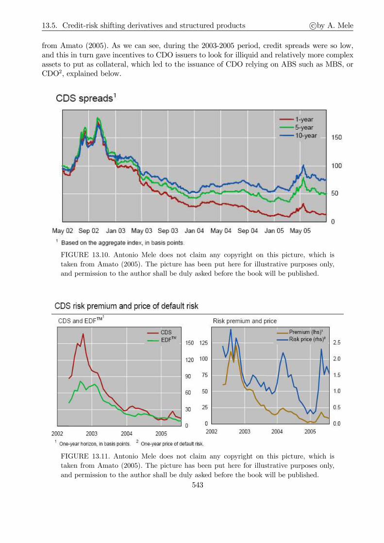
13.5. Credit-risk shifting derivatives and structured products c©by A. Mele
from Amato (2005). As we can see, during the 2003-2005 period, credit spreads were so low,and this in turn gave incentives to CDO issuers to look for illiquid and relatively more complexassets to put as collateral, which led to the issuance of CDO relying on ABS such as MBS, orCDO2, explained below.
FIGURE 13.10. Antonio Mele does not claim any copyright on this picture, which is
taken from Amato (2005). The picture has been put here for illustrative purposes only,
and permission to the author shall be duly asked before the book will be published.
FIGURE 13.11. Antonio Mele does not claim any copyright on this picture, which is
taken from Amato (2005). The picture has been put here for illustrative purposes only,
and permission to the author shall be duly asked before the book will be published.
543

13.5. Credit-risk shifting derivatives and structured products c©by A. Mele
The following picture illustrates the behavior of CDS indexes during approximately 20 yearsbefore the 2007-2009 credit market turmoil.
FIGURE 13.12. Valuation of Financial Instruments Based on Implied Probability of De-
fault. Antonio Mele does not claim any copyright on this picture, which is taken from
IMF (2008). The picture has been put here for illustrative purposes only, and permission
to the authors shall be duly asked before the book will be published.
13.5.5.5 Continuous time
We may relax the assumption the instantaneous intensity of default, λ, is constant. This inten-sity is defined under the risk-neutral probability and can change either because the intensity ofdefault under the physical probability changes or because risk-appetite changes, or both. Weexamine the asset pricing implications of time-varying intensities, by exploring how probabil-ities of survival change in a simple setting, where we do not single out the reasons leading tovariations in λ.First, we assume the instantaneous probability of default can only change discretely, giving
rise to random intensities λt, meaning that λt is the intensity of default in the time interval[t− 1, t]. Let Ft be the information set as of time t. We assume that λt is Ft-measurable. Whatis the probability of survival of any given name in this case? We have, by Bayes’s theorem,
Pr Surv at t| Surv at t− 1 = Pr Surv at tPr Surv at t− 1 . (13.27)
544

13.5. Credit-risk shifting derivatives and structured products c©by A. Mele
By a repeated use of Eq. (13.27),
Pr Surv at t = Pr Surv at t|Surv at t− 1Pr Surv at t− 1= · · ·
=
t∏
n=1
Pr Surv at n|Surv at n− 1 . (13.28)
So we are left with finding Pr Surv at n|Surv at n− 1. Consider the following arguments.If λn was not random and fixed at some λn, then, Pr Surv at n| Surv at n− 1 = e−λn .When λn is random, e−λn is the probability of survival, conditioned upon some particularvalue the intensity could possibly take. Heuristically, then, Pr Surv at n|Surv at n− 1 =∑
s∈S e−λn(s) Pr s, where λn (s) is, so to speak, the value λn would take in state s, Pr s is
the likelihood that state s occurs and, finally, S is the set of all possible states, as illustratedby the Figure 13.3.
2P r
( )2nλ
( )1nλ
1P r
d efau lt
d e fau lt
su rv iv a l
su rv iv a l
FIGURE 13.13. This picture illustrates the determination of the probability of survival in the case of
two states of intensities. At the beginning of period n, nature draws the event defining the intensity of
the default, which is either λn (1) with probability Pr 1, or λn (2) with probability Pr 2 = 1−Pr 1.Then, the two paths leading to survival have probability of occurrence equal to Pr 1 e−λn(1) and
Pr 2 e−λn(2), such that the total probability of survival equals Pr 1 e−λn(1) +Pr 2 e−λn(2).
Therefore, Pr Surv at n|Surv at n− 1 = E[e−λn
∣∣Fn−1
], where E denotes the expectation
taken under the risk-neutral probability. Inserting this result into Eq. (13.28), and using theLaw of Iterated Expectations, leaves:
Pr Surv at t = E[e−
∑t
n=1λn
].
Under regularity conditions, we can easily extend the previous result to a continuous timesetting. For example, we may assume that the risk-neutral default intensity, λ (t), is solutionto:
dλ (t) = φ(λ− λ (t)
)dt+ σ
√λ (t)dW (t) , λ (0) = λ. (13.29)
where W is a standard Brownian motion under the risk-neutral probability, and φ, λ and σ arethree positive constants. This is the same as the Cox, Ingersoll and Ross (1985) (CIR) modelof the short-term rate reviewed in Chapter 12. Therefore, under the parameter restrictions inChapter 12, λ (t) is always positive, and
Psurv (λ, t) ≡ Pr Surv at t = E[e−
∫ t
0λ(s)ds
]. (13.30)
545

13.5. Credit-risk shifting derivatives and structured products c©by A. Mele
Eq. (13.30) is, formally, the same as the Feynman-Kac representation of a solution to a PDE,solved by a bond price in the CIR model. In other words, the model for the survival probabilityin Eqs. (13.29)-(13.30) has the same mathematical structure as that leading to the price of abond in the CIR model. Therefore, a closed-form solution is available for Psurv (λ, t). It is givenby:
Psurv (λ,N) = Φ (N) e−B(N)λ,
Φ (N) =
(2γe
12(φ+γ)N
(φ+ γ) (eγN − 1) + 2γ
) 2φλ
σ2
, B (N) =2(eγN − 1
)
(φ+ γ) (eγN − 1) + 2γ , γ =√φ2 + 2σ2.
(13.31)More generally, we can build up a whole family of models with a closed-form solution, the
affine class reviewed in Chapter 12, by just assuming that:
λ (t) = λ0 + λ1 · y (t) , (13.32)
where λ0 is a constant, λ1 is a vector of constants, and y is a multivariate jump-diffusion process,with drift and diffusion terms as in Section 12.4.6 of Chapter 12. This model is interesting, aswe can judiciously choose the components of y (t) which we suppose may affect the defaultintensity. For example, some of them could be unobservable, and others could be observable,and relate, say, to the business cycle or even the structure of the firm.So given any solution for the survival probability predicted by any of these affine models
when y (0) = y, Psurv (y, t) say, we can easily compute
PrDefault ∈ (ti−1, ti) = Psurv (y, ti−1)− Psurv (y, ti) . (13.33)
We can then look at the bond spreads and the CDS spreads implied by this modeling choice.In Appendix 3, we show the price of a defaultable pure discount bond expiring in N years is:
P (y,N) = e−rNPsurv (y,N) +
∫ N
0
e−rt PrDefault ∈ dtRec (t) dt, (13.34)
where Rec (t) denotes the recovery value in case of default, supposed to be known. This eval-uation result is, naturally, consistent with a similar derivation provided in Section 12.4.7 ofChapter 12, although in this chapter we are emphasizing more “survival arguments.”As for the CDS spreads, we have, by Eq. (13.23),
CDSt (N) =
∑4Ni=1 e
−r(ti−t)LGD(ti) [Psurv (y, ti−1)− Psurv (y, ti)]∑4Ni=1 e
−r(ti−t)Psurv (y, ti),
where N is, again, the number of years the CDS refers to, and ti = t+i4.
Assume the short-term rate, r, is zero, and that loss-given-default is constant and equal toLGD. Then, as shown in Appendix 3, the price of a defaultable pure discount bond, P (λ,N),and the current CDS premium, CDS0 (N), are given by:
P (λ,N) = 1− LGD · (1− Psurv (λ,N)) , CDS0 (N) = LGD · 1− Psurv (λ,N)∑4Ni=1 Psurv (λ, ti)
. (13.35)
Figure 13.14 depicts the bonds spread, −1NlnP (λ,N), and the annualized credit default
spreads, 4×CDS0 (N), when the parameters in Eq. (13.29) are φ = 0.25, λ = 0.04 and σ =√λ,
546
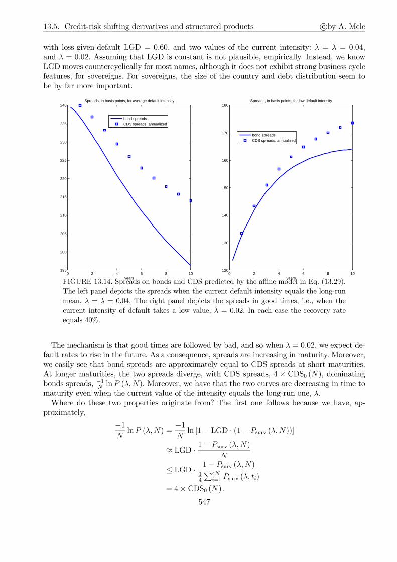
13.5. Credit-risk shifting derivatives and structured products c©by A. Mele
with loss-given-default LGD = 0.60, and two values of the current intensity: λ = λ = 0.04,and λ = 0.02. Assuming that LGD is constant is not plausible, empirically. Instead, we knowLGD moves countercyclically for most names, although it does not exhibit strong business cyclefeatures, for sovereigns. For sovereigns, the size of the country and debt distribution seem tobe by far more important.
0 2 4 6 8 10195
200
205
210
215
220
225
230
235
240Spreads, in basis points, for average default intensity
years
bond spreadsCDS spreads, annualized
0 2 4 6 8 10120
130
140
150
160
170
180Spreads, in basis points, for low default intensity
years
bond spreadsCDS spreads, annualized
FIGURE 13.14. Spreads on bonds and CDS predicted by the affine model in Eq. (13.29).
The left panel depicts the spreads when the current default intensity equals the long-run
mean, λ = λ = 0.04. The right panel depicts the spreads in good times, i.e., when the
current intensity of default takes a low value, λ = 0.02. In each case the recovery rate
equals 40%.
The mechanism is that good times are followed by bad, and so when λ = 0.02, we expect de-fault rates to rise in the future. As a consequence, spreads are increasing in maturity. Moreover,we easily see that bond spreads are approximately equal to CDS spreads at short maturities.At longer maturities, the two spreads diverge, with CDS spreads, 4 × CDS0 (N), dominatingbonds spreads, −1
NlnP (λ,N). Moreover, we have that the two curves are decreasing in time to
maturity even when the current value of the intensity equals the long-run one, λ.Where do these two properties originate from? The first one follows because we have, ap-
proximately,
−1NlnP (λ,N) =
−1Nln [1− LGD · (1− Psurv (λ,N))]
≈ LGD · 1− Psurv (λ,N)
N
≤ LGD · 1− Psurv (λ,N)14
∑4Ni=1 Psurv (λ, ti)
= 4× CDS0 (N) .547

13.5. Credit-risk shifting derivatives and structured products c©by A. Mele
As regards the second property, it’s a convexity effect. We can tackle this issue using argu-ments similar to those we made for another topic in Chapter 12, Section 12.3.4. For the bondspreads, since E (λ (s)) = λ+ e−φs
(λ− λ
), we have, approximately,
−1NlnP (λ,N) =
−1Nln [1− LGD · (1− Psurv (λ,N))]
=−1Nln
[1− LGD ·
(1− E
(e−
∫ N
0λ(s)ds
))]
≤ −1Nln
[1− LGD ·
(1− e−
∫ N
0E(λ(s))ds
)]
≈ LGD · 1− e−∫ N
0E(λ(s))ds
N
= LGD · 1− e−λN−(λ−λ) 1−e−φN
φ
N,
so that even if λ = λ, then, bond spreads are bounded away by a decreasing function (in N).Of course, it doesn’t necessarily mean that bond spreads have to be decreasing as well, but thatbounding function helps this happening. As for the CDS spreads, we have, approximately:
4× CDS0 (N) = LGD · 1− Psurv (λ,N)14
∑4Ni=1 Psurv (λ, ti)
≤ LGD · 1− Psurv (λ,N)
N · Psurv (λ,N)≈ − 1
NlnPsurv (λ,N) ,
such that for λ = λ, CDS0 (N) is bounded away by a decreasing function (in N), for the samearguments made as regards the bond spreads, − 1
NlnP (λ,N).
13.5.5.6 A trading strategy
Bond prices and CDS spreads are driven by the same state variable, the default intensity, andso they are restricted to lie on some space, to be consistent with no-arbitrage. To illustrate,consider, first, the simple case where the default intensity is constant, such that CDS spreadsare given by Eq. (13.24). Given this model, we can look at the market data for CDS spreads,
548

13.5. Credit-risk shifting derivatives and structured products c©by A. Mele
and infer the risk-neutral intensity, as in the picture below.
0 0.01 0.02 0.03 0.04 0.050
50
100
150
200
250
300
350C
DS
spr
eads
, mod
el−
base
d, in
bas
is p
oint
s
Default intensity
Inferring risk−neutral intensity from CDS market data
In this picture, the CDS spreads predicted by Eq. (13.24) are depicted as a function of therisk-neutral intensity, λ, assuming N = 5 years, LGD = 0.60 and the short-term rate r is zero.For example, if we had to observe a CDS equal to 200 basis points, we would infer a value ofλ approximately equal to λ = 0.033. The key point is this very same λ should be pricing thezero as well, such that for N = 5,
P (N) = 1− LGD ·(1− e−λN
)= 0.90874,
and so we might go long (short) the zero if its market price is lower (higher) than 0.90874.Naturally, this example is based on the unrealistic assumption that the default intensity is
constant. But the same strategy can be used in the more general case where default intensitiesare stochastic. In this case, bond prices and CDS spreads should also be restricted, by no-arbitrage. The picture below shows the restrictions between bond spreads and CDS spreads,obtained with the same parameter values as those used to produce Figure 13.14, and values of
549
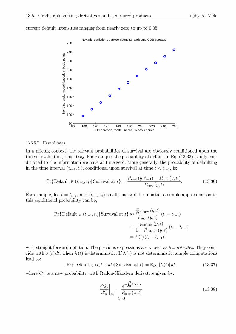
13.5. Credit-risk shifting derivatives and structured products c©by A. Mele
current default intensities ranging from nearly zero to up to 0.05.
80 100 120 140 160 180 200 220 240 26080
100
120
140
160
180
200
220
240
260
Bon
d sp
read
s, m
odel
−ba
sed,
in b
asis
poi
nts
CDS spreads, model−based, in basis points
No−arb restrictions between bond spreads and CDS spreads
13.5.5.7 Hazard rates
In a pricing context, the relevant probabilities of survival are obviously conditioned upon thetime of evaluation, time 0 say. For example, the probability of default in Eq. (13.33) is only con-ditioned to the information we have at time zero. More generally, the probability of defaultingin the time interval (ti−1, ti), conditional upon survival at time t < ti−1, is:
PrDefault ∈ (ti−1, ti)| Survival at t =Psurv (y, ti−1)− Psurv (y, ti)
Psurv (y, t). (13.36)
For example, for t = ti−1, and (ti−1, ti) small, and λ deterministic, a simple approximation tothis conditional probability can be,
PrDefault ∈ (ti−1, ti)|Survival at t ≈∂∂tPsurv (y, t)
Psurv (y, t)(ti − ti−1)
≡ pdefault (y, t)
1− Pdefault (y, t)(ti − ti−1)
= λ (t) (ti − ti−1) ,
with straight forward notation. The previous expressions are known as hazard rates. They coin-cide with λ (t) dt, when λ (t) is deterministic. If λ (t) is not deterministic, simple computationslead to:
PrDefault ∈ (t, t+ dt)| Survival at t = EQλ [λ (t)] dt, (13.37)
where Qλ is a new probability, with Radon-Nikodym derivative given by:
dQλ
dQ
∣∣∣∣F0
=e−
∫ t
0λ(s)ds
Psurv (λ, t). (13.38)
550
13.5. Credit-risk shifting derivatives and structured products c©by A. Mele
Accordingly, under Qλ, the state variables in Eq. (13.32) follow a diffusion process, with a driftprocess tilted, due to this change of measure. For example, in the simple setting of Eq. (13.29),we have that, for a fixed t,
dλ (s) = (B0 − Bt1 (s)λ (s)) ds+ σ√λ (s)dWλ (s) , s ∈ (0, t] , λ (0) = λ,
B0 = φλ, Bt1 (s) = φ+B (t− s) σ2, B (·) as in Eq. (13.31),(13.39)
where Wλ is a Brownian motion under Qλ. Therefore, by Eq. (13.37), and computations,
PrDefault ∈ (t, t+ dt)| Survival at t =[λ
G (t)+ B0
∫ t
0
G (s)
G (t)ds
]dt, G (x) ≡ e
∫ x
0Bt1(u)du.
Appendix 5 provides a proof of these results, which to the best of our knowledge, are developedhere for the first time.
13.5.5.8 Extracting probabilities of default from market data
Market data obviously convey information about probabilities of default, which might be ex-tracted from these data, under a number of assumptions. To illustrate this possibility in a simplecase, assume that the recovery rate is zero, and that the short-term rate and the instantaneousprobability of default are both continuous time Markov and independent of each other. Then,the price of a defaultable zero is: Pdef (λ,N) = P (N) ·Psurv (λ,N), where Pdef (λ,N) is the priceof a defaultable zero and P (N) is the price of a non-defaultable zero. Therefore, we can readthe risk-neutral probability of survival from the defaultable/non-defaultable bond price ratio:
Psurv (λ,N) =Pdef (λ,N)
P (N). (13.40)
Naturally, surviving until some time N2 means having survived until some time N1 < N2 andhaving survived from N1 to N2. Therefore, Psurv (λ,N2) = Psurv (λ,N1) ·Psurv (λ,N1,N2), wherePsurv (λ,N1, N2) is the risk-neutral probability of survival betweenN1 andN2. Using Eq. (13.40),then, we can extract this probability, as follows:
Psurv (λ,N1, N2) =Pdef (λ,N2)
Pdef (λ,N1)
P (N1)
P (N2).
The previous example relies on the simplifying assumption of a zero recovery rate, but it canbe generalized to the case where the recovery rate is nonzero. But in this case, bond prices wouldconvey information about both probabilities of default and recovery rates, an identification issueto be dealt with.
13.5.6 Collateralized Debt Obligations (CDOs)
13.5.6.1 A crash description
CDOs are securitized shares in pools of assets. Collateral assets include loans or debt instru-ments. A CDO may be a collateralized loan obligation (CLO) or collateralized bond obligation(CBO) according to whether it relies only on loans or bonds, respectively. CDO investors bearthe credit risk of the collateral. Multiple tranches of securities are issued by the CDO, offeringinvestors various maturity and credit risk characteristics. Tranches are categorized as senior,mezzanine, and subordinated, or junior, or equity, according to their degree of credit risk. If
551

13.5. Credit-risk shifting derivatives and structured products c©by A. Mele
there are defaults or the CDO’s collateral otherwise underperforms, scheduled payments tosenior tranches take precedence over those of mezzanine tranches, and scheduled payments tomezzanine tranches take precedence over those to junior tranches. Typically, senior tranchesare rated, with ratings of A to AAA. Mezzanine are also rated, typically with ratings of B toBBB. In principle, these ratings should reflect both the credit quality of the collateral and theprotection a given tranche is given by the tranches subordinating to it. CDOs are part of amore general securitization process, and can also include mortgages, as in the stylized examplebelow.
(i) In a first step, subprime mortgages are securitized, as illustrated below:
SubprimeMortgage
AssetBackedSecurity(ABS)
ABSinvestorMonthly
payments
ABSinvestor
ABSinvestor
SubprimeMortgage
SubprimeMortgage
Monthlypayments
(ii) In a second step, a CDO is created, out of the securitized subprime mortgages and addi-tional Asset Backed Secutities (ABS):
SubprimeABS
ABS relating to otherforms of collateral
(e.g. corporate debt)
Co
llate
raliz
edD
ebtO
blig
atio
n(C
DO
)
CDOInvestors
SubprimeABS CDO
Investors
CDOInvestors
(iii) In a third, and final step, the structuring process involves creating seniority rules.
Investors in CDOs senior tranches include banks and pension funds, which might benefit fromthe expertise of the asset managers, and the risk-return profiles difficult to find in the market.Investors in junior tranches are hedge funds searching for highly risky investment opportunitiesthat at the same time, are quite rewarding and certainly unavailable in the market. Additionalinvestors in junior tranches were dedicated off-balance-sheets entities such as “SIV,” “conduits,”and “SIV-lites,” which will be reviewed in Section 13.4.7.Underwriters of CDOs are investment banks, typically. They work closely with the asset
manager and create the “right” debt/equity ratio and perform collateral quality tests. Theyliase with law firms and create the special purpose vehicle (possibly in some tax heaven system)
552

13.5. Credit-risk shifting derivatives and structured products c©by A. Mele
that will purchase the assets and issue the tranches, price the various tranches, and obviouslyfind the investors. Fees to underwriters are very generous, due to the complexity of the CDOs.According to Thomson Financial, top underwriters in 2006 were: Bear Sterns, Merrill Lynch,Wachovia, Citigroup, Deutsche Bank, and Bank of America Securities.Involved in the structuring process are also (i) trustee and collateral administrator, who dis-
tribute noteholder reports, check compliance and execute priority of payments; (ii) accountants,who perform due diligence on the CDOs collateral pool, verifying for example credit ratings foreach asset; and (iii) rating agencies, which we shall discuss in the next subsection.The economics behind structured finance is quite interesting. An originator may have private
information about the quality of certain assets and/or a comparative advantage in evaluatingthese assets relative to other market participants. If the originator wishes to sell some of itsassets, an adverse selection problem will arise: because investors do not know the true quality ofthe assets, they will demand a premium to purchase them or even worse, a market might fail toarise. Structured finance helps originators mitigate this problem. First, by pooling the assets,diversification benefits can be achieved. Second, tranching allows relatively poorly informedinvestors to access senior tranches, and be relatively protected from default. In the process, theoriginator or arranger may retain subordinated exposure to alleviate investors’ concerns aboutincentive compatibility. The following scheme summarizes the structuring process.
Source: Committee on the Global Financial System: “The role of ratings in structured
finance: issues and implications,” January 2005.
13.5.6.2 The role of rating agencies
Structured finance has always been a “rated” market. Issuers of structured instruments hada natural appetite for a rating to occur at a scale comparable to that available for bonds.
553

13.5. Credit-risk shifting derivatives and structured products c©by A. Mele
The main reason was this would facilitate the sale of these products to investors bound byratings-based constraints defined by their investment mandates.However, the involvement of rating agencies into the delivery of their opinion about credit
risk differs from that related to traditional bonds. As regards traditional instruments, ratingagencies simply aim to assess the risk of default as given, which they take as given. As regardsstructured finance transactions, rating agencies play a much more ex-ante, reverse engineeringrole. A tranche rating reflects a view about both the credit risk of the asset pool and the extentof credit support to be provided. These two elements are organized to reverse engineer thetranche rating targeted by the deal’s arrangers. Deal origination thus involves rating agenciesin the structuring process.
13.5.6.3 Types of CDOs
In practice, CDOs are considerably more complex than the stylized examples outlined earlier.We have a number of cases. We say that a CDO is static, if it holds the same set of assets.Insetad, a CDO is managed, if the asset manager is allowed to change the composition of assets.If the claims to the CDO arise from the cash flows originated by the assets, we have a cash-flow CDO. If the claims to the CDO arise from the cash flows originated by the assets and/oractive asset management, we have a market-value CDO. CDOs can also be created to carve outbalance sheets, in which case we have balance-sheet CDOs. Moreover, and interestingly, CDOscan be created (i) to achieve investment grade bonds through a pool of noninvestment gradebonds, and (ii) to create riskier securities than those in the asset pool. In these cases, we havearbitrage CDOs. Naturally, “arbitrage” CDOs do not give rise to any arbitrage opportunity.These instruments merely “reshuffle” risk and returns of the assets in the pool, as we shall seein the next section. Typically, then, arbitrage CDOs differ from balance sheet CDOs, because ofcourse, issuers of arbitrage CDOs do not necessarily hold the underlying collateral in advance,which is obviously the case for issuers of balance-sheet CDOs. Therefore, the assets to be putinto the an arbitrage CDO pool have to be reasonably liquid.Furthermore, we have synthetic CDOs, which are exposed to a pool of assets that are not
strictly owned or in the asset pool, typically through CDS underwriting. Like a cash-flow CDO,the vehicle receives payments (the premium), which is then transferred to the tranche holders.Naturally, there can be default events, which are also passed through to the investors, accordingto the prespecified seniority rules. A synthetic CDO is funded, if the relevant tranche holders areto pay for in the case of a credit event related to the assets the CDO is exposed to. Typically,some funding is made available at the very time of investment. At maturity, the investor receivesa payoff equal to the funding minus the realized losses. Junior tranches are typically funded,and senior are typically not. However, senior tranches investors might have to make paymentsin the unlikely event losses had ever to erode their tranches.Finally, we have hybrid CDOs, which are partly cash-flow CDOs and partly synthetic CDOs.
In a single-tranche CDO, the entire CDO is structured to accommodate the specific needs of asmall group of investors, with some remaining tranche held by the dealer. And we have CDO2,where a large portion of the assets in the pool are tranches from other CDOs; or more generally,CDOn.
13.5.6.4 Pricing
CDOs repackage cash flows from a set of assets. We provide simple examples to show how toprice this repackaging process. We begin with a simple example, taken from McDonald (2006, p.583), which we further elaborate. Suppose we have three one-year bonds with face value = 100.
554

13.5. Credit-risk shifting derivatives and structured products c©by A. Mele
For each of these bonds, the risk-neutral probabilities of default equal 10% and the recoveryrates are 40. The safe interest rate for one year is 6%. So each bond price equals,
b = e−0.06 · ( 0.10︸︷︷︸≡Def. Prob
· 40 + 0.90︸︷︷︸≡Surv. Prob
· 100) = 88.526.
The yield is, naturally, − ln b100
= 12.19%.A CDO can restructure the payments promised by the three bonds in a way that transforms
the riskiness and attractiveness of the initial assets. Consider the following example:
Mezzanine tranche = 90
Senior tranche = 140
Junior tranche = 70
Asset Pool
Face Value= 300
CDO claims
In this example, each tranche receives the minimum between (i) the nominal value claimed bythe tranche and (ii) what is left available to the tranche after having satisfied the other tranchesby order of seniority.Let Ni be the nominal values claimed by the tranches, so that N1 = 140, N2 = 90 and
N3 = 70. Let π be the realized payoff of the asset pool, defined as,
π = No. of Defaults · 40 + (3− No. of Defaults)︸ ︷︷ ︸≡No. of surviving bonds
· 100.
Naturally, π is random because the number of defaults is random. At the expiration,
(i) the senior tranches receives the minimum between N1 and π. For example, if only onebond defaults, π = 240, and the senior tranche receives 140. If, however, three bondsdefault, then, π = 120, which is less than the senior tranch nominal value, and the seniortranche then receives 120. So a quite severe loss is needed to erode the senior trancheclaims.
(ii) The mezzanine tranche receives the minimum between N2 and the “left-over” from thesenior tranche.
(iii) Finally, at the expiration, the junior tranche reveives the minimum between N3 and the“left-over” from the senior and mezzanine tranches.
More generally, tranche no. i receives,
πi = min Left-over from previous tranches up to tranche i− 1 ,Ni ,
where
Left-over from previous tranches up to tranche i− 1 = max
π −
i−1∑k=1
πk, 0
.
555
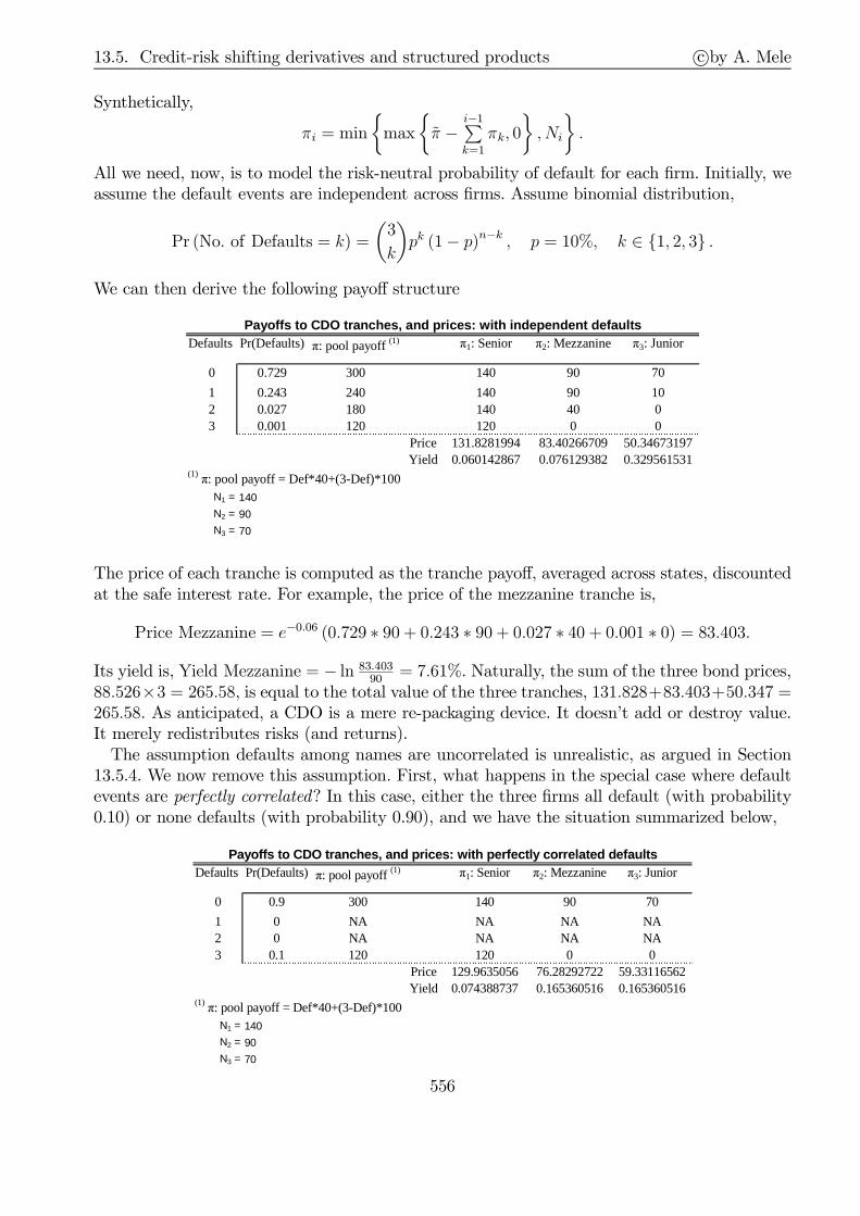
13.5. Credit-risk shifting derivatives and structured products c©by A. Mele
Synthetically,
πi = min
max
π −
i−1∑k=1
πk, 0
, Ni
.
All we need, now, is to model the risk-neutral probability of default for each firm. Initially, weassume the default events are independent across firms. Assume binomial distribution,
Pr (No. of Defaults = k) =
(3
k
)pk (1− p)n−k , p = 10%, k ∈ 1, 2, 3 .
We can then derive the following payoff structure
Defaults Pr(Defaults)π: pool payoff (1) π1: Senior π2: Mezzanine π3: Junior
0 0.729 300 140 90 70
1 0.243 240 140 90 102 0.027 180 140 40 03 0.001 120 120 0 0
Price 131.8281994 83.40266709 50.34673197Yield 0.060142867 0.076129382 0.329561531
N1 = 140
N2 = 90
N3 = 70
Payoffs to CDO tranches, and prices: with independe nt defaults
(1) π: pool payoff = Def*40+(3-Def)*100
The price of each tranche is computed as the tranche payoff, averaged across states, discountedat the safe interest rate. For example, the price of the mezzanine tranche is,
Price Mezzanine = e−0.06 (0.729 ∗ 90 + 0.243 ∗ 90 + 0.027 ∗ 40 + 0.001 ∗ 0) = 83.403.
Its yield is, Yield Mezzanine = − ln 83.40390
= 7.61%. Naturally, the sum of the three bond prices,88.526×3 = 265.58, is equal to the total value of the three tranches, 131.828+83.403+50.347 =265.58. As anticipated, a CDO is a mere re-packaging device. It doesn’t add or destroy value.It merely redistributes risks (and returns).The assumption defaults among names are uncorrelated is unrealistic, as argued in Section
13.5.4. We now remove this assumption. First, what happens in the special case where defaultevents are perfectly correlated? In this case, either the three firms all default (with probability0.10) or none defaults (with probability 0.90), and we have the situation summarized below,
Defaults Pr(Defaults)π: pool payoff (1) π1: Senior π2: Mezzanine π3: Junior
0 0.9 300 140 90 70
1 0 NA NA NA NA2 0 NA NA NA NA3 0.1 120 120 0 0
Price 129.9635056 76.28292722 59.33116562Yield 0.074388737 0.165360516 0.165360516
N1 = 140
N2 = 90
N3 = 70
Payoffs to CDO tranches, and prices: with perfectly correlated defaults
(1) π: pool payoff = Def*40+(3-Def)*100
556

13.5. Credit-risk shifting derivatives and structured products c©by A. Mele
Note, now, that mezzanine and junior tranches yield the same as they each pay off either theirnominal value or zero in exactly the same states of nature.The previous cases (with independent and perfectly correlated defaults) are extreme. It is
by far more relevant to see what happens when defaults are only imperfectly correlated. Whendefaults are imperfectly correlated, there are no simple tables to use to come up with tranchepricing. Instead, one might make use of simulations, described succinctly in the Appendix.Figure 13.14 below, obtained through Monte Carlo simulations, illustrates how the yield oneach tranche changes as a result of a change in the default correlation underlying the assets inthe CDO.
0 0.2 0.4 0.6 0.8 10.05
0.1
0.15
0.2
0.25
0.3
0.35
0.4
default correlation
Yie
ld
Yields on CDO tranches
JuniorMezzanineSenior
FIGURE 13.15. Yields on the three CDO tranches, as functions of the default correlation
among the assets in the structure, with probability of default for each name p = 20%. The
thick, horizontal, line is the yield on each securitized asset.
“Arbitrage” CDOs
Figure 13.15 illustrates how arbitrage CDOs work. The CDO has three assets yielding the same,12.19% (the horizontal line in the picture). However, by restructuring the asset base through aCDO, we can create claims (Senior and Mezzanine tranches) that yield less than 12.19%, as theyare considerably less risky than the asset base. Such an excess return, (12.19% − Yieldtranche),with Yieldtranche ∈ Senior,Mezzanine, is “made available” to the Junior tranche/equity hold-ers, once we account for management fees and expenses. Note, the previous redistribution ofrisk always works when the default correlation is relatively low. As the default correlation inthe asset base increases, the situation may change dramatically, as we now illustrate. Figure13.16 below makes some comparative statics: with p = 20%, instead of p = 10%. The yields areobviously larger for each tranche, and the three assets now yield 18.78%, reflecting the highr p.
557

13.5. Credit-risk shifting derivatives and structured products c©by A. Mele
Correlation assumptions
In Figures 13.15 and 13.16, the yield on the junior tranche decreases with default correlation.This happens because we are assuming that the probability of default is fixed at p = 10% foreach default correlation ρ (say). As ρ increases, the probability of clustering events increases,which makes the Senior and Mezzanine tranches relatively less valuable and, correspondingly,the Junior tranches more valuable. A more appropriate model is one in which p increases asρ increases, to capture the fact that in bad times, both default correlation and probability ofdefaults increase as these two things are intimately related (by, e.g., some common businesscycle factor).
0 0.2 0.4 0.6 0.8 10
0.1
0.2
0.3
0.4
0.5
0.6
0.7
default correlation
Yiel
d
Yields on CDO tranches
JuniorMezzanineSenior
FIGURE 13.16. Yields on the three CDO tranches, as functions of the default correlation
among the assets in the structure, with probability of default for each name p = 20%. The
thick, horizontal, line is the yield on each securitized asset.
Addressing the correlation assumption
Relax the assumption that the probability of default, p, and the default correlation, ρ areindependent. For simplicity, assume that ρ = 3.8116 ∗ ln (p+ 1), and let p vary from 0.10 to0.30, such that then, ρ varies from 0.3633 to 1. The situation, then, changes dramatically. Figure13.17 depicts the results, which show how modeling might substantially affect effective pricing.First, and naturally, the yield on each securitized asset is increasing in ρ because ρ is, itself,increasing in the probability of default. Second, the Junior tranche has a yield that increases
558
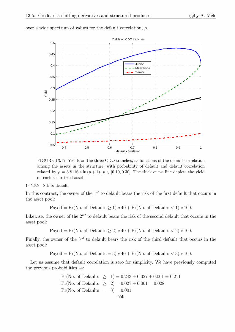
13.5. Credit-risk shifting derivatives and structured products c©by A. Mele
over a wide spectrum of values for the default correlation, ρ.
0.4 0.5 0.6 0.7 0.8 0.9 10.05
0.1
0.15
0.2
0.25
0.3
0.35
0.4
0.45
0.5
default correlation
Yie
ld
Yields on CDO tranches
JuniorMezzanineSenior
FIGURE 13.17. Yields on the three CDO tranches, as functions of the default correlation
among the assets in the structure, with probability of default and default correlation
related by ρ = 3.8116 ∗ ln (p+ 1), p ∈ [0.10, 0.30]. The thick curve line depicts the yield
on each securitized asset.
13.5.6.5 Nth to default
In this contract, the owner of the 1st to default bears the risk of the first default that occurs inthe asset pool:
Payoff = Pr(No. of Defaults ≥ 1) ∗ 40 + Pr(No. of Defaults < 1) ∗ 100.Likewise, the owner of the 2nd to default bears the risk of the second default that occurs in theasset pool:
Payoff = Pr(No. of Defaults ≥ 2) ∗ 40 + Pr(No. of Defaults < 2) ∗ 100.Finally, the owner of the 3rd to default bears the risk of the third default that occurs in theasset pool:
Payoff = Pr(No. of Defaults = 3) ∗ 40 + Pr(No. of Defaults < 3) ∗ 100.Let us assume that default correlation is zero for simplicity. We have previously computed
the previous probabilities as:
Pr(No. of Defaults ≥ 1) = 0.243 + 0.027 + 0.001 = 0.271
Pr(No. of Defaults ≥ 2) = 0.027 + 0.001 = 0.028
Pr(No. of Defaults = 3) = 0.001
559

13.5. Credit-risk shifting derivatives and structured products c©by A. Mele
Thus, we have the following prices,
Price1st-to-default = e−0.06 ∗ [0.271 ∗ 40 + (1− 0.271) ∗ 100] = 78.863
Price2nd-to-default = e−0.06 ∗ [0.028 ∗ 40 + (1− 0.028) ∗ 100] = 92.594
Price3rd-to-default = e−0.06 ∗ [0.001 ∗ 40 + (1− 0.001) ∗ 100] = 94.120
From here, we can compute the yields as follows, Yield1st-to-def = − ln (78.863/100) = 23.74%,Yield2nd-to-def = − ln (92.594/100) = 7.69%, and Yield3rd-to-def = − ln (94.120/100) = 6.06%.
13.5.7 One stylized numerical example of a structured product
A. Defaultable bonds
Suppose we observe the following risk-structure of spreads, related to two bonds maturing intwo years:
SpreadA (2 years) = 1.5%, SpreadB (2 years) = 2.5%,
where A and B denote the rating classes the bond issuers belong to. Assume that the one-yeartransition rating matrix, defined under the risk-neutral probability, is:
To
From
A B DefA 0.7 0.3 0B 0.3 0.5 0.2Def 0 0 1
where “Def” denotes default. We assume that in the event of default, the recovery value of thebond is paid off at the end of the second period. We want to determine the expected recoveryrates for the two bonds, and which expected recovery rate is the largest. We have:
erTD0,i
N=
[ReciNQi (2) + (1−Qi (2))
], i ∈ A,B .
Therefore,
SpreadA (2 years) = 1.5% = −12ln
[RecAN
QA (2) + (1−QA (2))
](13.41)
SpreadB (2 years) = 2.5% = −12ln
[RecBN
QB (2) + (1−QB (2))
](13.42)
We have to find QA (2) and QB (2). The transition matrix for two years is,
Q (2) =
0.7 0.3 00.3 0.5 0.20 0 1
0.7 0.3 00.3 0.5 0.20 0 1
,
such that,
Pr A defaults in 2 years = QA (2)
= 0.70 ∗ 0︸ ︷︷ ︸A→A→Def
+ 0.30 ∗ 0.20︸ ︷︷ ︸A→B→Def
+ 0 ∗ 1︸︷︷︸A→Def→Def
= 0.06
560

13.5. Credit-risk shifting derivatives and structured products c©by A. Mele
Pr B defaults in 2 years = QB (2)
= 0.20 ∗ 1︸ ︷︷ ︸B→Def→Def
+ 0.50 ∗ 0.20︸ ︷︷ ︸B→B→Def
+ 0.30 ∗ 0︸ ︷︷ ︸B→A→Def
= 0.20 + 0.10 = 0.30.
Hence, using Eqs. (13.41)-(13.42), we have
SpreadA (2 years) = 1.5% = −12ln
[RecAN
0.06 + (1− 0.06)]
SpreadB (2 years) = 2.5% = −12ln
[RecBN
0.30 + (1− 0.30)]
Solving, yields,RecAN
= 50.7%,RecBN
= 83.7%.
The expected recovery rate for the second bond is the largest. This is because the probabilityfirm B defaults is much larger than the probability firm A defaults and yet the two spreads arerelatively close to each other. So to rationalize the two spreads, we need a large recovery ratefor the second bond.What would happen to the two credit spreads, then, once we assume that the recovery rates
are the same, and equal to 50%? This question sheds additional light to the previous findings.If the recovery rates are the same and both equal 50%,
SpreadA (2 years) = −12ln [0.50QA (2) + (1−QA (2))]
SpreadB (2 years) = −12ln [0.50QB (2) + (1−QB (2))]
Then, using the previously computed transition probabilities for two years, we obtain:
SpreadA (2 years) = 1.52%, SpreadB (2 years) = 8.12%.
When the recovery rates are the same, the spread on the second bond diverges substantiallyfrom that on the first bond.
B. Collateralized debt obligations
Let us keep on using the same framework as before, but use different figures, so as to figure outthe implications for CDOs pricing. Consider the following one year transition matrix, under therisk-neutral probability:
To
From
A B DefA 0.7 0.3 0B 0.1 0.6 0.3Def 0 0 1
where “Def” denotes default. Consider (i) 1 one-year bond issued by a company rated A, and(ii) 3 one-year bonds issued by a company rated B. Both bonds have face value equal to 100.
561
13.5. Credit-risk shifting derivatives and structured products c©by A. Mele
We assume that the recovery values in case of default of all these bonds are the same, and equalto 50. Finally, we assume the safe interest rate is taken to be equal to zero.Consider a collateralized debt obligation (CDO, in the sequel), which gathers the previous
four bonds. Therefore, the CDO has nominal value of 400, and pays off in one year. The CDOhas (i) a senior tranche, with nominal value equal to 150; (ii) a mezzanine tranche, with nominalvalue equal to N1; and (iii) a junior tranche, with nominal value equal to N2. We assume thatthe structure is such that N1 > 100.First, we determine the price and yields on all the four bonds. Since the safe interest rate is
zero, and the company rated A is safe, up to the next year, the price of the A bond is 100, andits yield is zero. As for the three bonds rated B, we have:
P_B = 50 ∗ 0.3 + 100 ∗ 0.7 = 85.0, Y ield_B = − ln 0.85 = 16.25%.
Second, we determine the yield on the junior tranche, and derive the yield on the mezzanine,as a function of its nominal value N1. To determine the yield on the tranches, we need to figureout the following table:
No_Def Pr Π π0 π1 π2
0 0.7 400 150 N1 N2
1 0 NA NA NA NA2 0 NA NA NA NA3 0.3 250 150 100 04 4 NA NA NA NA
where No_Def denotes the number of defaults, Pr is the probability of No_Def, Π is the poolpayoff, defined as,
Π = No_Def ∗ 50 + (4−No_Def) ∗ 100,and, finally: π0 is the payoff to the senior tranche, π1 is the payoff to the mezzanine tranche,and, π2 is the payoff to the junior tranche. Therefore, we have:
price_mezzanine = 0.70 ∗N1 + 0.30 ∗ 100, price_junior = 0.70 ∗N2,
such that:
Yield_mezzanine = − ln(0.70 ∗N1 + 0.30 ∗ 100
N1
)= − ln
(0.70 + 0.30 ∗ 100
N1
)
Yield_junior = − ln(0.70 ∗N2
N2
)= 35.67%.
Naturally, we need to have that Yield_mezzanine < Yield_junior. It is simple to show thisrelation: it suffices to note that,
Yield_junior = − ln (0.70) > − ln(0.70 + 0.30 ∗ 100
N1
)= Yield_mezzanine.
A reverse enginnering question is, now, to determine which nominal value of the mezzaninetranche N1 is needed, to ensure that the yield on the mezzanine tranche is equal to or greaterthan the yields on the bonds issued by the company with credit rating B? The answer isN1 = 200, for in this case, the mezzanine tranche would have the same payoff structure as the
562
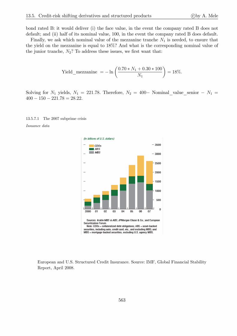
13.5. Credit-risk shifting derivatives and structured products c©by A. Mele
bond rated B: it would deliver (i) the face value, in the event the company rated B does notdefault; and (ii) half of its nominal value, 100, in the event the company rated B does default.Finally, we ask which nominal value of the mezzanine tranche N1 is needed, to ensure that
the yield on the mezzanine is equal to 18%? And what is the corresponding nominal value ofthe junior tranche, N2? To address these issues, we first want that:
Yield_mezzanine = − ln(0.70 ∗N1 + 0.30 ∗ 100
N1
)= 18%.
Solving for N1 yields, N1 = 221.78. Therefore, N2 = 400− Nominal_value_senior − N1 =400− 150− 221.78 = 28.22.
13.5.7.1 The 2007 subprime crisis
Issuance data
European and U.S. Structured Credit Insurance. Source: IMF, Global Financial Stability
Report, April 2008.
563
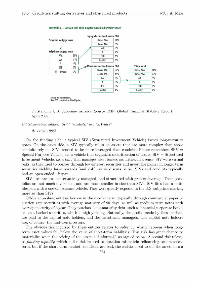
13.5. Credit-risk shifting derivatives and structured products c©by A. Mele
Outstanding U.S. Subprime issuance. Source: IMF, Global Financial Stability Report,
April 2008.
Off-balance-sheet entities: “SIV,” “conduits,” and “SIV-lites”
[b. circa 1985]
On the funding side, a typical SIV (Structured Investment Vehicle) issues long-maturitynotes. On the asset side, a SIV typically relies on assets that are more complex than thoseconduits rely on. SIVs tended to be more leveraged than conduits. Please remember: SPV =Special Purpose Vehicle, i.e. a vehicle that organizes securitization of assets; SIV = StructuredInvestment Vehicle, i.e. a fund that manages asset backed securities. In a sense, SIV were virtualbaks, as they used to borrow through low-interest securities and invest the money in longer termsecurities yielding large rewards (and risk), as we discuss below. SIVs and conduits typicallyhad an open-ended lifespan.SIV-lites are less conservatively managed, and structured with greater leverage. Their port-
folios are not much diversified, and are much smaller in size than SIVs. SIV-lites had a finitelifespan, with a one-off issuance vehicle. They were greatly exposed to the U.S. subprime market,more so than SIVs.Off-balance-sheet entities borrow in the shorter term, typically through commercial paper or
auction rate securities with average maturity of 90 days, as well as medium term notes withaverage maturity of a year. They purchase long-maturity debt, such as financial corporate bondsor asset-backed securities, which is high-yielding. Naturally, the profits made by these entitiesare paid to the capital note holders, and the investment managers. The capital note holdersare, of course, the first-loss investors.The obvious risk incurred by these entities relates to solvency, which happens when long-
term asset values fall below the value of short-term liabilities. This risk has great chance tomaterialize when the pricing of the assets is “informal,” as argued below. A second risk relatesto funding liquidity, which is the risk related to duration mismatch: refinancing occurs short-term, but if the short-term market conditions are bad, the entities need to sell the assets into a
564

13.5. Credit-risk shifting derivatives and structured products c©by A. Mele
depressed market. To cope with this risk, the sponsoring banks would grant credit lines. Typicalsponsors were: Citibank ($100bn), JP Morgan Chase ($77bn), Bank of America ($60bn). In theEuropean Union: HBOS ($42bn), ABN Amro ($40bn), HSBC ($32bn).
Source: IMF, Global Financial Stability Report, April 2008.
The 2007 meltdown
The first obvious issue to think about relates to pricing and the role played by credit ratings.Being illiquid, the pricing of structured credit products used to rely on that of similarly ratedcomparable products for which quotations were available. For example, the price of AAA ABXsubindices would be used to estimate the values of AAA-rated tranches of MBS. Or, the price ofBBB subindices would be used to value BBB-rated MBS tranches. This is the “mapping role”credit ratings played for the pricing of customized or illiquid structured credit products. How-ever, it is well-known that the risk profile of structured products differs from that of corporatebonds. Even if a tranche has the same expected loss as an otherwise similar corporate bond,unexpected loss or tail risk can be much larger than that for corporate bonds. Therefore, it is
565
13.5. Credit-risk shifting derivatives and structured products c©by A. Mele
misleading to extrapolate structured products ratings from corporate bonds ratings. Typically,ratings used to capture only the first moments of the distribution. Moreover, credit rating in-ertia for bonds does not necessarily work for structured products, as illustrtated in the picturebelow.Two additional fundamental aspects contributing to the meltdown. First, there was an ero-
sion in lending standards: statistical models were based on historically low mortgage defaultand delinquency rates that arose in a credit environment with tight credit standards. Second,there were correlation issues: past data suggested a quite weak correlation between regionalmortgages, which made investors perceive a sense of “diversification.” However, the housingdownturn turned up to be a nation-wide phenomenon.The mechanics of the crisis started with fears of contagion from the rising level of defaults
in subprime underlying instruments, many of which were incorporated in complex products.The fears of contagion related to safer tranches as well. They came from the investors’ un-derstanding the pricing models were misspecified, and their lack of trust vis-à-vis the ratingagencies. Banks, on the other side, were affected for a number of reasons: (i) they had investedin subprime securities directly; (ii) they had provided credit lines to SIV (indebted throughcommercial paper) and conduits that held these securities, thereby creating a shadow bank-ing system, which escaped accounting and supervision rules; and (iii) this very same shadowsystem generated banks’ loss of confidence in the ability of their counterparties to meet theircontractual obligations. So the Asset Backed Commercial Paper market dried up, triggeringcredit lines. The result was a sell-off of anything related to structured finance, from junk toAAA, which led to a complete “liquidity black hole,” and a severe reappraisal of structuredfinance.In turn, the reappraisal of structured finance determined severe writedowns, arising in part
through the “liquidity black hole,” i.e. by the market participants expectations. Repricing wasdifficult indeed. In the absence of a liquid market, writedowns have to rely on marking to model.But investors did not trust the models and the rating process leading to them! Meanwhile,credit agencies proceeded to severe downgrades, confirming the investors’ beliefs that ratingswere not entirely appropriate, a quite self-reinforcing mechanism. These events escalated toa complete dry up in September-October 2008, partly restored by painful bank bail-outs and
566

13.6. A few hints on the risk-management practice c©by A. Mele
recapitalizations.
Source: IMF, Global Financial Stability Report, April 2008.
13.6 A few hints on the risk-management practice
13.6.1 Value at Risk (VaR)
We need to review Value at Risk (VaR), in general. VaR is a method of assessing risk that usesstatistical techniques. Useful for supervision andmanagement of financial risks. Origins: reactionto financial disasters in the early 1990s involving Orange County, Barings, Metallgesellschaft,Daiwa, etc.
D I: VaR measures the worst expected loss over a given horizon under normal marketconditions at a given confidence level.
D II: We are (1− p)% certain that a given portfolio will not suffer of a loss largerthan £W over the next N weeks, Pr (Loss < −W ) = p. That is, £VaRp = $W .
567

13.6. A few hints on the risk-management practice c©by A. Mele
p
− W
Equivalently, note that
Loss
V0=∆V
V0= portfolio return
where ∆V denotes the change in value of the portfolio over the next N days, and $V0 is thecurrent value of the portfolio. Hence,
p = Pr (Loss < −VaRp) = Pr
(∆V
V0< −VaRp
V0
).
This formulation leads us to the following alternative definition:
D III: We are (1− p)% certain that a given portfolio will not experience a relativeloss larger than VaRp
V0over the next N weeks.
So in practice, we shall have to find the relative loss, ℓp, for a given confidence p, as follows:
p = Pr
(∆V
V0< −ℓp
), where ℓp =
VaRp
V0.
The corresponding VaRp is just
VaRp = ℓp · V0
For example, suppose that the portfolio return over the next 2 weeks, ∆VV0
, is normally dis-
tributed with mean zero and unit variance. We know that 0.01 = Pr(∆VV0
< −2.32), hence,VaRp = 2.32 · V0.
568

13.6. A few hints on the risk-management practice c©by A. Mele
−3 −2 −1 0 1 2 30
0.05
0.1
0.15
0.2
0.25
0.3
0.35
0.4
VaR/V0
1%
We are 99% certain that our portfolio will not suffer of a loss larger than −2.32 times itscurrent value over the next 2 weeks. We are 99% certain that our portfolio will not experiencea relative loss larger than −2.32 over the next 2 weeks.As a second example note that the previous assumption about the portfolio return was
extreme. Assume, instead, the porfolio return over the next 2 weeks, ∆VV0
, is normally distributed
with mean zero and variance σ2 = 252σ2year, where σ
2year is the annualized variance. We assume
that σ2year = 0.152. We have to re-scale the previous formulas, as follows. First, we introduce a
variable ǫ ∼ N (0, 1), i.e. ǫ is normally distributed with mean zero and variance = 1. So we canwrite,
∆V
V0
d= ǫ · σ ∼ N
(0, σ2
),
and, hence,0.01 = Pr (ǫ < −2.32) = Pr (∆V < −2.32 · V0 · σ) ,
whence, VaRp = 2.32 · V0 · σ. We know the annualized variance, σ2year = 0.152, from which we
can derive the two-week standard deviation, σ2 = 252σ2year ≈ 0.032, and, hence, VaRp
V0= 2.32 ·σ =
2.32 · 0.03 ≈ 7%. Thata is, we are 99% certain that our portfolio will not suffer of a loss largerthan 7% times its current value over the next 2 weeks. We are 99% certain that our portfoliowill not experience a relative loss larger than 7% over the next 2 weeks.More generally, we may assume the porfolio return over the next 2 weeks, ∆V
V0, is normally
distributed with mean µ and variance σ2. In this case,
∆V
V0
d= µ+ ǫ · σ ∼ N
(µ, σ2
),
and, hence,0.01 = Pr (ǫ < −2.32) = Pr (∆V < −V0 · (2.32 · σ − µ))
whence, VaRp = V0 · (2.32 · σ − µ). In practice, µ is very small if the horizon is as short as twoweeks.
569
13.6. A few hints on the risk-management practice c©by A. Mele
13.6.1.1 Challenges to VaR
Challenges related to distributional assumptions, nonlinearities, or conceptual difficulties.
Distributional assumptions
The assumption that data are generated by a normal distribution does not describe assetreturns well. Chapters 10 and 11 explain that we need ARCH effects, stochastic volatility andmultifactor models. More generally, data can exhibit changes in regimes, nonlinearities and fattails. Fat tails are particularly important to understand, since this is what we’re interestedin after all. More in general, it is quite challenging to understand what the data generatingprocess is, especially in so far as we consider portfolios of assets. Asset returns and volatilitiesare typically correlated, with correlation rising in bad times–correlation is stochastic.We may make distributional assumptions but, then, these assumptions have to be carefully
assessed through, for example, backtesting (to be explained below). We may proceed withnonparametric methods, and this is indeed a promising avenue, but with its caveats.How do nonparametric methods work? These methods rely on an old and idea, which is to
estimate the data distribution through histograms. These histograms, then, can be readily usedto compute VaR. This approach is nonparametric in nature, as it does not rely on any model.A more refined method replaces “rough” histograms with “smoothed” histograms, as follows.Suppose to have access to a time series of data xn, which are drawn from a certain probabilitylaw, with density f (x). We may define the following estimate of the density f (x),
fN (x) =1
N
N∑
n=1
1
λK
(x− xnλ
),
where N is the sample size, and K is some symmetric function integrating to one. We maythink of fN (x) as a smoothed histogram, with window bin equal to λ. It is possible to showthat as N goes to infinity and λ goes to zero at a certain rate, fN (x) converges “in probability”to f (x), for all x. But we are not done, since there are not obvious rules to choose λ and K?The choice of λ is notoriously difficult. Unfortunately, the “bias,” fN (x) − f (x), tends to belarge exactly on the tails of f (x), which do represent the region we’re interested in. In general,we can use Montecarlo simulations out of a smoothed density like this to compute VaR.
Nonlinearities
Finally, portfolios of assets can behave in a nonlinear fashion, especially when the portfoliocontains derivatives. In general, the value of a portfolio including M assets is,
P =M∑
j=1
αiSi,
where αi is the number of the i-th asset in the portfolio, and Si is the price of the i-th assetin the portfolio. Holding αi constant, the variation on the portfolio return is simply a weigthedaverage of all the asset returns,
∆PT ≡ PT − Pt =M∑
j=1
αi∆Si ⇐⇒∆P
P=
M∑
j=1
(αiSiP
)∆SiSi,
where the variations relate to any time interval. Often, the prices Si are rational functions ofthe state variables, or are interlinked through arbitrage restrictions. Use factors to determine
570

13.6. A few hints on the risk-management practice c©by A. Mele
the risk associated with fixed income securities. When the horizon of the VaR is large, it isunlikely that αi is constant. Typically, we shall need to go for numerical methods, based, forexample, on Monte Carlo simulations. So all in all, we need to have a careful understanding ofthe derivatives in the book, and proceed with back testing and stress testing.
VaR as an appropriate measure of risk
There are technical difficulties related to the very definition of VaR. VaR suffers from somestatistic-theoretic foundation. VaR tells us that 1% of the time, losses will exceed the VaR figure,but it does not tell us the entity of the loss. So we need to compute the expected shortfall. Anyrisk measure should enjoy a number of sensible properties. Artzner et al. (1999) have noted anumber of properties, and showed that VaR does not enjoy the so-called subadditivity property,according to which the sum of the risk measures for any two portfolios should be larger than therisk measure for the sum of the two portfolios. VaR doesn’t satisfy the subadditivity property,but expected shortfall does satisfy the subadditivity property.
13.6.2 Backtesting
How well the VaR estimate would have performed in the past? How often the loss in a givensample exceeded the reference-period 99% VaR? If the exceptions occur more than 1% of thetime, there is evidence that the models leading to VaR estimates are “misspecified”–a niceword for saying “bad” models.The mechanics of backtesting is as follows. Suppose the models leading to the VaR are
“good”. By construction, the probability the VaR number is exceeded in any reference periodis p, where p is the coverage rate for the VaR. Next, we go to our sample, which we assumeit comprises N days, and let M be the number of days the VaR is exceeded. We wish to testwhether the number of exceptions we observe in the sample “conforms” to the expected numberof exceptions based on the VaR. For example, it might be that the number of exceptions wehave observed, M , is larger than the expected number of exceptions, p ·N . We want to makesure this circumstance arose due to sample variability, rather than model misspecification. Asimple one-tail test is described below.Let us compute the probability that in N days, the VaR is exceeded for M or more days.
Assuming exceptions are binomially distributed, this probability is,
Πp =N∑
k=M
N !
k! (N − k)!pk (1− p)N−k .
Then, we can say the following. If Πp ≤ 5% (say), we reject the hypothesis that the probabilityof exceptions is p at the 5% level–the models we’re using are misspecified. If Πp > 5% (say),we cannot reject the hypothesis that the probability of exceptions is p at the 5% level–we can’tsay the models we’re using are misspecified. This test is reviewed in more detail by Hull (2007,p. 208). Other tests are reviewed by Christoffersen (2003, p. 184).
13.6.3 Stress testing
Stress testing is a technique through which we generate artificial data from a range of possiblesscenarios. Stress scenarios help cover a range of factors that can create extraordinary lossesor gains in trading portfolios, or make the control of risk in those portfolios very difficult.These factors include low-probability events in all major types of risks, including the various
571

13.6. A few hints on the risk-management practice c©by A. Mele
components of credit, market, and operational risks. Stress scenarios need to shed light on theimpact of such events on positions that display both linear and nonlinear price characteristics(i.e. options and instruments that have options-like characteristics).Possible scenarios include simulating (i) shocks that although rare or even absent from the
historical database at hand, are likely to happen anyway; and (ii) shocks leading to structuralbreaks and/or smooth transition in the data generating mechanism. One possible example is toset the percentage changes in all market variables in the portfolio equal to the worst percentagechanges having occured in ten days in a row during the subprime crisis 2007-2008.This example on the subprime crisis is related to the historical simulation approach to gener-
ate scenarios. This approach consists can be explained through a single formula. Let vt the valueof some market variable i in day t in our sample, where t = 0, · · · , T (say). We can generate Tscenarios for the next day, T + 1, as follows.
(i) The first scenario is that in which each variable grows by the same amount it grew attime 1,
vT+1 = vT ·v1v0.
(ii) The second scenario is that in which each variable grows by the same amount it grew attime 2,
vT+1 = vT ·v2v1.
(iii) · · ·
(iv) The T -th scenario is that in which each variable grows by the same amount it grew attime T ,
vT+1 = vT ·vTvT−1
.
(v) The T scenarios are generated for all the market variables, which would give us an artificialmultivariate sample of T observations. We can use this sample for many things, includingVaR.
13.6.4 Credit risk and VaR
We can use the tools in Section 13.2 to assess the likelihood of default for a given name. Theimportant thing to do is to use the physical probability of default, not the risk neutral one. Therisk neutral probability of default is likely to be larger than the physical one. Therefore, usingthe risk neutral probability leads to too conservative estimates.VaR for credit risks pose delicate issues as well. The key issue is the presence of default
correlation. In practice, defaults among names or loans are likely to be correlated, for manyreasons. First, there might be direct relationships or, more generally, network effects, amongnames. Second, firms performance could be driven by common economic conditions, as in theone factor model which we now describe. This one factor model, developed by Vasicek (1987),is at the heart of Basel II. In the appendix, we provide additional technical details about howthis model is related to a modeling tool known as copulae functions. We now proceed to developthis model in an intuitive manner. Let us define the following variable:
zi =√ρF +
√1− ρǫi, (13.43)
572

13.6. A few hints on the risk-management practice c©by A. Mele
where F is a common factor among the names in the portfolio, ǫi is an idiosynchratic term,and F ∼ N (0, 1), ǫi ∼ N (0, 1). As we explain in the Appendix, ρ ≥ 0 is meant to capture thedefault correlation among the names.Next, assume that the physical probability each firm defaults, by T , say P (T ), is the same
for each firm within the same class of risk, and given by,
P (T ) = Φ (ζPD) ≡ PD,
where PD is the probability of default, and Φ is the cumulative distribution of a standardnormal variable. That is, by time T , each firm defaults any time that,
zi < ζPD ≡ Φ−1 (PD) ,
where Φ−1 denotes the inverse of Φ. One economic interpretation of Eq. (13.43) is that zi is thevalue of a firm and, then, the firm defaults whenever this value hits some exogenously givenbarrier ζPD.Conditionally upon the realization of the macroeconomic factor F , the probability of default
for each firm is,
p (F ) ≡ Pr (Default|F ) = Φ
(Φ−1 (PD)−√ρF√
1− ρ
). (13.44)
By the law of large numbers, this is quite a good approximation to the default rate for a portfolioof a large number of assets falling within the same class of risk.We see that this conditional probability is decreasing in F : the larger the level of the common
macroeconomic factor, the smaller the probability each firm defaults. Hence, we can fix a valueof F such that Pr (Default|F ) = Default rate is what we want. Note, the probability F is largerthan −Φ−1 (x) is just x! Formally,
Pr(F > −Φ−1 (x)
)= Pr
(−F < Φ−1 (x)
)= Φ
(Φ−1 (x)
)= x.
Then, with probability x, the default rate will not exceed
VaRCredit Risk (x) = Φ
(Φ−1 (PD) +
√ρΦ−1 (x)√
1− ρ
).
It is easy to see that VaRCredit Risk (x) increases with ρ. Basel II sets x = 0.999 and, accordingly,it imposes a capital requirement equal to,
Loss-given-default ∗ [VaRCredit Risk (0.999)− PD] ∗Maturity adjustment.
The reason Basel II requires the term VaRCredit Risk (0.999)−PD, rather than just VaRCredit Risk,is that what is really needed here is the capital in excess of the 99.9% worst case loss over theexpected idiosyncratic loss, PD. Well functioning capital markets should already discount theidiosyncratic losses.Finally, Basel II requires banks to compute ρ through a formula in which ρ is inversely related
to PD. The formula is based on empirical research (see Lopez, 2004): for a firm which becomesless creditworthy, the PD increases and its probability of default becomes less affected by marketconditions. Basel II requires banks to compute a maturity adjustment factor that takes intoaccount that the longer the maturity the more likely it is a given name might eventually migratetowards a more risky asset class.
573

13.6. A few hints on the risk-management practice c©by A. Mele
The previous model can be further elaborated. We ask: (i) What is the unconditional prob-ability of defaults, and (ii) what is the density function of the fraction of defaulting loans?First, note that conditionally upon the realization of the macroeconomic factor F , defaults
are obviosly independent, being then driven by the idiosyncratic terms ǫi in Eq. (13.43). GivenN loans, and the realization of the macroeconomic factor F , these defaults are binomiallydistributed as:
Pr (No of defaults = n|F ) =(N
n
)p (F )n (1− p (F ))N−n ,
where p (F ) is as in Eq. (13.44). Therefore, the unconditional probability of n defaults is:
Pr (No of defaults = n) =
∫ ∞
−∞Pr (No of defaults = n|F )φ (F ) dF,
where φ denotes the standard normal density. This formula provides a valuable tool analysis inrisk-management. It can be shown that VaR levels increase with the correlation ρ.Next, let ω denote the fraction of defaulting loans. For a large portfolio of loans, ω = p (F ),
such that:
Pr (ω ≤ x) =
∫ ∞
−∞Pr (ω ≤ x|F )φ (F ) dF =
∫ ∞
−∞Ip(F )≤xφ (F ) dF = Φ(F ∗) , (13.45)
where I denotes the indicator function, and F ∗ satisfies, by Eq. (13.44), −F ∗ : x = p (−F ∗) =Φ(
Φ−1(PD)+√ρF∗√
1−ρ
). Solving for F ∗ leaves:
F ∗ =
√1− ρΦ−1 (x)− Φ−1 (PD)√
ρ.
It is the threshold value taken by the macroeconomic factor that guarantees a frequency of de-faults ω less than x. Replacing F ∗ into Eq. (13.45) delivers the cumulative distribution functionfor ω. The density function f (x) for the frequency of defaults is then:
f (x) =
√1− ρρ
e12(Φ−1(x))
2− 12ρ(
√1−ρΦ−1(x)−Φ−1(PD))
2
.
574
13.7. Appendix 1: Present values contingent on future bankruptcies c©by A. Mele
13.7 Appendix 1: Present values contingent on future bankruptcies
The value of debt in Leland’s (1994) model can be written as:
D (A) = E
(∫ TB
0e−rsCds
)+ E
[e−rTB (1− α)AB
], (13A.1)
where TB is the time at which the firm is liquidated. Eq. (13A.1) simply says that the value of debtequals the expected coupon payments plus the expected liquidation value of the bond. We have:
E(e−rTB
)=
∫ ∞
0e−rtf
(t;A,AB
)dt ≡ pB (A) , (13A.2)
where f(t;A,AB
)denotes the density of the first passage time from A to AB. It can be shown that
pB (A) is exactly as in Eq. (13.11) of the main text. Similarly,
E
(∫ TB
0e−rsCds
)= C · E
(∫ TB
0e−rsds
)
=
∫ ∞
0
(∫ t
0e−rsds
)f(t;A,AB
)dt
= C ·∫ ∞
0
1− e−rt
rf(t;A,AB
)dt
=C
r· (1− pB (A)) . (13A.3)
Replacing Eq. (13A.2)-(13A.3) into Eq. (13A.1) yields Eq. (13.10).
575

13.8. Appendix 2: Proof of selected results c©by A. Mele
13.8 Appendix 2: Proof of selected results
A . ,. E$. (13.13). Under the risk-neutral probability, the expected changeof any bond price must equal zero when the safe short-term rate is zero,
∂B (t)
∂t+ λ (Rec−B (t)) = rB = 0, with B (T ) = N,
where the first term, ∂B(t)∂t , reflects the change in the bond price arising from the mere passage of time,
and λ (Rec−B (t)) is the expected change in the bond price, arising from the event of default, i.e. theprobability of a sudden default arrival, λ, times the consequent jump in the bond price, Rec−B (t).
The solution to the previous equation is,
B (0) =
∫ T
0Rec · λe−λt︸ ︷︷ ︸
=PrDefault at t
dt+Ne−λT ,
which is Eq. (13.13).
P E$. (13.14). The spread is given by:
s (T ) = − 1
Tln
(RecT
(1− e−λT
)+Ne−λT
N
).
With N = 1, and RecT = R · e−κT , we have,
s (T ) = − 1
Tln
(Re−κT
(1− e−λT
)+ e−λT
)= λ− 1
Tln
(Re−(κ−λ)T
(1− e−λT
)+ 1
),
or equivalently,
s (T ) = − 1
Tln
(Re−κT
(1− e−λT
)+ e−λT
)= κ− 1
Tln
(R(1− e−λT
)+ e−(λ−κ)T
),
Therefore, if κ ≥ λ, then limT→∞ s (T ) = λ, and if κ ≤ λ, limT→∞ s (T ) = κ.
576

13.9. Appendix 3: Details on transition probability matrixes and pricing c©by A. Mele
13.9 Appendix 3: Details on transition probability matrixes and pricing
Consider the matrix P (T − t) for T − t ≡ ∆t, P (∆t), and write,
P (∆t)ij ≡
1 + λij∆t, i = jλij∆t, i = j
(13A.4)
We are defining the constants λij as they were the counterparts of the intensity of the Poisson processin Eq. (13.12). Accordingly, these constants are simply interpreted as the instantaneous probabilitiesof migration from rating i to rating j over the time interval ∆t. Naturally, for each i, we have that∑N
j=1 P (∆t)ij = 1, and using into Eq. (13A.4), we obtain,
λii = −N∑
j=1,j =iλij . (13A.5)
The matrix Λ containing the elements λij defined in Eqs. (13A.4) and (13A.5) is called the generatingmatrix.
Next, let us rewrite Eq. (13A.4) in matrix form,
P (∆t) = I +Λ∆t.
Suppose we have a time interval [0, T ], which we chop into n pieces, so to have ∆t = Tn . We have,
P (T ) = P (∆t)n =
(I +Λ
T
n
)n
.
For large n,P (T ) = exp (ΛT ) , (13A.6)
the matrix exponential, defined as, exp (ΛT ) ≡∑∞n=0
(TΛ)n
n! .To evaluate derivatives “written on states,” we proceed as follows. Suppose Fi is the price of deriv-
ative in state i ∈ 1, · · · , N. Suppose the Markov chain is the only source of uncertainty relevant forthe evaluation of this derivative. Then,
dFi =∂Fi∂t
dt+ [FR − Fi],
where R ∈ 1, · · · ,N, with the usual conditional probabilities. In words, the instantaneous changein the derivative value, dFi, is the sum of two components: one, ∂Fi
∂t dt, related to the mere passage oftime, and the other, [FR − Fi], related to the discrete change arising from a change in the rating.
Suppose that r = 0. Then,
rFi = 0 =E (dFi)
dt=∂Fi∂t
+N∑
j=1
λij [Fj − Fi] =∂Fi∂t
+∑
j =iλij [Fj − Fi] ,
with the appropriate boundary conditions.As an example, consider defaultable bonds. In this case, we may be looking for pricing functions
having the following form,
Fi (T − t) = xQi (T − t) + 1−Qi (T − t) ,
and then solve for Qi (T − t), for all i ∈ 1, · · · , N. Naturally, we have
0 = xQ′i −Q′i +∑
j =iλij [x (Qj −Qi)− (Qj −Qi)]
= x[Q′i +
∑j =i
λij (Qj −Qi)]−
[Q′i +
∑j =i
λij (Qj −Qi)],
577

13.9. Appendix 3: Details on transition probability matrixes and pricing c©by A. Mele
which holds if and only if,
Q′i = −∑
j =iλij (Qj −Qi) = −
∑
j =iλijQj +
∑
j =iλijQi = −
[∑j =i
λijQj + λiiQi
].
That is, Q′ = −ΛQ, which solved through the appropriate boundary conditions, yields precisely Eq.(13A.6).
578
13.10. Appendix 4: Derivation of bond spreads with stochastic default intensity c©by A. Mele
13.10 Appendix 4: Derivation of bond spreads with stochastic defaultintensity
We derive Eq. (13.34), by relying on the pricing formulae of Chapter 12. If the short-term is constant,the price of a defaultable bond derived in Section 13.4.7 of Chapter 12 can easily be extended to, withthe notation of the present chapter,
P (y,N) = e−rNE
[e−
∫ N0 λ(t)dt
]+
∫ N
0e−rtE
[λ (t) e−
∫ t0λ(u)du
]
︸ ︷︷ ︸=PrDefault∈(t,t+dt)
Rec (t)dt. (13A.7)
The term indicated inside the integral of the second term, is indeed the density of default time at t,because,
Pdefault by time t (λ) = 1− E[e−
∫ t0λ(s)ds
],
such that by differentiating with respect to t, yields, under the appropriate regularity conditions, thatPrDefault∈ (t, t+ dt) is just the term indicated in Eq. (13A.7). So Eq. (13.34) follows. Naturally,
PrDefault ∈ (t, t+ dt) = − ∂
∂tPsurv (λ, t) .
Replacing this into Eq. (13A.7),
P (y,N) = e−rNE
[e−
∫ N0 λ(t)dt
]+Rec
∫ N
0e−rt
[− ∂
∂tPsurv (λ, t)
]dt
= 1− LGD(1− e−rNPsurv (λ,N)
)− (1− LGD)
∫ N
0re−rtPsurv (λ, t)dt,
where the second equality follows by integration by parts and the assumption of constant recoveryrates. Setting r = 0, produces Eq. (13.35).
579

13.11. Appendix 5: Conditional probabilities of survival c©by A. Mele
13.11 Appendix 5: Conditional probabilities of survival
We prove Eqs. (13.37)-(13.39). First, for (ti−1, ti) small, the numerator in Eq. (13.36) can be replacedby
− ∂
∂tPsurv (λ, t) ≡ E
[λ (t) e−
∫ t0λ(s)ds
],
and rescaled by dt. Regularity conditions under which we can perform this differentiation can be foundin a related context developed in Mele (2003). Eqs. (13.37)-(13.38) follow.
As for Eq. (13.39), the proof follows the same lines of reasoning as that in Appendix 3 of Chapter12. That is, we can define a density process,
ηT (τ) =e−
∫ τ0 λ(s)dsPsurv (λ (τ) , τ , T )
E
[e−
∫ T0 λ(s)ds
] , Psurv (λ (τ) , τ , T ) ≡ E[e−
∫ Tτ λ(s)ds
∣∣∣∣Fτ].
It is easy to show that the drift of Psurv is λ (τ) dτ , such that by Itô’s lemma,
dηT (τ)
ηT (τ)= − [−Vol (Psurv (λ (τ) , τ , T ))] dW (τ) ,
where,
−Vol (Psurv (λ (τ) , τ , T )) ≡ −∂∂λPsurv (λ (τ) , τ , T )
Psurv (λ (τ) , τ , T )σ√λ (τ) = B (T − τ)σ
√λ (τ),
where the second line follows by the closed-form expression of Psurv in Eq. (13.31). Therefore, Wλ (τ)is a Brownian motion under Qλ, where
dWλ (τ) = dW (τ) +B (T − τ)σ√λ (τ)dτ,
and Eq. (13.39) follows.
580
13.12. Appendix 6: Modeling correlation with copulae functions c©by A. Mele
13.12 Appendix 6: Modeling correlation with copulae functions
A. Statistical independence and correlation
Two random variables are always uncorrelated, provided they are independently distributed. Yetthere might be situations where two random variables are not correlated and still exhibit statisticaldependence. As an example, suppose a random variable y relates to another, x, through y = kx3, forsome constant k, and x can take on 2N + 1 values, x ∈ −xN , xN−1, · · · ,−x1, 0, x1, · · · , xN−1, xN,and Pr xj = 1
2N+1 . Then, we have that Cov (x, y) ∝ ∑Nj=1 (−xj)x3j +
∑Nj=1 (xj)x
3j = 0 and yet, y
and x are obviously dependent. This example might be interpreted, economically, as one where y andx are two returns on two asset classes. These two returns are not correlated, overall. Yet the comove inthe same direction in both very bad and in very good times. This appendix is a succinct introductionto copulae, which are an important tool to cope with these issues.
Consider two random variables Y1 and Y2. We may relate Y1 to another random variable Z1 and wemay relate Y2 to a second random variable Z2, on a percentile-to-percentile basis, viz
Fi (yi) = Gi (zi) , i = 1, 2, (13A.8)
where Fi are the cumulative marginal distributions of Yi, and Gi are the cumulative marginal distribu-tions of Zi. That is, for each yi, we look for the value of zi such that the percentiles arising through themapping in Eq. (13A.8) are the same. Then, we may assume that Z1 and Z2 have a joint distributionand model the correlation between Y1 and Y2 through the correlation between Z1 and Z2. This indirectway to model the correlation between Y1 and Y2 is particularly helpful. It might be used to model thecorrelation of default times, as in the main text of this chapter. We now explain.
B. Copulae functions
We begin with the simple case of two random variables, This simple case shall be generalized to themultivariate one with a mere change in notation. Given two uniform random variables U1 and U2,consider the function C (u1, u2) = Pr (U1 ≤ u1, U2 ≤ u2), which is the joint cumulative distribution ofthe two uniforms. A copula function, then, is any such function C, with the property of being capableto aggregate the marginals Fi into a summary of them, in the following natural way:
C (F1 (y1) , F2 (y2)) = F (y1, y2) , (13A.9)
where F (y1, y2) is the joint distribution of (y1, y2). Thus, a copula function is simply a cumulativebivariate distribution function, as F (Y1) and F (Y2) are obviously uniformly distributed. To prove Eq.(13A.9), note that
C (F1 (y1) , F2 (y2)) = Pr (U1 ≤ F1 (y1) , U2 ≤ F2 (y2))
= Pr(F−11 (U1) ≤ y1, F
−12 (U2) ≤ y2
)
= Pr (Y1 ≤ y1, Y2 ≤ y2)
= F (y1, y2) . (13A.10)
That is, a copula function evaluated at the marginals F1 (y1) and F2 (y2) returns the joint densityF (y1, y2). In fact, Sklar (1959) proves that, conversely, any multivariate distribution function F canbe represented through some copula function.
The most known copula function is the Gaussian copula, which has the following form:
C (u1, u2) = Φ(Φ−1
1 (u1) ,Φ−12 (u2)
), (13A.11)
where Φ denotes the joint cumulative Normal distribution, and Φi denotes marginal cumulative Normaldistributions. So we have,
F (y1, y2) = C (F1 (y1) , F2 (y2)) = Φ(Φ−1
1 (F2 (y2)) ,Φ−12 (F2 (y2))
), (13A.12)
581

13.12. Appendix 6: Modeling correlation with copulae functions c©by A. Mele
where the first equality follows by Eq. (13A.10) and the second equality follows by Eq. (13A.11).As an example, we may interpret Y1 and Y2 as the times by which two names default. A simple
assumption, then, is to set:Fi (yi) = Φi (zi) , i = 1, 2, (13A.13)
for two random variables Zi that are “stretched” as explained in Part A of this appendix. By replacingEq. (13A.13) into Eq. (13A.12),
F (y1, y2) = Φ (z1, z2) .
This reasoning can be easily generalized to the N-dimensional case, where:
F (y1, · · · , yN) = C (F1 (y1) , · · · , FN (yN)) = Φ (z1, · · · , zN) ,
wherezi : Fi (yi) = Φi (zi) .
We use this approach to model default correlation among names, as explained in the main text, andin the next appendix.
582
13.13. Appendix 7: Details on CDO pricing with imperfect correlation c©by A. Mele
13.13 Appendix 7: Details on CDO pricing with imperfect correlation
We follow the copula approach to price the stylized CDOs in the main text of this chapter. For eachname, create the following random variable,
zi =√ρF +
√1− ρǫi, i = 1, 2, 3, (13A.14)
where F is a common factor among the three names, ǫi is an idiosynchratic term, and F ∼ N (0, 1),ǫi ∼ N (0, 1). Finally, ρ ≥ 0 is meant to capture the default correlation among the names, as follows.Assume that the risk-neutral probability each firm defaults, by T , is given by,
Qi (T ) = Φ (ζ0.10) ≡ 10%,
where Φ is the cumulative distribution of a standard normal variable. That is, by time T , each firmdefaults any time that,
zi < ζ0.10 ≡ Φ−1 (10%) .
Therefore, ρ is the default correlation among the assets in the CDO.We can now simulate Eq. (13A.14), build up payoffs for each simulation, and price the tranches
by just averaging over the simulations, as explained below. Naturally, the same simulation techniquecan be used to price tranches on CDOs with an arbitrary number of assets. Precisely, simulate Eq.(13A.14), and obtain values zi,s, s = 1, · · · , S, where S is the number of simulations and i = 1, 2, 3.At simulation no s, we have
z1,s, z2,s, z3,s, s ∈ 1, · · · , S .We use the previously simulated values as follows:
• For each simulation s, count the number of defaults across the three names, defined as thenumber of times that zi,s < ζ0.10, for i = 1, 2, 3. Denote the number of defaults as of simulations with Defs.
• For each simulation s, compute the total realized payoff of the asset pool, defined as,
πs = Defs · 40 + (3−Defs) · 100.
• For each simulation s, compute recursively the payoffs to each tranche, πi,s,
πi,s = min
max
πs −
i−1∑k=1
πk,s, 0
,Ni
,
where Ni is the nominal value of each tranche (N1 = 140, N2 = 90, N3 = 70).
• Estimate the price of each tranche by averaging across the simulations,
Price Senior = e−r1
S
S∑
s=1
π1,s, Price Mezzanine = e−r1
S
S∑
s=1
π2,s, Price Junior = e−r1
S
S∑
s=1
π3,s.
Note, the previous computations have to be performed under the risk-neutral probability Q. Usingthe probability P in the previous algorithm can only be lead to something useful for risk-managementand VaR calculations at best
Note, this model, can be generalized to a multifactor model where,
zi =√ρi1F1 + · · ·+√
ρidFd +√1− ρi1 − · · · − ρidǫi,
with obvious notation.
583
13.13. Appendix 7: Details on CDO pricing with imperfect correlation c©by A. Mele
References
Amato, J. D. (2005): “Risk Aversion and Risk Premia in the CDS Market.” BIS QuarterlyReview, September, 55-68.
Anderson, R. W. and S. Sundaresan (1996): “Design and Valuation of Debt Contracts.” Reviewof Financial Studies 9, 37-68.
Artzner, P., F. Delbaen, J.-M. Eber, and D. Heath (1999): “Coherent Measures of Risk.”Mathematical Finance 9, 203-228.
Berndt, A., R. Douglas, D. Duffie, M. Ferguson and D. Schranz (2005): “Measuring DefaultRisk-Premia from Default Swap Rates and EDFs.” BIS Working Papers no. 173.
Black, F. and J. Cox (1976): “Valuing Corporate Securities: Some Effect of Bond IndentureProvisions.” Journal of Finance 31, 351-367.
Black, F. and M. Scholes (1973): “The Pricing of Options and Corporate Liabilities.” Journalof Political Economy 81, 637-659.
Broadie, M., M. Chernov and S. Sundaresan (2007): “Optimal Debt and Equity Values in thePresence of Chapter 7 and Chapter 11.” Journal of Finance 62, 1341-1377.
Christoffersen, P. F. (2003): Elements of Financial Risk Management. Academic Press.
Cox, J. C., J. E. Ingersoll and S. A. Ross (1985): “A Theory of the Term Structure of InterestRates.” Econometrica 53, 385-407.
Duffie, D. and D. Lando (2001): “Term Structure of Credit Spreads with Incomplete Account-ing Information.” Econometrica 69, 633-664.
Fender, I. and P. Hördahl (2007): “Overview: Credit Retrenchement Triggers Liquidity Squeeze.”BIS Quarterly Review (September), 1-16.
Hull, J. C. (2007): Risk Management and Financial Institutions. Pearson Education Interna-tional.
Ingersoll, J. E. (1977): “A Contingent-Claims Valuation of Convertible Securities.” Journal ofFinancial Economics 5, 289-321.
International Monetary Fund, (2008): Global Financial Stability Report. April 2008.
Jamshidian, F. (1989): “An Exact Bond Option Pricing Formula.” Journal of Finance 44,205-209.
Jarrow, R. A., D. Lando and S. M. Turnbull (1997): “A Markov Model for the Term-Structureof Credit Risk Spreads.” Review of Financial Studies 10, 481-523.
Jorion, Ph. (2008): Value at Risk. New York: McGraw Hill.
Leland, H. E. (1994): “Corporate Debt Value, Bond Covenants and Optimal Capital Struc-ture.” Journal of Finance 49, 1213-1252.
584

13.13. Appendix 7: Details on CDO pricing with imperfect correlation c©by A. Mele
Leland, H. E. and K. B. Toft (1994): “Optimal Capital Structure, Endogenous Bankruptcy,and the Term Structure of Credit Spreads.” Journal of Finance 51, 987-1019.
Lopez, J. (2004): “The Empirical Relationship Between Average Asset Correlation, Firm Prob-ability of Default and Asset Size.” Journal of Financial Intermediation 13, 265-283.
McDonald, R. L. (2006): Derivatives Markets, Boston: Pearson International Edition.
Mele, A. (2003): “Fundamental Properties of Bond Prices in Models of the Short-Term Rate.”Review of Financial Studies 16, 679-716.
Merton, R. C. (1974): “On the Pricing of Corporate Debt: The Risk-Structure of InterestRates.” Journal of Finance 29, 449-470.
Modigliani, F. and M. Miller (1958): “The Cost of Capital, Corporation Finance and theTheory of Investment.” American Economic Review 48, 261-297.
Sklar, A. (1959): “Fonction de Répartition à N dimensions et Leurs Marges.” Publications del’Institut Statistique de l’Université de Paris 8, 229-231.
Vasicek, O. (1987): “Probability of Loss on Loan Portfolio.” Working paper KMV, publishedin: Risk (December 2002) under the title “Loan Portfolio Value.”
585
Related Documents