Lecture17: Plasma Physics 1 - Columbia Universitysites.apam.columbia.edu/courses/apph6101x/Plasma1...PIC Algorithm 9.4 Plasma Simulation with Particle Codes 247 the shielded Coulomb

Lecture17:

Plasma Physics 1APPH E6101x

Columbia UniversityFall, 2015

Last Lecture• Reduced MHD (plasma torus with a

strong toroidal field)

• Kink modes

This Lecture

• PIC simulation of kinetic instabilities Chapter 9, Section 9.4

https://plasmasim.physics.ucla.edu/codes

PIC Algorithm

9.4 Plasma Simulation with Particle Codes 247

the shielded Coulomb force. We had overcome this difficulty in the previous sectionby grinding the particles into ever finer “Vlasov sand” that has the same q/m foreach grain, and therefore preserves the interaction forces between volume elementsof finite size. This concept allowed a statistical treatment in terms of the Vlasovequation.

In this Section, we go into the other direction and merge all particles within a vol-ume element into a superparticle. Again this superparticle has the same q/m as theindividual particles it consists of. Typical numbers of particles within a superparticlecan be Ns = 104 − 106. A further improvement for the numerical simulations ofelectrostatic problems with superparticles is the assignment of the charge distribu-tion, the resulting electric field and potential to a fixed grid with Ng grid points. Thisreduces the calculation effort for a one-dimensional system to N Ng log2 Ng insteadof N 2 steps, which can be a substantial reduction, if N = 105 and Ng = 100,typically.

Plasma physics by computer simulation is now an established branch of our field.The fundamental methods are described in textbooks, e.g., [214, 215]. In the follow-ing, the particle-in-cell (PIC) method will be described, which is implemented inmany codes. Some of these codes are available for free.1 Have fun playing yourselfwith the codes. It will give you the impression that you can master the plasma.The experimental plasma physicists often experience that the plasma masters theexperimenter.

9.4.1 The Particle-in-Cell Algorithm

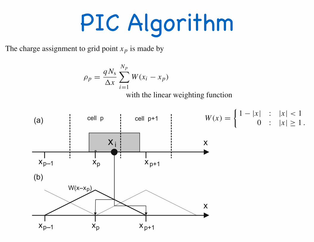
The discussion of plasma simulation will be restricted to one-dimensional (1-D)electrostatic problems, which we had studied before by analytical methods. The PICmethod assumes that the particle can be found with the same probability at any placewithin a cell of the computational grid. This is equivalent to assigning a box-shapedprofile of width !x for the particle. When the superparticle moves over the grid,there is a continuous change of its contribution to a cell p and its neighboring cellp + 1, as shown in Fig. 9.19.

The charge assignment to grid point x p is made by

ρp = q Ns

!x

Np!

i=1

W (xi − x p) (9.78)

with the linear weighting function

W (x) ="

1 − |x | : |x | < 10 : |x | ≥ 1 .

(9.79)

1 http://ptsg.eecs.berkeley.edu/

248 9 Kinetic Description of Plasmas

Fig. 9.19 (a) The particle at xi is represented by a box-like charge cloud of width !x . When itmoves over the calculation grid, charge is assigned to cells p and p + 1 according to the overlapof the cloud with the cell. (b) This charge assignment is described by the weighting functionW (x − x p) for the cell p

The advantage of such extended charge clouds lies in the smooth variation of theinteraction force between two such clouds. If the particle was represented by a thincharge sheet, then the interaction force between two such sheets, which is indepen-dent of the distance between the sheets, would suddenly switch sign when the sheetspenetrate each other.

The electric field results from solving Poisson’s equation on this grid. First thesecond derivative is replaced by a second difference

Φp−1 − 2Φp +Φp+1

(∆x)2 = −ρp

ε0. (9.80)

Then, the electric field results from

E p = φp−1 − φp+1

2∆x. (9.81)

Poisson’s equation can be readily solved by diagonalization of the matrix, see e.g.,[214]. For periodic boundary conditions, methods based on fast Fourier transformmay be even superior. The interpolation of the field force at the position of theparticle is made with the same weighting function (9.79) as used for the chargeassignment on the grid

Fi = q Ns

Ng−1!

p=0

W (xi − x p)E p . (9.82)


the shielded Coulomb force. We had overcome this difficulty in the previous sectionby grinding the particles into ever finer “Vlasov sand” that has the same q/m foreach grain, and therefore preserves the interaction forces between volume elementsof finite size. This concept allowed a statistical treatment in terms of the Vlasovequation.

In this Section, we go into the other direction and merge all particles within a vol-ume element into a superparticle. Again this superparticle has the same q/m as theindividual particles it consists of. Typical numbers of particles within a superparticlecan be Ns = 104 − 106. A further improvement for the numerical simulations ofelectrostatic problems with superparticles is the assignment of the charge distribu-tion, the resulting electric field and potential to a fixed grid with Ng grid points. Thisreduces the calculation effort for a one-dimensional system to N Ng log2 Ng insteadof N 2 steps, which can be a substantial reduction, if N = 105 and Ng = 100,typically.

Plasma physics by computer simulation is now an established branch of our field.The fundamental methods are described in textbooks, e.g., [214, 215]. In the follow-ing, the particle-in-cell (PIC) method will be described, which is implemented inmany codes. Some of these codes are available for free.1 Have fun playing yourselfwith the codes. It will give you the impression that you can master the plasma.The experimental plasma physicists often experience that the plasma masters theexperimenter.

9.4.1 The Particle-in-Cell Algorithm

The discussion of plasma simulation will be restricted to one-dimensional (1-D)electrostatic problems, which we had studied before by analytical methods. The PICmethod assumes that the particle can be found with the same probability at any placewithin a cell of the computational grid. This is equivalent to assigning a box-shapedprofile of width !x for the particle. When the superparticle moves over the grid,there is a continuous change of its contribution to a cell p and its neighboring cellp + 1, as shown in Fig. 9.19.

The charge assignment to grid point x p is made by

ρp = q Ns

!x

Np!

i=1

W (xi − x p) (9.78)

with the linear weighting function

W (x) ="

1 − |x | : |x | < 10 : |x | ≥ 1 .

(9.79)

1 http://ptsg.eecs.berkeley.edu/

Poisson’s Equation and Electric Force





Φp−1 − 2Φp +Φp+1

(∆x)2 = −ρp

ε0. (9.80)


E p = φp−1 − φp+1

2∆x. (9.81)


Fi = q Ns

Ng−1!

p=0

W (xi − x p)E p . (9.82)





Φp−1 − 2Φp +Φp+1

(∆x)2 = −ρp

ε0. (9.80)


E p = φp−1 − φp+1

2∆x. (9.81)


Fi = q Ns

Ng−1!

p=0

W (xi − x p)E p . (9.82)





Φp−1 − 2Φp +Φp+1

(∆x)2 = −ρp

ε0. (9.80)


E p = φp−1 − φp+1

2∆x. (9.81)


Fi = q Ns

Ng−1!

p=0

W (xi − x p)E p . (9.82)

“Leap Frog” Time-Stepping


The particle position is advanced by a discrete representation of Newton’s equationin terms of a leap-frog scheme

xn+1i − xn

i

∆t= v

n+1/2i

vn+1/2i − v

n−1/2i

∆t= F(xi )∆t

mi, (9.83)

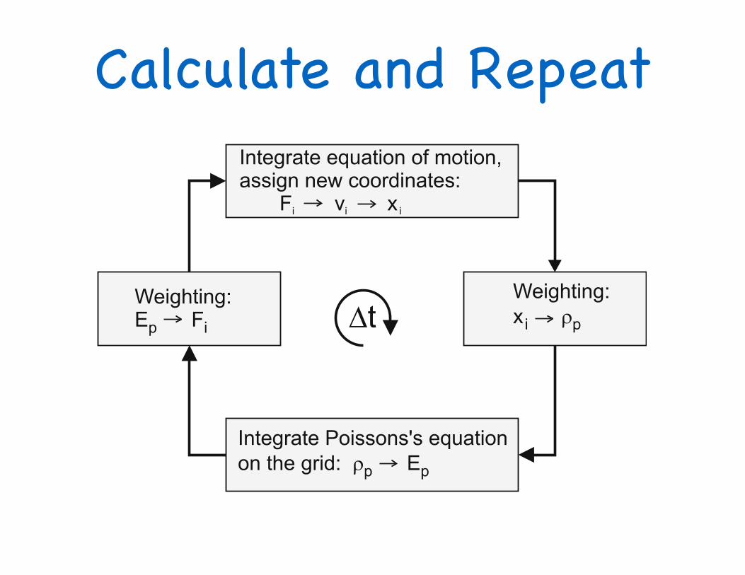
in which the superscript labels the number of the time step. The advancement ofthe velocity is made at half timesteps. A full cycle of the PIC time step is shown inFig. 9.20.

Fig. 9.20 Time step of theparticle-in-cell technique

9.4.2 Phase-Space Representation

Before discussing the interaction of electrons with wave fields, let us shortly recallthe description of a dynamical system in phase space. A simple one-dimensionalsystem, the pendulum, is described by the potential energy

Wpot = −W0 cos(ϕ) . (9.84)

For small excitation energies, the pendulum performs harmonic oscillations aboutthe equilibrium position at ϕ = 0. The potential well and the phase space ϕ–(dϕ/dt)of this pendulum are shown in Fig. 9.21. The phase space contours in Fig. 9.21bcorrespond to various values of total energy

Wtot = 12

I!

dϕdt

"2

− W0 cos(ϕ) , (9.85)

I being the moment of inertia for this pendulum.

Calculate and Repeat


The particle position is advanced by a discrete representation of Newton’s equationin terms of a leap-frog scheme

xn+1i − xn

i

∆t= v

n+1/2i

vn+1/2i − v

n−1/2i

∆t= F(xi )∆t

mi, (9.83)

in which the superscript labels the number of the time step. The advancement ofthe velocity is made at half timesteps. A full cycle of the PIC time step is shown inFig. 9.20.

Fig. 9.20 Time step of theparticle-in-cell technique

9.4.2 Phase-Space Representation

Before discussing the interaction of electrons with wave fields, let us shortly recallthe description of a dynamical system in phase space. A simple one-dimensionalsystem, the pendulum, is described by the potential energy

Wpot = −W0 cos(ϕ) . (9.84)

For small excitation energies, the pendulum performs harmonic oscillations aboutthe equilibrium position at ϕ = 0. The potential well and the phase space ϕ–(dϕ/dt)of this pendulum are shown in Fig. 9.21. The phase space contours in Fig. 9.21bcorrespond to various values of total energy

Wtot = 12

I!

dϕdt

"2

− W0 cos(ϕ) , (9.85)

I being the moment of inertia for this pendulum.

Dimensionless Parameters

• Δx = 1 and Δt = 1

• Δx/L << 1 (so L must be large, with Δx ≈ 1)

• (qe/me) = -1

• (qi/mi) = +1/25

• Δt ωpe << 1, so ω2pe = n (qe/me)(qe/ε0). Therefore, (qe/ε0) << 1 if n ≈ 1

Dynamics (Leap-Frog)

Poisson’s Eq

Simple Example

Two-Stream Instability

Plasma Clump

Next Week

• Ch. 9: Kinetic Theory

• Vlasov’s Equation

• Landau Damping

Lecture17: Plasma Physics 1 - Columbia Universitysites.apam.columbia.edu/courses/apph6101x/Plasma1...PIC Algorithm 9.4 Plasma Simulation with Particle Codes 247 the shielded Coulomb

Documents