Lecture Three: Time Series Analysis

Lecture Three: Time Series Analysis

“If your experiment needs statistics, you ought to have done a better experiment.” Ernest Rutherford

Time domain data (a day at a time)

Time domain data (a day at a time)

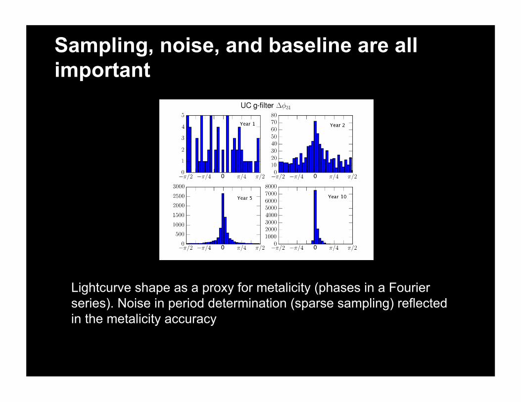
Sampling, noise, and baseline are all important

Lightcurve shape as a proxy for metalicity (phases in a Fourier series). Noise in period determination (sparse sampling) reflected in the metalicity accuracy

What is a light curve?

G(t|θ) are functions (uneven sampling, period or non-periodic) For example G(t) = sin(wt), or G(t) = exp(-Bt)

Fourier Analysis

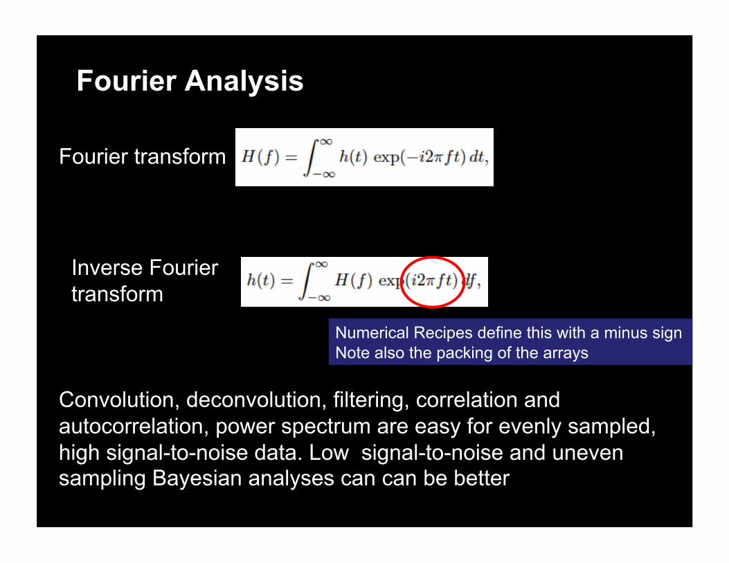
Convolution, deconvolution, filtering, correlation and autocorrelation, power spectrum are easy for evenly sampled, high signal-to-noise data. Low signal-to-noise and uneven sampling Bayesian analyses can can be better

Fourier transform

Inverse Fourier transform

Numerical Recipes define this with a minus sign Note also the packing of the arrays

Power Spectrum (PSD)

Power Spectrum is the amount of power in the frequency interval f f+df

FT

Total power is the same whether computed in frequency or time domain (Parsevals Theorem)

€

h(t) = sin(2πt /T)

€

PSD( f ) = δ( f =1/T)

Fourier Analysis in Python

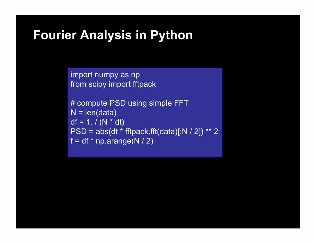
import numpy as np from scipy import fftpack

# compute PSD using simple FFT N = len(data) df = 1. / (N * dt) PSD = abs(dt * fftpack.fft(data)[:N / 2]) ** 2 f = df * np.arange(N / 2)

How do we deal with sampled data

Sampling of the data – you just cant get away from it…

Uniformly sampled

FFT O(NlogN) rather than N^2 (numpy.fft and scipy.fft)

Sampling frequencies: Nyquist

What is the relation between continuous and sampled FFTs

Nyquist sampling theorem •  For band-limited data (H(f)=0 for |f| > fc)

(the band limit or Nyquist frequency)

•  There is some resolution limit in time tc = 1/(2 fc) below which h(t) appears smooth

T

We can now reconstruct h(t) from evenly sampled data when δt < tc (Shannon interpolation formula or sinc shifting)

Estimating the PSD

Welch transform

Compute FFT for multiple overlapping windows on the data

Welch’s transform in Python

from matplotlib import mlab

# compute PSD using Welch's method # this uses overlapping windows to reduce noise PSDW, fW = mlab.psd(data, NFFT=4096, Fs = 1. / dt)

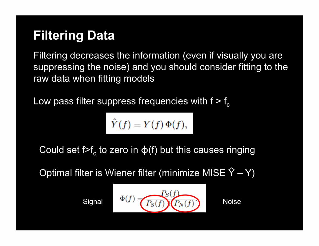
Filtering decreases the information (even if visually you are suppressing the noise) and you should consider fitting to the raw data when fitting models

Low pass filter suppress frequencies with f > fc

Could set f>fc to zero in ϕ(f) but this causes ringing

Optimal filter is Wiener filter (minimize MISE Ŷ – Y)

Filtering Data

Signal Noise

Wiener Filtering

An interesting relation to kernel density estimation

Usually fit signal and noise to PSD (assumes uncorrelated noise)

Wiener filtering in Python import numpy as np from scipy import optimize, fftpack

# compute the PSD

# Set up the Wiener filter: # fit a model to the PSD consisting of the sum of a Gaussian and white noise signal = lambda x, A, width: A * np.exp(-0.5 * (x / width) ** 2) noise = lambda x, n: n * np.ones(x.shape)

func = lambda v: np.sum((PSD - signal(f, v[0], v[1]) - noise(f, v[2])) ** 2) v0 = [5000, 0.1, 10] v = optimize.fmin(func, v0)

P_S = signal(f, v[0], v[1]) P_N = noise(f, v[2])

# define Wiener filter Phi = P_S / (P_S + P_N)

h_smooth = fftpack.ifft(Phi * HN)

Minimum component filtering

Used for the case of fitting the baseline (continuum) •  Mask regions of signal and fit low order polynomial model to unmask regions •  Subtract the low order model and FFT the signal •  Remove high frequencies using a low pass filter •  Inverse FT and add the baseline fit

Is there signal in my noise?

Hypothesis testing – are the data consistent with a stationary process

Simple example:

Minimum detected variability amplitude €

y(t) = Asin(wt)

€

var(t) =σ2 +A2

2

Χ2 of the data (assuming A=0)

Is there a periodicity in the data?

Non-linear in w and Φ Linear in all but w

Consider it a least-squares problem – without requiring evenly sampled data

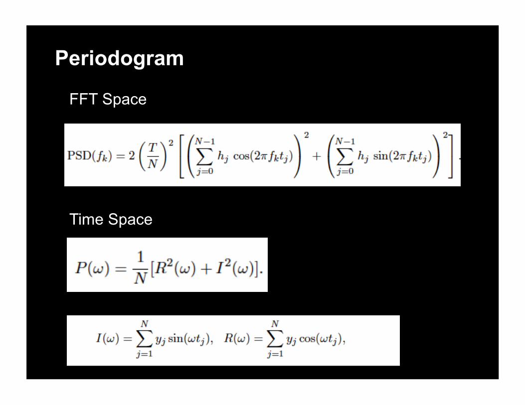
Periodogram

Time Space

FFT Space

Lomb-Scargle Periodogram

Generalized for heteroscedastic errors but still corresponds to a single sinusoidal model. Model is non-linear in frequency so we typically maximize that through a grid search

import numpy as np

from astroML.periodogram import lomb_scargle, search_frequencies # generate data t = np.random.randint(100, size=N) + 0.3 + 0.4 * np.random.random(N) y = 10 + np.sin(2 * np.pi * t / P) dy = 0.5 + 0.5 * np.random.random(N)

y_obs = y + np.random.normal(0, dy)

period = 10 ** np.linspace(-1, 0, 1000) omega = 2 * np.pi / period

sig = np.array([0.1, 0.01, 0.001]) PS, z = lomb_scargle(t, y_obs, dy, omega, modified=True, significance=sig)

omega_sample, PS_sample = search_frequencies(t, y_obs, dy, n_save=100, LS_kwargs=dict(modified=True))

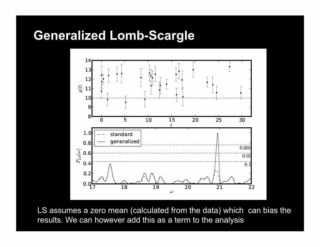
Generalized Lomb-Scargle

LS assumes a zero mean (calculated from the data) which can bias the results. We can however add this as a term to the analysis

Where next...

Classification Regression

Where next...

Read the book – send comments/corrections/suggestions

[email protected]